Mastering Machine Learning With Python In Six Steps A Practical Implementation Guide To Predictive Data Analytics Using Pytho
User Manual: Pdf
Open the PDF directly: View PDF ![]() .
.
Page Count: 374 [warning: Documents this large are best viewed by clicking the View PDF Link!]
- Contents at a Glance
- Contents
- About the Author
- About the Technical Reviewer
- Acknowledgments
- Introduction
- Chapter 1: Step 1 – Getting Started in Python
- The Best Things in Life Are Free
- The Rising Star
- Python 2.7.x or Python 3.4.x?
- Key Concepts
- Python Identifiers
- Keywords
- My First Python Program
- Code Blocks (Indentation & Suites)
- Basic Object Types
- When to Use List vs. Tuples vs. Set vs. Dictionary
- Comments in Python
- Multiline Statement
- Basic Operators
- Control Structure
- Lists
- Tuple
- Sets
- Dictionary
- User-Defined Functions
- Module
- File Input/Output
- Exception Handling
- Endnotes
- Chapter 2: Step 2 – Introduction to Machine Learning
- History and Evolution
- Artificial Intelligence Evolution
- Different Forms
- Machine Learning Categories
- Frameworks for Building Machine Learning Systems
- Machine Learning Python Packages
- Data Analysis Packages
- NumPy
- Pandas
- Matplotlib
- Using Global Functions
- Object Oriented
- Line Plots – Using ax.plot()
- Multiple Lines on Same Axis
- Multiple Lines on Different Axis
- Control the Line Style and Marker Style
- Line Style Reference
- Marker Reference
- Colomaps Reference
- Bar Plots – using ax.bar() and ax.barh()
- Horizontal Bar Charts
- Side-by-Side Bar Chart
- Stacked Bar Example Code
- Pie Chart – Using ax.pie()
- Example Code for Grid Creation
- Plotting – Defaults
- Machine Learning Core Libraries
- Endnotes
- Chapter 3: Step 3 – Fundamentals of Machine Learning
- Machine Learning Perspective of Data
- Scales of Measurement
- Feature Engineering
- Exploratory Data Analysis (EDA)
- Supervised Learning– Regression
- Supervised Learning – Classification
- Logistic Regression
- Evaluating a Classification Model Performance
- ROC Curve
- Fitting Line
- Stochastic Gradient Descent
- Regularization
- Multiclass Logistic Regression
- Generalized Linear Models
- Supervised Learning – Process Flow
- Decision Trees
- Support Vector Machine (SVM)
- k Nearest Neighbors (kNN)
- Time-Series Forecasting
- Unsupervised Learning Process Flow
- Endnotes
- Chapter 4: Step 4 – Model Diagnosis and Tuning
- Chapter 5: Step 5 – Text Mining and Recommender Systems
- Chapter 6: Step 6 – Deep and Reinforcement Learning
- Artificial Neural Network (ANN)
- What Goes Behind, When Computers Look at an Image?
- Why Not a Simple Classification Model for Images?
- Perceptron – Single Artificial Neuron
- Multilayer Perceptrons (Feedforward Neural Network)
- Restricted Boltzman Machines (RBM)
- MLP Using Keras
- Autoencoders
- Convolution Neural Network (CNN)
- Recurrent Neural Network (RNN)
- Transfer Learning
- Reinforcement Learning
- Endnotes
- Chapter 7: Conclusion
- Index

Mastering Machine
Learning with
Python in Six Steps
A Practical Implementation Guide to
Predictive Data Analytics Using Python
—
Manohar Swamynathan

Mastering Machine
Learning with
Python in Six Steps
A Practical Implementation Guide
to Predictive Data Analytics Using
Python
Manohar Swamynathan
Mastering Machine Learning with Python in Six Steps
Manohar Swamynathan
Bangalore, Karnataka, India
ISBN-13 (pbk): 978-1-4842-2865-4 ISBN-13 (electronic): 978-1-4842-2866-1
DOI 10.1007/978-1-4842-2866-1
Library of Congress Control Number: 2017943522
Copyright © 2017 by Manohar Swamynathan
This work is subject to copyright. All rights are reserved by the Publisher, whether the
whole or part of the material is concerned, specifically the rights of translation, reprinting,
reuse of illustrations, recitation, broadcasting, reproduction on microfilms or in any
other physical way, and transmission or information storage and retrieval, electronic
adaptation, computer software, or by similar or dissimilar methodology now known or
hereafter developed.
Trademarked names, logos, and images may appear in this book. Rather than use a
trademark symbol with every occurrence of a trademarked name, logo, or image we
use the names, logos, and images only in an editorial fashion and to the benefit of the
trademark owner, with no intention of infringement of the trademark.
The use in this publication of trade names, trademarks, service marks, and similar terms,
even if they are not identified as such, is not to be taken as an expression of opinion as to
whether or not they are subject to proprietary rights.
While the advice and information in this book are believed to be true and accurate at the
date of publication, neither the authors nor the editors nor the publisher can accept any
legal responsibility for any errors or omissions that may be made. The publisher makes
no warranty, express or implied, with respect to the material contained herein.
Cover image designed by Freepik
Managing Director: Welmoed Spahr
Editorial Director: Todd Green
Acquisitions Editor: Celestin Suresh John
Development Editor: Anila Vincent and James Markham
Technical Reviewer: Jojo Moolayil
Coordinating Editor: Sanchita Mandal
Copy Editor: Karen Jameson
Compositor: SPi Global
Indexer: SPi Global
Artist: SPi Global
Distributed to the book trade worldwide by Springer Science+Business Media New York,
233 Spring Street, 6th Floor, New York, NY 10013. Phone 1-800-SPRINGER, fax (201)
348-4505, e-mail orders-ny@springer-sbm.com, or visit www.springeronline.com.
Apress Media, LLC is a California LLC and the sole member (owner) is Springer
Science + Business Media Finance Inc (SSBM Finance Inc). SSBM Finance Inc is a
Delaware corporation.
For information on translations, please e-mail rights@apress.com, or visit
http://www.apress.com/rights-permissions.
Apress titles may be purchased in bulk for academic, corporate, or promotional use. eBook
versions and licenses are also available for most titles. For more information, reference our
Print and eBook Bulk Sales web page at http://www.apress.com/bulk-sales.
Any source code or other supplementary material referenced by the author in this book is
available to readers on GitHub via the book’s product page, located at www.apress.com/
978-1-4842-2865-4. For more detailed information, please visit http://www.apress.com/
source-code.
Printed on acid-free paper

iii
Contents at a Glance
About the Author ���������������������������������������������������������������������������� xiii
About the Technical Reviewer ��������������������������������������������������������� xv
Acknowledgments ������������������������������������������������������������������������� xvii
Introduction ������������������������������������������������������������������������������������ xix
■Chapter 1: Step 1 – Getting Started in Python �������������������������������� 1
■Chapter 2: Step 2 – Introduction to Machine Learning ����������������� 53
■Chapter 3: Step 3 – Fundamentals of Machine Learning ������������ 117
■Chapter 4: Step 4 – Model Diagnosis and Tuning ����������������������� 209
■Chapter 5: Step 5 – Text Mining and Recommender Systems ���� 251
■Chapter 6: Step 6 – Deep and Reinforcement Learning �������������� 297
■Chapter 7: Conclusion ���������������������������������������������������������������� 345
Index ���������������������������������������������������������������������������������������������� 351

v
Contents
About the Author ���������������������������������������������������������������������������� xiii
About the Technical Reviewer ��������������������������������������������������������� xv
Acknowledgments ������������������������������������������������������������������������� xvii
Introduction ������������������������������������������������������������������������������������ xix
■Chapter 1: Step 1 – Getting Started in Python �������������������������������� 1
The Best Things in Life Are Free �������������������������������������������������������������� 1
The Rising Star ���������������������������������������������������������������������������������������� 2
Python 2�7�x or Python 3�4�x? ������������������������������������������������������������������ 3
Windows Installation ������������������������������������������������������������������������������������������������4
OSX Installation �������������������������������������������������������������������������������������������������������� 4
Linux Installation ������������������������������������������������������������������������������������������������������ 4
Python from Official Website ������������������������������������������������������������������������������������ 4
Running Python �������������������������������������������������������������������������������������������������������� 5
Key Concepts ������������������������������������������������������������������������������������������� 5
Python Identifiers������������������������������������������������������������������������������������������������������ 5
Keywords ������������������������������������������������������������������������������������������������������������������6
My First Python Program ������������������������������������������������������������������������������������������ 6
Code Blocks (Indentation & Suites) ��������������������������������������������������������������������������6
Basic Object Types ���������������������������������������������������������������������������������������������������� 8
When to Use List vs� Tuples vs� Set vs� Dictionary ��������������������������������������������������10
Comments in Python����������������������������������������������������������������������������������������������� 10
Multiline Statement ������������������������������������������������������������������������������������������������ 11
■ Contents
vi
Basic Operators ������������������������������������������������������������������������������������������������������12
Control Structure ����������������������������������������������������������������������������������������������������20
Lists ������������������������������������������������������������������������������������������������������������������������ 22
Tuple ����������������������������������������������������������������������������������������������������������������������� 26
Sets������������������������������������������������������������������������������������������������������������������������� 29
Dictionary ��������������������������������������������������������������������������������������������������������������� 37
User-Defined Functions ������������������������������������������������������������������������������������������ 42
Module �������������������������������������������������������������������������������������������������������������������� 45
File Input/Output ����������������������������������������������������������������������������������������������������� 47
Exception Handling ������������������������������������������������������������������������������������������������� 48
Endnotes ����������������������������������������������������������������������������������������������� 52
■Chapter 2: Step 2 – Introduction to Machine Learning ����������������� 53
History and Evolution ���������������������������������������������������������������������������� 54
Artificial Intelligence Evolution �������������������������������������������������������������� 57
Different Forms ������������������������������������������������������������������������������������� 58
Statistics ����������������������������������������������������������������������������������������������������������������� 58
Data Mining ������������������������������������������������������������������������������������������������������������ 61
Data Analytics ��������������������������������������������������������������������������������������������������������� 61
Data Science ����������������������������������������������������������������������������������������������������������� 64
Statistics vs� Data Mining vs� Data Analytics vs� Data Science ������������������������������ 66
Machine Learning Categories ���������������������������������������������������������������� 67
Supervised Learning �����������������������������������������������������������������������������������������������67
Unsupervised Learning �������������������������������������������������������������������������������������������68
Reinforcement Learning ����������������������������������������������������������������������������������������� 69
Frameworks for Building Machine Learning Systems ��������������������������� 69
Knowledge Discovery Databases (KDD) ����������������������������������������������������������������� 69
Cross-Industry Standard Process for Data Mining ������������������������������������������������� 71
■ Contents
vii
SEMMA (Sample, Explore, Modify, Model, Assess) �������������������������������������������������� 74
KDD vs� CRISP-DM vs� SEMMA ������������������������������������������������������������������������������� 75
Machine Learning Python Packages ����������������������������������������������������� 76
Data Analysis Packages ������������������������������������������������������������������������ 76
NumPy �������������������������������������������������������������������������������������������������������������������� 77
Pandas �������������������������������������������������������������������������������������������������������������������� 89
Matplotlib �������������������������������������������������������������������������������������������������������������� 100
Machine Learning Core Libraries �������������������������������������������������������� 114
Endnotes ��������������������������������������������������������������������������������������������� 116
■Chapter 3: Step 3 – Fundamentals of Machine Learning ������������ 117
Machine Learning Perspective of Data������������������������������������������������ 117
Scales of Measurement ����������������������������������������������������������������������� 118
Nominal Scale of Measurement ���������������������������������������������������������������������������118
Ordinal Scale of Measurement �����������������������������������������������������������������������������119
Interval Scale of Measurement ����������������������������������������������������������������������������� 119
Ratio Scale of Measurement ��������������������������������������������������������������������������������119
Feature Engineering ���������������������������������������������������������������������������� 120
Dealing with Missing Data ������������������������������������������������������������������������������������ 121
Handling Categorical Data ������������������������������������������������������������������������������������ 121
Normalizing Data �������������������������������������������������������������������������������������������������� 123
Feature Construction or Generation ����������������������������������������������������������������������125
Exploratory Data Analysis (EDA) ���������������������������������������������������������� 125
Univariate Analysis �����������������������������������������������������������������������������������������������126
Multivariate Analysis ��������������������������������������������������������������������������������������������128
Supervised Learning– Regression ������������������������������������������������������ 131
Correlation and Causation ������������������������������������������������������������������������������������133
Fitting a Slope ������������������������������������������������������������������������������������������������������� 134
How Good Is Your Model? ������������������������������������������������������������������������������������� 136
■ Contents
viii
Polynomial Regression ����������������������������������������������������������������������������������������� 139
Multivariate Regression ����������������������������������������������������������������������������������������143
Multicollinearity and Variation Inflation Factor (VIF) ��������������������������������������������� 145
Interpreting the OLS Regression Results ��������������������������������������������������������������149
Regression Diagnosis ������������������������������������������������������������������������������������������� 152
Regularization ������������������������������������������������������������������������������������������������������� 156
Nonlinear Regression ������������������������������������������������������������������������������������������� 159
Supervised Learning – Classification �������������������������������������������������� 160
Logistic Regression ���������������������������������������������������������������������������������������������� 161
Evaluating a Classification Model Performance ��������������������������������������������������� 164
ROC Curve ������������������������������������������������������������������������������������������������������������� 166
Fitting Line ������������������������������������������������������������������������������������������������������������ 167
Stochastic Gradient Descent ��������������������������������������������������������������������������������168
Regularization ������������������������������������������������������������������������������������������������������� 169
Multiclass Logistic Regression ����������������������������������������������������������������������������� 171
Generalized Linear Models �����������������������������������������������������������������������������������173
Supervised Learning – Process Flow �������������������������������������������������������������������175
Decision Trees ������������������������������������������������������������������������������������������������������ 176
Support Vector Machine (SVM) ����������������������������������������������������������������������������� 180
k Nearest Neighbors (kNN) ����������������������������������������������������������������������������������� 183
Time-Series Forecasting��������������������������������������������������������������������������������������� 185
Unsupervised Learning Process Flow ������������������������������������������������� 194
Clustering ������������������������������������������������������������������������������������������������������������� 195
K-means ��������������������������������������������������������������������������������������������������������������� 195
Finding Value of k ������������������������������������������������������������������������������������������������� 199
Hierarchical Clustering �����������������������������������������������������������������������������������������203
Principal Component Analysis (PCA) ��������������������������������������������������������������������� 205
Endnotes ��������������������������������������������������������������������������������������������� 208
■ Contents
ix
■Chapter 4: Step 4 – Model Diagnosis and Tuning ����������������������� 209
Optimal Probability Cutoff Point ���������������������������������������������������������� 209
Which Error Is Costly? ������������������������������������������������������������������������������������������213
Rare Event or Imbalanced Dataset ������������������������������������������������������ 213
Known Disadvantages ������������������������������������������������������������������������������������������216
Which Resampling Technique Is the Best? ����������������������������������������������������������� 217
Bias and Variance �������������������������������������������������������������������������������� 218
Bias ����������������������������������������������������������������������������������������������������������������������� 218
Variance ����������������������������������������������������������������������������������������������������������������218
K-Fold Cross-Validation ����������������������������������������������������������������������� 219
Stratified K-Fold Cross-Validation ������������������������������������������������������� 221
Ensemble Methods ������������������������������������������������������������������������������ 221
Bagging ����������������������������������������������������������������������������������������������� 222
Feature Importance ����������������������������������������������������������������������������������������������224
RandomForest ������������������������������������������������������������������������������������������������������225
Extremely Randomized Trees (ExtraTree) ������������������������������������������������������������� 225
How Does the Decision Boundary Look? �������������������������������������������������������������� 226
Bagging – Essential Tuning Parameters ��������������������������������������������������������������� 228
Boosting ���������������������������������������������������������������������������������������������� 228
Example Illustration for AdaBoost ������������������������������������������������������������������������� 229
Gradient Boosting ������������������������������������������������������������������������������������������������� 233
Boosting – Essential Tuning Parameters �������������������������������������������������������������� 235
Xgboost (eXtreme Gradient Boosting) �������������������������������������������������������������������236
Ensemble Voting – Machine Learning’s Biggest Heroes United ���������� 240
Hard Voting vs� Soft Voting �����������������������������������������������������������������������������������242
Stacking ���������������������������������������������������������������������������������������������� 244
■ Contents
x
Hyperparameter Tuning ����������������������������������������������������������������������� 246
GridSearch ������������������������������������������������������������������������������������������������������������ 247
RandomSearch �����������������������������������������������������������������������������������������������������248
Endnotes ��������������������������������������������������������������������������������������������� 250
■Chapter 5: Step 5 – Text Mining and Recommender Systems ���� 251
Text Mining Process Overview ������������������������������������������������������������ 252
Data Assemble (Text) ��������������������������������������������������������������������������� 253
Social Media ��������������������������������������������������������������������������������������������������������� 255
Step 1 – Get Access Key (One-Time Activity) �������������������������������������������������������� 255
Step 2 – Fetching Tweets ������������������������������������������������������������������������������������� 255
Data Preprocessing (Text) ������������������������������������������������������������������� 259
Convert to Lower Case and Tokenize �������������������������������������������������������������������� 259
Removing Noise ����������������������������������������������������������������������������������������������������260
Part of Speech (PoS) Tagging ������������������������������������������������������������������������������� 262
Stemming ������������������������������������������������������������������������������������������������������������� 263
Lemmatization ������������������������������������������������������������������������������������������������������ 265
N-grams ���������������������������������������������������������������������������������������������������������������� 267
Bag of Words (BoW) ���������������������������������������������������������������������������������������������� 268
Term Frequency-Inverse Document Frequency (TF-IDF) �������������������������������������� 270
Data Exploration (Text) ������������������������������������������������������������������������ 272
Frequency Chart ���������������������������������������������������������������������������������������������������272
Word Cloud �����������������������������������������������������������������������������������������������������������273
Lexical Dispersion Plot �����������������������������������������������������������������������������������������274
Co-occurrence Matrix ������������������������������������������������������������������������������������������� 275
Model Building ������������������������������������������������������������������������������������ 276
Text Similarity �������������������������������������������������������������������������������������� 277
Text Clustering ������������������������������������������������������������������������������������� 279
■ Contents
xi
Latent Semantic Analysis (LSA) ���������������������������������������������������������������������������� 280
Topic Modeling ������������������������������������������������������������������������������������ 282
Latent Dirichlet Allocation (LDA) ��������������������������������������������������������������������������� 282
Non-negative Matrix Factorization ����������������������������������������������������������������������� 284
Text Classification ������������������������������������������������������������������������������� 284
Sentiment Analysis ������������������������������������������������������������������������������ 286
Deep Natural Language Processing (DNLP) ���������������������������������������� 287
Recommender Systems ���������������������������������������������������������������������� 291
Content-Based Filtering ���������������������������������������������������������������������������������������� 292
Collaborative Filtering (CF) �����������������������������������������������������������������������������������292
Endnotes ��������������������������������������������������������������������������������������������� 295
■Chapter 6: Step 6 – Deep and Reinforcement Learning �������������� 297
Artificial Neural Network (ANN) ����������������������������������������������������������� 298
What Goes Behind, When Computers Look at an Image? �������������������� 299
Why Not a Simple Classification Model for Images? ��������������������������� 300
Perceptron – Single Artificial Neuron �������������������������������������������������� 300
Multilayer Perceptrons (Feedforward Neural Network) ����������������������� 303
Load MNIST Data �������������������������������������������������������������������������������������������������� 304
Key Parameters for scikit-learn MLP �������������������������������������������������������������������� 305
Restricted Boltzman Machines (RBM) ������������������������������������������������� 307
MLP Using Keras ��������������������������������������������������������������������������������� 312
Autoencoders �������������������������������������������������������������������������������������� 315
Dimension Reduction Using Autoencoder ������������������������������������������������������������� 316
De-noise Image Using Autoencoder ��������������������������������������������������������������������� 319
Convolution Neural Network (CNN) ����������������������������������������������������� 320
CNN on CIFAR10 Dataset �������������������������������������������������������������������������������������� 321
CNN on MNIST Dataset ����������������������������������������������������������������������������������������� 327
■ Contents
xii
Recurrent Neural Network (RNN) �������������������������������������������������������� 332
Long Short-Term Memory (LSTM)������������������������������������������������������������������������� 333
Transfer Learning �������������������������������������������������������������������������������� 336
Reinforcement Learning ���������������������������������������������������������������������� 340
Endnotes ��������������������������������������������������������������������������������������������� 344
■Chapter 7: Conclusion ���������������������������������������������������������������� 345
Summary ��������������������������������������������������������������������������������������������� 345
Tips ������������������������������������������������������������������������������������������������������ 346
Start with Questions/Hypothesis Then Move to Data! ������������������������������������������ 347
Don’t Reinvent the Wheels from Scratch �������������������������������������������������������������� 347
Start with Simple Models ������������������������������������������������������������������������������������� 348
Focus on Feature Engineering ������������������������������������������������������������������������������ 349
Beware of Common ML Imposters �����������������������������������������������������������������������349
Happy Machine Learning ��������������������������������������������������������������������� 349
Index ���������������������������������������������������������������������������������������������� 351

xiii
About the Author
Manohar Swamynathan is a data science practitioner
and an avid programmer, with over 13 years of experience
in various data science-related areas that include data
warehousing, Business Intelligence (BI), analytical tool
development, ad hoc analysis, predictive modeling, data
science product development, consulting, formulating
strategy, and executing analytics program.
He’s had a career covering life cycles of data across
different domains such as U.S. mortgage banking,
retail, insurance, and industrial IoT. He has a bachelor’s
degree with specialization in physics, mathematics,
and computers; and a master’s degree in project
management. He’s currently living in Bengaluru,
the Silicon Valley of India, working as Staff Data Scientist with General Electric Digital,
contributing to the next big digital industrial revolution.
You can visit him at http://www.mswamynathan.com to learn more about his various
other activities.

xv
About the Technical
Reviewer
Jojo Moolayil is a Data Scientist and the author of
the book: Smarter Decisions – The Intersection of
Internet of Things and Decision Science. With over
4 years of industrial experience in Data Science,
Decision Science and IoT, he has worked with industry
leaders on high impact and critical projects across
multiple verticals. He is currently associated with
General Electric, the pioneer and leader in data
science for Industrial IoT and lives in Bengaluru—the
silicon valley of India.
He was born and raised in Pune, India and
graduated from University of Pune with a major in
Information Technology Engineering. He started his career with Mu Sigma Inc., the
world's largest pure play analytics provider and worked with the leaders of many Fortune
50 clients. One of the early enthusiasts to venture into IoT analytics, he converged
his learnings from decision science to bring the problem solving frameworks and his
learnings from data and decision science to IoT Analtyics.
To cement his foundations in data science for industrial IoT and scale the impact of
the problem solving experiments, he joined a fast growing IoT Analytics startup called
Flutura based in Bangalore and headquartered in the valley. After a short stint with
Flutura, Jojo moved on to work with the leaders of Industrial IoT - General Electric, in
Bangalore, where he focused on solving decision science problems for Industrial IoT
use cases. As a part of his role in GE, Jojo also focuses on developing data science and
decision science products and platforms for Industrial IoT.
Apart from authoring books on Decision Science and IoT, Jojo has also been
Technical Reviewer for various books on Machine Learning, Deep Learning and Business
Analytics with Apress. He is an active Data Science tutor and maintains a blog at
http://www.jojomoolayil.com/web/blog/.
Profile
http://www.jojomoolayil.com/
https://www.linkedin.com/in/jojo62000
I would like to thank my family, friends and mentors.
—Jojo Moolayil

xvii
Acknowledgments
I’m grateful to my mom, dad, and loving brother; I thank my wife Usha and son Jivin for
providing me the space for writing this book.
I would like to express my gratitude to my mentors, colleagues, and friends from
current/previous organizations for their inputs, inspiration, and support. Thanks to Jojo
for the encouragement to write this book and his technical review inputs. Big thanks to
the Apress team for their constant support and help.
Finally, I would like to thank you the reader for showing an interest in this book and
sincerely hope to help your pursuit to machine learning quest.
Note that the views expressed in this book are author’s personal.

xix
Introduction
This book is your practical guide towards novice to master in machine learning with
Python in six steps. The six steps path has been designed based on the “Six degrees of
separation” theory that states that everyone and everything is a maximum of six steps
away. Note that the theory deals with the quality of connections, rather than their
existence. So a great effort has been taken to design eminent, yet simple six steps covering
fundamentals to advanced topics gradually that will help a beginner walk his way from
no or least knowledge of machine learning in Python to all the way to becoming a master
practitioner. This book is also helpful for current Machine Learning practitioners to learn
the advanced topics such as Hyperparameter tuning, various ensemble techniques,
Natural Language Processing (NLP), deep learning, and the basics of reinforcement
learning. See Figure1.
Figure 1. Learning Journey - Mastering Python Machine Learning: In Six Steps
Each topic has two parts: the first part will cover the theoretical concepts and the
second part will cover practical implementation with different Python packages. The
traditional approach of math to machine learning, that is, learning all the mathematics then
understanding how to implement it to solve problems needs a great deal of time/effort,
which has proven to be not efficient for working professionals looking to switch careers.
Hence the focus in this book has been more on simplification, such that the theory/math
behind algorithms have been covered only to the extent required to get you started.
■ Contents
xx
I recommend you work with the book instead of reading it. Real learning goes on
only through active participation. Hence, all the code presented in the book is available
in the form of iPython notebooks to enable you to try out these examples yourselves and
extend them to your advantage or interest as required later.
Who This Book Is for
This book will serve as a great resource for learning machine learning concepts and
implementation techniques for the following:
• Python developers or data engineers looking to expand their
knowledge or career into the machine learning area.
• A current non-Python (R, SAS, SPSS, Matlab, or any other
language) machine learning practitioners looking to expand their
implementation skills in Python.
• Novice machine learning practitioners looking to learn advanced
topics such as hyperparameter tuning, various ensemble
techniques, Natural Language Processing (NLP), deep learning,
and basics of reinforcement learning.
What You Will Learn
Chapter 1, Step 1 - Getting started in Python. This chapter will help you to set up the
environment, and introduce you to the key concepts of Python programming language
in relevance to machine learning. If you are already well versed with Python basics, I
recommend you glance through the chapter quickly and move onto the next chapter.
Chapter 2, Step 2 - Introduction to Machine Learning. Here you will learn about the
history, evolution, and different frameworks in practice for building machine learning
systems. I think this understanding is very important as it will give you a broader
perspective and set the stage for your further expedition. You’ll understand the different
types of machine learning (supervised / unsupervised / reinforcement learning). You
will also learn the various concepts are involved in core data analysis packages (NumPy,
Pandas, Matplotlib) with example codes.
Chapter 3, Step 3 - Fundamentals of Machine Learning This chapter will expose you
to various fundamental concepts involved in feature engineering, supervised learning
(linear regression, nonlinear regression, logistic regression, time series forecasting and
classification algorithms), unsupervised learning (clustering techniques, dimension
reduction technique) with the help of scikit-learn and statsmodel packages.
Chapter 4, Step 4 - Model Diagnosis and Tuning. in this chapter you’ll learn advanced
topics around different model diagnosis, which covers the common problems that arise,
and various tuning techniques to overcome these issues to build efficient models. The
topics include choosing the correct probability cutoff, handling an imbalanced dataset,
the variance, and the bias issues. You’ll also learn various tuning techniques such as
ensemble models and hyperparameter tuning using grid / random search.
■ IntroduCtIon
xxi
Chapter 5, Step 5 - Text Mining and Recommender System. Statistics says 70% of
the data available in the business world is in the form of text, so text mining has vast
scope across various domains. You will learn the building blocks and basic concepts to
advanced NLP techniques. You’ll also learn the recommender systems that are most
commonly used to create personalization for customers.
Chapter 6, Step 6 - Deep and Reinforcement Learning. There has been a great
advancement in the area of Artificial Neural Network (ANN) through deep learning
techniques and it has been the buzzword in recent times. You’ll learn various aspects of
deep learning such as multilayer perceptrons, Convolution Neural Network (CNN) for
image classification, RNN (Recurrent Neural Network) for text classification, and transfer
learning. And you’ll also learn the q-learning example to understand the concept of
reinforcement learning.
Chapter 7, Conclusion. This chapter summarizes your six step learning and you’ll
learn quick tips that you should remember while starting with real-world machine
learning problems.

1
© Manohar Swamynathan 2017
M. Swamynathan, Mastering Machine Learning with Python in Six Steps,
DOI 10.1007/978-1-4842-2866-1_1
CHAPTER 1
Step 1 – Getting Started in
Python
In this chapter you will get a high-level overview of the Python language and its core
philosophy, how to set up the Python development environment, and the key concepts
around Python programming to get you started with basics. This chapter is an additional
step or the prerequisite step for non-Python users. If you are already comfortable with
Python, I would recommend that you quickly run through the contents to ensure you are
aware of all of the key concepts.
The Best Things in Life Are Free
As the saying goes, “The best things in life are free!” Python is an open source, high-level,
object-oriented, interpreted, and general-purpose dynamic programming language. It has a
community-based development model. Its core design theory accentuates code readability,
and its coding structure enables programmers to articulate computing concepts in fewer lines
of code as compared to other high-level programming languages such as Java, C or C++.
The design philosophy of Python is well summarized by the document “The Zen of
Python” (Python Enhancement Proposal, information entry number 20), which includes
mottos such as the following:
• Beautiful is better than ugly – be consistent.
• Complex is better than complicated – use existing libraries.
• Simple is better than complex – keep it simple and stupid (KISS).
• Flat is better than nested – avoid nested ifs.
• Explicit is better than implicit – be clear.
• Sparse is better than dense – separate code into modules.
• Readability counts – indenting for easy readability.
• Special cases aren’t special enough to break the rules – everything
is an object.
• Errors should never pass silently – good exception handler.
CHAPTER 1 ■ STEP 1 – GETTING STARTED IN PYTHON
2
• Although practicality beats purity - if required, break the rules.
• Unless explicitly silenced – error logging and traceability.
• In ambiguity, refuse the temptation to guess – Python syntax is
simpler; however, many times we might take a longer time to
decipher it.
• Although that way may not be obvious at first unless you’re Dutch
– there is not only one of way of achieving something.
• There should be preferably only one obvious way to do it – use
existing libraries.
• If the implementation is hard to explain, it’s a bad idea – if you can’t
explain in simple terms then you don’t understand it well enough.
• Now is better than never – there are quick/dirty ways to get the
job done rather than trying too much to optimize.
• Although never is often better than *right* now – although there
is a quick/dirty way, don’t head in the path that will not allow a
graceful way back.
• Namespaces are one honking great idea, so let’s do more of those!
– be specific.
• If the implementation is easy to explain, it may be a good idea –
simplicity.
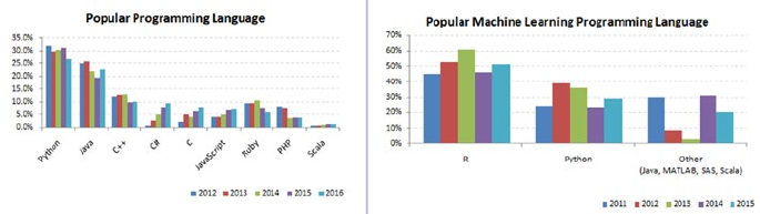
The Rising Star
Python was officially born on February 20, 1991, with version number 0.9.0 and has taken
a tremendous growth path to become the most popular language for the last 5 years in a
row (2012 to 2016). Its application cuts across various areas such as website development,
mobile apps development, scientific and numeric computing, desktop GUI, and complex
software development. Even though Python is a more general-purpose programming
and scripting language, it has been gaining popularity over the past 5 years among data
scientists and Machine Learning engineers. See Figure1-1.
Figure 1-1. Popular Coding Language(Source: codeeval.com) and Popular Machine
Learning Programming Language (Source:KDD poll)

CHAPTER 1 ■ STEP 1 – GETTING STARTED IN PYTHON
3
There are well-designed development environments such as IPython Notebook and
Spyder that allow for a quick introspection of the data and enable developing of machine
learning models interactively.
Powerful modules such as NumPy and Pandas exist for the efficient use of numeric
data. Scientific computing is made easy with SciPy package. A number of primary
machine learning algorithms have been efficiently implemented in scikit-learn (also
known as sklearn). HadooPy, PySpark provides seamless work experience with big data
technology stacks. Cython and Numba modules allow executing Python code in par
with the speed of C code. Modules such as nosetest emphasize high-quality, continuous
integration tests, and automatic deployment.
Combining all of the above has made many machine learning engineers embrace
Python as the choice of language to explore data, identify patterns, and build and deploy
models to the production environment. Most importantly the business-friendly licenses
for various key Python packages are encouraging the collaboration of businesses and the
open source community for the benefit of both worlds. Overall the Python programming
ecosystem allows for quick results and happy programmers. We have been seeing
the trend of developers being part of the open source community to contribute to the
bug fixes and new algorithms for the use by the global community, at the same time
protecting the core IP of the respective company they work for.
Python 2.7.x or Python 3.4.x?
Python 3.4.x is the latest version and comes with nicer, consistent functionalities!
However, there is very limited third-party module support for it, and this will be the trend
for at least a couple of more years. However, all major frameworks still run on version
2.7.x and are likely to continue to do so for a significant amount of time. Therefore, it
is advised to start with Python 2, for the fact that it is the most widely used version for
building machine learning systems as of today.
For an in-depth analysis of the differences between Python 2 vs. 3, you can refer to Wiki.
python.org (https://wiki.python.org/moin/Python2orPython3v), which says that there
are benefits to each.
I recommend Anaconda (Python distribution), which is BSD licensed and gives you
permission to use it commercially and for redistribution. It has around 270 packages
including the most important ones for most scientific applications, data analysis, and
machine learning such as NumPy, SciPy, Pandas, IPython, matplotlib, and scikit-learn. It
also provides a superior environment tool conda that allows you to easily switch between
environments, even between Python 2 and 3 (if required). It is also updated very quickly
as soon as a new version of a package is released and you can just use conda update
<packagename> to update it.
You can download the latest version of Anaconda from their official website at
https://www.continuum.io/downloads and follow the installation instructions.
CHAPTER 1 ■ STEP 1 – GETTING STARTED IN PYTHON
4
Windows Installation
• Download the installer depending on your system configuration
(32 or 64 bit).
• Double-click the .exe file to install Anaconda and follow the
installation wizard on your screen.
OSX Installation
For Mac OS, you can install either through a graphical installer or from a command line.
Graphical Installer
• Download the graphical installer.
• Double-click the downloaded .pkg file and follow the installation
wizard instructions on your screen.
Or
Command-Line Installer
• Download the command-line installer.
• In your terminal window type one of the below and follow the
instructions: bash <Anaconda2-x.x.x-MacOSX-x86_64.sh>.
Linux Installation
• Download the installer depending on your system configuration
(32 or 64 bit).
• In your terminal window type one of the below and follow the
instructions: bash Anaconda2-x.x.x-Linux-x86_xx.sh.
Python from Official Website
For some reason if you don’t want to go with the Anaconda build pack, alternatively you
can go to Python’s official website https://www.python.org/downloads/ and browse to
the appropriate OS section and download the installer. Note that OSX and most of the
Linux come with preinstalled Python so there is no need of additional configuring.
Setting up PATH for Windows: When you run the installer make sure to check the “Add
Python to PATH option.” This will allow us to invoke the Python interpreter from any directory.
If you miss ticking “Add Python to PATH option,” follow these instructions:
• Right-click on “My computer.”
• Click “Properties.”
• Click “Advanced system settings” in the side panel.
CHAPTER 1 ■ STEP 1 – GETTING STARTED IN PYTHON
5
• Click “Environment Variables.”
• Click the “New” below system variables.
• For the name, enter pythonexe (or anything you want).
• For the value, enter the path to your Python
(example: C:\Python32\).
• Now edit the Path variable (in the system part) and add
%pythonexe%; to the end of what’s already there.
Running Python
From the command line, type “Python” to open the interactive interpreter.
A Python script can be executed at the command line using the syntax here:
python <scriptname.py>
All the code used in this book are available as IPython Notebook (now known as
the Jupyter Notebook), it is an interactive computational environment, in which you can
combine code execution, rich text, mathematics, plots and rich media. You can launch
the Jupyter Notebook by clicking on the icon installed by Anaconda in the start menu
(Windows) or by typing ‘jupyter notebook’ in a terminal (cmd on Windows). Then browse
for the relevant IPython Notebook file that you would like to paly with.
Note that the codes can break with change is package version, hence for
reproducibility, I have shared my package version numbers, please refer
Module_Versions IPython Notebook.
Key Concepts
There are a couple of fundamental concepts in Python, and understanding these are
essential for a beginner to get started. A brief look at these concepts is to follow.
Python Identifiers
As the name suggests, identifiers help us to differentiate one entity from another. Python
entities such as class, functions, and variables are called identifiers.
• It can be a combination of upper- or lowercase letters
(a to z or A to Z).
• It can be any digits (0 to 9) or an underscore (_).
• The general rules to be followed for writing identifiers in Python.
• It cannot start with a digit. For example, 1variable is not valid,
whereas variable1 is valid.
• Python reserved keywords (refer to Table1-1) cannot be used as identifiers.
• Except for underscore (_), special symbols like !, @, #, $, % etc
cannot be part of the identifiers.

CHAPTER 1 ■ STEP 1 – GETTING STARTED IN PYTHON
6
Keywords
Table1-1 lists the set of reserved words used in Python to define the syntax and structure
of the language. Keywords are case sensitive, and all the keywords are in lowercase except
True, False, and None.
My First Python Program
Launch the Python interactive on the command prompt, and then type the following text
and press Enter.
>>> print "Hello, Python World!"
If you are running Python 2.7.x from the Anaconda build pack, then you can also use
the print statement with parentheses as in print (“Hello, Python World!”), which would
produce the following result: Hello, Python World! See Figure1-2.
Code Blocks (Indentation & Suites)
It is very important to understand how to write code blocks in Python. Let’s look at two
key concepts around code blocks.
Table 1-1. Python keywords
FALSE Class Finally Is return
None Continue For Lambda try
TRUE Def From nonlocal while
And Del Global Not with
As Elif If Or yield
Assert Else Import Pass
Break Except In Raise
Figure 1-2. Python vs. Others
CHAPTER 1 ■ STEP 1 – GETTING STARTED IN PYTHON
7
Indentation
One of the most unique features of Python is its use of indentation to mark blocks of code.
Each line of code must be indented by the same amount to denote a block of code in
Python. Unlike most other programming languages, indentation is not used to help make
the code look pretty. Indentation is required to indicate which block of code a code or
statement belongs to.
Suites
A collection of individual statements that makes a single code block are called suites
in Python. A header line followed by a suite are required for compound or complex
statements such as if, while, def, and class (we will understand each of these in details in
the later sections). Header lines begin with a keyword, and terminate with a colon (:) and
are followed by one or more lines that make up the suite. See Listings 1-1 and 1-2.
Listing 1-1. Example of correct indentation
# Correct indentation
print ("Programming is an important skill for Data Science")
print ("Statistics is a important skill for Data Science")
print ("Business domain knowledge is a important skill for Data Science")
# Correct indentation, note that if statement here is an example of suites
x = 1
if x == 1:
print ('x has a value of 1')
else:
print ('x does NOT have a value of 1')
Listing 1-2. Example of incorrect indentation
# incorrect indentation, program will generate a syntax error
# due to the space character inserted at the beginning of second line
print ("Programming is an important skill for Data Science")
print ("Statistics is a important skill for Data Science")
print ("Business domain knowledge is a important skill for Data Science")
3
# incorrect indentation, program will generate a syntax error
# due to the wrong indentation in the else statement
x = 1
if x == 1:
print ('x has a value of 1')
else:
print ('x does NOT have a value of 1')

CHAPTER 1 ■ STEP 1 – GETTING STARTED IN PYTHON
8
Basic Object Types
According to the Python data model reference, objects are Python’s notion for data. All
data in a Python program is represented by objects or by relations between objects. In
a sense, and in conformance to Von Neumann’s model of a “stored program computer,”
code is also represented by objects.Every object has an identity, a type, and a value. See
Table1-2 and Listing 1-3.
Table 1-2. Python object types
Type Examples Comments
None None # singleton null object
Boolean True, False
Integer -1, 0, 1, sys.maxint
Long 1L, 9787L
Float 3.141592654
inf, float(‘inf’) # infinity
-inf # neg infinity
nan, float(‘nan’) # not a number
Complex 2+8j # note use of j
String ‘this is a string’, “also me” # use single or double
quote
r‘raw string’, b‘ASCII string’
u‘unicode string’
Tuple empty = () # empty tuple
(1, True, ‘ML’) # immutable list or
unalterable list
List empty = [] empty list
[1, True, ‘ML’] # mutable list or
alterable list
Set empty = set() # empty set
set(1, True, ‘ML’) # mutable or alterable
dictionary empty = {}
{‘1’:‘A’, ‘2’:‘AA’, True = 1, False = 0}
# mutable object or
alterable object
File f = open(‘filename’, ‘rb’)
CHAPTER 1 ■ STEP 1 – GETTING STARTED IN PYTHON
9
Listing 1-3. Code For Basic Object Types
none = None # singleton null object
boolean = bool(True)
integer = 1
Long = 3.14
# float
Float = 3.14
Float_inf = float('inf')
Float_nan = float('nan')
# complex object type, note the usage of letter j
Complex = 2+8j
# string can be enclosed in single or double quote
string = 'this is a string'
me_also_string = "also me"
List = [1, True, 'ML'] # Values can be changed
Tuple = (1, True, 'ML') # Values can not be changed
Set = set([1,2,2,2,3,4,5,5]) # Duplicates will not be stored
# Use a dictionary when you have a set of unique keys that map to values
Dictionary = {'a':'A', 2:'AA', True:1, False:0}
# lets print the object type and the value
print type(none), none
print type(boolean), boolean
print type(integer), integer
print type(Long), Long
print type(Float), Float
print type(Float_inf), Float_inf
print type(Float_nan), Float_nan
print type(Complex), Complex
print type(string), string
print type(me_also_string), me_also_string
print type(Tuple), Tuple
print type(List), List
print type(Set), Set
print type(Dictionary), Dictionary
----- output ------
<type 'NoneType'> None
<type 'bool'> True
CHAPTER 1 ■ STEP 1 – GETTING STARTED IN PYTHON
10
<type 'int'> 1
<type 'float'> 3.14
<type 'float'> 3.14
<type 'float'> inf
<type 'float'> nan
<type 'complex'> (2+8j)
<type 'str'> this is a string
<type 'str'> also me
<type 'tuple'> (1, True, 'ML')
<type 'list'> [1, True, 'ML']
<type 'set'> set([1, 2, 3, 4, 5])
<type 'dict'> {'a': 'A', True: 1, 2: 'AA', False: 0}
When to Use List vs. Tuples vs. Set vs. Dictionary
• List: Use when you need an ordered sequence of homogenous
collections, whose values can be changed later in the program.
• Tuple: Use when you need an ordered sequence of heterogeneous
collections whose values need not be changed later in the
program.
• Set: It is ideal for use when you don’t have to store duplicates and
you are not concerned about the order or the items. You just want
to know whether a particular value already exists or not.
• Dictionary: It is ideal for use when you need to relate values with
keys, in order to look them up efficiently using a key.
Comments in Python
Single line comment: Any characters followed by the # (hash) and up to the end of the
line are considered a part of the comment and the Python interpreter ignores them.
Multiline comments: Any characters between the strings """ (referred as multiline
string), that is, one at the beginning and end of your comments will be ignored by the
Python interpreter. See Listing 1-4.
Listing 1-4. Example code for comments
# This is a single line comment in Python
print "Hello Python World" # This is also a single line comment in Python
""" This is an example of a multi line
comment that runs into multiple lines.
Everything that is in between is considered as comments
"""
CHAPTER 1 ■ STEP 1 – GETTING STARTED IN PYTHON
11
Multiline Statement
Python’s oblique line continuation inside parentheses, brackets, and braces is the
favorite way of casing longer lines. Using backslash to indicate line continuation makes
readability better; however if needed you can add an extra pair of parentheses around
the expression. It is important to correctly indent the continued line of your code. Note
that the preferred place to break around the binary operator is after the operator, and not
before it. See Listing 1-5.
Listing 1-5. Example code for multiline statements
# Example of implicit line continuation
x = ('1' + '2' +
'3' + '4')
# Example of explicit line continuation
y = '1' + '2' + \
'11' + '12'
weekdays = ['Monday', 'Tuesday', 'Wednesday',
'Thursday', 'Friday']
weekend = {'Saturday',
'Sunday'}
print ('x has a value of', x)
print ('y has a value of', y)
print days
print weekend
------ output -------
('x has a value of', '1234')
('y has a value of', '1234')
['Monday', 'Tuesday', 'Wednesday', 'Thursday', 'Friday']
set(['Sunday', 'Saturday'])
Multiple Statements on a Single Line
Python also allows multiple statements on a single line through usage of the semicolon
(;), given that the statement does not start a new code block. See Listing 1-6.
Listing 1-6. Code example for multistatements on a single line
import os; x = 'Hello'; print x

CHAPTER 1 ■ STEP 1 – GETTING STARTED IN PYTHON
12
Basic Operators
In Python, operators are the special symbols that can manipulate the value of operands.
For example, let’s consider the expression 1 + 2 = 3. Here, 1 and 2 are called operands,
which are the value on which operators operate and the symbol + is called an operator.
Python language supports the following types of operators.
• Arithmetic Operators
• Comparison or Relational Operators
• Assignment Operators
• Bitwise Operators
• Logical Operators
• Membership Operators
• Identity Operators
Let’s learn all operators through examples one by one.
Arithmetic Operators
Arithmetic operators are useful for performing mathematical operations on numbers such
as addition, subtraction, multiplication, division, etc. See Table1-3 and then Listing 1-7.
Table 1-3. Arithmetic operators
Operator Description Example
+ Addition x + y = 30
- Subtraction x – y = -10
* Multiplication x * y = 200
/ Division y / x = 2
% Modulus y % x = 0
** Exponent Exponentiation x**b =10 to the power 20
// Floor Division – Integer division rounded
toward minus infinity
9//2 = 4 and 9.0//2.0 = 4.0,
-11//3 = -4, -11.0/
CHAPTER 1 ■ STEP 1 – GETTING STARTED IN PYTHON
13
Listing 1-7. Example code for arithmetic operators
# Variable x holds 10 and variable y holds 5
x = 10
y = 5
# Addition
print "Addition, x(10) + y(5) = ", x + y
# Subtraction
print "Subtraction, x(10) - y(5) = ", x - y
# Multiplication
print "Multiplication, x(10) * y(5) = ", x * y
# Division
print "Division, x(10) / y(5) = ",x / y
# Modulus
print "Modulus, x(10) % y(5) = ", x % y
# Exponent
print "Exponent, x(10)**y(5) = ", x**y
# Integer division rounded towards minus infinity
print "Floor Division, x(10)//y(5) = ", x//y
-------- output --------
Addition, x(10) + y(5) = 15
Subtraction, x(10) - y(5) = 5
Multiplication, x(10) * y(5) = 50
Divions, x(10) / y(5) = 2
Modulus, x(10) % y(5) = 0
Exponent, x(10)**y(5) = 100000
Floor Division, x(10)//y(5) = 2
Comparison or Relational Operators
As the name suggests the comparison or relational operators are useful to compare
values. It would return True or False as a result for a given condition. See Table1-4 and
Listing 1-8.

CHAPTER 1 ■ STEP 1 – GETTING STARTED IN PYTHON
14
Listing 1-8. Example code for comparision/relational operators
# Variable x holds 10 and variable y holds 5
x = 10
y = 5
# Equal check operation
print "Equal check, x(10) == y(5) ", x == y
# Not Equal check operation
print "Not Equal check, x(10) != y(5) ", x != y
# Not Equal check operation
print "Not Equal check, x(10) <>y(5) ", x<>y
# Less than check operation
print "Less than check, x(10) <y(5) ", x<y
# Greater check operation
print "Greater than check, x(10) >y(5) ", x>y
# Less than or equal check operation
print "Less than or equal to check, x(10) <= y(5) ", x<= y
Table 1-4. Comparison or Relational operators
Operator Description Example
== The condition becomes True, if the values of two
operands are equal.
(x == y) is not true.
!= The condition becomes True, if the values of two
operands are not equal.
<> The condition becomes True, if values of two
operands are not equal.
(x<>y) is true. This
is similar to !=
operator.
> The condition becomes True, if the value of left
operand is greater than the value of right operand.
(x>y) is not true.
< The condition becomes True, if the value of left
operand is less than the value of right operand.
(x<y) is true.
>= The condition becomes True, if the value of left
operand is greater than or equal to the value of
right operand.
(x>= y) is not true.
<= The condition becomes True, if the value of left
operand is less than or equal to the value of right
operand.
(x<= y) is true.

CHAPTER 1 ■ STEP 1 – GETTING STARTED IN PYTHON
15
# Greater than or equal to check operation
print "Greater than or equal to check, x(10) >= y(5) ", x>= y
-------- output --------
Equal check, x(10) == y(5) False
Not Equal check, x(10) != y(5) True
Not Equal check, x(10) <>y(5) True
Less than check, x(10) <y(5) False
Greater than check, x(10) >y(5) True
Less than or equal to check, x(10) <= y(5) False
Greater than or equal to check, x(10) >= y(5) True
Assignment Operators
In Python, assignment operators are used for assigning values to variables. For example,
consider x = 5; it is a simple assignment operator that assigns the numeric value 5, which
is on the right side of the operator onto the variable x on the left side of operator. There
is a range of compound operators in Python like x += 5 that add to the variable and later
assign the same. It is as good as x = x + 5. See Table1-5 and Listing 1-9.
Table 1-5. Assignment operators
Operator Description Example
= Assigns values from right side operands
to left side operand.
z = x + y assigns value
of x + y into z
+= Add AND It adds right operand to the left operand
and assigns the result to left operand.
z += x is equivalent to
z = z + x
-= Subtract AND It subtracts right operand from the left
operand and assigns the result to left
operand.
z -= x is equivalent to
z = z - x
*= Multiply AND It multiplies right operand with the left
operand and assigns the result to left
operand.
z *= x is equivalent to
z = z * x
/= Divide AND It divides left operand with the right
operand and assigns the result to left
operand.
z /= x is equivalent
to z = z/ xz /= x is
equivalent to z = z / x
%= Modulus AND It takes modulus using two operands and
assigns the result to left operand.
z %= x is equivalent to
z = z % x
**= Exponent AND Performs exponential (power)
calculation on operators and assigns
value to the left operand.
z **= x is equivalent to
z = z ** x
//= Floor Division It performs floor division on operators
and assigns value to the left operand.
z //= x is equivalent to
z = z// x
CHAPTER 1 ■ STEP 1 – GETTING STARTED IN PYTHON
16
Listing 1-9. Example code for assignment operators
# Variable x holds 10 and variable y holds 5
x = 5
y = 10
x += y
print "Value of a post x+=y is ", x
x *= y
print "Value of a post x*=y is ", x
x /= y
print "Value of a post x/=y is ", x
x %= y
print "Value of a post x%=y is ", x
x **= y
print "Value of x post x**=y is ", x
x //= y
print "Value of a post x//=y is ", x
-------- output --------
Value of a post x+=y is 15
Value of a post x*=y is 150
Value of a post x/=y is 15
Value of a post x%=y is 5
Value of a post x**=y is 9765625
Value of a post x//=y is 976562
Bitwise Operators
As you might be aware, everything in a computer is represented by bits, that is, a series of
0’s (zero) and 1’s (one). Bitwise operators enable us to directly operate or manipulate bits.
Let’s understand the basic bitwise operations. One of the key usages of bitwise operators
is for parsing hexadecimal colors.
Bitwise operators are known to be confusing for newbies to Python programming,
so don’t be anxious if you don’t understand usability at first. The fact is that you aren’t
really going to see bitwise operators in your everyday machine learning programming.
However, it is good to be aware about these operators.
For example let’s assume that x = 10 (in binary 0000 1010) and y = 4 (in binary
0000 0100). See Table1-6 and Listing 1-10.

CHAPTER 1 ■ STEP 1 – GETTING STARTED IN PYTHON
17
Listing 1-10. Example code for bitwise operators
# Basic six bitwise operations
# Let x = 10 (in binary0000 1010) and y = 4 (in binary0000 0100)
x = 10
y = 4
print x >> y # Right Shift
print x << y # Left Shift
print x & y # Bitwise AND
print x | y # Bitwise OR
print x ^ y # Bitwise XOR
print ~x # Bitwise NOT
-------- output --------
0
160
0
14
14
-11
Table 1-6. Bitwise operators
Operator Description Example
& Binary AND This operator copies a bit to the
result if it exists in both operands.
(x&y) (means
0000 0000)
| Binary OR This operator copies a bit if it exists
in either operand.
(x | y) = 14
(means 0000
1110)
^ Binary XOR This operator copies the bit if it is set
in one operand but not both.
(x ^ y) = 14
(means 0000
1110)
~ Binary Ones Complement This operator is unary and has the
effect of ‘flipping’ bits.
(~x ) = -11
(means 1111
0101)
<< Binary Left Shift The left operands value is moved left
by the number of bits specified by
the right operand.
x<< 2= 42
(means 0010
1000)
>> Binary Right Shift The left operands value is moved
right by the number of bits specified
by the right operand.
x>> 2 = 2 (means
0000 0010)

CHAPTER 1 ■ STEP 1 – GETTING STARTED IN PYTHON
18
Logical Operators
The AND, OR, NOT operators are called logical operators. These are useful to check two
variables against given condition and the result will be True or False appropriately. See
Table1-7 and Listing 1-11.
Listing 1-11. Example code for logical operators
var1 = True
var2 = False
print('var1 and var2 is',var1and var2)
print('var1 or var2 is',var1 or var2)
print('not var1 is',not var1)
-------- output --------
('var1 and var2 is', False)
('var1 or var2 is', True)
('not var1 is', False)
Membership Operators
Membership operators are useful to test if a value is found in a sequence, that is, string,
list, tuple, set, or dictionary. There are two membership operators in Python, ‘in’ and
‘not in’. Note that we can only test for presence of key (and not the value) in case of a
dictionary. See Table1-8 and Listing 1-12.
Table 1-7. Logical operators
Operator Description Example
and Logical AND If both the operands are true then
condition becomes true.
(var1 and var2) is true.
or Logical OR If any of the two operands are non-zero
then condition becomes true.
(var1 or var2) is true.
not Logical NOT Used to reverse the logical state of its
operand.
Not (var1 and var2) is
false.
Table 1-8. Membership operators
Operator Description Example
In Results to True if a value is in the
specified sequence and False otherwise.
var1 in var2
not in Results to True, if a value is not in the
specified sequence and False otherwise.
var1 not in var2

CHAPTER 1 ■ STEP 1 – GETTING STARTED IN PYTHON
19
Listing 1-12. Example code for membership operators
var1 = 'Hello world' # string
var1 = {1:'a',2:'b'}# dictionary
print('H' in var1)
print('hello' not in var2)
print(1 in var2)
print('a' in var2)
-------- output --------
True
True
True
False
Identity Operators
Identity operators are useful to test if two variables are present on the same part of the
memory. There are two identity operators in Python, ‘is’ and ‘is not’ . Note that two variables
having equal values do not imply they are identical. See Table1-9 and Listing 1-13.
Listing 1-13. Example code for identity operators
var1 = 5
var1 = 5
var2 = 'Hello'
var2 = 'Hello'
var3 = [1,2,3]
var3 = [1,2,3]
print(var1 is not var1)
print(var2 is var2)
print(var3 is var3)
-------- output --------
False
True
False
Table 1-9. Identity operators
Operator Description Example
Is Results to True, if the variables on either side of
the operator point to the same object and False
otherwise.
var1 is var2
is not Results to False, if the variables on either side of
the operator point to the same object and True
otherwise.
Var1 is not var2
CHAPTER 1 ■ STEP 1 – GETTING STARTED IN PYTHON
20
Control Structure
A control structure is the fundamental choice or decision-making process in
programming. It is a chunk of code that analyzes values of variables and decides a
direction to go based on a given condition. In Python there are mainly two types of
control structures: (1) selection and (2) iteration.
Selection
Selection statements allow programmers to check a condition and based on the result
will perform different actions. There are two versions of this useful construct: (1) if and
(2) if…else. See Listings 1-14, 1-15, and 1-16.
Listing 1-14. Example code for a simple ‘if’ statement
var = -1
if var < 0:
print var
print("the value of var is negative")
# If there is only a signle cluse then it may go on the same line as the
header statement
if ( var == -1 ) : print "the value of var is negative"
Listing 1-15. Example code for ‘if else’ statement
var = 1
if var < 0:
print "the value of var is negative"
print var
else:
print "the value of var is positive"
print var
Listing 1-16. Example code for nested if else statements
Score = 95
if score >= 99:
print('A')
elif score >=75:
print('B')
elif score >= 60:
print('C')
elif score >= 35:
print('D')
else:
print('F')
CHAPTER 1 ■ STEP 1 – GETTING STARTED IN PYTHON
21
Iteration
A loop control statement enables us to execute a single or a set of programming
statements multiple times until a given condition is satisfied. Python provides two
essential looping statements: (1) for (2) while statement.
For loop: It allows us to execute code block for a specific number of times or against a
specific condition until it is satisfied. See Listing 1-17.
Listing 1-17. Example codes for a ‘for loop’ statement
# First Example
print "First Example"
for item in [1,2,3,4,5]:
print 'item :', item
# Second Example
print "Second Example"
letters = ['A', 'B', 'C']
for letter in letters:
print ' First loop letter :', letter
# Third Example - Iterating by sequency index
print "Third Example"
for index in range(len(letters)):
print 'First loop letter :', letters[index]
# Fourth Example - Using else statement
print "Fourth Example"
for item in [1,2,3,4,5]:
print 'item :', item
else:
print 'looping over item complete!'
----- output ------
First Example
item : 1
item : 2
item : 3
item : 4
item : 5
Second Example
First loop letter : A
First loop letter : B
First loop letter : C
Third Example
First loop letter : A
First loop letter : B
First loop letter : C
Fourth Example

CHAPTER 1 ■ STEP 1 – GETTING STARTED IN PYTHON
22
item : 1
item : 2
item : 3
item : 4
item : 5
looping over item complete!
While loop: The while statement repeats a set of code until the condition is true. See
Listing 1-18.
Listing 1-18. Example code for while loop statement
count = 0
while (count <3):
print 'The count is:', count
count = count + 1
■Caution If a condition never becomes FALSE, a loop becomes an infinite loop.
An else statement can be used with a while loop and the else will be executed when
the condition becomes false. See Listing 1-19.
Listing 1-19. example code for a ‘while with a else’ statement
count = 0
while count <3:
print count, " is less than 5"
count = count + 1
else:
print count, " is not less than 5"
Lists
Python’s lists are the most flexible data type. It can be created by writing a list of comma-
separated values between square brackets. Note that that the items in the list need not be
of the same data type. See Table1-10; and Listings 1-20, 1-21, 1-22, 1-23, and 1-24.

CHAPTER 1 ■ STEP 1 – GETTING STARTED IN PYTHON
23
Table 1-10. Python list operations
Description Python Expression Example Results
Creating a list of items [item1, item2, …] list = [‘a’,‘b’,‘c’,‘d’] [‘a’,‘b’,‘c’,‘d’]
Accessing items in list list[index] list = [‘a’,‘b’,‘c’,‘d’]
list[2]
c
Length len(list) len([1, 2, 3]) 3
Concatenation list_1 + list_2 [1, 2, 3] + [4, 5, 6] [1, 2, 3, 4, 5, 6]
Repetition list * int [‘Hello’] * 3 [‘Hello’, ‘Hello’,
‘Hello’]
Membership item in list 3 in [1, 2, 3] TRUE
Iteration for x in list: print x for x in [1, 2, 3]: print
x,
1 2 3
Count from the right list[-index] list = [1,2,3]; list[-2] 2
Slicing fetches sections list[index:] list = [1,2,3]; list[1:] [2,3]
Comparing lists cmp(list_1, list_2) print cmp([1,2,3,4],
[5,6,7]); print
cmp([1,2,3], [5,6,7,8])
1 -1
Return max item max(list) max([1,2,3,4,5]) 5
Return min item min(list) max([1,2,3,4,5]) 1
Append object to list list.append(obj) [1,2,3,4].append(5) [1,2,3,4,5]
Count item occurrence list.count(obj) [1,1,2,3,4].count(1) 2
Append content of
sequence to list
list.extend(seq) [‘a’, 1].extend([‘b’, 2]) [‘a’, 1, ‘b’, 2]
Return the first index
position of item
list.index(obj) [‘a’, ‘b’,‘c’,1,2,3].
index(‘c’)
2
Insert object to list at a
desired index
list.insert(index, obj) [‘a’, ‘b’,‘c’,1,2,3].
insert(4, ‘d’)
[‘a’, ‘b’,‘c’,‘d’,
1,2,3]
Remove and return last
object from list
list.pop(obj=list[-1]) [‘a’, ‘b’,‘c’,1,2,3].pop()
[‘a’, ‘b’,‘c’,1,2,3].pop(2)
3 c
Remove object from list list.remove(obj) [‘a’, ‘b’,‘c’,1,2,3].
remove(‘c’)
[‘a’, ‘b’, 1,2,3]
Reverse objects of list
in place
list.reverse() [‘a’, ‘b’,‘c’,1,2,3].
reverse()
[3,2,1,‘c’,‘b’,‘a’]
Sort objects of list list.sort() [‘a’, ‘b’,‘c’,1,2,3].sort()
[‘a’, ‘b’,‘c’,1,2,3].
sort(reverse = True)
[1,2,3,‘a’, ‘b’,‘c’]
[‘c’,‘b’,‘a’,3,2,1]
CHAPTER 1 ■ STEP 1 – GETTING STARTED IN PYTHON
24
Listing 1-20. Example code for accessing lists
# Create lists
list_1 = ['Statistics', 'Programming', 2016, 2017, 2018];
list_2 = ['a', 'b', 1, 2, 3, 4, 5, 6, 7 ];
# Accessing values in lists
print "list_1[0]: ", list_1[0]
print "list2_[1:5]: ", list_2[1:5]
---- output ----
list_1[0]: Statistics
list2_[1:5]: ['b', 1, 2, 3]
Listing 1-21. Example code for adding new values to lists
print "list_1 values: ", list_1
# Adding new value to list
list_1.append(2019)
print "list_1 values post append: ", list_1
---- output ----
list_1 values: ['c', 'b', 'a', 3, 2, 1]
list_1 values post append: ['c', 'b', 'a', 3, 2, 1, 2019]
Listing 1-22. Example code for updating existing values of lists
print "Values of list_1: ", list_1
# Updating existing value of list
print "Index 2 value : ", list_1[2]
list_1[2] = 2015;
print "Index 2's new value : ", list_1[2]
---- output ----
Values of list_1: ['c', 'b', 'a', 3, 2, 1, 2019]
Index 2 value : a
Index 2's new value : 2015
Listing 1-23. Example code for deleting a list element
Print "list_1 values: ", list_1
# Deleting list element
del list_1[5];
print "After deleting value at index 2 : ", list_1
---- output ----
CHAPTER 1 ■ STEP 1 – GETTING STARTED IN PYTHON
25
list_1 values: ['c', 'b', 2015, 3, 2, 1, 2019]
After deleting value at index 2 : ['c', 'b', 2015, 3, 2, 2019]
Listing 1-24. Example code for basic operations on lists
print "Length: ", len(list_1)
print "Concatenation: ", [1,2,3] + [4, 5, 6]
print "Repetition :", ['Hello'] * 4
print "Membership :", 3 in [1,2,3]
print "Iteration :"
for x in [1,2,3]: print x
# Negative sign will count from the right
print "slicing :", list_1[-2]
# If you dont specify the end explicitly, all elements from the specified
start index will be printed
print "slicing range: ", list_1[1:]
# Comparing elements of lists
print "Compare two lists: ", cmp([1,2,3, 4], [1,2,3])
print "Max of list: ", max([1,2,3,4,5])
print "Min of list: ", min([1,2,3,4,5])
print "Count number of 1 in list: ", [1,1,2,3,4,5,].count(1)
list_1.extend(list_2)
print "Extended :", list_1
print "Index for Programming : ", list_1.index( 'Programming')
print list_1
print "pop last item in list: ", list_1.pop()
print "pop the item with index 2: ", list_1.pop(2)
list_1.remove('b')
print "removed b from list: ", list_1
list_1.reverse()
print "Reverse: ", list_1
list_1 = ['a', 'b','c',1,2,3]
list_1.sort()
print "Sort ascending: ", list_1
list_1.sort(reverse = True)
print "Sort descending: ", list_1
---- output ----
Length: 5
Concatenation: [1, 2, 3, 4, 5, 6]
Repetition : ['Hello', 'Hello', 'Hello', 'Hello']
Membership : True
Iteration :
1
2
CHAPTER 1 ■ STEP 1 – GETTING STARTED IN PYTHON
26
3
slicing : 2017
slicing range: ['Programming', 2015, 2017, 2018]
Compare two lists: 1
Max of list: 5
Min of list: 1
Count number of 1 in list: 2
Extended : ['Statistics', 'Programming', 2015, 2017, 2018, 'a', 'b', 1, 2,
3, 4, 5, 6, 7]
Index for Programming : 1
['Statistics', 'Programming', 2015, 2017, 2018, 'a', 'b', 1, 2, 3, 4, 5, 6, 7]
pop last item in list: 7
pop the item with index 2: 2015
removed b from list: ['Statistics', 'Programming', 2017, 2018, 'a', 1, 2,
3, 4, 5, 6]
Reverse: [6, 5, 4, 3, 2, 1, 'a', 2018, 2017, 'Programming', 'Statistics']
Sort ascending: [1, 2, 3, 'a', 'b', 'c']
Sort descending: ['c', 'b', 'a', 3, 2, 1]
Tuple
A Python tuple is a sequences or series of immutable Python objects very much similar to
the lists. However there exist some essential differences between lists and tuples, which
are the following. See also Table1-11; and Listings 1-25, 1-26, 1-27, and 1-28.
1. Unlike list, the objects of tuples cannot be changed.
2. Tuples are defined by using parentheses, but lists are defined
by square brackets.

CHAPTER 1 ■ STEP 1 – GETTING STARTED IN PYTHON
27
Listing 1-25. Example code for creating tuple
# Creating a tuple
Tuple = ()
print "Empty Tuple: ", Tuple
Tuple = (1,)
print "Tuple with single item: ", Tuple
Table 1-11. Python Tuple operations
Description Python Expression Example Results
Creating a tuple (item1, item2, …)
() # empty tuple
(item1,) # Tuple
with one item, note
comma is required
tuple = (‘a’,‘b’,‘c’,
‘d’,1,2,3)
tuple = ()
tuple = (1,)
(‘a’,‘b’,‘c’,‘d’,1,2,3)
()
1
Accessing items in
tuple
tuple[index]
tuple[start_index:
end_index]
tuple = (‘a’,‘b’,‘c’,
‘d’,1,2,3)
tuple[2]
tuple[0:2]
c
a, b, c
Deleting a tuple del tuple_name del tuple
Length len(tuple) len((1, 2, 3)) 3
Concatenation tuple_1 + tuple_2 (1, 2, 3) + (4, 5, 6) (1, 2, 3, 4, 5, 6)
Repetition tuple * int (‘Hello’,) * 4 (‘Hello’, ‘Hello’,
‘Hello’, ‘Hello’)
Membership item in tuple 3 in (1, 2, 3) TRUE
Iteration for x in tuple: print x for x in (1, 2, 3):
print x
1 2 3
Count from the right tuple[-index] tuple = (1,2,3);
list[-2]
2
Slicing fetches
sections
tuple[index:] tuple = (1,2,3);
list[1:]
(2,3)
Comparing lists cmp(tuple_1,
tuple_2)
print cmp((1,2,3,4),
(5,6,7));
print cmp((1,2,3),
(5,6,7,8))
1
-1
Return max item max(tuple) max((1,2,3,4,5)) 5
Return min item min(tuple) max((1,2,3,4,5)) 1
Convert a list to tuple tuple(seq) tuple([1,2,3,4]) (1,2,3,4,5)
CHAPTER 1 ■ STEP 1 – GETTING STARTED IN PYTHON
28
Tuple = ('a','b','c','d',1,2,3)
print "Sample Tuple :", Tuple
---- output ----
Empty Tuple: ()
Tuple with single item: (1,)
Sample Tuple : ('a', 'b', 'c', 'd', 1, 2, 3)
Listing 1-26. Example code for accessing tuple
# Accessing items in tuple
Tuple = ('a', 'b', 'c', 'd', 1, 2, 3)
print "3rd item of Tuple:", Tuple[2]
print "First 3 items of Tuple", Tuple[0:2]
---- output ----
3rd item of Tuple: c
First 3 items of Tuple ('a', 'b')
Listing 1-27. Example code for deleting tuple
# Deleting tuple
print "Sample Tuple: ", Tuple
del Tuple
print Tuple # Will throw an error message as the tuple does not exist
---- output ----
Sample Tuple: ('a', 'b', 'c', 'd', 1, 2, 3)
---------------------------------------------------------------------------
NameError Traceback (most recent call last)
<ipython-input-35-6a0deb3cfbcf> in <module>()
3 print "Sample Tuple: ", Tuple
4 del Tuple
----> 5 print Tuple # Will throw an error message as the tuple does not exist
NameError: name 'Tuple' is not defined
Listing 1-28. Example code for basic operations on tupe (not exhaustive)
# Basic Tuple operations
Tuple = ('a','b','c','d',1,2,3)
print "Length of Tuple: ", len(Tuple)
Tuple_Concat = Tuple + (7,8,9)
print "Concatinated Tuple: ", Tuple_Concat
CHAPTER 1 ■ STEP 1 – GETTING STARTED IN PYTHON
29
print "Repetition: ", (1, 'a',2, 'b') * 3
print "Membership check: ", 3 in (1,2,3)
# Iteration
for x in (1, 2, 3): print x
print "Negative sign will retrieve item from right: ", Tuple_Concat[-2]
print "Sliced Tuple [2:] ", Tuple_Concat[2:]
# Comparing two tuples
print "Comparing tuples (1,2,3) and (1,2,3,4): ", cmp((1,2,3), (1,2,3,4))
print "Comparing tuples (1,2,3,4) and (1,2,3): ", cmp((1,2,3,4), (1,2,3))
# Find max
print "Max of the Tuple (1,2,3,4,5,6,7,8,9,10): ",
max((1,2,3,4,5,6,7,8,9,10))
print "Min of the Tuple (1,2,3,4,5,6,7,8,9,10): ",
min((1,2,3,4,5,6,7,8,9,10))
print "List [1,2,3,4] converted to tuple: ", type(tuple([1,2,3,4]))
---- output ----
Length of Tuple: 7
Concatinated Tuple: ('a', 'b', 'c', 'd', 1, 2, 3, 7, 8, 9)
Repetition: (1, 'a', 2, 'b', 1, 'a', 2, 'b', 1, 'a', 2, 'b')
Membership check: True
1
2
3
Negative sign will retrieve item from right: 8
Sliced Tuple [2:] ('c', 'd', 1, 2, 3, 7, 8, 9)
Comparing tuples (1,2,3) and (1,2,3,4): -1
Comparing tuples (1,2,3,4) and (1,2,3): 1
Max of the Tuple (1,2,3,4,5,6,7,8,9,10): 10
Min of the Tuple (1,2,3,4,5,6,7,8,9,10): 1
List [1,2,3,4] converted to tuple: <type 'tuple'>
Sets
As the name implies, sets are the implementations of mathematical sets. Three key
characteristic of set are the following.
1. The collection of items is unordered.
2. No duplicate items will be stored, which means that each item
is unique.
3. Sets are mutable, which means the items of it can be changed.

CHAPTER 1 ■ STEP 1 – GETTING STARTED IN PYTHON
30
An item can be added or removed from sets. Mathematical set operations such as
union, intersection, etc., can be performed on Python sets. See Table1-12 and Listing 1-29.
Table 1-12. Python set operations
Description Python Expression Example Results
Creating a set. set{item1, item2, …}
set() # empty set
languages =
set([‘Python’, ‘R’,
‘SAS’, ‘Julia’])
set([‘SAS’, ‘Python’,
‘R’, ‘Julia’])
Add an item/
element to a set.
add() languages.
add(‘SPSS’)
set([‘SAS’, ‘SPSS’,
‘Python’, ‘R’, ‘Julia’])
Remove all items/
elements from a set.
clear() languages.clear() set([])
Return a copy of
a set.
copy() lang = languages.
copy()
print lang
set([‘SAS’, ‘SPSS’,
‘Python’, ‘R’, ‘Julia’])
Remove an item/
element from set
if it is a member.
(Do nothing if the
element is not in set).
discard() languages = set([‘C’,
‘Java’, ‘Python’,
‘Data Science’,
‘Julia’, ‘SPSS’, ‘AI’,
‘R’, ‘SAS’, ‘Machine
Learning’])
languages.
discard(‘AI’)
set([‘C’, ‘Java’,
‘Python’, ‘Data
Science’, ‘Julia’,
‘SPSS’, ‘R’,
‘SAS’, ‘Machine
Learning’])
Remove an item/
element from a set.
If the element is not
a member, raise a
KeyError.
remove() languages = set([‘C’,
‘Java’, ‘Python’,
‘Data Science’,
‘Julia’, ‘SPSS’, ‘AI’,
‘R’, ‘SAS’, ‘Machine
Learning’])
languages.
remove(‘AI’)
set([‘C’, ‘Java’,
‘Python’, ‘Data
Science’, ‘Julia’,
‘SPSS’, ‘R’,
‘SAS’, ‘Machine
Learning’])
Remove and
return an arbitrary
set element.
RaiseKeyError if the
set is empty.
pop() languages = set([‘C’,
‘Java’, ‘Python’,
‘Data Science’,
‘Julia’, ‘SPSS’, ‘AI’,
‘R’, ‘SAS’, ‘Machine
Learning’])
print “Removed:”,
(languages.pop())
print(languages)
Removed: C
set([‘Java’, ‘Python’,
‘Data Science’,
‘Julia’, ‘SPSS’, ‘R’,
‘SAS’, ‘Machine
Learning’])
(continued)

CHAPTER 1 ■ STEP 1 – GETTING STARTED IN PYTHON
31
Table 1-12. (continued)
Description Python Expression Example Results
Return the
difference of two
or more sets as a
new set.
difference() # initialize A and B
A = {1, 2, 3, 4, 5}
B = {4, 5, 6, 7, 8}
A.difference(B)
{1, 2, 3}
Remove all item/
elements of another
set from this set.
difference_update() # initialize A and B
A = {1, 2, 3, 4, 5}
B = {4, 5, 6, 7, 8}
A.difference_
update(B) print A
set([1, 2, 3])
Return the
intersection of two
sets as a new set.
intersection() # initialize A and B
A = {1, 2, 3, 4, 5}
B = {4, 5, 6, 7, 8}
A.intersection(B)
{4, 5}
Update the set with
the intersection of
itself and another.
intersection_
update()
# initialize A and B
A = {1, 2, 3, 4, 5}
B = {4, 5, 6, 7, 8}
A.intersection_
update B print A
set([4, 5])
Return True if two
sets have a null
intersection.
isdisjoint() # initialize A and B
A = {1, 2, 3, 4, 5}
B = {4, 5, 6, 7, 8}
A.isdisjoint(B)
FALSE
Return True if
another set contains
this set.
issubset() # initialize A and B
A = {1, 2, 3, 4, 5}
B = {4, 5, 6, 7, 8} print
A.issubset(B)
FALSE
Return True if this
set contains another
set.
issuperset() # initialize A and B
A = {1, 2, 3, 4, 5}
B = {4, 5, 6, 7, 8} print
A.issuperset(B)
FALSE
Return the
symmetric
difference of two
sets as a new set.
symmetric_
difference()
# initialize A and B
A = {1, 2, 3, 4, 5}
B = {4, 5, 6, 7, 8}
A. symmetric_
difference(B)
{1, 2, 3, 6, 7, 8}
(continued)

CHAPTER 1 ■ STEP 1 – GETTING STARTED IN PYTHON
32
Listing 1-29. Example code for creating sets
# Creating an empty set
languages = set()
print type(languages), languages
languages = {'Python', 'R', 'SAS', 'Julia'}
print type(languages), languages
Table 1-12. (continued)
Description Python Expression Example Results
Update a set with
the symmetric
difference of itself
and another.
symmetric_
difference_update()
# initialize A and B
A = {1, 2, 3, 4, 5}
B = {4, 5, 6, 7, 8}
A.symmetric_
difference(B) print A
A.symmetric_
difference_update(B)
print A
set([1, 2, 3, 6, 7, 8])
Return the union of
sets in a new set.
union() # initialize A and B
A = {1, 2, 3, 4, 5}
B = {4, 5, 6, 7, 8}
A.union(B) print A
set([1, 2, 3, 4, 5])
Update a set with
the union of itself
and others.
update() # initialize A and B
A = {1, 2, 3, 4, 5}
B = {4, 5, 6, 7, 8}
A.update(B) print A
set([1, 2, 3, 4, 5, 6,
7, 8])
Return the length
(the number of
items) in the set.
len() A = {1, 2, 3, 4, 5}
len(A)
5
Return the largest
item in the set.
max() A = {1, 2, 3, 4, 5}
max(A)
1
Return the smallest
item in the set.
min() A = {1, 2, 3, 4, 5}
min(A)
5
Return a new sorted
list from elements
in the set. Does not
sort the set.
sorted() A = {1, 2, 3, 4, 5}
sorted(A)
[4, 5, 6, 7, 8]
Return the sum of
all items/elements
in the set.
sum() A = {1, 2, 3, 4, 5}
sum(A)
15
CHAPTER 1 ■ STEP 1 – GETTING STARTED IN PYTHON
33
# set of mixed datatypes
mixed_set = {"Python", (2.7, 3.4)}
print type(mixed_set), languages
---- output ----
<type 'set'> set([])
<type 'set'> set(['SAS', 'Python', 'R', 'Julia'])
<type 'set'> set(['SAS', 'Python', 'R', 'Julia'])
Accessing Set Elements
See Listing 1-30.
Listing 1-30. Example code for accessing set elements
print list(languages)[0]
print list(languages)[0:3]
---- output ----
C
['C', 'Java', 'Python']
Changing a Set in Python
Although sets are mutable, indexing on them will have no meaning due to the fact that
they are unordered. So sets do not support accessing or changing an item/element
using indexing or slicing. The add() method can be used to add a single element and the
update() method for adding multiple elements. Note that the update() method can take
the argument in the format of tuples, lists, strings, or other sets. However, in all cases the
duplicates are ignored. See Listing 1-31.
Listing 1-31. Example code for changing set elements
# initialize a set
languages = {'Python', 'R'}
print(languages)
# add an element
languages.add('SAS')
print(languages)
# add multiple elements
languages.update(['Julia','SPSS'])
print(languages)
# add list and set
languages.update(['Java','C'], {'Machine Learning','Data Science','AI'})
print(languages)
CHAPTER 1 ■ STEP 1 – GETTING STARTED IN PYTHON
34
---- output ----
set(['Python', 'R'])
set(['Python', 'SAS', 'R'])
set(['Python', 'SAS', 'R', 'Julia', 'SPSS'])
set(['C', 'Java', 'Python', 'Data Science', 'Julia', 'SPSS', 'AI', 'R',
'SAS', 'Machine Learning'])
Removing Items from Set
The discard() or remove() method can be used to remove a particular item from a set. The
fundamental difference between discard() and remove() is that the first do not take any
action if the item does not exist in the set, whereas remove() will raise an error in such a
scenario. See Listing 1-32.
Listing 1-32. Example code for removing items from set
# remove an element
languages.remove('AI')
print(languages)
# discard an element, although AI has already been removed discard will not
throw an error
languages.discard('AI')
print(languages)
# Pop will remove a random item from set
print "Removed:", (languages.pop()), "from", languages
---- output ----
set(['C', 'Java', 'Python', 'Data Science', 'Julia', 'SPSS', 'R', 'SAS',
'Machine Learning'])
set(['C', 'Java', 'Python', 'Data Science', 'Julia', 'SPSS', 'R', 'SAS',
'Machine Learning'])
Removed: C from set(['Java', 'Python', 'Data Science', 'Julia', 'SPSS', 'R',
'SAS', 'Machine Learning'])
Set Operations
As discussed earlier, sets allow us to use mathematical set operations such as union,
intersection, difference, and symmetric difference. We can achieve this with the help of
operators or methods.
Set Union
A union of two sets A and B will result in a set of all items combined from both sets. There
are two ways to perform union operation: 1) Using | operator 2) using union() method.
See Listing 1-33.
CHAPTER 1 ■ STEP 1 – GETTING STARTED IN PYTHON
35
Listing 1-33. Example code for set union operation
# initialize A and B
A = {1, 2, 3, 4, 5}
B = {4, 5, 6, 7, 8}
# use | operator
print "Union of A | B", A|B
# alternative we can use union()
A.union(B)
---- output ----
Union of A | B set([1, 2, 3, 4, 5, 6, 7, 8])
Set Intersection
An intersection of two sets A and B will result in a set of items that exists or is common
in both sets. There are two ways to achieve intersection operation: 1) using & operator 2)
using intersection() method. See Listing 1-34.
Listing 1-34. Example code for set intersesction operation
# use & operator
print "Intersection of A & B", A & B
# alternative we can use intersection()
print A.intersection(B)
---- output ----
Intersection of A & B set([4, 5])
Set Difference
The difference of two sets A and B (i.e., A - B) will result in a set of items that exists only in
A and not in B. There are two ways to perform a difference operation: 1) using ‘–’ operator,
and 2) using difference() method. See Listing 1-35.
Listing 1-35. Example code for set difference operation
# use - operator on A
print "Difference of A - B", A - B
# alternative we can use difference()
print A.difference(B)
---- output ----
Difference of A - B set([1, 2, 3])
Set Symmetric Difference
A symmetric difference of two sets A and B is a set of items from both sets that are not
common. There are two ways to perform a symmetric difference: 1) using ^ operator,
and 2) using symmetric_difference()method. See Listing 1-36.
CHAPTER 1 ■ STEP 1 – GETTING STARTED IN PYTHON
36
Listing 1-36. Example code for set symmetric difference operation
# use ^ operator
print "Symmetric difference of A ^ B", A ^ B
# alternative we can use symmetric_difference()
A.symmetric_difference(B)
---- output ----
Symmetric difference of A ^ B set([1, 2, 3, 6, 7, 8])
Basic Operations
Let’s look at fundamental operations that can be performed on Python sets. See Listing 1-37.
Listing 1-37. Example code for basic operations on sets
# Return a shallow copy of a set
lang = languages.copy()
print languages
print lang
# initialize A and B
A = {1, 2, 3, 4, 5}
B = {4, 5, 6, 7, 8}
print A.isdisjoint(B) # True, when two sets have a null intersection
print A.issubset(B) # True, when another set contains this set
print A.issuperset(B) # True, when this set contains another set
sorted(B) # Return a new sorted list
print sum(A) # Retrun the sum of all items
print len(A) # Return the length
print min(A) # Return the largestitem
print max(A) # Return the smallest item
---- output ----
set(['C', 'Java', 'Python', 'Data Science', 'Julia', 'SPSS', 'AI', 'R',
'SAS', 'Machine Learning'])
set(['C', 'Java', 'Python', 'Data Science', 'Julia', 'SPSS', 'AI', 'R',
'SAS', 'Machine Learning'])
False
False
False
15
5
1
5

CHAPTER 1 ■ STEP 1 – GETTING STARTED IN PYTHON
37
Table 1-13. Python Dictionary operations
Description Python Expression Example Results
Creating a
dictionary
dict =
{‘key1’:‘value1’,
‘key2’:‘value2’…..}
dict = {‘Name’:
‘Jivin’, ‘Age’: 6,
‘Class’: ‘First’}
{‘Name’: ‘Jivin’,
‘Age’: 6,
‘Class’: ‘First’}
Accessing items in
dictionary
dict [‘key’] dict[‘Name’] dict[‘Name’]: Jivin
Deleting a
dictionary
del dict[‘key’];
dict.clear();
del dict;
del dict[‘Name’];
dict.clear();
del dict;
{‘Age’:6, ‘Class’:‘First’};
{};
Updating a
dictionary
dict[‘key’] =
new_value
dict[‘Age’] = 6.5 dict[‘Age’]: 6.5
Length len(dict) len({‘Name’: ‘Jivin’,
‘Age’: 6,
‘Class’: ‘First’})
3
Comparing
elements of dicts
cmp(dict_1, dict_2) dict1 = {‘Name’:
‘Jivin’, ‘Age’: 6};
dict2 = {‘Name’:
‘Pratham’, ‘Age’: 7};
dict3 = {‘Name’:
‘Pranuth’, ‘Age’: 7};
dict4 = {‘Name’:
‘Jivin’, ‘Age’: 6};
print “Return Value: ”,
cmp (dict1, dict2)
print “Return Value: ” ,
cmp (dict2, dict3)
print “Return Value: ”,
cmp (dict1, dict4)
Return Value : -1
Return Value : 1
Return Value : 0
(continued)
Dictionary
The Python dictionary will have a key and value pair for each item that is part of it. The
key and value should be enclosed in curly braces. Each key and value is separated using a
colon (:), and further each item is separated by commas (,). Note that the keys are unique
within a specific dictionary and must be immutable data types such as strings, numbers,
or tuples, whereas values can take duplicate data of any type. See Table1-13; and Listings
1-38, 1-39, 1-40, 1-41, and 1-42.

CHAPTER 1 ■ STEP 1 – GETTING STARTED IN PYTHON
38
Table 1-13. (continued)
Description Python Expression Example Results
String
representation of
dict
str(dict) dict = {‘Name’:
‘Jivin’, ‘Age’: 6};
print “Equivalent
String: ”, str (dict)
Equivalent String :
{‘Age’: 6, ‘Name’: ‘Jivin’}
Return the shallow
copy of dict
dict.copy() dict = {‘Name’:
‘Jivin’, ‘Age’: 6};
dict1 = dict.copy()
print dict1
{‘Age’: 6, ‘Name’: ‘Jivin’}
Create a new
dictionary with
keys from seq and
values set to value
dict.fromkeys() seq = (‘name’,
‘age’, ‘sex’)
dict = dict.
fromkeys(seq) print
“New Dictionary: ”,
str(dict)
dict = dict.
fromkeys(seq, 10)
print “New
Dictionary: ”, str(dict)
New Dictionary : {‘age’:
None, ‘name’: None,
‘sex’: None} New
Dictionary : {‘age’: 10,
‘name’: 10, ‘sex’: 10}
For key key,
returns value or
default if key not
in dictionary
dict.get(key,
default=None)
dict = {‘Name’:
‘Jivin’, ‘Age’: 6}
print “Value for Age: ”,
dict.get(‘Age’)
print “Value for
Education: ”,
dict.get(‘Education’,
“First Grade”)
Value : 6 Value : First
Grade
Returns true if key
in dictionary dict,
false otherwise
dict.has_key(key) dict = {‘Name’:
‘Jivin’, ‘Age’: 6}
print “Age exists? ”,
dict.has_key(‘Age’)
print “Sex exists? ”,
dict.has_key(‘Sex’)
Value : True Value :
False
Returns a list of
dict’s (key, value)
tuple pairs
dict.items() dict = {‘Name’:
‘Jivin’, ‘Age’: 6}
print “dict items: ”,
dict.items()
Value : [(‘Age’, 6),
(‘Name’, ‘Jivin’)]
Returns list of
dictionary dict’s
keys
dict.keys() dict = {‘Name’: ‘Jivin‘,
‘Age’: 6}
print “dict keys: ”,
dict.keys()
Value : [‘Age’, ‘Name’]
(continued)

CHAPTER 1 ■ STEP 1 – GETTING STARTED IN PYTHON
39
Listing 1-38. Example code for creating dictionary
# Creating dictionary
dict = {'Name': 'Jivin', 'Age': 6, 'Class': 'First'}
print "Sample dictionary: ", dict
---- output ----
Sample dictionary: {'Age': 6, 'Name': 'Jivin', 'Class': 'First'}
Listing 1-39. Example code for accessing dictionary
# Accessing items in dictionary
print "Value of key Name, from sample dictionary:", dict['Name']
---- output ----
Value of key Name, from sample dictionary: Jivin
Table 1-13. (continued)
Description Python Expression Example Results
Similar to get(),
but will set
dict[key]=default if
key is not already
in dict
dict.setdefault(key,
default=None)
dict = {‘Name’:
‘Jivin’, ‘Age’: 6}
print “Value for Age: ”,
dict.setdefault
(‘Age’, None) print
“Value for Sex: ”, dict.
setdefault(‘Sex’, None)
Value : 6 Value : None
Adds dictionary
dict2’s key-values
pairs to dict
dict.update(dict2) dict = {‘Name’: ‘Jivin’,
‘Age’: 6}
dict2 = {‘Sex’: ‘male’ }
dict.update(dict2)
print “dict.
update(dict2) = ”, dict
Value : {‘Age’: 6,
‘Name’: ‘Jivin’,
‘Sex’: ‘male’}
Returns list of
dictionary dict’s
values
dict.values() dict = {‘Name’:
‘Jivin’, ‘Age’: 6}
print “Value: ”, dict.
values()
Value : [6, ‘Jivin’]
CHAPTER 1 ■ STEP 1 – GETTING STARTED IN PYTHON
40
Listing 1-40. Example for deleting dictionary
# Deleting a dictionary
dict = {'Name': 'Jivin', 'Age': 6, 'Class': 'First'}
print "Sample dictionary: ", dict
del dict['Name'] # Delete specific item
print "Sample dictionary post deletion of item Name:", dict
dict = {'Name': 'Jivin', 'Age': 6, 'Class': 'First'}
dict.clear() # Clear all the contents of dictionary
print "dict post dict.clear():", dict
dict = {'Name': 'Jivin', 'Age': 6, 'Class': 'First'}
del dict # Delete the dictionary
---- output ----
Sample dictionary: {'Age': 6, 'Name': 'Jivin', 'Class': 'First'}
Sample dictionary post deletion of item Name: {'Age': 6, 'Class': 'First'}
dict post dict.clear(): {}
Listing 1-41. Example code for updating dictionary
# Updating dictionary
dict = {'Name': 'Jivin', 'Age': 6, 'Class': 'First'}
print "Sample dictionary: ", dict
dict['Age'] = 6.5
print "Dictionary post age value update: ", dict
---- output ----
Sample dictionary: {'Age': 6, 'Name': 'Jivin', 'Class': 'First'}
Dictionary post age value update: {'Age': 6.5, 'Name': 'Jivin', 'Class':
'First'}
Listing 1-42. Example code for basic operations on dictionary
# Basic operations
dict = {'Name': 'Jivin', 'Age': 6, 'Class': 'First'}
print "Length of dict: ", len(dict)
dict1 = {'Name': 'Jivin', 'Age': 6};
dict2 = {'Name': 'Pratham', 'Age': 7};
dict3 = {'Name': 'Pranuth', 'Age': 7};
dict4 = {'Name': 'Jivin', 'Age': 6};
print "Return Value: dict1 vs dict2", cmp (dict1, dict2)
print "Return Value: dict2 vs dict3", cmp (dict2, dict3)
print "Return Value: dict1 vs dict4", cmp (dict1, dict4)
CHAPTER 1 ■ STEP 1 – GETTING STARTED IN PYTHON
41
# String representation of dictionary
dict = {'Name': 'Jivin', 'Age': 6}
print "Equivalent String: ", str (dict)
# Copy the dict
dict1 = dict.copy()
print dict1
# Create new dictionary with keys from tuple and values to set value
seq = ('name', 'age', 'sex')
dict = dict.fromkeys(seq)
print "New Dictionary: ", str(dict)
dict = dict.fromkeys(seq, 10)
print "New Dictionary: ", str(dict)
# Retrieve value for a given key
dict = {'Name': 'Jivin', 'Age': 6};
print "Value for Age: ", dict.get('Age')
# Since the key Education does not exist, the second argument will be
returned
print "Value for Education: ", dict.get('Education', "First Grade")
# Check if key in dictionary
print "Age exists? ", dict.has_key('Age')
print "Sex exists? ", dict.has_key('Sex')
# Return items of dictionary
print "dict items: ", dict.items()
# Return items of keys
print "dict keys: ", dict.keys()
# return values of dict
print "Value of dict: ", dict.values()
# if key does not exists, then the arguments will be added to dict and
returned
print "Value for Age : ", dict.setdefault('Age', None)
print "Value for Sex: ", dict.setdefault('Sex', None)
# Concatenate dicts
dict = {'Name': 'Jivin', 'Age': 6}
dict2 = {'Sex': 'male' }
dict.update(dict2)
print "dict.update(dict2) = ", dict
CHAPTER 1 ■ STEP 1 – GETTING STARTED IN PYTHON
42
---- output ----
Length of dict: 3
Return Value: dict1 vs dict2 -1
Return Value: dict2 vs dict3 1
Return Value: dict1 vs dict4 0
Equivalent String: {'Age': 6, 'Name': 'Jivin'}
{'Age': 6, 'Name': 'Jivin'}
New Dictionary: {'age': None, 'name': None, 'sex': None}
New Dictionary: {'age': 10, 'name': 10, 'sex': 10}
Value for Age: 6
Value for Education: First Grade
Age exists? True
Sex exists? False
dict items: [('Age', 6), ('Name', 'Jivin')]
dict keys: ['Age', 'Name']
Value for Age : 6
Value for Sex: None
dict.update(dict2) = {'Age': 6, 'Name': 'Jivin', 'Sex': 'male'}
Value of dict: [6, 'Jivin', 'male']
User-Defined Functions
A user-defined function is a block of related code statements that are organized to
achieve a single related action. The key objective of the user-defined functions concept is
to encourage modularity and enable reusability of code.
Defining a Function
Functions need to be defined, and below is the set of rules to be followed to define a
function in Python.
• The keyword def denotes the beginning of a function block, which
will be followed by the name of the function and open, close
parentheses. After this a colon (:) to be put to indicate the end of
the function header.
• Functions can accept arguments or parameters. Any such
input arguments or parameters should be placed within the
parentheses in the header of the parameter.
• The main code statements are to be put below the function
header and should be indented, which indicates that the code is
part of the same function.
• Functions can return an expression to the caller. If return method
is not used at the end of the function, it will act as a subprocedure.
The key difference between the function and the subprocedure
is that a function will always return expression whereas a
subprocedure will not. See Listings 1-43 and I-44.
CHAPTER 1 ■ STEP 1 – GETTING STARTED IN PYTHON
43
Syntax for creating functions without argument:
def functoin_name():
1st block line
2nd block line
...
Listing 1-43. Example code for creating functions without argument
# Simple function
def someFunction():
print "Hello World"
# Call the function
someFunction()
----- output -----
Hello world
Syntax for Creating Functions with Argument
def functoin_name(parameters):
1st block line
2nd block line
...
return [expression]
Listing 1-44. Example code for creating functions with arguments
# Simple function to add two numbers
def sum_two_numbers(x, y):
return x + y
# after this line x will hold the value 3
print sum_two_numbers(1,2)
----- output -----
3
Scope of Variables
The availability of a variable or identifier within the program during and after the
execution is determined by the scope of a variable. There are two fundamental variable
scopes in Python.
1. Global variables
2. Local variables

CHAPTER 1 ■ STEP 1 – GETTING STARTED IN PYTHON
44
Note that Python does support global variables without you having to explicitly express that
they are global variables. See Listing 1-45.
Listing 1-45. Example code for defining variable scopes
# Global variable
x = 10
# Simple function to add two numbers
def sum_two_numbers(y):
return x + y
# Call the function and print result
print sum_two_numbers(10)
----- output -----
20
Default Argument
You can define a default value for an argument of function, which means the function will
assume or use the default value in case any value is not provided in the function call for
that argument. See Listing 1-46.
Listing 1-46. Example code for function with default argument
# Simple function to add two number with b having default value of 10
def sum_two_numbers(x, y = 10):
return x + y
# Call the function and print result
print sum_two_numbers(10)
20
print sum_two_numbers(10, 5)
15
Variable Length Arguments
There are situations when you do not know the exact number of arguments while defining
the function and would want the ability to process all the arguments dynamically.
Python’s answer for this situation is the variable length argument that enables us to
process more arguments than you specified while defining the function. The *args and
**kwargs is a common idiom to allow a dynamic number of arguments.
CHAPTER 1 ■ STEP 1 – GETTING STARTED IN PYTHON
45
The *args Will Provide All Function Parameters in the Form of a
tuple
See Listing 1-47.
Listing 1-47. Example code for passing argumens as *args
# Simple function to loop through arguments and print them
def sample_function(*args):
for a in args:
print a
# Call the function
Sample_function(1,2,3)
1
2
3
The **kwargs will give you the ability to handle named or keyword arguments
keyword that you have not defined in advance. See Listing 1-48.
Listing 1-48. Example code for passing argumens as **kwargs
# Simple function to loop through arguments and print them
def sample_function(**kwargs):
for a in kwargs:
print a, kwargs[a]
# Call the function
sample_function(name='John', age=27)
age 27
name 'John'
Module
A module is a logically organized multiple independent but related set of codes
or functions or classes. The key principle behind module creating is it’s easier to
understand, use, and has efficient maintainability. You can import a module and the
Python interpreter will search for the module in interest in the following sequences.
1. Currently active directly, that is, the directory from which the
Python your program is being called.
2. If the module isn’t found in currently active directory,
Python then searches each directory in the path variable
PYTHONPATH. If this fails then it searches in the default
package installation path.
CHAPTER 1 ■ STEP 1 – GETTING STARTED IN PYTHON
46
Note that the module search path is stored in the system module called sys as the sys.
path variable, and this contains the current directory, PYTHONPATH, and the installation
dependent default.
When you import a module, it’s loaded only once, regardless of the number of times
it is imported. You can also import specific elements (functions, classes, etc.) from your
module into the current namespace. See Listing 1-49.
Listing 1-49. Example code for importing modules
# Import all functions from a module
import module_name
from modname import*
# Import specific function from module
from module_name import function_name
Python has an internal dictionary known as namespace that stores each variable or
identifier name as the key and their corresponding value is the respective Python object.
There are two types of namespace, local and global. The local namespace gets created
during execution of a Python program to hold all the objects that are being created by
the program. The local and global variable have the same name and the local variable
shadows the global variable. Each class and function has its own local namespace. Python
assumes that any variable assigned a value in a function is local. For global variables you
need to explicitly specify them.
Another key built-in function is the dir(), and running this will return a sorted list of
strings containing the names of all the modules, variables, and functions that are defined
in a module. See Listing 1-50.
Listing 1-50. Example code dir() operation
Import os
content = dir(os)
print content
---- output ----
['F_OK', 'O_APPEND', 'O_BINARY', 'O_CREAT', 'O_EXCL', 'O_NOINHERIT',
'O_RANDOM', 'O_RDONLY', 'O_RDWR', 'O_SEQUENTIAL', 'O_SHORT_LIVED',
'O_TEMPORARY', 'O_TEXT', 'O_TRUNC', 'O_WRONLY', 'P_DETACH', 'P_NOWAIT',
'P_NOWAITO', 'P_OVERLAY', 'P_WAIT', 'R_OK', 'SEEK_CUR', 'SEEK_END', 'SEEK_
SET', 'TMP_MAX', 'UserDict', 'W_OK', 'X_OK', '_Environ', '__all__', '__
builtins__', '__doc__', '__file__', '__name__', '__package__', '_copy_reg',
'_execvpe', '_exists', '_exit', '_get_exports_list', '_make_stat_result',
'_make_statvfs_result', '_pickle_stat_result', '_pickle_statvfs_result',
'abort', 'access', 'altsep', 'chdir', 'chmod', 'close', 'closerange',
'curdir', 'defpath', 'devnull', 'dup', 'dup2', 'environ', 'errno', 'error',
'execl', 'execle', 'execlp', 'execlpe', 'execv', 'execve', 'execvp',

CHAPTER 1 ■ STEP 1 – GETTING STARTED IN PYTHON
47
'execvpe', 'extsep', 'fdopen', 'fstat', 'fsync', 'getcwd', 'getcwdu',
'getenv', 'getpid', 'isatty', 'kill', 'linesep', 'listdir', 'lseek',
'lstat', 'makedirs', 'mkdir', 'name', 'open', 'pardir', 'path', 'pathsep',
'pipe', 'popen', 'popen2', 'popen3', 'popen4', 'putenv', 'read', 'remove',
'removedirs', 'rename', 'renames', 'rmdir', 'sep', 'spawnl', 'spawnle',
'spawnv', 'spawnve', 'startfile', 'stat', 'stat_float_times', 'stat_
result', 'statvfs_result', 'strerror', 'sys', 'system', 'tempnam', 'times',
'tmpfile', 'tmpnam', 'umask', 'unlink', 'unsetenv', 'urandom', 'utime',
'waitpid', 'walk', 'write']
Looking at the above output, __name__ is a special string variable name that denotes
the module’s name and __file__is the filename from which the module was loaded.
File Input/Output
Python provides easy functions to read and write information to a file. To perform read or
write operation on files we need to open them first. Once the required operation is complete,
it needs to be closed so that all the resources tied to that file are freed. See Table1-14.
Below is the sequence of a file operation.
• Open a file
• Perform operations that are read or write
• Close the file
Table 1-14. File input / output operations
Description Syntax Example
Opening a file obj=open(filename , access_
mode , buffer)
f = open(‘vehicles.txt’, ‘w’)
Reading from a file fileobject.read(value) f = open(‘vehicles.txt’)
f.readlines()
Closing a file fileobject.close() f.close()
Writing to a file fileobject.write(string str) vehicles = [‘scooter\n’, ‘bike\n’,
‘car\n’]
f = open(‘vehicles.txt’, ‘w’)
f.writelines(vehicles)
f.close()
Opening a File
While opening a file the access_mode will determine the file open mode that is read,
write, append etc. Read (r) mode is the default file access mode and this is an optional
parameter,
Please refer to Table1-15 for a complete list of file opening modes. Also see Listing 1-51.

CHAPTER 1 ■ STEP 1 – GETTING STARTED IN PYTHON
48
Listing 1-51. Example code for file operations
# Below code will create a file named vehicles and add the items. \n is a
newline character
vehicles = ['scooter\n', 'bike\n', 'car\n']
f = open('vehicles.txt', 'w')
f.writelines(vehicles)
# Reading from file
f = open('vechicles.txt')
print f.readlines()
f.close()
---- output ----
['scooter\n', 'bike\n', 'car\n']
Exception Handling
Any error that happens while a Python program is being executed that will interrupt the
expected flow of the program is called as exception. Your program should be designed to
handle both expected and unexpected errors.
Table 1-15. File opening modes
Modes Description
R reading only
Rb reading only in binary format
r+ file will be available for both read and write
rb+ file will be available for both read and write in binary format
W writing only
Wb writing only in binary format
w+ open for both writing and reading, if file existing overwrite else
create
wb+ open for both writing and reading in binary format; if file existing,
overwrite, else create
A Opens file in append mode. Creates a file if does not exist
Ab opens file in append mode. Creates a file if it does not exist
a+ opens file for both append and reading. Creates a file if does not
exist
ab+ Opens file for both append and reading in binary format. Creates a
file if it does not exist

CHAPTER 1 ■ STEP 1 – GETTING STARTED IN PYTHON
49
Python has rich set of built-in exceptions that forces your program to output an error
when something in it goes wrong.
Below in Table1-16 is the list of Python Standard Exceptions as described in Python’s
official documentation (https://docs.python.org/2/library/exceptions.html).
Table 1-16. Python built-in exception handling
Exception name Description
Exception Base class for all exceptions.
StopIteration Raised when the next() method of an iterator does not point
to any object.
SystemExit Raised by the sys.exit() function.
StandardError Base class for all built-in exceptions except StopIteration and
SystemExit.
ArithmeticError Base class for all errors that occur for numeric calculation.
OverflowError Raised when a calculation exceeds maximum limit for a
numeric type.
FloatingPointError Raised when a floating point calculation fails.
ZeroDivisonError Raised when division or modulo by zero takes place for all
numeric types.
AssertionError Raised in case of failure of the Assert statement.
AttributeError Raised in case of failure of attribute reference or assignment.
EOFError Raised when there is no input from either the raw_input() or
input() function and the end of file is reached.
ImportError Raised when an import statement fails.
KeyboardInterrupt Raised when the user interrupts program execution, usually
by pressing Ctrl+c.
LookupError Base class for all lookup errors.
IndexError Raised when an index is not found in a sequence.
KeyError Raised when the specified key is not found in the dictionary.
NameError Raised when an identifier is not found in the local or global
namespace.
UnboundLocalError Raised when trying to access a local variable in a function or
method but no value has been assigned to it.
EnvironmentError Base class for all exceptions that occur outside the Python
environment.
IOError Raised when an input/ output operation fails, such as the
print statement or the open() function when trying to open a
file that does not exist.
IOError Raised for operating system-related errors.
(continued)

CHAPTER 1 ■ STEP 1 – GETTING STARTED IN PYTHON
50
You can handle exceptions in your Python program using try, raise, except, and
finally statements.
try and except: try clause can be used to place any critical operation that can raise an
exception in your program and an exception clause should have the code that will handle
a raised exception. See Listing 1-52.
Listing 1-52. Example code for exception handling
try:
x = 1
y = 1
print "Result of x/y: ", x / y
except (ZeroDivisionError):
print("Can not divide by zero")
except (TypeError):
print("Wrong data type, division is allowed on numeric data type only")
except:
print "Unexpected error occurred", '\n', "Error Type: ", sys.exc_info()
[0], '\n', "Error Msg: ", sys.exc_info()[1]
Table 1-16. (continued)
Exception name Description
SyntaxError Raised when there is an error in Python syntax.
IndentationError Raised when indentation is not specified properly.
SystemError Raised when the interpreter finds an internal problem, but
when this error is encountered the Python interpreter does
not exit.
SystemExit Raised when Python interpreter is quit by using the sys.exit()
function. If not handled in the code, causes the interpreter
to exit.
Raised when Python
interpreter is quit by
using the sys.exit()
function. If not handled
in the code, causes the
interpreter to exit.
Raised when an operation or function is attempted that is
invalid for the specified data type.
ValueError Raised when the built-in function for a data type has the
valid type of arguments, but the arguments have invalid
values specified.
RuntimeError Raised when a generated error does not fall into any
category.
NotImplementedError Raised when an abstract method that needs to be
implemented in an inherited class is not actually
implemented.

CHAPTER 1 ■ STEP 1 – GETTING STARTED IN PYTHON
51
---- output ----
Result of x/y: 1
■Note 1) changing value of b to zero in the above code will print the statement “Can’t
divide by zero.”
2) Replacing ‘a’ with ‘A’ in divide statement will print below output.
Unexpected error occurred
Error Type: <type ‘exceptions.NameError’>
Error Msg: name ‘A’ is not defined
Finally: This is an optional clause that is intended to define clean-up actions that must be
executed under all circumstances. See Listing 1-53.
Listing 1-53. Example code for exception handling with file operations
# Below code will open a file and try to convert the content to integer
try:
f = open('vechicles.txt')
print f.readline()
i = int(s.strip())
except IOError as e:
print "I/O error({0}): {1}".format(e.errno, e.strerror)
except ValueError:
print "Could not convert data to an integer."
except:
print "Unexpected error occurred", '\n', "Error Type: ", sys.exc_info()
[0], '\n', "Error Msg: ", sys.exc_info()[1]
finally:
f.close()
print "file has been closed"
---- output ----
scooter
Could not convert data to an integer.
file has been closed
Python executes a finally clause always before leaving the try statement irrespective
of an exception occurrence. If an exception clause not designed to handle the exception
is raised in the try clause, the same is re-raised after the finally clause has been executed.
If usage of statements such as break, continue, or return forces the program to exit the try
clause, still the finally is executed on the way out. See Figure1-3.
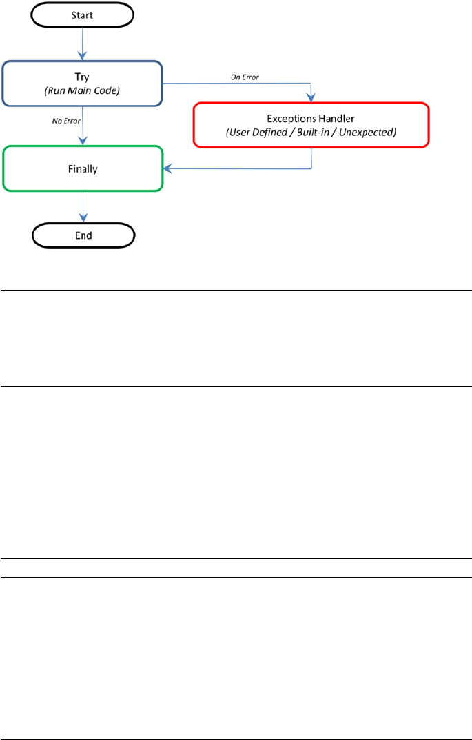
CHAPTER 1 ■ STEP 1 – GETTING STARTED IN PYTHON
52
Note that generally it’s a best practice to follow a single exit point principle by using finally.
This means that either after successful execution of your main code or your error handler
has finished handling an error, it should pass through the finally so that the code will be
exited at the same point under all circumstances.
Endnotes
With this we have reached the end of this chapter. So far I have tried to cover the basics
and the essential topics to get you started in Python, and there is an abundance of
online / offline resources available to increase your knowledge depth about Python as
a programming language. On the same note, I would like to leave you with some useful
resources for your future reference. See Table1-17.
Figure 1-3. Code Flow for Error Handler
Table 1-17. Additional resources
Resource Description Mode
http://docs.python-guide.
org/en/latest/intro/
learning/
This is the Python’s official tutorial, and it
covers all the basics and offers a detailed
tour of the language and standard libraries.
Online
http://awesome-python.com/ A curated list of awesome Python
frameworks, libraries, software, and
resources.
Online
The Hacker's Guide to Python This book is aimed at developers who
already know Python but want to learn
from more experienced Python developers.
Book

53
© Manohar Swamynathan 2017
M. Swamynathan, Mastering Machine Learning with Python in Six Steps,
DOI 10.1007/978-1-4842-2866-1_2
CHAPTER 2
Step 2 – Introduction to
Machine Learning
Machine learning is a subfield of computer science that evolved from the study of pattern
recognition and computational learning theory in Artificial Intelligence (AI).
Let’s look at a few other versions of definitions that exist for machine learning:
• In 1959, Arthur Samuel, an American pioneer in the field of
computer gaming, machine learning, and artificial intelligence
has defined machine learning as a “Field of study that
gives computers the ability to learn without being explicitly
programmed.”
• Machine learning is a field of computer science that involves
using statistical methods to create programs that either improve
performance over time, or detect patterns in massive amounts of
data that humans would be unlikely to find.
• Machine Learning explores the study and construction of
algorithms that can learn from and make predictions on data.
Such algorithms operate by building a model from example
inputs in order to make data driven predictions or decisions,
rather than following strictly static program instructions.
All the above definitions are correct; in short, “Machine Learning is a collection of
algorithms and techniques used to create computational systems that learn from data in
order to make predictions and inferences.”
Machine learning application area is abounding. Let’s look at some of the most
common day-to-day applications of Machine Learning that happens around us.
Recommendation System: YouTube brings videos for each of its users based on
a recommendation system that believes that the individual user will be interested in.
Similarly Amazon and other such e-retailers suggest products that the customer will be
interested in and likely to purchase by looking at the purchase history for a customer and
a large inventory of products.
Spam detection: Email service providers use a machine learning model that can
automatically detect and move the unsolicited messages to the spam folder.
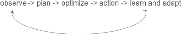
CHAPTER 2 ■ STEP 2 – INTRODUCTION TO MACHINE LEARNING
54
Prospect customer identification: Banks, insurance companies, and financial
organizations have machine learning models that trigger alerts so that organizations
intervene at the right time to start engaging with the right offers for the customer and
persuade them to convert early. These models observe the pattern of behavior by a user
during the initial period and map it to the past behaviors of all users to identify those that
will buy the product and those that will not.
History and Evolution
Machine learning is a subset of Artificial Intelligence (AI), so let’s first understand what AI
is and where machine learning fits within its wider umbrella. AI is a broad term that aims
at using data to offer solutions to existing problems. It is the science and engineering of
replicating, even surpassing human level intelligence in machines. That means observe
or read, learn, sense, and experience.
The AI process loop is as follows in Figure2-1:
• Observe – identify patterns using the data
• Plan – find all possible solutions
• Optimize – find optimal solution from the list of possible solutions
• Action – execute the optimal solution
• Learn and Adapt – is the result giving expected result, if no adapt
The AI process loop discussed above can be achieved using intelligent agents.
A robotic intelligent agent can be defined as a component that can perceive its
environment through different kinds of sensors (camera, infrared, etc.), and will take
actions within the environment through efforts. Here robotic agents are designed to
reflect humans. We have different sensory organs such as eyes, ears, noses, tongues, and
skin to perceive our environment and organs such as hands, legs, and mouths are the
effectors that enable us to take action within our environment based on the perception.
A detailed discussion on designing the agent has been discussed in the book
Artificial Intelligence, A Modern Approach by Stuart J. Russell and Peter Norvig in 1995.
Figure2-2 shows a sample pictorial representation.
Figure 2-1. AI process loop
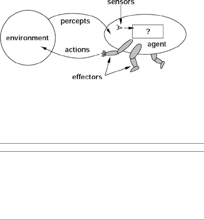
CHAPTER 2 ■ STEP 2 – INTRODUCTION TO MACHINE LEARNING
55
To get a better understanding of the concept, let’s look at an intelligent agent
designed for a particular environment or use case. Consider designing an automated taxi
driver. See Table2-1.
The taxi driver robotic intelligent agent will need to know its location, the direction
in which its traveling, the speed at which its traveling, what else is on the road! This
information can be obtained from the percepts such as controllable cameras in
appropriate places, the speedometer, odometer, and accelerometer. For understanding
the mechanical state of the vehicle and engine, it needs electrical system sensors. In
addition a satellite global positioning system (GPS) can help to provide its accurate
position information with respect to an electronic map and infrared/sonar sensors
to detect distances to other cars or obstacles around it. The actions available to the
intelligent taxi driver agent are the control over the engine through the pedals for
accelerating, braking, and steering for controlling the direction. There should also be a
way to interact with or talk to the passengers to understand the destination or goal.
Figure 2-2. Depict of robotic intelligent agent concept that interacts with its environment
through sensors and effectors
Table 2-1. Example intelligent agent components
Intelligent Agent’s Component Name Description
Agent Type Taxi driver
Goals Safe trip, legal, comfortable trip, maximize
profits, convenient, fast
Environment Roads, traffic, signals, signage, pedestrians,
customers
Percepts Speedometer, microphone, GPS, cameras,
sonar, sensors
Actions Steer, accelerate, break, talk to passenger
CHAPTER 2 ■ STEP 2 – INTRODUCTION TO MACHINE LEARNING
56
In 1950, Alan Turing a well-known computer scientist proposed a test known as
Turing test in his famous paper “Computing Machinery and Intelligence.” The test was
designed to provide a satisfactory operational definition of intelligence, which required
that a human being should not be able to distinguish the machine from another human
being by using the replies to questions put to both.
To be able to pass the Turing test, the computer should possess the following
capabilities:
• Natural language processing, to be able to communicate
successfully in a chosen language
• Knowledge representation, to store information provided
before or during the interrogation that can help in finding
information, making decisions, and planning. This is also
known as ‘Expert System’
• Automated reasoning (speech), to use the stored knowledge map
information to answer questions and to draw new conclusions
where required
• Machine learning, to analyzing data to detect and extrapolate
patters that will help adapt to new circumstances
• Computer vision to perceive objects or the analyzing of images to
find features of the images
• Robotics devices that can manipulate and interact with its
environment. That means to move the objects around based on
the circumstance
• Planning, scheduling, and optimization, which means figuring
ways to make decision plans or achieve specified goals, as well as
analyzing the performance of the plans and designs
The above-mentioned seven capability areas of AI have seen a great deal of research and
growth over the years. Although many of the terms in these areas are used interchangeably,
we can see from the description that their objectives are different. Particularly machine
learning has seen a scope to cut across all the seven areas of AI. See Figure2-3.

CHAPTER 2 ■ STEP 2 – INTRODUCTION TO MACHINE LEARNING
57
Artificial Intelligence Evolution
Let’s understand briefly the artificial intelligence past, present, and future.
Artificial Narrow Intelligence (ANI): Machine intelligence that equals or
exceeds human intelligence or efficiency at a specific task. An example
is IBM’s Watson, which requires close participation of subject matter or
domain experts to supply data/information and evaluate its performance.
Artificial General Intelligence (AGI): A machine with the ability to apply
intelligence to any problem for an area, rather than just one specific
problem. Self-driving cars are a good example of this.
Artificial Super Intelligence (ASI): An intellect that is much smarter than the
best human brains in practically every field, general wisdom, social skills,
and including scientific creativity. The key theme over here is “don’t model
the world, model the mind”.
Figure 2-3. Artificial Intelligence Areas
CHAPTER 2 ■ STEP 2 – INTRODUCTION TO MACHINE LEARNING
58
Different Forms
Is Machine Learning the only subject in which we use data to learn and use for
prediction/inference?
To answer the above questions, let’s have a look at the definition (Wikipedia) of the
few other key terms (not an exhaustive list) that are often heard relatively:
• Statistics: It is the study of the collection, analysis, interpretation,
presentation, and organization of data.
• Data Mining: It is an interdisciplinary subfield of computer
science. It is the computational process of discovering patterns in
large data sets (from data warehouse) involving methods at the
intersection of artificial intelligence, machine learning, statistics,
and database systems.
• Data Analytics: It is a process of inspecting, cleaning, transforming,
and modeling data with the goal of discovering useful information,
suggesting conclusions, and supporting decision making. This
is also known as Business Analytics and is widely used in many
industries to allow companies/organization to use the science
of examining raw data with the purpose of drawing conclusions
about that information and make better business decisions.
• Data Science: Data science is an interdisciplinary field about
processes and systems to extract knowledge or insights from data
in various forms, either structured or unstructured, which is a
continuation of some of the data analysis fields such as statistics,
machine learning, data mining, and predictive analytics, similar
to Knowledge Discovery in Databases (KDD).
Yes, from the above definitions it is clear and surprising to find out that Machine
Learning isn’t the only subject in which we use data to learn from it and use further for
prediction/inference. Almost identical themes, tools, and techniques are being talked about
in each of these areas. This raises a genuine question about why there are so many different
names with lots of overlap around learning from data? What is the difference between these?
The short answer is that all of these are practically the same. However, there exists
a subtle difference or shade of meaning, expression, or sound between each of these. To
get a better understanding we’ll have to go back to the history of each of these areas and
closely examine the origin, core area of application, and evolution of these terms.
Statistics
German scholar Gottfried Achenwall introduced the word “Statistics” in the middle of
the 18th century (1749). Usage of this word during this period meant that it was related to
the administrative functioning of a state, supplying the numbers that reflect the periodic
actuality regarding its various area of administration. The origin of the word statistics
may be traced to the Latin word “Status” (“council of state”) or the Italian word “Statista”
(“statesman” or “politician”); that is, the meaning of these words is “Political State” or a

CHAPTER 2 ■ STEP 2 – INTRODUCTION TO MACHINE LEARNING
59
Government. Shakespeare used a word Statist in his drama Hamlet (1602). In the past,
the statistics were used by rulers that designated the analysis of data about the state,
signifying the “science of state.”
In the beginning of the 19th century, statistics attained the meaning of the collection and
classification of data. The Scottish politician, Sir John Sinclair, introduced it to the English in
1791 in his book Statistical Account of Scotland. Therefore, the fundamental purpose of the
birth of statistics was around data to be used by government and centralized administrative
organizations to collect census data about the population for states and localities.
Frequentist
John Graunt was one of the first demographers and is our first vital statistician. He
published his observation on the Bills of Mortality (in 1662), and this work is often quoted
as the first instance of descriptive statistics. He presented vast amounts of data in a few
tables that can be easily comprehended, and this technique is now widely known as
descriptive statistics. In it we note that weekly mortality statistics first appeared in England
in 1603 at the Parish-Clerks Hall. We can learn from it that in 1623, of some 50,000 burials
in London, only 28 died of the plague. By 1632, this disease had practically disappeared
for the time being, to reappear in 1636 and again in the terrible epidemic of 1665. This
exemplifies that the fundamental nature of descriptive statistics is counting. From all
the Parish registers, he counted the number of persons who died, and who died of the
plague. The counted numbers every so often were relatively too large to follow, so he also
simplified them by using proportion rather than the actual number. For example, the year
1625 had 51,758 deaths and of which 35,417 were of the plague. To simplify this he wrote,
“We find the plague to bear unto the whole in proportion as 35 to 51. Or 7 to 10.” With these
he is introducing the concept that the relative proportions are often of more interest than
the raw numbers. We would generally express the above proportion as 70%. This type of
conjecture that is based on a sample data’s proportion spread or frequency is known as
“frequentist statistics.” . Statistical hypothesis testing is based on inference framework,
where you assume that observed phenomena are caused by unknown but fixed processes.
Bayesian
In contract Bayesian statistics (named after Thomas Bayes), it describes that the
probability of an event, based on conditions that might be related to the event. At the
core of Bayesian statistics is Bayes’s theorem, which describes the outcome probabilities
of related (dependent) events using the concept of conditional probability. For example,
if a particular illness is related to age and life style, then applying a Bay’s theorem by
considering a person’s age and life style more accurately increases the probability of that
individual having the illness can be assessed.
Bayes theorem is stated mathematically as the following equation:
PABPBAPA
PB
||
()
()
()
()
=
Where A and B are events and P (B) ≠ 0
CHAPTER 2 ■ STEP 2 – INTRODUCTION TO MACHINE LEARNING
60
• P (A) and P (B) are the probabilities of observing A and B without
regard to each other.
• P (A | B), a conditional probability, is the probability of observing
event A given that B is true.
• P (B | A) is the probability of observing event B given that A is true.
For example, a doctor knows that lack of sleep causes migraine 50% of the time. Prior
probability of any patient having lack of sleep is 10000/50000 and prior probability of any
patient having migraine is 300/1000. If a patient has a sleep disorder, let’s apply Bayes’s
theorem to calculate the probability he/she is having a migraine.
P (Sleep disorder | Migraine) = P(Migraine | Sleep disorder) * P(Migraine) / P(Sleep
disorder)
P (Sleep disorder | Migraine) = .5 * 10000/50000 / (300/1000) = 33%
In the above scenario, there is a 33% chance that a patient with a sleep disorder will
also have a migraine problem.
Regression
Another major milestone for statisticians was the regression, which was published by
Legendre in 1805 and by Guass in 1809. Legendre and Gauss both applied the method
to the problem of determining, from astronomical observations, the orbits of bodies
about the Sun, mostly comets, but also later the then newly discovered minor planets.
Gauss published a further development of the theory of least squares in 1821. Regression
analysis is an essential statistical process for estimating the relationships between
factors. It includes many techniques for analyzing and modeling various factors, and the
main focus here is about the relationship between a dependent factor and one or many
independent factors also called predictors or variables or features. We’ll learn about this
more in the fundamentals of machine learning with scikit-learn.
Over time the idea behind the word statistics has undergone an extraordinary
transformation. The character of data or information provided has been extended to all
spheres of human activity. Let’s understand the difference between two terms quite often
used along with statistics, that is, 1) data and 2) method. Statistical data is the numerical
statement of facts, whereas statistical methods deal with information of the principles
and techniques used in collecting and analyzing such data. Today, statistics as a separate
discipline from mathematics is closely associated with almost all branches of education
and human endeavor that are mostly numerically representable. In modem times, it has
innumerable and varied applications both qualitatively and quantitatively. Individuals
and organizations use statistics to understand data and make informed decisions
throughout the natural and social sciences, medicine, business, and other areas. Statistics
has served as the backbone and given rise to many other disciplines, which you’ll
understand as you read further.
CHAPTER 2 ■ STEP 2 – INTRODUCTION TO MACHINE LEARNING
61
Data Mining
The term “Knowledge Discovery in Databases” (KDD) is coined by Gregory Piatetsky-
Shapiro in 1989 and also at the same time he cofounded the first workshop named KDD.
The term “Data mining” was introduced in the 1990s in the database community, but
data mining is the evolution of a field with a slightly long history.
Data mining techniques are the result of research on the business process and
product development. This evolution began when business data was first stored on
computers in the relational databases and continued with improvements in data access,
and further produced new technologies that allow users to navigate through their data
in real time. In the business community, data mining focuses on providing “Right Data”
at the “Right Time” for the “Right Decisions.” This is achieved by enabling a tremendous
amount of data collection and applying algorithms to them with the help of distributed
multiprocessor computers to provide real-time insights from data.
We’ll learn more about the five stages proposed by KDD for data mining in the
section on the framework for building machine learning systems.
Data Analytics
Analytics have been known to be used in business, since the time of management
movements toward industrial efficiency that were initiated in late 19th century by
Frederick Winslow Taylor, an American mechanical engineer. The manufacturing
industry adopted measuring the pacing of the manufacturing and assembly line, as
a result revolutionizing industrial efficiency. But analytics began to command more
awareness in the late 1960s when computers had started playing a dominating role as
organizations’ decision support systems. Traditionally business managers were making
decisions based on past experiences or rules of thumb, or there were other qualitative
aspects to decision making; however, this changed with development of data warehouses
and enterprise resource planning (ERP) systems. The business managers and leaders
considered data and relied on ad hoc analysis to affirm their experience/knowledge-
based assumptions for daily and critical business decisions. This evolved as data-driven
business intelligence or business analytics for the decision-making process was fast
adopted by organizations and companies across the globe. Today, businesses of all sizes
use analytics. Often the word “Business Analytics” is used interchangeably for “Data
Analytics” in the corporate world.
In order for businesses to have a holistic view of the market and how a company
competes efficiently within that market to increase the RoI (Return on Investment),
requires a robust analytic environment around the kind of analytics that is possible.
This can be broadly categorized into four types. See Figure2-4.
1. Descriptive Analytics
2. Diagnostic Analytics
3. Predictive Analytics
4. Prescriptive Analytics
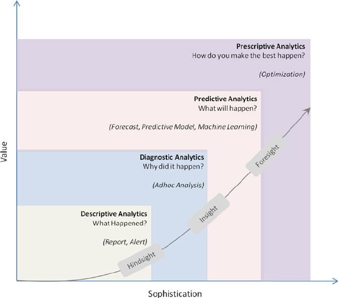
CHAPTER 2 ■ STEP 2 – INTRODUCTION TO MACHINE LEARNING
62
Descriptive Analytics
They are the analytics that describe the past to tell us “What has happened?” To elaborate,
as the name suggests, any activity or method that helps us to describe or summarize raw
data into something interpretable by humans can be termed ‘Descriptive Analytics’. These
are useful because they allow us to learn from past behaviors, and understand how they
might influence future outcomes.
The statistics such as arithmetic operation of count, min, max, sum, average,
percentage, and percent change, etc., fall into this category. Common examples of
descriptive analytics are a company’s business intelligence reports that cover different
aspects of the organization to provide historical hindsights regarding the company’s
production, operations, sales, revenue, financials, inventory, customers, and market share.
Figure 2-4. Data Analytics Types
CHAPTER 2 ■ STEP 2 – INTRODUCTION TO MACHINE LEARNING
63
Diagnostic Analytics
It is the next step to the descriptive analytics that examines data or information to answer
the question, “Why did it happen?,” and it is characterized by techniques such as drill-
down, data discovery, data mining, correlations, and causation. It basically provides a very
good understanding of a limited piece of the problem you want to solve. However, it is very
laborious work as significant human intervention is required to perform the drill-down or
data mining to go deeper into the data to understand why something happened or its root
cause. It focuses on determining the factors and events that contributed to the outcome.
For example, assume a retail company’s hardlines (it’s a category usually
encompassing furniture, appliance, tools, electronics, etc.) sales performance is not up to
the mark in certain stores and the product line manager would like to understand the root
cause. In this case the product manager may want to look backward to review past trends
and patterns for the product line sales across different stores based on its placement
(which floor, corner, aisle) within the store. It’s also to understand if there is any causal
relationship with other products that are closely kept with it. Look at different external
factors such as demographic, season, macroeconomic factors separately as well as in
unison to define relative ranking of related variables based on concluded explanations. To
accomplish this there is not a clearly defined set of ordered steps defined, and it depends
on the experience level and thinking style of the person carrying out the analysis.
There is a significant involvement of the subject matter expert and the data/
information may need to be presented visually for better understanding. There is a
plethora of tools: for example, Excel, Tableau, Qlikview, Spotfire, and D3, etc., are
available build tools that enable diagnostic analytics.
Predictive Analytics
It is the ability to make predictions or estimations of likelihoods about unknown future events
based on the past or historic patterns. Predictive analytics will give us insight into “What might
happen?”; it uses many techniques from data mining, statistics, modeling, machine learning,
and artificial intelligence to analyze current data to make predictions about the future.
It is important to remember that the foundation of predictive analytics is based on
probabilities, and the quality of prediction by statistical algorithms depends a lot on
the quality of input data. Hence these algorithms cannot predict the future with 100%
certainty. However, companies can use these statistics to forecast the probability of what
might happen in the future and considering these results alongside business knowledge
would result in profitable decisions.
Machine learning is heavily focused on predictive analytics, where we combine
historical data from different sources such as organizational ERP (Enterprise Resource
Planning), CRM (Customer Relation Management), POS (Point of Sales), Employees data,
Market research data to identify patterns and apply statistical model/algorithms to capture
the relationship between various data sets and further predict the likelihood of an event.
Some examples of predictive analytics are weather forecasting, email spam
identification, fraud detection, probability of customer purchasing a product or renewal
of insurance policy, predicting the chances of a person with a known illness, etc.
CHAPTER 2 ■ STEP 2 – INTRODUCTION TO MACHINE LEARNING
64
Prescriptive Analytics
It is the area of data or business analytics dedicated to finding the best course of action for
a given situation. Prescriptive analytics is related to all other three forms of analytics that
is, descriptive, diagnostic, and predictive analytics. The endeavor of prescriptive analytics
is to measure the future decision’s effect to enable the decision makers to foresee the
possible outcomes before the actual decisions are made. Prescriptive analytic systems are
a combination of business rules, machine learning algorithms, tools that can be applied
against historic and real-time data feed. The key objective here is not just to predict what
will happen, but also why it will happen by predicting multiple futures based on different
scenarios to allow companies to assess possible outcomes based on their actions.
Some examples of prescriptive analytics are by using simulation in design situations
to help users identify system behaviors under different configurations, and ensuring
that all key performance metrics are met such as wait times, queue length, etc. Another
example is to use linear or nonlinear programming to identify the best outcome for a
business, given constraints, and objective function.
Data Science
In 1960, Peter Naur used the term “data science” in his publication “Concise Survey of
Computer Methods,” which is about contemporary data processing methods in a wide
range of applications. In 1991, computer scientist Tim Berners-Lee announced the birth
of what would become the World Wide Web as we know it today, in a post in the “Usenet
group” where he set out the specifications for a worldwide, interconnected web of data,
accessible to anyone from anywhere. Over time the Web/Internet has been growing 10-
fold each year and became a global computer network providing a variety of information
and communication facilities, consisting of interconnected networks using standardized
communication protocols. Alongside the storage systems became too evolved and the
digital storage became more cost effective than paper.
As of 2008, the world’s servers processed 9.57 zeta-bytes (9.57 trillion gigabytes)
of information, which is equivalent to 12 gigabytes of information per person per day,
according to the “How Much Information? 2010 report on Enterprise Server Information.”
The rise of the Internet drastically increases the volume of structured,
semistructured, and unstructured data. This led to the birth of the term “Big Data”
characterized by 3V’s, which stands for Volume, Variety, and Velocity. Special tools and
systems are required to process high volumes of data, with a wide Variety (text, number,
audio, video, etc.), generated at a high velocity. See Figure2-5.
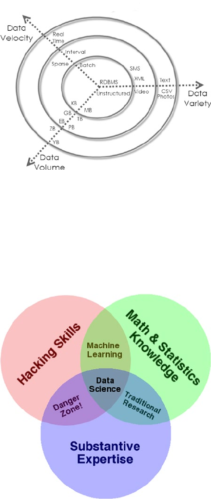
CHAPTER 2 ■ STEP 2 – INTRODUCTION TO MACHINE LEARNING
65
Big data revolution influenced the birth of the term “data science.” Although the term
“data science” came into existence from 1960 on, it became popular and this is attributed
to Jeff Hammerbacher and DJ Patil, of Facebook and LinkedIn because they carefully
chose it, attempting to describe their teams and work (as per Building Data Science
Teams by DJ Patil published in 2008); they settled on “data scientist” and a buzzword was
born. One picture explains well the essential skills set for data science that was presented
by Drew Conway in 2010. See Figure2-6.
Figure 2-5. 3 V’s of Big data (source: http://blog.sqlauthority.com)
Figure 2-6. Drew Conway’s Data Science Venn diagram
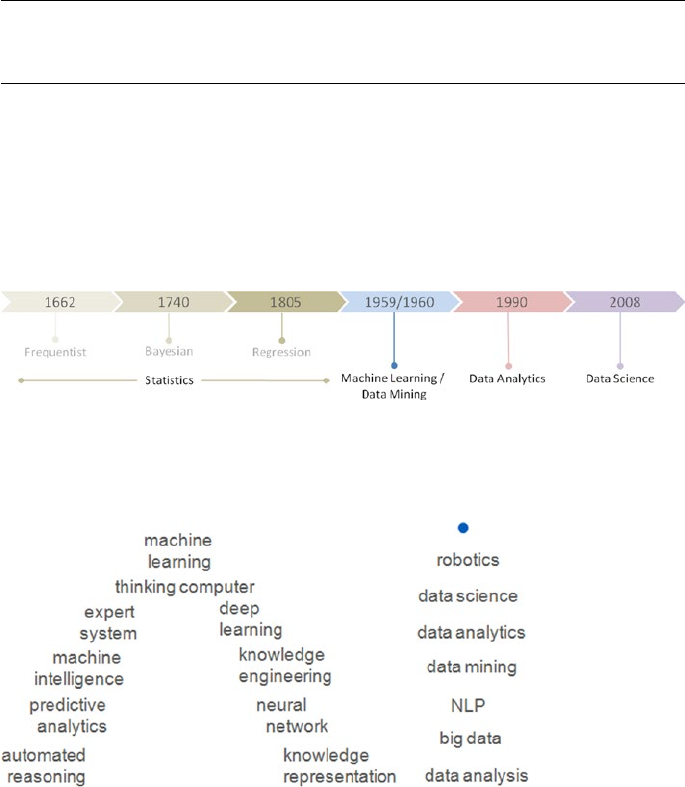
CHAPTER 2 ■ STEP 2 – INTRODUCTION TO MACHINE LEARNING
66
Executing data science projects require three key skills:
1. Programming or hacking skills,
2. Math & Statistics,
3. Business or subject matter expertise for a given area of scope.
Note that the Machine Learning is originated from Artificial Intelligence. It is not a branch of
Data science, rather it is only using Machine Learning as a tool.
Statistics vs. Data Mining vs. Data Analytics vs.
Data Science
We can learn from the history and evolution of subjects around learning from ‘Data’ is that
even though they use the same methods, they evolved as different cultures, so they have
different histories, nomenclature, notation, and philosophical perspectives. See Figure2-7.
Figure 2-8. All forms together, the path to ultimate Artificial Intelligence
Figure 2-7. Learn from ‘Data’ evolution
All form together to create the path to ultimate Artificial Intelligence. See Figure2-8.
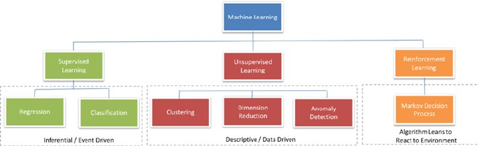
CHAPTER 2 ■ STEP 2 – INTRODUCTION TO MACHINE LEARNING
67
Machine Learning Categories
At a high level, Machine learning tasks can be categorized into three groups based on the
desired output and the kind of input required to produce it. See Figure2-9.
Supervised Learning
The machine learning algorithm is provided with a large enough example input dataset
respective output or event/class, usually prepared in consultation with the subject matter
expert of a respective domain. The goal of the algorithm is to learn patterns in the data
and build a general set of rules to map input to the class or event.
Broadly, there are two types commonly used as supervised learning algorithms.
1) Regression
The output to be predicted is a continuous number in relevance with a given input
dataset. Example use cases are predictions of retail sales, prediction of number of staff
required for each shift, number of car parking spaces required for a retail store, credit
score, for a customer, etc.
2) Classification
The output to be predicted is the actual or the probability of an event/class and the number
of classes to be predicted can be two or more. The algorithm should learn the patterns in
the relevant input of each class from historical data and be able to predict the unseen class
or event in the future considering their input. An example use case is spam email filtering
where the output expected is to classify an email into either a “spam” or “not spam.”
Building supervised learning machine learning models has three stages:
1. Training: The algorithm will be provided with historical input
data with the mapped output. The algorithm will learn the
patterns within the input data for each output and represent
that as a statistical equation, which is also commonly known
as a model.
Figure 2-9. Types of Machine Learning
CHAPTER 2 ■ STEP 2 – INTRODUCTION TO MACHINE LEARNING
68
2. Testing or validation: In this phase the performance of the
trained model is evaluated, usually by applying it on a dataset
(that was not used as part of the training) to predict the class
or event.
3. Prediction: Here we apply the trained model to a data set that
was not part of either the training or testing. The prediction
will be used to drive business decisions.
Unsupervised Learning
There are situations where the desired output class/event is unknown for historical
data. The objective in such cases would be to study the patterns in the input dataset to
get better understanding and identify similar patterns that can be grouped into specific
classes or events. As these types of algorithms do not require any intervention from the
subject matter experts beforehand, they are called unsupervised learning.
Let’s look at some examples of unsupervised learning.
Clustering
Assume that the classes are not known beforehand for a given dataset. The goal here is to
divide the input dataset into logical groups of related items. Some examples are grouping
similar news articles, grouping similar customers based on their profile, etc.
Dimension Reduction
Here the goal is to simplify a large input dataset by mapping them to a lower dimensional
space. For example, carrying analysis on a large dimension dataset is very computational
intensive, so to simplify you may want to find the key variables that hold a significant
percentage (say 95%) of information and only use them for analysis.
Anomaly Detection
Anomaly detection is also commonly known as outlier detection is the identification of
items, events or observations which do not conform to an expected pattern or behavior
in comparison with other items in a given dataset. It has applicability in a variety of
domains, such as machine or system health monitoring, event detection, fraud/intrusion
detection etc. In the recent days, anomaly detection has seen a big area of interest in
the word of Internet of Things (IoT) to enable detection of abnormal behavior in a given
context. A data point is termed anomaly if it is distant from other data points in a given
context, so calculating standard deviation or clustering are the most commonly used
techniques for detection of anomaly alongside a whole lot of other techniques. I’ll not be
covering the topic in this edition.
CHAPTER 2 ■ STEP 2 – INTRODUCTION TO MACHINE LEARNING
69
Reinforcement Learning
The basic objective of reinforcement learning algorithms is to map situations to actions
that yield the maximum final reward. While mapping the action, the algorithm should
not just consider the immediate reward but also next and all subsequent rewards. For
example, a program to play a game or drive a car will have to constantly interact with a
dynamic environment in which it is expected to perform a certain goal. We’ll learn the
basics of Markov decision process/q-learning with an example in a later chapter.
Examples of reinforcement learning techniques are the following:
• Markov decision process
• Q-learning
• Temporal Difference methods
• Monte-Carlo methods
Frameworks for Building Machine Learning
Systems
Over time data mining field has seen a massive expansion. There have been a lot of efforts
taken by many experts to standardize methodologies and define best practice for the ever-
growing, diversified, and iterative process of building machine learning systems. On top
of the last decade the field of machine learning has become very important for different
industries, businesses, and organizations because of its ability to extract insight from
huge amounts of data that had previously no use or was underutilized to learn the trend/
patterns and predict the possibilities that help to drive business decisions leading to profit.
Ultimately the risk of wasting the wealthy and valuable information contained by the rich
business data sources was raised, and this required the use of adequate techniques to get
useful knowledge so that the field of machine learning had emerged in the early 1980s, it
and has seen a great growth. With the emergence of this field, different process frameworks
were introduced. These process frameworks guide and carry the machine learning tasks
and its applications. Efforts were made to use data mining process frameworks that will
guide the implementation of data mining on big or huge amount of data.
Mainly three data mining process frameworks have been most popular, and widely
practiced by data mining experts/researchers to build machine learning systems. These
models are the following:
• Knowledge Discovery Databases (KDD) process model
• CRoss Industrial Standard Process for Data Mining (CRISP – DM)
• Sample, Explore, Modify, Model and Assess (SEMMA)
Knowledge Discovery Databases (KDD)
This refers to the overall process of discovering useful knowledge from data, which was
presented by a book by Fayyad etal., 1996. It is an integration of multiple technologies
for data management such as data warehousing, statistic machine learning, decision
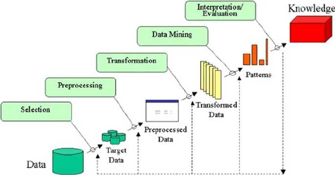
CHAPTER 2 ■ STEP 2 – INTRODUCTION TO MACHINE LEARNING
70
support, visualization, and parallel computing. As the name suggests, Knowledge
Discovery Databases center around the overall process of knowledge discovery from data
that covers the entire life cycle of data that includes how the data are stored, how it is
accessed, how algorithms can be scaled to enormous datasets efficiently, how results can
be interpreted and visualized.
There are five stages in KDD, presented in Figure2-10.
Figure 2-10. KDD Data Mining process flow
Selection
In this step, selection and integration of the target data from possibly many different
and heterogeneous sources is performed. Then the correct subset of variables and data
samples relevant to the analysis task is retrieved from the database.
Preprocessing
Real-world datasets are often incomplete that is, attribute values will be missing; noisy
(errors and outliers); and inconsistent, which means there exists discrepancies between
the collected data. The unclean data can confuse the mining procedures and lead to
unreliable and invalid outputs. Also, performing complex analysis and mining on a huge
amount of such soiled data may take a very long time. Preprocessing and cleaning should
improve the quality of data and mining results by enhancing the actual mining process.
The actions to be taken include the following:
• Collecting required data or information to model
• Outlier treatment or removal of noise
• Using prior domain knowledge to remove the inconsistencies and
duplicates from the data
• Choice of strategies for handling missing data
CHAPTER 2 ■ STEP 2 – INTRODUCTION TO MACHINE LEARNING
71
Transformation
In this step, data is transformed or consolidated into forms appropriate for mining,
that is, finding useful features to represent the data depending on the goal of the
task. For example, in high-dimensional spaces or the large number of attributes, the
distances between objects may become meaningless. So dimensionality reduction and
transformation methods can be used to reduce the effective number of variables under
consideration or find invariant representations for the data. There are various data
transformation techniques:
• Smoothing (binning, clustering, regression, etc.)
• Aggregation
• Generalization in which a primitive data object can be replaced
by higher-level concepts
• Normalization, which involves min-max-scaling or z-score
• Feature construction from the existing attributes (PCA, MDS)
• Data reduction techniques are applied to produce reduced
representation of the data (smaller volume that closely maintains
the integrity of the original data)
• Compression, for example, wavelets, PCA, clustering etc.
Data Mining
In this step, machine learning algorithms are applied to extract data patterns.
Exploration/summarization methods such as mean, median, mode, standard deviation,
class/concept description, and graphical techniques of low-dimensional plots can be
used to understand the data. Predictive models such as classification or regression can be
used to predict the event or future value. Cluster analysis can be used to understand the
existence of similar groups. Select the most appropriate methods to be used for the model
and pattern search.
Interpretation / Evaluation
This step is focused on interpreting the mined patterns to make them understandable
by the user, such as summarization and visualization. The mined pattern or models are
interpreted. Patterns are a local structure that makes statements only about restricted
regions of the space spanned by the variables. Whereas models are global structures that
makes statements about any point in measurement space, that is, Y = mX+C (linear model).
Cross-Industry Standard Process for Data Mining
It is generally known by its acronym CRISP-DM. It was established by the European
Strategic Program on Research in Information Technology initiative with an aim to create
an unbiased methodology that is not domain dependent. It is an effort to consolidate data
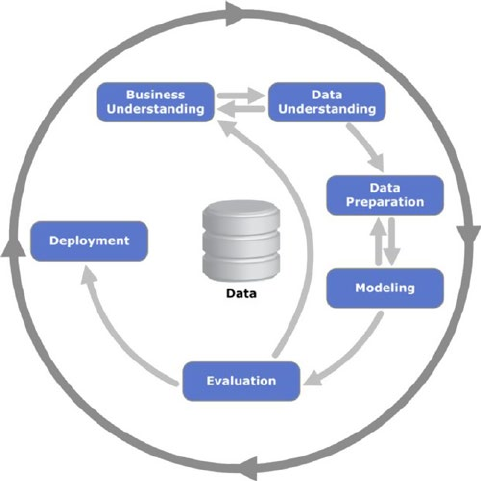
CHAPTER 2 ■ STEP 2 – INTRODUCTION TO MACHINE LEARNING
72
mining process best practices followed by experts to tackle data mining problems. It was
conceived in 1996 and first published in 1999 and was reported as the leading methodology
for data mining/predictive analytics projects in polls conducted in 2002, 2004, and 2007.
There was a plan between 2006 and 2008 to update CRISP-DM but that update did not take
place, and today the original CRISP-DM.org website is no longer active.
This framework is an idealized sequence of activities. It is an iterative process and
many of the tasks backtrack to previous tasks and repeat certain actions to bring more
clarity. There are six major phases as shown in Figure2-11.
• Business understanding
• Data understanding
• Data preparation
• Modeling
• Evaluation
• Deployment
Figure 2-11. Process diagram showing the relationship between the six phases of CRISP-DM
CHAPTER 2 ■ STEP 2 – INTRODUCTION TO MACHINE LEARNING
73
Phase 1: Business Understanding
As the name suggests the focus at this stage is to understand the overall project objectives and
expectations from a business perspective. These objectives are converted to a data mining
or machine learning problem definition and a plan of action around data requirements,
business owners input, and how outcome performance evaluation metrics are designed.
Phase 2: Data Understanding
In this phase, initial data are collected that were identified as requirements in the
previous phase. Activities are carried out to understanding data gaps or relevance of the
data to the objective in hand, any data quality issues, and first insights into the data to
bring out appropriate hypotheses. The outcome of this phase will be presented to the
business iteratively to bring more clarity into the business understanding and project
objective.
Phase 3: Data Preparation
This phase is all about cleaning the data so that it’s ready to be used for the model
building phase. Cleaning data could involve filling the known data gaps from
previous steps, missing value treatments, identifying the important features, applying
transformations, and creating new relevant features where applicable. This is one of the
most important phases as the model’s accuracy will depend significantly on the quality of
data that is being fed into the algorithm to learn the patterns.
Phase 4: Modeling
There are multiple machine learning algorithms available to solve a given problem. So
various appropriate machine learning algorithms are applied onto the clean dataset, and
their parameters are tuned to the optimal possible values. Model performance for each of
the applied models is recorded.
Phase 5: Evaluation
In this stage a benchmarking exercise will be carried out among all the different models
that were identified to have been giving high accuracy. Model will be tested against data
that was not used as part of the training to evaluate its performance consistency. The
results will be verified against the business requirement identified in phase 1. The subject
matter experts from the business will be involved to ensure that the model results are
accurate and usable as per required by the project objective.
Phase 6: Deployment
The key focus in this phase is the usability of the model output. So the final model signed
off by the subject matter expert will be implemented, and the consumers of the model
output will be trained on how to interpret or use it to take the business decisions defined
CHAPTER 2 ■ STEP 2 – INTRODUCTION TO MACHINE LEARNING
74
in the business understanding phase. The implementation could be as generating
a prediction report and sharing it with the user. Also periodic model training and
prediction times will be scheduled based on the business requirement.
SEMMA (Sample, Explore, Modify, Model, Assess)
SEMMA are the sequential steps to build machine learning models incorporated in
‘SAS Enterprise Miner’, a product by SAS Institute Inc., one of the largest producers of
commercial statistical and business intelligence software. However the sequential steps
guide the development of a machine learning system. Let’s look at the five sequential
steps to understand it better.
Sample
This step is all about selecting the subset of the right volume dataset from a large dataset
provided for building the model. This will help us to build the model efficiently. This
was a famous practice when the computation power was expensive, however it is still
in practice. The selected subset of data should be actual an representation of the entire
dataset originally collected, which means it should contain sufficient information to
retrieve. The data is also divided for training and validation at this stage.
Explore
In this phase activities are carried out to understand the data gaps and relationship with
each other. Two key activities are univariate and multivariate analysis. In univariate
analysis each variable looks individually to understand its distribution, whereas
in multivariate analysis the relationship between each variable is explored. Data
visualization is heavily used to help understand the data better.
Modify
In this phase variables are cleaned where required. New derived features are created
by applying business logic to existing features based on the requirement. Variables are
transformed if necessary. The outcome of this phase is a clean dataset that can be passed
to the machine learning algorithm to build the model.
Model
In this phase, various modeling or data mining techniques are applied on the
preprocessed data to benchmark their performance against desired outcomes.
Assess
This is the last phase. Here model performance is evaluated against the test data
(not used in model training) to ensure reliability and business usefulness.
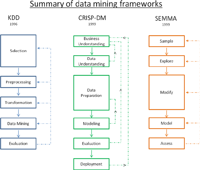
CHAPTER 2 ■ STEP 2 – INTRODUCTION TO MACHINE LEARNING
75
KDD vs. CRISP-DM vs. SEMMA
KDD is the oldest of three frameworks. CRISP-DM and SEMMA seem to be the practical
implementation of the KDD process. CRISP-DM is more complete as the iterative flow
of the knowledge across and between phases has been clearly defined. Also it covers all
areas of building a reliable machine learning systems from a business-world perspective.
In SEMMA’s sample stage it’s important that you have a true understanding of all
aspects of business to ensure the sampled data retains maximum information. However
the drastic innovation in the recent past has led to reduced costs for data storage and
computational power, which enables us to apply machine learning algorithms on the
entire data efficiently, almost removing the need for sampling.
We can see that generally the core phases are covered by all three frameworks and
there is not a huge difference between these frameworks. Overall these processes guide
us about how data mining techniques can be applied into practical scenarios. In general
most of the researchers and data mining experts follow the KDD and CRISP-DM process
model because it is more complete and accurate. I personally recommend following
CRISP-DM for usage in business environment as it provides coverage of end-to-end
business activity and the life cycle of building a machine learning system.
Figure 2-12. Summary of data mining frameworks
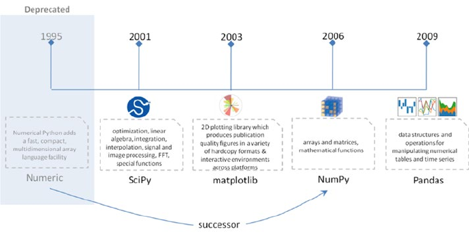
CHAPTER 2 ■ STEP 2 – INTRODUCTION TO MACHINE LEARNING
76
Machine Learning Python Packages
There is a rich number of open source libraries available to facilitate practical machine
learning. These are mainly known as scientific Python libraries and are generally put to use
when performing elementary machine learning tasks. At a high level we can divide these
libraries into data analysis and core machine learning libraries based on their usage/purpose.
Data analysis packages: These are the sets of packages that provide us the mathematic and
scientific functionalities that are essential to perform data preprocessing and transformation.
Core Machine learning packages: These are the set of packages that provide us with
all the necessary machine learning algorithms and functionalities that can be applied on
a given dataset to extract the patterns.
Data Analysis Packages
There are four key packages that are most widely used for data analysis.
• NumPy
• SciPy
• Matplotlib
• Pandas
Pandas, NumPy, and Matplotlib play a major role and have the scope of usage in almost
all data analysis tasks. So in this chapter we’ll focus on covering usage or concepts relevant
to these three packages as much as possible. Whereas SciPy supplements NumPy library
and has a variety of key high-level science and engineering modules, the usage of these
functions, however, largely depend on the use case to use case. So we’ll touch on or highlight
some of the useful functionalities in upcoming chapters where possible. See Figure2-13.
Figure 2-13. Data analysis packages

CHAPTER 2 ■ STEP 2 – INTRODUCTION TO MACHINE LEARNING
77
■Note For conciseness we’ll only be covering the key concepts within each of the
libraries with a brief introduction and code implementation. You can always refer to the
official user documents for these packages that have been well designed by the developer
community to cover a lot more in depth.
NumPy
NumPy is the core library for scientific computing in Python. It provides a high-
performance multidimensional array object, and tools for working with these arrays. It’s a
successor of Numeric package. In 2005, Travis Oliphant created NumPy by incorporating
features of the competing Numarray into Numeric, with extensive modifications. I think
the concepts and the code examples to a great extent have been explained in the simplest
form in his book Guide to NumPy. Here we’ll only be looking at some of the key NumPy
concepts that are a must or good to know in relevance to machine learning.
Array
A NumPy array is a collection of similar data type values, and is indexed by a tuple of
nonnegative numbers. The rank of the array is the number of dimensions, and the shape
of an array is a tuple of numbers giving the size of the array along each dimension.
We can initialize NumPy arrays from nested Python lists, and access elements using
square brackets. See Listing 2-1.
Listing 2-1. Example code for initializing NumPy array
import numpy as np
# Create a rank 1 array
a = np.array([0, 1, 2])
print type(a)
# this will print the dimension of the array
print a.shape
print a[0]
print a[1]
print a[2]
# Change an element of the array
a[0] = 5
print a
# ----output-----
# <type 'numpy.ndarray'>
# (3L,)
# 1
# 2
CHAPTER 2 ■ STEP 2 – INTRODUCTION TO MACHINE LEARNING
78
# 3
# [5 2 3]
# Create a rank 2 array
b = np.array([[0,1,2],[3,4,5]])
print b.shape
print b
print b[0, 0], b[0, 1], b[1, 0]
# ----output-----
# (2L, 3L)
# [[1 2 3]
# [4 5 6]]
# 1 2 4
Creating NumPy Array
NumPy also provides many built-in functions to create arrays. The best way to learn this
is through examples, so let’s jump into the code. See Listing 2-2.
Listing 2-2. Creating NumPy array
# Create a 3x3 array of all zeros
a = np.zeros((3,3))
print a
----- output -----
[[ 0. 0. 0.]
[ 0. 0. 0.]
[ 0. 0. 0.]]
# Create a 2x2 array of all ones
b = np.ones((2,2))
print b
---- output ----
[[ 1. 1.]
[ 1. 1.]]
# Create a 3x3 constant array
c = np.full((3,3), 7)
print c
---- output ----
[[ 7. 7. 7.]
[ 7. 7. 7.]
[ 7. 7. 7.]]
# Create a 3x3 array filled with random values
d = np.random.random((3,3))
print d
CHAPTER 2 ■ STEP 2 – INTRODUCTION TO MACHINE LEARNING
79
---- output ----
[[ 0.85536712 0.14369497 0.46311367]
[ 0.78952054 0.43537586 0.48996107]
[ 0.1963929 0.12326955 0.00923631]]
# Create a 3x3 identity matrix
e = np.eye(3)
print e
---- output ----
[[ 1. 0. 0.]
[ 0. 1. 0.]
[ 0. 0. 1.]]
# convert list to array
f = np.array([2, 3, 1, 0])
print f
---- output ----
[2 3 1 0]
# arange() will create arrays with regularly incrementing values
g = np.arange(20)
print g
---- output ----
[ 0 1 2 3 4 5 6 7 8 9 10 11 12 13 14 15 16 17 18 19]
# note mix of tuple and lists
h = np.array([[0, 1,2.0],[0,0,0],(1+1j,3.,2.)])
print h
---- output ----
[[ 0.+0.j 1.+0.j 2.+0.j]
[ 0.+0.j 0.+0.j 0.+0.j]
[ 1.+1.j 3.+0.j 2.+0.j]]
# create an array of range with float data type
i = np.arange(1, 8, dtype=np.float)
print i
---- output ----
[ 1. 2. 3. 4. 5. 6. 7.]
# linspace() will create arrays with a specified number of items which are
# spaced equally between the specified beginning and end values
j = np.linspace(2., 4., 5)
print j
---- output ----
[ 2. 2.5 3. 3.5 4. ]
# indices() will create a set of arrays stacked as a one-higher
# dimensioned array, one per dimension with each representing variation
CHAPTER 2 ■ STEP 2 – INTRODUCTION TO MACHINE LEARNING
80
# in that dimension
k = np.indices((2,2))
print k
---- output ----
[[[0 0]
[1 1]]
[[0 1]
[0 1]]]
Data Types
An array is a collection of items of the same data type and NumPy supports and provides
built-in functions to construct arrays with optional arguments to explicitly specify
required datatypes.
Listing 2-3. NumPy datatypes
# Let numpy choose the datatype
x = np.array([0, 1])
y = np.array([2.0, 3.0])
# Force a particular datatype
z = np.array([5, 6], dtype=np.int64)
print x.dtype, y.dtype, z.dtype
---- output ----
int32 float64 int64
Array Indexing
NumPy offers several ways to index into arrays. Standard Python x[obj] syntax can be
used to index NumPy array, where x is the array and obj is the selection.
There are three kinds of indexing available:
• Field access
• Basic slicing
• Advanced indexing
Field Access
If the ndarray object is a structured array, the fields of the array can be accessed by
indexing the array with strings, dictionary like. Indexing x[‘field-name’] returns a new
view to the array, which is of the same shape as x, except when the field is a subarray, but
of data type x.dtype[‘field-name’] and contains only the part of the data in the specified
field. See Listing 2-4.
CHAPTER 2 ■ STEP 2 – INTRODUCTION TO MACHINE LEARNING
81
Listing 2-4. Field access
x = np.zeros((3,3), dtype=[('a', np.int32), ('b', np.float64, (3,3))])
print "x['a'].shape: ",x['a'].shape
print "x['a'].dtype: ", x['a'].dtype
print "x['b'].shape: ", x['b'].shape
print "x['b'].dtype: ", x['b'].dtype
# ----output-----
# x['a'].shape: (2L, 2L)
# x['a'].dtype: int32
# x['b'].shape: (2L, 2L, 3L, 3L)
# x['b'].dtype: float64
Basic Slicing
NumPy arrays can be sliced, similar to lists. You must specify a slice for each dimension of
the array as the arrays may be multidimensional.
The basic slice syntax is i: j: k, where i is the starting index, j is the stopping index,
and k is the step and k is not equal to 0. This selects the m elements in the corresponding
dimension, with index values i, i + k, …,i + (m - 1) k where m = q + (r not equal to 0) and q
and r are the quotient and the remainder is obtained by dividing j - i by k: j - i = q k + r, so
that i + (m - 1) k < j. See Listing 2-5.
Listing 2-5. Basic slicing
x = np.array([5, 6, 7, 8, 9])
x[1:7:2]
---- output ----
array([6, 8])
Negative k makes stepping go toward smaller indices. Negative i and j are
interpreted as n + i and n + j where n is the number of elements in the
corresponding dimension.
print x[-2:5]
print x[-1:1:-1]
# ---- output ----
[8 9]
[9 8 7]
If n is the number of items in the dimension being sliced. Then if i is not
given then it defaults to 0 for k > 0 and n - 1 for k < 0. If j is not given
it defaults to n for k > 0 and -1 for k < 0. If k is not given it defaults
to 1. Note that :: is the same as : and means select all indices along this
axis.
x[4:]
CHAPTER 2 ■ STEP 2 – INTRODUCTION TO MACHINE LEARNING
82
# ---- output ----
array([9])
If the number of objects in the selection tuple is less than N, then : is
assumed for any subsequent dimensions.
Listing 2-6. Basic slicing
y = np.array([[[1],[2],[3]], [[4],[5],[6]]])
print "Shape of y: ", x.shape
y[1:3]
# ---- output ----
Shape of y: (3L)
array([[[4], [5], [6]], [7]], dtype=object)
Ellipsis expand to the number of : objects needed to make a selection tuple
of the same length as x.ndim. There may only be a single ellipsis present.
x[...,0]
---- output ----
array([[0], [1], [2], [3]], dtype=object)
# Create a rank 2 array with shape (3, 4)
a = np.array([[5,6,7,8], [1,2,3,4], [9,10,11,12]])
print "Array a:", a
# Use slicing to pull out the subarray consisting of the first 2 rows
# and columns 1 and 2; b is the following array of shape (2, 2):
# [[2 3]
# [6 7]]
b = a[:2, 1:3]
print "Array b:", b
---- output ----
Array a: [[ 5 6 7 8]
[ 1 2 3 4]
[ 9 10 11 12]]
Array b: [[6 7]
[2 3]]
A slice of an array is a view into the same data, so modifying itwill modify
the original array.
print a[0, 1]
b[0, 0] = 77
print a[0, 1]
# ---- output ----
# 6
# 77
.
CHAPTER 2 ■ STEP 2 – INTRODUCTION TO MACHINE LEARNING
83
Middle row array can be accessed in two ways. 1) Slices along with integer
indexing will result in an arry of lower rank. 2) Using only slices will
result in same rank array.
Example code:
row_r1 = a[1,:]# Rank 1 view of the second row of a
row_r2 = a[1:2,:]# Rank 2 view of the second row of a
print row_r1, row_r1.shape # Prints "[5 6 7 8] (4,)"
print row_r2, row_r2.shape # Prints "[[5 6 7 8]] (1, 4)"
---- output ----
[1 2 3 4] (4L,)
[[1 2 3 4]] (1L, 4L)
[[1 2 3 4]] (1L, 4L)
# We can make the same distinction when accessing columns of an array:
col_r1 = a[:, 1]
col_r2 = a[:, 1:2]
print col_r1, col_r1.shape # Prints "[ 2 6 10] (3,)"
print col_r2, col_r2.shape
---- output ----
[77 2 10] (3L,)
[[77]
[ 2]
[10]] (3L, 1L)
Advanced Indexing
Integer array indexing: Integer array indexing allows you to construct random arrays and
other arrays. See Listing 2-7.
Listing 2-7. Advanced indexinga = np.array([[1,2], [3, 4]])
# An example of integer array indexing.
# The returned array will have shape (2,) and
print a[[0, 1], [0, 1]]
# The above example of integer array indexing is equivalent to this:
print np.array([a[0, 0], a[1, 1]]) --- output ----
[1 4]
[1 4]
# When using integer array indexing, you can reuse the same
# element from the source array:
print a[[0, 0], [1, 1]]
# Equivalent to the previous integer array indexing example
print np.array([a[0, 1], a[0, 1]])
---- output ----
[2 2]
[2 2]
CHAPTER 2 ■ STEP 2 – INTRODUCTION TO MACHINE LEARNING
84
Boolean array indexing: This is useful to pick a random element from an array, which
is often used for filtering elements that satisfy a given condition. See Listing 2-8.
Listing 2-8. Boolean array indexing
a=np.array([[1,2], [3, 4], [5, 6]])
# Find the elements of a that are bigger than 2
print (a > 2)
# to get the actual value
print a[a > 2]
---- output ----
[[False False]
[ True True]
[ True True]]
[3 4 5 6]
Array Math
Basic mathematical functions are available as operators and also as functions in NumPy.
It operates element-wise on an array. See Listing 2-9.
Listing 2-9. Array math
import numpy as np
x=np.array([[1,2],[3,4],[5,6]])
y=np.array([[7,8],[9,10],[11,12])
# Elementwise sum; both produce the array
printx+y
printnp.add(x, y)
# ---- output ----
[[ 8 10]
[12 14]
[16 18]]
[[ 8 10]
[12 14]
[16 18]]
# Elementwise difference; both produce the array
printx-y
printnp.subtract(x, y)
# ---- output ----
[[-4. -4.]
[-4. -4.]]
[[-4. -4.]
[-4. -4.]]
CHAPTER 2 ■ STEP 2 – INTRODUCTION TO MACHINE LEARNING
85
# Elementwise product; both produce the array
printx*y
printnp.multiply(x, y)
# ---- output ----
[[ 5. 12.]
[ 21. 32.]]
[[ 5. 12.]
[ 21. 32.]]
# Elementwise division; both produce the array
printx/y
printnp.divide(x, y)
# ---- output ----
[[ 0.2 0.33333333]
[ 0.42857143 0.5 ]]
[[ 0.2 0.33333333]
[ 0.42857143 0.5 ]]
# Elementwise square root; produces the array
printnp.sqrt(x)
# ---- output ----
[[ 1. 1.41421356]
[ 1.73205081 2.]]
We can use the “dot” function to calculate inner products of vectors or to multiply
matrices or multiply a vector by a matrix. See Listing 2-10.
Listing 2-10. Array math (continued)
x=np.array([[1,2],[3,4]])
y=np.array([[5,6],[7,8]])
a=np.array([9,10])
b=np.array([11, 12])
# Inner product of vectors; both produce 219
Printa.dot(b)
Printnp.dot(a, b)
# ---- output ----
219
219
# Matrix / vector product; both produce the rank 1 array [29 67]
Printx.dot(a)
Printnp.dot(x, a)
# ---- output ----
[29 67]
[29 67]
CHAPTER 2 ■ STEP 2 – INTRODUCTION TO MACHINE LEARNING
86
# Matrix / matrix product; both produce the rank 2 array
printx.dot(y)
printnp.dot(x, y)
# ---- output ----
[[19 22]
[43 50]]
[[19 22]
[43 50]]
NumPy provides many useful functions for performing computations on arrays. One
of the most useful is sum. See Listing 2-11.
Listing 2-11. Sum function
x=np.array([[1,2],[3,4]])
# Compute sum of all elements
print np.sum(x)
# Compute sum of each column
print np.sum(x, axis=0)
# Compute sum of each row
print np.sum(x, axis=1)
# ---- output ----
10
[4 6]
[3 7]
Transpose is one of the common operations often performed on matrix, which can
be achieved using the T attribute of an array object. See Listing 2-12.
Listing 2-12. Transpose function
x=np.array([[1,2], [3,4]])
printx
printx.T
# ---- output ----
[[1 2]
[3 4]]
[[1 3]
[2 4]]
# Note that taking the transpose of a rank 1 array does nothing:
v=np.array([1,2,3])
printv
printv.T
# ---- output ----
[1 2 3]
[1 2 3]
CHAPTER 2 ■ STEP 2 – INTRODUCTION TO MACHINE LEARNING
87
Broadcasting
Broadcasting enables arithmetic operations to be performed between different shaped
arrays. Let’s look at a simple example of adding a constant vector to each row of a matrix.
See Listing 2-13.
Listing 2-13. Broadcasting
# create a matrix
a = np.array([[1,2,3], [4,5,6], [7,8,9]])
# create a vector
v = np.array([1, 0, 1])
# create an empty matrix with the same shape as a
b = np.empty_like(a)
# Add the vector v to each row of the matrix x with an explicit loop
for i in range(3):
b[i, :] = a[i, :] + v
print b
# ---- output ----
[[ 2 2 4]
[ 5 5 7]
[ 8 8 10]]
If you have to perform the above operation on a large matrix, the through loop in
Python could be slow. Let’s look at an alternative approach. See Listing 2-14.
Listing 2-14. Broadcasting for large matrix
# Stack 3 copies of v on top of each other
vv = np.tile(v, (3, 1))
print vv
# ---- output ----
[[1 0 1]
[1 0 1]
[1 0 1]]
# Add a and vv elementwise
b = a + vv
print b
# ---- output ----
[[ 2 2 4]
[ 5 5 7]
[ 8 8 10]]
Now let’s see in Listing 2-15 how the above can be achieved using NumPy
broadcasting.
CHAPTER 2 ■ STEP 2 – INTRODUCTION TO MACHINE LEARNING
88
Listing 2-15. Broadcasting using NumPy
a = np.array([[1,2,3], [4,5,6], [7,8,9]])
v = np.array([1, 0, 1])
# Add v to each row of a using broadcasting
b = a + v
print b
# ---- output ----
[[ 2 2 4]
[ 5 5 7]
[ 8 8 10]]
Now let’s look at some applications of broadcasting in Listing 2-16.
Listing 2-16. Applications of broadcasting
# Compute outer product of vectors
# v has shape (3,)
v = np.array([1,2,3])
# w has shape (2,)
w = np.array([4,5])
# To compute an outer product, we first reshape v to be a column
# vector of shape (3, 1); we can then broadcast it against w to yield
# an output of shape (3, 2), which is the outer product of v and w:
print np.reshape(v, (3, 1)) * w
# ---- output ----
[[ 4 5]
[ 8 10]
[12 15]]
# Add a vector to each row of a matrix
x = np.array([[1,2,3],[4,5,6]])
# x has shape (2, 3) and v has shape (3,) so they broadcast to (2, 3)
printx + v
# ---- output ----
[[2 4 6]
[5 7 9]]
# Add a vector to each column of a matrix
# x has shape (2, 3) and w has shape (2,).
# If we transpose x then it has shape (3, 2) and can be broadcast
# against w to yield a result of shape (3, 2); transposing this result
# yields the final result of shape (2, 3) which is the matrix x with
# the vector w added to each column
print(x.T + w).T
CHAPTER 2 ■ STEP 2 – INTRODUCTION TO MACHINE LEARNING
89
# ---- output ----
[[ 5 6 7]
[ 9 10 11]]
# Another solution is to reshape w to be a row vector of shape (2, 1);
# we can then broadcast it directly against x to produce the same
# output.
printx + np.reshape(w,(2,1))
# ---- output ----
[[ 5 6 7]
[ 9 10 11]]
# Multiply a matrix by a constant:
# x has shape (2, 3). Numpy treats scalars as arrays of shape ();
# these can be broadcast together to shape (2, 3)
printx * 2
# ---- output ----
[[ 2 4 6]
[ 8 10 12]]
Broadcasting typically makes your code more concise and faster, so you should strive
to use it where possible.
Pandas
Python has always been great for data munging; however it was not great for analysis
compared to databases using SQL or Excel or R data frames. Pandas are an open source
Python package providing fast, flexible, and expressive data structures designed to make
working with “relational” or “labeled” data both easy and intuitive. Pandas were developed
by Wes McKinney in 2008 while at AQR Capital Management out of the need for a high
performance, flexible tool to perform quantitative analysis on financial data. Before
leaving AQR he was able to convince management to allow him to open source the library.
Pandas are well suited for tabular data with heterogeneously typed columns, as in an
SQL table or Excel spreadsheet.
Data Structures
Pandas introduces two new data structures to Python – Series and DataFrame, both of
which are built on top of NumPy (this means it’s fast).
Series
This is a one-dimensional object similar to column in a spreadsheet or SQL table. By
default each item will be assigned an index label from 0 to N. See Listing 2-17.
CHAPTER 2 ■ STEP 2 – INTRODUCTION TO MACHINE LEARNING
90
Listing 2-17. Creating a pandas series
# creating a series by passing a list of values, and a custom index label.
Note that the labeled index reference for each row and it can have duplicate
values
s = pd.Series([1,2,3,np.nan,5,6], index=['A','B','C','D','E','F'])
print s
# ---- output ----
# A 1.0
# B 2.0
# C 3.0
# D NaN
# E 5.0
# F 6.0
# dtype: float64
DataFrame
It is a two-dimensional object similar to a spreadsheet or an SQL table. This is the most
commonly used pandas object. See Listing 2-18.
Listing 2-18. Creating a pandas dataframe
data = {'Gender': ['F', 'M', 'M'],'Emp_ID': ['E01', 'E02',
'E03'], 'Age': [25, 27, 25]}
# We want the order the columns, so lets specify in columns parameter
df = pd.DataFrame(data, columns=['Emp_ID','Gender', 'Age'])
df
# ---- output ----
# Emp_ID Gender Age
#0 E01 F 25
#1 E02 M 27
#2 E03 M 25
Reading and Writing Data
We’ll see three commonly used file formats: csv, text file, and Excel in Listing 2-19.
Listing 2-19. Reading / writing data from csv, text, Excel
# Reading
df=pd.read_csv('Data/mtcars.csv') # from csv
df=pd.read_csv('Data/mtcars.txt', sep='\t') # from text file
df=pd.read_excel('Data/mtcars.xlsx','Sheet2') # from Excel

CHAPTER 2 ■ STEP 2 – INTRODUCTION TO MACHINE LEARNING
91
# reading from multiple sheets of same Excel into different dataframes
xlsx = pd.ExcelFile('file_name.xls')
sheet1_df = pd.read_excel(xlsx, 'Sheet1')
sheet2_df = pd.read_excel(xlsx, 'Sheet2')
# writing
# index = False parameter will not write the index values, default is True
df.to_csv('Data/mtcars_new.csv', index=False)
df.to_csv('Data/mtcars_new.txt', sep='\t', index=False)
df.to_excel('Data/mtcars_new.xlsx',sheet_name='Sheet1', index = False)
■Note Write will by default overwrite any existing file with the same name.
Basic Statistics Summary
Pandas has some built-in functions to help us to get better understanding of data using
basic statistical summary methods. See Listings 2-20, 2-21, and 2-22.
describe()- will returns the quick stats such as count, mean, std (standard
deviation), min, first quartile, median, third quartile, max on each column
of the dataframe
Listing 2-20. Basic statistics on dataframe
df = pd.read_csv('Data/iris.csv')
df.describe()
#---- output ----
#Sepal.Length Sepal.Width Petal.Length Petal.Width
#count 150.000000 150.000000 150.000000 150.000000
#mean 5.843333 3.057333 3.758000 1.199333
#std 0.828066 0.435866 1.765298 0.762238
#min 4.300000 2.000000 1.000000 0.100000
#25% 5.100000 2.800000 1.600000 0.300000
#50% 5.800000 3.000000 4.350000 1.300000
#75% 6.400000 3.300000 5.100000 1.800000
#max 7.900000 4.400000 6.900000 2.500000
cov() - Covariance indicates how two variables are related. A positive
covariance means the variables are positively related, while a negative
covariance means the variables are inversely related. Drawback of covariance
is that it does not tell you the degree of positive or negative relation
CHAPTER 2 ■ STEP 2 – INTRODUCTION TO MACHINE LEARNING
92
Listing 2-21. Creating covariance on dataframe
df = pd.read_csv('Data/iris.csv')
df.cov()
#---- output ----
#Sepal.Length Sepal.Width Petal.Length Petal.Width
#Sepal.Length 0.685694 -0.042434 1.274315 0.516271
#Sepal.Width -0.042434 0.189979 -0.329656 -0.121639
#Petal.Length 1.274315 -0.329656 3.116278 1.295609
#Petal.Width 0.516271 -0.121639 1.295609 0.581006
corr() - Correlation is another way to determine how two variables are
related. In addition to telling you whether variables are positively or
inversely related, correlation also tells you the degree to which the
variables tend to move together. When you say that two items correlate, you
are saying that the change in one item effects a change in another item. You
will always talk about correlation as a range between -1 and 1. In the below
example code, petal length is 87% positively related to sepal length that
means a change in petal length results in a positive 87% change to sepal
lenth and vice versa.
Listing 2-22. Creating correlation matrix on dataframe
df = pd.read_csv('Data/iris.csv')
df.corr()
#----output----
# Sepal.Length Sepal.Width Petal.Length Petal.Width
#Sepal.Length 1.000000 -0.117570 0.871754 0.817941
#Sepal.Width -0.117570 1.000000 -0.428440 -0.366126
#Petal.Length 0.871754 -0.428440 1.000000 0.962865
#Petal.Width 0.817941 -0.366126 0.962865 1.000000
Viewing Data
The Pandas dataframe comes with built-in functions to view the contained data. See
Table2-2.

CHAPTER 2 ■ STEP 2 – INTRODUCTION TO MACHINE LEARNING
93
Table 2-2. Pandas view function
Describe Syntax
Looking at the top n records default
n value is 5 if not specified
df.head(n=2)
Looking at the bottom n records df.tail()
Get column names df.columns
Get column datatypes df.dtypes
Get dataframe index df.index
Get unique values df[column_name].unique()
Get values df.values
Sort DataFrame df.sort_values(by =[‘Column1’, ‘Column2’],
ascending=[True,True’])
select/view by column name df[column_name]
select/view by row number df[0:3]
selection by index df.loc[0:3] # index 0 to 3
df.loc[0:3,[‘column1’, ‘column2’]] # index 0 to 3
for specific columns
selection by position df.iloc[0:2] # using range, first 2 rows
df.iloc[2,3,6] # specific position
df.iloc[0:2,0:2] # first 2 rows and first 2 columns
selection without it being in the
index
print df.ix[1,1] # value from fist row and first
column
print df.ix[:,2] # all rows of column at 2nd position
Faster alternative to iloc to get
scalar values
print df.iat[1,1]
Transpose DataFrame df.T
Filter DataFrame based on value
condition for one column
df[df[‘column_name’] > 7.5]
Filter DataFrame based on a value
condition on one column
df[df[‘column_name’].isin([‘condition_value1’,
‘condition_value2’])]
Filter based on multiple conditions
on multiple columns using AND
operator
df[(df[‘column1’]>7.5) & (df[‘column2’]>3)]
Filter based on multiple conditions
on multiple columns using OR
operator
df[(df[‘column1’]>7.5) | (df[‘column2’]>3)]

CHAPTER 2 ■ STEP 2 – INTRODUCTION TO MACHINE LEARNING
94
Basic Operations
Pandas comes with a rich set of built-in functions for basic operations. See Table2-3.
Table 2-3. Pandas basic operations
Description Syntax
Convert string to date series pd.to_datetime(pd.
Series([‘2017-04-01’,‘2017-04-02’,‘2017-04-03’]))
Rename a specific column name df.rename(columns={‘old_columnname’:‘new_
columnname’}, inplace=True)
Rename all column names of
DataFrame
df.columns = [‘col1_new_name’,‘col2_new_
name’….]
Flag duplicates df.duplicated()
Drop duplicates df = df.drop_duplicates()
Drop duplicates in specific column df.drop_duplicates([‘column_name’])
Drop duplicates in specific column,
but retain the first or last observation
in duplicate set
df.drop_duplicates([‘column_name’], keep =
‘first’) # change to last for retaining last obs of
duplicate
Creating new column from existing
column
df[‘new_column_name’] = df[‘existing_
column_name’] + 5
Creating new column from elements of
two columns
df[‘new_column_name’] = df[‘existing_
column1’] + ‘_’ + df[‘existing_column2’]
Adding a list or a new column to
DataFrame
df[‘new_column_name’] = pd.Series(mylist)
Drop missing rows and columns
having missing values
df.dropna()
Replaces all missing values with 0 (or
you can use any int or str)
df.fillna(value=0)
Replace missing values with last valid
observation (useful in time series
data). For example, temperature does
not change drastically compared
to previous observation. So better
approach is to fill NA is to forward or
backward fill than mean. There are
mainly two methods available
1) ‘pad’ / ‘ffill’ - forward fill
2) ‘bfill’ / ‘backfill’ - backward fill
Limit: If method is specified, this is the
maximum number of consecutive NaN
values to forward/backward fill
df.fillna(method=‘ffill’, inplace=True, limit = 1)
(continued)

CHAPTER 2 ■ STEP 2 – INTRODUCTION TO MACHINE LEARNING
95
Merge/Join
Pandas provide various facilities for easily combining together Series, DataFrame,
and Panel objects with various kinds of set logic for the indexes and relational algebra
functionality in the case of join merge-type operations. See Figure 2-27.
Listing 2-23. Concat or append operation
data = {
'emp_id': ['1', '2', '3', '4', '5'],
'first_name': ['Jason', 'Andy', 'Allen', 'Alice', 'Amy'],
'last_name': ['Larkin', 'Jacob', 'A', 'AA', 'Jackson']}
df_1 = pd.DataFrame(data, columns = ['emp_id', 'first_name', 'last_name'])
data = {
'emp_id': ['4', '5', '6', '7'],
'first_name': ['Brian', 'Shize', 'Kim', 'Jose'],
'last_name': ['Alexander', 'Suma', 'Mike', 'G']}
df_2 = pd.DataFrame(data, columns = ['emp_id', 'first_name', 'last_name'])
Table 2-3. (continued)
Description Syntax
Check missing value condition and
return Boolean value of true or false for
each cell
pd.isnull(df)
Replace all missing values for a given
column with its mean
mean=df[‘column_name’].mean(); df[‘column_
name’].fillna(mean)
Return mean for each column df.mean()
Return max for each column df.max()
Return min for each column df.min()
Return sum for each column df.sum()
Return count for each column df.count()
Return cumulative sum for each
column
df.cumsum()
Applies a function along any axis of the
DataFrame
df.apply(np.cumsum)
Iterate over each element of a series
and perform desired action
df[‘column_name’].map(lambda x: 1+x) # this
iterates over the column and adds value 1 to
each element
Apply a function to each element of
dataframe
func = lambda x: x + 1 # function to add a
constant 1 to each element of dataframe
df.applymap(func)
CHAPTER 2 ■ STEP 2 – INTRODUCTION TO MACHINE LEARNING
96
# Usingconcat
df = pd.concat([df_1, df_2])
printdf
# or
# Using append
print df_1.append(df_2)
# Join the two dataframes along columns
pd.concat([df_1, df_2], axis=1)
# ---- output ----
# Table df_1
# emp_idfirst_namelast_name
#0 1 Jason Larkin
#1 2 Andy Jacob
#2 3 Allen A
#3 4 Alice AA
#4 5 Amy Jackson
# Table df_2
#emp_idfirst_namelast_name
#0 4 Brian Alexander
#1 5 Shize Suma
#2 6 Kim Mike
#3 7 Jose G
# concated table
# emp_idfirst_namelast_name
#0 1 Jason Larkin
#1 2 Andy Jacob
#2 3 Allen A
#3 4 Alice AA
#4 5 Amy Jackson
#0 4 Brian Alexander
#1 5 Shize Suma
#2 6 Kim Mike
#3 7 Jose G
# concated along columns
#emp_idfirst_namelast_nameemp_idfirst_namelast_name
#0 1 Jason Larkin 4 Brian Alexander
#1 2 Andy Jacob 5 Shize Suma
#2 3 Allen A 6 Kim Mike
#3 4 Alice AA 7 Jose G
#4 5 Amy Jackson NaNNaNNaN

CHAPTER 2 ■ STEP 2 – INTRODUCTION TO MACHINE LEARNING
97
Merge two dataframes based on a common column as shown in Listing 2-24.
Listing 2-24. Merge two dataframes
# Merge two dataframes based on the emp_id value
# in this case only the emp_id's present in both table will be joined
pd.merge(df_1, df_2, on='emp_id')
# ---- output ----
# emp_id first_name_x last_name_x first_name_y last_name_y
#0 4 Alice AA Brian Alexander
#1 5 Amy Jackson Shize Suma
Join
Pandas offer SQL style merges as well.
Left join produces a complete set of records from Table A, with the matching records
where available in Table B. If there is no match, the right side will contain null.
■Note Note that you can suffix to avoid duplicate; if not provided it will automatically add
x to the Table A and y to Table B. See Listings 2-25 and 2-26.
Listing 2-25. Left join two dataframes
# Left join
print pd.merge(df_1, df_2, on='emp_id', how='left')
# Merge while adding a suffix to duplicate column names of both table
print pd.merge(df_1, df_2, on='emp_id', how='left', suffixes=('_left', '_right'))
# ---- output ----
# ---- without suffix ----
# emp_id first_name_x last_name_x first_name_y last_name_y
#0 1 Jason Larkin NaN NaN
#1 2 Andy Jacob NaN NaN
#2 3 Allen A NaN NaN
#3 4 Alice AA Brian Alexander
#4 5 Amy Jackson Shize Suma
# ---- with suffix ----
# emp_id first_name_left last_name_left first_name_right last_name_right
#0 1 Jason Larkin NaN NaN
#1 2 Andy Jacob NaN NaN
#2 3 Allen A NaN NaN
#3 4 Alice AA Brian Alexander
#4 5 Amy Jackson Shize Suma
CHAPTER 2 ■ STEP 2 – INTRODUCTION TO MACHINE LEARNING
98
Right join - Right join produces a complete set of records from Table B,
with the matching records where available in Table A. If there is no match,
the left side will contain null.
Listing 2-26. Right join two dataframes
# Left join
pd.merge(df_1, df_2, on='emp_id', how='right')'
# ---- output ----
# emp_id first_name_x last_name_x first_name_y last_name_y
#0 4 Alice AA Brian Alexander
#1 5 Amy Jackson Shize Suma
#2 6 NaN NaN Kim Mike
#3 7 NaN NaN Jose G
Inner Join - Inner join produces only the set of records that match in both Table A
and Table B. See Listing 2-27.
Listing 2-27. Inner join two dataframespd.merge(df_1, df_2, on=‘emp_id’, how=‘inner’)
# ---- output ----
# emp_id first_name_x last_name_x first_name_y last_name_y
#0 4 Alice AA Brian Alexander
#1 5 Amy Jackson Shize Suma
Outer Join - Full outer join produces the set of all records in Table A and Table B, with
matching records from both sides where available. If there is no match, the missing side
will contain null as in Listing 2-28.
Listing 2-28. Outer join two dataframes
pd.merge(df_1, df_2, on='emp_id', how='outer')
# ---- output ----
# emp_id first_name_x last_name_x first_name_y last_name_y
#0 1 Jason Larkin NaN NaN
#1 2 Andy Jacob NaN NaN
#2 3 Allen A NaN NaN
#3 4 Alice AA Brian Alexander
#4 5 Amy Jackson Shize Suma
#5 6 NaN NaN Kim Mike
#6 7 NaN NaN Jose G
Grouping
Grouping involves one or more of the following steps:
• Splitting the data into groups based on some criteria,
• Applying a function to each group independently,
• Combining the results into a data structure (see Listing 2-29).
CHAPTER 2 ■ STEP 2 – INTRODUCTION TO MACHINE LEARNING
99
Listing 2-29. Grouping operation
df = pd.DataFrame({'Name' : ['jack', 'jane', 'jack', 'jane', 'jack', 'jane',
'jack', 'jane'],
'State' : ['SFO', 'SFO', 'NYK', 'CA', 'NYK', 'NYK',
'SFO', 'CA'],
'Grade':['A','A','B','A','C','B','C','A'],
'Age' : np.random.uniform(24, 50, size=8),
'Salary' : np.random.uniform(3000, 5000, size=8),})
# Note that the columns are ordered automatically in their alphabetic order
df
# for custom order please use below code
# df = pd.DataFrame(data, columns = ['Name', 'State', 'Age','Salary'])
# Find max age and salary by Name / State
# with groupby, we can use all aggregate functions such as min, max, mean,
count, cumsum
df.groupby(['Name','State']).max()
# ---- output ----
# ---- DataFrame ----
# Age Grade Name Salary State
#0 45.364742 A jack 3895.416684 SFO
#1 48.457585 A jane 4215.666887 SFO
#2 47.742285 B jack 4473.734783 NYK
#3 35.181925 A jane 4866.492808 CA
#4 30.285309 C jack 4874.123001 NYK
#5 35.649467 B jane 3689.269083 NYK
#6 42.320776 C jack 4317.227558 SFO
#7 46.809112 A jane 3327.306419 CA
# ----- find max age and salary by Name / State -----
# Age Grade Salary
#Name State
#jack NYK 47.742285 C 4874.123001
# SFO 45.364742 C 4317.227558
#jane CA 46.809112 A 4866.492808
# NYK 35.649467 B 3689.269083
# SFO 48.457585 A 4215.666887
CHAPTER 2 ■ STEP 2 – INTRODUCTION TO MACHINE LEARNING
100
Pivot Tables
Pandas provides a function ‘pivot_table’ to create MS-Excel spreadsheet style pivot tables.
It can take following arguments:
• data: DataFrame object,
• values: column to aggregate,
• index: row labels,
• columns: column labels,
• aggfunc: aggregation function to be used on values, default is
NumPy.mean (see Listing 2-30).
Listing 2-30. Pivot tables
# by state and name find mean age for each grade
pd.pivot_table(df, values='Age', index=['State', 'Name'], columns=['Grade'])
# ---- output ----
#Grade A B C
#State Name
#CA jane 40.995519 NaN NaN
#NYK jack NaN 47.742285 30.285309
# jane NaN 35.649467 NaN
#SFO jack 45.364742 NaN 42.320776
# jane 48.457585 NaN NaN
Matplotlib
Matplotlib is a numerical mathematics extension NumPy and a great package to view or
present data in a pictorial or graphical format. It enables analysts and decision makers to see
analytics presented visually, so they can grasp difficult concepts or identify new patterns.
There are two broad ways of using pyplo.
Using Global Functions
The most common and easy approach is by using global functions to build and display
a global figure using matplotlib as a global state machine. Let’s look at some of the most
commonly used charts. Then see Listing 2-31.
• plt.bar – creates a bar chart
• plt.scatter – makes a scatter plot
• plt.boxplot – makes a box and whisker plot
• plt.hist – makes a histogram
• plt.plot – creates a line plot
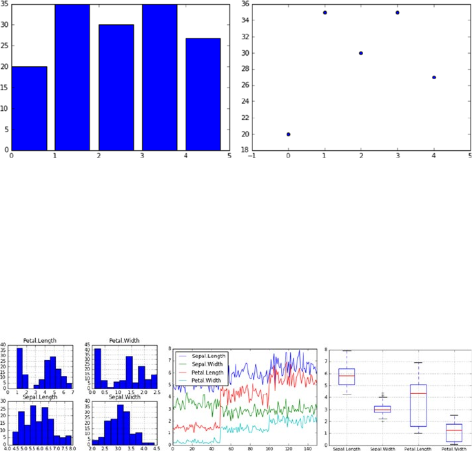
CHAPTER 2 ■ STEP 2 – INTRODUCTION TO MACHINE LEARNING
101
Listing 2-31. Creating plot on variables
# simple bar and scatter plot
x = np.arange(5) # assume there are 5 students
y = (20, 35, 30, 35, 27) # their test scores
plt.bar(x,y) # Bar plot
# need to close the figure using show() or close(), if not closed any follow
up plot commands will use same figure.
plt.show() # Try commenting this an run
plt.scatter(x,y) # scatter plot
plt.show()
# ---- output ----
You can use the histogram, line graph, and boxplot directly on a dataframe. You can
see that it’s very quick and does not take much coding effort. See Listing 2-32.
Listing 2-32. Creating plot on dataframe df = pd.read_csv(‘Data/iris.csv’)# Read sample
data
df.hist()# Histogram
df.plot() # Line Graph
df.boxplot() # Box plot
# --- histogram----------line graph ----------box plot-------
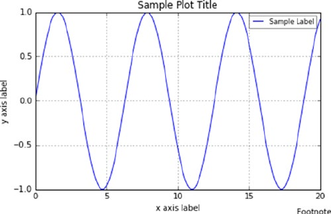
CHAPTER 2 ■ STEP 2 – INTRODUCTION TO MACHINE LEARNING
102
Customizing Labels
You can customize the labels to make them more meaningful. See Listing 2-33.
Listing 2-33. Customize labels
# generate sample data
x = np.linspace(0, 20, 1000) #100 evenly-spaced values from 0 to 50
y = np.sin(x)
# customize axis labels
plt.plot(x, y, label = 'Sample Label')
plt.title('Sample Plot Title') # chart title
plt.xlabel('x axis label') # x axis title
plt.ylabel('y axis label') # y axis title
plt.grid(True) # show gridlines
# add footnote
plt.figtext(0.995, 0.01, 'Footnote', ha='right', va='bottom')
# add legend, location pick the best automatically
plt.legend(loc='best', framealpha=0.5, prop={'size':'small'})
# tight_layout() can take keyword arguments of pad, w_pad and h_pad.
# these control the extra padding around the figure border and between
subplots.
# The pads are specified in fraction of fontsize.
plt.tight_layout(pad=1)
# Saving chart to a file
plt.savefig('filename.png')
plt.close() # Close the current window to allow new plot creation on
separate window / axis, alternatively we can use show()
plt.show()
# ---- output ----
CHAPTER 2 ■ STEP 2 – INTRODUCTION TO MACHINE LEARNING
103
Object Oriented
You obtain an empty figure from a global factory, and then build the plot explicitly using
the methods of the Figure and the classes it contains. The Figure is the top-level container
for everything on a canvas. Axes is a container class for a specific plot. A figure may
contain many Axes and/or Subplots. Subplots are laid out in a grid within the Figure. Axes
can be placed anywhere on the Figure. We can use the subplots factory to get the Figure
and all the desired Axes at once. See Listing 2-34.
Listing 2-34. Object-oriented customization
fig, ax = plt.subplots()
fig,(ax1,ax2,ax3) = plt.subplots(nrows=3, ncols=1, sharex=True,
figsize=(8,4))
# Iterating the Axes within a Figure
for ax in fig.get_axes():
pass # do something
# ---- output ----
Line Plots – Using ax.plot()
Single plot constructed with Figure and Axes in Llisting 2-35.
Listing 2-35. Single line plot using ax.plot()
# generate sample data
x = np.linspace(0, 20, 1000)
y = np.sin(x)
fig = plt.figure(figsize=(8,4)) # get an empty figure
and add an Axes
ax = fig.add_subplot(1,1,1) # row-col-num
ax.plot(x, y, 'b-', linewidth=2, label='Sample label') # line plot data on
the Axes
# add title, labels and legend, etc.
ax.set_ylabel('y axis label', fontsize=16) # y label
ax.set_xlabel('x axis lable', fontsize=16) # x label
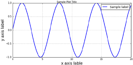
CHAPTER 2 ■ STEP 2 – INTRODUCTION TO MACHINE LEARNING
104
ax.legend(loc='best') # legend
ax.grid(True) # show grid
fig.suptitle('Sample Plot Title') # title
fig.tight_layout(pad=1) # tidy laytout
fig.savefig('filename.png', dpi=125)
# ---- output ----
Multiple Lines on Same Axis
See Listing 2-36.
Listing 2-36. Multiple line plot on same axis
# get the Figure and Axes all at once
fig, ax = plt.subplots(figsize=(8,4))
x1 = np.linspace(0, 100, 20)
x2 = np.linspace(0, 100, 20)
x3 = np.linspace(0, 100, 20)
y1 = np.sin(x1)
y2 = np.cos(x2)
y3 = np.tan(x3)
ax.plot(x1, y1, label='sin')
ax.plot(x2, y2, label='cos')
ax.plot(x3, y3, label='tan')
# add grid, legend, title and save
ax.grid(True)
ax.legend(loc='best', prop={'size':'large'})
fig.suptitle('A Simple Multi Axis Line Plot')
fig.savefig('filename.png', dpi=125)
# ---- output ----
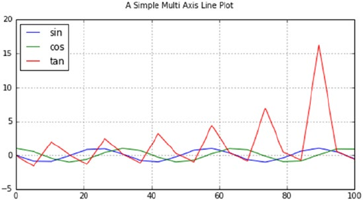
CHAPTER 2 ■ STEP 2 – INTRODUCTION TO MACHINE LEARNING
105
Multiple Lines on Different Axis
See Listing 2-37.
Listing 2-37. Multiple lines on different axis
# Changing sharex to True will use the same x axis
fig, (ax1,ax2,ax3) = plt.subplots(nrows=3, ncols=1, sharex=False, sharey =
False, figsize=(8,4))
# plot some lines
x1 = np.linspace(0, 100, 20)
x2 = np.linspace(0, 100, 20)
x3 = np.linspace(0, 100, 20)
y1 = np.sin(x1)
y2 = np.cos(x2)
y3 = np.tan(x3)
ax1.plot(x1, y1, label='sin')
ax2.plot(x2, y2, label='cos')
ax3.plot(x3, y3, label='tan')
# add grid, legend, title and save
ax1.grid(True)
ax2.grid(True)
ax3.grid(True)
ax1.legend(loc='best', prop={'size':'large'})
ax2.legend(loc='best', prop={'size':'large'})
ax3.legend(loc='best', prop={'size':'large'})
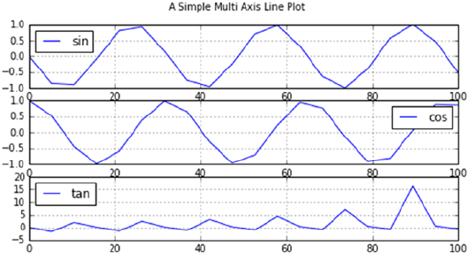
CHAPTER 2 ■ STEP 2 – INTRODUCTION TO MACHINE LEARNING
106
fig.suptitle('A Simple Multi Axis Line Plot')
fig.savefig('filename.png', dpi=125)
# ---- output ----
Control the Line Style and Marker Style
See Listing 2-38.
Listing 2-38. Line style and marker style controls
# get the Figure and Axes all at once
fig, ax = plt.subplots(figsize=(8,4))
# plot some lines
N = 3 # the number of lines we will plot
styles = ['-', '--', '-.', ':']
markers = list('+ox')
x = np.linspace(0, 100, 20)
for i in range(N): # add line-by-line
y = x + x/5*i + i
s = styles[i % len(styles)]
m = markers[i % len(markers)]
ax.plot(x, y, alpha = 1, label='Line '+str(i+1)+' '+s+m,
marker=m, linewidth=2, linestyle=s)
# add grid, legend, title and save
ax.grid(True)
ax.legend(loc='best', prop={'size':'large'})
fig.suptitle('A Simple Line Plot')
fig.savefig('filename.png', dpi=125)
# ---- output ----
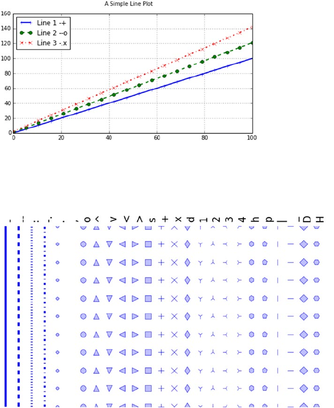
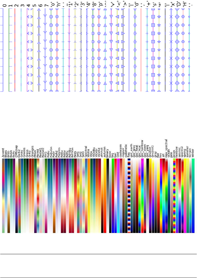
CHAPTER 2 ■ STEP 2 – INTRODUCTION TO MACHINE LEARNING
108
Marker Reference
See Figure2-15.
Figure 2-15. matplotlib marker reference
Figure 2-16. Matplotlib colormaps reference
Colomaps Reference
See Figure2-16.
■Note All color maps can be reversed by appending _r. For instance, gray_r is the
reverse of gray.
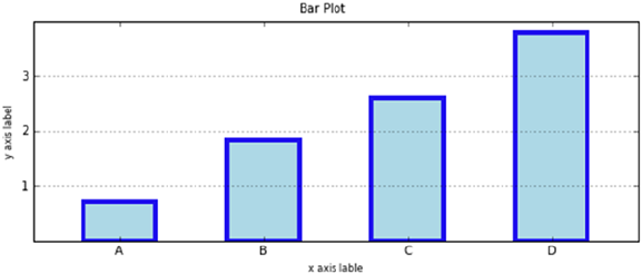
CHAPTER 2 ■ STEP 2 – INTRODUCTION TO MACHINE LEARNING
109
Bar Plots – using ax.bar() and ax.barh()
See Listing 2-39.
Listing 2-39. Bar plots using ax.bar() and ax.barh()
# get the data
N = 4
labels = list('ABCD')
data = np.array(range(N)) + np.random.rand(N)
#plot the data
fig, ax = plt.subplots(figsize=(8, 3.5))
width = 0.5;
tickLocations = np.arange(N)
rectLocations = tickLocations-(width/2.0)
# for color either HEX value of the name of the color can be used
ax.bar(rectLocations, data, width,
color='lightblue',
edgecolor='#1f10ed', linewidth=4.0)
# tidy-up the plot
ax.set_xticks(ticks= tickLocations)
ax.set_xticklabels(labels)
ax.set_xlim(min(tickLocations)-0.6, max(tickLocations)+0.6)
ax.set_yticks(range(N)[1:])
ax.set_ylim((0,N))
ax.yaxis.grid(True)
ax.set_ylabel('y axis label', fontsize=8) # y label
ax.set_xlabel('x axis lable', fontsize=8) # x label
# title and save
fig.suptitle("Bar Plot")
fig.tight_layout(pad=2)
fig.savefig('filename.png', dpi=125)
# ---- output ----
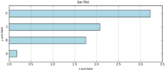
CHAPTER 2 ■ STEP 2 – INTRODUCTION TO MACHINE LEARNING
110
Horizontal Bar Charts
Just as tick placement needs to be managed with vertical bars, so it is with horizontal
bars, which are above the y-tick mark as shown in Listing 2-40.
Listing 2-40. Horizontal bar charts
# get the data
N = 4
labels = list('ABCD')
data = np.array(range(N)) + np.random.rand(N)
#plot the data
fig, ax = plt.subplots(figsize=(8, 3.5))
width = 0.5;
tickLocations = np.arange(N)
rectLocations = tickLocations-(width/2.0)
# for color either HEX value of the name of the color can be used
ax.barh(rectLocations, data, width, color='lightblue')
# tidy-up the plot
ax.set_yticks(ticks= tickLocations)
ax.set_yticklabels(labels)
ax.set_ylim(min(tickLocations)-0.6, max(tickLocations)+0.6)
ax.xaxis.grid(True)
ax.set_ylabel('y axis label', fontsize=8) # y label
ax.set_xlabel('x axis lable', fontsize=8) # x label
# title and save
fig.suptitle("Bar Plot")
fig.tight_layout(pad=2)
fig.savefig('filename.png', dpi=125)
# ---- output ----
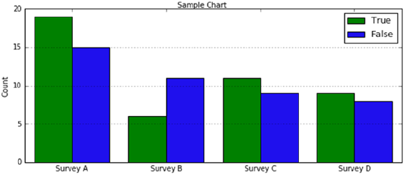
CHAPTER 2 ■ STEP 2 – INTRODUCTION TO MACHINE LEARNING
111
Side-by-Side Bar Chart
See Listing 2-41.
Listing 2-41. Side-by-side bar chart
# generate sample data
pre = np.array([19, 6, 11, 9])
post = np.array([15, 11, 9, 8])
labels=['Survey '+x for x in list('ABCD')]
# the plot – left then right
fig, ax = plt.subplots(figsize=(8, 3.5))
width = 0.4 # bar width
xlocs = np.arange(len(pre))
ax.bar(xlocs-width, pre, width,
color='green', label='True')
ax.bar(xlocs, post, width,
color='#1f10ed', label='False')
# labels, grids and title, then save
ax.set_xticks(ticks=range(len(pre)))
ax.set_xticklabels(labels)
ax.yaxis.grid(True)
ax.legend(loc='best')
ax.set_ylabel('Count')
fig.suptitle('Sample Chart')
fig.tight_layout(pad=1)
fig.savefig('filename.png', dpi=125)
# ---- output ----
Stacked Bar Example Code
See Listing 2-42.
Listing 2-42. Stacked bar charts
# generate sample data
pre = np.array([19, 6, 11, 9])
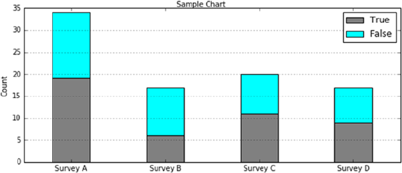
CHAPTER 2 ■ STEP 2 – INTRODUCTION TO MACHINE LEARNING
112
post = np.array([15, 11, 9, 8])
labels=['Survey '+x for x in list('ABCD')]
# the plot – left then right
fig, ax = plt.subplots(figsize=(8, 3.5))
width = 0.4 # bar width
xlocs = np.arange(len(pre)+2)
adjlocs = xlocs[1:-1] - width/2.0
ax.bar(adjlocs, pre, width,
color='grey', label='True')
ax.bar(adjlocs, post, width,
color='cyan', label='False',
bottom=pre)
# labels, grids and title, then save
ax.set_xticks(ticks=xlocs[1:-1])
ax.set_xticklabels(labels)
ax.yaxis.grid(True)
ax.legend(loc='best')
ax.set_ylabel('Count')
fig.suptitle('Sample Chart')
fig.tight_layout(pad=1)
fig.savefig('filename.png', dpi=125)
# ---- output ----
Pie Chart – Using ax.pie()
See Listing 2-43.
Listing 2-43. Pie chart
# generate sample data
data = np.array([15,8,4])
labels = ['Feature Engineering', 'Model Tuning', 'Model Building']
explode = (0, 0.1, 0) # explode feature engineering
colrs=['cyan', 'tan', 'wheat']
# plot
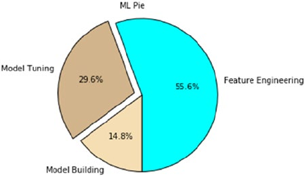
CHAPTER 2 ■ STEP 2 – INTRODUCTION TO MACHINE LEARNING
113
fig, ax = plt.subplots(figsize=(8, 3.5))
ax.pie(data, explode=explode,
labels=labels, autopct='%1.1f%%',
startangle=270, colors=colrs)
ax.axis('equal') # keep it a circle
# tidy-up and save
fig.suptitle("ML Pie")
fig.savefig('filename.png', dpi=125)
# ---- output ----
Example Code for Grid Creation
See Listing 2-44.
Listing 2-44. Grid creation
# Simple subplot grid layouts
fig = plt.figure(figsize=(8,4))
fig.text(x=0.01, y=0.01, s='Figure',color='#888888', ha='left', va='bottom',
fontsize=20)
for i in range(4):
# fig.add_subplot(nrows, ncols, num)
ax = fig.add_subplot(2, 2, i+1)
ax.text(x=0.01, y=0.01, s='Subplot 2 2 '+str(i+1), color='red',
ha='left', va='bottom', fontsize=20)
ax.set_xticks([]); ax.set_yticks([])
ax.set_xticks([]); ax.set_yticks([])
fig.suptitle('Subplots')
fig.savefig('filename.png', dpi=125)
# ---- output ----
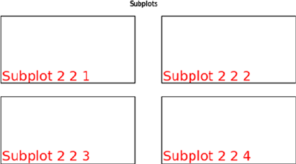
CHAPTER 2 ■ STEP 2 – INTRODUCTION TO MACHINE LEARNING
114
Plotting – Defaults
Matplotlib uses matplotlibrc configuration files to customize all kinds of properties,
which we call rc settings or rcparameters. You can control the defaults of almost every
property in matplotlib such as figure size and dpi, line width, color and style, axes, axis
and grid properties, text and font properties, and so on. The location of the configuration
file can be found using the code in Listing 2-45 so that you can edit it if required.
Listing 2-45. Plotting defaults
# get configuration file location
print (matplotlib.matplotlib_fname())
# get configuration current settings
print (matplotlib.rcParams)
# Change the default settings
plt.rc('figure', figsize=(8,4), dpi=125,facecolor='white',
edgecolor='white')
plt.rc('axes', facecolor='#e5e5e5', grid=True, linewidth=1.0,
axisbelow=True)
plt.rc('grid', color='white', linestyle='-', linewidth=2.0, alpha=1.0)
plt.rc('xtick', direction='out')
plt.rc('ytick', direction='out')
plt.rc('legend', loc='best')
Machine Learning Core Libraries
Python has a plethora of open source machine learning libraries. Table2-4 gives a quick
summary of the top 10 Python machine learning libraries ranked, based on their number
of contributors, and also shows the change in percentage of growth in their contributors
count between 2015 and 2016.

CHAPTER 2 ■ STEP 2 – INTRODUCTION TO MACHINE LEARNING
115
Scikit-learn is the most popular and widely used machine learning library. It is built on
top of SciPy and features a rich number of supervised and unsupervised learning algorithms.
We’ll learn more about different algorithms of Scikit-learn in detail in the next
chapter.
■Note StatsModels is another important library often used for running regression
models; however, it does not have the implementation of other machine learning algorithms.
It’s BSD-3 licensed with 110 contributors as of 2016.
Table 2-4. Python machine learning libraries
Contributors
Project Name 2015 2016 Change (%) License Type Source
Scikit-learn 404 732 81% BSD 3 www.github.com/
scikit-learn/
scikit-learn
Pylearn2 117 115 -2% BSD 3 www.github.com/
lisa-lab/pylearn2
NuPIC 60 75 25% AGPL 3 www.github.com/
numenta/nupic
Nilearn 28 46 64% BSD www.github.com/
nilearn/nilearn
PyBrain 27 31 15% BSD 3 www.github.com/
pybrain/pybrain
Pattern 20 20 0% BSD 3 www.github.com/
clips/pattern
Fuel 12 29 142% MIT www.github.com/
mila-udem/fuel
Bob 11 13 18% BSD www.github.com/
idiap/bob
Skdata 10 11 10% N/A www.github.com/
jaberg/skdata
MILK 9 9 0% MIT www.github.com/
luispedro/milk
Table2-4 - Top 10 Python machine learning libraries
Note: 2015 numbers are based on KDNuggets news publish

CHAPTER 2 ■ STEP 2 – INTRODUCTION TO MACHINE LEARNING
116
Endnotes
With this we have reached the end of this chapter. We have learned what machine
learning is, and where it fits in the wider artificial intelligence family. We have also learned
about the different related forms/terms (such as statistics, data or business analytics,
data science) that exist parallel to machine learning and why they exist. We have briefly
explained the high-level categories of machine learning, and most commonly used
frameworks to build efficient machine learning systems. Toward the end we learned
that the machine learning libraries can be categorized into data analysis and core ML
packages. We also looked at the key concepts and example implementation code for three
important data analysis packages: NumPy, Pandas, and Matplotlib. I would like to leave
you with some useful resources for your future reference to deepen your knowledge in the
data analysis packages. See Table2-5.
Table 2-5. Additional resources
Resource Description Mode
https://docs.scipy.
org/doc/numpy/
reference/
This is a quick start tutorial for NumPy
and covers all the concepts in detail.
Online
http://pandas.pydata.
org/pandas-docs/
stable/tutorials.html
This is a guide to many pandas tutorials,
geared mainly for new users.
Online
http://matplotlib.org/
users/beginner.html
Beginners guide, Pyplot tutorial. Online
Python for Data Analysis This book is concerned with the nuts
and bolts of manipulating, processing,
cleaning, and crunching data in Python.
Book

117
© Manohar Swamynathan 2017
M. Swamynathan, Mastering Machine Learning with Python in Six Steps,
DOI 10.1007/978-1-4842-2866-1_3
CHAPTER 3
Step 3 – Fundamentals
of Machine Learning
This chapter is focused on different algorithms of supervised and unsupervised machine
learning using two key Python packages.
Scikit-learn: In 2007, David Cournapeau developed Scikit-learn as part of the
Google summer of code project. INRIA got involved in 2010 and beta v0.1 was released
for the public. Currently there are more than 700 plus active contributors and it has paid
sponsorship from INRIA, Python Software Foundation, Google, and Tinyclues. Many
of the functions of Scikit-learn are built upon SciPy (Scientific Python) library, and it
provides great breadth of efficiently implemented essential supervised and unsupervised
learning algorithms.
■Note Scikit-learn is also known as sklearn in short, so these two terms are used
interchangeably throughout this book.
Statsmodels: This complements the SciPy package and is one of the best packages
to run regression models as it provides an extensive list of statistics results for each
estimator of the model.
Machine Learning Perspective of Data
Data is the fact and figures (can also be referred as raw data) that we have available with
respect to the business context. Data are made up of these two aspects:
a. Objects such as people, tree, animals, etc.
b. Attributes that were recorded for objects such as age, size,
weight, cost, etc.
When we measure the attributes of an object, we obtain a value that varies between
objects. For example, if we consider individual plants in a garden as objects, and the
attribute ‘height' will vary between them. Correspondingly different attributes vary
between objects, so attributes are more collectively known as variables.

CHAPTER 3 ■ STEP 3 – FUNDAMENTALS OF MACHINE LEARNING
118
The things we measure, control, or manipulate for objects are the variables and it
differs in “how well” they can be measured that is how much measurable information
their measurement scale can provide. The amount of information that can be provided by
a variable is determined by its type of measurement scale.
At a high level there are two types of variables based on the type of values that it
can take.
1. Continuous or quantitative: variables can take any positive
or negative numerical value between a large range. Retail
sales amount, insurance claims amounts are examples for
continuous variables that can take any number within large
ranges. These types of variables are also generally known as
numerical variables.
2. Discrete or qualitative: variables can take only particular
values: retail store location area, state, city are examples for
discrete variables as it can take only one particular value for
a store (here store is our object). These types of variables are
also known as categorical variables.
Scales of Measurement
In general, variables can be measured on four different scales. Mean, median, and
mode are the way to understand the central tendency, that is, the middle point of data
distribution. Standard deviation, variance, and range are the most commonly used
dispersion measures used to understand the spread of the data.
Nominal Scale of Measurement
Data are measured at the nominal level when each case is classified into one of a number
of discrete categories. This is also called categorical, that is, used only for classification.
As mean is not meaningful, all that we can do is to count the number of occurrences
of each type and compute the proportion (number of occurrences of each type / total
occurrences). See Table3-1.
Table 3-1. Nomial scale examples
Variable Name Example Measurement Values
Color Red, Green, Yellow, etc.
Gender Female, Male
Football Players Jersey Number 1, 2, 3, 4, 5, etc.

CHAPTER 3 ■ STEP 3 – FUNDAMENTALS OF MACHINE LEARNING
119
Ordinal Scale of Measurement
Data are measured on an ordinal scale if the categories imply order. The difference
between ranks is consistent in direction and authority, but not magnitude. See Table3-2.
Interval Scale of Measurement
If the differences between values have meanings, the data are measured at the interval
scale. See Table3-3.
Ratio Scale of Measurement
Data measured on a ratio scale have differences that are meaningful, and relate to some
true zero point. This is the most common scale of measurement. See Tables3-4 and 3-5.
Table 3-2. Ordinal scale example
Variable Name Example Measurement Values
Military rank Second Lieutenant, First Lieutenant, Captain, Major,
Lieutenant Colonel, Colonel, etc.
Clothing size Small, Medium, Large, Extra Large. Etc.
Class rank in an exam 1,2,3,4,5, etc.
Table 3-3. Interval scale example
Variable Name Example Measurement Values
Temperature 10, 20, 30, 40, etc.
IQ rating 85 - 114, 115 - 129, 130 - 144, 145 – 159, etc.
Table 3-4. Ratio scale example
Variable Name Example Measurement Values
Weight 10, 20, 30, 40, 50, 60, etc.
Height 5, 6, 7, 8, 9, etc.
Age 1, 2, 3, 4, 5, 6, 7, etc.

CHAPTER 3 ■ STEP 3 – FUNDAMENTALS OF MACHINE LEARNING
120
Feature Engineering
The output or the prediction quality of any machine learning algorithm depends
predominantly on the quality of input being passed. The process of creating appropriate
data features by applying business context is called feature engineering, and it is one
of the most important aspects of building efficient machine learning systems. Business
context here means the expression of the business problem that we are trying to address,
why we are trying to solve it, and what is the expected outcome. So let’s understand the
fundamentals of feature engineering before proceeding to different types of machine
learning algorithms.
The logical flow of raw data to machine learning algorithm is represented in
Figure3-1. Data from different sources “as-is” is the raw data and when we apply business
logic to process the raw data, the outcome is information (processed data). Further
insight is derived from information. The process of converting raw data into information
into insight with a business context to address a particular business problem is an
important aspect of feature engineering. The output of feature engineering is a clean
Table 3-5. Comparison of the different scales of measurement
Scales of measurement
Nominal Ordinal Interval Ratio
Properties Identity Identity
Magnitude
Identity
Magnitude Equal
intervals
Identity
Magnitude Equal
intervals True
zero
Mathematical
Operations
Count Rank order Addition
Subtraction
Addition
Subtraction
Multiplication
Division
Descriptive
Statistics
Mode
Proportion
Mode Median
Range statistics
Mode Median
Range statistics
Variance
Standard
deviation
Mode
Median
Range statistics
Variance
Standard
deviation
Figure 3-1. Logical flow of data in Machine Learning model building
CHAPTER 3 ■ STEP 3 – FUNDAMENTALS OF MACHINE LEARNING
121
and meaningful set of features that can be consumed by algorithms to identify patterns
and build a machine learning model, which can further be applied on unseen data to
predict the possible outcome. In order to have an efficient machine learning system,
often feature optimization is carried out to reduce the feature dimension and retain only
the important/meaningful features that will reduce the computation time and improve
prediction performance. Note that machine learning model building is an iterative
process. Let’s look at some of the common practices that are part of feature engineering.
Dealing with Missing Data
Missing data can mislead or create problems for analyzing the data. In order to avoid
any such issues, you need to impute missing data. There are four most commonly used
techniques for data imputation.
• Delete: You could simply delete the rows containing missing
values. This technique is more suitable and effective when the
number of missing value rows count is insignificant (say < 5%)
compare to the overall record count. You can achieve this using
Panda's dropna() function.
• Replace with summary: This is probably the most commonly used
imputation technique. Summarization here is the mean, mode, or
median for a respective column. For continuous or quantitative
variables, either mean/average or mode or median value of the
respective column can be used to replace the missing values.
Whereas for categorical or qualitative variables, the mode (most
frequent) summation technique works better. You can achieve
this using Panda's fillna() function (please refer to Chapter 2
Pandas section).
• Random replace: You can also replace the missing values with
a randomly picked value from the respective column. This
technique would be appropriate where the missing values row
count is insignificant.
• Using predictive model: This is an advanced technique. Here
you can train a regression model for continuous variables and
classification model for categorical variables with the available
data and use the model to predict the missing values.
Handling Categorical Data
Most of the machine’s learning libraries are designed to work well with numerical
variables. So categorical variables in their original form of text description can’t be
directly used for model building. Let’s learn some of the common methods of handling
categorical data based on their number of levels.
CHAPTER 3 ■ STEP 3 – FUNDAMENTALS OF MACHINE LEARNING
122
Create dummy variable: This is a Boolean variable that indicates the presence of
a category with the value 1 and 0 for absence. You should create k-1 dummy variables,
where k is the number of levels. Scikit-learn provides a useful function ‘One Hot Encoder’
to create a dummy variable for a given categorical variable. See Listing 3-1.
Listing 3-1. Creating dummy variables
import pandas as pd
from patsy import dmatrices
df = pd.DataFrame({'A': ['high', 'medium', 'low'],
'B': [10,20,30]},
index=[0, 1, 2])
print df
#----output----
A B
0 high 10
1 medium 20
2 low 30
# using get_dummies function of pandas package
df_with_dummies= pd.get_dummies(df, prefix='A', columns=['A'])
print df_with_dummies
#----output----
B A_high A_low A_medium
0 10 1.0 0.0 0.0
1 20 0.0 0.0 1.0
2 30 0.0 1.0 0.0
Convert to number: Another simple method is to represent the text description
of each level with a number by using the ‘Label Encoder’ function of Scikit-learn. If the
number of levels are high (example zip code, state, etc.), then you apply the business logic
to combine levels to groups. For example zip code or state can be combined to regions;
however, in this method there is a risk of losing critical information. Another method is
to combine categories based on similar frequency (new category can be high, medium,
low). See Listing 3-2.

CHAPTER 3 ■ STEP 3 – FUNDAMENTALS OF MACHINE LEARNING
123
Listing 3-2. Converting categorical variable to numerics
import pandas as pd
# using pandas package's factorize function
df['A_pd_factorized'] = pd.factorize(df['A'])[0]
# Alternatively you can use sklearn package's LabelEncoder function
from sklearn.preprocessing import LabelEncoder
le = LabelEncoder()
df['A_LabelEncoded'] = le.fit_transform(df.A)
print df
#----output----
A B A_pd_factorized A_LabelEncoded
0 high 10 0
0
1 medium 20 1
2
2 low 30
2 1
Normalizing Data
A unit or scale of measurement for different variables varies, so an analysis with the raw
measurement could be artificially skewed toward the variables with higher absolute
values. Bringing all the different types of variable units in the same order of magnitude
thus eliminates the potential outlier measurements that would misrepresent the finding
and negatively affect the accuracy of the conclusion. Two broadly used methods for
rescaling data are normalization and standardization.
Normalizing data can be achieved by Min-Max scaling; the formula is given below,
which will scale all numeric values in the range 0 to 1.
XXX
XX
normalized
min
ma
xm
in
=
()
()
–
–
■Note Ensure you remove extreme outliers before applying the above technique as it
can skew the normal values in your data to a small interval.
The standardization technique will transform the variables to have a zero mean
and standard deviation of one. The formula for standardization is given below and the
outcome is commonly known as z-scores.
ZX
=-
()
m
s
CHAPTER 3 ■ STEP 3 – FUNDAMENTALS OF MACHINE LEARNING
124
Where μ is the mean and σ is the standard deviation.
Standardization has often been the preferred method for various analysis as it tells
us where each data point lies within its distribution and a rough indication of outliers. See
Listing 3-3.
Listing 3-3. Normalization and scaling
from sklearn import datasets
import numpy as np
from sklearn import preprocessing
iris = datasets.load_iris()
X = iris.data[:, [2, 3]]
y = iris.target
std_scale = preprocessing.StandardScaler().fit(X)
X_std = std_scale.transform(X)
minmax_scale = preprocessing.MinMaxScaler().fit(X)
X_minmax = minmax_scale.transform(X)
print('Mean before standardization: petal length={:.1f}, petal width={:.1f}'
.format(X[:,0].mean(), X[:,1].mean()))
print('SD before standardization: petal length={:.1f}, petal width={:.1f}'
.format(X[:,0].std(), X[:,1].std()))
print('Mean after standardization: petal length={:.1f}, petal width={:.1f}'
.format(X_std[:,0].mean(), X_std[:,1].mean()))
print('SD after standardization: petal length={:.1f}, petal width={:.1f}'
.format(X_std[:,0].std(), X_std[:,1].std()))
print('\nMin value before min-max scaling: patel length={:.1f}, patel
width={:.1f}'
.format(X[:,0].min(), X[:,1].min()))
print('Max value before min-max scaling: petal length={:.1f}, petal
width={:.1f}'
.format(X[:,0].max(), X[:,1].max()))
print('Min value after min-max scaling: patel length={:.1f}, patel
width={:.1f}'
.format(X_minmax[:,0].min(), X_minmax[:,1].min()))
print('Max value after min-max scaling: petal length={:.1f}, petal
width={:.1f}'
.format(X_minmax[:,0].max(), X_minmax[:,1].max()))
#----output----
Mean before standardization: petal length=3.8, petal width=1.2
SD before standardization: petal length=1.8, petal width=0.8
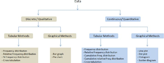
CHAPTER 3 ■ STEP 3 – FUNDAMENTALS OF MACHINE LEARNING
125
Mean after standardization: petal length=0.0, petal width=-0.0
SD after standardization: petal length=1.0, petal width=1.0
Min value before min-max scaling: patel length=1.0, patel width=0.1
Max value before min-max scaling: petal length=6.9, petal width=2.5
Min value after min-max scaling: patel length=0.0, patel width=0.0
Max value after min-max scaling: petal length=1.0, petal width=1.0
Feature Construction or Generation
Machine learning algorithms give best results only when we provide it the best possible
features that structure the underlying form of the problem that you are trying to address.
Often these features have to be manually created by spending a lot of time with actual raw
data and trying to understand its relationship with all other data that you have collected
to address a business problem.
It means thinking about aggregating, splitting, or combining features to create new
features, or decomposing features. Often this part is talked about as an art form and is the
key differentiator in competitive machine learning.
Feature construction is manual, slow, and requires subject-matter expert
intervention heavily in order to create rich features that can be exposed to predictive
modeling algorithms to produce best results.
Summarizing the data is a fundamental technique to help us understand the data
quality and issues/gaps. Figure3-2 maps the tabular and graphical data summarization
methods for different data types. Note that this mapping is the obvious or commonly used
methods, and not an exhaustive list.
Exploratory Data Analysis (EDA)
EDA is all about understanding your data by employing summarizing and visualizing
techniques. At a high level the EDA can be performed in two folds, that is, univariate
analysis and multivariate analysis.
Figure 3-2. Commonly used data summarization methods
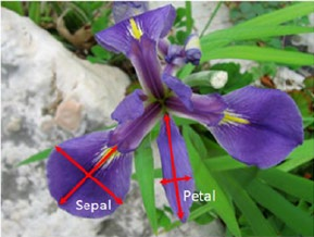
CHAPTER 3 ■ STEP 3 – FUNDAMENTALS OF MACHINE LEARNING
126
Let’s learn and consider an example dataset to learn practicality. Iris dataset is one
of a well-known datasets used extensively in pattern recognition literature. It is hosted at
UC Irvine Machine Learning Repository. The dataset contains petal length, petal width,
sepal length, and sepal width measurement for three types of iris flowers, that is, setosa,
versicolor, and virginica. See Figure3-3.
Univariate Analysis
Individual variables are analyzed in isolation to have a better understanding about them.
Pandas provide the describe function to create summary statistics in tabular format for all
variables. These statistics are very useful for numerical types of variables to understand
any quality issues such as missing values and the presence of outliers. See Listings 3-4
and 3-5.
Listing 3-4. Univariate analysis
from sklearn import datasets
import numpy as np
import pandas as pd
import matplotlib.pyplot as plt
iris = datasets.load_iris()
# Let's convert to dataframe
iris = pd.DataFrame(data= np.c_[iris['data'], iris['target']],
columns= iris['feature_names'] + ['species'])
# replace the values with class labels
iris.species = np.where(iris.species == 0.0, 'setosa', np.where(iris.
species==1.0,'versicolor', 'virginica'))
# let's remove spaces from column name
iris.columns = iris.columns.str.replace(' ','')
iris.describe()
Figure 3-3. Iris verisicolor
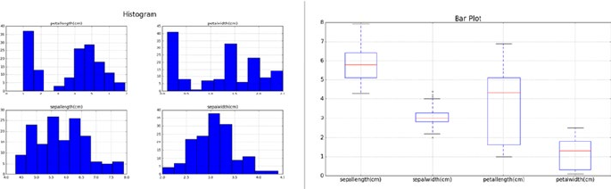
CHAPTER 3 ■ STEP 3 – FUNDAMENTALS OF MACHINE LEARNING
127
#----output----
sepallength(cm)sepalwidth(cm)petallength(cm) petalwidth(cm)
Count 150.00 150.00
150.00 150.00
Mean5.84 3.05 3.75 1.19
std 0.82 0.43 1.76 0.76
min 4.30 2.00 1.00 0.10
25% 5.10 2.80 1.60 0.30
50% 5.80 3.00 4.35 1.30
75% 6.40 3.30 5.10 1.80
max 7.90 4.40 6.90 2.50
The columns ‘species’ is categorical, so lets check the frequency distribution for each
category.
print iris['species'].value_counts()
#----output----
setosa50
versicolor 50
virginica 50
Pandas supports plotting functions to quick visualization on attributes. We can see
from the plot that 'species' has 3 category with 50 records each.
Listing 3-5. Pandas dataframe visualization
# Set the size of the plot
plt.figsize(15, 8)
iris.hist() # plot histogram
plt.suptitle("Histogram", fontsize=16) # use suptitle to add title to all
sublots
plt.show()
iris.boxplot() # plot boxplot
plt.title("Bar Plot", fontsize=16)
plt.show()
#----output----
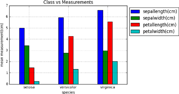
CHAPTER 3 ■ STEP 3 – FUNDAMENTALS OF MACHINE LEARNING
128
Multivariate Analysis
In multivariate analysis you try to establish a sense of relationship of all variables with
one other.
Let’s understand the mean of each feature by species type. See Listing 3-6.
Listing 3-6. Multivariate analysis
# print the mean for each column by species
iris.groupby(by = "species").mean()
# plot for mean of each feature for each label class
iris.groupby(by = "species").mean().plot(kind="bar")
plt.title('Class vs Measurements')
plt.ylabel('mean measurement(cm)')
plt.xticks(rotation=0) # manage the xticks rotation
plt.grid(True)
# Use bbox_to_anchor option to place the legend outside plot area to be tidy
plt.legend(loc="upper left", bbox_to_anchor=(1,1))
#----output----
sepallength(cm)sepalwidth(cm) petallength(cm) petalwidth(cm)
setosa 5.006 3.418 1.464 0.244
versicolor 5.936 2.770 4.260 1.326
virginica 6.588 2.974 5.552 2.026
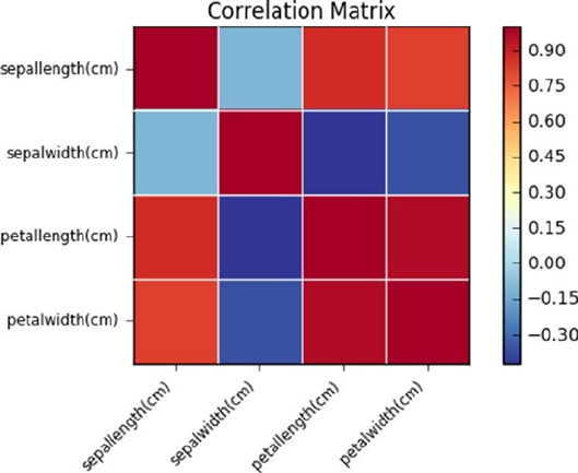
CHAPTER 3 ■ STEP 3 – FUNDAMENTALS OF MACHINE LEARNING
129
Correlation Matrix
The correlation function uses Pearson correlation coefficient, which results in a number
between -1 to 1. A strong negative relationship is indicated by a coefficient closer to -1
and a strong positive correlation is indicated by a coefficient toward 1. See Listing 3-7.
Listing 3-7. Correlation matrix
# create correlation matrix
corr = iris.corr()
print(corr)
import statsmodels.api as sm
sm.graphics.plot_corr(corr, xnames=list(corr.columns))
plt.show()
#----output----
sepallength(cm) sepalwidth(cm) petallength(cm) sepallength(cm)
1.000000 -0.109369 0.871754
sepalwidth(cm) -0.109369 1.000000 -0.420516
petallength(cm) 0.871754 -0.420516 1.000000
petalwidth(cm) 0.817954 -0.356544 0.962757
petalwidth(cm)
sepallength(cm) 0.817954
sepalwidth(cm) -0.356544
petallength(cm) 0.962757
petalwidth(cm) 1.000000
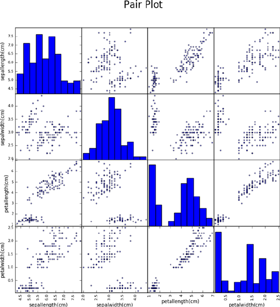
CHAPTER 3 ■ STEP 3 – FUNDAMENTALS OF MACHINE LEARNING
130
Pair Plot
You can understand the relationship attributes by looking at the distribution of the
interactions of each pair of attributes. This uses a built-in function to create a matrix of
scatter plots of all attributes against all attributes. See Listing 3-8.
Listing 3-8. Pair plot
from pandas.tools.plotting import scatter_matrix
scatter_matrix(iris, figsize=(10, 10))
# use suptitle to add title to all sublots
plt.suptitle("Pair Plot", fontsize=20)
#----output----

CHAPTER 3 ■ STEP 3 – FUNDAMENTALS OF MACHINE LEARNING
131
Findings from EDA
• There are no missing values.
• Sepal is longer than petal. Sepal length ranges between 4.3 to 7.9
with average length of 5.8, whereas petal length ranges between 1
to 6.9 with average length of 3.7.
• Sepal is also wider than petal. Sepal width ranges between 2 to 4.4
with a average width of 3.05, whereas petal width ranges between
0.1 to 2.5 with average width of 1.19.
• Average petal length of setosa is much smaller than versicolor and
virginica; however the average sepal width of setosa is higher than
versicolor and virginica.
• Petal length and width are strongly correlated, that is, 96% of the
time width increases with increase in length.
• Petal length has negative correlation with sepal width, that is, 42%
of the time increase in sepal width will decrease petal length.
• Initial conclusion from data: Based on length and width of sepal/
petal alone, you can conclude that versicolor/virginica might
resemble in size; however setosa characteristics seem to be
noticeably different from the other two.
Further looking at the characteristics of the three Iris flower characteristics visually
in Figure3-4, we can ascertain the hypothesis from our EDA.
Figure 3-4. Iris flowers
Statistics and mathematics is the base for machine learning algorithms. Let’s begin
by understanding some of the basic concepts and algorithms that are derived from the
statistical world and gradually move onto advanced machine learning algorithms.
Supervised Learning– Regression
Can you guess what is common in the below set of business questions across different
domains? See Table3-6.

CHAPTER 3 ■ STEP 3 – FUNDAMENTALS OF MACHINE LEARNING
132
Table 3-6. Supervised learning use cases examples
Domain Question
Retail How much will be the daily, monthly, and yearly sales for a
given store for the next three years?
Retail How many car parking spaces should be allocated for a retail
store?
Manufacturing How much will be the product-wise manufacturing labor cost?
Manufacturing / Retail How much will be my monthly electricity cost for the next
three years?
Banking What is the credit score of a customer?
Insurance How many customers will claim the insurance this year?
Energy / Environmental What will be the temperature for the next five days?
You might have guessed it right! The presence of the words ‘how much’ and ‘how
many’ implies that the answer for these questions will be a quantitative or continuous
number. The regression is one of the fundamental techniques that will help us to find
answers to these types of questions by studying the relationship between the different
variables that are relevant to the questions that we are trying to answer.
Let’s consider a use case where we have collected students’ average test grade scores
and their respective average number of study hours for the test for group of similar IQ
students. See Listing 3-9.
Listing 3-9. Students score vs. hours studied
import pandas as pd
import matplotlib.pyplot as plt
%matplotlib inline
# Load data
df = pd.read_csv('Data/Grade_Set_1.csv')
print df
# Simple scatter plot
df.plot(kind='scatter', x='Hours_Studied', y='Test_Grade', title='Grade vs
Hours Studied')
# check the correlation between variables
Print df.corr()
# ---- output ----
Hours_Studied Test_Grade
0 2 57
1 3 66
2 4 73
3 5 76
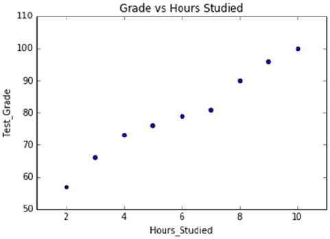
CHAPTER 3 ■ STEP 3 – FUNDAMENTALS OF MACHINE LEARNING
133
4 6 79
5 7 81
6 8 90
7 9 96
8 10 100
Correlation Matrix:
Hours_Studied Test_Grade
Hours_Studied 1.000000 0.987797
Test_Grade 0.987797 1.000000
A simple scatter plot with hours studied on the x-axis and the test grades on the
y-axis shows that the grade gradually increases with the increase in hours studied. This
implies that there is a linear relationship between the two variables. Further performing
the correlation analysis shows that there is 98% positive relationship between the two
variables, which means there is 98% chance that any change in study hours will lead to a
change in grade.
Correlation and Causation
Although correlation helps us determine the degree of relationship between two or
more variables, it does not tell about the cause and effect relationship. A high degree of
correlation does not always necessarily mean a relationship of cause and effect exists
between variables. Note that correlation does not imply causation though the existence of
causation always implies correlation. Let’s understand this better with examples.
• More firemen’s presence during a fire instance signifies that the
fire is big but the fire is not caused by firemen.
• When one sleeps with shoes on, he is likely to get a headache.
This may be due to alcohol intoxication.
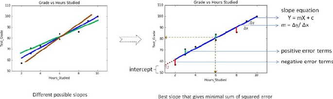
CHAPTER 3 ■ STEP 3 – FUNDAMENTALS OF MACHINE LEARNING
134
The significant degree of correlation in the above examples may be due to below
reasons
• Small samples are prone to show a higher correlation due to pure
chance.
• Variables may be influencing each other so it becomes hard to
designate one as the cause and the other as the effect.
• Correlated variables may be influenced by one or more other
related variables.
The domain knowledge or involvement of subject matter expert is very important to
ascertain the correlation due to causation.
Fitting a Slope
Let’s try to fit a slope line through all the points such that the error or residual, that is, the
distance of line from each point is the best possible minimal. See Figure3-5.
Figure 3-5. Linear regression model components
The error could be positive or negative based on its location from the slope, because
of which if we take a simple sum of all the errors, it will be zero. So we should square
the error to get rid of negativity and then sum the squared error. Hence, the slope is also
referred to as least squares line.
• The slope equation is given by Y = mX + c, where Y is the
predicted value for a given x value.
• m is the change in y, divided by change in x, that is, m is the slope
of the line for the x variable and it indicates the steepness at which
it increases with every unit increase in x variable value.
• c is the intercept that indicates the location or point on the axis
where it intersects, in the case of Figure3-5 it is 52. Intercept is a
constant that represents the variability in Y that is not explained
by the X. It is the value of Y when X is zero.
CHAPTER 3 ■ STEP 3 – FUNDAMENTALS OF MACHINE LEARNING
135
Together the slope and intercept define the linear relationship between the two
variables and can be used to predict or estimate an average rate of change. Now using
this relation, for a new student we can determine the score based on his study hours.
Say a student is planning to study an overall of 6 hours in preparation for the test. Simply
drawing a connecting line from the x-axis and y-axis to the slope shows that there is a
possibility of him scoring 80. We can use the slope equation to predict the score for any
given number of hours of study. In this case the test grade is the dependent variable,
denoted by ‘Y’ and hours studied is an independent variable or predictor, denoted by ‘X’.
Let’s use the linear regression function from the scikit-learn library to find the values of m
(x’s coefficient) and c (intercept). See Listing 3-10.
Listing 3-10. Linear regression
# importing linear regression function
import sklearn.linear_model as lm
# Create linear regression object
lr = lm.LinearRegression()
x= df.Hours_Studied[:, np.newaxis] # independent variable
y= df.Test_Grade.values # dependent variable
# Train the model using the training sets
lr.fit(x, y)
print "Intercept: ", lr.intercept_
print "Coefficient: ", lr.coef_
# manual prediction for a given value of x
print "Manual prdiction :", 52.2928994083 + 4.74260355*6
# predict using the built-in function
print "Using predict function: ", lr.predict(6)
# plotting fitted line
plt.scatter(x, y, color='black')
plt.plot(x, lr.predict(x), color='blue', linewidth=3)
plt.title('Grade vs Hours Studied')
plt.ylabel('Test_Grade')
plt.xlabel('Hours_Studied')
# ---- output ----
Intercept: 52.2928994083
Coefficient: [ 4.74260355]
Manual prdiction : 80.7485207083
Using predict function: [ 80.74852071]
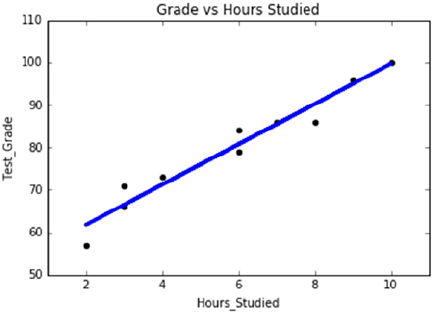
CHAPTER 3 ■ STEP 3 – FUNDAMENTALS OF MACHINE LEARNING
136
Let’s put the appropriate values in the slope equation (m * X + c = Y), 4.74260355 *
6 + 52.2928994083 = 80.74 that means a student studying 6 hours has the probability of
scoring 80.74 test grade.
Note that if X is zero, the value of Y will be 52.29 that mean even if the student does
not study there is a possibility that he’ll score 52.29; this signifies that there are other
variables that have a causation effect on score that we currently do not have access to.
How Good Is Your Model?
There are three metrics widely used for evaluating linear model performance.
• R-squared
• RMSE
• MAE
R-Squared for Goodness of Fit
The R-squared metric is the most popular practice of evaluating how well your model fits
the data. R-squared value designates the total proportion of variance in the dependent
variable explained by the independent variable. It is a value between 0 and 1; the value
toward 1 indicates a better model fit. See Table3-7.
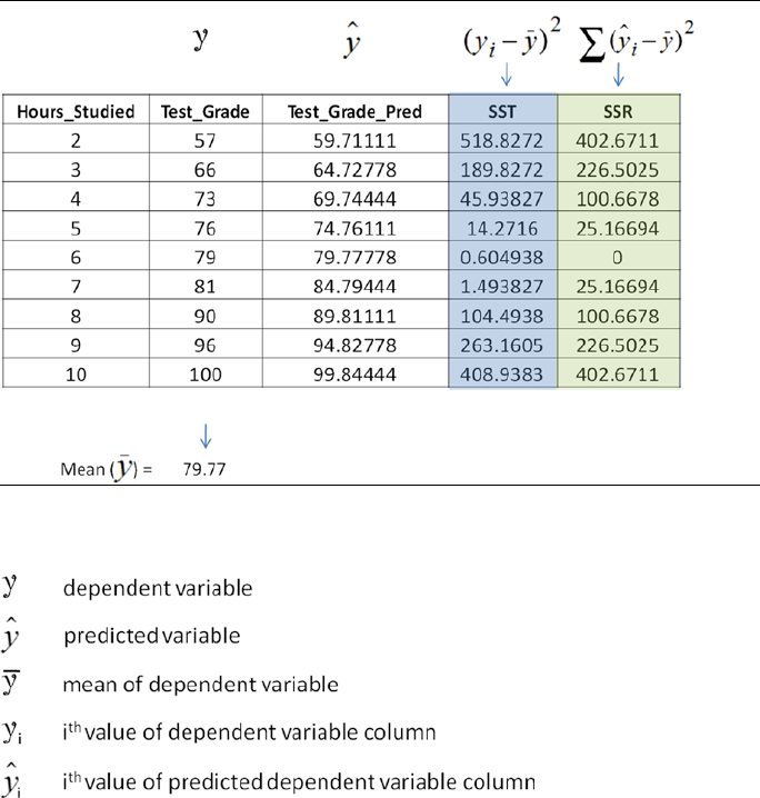
CHAPTER 3 ■ STEP 3 – FUNDAMENTALS OF MACHINE LEARNING
137
Where,
Total Sum of Square Residual (∑ SSR)
R-squared = ------------------------------------
Sum of Square Total(∑ SST)
R-squared = 1510.01 / 1547.55 = 0.97
In this case R-squared can be interpreted as 97% of variablility in the
dependent variable (test score) can be explained by the independent variable
(hours studied).
Table 3-7. Sample table for R-squared calculation
CHAPTER 3 ■ STEP 3 – FUNDAMENTALS OF MACHINE LEARNING
138
Root Mean Squared Error (RMSE)
This is the square root of the mean of the squared errors. RMSE indicates how close the
predicted values are to the actual values; hence a lower RMSE value signifies that the
model performance is good. One of the key properties of RMSE is that the unit will be the
same as the target variable.
1
1
2
nyy
i
n
ii
=
å-
()
ˆ
Mean Absolute Error
This is the mean or average of absolute value of the errors, that is, the predicted - actual.
See Listing 3-11.
1
1
n
yy
i
n
ii
=
å-ˆ
Listing 3-11. Linear regression model accuracy matrices
# function to calculate r-squared, MAE, RMSE
from sklearn.metrics import r2_score , mean_absolute_error, mean_squared_error
# add predict value to the data frame
df['Test_Grade_Pred'] = lr.predict(x)
# Manually calculating R Squared
df['SST'] = np.square(df['Test_Grade'] - df['Test_Grade'].mean())
df['SSR'] = np.square(df['Test_Grade_Pred'] - df['Test_Grade'].mean())
print "Sum of SSR:", df['SSR'].sum()
print "Sum of SST:", df['SST'].sum()
print "R Squared using manual calculation: ", df['SSR'].sum() / df['SST'].sum()
# Using built-in function
print "R Squared using built-in function: ", r2_score(df.Test_Grade, y)
print "Mean Absolute Error: ", mean_absolute_error(df.Test_Grade, df.Test_
Grade_Pred)
print "Root Mean Squared Error: ", np.sqrt(mean_squared_error(df.Test_Grade,
df.Test_Grade_Pred))
# ---- output ----
Sum of SSR: 1510.01666667
Sum of SST: 1547.55555556

CHAPTER 3 ■ STEP 3 – FUNDAMENTALS OF MACHINE LEARNING
139
R Squared using manual calculation: 0.97574310741
R Squared using built-in function: 0.97574310741
Mean Absolute Error: 1.61851851852
Root Mean Squared Error: 2.04229959955
Polynomial Regression
It is a form of higher-order linear regression modeled between dependent and
independent variables as an nth degree polynomial. Although it’s linear it can fit curves
better. Essentially we’ll be introducing higher-order degree variables of the same
independent variable in the equation. See Table3-8 and Listing 3-12.
Table 3-8. Polynomial regression higher degrees
Degree Regression Equation
Quadratic (2) YmXm
Xc=+ +
12
2^
Cubic (3) YmXmXm
Xc=+ ++
12 3
23^^
Nth YmXmXm
Xm
Xn c
n
=+ ++++
12 3
23^^.... ^
Listing 3-12. Polynomial regression
x = np.linspace(-3,3,1000) # 1000 sample number between -3 to 3
# Plot subplots
fig, ((ax1, ax2, ax3), (ax4, ax5, ax6)) = plt.subplots(nrows=2, ncols=3)
ax1.plot(x, x)
ax1.set_title('linear')
ax2.plot(x, x**2)
ax2.set_title('degree 2')
ax3.plot(x, x**3)
ax3.set_title('degree 3')
ax4.plot(x, x**4)
ax4.set_title('degree 4')
ax5.plot(x, x**5)
ax5.set_title('degree 5')
ax6.plot(x, x**6)
ax6.set_title('degree 6')
plt.tight_layout()# tidy layout
# --- output ----
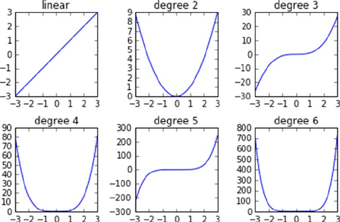
CHAPTER 3 ■ STEP 3 – FUNDAMENTALS OF MACHINE LEARNING
140
Let’s consider another set of students’ average test grade scores and their respective
average number of hours studied for similar IQ students. See Listing 3-13.
Listing 3-13. Polynomial regression example
# Load data
df = pd.read_csv('Data/Grade_Set_2.csv')
print df
# Simple scatter plot
df.plot(kind='scatter', x='Hours_Studied', y='Test_Grade', title='Grade vs
Hours Studied')
# check the correlation between variables
print("Correlation Matrix: ")
df.corr()
# Create linear regression object
lr = lm.LinearRegression()
x= df.Hours_Studied[:, np.newaxis] # independent variable
y= df.Test_Grade # dependent variable
# Train the model using the training sets
lr.fit(x, y)
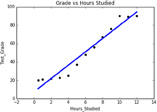
CHAPTER 3 ■ STEP 3 – FUNDAMENTALS OF MACHINE LEARNING
141
# plotting fitted line
plt.scatter(x, y, color='black')
plt.plot(x, lr.predict(x), color='blue', linewidth=3)
plt.title('Grade vs Hours Studied')
plt.ylabel('Test_Grade')
plt.xlabel('Hours_Studied')
print "R Squared: ", r2_score(y, lr.predict(x))
# ---- output ----
Hours_Studied Test_Grade
0 0.5 20
1 1.0 21
2 2.0 22
3 3.0 23
4 4.0 25
5 5.0 37
6 6.0 48
7 7.0 56
8 8.0 67
9 9.0 76
10 10.0 90
11 11.0 89
12 12.0 90
Correlation Matrix:
Hours_Studied Test_Grade
Hours_Studied 1.000000 0.974868
Test_Grade 0.974868 1.000000
R Squared: 0.9503677767
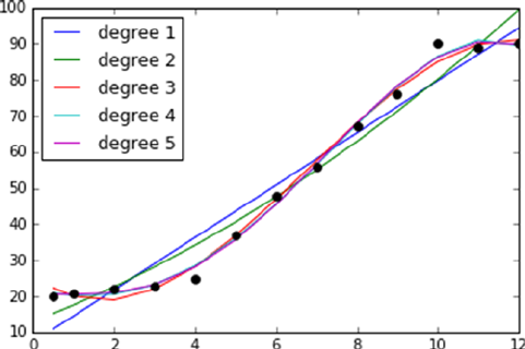
CHAPTER 3 ■ STEP 3 – FUNDAMENTALS OF MACHINE LEARNING
142
The correlation analysis shows a 97% positive relationship between hours studied
and the test grade, and 95% (r-squared) of variation in test grade can be explained by
hours studied. Note that up to 4 hours of average study results in less than a 30 test
grade and post 9 hours of study there is not a grade value to add to the grade. This is
not a perfect linear relationship, although we can fit a linear line. Let’s try higher-order
polynomial degrees. See Listing 3-14.
Listing 3-14. r-squared for different polynomial degrees
lr = lm.LinearRegression()
x= df.Hours_Studied # independent variable
y= df.Test_Grade # dependent variable
NumPy's vander function will return powers of the input vector
for deg in [1, 2, 3, 4, 5]:
lr.fit(np.vander(x, deg + 1), y);
y_lr = lr.predict(np.vander(x, deg + 1))
plt.plot(x, y_lr, label='degree ' + str(deg));
plt.legend(loc=2);
print r2_score(y, y_lr)
plt.plot(x, y, 'ok')
# ---- output ----
R-squared for degree 1 = 0.9503677767
R-squared for degree 2 = 0.960872656868
R-squared for degree 3 = 0.993832312037
R-squared for degree 4 = 0.99550001841
R-squared for degree 5 = 0.99562049139
Note degree 1 here is the linear fit, and the higher-order polynomial regression is
fitting the curve better and r-square jumps 4% higher at degree 3. Beyond the 3rd degree
there is not a massive change in r-squared so we can say that the 3rd degree fits better.
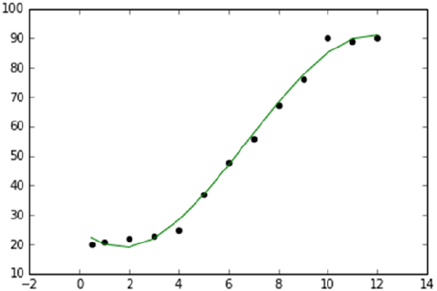
CHAPTER 3 ■ STEP 3 – FUNDAMENTALS OF MACHINE LEARNING
143
Scikit-learn provides a function to generate a new feature matrix consisting of
all polynomial combinations of the features with the degree less than or equal to the
specified degree. See Listing 3-15.
Listing 3-15. scikit-learn polynomial features
from sklearn.preprocessing import PolynomialFeatures
from sklearn.pipeline import make_pipeline
x= df.Hours_Studied[:, np.newaxis] # independent variable
y= df.Test_Grade # dependent variable
degree = 4
model = make_pipeline(PolynomialFeatures(degree), lr)
model.fit(x, y)
plt.scatter(x, y, color='black')
plt.plot(x, model.predict(x), color='green')
print "R Squared using built-in function: ", r2_score(y, model.predict(x))
# ---- output ----
R Squared using built-in function: 0.993832312037
Multivariate Regression
So far we have seen simple regression with one independent variable for a given
dependent variable. In most of the real-life use cases there will be more than one
independent variable, so the concept of having multiple independent variables is called
multivariate regression. The equation takes the form below.
ymxmxm
xm
x
nn
=+++¼+
11 22 33

CHAPTER 3 ■ STEP 3 – FUNDAMENTALS OF MACHINE LEARNING
144
Here, each independent variable is represented by x’s, and m’s are the corresponding
coefficients. We’ll be using the ‘statsmodels’ Python library to learn the basics of
multivariate regression, as it provide more useful statistics results that are helpful from a
learning perspective. Once you understand the fundamental concepts, you can either use
‘scikit-learn’ or ‘statsmodels’ package as both are efficient.
We'll be using the housing dataset (from RDatasets), which contains sales prices
of houses in the city of Windsor. Below is the brief description about each variable. See
Table3-9.
Table 3-9. Housing dataset (from RDatasets)
Variable Name Description Data type
Price Sale price of a house Numeric
Lotsize The lot size of a property in square feet Numeric
Bedrooms Number of bedrooms Numeric
Bathrms Number of full bathrooms Numeric
Stories Number of stories excluding basement Categorical
Driveway Does the house have a driveway? Boolean/Categorical
Recroom Does the house have a recreational
room?
Boolean/Categorical
Fullbase Does the house have a full finished
basement?
Boolean/Categorical
Gashw Does the house use gas for hot water
heating?
Boolean/Categorical
Airco Does the house have central air
conditioning?
Boolean/Categorical
Garagepl Number of garage places Numeric
Prefarea Is the house located in the preferred
neighborhood of the city?
Boolean/Categorical
Let’s build a model to predict the house price (dependent variable), by considering
the rest of the variables as independent variables.
The categorical variables need to be handled appropriately before running the first
iteration of the model. Scikit-learn provides useful built-in preprocessing functions to
handle categorical variables.
• Label Binarizer: This will replace the binary variable text with
numeric vales. We’ll be using this function for the binary
categorical variables.
• Label Encoder: This will replace category level with number
representation.

CHAPTER 3 ■ STEP 3 – FUNDAMENTALS OF MACHINE LEARNING
145
• One Hot Encoder: This will convert n levels to n-1 new variable,
and the new variables will use 1 to indicate the presence of level
and 0 for otherwise. Note that before calling OneHotEncoder,
we should use LabelEncoder to convert levels to number.
Alternatively we can achieve the same using get_dummies of the
Pandas package. This is much more efficient to use as we can
directly use it on the column with text description without having
to convert to numbers first.
Multicollinearity and Variation Inflation Factor (VIF)
The dependent variable should have a strong relationship with independent variables.
However, any independent variables should not have strong correlations among other
independent variables. Multicollinearity is an incident where one or more of the
independent variables are strongly correlated with each other. In such incidents, we
should use only one among correlated independent variables.
VIF is an indicator of the existence of multicollinearity, and ‘statsmodel’ provides a
function to calculate the VIF for each independent variable and a value of greater than
10 is the rule of thumb for possible existence of high multicollinearity. The standard
guideline for VIF value is as follows, VIF = 1 means no correlation exists, VIF > 1, but < 5
means moderate correlation exists. See Listing 3-16.
VIF
R
i
i
=
-
1
12
Where Ri
2 is the coefficient of determination of variable Xi
Listing 3-16. Multicollinearity and VIF
# Load data
df = pd.read_csv('Data/Housing_Modified.csv')
# Convert binary fields to numeric boolean fields
lb = preprocessing.LabelBinarizer()
df.driveway = lb.fit_transform(df.driveway)
df.recroom = lb.fit_transform(df.recroom)
df.fullbase = lb.fit_transform(df.fullbase)
df.gashw = lb.fit_transform(df.gashw)
df.airco = lb.fit_transform(df.airco)
df.prefarea = lb.fit_transform(df.prefarea)
# Create dummy variables for stories
df_stories = pd.get_dummies(df['stories'], prefix='stories', drop_
first=True)
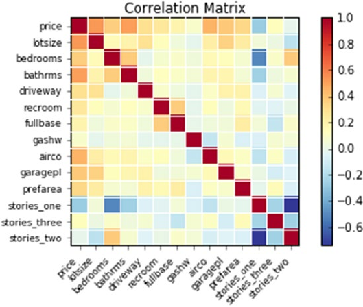
CHAPTER 3 ■ STEP 3 – FUNDAMENTALS OF MACHINE LEARNING
146
# Join the dummy variables to the main dataframe
df = pd.concat([df, df_stories], axis=1)
del df['stories']
# lets plot correlation matrix using statmodels graphics packages's plot_corr
# create correlation matrix
corr = df.corr()
sm.graphics.plot_corr(corr, xnames=list(corr.columns))
plt.show()
# ---- output ----
We can notice from the plot that stories_one has a strong negative correlation with
stories_two. Let’s perform the VIF analysis to eliminate strongly correlated independent
variables. See Listings 3-17 and 3-18.
Listing 3-17. Remove multicollinearity
# create a Python list of feature names
independent_variables = ['lotsize', 'bedrooms', 'bathrms','driveway',
'recroom', 'fullbase','gashw','airco','garagepl', 'prefarea', 'stories_
one','stories_two','stories_three']
# use the list to select a subset from original DataFrame
X = df[independent_variables]
y = df['price']
CHAPTER 3 ■ STEP 3 – FUNDAMENTALS OF MACHINE LEARNING
147
thresh = 10
for i in np.arange(0,len(independent_variables)):
vif = [variance_inflation_factor(X[independent_variables].values, ix)
for ix in range(X[independent_variables].shape[1])]
maxloc = vif.index(max(vif))
if max(vif) > thresh:
print "vif :", vif
print('dropping \'' + X[independent_variables].columns[maxloc] + '\'
at index: ' + str(maxloc))
del independent_variables[maxloc]
else:
break
print 'Final variables:', independent_variables
# ---- output ----
vif : [8.9580980878443359, 18.469878559519948, 8.9846723472908643,
7.0885785420918861, 1.4770152815033917, 2.013320236472385,
1.1034879198994192, 1.7567462065609021, 1.9826489313438442,
1.5332946465459893, 3.9657526747868612, 5.5117024083548918,
1.7700402770614867]
dropping 'bedrooms' at index: 1
Final variables: ['lotsize', 'bathrms', 'driveway', 'recroom', 'fullbase',
'gashw', 'airco', 'garagepl', 'prefarea', 'stories_one', 'stories_two',
'stories_three']
We can notice that VIF analysis has elemenated bedrooms has its greater than
10, however stories_one and stories_two has been retained.
Let’s run the first iteration of multivariate regression model with the set
of independent variables that has passed the VIF analysis.
To test the model performance the common practice is to split the dataset
into 80/20 (or 70/30) for train/test respectively and use the train data
set to build the model, then apply the trained model on the test dataset
evaluate the performance of the model.
Listing 3-18. Build the multivariate linear regression model
# create a Python list of feature names
independent_variables = ['lotsize', 'bathrms','driveway', 'recroom', 'fu
llbase','gashw','airco','garagepl', 'prefarea', 'stories_one','stories_
two','stories_three']
# use the list to select a subset from original DataFrame
X = df[independent_variables]
y = df['price']
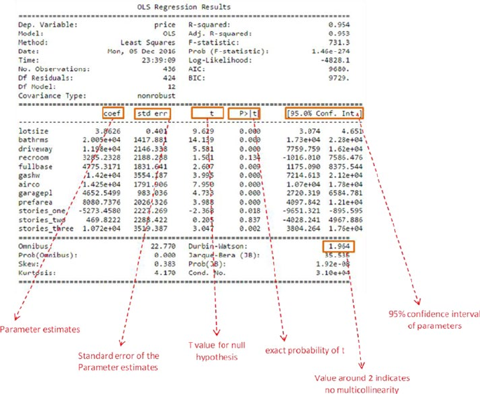
CHAPTER 3 ■ STEP 3 – FUNDAMENTALS OF MACHINE LEARNING
148
# Split your data set into 80/20 for train/test datasets
from sklearn.cross_validation import train_test_split
X_train, X_test, y_train, y_test = train_test_split(X, y, train_size=.80,
random_state=1)
# create a fitted model & print the summary
lm = sm.OLS(y_train, X_train).fit()
print lm.summary()
# make predictions on the testing set
y_train_pred = lm.predict(X_train)
y_test_pred = lm.predict(X_test)
print "Train MAE: ", metrics.mean_absolute_error(y_train, y_train_pred)
print "Train RMSE: ", np.sqrt(metrics.mean_squared_error(y_train, y_train_pred))
print "Test MAE: ", metrics.mean_absolute_error(y_test, y_test_pred)
print "Test RMSE: ", np.sqrt(metrics.mean_squared_error(y_test, y_test_pred))
# ---- output ----
Train MAE: 11987.66016
Train RMSE: 15593.4749178
Test MAE: 12722.0796754
Test RMSE: 17509.25004
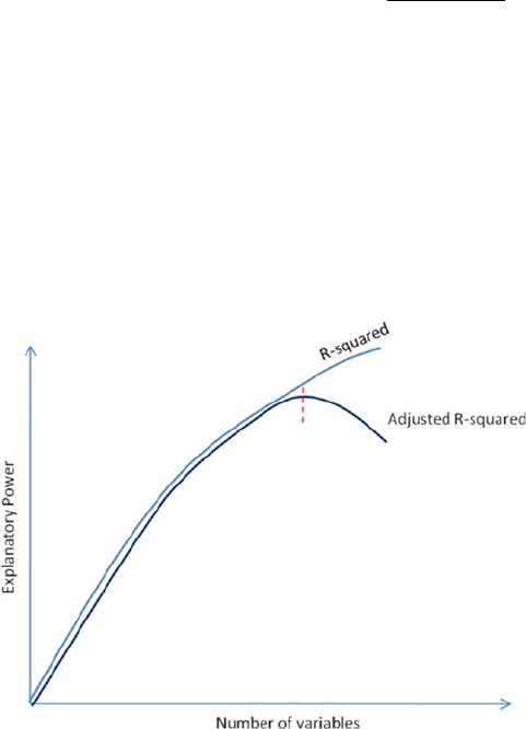
CHAPTER 3 ■ STEP 3 – FUNDAMENTALS OF MACHINE LEARNING
149
Interpreting the OLS Regression Results
Adjusted R-squared: Simple R-squared value will keep increase with addition of
independent variable. To fix this issue adjusted R-squared is considered for multivariate
regression to understand the explanatory power of the independent variables.
Adjusted RRN
Np
2
2
1
11
1
=- -
()
-
()
--
Here, N is total observations or sample size and p is the number of predictors.
See Figure3-6.
- Figure3-6 shows how R-squared follows Adjusted R-squared with
increase of more variables
- With inclusion of more variables R-squared always tend to
increase
- Adjusted R-squared will drop if the variable added does not
explain the variable in the dependent variable
Figure 3-6. R-squared vs. Adjusted R-squared
Coefficient: These are the individual coefficients for respective independent
variables. It can be either a positive or negative number, which indicates that an increase
in every unit of that independent variable will have a positive or negative impact on the
dependent variable value.
Standard error: This is the average distance of the respective independent observed
values from the regression line. The smaller values show that the model fitting is good.
CHAPTER 3 ■ STEP 3 – FUNDAMENTALS OF MACHINE LEARNING
150
Durbin-Watson: It’s one of the common statistics used to determine the existence
of multicollinearity, which means two or more independent variables used in the
multivariate regression model are highly correlated. The Durbin-Watson statistics are
always between the number 0 and 4. A value around 2 is ideal (range of 1.5 to 2.5 is
relatively normal), and it means that there is no autocorrelation between the variables
used in the model.
Confidence interval: This is the coefficient to calculate 95% confidence interval for
the independent variable’s slope.
t and p-value: p-value is one of the import statistics. In order to get a better
understanding we’ll have to understand the concept of hypothesis testing and normal
distribution.
Hypothesis testing is an assertion regarding the distribution of the observations and
validating this assertion. The hypothesis testing steps are given below.
• A hypothesis is made.
• The validity of the hypothesis is tested.
• If the hypothesis is found to be true, it is accepted.
• If it is found to be untrue, it is rejected.
• The hypothesis that is being tested for possible rejection is called
null hypothesis.
• Null hypothesis is denoted by H0.
• The hypothesis that is accepted when null hypothesis is rejected
is called alternate hypothesis Ha.
• The alternative hypothesis is often the interesting one and often
the one that someone sets out to prove.
• For example, null hypothesis H0 is that the lot size has a real effect
on house price; in this case the coefficient m is equal to zero in
the regression equation (y = m * lot size + c).
• Alternative hypothesis Ha is that the lot size does not have a real
effect on house price and the effect you saw was due to chance.
This means the coefficient m is not equal to zero in the regression
equation.
• In order to be able to say whether the regression estimate is close
enough to the hypothesized value to be acceptable, we take the
range of estimate implied by the estimated variance and look to
see whether this range will contain the hypothesized value. To
do this, we can transform the estimate into a standard normal
distribution and we know that 95% of all values of a variable that
has a mean of 0 and a variance of 1 will lie within 0 to 2 standard
deviations. Given a regression estimate and its standard error, we
can be 95% confident that the true (unknown) value of m will lie
in this region. See Figure3-7.
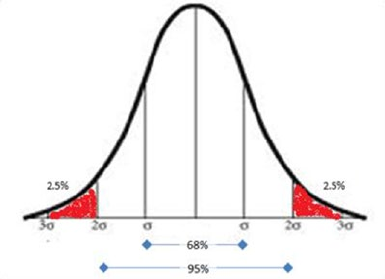
CHAPTER 3 ■ STEP 3 – FUNDAMENTALS OF MACHINE LEARNING
151
• The t-value is used to determine a p value (probability),
and p-value ≤ 0.05 signifies strong evidence against the
null hypothesis, so you reject the null hypothesis. A p-value
> 0.05 signifies weak evidence against the null hypothesis, so
you fail to reject the null hypothesis. So in our case the
variables with ≤ 0.05 means the variables are significant for
the model.
• Process of testing a hypothesis indicates that there is a possibility
of making an error. There are two types of errors for any given
dataset, and these two types of errors are inversely related,
which means the smaller the risk of one, the higher the risk of
the other.
• Type I error: The error of rejecting the null hypothesis H0 even
though H0 was true.
• Type II error: The error of accepting the null hypothesis H0 even
though H0 was false.
Figure 3-7. Normal distribution (red is the rejection region)
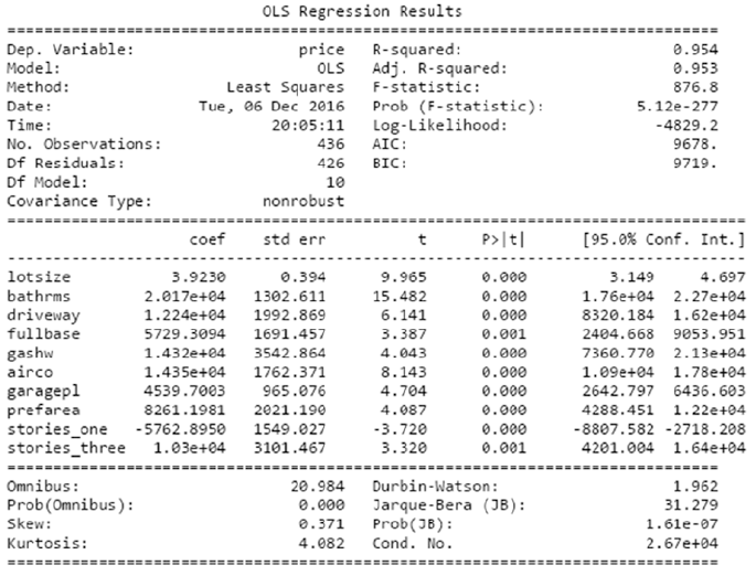
CHAPTER 3 ■ STEP 3 – FUNDAMENTALS OF MACHINE LEARNING
152
• Note that variable ‘stores_three’ and ‘recroom’ have a large p
value indicating it’s insignificant. So let’s re-run the regression
without this variable and look at the results.
Train MAE: 11993.3436816
Train RMSE: 15634.9995429
Test MAE: 12902.4799591
Test RMSE: 17694.9341405
• Note that dropping the variables has not impacted adjusted
R-squared negatively.
Regression Diagnosis
• There is a set of procedures and assumptions that need to be
verified about our model results; without that the model could
be misleading. Let’s look at some of the important regression
diagnostics.
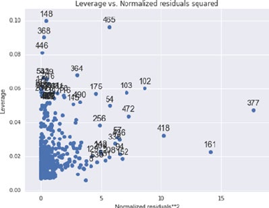
CHAPTER 3 ■ STEP 3 – FUNDAMENTALS OF MACHINE LEARNING
153
Outliers
• Data points that are far away from the fitted regression line are
called outliers, and these can impact the accuracy of the model.
Plotting normalized residual vs. leverage will give us a good
understanding of the outliers points. Residual is the difference
between actual vs. predicted, and leverage is a measure of how far
away the independent variable values of an observation are from
those of the other observations.
# lets plot the normalized residual vs leverage
from statsmodels.graphics.regressionplots import plot_leverage_resid2
fig, ax = plt.subplots(figsize=(8,6))
fig = plot_leverage_resid2(lm, ax = ax)
# ---- output ----
From the chart we see that there are many observations that have high leverage and
residual. Running a Bonferroni outlier test will give us p-values for each observation, and
those observations with p value < 0.05 are the outliers affecting the accuracy. It is a good
practice to consult or apply business domain knowledge to make a decision on removing
the outlier points and re-running the model, as these points could be natural in the
process although they are mathematically found as outliers. See Listing 3-19.
Listing 3-19. Find outliers
# Find outliers #
# Bonferroni outlier test
test = lm.outlier_test()
print 'Bad data points (bonf(p) < 0.05):'
print test[test.icol(2) < 0.05]
# ---- output ----
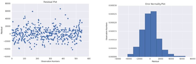
CHAPTER 3 ■ STEP 3 – FUNDAMENTALS OF MACHINE LEARNING
154
Bad data points (bonf(p) < 0.05):
student_resid unadj_p bonf(p)
377 4.387449 0.000014 0.006315
Homoscedasticity and Normality
The error variance should be constant, which is known has homoscedasticity and the
error should be normally distributed. See Listing 3-20.
Listing 3-20. Homoscedasticity test
# plot to check homoscedasticity
plt.plot(lm.resid,'o')
plt.title('Residual Plot')
plt.ylabel('Residual')
plt.xlabel('Observation Numbers')
plt.show()
plt.hist(lm.resid, normed=True)
# ---- output ----
Linearity – the relationships between the predictors and the outcome variables
should be linear. If the relationship is not linear then appropriate transformation (such as
log, square root, and higher-order polynomials etc) should be applied to the dependent/
independent variable to fix the issue. See Listing 3-21.
Listing 3-21. Linearity check
# linearity plots
fig = plt.figure(figsize=(10,15))
fig = sm.graphics.plot_partregress_grid(lm, fig=fig)
# ---- output ----
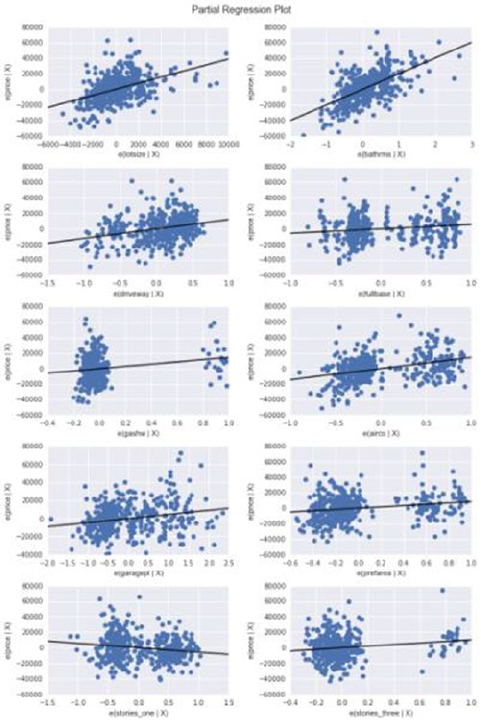
CHAPTER 3 ■ STEP 3 – FUNDAMENTALS OF MACHINE LEARNING
155
Over-fitting and Under-fitting
Under-fitting occurs when the model does not fit the data well and is unable to capture the
underlying trend in it. In this case we can notice a low accuracy in training and test dataset.
To the contrary, over-fitting occurs when the model fits the data too well, capturing
all the noises. In this case we can notice a high accuracy in the training dataset, whereas
the same model will result in a low accuracy on the test dataset. This means the model
has fitted the line so well to the train dataset that it failed to generalize it to fit well on
an unseen dataset. Figure3-8 shows how the different fitting would look like on the
earlier discussed example use case. The choice of right order polynomial degree is very
important to avoid an over-fitting or under-fitting issue in regression. We’ll also discuss in
detail about different ways of handling these problems in the next chapter. See Figure3-8.
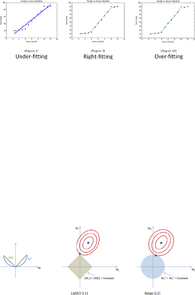
CHAPTER 3 ■ STEP 3 – FUNDAMENTALS OF MACHINE LEARNING
156
Regularization
With an increase in number of variables, and increase in model complexity, the probability
of over-fitting also increases. Regularization is a technique to avoid the over-fitting
problem. Over-fitting occurs when the model fits the data too well, capturing all the noises.
In this case we can notice a high accuracy in the training dataset, whereas the same model
will result in a low accuracy on the test dataset. This means the model has fitted the line so
well to the train dataset that it failed to generalize it to fit well on the unseen dataset.
Statsmodel and the scikit-learn provides Ridge and LASSO (Least Absolute Shrinkage
and Selection Operator) regression to handle the over-fitting issue. With an increase in
model complexity, the size of coefficients increase exponentially, so the ridge and LASSO
regression apply penalty to the magnitude of the coefficient to handle the issue.
LASSO: This provides a sparse solution, also known as L1 regularization. It guides
parameter value to be zero, that is, the coefficients of the variables that add minor
value to the model will be zero, and it adds a penalty equivalent to absolute value of the
magnitude of coefficients.
Ridge Regression: Also known as Tikhonov (L2) regularization, it guides parameters to
be close to zero, but not zero. You can use this when you have many variables that add minor
value to the model accuracy individually; however it improves overall the model accuracy
and cannot be excluded from the model. Ridge regression will apply a penalty to reduce the
magnitude of the coefficient of all variables that add minor value to the model accuracy,
and which adds penalty equivalent to square of the magnitude of coefficients. Alpha is the
regularization strength and must be a positive float. See Figure3-9 and Listing 3-22.
Figure 3-8. Model fittings
Figure 3-9. Regularizations
CHAPTER 3 ■ STEP 3 – FUNDAMENTALS OF MACHINE LEARNING
157
Listing 3-22. Regularization
from sklearn import linear_model
# Load data
df = pd.read_csv('Data/Grade_Set_2.csv')
df.columns = ['x','y']
for i in range(2,50): # power of 1 is already there
colname = 'x_%d'%i # new var will be x_power
df[colname] = df['x']**i
independent_variables = list(df.columns)
independent_variables.remove('y')
X= df[independent_variables] # independent variable
y= df.y # dependent variable
# split data into train and test
X_train, X_test, y_train, y_test = train_test_split(X, y, train_size=.80,
random_state=1)
# Ridge regression
lr = linear_model.Ridge(alpha=0.001)
lr.fit(X_train, y_train)
y_train_pred = lr.predict(X_train)
y_test_pred = lr.predict(X_test)
print("------ Ridge Regression ------")
print "Train MAE: ", metrics.mean_absolute_error(y_train, y_train_pred)
print "Train RMSE: ", np.sqrt(metrics.mean_squared_error(y_train, y_train_
pred))
print "Test MAE: ", metrics.mean_absolute_error(y_test, y_test_pred)
print "Test RMSE: ", np.sqrt(metrics.mean_squared_error(y_test, y_test_
pred))
print "Ridge Coef: ", lr.coef_
# LASSO regression
lr = linear_model.Lasso(alpha=0.001)
lr.fit(X_train, y_train)
y_train_pred = lr.predict(X_train)
y_test_pred = lr.predict(X_test)
print("----- LASSO Regression -----")
print "Train MAE: ", metrics.mean_absolute_error(y_train, y_train_pred)
print "Train RMSE: ", np.sqrt(metrics.mean_squared_error(y_train, y_train_
pred))
CHAPTER 3 ■ STEP 3 – FUNDAMENTALS OF MACHINE LEARNING
158
print "Test MAE: ", metrics.mean_absolute_error(y_test, y_test_pred)
print "Test RMSE: ", np.sqrt(metrics.mean_squared_error(y_test, y_test_
pred))
print "LASSO Coef: ", lr.coef_
#--- output ----
------ Ridge Regression ------
Train MAE: 13.1168856247
Train RMSE: 16.8257485401
Test MAE: 22.0861723747
Test RMSE: 22.1213599428
Ridge Coef: [ 9.99646940e-89 1.26287785e-87 1.39941783e-86 1.48384493e-85
1.53867101e-84 1.57509733e-83 1.59948276e-82 1.61560028e-81
1.62575609e-80 1.63139718e-79 1.63345182e-78 1.63252488e-77
1.62901252e-76 1.62317116e-75 1.61516012e-74 1.60506865e-73
1.59293349e-72 1.57875067e-71 1.56248359e-70 1.54406874e-69
1.52341994e-68 1.50043156e-67 1.47498127e-66 1.44693238e-65
1.41613625e-64 1.38243475e-63 1.34566311e-62 1.30565333e-61
1.26223824e-60 1.21525668e-59 1.16455980e-58 1.11001906e-57
1.05153619e-56 9.89055473e-56 9.22579214e-55 8.52186708e-54
7.78057774e-53 7.00501714e-52 6.19992888e-51 5.37214345e-50
4.53111186e-49 3.68955745e-48 2.86427041e-47 2.07707515e-46
1.35600615e-45 7.36735837e-45 2.64306411e-44 -4.77164338e-45
2.09761759e-46]
----- LASSO Regression -----
Train MAE: 0.842374298887
Train RMSE: 1.21912918556
Test MAE: 4.32364759404
Test RMSE: 4.8723243497
LASSO Coef: [ 1.29948409e+00 3.92103580e-01 1.75369422e-02 7.79647589e-04
3.02339084e-05 3.35699852e-07 -1.13749601e-07 -1.79773817e-08
-1.93826156e-09 -1.78643532e-10 -1.50240566e-11 -1.18610891e-12
-8.91794276e-14 -6.43309631e-15 -4.46487394e-16 -2.97784537e-17
-1.89686955e-18 -1.13767046e-19 -6.22157254e-21 -2.84658206e-22
-7.32019963e-24 5.16015995e-25 1.18616856e-25 1.48398312e-26
1.55203577e-27 1.48667153e-28 1.35117812e-29 1.18576052e-30
1.01487234e-31 8.52473862e-33 7.05722034e-34 5.77507464e-35
4.68162529e-36 3.76585569e-37 3.00961249e-38 2.39206785e-39
1.89235649e-40 1.49102460e-41 1.17072537e-42 9.16453614e-44
7.15512017e-45 5.57333358e-46 4.33236496e-47 3.36163309e-48
2.60423554e-49 2.01461728e-50 1.55652093e-51 1.20123190e-52
9.26105400e-54]
CHAPTER 3 ■ STEP 3 – FUNDAMENTALS OF MACHINE LEARNING
159
Nonlinear Regression
Linear models are mostly linear in nature, although they need not be straight fitting.
In contrast the nonlinear model’s fitted line can take any shape; this scenario usually
occurs when models are derived on the basis of physical or biological considerations.
The nonlinear models have direct interpretation in terms of the process under study.
Scipy library provides curve_fit function to fit models to scientific data based on a theory
to determine the parameters of a physical system. Some of the example use cases are
Michaelis–Menten’s enzyme kinetics, weibull distribution, power law distribution, etc.
See Listing 3-23.
Listing 3-23. Nonlinear regression
import numpy as np
import matplotlib.pyplot as plt
%matplotlib inline
from scipy.optimize import curve_fit
x= np.array([-2,-1.64,-0.7,0,0.45,1.2,1.64,2.32,2.9])
y = np.array([1.0, 1.5, 2.4, 2, 1.49, 1.2, 1.3, 1.2, 0.5])
def func(x, p1,p2):
return p1*np.sin(p2*x) + p2*np.cos(p1*x)
popt, pcov = curve_fit(func, x, y,p0=(1.0,0.2))
p1 = popt[0]
p2 = popt[1]
residuals = y - func(x,p1,p2)
fres = sum(residuals**2)
curvex=np.linspace(-2,3,100)
curvey=func(curvex,p1,p2)
plt.plot(x,y,'bo ')
plt.plot(curvex,curvey,'r')
plt.title('Non-linear fitting')
plt.xlabel('x')
plt.ylabel('y')
plt.legend(['data','fit'],loc='best')
plt.show()
# ---- output ----
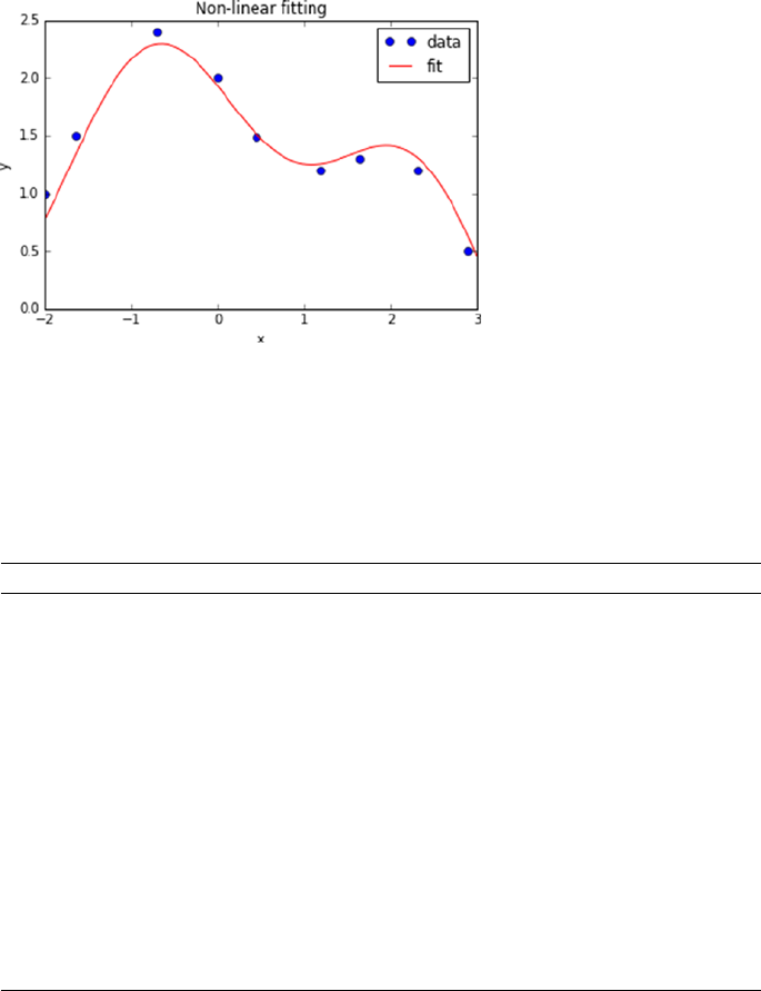
CHAPTER 3 ■ STEP 3 – FUNDAMENTALS OF MACHINE LEARNING
160
Supervised Learning – Classification
Let’s look at another set of questions, and can you guess what is common in these set of
business questions across different domains. See Table3-10.
Table 3-10. Classification use case examples
Domain Question
Telecom Is a customer likely to leave the network? (churn prediction)
Retail Is he a prospective customer?, that is, likelihood of purchase vs.
non-purchase?
Insurance To issue insurance, should a customer be sent for a medical
checkup?
Insurance Will the customer renew the insurance?
Banking Will a customer default on the loan amount?
Banking Should a customer be given a loan?
Manufacturing Will the equipment fail?
Health Care Is the patient infected with a disease?
Health Care What type of disease does a patient have?
Entertainment What is the genre of music?
The answers to these questions are a discrete class. The number of level or class can
vary from a minimum of two (example: true or false, yes or no) to multiclass. In machine
learning, classification deals with identifying the probability of a new object being a
member of a class or set. The classifiers are the algorithms that map the input data (also
called features) to categories.
CHAPTER 3 ■ STEP 3 – FUNDAMENTALS OF MACHINE LEARNING
161
Logistic Regression
Let’s consider a use case where we have to predict students’ test outcomes, that is, pass
(1) or fail (0) based on hours studied. In this case the outcome to be predicted is discrete.
Let’s build a linear regression and try to use a threshold, that is, anything over some value
is pass, or else it’s fail. See Listing 3-24.
Listing 3-24. Logistic regression
# Load data
df = pd.read_csv('Data/Grade_Set_1_Classification.csv')
print df
x= df.Hours_Studied[:, np.newaxis] # independent variable
y= df.Result # dependent variable
# Create linear regression object
lr = lm.LinearRegression()
# Train the model using the training sets
lr.fit(x, y)
# plotting fitted line
plt.scatter(x, y, color='black')
plt.plot(x, lr.predict(x), color='blue', linewidth=3)
plt.title('Hours Studied vs Result')
plt.ylabel('Result')
plt.xlabel('Hours_Studied')
# add predict value to the data frame
df['Result_Pred'] = lr.predict(x)
# Using built-in function
print "R Squared : ", r2_score(df.Result, df.Result_Pred)
print "Mean Absolute Error: ", mean_absolute_error(df.Result, df.Result_
Pred)
print "Root Mean Squared Error: ", np.sqrt(mean_squared_error(df.Result,
df.Result_Pred))
# ---- output ----
R Squared : 0.675
Mean Absolute Error: 0.22962962963
Root Mean Squared Error: 0.268741924943
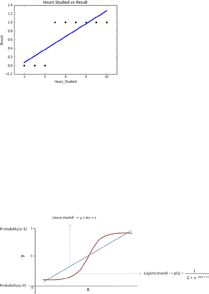
CHAPTER 3 ■ STEP 3 – FUNDAMENTALS OF MACHINE LEARNING
162
The outcome that we are expecting is either 1 or 0, and the issue with linear
regression is that it can give values large than 1 or less than 0. In the above plot we can see
that linear regression is not able to draw boundaries to classify observations.
The solution to this is to introduce sigmoid or Logit function (which takes a S shape)
to the regression equation. The fundamental idea here is that the hypothesis will use the
linear approximation, then map it with a logistic function for binary prediction.
linear regression equation in this case is y = mx + c
Logistic regression can be explained better in odds ratio. The odds of an event
occurring are defined as the probability of an event occurring divided by the probability
of that event not occurring. See Figure3-10 and Listing 3-25.
odds ratio of pass vs fail = probabilityy probabilityy=
()
-=
()
11 1/
A logit is the log base e(log) of the odds, so using the logit model:
log(p / p(1 - p)) = mx + c
Logistic regression equation probability(y=1) = 1 / 1+
-+
()
emx c
Figure 3-10. Linear regression vs. logistic regression
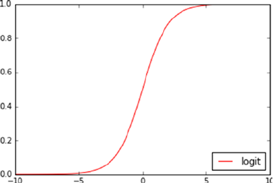
CHAPTER 3 ■ STEP 3 – FUNDAMENTALS OF MACHINE LEARNING
163
Listing 3-25. Plot sigmoid function
# plot sigmoid function
x = np.linspace(-10, 10, 100)
y = 1.0 / (1.0 + np.exp(-x))
plt.plot(x, y, 'r-', label='logit')
plt.legend(loc='lower right')
# --- output ----
Let’s run logistic regression using the scikit-learn package. See Listing 3-26.
Listing 3-26. Logistic regression using scikit-learn
from sklearn.linear_model import LogisticRegression
# manually add intercept
df['intercept'] = 1
independent_variables = ['Hours_Studied', 'intercept']
x = df[independent_variables] # independent variable
y = df['Result'] # dependent variable
# instantiate a logistic regression model, and fit with X and y
model = LogisticRegression(\)
model = model.fit(x, y)
# check the accuracy on the training set
model.score(x, y)
print model.predict(x)
print model.predict_proba(x)[:,0]
# plotting fitted line
plt.scatter(df.Hours_Studied, y, color='black')
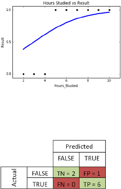
CHAPTER 3 ■ STEP 3 – FUNDAMENTALS OF MACHINE LEARNING
164
plt.yticks([0.0, 0.5, 1.0])
plt.plot(df.Hours_Studied, model.predict_proba(x)[:,1], color='blue',
linewidth=3)
plt.title('Hours Studied vs Result')
plt.ylabel('Result')
plt.xlabel('Hours_Studied')
# ---- output ----
Evaluating a Classification Model Performance
Confusion matrix is the table that is used for describing the performance of a
classification model. Figure3-11 shows the confusion matrix.
Figure 3-11. Confusion matrix
• True Negatives (TN): Actual FALSE, which was predicted as
FALSE
• False Positives (FP): Actual FALSE, which was predicted as TRUE
(Type I error)
• False Negatives (FN): Actual TRUE, which was predicted as FALSE
(Type II error)
• True Positives (TP): Actual TRUE, which was predicted as TRUE

CHAPTER 3 ■ STEP 3 – FUNDAMENTALS OF MACHINE LEARNING
165
Ideally a good model should have high TN and TP and less of Type I & II errors.
Table3-11 describes the key metrics derived out of the confusion matrix to understand
the classification model performance. Also see Listing 3-27.
Table 3-11. Classification performance matrices
Metric Description Formula
Accuracy what % of predictions were
correct?
(TP+TN)/
(TP+TN+FP+FN)
Misclassification Rate what % of prediction is wrong? (FP+FN)/(TP+TN+FP+FN)
True Positive Rate OR
Sensitivity OR Recall
(completeness)
what % of positive cases did
model catch?
TP/(FN+TP)
False Positive Rate what % of 'No' were predicted
as 'Yes'?
FP/(FP+TN)
Specificity what % of 'No' were predicted
as 'No'?
TN/(TN+FP)
Precision (exactness) what % of positive predictions
were correct?
TP/(TP+FP)
F1 score Weighted average of precision
and recall
2*((precision * recall) /
(precision + recall))
Listing 3-27. Confusion matrix
from sklearn import metrics
# generate evaluation metrics
print "Accuracy :", metrics.accuracy_score(y, model.predict(x))
print "AUC :", metrics.roc_auc_score(y, model.predict_proba(x)[:,1])
print "Confusion matrix :",metrics.confusion_matrix(y, model.predict(x))
print "classification report :", metrics.classification_report(y, model.
predict(x))
# ----output----
Accuracy : 0.88
AUC : 1.0
Confusion matrix : [[2 1]
[0 6]]
classification report :
precision recall f1-score support
0 1.00 0.67 0.80 3
1 0.86 1.00 0.92 6
avg/total 0.90 0.89 0.88 9
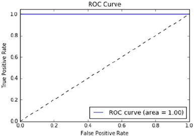
CHAPTER 3 ■ STEP 3 – FUNDAMENTALS OF MACHINE LEARNING
166
ROC Curve
A ROC curve is one more important metric, and it’s a most commonly used way to
visualize the performance of a binary classifier, and AUC is believed to be one of the best
ways to summarize performance in a single number. AUC indicates that the probability
of a randomly selected positive example will be scored higher by the classifier than a
randomly selected negative example. If you have multiple models with nearly the same
accuracy, you can pick the one that gives a higher AUC. See Listing 3-28.
Listing 3-28. Area Under the Curve
# Determine the false positive and true positive rates
fpr, tpr, _ = metrics.roc_curve(y, model.predict_proba(x)[:,1])
# Calculate the AUC
roc_auc = metrics.auc(fpr, tpr)
print 'ROC AUC: %0.2f' % roc_auc
# Plot of a ROC curve for a specific class
plt.figure()
plt.plot(fpr, tpr, label='ROC curve (area = %0.2f)' % roc_auc)
plt.plot([0, 1], [0, 1], 'k--')
plt.xlim([0.0, 1.0])
plt.ylim([0.0, 1.05])
plt.xlabel('False Positive Rate')
plt.ylabel('True Positive Rate')
plt.title('ROC Curve')
plt.legend(loc="lower right")
plt.show()
#---- output ----
In the above case, AUC is 100% as the model is able to predict all the positive
instances as true positive.
CHAPTER 3 ■ STEP 3 – FUNDAMENTALS OF MACHINE LEARNING
167
Fitting Line
The inverse of regularization is one of the key aspects of fitting a logistic regression line.
It defines the complexity of the fitted line. Let’s try to fit lines for different values for this
parameter (C, default is 1) and see how the fitting line and the accuracy changes. See
Listing 3-29.
Listing 3-29. Controling complexity for fitting a line
#instantiate a logistic regression model with default c value, and fit with
X and y
model = LogisticRegression()
model = model.fit(x, y)
#check the accuracy on the training set
print "C = 1 (default), Accuracy :", metrics.accuracy_score(y, model.
predict(x))
#instantiate a logistic regression model with c = 10, and fit with X and y
model1 = LogisticRegression(C=10)
model1 = model1.fit(x, y)
#check the accuracy on the training set
print "C = 10, Accuracy :", metrics.accuracy_score(y, model1.predict(x))
#instantiate a logistic regression model with c = 100, and fit with X and y
model2 = LogisticRegression(C=100)
model2 = model2.fit(x, y)
#check the accuracy on the training set
print "C = 100, Accuracy :", metrics.accuracy_score(y, model2.predict(x))
#instantiate a logistic regression model with c = 1000, and fit with X and y
model3 = LogisticRegression(C=1000)
model3 = model3.fit(x, y)
#check the accuracy on the training set
print "C = 1000, Accuracy :", metrics.accuracy_score(y, model3.predict(x))
#plotting fitted line
plt.scatter(df.Hours_Studied, y, color='black', label='Result')
plt.yticks([0.0, 0.5, 1.0])
plt.plot(df.Hours_Studied, model.predict_proba(x)[:,1], color='gray',
linewidth=2, label='C=1.0')
plt.plot(df.Hours_Studied, model1.predict_proba(x)[:,1], color='blue',
linewidth=2,label='C=10')
plt.plot(df.Hours_Studied, model2.predict_proba(x)[:,1], color='green',
linewidth=2,label='C=100')
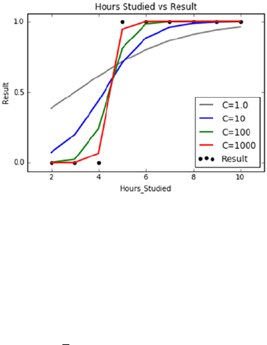
CHAPTER 3 ■ STEP 3 – FUNDAMENTALS OF MACHINE LEARNING
168
plt.plot(df.Hours_Studied, model3.predict_proba(x)[:,1], color='red',
linewidth=2,label='C=1000')
plt.legend(loc='lower right') # legend location
plt.title('Hours Studied vs Result')
plt.ylabel('Result')
plt.xlabel('Hours_Studied')
plt.show()
#----output----
C = 1 (default), Accuracy : 0.88
C = 10, Accuracy : 1.0
C = 100, Accuracy : 1.0
C = 1000, Accuracy : 1.0
Stochastic Gradient Descent
Fitting the right slope that minimizes the error (also known as cost function) for a large
dataset can be tricky. However this can be achieved through a stochastic gradient descent
(steepest descent) optimization algorithm. In case of regression problems, the cost
function J to learn the weights can be defined as the sum of squared errors (SSE) between
actual vs. predicted value.
J(w) = 1
2i
ii
yy
å-
()
ˆ, Where yi the ith is actual value, and ŷi is the ith predicted value.
The stochastic gradient descent algorithm to update weight (w), for every weight j of
every training sample i can be given as, repeat until convergence { W:=W x
jj
i
m
j
i
+-
()
=
å
ayy
ii
ˆ
1 }.
Alpha (α) is the learning rate, and choosing a smaller value for the same will ensure that
the algorithm dos not miss global cost minimum. See Figure3-12.
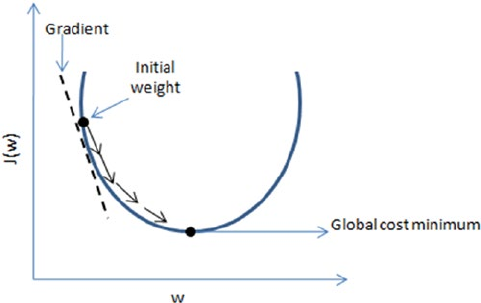
CHAPTER 3 ■ STEP 3 – FUNDAMENTALS OF MACHINE LEARNING
169
The default solver parameter for logistic regression in scikit-learn is 'liblinear', which
works fine for smaller datasets. For a large dataset with a large number of independent
variables, ‘sag’ (stochastic average gradient descent) is the recommended solver to fit the
optimal slope faster.
Regularization
With an increase in the number of variables, the probability of over-fitting also increases.
LASSO (L1) and Ridge (L2) can be applied for logistic regression as well to avoid over-
fitting. Let’s look at an example to understand the over-/under-fitting issue in logistic
regression. See Listing 3-30.
Listing 3-30. Under-fitting, right-fitting, and over-fitting
import pandas as pd
data = pd.read_csv('Data\LR_NonLinear.csv')
pos = data['class'] == 1
neg = data['class'] == 0
x1 = data['x1']
x2 = data['x2']
# function to draw scatter plot between two variables
def draw_plot():
plt.figure(figsize=(6, 6))
plt.scatter(np.extract(pos, x1),
np.extract(pos, x2),
c='b', marker='s', label='pos')
plt.scatter(np.extract(neg, x1),
np.extract(neg, x2),
Figure 3-12. Gradient descent
CHAPTER 3 ■ STEP 3 – FUNDAMENTALS OF MACHINE LEARNING
170
c='r', marker='o', label='neg')
plt.xlabel('x1');
plt.ylabel('x2');
plt.axes().set_aspect('equal', 'datalim')
plt.legend();
# create hihger order polynomial for independent variables
order_no = 6
# map the variable 1 & 2 to its higher order polynomial
def map_features(variable_1, variable_2, order=order_no):
assert order >= 1
def iter():
for i in range(1, order + 1):
for j in range(i + 1):
yield np.power(variable_1, i - j) * np.power(variable_2, j)
return np.vstack(iter())
out = map_features(data['x1'], data['x2'], order=order_no)
X = out.transpose()
y = data['class']
# split the data into train and test
X_train, X_test, y_train, y_test = train_test_split(X, y, test_size=0.3,
random_state=0)
# function to draw classifier line
def draw_boundary(classifier):
dim = np.linspace(-0.8, 1.1, 100)
dx, dy = np.meshgrid(dim, dim)
v = map_features(dx.flatten(), dy.flatten(), order=order_no)
z = (np.dot(classifier.coef_, v) + classifier.intercept_).reshape(100, 100)
plt.contour(dx, dy, z, levels=[0], colors=['r'])
# fit with c = 0.01
clf = LogisticRegression(C=0.01).fit(X_train, y_train)
print 'Train Accuracy for C=0.01: ', clf.score(X_train, y_train)
print 'Test Accuracy for C=0.01: ', clf.score(X_test, y_test)
draw_plot()
plt.title('Fitting with C=0.01')
draw_boundary(clf)
plt.legend();
# fit with c = 1
clf = LogisticRegression(C=1).fit(X_train, y_train)
print 'Train Accuracy for C=1: ', clf.score(X_train, y_train)
print 'Test Accuracy for C=1: ', clf.score(X_test, y_test)
draw_plot()
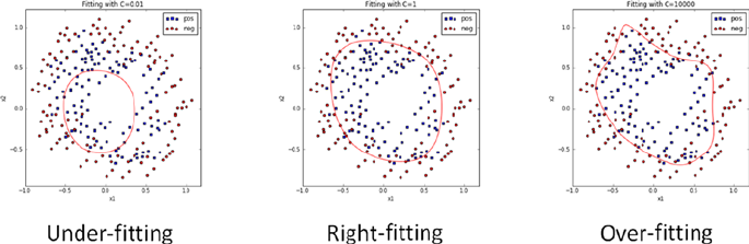
CHAPTER 3 ■ STEP 3 – FUNDAMENTALS OF MACHINE LEARNING
171
plt.title('Fitting with C=1')
draw_boundary(clf)
plt.legend();
# fit with c = 10000
clf = LogisticRegression(C=10000).fit(X_train, y_train)
print 'Train Accuracy for C=10000: ', clf.score(X_train, y_train)
print 'Test Accuracy for C=10000: ', clf.score(X_test, y_test)
draw_plot()
plt.title('Fitting with C=10000')
draw_boundary(clf)
plt.legend();
#----output----
Train Accuracy for C=0.01: 0.624242424242
Test Accuracy for C=0.01: 0.619718309859
Train Accuracy for C=1: 0.842424242424
Test Accuracy for C=1: 0.859154929577
Train Accuracy for C=10000: 0.860606060606
Test Accuracy for C=10000: 0.788732394366
Notice that with higher-order regularization, value over-fitting occurs, and the same
can be determined by looking at the accuracy between train and test datasets, that is, the
accuracy drops significantly in the test dataset.
Multiclass Logistic Regression
Logistic regression can also be used to predict the dependent or target variable with
multiclass. Let’s learn multiclass prediction with iris dataset, one of the best-known
databases to be found in the pattern recognition literature. The dataset contains 3 classes
of 50 instances each, where each class refers to a type of iris plant. This comes as part
of the scikit-learn datasets, where the third column represents the petal length, and the
fourth column the petal width of the flower samples. The classes are already converted to
integer labels where 0=Iris-Setosa, 1=Iris-Versicolor, 2=Iris-Virginica. See Listing 3-31.
CHAPTER 3 ■ STEP 3 – FUNDAMENTALS OF MACHINE LEARNING
172
Load Data
Listing 3-31. Load data
from sklearn import datasets
import numpy as np
import pandas as pd
iris = datasets.load_iris()
X = iris.data
y = iris.target
print('Class labels:', np.unique(y))
#----output----
('Class labels:', array([0, 1, 2]))
Normalize Data
The unit of measurement might differ so let’s normalize the data before building the
model. See Listing 3-32.
Listing 3-32. Normalize data
from sklearn.preprocessing import StandardScaler
sc = StandardScaler()
sc.fit(X)
X = sc.transform(X)
Split Data
Split data into train and test. Whenever we are using random function it’s advised to use a
seed to ensure the reproducibility of the results. See Listing 3-33.
Listing 3-33. Split data into train and test
# split data into train and test
from sklearn.cross_validation import train_test_split
X_train, X_test, y_train, y_test = train_test_split(X, y, test_size=0.3,
random_state=0)
Training Logistic Regression Model and Evaluating
Listing 3-34. Logistic regression model training and evaluation
from sklearn.linear_model import LogisticRegression
# l1 regularization gives better results
lr = LogisticRegression(penalty='l1', C=10, random_state=0)
lr.fit(X_train, y_train)
CHAPTER 3 ■ STEP 3 – FUNDAMENTALS OF MACHINE LEARNING
173
from sklearn import metrics
# generate evaluation metrics
print "Train - Accuracy :", metrics.accuracy_score(y_train, lr.predict
(X_train))
print "Train - Confusion matrix :",metrics.confusion_matrix(y_train,
lr.predict(X_train))
print "Train - classification report :", metrics.classification_report
(y_train, lr.predict(X_train))
print "Test - Accuracy :", metrics.accuracy_score(y_test, lr.predict
(X_test))
print "Test - Confusion matrix :",metrics.confusion_matrix(y_test,
lr.predict(X_test))
print "Test - classification report :", metrics.classification_report
(y_test, lr.predict(X_test))
#----output----
Train - Accuracy : 0.990476190476
Train - Confusion matrix : [[34 0 0]
[ 0 31 1]
[ 0 0 39]]
Train - classification report : precision recall f1-score support
0 1.00 1.00 1.00 34
1 1.00 0.97 0.98 32
2 0.97 1.00 0.99 39
avg / total 0.99 0.99 0.99 105
Test - Accuracy : 0.933333333333
Test - Confusion matrix : [[16 0 0]
[ 0 15 3]
[ 0 0 11]]
Test - classification report : precision recall f1-score support
0 1.00 1.00 1.00 16
1 1.00 0.83 0.91 18
2 0.79 1.00 0.88 11
avg / total 0.95 0.93 0.93 45
Generalized Linear Models
GLM was an effort by John Nelder and Robert Wedderburn to unify commonly used
various statistical models such as linear, logistic, and poisson, etc. See Table3-12 and
Listing 3-35.

CHAPTER 3 ■ STEP 3 – FUNDAMENTALS OF MACHINE LEARNING
174
Listing 3-35. Generalized Linear Model
df = pd.read_csv('Data/Grade_Set_1.csv')
print('####### Linear Regression Model ########')
# Create linear regression object
lr = lm.LinearRegression()
x= df.Hours_Studied[:, np.newaxis] # independent variable
y= df.Test_Grade.values # dependent variable
# Train the model using the training sets
lr.fit(x, y)
print "Intercept: ", lr.intercept_
print "Coefficient: ", lr.coef_
print('\n####### Generalized Linear Model ########')
import statsmodels.api as sm
# To be able to run GLM, we'll have to add the intercept constant to x
variable
x = sm.add_constant(x, prepend=False)
Table 3-12. Different GLM distribution family
Family Description
Binomial Target variable is binary response.
Poisson Target variable is a count of occurrence.
Gaussian Target variable is a continuous number.
Gamma This distribution arises when the waiting times between Poisson
distribution events are relevant, that is, the number of events
occurred between two time periods.
InverseGaussian The tails of the distribution decrease slower than normal distribution,
that is, there is an inverse relationship between the time required to
cover a unit distance and distance covered in unit time.
NegativeBinomial Target variable denotes number of successes in a sequence before
a random failure.
CHAPTER 3 ■ STEP 3 – FUNDAMENTALS OF MACHINE LEARNING
175
# Instantiate a gaussian family model with the default link function.
model = sm.GLM(y, x, family = sm.families.Gaussian())
model = model.fit()
print model.summary()
#----output----
####### Linear Regression Model ########
Intercept: 49.6777777778
Coefficient: [ 5.01666667]
####### Generalized Linear Model ########
Generalized Linear Model Regression Results
==========================================================================
Dep. Variable: y No. Observations: 9
Model: GLM Df Residuals: 7
Model Family: Gaussian Df Model: 1
Link Function: identity Scale: 5.3626984127
Method: IRLS Log-Likelihood: -19.197
Date: Sun, 25 Dec 2016 Deviance: 37.539
Time: 21:27:42 Pearson chi2: 37.5
No. Iterati 4
=========================================================================
coef std err z P>|z| [95.0% Conf. Int.]
-------------------------------------------------------------------------
x1 5.0167 0.299 16.780 0.000 4.431 5.603
const 49.6778 1.953 25.439 0.000 45.850 53.505
=========================================================================
Note that the coefficients are the same for both linear regression and GLM. However
GLM can be used for other distributions such as binomial, poisson, etc., by just changing
the family parameter.
Supervised Learning – Process Flow
At this point you have seen how to build a regression and a logistic regression model, so
let me summarize the process flow for supervised learning in Figure3-13.
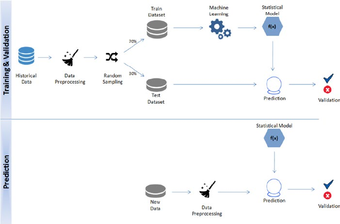
CHAPTER 3 ■ STEP 3 – FUNDAMENTALS OF MACHINE LEARNING
176
First you need to train and validate a supervised model by applying machine
learning techniques to historical data. Then apply this model onto the new dataset to
predict the future value.
Decision Trees
In 1986, J. R. Quinlan published Induction of Decision Trees summarizing an approach to
synthesizing decision trees using machine learning with an illustrative example dataset,
where the objective is to make a decision on whether to play outside on a Saturday
morning. As the name suggests, a decision tree is a tree-like structure where internal
nodes represent a test on an attribute, each branch represents outcome of a test, and each
leaf node represents class label, and the decision is made after computing all attributes.
A path from root to leaf represents classification rules. Thus, a decision tree consists of
three types of nodes. See Figure3-14.
• Root node
• Branch node
• Leaf node (class label)
Figure 3-13. Supervised learning process flow
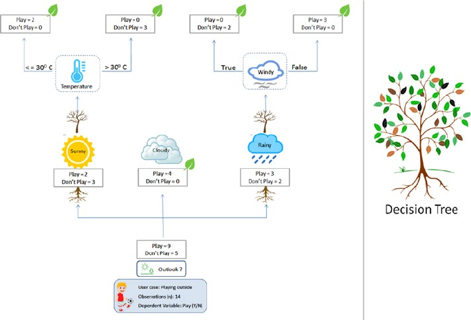
CHAPTER 3 ■ STEP 3 – FUNDAMENTALS OF MACHINE LEARNING
177
Decision tree model output is easy to interpret and it provides the rules that drive
a decision or event; in the above use case we can get the rules that lead to a don’t
play scenario, that is 1) sunny and temperature >30°c 2)rainy and windy is true. Often
businesses might be interested in these decision rules rather than the decision itself. For
example, an insurance company might be interested in the rules or conditions in which
an insurance applicant should be sent for a medical checkup rather than feeding the
applicants data to a black box model to find the decision.
Use training data to build a tree generator model, which will determine which
variable to split at a node and the value of the split. A decision to stop or split again
assigns leaf nodes to a class. An advantage of a decision tree is that there is no need for
the exclusive creation of dummy variables.
How the Tree Splits and Grows?
• The base algorithm is known as a greedy algorithm, in which the
tree is constructed in a top-down recursive divide-and-conquer
manner.
• At start, all the training examples are at the root.
• Input data is partitioned recursively based on selected attributes.
• Test attributes at each node are selected on the basis of a heuristic
or statistical impurity measure example, gini, or information gain
(entropy).
Figure 3-14. J. R. Quinlan’s example for synthesizing decision tree

CHAPTER 3 ■ STEP 3 – FUNDAMENTALS OF MACHINE LEARNING
178
• Gini = 1 - i
i
p
å
()
2
, where pi is the probability of each label.
• Entropy = -p log2(p) – q log2(q), where p and q represent the
probability of success/failure respectively in a given node.
Conditions for Stopping Partitioning
• All samples for a given node belong to the same class.
• There are no remaining attributes for further partitioning –
majority voting is employed for classifying the leaf.
• There are no samples left.
■Note Default criterion is “gini” as it’s comparatively faster to compute than “entropy”;
however both measures give almost identical decisions on split. See Listing 3-36.
Listing 3-36. Decision tree model
from sklearn import datasets
import numpy as np
import pandas as pd
from sklearn import tree
iris = datasets.load_iris()
# X = iris.data[:, [2, 3]]
X = iris.data
y = iris.target
from sklearn.preprocessing import StandardScaler
sc = StandardScaler()
sc.fit(X)
X = sc.transform(X)
# split data into train and test
from sklearn.cross_validation import train_test_split
X_train, X_test, y_train, y_test = train_test_split(X, y, test_size=0.3,
random_state=0)
clf = tree.DecisionTreeClassifier(criterion = 'entropy', random_state=0)
clf.fit(X_train, y_train)
# generate evaluation metrics
print "Train - Accuracy :", metrics.accuracy_score(y_train, clf.predict(X_train))
print "Train - Confusion matrix :",metrics.confusion_matrix(y_train, clf.
predict(X_train))
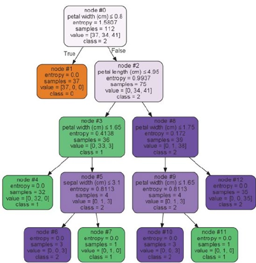
CHAPTER 3 ■ STEP 3 – FUNDAMENTALS OF MACHINE LEARNING
179
print "Train - classification report :", metrics.classification_report
(y_train, clf.predict(X_train))
print "Test - Accuracy :", metrics.accuracy_score(y_test, clf.predict(X_test))
print "Test - Confusion matrix :",metrics.confusion_matrix(y_test, clf.
predict(X_test))
print "Test - classification report :", metrics.classification_report(y_
test, clf.predict(X_test))
tree.export_graphviz(clf, out_file='tree.dot')
from sklearn.externals.six import StringIO
import pydot
out_data = StringIO()
tree.export_graphviz(clf, out_file=out_data,
feature_names=iris.feature_names,
class_names=clf.classes_.astype(int).astype(str),
filled=True, rounded=True,
special_characters=True,
node_ids=1,)
graph = pydot.graph_from_dot_data(out_data.getvalue())
graph[0].write_pdf("iris.pdf") # save to pdf
#----output----
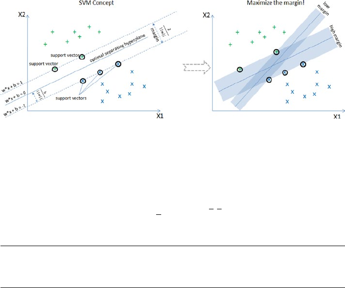
CHAPTER 3 ■ STEP 3 – FUNDAMENTALS OF MACHINE LEARNING
180
Key Parameters for Stopping Tree Growth
One of the key issues with the decision tree is that the tree can grow very large, ending up
creating one leaf per observation.
max_features: maximum features to be considered while deciding each split,
default=“None” which means all features will be considered
min_samples_split: split will not be allowed for nodes that do not meet this number
min_samples_leaf: leaf node will not be allowed for nodes less than the minimum
samples
max_depth: no further split will be allowed, default=“None”
Support Vector Machine (SVM)
Vladimir N. Vapnik and Alexey Ya. Chervonenkis in 1963 proposed SVM. The key
objective of SVM is to draw a hyperplane that separates the two classes optimally such
that the margin is maximum between the hyperplane and the observations. Figure3-15
illustrates that there is the possibility of different hyperplanes. However the objective of
SVM is to find the one which gives us a high margin.
Figure 3-15. Support Vector Machine
To maximize the margin we need to minimize (1/2)||w||2 subject to yi(WTXi + b)-1 ≥
0 for all i.
The final SVM equation can be written mathematically as
Li
j=-
()
åå
iij
ijij
di yy XX
1
2
aa
■Note SVM is comparatively less prone to outliers than logistic regression as it only
cares about the points that are closest to the decision boundary or support vectors.
CHAPTER 3 ■ STEP 3 – FUNDAMENTALS OF MACHINE LEARNING
181
Key Parameters
C: This is the penalty parameter and helps in fitting the boundaries smoothly and
appropriately, default=1
Kernel: A kernel is a similarity function for pattern analysis. It must be one of rbf/
linear/poly/sigmoid/precomputed, default=’rbf’ (Radial Basis Function). Choosing an
appropriate kernel will result in a better model fit. See Listings 3-37 and 3-38.
Listing 3-37. Support vector machine (SVM) model
from sklearn import datasets
import numpy as np
import pandas as pd
from sklearn import tree
from sklearn import metrics
iris = datasets.load_iris()
X = iris.data[:, [2, 3]]
y = iris.target
print('Class labels:', np.unique(y))
from sklearn.preprocessing import StandardScaler
sc = StandardScaler()
sc.fit(X)
X = sc.transform(X)
# split data into train and test
from sklearn.cross_validation import train_test_split
X_train, X_test, y_train, y_test = train_test_split(X, y, test_size=0.3,
random_state=0)
from sklearn.svm import SVC
clf = SVC(kernel='linear', C=1.0, random_state=0)
clf.fit(X_train, y_train)
# generate evaluation metrics
print "Train - Accuracy :", metrics.accuracy_score(y_train, clf.predict
(X_train))
print "Train - Confusion matrix :",metrics.confusion_matrix(y_train, clf.
predict(X_train))
print "Train - classification report :", metrics.classification_report
(y_train, clf.predict(X_train))
print "Test - Accuracy :", metrics.accuracy_score(y_test, clf.predict
(X_test))
print "Test - Confusion matrix :",metrics.confusion_matrix(y_test, clf.
predict(X_test))
CHAPTER 3 ■ STEP 3 – FUNDAMENTALS OF MACHINE LEARNING
182
print "Test - classification report :", metrics.classification_report
(y_test, clf.predict(X_test))
#----output----
Train - Accuracy : 0.952380952381
Train - Confusion matrix : [[34 0 0]
[ 0 30 2]
[ 0 3 36]]
Train - classification report : precision recall f1-score support
0 1.00 1.00 1.00 34
1 0.91 0.94 0.92 32
2 0.95 0.92 0.94 39
avg / total 0.95 0.95 0.95 105
Test - Accuracy : 0.977777777778
Test - Confusion matrix : [[16 0 0]
[ 0 17 1]
[ 0 0 11]]
Test - classification report : precision recall f1-score support
0 1.00 1.00 1.00 16
1 1.00 0.94 0.97 18
2 0.92 1.00 0.96 11
avg / total 0.98 0.98 0.98 45
Plotting Decision Boundary:
Let's consider a two-class example to keep things simple
Listing 3-38. Ploting SVM decision boundaries
# Let's use sklearn make_classification function to create some test data.
from sklearn.datasets import make_classification
X, y = make_classification(100, 2, 2, 0, weights=[.5, .5], random_state=0)
# build a simple logistic regression model
clf = SVC(kernel='linear', random_state=0)
clf.fit(X, y)
# get the separating hyperplane
w = clf.coef_[0]
a = -w[0] / w[1]
xx = np.linspace(-5, 5)
yy = a * xx - (clf.intercept_[0]) / w[1]
# plot the parallels to the separating hyperplane that pass through the
# support vectors
b = clf.support_vectors_[0]
yy_down = a * xx + (b[1] - a * b[0])
b = clf.support_vectors_[-1]
yy_up = a * xx + (b[1] - a * b[0])
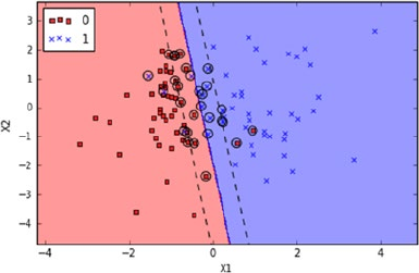
CHAPTER 3 ■ STEP 3 – FUNDAMENTALS OF MACHINE LEARNING
183
# Plot the decision boundary
plot_decision_regions(X, y, classifier=clf)
# plot the line, the points, and the nearest vectors to the plane
plt.scatter(clf.support_vectors_[:, 0], clf.support_vectors_[:, 1], s=80,
facecolors='none')
plt.plot(xx, yy_down, 'k--')
plt.plot(xx, yy_up, 'k--')
plt.xlabel('X1')
plt.ylabel('X2')
plt.legend(loc='upper left')
plt.tight_layout()
plt.show()
#----output----
k Nearest Neighbors (kNN)
K nearest neighbor classification was developed from the need to perform discriminant
analysis when reliable parametric estimates of probability densities are unknown or
difficult to determine. Fix and Hodges in 1951 introduced a non-parametric method for
pattern classification that has since become known the k nearest neighbor rule.
As the name suggests the algorithm works based on a majority vote of its k nearest
neighbors class. In Figure3-16, k = 5 nearest neighbors for the unknown data point
are identified based on the chosen distance measure, and the unknown point will be
classified based on the majority class among identified nearest data points class. The key
drawback of kNN is the complexity in searching the nearest neighbors for each sample.
See Listing 3-39.
Things to remember:
• Choose an odd k value for a two-class problem
• k must not be a multiple of the number of classes.
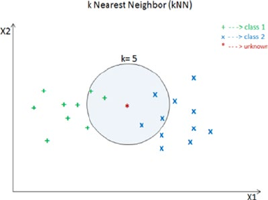
CHAPTER 3 ■ STEP 3 – FUNDAMENTALS OF MACHINE LEARNING
184
Listing 3-39. k Nearest Neighbors model
from sklearn.neighbors import KNeighborsClassifier
clf = KNeighborsClassifier(n_neighbors=5, p=2, metric='minkowski')
clf.fit(X_train, y_train)
# generate evaluation metrics
print "Train - Accuracy :", metrics.accuracy_score(y_train, clf.predict
(X_train))
print "Train - Confusion matrix :",metrics.confusion_matrix(y_train, clf.
predict(X_train))
print "Train - classification report :", metrics.classification_report
(y_train, clf.predict(X_train))
print "Test - Accuracy :", metrics.accuracy_score(y_test, clf.predict
(X_test))
print "Test - Confusion matrix :",metrics.confusion_matrix(y_test, clf.
predict(X_test))
print "Test - classification report :", metrics.classification_report
(y_test, clf.predict(X_test))
#----output----
Train - Accuracy : 0.971428571429
Train - Confusion matrix : [[34 0 0]
[ 0 31 1]
[ 0 2 37]]
Train - classification report : precision recall f1-score support
0 1.00 1.00 1.00 34
1 0.94 0.97 0.95 32
2 0.97 0.95 0.96 39
avg / total 0.97 0.97 0.97 105
Test - Accuracy : 0.977777777778
Figure 3-16. k Nearest Neighbors with k = 5

CHAPTER 3 ■ STEP 3 – FUNDAMENTALS OF MACHINE LEARNING
185
Test - Confusion matrix : [[16 0 0]
[ 0 17 1]
[ 0 0 11]]
Test - classification report : precision recall f1-score support
0 1.00 1.00 1.00 16
1 1.00 0.94 0.97 18
2 0.92 1.00 0.96 11
avg / total 0.98 0.98 0.98 45
■Note Decision Trees, SVM, and kNNbase algorithm concepts can essentially be applied
to predict dependent variables that are continuous numbers in nature, and Scikit-learn
provides DecisionTreeRegressor, SVR (support vector regressor), and kNeighborsRegressor
for the same.
Time-Series Forecasting
In simple terms data points that are collected sequentially at a regular interval with
association over a time period is termed time-series data. A time-series data having the
mean and variance as a constant is called a stationary time series.
Time series tend to have a linear relationship between lagged variables and this is
called an autocorrelation. Hence a time series historic data can be modeled to forecast
the future data points without involvement of any other independent variables; these
types of models are generally known as time-series forecasting. To name some key areas
of applications of time series, these include sales forecasting, economic forecasting, stock
market forecasting, etc.
Components of Time Series
A time series can be made up of three key components. See Figure3-17.
• Trend – A long-term increase or decrease are termed trends.
• Seasonality An effect of seasonal factors for a fixed or known
period. For example, retail stores sales will be high during
weekends and festival seasons.
• Cycle – These are the longer ups and downs that are not of fixed or
known periods caused by external factors.
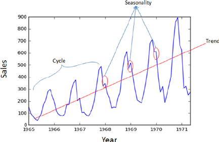
CHAPTER 3 ■ STEP 3 – FUNDAMENTALS OF MACHINE LEARNING
186
Autoregressive Integrated Moving Average (ARIMA)
ARIMA is one of the key and popular time-series models, so understanding the concept
involved will set the base for you around time-series modeling.
Autoregressive Model (AM): As the name indicates, it is a regression of the variable
against itself , that is, the linear combination of past values of the variables are used to
forecast the future value.
yc yy
ye
tt
tn
tn t
=+ +++
-- -
FF F
11 22... , where c is constant, et is the random error, yt-1
is first-order correlation, and yt-2 is second-order correlation between values two
periods apart.
Moving average (MA): Instead of past values, a past forecast’s errors are used to build
a model.
yc yy
ye
tt
tn
tn t
=+ ++¼+ +
-- -
qq q
122
Autoregressive (AR), moving average (MA) model with integration (opposite of
differencing) is called the ARIMA model.
yc yy yy
yy
e
tttntn tt nt
nt
=+ ++++++++
-- --
--
FF F
11 22 11 22
... ...
qq q
The predictors on the right side of the equation are the lagged values, errors, and
it is also known as ARIMA (p, d, q) model. These are the key parameters of ARIMA and
picking the right value for p, d, q will yield better model results.
p = order of the autoregressive part. That is the number of unknown terms that
multiply your signal at past times (so many past times as your value p).
d = degree of first differencing involved. Number of times you have to difference your
time series to have a stationary one.
q = order of the moving average part. That is the number of unknown terms that
multiply your forecast errors at past times (so many past times as your value q). See
Listing 3-40.
Figure 3-17. Time series components
CHAPTER 3 ■ STEP 3 – FUNDAMENTALS OF MACHINE LEARNING
187
Running ARIMA Model
• Plot the chart to ensure trend, cycle, or seasonality exists in the
dataset.
• Stationarize series: To stationarize series we need to remove trend
(varying mean) and seasonality (variance) components from the
series. Moving average and differencing technique can be used to
stabilize trend, whereas log transform will stabilize the seasonality
variance. Further, the Dickey Fuller test can be used to assess the
stationarity of series, that is, null hypothesis for a Dickey Fuller
test is that the data are stationary, so test result with p value > 0.05
means data is non-stationary.
• Find optimal parameter: Once the series is stationarized you
can look at the Autocorrelation function (ACF) and Partial
autocorrelation function (PACF) graphical plot to pick the
number of AR or MA terms needed to remove autocorrelation.
ACF is a bar chart between correlation coefficients and lags;
similarly PACF is the bar chart between partial correlation
(correlation between variable and lag of itself not explained by
correlation at all lower-order lags) coefficient and lags.
• Build Model and Evaluate: Since time series is a continuous
number Mean Absolute Error and Root Mean Squared Error can
be used to evaluate the deviation between actual and predicted
values in train dataset. Other useful matrices would be Akaike
Information Criterion (AIC) and Bayesian Information Criterion
(BIC); these are part of information theory to estimate the quality
of individual models given a collection of models, and they favor a
model with smaller residual errors.
AIC = -2log(L) + 2(p+q+k+1) where L is the maximum
likelihood function of fitted model and p, q, k are the number
of parameters in the model
BIC = AIC+(log(T)−2)(p+q+k+1)
Listing 3-40. Decompose time series
# Data Source: O.D. Anderson (1976), in file: data/anderson14, Description:
Monthly sales of company X Jan ’65 – May ’71 C. Cahtfield
df = pd.read_csv('Data/TS.csv')
ts = pd.Series(list(df['Sales']), index=pd.to_
datetime(df['Month'],format='%Y-%m'))
from statsmodels.tsa.seasonal import seasonal_decompose
decomposition = seasonal_decompose(ts_log)
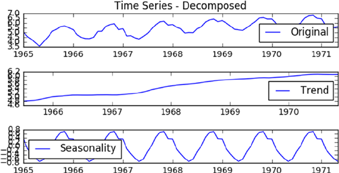
CHAPTER 3 ■ STEP 3 – FUNDAMENTALS OF MACHINE LEARNING
188
trend = decomposition.trend
seasonal = decomposition.seasonal
residual = decomposition.resid
plt.subplot(411)
plt.plot(ts_log, label='Original')
plt.legend(loc='best')
plt.subplot(412)
plt.plot(trend, label='Trend')
plt.legend(loc='best')
plt.subplot(413)
plt.plot(seasonal,label='Seasonality')
plt.legend(loc='best')
plt.tight_layout()
Checking for Stationary
Listing 3-41. Check stationary
# log transform
ts_log = np.log(ts)
ts_log.dropna(inplace=True)
s_test = adfuller(ts_log, autolag='AIC')
print "Log transform stationary check p value: ", s_test[1]
#Take first difference:
ts_log_diff = ts_log - ts_log.shift()
ts_log_diff.dropna(inplace=True)
plt.title('Trend removed plot with first order difference')
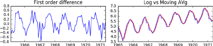
CHAPTER 3 ■ STEP 3 – FUNDAMENTALS OF MACHINE LEARNING
189
plt.plot(ts_log_diff)
plt.ylabel('First order log diff')
s_test = adfuller(ts_log_diff, autolag='AIC')
print "First order difference stationary check p value: ", s_test[1]
#----output----
Log transform stationary check p value: 0.785310212485
First order difference stationary check p value: 0.0240253928399
Autocorrelation Test
We determined that the log of time series requires at least one order differencing to
stationarize. Now let’s plot ACV and PACF charts for a first-order log series. See Figure 3-42.
Listing 3-42. Check autocorrelation
fig, (ax1, ax2) = plt.subplots(1, 2, figsize = (10,3))
# ACF chart
fig = sm.graphics.tsa.plot_acf(ts_log_diff.values.squeeze(), lags=20,
ax=ax1)
# draw 95% confidence interval line
ax1.axhline(y=-1.96/np.sqrt(len(ts_log_diff)),linestyle='--',color='gray')
ax1.axhline(y=1.96/np.sqrt(len(ts_log_diff)),linestyle='--',color='gray')
ax1.set_xlabel('Lags')
# PACF chart
fig = sm.graphics.tsa.plot_pacf(ts_log_diff, lags=20, ax=ax2)
# draw 95% confidence interval line
ax2.axhline(y=-1.96/np.sqrt(len(ts_log_diff)),linestyle='--',color='gray')
ax2.axhline(y=1.96/np.sqrt(len(ts_log_diff)),linestyle='--',color='gray')
ax2.set_xlabel('Lags')
#----output----
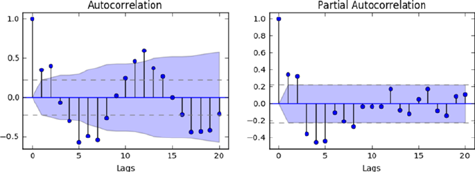
CHAPTER 3 ■ STEP 3 – FUNDAMENTALS OF MACHINE LEARNING
190
PACF plot has a significant spike only at lag 1, meaning that all the higher-order
autocorrelations are effectively explained by the lag-1 and lag-2 autocorrelation. Ideal
lag values are p = 2 and q = 2, that is, the lag value where the ACF/PACF chart crosses the
upper confidence interval for the first time.
Build Model and Evaluate
Let’s fit the ARIMA model on the dataset and evaluate the model performance as shown
in Listing 3-43.
Listing 3-43. Build ARIMA model and evaluate
# build model
model = sm.tsa.ARIMA(ts_log, order=(2,0,2))
results_ARIMA = model.fit(disp=-1)
# Evaluate model
print "AIC: ", results_ARIMA.aic
print "BIC: ", results_ARIMA.bic
print "Mean Absolute Error: ", mean_absolute_error(ts_log.values, ts_
predict.values)
print "Root Mean Squared Error: ", np.sqrt(mean_squared_error(ts_log.values,
ts_predict.values))
# check autocorrelation
print "Durbin-Watson statistic :", sm.stats.durbin_watson(results_ARIMA.
resid.values)
#----output-----
AIC: 7.85211053808
BIC: 21.9149430692
Mean Absolute Error: 0.167260085121
Root Mean Squared Error: 0.216145783845
Durbin-Watson statistic : 1.86457752659
CHAPTER 3 ■ STEP 3 – FUNDAMENTALS OF MACHINE LEARNING
191
Usual practice is to build several models with different p and q and select
the one with smallest value of AIC, BIC, MAE and RMSE. Now lets' increase p
to 3 and see if there is any difference in result.
model = sm.tsa.ARIMA(ts_log, order=(3,0,2))
results_ARIMA = model.fit(disp=-1)
# ts_predict = results_ARIMA.predict('1965-01-01', '1972-05-01',
dynamic=True)
ts_predict = results_ARIMA.predict()
plt.title('ARIMA Prediction')
plt.plot(ts_log, label='Actual')
plt.plot(ts_predict, 'r--', label='Predicted')
plt.xlabel('Year-Month')
plt.ylabel('Sales')
plt.legend(loc='best')
print "AIC: ", results_ARIMA.aic
print "BIC: ", results_ARIMA.bic
print "Mean Absolute Error: ", mean_absolute_error(ts_log.values, ts_
predict.values)
print "Root Mean Squared Error: ", np.sqrt(mean_squared_error(ts_log.values,
ts_predict.values))
# check autocorrelation
print "Durbin-Watson statistic :", sm.stats.durbin_watson(results_ARIMA.
resid.values)
#----output----
AIC: -7.78613717769
BIC: 8.62050077528
Mean Absolute Error: 0.167260085121
Root Mean Squared Error: 0.216145783845
Durbin-Watson statistic : 2.51941762513
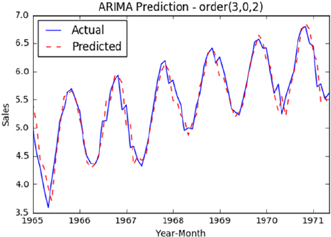
CHAPTER 3 ■ STEP 3 – FUNDAMENTALS OF MACHINE LEARNING
192
Let's try with first-order differencing, that is, d = 1. See Listing 3-44.
Listing 3-44. ARIMA with first-order differencing
model = sm.tsa.ARIMA(ts_log, order=(3,1,2))
results_ARIMA = model.fit(disp=-1)
ts_predict = results_ARIMA.predict()
# Correctcion for difference
predictions_ARIMA_diff = pd.Series(ts_predict, copy=True)
predictions_ARIMA_diff_cumsum = predictions_ARIMA_diff.cumsum()
predictions_ARIMA_log = pd.Series(ts_log.ix[0], index=ts_log.index)
predictions_ARIMA_log = predictions_ARIMA_log.add(predictions_ARIMA_diff_
cumsum,fill_value=0)
#----output----
AIC: -35.4189877386
BIC: -19.1038543566
Mean Absolute Error: 0.138765317903
Root Mean Squared Error: 0.183102425139
Durbin-Watson statistic : 1.94116742899
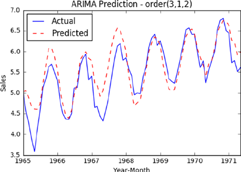
CHAPTER 3 ■ STEP 3 – FUNDAMENTALS OF MACHINE LEARNING
193
In the above chart we can see that the model is over predicting at some places and
AIC and BIC values is higher than the previous model. Note: AIC/BIC can be positive or
negative; however we should look at the absolute value of it for evaluation.
Predicting the Future Values
Below values (p=3, d=0, q=2) are giving the smaller number for evaluation matrices,
so let’s use this as a final model to predict the future values for the year 1972. See
Listing 3-45.
Listing 3-45. ARIMA predict function
# final model
model = sm.tsa.ARIMA(ts_log, order=(3,0,2))
results_ARIMA = model.fit(disp=-1)
# predict future values
ts_predict = results_ARIMA.predict('1971-06-01', '1972-05-01')
plt.title('ARIMA Future Value Prediction - order(3,1,2)')
plt.plot(ts_log, label='Actual')
plt.plot(ts_predict, 'r--', label='Predicted')
plt.xlabel('Year-Month')
plt.ylabel('Sales')
plt.legend(loc='best')
#----output----
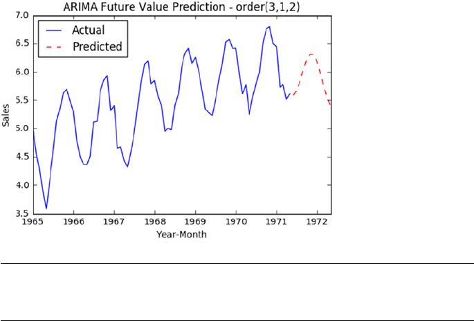
CHAPTER 3 ■ STEP 3 – FUNDAMENTALS OF MACHINE LEARNING
194
■Note A minimum of 3 to 4 years’ worth of historic data is required to ensure the
seasonal patterns are regular.
Unsupervised Learning Process Flow
Unsupervised learning process flow is given in Figure3-18 below. Similar to supervised
learning, we can train a model and use it to predict the unknown dataset; however the key
difference is that there is no predefined category or labels available for target variables, and
the goal often is to create a category or label based on patterns available in data.
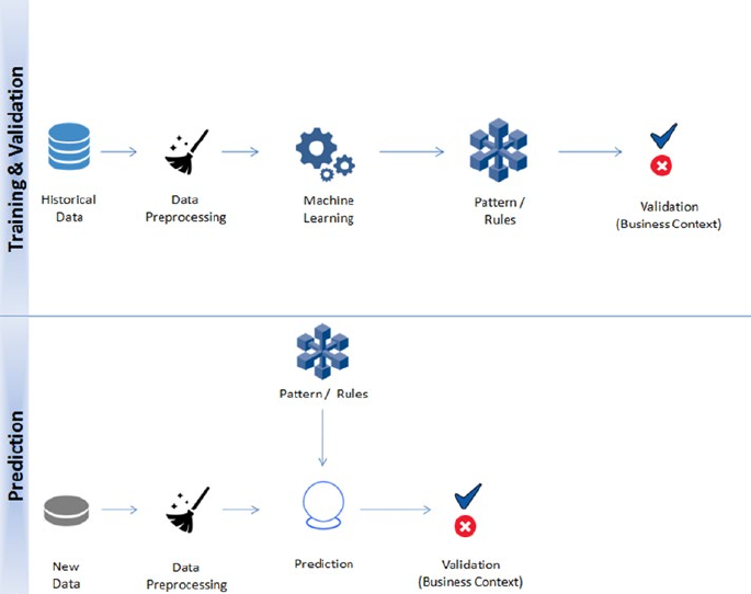
CHAPTER 3 ■ STEP 3 – FUNDAMENTALS OF MACHINE LEARNING
195
Clustering
Clustering is an unsupervised learning problem. Key objective is to identify distinct
groups (called clusters) based on some notion of similarity within a given dataset.
Clustering analysis origins can be traced to the area of Anthropology and Psychology
in the 193’s. The most popularly used clustering techniques are k-means (divisive) and
hierarchical (agglomerative).
K-means
The key objective of a k-means algorithm is to organize data into clusters such that there
is high intra-cluster similarity and low inter-cluster similarity. An item will only belong to
one cluster, not several, that is, it generates a specific number of disjoint, non-hierarchical
clusters. K-means uses the strategy of divide and concur, and it is a classic example for
an expectation maximization (EM) algorithm. EM algorithms are made up of two steps:
the first step is known as expectation(E) and is used to find the expected point associated
with a cluster; and the second step is known as maximization(M) and is used to improve
the estimation of the cluster using knowledge from the first step. The two steps are
processed repeatedly until convergence is reached.
Figure 3-18. Unsupervised learning process flow
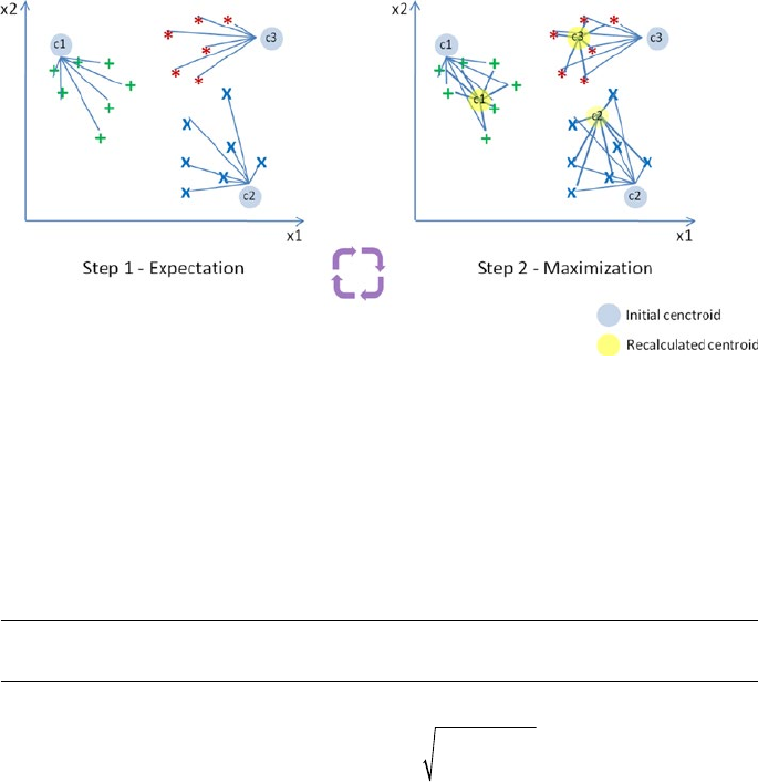
CHAPTER 3 ■ STEP 3 – FUNDAMENTALS OF MACHINE LEARNING
196
Suppose we have ‘n’ data points that we need to cluster into k (c1, c2, c3) groups. See
Figure3-19.
Step 1: In the first step k centroids (in above case k=3) is randomly picked (only in
the first iteration) and all the points that are nearest to each centroid point are assigned to
that specific cluster. Centroid is the arithmetic mean or average position of all the points.
Step 2: Here the centroid point is recalculated using the average of the coordinates
of all the points in that cluster. Then step one is repeated (assign nearest point) until the
clusters converge.
■Note K-means is designed for Euclidean distance only.
EuclideanDistace
dX
iYi
i
N
== -
()
=
å
1
2
Limitations of K-means
• K-means clustering needs the number of clusters to be specified.
• K-means has problems when clusters are of differing sized,
densities, and non-globular shapes.
• Presence of outlier can skew the results.
Figure 3-19. Expectation maximization algorithm work flow
CHAPTER 3 ■ STEP 3 – FUNDAMENTALS OF MACHINE LEARNING
197
Let's load the iris data and assume for a moment that the species column is missing,
that is, we have the measured values for sepal length/width and petal length/width but
we do not know how many species exists.
Now let's use unsupervised learning, that is, clustering to find out how many species
exists. The goal here is to group all similar items into a cluster. We can assume a k of 3 for
now; we’ll learn later about an approach to find the value of k. See Listings 3-46 and 3-47.
Listing 3-46. k-means clustering
from sklearn import datasets
import numpy as np
import pandas as pd
from sklearn.cluster import KMeans
from sklearn.preprocessing import StandardScaler
iris = datasets.load_iris()
# Let's convert to dataframe
iris = pd.DataFrame(data= np.c_[iris['data'], iris['target']],
columns= iris['feature_names'] + ['species'])
# let's remove spaces from column name
iris.columns = iris.columns.str.replace(' ','')
iris.head()
X = iris.ix[:,:3] # independent variables
y = iris.species # dependent variable
sc = StandardScaler()
sc.fit(X)
X = sc.transform(X)
# K Means Cluster
model = KMeans(n_clusters=3, random_state=11)
model.fit(X)
print model.labels_
# ----output----
[1 1 1 1 1 1 1 1 1 1 1 1 1 1 1 1 1 1 1 1 1 1 1 1 1 1 1 1 1 1 1 1 1 1 1 1 1
1 1 1 1 0 1 1 1 1 1 1 1 1 2 2 2 0 2 0 2 0 2 0 0 0 0 0 0 2 0 0 0 0 2 0 0 0
2 2 2 2 0 0 0 0 0 0 0 2 2 0 0 0 0 2 0 0 0 0 0 0 0 0 2 0 2 2 2 2 0 2 2 2 2
2 2 0 0 2 2 2 2 0 2 0 2 0 2 2 0 2 2 2 2 2 2 2 0 2 2 2 0 2 2 2 0 2 2 2 0 2
2 0]
We see that the clustering algorithm has assigned a cluster label for each
record. Let’s compare this with the actual species label to understand the
accuracy of grouping similar records.
CHAPTER 3 ■ STEP 3 – FUNDAMENTALS OF MACHINE LEARNING
198
Lising 3-47. Accuracy of k-means clustering
# since its unsupervised the labels have been assigned
# not in line with the actual lables so let's convert all the 1s to 0s and
0s to 1s
# 2's look fine
iris['pred_species'] = np.choose(model.labels_, [1, 0, 2]).astype(np.int64)
print "Accuracy :", metrics.accuracy_score(iris.species, iris.pred_species)
print "Classification report :", metrics.classification_report(iris.species,
iris.pred_species)
# Set the size of the plot
plt.figure(figsize=(10,7))
# Create a colormap
colormap = np.array(['red', 'blue', 'green'])
# Plot Sepal
plt.subplot(2, 2, 1)
plt.scatter(iris['sepallength(cm)'], iris['sepalwidth(cm)'],
c=colormap[iris.species], marker='o', s=50)
plt.xlabel('sepallength(cm)')
plt.ylabel('sepalwidth(cm)')
plt.title('Sepal (Actual)')
plt.subplot(2, 2, 2)
plt.scatter(iris['sepallength(cm)'], iris['sepalwidth(cm)'],
c=colormap[iris.pred_species], marker='o', s=50)
plt.xlabel('sepallength(cm)')
plt.ylabel('sepalwidth(cm)')
plt.title('Sepal (Predicted)')
plt.subplot(2, 2, 3)
plt.scatter(iris['petallength(cm)'], iris['petalwidth(cm)'],
c=colormap[iris.species],marker='o', s=50)
plt.xlabel('petallength(cm)')
plt.ylabel('petalwidth(cm)')
plt.title('Petal (Actual)')
plt.subplot(2, 2, 4)
plt.scatter(iris['petallength(cm)'], iris['petalwidth(cm)'],
c=colormap[iris.pred_species],marker='o', s=50)
plt.xlabel('petallength(cm)')
plt.ylabel('petalwidth(cm)')
plt.title('Petal (Predicted)')
plt.tight_layout()
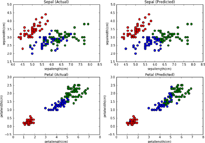
CHAPTER 3 ■ STEP 3 – FUNDAMENTALS OF MACHINE LEARNING
199
#----output----
Accuracy : 0.806666666667
Classification report : precision recall f1-score support
0.0 1.00 0.98 0.99 50
1.0 0.71 0.70 0.71 50
2.0 0.71 0.74 0.73 50
avg / total 0.81 0.81 0.81 150
We can see from the above chart that k-means has done a decent job of clustering the
similar labels with an accuracy of 80% compared to the actual labels.
Finding Value of k
Two methods are commonly used to determine the value of k.
• Elbow method
• Average silhouette method
Elbow Method
Perform k-means clustering on the dataset for a range of value k (for example 1 to 10) and
calculate the sum of squared error (SSE) or percentage of variance explained for each k.
Plot a line chart for cluster number vs. SSE and then look for an elbow shape on the line
graph, which is the ideal number of clusters. With increase in k the SSE tends to decrease
CHAPTER 3 ■ STEP 3 – FUNDAMENTALS OF MACHINE LEARNING
200
toward 0. The SSE is zero if k is equal to the total number of data points in the dataset as
at this stage each data point becomes its own cluster, and no error exists between cluster
and its center. So the goal with the elbow method is to choose a small value of k that has
a low SSE, and the elbow usually represents this value. Percentage of variance explained
tends to increase with increase in k and we’ll pick the point where the elbow shape
appears. See Listing 3-48.
Listing 3-48. Elbow method
from scipy.spatial.distance import cdist, pdist
from sklearn.cluster import KMeans
K = range(1,10)
KM = [KMeans(n_clusters=k).fit(X) for k in K]
centroids = [k.cluster_centers_ for k in KM]
D_k = [cdist(X, cent, 'euclidean') for cent in centroids]
cIdx = [np.argmin(D,axis=1) for D in D_k]
dist = [np.min(D,axis=1) for D in D_k]
avgWithinSS = [sum(d)/X.shape[0] for d in dist]
# Total with-in sum of square
wcss = [sum(d**2) for d in dist]
tss = sum(pdist(X)**2)/X.shape[0]
bss = tss-wcss
varExplained = bss/tss*100
kIdx = 10-1
##### plot ###
kIdx = 2
# elbow curve
# Set the size of the plot
plt.figure(figsize=(10,4))
plt.subplot(1, 2, 1)
plt.plot(K, avgWithinSS, 'b*-')
plt.plot(K[kIdx], avgWithinSS[kIdx], marker='o', markersize=12,
markeredgewidth=2, markeredgecolor='r', markerfacecolor='None')
plt.grid(True)
plt.xlabel('Number of clusters')
plt.ylabel('Average within-cluster sum of squares')
plt.title('Elbow for KMeans clustering')
plt.subplot(1, 2, 2)
plt.plot(K, varExplained, 'b*-')
plt.plot(K[kIdx], varExplained[kIdx], marker='o', markersize=12,
markeredgewidth=2, markeredgecolor='r', markerfacecolor='None')
plt.grid(True)
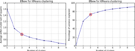
CHAPTER 3 ■ STEP 3 – FUNDAMENTALS OF MACHINE LEARNING
201
plt.xlabel('Number of clusters')
plt.ylabel('Percentage of variance explained')
plt.title('Elbow for KMeans clustering')
plt.tight_layout()
#----output----
Average Silhouette Method
In 1986, Peter J. Rousseuw described the silhouette method, which aims to explain the
consistancy within cluster data. The silhouette value will range between -1 and 1 and a
high value indicates that items are well matched within clusters and weakly matched to
neighboring clusters. See Listing 4-49.
s(i) = b(i) – a(i) / max {a(i), b(i)}, where a(i) is average dissimilarity
of ith item with other data points from same cluster, b(i) lowest average
dissimilarity of i to other cluster to which i is not a member.
Listing 4-49. Silhouette method
from sklearn.metrics import silhouette_score
from matplotlib import cm
score = []
for n_clusters in range(2,10):
kmeans = KMeans(n_clusters=n_clusters)
kmeans.fit(X)
labels = kmeans.labels_
centroids = kmeans.cluster_centers_
score.append(silhouette_score(X, labels, metric='euclidean'))
# Set the size of the plot
plt.figure(figsize=(10,4))
plt.subplot(1, 2, 1)
plt.plot(score)
plt.grid(True)
plt.ylabel("Silouette Score")
plt.xlabel("k")
plt.title("Silouette for K-means")
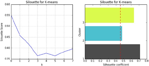
CHAPTER 3 ■ STEP 3 – FUNDAMENTALS OF MACHINE LEARNING
202
# Initialize the clusterer with n_clusters value and a random generator
model = KMeans(n_clusters=3, init='k-means++', n_init=10, random_state=0)
model.fit_predict(X)
cluster_labels = np.unique(model.labels_)
n_clusters = cluster_labels.shape[0]
# Compute the silhouette scores for each sample
silhouette_vals = silhouette_samples(X, model.labels_)
plt.subplot(1, 2, 2)
y_lower, y_upper = 0,0
yticks = []
for i, c in enumerate(cluster_labels):
c_silhouette_vals = silhouette_vals[cluster_labels ==c]
c_silhouette_vals.sort()
y_upper += len(c_silhouette_vals)
color = cm.spectral(float(i) / n_clusters)
plt.barh(range(y_lower, y_upper), c_silhouette_vals, facecolor=color,
edgecolor=color, alpha=0.7)
yticks.append((y_lower + y_upper) / 2)
y_lower += len(c_silhouette_vals)
silhouette_avg = np.mean(silhouette_vals)
plt.yticks(yticks, cluster_labels+1)
# The vertical line for average silhouette score of all the values
plt.axvline(x=silhouette_avg, color="red", linestyle="--")
plt.ylabel('Cluster')
plt.xlabel('Silhouette coefficient')
plt.title("Silouette for K-means")
plt.show()
#---output----
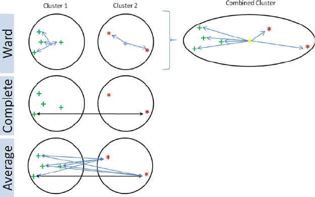
CHAPTER 3 ■ STEP 3 – FUNDAMENTALS OF MACHINE LEARNING
203
Hierarchical Clustering
Agglomerative clustering is a hierarchical cluster technique that builds nested clusters
with a bottom-up approach where each data point starts in its own cluster and as we
move up, the clusters are merged, based on a distance matrix.
Key Parameters
n_clusters: number of clusters to find, default is 2.
linkage: It has to be one of the following, that is, ward or complete or average,
default=ward.
Let’s understand each linkage a bit more. The Ward’s method will merge clusters if
the in-cluster variance or the sum of square error is a minimum. All pairwise distances
of both clusters are used in ‘average’ method, and it is less affected by outliers. The
‘complete’ method considers the distance between the farthest elements of two clusters,
so it is also known as maximum linkage. See Figure3-20 and Listing 3-50.
Figure 3-20. Agglomerative clustering linkage
Listing 3-50. Hierarchical clustering
from sklearn.cluster import AgglomerativeClustering
# Agglomerative Cluster
model = AgglomerativeClustering(n_clusters=3)
model.fit(X)
iris['pred_species'] = model.labels_
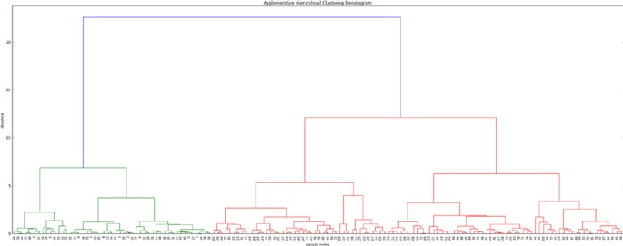
CHAPTER 3 ■ STEP 3 – FUNDAMENTALS OF MACHINE LEARNING
204
print "Accuracy :", metrics.accuracy_score(iris.species, iris.pred_species)
print "Classification report :", metrics.classification_report(iris.species,
iris.pred_species)
#----outout----
Accuracy : 0.773333333333
Classification report : precision recall f1-score support
0.0 1.00 0.98 0.99 50
1.0 0.64 0.74 0.69 50
2.0 0.70 0.60 0.65 50
avg / total 0.78 0.77 0.77 150
Heirarchical clusterings results arrangement can be better interpreted with
dendogram visualization. Scipy provides necessary functions for dendogram
visualization (currently scikit-learn lack these functions)
from scipy.cluster.hierarchy import cophenet, dendrogram, linkage
from scipy.spatial.distance import pdist
# generate the linkage matrix
Z = linkage(X, 'ward')
c, coph_dists = cophenet(Z, pdist(X))
# calculate full dendrogram
plt.figure(figsize=(25, 10))
plt.title('Agglomerative Hierarchical Clustering Dendrogram')
plt.xlabel('sample index')
plt.ylabel('distance')
dendrogram(
Z,
leaf_rotation=90., # rotates the x axis labels
leaf_font_size=8., # font size for the x axis labels
)
plt.tight_layout()
#----output----
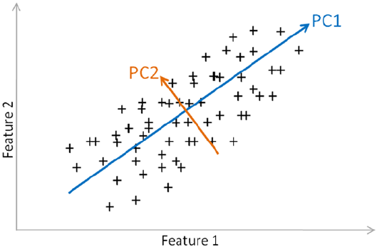
CHAPTER 3 ■ STEP 3 – FUNDAMENTALS OF MACHINE LEARNING
205
Since we know that k=3, we can cut the tree at a distance threshold of around 10 to
get exactly 3 distinct clusters.
Principal Component Analysis (PCA)
Existence of a large number of features or dimensions makes analysis computationally
intensive and hard for performing machine learning tasks for pattern identification. PCA
is the most popular unsupervised linear transformation technique for dimensionality
reduction. PCA finds the directions of maximum variance in high-dimensional data
such that most of the information is retained and projects it onto a smaller dimensional
subspace. See Figure3-21.
The PCA approach can be summarized as below. And see Listing 3-51.
• Standardize data.
• Use standardized data to generate covariance matrix or
correlation matrix.
• Perform eigen decomposition, that is, compute eigen vectors that
are the principal component which will give the direction and
compute eigen values which will give the magnitude.
• Sort the eigen pairs and select eigen vectors with the largest eigen
values that cumulatively capture information above a certain
threshold (say 95%).
Figure 3-21. Principal Component Analysis
CHAPTER 3 ■ STEP 3 – FUNDAMENTALS OF MACHINE LEARNING
206
Listing 3-51. Principal component analysis
from sklearn.preprocessing import StandardScaler
from sklearn.decomposition import PCA
iris = load_iris()
X = iris.data
# standardize data
X_std = StandardScaler().fit_transform(X)
# create covariance matrix
cov_mat = np.cov(X_std.T)
print('Covariance matrix \n%s' %cov_mat)
eig_vals, eig_vecs = np.linalg.eig(cov_mat)
print('Eigenvectors \n%s' %eig_vecs)
print('\nEigenvalues \n%s' %eig_vals)
# sort eigenvalues in decreasing order
eig_pairs = [(np.abs(eig_vals[i]), eig_vecs[:,i]) for i in range
(len(eig_vals))]
tot = sum(eig_vals)
var_exp = [(i / tot)*100 for i in sorted(eig_vals, reverse=True)]
print "Cummulative Variance Explained", cum_var_exp
plt.figure(figsize=(6, 4))
plt.bar(range(4), var_exp, alpha=0.5, align='center',
label='Individual explained variance')
plt.step(range(4), cum_var_exp, where='mid',
label='Cumulative explained variance')
plt.ylabel('Explained variance ratio')
plt.xlabel('Principal components')
plt.legend(loc='best')
plt.tight_layout()
plt.show()
#----output----
Covariance matrix
[[ 1.00671141 -0.11010327 0.87760486 0.82344326]
[-0.11010327 1.00671141 -0.42333835 -0.358937 ]
[ 0.87760486 -0.42333835 1.00671141 0.96921855]
[ 0.82344326 -0.358937 0.96921855 1.00671141]]
Eigenvectors
[[ 0.52237162 -0.37231836 -0.72101681 0.26199559]
[-0.26335492 -0.92555649 0.24203288 -0.12413481]
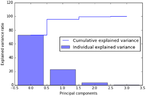
CHAPTER 3 ■ STEP 3 – FUNDAMENTALS OF MACHINE LEARNING
207
[ 0.58125401 -0.02109478 0.14089226 -0.80115427]
[ 0.56561105 -0.06541577 0.6338014 0.52354627]]
Eigenvalues
[ 2.93035378 0.92740362 0.14834223 0.02074601]
Cummulative Variance Explained:[72.77045 95.8009799.48480 100]
In the above plot we can see that the first three principal components are explaining
99% of the variance. Let’s perform PCA using scikit-learn and plot the first three eigen
vectors. See Listing 3-52.
Listing 3-52. Visualize pca
# source: http://scikit-learn.org/stable/auto_examples/datasets/plot_iris_
dataset.html#
import matplotlib.pyplot as plt
from mpl_toolkits.mplot3d import Axes3D
from sklearn import datasets
from sklearn.decomposition import PCA
# import some data to play with
iris = datasets.load_iris()
Y = iris.target
# To getter a better understanding of interaction of the dimensions
# plot the first three PCA dimensions
fig = plt.figure(1, figsize=(8, 6))
ax = Axes3D(fig, elev=-150, azim=110)
X_reduced = PCA(n_components=3).fit_transform(iris.data)
ax.scatter(X_reduced[:, 0], X_reduced[:, 1], X_reduced[:, 2], c=Y, cmap=plt.
cm.Paired)
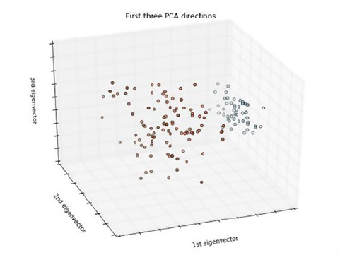
CHAPTER 3 ■ STEP 3 – FUNDAMENTALS OF MACHINE LEARNING
208
ax.set_title("First three PCA directions")
ax.set_xlabel("1st eigenvector")
ax.w_xaxis.set_ticklabels([])
ax.set_ylabel("2nd eigenvector")
ax.w_yaxis.set_ticklabels([])
ax.set_zlabel("3rd eigenvector")
ax.w_zaxis.set_ticklabels([])
plt.show()
#---output----
Endnotes
With this we have reached the end of step 3. We briefly learned different fundamental
machine learning concepts and their implementation. Data quality is an important
aspect to build efficient machine learning systems; in line with this we learned about
different types of data, commonly practiced EDA techniques for understanding the data
quality, and the fundamental preprocessing techniques to fix the data gaps. Supervised
models such as linear and nonlinear regression techniques are useful to model patterns
to predict continuous numerical data types. Whereas logistic regression, decision trees,
SVM and kNN are useful to model classification problems (functions are available
to use for regression as well).You also learned ARIMA, which is one of the key time-
series forecasting models. Unsupervised techniques such as k-means and hierarchical
clustering are useful to group similar items, whereas principal component analysis
can be used to reduce a large dimension data to lower a dimension to enable efficient
computation.
In the next step you’ll learn how to pick best parameters for a model, widely known
as “Hyperparamerter tuning” to improve model accuracy. What are the common
practices followed to pick the best model among multiple models for a given problem?
You'll also learn to combine multiple models to get the best from individual models.

209
© Manohar Swamynathan 2017
M. Swamynathan, Mastering Machine Learning with Python in Six Steps,
DOI 10.1007/978-1-4842-2866-1_4
CHAPTER 4
Step 4 – Model Diagnosis
and Tuning
In this chapter you’ll learn about the different pitfalls that one should be aware of and that
you will encounter while building machine learning systems. You’ll also learn industry
standard-efficient designs practiced to solve them.
Throughout this chapter, we’ll mostly be using a dataset from the UCI repository,
“Pima Indian diabetes,” which has 768 records, 8 attributes, 2 classes, 268 (34.9%) positive
results for diabetes test, and 500 (65.1%) negative results. All patients were females at least
21 years old of Pima Indian heritage.
Attributes of dataset:
1. Number of times pregnant
2. Plasma glucose concentration at 2 hours in an oral glucose
tolerance test
3. Diastolic blood pressure (mm Hg)
4. Triceps skin fold thickness (mm)
5. 2-Hour serum insulin (mu U/ml)
6. Body mass index (weight in kg/(height in m)^2)
7. Diabetes pedigree function
8. Age (years)
Optimal Probability Cutoff Point
Predicted probability is a number between 0 and 1. Traditionally >.5 is the cutoff point
used for converting predicted probability to 1 (positive), otherwise it is 0 (negative). This
logic works well when your training dataset has equal examples of positive and negative
cases; however this is not the case in real-world scenarios.
CHAPTER 4 ■ STEP 4 – MODEL DIAGNOSIS AND TUNING
210
The solution is to find the optimal cutoff point, that is, the point where the true
positive rate is high and the false positive rate is low. Anything above this threshold can
be labeled as 1 or else it is 0. Let’s understand this better with an example.
Let’s load the data and check the class distribution. See Listing 4-1.
Listing 4-1. Load data and check the class distribution
import pandas as pd
import pylab as plt
import numpy as np
from sklearn.cross_validation import train_test_split
from sklearn.linear_model import LogisticRegression
from sklearn import metrics
# read the data in
df = pd.read_csv("Data/Diabetes.csv")
# target variable % distribution
print df['class'].value_counts(normalize=True)
#----output----
0 0.651042
1 0.348958
Let’s build a quick logistic regression model and check the accuracy. See Listing 4-2.
Listing 4-2. Build logistic regression model and evaluate performance
X = df.ix[:,:8] # independent variables
y = df['class'] # dependent variables
# evaluate the model by splitting into train and test sets
X_train, X_test, y_train, y_test = train_test_split(X, y, test_size=0.3,
random_state=0)
# instantiate a logistic regression model, and fit
model = LogisticRegression()
model = model.fit(X_train, y_train)
# predict class labels for the train set. The predict fuction converts
probability values > .5 to 1 else 0
y_pred = model.predict(X_train)
# generate class probabilities
# Notice that 2 elements will be returned in probs array,
# 1st element is probability for negative class,
# 2nd element gives probability for positive class
probs = model.predict_proba(X_train)
y_pred_prob = probs[:, 1]
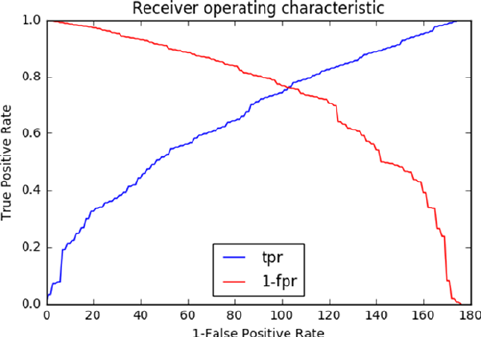
CHAPTER 4 ■ STEP 4 – MODEL DIAGNOSIS AND TUNING
211
# generate evaluation metrics
print "Accuracy: ", metrics.accuracy_score(y_train, y_pred)
#----output----
Accuracy: 0.767225325885
The optimal cutoff would be where the true positive rate (tpr) is high and the
false positive rate (fpr) is low, and tpr - (1-fpr) is zero or near to zero. Let’s plot an ROC
(receiver operating characteristic) plot of tprvs, 1-fpr. See Listing 4-3.
Listing 4-3. Find optimal cutoff point
# extract false positive, true positive rate
fpr, tpr, thresholds = metrics.roc_curve(y_train, y_pred_prob)
roc_auc = metrics.auc(fpr, tpr)
print("Area under the ROC curve : %f" % roc_auc)
i = np.arange(len(tpr)) # index for df
roc = pd.DataFrame({'fpr' : pd.Series(fpr, index=i),'tpr' : pd.Series(tpr,
index = i),'1-fpr' : pd.Series(1-fpr, index = i), 'tf' : pd.Series(tpr - (1-
fpr), index = i),'thresholds' : pd.Series(thresholds, index = i)})
roc.ix[(roc.tf-0).abs().argsort()[:1]]
# Plot tpr vs 1-fpr
fig, ax = plt.subplots()
plt.plot(roc['tpr'], label='tpr')
plt.plot(roc['1-fpr'], color = 'red', label='1-fpr')
plt.legend(loc='best')
plt.xlabel('1-False Positive Rate')
plt.ylabel('True Positive Rate')
plt.title('Receiver operating characteristic')
plt.show()
#----output----
CHAPTER 4 ■ STEP 4 – MODEL DIAGNOSIS AND TUNING
212
From the chart the point where tpr crosses 1-fpr is the optimal cutoff point. To
simplify finding the optimal probability threshold and bringing in reusability, I have
made a function to find the optimal probability cutoff point. See Listing 4-4.
Listing 4-4. Function for finding optimal probability cutoff
def Find_Optimal_Cutoff(target, predicted):
""" Find the optimal probability cutoff point for a classification model
related to event rate
Parameters
----------
target : Matrix with dependent or target data, where rows are observations
predicted : Matrix with predicted data, where rows are observations
Returns
-------
list type, with optimal cutoff value
"""
fpr, tpr, threshold = metrics.roc_curve(target, predicted)
i = np.arange(len(tpr))
roc = pd.DataFrame({'tf' : pd.Series(tpr-(1-fpr), index=i), 'threshold' :
pd.Series(threshold, index=i)})
roc_t = roc.ix[(roc.tf-0).abs().argsort()[:1]]
return list(roc_t['threshold'])
# Find optimal probability threshold
# Note: probs[:, 1] will have probability of being positive label
threshold = Find_Optimal_Cutoff(y_train, probs[:, 1])
print "Optimal Probability Threshold: ", threshold
# Applying the threshold to the prediction probability
y_pred_optimal = np.where(y_pred_prob >= threshold, 1, 0)
# Let's compare the accuracy of traditional/normal approach vs optimal cutoff
print "\nNormal - Accuracy: ", metrics.accuracy_score(y_train, y_pred)
print "Optimal Cutoff - Accuracy: ", metrics.accuracy_score(y_train, y_pred_optimal)
print "\nNormal - Confusion Matrix: \n", metrics.confusion_matrix(y_train, y_pred)
print "Optimal - Cutoff Confusion Matrix: \n", metrics.confusion_matrix
(y_train, y_pred_optimal)
#----output----
Optimal Probability Threshold: [0.36133240553264734]
Normal - Accuracy: 0.767225325885
Optimal Cutoff - Accuracy: 0.761638733706
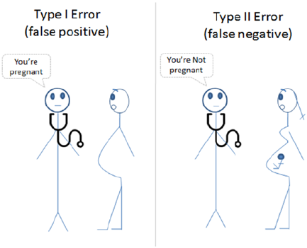
CHAPTER 4 ■ STEP 4 – MODEL DIAGNOSIS AND TUNING
213
Normal - Confusion Matrix:
[[303 40]
[ 85 109]]
Optimal - Cutoff Confusion Matrix:
[[261 82]
[ 46 148]]
Notice that there is no significant difference in overall accuracy between normal vs.
optimal cutoff method; both are 76%. However there is a 36% increase in the true positive
rate in the optimal cutoff method; that is, you are now able to capture 36% more positive
cases as positive; also the false positive (Type I error) has doubled, that is, the probability
of predicting an individual not having diabetes as positive has increases.
Which Error Is Costly?
Well, there is no one answer for this question! It depends on the domain, problem that
you are trying to address, and the business requirement. In our Pima diabetic case,
comparatively a type II error might be more damaging than a type I error, however it’s
arguable. See Figure4-1.
Rare Event or Imbalanced Dataset
Providing an equal sample of positive and negative instances to the classification
algorithm will result in an optimal result. Datasets that are highly skewed toward one or
more classes have proven to be a challenge.
Figure 4-1. Type I vs. Type II error
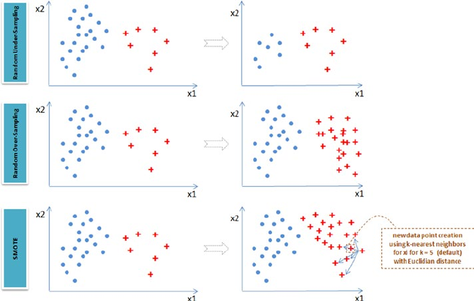
CHAPTER 4 ■ STEP 4 – MODEL DIAGNOSIS AND TUNING
214
Resampling is a common practice to address the imbalanced dataset issue. Although
there are many techniques within resampling, here we’ll be learning the three most
popular techniques.
• Random under-sampling – Reduce majority class to match
minority class count.
• Random over-sampling – Increase minority class by randomly
picking samples within minority class till counts of both class
match.
• Synthetic Minority Over-Sampling Technique (SMOTE) – Increase
minority class by introducing synthetic examples through
connecting all k (default = 5) minority class nearest neighbors
using feature space similarity (Euclidean distance). See Figure4-2.
Let’s create a sample imbalanced dataset using make_classification function of
sklearn. See Listing 4-5.
Listing 4-5. Rare event or imbalanced data handling
# Load libraries
import matplotlib.pyplot as plt
from sklearn.datasets import make_classification
Figure 4-2. Imbalanced dataset handling techniques
CHAPTER 4 ■ STEP 4 – MODEL DIAGNOSIS AND TUNING
215
from imblearn.under_sampling import RandomUnderSampler
from imblearn.over_sampling import RandomOverSampler
from imblearn.over_sampling import SMOTE
# Generate the dataset with 2 features to keep it simple
X, y = make_classification(n_samples=5000, n_features=2, n_informative=2,
n_redundant=0, weights=[0.9, 0.1], random_state=2017)
print "Positive class: ", y.tolist().count(1)
print "Negative class: ", y.tolist().count(0)
#----output----
Positive class: 514
Negative class: 4486
Let’s apply the above described three sampling techniques to the dataset to balance
the dataset and visualize for better understanding.
# Apply the random under-sampling
rus = RandomUnderSampler()
X_RUS, y_RUS = rus.fit_sample(X, y)
# Apply the random over-sampling
ros = RandomOverSampler()
X_ROS, y_ROS = ros.fit_sample(X, y)
# Apply regular SMOTE
sm = SMOTE(kind='regular')
X_SMOTE, y_SMOTE = sm.fit_sample(X, y)
# Original vs resampled subplots
plt.figure(figsize=(10, 6))
plt.subplot(2,2,1)
plt.scatter(X[y==0,0], X[y==0,1], marker='o', color='blue')
plt.scatter(X[y==1,0], X[y==1,1], marker='+', color='red')
plt.xlabel('x1')
plt.ylabel('x2')
plt.title('Original: 1=%s and 0=%s' %(y.tolist().count(1), y.tolist().
count(0)))
plt.subplot(2,2,2)
plt.scatter(X_RUS[y_RUS==0,0], X_RUS[y_RUS==0,1], marker='o', color='blue')
plt.scatter(X_RUS[y_RUS==1,0], X_RUS[y_RUS==1,1], marker='+', color='red')
plt.xlabel('x1')
plt.ylabel('y2')
plt.title('Random Under-sampling: 1=%s and 0=%s' %(y_RUS.tolist().count(1),
y_RUS.tolist().count(0)))
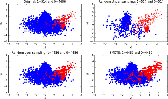
CHAPTER 4 ■ STEP 4 – MODEL DIAGNOSIS AND TUNING
216
plt.subplot(2,2,3)
plt.scatter(X_ROS[y_ROS==0,0], X_ROS[y_ROS==0,1], marker='o', color='blue')
plt.scatter(X_ROS[y_ROS==1,0], X_ROS[y_ROS==1,1], marker='+', color='red')
plt.xlabel('x1')
plt.ylabel('x2')
plt.title('Random over-sampling: 1=%s and 0=%s' %(y_ROS.tolist().count(1),
y_ROS.tolist().count(0)))
plt.subplot(2,2,4)
plt.scatter(X_SMOTE[y_SMOTE==0,0], X_SMOTE[y_SMOTE==0,1], marker='o', color='blue')
plt.scatter(X_SMOTE[y_SMOTE==1,0], X_SMOTE[y_SMOTE==1,1], marker='+', color='red')
plt.xlabel('x1')
plt.ylabel('y2')
plt.title('SMOTE: 1=%s and 0=%s' %(y_SMOTE.tolist().count(1), y_SMOTE.
tolist().count(0)))
plt.tight_layout()
plt.show()
#----output----
Known Disadvantages
• Random Under-Sampling raises the opportunity for loss of
information or concepts as we are reducing the majority class.
• Random Over-Sampling and SMOTE can lead to over-fitting
issues due to multiple related instances.
CHAPTER 4 ■ STEP 4 – MODEL DIAGNOSIS AND TUNING
217
Which Resampling Technique Is the Best?
Well, yet again there is no one answer to this question! Let’s try a quick classification
model on the above three resampled data and compare the accuracy (we’ll use AUC
metric as this is one of the best representations of model performance). See Listing 4-6.
Listing 4-6. Build models on various resampling methods and evaluate performance
from sklearn import tree
from sklearn import metrics
from sklearn.cross_validation import train_test_split
X_RUS_train, X_RUS_test, y_RUS_train, y_RUS_test = train_test_split(X_RUS,
y_RUS, test_size=0.3, random_state=2017)
X_ROS_train, X_ROS_test, y_ROS_train, y_ROS_test = train_test_split(X_ROS,
y_ROS, test_size=0.3, random_state=2017)
X_SMOTE_train, X_SMOTE_test, y_SMOTE_train, y_SMOTE_test = train_test_
split(X_SMOTE, y_SMOTE, test_size=0.3, random_state=2017)
# build a decision tree classifier
clf = tree.DecisionTreeClassifier(random_state=2017)
clf_rus = clf.fit(X_RUS_train, y_RUS_train)
clf_ros = clf.fit(X_ROS_train, y_ROS_train)
clf_smote = clf.fit(X_SMOTE_train, y_SMOTE_train)
# evaluate model performance
print "\nRUS - Train AUC : ",metrics.roc_auc_score(y_RUS_train, clf.
predict(X_RUS_train))
print "RUS - Test AUC : ",metrics.roc_auc_score(y_RUS_test, clf.predict(X_RUS_test))
print "ROS - Train AUC : ",metrics.roc_auc_score(y_ROS_train, clf.predict(X_ROS_train))
print "ROS - Test AUC : ",metrics.roc_auc_score(y_ROS_test, clf.predict(X_ROS_test))
print "\nSMOTE - Train AUC : ",metrics.roc_auc_score(y_SMOTE_train, clf.
predict(X_SMOTE_train))
print "SMOTE - Test AUC : ",metrics.roc_auc_score(y_SMOTE_test, clf.predict
(X_SMOTE_test))
#----output----
RUS - Train AUC : 0.988945248974
RUS - Test AUC : 0.983964646465
ROS - Train AUC : 0.985666951094
ROS - Test AUC : 0.986630288452
SMOTE - Train AUC : 1.0
SMOTE - Test AUC : 0.956132695918
Here random over-sampling is performing better on both train and test sets. As a
best practice, in real-world use cases it is recommended to look at other metrics (such as
precision, recall, confusion matrix) and apply business context or domain knowledge to
assess the true performance of a model.
CHAPTER 4 ■ STEP 4 – MODEL DIAGNOSIS AND TUNING
218
Bias and Variance
A fundamental problem with supervised learning is the bias variance trade-off. Ideally a
model should have two key characteristics.
1. Sensitive enough to accurately capture the key patterns in the
training dataset.
2. It should be generalized enough to work well on any unseen
datasets.
Unfortunately, while trying to achieve the above-mentioned first point, there is an
ample chance of over-fitting to noisy or unrepresentative training data points leading to
a failure of generalizing the model. On the other hand, trying to generalize a model may
result in failing to capture important regularities.
Bias
If model accuracy is low on a training dataset as well as test dataset the model is said to
be under-fitting or that the model has high bias. This means the model is not fitting the
training dataset points well in regression or the decision boundary is not separating the
classes well in classification; and two key reasons for bias are 1) not including the right
features, and 2) not picking the correct order of polynomial degrees for model fitting.
To solve an under-fitting issue or to reduced bias, try including more meaningful
features and try to increase the model complexity by trying higher-order polynomial fittings.
Variance
If a model is giving high accuracy on a training dataset, however on a test dataset the
accuracy drops drastically, then the model is said to be over-fitting or a model that has
high variance. The key reason for over-fitting is using higher-order polynomial degree
(may not be required), which will fit decision boundary tools well to all data points
including the noise of train dataset, instead of the underlying relationship. This will lead
to a high accuracy (actual vs. predicted) in the train dataset and when applied to the test
dataset, the prediction error will be high.
To solve the over-fitting issue:
• Try to reduce the number of features, that is, keep only the
meaningful features or try regularization methods that will keep
all the features, however reduce the magnitude of the feature
parameter.
• Dimension reduction can eliminate noisy features, in turn,
reducing the model variance.
• Brining more data points to make training dataset large will also
reduce variance.
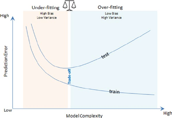
CHAPTER 4 ■ STEP 4 – MODEL DIAGNOSIS AND TUNING
219
• Choosing right model parameters can help to reduce the bias and
variance, for example.
• Using right regularization parameters can decrease variance
in regression-based models.
• For a decision tree reducing the depth of the decision tree
will reduce the variance. See Figure4-3.
K-Fold Cross-Validation
K-folds cross-validation splits the training dataset into k-folds without replacement, that
is, any given data point will only be part of one of the subset, where k-1 folds are used for
the model training and one fold is used for testing. The procedure is repeated k times so
that we obtain k models and performance estimates.
We then calculate the average performance of the models based on the individual
folds to obtain a performance estimate that is less sensitive to the subpartitioning of the
training data compared to the holdout or single fold method. See Figure4-4.
Figure 4-3. Bias Variance trade-off
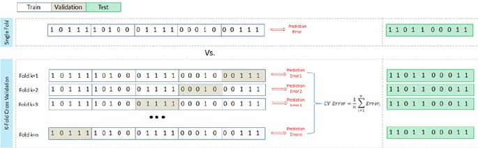
CHAPTER 4 ■ STEP 4 – MODEL DIAGNOSIS AND TUNING
220
Let’s use K-fold cross-validation of sklearn to build a classification model. See Listing 4-7.
Listing 4-7. K-fold cross-validation
from sklearn.cross_validation import cross_val_score
# read the data in
df = pd.read_csv("Data/Diabetes.csv")
X = df.ix[:,:8].values # independent variables
y = df['class'].values # dependent variables
# Normalize Data
sc = StandardScaler()
sc.fit(X)
X = sc.transform(X)
# evaluate the model by splitting into train and test sets
X_train, X_test, y_train, y_test = train_test_split(X, y, test_size=0.3,
random_state=2017)
# build a decision tree classifier
clf = tree.DecisionTreeClassifier(random_state=2017)
# evaluate the model using 10-fold cross-validation
train_scores = cross_val_score(clf, X_train, y_train, scoring='accuracy', cv=5)
test_scores = cross_val_score(clf, X_test, y_test, scoring='accuracy', cv=5)
print "Train Fold AUC Scores: ", train_scores
print "Train CV AUC Score: ", train_scores.mean()
print "\nTest Fold AUC Scores: ", test_scores
print "Test CV AUC Score: ", test_scores.mean()
#---output----
Train Fold AUC Scores: [0.80 0.73 0.81 0.76 0.71]
Train CV AUC Score: 0.76
Test Fold AUC Scores: [0.80 0.78 0.78 0.77 0.8]
Test CV AUC Score: 0.79
Figure 4-4. K-fold cross-validation
CHAPTER 4 ■ STEP 4 – MODEL DIAGNOSIS AND TUNING
221
Stratified K-Fold Cross-Validation
An extended cross-validation is the Stratified K-fold cross-validation, where the class
proportions are preserved in each fold, leading to better bias and variance estimates. See
Listing 4-8.
Listing 4-8. Stratified k-fold cross-validation
# stratified kfold cross-validation
kfold = cross_validation.StratifiedKFold(y=y_train, n_folds=5, random_
state=2017)
train_scores = []
test_scores = []
for k, (train, test) in enumerate(kfold):
clf.fit(X_train[train], y_train[train])
train_score = clf.score(X_train[train], y_train[train])
train_scores.append(train_score)
# score for test set
test_score = clf.score(X_train[test], y_train[test])
test_scores.append(test_score)
print('Fold: %s, Class dist.: %s, Train Acc: %.3f, Test Acc: %.3f'
% (k+1, np.bincount(y_train[train]), train_score, test_score))
print('\nTrain CV accuracy: %.3f' % (np.mean(train_scores)))
print('Test CV accuracy: %.3f' % (np.mean(test_scores)))
#----output----
Fold: 1, Class dist.: [277 152], Train Acc: 0.758, Test Acc: 0.806
Fold: 2, Class dist.: [277 152], Train Acc: 0.779, Test Acc: 0.731
Fold: 3, Class dist.: [278 152], Train Acc: 0.767, Test Acc: 0.813
Fold: 4, Class dist.: [278 152], Train Acc: 0.781, Test Acc: 0.766
Fold: 5, Class dist.: [278 152], Train Acc: 0.781, Test Acc: 0.710
Train CV accuracy: 0.773
Test CV accuracy: 0.765
Ensemble Methods
Ensemble methods enable combining multiple model scores into a single score to create
a robust generalized model.
At a high level there are two types of ensemble methods.
1. Combine multiple models of similar type
• Bagging (Bootstrap aggregation)
• Boosting
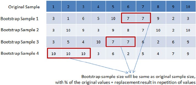
CHAPTER 4 ■ STEP 4 – MODEL DIAGNOSIS AND TUNING
222
2. Combine multiple models of various types
• Vote Classification
• Blending or Stacking
Bagging
Bootstrap aggregation (also known as bagging) was proposed by Leo Breiman in 1994,
which is a model aggregation technique to reduce model variance. The training data
is split into multiple samples with replacements called bootstrap samples. Bootstrap
sample size will be the same as the original sample size, with 3/4th of the original values
and replacement result in repetition of values. See Figure4-5.
Independent models on each of the bootstrap samples are built, and the average of the
predictions for regression or majority vote for classification is used to create the final model.
Figure4-6 shows the bagging process flow. Let N be the number of bootstrap
samples created out of the original training set. For i = 1 to N, train a base machine
learning model Ci.
Caggregate of yI
Cy
final
i
i
==
å
()
max
Figure 4-5. Bootstraping
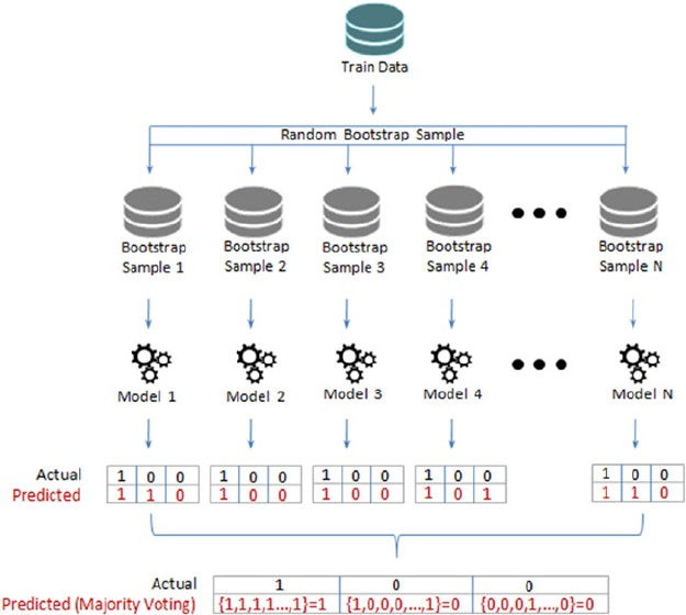
CHAPTER 4 ■ STEP 4 – MODEL DIAGNOSIS AND TUNING
223
Let’s compare the performance of a stand-alone decision tree model and a bagging
decision tree model of 100 trees. See Listing 4-9.
Listing 4-9. Stand-alone decision tree vs. bagging
# Bagged Decision Trees for Classification
from sklearn.ensemble import BaggingClassifier
from sklearn.tree import DecisionTreeClassifier
# read the data in
df = pd.read_csv("Data/Diabetes.csv")
X = df.ix[:,:8].values # independent variables
y = df['class'].values # dependent variables
#Normalize
X = StandardScaler().fit_transform(X)
# evaluate the model by splitting into train and test sets
X_train, X_test, y_train, y_test = train_test_split(X, y, test_size=0.2,
random_state=2017)
Figure 4-6. Bagging
CHAPTER 4 ■ STEP 4 – MODEL DIAGNOSIS AND TUNING
224
kfold = cross_validation.StratifiedKFold(y=y_train, n_folds=5, random_state=2017)
num_trees = 100
# Decision Tree with 5 fold cross validation
clf_DT = DecisionTreeClassifier(random_state=2017).fit(X_train,y_train)
results = cross_validation.cross_val_score(clf_DT, X_train,y_train, cv=kfold)
print "Decision Tree (stand alone) - Train : ", results.mean()
print "Decision Tree (stand alone) - Test : ", metrics.accuracy_score(clf_
DT.predict(X_test), y_test)
# Using Bagging Lets build 100 decision tree models and average/majority
vote prediction
clf_DT_Bag = BaggingClassifier(base_estimator=clf_DT, n_estimators=num_
trees, random_state=2017).fit(X_train,y_train)
results = cross_validation.cross_val_score(clf_DT_Bag, X_train, y_train, cv=kfold)
print "\nDecision Tree (Bagging) - Train : ", results.mean()
print "Decision Tree (Bagging) - Test : ", metrics.accuracy_score(clf_DT_
Bag.predict(X_test), y_test)
#----output----
Decision Tree (stand alone) - Train : 0.701983077737
Decision Tree (stand alone) - Test : 0.753246753247
Decision Tree (Bagging) - Train : 0.747461660497
Decision Tree (Bagging) - Test : 0.818181818182
Feature Importance
The decision tree model has an attribute to show important features that are based on the
gini or entropy information gain. See Listing 4-10.
Listing 4-10. Decision tree feature importance function
feature_importance = clf_DT.feature_importances_
# make importances relative to max importance
feature_importance = 100.0 * (feature_importance / feature_importance.max())
sorted_idx = np.argsort(feature_importance)
pos = np.arange(sorted_idx.shape[0]) + .5
plt.subplot(1, 2, 2)
plt.barh(pos, feature_importance[sorted_idx], align='center')
plt.yticks(pos, df.columns[sorted_idx])
plt.xlabel('Relative Importance')
plt.title('Variable Importance')
plt.show()
#----output----
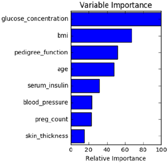
CHAPTER 4 ■ STEP 4 – MODEL DIAGNOSIS AND TUNING
225
RandomForest
A subset of observations and a subset of variables are randomly picked to build multiple
independent tree-based models. The trees are more un-correlated as only a subset of
variables are used during the split of the tree, rather than greedily choosing the best split
point in the construction of the tree. See Listing 4-11.
Listing 4-11. RandomForest classifier
from sklearn.ensemble import RandomForestClassifier
num_trees = 100
clf_RF = RandomForestClassifier(n_estimators=num_trees).fit(X_train, y_train)
results = cross_validation.cross_val_score(clf_RF, X_train, y_train, cv=kfold)
print "\nRandom Forest (Bagging) - Train : ", results.mean()
print "Random Forest (Bagging) - Test : ", metrics.accuracy_score(clf_
RF.predict(X_test), y_test)
#----output----
Random Forest - Train : 0.758857747224
Random Forest - Test : 0.798701298701
Extremely Randomized Trees (ExtraTree)
This algorithm is an effort to introduce more randomness to the bagging process. Tree
splits are chosen completely at random from the range of values in the sample at each
split, which allows us to reduce the variance of the model further – however, at the cost of
a slight increase in bias. See Listing 4-12.
CHAPTER 4 ■ STEP 4 – MODEL DIAGNOSIS AND TUNING
226
Listing 4-12. Extremely randomized trees (ExtraTree)
from sklearn.ensemble import ExtraTreesClassifier
num_trees = 100
clf_ET = ExtraTreesClassifier(n_estimators=num_trees).fit(X_train, y_train)
results = cross_validation.cross_val_score(clf_ET, X_train, y_train, cv=kfold)
print "\nExtraTree - Train : ", results.mean()
print "ExtraTree - Test : ", metrics.accuracy_score(clf_ET.predict(X_test), y_test)
#----output----
ExtraTree - Train : 0.747408778424
ExtraTree - Test : 0.811688311688
How Does the Decision Boundary Look?
Let’s perform PCA and consider only the first two principal components for easy plotting.
The model building code would remain the same as above except that after normalization
and before splitting the data to train and test, we will need to add the line below. See
Listing 4-13.
Listing 4-13. Plot the decision boundaries
# PCA
X = PCA(n_components=2).fit_transform(X)
Once we have run the model succesfully we can use the below code to draw
decision boundaries for stand alone vs different bagging models.
def plot_decision_regions(X, y, classifier):
h = .02 # step size in the mesh
# setup marker generator and color map
markers = ('s', 'x', 'o', '^', 'v')
colors = ('red', 'blue', 'lightgreen', 'gray', 'cyan')
cmap = ListedColormap(colors[:len(np.unique(y))])
# plot the decision surface
x1_min, x1_max = X[:, 0].min() - 1, X[:, 0].max() + 1
x2_min, x2_max = X[:, 1].min() - 1, X[:, 1].max() + 1
xx1, xx2 = np.meshgrid(np.arange(x1_min, x1_max, h),
np.arange(x2_min, x2_max, h))
Z = classifier.predict(np.array([xx1.ravel(), xx2.ravel()]).T)
Z = Z.reshape(xx1.shape)
plt.contourf(xx1, xx2, Z, alpha=0.4, cmap=cmap)
plt.xlim(xx1.min(), xx1.max())
plt.ylim(xx2.min(), xx2.max())
CHAPTER 4 ■ STEP 4 – MODEL DIAGNOSIS AND TUNING
227
for idx, cl in enumerate(np.unique(y)):
plt.scatter(x=X[y == cl, 0], y=X[y == cl, 1],
alpha=0.8, c=cmap(idx),
marker=markers[idx], label=cl)
# Plot the decision boundary
plt.figure(figsize=(10,6))
plt.subplot(221)
plot_decision_regions(X, y, clf_DT)
plt.title('Decision Tree (Stand alone)')
plt.xlabel('PCA1')
plt.ylabel('PCA2')
plt.subplot(222)
plot_decision_regions(X, y, clf_DT_Bag)
plt.title('Decision Tree (Bagging - 100 trees)')
plt.xlabel('PCA1')
plt.ylabel('PCA2')
plt.legend(loc='best')
plt.subplot(223)
plot_decision_regions(X, y, clf_RF)
plt.title('RandomForest Tree (100 trees)')
plt.xlabel('PCA1')
plt.ylabel('PCA2')
plt.legend(loc='best')
plt.subplot(224)
plot_decision_regions(X, y, clf_ET)
plt.title('Extream Random Tree (100 trees)')
plt.xlabel('PCA1')
plt.ylabel('PCA2')
plt.legend(loc='best')
plt.tight_layout()
#----output----
Decision Tree (stand alone) - Train : 0.595875198308
Decision Tree (stand alone) - Test : 0.616883116883
Decision Tree (Bagging) - Train : 0.646298254892
Decision Tree (Bagging) - Test : 0.714285714286
Random Forest - Train : 0.665917503966
Random Forest - Test : 0.707792207792
ExtraTree - Train : 0.635034373347
ExtraTree - Test : 0.707792207792
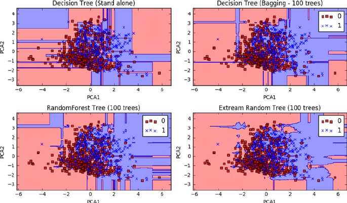
CHAPTER 4 ■ STEP 4 – MODEL DIAGNOSIS AND TUNING
228
Bagging – Essential Tuning Parameters
n_estimators: This is the number of trees, the larger the better. Note that beyond a certain
point the results will not improve significantly.
max_features: This is the random subset of features to be used for splitting node,
the lower the better to reduce variance (but increases bias). Ideally, for a regression
problem it should be equal to n_features (total number of features) and for classification
square root of n_features.
n_ jobs: Number of cores to be used for parallel construction of trees. If set to -1,
all available cores in the system are used, or you can specify the number.
Boosting
Freud and Schapire in 1995 introduced the concept of boosting with the well-known
AdaBoost algorithm (adaptive boosting). The core concept of boosting is that rather
than an independent individual hypothesis, combining hypotheses in a sequential order
increases the accuracy. Essentially, boosting algorithms convert the weak learners into
strong learners. Boosting algorithms are well designed to address the bias problems.
At a high level the AdaBoosting process can be divided into three steps. See Figure4-7.
• Assign uniform weights for all data points W0(x) = 1 / N, where N
is the total number of training data points.
• At each iteration fit a classifier ym(xn) to the training data and
update weights to minimize the weighted error function.
The weight is calculated as WW yx t
n
m
n
m
mm
nn
+
() ()
=µ
()
¹
{}
1exp.
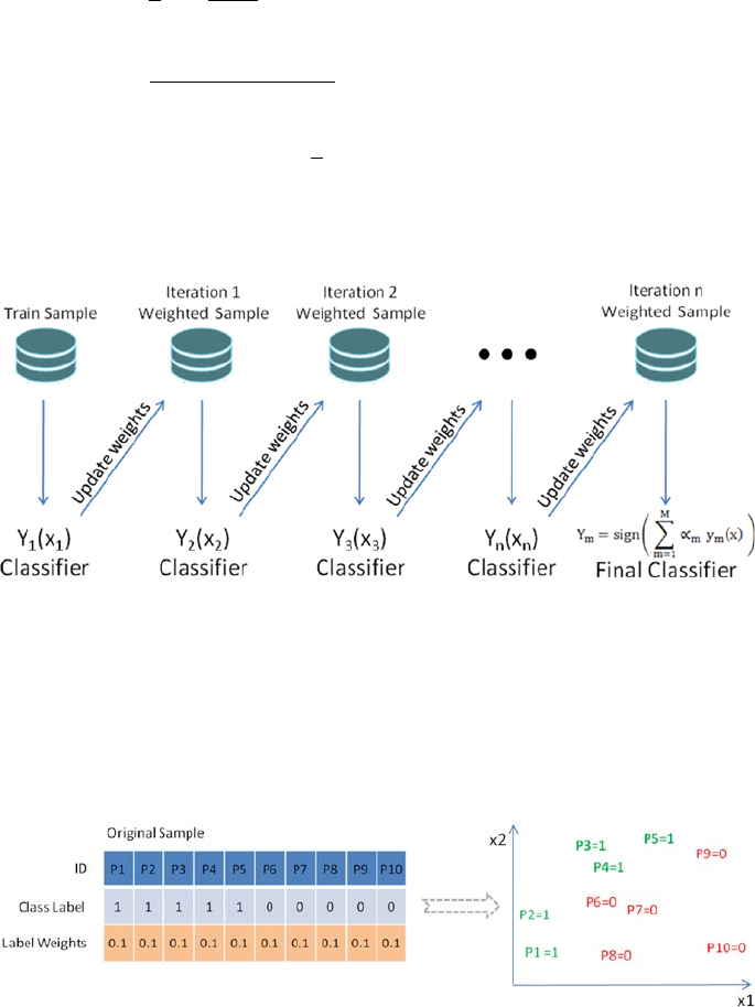
CHAPTER 4 ■ STEP 4 – MODEL DIAGNOSIS AND TUNING
229
The hypothesis weight or the loss function is given by
µ= -Î
Î
ì
í
î
ü
ý
þ
m
m
m
1
2
1
log , and the term rate is given by
Î=
()
¹
()
=
()
=
()
å
å
m
n
N
n
m
mn n
n
N
n
m
WIyx t
W
1
1
, where
yx thas values ie if xcorrectly classified else
mn nn
()
¹
()
()
0
101
..,
• The final model is given by Ysig
ny
x
m
m
M
mm
=µ
()
æ
è
çö
ø
÷
=
å
1
Example Illustration for AdaBoost
Let’s consider a training data with two class labels of 10 data points. Assume, initially all
the data points will have equal weights given by, for example, 1/10 as shown in Figure4-8
below.
Figure 4-7. AdaBoosting
Figure 4-8. Sample dataset with 10 data points
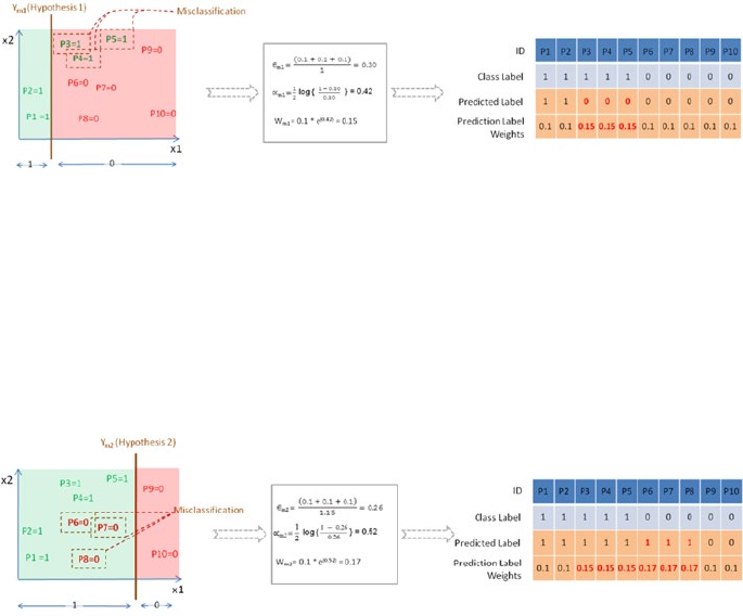
CHAPTER 4 ■ STEP 4 – MODEL DIAGNOSIS AND TUNING
230
Boosting Iteration 1
Notice in Figure4-9 that three points of positive class are misclassified by the first simple
classification model, so they will be assigned higher weights. The error term and loss
function (learning rate) is calcuated as 0.30 and 0.42 respectively. The data points P3, P4,
and P5 will get higher weight (0.15) due to misclassification, whereas other data points
will retain the original weight (0.1).
Boosting Iteration 2
Let’s fit another classification model as shown in Figure4-10 below and notice that
three data points of negative class are misclassified. The data points P6, P7, and P8 are
misclassified. Hence these will be assigned higher weights of 0.17 as calculated, whereas
the remaining data point’s weights will remain the same as they are correctly classified.
Boosting Iteration 3
The third classification model has misclassified a toal of three data points, that is, two
positive class P1, P2, and one negative class P9. So these misclassified data points will
be assigned a new higher weight of 0.19 as calculated and the remaining data points will
retain their earlier weights. See Figure4-11.
Figure 4-10. Ym2 the second classification or hypothesis
Figure 4-9. Ym1 the first classification or hypothesis
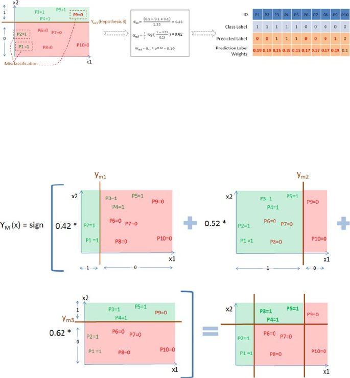
CHAPTER 4 ■ STEP 4 – MODEL DIAGNOSIS AND TUNING
231
Final Model
Now as per the AdaBoost algorithm, let’s combine the weak classification models as
shown in Figure4-12 below. Notice that the final model combined model will have a
minimum error term and maximum learning rate leading to a higher degree of accuracy.
Let’s pick weak predictors from the Pima diabetic dataset and compare the
performance of a stand-alone decision tree model vs. AdaBoost with 100 boosting rounds
on the decision tree model. See Listing 4-14.
Listing 4-14. Stand-alone decision tree vs. adaboost
# Bagged Decision Trees for Classification
from sklearn.ensemble import AdaBoostClassifier
from sklearn.tree import DecisionTreeClassifier
Figure 4-11. Ym3 the third classification or hypothesis
Figure 4-12. AdaBoost algorithm to combine weak classifiers
CHAPTER 4 ■ STEP 4 – MODEL DIAGNOSIS AND TUNING
232
# read the data in
df = pd.read_csv("Data/Diabetes.csv")
# Let's use some week features to build the tree
X = df[['age','serum_insulin']] # independent variables
y = df['class'].values # dependent variables
#Normalize
X = StandardScaler().fit_transform(X)
# evaluate the model by splitting into train and test sets
X_train, X_test, y_train, y_test = train_test_split(X, y, test_size=0.2,
random_state=2017)
kfold = cross_validation.StratifiedKFold(y=y_train, n_folds=5, random_
state=2017)
num_trees = 100
# Dection Tree with 5 fold cross validation
# lets restrict max_depth to 1 to have more impure leaves
clf_DT = DecisionTreeClassifier(max_depth=1, random_state=2017).fit(X_
train,y_train)
results = cross_validation.cross_val_score(clf_DT, X_train,y_train,
cv=kfold)
print "Decision Tree (stand alone) - Train : ", results.mean()
print "Decision Tree (stand alone) - Test : ", metrics.accuracy_score(clf_
DT.predict(X_test), y_test)
# Using Adaptive Boosting of 100 iteration
clf_DT_Boost = AdaBoostClassifier(base_estimator=clf_DT, n_estimators=num_
trees, learning_rate=0.1, random_state=2017).fit(X_train,y_train)
results = cross_validation.cross_val_score(clf_DT_Boost, X_train, y_train,
cv=kfold)
print "\nDecision Tree (AdaBoosting) - Train : ", results.mean()
print "Decision Tree (AdaBoosting) - Test : ", metrics.accuracy_score(clf_
DT_Boost.predict(X_test), y_test)
#----output----
Decision Tree (stand alone) - Train : 0.635113696457
Decision Tree (stand alone) - Test : 0.649350649351
Decision Tree (AdaBoosting) - Train : 0.688709677419
Decision Tree (AdaBoosting) - Test : 0.707792207792
Notice that in this case AdaBoost algorithm has given an average rise of 9%
in accuracy score between train / test dataset compared to the stanalone
decision tree model.
CHAPTER 4 ■ STEP 4 – MODEL DIAGNOSIS AND TUNING
233
Gradient Boosting
Due to the stage-wise addictivity, the loss function can be represented in a form suitable
for optimization. This gave birth to a class of generalized boosting algorithms known as
generalized boosting algorithm (GBM). Gradient boosting is an example implementation
of GBM and it can work with different loss functions such as regression, classification,
risk modeling, etc. As the name suggests it is a boosting algorithm that identifies
shortcomings of a weak learner by gradients (AdaBoost uses high-weight data points),
hence the name Gradient Boosting. See Listing 4-15.
• Iteratively fit a classifier ym(xn) to the training data. The initial
model will be with a constant value yx Ly
i
n
m0
1
()
=
()
=
å
argmin ,
dd
• Calculate the loss (i.e., the predicted value vs. actual value) for each
model fit iteration gm(x)or compute the negative gradient, and use
it to fit a new base learner function hm(x), and find the best gradient
decent step-size
dd d
m
i
n
mm m
Ly yx hx=
()
+
()
()
=
-
å
argmin ,
1
1
• Update the function estimate yx yx
hx
mm m
()
=
()
+
()
-1
d
and
output ym(x)
Listing 4-15. Gradient boosting classifier
from sklearn.ensemble import GradientBoostingClassifier
# Using Gradient Boosting of 100 iterations
clf_GBT = GradientBoostingClassifier(n_estimators=num_trees, learning_
rate=0.1, random_state=2017).fit(X_train, y_train)
results = cross_validation.cross_val_score(clf_GBT, X_train, y_train,
cv=kfold)
print "\nGradient Boosting - CV Train : %.2f" % results.mean()
print "Gradient Boosting - Train : %.2f" % metrics.accuracy_score(clf_GBT.
predict(X_train), y_train)
print "Gradient Boosting - Test : %.2f" % metrics.accuracy_score(clf_GBT.
predict(X_test), y_test)
#----output----
Gradient Boosting - CV Train : 0.70
Gradient Boosting - Train : 0.81
Gradient Boosting - Test : 0.66
Let’s look at the digit classification to illustrate how the model performance improves
with each iteration.
CHAPTER 4 ■ STEP 4 – MODEL DIAGNOSIS AND TUNING
234
from sklearn.ensemble import GradientBoostingClassifier
df= pd.read_csv('Data/digit.csv')
X = df.ix[:,1:17].values
y = df['lettr'].values
# evaluate the model by splitting into train and test sets
X_train, X_test, y_train, y_test = train_test_split(X, y, test_size=0.2,
random_state=2017)
kfold = cross_validation.StratifiedKFold(y=y_train, n_folds=5, random_
state=2017)
num_trees = 10
clf_GBT = GradientBoostingClassifier(n_estimators=num_trees, learning_
rate=0.1, max_depth=3, random_state=2017).fit(X_train, y_train)
results = cross_validation.cross_val_score(clf_GBT, X_train, y_train,
cv=kfold)
print "\nGradient Boosting - Train : ", metrics.accuracy_score(clf_GBT.
predict(X_train), y_train)
print "Gradient Boosting - Test : ", metrics.accuracy_score(clf_GBT.
predict(X_test), y_test)
# Let's predict for the letter 'T' and understand how the prediction
accuracy changes in each boosting iteration
X_valid= (2,8,3,5,1,8,13,0,6,6,10,8,0,8,0,8)
print "Predicted letter: ", clf_GBT.predict(X_valid)
# Staged prediction will give the predicted probability for each boosting
iteration
stage_preds = list(clf_GBT.staged_predict_proba(X_valid))
final_preds = clf_GBT.predict_proba(X_valid)
# Plot
x = range(1,27)
label = np.unique(df['lettr'])
plt.figure(figsize=(10,3))
plt.subplot(131)
plt.bar(x, stage_preds[0][0], align='center')
plt.xticks(x, label)
plt.xlabel('Label')
plt.ylabel('Prediction Probability')
plt.title('Round One')
plt.autoscale()
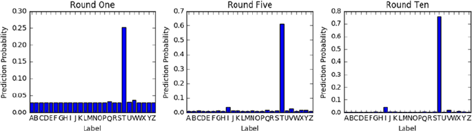
CHAPTER 4 ■ STEP 4 – MODEL DIAGNOSIS AND TUNING
235
plt.subplot(132)
plt.bar(x, stage_preds[5][0],align='center')
plt.xticks(x, label)
plt.xlabel('Label')
plt.ylabel('Prediction Probability')
plt.title('Round Five')
plt.autoscale()
plt.subplot(133)
plt.bar(x, stage_preds[9][0],align='center')
plt.xticks(x, label)
plt.autoscale()
plt.xlabel('Label')
plt.ylabel('Prediction Probability')
plt.title('Round Ten')
plt.tight_layout()
plt.show()
#----output----
Gradient Boosting - Train : 0.7525625
Gradient Boosting - Test : 0.7305
Predicted letter: 'T'
Gradient boosting corrects the erroneous boosting iteration’s negative impact in
subsequent iterations. Notice that in the first iteration the predicted probability for letter
‘T’ is 0.25 and it gradually increased to 0.76 by the 10th iteration, whereas the proability
percentage for other letters have decreased over each round.
Boosting – Essential Tuning Parameters
Model complexity and over-fitting can be controlled by using correct values for two
categories of parameters.
1. Tree structure
n_estimators: This is the number of weak learners to be built.
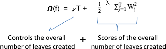
CHAPTER 4 ■ STEP 4 – MODEL DIAGNOSIS AND TUNING
236
max_depth: Maximum depth of the individual estimators. The
best value depends on the interaction of the input variables.
min_samples_leaf: This will be helpful to ensure sufficient
number of samples result in leaf.
subsample: The fraction of sample to be used for fitting
individual models (default=1). Typically .8 (80%) is used
to introduce random selection of samples, which, in turn,
increases the robustness against over-fitting.
2. Regularization parameter
learning_rate: this controls the magnitude of change in
estimators. Lower learning rate is better, which requires
higher n_estimators (that is the trade-off).
Xgboost (eXtreme Gradient Boosting)
In March 2014, Tianqui Chen built xgboost in C++ as part of the Distributed (Deep)
Machine Learning Community, and it has an interface for Python. It is an extended,
more regularized version of a gradient boosting algorithm. This is one of the most well-
performing large-scale, scalable machine learning algorithms that has been playing a
major role in winning solutions of Kaggle (forum for predictive modeling and analytics
competition) data science competition.
XGBoost objective function obj(ϴ) =
i
n
ii
k
K
k
ly
yf
åå
-
æ
è
çö
ø
÷+
()
=
1
W
Regularization term is given by
The gradient descent technique is used for optimizing the objective function, and
more mathematics about the algorithms can be found at the following site: http://
xgboost.readthedocs.io/en/latest/
Some of the key advantages of the xgboost algorithm are these:
• It implements parallel processing.
• It has a built-in standard to handle missing values, which
means user can specify a particular value different than other
observations (such as -1 or -999) and pass it as a parameter.
CHAPTER 4 ■ STEP 4 – MODEL DIAGNOSIS AND TUNING
237
• It will split the tree up to a maximum depth unlike Gradient
Boosting where it stops splitting node on encounter of a negative
loss in the split.
XGboost has bundle of parameters, and at a high level we can group them into three
categories. Let’s look at the most important within these categories.
1. General Parameters
a. nthread – Number of parallel threads; if not given a value
all cores will be used.
b. Booster – This is the type of model to be run with gbtree
(tree-based model) being the default. ‘gblinear’ to be
used for linear models
2. Boosting Parameters
a. eta – This is the learning rate or step size shrinkage
to prevent over-fitting; default is 0.3 and it can range
between 0 to 1
b. max_depth – Maximum depth of tree with default being 6.
c. min_child_weight – Minimum sum of weights of all
observations required in child. Start with 1/square root of
event rate
d. colsample_bytree – Fraction of columns to be randomly
sampled for each tree with default value of 1.
e. Subsample –Fraction of observations to be randomly
sampled for each tree with default of value of 1. Lowering
this value makes algorithm conservative to avoid over-
fitting.
f. lambda - L2 regularization term on weights with default
value of 1.
g. alpha - L1 regularization term on weight.
3. Task Parameters
a. objective – This defines the loss function to be
minimized with default value ‘reg:linear’. For binary
classification it should be ‘binary:logistic’ and for
multiclass ‘multi:softprob’ to get the probability value
and ‘multi:softmax’ to get predicted class. For multiclass
num_class (number of unique classes) to be specified.
b. eval_metric – Metric to be use for validating model
performance.
sklearn has a wrapper for xgboost (XGBClassifier). Let’s continue with the diabetic’s
dataset and build a model using the weak learner. See Listing 4-16.
CHAPTER 4 ■ STEP 4 – MODEL DIAGNOSIS AND TUNING
238
Listing 4-16. xgboost classifer using sklearn wrapper
import xgboost as xgb
from xgboost.sklearn import XGBClassifier
# read the data in
df = pd.read_csv("Data/Diabetes.csv")
# Let's use some weak features as predictors
predictors = ['age','serum_insulin']
target = 'class'
# Most common preprocessing step include label encoding and missing value treatment
from sklearn import preprocessing
for f in df.columns:
if df[f].dtype=='object':
lbl = preprocessing.LabelEncoder()
lbl.fit(list(df[f].values))
df[f] = lbl.transform(list(df[f].values))
df.fillna((-999), inplace=True) # missing value treatment
# Let's use some week features to build the tree
X = df[['age','serum_insulin']] # independent variables
y = df['class'].values # dependent variables
#Normalize
X = StandardScaler().fit_transform(X)
# evaluate the model by splitting into train and test sets
X_train, X_test, y_train, y_test = train_test_split(X, y, test_size=0.2,
random_state=2017)
num_rounds = 100
clf_XGB = XGBClassifier(n_estimators = num_rounds,
objective= 'binary:logistic',
seed=2017)
# use early_stopping_rounds to stop the cv when there is no score imporovement
clf_XGB.fit(X_train,y_train, early_stopping_rounds=20, eval_set=[(X_test,
y_test)], verbose=False)
results = cross_validation.cross_val_score(clf_XGB, X_train,y_train, cv=kfold)
print "\nxgBoost - CV Train : %.2f" % results.mean()
print "xgBoost - Train : %.2f" % metrics.accuracy_score(clf_XGB.predict
(X_train), y_train)
print "xgBoost - Test : %.2f" % metrics.accuracy_score(clf_XGB.predict
(X_test), y_test)
#----output----
CHAPTER 4 ■ STEP 4 – MODEL DIAGNOSIS AND TUNING
239
Now let’s also look at how to build a model using xgboost native interface. DMatrix
the internal data structure of xgboost for input data. It is good practice to convert a large
dataset to DMatrix object to save preprocessing time. See Listing 4-17.
Listing 4-17. xgboost using it’s native python package code
xgtrain = xgb.DMatrix(X_train, label=y_train, missing=-999)
xgtest = xgb.DMatrix(X_test, label=y_test, missing=-999)
# set xgboost params
param = {'max_depth': 3, # the maximum depth of each tree
'objective': 'binary:logistic'}
clf_xgb_cv = xgb.cv(param, xgtrain, num_rounds,
stratified=True,
nfold=5,
early_stopping_rounds=20,
seed=2017)
print ("Optimal number of trees/estimators is %i" % clf_xgb_cv.shape[0])
watchlist = [(xgtest,'test'), (xgtrain,'train')]
clf_xgb = xgb.train(param, xgtrain,clf_xgb_cv.shape[0], watchlist)
# predict function will produce the probability
# so we'll use 0.5 cutoff to convert probability to class label
y_train_pred = (clf_xgb.predict(xgtrain, ntree_limit=clf_xgb.best_iteration)
> 0.5).astype(int)
y_test_pred = (clf_xgb.predict(xgtest, ntree_limit=clf_xgb.best_iteration) >
0.5).astype(int)
print "XGB - Train : %.2f" % metrics.accuracy_score(y_train_pred, y_train)
print "XGB - Test : %.2f" % metrics.accuracy_score(y_test_pred, y_test)
#----output----
Optimal number of trees (estimators) is 7
[0] test-error:0.344156 train-error:0.299674
[1] test-error:0.324675 train-error:0.273616
[2] test-error:0.272727 train-error:0.281759
[3] test-error:0.266234 train-error:0.278502
[4] test-error:0.266234 train-error:0.273616
[5] test-error:0.311688 train-error:0.254072
[6] test-error:0.318182 train-error:0.254072
XGB - Train : 0.75
XGB - Test : 0.69
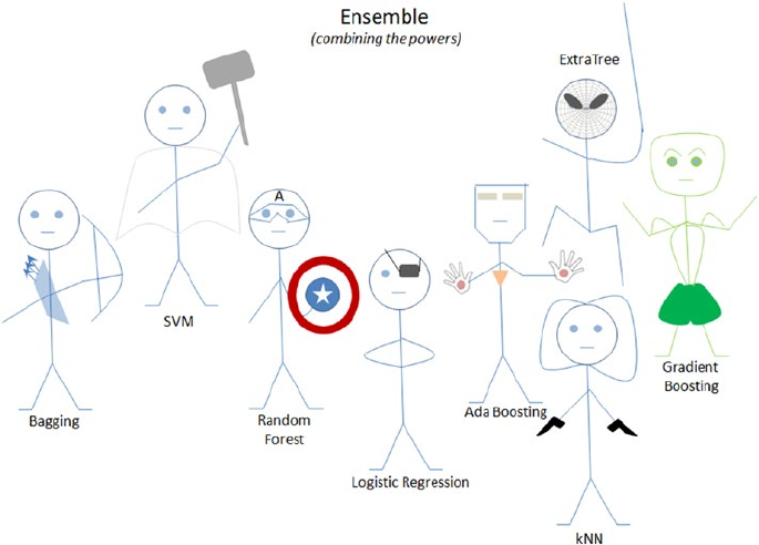
CHAPTER 4 ■ STEP 4 – MODEL DIAGNOSIS AND TUNING
240
Ensemble Voting – Machine Learning’s Biggest
Heroes United
A voting classifier enables us to combine the predictions through majority voting
from multiple machine learning algorithms of different types, unlike Bagging/Boosting
where similar types of multiple classifiers are used for majority voting.
First you can create multiple stand-alone models from your training dataset. Then a
voting classifier can be used to wrap your models and average the predictions of the sub-
models when asked to make predictions for new data. The predictions of the sub-models
can be weighted, but specifying the weights for classifiers manually or even heuristically
is difficult. More advanced methods can learn how to best weigh the predictions from
sub-models, but this is called stacking (stacked aggregation) and is currently not provided
in scikit-learn.
Let’s build individual models on the Pima diabetes dataset and try the voting
classifier to combine model results to compare the change in accuracy. See Listing 4-18.
Listing 4-18. Ensemble model
import pandas as pd
import numpy as np
Figure 4-13. Ensemble: ML's biggest heroes united
CHAPTER 4 ■ STEP 4 – MODEL DIAGNOSIS AND TUNING
241
# set seed for reproducability
np.random.seed(2017)
import statsmodels.api as sm
from sklearn import metrics
from sklearn.linear_model import LogisticRegression
from sklearn.ensemble import RandomForestClassifier
from sklearn.svm import SVC
from sklearn.neighbors import KNeighborsClassifier
from sklearn.tree import DecisionTreeClassifier
from sklearn.ensemble import AdaBoostClassifier
from sklearn.ensemble import BaggingClassifier
from sklearn.ensemble import GradientBoostingClassifier
# currently its available as part of mlxtend and not sklearn
from mlxtend.classifier import EnsembleVoteClassifier
from sklearn import cross_validation
from sklearn import metrics
from sklearn.cross_validation import train_test_split
# read the data in
df = pd.read_csv("Data/Diabetes.csv")
X = df.ix[:,:8] # independent variables
y = df['class'] # dependent variables
# evaluate the model by splitting into train and test sets
X_train, X_test, y_train, y_test = train_test_split(X, y, test_size=0.3,
random_state=2017)
LR = LogisticRegression(random_state=2017)
RF = RandomForestClassifier(n_estimators = 100, random_state=2017)
SVM = SVC(random_state=0, probability=True)
KNC = KNeighborsClassifier()
DTC = DecisionTreeClassifier()
ABC = AdaBoostClassifier(n_estimators = 100)
BC = BaggingClassifier(n_estimators = 100)
GBC = GradientBoostingClassifier(n_estimators = 100)
clfs = []
print('5-fold cross validation:\n')
for clf, label in zip([LR, RF, SVM, KNC, DTC, ABC, BC, GBC],
['Logistic Regression',
'Random Forest',
'Support Vector Machine',
'KNeighbors',
'Decision Tree',
'Ada Boost',
CHAPTER 4 ■ STEP 4 – MODEL DIAGNOSIS AND TUNING
242
'Bagging',
'Gradient Boosting']):
scores = cross_validation.cross_val_score(clf, X_train, y_train, cv=5,
scoring='accuracy')
print("Train CV Accuracy: %0.2f (+/- %0.2f) [%s]" % (scores.mean(),
scores.std(), label))
md = clf.fit(X, y)
clfs.append(md)
print("Test Accuracy: %0.2f " % (metrics.accuracy_score(clf.predict(X_
test), y_test)))
#----output----
5-fold cross validation:
Train CV Accuracy: 0.76 (+/- 0.03) [Logistic Regression]
Test Accuracy: 0.79
Train CV Accuracy: 0.74 (+/- 0.03) [Random Forest]
Test Accuracy: 1.00
Train CV Accuracy: 0.65 (+/- 0.00) [Support Vector Machine]
Test Accuracy: 1.00
Train CV Accuracy: 0.70 (+/- 0.05) [KNeighbors]
Test Accuracy: 0.84
Train CV Accuracy: 0.69 (+/- 0.02) [Decision Tree]
Test Accuracy: 1.00
Train CV Accuracy: 0.73 (+/- 0.04) [Ada Boost]
Test Accuracy: 0.83
Train CV Accuracy: 0.75 (+/- 0.04) [Bagging]
Test Accuracy: 1.00
Train CV Accuracy: 0.75 (+/- 0.03) [Gradient Boosting]
Test Accuracy: 0.92
From the above benchmarking we see that ‘Logistic Regression’, ‘Random Forest’,
‘Bagging’, and Ada/Gradient Boosting algorithms are giving better accuracy compared
to other models. Let’s combine non-similar models such as Logistic regression (base
model), Random Forest (bagging model), and gradient boosting (boosting model) to
create a robust generalized model.
Hard Voting vs. Soft Voting
Majority voting is also known as hard voting. The argmax of the sum of predicted
probabilities is known as soft voting. Parameter ‘weights’ can be used to assign specific
weights to classifiers. The predicted class probabilities for each classifier are multiplied by
the classifier weight and averaged. Then the final class label is derived from the highest
average probability class label.
Assume we assign equal weight of 1 to all classifiers (see Table4-1). Based on soft
voting, the predicted class label is 1, as it has the highest average probability. See also
Listing 4-19.
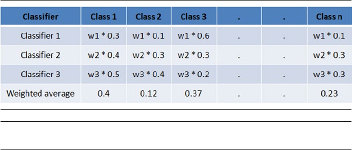
CHAPTER 4 ■ STEP 4 – MODEL DIAGNOSIS AND TUNING
243
■Note Some classifiers of scikit-learn do not support the predict_proba method.
Listing 4-19. Ensemble voting model
# Ensemble Voting
clfs = []
print('5-fold cross validation:\n')
ECH = EnsembleVoteClassifier(clfs=[LR, RF, GBC], voting='hard')
ECS = EnsembleVoteClassifier(clfs=[LR, RF, GBC], voting='soft',
weights=[1,1,1])
for clf, label in zip([ECH, ECS],
['Ensemble Hard Voting',
'Ensemble Soft Voting']):
scores = cross_validation.cross_val_score(clf, X_train, y_train, cv=5,
scoring='accuracy')
print("Train CV Accuracy: %0.2f (+/- %0.2f) [%s]" % (scores.mean(),
scores.std(), label))
md = clf.fit(X, y)
clfs.append(md)
print("Test Accuracy: %0.2f " % (metrics.accuracy_score(clf.predict(X_test),
y_test)))
#----output----
5-fold cross validation:
Train CV Accuracy: 0.75 (+/- 0.02) [Ensemble Hard Voting]
Test Accuracy: 0.93
Train CV Accuracy: 0.76 (+/- 0.02) [Ensemble Soft Voting]
Test Accuracy: 0.95
Table 4-1. Soft voting
-
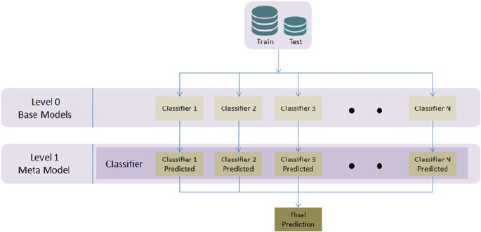
CHAPTER 4 ■ STEP 4 – MODEL DIAGNOSIS AND TUNING
244
Stacking
Wolpert David H presented (in 1992) the concept of stacked generalization, most
commonly known as ‘stacking’ in his publication with the journal Neural Networks. In
stacking initially, you train multiple base models of different types on training/test datasets.
It is ideal to mix models that work differently (kNN, bagging, boosting, etc.) so that it can
learn some part of the problem. At level 1, use the predicted values from base models as
features and train a model that is known as a meta-model, thus combining the learning of
an individual model will result in improved accuracy. This is a simple level 1 stacking, and
similarly you can stack multiple levels of different type of models. See Figure4-14.
Let’s apply the stacking concept discussed above on the diabetes dataset and
compare the accuracy of base vs. meta-model. See Listing 4-20.
Listing 4-20. Model stacking
# Classifiers
from sklearn.ensemble import RandomForestClassifier
from sklearn.ensemble import GradientBoostingClassifier
from sklearn.linear_model import LogisticRegression
from sklearn.neighbors import KNeighborsClassifier
np.random.seed(2017) # seed to shuffle the train set
# read the data in
df = pd.read_csv("Data/Diabetes.csv")
X = df.ix[:,0:8] # independent variables
y = df['class'].values # dependent variables
Figure 4-14. Simple Level 2 stacking model
CHAPTER 4 ■ STEP 4 – MODEL DIAGNOSIS AND TUNING
245
#Normalize
X = StandardScaler().fit_transform(X)
# evaluate the model by splitting into train and test sets
X_train, X_test, y_train, y_test = train_test_split(X, y, test_size=0.2,
random_state=2017)
kfold = cross_validation.StratifiedKFold(y=y_train, n_folds=5, random_state=2017)
num_trees = 10
verbose = True # to print the progress
clfs = [KNeighborsClassifier(),
RandomForestClassifier(n_estimators=num_trees, random_state=2017),
GradientBoostingClassifier(n_estimators=num_trees, random_state=2017)]
#Creating train and test sets for blending
dataset_blend_train = np.zeros((X_train.shape[0], len(clfs)))
dataset_blend_test = np.zeros((X_test.shape[0], len(clfs)))
print('5-fold cross validation:\n')
for i, clf in enumerate(clfs):
scores = cross_validation.cross_val_score(clf, X_train, y_train, cv=kfold,
scoring='accuracy')
print("##### Base Model %0.0f #####" % i)
print("Train CV Accuracy: %0.2f (+/- %0.2f)" % (scores.mean(), scores.std()))
clf.fit(X_train, y_train)
print("Train Accuracy: %0.2f " % (metrics.accuracy_score(clf.predict(X_train),
y_train)))
dataset_blend_train[:,i] = clf.predict_proba(X_train)[:, 1]
dataset_blend_test[:,i] = clf.predict_proba(X_test)[:, 1]
print("Test Accuracy: %0.2f " % (metrics.accuracy_score(clf.predict(X_test),
y_test)))
print "##### Meta Model #####"
clf = LogisticRegression()
scores = cross_validation.cross_val_score(clf, dataset_blend_train, y_train,
cv=kfold, scoring='accuracy')
clf.fit(dataset_blend_train, y_train)
print("Train CV Accuracy: %0.2f (+/- %0.2f)" % (scores.mean(), scores.std()))
print("Train Accuracy: %0.2f " % (metrics.accuracy_score(clf.predict(dataset_blend_
train), y_train)))
print("Test Accuracy: %0.2f " % (metrics.accuracy_score(clf.predict(dataset_
blend_test), y_test)))
#----output----
5-fold cross validation:
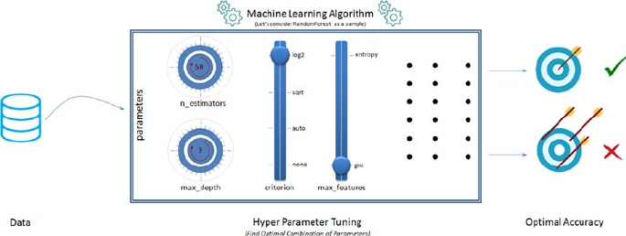
CHAPTER 4 ■ STEP 4 – MODEL DIAGNOSIS AND TUNING
246
##### Base Model 0 #####
Train CV Accuracy: 0.72 (+/- 0.03)
Train Accuracy: 0.82
Test Accuracy: 0.78
##### Base Model 1 #####
Train CV Accuracy: 0.70 (+/- 0.05)
Train Accuracy: 0.98
Test Accuracy: 0.81
##### Base Model 2 #####
Train CV Accuracy: 0.75 (+/- 0.02)
Train Accuracy: 0.79
Test Accuracy: 0.82
##### Meta Model #####
Train CV Accuracy: 0.98 (+/- 0.02)
Train Accuracy: 0.98
Test Accuracy: 0.81
Hyperparameter Tuning
One of the primary objectives and challenges in machine learning process is improving
the performance score, based on data patterns and observed evidence. To achieve this
objective, almost all machine learning algorithms have a specific set of parameters that
needs to estimate from the dataset, which will maximize the performance score. Assume
that these parameters are the knobs that you need to adjust to different values to find the
optimal combination of parameters that give you the best model accuracy. The best way
to choose good hyperparameter is through trial and error of all possible combinations of
parameter values. Scikit-learn provides GridSearchCV and RandomSearchCV functions to
facilitate automatic and reproducible approach for hyperparameter tuning. See Figure4-15.
Figure 4-15. Hyperparameter Tuning
CHAPTER 4 ■ STEP 4 – MODEL DIAGNOSIS AND TUNING
247
GridSearch
For a given model, you can define a set of parameter values that you would like to try.
Then using the GridSearchCV function of scikit-learn, models are built for all possible
combinations of a preset list of values of hyperparameter provided by you, and the best
combination is chosen based on the cross-validation score. There are two disadvantages
associated with GridSearchCV.
1. Computationally expensive: It is then obvious that with more
parameter values the GridSearch will be computationally
expensive. Consider an example where you have 5 parameters
and assume that you would like to try 5 values for each
parameters that will result in 5**5 = 3125 combinations; further
multiply this with number of cross-validation folds being used,
that is, if k-fold is 5 then 3125 * 5 = 15625 model fits.
2. Not perfect optimal but nearly optimal parameters: Grid
Search will look at fixed points that you provide for the
numerical parameters, hence there is a great chance of
missing the optimal point that lies between the fixed points.
For example, assume that you would like to try the fixed points
for ‘n_estimators’: [100, 250, 500, 750, 1000] for a decision
tree model and there is a chance that the optimal point might
lie between the two fixed points; however GridSearch is not
designed to search between fixed points.
Let’s try GridSearchCV for a RandomForest classifier on the Pima diabetes dataset to
find the optimal parameter values. See Listing 4-21.
Listing 4-21. Grid search for hyperparameter tuning
from sklearn.ensemble import RandomForestClassifier
from sklearn.grid_search import GridSearchCV
seed = 2017
# read the data in
df = pd.read_csv("Data/Diabetes.csv")
X = df.ix[:,:8].values # independent variables
y = df['class'].values # dependent variables
#Normalize
X = StandardScaler().fit_transform(X)
# evaluate the model by splitting into train and test sets
X_train, X_test, y_train, y_test = train_test_split(X, y, test_size=0.3,
random_state=seed)
kfold = cross_validation.StratifiedKFold(y=y_train, n_folds=5, random_state=seed)
num_trees = 100
CHAPTER 4 ■ STEP 4 – MODEL DIAGNOSIS AND TUNING
248
clf_rf = RandomForestClassifier(random_state=seed).fit(X_train, y_train)
rf_params = {
'n_estimators': [100, 250, 500, 750, 1000],
'criterion': ['gini', 'entropy'],
'max_features': [None, 'auto', 'sqrt', 'log2'],
'max_depth': [1, 3, 5, 7, 9]
}
# setting verbose = 10 will print the progress for every 10 task completion
grid = GridSearchCV(clf_rf, rf_params, scoring='roc_auc', cv=kfold,
verbose=10, n_jobs=-1)
grid.fit(X_train, y_train)
print 'Best Parameters: ', grid.best_params_
results = cross_validation.cross_val_score(grid.best_estimator_, X_train,y_
train, cv=kfold)
print "Accuracy - Train CV: ", results.mean()
print "Accuracy - Train : ", metrics.accuracy_score(grid.best_estimator_.
predict(X_train), y_train)
print "Accuracy - Test : ", metrics.accuracy_score(grid.best_estimator_.
predict(X_test), y_test)
#----output----
Fitting 5 folds for each of 200 candidates, totalling 1000 fits
Best Parameters: {'max_features': 'log2', 'n_estimators': 500, 'criterion':
'entropy', 'max_depth': 5}
Accuracy - Train CV: 0.744790584978
Accuracy - Train : 0.862197392924
Accuracy - Test : 0.796536796537
RandomSearch
As the name suggests the RandomSearch algorithm tries random combinations of a range
of values of given parameters. The numerical parameters can be specified as a range
(unlike fixed values in GridSearch). You can control the number of iterations of random
searches that you would like to perform. It is known to find a very good combination in a
lot less time compared to GridSearch; however you have to carefully choose the range for
parameters and the number of random search iteration as it can miss the best parameter
combination with lesser iterations or smaller ranges.
Let’s try the RandomSearchCV for same combination that we tried for GridSearch
and compare the time / accuracy. See Listing 4-22.
CHAPTER 4 ■ STEP 4 – MODEL DIAGNOSIS AND TUNING
249
Listing 4-22. Random search for hyperparameter tuning
from sklearn.model_selection import RandomizedSearchCV
from scipy.stats import randint as sp_randint
# specify parameters and distributions to sample from
param_dist = {'n_estimators':sp_randint(100,1000),
'criterion': ['gini', 'entropy'],
'max_features': [None, 'auto', 'sqrt', 'log2'],
'max_depth': [None, 1, 3, 5, 7, 9]
}
# run randomized search
n_iter_search = 20
random_search = RandomizedSearchCV(clf_rf, param_distributions=param_dist, cv=kfold,
n_iter=n_iter_search, verbose=10, n_
jobs=-1, random_state=seed)
random_search.fit(X_train, y_train)
# report(random_search.cv_results_)
print 'Best Parameters: ', random_search.best_params_
results = cross_validation.cross_val_score(random_search.best_estimator_,
X_train,y_train, cv=kfold)
print "Accuracy - Train CV: ", results.mean()
print "Accuracy - Train : ", metrics.accuracy_score(random_search.best_
estimator_.predict(X_train), y_train)
print "Accuracy - Test : ", metrics.accuracy_score(random_search.best_
estimator_.predict(X_test), y_test)
#----output----
Fitting 5 folds for each of 20 candidates, totalling 100 fits
Best Parameters: {'max_features': None, 'n_estimators': 694, 'criterion':
'entropy', 'max_depth': 3}
Accuracy - Train CV: 0.75424022153
Accuracy - Train : 0.780260707635
Accuracy - Test : 0.805194805195
Notice that in this case, with RandomSearchCV we were able to achieve comparable
accuracy results with 100 fits to that of a GridSearchCV’s 1000 fit.
Figure4-16 is a sample illustration of how grid search vs. random search results differ
(it’s not the actual representation) between two parameters. Assume that the optimal
area for max_depth lies between 3 and 5 (blue shade) and for n_estimators it lies between
500 and 700 (amber shade). The ideal optimal value for combined parameters would lie
where the individual regions intersect. Both methods will be able to find a nearly optimal
parameter and not necessarily the perfect optimal point.
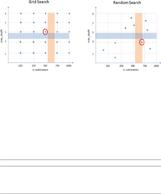
CHAPTER 4 ■ STEP 4 – MODEL DIAGNOSIS AND TUNING
250
Endnotes
In this step, we have learned various common issues that can hinder the model accuracy
such as not choosing the optimal probability cutoff point for class creation, variance,
and bias. We also briefly looked at different model tuning techniques practiced such as
bagging, boosting, ensemble voting, and grid search/random search for hyperparameter
tuning. To be concise we only looked at the most important aspect for each of the topics
discussed above to get you started. However there are more options for each of the
algorithms for tuning and each of these techniques have been evolving at a fast phase. So
I encourage you to keep an eye on their respective officially hosted webpage and github
repository. See Table4-2.
We have reached the end of step 4, which means you’re half way through your
machine learning journey. In the next chapter we’ll learn text mining techniques and
fundamentals of the recommender system.
Figure 4-16. Grid Search vs. Random Search
Table 4-2. Additional resources
Name Web Page Github Repository
Scikit-learn http://scikit-learn.org/stable/# https://github.com/scikit-
learn/scikit-learn
Xgboost https://xgboost.readthedocs.io/
en/latest/
https://github.com/dmlc/
xgboost

251
© Manohar Swamynathan 2017
M. Swamynathan, Mastering Machine Learning with Python in Six Steps,
DOI 10.1007/978-1-4842-2866-1_5
CHAPTER 5
Step 5 – Text Mining and
Recommender Systems
One of the key areas of artificial intelligence is Natural Language Processing (NLP) or
text mining as it is generally known that deals with teaching computers how to extract
meaning from text. Over the last two decades, with the explosion of the Internet world
and rise of social media, there is plenty of valuable data being generated in the form of
text. The process of unearthing meaningful patterns from text data is called Text Mining.
In this chapter you’ll learn the high-level text mining process overview, key concepts, and
common techniques involved.
Apart from scikit-learn, there is a number of established NLP-focused libraries
available for Python, and the number has been growing over time. Refer to Table5-1 for
the most popular libraries based on their number of contributors as of 2016.
Table 5-1. Python popular text mining libraries
Package
Name
# of contributors
(2016)
License Description
NLTK 187 Apache It’s the most popular and widely
used toolkit predominantly built to
support research and development
of NLP.
Gensim 154 LGPL-2 Mainly built for large corpus topic
modeling, document indexing, and
similarity retrieval.,
spaCy 68 MIT Built using Python + Cython for
efficient production implementation
of NLP concepts.
(continued)
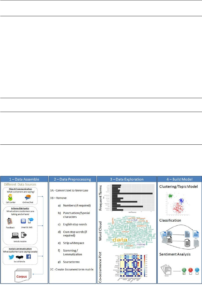
CHAPTER 5 ■ STEP 5 – TEXT MINING AND RECOMMENDER SYSTEMS
252
■Note Another well-known library is Stanford CoreNLP, a suite of the Java-based toolkit.
There are number of Python wrappers available for the same; however, the number of
contributors for these wrappers is on the lower side as of now.
Text Mining Process Overview
Package
Name
# of contributors
(2016)
License Description
Pattern 20 BSD-3 It’s a web mining module for Python
with capabilities included for
scraping, NLP, machine learning and
network analysis/visualization.
Polyglot 13 GPL-3 This is a multilingual text processing
toolkit and supports massive
multilingual applications.
Textblob 11 MIT It’s a wrapper around NLTK and
Pattern libraries for easy accessibility
of their capabilities. Suitable for fast
prototyping.
Table 5-1. (contiuned)
Figure 5-1. Text Mining Process Overview

CHAPTER 5 ■ STEP 5 – TEXT MINING AND RECOMMENDER SYSTEMS
253
The overall text mining process can be broadly categorized into four phases.
1. Text Data Assemble
2. Text Data Preprocessing
3. Data Exploration or Visualization
4. Model Building
Data Assemble (Text)
It is observed that 70% of data available to any business is unstructured. The first step is
collating unstructured data from different sources such as open-ended feedback, phone
calls, email support, online chat and social media networks like Twitter, LinkedIn, and
Facebook. Assembling these data and applying mining/machine learning techniques to
analyze them provides valuable opportunities for organizations to build more power into
customer experience.
There are several libraries available for extracting text content from different formats
discussed above. By far the best library that provides a simple and single interface for
multiple formats is ‘textract’ (open source MIT license). Note that as of now this library/
package is available for Linux, Mac OS but not Windows. Table5-2 shows a list of
supported formats.
Table 5-2. textract supported formats
Format Supported Via Additional Info
.csv / .eml / .json
/ .odt / .txt /
Python built-ins
.doc Antiword http://www.winfield.demon.nl/
.docx Python-docx https://python-docx.readthedocs.io/en/
latest/
.epub Ebooklib https://github.com/aerkalov/ebooklib
.gif / .jpg / .jpeg /
.png / .tiff / .tif
tesseract-ocr https://github.com/tesseract-ocr
.html / .htm Beautifulsoup4 http://beautiful-soup-4.readthedocs.
io/en/latest/
.mp3 / .ogg / .wav SpeechRecongnition
and sox
URL 1: https://pypi.python.org/pypi/
SpeechRecognition/
URL 2: http://sox.sourceforge.net/
.msg msg-extractor https://github.com/mattgwwalker/msg-
extractor
(continued)

CHAPTER 5 ■ STEP 5 – TEXT MINING AND RECOMMENDER SYSTEMS
254
Let’s look at the code for the most widespread formats in the business world: pdf, jpg,
and audio file. Note that extracting text from other formats is also relatively simple. See
Listing 5-1.
Listing 5-1. Example code for extracting data from pdf, jpg, audio
# You can read/learn more about latest updates about textract on their
official documents site at http://textract.readthedocs.io/en/latest/
import textract
# Extracting text from normal pdf
text = textract.process('Data/PDF/raw_text.pdf', language='eng')
# Extracting text from two columned pdf
text = textract.process('Data/PDF/two_column.pdf', language='eng')
# Extracting text from scanned text pdf
text = textract.process('Data/PDF/ocr_text.pdf', method='tesseract',
language='eng')
# Extracting text from jpg
text = textract.process('Data/jpg/raw_text.jpg', method='tesseract',
language='eng')
# Extracting text from audio file
text = textract.process('Data/wav/raw_text.wav', language='eng')
Format Supported Via Additional Info
.pdf pdftotext and
pdfminer.six
URL 1: https://poppler.freedesktop.org/
URL 2: https://github.com/pdfminer/
pdfminer.six
.pptx Python-pptx https://python-pptx.readthedocs.io/en/
latest/
.ps ps2text http://pages.cs.wisc.edu/~ghost/doc/
pstotext.htm
.rtf Unrtf http://www.gnu.org/software/unrtf/
.xlsx / .xls Xlrd https://pypi.python.org/pypi/xlrd
Table 5-2. (contiuned)
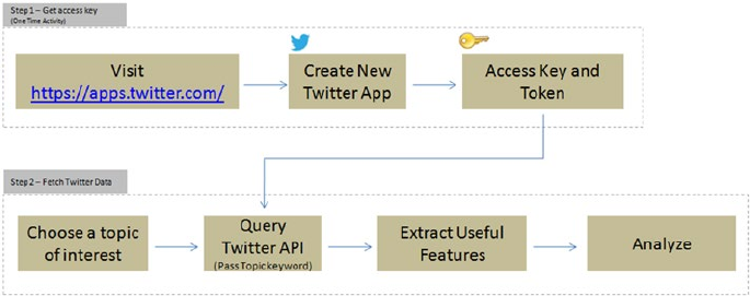
CHAPTER 5 ■ STEP 5 – TEXT MINING AND RECOMMENDER SYSTEMS
255
Social Media
Did you know that Twitter, the online news and social networking service provider, has
320 million users, with an average of 42 million active tweets every day! (Source: Global
social media research summary 2016 by smartinsights).
Let’s understand how to explore the rich information of social media (I’ll consider
Twitter as an example) to explore what is being spoken about a chosen topic. Most of
these forums provide API for developers to access the posts. See Figure5-2.
Figure 5-2. Pulling Twitter posts for analysis
Step 1 – Get Access Key (One-Time Activity)
Follow the below steps to set up a new Twitter app to get consumer/access key, secret,
and token (do not share the key token with unauthorized persons).
• Go to https://apps.twitter.com/
• Click on ‘Create New App’
• Fill the required information and click on ‘Create your Twitter
Application’
• You’ll get the access details under ‘Keys and Access Tokens’ tab
Step 2 – Fetching Tweets
Once you have the authorization secret and access tokens, you can use the below code in
Listing 5-2 to establish the connection.
Listing 5-2. Twitter authentication
#Import the necessary methods from tweepy library
import tweepy
from tweepy.streaming import StreamListener

CHAPTER 5 ■ STEP 5 – TEXT MINING AND RECOMMENDER SYSTEMS
256
from tweepy import OAuthHandler
from tweepy import Stream
#provide your access details below
access_token = "Your token goes here"
access_token_secret = "Your token secret goes here"
consumer_key = "Your consumer key goes here"
consumer_secret = "Your consumer secret goes here"
# establish a connection
auth = tweepy.auth.OAuthHandler(consumer_key, consumer_secret)
auth.set_access_token(access_token, access_token_secret)
api = tweepy.API(auth)
Let’s assume that you would like to understand what is being said about the iPhone 7
and its camera feature. So let’s pull the most recent 10 posts.
■Note You can pull historic user posts about a topic for a max of 10 to 15 days only,
depending on the volume of the posts.
#fetch recent 10 tweets containing words iphone7, camera
fetched_tweets = api.search(q=['iPhone 7','iPhone7','camera'], result_
type='recent', lang='en', count=10)
print “Number of tweets: ”,len(fetched_tweets)
#----output----
Number of tweets: 10
# Print the tweet text
for tweet in fetched_tweets:
print 'Tweet ID: ', tweet.id
print 'Tweet Text: ', tweet.text, '\n'
#----output----
Tweet ID: 825155021390049281
Tweet Text: RT @volcanojulie: A Tau Emerald dragonfly. The iPhone 7 camera
is exceptional!
#nature #insect #dragonfly #melbourne #australia #iphone7 #...
Tweet ID: 825086303318507520
Tweet Text: Fuzzy photos? Protect your camera lens instantly with #iPhone7
Full Metallic Case. Buy now! https://t.co/d0dX40BHL6 https://t.co/AInlBoreht
CHAPTER 5 ■ STEP 5 – TEXT MINING AND RECOMMENDER SYSTEMS
257
You can capture useful features onto a dataframe for further analysis. See Listing 5-3.
Listing 5-3. Save features to dataframe
# function to save required basic tweets info to a dataframe
def populate_tweet_df(tweets):
#Create an empty dataframe
df = pd.DataFrame()
df['id'] = list(map(lambda tweet: tweet.id, tweets))
df['text'] = list(map(lambda tweet: tweet.text, tweets))
df['retweeted'] = list(map(lambda tweet: tweet.retweeted, tweets))
df['place'] = list(map(lambda tweet: tweet.user.location, tweets))
df['screen_name'] = list(map(lambda tweet: tweet.user.screen_name,
tweets))
df['verified_user'] = list(map(lambda tweet: tweet.user.verified,
tweets))
df['followers_count'] = list(map(lambda tweet: tweet.user.followers_
count, tweets))
df['friends_count'] = list(map(lambda tweet: tweet.user.friends_count,
tweets))
# Highly popular user's tweet could possibly seen by large audience, so
lets check the popularity of user
df['friendship_coeff'] = list(map(lambda tweet: float(tweet.user.
followers_count)/float(tweet.user.friends_count), tweets))
return df
df = populate_tweet_df(fetched_tweets)
print df.head(10)
#---output----
id text
0 825155021390049281 RT @volcanojulie: A Tau Emerald dragonfly. The...
1 825086303318507520 Fuzzy photos? Protect your camera lens instant...
2 825064476714098690 RT @volcanojulie: A Tau Emerald dragonfly. The...
3 825062644986023936 RT @volcanojulie: A Tau Emerald dragonfly. The...
4 824935025217040385 RT @volcanojulie: A Tau Emerald dragonfly. The...
5 824933631365779458 A Tau Emerald dragonfly. The iPhone 7 camera i...
6 824836880491483136 The camera on the IPhone 7 plus is fucking awe...
7 823805101999390720 'Romeo and Juliet' Ad Showcases Apple's iPhone...
8 823804251117850624 iPhone 7 Images Show Bigger Camera Lens - I ha...
9 823689306376196096 RT @computerworks5: Premium HD Selfie Stick &a...
CHAPTER 5 ■ STEP 5 – TEXT MINING AND RECOMMENDER SYSTEMS
258
retweeted place screen_name verified_user
0 False Melbourne, Victoria MonashEAE False
1 False California, USA ShopNCURV False
2 False West Islip, Long Island, NY FusionWestIslip False
3 False 6676 Fresh Pond Rd Queens, NY FusionRidgewood False
4 False Iphone7review False
5 False Melbourne; Monash University volcanojulie False
6 False Hollywood, FL Hbk_Mannyp False
7 False Toronto.NYC.the Universe AaronRFernandes False
8 False Lagos, Nigeria moyinoluwa_mm False
9 False Iphone7review False
followers_count friends_count friendship_coeff
0 322 388 0.829897
1 279 318 0.877358
2 13 193 0.067358
3 45 218 0.206422
4 199 1787 0.111360
5 398 551 0.722323
6 57 64 0.890625
7 18291 7 2613.000000
8 780 302 2.582781
9 199 1787 0.111360
Instead of a topic you can also choose a screen_name focused on a topic; let’s look at
the posts by the screen name Iphone7review. See Listing 5-4.
Listing 5-4. Example code for extracting tweets based on screen name
# For help about api look here http://tweepy.readthedocs.org/en/v2.3.0/api.
html
fetched_tweets = api.user_timeline(id='Iphone7review', count=5)
# Print the tweet text
for tweet in fetched_tweets:
print 'Tweet ID: ', tweet.id
print 'Tweet Text: ', tweet.text, '\n'
#----output----
Tweet ID: 825169063676608512
Tweet Text: RT @alicesttu: iPhone 7S to get Samsung OLED display next year
#iPhone https://t.co/BylKbvXgAG #iphone
Tweet ID: 825169047138533376
Tweet Text: Nothing beats the Iphone7! Who agrees? #Iphone7 https://t.co/
e03tXeLOao
Glancing through the posts quickly can generally help you conclude that there are
positive comments about the camera feature of iPhone 7.
CHAPTER 5 ■ STEP 5 – TEXT MINING AND RECOMMENDER SYSTEMS
259
Data Preprocessing (Text)
This step deals with cleansing the consolidated text to remove noise to ensure efficient
syntactic, semantic text analysis for deriving meaningful insights from text. Some
common cleaning steps are briefed below.
Convert to Lower Case and Tokenize
Here, all the data is converted into lowercase. This is carried out to prevent words like
“LIKE” or “Like” being interpreted as different words. Python provides a function lower()
to convert text to lowercase.
Tokenizing is the process of breaking a large set of texts into smaller meaningful
chunks such as sentences, words, and phrases.
Sentence Tokenizing
The NLTK library provides a sent_tokenize for sentence-level tokenizing, which uses a
pre-trained model PunktSentenceTokenize, to determine punctuation and characters
marking the end of sentence for European languages. See Listing 5-5.
Listing 5-5. Example code for sentence tokenization
import nltk
from nltk.tokenize import sent_tokenize
text='Statistics skills, and programming skills are equally important
for analytics. Statistics skills, and domain knowledge are important for
analytics. I like reading books and travelling.'
sent_tokenize_list = sent_tokenize(text)
print(sent_tokenize_list)
#----output----
['Statistics skills, and programming skills are equally important for
analytics.', 'Statistics skills, and domain knowledge are important for
analytics.', 'I like reading books and travelling.']
There are a total of 17 European languages that NLTK supports for sentence
tokenization. You can load the tokenized model for specific language saved as a pickle file
as part of nltk.data. see Listing 5-6.
Listing 5-6. Sentence tokenization for European languages
import nltk.data
spanish_tokenizer = nltk.data.load('tokenizers/punkt/spanish.pickle')
spanish_tokenizer.tokenize('Hola. Esta es una frase espanola.')
#----output----
['Hola.', 'Esta es una frase espanola.']
CHAPTER 5 ■ STEP 5 – TEXT MINING AND RECOMMENDER SYSTEMS
260
Word Tokenizing
The word_tokenize function of NLTK is a wrapper function that calls tokenize by the
TreebankWordTokenizer. See Listing 5-7.
Listing 5-7. Example code for word tokenizing
from nltk.tokenize import word_tokenize
print word_tokenize(text)
# Another equivalent call method using TreebankWordTokenizer
from nltk.tokenize import TreebankWordTokenizer
tokenizer = TreebankWordTokenizer()
print tokenizer.tokenize(text)
#----output----
[‘Statistics’, ‘skills’, ‘ , ’, ‘and’, ‘programming’, ‘skills’, ‘are’, ‘equally’, ‘important’, ‘for’,
‘analytics’, ‘ . ’, ‘Statistics’, ‘skills’, ‘ , ’, ‘and’, ‘domain’, ‘knowledge’, ‘are’, ‘important’, ‘for’,
‘analytics’, ‘ . ‘, ‘I’, ‘like’, ‘reading’, ‘books’, ‘and’, ‘travelling’, ‘ . ’]
Removing Noise
You should remove all information that is not comparative or relevant to text analytics.
These can be seen as noise to the text analytics. Most common noises are numbers,
punctuations, stop words, white space, etc
Numbers: Numbers are removed as they may not be relevant and not hold valuable
information. See Listing 5-8.
Listing 5-8. Example code for removing noise from text
def remove_numbers(text):
return re.sub(r'\d+', '', text)
text = 'This is a sample English sentence, \n with whitespace and numbers 1234!'
print 'Removed numbers: ', remove_numbers(text)
#----output----
Removed numbers: This is a sample English sentence,
with whitespace and numbers !
Punctuation: It is to be removed for better identifying each word and remove
punctuation characters from the dataset. For example “like” and “like” or “coca-cola” and
“cocacola” would be interpreted as different words if the punctuation was not removed.
See Listing 5-9.

CHAPTER 5 ■ STEP 5 – TEXT MINING AND RECOMMENDER SYSTEMS
261
Listing 5-9. Example code for removing punctuation from text
import string
# Function to remove punctuations
def remove_punctuations(text):
words = nltk.word_tokenize(text)
punt_removed = [w for w in words if w.lower() not in string.punctuation]
return " ".join(punt_removed)
print remove_punctuations('This is a sample English sentence, with punctuations!')
#----output----
This is a sample English sentence with punctuations
Stop words: Words like “the,” “and,” “or” are uninformative and add unneeded noise
to the analysis. For this reason they are removed. See Listing 5-10.
Listing 5-10. Example code for removing stop words from text
from nltk.corpus import stopwords
# Function to remove stop words
def remove_stopwords(text, lang='english'):
words = nltk.word_tokenize(text)
lang_stopwords = stopwords.words(lang)
stopwords_removed = [w for w in words if w.lower() not in lang_stopwords]
return " ".join(stopwords_removed)
print remove_stopwords('This is a sample English sentence')
#----output----
sample English sentence
■Note Remove own stop words (if required) – Certain words could be very commonly
used in a particular domain. Along with English stop words, we could instead, or in addition,
remove our own stop words. The choice of our own stop word might depend on the domain
of discourse and might not become apparent until we’ve done some analysis.
Whitespace: Often in text analytics, an extra whitespace (space, tab, Carriage Return,
Line Feed) becomes identified as a word. This anomaly is avoided through a basic
programming procedure in this step. See Listing 5-11.

CHAPTER 5 ■ STEP 5 – TEXT MINING AND RECOMMENDER SYSTEMS
262
Listing 5-11. Example code for removing whitespace from text
# Function to remove whitespace
def remove_whitespace(text):
return " ".join(text.split())
text = 'This is a sample English sentence, \n with whitespace and
numbers 1234!'
print 'Removed whitespace: ', remove_whitespace(text)
#----output----
Removed whitespace: This is a sample English sentence, with whitespace and
numbers 1234!
Part of Speech (PoS) Tagging
PoS tagging is the process of assigning language-specific parts of speech such as nouns,
verbs, adjectives, and adverbs, etc., for each word in the given text.
NLTK supports multiple PoS tagging models, and the default tagger is maxent_
treebank_pos_tagger, which uses Penn (Pennsylvania University) Tree bank corpus. The
same has 36 possible parts of speech tags, a sentence (S) is represented by the parser as a
tree having three children: a noun phrase (NP), a verbal phrase (VP), and the full stop (.).
The root of the tree will be S. See Table5-3 and Listings 5-12 and 5-13.
Table 5-3. NLTK PoS taggers
PoS Tagger Short Description
maxent_treebank_pos_tagger It’s based on Maximum Entropy (ME) classification
principles trained on Wall Street Journal subset of the
Penn Tree bank corpus.
BrillTagger Brill’s transformational rule-based tagger.
CRFTagger Conditional Random Fields.
HiddenMarkovModelTagger Hidden Markov Models (HMMs) largely used to assign
the correct label sequence to sequential data or assess
the probability of a given label and data sequence.
HunposTagge A module for interfacing with the HunPos open source
POS-tagger.
PerceptronTagger Based on averaged perceptron technique proposed by
Matthew Honnibal.
SennaTagger Semantic/syntactic Extraction using a Neural Network
Architecture.
SequentialBackoffTagger Classes for tagging sentences sequentially, left to right.
StanfordPOSTagger Researched and developed at Stanford University.
TnT Implementation of ‘TnT - A Statistical Part of Speech
Tagger’ by Thorsten Brants.
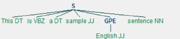
CHAPTER 5 ■ STEP 5 – TEXT MINING AND RECOMMENDER SYSTEMS
263
Listing 5-12. Example code for PoS, the sentence, and visualize sentence tree
from nltk import chunk
tagged_sent = nltk.pos_tag(nltk.word_tokenize('This is a sample English sentence'))
print tagged_sent
tree = chunk.ne_chunk(tagged_sent)
tree.draw() # this will draw the sentence tree
#----output----
[('This', 'DT'), ('is', 'VBZ'), ('a', 'DT'), ('sample', 'JJ'), ('English', 'JJ'),
('sentence', 'NN')]
Listing 5-13. Example code for using perceptron tagger and getting help on tags
# To use PerceptronTagger
from nltk.tag.perceptron import PerceptronTagger
PT = PerceptronTagger()
print PT.tag('This is a sample English sentence'.split())
#----output----
[('This', 'DT'), ('is', 'VBZ'), ('a', 'DT'), ('sample', 'JJ'), ('English', 'JJ'),
('sentence', 'NN')]
# To get help about tags
nltk.help.upenn_tagset('NNP')
#----output----
NNP: noun, proper, singular
Stemming
It is the process of transforming to the root word, that is, it uses an algorithm that removes
common word endings from English words, such as “ly,” “es,” “ed,” and “s.” For example,
assuming for an analysis you may want to consider “carefully,” “cared,” “cares,” “caringly”
as “care” instead of separate words. There are three widely used stemming algorithms as
listed in Figure5-3. See Listing 5-14.
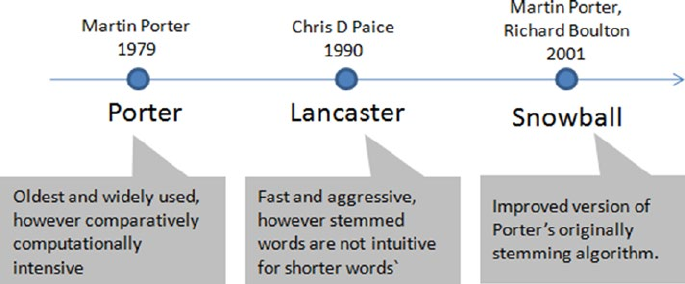
CHAPTER 5 ■ STEP 5 – TEXT MINING AND RECOMMENDER SYSTEMS
264
Listing 5-14. Example code for stemming
from nltk import PorterStemmer, LancasterStemmer, SnowballStemmer
# Function to apply stemming to a list of words
def words_stemmer(words, type="PorterStemmer", lang="english", encoding="utf8"):
supported_stemmers = ["PorterStemmer","LancasterStemmer","SnowballStemmer"]
if type is False or type not in supported_stemmers:
return words
else:
stem_words = []
if type == "PorterStemmer":
stemmer = PorterStemmer()
for word in words:
stem_words.append(stemmer.stem(word).encode(encoding))
if type == "LancasterStemmer":
stemmer = LancasterStemmer()
for word in words:
stem_words.append(stemmer.stem(word).encode(encoding))
if type == "SnowballStemmer":
stemmer = SnowballStemmer(lang)
for word in words:
stem_words.append(stemmer.stem(word).encode(encoding))
return " ".join(stem_words)
words = 'caring cares cared caringly carefully'
print "Original: ", words
print "Porter: ", words_stemmer(nltk.word_tokenize(words), "PorterStemmer")
print "Lancaster: ", words_stemmer(nltk.word_tokenize(words), "LancasterStemmer")
print "Snowball: ", words_stemmer(nltk.word_tokenize(words), "SnowballStemmer")
#----output----
Figure 5-3. Most popular NLTK stemmers
CHAPTER 5 ■ STEP 5 – TEXT MINING AND RECOMMENDER SYSTEMS
265
Original: caring cares cared caringly carefully
Porter: care care care caringli care
Lancaster: car car car car car
Snowball: care care care care care
Lemmatization
It is the process of transforming to the dictionary base form. For this you can use
WordNet, which is a large lexical database for English words that are linked together by
their semantic relationships. It works as a thesaurus, that is, it groups words together
based on their meanings. See Listing 5-15.
Listing 5-15. Example code for lemmatization
from nltk.stem import WordNetLemmatizer
wordnet_lemmatizer = WordNetLemmatizer()
# Function to apply lemmatization to a list of words
def words_lemmatizer(text, encoding="utf8"):
words = nltk.word_tokenize(text)
lemma_words = []
wl = WordNetLemmatizer()
for word in words:
pos = find_pos(word)
lemma_words.append(wl.lemmatize(word, pos).encode(encoding))
return " ".join(lemma_words)
# Function to find part of speech tag for a word
def find_pos(word):
# Part of Speech constants
# ADJ, ADJ_SAT, ADV, NOUN, VERB = 'a', 's', 'r', 'n', 'v'
# You can learn more about these at http://wordnet.princeton.edu/
wordnet/man/wndb.5WN.html#sect3
# You can learn more about all the penn tree tags at https://www.ling.
upenn.edu/courses/Fall_2003/ling001/penn_treebank_pos.html
pos = nltk.pos_tag(nltk.word_tokenize(word))[0][1]
# Adjective tags - 'JJ', 'JJR', 'JJS'
if pos.lower()[0] == 'j':
return 'a'
# Adverb tags - 'RB', 'RBR', 'RBS'
elif pos.lower()[0] == 'r':
return 'r'
# Verb tags - 'VB', 'VBD', 'VBG', 'VBN', 'VBP', 'VBZ'
elif pos.lower()[0] == 'v':
return 'v'
CHAPTER 5 ■ STEP 5 – TEXT MINING AND RECOMMENDER SYSTEMS
266
# Noun tags - 'NN', 'NNS', 'NNP', 'NNPS'
else:
return 'n'
print "Lemmatized: ", words_lemmatizer(words)
#----output----
Lemmatized: care care care caringly carefully
In the above case,‘caringly’/’carefully’ are inflected form of care and they
are an entry word listed in WordNet Dictoinary so they are retained in their
actual form itself.
NLTK English WordNet includes approximately 155,287 words and 117000 synonym
sets. For a given word, WordNet includes/provides definition, example, synonyms (group
of nouns, adjectives, verbs that are similar), atonyms (opposite in meaning to another),
etc. See Listing 5-16.
Listing 5-16. Example code for wordnet
from nltk.corpus import wordnet
syns = wordnet.synsets("good")
print "Definition: ", syns[0].definition()
print "Example: ", syns[0].examples()
synonyms = []
antonyms = []
# Print synonums and antonyms (having opposite meaning words)
for syn in wordnet.synsets("good"):
for l in syn.lemmas():
synonyms.append(l.name())
if l.antonyms():
antonyms.append(l.antonyms()[0].name())
print "synonyms: \n", set(synonyms)
print "antonyms: \n", set(antonyms)
#----output----
Definition: benefit
Example: [u'for your own good', u"what's the good of worrying?"]
synonyms:
set([u'beneficial', u'right', u'secure', u'just', u'unspoilt', u'respectable',
u'good', u'goodness', u'dear', u'salutary', u'ripe', u'expert', u'skillful',
u'in_force', u'proficient', u'unspoiled', u'dependable', u'soundly',
u'honorable', u'full', u'undecomposed', u'safe', u'adept', u'upright',
u'trade_good', u'sound', u'in_effect', u'practiced', u'effective',
u'commodity', u'estimable', u'well', u'honest', u'near', u'skilful',
u'thoroughly', u'serious'])
antonyms:
set([u'bad', u'badness', u'ill', u'evil', u'evilness'])

CHAPTER 5 ■ STEP 5 – TEXT MINING AND RECOMMENDER SYSTEMS
267
N-grams
One of the important concepts in text mining is n-grams, which are fundamentally a set of
co-occurring or continuous sequence of n items from a given sequence of large text. The
item here could be words, letters, and syllables. Let’s consider a sample sentence and try
to extract n-grams for different values of n. See Listing 5-17.
Listing 5-17. Example code for extracting n-grams from sentence
from nltk.util import ngrams
from collections import Counter
# Function to extract n-grams from text
def get_ngrams(text, n):
n_grams = ngrams(nltk.word_tokenize(text), n)
return [ ' '.join(grams) for grams in n_grams]
text = 'This is a sample English sentence'
print "1-gram: ", get_ngrams(text, 1)
print "2-gram: ", get_ngrams(text, 2)
print "3-gram: ", get_ngrams(text, 3)
print "4-gram: ", get_ngrams(text, 4)
#----output----
1-gram:['This', 'is', 'a', 'sample', 'English', 'sentence']
2-gram:['This is', 'is a', 'a sample', 'sample English', 'English sentence']
3-gram:['This is a', 'is a sample', 'a sample English', 'sample English sentence']
4-gram: ['This is a sample', 'is a sample English', 'a sample English sentence']
■Note 1-gram is also called as unigram, 2-gram, and 3-gram as bigram and trigram,
respectively.
The N-gram technique is relatively simple and simply increasing the value of n will
give us more contexts. It is widely used in the probabilistic language model of predicting
the next item in a sequence: for example, search engines use this technique to predict/
recommend the possibility of next character/words in the sequence to users as they type.
See Listing 5-18.
CHAPTER 5 ■ STEP 5 – TEXT MINING AND RECOMMENDER SYSTEMS
268
Listing 5-18. Example code for extracting 2-grams from sentence and store it in a dataframe
text = 'Statistics skills, and programming skills are equally important for
analytics. Statistics skills, and domain knowledge are important for analytics'
# remove punctuations
text = remove_punctuations(text)
# Extracting bigrams
result = get_ngrams(text,2)
# Counting bigrams
result_count = Counter(result)
# Converting to the result to a data frame
import pandas as pd
df = pd.DataFrame.from_dict(result_count, orient='index')
df = df.rename(columns={'index':'words', 0:'frequency'}) # Renaming index
and column name
print df
#----output----
frequency
are equally 1
domain knowledge 1
skills are 1
knowledge are 1
programming skills 1
are important 1
skills and 2
for analytics 2
and domain 1
important for 2
and programming 1
Statistics skills 2
equally important 1
analytics Statistics 1
Bag of Words (BoW)
The texts have to be represented as numbers to be able to apply any algorithms. Bag of
words is the method where you count the occurrence of words in a document without
giving importance to the grammar and the order of words. This can be achieved by
creating Term Document Matrix (TDM). It is simply a matrix with terms as the rows
and document names as the columns and a count of the frequency of words as the
cells of the matrix. Let’s learn about creating DTM through an example; consider three
text documents with some text in it. Sklearn provides good functions under feature_
extraction.text to convert a collection of text documents to a matrix of word counts. See
Listing 5-19 and Figure5-4.
CHAPTER 5 ■ STEP 5 – TEXT MINING AND RECOMMENDER SYSTEMS
269
Listing 5-19. Creating document term matrix from corpus of sample documents
import os
import pandas as pd
from sklearn.feature_extraction.text import CountVectorizer
# Function to create a dictionary with key as file names and values as text
for all files in a given folder
def CorpusFromDir(dir_path):
result = dict(docs = [open(os.path.join(dir_path,f)).read() for f in
os.listdir(dir_path)],
ColNames = map(lambda x: x, os.listdir(dir_path)))
return result
docs = CorpusFromDir('Data/')
# Initialize
vectorizer = CountVectorizer()
doc_vec = vectorizer.fit_transform(docs.get('docs'))
#create dataFrame
df = pd.DataFrame(doc_vec.toarray().transpose(), index = vectorizer.get_
feature_names())
# Change column headers to be file names
df.columns = docs.get('ColNames')
print df
#----output----
Doc_1.txt Doc_2.txt Doc_3.txt
analytics 1 1 0
and 1 1 1
are 1 1 0
books 0 0 1
domain 0 1 0
equally 1 0 0
for 1 1 0
important 1 1 0
knowledge 0 1 0
like 0 0 1
programming 1 0 0
reading 0 0 1
skills 2 1 0
statistics 1 1 0
travelling 0 0 1
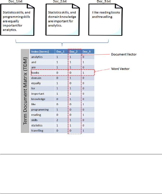
CHAPTER 5 ■ STEP 5 – TEXT MINING AND RECOMMENDER SYSTEMS
270
■Note Document Term Matrix (DTM) is the transpose of Term Document Matrix. In DTM
the rows will be the document names and column headers will be the terms. Both are in the
matrix format and useful for carrying out analysis; however TDM is commonly used due to
the fact that the number of terms tends to be way larger than the document count. In this
case having more rows is better than having a large number of columns.
Term Frequency-Inverse Document Frequency (TF-IDF)
In the area of information retrieval, TF-IDF is a good statistical measure to reflect the
relevance of the term to the document in a collection of documents or corpus. Let’s break
TF_IDF and apply an example to understand it better. See Listing 5-20.
Figure 5-4. Document Term Matrix

CHAPTER 5 ■ STEP 5 – TEXT MINING AND RECOMMENDER SYSTEMS
271
Term frequency will tell you how frequently a given term appears.
TF term
()
=Number of timestermappearsinadocument
Totalnumberoft
eerms in thedocument
For example, consider a document containing 100 words wherein the word ‘ML’
appears 3 times, then TF (ML) = 3 / 100 =0.03
Document frequency will tell you how important a term is?
DF term
()
=
()
dnumberofdocuments containing agiven term
Dthe size offthe collection of documents
()
Assume we have 10 million documents and the word ML appears in one thousand of
these, then DF (ML) = 1000/10,000,000 = 0.0001
To normalize let’s take a log (d/D), that is, log (0.0001) = -4
Quite often D > d and log (d/D) will give a negative value as seen in the above
example. So to solve this problem let’s invert the ratio inside the log expression, which is
known as Inverse document frequency (IDF). Essentially we are compressing the scale of
values so that very large or very small quantities are smoothly compared.
IDFterm
()
=logTotalnumberofdocuments
Number of documentswithagiiven term in it
æ
è
çö
ø
÷
Continuing with the above example, IDF(ML) = log(10,000,000 / 1,000) = 4
TF-IDF is the weight product of quantities, that is, for the above example TF-IDF
(ML) = 0.03 * 4 = 0.12
sklearn provides provides a function TfidfVectorizer to calculate TF-
IDF for text, however by default it normalizes the term vector using L2
normalization and also IDF is smoothed by adding one to the document
frequency to prevent zero divisions.
Listing 5-20. Create document term matrix with TF-IDF
from sklearn.feature_extraction.text import TfidfVectorizer
vectorizer = TfidfVectorizer()
doc_vec = vectorizer.fit_transform(docs.get('docs'))
#create dataFrame
df = pd.DataFrame(doc_vec.toarray().transpose(), index = vectorizer.get_
feature_names())
# Change column headers to be file names
df.columns = docs.get('ColNames')
print df
#----output----
CHAPTER 5 ■ STEP 5 – TEXT MINING AND RECOMMENDER SYSTEMS
272
Doc_1.txt Doc_2.txt Doc_3.txt
analytics 0.276703 0.315269 0.000000
and 0.214884 0.244835 0.283217
are 0.276703 0.315269 0.000000
books 0.000000 0.000000 0.479528
domain 0.000000 0.414541 0.000000
equally 0.363831 0.000000 0.000000
for 0.276703 0.315269 0.000000
important 0.276703 0.315269 0.000000
knowledge 0.000000 0.414541 0.000000
like 0.000000 0.000000 0.479528
programming 0.363831 0.000000 0.000000
reading 0.000000 0.000000 0.479528
skills 0.553405 0.315269 0.000000
statistics 0.276703 0.315269 0.000000
travelling 0.000000 0.000000 0.479528
Data Exploration (Text)
In this stage the corpus is explored to understand the common key words, content,
relationship, and presence of level of noise. This can be achieved by creating basic statistics
and embracing visualization techniques such as word frequency count, word co-occurrence,
or correlation plot, etc., which will help us to discover hidden patterns if any.
Frequency Chart
This visualization presents a bar chart whose length corresponds to the frequency a
particular word occurred. Let’s plot a frequency chart for Doc_1.txt file. See Listing 5-21.
Listing 5-21. Example code for frequency chart
words = df.index
freq = df.ix[:,0].sort(ascending=False, inplace=False)
pos = np.arange(len(words))
width=1.0
ax=plt.axes(frameon=True)
ax.set_xticks(pos)
ax.set_xticklabels(words, rotation='vertical', fontsize=9)
ax.set_title('Word Frequency Chart')
ax.set_xlabel('Words')
ax.set_ylabel('Frequency')
plt.bar(pos, freq, width, color='b')
plt.show()
#----output----
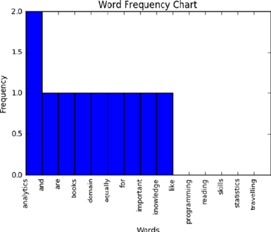
CHAPTER 5 ■ STEP 5 – TEXT MINING AND RECOMMENDER SYSTEMS
273
Word Cloud
This is a visual representation of text data, which is helpful to get a high-level
understanding about the important keywords from data in terms of its occurrence.
‘WordCloud’ package can be used to generate words whose font size relates to its
frequency. See Listing 5-22.
Listing 5-22. Example code for wordcloud
from wordcloud import WordCloud
# Read the whole text.
text = open('Data/Text_Files/Doc_1.txt').read()
# Generate a word cloud image
wordcloud = WordCloud().generate(text)
# Display the generated image:
# the matplotlib way:
import matplotlib.pyplot as plt
plt.imshow(wordcloud.recolor(random_state=2017))
plt.title('Most Frequent Words')
plt.axis("off")
plt.show()
#----output----
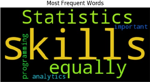
CHAPTER 5 ■ STEP 5 – TEXT MINING AND RECOMMENDER SYSTEMS
274
From the above chart we can see that ‘skills’ appear the most number of times
comparatively.
Lexical Dispersion Plot
This plot is helpful to determine the location of a word in a sequence of text sentences.
On the x-axis you’ll have word offset numbers and on the y-axis each row is a
representation of the entire text and the marker indicates an instance of the word of
interest. See Listing 5-23.
Listing 5-23. Example code for lexical dispersion plot
from nltk import word_tokenize
def dispersion_plot(text, words):
words_token = word_tokenize(text)
points = [(x,y) for x in range(len(words_token)) for y in
range(len(words)) if words_token[x] == words[y]]
if points:
x,y=zip(*points)
else:
x=y=()
plt.plot(x,y,"rx",scalex=.1)
plt.yticks(range(len(words)),words,color="b")
plt.ylim(-1,len(words))
plt.title("Lexical Dispersion Plot")
plt.xlabel("Word Offset")
plt.show()
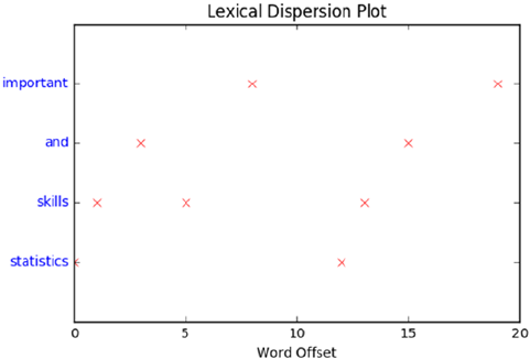
CHAPTER 5 ■ STEP 5 – TEXT MINING AND RECOMMENDER SYSTEMS
275
text = 'statistics skills, and programming skills are equally important for
analytics. statistics skills, and domain knowledge are important for analytics'
dispersion_plot(text, ['statistics', 'skills', 'and', 'important'])
#----output----
Co-occurrence Matrix
Calculating the co-occurrence between words in a sequence of text will be helpful
matrices to explain the relationship between words. A co-occurrence matrix tells us how
many times every word has co-occurred with the current word. Further plotting this
matrix into a heat map is a powerful visual tool to spot the relationships between words
efficiently. See Listing 5-24.
Listing 5-24. Example code for co-occurrence matrix
import statsmodels.api as sm
import scipy.sparse as sp
# default unigram model
count_model = CountVectorizer(ngram_range=(1,1))
docs_unigram = count_model.fit_transform(docs.get('docs'))
# co-occurrence matrix in sparse csr format
docs_unigram_matrix = (docs_unigram.T * docs_unigram)
# fill same word cooccurence to 0
docs_unigram_matrix.setdiag(0)
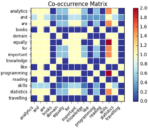
CHAPTER 5 ■ STEP 5 – TEXT MINING AND RECOMMENDER SYSTEMS
276
# co-occurrence matrix in sparse csr format
docs_unigram_matrix = (docs_unigram.T * docs_unigram) docs_unigram_matrix_
diags = sp.diags(1./docs_unigram_matrix.diagonal())
# normalized co-occurence matrix
docs_unigram_matrix_norm = docs_unigram_matrix_diags * docs_unigram_matrix
# Convert to a dataframe
df = pd.DataFrame(docs_unigram_matrix_norm.todense(), index = count_model.
get_feature_names())
df.columns = count_model.get_feature_names()
# Plot
sm.graphics.plot_corr(df, title='Co-occurrence Matrix', xnames=list(df.index))
plt.show()
#----output----
Model Building
As you might be familiar with by now, model building is the process of understanding
and establishing relationships between variables. So far you have learned how to extract
text content from various sources, preprocess to remove noise, and perform exploratory
analysis to get basic understanding/statistics about the text data in hand. Now you’ll learn
to apply machine learning techniques on the processed data to build models.

CHAPTER 5 ■ STEP 5 – TEXT MINING AND RECOMMENDER SYSTEMS
277
Text Similarity
A measure that indicates how similar two objects are is described through a distance
measure with dimensions represented by features of the objects (here text). A smaller
distance indicates a high degree of similarity and vice versa. Note that similarity is highly
subjective and dependent on domain or application. For text similarity, it is important
to choose the right distance measure to get better results. There are various distance
measures available and Euclidian metric is the most common, which is a straight line
distance between two points. However a significant amount of research has been carried
out in the field of text mining to learn that cosine distance better suits for text similarity.
Let’s look at a simple example to understand similarity better. Consider three
documents containing certain simple text keywords and assume that the top two keywords
are accident and New York. For the moment ignore other keywords and let’s calculate the
similarity of document based on these two keywords frequency. See Table5-4.
Table 5-4. Sample document term matrix
Document # Count of ‘Accident’ Count of ‘New York’
1 2 8
2 3 7
3 7 3
Plotting the document word vector points on a two-dimensional chart is depicted
on Figure 5-5. Notice that the cosine similarity equation is the representation of the angle
between the two data points, whereas Euclidian distance is the square root of straight
line differences between data points. The cosine similarity equation will result in a value
between 0 and 1. The smaller cosine angle results in a bigger cosine value, indicating
higher similarity. In this case Euclidean distance will result in a zero. Let’s put the values
in the formula to find the similarity between documents 1 and 2.
Euclidian distance (doc1, doc2) = 23 2872 11 14
10
-
()
+-
()
=+
()
==
^^ .
Cosine (doc1, doc2) = 62
824761
098
.*.
.=, where
doc1 = (2,8)
doc2 = (3,7)
doc1 . doc2 = (2*3 + 8*7) = (56 + 6) = 62
||doc1|| = ` 22 88 824** .
()
+
()
=
||doc2|| = 33 77 761** .
()
+
()
=
Similarly let’s find the similarity between documents 1 and 3. See Figure 5-5.
Euclidian distance (doc1, doc3) = 27 2832 25 25 70
70
-
()
+-
()
=+
()
==
^^ .
Cosine (doc1, doc3)= 38
824761
060
.*.
.=
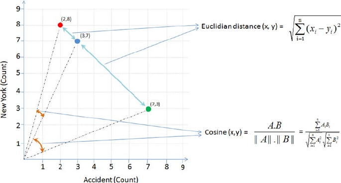
CHAPTER 5 ■ STEP 5 – TEXT MINING AND RECOMMENDER SYSTEMS
278
According to the cosine equation, documents 1 and 2 are 98% similar; this could
mean that these two documents may be talking about ‘New York’. Whereas document 3
can be assumed to be focused more about ‘Accident’, however, there is a mention of ‘New
York’ a couple of times resulting in a similarity of 60% between documents 1 and 3.
Let’s apply cosine similarity for the example given in Figure 5-5. See Listing 5-25.
Listing 5-25. Example code for calculating cosine similarity for documents
from sklearn.metrics.pairwise import cosine_similarity
print "Similarity b/w doc 1 & 2: ", cosine_similarity(df['Doc_1.txt'],
df['Doc_2.txt'])
print "Similarity b/w doc 1 & 3: ", cosine_similarity(df['Doc_1.txt'],
df['Doc_3.txt'])
print "Similarity b/w doc 2 & 3: ", cosine_similarity(df['Doc_2.txt'],
df['Doc_3.txt'])
#----output----
Similarity b/w doc 1 & 2: [[ 0.76980036]]
Similarity b/w doc 1 & 3: [[ 0.12909944]]
Similarity b/w doc 2 & 3: [[ 0.1490712]]
Figure 5-5. Euclidian vs. Cosine
CHAPTER 5 ■ STEP 5 – TEXT MINING AND RECOMMENDER SYSTEMS
279
Text Clustering
As an example we’ll be using the 20 newsgroups dataset consisting of 18,000+
newsgroup posts on 20 topics. You can learn more about the dataset at http://qwone.
com/~jason/20Newsgroups/. Let’s load the data and check the topic names. See Listing 5-26.
Listing 5-26. Example code for text clustering
from sklearn.datasets import fetch_20newsgroups
from sklearn.feature_extraction.text import TfidfVectorizer
from sklearn.preprocessing import Normalizer
from sklearn import metrics
from sklearn.cluster import KMeans, MiniBatchKMeans
import numpy as np
# load data and print topic names
newsgroups_train = fetch_20newsgroups(subset='train')
print(list(newsgroups_train.target_names))
#----output----
['alt.atheism', 'comp.graphics', 'comp.os.ms-windows.misc', 'comp.sys.ibm.
pc.hardware', 'comp.sys.mac.hardware', 'comp.windows.x', 'misc.forsale',
'rec.autos', 'rec.motorcycles', 'rec.sport.baseball', 'rec.sport.hockey',
'sci.crypt', 'sci.electronics', 'sci.med', 'sci.space', 'soc.religion.
christian', 'talk.politics.guns', 'talk.politics.mideast', 'talk.politics.
misc', 'talk.religion.misc']
To keep it simple, let’s filter only three topics. Assume that we do not know the topics,
so let’s run a clustering algorithm and examine the keywords of each cluster.
categories = ['alt.atheism', 'comp.graphics', 'rec.motorcycles']
dataset = fetch_20newsgroups(subset='all', categories=categories,
shuffle=True, random_state=2017)
print("%d documents" % len(dataset.data))
print("%d categories" % len(dataset.target_names))
labels = dataset.target
print("Extracting features from the dataset using a sparse vectorizer")
vectorizer = TfidfVectorizer(stop_words='english')
X = vectorizer.fit_transform(dataset.data)
print("n_samples: %d, n_features: %d" % X.shape)
#----output----
2768 documents
3 categories
Extracting features from the dataset using a sparse vectorizer
n_samples: 2768, n_features: 35311
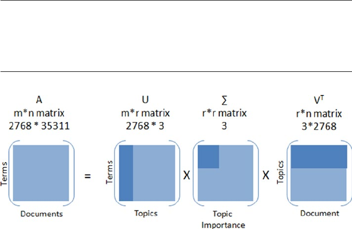
CHAPTER 5 ■ STEP 5 – TEXT MINING AND RECOMMENDER SYSTEMS
280
Latent Semantic Analysis (LSA)
LSA is a mathematical method that tries to bring out latent relationships within
a collection of documents. Rather than looking at each document isolated from
the others, it looks at all the documents as a whole and the terms within them to
identify relationships. Let’s perform LSA by running SVD on the data to reduce the
dimensionality.
SVD of matrix A = U * ∑ * VT
r = rank of matrix X
U = column orthonormal m * r matrix
∑ = diagonal r * r matrix with singular value sorted in descending order
V = column orthonormal r * n matrix
In our case we have 3 topics, 2768 documents and 35311 word vocabulary.
* Original matrix = 2768*35311 ~ 108
* SVD = 3*2768 + 3 + 3*35311 ~ 105.3
Resulted SVD is taking approximately 460 times less space than original matrix.
■Note “Latent Semantic Analysis (LSA)” and “Latent Semantic Indexing (LSI)” is the
same thing, with the latter name being used sometimes when referring specifically to
indexing a collection of documents for search (“Information Retrieval”). See Figure 5-6 and
Listing 5-27.
Figure 5-6. Singular Value Decomposition
CHAPTER 5 ■ STEP 5 – TEXT MINING AND RECOMMENDER SYSTEMS
281
Listing 5-27. Example code for LSA through SVD
from sklearn.decomposition import TruncatedSVD
# Lets reduce the dimensionality to 2000
svd = TruncatedSVD(2000)
lsa = make_pipeline(svd, Normalizer(copy=False))
X = lsa.fit_transform(X)
explained_variance = svd.explained_variance_ratio_.sum()
print("Explained variance of the SVD step: {}%".format(int(explained_
variance * 100)))
#----output----
Explained variance of the SVD step: 95%
Let’s run k-means clustering on the SVD output as shown in Listing 5-28.
Listing 5-28. k-means clustering on SVD dataset
from __future__ import print_function
km = KMeans(n_clusters=3, init='k-means++', max_iter=100, n_init=1)
# Scikit learn provides MiniBatchKMeans to run k-means in batch mode
suitable for a very large corpus
# km = MiniBatchKMeans(n_clusters=5, init='k-means++', n_init=1, init_
size=1000, batch_size=1000)
print("Clustering sparse data with %s" % km)
km.fit(X)
print("Top terms per cluster:")
original_space_centroids = svd.inverse_transform(km.cluster_centers_)
order_centroids = original_space_centroids.argsort()[:, ::-1]
terms = vectorizer.get_feature_names()
for i in range(3):
print("Cluster %d:" % i, end='')
for ind in order_centroids[i, :10]:
print(' %s' % terms[ind], end='')
print()
#----output----
Top terms per cluster:
Cluster 0: edu graphics university god subject lines organization com posting uk
Cluster 1: com bike edu dod ca writes article sun like organization
Cluster 2: keith sgi livesey caltech com solntze wpd jon edu sandvik
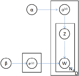
CHAPTER 5 ■ STEP 5 – TEXT MINING AND RECOMMENDER SYSTEMS
282
Topic Modeling
Topic modeling algorithms enable you to discover hidden topical patterns or thematic
structure in a large collection of documents. The most popular topic modeling techniques
are Latent Dirichlet Allocation (LDA) and Non-negative Matrix Factorization (NMF).
Latent Dirichlet Allocation (LDA)
LDA was presented by David Blei, Andrew Ng, and Michael I.J in 2003 as a graphical
model. See Figure5-7.
Figure 5-7. LDA graph model
LDA is given by PdwPdP PPwz Pz
d
z
zz
d
,*|* |* |, *|
()
=
()
()()()()
() () () ()
å
qa
bq
¦¦
Where, F(z) = word distribution for topic,
a = Dirichlet parameter prior the per-document topic distribution,
b = Dirichlet parameter prior the per-document word distribution,
q(d) = topic distribution for a document
LDA’s objective is to maximize separation between means of projected topics and
minimize variance within each projected topic. So LDA defines each topic as a bag of
words by carrying out three steps described below.
Step 1: Initialize k clusters and assign each word in the document to one of the k
topics.
Step 2: Re-assign word to new topic based on a) how is the proportion of words
for a document to a topic, and b) how is the proportion of a topic widespread across all
documents.
Step 3: Repeat step 2 until coherent topics result. See Figure5-8 and Listing 5-29.
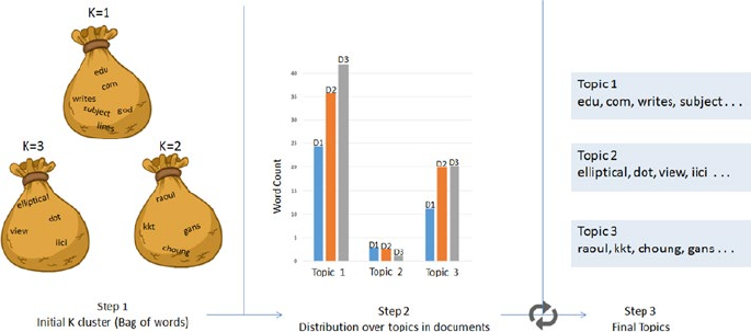
CHAPTER 5 ■ STEP 5 – TEXT MINING AND RECOMMENDER SYSTEMS
283
Listing 5-29. Example code for LDA
from sklearn.decomposition import LatentDirichletAllocation
# continuing with the 20 newsgroup dataset and 3 topics
total_topics = 3
lda = LatentDirichletAllocation(n_topics=total_topics,
max_iter=100,
learning_method='online',
learning_offset=50.,
random_state=2017)
lda.fit(X)
feature_names = np.array(vectorizer.get_feature_names())
for topic_idx, topic in enumerate(lda.components_):
print("Topic #%d:" % topic_idx)
print(" ".join([feature_names[i] for i in topic.argsort()[:-20 - 1:-1]]))
#----output----
Topic #0:
edu com writes subject lines organization article posting university nntp
host don like god uk ca just bike know graphics
Topic #1:
anl elliptical maier michael_maier qmgate separations imagesetter 5298 unscene
appreshed linotronic l300 iici amnesia glued veiw halftone 708 252 dot
Topic #2:
hl7204 eehp22 raoul vrrend386 qedbbs choung qed daruwala ims kkt briarcliff
kiat philabs col op_rows op_cols keeve 9327 lakewood gans
Figure 5-8. Latent Dirichlet Allocation (LDA)
CHAPTER 5 ■ STEP 5 – TEXT MINING AND RECOMMENDER SYSTEMS
284
Non-negative Matrix Factorization
NMF is a decomposition method for multivariate data, and is given by V = MH, where V
is the product of matrices W and H. W is a matrix of word rank in the features, and H is
the coefficient matrix with each row being a feature. The three matrices have no negative
elements. See Listing 5-30.
Listing 5-30. Example code for Non-negative matrix factorization
from sklearn.decomposition import NMF
nmf = NMF(n_components=total_topics, random_state=2017, alpha=.1, l1_ratio=.5)
nmf.fit(X)
for topic_idx, topic in enumerate(nmf.components_):
print("Topic #%d:" % topic_idx)
print(" ".join([feature_names[i] for i in topic.argsort()[:-20 - 1:-1]]))
#----output----
Topic #0:
edu com god writes article don subject lines organization just university
bike people posting like know uk ca think host
Topic #1:
sgi livesey keith solntze wpd jon caltech morality schneider cco moral com
allan edu objective political cruel atheists gap writes
Topic #2:
sun east green ed egreen com cruncher microsystems ninjaite 8302 460 rtp
0111 nc 919 grateful drinking pixel biker showed
Text Classification
The ability of representing text features as numbers opens up the opportunity to run
classification machine learning algorithms. Let’s use a subset of 20 newsgroups data to
build a classification model and assess its accuracy. See Listing 5-31.
Listing 5-31. Example code text classification on 20 news groups dataset
categories = ['alt.atheism', 'comp.graphics', 'rec.motorcycles', 'sci.
space', 'talk.politics.guns']
newsgroups_train = fetch_20newsgroups(subset='train', categories=categories,
shuffle=True, random_state=2017, remove=('headers', 'footers', 'quotes'))
newsgroups_test = fetch_20newsgroups(subset='test', categories=categories,
shuffle=True, random_state=2017, remove=('headers', 'footers', 'quotes'))
y_train = newsgroups_train.target
y_test = newsgroups_test.target
CHAPTER 5 ■ STEP 5 – TEXT MINING AND RECOMMENDER SYSTEMS
285
vectorizer = TfidfVectorizer(sublinear_tf=True, smooth_idf = True, max_
df=0.5, ngram_range=(1, 2), stop_words='english')
X_train = vectorizer.fit_transform(newsgroups_train.data)
X_test = vectorizer.transform(newsgroups_test.data)
print("Train Dataset")
print("%d documents" % len(newsgroups_train.data))
print("%d categories" % len(newsgroups_train.target_names))
print("n_samples: %d, n_features: %d" % X_train.shape)
print("Test Dataset")
print("%d documents" % len(newsgroups_test.data))
print("%d categories" % len(newsgroups_test.target_names))
print("n_samples: %d, n_features: %d" % X_test.shape)
#----output----
Train Dataset
2801 documents
5 categories
n_samples: 2801, n_features: 241036
Test Dataset
1864 documents
5 categories
n_samples: 1864, n_features: 241036
Let’s build a simple naïve Bayes classification model and assess the accuracy.
Essentially we can replace naïve Bayes with any other classification algorithm or use an
ensemble model to build an efficient model. See Listing 5-32.
Listing 5-32. Example code text classification using Multinomial naïve Bayes
from sklearn.naive_bayes import MultinomialNB
from sklearn import metrics
clf = MultinomialNB()
clf = clf.fit(X_train, y_train)
y_train_pred = clf.predict(X_train)
y_test_pred = clf.predict(X_test)
print 'Train accuracy_score: ', metrics.accuracy_score(y_train, y_train_pred)
print 'Test accuracy_score: ',metrics.accuracy_score(newsgroups_test.target,
y_test_pred)
print "Train Metrics: ", metrics.classification_report(y_train, y_train_pred)
print "Test Metrics: ", metrics.classification_report(newsgroups_test.target,
y_test_pred)
CHAPTER 5 ■ STEP 5 – TEXT MINING AND RECOMMENDER SYSTEMS
286
#----output----
Train accuracy_score: 0.976079971439
Test accuracy_score: 0.832081545064
Train Metrics: precision recall f1-score support
0 1.00 0.97 0.98 480
1 1.00 0.97 0.98 584
2 0.91 1.00 0.95 598
3 0.99 0.97 0.98 593
4 1.00 0.97 0.99 546
avg / total 0.98 0.98 0.98 2801
Test Metrics: precision recall f1-score support
0 0.91 0.62 0.74 319
1 0.90 0.90 0.90 389
2 0.81 0.90 0.86 398
3 0.80 0.84 0.82 394
4 0.78 0.86 0.82 364
avg / total 0.84 0.83 0.83 1864
Sentiment Analysis
The procedure of discovering and classifying opinions expressed in a piece of text (like
comments/feedback text) is called the sentiment analysis. The intended output of this
analysis would be to determine whether the writer’s mindset toward a topic, product,
service etc., is neutral, positive, or negative. See Listing 5-33.
Listing 5-33. Example code for sentiment analysis
from nltk.sentiment.vader import SentimentIntensityAnalyzer
from nltk.sentiment.util import *
data = pd.read_csv('Data/customer_review.csv')
SIA = SentimentIntensityAnalyzer()
data['polarity_score']=data.Review.apply(lambda x:SIA.polarity_scores(x)
['compound'])
data['neutral_score']=data.Review.apply(lambda x:SIA.polarity_scores(x)['neu'])
data['negative_score']=data.Review.apply(lambda x:SIA.polarity_scores(x)['neg'])
data['positive_score']=data.Review.apply(lambda x:SIA.polarity_scores(x)['pos'])
data['sentiment']=''
data.loc[data.polarity_score>0,'sentiment']='POSITIVE'
data.loc[data.polarity_score==0,'sentiment']='NEUTRAL'
data.loc[data.polarity_score<0,'sentiment']='NEGATIVE'
data.head()
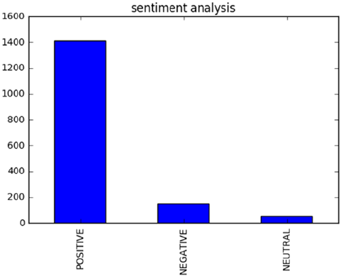
CHAPTER 5 ■ STEP 5 – TEXT MINING AND RECOMMENDER SYSTEMS
287
data.sentiment.value_counts().plot(kind='bar',title="sentiment analysis")
plt.show()
#----output----
ID Review polarity_score
0 1 Excellent service my claim was dealt with very... 0.7346
1 2 Very sympathetically dealt within all aspects ... -0.8155
2 3 Having received yet another ludicrous quote fr... 0.9785
3 4 Very prompt and fair handling of claim. A mino... 0.1440
4 5 Very good and excellent value for money simple... 0.8610
neutral_score negative_score positive_score sentiment
0 0.618 0.000 0.382 POSITIVE
1 0.680 0.320 0.000 NEGATIVE
2 0.711 0.039 0.251 POSITIVE
3 0.651 0.135 0.214 POSITIVE
4 0.485 0.000 0.515 POSITIVE
Deep Natural Language Processing (DNLP)
First, let me clarify that DNLP is not to be mistaken for Deep Learning NLP. A technique
such as topic modeling is generally known as shallow NLP where you try to extract
knowledge from text through semantic or syntactic analysis approach, that is, try to
form groups by retaining words that are similar and hold higher weight in a sentence/
document. Shallow NLP is less noise than the n-grams; however the key drawback
is that it does not specify the role of items in the sentence. In contrast, DNLP focuses
CHAPTER 5 ■ STEP 5 – TEXT MINING AND RECOMMENDER SYSTEMS
288
on a semantic approach, that is, it detects relationships within the sentences, and
further it can be represented or expressed as a complex construction of the form such
as subject:predicate:object (known as triples or triplets) out of syntactically parsed
sentences to retain the context. Sentences are made up of any combination of actor,
action, object, and named entities (person, organizations, locations, dates, etc.). For
example, consider the sentence "the flat tire was replaced by the driver." Here driver is the
subject (actor), replaced is the predicate (action), and flat tire is the object (action). So the
triples for would be driver:replaced:tire, which captures the context of the sentence. Note
that triples are one of the forms widely used and you can form a similar complex structure
based on the domain or problem at hand.
For demonstration I’ll use the sopex package, which uses Stanford Core NLP tree
parser. See Listing 5-34.
Listing 5-34. Example code for Deep NLP
from chunker import PennTreebackChunker
from extractor import SOPExtractor
# Initialize chunker
chunker = PennTreebackChunker()
extractor = SOPExtractor(chunker)
# function to extract triples
def extract(sentence):
sentence = sentence if sentence[-1] == '.' else sentence+'.'
global extractor
sop_triplet = extractor.extract(sentence)
return sop_triplet
sentences = [
'The quick brown fox jumps over the lazy dog.',
'A rare black squirrel has become a regular visitor to a suburban garden',
'The driver did not change the flat tire',
"The driver crashed the bike white bumper"
]
#Loop over sentence and extract triples
for sentence in sentences:
sop_triplet = extract(sentence)
print sop_triplet.subject + ':' + sop_triplet.predicate + ':' + sop_
triplet.object
#----output----
fox:jumps:dog
squirrel:become:visitor
driver:change:tire
driver:crashed:bumper
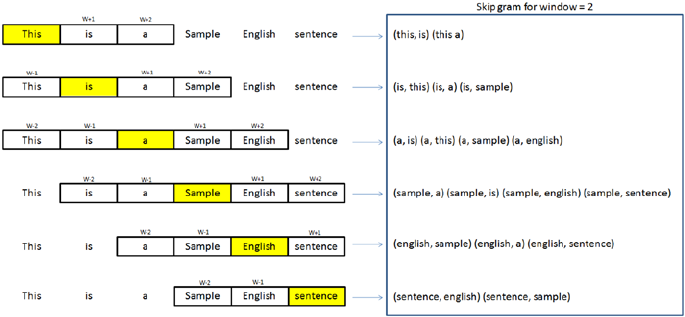
CHAPTER 5 ■ STEP 5 – TEXT MINING AND RECOMMENDER SYSTEMS
289
Word2Vec
Tomas Mikolov’s lead team at Google created Word2Vec (word to vector) model in 2013,
which uses documents to train a neural network model to maximize the conditional
probability of a context given the word.
It utilizes two models: CBOW and skip-gram.
1. Continuous bag-of-words (CBOW) model predicts the current
word from a window of surrounding context words or given a
set of context words predict the missing word that is likely to
appear in that context. CBOW is faster than skip-gram to train
and gives better accuracy for frequently appearing words.
2. Continuous skip-gram model predicts the surrounding
window of context words using the current word or given a
single word, predict the probability of other words that are
likely to appear near it in that context. Skip-gram is known to
show good results for both frequent and rare words. Let’s look
at an example sentence and create skip-gram for a window of
2 (refer to Figure5-9). The word highlighted in yellow is the
input word.
Figure 5-9. Skip-gram for window 2
You can download Google’s pre-trained model (from given link below) for word2vec,
which includes a vocabulary of 3 million words/phrases taken from 100 billion words
from a Google News dataset. See Listings 5-35 and 5-36.
URL: https://drive.google.com/file/d/0B7XkCwpI5KDYNlNUTTlSS21pQmM/edit
CHAPTER 5 ■ STEP 5 – TEXT MINING AND RECOMMENDER SYSTEMS
290
Listing 5-35. Example code for word2vec
import gensim
# Load Google's pre-trained Word2Vec model.
model = gensim.models.Word2Vec.load_word2vec_format('Data/GoogleNews-
vectors-negative300.bin', binary=True)
model.most_similar(positive=['woman', 'king'], negative=['man'], topn=5)
#----output----
[(u'queen', 0.7118192911148071),
(u'monarch', 0.6189674139022827),
(u'princess', 0.5902431607246399),
(u'crown_prince', 0.5499460697174072),
(u'prince', 0.5377321243286133)]
model.most_similar(['girl', 'father'], ['boy'], topn=3)
#----output----
[(u'mother', 0.831214427947998),
(u'daughter', 0.8000643253326416),
(u'husband', 0.769158124923706)]
model.doesnt_match("breakfast cereal dinner lunch".split())
#----output----
'cereal'
You can train a word2vec model on your own data set. The key model
parameters to be remembered are size, window, min_count and sg.
size: The dimensionality of the vectors, the bigger size values require more
training data, but can lead to more accurate models
sg = 0 for CBOW model and 1 for skip-gram model
min_count: Ignore all words with total frequency lower than this.
window: The maximum distance between the current and predicted word within a
sentence
Listing 5-36. Example code for training word2vec on your own dataset
sentences = [['cigarette','smoking','is','injurious', 'to', 'health'],['cig
arette','smoking','causes','cancer'],['cigarette','are','not','to','be','so
ld','to','kids']]
# train word2vec on the two sentences
model = gensim.models.Word2Vec(sentences, min_count=1, sg=1, window = 3)
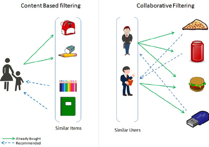
CHAPTER 5 ■ STEP 5 – TEXT MINING AND RECOMMENDER SYSTEMS
291
model.most_similar(positive=['cigarette', 'smoking'], negative=['kids'],
topn=1)
#----output----
[('injurious', 0.16142114996910095)]
Recommender Systems
Personalization of the user experience has been a high priority and has become the
new mantra in the consumer-focused industry. You might have observed e-commerce
companies casting personalized ads for you suggesting what to buy, which news to
read, which video to watch, where/what to eat, and who you might be interested in
networking (friends/professionals) on social media sites. Recommender systems are
the core information filtering system designed to predict the user preference and help to
recommend correct items to create a user-specific personalization experience. There are
two types of recommendation systems: 1) content-based filtering and 2) collaborative
filtering. See Figure5-10.
Figure 5-10. Recommender systems
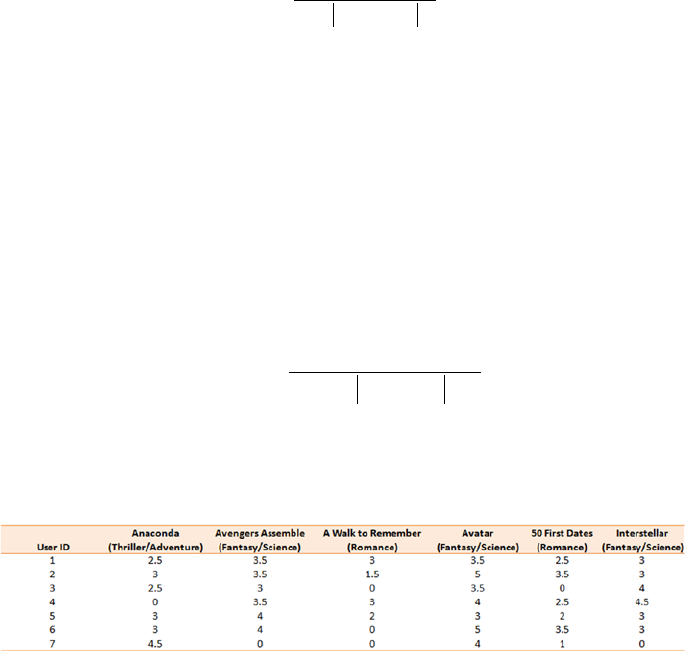
CHAPTER 5 ■ STEP 5 – TEXT MINING AND RECOMMENDER SYSTEMS
292
Content-Based Filtering
This type of system focuses on the similarity attributes of the items to give you
recommendations. This is best understood with an example, so if a user has purchased
items of a particular category then other similar items from the same category are
recommended to the user (refer to Figure5-10).
An item-based similarity recommendation algorithm can be represented as shown
here:
ˆ,
,
x
simi ix
simi i
km
i
im
bk
b
i
imb
b
b
=
()
()
()
å
å
,
,
Collaborative Filtering (CF)
CF focuses on the similarity attribute of the users, that is,it finds people with similar tastes
based on a similarity measure from the large group of users. There are two types of CF
implementation in practice: memory-based and model-based.
The memory-based recommendation is mainly based on the similarity
algorithm; the algorithm looks at items liked by similar people to create a ranked list of
recommendations. You can then sort the ranked list to recommend the top n items to the
user.
The user-based similarity recommendation algorithm can be represented as:
pr m
rm uu
uu
xk x
uN
yk
yx
y
uN
xy
yx
yx
,
,
=+
-
()()
()
Î
Î
å
å
sim,
sim,
Let’s consider an example dataset of movie ratings (Figure5-11) and apply item- and
user-based recommendations to get a better understanding. See Listing 5-37.
Figure 5-11. Movie rating sample dataset
CHAPTER 5 ■ STEP 5 – TEXT MINING AND RECOMMENDER SYSTEMS
293
Listing 5-37. Example code for recommender system
import numpy as np
import pandas as pd
df = pd.read_csv('Data/movie_rating.csv')
n_users = df.userID.unique().shape[0]
n_items = df.itemID.unique().shape[0]
print '\nNumber of users = ' + str(n_users) + ' | Number of movies = ' +
str(n_items)
#----output----
Number of users = 7 | Number of movies = 6
# Create user-item similarity matrices
df_matrix = np.zeros((n_users, n_items))
for line in df.itertuples():
df_matrix[line[1]-1, line[2]-1] = line[3]
from sklearn.metrics.pairwise import pairwise_distances
user_similarity = pairwise_distances(df_matrix, metric='cosine')
item_similarity = pairwise_distances(df_matrix.T, metric='cosine')
# Top 3 similar users for user id 7
print "Similar users for user id 7: \n", pd.DataFrame(user_
similarity).loc[6,pd.DataFrame(user_similarity).loc[6,:] > 0].sort_
values(ascending=False)[0:3]
#----output----
Similar users for user id 7:
3 8.000000
0 6.062178
5 5.873670
# Top 3 similar items for item id 6
print "Similar items for item id 6: \n", pd.DataFrame(item_
similarity).loc[5,pd.DataFrame(item_similarity).loc[5,:] > 0].sort_
values(ascending=False)[0:3]
#----output----
0 6.557439
2 5.522681
3 4.974937
Let’s build the user-based predict and item-based prediction for forumla as a
function. Apply this function to predict ratings and use root mean squared error (RMSE)
to evaluate the model performance.
See Listing 5-38.
CHAPTER 5 ■ STEP 5 – TEXT MINING AND RECOMMENDER SYSTEMS
294
Listing 5-38. Example code for recommender system & accuracy evaluation
# Function for item based rating prediction
def item_based_prediction(rating_matrix, similarity_matrix):
return rating_matrix.dot(similarity_matrix) / np.array([np.
abs(similarity_matrix).sum(axis=1)])
# Function for user based rating prediction
def user_based_prediction(rating_matrix, similarity_matrix):
mean_user_rating = rating_matrix.mean(axis=1)
ratings_diff = (rating_matrix - mean_user_rating[:, np.newaxis])
return mean_user_rating[:, np.newaxis] + similarity_matrix.dot(ratings_
diff) / np.array([np.abs(similarity_matrix).sum(axis=1)]).T
item_based_prediction = item_based_prediction(df_matrix, item_similarity)
user_based_prediction = user_based_prediction(df_matrix, user_similarity)
# Calculate the RMSE
from sklearn.metrics import mean_squared_error
from math import sqrt
def rmse(prediction, actual):
prediction = prediction[actual.nonzero()].flatten()
actual = actual[actual.nonzero()].flatten()
return sqrt(mean_squared_error(prediction, actual))
print 'User-based CF RMSE: ' + str(rmse(user_based_prediction, df_matrix))
print 'Item-based CF RMSE: ' + str(rmse(item_based_prediction, df_matrix))
#----output----
User-based CF RMSE: 1.0705767849
Item-based CF RMSE: 1.37392288971
y_user_based = pd.DataFrame(user_based_prediction)
# Predictions for movies that the user 6 hasn't rated yet
predictions = y_user_based.loc[6,pd.DataFrame(df_matrix).loc[6,:] == 0]
top = predictions.sort_values(ascending=False).head(n=1)
recommendations = pd.DataFrame(data=top)
recommendations.columns = ['Predicted Rating']
print recommendations
#----output----
Predicted Rating
1 2.282415
y_item_based = pd.DataFrame(item_based_prediction)
# Predictions for movies that the user 6 hasn't rated yet
predictions = y_item_based.loc[6,pd.DataFrame(df_matrix).loc[6,:] == 0]
top = predictions.sort_values(ascending=False).head(n=1)
CHAPTER 5 ■ STEP 5 – TEXT MINING AND RECOMMENDER SYSTEMS
295
recommendations = pd.DataFrame(data=top)
recommendations.columns = ['Predicted Rating']
print recommendations
#----output----
Predicted Rating
5 2.262497
Based on user based the recommended Intersellar is recommended (5th index).
Based on item based the recommended movie is Avengers Assemble (index number 1).
Model-based CF is based on matrix factorization (MF) such as Singular Value
Decomposition (SVD) and Non-nagative matrix factorization (NMF) etc. Let’s look how
to implement using SVD.
See Listing 5-39.
Listing 5-39. Example code for recommender system using SVD
# calculate sparsity level
sparsity=round(1.0-len(df)/float(n_users*n_items),3)
print 'The sparsity level of is ' + str(sparsity*100) + '%'
import scipy.sparse as sp
from scipy.sparse.linalg import svds
# Get SVD components from train matrix. Choose k.
u, s, vt = svds(df_matrix, k = 5)
s_diag_matrix=np.diag(s)
X_pred = np.dot(np.dot(u, s_diag_matrix), vt)
print 'User-based CF MSE: ' + str(rmse(X_pred, df_matrix))
#----output----
The sparsity level of is 0.0%
User-based CF MSE: 0.015742898995
Note that, in our case the data set is small, hence sparsity level is 0%. I recommend
you to try this method on the MovieLens 100k dataset which you can download from
https://grouplens.org/datasets/movielens/100k/
Endnotes
In this step you have learned the fundamentals of the text mining process and different
tools/techniques to extract text from various file formats. You also learned the basic text
preprocessing steps to remove noise from data and different visualization techniques to
better understand the corpus at hand. Then you learned various models that can be built
to understand the relationship between the data and gain insight from it.
We also learned two important recommender system methods such as content-
based filtering and collaborative filtering.

297
© Manohar Swamynathan 2017
M. Swamynathan, Mastering Machine Learning with Python in Six Steps,
DOI 10.1007/978-1-4842-2866-1_6
CHAPTER 6
Step 6 – Deep and
Reinforcement Learning
Deep learning has been the buzzword in the machine learning world in recent times. The
main objective of the deep learning algorithm so far has been to use machine learning to
achieve Artificial General Intelligence (AGI), that is, replicate human-level intelligence
in machines to solve any problems for a given area. Deep learning has shown promising
outcomes in computer vision, audio processing, and text mining. The advancements
in this area has led to a breakthrough such as self-driving cars. In this chapter you’ll
learn about deep leaning’s core concept, evolution (Perceptron to Convolution Neural
Network), key applications, and implementation.
There has been a number of powerful and popular open source libraries built in the
last few years predominantly focused on deep learning. See Table6-1.
Table 6-1. Popular deep learning libraries (as of end of year 2016)
Library Name Launch
Year
License # of Contributors Official Website
Theano 2010 BSD 284 http://deeplearning.
net/software/theano/
Pylearn2 2011 BSD-3-Clause 117 http://deeplearning.
net/software/
pylearn2/
Tensorflow 2015 Apache-2.0 660 http://tensorflow.org
Keras 2015 MIT 349 https://keras.io/
MXNet 2015 Apache-2.0 280 http://mxnet.io/
Caffe 2015 BSD-2-Clause 238 http://caffe.
berkeleyvision.org/
Lasagne 2015 MIT 58 http://lasagne.
readthedocs.org/

CHAPTER 6 ■ STEP 6 – DEEP AND REINFORCEMENT LEARNING
298
Below is a short description about each of the libraries (from Table6-1). Their official
websites provide quality documentation and examples. I strongly recommend you to visit
the respective site to learn more if required post completion of this chapter.
Theano: It is a Python library predominantly developed by academics at Universite
de Montreal. Theano allows you to define, optimize, and evaluate mathematical
expressions involving complex multidimensional arrays efficiently. It is designed to work
with GPUs and perform efficient symbolic differentiation. It is fast and stable with an
extensive unit test in place.
TensorFlow: As per the official documentation, it is a library for numerical
computation using data flow graphs for scalable machine learning developed by Google
researchers. It is currently being used by Google products for research and production. It
was open sourced in 2015 and has gained wide popularity in the machine learning world.
Pylearn2: A Machine Learning library based on Theano, which means users can
write new models/algorithms using mathematical expressions and Theano will optimize,
stabilize, and compile those expressions.
Keras: It is known as a high-level neural networks library, written in Python and
capable of running on top of either TensorFlow or Theano. It’s an interface rather than an
end-end machine learning framework. It’s written in Python, simple to get started, highly
module, and easy yet deep enough to expand to build/support complex models.
MXNet: It was developed in collaboration with researchers from CMU, NYU, NUS,
and MIT. It’s a lightweight, Portable, Flexible Distributed/mobile library supported across
many languages such as Python, R, Julia, Scala, Go, JavaScript, etc.
Caffe: It is a deep learning framework by Berkeley Vision and Learning Center
(BVLC) written in C++ and has python/matlab-buildings.
Lasagne: It is a lightweight library to build and train neural networks in Theano.
Throughout this chapter ‘Scikit-learn’ and ‘Keras’ library with back end as
TensorFlow or Theano appropriately has been used, due to the fact that these are the best
choices for a beginner to get hold of the concepts. Also these are most widely used by the
machine learning practitioners.
■Note There are enough good materials on how to set up Keras with Tensorflow or
Theano so the same will not be covered here. Also remember to install ‘graphviz’ and
‘pydot-ng’ packages to support a graphical view of the neural network. The Keras codes in
this chapter was built on Linux platform; however they should work fine on other platforms
without any modifications provided that supporting packages are correctly installed.
Systems with GPU capabilities are ideal for deep learning libraries as images/text/audio data
set’s numerical representations are large and compute intensive.
Artificial Neural Network (ANN)
Before jumping into details of deep learning, I think it is very important to briefly
understand how human vision works. The human brain is a complex connected neural
network where different regions of the brain are responsible for different jobs, and these
regions are machines of the brain that receive signals and processes it to take necessary
action. Figure6-1 shows the visual pathway of the human brain.
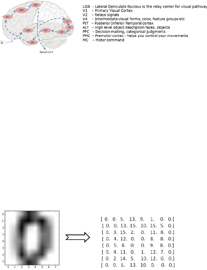
CHAPTER 6 ■ STEP 6 – DEEP AND REINFORCEMENT LEARNING
299
Our brain is made up of a cluster of small connected units called neurons, which
send electrical signals to one another. The long-term knowledge is represented by the
strength of the connections between neurons. When we see objects, light travels through
the retina and the visual information gets converted to electrical signals, and further on
the electric signal passes through the hierarchy of connected neurons of different regions
within the brain in a few milliseconds to decode signals/information.
What Goes Behind, When Computers Look at
an Image?
In computers an image is represented as one large three-dimensional array of numbers.
For example, consider Figure6-2; it is the handwritten digit image of gray scale 28x28x1
(width x height x depth) size resulting in 784 data points. Each number in the array is an
integer that ranges from 0 (black) to 255(white). In a typical classification problem the
model has to turn this large matrix into a single label. For a color image additionally it will
have three color channels: Red, Green, Blue (RGB) for each pixel, so the same image in
color would be of size 28x28x3 = 2352 data points.
Figure 6-1. Visual pathway
Figure 6-2. Handwritten digit(zero)image and correponding array
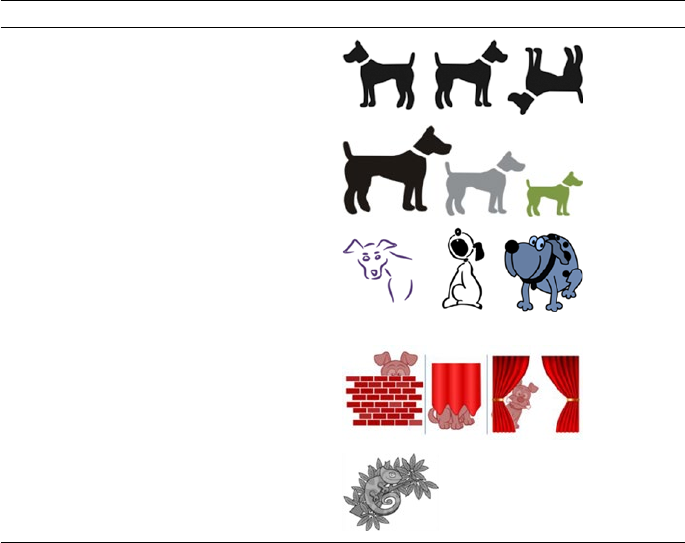
CHAPTER 6 ■ STEP 6 – DEEP AND REINFORCEMENT LEARNING
300
Why Not a Simple Classification Model for
Images?
Image classification can be challenging for a computer as there are a variety of challenges
associated with representation of the images. A simple classification model might not
be able to address most of these issues without a lot of feature engineering effort. Let’s
understand some of the key issues (refer to Table6-2).
Table 6-2. Visual challenges in image data
Description Example
View point variation: Same object can
have different orientation.
Scale and illumination variation:
Variation in object’s size and the level of
illumination on pixel level can vary.
Deformation/twist and intra-class
variation: Non-rigid bodies can be
deformed in great ways and there can
be different types of objects with varying
appearance within a class.
Blockage: Only small portion of object in
interest can be visible.
Background clutter: Objects can blend
into their environment, which will make it
hard to identify.
Perceptron – Single Artificial Neuron
Inspired by the biological neurons, McCulloch and Pitts in 1943 introduced the concept
of perceptron as an artificial neuron that is the basic building block of the artificial neural
network. They are not only named after their biological counterparts but also modeled
after the behavior of the neurons in our brain. See Figure6-3.
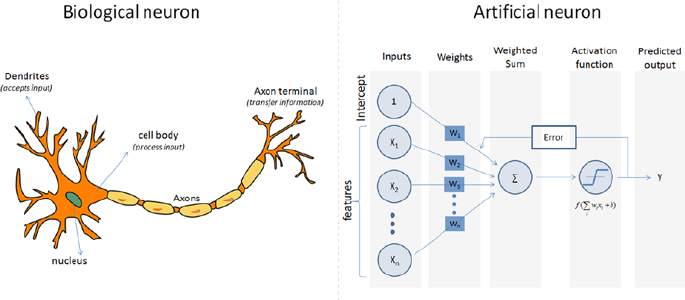
CHAPTER 6 ■ STEP 6 – DEEP AND REINFORCEMENT LEARNING
301
Biological neurons have dendrites to receive signals, a cell body to process them,
and an axon/axon terminal to transfer signals out to other neurons. Similarly an artificial
neuron has multiple input channels to accept training samples represented as a vector,
and a processing stage where the weights(w) are adjusted such that the output error
(actual vs. predicted) is minimized. Then the result is fed into an activation function
to produce output, for example, a classification label. The activation function for a
classification problem is a threshold cutoff (standard is .5) above which class is 1 else 0.
Let’s see how this can be implemented using scikit-learn. See Listing 6-1.
Listing 6-1. Example code for sklearn perceptron
# import sklearn.linear_model.perceptron
from sklearn.linear_model import perceptron
import matplotlib.pyplot as plt
from matplotlib.colors import ListedColormap
# Let's use sklearn make_classification function to create some test data.
from sklearn.datasets import make_classification
X, y = make_classification(20, 2, 2, 0, weights=[.5, .5], random_state=2017)
# Create the model
clf = perceptron.Perceptron(n_iter=100, verbose=0, random_state=2017, fit_
intercept=True, eta0=0.002)
clf.fit(X,y)
print "Prediction: " + str(clf.predict(X))
print "Actual: " + str(y)
print "Accuracy: " + str(clf.score(X, y)*100) + "%"
Figure 6-3. Biological vs. Artificial Neuron
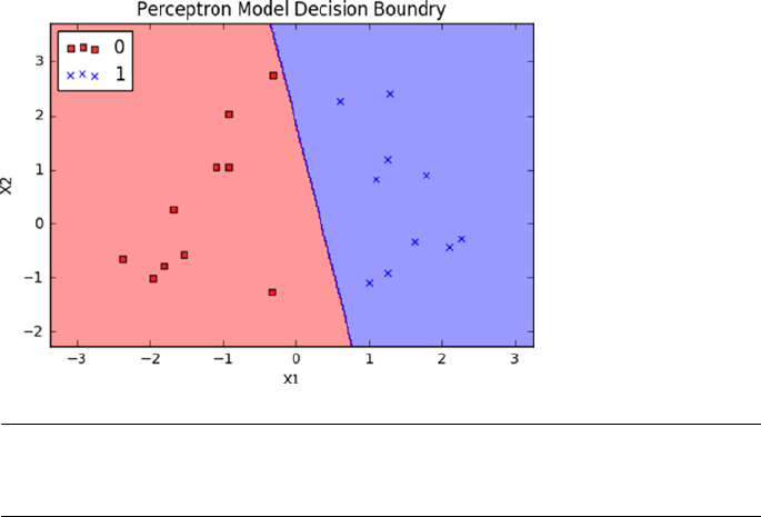
CHAPTER 6 ■ STEP 6 – DEEP AND REINFORCEMENT LEARNING
302
# Output the values
print "X1 Coefficient: " + str(clf.coef_[0,0])
print "X2 Coefficient: " + str(clf.coef_[0,1])
print "Intercept: " + str(clf.intercept_)
# Plot the decision boundary using cusom function ‘plot_decision_regions’
plot_decision_regions(X, y, classifier=clf)
plt.title('Perceptron Model Decision Boundry')
plt.xlabel('X1')
plt.ylabel('X2')
plt.legend(loc='upper left')
plt.show()
#----output----
Prediction: [1 1 1 0 0 0 0 1 0 1 1 0 0 1 0 1 0 0 1 1]
Actual: [1 1 1 0 0 0 0 1 0 1 1 0 0 1 0 1 0 0 1 1]
Accuracy: 100.0%
X1 Coefficient: 0.00575308754305
X2 Coefficient: 0.00107517941422
Intercept: [-0.002]
■Note A drawback of the single perceptron approach is that it can only learn linearly
separable functions.
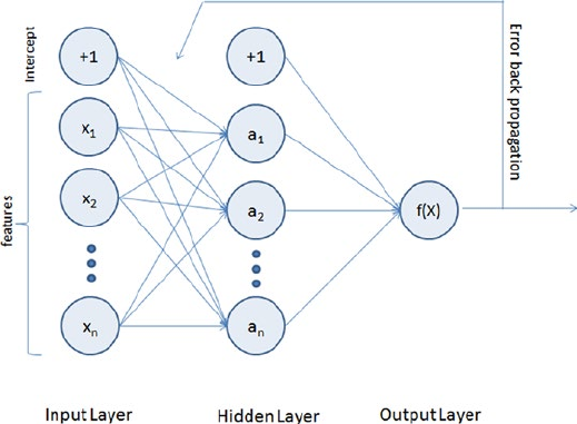
CHAPTER 6 ■ STEP 6 – DEEP AND REINFORCEMENT LEARNING
303
Multilayer Perceptrons (Feedforward Neural
Network)
To address the drawback of single perceptrons, multilayer perceptrons were proposed;
also commonly known as a feedforward neural network, it is a composition of multiple
perceptrons connected in different ways and operating on distinctive activation functions
to enable improved learning mechanisms. The training sample propagates forward
through the network and the output error is back propagated and the error is minimized
using the gradient descent method, which will calculate a loss function for all the weights
in the network. See Figure6-4.
The activation function for a simple one-level hidden layer of a multilayer
perceptron can be given by:
fx gWgWx
j
M
kj
i
d
ji i
()
=æ
è
çö
ø
÷
æ
è
ç
ç
ö
ø
÷
÷
=
()
=
()
åå
0
2
0
1, where xi is the input and Wji
(1) is the input layer
weights and Wkj
(2) is the weight of hidden layer.
A multilayered neural network can have many hidden layers, where the network
holds its internal abstract representation of the training sample. The upper layers will be
building new abstractions on top of the previous layers. So having more hidden layers for
a complex dataset will help the neural network to learn better.
As you can see from Figure6-4, the MLP architecture has a minimum of three layers,
that is, input, hidden, and output layers. The input layer’s neuron count will be equal to
the total number of features and in some libraries an additional neuron for intercept/bias.
These neurons are represented as nodes. The output layers will have a single neuron for
regression models and binary classifier; otherwise it will be equal to the total number of
class labels for multiclass classification models.
Figure 6-4. Multilayer perceptron representation
CHAPTER 6 ■ STEP 6 – DEEP AND REINFORCEMENT LEARNING
304
Note that using too few neurons for a complex dataset can result in an under-fitted
model due to the fact that it might fail to learn the patterns in complex data. However,
using too many neurons can result in an over-fitted model as it has capacity to capture
patterns that might be noise or specific for the given training dataset. So to build an efficient
multilayered neural network, the fundamental questions to be answered about hidden
layers while implementation is 1) what is the ideal number of hidden layers?, and 2) what
should be the number of neurons in hidden layers?
A widely accepted rule of thumb is that you can start with one hidden layer, as
there is a theory that one hidden layer is sufficient for the majority of problems. Then,
gradually increase the layers on a trial-and-error basis to see if there is any improvement
in accuracy. The number of neurons in the hidden layer can ideally be the mean of the
neurons in the input and output layers.
Let’s see an MLP algorithm in action from scikit-learn library on a classification
problem. We’ll be using the digits dataset available as part of scikit-learn dataset, which
is made up of 1797 samples (which is a subset of MNIST dataset) handwritten grayscale
digit of 8x8 images.
Load MNIST Data
Listing 6-2. Example code for loading MNIST data for training MLP classifier
import pandas as pd
import numpy as np
import matplotlib.pyplot as plt
from sklearn.neural_network import MLPClassifier
from sklearn.model_selection import train_test_split
from sklearn.preprocessing import StandardScaler
from sklearn.metrics import confusion_matrix
from sklearn.datasets import load_digits
np.random.seed(seed=2017)
# load data
digits = load_digits()
print('We have %d samples'%len(digits.target))
## plot the first 32 samples to get a sense of the data
fig = plt.figure(figsize = (8,8))
fig.subplots_adjust(left=0, right=1, bottom=0, top=1, hspace=0.05,
wspace=0.05)
for i in range(32):
ax = fig.add_subplot(8, 8, i+1, xticks=[], yticks=[])
ax.imshow(digits.images[i], cmap=plt.cm.gray_r)
ax.text(0, 1, str(digits.target[i]), bbox=dict(facecolor='white'))
#----output----
We have 1797 samples
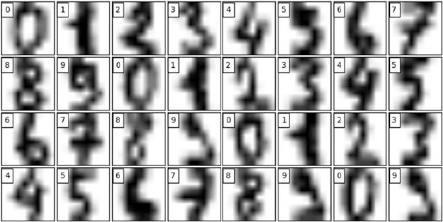
CHAPTER 6 ■ STEP 6 – DEEP AND REINFORCEMENT LEARNING
305
Key Parameters for scikit-learn MLP
hidden_layer_sizes – You have to provide the number of hidden layers and neurons
for each hidden layer. For example, hidden_layer_sizes – (5,3,3) means there are 3
hidden layers and the number of neurons for layer 1 is 5, layer 2 is 3, and for layer 3 is 3
respectively. The default value is (100,) that is, 1 hidden layer with 100 neurons.
Activation – This is the activation function for hidden layer, and there are four
activation functions available for use, default is ‘relu’.
• relu: The rectified linear unit function, returns f(x) = max(0, x).
• logistic: The logistic sigmoid function, returns f(x) = 1 / (1 +
exp(-x)).
• identity: No-op activation, useful to implement linear bottleneck,
returns f(x) = x.
• tanh: The hyperbolic tan function, returns f(x) = tanh(x).
solver – This is for weight optimization’ there are three options available, the default
being ‘adam’.
• adam: Stochastic gradient-based optimizer proposed by Kingma/
Diederik/Jimmy Ba, which works well for large dataset.
• lbfgs: Belongs to family of quasi-Newton methods, works well for
small datasets.
• sgd: Stochastic gradient descent.
max_iter – This is the maximum number of iterations for solver to converge, default
is 200.
learning_rate_init – This is the initial learning rate to control step size for updating
the weights (only applicable for solvers sgd/adam), default is 0.001.

CHAPTER 6 ■ STEP 6 – DEEP AND REINFORCEMENT LEARNING
306
It is recommended to scale or normalize your data before modeling as MLP is sensitive to
feature scaling. See Listing 6-3.
Listing 6-3. Example code for sklearn MLP classifier
# split data to training and testing data
X_train, X_test, y_train, y_test = train_test_split(digits.data, digits.
target, test_size=0.2, random_state=2017)
print 'Number of samples in training set: %d' %(len(y_train))
print 'Number of samples in test set: %d' %(len(y_test))
# Standardise data, and fit only to the training data
scaler = StandardScaler()
scaler.fit(X_train)
# Apply the transformations to the data
X_train_scaled = scaler.transform(X_train)
X_test_scaled = scaler.transform(X_test)
# Initialize ANN classifier
mlp = MLPClassifier(hidden_layer_sizes=(100), activation='logistic', max_
iter = 100)
# Train the classifier with the traning data
mlp.fit(X_train_scaled,y_train)
#----output----
Number of samples in training set: 1437
Number of samples in test set: 360
MLPClassifier(activation='logistic', alpha=0.0001, batch_size='auto',
beta_1=0.9, beta_2=0.999, early_stopping=False, epsilon=1e-08,
hidden_layer_sizes=(30, 30, 30), learning_rate='constant',
learning_rate_init=0.001, max_iter=100, momentum=0.9,
nesterovs_momentum=True, power_t=0.5, random_state=None,
shuffle=True, solver='adam', tol=0.0001, validation_fraction=0.1,
verbose=False, warm_start=False)
print("Training set score: %f" % mlp.score(X_train_scaled, y_train))
print("Test set score: %f" % mlp.score(X_test_scaled, y_test))
#----output----
Training set score: 0.990953
Test set score: 0.983333
# predict results from the test data
X_test_predicted = mlp.predict(X_test_scaled)
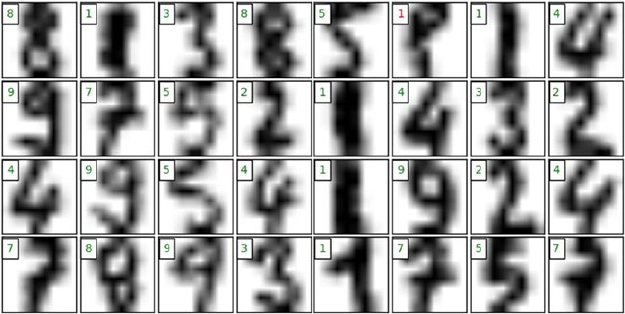
CHAPTER 6 ■ STEP 6 – DEEP AND REINFORCEMENT LEARNING
307
fig = plt.figure(figsize=(8, 8)) # figure size in inches
fig.subplots_adjust(left=0, right=1, bottom=0, top=1, hspace=0.05,
wspace=0.05)
# plot the digits: each image is 8x8 pixels
for i in range(32):
ax = fig.add_subplot(8, 8, i + 1, xticks=[], yticks=[])
ax.imshow(X_test.reshape(-1, 8, 8)[i], cmap=plt.cm.gray_r)
# label the image with the target value
if X_test_predicted[i] == y_test[i]:
ax.text(0, 1, X_test_predicted[i], color='green',
bbox=dict(facecolor='white'))
else:
ax.text(0, 1, X_test_predicted[i], color='red',
bbox=dict(facecolor='white'))
#----output----
Restricted Boltzman Machines (RBM)
The RBM algorithm was proposed by Geoffrey Hinton (2007), which learns probability
distribution over its sample training data inputs. It has seen wide applications in
different areas of supervised/unsupervised machine learning such as feature learning,
dimensionality reduction, classification, collaborative filtering, and topic modeling.
Consider the example movie rating discussed in the recommender system section.
Movies like Avengers, Avatar, and Interstellar have strong associations with a latest fantasy
and science fiction factor. Based on the user rating RBM will discover latent factors
that can explain the activation of movie choices. In short, RBM describes variability
among correlated variables of input dataset in terms of a potentially lower number of
unobserved variables.
The energy function is given by E(v, h) = - aTv – bTh – vTWh
CHAPTER 6 ■ STEP 6 – DEEP AND REINFORCEMENT LEARNING
308
The probability function of a visible input layer can be given by
fv av e
T
ih
hb Wv
i
ii i
()
=- -
åå
+
()
log
Let’s build a logistic regression model on a digits dataset with Bernoulli RBM and compare
its accuracy with straight logistic regression (without Bernoulli RBM) model’s accuracy.
Let’s nudge the dataset set by moving the 8x8 images by 1 pixel on the left, right,
down, and up to convolute the image. See Listing 6-4.
Listing 6-4. Function to nudge the dataset
# Function to nudge the dataset
def nudge_dataset(X, Y):
"""
This produces a dataset 5 times bigger than the original one,
by moving the 8x8 images in X around by 1px to left, right, down, up
"""
direction_vectors = [
[[0, 1, 0],
[0, 0, 0],
[0, 0, 0]],
[[0, 0, 0],
[1, 0, 0],
[0, 0, 0]],
[[0, 0, 0],
[0, 0, 1],
[0, 0, 0]],
[[0, 0, 0],
[0, 0, 0],
[0, 1, 0]]]
shift = lambda x, w: convolve(x.reshape((8, 8)), mode='constant',
weights=w).ravel()
X = np.concatenate([X] +
[np.apply_along_axis(shift, 1, X, vector)
for vector in direction_vectors])
Y = np.concatenate([Y for _ in range(5)], axis=0)
return X, Y
CHAPTER 6 ■ STEP 6 – DEEP AND REINFORCEMENT LEARNING
309
The Bernoulli RBM assumes that the columns of our feature vectors fall within the
range 0 to 1. However, the MNIST dataset is represented as unsigned 8-bit integers, falling
within the range of 0 to 255.
Define a function to scale the columns into the range (0, 1). The scale function takes
two parameters: our data matrix X and an epsilon value used to prevent division by zero
errors. See Listing 6-5.
Listing 6-5. Example code for using Bernoulli RBM with classifier
# Example adapted from scikit-learn documentation
import numpy as np
import matplotlib.pyplot as plt
from sklearn import linear_model, datasets, metrics
from sklearn.model_selection import train_test_split
from sklearn.neural_network import BernoulliRBM
from sklearn.pipeline import Pipeline
from scipy.ndimage import convolve
# Load Data
digits = datasets.load_digits()
X = np.asarray(digits.data, 'float32')
y = digits.target
X, y = nudge_dataset(X, digits.target)
# Scale the features such that the values are between 0-1 scale
X = (X - np.min(X, 0)) / (np.max(X, 0) + 0.0001)
X_train, X_test, y_train, y_test = train_test_split(X, y, test_size=0.2,
random_state=2017)
print X.shape
print y.shape
#----output----
(8985L, 64L)
(8985L,)
# Gridsearch for logistic regression
# perform a grid search on the 'C' parameter of Logistic
params = {"C": [1.0, 10.0, 100.0]}
Grid_Search = GridSearchCV(LogisticRegression(), params, n_jobs = -1,
verbose = 1)
Grid_Search.fit(X_train, y_train)
# print diagnostic information to the user and grab the
print "Best Score: %0.3f" % (Grid_Search.best_score_)
# best model
CHAPTER 6 ■ STEP 6 – DEEP AND REINFORCEMENT LEARNING
310
bestParams = Grid_Search.best_estimator_.get_params()
print bestParams.items()
#----output----
Fitting 3 folds for each of 3 candidates, totalling 9 fits
Best Score: 0.774
[('warm_start', False), ('C', 100.0), ('n_jobs', 1), ('verbose', 0),
('intercept_scaling', 1), ('fit_intercept', True), ('max_iter', 100),
('penalty', 'l2'), ('multi_class', 'ovr'), ('random_state', None), ('dual',
False), ('tol', 0.0001), ('solver', 'liblinear'), ('class_weight', None)]
# evaluate using Logistic Regression and only the raw pixel
logistic = LogisticRegression(C = 100)
logistic.fit(X_train, y_train)
print "Train accuracy: ", metrics.accuracy_score(y_train, logistic.
predict(X_train))
print "Test accuracyL ", metrics.accuracy_score(y_test, logistic.predict(X_
test))
#----output----
Train accuracy: 0.797440178075
Test accuracyL 0.800779076238
Let’s perform a grid search for RBM + Logistic Regression model. A grid search is on
the learning rate, number of iterations, and number of components on the RBM and C for
Logistic Regression. See Listing 6-6.
Listing 6-6. Example code for grid search with RBM + logistic regression
# initialize the RBM + Logistic Regression pipeline
rbm = BernoulliRBM()
logistic = LogisticRegression()
classifier = Pipeline([("rbm", rbm), ("logistic", logistic)])
params = {
"rbm__learning_rate": [0.1, 0.01, 0.001],
"rbm__n_iter": [20, 40, 80],
"rbm__n_components": [50, 100, 200],
"logistic__C": [1.0, 10.0, 100.0]}
# perform a grid search over the parameter
Grid_Search = GridSearchCV(classifier, params, n_jobs = -1, verbose = 1)
Grid_Search.fit(X_train, y_train)
# print diagnostic information to the user and grab the
# best model
print "Best Score: %0.3f" % (Grid_Search.best_score_)
CHAPTER 6 ■ STEP 6 – DEEP AND REINFORCEMENT LEARNING
311
print "RBM + Logistic Regression parameters"
bestParams = Grid_Search.best_estimator_.get_params()
# loop over the parameters and print each of them out
# so they can be manually set
for p in sorted(params.keys()):
print "\t %s: %f" % (p, bestParams[p])
#----output----
Fitting 3 folds for each of 81 candidates, totalling 243 fits
Best Score: 0.505
RBM + Logistic Regression parameters
logistic__C: 100.000000
rbm__learning_rate: 0.001000
rbm__n_components: 200.000000
rbm__n_iter: 20.000000
# initialize the RBM + Logistic Regression classifier with
# the cross-validated parameters
rbm = BernoulliRBM(n_components = 200, n_iter = 20, learning_rate = 0.1,
verbose = False)
logistic = LogisticRegression(C = 100)
# train the classifier and show an evaluation report
classifier = Pipeline([("rbm", rbm), ("logistic", logistic)])
classifier.fit(X_train, y_train)
print metrics.accuracy_score(y_train, classifier.predict(X_train))
print metrics.accuracy_score(y_test, classifier.predict(X_test))
#----output----
0.936839176405
0.932109070673
# plot RBM components
plt.figure(figsize=(15, 15))
for i, comp in enumerate(rbm.components_):
plt.subplot(20, 20, i + 1)
plt.imshow(comp.reshape((8, 8)), cmap=plt.cm.gray_r,
interpolation='nearest')
plt.xticks(())
plt.yticks(())
plt.suptitle('200 components extracted by RBM', fontsize=16)
plt.show()
#----output----
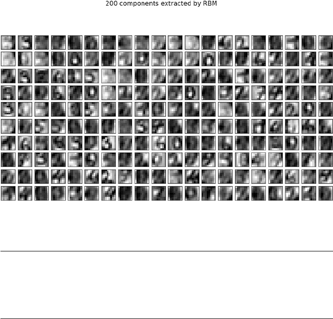
CHAPTER 6 ■ STEP 6 – DEEP AND REINFORCEMENT LEARNING
312
Notice that the logistic regression model with RBM lifts the model score by more
than 10% compared to the model without RBM.
■Note To practice further and get better understanding, I recommend that you try the
above example code on scikit-learns Olivetti faces dataset, which contains face images
taken between April 1992 and April 1994 at AT&T Laboratories Cambridge. You can load the
data using olivetti = datasets.fetch_olivetti_faces()
Stacked RBM is known as Deep Believe Network (DBN), which is an initialization
technique. However, this technique was popular during 2006-2007, and is reasonably
outdated. So there is no out-of-box implementation of DBN in Keras. However if you are
interested in a simple DBN implementation, I recommend you to have a look at
https://github.com/albertbup/deep-belief-network, which has an MIT license.
MLP Using Keras
In Keras, neural networks are defined as a sequence of layers, and the container for these
layers is the sequential class. The sequential models are linear stack of layers, and each
layer is an object that feeds into the next.
The first layer in the neural network will define the number of inputs to expect.
The activation functions that transform a summed signal from each neuron in a layer,
the same can be extracted and added to the sequential as a layer-like object called
activation. The choice of action depends on the type of problem (like regression or binary
classification or multiclass classification) that we are trying to address. See Listing 6-7.
CHAPTER 6 ■ STEP 6 – DEEP AND REINFORCEMENT LEARNING
313
Listing 6-7. Example code for Keras MLP
from matplotlib import pyplot as plt
import numpy as np
np.random.seed(2017)
from keras.models import Sequential
from keras.datasets import mnist
from keras.layers import Dense, Activation, Dropout, Input
from keras.models import Model
from keras.utils import np_utils
# from keras.utils.visualize_util import plot
from IPython.display import SVG
from keras import backend as K
from keras.callbacks import EarlyStopping
from keras.utils.visualize_util import model_to_dot, plot
# load data
(X_train, y_train), (X_test, y_test) = mnist.load_data()
X_train = X_train.reshape(X_train.shape[0], input_unit_size)
X_test = X_test.reshape(X_test.shape[0], input_unit_size)
X_train = X_train.astype('float32')
X_test = X_test.astype('float32')
# Scale the values by dividing 255 i.e., means foreground (black)
X_train /= 255
X_test /= 255
# one-hot representation, required for multiclass problems
y_train = np_utils.to_categorical(y_train, nb_classes)
y_test = np_utils.to_categorical(y_test, nb_classes)
print('X_train shape:', X_train.shape)
print(X_train.shape[0], 'train samples')
print(X_test.shape[0], 'test samples')
#----output----
('X_train shape:', (60000, 784))
(60000, 'train samples')
(10000, 'test samples')
nb_classes = 10 # class size
# flatten 28*28 images to a 784 vector for each image
input_unit_size = 28*28
# create model
model = Sequential()
CHAPTER 6 ■ STEP 6 – DEEP AND REINFORCEMENT LEARNING
314
model.add(Dense(input_unit_size, input_dim=input_unit_size, init='normal',
activation='relu'))
model.add(Dense(nb_classes, init='normal', activation='softmax'))
Compilation is a model that is a pre-compute step that transforms the sequence of
layers that we defined into a highly efficient series of matrix transforms. It takes three
arguments: an optimizer, a loss function, and a list of evaluation metrics.
Unlike scikit-learn implementation, Keras provides a rich number of optimizers such
as SGD (Stochastic gradient descent), RMSprop, Adagrad (Adaptive subgradient), Adadelta
(adaptive learning rate), Adam, Adamax, Nadam, and TFOptimizer. For brevity, I won’t
explain these here but recommend that you refer to the official Keras site for further reference.
Some standard loss functions are ‘mse’ for regression, binary_crossentropy
(logarithmic loss) for binary classification, and categorical_crossentropy (multiclass
logarithmic loss) for multiclassification problems.
The standard evaluation metrics for different types of problems are supported and
you can pass a list for them to evaluate. See Listing 6-8.
Listing 6-8. Compile model
# Compile model
model.compile(loss='categorical_crossentropy', optimizer='adam',
metrics=['accuracy'])
The network is trained using a back propogation algorithm, and optimized according
to the specified method, loss function. Each epoch can be partitioned into batches.
See Listing 6-9.
Listing 6-9. Train model and evaluate
# model training
model.fit(X_train, y_train, validation_data=(X_test, y_test), nb_epoch=5,
batch_size=500, verbose=2)
# Final evaluation of the model
scores = model.evaluate(X_test, y_test, verbose=0)
print("Error: %.2f%%" % (100-scores[1]*100))
#----output----
Train on 60000 samples, validate on 10000 samples
Epoch 1/5
6s - loss: 0.3828 - acc: 0.8922 - val_loss: 0.1866 - val_acc: 0.9486
Epoch 2/5
6s - loss: 0.1561 - acc: 0.9559 - val_loss: 0.1274 - val_acc: 0.9630
Epoch 3/5
5s - loss: 0.1077 - acc: 0.9697 - val_loss: 0.0991 - val_acc: 0.9704
Epoch 4/5
6s - loss: 0.0803 - acc: 0.9777 - val_loss: 0.0842 - val_acc: 0.9747
Epoch 5/5
6s - loss: 0.0616 - acc: 0.9829 - val_loss: 0.0771 - val_acc: 0.9754
Error: 2.46%
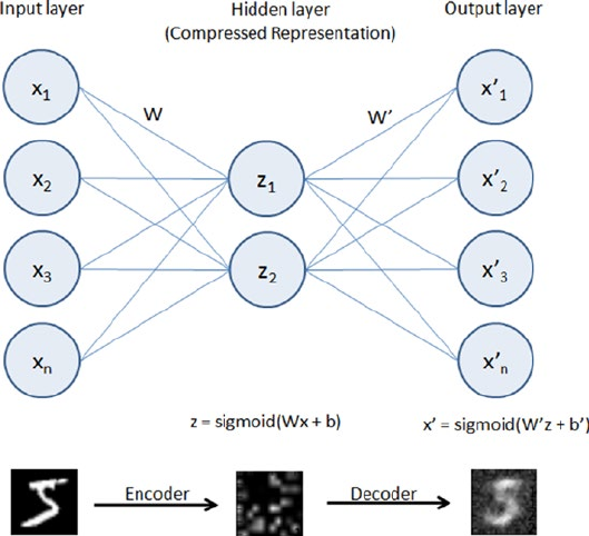
CHAPTER 6 ■ STEP 6 – DEEP AND REINFORCEMENT LEARNING
315
Autoencoders
As the name suggests, an autoencoder aims to learn encoding as a representation of
training sample data automatically without human intervention. The autoencoder is
widely used for dimensionality reduction and data de-nosing. See Figure6-5.
Building an autoencoder will typically have three elements.
1. Encoding function to map input to a hidden representation
through a nonlinear function, z = sigmoid (Wx + b).
2. A decoding function such as x’ = sigmoid(W’y + b’), which will
map back into reconstruction x’ with same shape as x.
3. A loss function, which is a distance function to measure the
information loss between the compressed representation of
data and the decompressed representation. Reconstruction
error can be measured using traditional squared error ||x-z||2.
We’ll be using the well-known MNIST database of handwritten digits, which
consists of approximately 70,000 total samples of handwritten grayscale digit images for
numbers 0 to 9, each image of size is 28x28 and intensity level varies from 0 to 255 with
accompanying label integer 0 to 9 for 60,000 of them and remaining ones without labels
(test dataset).
Figure 6-5. Autoencoder
CHAPTER 6 ■ STEP 6 – DEEP AND REINFORCEMENT LEARNING
316
Dimension Reduction Using Autoencoder
Listing 6-10. Example code for dimension reduction using autoencoder
import numpy as np
np.random.seed(2017)
from keras.datasets import mnist
from keras.models import Model
from keras.layers import Input, Dense
from keras.optimizers import Adadelta
from keras.utils import np_utils
# from keras.utils.visualize_util import plot
from IPython.display import SVG
from keras import backend as K
from keras.callbacks import EarlyStopping
from keras.utils.visualize_util import model_to_dot
from matplotlib import pyplot as plt
# Load mnist data
input_unit_size = 28*28
(X_train, y_train), (X_test, y_test) = mnist.load_data()
# function to plot digits
def draw_digit(data, row, col, n):
size = int(np.sqrt(data.shape[0]))
plt.subplot(row, col, n)
plt.imshow(data.reshape(size, size))
plt.gray()
# Normalize
X_train = X_train.reshape(X_train.shape[0], input_unit_size)
X_train = X_train.astype('float32')
X_train /= 255
print('X_train shape:', X_train.shape)
#----output----
('X_train shape:', (60000, 784))
# Autoencoder
inputs = Input(shape=(input_unit_size,))
x = Dense(144, activation='relu')(inputs)
outputs = Dense(input_unit_size)(x)
model = Model(input=inputs, output=outputs)
model.compile(loss='mse', optimizer='adadelta')
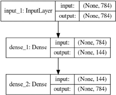
CHAPTER 6 ■ STEP 6 – DEEP AND REINFORCEMENT LEARNING
317
SVG(model_to_dot(model, show_shapes=True).create(prog='dot', format='svg'))
#----output----
Note that the 784 dimension is reduced through encoding to 144 in the hidden
layer and again in layer 3 constructed back to 784 using decoder.
model.fit(X_train, X_train, nb_epoch=5, batch_size=258)
#----output----
Epoch 1/5
60000/60000 [==============================] - 8s - loss: 0.0733
Epoch 2/5
60000/60000 [==============================] - 9s - loss: 0.0547
Epoch 3/5
60000/60000 [==============================] - 11s - loss: 0.0451
Epoch 4/5
60000/60000 [==============================] - 11s - loss: 0.0392
Epoch 5/5
60000/60000 [==============================] - 11s - loss: 0.0354
# plot the images from input layers
show_size = 5
total = 0
plt.figure(figsize=(5,5))
for i in range(show_size):
for j in range(show_size):
draw_digit(X_train[total], show_size, show_size, total+1)
total+=1
plt.show()
#----output----
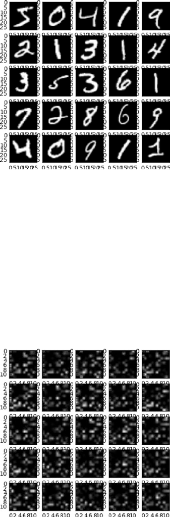
CHAPTER 6 ■ STEP 6 – DEEP AND REINFORCEMENT LEARNING
318
# plot the encoded (compressed) layer image
get_layer_output = K.function([model.layers[0].input],
[model.layers[1].output])
hidden_outputs = get_layer_output([X_train[0:show_size**2]])[0]
total = 0
plt.figure(figsize=(5,5))
for i in range(show_size):
for j in range(show_size):
draw_digit(hidden_outputs[total], show_size, show_size, total+1)
total+=1
plt.show()
#----output----
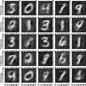
CHAPTER 6 ■ STEP 6 – DEEP AND REINFORCEMENT LEARNING
319
# Plot the decoded (de-compressed) layer images
get_layer_output = K.function([model.layers[0].input],
[model.layers[2].output])
last_outputs = get_layer_output([X_train[0:show_size**2]])[0]
total = 0
plt.figure(figsize=(5,5))
for i in range(show_size):
for j in range(show_size):
draw_digit(last_outputs[total], show_size, show_size, total+1)
total+=1
plt.show()
#----output----
De-noise Image Using Autoencoder
Discovering robust features from the compressed hidden layer is an important aspect to
enable the autoencoder to efficiently reconstruct the input from a de-noised version or
original image. This is addressed by the de-noising autoencoder, which is a stochastic
version of autoencoder.
Let’s introduce some noise to the digit dataset and try to build a model to de-noise
the image. See Listing 6-11.
Listing 6-11. Example code for de-noising using autoencoder
# Introducing noise to the image
noise_factor = 0.5
X_train_noisy = X_train + noise_factor * np.random.normal(loc=0.0,
scale=1.0, size=X_train.shape)
X_train_noisy = np.clip(X_train_noisy, 0., 1.)
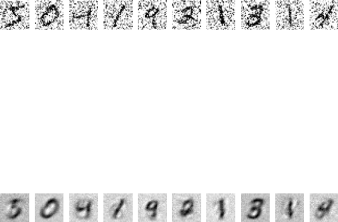
CHAPTER 6 ■ STEP 6 – DEEP AND REINFORCEMENT LEARNING
320
# Function for visualization
def draw(data, row, col, n):
plt.subplot(row, col, n)
plt.imshow(data, cmap=plt.cm.gray_r)
plt.axis('off')
show_size = 10
plt.figure(figsize=(20,20))
for i in range(show_size):
draw(X_train_noisy[i].reshape(28,28), 1, show_size, i+1)
plt.show()
#----output----
#Let’s fit a model on noisy training dataset.
model.fit(X_train_noisy, X_train, nb_epoch=5, batch_size=258)
# Prediction for denoised image
X_train_pred = model.predict(X_train_noisy)
show_size = 10
plt.figure(figsize=(20,20))
for i in range(show_size):
draw(X_train_pred[i].reshape(28,28), 1, show_size, i+1)
plt.show()
#----output----
Note that we can tune the model to improve the sharpness of de-noised image.
Convolution Neural Network (CNN)
In the world of image classification, CNN has become the go-to algorithm to build
efficient models. CNN’s are similar to ordinary neural networks, except that it explicitly
assumes that the inputs are images, which allows us to encode certain properties into the
architecture. These then make the forward function efficient to implement and reduces
the parameters in the network. The neurons are arranged in three dimensions: width,
height, and depth.
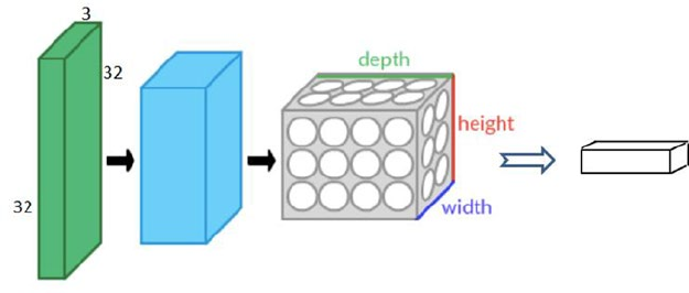
CHAPTER 6 ■ STEP 6 – DEEP AND REINFORCEMENT LEARNING
321
CNN on CIFAR10 Dataset
Let’s consider CIFAR-10 (Canadian Institute for Advanced Research), which is a standard
computer vision and deep learning image dataset. It consists of 60,000 color photos of
32 by 32 pixel squared with RGB for each pixel, divided into 10 classes, which include
common objects such as airplanes, automobiles, birds, cats, deer, dog, frog, horse, ship,
and truck. Essentially each image is of size 32x32x3 (width x height x RGB color channels).
CNN consists of four main types of layers: input layer, convolution layer, pooling
layer, fully connected layer.
The input layer will hold the raw pixel, so an image of CIFAR-10 will have 32x32x3
dimensions of input layer. The convolution layer will compute a dot product between
the weights of small local regions from the input layer, so if we decide to have 5 filters the
resulted reduced dimension will be 32x32x5. The RELU layer will apply an element-wise
activation function that will not affect the dimension. The Pool layer will down sample
the spatial dimension along width and height, resulting in dimension 16x16x5. Finally,
the fully connected layer will compute the class score, and the resulted dimension will
be a single vector 1x1x10 (10 class scores). Each neural in this layer is connected to all
numbers in the previous volume. See Figure6-6.
The next example illustration uses Keras with Theano aback end. To start Keras with
Theano back end please run the following command while starting jupyter notebook,
“KERAS_BACKEND=theano jupyter notebook.” See Listing 6-12.
Listing 6-12. CNN using keras with theano backend on CIFAR10 dataset
import keras
if K=='tensorflow':
keras.backend.set_image_dim_ordering('tf')
else:
keras.backend.set_image_dim_ordering('th')
from keras.models import Sequential
from keras.datasets import cifar10
from keras.layers import Dense, Activation, Flatten
Figure 6-6. Convolution Neural Network
CHAPTER 6 ■ STEP 6 – DEEP AND REINFORCEMENT LEARNING
322
from keras.optimizers import Adadelta
from keras.utils import np_utils
from keras.layers.convolutional import Convolution2D, MaxPooling2D
from keras.utils.visualize_util import model_to_dot, plot
from keras import backend as K
import numpy as np
from IPython.display import SVG
from matplotlib import pyplot as plt
import matplotlib.image as mpimg
%matplotlib inline
np.random.seed(2017)
batch_size = 256
nb_classes = 10
nb_epoch = 4
nb_filter = 10
img_rows, img_cols = 32, 32
img_channels = 3
# image dimension based on backend. 'th' = theano and 'tf' = tensorflow
if K.image_dim_ordering() == 'th':
input_shape = (3, img_rows, img_cols)
else:
input_shape = (img_rows, img_cols, 3)
(X_train, y_train), (X_test, y_test) = cifar10.load_data()
print('X_train shape:', X_train.shape)
print(X_train.shape[0], 'train samples')
print(X_test.shape[0], 'test samples')
X_train = X_train.astype('float32')
X_test = X_test.astype('float32')
X_train /= 255
X_test /= 255
Y_train = np_utils.to_categorical(y_train, nb_classes)
Y_test = np_utils.to_categorical(y_test, nb_classes)
#----output----
('X_train shape:', (50000, 3, 32, 32))
(50000, 'train samples')
(10000, 'test samples')
# Model Configuration
# define two groups of layers: feature (convolutions) and classification
(dense)
feature_layers = [
CHAPTER 6 ■ STEP 6 – DEEP AND REINFORCEMENT LEARNING
323
Convolution2D(nb_filters, nb_conv, nb_conv, input_shape=input_shape),
Activation('relu'),
Convolution2D(nb_filters, nb_conv, nb_conv),
Activation('relu'),
MaxPooling2D(pool_size=(nb_pool, nb_pool)),
Flatten(),
]
classification_layers = [
Dense(512),
Activation('relu'),
Dense(nb_classes),
Activation('softmax')
]
# create complete model
model = Sequential(feature_layers + classification_layers)
model.compile(loss='categorical_crossentropy', optimizer="adadelta",
metrics=['accuracy'])
# print model layer summary
print(model.summary())
#----output----
__________________________________________________________________________
Layer (type) Output Shape Param # Connected to
==========================================================================
convolution2d_1 (Convolution2D) (None, 10, 30, 30) 280
convolution2d_input_1[0][0]
__________________________________________________________________________
activation_1 (Activation) (None, 10, 30, 30) 0 convolution2d_1[0][0]
__________________________________________________________________________
convolution2d_2 (Convolution2D) (None, 10, 28, 28) 910 activation_1[0][0]
__________________________________________________________________________
activation_2 (Activation) (None, 10, 28, 28) 0 convolution2d_2[0][0]
__________________________________________________________________________
maxpooling2d_1 (MaxPooling2D) (None, 10, 14, 14) 0 activation_2[0][0]
__________________________________________________________________________
flatten_1 (Flatten) (None, 1960) 0 maxpooling2d_1[0][0]
__________________________________________________________________________
dense_1 (Dense) (None, 512) 1004032 flatten_1[0][0]
_________________________________________________________________________
activation_3 (Activation) (None, 512) 0 dense_1[0][0]
_______________________________________________________________________
dense_2 (Dense) (None, 10) 5130 activation_3[0][0]
__________________________________________________________________________
activation_4 (Activation) (None, 10) 0 dense_2[0][0]
=========================================================================
Total params: 1010352
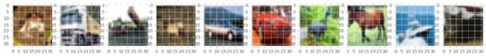
CHAPTER 6 ■ STEP 6 – DEEP AND REINFORCEMENT LEARNING
324
# fit model
model.fit(X_train, Y_train, batch_size=batch_size, nb_epoch=nb_epoch,
validation_data=(X_test, Y_test))
#----output----
Train on 50000 samples, validate on 10000 samples
Epoch 1/4
83s - loss: 1.9102 - acc: 0.3235 - val_loss: 1.5988 - val_acc: 0.4268
Epoch 2/4
90s - loss: 1.5174 - acc: 0.4671 - val_loss: 1.4651 - val_acc: 0.4846
Epoch 3/4
93s - loss: 1.3359 - acc: 0.5346 - val_loss: 1.4031 - val_acc: 0.5086
Epoch 4/4
85s - loss: 1.2222 - acc: 0.5739 - val_loss: 1.3008 - val_acc: 0.5483
Let’s visualize each layers. Note that we applied 10 filters.
# function for Visualization
def draw(data, row, col, n):
plt.subplot(row, col, n)
plt.imshow(data)
### Input layer (original image)
show_size = 10
plt.figure(figsize=(20,20))
for i in range(show_size):
draw(X_train[i].reshape(3, 32, 32).transpose(1, 2, 0), 1, show_size,
i+1)
plt.show()
#----output----
Notice below that in the hidden layers features are stored in 10 filters
# first layer
get_first_layer_output = K.function([model.layers[0].input], [model.
layers[1].output])
first_layer = get_first_layer_output([X_train[0:show_size]])[0]
plt.figure(figsize=(20,20))
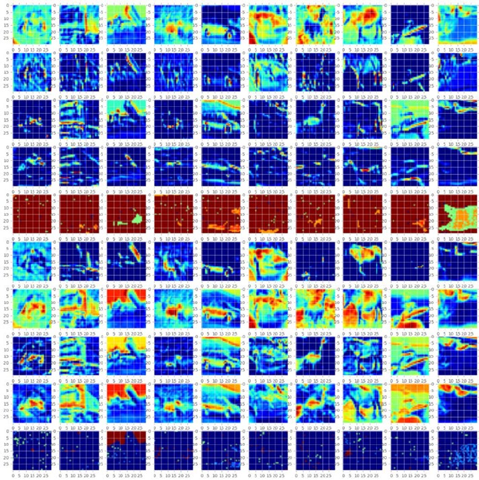
CHAPTER 6 ■ STEP 6 – DEEP AND REINFORCEMENT LEARNING
325
for img_index, filters in enumerate(first_layer, start=1):
for filter_index, mat in enumerate(filters):
pos = (filter_index)*show_size+img_index
draw(mat, nb_filters, show_size, pos)
plt.show()
#----output----
# second layer
get_second_layer_output = K.function([model.layers[0].input],
[model.layers[3].output])
second_layers = get_second_layer_output([X_train[0:show_size]])[0]
plt.figure(figsize=(20,20))
for img_index, filters in enumerate(second_layers, start=1):
for filter_index, mat in enumerate(filters):
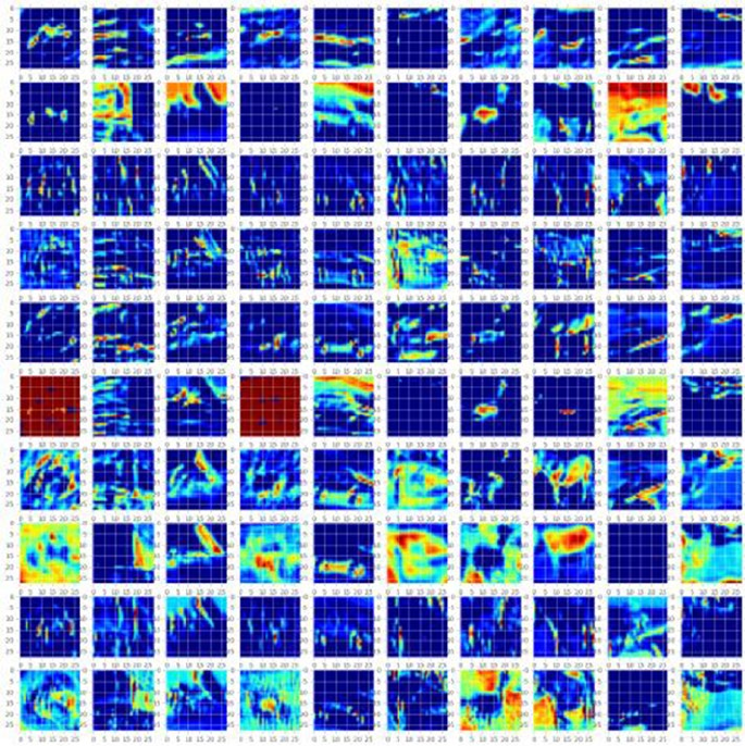
CHAPTER 6 ■ STEP 6 – DEEP AND REINFORCEMENT LEARNING
326
pos = (filter_index)*show_size+img_index
draw(mat, nb_filters, show_size, pos)
plt.show()
#----output----
# third layer
get_third_layer_output = K.function([model.layers[0].input],
[model.layers[4].output])
third_layers = get_third_layer_output([X_train[0:show_size]])[0]
plt.figure(figsize=(20,20))
for img_index, filters in enumerate(third_layers, start=1):
for filter_index, mat in enumerate(filters):
pos = (filter_index)*show_size+img_index
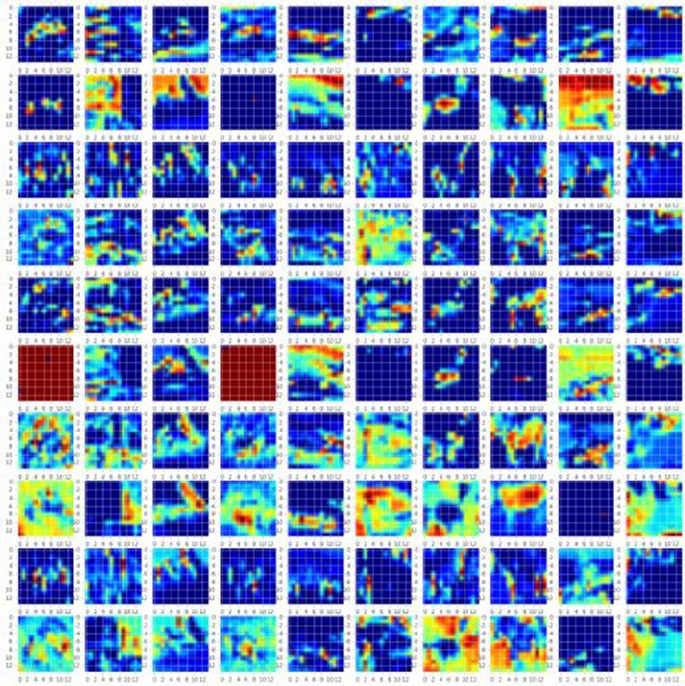
CHAPTER 6 ■ STEP 6 – DEEP AND REINFORCEMENT LEARNING
327
mat_size = mat.shape[1]
draw(mat, nb_filters, show_size, pos)
plt.show()
#----output-----
CNN on MNIST Dataset
As an additional example, let’s look at how the CNN might look on a digits dataset. See
Listing 6-13.
Listing 6-13. CNN using keras with theano back end on MNIST dataset
import keras
keras.backend.backend()
keras.backend.image_dim_ordering()
CHAPTER 6 ■ STEP 6 – DEEP AND REINFORCEMENT LEARNING
328
# using theano has backend
K = keras.backend.backend()
if K=='tensorflow':
keras.backend.set_image_dim_ordering('tf')
else:
keras.backend.set_image_dim_ordering('th')
from matplotlib import pyplot as plt
%matplotlib inline
import numpy as np
np.random.seed(2017)
from keras import backend as K
from keras.models import Sequential
from keras.datasets import mnist
from keras.layers import Dense, Dropout, Activation, Convolution2D,
MaxPooling2D, Flatten
from keras.utils import np_utils
from keras.utils.visualize_util import plot
from keras.preprocessing import sequence
from keras import backend as K
from keras.utils.visualize_util import plot
from IPython.display import SVG, display
from keras.utils.visualize_util import model_to_dot, plot
img_rows, img_cols = 28, 28
nb_classes = 10
nb_filters = 5 # the number of filters
nb_pool = 2 # window size of pooling
nb_conv = 3 # window or kernel size of filter
nb_epoch = 5
# image dimension based on backend. ‘th’ = theano and ‘tf’ = tensorflow
if K.image_dim_ordering() == 'th':
input_shape = (1, img_rows, img_cols)
else:
input_shape = (img_rows, img_cols, 1)
# data
(X_train, y_train), (X_test, y_test) = mnist.load_data()
X_train = X_train.reshape(X_train.shape[0], 1, img_rows, img_cols)
X_test = X_test.reshape(X_test.shape[0], 1, img_rows, img_cols)
X_train = X_train.astype('float32')
X_test = X_test.astype('float32')
CHAPTER 6 ■ STEP 6 – DEEP AND REINFORCEMENT LEARNING
329
X_train /= 255
X_test /= 255
print('X_train shape:', X_train.shape)
print(X_train.shape[0], 'train samples')
print(X_test.shape[0], 'test samples')
# convert class vectors to binary class matrices
Y_train = np_utils.to_categorical(y_train, nb_classes)
Y_test = np_utils.to_categorical(y_test, nb_classes)
#----output----
('X_train shape:', (60000, 1, 28, 28))
(60000, 'train samples')
(10000, 'test samples')
# define two groups of layers: feature (convolutions) and classification
(dense)
feature_layers = [
Convolution2D(nb_filters, nb_conv, nb_conv, input_shape=input_shape),
Activation('relu'),
Convolution2D(nb_filters, nb_conv, nb_conv),
Activation('relu'),
MaxPooling2D(pool_size=(nb_pool, nb_pool)),
Dropout(0.25),
Flatten(),
]
classification_layers = [
Dense(128),
Activation('relu'),
Dropout(0.5),
Dense(nb_classes),
Activation('softmax')
]
# create complete model
model = Sequential(feature_layers + classification_layers)
# define two groups of layers: feature (convolutions) and classification
(dense)
feature_layers = [
Convolution2D(nb_filters, nb_conv, nb_conv, input_shape=input_shape),
Activation('relu'),
Convolution2D(nb_filters, nb_conv, nb_conv),
Activation('relu'),
MaxPooling2D(pool_size=(nb_pool, nb_pool)),
Dropout(0.25),
Flatten(),
]
CHAPTER 6 ■ STEP 6 – DEEP AND REINFORCEMENT LEARNING
330
classification_layers = [
Dense(128),
Activation('relu'),
Dropout(0.5),
Dense(nb_classes),
Activation('softmax')
]
# create complete model
model = Sequential(feature_layers + classification_layers)
print(model.summary())
#----output----
__________________________________________________________________________
Layer (type) Output ShapeParam # Connected to
==========================================================================
convolution2d_1 (Convolution2D) (None, 5, 26, 26) 50
convolution2d_input_1[0][0]
__________________________________________________________________________
activation_1 (Activation) (None, 5, 26, 26) 0 convolution2d_1[0][0]
__________________________________________________________________________
convolution2d_2 (Convolution2D) (None, 5, 24, 24) 230 activation_1[0][0]
__________________________________________________________________________
activation_2 (Activation) (None, 5, 24, 24) 0 convolution2d_2[0][0]
__________________________________________________________________________
maxpooling2d_1 (MaxPooling2D) (None, 5, 12, 12) 0 activation_2[0][0]
__________________________________________________________________________
dropout_1 (Dropout) (None, 5, 12, 12) 0 maxpooling2d_1[0][0]
__________________________________________________________________________
flatten_1 (Flatten) (None, 720) 0 dropout_1[0][0]
__________________________________________________________________________
dense_1 (Dense) (None, 128) 92288 flatten_1[0][0]
__________________________________________________________________________
activation_3 (Activation) (None, 128) 0 dense_1[0][0]
__________________________________________________________________________
dropout_2 (Dropout) (None, 128) 0 activation_3[0][0]
__________________________________________________________________________
dense_2 (Dense) (None, 10) 1290 dropout_2[0][0]
__________________________________________________________________________
activation_4 (Activation) (None, 10) 0 dense_2[0][0]
==========================================================================
Total params: 93858
model.fit(X_train, Y_train, nb_epoch=nb_epoch, batch_size=256,
verbose=2, validation_split=0.2)
#----output----
Train on 48000 samples, validate on 12000 samples
Epoch 1/5

CHAPTER 6 ■ STEP 6 – DEEP AND REINFORCEMENT LEARNING
331
24s - loss: 0.9369 - acc: 0.6947 - val_loss: 0.2509 - val_acc: 0.9260
Epoch 2/5
27s - loss: 0.3576 - acc: 0.8901 - val_loss: 0.1592 - val_acc: 0.9548
Epoch 3/5
27s - loss: 0.2714 - acc: 0.9173 - val_loss: 0.1254 - val_acc: 0.9629
Epoch 4/5
25s - loss: 0.2271 - acc: 0.9319 - val_loss: 0.1084 - val_acc: 0.9690
Epoch 5/5
25s - loss: 0.2070 - acc: 0.9376 - val_loss: 0.0967 - val_acc: 0.9722
Visualization of Layers
# visualization
def draw(data, row, col, n):
plt.subplot(row, col, n)
plt.imshow(data, cmap=plt.cm.gray_r)
plt.axis('off')
# Sample input layer (original image)
show_size = 10
plt.figure(figsize=(20,20))
for i in range(show_size):
draw(X_train[i].reshape(28,28), 1, show_size, i+1)
plt.show()
#----output----
# First layer with 5 filters
get_first_layer_output = K.function([model.layers[0].input], [model.
layers[1].output])
first_layer = get_first_layer_output([X_train[0:show_size]])[0]
plt.figure(figsize=(20,20))
print 'first layer shape: ', first_layer.shape
for img_index, filters in enumerate(first_layer, start=1):
for filter_index, mat in enumerate(filters):
pos = (filter_index)*10+img_index
draw(mat, nb_filters, show_size, pos)
plt.tight_layout()
plt.show()
#----output----

CHAPTER 6 ■ STEP 6 – DEEP AND REINFORCEMENT LEARNING
332
Recurrent Neural Network (RNN)
The MLP (feedforward network) is not known to do well on sequential events models
such as the probabilistic language model of predicting the next word based on the
previous word at every given point. RNN architecture addresses this issue. It is similar to
MLP except that they have a feedback loop, which means they feed previous time steps
into the current step. This type of architecture generates sequences to simulate situation
and create synthetic data, making them the ideal modeling choice to work on sequence
data such as speech text mining, image captioning, time series prediction, robot control,
language modeling, etc. See Figure6-7.
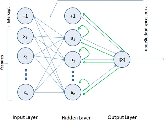
CHAPTER 6 ■ STEP 6 – DEEP AND REINFORCEMENT LEARNING
333
The previous step’s hidden layer and final outputs are fed back into the network
and will be used as input to the next steps’ hidden layer, which means the network will
remember the past and it will repeatedly predict what will happen next. The drawback in
the general RNN architecture is that it can be memory heavy, and hard to train for long-
term temporal dependency (i.e., context of long text should be known at any given stage).
Long Short-Term Memory (LSTM)
LSTM is an implementation of improved RNN architecture to address the issues of
general RNN, and it enables long-range dependencies. It is designed to have better
memory through linear memory cells surrounded by a set of gate units used to control
the flow of information, when information should enter the memory, when to forget, and
when to output. It uses no activation function within its recurrent components, thus the
gradient term does not vanish with back propagation. Figure6-8 gives a comparison of
simple multilayer perceptron vs. RNN vs. LSTM.
Figure 6-7. Recurrent Neural Network
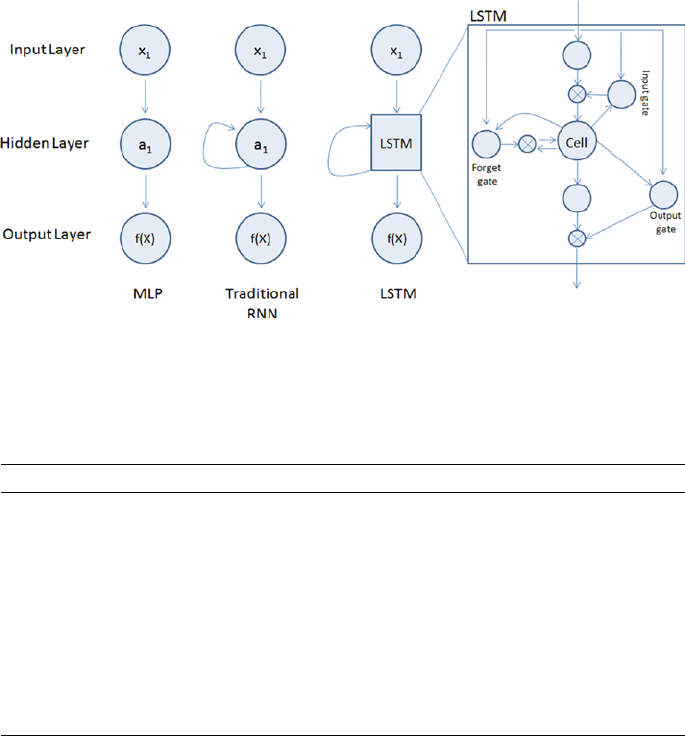
CHAPTER 6 ■ STEP 6 – DEEP AND REINFORCEMENT LEARNING
334
Please refer to Table6-3 below to understand the key LSTM component formulas.
Let’s look at an example of IMDB dataset that has a labeled sentiment (positive/
negative) for movie reviews. The reviews have been preprocessed, and encoded as
sequence of word indexes. See Listing 6-14.
Listing 6-14. Example code for Keras LSTM
import numpy as np
np.random.seed(2017) # for reproducibility
from keras.preprocessing import sequence
from keras.models import Sequential
from keras.layers import Dense, Activation, Embedding
from keras.layers import LSTM
from keras.datasets import imdb
Figure 6-8. Simple MLP vs RNN vs LSTM
Table 6-3. LSTM Components
LSTM Component Formula
Input gate layer: This decides which values to store
in the cell state.
it = sigmoid(wixt + uiht-1 + bi)
Forget gate layer: As the name suggested this
decides what information to throw away from the
cell state.
ft = sigmoid(Wfxt + Ufht-1 + bf)
Output gate layer: Create a vector of values that can
be added to the cell state.
Ot = sigmoid(Woxt + uiht-1 + bo)
Memory cell state vector. ct = ft o ct-1+ ito * hyperbolic
tangent(Wcxt + ucht-1 + bc)
CHAPTER 6 ■ STEP 6 – DEEP AND REINFORCEMENT LEARNING
335
max_features = 20000
maxlen = 80 # cut texts after this number of words (among top max_features
most common words)
batch_size = 32
# Load data
(X_train, y_train), (X_test, y_test) = imdb.load_data(nb_words=max_features)
print(len(X_train), 'train sequences')
print(len(X_test), 'test sequences')
print('Pad sequences (samples x time)')
X_train = sequence.pad_sequences(X_train, maxlen=maxlen)
X_test = sequence.pad_sequences(X_test, maxlen=maxlen)
print('X_train shape:', X_train.shape)
print('X_test shape:', X_test.shape)
#----output----
(25000, 'train sequences')
(25000, 'test sequences')
Pad sequences (samples x time)
('X_train shape:', (25000, 80))
('X_test shape:', (25000, 80))
#Model configuration
model = Sequential()
model.add(Embedding(max_features, 128, dropout=0.2))
model.add(LSTM(128, dropout_W=0.2, dropout_U=0.2)) # try using a GRU
instead, for fun
model.add(Dense(1))
model.add(Activation('sigmoid'))
# try using different optimizers and different optimizer configs
model.compile(loss='binary_crossentropy', optimizer='adam',
metrics=['accuracy'])
#Train
model.fit(X_train, y_train, batch_size=batch_size, nb_epoch=5,
#----output----
validation_data=(X_test, y_test))
Train on 25000 samples, validate on 25000 samples
Epoch 1/5
25000/25000 - 328s - loss: 0.5293 - acc: 0.7332 - val_loss: 0.4101 - val_
acc: 0.8206
Epoch 2/5
25000/25000 - 305s - loss: 0.3805 - acc: 0.8354 - val_loss: 0.3814 - val_
acc: 0.8297
Epoch 3/5
25000/25000 - 611s - loss: 0.3024 - acc: 0.8746 - val_loss: 0.4037 - val_
acc: 0.8343
CHAPTER 6 ■ STEP 6 – DEEP AND REINFORCEMENT LEARNING
336
Epoch 4/5
25000/25000 - 352s - loss: 0.2454 - acc: 0.9016 - val_loss: 0.4397 - val_
acc: 0.8304
Epoch 5/5
25000/25000 - 471s - loss: 0.2083 - acc: 0.9164 - val_loss: 0.4175 - val_
acc: 0.8342
25000/25000 - 99s
Test score: 0.417513472309
Test accuracy: 0.83424
# Evaluate
train_score, train_acc = model.evaluate(X_train, y_train, batch_size=batch_
size)
test_score, test_acc = model.evaluate(X_test, y_test, batch_size=batch_size)
print 'Train score:', train_score
print 'Train accuracy:', train_acc
print 'Test score:', test_score
print 'Test accuracy:', test_acc
#----output----
25000/25000 [==============================] - 83s
25000/25000 [==============================] - 83s
Train score: 0.0930857129323
Train accuracy: 0.97228
Test score: 0.417513472309
Test accuracy: 0.83424
Transfer Learning
Based on our past experience, we humans can learn a new skill easily. We are more efficient
in learning, particularly if the task in hand is similar to what we have done in the past, for
example, learning a new programming language for a computer professional or driving a
new type of vehicle for a seasoned driver is relatively easy based on our past experience.
Transfer learning is an area in machine learning that aims to utilize the knowledge
gained while solving one problem to solve a different but related problem. See Figure6-9.
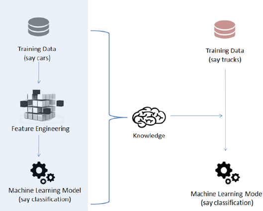
CHAPTER 6 ■ STEP 6 – DEEP AND REINFORCEMENT LEARNING
337
Nothing better than understanding through example, so let’s train a simple CNN
model of two level layers, that is, a feature layer and a classification layer on the first 5
digits (0 to 4) of the MNIST dataset, then apply transfer learning to freeze the features
layer and fine-tune dense layers for the classification of digits 5 to 9. See Listing 6-15.
Listing 6-15. Example code for transfer learning
import numpy as np
np.random.seed(2017) # for reproducibility
from keras.datasets import mnist
from keras.models import Sequential
from keras.layers import Dense, Dropout, Activation, Flatten
from keras.layers import Convolution2D, MaxPooling2D
from keras.utils import np_utils
from keras import backend as K
batch_size = 128
nb_classes = 5
nb_epoch = 5
# input image dimensions
img_rows, img_cols = 28, 28
# number of convolutional filters to use
nb_filters = 32
Figure 6-9. Transfer Learning
CHAPTER 6 ■ STEP 6 – DEEP AND REINFORCEMENT LEARNING
338
# size of pooling area for max pooling
pool_size = 2
# convolution kernel size
kernel_size = 3
input_shape = (img_rows, img_cols, 1)
# the data, shuffled and split between train and test sets
(X_train, y_train), (X_test, y_test) = mnist.load_data()
# create two datasets one with digits below 5 and one with 5 and above
X_train_lt5 = X_train[y_train < 5]
y_train_lt5 = y_train[y_train < 5]
X_test_lt5 = X_test[y_test < 5]
y_test_lt5 = y_test[y_test < 5]
X_train_gte5 = X_train[y_train >= 5]
y_train_gte5 = y_train[y_train >= 5] - 5 # make classes start at 0 for
X_test_gte5 = X_test[y_test >= 5]
# np_utils.to_categorical
y_test_gte5 = y_test[y_test >= 5] - 5
# Train model for digits 0 to 4
def train_model(model, train, test, nb_classes):
X_train = train[0].reshape((train[0].shape[0],) + input_shape)
X_test = test[0].reshape((test[0].shape[0],) + input_shape)
X_train = X_train.astype('float32')
X_test = X_test.astype('float32')
X_train /= 255
X_test /= 255
print('X_train shape:', X_train.shape)
print(X_train.shape[0], 'train samples')
print(X_test.shape[0], 'test samples')
# convert class vectors to binary class matrices
Y_train = np_utils.to_categorical(train[1], nb_classes)
Y_test = np_utils.to_categorical(test[1], nb_classes)
model.compile(loss='categorical_crossentropy',
optimizer='adadelta',
metrics=['accuracy'])
model.fit(X_train, Y_train,
batch_size=batch_size, nb_epoch=nb_epoch,
verbose=1,
validation_data=(X_test, Y_test))
score = model.evaluate(X_test, Y_test, verbose=0)
print('Test score:', score[0])
print('Test accuracy:', score[1])
CHAPTER 6 ■ STEP 6 – DEEP AND REINFORCEMENT LEARNING
339
# define two groups of layers: feature (convolutions) and classification (dense)
feature_layers = [
Convolution2D(nb_filters, kernel_size, kernel_size,
border_mode='valid',
input_shape=input_shape),
Activation('relu'),
Convolution2D(nb_filters, kernel_size, kernel_size),
Activation('relu'),
MaxPooling2D(pool_size=(pool_size, pool_size)),
Dropout(0.25),
Flatten(),
]
classification_layers = [
Dense(128),
Activation('relu'),
Dropout(0.5),
Dense(nb_classes),
Activation('softmax')
]
# create complete model
model = Sequential(feature_layers + classification_layers)
# train model for 5-digit classification [0..4]
train_model(model, (X_train_lt5, y_train_lt5), (X_test_lt5, y_test_lt5),
nb_classes)
#----output----
('X_train shape:', (30596, 28, 28, 1))
(30596, 'train samples')
(5139, 'test samples')
Train on 30596 samples, validate on 5139 samples
Epoch 1/5
30596/30596 [==============================] - 57s - loss: 0.2125 - acc:
0.9332 - val_loss: 0.0504 - val_acc: 0.9837
Epoch 2/5
30596/30596 [==============================] - 59s - loss: 0.0734 - acc:
0.9787 - val_loss: 0.0266 - val_acc: 0.9914
Epoch 3/5
30596/30596 [==============================] - 63s - loss: 0.0510 - acc:
0.9854 - val_loss: 0.0189 - val_acc: 0.9940
Epoch 4/5
30596/30596 [==============================] - 64s - loss: 0.0404 - acc:
0.9883 - val_loss: 0.0178 - val_acc: 0.9942
Epoch 5/5
30596/30596 [==============================] - 67s - loss: 0.0340 - acc:
0.9901 - val_loss: 0.0226 - val_acc: 0.9928
('Test score:', 0.022608739081115953)
('Test accuracy:', 0.99280015567230984)
CHAPTER 6 ■ STEP 6 – DEEP AND REINFORCEMENT LEARNING
340
Transfer existing trained model on 0 to 4 to build model for digits 5 to 9
# freeze feature layers and rebuild model
for layer in feature_layers:
layer.trainable = False
# transfer: train dense layers for new classification task [5..9]
train_model(model, (X_train_gte5, y_train_gte5), (X_test_gte5, y_test_gte5),
nb_classes)
#----output----
('X_train shape:', (29404, 28, 28, 1))
(29404, 'train samples')
(4861, 'test samples')
Train on 29404 samples, validate on 4861 samples
Epoch 1/5
29404/29404 [==============================] - 26s - loss: 0.4097 - acc:
0.8762 - val_loss: 0.1096 - val_acc: 0.9677
Epoch 2/5
29404/29404 [==============================] - 26s - loss: 0.1314 - acc:
0.9587 - val_loss: 0.0664 - val_acc: 0.9790
Epoch 3/5
29404/29404 [==============================] - 26s - loss: 0.0975 - acc:
0.9694 - val_loss: 0.0499 - val_acc: 0.9856
Epoch 4/5
29404/29404 [==============================] - 26s - loss: 0.0786 - acc:
0.9760 - val_loss: 0.0424 - val_acc: 0.9866
Epoch 5/5
29404/29404 [==============================] - 26s - loss: 0.0690 - acc:
0.9794 - val_loss: 0.0386 - val_acc: 0.9866
('Test score:', 0.038644227712815393)
('Test accuracy:', 0.98662826567857609)
Notice that we got 99.8% test accuracy after five epochs for the first five digits
classifier and 99.2% for the last five digits after transfer and fine-tuning.
Reinforcement Learning
Reinforcement learning is a goal-oriented learning method based on interaction with
its environment. The objective is getting an agent to act in an environment in order to
maximize its rewards. Here the agent is an intelligent program, and environment is the
external condition. See Figure6-10.
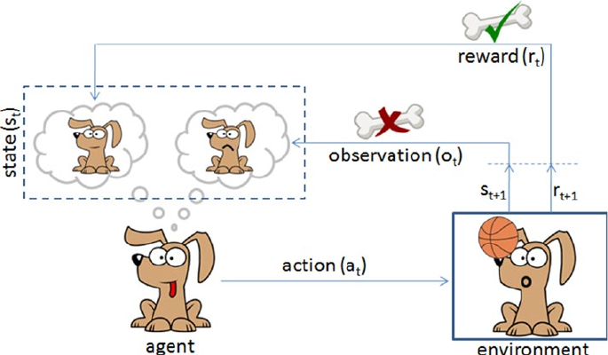
CHAPTER 6 ■ STEP 6 – DEEP AND REINFORCEMENT LEARNING
341
Let’s consider an example of a predefined system for teaching a new trick to a dog,
where you do not have to tell the dog what to do. However, you can reward the dog, if it
does it right or punish if it does wrong. With every step, it has to remember what made it
get the reward or punishment; this is commonly known as a credit assignment problem.
Similarly, we can train a computer agent such that its objective is to take action to move
from state st to state st+1 and find behavior function to maximize the expected sum of
discounted rewards and map the states to actions. According to the paper published
by Deepmind Technologies in 2013, the Q-learning rule for updating status is given by:
Q[s,a]new = Q[s,a]prev + α * (r + ƴ*max(s,a) – Q[s,a]prev), where
α is the learning rate,
r is reward for latest action,
ƴ is the discounted factor, and
max(s,a) is the estimate of new value from best action.
If the optimal value Q[s,a] of the sequence s’ at the next time step was known for
all possible actions a’, then the optimal strategy is to select the action a’ maximizing the
expected value of r + ƴ*max(s,a) – Q[s,a]prev.
Let’s consider an example where an agent is trying to come out of a maze. It can
move one random square or area in any direction, and get a reward if exits. The most
common way to formalize a reinforcement problem is to represent it as a Markov decision
process. Assume the agent is in state b (maze area) and the target is to reach state f. So
within one step agent can reach from b to f, let’s put a reward of 100 (otherwise 0) for links
between nodes that allows agents to reach target state. See Figure6-11 and Listing 6-16.
Figure 6-10. Reinforcement learning is like teaching your dog a trick
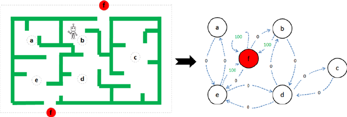
CHAPTER 6 ■ STEP 6 – DEEP AND REINFORCEMENT LEARNING
342
Listing 6-16. Example code for q-learning
import numpy as np
import matplotlib.pyplot as plt
from matplotlib.collections import LineCollection
# defines the reward/link connection graph
R = np.array([[-1, -1, -1, -1, 0, -1],
[-1, -1, -1, 0, -1, 100],
[-1, -1, -1, 0, -1, -1],
[-1,0, 0, -1, 0, -1],
[ 0, -1, -1, 0, -1, 100],
[-1, 0, -1, -1, 0, 100]]).astype("float32")
Q = np.zeros_like(R)
The -1’s in the table means there isn’t a link between nodes. For example, State ‘a’
cannot go to State ‘b’.
# learning parameter
gamma = 0.8
# Initialize random_state
initial_state = randint(0,4)
# This function returns all available actions in the state given as an
argument
def available_actions(state):
current_state_row = R[state,]
av_act = np.where(current_state_row >= 0)[1]
return av_act
# This function chooses at random which action to be performed within the range
# of all the available actions.
def sample_next_action(available_actions_range):
Figure 6-11. Left: Maze with 5 states, Right: Markov Decision process
CHAPTER 6 ■ STEP 6 – DEEP AND REINFORCEMENT LEARNING
343
next_action = int(np.random.choice(available_act,1))
return next_action
# This function updates the Q matrix according to the path selected and the Q
# learning algorithm
def update(current_state, action, gamma):
max_index = np.where(Q[action,] == np.max(Q[action,]))[1]
if max_index.shape[0] > 1:
max_index = int(np.random.choice(max_index, size = 1))
else:
max_index = int(max_index)
max_value = Q[action, max_index]
# Q learning formula
Q[current_state, action] = R[current_state, action] + gamma * max_value
# Get available actions in the current state
available_act = available_actions(initial_state)
# Sample next action to be performed
action = sample_next_action(available_act)
# Train over 100 iterations, re-iterate the process above).
for i in range(100):
current_state = np.random.randint(0, int(Q.shape[0]))
available_act = available_actions(current_state)
action = sample_next_action(available_act)
update(current_state,action,gamma)
# Normalize the "trained" Q matrix
print "Trained Q matrix: \n", Q/np.max(Q)*100
# Testing
current_state = 2
steps = [current_state]
while current_state != 5:
next_step_index = np.where(Q[current_state,] == np.max(Q[current_
state,]))[1]
if next_step_index.shape[0] > 1:
next_step_index = int(np.random.choice(next_step_index, size = 1))
else:
next_step_index = int(next_step_index)
steps.append(next_step_index)
current_state = next_step_index
CHAPTER 6 ■ STEP 6 – DEEP AND REINFORCEMENT LEARNING
344
# Print selected sequence of steps
print "Best sequence path: ", steps
#----output----
Best sequence path: [2, 3, 1, 5]
Endnotes
In this chapter you have learned briefly about various topics of deep learning techniques
using artificial neural networks, starting from single perceptron, multilayer perceptron, to
more complex forms of deep neural networks such as CNN / RNN. You have learned about
the various issues associated with image data and how researchers have tried to mimic the
human brain for building models that can solve complex problems related to computer
vision and text mining using the convolution neural network and recurrent neural network
respectively. You also learned how autoencoders can be used to compress / de-compress
data or remove noise from image data. You learned about the widely popular RBN, which
can learn the probabilistic distribution in the input data enabling us to build better
models. You learned about the transfer learn that helps us to use the knowledge from one
model to another model of a similar nature. Finally, we briefly looked at a simple example
of reinforcement learning using q-learning.
Congratulations! With this you have reached the end of your six-step expedition of
mastering machine learning.

345
© Manohar Swamynathan 2017
M. Swamynathan, Mastering Machine Learning with Python in Six Steps,
DOI 10.1007/978-1-4842-2866-1_7
CHAPTER 7
Conclusion
Summary
I hope you have enjoyed the six-step simplified machine learning expedition. You started
your learning journey with step 1, getting started in Python, where you learned the
core philosophy and key concepts of the Python programming language. In step 2, you
learned about machine learning history, high-level categories (supervised/unsupervised/
reinforcement learning), and three important frameworks for building ML systems
(SEMMA, CRISP-DM, KDD Data Mining process), primary data analysis packages (NumPy,
Pandas, Matplotlib) and their key concepts, comparison of different core machine learning
libraries. In step 3, fundamentals of machine learning, you learned different data types,
key data quality issues and how to handle them, exploratory analysis, core methods
of supervised / unsupervised learning and their implementation with an example.
In step 4, model diagnosis and tuning, you learned the various techniques for model
diagnosis, bagging for over-fitting, boosting for under-fitting, and ensemble techniques,
hyperparameter tuning (grid / random search) for building efficient models. In step 5, text
mining and recommender systems, you learned about the text mining process overview,
data assemble, data preprocessing, data exploration or visualization, and various models
that can be built. You also learned how to build collaborative/content-based recommender
systems to personalize the user experience. In step 6, deep and reinforcement learning,
you learned about Artificial Neural Network through Perceptron, Convolution Neural
Network (CNN) for image analytics, and Recurrent Neural Network (RNN) for text analytics,
and a simple toy example for learning the reinforcement learning concept. These are the
advanced topics that have seen great development in the last few years.
Overall, you have learned a broad range of commonly used machine learning topics,
and each of them come with a number of parameters to control and tune the model
performance. To keep it simple throughout the book, I have either used the default
parameters or you were introduced only to the key parameters (in some places). The
default options for parameters have been carefully chosen by the creators of the packages
to give decent results to get you started. So, to start with, you can go with the default
parameters. However I recommend that you explore the other parameters and play with
them using manual / grid / random searches to ensure a robust model. Table 7-1, below,
is a summary of various possible problem types, example use cases, and the potential
machine learning algorithms that you can use. Note that this is a sample list only, not an
exhaustive list.

Chapter 7 ■ ConClusion
346
Tips
Building an efficient model can be a challenging task for a starter. Now that you have
learned which algorithm to use, I would like to give my 2 cents list of things to remember
while you get started on the model building activity.
Table 7-1. Problem types vs. potential ML algorithms
Problem Type Example Use Case(s) Potential ML Algorithms
Predicting a
continuous number
What will be store daily/
weekly sales?
Linear Regression or
Polynomial regression
Predicting a count type
continuous number
How many staffs are required
for a shift? How many number
of car parking spaces are
required for a new store?
Generalized Linear Model
with Poisson distribution
Predict probability of
event (True/False)
What is the probability of a
transaction being fraud?
Binary Classification models
(Logistic regression, Decision
tree models, Boosting models,
KNN, etc.)
Predict probability
of event out of many
possible events (Multi
class)
What is the probability of a
transaction being high risk/
medium risk/low risk?
Multiclass Classification
models (Logistic regression,
Decision tree models,
Boosting models, KNN, etc.)
Group the contents
based on similarity
Group similar customers?
Group similar categories?
K-means clustering,
Hierarchical clustering
Dimension reduction What are the important
dimensions that hold
maximum percentage of
information
Principal Component
Analysis (PCA), Singular Value
Decomposition (SVD)
Topic Modeling Group documents based on
topics or thematic structure?
Latent Dirichlet Allocation,
Non-negative matrix
factorization
Opinion Mining Predict the sentiment
associated with text?
Natural Language Tool
Kit(NLTK)
Recommend systems What products/items to be
marketed to a user?
Content-based filtering,
Collaborative filtering
Text Classification Predict probability of
document being part of a
known class?
Recurrent Neural Network
(RNN), Binary or Multiclass
classification models
Image Classification Predict probability of image
being part of a known class?
Convolution Neural Network
(CNN), Binary or Multiclass
classification models
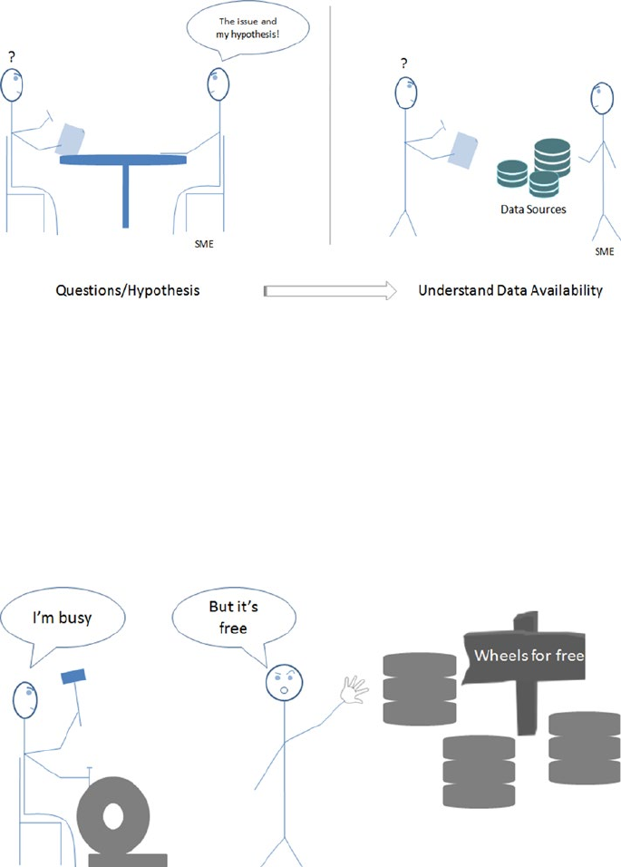
Chapter 7 ■ ConClusion
347
Start with Questions/Hypothesis Then Move to Data!
Figure 7-1. Questions/Hypothesis to Data
Figure 7-2. Don’t reinvent the wheel
Don’t jump into understanding the data before formulating the objective to be
achieved using data. It is a good practice to start with a good list of questions, and work
closely with domain experts to understand core issues and frame the problem statement.
This will help you in choosing the right machine learning algorithm (supervised vs.
unsupervised) then move onto understanding different data sources.
Don’t Reinvent the Wheels from Scratch
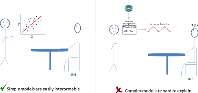
Chapter 7 ■ ConClusion
348
Machine learning open source community is very active, there are plenty of efficient
tools available, and lot more are being developed/released often, so do not try to reinvent
the wheel in terms of solutions/algorithms/tools unless required. Try to understand what
solutions exist in the market before venturing into building something from scratch.
Start with Simple Models
Always start with simple models (such as regressions), as these can be explained
easily in layman terms to any non-techie people. This will help you and the subject
matter experts to understand the variable relationships and gain confidence in the
model. Further it will significantly help you to create the right features. Move to complex
models only if you see a noteworthy increase in the model performance.
Figure 7-3. Start with simple model
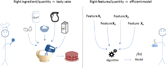
Chapter 7 ■ ConClusion
349
Focus on Feature Engineering
Relevant features lead to efficient models, not more features! Note that including
a large number of features might lead to an over-fitting problem. Including relevant
features in the model is the key to building an efficient model. Remember that the feature
engineering part is talked about as an art form and is the key differentiator in competitive
machine learning. The right ingredients mixed to the right quantity are the secret for tasty
food, similarly passing the relevant/right features to the machine learning algorithm is
the secret to efficient model.
Beware of Common ML Imposters
Carefully handle some of the common machine learning imposters such as data quality
issues (such as missing data, outliers, categorical data, scaling), imbalanced dataset for
classification, over-fitting, and under-fitting. Use the appropriate techniques discussed
in Chapter 3 for handling data quality issues and techniques discussed in Chapter 4,
model diagnosis and tuning, such as ensemble techniques, and hyperparameter tuning
to improve the model performance. To get started on real life use cases, I encourage you
to try using the dataset or the problem statements provided by various online forums
such as UCI Machine Learning Repository, Kaggle etc. As it goes “if you want to go fast
go alone, if you want to go far go together”, so remember that using a single machine
learning algorithm you can solve a given problem quickly, however using ensemble or
stacking techniques will give you the edge in achieving the greatest results possible.
Happy Machine Learning
I hope this expedition of machine learning in simplified six steps has been worthwhile,
and I hope this helps you to start a new journey of applying them on real-world problems.
I wish you all the very best and success for your further quests.
Figure 7-4. Feature engineering is an art

351
© Manohar Swamynathan 2017
M. Swamynathan, Mastering Machine Learning with Python in Six Steps,
DOI 10.1007/978-1-4842-2866-1
A
AdaBoosting process
dataset, 229
iteration 1, 230
iteration 2, 230
iteration 3, 230
vs. stand-alone decision
tree model, 231–232
steps, 228
weak classication models, 231
Agglomerative clustering. See Hierarchical
cluster technique
Analytics, 61
categorization, 61
descriptive analytics, 62
diagnostics, 63
predictions/estimations, 63
prescriptive, 64
types, 62
Articial general intelligence
(AGI), 57
Articial intelligence (AI)
analytics, 61
data mining, 60
data science, 64
evolution
AGI, 57
ANI, 57
ASI, 57
data analytics, 58
data mining, 58
data science, 58
denition, 58
statistics, 58
statistics, 58
Bayesian, 59
frequentist, 59
regression, 60
statistics vs. data mining vs. data
analytics vs. data science, 66
Articial narrow intelligence (ANI), 57
Articial neural network (ANN)
activation function, 305
autoencoders, 315
biological neurons, 301
CNN, 320
CNN and MNIST dataset, 327
correponding array, 299
deep learning, 298
handwritten digit(zero)image, 299
hidden_layer_sizes, 305
image classication, 299
learning_rate_init, 305
load MNIST data, 304
LSTM, 333
max_iter, 305
MLP and Keras, 312
MLP (feedforward network), 332
multilayer perceptron
representation, 303
multilayer perceptrons (feedforward
neural network), 303
perceptron, 300
RBM algorithm, 307
reinforcement learning, 340
scikit-learn MLP, 305
solver, 305
transfer learning, 336
visual challenges, 300
Index
■ INDEX
352
visualization, 331
visual pathway, 299
Articial super intelligence (ASI), 57
Autocorrelation function (ACF), 187
Autoencoders, 315
de-noise image, 319
dimension reduction, 316
elements, 315
Autoregressive integrated moving
average (ARIMA)
AM and MA, 186
autocorrelation, 189
build model and evaluate, 190
check stationary, 188
decompose time series, 187
model, 187
predict function, 193
predictors, 186
Autoregressive model (AM), 186
Average silhouette method, 201
B
Bagging, 222
Bag of words (BoW), 268
Bayesian statistics, 59
Biological vs. articial neuron, 301
Bootstrapaggregation. See Bagging
C
Clustering
hierarchicalcluster (see Hierarchical
cluster technique)
K-means
accuracy, 198–199
average silhouette method, 201
elbow method, 199
expectation maximization, 195
limitations, 196–197
methods, 199
text
k-means, 281
LSA, 280
singular value decomposition, 280
source code, 279
SVD, 281
Collaborative ltering (CF), 292
Command-line installer, 4
Convolution neural network (CNN), 320
Cross-industry standard process for data
mining (CRISP-DM)
business, 72
data gaps/relevance, 73
deployment, 73
evaluation, 73
framework and phases, 72
modeling, 73
preparation, 73
process diagram, 72
D
Data assemble (text), 253
dataframe, 257
get access key, 255
pdf, jpg, and audio le, 254
social media, 255
textract formats, 253
twitter authentication, 255
DataFrame, 90
Data mining
KDD, 70
techniques, 61
Data preprocessing (text), 259
bag of words, 268
lemmatization, 265
lower() function, 259
n-grams, 267
PoS tagging, 262
removing noise, 260
sentence tokenization, 259
stemming, 263
TF-IDF, 270
word tokenization, 260
Data science, 64
Deep learning
ANN (see Articial neural network
(ANN))
Cae, 298
Keras, 298
Lasagne, 298
libraries, 297
MXNet, 298
Pylearn2, 298
TensorFlow, 298
eano, 298
Deep natural language processing
(DNLP), 287
sopex package, 288
Word2Vec, 289
Articial neural network (ANN) (cont.)
■ INDEX
353
Descriptive analytics, 62
Diagnostic analytics, 63
dir() operation code, 46
Document term matrix (DTM), 270
E
Elbow method, 199
Ensemble methods
bagging, 222, 228
decision boundaries, 226
ExtraTree, 225
feature importance function, 224
RandomForest, 225
types of, 221
Enterprise resource planning (ERP)
systems, 61
Exception handling
code ow, 52
le operations, 51
Python built-in, 49–50
source code, 50
try clause, 50
Exploration (text), 272
co-occurrence matrix, 275
frequency chart, 272
lexical dispersion plot, 274
word cloud, 273
Exploratory data analysis (EDA)
Iris dataset, 126
multivariate analysis
code creation, 128
correlation matrix, 129
ndings values, 131
pair plot, 130–131
pandas dataframe visualization, 127
univariate analysis, 126
Extremely randomized trees
(ExtraTree), 225
F
Feature engineering
construction/generation, 125
handling categorical data
dummy variable
creation, 121–122
number conversion, 122–123
logical ow, 120
missing data, 121
normalization and scaling, 124
raw data, 120
summarization methods, 125
G
Generalized linear models (GLM), 173
Global positioning system (GPS), 55
Gradient boosting, 233
GridSearch, 247
H
Hard voting vs. soft voting, 242
Hierarchical cluster technique, 203
key parameters, 203
maximum linkage, 203
source code, 203
Hyperparameter tuning, 246
approach, 246
GridSearch, 247
RandomSearch, 248
I
Identity operators, 19
Input/output le
opening mode, 48
operations, 47
sequence, 47
J
Join statement
inner, 98
left, 97
outer, 98
right, 98
K
K-folds cross-validation
classication model, 220
holdout/single fold method, 219–220
stratication, 221
k nearest neighbors (kNN), 183
Knowledge discovery databases (KDD)
data mining, 71
data mining process ow, 70
interpretation/evaluation, 71
preprocessing and cleaning, 70
selection, 70
■ INDEX
354
stages, 69
transformation techniques, 71
L
Latent Dirichlet Allocation (LDA),
282–283
Latent semantic analysis (LSA), 280
Lemmatization, 265
Linear regression vs. logistic regression, 162
Logistic regression, 161
GLM distribution, 173–175
load data, 172
model training and evaluation, 172–173
multi-classes, 171
normalize data, 172
split data, 172
Long short-term memory (LSTM), 333
M
Machine learning
AI (see Articial intelligence (AI))
AI evolution
areas, 57
categorization, 67
CRISP-DM (see Cross-industry
standard process for data
mining (CRISP-DM))
data
attributes, 117
comparison, 120
continuous or quantitative, 118
discrete/qualitative, 118
fact and gures, 117
interval scale, 119
measurement scales, 118
nominal level, 118
ordinal scale, 119
ratio scale, 119–120
denitions, 53
EDA (see Exploratory data analysis
(EDA))
feature engineering (see Feature
engineering)
frameworks, 69
history, 54
KDD (see Knowledge discovery
databases (KDD))
libraries, 114
ML imposters, 349
overview, 345
pattern recognition, 53
process loop, 54
prospect customer identication, 53
Python (see Python packages)
questions/hypothesis, 347
recommendation system, 53
regression (see Supervised learning)
reinforcement, 68
resources, 116
robotic intelligent", 54
scikit-learn, 117
SEMMA (see Sample, explore, modify,
model, assess (SEMMA))
simple models, 348
spam detection, 53
statsmodels, 115, 117
supervised learning
classication, 67
regression, 67
Turing test, 56
unsupervised learning
clustering, 68
dimension reduction, 68
wheels from scratch, 347
Matplotlib, 100
Mean absolute error, 138
Model building, text similarity, 277
Model diagnosis and tuning
attributes, 209
bias and variance, 218
boosting, 228
AdaBoosting process, 228
ensemble voting, 240
essential tuning parameters, 235
gradient boosting, 233
illustration, 229
sklearn wrapper, 238
stacking, 244
xgboost, 236
ensemble methods
bagging, 222, 228
decision boundaries, 226
ExtraTree, 225
feature importance function, 224
RandomForest, 225
types of, 221
hyperparameter (see Hyperparameter
tuning)
Knowledge discovery databases (KDD)
(cont.)
■ INDEX
355
k-fold cross-validation, 219
probability cuto point
class distribution, 209
error message, 213
functions, 212
logistic regression model, 210
optimal cuto point, 211
rare event/imbalanced dataset
disadvantages, 216
handling techniques, 214
make_classication
function, 214–216
re-sampling, 213
variance, 218
Moving average (MA), 186
Multivariate linear regression
model, 147
Multivariate regression
housing dataset (RDatasets), 143
multicollinearity and VIF, 145
regression diagnostics, 152
homoscedasticity test, 154
linearity check, 154
model ttings, 156
outliers, 153
over-tting, 155
under-tting, 155
N
Natural language processing (NLP).
See Text mining
N-grams, 267
Nonlinear regression, 159
Non-negative matrix factorization
(NMF), 284
NumPy
arrays, 77
broadcasting, 87
built-in functions, 78
indexing
boolean, 84
eld access, 80
integer, 83
slice syntax, 81
types, 80
mathematical functions
array math, 84
sum function, 86
transpose function, 86
types, 80
O
Object-oriented
bar plots–ax.bar() and ax.barh(), 109
colomaps reference, 108
customization, 103
grid creation, 113
horizontal bar charts, 110
line plots–ax.plot(), 103
line style and marker style, 106
marker reference, 108
matplotlib line style reference, 107
multiple lines-dierent axis, 105
multiple lines-same axis, 104
pie chart–ax.pie(), 112
plotting defaults, 114
side-by-side bar chart, 111
stacked bar charts, 111
P, Q
Pandas
DataFrame, 90
data structures, 89–90
grouping operation, 99
join, 97
merge/join, 95
operations, 94–95
pivot tables, 100
reading and writing data, 90
SQL/excel/R data frames, 89
statistics, 91–92
view function, 93
Partial autocorrelation function (PACF), 187
Part of speech (PoS) tagging, 262
Polynomial regression, 139
Predictive analytics, 63
Prescriptive analytics, 64
Principal component analysis (PCA), 205
Problem types vs. potential ML
algorithms, 346
Python
code blocks
correct indentation, 7
incorrect indentation, 7
indentation, 7
suites, 7
control structure, 20
iteration, 21
loop control statement, 21
selection statements, 20
■ INDEX
356
denition, 1
dictionary, 37
exception handling, 48
le input/output, 47
identier, 5
interactive, 6
keywords, 6
lists, 22
module, 45
mottos, 1
multiline statements, 11
NumPy and Pandas, 3
object types
comments, 8
list vs. tuple vs. set vs.
dictionary, 10
multiline comments, 10
single line, 11
operators
arithmetic operators, 12
assignment operators, 15
bitwise operators, 16
comparison/relational
operators, 13
identity operators, 19
logical operators, 18
membership operators, 18
types, 12
vs. others, 6
popular coding language, 2
sets, 29
tuple
accessing tuple, 28
deleting items, 28
operations, 26
user-dened functions, 42
2.7/3.4.x
Anaconda, 3
graphical installer, 4
Linux installation, 4
ocial website, 4
OSX installation, 4
run command line, 5
version, 3
Windows installation, 4
Python packages
customizing labels, 102
data analysis
global functions, 100
key packages, 76
Matplotlib, 100
NumPy, 77
Pandas, 89
libraries, 76
object oriented, 103
R
RandomForest, 225
RandomSearch, 248
Recommender systems
collaborative ltering (CF), 292
content-based ltering, 292
types, 291
Recurrent neural network (RNN), 332
Regression analysis, 60
Regularization, 156
Reinforcement learning, 68, 340
Restricted Boltzman Machines
(RBM), 307
Robotic intelligent agent
components, 55
denition, 54
sensors and eectors, 55
Turing test, 56
Root mean squared error (RMSE), 138
S
Sample, explore, modify, model, assess
(SEMMA)
assess, 74
CRISP-DM and KDD, 75
explore, 74
frameworks, 75
modeling/data mining, 74
modify, 74
sample, 74
Sentiment analysis, 286
Sets
accessing set elements, 33
changing elements, 33
code creation, 32
dierence, 35
discard()/remove() method, 34
intersection, 35
key characteristics, 29
operations, 30, 32, 36
symmetric_dierence()method, 35
union, 34
Stacking, 244
Python (cont.)
■ INDEX
357
Stochastic gradient descent algorithm, 168
Supervised learning
cases, 132
classication, 160
confusion matrix, 164
correlation and causation, 133–134
decision trees
key parameters, 180
model, 178–180
nodes, 176
splits and grows, 177
stopping partition, 178
tting line, 167
k nearest neighbors (kNN), 183
linear regression model, 134
mean absolute error, 138
metrics, 136
RMSE, 138
R-squared metrics, 136–137
logistic regression, 161
model performance classication, 164
multiclass logistic regression, 171
multivariate regression
coecient, 149, 150
Durbin-Watson statistics, 150
housing dataset (RDatasets), 143
hypothesis testing steps, 150
multicollinearity and VIF, 145
normal distribution, 151
OLS regression results, 149
regression diagnostics, 152
results, 152
R-squared value, 149
standard error, 149
t and p-value, 150
nonlinear regression, 159
plot sigmoid function, 163
polynomial regression, 139
process ow, 175–176
regularization, 156, 169
ROC curve, 166
scatter plot, 133
slope line tting, 134
stochastic gradient descent, 168
students score vs. hours, 132
SVM (see Support vector machine
(SVM))
time-series forecasting
ARIMA, 186
components, 185
stationary time series, 185
under-tting, right-tting, and
over-tting, 169
Supervised learning algorithms
classication, 67
regression, 67
Support vector machine (SVM)
decision boundaries, 182
equation, 180
key objective, 180
key parameters, 181
symmetric_dierence()method, 35
T
Term document matrix (TDM), 268
Term frequency-inverse document
frequency (TF-IDF), 270
Text mining, 251
data assemble, 253
datapreprocessing (see Data
preprocessing (text))
DNLP (see Deep natural language
processing (DNLP))
exploration, 272
co-occurrence matrix, 275
frequency chart, 272
lexical dispersion plot, 274
word cloud, 273
libraries, 251–252
model building
classication, 284
clustering, 279
document term matrix, 277
Euclidian vs. cosine, 278
sentiment analysis, 286
text similarity, 277
topic modeling, 282
phases, 253
process overview, 252
Time-series forecasting
ARIMA, 186
components, 185
stationary time series, 185
Transfer learning, 336
Tuple, operations, 26
Turing test, 56
U, V
Unsupervised learning
clustering (see Clustering)
■ INDEX
358
PCA, 205
process ow, 194–195
User-dened functions
default argument, 44
denition, 42
functions with arguments, 43
functions without argument, 43
**kwargs, 45
length arguments, 44
passing argumens (*args), 45
variable/identier, 43
W
Word2Vec, 289
X, Y, Z
Xgboost (eXtreme gradient boosting), 236
Unsupervised learning (cont.)
