Instructor's Solutions Manual For Modern Control Systems, 12th Ed Systems Edition

User Manual: Pdf

Open the PDF directly: View PDF .
Page Count: 754 [warning: Documents this large are best viewed by clicking the View PDF Link!]

Cover Page
Title Page
ISBN 013602498X
Preface: Problem types
Contents
1 Introduction to Control Systems
2 Mathematical Models of Systems
3 State Variable Models
4 Feedback Control System Characteristics
5 The Performance of Feedback Control Systems
6 The Stability of Linear Feedback Systems
7 The Root Locus Method
8 Frequency Response Methods
9 Stability in the Frequency Domain
10 The Design of Feedback Control Systems
11 The Design of State Variable Feedback Systems
12 Robust Control Systems
13 Digital Control Systems

MODERN CONTROL SYSTEMS

SOLUTION MANUAL

Richard C. Dorf Robert H. Bishop

University of California, Davis Marquette University

A companion to

MODERN CONTROL SYSTEMS

TWELFTH EDITION

Richard C. Dorf

Robert H. Bishop

Prentice Hall

Upper Saddle River Boston Columbus San Francisco New York

Indianapolis London Toronto Sydney Singapore Tokyo Montreal Dubai

Madrid Hong Kong Mexico City Munich Paris Amsterdam Cape Town

from the publisher prior to any prohibited reproduction, storage in a retrieval system, or transmission in any form or by any means, electronic, mechanical, photocopying,

recording, or likewise. For information regarding permission(s), write to: Rights and Permissions Department, Pearson Education, Inc., Upper Saddle River, NJ 07458.

Instructor's Solutions Manual

Richard C. Dorf, University of California, Davis

Robert H. Bishop, University of Texas at Austin

ISBN-10: 013602498X

ISBN-13: 9780136024989

Publisher: Prentice Hall

Format: On-line Supplement

Published: 08/16/2010

Educator Home | eLearning & Assessment | Support/Contact Us | Find your rep | Exam copy bookbag

from the publisher prior to any prohibited reproduction, storage in a retrieval system, or transmission in any form or by any means, electronic, mechanical, photocopying,

recording, or likewise. For information regarding permission(s), write to: Rights and Permissions Department, Pearson Education, Inc., Upper Saddle River, NJ 07458.

for

Modern

Control Systems, 12/E

P R E F A C E

In each chapter, there are ﬁve problem types:

Exercises

Problems

Advanced Problems

Design Problems/Continuous Design Problem

Computer Problems

In total, there are over 1000 problems. The abundance of problems of in-

creasing complexity gives students conﬁdence in their problem-solving

ability as they work their way from the exercises to the design and

computer-based problems.

It is assumed that instructors (and students) have access to MATLAB

and the Control System Toolbox or to LabVIEW and the MathScript RT

Module. All of the computer solutions in this Solution Manual were devel-

oped and tested on an Apple MacBook Pro platform using MATLAB 7.6

Release 2008a and the Control System Toolbox Version 8.1 and LabVIEW

2009. It is not possible to verify each solution on all the available computer

platforms that are compatible with MATLAB and LabVIEW MathScript

RT Module. Please forward any incompatibilities you encounter with the

scripts to Prof. Bishop at the email address given below.

The authors and the staﬀ at Prentice Hall would like to establish an

open line of communication with the instructors using Modern Control

Systems. We encourage you to contact Prentice Hall with comments and

suggestions for this and future editions.

Robert H. Bishop rhbishop@marquette.edu

iii

from the publisher prior to any prohibited reproduction, storage in a retrieval system, or transmission in any form or by any means, electronic, mechanical, photocopying,

recording, or likewise. For information regarding permission(s), write to: Rights and Permissions Department, Pearson Education, Inc., Upper Saddle River, NJ 07458.

T A B L E - O F - C O N T E N T S

1. Introduction to Control Systems ..................................1

2. Mathematical Models of Systems . . . . . . . . . . . . . . . . . . . . . . . . . . . . . . . . 22

3. State Variable Models ...........................................85

4. Feedback Control System Characteristics . . . . . . . . . . . . . . . . . . . . . . . 133

5. The Performance of Feedback Control Systems . . . . . . . . . . . . . . . . . 177

6. The Stability of Linear Feedback Systems . . . . . . . . . . . . . . . . . . . . . . 234

7. The Root Locus Method .......................................277

8. Frequency Response Methods .................................. 382

9. Stability in the Frequency Domain . . . . . . . . . . . . . . . . . . . . . . . . . . . . . 445

10. The Design of Feedback Control Systems . . . . . . . . . . . . . . . . . . . . . . .519

11. The Design of State Variable Feedback Systems . . . . . . . . . . . . . . . . 600

12. Robust Control Systems .......................................659

13. Digital Control Systems ........................................714

from the publisher prior to any prohibited reproduction, storage in a retrieval system, or transmission in any form or by any means, electronic, mechanical, photocopying,

recording, or likewise. For information regarding permission(s), write to: Rights and Permissions Department, Pearson Education, Inc., Upper Saddle River, NJ 07458.

C H A P T E R 1

Introduction to Control Systems

There are, in general, no unique solutions to the following exercises and

problems. Other equally valid block diagrams may be submitted by the

student.

Exercises

E1.1 A microprocessor controlled laser system:

Controller

Error Current i(t) Power

out

Desired

power

output

Measured

power

-Laser

Process

processor

Micro-

Power

Sensor

Measurement

E1.2 A driver controlled cruise control system:

Desired

speed

Foot pedal Actual

auto

speed

Visual indication

of speed

Controller

Process

Measurement

Driver Car and

Engine

Speedometer

E1.3 Although the principle of conservation of momentum explains much of

the process of ﬂy-casting, there does not exist a comprehensive scientiﬁc

explanation of how a ﬂy-ﬁsher uses the small backward and forward mo-

tion of the ﬂy rod to cast an almost weightless ﬂy lure long distances (the

from the publisher prior to any prohibited reproduction, storage in a retrieval system, or transmission in any form or by any means, electronic, mechanical, photocopying,

recording, or likewise. For information regarding permission(s), write to: Rights and Permissions Department, Pearson Education, Inc., Upper Saddle River, NJ 07458.

2CHAPTER 1 Introduction to Control Systems

current world-record is 236 ft). The ﬂy lure is attached to a short invisible

leader about 15-ft long, which is in turn attached to a longer and thicker

Dacron line. The objective is cast the ﬂy lure to a distant spot with dead-

eye accuracy so that the thicker part of the line touches the water ﬁrst

and then the ﬂy gently settles on the water just as an insect might.

Desired

position of

the y

Actual

position

of the y

Visual indication

of the position of

the y

Fly-sher

Wind

disturbance

Controller

Process

Measurement

Mind and

body of the

y-sher

Rod, line,

and cast

Vision of

the y-sher

E1.4 An autofocus camera control system:

One-way trip time for the beam

Distance to subject

Lens focusing

motor

K 1

Lens

Conversion factor

(speed of light or

sound)

Emitter/

Receiver

Beam

Beam return Subject

from the publisher prior to any prohibited reproduction, storage in a retrieval system, or transmission in any form or by any means, electronic, mechanical, photocopying,

recording, or likewise. For information regarding permission(s), write to: Rights and Permissions Department, Pearson Education, Inc., Upper Saddle River, NJ 07458.

Exercises 3

E1.5 Tacking a sailboat as the wind shifts:

Desired

sailboat

direction

Actual

sailboat

direction

Measured sailboat direction

Wind

Error

Process

Measurement

Actuators

Controller

Sailboat

Gyro compass

Rudder and

sail adjustment

Sailor

E1.6 An automated highway control system merging two lanes of traﬃc:

Desired

gap Actual

gap

Measured gap

Error

Process

Measurement

Actuators

Controller

Active

vehicle

Brakes, gas or

steering

Embedded

computer

Radar

E1.7 Using the speedometer, the driver calculates the diﬀerence between the

measured speed and the desired speed. The driver throotle knob or the

brakes as necessary to adjust the speed. If the current speed is not too

much over the desired speed, the driver may let friction and gravity slow

the motorcycle down.

Desired

speed

Visual indication of speed

Actual

motorcycle

speed

Error

Process

Measurement

Actuators

Controller

Throttle or

brakes

Driver Motorcycle

Speedometer

from the publisher prior to any prohibited reproduction, storage in a retrieval system, or transmission in any form or by any means, electronic, mechanical, photocopying,

recording, or likewise. For information regarding permission(s), write to: Rights and Permissions Department, Pearson Education, Inc., Upper Saddle River, NJ 07458.

4CHAPTER 1 Introduction to Control Systems

E1.8 Human biofeedback control system:

Measurement

Desired

body

temp

Actual

body

temp

Visual indication of

body temperature

Message to

blood vessels

Process

Controller

Body sensor

Hypothalumus Human body

TV display

E1.9 E-enabled aircraft with ground-based ﬂight path control:

Corrections to the

ight path

Controller

Gc(s)

Aircraft

G(s)

Desired

Flight

Path

Flight

Path

Corrections to the

ight path

Controller

Gc(s)

Aircraft

G(s)

Desired

Flight

Path

Flight

Path

Ground-Based Computer Network

Health

Parameters

Health

Parameters

Meteorological

data

Meteorological

data

Optimal

ight path

Optimal

ight path

Location

and speed

Location

and speed

E1.10 Unmanned aerial vehicle used for crop monitoring in an autonomous

mode:

Gc(s)G(s)

Camera

Ground

photo

Controller UAV

Specified

Flight

Trajectory

Location with

respect to the ground

Flight

Trajectory

Map

Correlation

Algorithm

Trajectory

error

Sensor

from the publisher prior to any prohibited reproduction, storage in a retrieval system, or transmission in any form or by any means, electronic, mechanical, photocopying,

recording, or likewise. For information regarding permission(s), write to: Rights and Permissions Department, Pearson Education, Inc., Upper Saddle River, NJ 07458.

Exercises 5

E1.11 An inverted pendulum control system using an optical encoder to measure

the angle of the pendulum and a motor producing a control torque:

Error Angle

Desired

angle

Measured

angle

-Pendulum

Process

Optical

encoder

Measurement

Motor

Actuator

Torque

Voltage

Controller

E1.12 In the video game, the player can serve as both the controller and the sen-

sor. The objective of the game might be to drive a car along a prescribed

path. The player controls the car trajectory using the joystick using the

visual queues from the game displayed on the computer monitor.

Error Game

objective

Desired

game

objective -Video game

Process

Player

(eyesight, tactile, etc.)

Measurement

Joystick

Actuator

Player

Controller

from the publisher prior to any prohibited reproduction, storage in a retrieval system, or transmission in any form or by any means, electronic, mechanical, photocopying,

recording, or likewise. For information regarding permission(s), write to: Rights and Permissions Department, Pearson Education, Inc., Upper Saddle River, NJ 07458.

6CHAPTER 1 Introduction to Control Systems

Problems

P1.1 An automobile interior cabin temperature control system block diagram:

Desired

temperature

set by the

driver

Automobile

cabin temperature

Measured temperature

Error

Process

Measurement

Controller

Automobile

cabin

Temperature

sensor

Thermostat and

air conditioning

unit

P1.2 A human operator controlled valve system:

Desired

uid

output *

Error * Fluid

output

* = operator functions

Visual indication

of uid output *

Process

Measurement

Controller

Valve

Meter

Tank

P1.3 A chemical composition control block diagram:

Desired

chemical

composition

Error

Chemical

composition

Measured chemical

composition

Process

Measurement

Controller

Valve Mixer tube

Infrared analyzer

from the publisher prior to any prohibited reproduction, storage in a retrieval system, or transmission in any form or by any means, electronic, mechanical, photocopying,

recording, or likewise. For information regarding permission(s), write to: Rights and Permissions Department, Pearson Education, Inc., Upper Saddle River, NJ 07458.

Problems 7

P1.4 A nuclear reactor control block diagram:

Desired

power level

Output

power level

Error

Measured chemical

composition

Process

Measurement

Controller

Ionization chamber

Reactor

and rods

Motor and

amplier

P1.5 A light seeking control system to track the sun:

Ligh

intensity

Desired

carriage

position

Light

source Photocell

carriage

position

Motor

inputs

Error

ProcessController

Motor,

carriage,

and gears

Controller

Trajectory

Planner

Dual

Photocells

Measurement

P1.6 If you assume that increasing worker’s wages results in increased prices,

then by delaying or falsifying cost-of-living data you could reduce or elim-

inate the pressure to increase worker’s wages, thus stabilizing prices. This

would work only if there were no other factors forcing the cost-of-living

up. Government price and wage economic guidelines would take the place

of additional “controllers” in the block diagram, as shown in the block

diagram.

Initial

wages

Prices

Wage increases

Market-based prices

Cost-of-living

Controller

Industry Government

price

guidelines

Government

wage

guidelines

Controller

Process

from the publisher prior to any prohibited reproduction, storage in a retrieval system, or transmission in any form or by any means, electronic, mechanical, photocopying,

recording, or likewise. For information regarding permission(s), write to: Rights and Permissions Department, Pearson Education, Inc., Upper Saddle River, NJ 07458.

8CHAPTER 1 Introduction to Control Systems

P1.7 Assume that the cannon ﬁres initially at exactly 5:00 p.m.. We have a

positive feedback system. Denote by ∆tthe time lost per day, and the

net time error by ET. Then the follwoing relationships hold:

∆t= 4/3 min.+ 3 min.= 13/3 min.

and

ET= 12 days ×13/3 min./day .

Therefore, the net time error after 15 days is

ET= 52 min.

P1.8 The student-teacher learning process:

Desired

knowledge

Error Lectures

Knowledge

Measured knowledge

Controller Process

Teacher Student

Measurement

Exams

P1.9 A human arm control system:

Visual indication of

arm location

u e

Controller Process

Measurement

Desired

arm

location

Arm

location

Nerve signals

Eyes and

pressure

receptors

Brain Arm &

muscles

Pressure

from the publisher prior to any prohibited reproduction, storage in a retrieval system, or transmission in any form or by any means, electronic, mechanical, photocopying,

recording, or likewise. For information regarding permission(s), write to: Rights and Permissions Department, Pearson Education, Inc., Upper Saddle River, NJ 07458.

Problems 9

P1.10 An aircraft ﬂight path control system using GPS:

Desired

ight path

from air trac

controllers

Flight

path

Measured ight path

Error

Process

Measurement

Actuators

Controller

Aircraft

Global Positioning

System

Computer

Auto-pilot Ailerons, elevators,

rudder, and

engine power

P1.11 The accuracy of the clock is dependent upon a constant ﬂow from the

oriﬁce; the ﬂow is dependent upon the height of the water in the ﬂoat

tank. The height of the water is controlled by the ﬂoat. The control system

controls only the height of the water. Any errors due to enlargement of

the oriﬁce or evaporation of the water in the lower tank is not accounted

for. The control system can be seen as:

Desired

height of

the water

in oat tank

Actual

height

Process

Controller

Flow from

upper tank

to oat tank

Float level

P1.12 Assume that the turret and fantail are at 90◦, if θw6=θF-90◦. The fantail

operates on the error signal θw-θT, and as the fantail turns, it drives the

turret to turn.

Wind

Fantail

Turret

= Wind angle

= Fantail angle

= Turret angle

Torque

Error

Process

Controller

Gears & turret

Fantail

from the publisher prior to any prohibited reproduction, storage in a retrieval system, or transmission in any form or by any means, electronic, mechanical, photocopying,

recording, or likewise. For information regarding permission(s), write to: Rights and Permissions Department, Pearson Education, Inc., Upper Saddle River, NJ 07458.

10 CHAPTER 1 Introduction to Control Systems

P1.13 This scheme assumes the person adjusts the hot water for temperature

control, and then adjusts the cold water for ﬂow rate control.

Desired water

temperature

Actual

water temperature

and ow rate

Cold

water

Desired water

ow rate

Measured water ow

Measured water temperature

Error

ProcessController

Measurement

Human: visual

and touch

Valve adjust

Valve adjust Hot water

system

Cold water

system

Hot

water

P1.14 If the rewards in a speciﬁc trade is greater than the average reward, there

is a positive inﬂux of workers, since

q(t) = f1(c(t)−r(t)).

If an inﬂux of workers occurs, then reward in speciﬁc trade decreases,

since

c(t) = −f2(q(t)).

Error

Process

Controller

f1(c(t)-r(t)) f2(q(t))

q(t)Total of

rewards

c(t)

Average

rewards

r(t)

P1.15 A computer controlled fuel injection system:

Desired

Fuel

Pressure

Fuel

Pressure

Measured fuel pressure

Process

Measurement

Controller

Fuel Pressure

Sensor

Electronic

Control Unit

High Pressure Fuel

Supply Pump and

Electronic Fuel

Injectors

from the publisher prior to any prohibited reproduction, storage in a retrieval system, or transmission in any form or by any means, electronic, mechanical, photocopying,

recording, or likewise. For information regarding permission(s), write to: Rights and Permissions Department, Pearson Education, Inc., Upper Saddle River, NJ 07458.

Problems 11

P1.16 With the onset of a fever, the body thermostat is turned up. The body

adjusts by shivering and less blood ﬂows to the skin surface. Aspirin acts

to lowers the thermal set-point in the brain.

Body

temperature

Desired temperature

or set-point from body

thermostat in the brain

Measured body temperature

Process

Measurement

Controller

Internal sensor

Body

Adjustments

within the

body

P1.17 Hitting a baseball is arguably one of the most diﬃcult feats in all of sports.

Given that pitchers may throw the ball at speeds of 90 mph (or higher!),

batters have only about 0.1 second to make the decision to swing—with

bat speeds aproaching 90 mph. The key to hitting a baseball a long dis-

tance is to make contact with the ball with a high bat velocity. This is

more important than the bat’s weight, which is usually around 33 ounces

(compared to Ty Cobb’s bat which was 41 ounces!). Since the pitcher can

throw a variety of pitches (fast ball, curve ball, slider, etc.), a batter must

decide if the ball is going to enter the strike zone and if possible, decide

the type of pitch. The batter uses his/her vision as the sensor in the feed-

back loop. A high degree of eye-hand coordination is key to success—that

is, an accurate feedback control system.

P1.18 Deﬁne the following variables: p= output pressure, fs= spring force

=Kx,fd= diaphragm force = Ap, and fv= valve force = fs-fd.

The motion of the valve is described by ¨y=fv/m where mis the valve

mass. The output pressure is proportional to the valve displacement, thus

p=cy , where cis the constant of proportionality.

Screw

displacement

x(t)

Valve position

Output

pressure

p(t)

Diaphragm area

Valve

Constant of

proportionality

Spring

from the publisher prior to any prohibited reproduction, storage in a retrieval system, or transmission in any form or by any means, electronic, mechanical, photocopying,

recording, or likewise. For information regarding permission(s), write to: Rights and Permissions Department, Pearson Education, Inc., Upper Saddle River, NJ 07458.

12 CHAPTER 1 Introduction to Control Systems

P1.19 A control system to keep a car at a given relative position oﬀset from a

lead car:

Throttle Position of

follower

uReference

photo

Relative

position

Desired relative position

Position

of lead

Controller Video camera

& processing

algorithms

Follower

car

Actuator

Fuel

throttle

(fuel)

Lead car

P1.20 A control system for a high-performance car with an adjustable wing:

Desired

road

adhesion

Road

adhesion

Measured road adhesion

Road

conditions

Process

Measurement

Controller

Tire internal

strain gauges

Race Car

Actuator

Adjustable

wing

Computer

P1.21 A control system for a twin-lift helicopter system:

Desired altitude Altitude

Measured altitude

Separation distance

Desired separation

distance

Measured separation

distance

Measurement

Radar

Altimeter

Controller

Pilot

Process

Helicopter

from the publisher prior to any prohibited reproduction, storage in a retrieval system, or transmission in any form or by any means, electronic, mechanical, photocopying,

recording, or likewise. For information regarding permission(s), write to: Rights and Permissions Department, Pearson Education, Inc., Upper Saddle River, NJ 07458.

Problems 13

P1.22 The desired building deﬂection would not necessarily be zero. Rather it

would be prescribed so that the building is allowed moderate movement

up to a point, and then active control is applied if the movement is larger

than some predetermined amount.

Desired

deection

Deection

Measured deection

Process

Measurement

Controller

Building

Hydraulic

stieners

Strain gauges

on truss structure

P1.23 The human-like face of the robot might have micro-actuators placed at

strategic points on the interior of the malleable facial structure. Coopera-

tive control of the micro-actuators would then enable the robot to achieve

various facial expressions.

Desired

actuator

position

Voltage Actuator

position

Measured position

Error

Process

Measurement

Controller

Amplier

Position

sensor

Electro-

mechanical

actuator

P1.24 We might envision a sensor embedded in a “gutter” at the base of the

windshield which measures water levels—higher water levels corresponds

to higher intensity rain. This information would be used to modulate the

wiper blade speed.

Desired

wiper speed

Wiper

blade

speed

Measured water level

Process

Measurement

Controller

KWater depth

sensor

Wiper blade

and motor

Electronic

Control Unit

from the publisher prior to any prohibited reproduction, storage in a retrieval system, or transmission in any form or by any means, electronic, mechanical, photocopying,

recording, or likewise. For information regarding permission(s), write to: Rights and Permissions Department, Pearson Education, Inc., Upper Saddle River, NJ 07458.

14 CHAPTER 1 Introduction to Control Systems

P1.25 A feedback control system for the space traﬃc control:

Desired

orbit position

Actual

orbit position

Measured orbit position

Jet

commands

Applied

forces

Error

Process

Measurement

Actuator

Controller

Satellite

Reaction

control jets

Control

law

Radar or GPS

P1.26 Earth-based control of a microrover to point the camera:

Microrover

Camera position

command

Controller

Gc(s)

Camera position command

Camera

Position

Receiver/

Transmitter Rover

position

Camera

Measured camera position

G(s)

Measured camera

position Sensor

P1.27 Control of a methanol fuel cell:

Methanol water

solution

Controller

Gc(s)

Recharging

System

GR(s)

Fuel Cell

G(s)

-Charge

Level

Desired

Charge

Level

Measured charge level

Sensor

H(s)

from the publisher prior to any prohibited reproduction, storage in a retrieval system, or transmission in any form or by any means, electronic, mechanical, photocopying,

recording, or likewise. For information regarding permission(s), write to: Rights and Permissions Department, Pearson Education, Inc., Upper Saddle River, NJ 07458.

Advanced Problems 15

Advanced Problems

AP1.1 Control of a robotic microsurgical device:

Controller

Gc(s)

Microsurgical

robotic manipulator

G(s)

-End-effector

Position

Desired

End-effector

Position

Sensor

H(s)

AP1.2 An advanced wind energy system viewed as a mechatronic system:

WIND ENERGY

SYSTEM

Physical System Modeling

Signals and Systems

Sensors and Actuators

Computers and

Logic Systems

Software and

Data Acquisition

COMPUTER EQUIPMENT FOR CONTROLLING THE SYSTEM

SAFETY MONITORING SYSTEMS

CONTROLLER ALGORITHMS

DATA ACQUISTION: WIND SPEED AND DIRECTION

ROTOR ANGULAR SPEED

PROPELLOR PITCH ANGLE

CONTROL SYSTEM DESIGN AND ANALYSIS

ELECTRICAL SYSTEM DESIGN AND ANALYSIS

POWER GENERATION AND STORAGE

SENSORS

Rotor rotational sensor

Wind speed and direction sensor

ACTUATORS

Motors for manipulatiing the propeller pitch

AERODYNAMIC DESIGN

STRUCTURAL DESIGN OF THE TOWER

ELECTRICAL AND POWER SYSTEMS

AP1.3 The automatic parallel parking system might use multiple ultrasound

sensors to measure distances to the parked automobiles and the curb.

The sensor measurements would be processed by an on-board computer

to determine the steering wheel, accelerator, and brake inputs to avoid

collision and to properly align the vehicle in the desired space.

from the publisher prior to any prohibited reproduction, storage in a retrieval system, or transmission in any form or by any means, electronic, mechanical, photocopying,

recording, or likewise. For information regarding permission(s), write to: Rights and Permissions Department, Pearson Education, Inc., Upper Saddle River, NJ 07458.

16 CHAPTER 1 Introduction to Control Systems

Even though the sensors may accurately measure the distance between

the two parked vehicles, there will be a problem if the available space is

not big enough to accommodate the parking car.

Error Actual

automobile

position

Desired

automobile

position -Automobile

Process

Ultrasound

Measurement

Steering wheel,

accelerator, and

brake

Actuators

On-board

computer

Controller

Position of automobile

relative to parked cars

and curb

AP1.4 There are various control methods that can be considered, including plac-

ing the controller in the feedforward loop (as in Figure 1.3). The adaptive

optics block diagram below shows the controller in the feedback loop, as

an alternative control system architecture.

Compensated

image

Uncompensated

image Astronomical

telescope

mirror

Process

Wavefront

sensor

Measurement

Wavefront

corrector

Actuator & controller

Wavefront

reconstructor

Astronomical

object

AP1.5 The control system might have an inner loop for controlling the acceler-

ation and an outer loop to reach the desired ﬂoor level precisely.

Elevator Floor

Desired

acceleration

Desired

floor

Elevator

motor,

cables, etc.

Controller #2 Controller #1

Error

Acceleration

Measurement

Measured acceleration

Outer

Loop

Inner

Loop

from the publisher prior to any prohibited reproduction, storage in a retrieval system, or transmission in any form or by any means, electronic, mechanical, photocopying,

recording, or likewise. For information regarding permission(s), write to: Rights and Permissions Department, Pearson Education, Inc., Upper Saddle River, NJ 07458.

Advanced Problems 17

AP1.6 An obstacle avoidance control system would keep the robotic vacuum

cleaner from colliding with furniture but it would not necessarily put the

vacuum cleaner on an optimal path to reach the entire ﬂoor. This would

require another sensor to measure position in the room, a digital map of

the room layout, and a control system in the outer loop.

Desired

distance

from

obstacles

Distance

from

obstacles

Error

Infrared

sensors

Measured distance from obstacle

Controller

Process

Robotic

vacuum

cleaner

Motors,

wheels, etc.

from the publisher prior to any prohibited reproduction, storage in a retrieval system, or transmission in any form or by any means, electronic, mechanical, photocopying,

recording, or likewise. For information regarding permission(s), write to: Rights and Permissions Department, Pearson Education, Inc., Upper Saddle River, NJ 07458.

18 CHAPTER 1 Introduction to Control Systems

Design Problems

The machine tool with the movable table in a feedback control conﬁgu-CDP1.1

ration:

Desired

position

Measured position

Actual

position

Error

Process

Measurement

Actuator

Controller

Position sensor

Machine

tool with

table

Amplier Positioning

motor

DP1.1 Use the stereo system and ampliﬁers to cancel out the noise by emitting

signals 180◦out of phase with the noise.

Desired

noise = 0

Noise

signal

Noise in

cabin

Process

Measurement

Controller

Machine

tool with

table

Positioning

motor

Microphone

Shift phase

by 180 deg

DP1.2 An automobile cruise control system:

Desired

speed

of auto

set by

driver

Desired

shaft

speed Actual

speed

of auto

Drive shaf t speed

Measured shaft speed

Process

Measurement

Controller

Automobile

and engine

Valve

Electric

motor

Shaft speed

sensor

1/K

from the publisher prior to any prohibited reproduction, storage in a retrieval system, or transmission in any form or by any means, electronic, mechanical, photocopying,

recording, or likewise. For information regarding permission(s), write to: Rights and Permissions Department, Pearson Education, Inc., Upper Saddle River, NJ 07458.

Design Problems 19

DP1.3 An automoted cow milking system:

Location

of cup Milk

Desired cup

location

Measured cup location

Cow location

Measurement

Vision system

Measurement

Vision system

Controller Process

Motor and

gears Robot arm and

cup gripper

Actuator

Cow and

milker

DP1.4 A feedback control system for a robot welder:

Desired

position

Voltage

Weld

top

position

Measured position

Error

Process

Measurement

Controller

Motor and

arm

Computer and

amplier

Vision camera

DP1.5 A control system for one wheel of a traction control system:

Brake torque

Wheel

speed

Actual slip Measured

slip

Vehicle speed

Rw= Radius of wheel

Sensor

Vehicle

dynamics

Sensor

Antiskid

controller

Wheel

dynamics

Engine torque Antislip

controller

1/Rw

from the publisher prior to any prohibited reproduction, storage in a retrieval system, or transmission in any form or by any means, electronic, mechanical, photocopying,

recording, or likewise. For information regarding permission(s), write to: Rights and Permissions Department, Pearson Education, Inc., Upper Saddle River, NJ 07458.

20 CHAPTER 1 Introduction to Control Systems

DP1.6 A vibration damping system for the Hubble Space Telescope:

Signal to

cancel the jitter Jitter of

vibration

Measurement of 0.05 Hz jitter

Desired

jitter = 0

Error

Process

Measurement

Actuators

Controller

Rate gyro

sensor

Computer Gyro and

reaction wheels

Spacecraft

dynamics

DP1.7 A control system for a nanorobot:

Error Actual

nanorobot

position

Desired

nanorobot

position -Nanorobot

Process

External beacons

Measurement

Plane surfaces

and propellers

Actuators

Bio-

computer

Controller

Many concepts from underwater robotics can be applied to nanorobotics

within the bloodstream. For example, plane surfaces and propellers can

provide the required actuation with screw drives providing the propul-

sion. The nanorobots can use signals from beacons located outside the

skin as sensors to determine their position. The nanorobots use energy

from the chemical reaction of oxygen and glucose available in the human

body. The control system requires a bio-computer–an innovation that is

not yet available.

For further reading, see A. Cavalcanti, L. Rosen, L. C. Kretly, M. Rosen-

feld, and S. Einav, “Nanorobotic Challenges n Biomedical Application,

Design, and Control,” IEEE ICECS Intl Conf. on Electronics, Circuits

and Systems, Tel-Aviv, Israel, December 2004.

DP1.8 The feedback control system might use gyros and/or accelerometers to

measure angle change and assuming the HTV was originally in the vertical

position, the feedback would retain the vertical position using commands

to motors and other actuators that produced torques and could move the

HTV forward and backward.

from the publisher prior to any prohibited reproduction, storage in a retrieval system, or transmission in any form or by any means, electronic, mechanical, photocopying,

recording, or likewise. For information regarding permission(s), write to: Rights and Permissions Department, Pearson Education, Inc., Upper Saddle River, NJ 07458.

Design Problems 21

Desired angle

from vertical (0o)

Angle from

vertical

Error

Gyros &

accelerometers

Measured angle from vertical

Controller

Process

HTV

Motors,

wheels, etc.

from the publisher prior to any prohibited reproduction, storage in a retrieval system, or transmission in any form or by any means, electronic, mechanical, photocopying,

recording, or likewise. For information regarding permission(s), write to: Rights and Permissions Department, Pearson Education, Inc., Upper Saddle River, NJ 07458.

C H A P T E R 2

Mathematical Models of Systems

Exercises

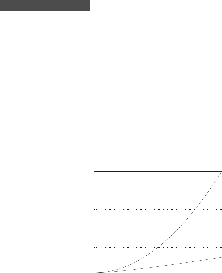
E2.1 We have for the open-loop

y=r2

and for the closed-loop

e=r−yand y=e2.

So, e=r−e2and e2+e−r= 0 .

0 0.5 1 1.5 2 2.5 3 3.5 4

open-loop

closed-loop

FIGURE E2.1

Plot of open-loop versus closed-loop.

For example, if r= 1, then e2+e−1 = 0 implies that e= 0.618. Thus,

y= 0.382. A plot yversus ris shown in Figure E2.1.

from the publisher prior to any prohibited reproduction, storage in a retrieval system, or transmission in any form or by any means, electronic, mechanical, photocopying,

recording, or likewise. For information regarding permission(s), write to: Rights and Permissions Department, Pearson Education, Inc., Upper Saddle River, NJ 07458.

Exercises 23

E2.2 Deﬁne

f(T) = R=R0e−0.1T

and

∆R=f(T)−f(T0),∆T=T−T0.

Then,

∆R=f(T)−f(T0) = ∂f

∂T T=T0=20◦

∆T+···

where

∂f

∂T T=T0=20◦

=−0.1R0e−0.1T0=−135,

when R0= 10,000Ω. Thus, the linear approximation is computed by

considering only the ﬁrst-order terms in the Taylor series expansion, and

is given by

∆R=−135∆T .

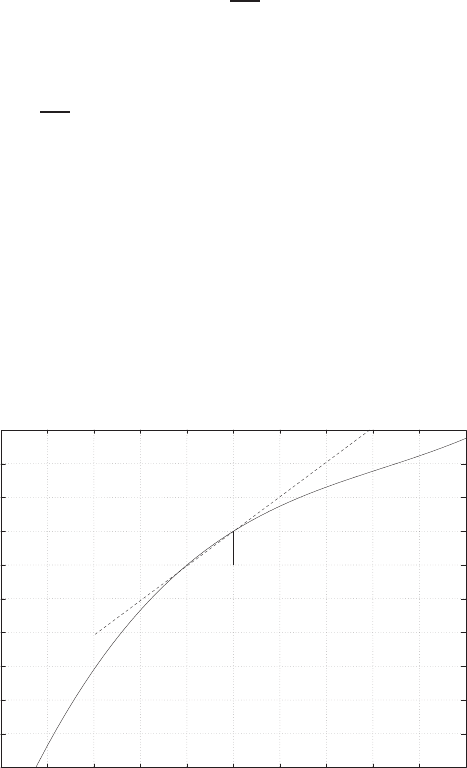
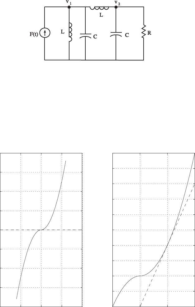
E2.3 The spring constant for the equilibrium point is found graphically by

estimating the slope of a line tangent to the force versus displacement

curve at the point y= 0.5cm, see Figure E2.3. The slope of the line is

K≈1.

-3

-2.5

-2

-1.5

-1

-0.5

0.5

1.5

-2 -1.5 -1 -0.5 0 0.5 1 1.5 2 2.5 3

y=Displacement (cm)

Force (n)

Spring compresses

Spring breaks

FIGURE E2.3

Spring force as a function of displacement.

from the publisher prior to any prohibited reproduction, storage in a retrieval system, or transmission in any form or by any means, electronic, mechanical, photocopying,

recording, or likewise. For information regarding permission(s), write to: Rights and Permissions Department, Pearson Education, Inc., Upper Saddle River, NJ 07458.

24 CHAPTER 2 Mathematical Models of Systems

E2.4 Since

R(s) = 1

we have

Y(s) = 4(s+ 50)

s(s+ 20)(s+ 10) .

The partial fraction expansion of Y(s) is given by

Y(s) = A1

s+A2

s+ 20 +A3

s+ 10

where

A1= 1 , A2= 0.6 and A3=−1.6.

Using the Laplace transform table, we ﬁnd that

y(t) = 1 + 0.6e−20t−1.6e−10t.

The ﬁnal value is computed using the ﬁnal value theorem:

lim

t→∞ y(t) = lim

s→0s4(s+ 50)

s(s2+ 30s+ 200) = 1 .

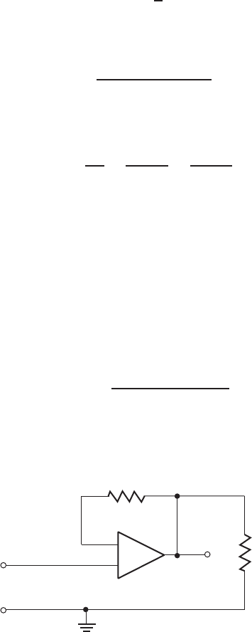
E2.5 The circuit diagram is shown in Figure E2.5.

vin v0

FIGURE E2.5

Noninverting op-amp circuit.

With an ideal op-amp, we have

vo=A(vin −v−),

from the publisher prior to any prohibited reproduction, storage in a retrieval system, or transmission in any form or by any means, electronic, mechanical, photocopying,

recording, or likewise. For information regarding permission(s), write to: Rights and Permissions Department, Pearson Education, Inc., Upper Saddle River, NJ 07458.

Exercises 25

where Ais very large. We have the relationship

v−=R1

R1+R2

vo.

Therefore,

vo=A(vin −R1

R1+R2

vo),

and solving for voyields

vo=A

1 + AR1

R1+R2

vin.

Since A≫1, it follows that 1 + AR1

R1+R2≈AR1

R1+R2. Then the expression for

vosimpliﬁes to

vo=R1+R2

vin.

E2.6 Given

y=f(x) = ex

and the operating point xo= 1, we have the linear approximation

y=f(x) = f(xo) + ∂f

∂x x=xo

(x−xo) + ···

where

f(xo) = e, df

dxx=xo=1

=e, and x−xo=x−1.

Therefore, we obtain the linear approximation y=ex.

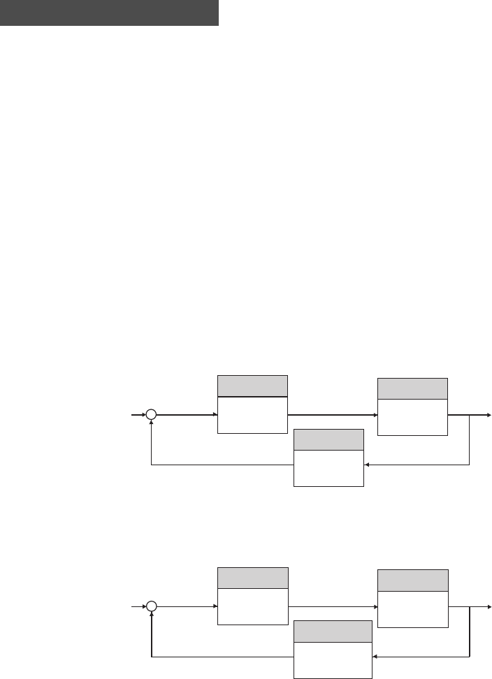
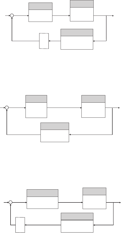
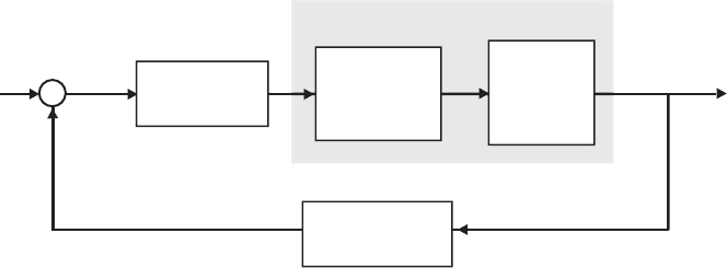
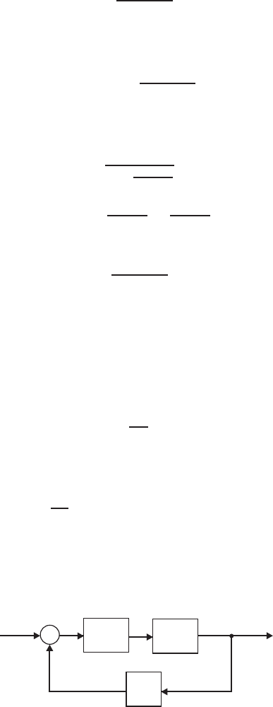
E2.7 The block diagram is shown in Figure E2.7.

+I(s)

R(s)

H(s)

G2(s)

G1(s)

Ea(s)

FIGURE E2.7

Block diagram model.

from the publisher prior to any prohibited reproduction, storage in a retrieval system, or transmission in any form or by any means, electronic, mechanical, photocopying,

recording, or likewise. For information regarding permission(s), write to: Rights and Permissions Department, Pearson Education, Inc., Upper Saddle River, NJ 07458.

26 CHAPTER 2 Mathematical Models of Systems

Starting at the output we obtain

I(s) = G1(s)G2(s)E(s).

But E(s) = R(s)−H(s)I(s), so

I(s) = G1(s)G2(s) [R(s)−H(s)I(s)] .

Solving for I(s) yields the closed-loop transfer function

I(s)

R(s)=G1(s)G2(s)

1 + G1(s)G2(s)H(s).

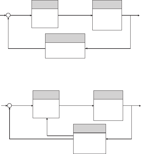
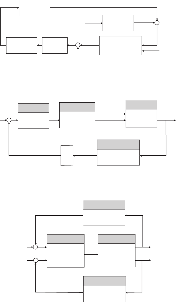
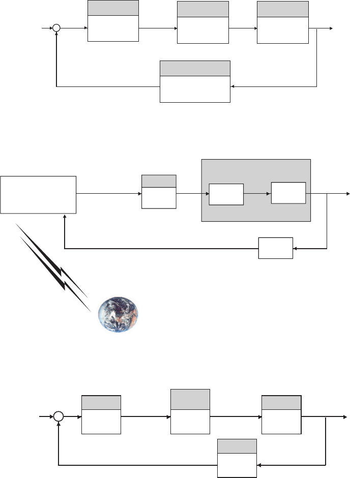
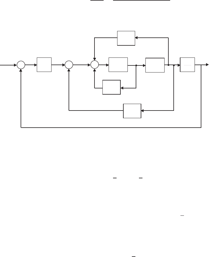
E2.8 The block diagram is shown in Figure E2.8.

Y(s)

G2(s)

G1(s)

R(s)

H3(s)

H1(s)

H2(s)

A(s)

W(s)

Z(s)

E(s)

FIGURE E2.8

Block diagram model.

Starting at the output we obtain

Y(s) = 1

sZ(s) = 1

sG2(s)A(s).

But A(s) = G1(s) [−H2(s)Z(s)−H3(s)A(s) + W(s)] and Z(s) = sY (s),

Y(s) = −G1(s)G2(s)H2(s)Y(s)−G1(s)H3(s)Y(s) + 1

sG1(s)G2(s)W(s).

Substituting W(s) = KE(s)−H1(s)Z(s) into the above equation yields

Y(s) = −G1(s)G2(s)H2(s)Y(s)−G1(s)H3(s)Y(s)

sG1(s)G2(s) [KE(s)−H1(s)Z(s)]

from the publisher prior to any prohibited reproduction, storage in a retrieval system, or transmission in any form or by any means, electronic, mechanical, photocopying,

recording, or likewise. For information regarding permission(s), write to: Rights and Permissions Department, Pearson Education, Inc., Upper Saddle River, NJ 07458.

Exercises 27

and with E(s) = R(s)−Y(s) and Z(s) = sY (s) this reduces to

Y(s) = [−G1(s)G2(s) (H2(s) + H1(s)) −G1(s)H3(s)

−1

sG1(s)G2(s)K]Y(s) + 1

sG1(s)G2(s)KR(s).

Solving for Y(s) yields the transfer function

Y(s) = T(s)R(s),

where

T(s) = KG1(s)G2(s)/s

1 + G1(s)G2(s) [(H2(s) + H1(s)] + G1(s)H3(s) + KG1(s)G2(s)/s.

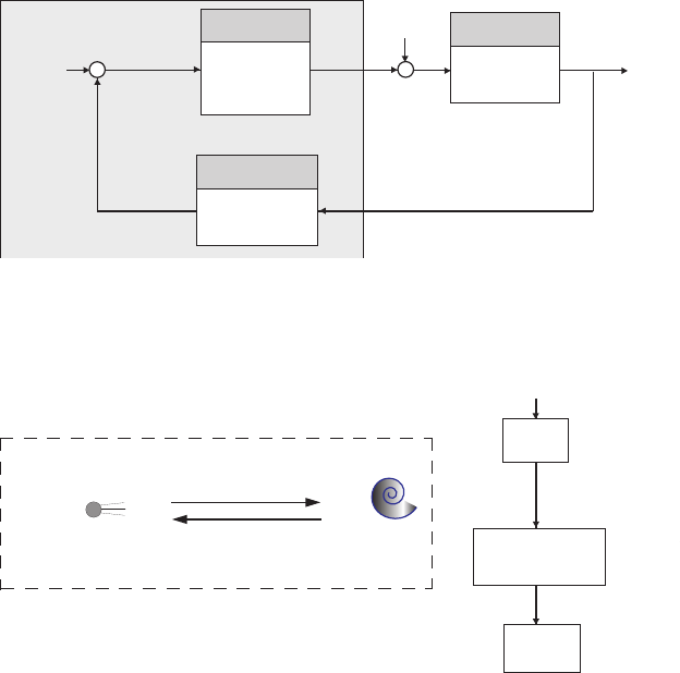
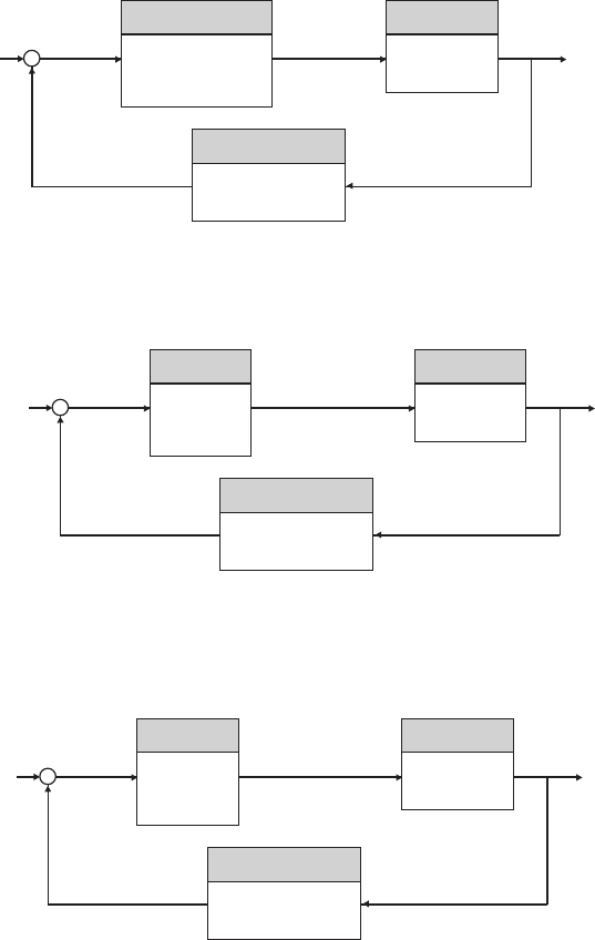
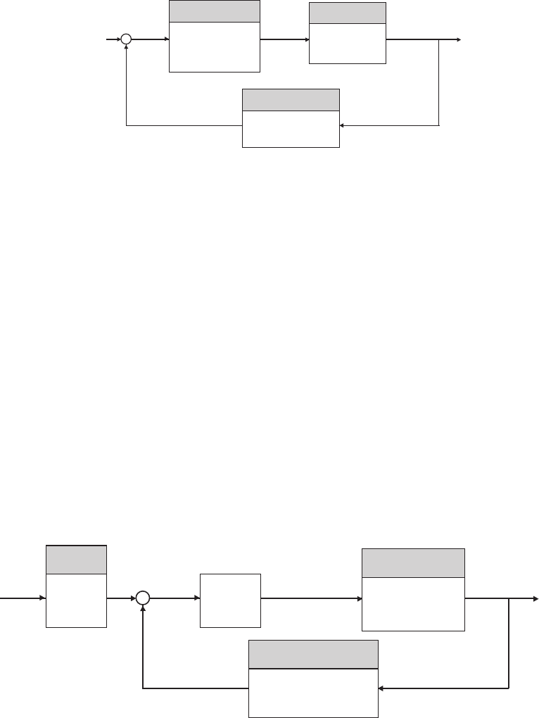
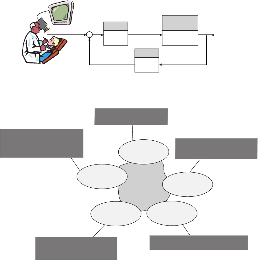
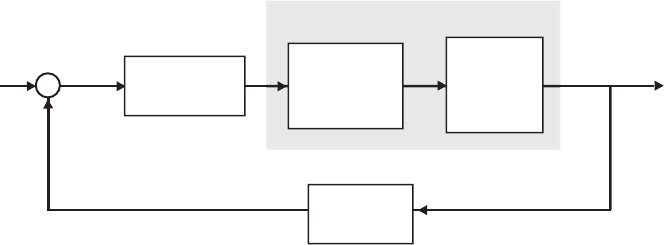
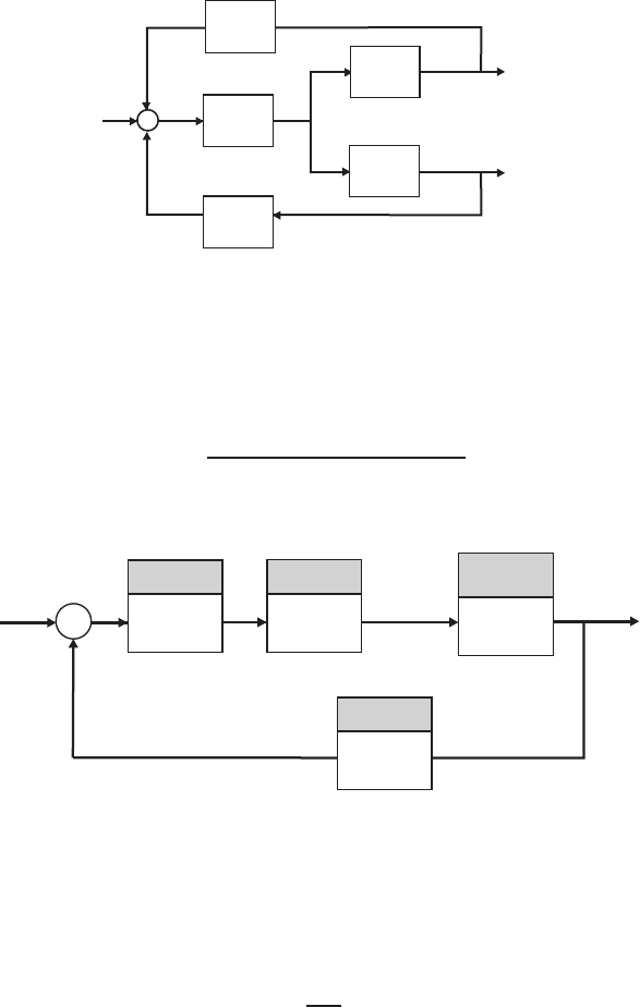
E2.9 From Figure E2.9, we observe that

Ff(s) = G2(s)U(s)

and

FR(s) = G3(s)U(s).

Then, solving for U(s) yields

U(s) = 1

G2(s)Ff(s)

and it follows that

FR(s) = G3(s)

G2(s)U(s).

Again, considering the block diagram in Figure E2.9 we determine

Ff(s) = G1(s)G2(s)[R(s)−H2(s)Ff(s)−H2(s)FR(s)] .

But, from the previous result, we substitute for FR(s) resulting in

Ff(s) = G1(s)G2(s)R(s)−G1(s)G2(s)H2(s)Ff(s)−G1(s)H2(s)G3(s)Ff(s).

Solving for Ff(s) yields

Ff(s) = G1(s)G2(s)

1 + G1(s)G2(s)H2(s) + G1(s)G3(s)H2(s)R(s).

from the publisher prior to any prohibited reproduction, storage in a retrieval system, or transmission in any form or by any means, electronic, mechanical, photocopying,

recording, or likewise. For information regarding permission(s), write to: Rights and Permissions Department, Pearson Education, Inc., Upper Saddle River, NJ 07458.

28 CHAPTER 2 Mathematical Models of Systems

R(s)G1(s)

H2(s)

G2(s)

G3(s)

H2(s)

Ff (s)

FR(s)

U(s)

FIGURE E2.9

Block diagram model.

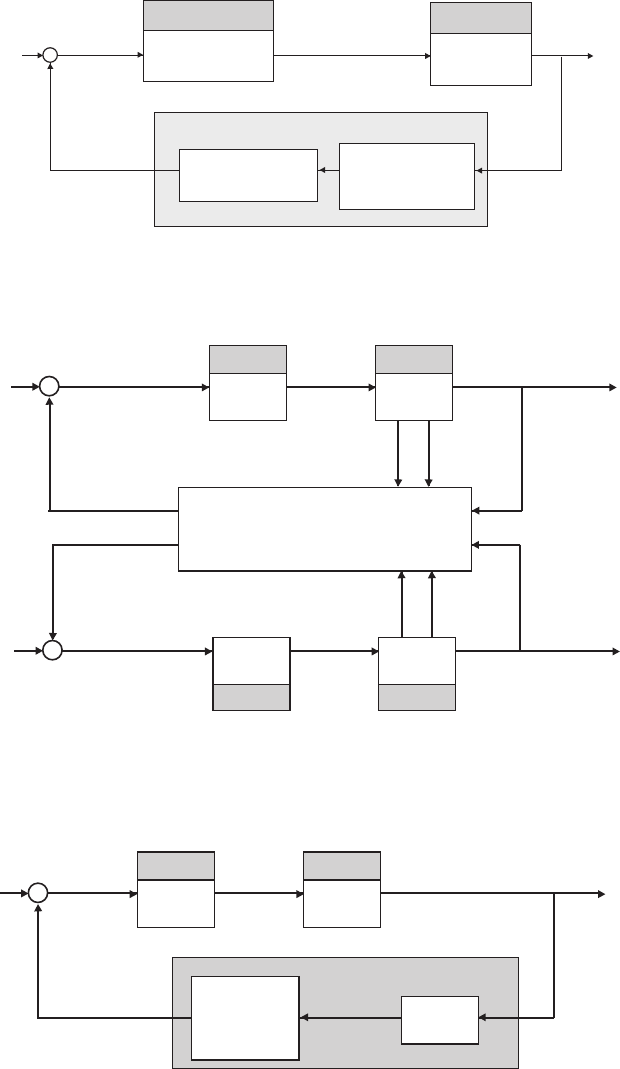
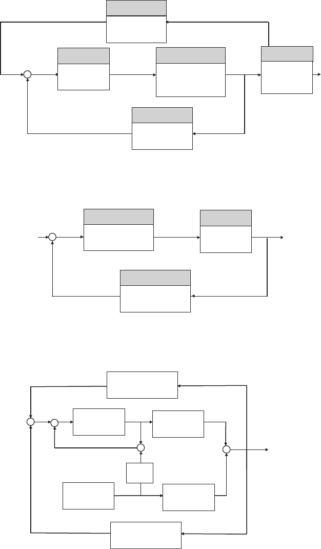
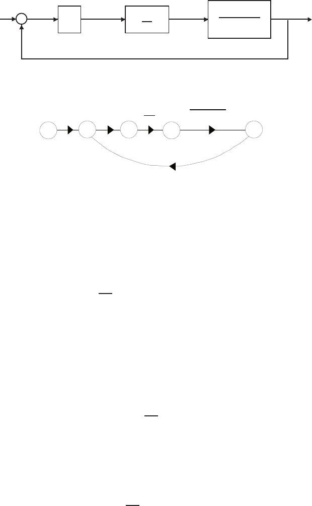
E2.10 The shock absorber block diagram is shown in Figure E2.10. The closed-

loop transfer function model is

T(s) = Gc(s)Gp(s)G(s)

1 + H(s)Gc(s)Gp(s)G(s).

R(s)

Desired piston

travel

Y(s)

Piston

travel

Controller

Gc(s)

Plunger and

Piston System

G(s)

Sensor

H(s)

Gear Motor

Gp(s)

Piston travel

measurement

FIGURE E2.10

Shock absorber block diagram.

E2.11 Let fdenote the spring force (n) and xdenote the deﬂection (m). Then

K=∆f

∆x.

Computing the slope from the graph yields:

(a) xo=−0.14m →K= ∆f /∆x= 10 n / 0.04 m = 250 n/m

(b) xo= 0m →K= ∆f /∆x= 10 n / 0.05 m = 200 n/m

from the publisher prior to any prohibited reproduction, storage in a retrieval system, or transmission in any form or by any means, electronic, mechanical, photocopying,

recording, or likewise. For information regarding permission(s), write to: Rights and Permissions Department, Pearson Education, Inc., Upper Saddle River, NJ 07458.

Exercises 29

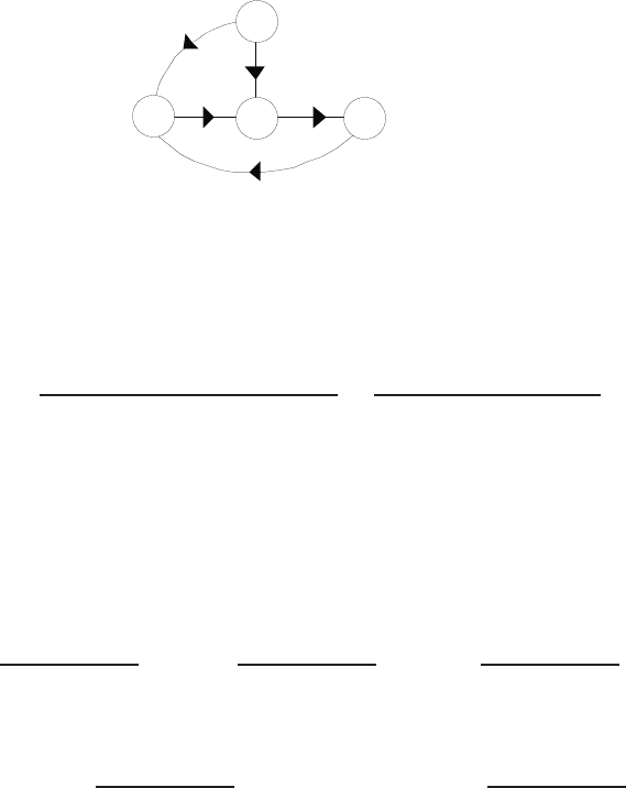
E2.12 The signal ﬂow graph is shown in Fig. E2.12. Find Y(s) when R(s) = 0.

Y (s)

-1

K2G(s)

-K 1

Td(s)

FIGURE E2.12

Signal ﬂow graph.

The transfer function from Td(s) to Y(s) is

Y(s) = G(s)Td(s)−K1K2G(s)Td(s)

1−(−K2G(s)) =G(s)(1 −K1K2)Td(s)

1 + K2G(s).

If we set

K1K2= 1 ,

then Y(s) = 0 for any Td(s).

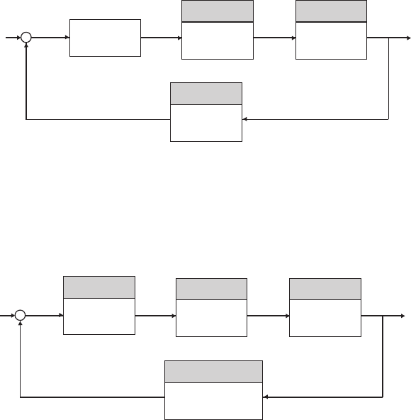
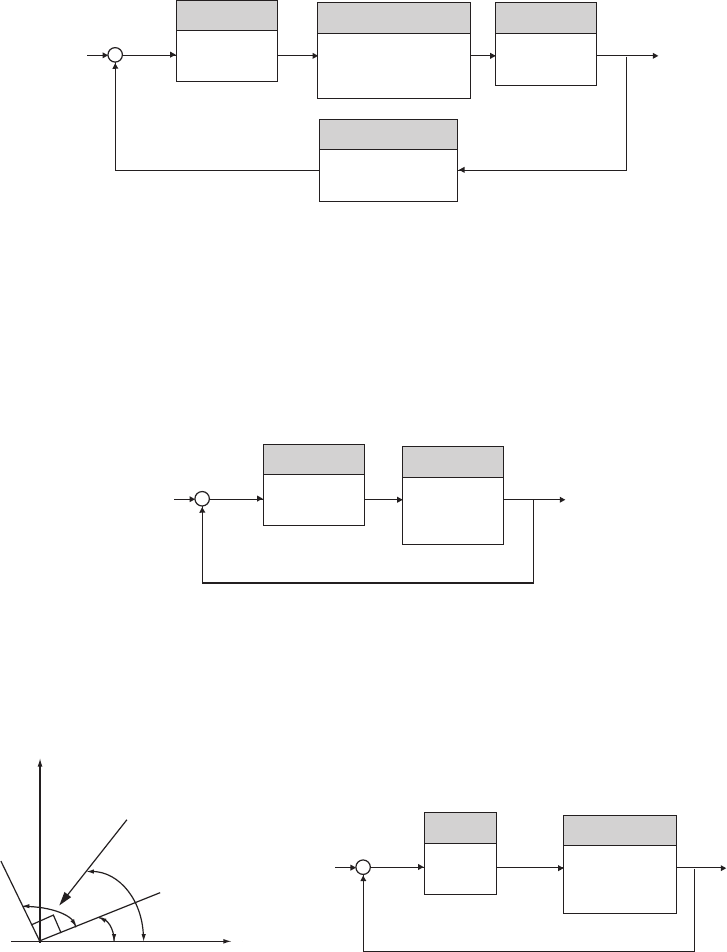
E2.13 The transfer function from R(s), Td(s), and N(s) to Y(s) is

Y(s) = K

s2+ 10s+KR(s)+1

s2+ 10s+KTd(s)−K

s2+ 10s+KN(s)

Therefore, we ﬁnd that

Y(s)/Td(s) = 1

s2+ 10s+Kand Y(s)/N(s) = −K

s2+ 10s+K

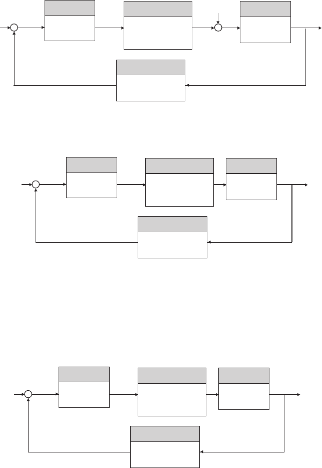
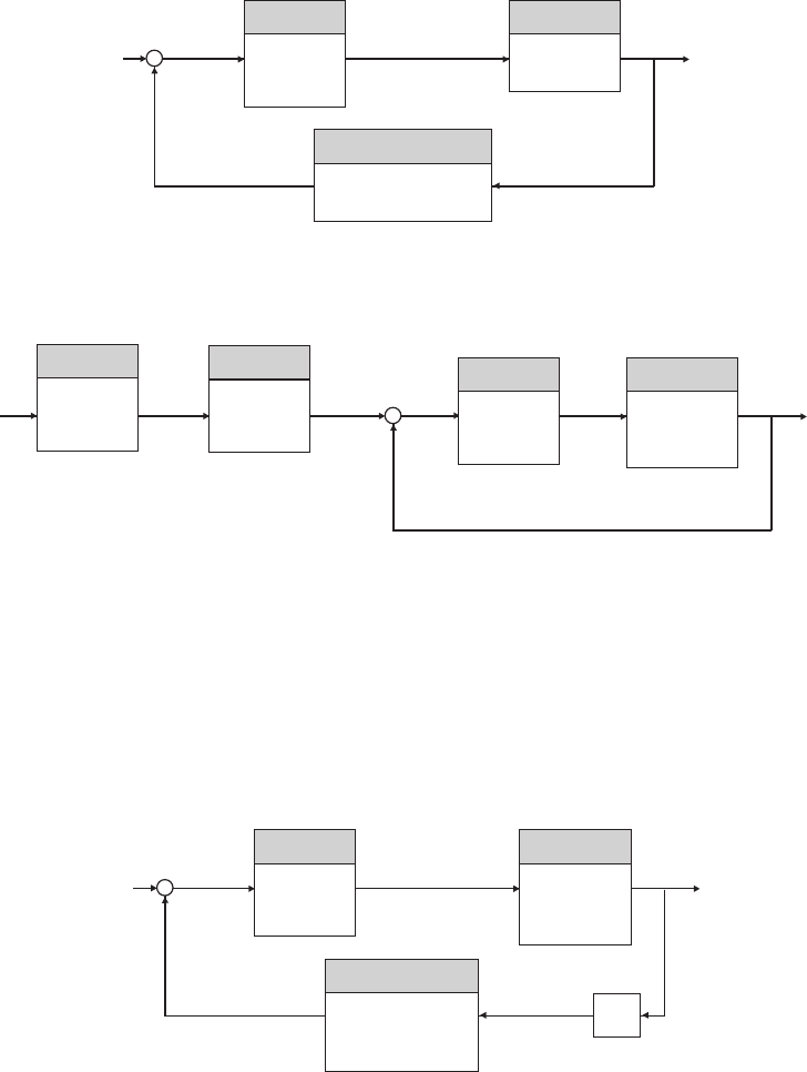
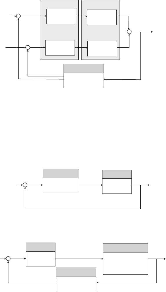
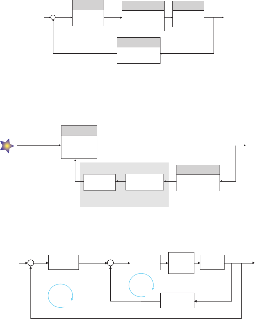
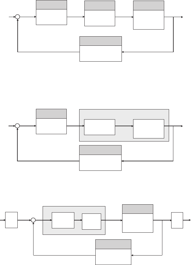
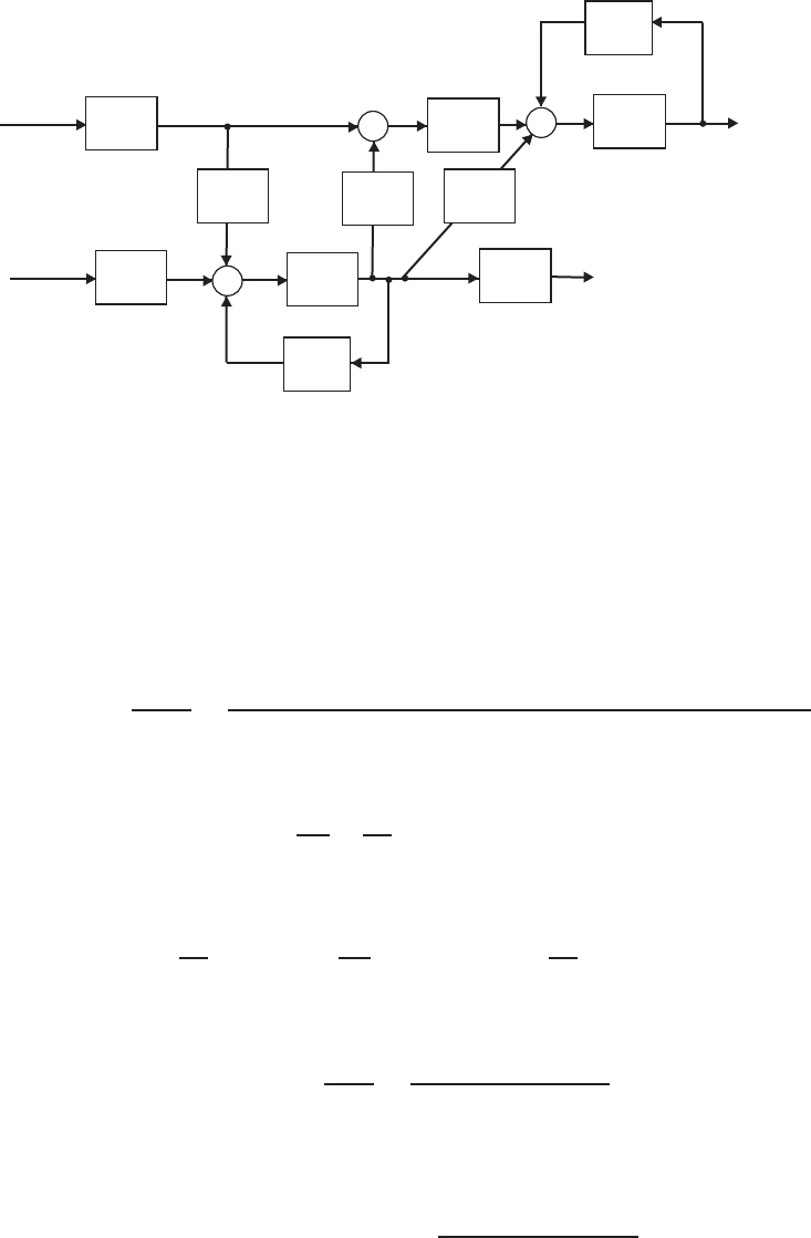
E2.14 Since we want to compute the transfer function from R2(s) to Y1(s), we

can assume that R1= 0 (application of the principle of superposition).

Then, starting at the output Y1(s) we obtain

Y1(s) = G3(s) [−H1(s)Y1(s) + G2(s)G8(s)W(s) + G9(s)W(s)] ,

[1 + G3(s)H1(s)] Y1(s) = [G3(s)G2(s)G8(s)W(s) + G3(s)G9(s)] W(s).

Considering the signal W(s) (see Figure E2.14), we determine that

W(s) = G5(s) [G4(s)R2(s)−H2(s)W(s)] ,

from the publisher prior to any prohibited reproduction, storage in a retrieval system, or transmission in any form or by any means, electronic, mechanical, photocopying,

recording, or likewise. For information regarding permission(s), write to: Rights and Permissions Department, Pearson Education, Inc., Upper Saddle River, NJ 07458.

30 CHAPTER 2 Mathematical Models of Systems

G2(s)

G1(s)

H1(s)

G3(s)

G5(s)

G4(s)

H2(s)

G6(s)

R1(s)

R2(s)

Y1(s)

Y2(s)

G7(s) G8(s) G9(s)

W(s)

FIGURE E2.14

Block diagram model.

[1 + G5(s)H2(s)] W(s) = G5(s)G4(s)R2(s).

Substituting the expression for W(s) into the above equation for Y1(s)

yields

Y1(s)

R2(s)=G2(s)G3(s)G4(s)G5(s)G8(s) + G3(s)G4(s)G5(s)G9(s)

1 + G3(s)H1(s) + G5(s)H2(s) + G3(s)G5(s)H1(s)H2(s).

E2.15 For loop 1, we have

R1i1+L1

di1

dt +1

C1Z(i1−i2)dt +R2(i1−i2) = v(t).

And for loop 2, we have

C2Zi2dt +L2

di2

dt +R2(i2−i1) + 1

C1Z(i2−i1)dt = 0 .

E2.16 The transfer function from R(s) to P(s) is

P(s)

R(s)=4.2

s3+ 2s2+ 4s+ 4.2.

The block diagram is shown in Figure E2.16a. The corresponding signal

ﬂow graph is shown in Figure E2.16b for

P(s)/R(s) = 4.2

s3+ 2s2+ 4s+ 4.2.

from the publisher prior to any prohibited reproduction, storage in a retrieval system, or transmission in any form or by any means, electronic, mechanical, photocopying,

recording, or likewise. For information regarding permission(s), write to: Rights and Permissions Department, Pearson Education, Inc., Upper Saddle River, NJ 07458.

Exercises 31

v1(s)

R(s)P(s)

v2(s)0.6

q(s)1

s2+2s+4

(a)

0.6

R(s) P (s)

-1

1 7

s2+ 2 s + 4

(b)

FIGURE E2.16

(a) Block diagram, (b) Signal ﬂow graph.

E2.17 A linear approximation for fis given by

∆f=∂f

∂x x=xo

∆x= 2kxo∆x=k∆x

where xo= 1/2, ∆f=f(x)−f(xo), and ∆x=x−xo.

E2.18 The linear approximation is given by

∆y=m∆x

where

m=∂y

∂x x=xo

(a) When xo= 1, we ﬁnd that yo= 2.4, and yo= 13.2 when xo= 2.

(b) The slope mis computed as follows:

m=∂y

∂x x=xo

= 1 + 4.2x2

Therefore, m= 5.2 at xo= 1, and m= 18.8 at xo= 2.

from the publisher prior to any prohibited reproduction, storage in a retrieval system, or transmission in any form or by any means, electronic, mechanical, photocopying,

recording, or likewise. For information regarding permission(s), write to: Rights and Permissions Department, Pearson Education, Inc., Upper Saddle River, NJ 07458.

32 CHAPTER 2 Mathematical Models of Systems

E2.19 The output (with a step input) is

Y(s) = 15(s+ 1)

s(s+ 7)(s+ 2) .

The partial fraction expansion is

Y(s) = 15

14s−18

s+ 7 +3

s+ 2 .

Taking the inverse Laplace transform yields

y(t) = 15

14 −18

7e−7t+3

2e−2t.

E2.20 The input-output relationship is

V=A(K−1)

1 + AK

where

K=Z1

Z1+Z2

Assume A≫1. Then,

V=K−1

K=−Z2

where

Z1=R1

R1C1s+ 1 and Z2=R2

R2C2s+ 1 .

Therefore,

Vo(s)

V(s)=−R2(R1C1s+ 1)

R1(R2C2s+ 1) =−2(s+ 1)

s+ 2 .

E2.21 The equation of motion of the mass mcis

mc¨xp+ (bd+bs) ˙xp+kdxp=bd˙xin +kdxin .

Taking the Laplace transform with zero initial conditions yields

[mcs2+ (bd+bs)s+kd]Xp(s) = [bds+kd]Xin(s).

So, the transfer function is

Xp(s)

Xin(s)=bds+kd

mcs2+ (bd+bs)s+kd

=0.7s+ 2

s2+ 2.8s+ 2 .

from the publisher prior to any prohibited reproduction, storage in a retrieval system, or transmission in any form or by any means, electronic, mechanical, photocopying,

recording, or likewise. For information regarding permission(s), write to: Rights and Permissions Department, Pearson Education, Inc., Upper Saddle River, NJ 07458.

Exercises 33

E2.22 The rotational velocity is

ω(s) = 2(s+ 4)

(s+ 5)(s+ 1)2

Expanding in a partial fraction expansion yields

ω(s) = 8

s+1

s+ 5 −3

(s+ 1)2−13

s+ 1 .

Taking the inverse Laplace transform yields

ω(t) = 8

5+1

40e−5t−3

2te−t−13

8e−t.

E2.23 The closed-loop transfer function is

Y(s)

R(s)=T(s) = K1K2

s2+ (K1+K2K3+K1K2)s+K1K2K3

E2.24 The closed-loop tranfser function is

Y(s)

R(s)=T(s) = 10

s2+ 21s+ 10 .

E2.25 Let x= 0.6 and y= 0.8. Then, with y=ax3, we have

0.8 = a(0.6)3.

Solving for ayields a= 3.704. A linear approximation is

y−yo= 3ax2

o(x−xo)

or y= 4x−1.6, where yo= 0.8 and xo= 0.6.

E2.26 The equations of motion are

m1¨x1+k(x1−x2) = F

m2¨x2+k(x2−x1) = 0 .

Taking the Laplace transform (with zero initial conditions) and solving

for X2(s) yields

X2(s) = k

(m2s2+k)(m1s2+k)−k2F(s).

Then, with m1=m2=k= 1, we have

X2(s)/F (s) = 1

s2(s2+ 2) .

from the publisher prior to any prohibited reproduction, storage in a retrieval system, or transmission in any form or by any means, electronic, mechanical, photocopying,

recording, or likewise. For information regarding permission(s), write to: Rights and Permissions Department, Pearson Education, Inc., Upper Saddle River, NJ 07458.

34 CHAPTER 2 Mathematical Models of Systems

E2.27 The transfer function from Td(s) to Y(s) is

Y(s)/Td(s) = G2(s)

1 + G1G2H(s).

E2.28 The transfer function is

Vo(s)

V(s)=R2R4C

s+R2R4

R1R3

= 24s+ 144 .

E2.29 (a) If

G(s) = 1

s2+ 15s+ 50 and H(s) = 2s+ 15 ,

then the closed-loop transfer function of Figure E2.28(a) and (b) (in

Dorf & Bishop) are equivalent.

(b) The closed-loop transfer function is

T(s) = 1

s2+ 17s+ 65 .

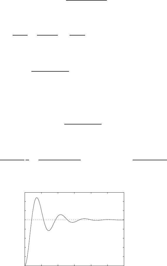
E2.30 (a) The closed-loop transfer function is

T(s) = G(s)

1 + G(s)

s=10

s(s2+ 2s+ 20) where G(s) = 10

s2+ 2s+ 10 .

0 1 2 3 4 5 6

0.1

0.2

0.3

0.4

0.5

0.6

0.7

0.8

Time sec

Amplitude

FIGURE E2.30

Step response.

from the publisher prior to any prohibited reproduction, storage in a retrieval system, or transmission in any form or by any means, electronic, mechanical, photocopying,

recording, or likewise. For information regarding permission(s), write to: Rights and Permissions Department, Pearson Education, Inc., Upper Saddle River, NJ 07458.

Exercises 35

(b) The output Y(s) (when R(s) = 1/s) is

Y(s) = 0.5

s−−0.25 + 0.0573j

s+ 1 −4.3589j+−0.25 −0.0573j

s+ 1 + 4.3589j.

y(t) = 1

21−e−tcos √19t−1

√19 sin √19t

E2.31 The partial fraction expansion is

V(s) = a

s+p1

s+p2

where p1= 4 −19.6jand p2= 4 + 19.6j. Then, the residues are

a=−10.2j b = 10.2j .

The inverse Laplace transform is

v(t) = −10.2je(−4+19.6j)t+ 10.2je(−4−19.6j)t= 20.4e−4tsin 19.6t .

from the publisher prior to any prohibited reproduction, storage in a retrieval system, or transmission in any form or by any means, electronic, mechanical, photocopying,

recording, or likewise. For information regarding permission(s), write to: Rights and Permissions Department, Pearson Education, Inc., Upper Saddle River, NJ 07458.

36 CHAPTER 2 Mathematical Models of Systems

Problems

P2.1 The integrodiﬀerential equations, obtained by Kirchoﬀ’s voltage law to

each loop, are as follows:

R1i1+1

C1Zi1dt +L1

d(i1−i2)

dt +R2(i1−i2) = v(t) (loop 1)

and

R3i2+1

C2Zi2dt +R2(i2−i1) + L1

d(i2−i1)

dt = 0 (loop 2) .

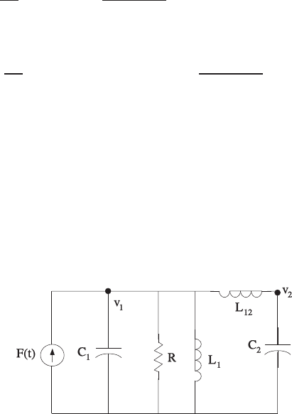
P2.2 The diﬀerential equations describing the system can be obtained by using

a free-body diagram analysis of each mass. For mass 1 and 2 we have

M1¨y1+k12(y1−y2) + b˙y1+k1y1=F(t)

M2¨y2+k12(y2−y1) = 0 .

Using a force-current analogy, the analagous electric circuit is shown in

Figure P2.2, where Ci→Mi, L1→1/k1, L12 →1/k12 ,and R→1/b .

FIGURE P2.2

Analagous electric circuit.

P2.3 The diﬀerential equations describing the system can be obtained by using

a free-body diagram analysis of each mass. For mass 1 and 2 we have

M¨x1+kx1+k(x1−x2) = F(t)

M¨x2+k(x2−x1) + b˙x2= 0 .

Using a force-current analogy, the analagous electric circuit is shown in

Figure P2.3, where

C→M L →1/k R →1/b .

from the publisher prior to any prohibited reproduction, storage in a retrieval system, or transmission in any form or by any means, electronic, mechanical, photocopying,

recording, or likewise. For information regarding permission(s), write to: Rights and Permissions Department, Pearson Education, Inc., Upper Saddle River, NJ 07458.

Problems 37

FIGURE P2.3

Analagous electric circuit.

P2.4 (a) The linear approximation around vin = 0 is vo= 0vin, see Fig-

ure P2.4(a).

(b) The linear approximation around vin = 1 is vo= 2vin −1, see Fig-

ure P2.4(b).

-1 -0.5 0 0.5 1

-0.4

-0.3

-0.2

-0.1

0.1

0.2

0.3

0.4

(a)

vin

linear approximation

-1 0 1 2

-1

-0.5

0.5

1.5

2.5

3.5

(b)

vin

linear approximation

FIGURE P2.4

Nonlinear functions and approximations.

from the publisher prior to any prohibited reproduction, storage in a retrieval system, or transmission in any form or by any means, electronic, mechanical, photocopying,

recording, or likewise. For information regarding permission(s), write to: Rights and Permissions Department, Pearson Education, Inc., Upper Saddle River, NJ 07458.

38 CHAPTER 2 Mathematical Models of Systems

P2.5 Given

Q=K(P1−P2)1/2.

Let δP =P1−P2and δPo= operating point. Using a Taylor series

expansion of Q, we have

Q=Qo+∂Q

∂δP δP =δPo

(δP −δPo) + ···

where

Qo=KδP 1/2

oand ∂Q

∂δP δP =δPo

2δP −1/2

Deﬁne ∆Q=Q−Qoand ∆P=δP −δPo. Then, dropping higher-order

terms in the Taylor series expansion yields

∆Q=m∆P

where

m=K

2δP 1/2

P2.6 From P2.1 we have

R1i1+1

C1Zi1dt +L1

d(i1−i2)

dt +R2(i1−i2) = v(t)

and

R3i2+1

C2Zi2dt +R2(i2−i1) + L1

d(i2−i1)

dt = 0 .

Taking the Laplace transform and using the fact that the initial voltage

across C2is 10v yields

[R1+1

C1s+L1s+R2]I1(s) + [−R2−L1s]I2(s) = 0

and

[−R2−L1s]I1(s) + [L1s+R3+1

C2s+R2]I2(s) = −10

Rewriting in matrix form we have





R1+1

C1s+L1s+R2−R2−L1s

−R2−L1s L1s+R3+1

C2s+R2





I1(s)

I2(s)

=



−10/s 

.

from the publisher prior to any prohibited reproduction, storage in a retrieval system, or transmission in any form or by any means, electronic, mechanical, photocopying,

recording, or likewise. For information regarding permission(s), write to: Rights and Permissions Department, Pearson Education, Inc., Upper Saddle River, NJ 07458.

Problems 39

Solving for I2yields





I1(s)

I2(s)

=1

∆



L1s+R3+1

C2s+R2R2+L1s

R2+L1s R1+1

C1s+L1s+R2





−10/s 

.

I2(s) = −10(R1+ 1/C1s+L1s+R2)

s∆

where

∆ = (R1+1

C1s+L1s+R2)(L1s+R3+1

C2s+R2)−(R2+L1s)2.

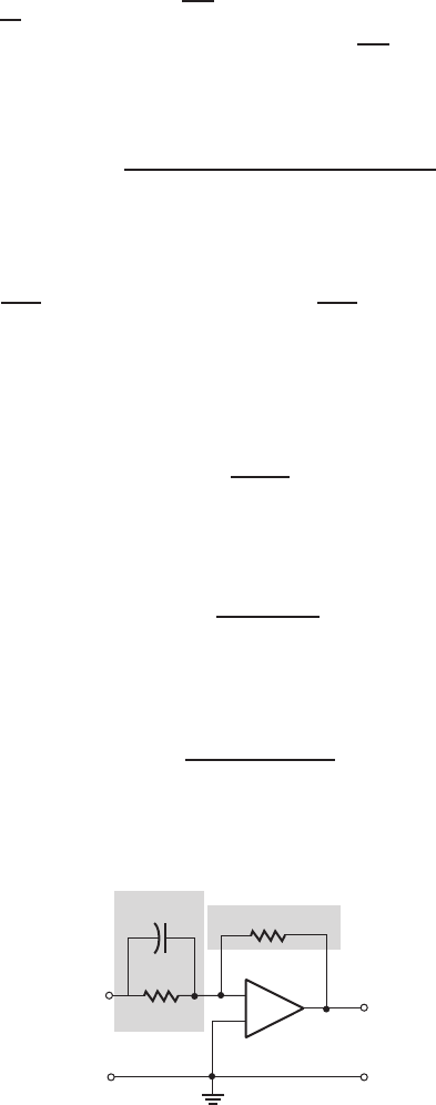
P2.7 Consider the diﬀerentiating op-amp circuit in Figure P2.7. For an ideal

op-amp, the voltage gain (as a function of frequency) is

V2(s) = −Z2(s)

Z1(s)V1(s),

where

Z1=R1

1 + R1Cs

and Z2=R2are the respective circuit impedances. Therefore, we obtain

V2(s) = −R2(1 + R1Cs)

R1V1(s).

V1(s)V2(s)

Z1Z2

FIGURE P2.7

Diﬀerentiating op-amp circuit.

from the publisher prior to any prohibited reproduction, storage in a retrieval system, or transmission in any form or by any means, electronic, mechanical, photocopying,

recording, or likewise. For information regarding permission(s), write to: Rights and Permissions Department, Pearson Education, Inc., Upper Saddle River, NJ 07458.

40 CHAPTER 2 Mathematical Models of Systems

P2.8 Let

∆ = 

G2+Cs −Cs −G2

−Cs G1+ 2Cs −Cs

−G2−Cs Cs +G2



Then,

Vj=∆ij

∆I1or or V3

=∆13I1/∆

∆11I1/∆.

Therefore, the transfer function is

T(s) = V3

=∆13

∆11



−Cs 2Cs +G1

−G2−Cs 



2Cs +G1−Cs

−Cs Cs +G2

-3

-2

-1

-8 -7 -6 -5 -4 -3 -2 -1 0

x x

Real Axis

Imag Axis

Pole-zero map (x:poles and o:zeros)

FIGURE P2.8

Pole-zero map.

from the publisher prior to any prohibited reproduction, storage in a retrieval system, or transmission in any form or by any means, electronic, mechanical, photocopying,

recording, or likewise. For information regarding permission(s), write to: Rights and Permissions Department, Pearson Education, Inc., Upper Saddle River, NJ 07458.

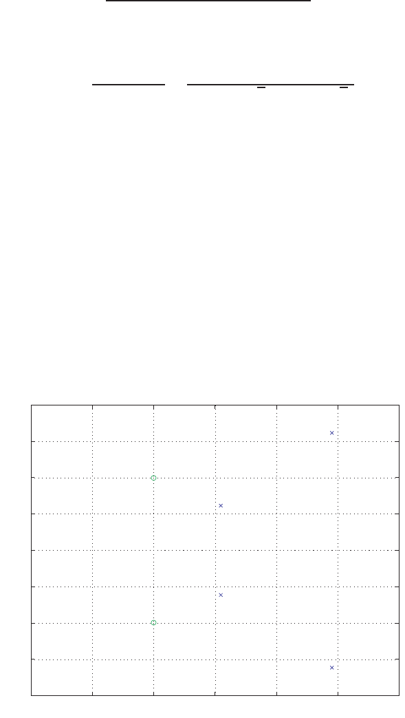
Problems 41

=C2R1R2s2+ 2CR1s+ 1

C2R1R2s2+ (2R1+R2)Cs + 1 .

Using R1= 0.5, R2= 1, and C= 0.5, we have

T(s) = s2+ 4s+ 8

s2+ 8s+ 8 =(s+ 2 + 2j)(s+ 2 −2j)

(s+ 4 + √8)(s+ 4 −√8) .

The pole-zero map is shown in Figure P2.8.

P2.9 From P2.3 we have

M¨x1+kx1+k(x1−x2) = F(t)

M¨x2+k(x2−x1) + b˙x2= 0 .

Taking the Laplace transform of both equations and writing the result in

matrix form, it follows that





Ms2+ 2k−k

−k Ms2+bs +k





X1(s)

X2(s)

=



F(s)

0

,

-0.03 -0.025 -0.02 -0.015 -0.01 -0.005 0

-0.4

-0.3

-0.2

- 0.1

0.1

0.2

0.3

0.4

Real Axis

Imag Axis

Pole zero map

FIGURE P2.9

Pole-zero map.

from the publisher prior to any prohibited reproduction, storage in a retrieval system, or transmission in any form or by any means, electronic, mechanical, photocopying,

recording, or likewise. For information regarding permission(s), write to: Rights and Permissions Department, Pearson Education, Inc., Upper Saddle River, NJ 07458.

42 CHAPTER 2 Mathematical Models of Systems





X1(s)

X2(s)

=1

∆



Ms2+bs +k k

k Ms2+ 2k





F(s)

0



where ∆ = (Ms2+bs +k)(Ms2+ 2k)−k2.So,

G(s) = X1(s)

F(s)=Ms2+bs +k

∆.

When b/k = 1, M= 1 , b2/M k = 0.04, we have

G(s) = s2+ 0.04s+ 0.04

s4+ 0.04s3+ 0.12s2+ 0.0032s+ 0.0016 .

The pole-zero map is shown in Figure P2.9.

P2.10 From P2.2 we have

M1¨y1+k12(y1−y2) + b˙y1+k1y1=F(t)

M2¨y2+k12(y2−y1) = 0 .

Taking the Laplace transform of both equations and writing the result in

matrix form, it follows that





M1s2+bs +k1+k12 −k12

−k12 M2s2+k12 





Y1(s)

Y2(s)

=



F(s)

0







Y1(s)

Y2(s)

=1

∆



M2s2+k12 k12

k12 M1s2+bs +k1+k12 





F(s)

0



where

∆ = (M2s2+k12)(M1s2+bs +k1+k12)−k2

12 .

So, when f(t) = asin ωot, we have that Y1(s) is given by

Y1(s) = aM2ωo(s2+k12/M2)

(s2+ω2

o)∆(s).

For motionless response (in the steady-state), set the zero of the transfer

function so that

(s2+k12

) = s2+ω2

oorω2

o=k12

from the publisher prior to any prohibited reproduction, storage in a retrieval system, or transmission in any form or by any means, electronic, mechanical, photocopying,

recording, or likewise. For information regarding permission(s), write to: Rights and Permissions Department, Pearson Education, Inc., Upper Saddle River, NJ 07458.

Problems 43

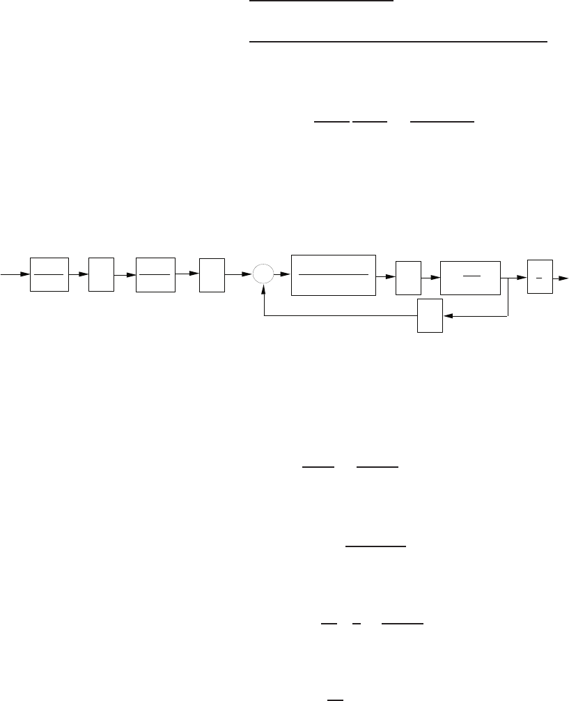
P2.11 The transfer functions from Vc(s) to Vd(s) and from Vd(s) to θ(s) are:

Vd(s)/Vc(s) = K1K2

(Lqs+Rq)(Lcs+Rc),and

θ(s)/Vd(s) = Km

(Js2+fs)((Ld+La)s+Rd+Ra) + K3Kms.

The block diagram for θ(s)/Vc(s) is shown in Figure P2.11, where

θ(s)/Vc(s) = θ(s)

Vd(s)

Vc(s)=K1K2Km

∆(s),

where

∆(s) = s(Lcs+Rc)(Lqs+Rq)((Js +b)((Ld+La)s+Rd+Ra) + KmK3).

(L d

+L a)s+R d+R a

Js+f 1

Lcs+R c

s+R q

K1K2

IcVqVdIdTm

Iqw

FIGURE P2.11

Block diagram.

P2.12 The open-loop transfer function is

Y(s)

R(s)=K

s+ 20 .

With R(s) = 1/s, we have

Y(s) = K

s(s+ 20) .

The partial fraction expansion is

Y(s) = K

20 1

s−1

s+ 20,

and the inverse Laplace transform is

y(t) = K

20 1−e−20t,

As t→ ∞, it follows that y(t)→K/20. So we choose K= 20 so that y(t)

from the publisher prior to any prohibited reproduction, storage in a retrieval system, or transmission in any form or by any means, electronic, mechanical, photocopying,

recording, or likewise. For information regarding permission(s), write to: Rights and Permissions Department, Pearson Education, Inc., Upper Saddle River, NJ 07458.

44 CHAPTER 2 Mathematical Models of Systems

approaches 1. Alternatively we can use the ﬁnal value theorem to obtain

y(t)t→∞ = lim

s→0sY (s) = K

20 = 1 .

It follows that choosing K= 20 leads to y(t)→1 as t→ ∞.

P2.13 The motor torque is given by

Tm(s) = (Jms2+bms)θm(s) + (JLs2+bLs)nθL(s)

=n((Jms2+bms)/n2+JLs2+bLs)θL(s)

where

n=θL(s)/θm(s) = gear ratio .

But

Tm(s) = KmIg(s)

and

Ig(s) = 1

(Lg+Lf)s+Rg+Rf

Vg(s),

and

Vg(s) = KgIf(s) = Kg

Rf+LfsVf(s).

Combining the above expressions yields

θL(s)

Vf(s)=KgKm

n∆1(s)∆2(s).

where

∆1(s) = JLs2+bLs+Jms2+bms

and

∆2(s) = (Lgs+Lfs+Rg+Rf)(Rf+Lfs).

P2.14 For a ﬁeld-controlled dc electric motor we have

ω(s)/Vf(s) = Km/Rf

Js +b.

from the publisher prior to any prohibited reproduction, storage in a retrieval system, or transmission in any form or by any means, electronic, mechanical, photocopying,

recording, or likewise. For information regarding permission(s), write to: Rights and Permissions Department, Pearson Education, Inc., Upper Saddle River, NJ 07458.

Problems 45

With a step input of Vf(s) = 80/s, the ﬁnal value of ω(t) is

ω(t)t→∞ = lim

s→0sω(s) = 80Km

Rfb= 2.4 or Km

Rfb= 0.03 .

Solving for ω(t) yields

ω(t) = 80Km

RfJL−11

s(s+b/J)=80Km

Rfb(1−e−(b/J)t) = 2.4(1−e−(b/J)t).

At t= 1/2, ω(t) = 1, so

ω(1/2) = 2.4(1 −e−(b/J)t) = 1 implies b/J = 1.08 sec .

Therefore,

ω(s)/Vf(s) = 0.0324

s+ 1.08 .

P2.15 Summing the forces in the vertical direction and using Newton’s Second

Law we obtain

¨x+k

mx= 0 .

The system has no damping and no external inputs. Taking the Laplace

transform yields

X(s) = x0s

s2+k/m ,

where we used the fact that x(0) = x0and ˙x(0) = 0. Then taking the

inverse Laplace transform yields

x(t) = x0cos sk

mt .

P2.16 Using Cramer’s rule, we have





1 1.5

2 4 





x2

=



11 







x2

=1

∆



4−1.5

−2 1 





11 



from the publisher prior to any prohibited reproduction, storage in a retrieval system, or transmission in any form or by any means, electronic, mechanical, photocopying,

recording, or likewise. For information regarding permission(s), write to: Rights and Permissions Department, Pearson Education, Inc., Upper Saddle River, NJ 07458.

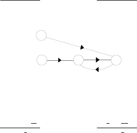
46 CHAPTER 2 Mathematical Models of Systems

where ∆ = 4(1) −2(1.5) = 1 .Therefore,

x1=4(6) −1.5(11)

1= 7.5 and x2=−2(6) + 1(11)

1=−1.

The signal ﬂow graph is shown in Figure P2.16.

1/4

-1.5

6-1/2 X2

FIGURE P2.16

Signal ﬂow graph.

So,

x1=6(1) −1.5(11

1−3

= 7.5 and x2=11(1

4) + −1

2(6)

1−3

=−1.

P2.17 (a) For mass 1 and 2, we have

M1¨x1+K1(x1−x2) + b1( ˙x3−˙x1) = 0

M2¨x2+K2(x2−x3) + b2( ˙x3−˙x2) + K1(x2−x1) = 0 .

(b) Taking the Laplace transform yields

(M1s2+b1s+K1)X1(s)−K1X2(s) = b1sX3(s)

−K1X1(s) + (M2s2+b2s+K1+K2)X2(s) = (b2s+K2)X3(s).

G1(s) = K2+b2s

G2(s) = 1/p(s)

G3(s) = 1/q(s)

G4(s) = sb1,

where

p(s) = s2M2+sf2+K1+K2

and

q(s) = s2M1+sf1+K1.

from the publisher prior to any prohibited reproduction, storage in a retrieval system, or transmission in any form or by any means, electronic, mechanical, photocopying,

recording, or likewise. For information regarding permission(s), write to: Rights and Permissions Department, Pearson Education, Inc., Upper Saddle River, NJ 07458.

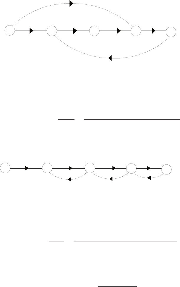
Problems 47

The signal ﬂow graph is shown in Figure P2.17.

X3X1

FIGURE P2.17

Signal ﬂow graph.

(d) The transfer function from X3(s) to X1(s) is

X1(s)

X3(s)=K1G1(s)G2(s)G3(s) + G4(s)G3(s)

1−K2

1G2(s)G3(s).

P2.18 The signal ﬂow graph is shown in Figure P2.18.

V1V2

-Y 3

-Y 1

-Z 2

FIGURE P2.18

Signal ﬂow graph.

The transfer function is

V2(s)

V1(s)=Y1Z2Y3Z4

1 + Y1Z2+Y3Z2+Y3Z4+Y1Z2Z4Y3

P2.19 For a noninerting op-amp circuit, depicted in Figure P2.19a, the voltage

gain (as a function of frequency) is

Vo(s) = Z1(s) + Z2(s)

Z1(s)Vin(s),

where Z1(s) and Z2(s) are the impedances of the respective circuits. In

the case of the voltage follower circuit, shown in Figure P2.19b, we have

from the publisher prior to any prohibited reproduction, storage in a retrieval system, or transmission in any form or by any means, electronic, mechanical, photocopying,

recording, or likewise. For information regarding permission(s), write to: Rights and Permissions Department, Pearson Education, Inc., Upper Saddle River, NJ 07458.

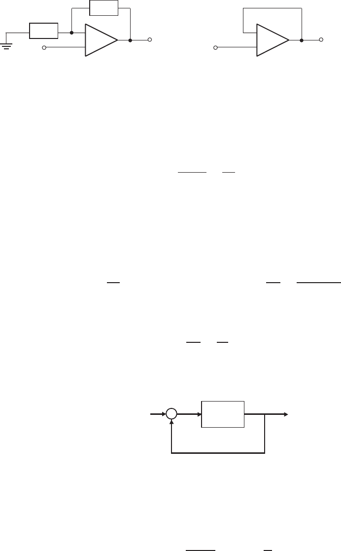
48 CHAPTER 2 Mathematical Models of Systems

vin

(a)(a) (b)

FIGURE P2.19

(a) Noninverting op-amp circuit. (b) Voltage follower circuit.

Z1=∞(open circuit) and Z2= 0. Therefore, the transfer function is

Vo(s)

Vin(s)=Z1

= 1.

P2.20 (a) Assume Rg≫Rsand Rs≫R1. Then Rs=R1+R2≈R2, and

vgs =vin −vo,

where we neglect iin, since Rg≫Rs. At node S, we have

=gmvgs =gm(vin −vo) or vo

vin

=gmRs

1 + gmRs

(b) With gmRs= 20, we have

vin

=20

21 = 0.95 .

gmRs

vin(s)vo(s)

FIGURE P2.20

Block diagram model.

P2.21 From the geometry we ﬁnd that

∆z=kl1−l2

(x−y)−l2

y .

from the publisher prior to any prohibited reproduction, storage in a retrieval system, or transmission in any form or by any means, electronic, mechanical, photocopying,

recording, or likewise. For information regarding permission(s), write to: Rights and Permissions Department, Pearson Education, Inc., Upper Saddle River, NJ 07458.

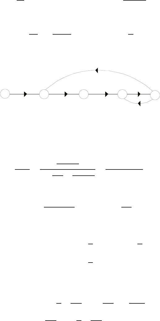
Problems 49

The ﬂow rate balance yields

Ady

dt =p∆zwhich implies Y(s) = p∆Z(s)

As .

By combining the above results it follows that

Y(s) = p

As kl1−l2

l1(X(s)−Y(s)) −l2

Y(s).

Therefore, the signal ﬂow graph is shown in Figure P2.21. Using Mason’s

p/As

-l / l

2 1

(l - l

1 2)/l 1

-1

FIGURE P2.21

Signal ﬂow graph.

gain formula we ﬁnd that the transfer function is given by

Y(s)

X(s)=

k(l1−l2)p

l1As

1 + l2p

l1As +k(l1−l2)p

l1As

=K1

s+K2+K1

where

K1=k(l1−l2)p

l1Apand K2=l2p

l1A.

P2.22 (a) The equations of motion for the two masses are

ML2¨

θ1+MgLθ1+kL

22

(θ1−θ2) = L

2f(t)

ML2¨

θ2+MgLθ2+kL

22

(θ2−θ1) = 0 .

With ˙

θ1=ω1and ˙

θ2=ω2, we have

˙ω1=−g

L+k

4Mθ1+k

4Mθ2+f(t)

2ML

˙ω2=k

4Mθ1−g

L+k

4Mθ2.

from the publisher prior to any prohibited reproduction, storage in a retrieval system, or transmission in any form or by any means, electronic, mechanical, photocopying,

recording, or likewise. For information regarding permission(s), write to: Rights and Permissions Department, Pearson Education, Inc., Upper Saddle River, NJ 07458.

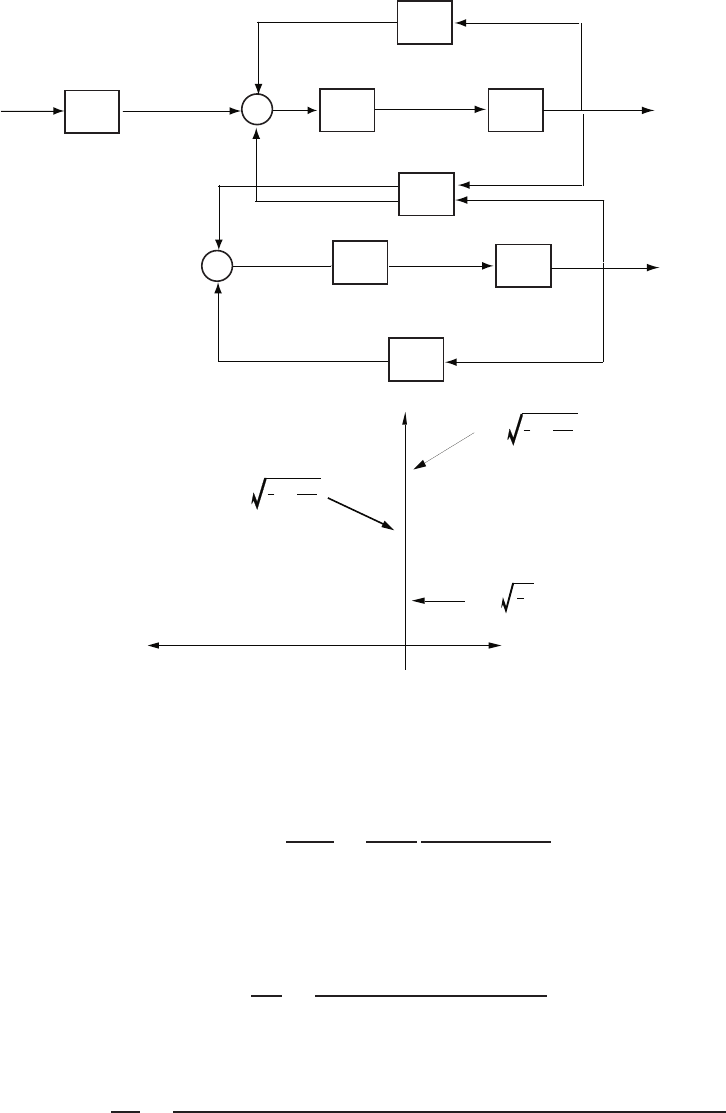
50 CHAPTER 2 Mathematical Models of Systems

1/2ML

1/s 1/s

F (t) w1q1

(a)

+ j g

L+k

+ j g

L+k

Re(s)

Imag(s)

(b)

FIGURE P2.22

(a) Block diagram. (b) Pole-zero map.

(b) Deﬁne a=g/L +k/4Mand b=k/4M. Then

θ1(s)

F(s)=1

2ML

s2+a

(s2+a)2−b2.

P2.23 The input-output ratio, Vce/Vin, is found to be

Vce

Vin

=β(R−1) + hieRf

−βhre +hie(−hoe +Rf).

P2.24 (a) The voltage gain is given by

vin

=RLβ1β2(R1+R2)

(R1+R2)(Rg+hie1)+R1(R1+R2)(1 + β1) + R1RLβ1β2

from the publisher prior to any prohibited reproduction, storage in a retrieval system, or transmission in any form or by any means, electronic, mechanical, photocopying,

recording, or likewise. For information regarding permission(s), write to: Rights and Permissions Department, Pearson Education, Inc., Upper Saddle River, NJ 07458.

Problems 51

(b) The current gain is found to be

ic2

ib1

=β1β2.

vin

ib1

=(R1+R2)(Rg+hie1) + R1(R1+R2)(1 + β1) + R1RLβ1β2

R1+R2

and when β1β2is very large, we have the approximation

vin

ib1≈RLR1β1β2

R1+R2

P2.25 The transfer function from R(s) and Td(s) to Y(s) is given by

Y(s) = G(s)R(s)−1

G(s)(G(s)R(s) + Td(s))+Td(s) + G(s)R(s)

=G(s)R(s).

Thus,

Y(s)/R(s) = G(s).

Also, we have that

Y(s) = 0 .

when R(s) = 0. Therefore, the eﬀect of the disturbance, Td(s), is elimi-

nated.

P2.26 The equations of motion for the two mass model of the robot are

M¨x+b( ˙x−˙y) + k(x−y) = F(t)

m¨y+b( ˙y−˙x) + k(y−x) = 0 .

Taking the Laplace transform and writing the result in matrix form yields





Ms2+bs +k−(bs +k)

−(bs +k)ms2+bs +k





X(s)

Y(s)

=



F(s)

0

.

Solving for Y(s) we ﬁnd that

Y(s)

F(s)=

mM (bs +k)

s2[s2+1 + m

Mb

ms+k

m].

from the publisher prior to any prohibited reproduction, storage in a retrieval system, or transmission in any form or by any means, electronic, mechanical, photocopying,

recording, or likewise. For information regarding permission(s), write to: Rights and Permissions Department, Pearson Education, Inc., Upper Saddle River, NJ 07458.

52 CHAPTER 2 Mathematical Models of Systems

P2.27 The describing equation of motion is

m¨z=mg −ki2

z2.

Deﬁning

f(z, i) = g−ki2

mz2

leads to

¨z=f(z, i).

The equilibrium condition for ioand zo, found by solving the equation of

motion when

˙z= ¨z= 0 ,

ki2

mg =z2

We linearize the equation of motion using a Taylor series approximation.

With the deﬁnitions

∆z=z−zoand ∆i=i−io,

we have ˙

∆z= ˙zand ¨

∆z= ¨z. Therefore,

∆z=f(z, i) = f(zo, io) + ∂f

∂z z=zo

i=io

∆z+∂f

∂i z=zo

i=io

∆i+···

But f(zo, io) = 0, and neglecting higher-order terms in the expansion

yields

∆z=2ki2

mz3

∆z−2kio

mz2

∆i .

Using the equilibrium condition which relates zoto io, we determine that

∆z=2g

∆z−g

∆i .

Taking the Laplace transform yields the transfer function (valid around

the equilibrium point)

∆Z(s)

∆I(s)=−g/io

s2−2g/zo

from the publisher prior to any prohibited reproduction, storage in a retrieval system, or transmission in any form or by any means, electronic, mechanical, photocopying,

recording, or likewise. For information regarding permission(s), write to: Rights and Permissions Department, Pearson Education, Inc., Upper Saddle River, NJ 07458.

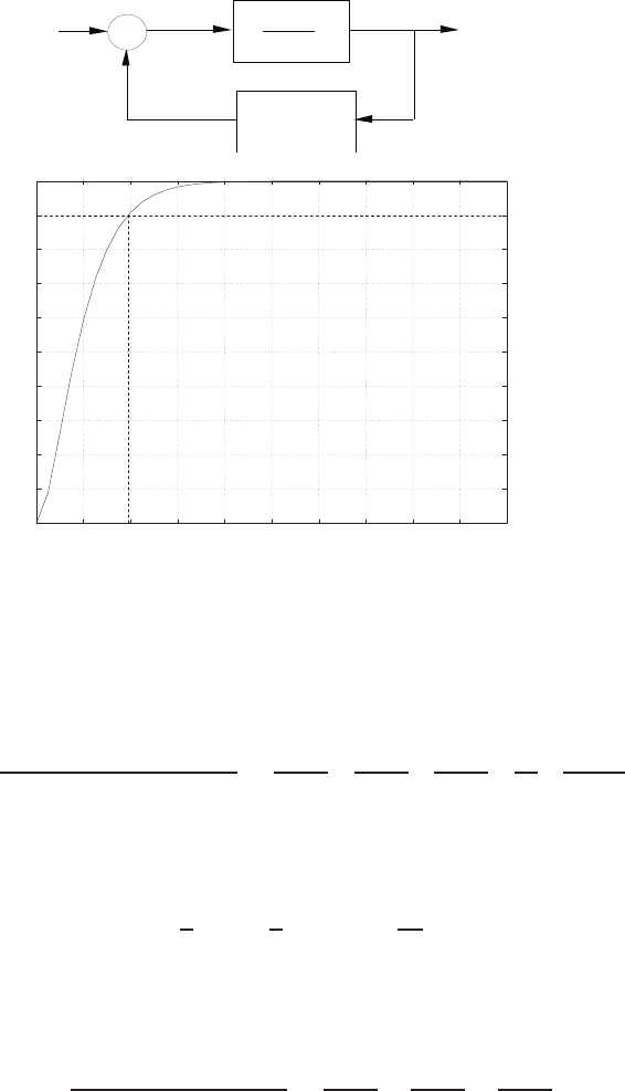
Problems 57

s (s+1)

1 + K 2s

R(s ) Y (s)

0.1

0.2

0.3

0.4

0.5

0.6

0.7

0.8

0.9

0 0.2 0.4 0.6 0.8 1 1.2 1.4 1.6 1.8 2

time(sec)

y(t)

<---- time to 90% = 0.39 sec

FIGURE P2.35

The equivalent block diagram and the system step response.

P2.36 (a) Given R(s) = 1/s2, the partial fraction expansion is

Y(s) = 24

s2(s+ 2)(s+ 3)(s+ 4) =3

s+ 2 −8/3

s+ 3 +3/4

s+ 4 +1

s2−13/12

Therefore, using the Laplace transform table, we determine that the

ramp response is

y(t) = 3e−2t−8

3e−3t+3

4e−4t+t−13

12 , t ≥0.

(b) For the ramp input, y(t)≈0.21 at t= 1.second (see Figure P2.36a).

Y(s) = 24

(s+ 2)(s+ 3)(s+ 4) =12

s+ 2 −24

s+ 3 +12

s+ 4 .

Therefore, using the Laplace transform table, we determine that the

impulse response is

y(t) = 12e−2t−24e−3t+ 412e−4t, t ≥0.

from the publisher prior to any prohibited reproduction, storage in a retrieval system, or transmission in any form or by any means, electronic, mechanical, photocopying,

recording, or likewise. For information regarding permission(s), write to: Rights and Permissions Department, Pearson Education, Inc., Upper Saddle River, NJ 07458.

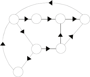
Problems 53

P2.28 The signal ﬂow graph is shown in Figure P2.28.

P D

+b +c

-m -k

-d

FIGURE P2.28

Signal ﬂow graph.

(a) The PGBDP loop gain is equal to -abcd. This is a negative transmis-

sion since the population produces garbage which increases bacteria

and leads to diseases, thus reducing the population.

(b) The PMCP loop gain is equal to +efg. This is a positive transmis-

sion since the population leads to modernization which encourages

immigration, thus increasing the population.

mission since the population leads to modernization and an increase

in sanitation facilities which reduces diseases, thus reducing the rate

of decreasing population.

(d) The PMSBDP loop gain is equal to +ehmcd. This is a positive

transmission by similar argument as in (3).

P2.29 Assume the motor torque is proportional to the input current

Tm=ki .

Then, the equation of motion of the beam is

J¨

φ=ki ,

where Jis the moment of inertia of the beam and shaft (neglecting the

inertia of the ball). We assume that forces acting on the ball are due to

gravity and friction. Hence, the motion of the ball is described by

m¨x=mgφ −b˙x

from the publisher prior to any prohibited reproduction, storage in a retrieval system, or transmission in any form or by any means, electronic, mechanical, photocopying,

recording, or likewise. For information regarding permission(s), write to: Rights and Permissions Department, Pearson Education, Inc., Upper Saddle River, NJ 07458.

54 CHAPTER 2 Mathematical Models of Systems

where mis the mass of the ball, bis the coeﬃcient of friction, and we

have assumed small angles, so that sin φ≈φ. Taking the Laplace transfor

of both equations of motion and solving for X(s) yields

X(s)/I(s) = gk/J

s2(s2+b/m).

P2.30 Given

H(s) = k

τs + 1

where τ= 4µs = 4 ×10−6seconds and 0.999 ≤k < 1.001. The step

response is

Y(s) = k

τs + 1 ·1

s=k

s−k

s+ 1/τ .

Taking the inverse Laplace transform yields

y(t) = k−ke−t/τ =k(1 −e−t/τ ).

The ﬁnal value is k. The time it takes to reach 98% of the ﬁnal value is

t= 15.6µs independent of k.

P2.31 From the block diagram we have

Y1(s) = G2(s)[G1(s)E1(s) + G3(s)E2(s)]

=G2(s)G1(s)[R1(s)−H1(s)Y1(s)] + G2(s)G3(s)E2(s).

Therefore,

Y1(s) = G1(s)G2(s)

1 + G1(s)G2(s)H1(s)R1(s) + G2(s)G3(s)

1 + G1(s)G2(s)H1(s)E2(s).

And, computing E2(s) (with R2(s) = 0) we ﬁnd

E2(s) = H2(s)Y2(s) = H2(s)G6(s)G4(s)

G2(s)Y1(s) + G5(s)E2(s)

E2(s) = G4(s)G6(s)H2(s)

G2(s)(1 −G5(s)G6(s)H2(s))Y1(s).

Substituting E2(s) into equation for Y1(s) yields

Y1(s) = G1(s)G2(s)

1 + G1(s)G2(s)H1(s)R1(s)

from the publisher prior to any prohibited reproduction, storage in a retrieval system, or transmission in any form or by any means, electronic, mechanical, photocopying,

recording, or likewise. For information regarding permission(s), write to: Rights and Permissions Department, Pearson Education, Inc., Upper Saddle River, NJ 07458.

Problems 55

+G3(s)G4(s)G6(s)H2(s)

(1 + G1(s)G2(s)H1(s))(1 −G5(s)G6(s)H2(s)) Y1(s).

Finally, solving for Y1(s) yields

Y1(s) = T1(s)R1(s)

where

T1(s) =

G1(s)G2(s)(1 −G5(s)G6(s)H2(s))

(1 + G1(s)G2(s)H1(s))(1 −G5(s)G6(s)H2(s)) −G3(s)G4(s)G6(s)H2(s).

Similarly, for Y2(s) we obtain

Y2(s) = T2(s)R1(s).

where

T2(s) =

G1(s)G4(s)G6(s)

(1 + G1(s)G2(s)H1(s))(1 −G5(s)G6(s)H2(s)) −G3(s)G4(s)G6(s)H2(s).

P2.32 The signal ﬂow graph shows three loops:

L1=−G1G3G4H2

L2=−G2G5G6H1

L3=−H1G8G6G2G7G4H2G1.

The transfer function Y2/R1is found to be

Y2(s)

R1(s)=G1G8G6∆1−G2G5G6∆2

1−(L1+L2+L3) + (L1L2),

where for path 1

∆1= 1

and for path 2

∆2= 1 −L1.

Since we want Y2to be independent of R1, we need Y2/R1= 0. Therefore,

we require

G1G8G6−G2G5G6(1 + G1G3G4H2) = 0 .

from the publisher prior to any prohibited reproduction, storage in a retrieval system, or transmission in any form or by any means, electronic, mechanical, photocopying,

recording, or likewise. For information regarding permission(s), write to: Rights and Permissions Department, Pearson Education, Inc., Upper Saddle River, NJ 07458.

56 CHAPTER 2 Mathematical Models of Systems

P2.33 The closed-loop transfer function is

Y(s)

R(s)=G3(s)G1(s)(G2(s) + K5K6)

1−G3(s)(H1(s) + K6) + G3(s)G1(s)(G2(s) + K5K6)(H2(s) + K4).

P2.34 The equations of motion are

m1¨y1+b( ˙y1−˙y2) + k1(y1−y2) = 0

m2¨y2+b( ˙y2−˙y1) + k1(y2−y1) + k2y2=k2x

Taking the Laplace transform yields

(m1s2+bs +k1)Y1(s)−(bs +k1)Y2(s) = 0

(m2s2+bs +k1+k2)Y2(s)−(bs +k1)Y1(s) = k2X(s)

Therefore, after solving for Y1(s)/X(s), we have

Y2(s)

X(s)=k2(bs +k1)

(m1s2+bs +k1)(m2s2+bs +k1+k2)−(bs +k1)2.

P2.35 (a) We can redraw the block diagram as shown in Figure P2.35. Then,

T(s) = K1/s(s+ 1)

1 + K1(1 + K2s)/s(s+ 1) =K1

s2+ (1 + K2K1)s+K2

(b) The signal ﬂow graph reveals two loops (both touching):

L1=−K1

s(s+ 1) and L2=−K1K2

s+ 1 .

Therefore,

T(s) = K1/s(s+ 1)

1 + K1/s(s+ 1) + K1K2/(s+ 1) =K1

s2+ (1 + K2K1)s+K1

s2+ (1 + K2K1)s+K1=s2+ 20s+ 100 = (s+ 10)2.

Therefore, K1= 100 and 1 + K2K1= 20 or K2= 0.19.

(d) The step response is shown in Figure P2.35.

from the publisher prior to any prohibited reproduction, storage in a retrieval system, or transmission in any form or by any means, electronic, mechanical, photocopying,

recording, or likewise. For information regarding permission(s), write to: Rights and Permissions Department, Pearson Education, Inc., Upper Saddle River, NJ 07458.

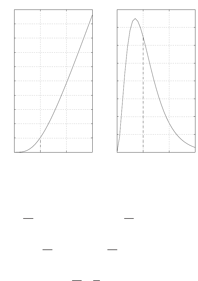
58 CHAPTER 2 Mathematical Models of Systems

(d) For the impulse input, y(t)≈0.65 at t= 1 seconds (see Figure P2.36b).

0123

0.2

0.4

0.6

0.8

1.2

1.4

1.6

1.8

Time (sec)

y(t)

(a) Ramp input

0123

0.1

0.2

0.3

0.4

0.5

0.6

0.7

0.8

Time (sec)

y(t)

(b) Impulse input

FIGURE P2.36

(a) Ramp input response. (b) Impulse input response.

P2.37 The equations of motion are

d2x

dt2=−(k1+k2)x+k2yand m2

d2y

dt2=k2(x−y) + u .

When m1=m2= 1 and k1=k2= 1, we have

d2x

dt2=−2x+yand d2y

dt2=x−y+u .

P2.38 The equation of motion for the system is

Jd2θ

dt2+bdθ

dt +kθ = 0 ,

where kis the rotational spring constant and bis the viscous friction

coeﬃcient. The initial conditions are θ(0) = θoand ˙

θ(0) = 0. Taking the

from the publisher prior to any prohibited reproduction, storage in a retrieval system, or transmission in any form or by any means, electronic, mechanical, photocopying,

recording, or likewise. For information regarding permission(s), write to: Rights and Permissions Department, Pearson Education, Inc., Upper Saddle River, NJ 07458.

Problems 59

Laplace transform yields

J(s2θ(s)−sθo) + b(sθ(s)−θo) + kθ(s) = 0 .

Therefore,

θ(s) = (s+b

Jθo)

(s2+b

Js+K

J)=(s+ 2ζωn)θo

s2+ 2ζωns+ω2

Neglecting the mass of the rod, the moment of inertia is detemined to be

J= 2Mr2= 0.5 kg ·m2.

Also,

ωn=sk

J= 0.02 rad/s and ζ=b

2Jωn

= 0.01 .

Solving for θ(t), we ﬁnd that

θ(t) = θo

p1−ζ2e−ζωntsin(ωnq1−ζ2t+φ),

where tan φ=p1−ζ2/ζ). Therefore, the envelope decay is

θe=θo

p1−ζ2e−ζωnt.

So, with ζωn= 2 ×10−4,θo= 4000oand θf= 10o, the elapsed time is

computed as

t=1

ζωn

ln θo

p1−ζ2θf

= 8.32 hours .

P2.39 When t < 0, we have the steady-state conditions

i1(0) = 1A , va(0) = 2Vand vc(0) = 5V ,

where vc(0) is associated with the 1F capacitor. After t≥0, we have

2di1

dt + 2i1+ 4(i1−i2) = 10e−2t

and

Zi2dt + 10i2+ 4(i2−i1)−i1= 0 .

from the publisher prior to any prohibited reproduction, storage in a retrieval system, or transmission in any form or by any means, electronic, mechanical, photocopying,

recording, or likewise. For information regarding permission(s), write to: Rights and Permissions Department, Pearson Education, Inc., Upper Saddle River, NJ 07458.

60 CHAPTER 2 Mathematical Models of Systems

Taking the Laplace transform (using the initial conditions) yields

2(sI1−i1(0))+ 2I1+ 4I1−4I2=10

s+ 2 or (s+ 3)I1(s)−2I2(s) = s+ 7

s+ 2

and

sI2−vc(0)]+10I2+4(I2−I1) = I1(s) or −5sI1(s)+(14s+1)I2(s) = 5s .

Solving for I2(s) yields

I2=5s(s2+ 6s+ 13)

14(s+ 2)∆(s),

where

∆(s) = 

s+ 3 −2

−5s14s+ 1 

= 14s2+ 33s+ 3 .

Then,

Vo(s) = 10I2(s).

P2.40 The equations of motion are

J1¨

θ1=K(θ2−θ1)−b(˙

θ1−˙

θ2) + Tand J2¨

θ2=b(˙

θ1−˙

θ2).

Taking the Laplace transform yields

(J1s2+bs +K)θ1(s)−bsθ2(s) = Kθ2(s) + T(s)

and

(J2s2+bs)θ2(s)−bsθ1(s) = 0 .

Solving for θ1(s) and θ2(s), we ﬁnd that

θ1(s) = (Kθ2(s) + T(s))(J2s+b)

∆(s)and θ2(s) = b(Kθ2(s) + T(s))

∆(s),

where

∆(s) = J1J2s3+b(J1+J2)s2+J2Ks +bK .

P2.41 Assume that the only external torques acting on the rocket are control

torques, Tcand disturbance torques, Td, and assume small angles, θ(t).

Using the small angle approximation, we have

h=V θ

from the publisher prior to any prohibited reproduction, storage in a retrieval system, or transmission in any form or by any means, electronic, mechanical, photocopying,

recording, or likewise. For information regarding permission(s), write to: Rights and Permissions Department, Pearson Education, Inc., Upper Saddle River, NJ 07458.

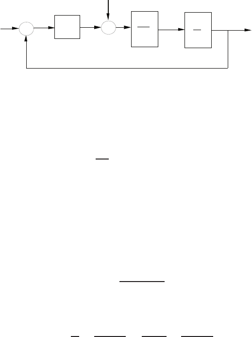
Problems 61

J¨

θ=Tc+Td,

where Jis the moment of inertia of the rocket and Vis the rocket velocity

(assumed constant). Now, suppose that the control torque is proportional

to the lateral displacement, as

Tc(s) = −KH(s),

where the negative sign denotes a negative feedback system. The corre-

sponding block diagram is shown in Figure P2.41.

Js2V

K+

Hdesired

=0 H( s)

FIGURE P2.41

Block diagram.

P2.42 (a) The equation of motion of the motor is

Jdω

dt =Tm−bω ,

where J= 0.1, b= 0.06, and Tmis the motor input torque.

(b) Given Tm(s) = 1/s, and ω(0) = 0.7, we take the Laplace transform

of the equation of motion yielding

sω(s)−ω(0) + 0.6ω(s) = 10Tm

ω(s) = 0.7s+ 10

s(s+ 0.6) .

Then, computing the partial fraction expansion, we ﬁnd that

ω(s) = A

s+B

s+ 0.6=16.67

s−15.97

s+ 0.6.

The step response, determined by taking the inverse Laplace trans-

form, is

ω(t) = 16.67 −15.97e−0.6t, t ≥0.

from the publisher prior to any prohibited reproduction, storage in a retrieval system, or transmission in any form or by any means, electronic, mechanical, photocopying,

recording, or likewise. For information regarding permission(s), write to: Rights and Permissions Department, Pearson Education, Inc., Upper Saddle River, NJ 07458.

62 CHAPTER 2 Mathematical Models of Systems

P2.43 The work done by each gear is equal to that of the other, therefore

Tmθm=TLθL.

Also, the travel distance is the same for each gear, so

r1θm=r2θL.

The number of teeth on each gear is proportional to the radius, or

r1N2=r2N1.

So,

θm

θL

=r2

=N2

and

N1θm=N2θL

θL=N1

θm=nθm,

where

n=N1/N2.

Finally,

=θL

θm

=N1

=n .

P2.44 The inertia of the load is

JL=πρLr4

Also, from the dynamics we have

T2=JL˙ω2+bLω2

and

T1=nT2=n(JL˙ω2+bLω2).

So,

T1=n2(JL˙ω1+bLω1),

from the publisher prior to any prohibited reproduction, storage in a retrieval system, or transmission in any form or by any means, electronic, mechanical, photocopying,

recording, or likewise. For information regarding permission(s), write to: Rights and Permissions Department, Pearson Education, Inc., Upper Saddle River, NJ 07458.

Problems 63

since

ω2=nω1.

Therefore, the torque at the motor shaft is

T=T1+Tm=n2(JL˙ω1+bLω1) + Jm˙ω1+bmω1.

P2.45 Let U(s) denote the human input and F(s) the load input. The transfer

function is

P(s) = G(s) + KG1(s)

∆(s)U(s) + Gc(s) + KG1(s)

∆(s)F(s),

where

∆ = 1 + GH(s) + G1KBH(s) + GcE(s) + G1KE(s).

P2.46 Consider the application of Newton’s law (PF=m¨x). From the mass

mvwe obtain

mv¨x1=F−k1(x1−x2)−b1( ˙x1−˙x2).

Taking the Laplace transform, and solving for X1(s) yields

X1(s) = 1

∆1(s)F(s) + b1s+k1

∆1(s)X2(s),

where

∆1:= mvs2+b1s+k1.

From the mass mtwe obtain

mt¨x2=−k2x2−b2˙x2+k1(x1−x2) + b1( ˙x1−˙x2).

Taking the Laplace transform, and solving for X2(s) yields

X2(s) = b1s+k1

∆2(s)X1(s),

where

∆2:= mts2+ (b1+b2)s+k1+k2.

Substituting X2(s) above into the relationship fpr X1(s) yields the trans-

fer function

X1(s)

F(s)=∆2(s)

∆1(s)∆2(s)−(b1s+k1)2.

from the publisher prior to any prohibited reproduction, storage in a retrieval system, or transmission in any form or by any means, electronic, mechanical, photocopying,

recording, or likewise. For information regarding permission(s), write to: Rights and Permissions Department, Pearson Education, Inc., Upper Saddle River, NJ 07458.

64 CHAPTER 2 Mathematical Models of Systems

P2.47 Using the following relationships

h(t) = Z(1.6θ(t)−h(t))dt

ω(t) = ˙

θ(t)

J˙ω(t) = Kmia(t)

va(t) = 50vi(t) = 10ia(t) + vb(t)

θ=Kvb

we ﬁnd the diﬀerential equation is

d3h

dt3+1 + Km

10JK d2h

dt2+Km

10JK

dt =8Km

Jvi.

P2.48 (a) The transfer function is

V2(s)

V1(s)=(1 + sR1C1)(1 + sR2C2)

R1C2s.

(b) When R1= 100 kΩ, R2= 200 kΩ, C1= 1 µF and C2= 0.1µF , we

have

V2(s)

V1(s)=0.2(s+ 10)(s+ 50)

P2.49 (a) The closed-loop transfer function is

T(s) = G(s)

1 + G(s)=6205

s3+ 13s2+ 1281s+ 6205 .

(b) The poles of T(s) are s1=−5 and s2,3=−4±j35.

Y(s) = 1 −1.0122

s+ 5 +0.0061 + 0.0716j

s+ 4 + j35 +0.0061 −0.0716j

s+ 4 −j35 .

(d) The step response is shown in Figure P2.49. The real and complex

roots are close together and by looking at the poles in the s-plane we

have diﬃculty deciding which is dominant. However, the residue at

the real pole is much larger and thus dominates the response.

from the publisher prior to any prohibited reproduction, storage in a retrieval system, or transmission in any form or by any means, electronic, mechanical, photocopying,

recording, or likewise. For information regarding permission(s), write to: Rights and Permissions Department, Pearson Education, Inc., Upper Saddle River, NJ 07458.

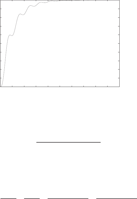
Problems 65

0.1

0.2

0.3

0.4

0.5

0.6

0.7

0.8

0.9

00.2 0.4 0.6 0.8 1 1.2 1.4 1.6 1.8 2

Time (secs)

Amplitude

FIGURE P2.49

Step response.

P2.50 (a) The closed-loop transfer function is

T(s) = 14000

s3+ 45s2+ 3100s+ 14500 .

(b) The poles of T(s) are

s1=−5 and s2,3=−20 ±j50.

Y(s) = 0.9655

s−1.0275

s+ 5 +0.0310 −0.0390j

s+ 20 + j50 +0.0310 + 0.0390j

s+ 20 −j50 .

(d) The step response is shown in Figure P2.50. The real root dominates

the response.

(e) The ﬁnal value of y(t) is

yss = lim

s→0sY (s) = 0.9655 .

from the publisher prior to any prohibited reproduction, storage in a retrieval system, or transmission in any form or by any means, electronic, mechanical, photocopying,

recording, or likewise. For information regarding permission(s), write to: Rights and Permissions Department, Pearson Education, Inc., Upper Saddle River, NJ 07458.

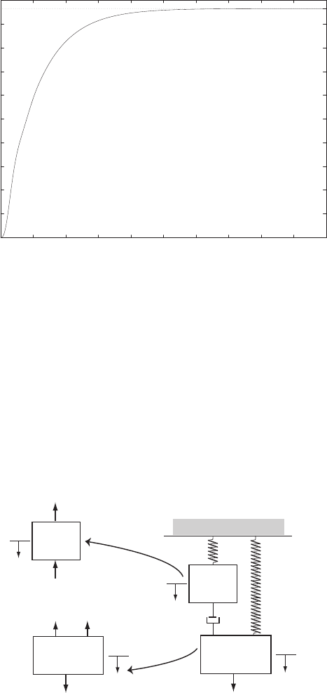
66 CHAPTER 2 Mathematical Models of Systems

0.1

0.2

0.3

0.4

0.5

0.6

0.7

0.8

0.9

00.2 0.4 0.6 0.8 1 1.2 1.4 1.6 1.8 2

Time (secs)

Amplitude

FIGURE P2.50

Step response.

P2.51 Consider the free body diagram in Figure P2.51. Using Newton’s Law

and summing the forces on the two masses yields

M1¨x(t) + b1˙x(t) + k1x(t) = b1˙y(t)

M2¨y(t) + b1˙y(t) + k2y(t) = b1˙x(t) + u(t)

u(t)

k1x

u(t)

b1(x - y)

. .

b1(y - x)

. . y

FIGURE P2.51

Free body diagram.

from the publisher prior to any prohibited reproduction, storage in a retrieval system, or transmission in any form or by any means, electronic, mechanical, photocopying,

recording, or likewise. For information regarding permission(s), write to: Rights and Permissions Department, Pearson Education, Inc., Upper Saddle River, NJ 07458.

Advanced Problems 67

Advanced Problems

AP2.1 The transfer function from V(s) to ω(s) has the form

ω(s)

V(s)=Km

τms+ 1 .

In the steady-state,

ωss = lim

s→0sKm

τms+ 15

s= 5Km.

So,

Km= 70/5 = 14 .

Also,

ω(t) = VmKm(1 −e−t/τm)

where V(s) = Vm/s. Solving for τmyields

τm=−t

ln(1 −ω(t)/ωss).

When t= 2, we have

τm=−2

ln(1 −30/70) = 3.57 .

Therefore, the transfer function is

ω(s)

V(s)=14

3.57s+ 1 .

AP2.2 The closed-loop transfer function form R1(s) to Y2(s) is

Y2(s)

R1(s)=G1G4G5(s) + G1G2G3G4G6(s)

∆

where

∆ = [1 + G3G4H2(s)][1 + G1G2H3(s)] .

If we select

G5(s) = −G2G3G6(s)

then the numerator is zero, and Y2(s)/R1(s) = 0. The system is now

decoupled.

from the publisher prior to any prohibited reproduction, storage in a retrieval system, or transmission in any form or by any means, electronic, mechanical, photocopying,

recording, or likewise. For information regarding permission(s), write to: Rights and Permissions Department, Pearson Education, Inc., Upper Saddle River, NJ 07458.

68 CHAPTER 2 Mathematical Models of Systems

AP2.3 (a) Computing the closed-loop transfer function:

Y(s) = G(s)Gc(s)

1 + Gc(s)G(s)H(s)R(s).

Then, with E(s) = R(s)−Y(s) we obtain

E(s) = 1 + Gc(s)G(s)(H(s)−1)

1 + Gc(s)G(s)H(s)R(s).

If we require that E(s)≡0 for any input, we need 1 + Gc(s)G(s)(H(s)−

1) = 0 or

H(s) = Gc(s)G(s)−1

Gc(s)G(s)=n(s)

d(s).

Since we require H(s) to be a causal system, the order of the numerator

polynomial, n(s), must be less than or equal to the order of the denom-

inator polynomial, d(s). This will be true, in general, only if both Gc(s)

and G(s) are proper rational functions (that is, the numerator and de-

nominator polynomials have the same order). Therefore, making E≡0

for any input R(s) is possible only in certain circumstances.

(b) The transfer function from Td(s) to Y(s) is

Y(s) = Gd(s)G(s)

1 + Gc(s)G(s)H(s)Td(s).

With H(s) as in part (a) we have

Y(s) = Gd(s)

Gc(s)Td(s).

Y(s) = Gd(s)G(s)

1 + Gc(s)G(s)H(s)Td(s) = T(s)Td(s),

the only way to have Y(s)≡0 for any Td(s) is for the transfer function

T(s)≡0 which is not possible in general (since G(s)6= 0).

AP2.4 (a) With q(s) = 1/s we obtain

τ(s) = 1/Ct

s+QS+1/R

Ct·1

Deﬁne

α:= QS + 1/R

andβ:= 1/Ct.

from the publisher prior to any prohibited reproduction, storage in a retrieval system, or transmission in any form or by any means, electronic, mechanical, photocopying,

recording, or likewise. For information regarding permission(s), write to: Rights and Permissions Department, Pearson Education, Inc., Upper Saddle River, NJ 07458.

Advanced Problems 69

Then, it follows that

τ(s) = β

s+α·1

s=−β/α

s+α+β/α

Taking the inverse Laplace transform yields

τ(t) = −β

αe−αt +β

α=β

α[1 −e−αt].

(b) As t→ ∞,τ(t)→β

α=1

Qs+1/R .

Rsuch that

α:= Qs + 1/R

is ”large.”

AP2.5 Considering the motion of each mass, we have

M3¨x3+b3˙x3+k3x3=u3+b3˙x2+k3x2

M2¨x2+ (b2+b3) ˙x2+ (k2+k3)x2=u2+b3˙x3+k3x3+b2˙x1+k2x1

M1¨x1+ (b1+b2) ˙x1+ (k1+k2)x1=u1+b2˙x2+k2x2

In matrix form the three equations can be written as







M10 0

0M20

0 0 M3













¨x1

¨x2

¨x3







+





b1+b2−b20

−b2b2+b3−b3

0−b3b3













˙x1

˙x2

˙x3







+





k1+k2−k20

−k2k2+k3−k3

0−k3k3



















=











AP2.6 Considering the cart mass and using Newton’s Law we obtain

M¨x=u−b˙x−Fsin ϕ

where Fis the reaction force between the cart and the pendulum. Con-

sidering the pendulum we obtain

md2(x+Lsin ϕ)

dt2=Fsinϕ

from the publisher prior to any prohibited reproduction, storage in a retrieval system, or transmission in any form or by any means, electronic, mechanical, photocopying,

recording, or likewise. For information regarding permission(s), write to: Rights and Permissions Department, Pearson Education, Inc., Upper Saddle River, NJ 07458.

70 CHAPTER 2 Mathematical Models of Systems

md2(Lcos ϕ)

dt2=Fcos ϕ+mg

Eliminating the reaction force Fyields the two equations

(m+M)¨x+b˙x+mL ¨ϕcos ϕ−mL ˙ϕ2sin ϕ=u

mL2¨ϕ+mgL sin ϕ+mL¨xcos ϕ= 0

If we assume that the angle ϕ≈0, then we have the linear model

(m+M)¨x+b˙x+mL ¨ϕ=u

mL2¨ϕ+mgLϕ =−mL¨x

AP2.7 The transfer function from the disturbance input to the output is

Y(s) = 1

s+ 20 + KTd(s).

When Td(s) = 1, we obtain

y(t) = e−(20+K)t.

Solving for twhen y(t)<0.1 yields

t > 2.3

20 + K.

When t= 0.05 and y(0.05) = 0.1, we ﬁnd K= 26.05.

AP2.8 The closed-loop transfer function is

T(s) = 200K(0.25s+ 1)

(0.25s+ 1)(s+ 1)(s+ 8) + 200K

The ﬁnal value due to a step input of R(s) = A/s is

v(t)→A200K

200K+ 8.

We need to select Kso that v(t)→50. However, to keep the percent

overshoot to less than 10%, we need to limit the magnitude of K. Fig-

ure AP2.8a shows the percent overshoot as a function of K. Let K= 0.06

and select the magnitude of the input to be A= 83.3. The inverse Laplace

transform of the closed-loop response with R(s) = 83.3/s is

v(t) = 50 + 9.85e−9.15t−e−1.93t(59.85 cos(2.24t) + 11.27 sin(2.24t))

from the publisher prior to any prohibited reproduction, storage in a retrieval system, or transmission in any form or by any means, electronic, mechanical, photocopying,

recording, or likewise. For information regarding permission(s), write to: Rights and Permissions Department, Pearson Education, Inc., Upper Saddle River, NJ 07458.

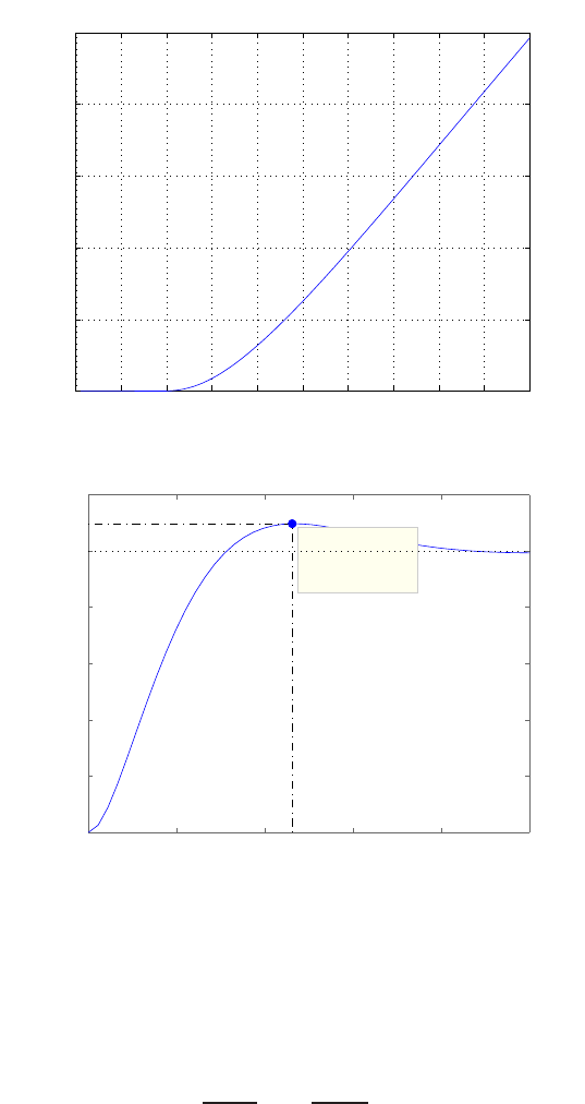
Advanced Problems 71

The result is P.O. = 9.74% and the steady-state value of the output is

approximately 50 m/s, as shown in Figure AP2.8b.

0 0.01 0.02 0.03 0.04 0.05 0.06 0.07 0.08 0.09 0.1

Percent Overshoot (%)

Step Response

Time (sec)

Amplitude

0 0.5 1 1.5 2 2.5

System: untitled1

Peak amplitude: 54.9

Overshoot (%): 9.74

At time (sec): 1.15

FIGURE AP2.8

(a) Percent overshoot versus the gain K. (b) Step response.

AP2.9 The transfer function is

Vo(s)

Vi(s)=−Z2(s)

Z1(s),

from the publisher prior to any prohibited reproduction, storage in a retrieval system, or transmission in any form or by any means, electronic, mechanical, photocopying,

recording, or likewise. For information regarding permission(s), write to: Rights and Permissions Department, Pearson Education, Inc., Upper Saddle River, NJ 07458.

72 CHAPTER 2 Mathematical Models of Systems

where

Z1(s) = R1

R1C1s+ 1 and Z2(s) = R2C2s+ 1

C2s.

Then we can write

Vo(s)

Vi(s)=Kp+KI

s+KDs

where

KP=−R1C1

R2C2

+ 1, KI=−1

R1C2

, KD=−R2C1.

from the publisher prior to any prohibited reproduction, storage in a retrieval system, or transmission in any form or by any means, electronic, mechanical, photocopying,

recording, or likewise. For information regarding permission(s), write to: Rights and Permissions Department, Pearson Education, Inc., Upper Saddle River, NJ 07458.

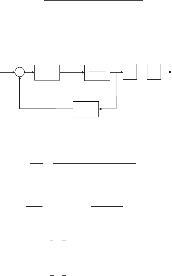
Design Problems 73

Design Problems

The model of the traction drive, capstan roller, and linear slide followsCDP2.1

closely the armature-controlled dc motor model depicted in Figure 2.18

in Dorf and Bishop. The transfer function is

T(s) = rKm

s[(Lms+Rm)(JTs+bm) + KbKm],

where

JT=Jm+r2(Ms+Mb).

Va(s) X(s)

Back EMF

Lms+Rm

JTs+bm

DP2.1 The closed-loop transfer function is

Y(s)

R(s)=G1(s)G2(s)

1 + G1(s)H1(s)−G2(s)H2(s).

When G1H1=G2H2and G1G2= 1, then Y(s)/R(s) = 1. Therefore,

select

G1(s) = 1

G2(s)and H1(s) = G2(s)H2(s)

G1(s)=G2

2(s)H2(s).

DP2.2 At the lower node we have

v1

4+1

3+G+ 2i2−20 = 0 .

Also, we have v= 24 and i2=Gv . So

v1

4+1

3+G+ 2Gv−20 = 0

from the publisher prior to any prohibited reproduction, storage in a retrieval system, or transmission in any form or by any means, electronic, mechanical, photocopying,

recording, or likewise. For information regarding permission(s), write to: Rights and Permissions Department, Pearson Education, Inc., Upper Saddle River, NJ 07458.

74 CHAPTER 2 Mathematical Models of Systems

and

G=20 −v1

4+1

3

3v=1

12 S .

DP2.3 Taking the Laplace transform of

y(t) = e−t−1

4e−2t−3

4+1

yields

Y(s) = 1

s+ 1 −1

4(s+ 2) −3

4s+1

2s2.

Similarly, taking the Laplace transform of the ramp input yields

R(s) = 1

s2.

Therefore

G(s) = Y(s)

R(s)=1

(s+ 1)(s+ 2) .

DP2.4 For an ideal op-amp, at node a we have

vin −va

+vo−va

= 0 ,

and at node b

vin −vb

=C˙vb,

from it follows that

1

+CsVb=1

Vin .

Also, for an ideal op-amp, Vb−Va= 0. Then solving for Vbin the above

equation and substituting the result into the node a equation for Vayields

Vin

R2+Cs "1

R2−

R2+Cs

Vo(s)

Vin(s)=−R2Cs −1

R2Cs + 1 .

from the publisher prior to any prohibited reproduction, storage in a retrieval system, or transmission in any form or by any means, electronic, mechanical, photocopying,

recording, or likewise. For information regarding permission(s), write to: Rights and Permissions Department, Pearson Education, Inc., Upper Saddle River, NJ 07458.

Design Problems 75

For vin(t) = At, we have Vin(s) = A/s2, therefore

vo(t) = A2

βe−βt +t−2

β

where β= 1/R2C.

DP2.5 The equation of motion describing the motion of the inverted pendulum

(assuming small angles) is

¨ϕ+g

Lϕ= 0 .

Assuming a solution of the form ϕ=kcos ϕ, taking the appropriate

derivatives and substituting the result into the equation of motion yields

the relationship

˙ϕ=rg

If the period is T= 2 seconds, we compute ˙ϕ= 2π/T . Then solving for L

yields L= 0.99 meters when g= 9.81 m/s2. So, to ﬁt the pendulum into

the grandfather clock, the dimensions are generally about 1.5 meters or

more.

from the publisher prior to any prohibited reproduction, storage in a retrieval system, or transmission in any form or by any means, electronic, mechanical, photocopying,

recording, or likewise. For information regarding permission(s), write to: Rights and Permissions Department, Pearson Education, Inc., Upper Saddle River, NJ 07458.

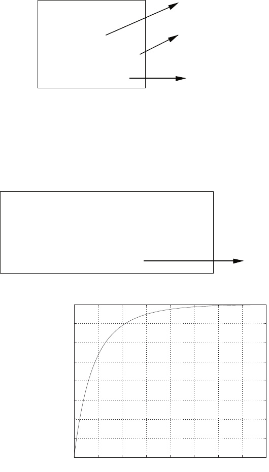
76 CHAPTER 2 Mathematical Models of Systems

Computer Problems

CP2.1 The m-ﬁle script is shown in Figure CP2.1.

pq =

1 9 24 20

P =

-5

-2

Z =

-2

value =

p=[1 7 10]; q=[1 2];

% Part (a)

pq=conv(p,q)

% Part (b)

P=roots(p), Z=roots(q)

% Part (c)

value=polyval(p,-1)

FIGURE CP2.1

Script for various polynomial evaluations.

CP2.2 The m-ﬁle script and step response is shown in Figure CP2.2.

numc = [1]; denc = [1 1]; sysc = tf(numc,denc)

numg = [1 2]; deng = [1 3]; sysg = tf(numg,deng)

% part (a)

sys_s = series(sysc,sysg);

sys_cl = feedback(sys_s,[1])

% part (b)

step(sys_cl); grid on

Transfer function:

s + 2

-------------

s^2 + 5 s + 5

Time (sec.)

Amplitude

Step Response

0 0.5 1 1.5 2 2.5 3 3.5 4

0.05

0.1

0.15

0.2

0.25

0.3

0.35

0.4

From: U(1)

To: Y(1)

FIGURE CP2.2

Step response.

from the publisher prior to any prohibited reproduction, storage in a retrieval system, or transmission in any form or by any means, electronic, mechanical, photocopying,

recording, or likewise. For information regarding permission(s), write to: Rights and Permissions Department, Pearson Education, Inc., Upper Saddle River, NJ 07458.

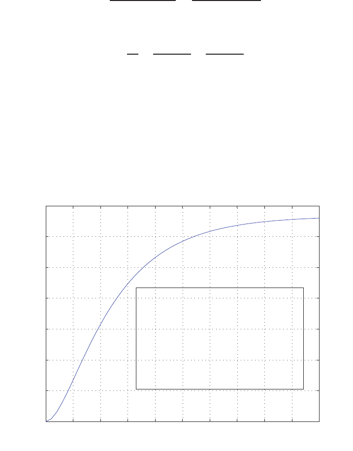
Computer Problems 77

CP2.3 Given

¨y+ 4 ˙y+ 3y=u

with y(0) = ˙y= 0 and U(s) = 1/s, we obtain (via Laplace transform)

Y(s) = 1

s(s2+ 4s+ 3) =1

s(s+ 3)(s+ 1) .

Expanding in a partial fraction expansion yields

Y(s) = 1

3s−1

6(s+ 3) −1

2(s+ 1) .

Taking the inverse Laplace transform we obtain the solution

y(t) = 0.3333 + 0.1667e−3t−0.5e−t.

The m-ﬁle script and step response is shown in Figure CP2.3.

0 0.5 1 1.5 2 2.5 3 3.5 4 4.5 5

0.05

0.1

0.15

0.2

0.25

0.3

0.35

Step Response

Time (sec)

Amplitude

n=[1]; d=[1 4 3]; sys = tf(n,d);

t=[0:0.1:5];

y = step(sys,t);

ya=0.3333+0.1667*exp(-3*t)-0.5*exp(-t);

plot(t,y,t,ya); grid;

title('Step Response');

xlabel('Time (sec)');

ylabel('Amplitude');

FIGURE CP2.3

Step response.

from the publisher prior to any prohibited reproduction, storage in a retrieval system, or transmission in any form or by any means, electronic, mechanical, photocopying,

recording, or likewise. For information regarding permission(s), write to: Rights and Permissions Department, Pearson Education, Inc., Upper Saddle River, NJ 07458.

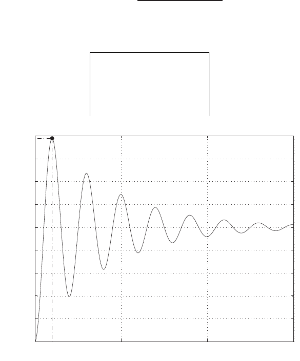
78 CHAPTER 2 Mathematical Models of Systems

CP2.4 The mass-spring-damper system is represented by

m¨x+b˙x+kx =f .

Taking the Laplace transform (with zero initial conditions) yields the

transfer function

X(s)/F (s) = 1/m

s2+bs/m +k/m .

The m-ﬁle script and step response is shown in Figure CP2.4.

m=10; k=1; b=0.5;

num=[1/m]; den=[1 b/m k/m];

sys = tf(num,den);

t=[0:0.1:150];

step(sys,t)

Time (sec.)

Amplitude

Step Response

0 50 100 150

0.2

0.4

0.6

0.8

1.2

1.4

1.6

1.8

From: U(1)

To: Y(1)

FIGURE CP2.4

Step response.

CP2.5 The spacecraft simulations are shown in Figure CP2.5. We see that as J

is decreased, the time to settle down decreases. Also, the overhoot from

10odecreases as Jdecreases. Thus, the performance seems to get better

(in some sense) as Jdecreases.

from the publisher prior to any prohibited reproduction, storage in a retrieval system, or transmission in any form or by any means, electronic, mechanical, photocopying,

recording, or likewise. For information regarding permission(s), write to: Rights and Permissions Department, Pearson Education, Inc., Upper Saddle River, NJ 07458.

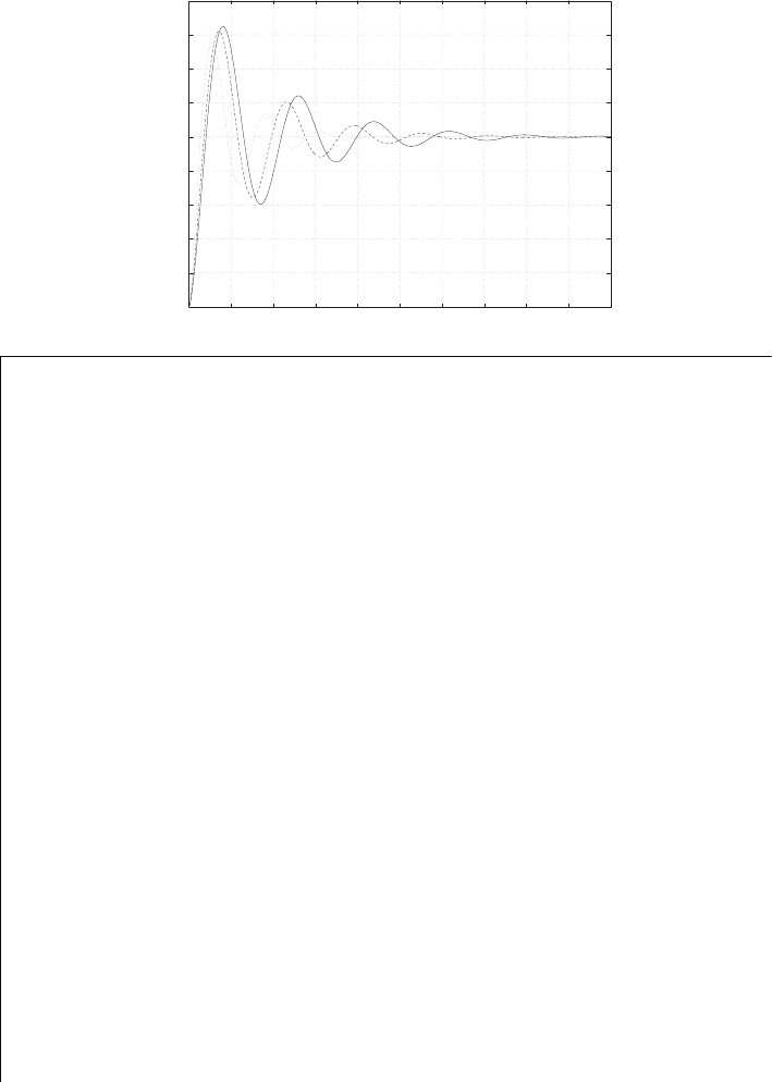
Computer Problems 79

0 10 20 30 40 50 60 70 80 90 100

Time (sec)

Spacecraft attitude (deg)

Nominal (solid); O-nominal 80% (dashed); O-nominal 50% (dotted)

%Part (a)

a=1; b=8; k=10.8e+08; J=10.8e+08;

num=k*[1 a];

den=J*[1 b 0 0]; sys=tf(num,den);

sys_cl=feedback(sys,[1]);

% Part (b) and (c)

t=[0:0.1:100];

% Nominal case

f=10*pi/180; sysf=sys_cl*f;

y=step(sysf,t);

% O-nominal case 80%

J=10.8e+08*0.8; den=J*[1 b 0 0];

sys=tf(num,den); sys_cl=feedback(sys,[1]);

sysf=sys_cl*f;

y1=step(sysf,t);

% O-nominal case 50%

J=10.8e+08*0.5; den=J*[1 b 0 0];

sys=tf(num,den); sys_cl=feedback(sys,[1]);

sysf=sys_cl*f;

y2=step(sysf,t);

plot(t,y*180/pi,t,y1*180/pi,'--',t,y2*180/pi,':'),grid

xlabel('Time (sec)')

ylabel('Spacecraft attitude (deg)')

title('Nominal (solid); O-nominal 80% (dashed); O-nominal 50% (dotted)')

FIGURE CP2.5

Step responses for the nominal and oﬀ-nominal spacecraft parameters.

from the publisher prior to any prohibited reproduction, storage in a retrieval system, or transmission in any form or by any means, electronic, mechanical, photocopying,

recording, or likewise. For information regarding permission(s), write to: Rights and Permissions Department, Pearson Education, Inc., Upper Saddle River, NJ 07458.

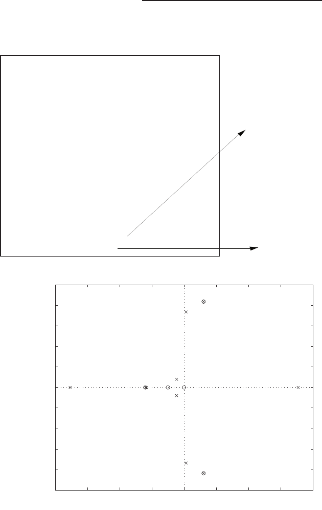
80 CHAPTER 2 Mathematical Models of Systems

CP2.6 The closed-loop transfer function is

T(s) = 4s6+ 8s5+ 4s4+ 56s3+ 112s2+ 56s

∆(s),

num1=[4]; den1=[1]; sys1 = tf(num1,den1);

num2=[1]; den2=[1 1]; sys2 = tf(num2,den2);

num3=[1 0]; den3=[1 0 2]; sys3 = tf(num3,den3);

num4=[1]; den4=[1 0 0]; sys4 = tf(num4,den4);

num5=[4 2]; den5=[1 2 1]; sys5 = tf(num5,den5);

num6=[50]; den6=[1]; sys6 = tf(num6,den6);

num7=[1 0 2]; den7=[1 0 0 14]; sys7 = tf(num7,den7);

sysa = feedback(sys4,sys6,+1);

sysb = series(sys2,sys3);

sysc = feedback(sysb,sys5);

sysd = series(sysc,sysa);

syse = feedback(sysd,sys7);

sys = series(sys1,syse)

pzmap(sys)

p=pole(sys)

z=zero(sys)

p =

7.0709

-7.0713

1.2051 + 2.0863i

1.2051 - 2.0863i

0.1219 + 1.8374i

0.1219 - 1.8374i

-2.3933

-2.3333

-0.4635 + 0.1997i

-0.4635 - 0.1997i

z =

1.2051 + 2.0872i

1.2051 - 2.0872i

-2.4101

-1.0000 + 0.0000i

-1.0000 - 0.0000i

poles

Real Axis

Imag Axis

Polezero map

-8 -6 -4 -2 0 2 4 6 8

-2.5

-2

-1.5

-1

-0.5

0.5

1.5

2.5

FIGURE CP2.6

Pole-zero map.

from the publisher prior to any prohibited reproduction, storage in a retrieval system, or transmission in any form or by any means, electronic, mechanical, photocopying,

recording, or likewise. For information regarding permission(s), write to: Rights and Permissions Department, Pearson Education, Inc., Upper Saddle River, NJ 07458.

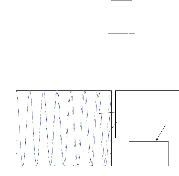
Computer Problems 81

where

∆(s) = s10 + 3s9−45s8−125s7−200s6−1177s5

−2344s4−3485s3−7668s2−5598s−1400 .

CP2.7 The m-ﬁle script and plot of the pendulum angle is shown in Figure CP2.7.

With the initial conditions, the Laplace transform of the linear system is

θ(s) = θ0s

s2+g/L.

To use the step function with the m-ﬁle, we can multiply the transfer

function as follows:

θ(s) = s2

s2+g/L

θ0

which is equivalent to the original transfer function except that we can

use the step function input with magnitude θ0. The nonlinear response

is shown as the solid line and the linear response is shown as the dashed

line. The diﬀerence between the two responses is not great since the initial

condition of θ0= 30◦is not that large.

0246810

-30

-20

-10

Time (s)

θ (deg)

L=0.5; m=1; g=9.8;

theta0=30;

% Linear simulation

sys=tf([1 0 0],[1 0 g/L]);

[y,t]=step(theta0*sys,[0:0.01:10]);

% Nonlinear simulation

[t,ynl]=ode45(@pend,t,[theta0*pi/180 0]);

plot(t,ynl(:,1)*180/pi,t,y,'--');

xlabel('Time (s)')

ylabel('\theta (deg)')

function [yd]=pend(t,y)

L=0.5; g=9.8;

yd(1)=y(2);

yd(2)=-(g/L)*sin(y(1));

yd=yd';

FIGURE CP2.7

Plot of θversus xt when θ0= 30◦.

from the publisher prior to any prohibited reproduction, storage in a retrieval system, or transmission in any form or by any means, electronic, mechanical, photocopying,

recording, or likewise. For information regarding permission(s), write to: Rights and Permissions Department, Pearson Education, Inc., Upper Saddle River, NJ 07458.

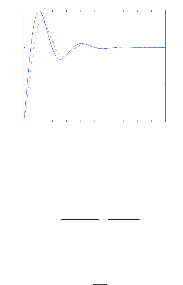
82 CHAPTER 2 Mathematical Models of Systems

CP2.8 The system step responses for z= 5,10, and 15 are shown in Fig-

ure CP2.8.

0 0.5 1 1.5 2 2.5 3 3.5 4 4.5 5

0.5

1.5 z=5 (solid), z=10 (dashed), z=15 dotted)

Time (sec)

x(t)

FIGURE CP2.8

The system response.

CP2.9 (a,b) Computing the closed-loop transfer function yields

T(s) = G(s)

1 + G(s)H(s)=s2+ 2s+ 1

s2+ 4s+ 3 .

The poles are s=−3,−1 and the zeros are s=−1,−1.

pole-zero cancellation) is

T(s) = s+ 1

s+ 3 .

from the publisher prior to any prohibited reproduction, storage in a retrieval system, or transmission in any form or by any means, electronic, mechanical, photocopying,

recording, or likewise. For information regarding permission(s), write to: Rights and Permissions Department, Pearson Education, Inc., Upper Saddle River, NJ 07458.

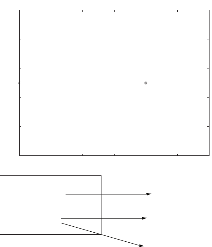
Computer Problems 83

?-3 ?-2.5 ?-2 ?-1.5 ?-1 ?-0.5 0

?-1

?-0.8

?-0.6

?-0.4

?-0.2

0.2

0.4

0.6

0.8

Pole?Zero Map

Real Axi s

Imaginary Axi s

poles

ng=[1 1]; dg=[1 2]; sysg = tf(ng,dg);

nh=[1]; dh=[1 1]; sysh = tf(nh,dh);

sys=feedback(sysg,sysh)

pzmap(sys)

pole(sys)

zero(sys)

Transfer function:

s^2 + 2 s + 1

-------------

s^2 + 4 s + 3

p =

-3

-1

z =

-1

zeros

FIGURE CP2.9

Pole-zero map.

CP2.10 Figure CP2.10 shows the steady-state response to a unit step input and a

unit step disturbance. We see that K= 1 leads to the same steady-state

response.

from the publisher prior to any prohibited reproduction, storage in a retrieval system, or transmission in any form or by any means, electronic, mechanical, photocopying,

recording, or likewise. For information regarding permission(s), write to: Rights and Permissions Department, Pearson Education, Inc., Upper Saddle River, NJ 07458.

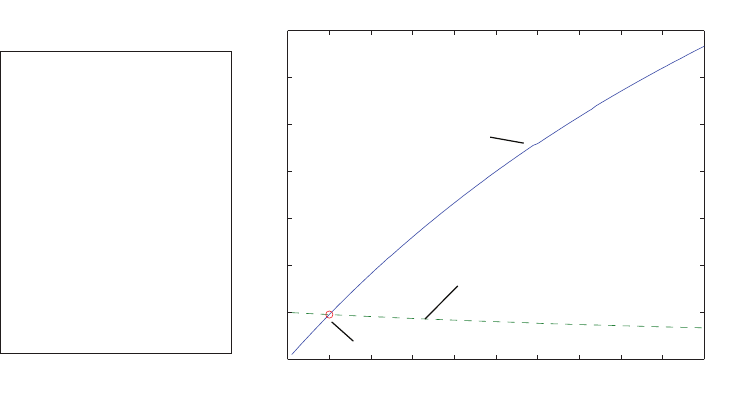
84 CHAPTER 2 Mathematical Models of Systems

0 1 2 3 4 5 6 7 8 9 10

0.05

0.1

0.15

0.2

0.25

0.3

0.35

Steady−state response

Disturbance Response Steady-State

Input Response Steady-State

K=1

K=[0.1:0.1:10];

sysg=tf([1],[1 20 20]);

for i=1:length(K)

nc=K(i); dc=[1];sysc=tf(nc,dc);

syscl=feedback(sysc*sysg,1);

systd=feedback(sysg,sysc);

y1=step(syscl);

Tf1(i)=y1(end);

y2=step(systd);

Tf2(i)=y2(end);

end

plot(K,Tf1,K,Tf2,'--')

xlabel('K')

ylabel('Steady-state response')

FIGURE CP2.10

Gain Kversus steady-state value.

from the publisher prior to any prohibited reproduction, storage in a retrieval system, or transmission in any form or by any means, electronic, mechanical, photocopying,

recording, or likewise. For information regarding permission(s), write to: Rights and Permissions Department, Pearson Education, Inc., Upper Saddle River, NJ 07458.

C H A P T E R 3

State Variable Models

Exercises

E3.1 One possible set of state variables is

(a) the current iL2through L2,

(b) the voltage vC2across C2, and

We can also choose vC1, the voltage across C1as the third state variable,

in place of the current through L1.

E3.2 We know that the velocity is the derivative of the position, therefore we

have

dt =v ,

and from the problem statement

dt =−k1v(t)−k2y(t) + k3i(t).

This can be written in matrix form as

dt 



v

=



0 1

−k2−k1





v

+



k3

i .

Deﬁne u=i, and let k1=k2= 1. Then,

x=Ax +Bu

where

A=



0 1

−1−1

,B=



k3

,and x=



v

.

from the publisher prior to any prohibited reproduction, storage in a retrieval system, or transmission in any form or by any means, electronic, mechanical, photocopying,

recording, or likewise. For information regarding permission(s), write to: Rights and Permissions Department, Pearson Education, Inc., Upper Saddle River, NJ 07458.

86 CHAPTER 3 State Variable Models

E3.3 The charactersitic roots, denoted by λ, are the solutions of det(λI−A) =

0. For this problem we have

det(λI−A) = det 





λ−1

1λ+ 2 



=λ(λ+ 2) + 1 = λ2+ 2λ+ 1 = 0 .

Therefore, the characteristic roots are

λ1=−1 and λ2=−1.

E3.4 The system in phase variable form is

x=Ax +Bu

y=Cx

where

A=





0 1 0

0 0 1

−8−6−4







,B=











,C=h1 0 0 i.

E3.5 From the block diagram we determine that the state equations are

˙x2=−(fk +d)x2+ax1+fu

˙x1=−kx2+u

and the output equation is

y=bx2.

Therefore,

x=Ax +Bu

y=Cx +Du ,

where

A=



0−k

a−(fk +d)

,B=



f

,C=h0biand D= [0] .

E3.6 (a) The state transition matrix is

Φ(t) = eAt=I+At+1

2!A2t2+···

from the publisher prior to any prohibited reproduction, storage in a retrieval system, or transmission in any form or by any means, electronic, mechanical, photocopying,

recording, or likewise. For information regarding permission(s), write to: Rights and Permissions Department, Pearson Education, Inc., Upper Saddle River, NJ 07458.

Exercises 87

But A2= 0, thus A3=A4=···= 0. So,

Φ(t) = eAt=I+At=



1 0

0 1 

+



0 1

0 0 

t=



0 1 

.

(b) The state at any time t≥0 is given by

x(t) = Φ(t)x(0)

and since x1(0) = x2(0) = 1, we determine that

x1(t) = x1(0) + tx2(0) = 1 + t

x2(t) = x2(0) = 1 .

E3.7 The state equations are

˙x1=x2

˙x2=−100x1−20x2+u

or, in matrix form

x=



0 1

−100 −20 

x+



1

u .

So, the characteristic equation is determined to be

det(λI−A) = det 



λ−1

100 λ+ 20 

=λ2+ 20λ+ 100 = (λ+ 10)2= 0 .

Thus, the roots of the characteristic equation are

λ1=λ2=−10 .

E3.8 The characteristic equation is

det(λI−A) = det 





λ−1 0

0λ−1

0 6 λ+ 3







=λ(λ2+ 3λ+ 6) = 0 .

Thus, the roots of the characteristic equation are

λ1= 0 , λ2=−1.5 + j1.9365 and λ3=−1.5−j1.9365 .

from the publisher prior to any prohibited reproduction, storage in a retrieval system, or transmission in any form or by any means, electronic, mechanical, photocopying,

recording, or likewise. For information regarding permission(s), write to: Rights and Permissions Department, Pearson Education, Inc., Upper Saddle River, NJ 07458.

88 CHAPTER 3 State Variable Models

E3.9 Analyzing the block diagram yields

˙x1=−x1+1

2x2+r

˙x2=x1−3

2x2−r

y=x1−3

2x2−r.

In state-variable form we have

x=

−11

1−3

2

x+



−1

r , y =1−3

2x+h−1ir .

The characteristic equation is

s2+5

2s+ 1 = (s+ 2)(s+1

2) = 0 .

E3.10 (a) The characteristic equation is

det[λI−A] = det 



λ−6

1 (λ+ 5) 

=λ(λ+5)+6 = (λ+2)(λ+3) = 0 .

So, the roots are λ1=−2 and λ2=−3.

(b) We note that

Φ(s) = [sI−A]−1=



s−6

1s+ 5 



−1

(s+ 2)(s+ 3) 



s+ 5 6

−1s

.

Taking the inverse Laplace transform yields the transition matrix

Φ(t) = 



3e−2t−2e−3t6e−2t−6e−3t

−e−2t+e−3t−2e−2t+ 3e−3t

.

E3.11 A state variable representation is

x=Ax +Br

y=Cx

where

A=



0 1

−12 −8

,B=



1

,C=h12 4 i.

from the publisher prior to any prohibited reproduction, storage in a retrieval system, or transmission in any form or by any means, electronic, mechanical, photocopying,

recording, or likewise. For information regarding permission(s), write to: Rights and Permissions Department, Pearson Education, Inc., Upper Saddle River, NJ 07458.

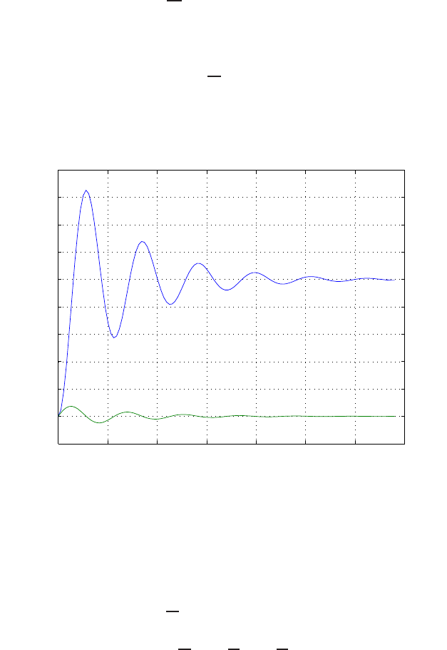
Exercises 89

E3.12 The equation of motion is

Ldi

dt +Ri +vc=vin

where

vc=1

CZi dt .

0 0.05 0.1 0.15 0.2 0.25 0.3 0.35

−0.2

0.2

0.4

0.6

0.8

1.2

1.4

1.6

1.8

Time(sec)

State response

x1: capacitor voltage

x2: inductor current

Unit step response

FIGURE E3.12

State variable time history for a unit step input.

Selecting the state variables x1=vcand x2=i, we have

˙x1=1

Cx2

˙x2=−R

Lx2−1

Lx1+1

Lvin .

This can be written in matrix form as

x=



0 1/C

−1/L −R/L 

x+



1/L 

vin .

from the publisher prior to any prohibited reproduction, storage in a retrieval system, or transmission in any form or by any means, electronic, mechanical, photocopying,

recording, or likewise. For information regarding permission(s), write to: Rights and Permissions Department, Pearson Education, Inc., Upper Saddle River, NJ 07458.

90 CHAPTER 3 State Variable Models

When C= 0.001F,R= 4Ω, and L= 0.1H, we have

x=



0 1000

−10 −40 

x+



10 

vin .

The step response is shown in Figure E3.12.

E3.13 (a) Select the state variables as x1=yand x2=ω.

(b) The corresponding state equation is

˙x1=−x1−ax2+ 2u

˙x2=bx1−4u

or, in matrix form

x=

−1−a

b0

x+



−4

uand x=



x2

.

det[λI−A] = det 



λ+ 1 a

−b λ 

=λ2+λ+ab = 0 .

So, the roots are

λ=−1

2±1

2√1−4ab .

E3.14 Assume that the mass decay is proportional to the mass present, so that

M=−qM +Ku

where qis the constant of proportionality. Select the state variable, x, to

be the mass, M. Then, the state equation is

˙x=−qx +Ku .

E3.15 The equations of motion are

m¨x+kx +k1(x−q) + b˙x= 0

m¨q+kq +b˙q+k1(q−x) = 0 .

from the publisher prior to any prohibited reproduction, storage in a retrieval system, or transmission in any form or by any means, electronic, mechanical, photocopying,

recording, or likewise. For information regarding permission(s), write to: Rights and Permissions Department, Pearson Education, Inc., Upper Saddle River, NJ 07458.

Exercises 91

In state variable form we have







0100

−(k+k1)

m−b

0 0 0 1

m0−(k+k1)

m−b







where x1=x, x2= ˙x, x3=qand x4= ˙q.

E3.16 The governing equations of motion are

m1¨x+k1(x−q) + b1( ˙x−˙q) = u(t)

m2¨q+k2q+b2˙q+b1( ˙q−˙x) + k1(q−x) = 0 .

Let x1=x, x2= ˙x, x3=qand x4= ˙q. Then,







0 1 0 0

−k1

m1−b1

0 0 0 1

m2−(k1+k2)

m2−(b1+b2)



















u(t).

Since the output is y(t) = q(t), then

y=h0 0 1 0 ix.

E3.17 At node 1 we have

C1˙v1=va−v1

+v2−v1

and at node 2 we have

C2˙v2=vb−v2

+v1−v2

Let

x1=v1

and

x2=v2.

from the publisher prior to any prohibited reproduction, storage in a retrieval system, or transmission in any form or by any means, electronic, mechanical, photocopying,

recording, or likewise. For information regarding permission(s), write to: Rights and Permissions Department, Pearson Education, Inc., Upper Saddle River, NJ 07458.

92 CHAPTER 3 State Variable Models

Then, in matrix form we have

x=



−1

R1C1+1

R2C11

R2C1

−1

R2C2−1

R3C2+1

R2C2



x+



R1C10

R3C2







vb

.

E3.18 The governing equations of motion are

Ri1+L1

di1

dt +v=va

di2

dt +v=vb

iL=i1+i2=Cdv

dt .

Let x1=i1, x2=i2, x3=v, u1=vaand u2=vb. Then,

x=





−R

L10−1

0 0 −1







x+





L10

0 0







y=h0 0 1 ix+ [0] u.

E3.19 First, compute the matrix

sI −A=



s−1

3s+ 4 

.

Then, Φ(s) is

Φ(s) = (sI−A)−1=1

∆(s)



s+ 4 1

−3s



where ∆(s) = s2+ 4s+ 3, and

G(s) = h10 0 i



s+4

∆(s)

−3

∆(s)

∆(s)





1

=10

s2+ 4s+ 3 .

E3.20 The linearized equation can be derived from the observation that sin θ≈θ

when θ≈0. In this case, the linearized equations are

θ+g

Lθ+k

m˙

θ= 0 .

from the publisher prior to any prohibited reproduction, storage in a retrieval system, or transmission in any form or by any means, electronic, mechanical, photocopying,

recording, or likewise. For information regarding permission(s), write to: Rights and Permissions Department, Pearson Education, Inc., Upper Saddle River, NJ 07458.

Exercises 93

Let x1=θand x2=˙

θ. Then in state variable form we have

x=Ax

y=Cx

where

A=



0 1

−g/L −k/m 

,C=h1 0 i,and x(0) = 



θ(0)

θ(0) 

.

E3.21 The transfer function is

G(s) = C[sI−A]−1B+D=−1

s2+ 2s+ 1 .

The unit step response is

y(t) = −1 + e−t+te−t.

E3.22 The transfer function is

G(s) = s−6

s2−7s+ 6 .

The poles are at s1= 1 and s2= 6. The zero is at s= 6. So, we see

that there is a pole-zero cancellation. We can write the system in state

variable form as

˙x=x−√2u

y=−√2

and the transfer function is

G(s) = 1

s−1.

E3.23 The system in state variable form can be represented by

x=Ax +Bu

y=Cx +Du

where

A=





0 1 0

0 0 1

−1−3−3







,B=











,C=h0 1 −1i,D=h1i.

from the publisher prior to any prohibited reproduction, storage in a retrieval system, or transmission in any form or by any means, electronic, mechanical, photocopying,

recording, or likewise. For information regarding permission(s), write to: Rights and Permissions Department, Pearson Education, Inc., Upper Saddle River, NJ 07458.

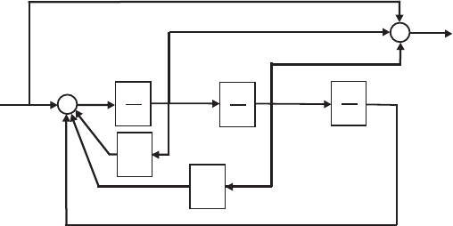
94 CHAPTER 3 State Variable Models

U(s)

X(s)

FIGURE E3.23

Block diagram.

from the publisher prior to any prohibited reproduction, storage in a retrieval system, or transmission in any form or by any means, electronic, mechanical, photocopying,

recording, or likewise. For information regarding permission(s), write to: Rights and Permissions Department, Pearson Education, Inc., Upper Saddle River, NJ 07458.

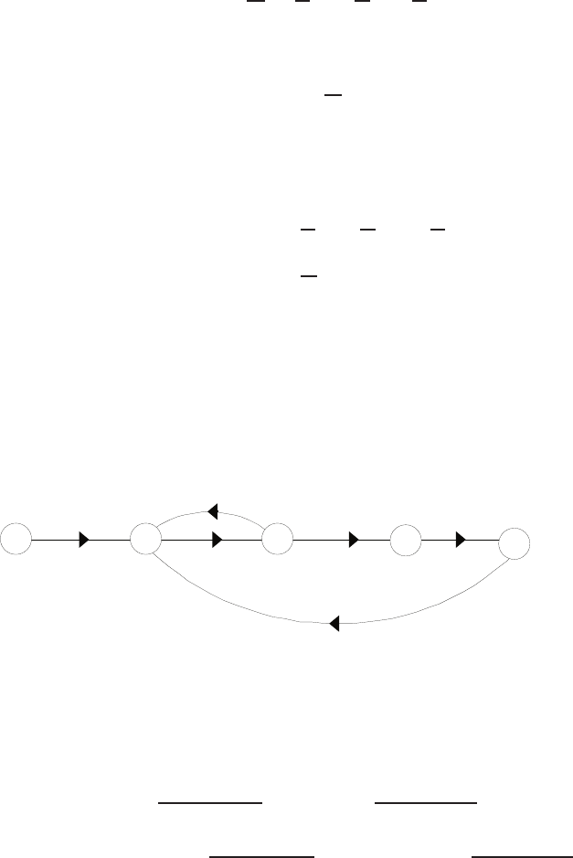
Problems 95

Problems

P3.1 The loop equation, derived from Kirchoﬀ’s voltage law, is

dt =1

Lv−R

Li−1

Lvc

where

vc=1

CZi dt .

(a) Select the state variables as x1=iand x2=vc.

(b) The corresponding state equations are

˙x1=1

Lv−R

Lx1−1

Lx2

˙x2=1

Cx1.

x=

−R/L −1/L

1/C 0

x+



1/L

0

u .

1/L

-1/L

1/s

-R/L

1/C 1/s

FIGURE P3.1

Signal ﬂow graph.

P3.2 Let

a11 =−2

(R1+R2)C, a22 =−2R1R2

(R1+R2)L,

b11 =b12 =1

(R1+R2)C, b21 =−b22 =R2

(R1+R2)L.

The corresponding block diagram is shown in Figure P3.2.

from the publisher prior to any prohibited reproduction, storage in a retrieval system, or transmission in any form or by any means, electronic, mechanical, photocopying,

recording, or likewise. For information regarding permission(s), write to: Rights and Permissions Department, Pearson Education, Inc., Upper Saddle River, NJ 07458.

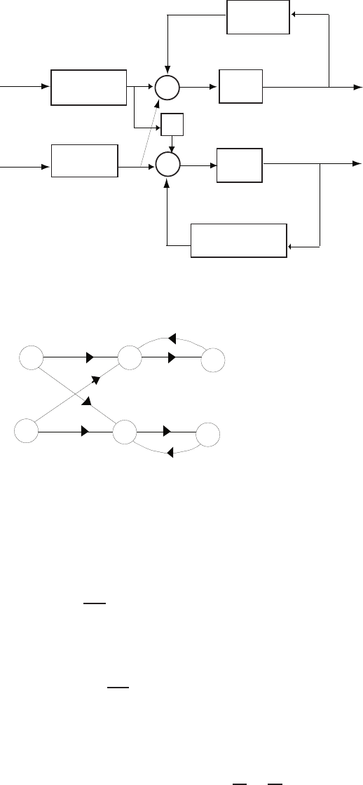
96 CHAPTER 3 State Variable Models

1/(R1+R2)C

1/s

2/(R1+R2)C

1/(R1+R2)C

1/s

2R1R2/(R1+R2)C

1/s

b22

b21

b12

b11

a22

a11

(a)

(b)

FIGURE P3.2

(a) Block diagram. (b) Signal ﬂow graph.

P3.3 Using Kirchoﬀ’s voltage law around the outer loop, we have

LdiL

dt −vc+v2−v1= 0 .

Then, using Kirchoﬀ’s current law at the node, we determine that

Cdvc

dt =−iL+iR,

where iRis the current through the resistor R. Considering the right loop

we have

iRR−v2+vc= 0 or iR=−vc

R+v2

from the publisher prior to any prohibited reproduction, storage in a retrieval system, or transmission in any form or by any means, electronic, mechanical, photocopying,

recording, or likewise. For information regarding permission(s), write to: Rights and Permissions Department, Pearson Education, Inc., Upper Saddle River, NJ 07458.

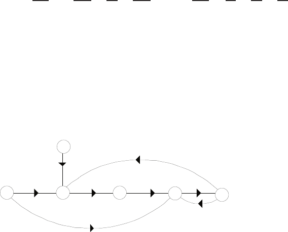
Problems 97

Thus,

dvc

dt =−vc

RC −iL

C+v2

RC and diL

dt =vc

dt +v1

L−v2

In matrix form, the state equations are





˙x1

˙x2

=



0 1/L

−1/C −1/RC 





x2

+



1/L −1/L

0 1/RC 





v2

,

where x1=iLand x2=vc. The signal ﬂow graph is shown in Figure P3.3.

1/L

1/RC

1/s

1/L

-1/C 1/s

-1/L

-1/RC

FIGURE P3.3

Signal ﬂow graph.

P3.4 (a) The block diagram model for phase variable form is shown in Fig-

ure P3.4a. The phase variable form is given by

x=





0 1 0

0 0 1

−10 −6−4







x+











y=h10 2 1 ix.

(b) The block diagram in input feedforward form is shown in Figure P3.4b.

The input feedforward form is given by

x=





−4 1 0

−6 0 1

−10 0 0







x+











r(t)

y=h1 0 0 ix.

from the publisher prior to any prohibited reproduction, storage in a retrieval system, or transmission in any form or by any means, electronic, mechanical, photocopying,

recording, or likewise. For information regarding permission(s), write to: Rights and Permissions Department, Pearson Education, Inc., Upper Saddle River, NJ 07458.

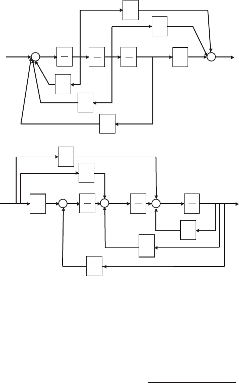
98 CHAPTER 3 State Variable Models

R(s)Y(s)

(a)

R(s)Y(s)

10 s

+++++

(b)

FIGURE P3.4

(a)Block diagram model for phase variable form. (b) Block diagram model for input feedforward form.

P3.5 (a) The closed-loop transfer function is

T(s) = s+ 1

s3+ 4s2−11s+ 1 .

(b) A matrix diﬀerential equation is

x=Ax +Bu

y=Cx

where

A=





0 1 0

0 0 1

−1 11 −4







,B=











,C=h1 1 0 i.

The block diagram is shown in Figure P3.5.

from the publisher prior to any prohibited reproduction, storage in a retrieval system, or transmission in any form or by any means, electronic, mechanical, photocopying,

recording, or likewise. For information regarding permission(s), write to: Rights and Permissions Department, Pearson Education, Inc., Upper Saddle River, NJ 07458.

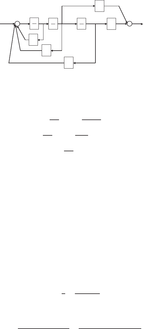
Problems 99

R(s)Y(s)

-11

FIGURE P3.5

Block diagram model.

P3.6 The node equations are

0.00025dv1

dt +iL−vi−v1

4000 = 0

0.0005dv2

dt −iL+v2

1000 −i3= 0

0.002diL

dt +v2−v1= 0 .

Deﬁne the state variables

x1=v1x2=v2x3=iL.

Then,

x=Ax +Bu

where

A=





−1 0 −4000

0−2 2000

500 −500 0







,B=





1 0

0 2000

0 0







P3.7 Given K= 1, we have

KG(s)·1

s=(s+ 1)2

s(s2+ 1) .

We then compute the closed-loop transfer function as

T(s) = s2+ 2s+ 1

3s3+ 5s2+ 5s+ 1 =s−1+ 2s−2+s−3

3 + 5s−1+ 5s−2+s−3.

from the publisher prior to any prohibited reproduction, storage in a retrieval system, or transmission in any form or by any means, electronic, mechanical, photocopying,

recording, or likewise. For information regarding permission(s), write to: Rights and Permissions Department, Pearson Education, Inc., Upper Saddle River, NJ 07458.

100 CHAPTER 3 State Variable Models

A state variable model is

x=





010

001

−1/3−5/3−5/3







x+





1/3







y=h1 2 1 ix.

P3.8 The state-space equations are

˙x1=x2

˙x2=ku

x3−g

˙x3=u .

This is a set of nonlinear equations.

P3.9 (a) The closed-loop transfer function is

T(s) = 10

Js3+ (b+ 10J)s2+ 10bs + 10K1

=10s−3

1 + 10.1s−1+s−2+ 5s−3,

where K1= 0.5, J= 1, and b= 0.1.

(b) A state-space model is

x=





0 1 0

0 0 1

−5−1−10.1







x+











ω=h1 0 0 ix.

det[sI−A] = det 





s−1 0

0s−1

5 1 s+ 10.1







=s3+ 10.1s2+s+ 5 = 0 .

The roots of the characteristic equation are

s1=−10.05 and s2,3=−0.0250 ±0.7049j .

All roots lie in the left hand-plane, therefore, the system is stable.

from the publisher prior to any prohibited reproduction, storage in a retrieval system, or transmission in any form or by any means, electronic, mechanical, photocopying,

recording, or likewise. For information regarding permission(s), write to: Rights and Permissions Department, Pearson Education, Inc., Upper Saddle River, NJ 07458.

Problems 101

P3.10 (a) From the signal ﬂow diagram, we determine that a state-space model

is given by

x=

−K1K2

−K1−K2

x+



K1−K2

K1K2





r2



y=



y2

=



1 0

0 1 

x.

(b) The characteristic equation is

det[sI−A] = s2+ (K2+K1)s+ 2K1K2= 0 .

A=

−1 1

−1−1

.

The state transition matrix associated with Ais

Φ=L−1n[sI−A]−1o=e−t



cos tsin t

−sin tcos t

.

P3.11 The state transition matrix is

Φ(t) = 



(2t−1)e−t−2te−t

2te−t(−2t+ 1)e−t

.

So, when x1(0) = x2(0) = 10, we have

x(t) = Φ(t)x(0)

x1(t) = 10e−t

x2(t) = 10e−t

P3.12 (a) A state variable representation is given by

x=





0 1 0

0 0 1

−48 −44 −12







x+











from the publisher prior to any prohibited reproduction, storage in a retrieval system, or transmission in any form or by any means, electronic, mechanical, photocopying,

recording, or likewise. For information regarding permission(s), write to: Rights and Permissions Department, Pearson Education, Inc., Upper Saddle River, NJ 07458.

102 CHAPTER 3 State Variable Models

y= [40 8 0]x.

(b) The state transition matrix is

Φ(t) = Φ1(t).

.Φ2(t).

.Φ3(t),

where

Φ1(t) = 





e−6t−3e−4t+ 3e−2t

−6e−6t+ 12e−4t−6e−2t

36e−6t−48e−4t+ 12e−2t







Φ2(t) = 





4e−6t−2e−4t+5

4e−2t

−9

2e−6t+ 8e−4t−5

2e−2t

27e−6t−32e−4t+ 5e−2t







Φ3(t) = 





8e−6t−1

4e−4t+1

8e−2t

−3

4e−6t+e−4t−1

4e−2t

2e−6t−4e−4t+1

2e−2t







P3.13 (a) The RLC circuit state variable representation is

x=

−10 −4

6 0 

x+



0

u .

The characteristic equation is

s2+ 10s+ 24 = 0 .

All roots of the characteristic equation (that is, s1=−4 and s2=−6)

are in the left half-plane; therefore the system is stable.

(b) The state transition matrix is

Φ(t) = 



3e−6t−2e−4t2e−6t+ 2e−4t

−3e−6t+ 3e−4t−2e−6t+ 3e−4t

.

x1(0) = 0.1, x2(0) = 0 and e(t) = 0 ,

we have

i(t) = x1(t) = 0.3e−6t−0.2e−4t

vc(t) = x2(t) = −0.3e−6t+ 0.3e−4t.

from the publisher prior to any prohibited reproduction, storage in a retrieval system, or transmission in any form or by any means, electronic, mechanical, photocopying,

recording, or likewise. For information regarding permission(s), write to: Rights and Permissions Department, Pearson Education, Inc., Upper Saddle River, NJ 07458.

Problems 103

(d) When x(0) = 0 and u(t) = E, we have

x(t) = Zt

Φ(t−τ)Bu(τ)dτ ,

where

Bu(t) = 



0

.

Integrating yields

x1(t) = (−2e−6t+ 2e−4t)E

x2(t) = (1 + 2e−6t−3e−4t)E .

P3.14 A state space representation is

x=Ax+Br , y =Cx

where







0 1 0 0

0 0 1 0

0 0 0 1

−50 −34 −10 −12







,B=













,C= [50 1 0 0] .

P3.15 A state variable representation is

x=





0 1 0

0 0 1

−16 −31 −10







x+











y= [56 14 0]x.

The block diagram is shown in Figure P3.15.

from the publisher prior to any prohibited reproduction, storage in a retrieval system, or transmission in any form or by any means, electronic, mechanical, photocopying,

recording, or likewise. For information regarding permission(s), write to: Rights and Permissions Department, Pearson Education, Inc., Upper Saddle River, NJ 07458.

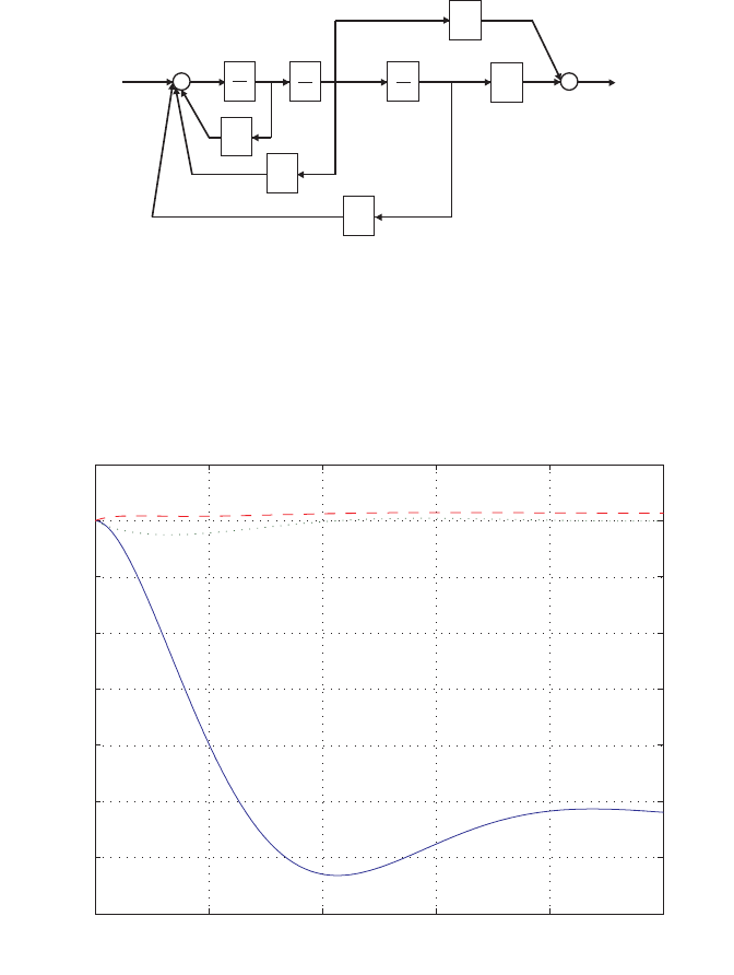
104 CHAPTER 3 State Variable Models

R(s)Y(s)

FIGURE P3.15

Block diagram model.

P3.16 (a) The characteristic equation is

0 20 40 60 80 100

-3.5

-3

-2.5

-2

-1.5

-1

-0.5

0.5

Time (s)

Step response)

x1 - solid; x2 - dotted; x3 - dashed

FIGURE P3.16

Step response of magnitude 0.285◦.

det(sI−A) = det 





s−1 0

0.0071 s+ 0.111 −0.12

0−0.07 s+ 0.3







from the publisher prior to any prohibited reproduction, storage in a retrieval system, or transmission in any form or by any means, electronic, mechanical, photocopying,

recording, or likewise. For information regarding permission(s), write to: Rights and Permissions Department, Pearson Education, Inc., Upper Saddle River, NJ 07458.

Problems 105

=s3+ 0.411s2+ 0.032s+ 0.00213 = 0 .

The roots are

s1=−0.3343 and s2,3=−0.0383 ±0.0700j .

All the poles lie in the left half-plane, therefore, the system is stable.

(b) The solution of the system to a step of magnitude 0.285◦is given by

x1(t) = −2.66 −0.11e−0.33t+e−0.038t(2.77 cos 0.07t+ 0.99 sin 0.07t)

x2(t) = 0.037e−0.33t−e−0.038t(0.037 cos 0.07t+ 0.23 sin 0.07t)

x3(t) = 0.069 −0.075e−0.33t+e−0.038t(0.006 cos 0.07t−0.06 sin 0.07t)

P3.17 The transfer function is

G(s) = C(sI−A)−1B=−4s+ 12

s3−14s2+ 37s+ 20 .

P3.18 Deﬁne the state variables as

x1=φ1−φ2

x2=ω1

ωo

x3=ω2

ωo

Then, the state equations of the robot are

˙x1=ωox2−ωox3

˙x2=−J2ωo

J1+J2

x1−b

x2+b

x3+Km

J1ωo

˙x3=J1ωo

J1+J2

x2+b

x2−b

or, in matrix form

x=ωo





0 1 −1

a−1−b1b1

a b2−b2







x+











where

a=J1

(J1+J2), b1=b

J1ωo

, b2=b

J2ωo

and d=Km

J1ωo

from the publisher prior to any prohibited reproduction, storage in a retrieval system, or transmission in any form or by any means, electronic, mechanical, photocopying,

recording, or likewise. For information regarding permission(s), write to: Rights and Permissions Department, Pearson Education, Inc., Upper Saddle River, NJ 07458.

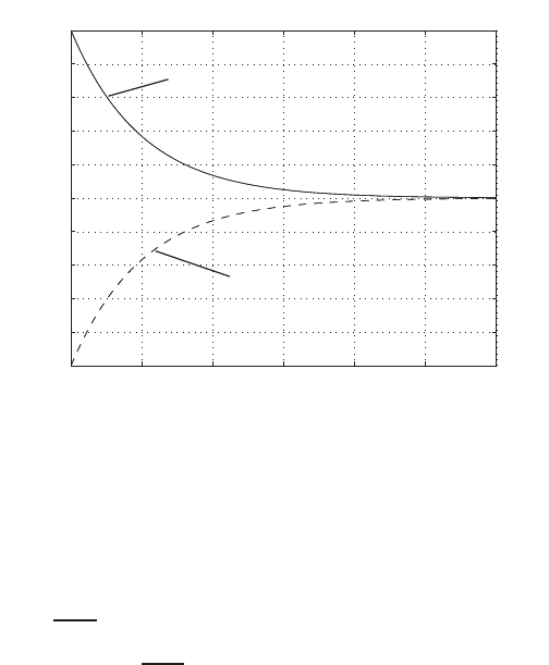
106 CHAPTER 3 State Variable Models

P3.19 The state equation is given by

x=



0 1

−2−3

x

where x1(0) = 1 and x2(0) = −1. The state transition matrix is

Φ(t) = 

−e−2t+ 2e−t−e−2t+e−t

2e−2t−2e−t2e−2t−e−t

.

The system response is

x1(t) = −e−2t+ 2e−tx1(0) + −e−2t+e−tx2(0)

x2(t) = 2e−2t−2e−tx1(0) + 2e−2t−e−tx2(0) .

The state response is shown in Figure P3.19.

0123456

-1

-0.8

-0.6

-0.4

-0.2

0.2

0.4

0.6

0.8

Time (s)

System response

FIGURE P3.19

Response with x1(0) = 1 and x2(0) = −1.

P3.20 The state equation is given by

x=

−0.693

6.70

−1−0.693

9.2

xwhere x(0) = 



0.3×1016

7×1016 

.

from the publisher prior to any prohibited reproduction, storage in a retrieval system, or transmission in any form or by any means, electronic, mechanical, photocopying,

recording, or likewise. For information regarding permission(s), write to: Rights and Permissions Department, Pearson Education, Inc., Upper Saddle River, NJ 07458.

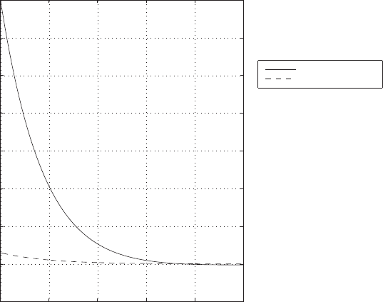
Problems 107

The state transition matrix is

Φ(t) = 



e−0.103433t0

35.5786(e−0.103433t−e−0.0753261t)e−0.075326t

.

The system response is

x1(t) = e−0.103433tx1(0)

x2(t) = 35.5786 he−0.103433t−e−0.0753261tix1(0) + e−0.075326tx2(0) .

The state response is shown in Figure P3.20.

0 10 20 30 40 50

-1

Time (hours)

Nucleide densities in atoms per unit volume

X=Xenon 135

I=Iodine 135

FIGURE P3.20

Nuclear reactor state response to initial conditions.

from the publisher prior to any prohibited reproduction, storage in a retrieval system, or transmission in any form or by any means, electronic, mechanical, photocopying,

recording, or likewise. For information regarding permission(s), write to: Rights and Permissions Department, Pearson Education, Inc., Upper Saddle River, NJ 07458.

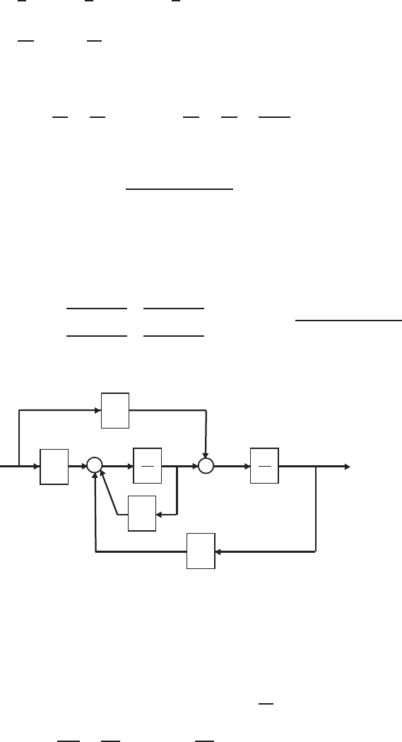
108 CHAPTER 3 State Variable Models

P3.21 Referring to Figure P3.21 we have

Y(s) = 1

sW(s) = 1

sh1U(s) + 1

sQ(s)

=h1

sU(s) + 1

s2[h0U(s)−a0Y(s)−a1sY (s) + a1h1U(s)] .

Gathering like terms and re-arranging yields

1 + a1

s+a0

s2Y(s) = h1

s+h0

s2+a1h1

s2U(s)

Y(s) = h1s+h0+a1h1

s2+a1s+a0U(s).

Computing the transfer function from the state variable representation

yields

G(s) = C(sI−A)−1B

=h1 0 i



s+a1

s2+a1s+a0

−a0

s2+a1s+a0







h0

=h1s+h0+a1h1

s2+a1s+a0

U(s)

W(s)

Q(s)

1Y(s)

+ +

FIGURE P3.21

Block diagram with labeled signals.

P3.22 The governing equations are

Ldi

dt =v2

dv1

dt +1

(v1−v) + 1

(v1−v2) = 0

from the publisher prior to any prohibited reproduction, storage in a retrieval system, or transmission in any form or by any means, electronic, mechanical, photocopying,

recording, or likewise. For information regarding permission(s), write to: Rights and Permissions Department, Pearson Education, Inc., Upper Saddle River, NJ 07458.

Problems 109

dv2

dt +1

(v2−v1) + i+v2

= 0 .

Let u=v, x1=i, x2=v1and x3=v2. Then,

x=





0 0 1

0−1

a1

R1+1

R21

C1R2

−1

R2C2−1

R2C2+1

R3C2







x+





R1C1







y= [0 0 1]x.

P3.23 A state variable representation is given by

x=





0 1 0

0 0 1

−30 −31 −10







x+











y= [1 0 0]x.

Other representations include the input feedforward representation

x=





−10 1 0

−31 0 1

−30 0 0







x+











y= [1 0 0]x,

the physical variable representation

x=





−310

0−2 1

0 0 −5







x+











y= [1 0 0]x,

and the decoupled representation

x=





−300

0−2 0

0 0 −5







x+











from the publisher prior to any prohibited reproduction, storage in a retrieval system, or transmission in any form or by any means, electronic, mechanical, photocopying,

recording, or likewise. For information regarding permission(s), write to: Rights and Permissions Department, Pearson Education, Inc., Upper Saddle River, NJ 07458.

110 CHAPTER 3 State Variable Models

y=1

3−1

2x.

P3.24 The matrix representation of the state equations is

x=



3 0

0 2 

x+



1 1

0 1 





u2

+



1

d .

When u1= 0 and u2=d= 1, we have

˙x1= 3x1+u2

˙x2= 2x2+ 2u2

So we see that we have two independent equations for x1and x2. With

U2(s) = 1/s and zero initial conditions, the solution for x1is found to be

x1(t) = L−1{X1(s)}=L−11

s(s−3)

=L−1−1

3s+1

s−3=−1

31−e3t

and the solution for x2is

x2(t) = L−1{X2(s)}=L−12

s(s−2)=L−1−1

s+1

s−2=−1+e2t.

P3.25 Since Φ(s) = (sI−A)−1, we have

Φ(s) = 



s+ 1 0

−2s+ 3 



−1

=



s+ 3 0

2s+ 1 



∆(s)

where ∆(s) = (s+ 1)(s+ 3). The state transition matrix is

Φ(t) = L−1{Φ(s)}=



e−t0

e−t−e−3te−3t

.

P3.26 The state variable diﬀerential equation is

x=



0 1

−25 −6

x+



25 

r

y= [1 0]x.

from the publisher prior to any prohibited reproduction, storage in a retrieval system, or transmission in any form or by any means, electronic, mechanical, photocopying,

recording, or likewise. For information regarding permission(s), write to: Rights and Permissions Department, Pearson Education, Inc., Upper Saddle River, NJ 07458.

Problems 111

and

Φ(s) = (sI−A)−1=



s+ 6 1

−25 s



∆(s)

where ∆(s) = s2+ 6s+ 25.

P3.27 Equating the change in angular momentum to the sum of the external

torques yields

J¨

θ−Hω cos θ=−b˙

θ−kθ

where bis the damping coeﬃcient, kis the spring constant, and Jis the

wheel moment of inertia. Deﬁning the state variables x1=θand x2= ˙x

and the input u=ω, we can write the equations of motion as

˙x1=x2

˙x2=−k

Jx1−b

Jx2+H

Jucos x1

With a small angle assumption (that is, cos x1≈1) we have

x=



0 1

−k/J −b/J 

x+



H/J 

u

y=θ=h1 0 ix.

P3.28 The governing equations of motion are

m1¨y1+k(y1−y2) + b˙y1=u

m2¨y2+k(y2−y1) + b˙y2= 0

y=y2.

Let x1=y1, x2= ˙y1, x3=y2and x4= ˙y2. Then







0 1 0 0

−k

m1−b

m10

0 0 0 1

m20−k

m2−b



















y=h0 0 1 0 ix.

from the publisher prior to any prohibited reproduction, storage in a retrieval system, or transmission in any form or by any means, electronic, mechanical, photocopying,

recording, or likewise. For information regarding permission(s), write to: Rights and Permissions Department, Pearson Education, Inc., Upper Saddle River, NJ 07458.

112 CHAPTER 3 State Variable Models

P3.29 The equations of motion are

I¨q1+M gL sin q1+k(q1−q2) = 0

J¨q2−k(q1−q2) = u .

Let x1=q1,x2= ˙q1,x3=q2, and x4= ˙q2and linearize the equations

using small angle assumptions (i.e. sin q1≈q1). Then, we have

˙x1=x2

˙x2=−M gL

Ix1−k

I(x1−x3)

˙x3=x4

˙x4=k

J(x1−x3) + 1

Ju .

P3.30 Using Kirchoﬀ’s current law, we ﬁnd that

Cdvc

dt =i2+i3

where i3= current in R3. Let i1= current in R1. Using Kirchoﬀ’s voltage

law, we have

LdiL

dt =v1−R1i1

and

R1i1+R2i2+vc=v1.

But

i2=i1−iL,

(R1+R2)i1=v1−vc+R2iL.

Using Kirchoﬀ’s voltage law once again, we calculate i3as

i3=v2−vc

Utilizing the above equations, we can solve for diL/dt and dvc/dt, as

follows:

diL

dt =R2

L(R1+R2)v1+R1

L(R1+R2)vc−R1R2

L(R1+R2)iL

dt =v1

C(R1+R2)−vc

CR3−R1iL

C(R1+R2)+v2

CR3

from the publisher prior to any prohibited reproduction, storage in a retrieval system, or transmission in any form or by any means, electronic, mechanical, photocopying,

recording, or likewise. For information regarding permission(s), write to: Rights and Permissions Department, Pearson Education, Inc., Upper Saddle River, NJ 07458.

Problems 113

Deﬁne the state variables x1=vcand x2=iL. Then, in matrix form we

have

x=

−(R1+R2+R3)

CR3(R1+R2)−R1

C(R1+R2)

L(R1+R2)−R1R2

L(R1+R2)

x+



C(R1+R2)

CR3

L(R1+R2)0





v2



y=i2=h−1

(R1+R2)−R1

(R1+R2)ix+h1

(R1+R2)0i



v2



P3.31 A state variable representation is

x=



0 1

−3−4

x+



30 

u .

The state transition matrix can be computed as follows:

Φ=L−1n[sI−A]−1o=L−1





∆(s)



s+ 4 1

−3s







=



2e−t−1

2e−3t1

2e−t−1

2e−3t

−3

2e−t+3

2e−3t−1

2e−t+3

2e−3t



where

∆(s) = s2+ 4s+ 3 = (s+ 1)(s+ 3) .

P3.32 A state variable representation is

˙m1=−k1m1+r

˙m2=k1m1−k2m2

where k1and k2are constants of proportionality. In matrix form, we have

x=Ax +Br=

−k10

k1−k2

x+



0

r

where x1=m1and x2=m2. Let k1=k2= 1 and assume that r(t) = 0

and x1= 1 and x2= 0. Then

x(t) = Φ(t)x(0) = 



e−t0

te−te−t

x(0) = 



e−t

te−t

.

from the publisher prior to any prohibited reproduction, storage in a retrieval system, or transmission in any form or by any means, electronic, mechanical, photocopying,

recording, or likewise. For information regarding permission(s), write to: Rights and Permissions Department, Pearson Education, Inc., Upper Saddle River, NJ 07458.

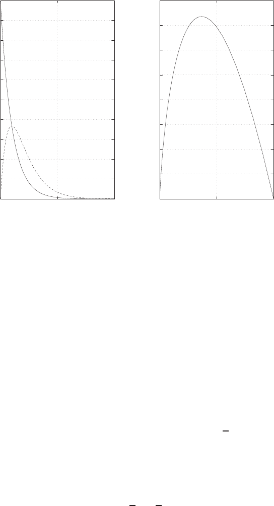
114 CHAPTER 3 State Variable Models

The simulation is shown in Figure P3.32.

0.1

0.2

0.3

0.4

0.5

0.6

0.7

0.8

0.9

05 10

time (sec)

state history, x(t)

0.05

0.1

0.15

0.2

0.25

0.3

0.35

0.4

0 0.5 1

t=0

FIGURE P3.32

Actual versus approximate state response.

P3.33 The system (including the feedback) is described by

x=Ax =



0 1

−1/2−1

x.

The charactersitic equation is

det[λI−A] = det 



λ−1

1/2λ+ 1 

=λ2+λ+1

2= 0 .

The roots of the characteristic equation are

λ1,2=−1

2±j1

from the publisher prior to any prohibited reproduction, storage in a retrieval system, or transmission in any form or by any means, electronic, mechanical, photocopying,

recording, or likewise. For information regarding permission(s), write to: Rights and Permissions Department, Pearson Education, Inc., Upper Saddle River, NJ 07458.

Problems 115

The system response is

x(t) = eAtx(0) = 



e−t/2cos t

2+e−t/2sin t

22e−t/2sin t

−e−t/2sin t

2e−t/2cos t

2−e−t/2sin t

2

x(0)

=e−t/2



2 sin t

cos t

2−sin t

2



where x1(0) = 0 and x2(0) = 1.

P3.34 (a) The state space representation is

x=





0 1 0

0 0 1

−6−11 −6







x+











y= [6 0 0] x.

(b) The element φ11(t) of the state transition matrix is

φ11(t) = e−3t−3e−2t+ 3e−t.

P3.35 The state equations are

h= ˙x1=1

50[80θ−50h] = −x1+8

5x2

θ= ˙x2=ω=x3

˙ω= ˙x3=Km

Jia=−KmKb

JRa

ω+KmKa

JRa

vi=−353

30 x3+25000

3vi.

In state variable form, we have

x=





−18

0 0 1

0 0 −353







x+





25000







vi.

P3.36 Using Newton’s Law and summing the forces on the two masses yields

M1¨x(t) + b1˙x(t) + k1x(t) = b1˙y(t)

M2¨y(t) + b1˙y(t) + k2y(t) = b1˙x(t) + u(t)

Let

z1=x, z2= ˙x, z3=y, and z4= ˙y .

from the publisher prior to any prohibited reproduction, storage in a retrieval system, or transmission in any form or by any means, electronic, mechanical, photocopying,

recording, or likewise. For information regarding permission(s), write to: Rights and Permissions Department, Pearson Education, Inc., Upper Saddle River, NJ 07458.

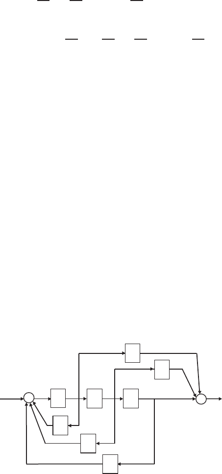
116 CHAPTER 3 State Variable Models

Then we write the system in state variable form as







0100

−k1

M1−b1

M10b1

0 0 0 1

0b1

M2−k2

M2−b1



















y=h1 0 0 0 iz.

P3.37 From the block diagram in Figure P3.37, we obtain

˙x1=x2

˙x2=x3

˙x3=−10x1−4x2−3x3+u

y=x1+ 12x2+ 5x3

x=





0 1 0

0 0 1

−10 −4−3







x+











y= [1 12 5] x.

The third-order diﬀerential equation model is

...

y+3¨y+ 4 ˙y+ 10y= 5¨u+ 12 ˙u+u .

∫∫ ∫

U(s)Y(s)

x3x2x1

FIGURE P3.37

Block diagram with states labeled.

from the publisher prior to any prohibited reproduction, storage in a retrieval system, or transmission in any form or by any means, electronic, mechanical, photocopying,

recording, or likewise. For information regarding permission(s), write to: Rights and Permissions Department, Pearson Education, Inc., Upper Saddle River, NJ 07458.

Advanced Problems 117

Advanced Problems

AP3.1 With the state variables are deﬁned as

z=





˙x







the nonlinear equations of motion are







˙z1

˙z2

˙z3







=





g−K

(Io+z3)2

(Xo+z1)2

L(v−Rz3)







where the control is the voltage v. We assume that z1=xis measurable.

The linearized equations of motion are

z=Az +Bv

y=Cz

where

A=





0 1 0

o0−2K

0 0 −R







,B=











,and C=h1 0 0 i.

The transfer function is

G(s) = C(sI−A)−1B.

With the constants

R= 23.2

L= 0.508

m= 1.75

K= 2.9×10−4

Io= 1.06

Xo= 4.36 ×10−3

from the publisher prior to any prohibited reproduction, storage in a retrieval system, or transmission in any form or by any means, electronic, mechanical, photocopying,

recording, or likewise. For information regarding permission(s), write to: Rights and Permissions Department, Pearson Education, Inc., Upper Saddle River, NJ 07458.

118 CHAPTER 3 State Variable Models

the transfer function is

G(s) = −36.38

s3+ 45.67s2+ 4493s+ 205195 .

AP3.2 The diﬀerential equation describing the motion of yis

m¨y+b˙y+ky =b˙u+ku .

Taking Laplace tranforms (with zero initial conditions) yields the transfer

function

Y(s)

U(s)=(b/m)s+ (k/m)

s2+ (b/m)s+ (k/m).

In state space form, we have

x=



0 1

−k/m −b/m 

x+



1

u

y=hk/m b/m ix.

AP3.3 The transfer function is

Y(s)

R(s)=2s2+ 6s+ 5

s3+ 4s2+ 5s+ 2 .

In (nearly) diagonal form, we have

A=





−110

0−1 0

0 0 −2







,B=











,and C=h1 1 1 i.

The matrix Ais not exactly diagonal due to the repeated roots in the

denominator of the transfer function.

AP3.4 The diﬀerential equations describing the motion of yand qare

m¨y+k2˙y+k1(y−q) = f

−b˙q+k1(y−q) = f

where k1= 2 and k2= 1. Assume the mass m= 1. Then with the state

from the publisher prior to any prohibited reproduction, storage in a retrieval system, or transmission in any form or by any means, electronic, mechanical, photocopying,

recording, or likewise. For information regarding permission(s), write to: Rights and Permissions Department, Pearson Education, Inc., Upper Saddle River, NJ 07458.

Advanced Problems 119

variables deﬁned as z=hy˙y q iT, we have the state variable model

z=





0 1 0

−3 0 2

2/b 0−2/b







z+





−1/b







y=h1 0 0 iz

If we model a large bump at high speeds as an impulse and a small bump

at low speeds as a step, then b= 0.8 provides good performance. In both

cases, the ride settles out completely in about 10 seconds.

AP3.5 The diﬀerential equations describing the motion of xand θare

(M+m)¨x+ML cos θ¨

θ−ML sin θ˙

θ2=−kx

gsin θ+ cos θ¨x+L¨

θ= 0

Assuming θand ˙

θare small, it follows that

(M+m)¨x+ML¨

θ=−kx

¨x+L¨

θ=−gθ

Deﬁne the state variables as z=hx˙x θ ˙

θiT. Then, the state vari-

able model is







0 1 0 0

−k/m 0gM/m 0

0 0 0 1

k/(Lm) 0 −g(M+m)/(Lm) 0







AP3.6

AP3.7 Computing the closed-loop system yields

A−BK =

−1 1

−K1−K2

,B=



1

,and C=h2 1 i.

The characteristic polynomial is

|sI−(A−BK)|=s2+ (K2+ 1)s+K1+K2= 0.

The roots are in the left-half plane whenever K2+1 >0 and K1+K2>0.

from the publisher prior to any prohibited reproduction, storage in a retrieval system, or transmission in any form or by any means, electronic, mechanical, photocopying,

recording, or likewise. For information regarding permission(s), write to: Rights and Permissions Department, Pearson Education, Inc., Upper Saddle River, NJ 07458.

120 CHAPTER 3 State Variable Models

AP3.8 (a) A state variable representation is given by

˙x1=x2

˙x2=x3

˙x3=−Kx1−12x2−6x3+Kr

y=x1

or, in matrix form

x=





0 1 0

0 0 1

−K−12 −6







x+











y=h1 0 0 ix

(b) The characteristic roots are found by solving

det [λI−A] = 0

λ3+ 6λ2+ 12λ+K= 0

When K= 8, we have characteristic roots at λ1=−2, λ2=−2, and

λ3=−2, as desired.

y(t) = 1 −e−2t−2te−2t−2t2e−2t.

from the publisher prior to any prohibited reproduction, storage in a retrieval system, or transmission in any form or by any means, electronic, mechanical, photocopying,

recording, or likewise. For information regarding permission(s), write to: Rights and Permissions Department, Pearson Education, Inc., Upper Saddle River, NJ 07458.

Design Problems 121

Design Problems

The transfer model of the traction drive, capstan roller, and linear slideCDP3.1

was given in CDP2.1 as

X(s)

Va(s)=rKm

s[(Lms+Rm)(JTs+bm) + KbKm],

where

JT=Jm+r2(Ms+Mb).

Deﬁne x1=x,x2= ˙x, and x3= ¨x. Then, a state variable representation

x=Ax +Bva

y=Cx

where

A=





0 1 0

0 0 1

0−Rmbm+KbKm

LmJT−Lmbm+RmJT

LmJT







,B=





rKm

LmJT







C=h1 0 0 i.

DP3.1 (a) The equation of motion of the spring-mass-damper is

m¨y+b˙y+ky =u

¨y=−b

m˙y−k

my+1

mu .

Select the state variables

x1=yand x2= ˙y .

Then, we have

x=Ax +Bu

y=Cx

from the publisher prior to any prohibited reproduction, storage in a retrieval system, or transmission in any form or by any means, electronic, mechanical, photocopying,

recording, or likewise. For information regarding permission(s), write to: Rights and Permissions Department, Pearson Education, Inc., Upper Saddle River, NJ 07458.

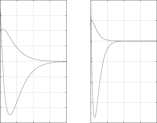
122 CHAPTER 3 State Variable Models

where

A=



0 1

−20 −9

,B=



1

,C=h1 0 i.

Ais the system matrix. The characteristic equation is

det[λI−A] = det 



s−1

20 s+ 9 

=s2+ 9s+ 20 = 0 .

The roots of the characteristic equation are s1=−4 and s2=−5,

and the transistion matrix is

Φ(t) = 



5e−4t−4e−5te−4t−e−5t

−20e−4t+ 20e−5t−4e−4t+ 5e−5t

.

(b) Assume the initial conditions are x1(0) = 1 and x2(0) = 2. The zero-

input response is shown in Figure DP3.1.

out x2and x1. We can select band kto achieve critical damping.

0 0.5 1 1.5 2

-2

-1.5

-1

-0.5

0.5

1.5

Time(sec)

State response, x

b/m=9, k/m=20

0 0.5 1 1.5 2

-4

-3

-2

-1

Time(sec)

State response, x

Critical damping: b/m=20, k/m=100

FIGURE DP3.1

Zero input state response.

from the publisher prior to any prohibited reproduction, storage in a retrieval system, or transmission in any form or by any means, electronic, mechanical, photocopying,

recording, or likewise. For information regarding permission(s), write to: Rights and Permissions Department, Pearson Education, Inc., Upper Saddle River, NJ 07458.

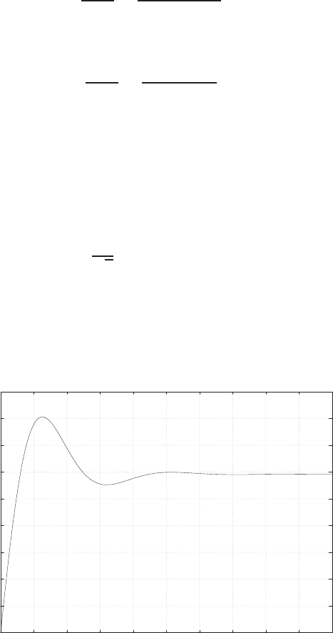
Design Problems 123

If we desire the characteristic polynomial to be pd(s) = (s+ 10)2=

s2+ 20s+ 100, then we need b= 20 and k= 100.

DP3.2 The desired transfer function is

Y(s)

U(s)=6

s2+ 7s+ 10 .

The transfer function derived from the phase variable representation is

Y(s)

U(s)=d

s2+bs +a.

Therefore, we select d= 6, a= 10 and b= 7.

DP3.3 Assume the aircraft lands precisely on the centerline. The linearized equa-

tions of motion are

m3¨x3+KD˙x3+K2(x3−x2) = 0

m2¨x2+K2(x2−x3) + K1(x2−x1) = 0

m1¨x1=−2

√2K2(x1−x2)

where x1(0) = x2(0) = ˙x2(0) = ˙x3= 0 and ˙x1(0) = 60. The system

response is shown in Figure DP3.3 where KD= 215. The aircraft settles

out at 30 m, although initially it overshoots by about 10 m at 1 second.

0 1 2 3 4 5 6 7 8 9 10

Time (secs)

Amplitude

FIGURE DP3.3

Aircraft arresting gear response.

from the publisher prior to any prohibited reproduction, storage in a retrieval system, or transmission in any form or by any means, electronic, mechanical, photocopying,

recording, or likewise. For information regarding permission(s), write to: Rights and Permissions Department, Pearson Education, Inc., Upper Saddle River, NJ 07458.

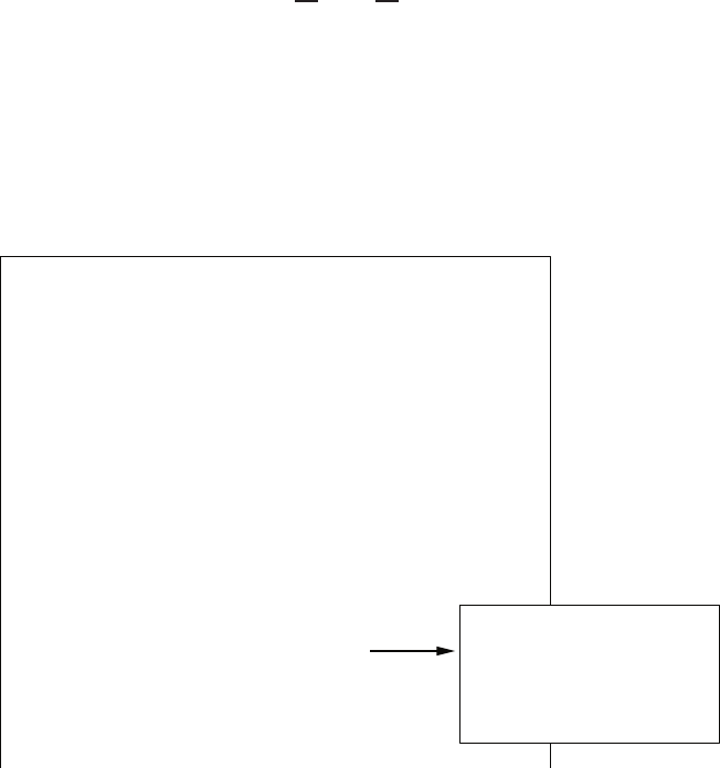
124 CHAPTER 3 State Variable Models

DP3.4 We can model the bungi cord system as a mass-spring-damper. This is

actually an over-simpliﬁcation because the bungi cord cannot “push” the

jumper down as a spring would—it can only exert a restoring force when

the cord is stretched (that is, when the jumper exceeds the length, L, of

the cord). The problem is nonlinear! When the distance of the jumper

from the platform is less than Lwe should model the cord spring constant

and damping as K= 0 and b= 0, respectively. Only gravity acts on the

jumper. Also, when ˙x(the jumper velocity) is negative (where we deﬁne

positive towards the ground), then we should model b= 0. A reasonable

set of equations of motion are

˙x1=x2

˙x2=−K

mx1−b

mx2+g

where x1is the distance measured from the top of the platform and x2

is the jumper velocity. For the initial conditions we have x1(0) = 10

and x2(0) = 0. A reasonable set of parameters for the bungi cord are

L= 40 m, K= 40 N/m and b= 20 kg/m. The system response is

shown in Figure DP3.4 for a person with m= 100 kg. The accelerations

experienced by the jumper never exceed 1.5 g.

global MASS GRAVITY LENGTH K b

MASS=100; HEIGHT=100; GRAVITY=9.806;

LENGTH=40; SPRINGCONSTANT=40; SPRINGDAMPING=20;

x0=[10;0];

t=0; dt=0.1;

n=round(120/dt);

for i=1:n;

if x0(1)<LENGTH

K=0; b=0;

elseif x0(2)<0

b=0;

else

K=SPRINGCONSTANT; b=SPRINGDAMPING;

end

tf=t+dt;

[T,x] = ode45('bungi',[t tf],x0);

xs(i,:)=x(length(x),:); t=tf;

x0=x(length(x),:); ts(i)=tf;

end

plot(ts,HEIGHT-xs(:,1)), grid

function [xdot] = bungi(t,x)

global MASS GRAVITY LENGTH K b

xdot(1)=x(2);

xdot(2)=-(K/MASS)*(x(1)-

LENGTH)-(b/MASS)*x(2)+GRAVITY;

xdot=xdot';

FIGURE DP3.4

(a) Bungi cord system response m-ﬁle script.

from the publisher prior to any prohibited reproduction, storage in a retrieval system, or transmission in any form or by any means, electronic, mechanical, photocopying,

recording, or likewise. For information regarding permission(s), write to: Rights and Permissions Department, Pearson Education, Inc., Upper Saddle River, NJ 07458.

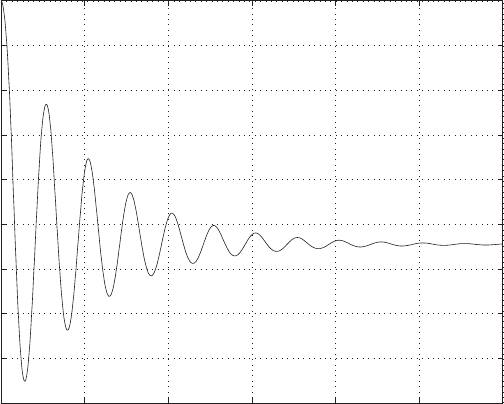
Design Problems 125

0 20 40 60 80 100 120

Time (sec)

Distance (m)

FIGURE DP3.4

CONTINUED: Bungi cord system time history response.

DP3.5 Computing the closed-loop system yields

A−BK =



0 1

−2−K13−K2

,B=



1

,and C=h1 0 i.

The characteristic polynomial is

|sI−(A−BK)|=s2+ (K2−3)s+K1+ 2 = 0.

Suppose that the desired poles are in the left-half plane and are denoted

by −p1and −p2. Then the desired characteristic polynomial is

(s+p1)(s+p2) = s2+ (p1+p2)s+p1p2= 0.

Equating coeﬃcients and solving for K= [K1K2] yields

K1=p1p2−2

K2=p1+p2+ 3.

from the publisher prior to any prohibited reproduction, storage in a retrieval system, or transmission in any form or by any means, electronic, mechanical, photocopying,

recording, or likewise. For information regarding permission(s), write to: Rights and Permissions Department, Pearson Education, Inc., Upper Saddle River, NJ 07458.

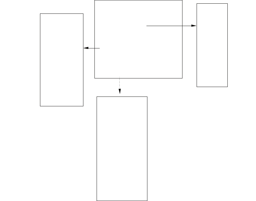
126 CHAPTER 3 State Variable Models

Computer Problems

CP3.1 The m-ﬁle script to compute the state-space models using the ss function

is shown in Figure CP3.1.

% Part(a)

num = [1]; den = [1 25];

sys = tf(num,den);

sys_ss = ss(sys)

% Part(b)

num = [3 10 3]; den = [1 8 5];

sys = tf(num,den);

sys_ss = ss(sys)

% Part(c)

num = [1 10]; den = [1 3 3 1];

sys = tf(num,den);

sys_ss = ss(sys)

a =

x1 -25

b =

x1 1

c =

y1 1

d =

y1 0

a =

x1 x2

x1 -8 -2.5

x2 2 0

b =

x1 4

x2 0

c =

x1 x2

y1 -3.5 -1.5

d =

y1 3 a =

x1 x2 x3

x1 -3 -1.5 -0.25

x2 2 0 0

x3 0 2 0

b =

x1 2

x2 0

x3 0

c =

x1 x2 x3

y1 0 0.25 1.25

d =

y1 0

FIGURE CP3.1

Script to compute state-space models from transfer functions.

For example, in part (c) the state-space model is

x=Ax +Bu

y=Cx +Du ,

from the publisher prior to any prohibited reproduction, storage in a retrieval system, or transmission in any form or by any means, electronic, mechanical, photocopying,

recording, or likewise. For information regarding permission(s), write to: Rights and Permissions Department, Pearson Education, Inc., Upper Saddle River, NJ 07458.

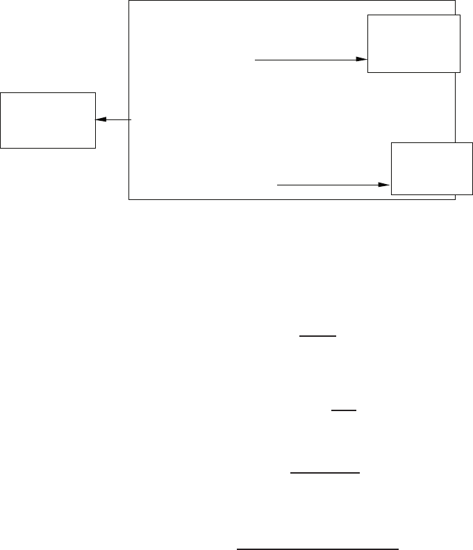
Computer Problems 127

where D= [0] and

A=





−3−1.5−0.25

2 0 0

0 2 0







,B=











,C=h0 0.25 1.25 i.

CP3.2 The m-ﬁle script to compute the transfer function models using the tf

function is shown in Figure CP3.2.

Transfer function:

-------------

s^2 - 4 s - 2

Transfer function:

6s - 48

-----------------------

s^3 - 11 s^2 + 4 s - 36

Transfer function:

s - 2

-------------

s^2 + 2 s + 1

% Part (a)

A=[0 1;2 4]; B=[0;1]; C=[1 0]; D=[0];

sys_ss=ss(A,B,C,D);

sys_tf = tf(sys_ss)

% Part (b)

A=[1 1 0;-2 0 4; 6 2 10]; B=[-1;0;1]; C=[0 1 0]; D=[0];

sys_ss=ss(A,B,C,D);

sys_tf = tf(sys_ss)

% Part (c)

A=[0 1;-1 -2]; B=[0;1]; C=[-2 1]; D=[0];

sys_ss=ss(A,B,C,D);

sys_tf = tf(sys_ss)

FIGURE CP3.2

Script to compute transfer function models from the state-space models.

CP3.3 For an ideal op-amp, the voltage gain (as a function of frequency) is

Vo(s) = −Z2(s)

Z1(s)Vin(s),

where

Z1=R1+1

C1s

Z2=R2

1 + R2C2s

are the respective circuit impedances. Therefore, we obtain

Vo(s) = −R2C1s

(1 + R1C1s)(1 + R2C2s)Vin(s).

The m-ﬁle script and step response is shown in Figure CP3.3.

from the publisher prior to any prohibited reproduction, storage in a retrieval system, or transmission in any form or by any means, electronic, mechanical, photocopying,

recording, or likewise. For information regarding permission(s), write to: Rights and Permissions Department, Pearson Education, Inc., Upper Saddle River, NJ 07458.

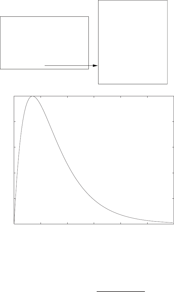
128 CHAPTER 3 State Variable Models

R1=1000; R2=10000; C1=0.0005; C2=0.0001;

numg=[R2*C1 0];

deng=conv([R1*C1 1],[R2*C2 1]);

sys_tf=tf(numg,deng)

% Part (a)

sys_ss=ss(sys_tf)

% Part (b)

step(sys_ss)

a =

x1 x2

x1 -3.00000 -1.00000

x2 2.00000 0

b =

x1 4.00000

x2 0

c =

x1 x2

y1 2.50000 0

d =

y1 0

Continuous-time system.

Time (sec.)

Amplitude

Step Response

0 1 2 3 4 5 6

0.5

1.5

2.5

FIGURE CP3.3

The m-ﬁle script using the step function to determine the step response.

CP3.4 The m-ﬁle script and state history is shown in Figure CP3.4. The transfer

function equivalent is

G(s) = 1

s3+ 5s2+ 2s+ 3 .

The computed state vector at t= 10 is the same using the simulation and

the state transition matrix.

from the publisher prior to any prohibited reproduction, storage in a retrieval system, or transmission in any form or by any means, electronic, mechanical, photocopying,

recording, or likewise. For information regarding permission(s), write to: Rights and Permissions Department, Pearson Education, Inc., Upper Saddle River, NJ 07458.

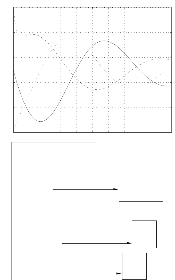
Computer Problems 129

0 1 2 3 4 5 6 7 8 9 10

- 1

- 0.8

- 0.6

- 0.4

- 0.2

0.2

0.4

0.6

0.8

time (sec)

x(t)

x1 solid; x2 dotted; x3 dashed

a=[0 1 0; 0 0 1; -3 -2 -5];

b=[0;0;1];

c=[1 0 0];

d=[0];

% Part (a)

sys_ss = ss(a,b,c,d)

sys_tf = tf(sys_ss)

% Part (b)

x0 = [0 -1 1];

t = [0:0.1:10];

u = 0*t;

[y,t,x] = lsim(sys_ss,u,t,x0);

plot(t,x(:,1),t,x(:,2),':',t,x(:,3),'--');

xlabel('time (sec)'), ylabel('x(t)'), grid

title('x1 - solid; x2 - dotted; x3 - dashed')

xf_sim = x(length(t),:)'

% Part (c)

dt = 10;

Phi = expm(a*dt);

xf_phi = Phi*x0'

Transfer function:

---------------------

s^3 + 5 s^2 + 2 s + 3

xf_sim =

-0.2545

0.0418

0.1500

xf_phi =

-0.2545

0.0418

0.1500

FIGURE CP3.4

The m-ﬁle script using the lsim function to determine the step response.

from the publisher prior to any prohibited reproduction, storage in a retrieval system, or transmission in any form or by any means, electronic, mechanical, photocopying,

recording, or likewise. For information regarding permission(s), write to: Rights and Permissions Department, Pearson Education, Inc., Upper Saddle River, NJ 07458.

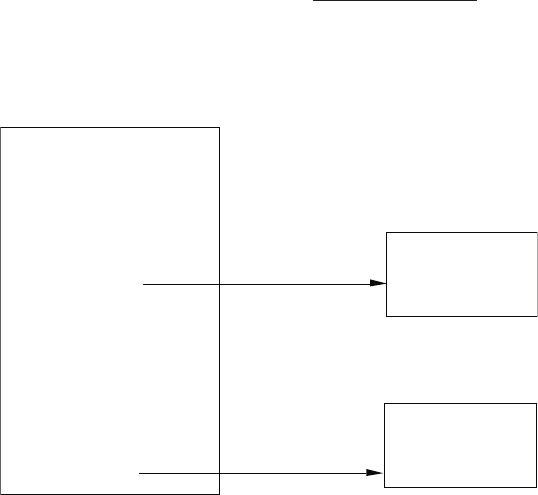
130 CHAPTER 3 State Variable Models

CP3.5 The two state-space models represent the same transfer function, as shown

in Figure CP3.5. The transfer function in both cases is

G(s) = 4

s3+ 8s2+ 5s+ 4 .

We see that a state-space representation of a transfer function is not

unique.

a1=[0 1 0; 0 0 1; -4 -5 -8];

b1=[0;0;4];

c1=[1 0 0];

d1=[0];

% Part (a)

sys_ss = ss(a1,b1,c1,d1);

sys_tf = tf(sys_ss)

% Part (b)

a2=[ 0.5000 0.5000 0.7071;

-0.5000 -0.5000 0.7071;

-6.3640 -0.7071 -8.0000];

b2=[0;0;4];

c2=[0.7071 -0.7071 0];

d2=[0];

sys_ss = ss(a2,b2,c2,d2);

sys_tf = tf(sys_ss)

Transfer function:

---------------------

s^3 + 8 s^2 + 5 s + 4

Transfer function:

---------------------

s^3 + 8 s^2 + 5 s + 4

FIGURE CP3.5

Comparison of the transfer functions of two state-space models.

CP3.6 The m-ﬁle script and impulse response are shown in Figure CP3.6. The

controller state-space representation is

˙x=−2x+u

y=x

and the plant state-space representation is

x=

−2−2

2 0 

x+



0.5

0

u

y=h0 1 ix

The closed-loop system state variable representation is

x=Ax +Bu

y=Cx +Du ,

from the publisher prior to any prohibited reproduction, storage in a retrieval system, or transmission in any form or by any means, electronic, mechanical, photocopying,

recording, or likewise. For information regarding permission(s), write to: Rights and Permissions Department, Pearson Education, Inc., Upper Saddle River, NJ 07458.

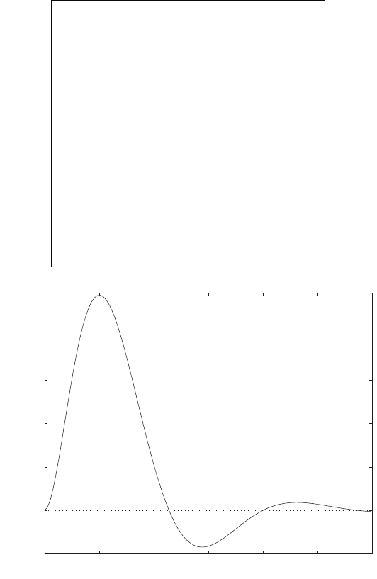
Computer Problems 131

where D= [0] and

A=





−2−2 0.5

200

0−1−2







,B=











,C=h0 1 0 i.

numc=[1]; denc=[1 2]; sys_tfc = tf(numc,denc)

numg=[1]; deng=[1 2 4]; sys_tfg = tf(numg,deng)

% Part (a)

sys_ssc = ss(sys_tfc)

% Part (b)

sys_ssg = ss(sys_tfg)

% Part (c)

sys_s = series(sys_ssc,sys_ssg);

sys_cl = feedback(sys_s,[1]);

impulse(sys_cl)

Time (sec.)

Amplitude

Impulse Response

0123456

-0.02

0.02

0.04

0.06

0.08

0.1

From: U(1)

To: Y(1)

FIGURE CP3.6

Computing the state-space representations and the impulse response.

from the publisher prior to any prohibited reproduction, storage in a retrieval system, or transmission in any form or by any means, electronic, mechanical, photocopying,

recording, or likewise. For information regarding permission(s), write to: Rights and Permissions Department, Pearson Education, Inc., Upper Saddle River, NJ 07458.

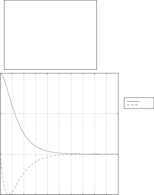
132 CHAPTER 3 State Variable Models

CP3.7 The m-ﬁle script and system response is shown in Figure CP3.7.

a=[0 1;-2 -3]; b=[0;1]; c=[1 0]; d=[0];

sys = ss(a,b,c,d);

x0=[1;0];

t=[0:0.1:10]; u=0*t;

[y,t,x]=lsim(sys,u,t,x0);

plot(t,x(:,1),t,x(:,2),'--')

xlabel('Time (sec)')

ylabel('State Response')

legend('x1','x2',-1)

grid

0 1 2 3 4 5 6 7 8 9 10

-0.5

0.5

Time (sec)

State Response

FIGURE CP3.7

Using the lsim function to compute the zero input response.

from the publisher prior to any prohibited reproduction, storage in a retrieval system, or transmission in any form or by any means, electronic, mechanical, photocopying,

recording, or likewise. For information regarding permission(s), write to: Rights and Permissions Department, Pearson Education, Inc., Upper Saddle River, NJ 07458.

C H A P T E R 4

Feedback Control System

Characteristics

Exercises

E4.1 (a) The system sensitivity to τis given by

τ=ST

GSG

τ.

In this case, we have

G=1

1 + GH(s)=1

1 + 100

3s+1

=3s+ 1

3s+ 101

and

τ=−τs

τs + 1 =−3s

3s+ 1 ,

where τ= 3. Therefore,

τ=−3s

3s+ 101 .

(b) The closed-loop transfer function is

T(s) = G(s)

1 + GH(s)=100

3s+ 101 =100/101

101 s+ 1 =0.99

τcs+ 1 ,

where the time-constant τc= 3/101 = 0.0297 second.

E4.2 (a) The system sensitivity to K2is

K2=∂T

∂K2

T=1

1 + K1K2

133

from the publisher prior to any prohibited reproduction, storage in a retrieval system, or transmission in any form or by any means, electronic, mechanical, photocopying,

recording, or likewise. For information regarding permission(s), write to: Rights and Permissions Department, Pearson Education, Inc., Upper Saddle River, NJ 07458.

134 CHAPTER 4 Feedback Control System Characteristics

(b) The transfer function from Td(s) to Vo(s) is

Vo(s) = K2

1 + K1K2

Td(s).

Vo(s) is small.

E4.3 (a) The tracking error, E(s) = R(s)−Y(s), is given by

E(s) = R(s)

1 + G(s)=A/s

1 + K/(s+ 5)2.

The steady-state error (computed using the ﬁnal value theorem) is

ess = lim

s→0sE(s) = lim

s→0



1 + K

(s+5)2

=A

1 + K/25 .

(b) A disturbance would be the wind shaking the robot arm.

E4.4 (a) The tracking error, E(s) = R(s)−Y(s), is given by

E(s) = R(s)

1 + KG(s).

The steady-state position error is computed (using the ﬁnal value

theorem) to be

ess = lim

s→0sA/s

1 + KG(s)= lim

s→0



1 + 10K

s(τs+1) 

= 0 .

(b) The ramp input of 0.1 m/sec is given by

R(s) = 0.1

s2.

Then, using the ﬁnal value theorem, we have

ess = lim

s→0s



0.1/s2

1 + 10K

s(τs+1) 

= lim

s→0"0.1

s+10K

τs+1 #,

ess =0.1

10K=0.01

from the publisher prior to any prohibited reproduction, storage in a retrieval system, or transmission in any form or by any means, electronic, mechanical, photocopying,

recording, or likewise. For information regarding permission(s), write to: Rights and Permissions Department, Pearson Education, Inc., Upper Saddle River, NJ 07458.

Exercises 135

We desire ess ≤0.0001 m, so

K≥0.01

0.0001 = 100 .

E4.5 (a) The sensitivity is

p=∂T

∂p

T=p"−s4−15s2+ 3s+ 10

(s2+ps + 10)2#T(s).

(b) The tracking error is

E(s) = [1 −T(s)] R(s) = s3+ (2p−1)s2+ (4 −p)s−7−p

s3+ 2ps2+ 4s+ 3 −pR(s)

Using the ﬁnal value theorem with R(s) = 1/s we obtain the steady-

state tracking error as

ess = lim

s→0sE(s) = −7−p

3−p.

E4.6 The closed-loop transfer function is

T(s) = 10K

s2+bs + 10K.

The tracking error is

E(s) = [1 −T(s)] R(s) = s(s+b)

s2+bs + 10K

s2,

where we let R(s) = 1/s2. Using the ﬁnal value theorem we obtain the

steady-state tracking error as

ess = lim

s→0sE(s) = b

10K.

If we require that b < K then the steady-state error is less than 0.1 to

the ramp input.

E4.7 The light bounces oﬀ the surface of the slide and into a detector. If the

light fails to hit the detector dead center, the unbalanced electric signal

causes the motor to adjust the position of the light source, and simulta-

neously the lens.

E4.8 The closed-loop transfer function is

T(s) = 5(s+ 3)

s2+ 20s+ 15 .

The step response is shown in Figure E4.8.

from the publisher prior to any prohibited reproduction, storage in a retrieval system, or transmission in any form or by any means, electronic, mechanical, photocopying,

recording, or likewise. For information regarding permission(s), write to: Rights and Permissions Department, Pearson Education, Inc., Upper Saddle River, NJ 07458.

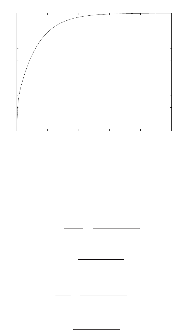
136 CHAPTER 4 Feedback Control System Characteristics

0 1 2 3 4 5 6 7 8 9 10

0.1

0.2

0.3

0.4

0.5

0.6

0.7

0.8

0.9

Step Response

Time (sec)

y(t)/A

FIGURE E4.8

Step response.

E4.9 (a) The closed-loop transfer function is

T(s) = KK1

s+K1(K+K2).

(b) The sensitivities are

K=∂T /T

∂K/K =s+K1K2

s+K1(K+K2)

and

K1=s

s+K1(K+K2).

Y(s)

Td(s)=−1

s+K1(K2+K).

Therefore, since E(s) = −KY (s) (when R(s) = 0), we have

E(s) = K

s+K1(K2+K)Td(s)

from the publisher prior to any prohibited reproduction, storage in a retrieval system, or transmission in any form or by any means, electronic, mechanical, photocopying,

recording, or likewise. For information regarding permission(s), write to: Rights and Permissions Department, Pearson Education, Inc., Upper Saddle River, NJ 07458.

Exercises 137

and

ess = lim

s→0sE(s) = K

K1(K+K2).

(d) With K=K2= 1, we have

T(s) = K1

s+ 2K1

Then,

Y(s) = K1

s+ 2K1

and

y(t) = 1

2h1−e−2K1tiu(t),

where u(t) is the unit step function. Therefore, select K1= 10 for the

fastest response.

E4.10 The closed-loop transfer function is

T(s) = 46.24K(s+ 50)(s+ 425)

(s+ 200)(s+ 425)(s2+ 16.7s+ 72.9) + 19652K(s+ 50) .

The steady-state error is determined to be

ess = lim

s→0sE(s) = lim

s→0s(1 −T(s))1

= 1 −lim

s→0T(s) = 1 −T(0)

=6.3

6.3 + K.

The plots of the steady-state error versus Kand the percent overshoot

P.O. versus Kare shown in Figure E4.10 for

40 ≤K≤400.

from the publisher prior to any prohibited reproduction, storage in a retrieval system, or transmission in any form or by any means, electronic, mechanical, photocopying,

recording, or likewise. For information regarding permission(s), write to: Rights and Permissions Department, Pearson Education, Inc., Upper Saddle River, NJ 07458.

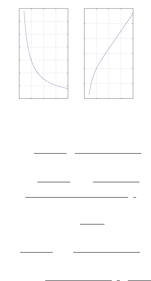
138 CHAPTER 4 Feedback Control System Characteristics

0 100 200 300 400

0.02

0.04

0.06

0.08

0.1

0.12

0.14

steady-state error

0 100 200 300 400

percent overshoot (%)

FIGURE E4.10

(a) Steady-state error. (b) Percent overshoot.

E4.11 (a) The closed-loop transfer function is

T(s) = G(s)

1 + G(s)H(s)=K(s2+ 5s+ 6)

s3+ 15s2+ 56s+ 60 + 14K

(b) With E(s) = R(s)−Y(s) we obtain

E(s) = 1−G(s)

1 + G(s)H(s)R(s) = 1−G(s)(1 −H(s))

1 + G(s)H(s)R(s)

=s3+ (15 −K)s2+ (56 −5K)s+ (60 + 8K)

s3+ 15s2+ 56s+ 60 + 14K·1

Then, using the ﬁnal value theorem we ﬁnd

lim

s→0sE(s) = (60 + 8K)

60 + 14K.

Y(s) = 1

1 + G(s)H(s)Td(s) = s3+ 15s2+ 56s+ 60

s3+ 15s2+ 56s+ 60 + 14KTd(s).

The steady-state error to a unit step disturbance is

lim

s→0sY (s) = lim

s→0ss3+ 15s2+ 56s+ 60

s3+ 15s2+ 56s+ 60 + 14K·1

s=60

60 + 14K.

from the publisher prior to any prohibited reproduction, storage in a retrieval system, or transmission in any form or by any means, electronic, mechanical, photocopying,

recording, or likewise. For information regarding permission(s), write to: Rights and Permissions Department, Pearson Education, Inc., Upper Saddle River, NJ 07458.

Exercises 139

(d) The sensitivity is

K=∂T

∂K

T=∂T

∂G

∂K

(1 + G(s)H(s))2K

s+ 101 + G(s)H(s)

G(s)=1

1 + G(s)H(s).

E4.12 (a) The closed-loop transfer function is

T(s) = Gc(s)G(s)

1 + Gc(s)G(s)H(s)=100K1(s+ 5)

s2+ 105s+ (500 + 100K1K2).

The steady-state tracking error is

E(s) = R(s)−Y(s) = 1−Gc(s)G(s)(1 −H(s))

1 + Gc(s)G(s)H(s)R(s)

=s2+ (105 −100K1)s+ 500 −100K1(5 −K2)

s2+ 105s+ 500 + 100K1K2·1

and

lim

s→0sE(s) = 5−K1(5 −K2)

5 + K1K2

(b) The transfer function from the noise disturbance N(s) to the output

Y(s) is

Y(s) = −Gc(s)G(s)H(s)

1 + Gc(s)G(s)H(s)N(s) = −100K1K2

s2+ 105s+ (500 + 100K1K2)N(s).

The steady-state error to a unit step N(s) = 1/s is

lim

s→0sY (s) = lim

s→0s−100K1K2

s2+ 105s+ (500 + 100K1K2)·1

s=−K1K2

5 + K1K2

to improve tracking performance while keeping K1K2as small as

possible to reject the noise.

E4.13 The closed-loop transfer function is

T(s) = K

s2+ 20s+K.

The sensitivity is

K=∂T /T

∂K/K =s2+ 20s

s2+ 20s+K.

from the publisher prior to any prohibited reproduction, storage in a retrieval system, or transmission in any form or by any means, electronic, mechanical, photocopying,

recording, or likewise. For information regarding permission(s), write to: Rights and Permissions Department, Pearson Education, Inc., Upper Saddle River, NJ 07458.

140 CHAPTER 4 Feedback Control System Characteristics

E4.14 (a) The closed-loop transfer function is

T(s) = Gc(s)G(s)

1 + Gc(s)G(s)H(s)=K

s2+K1s+K.

The sensitivity is

K1=∂T /T

∂K1/K1

=−sK1

s2+K1s+K.

(b) You would make Kas large as possible to reduce the sensitivity to

changes in K1. But the design trade-oﬀ would be to keep Kas small

as possible to reject measurement noise.

E4.15 (a) The closed-loop transfer function is

T(s) = Gc(s)G(s)

1 + Gc(s)G(s)H(s)=120

s2+ 10s+ 120 .

The steady-state tracking error is

E(s) = R(s)−Y(s) = 1

1 + Gc(s)G(s)R(s)

=s2+ 10s

s2+ 10s+ 120 ·1

and

lim

s→0sE(s) = 0 .

(b) The transfer function from the disturbance Td(s) to the output Y(s)

Y(s) = 1

s2+ 10s+ 120Td(s).

The steady-state error to a unit step Td(s) = 1/s is

lim

s→0sY (s) = lim

s→0s1

s2+ 10s+ 120·1

s=1

120 .

from the publisher prior to any prohibited reproduction, storage in a retrieval system, or transmission in any form or by any means, electronic, mechanical, photocopying,

recording, or likewise. For information regarding permission(s), write to: Rights and Permissions Department, Pearson Education, Inc., Upper Saddle River, NJ 07458.

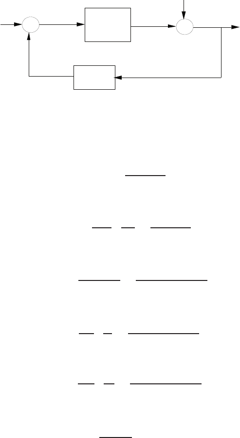
Problems 141

Problems

P4.1 The tank level control block diagram is shown in Figure P4.1.

+G1(s)

DQ1

FIGURE P4.1

Tank level control block diagram.

(a) For the open-loop system the transfer function is

G1(s) = R

RCs + 1 .

Thus,

SG1

R=∂G1

∂R ·R

RCs + 1 .

For the closed-loop system, the transfer function is

T(s) = G1

1 + KG1

RCs + 1 + KR .

Thus,

R=∂T

∂R ·R

T=1

RCs + 1 + KR ,

and

K=∂T

∂K ·K

T=−KR

RCs + 1 + KR .

(b) For the open-loop system

∆H(s)

δH(s)= 1 .

All disturbances show up directly in the output, thus the open-loop

system has no capability to reject disturbances. On the other hand,

from the publisher prior to any prohibited reproduction, storage in a retrieval system, or transmission in any form or by any means, electronic, mechanical, photocopying,

recording, or likewise. For information regarding permission(s), write to: Rights and Permissions Department, Pearson Education, Inc., Upper Saddle River, NJ 07458.

142 CHAPTER 4 Feedback Control System Characteristics

for the closed-loop system we have

∆H(s)

δH(s)=1

1 + KG1(s)=RCs + 1

RCs + 1 + KR .

By selecting Klarge, we reduce the eﬀects of any disturbances. For

example, consider a step disturbance. The steady-state error due to

the disturbance is

ess = lim

s→0s−(RCs + 1)

RCs + 1 + KR A

s=−A

1 + KR .

As Kgets larger, the steady-state error magnitude gets smaller, as

desired.

∆Q1(s) = A

Then, for the open-loop system we have

ess = lim

s→0s(1 −G1)A

s= (1 −R)A .

The steady-state error is zero when R= 1, but is sensitive to changes

in R. For the closed-loop system we have

ess = lim

s→0s1

1 + KG1A

s=A

1 + KR .

By selecting Klarge, the eﬀect of the disturbance is reduced and is

relatively insensitive to changes in R.

P4.2 (a) The open-loop transfer function is

T(s) = KaG(s).

Therefore, ST

K1is undeﬁned and

Ka= 1 .

The closed-loop transfer function is

T(s) = KaG(s)

1 + KaK1G(s).

Therefore,

K1=∂T

∂K1·K1

T=−KaK1G(s)

1 + KaK1G(s)

from the publisher prior to any prohibited reproduction, storage in a retrieval system, or transmission in any form or by any means, electronic, mechanical, photocopying,

recording, or likewise. For information regarding permission(s), write to: Rights and Permissions Department, Pearson Education, Inc., Upper Saddle River, NJ 07458.

Problems 143

and

Ka=1

1 + K1KaG(s).

(b) The tracking error, E(s) = θd(s)−θ(s) = −θ(s), since θd(s) = 0. The

transfer function from the wave disturbance to the output θ(s) is

θ(s) = G(s)

1 + K1KaG(s)Td(s).

Consider a step disturbance input for the open- and closed-loop sys-

tems. For the open-loop system, we have

ess =−lim

s→0sG(s)A

s=−A .

Thus, we see that the open-loop system does not have the capability

to reduce the eﬀect of disturbances. For the closed-loop system, we

have

ess = lim

s→0s−G(s)

1 + K1KaG(s)A

s=−Aω2

1 + K1Kaω2

We see that the larger we make K1Ka, that smaller the eﬀect of the

wave disturbance on the output in steady-state.

P4.3 (a) The open-loop transfer function is

G(s) = K

τs + 1

where K=k1kaEb. Then, computing the sensitivity yields

K= 1 .

The closed-loop system transfer function is

T(s) = K

τs +KKth + 1 .

Similarly, computing the sensitivity yields

K=1

1 + KthG(s)=τs + 1

τs + 1 + KKth

(b) For the closed-loop system

T(s) = 1/(τs + 1)

1 + KKth/(τs + 1)Te(s)≈Te(s)

KKth

from the publisher prior to any prohibited reproduction, storage in a retrieval system, or transmission in any form or by any means, electronic, mechanical, photocopying,

recording, or likewise. For information regarding permission(s), write to: Rights and Permissions Department, Pearson Education, Inc., Upper Saddle River, NJ 07458.

144 CHAPTER 4 Feedback Control System Characteristics

when KKth ≫1. So, by choosing KKth large, we can reduce the

eﬀect of the disturbance. This cannot be done with the open-loop

system.

Edes(s) = A

The tracking error for the open-loop system is

E(s) = Edes(s)− T (s).

Thus,

ess = lim

s→0s1−K

τs + 1A

s= (1 −K)A .

So, ess = 0 when K= 1, but is sensitive to changes in K. The tracking

error for the closed-loop system is

E(s) = τs + 1 + K(Kth −1)

τs + 1 + KKth

Edes(s)

and

ess = lim

s→0sE(s) = lim

s→0sτs + 1 + K(Kth −1)

τs + 1 + KKth A

s=A(1 + K(Kth −1))

1 + KKth

Selecting Kth = 1 and K≫1 reduces the steady-state error.

P4.4 (a) The overall transfer function is

T(s) = Y(s)

R(s)=MG(s) + UQG(s)

1 + QG(s).

(b) From Eq. (4.16) in Dorf & Bishop, we have

G=SN

G−SD

In our case, we ﬁnd that

G= 1 ,

and

G=QG(s)

1 + QG(s).

from the publisher prior to any prohibited reproduction, storage in a retrieval system, or transmission in any form or by any means, electronic, mechanical, photocopying,

recording, or likewise. For information regarding permission(s), write to: Rights and Permissions Department, Pearson Education, Inc., Upper Saddle River, NJ 07458.

Problems 145

Thus,

G= 1 −QG(s)

1 + QG(s)=1

1 + QG(s).

P4.5 The closed-loop transfer function is

T(s) = G1G(s)

1 + G1G(s).

(a) The sensitivity of T(s) to changes in kais

ka=1

1 + G1G(s).

(b) The transfer function from Td(s) to θ(s) is

θ(s) = G(s)

1 + G1G(s)Td(s).

Since we want θ(s) due to a disturbance, E(s) = −θ(s) and

ess = lim

s→0sE(s) = lim

s→0s−G(s)

1 + G1G(s)10

s=−10

Since our maximum desired error magnitude is

ess =0.10o·π

180 = 0.001745 rad ,

we select

ka≥5730 .

θ(s) = G(s)Td(s).

So,

ess =−lim

s→0sG(s)10

s→ ∞ .

P4.6 The closed-loop transfer function is

T(s) = G1G(s)

1 + G1G(s).

from the publisher prior to any prohibited reproduction, storage in a retrieval system, or transmission in any form or by any means, electronic, mechanical, photocopying,

recording, or likewise. For information regarding permission(s), write to: Rights and Permissions Department, Pearson Education, Inc., Upper Saddle River, NJ 07458.

146 CHAPTER 4 Feedback Control System Characteristics

(a) The sensitivity is

Ke=1

1 + G1G(s)=(τ1s+ 1)(τes+ 1)

(τ1s+ 1)(τes+ 1) + K1Ke

(b) The speed is aﬀected by the load torque through the transfer function

V(s) = −KgG(s)

1 + GG1(s)∆Td(s).

Using the ﬁnal value theorem, we ﬁnd

lim

s→0s−KgG(s)

1 + GG1(s)∆d

s+ lim

s→0sG1G(s)

1 + GG1(s)30

=−∆d+KgKe

1 + KeK1+ 30 K1Ke

1 + K1Ke.

Since KeK1≫1, we have

Vss =−∆dKg

K1+ 30 .

When Vss = 0, we have

∆d=30K1

Thus, if

= 2 ,

then ∆d= 15 percent grade ( i.e. ∆d= 15 ft rise per 100 ft horizon-

tally) will stall the car.

P4.7 (a) Let

G1(s) = k1, G2(s) = k2

s(τs + 1) ,and H(s) = k3+k4s .

Then the transfer function from TL(s) to Y(s) is

Y(s) = −G2(s)

1 + G1G2H(s)TL(s) = −k2

s(τs + 1) + k1k2(k3+k4s)TL(s).

(b) The sensitivity of the closed-loop system to k2is

k2=1

1 + G1G2H(s),

from the publisher prior to any prohibited reproduction, storage in a retrieval system, or transmission in any form or by any means, electronic, mechanical, photocopying,

recording, or likewise. For information regarding permission(s), write to: Rights and Permissions Department, Pearson Education, Inc., Upper Saddle River, NJ 07458.

Problems 147

where T(s) is the closed loop transfer function

T(s) = G1G2(s)

1 + G1G2H(s)=k1k2

s(τs + 1) + k1k2(k3+k4s).

E(s) = R(s)−T(s)R(s).

With

R(s) = 1

we have

ess = lim

s→0s(1 −T(s))1

s= 1 −T(0) = 1 −1

P4.8 (a) The sensitivity is

K=1

1 + GcG(s)=(0.1s+ 1)(s2+ 20s+ 180)

(0.1s+ 1)(s2+ 20s+ 180) + 180K.

(b) The transfer function from Td(s) to Y(s) is

Y(s) = G(s)

1 + GcG(s)Td(s) = 180(0.1s+ 1)

(0.1s+ 1)(s2+ 20s+ 180) + 180KTd(s).

P4.9 (a) Computing the derivative of Rwith respect to iyields

di =−0.201R

(i−0.005)3/2.

When vout = 35 volts, we have

i=35

5000 = 7ma .

At the operating point i= 7 ma, we ﬁnd from Figure P4.9(b) in Dorf

& Bishop that R≈20K(note: If we use the given formula, we ﬁnd

that R≈8.2Kwhen i= 7 ma, thus we see that the formula is just

an approximation to the plot). Using R= 20K, we have

di =−0.402 ×104

0.896 ×10−4=−45 kohms/ma .

from the publisher prior to any prohibited reproduction, storage in a retrieval system, or transmission in any form or by any means, electronic, mechanical, photocopying,

recording, or likewise. For information regarding permission(s), write to: Rights and Permissions Department, Pearson Education, Inc., Upper Saddle River, NJ 07458.

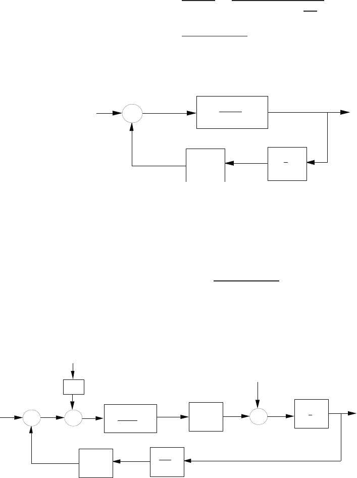
148 CHAPTER 4 Feedback Control System Characteristics

The transfer function (valid around the operating point) is

T(s) = Vout(s)

Vin(s)=K

(sτ + 1) + K45I

5

sτ + 1 + 9KI .

The photosensor block diagram is shown in Figure P4.9.

ts+ 1

45 I

i (ma)

vin vout

FIGURE P4.9

Photosensor block diagram.

(b) The sensitivity of the system to changes in Kis

K=τs + 1

τs + 1 + 9KI .

P4.10 (a) and (b) The paper tension control block diagram is shown in Fig-

ure P4.10.

T( s)

R(s) Km

ts + 1

DT (s)

V1+DV1(s)

Y (s)

Eo( s) wo( s)

FIGURE P4.10

Paper tension control block diagram.

from the publisher prior to any prohibited reproduction, storage in a retrieval system, or transmission in any form or by any means, electronic, mechanical, photocopying,

recording, or likewise. For information regarding permission(s), write to: Rights and Permissions Department, Pearson Education, Inc., Upper Saddle River, NJ 07458.

Problems 149

Tc(s) = T(s)

R(s)=

2Km

s(τs+1)

1 + 4Kmk2

k1s(τs+1)

=2Km

τs2+s+4Kmk2

The sensitivity of Tcto changes in Kmis

STc

Km=1

1 + 4Kmk2

k1s(τs+1)

=s(τs + 1)

τs2+s+4Kmk2

(d) The transfer function from ∆V1(s) to T(s) is

T(s) = −1

1 + 4Kmk2

k1s(τs+1)

∆V1(s) = −1

s+4Kmk2

k1(τs+1)

∆V1(s).

When ∆V1(s) = A/s, we have

T(s) = −(τs + 1)

τs2+s+4Kmk2

and

lim

t→∞ T(t) = lim

s→0sT (s) = −Ak1

4Kmk2

P4.11 (a) The closed-loop transfer function is

T(s) = Gc(s)G(s)

1 + Gc(s)G(s)=K

(8s+ 1)(3s+ 1) + K=K

24s2+ 11s+ 1 + K.

(b) The sensitivity ST

Kis

K=∂T

∂K ·K

T=24s2+ 11s+ 1

24s2+ 11s+ 1 + K.

E(s) = R(s)

1 + Gc(s)G(s)="24s2+ 11s+ 1

24s2+ 11s+K+ 1#R(s).

With

R(s) = A

we have

ess = lim

s→0sE(s) = A

1 + K.

from the publisher prior to any prohibited reproduction, storage in a retrieval system, or transmission in any form or by any means, electronic, mechanical, photocopying,

recording, or likewise. For information regarding permission(s), write to: Rights and Permissions Department, Pearson Education, Inc., Upper Saddle River, NJ 07458.

150 CHAPTER 4 Feedback Control System Characteristics

(d) We want |e(t)| ≤ 0.02Aas t→ ∞ . So,

0.02A≥A

K+ 1

implies

K≥49 .

P4.12 (a) The two transfer functions are

T1(s) = K1K2

s2+ 3s−4 + 6K1K2

and

T2(s) = K1K2

s2+ (3 −2K1+ 2K2)s−4 + 8K2+ 2K1−4K1K2

When K1=K2= 1, we ﬁnd that

T1(s) = T2(s) = 1

s2+ 3s+ 2.

(b) The sensitivity ST1

K1is

ST1

K1=∂T1

∂K1·K1

=s2+ 3s−4

s2+ 3s−4 + 6K1K2

=(s+ 4)(s−1)

(s+ 2)(s+ 1) ,

when K1=K2= 1. The sensitivity ST2

K1is

ST2

K1=∂T2

∂K1·K1

=s+ 4

s+ 4 −2K1

=s+ 4

s+ 2 ,

when K1= 1. Thus,

ST1

K1=ST2

s−1

s+ 1 .

P4.13 (a) Let N(s) = G1(s) + kG2(s) and Td(s) = G3(s) + kG4(s). Then

k=∂N

∂k ·k

N−∂D

∂k ·k

D=G2k

G1+kG2−G4k

G3+kG4

=k(G2G3−G1G4)

(G1+kG2)(G3+kG4).

(b) The closed-loop transfer function is

T(s) = MG(s) + kUG(s)

1 + kGH(s)=G1(s) + kG2(s)

G3(s) + kG4(s).

from the publisher prior to any prohibited reproduction, storage in a retrieval system, or transmission in any form or by any means, electronic, mechanical, photocopying,

recording, or likewise. For information regarding permission(s), write to: Rights and Permissions Department, Pearson Education, Inc., Upper Saddle River, NJ 07458.

Problems 151

Then using result from (a), we have

k=k(UG(s)−MG2H(s))

(MG(s) + kUG(s))(1 + kGH(s)) .

P4.14 The closed-loop transfer function is

T(s) = G(s)

1 + G(s)=10(s+ 4)

s(s+a)(s+ 1) + 10(s+ 4) .

Then

a=SN

a−SD

where Nis the numerator and Dis the denominator. We have

a= 0 .

Let

G(s) = p(s)

q(s)(s+a),

where p(s) = 10(s+ 4) and q(s) = s(s+ 1). Then

T(s) = G(s)

1 + G(s)=p(s)

q(s)(s+a) + p(s),

and

a=−SD

a=−dD

da ·a

D=−aq(s)

q(s)(s+a) + p(s)=−a

s+a·1

1 + G(s).

P4.15 (a) The closed-loop transfer function for the disturbance to the output is

Y(s)

Td(s)=G(s)

1 + KG(s),

with R= 0. The steady-state deviation is

yss = lim

s→0sG(s)

1 + KG(s)1

s=G(0)

1 + KG(0) =1

1 + K.

So, with K= 10 we have yss = 1/11, and with K= 25 we have

yss = 1/26.

(b) Considering the rudder input, we have

Y(s) = G(s)Td(s) + KG(s)R(s)

1 + KG(s)=G(s)(Td(s) + KR(s))

1 + KG(s).

from the publisher prior to any prohibited reproduction, storage in a retrieval system, or transmission in any form or by any means, electronic, mechanical, photocopying,

recording, or likewise. For information regarding permission(s), write to: Rights and Permissions Department, Pearson Education, Inc., Upper Saddle River, NJ 07458.

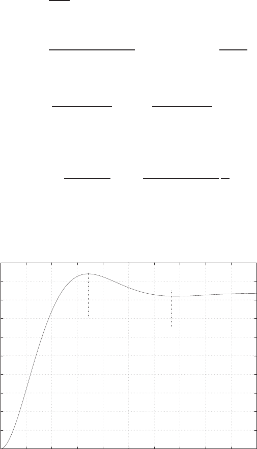
152 CHAPTER 4 Feedback Control System Characteristics

Setting R(s) = −Td(s)

Kyields Y(s) = 0.

P4.16 (a) Let

G1(s) = 1

(τ1s+ 1)(τ2s+ 1) and G2(s) = G1(s)

100 .

Then

T2(s) = G1(s)

1 + G2Gc(s)To(s) + G2Gc(s)

1 + G2Gc(s)T2d(s).

(b) We can equivalently consider the case of a step input, T2d=A/s,

To= 0, and zero initial conditions. Thus,

T2(s) = GcG2

1 + GcG2

T2d=5

500s2+ 60s+ 6

where Gc(s) = 500. The transient response is shown in the Fig-

ure P4.16 for a unit step input (A= 1).

0.1

0.2

0.3

0.4

0.5

0.6

0.7

0.8

0.9

0 10 20 30 40 50 60 70 80 90 100

time (sec)

Tp=34.3 sec

p.o. = 12.8% Ts=66.7 sec

Unit step response, A=1

FIGURE P4.16

Two tank temperature control system response.

E(s) = T2d(s)−T2(s),

from the publisher prior to any prohibited reproduction, storage in a retrieval system, or transmission in any form or by any means, electronic, mechanical, photocopying,

recording, or likewise. For information regarding permission(s), write to: Rights and Permissions Department, Pearson Education, Inc., Upper Saddle River, NJ 07458.

Problems 153

we have

E(s) = T2d(s)−M(s)T2d(s)

where

M(s) = G2Gc(s)

1 + G2Gc(s).

Then

ess = lim

s→0s(1 −M(s))A

s= (1 −M(0))A= (1 −5

6)A=A

P4.17 (a) The closed-loop transfer function is

θ(s)

θd(s)=600

0.1s2+s+ 600 =6000

s2+ 10s+ 6000 .

The solution for a step input is

θ(t) = 1 −1.0021e−5.0349tsin(77.2962t+ 1.5058).

(b) The transfer function from the disturbance to the output is

θ(s)

Td(s)=−1

0.1s2+s+ 600 .

Thus,

θss =−lim

s→0sθ(s) = A

600 .

Therefore, the disturbance input magnitude reduced by 600 at the

output.

ess = lim

s→0sE(s) = lim

s→0s(1 −T(s))θd(s)

= lim

s→0s 0.1s2+s

0.1s2+s+ 600!1

s2=1

600 .

from the publisher prior to any prohibited reproduction, storage in a retrieval system, or transmission in any form or by any means, electronic, mechanical, photocopying,

recording, or likewise. For information regarding permission(s), write to: Rights and Permissions Department, Pearson Education, Inc., Upper Saddle River, NJ 07458.

154 CHAPTER 4 Feedback Control System Characteristics

Advanced Problems

AP4.1 The plant transfer function is

Gp(s) = R

RCs + 1 .

The closed-loop output is given by

H(s) = 1

1 + GGp(s)Q3(s) + GGp(s)

1 + GGp(s)Hd(s).

Therefore, with E(s) = Hd(s)−H(s), we have

E(s) = −1

1 + GGp(s)Q3(s),

since Hd(s) = 0.

(a) When G(s) = K, we have

ess = lim

s→0sE(s) = −1

1 + KR .

(b) When G(s) = K/s, we have

ess = lim

s→0sE(s) = 0 .

AP4.2 Deﬁne

G(s) = KmGc(s)

s(Las+Ra)(Js +f) + KmKbGc(s).

Then,

θ(s)/θd(s) = nG(s)

1 + nG(s)

and

E(s) = 1

1 + nG(s)θd(s).

So,

ess = lim

s→0sE(s) = lim

s→0s1

1 + nG(s)

s=A

1 + nG(0) =AKb

Kb+n.

from the publisher prior to any prohibited reproduction, storage in a retrieval system, or transmission in any form or by any means, electronic, mechanical, photocopying,

recording, or likewise. For information regarding permission(s), write to: Rights and Permissions Department, Pearson Education, Inc., Upper Saddle River, NJ 07458.

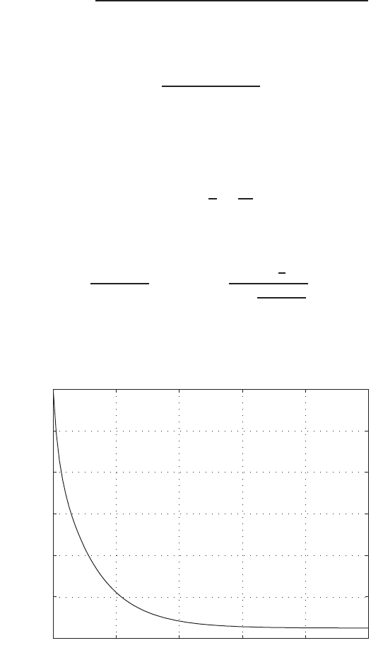
Advanced Problems 155

When θd(s) = 0 and Td(s) = M/s, we have

θ(s)/Td(s) = n(Las+Ra)

s(Las+Ra)(Js +f) + KmKb+KmGcn.

If Gc(s) = K, then

ess =−nMRa

Km(Kb+nK)

and if Gc(s) = K/s, we determine that ess = 0.

AP4.3 (a) The input R(s) is

R(s) = 1

s−1

and the disturbance is Td(s) = 0. So,

ess = lim

s→0s1

1 + G(s)R(s) = lim

s→0

1−1

1 + 10(2s+4)

7s(s+5)

=−0.8750 .

(b) The error plot is shown in Figure AP4.3a.

0 2 4 6 8 10

?-1

?-0.5

0.5

1.5

Time (sec)

e(t)

FIGURE AP4.3

(a) Error plot with d(t)=0.

from the publisher prior to any prohibited reproduction, storage in a retrieval system, or transmission in any form or by any means, electronic, mechanical, photocopying,

recording, or likewise. For information regarding permission(s), write to: Rights and Permissions Department, Pearson Education, Inc., Upper Saddle River, NJ 07458.

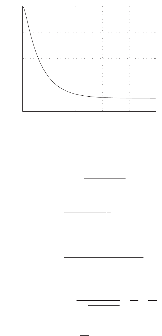
156 CHAPTER 4 Feedback Control System Characteristics

0 2 4 6 8 10

-?2

?-1.5

?-1

?-0.5

Time (sec)

e(t)

FIGURE AP4.3

CONTINUED: (b) Error plot with r(t)=0.

Y(s)/Td(s) = −70

7s2+ 55s+ 40 .

The steady-state error due to a disturbance Td(s) = 1/s is

ess = lim

s→0s−70

7s2+ 55s+ 40

s=−1.75 .

(d) The error e(t) is shown in Figure AP4.3b.

AP4.4 (a) The closed-loop transfer function is

ω(s)/V (s) = Km

RaJs2+KbKms+KmKKt

With v(t) = t, we have V(s) = 1/s2, and Td(s) = 0. Using the ﬁnal

value theorem yields

ess = lim

s→0sE(s) = lim

s→0

s+KKm

RaJs+KmKb

=Kb

K=0.1

We desire that

ess =0.1

K<0.1.

from the publisher prior to any prohibited reproduction, storage in a retrieval system, or transmission in any form or by any means, electronic, mechanical, photocopying,

recording, or likewise. For information regarding permission(s), write to: Rights and Permissions Department, Pearson Education, Inc., Upper Saddle River, NJ 07458.

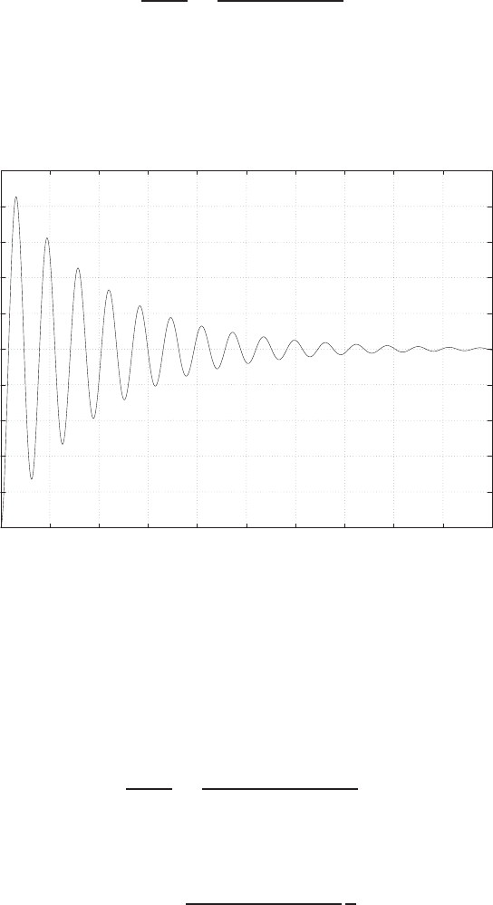
Advanced Problems 157

Therefore, we should select K > 1. For example, we can take K= 8.

(b) The transfer function from Td(s) to ω(s) is given by

ω(s)

Td(s)=−10s

s2+ 10s+ 100 .

The error plot is shown in Figure AP4.4, where e(s) = −ω(s) (V(s) =

0.)

0.02

0.04

0.06

0.08

0.1

0.12

0.14

0.16

0.18

0.2

0 1 2 3 4 5 6 7 8 9 10

Time (sec)

e(t)

FIGURE AP4.4

Error plot with a ramp disturbance input.

AP4.5 (a) The transfer function from the disturbance Td(s) to the output Y(s)

Y(s)

Td(s)=−s

s3+ 4s2+ 4s+K.

The steady-state error (when Td(s) = 1/s) is

ess = lim

s→0ss

s3+ 4s2+4s+K

s= 0 .

from the publisher prior to any prohibited reproduction, storage in a retrieval system, or transmission in any form or by any means, electronic, mechanical, photocopying,

recording, or likewise. For information regarding permission(s), write to: Rights and Permissions Department, Pearson Education, Inc., Upper Saddle River, NJ 07458.

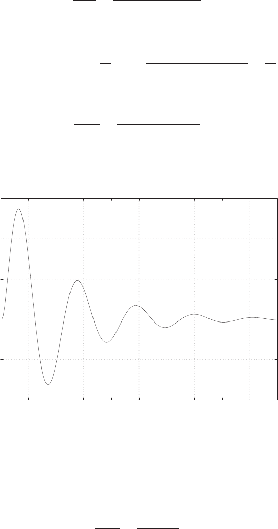
158 CHAPTER 4 Feedback Control System Characteristics

(b) The closed-loop transfer function is

Y(s)

R(s)=K

s3+ 4s2+ 4s+K.

The steady-state error (when R(s) = 1/s2) is

ess = lim

s→0s(1 −T(s)) 1

s2= lim

s→0

s3+ 4s2+ 4s

s(s3+ 4s2+ 4s+K)=4

Y(s)

Td(s)=−s

s3+ 4s2+ 4s+ 8 .

The error plot is shown in Figure AP4.5, for r(t) = 0.

-0.1

-0.05

0.05

0.1

0.15

0 2 4 6 8 10 12 14 16 18 20

Time (sec)

e(t)

FIGURE AP4.5

Error plot with a step disturbance input and K=8.

AP4.6 (a) The transfer function is

Vo(s)

V(s)=1 + RCs

2 + RCs .

from the publisher prior to any prohibited reproduction, storage in a retrieval system, or transmission in any form or by any means, electronic, mechanical, photocopying,

recording, or likewise. For information regarding permission(s), write to: Rights and Permissions Department, Pearson Education, Inc., Upper Saddle River, NJ 07458.

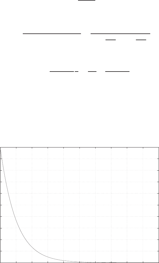
Advanced Problems 159

(b) The system sensitivity is deﬁned as

C=∂G/G

∂C/C .

Therefore, the sensitivity is determined to be

C=RCs

(2 + RCs)(1 + RCs)=1

1 + 2

RCs 1 + 1

RCs .

Vo(s) = 1 + RCs

2 + RCs

s=0.5

s+0.5RC

RCs + 2 .

Taking the inverse Laplace transform yields

vo(t) = 0.5(1 + e−2t/RC )u(t)

where u(t) is the unit step function. A plot of vo(t) versus t/RC is

shown in Figure AP4.6.

0.5

0.55

0.6

0.65

0.7

0.75

0.8

0.85

0.9

0.95

0 0.5 1 1.5 2 2.5 3 3.5 4 4.5 5

t / RC

FIGURE AP4.6

Step response.

from the publisher prior to any prohibited reproduction, storage in a retrieval system, or transmission in any form or by any means, electronic, mechanical, photocopying,

recording, or likewise. For information regarding permission(s), write to: Rights and Permissions Department, Pearson Education, Inc., Upper Saddle River, NJ 07458.

160 CHAPTER 4 Feedback Control System Characteristics

AP4.7 (a) The transfer function from Td(s) to Y(s) is

Y(s)

Td(s)=−s

s(s+ 1) + K.

(b) The transfer function from N(s) to Y(s) is

Y(s)

N(s)=K

s(s+ 1) + K.

ess =−yss = lim

s→0ss

s(s+ 1) + K

s−lim

s→0sK

s(s+ 1) + K

s=−B .

So, Khas no eﬀect on the steady-state errors. However, choosing

K= 100 will minimize the eﬀects of the disturbance Td(s) during the

transient period.

AP4.8 (a) The closed-loop transfer function is

T(s) = Kb

s+Kb + 2 .

(b) The sensitivity is determined to be

b=∂T /T

∂b/b =s+ 2

s+Kb + 2 .

Y(s)

Td(s)=b

s+Kb + 2 .

So, choose Kas large as possible, to make Y(s)/Td(s) as “small” as

possible. Thus, select

K= 50 .

This also minimizes ST

bat low frequencies.

from the publisher prior to any prohibited reproduction, storage in a retrieval system, or transmission in any form or by any means, electronic, mechanical, photocopying,

recording, or likewise. For information regarding permission(s), write to: Rights and Permissions Department, Pearson Education, Inc., Upper Saddle River, NJ 07458.

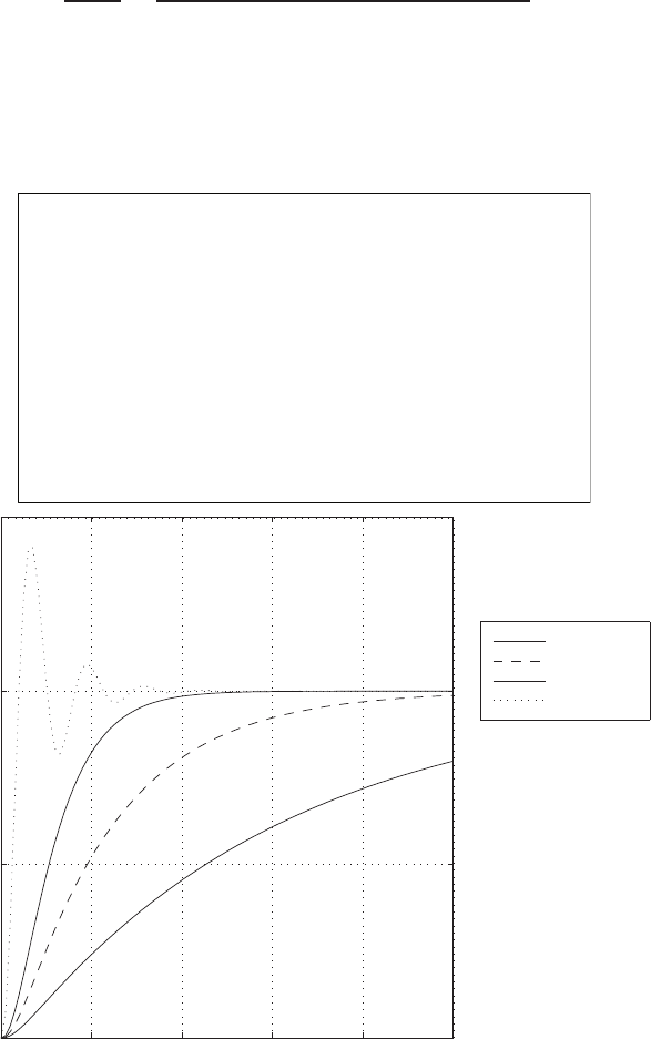
Design Problems 161

Design Problems

The model of the traction drive, capstan roller, and linear slide was de-CDP4.1

veloped in CDP2.1:

θ(s)

Va(s)=Km

s[(Lms+Rm)(JTs+bm) + KbKm].

The step response for the closed-loop system (with the tachometer not in

the loop) and various values of the controller gain Kais shown below.

% System parameters

Ms=5.693; Mb=6.96; Jm=10.91e-03; r=31.75e-03;

bm=0.268; Km=0.8379; Kb=0.838; Rm=1.36; Lm=3.6e-03; Lm=0;

% Controller gain

Ka=100;

% Motor and slide model

Jt=Jm+r^2*(Ms+Mb);

num=[Km];

den=[Lm*Jt Rm*Jt+Lm*bm Kb*Km+Rm*bm 0];

sys=tf(num,den);

%Closed-loop tf and step response

sys_cl=feedback(Ka*sys,[1]);

step(sys_cl)

0 0.2 0.4 0.6 0.8 1

0.5

1.5

Time (sec)

Theta step response

Ka=2

Ka=5

Ka=10

Ka=100

from the publisher prior to any prohibited reproduction, storage in a retrieval system, or transmission in any form or by any means, electronic, mechanical, photocopying,

recording, or likewise. For information regarding permission(s), write to: Rights and Permissions Department, Pearson Education, Inc., Upper Saddle River, NJ 07458.

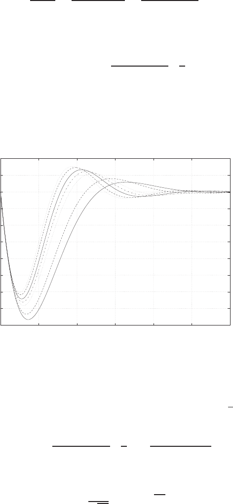
162 CHAPTER 4 Feedback Control System Characteristics

DP4.1 (a) The transfer function from the load disturbance to the output speed

ω(s)

Td(s)=−G(s)

1 + GcG(s)=−s

s2+ 4s+K.

Thus, the eﬀect on ω(s) (of a unit step disturbance) at steady-state

lim

t→∞ ω(t) = lim

s→0s−s

s2+ 4s+K1

s= 0 .

We see that the load disturbance has no eﬀect on the output at steady-

state.

(b) The system response for 10 ≤K≤25 is shown in Figure DP4.1.

99.84

99.86

99.88

99.9

99.92

99.94

99.96

99.98

100

100.02

100.04

0 0.5 1 1.5 2 2.5 3

Time(sec)

w(t)

K=10

K=25

K=10,12,16,18,20,23,25

FIGURE DP4.1

Speed control system response.

For example , if we select K= 16, then ωn= 4, ζ =1

2, and the

response due to a unit step disturbance is

ω(s) = −s

s2+ 4s+ 16 1

s=−1

(s+ 2)2+ 12 .

Hence, if we are originally at ω(t) = 100 for t < τ, we have

ω(t) = 100 −1

√12e−2tsin√12t t ≥τ .

from the publisher prior to any prohibited reproduction, storage in a retrieval system, or transmission in any form or by any means, electronic, mechanical, photocopying,

recording, or likewise. For information regarding permission(s), write to: Rights and Permissions Department, Pearson Education, Inc., Upper Saddle River, NJ 07458.

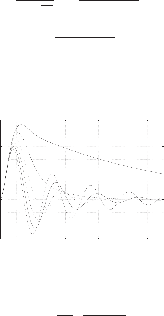
Design Problems 163

DP4.2 With θd= 0, we have

θ(s) = G(s)

1 + G(s)KK1

Td(s) = s

s3+ 4s2+ 9s+KK1

Td(s).

For Td=A/s, we have

θ(s) = A

s3+ 4s2+ 9s+KK1

The system response to a unit step disturbance for various values of KK1

are shown in Figure DP4.2. From the plot we see that when KK1is small

the response is slow but not oscillatory. On the other hand, when KK1

is large the response is fast but highly oscillatory. In fact, if KK1>35,

the system is unstable. Thus, we might select KK1= 10 as a reasonable

trade-oﬀ between fast performance and stability.

-0.06

-0.04

-0.02

0.02

0.04

0.06

0.08

0.1

0.12

01 2 3 4 5 6 7 8 9 10

time(sec)

Unit step response for KK1=1,5,10,15,20,25

KK1=1

KK1=5

KK1=25

FIGURE DP4.2

Aircraft roll angle control system response to a disturbance.

DP4.3 (a) The closed-loop transfer function is

T(s) = ω(s)

ωd(s)=K

s2+ 5s+KK1

from the publisher prior to any prohibited reproduction, storage in a retrieval system, or transmission in any form or by any means, electronic, mechanical, photocopying,

recording, or likewise. For information regarding permission(s), write to: Rights and Permissions Department, Pearson Education, Inc., Upper Saddle River, NJ 07458.

164 CHAPTER 4 Feedback Control System Characteristics

Then,

E(s) = (1 −T(s))ωd(s) = s2+ 5s+K(K1−1)

s2+ 5s+KK1

So, if

0.99 < K1<1.01 ,

then

|ess|<0.01 .

(b) The transfer function from Td(s) to ω(s) is

ω(s) = −s

s2+ 5s+KK1

Td(s).

So, with E(s) = −ω(s) and Td(s) = 2/s2, we have

lim

s→0sE(s) = 2

KK1

Therefore, we select KK1>20 to obtain ess <0.1.

DP4.4 The steady-state error for a step input command is zero for any K1. The

transfer function from Td(s) to Y(s) is

Y(s)

Td(s)=G(s)

1 + KG(s)=2

s3+ 5s2+ 4s+ 2K.

Thus, the output at steady-state due to a step disturbance Td(s) = A/s

lim

s→0sY (s) = A

We want to maximize Kto reduce the eﬀect of the disturbance. As we will

see in Chapter 6, we cannot select Ktoo high or the system will become

unstable. That is why the problem statement suggests a maximum gain

of K= 10. For the design we choose

K= 10 .

DP4.5 The transfer function from V(s) to Vo(s) is

Vo(s)/V (s) = ks

s+a

from the publisher prior to any prohibited reproduction, storage in a retrieval system, or transmission in any form or by any means, electronic, mechanical, photocopying,

recording, or likewise. For information regarding permission(s), write to: Rights and Permissions Department, Pearson Education, Inc., Upper Saddle River, NJ 07458.

Design Problems 165

where

k=R2+R3

and a=1

R1C.

Computing the step response, we ﬁnd that

vo(t) = ke−at = 5e−100t.

Solving for R1, R2, R3and Cyields

R1C= 0.01 and R2

= 4 .

DP4.6 (a) The closed-loop transfer function is

θ(s) = K/J

s2+K/J θd(s).

Since J > 0, the system is unstable when K < 0 and marginally

stable when K > 0.

(b) Since the system is marginally stable, the system response does not

have a steady-state value—it oscillates indeﬁnitely.

θ(s) = KDs+KP

Js2+KDs+KP

θd(s).

The system is stable for all KD>0 and KP>0, given that J > 0.

(d) The tracking error E(s) = θd(s)−θ(s) is

E(s) = Js2

Js2+KDs+KP

Therefore, using the ﬁnal value theorem we obtain the steady-state

value

lim

s→0sE(s) = lim

s→0sJs2

Js2+KDs+KP·1

s= 0 .

DP4.7 (a) The closed-loop transfer function is

Y(s) = s

s2+Ks + 2KTd(s) = 1

s2+Ks + 2K

where the disturbance is a unit step Td(s) = 1/s. Considering the

poles of the closed-loop system, we ﬁnd that when K > 8 the system

from the publisher prior to any prohibited reproduction, storage in a retrieval system, or transmission in any form or by any means, electronic, mechanical, photocopying,

recording, or likewise. For information regarding permission(s), write to: Rights and Permissions Department, Pearson Education, Inc., Upper Saddle River, NJ 07458.

166 CHAPTER 4 Feedback Control System Characteristics

has two real poles. In that case the disturbance step response is

y(t) = 1

√K2−8Ke−αt −e−βt,

where

α=K−√K2−8K

2and β=K+√K2−8K

Bounding the maximum y(t) yields the inequality

|y(t)|=1

√K2−8Ke−αt −e−βt≤0.05.

We know that

e−αt −e−βt≤1,

for any αand βcomputed as shown above where K > 8. So, if we

choose Ksuch that

√K2−8K≤0.05.

we will guarantee that the maximum bound of 0.05 is not exceeded.

Solving for Kyields

K > 24.4.

For any K > 24.4 we know that the maximum value of the disturbance

step response will be less than 0.05. When K= 24.4 the maximum

unit step disturbance response is 0.035. Solving explicitly for Kso

that the maximum is 0.05 we ﬁnd that K= 16.3 (this was found

numerically since it is very diﬃcult to obtain analytically).

(b) Since the system is type 2, we know that the steady-state value of

the disturbance step response is zero for a unit step disturbance.

DP4.8 (a) The sensitivities are

τ1=∂T/T

∂τ1/τ1

="−s2(τ2s+ 1) τ1

K#T(s)

and

τ2=∂T/T

∂τ2/τ2

="−s2(τ1s+ 1) τ2

K#T(s)

where we assume that K6= 0.

from the publisher prior to any prohibited reproduction, storage in a retrieval system, or transmission in any form or by any means, electronic, mechanical, photocopying,

recording, or likewise. For information regarding permission(s), write to: Rights and Permissions Department, Pearson Education, Inc., Upper Saddle River, NJ 07458.

Design Problems 167

(b) Computing the closed-loop transfer function yields

Y(s) = s(τ1s+ 1)

s(τ1s+ 1) (τ2s+ 1) + KTd(s)

When Td(s) = 1/s, using the ﬁnal value theorem we ﬁnd that

lim

s→0sY (s) = lim

s→0

s(τ1s+ 1)

s(τ1s+ 1) (τ2s+ 1) + K= 0

as long as K6= 0. We assume here that ﬁnal value theorem applies

(i.e., the system is stable, more on this in Chapter 6).

from the publisher prior to any prohibited reproduction, storage in a retrieval system, or transmission in any form or by any means, electronic, mechanical, photocopying,

recording, or likewise. For information regarding permission(s), write to: Rights and Permissions Department, Pearson Education, Inc., Upper Saddle River, NJ 07458.

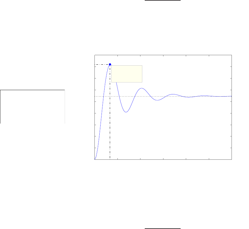
168 CHAPTER 4 Feedback Control System Characteristics

Computer Problems

CP4.1 The step response and an m-ﬁle script which generates the step response

is shown in Figure CP4.1. The closed-loop transfer function is

T(s) = 12

s2+ 2s+ 22 .

The percent overshoot is P.O. = 50.2% and the steady-state error is

ess = 0.45.

num = [12]; den = [1 2 10];

sys = tf(num,den);

sys_cl = feedback(sys,[1])

step(sys_cl)

Step Response

Time (sec)

Amplitude

0123456

0.1

0.2

0.3

0.4

0.5

0.6

0.7

0.8

0.9

System: sys_cl

Peak amplitude: 0.82

Overshoot (%): 50.2

At time (sec): 0.67

FIGURE CP4.1

Step response.

CP4.2 The transfer function is

G(s) = 4

s2+ 2s+ 20 .

An m-ﬁle script which generates the step response is shown in Figure CP4.2.

The step response is also shown in Figure CP4.2. The step response is

generated using the step function. In the script, the transfer function

numerator is represented by num and the denominator is represented by

den. The steady-state value is yss = 0.2 and the desired value is 1.0.

Therefore, the steady-state error is

ess = 0.8.

from the publisher prior to any prohibited reproduction, storage in a retrieval system, or transmission in any form or by any means, electronic, mechanical, photocopying,

recording, or likewise. For information regarding permission(s), write to: Rights and Permissions Department, Pearson Education, Inc., Upper Saddle River, NJ 07458.

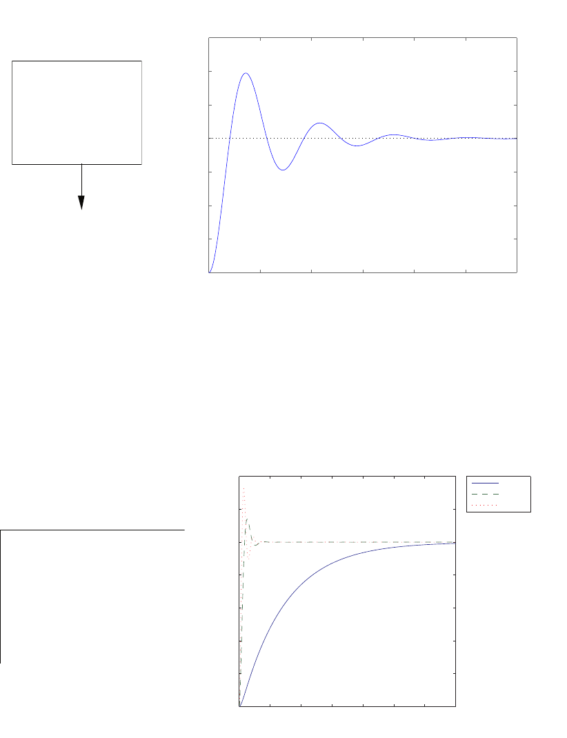
Computer Problems 169

num=[4]; den=[1 2 20];

sys = tf(num,den);

axis([0 6 0 1]);

t=[0:0.01:6];

step(sys,t)

y = step(sys,t);

yss = y(length(t))

yss =

0.20

0 1 2 3 4 5 6

0.05

0.1

0.15

0.2

0.25

0.3

0.35

Step Response

Time (sec)

Amplitude

FIGURE CP4.2

Step response.

CP4.3 The step responses and the m-ﬁle script which generates the step re-

sponses is shown in Figure CP4.3.

K=[10,200,500];

t=[0:0.01:7];

for i=1:3

num=5*K(i); den=[1 15 K(i)];

sys = tf(num,den)

y(:,i)= step(sys,t);

end

plot(t,y(:,1),t,y(:,2),'--',t,y(:,3),':')

legend('K=10','K=200','K=500',-1)

01234567

K=10

K=200

K=500

FIGURE CP4.3

Step responses for K= 10,100,500.

from the publisher prior to any prohibited reproduction, storage in a retrieval system, or transmission in any form or by any means, electronic, mechanical, photocopying,

recording, or likewise. For information regarding permission(s), write to: Rights and Permissions Department, Pearson Education, Inc., Upper Saddle River, NJ 07458.

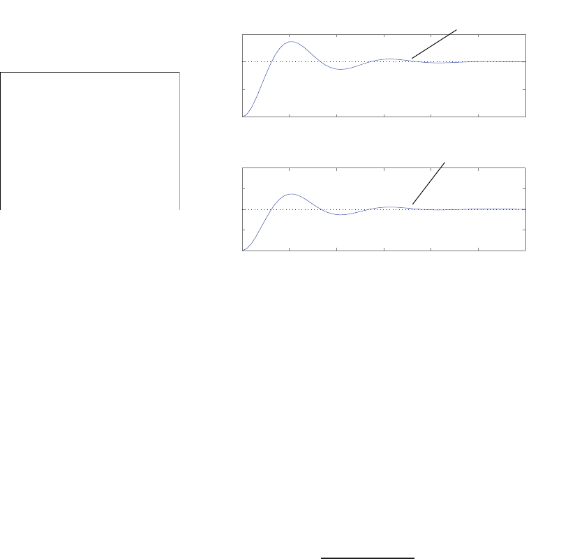
170 CHAPTER 4 Feedback Control System Characteristics

CP4.4 (a,b) The m-ﬁle and plots are shown in Figure CP4.4.

ng=1;dg=[1 1.91 0];sysg=tf(ng,dg);

K=10;

syscl=feedback(K*sysg,1);

figure(1)

subplot(211)

step(syscl)

subplot(212)

syst=feedback(sysg,K)

step(syst)

0 1 2 3 4 5 6

0.5

1.5

Time (sec)

0 1 2 3 4 5 6

0.05

0.1

0.15

0.2

Time (sec)

Step response

Disturbance response

y(t)

FIGURE CP4.4

Step response and disturbance response.

zero, and the estimated steady-state tracking error to a unit distur-

bance is 0.1.

(d) The estimated maximum tracking error due to a unit step input is

0.4, and the estimated maximum tracking error to a unit disturbance

is 0.14. The maximum occurs at approximately t= 1 s.

CP4.5 The step response and the m-ﬁle script which generates the step response

is shown in Figure CP4.5. The closed-loop transfer function is determined

to be

T(s) = 10

s2+ 3.7s+ 10 .

Using the m-ﬁle script, a trial-and-error search on kyields

k= 3.7.

The percent overshoot P.O. = 10% and the steady-state value is 1, as

expected.

from the publisher prior to any prohibited reproduction, storage in a retrieval system, or transmission in any form or by any means, electronic, mechanical, photocopying,

recording, or likewise. For information regarding permission(s), write to: Rights and Permissions Department, Pearson Education, Inc., Upper Saddle River, NJ 07458.

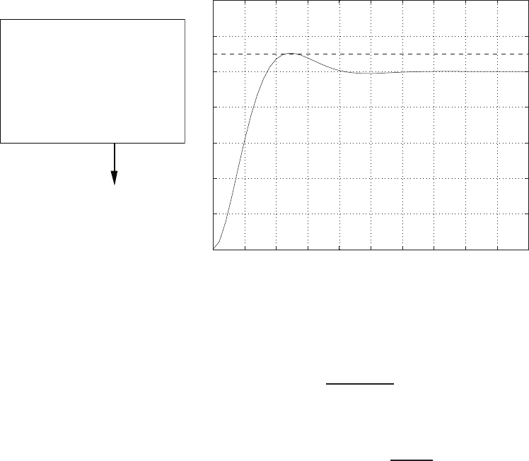
Computer Problems 171

k = 3.7; % Final value of k=3.7

numcg = [10]; dencg = [1 k 0];

sys_o = tf(numcg,dencg);

sys_cl = feedback(sys_o,[1])

t = [0:0.1:5];

[y,t] = step(sys_cl,t);

plot(t,y,[0 5],[1.1 1.1],'--'); grid

xlabel('Time (sec)'); ylabel('y(t)');

Transfer function:

----------------

s^2 + 3.7 s + 10

0 0.5 1 1.5 2 2.5 3 3.5 4 4.5 5

0.2

0.4

0.6

0.8

1.2

1.4

Time (sec)

y(t)

FIGURE CP4.5

Step response.

CP4.6 The closed-loop transfer function is

T(s) = K

s−a+K

where K= 2. When a= 1 and R(s) = 1/s, the ﬁnal value is

lim

s→0sT (s)R(s) = lim

s→0T(s) = K

K−a= 2 .

The output is within 2% of the ﬁnal value at around t= 4.6 seconds. The

plot of the step responses for

a= 1,0.5,2,5

is shown in Figure CP4.6. The output is unstable for

a > 2.

from the publisher prior to any prohibited reproduction, storage in a retrieval system, or transmission in any form or by any means, electronic, mechanical, photocopying,

recording, or likewise. For information regarding permission(s), write to: Rights and Permissions Department, Pearson Education, Inc., Upper Saddle River, NJ 07458.

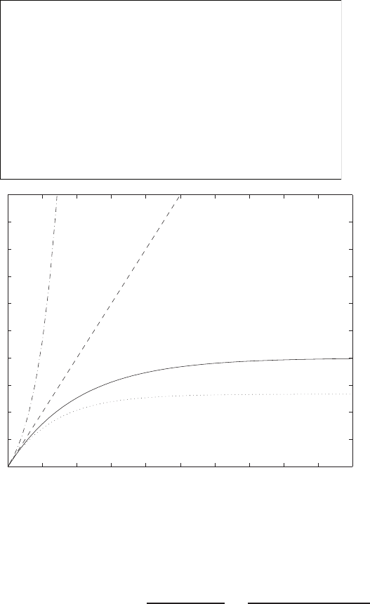
172 CHAPTER 4 Feedback Control System Characteristics

K=2; t=[0:0.1:5];

num=K*[1];

a=[1 0.5 2 5];

for i=1:4

den=[1 -a(i)]; sys = tf(num,den);

sys_cl = feedback(sys,[1]);

y(:,i)=step(sys_cl,t);

end

plot(t,y(:,1),t,y(:,2),':',t,y(:,3),'--',t,y(:,4),'-.')

axis([0 5 0 5]);

xlabel('Time (sec)'), ylabel('y(t)')

title('a=1 (solid); a=0.5 (dotted); a=2 (dashed); a=5 (dashdot)')

0 0.5 1 1.5 2 2.5 3 3.5 4 4.5 5

0.5

1.5

2.5

3.5

4.5

Time (sec)

y(t)

a=1 (solid); a=0.5 (dotted); a=2 (dashed); a=5 (dashdot)

FIGURE CP4.6

Step response for a=1, 0.5, 2, and 5.

CP4.7 The transfer function from the disturbance to the output is

T(s) = G(s)

1 + K0G(s)=1

Js2+bs +k+K0

The disturbance response is shown in Figure CP4.7. The compensated

system response is signiﬁcantly reduced from the uncompensated system

response. The compensated system output is about 11 times less than the

uncompensated system output. So, closed-loop feedback has the advan-

tage of reducing the eﬀect of unwanted disturbances on the output.

from the publisher prior to any prohibited reproduction, storage in a retrieval system, or transmission in any form or by any means, electronic, mechanical, photocopying,

recording, or likewise. For information regarding permission(s), write to: Rights and Permissions Department, Pearson Education, Inc., Upper Saddle River, NJ 07458.

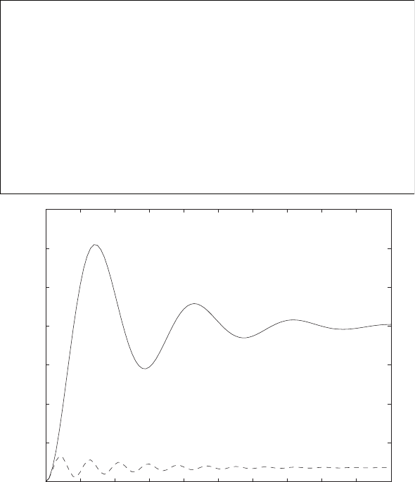
Computer Problems 173

J=1; k=5; c=0.9;

num=[1/J]; den=[1 c/J k/J];

sys = tf(num,den);

t=[0:0.1:10];

yu=step(sys,t); % Part (a)

K0=50;

numk=[K0]; denk=[1]; sysk = tf(numk,denk);

sys_cl = feedback(sys,sysk);

yc=step(sys_cl,t); % Part (b)

plot(t,yu,t,yc,'--')

xlabel('Time (sec)'), ylabel('\theta')

title('Uncompensated response (solid) & Compensated response (dashed)')

0 1 2 3 4 5 6 7 8 9 10

0.05

0.1

0.15

0.2

0.25

0.3

0.35

Time (sec)

Uncompensated response (solid) & Compensated response (dashed)

FIGURE CP4.7

Disturbance responses for both the uncompensated and compensated systems.

CP4.8 The step responses for the proportional and PI controller are shown in

Figure CP4.8. The steady-state tracking error for the proportional con-

troller is

ess = 0.33 .

Increasing the complexity of the controller from a proportional controller

to a proportional plus integral (PI) controller allows the closed-loop sys-

tem to track the unit step response with zero steady-state error. The cost

is controller complexity, which translates into higher costs ($).

from the publisher prior to any prohibited reproduction, storage in a retrieval system, or transmission in any form or by any means, electronic, mechanical, photocopying,

recording, or likewise. For information regarding permission(s), write to: Rights and Permissions Department, Pearson Education, Inc., Upper Saddle River, NJ 07458.

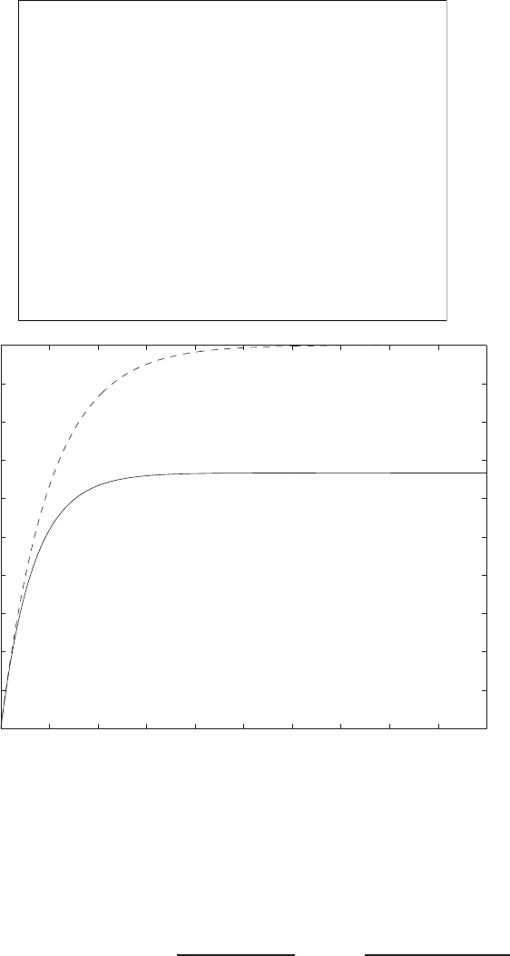
174 CHAPTER 4 Feedback Control System Characteristics

numg=[10]; deng=[1 10]; sysg = tf(numg,deng);

t=[0:0.001:0.5];

% Part (a)

numc=[2]; denc=[1]; sysc = tf(numc,denc);

sys_o = series(sysc,sysg);

sys_cl = feedback(sys_o,[1]);

yk=step(sys_cl,t);

% Part (b)

numc=[2 20]; denc=[1 0]; sysc = tf(numc,denc);

sys_o = series(sysc,sysg);

sys_cl = feedback(sys_o,[1]);

yp=step(sys_cl,t);

plot(t,yk,t,yp,'--')

xlabel('Time (sec)'),ylabel('y(t)')

title('Proportional controller (solid) & PI controller (dashed)')

0 0.05 0.1 0.15 0.2 0.25 0.3 0.35 0.4 0.45 0.5

0.1

0.2

0.3

0.4

0.5

0.6

0.7

0.8

0.9

Time (sec)

y(t)

Proportional controller (solid) & PI controller (dashed)

FIGURE CP4.8

Step response for proportional controller and PI controller.

CP4.9 (a) The closed-loop transfer function is

T(s) = G(s)

1 + G(s)H(s)R(s) = 10s2+ 500s

s2+ 200s+ 5000 R(s).

The step response is shown in Figure CP4.9a.

from the publisher prior to any prohibited reproduction, storage in a retrieval system, or transmission in any form or by any means, electronic, mechanical, photocopying,

recording, or likewise. For information regarding permission(s), write to: Rights and Permissions Department, Pearson Education, Inc., Upper Saddle River, NJ 07458.

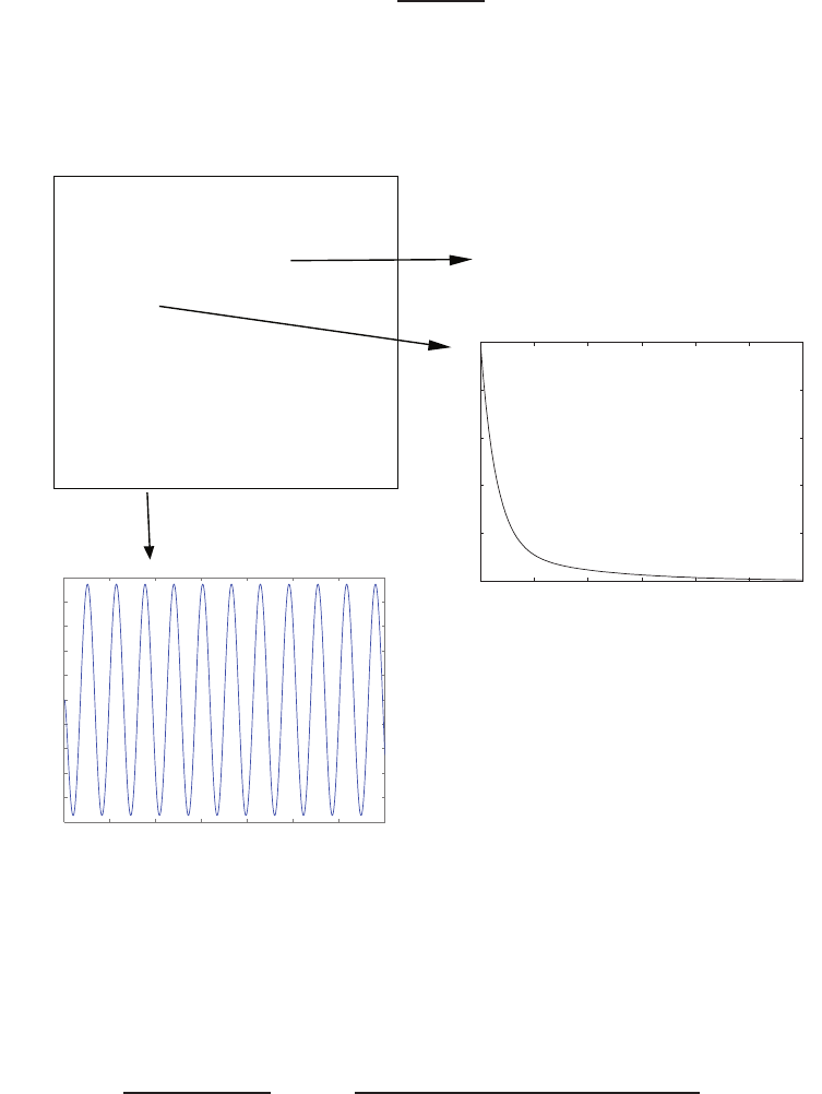
Computer Problems 175

(b) The response of the system to the sinusoidal disturbance

N(s) = 100

s2+ 100

is shown in Figure CP4.9b.

the frequency is 10 rad/sec (see Figure CP4.9b).

0 1 2 3 4 5 6 7

−0.1

−0.08

−0.06

−0.04

−0.02

0.02

0.04

0.06

0.08

0.1

Step Response

Time (sec)

Amplitude

0 0.02 0.04 0.06 0.08 0.1 0.12

Step Response

Time

(

sec

)

Amplitude

% Part (a)

ng=10*[1 0]; dg=[1 100]; sysg=tf(ng,dg);

nh=[5]; dh=[1 50]; sysh=tf(nh,dh);

sys=feedback(sysg,sysh)

figure(1)

step(sys)

% Part (b)

sysn=-feedback(sysg*sysh,1)

syss=tf([100],[1 0 100]);

% This is the sinusoidal input

figure(2)

t=[0:0.001:7];

step(syss*sysn,t)

Transfer function:

10 s^2 + 500 s

------------------

s^2 + 200 s + 5000

(a)

(b)

FIGURE CP4.9

(a) Unit step response. (b) Response to sinusoidal noise input at ω= 10 rad/sec.

CP4.10 (a) The closed-loop transfer function is

T(s) = Gc(s)G(s)

1 + G(s)Gc(s)R(s) = K(s+ 1)

(s+ 15)(s2+s+ 6.5) + K(s+ 1)R(s).

(b) The step responses are shown in Figure CP4.10a.

from the publisher prior to any prohibited reproduction, storage in a retrieval system, or transmission in any form or by any means, electronic, mechanical, photocopying,

recording, or likewise. For information regarding permission(s), write to: Rights and Permissions Department, Pearson Education, Inc., Upper Saddle River, NJ 07458.

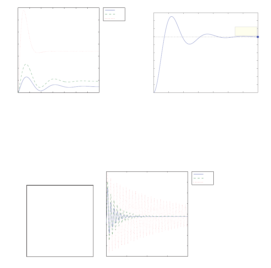
176 CHAPTER 4 Feedback Control System Characteristics

The steady-state value is 0.14.

Step Response

Time (sec)

Amplitude

0 1 2 3 4 5 6 7

0.02

0.04

0.06

0.08

0.1

0.12

0.14

0.16

0.18

0.2

System: syscl

Final Value: 0.14

(a) (b)

01234567

0.1

0.2

0.3

0.4

0.5

0.6

0.7

Time (s)

Step response

K=5

K=10

K=50

FIGURE CP4.10

(a) Unit step responses for K= [5,10,50]. (b) Disturbance unit step response.

CP4.11 The m-ﬁle is shown in Figure CP4.11a and the step responses in Fig-

ure CP4.11b.

0 5 10 15 20

−3

−2

−1

Time (s)

Step response

K=10

K=12

K=15

K=[10, 12, 15];

t=[0:0.1:20];

ng=[20]; dg=[1 4.5 64]; sysg=tf(ng,dg);

nh=[1]; dh=[1 1]; sysh=tf(nh,dh);

for i=1:length(K)

sys=K(i)*sysg;

syscl=feedback(sys,sysh)

y(:,i)= step(syscl,t);

end

plot(t,y(:,1),t,y(:,2),'--',t,y(:,3),':')

xlabel('Time (s)')

ylabel('Step response')

legend('K=10','K=12','K=15',-1)

(a) (b)

FIGURE CP4.11

(a) M-ﬁle script. (b) Unit step responses for K= [10,12,15].

from the publisher prior to any prohibited reproduction, storage in a retrieval system, or transmission in any form or by any means, electronic, mechanical, photocopying,

recording, or likewise. For information regarding permission(s), write to: Rights and Permissions Department, Pearson Education, Inc., Upper Saddle River, NJ 07458.

C H A P T E R 5

The Performance of Feedback

Control Systems

Exercises

E5.1 For a zero steady-state error, when the input is a step we need one inte-

gration, or a type 1 system. A type 2 system is required for ess = 0 for a

ramp input.

E5.2 (a) The closed-loop transfer function is

T(s) = Y(s)

R(s)=G(s)

1 + G(s)=240

(s+ 4)(s+ 6) + 240 =240

s2+ 2ζωns+ω2

The steady-state error is given by

ess =A

1 + Kp

where R(s) = A/s and

Kp= lim

s→0G(s) = 240

24 = 10 .

Therefore,

ess =A

11 .

(b) The closed-loop system is a second-order system with natural fre-

quency

ωn=√264 ,

177

from the publisher prior to any prohibited reproduction, storage in a retrieval system, or transmission in any form or by any means, electronic, mechanical, photocopying,

recording, or likewise. For information regarding permission(s), write to: Rights and Permissions Department, Pearson Education, Inc., Upper Saddle River, NJ 07458.

178 CHAPTER 5 The Performance of Feedback Control Systems

and damping ratio

ζ=10

2√264 = 0.31 .

The percent overshoot is thus computed to be

P.O. = 100e−πζ/√1−ζ2= 36% .

E5.3 The closed-loop transfer function is

Y(s)

I(s)=G(s)

1 + G(s)=K

s(s+ 14) + K=K

s2+ 14s+K.

Utilizing Table 5.6 in Dorf & Bishop, we ﬁnd that the optimum coeﬃcients

are given by

s2+ 1.4ωns+ω2

We have

s2+ 14s+K ,

so equating coeﬃcients yields ωn= 10 and K=ω2

n= 100 .We can also

compute the damping ratio as

ζ=14

2ωn

= 0.7.

Then, using Figure 5.8 in Dorf & Bishop, we ﬁnd that P.O. ≈5%.

E5.4 (a) The closed-loop transfer function is

T(s) = G(s)

1 + G(s)=2(s+ 8)

s2+ 6s+ 16 .

(b) We can expand Y(s) in a partial fraction expansion as

Y(s) = 2(s+ 8)

(s2+ 6s+ 16)

s=A1

s−s+ 4

s2+ 6s+ 16.

Taking the inverse Laplace transform (using the Laplace transform

tables), we ﬁnd

y(t) = A[1 −1.07e−3tsin(√7t+ 1.21)] .

from the publisher prior to any prohibited reproduction, storage in a retrieval system, or transmission in any form or by any means, electronic, mechanical, photocopying,

recording, or likewise. For information regarding permission(s), write to: Rights and Permissions Department, Pearson Education, Inc., Upper Saddle River, NJ 07458.

Exercises 179

ωn= 4. Thus,

ζωn

3= 2.67 ,

where a= 8. From Figure 5.13(a) in Dorf & Bishop, we ﬁnd (approx-

imately) that P.O. = 4% .

(d) This is a type 1 system, thus the steady-state error is zero and y(t)→

Aas t→ ∞.

E5.5 The closed-loop transfer function is

Y(s)

R(s)=K

s2+ 4s+K.

Utilizing Table 5.6 in Dorf & Bishop, we ﬁnd that the optimum coeﬃcients

are given by

s2+ 1.4ωns+ω2

We have

s2+ 4s+K ,

so equating coeﬃcients yields ωn= 2.86 and K=ω2

n= 8.16 .We can

also compute the damping ratio as

ζ=4

2ωn

= 0.7.

Then, using Figure 5.8 in Dorf & Bishop, we ﬁnd that P.O. ≈5%.

E5.6 (a) The closed-loop transfer function is

T(s) = Y(s)

R(s)=G(s)

1 + GH(s)=100

s2+ 100Ks + 100 ,

where H(s) = 1 + Ks and G(s) = 100/s2. The steady-state error is

computed as follows:

ess = lim

s→0s[R(s)−Y(s)] = lim

s→0s[1 −T(s)] A

= lim

s→0"1−

100

1 + 100

s2(1 + Ks)#A

s=KA .

(b) From the closed-loop transfer function, T(s), we determine that ωn=

from the publisher prior to any prohibited reproduction, storage in a retrieval system, or transmission in any form or by any means, electronic, mechanical, photocopying,

recording, or likewise. For information regarding permission(s), write to: Rights and Permissions Department, Pearson Education, Inc., Upper Saddle River, NJ 07458.

180 CHAPTER 5 The Performance of Feedback Control Systems

10 and

ζ=100K

2(10) = 5K .

We want to choose Kso that the system is critically damped, or

ζ= 1.0. Thus,

K=1

5= 0.20 .

The closed-loop system has no zeros and the poles are at

s1,2=−50K±10p25K2−1.

The percent overshoot to a step input is

P.O. = 100e

−5πK

√1−25K2for 0 < K < 0.2

and P.O. = 0 for K > 0.2.

E5.7 The closed-loop transfer function is

T(s) = Y(s)

R(s)=KG(s)

1 + KG(s)=K(s+ 2)

s(s+ 1) + K(s+ 2) =K(s+ 2)

s2+s(K+ 1) + 2K.

Therefore, ωn=√2Kand ζ=K+1

2√2K. So,

ζωn

K+ 1 .

From Figure 5.13a in Dorf & Bishop, we determine that

ζωn≈1.5

when ζ= 0.707. Thus, solving for Kyields

K+ 1 = 1.5

or K= 1.67.

E5.8 The pole-zero map is shown in Figure E5.8. Since the dominant poles are

at s=−2±2.45iwe have a damping ratio ζ= 0.63. We estimate the

percent overshoot to be

P.O. = 100e−πζ/√1−ζ2= 7.69%

The step response is shown in Figure E5.8b. The actual overshoot is 8%.

from the publisher prior to any prohibited reproduction, storage in a retrieval system, or transmission in any form or by any means, electronic, mechanical, photocopying,

recording, or likewise. For information regarding permission(s), write to: Rights and Permissions Department, Pearson Education, Inc., Upper Saddle River, NJ 07458.

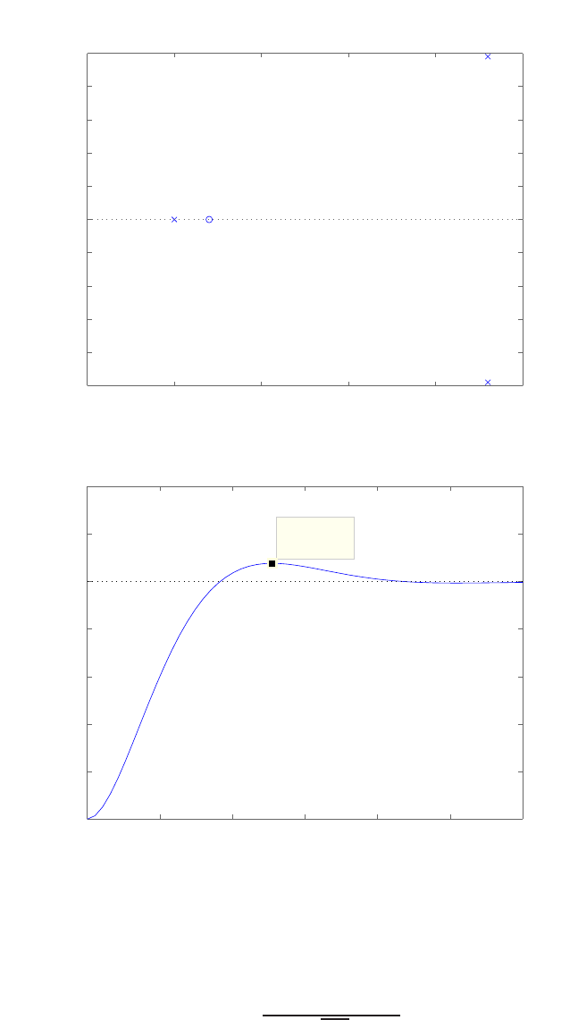
Exercises 181

Pole−Zero Map

Real Axis

Imaginary Axis

−25 −20 −15 −10 −5 0

−2.5

−2

−1.5

−1

−0.5

0.5

1.5

2.5

0 0.5 1 1.5 2 2.5 3

0.2

0.4

0.6

0.8

1.2

1.4

System: sys

Time (sec): 1.28

Amplitude: 1.08

Step Response

Time (sec)

Amplitude

FIGURE E5.8

(a) Pole-zero map. (b) Unit step response.

E5.9 (a) The closed-loop transfer function is

T(s) = K

s2+√2Ks +K.

from the publisher prior to any prohibited reproduction, storage in a retrieval system, or transmission in any form or by any means, electronic, mechanical, photocopying,

recording, or likewise. For information regarding permission(s), write to: Rights and Permissions Department, Pearson Education, Inc., Upper Saddle River, NJ 07458.

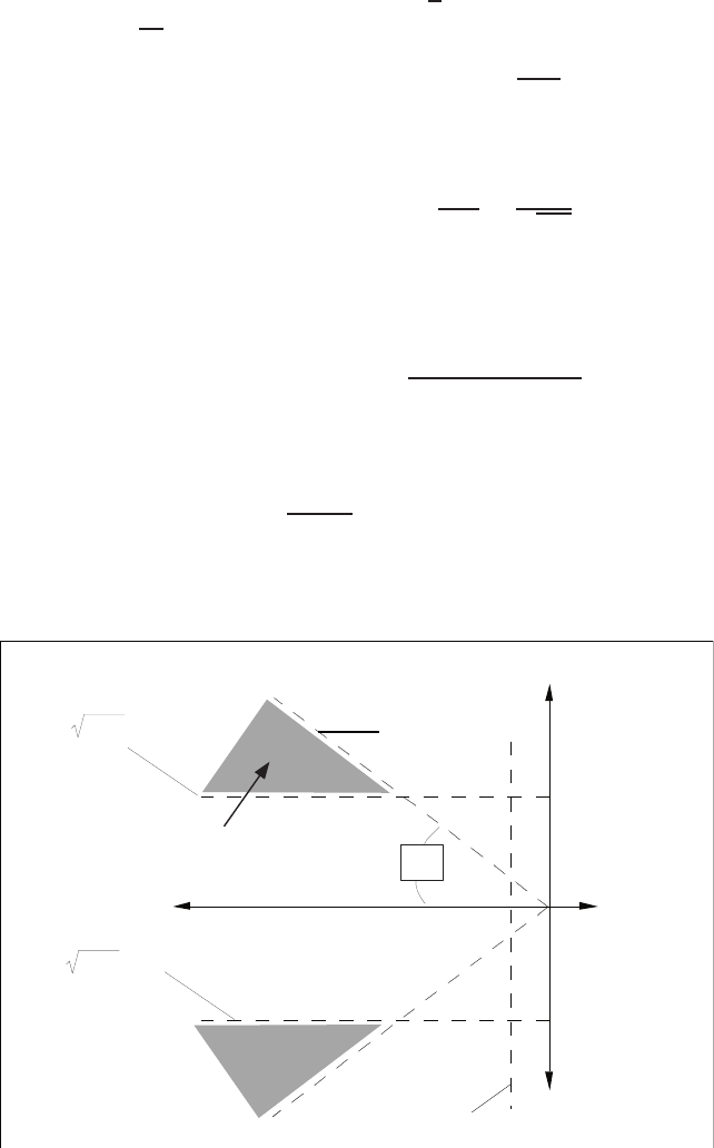
182 CHAPTER 5 The Performance of Feedback Control Systems

The damping ratio is ζ=√2/2 and the natural frequency is ωn=

√K. Therefore, we compute the percent overshoot to be

P.O. = 100e−πζ/√1−ζ2= 4.3%

for ζ= 0.707. The settling time is estimated via

Ts=4

ζωn

√2K.

(b) The settling time is less than 1 second whenever K > 32.

E5.10 The second-order closed-loop transfer function is given by

T(s) = ω2

s2+ 2ζωns+ω2

From the percent overshoot speciﬁcation, we determine that P.O. ≤5%

implies ζ≥0.69. From the settling time speciﬁcation, we ﬁnd that Ts<4

implies ωnζ > 1. And ﬁnally, from the peak time speciﬁcation we have

Tp<1 implies ωnp1−ζ2> π. The constraints imposed on ζand ωnby

the performance speciﬁcations deﬁne the permissible area for the poles of

T(s), as shown in Figure E5.10.

Re(s)

Im(s)

desired

region

for poles

z wn = -1

wn1-z2= - P

wn1-z2=P

46o

z = 0.69

FIGURE E5.10

Permissible area for poles of T(s).

from the publisher prior to any prohibited reproduction, storage in a retrieval system, or transmission in any form or by any means, electronic, mechanical, photocopying,

recording, or likewise. For information regarding permission(s), write to: Rights and Permissions Department, Pearson Education, Inc., Upper Saddle River, NJ 07458.

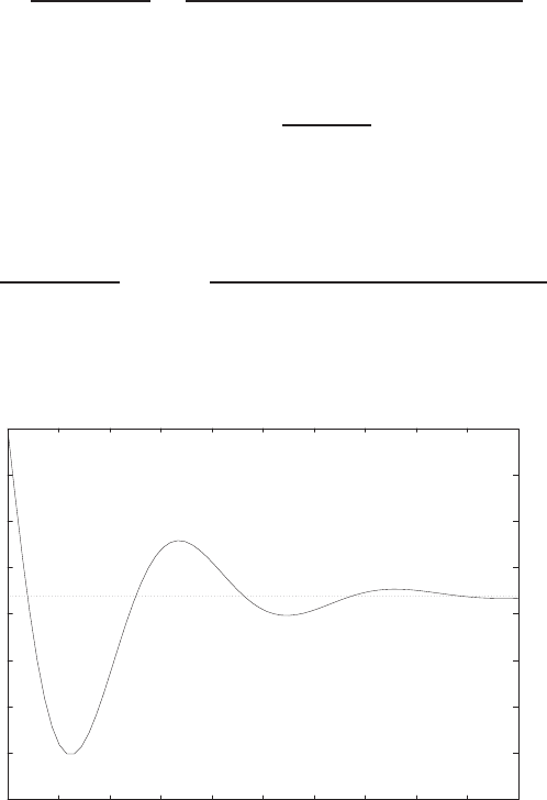
Exercises 183

E5.11 The system is a type 1. The error constants are

Kp=∞and Kv= 1.0.

Therefore, the steady-state error to a step input is 0; the steady-state

error to a ramp input is 1.0A0, where A0is the magnitude (slope) of the

ramp input.

E5.12 (a) The tracking error is given by

E(s) = R(s)

1 + GcG(s)=(s+ 9)(s+ 2)(s+ 4)

(s+ 9)(s+ 2)(s+ 4) + K(s+ 6)R(s).

The steady-state tracking error (with R(s) = 1/s) is

lim

s→0sE(s) = 72

72 + 6K.

We require ess <0.05, so solving for Kyields K > 228.

(b) The tracking error due to the disturbance is

E(s) = −G(s)

1 + GcG(s)Td(s) = −(s+ 9)(s+ 6)

(s+ 9)(s+ 2)(s+ 4) + K(s+ 6)Td(s).

The tracking error is shown in Figure E5.12.

-0.08

-0.07

-0.06

-0.05

-0.04

-0.03

-0.02

-0.01

0 0.1 0.2 0.3 0.4 0.5 0.6 0.7 0.8 0.9 1

Time (secs)

Amplitude

FIGURE E5.12

Tracking error due a step disturbance.

from the publisher prior to any prohibited reproduction, storage in a retrieval system, or transmission in any form or by any means, electronic, mechanical, photocopying,

recording, or likewise. For information regarding permission(s), write to: Rights and Permissions Department, Pearson Education, Inc., Upper Saddle River, NJ 07458.

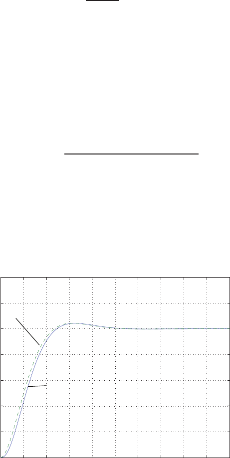
184 CHAPTER 5 The Performance of Feedback Control Systems

E5.13 The system is a type 0. The error constants are Kp= 0.4 and Kv= 0.

The steady-state error to a ramp input is ∞. The steady-state error to a

step input is

ess =1

1 + Kp

= 0.71.

E5.14 (a) The tracking error is given by

E(s) = [1 −T(s)] R(s).

The steady-state tracking error (with R(s) = 1/s) is

ess = lim

s→0s[1 −T(s)] R(s) = lim

s→0[1 −T(s)] = 1 −T(0) .

The closed-loop transfer function is

T(s) = K(s+ 0.1)

s(s+ 0.1)(s+ 2) + K(s+ 3) ,

and T(0) = 0.033. Therefore, ess = 1 −T(0) = 0.967.

(b) Use Gp(s) = 30. Then,

ess = lim

s→0s[1 −T(s)Gp(s)] R(s) = 1−lim

s→0T(s)Gp(s) = 1−30 T(0) = 0 .

E5.15 The plot of y(t) is shown in Figure E5.15.

0 0.2 0.4 0.6 0.8 1 1.2 1.4 1.6 1.8 2

0.2

0.4

0.6

0.8

1.2

1.4

Time (sec)

y(t)

Response using only dominate poles

Actual response

FIGURE E5.15

Plot of y(t)with T(s)(solid line) and approximate Ta(s)(dashed line).

from the publisher prior to any prohibited reproduction, storage in a retrieval system, or transmission in any form or by any means, electronic, mechanical, photocopying,

recording, or likewise. For information regarding permission(s), write to: Rights and Permissions Department, Pearson Education, Inc., Upper Saddle River, NJ 07458.

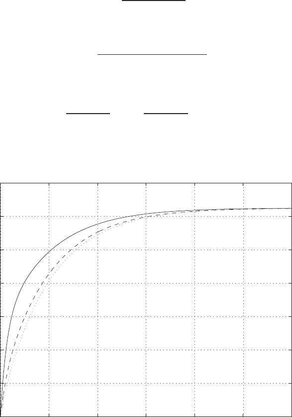
Exercises 185

Using the dominant poles, the approximate closed-loop transfer function

Ta(s) = 50

s2+ 10s+ 50 .

The actual transfer function is

T(s) = 500

(s+ 10)(s2+ 10s+ 50) .

E5.16 The partial fraction expansion is

y(t) = −10(z−1)

7ze−t+10(z−8)

56ze−8t+ 1.25 .

The plot of y(t) for z= 2,4,6 is shown in Figure E5.16.

0 1 2 3 4 5 6

0.2

0.4

0.6

0.8

1.2

1.4

Time (sec)

y(t)

z=2 (solid) & z=4 (dashed) & z=6 (dotted)

FIGURE E5.16

Plot of y(t)for z=2, 4, 6.

E5.17 The desired pole locations for the 5 diﬀerent cases are shown in Fig-

ure E5.17.

from the publisher prior to any prohibited reproduction, storage in a retrieval system, or transmission in any form or by any means, electronic, mechanical, photocopying,

recording, or likewise. For information regarding permission(s), write to: Rights and Permissions Department, Pearson Education, Inc., Upper Saddle River, NJ 07458.

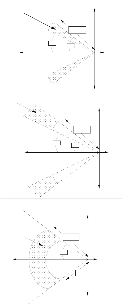
186 CHAPTER 5 The Performance of Feedback Control Systems

Re(s)

Im(s)

desired

region

for poles

37 o

wn = 10

(a) 0.6 < z < 0.8 and wn <10

Re(s)

Im(s)

desired

region

for poles

45 o

wn = 10

(b) 0.5 < z < 0.707 and wn >10

Re(s)

Im(s)

desired

region

for poles

wn = 10

wn = 5

FIGURE E5.17

Desired pole locations.

from the publisher prior to any prohibited reproduction, storage in a retrieval system, or transmission in any form or by any means, electronic, mechanical, photocopying,

recording, or likewise. For information regarding permission(s), write to: Rights and Permissions Department, Pearson Education, Inc., Upper Saddle River, NJ 07458.

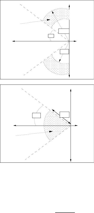
Exercises 187

(d) 0.707 > z and 5 < wn <10

Re(s)

Im(s)

desired

region

for poles

wn = 5

wn = 10

(e) 0.6 < z and wn < 6

Re(s)

Im(s)

desired

region

for poles

own = 6

FIGURE E5.17

CONTINUED: Desired pole locations.

E5.18 The output is given by

Y(s) = T(s)R(s) = KG(s)

1 + G(s)R(s).

When K= 1, the steady-state error is

ess = 0.2

which implies that

lim

s→0sY (s) = 0.8.

from the publisher prior to any prohibited reproduction, storage in a retrieval system, or transmission in any form or by any means, electronic, mechanical, photocopying,

recording, or likewise. For information regarding permission(s), write to: Rights and Permissions Department, Pearson Education, Inc., Upper Saddle River, NJ 07458.

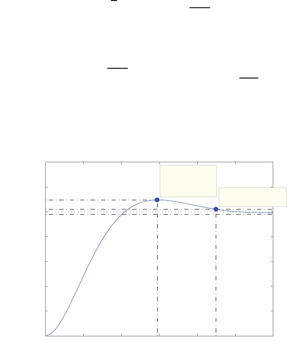
188 CHAPTER 5 The Performance of Feedback Control Systems

Since we want ess = 0, it follows that

lim

s→0sY (s) = 1 ,

0.8K= 1 .

Therefore, K= 1.25.

E5.19 (a) The characteristic equation is

s2= 2ζωns+ω2

n=s2+ 3.17s+ 7 = 0 ,

from which it follows that

ωn=√7 = 2.65, ζ =3.17

2ωn

= 0.6.

Therefore, we compute the percent overshoot and the estimated set-

tling time to be

P.O. = 100e−πζ/√1−ζ2= 9.53% and Ts=4

ζωn

= 2.5 s .

(b) The unit step response is shown in Figure E5.19.

Step Response

Time (sec)

Amplitude

0 0.5 1 1.5 2 2.5 3

0.2

0.4

0.6

0.8

1.2

1.4

System: sys

Peak amplitude: 1.1

Overshoot (%): 9.53

At time (sec): 1.47 System: sys

Settling Time (sec): 2.25

FIGURE E5.19

Unit step response.

from the publisher prior to any prohibited reproduction, storage in a retrieval system, or transmission in any form or by any means, electronic, mechanical, photocopying,

recording, or likewise. For information regarding permission(s), write to: Rights and Permissions Department, Pearson Education, Inc., Upper Saddle River, NJ 07458.

Exercises 189

E5.20 (a) The closed-loop transfer function is

T(s) = K

s2+√2Ks +K.

The damping ratio is

ζ=√2

and the natural frequency is ωn=√K. Therefore, we compute the

percent overshoot to be

P.O. = 100e−πζ/√1−ζ2= 4.3%

for ζ= 0.707. The settling time is estimated via

Ts=4

ζωn

√2K.

(b) The settling time is less than 1 second whenever K > 32.

from the publisher prior to any prohibited reproduction, storage in a retrieval system, or transmission in any form or by any means, electronic, mechanical, photocopying,

recording, or likewise. For information regarding permission(s), write to: Rights and Permissions Department, Pearson Education, Inc., Upper Saddle River, NJ 07458.

190 CHAPTER 5 The Performance of Feedback Control Systems

Problems

P5.1 (a) The system error is

E(s) = 1

1 + KaKm

sτm+1

R(s)

where

R(s) = 25o/sec

So,

lim

t→0e(t) = lim

s→0sE(s) = 25

1 + KaKm

(b) If we desire ess ≤1o/sec, then

25o/s

1 + KaKm≤1o/sec ,

and solving for KaKmyields

KaKm≥24 .

T(s) = Vb(s)

Vc(s)=KaKm

sτm+ 1 + KaKm

The step response of the system (i.e. vc(t) = A) is

vb(t) = AKaKm

1 + KaKm1−e

−(KaKm+1)

τmt.

So, at settling time, we have

1−e

−(1+KaKm)

τmt≥0.98 ,

where τm= 0.4. Setting t= 0.03 and solving for KaKmyields

KaKm≥52 .

P5.2 (a) The settling time speciﬁcation

Ts=4

ζωn

<0.6

from the publisher prior to any prohibited reproduction, storage in a retrieval system, or transmission in any form or by any means, electronic, mechanical, photocopying,

recording, or likewise. For information regarding permission(s), write to: Rights and Permissions Department, Pearson Education, Inc., Upper Saddle River, NJ 07458.

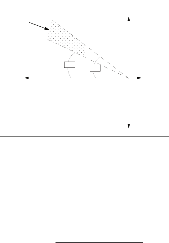
Problems 191

is used to determine that ζωn>6.67. The P.O. < 20% requirement

is used to determine

ζ < 0.45 which implies θ < 63o

and the P.O. > 10% requirement is used to determine

ζ > 0.60 which implies θ > 53o,

since cos θ=ζ. The desired region for the poles is shown in Fig-

ure P5.2.

Re(s)

Im(s)

s = -6.67

63o

desired

region

for poles

53o

FIGURE P5.2

Desired region for pole placement.

(b) The third root should be at least 10 times farther in the left half-

plane, so

|r3| ≥ 10|ζωn|= 66.7.

and ζωn= 6.67, we determine that ωn= 14.8. So, the closed-loop

transfer function is

T(s) = 66.7(219.7)

(s+ 66.7)(s2+ 13.3s+ 219.7) ,

where the gain K= (66.7)(219.7) is chosen so that the steady-state

from the publisher prior to any prohibited reproduction, storage in a retrieval system, or transmission in any form or by any means, electronic, mechanical, photocopying,

recording, or likewise. For information regarding permission(s), write to: Rights and Permissions Department, Pearson Education, Inc., Upper Saddle River, NJ 07458.

192 CHAPTER 5 The Performance of Feedback Control Systems

tracking error due to a step input is zero. Then,

T(s) = G(s)

1 + G(s),

G(s) = T(s)

1−T(s).

P5.3 Given the input

R(s) = 1

s3,

we compute the steady-state error as

ess = lim

s→0s1

1 + G(s)1

s3= lim

s→01

s2G(s)= lim

s→0



s2K

s2

=1

Since we require that ess ≤0.5 cm, we determine

K≥2.

P5.4 (a) The closed-loop transfer function is

T(s) = G(s)

1 + G(s)=K

s2+ 2s+K=ω2

s2+ 2ζωns+ω2

Thus,

ωn=√Kand ζ= 1/ωn= 1/√K .

Our percent overshoot requirement of 5% implies that ζ= 1/√2 ,

which in turn implies that ωn=√2. However, the corresponding

time to peak would be

Tp=4.4

√2= 3.15 .

Our desired Tp= 1.1—we cannot meet both speciﬁcation simultane-

ously.

(b) Let Tp= 1.1∆ and P.O. = 0.05∆, where ∆ is the relaxation factor

to be determined. We have that K=ω2

nand ζωn= 1, so

ζ=1

√K.

from the publisher prior to any prohibited reproduction, storage in a retrieval system, or transmission in any form or by any means, electronic, mechanical, photocopying,

recording, or likewise. For information regarding permission(s), write to: Rights and Permissions Department, Pearson Education, Inc., Upper Saddle River, NJ 07458.

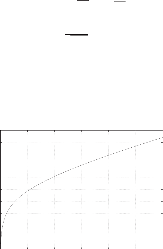
Problems 193

Thus,

P.O. =e−πζ/√1−ζ2=e−π/√K−1.

Also,

Tp=π

√K−1= 1.1∆ .

Therefore, from the proceeding two equations we determine that

P.O. = 0.05∆ = e−1.1∆ .

Solving for ∆ yields

f(∆) = ln ∆ + ln(0.05) + 1.1∆ = 0 .

The plot of f(∆) versus ∆ is shown in Figure P5.4. From the plot we

-8

-7

-6

-5

-4

-3

-2

-1

0 0.5 1 1.5 2 2.5 3

f(D)

=2.07

FIGURE P5.4

Solving for the zeros of f.

see that ∆ = 2.07 results in f(∆) = 0. Thus,

P.O. = 0.05∆ = 10%

Tp= 1.1∆ = 2.3 sec.

from the publisher prior to any prohibited reproduction, storage in a retrieval system, or transmission in any form or by any means, electronic, mechanical, photocopying,

recording, or likewise. For information regarding permission(s), write to: Rights and Permissions Department, Pearson Education, Inc., Upper Saddle River, NJ 07458.

194 CHAPTER 5 The Performance of Feedback Control Systems

So, we can meet the speciﬁcations if they are relaxed by a factor of

about 2 (i.e. ∆ = 2.07).

P5.5 (a) The closed-loop transfer function is

T(s) = K1K2(s+ 1)

s2+K1K2s+K1K2

A percent overshoot less than 5% implies ζ≥0.69. So, choose ζ=

0.69. Then set 2ζωn=K1K2and ω2

n=K1K2. Then

2(0.69)ωn=ω2

and solving for ωnyields

ωn= 1.38 .

Therefore K1K2=ω2

n= 1.9. When K1K2≥1.9 it follows that

ζ≥0.69.

(b) We have a type 2 system, so the steady-state tracking error to both

a step and ramp input is zero.

s2+ 1.4ωns+ω2

n= 0 .

For a ramp input, the optimum ITAE characteristic equation is

s2+ 3.2ωns+ω2

n= 0 .

Thus, K1K2=ω2

n= 3.2ωn. So, ωn= 3.2 and K1K2= 10.24.

P5.6 We have a ramp input, r(t) = t. So

Kv= lim

s→0sG(s) = lim

s→0s75(s+ 1)

s(s+ 5)(s+ 25) =75

125 = 0.6,

and

ess =|R|

0.6= 1.67 .

P5.7 (a) The closed-loop transfer function is

T(s) = K1K2

Is2+K1K2K3s+K1K2

The steady-state tracking error for a ramp input is

ess = lim

s→0sE(s) = lim

s→0s(1 −T(s))R(s) = lim

s→0s(1 −T(s)) 1

from the publisher prior to any prohibited reproduction, storage in a retrieval system, or transmission in any form or by any means, electronic, mechanical, photocopying,

recording, or likewise. For information regarding permission(s), write to: Rights and Permissions Department, Pearson Education, Inc., Upper Saddle River, NJ 07458.

Problems 195

= lim

s→0

Is +K1K2K3

Is2+K1K2K3s+K1K2

=K3.

But we desire ess = 0.01 m, so K3= 0.01.

(b) For P.O. = 10%, we have ζ= 0.6. Also,

2ζωn=0.01K1K2

and

ω2

n=K1K2

25 .

Thus, solving for K1K2yields K1K2= 36 ×104.

P5.8 (a) The closed-loop transfer function is

T(s) = P(s)

R(s)=G(s)/s

1 + G(s)H(s)/s =20

s(s+ 40) .

Therefore, the closed-loop system time constant is τ= 1/40 sec.

(b) The transfer function from Td(s) to the output P(s) is

P(s)

Td(s)=−G(s)

1 + G(s)H(s)/s =−20

s+ 40 .

The response to a unit step disturbance is

p(t) = −1

2(1 −e−40t).

At settling time, p(t) = 0.98pss =−0.49. Thus, solving for t(= Ts)

we determine that Ts= 0.098 sec.

P5.9 We need to track at the rate

ω=v

r=16000

2500 = 1.78 ×10−3radians/sec .

The desired steady-state tracking error is

ess ≤1

10 degree = 0.1754 ×10−2rad .

Therefore, with

ess =|ω|

from the publisher prior to any prohibited reproduction, storage in a retrieval system, or transmission in any form or by any means, electronic, mechanical, photocopying,

recording, or likewise. For information regarding permission(s), write to: Rights and Permissions Department, Pearson Education, Inc., Upper Saddle River, NJ 07458.

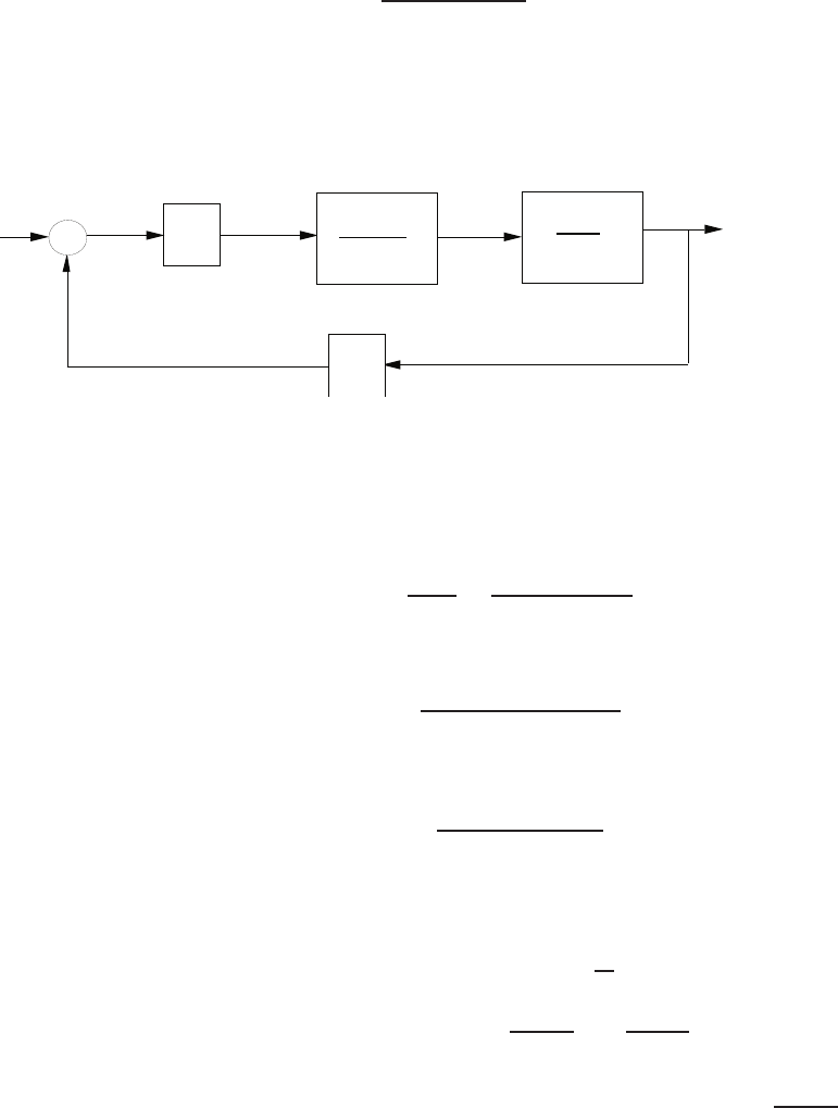
196 CHAPTER 5 The Performance of Feedback Control Systems

we compute Kvas

Kv=1.78 ×10−3

0.1754 ×10−2= 1.02 .

This assumes that the system is type 1.

P5.10 (a) The armature controlled DC motorblock diagram is shown in Fig-

ure P5.10.

Ra+ L as

J s + b

w(s)

R(s )

back emf

amplier

FIGURE P5.10

Armature controlled DC motor block diagram.

(b) The closed-loop transfer function is

T(s) = ω(s)

R(s)=KG(s)

1 + KKbG(s),

where

G(s) = Km

(Ra+Las)(Js +b).

Thus,

T(s) = K

s2+ 2s+ 1 + K,

where Ra=La=J=b=Kb=Km= 1. The steady-state tracking

error is

ess = lim

s→0s(R(s)−Y(s)) = lim

s→0sA

s(1 −T(s))

=A(1 −T(0)) = 1−K

1 + K=A

1 + K.

our characteristic polynomial we have 2ζωn= 2 and ωn=√1 + K.

Solving for ωnyields ωn= 2, thus K= 3.

from the publisher prior to any prohibited reproduction, storage in a retrieval system, or transmission in any form or by any means, electronic, mechanical, photocopying,

recording, or likewise. For information regarding permission(s), write to: Rights and Permissions Department, Pearson Education, Inc., Upper Saddle River, NJ 07458.

Problems 197

P5.11 (a) The closed-loop transfer function is

T(s) = Y(s)

R(s)=K

s+K.

To include the initial condition, we obtain the diﬀerential equation:

˙y(t) + Ky(t) = Kr(t).

Taking the Laplace transform yields:

sY (s)−y(to) + KY (s) = KA

s,

where y(to) = Q. Computing the inverse Laplace transform, L−1{Y(s)}

yields

y(t) = A(1 −e−Kt) + Qe−Kt .

Also, the tracking error is given by

e(t) = A−y(t) = e−Kt(A−Q).

Thus, the performance index, Iis determined to be (for K > 0)

I=Z∞

(A−Q)2e−2Ktdt = (A−Q)21

−2Ke−2Kt

∞

=(A−Q)2

2K.

(b) The minimum I is obtained when K=∞, which is not practical.

saturate. For example, if K= 50, then

I=(A−Q)2

100 .

P5.12 The optimum ITAE transfer function for a ramp input is

T(s) = 3.25ω2

ns+ω3

s3+ 1.75ωns+ 3.25ω2

ns+ω3

The steady-state tracking error, ess = 0, for a ramp input. The step

response is shown in Figure P5.12 for ωn= 10. The percent overshoot is

P.O. = 39%, and the settling time is Ts= 0.72 s .

from the publisher prior to any prohibited reproduction, storage in a retrieval system, or transmission in any form or by any means, electronic, mechanical, photocopying,

recording, or likewise. For information regarding permission(s), write to: Rights and Permissions Department, Pearson Education, Inc., Upper Saddle River, NJ 07458.

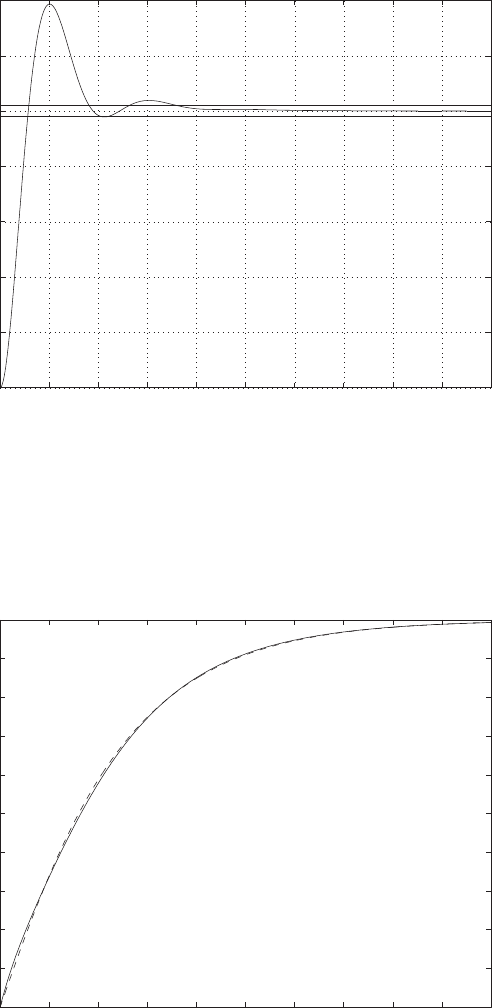
198 CHAPTER 5 The Performance of Feedback Control Systems

0 0.2 0.4 0.6 0.8 1 1.2 1.4 1.6 1.8 2

0.2

0.4

0.6

0.8

1.2

1.4

PO=39%

Ts=0.72s

time (sec)

y(t)

FIGURE P5.12

Step input system response.

P5.13 The step responses for the actual system and the approximate system

are shown in Figure P5.13. It can be seen that the responses are nearly

identical.

0 0.5 1 1.5 2 2.5 3 3.5 4 4.5 5

0.1

0.2

0.3

0.4

0.5

0.6

0.7

0.8

0.9

Time (sec)

y(t)

FIGURE P5.13

Closed-loop system step response: Actual T(s) (solid line) and second-order approximation

(dashed line).

from the publisher prior to any prohibited reproduction, storage in a retrieval system, or transmission in any form or by any means, electronic, mechanical, photocopying,

recording, or likewise. For information regarding permission(s), write to: Rights and Permissions Department, Pearson Education, Inc., Upper Saddle River, NJ 07458.

Problems 199

P5.14 Consider

L(s) = 2(c1s+ 1)

(s+ 1)(s+ 2) .

After cancellation of like factors, we compute H(s)/L(s),

H(s)

L(s)=s3+ 7s2+ 24s+ 24

(s+ 3)(s+ 4)2(c1s+ 1) .

Therefore,

M(s) = s3+ 7s2+ 24s+ 24 ,and

∆(s) = 2[c1s3+ (7c1+ 1)s2+ (12c1+ 7)s+ 12] .

Then, following the procedure outlined in Section 5.10, we have

Mo(0) = 24, M1(0) = 24, M2(0) = 14, M3(0) = 6,and

∆0(0) = 24,∆1(0) = (12c1+ 7)2,∆2(0) = 2(2·(7c1+ 1)),∆3(0) = 12c1.

For q= 1:

M2= 240,and

∆2= 4[144c2

1+ 25] .

Then, equating ∆2and M2, we ﬁnd c1,

c1= 0.493 .

So,

L(s) = 2(0.493s+ 1)

(s+ 1)(s+ 2) =0.986s+ 2

s2+ 3s+ 2 =0.986(s+ 2.028)

(s+ 1)(s+ 2) .

P5.15 The closed-loop transfer function is

T(s) = K(s+ 1)

(s+ 4)(s2+s+ 10) + K(s+ 1) .

The percent overshoot as function of the gain, K, is shown in Figure P5.15.

It can be seen that the percent overshoot decreases as the gain increases

approaching a minimum around 85%. The larger the gain, the smaller the

percent overshoot. For a gain K≈250, we have essentially minimized the

percent overshoot.

from the publisher prior to any prohibited reproduction, storage in a retrieval system, or transmission in any form or by any means, electronic, mechanical, photocopying,

recording, or likewise. For information regarding permission(s), write to: Rights and Permissions Department, Pearson Education, Inc., Upper Saddle River, NJ 07458.

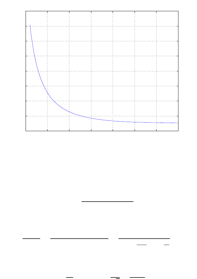
200 CHAPTER 5 The Performance of Feedback Control Systems

0 50 100 150 200 250 300 350

100

110

120

130

140

150

160

Percent Overshoot (%)

FIGURE P5.15

Percent overshoot versus the gain, K.

P5.16 The open-loop transfer function is

G(s) = 10

(s+ 1)(50Cs + 1) .

Deﬁne τ= 50C. Then, the closed-loop transfer function is

Vo(s)

Vin(s)=10

(s+ 1)(τs + 1) + 10 =10/τ

s2+τ+1

τs+11

With

ω2

n=11

τand ζ=1

√2=τ+ 1

2τωn

we can solve for τ, yielding

τ2−20τ+ 1 = 0 .

Therefore, τ= 19.95 and 0.05. For each value of τwe determine Cas

follows: τ= 19.95 = 50C, implies C= 0.399F, and τ= 0.05 = 50C,

implies C= 1mF .

from the publisher prior to any prohibited reproduction, storage in a retrieval system, or transmission in any form or by any means, electronic, mechanical, photocopying,

recording, or likewise. For information regarding permission(s), write to: Rights and Permissions Department, Pearson Education, Inc., Upper Saddle River, NJ 07458.

Problems 201

P5.17 (a) The closed-loop transfer function is

T(s) = Y(s)

R(s)=12K

s2+ 12s+ 12K.

The percent overshoot speciﬁcation P.O. ≤10% implies ζ≥0.59.

From the characteristic equation we ﬁnd that

ω2

n= 12Kand ζωn= 6 .

Solving for Kyields

2(0.59)√12K= 12 which implies that K= 8.6.

So, any gain in the interval 0 < K < 8.6 is valid. The settling time is

Ts= 4/ζωn= 4/6 seconds and satisﬁes the requirement. Notice that

Tsis not a function of K.

(b) The sensitivity is

K(s) = 1

1 + G(s)=s(s+ 12)

s2+ 12s+ 120

when K= 10.

K(0) = 0 .

(d) In this case, s=j2π·1 beat/sec = j2π. So, the sensitivity at s= 2πj

|ST

K(j2π)|=85.1084

110.31 = 0.77 .

P5.18 We select L(s) as

L(s) = 1

αs + 1 ,

then

H(s)

L(s)=6αs + 6

s3+ 6s2+ 11s+ 6 .

Therefore,

M(s) = 6αs + 6 ,

from the publisher prior to any prohibited reproduction, storage in a retrieval system, or transmission in any form or by any means, electronic, mechanical, photocopying,

recording, or likewise. For information regarding permission(s), write to: Rights and Permissions Department, Pearson Education, Inc., Upper Saddle River, NJ 07458.

202 CHAPTER 5 The Performance of Feedback Control Systems

and Mo(0) = 6, M1(0) = 6α,M2(0) = 0. Also,

∆(s) = s3+ 6s2+ 11s+ 6 ,

and ∆o(0) = 6 , ∆1(0) = 11 , ∆2(0) = 12. So, computing M2and ∆2

yields

M2= 36α2,and

∆2= 49 .

Finally, equating M2= ∆2yields 36α2= 49 ,or

α= 1.167 .

Thus,

L(s) = 1

1.167s+ 1 =0.857

s+ 0.857 .

P5.19 (a) The closed-loop transfer function is

T(s) = 8

s3+ 6s2+ 12s+ 8 .

(b) The second-order approximation is

L(s) = 1

d2s2+d1s+ 1 ,

where d1and d2are to be determined using the methods of Section

5.10 in Dorf & Bishop. Given

M(s) = 8d2s2+ 8d1s+ 8

∆(s) = s3+ 6s2+ 12s+ 8

we determine that

M2=−128d2+ 64d2

M4= 64d2

∆2= 48

∆4= 18 .

Equating M2= ∆2and M4= ∆4, and solving for d1and d2yields

d1= 1.35 and d2= 0.53 .

from the publisher prior to any prohibited reproduction, storage in a retrieval system, or transmission in any form or by any means, electronic, mechanical, photocopying,

recording, or likewise. For information regarding permission(s), write to: Rights and Permissions Department, Pearson Education, Inc., Upper Saddle River, NJ 07458.

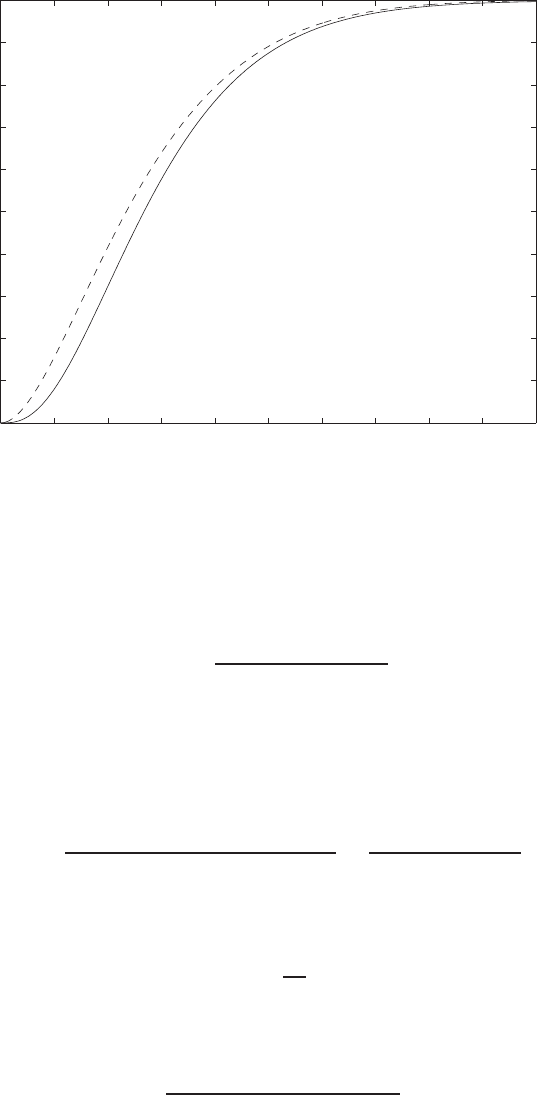
Problems 203

0 0.5 1 1.5 2 2.5 3 3.5 4 4.5 5

0.1

0.2

0.3

0.4

0.5

0.6

0.7

0.8

0.9

Time (sec)

y(t)

FIGURE P5.19

Closed-loop system step response: Actual T(s)(solid line) and second-order approximation

(dashed line).

Thus, the second-order approximation is

L(s) = 1

0.53s2+ 1.35s+ 1 .

mate system is shown in Figure P5.19.

P5.20 The steady-state error is

ess = lim

s→0

(s+ 5)(s+ 11) + K(1 −K1)

(s+ 5)(s+ 11) + K=55 + K(1 −K1)

55 + K.

To achieve a zero steady-state tracking error, select K1as follows:

K1= 1 + 55

P5.21 The closed-loop transfer function is

T(s) = s+a

s2+ (2k+a)s+ 2ak + 1 .

from the publisher prior to any prohibited reproduction, storage in a retrieval system, or transmission in any form or by any means, electronic, mechanical, photocopying,

recording, or likewise. For information regarding permission(s), write to: Rights and Permissions Department, Pearson Education, Inc., Upper Saddle River, NJ 07458.

204 CHAPTER 5 The Performance of Feedback Control Systems

(a) If R(s) = 1/s, we have the tracking error

E(s) = R(s)−Y(s) = [1 −T(s)]R(s)

E(s) = s2+ (2k+a−1)s+ 2ak + 1 −a

s2+ (2k+a)s+ 2ak + 1 ·1

From the ﬁnal value theorem we obtain

ess = lim

s→0sE(s) = 2ak + 1 −a

2ak + 1 .

Selecting k= (a−1)/(2a) leads to a zero steady-state error due to a

unit step input.

(b) To meet the percent overshoot speciﬁcation we desire ζ≥0.69. From

T(s) we ﬁnd ω2

n= 2ak + 1 and 2ζωn= 2k+a. Therefore, solving for

aand kyields

a= 1.5978 and k = 0.1871

when we select ζ= 0.78. We select ζ > 0.69 to account for the zero

in the closed-loop transfer function which will impact the percent

overshoot. With aand k, as chosen, we have

T(s) = s+ 1.598

s2+ 1.972s+ 1.598

and the step response yields P.O. ≈4%.

P5.22 The closed-loop transfer function is

T(s) = 2(2s+τ)

(s+ 0.2K)(2s+τ) + 4 .

(a) If R(s) = 1/s, we have the unit step response

Y(s) = 2(2s+τ)

(s+ 0.2K)(2s+τ) + 4

From the ﬁnal value theorem we obtain

yss = lim

s→0sY (s) = 2τ

0.2Kτ + 4 .

Selecting K= 10−20/τ leads to yss = 1 and a zero steady-state error

due to a unit step input.

from the publisher prior to any prohibited reproduction, storage in a retrieval system, or transmission in any form or by any means, electronic, mechanical, photocopying,

recording, or likewise. For information regarding permission(s), write to: Rights and Permissions Department, Pearson Education, Inc., Upper Saddle River, NJ 07458.

Problems 205

(b) The characteristic equation is

(s+ 0.2K)(2s+τ) + 4 = 2s2+ (0.4K+τ)s+ 0.2Kτ + 4 = 0 .

So, with K= 10 −20/τ , the natural frequency and damping ratio

are:

ωn=√τand ζ=τ2+ 4τ−8

4τ3/2.

The settling time and percent overshoot are found using the standard

design formulas

Tp=π

ωnp1−ζ2and P.O. = 100e−ζπ√1−ζ2

with ωnand ζgiven above (as a function of τ). Since the closed-loop

system has a zero at s=−τ /2, the formulas for Tpand P.O. will

only be approximate. Also, note that for the closed-loop system poles

to be in the left half-plane (that is, all the poles have negative real

parts), we require that τ > 2√3−2≈1.4642. As seen in the next

chapter, this is the condition for stability. Having τ > 2√3−2 insures

that the damping ratio ζis positive.

from the publisher prior to any prohibited reproduction, storage in a retrieval system, or transmission in any form or by any means, electronic, mechanical, photocopying,

recording, or likewise. For information regarding permission(s), write to: Rights and Permissions Department, Pearson Education, Inc., Upper Saddle River, NJ 07458.

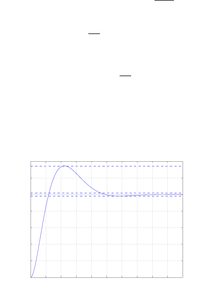
206 CHAPTER 5 The Performance of Feedback Control Systems

Advanced Problems

AP5.1 (a) The steady-state error is

ess = lim

s→0s(1 −T(s))R(s) = 1 −T(0) = 1 −108(3)

9(36) = 0 .

(b) Assume the complex poles are dominant. Then, we compute

ζωn

= 0.75 ,

since a= 3, ζ= 0.67 and ωn= 6. Using Figure 5.13 in Dorf & Bishop,

we estimate the settling time and percent overshoot to be

P.O. = 45% and Ts=4

ζωn

= 1 second .

and percent overshoot are

P.O. = 34.4% and Ts= 1.18 second .

0 0.2 0.4 0.6 0.8 1 1.2 1.4 1.6 1.8 2

0.2

0.4

0.6

0.8

1.2

1.4

Step Response

Time (sec)

Amplitude

FIGURE AP5.1

Closed-loop system step response.

from the publisher prior to any prohibited reproduction, storage in a retrieval system, or transmission in any form or by any means, electronic, mechanical, photocopying,

recording, or likewise. For information regarding permission(s), write to: Rights and Permissions Department, Pearson Education, Inc., Upper Saddle River, NJ 07458.

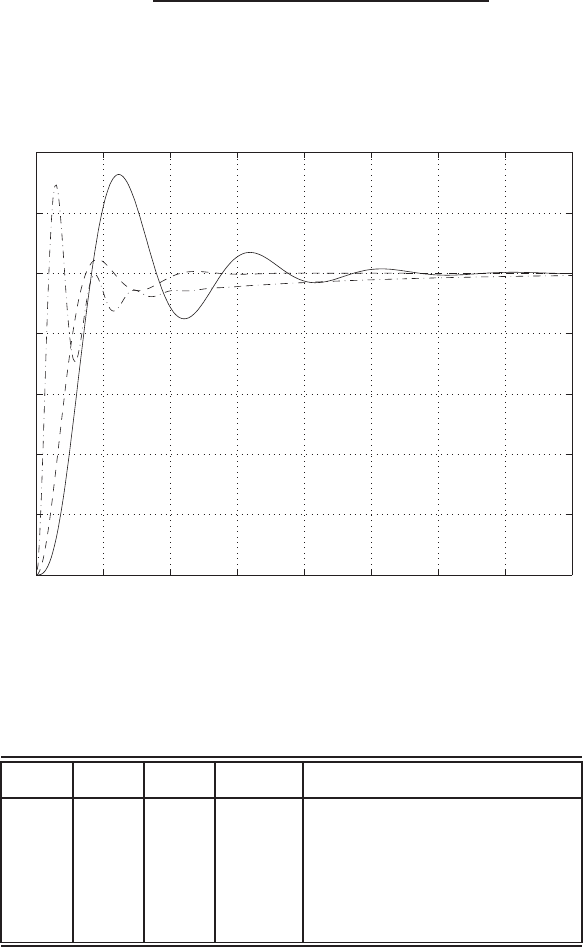
Advanced Problems 207

AP5.2 The closed-loop transfer function is

T(s) = 5440(τzs+ 1)

s3+ 28s2+ (432 + 5440τz)s+ 5440 .

The closed-loop step responses are shown in Figure AP5.2. The perfor-

mance results are summarized in Table AP5.2.

0 0.2 0.4 0.6 0.8 1 1.2 1.4 1.6

0.2

0.4

0.6

0.8

1.2

1.4

Time (sec)

y(t)

tau=0 (solid) & tau=0.05 (dashed) & tau=0.1 (dotted) & tau=0.5 (dot-dash)

FIGURE AP5.2

Closed-loop system step responses.

τzTrTsP.O. closed-loop poles

0 0.16 0.89 32.7% p=−20,−4±16j

0.05 0.14 0.39 4.5% p=−10.4,−8.77 ±21.06j

0.1 0.10 0.49 0% p=−6.5,−10.74 ±26.84j

0.5 0.04 1.05 29.2% p=−1.75,−13.12 ±54.16j

TABLE AP5.2 Performance summary.

As τzincreases from 0 to 0.1, the P.O. decreases and the response is faster

from the publisher prior to any prohibited reproduction, storage in a retrieval system, or transmission in any form or by any means, electronic, mechanical, photocopying,

recording, or likewise. For information regarding permission(s), write to: Rights and Permissions Department, Pearson Education, Inc., Upper Saddle River, NJ 07458.

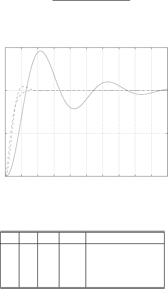
208 CHAPTER 5 The Performance of Feedback Control Systems

and more stable. However, as τzis increased beyond 0.1, the P.O. and Ts

increase, although Trcontinues to decrease.

AP5.3 The closed-loop transfer function is

T(s) = 1

τps3+ (1 + 2τp)s2+ 2s+ 1 .

The closed-loop step responses for τp= 0,0.5,2,5 are shown in Fig-

ure AP5.3. The performance results are summarized in Table AP5.3.

0 5 10 15 20 25 30 35 40 45 50

0.5

1.5

Time (sec)

y(t)

tau=5 (solid) & tau=2 (dotted) & tau=0.5 (dashed) & tau=0 (dot-dash)

FIGURE AP5.3

Closed-loop system step responses.

τpTrTsP.O. closed-loop poles

0 4 5.8 0% p=−1,−1

0.5 3.6 7.4 4.75% p=−2.84,−0.58 ±0.6j

2 4.6 22.4 27.7% p=−2.14,−0.18 ±0.45j

5 6 45.8 46% p=−2.05,−0.07 ±0.3j

TABLE AP5.3 Performance summary.

from the publisher prior to any prohibited reproduction, storage in a retrieval system, or transmission in any form or by any means, electronic, mechanical, photocopying,

recording, or likewise. For information regarding permission(s), write to: Rights and Permissions Department, Pearson Education, Inc., Upper Saddle River, NJ 07458.

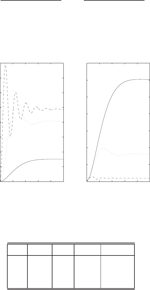
Advanced Problems 209

As τpincreases, the P.O.,Trand Tsalso increase; adding the pole makes

the system less stable with more overshoot.

AP5.4 The system transfer function is

Y(s) = 15K

(s+ 5)(s+ 7) + 15KR(s) + 15

(s+ 5)(s+ 7) + 15KTd(s).

When considering the input response, we set Td(s) = 0, and similarly,

when considering the disturbance response, we set R(s) = 0. The closed-

loop step input and disturbance responses for K= 1,10,100 are shown in

Figure AP5.4. The performance results are summarized in Table AP5.4.

0 0.2 0.4 0.6 0.8 1

0.2

0.4

0.6

0.8

1.2

1.4

1.6

Time (sec)

y(t)

Unit step input response

0 0.2 0.4 0.6 0.8 1

0.05

0.1

0.15

0.2

0.25

0.3

0.35

Time (sec)

y(t)

Unit step distrubance response

FIGURE AP5.4

Closed-loop system input and disturbance responses (K=1: solid line, K=10: dotted line,

and K=100:dashed line).

K ess TsP.O. |y/d|max

1 0.7 0.45 0% 0.3

10 0.19 0.6 17.3% 0.1

100 0.023 0.59 60.0% 0.01

TABLE AP5.4 Performance summary.

from the publisher prior to any prohibited reproduction, storage in a retrieval system, or transmission in any form or by any means, electronic, mechanical, photocopying,

recording, or likewise. For information regarding permission(s), write to: Rights and Permissions Department, Pearson Education, Inc., Upper Saddle River, NJ 07458.

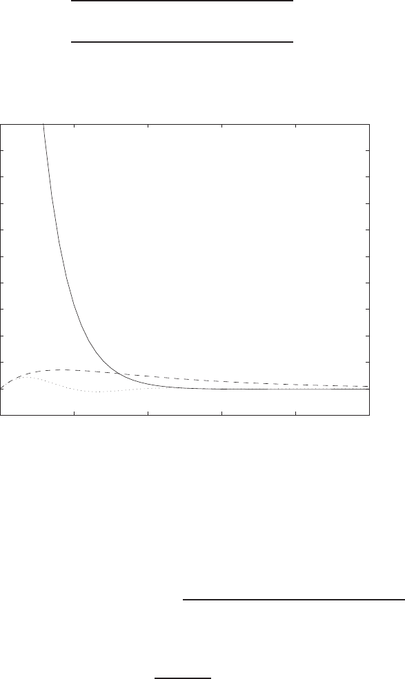
210 CHAPTER 5 The Performance of Feedback Control Systems

The best value of the gain is K= 10, which is compromise between (i)

percent overshoot, and (ii) disturbance rejection and tracking error.

AP5.5 The system transfer function is

Y(s) = 50(s+α)(s+ 2)

s(s+ 3)(s+ 4) + 50(s+α)(s+ 2)R(s)

+50s(s+ 2)

s(s+ 3)(s+ 4) + 50(s+α)(s+ 2)Td(s).

0 0.05 0.1 0.15 0.2 0.25

-1

Time (sec)

y(t)

Disturbance response: alpha=0 (solid) & alpha=10 (dashed) & alpha=100 (dotted)

FIGURE AP5.5

Closed-loop system disturbance response.

When considering the input response, we set Td(s) = 0, and similarly,

when considering the disturbance response, we set R(s) = 0. The steady-

state tracking error is

ess = lim

s→0s(1 −T(s))R(s) = lim

s→01−50(s+α)(s+ 2)

s(s+ 3)(s+ 4) + 50(s+α)(s+ 2) .

When α= 0, we have

ess = 1 −100

100 + 12 = 0.11 ,

from the publisher prior to any prohibited reproduction, storage in a retrieval system, or transmission in any form or by any means, electronic, mechanical, photocopying,

recording, or likewise. For information regarding permission(s), write to: Rights and Permissions Department, Pearson Education, Inc., Upper Saddle River, NJ 07458.

Advanced Problems 211

and, for α6= 0

ess = 0 .

The closed-loop step input and disturbance responses for α= 0,10,100

are shown in Figure AP5.5. For disturbance rejection and steady-state

tracking error the best value of the parameter is

α= 100 .

However, when considering both the disturbance and input response we

would select the parameter

α= 10 ,

since it oﬀers a good compromise between input response overshoot (about

5% for α= 10) and disturbance rejection/tracking error.

AP5.6 (a) The closed-loop transfer function is

T(s) = KKm

KKm+s(s+KmKb+ 0.01) .

The steady-state tracking error for a ramp input R(s) = 1/s2is

ess = lim

s→0s(1 −T(s))R(s)

= lim

s→0

s+KmKb+ 0.01

KKm+s(s+KmKb+ 0.01)

=KmKb+ 0.01

KKm

(b) With

Km= 10

and

Kb= 0.05 ,

we have

KmKb+ 0.01

KKm

=10(0.05) + 0.01

10K= 1 .

Solving for Kyields

K= 0.051 .

from the publisher prior to any prohibited reproduction, storage in a retrieval system, or transmission in any form or by any means, electronic, mechanical, photocopying,

recording, or likewise. For information regarding permission(s), write to: Rights and Permissions Department, Pearson Education, Inc., Upper Saddle River, NJ 07458.

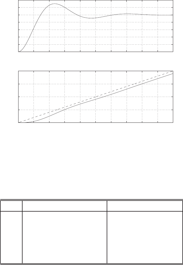
212 CHAPTER 5 The Performance of Feedback Control Systems

The responses are acceptable.

0 2 4 6 8 10 12 14 16 18 20

0.2

0.4

0.6

0.8

1.2

1.4

Time (sec)

y(t)

Step input response

0 2 4 6 8 10 12 14 16 18 20

Time (sec)

y(t)

Ramp input response

FIGURE AP5.6

Closed-loop system step and ramp responses.

AP5.7 The performance is summarized in Table AP5.7 and shown in graphical

form in Fig. AP5.7.

KEstimated Percent Overshoot Actual Percent Overshoot

1000 8.8 % 8.5 %

2000 32.1 % 30.2 %

3000 50.0 % 46.6 %

4000 64.4 % 59.4 %

5000 76.4 % 69.9 %

TABLE AP5.7 Performance summary.

from the publisher prior to any prohibited reproduction, storage in a retrieval system, or transmission in any form or by any means, electronic, mechanical, photocopying,

recording, or likewise. For information regarding permission(s), write to: Rights and Permissions Department, Pearson Education, Inc., Upper Saddle River, NJ 07458.

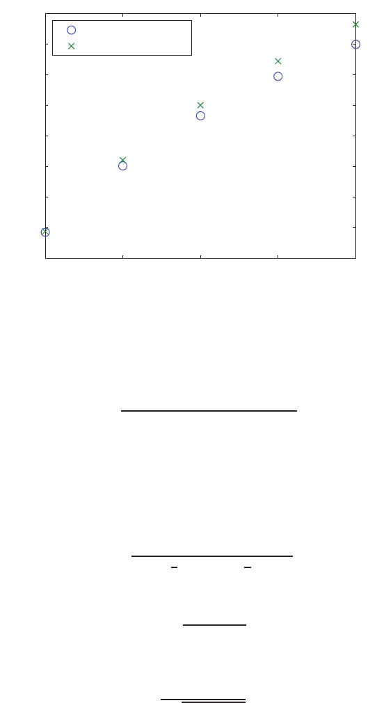
Advanced Problems 213

1000 2000 3000 4000 5000

Percent Overshoot (% )

Actual P.O .

Estimated P.O.

FIGURE AP5.7

Percent overshoot versus K.

The closed-loop transfer function is

T(s) = 100K

s(s+ 50)(s+ 100) + 100K.

The impact of the third pole is more evident as Kgets larger as the

estimated and actual percent overshoot deviate in the range 0.3% at K=

1000 to 6.5% at K= 5000.

AP5.8 The closed-loop transfer function is

T(s) = K(s+ 2)

s2+ (2

3+K)s+1

3+ 2K.

Comparing T(s) to a second-order system we have

ωn=q1/3 + 2K

ζ=2/3 + K

2p1/3 + 2K

For the closed-loop transfer function to have complex roots, we require

K2−(20/3)K−(8/9) <0. This occurs when −0.13 ≤K≤6.8. When

K= 1/3, we have the minimum ζ= 0.5, as shown in Figure AP5.8.

from the publisher prior to any prohibited reproduction, storage in a retrieval system, or transmission in any form or by any means, electronic, mechanical, photocopying,

recording, or likewise. For information regarding permission(s), write to: Rights and Permissions Department, Pearson Education, Inc., Upper Saddle River, NJ 07458.

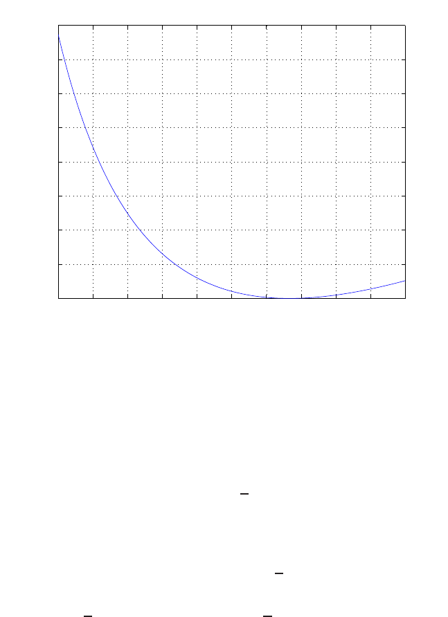
214 CHAPTER 5 The Performance of Feedback Control Systems

0 0.05 0.1 0.15 0.2 0.25 0.3 0.35 0.4 0.45 0.5

0.5

0.51

0.52

0.53

0.54

0.55

0.56

0.57

0.58

FIGURE AP5.8

Damping ratio, ζ, versus K.

AP5.9 The closed-loop characteristic equation is

s4+ 40s3+ 375s2+KPs+KI= 0.

The desired characteristic equation is

(s+a)(s+b)(s2+√2ωns+ω2

n) = 0.

Expanding the desired characteristic equation and equating terms to the

actual characteristic equation yields

abω2

n=KI, ω2

n(a+b) + √2abωn=KP

√2(a+b)ωn+ab = 375,√2ωn+a+b= 40

This represents 4 equations with 5 unknowns (a,b,KP,KI, and ωn).

We can choose one variable as part of the controller design. Let KI=

0.1KP. Then, solving the 4 equations for the remaining 4 variables yields

a= 29.15, b= 0.1, KP= 1720, KI= 172, and ωn= 7.6. The resulting

Ts= 1.1s and P.O. = 6.4%, as shown in Figure AP5.9.

from the publisher prior to any prohibited reproduction, storage in a retrieval system, or transmission in any form or by any means, electronic, mechanical, photocopying,

recording, or likewise. For information regarding permission(s), write to: Rights and Permissions Department, Pearson Education, Inc., Upper Saddle River, NJ 07458.

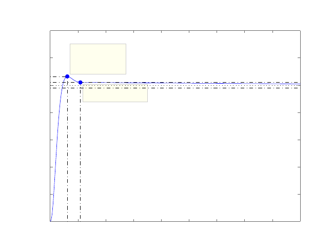
Advanced Problems 215

Step Response

Time (sec)

Amplitude

0 1 2 3 4 5 6 7 8 9

0.2

0.4

0.6

0.8

1.2

1.4

System: sysa

Settling Time (sec): 1.09

System: sysa

Peak amplitude: 1.06

Overshoot (%): 6.39

At time (sec): 0.618

FIGURE AP5.9

Step response for KP= 1720 and KI= 172.

from the publisher prior to any prohibited reproduction, storage in a retrieval system, or transmission in any form or by any means, electronic, mechanical, photocopying,

recording, or likewise. For information regarding permission(s), write to: Rights and Permissions Department, Pearson Education, Inc., Upper Saddle River, NJ 07458.

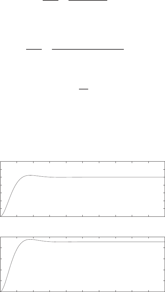
216 CHAPTER 5 The Performance of Feedback Control Systems

Design Problems

The plant model with parameters given in Table CDP2.1 in Dorf andCDP5.1

Bishop is given by:

θ(s)

Va(s)=26.035

s(s+ 33.142) ,

where we neglect the motor inductance Lm. The closed-loop transfer func-

tion from the disturbance to the output is

θ(s)

Td(s)=26.035

s2+ 33.142s+ 26.035Ka

For a unit step disturbance input the steady-state response is

θss =1

Therefore, we want to use the maximum Kawhile keeping the percent

overshoot less than 5%. The step response for the closed-loop system (with

the tachometer not in the loop) and Ka= 22 is shown below. Values of

Kagreater than 22 lead to overshoots greater than 5%.

0 0.1 0.2 0.3 0.4 0.5 0.6 0.7 0.8 0.9 1

0.2

0.4

0.6

0.8

1.2

1.4

Time (sec)

q(t)/A

Step response

0 0.1 0.2 0.3 0.4 0.5 0.6 0.7 0.8 0.9 1

0.01

0.02

0.03

0.04

0.05

Time (sec)

q(t)

Unit disturbance response

from the publisher prior to any prohibited reproduction, storage in a retrieval system, or transmission in any form or by any means, electronic, mechanical, photocopying,

recording, or likewise. For information regarding permission(s), write to: Rights and Permissions Department, Pearson Education, Inc., Upper Saddle River, NJ 07458.

Design Problems 217

DP5.1 (a) The closed-loop transfer function is

φ(s)

φd(s)=12.2K

s(s+ 2.2)(s+ 7) + 12.2K=12.2K

s3+ 9.2s2+ 15.4s+ 12.2K.

(b) For K= 0.7, we have the characteristic equation

s3+ 9.2s2+ 15.4s+ 8.54 = 0 ,

with roots s1=−7.23 and s2,3=−0.98 ±0.46j. For K= 3, we have

the characteristic equation

s3+ 9.2s2+ 15.4s+ 36.6 = 0 ,

with roots s1=−7.83 and s2,3=−0.68 ±2.05j. And for K= 6, we

have the characteristic equation

s3+ 9.2s2+ 15.4s+ 73.2 = 0 ,

with roots s1=−8.4 and s2,3=−0.4±2.9j.

expect the following:

(i) for K= 0.7: P.O.=0.13% and Tp= 6.8 sec

(ii) for K= 3: P.O.=35.0% and Tp= 1.5 sec

(iii) for K= 6: P.O.=65.2% and Tp= 1.1 sec

(d),(e) We select

K= 1.71

to have a P.O. = 16% and Tp= 2.18sec. All four cases (K=

0.7,3,6,1.71) are shown in Figure DP5.1. In each case, the approxi-

mate transfer function is derived by neglecting the non-dominant real

pole and adjusting the gain for zero steady-state error. The approxi-

mate transfer functions are

TK=0.7(s) = 1.18

s2+ 1.965s+ 1.18 =0.7908

(s+ 0.98 + 0.46j)(s+ 0.98 −0.46j)

TK=3(s) = 4.67

s2+ 1.37s+ 4.67 =3.299

(s+ 0.68 + 2.05j)(s+ 0.68 −2.05j)

TK=6(s) = 8.71

s2+ 0.796s+ 8.71 =6.399

(s+ 0.4 + 2.9j)(s+ 0.4−2.9j)

TK=1.71(s) = 2.77

s2+ 1.679s+ 2.77 =1.458

(s+ 0.83 + 1.43j)(s+ 0.83 −1.43j)

from the publisher prior to any prohibited reproduction, storage in a retrieval system, or transmission in any form or by any means, electronic, mechanical, photocopying,

recording, or likewise. For information regarding permission(s), write to: Rights and Permissions Department, Pearson Education, Inc., Upper Saddle River, NJ 07458.

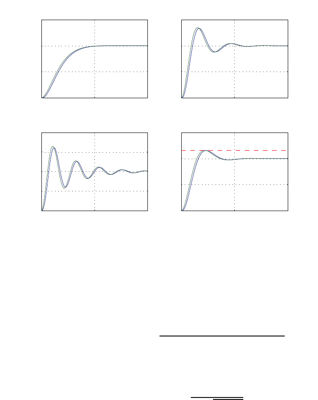
218 CHAPTER 5 The Performance of Feedback Control Systems

0 5 10

0.5

1.5

time (sec)

phi

K=0.7

0 5 10

0.5

1.5

time (sec)

phi

K=3

0 5 10

0.5

1.5

time (sec)

phi

K=6

0 5 10

0.5

1.5

K=1.71

time (sec)

phi

FIGURE DP5.1

Step responses (actual response:solid lines; approximate response: dotted lines).

DP5.2 The closed-loop transfer function is

T(s) = Kω2

s3+ 2ζωns2+ω2

ns+Kω2

where ζ= 0.6. From the second-order system approximation, we have

Tp=π

ωnp1−ζ2.

So, with ζ= 0.6 given, we should select ωn“large” to make Tp“small.”

Also, from the problem hint, let

0.2< K/ωn<0.4.

As a ﬁrst attempt, we can select ωn= 10. See Figure DP5.8 for various

values of K/ωn. Our ﬁnal selection is

K= 3.33 and ωn= 10 .

This results in P.O. = 3.6% and Tp= 0.66 second.

from the publisher prior to any prohibited reproduction, storage in a retrieval system, or transmission in any form or by any means, electronic, mechanical, photocopying,

recording, or likewise. For information regarding permission(s), write to: Rights and Permissions Department, Pearson Education, Inc., Upper Saddle River, NJ 07458.

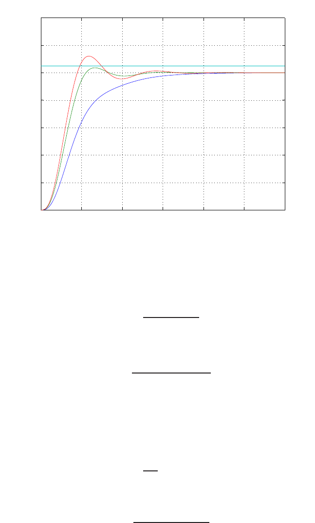
Design Problems 219

0 0.5 1 1.5 2 2.5 3

0.2

0.4

0.6

0.8

1.2

1.4

K/ωn=0.2

K/ωn=0.4

K/ωn=0.33

Time (sec)

y(t)

FIGURE DP5.2

Closed-loop system response.

DP5.3 The closed-loop transfer function is

T(s) = K

s2+qs +K.

From the ITAE speciﬁcation, we desire

T(s) = ω2

s2+ 1.4ωns+ω2

But

2ζωn= 1.4ωnwhich implies ζ= 0.7.

Since we want Ts≤0.5, we require ζωn≥8. So,

ωn≥8

0.7= 11.4.

We can select ωn= 12. Then,

T(s) = 144

s2+ 16.8s+ 144 .

Therefore, K= 144 and q= 16.8. The predicted percent overshoot is

from the publisher prior to any prohibited reproduction, storage in a retrieval system, or transmission in any form or by any means, electronic, mechanical, photocopying,

recording, or likewise. For information regarding permission(s), write to: Rights and Permissions Department, Pearson Education, Inc., Upper Saddle River, NJ 07458.

220 CHAPTER 5 The Performance of Feedback Control Systems

P.O. = 4.5%.

DP5.4 The loop transfer function is

Gc(s)G(s) = 10K

(s+ 70)(s+ 3)(s+ 7) =10K/70

(s/70 + 1)(s+ 3)(s+ 7) .

The second-order approximation is obtained by neglecting the fastest ﬁrst-

order pole. Thus,

Gc(s)G(s)≈K/7

(s+ 3)(s+ 7) .

The closed-loop transfer function is

T(s) = K/7

s2+ 10s+ 21 + K/7.

When ζ≥0.52, we have less than 15% overshoot. So, we have

2ζωn= 10

and

ωn=q21 + K/7.

Eliminating ωnand solving for K(with P.O. ≤15%) yields

K≤500.19 .

Also,

Kp= lim

s→0GGc(s) = K

7(21)

and

ess =1

1 + Kp

1 + K

147

<0.12

implies

K≥1078 .

Therefore, we have an inconsistency. We require 1078 ≤Kto meet the

steady-state requirement and K≤500.18 to meet the percent overshoot

requirement. It is not possible to meet both speciﬁcations.

from the publisher prior to any prohibited reproduction, storage in a retrieval system, or transmission in any form or by any means, electronic, mechanical, photocopying,

recording, or likewise. For information regarding permission(s), write to: Rights and Permissions Department, Pearson Education, Inc., Upper Saddle River, NJ 07458.

Design Problems 221

DP5.5 The closed-loop characteristic equation is

1 + K1G1(s) + K2G1G2(s) = 1 + K1

s(s+ 1) −2K2

s(s+ 1)(s+ 2) = 0

s3+ 3s2+ (2 + K1)s+ 2(K1−K2) = 0 .

Assuming that K1>0 and K2>0, the range of the gains for stability is

0< K2< K1.

DP5.6 The closed-loop transfer function is

T(s) = K1

s2+ (K1K2+ 1)s+K1

The percent overshoot speciﬁcation P.O. ≤2% is satisﬁed when ζ > 0.78.

The peak time speciﬁcation Tp≤0.5 s is satisﬁed when ωn= 10 and

ζ= 0.78. So, given

K1=ω2

nand K1K2+ 1 = 2ζωn,

we determine that the speciﬁcations are satisﬁed when

K1= 100

and

K2= 0.15 .

DP5.7 The plant is

G(s) = 2

s(s+ 1)(s+ 4)

and the PD controller is

Gc(s) = KDs+KP.

The characteristic equation is

s3+ 6s2+ (8 + 2KD)s+ 2KP= 0.

The desired characteristic equation is

(s+a)(s2+ 2ζωns+ω2

n) = s3+ (2ζωn+a)s2+ (ω2

n+ 2ζωna)s+aω2

n= 0.

Equating the desired characteristic equation to the actual characteristic

from the publisher prior to any prohibited reproduction, storage in a retrieval system, or transmission in any form or by any means, electronic, mechanical, photocopying,

recording, or likewise. For information regarding permission(s), write to: Rights and Permissions Department, Pearson Education, Inc., Upper Saddle River, NJ 07458.

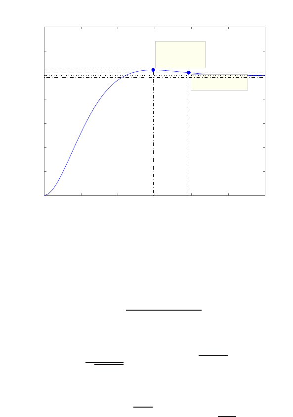
222 CHAPTER 5 The Performance of Feedback Control Systems

equation yields

2ζωn+a= 6, ω2

n+ 2ζωna= 8 + 2KD, aω2

n= 2KP,

where ζ= 0.69 and ωn= 3 to meet the design speciﬁcations. This repre-

sents 3 equations in 3 unknowns (a,KD, and KP). Solving yields a= 1.86,

KD= 4.35 and KP= 8.37. The step response is shown in Figure DP5.7.

Step Response

Time (sec)

Amplitude

0 0.5 1 1.5 2 2.5 3

0.2

0.4

0.6

0.8

1.2

1.4

System: sys_cl

Peak amplitude: 1.04

Overshoot (%): 4.28

At time (sec): 1.48

System: sys_cl

Settling Time (sec): 1.96

FIGURE DP5.7

Step response withKD= 4.35 and KP= 8.37.

DP5.8 The closed-loop transfer function is

T(s) = K

s2+ 6s+ 5 + K

The damping ratio and natural frequency is

ζ=3

√K+ 5 and ωn=√K+ 5

Using the design formulas for second-order systems we have

P O = 100e−ζπ/√1−ζ2and Ts=4

ζωn

We know that the formula for Tsis approximate and that the formulas

apply only to systems with ζ < 1. For K= 1 the closed-loop poles are

from the publisher prior to any prohibited reproduction, storage in a retrieval system, or transmission in any form or by any means, electronic, mechanical, photocopying,

recording, or likewise. For information regarding permission(s), write to: Rights and Permissions Department, Pearson Education, Inc., Upper Saddle River, NJ 07458.

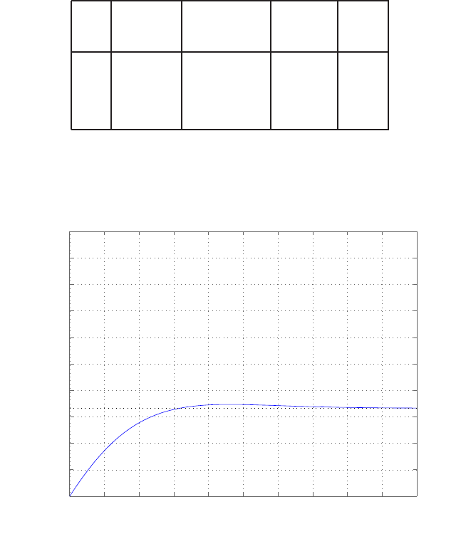
Design Problems 223

both real, so there is no overshoot and the design formula for settling time

does not apply. Thus we obtain the results shown in Table DP5.8. We can

choose K= 10 as a good trade-oﬀ between percent overshoot, settling

time, and steady-state tracking error. The disturbance response is shown

in Figure DP5.8.

TABLE DP5.8 Step response for K=1, 10, and 20.

K % P.O. Ts, sec Ts, sec ess

Estimated Actual

1 0 - 3.24 0.83

10 2.13 1.33 1.38 0.33

20 9.48 1.33 1.19 0.20

0 0.2 0.4 0.6 0.8 1 1.2 1.4 1.6 1.8 2

0.1

0.2

0.3

0.4

0.5

0.6

0.7

0.8

0.9

Time (sec)

y(t)

FIGURE DP5.8

Closed-loop system disturbance response for K= 10.

from the publisher prior to any prohibited reproduction, storage in a retrieval system, or transmission in any form or by any means, electronic, mechanical, photocopying,

recording, or likewise. For information regarding permission(s), write to: Rights and Permissions Department, Pearson Education, Inc., Upper Saddle River, NJ 07458.

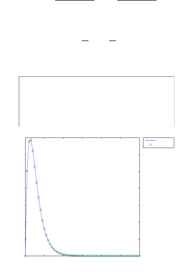
224 CHAPTER 5 The Performance of Feedback Control Systems

Computer Problems

CP5.1 With the impulse input we have R(s) = 1. The transfer function is

Y(s) = 15

(s+ 3)(s+ 5)R(s) = 15

(s+ 3)(s+ 5) .

Therefore, taking the inverse Laplace transforms yields the output re-

sponse:

y(t) = 15

2e−3t−15

2e−5t.

The impulse response and the analytic response is shown in Figure CP5.1.

n=15; d=[1 8 15];

t=[0:0.1:6];

ya=(15/2)*exp(-3.*t)-(15/2)*exp(-5.*t);

sys = tf(n,d)

y=impulse(sys,t);

plot(t,y,t,ya,'o')

xlabel('Time (sec)'), ylabel('y(t)'), legend('Computer','Analytic',-1)

0123456

0.2

0.4

0.6

0.8

1.2

1.4

Time (sec)

y(t)

Computer

Analytic

FIGURE CP5.1

Impulse responses.

from the publisher prior to any prohibited reproduction, storage in a retrieval system, or transmission in any form or by any means, electronic, mechanical, photocopying,

recording, or likewise. For information regarding permission(s), write to: Rights and Permissions Department, Pearson Education, Inc., Upper Saddle River, NJ 07458.

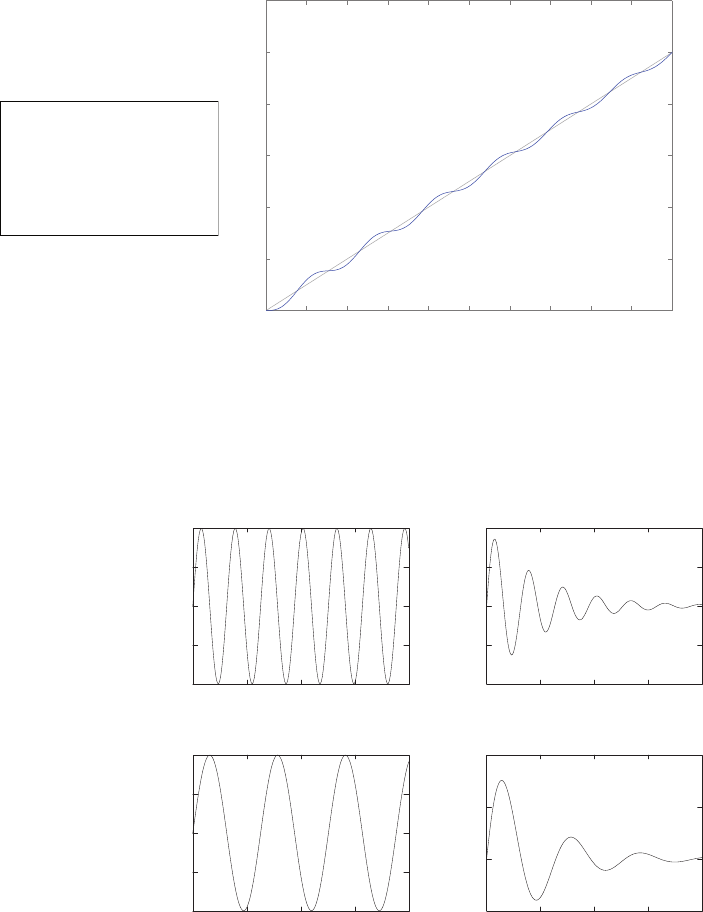
Computer Problems 225

CP5.2 The ramp response is shown in Figure CP5.2. The unity feedback system

is type 2, so that the steady-state tracking error is lim

t→∞ ess →0.

n=[1 10]; d=[1 15 0 0];

t=[0:0.1:50];

sys= tf(n,d);

sys_cl = feedback(sys,[1]);

u=t;

lsim(sys_cl,u,t);

0 5 10 15 20 25 30 35 40 45 50

Time (sec)

Amplitude

FIGURE CP5.2

Ramp responses.

CP5.3 The m-ﬁle script and the four plots are shown in Figure CP5.3. The plots

can be compared to Figure 5.17 in Dorf & Bishop.

-2

-1

0 5 10 15 20

wn=2, zeta=0

-2

-1

0 5 10 15 20

wn=2, zeta=0.1

-1

-0.5

0.5

0 5 10 15 20

wn=1, zeta=0

-0.5

0.5

0 5 10 15 20

wn=1, zeta=0.2

FIGURE CP5.3

Impulse responses.

from the publisher prior to any prohibited reproduction, storage in a retrieval system, or transmission in any form or by any means, electronic, mechanical, photocopying,

recording, or likewise. For information regarding permission(s), write to: Rights and Permissions Department, Pearson Education, Inc., Upper Saddle River, NJ 07458.

226 CHAPTER 5 The Performance of Feedback Control Systems

w1=2; z1=0;

w2=2; z2=0.1;

w3=1; z3=0;

w4=1; z4=0.2;

t=[0:0.1:20];

num1=[w1^2]; den1=[1 2*z1*w1 w1^2];

sys1 = tf(num1,den1);

[y1,x1]=impulse(sys1,t);

num2=[w2^2]; den2=[1 2*z2*w2 w2^2];

sys2 = tf(num2,den2);

[y2,x2]=impulse(sys2,t);

num3=[w3^2]; den3=[1 2*z3*w3 w3^2];

sys3 = tf(num3,den3);

[y3,x3]=impulse(sys3,t);

num4=[w4^2]; den4=[1 2*z4*w4 w4^2];

sys4 = tf(num4,den4);

[y4,x4]=impulse(sys4,t);

clf

subplot(221),plot(t,y1),title('wn=2, zeta=0')

subplot(222),plot(t,y2),title('wn=2, zeta=0.1')

subplot(223),plot(t,y3),title('wn=1, zeta=0')

subplot(224),plot(t,y4),title('wn=1, zeta=0.2')

FIGURE CP5.3

CONTINUED: Impulse response m-ﬁle script.

CP5.4 The closed-loop system is

T(s) = 21

s2+ 2s+ 21 .

Therefore, the natural frequency is

ωm=√21 = 4.58

and the damping ratio is computed as

2ζωn= 2 ,

which implies

ζ= 0.218 .

The percent overshoot is estimated to be

P.O. = 100e−ζπ/√1−ζ2= 50% ,

since ζ= 0.218. The actual overshoot is shown in Figure CP5.4.

from the publisher prior to any prohibited reproduction, storage in a retrieval system, or transmission in any form or by any means, electronic, mechanical, photocopying,

recording, or likewise. For information regarding permission(s), write to: Rights and Permissions Department, Pearson Education, Inc., Upper Saddle River, NJ 07458.

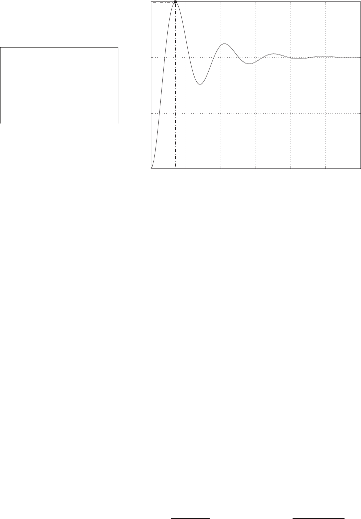
Computer Problems 227

numc=[21]; denc=[1 0];

sysc = tf(numc,denc);

numg=[1]; deng=[1 2];

sysg = tf(numg,deng);

sys_o = series(sysc,sysg);

sys_cl = feedback(sys_o,[1])

step(sys_cl)

Time (sec.)

Amplitude

Step Response

0123456

0.5

1.5

From: U(1)

To: Y(1)

FIGURE CP5.4

Impulse responses.

CP5.5 For a step input, the optimum ITAE characteristic equation is

s3+ 1.75ωs2+ 2.15ω2s+ω3= 0 .

Examining Figure 5.30 for n=3 in Dorf & Bishop, we estimate that

ωTs= 8.

So, once we decide on the desired Tswe can estimate ω. For this design we

let Ts=8 so that ω= 1. Computing the desired characteristic equation and

the actual characteristic equation and comparing the coeﬃcients leads to

the following relationships:

p= 1.75ω−2ζωn

K= (2.15ω2−ω2

n−2ζωnp)/ω2

z= (ω3−pω2

n)/(Kω2

where ζ= 0.59 and ωn= 0.45. The controller and preﬁlter are

Gc(s) = 6.42s+ 0.58

s+ 1.22 and Gp(s) = 1

1.3s+ 0.75 .

The unit step response is shown in Figure CP5.5.

from the publisher prior to any prohibited reproduction, storage in a retrieval system, or transmission in any form or by any means, electronic, mechanical, photocopying,

recording, or likewise. For information regarding permission(s), write to: Rights and Permissions Department, Pearson Education, Inc., Upper Saddle River, NJ 07458.

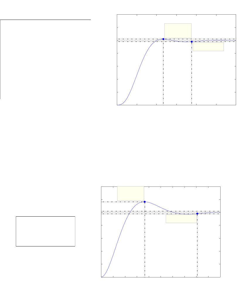
228 CHAPTER 5 The Performance of Feedback Control Systems

wn=0.45; zeta=0.59

ng=wn^2; dg=[1 2*zeta*wn wn^2];

sysg=tf(ng,dg);

Ts=8; w=8/Ts;

p=1.75*w-2*zeta*wn;

K=(2.15*w^2-wn^2-2*zeta*wn*p)/wn^2;

z=(w^3-p*wn^2)/(K*wn^2);

nc=K*[1 z]; dc=[1 p]; sysc=tf(nc,dc);

sys=series(sysc,sysg);

syscl=feedback(sys,1);

[num,den]=tfdata(syscl,'v');

sysp=tf([den(end)],num);

step(syscl*sysp)

Step Response

Time (sec)

Amplitude

0 2 4 6 8 10 12

0.2

0.4

0.6

0.8

1.2

1.4

System: untitled1

Peak amplitude: 1.02

Overshoot (%): 1.98

At time (sec): 4.68

System: untitled1

Settling Time (sec): 7.54

FIGURE CP5.5

Closed-loop system step response m-ﬁle script.

CP5.6 The unit step response is shown in Figure CP5.6. The performance num-

bers are as follows: Mp= 1.16, Tp= 0.73, and Ts= 1.62.

numg=[25]; deng=[1 5 0];

sys = tf(numg,deng);

sys_cl = feedback(sys,[1]);

t=[0:0.01:2];

step(sys_cl,t);

Step Response

Time (sec)

Amplitude

0 0.2 0.4 0.6 0.8 1 1.2 1.4 1.6 1.8 2

0.2

0.4

0.6

0.8

1.2

1.4 System: sys_cl

Peak amplitude: 1.16

Overshoot (%): 16.3

At time (sec): 0.73

System: sys_cl

Settling Time (sec): 1.62

FIGURE CP5.6

Closed-loop system step response m-ﬁle script.

from the publisher prior to any prohibited reproduction, storage in a retrieval system, or transmission in any form or by any means, electronic, mechanical, photocopying,

recording, or likewise. For information regarding permission(s), write to: Rights and Permissions Department, Pearson Education, Inc., Upper Saddle River, NJ 07458.

Computer Problems 229

CP5.7 The m-ﬁle script and the simulations are shown in Figure CP5.7.

% Part (a)

numc=[2]; denc=[1]; sys_c = tf(numc,denc);

nums=[-10]; dens=[1 10]; sys_s = tf(nums,dens);

numg=[-1 -5]; deng=[1 3.5 6 0]; sys_g = tf(numg,deng);

sysa = series(sys_c,sys_s);

sysb = series(sysa,sys_g);

sys = feedback(sysb,[1]);

f=0.5*pi/180; % Convert to rad/sec

t=[0:0.1:10]; u=f*t;

[y,x]=lsim(sys,u,t);(y(length(t),1)-u(1,length(t)))*180/pi

subplot(211)

plot(t,y*180/pi,t,u*180/pi,'--'), grid

xlabel('Time (sec)'),ylabel('theta')

title('Constant gain C(s) = 2: theta (solid) & input (dashed)')

% Part (b)

numc=[2 1]; denc=[1 0]; sys_c = tf(numc,denc);

[numa,dena]=series(numc,denc,nums,dens);

sysa = series(sys_c,sys_s);

sysb = series(sysa,sys_g);

sys = feedback(sysb,[1]);

[y,x]=lsim(sys,u,t);(y(length(t),1)-u(1,length(t)))*180/pi

subplot(212), plot(t,y*180/pi,t,u*180/pi,'--'), grid

xlabel('Time (sec)'),ylabel('theta')

title('PI controller C(s) = 2 + 1/s: theta (solid) & input (dashed)')

0 1 2 3 4 5 6 7 8 9 10

Time (sec)

theta

Constant gain C(s) = 2: theta (solid) & input (dashed)

0 1 2 3 4 5 6 7 8 9 10

Time (sec)

theta

PI controller C(s) = 2 + 1/s: theta (solid) & input (dashed)

FIGURE CP5.7

Closed-loop system response to a ramp input for two controllers.

For the constant gain controller, the attitude error after 10 seconds is

ess =−0.3 deg. On the other hand, the PI controller has a zero steady-

state error ess = 0 deg. So, we can decrease the steady-state error by

from the publisher prior to any prohibited reproduction, storage in a retrieval system, or transmission in any form or by any means, electronic, mechanical, photocopying,

recording, or likewise. For information regarding permission(s), write to: Rights and Permissions Department, Pearson Education, Inc., Upper Saddle River, NJ 07458.

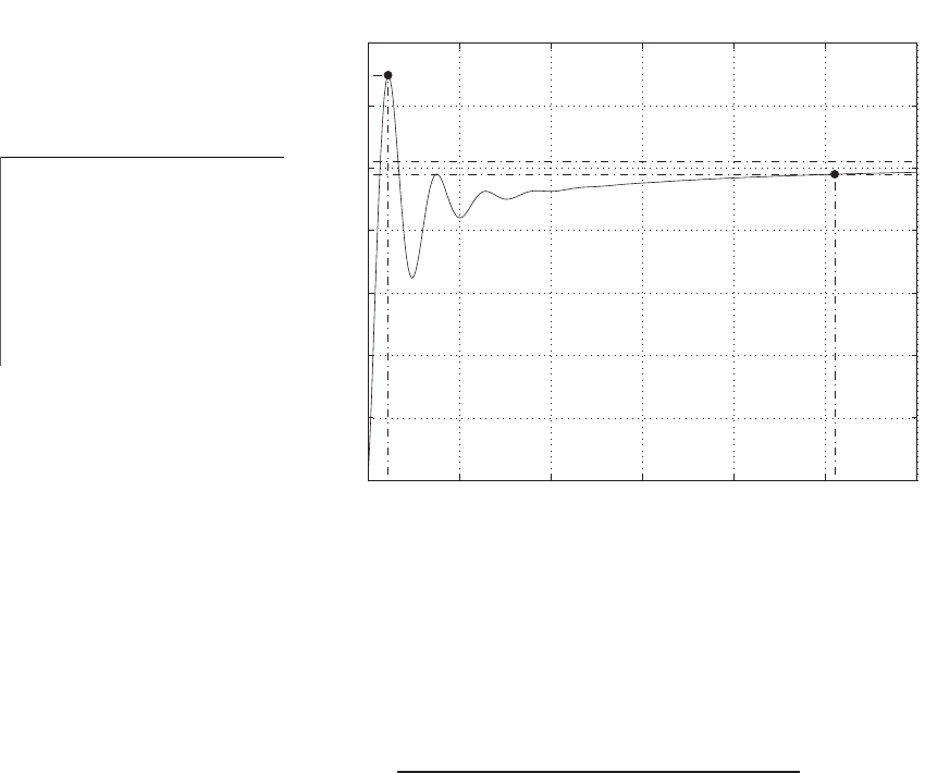
230 CHAPTER 5 The Performance of Feedback Control Systems

using a more sophisticated controller, in this case a PI controller versus a

constant gain controller.

CP5.8 The closed-loop characteristic equation is

s3+ 12s2+ 610s+ 500 = (s+ 0.8324)(s2+ 11.1676s+ 600.7027) = 0 .

The natural frequency and damping ratio of the complex roots are ωn=

24.5 and ζ= 0.23. From this we predict Mp= 1.48, Ts= 0.72, and

Tp= 0.13. The actual response is shown in Figure CP5.8. The diﬀerences

numg=[100 100]; deng=[1 2 100];

sysg = tf(numg,deng);

numc=[0.1 5]; denc=[1 0];

sysc = tf(numc,denc);

sys_o = series(sysg,sysc);

sys_cl = feedback(sys_o,[1])

t=[0:0.01:3];

step(sys_cl,t);

ylabel('theta dot')

Time (sec.)

theta dot

Step Response

0 0.5 1 1.5 2 2.5 3

0.2

0.4

0.6

0.8

1.2

1.4

From: U(1)

To: Y(1)

FIGURE CP5.8

Missile rate loop autopilot simulation.

can be explained by realizing that the system is not a second-order system.

The closed-loop system actually has two zeros, one real pole, and two

complex-conjugate poles:

T(s) = (s+ 50)(s+ 1)

(s+ 0.8324)(s2+ 11.1676s+ 600.7027) .

The eﬀect of the pole at s=−0.8324 is diminished by the zero at s=−1.

The third pole and the zeros aﬀect the overall response such that the

analytic formulas for second-order systems are not exact predictors of the

transient response.

from the publisher prior to any prohibited reproduction, storage in a retrieval system, or transmission in any form or by any means, electronic, mechanical, photocopying,

recording, or likewise. For information regarding permission(s), write to: Rights and Permissions Department, Pearson Education, Inc., Upper Saddle River, NJ 07458.

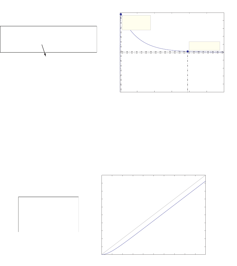
Computer Problems 231

CP5.9 Figure CP5.9 shows an m-ﬁle to compute the closed-loop transfer function

and to simulate and plot the step response.

numg=[10]; deng=[1 10]; sysg = tf(numg,deng);

numh=[0.5]; denh=[10 0.5]; sysh = tf(numh,denh);

sys = feedback(sysg,sysh)

step(sys);

Transfer function:

100 s + 5

---------------------

10 s^2 + 100.5 s + 10

Step Response

Time (sec)

Amplitude

0 10 20 30 40 50 60

0.1

0.2

0.3

0.4

0.5

0.6

0.7

0.8

0.9

System: sys

Settling Time (sec): 39.1

System: sys

Peak amplitude: 0.979

Overshoot (%): 95.7

At time (sec): 0.533

FIGURE CP5.9

M-ﬁle to compute the transfer function and to simulate the step response.

CP5.10 Figure CP5.10 shows an m-ﬁle to compute the closed-loop transfer func-

tion and to simulate and plot the ramp response. The steady-state error

numg=[10]; deng=[1 20 75 0];

sysg = tf(numg,deng);

sys = feedback(sysg,1)

t=[0:0.1:100];

u=t; % Unit ramp input

lsim(sys,u,t);

0 10 20 30 40 50 60 70 80 90 100

100

Linear Simulation Results

Time (sec)

Amplitude

FIGURE CP5.10

M-ﬁle to compute the transfer function and to simulate the ramp response.

is 7.5.

from the publisher prior to any prohibited reproduction, storage in a retrieval system, or transmission in any form or by any means, electronic, mechanical, photocopying,

recording, or likewise. For information regarding permission(s), write to: Rights and Permissions Department, Pearson Education, Inc., Upper Saddle River, NJ 07458.

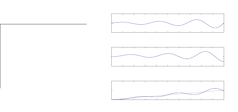
232 CHAPTER 5 The Performance of Feedback Control Systems

CP5.11 Figure CP5.11 shows an m-ﬁle to compute the closed-loop transfer func-

tion and to simulate and plot the impulse, step, and ramp responses.

Notice that the closed-loop system is unstable.

numg=[1]; deng=[1 2 0]; sysg = tf(numg,deng);

numc=[0.5 2]; denc=[1 0]; sysc = tf(numc,denc);

syss=series(sysg,sysc);

sys = feedback(syss,1)

t=[0:0.1:20];

subplot(311)

impulse(sys,t);

subplot(312)

step(sys,t);

subplot(313)

u=t; % Unit ramp input

lsim(sys,u,t);

0 2 4 6 8 10 12 14 16 18 20

-10

Impulse Response

Time (sec)

Amplitude

0 2 4 6 8 10 12 14 16 18 20

-10

Step Response

Time (sec)

Amplitude

0 2 4 6 8 10 12 14 16 18 20

Linear Simulation Results

Time (sec)

Amplitude

FIGURE CP5.11

M-ﬁle to compute the transfer function and to simulate the ramp response.

CP5.12 Figure CP5.12 shows an m-ﬁle to simulate and plot the step response

for the original system and the 2nd-order approximation. For the orig-

inal system, we ﬁnd Ts= 2.28 and P.O. = 80.6%. For the 2nd-order

approximation we ﬁnd Ts= 2.16 and P.O. = 101%

from the publisher prior to any prohibited reproduction, storage in a retrieval system, or transmission in any form or by any means, electronic, mechanical, photocopying,

recording, or likewise. For information regarding permission(s), write to: Rights and Permissions Department, Pearson Education, Inc., Upper Saddle River, NJ 07458.

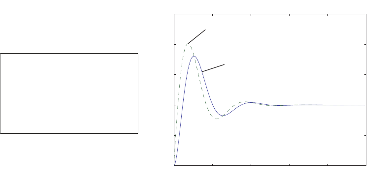
Computer Problems 233

num=77*[1 2]; den=conv([1 7],[1 4 22]);

sys = tf(num,den)

na=(77/7)*[1 2]; da=[1 4 22]; sysa=tf(na,da);

t=[0:0.01:5];

y=step(sys,t);

ya=step(sysa,t);

plot(t,y,t,ya,'--')

xlabel('Time (s)'), ylabel('Step response')

012345

0.5

1.5

2.5

Time (s)

Step response

2nd order approximation

3rd order system response

FIGURE CP5.12

Step response.

from the publisher prior to any prohibited reproduction, storage in a retrieval system, or transmission in any form or by any means, electronic, mechanical, photocopying,

recording, or likewise. For information regarding permission(s), write to: Rights and Permissions Department, Pearson Education, Inc., Upper Saddle River, NJ 07458.

C H A P T E R 6

The Stability of Linear Feedback

Systems

Exercises

E6.1 The Routh array is

s31K+ 1

s2K6

s1b0

so6

where

b=K(K+ 1) −6

For stability, we require K > 0 and b > 0. Therefore, using the condition

that b > 0, we obtain

K2+K−6>0,

and solving for Kyields K > 2 and K < −3. We select K > 2, since we

also have the condition that K > 0.

E6.2 The Routh array is

s31 2

s210 30

s1-1 0

so30

The system is unstable since the ﬁrst column shows two sign changes.

234

from the publisher prior to any prohibited reproduction, storage in a retrieval system, or transmission in any form or by any means, electronic, mechanical, photocopying,

recording, or likewise. For information regarding permission(s), write to: Rights and Permissions Department, Pearson Education, Inc., Upper Saddle River, NJ 07458.

Exercises 235

E6.3 The Routh array is

s41 32 20

s310 37

s228.3 20

s129.9

s020

By the Routh-Hurwitz criterion, the system is stable (i.e., all the numbers

in the ﬁrst column are positive).

E6.4 The closed-loop transfer function is

T(s) = −K(s−2)

s3+ 5s2+ (4 −K)s+ 2K.

Therefore, the characteristic equation is

s3+ 5s2+ (4 −K)s+ 2K= 0 .

The corresponding Routh array is given by

s31 4 −K

s25 2K

s1b0

so2K

where

b=5(4 −K)−2K

5=20 −7K

For stability we require K > 0 and b > 0 . Thus, the range of Kfor

stability is 0 < K < 20/7.

E6.5 The closed-loop transfer function is

T(s) = K

s3+ 10s2+ 27s+ 18 + K.

When K= 20, the roots of the characteristic polynomial are

s1,2=−1.56 ±j1.76

from the publisher prior to any prohibited reproduction, storage in a retrieval system, or transmission in any form or by any means, electronic, mechanical, photocopying,

recording, or likewise. For information regarding permission(s), write to: Rights and Permissions Department, Pearson Education, Inc., Upper Saddle River, NJ 07458.

236 CHAPTER 6 The Stability of Linear Feedback Systems

and

s3=−6.88 .

E6.6 When K= 252, the roots of the characteristic equation are on the imag-

inary axis. The roots are

s1,2=±j5.2 and s3=−10 .

E6.7 (a) The closed-loop system characteristic equation is

1 + GH(s) = 1 + K(s+ 2)

s(s−1) = 0 ,

s2+ (K−1)s+ 2K= 0 .

We have the relationships ωn=√2Kand 2ζωn=K−1, where

ζ= 0.707. Thus,

21

√2√2K=K−1,

2

√22

=K−1

√2K2

and

K2−6K+ 1 = 0 .

Solving for Kyields K= 5.83 and K= 0.17. However, for stability

we require K > 1 (from the Routh array), so we select K= 5.83.

(b) The two roots on the imaginary axis when K= 1 are s1,2=±j√2.

E6.8 The closed-loop system characteristic equation is

3+ 20s2+ (100 + K)s+ 20K= 0 .

The corresponding Routh array is

s31 (100 + K)

s220 20K

s1b0

so20K

from the publisher prior to any prohibited reproduction, storage in a retrieval system, or transmission in any form or by any means, electronic, mechanical, photocopying,

recording, or likewise. For information regarding permission(s), write to: Rights and Permissions Department, Pearson Education, Inc., Upper Saddle River, NJ 07458.

Exercises 237

where

b=20(100 + K)−20K

20 =20(100)

20 = 100 .

Therefore, the system is stable for all K > 0.

E6.9 The characteristic equation is

s3+ 2s2+ (K+ 1)s+ 8 = 0 ,

and the Routh array is given by

s31K+ 1

s22 8

s1b0

so8

where

b=2(K+ 1) −8

2=K−3.

Setting b= 0, yields

K−3 = 0 or K > 3.

E6.10 Stable with your eyes open and (generally) unstable with your eyes closed.

E6.11 The system is unstable. The poles are s1=−5.66, s2=−0.90 and s3,4=

0.28 ±j0.714.

E6.12 The characteristic equation is

s2+as +b= 0,

so, the Routh array is

s21b

s1a0

sob

The system is stable if and only if a > 0 and b > 0. For a second-order

system, a necessary and suﬃcient condition for stability is that all the

coeﬃcients have the same sign.

E6.13 The characteristic equation is

s2+ (KD+ 2)s+ 4KP= 0.

from the publisher prior to any prohibited reproduction, storage in a retrieval system, or transmission in any form or by any means, electronic, mechanical, photocopying,

recording, or likewise. For information regarding permission(s), write to: Rights and Permissions Department, Pearson Education, Inc., Upper Saddle River, NJ 07458.

238 CHAPTER 6 The Stability of Linear Feedback Systems

The Routh array is

s21 4KP

s1KD+ 2 0

so4KP

The system is stable if and only if KP>0 and KD>−2.

E6.14 The characteristic equation associated with the system matrix is

s3+ 3s2+ 5s+ 6 = 0 .

The roots of the characteristic equation are s1=−2 and s2,3=−5±j1.66.

The system is stable.

E6.15 The roots of q(s) are s1=−4, s2=−3, s3,4=−1±j2 and s5,6=±j0.5.

The system is marginally stable. The Routh array is

s61 31.25 67.75 15

s59 61.25 14.75

s424.44 66.11 15

s331.909 9.2273 0

s260 15

s10 0

The auxillary equation is

60s2+ 15 = 0 .

Solving the auxillary equation yields two roots at s1,2=±j0.5. After

accounting for the row of zeros, the completed Routh array veriﬁes that

the system has no poles in the right half-plane.

E6.16 The Routh array is

s41 45 50

s39 87

s235.33 50

s174.26 0

so50

from the publisher prior to any prohibited reproduction, storage in a retrieval system, or transmission in any form or by any means, electronic, mechanical, photocopying,

recording, or likewise. For information regarding permission(s), write to: Rights and Permissions Department, Pearson Education, Inc., Upper Saddle River, NJ 07458.

Exercises 239

The system is stable. The roots of q(s) are s1,2=−3±j4, s3=−2 and

s4=−1.

E6.17 The characteristic equation is

s3+ 7s2+ 36s+ 24 = 0 .

The system is stable. The roots of the characteristic equation are s1=

−0.77, s2,3=−3.12 ±4.64i.

E6.18 The roots of q(s) are s1=−20 and s2,3=±j2.24. The system is marginally

stable. The Routh array is

s31 5

s220 100

s10 0

The auxillary equation is

20s2+ 100 = 0 .

The roots are s=±j2.24. So, the system has roots at s=±j2.24.

Completing the Routh array (after accounting for the row of zeros) veriﬁes

that no poles lie in the right half-plane.

E6.19 (a) Unstable.

(b) Stable.

E6.20 (a) The roots are s1,2=−2 and s3=−1.

(b) The roots are s1,2,3=−3.

E6.21 The characteristic equation is

(sn−2)3+ 10(sn−2)2+ 29(sn−2) + K= 0

n+ 4s2

n+sn−26 + K= 0 .

The Routh array is

from the publisher prior to any prohibited reproduction, storage in a retrieval system, or transmission in any form or by any means, electronic, mechanical, photocopying,

recording, or likewise. For information regarding permission(s), write to: Rights and Permissions Department, Pearson Education, Inc., Upper Saddle River, NJ 07458.

240 CHAPTER 6 The Stability of Linear Feedback Systems

s31 1

s24K−26

s130−K

soK−26

If K= 30, then the auxillary equation is 4s2

n+ 4 = 0 or sn=±j.

Therefore, s=sn−2 implies s=−2±j.

E6.22 This system is not stable. The output response to a step input is a ramp

y(t) = kt.

E6.23 The characteristic polynomial is

s3+ 4s2+ks + 8 = 0 .

The Routh array is

s31k

s24 8

s14k−8

so8

So, k > 2 for stability.

E6.24 The transfer function is

G(s) = C(sI−A)−1B+D

= [ 1 0 0 ]





s−1 0

0s−1

k k s +k



















= [ 1 0 0 ]





s2+ks +k s +k1

−k s2+ks s

−ks −ks −k s2



















∆(s)

where ∆(s) = s3+ks2+ks +k. Thus, the transfer function is

G(s) = 1

s3+ks2+ks +k.

The Routh array is

from the publisher prior to any prohibited reproduction, storage in a retrieval system, or transmission in any form or by any means, electronic, mechanical, photocopying,

recording, or likewise. For information regarding permission(s), write to: Rights and Permissions Department, Pearson Education, Inc., Upper Saddle River, NJ 07458.

Exercises 241

s31k

s2k k

s1k−1

sok

For stability k > 1.

E6.25 The closed-loop transfer function is

T(s) = Ks + 1

s2(s+p) + Ks + 1 .

Therefore, the characteristic equation is

s3+ps2+Ks + 1 = 0 .

The Routh array is

s31 K

s2p 1

s1(pK −1)/p

so1

We see that the system is stable for any value of p > 0 and pK −1>0.

E6.26 The closed-loop transfer function is

T(s) = 10

2s2+ (K−20)s+ 10 −10K.

Therefore, the characteristic equation is

2s2+ (K−20)s+ 10 −10K= 0 .

The Routh array is

s22 10-10K

s1K−20

so10 −10K

We see that the system is stable for any value of K > 20 and any K < 1.

Therefore, the system is unstable for all K > 0 since the gain Kcannot

be simultaneously greater than 20 and less than 1.

from the publisher prior to any prohibited reproduction, storage in a retrieval system, or transmission in any form or by any means, electronic, mechanical, photocopying,

recording, or likewise. For information regarding permission(s), write to: Rights and Permissions Department, Pearson Education, Inc., Upper Saddle River, NJ 07458.

242 CHAPTER 6 The Stability of Linear Feedback Systems

Problems

P6.1 (a) Given

s2+ 5s+ 2 ,

we have the Routh array

s21 2

s15 0

so2

Each element in the ﬁrst column is positive, thus the system is stable.

(b) Given

s3+ 4s2+ 8s+ 4 ,

we have the Routh array

s31 8

s24 4

s17 0

so4

Each element in the ﬁrst column is positive, thus the system is stable.

s3+ 2s2−6s+ 20 ,

we determine by inspection that the system is unstable, since it is

necessary that all coeﬃcients have the same sign. There are two roots

in the right half-plane.

(d) Given

s4+s3+ 2s2+ 12s+ 10 ,

we have the Routh array

s41 2 10

s31 12 0

s2-10 10 0

s113 0

so10

from the publisher prior to any prohibited reproduction, storage in a retrieval system, or transmission in any form or by any means, electronic, mechanical, photocopying,

recording, or likewise. For information regarding permission(s), write to: Rights and Permissions Department, Pearson Education, Inc., Upper Saddle River, NJ 07458.

Problems 243

There are two sign changes in the ﬁrst column, thus the system is

unstable with two roots in the right half-plane.

(e) Given

s4+s3+ 3s2+ 2s+K ,

we have the Routh array

s41 3 K

s31 2 0

s21K

s12−K0

soK

Examining the ﬁrst column, we determine that the system is stable

for 0 < K < 2.

(f) Given

s5+s4+ 2s3+s+ 6 ,

we know the system is unstable since the coeﬃcient of the s2term is

missing. There are two roots in the right half-plane.

(g) Given

s5+s4+ 2s3+s2+s+K ,

we have the Routh array

s51 2 1

s41 1 K

s31 1 −K

s2K K

s1−K0

soK

Examining the ﬁrst column, we determine that for stability we need

K > 0 and K < 0. Therefore the system is unstable for all K.

P6.2 (a) The closed-loop characteristic polynomial is

s4+ 27.88s3+ 366.4s2+ 1500s+ 1500ka= 0 .

The Routh array is

from the publisher prior to any prohibited reproduction, storage in a retrieval system, or transmission in any form or by any means, electronic, mechanical, photocopying,

recording, or likewise. For information regarding permission(s), write to: Rights and Permissions Department, Pearson Education, Inc., Upper Saddle River, NJ 07458.

244 CHAPTER 6 The Stability of Linear Feedback Systems

s41 366.4 1500ka

s327.88 1500

s2312.6 1500ka

s1b

so1500ka

where

b= 1500 −133.78ka.

Examining the ﬁrst column of the Routh array, we ﬁnd that b > 0

and 1500ka>0 for stability. Thus,

0< ka<11.21 .

(b) With

Ts= 1.5 = 4

ζωn

we determine that

ζωn= 2.67 .

So, shift the axis by s=so−2.67, and

(so−2.67)4+ 27.88(so−2.67)3+ 366.4(so−2.67)2+ 1500(so−2.67) +

1500ka=s4

o+ 17.2s3

o+ 185.85s2

o+ 63.55so−1872.8 + 1500ka.

The Routh array is

s41 185.85 1500ka-1872.8

s317.2 63.55

s2182.16 1500ka-1872.8

s1b

so1500ka-1872.8

where

b= 240.38 −141.63ka.

Examining the ﬁrst column of the Routh array, we ﬁnd that b > 0

and 1500ka−1872.8>0. Thus, 1.25 < ka<1.69.

from the publisher prior to any prohibited reproduction, storage in a retrieval system, or transmission in any form or by any means, electronic, mechanical, photocopying,

recording, or likewise. For information regarding permission(s), write to: Rights and Permissions Department, Pearson Education, Inc., Upper Saddle River, NJ 07458.

Problems 245

P6.3 (a) Given

G(s) = K

(s+ 1)(s+ 2)(0.5s+ 1) ,

and

H(s) = 1

0.005s+ 1 ,

the closed-loop transfer function is

T(s) = K(0.005s+ 1)

0.0025s4+ 0.5125s3+ 2.52s2+ 4.01s+ 2 + K.

Therefore, the characteristic equation is

0.0025s4+ 0.5125s3+ 2.52s2+ 4.01s+ (2 + K) = 0 .

The Routh array is given by

s40.0025 2.52 2 + K

s30.5125 4.01 0

s22.50 2 + K

s13.6−0.205K0

so2 + K

Examining the ﬁrst column, we determine that for stability we require

−2< K < 17.6.

(b) Using K= 9, the roots of the characteristic equation are

s1=−200 , s2,3=−0.33 ±2.23j , and s4=−4.35 .

Assuming the complex roots are dominant, we compute the damping

ratio ζ= 0.15. Therefore, we estimate the percent overshoot as

P.O. = 100e−πζ/√1−ζ2= 62% .

The actual overshoot is 27%, so we see that assuming that the complex

poles are dominant does not lead to accurate predictions of the system

response.

P6.4 (a) The closed-loop characteristic equation is

1 + GH(s) = 1 + K(s+ 40)

s(s+ 10)(s+ 20) = 0 ,

from the publisher prior to any prohibited reproduction, storage in a retrieval system, or transmission in any form or by any means, electronic, mechanical, photocopying,

recording, or likewise. For information regarding permission(s), write to: Rights and Permissions Department, Pearson Education, Inc., Upper Saddle River, NJ 07458.

246 CHAPTER 6 The Stability of Linear Feedback Systems

s3+ 30s2+ 200s+Ks + 40K= 0 .

The Routh array is

s31 200 + K

s230 40K

s1200 −K

so40K

Therefore, for stability we require 200 −K/3>0 and 40K > 0. So,

the range of Kfor stability is

0< K < 600 .

(b) At K= 600, the auxilary equation is

30s2+ 40(600) = 0 or s2+ 800 = 0 .

The roots of the auxiliary equation are

s=±j28.3.

s+ 1. Substituting s=so−1 into the characteristic equation yields

(so−1)3+30(so−1)2+500(so−1)+12000 = s3

o+27s2

o+443so+11529 .

The Routh array is

s31 443

s227 11529

s116 0

so11529

All the elements of the ﬁrst column are positive, therefore all the

roots lie to left of s=−1. We repeat the procedure for s=so−2

and obtain

o+ 24s2

o+ 392so+ 10992 = 0 .

The Routh array is

from the publisher prior to any prohibited reproduction, storage in a retrieval system, or transmission in any form or by any means, electronic, mechanical, photocopying,

recording, or likewise. For information regarding permission(s), write to: Rights and Permissions Department, Pearson Education, Inc., Upper Saddle River, NJ 07458.

Problems 247

s31 392

s224 10992

s1-66 0

so10992

There are two sign changes in the ﬁrst column indicating two roots

to right of s=−2. Combining the results, we determine that there

are two roots located between s=−1 and s=−2. The roots of the

characteristic equation are

s1=−27.6250 and s2,3=−1.1875 ±20.8082j .

We see that indeed the two roots s2,3=−1.1875±20.8082jlie between

-1 and -2.

P6.5 (a) Given the characteristic equation,

s3+ 3s2+ 4s+ 2 = 0 ,

we compute the roots s1=−1, and s2,3=−1±j.

(b) The roots of the characteristic equation

s4+ 9s3+ 30s2+ 42s+ 20 = 0

are s1=−1, s2=−2, and s3,4=−3±j1.

s3+ 19s2+ 110s+ 200 = 0

are s1=−4, s2=−5, and s3=−10.

P6.6 (a) The characteristic equation is

1 + G(s) = 0 ,

s3+s2+ 10s+ 2 = 0 .

The roots are: s1=−0.2033, and s2,3=−0.3984 ±j3.1112.

(b) The characteristic equation is

s4+ 10s3+ 35s2+ 50s+ 24 = 0 .

The roots are s1=−1, s2=−2, s3=−3, and s4=−4.

from the publisher prior to any prohibited reproduction, storage in a retrieval system, or transmission in any form or by any means, electronic, mechanical, photocopying,

recording, or likewise. For information regarding permission(s), write to: Rights and Permissions Department, Pearson Education, Inc., Upper Saddle River, NJ 07458.

248 CHAPTER 6 The Stability of Linear Feedback Systems

s3+ 11s2+ 29s+ 6 = 0 .

The roots are s1=−0.2258, s2=−3.8206 and s3=−6.9536.

P6.7 (a) The closed-loop characteristic equation is

s3+ 101s2+ (100 + 10KKa)s+ 100KKa= 0 .

The Routh array is

s31 100 + 10KKa

s2101 100KKa

s1b

so100KKa

where

b= 100 + 910

101 KKa>0.

Thus, examing the ﬁrst column, we determine that KKa>0 stabi-

lizes the system.

(b) The tracking error is

e(s) = lim

s→0s(1 −T(s))100

s2=100

KKa

We require E(s)<1o= 0.01745. So,

KKa>100

0.01745 = 5729 .

When KKa= 5729, the roots of the characteristic polynomial are

s1=−10.15 and s2,3=−45.43 ±j233.25 .

P6.8 (a) The closed-loop characteristic equation is

1 + K

(0.5s+ 1)(s+ 1)(1

4s+ 1) = 0 ,

s3+ 7s2+ 14s+ 8(1 + K) = 0 .

The Routh array is

from the publisher prior to any prohibited reproduction, storage in a retrieval system, or transmission in any form or by any means, electronic, mechanical, photocopying,

recording, or likewise. For information regarding permission(s), write to: Rights and Permissions Department, Pearson Education, Inc., Upper Saddle River, NJ 07458.

Problems 249

s31 14

s27 8(1 + K)

s1b

so8(1 + K)

where

b=7(14) −8(1 + K)

For stability, we require b > 0 and 8(1 + K)>0. Therefore, the range

of Kfor stability is

−1< K < 11.25 .

(b) Let K= 11.25/3 = 3.75. Then, the closed-loop transfer function is

T(s) = 3.37

s3+ 7s2+ 14s+ 38 .

The settling time to a step input is Ts≈6 seconds.

Ts= 4 = 4

ζωn

implies ζωn= 1 .

Our desired characteristic polynomial is

(s+b)(s2+ 2ζωns+ω2

n) = s3+ (2 + b)s2+ (ω2

n+ 2b)s+bω2

where we have used the fact that ζωn= 1 and ωnand bare to be

determined. Our actual characteristic polynomial is

s3+ 7s2+ 14s+ 8(1 + K) = 0 .

Comparing the coeﬃcients of the actual and desired characteristic

polynomials, we ﬁnd the following relationships:

2 + b= 7

ω2

n+ 2b= 14

bω2

n= 8(1 + K).

Solving these three equations yields

b= 5 , ωn= 2 and K= 1.5.

The actual settling time is Ts= 4.17 sec. This is not exactly our

from the publisher prior to any prohibited reproduction, storage in a retrieval system, or transmission in any form or by any means, electronic, mechanical, photocopying,

recording, or likewise. For information regarding permission(s), write to: Rights and Permissions Department, Pearson Education, Inc., Upper Saddle River, NJ 07458.

250 CHAPTER 6 The Stability of Linear Feedback Systems

desired Tssince we have the contribution of the additional pole at

s=−5. The closed-loop poles are

s1=−5 and s2,3=−1±1.73j .

P6.9 (a) The closed-loop characteristic equation is

1 + GH(s) = 1 + 10K

(s+ 100)(s+ 20)2,

s3+ 140s2+ 4400s+ 40000 + 10K= 0 .

The Routh array is

s31 4400

s2140 40000 + 10K

s1b

so40000 + 10K

where

b=140(4400) −(40000 + 10K)

140 .

Examining the ﬁrst column and requiring all the terms to be positive,

we determine that the system is stable if

−4000 < K < 57600 .

(b) The desired characteristic polynomial is

(s+b)(s2+1.38ωns+ω2

n) = s3+(1.38ωn+b)s2+(ω2

n+1.38ωnb)s+bω2

where we have used the fact that ζ= 0.69 to achieve a 5% over-

shoot, and ωnand bare to be determined. The actual characteristic

polynomial is

s3+ 140s2+ 4400s+ 40000 + 10K= 0 .

Equating the coeﬃcients of the actual and desired characteristic poly-

nomials, and solving for K,b, and ωnyields

b= 104.2, ωn= 25.9 and K= 3003 .

So, a suitable gain is K= 3003.

from the publisher prior to any prohibited reproduction, storage in a retrieval system, or transmission in any form or by any means, electronic, mechanical, photocopying,

recording, or likewise. For information regarding permission(s), write to: Rights and Permissions Department, Pearson Education, Inc., Upper Saddle River, NJ 07458.

Problems 251

P6.10 (a) The closed-loop characteristic equation is

s4+ 7s3+ 20s2+ (24 + K)s+ 10K= 0 .

The Routh array is

s41 20 10K

s37 24 + K0

s2116−K

710K

s1b

so10K

where

b=116−K

7(24 + K)−70K

116−K

7.

Setting b > 0 yields

2784 −398K−K2>0,

which holds when

−404.88 < K < 6.876 .

Examining the ﬁrst column, we also ﬁnd that K < 116 and K > 0

for stability. Combining all the stability regions, we determine that

for stability

0< K < 6.876 .

(b) When K= 6.876, the roots are

s1,2=−3.5±1.63j , and s3,4=±2.1j .

P6.11 Given

s3+ (1 + K)s2+ 10s+ (5 + 15K) = 0 ,

the Routh array is

s31 10

s21 + K5 + 15K

s1b

so5 + 15K

from the publisher prior to any prohibited reproduction, storage in a retrieval system, or transmission in any form or by any means, electronic, mechanical, photocopying,

recording, or likewise. For information regarding permission(s), write to: Rights and Permissions Department, Pearson Education, Inc., Upper Saddle River, NJ 07458.

252 CHAPTER 6 The Stability of Linear Feedback Systems

where

b=(1 + K)10 −(5 + 15K)

1 + K=5−5K

1 + K.

Given that K > 0, we determine that the system is stable when 5−5K > 0

0< K < 1.

When K= 1, the s2row yields the auxilary equation

2s2+ 20 = 0 .

The roots are s=±j√10. So, the system frequency of oscillation is √10

rads/sec.

P6.12 The characteristic equation is

s3+as2+bs +c= 0,

so, the Routh array is

s31b

s2ac

s1ab−c

s0c

For the system to be stable, we require that a > 0, ab −c > 0 and c > 0.

When a > 0 and c > 0, we know that b > 0. So, a necessary condition for

stability is that all coeﬃcients a,b, and cbe positive. The necessary and

suﬃcient conditions for stability also require that b > c/a, in addition to

a > 0 and c > 0.

P6.13 The characteristic equation is

s3+ (p+ 2ζωn)s2+ (2ζωnp+Kω2

n)s+Kω2

nz= 0.

The conditions for stability (see P6.12) are p+ 2ζωn>0, 2ζωnp+Kω2

(Kω2

nz)/(p+ 2ζωn), and Kω2

nz > 0. Since we know that K > 0, ζ > 0,

and ωn>0, it follows that for stability z > 0, p > −2ζωn, and

2ζωnp+Kω2

n>Kω2

p+ 2ζωn

P6.14 The system has the roots

s1,2=±j , s3,4=±j , and s5,6=−1±3j ,

from the publisher prior to any prohibited reproduction, storage in a retrieval system, or transmission in any form or by any means, electronic, mechanical, photocopying,

recording, or likewise. For information regarding permission(s), write to: Rights and Permissions Department, Pearson Education, Inc., Upper Saddle River, NJ 07458.

Problems 253

Therefore, the system is not stable since there are repeated roots on the

jω-axis.

P6.15 (a) Neglecting the zeros and poles, we have the characteristic equation

s4+ 30s3+ 325s2+ 2500s+K= 0 .

The Routh array is

s41 325 K

s330 2500 0

s2241.67 K

s1b

soK

where

b=604166.67 −30K

241.67 .

Therefore, the system is stable for 0 < K < 20139.

(b) Without neglecting the zeros and poles, the closed-loop characteristic

equation is

s6+ 90s5+ 5525s4+ 12400s3+ (1255000 + K)s2

+ (8500000 + 30K)s+ 1125K= 0 .

This is stable for

0< K < 61818 .

We see that the additional poles and zero makes the system stable

for a much larger gain K.

P6.16 (a) The Routh array is

s31 5

s25 6

s13.8

so6

Examining the ﬁrst column of the Routh array, we see no sign changes.

So, the system is stable.

(b) The roots of the system are s1=−0.3246 and s2,3=−2.3377 ±

3.6080j.

from the publisher prior to any prohibited reproduction, storage in a retrieval system, or transmission in any form or by any means, electronic, mechanical, photocopying,

recording, or likewise. For information regarding permission(s), write to: Rights and Permissions Department, Pearson Education, Inc., Upper Saddle River, NJ 07458.

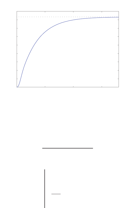
254 CHAPTER 6 The Stability of Linear Feedback Systems

0 5 10 15

0.02

0.04

0.06

0.08

0.1

0.12

0.14

0.16

0.18

Step Response

Time

(

sec

)

Amplitude

FIGURE P6.16

Unit step response.

P6.17 The closed-loop transfer function is

T(s) = K+ 1

s3+ 3s2+ 3s+K+ 1 .

The Routh array is

s31 3

s23K+ 1

s18−K

soK+ 1

So, for stability we require −1< K < 8.

P6.18 The system characteristic equation is

s2+ (h−k)s+ab −kh = 0 .

For stability we require h > k and ab > kh. If k > h, the system is

unstable.

from the publisher prior to any prohibited reproduction, storage in a retrieval system, or transmission in any form or by any means, electronic, mechanical, photocopying,

recording, or likewise. For information regarding permission(s), write to: Rights and Permissions Department, Pearson Education, Inc., Upper Saddle River, NJ 07458.

Problems 255

P6.19 (a) The characteristic equation is

s3+ 9s2+ (K−10)s+ 2K= 0 .

The Routh array is

s31K−10

s29 2K

s17K−90

so2K

For stability

K > 90/7.

(b) When K= 90/7, the system is marginally stable. The roots are

s1,2=±jq20/7,

at the jω-axis crossing.

P6.20 The closed-loop characteristic equation is

q(s) = s5+s4+ 9s3+Ks2+ 2Ks +K .

The range of stability for the vertical-liftoﬀ vehicle is

5.177 < K < 7.823 .

Therefore, for K= 6, the system is stable. When K= 6 we have

q(s) = s5+s4+ 9s3+ 6s2+ 12s+ 6

The Routh array is

s51 9 12

s41 6 6

s33 6

s24 6

s11.5

so6

All entries in the ﬁrst column are positive, so the system is stable.

from the publisher prior to any prohibited reproduction, storage in a retrieval system, or transmission in any form or by any means, electronic, mechanical, photocopying,

recording, or likewise. For information regarding permission(s), write to: Rights and Permissions Department, Pearson Education, Inc., Upper Saddle River, NJ 07458.

256 CHAPTER 6 The Stability of Linear Feedback Systems

P6.21 The state transition matrix is

Φ(t, 0) = 1

p2−p1



(k2−p1)e−p1t−(k2−p2)e−p2te−p1t−e−p2t

−k1e−p1t+k1e−p2t−p1e−p1t+p2e−p2t



where p1p2=k1and p1+p2=k2. We assume that p16=p2. In the case

when p1=p2, the state transition matrix will change, but the factors e−p1t

and e−p2twill remain. The eigenvalues of Aare given by the solution to

det |λI−A|=λ2+k2λ+k1= 0 .

Therefore, the eigenvalues are λ1,2=−k2/2±qk2

2−4k1. If k2>0 and

k1>0, then the eigenvalues are in the left half-plane, and the system is

stable. The transfer function is given by

G(s) = C(sI−A)−1B=−s−1

s2+k2s+k1

Therefore the characteristic equation is s2+k2s+k1= 0 and the poles

are s1,2=−k2/2±qk2

2−4k1. If k2>0 and k1>0, then the poles are in

the left half-plane, and the system is stable. Notice that the values of λ1,2

and s1,2are the same. Also, the eigenvalues are the same as the values of

−p1and −p2. So, if the eigenvalues are negative, then the elements of the

state transition matrix will decay exponentially.

from the publisher prior to any prohibited reproduction, storage in a retrieval system, or transmission in any form or by any means, electronic, mechanical, photocopying,

recording, or likewise. For information regarding permission(s), write to: Rights and Permissions Department, Pearson Education, Inc., Upper Saddle River, NJ 07458.

Advanced Problems 257

Advanced Problems

AP6.1 The Routh array is

s41K1K2

s320 4

s220K1−4

20 K2

s1b0

soK2

where

b=20K1−4−100K2

5K1−1.

For stability, we require K2>0, K1>0.2, and b > 0. Therefore, using

the condition that b > 0, we obtain

K2<0.2K1−0.04 .

The stability region is shown in Figure AP6.1.

0.2 0.4 0.6 0. 8 1 1.2 1.4 1.6 1.8 2

0.05

0.1

0.15

0.2

0.25

0.3

0.35

0.4

STABLE REGION

FIGURE AP6.1

Stability region.

from the publisher prior to any prohibited reproduction, storage in a retrieval system, or transmission in any form or by any means, electronic, mechanical, photocopying,

recording, or likewise. For information regarding permission(s), write to: Rights and Permissions Department, Pearson Education, Inc., Upper Saddle River, NJ 07458.

258 CHAPTER 6 The Stability of Linear Feedback Systems

AP6.2 The Routh array is

s41 30 K

s39K−40

s2310−K

s1b0

soK

where

b=(310 −K)(K−40) −81K

310 −K.

Therefore, using the condition that b > 0, we obtain the stability range

for K:

59.07 < K < 209.94 .

AP6.3 (a) The steady-state tracking error to a step input is

ess = lim

s→0s(1 −T(s))R(s) = 1 −T(0) = 1 −α .

We want

|1−α|<0.05 .

This yields the bounds for α

0.95 < α < 1.05 .

(b) The Routh array is

s31α

s21 + α1

s1b0

so1

where

b=α2+α−1

1 + α.

Therefore, using the condition that b > 0, we obtain the stability

range for α:

α > 0.618 .

from the publisher prior to any prohibited reproduction, storage in a retrieval system, or transmission in any form or by any means, electronic, mechanical, photocopying,

recording, or likewise. For information regarding permission(s), write to: Rights and Permissions Department, Pearson Education, Inc., Upper Saddle River, NJ 07458.

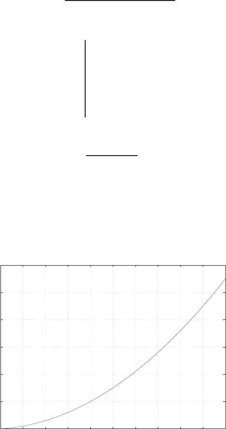
Advanced Problems 259

and the stability requirement.

AP6.4 The closed-loop transfer function is

T(s) = K

s3+ (p+ 1)s2+ps +K.

The Routh array is

s31p

s21 + p K

s1b0

soK

where

b=p2+p−K

1 + p.

Therefore, using the condition that b > 0, we obtain the the relationship

K < p2+p .

The plot of Kas a function of pis shown in Figure AP6.4.

100

120

0 1 2 3 4 5 6 7 8 9 10

STABLE REGION

FIGURE AP6.4

Stability region.

from the publisher prior to any prohibited reproduction, storage in a retrieval system, or transmission in any form or by any means, electronic, mechanical, photocopying,

recording, or likewise. For information regarding permission(s), write to: Rights and Permissions Department, Pearson Education, Inc., Upper Saddle River, NJ 07458.

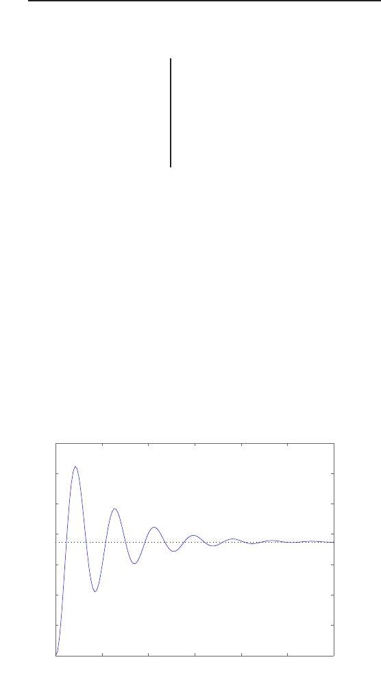
260 CHAPTER 6 The Stability of Linear Feedback Systems

AP6.5 The closed-loop transfer function is

T(s) = 30K1K2

(s+ 1 + K1K3)(s−10)(2s+K2K3−4) + 30K1K2K4

The Routh array is

s32a

s2b c

s1d0

soc

where a=−9K2K3+ 16 + K1K2K2

3−24K1K3,b= 2K1K3+K2K3−22,

and c=−10K2K3+ 40 −10K1K2K2

3+ 40K1K3and d= (ab −2c)/b .

The conditions for stability are

2K1K3+K2K3−22 >0

−10K2K3+ 40 −10K1K2K2

3+ 40K1K3>0

−2(−10K2K3+ 40 −10K1K2K2

3+ 40K1K3) + (9K2K3

+16 + K1K2K2

3−24K1K3)(2K1K3+K2K3−22) >0

Valid values for the various gains are: K1= 50, K2= 30, K3= 1, and

K4= 0.3. The step response is shown in Figure AP6.5.

0 5 10 15 20 25 30

100

150

200

250

300

350

Step Response

Time (sec)

Amplitude

FIGURE AP6.5

Stability region.

from the publisher prior to any prohibited reproduction, storage in a retrieval system, or transmission in any form or by any means, electronic, mechanical, photocopying,

recording, or likewise. For information regarding permission(s), write to: Rights and Permissions Department, Pearson Education, Inc., Upper Saddle River, NJ 07458.

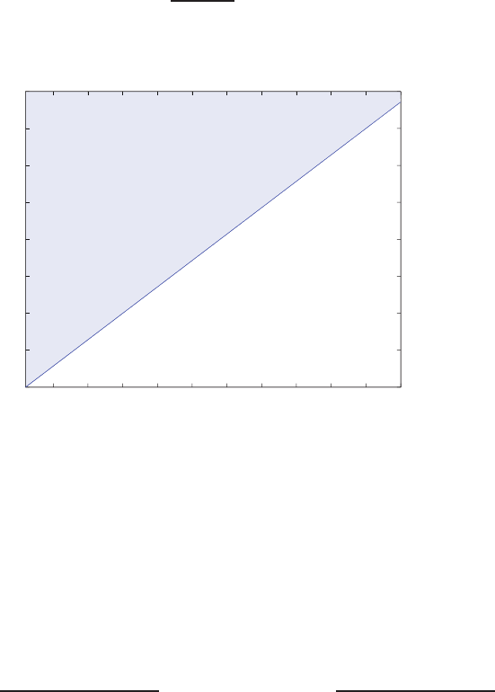
Advanced Problems 261

AP6.6 The characteristic equation is

s3+ 7s2+ (KD+ 14)s+KP+ 8 = 0.

For stability we require that KP>−8 and

KD>KP+ 8

7−14.

The relationship between KDand KPis shown in Figure AP6.6.

0 10 20 30 40 50 60 70 80 90 100

−14

−12

−10

−8

−6

−4

−2

UNSTABLE REGION

STABLE REGION

FIGURE AP6.6

Stability region.

AP6.7 The characteristic equation is

0.1s4+ 2.05s3+s2+ 8KPs+ 8KI= 0.

From the Routh array we ﬁnd the conditions for stability are

0< KI<0.3125

1.2812 −p1.6416 −5.2531KI< KP<1.2812 + p1.6416 −5.2531KI

from the publisher prior to any prohibited reproduction, storage in a retrieval system, or transmission in any form or by any means, electronic, mechanical, photocopying,

recording, or likewise. For information regarding permission(s), write to: Rights and Permissions Department, Pearson Education, Inc., Upper Saddle River, NJ 07458.

262 CHAPTER 6 The Stability of Linear Feedback Systems

Design Problems

The plant model with parameters given in Table CDP2.1 in Dorf andCDP6.1

Bishop is given by:

θ(s)

Va(s)=26.035

s(s+ 33.142) .

In the above transfer function we have neglected the motor inductance

Lm. The closed-loop transfer function from the input to the output is

θ(s)

R(s)=26.035Ka

s2+ 33.142s+ 26.035Ka

The Routh array is

s21 26.035Ka

s133.142 0

s026.035Ka

Stability is achieved for any 0 < Ka<∞.

DP6.1 The closed-loop characteristic polynomial is

s3+s2(5 + p+1

5K) + s(1

5Kp +1

5K+ 5p) + K= 0 .

(i) When p= 2, we have

s3+s2(7 + 1

5K) + s(10 + 3

5K) + K= 0 .

The Routh array is

s31 10 + 3

s27 + K

s1b

soK

where

b=(7 + K/5)(10 + 3K/5) −K

7 + 1

5K.

When −32.98 < K < −17.69, we ﬁnd that b > 0. Examining the

other terms in the ﬁrst column of the array, we ﬁnd that the system

from the publisher prior to any prohibited reproduction, storage in a retrieval system, or transmission in any form or by any means, electronic, mechanical, photocopying,

recording, or likewise. For information regarding permission(s), write to: Rights and Permissions Department, Pearson Education, Inc., Upper Saddle River, NJ 07458.

Design Problems 263

is stable for any K > 0.

(ii) When p= 0, we have

s3+s2(5 + 1

5K) + s(1

5K) + K= 0 .

The Routh array is

s311

s25 + 1

5K K

s1b

soK

where

b=(5 + 1

5K)1

5K−K

(5 + K/5) =K2/25

(5 + K/5) .

Again, examination of the ﬁrst column reveals that any K > 0 results

in a stable system. So, we just need to select any K > 0; e.g. K= 10.

DP6.2 (a) The closed-loop characteristic equation is

1 + 20(Ks + 1)

s2(s+ 20) = 0 ,

s3+ 20s2+ 20Ks + 20 = 0 .

The Routh array is

s31 20K

s220 20

s1b

so1

where

b=20K−1

For stability, we require K > 0.05.

(b) The desired characteristic polynomial is

(s2+as +b)(s+ 5) = s3+s2(a+ 5) + s(5a+b) + 5b= 0 .

Equating coeﬃcients with the actual characteristic equation we can

from the publisher prior to any prohibited reproduction, storage in a retrieval system, or transmission in any form or by any means, electronic, mechanical, photocopying,

recording, or likewise. For information regarding permission(s), write to: Rights and Permissions Department, Pearson Education, Inc., Upper Saddle River, NJ 07458.

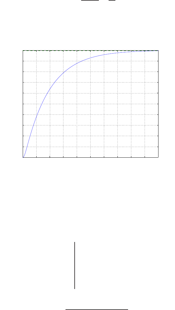
264 CHAPTER 6 The Stability of Linear Feedback Systems

solve for a, b and K, yielding b= 4, a= 15, and

K=5a+b

20 =79

20 .

(d) The step response is shown in Figure DP6.2.

0 2 4 6 8 10 12 14 16 18 20

0.1

0.2

0.3

0.4

0.5

0.6

0.7

0.8

0.9

time (sec)

y(t)

FIGURE DP6.2

Mars guided vehicle step response.

DP6.3 (a) The closed-loop characteristic equation is

2τs3+ (τ+ 2)s2+ (K+ 1)s+ 2K= 0 .

The Routh array is

s32τ K + 1

s2τ+ 2 2K

s1b

so2K

where

b=(τ+ 2)(K+ 1) −4Kτ

(τ+ 2) .

from the publisher prior to any prohibited reproduction, storage in a retrieval system, or transmission in any form or by any means, electronic, mechanical, photocopying,

recording, or likewise. For information regarding permission(s), write to: Rights and Permissions Department, Pearson Education, Inc., Upper Saddle River, NJ 07458.

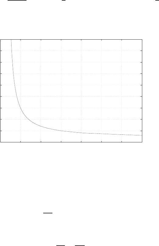
Design Problems 265

Examining the ﬁrst column of the Routh array, we determine that for

stability τ > 0, K > 0 and setting b > 0 yields the relationships:

(1) K < τ+ 2

3τ−2when τ > 2

3(2) K > 0 when 0 < τ ≤2

The plot of τversus Kis shown in Figure DP6.3a.

0.5

1.5

2.5

3.5

4.5

0 1 2 3 4 5 6 7

tau

STABLE REGION

FIGURE DP6.3

(a) The plot of τversus K.

(b) The steady-state error is

ess =A

,where Kv= 2K .

So,

ess

A=1

2K.

We require that ess ≤0.25A, therefore

K≥2.

One solution is to select τ= 0.5, then we remain within the stable

region.

is P.O. = 57%.

from the publisher prior to any prohibited reproduction, storage in a retrieval system, or transmission in any form or by any means, electronic, mechanical, photocopying,

recording, or likewise. For information regarding permission(s), write to: Rights and Permissions Department, Pearson Education, Inc., Upper Saddle River, NJ 07458.

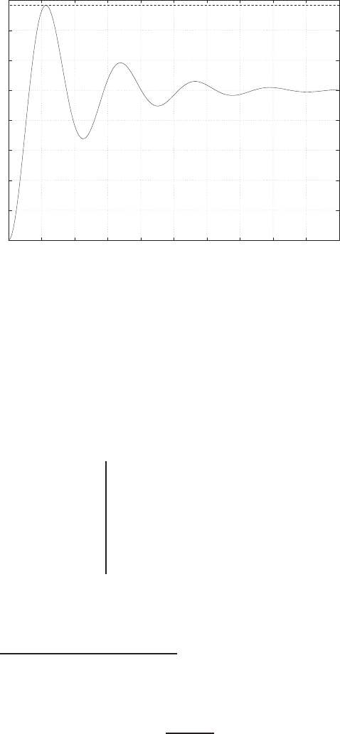
266 CHAPTER 6 The Stability of Linear Feedback Systems

0.2

0.4

0.6

0.8

1.2

1.4

1.6

0 2 4 6 8 10 12 14 16 18 20

time (sec)

y(t)

P. O . = 56.77 %

FIGURE DP6.3

CONTINUED: (b) Closed-loop system step response.

DP6.4 (a) The closed-loop characteristic polynomial is

s3+Ks2+ [(2 + m)K−1]s+ 2mK = 0 .

The Routh array is

s31 2K+mK −1

s2K2mK

s1b

so2mK

Examining the ﬁrst column of the Routh array, we see that for sta-

bility we require m > 0, K > 0, and b > 0, where

b=(2K+mK −1)K−2mK

K= (2 + m)K−(1 + 2m)>0,

K > 1 + 2m

2 + m.

The plot of Kvs mis shown in Figure DP6.4a.

from the publisher prior to any prohibited reproduction, storage in a retrieval system, or transmission in any form or by any means, electronic, mechanical, photocopying,

recording, or likewise. For information regarding permission(s), write to: Rights and Permissions Department, Pearson Education, Inc., Upper Saddle River, NJ 07458.

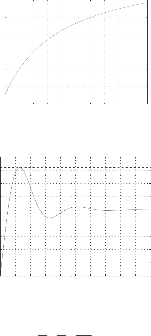
Design Problems 267

0.4

0.6

0.8

1.2

1.4

1.6

0 0.5 1 1.5 2 2.5 3 3.5 4 4.5 5

STABLE REGION

FIGURE DP6.4

(a) The plot of Kversus m.

0 1 2 3 4 5 6 7 8 9 10

0.2

0.4

0.6

0.8

1.2

1.4

1.6

1.8

time (sec)

y(t)

P. O . = 64.3208 %

FIGURE DP6.4

CONTINUED: (b) Shuttle attitude control step response.

(b) The steady-state error is

ess

A=1

2mK <0.10,

from the publisher prior to any prohibited reproduction, storage in a retrieval system, or transmission in any form or by any means, electronic, mechanical, photocopying,

recording, or likewise. For information regarding permission(s), write to: Rights and Permissions Department, Pearson Education, Inc., Upper Saddle River, NJ 07458.

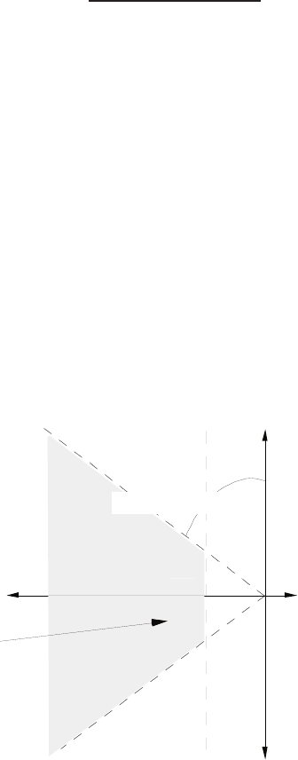
268 CHAPTER 6 The Stability of Linear Feedback Systems

or mK > 5. For example, we can select m= 0.5 and K= 2.

DP6.5 The closed-loop transfer function is

T(s) = K

s3+ 10s2+ 20s+K.

The range of Kfor stability is 0 < K < 200. If we let K=Km/N where

Km= 200, then N= 6.25 results in a step response with P.O. = 15.7%

and Ts= 1.96 seconds.

DP6.6 The closed-loop system is given by

x=



0 1

2−K1−2−K2

x+



1

r

The characteristic polynomial is s2+(2+K2)s+K1−2 = 0. So the system

is stable for K1>2 and K2>−2. Selecting K=h10 2 iresults in

closed-loop eigenvalues at s=−2±2j. The closed-loop step response has

a settling time of 2.11 s and a percent overshoot of 4.32%.

Re(s)

Im(s)

desired

region

for eigenvalues

ζωn = -1

sin-1 ζ = sin-1 0.69=43.63ο

FIGURE DP6.6

Performance region.

from the publisher prior to any prohibited reproduction, storage in a retrieval system, or transmission in any form or by any means, electronic, mechanical, photocopying,

recording, or likewise. For information regarding permission(s), write to: Rights and Permissions Department, Pearson Education, Inc., Upper Saddle River, NJ 07458.

Design Problems 269

DP6.7 (a) The inner loop closed-loop transfer function is

Y(s)

U(s)=20s

s3+ 10s2+ 20s+ 20K1

The Routh array is

s31 20

s2ω20K1

s1200−20K1

so20K1

For stability 0 < K1<10.

(b) The fastest response (that is, the quickest settling time) occurs when

K1= 2.2

Y(s)

R(s)=20K2s

s3+ 10s2+ (20 + 20K2)s+ 44 .

The Routh array is

s31 20(K2+ 1)

s210 44

s1200K2+156

so44

For stability, we require

200K2+ 156 >0.

Therefore, K2>−0.78.

DP6.8 The closed-loop characteristic equation is

s2+ 4KDs+ 4(KP+ 1) = 0.

So, it is possible to ﬁnd KPand KDto stabilize the system. For example,

any KP>0 and KD>0 leads to stability. Choosing KP≥9 results in a

steady-state tracking error less than 0.1 due to a unit step input. Then,

the damping ratio ζ=√2/2 is achieved by selecting

KD=√2√KP+ 1

from the publisher prior to any prohibited reproduction, storage in a retrieval system, or transmission in any form or by any means, electronic, mechanical, photocopying,

recording, or likewise. For information regarding permission(s), write to: Rights and Permissions Department, Pearson Education, Inc., Upper Saddle River, NJ 07458.

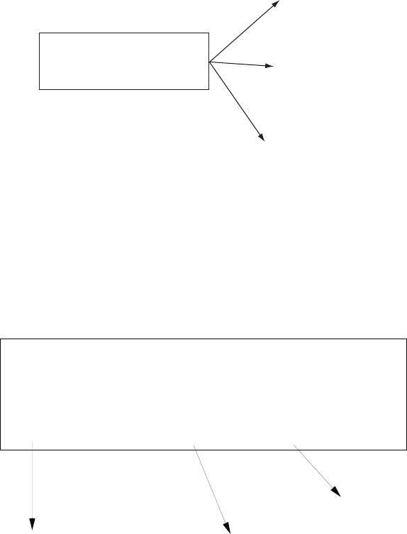
270 CHAPTER 6 The Stability of Linear Feedback Systems

Computer Problems

CP6.1 The m-ﬁle script is shown in Figure CP6.1.

ans =

-0.6063 + 2.7322i

-0.6063 - 2.7322i

-1.7874

ans =

-2.0004

-2.0000 + 0.0004i

-2.0000 - 0.0004i

-1.9996

ans =

0.2267 + 1.4677i

0.2267 - 1.4677i

-0.4534

pa=[1 3 10 14]; roots(pa)

pb=[1 8 24 32 16]; roots(pb)

pc=[1 0 2 1]; roots(pc)

FIGURE CP6.1

Computing the polynomial roots with the rootsfunction.

CP6.2 The m-ﬁle script is shown in Figure CP6.2.

ans =

-2.5000e-01 + 1.1990e+00i

-2.5000e-01 - 1.1990e+00i

ans =

0 + 1.2910e+00i

0 - 1.2910e+00i

ans =

2.5000e-01 + 1.3307e+00i

2.5000e-01 - 1.3307e+00i

K1=1;K2=2;K3=5; den=[1 2 1];

num1=K1*[1 -1 2];num2=K2*[1 -1 2];num3=K3*[1 -1 2];

sys1 = tf(num1,den); sys2 = tf(num2,den); sys3 = tf(num3,den);

sys1_cl=feedback(sys1,[1]);

sys2_cl=feedback(sys2,[1]);

sys3_cl=feedback(sys3,[1]);

p1 = pole(sys1_cl), p2 = pole(sys2_cl), p3 = pole(sys3_cl)

FIGURE CP6.2

K= 1 is stable;K= 2 is marginally stable; and K= 5 is unstable.

from the publisher prior to any prohibited reproduction, storage in a retrieval system, or transmission in any form or by any means, electronic, mechanical, photocopying,

recording, or likewise. For information regarding permission(s), write to: Rights and Permissions Department, Pearson Education, Inc., Upper Saddle River, NJ 07458.

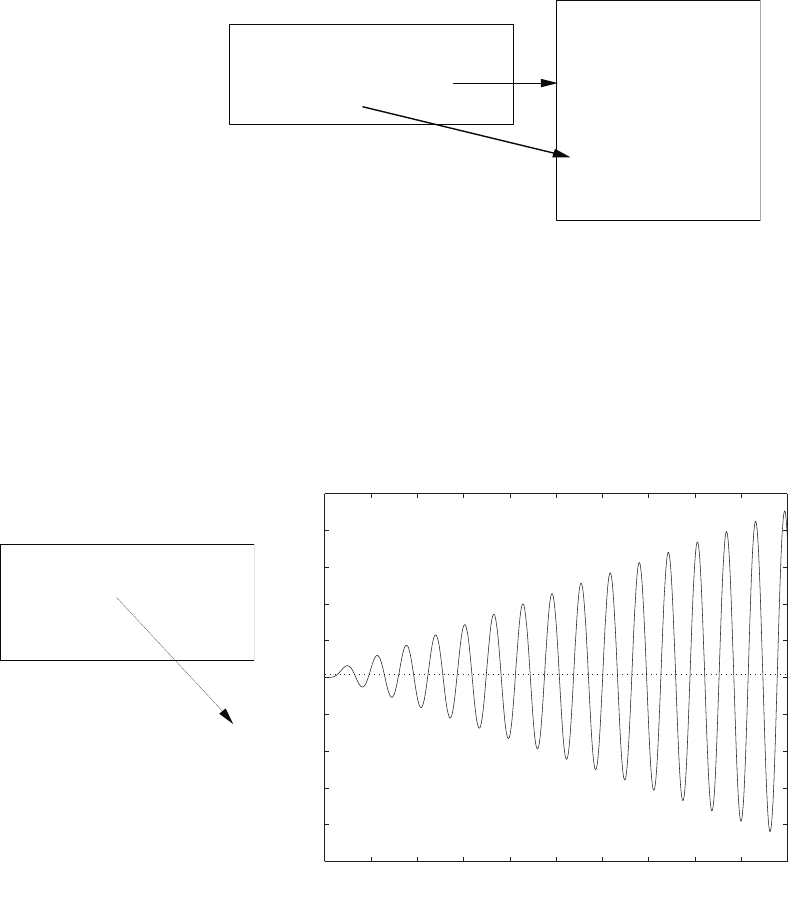
Computer Problems 271

CP6.3 The closed-loop transfer function and the roots of the characteristic equa-

tion are shown in Figure CP6.3.

numg=[1 1]; deng=[1 4 6 10];

sysg = tf(numg,deng);

sys = feedback(sysg,[1])

r=pole(sys)

Transfer function:

s + 1

----------------------

s^3 + 4 s^2 + 7 s + 11

r =

-2.8946

-0.5527 + 1.8694i

-0.5527 - 1.8694i

FIGURE CP6.3

Closed-loop transfer function and roots.

CP6.4 There are no poles in the right half-plane, but the system is unstable

since there are multiple poles on the jω-axis at s=±jand s=±j(see

Figure CP6.4).

num=[1]; den=[1 2 2 4 1 2];

sys = tf(num,den);

pole(sys)

t = 0:0.1:100;

step(sys,t)

ans =

-2.0000

0.0000 + 1.0000i

0.0000 - 1.0000i

-0.0000 + 1.0000i

-0.0000 - 1.0000i

Time (sec.)

Amplitude

Step Response

0 10 20 30 40 50 60 70 80 90 100

-25

-20

-15

-10

-5

From: U(1)

To: Y(1)

FIGURE CP6.4

Unstable system step response.

from the publisher prior to any prohibited reproduction, storage in a retrieval system, or transmission in any form or by any means, electronic, mechanical, photocopying,

recording, or likewise. For information regarding permission(s), write to: Rights and Permissions Department, Pearson Education, Inc., Upper Saddle River, NJ 07458.

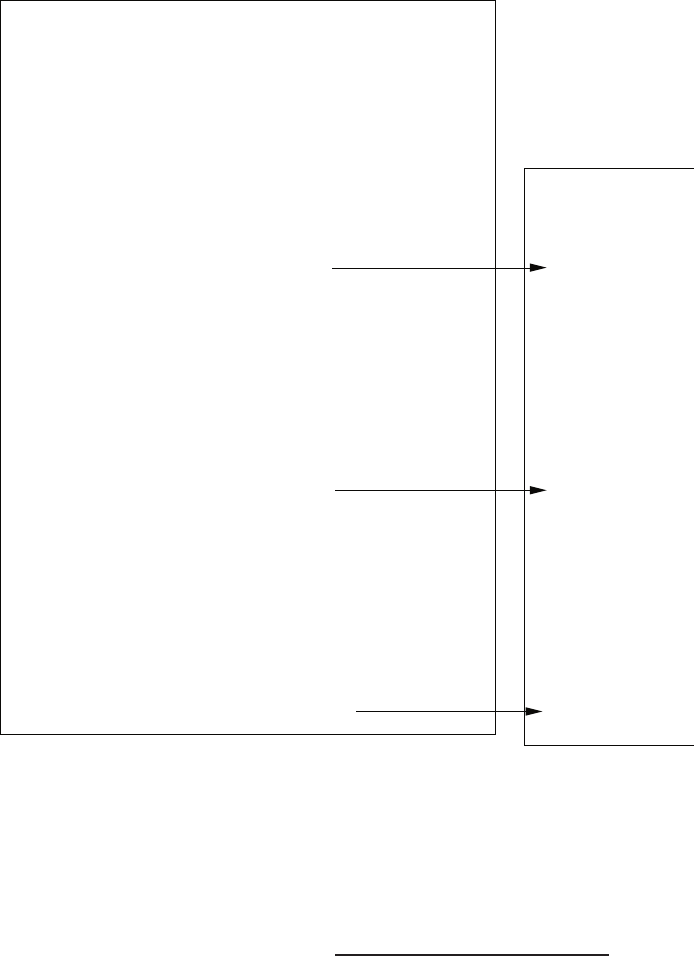
272 CHAPTER 6 The Stability of Linear Feedback Systems

CP6.5 The closed-loop system poles for the slow/fast pilots are shown in Fig-

ure CP6.5. The maximum allowable time delay is 0.2045seconds. At the

maximum allowable time delay, the system has roots on the jω-axis at

s=±2.6j. The slow pilot destabilizes the aircraft.

closed-loop

system poles

nume=[-10]; dene=[1 10]; syse = tf(nume,dene);

numg=[-1 -6]; deng=[1 3 6 0]; sysg = tf(numg,deng);

% Fast pilot

tau=0.1; tau1=2; K=1; tau2=0.5;

nump=-K*[tau1*tau tau-2*tau1 -2];

denp=[tau2*tau tau+2*tau2 2];

sysp = tf(nump,denp);

sysa = series(sysp,syse);

sysb = series(sysa, sysg);

sys = feedback(sysb,[1]);

fast_pilot=pole(sys)

% Slow pilot

tau=0.6; tau1=2; K=1; tau2=0.5;

nump=-K*[tau1*tau tau-2*tau1 -2];

denp=[tau2*tau tau+2*tau2 2];

sysp = tf(nump,denp);

sysa = series(sysp,syse);

sysb = series(sysa, sysg);

sys = feedback(sysb,[1]);

slow_pilot = pole(sys)

% Maximum pilot time delay, tau = 0.2045 sec

tau=0.2045; tau1=2; K=1; tau2=0.5;

nump=-K*[tau1*tau tau-2*tau1 -2];

denp=[tau2*tau tau+2*tau2 2];

sysp = tf(nump,denp);

sysa = series(sysp,syse);

sysb = series(sysa, sysg);

sys = feedback(sysb,[1]);

max_pilot_delay=pole(sys)

fast_pilot =

-19.6267

-10.7712

-3.8885

-0.1697 + 2.7880i

-0.1697 - 2.7880i

-0.3742

slow_pilot =

-9.4526

-4.5228 + 2.2595i

-4.5228 - 2.2595i

0.2793 + 2.0314i

0.2793 - 2.0314i

-0.3937

max_pilot_delay =

-10.0433 + 2.2684i

-10.0433 - 2.2684i

-4.3153

0.0001 + 2.6040i

0.0001 - 2.6040i

-0.3783

FIGURE CP6.5

Closed-loop system poles for an aircraft with a pilot in-the-loop.

CP6.6 The closed-loop transfer function is

T(s) = 1

s3+ 5s2+ (K−3)s+K+ 1 .

from the publisher prior to any prohibited reproduction, storage in a retrieval system, or transmission in any form or by any means, electronic, mechanical, photocopying,

recording, or likewise. For information regarding permission(s), write to: Rights and Permissions Department, Pearson Education, Inc., Upper Saddle River, NJ 07458.

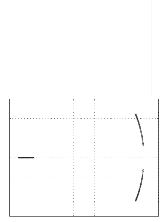
Computer Problems 273

Utilizing the Routh-Hurwitz approach, for stability we determine that

K > 4.

When K= 4, the roots of the characteristic equation are

s1=−5 and s2,3=±j .

The m-ﬁle script which generates a plot of the roots of the characteristic

equation as a function of Kis shown in Figure CP6.6.

K=[0:0.1:5];

n=length(K);

for i=1:n

numg=[1]; deng=[1 5 K(i)-3 K(i)];

sys_o = tf(numg,deng);

sys_cl = feedback(sys_o,[1]);

p(:,i)=pole(sys_cl);

end

plot(real(p),imag(p),'x'), grid

text(-0.9,0.95,'K=4 -->'); text(-0.2,1.3,'K=5'); text(0,0.2,'K=0')

% From a Routh-Hurwitz analysis we nd that

% minimum K for stability is K=4

Kmax=4;

numg=[1]; deng=[1 5 Kmax-3 Kmax]; sysg = tf(numg,deng);

sys_cl = feedback(sysg,[1]); pole(sys_cl)

-6 -5 -4 -3 -2 -1 0 1

-1.5

-1

-0.5

0.5

1.5

K=4 -->

K=5

K=0

FIGURE CP6.6

Roots of the characteristic equation as a function of K, where 0< K < 5.

from the publisher prior to any prohibited reproduction, storage in a retrieval system, or transmission in any form or by any means, electronic, mechanical, photocopying,

recording, or likewise. For information regarding permission(s), write to: Rights and Permissions Department, Pearson Education, Inc., Upper Saddle River, NJ 07458.

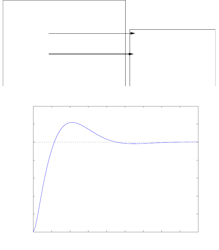
274 CHAPTER 6 The Stability of Linear Feedback Systems

CP6.7 The characteristic equation is

p(s) = s3+ 10s2+ 14s+ 12 .

A=[0 1 0;0 0 1;-12 -14 -10]; b=[0;0;12]; c=[1 1 0]; d=[0];

sys = ss(A,b,c,d);

% Part (a)

p=poly(A)

% Part (b)

roots(p)

% Part (c)

step(sys)

p =

1.0000 10.0000 14.0000 12.0000

ans =

-8.5225

-0.7387 + 0.9286i

-0.7387 - 0.9286i

0 1 2 3 4 5 6 7 8 9

0.2

0.4

0.6

0.8

1.2

1.4

Step Response

Time (sec)

Amplitude

FIGURE CP6.7

Characteristic equation from the state-space representation using the poly function.

The roots of the characteristic equation are

s1=−8.5225 and s2,3=−0.7387 ±0.9286j .

from the publisher prior to any prohibited reproduction, storage in a retrieval system, or transmission in any form or by any means, electronic, mechanical, photocopying,

recording, or likewise. For information regarding permission(s), write to: Rights and Permissions Department, Pearson Education, Inc., Upper Saddle River, NJ 07458.

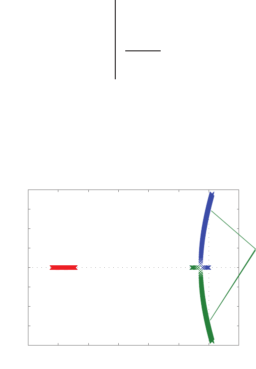
Computer Problems 275

The system is stable since all roots of the characteristic equation are in

the left half-plane. The unit step response and associated m-ﬁle script are

shown in Figure CP6.7.

CP6.8 The characteristic equation is

s3+ 10s2+ 10s+ 5K1= 0 .

(a) The Routh array is

s31 10

s210 5K1

s1100−5K1

so5K1

From the Routh-Hurwitz criterion, we obtain the limits 0 < K1<20

for stability.

(b) The plot of the pole locations is 0 < K1<30 is shown in Fig-

ure CP6.8. As seen in Figure CP6.8, when K1>20, the pole locations

move into the right half-plane.

?-12 ?-10 ?-8 ?-6 ?-4 ?-2 0 2

?-4

?-3

?-2

?-1

Root Locus

Real Axi s

Imaginary Axi s

k=20

FIGURE CP6.8

Pole locations for 0< K1<30.

CP6.9 (a) The characteristic equation is

s3+ 2s2+s+k−4 = 0 .

from the publisher prior to any prohibited reproduction, storage in a retrieval system, or transmission in any form or by any means, electronic, mechanical, photocopying,

recording, or likewise. For information regarding permission(s), write to: Rights and Permissions Department, Pearson Education, Inc., Upper Saddle River, NJ 07458.

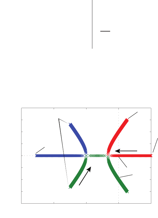
276 CHAPTER 6 The Stability of Linear Feedback Systems

The Routh array is

s31 1

s22k−4

s16−k

sok−4

For stability, we obtain 4 < k < 6.

(b) The pole locations for 0 < k < 10 are shown in Figure CP6.9. We see

that for 0 < k < 4 the system is unstable. Similarly, for 6 < k < 10,

the system is unstable.

?-3 ?-2 ?-1 0 1

?-2

?-1.5

?-1

?-0.5

0.5

1.5

Root Locus

Real Axi s

Imaginary Axi s

pole locations when k=0

pole location when k=0

increasing k

k=4

k=6

k=10

FIGURE CP6.9

Pole locations for 0< k < 10.

from the publisher prior to any prohibited reproduction, storage in a retrieval system, or transmission in any form or by any means, electronic, mechanical, photocopying,

recording, or likewise. For information regarding permission(s), write to: Rights and Permissions Department, Pearson Education, Inc., Upper Saddle River, NJ 07458.

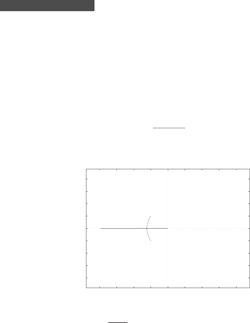
C H A P T E R 7

The Root Locus Method

Exercises

E7.1 (a) For the characteristic equation

1 + Ks(s+ 4)

s2+ 2s+ 2 = 0 ,

the root locus is shown in Figure E7.1.

-4

-3

-2

-1

-4 -3 -2 -1 0 1 2 3 4

Real Axis

Imag Axis

FIGURE E7.1

Root locus for 1 + Ks(s+4)

s2+2s+2 = 0.

277

from the publisher prior to any prohibited reproduction, storage in a retrieval system, or transmission in any form or by any means, electronic, mechanical, photocopying,

recording, or likewise. For information regarding permission(s), write to: Rights and Permissions Department, Pearson Education, Inc., Upper Saddle River, NJ 07458.

278 CHAPTER 7 The Root Locus Method

(b) The system characteristic equation can be written as

(1 + K)s2+ (2 + 4K)s+ 2 = 0 .

Solving for syields

s=−(1 + 2K)

(1 + K)±p(2 + 4K)2−8(1 + K)

2(1 + K).

When

(2 + 4K)2−8(1 + K) = 0 ,

then we have two roots at s1,2=−(1+2K)

1+K. Solving for Kyields K=

0.31.

s1,2=−(1 + 0.62)

(1.31) =−1.24 .

(d) When K= 0.31, the characterisitc equation is

s2+ 2.472s+ 1.528 = (s+ 1.24)2= 0 .

Thus, ωn= 1.24 and ζ= 1, the system is critically damped. The

settling time is Ts≈4 sec.

E7.2 (a) The root locus is shown in Figure E7.2. When K= 6.5, the roots of

the characteristic equation are

s1,2=−2.65 ±j1.23 and s3,4=−0.35 ±j0.8.

The real part of the dominant root is 8 times smaller than the other

two roots.

(b) The dominant roots are

(s+ 0.35 + j0.8)(s+ 0.35 −j0.8) = s2+ 0.7s+ 0.7625 .

From this we determine that

ωn= 0.873 and ζ=0.7

2(0.873) = 0.40 .

Thus, the settling time is

Ts=4

ζωn

0.35 = 11.43 sec .

The percent overshoot is P.O. =e−πζ/√1−ζ2= 25.4%.

from the publisher prior to any prohibited reproduction, storage in a retrieval system, or transmission in any form or by any means, electronic, mechanical, photocopying,

recording, or likewise. For information regarding permission(s), write to: Rights and Permissions Department, Pearson Education, Inc., Upper Saddle River, NJ 07458.

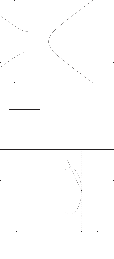
Exercises 279

-4

-3

-2

-1

-4 -3 -2 -1 0 1 2 3 4

Real Axis

Imag Axis

* K=6.5

FIGURE E7.2

Root locus for 1 + K1

s(s+2)(s2+4s+5) = 0.

E7.3 The root locus is shown in Figure E7.3. The roots are s1=−8.7, s2,3=

−1.3±j2.2 when K= 7.35 and ζ= 0.5.

-4

-3

-2

-1

-10 -8 -6 -4 -2 0 2 4

xxx

Real Axis

Imag Axis

<----- K=7.35

zeta=0.5

FIGURE E7.3

Root locus for 1 + Ks2+4s+8

s2(s+4) = 0.

from the publisher prior to any prohibited reproduction, storage in a retrieval system, or transmission in any form or by any means, electronic, mechanical, photocopying,

recording, or likewise. For information regarding permission(s), write to: Rights and Permissions Department, Pearson Education, Inc., Upper Saddle River, NJ 07458.

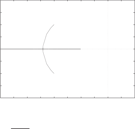
280 CHAPTER 7 The Root Locus Method

E7.4 The root locus is shown in Figure E7.4.

-2

-1.5

-1

-0.5

0.5

1.5

-4 -3.5 -3 -2.5 -2 -1.5 -1 -0.5 0 0.5 1

Real Axis

Imag Axis

FIGURE E7.4

Root locus for 1 + Ks+1

s2+4s+5 = 0.

The departure angles and entry points are

θd= 225o,−225o

and

σb=−2.4.

E7.5 (a) The root locus is in Figure E7.5. The breakaway points are

σb1=−13.0, σb2=−5.89 .

(b) The asymptote centroid is

σcent =−18 ,

and

φasym =±90o.

from the publisher prior to any prohibited reproduction, storage in a retrieval system, or transmission in any form or by any means, electronic, mechanical, photocopying,

recording, or likewise. For information regarding permission(s), write to: Rights and Permissions Department, Pearson Education, Inc., Upper Saddle River, NJ 07458.

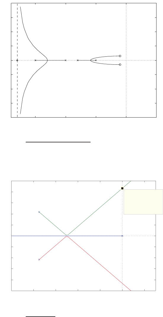
Exercises 281

-15 -10 -5 0 5

-40

-30

-20

-10

Real Axis

Imag Axis

< asymptote< asymptote

FIGURE E7.5

Root locus for 1 + Ks2+2s+10

(s4+38s3+515s2+2950s+6000) = 0.

E7.6 The system is unstable for K > 75.

Real Axis

Imaginary Axis

−10 −8 −6 −4 −2 0 2

−10

−8

−6

−4

−2

System: sys

Gain: 75

Pole: −0.000981 + 8.66i

Damping: 0.000113

Overshoot (%): 100

Frequency (rad/sec): 8.66

FIGURE E7.6

Root locus for 1 + K15K

s(s2+15s+75) = 0.

from the publisher prior to any prohibited reproduction, storage in a retrieval system, or transmission in any form or by any means, electronic, mechanical, photocopying,

recording, or likewise. For information regarding permission(s), write to: Rights and Permissions Department, Pearson Education, Inc., Upper Saddle River, NJ 07458.

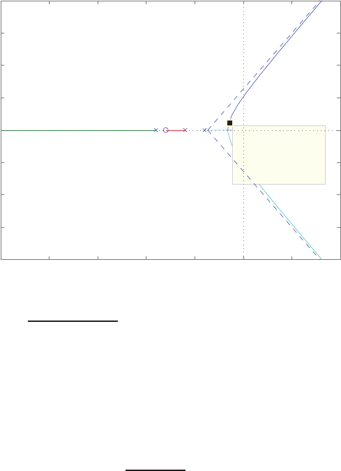
282 CHAPTER 7 The Root Locus Method

E7.7 The root locus is shown in Figure E7.7. The characteristic equation has

Real Axis

Imaginary Axis

−25 −20 −15 −10 −5 0 5 10

−20

−15

−10

−5

asymptote −−−>

System: sys

Gain: 27.3

Pole: −1.44 + 1.11i

Damping: 0.792

Overshoot (%): 1.7

Frequency (rad/sec): 1.81

FIGURE E7.7

Root locus for 1 + Ks+8

s(s+4)(s+6)(s+9) = 0.

4 poles and 1 zero. The asymptote angles are φ= +60o,−60o,−180o

centered at σcent =−3.7. When K= 27.35 then ζ= 0.8 for the complex

roots.

E7.8 The characteristic equation is

1 + K(s+ 1)

s2(s+ 9) = 0 ,

s3+ 9s2+Ks +K= 0 .

For all the roots to be equal and real, we require

(s+r)3=s3+ 3rs2+ 3r2s+r3= 0 .

Equating terms and solving for Kyields K= 27. All three roots are equal

at s=−3, when K= 27. The root locus is shown in Figure E7.8.

from the publisher prior to any prohibited reproduction, storage in a retrieval system, or transmission in any form or by any means, electronic, mechanical, photocopying,

recording, or likewise. For information regarding permission(s), write to: Rights and Permissions Department, Pearson Education, Inc., Upper Saddle River, NJ 07458.

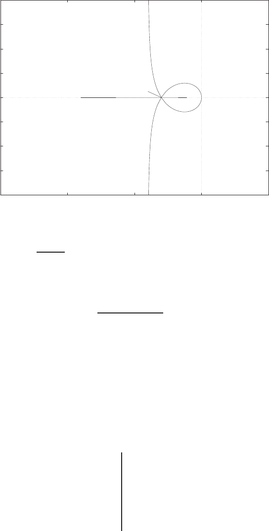
Exercises 283

-8

-6

-4

-2

-15 -10 -5 0 5

o xx

3 roots at s=-3

Real Axis

Imag Axis

FIGURE E7.8

Root locus for 1 + Ks+1

s2(s+9) = 0.

E7.9 The characteristic equation is

1 + K1

s(s2+ 2s+ 5) = 0

s3+ 2s2+ 5s+K= 0 .

(a) The system has three poles at s= 0 and −1±j2. The number of

asymptotes is np−nz= 3 centered at σcent =−2/3, and the angles

are φasymp at ±60o,180o.

(b) The angle of departure, θd, is 90o+θd+116.6o= 180o, so θd=−26.6o.

s31 5

s22K

s1b

soK

where b= 5 −K/2. So, when K= 10 the roots lie on the imaginary

from the publisher prior to any prohibited reproduction, storage in a retrieval system, or transmission in any form or by any means, electronic, mechanical, photocopying,

recording, or likewise. For information regarding permission(s), write to: Rights and Permissions Department, Pearson Education, Inc., Upper Saddle River, NJ 07458.

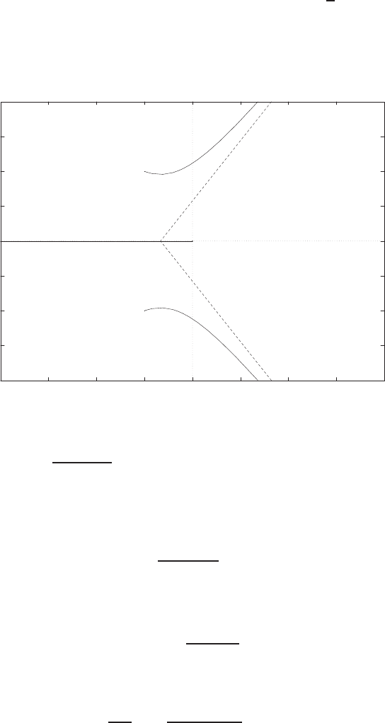
284 CHAPTER 7 The Root Locus Method

axis. The auxilary equation is

2s2+ 10 = 0 which implies s1,2=±j√5.

(d) The root locus is shown in Figure E7.9.

-4

-3

-2

-1

-4 -3 -2 -1 0 1 2 3 4

Real Axis

Imag Axis

asymptote --->

FIGURE E7.9

Root locus for 1 + K1

s(s2+2s+5) = 0.

E7.10 (a) The characteristic equation is

1 + K(s+ 2)

s(s+ 1) = 0 .

Therefore,

K=−(s2+s)

(s+ 2) ,

and

ds =−s2+ 4s+ 2

(s+ 2)2= 0 .

Solving s2+4s+2 = 0 yields s=−0.586 and −3.414. Thus, the system

from the publisher prior to any prohibited reproduction, storage in a retrieval system, or transmission in any form or by any means, electronic, mechanical, photocopying,

recording, or likewise. For information regarding permission(s), write to: Rights and Permissions Department, Pearson Education, Inc., Upper Saddle River, NJ 07458.

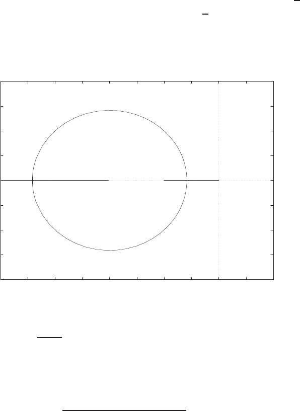
Exercises 285

breakaway and entry points are at s=−0.586 and s=−3.414.

(b) The desired characteristic polynomial is

(s+ 2 + aj)(s+ 2 −aj) = s2+ 4s+ 4 + a2= 0 ,

where ais not speciﬁed. The actual characteristic polynomial is

s2+ (1 + K)s+ 2K= 0 .

Equating coeﬃcients and solving for Kyields K= 3 and a=√2.

Thus, when K= 3, the roots are s1,2=−2±√2j.

-2

-1.5

-1

-0.5

0.5

1.5

-4 -3.5 -3 -2.5 -2 -1.5 -1 -0.5 0 0.5 1

xxo

Real Axis

Imag Axis

K=3, s=-2+1.414j

s=-0.58s=-3.41

FIGURE E7.10

Root locus for 1 + Ks+2

s(s+1) = 0.

E7.11 The root locus is shown in Figure E7.11 for the characteristic equation

1 + K(s+ 2.5)

(s2+ 2s+ 2)(s2+ 4s+ 5) = 0 .

From the root locus we see that we can only achieve ζ= 0.707 when

K= 0.

from the publisher prior to any prohibited reproduction, storage in a retrieval system, or transmission in any form or by any means, electronic, mechanical, photocopying,

recording, or likewise. For information regarding permission(s), write to: Rights and Permissions Department, Pearson Education, Inc., Upper Saddle River, NJ 07458.

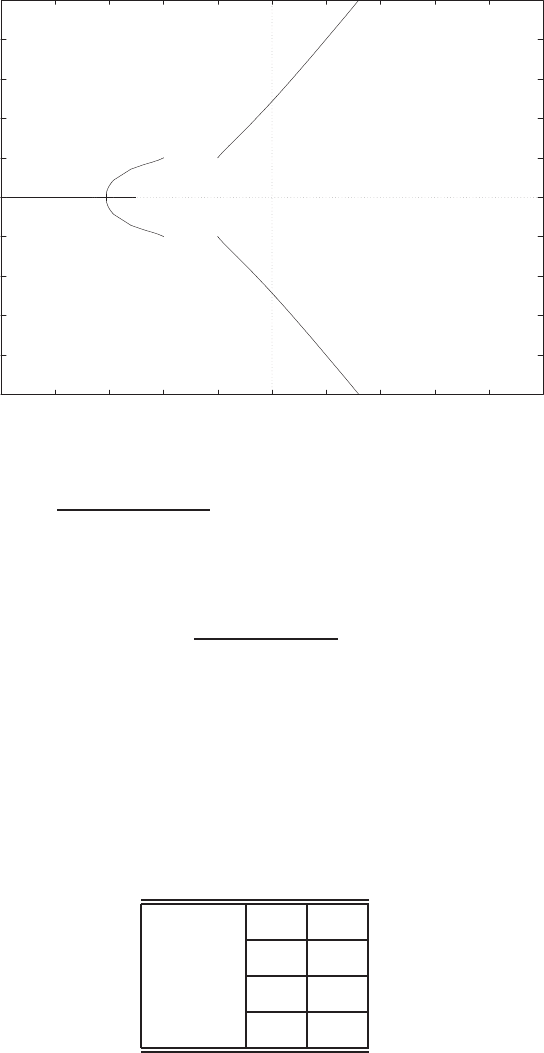
286 CHAPTER 7 The Root Locus Method

-5

-4

-3

-2

-1

-5 -4 -3 -2 -1 0 1 2 3 4 5

Real Axis

Imag Axis

<---- zeta=0.707 & K=0

FIGURE E7.11

Root locus for 1 + K(s+2.5)

(s2+2s+2)(s2+4s+5) = 0.

E7.12 (a) The root locus is shown in Figure E7.12 for the characteristic equation

1 + K(s+ 1)

s(s2+ 6s+ 18) = 0 .

(b) The roots of the characteristic equation are

(i) K= 10: s1,2=−2.8064 ±4.2368jand s3=−0.3872

(ii) K= 20: s1,2=−2.7134 ±5.2466jand s3=−0.5732

ble E7.12.

K10 20

Ts(sec) 9.0 5.5

P.O. 0 0

Tr(sec) 4.8 2.6

TABLE E7.12 System performance when K= 10 and K= 20.

from the publisher prior to any prohibited reproduction, storage in a retrieval system, or transmission in any form or by any means, electronic, mechanical, photocopying,

recording, or likewise. For information regarding permission(s), write to: Rights and Permissions Department, Pearson Education, Inc., Upper Saddle River, NJ 07458.

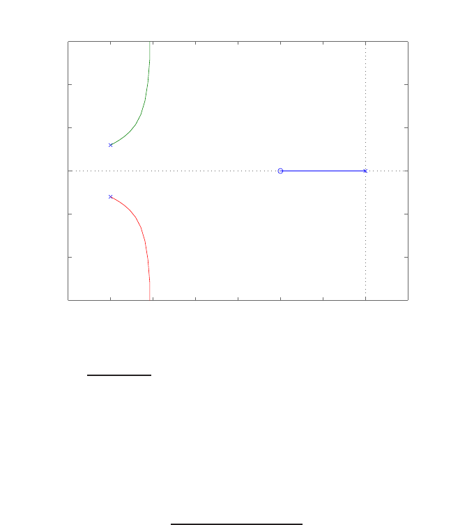
Exercises 287

−3.5 −3 −2.5 −2 −1.5 −1 −0.5 0 0.5

−15

−10

−5

Root Locus

Real Axis

Imaginary Axis

FIGURE E7.12

Root locus for 1 + K(s+1)

s(s2+6s+18) = 0.

E7.13 (a) The characteristic equation is

s(s+ 1)(s+ 3) + 4s+ 4z= 0 .

Rewriting with zas the parameter of interest yields

1 + z4

s(s+ 1)(s+ 3) + 4s= 0 .

The root locus is shown in Figure E7.13a.

(b) The root locations for

z= 0.6,2.0,and 4.0

are shown in Figure E7.13a. When z= 0.6, we have ζ= 0.76 and

ωn= 2.33. Therefore, the predicted step response is

P.O. = 2.4% and Ts= 2.3 sec (ζ= 0.6) .

When z= 2.0, we have ζ= 0.42 and ωn= 1.79. Therefore, the

predicted step response is

P.O. = 23% and Ts= 5.3 sec (ζ= 2.0) .

from the publisher prior to any prohibited reproduction, storage in a retrieval system, or transmission in any form or by any means, electronic, mechanical, photocopying,

recording, or likewise. For information regarding permission(s), write to: Rights and Permissions Department, Pearson Education, Inc., Upper Saddle River, NJ 07458.

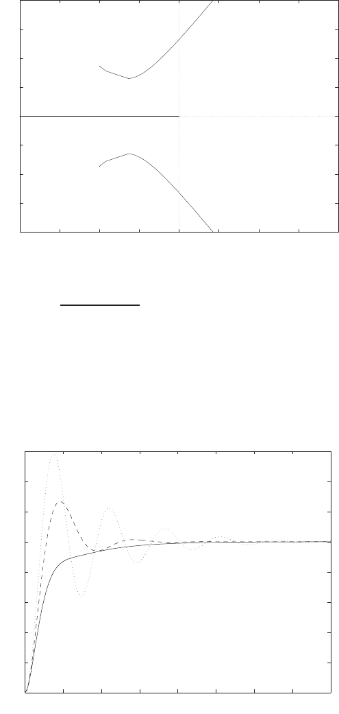
288 CHAPTER 7 The Root Locus Method

-4

-3

-2

-1

-4 -3 -2 -1 0 1 2 3 4

Real Axis

Imag Axis

* z=0.6

o z=2.0

+ z=4.0

FIGURE E7.13

(a) Root locus for 1 + z4

s(s+1)(s+3)+4s= 0.

Finally, when z= 4.0, we have ζ= 0.15 and ωn= 2.19. Therefore,

the predicted step response is P.O. = 62% and Ts= 12 sec.

0 2 4 6 8 10 12 14 16

0.2

0.4

0.6

0.8

1.2

1.4

1.6

time (sec)

y(t)

___ z=0.6

- - - z=2.0

..... z=4.0

FIGURE E7.13

CONTINUED: (b) Step Responses for z= 0.6,2.0,and 4.0.

from the publisher prior to any prohibited reproduction, storage in a retrieval system, or transmission in any form or by any means, electronic, mechanical, photocopying,

recording, or likewise. For information regarding permission(s), write to: Rights and Permissions Department, Pearson Education, Inc., Upper Saddle River, NJ 07458.

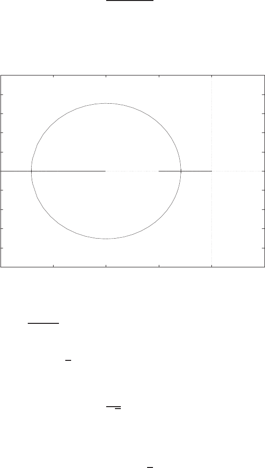
Exercises 289

E7.14 (a) The root locus is shown in Figure E7.14 for the characteristic equation

1 + K(s+ 10)

s(s+ 5) = 0 .

The breakaway point is sb=−2.93; the entry point is se=−17.1.

-10

-8

-6

-4

-2

-20 -15 -10 -5 0 5

xxo

Real Axis

Imag Axis

K=5, s=-5+5j

s=-2.93s=-17.1

FIGURE E7.14

Root locus for 1 + K(s+10)

s(s+5) = 0.

(b) We desire ζ= 1/√2 = 0.707. So, the desired characteristic polyno-

mial is

s2+ 2 1

√2ωns+ω2

n= 0 .

Comparing the desired characteristic polynomial to the actual we ﬁnd

the relationships

ω2

n= 10Kand √2ωn= 5 + K .

Solving for Kand ωnyields K= 5 and ωn= 7.07. The roots are

s1,2=−5±j5 when K= 5.

from the publisher prior to any prohibited reproduction, storage in a retrieval system, or transmission in any form or by any means, electronic, mechanical, photocopying,

recording, or likewise. For information regarding permission(s), write to: Rights and Permissions Department, Pearson Education, Inc., Upper Saddle River, NJ 07458.

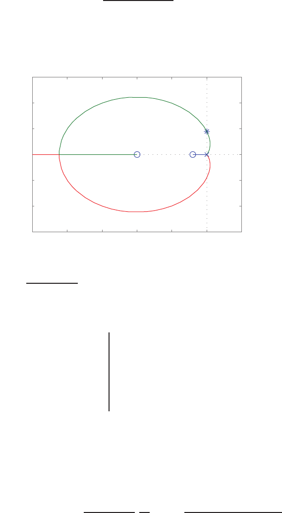
290 CHAPTER 7 The Root Locus Method

E7.15 (a) The characteristic equation

1 + K(s+ 10)(s+ 2)

s3= 0

has the root locus in Figure E7.15.

?-25 ?-20 ?-15 ?-10 -5 0 5

?-15

?-10

?-5

K=1.67

Root Locus

Real Axi s

Imaginary Axi s

FIGURE E7.15

Root locus for 1 + K(s+10)(s+2)

s3= 0.

(b) The Routh array is

s31 12K

s2K20K

s1b

so20K

when b= 12K−20. For stability, we require all elements in the ﬁrst

column to be positive. Therefore,

K > 1.67 .

ess = lim

s→0sE(s) = lim

s→0s1

1 + GH(s)·1

s2= lim

s→0

s3+K(s+ 1)(s+ 3) = 0 .

from the publisher prior to any prohibited reproduction, storage in a retrieval system, or transmission in any form or by any means, electronic, mechanical, photocopying,

recording, or likewise. For information regarding permission(s), write to: Rights and Permissions Department, Pearson Education, Inc., Upper Saddle River, NJ 07458.

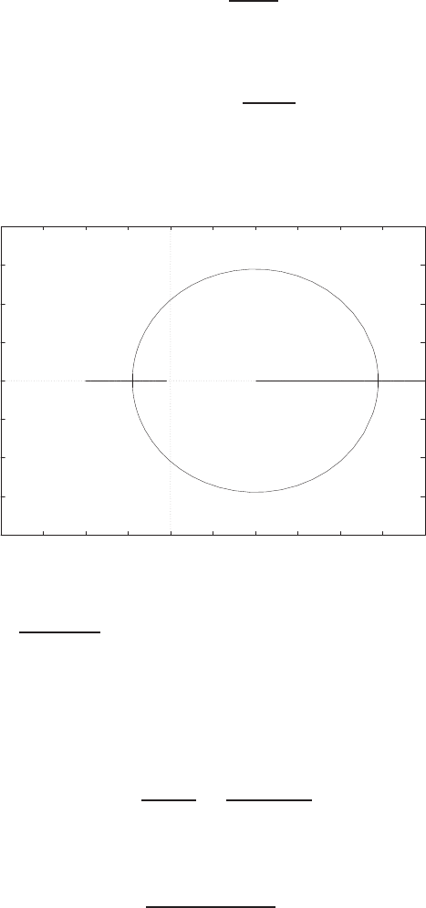
Exercises 291

E7.16 The expansion for e−T s is

e−T s = 1 −T s +(T s)2

2! −...

If (T s)<< 1, then

e−T s ≈1−T s =a+bs

c+ds ,

where a, b, c and dare constants to be determined. Using long division,

-40

-30

-20

-10

-40 -30 -20 -10 0 10 20 30 40 50 60

x x o

Real Axis

Imag Axis

K=21

FIGURE E7.16

Root locus for 1 + K(20−s)

(s+1)(20+s)= 0.

we expand (a+bs)/(c+ds) and match as many coeﬃcients as possible. In

this case, we determine that a=c= (2/T ) and also that b=−d=−1.

In this case, with T= 0.1, we have

e−T s =20 −s

20 + s=−(s−20)

(s+ 20) .

So, the characteristic equation is

1 + −K(s−20)

(s+ 1)(s+ 20) ,

and the root locus is shown in Figure E7.16. Using a Routh-Hurwitz

from the publisher prior to any prohibited reproduction, storage in a retrieval system, or transmission in any form or by any means, electronic, mechanical, photocopying,

recording, or likewise. For information regarding permission(s), write to: Rights and Permissions Department, Pearson Education, Inc., Upper Saddle River, NJ 07458.

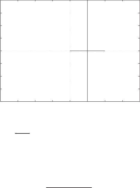
292 CHAPTER 7 The Root Locus Method

analysis with the characteristic polynomial

s2+ (21 −K)s+ 20 + 20K= 0 ,

we determine that the system is stable for −1< K < 21.

E7.17 (a) The root locus is in Figure E7.17a.

-2

-1.5

-1

-0.5

0.5

1.5

-2 -1.5 -1 -0.5 0 0.5 1 1.5 2

x x

Real Axis

Imag Axis

FIGURE E7.17

(a) Root locus for 1 + K

s(s−1) = 0.

The root locus is always in the right half-plane; the system is unstable

for K > 0.

(b) The characteristic equation is

1 + K(s+ 2)

s(s−1)(s+ 20) = 0 ,

and the root locus is shown in Figure E7.17b. The system is stable

for K > 22.3 and when K= 22.3, the roots are

s1,2=±j1.53 and s3=−19 .

from the publisher prior to any prohibited reproduction, storage in a retrieval system, or transmission in any form or by any means, electronic, mechanical, photocopying,

recording, or likewise. For information regarding permission(s), write to: Rights and Permissions Department, Pearson Education, Inc., Upper Saddle River, NJ 07458.

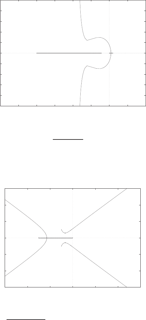
Exercises 293

-10

-8

-6

-4

-2

-30 -25 -20 -15 -10 -5 0 5 10

x xx o

Real Axis

Imag Axis

*K=22.3

FIGURE E7.17

CONTINUED: (b) Root locus for 1 + K(s+2)

s(s+20)(s−1) = 0.

E7.18 The root locus is shown in Figure E7.18.

-6

-4

-2

-6 -4 -2 0 2 4 6

Real Axis

Imag Axis

K=8.15

FIGURE E7.18

Root locus for 1 + K

s(s+3)(s2+2s+2) = 0.

When K= 8.15, the roots are s1,2=±j1.095 and s3,4=−2.5±j0.74.

from the publisher prior to any prohibited reproduction, storage in a retrieval system, or transmission in any form or by any means, electronic, mechanical, photocopying,

recording, or likewise. For information regarding permission(s), write to: Rights and Permissions Department, Pearson Education, Inc., Upper Saddle River, NJ 07458.

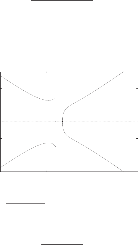
294 CHAPTER 7 The Root Locus Method

E7.19 The characteristic equation is

1 + K

s(s+ 3)(s2+ 6s+ 64) = 0 ,

and the root locus is shown in Figure E7.19. When K= 1292.5, the roots

are

s1,2=±j4.62 and s3,4=−4.49 ±j6.36 .

-15

-10

-5

-15 -10 -5 0 5 10 15

Real Axis

Imag Axis

K=1292.5

FIGURE E7.19

Root locus for 1 + K

s(s+3)(s2+6s+64) = 0.

E7.20 The characteristic equation is

1 + K(s+ 1)

s(s−2)(s+ 6) = 0 ,

and the root locus is shown in Figure E7.20. The system is stable for

K > 16 .

The maximum damping ratio of the stable complex roots is

ζ= 0.25 .

from the publisher prior to any prohibited reproduction, storage in a retrieval system, or transmission in any form or by any means, electronic, mechanical, photocopying,

recording, or likewise. For information regarding permission(s), write to: Rights and Permissions Department, Pearson Education, Inc., Upper Saddle River, NJ 07458.

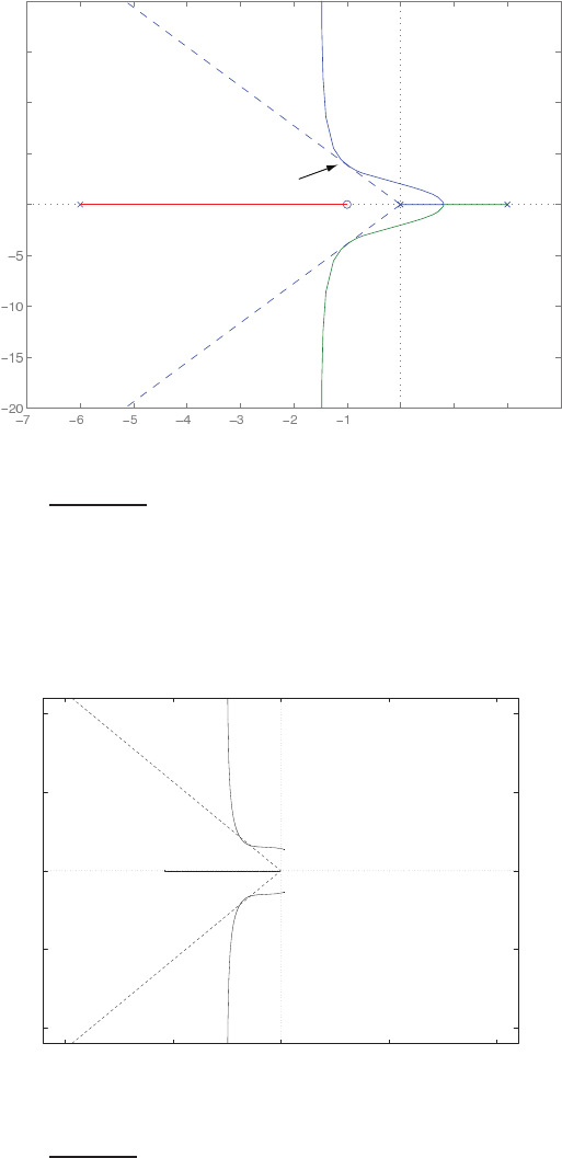
Exercises 295

0 1 2 3

Real Axis

Imaginary Axis

ζmax = 0.25

FIGURE E7.20

Root locus for 1 + K(s+1)

s(s−2)(s+6) = 0.

E7.21 The gain is K= 10.8 when the complex roots have ζ= 0.66.

-10

-5

-10 -5 0 5 10

Real Axis

Imag Axis

K=10.8

FIGURE E7.21

Root locus for 1 + Ks

s3+5s2+10 = 0.

from the publisher prior to any prohibited reproduction, storage in a retrieval system, or transmission in any form or by any means, electronic, mechanical, photocopying,

recording, or likewise. For information regarding permission(s), write to: Rights and Permissions Department, Pearson Education, Inc., Upper Saddle River, NJ 07458.

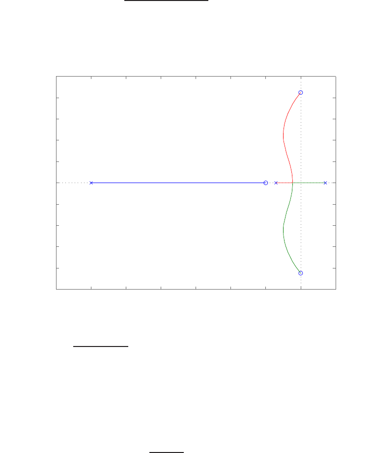
296 CHAPTER 7 The Root Locus Method

E7.22 The root locus is shown in Figure E7.22. The characteristic equation is

1 + K(s2+ 18)(s+ 2)

(s2−2)(s+ 12) = 0 .

−14 −12 −10 −8 −6 −4 −2 0 2

−5

−4

−3

−2

−1

Root Locus

Real Axis

Imaginary Axis

FIGURE E7.22

Root locus for 1 + K(s2+18)(s+2)

(s2−2)(s+12) = 0.

E7.23 The characteristic equation is

5s2+as + 4 = 0 ,

which can rewritten as

1 + as

5s2+ 4 = 0 .

The roots locus (with aas the parameter) is shown in Figure E7.23.

from the publisher prior to any prohibited reproduction, storage in a retrieval system, or transmission in any form or by any means, electronic, mechanical, photocopying,

recording, or likewise. For information regarding permission(s), write to: Rights and Permissions Department, Pearson Education, Inc., Upper Saddle River, NJ 07458.

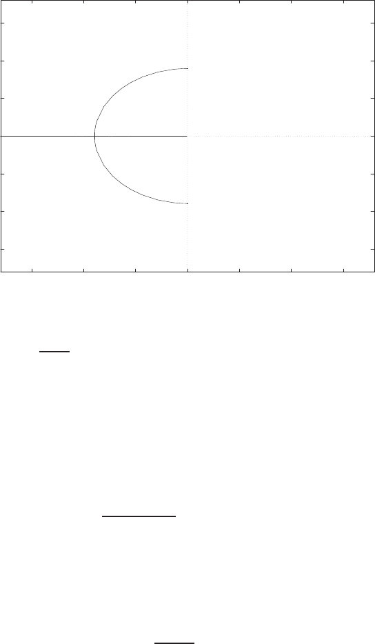
Exercises 297

-1.5

-1

-0.5

0.5

1.5

-1.5 -1 -0.5 0 0.5 1 1.5

Real Axis

Imag Axis

FIGURE E7.23

Root locus for 1 + as

5s2+4 = 0.

E7.24 The transfer function is

G(s) = C(sI−A)−1B+D

= [ 1 0 ]



s−1

4s+k



−1



1



s2+ks + 4 .

Therefore, the characteristic equation is

s2+ks + 4 = 0 ,

1 + ks

s2+ 4 = 0 .

The root locus for 0 < k < ∞is shown in Figure E7.24. The closed-loop

system is stable for all 0 < k < ∞.

from the publisher prior to any prohibited reproduction, storage in a retrieval system, or transmission in any form or by any means, electronic, mechanical, photocopying,

recording, or likewise. For information regarding permission(s), write to: Rights and Permissions Department, Pearson Education, Inc., Upper Saddle River, NJ 07458.

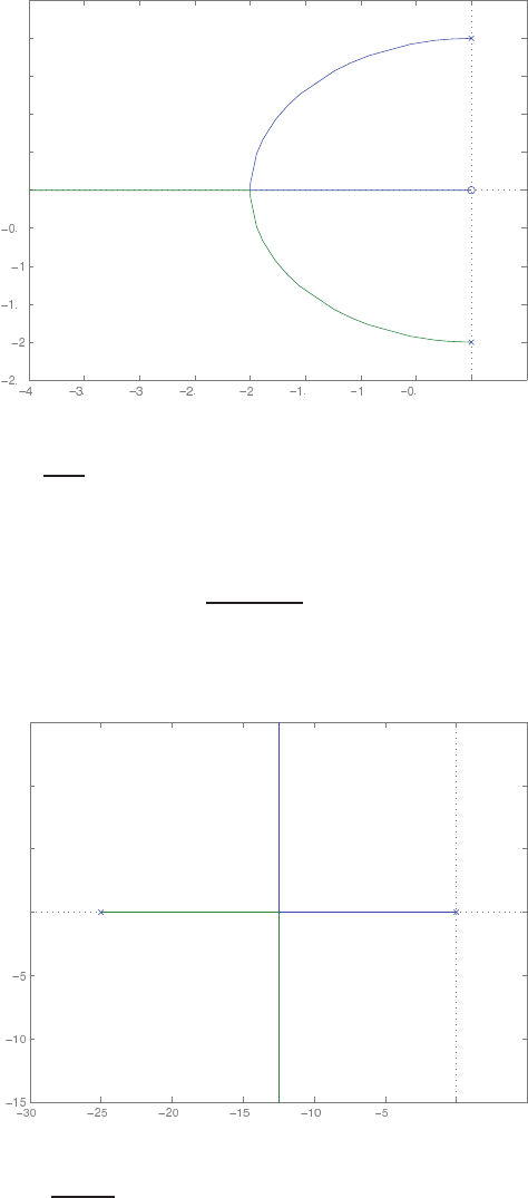
298 CHAPTER 7 The Root Locus Method

5 5 5 5 0 0.5

0.5

1.5

2.5

Real Axis

Imaginary Axis

FIGURE E7.24

Root locus for 1 + ks

s2+4 = 0.

E7.25 The characteristic equation is

1 + K10

s(s+ 25) = 0 .

The root locus shown in Figure E7.25 is stable for all 0 < K < ∞.

0 5

Real Axis

Imaginary Axis

FIGURE E7.25

Root locus for 1 + K10

s(s+25) = 0.

from the publisher prior to any prohibited reproduction, storage in a retrieval system, or transmission in any form or by any means, electronic, mechanical, photocopying,

recording, or likewise. For information regarding permission(s), write to: Rights and Permissions Department, Pearson Education, Inc., Upper Saddle River, NJ 07458.

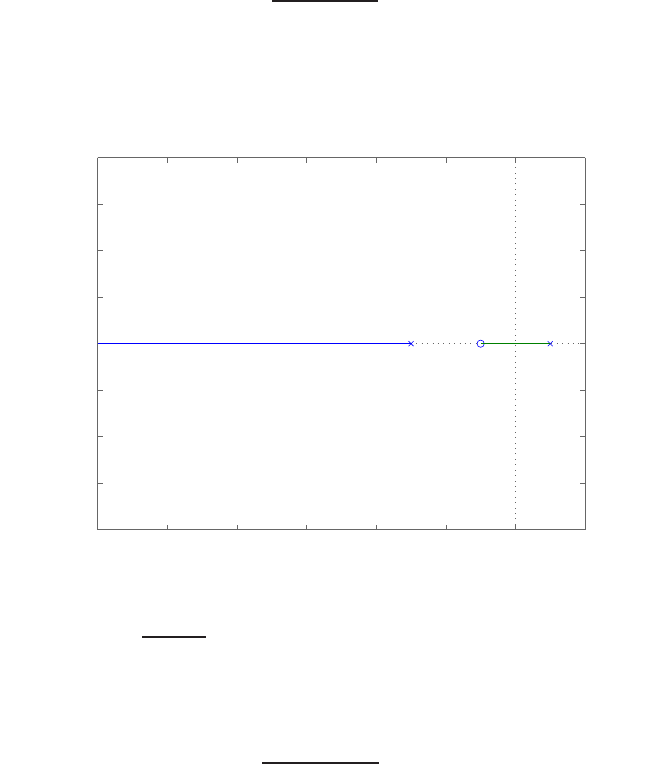
Exercises 299

E7.26 The characteristic polynomial is

det 



s−1

s+K−3s+K+ 2 

= 0

1 + Ks+ 1

s2+ 2s−3= 0 .

The root locus shown in Figure E7.26 is stable for all 0 < K < 3.

−12 −10 −8 −6 −4 −2 0 2

−0.8

−0.6

−0.4

−0.2

0.2

0.4

0.6

0.8

Root Locus

Real Axis

Imaginary Axis

FIGURE E7.26

Root locus for 1 + Ks+1

s2+2s−3= 0.

E7.27 The characteristic equation is

1 + ps

s2+ 4s+ 40 = 0 .

The root locus shown in Figure E7.27 is stable for all 0 < p < ∞.

from the publisher prior to any prohibited reproduction, storage in a retrieval system, or transmission in any form or by any means, electronic, mechanical, photocopying,

recording, or likewise. For information regarding permission(s), write to: Rights and Permissions Department, Pearson Education, Inc., Upper Saddle River, NJ 07458.

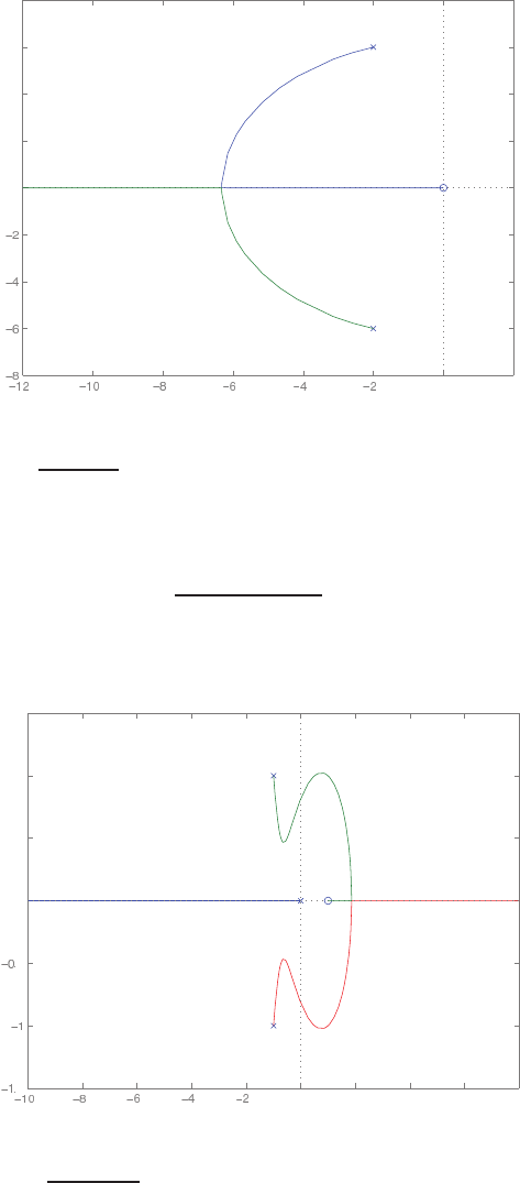
300 CHAPTER 7 The Root Locus Method

0 2

Real Axis

Imaginary Axis

FIGURE E7.27

Root locus for 1 + ps

s2+4s+40 = 0.

E7.28 The characteristic equation is

1 + Ks−1

s(s2+ 2s+ 2) = 0 .

The system is stable for −1.33 < K < 0.

0 2 4 6 8

0.5

1.5

Real Axis

Imaginary Axis

FIGURE E7.28

Root locus for 1 + Ks−1

s(s2+2s+2) = 0.

from the publisher prior to any prohibited reproduction, storage in a retrieval system, or transmission in any form or by any means, electronic, mechanical, photocopying,

recording, or likewise. For information regarding permission(s), write to: Rights and Permissions Department, Pearson Education, Inc., Upper Saddle River, NJ 07458.

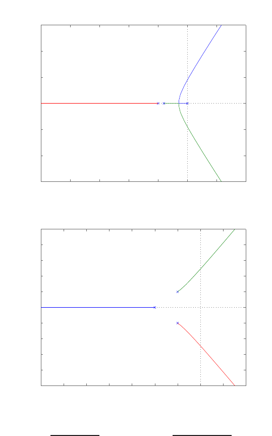
Problems 301

Problems

P7.1

−50 −40 −30 −20 −10 0 10 20

−30

−20

−10

Root Locus

Real Axis

Imaginary Axis

−7 −6 −5 −4 −3 −2 −1 0 1 2

−5

−4

−3

−2

−1

Root Locus

Real Axis

Imaginary Axis

FIGURE P7.1

(a) Root locus for 1 + K

s(s+10)(s+8) = 0, and (b) 1 + K

(s2+2s+2)(s+1) = 0.

from the publisher prior to any prohibited reproduction, storage in a retrieval system, or transmission in any form or by any means, electronic, mechanical, photocopying,

recording, or likewise. For information regarding permission(s), write to: Rights and Permissions Department, Pearson Education, Inc., Upper Saddle River, NJ 07458.

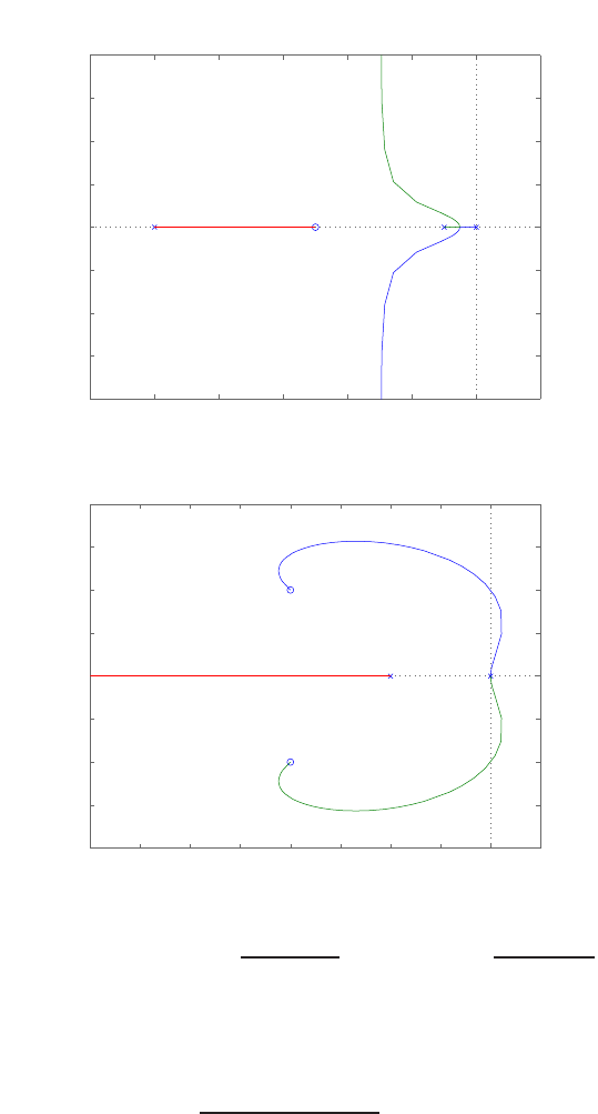
302 CHAPTER 7 The Root Locus Method

−12 −10 −8 −6 −4 −2 0 2

−40

−30

−20

−10

Root Locus

Real Axis

Imaginary Axis

−4 −3.5 −3 −2.5 −2 −1.5 −1 −0.5 0 0.5

−4

−3

−2

−1

Root Locus

Real Axis

Imaginary Axis

FIGURE P7.1

CONTINUED: (c) Root locus for 1 + K(s+5)

s(s+2)(s+7) = 0, and (d)1 + K(s2+4s+8)

s2(s+7) = 0.

P7.2 The root locus is shown in Figure P7.2 for the characteristic equation

1 + 10Kv(s+ 10)

s(s+ 1)(s+ 100) = 0 .

The damping ratio is ζ= 0.6 when Kv= 0.8, 135 and 648. The roots of

the characteristic equation are:

(a) Kv= 0.8 : s1=−99.9, s2,3=−0.54 ±j0.71

from the publisher prior to any prohibited reproduction, storage in a retrieval system, or transmission in any form or by any means, electronic, mechanical, photocopying,

recording, or likewise. For information regarding permission(s), write to: Rights and Permissions Department, Pearson Education, Inc., Upper Saddle River, NJ 07458.

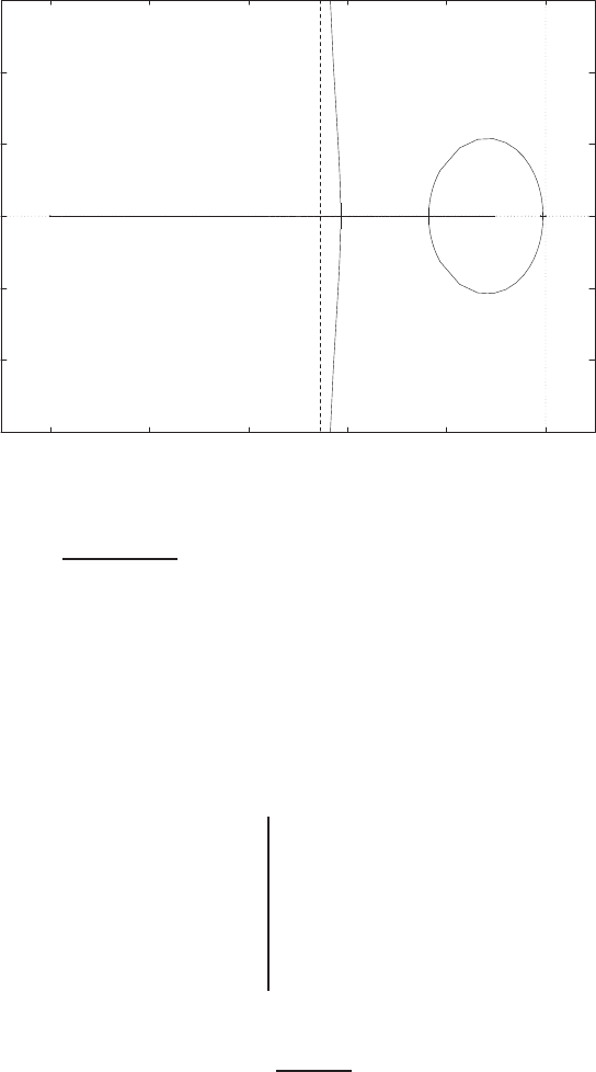
Problems 303

(b) Kv= 135 : s1=−85.9, s2,3=−7.5±j10

-30

-20

-10

-100 -80 -60 -40 -20 0

xxx o

Real Axis

Imag Axis

FIGURE P7.2

Root locus for 1 + 10Kv(s+10)

s(s+1)(s+100) = 0.

P7.3 (a) The breakaway point is s=−0.88 at K= 4.06.

(b) The characteristic equation can be written as

s(s+ 2)(s+ 5) + K= 0 .

The Routh array is

s31 10

s27K

s1b0

soK

where

b=70 −K

from the publisher prior to any prohibited reproduction, storage in a retrieval system, or transmission in any form or by any means, electronic, mechanical, photocopying,

recording, or likewise. For information regarding permission(s), write to: Rights and Permissions Department, Pearson Education, Inc., Upper Saddle River, NJ 07458.

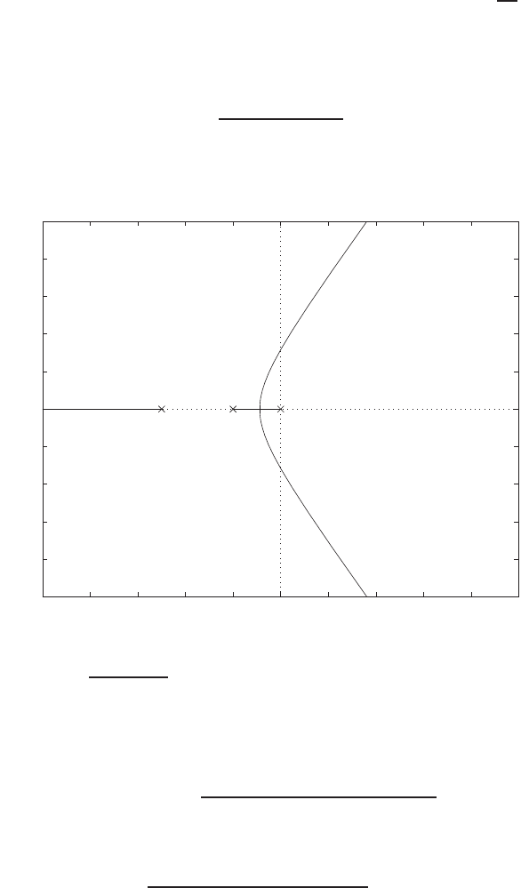
304 CHAPTER 7 The Root Locus Method

When K= 70, the system has roots on jω-axis at s=±j√10.

(d) The characteristic equation

1 + K

s(s+ 2)(s+ 5) = 0

has the root locus shown in Figure P7.3.

-10 -8 -6 -4 -2 0 2 4 6 8 10

-10

-8

-6

-4

-2

Real Axis

Imag Axis

FIGURE P7.3

Root locus for 1 + K

s(s+2)(s+5) = 0.

P7.4 The characteristic equation for the large antenna is

1 + G1G(s) = 1 + 100ka

(0.1s+ 1)(s2+ 14.4s+ 100) = 0 ,

1 + 1000ka

(s+ 10)(s2+ 14.4s+ 100) = 0 .

The root locus is shown in Figure P7.4. Using Routh’s criteria, we ﬁnd

that the system is stable for

−1< ka<4.83 .

from the publisher prior to any prohibited reproduction, storage in a retrieval system, or transmission in any form or by any means, electronic, mechanical, photocopying,

recording, or likewise. For information regarding permission(s), write to: Rights and Permissions Department, Pearson Education, Inc., Upper Saddle River, NJ 07458.

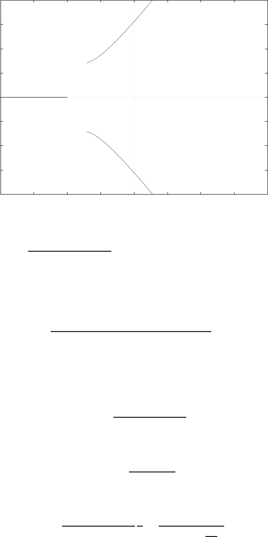
Problems 305

-20

-15

-10

-5

-20 -15 -10 -5 0 5 10 15 20

Real Axis

Imag Axis

<-- K=4.827

FIGURE P7.4

Root locus for 1 + 1000ka

(s2+14.14s+100)(s+10) = 0.

When ka= 4.83, we have s1,2=±j15.53.

P7.5 (a) The characteristic equation for hands-oﬀ control is

1 + 25K2(s+ 0.03)(s+ 1)

(s+ 0.4)(s2−0.36s+ 0.16)(s+ 9) = 0 .

The root locus is shown in Figure P7.5a. The damping ratio is ζ=

0.707 when K2= 1.6 or K2= 0.74.

(b) The transfer function from Td(s) to Y(s) is

Y(s) = G2(s)Td(s)

1 + G2(s)Gf(s),

where

Gf(s) = K2(s+ 1)

s+ 9 .

Using the ﬁnal value theorem, we determine that

yss = lim

s→0sG2(s)

1 + G2(s)Gf(s)

s=11.7

1 + 11.7K2

9= 3.8,

from the publisher prior to any prohibited reproduction, storage in a retrieval system, or transmission in any form or by any means, electronic, mechanical, photocopying,

recording, or likewise. For information regarding permission(s), write to: Rights and Permissions Department, Pearson Education, Inc., Upper Saddle River, NJ 07458.

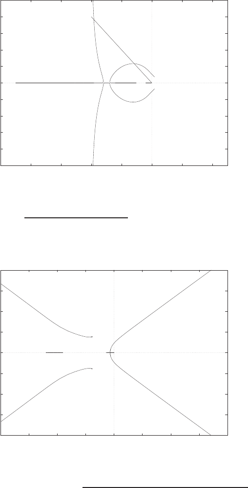
306 CHAPTER 7 The Root Locus Method

-5

-4

-3

-2

-1

-10 -8 -6 -4 -2 0 2 4

o ox x

Real Axis

Imag Axis

<-- K=1.6

<-- K=0.74

FIGURE P7.5

(a) Root locus for 1 + 25K2(s+0.03)(s+1)

(s+9)(s2−0.36s+0.16)(s+0.4) = 0.

-20

-15

-10

-5

-20 -15 -10 -5 0 5 10 15 20

x xxo o

Real Axis

Imag Axis

FIGURE P7.5

CONTINUED: (b) Root locus for 1 + 25K1(s+0.03)(s+9)

(s+0.045)(s2+12s+1)(s+1.33)(s2+7.66s+29.78) = 0.

where we have selected K2= 1.6. For K2= 0.74, we ﬁnd that yss =

5.96.

from the publisher prior to any prohibited reproduction, storage in a retrieval system, or transmission in any form or by any means, electronic, mechanical, photocopying,

recording, or likewise. For information regarding permission(s), write to: Rights and Permissions Department, Pearson Education, Inc., Upper Saddle River, NJ 07458.

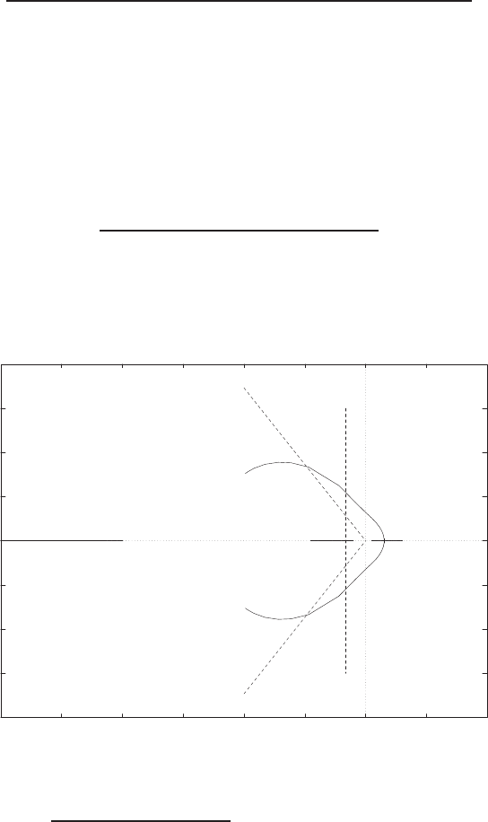
Problems 307

1 + 25K1(s+ 0.03)(s+ 9)

(s+ 0.045)(s+ 1.33)(s2+ 7.66s+ 29.78)(s2+ 12s+ 1) = 0 .

The root locus is shown in Figure P7.5b.

(d) Using K1= 2, we determine that

ess = 0.44 .

P7.6 (a) The characteristic equation is

1 + K(s+ 0.20)(s2+ 4s+ 6.25)

(s+ 0.9)(s−0.6)(s−0.1)(s+ 4) = 0 .

The root locus is shown in Figure P7.6.

-4

-3

-2

-1

-6 -5 -4 -3 -2 -1 0 1 2

x x xx

Real Axis

Imag Axis

zeta=0.5

zeta*wn=-1/3

K=4 -->

FIGURE P7.6

Root locus for 1 + K(s+0.2)(s2+4s+6.25)

(s+0.9)(s−0.6)(s−0.1)(s+4) = 0.

(b) For Ts<12 sec, we require ζωn>1/3. Also, we want ζ > 0.5. So,

we seek roots for a stable system with ζωn>1/3 and ζ > 0.5. This

occurs when K > 4.

from the publisher prior to any prohibited reproduction, storage in a retrieval system, or transmission in any form or by any means, electronic, mechanical, photocopying,

recording, or likewise. For information regarding permission(s), write to: Rights and Permissions Department, Pearson Education, Inc., Upper Saddle River, NJ 07458.

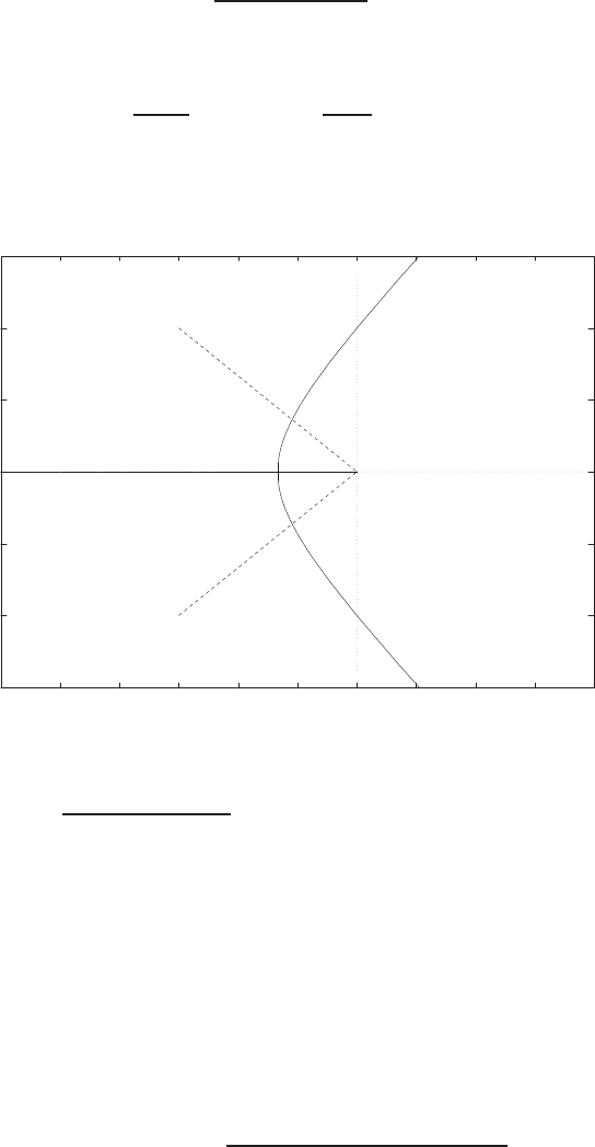
308 CHAPTER 7 The Root Locus Method

P7.7 (a) The characteristic equation for the speed control system is

1 + K

(s+ 4)2(s+δ)= 0 ,

where

K=0.004

Rand δ=0.75

4000 = 0.0001875 .

The root locus is shown in Figure P7.7. At ζ= 0.6, we have K= 19.1,

-6

-4

-2

-6 -5 -4 -3 -2 -1 0 1 2 3 4

xx x

Real Axis

Imag Axis

<-- K=19.1

FIGURE P7.7

Root locus for 1 + K

(s+4)2(s+1.875e−04) = 0.

therefore

R= 0.00021 .

When K= 19.1 the roots are

s1,2=−1.1±j1.43 and s3=−5.80 .

(b) The steady-state error is

lim

s→0s∆ω(s) = lim

s→0s(0.25s+ 1)2

(0.25s+ 1)2(Js +b) + 1/R∆L(s)

from the publisher prior to any prohibited reproduction, storage in a retrieval system, or transmission in any form or by any means, electronic, mechanical, photocopying,

recording, or likewise. For information regarding permission(s), write to: Rights and Permissions Department, Pearson Education, Inc., Upper Saddle River, NJ 07458.

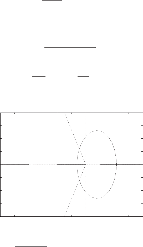
Problems 309

b+ 1/R∆L≈∆LR ,

when R < 0.1.

P7.8 (a) The characteristic equation for the speed control system with the

hydroturbine is

1 + K(−s+ 1)

(s+ 4)(s+ 2)(s+δ)= 0 ,

where

K=0.002

Rand δ=0.75

4000 = 0.0001875 .

The root locus is shown in Figure P7.8. At ζ= 0.6, we have K= 2.85,

-2

-1.5

-1

-0.5

0.5

1.5

-6 -5 -4 -3 -2 -1 0 1 2 3 4

x x x o

Real Axis

Imag Axis

K=2.85 -->

FIGURE P7.8

Root locus for 1 + K(−s+1)

(s+4)(s+2)(s+δ)= 0.

therefore

R= 0.0007 .

When K= 2.85 the roots are −0.45 ±j0.60, and -5.1.

from the publisher prior to any prohibited reproduction, storage in a retrieval system, or transmission in any form or by any means, electronic, mechanical, photocopying,

recording, or likewise. For information regarding permission(s), write to: Rights and Permissions Department, Pearson Education, Inc., Upper Saddle River, NJ 07458.

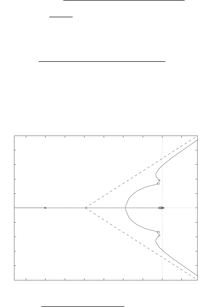
310 CHAPTER 7 The Root Locus Method

(b) The steady-state error is

lim

s→0s∆ω(s) = lim

s→0s(0.25s+ 1)(0.5s+ 1)

(0.25s+ 1)(0.5s+ 1)(Js +f) + (−s+ 1)/R ∆L(s)

f+ 1/R∆L≈∆LR ,

when R < 0.1.

P7.9 The characteristic equation is

1 + K(s+ 0.5)(s+ 0.1)(s2+ 2s+ 289)

s(s+ 30)2(s−0.4)(s+ 0.8)(s2+ 1.45s+ 361) = 0

where K=K1K2. The root locus is shown in Figure P7.9. When

K= 4000 ,

the roots are

s1,2=−0.82 ±j19.4

-35 -30 -25 -20 -15 -10 -5 0 5

-50

-40

-30

-20

-10

Real Axis

Imag Axis

FIGURE P7.9

Root locus for 1 + K(s+0.5)(s+0.1)(s2+2s+289)

s(s+30)2(s−0.4)(s+0.8)(s2+1.45s+361) = 0.

from the publisher prior to any prohibited reproduction, storage in a retrieval system, or transmission in any form or by any means, electronic, mechanical, photocopying,

recording, or likewise. For information regarding permission(s), write to: Rights and Permissions Department, Pearson Education, Inc., Upper Saddle River, NJ 07458.

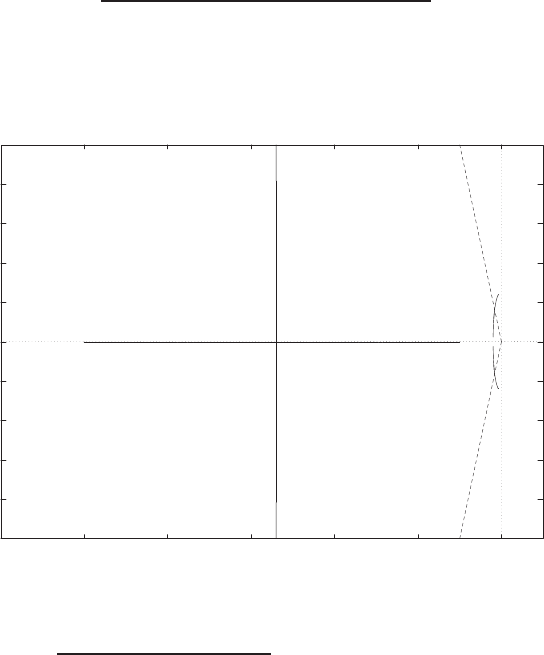
Problems 311

s3=−39.8

s4=−14.9

s5=−5.0

s6=−0.38

s7=−0.14 .

P7.10 (a) The characteristic equation is

1 + K1K2(s+ 2)2

(s+ 10)(s+ 100)(s2+ 1.5s+ 6.25) = 0 .

The root locus is shown in Figure P7.10.

-10

-8

-6

-4

-2

-120 -100 -80 -60 -40 -20 0

x x

Real Axis

Imag Axis

FIGURE P7.10

Root locus for 1 + K1K2(s+2)2

(s+10)(s+100)(s2+1.5s+6.25) = 0.

(b) The gain

K1K2= 1620

when ζ= 0.707. Therefore,

K2= 81000 ,

from the publisher prior to any prohibited reproduction, storage in a retrieval system, or transmission in any form or by any means, electronic, mechanical, photocopying,

recording, or likewise. For information regarding permission(s), write to: Rights and Permissions Department, Pearson Education, Inc., Upper Saddle River, NJ 07458.

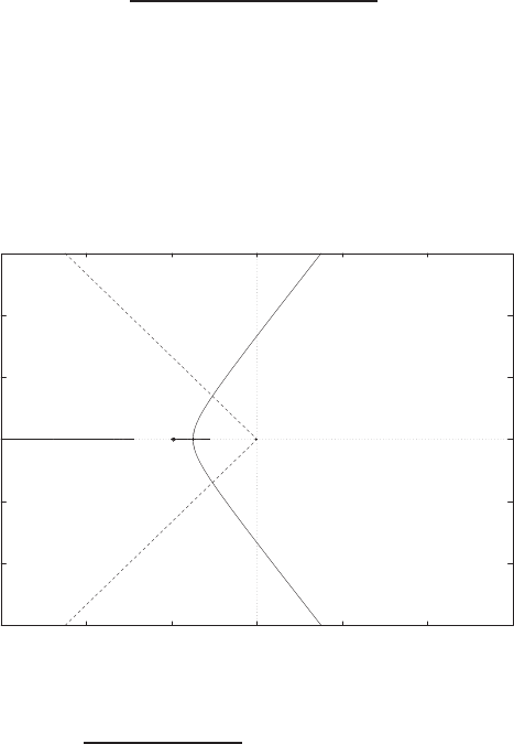
312 CHAPTER 7 The Root Locus Method

since K1= 0.02 at medium weight cruise condition.

K1= 0.2.

Using K2= 81000, we ﬁnd the roots are

s1,2=−54 ±j119

s3,4=−2±j0.6.

The roots s3,4become negligible and the roots at s1,2become highly

oscillatory. Hence, in this case

ζ= 0.41 .

P7.11 (a) The closed-loop characteristic equation is

1 + 20Ka(s2+s+ 0.02)

s(s+ 1)2(s2+ 2s+ 0.8) = 0 ,

where

K2= 10 .

Then, the root locus is shown in Figure P7.11a.

-3

-2

-1

-3 -2 -1 0 1 2 3

xxx xx o o

Real Axis

Imag Axis

Ka=0.035 -->

FIGURE P7.11

(a) Root locus for 1 + Ka20s2+20s+0.4

s(s+1)2(s2+2s+0.8) = 0, where K2= 10.

from the publisher prior to any prohibited reproduction, storage in a retrieval system, or transmission in any form or by any means, electronic, mechanical, photocopying,

recording, or likewise. For information regarding permission(s), write to: Rights and Permissions Department, Pearson Education, Inc., Upper Saddle River, NJ 07458.

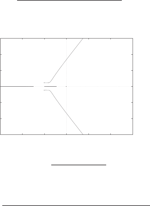
Problems 313

(b) When

Ka<0.035 ,

all the roots have a damping greater than or equal to 0.60.

Ka= 0.035 .

Then, the characteristic equation with K2as the parameter is

1 + K2

0.07(s2+s)

s5+ 4s4+ 5.8s3+ 3.6s2+ 0.8s+ 0.014 = 0 .

The root locus is shown in Figure P7.11b.

-3

-2

-1

-3 -2 -1 0 1 2 3

x xoo

Real Axis

Imag Axis

Ka=0.035

FIGURE P7.11

CONTINUED: (b) Root locus for 1+K20.07s(s+1)

s(s+1)2(s2+2s+0.8)+0.014 = 0, where Ka= 0.035.

P7.12 (a) The closed-loop transfer function is

T(s) = KaKm(s+ 25)(s+ 15)

1.8s2(s+ 2) + KaKm(s+ 25)(s+ 15) + 1.6Kms(s+ 2) .

So, with E(s) = R(s)−Y(s), we have E(s) = (1 −T(s))R(s) and

ess = lim

s→0sE(s) = 1 −T(0) = 0 .

from the publisher prior to any prohibited reproduction, storage in a retrieval system, or transmission in any form or by any means, electronic, mechanical, photocopying,

recording, or likewise. For information regarding permission(s), write to: Rights and Permissions Department, Pearson Education, Inc., Upper Saddle River, NJ 07458.

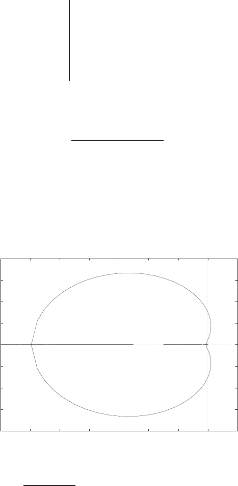
314 CHAPTER 7 The Root Locus Method

Therefore, when the system is stable, it has zero steady-state error.

(b) The characteristic equation is

s3+ (3.6 + Ka)s2+ (3.2 + 40Ka)s+ 375Ka.

The Routh array is

s31 3.2 + 40Ka

s23.6 + Ka375Ka

s1b

so375K

Solving for b > 0 leads to 0 < Ka<0.05 or Ka>5.64 for stability.

1 + Ka(s+ 25)(s+ 15)

s(s+ 2)(s+ 1.6) = 0 .

The root locus is shown in Figure P7.12.

(d) When

K > 40 ,

-40

-30

-20

-10

-70 -60 -50 -40 -30 -20 -10 0 10

xxxo o

Real Axis

Imag Axis

FIGURE P7.12

Root locus for 1 + Ka(s+25)(s+15)

s(s+2)(s+1.6) = 0, where Km= 1.8.

from the publisher prior to any prohibited reproduction, storage in a retrieval system, or transmission in any form or by any means, electronic, mechanical, photocopying,

recording, or likewise. For information regarding permission(s), write to: Rights and Permissions Department, Pearson Education, Inc., Upper Saddle River, NJ 07458.

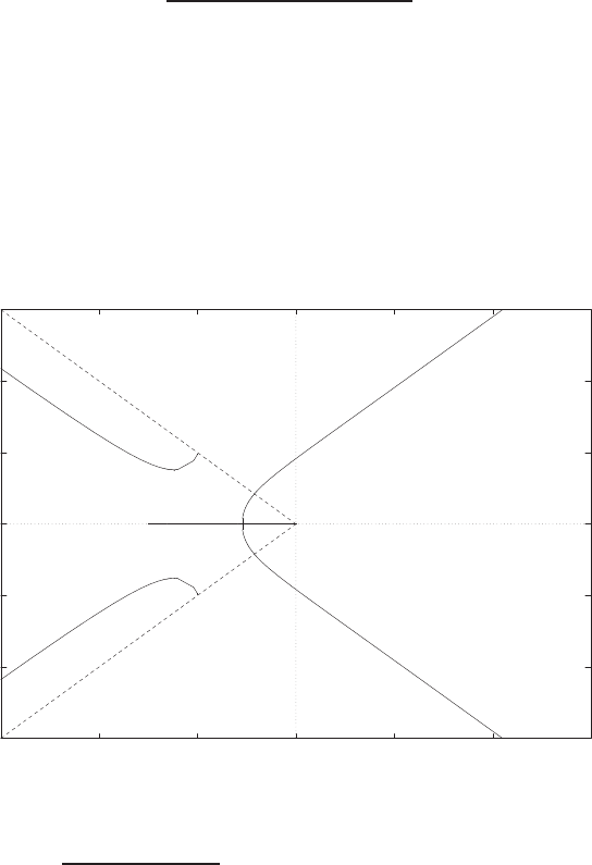
Problems 315

the roots are

s1=−123 and s2,3=−15.6±j31.2.

From the step response we ﬁnd

P.O. = 5%

Tp= 0.67 sec

Ts= 0.25 sec .

P7.13 (a) The characteristic equation is

1 + K

s(s+ 3)(s2+ 4s+ 7.84) = 0 .

The root locus is shown in Figure P7.13. The breakaway point is

s=−1.09 at K= 9.72.

(b) When K= 13.5, the roots are

s1,2=−0.84 ±j0.84

s3,4=−2.66 ±j1.55 .

-6

-4

-2

-6 -4 -2 0 2 4 6

Real Axis

Imag Axis

FIGURE P7.13

Root locus for 1 + K

s(s+3)(s2+4s+7.84) = 0.

from the publisher prior to any prohibited reproduction, storage in a retrieval system, or transmission in any form or by any means, electronic, mechanical, photocopying,

recording, or likewise. For information regarding permission(s), write to: Rights and Permissions Department, Pearson Education, Inc., Upper Saddle River, NJ 07458.

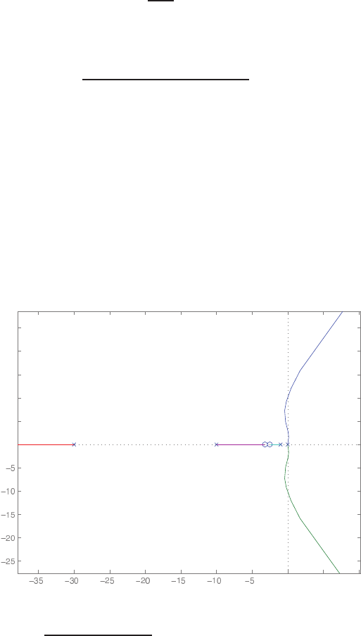
316 CHAPTER 7 The Root Locus Method

s=−0.84 ±j0.84

are dominant roots.

(d) For the dominant roots, we determine that ζ= 0.7 and ωn= 1.19.

Therefore, the settling time is

Ts=4

ζωn

= 4.8 sec .

P7.14 The characteristic equation is

1 + K(s+ 2.5)(s+ 3.2)

s2(s+ 1)(s+ 10)(s+ 30) = 0 .

The root locus is shown in Figure P7.14. When K= 559.3, the roots are

s1=−30.75 s2=−8.48 s3=−1.78 s4,5=±j3.11 .

When K= 4321, the roots are

s1=−34.45 s2=−4.35 s3=−2.21 s4,5=±j10.23 .

The crossover points are

s=±j3.11 and s=±j10.23 .

0 5 10

Real Axis

Imaginary Axis

FIGURE P7.14

Root locus for 1 + K(s+2.5)(s+3.5)

s2(s+1)(s+10)(s+30) = 0.

from the publisher prior to any prohibited reproduction, storage in a retrieval system, or transmission in any form or by any means, electronic, mechanical, photocopying,

recording, or likewise. For information regarding permission(s), write to: Rights and Permissions Department, Pearson Education, Inc., Upper Saddle River, NJ 07458.

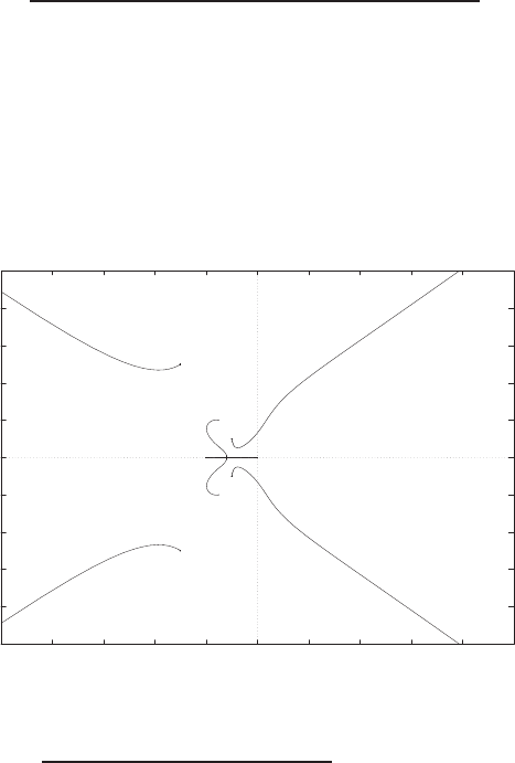
Problems 317

Therefore, the system is stable for

559.3< K < 4321 .

P7.15 The characteristic equation is

1 + K(s2+ 30s+ 625)

s(s+ 20)(s2+ 20s+ 200)(s2+ 60s+ 3400) .

The root locus is shown in Figure P7.15. When K= 30000, the roots are

s1=−18.5s2=−1.69 s3,4=−9.8±j8.9s5,6=−30.1±j49.9.

The real root near the origin dominates, and the step response is over-

damped.

-100

-80

-60

-40

-20

100

-100 -80 -60 -40 -20 0 20 40 60 80 100

Real Axis

Imag Axis

FIGURE P7.15

Root locus for 1 + Ks2+30s+625

s(s+20)(s2+20s+200)(s2+60s+3400) = 0.

from the publisher prior to any prohibited reproduction, storage in a retrieval system, or transmission in any form or by any means, electronic, mechanical, photocopying,

recording, or likewise. For information regarding permission(s), write to: Rights and Permissions Department, Pearson Education, Inc., Upper Saddle River, NJ 07458.

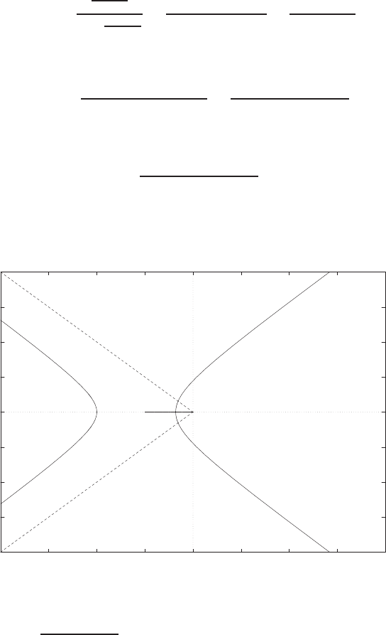
318 CHAPTER 7 The Root Locus Method

P7.16 (a) Let τ= 0. Then, ﬁrst reduce the motor and rolls to an equivalent

G(s) as follows:

G(s) =

0.25

s(s+1)

1 + 0.25

s(s+1)

=0.25

s(s+ 1) + 0.25 =0.25

(s+ 0.5)2.

The loop transfer function is then

L(s) = 2(s+ 0.5)Ka(0.25)

s(s+ 1)2(s+ 0.5)2=0.5Ka

s(s+ 1)2(s+ 0.5) .

The characteristic equation is

1 + Ka

0.5

s(s+ 1)2(s+ 0.5) = 0 .

The root locus is shown in Figure P7.16.

-2

-1.5

-1

-0.5

0.5

1.5

-2 -1.5 -1 -0.5 0 0.5 1 1.5 2

xxx x

Real Axis

Imag Axis

FIGURE P7.16

Root locus for 1 + 0.5Ka

s(s+1)2(s+0.5) = 0.

(b) When K= 0.123, the roots of the characteristic equation are

s1,2=−1.1±j0.27

s3,4=−0.15 ±j0.15 .

from the publisher prior to any prohibited reproduction, storage in a retrieval system, or transmission in any form or by any means, electronic, mechanical, photocopying,

recording, or likewise. For information regarding permission(s), write to: Rights and Permissions Department, Pearson Education, Inc., Upper Saddle River, NJ 07458.

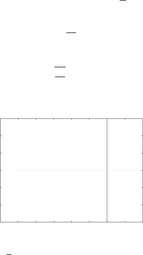
Problems 319

The roots at s=−0.15 ±j0.15 have a damping ratio of ζ= 0.707.

pole, and the root locus will change accordingly.

P7.17 The characteristic equation is

(M1s2+bs +k1+k12)(M2s2+k12)−k2

12 = 0 .

If we let M1=k1=b= 1, and assume k12 <1 so that k2

12 is negligible

and k1+k12 ≈k1, then the characteristic equation is

(s2+s+ 1)(M2s2+k12) = 0 or 1 + k

s2= 0 ,

where

k=k12

The root locus is shown in Figure P7.17. All the roots lie on the jω axis.

If we select

sk12

=ωo,

then we cancel the vibration.

-3

-2

-1

-3 -2.5 -2 -1.5 -1 -0.5 0 0.5 1

Real Axis

Imag Axis

root locus -->

FIGURE P7.17

Root locus for 1 + k

s2= 0.

from the publisher prior to any prohibited reproduction, storage in a retrieval system, or transmission in any form or by any means, electronic, mechanical, photocopying,

recording, or likewise. For information regarding permission(s), write to: Rights and Permissions Department, Pearson Education, Inc., Upper Saddle River, NJ 07458.

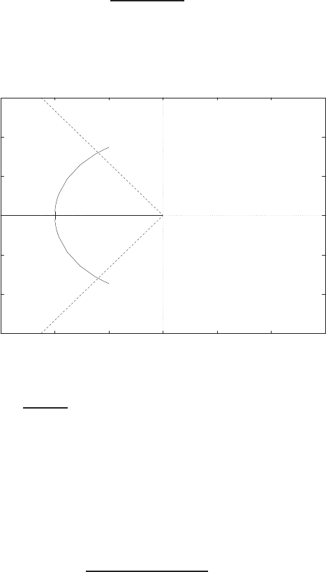
320 CHAPTER 7 The Root Locus Method

P7.18 The characteristic equation is

βs3+ (1 + 2β)s2+ (2 + 4α)s+ 4 = 0 .

When β= 0 we have

1 + 4αs

s2+ 2s+ 4 = 0 .

The root locus for β= 0 is shown in Figure P7.18.

-3

-2

-1

-3 -2 -1 0 1 2 3

Real Axis

Imag Axis

beta=0<-- zeta=0.6

FIGURE P7.18

Root locus for 1 + α4s

s2+2s+4 = 0, where β= 0.

For α= 0.3, the poles are

s=−1.6±j1.2.

Then, we have

1 + β(s+ 2)s2

s2+ (2 + 4α)s+ 4 = 0 .

When β= 0.121

s1,2=−1.51 ±j1.51

s3=−7.24 .

from the publisher prior to any prohibited reproduction, storage in a retrieval system, or transmission in any form or by any means, electronic, mechanical, photocopying,

recording, or likewise. For information regarding permission(s), write to: Rights and Permissions Department, Pearson Education, Inc., Upper Saddle River, NJ 07458.

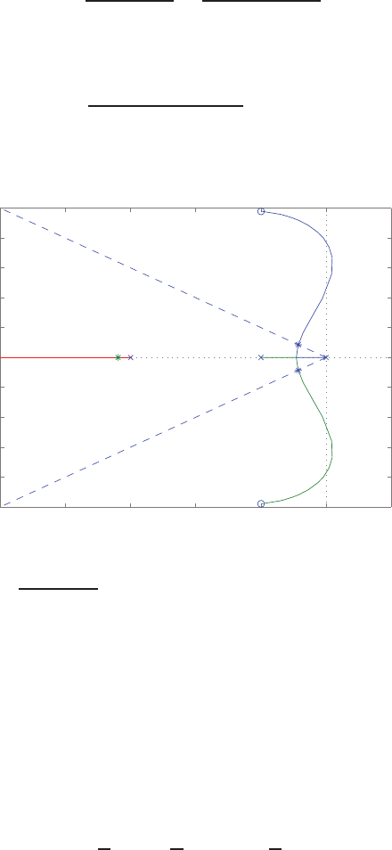
Problems 321

Thus,

ζ= 0.707 and ζωn= 1.5.

So, the performance specs are met. Also,

Gc(s) = 0.3s+ 1

0.121s+ 1 =2.48(s+ 3.33)

(s+ 8.26) .

P7.19 The characteristic equation is

1 + Ka(s2+ 4s+ 100)

s(s+ 2)(s+ 6) = 0 .

The root locus is shown in Figure P7.19.

−10 −8 −6 −4 −2 0 2

−10

−8

−6

−4

−2

Real Axis

Imaginary Axis

FIGURE P7.19

Root locus for 1 + Kas2+4s+100

s(s+2)(s+6) = 0.

When Ka= 0.094;, the roots are

s1,2=−0.85 ±j0.85

s3=−6.38 .

Thus, the complex roots have a damping ratio of ζ= 0.707.

P7.20 The characteristic equation is

s3+ (2 + 1

β)s2+ ( 2

β+K)s+4

β= 0 ,

from the publisher prior to any prohibited reproduction, storage in a retrieval system, or transmission in any form or by any means, electronic, mechanical, photocopying,

recording, or likewise. For information regarding permission(s), write to: Rights and Permissions Department, Pearson Education, Inc., Upper Saddle River, NJ 07458.

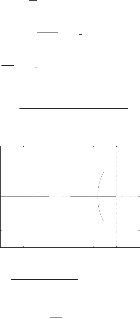
322 CHAPTER 7 The Root Locus Method

where

K=4α

βα= 0.3β= 0.121 .

The root sensitivity to changes in Kis found to be

Sr1

K∼

=∆r1

∆K/K = 1.186−149.75o.

The root sensitivity to changes in the pole at s=−2 is found to be

Sr1

∆∼

=∆r1

∆/2= 1.656−137o,where the pole is s+ 2 + ∆.

P7.21 (a) Let the pole be (s+ 4 + ∆) and neglect ∆2terms. Then, the charac-

teristic equation is

1 + ∆ 2s2+ (8 + 2δ)s+ 8δ

s3+ (8 + δ)s2+ (16 + 8δ)s+ 16δ+K= 0

where δ= 0.000788 and K= 19.1.

-3

-2

-1

-10 -8 -6 -4 -2 0 2

o o

Real Axis

Imag Axis

FIGURE P7.21

Root locus for 1 + ∆ 2s2+(8+2δ)s+8δ

s3+(8+δ)s2+(16+8δ)s+16δ+K= 0, (δ= 0.000788 and K= 19.1).

The root sensitivity is determined to be

Sr1

∆∼

=∆r1

∆/4= 3.3146−132o.

from the publisher prior to any prohibited reproduction, storage in a retrieval system, or transmission in any form or by any means, electronic, mechanical, photocopying,

recording, or likewise. For information regarding permission(s), write to: Rights and Permissions Department, Pearson Education, Inc., Upper Saddle River, NJ 07458.

Problems 323

(b) Let R=Ro+ ∆R, where R= 0.00021. Then,

Sr1

R∼

=∆r1

∆R/R = 1.31 6−107o.

P7.22 The characteristic equation is

s3+ 2s2+s+K ,

where K= 0.24 for ζ= 0.707. The root sensitivity to changes in the pole

at s=−1 is found to be

Sr1

∆∼

=∆r1

∆= 0.956−126o,

where the pole is s+ 1 + ∆.

P7.23 The characteristic equation is

s3+ 5s2+ (6 + K)s+K ,

where K= 6.3 for ζ= 0.707. The root sensitivity to changes in the pole

at s=−2 is found to be

Sr1

∆∼

=∆r1

∆/2= 1.256−169.4o,

where the pole is s+ 2 + ∆. The root sensitivity to changes in the zero at

s=−1 is found to be

Sr1

∆∼

=∆r1

∆= 0.55634.4o,

where the zero is s+ 1 + ∆.

P7.24 The root locus for each of the four cases shown is shown in Figure P7.24.

The four open-loop transfer functions are

(a)KF (s) = s2+ 7s+ 8.25

s3+ 6s2+ 5s

(b)KF (s) = s+ 8

s5+ 30s4+ 296s3+ 1170s2+ 1575s

(c)KF (s) = 1

s6+ 2s5+s4(d)KF (s) = s2+ 6s+ 6.75

s3+ 5s2+ 4s

from the publisher prior to any prohibited reproduction, storage in a retrieval system, or transmission in any form or by any means, electronic, mechanical, photocopying,

recording, or likewise. For information regarding permission(s), write to: Rights and Permissions Department, Pearson Education, Inc., Upper Saddle River, NJ 07458.

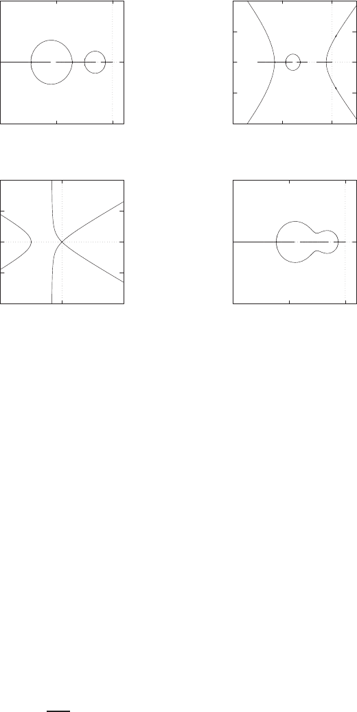
324 CHAPTER 7 The Root Locus Method

-5

-10 -5 0

xxxo o

Real Axis

Imag Axis

(a)

-10

-5

-20 -10 0

xx x xxo

Real Axis

Imag Axis

(b)

-2

-1

-2 0 2

xxxxxx

Real Axis

Imag Axis

(c)

-5

-10 -5 0

xxxo o

Real Axis

Imag Axis

(d)

FIGURE P7.24

Root locus for the four cases.

P7.25 The characteristic equation is

1 + KGc(s)G(s) = 0 ,

therefore,

KGc(s)G(s) = −1.

Squaring both sides yields K2G2

c(s)G2(s) = 1 and

1−K2G2

c(s)G2(s) = 0 .

The root locus with 0 < K2<∞is shown in Figure P7.25. The value of

K2for which the locus crosses the imaginary axis is

K2= 2/3,

therefore K=p2/3 = 0.8165 corresponds to the jω-axis crossing (at

s= 0). You can check that 1 + KGc(s)G(s) = 0 for K= 0.8165 and

s= 0.

from the publisher prior to any prohibited reproduction, storage in a retrieval system, or transmission in any form or by any means, electronic, mechanical, photocopying,

recording, or likewise. For information regarding permission(s), write to: Rights and Permissions Department, Pearson Education, Inc., Upper Saddle River, NJ 07458.

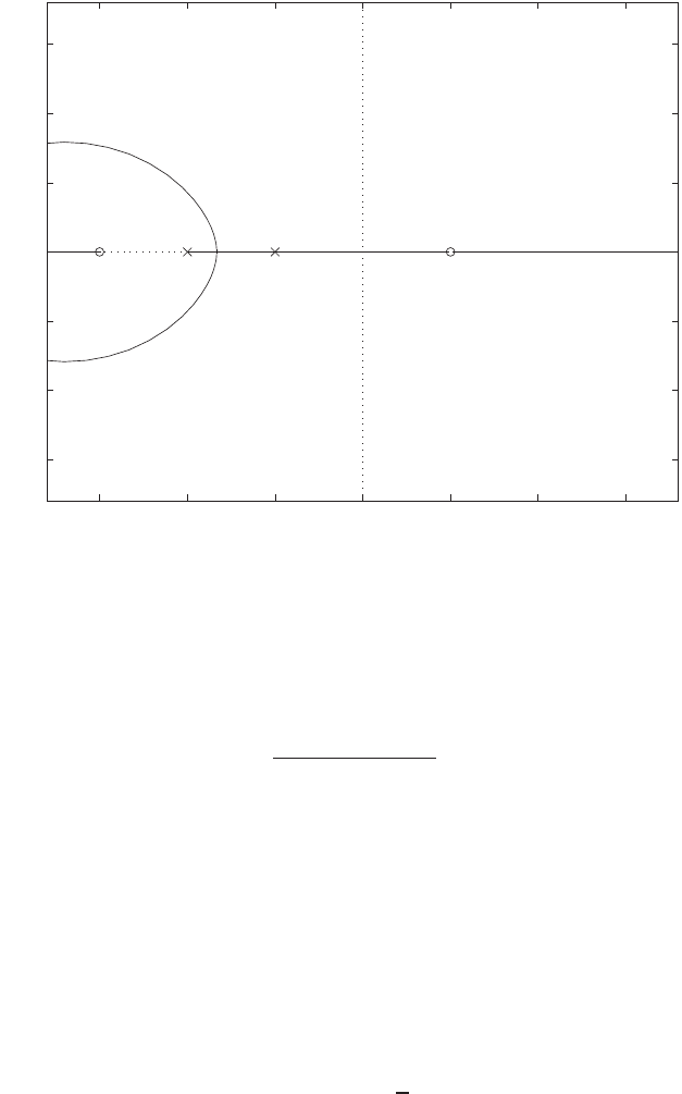
Problems 325

-3 -2 -1 0 1 2 3

-3

-2

-1

Real Axis

Imag Axis

FIGURE P7.25

Root locus for the equation 1−K2G2

c(s)G2(s) = 0.

P7.26 (a) The characteristic equation is

1 + K(s+ 2)2

s(s2+ 1)(s+ 8) = 0 .

The root locus is shown in Figure P7.26.

(b) Using Routh’s criteria, we determine that

K > 14

for stability.

purely imaginary poles at

s=±j√8.

(d) When K > 50, the real part of the complex roots is approximately

equal to the real part of the two real roots and therefore the complex

roots are not dominant roots.

from the publisher prior to any prohibited reproduction, storage in a retrieval system, or transmission in any form or by any means, electronic, mechanical, photocopying,

recording, or likewise. For information regarding permission(s), write to: Rights and Permissions Department, Pearson Education, Inc., Upper Saddle River, NJ 07458.

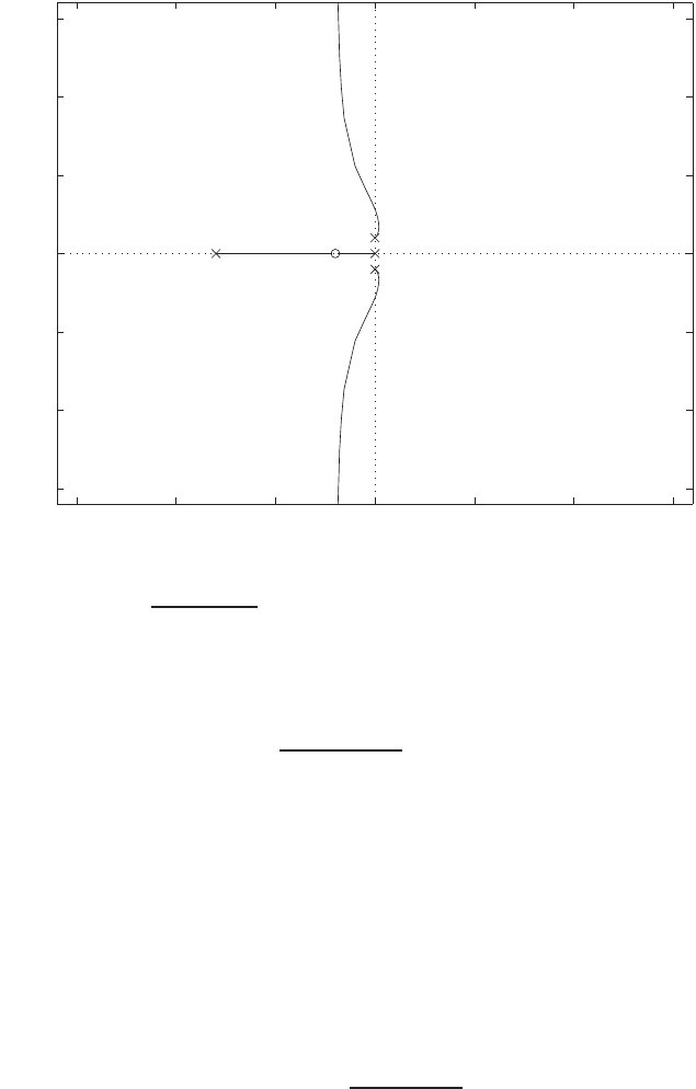
326 CHAPTER 7 The Root Locus Method

-15 -10 -5 0 5 10 15

-15

-10

-5

Real Axis

Imag Axis

FIGURE P7.26

Root locus for 1 + K(s+2)2

s(s2+1)(s+8) = 0.

P7.27 The characteristic equation is

1 + K(s2+ 0.1)

s(s2+ 2) = 0 .

The root locus is shown in Figure P7.27a. The locus enters the axis at

s=−1.26

and leaves the axis at

s=−0.36 .

Deﬁne

p(s) = K=−(s3+ 2s)

s2+ 0.1.

Then, a plot of p(s) vs sis shown in Figure P7.27b, where it can be seen

that p(s) has two inﬂection points at

s=−1.28 and s=−0.36 .

from the publisher prior to any prohibited reproduction, storage in a retrieval system, or transmission in any form or by any means, electronic, mechanical, photocopying,

recording, or likewise. For information regarding permission(s), write to: Rights and Permissions Department, Pearson Education, Inc., Upper Saddle River, NJ 07458.

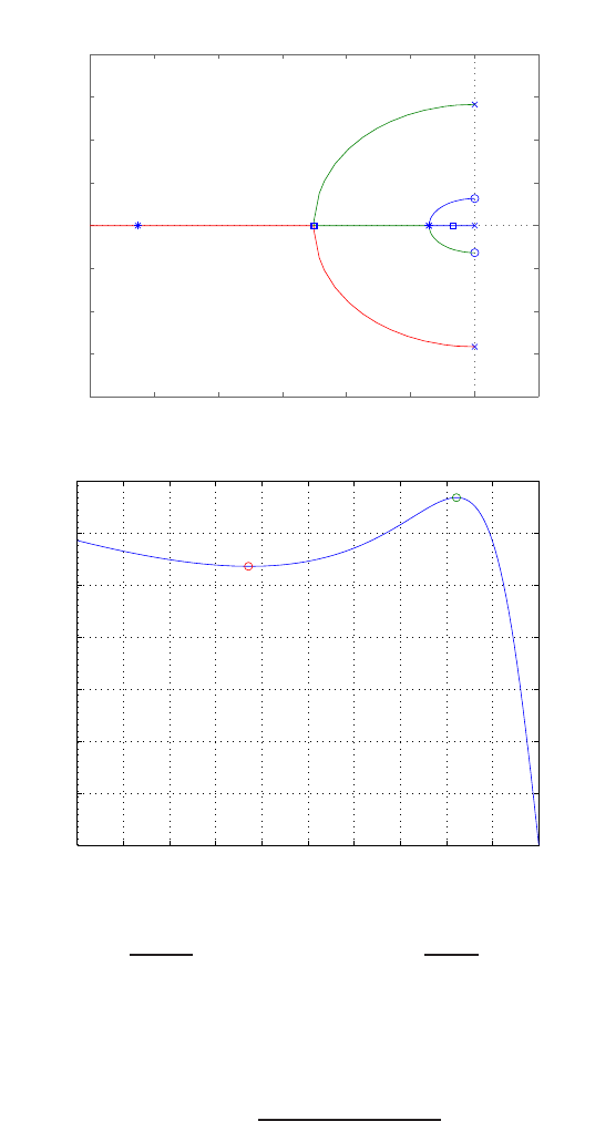
Problems 327

−3 −2.5 −2 −1.5 −1 −0.5 0 0.5

−2

−1.5

−1

−0.5

0.5

1.5

Root Locus

Real Axis

Imaginary Axis

−2 −1.8 −1.6 −1.4 −1.2 −1 −0.8 −0.6 −0.4 −0.2 0

0.5

1.5

2.5

3.5

p(s)

FIGURE P7.27

(a) Root locus for 1 + Ks2+0.1

s(s2+2) = 0. (b) Plot of p(s) = −s3+2s

s2+0.1versus s.

P7.28 The characteristic equation is

1 + L(s) = 1 + K(s2+ 12s+ 20)

s3+ 10s2+ 25s= 0 .

The root locus is shown in Figure P7.28. The breakaway point is s=−5.0

from the publisher prior to any prohibited reproduction, storage in a retrieval system, or transmission in any form or by any means, electronic, mechanical, photocopying,

recording, or likewise. For information regarding permission(s), write to: Rights and Permissions Department, Pearson Education, Inc., Upper Saddle River, NJ 07458.

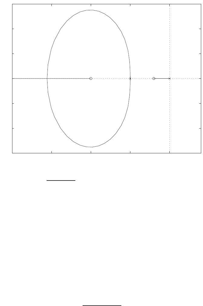
328 CHAPTER 7 The Root Locus Method

-20 -15 -10 -5 0

-6

-4

-2

Real Axis

Imag Axis

FIGURE P7.28

Root locus for 1 + K(s2+12s+20)

s3+10s2+25s= 0.

and the entry point is s=−15.6. When K= 2, the roots are

s1=−1.07

s2,3=−5.46 ±j2.75 .

When K= 2, the roots are

s1=−1.07

s2,3=−4.36 ±j1.68 .

The predicted step response when K= 2 is Ts= 9 sec and P O ≈0%.

P7.29 The characteristic equation is

1 + Ks2+ 10s+ 30

s2(s+ 10) = 0 .

The root locus is shown in Figure P7.29. When ζ= 0.707, the necessary

gain is K= 16. The corresponding roots are s1=−18.87 and s2,3=

−3.56 ±j3.56.

from the publisher prior to any prohibited reproduction, storage in a retrieval system, or transmission in any form or by any means, electronic, mechanical, photocopying,

recording, or likewise. For information regarding permission(s), write to: Rights and Permissions Department, Pearson Education, Inc., Upper Saddle River, NJ 07458.

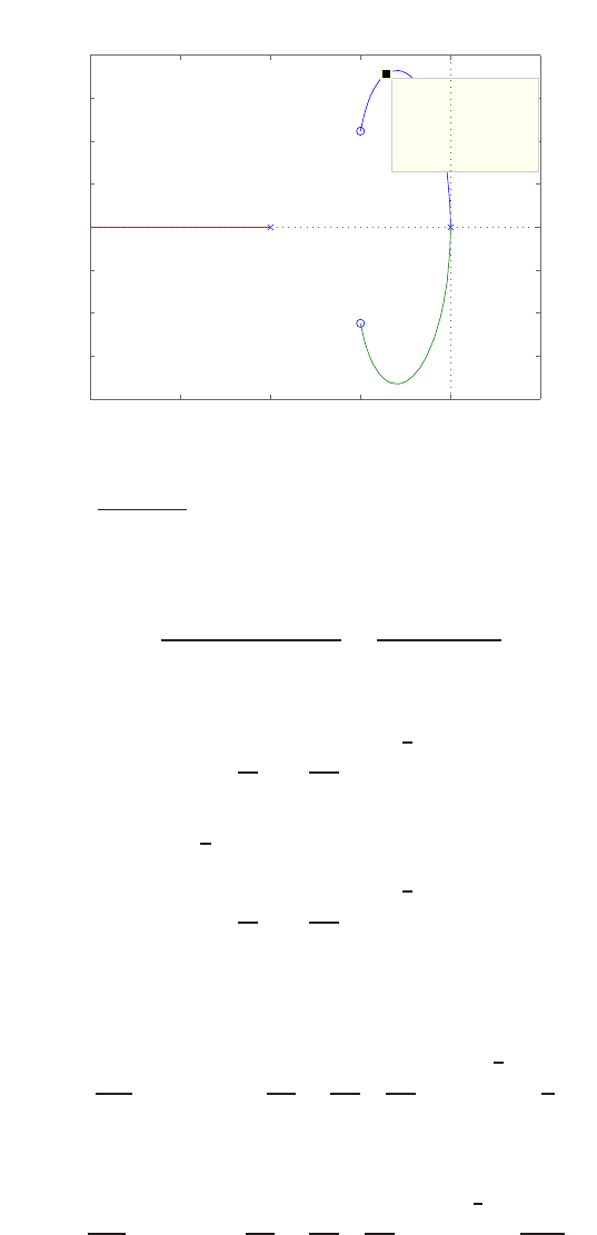
Problems 329

Root Locus

Real Axis

Imaginary Axis

−20 −15 −10 −5 0 5

−4

−3

−2

−1

System: sys

Gain: 16

Pole: −3.56 + 3.57i

Damping: 0.707

Overshoot (%): 4.34

Frequency (rad/sec): 5.04

FIGURE P7.29

Root locus for 1 + Ks2+10s+30

s2(s+10) = 0.

P7.30 The transfer function is

Z(s) = LCRs2+Ls

LCs2+CRs + 1 =Rs2+s

s2+Rs + 1 .

So,

r1=−R

2+ R2

4−1!1

Thus, the nominal r1o=−1

2. Simultaneously,

r2=−R

2− R2

4−1!1

Thus, the nominal r2o=−2. We see that there is a diﬀerence by a factor

of 4. Also,

Sri

R=∂r1

∂R Ro·Ro=−Ro

2+R2

4 R2

4−1!−1

where Ro= 2.5. And

Sr2

R=∂r2

∂R Ro

Ro=−Ro

2−R2

4 R2

4−1!−1

=−10

from the publisher prior to any prohibited reproduction, storage in a retrieval system, or transmission in any form or by any means, electronic, mechanical, photocopying,

recording, or likewise. For information regarding permission(s), write to: Rights and Permissions Department, Pearson Education, Inc., Upper Saddle River, NJ 07458.

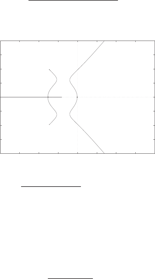
330 CHAPTER 7 The Root Locus Method

So, the magnitude of |Sr2

R|= 4|Sr1

R|.

P7.31 The characteristic equation is

1 + Ks+ 4

s(s+ 0.16)(s2+ 14.6s+ 148.999) = 0 .

The root locus is shown in Figure P7.31. When K= 1350, the roots are

-20

-15

-10

-5

-20 -15 -10 -5 0 5 10 15 20

Real Axis

Imag Axis

<-- K=1350 (*)

(+) K=326 -->

FIGURE P7.31

Root locus for 1 + Ks+4

s(s+0.16)(s2+14.6s+148.999) = 0.

s1,2=±j9.6

s3,4=−7.4±j1.9.

When K= 326, the roots are

s1,2=−6.5±j8.7s3,4=−0.9±j3.2.

P7.32 The characteristic equation is

1 + K(s+ 1)(s+ 5)

s(s+ 1.5)(s+ 2) = 0 .

from the publisher prior to any prohibited reproduction, storage in a retrieval system, or transmission in any form or by any means, electronic, mechanical, photocopying,

recording, or likewise. For information regarding permission(s), write to: Rights and Permissions Department, Pearson Education, Inc., Upper Saddle River, NJ 07458.

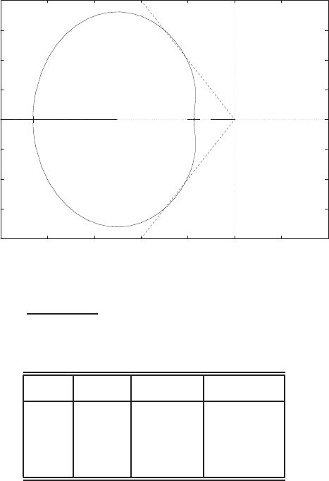
Problems 331

-4

-3

-2

-1

-10 -8 -6 -4 -2 0 2 4

xxxo o

Real Axis

Imag Axis

FIGURE P7.32

Root locus for 1 + K(s+1)(s+5)

s(s+1.5)(s+2) = 0.

K ζ Ts(sec) P.O. (%)

1.57 0.707 0.98 1.4

3.48 0.707 1.1 5.8

2.35 0.69 1.3 4.0

TABLE P7.32 Step Response Results for K= 1.57,K= 3.48, and K= 2.35.

(a) The breakaway point is s=−1.73; the entry point is s=−8.62.

(b) The damping ratio ζ= 0.707 when K= 1.57 and again when K=

3.46.

(d) The results are summarized in Table P7.32.The best choice of gain is

K= 1.57.

P7.33 (a) The root locus for the V-22 is shown in Figure P7.33a. The system is

stable when 0 < K < 0.48 and K > 136.5.

(b) The unit step input response (for K= 280) is shown in Figure P7.33b.

The step response has a P.O. = 90% and Ts≈50 sec.

from the publisher prior to any prohibited reproduction, storage in a retrieval system, or transmission in any form or by any means, electronic, mechanical, photocopying,

recording, or likewise. For information regarding permission(s), write to: Rights and Permissions Department, Pearson Education, Inc., Upper Saddle River, NJ 07458.

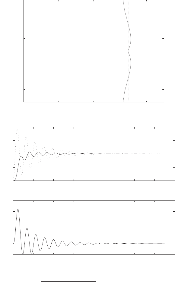
332 CHAPTER 7 The Root Locus Method

-2

-1.5

-1

-0.5

0.5

1.5

-3 -2.5 -2 -1.5 -1 -0.5 0 0.5 1

xxx xo o

Real Axis

Imag Axis

0 10 20 30 40 50 60 70 80

0.5

1.5

Time (sec)

y(t)

(i) Unit step input response

y(t) w/o prelter .... (dotted line)

y(t) with prelter ____ (solid line)

0 10 20 30 40 50 60 70 80

-1

4x 10 -3

Time (sec)

y(t)

(ii) Unit step disturbance response

FIGURE P7.33

(a) Root locus for 1 + Ks2+1.5s+0.5

s(20s+1)(10s+1)(0.5s+1) = 0. (b) (i) Unit step input response with

and without preﬁlter; (ii) Unit step disturbance response.

The response to the disturbance is oscillatory, but the maximum value

of oscillation is about 0.003; so it is negligible.

(d) The eﬀect of adding a preﬁlter can be seen in Figure P7.33b. With

from the publisher prior to any prohibited reproduction, storage in a retrieval system, or transmission in any form or by any means, electronic, mechanical, photocopying,

recording, or likewise. For information regarding permission(s), write to: Rights and Permissions Department, Pearson Education, Inc., Upper Saddle River, NJ 07458.

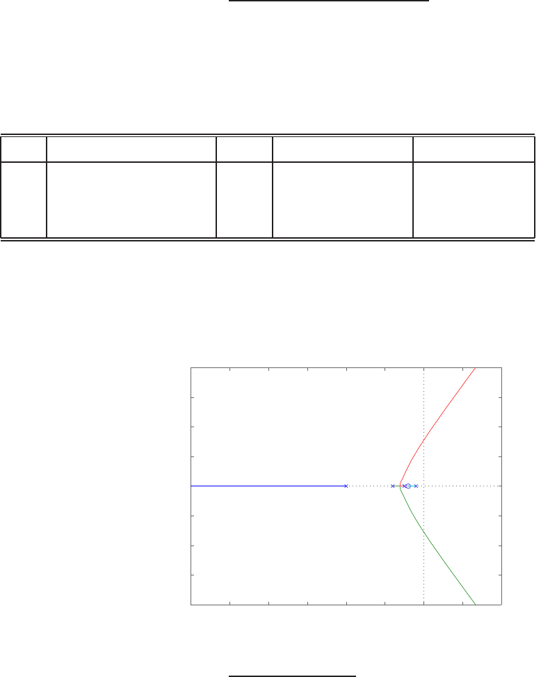
Problems 333

the preﬁlter we ﬁnd P O = 7% and Ts≈40 sec.

P7.34 The characteristic equation is

1 + K(s+ 2)

(s+ 1)(s+ 2.5)(s+ 4)(s+ 10) = 0 .

The root locus is shown in Figure P7.34a. The roots, predicted and ac-

tual percent overshoot for K= 400,500, and 600 are summarized in

Table P7.34. The actual unit step input responses are shown in Fig-

ure P7.34b.

Kroots ζpredicted P.O. (%) actual P.O. (%)

400 -13.5,-1.00 ±5.71j,-1.98 0.173 57.6 51.6

500 -14.0,-0.75 ±6.24j,-1.98 0.120 68.4 61.2

600 -14.4,-0.53 ±6.71j,-1.98 0.079 77.9 69.6

TABLE P7.34 Summary for K= 400,500,600.

−30 −25 −20 −15 −10 −5 0 5 10

−20

−15

−10

−5

Root Locus

Real Axis

Imaginary Axis

FIGURE P7.34

(a) Root locus for 1 + Ks+2

(s+1)(s+2.5)(s+4)(s+10) = 0.

from the publisher prior to any prohibited reproduction, storage in a retrieval system, or transmission in any form or by any means, electronic, mechanical, photocopying,

recording, or likewise. For information regarding permission(s), write to: Rights and Permissions Department, Pearson Education, Inc., Upper Saddle River, NJ 07458.

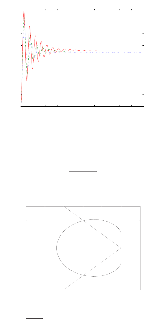
334 CHAPTER 7 The Root Locus Method

0 2 4 6 8 10 12 14 16 18 20

0.2

0.4

0.6

0.8

1.2

1.4

1.6

Time (sec)

y(t)

K=400 .... (dotted line)

K=500 −−− (dashed line)

K=600 ___ (solid line)

FIGURE P7.34

CONTINUED (b) Unit step input responses for K= 400,500,600.

P7.35 (a) The root locus is shown in Figure P7.35 for the characteristic equation

1 + K(s+ 1)2

s(s2+ 1) = 0 .

-3

-2

-1

-5 -4 -3 -2 -1 0 1

Real Axis

Imag Axis

K=4.52 *

FIGURE P7.35

Root locus for 1 + K(s+1)2

s(s2+1) = 0.

from the publisher prior to any prohibited reproduction, storage in a retrieval system, or transmission in any form or by any means, electronic, mechanical, photocopying,

recording, or likewise. For information regarding permission(s), write to: Rights and Permissions Department, Pearson Education, Inc., Upper Saddle River, NJ 07458.

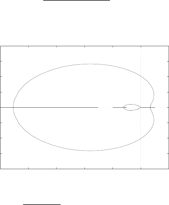
Problems 335

(b) When K= 4.52, the roots are

s1=−0.58

s2,3=−1.96 ±j1.96 .

The complex roots have ζ= 0.707.

(d) The predicted P.O. = 4.5% (ζ= 0.707) and the actual P.O. = 17%.

P7.36 The characteristic equation is

1 + K(s+ 1)(s+ 2)(s+ 3)

s3(s−1) = 0 .

(a) The root locus is shown in Figure P7.36.

-8

-6

-4

-2

-10 -8 -6 -4 -2 0 2

xxx xo o o

Real Axis

Imag Axis

FIGURE P7.36

Root locus for 1 + K(s+1)(s+2)(s+3)

s3(s−1) = 0.

(b) When K= 2.96, the roots are

s1,2=±j4.08

s3,4=−0.98 ±j0.33 .

from the publisher prior to any prohibited reproduction, storage in a retrieval system, or transmission in any form or by any means, electronic, mechanical, photocopying,

recording, or likewise. For information regarding permission(s), write to: Rights and Permissions Department, Pearson Education, Inc., Upper Saddle River, NJ 07458.

336 CHAPTER 7 The Root Locus Method

s1=−1.46

s2=−1.07

s3,4=−8.23 ±j2.99 .

When K= 100, the roots are

s1=−92.65

s2=−3.51

s3=−1.82

s4=−1.01 .

(d) When K= 20, the damping ratio is ζ= 0.94. Therefore, the predicted

P.O. = 0.02%. The actual overshoot is P.O. = 23%.

P7.37 Since we know that ess = 0 for a step input, we know that a= 0 or b= 0.

Select a= 0. Also, ωn= 2π/T = 20 rad/sec. The desired characteristic

polynomial is

(s+r1)(s+j20)(s−j20) = s3+r1s2+ 400s+ 400r1= 0 .

The actual characteristic polynomial is

1 + 2K

s(s+b)(s+ 40) = 0 ,or s3+ (40 + b)s2+ 40bs + 2K= 0 .

Comparing the coeﬃcients in the desired and actual characteristic poly-

nomials, we determine that b= 10, r1= 50, and K= 10000.

P7.38 (a) The characteristic equation is

1 + K(s+ 1)

s(s−3) = 0 .

The system is stable for K > 3. When K= 3, the roots are s=±j√3.

(b) The root locus is shown in Figure P7.38a.

s1=−2

s2=−5.

Since both roots are real and stable, we expect that there will be

zero overshoot. The actual response has a 40% overshoot, as seen in

Figure P7.38b.

from the publisher prior to any prohibited reproduction, storage in a retrieval system, or transmission in any form or by any means, electronic, mechanical, photocopying,

recording, or likewise. For information regarding permission(s), write to: Rights and Permissions Department, Pearson Education, Inc., Upper Saddle River, NJ 07458.

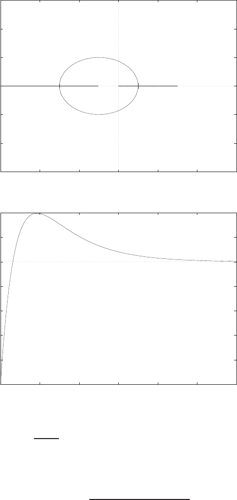
Problems 337

-6

-4

-2

-6 -4 -2 0 2 4 6

x xo

Real Axis

Imag Axis

0.2

0.4

0.6

0.8

1.2

1.4

00.5 1 1.5 2 2.5 3

Time (secs)

Amplitude

FIGURE P7.38

(a) Root locus for 1 + Ks+1

s(s−3) = 0. (b) Unit step response.

P7.39 The loop transfer function is

Gc(s)G(s) = 22K

(s+ 1)(s2+ 8s+ 22) .

When K= 0.529, the closed-loop poles are s1,2=−3.34 ±1.83jand

s3=−2.32 and have the maximum damping ζ= 0.877. The root locus is

shown in Figure P7.39a. The step response is shown in Figure P7.39b.

from the publisher prior to any prohibited reproduction, storage in a retrieval system, or transmission in any form or by any means, electronic, mechanical, photocopying,

recording, or likewise. For information regarding permission(s), write to: Rights and Permissions Department, Pearson Education, Inc., Upper Saddle River, NJ 07458.

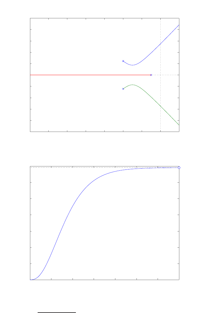
338 CHAPTER 7 The Root Locus Method

−14 −12 −10 −8 −6 −4 −2 0 2

−10

−8

−6

−4

−2

Root Locus

Real Axis

Imaginary Axis

Step Response

Time (sec)

Amplitude

0 0.5 1 1.5 2 2.5 3 3.5

0.05

0.1

0.15

0.2

0.25

0.3

0.35

FIGURE P7.39

(a) Root locus for 22K

(s+1)(s2+8s+22) = 0. (b) Unit step response.

from the publisher prior to any prohibited reproduction, storage in a retrieval system, or transmission in any form or by any means, electronic, mechanical, photocopying,

recording, or likewise. For information regarding permission(s), write to: Rights and Permissions Department, Pearson Education, Inc., Upper Saddle River, NJ 07458.

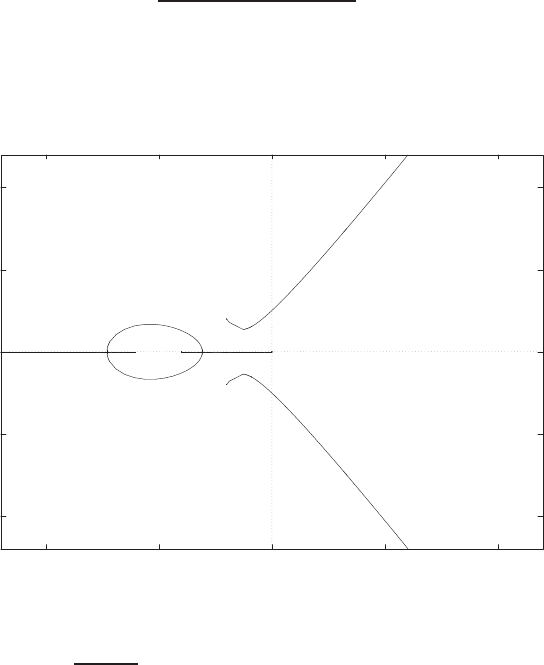
Advanced Problems 339

Advanced Problems

AP7.1 The characteristic equation is

1 + Ks+ 6

s(s+ 4)(s2+ 4s+ 8) = 0 .

The root locus is shown in Figure AP7.1. The gain at maximum ζis

-10

-5

-10 -5 0 5 10

Real Axis

Imag Axis

FIGURE AP7.1

Root locus for 1 + Ks(s+4)

s2+2s+2 = 0.

K= 3.7.

The roots at K= 3.7 are

s1=−3.6424 s2,3=−1.3395 ±+1.3553j s4=−1.6786 .

Using Figure 5.13 in Dorf & Bishop, the predicted percent overshoot and

settling time are

P.O. = 5% and Ts= 3 sec ,

from the publisher prior to any prohibited reproduction, storage in a retrieval system, or transmission in any form or by any means, electronic, mechanical, photocopying,

recording, or likewise. For information regarding permission(s), write to: Rights and Permissions Department, Pearson Education, Inc., Upper Saddle River, NJ 07458.

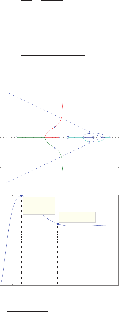
340 CHAPTER 7 The Root Locus Method

since ζ= 0.7 and

ωnζ=6

1.9(0.7) = 4.5.

The actual percent overshoot and settling time are P.O. = 1% and Ts=

2.8 sec.

AP7.2 The characteristic equation is

1 + K(s+ 1)(s+ 4)

s(s−1)(s+ 5)(s+ 10) = 0 .

The root locus is shown in Figure AP7.2a. The selected gain is K= 43.7.

−12 −10 −8 −6 −4 −2 0 2

−15

−10

−5

Real Axis

Imaginary Axis

Time (sec)

Amplitude

0 0.5 1 1.5 2 2.5 3 3.5 4 4.5

0.5

1.5

System: syscl

Peak amplitude: 1.48

Overshoot (%): 48.3

At time (sec): 0.857

System: syscl

Settling Time (sec): 2.31

FIGURE AP7.2

(a) Root locus for 1 + K(s+1)(s+4)

s(s−1)(s+5)(s+10) = 0; (b) Step response for K= 43.7.

from the publisher prior to any prohibited reproduction, storage in a retrieval system, or transmission in any form or by any means, electronic, mechanical, photocopying,

recording, or likewise. For information regarding permission(s), write to: Rights and Permissions Department, Pearson Education, Inc., Upper Saddle River, NJ 07458.

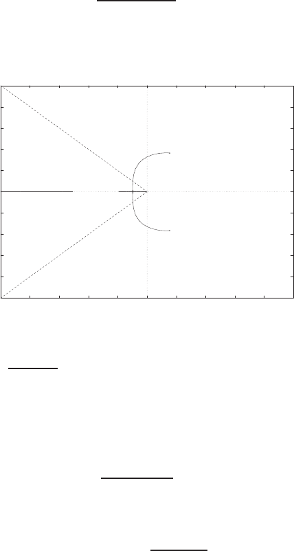
Advanced Problems 341

The actual percent overshoot (see Figure AP7.2b) is P.O. = 48.3%.

AP7.3 The characteristic equation (with pas the parameter) is

1 + ps(s+ 1)

s3+s2+ 10 = 0 .

The root locus is shown in Figure AP7.3.

-5

-4

-3

-2

-1

-5 -4 -3 -2 -1 0 1 2 3 4 5

Real Axis

Imag Axis

FIGURE AP7.3

Root locus for 1 + ps(s+1)

s3+s2+10 = 0.

When p= 21 the dominant roots have a damping ratio of ζ= 0.707.

AP7.4 The characteristic equation (with αas the parameter) is

1 + αs(s+ 1)

s3+s2+ 1 = 0 .

The root locus is shown in Figure AP7.4a. The steady-state error is

ess = lim

s→0sE(s) = lim

s→0

1 + G(s)= 1 −α .

To meet the steady-state error speciﬁcation, we require

0.9< α < 1.1.

The step responses for α= 0.9,1 and 1.1 are shown in Figure AP7.4b.

from the publisher prior to any prohibited reproduction, storage in a retrieval system, or transmission in any form or by any means, electronic, mechanical, photocopying,

recording, or likewise. For information regarding permission(s), write to: Rights and Permissions Department, Pearson Education, Inc., Upper Saddle River, NJ 07458.

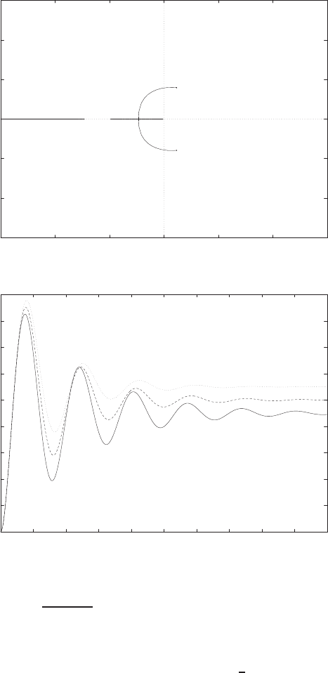
342 CHAPTER 7 The Root Locus Method

-3

-2

-1

-3 -2 -1 0 1 2 3

Real Axis

Imag Axis

0.2

0.4

0.6

0.8

1.2

1.4

1.6

1.8

0 5 10 15 20 25 30 35 40 45 50

Time (sec)

Amplitude

alpha=0.9 (solid); alpha=1.0 (dashed); alpha=1.1 (dotted)

FIGURE AP7.4

(a) Root locus for 1 + ps(s+1)

s3+s2+10 = 0. (b) Step responses for α= 0.9,1and 1.1.

AP7.5 The root locus is shown in Figure AP7.5. When K= 20.45, ζ= 0.707. The

root sensitivity is Sr1

K∼

=∆r1/(∆K/20.45) = 3.15687.76o. When K= 88,

the complex roots lie on the jω-axis—a 330% increase in the gain.

from the publisher prior to any prohibited reproduction, storage in a retrieval system, or transmission in any form or by any means, electronic, mechanical, photocopying,

recording, or likewise. For information regarding permission(s), write to: Rights and Permissions Department, Pearson Education, Inc., Upper Saddle River, NJ 07458.

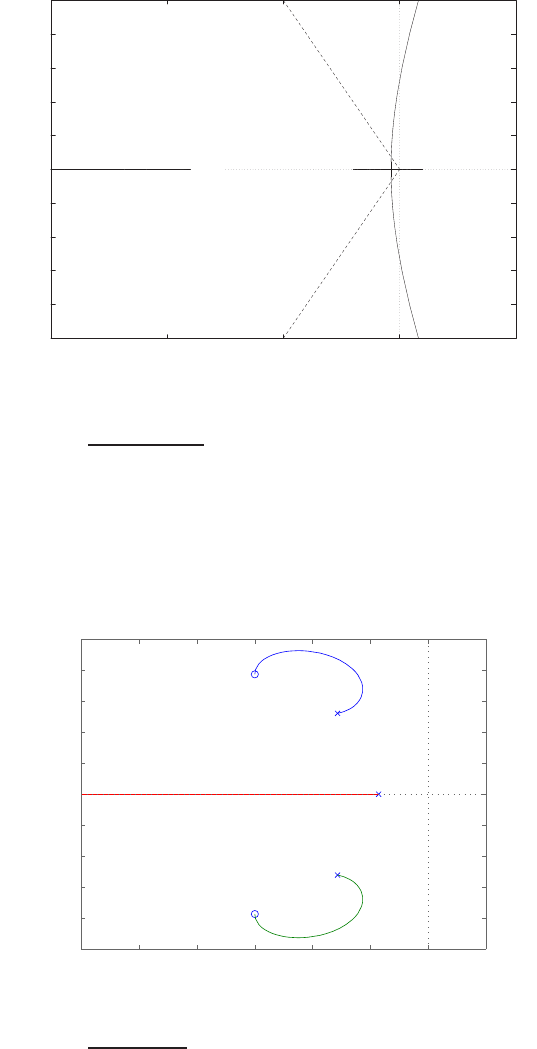
Advanced Problems 343

-5

-4

-3

-2

-1

-15 -10 -5 0 5

x x x

Real Axis

Imag Axis

FIGURE AP7.5

Root locus for 1 + K1

s3+10s2+7s−18 = 0.

AP7.6 A gain of K= 13 provides an acceptable response of Ts<1 and P.O. <

7.5%. The root locus is shown in Figure AP7.6.

−3 −2.5 −2 −1.5 −1 −0.5 0 0.5

−2.5

−2

−1.5

−1

−0.5

0.5

1.5

2.5

Root Locus

Real Axis

Imaginary Axis

FIGURE AP7.6

Root locus for 1 + Ks2+3s+6

s3+2s2+3s+1 = 0.

from the publisher prior to any prohibited reproduction, storage in a retrieval system, or transmission in any form or by any means, electronic, mechanical, photocopying,

recording, or likewise. For information regarding permission(s), write to: Rights and Permissions Department, Pearson Education, Inc., Upper Saddle River, NJ 07458.

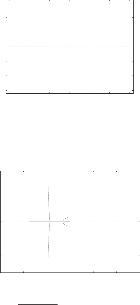
344 CHAPTER 7 The Root Locus Method

AP7.7 The root locus for the positive feedback system is shown in Figure AP7.7.

-15

-10

-5

-15 -10 -5 0 5 10 15

x x

Real Axis

Imag Axis

FIGURE AP7.7

Root locus for 1 + K−1

s2+12s+32 = 0.

AP7.8 The root locus is shown in Figure AP7.8a. When k= 0.448, all the roots

-30

-20

-10

-30 -20 -10 0 10 20 30

Real Axis

Imag Axis

FIGURE AP7.8

(a) Root locus for 1 + k120s

s3+19s2+34s+120 = 0.

from the publisher prior to any prohibited reproduction, storage in a retrieval system, or transmission in any form or by any means, electronic, mechanical, photocopying,

recording, or likewise. For information regarding permission(s), write to: Rights and Permissions Department, Pearson Education, Inc., Upper Saddle River, NJ 07458.

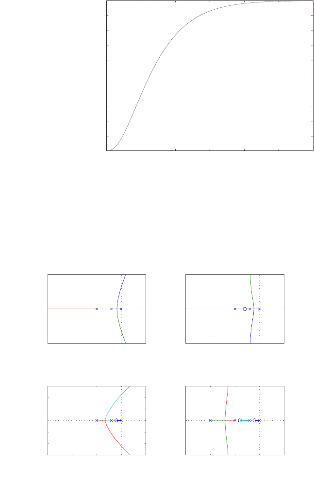
Advanced Problems 345

of the characteristic equation are real—the step response is shown in

Figure AP7.8b.

0.1

0.2

0.3

0.4

0.5

0.6

0.7

0.8

0.9

0 0.5 1 1.5 2 2.5 3

Time (secs)

Amplitude

FIGURE AP7.8

CONTINUED (b) Step response with k= 0.448.

AP7.9 The root locus for each controller is shown in Figure AP7.9.

−15 −10 −5 0 5

−5

(a)

Real Axis

Imaginary Axis

−15 −10 −5 0 5

−5

(b)

Real Axis

Imaginary Axis

−15 −10 −5 0 5

−15

−10

−5

(c)

Real Axis

Imaginary Axis

−15 −10 −5 0 5

−5

(d)

Real Axis

Imaginary Axis

FIGURE AP7.9

Root locus for the various controllers.

from the publisher prior to any prohibited reproduction, storage in a retrieval system, or transmission in any form or by any means, electronic, mechanical, photocopying,

recording, or likewise. For information regarding permission(s), write to: Rights and Permissions Department, Pearson Education, Inc., Upper Saddle River, NJ 07458.

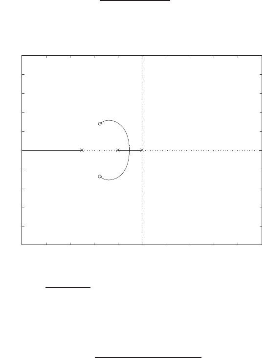
346 CHAPTER 7 The Root Locus Method

AP7.10 The characteristic equation (with Kas the parameter) is

1 + Ks2+ 7s+ 20

s(s2+ 7s+ 10) = 0 .

The root locus is shown in Figure AP7.10. The steady-state value of the

-10 -8 -6 -4 -2 0 2 4 6 8 10

-10

-8

-6

-4

-2

Real Axis

Imag Axis

FIGURE AP7.10

Root locus for 1 + Ks2+7s+20

s(s2+7s+10) = 0.

step response for any Kis 0.5. With K= 15 the closed-loop transfer

function is

T(s) = 10s+ 150

s3+ 22s2+ 115s+ 300 .

The step response has the following characteristics:

P.O. = 4.8% and Ts= 2 seconds .

AP7.11 The root locus is shown in Figure AP7.11a. A suitable gain is

K= 500.

The step response is shown in Figure AP7.11b.

from the publisher prior to any prohibited reproduction, storage in a retrieval system, or transmission in any form or by any means, electronic, mechanical, photocopying,

recording, or likewise. For information regarding permission(s), write to: Rights and Permissions Department, Pearson Education, Inc., Upper Saddle River, NJ 07458.

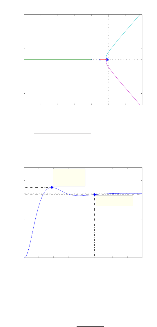
Advanced Problems 347

−100 −80 −60 −40 −20 0 20 40

−80

−60

−40

−20

Root Locus

Real Axis

Imaginary Axis

FIGURE AP7.11

(a) Root locus for 1 + K(s+2)2

s(s+10)(s+20)(s2+3s+3.5) = 0.

Step Response

Time (sec)

Amplitude

0 0.5 1 1.5 2 2.5 3 3.5 4

0.2

0.4

0.6

0.8

1.2

1.4

System: sys_cl

Peak amplitude: 1.09

Overshoot (%): 9.01

At time (sec): 0.945

System: sys_cl

Settling Time (sec): 2.39

FIGURE AP7.11

CONTINUED: (b) Step response with K= 500.

AP7.12 The root locus is shown in Figure AP7.12a. The PI controller can be

written as

Gc(s) = Kps+KI

from the publisher prior to any prohibited reproduction, storage in a retrieval system, or transmission in any form or by any means, electronic, mechanical, photocopying,

recording, or likewise. For information regarding permission(s), write to: Rights and Permissions Department, Pearson Education, Inc., Upper Saddle River, NJ 07458.

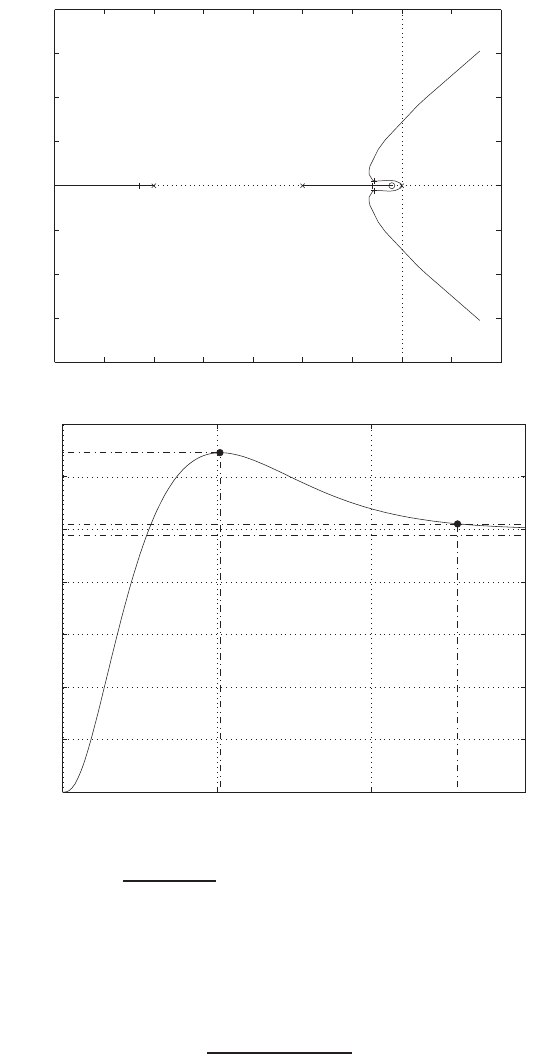
348 CHAPTER 7 The Root Locus Method

-7 -6 -5 -4 -3 -2 -1 0 1 2

-8

-6

-4

-2

Real Axis

Imag Axis

Time (sec.)

Amplitude

Step Response

0 5 10 15

0.2

0.4

0.6

0.8

1.2

1.4

From: U(1)

To: Y(1)

FIGURE AP7.12

(a) Root locus for 1 + Kp(s+0.2)

s(s2+7s+10) = 0. (b) Step response with Kp= 5.54.

and setting KI= 0.2Kp, the characteristic equation can be written as

1 + Kp

(s+ 0.2)

s(s2+ 7s+ 10) = 0

A suitable gain is Kp= 5.55. The step response is shown in Figure AP7.12b.

from the publisher prior to any prohibited reproduction, storage in a retrieval system, or transmission in any form or by any means, electronic, mechanical, photocopying,

recording, or likewise. For information regarding permission(s), write to: Rights and Permissions Department, Pearson Education, Inc., Upper Saddle River, NJ 07458.

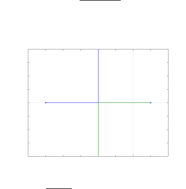
Advanced Problems 349

AP7.13 The characteristic equation is

1 + K1K2

(s+ 5)(s−1) = 0.

The root locus is shown in Figure AP7.12a. The fastest expected settling

−6 −5 −4 −3 −2 −1 0 1 2

−4

−3

−2

−1

Root Locus

Real Axis

Imaginary Axis

FIGURE AP7.13

Root locus for 1 + K1K21

(s+5)(s−1) = 0.

time is Ts= 4/ωnζ= 2 seconds since maximum |ωnζ|= 2.

AP7.14 The root locus of the uncompensated transfer function is shown in Fig-

ure AP7.14a. It can be seen that the system is unstable for Ku= 131.25

with a period of Tu= 0.72, as illustrated in FigureAP7.14b. Using the

Ziegler-Nichols design formulas yields KP= 0.6Ku= 78.75, KI= 1.2Ku/Tu=

218.75, and KD= 0.6KuTu= 7.0875 where

from the publisher prior to any prohibited reproduction, storage in a retrieval system, or transmission in any form or by any means, electronic, mechanical, photocopying,

recording, or likewise. For information regarding permission(s), write to: Rights and Permissions Department, Pearson Education, Inc., Upper Saddle River, NJ 07458.

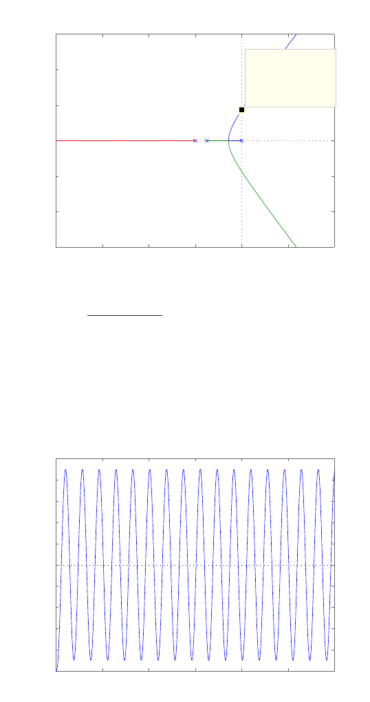
350 CHAPTER 7 The Root Locus Method

−40 −30 −20 −10 0 10 20

−30

−20

−10

System: sysg

Gain: 131

Pole: 0.0153 + 8.66i

Damping: −0.00176

Overshoot (%): 101

Frequency (rad/sec): 8.66

Root Locus

Real Axis

Imaginary Axis

FIGURE AP7.14

(a) Root locus for 1 + Ku10

s(s+10)(s+7.5) = 0.

0 2 4 6 8 10 12

0.2

0.4

0.6

0.8

1.2

1.4

1.6

1.8

Step Response

Time (sec)

Amplitude

FIGURE AP7.14

CONTIUED: (b) Step response at the ultimate gain Ku= 131.

from the publisher prior to any prohibited reproduction, storage in a retrieval system, or transmission in any form or by any means, electronic, mechanical, photocopying,

recording, or likewise. For information regarding permission(s), write to: Rights and Permissions Department, Pearson Education, Inc., Upper Saddle River, NJ 07458.

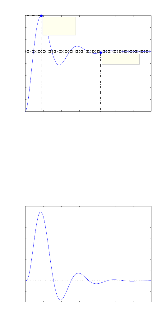
Advanced Problems 351

Step Response

Time (sec)

Amplitude

0 0.5 1 1.5 2 2.5 3 3.5

0.2

0.4

0.6

0.8

1.2

1.4

1.6

System: sys_cl

Peak amplitude: 1.6

Overshoot (%): 59.5

At time (sec): 0.445

System: sys_cl

Settling Time (sec): 2.1

FIGURE AP7.14

CONTINUED: (c) Step response with the Ziegler-Nichols tuned PID controller.

0 0.5 1 1.5 2 2.5 3 3.5

−4

−2

14 x 10−3 Step Response

Time (sec)

Amplitude

FIGURE AP7.14

CONTINUED: (d) Disturbance response with the Ziegler-Nichols tuned PID controller.

from the publisher prior to any prohibited reproduction, storage in a retrieval system, or transmission in any form or by any means, electronic, mechanical, photocopying,

recording, or likewise. For information regarding permission(s), write to: Rights and Permissions Department, Pearson Education, Inc., Upper Saddle River, NJ 07458.

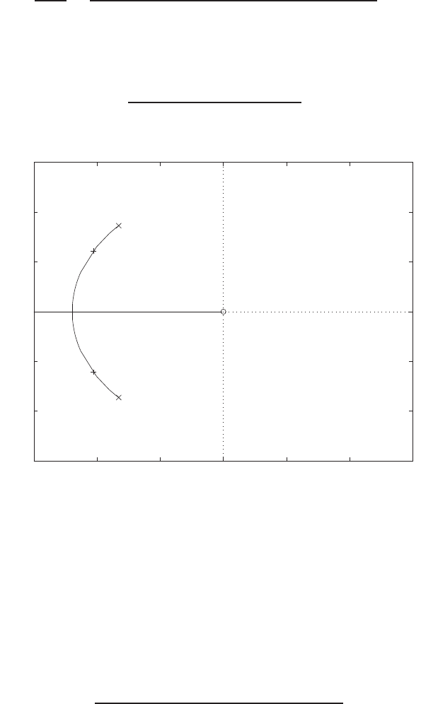
352 CHAPTER 7 The Root Locus Method

Design Problems

The closed-loop transfer function from the input to the output isCDP7.1

θ(s)

R(s)=26.035Ka

s2+ (33.1415 + 26.035KaK1)s+ 26.035Ka

where we consider for the ﬁrst time the tachometer feedback (see Figure

CDP4.1 in Dorf and Bishop). The characteristic equation is

1 + K1

26.035Kas

s2+ 33.1415s+ 26.035Ka

= 0 .

The root locus is shown below. In accordance with the discussion in Chap-

-30 -20 -10 0 10 20 30

-30

-20

-10

Real Axis

Imag Axis

ter 5, we continue to use Ka= 22. This allows us to meet the overshoot

speciﬁcation (P.O. < 5%) without the tachometer feedback and to pro-

vides good steady-state tracking errors to a step input. To meet the design

speciﬁcations of both P.O. and Tswe want the closed-loop poles to the

left of −ζω =−4/0.3 = −13.33 and ζ > 0.69. A reasonable selection is

K1= 0.012. This places the closed-loop poles at s=−20 ±j13.

DP7.1 (a) The characteristic equation is

1 + 18K(s+ 0.015)(s+ 0.45)

(s2+ 1.2s+ 12)(s2+ 0.01s+ 0.0025) = 0 .

from the publisher prior to any prohibited reproduction, storage in a retrieval system, or transmission in any form or by any means, electronic, mechanical, photocopying,

recording, or likewise. For information regarding permission(s), write to: Rights and Permissions Department, Pearson Education, Inc., Upper Saddle River, NJ 07458.

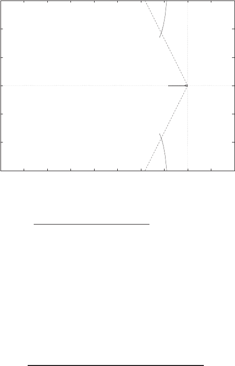
Design Problems 353

Since we want a negative feedback system, we have Gc(s) = −K.

When ωn>2 and ζ= 0.15, the gain K= 0.12. The root locus is

shown in Figure DP7.1a.

-6

-4

-2

-4 -3.5 -3 -2.5 -2 -1.5 -1 -0.5 0 0.5 1

o o

Real Axis

Imag Axis

FIGURE DP7.1

(a) Root locus for 1 + K18(s+0.015)(s+0.45)

(s2+1.2s+12)(s2+0.01s+0.0025) = 0.

(b) The unit step response is shown in Figure DP7.1b. The percent over-

shoot is

P.O. = 100% .

1 + 18K(s+ 2)(s+ 0.015)(s+ 0.45)

(s2+ 1.2s+ 12)(s2+ 0.01s+ 0.002s)= 0 .

The root locus is shown in Figure DP7.1c. If we select

K= 9.2/18 ,

then the complex roots have a damping ζ= 0.90. The roots are at

s1=−0.253

s2=−0.019

s3,4=−5.07 ±j2.50 .

from the publisher prior to any prohibited reproduction, storage in a retrieval system, or transmission in any form or by any means, electronic, mechanical, photocopying,

recording, or likewise. For information regarding permission(s), write to: Rights and Permissions Department, Pearson Education, Inc., Upper Saddle River, NJ 07458.

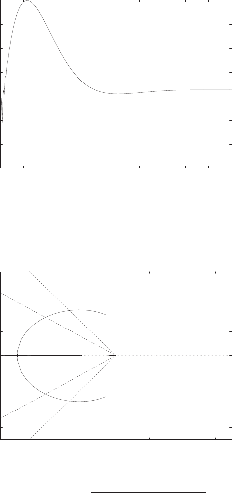
354 CHAPTER 7 The Root Locus Method

0.1

0.2

0.3

0.4

0.5

0.6

0.7

020 40 60 80 100 120 140 160 180 200

Time (secs)

Amplitude

FIGURE DP7.1

CONTINUED: (b) Unit step response for gain controller.

-6

-4

-2

-6 -4 -2 0 2 4 6

o o o

Real Axis

Imag Axis

FIGURE DP7.1

CONTINUED: (c) Root locus for 1 + K18(s+2)(s+0.015)(s+0.45)

(s2+1.2s+12)(s2+0.01s+0.0025) = 0.

(d) The unit step response for the system with the anticipatory controller

is shown in Figure DP7.1d.

from the publisher prior to any prohibited reproduction, storage in a retrieval system, or transmission in any form or by any means, electronic, mechanical, photocopying,

recording, or likewise. For information regarding permission(s), write to: Rights and Permissions Department, Pearson Education, Inc., Upper Saddle River, NJ 07458.

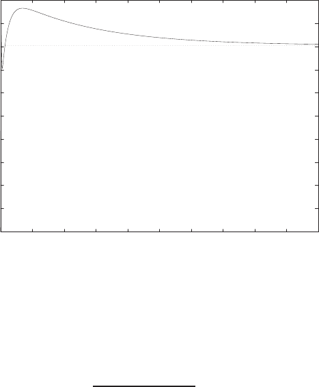
Design Problems 355

0.1

0.2

0.3

0.4

0.5

0.6

0.7

0.8

0.9

020 40 60 80 100 120 140 160 180 200

Time (secs)

Amplitude

FIGURE DP7.1

CONTINUED: (d) Unit step response for anticipatory controller.

DP7.2 The characteristic equation is

1 + 10K(s+ 1)

s(s2+ 4.5s+ 9) = 0 .

(a) The root locus is shown in Figure DP7.2a. When K= 0.435, we have

ζ= 0.6 and the roots are

s1=−0.368

s2,3=−2.1±j2.75 .

(b) The response to a step input is shown in Figure DP7.2b. The per-

formance results are

P.O. = 0%

Tss = 10 sec

ess = 0 .

Figure DP7.2b. The performance results to the step input are

P.O. = 0%

Ts= 4 sec

ess = 0 .

from the publisher prior to any prohibited reproduction, storage in a retrieval system, or transmission in any form or by any means, electronic, mechanical, photocopying,

recording, or likewise. For information regarding permission(s), write to: Rights and Permissions Department, Pearson Education, Inc., Upper Saddle River, NJ 07458.

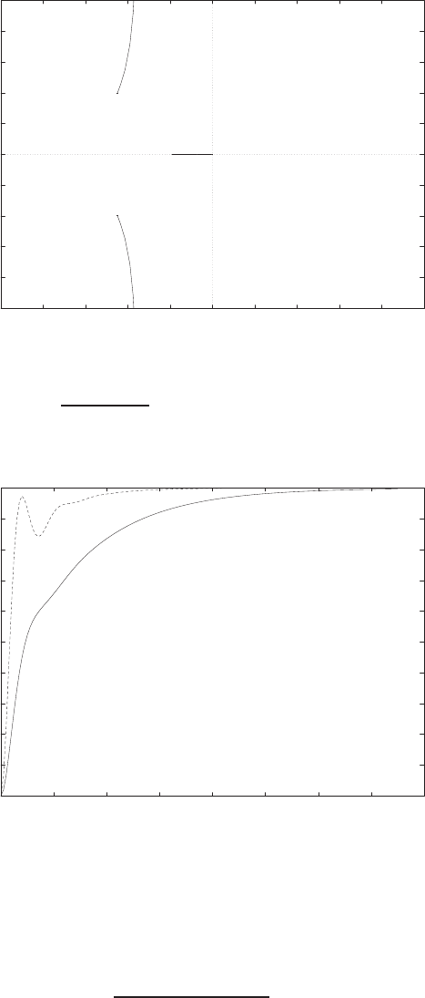
356 CHAPTER 7 The Root Locus Method

-5

-4

-3

-2

-1

-5 -4 -3 -2 -1 0 1 2 3 4 5

Real Axis

Imag Axis

FIGURE DP7.2

(a) Root locus for 1 + K10(s+1)

s(s2+4.5s+9) = 0.

0.1

0.2

0.3

0.4

0.5

0.6

0.7

0.8

0.9

02 4 6 8 10 12 14 16

Time (sec)

Amplitude

K=0.435 ____ (solid line)

K=1.510 ---- (dashed line)

FIGURE DP7.2

CONTINUED: (b) Unit step responses for K= 0.425,1.51.

DP7.3 The characteristic equation is

1 + K(s2+ 6.5s+ 12)

s(s+ 1)(s+2) = 0 .

from the publisher prior to any prohibited reproduction, storage in a retrieval system, or transmission in any form or by any means, electronic, mechanical, photocopying,

recording, or likewise. For information regarding permission(s), write to: Rights and Permissions Department, Pearson Education, Inc., Upper Saddle River, NJ 07458.

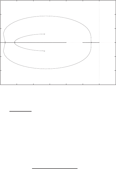
Design Problems 357

(a) The root locus is shown in Figure DP7.3.

-6

-4

-2

-6 -5 -4 -3 -2 -1 0 1

xxx

Real Axis

Imag Axis

FIGURE DP7.3

Root locus for 1 + Ks2+6.5s+12

s(s+1)(s+2) = 0.

When K= 41, the roots are s1=−37.12 and s2,3=−3.44 ±j1.19 .

(b) The percent overshoot is P.O. ≈1% when ζ= 0.82 at K= 0.062.

DP7.4 The characteristic equation is

1 + K10(0.01s+ 1)

s(s2+ 10s+ 10K1)= 0 .

If we choose K1= 2.5, then the root locus will start at s= 0,−5 and

-5. This is shown in Figure DP7.4. The root locus then has a nice shape

so that we can select Kto place the complex poles where desired and

the one real root will be farther in the left half-plane; thus the notion

of dominant poles will be valid. So, if we desire a P.O. < 5%, we want

ζ > 0.69. This occurs when K≈3. Thus, our design is

K1= 2.5 and K= 3 .

The unit step response is shown in Figure DP7.4. The settling time is less

than 3.5 sec and the P O < 4%. The response to a unit step disturbance

is also shown in Figure DP7.4. The steady-state error magnitude to the

disturbance is 0.33.

from the publisher prior to any prohibited reproduction, storage in a retrieval system, or transmission in any form or by any means, electronic, mechanical, photocopying,

recording, or likewise. For information regarding permission(s), write to: Rights and Permissions Department, Pearson Education, Inc., Upper Saddle River, NJ 07458.

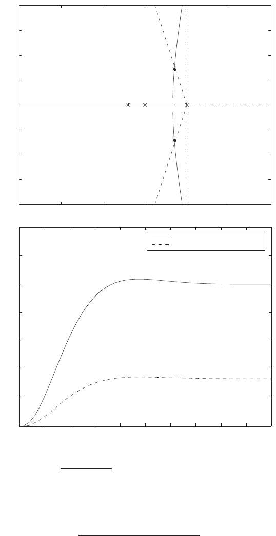
358 CHAPTER 7 The Root Locus Method

-20 -15 -10 -5 0 5 10

-4

-3

-2

-1

Real Axis

Imag Axis

K=3 -->

0 0.5 1 1.5 2 2.5 3 3.5 4 4.5 5

0.2

0.4

0.6

0.8

1.2

1.4

Time (sec)

y(t)

Input step response

Disturbance step response

FIGURE DP7.4

(a) Root locus for 1 + K10(0.01s+1)

s(s2+10s+25) = 0. (b) System response to step input and distur-

bance.

DP7.5 The characteristic equation is

1 + Ks+ 1

s(s−0.1)(s2+ 10s+ 41) = 0 .

The root locus is shown in Figure DP7.5a.

The system is stable for 5 < K < 300. The step response with K=

from the publisher prior to any prohibited reproduction, storage in a retrieval system, or transmission in any form or by any means, electronic, mechanical, photocopying,

recording, or likewise. For information regarding permission(s), write to: Rights and Permissions Department, Pearson Education, Inc., Upper Saddle River, NJ 07458.

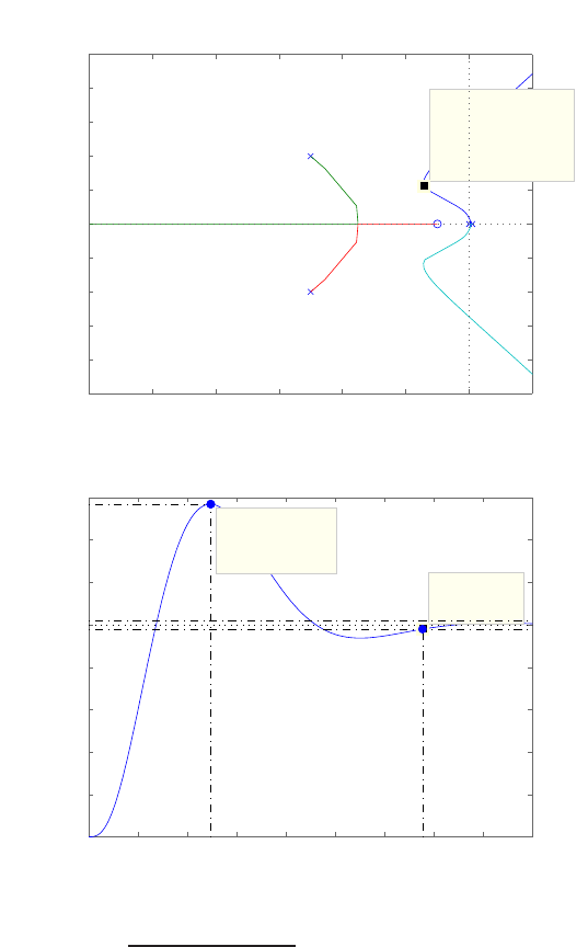
Design Problems 359

−12 −10 −8 −6 −4 −2 0 2

−10

−8

−6

−4

−2

System: sysgc

Gain: 90.5

Pole: −1.42 + 2.24i

Damping: 0.536

Overshoot (%): 13.6

Frequency (rad/sec): 2.66

Root Locus

Real Axis

Imaginary Axis

Step Response

Time (sec)

Amplitude

0 0.5 1 1.5 2 2.5 3 3.5 4 4.5

0.2

0.4

0.6

0.8

1.2

1.4

1.6

System: sys_cl

Peak amplitude: 1.57

Overshoot (%): 57

At time (sec): 1.24

System: sys_cl

Time (sec): 3.39

Amplitude: 0.98

FIGURE DP7.5

(a) Root locus for 1 + Ks+1

s(s−0.1)(s2+10s+41) = 0. (b) Step response with K= 875.

90.5 is shown in Figure DP7.5b. We choose K= 90.5 to minimize the

settling time. The damping of the dominant poles is ζ= 0.54, so that the

estimated percent overshoot is P.O. = 13%. The actual percent overshoot

and settling time are P.O. = 57% and Ts= 3.4 seconds. The match

between the actual and predicted percent overshoot can be improved by

selecting a much higher gain K, but then the step response becomes

overy oscillatory and the settling time increases too much for a typical

high-performance aircraft.

from the publisher prior to any prohibited reproduction, storage in a retrieval system, or transmission in any form or by any means, electronic, mechanical, photocopying,

recording, or likewise. For information regarding permission(s), write to: Rights and Permissions Department, Pearson Education, Inc., Upper Saddle River, NJ 07458.

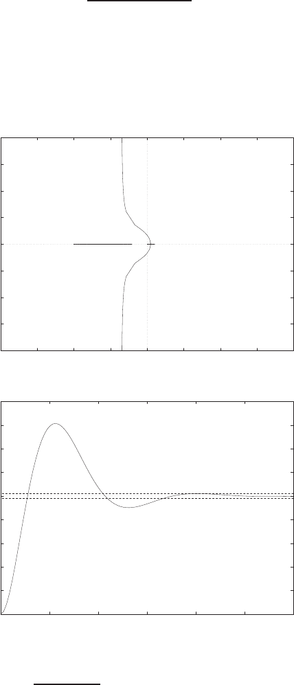
360 CHAPTER 7 The Root Locus Method

DP7.6 The characteristic equation is

1 + Ks+ 2

s(s+ 10)(s−1) = 0 .

The maximum damping is ζ= 0.46 at K= 55. The root locus is shown in

Figure DP7.6a; the step response is shown in Figure DP7.6b. The percent

overshoot and settling time are P.O. = 61.3% and Ts= 2 seconds.

-20

-15

-10

-5

-20 -15 -10 -5 0 5 10 15 20

x xx o

Real Axis

Imag Axis

0.2

0.4

0.6

0.8

1.2

1.4

1.6

1.8

0 0.5 1 1.5 2 2.5 3

Time (secs)

Amplitude

FIGURE DP7.6

(a) Root locus for 1 + Ks+2

s(s+10)(s−1) = 0. (b) Step response with K= 55.

from the publisher prior to any prohibited reproduction, storage in a retrieval system, or transmission in any form or by any means, electronic, mechanical, photocopying,

recording, or likewise. For information regarding permission(s), write to: Rights and Permissions Department, Pearson Education, Inc., Upper Saddle River, NJ 07458.

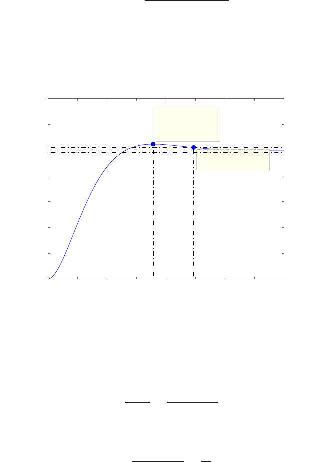
Design Problems 361

DP7.7 The loop transfer function is

Gc(s)G(s) = KPs+KI

s(s+ 1)(0.5s+ 1).

One possible set of PI controller gains are KP= 0.82 and KI= 0.9. The

step response is shown in Figure DP7.7.

Step Response

Time (sec)

Amplitude

0 1 2 3 4 5 6 7 8

0.2

0.4

0.6

0.8

1.2

1.4

System: syscl

Peak amplitude: 1.05

Overshoot (%): 4.59

At time (sec): 3.57

System: syscl

Settling Time (sec): 4.94

FIGURE DP7.7

Step response for with PI controller Gc(s) = (0.82s+ 0.9)/s.

DP7.8 The closed-loop transfer function is

T(s) = Vo(s)

V(s)=G(s)

1 + KG(s).

The dc gain is

T(0) = G(0)

1 + KG(0) ≈1

The root locus is shown in Figure DP7.8. The maximum value of Kfor

stability is

K= 0.062 .

from the publisher prior to any prohibited reproduction, storage in a retrieval system, or transmission in any form or by any means, electronic, mechanical, photocopying,

recording, or likewise. For information regarding permission(s), write to: Rights and Permissions Department, Pearson Education, Inc., Upper Saddle River, NJ 07458.

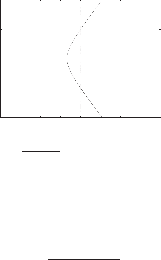
362 CHAPTER 7 The Root Locus Method

-2

-1.5

-1

-0.5

0.5

1.5

x107

-2 -1.5 -1 -0.5 0 0.5 1 1.5 2

x107

xx x

Real Axis

Imag Axis

FIGURE DP7.8

Root locus for 1 + K3.142K1×1017

(s+3142)(s+107)2= 0.

Therefore, the minimum dc gain is about 1/0.062=16. Selecting

K= 0.05 and R1= 10 K

yields

R2= 19R1= 190 K .

DP7.9 The closed-loop transfer function (with Gp(s) = 1 and K= 1) is

T(s) = 2s3+ 6s2+ 14s+ 10

s4+ 6s3+ 13s2+ 26s+ 6 .

So, if we select Gp(s) = 1/T (0) = 0.6, the step response (with K= 1)

will have a zero steady-state tracking error. The root locus is shown in

Figure DP7.9a. The step responses for K= 1,1.5 and 2.85 are shown in

Figure DP7.9b. For K= 1, we have P.O. = 0%, Tr= 7.8 and Ts= 13.9;

for K= 1.5, we have P.O. = 0%, Tr= 5.4 and Ts= 9.6; and for K= 2.85,

we have P.O. = 5.2%, Tr= 0.5 and Ts= 7.3. The best gain selection is

K= 2.85.

from the publisher prior to any prohibited reproduction, storage in a retrieval system, or transmission in any form or by any means, electronic, mechanical, photocopying,

recording, or likewise. For information regarding permission(s), write to: Rights and Permissions Department, Pearson Education, Inc., Upper Saddle River, NJ 07458.

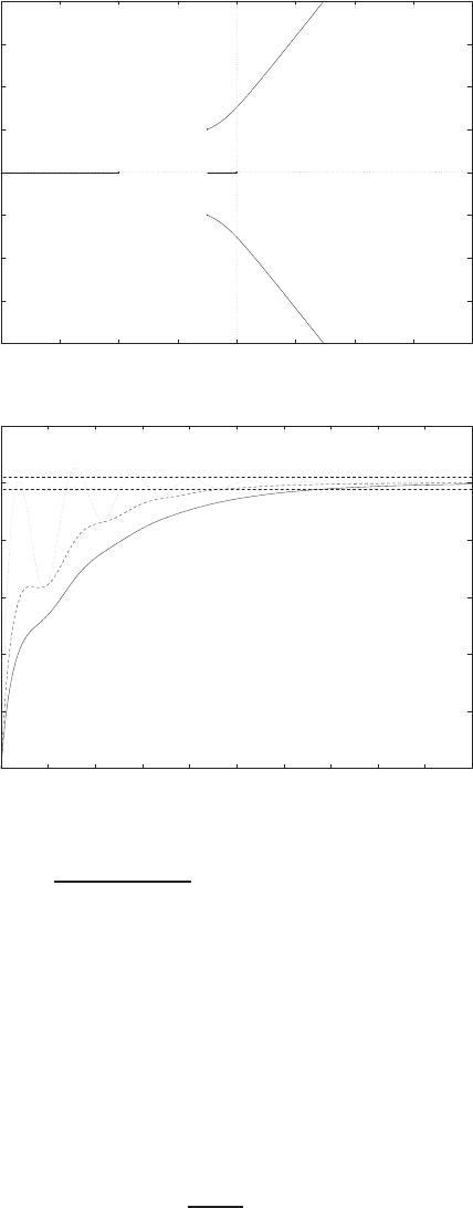
Design Problems 363

-8

-6

-4

-2

-8 -6 -4 -2 0 2 4 6 8

x o

Real Axis

Imag Axis

0.2

0.4

0.6

0.8

1.2

0 2 4 6 8 10 12 14 16 18 20

Time (sec)

Amplitude

K=1 (solid); K=1.5 (dashed); K=2.85 (dotted)

FIGURE DP7.9

(a) Root locus for 1 + K6(s+1)

s(s+4)(s2+2s+5) = 0. (b) Step responses with K= 1,1.5,2.85.

DP7.10 A suitable selection of the various parameters is

ζ= 0.5 and q= 3/5.

With q= 3/5, the open-loop zeros are real and equal. Then, it follows

that

λ=2q

1−q= 3 .

from the publisher prior to any prohibited reproduction, storage in a retrieval system, or transmission in any form or by any means, electronic, mechanical, photocopying,

recording, or likewise. For information regarding permission(s), write to: Rights and Permissions Department, Pearson Education, Inc., Upper Saddle River, NJ 07458.

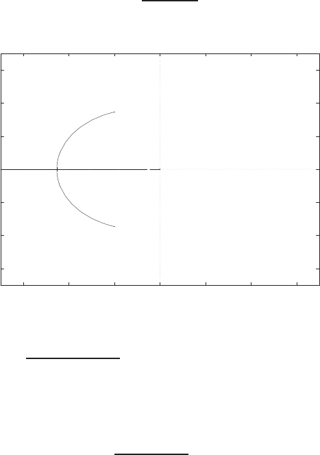
364 CHAPTER 7 The Root Locus Method

The root locus is shown in Figure DP7.10. A reasonable choice of gain is

K= 30 .

The resulting step response is extremely fast with no overshoot. The

closed-loop transfer function is approximately given by

T(s)≈1923

s+ 1923 .

-6

-4

-2

-6 -4 -2 0 2 4 6

Real Axis

Imag Axis

FIGURE DP7.10

Root locus for 1 + K4s2+4s+1

0.0625s3+0.25s2+s= 0.

DP7.11 The characteristic equation (with Kas the parameter) is

1 + K10(s2+ 10)

s3+ 20s= 0 .

The root locus is shown in Figure DP7.11a. To maximize the closed-loop

system damping we choose

K= 0.513.

The step response is shown in Figure DP7.11b.

from the publisher prior to any prohibited reproduction, storage in a retrieval system, or transmission in any form or by any means, electronic, mechanical, photocopying,

recording, or likewise. For information regarding permission(s), write to: Rights and Permissions Department, Pearson Education, Inc., Upper Saddle River, NJ 07458.

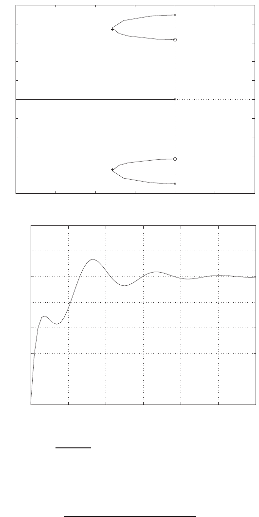
Design Problems 365

-2 -1.5 -1 -0.5 0 0.5 1

-5

-4

-3

-2

-1

Real Axis

Imag Axis

Time (sec.)

Amplitude

Step Response

0123456

0.2

0.4

0.6

0.8

1.2

1.4

From: U(1)

To: Y(1)

FIGURE DP7.11

(a) Root locus for 1 + K10(s2+10)

s3+20s= 0. (b) Step response with K= 0.513.

DP7.12 The characteristic equation is

1 + Ks+ 1.5

(s+ 1)(s+ 2)(s+ 4)(s+ 10) = 0 .

The root locus is shown in Figure DP7.12a.

from the publisher prior to any prohibited reproduction, storage in a retrieval system, or transmission in any form or by any means, electronic, mechanical, photocopying,

recording, or likewise. For information regarding permission(s), write to: Rights and Permissions Department, Pearson Education, Inc., Upper Saddle River, NJ 07458.

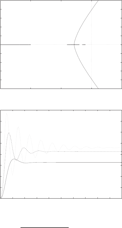
366 CHAPTER 7 The Root Locus Method

-10

-8

-6

-4

-2

-15 -10 -5 0 5

x x x xo

Real Axis

Imag Axis

0.2

0.4

0.6

0.8

1.2

1.4

1.6

012345678910

Time (sec)

Amplitude

K=100 (solid); K=300 (dashed); K=600 (dotted)

FIGURE DP7.12

(a) Root locus for 1 + Ks+1.5

(s+1)(s+2)(s+4)(s+10) = 0. (b) Step response with K=

100,300,600.

The closed-loop system roots are:

K= 100 : s1=−11.38 s2,3=−2.09 ±3.10j s4=−1.45

K= 300 : s1=−12.94 s2,3=−1.29 ±5.10j s4=−1.48

K= 600 : s1=−14.44 s2,3=−0.53 ±6.72j s4=−1.49

The step responses are shown in Figure DP7.12b.

from the publisher prior to any prohibited reproduction, storage in a retrieval system, or transmission in any form or by any means, electronic, mechanical, photocopying,

recording, or likewise. For information regarding permission(s), write to: Rights and Permissions Department, Pearson Education, Inc., Upper Saddle River, NJ 07458.

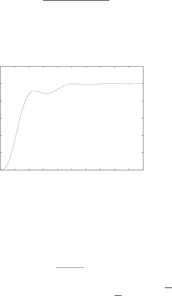
Design Problems 367

DP7.13 The closed-loop transfer function is

T(s) = Ka

s3+s2+KaK2s+Ka

A suitable choice of gains is

Ka= 0.52 and K2= 3 .

The step response is shown in Figure DP7.13.

0.2

0.4

0.6

0.8

1.2

0 2 4 6 8 10 12 14 16 18 20

Time (secs)

Amplitude

FIGURE DP7.13

Step response with Ka= 0.52 and K2= 3.

DP7.14 The characteristic equation is

s2+ 10KDs+ 10(KP+ 1) = 0 .

In the Evans form we have

1 + KD

10(s+τ)

s2+ 10 = 0 .

The root locus is shown in Figure DP7.14 for τ= 6. As τ→0, the

dominant closed-loop pole approaches s= 0 as KD→ ∞. As τ→√10,

the dominant closed-loop pole approaches s=−√10 as KD→ ∞. A

viable controller is KP= 72 and KD= 12 when τ= 6.

from the publisher prior to any prohibited reproduction, storage in a retrieval system, or transmission in any form or by any means, electronic, mechanical, photocopying,

recording, or likewise. For information regarding permission(s), write to: Rights and Permissions Department, Pearson Education, Inc., Upper Saddle River, NJ 07458.

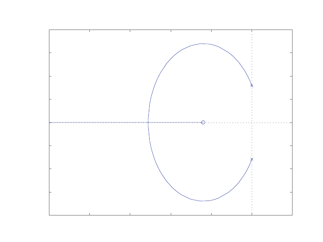
368 CHAPTER 7 The Root Locus Method

−25 −20 −15 −10 −5 0 5

−8

−6

−4

−2

Root Locus

Real Axis

Imaginary Axis

FIGURE DP7.14

Root locus when τ= 6.

from the publisher prior to any prohibited reproduction, storage in a retrieval system, or transmission in any form or by any means, electronic, mechanical, photocopying,

recording, or likewise. For information regarding permission(s), write to: Rights and Permissions Department, Pearson Education, Inc., Upper Saddle River, NJ 07458.

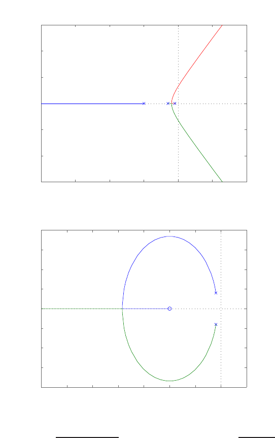
Computer Problems 369

Computer Problems

CP7.1 The root locus for parts (a)-(d) are shown in Figures CP7.1a - CP7.1d.

−40 −30 −20 −10 0 10 20

−30

−20

−10

num=[30]; den=[1 14 43 30]; rlocus(sys)

Real Axis

Imaginary Axis

−70 −60 −50 −40 −30 −20 −10 0 10

−20

−15

−10

−5

num=[1 20]; den=[1 4 20]; rlocus(sys)

Real Axis

Imaginary Axis

FIGURE CP7.1

(a) Root locus for 1 + k30

s3+14s2+43s+30 = 0.(b) Root locus for 1 + ks+20

s2+4s+20 = 0.

from the publisher prior to any prohibited reproduction, storage in a retrieval system, or transmission in any form or by any means, electronic, mechanical, photocopying,

recording, or likewise. For information regarding permission(s), write to: Rights and Permissions Department, Pearson Education, Inc., Upper Saddle River, NJ 07458.

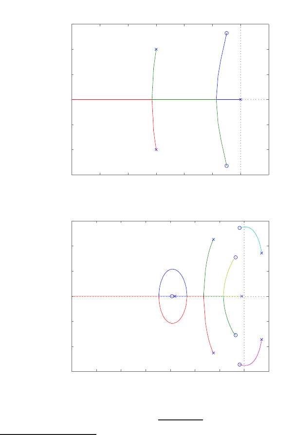
370 CHAPTER 7 The Root Locus Method

−6 −5 −4 −3 −2 −1 0 1

−1.5

−1

−0.5

0.5

1.5

num=[1 1 2]; den=[1 6 10 0]; rlocus(sys)

Real Axis

Imaginary Axis

−7 −6 −5 −4 −3 −2 −1 0 1

−1.5

−1

−0.5

0.5

1.5

num=[1 4 6 10 6 4]; den=[1 4 4 1 1 10 1]; rlocus(sys)

Real Axis

Imaginary Axis

FIGURE CP7.1

CONTINUED: (c) Root locus for 1 + ks2+s+2

s(s2+6s+10) = 0.(d) Root locus for 1 +

ks5+4s4+6s3+10s2+6s+4

s6+4s5+4s4+s3+s2+10s+1 = 0.

from the publisher prior to any prohibited reproduction, storage in a retrieval system, or transmission in any form or by any means, electronic, mechanical, photocopying,

recording, or likewise. For information regarding permission(s), write to: Rights and Permissions Department, Pearson Education, Inc., Upper Saddle River, NJ 07458.

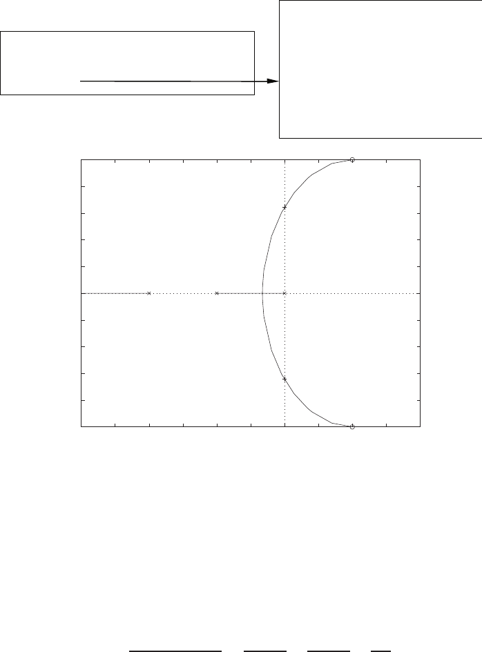
Computer Problems 371

CP7.2 The maximum value of the gain for stability is k= 0.791. The m-ﬁle

script and root locus is shown in Figure CP7.2.

num=[1 -2 2]; den=[1 3 2 0]; sys = tf(num,den);

rlocus(sys)

rlocnd(sys)

Select a point in the graphics window

selected_point =

-0.0025 + 0.6550i

ans =

0.8008

−3 −2.5 −2 −1.5 −1 −0.5 0 0.5 1 1.5 2

−1

−0.8

−0.6

−0.4

−0.2

0.2

0.4

0.6

0.8

Real Axis

Imag Axis

FIGURE CP7.2

Using the rlocﬁnd function.

The value of k= 0.8008 selected by the rlocﬁnd function is not exact

since you cannot select the jω-axis crossing precisely. The actual value is

determined using Routh-Hurwitz analysis.

CP7.3 The partial fraction expansion of Y(s) is

Y(s) = s+ 6

s(s2+ 5s+ 4) =0.1667

s+ 4 −1.6667

s+ 1 +1.5

The m-ﬁle script and output is shown in Figure CP7.3.

from the publisher prior to any prohibited reproduction, storage in a retrieval system, or transmission in any form or by any means, electronic, mechanical, photocopying,

recording, or likewise. For information regarding permission(s), write to: Rights and Permissions Department, Pearson Education, Inc., Upper Saddle River, NJ 07458.

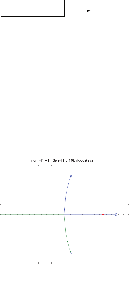
372 CHAPTER 7 The Root Locus Method

num=[1 6]; den=[1 5 4 0];

[r,p,k]=residue(num,den)

r =

0.1667

-1.6667

1.5000

p =

-4

-1

k =

[]

FIGURE CP7.3

Using the residue function.

CP7.4 The characteristic equation is

1 + ps−1

s2+ 5s+ 10 = 0 .

The root locus is shown in Figure CP7.4. The closed-loop system is stable

for

0< p < 10 .

−8 −7 −6 −5 −4 −3 −2 −1 0 1 2

−2.5

−2

−1.5

−1

−0.5

0.5

1.5

2.5

Real Axis

Imaginary Axis

FIGURE CP7.4

Root locus for 1 + ps−1

s2+5s+10 = 0.

from the publisher prior to any prohibited reproduction, storage in a retrieval system, or transmission in any form or by any means, electronic, mechanical, photocopying,

recording, or likewise. For information regarding permission(s), write to: Rights and Permissions Department, Pearson Education, Inc., Upper Saddle River, NJ 07458.

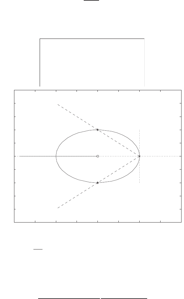
Computer Problems 373

CP7.5 The characteristic equation is

1 + ks+ 1

s2= 0 .

The root locus is shown in Figure CP7.5. For k= 2 we obtain s1,2=

−1±j, that is, we have ζ= 0.707.

num=[1 1]; den=[1 0 0]; sys = tf(num,den);

hold o, clf

rlocus(sys);

hold on

plot([0 -2],[0 2*tan(acos(0.707))],'--')

plot([0 -2],[0 -2*tan(acos(0.707))],'--')

plot([-1 -1],[1 -1],'*')

-3 -2.5 -2 -1.5 -1 -0.5 0 0.5 1

-2.5

-2

-1.5

-1

-0.5

0.5

1.5

2.5

Real Axis

Imag Axis

FIGURE CP7.5

Root locus for 1 + ks+1

s2= 0.

CP7.6 We choose a controller with two real poles and two real zeros selected to

meet the steady-state speciﬁcation. The characteristic equation is

1 + K(s+ 5.5)(s+ 0.01)

(s+ 6.5)(s+ 0.0001)

s3+ 15s2+ 50s= 0 .

The m-ﬁle and root locus is shown in Figure CP7.4a. From the root lo-

cus we can select the value of the gain Kthat results in an estimated

P.O. ≤5% and a ζωn≤ −2 to meet the settling time speciﬁcation. We

from the publisher prior to any prohibited reproduction, storage in a retrieval system, or transmission in any form or by any means, electronic, mechanical, photocopying,

recording, or likewise. For information regarding permission(s), write to: Rights and Permissions Department, Pearson Education, Inc., Upper Saddle River, NJ 07458.

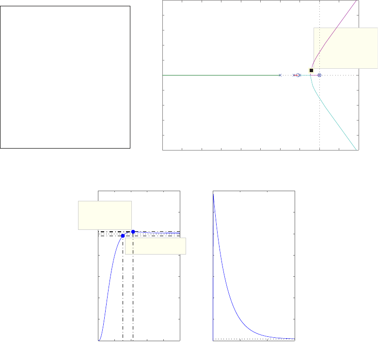
374 CHAPTER 7 The Root Locus Method

select K= 8.58. The step response is shown in Figure CP7.6b showing

the percent overshoot and settling time speciﬁcations are satisﬁed. The

velocity constant is kv= 145.2 which implies a steady-state error to a

ramp input of ess = 1/kv= 0.0069.

−40 −35 −30 −25 −20 −15 −10 −5 0 5 10

−25

−20

−15

−10

−5

System: untitled1

Gain: 8.58

Pole:

Damping: 0.807

Overshoot (%): 1.37

Frequency (rad/sec): 2.58

Real Axis

Imaginary Axis

ng=10; dg=conv([1 10 0],[1 5]); s

ysg=tf(ng,dg);

nh=conv([1 0.01],[1 5.5]);

dh=conv([1 6.5],[1 0.0001]);

sysh=tf(nh,dh);

gure(1)

rlocus(sysg*sysh)

K=8.58; sysh=tf(K*nh,dh);

sys=series(sysg,sysh);syscl=feedback(sys,1)

gure(2)

subplot(121)

step(syscl);

Kv=10*8.58*0.01*5.5/10/6.5/0.0001/5

systd=feedback(sysg,sysh);

subplot(122)

step(systd)

Step Response

Time (sec)

Amplitude

0 200 400 600

0.02

0.04

0.06

0.08

0.1

0.12

0.14

Disturbance Response

Time (sec)

y(t)/Q

012345

0.2

0.4

0.6

0.8

1.2

1.4

System: syscl

Peak amplitude: 1.02

Overshoot (%): 1.77

At time (sec): 2.14

System: syscl

Settling Time (sec): 1.51

FIGURE CP7.6

(a) Root locus. (b) Step response and disturbance response.

CP7.7 The m-ﬁle script to generate the root locus for each controller in parts

(a)-(c) is shown in Figure CP7.7. The performance region is indicated on

each root locus in Figures CP7.7b - CP7.7d. For part (a), the controller

gain is found to be Gc(s) = 11.3920. The integral controller in part (b)

from the publisher prior to any prohibited reproduction, storage in a retrieval system, or transmission in any form or by any means, electronic, mechanical, photocopying,

recording, or likewise. For information regarding permission(s), write to: Rights and Permissions Department, Pearson Education, Inc., Upper Saddle River, NJ 07458.

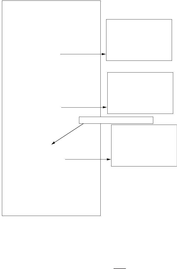
Computer Problems 375

ÈSelect a point in the graphics window

selected_point =

-2.5030 + 3.3380i

ans =

11.3920

Select a point in the graphics window

selected_point =

-0.6690 + 0.8210i

ans =

4.0930

Select a point in the graphics window

selected_point =

-2.0695+ 2.7387i

ans =

9.2516

on graph.Plot performance region boundaries

numg=[1]; deng=[1 5 6]; sysg = tf(numg,deng);

t=[0:0.1:15];

% Part (a)

sys1 = sysg;

rlocus(sys1), grid

hold on

plot([-0.4 -0.4],[-6 6],'--',...

[0 -6*tan(36.2*pi/180)],[0 6],'--',...

[0 -6*tan(36.2*pi/180)],[0 -6],'--')

hold o

[kp,poles] = rlocnd(sys1)

% Part (b)

numc=[1]; denc=[1 0]; sysc = tf(numc,denc);

sys2 = series(sysc,sysg);

gure

rlocus(sys2), grid

hold on

plot([-0.4 -0.4],[-6 6],'--',...

[0 -6*tan(36.2*pi/180)],[0 6],'--',...

[0 -6*tan(36.2*pi/180)],[0 -6],'--')

hold o

[ki,poles] = rlocnd(sys2)

% Part (c)

gure

numc=[1 1]; denc=[1 0]; sysc = tf(numc,denc);

sys3 = series(sysc,sysg);

rlocus(sys3), grid

hold on

plot([-0.4 -0.4],[-6 6],'--',...

[0 -6*tan(36.2*pi/180)],[0 6],'--',...

[0 -6*tan(36.2*pi/180)],[0 -6],'--')

hold o

[kpi,poles] = rlocnd(sys3)

% Part (d)

gure

sys1_o = kp*sys1; sys1_cl = feedback(sys1_o,[1]);

sys2_o = ki*sys2; sys2_cl = feedback(sys2_o,[1]);

sys3_o = kpi*sys3; sys3_cl = feedback(sys3_o,[1]);

[y1,t]=step(sys1_cl,t);

[y2,t]=step(sys2_cl,t);

[y3,t]=step(sys3_cl,t);

plot(t,y1,t,y2,'--',t,y3,':'),grid

xlabel('time [sec]'),ylabel('y(t)')

title('Gc(s): proportional (solid), integral (dashed) & PI (dotted)')

FIGURE CP7.7

(a) Script to generate the root locus for each controller.

is determined to be

Gc(s) = 4.093

from the publisher prior to any prohibited reproduction, storage in a retrieval system, or transmission in any form or by any means, electronic, mechanical, photocopying,

recording, or likewise. For information regarding permission(s), write to: Rights and Permissions Department, Pearson Education, Inc., Upper Saddle River, NJ 07458.

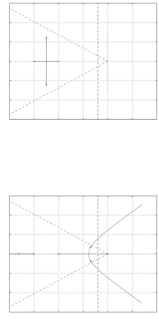
376 CHAPTER 7 The Root Locus Method

-4 -3 -2 -1 0 1 2

-6

-4

-2

Real Axis

Imag Axis

FIGURE CP7.7

CONTINUED: (b) Root locus for proportional controller with selected K= 11.3920.

The proportional integral (PI) controller in part (c) is

-4 -3 -2 -1 0 1 2

-6

-4

-2

Real Axis

Imag Axis

FIGURE CP7.7

CONTINUED: (c) Root locus for integral controller with selected K= 4.0930.

from the publisher prior to any prohibited reproduction, storage in a retrieval system, or transmission in any form or by any means, electronic, mechanical, photocopying,

recording, or likewise. For information regarding permission(s), write to: Rights and Permissions Department, Pearson Education, Inc., Upper Saddle River, NJ 07458.

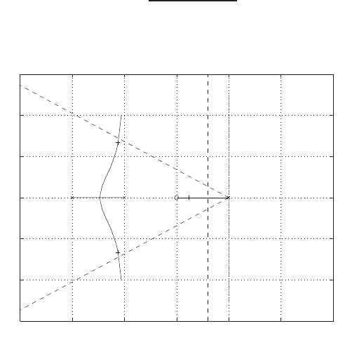
Computer Problems 377

Gc(s) = 9.2516(s+ 1)

The proportional controller is stable for all K > 0 but has a signiﬁcant

-4 -3 -2 -1 0 1 2

-6

-4

-2

Real Axis

Imag Axis

FIGURE CP7.7

CONTINUED: (d) Root locus for PI controller with selected K= 9.2516.

steady-state error. The integral controller has no steady-state error,

but is stable only for K < 30. The PI controller has zero steady-state

error and is stable for all K > 0. Additionally, the PI controller has a

fast transient response. The step responses for each controller is shown in

Figure CP7.7e.

from the publisher prior to any prohibited reproduction, storage in a retrieval system, or transmission in any form or by any means, electronic, mechanical, photocopying,

recording, or likewise. For information regarding permission(s), write to: Rights and Permissions Department, Pearson Education, Inc., Upper Saddle River, NJ 07458.

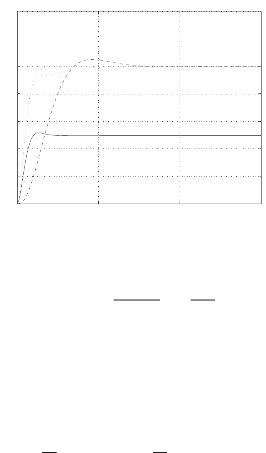
378 CHAPTER 7 The Root Locus Method

0 5 10 15

0.2

0.4

0.6

0.8

1.2

1.4

time [sec]

y(t)

Gc(s): proportional (solid), integral (dashed) & PI (dotted)

FIGURE CP7.7

CONTINUED: (e) Step responses for each controller.

CP7.8 The loop transfer function can be written as

Gc(s)G(s) = K1+K2s

Js2=¯

s+ 5

where

K2=K2/J .

The parameter of interest for the root locus is ¯

K2. The root locus is shown

in Figure CP7.8. The selected value of

K2= 7.1075 .

Therefore,

J= 7.1075 and K1

J= 35.5375 .

from the publisher prior to any prohibited reproduction, storage in a retrieval system, or transmission in any form or by any means, electronic, mechanical, photocopying,

recording, or likewise. For information regarding permission(s), write to: Rights and Permissions Department, Pearson Education, Inc., Upper Saddle River, NJ 07458.

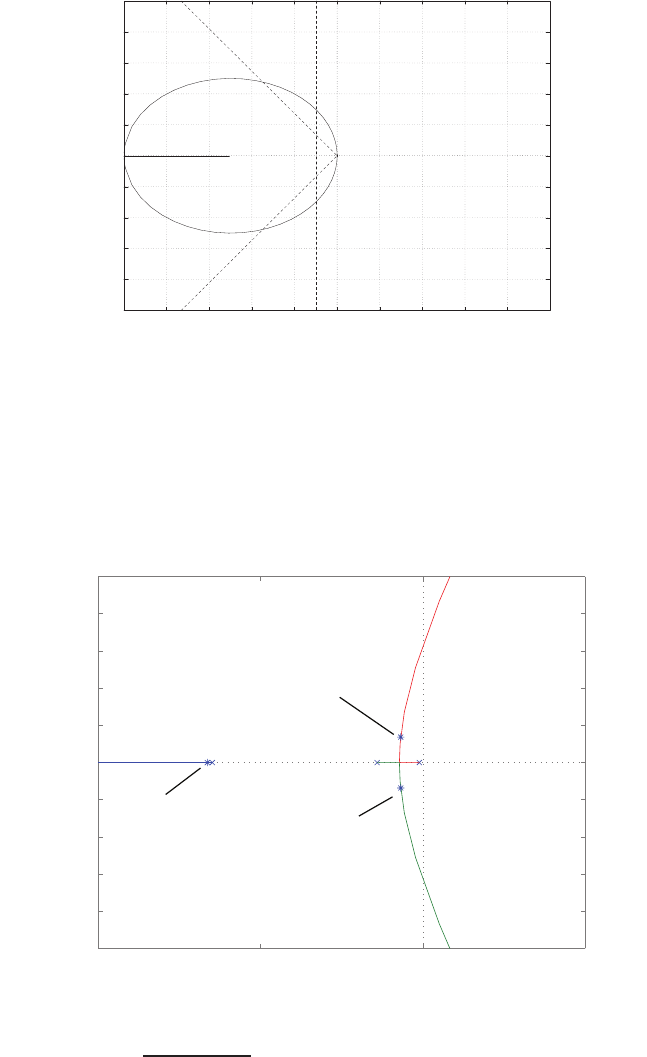
Computer Problems 379

-10

-8

-6

-4

-2

-10 -8 -6 -4 -2 0 2 4 6 8 10

xxo

Real Axis

Imag Axis

num=[1 5]; den=[1 0 0]; sys=tf(num,den); rlocus(sys); rlocnd(sys)

FIGURE CP7.8

Root locus to determine ¯

K2.

CP7.9 The value of Kthat results in a damping ratio of ζ= 0.707 is K= 5.2.

The root locus is shown in Figure CP7.9.

−10 −5 0 5

−5

−4

−3

−2

−1

Root Locus

Real Axis

Imaginary Axis

s = -0.68 + 0.68j

s = -6.63

s = -0.68 - 0.68j

FIGURE CP7.9

Root locus for 1 + K1

s3+8s2+10s+1 = 0.

from the publisher prior to any prohibited reproduction, storage in a retrieval system, or transmission in any form or by any means, electronic, mechanical, photocopying,

recording, or likewise. For information regarding permission(s), write to: Rights and Permissions Department, Pearson Education, Inc., Upper Saddle River, NJ 07458.

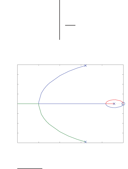
380 CHAPTER 7 The Root Locus Method

CP7.10 (a) The characteristic equation is

s3+ (2 + k)s2+ 5s+ 1 = 0 .

(b) The Routh array is

s31 5

s22 + k1

s15k+9

2+k

so1

?-2.5 ?-2 ?-1.5 ?-1 ?-0.5 0

?-2

?-1.5

?-1

?-0.5

0.5

1.5

Root Locus

Real Axi s

Imaginary Axi s

FIGURE CP7.10

Root locus for 1 + ks2

s3+2s2+5s+1 = 0.

For stability we require

2 + k > 0 or k >−2

and

5k+ 9 >0 or k >−9/5.

Therefore, the stability region is deﬁned by

k > −1.8.

from the publisher prior to any prohibited reproduction, storage in a retrieval system, or transmission in any form or by any means, electronic, mechanical, photocopying,

recording, or likewise. For information regarding permission(s), write to: Rights and Permissions Department, Pearson Education, Inc., Upper Saddle River, NJ 07458.

Computer Problems 381

1 + ks2

s3+ 2s2+ 5s+ 1 = 0 .

The root locus is shown in Figure CP7.10. We see that the system is

stable for all k > 0.

from the publisher prior to any prohibited reproduction, storage in a retrieval system, or transmission in any form or by any means, electronic, mechanical, photocopying,

recording, or likewise. For information regarding permission(s), write to: Rights and Permissions Department, Pearson Education, Inc., Upper Saddle River, NJ 07458.

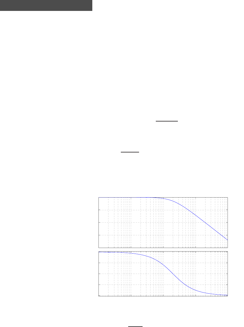
C H A P T E R 8

Frequency Response Methods

Exercises

E8.1 Given the loop transfer function

L(s) = 4

(s+ 2)2,

we determine that

|L(jω)|=4

4 + ω2and φ(ω) = −2 tan−1ω/2.

The frequency response is shown in Figure E8.1.

−80

−60

−40

−20

Magnitude (dB)

10−2 10−1 100101102

−180

−135

−90

−45

Phase (deg)

Bode Diagram

Frequency (rad/sec)

FIGURE E8.1

Frequency response for L(s) = 4

(s+2)2.

382

from the publisher prior to any prohibited reproduction, storage in a retrieval system, or transmission in any form or by any means, electronic, mechanical, photocopying,

recording, or likewise. For information regarding permission(s), write to: Rights and Permissions Department, Pearson Education, Inc., Upper Saddle River, NJ 07458.

Exercises 383

The magnitude and phase angle for ω= 0,0.5,1,2,4,∞are summarized

in Table E8.1.

ω0 0.5 1 2 4 ∞

|L(jω)|1 0.94 0.80 0.50 0.20 0

φ(deg) 0 -28.07 -53.13 -90 –126.87 -180

TABLE E8.1 Magnitude and phase for L(s) = 4

(s+2)2.

E8.2 The transfer function is

G(s) = 5000

(s+ 70)(s+ 500) .

The frequency response plot is shown in Figure E8.2. The phase angle is

computed from

φ=−tan−1ω

70 −tan−1ω

500 .

The phase angles for ω= 10,100 and 700 are summarized in Table E8.2.

ω10 200 700

|G(jω)|-16.99 -27.17 -41.66

φ(deg) -9.28 -92.51 -138.75

TABLE E8.2 Magnitude and phase for G(s) = 5000

(s+70)(s+500) .

from the publisher prior to any prohibited reproduction, storage in a retrieval system, or transmission in any form or by any means, electronic, mechanical, photocopying,

recording, or likewise. For information regarding permission(s), write to: Rights and Permissions Department, Pearson Education, Inc., Upper Saddle River, NJ 07458.

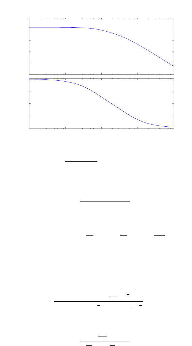
384 CHAPTER 8 Frequency Response Methods

−100

−80

−60

−40

−20

Magnitude (dB)

100101102103104

−180

−135

−90

−45

Phase (deg)

Bode Diagram

Frequency (rad/sec)

FIGURE E8.2

Frequency response for G(s) = 5000

(s+70)(s+500) .

E8.3 The loop transfer function is

L(s) = 300(s+ 100)

s(s+ 10)(s+ 40) .

The phase angle is computed via

φ(ω) = −90o−tan−1ω

10 −tan−1ω

40 + tan−1ω

100 .

At ω= 28.3, we determine that

φ=−90o−70.5o−35.3o+ 15.8o= 180o.

Computing the magnitude yields

|L(jω)|=300(100)(1 + ( ω

100 )2)1

ω10(1 + ( ω

10 )2)1

240(1 + ( ω

40 )2)1

= 0.75 ,

when ω= 28.3. We can also rewrite L(s) as

L(s) = 75( s

100 + 1)

s(s

10 + 1)( s

40 + 1).

from the publisher prior to any prohibited reproduction, storage in a retrieval system, or transmission in any form or by any means, electronic, mechanical, photocopying,

recording, or likewise. For information regarding permission(s), write to: Rights and Permissions Department, Pearson Education, Inc., Upper Saddle River, NJ 07458.

Exercises 385

Then, the magnitude in dB is

20 log10 |L|= 20 log10(75) + 10 log10(1 + ( ω

100 )2)−10 log10(1 + ( ω

10)2)

−10 log10(1 + ( ω

40)2)−20 log10 ω=−2.5 dB ,

at ω= 28.3.

E8.4 The transfer function is

G(s) = Ks

(s+a)(s+ 10)2.

Note that φ= 0oat ω= 3, and that

φ= +90o−tan−1ω

a−2 tan−1ω

10 .

Substituting ω= 3 and solving for ayields

a= 2 .

Similarly, from the magnitude relationship we determine that

K= 400 .

E8.5 The lower portion for ω < 2 is

20 log K

ω= 0 dB ,

at ω= 8. Therefore,

20 log K

8= 0 dB

which occurs when

K= 8 .

We have a zero at ω= 2 and another zero at ω= 4. The zero at ω= 4

yields

a= 0.25 .

We also have a pole at ω= 8, and a second pole at ω= 24. The pole at

ω= 24 yields

b= 1/24 .

from the publisher prior to any prohibited reproduction, storage in a retrieval system, or transmission in any form or by any means, electronic, mechanical, photocopying,

recording, or likewise. For information regarding permission(s), write to: Rights and Permissions Department, Pearson Education, Inc., Upper Saddle River, NJ 07458.

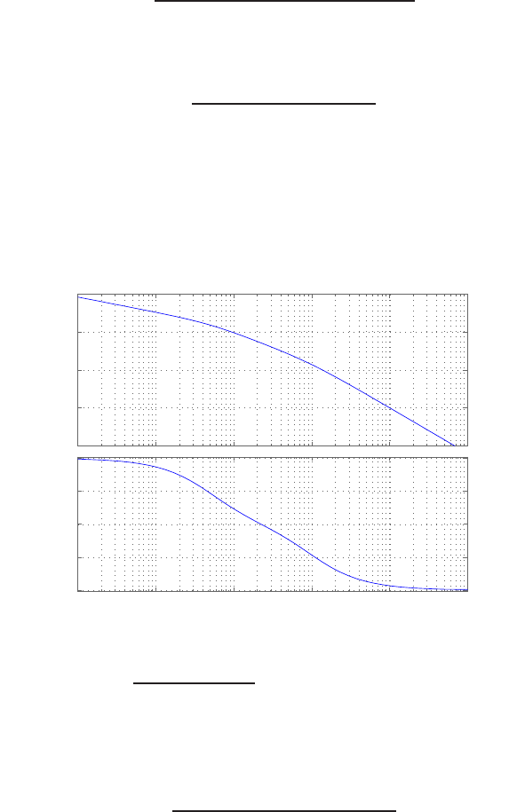
386 CHAPTER 8 Frequency Response Methods

Therefore,

G(s) = 8(1 + s/2)(1 + s/4)

s(1 + s/8)(1 + s/24)(1 + s/36) .

E8.6 The loop transfer function is

L(s) = 10

s(s/5 + 1)(s/100 + 1) .

The Bode diagram is shown in Figure E8.6. When 20 log10 |L(jω)|= 0 dB,

we have

ω= 9.4 rad/sec .

−150

−100

−50

Magnitude (dB)

10−1 100101102103104

−270

−225

−180

−135

−90

Phase (deg)

Bode Diagram

Frequency (rad/sec)

FIGURE E8.6

Bode Diagram for L(s) = 10

s(s/5+1)(s/100+1) .

E8.7 The transfer function is

T(s) = 4

(s2+s+ 1)(s2+ 0.4s+ 4) .

(a) The frequency response magnitude is shown in Figure E8.7.

The frequency response has two resonant peaks at

ωr1= 0.8 rad/sec and ωr2= 1.9 rad/sec .

from the publisher prior to any prohibited reproduction, storage in a retrieval system, or transmission in any form or by any means, electronic, mechanical, photocopying,

recording, or likewise. For information regarding permission(s), write to: Rights and Permissions Department, Pearson Education, Inc., Upper Saddle River, NJ 07458.

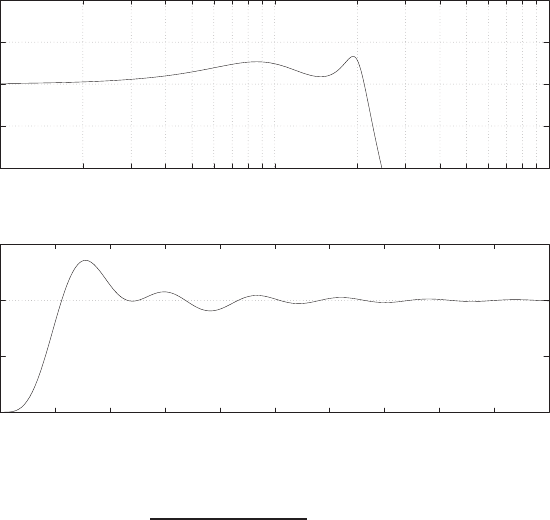
Exercises 387

-10

-5

10-1 100101

Gain dB

Frequency (rad/sec)

0.5

1.5

02 4 6 8 10 12 14 16 18 20

Time (secs)

Amplitude

FIGURE E8.7

(a) Bode Diagram for T(s) = 4

(s2+s+1)(s2+0.4s+4) . (b) Unit step response.

(b) The percent overshoot is

P.O. = 35% ,

and the settling time is

Ts≈16 sec .

E8.8 (a) The break frequencies are

ω1= 1 rad/sec, ω2= 5 rad/sec,and ω3= 20 rad/sec .

(b) The slope of the asymptotic plot at low frequencies is 0 dB/decade.

And at high frequencies the slope of the asymptotic plot is -20 dB/decade.

from the publisher prior to any prohibited reproduction, storage in a retrieval system, or transmission in any form or by any means, electronic, mechanical, photocopying,

recording, or likewise. For information regarding permission(s), write to: Rights and Permissions Department, Pearson Education, Inc., Upper Saddle River, NJ 07458.

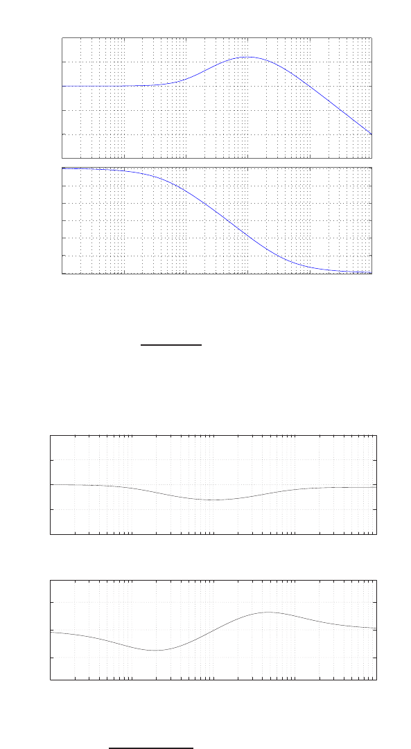
388 CHAPTER 8 Frequency Response Methods

−30

−20

−10

Magnitude (dB)

10−2 10−1 100101102103

−90

−45

135

180

Phase (deg)

Bode Diagram

Frequency (rad/sec)

FIGURE E8.8

Bode Diagram for Gc(s)G(s) = 100(s−1)

s2+25s+100 .

E8.9 The Bode diagram for G(s) is shown in Figure E8.9.

-40

-20

10-1 100101102103

Frequency (rad/sec)

Gain dB

-50

10-1 100101102103

Frequency (rad/sec])

Phase deg

FIGURE E8.9

Bode Diagram for G(s) = (s/5+1)(s/20+1)

(s+1)(s/80+1) .

from the publisher prior to any prohibited reproduction, storage in a retrieval system, or transmission in any form or by any means, electronic, mechanical, photocopying,

recording, or likewise. For information regarding permission(s), write to: Rights and Permissions Department, Pearson Education, Inc., Upper Saddle River, NJ 07458.

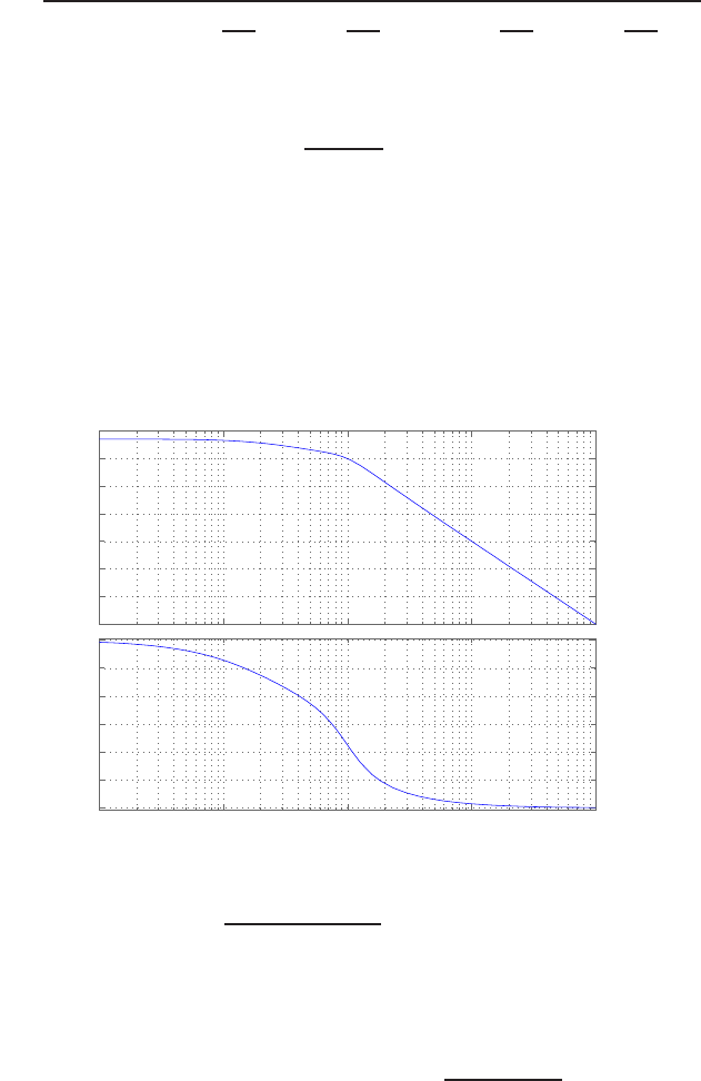
Exercises 389

E8.10 The frequency response has two peaks; the ﬁrst peak at f≈1.8 and the

second peak at f≈3.1. One possible G(jω) is

G(jω) = 1

(jωτ + 1) 1 + 2ζ1

ωn1jω +jω

ωn121 + 2ζ2

ωn2jω +jω

ωn22,

where

τ=1

2π(0.2) ,

ζ1= 0.15; ωn1= 2π(1.8×103)ζ2= 0.15; ωn2= 2π(3.1×103).

The damping ratios are estimated using Figure 8.10 in Dorf & Bishop.

E8.11 The Bode plot is shown in Figure E8.11. The frequency when 20 log10 |GCG(ω)|=

0 is ω= 9.9 rad/sec.

−120

−100

−80

−60

−40

−20

Magnitude (dB)

10−1 100101102103

−270

−225

−180

−135

−90

−45

Phase (deg)

Bode Diagram

Frequency (rad/sec)

FIGURE E8.11

Bode Diagram for Gc(s)G(s) = 1000

(s2+10s+100)(s+2) .

E8.12 (a) The transfer function is

G(s) = C(sI−A)−1B+D=−5(s−1)

s2+ 3s+ 2 .

(b) The Bode plot is shown in Figure E8.12.

from the publisher prior to any prohibited reproduction, storage in a retrieval system, or transmission in any form or by any means, electronic, mechanical, photocopying,

recording, or likewise. For information regarding permission(s), write to: Rights and Permissions Department, Pearson Education, Inc., Upper Saddle River, NJ 07458.

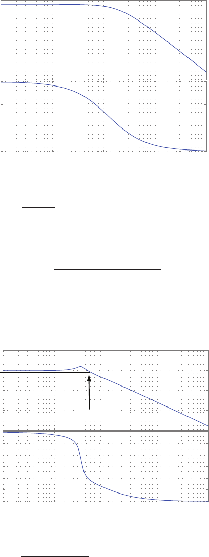
390 CHAPTER 8 Frequency Response Methods

-20

-10

Magnitude (dB)

10 -2 10 -1 100101102

180

270

Phase (deg)

Bode Diagram

Frequency (rad/sec)

FIGURE E8.12

Bode Diagram for G(s) = −5(s−‘1)

s2+3s+2 .

E8.13 The closed-loop transfer function is

T(s) = 100

s3+ 11s2+ 20s+ 110 .

The Bode plot of T(s) is shown in Figure E8.13, where ωB= 4.9 rad/sec.

-100

-50

Magnitude (dB)

10 -1 100101102103

-270

-225

-180

-135

-90

-45

Phase (deg)

Bode Diagram

ωb=4.9

-3 dB

Frequency (rad/sec)

FIGURE E8.13

Bode Diagram for T(s) = 100

s3+11s2+20s+110 .

from the publisher prior to any prohibited reproduction, storage in a retrieval system, or transmission in any form or by any means, electronic, mechanical, photocopying,

recording, or likewise. For information regarding permission(s), write to: Rights and Permissions Department, Pearson Education, Inc., Upper Saddle River, NJ 07458.

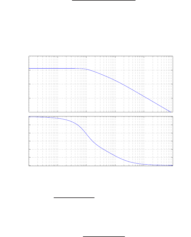
Exercises 391

E8.14 The loop transfer function is

L(s) = 20

(s2+ 1.4s+ 1)(s+ 10) .

The Bode plot of L(s) is shown in Figure E8.14. The frequency when

20 log10 |L(ω)|= 0 is ω= 1.32 rad/sec.

−150

−100

−50

Magnitude (dB)

10−2 10−1 100101102103

−270

−225

−180

−135

−90

−45

Phase (deg)

Bode Diagram

Frequency (rad/sec)

FIGURE E8.14

Bode Diagram for L(s) = 20

(s2+1.4s+1)(s+10) .

E8.15 The closed-loop transfer function is

T(s) = 3s+ 5

s2+s+K+ 6 .

The bandwidth as a function of Kis shown in Figure E8.15. The band-

width as a function of Kis:

(a) K= 1 and ωb= 7.0 rad/sec.

(b) K= 2 and ωb= 7.9 rad/sec.

The bandwidth increases as Kincreases.

from the publisher prior to any prohibited reproduction, storage in a retrieval system, or transmission in any form or by any means, electronic, mechanical, photocopying,

recording, or likewise. For information regarding permission(s), write to: Rights and Permissions Department, Pearson Education, Inc., Upper Saddle River, NJ 07458.

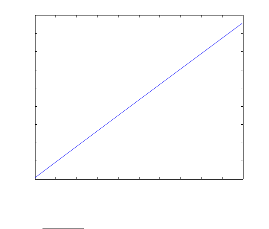
392 CHAPTER 8 Frequency Response Methods

0 2 4 6 8 10 12 14 16 18 20

ωb (rad/s)

FIGURE E8.15

Bandwith of T(s) = 3s+5

s2+s+K+6 .

from the publisher prior to any prohibited reproduction, storage in a retrieval system, or transmission in any form or by any means, electronic, mechanical, photocopying,

recording, or likewise. For information regarding permission(s), write to: Rights and Permissions Department, Pearson Education, Inc., Upper Saddle River, NJ 07458.

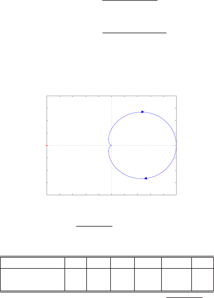
Problems 393

Problems

P8.1 (a) The transfer function is

Gc(s)G(s) = 1

(1 + 0.25s)(1 + 3s),

and

Gc(jω)G(jω) = 1

(1 −0.75ω2) + j3.25ω.

The polar plot is shown in Figure P8.1a. A summary of the magni-

tude and phase angles for ω= 0,0.5,1,2,5 and ∞can be found in

Table P8.1a.

−1 −0.8 −0.6 −0.4 −0.2 0 0.2 0.4 0.6 0.8 1

−0.8

−0.6

−0.4

−0.2

0.2

0.4

0.6

0.8

Nyquist Diagram

Real Axis

Imaginary Axis

FIGURE P8.1

(a) Polar plot for Gc(s)G(s) = 1

(1+0.25s)(1+3s).

ω0 0.5 1 2 5 ∞

|Gc(jω)G(jω)|(dB) 1.00 0.55 0.31 0.15 0.04 0

φ(deg) 0 -63.4 -85.6 -107.1 -137.51 -180

TABLE P8.1 (a) Magnitudes and phase angles for Gc(s)G(s) = 1

(1+0.25s)(1+3s).

from the publisher prior to any prohibited reproduction, storage in a retrieval system, or transmission in any form or by any means, electronic, mechanical, photocopying,

recording, or likewise. For information regarding permission(s), write to: Rights and Permissions Department, Pearson Education, Inc., Upper Saddle River, NJ 07458.

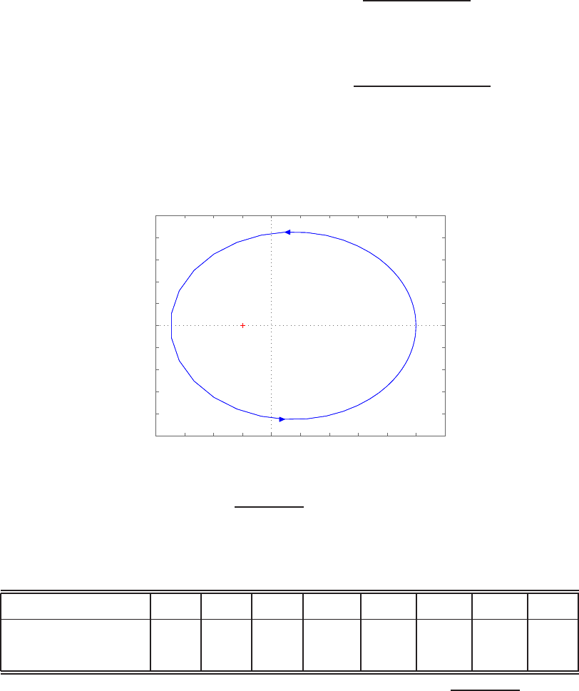
394 CHAPTER 8 Frequency Response Methods

(b) The transfer function is

Gc(s)G(s) = 5(s2+ 1.4s+ 1)

(s−1)2

and

Gc(jω)G(jω) = 5(1 −ω2) + 1.4jω

(1 −ω2)−2jω .

The polar plot is shown in Figure P8.1b. A summary of the magnitude

and phase angles for ω= 0,0.25,0.5,1,2,8,16 and ∞can be found in

Table P8.1b.

−4 −3 −2 −1 0 1 2 3 4 5 6

−5

−4

−3

−2

−1

Nyquist Diagram

Real Axis

Imaginary Axis

FIGURE P8.1

CONTINUED: (b) Polar plot for Gc(s)G(s) = 5(s2+1.4s+1)

(s−1)2.

ω0 0.25 0.5 1 2 8 16 ∞

|Gc(jω)G(jω)|(dB) 5.00 4.71 4.10 3.50 4.10 4.92 4.98 5.00

φ(deg) 0 48.5 96.1 180.0 -96.2 -24.3 -12.2 0

TABLE P8.1 CONTINUED: (b) Magnitudes and phase angles for Gc(s)G(s) = 5(s2+1.4s+1)

(s−1)2.

from the publisher prior to any prohibited reproduction, storage in a retrieval system, or transmission in any form or by any means, electronic, mechanical, photocopying,

recording, or likewise. For information regarding permission(s), write to: Rights and Permissions Department, Pearson Education, Inc., Upper Saddle River, NJ 07458.

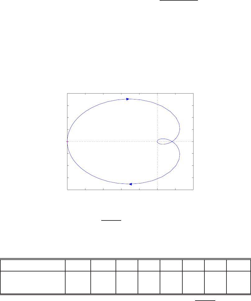
Problems 395

Gc(s)G(s) = (s−8

(s2+ 6s+ 8) .

The polar plot is shown in Figure P8.1c. A summary of the magnitude

and phase angles for

ω= 0,1,2,3,4,5,6,∞

can be found in Table P8.1c.

−1 −0.8 −0.6 −0.4 −0.2 0 0.2 0.4

−0.8

−0.6

−0.4

−0.2

0.2

0.4

0.6

0.8

Nyquist Diagram

Real Axis

Imaginary Axis

FIGURE P8.1

CONTINUED: (c) Polar plot for Gc(s)G(s) = s−8

s2+6s+8 .

ω0 1 2 3 4 5 6 ∞

|Gc(jω)G(jω)|(dB) 1.00 0.87 0.65 0.47 0.35 0.27 0.22 0.00

φ(deg) 180.0 132.3 94.4 66.3 45.0 28.5 15.3 -90.0

TABLE P8.1 CONTINUED: (c) Magnitudes and phase angles for Gc(s)G(s) = s−8

s2+6s+8 .

from the publisher prior to any prohibited reproduction, storage in a retrieval system, or transmission in any form or by any means, electronic, mechanical, photocopying,

recording, or likewise. For information regarding permission(s), write to: Rights and Permissions Department, Pearson Education, Inc., Upper Saddle River, NJ 07458.

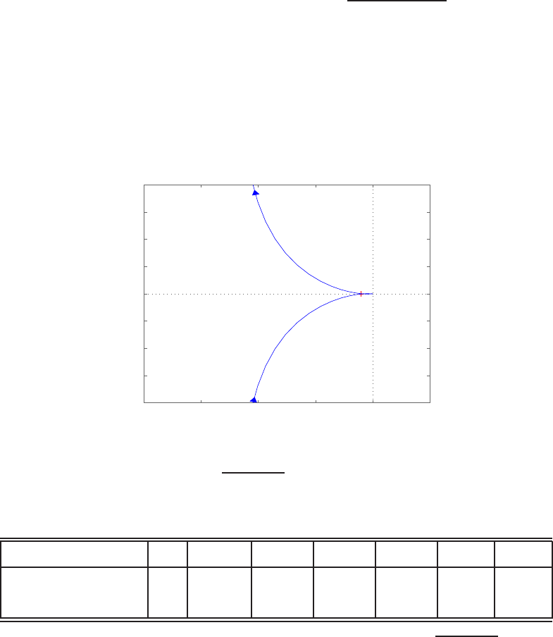
396 CHAPTER 8 Frequency Response Methods

(d) The transfer function is

Gc(s)G(s) = 20(s+ 8)

s(s+ 2)(s+ 4) .

The polar plot is shown in Figure P8.1d. A summary of the magnitude

and phase angles for

ω= 1,0.1,0.8,1.6,3.2,12.8,∞

can be found in Table P8.1d.

−20 −15 −10 −5 0 5

−20

−15

−10

−5

Nyquist Diagram

Real Axis

Imaginary Axis

FIGURE P8.1

CONTINUED: (d) Polar plot for Gc(s)G(s) = 20(s+8)

s(s+2)(s+4) .

ω0 0.1 0.8 1.6 3.2 12.8 ∞

|Gc(jω)G(jω)|(dB) ∞199.70 22.87 9.24 2.79 0.14 0.00

φ(deg) 0 -93.6 -117.4 -139.1 -164.8 174.3 180.0

TABLE P8.1 CONTINUED: (d) Magnitudes and phase angles for Gc(s)G(s) = 20(s+8)

s(s+2)(s+4) .

from the publisher prior to any prohibited reproduction, storage in a retrieval system, or transmission in any form or by any means, electronic, mechanical, photocopying,

recording, or likewise. For information regarding permission(s), write to: Rights and Permissions Department, Pearson Education, Inc., Upper Saddle River, NJ 07458.

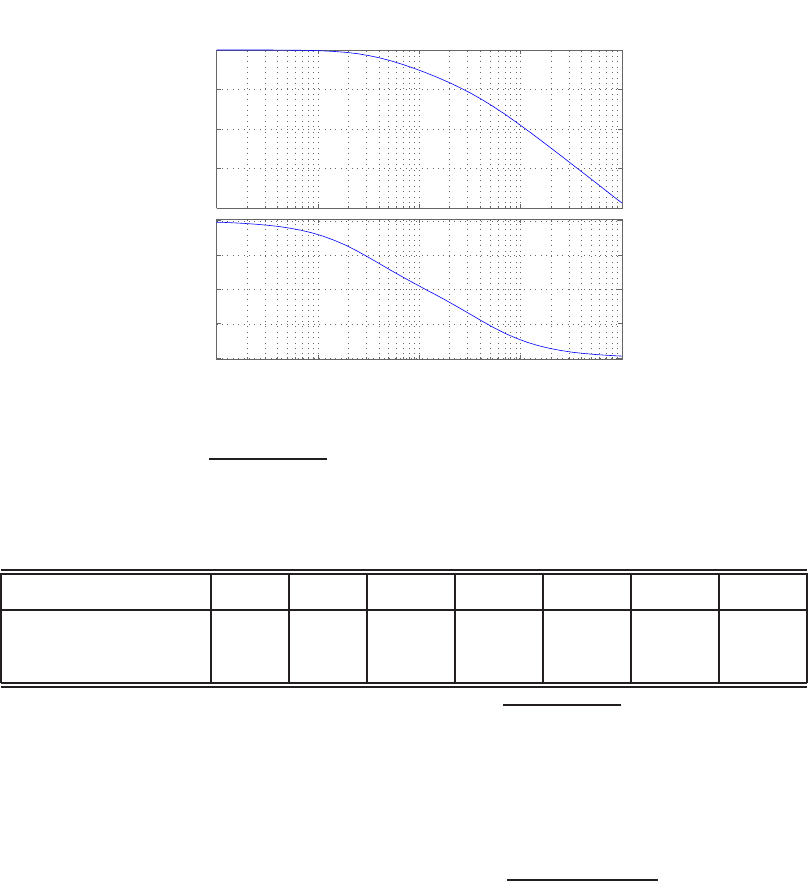
Problems 397

P8.2 (a) The Bode plot is shown in Figure P8.2a. A summary of the magnitude

and phase angles for

ω= 0.25,0.5,1,2,4,8,16

can be found in Table P8.2a.

−80

−60

−40

−20

Magnitude (dB)

10−2 10−1 100101102

−180

−135

−90

−45

Phase (deg)

Bode Diagram

Frequency (rad/sec)

FIGURE P8.2

(a) Bode plot for Gc(s)G(s) = 1

(1+0.25s)(1+3s).

ω0.25 0.5 1.0 2.0 4.0 8.0 16.0

|Gc(jω)G(jω)|(dB) -1.95 -5.19 -10.26 -16.65 -24.62 -34.60 -45.93

φ(deg) -40.5 -63.4 -85.6 -107.1 -130.2 -151.0 -164.8

TABLE P8.2 (a) Magnitudes and phase angles for Gc(s)G(s) = 1

(1+0.25s)(1+3s).

(b) The transfer function is

Gc(s)G(s) = 5(s2+ 1.4s+ 1)

(s−1)2

The Bode plot is shown in Figure P8.2b. A summary of the magnitude

from the publisher prior to any prohibited reproduction, storage in a retrieval system, or transmission in any form or by any means, electronic, mechanical, photocopying,

recording, or likewise. For information regarding permission(s), write to: Rights and Permissions Department, Pearson Education, Inc., Upper Saddle River, NJ 07458.

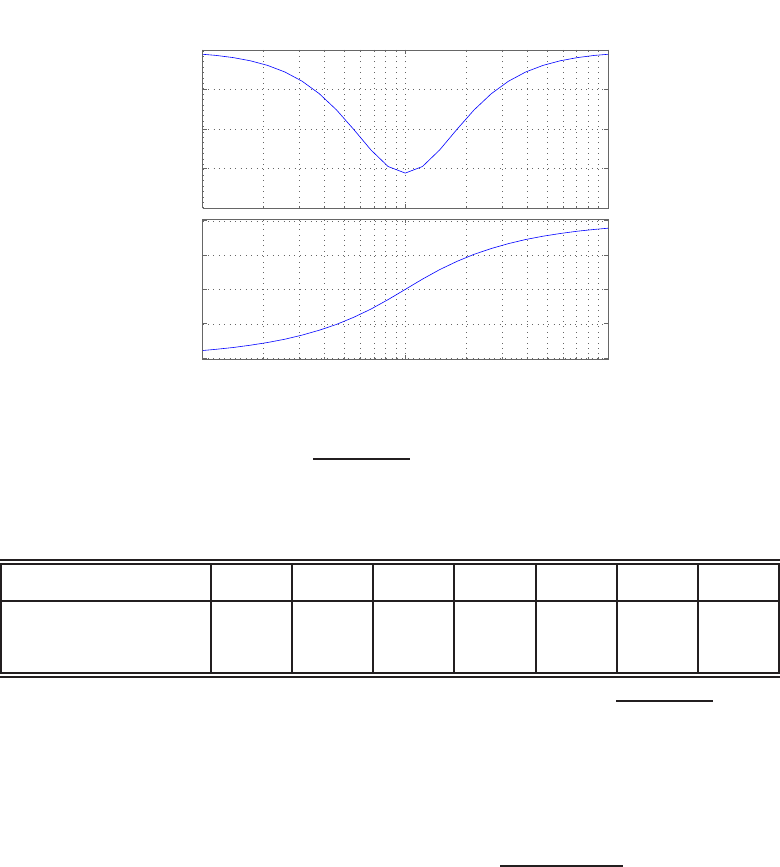
398 CHAPTER 8 Frequency Response Methods

and phase angles for

ω= 0.25,0.5,1,2,4,8,16

can be found in Table P8.2b.

Magnitude (dB)

10−1 100101

−360

−270

−180

−90

Phase (deg)

Bode Diagram

Frequency (rad/sec)

FIGURE P8.2

CONTINUED: (b) Bode plot for Gc(s)G(s) = 5(s2+1.4s+1)

(s−1)2.

ω0.25 0.5 1.0 2.0 4.0 8.0 16.0

|Gc(jω)G(jω)|(dB) 13.46 12.26 10.88 12.26 13.46 13.84 13.95

φ(deg) 48.5 96.2 180.0 -96.2 -48.5 -24.3 -12.2

TABLE P8.2 CONTINUED: (b) Magnitudes and phase angles for Gc(s)G(s) = 5(s2+1.4s+1)

(s−1)2.

Gc(s)G(s) = (s−8)

(s2+ 6s+ 8) .

The Bode plot is shown in Figure P8.2c. A summary of the magnitude

and phase angles for ω= 0.6,1,2,3,4,5,6,∞can be found in

Table P8.2c.

from the publisher prior to any prohibited reproduction, storage in a retrieval system, or transmission in any form or by any means, electronic, mechanical, photocopying,

recording, or likewise. For information regarding permission(s), write to: Rights and Permissions Department, Pearson Education, Inc., Upper Saddle River, NJ 07458.

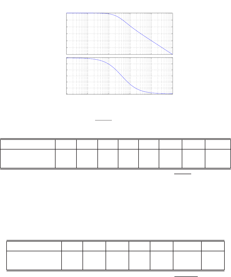
Problems 399

−60

−50

−40

−30

−20

−10

Magnitude (dB)

10−2 10−1 100101102103

−90

−45

135

180

Phase (deg)

Bode Diagram

Frequency (rad/sec)

FIGURE P8.2

CONTINUED: (c) Bode plot for Gc(s)G(s) = s−8

s2+6s+8 .

ω0.6 1 2 3 4 5 6 ∞

|Gc(jω)G(jω)|(dB) -0.45 -1.17 -3.72 -6.49 -9.03 -11.26 -13.18 -120.00

φ(deg) 150.5 132.3 94.4 66.3 45.0 28.5 15.3 -90.0

TABLE P8.2 CONTINUED: (c) Magnitudes and phase angles for Gc(s)G(s) = s−8

s2+6s+8 .

(d) A summary of the magnitude and phase angles for

ω= 0.2,0.8,3.2,6.4,12.8,25.6,51.2

can be found in Table P8.2d. The Bode plot is shown in Figure P8.2d.

ω0.2 0.8 3.2 6.4 12.8 25.6 51.2

|Gc(jω)G(jω)|(dB) 39.95 27.19 8.90 -3.98 -17.35 -30.0355 -42.28

φ(deg) -97.1 -117.4 -164.8 178.0 174.2 176.0 177.8

TABLE P8.2 CONTINUED: (d) Magnitudes and phase angles for Gc(s)G(s) = 20(s+8)

s(s+2)(s+4) .

from the publisher prior to any prohibited reproduction, storage in a retrieval system, or transmission in any form or by any means, electronic, mechanical, photocopying,

recording, or likewise. For information regarding permission(s), write to: Rights and Permissions Department, Pearson Education, Inc., Upper Saddle River, NJ 07458.

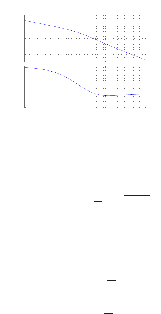
400 CHAPTER 8 Frequency Response Methods

−60

−40

−20

Magnitude (dB)

10−1 100101102

−225

−180

−135

−90

Phase (deg)

Bode Diagram

Frequency (rad/sec)

FIGURE P8.2

CONTINUED: (d) Bode plot for Gc(s)G(s) = 20(s+8)

s(s+2)(s+4) .

P8.3 (a) The bridged-T network we found has zeros at

s=±jωn

and poles at

s=−ωn

Q±ωnq1/Q2−1.

The frequency response is shown in Figure P8.3 for Q= 10.

(b) For the twin-T network, we evaluate the magnitude at

ω= 1.1ωn

or 10% from the center frequency (see Example 8.4 in Dorf & Bishop).

This yields

|G| ≈ 2.1×0.1

3.9×1.1 = 0.05 .

Similarly, for the bridged-T network

|G|= 2.1×0.1

2.1×0.14 = 0.707 .

The bridged-T network possesses a narrower band than the twin-T

network.

from the publisher prior to any prohibited reproduction, storage in a retrieval system, or transmission in any form or by any means, electronic, mechanical, photocopying,

recording, or likewise. For information regarding permission(s), write to: Rights and Permissions Department, Pearson Education, Inc., Upper Saddle River, NJ 07458.

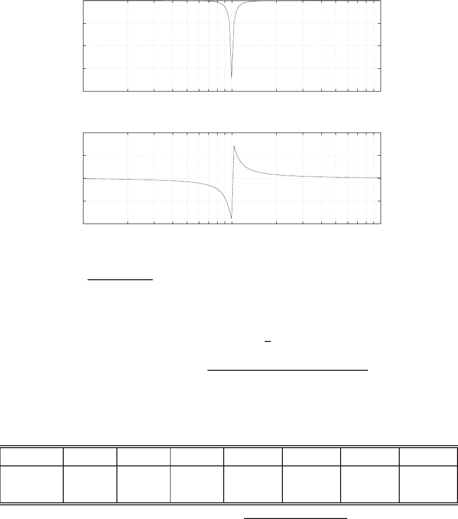
Problems 401

-40

-30

-20

-10

10-1 100101

w/wn

Gain dB

-100

-50

100

10-1 100101

w/wn

Phase deg

FIGURE P8.3

Bode plot for G(s) = s2+ω2

s2+(2ωn/Q)s+ω2

n, where ζ= 1/Q = 0.1.

P8.4 The transfer function is

G(s) = GcG1H(s)1

s

=30000(2s+ 1)

s(s+ 10)(s+ 20)(s2+ 15s+ 150) .

A summary of the magnitude and phase angles can be found in Table P8.4.

The Bode plot is shown in Figure P8.4.

ω1 3 5 8 10 15 24

|G(jω|dB 6.95 5.78 5.08 3.38 1.59 -5.01 -17.56

φ(deg)−40.89o−52.39o−77.28o−118.41o−145.99o−203.52o−258.57o

TABLE P8.4 Magnitudes and phase angles for GH(s) = 30000(2s+1)

s(s+10)(s+20)(s2+15s+150) .

from the publisher prior to any prohibited reproduction, storage in a retrieval system, or transmission in any form or by any means, electronic, mechanical, photocopying,

recording, or likewise. For information regarding permission(s), write to: Rights and Permissions Department, Pearson Education, Inc., Upper Saddle River, NJ 07458.

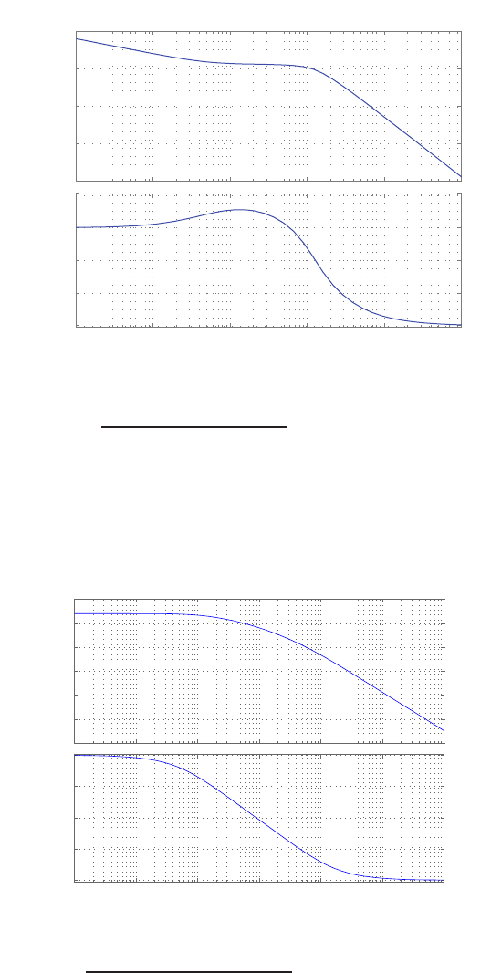
402 CHAPTER 8 Frequency Response Methods

-150

-100

-50

Magnitude (dB)

10-2 10-1 100101102103

-360

-270

-180

-90

Phase (deg)

Bode Diagram

Frequency (rad/sec)

FIGURE P8.4

Bode plot for GH(s) = 30000(2s+1)

s(s+10)(s+20)(s2+15s+150) .

P8.5 The Bode plot is shown in Figure P8.5.

−250

−200

−150

−100

−50

Magnitude (dB)

10−2 10−1 100101102103104

−360

−270

−180

−90

Phase (deg)

Bode Diagram

Frequency (rad/sec)

FIGURE P8.5

Bode plot for G(s) = 10

(s/4+1)(s+1)(s/20+1)(s/80+1) .

from the publisher prior to any prohibited reproduction, storage in a retrieval system, or transmission in any form or by any means, electronic, mechanical, photocopying,

recording, or likewise. For information regarding permission(s), write to: Rights and Permissions Department, Pearson Education, Inc., Upper Saddle River, NJ 07458.

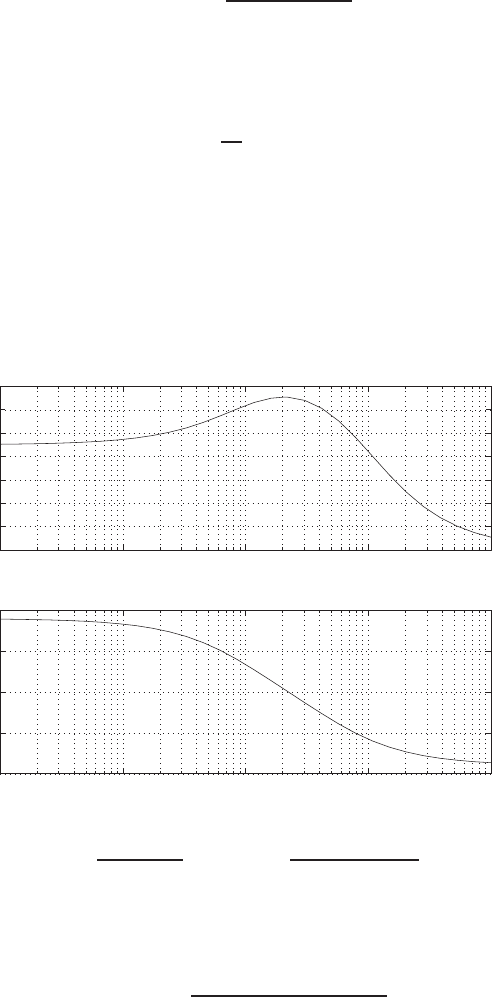
Problems 403

P8.6 (a) The transfer function is

GH(s) = 3.98(1 + s/1)

s(1 + s/10)2.

We have a zero at ω= 1 and two poles at ω= 10.0. The low frequency

approximation is K/s and at ω= 1 we have

20 log K

ω= 12dB .

Therefore,

K= 3.98

at ω= 1 (an approximation). The phase plot is shown in Figure P8.6a.

10-2 10-1 100101102

-180

-160

-140

-120

-100

-80

-60

-40

Phase deg

(a)

10-1 100101102103

-100

-50

100

Frequency (rad/sec)

Phase deg

(b)

FIGURE P8.6

Phase plots for (a) G(s) = 3.98(s/1+1)

s(s/10+1)2. (b) G(s) = s

(s/10+1)(s/50+1) .

(b) The transfer function is

GH(s) = s

(1 + s/10)(1 + s/50) .

The poles are located by noting that the slope is ±20 dB/dec. The

from the publisher prior to any prohibited reproduction, storage in a retrieval system, or transmission in any form or by any means, electronic, mechanical, photocopying,

recording, or likewise. For information regarding permission(s), write to: Rights and Permissions Department, Pearson Education, Inc., Upper Saddle River, NJ 07458.

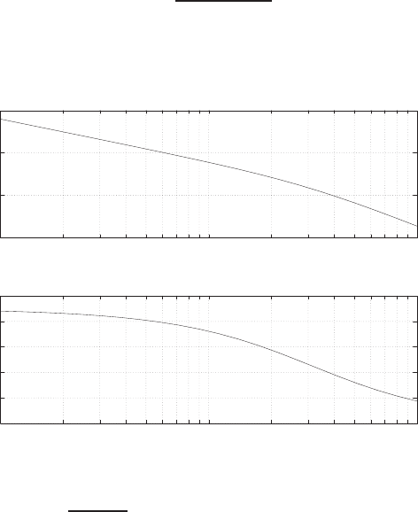
404 CHAPTER 8 Frequency Response Methods

low frequency approximation is Ks, so

20 log Kω = 0dB .

At ω= 1 we determine that

K= 1 .

The phase plot is shown in Figure P8.6b.

P8.7 The loop transfer function is

L(s) = Kv

s(s/π + 1)2.

(a) Set Kv= 2π. The Bode plot is shown in Figure P8.7a.

-20

10-1 100101

Frequency (rad/sec)

Gain dB

-180

-160

-140

-120

-100

-80

10-1 100101

Frequency (rad/sec)

Phase deg

FIGURE P8.7

(a) Bode plot for L(s) = Kv

s(s/π+1) , where Kv= 2π.

(b) The logarithmic magnitude versus the phase angle is shown in Fig-

ure P8.7b.

from the publisher prior to any prohibited reproduction, storage in a retrieval system, or transmission in any form or by any means, electronic, mechanical, photocopying,

recording, or likewise. For information regarding permission(s), write to: Rights and Permissions Department, Pearson Education, Inc., Upper Saddle River, NJ 07458.

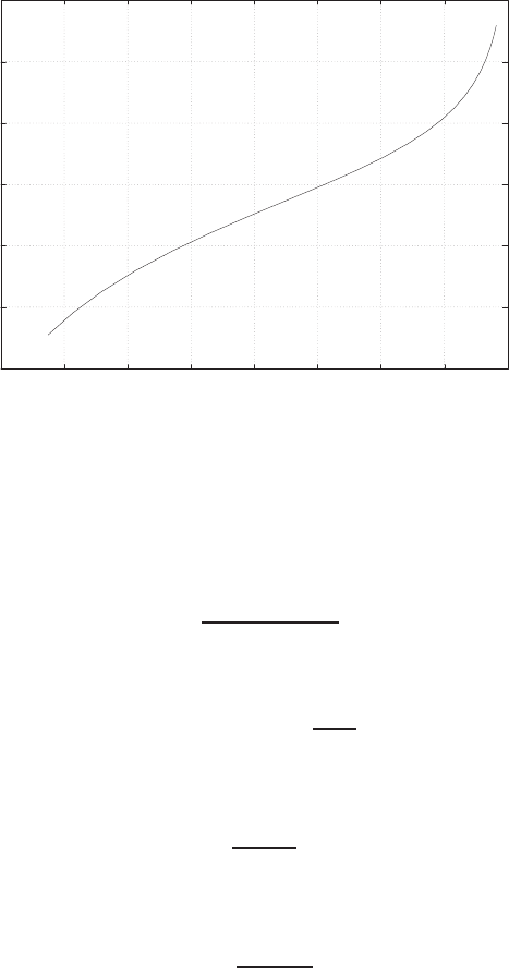
Problems 405

-20

-10

-170 -160 -150 -140 -130 -120 -110 -100 -90

Phase deg

Gain dB

FIGURE P8.7

CONTINUED: (b) Log-magnitude-phase curve for L(jω).

P8.8 The transfer function is

T(s) = K

s2+ 10s+K.

(a) When P.O. = 15%, we determine that ζ= 0.517 by solving

15 = 100e−πζ/√1−ζ2.

So, 2ζωn= 10 implies that ωn= 9.67, hence K=ω2

n= 93.53. Also,

Mpω = (2ζq1−ζ2)−1= 1.13 .

(b) For second-order systems we have

ωr=ωnq1−2ζ2= 6.59

when ζ= 0.517 and ωn= 9.67.

ωB≈(−1.19ζ+ 1.85)ωn= 11.94 rad/s.

P8.9 The log-magnitude phase curves are shown in Figure P8.9.

from the publisher prior to any prohibited reproduction, storage in a retrieval system, or transmission in any form or by any means, electronic, mechanical, photocopying,

recording, or likewise. For information regarding permission(s), write to: Rights and Permissions Department, Pearson Education, Inc., Upper Saddle River, NJ 07458.

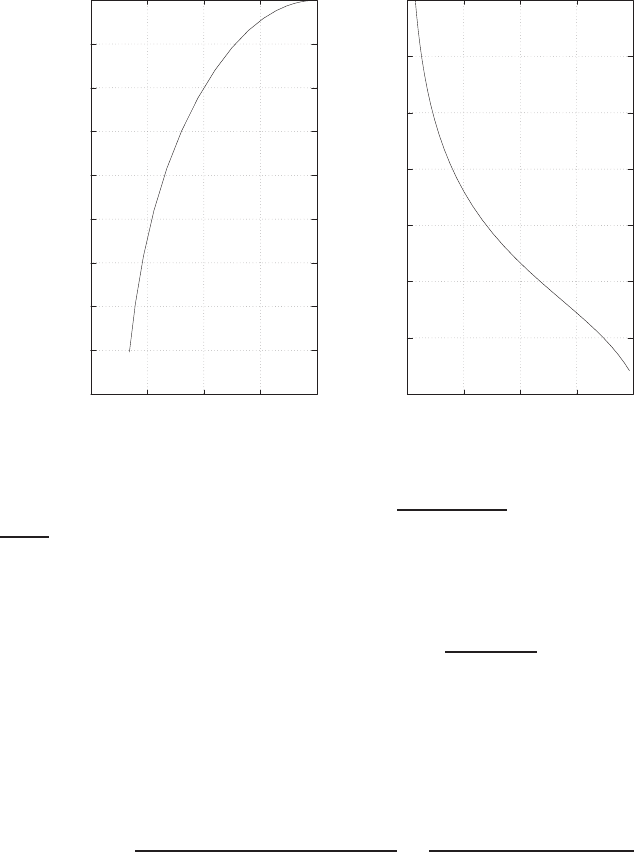
406 CHAPTER 8 Frequency Response Methods

-45

-40

-35

-30

-25

-20

-15

-10

-5

-200 -150 -100 -50 0

Phase deg

Gain dB

(a)

-30

-20

-10

-180 -160 -140 -120 -100

Phase deg

Gain dB

(b)

FIGURE P8.9

Log-magnitude-phase curve for (a) Gc(s)G(s) = 1

(1+0.5s)(1+2s)and (b) Gc(s)G(s) =

1+0.5s

s2.

P8.10 The governing equations of motion are

F(s) = KfIf(s) and If(s) = Vf(s)

Rf+Lfs.

Without loss of generality we can let Kf= 1.0. Also, we have

F(s) = (Ms2+bs +K)Y(s).

Therefore, the transfer function is

GH(s) = KKf

(Rf+Lfs)(Ms2+bs +K)=50K

(s+ 0.5)(s2+ 2s+ 4) .

This is a type 0 system, therefore Kp= 25K.

(a) If we allow a 1% error , we have ess =|R|/(1 + Kp) = 0.01|R|. Thus

Kp= 25K= 99. Select

K= 4 .

(b) The Bode plot is shown in Figure P8.10a.

from the publisher prior to any prohibited reproduction, storage in a retrieval system, or transmission in any form or by any means, electronic, mechanical, photocopying,

recording, or likewise. For information regarding permission(s), write to: Rights and Permissions Department, Pearson Education, Inc., Upper Saddle River, NJ 07458.

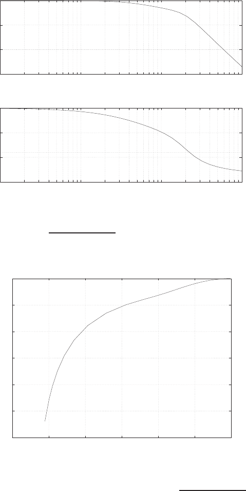
Problems 407

-20

10-2 10-1 100101

Frequency (rad/sec)

Gain dB

-300

-200

-100

10-2 10-1 100101

Frequency (rad/sec)

Phase deg

FIGURE P8.10

(a) Bode plot for GH(s) = 200

(s2+2s+4)(s+0.5) .

-20

-10

-300 -250 -200 -150 -100 -50 0

Phase deg

Gain dB

FIGURE P8.10

CONTINUED: (b) Log-magnitude-phase curve for GH(s) = 200

(s2+2s+4)(s+0.5) .

(d) The closed-loop transfer function Bode plot is shown in Figure P8.10c.

We determine from the plot that Mpω = 1.6, ωr= 4.4 and ωB= 6.8.

from the publisher prior to any prohibited reproduction, storage in a retrieval system, or transmission in any form or by any means, electronic, mechanical, photocopying,

recording, or likewise. For information regarding permission(s), write to: Rights and Permissions Department, Pearson Education, Inc., Upper Saddle River, NJ 07458.

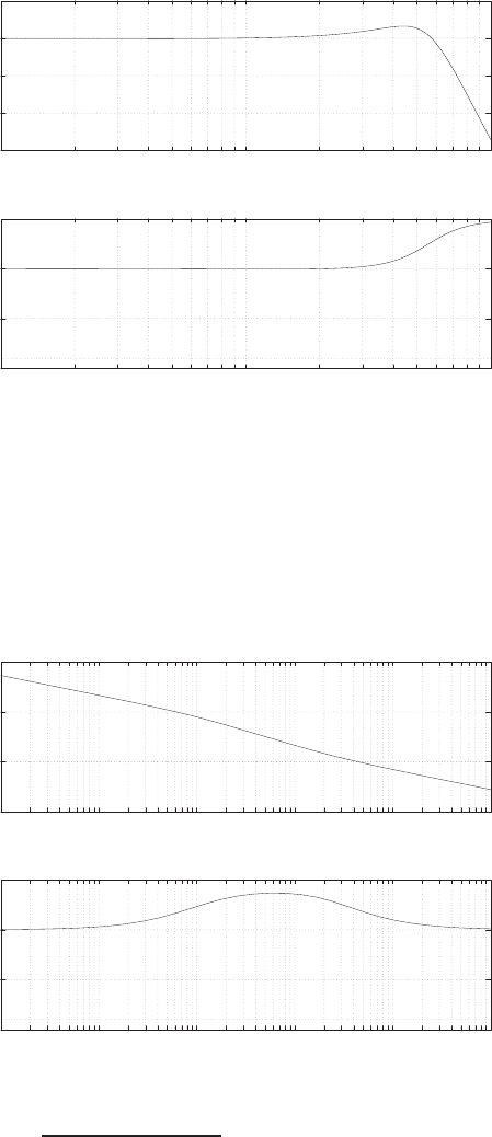
408 CHAPTER 8 Frequency Response Methods

-15

-10

-5

10-1 100101

Frequency (rad/sec)

Gain dB

-200

-100

100

10-1 100101

Frequency (rad/sec)

Phase deg

FIGURE P8.10

CONTINUED: (c) Bode plot for closed-loop T(s) = Y(s)/R(s).

P8.11 The Bode plot is shown in Figure P8.11.

-100

100

200

10-4 10-3 10-2 10-1 100101

Frequency (rad/sec)

Gain dB

-200

-100

100

10-4 10-3 10-2 10-1 100101

Frequency (rad/sec)

Phase deg

FIGURE P8.11

Bode plot for G(s) = 0.164(s+0.2)(−s+0.32)

s2(s+0.25)(s−0.009) .

from the publisher prior to any prohibited reproduction, storage in a retrieval system, or transmission in any form or by any means, electronic, mechanical, photocopying,

recording, or likewise. For information regarding permission(s), write to: Rights and Permissions Department, Pearson Education, Inc., Upper Saddle River, NJ 07458.

Problems 409

P8.12 The three transfer functions are

G1(s) = 10 G2(s) = 1

s(s/0.6 + 1) G3(s) = 3s .

(a) When G3(s) is out of the loop, the characteristic equation is

1 + G1G2(s) = 1 + 10

s(s/0.6 + 1) = 0

or s2+ 0.6s+ 6 = 0. Thus, ζ= 0.6/(2√6) = 0.12.

(b) With G3(s), the characteristic equation is

1 + G1G2(s) + G2G3(s) = 1 + 6

s(s+ 0.6) +1.85

s(s+ 0.6) = 0 ,

s2+ 2.4s+ 6 = 0 .

Thus, ζ= 2.4/(2√6) = 0.49.

P8.13 By inspection of the frequency response, we determine

L(s) = Gc(s)G(s)H(s) = K

s(s/100 + 1)(s/1000 + 1)2.

For small ω, we have 20 log K/ω = 40 dB at ω= 10. So, K= 1000.

P8.14 The data we have are R1=R2= 1000Ω, c1= 10−7farad and c2= 10−6

farad. The governing equations are

V2(s)

V1(s)=

C1s

R1+1

C1s

and

Vo(s)

V2(s)=KR2

R2+1

C2s

Vo(s)

V1(s)=KR2C2s

(R1C1s+ 1)(R2C2s+ 1) =109s

(s+ 107)(s+ 1000) .

(a) The Bode plot is shown in Figure P8.14.

(b) The mid-band gain is = 40 dB.

from the publisher prior to any prohibited reproduction, storage in a retrieval system, or transmission in any form or by any means, electronic, mechanical, photocopying,

recording, or likewise. For information regarding permission(s), write to: Rights and Permissions Department, Pearson Education, Inc., Upper Saddle River, NJ 07458.

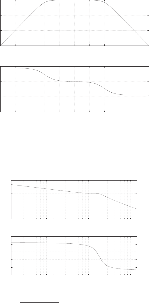
410 CHAPTER 8 Frequency Response Methods

-20

1001011021031041051061071081091010

Frequency (rad/sec)

Gain dB

-200

-100

100

1001011021031041051061071081091010

Frequency (rad/sec)

Phase deg

FIGURE P8.14

Bode plot for G(s) = 109s

(s+107)(s+103).

P8.15 The data are plotted in Figure P8.15, denoted by an asterisk (*).

-100

-50

10-1 100101102

********

-300

-250

-200

-150

-100

-50

10-1 100101102

*******

FIGURE P8.15

Bode plot for G(s) = 809.7

s(s2+6.35s+161.3) ; tabular data is indicated by an asterick (*).

The low frequency slope is -20 dB/dec and the initial low frequency φis

from the publisher prior to any prohibited reproduction, storage in a retrieval system, or transmission in any form or by any means, electronic, mechanical, photocopying,

recording, or likewise. For information regarding permission(s), write to: Rights and Permissions Department, Pearson Education, Inc., Upper Saddle River, NJ 07458.

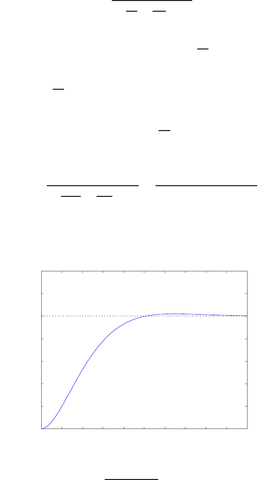
Problems 411

−90o, so we have an integrator of the form K/s. The initial phase is −90o

and the ﬁnal phase −270o, so we have a minimum phase G(s). Now, |G|

is 0.97 at ω= 8 and ω= 10 indicating two complex poles. We postulate

a transfer function of the form

G(s) = K

ss2

ω2

n+2ζs

ωn+ 1.

The phase angle φ=−180oat ω=ωn. Then, from Figure 8.10 in Dorf &

Bishop, we determine that ωn= 12.7. At ω= 8, ω

ωn= 0.63 and φ, due to

the complex poles is −30o(subtract −90odue to the integrator). Again,

from Figure 8.10 in Dorf & Bishop, we estimate ζ= 0.25. To determine

K, note that when ω

ωn≤0.1, the eﬀect of the complex poles on magnitude

is negligible, so at ω= 1 we have

|G|= 5.02 ∼

=

j1

So K= 5.02. Therefore,

G(s) = 5.02

ss2

161.3+0.5s

12.7+ 1=809.7

s(s2+ 6.35s+ 161.3) .

P8.16 (a) The unit step input response is shown in Figure P8.16. The step

0 0.1 0.2 0.3 0.4 0.5 0.6 0.7 0.8 0.9 1

0.2

0.4

0.6

0.8

1.2

1.4

Step Response

Time (sec)

Amplitude

FIGURE P8.16

Unit step input response for T(s) = 60.2

s2+12.1s+60.2.

from the publisher prior to any prohibited reproduction, storage in a retrieval system, or transmission in any form or by any means, electronic, mechanical, photocopying,

recording, or likewise. For information regarding permission(s), write to: Rights and Permissions Department, Pearson Education, Inc., Upper Saddle River, NJ 07458.

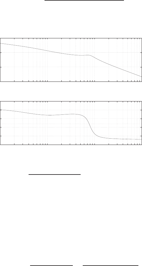
412 CHAPTER 8 Frequency Response Methods

response is given by

y(t) = 1 −e−6.05t(cos 4.85t+ 1.25 sin 4.85t).

(b) The system bandwidth is ωB= 4.95 rad/sec.

P8.17 The transfer function is

Gc(s)G(s) = 4(0.5s+ 1)

s(2s+ 1)(s2/64 + s/20 + 1) .

(a) The Bode plot is shown in Figure P8.17.

-100

-50

10-1 100101102

Frequency (rad/sec)

Gain dB

-300

-250

-200

-150

-100

-50

10-1 100101102

Frequency (rad/sec)

Phase deg

FIGURE P8.17

Bode plot for Gs(s)G(s) = 4(0.5s+1)

s(2s+1)(s2/64+s/20+1) .

(b) When the magnitude is 0 dB, we have

ω1= 1.6 rad/sec

and when φ=−180o, we have

ω2= 7.7 rad/sec .

P8.18 The transfer function is

Gc(s)G(s) = 12(s+ 0.5)

(s+ 3)(s+ 10) =0.2(2s+ 1)

(s/3 + 1)(s/10 + 1) .

The Bode plot is shown in Figure P8.18. Near 0 dB, the frequency is

from the publisher prior to any prohibited reproduction, storage in a retrieval system, or transmission in any form or by any means, electronic, mechanical, photocopying,

recording, or likewise. For information regarding permission(s), write to: Rights and Permissions Department, Pearson Education, Inc., Upper Saddle River, NJ 07458.

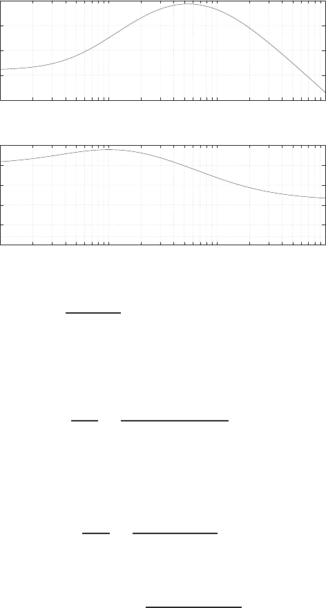
Problems 413

ω= 5.4 rad/sec.

-20

-15

-10

-5

10-1 100101102

Frequency (rad/sec)

Gain dB

-200

-150

-100

-50

10-1 100101102

Frequency (rad/sec)

Phase deg

FIGURE P8.18

Bode plot for Gc(s)G(s) = 12(s+0.5)

s2+13s+30 .

P8.19 Examining the frequency response, we postulate a second-order transfer

function

θ(s)

I(s)=ω2

s2+ 2ζωns+ω2

From the data we see that φ=−90oat ω= 2. Using Figure 8.10 in Dorf

& Bishop, we determine that ωn=ω= 2. We also estimate ζ= 0.4 from

Figure 8.10. Thus,

θ(s)

I(s)=4

s2+ 1.6s+ 4 .

P8.20 The transfer function is

Gc(s)G(s) = 823(s+ 9.8)

s2+ 22s+ 471 .

The Bode plot is shown in Figure P8.20. The maximum value of

20 log10 |Gc(jω)G(jω)|= 32.3 dB

occurs at ω= 20.6 rad/sec and the corresponding phase is φ=−19.6o.

from the publisher prior to any prohibited reproduction, storage in a retrieval system, or transmission in any form or by any means, electronic, mechanical, photocopying,

recording, or likewise. For information regarding permission(s), write to: Rights and Permissions Department, Pearson Education, Inc., Upper Saddle River, NJ 07458.

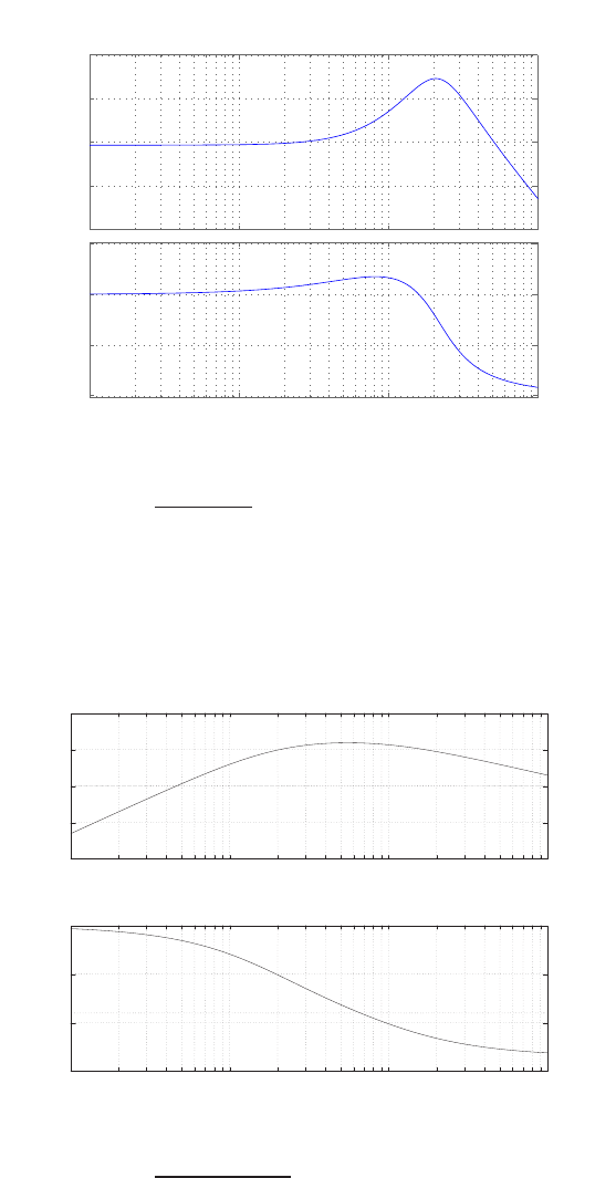
414 CHAPTER 8 Frequency Response Methods

Magnitude (dB)

10−1 100101102

−90

−45

Phase (deg)

Bode Diagram

Frequency (rad/sec)

FIGURE P8.20

Bode plot for Gc(s)G(s) = 832(s+9.8)

s2+22s+471 .

P8.21 The Bode plot is shown in Figure P8.21. The gain is 24 dB when φ=

−180o

-40

-20

10-1 100101102

Frequency (rad/sec)

Gain dB

-300

-200

-100

10-1 100101102

Frequency (rad/sec)

Phase deg

FIGURE P8.21

Bode plot for Gc(s)G(s) = −200s2

s3+14s2+44s+40 .

from the publisher prior to any prohibited reproduction, storage in a retrieval system, or transmission in any form or by any means, electronic, mechanical, photocopying,

recording, or likewise. For information regarding permission(s), write to: Rights and Permissions Department, Pearson Education, Inc., Upper Saddle River, NJ 07458.

Problems 415

P8.22 The transfer function is

G(s) = 10000(s+ 1)(s+ 80)

s(s+ 300)(s+ 9000) .

P8.23 The transfer function is

G(s) = 100(s+ 20)(s+ 8000)

(s+ 1)(s+ 80)(s+ 500) .

The system is type 0 and the steady-state error to a unit step input is

ess =1

1 + Kp

= 0.0025

since

Kp= lim

s→0G(s) = 400 .

P8.24 (a) From the Bode plot we see that

20 log10 Mpω = 12

or Mpω = 3.981. For a second-order system we know that

Mpω = (2ζq1−ζ2)−1.

Solving for ζ(with Mpω = 3.981) yields ζ= 0.12. Also, from the Bode

plot,

ωr= 0.9rad/sec .

So,

ωn=ωr

p1−2ζ2= 0.91 .

Therefore, the second-order approximate transfer function is

T(s) = ω2

s2+ 2ζωns+ω2

=0.83

s2+ 0.22s+ 0.83 .

(b) The predicted overshoot and settling time are P.O. = 68% and Ts=

37 sec.

P8.25 The transfer function is

G(s) = 100(s+ 10)

s2(s+ 100) .

from the publisher prior to any prohibited reproduction, storage in a retrieval system, or transmission in any form or by any means, electronic, mechanical, photocopying,

recording, or likewise. For information regarding permission(s), write to: Rights and Permissions Department, Pearson Education, Inc., Upper Saddle River, NJ 07458.

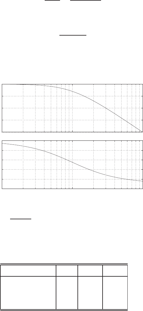
416 CHAPTER 8 Frequency Response Methods

P8.26 The transfer function is

T(s) = Vo(s)

V(s)=1 + R1/R2

1 + RCs .

Substituting R= 10kΩ, C= 1µF ,R1= 9kΩ, and R2= 1kΩ yields

T(s) = 10

1 + 0.01s.

The frequency response is shown in Figure P8.26.

Frequency (rad/sec)

Phase (deg); Magnitude (dB)

Bode Diagrams

101102103

-100

-80

-60

-40

-20

FIGURE P8.26

Bode plot for T(s) = 1+R1/R2

1+RCs

P8.27 The frequency response is shown in Figure P8.27.

K0.75 1 10

|L(jω)|jω=0 ,dB 3.52 12.04 26.02

ωb,rad/s 8.3 14.0 33.4

ωc,rad/s 3.5 8.7 22.9

TABLE P8.27 System performance as Kvaries.

from the publisher prior to any prohibited reproduction, storage in a retrieval system, or transmission in any form or by any means, electronic, mechanical, photocopying,

recording, or likewise. For information regarding permission(s), write to: Rights and Permissions Department, Pearson Education, Inc., Upper Saddle River, NJ 07458.

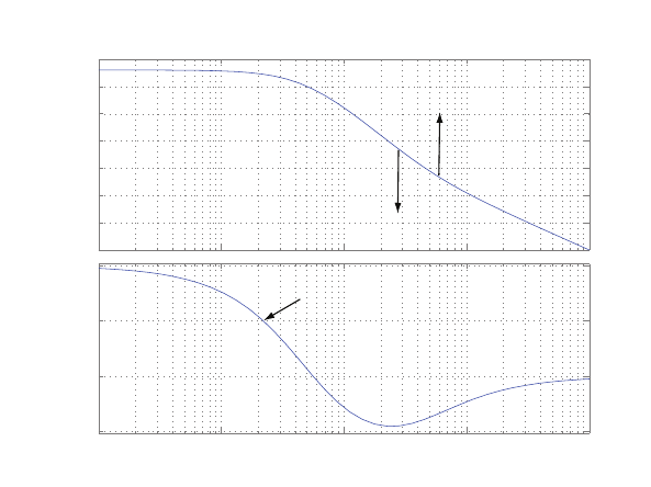
Problems 417

−60

−50

−40

−30

−20

−10

Magnitude (dB)

10−1 100101102103

−135

−90

−45

Phase (deg)

Bode Diagram

Frequency (rad/sec)

K increases

K decreases

Phase plot remains unchanged as K varies

FIGURE P8.27

Bode plot for K= 1

from the publisher prior to any prohibited reproduction, storage in a retrieval system, or transmission in any form or by any means, electronic, mechanical, photocopying,

recording, or likewise. For information regarding permission(s), write to: Rights and Permissions Department, Pearson Education, Inc., Upper Saddle River, NJ 07458.

418 CHAPTER 8 Frequency Response Methods

Advanced Problems

AP8.1 The spring-mass-damper system is described by

m¨x+b˙x+kx =p .

Taking the Laplace transform (with zero initial conditions) yields

X(s)

P(s)=1

ms2+bs +k.

From Figure AP8.1(b) in Dorf & Bishop, we determine that

20 log 

X(j0)

P(j0) 

= 20 log 

k

=−26dB .

Solving for kyields

k= 19.96 N/m.

Also, ω2

n=k/m implies m=k/ω2

n, where ωn= corner frequency = 3.2

rad/sec. So,

m= 1.949 kg .

Comparing Figure AP8.1(b) in Dorf & Bishop to the known standard

Bode plot of a second-order system, we estimate ζ≈0.32. Therefore,

b= 2mζωn= 2(1.949)(0.32)(3.2) = 3.992 N −s/m.

AP8.2 The closed-loop transfer function is

T(s) = Y(s)

R(s)=Kb

s+ 1 + 0.2Kb .

WIth K= 5, we have

T(s) = 5b

s+ 1 + b.

The sensitivity is

b=∂T

∂b

T=s+ 1

s+ 1 + b.

With the nominal value of b= 4, we have

b=s+ 1

s+ 5 .

from the publisher prior to any prohibited reproduction, storage in a retrieval system, or transmission in any form or by any means, electronic, mechanical, photocopying,

recording, or likewise. For information regarding permission(s), write to: Rights and Permissions Department, Pearson Education, Inc., Upper Saddle River, NJ 07458.

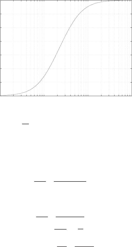
Advanced Problems 419

The sensitivity plot is shown in Figure AP8.2.

-14

-12

-10

-8

-6

-4

-2

10-1 100101102

Frequency (rad/sec)

20*log(mag) (dB)

FIGURE AP8.2

Bode plot for ST

b(s) = s+1

s+5 .

AP8.3 The equation of motion is

m¨x+b˙x+Kx =b˙r+Kr .

Taking Laplace transforms yields

X(s)

R(s)=bs +K

ms2+bs +K.

Then, given the various system parameters m= 1 kg, b= 4 Ns/m, K= 18

N/m, we obtain the transfer function:

X(s)

R(s)=4s+ 18

s2+ 4s+ 18 .

Also, ωn= corner frequency = pK/m =√18 = 4.243 rad/s and

ζ= damping ratio = b/m

2ωn

2(4.243) = 0.471 .

from the publisher prior to any prohibited reproduction, storage in a retrieval system, or transmission in any form or by any means, electronic, mechanical, photocopying,

recording, or likewise. For information regarding permission(s), write to: Rights and Permissions Department, Pearson Education, Inc., Upper Saddle River, NJ 07458.

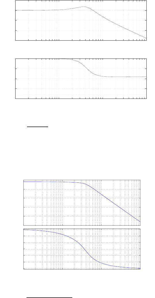
420 CHAPTER 8 Frequency Response Methods

The Bode plot is shown in Figure AP8.3.

-30

-20

-10

10-1 100101102

Frequency (rad/sec)

Gain dB

-200

-150

-100

-50

10-1 100101102

Frequency (rad/sec)

Phase deg

FIGURE AP8.3

Bode plot for G(s) = 4s+18

s2+4s+18 .

AP8.4 The Bode plot is shown in Figure AP8.4.

−120

−100

−80

−60

−40

−20

Magnitude (dB)

10−1 100101102

−270

−225

−180

−135

−90

−45

Phase (deg)

Bode Diagram

Frequency (rad/sec)

FIGURE AP8.4

Bode plot for L(s) = 1

(0.4s+1)(s2+3.9s+15) .

from the publisher prior to any prohibited reproduction, storage in a retrieval system, or transmission in any form or by any means, electronic, mechanical, photocopying,

recording, or likewise. For information regarding permission(s), write to: Rights and Permissions Department, Pearson Education, Inc., Upper Saddle River, NJ 07458.

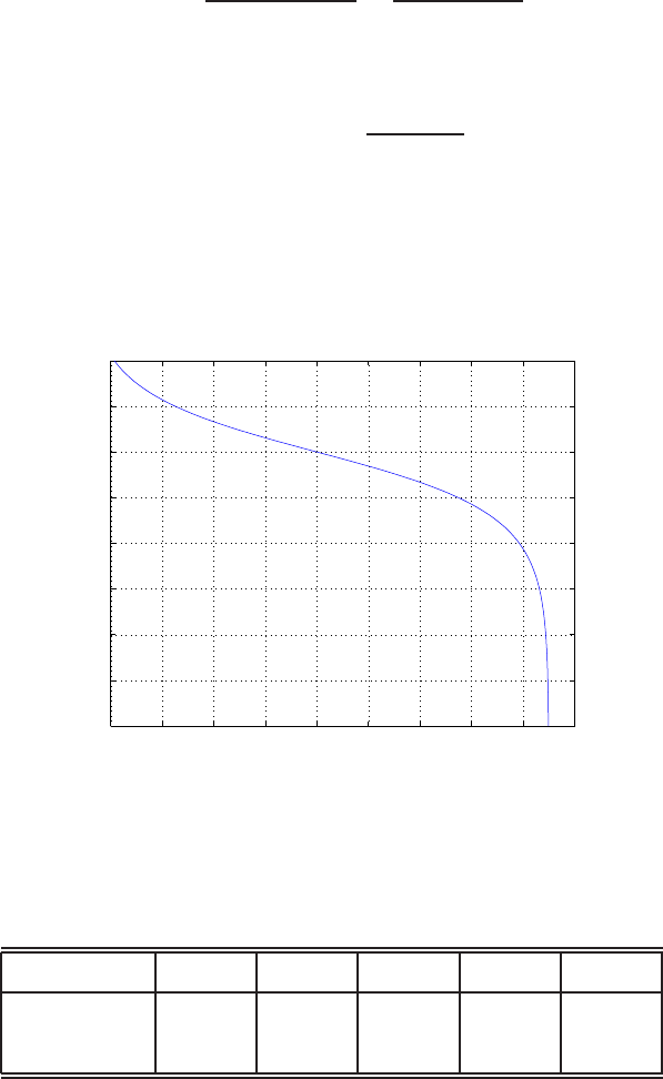
Advanced Problems 421

AP8.5 The closed-loop transfer function with unity feedback is given by

T(s) = Gc(s)G(s)

1 + Gc(s)G(s)=10(s+ 1)

s2+ 9s+ 10 .

(a) Solving for Gc(s)G(s) yields

Gc(s)G(s) = 10(s+ 1)

s(s−1) .

(b) A summary of the plot data (see Figure AP8.5) is presented in Ta-

ble AP8.5.

100 120 140 160 180 200 220 240 260 280

−40

−30

−20

−10

Phase, degrees

20 log|GcG(j ω)|, dB

FIGURE AP8.5

Log-magnitude-phase curve for GcG(jω).

ω1 10 50 110 500

20 log |GcG|40 4.85 -13.33 -20.61 -33.94

phase (deg) 101.42 250.17 267.53 268.93 269.77

TABLE AP8.5 Summary of magnitude and phase for ω= 1,10,50,110,500.

from the publisher prior to any prohibited reproduction, storage in a retrieval system, or transmission in any form or by any means, electronic, mechanical, photocopying,

recording, or likewise. For information regarding permission(s), write to: Rights and Permissions Department, Pearson Education, Inc., Upper Saddle River, NJ 07458.

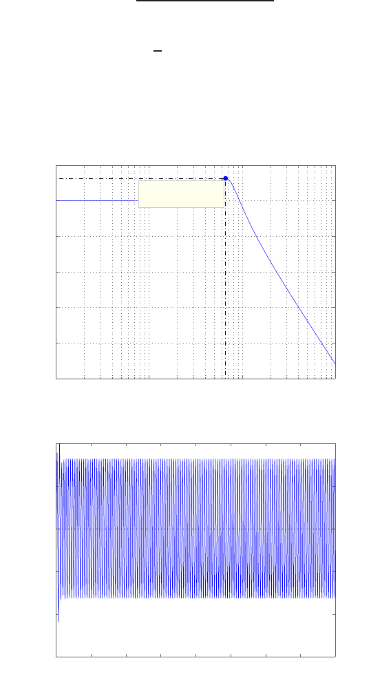
422 CHAPTER 8 Frequency Response Methods

AP8.6 The transfer function is given by

T(s) = 1/m

s2+ (b/m)s+ (k/m).

Selecting k= 1 and b= 2 results in the Bode plot magnitude always

less than 0 dB. Choosing b=√2/2 leads to a peak response with a sinu-

soidal input at ω= 0.66 rad/s. Figure AP8.6a shows the Bode plot and

Figure AP8.6b shows the response to a sinusiodal input with frequency

ω= 1 rad/s is less than 1 in the steady-state, as desired.

Bode Diagram

Frequency (rad/sec)

10−2 10−1 100101

−50

−40

−30

−20

−10

System: sys

Peak gain (dB): 6.3

At frequency (rad/sec): 0.661

Magnitude (dB)

0 100 200 300 400 500 600 700 800

−1.5

−1

−0.5

0.5

Impulse Response

Time (sec)

Amplitude

FIGURE AP8.6

(a) Bode plot for b/m = 1 and k/m = 1. (b) Response to a sinusiodal input.

from the publisher prior to any prohibited reproduction, storage in a retrieval system, or transmission in any form or by any means, electronic, mechanical, photocopying,

recording, or likewise. For information regarding permission(s), write to: Rights and Permissions Department, Pearson Education, Inc., Upper Saddle River, NJ 07458.

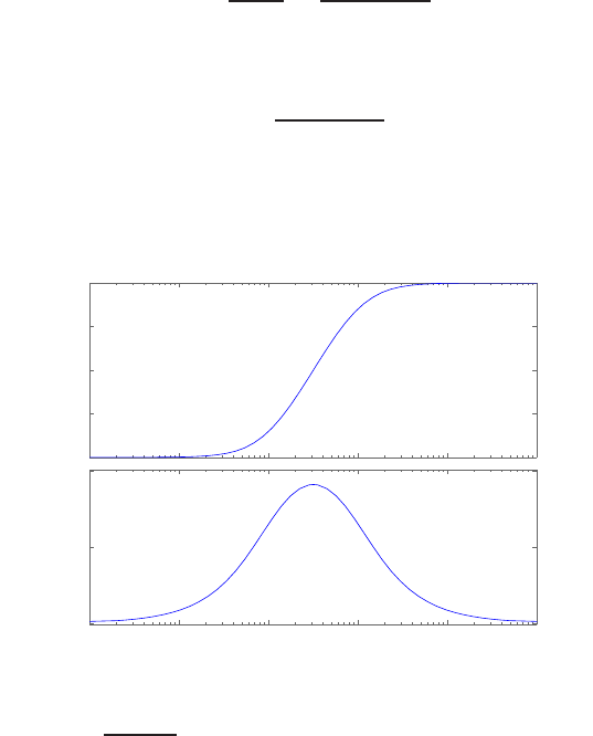
Advanced Problems 423

AP8.7 The transfer function is

G(s) = Vo(s)

Vi(s)=1 + R2C2s

1 + R1C1s.

Substituting C1= 0.1µF ,C2= 1 mF ,R1= 10 kΩ, and R2= 10 Ω yields

G(s) = 0.01s+ 1

0.001s+ 1 .

The frequency response is shown in Figure AP8.7.

Magnitude (dB)

100101102103104105

Phase (deg)

Bode Diagram

Frequency (rad/sec)

FIGURE AP8.7

Bode plot for G(s) = 0.01s+1

0.001s+1

from the publisher prior to any prohibited reproduction, storage in a retrieval system, or transmission in any form or by any means, electronic, mechanical, photocopying,

recording, or likewise. For information regarding permission(s), write to: Rights and Permissions Department, Pearson Education, Inc., Upper Saddle River, NJ 07458.

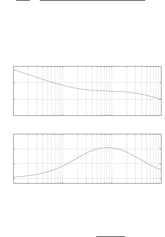
424 CHAPTER 8 Frequency Response Methods

Design Problems

With the PI controller in the loop, the closed-loop transfer function fromCDP8.1

the input to the output is

θ(s)

R(s)=26.035K(s+ 2)

s2+ (33.1415 + 26.035K)s+ 52.07K,

where we switch oﬀ the tachometer feedback (see Figure CDP4.1 in Dorf

and Bishop). The Bode plot is shown below for K= 40. From the step

response we determine that P.O. = 0 and Ts= 0.19. With K= 40, the

closed-loop poles are both real roots with values of s1=−1072.6 and

s2=−1.9.

10-1 100101102

Frequency (rad/sec)

Gain dB

10-1 100101102

-30

-60

-90

Frequency (rad/sec)

Phase deg

DP8.1 The loop transfer function is

L(s) = Gc(s)G(s) = K(s+ 2)

s2(s+ 12) .

(a,b) Let K= 1. The Bode plot of the loop transfer function and the

closed-loop transfer functions are shown in Figure DP8.1a and Fig-

ure DP8.1b, respectively.

closed-loop transfer functions are shown in Figure DP8.1c and Fig-

ure DP8.1d, respectively.

from the publisher prior to any prohibited reproduction, storage in a retrieval system, or transmission in any form or by any means, electronic, mechanical, photocopying,

recording, or likewise. For information regarding permission(s), write to: Rights and Permissions Department, Pearson Education, Inc., Upper Saddle River, NJ 07458.

Design Problems 425

10-1 100101102

-100

-50

Frequency (rad/sec)

Gain dB

10-1 100101102

-180

-160

-140

-120

Frequency (rad/sec)

Phase deg

FIGURE DP8.1

(a) Bode plot for the loop transfer function Gc(s)G(s) = (s+2)

s2(s+12) .

10-2 10-1 100101102

-100

-50

Frequency (rad/sec)

Gain dB

10-2 10-1 100101102

-90

-180

Frequency (rad/sec)

Phase deg

FIGURE DP8.1

CONTINUED: (b) Bode plot for the closed-loop T(s) = (s+2)

s3+12s2+s+2 .

from the publisher prior to any prohibited reproduction, storage in a retrieval system, or transmission in any form or by any means, electronic, mechanical, photocopying,

recording, or likewise. For information regarding permission(s), write to: Rights and Permissions Department, Pearson Education, Inc., Upper Saddle River, NJ 07458.

426 CHAPTER 8 Frequency Response Methods

10-1 100101102

-50

100

Frequency (rad/sec)

Gain dB

10-1 100101102

-180

-160

-140

-120

Frequency (rad/sec)

Phase deg

FIGURE DP8.1

CONTINUED: (c) Bode plot for the loop transfer function Gc(s)G(s) = 50(s+2)

s2(s+12) .

10-1 100101102

-60

-40

-20

Frequency (rad/sec)

Gain dB

10-1 100101102

-90

-180

Frequency (rad/sec)

Phase deg

FIGURE DP8.1

CONTINUED: (d) Bode plot for the closed-loop T(s) = 50(s+2)

s3+12s2+50s+100 .

from the publisher prior to any prohibited reproduction, storage in a retrieval system, or transmission in any form or by any means, electronic, mechanical, photocopying,

recording, or likewise. For information regarding permission(s), write to: Rights and Permissions Department, Pearson Education, Inc., Upper Saddle River, NJ 07458.

Design Problems 427

(d) The peak value of Mp≤2 occurs for 14 ≤K≤350. The maximum

bandwidth is achieved for the largest gain K. Thus, we select K= 350

and the corresponding bandwidth is ωB= 29 rad/sec.

(e) The system is type 2—the steady-state error is zero for a ramp input.

DP8.2 The open-loop transfer function is

Gc(s)G(s) = 20(s+ 1)

s(s+ 4)(s2+ 2s+ 8) .

(a) The phase angle is φ=−180owhen ω= 3.54 rad/sec. The magnitude

is 0 dB when ω= 0.87 rad/sec.

(b) The closed-loop transfer function is

T(s) = 20(s+ 1)

s4+ 6s3+ 16s2+ 52s+ 20 .

The closed-loop Bode plot is shown in Figure DP8.2.

−100

−80

−60

−40

−20

Magnitude (dB)

10−1 100101102

−270

−225

−180

−135

−90

−45

Phase (deg)

Bode Diagram

Gm = 6.71 dB (at 3.54 rad/sec) , Pm = 105 deg (at 0.869 rad/sec)

Frequency (rad/sec)

FIGURE DP8.2

Bode plot for closed-loop T(s) = 20(s+1)

s4+6s3+16s2+52s+20 .

Mpω= 4.84dB , ωr= 3.11 ,and ωB= 3.78 rad/sec .

When K= 25, we have

Mpω= 7.18 dB , ωr= 3.18 rad/sec ,and ωB= 3.94 rad/sec .

from the publisher prior to any prohibited reproduction, storage in a retrieval system, or transmission in any form or by any means, electronic, mechanical, photocopying,

recording, or likewise. For information regarding permission(s), write to: Rights and Permissions Department, Pearson Education, Inc., Upper Saddle River, NJ 07458.

428 CHAPTER 8 Frequency Response Methods

(d) Select K= 22.

DP8.3 The closed-loop transfer function is

T(s) = K(s+ 5)

s3+ 7s2+ 12s+ 10 + 5K.

When K= 4.2, we have 10 log10 Mpω= 3 dB. The system bandwidth is

ωb= 3.7178 rad/sec. The steady-state tracking error to a unit step input

ess = lim

s→0sE(s) = lim

s→01−T(s).

So,

ess = 1 −5K

10 + 5K= 0.322 ,

when K= 4.2. Since the system is unstable when K > 14.8, the steady-

state error does not exist after K= 14.8. The Bode plot is shown in

Figure DP8.3.

-80

-60

-40

-20

10-1 100101102

Frequency (rad/sec)

Gain dB

-200

-150

-100

-50

10-1 100101102

Frequency (rad/sec)

Phase deg

FIGURE DP8.3

Bode plot for closed-loop T(s) = K(s+5)

s3+7s2+12s+10+5K, where K= 4.2.

DP8.4 We have a second-order loop transfer function

Gc(s)G(s) = K

(0.3s+ 1)(0.6s+ 1) .

from the publisher prior to any prohibited reproduction, storage in a retrieval system, or transmission in any form or by any means, electronic, mechanical, photocopying,

recording, or likewise. For information regarding permission(s), write to: Rights and Permissions Department, Pearson Education, Inc., Upper Saddle River, NJ 07458.

Design Problems 429

With Mpω= 1.5, we determine that

Mpω = (2ζq1−ζ2)−1or ζ= 0.3568 .

Now the characteristic equation is

s2+ 5s+ 5.56(1 + K) = 0 .

So, solving 2ζωn= 5 yields ωn= 7. Therefore,

K= 0.18ω2

n−1 = 7.82 .

The closed-loop transfer function is

T(s) = K

K+ 1

5.56(K+ 1)

s2+ 5s+ 5.56(K+ 1) .

So, the overall gain of the standard second-order system will be attenuated

by the factor K/(K+ 1). To compensate, we amplify the gain by a small

factor. Thus we choose K= 10. The bandwidth is ωb= 11.25 rad/sec and

the peak magnitude is Mpω=1.5.

DP8.5 From the Bode plot of G(s) we ﬁnd that there exists two pnoles, at ap-

proximately ω= 1 rad/sec and ω= 10 rad/sec. Then, by examining the

Bode plot we estimate

G(s) = 10

(s+ 1)(s+ 10) .

We use a scale factor of 10 because at low frequency the Bode plot has

magnitude 0 dB (or a DC gain of 1). With G(s) as above, we can utilize

the controller

Gc(s) = 500

s+ 20

yielding a crossover

ωc= 12.9 rad/sec

and a magnitude of at least 25 dB for ω < 0.1 rad/sec. Figure DP8.5

shows the compensator Bode plot of Gc(s)G(s).

from the publisher prior to any prohibited reproduction, storage in a retrieval system, or transmission in any form or by any means, electronic, mechanical, photocopying,

recording, or likewise. For information regarding permission(s), write to: Rights and Permissions Department, Pearson Education, Inc., Upper Saddle River, NJ 07458.

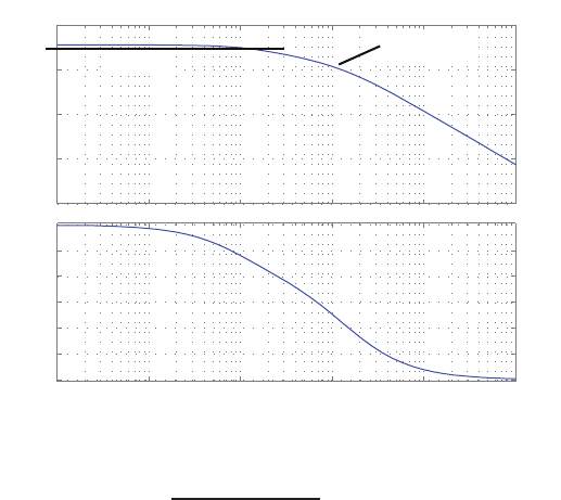
430 CHAPTER 8 Frequency Response Methods

-150

-100

-50

Magnitude (dB)

10 -2 10 -1 100101102103

-225

-180

-135

-90

-45

Phase (deg)

Bode Diagram

ωc=12.9

25 dB

Frequency (rad/sec)

FIGURE DP8.5

Bode Diagram for G(s)Gc(s) = 5000

(s+1)(s+10)(s+20) .

DP8.6 Let K=−1 to meet the steady-state tracking error requirement and

p= 2ζ, where ζ= 0.69 to obtain a 5% overshoot. The system is given by

x=Ax +Bu

where

A=



0 1

−1−1.38 

,B=

−1

0

,and C=0 1 .

The characteristic polynomial is

s2+ 1.38s+ 1 = 0 .

The associated damping ratio is ζ= 0.69 and the natural frequency is

ωn= 1 rad/s. Using the approximation

ωb= (−1.19ζ+ 1.85)ωn

we obtain ωb≈1.028 rad/s. The Bode plot is shown in Figure DP8.6.

The bandwidth is ωb= 1.023 rad/s.

from the publisher prior to any prohibited reproduction, storage in a retrieval system, or transmission in any form or by any means, electronic, mechanical, photocopying,

recording, or likewise. For information regarding permission(s), write to: Rights and Permissions Department, Pearson Education, Inc., Upper Saddle River, NJ 07458.

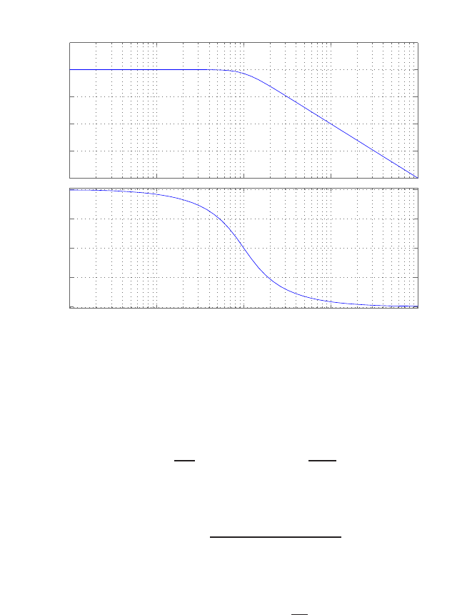
Design Problems 431

−80

−60

−40

−20

Magnitude (dB)

10−2 10−1 100101102

−180

−135

−90

−45

Phase (deg)

Bode Diagram

Frequency (rad/sec)

FIGURE DP8.6

Bode diagram for K=−1and p= 1.38.

DP8.7 A viable controler is

Gc(s) = KP+KI

s+KDs= 5.5 + 3.33

s+ 3.5s.

The loop transfer function is

Gc(s)G(s) = 10.5s2+ 16.5s+ 10

s2(s2+ 4s+ 5)

and computing Kayields

Ka= lim

s→0s2Gc(s)G(s) = 10

5= 2,

as desired. The phase margin is P.O. = 44.35◦and the bandwidth is

ωb= 4.5 rad/sec. The step response is shown in Figure DP8.7.

from the publisher prior to any prohibited reproduction, storage in a retrieval system, or transmission in any form or by any means, electronic, mechanical, photocopying,

recording, or likewise. For information regarding permission(s), write to: Rights and Permissions Department, Pearson Education, Inc., Upper Saddle River, NJ 07458.

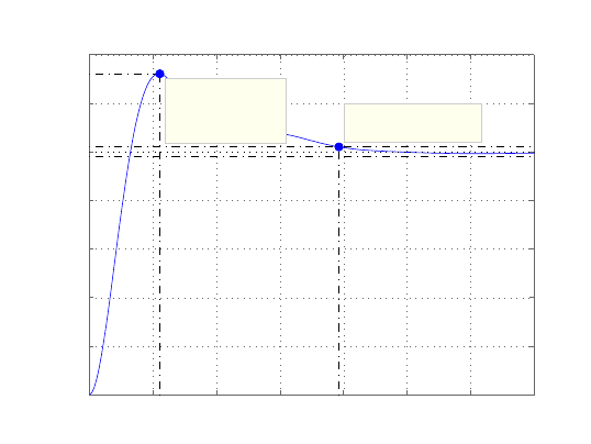
432 CHAPTER 8 Frequency Response Methods

Step Response

Time (sec)

Amplitude

01234567

0.2

0.4

0.6

0.8

1.2

1.4

System: sys_cl

Settling Time (sec): 3.93

System: sys_cl

Peak amplitude: 1.32

Overshoot (%): 32.1

At time (sec): 1.11

FIGURE DP8.7

Step response for KP= 5.5, KI= 3.33, and KD= 3.5.

from the publisher prior to any prohibited reproduction, storage in a retrieval system, or transmission in any form or by any means, electronic, mechanical, photocopying,

recording, or likewise. For information regarding permission(s), write to: Rights and Permissions Department, Pearson Education, Inc., Upper Saddle River, NJ 07458.

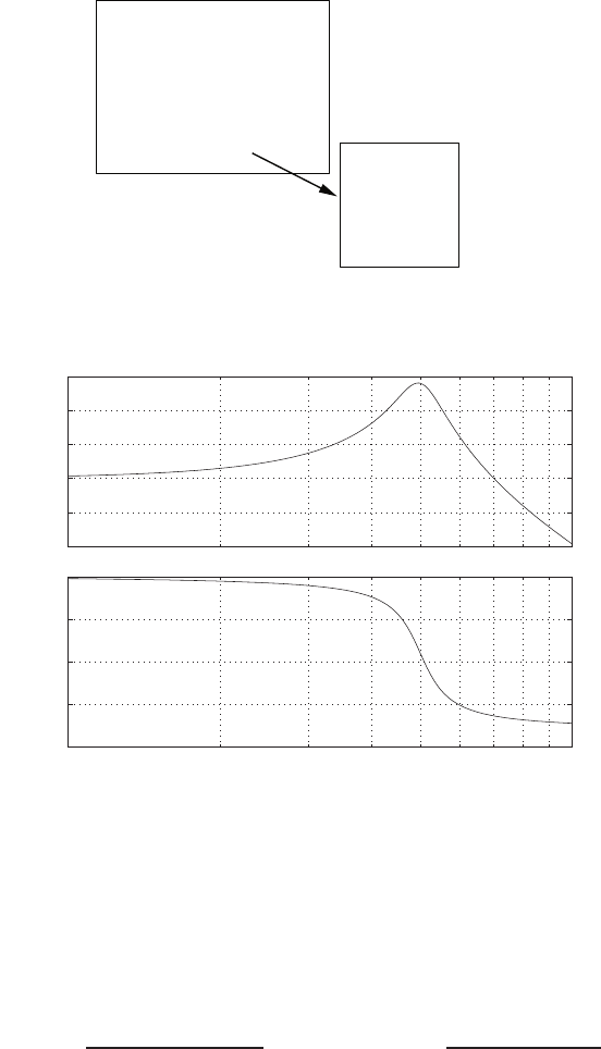
Computer Problems 433

Computer Problems

CP8.1 The m-ﬁle script and Bode plot are shown in Figure CP8.1. The script

automatically computes Mpωand ωr.

mp =

14.0228

wr =

4.9458

num=[25]; den=[1 1 25];

sys = tf(num,den);

w=logspace(0,1,400);

[mag,phase]=bode(sys,w);

[y,l]=max(mag);

mp=20*log10(y), wr=w(l)

bode(sys,w);

Frequency (rad/sec)

Phase (deg); Magnitude (dB)

Bode Diagrams

- 10

- 5

From: U(1)

100101

- 200

- 150

- 100

- 50

To: Y(1)

FIGURE CP8.1

Generating a Bode plot with the bode function.

CP8.2 The m-ﬁle script to generate the Bode plots is shown in Figure CP8.2a.

The Bode plots are presented in Figures CP8.2b-CP8.2e. The transfer

functions are

(a) : G(s) = 1000

(s+ 10)(s+ 100) ; (b) : G(s) = s+ 100

(s+ 2)(s+ 25) ;

from the publisher prior to any prohibited reproduction, storage in a retrieval system, or transmission in any form or by any means, electronic, mechanical, photocopying,

recording, or likewise. For information regarding permission(s), write to: Rights and Permissions Department, Pearson Education, Inc., Upper Saddle River, NJ 07458.

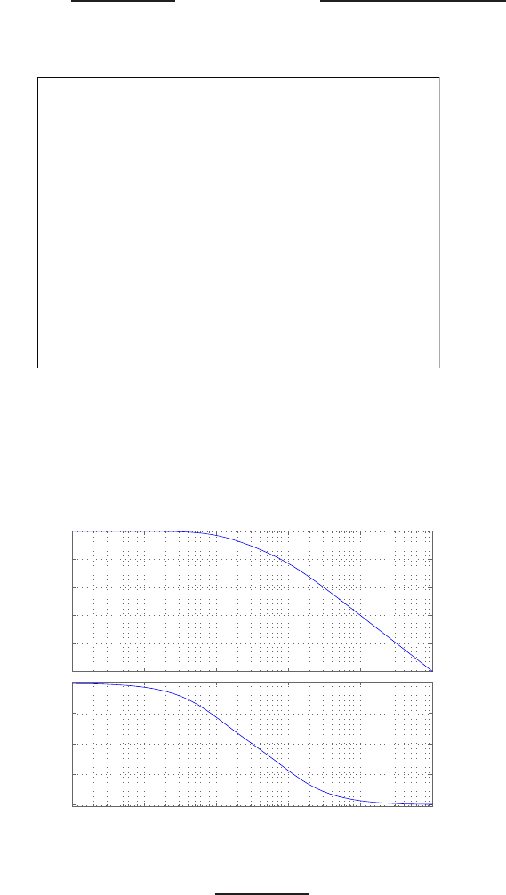
434 CHAPTER 8 Frequency Response Methods

s2+ 2s+ 50 ; (d) : G(s) = s−6

(s+ 3)(s2+ 12s+ 50) .

% Part (a)

num=[1000]; den=conv([1 10],[1 100]); sys1=tf(num,den);

sys = tf(num,den);

figure(1), bode(sys1), grid

% Part (b)

num=[1 100]; den=conv([1 2],[1 25]); sys2=tf(num,den);

sys = tf(num,den);

figure(2), bode(sys2), grid

% Part (c)

num=[100]; den=[1 2 50]; sys3=tf(num,den);

sys = tf(num,den);

figure(3), bode(sys3), grid

% Part (d)

num=[1 -6]; den=conv([1 3],[1 12 50]); sys4=tf(num,den);

sys = tf(sys);

figure(4), bode(sys4), grid

FIGURE CP8.2

(a) Script to generate the four Bode plots.

−100

−80

−60

−40

−20

Magnitude (dB)

10−1 100101102103104

−180

−135

−90

−45

Phase (deg)

Bode Diagram

Frequency (rad/sec)

FIGURE CP8.2

CONTINUED: (b) Bode plot for G(s) = 1000

(s+10)(s+100) .

from the publisher prior to any prohibited reproduction, storage in a retrieval system, or transmission in any form or by any means, electronic, mechanical, photocopying,

recording, or likewise. For information regarding permission(s), write to: Rights and Permissions Department, Pearson Education, Inc., Upper Saddle River, NJ 07458.

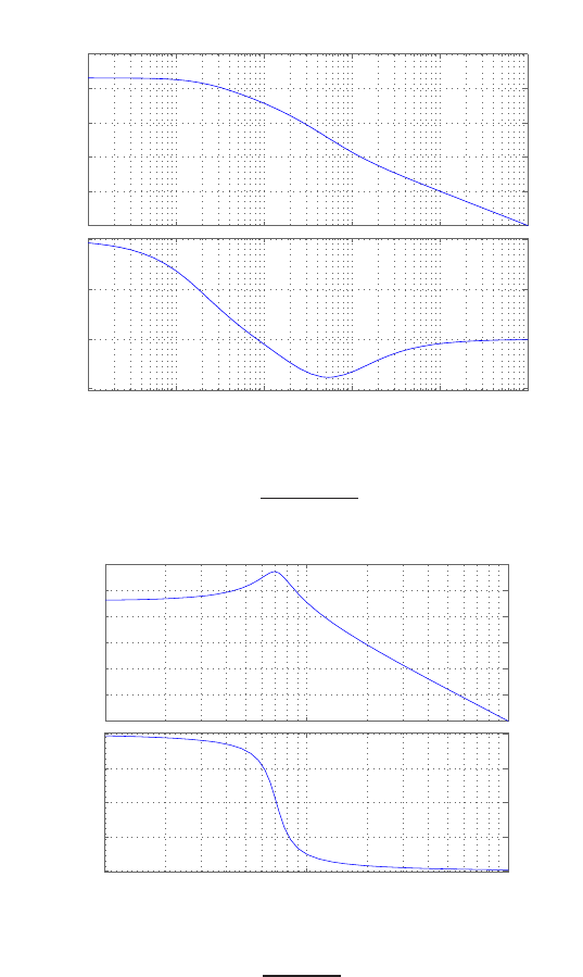
Computer Problems 435

−80

−60

−40

−20

Magnitude (dB)

10−1 100101102103104

−135

−90

−45

Phase (deg)

Bode Diagram

Frequency (rad/sec)

FIGURE CP8.2

CONTINUED: (c) Bode plot for G(s) = s+100

(s+2)(s+25) .

−40

−30

−20

−10

Magnitude (dB)

100101102

−180

−135

−90

−45

Phase (deg)

Bode Diagram

Frequency (rad/sec)

FIGURE CP8.2

CONTINUED: (d) Bode plot for G(s) = 100

s2+2s+50 .

from the publisher prior to any prohibited reproduction, storage in a retrieval system, or transmission in any form or by any means, electronic, mechanical, photocopying,

recording, or likewise. For information regarding permission(s), write to: Rights and Permissions Department, Pearson Education, Inc., Upper Saddle River, NJ 07458.

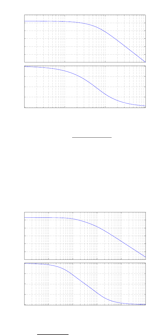
436 CHAPTER 8 Frequency Response Methods

−80

−70

−60

−50

−40

−30

−20

Magnitude (dB)

10−1 100101102

−180

−90

180

Phase (deg)

Bode Diagram

Frequency (rad/sec)

FIGURE CP8.2

CONTINUED: (e) Bode plot for G(s) = s−6

(s+3)(s2+12s+50) .

CP8.3 The Bode plots are shown in Figure CP8.3(a-d) with the transfer functions

listed in the caption. The crossover frequency for (a) is 17 rad/sec.

−100

−80

−60

−40

−20

Magnitude (dB)

10−1 100101102103104

−180

−135

−90

−45

Phase (deg)

Bode Diagram

Frequency (rad/sec)

FIGURE CP8.3

(a) Bode plot for G(s) = 2000

(s+10)(s+100) .

from the publisher prior to any prohibited reproduction, storage in a retrieval system, or transmission in any form or by any means, electronic, mechanical, photocopying,

recording, or likewise. For information regarding permission(s), write to: Rights and Permissions Department, Pearson Education, Inc., Upper Saddle River, NJ 07458.

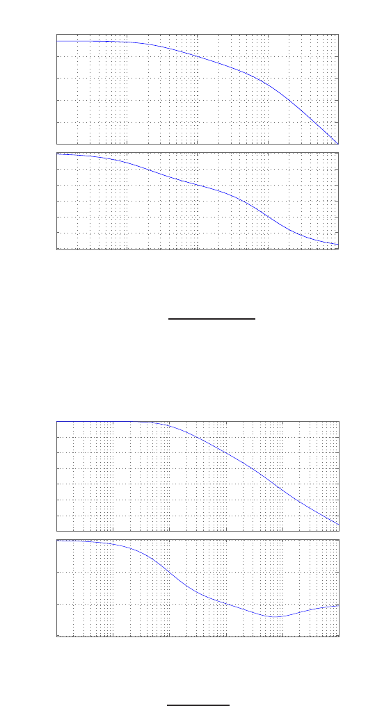
Computer Problems 437

The crossover frequency for (b) is 0.99 rad/sec.

−80

−60

−40

−20

Magnitude (dB)

10−2 10−1 100101102

−270

−225

−180

−135

−90

−45

Phase (deg)

Bode Diagram

Frequency (rad/sec)

FIGURE CP8.3

CONTINUED: (b) Bode plot for G(s) = 100

(s+1)(s2+10s+2) .

The crossover frequency for (c) is 70.7 rad/sec.

−30

−20

−10

Magnitude (dB)

10−2 10−1 100101102103

−135

−90

−45

Phase (deg)

Bode Diagram

Frequency (rad/sec)

FIGURE CP8.3

CONTINUED: (c) Bode plot for G(s) = 50(s+100)

(s+1)(s+50) .

The crossover frequency for (d) is 3.1 rad/sec.

from the publisher prior to any prohibited reproduction, storage in a retrieval system, or transmission in any form or by any means, electronic, mechanical, photocopying,

recording, or likewise. For information regarding permission(s), write to: Rights and Permissions Department, Pearson Education, Inc., Upper Saddle River, NJ 07458.

438 CHAPTER 8 Frequency Response Methods

−40

−30

−20

−10

Magnitude (dB)

10−1 100101102103104

−90

−45

Phase (deg)

Bode Diagram

Frequency (rad/sec)

FIGURE CP8.3

CONTINUED: (d) Bode plot for G(s) = 100(s2+14s+50)

(s+1)(s+2)(s+500) .

CP8.4 The m-ﬁle script and Bode plot are shown in Figure CP8.4a and b. The

bandwidth is ωb= 10 rad/sec.

−50

−40

−30

−20

−10

Magnitude (dB)

10−1 100101102

−180

−135

−90

−45

Phase (deg)

Bandwidth=10.0394 rad/sec

Frequency (rad/sec)

FIGURE CP8.4

(a) Bode plot for T(s) = 54

s2+6s+54 .

from the publisher prior to any prohibited reproduction, storage in a retrieval system, or transmission in any form or by any means, electronic, mechanical, photocopying,

recording, or likewise. For information regarding permission(s), write to: Rights and Permissions Department, Pearson Education, Inc., Upper Saddle River, NJ 07458.

Computer Problems 439

numg=[54]; deng=[1 6 0];

sys_o = tf(numg,deng);

sys_cl = feedback(sys_o,[1])

wb=bandwidth(sys_cl)

bode(sys_cl), grid

titlename=strcat('Bandwidth= ', num2str(wb), ' rad/sec')

title(titlename)

FIGURE CP8.4

CONTINUED: (b) M-ﬁle script to obtain the closed-loop Bode plot.

CP8.5 The Bode plot of the closed-loop system is shown in Figure CP8.5. The

closed-loop transfer function is

T(s) = 100

s2+ 6s+ 100 .

(a) From the Bode plot we determine that

Mpω≈5 dB and ωr≈9 rad/sec .

Frequency (rad/sec)

Phase (deg); Magnitude (dB)

Bode Diagrams

- 80

- 60

- 40

- 20

From: U(1)

10- 1100101102103

- 200

- 150

- 100

- 50

To: Y(1)

FIGURE CP8.5

Closed-loop system Bode plot.

from the publisher prior to any prohibited reproduction, storage in a retrieval system, or transmission in any form or by any means, electronic, mechanical, photocopying,

recording, or likewise. For information regarding permission(s), write to: Rights and Permissions Department, Pearson Education, Inc., Upper Saddle River, NJ 07458.

440 CHAPTER 8 Frequency Response Methods

(b) From Equations (8.36) and (8.37) in Dorf & Bishop, we ﬁnd that

ζ≈0.28 and ωr/ωn≈0.92

which implies that

ωn=ωr/0.92 = 9.8 rad/sec .

ωn= 10 rad/sec and ζ= 0.3.

The actual values and the estimated values compare very well.

CP8.6 The open-loop and closed-loop Bode plots are shown in Figure CP8.6a

and b. The open-loop and closed-loop transfers functions are

Gc(s)G(s) = 25

s3+ 3s2+ 27s+ 25

and

T(s) = Gc(s)G(s)

1 + Gc(s)G(s)=25

s3+ 3s2+ 27s+ 50 .

−100

−80

−60

−40

−20

Magnitude (dB)

10−2 10−1 100101102

−270

−225

−180

−135

−90

−45

Phase (deg)

Loop transfer function; bode(syso)

Frequency (rad/sec)

FIGURE CP8.6

(a) Open-loop system Bode plot for Gc(s)G(s) = 25

s3+3s2+27s+25 .

from the publisher prior to any prohibited reproduction, storage in a retrieval system, or transmission in any form or by any means, electronic, mechanical, photocopying,

recording, or likewise. For information regarding permission(s), write to: Rights and Permissions Department, Pearson Education, Inc., Upper Saddle River, NJ 07458.

Computer Problems 441

−100

−80

−60

−40

−20

Magnitude (dB)

10−1 100101102

−270

−225

−180

−135

−90

−45

Phase (deg)

Closed−loop system; bode(syscl)

Frequency (rad/sec)

FIGURE CP8.6

CONTINUED: (b) Closed-loop system Bode plot T(s) = 25

s3+3s2+27s+50 .

CP8.7 The m-ﬁle script and plot of ωbversus pare shown in Figure CP8.7a and

p=[0:0.001:1];

w=logspace(-1,1,1000);

n=length(p);

for i=1:n

num=[1]; den=[1 2*p(i) 0];

sys = tf(num,den);

sys_cl = feedback(sys,[1]);

[mag,phase,w]=bode(sys_cl,w);

a=nd(mag<0.707); wb(i)=w(a(1));

end

plot(p,wb)

xlabel('p'), ylabel('Bandwidth (rad/sec)')

FIGURE CP8.7

(a) M-ﬁle script to generate plot of ωbversus p.

from the publisher prior to any prohibited reproduction, storage in a retrieval system, or transmission in any form or by any means, electronic, mechanical, photocopying,

recording, or likewise. For information regarding permission(s), write to: Rights and Permissions Department, Pearson Education, Inc., Upper Saddle River, NJ 07458.

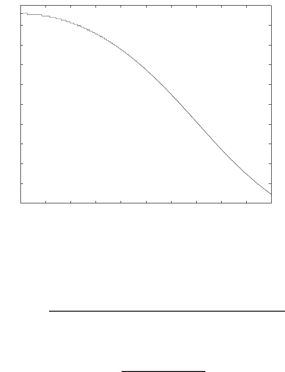
442 CHAPTER 8 Frequency Response Methods

0 0.1 0.2 0.3 0.4 0.5 0.6 0.7 0.8 0.9 1

0.6

0.7

0.8

0.9

1.1

1.2

1.3

1.4

1.5

1.6

Bandwidth (rad/sec)

FIGURE CP8.7

CONTINUED: (b) Plot of ωbversus p.

CP8.8 The transfer function from Td(s) to θ(s) is

θ(s)/Td(s) = −0.01(s+ 10)

s3+ 10s2+ (0.01K−10.791)s−107.91 + 0.05K.

Using the ﬁnal value theorem and Td(s) = 1/s, we determine that

lim

s→0sθ(s) = −0.1

−107.91 + 0.05K.

The design speciﬁcations require that

|ess|<0.1o.

So, solving for Kyields

K > 3300 .

We can select

K= 3300

as the initial value of Kfor the design. The m-ﬁle script is shown in

Figure CP8.8a. For the design shown, the ﬁnal selection for the gain is

K= 6000. The disturbance response is shown in Figure CP8.8b.

from the publisher prior to any prohibited reproduction, storage in a retrieval system, or transmission in any form or by any means, electronic, mechanical, photocopying,

recording, or likewise. For information regarding permission(s), write to: Rights and Permissions Department, Pearson Education, Inc., Upper Saddle River, NJ 07458.

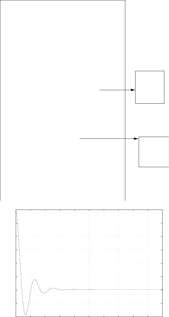
Computer Problems 443

MpDb =

4.0003

wr =

4.7226

ts =

2.23

po =

32.75

meets specs

Mb=100; Ms=10; L=1; g=9.81; a=5; b=10;

K=6000; % Final design value of K

numg=[-1/Mb/L]; deng=[1 0 -(Mb+Ms)*g/Mb/L];

sysg = tf(numg,deng);

numc=-K*[1 a]; denc=[1 b];

sysc = tf(numc,denc);

% Part (a)

sys = feedback(sysg,sysc);

w=logspace(0,1,400);

bode(sys,w)

[mag,phase]=bode(sys,w);

[M,l]=max(mag);

MpDb=20*log10(M)-20*log10(mag(1)) % Mpw in decibels

wr=w(l) % Mpw and peak frequency

% Part (b)

% From Eqs. (8.35) and (8.37)

Mpw=10^(MpDb/20);zeta=sqrt((1-sqrt(1-(1/Mpw^2)))/2);

wn=wr/sqrt(1-2*zeta^2);

ts=4/zeta/wn

po=100*exp(-zeta*pi/sqrt(1-zeta^2))

% Part (c)

t=[0:0.1:10];

[y,x]=step(sys,t);

plot(t,y*180/pi)

xlabel('time [sec]')

ylabel('theta [deg]')

grid

-0.04

-0.035

-0.03

-0.025

-0.02

-0.015

-0.01

-0.005

0 1 2 3 4 5 6 7 8 9 10

time [sec]

theta [deg]

FIGURE CP8.8

(a) Design script. (b) Disturbance response - meets all specs!

from the publisher prior to any prohibited reproduction, storage in a retrieval system, or transmission in any form or by any means, electronic, mechanical, photocopying,

recording, or likewise. For information regarding permission(s), write to: Rights and Permissions Department, Pearson Education, Inc., Upper Saddle River, NJ 07458.

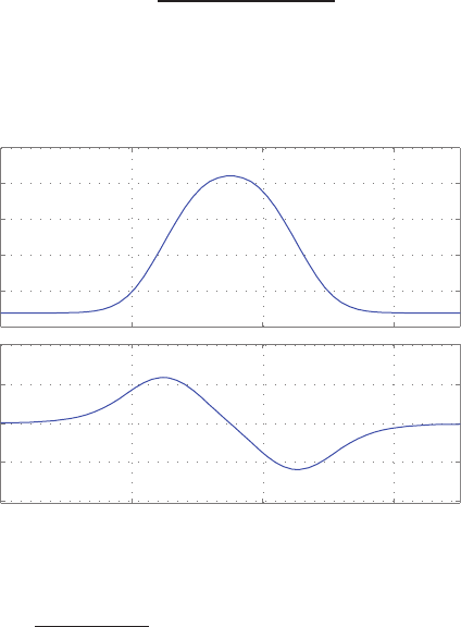
444 CHAPTER 8 Frequency Response Methods

CP8.9 A viable ﬁlter is

G(s) = 0.7(s+ 1000)(s+ 1)

(s+ 100)(s+ 10) .

The Bode plot is shown in Figure CP8.9

Magnitude (dB)

10 -2 100102104

-90

-45

Phase (deg)

Bode Diagram

Frequency (rad/sec)

-5

FIGURE CP8.9

Bode plot for G(s) = 0.7(s+1000)(s+1)

(s+100)(s+10) .

from the publisher prior to any prohibited reproduction, storage in a retrieval system, or transmission in any form or by any means, electronic, mechanical, photocopying,

recording, or likewise. For information regarding permission(s), write to: Rights and Permissions Department, Pearson Education, Inc., Upper Saddle River, NJ 07458.

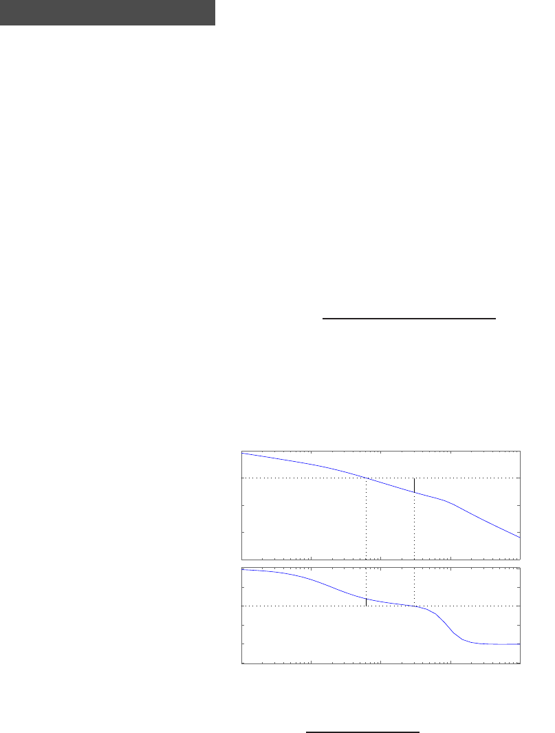
C H A P T E R 9

Stability in the Frequency Domain

Exercises

E9.1 The Bode plot for the transfer function Gc(s)G(s) is shown in Figure E9.1,

where

Gc(s)G(s) = 2(1 + s/10)

s(1 + 5s)(1 + s/9 + s2/81) .

The gain and phase margins are

G.M. = 26.2 dB and P.M. = 17.5o.

−150

−100

−50

Magnitude (dB)

10−2 10−1 100101102

−315

−270

−225

−180

−135

−90

Phase (deg)

Bode Diagram

Gm = 26.2 dB (at 2.99 rad/sec) , Pm = 17.5 deg (at 0.618 rad/sec)

Frequency (rad/sec)

FIGURE E9.1

Bode Diagram for Gc(s)G(s) = 2(1+s/10)

s(1+5s)(1+s/9+s2/81) .

445

from the publisher prior to any prohibited reproduction, storage in a retrieval system, or transmission in any form or by any means, electronic, mechanical, photocopying,

recording, or likewise. For information regarding permission(s), write to: Rights and Permissions Department, Pearson Education, Inc., Upper Saddle River, NJ 07458.

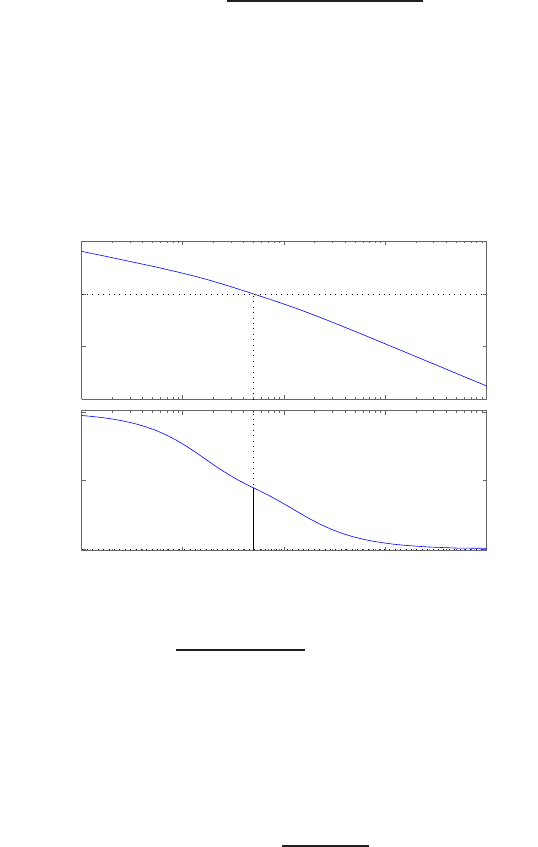
446 CHAPTER 9 Stability in the Frequency Domain

E9.2 The loop transfer function is

Gc(s)G(s) = 10.5(1 + s/5)

s(1 + s/2)(1 + s/10) .

The Bode plot is shown in Figure E9.2. The phase margin is

P.M. = 40.4o

at ωc= 4.96 rad/sec.

−100

−50

Magnitude (dB)

10−1 100101102103

−180

−135

−90

Phase (deg)

Bode Diagram

Gm = Inf dB (at Inf rad/sec) , Pm = 40.4 deg (at 4.96 rad/sec)

Frequency (rad/sec)

FIGURE E9.2

Bode Diagram for Gc(s)G(s) = 10.5(1+s/5)

s(1+s/2)(1+s/10) .

E9.3 The phase margin P.M. ≈75oat 200 kHz. We estimate the −180ophase

angle at 2 MHz, so the gain margin is G.M. ≈25 dB.

E9.4 The loop transfer function is

Gc(s)G(s) = 100

s(s+ 10) .

The Nichols diagram is shown in Figure E9.4. When the gain is raised by

4.6 dB, Mpω= 3 and the resonant frequency is ωR= 11 rad/sec.

from the publisher prior to any prohibited reproduction, storage in a retrieval system, or transmission in any form or by any means, electronic, mechanical, photocopying,

recording, or likewise. For information regarding permission(s), write to: Rights and Permissions Department, Pearson Education, Inc., Upper Saddle River, NJ 07458.

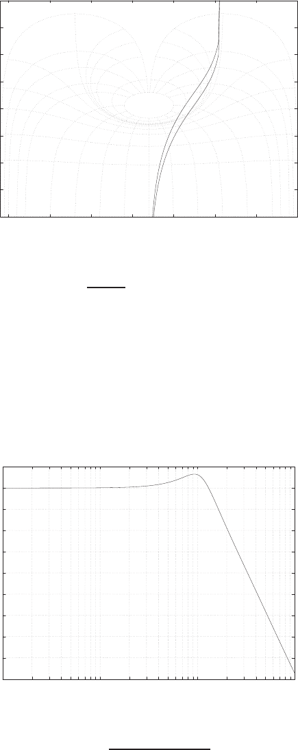
Exercises 447

-40

-30

-20

-10

-350 -300 -250 -200 -150 -100 -50 0

-40

-20

-12

-6

-3

-1

0.25

0.5

Phase (deg)

Gain dB

Phase (deg)

Gain dB

------ K=100K=171 ------

FIGURE E9.4

Nichols Diagram for Gc(s)G(s) = K)

s(s+10) , where K= 100 and K= 171.

E9.5 (a) The G.M. ≈5 dB and the P.M. ≈10o. (b) Lower the gain by 10 dB

to obtain P.M. ≈60o.

E9.6 The Bode plot of the closed-loop transfer function is shown in Figure E9.6.

The value of Mpω= 3 dB. The phase margin is P.M. = 40owhen K= 50.

-45

-40

-35

-30

-25

-20

-15

-10

-5

10-1 100101102

Frequency (rad/sec)

Gain dB

FIGURE E9.6

Closed-loop Bode Diagram for T(s) = 50(s+100)

s3+50s2+450s+5000 .

from the publisher prior to any prohibited reproduction, storage in a retrieval system, or transmission in any form or by any means, electronic, mechanical, photocopying,

recording, or likewise. For information regarding permission(s), write to: Rights and Permissions Department, Pearson Education, Inc., Upper Saddle River, NJ 07458.

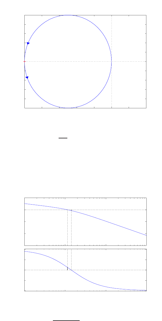
448 CHAPTER 9 Stability in the Frequency Domain

E9.7 The Nyquist plot is shown in Figure E9.7 for K= 5; the plot is a circle

with diameter= K/5. For K > 5, we have P= 1 and N=−1 (ccw as

−1 −0.8 −0.6 −0.4 −0.2 0 0.2 0.4

−0.5

−0.4

−0.3

−0.2

−0.1

0.1

0.2

0.3

0.4

0.5

Nyquist Diagram

Real Axis

Imaginary Axis

FIGURE E9.7

Nyquist Diagram for Gc(s)G(s) = K

s−5, where K= 5.

shown). So Z=N+P=−1 + 1 = 0 and the system is stable for K > 5.

E9.8 (a) When K= 4, the G.M. = 3.5 dB. This is illustrated in Figure E9.8.

−150

−100

−50

Magnitude (dB)

10−1 100101102

−270

−225

−180

−135

−90

Phase (deg)

Bode Diagram

Gm = 3.52 dB (at 1.41 rad/sec) , Pm = 11.4 deg (at 1.14 rad/sec)

Frequency (rad/sec)

FIGURE E9.8

Bode Diagram for Gc(s)G(s) = K

s(s+1)(s+2) , where K= 4.

from the publisher prior to any prohibited reproduction, storage in a retrieval system, or transmission in any form or by any means, electronic, mechanical, photocopying,

recording, or likewise. For information regarding permission(s), write to: Rights and Permissions Department, Pearson Education, Inc., Upper Saddle River, NJ 07458.

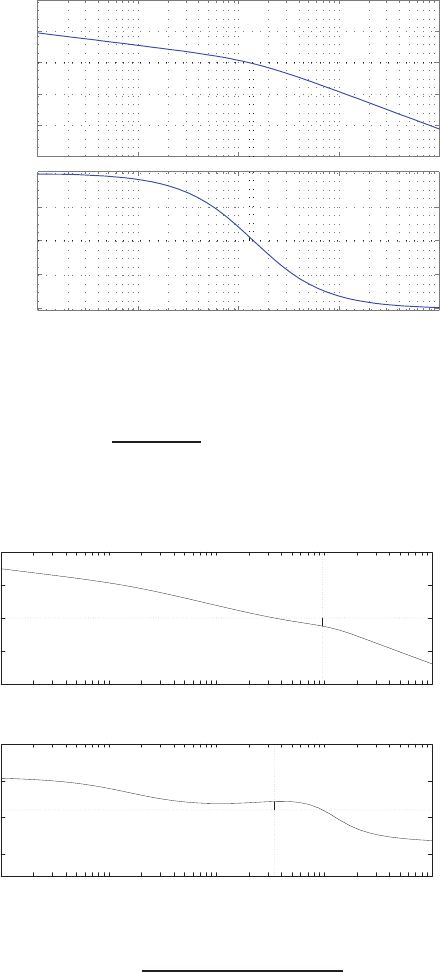
Exercises 449

(b) The new gain should be K= 1 for a gain margin G.M. = 16 dB.

E9.9 For K= 5, the phase margin P.M. = 5oas shown in Figure E9.9.

-150

-100

-50

100

Magnitude (dB)

10 -2 10 -1 100101102

-270

-225

-180

-135

-90

Phase (deg)

Bode Diagram

Gm = 1.58 dB (at 1.41 rad/sec) , Pm = 5.02 deg (at 1.29 rad/sec)

Frequency (rad/sec)

FIGURE E9.9

Bode Diagram for Gc(s)G(s) = K

s(s+1)(s+2) , where K= 5.

E9.10 The Bode plot is shown in Figure E9.10a. The closed-loop frequency

-100

-50

100

10-2 10-1 100101102

Frequency (rad/sec)

Gain dB

-300

-200

-100

10-2 10-1 100101102

Frequency (rad/sec)

Phase deg

PM=23.14 deg

GM=12.35 dB

FIGURE E9.10

(a) Bode Diagram for Gc(s)G(s) = 326s+1304

s4+14.76s3+151.3s2+23.84s.

from the publisher prior to any prohibited reproduction, storage in a retrieval system, or transmission in any form or by any means, electronic, mechanical, photocopying,

recording, or likewise. For information regarding permission(s), write to: Rights and Permissions Department, Pearson Education, Inc., Upper Saddle River, NJ 07458.

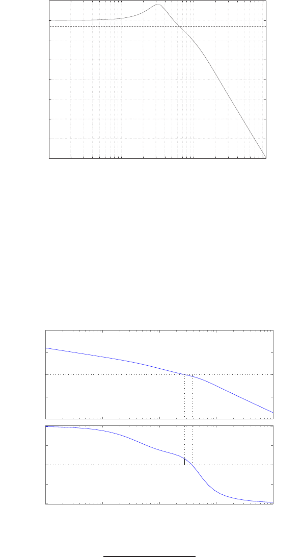
450 CHAPTER 9 Stability in the Frequency Domain

-70

-60

-50

-40

-30

-20

-10

10-1 100101102

Frequency (rad/sec)

Gain dB

FIGURE E9.10

CONTINUED: (b) Closed-loop frequency response: ωB= 6 rad/sec.

response is shown in Figure E9.10b. The bandwidth is ωB= 6 rad/sec.

E9.11 The Bode plot is shown in Figure E9.11. The system is stable.

−100

−50

100

Magnitude (dB)

10−2 10−1 100101102

−270

−225

−180

−135

−90

Phase (deg)

Bode Diagram

Gm = 3.91 dB (at 3.74 rad/sec) , Pm = 14.4 deg (at 2.76 rad/sec)

Frequency (rad/sec)

FIGURE E9.11

Bode Diagram for Gc(s)G(s) = 10(1+0.4s)

s(1+2s)(1+0.24s+0.04s2).

from the publisher prior to any prohibited reproduction, storage in a retrieval system, or transmission in any form or by any means, electronic, mechanical, photocopying,

recording, or likewise. For information regarding permission(s), write to: Rights and Permissions Department, Pearson Education, Inc., Upper Saddle River, NJ 07458.

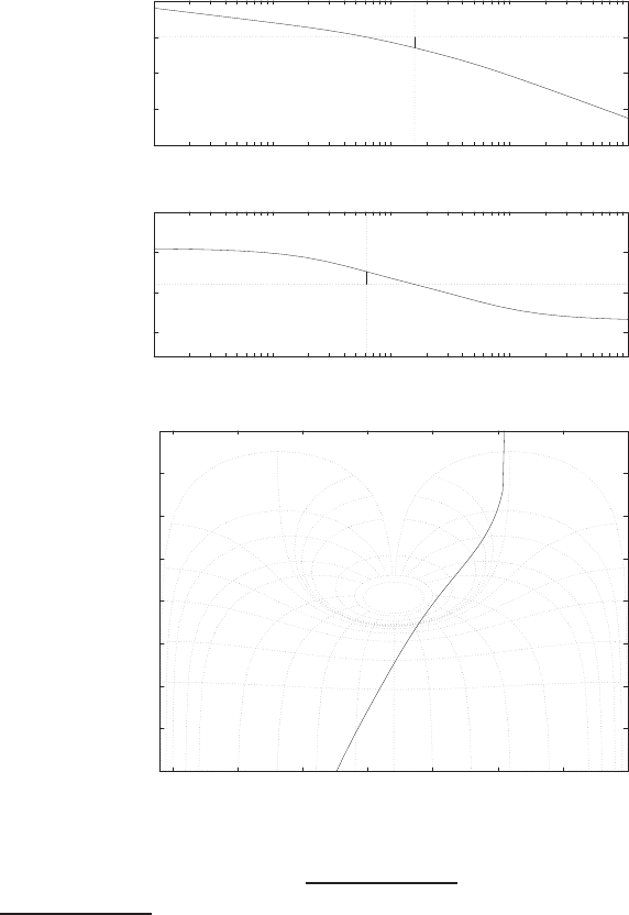
Exercises 451

E9.12 We select the gain K= 10 to meet the 10% steady-state tracking error

speciﬁcation for a ramp input. The Bode plot and Nichols chart are shown

in Figures E9.12a and E9.12b, respectively.

-150

-100

-50

10-1 100101102103

Frequency (rad/sec)

Gain dB

-300

-200

-100

10-1 100101102103

Frequency (rad/sec)

Phase deg

PM=31.79 deg

GM=14.82 dB

-40

-30

-20

-10

-350 -300 -250 -200 -150 -100 -50 0

-40

-20

-12

-6

-3

-1

0.25

0.5

Phase (deg)

Gain dB

FIGURE E9.12

(a) Bode Diagram for Gc(s)G(s) = 10

s(0.02s+1)(0.2s+1) . (b) Nichols chart for Gc(s)G(s) =

s(0.02s+1)(0.2s+1) .

E9.13 (a) The Nichols diagram is shown in Figure E9.13a and Mpω= 7.97 dB.

(b) The closed-loop Bode plot is shown in Figure E9.13b. The bandwidth

ωB= 18.65 rad/sec and the resonant frequency is ωr= 11.69 rad/sec.

from the publisher prior to any prohibited reproduction, storage in a retrieval system, or transmission in any form or by any means, electronic, mechanical, photocopying,

recording, or likewise. For information regarding permission(s), write to: Rights and Permissions Department, Pearson Education, Inc., Upper Saddle River, NJ 07458.

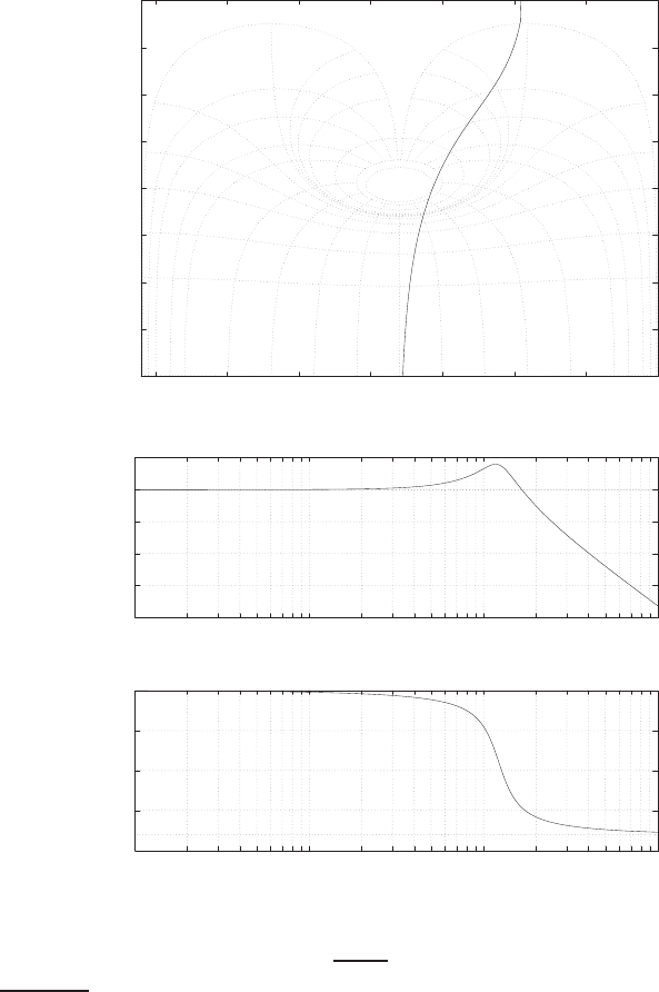
452 CHAPTER 9 Stability in the Frequency Domain

-40

-30

-20

-10

-350 -300 -250 -200 -150 -100 -50 0

-40

-20

-12

-6

-3

-1

0.25

0.5

Phase (deg)

Gain dB

-40

-30

-20

-10

10-1 100101102

Frequency (rad/sec)

Gain dB

-200

-150

-100

-50

10-1 100101102

Frequency (rad/sec)

Phase deg

FIGURE E9.13

(a) Nichols Diagram for Gc(s)G(s) = 150

s(s+5) . (b) Closed-loop Bode Diagram for T(s) =

150

s2+5s+150 .

E9.14 (a) The peak resonance Mpω= 6 dB.

(b) The resonant frequency is ωr=ω2= 3 rad/sec.

(d) The phase margin is P.M. = 30o.

from the publisher prior to any prohibited reproduction, storage in a retrieval system, or transmission in any form or by any means, electronic, mechanical, photocopying,

recording, or likewise. For information regarding permission(s), write to: Rights and Permissions Department, Pearson Education, Inc., Upper Saddle River, NJ 07458.

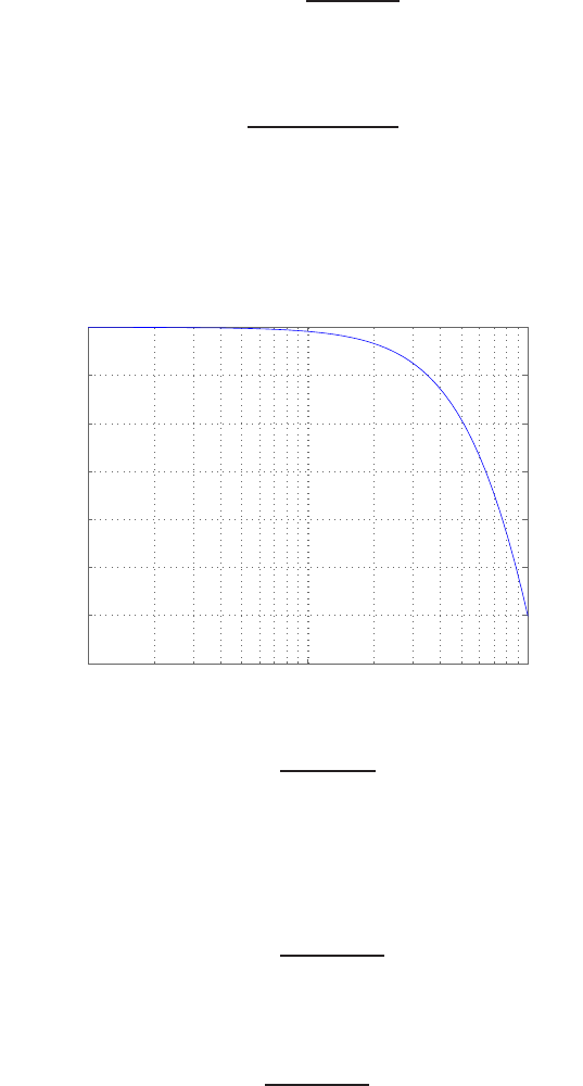
Exercises 453

E9.15 The loop transfer function is

Gc(s)G(s) = 100

s(s+ 20) ,

and the closed-loop transfer function is

T(s) = 100

s2+ 20s+ 100 .

The magnitude plot for the closed-loop system is shown in Figure E9.15.

With bandwidth deﬁned as frequency at which the magnitude is reduced

10−1 100101

−7

−6

−5

−4

−3

−2

−1

Magnitude (dB)

Bode Diagram

Frequency (rad/sec)

FIGURE E9.15

Magnitude plot for the closed-loop T(s) = 100

s2+20s+100 .

-3 dB from the dc value, we determine that ωB= 6.4 rad/sec.

E9.16 The transfer function of the approximation is

G(jω) = 1−jω/10

1 + jω/10 ,

and the magnitude is

|G(jω)|=

1−jω/10

1 + jω/10 

= 1 ,

which is equivalent to the actual time delay magnitude. The phase ap-

from the publisher prior to any prohibited reproduction, storage in a retrieval system, or transmission in any form or by any means, electronic, mechanical, photocopying,

recording, or likewise. For information regarding permission(s), write to: Rights and Permissions Department, Pearson Education, Inc., Upper Saddle River, NJ 07458.

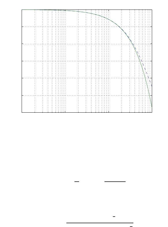
454 CHAPTER 9 Stability in the Frequency Domain

proximation is

φ=−tan−1ω/10 + tan−1(−ω/10) = −2 tan−1ω/10

and the actual phase is

φ=−0.2ω .

The phase plots are shown in Figure E9.16. The approximation is accurate

for ω < 3 rad/sec.

10−2 10−1 100101

−120

−100

−80

−60

−40

−20

Frequency (rad/sec)

Phase deg

Actual _______ & Approximation −−−−−−−

FIGURE E9.16

Phase plots for time delay actual vs approximation.

E9.17 (a,b) The phase angle for P.M. = 30 is

φ=−90o+ tan−1ω

2−tan−12ω

15 −ω2=−150o.

Solving for ωyields ω= 4.7. Then, at ω= 4.7, we have K= 10.82

when

|GcG(jω)|=K(ω2+ 4)1

ω((2ω2)2+ (15 −ω2)2)1

= 1 .

The Bode plot is shown in Figure E9.17.

from the publisher prior to any prohibited reproduction, storage in a retrieval system, or transmission in any form or by any means, electronic, mechanical, photocopying,

recording, or likewise. For information regarding permission(s), write to: Rights and Permissions Department, Pearson Education, Inc., Upper Saddle River, NJ 07458.

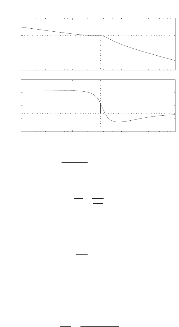
Exercises 455

Frequency (rad/sec)

Phase (deg); Magnitude (dB)

Bode Diagrams

- 100

- 50

Gm=3.5545 dB (at 4.3301 rad/sec), Pm=40 deg. (at 3.5147 rad/sec)

10- 1100101102

- 250

- 200

- 150

- 100

- 50

FIGURE E9.17

Bode Diagram for Gc(s)G(s) = K(s+2)

s3+2s2+15s, where K= 10.82.

ess =A

10K

= 0.60A ,

where R(s) = A/s2.

E9.18 (a) The gain crossover is at ωc= 486 Hz, and the phase margin P.O. =

36.2o. So, ζ≈0.36. Then, the expected percent overshoot to a step

input is

P.O. = 100e−ζπ/√1−ζ2= 30% ,where ζ= 0.36 .

(b) The estimated bandwidth is ωB≈2π(600).

ωn≈ωr= 2π(480) .

Then,

Ts=4

ζωn

(0.36)2π(480) ≈4 ms .

from the publisher prior to any prohibited reproduction, storage in a retrieval system, or transmission in any form or by any means, electronic, mechanical, photocopying,

recording, or likewise. For information regarding permission(s), write to: Rights and Permissions Department, Pearson Education, Inc., Upper Saddle River, NJ 07458.

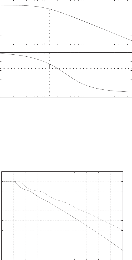
456 CHAPTER 9 Stability in the Frequency Domain

E9.19 The Bode plot is shown in Figure E9.19 for K= 16.75. The phase and

gain margins are P M = 50.0oand GM = 2.72 dB.

Frequency (rad/sec)

Phase (deg); Magnitude (dB)

- 40

- 30

- 20

- 10

10 Gm=2.7233 dB (at 20.618 rad/sec), Pm=50 deg. (at 13.434 rad/sec)

100101102103

- 500

- 400

- 300

- 200

- 100

FIGURE E9.19

Bode Diagram for Gc(s)G(s) = Ke−0.1s

s+10 , where K= 16.75.

E9.20 The system response for both drivers is shown in Figure E9.20.

-8

-7

-6

-5

-4

-3

-2

-1

012345678910

Time (sec)

Automobile velocity change

T=1 sec (solid line) & T=1.5 sec (dashed line)

FIGURE E9.20

Change in automobile velocity due to braking for two drivers.

from the publisher prior to any prohibited reproduction, storage in a retrieval system, or transmission in any form or by any means, electronic, mechanical, photocopying,

recording, or likewise. For information regarding permission(s), write to: Rights and Permissions Department, Pearson Education, Inc., Upper Saddle River, NJ 07458.

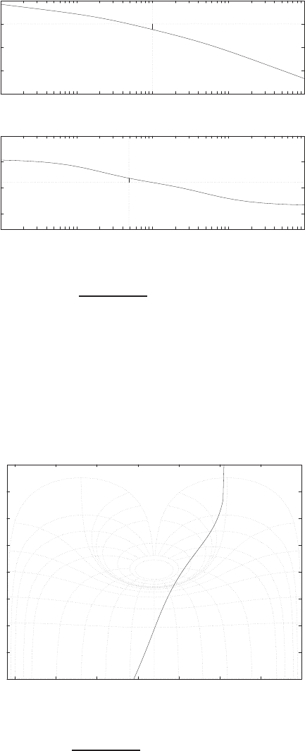
Exercises 457

E9.21 The Bode plot is shown in Figure E9.21.

-150

-100

-50

10-1 100101102103

Frequency (rad/sec)

Gain dB

-300

-200

-100

10-1 100101102103

Frequency (rad/sec)

Phase deg

PM=16.85 deg

GM=12.04 dB

FIGURE E9.21

Bode Diagram for Gc(s)G(s) = 1300

s(s+2)(s+50) .

E9.22 When K= 10, the P.M. = 36.9o; the system is stable. Decreasing the

gain to K= 4 results in a P.M. = 60o.

E9.23 The Nichols chart is shown in Figure E9.23.

-40

-30

-20

-10

-350 -300 -250 -200 -150 -100 -50 0

-40

-20

-12

-6

-3

-1

0.25

0.5

Phase (deg)

Gain dB

FIGURE E9.23

Nichols chart for Gc(s)G(s) = 438

s(s+2)(s+50) .

from the publisher prior to any prohibited reproduction, storage in a retrieval system, or transmission in any form or by any means, electronic, mechanical, photocopying,

recording, or likewise. For information regarding permission(s), write to: Rights and Permissions Department, Pearson Education, Inc., Upper Saddle River, NJ 07458.

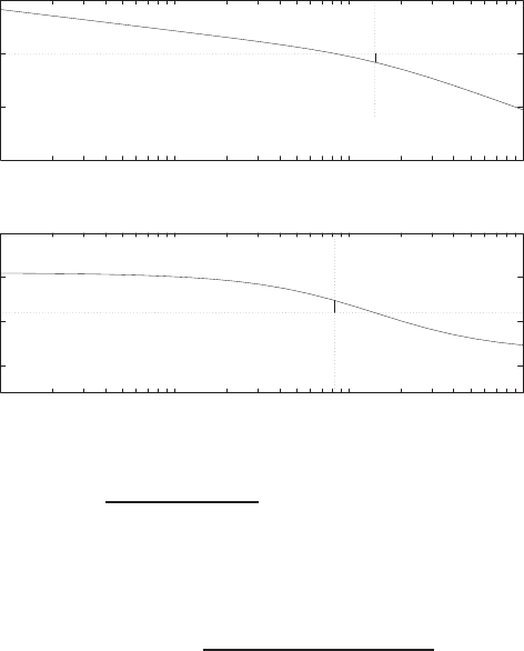
458 CHAPTER 9 Stability in the Frequency Domain

The actual values are

Mpω= 1.6598 (4.4 dB) ωr= 2.4228 rad/sec ωB= 4.5834 rad/sec .

E9.24 Using the Nyquist criterion, we have

P= 1 and N= 0

which implies

Z=N+P= 1 .

Therefore, the system has one root in the right half-plane.

E9.25 The Bode plot is shown in Figure E9.25.

-100

-50

10-1 100101102

Frequency (rad/sec)

Gain dB

-300

-200

-100

10-1 100101102

Frequency (rad/sec)

Phase deg

PM=27.73 deg at wc=8.29 rad/sec

FIGURE E9.25

Bode plot for Gc(s)G(s) = 11.7

s(0.05s+1)(0.1s+1) .

E9.26 The Nichols chart for

Gc(s)G(s) = 11.7

s(0.05s+ 1)(0.1s+ 1)

is shown in Figure E9.26, where we ﬁnd that

Mpω= 6.76 dB ωr= 8.96 rad/sec ωB= 13.73 rad/sec .

from the publisher prior to any prohibited reproduction, storage in a retrieval system, or transmission in any form or by any means, electronic, mechanical, photocopying,

recording, or likewise. For information regarding permission(s), write to: Rights and Permissions Department, Pearson Education, Inc., Upper Saddle River, NJ 07458.

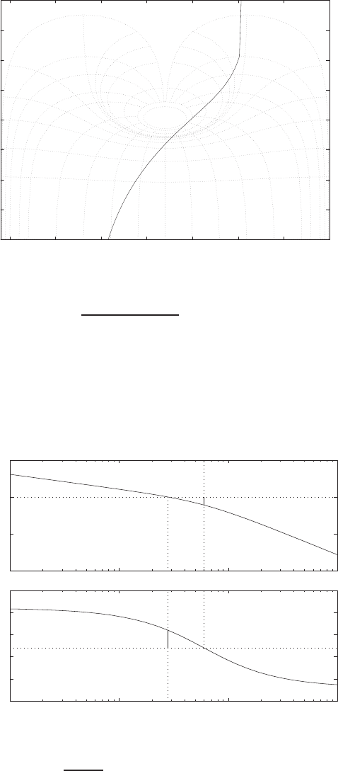
Exercises 459

-40

-30

-20

-10

-350 -300 -250 -200 -150 -100 -50 0

-40

-20

-12

-6

-3

-1

0.25

0.5

Phase (deg)

Gain dB

FIGURE E9.26

Nichols chart for Gc(s)G(s) = 11.7

s(0.05s+1)(0.1s+1) .

E9.27 The Bode plot for G(s) with K= 122.62 is shown in Figure E9.27.

Frequency (rad/sec)

Phase (deg); Magnitude (dB)

K=122.63

- 100

- 50

Gm=10.938 dB (at 6 rad/sec), Pm=40 deg. (at 2.7978 rad/sec)

10- 1100101102

- 300

- 250

- 200

- 150

- 100

- 50

FIGURE E9.27

Bode plot for Gc(s)G(s) = K

s(s+6)2,with K= 122.62.

from the publisher prior to any prohibited reproduction, storage in a retrieval system, or transmission in any form or by any means, electronic, mechanical, photocopying,

recording, or likewise. For information regarding permission(s), write to: Rights and Permissions Department, Pearson Education, Inc., Upper Saddle River, NJ 07458.

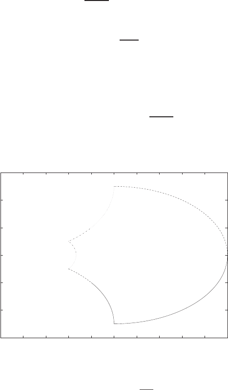
460 CHAPTER 9 Stability in the Frequency Domain

The phase margin is

P.M. = 40.0o

and the gain margin is

G.M. = 10.94 dB .

E9.28 The phase margin is P.M. = 28o. The estimated damping is

ζ=P.M.

100 = 0.28 .

The estimated percent overshoot is

P.O. = 100e−πζ/√1−ζ2= 40% .

The actual overshoot is P.O. = 44.43%.

E9.29 The F(s)-plane contour is shown in Figure E9.29, where

F(s) = 1 + Gc(s)G(s) = s+ 3

s+ 2 .

-0.6

-0.4

-0.2

0.2

0.4

0.6

1 1.1 1.2 1.3 1.4 1.5 1.6 1.7 1.8 1.9 2

F(s)-plane

FIGURE E9.29

F(s)-plane contour, where F(s) = 1 + Gc(s)G(s) = s+3

s+2 .

E9.30 The Bode plot is shown in Figure E9.30.

from the publisher prior to any prohibited reproduction, storage in a retrieval system, or transmission in any form or by any means, electronic, mechanical, photocopying,

recording, or likewise. For information regarding permission(s), write to: Rights and Permissions Department, Pearson Education, Inc., Upper Saddle River, NJ 07458.

Exercises 461

-50

Magnitude (dB)

10 -2 100102104

-180

-135

-90

-45

Phase (deg)

Bode Diagram

Frequency (rad/sec)

-100

FIGURE E9.30

Bode plot for G(s) = C[sI−A]−1B+D=1000

s2+100s+10 .

E9.31 The Bode plot is shown in Figure E9.31. The phase margin is P.M. = 50.6

deg.

-40

-20

Magnitude (dB)

10-3 10-2 10-1 100101

-150

-120

-90

Phase (deg)

Bode Diagram

Gm = Inf , Pm = 50.6 deg (at 0.341 rad/sec)

Frequency (rad/sec)

FIGURE E9.31

Bode plot for L(s) = G(s)H(s) = 2s+1

10s2+s.

from the publisher prior to any prohibited reproduction, storage in a retrieval system, or transmission in any form or by any means, electronic, mechanical, photocopying,

recording, or likewise. For information regarding permission(s), write to: Rights and Permissions Department, Pearson Education, Inc., Upper Saddle River, NJ 07458.

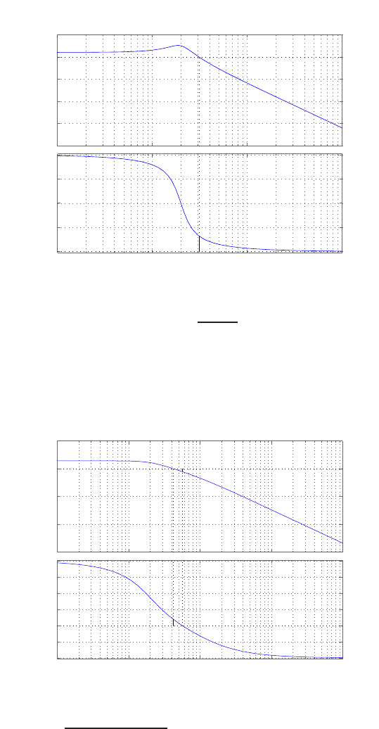
462 CHAPTER 9 Stability in the Frequency Domain

E9.32 The Bode plot is shown in Figure E9.32. The phase margin is P.M. = 29◦.

−80

−60

−40

−20

Magnitude (dB)

10−1 100101102

−180

−135

−90

−45

Phase (deg)

Bode Diagram

Gm = Inf dB (at Inf rad/sec) , Pm = 29 deg (at 3.1 rad/sec)

Frequency (rad/sec)

FIGURE E9.32

Bode plot for G(s) = C[sI−A]−1B+D=6.4

s2+s+4 .

E9.33 The Bode plot is shown in Figure E9.33. The phase margin is P.M. =

17.7◦and the gain margin is G.M. = 5.45 dB.

−150

−100

−50

Magnitude (dB)

10−1 100101102103

−270

−225

−180

−135

−90

−45

Phase (deg)

Bode Diagram

Gm = 5.45 dB (at 5.68 rad/sec) , Pm = 17.7 deg (at 4.24 rad/sec)

Frequency (rad/sec)

FIGURE E9.33

Bode plot for L(s) = 200

(s2+2.83s+4)(s+10) .

from the publisher prior to any prohibited reproduction, storage in a retrieval system, or transmission in any form or by any means, electronic, mechanical, photocopying,

recording, or likewise. For information regarding permission(s), write to: Rights and Permissions Department, Pearson Education, Inc., Upper Saddle River, NJ 07458.

Problems 463

Problems

P9.1 (a) The loop transfer function is

Gc(s)G(s) = 1

(1 + 0.5s)(1 + 2s).

P= 0, N = 0; therefore Z=N+P= 0. The system is stable. (Note:

See P8.1 for the polar plots.)

(b) The loop transfer function is

1 + 0.5s

s2.

P= 0, N = 0, therefore Z=N+P= 0. The system is stable.

s+ 4

s2+ 5s+ 25 .

P= 0, N = 0, Z =N+P= 0. Therefore, the system is stable.

(d) The loop transfer function is

30(s+ 8)

s(s+ 2)(s+ 4) .

P= 0, N = 2 therefore Z=P+N= 2. Therefore, the system has

two roots in the right half-plane, and is unstable.

P9.2 (a) The loop transfer function is

Gc(s)G(s) = K

s(s2+s+ 6) ,

and

Gc(jω)G(jω) = K

jω(−ω2+jω + 6) == K[−ω2−jω(6 −ω2)]

[(6 −ω2)2ω2+ω4].

To determine the real axis crossing, we let

Im{Gc(jω)G(jω)}= 0 = −Kω(6 −ω2)

ω=√6.

from the publisher prior to any prohibited reproduction, storage in a retrieval system, or transmission in any form or by any means, electronic, mechanical, photocopying,

recording, or likewise. For information regarding permission(s), write to: Rights and Permissions Department, Pearson Education, Inc., Upper Saddle River, NJ 07458.

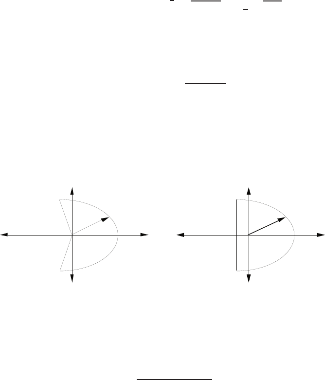
464 CHAPTER 9 Stability in the Frequency Domain

Then,

Re{Gc(jω)G(jω)}ω=√6=−Kω2

ω4ω=√6

=−K

So, −K/6>−1 for stability. Thus K < 6 for a stable system.

(b) The loop transfer function is

Gc(s)G(s) = K(s+ 1)

s2(s+ 6) .

The polar plot never encircles the -1 point, so the system is stable for

all gains K(See Figure 10 in Table 9.6 in Dorf & Bishop).

P9.3 (a,b) The suitable contours are shown in Figure P9.3.

q=cosz

r approaches

innity

(a)

(b)

-s1

r approaches

innity

FIGURE P9.3

Suitable contours Γsfor (a) and (b).

1 + 96

s(s2+ 11s+ 56) = 0 .

In this case, −σ1=−1. Therefore, we have one pole inside the contour

at s= 0, so P= 1. The polar plot yields N=−1, so Z=N+P= 0.

Therefore, all three roots have real parts less than -1. In fact, the

roots are s1=−3, and s2,3=−4±j4.

P9.4 (a) P= 0, N = 2, therefore Z= 2. The system has two roots in the right

hand s-plane.

(b) In this case, N= +1 −1 = 0, so Z= 0. Therefore the system is

stable.

from the publisher prior to any prohibited reproduction, storage in a retrieval system, or transmission in any form or by any means, electronic, mechanical, photocopying,

recording, or likewise. For information regarding permission(s), write to: Rights and Permissions Department, Pearson Education, Inc., Upper Saddle River, NJ 07458.

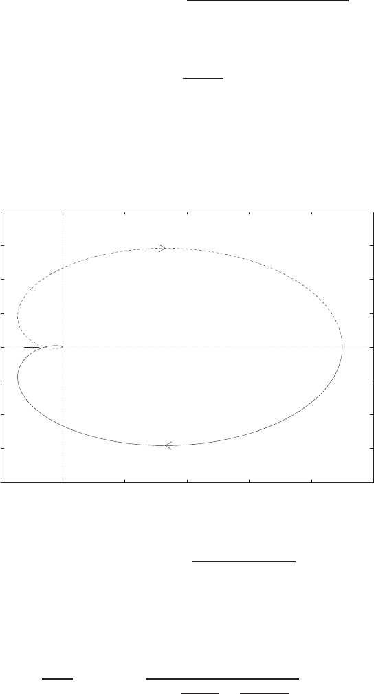
Problems 465

P9.5 (a) The loop transfer function is

L(s) = Gc(s)G(s)H(s) = K

(s+ 1)(3s+ 1)(0.4s+ 1) .

The steady-state error is

ess =|R|

1 + K.

We require ess = 0.1|R|, so K > 9.

(b) Use K= 9. The Nyquist plot is shown in Figure P9.5. We determine

that P= 0 and N= 0. Therefore, Z= 0 and the system is stable.

-8

-6

-4

-2

-2 0 2 4 6 8 10

Real Axis

Imag Axis

FIGURE P9.5

Nyquist Diagram for L(s) = Gc(s)G(s)H(s) = 9

(s+1)(3s+1)(0.4s+1) .

P9.6 The rotational velocity transfer function is

ω(s)

R(s)=G(s) = K

1 + s

3.7(2π) s

68(2π)+1 .

At low frequency, we have the magnitude near 35 dB, so 20 log K= 35 dB

from the publisher prior to any prohibited reproduction, storage in a retrieval system, or transmission in any form or by any means, electronic, mechanical, photocopying,

recording, or likewise. For information regarding permission(s), write to: Rights and Permissions Department, Pearson Education, Inc., Upper Saddle River, NJ 07458.

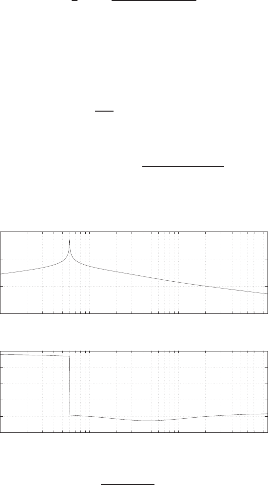
466 CHAPTER 9 Stability in the Frequency Domain

and K= 56. Since the frequency response plot is for rotational velocity

ω(s), and we are interested in position control, we add an integrator. The

characteristic equation is

1 + G(s)1

s= 1 + 56(23)(427)

s(s+ 23)(s+ 427) = 0 .

The roots are

s1=−430 and s2,3=−10 ±j35 .

Thus, ωn= 36 and ζ= 0.28. The time constant of the closed-loop system

τ=1

ζωn

= 99.6 msec .

P9.7 The loop transfer function is

L(s) = Gc(s)G(s)H(s) = 10K1s(s+ 7)

(s+ 3)(s2+ 0.36) .

(a) The Bode plot is shown in Figure P9.7 for K1= 2.

-50

100

10-1 100101102

Frequency (rad/sec)

Gain dB

-150

-100

-50

100

10-1 100101102

Frequency (rad/sec)

Phase deg

FIGURE P9.7

Bode Diagram for Gc(s)G(s)H(s) = 10K1s(s+7)

(s+3)(s2+0.36) , where K1= 2.

from the publisher prior to any prohibited reproduction, storage in a retrieval system, or transmission in any form or by any means, electronic, mechanical, photocopying,

recording, or likewise. For information regarding permission(s), write to: Rights and Permissions Department, Pearson Education, Inc., Upper Saddle River, NJ 07458.

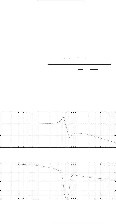
Problems 467

(b) The phase margin P.M. = 80oand the gain margin G.M. =∞, since

φnever crosses = −180o.

θ(s) = G(s)

1 + Gc(s)G(s)H(s)Td(s).

Then, for a step disturbance θ(∞) = lims→0sθ(s) = G(0) = 10/0.36 =

27.8, since H(0) = 0.

(d) The system is so highly damped, there is very little resonant peak.

(e) The estimated ζ=P.M./100 = 0.80. The actual ζ= 0.97.

P9.8 (a) The loop transfer function is

Gc(s)G(s)H(s) = s2

ω2

1+2ζ1s

ω1+ 1

(0.02s+ 1) s2

ω2

2+2ζ2s

ω2+ 1,

where ω1= 20π= 62.8, ω2= 14π= 43.9, ζ1= 0.05 and ζ2= 0.05.

The Bode plot is shown in Figure P9.8a. The phase margin is P.M. =

−9o. Therefore, the system is unstable.

-40

-20

100101102103

Frequency (rad/sec)

Gain dB

-200

-150

-100

-50

100101102103

Frequency (rad/sec)

Phase deg

FIGURE P9.8

(a) Bode Diagram for Gc(s)G(s)H(s) = s2/ω2

1+(0.1/ω1)s+1

(0.02s+1)(s2/ω2

2+(0.1/ω2)s+1) , where ω1= 20π

and ω2= 14π.

(b) In this case ζ2= 0.25, with all other parameters the same as before.

from the publisher prior to any prohibited reproduction, storage in a retrieval system, or transmission in any form or by any means, electronic, mechanical, photocopying,

recording, or likewise. For information regarding permission(s), write to: Rights and Permissions Department, Pearson Education, Inc., Upper Saddle River, NJ 07458.

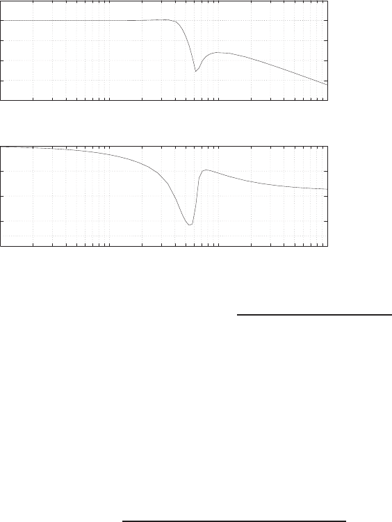
468 CHAPTER 9 Stability in the Frequency Domain

-40

-30

-20

-10

100101102103

Frequency (rad/sec)

Gain dB

-200

-150

-100

-50

100101102103

Frequency (rad/sec)

Phase deg

FIGURE P9.8

CONTINUED: (b) Bode Diagram for Gc(s)G(s)H(s) = s2/ω2

1+(0.1/ω1)s+1

(0.02s+1)(s2/ω2

2+(0.5/ω2)s+1) ,

where ω1= 20πand ω2= 14π.

The Bode plot is shown in Figure P9.8b. The phase margin is P.M. =

86o. Therefore, the system is now stable.

P9.9 (a) The Bode plot is shown in Figure P9.9a

The phase margin is P.M. = 83oand the gain margin is G.M. =∞.

(b) With the compensator, the loop transfer function is

Gc(s)G(s)H(s) = K1

0.30(s+ 0.05)(s2+ 1600)(s+ 0.5)

s(s2+ 0.05s+ 16)(s+ 70) ,

where

K2/K1= 0.5.

Let K1= 1. The Bode plot is shown in Figure P9.9b. The phase

margin is P.M. = 80oand the gain margin is G.M. =∞, essentially

the same as in (a). But the system in (b) is a type one, so that ess = 0

to a step input or disturbance. We cannot achieve a G.M. = 10 dB

by increasing or decreasing K1.

from the publisher prior to any prohibited reproduction, storage in a retrieval system, or transmission in any form or by any means, electronic, mechanical, photocopying,

recording, or likewise. For information regarding permission(s), write to: Rights and Permissions Department, Pearson Education, Inc., Upper Saddle River, NJ 07458.

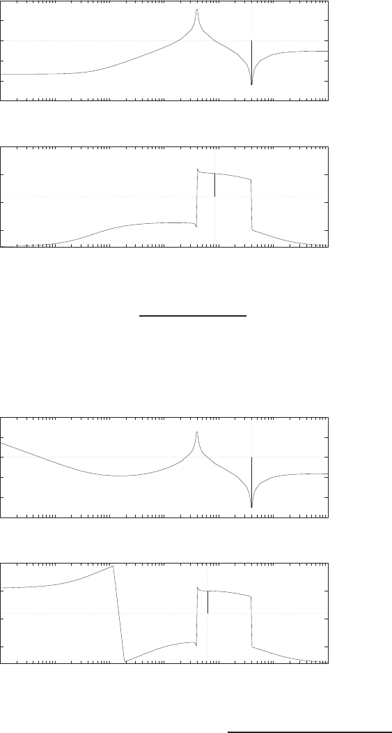
Problems 469

-60

-40

-20

10-3 10-2 10-1 100101102103

Frequency (rad/sec)

Gain dB

-300

-200

-100

10-3 10-2 10-1 100101102103

Frequency (rad/sec)

Phase deg

FIGURE P9.9

(a) Bode Diagram for Gc(s)G(s)H(s) = 0.3(s+0.05)(s2+1600)

(s+70)(s2+0.05s+16) .

-60

-40

-20

10-3 10-2 10-1 100101102103

Frequency (rad/sec)

Gain dB

-300

-200

-100

10-3 10-2 10-1 100101102103

Frequency (rad/sec)

Phase deg

FIGURE P9.9

CONTINUED: (b) Bode Diagram for Gs(s)G(s)H(s) = 0.15K1(s+0.05)(s2+1600)(s+0.5)

(s+70)(s2+0.05s+16) ,

K1= 1.

from the publisher prior to any prohibited reproduction, storage in a retrieval system, or transmission in any form or by any means, electronic, mechanical, photocopying,

recording, or likewise. For information regarding permission(s), write to: Rights and Permissions Department, Pearson Education, Inc., Upper Saddle River, NJ 07458.

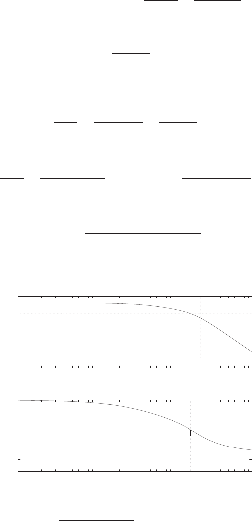
470 CHAPTER 9 Stability in the Frequency Domain

P9.10 The equations of motion are

F(s) = 3I(s) and I(s) = Eo(s)

R+Ls =Eo(s)

0.1 + 0.2s.

So,

F(s) = 30

(2s+ 1)Eo(s).

The actuator without the spring (see Table 2.7, Number 9 in Dorf &

Bishop) is modeled via

X(s)

Y(s)=1

Ms2+Bs =Ka

τas2+s.

With the spring, we have

X(s)

Y(s)=Ka

τas2+s+Ks

or GA(s) = 1

0.4s2+s+ 1.5.

Then, the loop transfer function is

L(s) = 30K1

(2s+ 1)(0.4s2+s+ 1.5) .

(a) The Bode plot for K1= 0.2 in Fig. P9.10 shows the P.M. = 30o.

-60

-40

-20

10-2 10-1 100101

Frequency (rad/sec)

Gain dB

-300

-200

-100

10-2 10-1 100101

Frequency (rad/sec)

Phase deg

FIGURE P9.10

Bode Diagram for L(s) = 30K1

(2s+1)(0.4s2+s+1.5) , where K1= 0.2.

from the publisher prior to any prohibited reproduction, storage in a retrieval system, or transmission in any form or by any means, electronic, mechanical, photocopying,

recording, or likewise. For information regarding permission(s), write to: Rights and Permissions Department, Pearson Education, Inc., Upper Saddle River, NJ 07458.

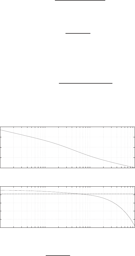
Problems 471

(b) For K1= 0.2, we determine that Mpω= 7.8 dB, ωr= 1.9 rad/sec,

and ωB= 2.8 rad/sec.

settling time is Ts= 10 sec. This is based on ζ= 0.21 and ωn≈ωr=

1.9 rad/sec.

P9.11 The loop transfer function is

Gc(s)G(s) = 5(K1s+K2)e−1.5s

s(5s+ 1) .

(a) Let K1=K2= 1. Then

Gc(s)G(s) = 5(s+ 1)

s(5s+ 1)e−1.5s.

The Bode plot is shown in Figure P9.11a. The phase margin is P.M. =

−48o. The system is unstable.

(b) Let K1= 0.1 and K2= 0.04. Then, the loop transfer function is

Gc(s)G(s) = 5(0.1s+ 0.04)e−1.5s

s(5s+ 1) .

The Bode plot shown in Figure P9.11b shows P.M. = 45o. Thus, the

system is stable.

-20

10-2 10-1 100101

Frequency (rad/sec)

Gain dB

-1000

-800

-600

-400

-200

10-2 10-1 100101

Frequency (rad/sec)

Phase deg

FIGURE P9.11

(a) Bode Diagram for Gc(s)G(s) = 5(s+1)e−sT

s(5s+1) , where T= 1.5.

from the publisher prior to any prohibited reproduction, storage in a retrieval system, or transmission in any form or by any means, electronic, mechanical, photocopying,

recording, or likewise. For information regarding permission(s), write to: Rights and Permissions Department, Pearson Education, Inc., Upper Saddle River, NJ 07458.

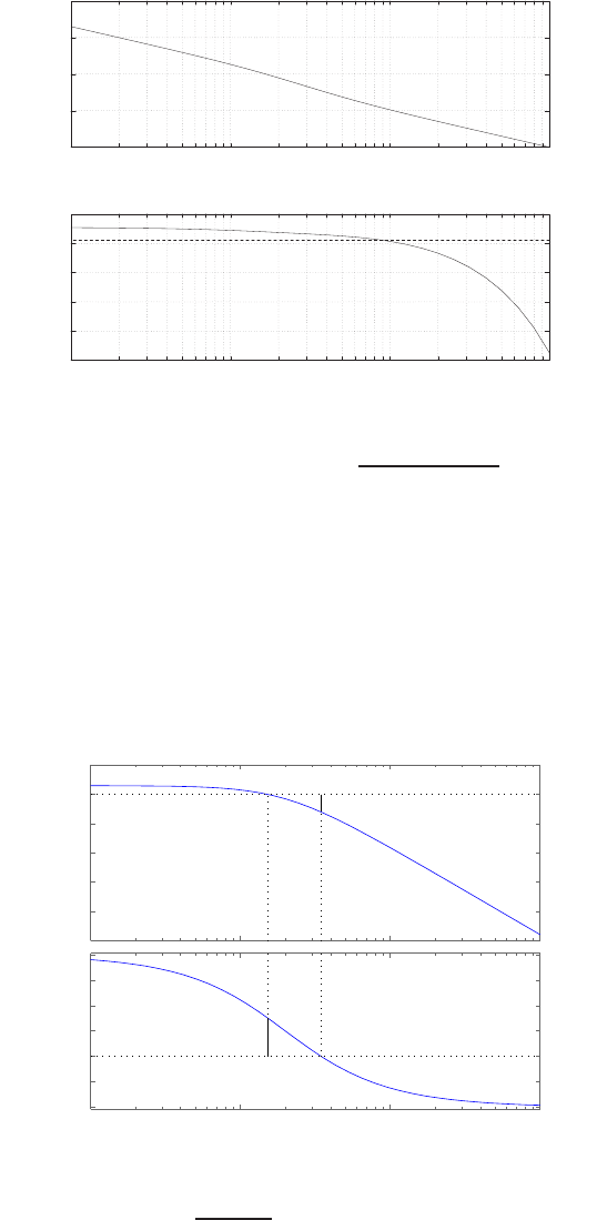
472 CHAPTER 9 Stability in the Frequency Domain

-40

-20

10-2 10-1 100101

Frequency (rad/sec)

Gain dB

-1000

-800

-600

-400

-200

10-2 10-1 100101

Frequency (rad/sec)

Phase deg

FIGURE P9.11

CONTINUED: (b) Bode Diagram for Gc(s)G(s) = 5(0.1s+0.04)e−sT

s(5s+1) , where T= 1.5.

dB. So, for stability we require K2≤0.1394 when K1= 0.

P9.12 (a) The Bode plot is shown in Figure P9.12.

−100

−80

−60

−40

−20

Magnitude (dB)

10−1 100101102

−270

−225

−180

−135

−90

−45

Phase (deg)

Bode Diagram

Gm = 12 dB (at 3.46 rad/sec) , Pm = 67.6 deg (at 1.53 rad/sec)

Frequency (rad/sec)

FIGURE P9.12

Bode Diagram for Gc(s)G(s) = 2

(0.5s+1)3.

from the publisher prior to any prohibited reproduction, storage in a retrieval system, or transmission in any form or by any means, electronic, mechanical, photocopying,

recording, or likewise. For information regarding permission(s), write to: Rights and Permissions Department, Pearson Education, Inc., Upper Saddle River, NJ 07458.

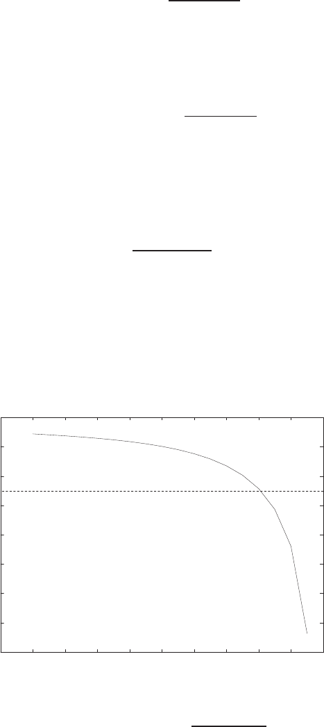
Problems 473

The loop transfer function (without the time delay) is

Gc(s)G(s) = 2

(0.5s+ 1)3.

The phase margin is P.M. = 67.6o.

(b) With the delay, the loop transfer function is

Gc(s)G(s)H(s) = 2e−0.5s

(0.5s+ 1)3.

The phase margin is now P.M. = 23.7o. So the 0.5 sec time delay has

reduced the phase margin by 43.9◦.

P9.13 The loop transfer function is

Gc(s)G(s) = Ka(Ks + 1)

se−1.2s.

(a) Let Ka=K= 1. Without the time delay, the system has inﬁnite

phase and gain margin. However, with the time delay, the system has

a negative gain margin, hence it is unstable.

(b) A plot of phase margin versus Kais shown in Figure P9.13.

-60

-40

-20

100

0 0.1 0.2 0.3 0.4 0.5 0.6 0.7 0.8 0.9 1

Phase margin deg

FIGURE P9.13

Phase margin as a function of Kafor Gc(s)G(s) = Ka(s+1)e−1.2s

from the publisher prior to any prohibited reproduction, storage in a retrieval system, or transmission in any form or by any means, electronic, mechanical, photocopying,

recording, or likewise. For information regarding permission(s), write to: Rights and Permissions Department, Pearson Education, Inc., Upper Saddle River, NJ 07458.

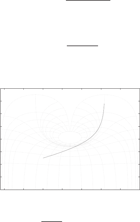
474 CHAPTER 9 Stability in the Frequency Domain

Let K= 1, and ﬁnd Kafor a stable system. Then,

Gc(s)G(s) = Ka(s+ 1)e−1.2s

If Ka= 0.8, then the phase margin is P.M. = 50o.

P9.14 The loop transfer function is

Gc(s)G(s) = Ke−0.2s

s(0.1s+ 1) .

(a) The Nichols diagram is shown in Figure P9.14 for K= 2.5.

-40

-30

-20

-10

-350 -300 -250 -200 -150 -100 -50 0

-40

-20

-12

-6

-3

-1

0.25

0.5

Phase (deg)

Gain dB

FIGURE P9.14

Nichols diagram for Gc(s)G(s) = Ke−0.2s

s(0.1s+1) , for K= 2.5.

It can be seen that

Mpω= 2.0 dB .

The phase and gain margins are P.M. = 48.5oand G.M. = 7.77 dB.

(b) We determine that ζ= 0.43 (based on Mpω= 2 dB) and ζ= 0.48

(based on the phase margin P.M. = 48.5o).

ωB= 5.4 rad/sec .

from the publisher prior to any prohibited reproduction, storage in a retrieval system, or transmission in any form or by any means, electronic, mechanical, photocopying,

recording, or likewise. For information regarding permission(s), write to: Rights and Permissions Department, Pearson Education, Inc., Upper Saddle River, NJ 07458.

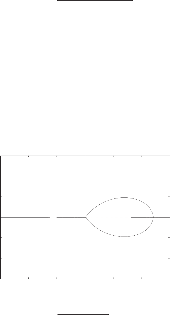
Problems 475

P9.15 (a) The ship transfer function is

G(s) = −0.164(s+ 0.2)(s−0.32)

s2(s+ 0.25)(s−0.009) .

The closed-loop system is unstable; the roots are

s1=−0.5467

s2,3= 0.2503 ±0.1893j

s4=−0.1949

Therefore the ship will not track the straight track.

(b) The system cannot be stabilized by lowering the gain; this is veriﬁed

in the root locus in Figure P9.15, where it is seen that the locus has

a branch in the right half-plane for all K > 0.

(d) When the switch is closed, we have a derivative feedback, which adds

90ophase lead. This is not enough to stabilize the system. Additional

lead networks are necessary.

-0.6

-0.4

-0.2

0.2

0.4

0.6

-0.6 -0.4 -0.2 0 0.2 0.4 0.6

xxxx oo

Real Axis

Imag Axis

FIGURE P9.15

Root locus for 1 + GH(s) = 1 + K−0.164(s+0.2)(s−0.32)

s2(s+0.25)(s−0.009) = 0.

from the publisher prior to any prohibited reproduction, storage in a retrieval system, or transmission in any form or by any means, electronic, mechanical, photocopying,

recording, or likewise. For information regarding permission(s), write to: Rights and Permissions Department, Pearson Education, Inc., Upper Saddle River, NJ 07458.

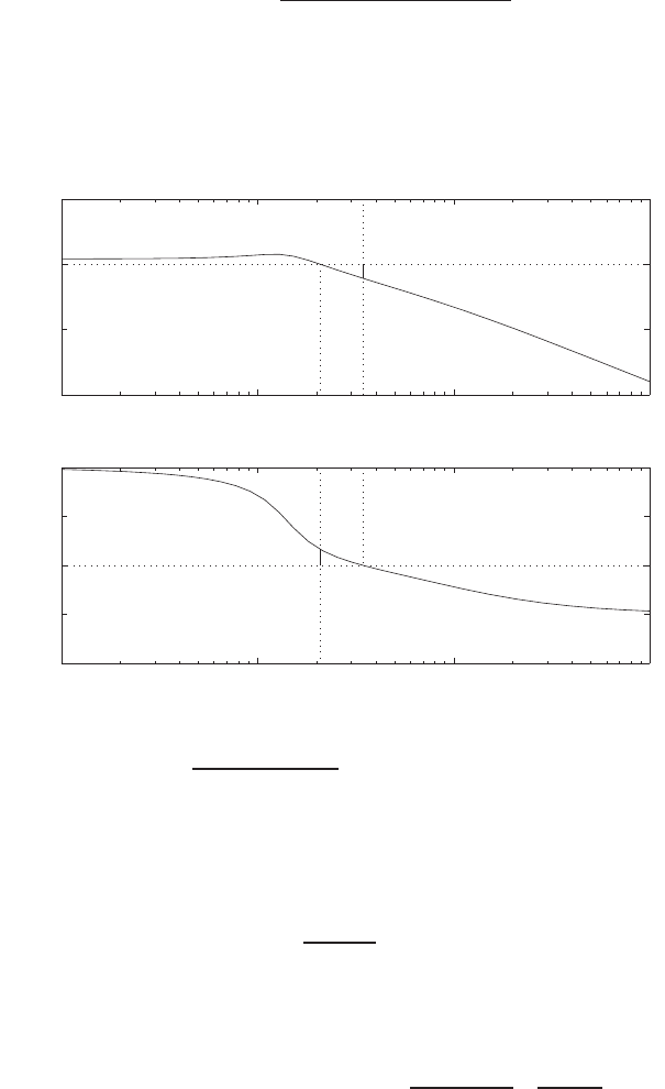
476 CHAPTER 9 Stability in the Frequency Domain

P9.16 The loop transfer function is

Gc(s)G(s) = K

(s/10 + 1)(s2+s+ 2) .

When K= 3.2, the phase margin is P.M. ≈30o. The Bode plot is shown

in Figure P9.16.

10-1 100101102

-100

-50

Frequency (rad/sec)

Gain dB

Gm=10.88 dB, (w= 3.464) Pm=29.91 deg. (w=2.083)

10-1 100101102

-90

-180

-270

-360

Frequency (rad/sec)

Phase deg

FIGURE P9.16

Bode plot for Gc(s)G(s) = K

(s/10+1)(s2+s+2) , where K= 3.2.

P9.17 (a) We require ess ≤0.05A, and we have

ess =A

1 + Kp

<0.05A

or Kp>19. But

Kp= lim

s→0G1(s)G2(s)G3(s)G4(s) = lim

s→0

20K1

(0.5s+ 1) 0.1

1 + 4s2

= 0.2K1.

So, Kp= 0.2K1>19, or K1>95.

from the publisher prior to any prohibited reproduction, storage in a retrieval system, or transmission in any form or by any means, electronic, mechanical, photocopying,

recording, or likewise. For information regarding permission(s), write to: Rights and Permissions Department, Pearson Education, Inc., Upper Saddle River, NJ 07458.

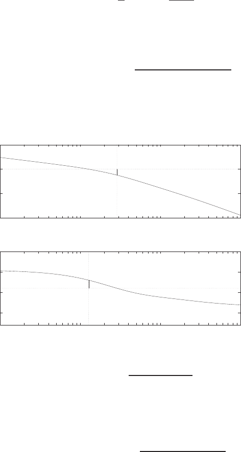
Problems 477

(b) Given

G1(s) = K1(1 + 1

s) = K1s+ 1

s,

we require 1.05 < MPt<1.30, or 0.70 > ζ > 0.36, or 70o> P.M. >

36o. Then,

G1(s)G2(s)G3(s)G4(s) = 0.2K1(s+ 1)

s(0.5s+ 1)(4s+ 1)2.

When K1= 0.8, the P.M. = 40o. The Bode plot is shown in Fig-

ure P9.17a.

-100

-50

10-2 10-1 100101

Frequency (rad/sec)

Gain dB

-300

-200

-100

10-2 10-1 100101

Frequency (rad/sec)

Phase deg

FIGURE P9.17

(a) Bode plot for G1(s)G2(s)G3(s)G4(s) = 0.2K1(s+1)

s(0.5s+1)(4s+1)2, where K1= 0.8and

P.M. = 40o.

G1(s)G2(s)G3(s)G4(s) = 2.375

(s+ 2)(s+ 0.25)2.

The characteristic equation is

s3+ 2.5s2+ 1.06s+ 2.50 = (s+ 2.48)(s2+ 0.02s+ 1.013) .

The dominant complex roots are lightly damped since ζ= 0.01 and

ζωn= 0.01.

from the publisher prior to any prohibited reproduction, storage in a retrieval system, or transmission in any form or by any means, electronic, mechanical, photocopying,

recording, or likewise. For information regarding permission(s), write to: Rights and Permissions Department, Pearson Education, Inc., Upper Saddle River, NJ 07458.

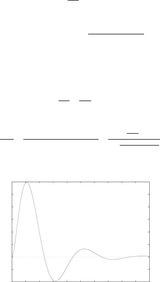
478 CHAPTER 9 Stability in the Frequency Domain

Thus,

Ts=4

ζωn

= 400 sec .

For part (b), we had

G1(s)G2(s)G3(s)G4(s) = (0.2)(0.8)(s+ 1)

s(0.5s+ 1)(4s+ 1)2.

The characteristic equation is

8s4+ 20s3+ 8.5s2+ 1.16s+ 0.16 = 0 .

The roots are s1=−2, s2=−0.4 and s3,4=−0.05 ±j0.15. Thus

ζ= 0.16 and ζωn= 0.05. So,

Ts=4

ζωn

0.05 = 75 sec .

(d) Let U(s) be a unit step disturbance and R(s) = 0. Then

Y(s)

U(s)=G3(s)G4(s)

1 + G1(s)G2(s)G3(s)G4(s)=0.1

1+4s2

1 + 20K1(s+1)

s(0.5s+1)(4s+1)2

The disturbance response is shown in Figure P9.17b.

-2

-1

x10-3

0 10 20 30 40 50 60 70 80 90 100

Time (secs)

Amplitude

FIGURE P9.17

CONTINUED: (b) System response to a unit disturbance U(s).

from the publisher prior to any prohibited reproduction, storage in a retrieval system, or transmission in any form or by any means, electronic, mechanical, photocopying,

recording, or likewise. For information regarding permission(s), write to: Rights and Permissions Department, Pearson Education, Inc., Upper Saddle River, NJ 07458.

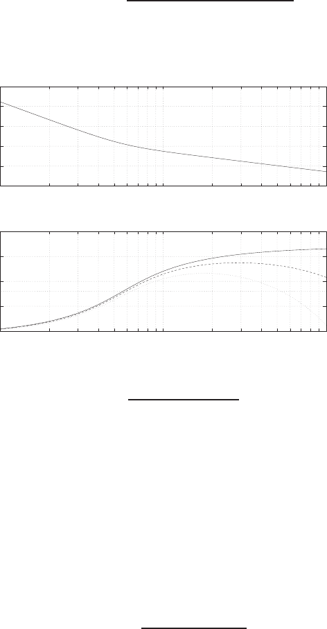
Problems 479

P9.18 The transfer function is

Gc(s)G(s)H(s) = 5.3(s2+ 0.8s+ 0.32)e−T s

s3.

The Bode plot is shown in Figure P9.18.

-20

10-1 100101

Frequency (rad/sec)

Gain dB

100

150

200

250

300

10-1 100101

Frequency (rad/sec)

Phase deg

T=0 solid ___ & T=0.1 dashed ---- & T=0.2674 dotted ....

FIGURE P9.18

Bode diagram for Gc(s)G(s)H(s) = K(s2+0.8s+0.32)e−sT

s3, where T= 0 (solid line),

T= 0.1(dashed line), and T= 0.2674 (dotted line).

The following results are veriﬁed in the ﬁgure.

(a) The phase margin is P.M. = 81oat ω= 5.3 when T= 0.

(b) For T= 0.1, the added phase is φ=−T ω (in radians). The phase

margin is P.M. = 51oat ω= 5.3 when T= 0.1.

margin is P.M. = 0oat ω= 5.3.

P9.19 The transfer function is

Gc(s)G(s) = 0.5

s(1 + 2s)(4 + s).

(a) The Nichols diagram is shown in Figure P9.19. The gain margin is

G.M. = 31.4 dB.

(b) The phase margin is P.M. = 75oand Mpω= 0 dB. The bandwidth is

0.17 rad/sec.

from the publisher prior to any prohibited reproduction, storage in a retrieval system, or transmission in any form or by any means, electronic, mechanical, photocopying,

recording, or likewise. For information regarding permission(s), write to: Rights and Permissions Department, Pearson Education, Inc., Upper Saddle River, NJ 07458.

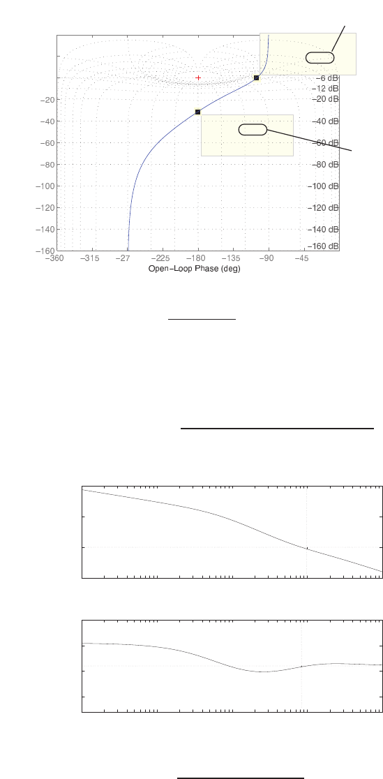
480 CHAPTER 9 Stability in the Frequency Domain

Nichols Chart

Open

0 0

System: sys

Gain (dB): 4

Phase (deg):

Frequency (rad/sec): 1.44

System: sys

Gain (dB):

Phase (deg):

Frequency (rad/sec): 0.122

6 dB

3 dB

1 dB

0.5 dB

0.25 dB 0 dB

Gain margin = 31.4 dB

Phase margin = 180-105=75o

FIGURE P9.19

Nichols diagram for Gc(s)G(s) = 0.5

s(2s+1)(s+4) .

P9.20 (a) Let K= 100. The Bode plot is shown in Figure P9.20a. The loop

transfer function is

Gc(s)G(s) = K(s2+ 1.5s+ 0.5)

s(20s+ 1)(10s+ 1)(0.5s+ 1) .

-50

100

10-3 10-2 10-1 100101

Frequency (rad/sec)

Gain dB

-300

-200

-100

10-3 10-2 10-1 100101

Frequency (rad/sec)

Phase deg

FIGURE P9.20

(a) Bode diagram for Gc(s)G(s) = K(s2+1.5s+0.5)

s(20s+1)(10s+1)(0.5s+1) , where K= 100.

from the publisher prior to any prohibited reproduction, storage in a retrieval system, or transmission in any form or by any means, electronic, mechanical, photocopying,

recording, or likewise. For information regarding permission(s), write to: Rights and Permissions Department, Pearson Education, Inc., Upper Saddle River, NJ 07458.

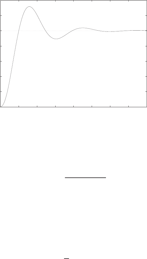
Problems 481

(b) The phase margin is P.M. =−3.5oand the gain margin is G.M. = 2.7

dB.

the phase margin P.M. = 37.9o.

(d) The step response is shown in Figure P9.20b for K= 0.1.

0.2

0.4

0.6

0.8

1.2

1.4

0 50 100 150 200 250 300 350 400

Time (secs)

Amplitude

FIGURE P9.20

CONTINUED: (b) Unit step response K= 0.1.

P9.21 The loop transfer function is

Gc(s)G(s) = K

s(s+ 1)(s+ 4) .

(a) The Bode plot is shown in Figure P9.21 for K= 4.

(b) The gain margin is

G.M. = 14 dB .

G.M. = 12 dB .

(d) We require Kv>3, but Kv=K

4. So, we need K > 12. This gain can

be utilized since K < 20 is required for stability.

from the publisher prior to any prohibited reproduction, storage in a retrieval system, or transmission in any form or by any means, electronic, mechanical, photocopying,

recording, or likewise. For information regarding permission(s), write to: Rights and Permissions Department, Pearson Education, Inc., Upper Saddle River, NJ 07458.

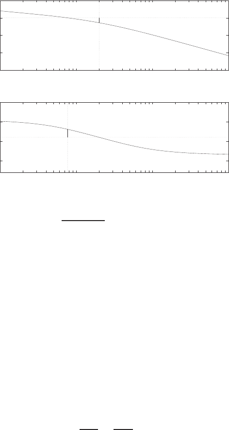
482 CHAPTER 9 Stability in the Frequency Domain

-150

-100

-50

10-1 100101102

Frequency (rad/sec)

Gain dB

-300

-200

-100

10-1 100101102

Frequency (rad/sec)

Phase deg

FIGURE P9.21

Bode diagram for Gc(s)G(s) = K

s(s+1)(s+4) , where K= 4.

P9.22 (a) The resonant frequency ωr= 5.2 rad/sec is point 6 on the Nichol’s

chart.

(b) The bandwidth is between points 8 and 9. We estimate the bandwidth

to be ωB= 7.5 rad/sec.

(d) The gain margin G.M. = 8 dB.

(e) Since we have P.M. = 30o, then we estimate ζ= 0.3. We can also

approximate

ωn≈ωr= 5.2.ap9.1

Thus,

Ts=4

ζωn

1.56 = 2.5sec .

P9.23 The phase margin is P.M. = 60 deg when K= 266. The gain margin is

G.M. = 17.2 dB .

The Bode plot is shown in Figure P9.23.

from the publisher prior to any prohibited reproduction, storage in a retrieval system, or transmission in any form or by any means, electronic, mechanical, photocopying,

recording, or likewise. For information regarding permission(s), write to: Rights and Permissions Department, Pearson Education, Inc., Upper Saddle River, NJ 07458.

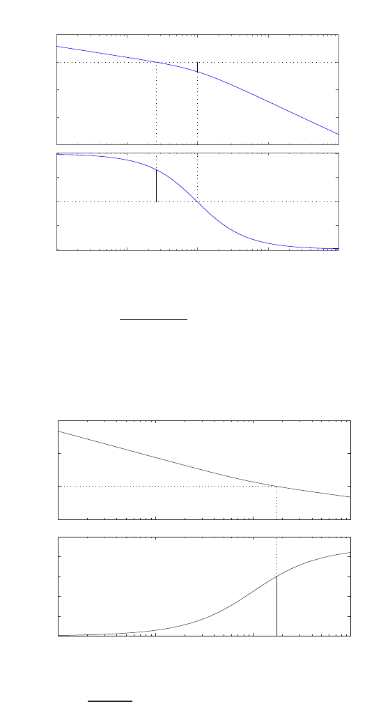
Problems 483

−150

−100

−50

Magnitude (dB)

10−1 100101102103

−270

−225

−180

−135

−90

Phase (deg)

Bode Diagram

Gm = 17.2 dB (at 9.8 rad/sec) , Pm = 60 deg (at 2.58 rad/sec)

Frequency (rad/sec)

FIGURE P9.23

Bode diagram for Gc(s)G(s) = K

s(s+8)(s+12) , where K= 266.

P9.24 When K= 14.1, then P.M. = 45 deg, G.M. =∞dB and ωB= 29.3

rad/sec.

Frequency (rad/sec)

Phase (deg); Magnitude (dB)

- 50

100

Gm=356.59 dB (at 0 rad/sec), Pm=60 deg. (at 17.321 rad/sec)

10- 110010 1102

- 180

- 160

- 140

- 120

- 100

- 80

FIGURE P9.24

Bode diagram for G(s) = K(s+20)

s2, where K= 14.1.

P9.25 The phase margin is P.M. = 60 deg when K= 2.61 and T= 0.2 second.

The Bode plot is shown in Figure P9.25.

from the publisher prior to any prohibited reproduction, storage in a retrieval system, or transmission in any form or by any means, electronic, mechanical, photocopying,

recording, or likewise. For information regarding permission(s), write to: Rights and Permissions Department, Pearson Education, Inc., Upper Saddle River, NJ 07458.

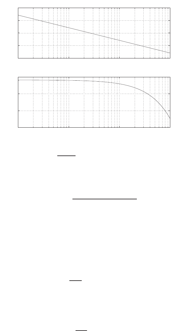
484 CHAPTER 9 Stability in the Frequency Domain

10-1 100101102

-40

-20

K=2.61; PM=60.09 at wc=2.61 rad/sec

Frequency (rad/sec)

Gain dB

10-1 100101102

-1500

-1000

-500

Frequency (rad/sec)

Phase deg

FIGURE P9.25

Bode diagram for Gc(s)G(s) = Ke−0.2s

s, where K= 2.61.

P9.26 The loop transfer function is

Gc(s)G(s) = K

s(0.25s+ 1)(0.1s+ 1) .

The Bode plot is shown in Figure P9.26a for K= 10. The Nichols chart

is shown in Figure P9.26b. The phase and gain margins are

P.M. = 9oand G.M. = 3 dB .

The system bandwidth is ωB= 8 rad/sec. From the P.M. = 9o, we

estimate ζ= 0.09. Therefore, the predicted overshoot is

P.O. = 100e−πζ/√1−ζ2= 75% ,where ζ= 0.09 .

The resonant peak occurs at ωr= 5.5 rad/sec. If we estimate ωn≈ωr=

5.5 rad/sec, then the settling time is

Ts=4

ζωn

= 8 sec .

from the publisher prior to any prohibited reproduction, storage in a retrieval system, or transmission in any form or by any means, electronic, mechanical, photocopying,

recording, or likewise. For information regarding permission(s), write to: Rights and Permissions Department, Pearson Education, Inc., Upper Saddle River, NJ 07458.

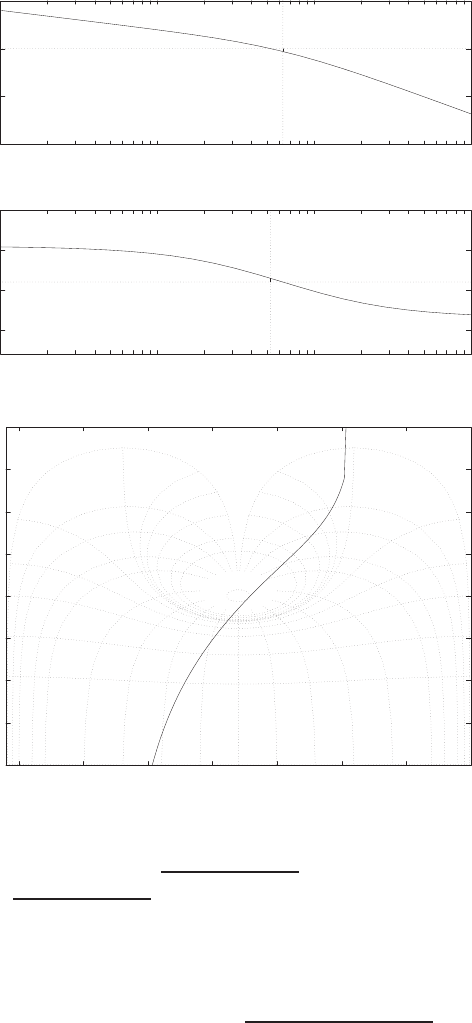
Problems 485

-100

-50

10-1 100101102

Frequency (rad/sec)

Gain dB

-300

-200

-100

10-1 100101102

Frequency (rad/sec)

Phase deg

-40

-30

-20

-10

-350 -300 -250 -200 -150 -100 -50 0

-40

-20

-12

-6

-3

-1

0.25

0.5

Phase (deg)

Gain dB

FIGURE P9.26

(a) Bode diagram for Gc(s)G(s) = K

s(0.25s+1)(0.1s+1) , where K= 10. (b) Nichols chart

for Gc(s)G(s) = K

s(0.25s+1)(0.1s+1) , where K= 10.

P9.27 The loop transfer function is

L(s) = Gc(s)G(s)H(s) = 4K

(s2+ 2s+ 4)(s+ 1) .

The plot of the phase margin versus the gain Kis shown in Figure P9.27.

As the gain increases towards Kmax = 3.5, the phase margin decreases

from the publisher prior to any prohibited reproduction, storage in a retrieval system, or transmission in any form or by any means, electronic, mechanical, photocopying,

recording, or likewise. For information regarding permission(s), write to: Rights and Permissions Department, Pearson Education, Inc., Upper Saddle River, NJ 07458.

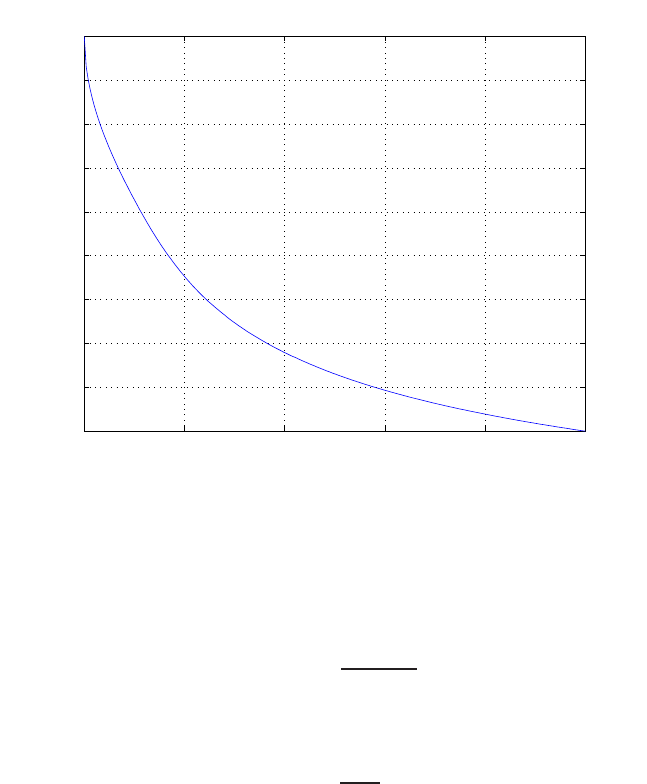
486 CHAPTER 9 Stability in the Frequency Domain

towards zero.

1 1.5 2 2.5 3 3.5

100

120

140

160

180

Phase margin (deg)

FIGURE P9.27

Phase margin versus the gain K.

P9.28 The loop transfer function is

Gc(s)G(s) = KP

s(s+ 1) .

When KP= 1.414, we have P.M. ≈45◦. Using the approximation that

ζ≈P.M./100 we estimate that ζ= 0.45. Then using the design formula

P.O. = 100e−πζ/√1−ζ2= 20.5% .

The actual overshoot is 23.4%. The step input response is shown in Fig-

ure P9.28. The actual damping ratio is ζ= 0.42. This shows that the

approximation ζ≈P.M./100 is quite applicable and useful in predicting

the percent overshoot.

from the publisher prior to any prohibited reproduction, storage in a retrieval system, or transmission in any form or by any means, electronic, mechanical, photocopying,

recording, or likewise. For information regarding permission(s), write to: Rights and Permissions Department, Pearson Education, Inc., Upper Saddle River, NJ 07458.

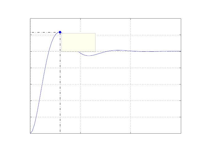
Problems 487

Step Response

Time (sec)

Amplitude

0 5 10 15

0.2

0.4

0.6

0.8

1.2

1.4

System: syscl

Peak amplitude: 1.23

Overshoot (%): 23.3

At time (sec): 2.97

FIGURE P9.28

Step response showing a 23.3% overshoot.

from the publisher prior to any prohibited reproduction, storage in a retrieval system, or transmission in any form or by any means, electronic, mechanical, photocopying,

recording, or likewise. For information regarding permission(s), write to: Rights and Permissions Department, Pearson Education, Inc., Upper Saddle River, NJ 07458.

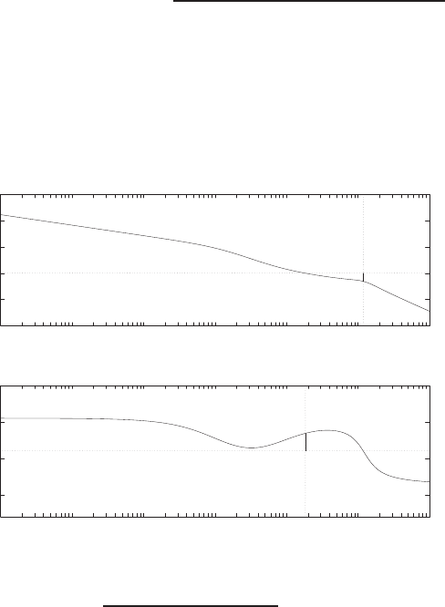
488 CHAPTER 9 Stability in the Frequency Domain

Advanced Problems

AP9.1 The loop transfer function is

L(s) = Gc(s)G(s)H(s) = 236607.5(s+ 10)(s+ 5)

s(s+ 2)(s2+ 100s+ω2

n)(s+ 1) .

(a) The Bode plot for

ω2

n= 15267

is shown in Figure AP9.1a.

-100

-50

100

150

10-3 10-2 10-1 100101102103

Frequency (rad/sec)

Gain dB

-300

-200

-100

10-3 10-2 10-1 100101102103

Frequency (rad/sec)

Phase deg

FIGURE AP9.1

(a) Bode Diagram for L(s) = 236607.5(s+10)(s+5)

s(s+2)(s2+100s+ω2

n)(s+1) , where ω2

n= 15267.

The phase and gain margins are

P.M. = 48.6oand G.M. = 15.5 dB .

(b) The Bode plot for ω2

n= 9500 is shown in Figure AP9.1b. The gain

and phase margins are

P.M. = 48.5oand G.M. = 10.9 dB .

Reducing the natural frequency by 38% has the eﬀect of reducing the

gain margin by 30%.

from the publisher prior to any prohibited reproduction, storage in a retrieval system, or transmission in any form or by any means, electronic, mechanical, photocopying,

recording, or likewise. For information regarding permission(s), write to: Rights and Permissions Department, Pearson Education, Inc., Upper Saddle River, NJ 07458.

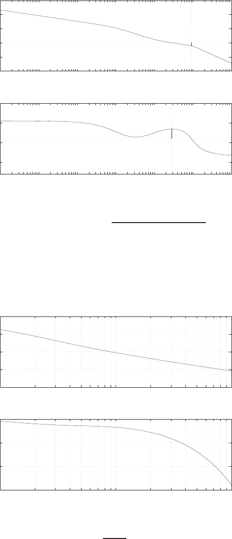
Advanced Problems 489

-100

-50

100

150

10-3 10-2 10-1 100101102103

Frequency (rad/sec)

Gain dB

-300

-200

-100

10-3 10-2 10-1 100101102103

Frequency (rad/sec)

Phase deg

FIGURE AP9.1

CONTINUED: (b) Bode Diagram for L(s) = 236607.5(s+10)(s+5)

s(s+2)(s2+100s+ω2

n)(s+1) , where ω2

n= 9500.

AP9.2 (a) The Bode plot with T= 0.05 sec is shown in Figure AP9.2a. The

phase margin is P.M. = 47.7oand the gain margin is G.M. = 11.2

dB.

-40

-20

100101102

Gain dB

Frequency (rad/s)

-400

-300

-200

-100

100101102

Phase deg

Frequency (rad/s)

FIGURE AP9.2

(a) Bode Diagram for Gc(s)G(s)H(s) = 8 (s+5)

s(s+2) e−sT, where T= 0.05s.

from the publisher prior to any prohibited reproduction, storage in a retrieval system, or transmission in any form or by any means, electronic, mechanical, photocopying,

recording, or likewise. For information regarding permission(s), write to: Rights and Permissions Department, Pearson Education, Inc., Upper Saddle River, NJ 07458.

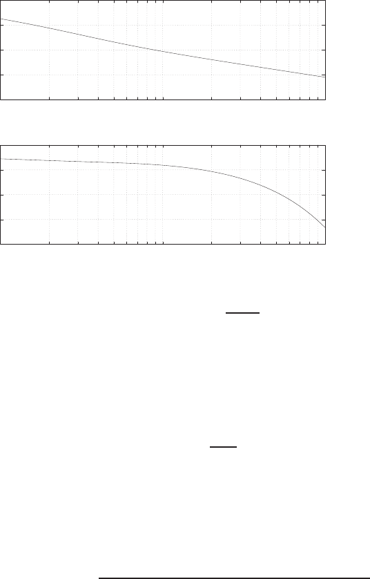
490 CHAPTER 9 Stability in the Frequency Domain

(b) The Bode plot with T= 0.1 sec is shown in Figure AP9.2b. The

-40

-20

100101102

Gain dB

Frequency (rad/s)

-800

-600

-400

-200

100101102

Phase deg

Frequency (rad/s)

FIGURE AP9.2

CONTINUED: (b) Bode Diagram for Gc(s)G(s)H(s) = 8 (s+5)

s(s+2) e−sT , where T= 0.1s.

phase margin is P.M. = 22.1oand the gain margin is G.M. = 4.18

dB. A 100% increase in time delay Tleads to a 50% decrease in phase

and gain margins.

P.O. ≈100e−πζ/√1−ζ2.

So, for T= 0.05 sec, ζ≈0.47 and P.O. ≈18.7%. Also, for T= 0.1

sec, ζ≈0.22 and P.O. ≈49.2%.

AP9.3 The loop transfer function is

L(s) = Gc(s)G(s)H(s) = 66K(1 + 0.1s)

(1 + 0.01s)(1 + 0.01s)(1 + 1.5s)(1 + 0.2s).

(a) When K= 1, the gain and phase margins are

G.M. = 18.4 dB and P.M. = 55o.

(b) When K= 1.5, the gain and phase margins are

G.M. = 14.9 dB and P.M. = 47.8o.

from the publisher prior to any prohibited reproduction, storage in a retrieval system, or transmission in any form or by any means, electronic, mechanical, photocopying,

recording, or likewise. For information regarding permission(s), write to: Rights and Permissions Department, Pearson Education, Inc., Upper Saddle River, NJ 07458.

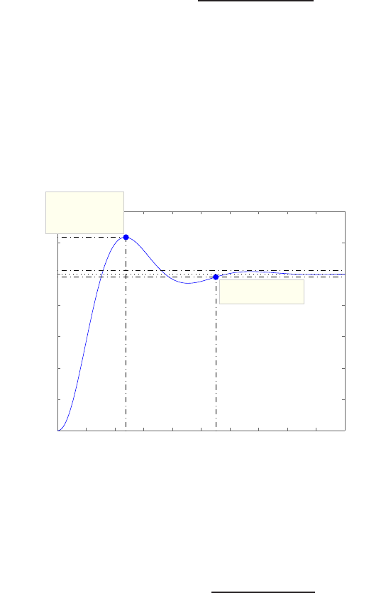
Advanced Problems 491

(c,d) The bandwidth and settling time with K= 1 are ωB= 233.6

rad/sec and Ts= 0.4 second. When K= 1.5, we determine that

ωB= 294.20 rad/sec and Ts= 0.33 second.

AP9.4 The loop transfer function is

L(s) = Gc(s)G(s) = K(s+ 40)

s(s+ 15)(s+ 10) .

The gain K= 28.8 satisﬁes the speciﬁcations. The actual gain and phase

margins are

G.M. = 18.8 dB and P.M. = 45o.

The system bandwidth is ωB= 10.3 rad/sec. The step response is shown

in Figure AP9.4.

Step Response

Time (sec)

Amplitude

0 0.2 0.4 0.6 0.8 1 1.2 1.4 1.6 1.8 2

0.2

0.4

0.6

0.8

1.2

1.4

System: sys_cl

Peak amplitude: 1.23

Overshoot (%): 23.4

At time (sec): 0.476

System: sys_cl

Settling Time (sec): 1.1

FIGURE AP9.4

Closed-loop system step response.

AP9.5 The loop transfer function is

L(s) = Gc(s)G(s) = Ks+ 0.4

s4+ 9s3+ 18s2.

The Bode plot for K= 1 is shown in Figure AP9.5. From the phase

response, we determine that the maximum P.M. ≈41o. From the mag-

nitude response (for K= 1), we ﬁnd that the gain needs to be raised to

K= 14 to achieve maximum phase margin at ω= 0.826 rad/sec. The

from the publisher prior to any prohibited reproduction, storage in a retrieval system, or transmission in any form or by any means, electronic, mechanical, photocopying,

recording, or likewise. For information regarding permission(s), write to: Rights and Permissions Department, Pearson Education, Inc., Upper Saddle River, NJ 07458.

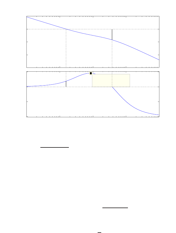
492 CHAPTER 9 Stability in the Frequency Domain

gain and phase margin with K= 14 are

G.M. = 19.3 dB and P.M. = 40.9o.

Also, the overshoot is P.O. = 38.3%.

−150

−100

−50

Magnitude (dB)

10−2 10−1 100101102

−270

−225

−180

−135

System: sys

Frequency (rad/sec): 0.865

Phase (deg): −139

Phase (deg)

Bode Diagram

Gm = 42.3 dB (at 3.79 rad/sec) , Pm = 16.7 deg (at 0.154 rad/sec)

Frequency (rad/sec)

FIGURE AP9.5

Bode plot for L(s) = Ks+0.4

s4+9s3+18s2with K= 1.

AP9.6 With D > 2m, the gain can be increased up to K= 100, while still

retaining stability.

AP9.7 The loop transfer function is

L(s) = Gc(s)G(s) = K(s+ 4)

s2.

We select

K= 2√2

for P.M. = 45o. The system bandwidth is

ωB= 5.88 rad/sec .

The disturbance response is shown in Figure AP9.7. The maximum output

due to a disturbance is y(t) = 0.11.

from the publisher prior to any prohibited reproduction, storage in a retrieval system, or transmission in any form or by any means, electronic, mechanical, photocopying,

recording, or likewise. For information regarding permission(s), write to: Rights and Permissions Department, Pearson Education, Inc., Upper Saddle River, NJ 07458.

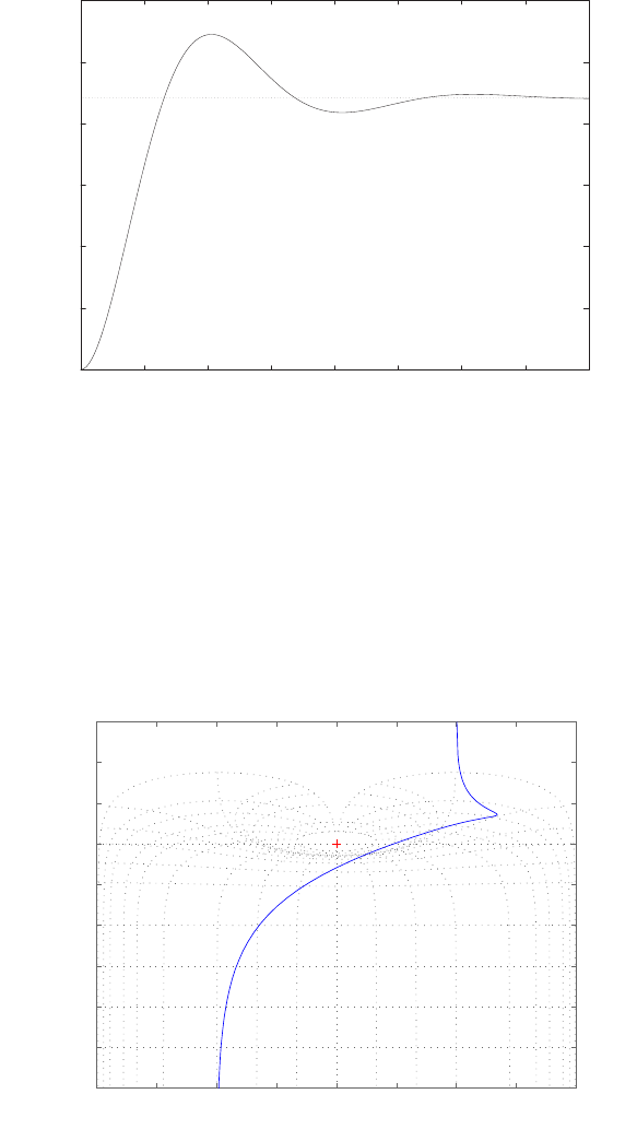
Advanced Problems 493

0.02

0.04

0.06

0.08

0.1

0.12

0 0.5 1 1.5 2 2.5 3 3.5 4

Time (secs)

Amplitude

FIGURE AP9.7

Closed-loop system disturbance response.

AP9.8 A reasonable choice for the gain is K= 2680. The phase margin is P.M. =

42.8◦and the percent overshoot is P.O. = 18.9%. The Nichols chart is

shown in Figure AP9.8.

Nichols Chart

Open−Loop Phase (deg)

Open−Loop Gain (dB)

−360 −315 −270 −225 −180 −135 −90 −45 0

−120

−100

−80

−60

−40

−20

6 dB

3 dB

1 dB

0.5 dB

0.25 dB 0 dB

−1 dB

−3 dB

−6 dB

−12 dB

−20 dB

−40 dB

−60 dB

−80 dB

−100 dB

−120 dB

FIGURE AP9.8

Nichols chart.

from the publisher prior to any prohibited reproduction, storage in a retrieval system, or transmission in any form or by any means, electronic, mechanical, photocopying,

recording, or likewise. For information regarding permission(s), write to: Rights and Permissions Department, Pearson Education, Inc., Upper Saddle River, NJ 07458.

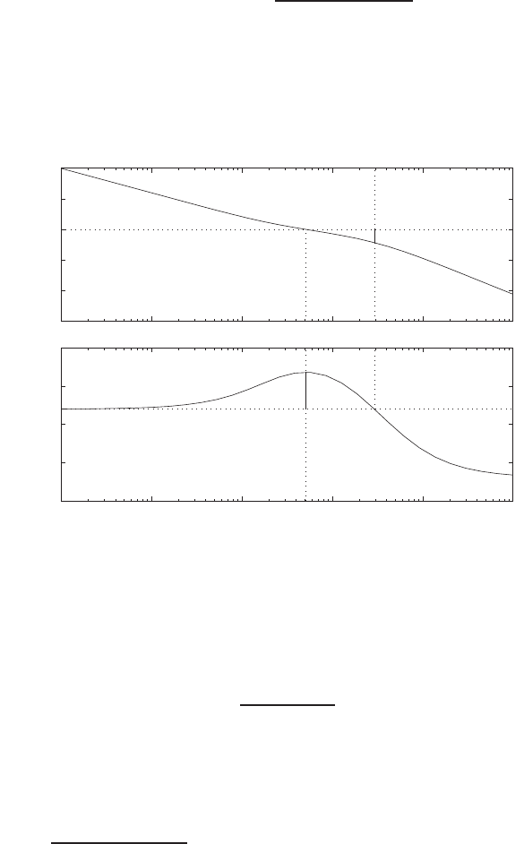
494 CHAPTER 9 Stability in the Frequency Domain

AP9.9 The loop transfer function is

L(s) = Gc(s)G(s) = Kp(s+ 0.2)

s2(s2+ 7s+ 10) .

At the maximum phase margin, Kp= 4.9 for P.M. = 48.6o. The Bode

diagram is shown in Figure AP9.9.

Frequency (rad/sec)

Phase (deg); Magnitude (dB)

Bode Diagrams

-150

-100

-50

100

Gm=21.788 dB (at 2.9326 rad/sec), Pm=48.457 deg. (at 0.50782 rad/sec)

10-3 10-2 10-1 100101102

-300

-250

-200

-150

-100

FIGURE AP9.9

Phase and gain margin.

AP9.10 The closed-loop transfer function is

T(s) = K

s2+ 3s+ 1 .

We require K= 1 a zero steady-state tracking error to a unit step. The

step response is shown in Figure AP9.10. Computing T(jω) = 0.707 it

follows that



(jω)2+ 3jω + 1 

= 0.707 or ω4+ 7ω2−1 = 0 .

Solving for ωyields ω= 0.37 rad/s. This is the bandwidth of the system.

from the publisher prior to any prohibited reproduction, storage in a retrieval system, or transmission in any form or by any means, electronic, mechanical, photocopying,

recording, or likewise. For information regarding permission(s), write to: Rights and Permissions Department, Pearson Education, Inc., Upper Saddle River, NJ 07458.

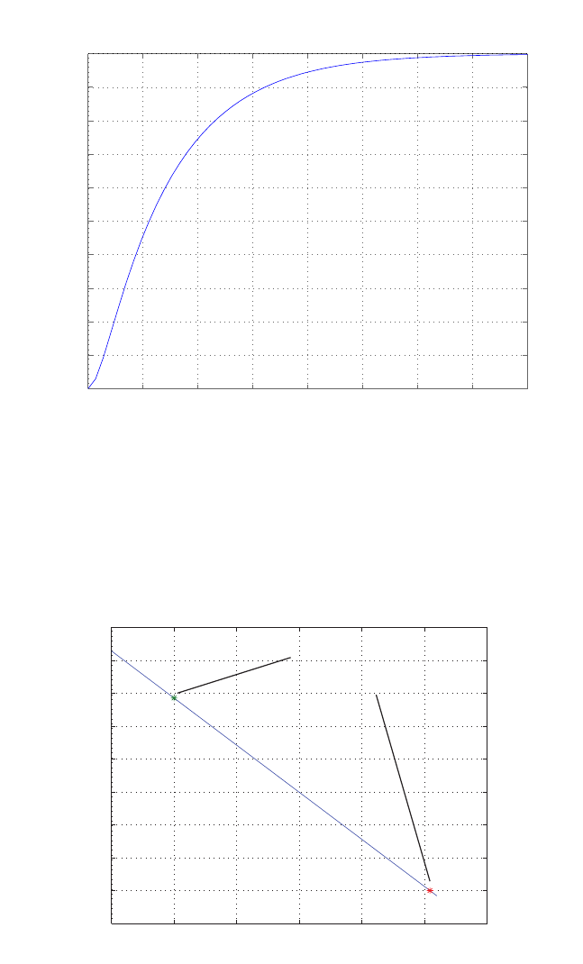
Advanced Problems 495

0 2 4 6 8 10 12 14 16

0.1

0.2

0.3

0.4

0.5

0.6

0.7

0.8

0.9

Step Response

Time (sec)

Amplitude

FIGURE AP9.10

Unit step response.

AP9.11 The phase margin versus time delay is shown in Figure AP9.11a.

0.5 1 1.5 2 2.5 3 3.5

−10

Time Delay (s)

Phase Margin (deg)

Time Delay=1 PM=58.5285

Time Delay=3.0455 PM=0.001

FIGURE AP9.11

Phase margin versus time delay.

from the publisher prior to any prohibited reproduction, storage in a retrieval system, or transmission in any form or by any means, electronic, mechanical, photocopying,

recording, or likewise. For information regarding permission(s), write to: Rights and Permissions Department, Pearson Education, Inc., Upper Saddle River, NJ 07458.

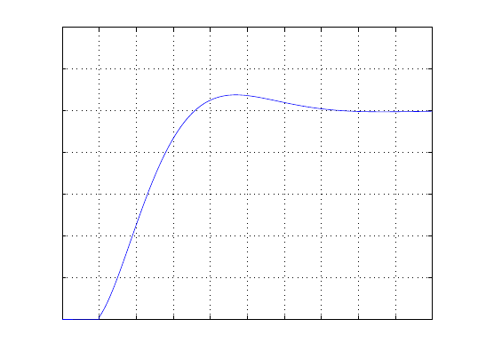
496 CHAPTER 9 Stability in the Frequency Domain

The maximum time delay is T= 3.04 s for stability. The step response is

shown in Figure AP9.11b. The percent overshoot is P.O. = 7.6%.

0 1 2 3 4 5 6 7 8 9 10

0.2

0.4

0.6

0.8

1.2

1.4

Time (sec)

Amplitude

FIGURE AP9.11

Unit step response.

from the publisher prior to any prohibited reproduction, storage in a retrieval system, or transmission in any form or by any means, electronic, mechanical, photocopying,

recording, or likewise. For information regarding permission(s), write to: Rights and Permissions Department, Pearson Education, Inc., Upper Saddle River, NJ 07458.

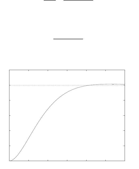
Design Problems 497

Design Problems

The plant model with parameters given in Table CDP2.1 in Dorf andCDP9.1

Bishop is given by:

θ(s)

Va(s)=26.035

s(s+ 33.142) ,

where we neglect the motor inductance Lmand where we switch oﬀ the

tachometer feedback (see Figure CDP4.1 in Dorf and Bishop). The closed-

loop system characteristic equation is

1 + 26.035Ka

s(s+ 33.142) = 0 .

The phase margin is P.M. = 70.4◦when Ka= 16. The step response with

K= 16 is shown below.

0 0.05 0.1 0.15 0.2 0.25 0.3

0.2

0.4

0.6

0.8

1.2

Time (secs)

Amplitude

DP9.1 (a) The gain and phase margins are G.M. = 7 dB and P.M. = 60o.

(b) The resonant peak and frequency are Mpω= 2 dB and ωr= 5 rad/sec.

(Figure 8.11 in Dorf & Bishop). Also, ωr/ωn= 0.8, so ωn= 6.25.

Thus, Ts= 1.4.

(d) We need P.O. = 30oor ζ= 0.3 or P.M. ≈30o. So, we need to raise

the gain by 10 dB or K= 3.2.

from the publisher prior to any prohibited reproduction, storage in a retrieval system, or transmission in any form or by any means, electronic, mechanical, photocopying,

recording, or likewise. For information regarding permission(s), write to: Rights and Permissions Department, Pearson Education, Inc., Upper Saddle River, NJ 07458.

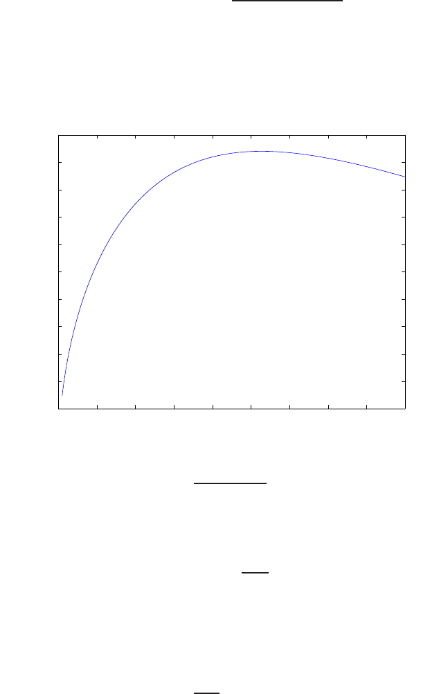
498 CHAPTER 9 Stability in the Frequency Domain

DP9.2 The loop transfer function is

L(s) = Gc(s)G(s) = K(s+ 0.5)

s2(s2+ 7.5s+ 9) .

When K= 6.25, we have the maximum phase margin. The phase mar-

gin maximum is P.M. = 23o. The plot of P.M. versus Kis shown in

Figure DP9.2a.

0123456789

Phase Margin deg

FIGURE DP9.2

(a) Phase margin versus Kfor L(s) = K(s+0.5)

s2(s2+7.5s+9) .

The predicted damping is ζ= 0.23. It then follows that the predicted

percent overshoot is

P.O. = 100e−πζ/√1−ζ2= 48% .

The actual overshoot is 65%. The step input response is shown in Fig-

ure DP9.2b. The resonant peak occurs at ωr= 0.75 rad/sec. Approxi-

mating ωn≈ωr= 0.75 rad/sec, we can estimate the settling time as

Ts=4

ζωn

= 23 sec .

The actual settling time is 20 sec.

from the publisher prior to any prohibited reproduction, storage in a retrieval system, or transmission in any form or by any means, electronic, mechanical, photocopying,

recording, or likewise. For information regarding permission(s), write to: Rights and Permissions Department, Pearson Education, Inc., Upper Saddle River, NJ 07458.

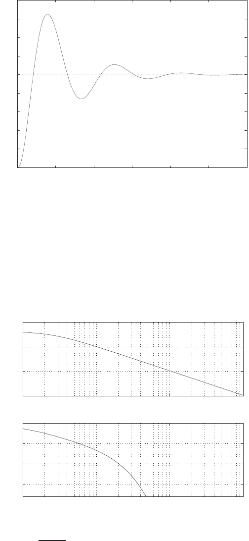
Design Problems 499

0.2

0.4

0.6

0.8

1.2

1.4

1.6

1.8

0 5 10 15 20 25 30

Time (secs)

Amplitude

FIGURE DP9.2

CONTINUE: (b) Closed-loop unit step response.

DP9.3 We want to select the gain Kas large as possible to reduce the steady-state

error, but we want a minimum phase margin of P.M. = 45oto achieve

good dynamic response. A suitable gain is K= 4.2, see Figure DP9.3.

10-2 10-1 100101

-300

-200

-100

Frequency (rad/sec)

Phase deg

10-2 10-1 100101

-40

-20

K=4.2; PM=45.34 at wc=0.102 rad/sec

Frequency (rad/sec)

Gain dB

FIGURE DP9.3

Bode plot for G(s) = Ke−10s

40s+1 .

from the publisher prior to any prohibited reproduction, storage in a retrieval system, or transmission in any form or by any means, electronic, mechanical, photocopying,

recording, or likewise. For information regarding permission(s), write to: Rights and Permissions Department, Pearson Education, Inc., Upper Saddle River, NJ 07458.

500 CHAPTER 9 Stability in the Frequency Domain

DP9.4 We are given the loop transfer function

L(s) = Gc(s)G(s) = K

s(s+ 1)(s+ 4)

which can be written as

Gc(s)G(s) = Kv

s(s+ 1)(0.25s+ 1) .

The performance results are summarized in Table DP9.4.

KvG.M. P.M. ωBP.O. Ts

(dB) (deg) (rad/sec) (%) (sec)

0.40 21.9 64.2 0.62 4.4 9.8

0.75 16.5 49.0 1.09 19.0 10.1

TABLE DP9.4 Summary for Kv= 0.40 and Kv= 0.75.

When Kv= 0.40, we have

ess

A=1

0.40 = 2.5,

or 2 1/2 times the magnitude of the ramp. This system would be accept-

able for step inputs, but unacceptable for ramp inputs.

DP9.5 (a) With a time delay of T= 0.8 second, we determine that the propor-

tional controller

Gc(s) = K= 7

provides a suitable response with

P.O. = 8.3 % ess = 12.5 % Ts= 4.38 sec .

(b) A suitable proportional, integral controller is

Gc(s) = K1+K2/s = 6 + 0.6/s .

from the publisher prior to any prohibited reproduction, storage in a retrieval system, or transmission in any form or by any means, electronic, mechanical, photocopying,

recording, or likewise. For information regarding permission(s), write to: Rights and Permissions Department, Pearson Education, Inc., Upper Saddle River, NJ 07458.

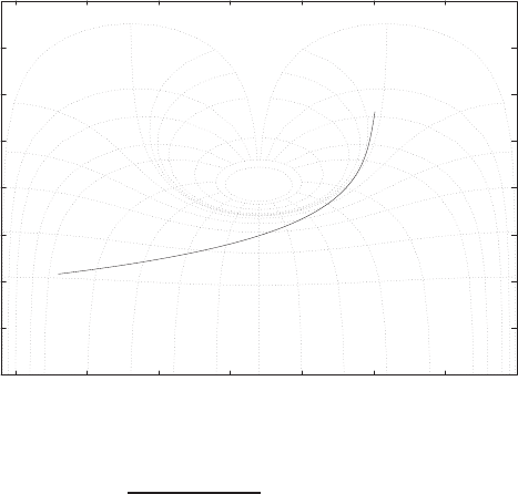
Design Problems 501

The response to a unit step is

P.O. = 5.14 % ess = 0 % Ts= 6.37 sec .

The Nichols chart is shown in Figure DP9.5.

-40

-30

-20

-10

-350 -300 -250 -200 -150 -100 -50 0

-40

-20

-12

-6

-3

-1

0.25

0.5

Phase (deg)

Gain dB

FIGURE DP9.5

Nichols chart for Gc(s)G(s) = (K1s+K2)e−0.8s

s(10s+1) , where K1= 6 and K2= 0.6.

DP9.6 With K= 170, at the two extreme values of b, we have

b= 80 P.M. = 91.62oG.M. = 13.66 dB

b= 300 P.M. = 75.23oG.M. = 25.67 dB .

Since reducing the value of Konly increases the P.M. and G.M., a value

K= 170

is suitable to meet P.M. = 40oand G.M. = 8 dB for the range of b.

DP9.7 A suitable gain is

K= 0.22 .

This results in P.M. = 60.17oand G.M. = 13.39 dB. The step reponse is

shown in Figure DP9.7.

from the publisher prior to any prohibited reproduction, storage in a retrieval system, or transmission in any form or by any means, electronic, mechanical, photocopying,

recording, or likewise. For information regarding permission(s), write to: Rights and Permissions Department, Pearson Education, Inc., Upper Saddle River, NJ 07458.

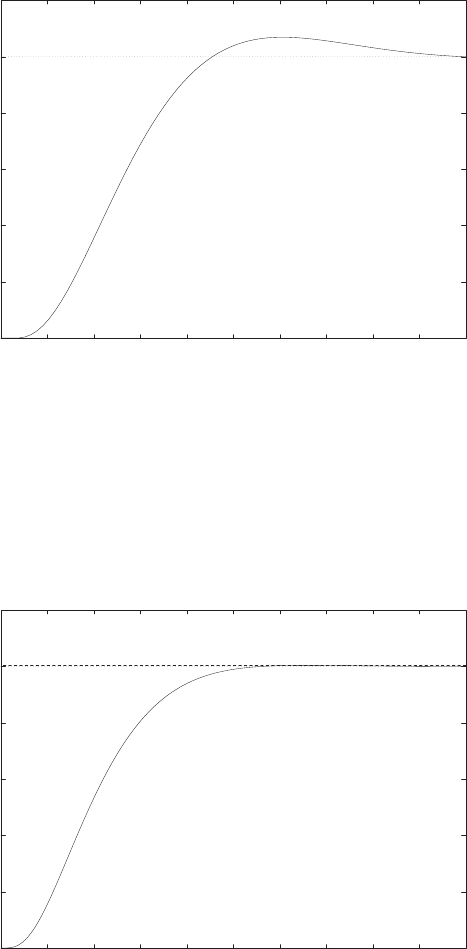
502 CHAPTER 9 Stability in the Frequency Domain

0.2

0.4

0.6

0.8

1.2

0 2 4 6 8 10 12 14 16 18 20

Time (secs)

Amplitude

FIGURE DP9.7

Lunar vehicle step response.

DP9.8 A gain of K= 315000 will satisfy the P.O. speciﬁcation, while giving the

fastest response. The step response is shown in Figure DP9.8.

0.2

0.4

0.6

0.8

1.2

0 0.1 0.2 0.3 0.4 0.5 0.6 0.7 0.8 0.9 1

Time (secs)

Amplitude

FIGURE DP9.8

Steel rolling mill step response.

from the publisher prior to any prohibited reproduction, storage in a retrieval system, or transmission in any form or by any means, electronic, mechanical, photocopying,

recording, or likewise. For information regarding permission(s), write to: Rights and Permissions Department, Pearson Education, Inc., Upper Saddle River, NJ 07458.

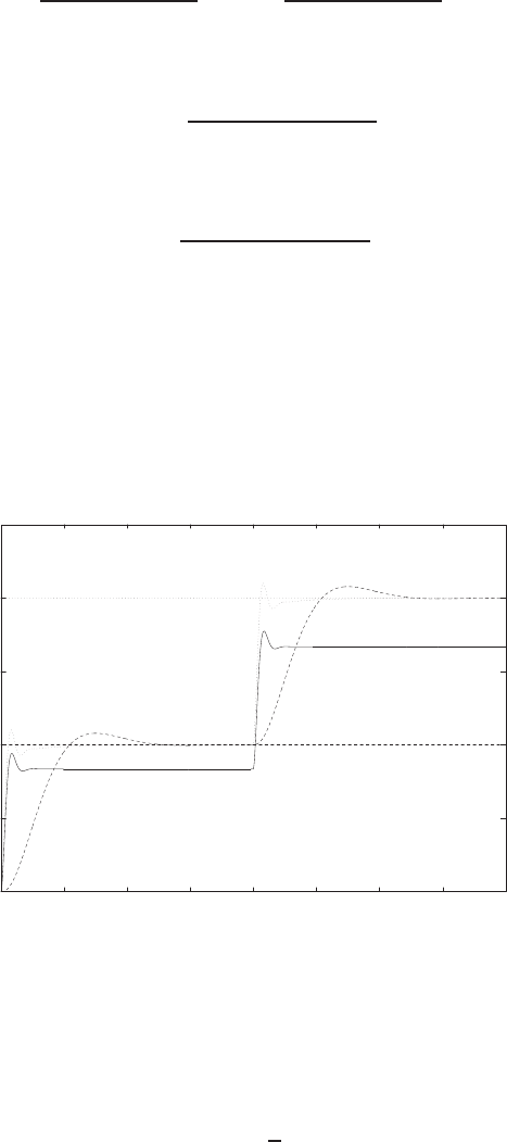
Design Problems 503

DP9.9 The closed-loop transfer function is

Ts(2) = G1(s)

1 + Gc(s)G2(s)To(s) + Gc(s)G2(s)

1 + Gc(s)G2(s)T2d(s).

where

G1(s) = 1

(10s+ 1)(50s+ 1)

and

G2(s) = 0.01

(10s+ 1)(50s+ 1) .

The steady-state error (with Gc(s) = 500) to a unit step 2A(and after

the system has settled out subsequent to a step of magnitude A) is

ess = 2(0.167) = 0.33 .

The step response is shown in Figure DP9.9.

0.5

1.5

2.5

0 200 400 600 800 1000 1200 1400 1600

Time (sec)

T2/A

Gc=500 (solid); Gc=1/s (dashed); Gc=600+6/s (dotted)

FIGURE DP9.9

Two tank temperature control step response.

A suitable integral controller is

Gc(s) = 1

from the publisher prior to any prohibited reproduction, storage in a retrieval system, or transmission in any form or by any means, electronic, mechanical, photocopying,

recording, or likewise. For information regarding permission(s), write to: Rights and Permissions Department, Pearson Education, Inc., Upper Saddle River, NJ 07458.

504 CHAPTER 9 Stability in the Frequency Domain

In this case, the steady-state tracking error is zero , since the system is a

type 1. The system response is shown in Figure DP9.9. With the integral

controller, the settling time is about Ts= 438 seconds and the P.O. = 7%.

A suitable PI controller is

Gc(s) = 600 + 6

With the PI controller, the settling time is about Ts= 150 seconds and

the P.O. = 10%.

DP9.10 The system is given by

x=Ax +Br

y=Cx

where

A=



0 1

2−K13−K2

,B=



1

,and C=1 0 .

The associated transfer function is

T(s) = 1

s2+ (K2−3)s+K1−2.

The characteristic polynomial is

s2+ (K2−3)s+K1−2 = 0 .

If we select K1= 3, then we have a zero-steady error to a unit step

response R(s) = 1/s, since

lim

s→0s[1 −T(s)] R(s) = lim

s→0

s2+ (K2−3)s

s2+ (K2−3)s+K1−2= 0 .

Let

K=3 4.3.

The step response is shown in Figure DP9.10a. The bandwidth is ωb=

1.08 rad/s, as seen in Figure DP9.10b.

from the publisher prior to any prohibited reproduction, storage in a retrieval system, or transmission in any form or by any means, electronic, mechanical, photocopying,

recording, or likewise. For information regarding permission(s), write to: Rights and Permissions Department, Pearson Education, Inc., Upper Saddle River, NJ 07458.

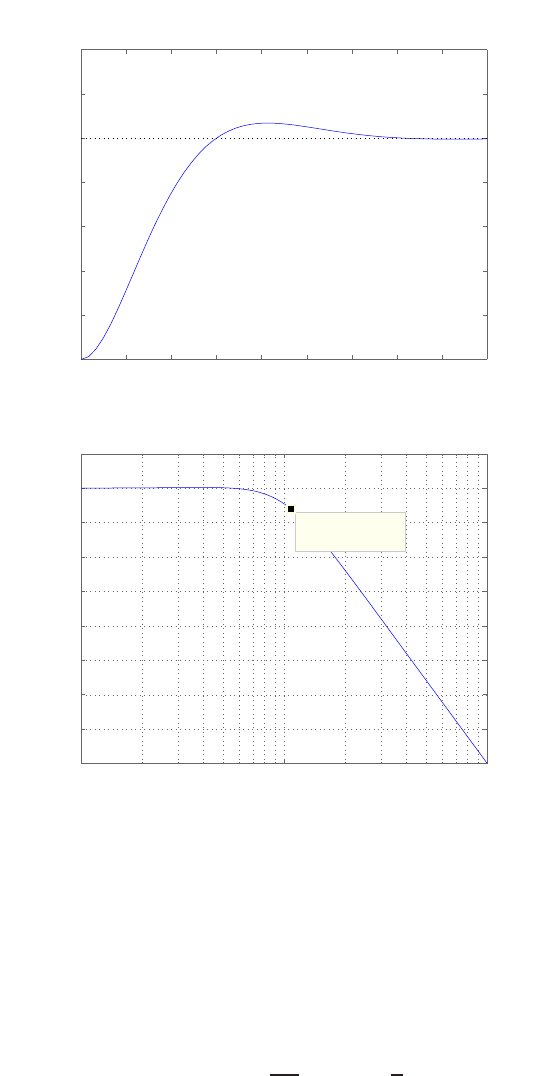
Design Problems 505

0 1 2 3 4 5 6 7 8 9

0.2

0.4

0.6

0.8

1.2

1.4

Step Response

Time (sec)

Amplitude

Bode Diagram

Frequency (rad/sec)

10−1 100101

−40

−35

−30

−25

−20

−15

−10

−5

System: sys

Frequency (rad/sec): 1.08

Magnitude (dB): −3

Magnitude (dB)

FIGURE DP9.10

Step response with K= [3 4.3] and closed-loop Bode plot.

DP9.11 A time domain step response speciﬁcation P.O. > 10% requires the dom-

inant poles to have a damping ration of ζ= 0.6. This time domain spec-

iﬁcation can be transformed to a frequency response speciﬁcation using

the approximation P.M. ≈100ζ= 60◦. To keep the problem tractable,

we consider the controller with the form

Gc(s) = KP+KI

s=KP+1

where we let KI= 1. The plot of the P.M. as a function of KPis shown

from the publisher prior to any prohibited reproduction, storage in a retrieval system, or transmission in any form or by any means, electronic, mechanical, photocopying,

recording, or likewise. For information regarding permission(s), write to: Rights and Permissions Department, Pearson Education, Inc., Upper Saddle River, NJ 07458.

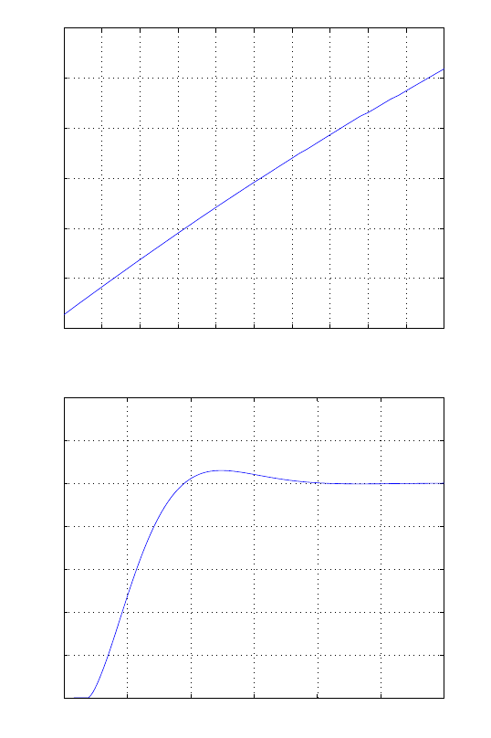
506 CHAPTER 9 Stability in the Frequency Domain

in Figure DP9.11a. If we select KP= 0.07 we expect a phase margin

of approximately 60◦, hence a percent overshoot P.O. ≤10%. The step

response is shown in Figure DP9.11b. The actual phase margin is P.M. =

60.2◦, the percent overshoot is P.O. = 5.9% and the settling time is

Ts= 3.4 sec.

0 0.05 0.1 0.15 0.2 0.25 0.3 0.35 0.4 0.45 0.5

Phase Margin (deg)

0123456

0.2

0.4

0.6

0.8

1.2

1.4

Time (sec)

Amplitude

FIGURE DP9.11

(a) Phase margin versus controller gain KPand KI= 1. (b) Step response with KP= 0.07

and KI= 1.

from the publisher prior to any prohibited reproduction, storage in a retrieval system, or transmission in any form or by any means, electronic, mechanical, photocopying,

recording, or likewise. For information regarding permission(s), write to: Rights and Permissions Department, Pearson Education, Inc., Upper Saddle River, NJ 07458.

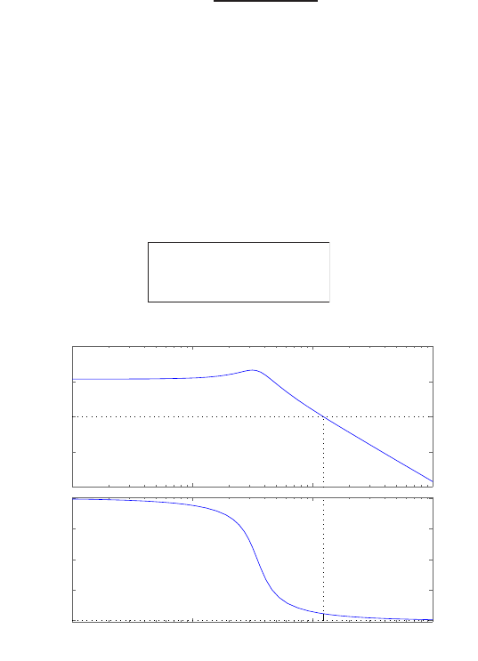
Computer Problems 507

Computer Problems

CP9.1 The m-ﬁle script to generate the Bode plot (from which the gain and

phase margin can be determined) is shown in Figure CP9.1. The transfer

function is

G(s) = 141

s2+ 2s+ 12 .

The gain margin is

G.M. =∞

and the phase margin is

P.M. = 10o.

num=141; den=[1 2 12];

sys = tf(num,den);

margin(sys);

−40

−20

Magnitude (dB)

10−1 100101102

−180

−135

−90

−45

Phase (deg)

Bode Diagram

Gm = Inf dB (at Inf rad/sec) , Pm = 10 deg (at 12.3 rad/sec)

Frequency (rad/sec)

FIGURE CP9.1

Gain and phase margin with the margin function.

from the publisher prior to any prohibited reproduction, storage in a retrieval system, or transmission in any form or by any means, electronic, mechanical, photocopying,

recording, or likewise. For information regarding permission(s), write to: Rights and Permissions Department, Pearson Education, Inc., Upper Saddle River, NJ 07458.

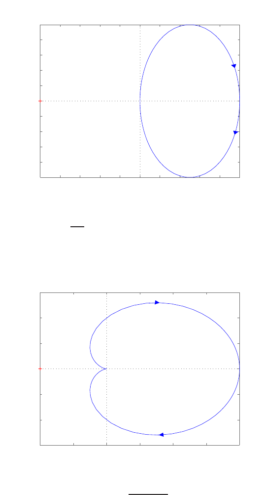
508 CHAPTER 9 Stability in the Frequency Domain

CP9.2 The Nyquist plots are shown in Figures CP9.2a-c.

−1 −0.8 −0.6 −0.4 −0.2 0 0.2 0.4 0.6 0.8 1

−0.5

−0.4

−0.3

−0.2

−0.1

0.1

0.2

0.3

0.4

0.5

num=[5]; den=[1 5]; sys=tf(num,den); nyquist(sys)

Real Axis

Imaginary Axis

FIGURE CP9.2

(a) Nyquist plot for G(s) = 5

s+5 .

−1 −0.5 0 0.5 1 1.5 2

−1.5

−1

−0.5

0.5

1.5

num=[50]; den=[1 10 25]; sys=tf(num,den); nyquist(sys)

Real Axis

Imaginary Axis

FIGURE CP9.2

CONTINUED: (b) Nyquist plot for G(s) = 50

s2+10s+25 .

from the publisher prior to any prohibited reproduction, storage in a retrieval system, or transmission in any form or by any means, electronic, mechanical, photocopying,

recording, or likewise. For information regarding permission(s), write to: Rights and Permissions Department, Pearson Education, Inc., Upper Saddle River, NJ 07458.

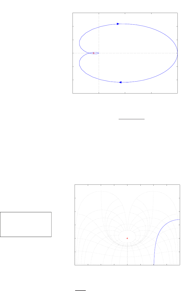
Computer Problems 509

−5 0 5 10 15

−15

−10

−5

num=[15]; den=[1 3 3 1]; sys=tf(num,den); nyquist(sys)

Real Axis

Imaginary Axis

FIGURE CP9.2

CONTINUED: (c) Nyquist plot for G(s) = 15

s3+3s2+3s+1 .

CP9.3 The m-ﬁle script to generate the Nichols chart for part (a) is shown in

Figure CP9.3a. The Nichols charts for (b) and (c) are similiarly generated;

all plots are in Figure CP9.3a-c.

num = [1]; den = [1 0.2];

sys = tf(num,den);

nichols(sys)

ngrid

−360 −315 −270 −225 −180 −135 −90 −45 0

−20

−10

6 dB

3 dB

1 dB

0.5 dB

0.25 dB

0 dB

−1 dB

−3 dB

−6 dB

−12 dB

−20 dB

Nichols Chart

Open−Loop Phase (deg)

Open−Loop Gain (dB)

FIGURE CP9.3

(a) M-ﬁle script and Nichols chart for G(s) = 1

s+0.1.

from the publisher prior to any prohibited reproduction, storage in a retrieval system, or transmission in any form or by any means, electronic, mechanical, photocopying,

recording, or likewise. For information regarding permission(s), write to: Rights and Permissions Department, Pearson Education, Inc., Upper Saddle River, NJ 07458.

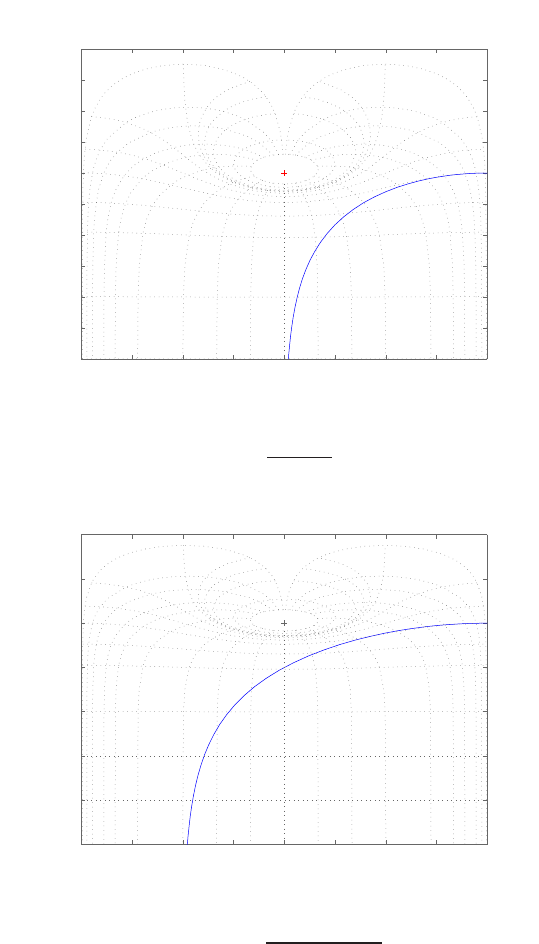
510 CHAPTER 9 Stability in the Frequency Domain

The gain and phase margin for each transfer function are as follows:

(a) G.M. =∞and P.M. = 102o

(b) G.M. =∞and P.M. =∞

−360 −315 −270 −225 −180 −135 −90 −45 0

−60

−50

−40

−30

−20

−10

6 dB

3 dB

1 dB

0.5 dB

0.25 dB

0 dB

−1 dB

−3 dB

−6 dB

−12 dB

−20 dB

−40 dB

−60 dB

Nichols Chart

Open−Loop Phase (deg)

Open−Loop Gain (dB)

FIGURE CP9.3

CONTINUED: (b) Nichols chart for G(s) = 1

s2+2s+1 .

−360 −315 −270 −225 −180 −135 −90 −45 0

−100

−80

−60

−40

−20

6 dB

3 dB

1 dB

0.5 dB

0.25 dB 0 dB

−1 dB

−3 dB

−6 dB

−12 dB

−20 dB

−40 dB

−60 dB

−80 dB

−100 dB

Nichols Chart

Open−Loop Phase (deg)

Open−Loop Gain (dB)

FIGURE CP9.3

CONTINUED: (c) Nichols chart for G(s) = 24

s3+9s2+26s+24 .

from the publisher prior to any prohibited reproduction, storage in a retrieval system, or transmission in any form or by any means, electronic, mechanical, photocopying,

recording, or likewise. For information regarding permission(s), write to: Rights and Permissions Department, Pearson Education, Inc., Upper Saddle River, NJ 07458.

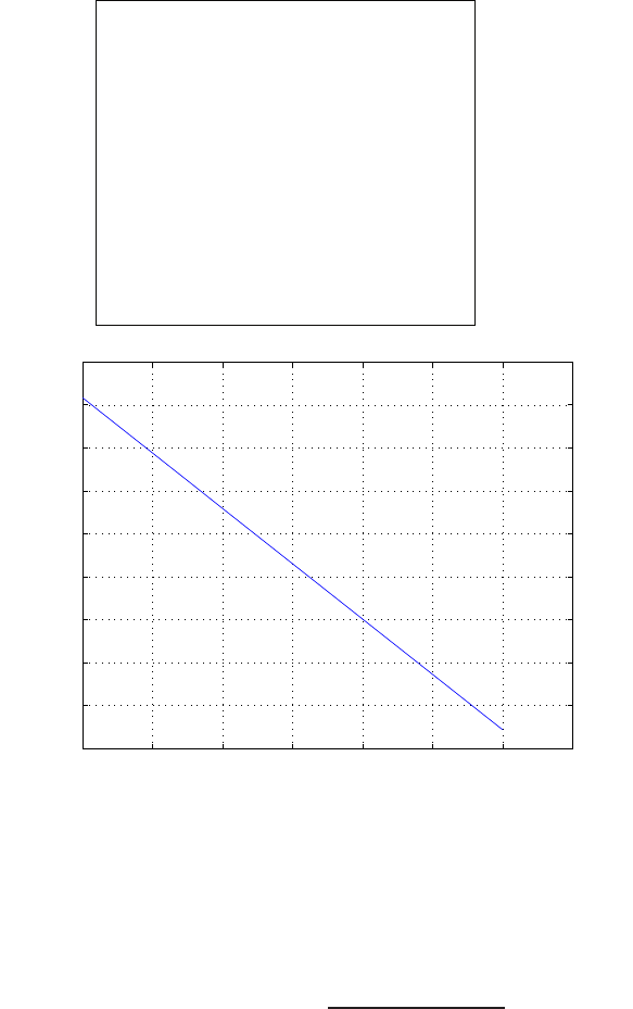
Computer Problems 511

CP9.4 To obtain a phase margin P.M. = 40◦we select

K= 15

when T= 0.2 second. The variation in the phase margin for 0 ≤T≤0.3

is shown in Figure CP9.4.

T=[0:0.01:0.3]; K=15;

num=K;den=[1 12]; sys = tf(num,den);

% w=logspace(-2,1,400);

for i=1:length(T)

[mag,phase,w]=bode(sys);

ph(1:length(phase))=phase(1,1,:); ph=ph';

ph2=ph-w*T(i)*180/pi;

[Gm,Pm,Wcg,Wcp]=margin(mag,ph2,w);

clear ph ph2

PMo(i)=Pm;

end

plot(T,PMo), grid

xlabel('Time delay (sec)')

ylabel('Phase margin (deg)')

0 0.05 0.1 0.15 0.2 0.25 0.3 0.35

−20

100

120

140

160

Time delay (sec)

Phase margin (deg)

K=15

FIGURE CP9.4

Variation in the phase margin for 0≤T≤0.3with K= 15.

CP9.5 The loop transfer function is

L(s) = Gc(s)G(s) = K(s+ 50)

s(s+ 20)(s+ 10) .

from the publisher prior to any prohibited reproduction, storage in a retrieval system, or transmission in any form or by any means, electronic, mechanical, photocopying,

recording, or likewise. For information regarding permission(s), write to: Rights and Permissions Department, Pearson Education, Inc., Upper Saddle River, NJ 07458.

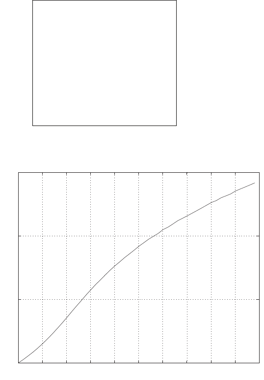
512 CHAPTER 9 Stability in the Frequency Domain

The plot of system bandwidth versus the gain Kis shown in Figure CP9.7.

K=[0.1:1:50];

w=logspace(-2,3,2000);

den=[1 30 200 0];

for i=1:length(K)

num=K(i)*[1 50]; sys = tf(num,den);

sys_cl = feedback(sys,[1]);

[mag,phase,w]=bode(sys_cl,w);

L=nd(mag<0.707); wb(i)=w(L(1));

end

plot(K,wb), grid

xlabel('Gain K')

ylabel('Bandwidth (rad/sec)')

0 5 10 15 20 25 30 35 40 45 50

Gain K

Bandwidth (rad/sec)

FIGURE CP9.5

Variation in the system bandwidth for 0≤K≤50.

CP9.6 The m-ﬁle script and Bode plot are shown in Figure CP9.6. The gain and

phase margin and ωcare determined to be G.M. = 2.23, P.M. = 26oand

ωc= 12.6 rad/sec. So, the maximum value of bois found to be

bomax = 2.13bo= 1.11 .

In this problem, there is also a minimum value of bo. Using the Routh-

from the publisher prior to any prohibited reproduction, storage in a retrieval system, or transmission in any form or by any means, electronic, mechanical, photocopying,

recording, or likewise. For information regarding permission(s), write to: Rights and Permissions Department, Pearson Education, Inc., Upper Saddle River, NJ 07458.

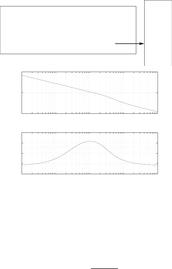
Computer Problems 513

numg = -0.5*[1 0 -2500]; deng = [1 47 850 -3000];

sysg = tf(numg,deng);

numc = 10*[1 3]; denc = [1 0]; sysc = tf(numc,denc);

sys_o = series(sysc,sysg);

bode(sys_o)

[mag,phase,w] = bode(sys_o);

[gm,pm,wg,wc] = margin(mag,phase,w)

gm =

2.2238

pm =

26.3187

wg =

26.1155

wc =

12.6487

-50

10-1 100101102103

Frequency (rad/sec)

Gain dB

100

150

200

250

10-1 100101102103

Frequency (rad/sec)

Phase deg

FIGURE CP9.6

Using the margin function to compute stability margins.

Hurwitz method, we determine that (for stability) the range of bois

0.14 < bo<1.11 .

CP9.7 The m-ﬁle script is shown in Figure CP9.7a. Since we do not have a value

for J, we write the loop transfer function as

Gc(s)G(s) = ¯

K1+¯

K2s

where ¯

K1=K1/J and ¯

K2=K2/J. We work with ¯

K1and ¯

K2, then we

can always compute K1and K2whenever Jis speciﬁed. A PD controller

which meets the specs is given by

Gc(s) = 0.04 + 0.3s .

The step response is shown in Figure CP9.7b. The Bode plot is shown in

from the publisher prior to any prohibited reproduction, storage in a retrieval system, or transmission in any form or by any means, electronic, mechanical, photocopying,

recording, or likewise. For information regarding permission(s), write to: Rights and Permissions Department, Pearson Education, Inc., Upper Saddle River, NJ 07458.

514 CHAPTER 9 Stability in the Frequency Domain

% Part (a)

numc = [0.3 0.04]; denc = [1]; sysc = tf(numc,denc);

numg = [1]; deng = [1 0 0]; sysg = tf(numg,deng);

sys_o = series(sysc,sysg);

sys_cl = feedback(sys_o,[1]);

step(sys_cl), pause

% Part (b)

w = logspace(-1,1,400);

[mag,phase] = bode(sys_o,w);

[gm,pm,w1,w2] = margin(mag,phase,w);

margin(mag,phase,w), pause

% Part (c)

T = [1:0.1:5];

for i = 1:length(T)

[numd,dend] = pade(T(i),2); sysd = tf(numd,dend);

sys_o1 = series(sysd,sys_o);

sys_cl1 = feedback(sys_o1,sysd);

p(:,i) = pole(sys_cl1);

end

plot(real(p),imag(p),'*');grid

xlabel('Real Axis');

ylabel('Imag Axis')

FIGURE CP9.7

Script to assist in all three parts of the problem.

Figure CP9.7c. The phase margin is P.M. = 67.7oat ω= 0.32 rad/sec.

The loop transfer function is

Gc(s)G(s)H(s) = ¯

K1+¯

K2s

s2e−2T s

where Tis the one-way time delay. If the phase lag introduced by the

delay is greater than 67.7oat ω= 0.32 rad/sec, then the system will

become unstable. So, since the phase lag due to the time delay ˜

Tis

φ(ω) = ω˜

we have 67.7oπ/180 = 0.32(2T) where ˜

T= 2T. Solving for Tyields

T= 1.82 seconds. This is the maximum allowable one-way time delay.

Executing the third part of the m-ﬁle script in Figure CP9.7a generates

the plot illustrating the movement of the closed-loop system roots as the

time delay is varied. The plot is shown in Figure CP9.7d. Examining

the root locations, we ﬁnd that when T= 1.9, the closed-loop roots

from the publisher prior to any prohibited reproduction, storage in a retrieval system, or transmission in any form or by any means, electronic, mechanical, photocopying,

recording, or likewise. For information regarding permission(s), write to: Rights and Permissions Department, Pearson Education, Inc., Upper Saddle River, NJ 07458.

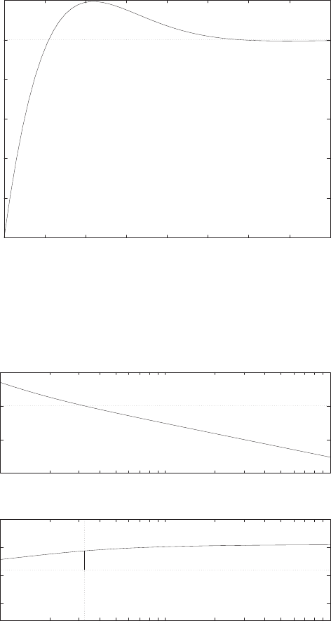
Computer Problems 515

0.2

0.4

0.6

0.8

1.2

0 5 10 15 20 25 30 35 40

Time (secs)

Amplitude

FIGURE CP9.7

CONTINUED: (b) Step response without time delays meets specs.

-40

-20

10-1 100101

Frequency (rad/sec)

Gain dB

-300

-200

-100

10-1 100101

Frequency (rad/sec)

Phase deg

FIGURE CP9.7

CONTINUED: (c) System Bode plot shows P.M. = 67.7o.

are s1=−4.56, s2,3=−0.94 ±2.02j,s4=−0.19, and s5,6=±0.32j.

Therefore, the system is marginally stable when T= 1.9, and is unstable

as the time delay increases.

from the publisher prior to any prohibited reproduction, storage in a retrieval system, or transmission in any form or by any means, electronic, mechanical, photocopying,

recording, or likewise. For information regarding permission(s), write to: Rights and Permissions Department, Pearson Education, Inc., Upper Saddle River, NJ 07458.

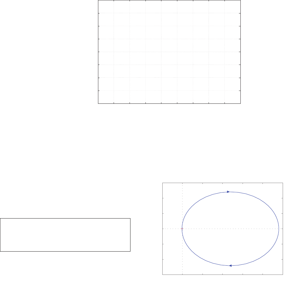
516 CHAPTER 9 Stability in the Frequency Domain

-4

-3

-2

-1

-8 -7 -6 -5 -4 -3 -2 -1 0 1

Real Axis

Imag Axis

FIGURE CP9.7

CONTINUED: (d) Closed-loop root locations as the time delay varies.

CP9.8 The Nyquist plot and associated m-ﬁle code are shown in Figure CP9.8.

a=[0 1;-1 -15]; b=[0;30]; c=[8 0]; d=[0];

sys=ss(a,b,c,d);

nyquist(sys)

−50 0 50 100 150 200 250

−150

−100

−50

100

150

Nyquist Diagram

Real Axis

Imaginary Axis

FIGURE CP9.8

Using the Nyquist function to obtain a Nyquist plot.

from the publisher prior to any prohibited reproduction, storage in a retrieval system, or transmission in any form or by any means, electronic, mechanical, photocopying,

recording, or likewise. For information regarding permission(s), write to: Rights and Permissions Department, Pearson Education, Inc., Upper Saddle River, NJ 07458.

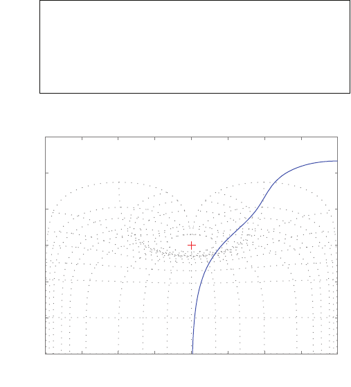
Computer Problems 517

CP9.9 The Nichols chart is shown in Figure CP9.9. The phase and gain margins

are 37.1 degrees and ∞dB, respectively.

-360 -315 -270 -225 -180 -135 -90 -45 0

-60

-40

-20

?-40 dB

?-20 dB

?-60 dB

?-1 dB

?-6 dB

0.5 dB

0 dB

6 dB ?-3 dB

3 dB

?-12 dB

1 dB

0.25 dB

Nichols Chart

en-Loop Phase

(

Open-Loop Gain (dB)

a=[0 1;-1 -10]; b=[0;22]; c=[10 0]; d=[0];

sys=ss(a,b,c,d);

nichols(sys)

ngrid

FIGURE CP9.9

The Nichols chart for the system in CP9.8.

CP9.10 (a) The Nyquist plot is shown in Figure CP9.10. The phase margin is

P.M. = 18o.

(b) When the time delay is T= 0.05 seconds, the phase margin is P.M. =

9o.

stable. So, for T > 0.1 seconds, the system is unstable.

from the publisher prior to any prohibited reproduction, storage in a retrieval system, or transmission in any form or by any means, electronic, mechanical, photocopying,

recording, or likewise. For information regarding permission(s), write to: Rights and Permissions Department, Pearson Education, Inc., Upper Saddle River, NJ 07458.

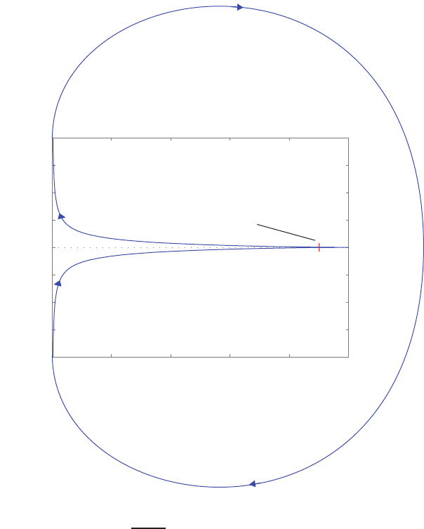
518 CHAPTER 9 Stability in the Frequency Domain

-10 -8 -6 -4 -2 0

-200

-150

-100

-50

100

150

200

Nyquist Diagram

Real Axi s

Imaginary Axi s

-1 point

FIGURE CP9.10

Nyquist plot for G(s)H(s) = 10

s(s+1) .

from the publisher prior to any prohibited reproduction, storage in a retrieval system, or transmission in any form or by any means, electronic, mechanical, photocopying,

recording, or likewise. For information regarding permission(s), write to: Rights and Permissions Department, Pearson Education, Inc., Upper Saddle River, NJ 07458.

C H A P T E R 1 0

The Design of Feedback Control

Systems

Exercises

E10.1 From the design speciﬁcations, we determine that our desired ζ= 0.69

and ωn= 5.79. The characteristic equation is

1 + Gc(s)G(s) = 1 + K(s+a)

s(s+ 2) = 0 ,

s2+ (2 + K)s+Ka = 0 .

Our desired characteristic polynomial is

s2+ 2ζωns+ω2

n=s2+ 8s+ 33.6 = 0 .

Thus, K+ 2 = 8, or

K= 6

and Ka = 33.6, so a= 5.6. The actual percent overshoot and settling

time will be diﬀerent from the predicted values due to the presence of the

closed-loop system zero at s=−a. In fact, the actual percent overshoot

and settling time are P.O. = 12.6% and Ts= 0.87s, respectively.

E10.2 The characteristic equation is

1 + Gc(s)G(s) = 1 + 400

s(s+ 40) K1+1

s= 1 + 400(K1s+ 1)

s2(s+ 40) = 0 ,

1 + K1

400s

s3+ 40s2+ 400 = 0 .

519

from the publisher prior to any prohibited reproduction, storage in a retrieval system, or transmission in any form or by any means, electronic, mechanical, photocopying,

recording, or likewise. For information regarding permission(s), write to: Rights and Permissions Department, Pearson Education, Inc., Upper Saddle River, NJ 07458.

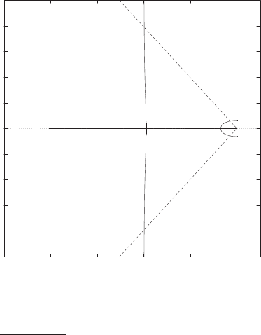
520 CHAPTER 10 The Design of Feedback Control Systems

We desire ζ= 0.45 for an overshoot of 20%. The root locus is shown

in Figure E10.2. We select a point slightly inside the performance region

(deﬁned by ζ= 0.45 ) to account for the zero. Thus,

K1= 0.5

and the closed-loop poles are

s1=−35

s2,3=−2.7±j2.

The actual

P.O. = 20.7% .

-50

-40

-30

-20

-10

-50 -40 -30 -20 -10 0

Real Axis

Imag Axis

FIGURE E10.2

Root locus for 1 + K1400s

s3+40s2+400 = 0.

E10.3 The step response is shown in Figure E10.3 for τ= 1 and K= 0.5. It can

be seen that the

P.O. = 4% ,

so this is a valid solution.

from the publisher prior to any prohibited reproduction, storage in a retrieval system, or transmission in any form or by any means, electronic, mechanical, photocopying,

recording, or likewise. For information regarding permission(s), write to: Rights and Permissions Department, Pearson Education, Inc., Upper Saddle River, NJ 07458.

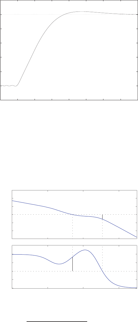
Exercises 521

-0.2

0.2

0.4

0.6

0.8

1.2

01 2 3 4 5 6 7 8

Time (secs)

Amplitude

FIGURE E10.3

Step response for K= 0.5and τ= 1.

E10.4 The Bode plot is shown in Figure E10.4. The phase and gain margins

are marked on the plot, where it can be seen that P.M. = 75.4oand

G.M. = 28.6 dB.

-150

-100

-50

100

150

Magnitude (dB)

10-4 10-2 100102

-270

-225

-180

-135

-90

-45

Phase (deg)

Bode Diagram

Gm = 28.6 dB (at 11.8 rad/sec) , Pm = 75.4 deg (at 0.247 rad/sec)

Frequency (rad/sec)

FIGURE E10.4

Bode plot for Gc(s)G(s) = 100(s+0.15)(s+0.7)

s(s+5)(s+10)(s+0.015)(s+7) .

from the publisher prior to any prohibited reproduction, storage in a retrieval system, or transmission in any form or by any means, electronic, mechanical, photocopying,

recording, or likewise. For information regarding permission(s), write to: Rights and Permissions Department, Pearson Education, Inc., Upper Saddle River, NJ 07458.

522 CHAPTER 10 The Design of Feedback Control Systems

E10.5 We require that Kv≥2.7, ζ= 0.5 and ωn= 3 for the dominant roots.

We want to place a zero to left of the pole at -2, so the complex roots will

dominate. Set the zero at s=−2.2. Then for the desired roots ﬁnd the

location of pole pin compensator

Gc(s) = K1(s+ 2.2)

(s+p)

to satisfy 180ophase at the desired roots. This yields p= 16.4. Using

root locus methods, we ﬁnd that KK1= 165.7, so with K1= 7.53, we

determine that K= 22, and

Gc(s) = 7.46(s+ 2.2)

(s+ 16.4) .

Then

Kv= 2.78 .

E10.6 The closed-loop transfer function is

T(s) = Gc(s)G(s)

1 + Gc(s)G(s)=326(s+ 4)

s4+ 14.76s3+ 151.3s2+ 349.8s+ 1304 .

The roots are

s1,2=−0.87 ±j3.2

s3,4=−6.5±j8.7.

Assuming s1,2dominates, then we expect overshoot

P.O. = 43% and Ts= 4.6 sec .

The discrepencies with the actual P.O. and Tsare due to the poles s3,4

and the zero at s=−4.

E10.7 The loop transfer function is

L(s) = Ke−0.6s

s(s+ 20) .

A plot of P.M. as a function of Kis shown in Figure E10.7. It can be

seen that

P.M. = 40o

when K= 26.93.

from the publisher prior to any prohibited reproduction, storage in a retrieval system, or transmission in any form or by any means, electronic, mechanical, photocopying,

recording, or likewise. For information regarding permission(s), write to: Rights and Permissions Department, Pearson Education, Inc., Upper Saddle River, NJ 07458.

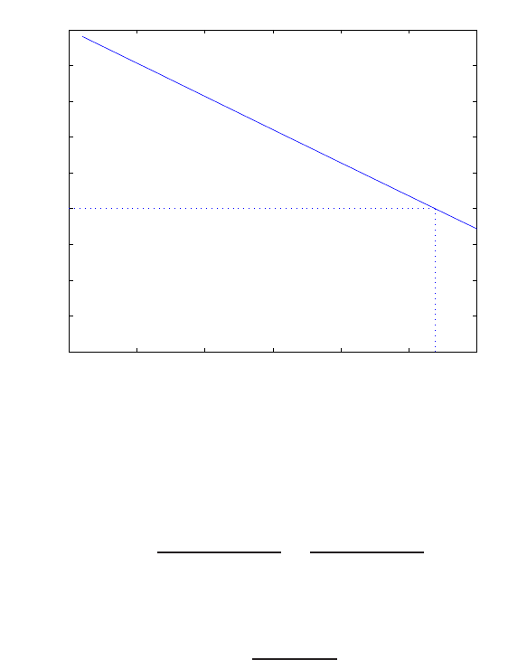
Exercises 523

0 5 10 15 20 25 30

Phase Margin deg

phase margin versus K (PM=40º, K=26.93)

FIGURE E10.7

Plot of phase margin versus K.

E10.8 The open-loop transfer function is

G(s) = 2257

s(0.0028s+ 1) =806071.4

s(s+ 357.14) ,

and the compensator is

Gc(s) = K1(s+z)

where z=K2/K1. The characteristic equation is

s3+ 357.14s2+K1s+K2= 0 .

Using Routh-Hurwitz methods, the system is stable for

0< K2<357.14 K1

or K2/K1<357.14. Select the zero zat s=−10, then using root locus

methods we determine that K1= 0.08 and K2= 0.8. The roots of the

characteristic equation are

s1=−10.6 and s2,3=−175 ±j175 ,

and ζ= 0.707, as desired. The step response is shown in Figure E10.8.

from the publisher prior to any prohibited reproduction, storage in a retrieval system, or transmission in any form or by any means, electronic, mechanical, photocopying,

recording, or likewise. For information regarding permission(s), write to: Rights and Permissions Department, Pearson Education, Inc., Upper Saddle River, NJ 07458.

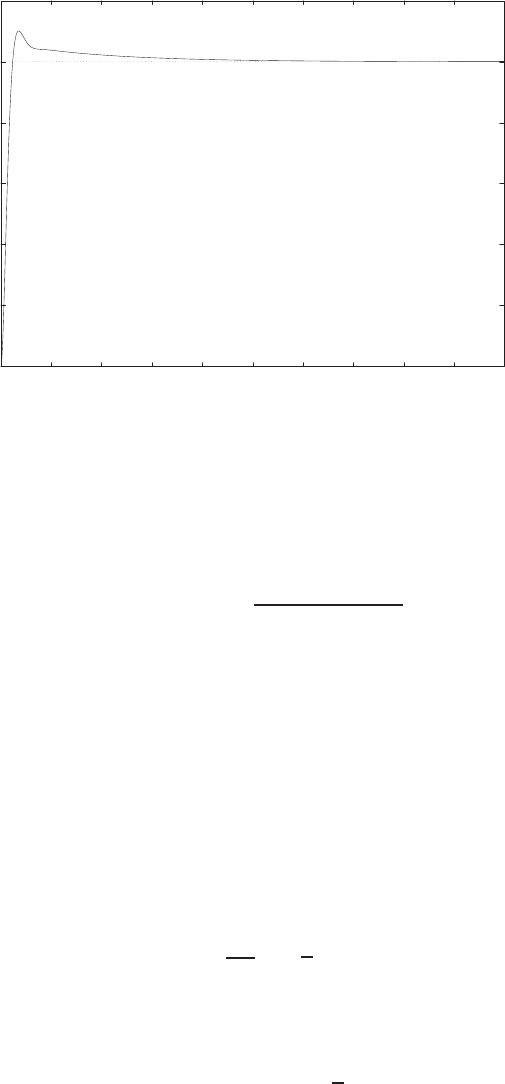
524 CHAPTER 10 The Design of Feedback Control Systems

0.2

0.4

0.6

0.8

1.2

0 0.05 0.1 0.15 0.2 0.25 0.3 0.35 0.4 0.45 0.5

Time (secs)

Amplitude

FIGURE E10.8

Step response with K1= 0.08 and K2= 0.8.

E10.9 The loop transfer function is

L(s) = Gc(s)G(s) = K1(s+K2/K1)

s(s+ 1) ,

and

Kv= lim

s→0sGc(s)G(s) = K2.

Select K2= 5. The characteristic equation is

s2+ (K1+ 1) + K2= 0 ,

and we want

s2+ 2ζωns+ω2

n= 0 .

Equating coeﬃcients yields ωn=√K2=√5. Also, since we want P.O. =

5%, we require ζ= 0.69. Thus,

2ζωn=K1+ 1 implies K1= 2.08 .

The step response with K1= 2.08 and K2=√5 yields a P.O. > 5%. This

from the publisher prior to any prohibited reproduction, storage in a retrieval system, or transmission in any form or by any means, electronic, mechanical, photocopying,

recording, or likewise. For information regarding permission(s), write to: Rights and Permissions Department, Pearson Education, Inc., Upper Saddle River, NJ 07458.

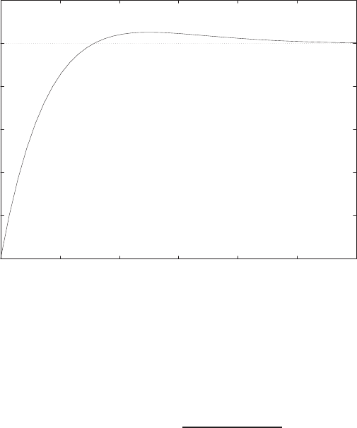
Exercises 525

is due to the zero at

s=−1.08 .

So, we raise the gain K1= 3 and then the P.O. = 5%. The step response

is shown in Figure E10.9.

0.2

0.4

0.6

0.8

1.2

00.5 1 1.5 2 2.5 3

Time (secs)

Amplitude

FIGURE E10.9

Step response with K1= 3 and K2= 5.

E10.10 The loop transfer function is

L(s) = Gc(s)G(s) = (KPs+KI)

s(s+ 1)(s+ 2) .

Let KI= 2. Then, the plot of the phase margin as a function of KPis

shown in Figure E10.10, where it can be seen that

P.M. = 71.6o

is the maximum achievable phase margin. When KP= 1.54 and KI= 2

we have P.M. = 60o, as desired, and P.O. = 9% and Tp= 3.4 sec.

from the publisher prior to any prohibited reproduction, storage in a retrieval system, or transmission in any form or by any means, electronic, mechanical, photocopying,

recording, or likewise. For information regarding permission(s), write to: Rights and Permissions Department, Pearson Education, Inc., Upper Saddle River, NJ 07458.

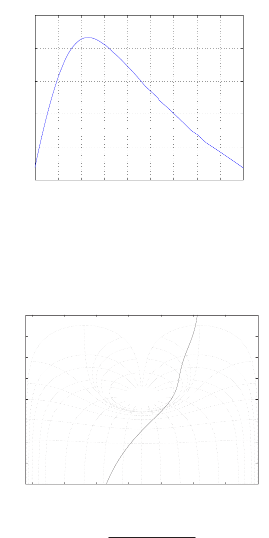
526 CHAPTER 10 The Design of Feedback Control Systems

12345678910

Phase Margin (deg)

FIGURE E10.10

Phase margin versus KPwith KI= 2.

E10.11 The Nichols diagram and the closed-loop Bode plot are shown in Fig-

ures E10.11a and E10.11b, respectively.

-40

-30

-20

-10

-350 -300 -250 -200 -150 -100 -50 0

-40

-20

-12

-6

-3

-1

0.25

0.5

2.3

Phase (deg)

Gain dB

FIGURE E10.11

(a) Nichols diagram for Gc(s)G(s) = 1350(1+0.25s)

s(s+2)(s+30)(1+0.025s).

from the publisher prior to any prohibited reproduction, storage in a retrieval system, or transmission in any form or by any means, electronic, mechanical, photocopying,

recording, or likewise. For information regarding permission(s), write to: Rights and Permissions Department, Pearson Education, Inc., Upper Saddle River, NJ 07458.

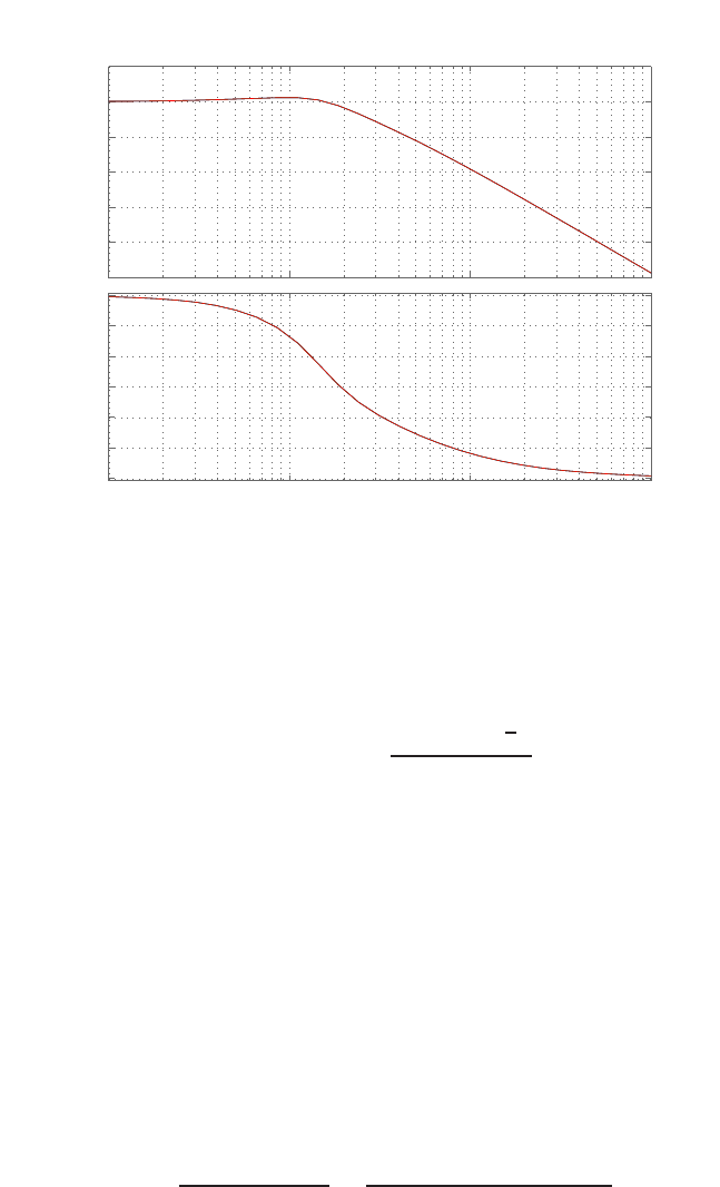
Exercises 527

−100

−80

−60

−40

−20

Magnitude (dB)

100101102103

−270

−225

−180

−135

−90

−45

Phase (deg)

Bode Diagram

Frequency (rad/sec)

FIGURE E10.11

CONTINUED: (b) Closed-loop Bode plot.

E10.12 The loop transfer function is

L(s) = Gc(s)G(s) = KK1s+1

2

s2(s+ 5) .

When KK1= 5.12, the roots are

s1,2=−0.58 ±j0.58

s3=−3.84 .

The complex poles have ζ= 0.707 and the predicted settling time is

Ts= 4/0.58 = 6.89 sec .

The actual settling time is Ts= 6.22 s.

E10.13 For the cascade compensator, we have

T1(s) = Gc(s)G(s)

1 + Gc(s)G(s)=8.1(s+ 1)

(s+r1)(s+ ˆr1)(s+r2),

where r1=−1 + j2 and r2=−1.67. For the feedback compensator, we

from the publisher prior to any prohibited reproduction, storage in a retrieval system, or transmission in any form or by any means, electronic, mechanical, photocopying,

recording, or likewise. For information regarding permission(s), write to: Rights and Permissions Department, Pearson Education, Inc., Upper Saddle River, NJ 07458.

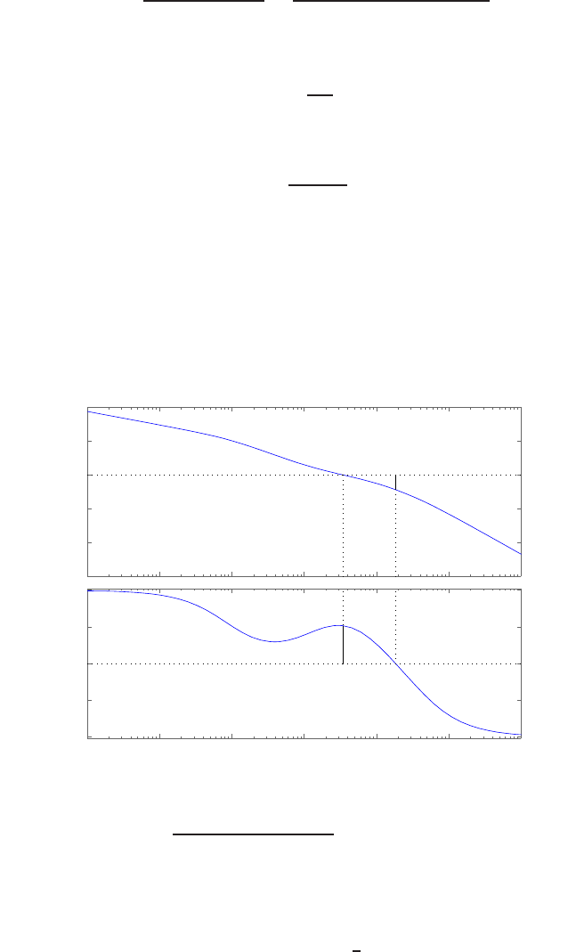
528 CHAPTER 10 The Design of Feedback Control Systems

have

T2(s) = G(s)

1 + Gc(s)G(s)=8.1(s+ 3.6)

(s+r1)(s+ ˆr1)(s+r2),

where

G(s) = 8.1

and

Gc(s) = s+ 1

s+ 3.6.

The response of the two systems diﬀer due to diﬀerent value of the zero of

T1and T2, however, both systems have the same characteristic equation.

E10.14 The Bode plot (with the lag network) is shown in Figure E10.14; the

phase margin is P.M. = 46o.

−150

−100

−50

100

Magnitude (dB)

10−4 10−3 10−2 10−1 100101102

−270

−225

−180

−135

−90

Phase (deg)

Bode Diagram

Gm = 21.9 dB (at 1.84 rad/sec) , Pm = 46.4 deg (at 0.344 rad/sec)

Frequency (rad/sec)

FIGURE E10.14

Bode plot for Gc(s)G(s) = 5(7.5s+1)

s(s+1)(0.25s+1)(110s+1) = 0.

E10.15 At the desired crossover frequency ωc= 10 rad/sec, we have

20 log |Gc(j10)G(j10)|=−8.1 dB and 6Gc(j10)G(j10) = −169o.

from the publisher prior to any prohibited reproduction, storage in a retrieval system, or transmission in any form or by any means, electronic, mechanical, photocopying,

recording, or likewise. For information regarding permission(s), write to: Rights and Permissions Department, Pearson Education, Inc., Upper Saddle River, NJ 07458.

Exercises 529

Therefore, the phase margin is P.M. = 11o. So,

φ= 30o−11o= 19oand M= 8.1 dB .

Since φ > 0 and M > 0, a lead compensator is required.

E10.16 At the desired crossover frequency ωc= 2 rad/sec, we have

20 log |Gc(j2)G(j2)|= 17 dB and 6Gc(j2)G(j2) = −134o.

Therefore, the phase margin is P.M. = 46o. So,

φ= 30o−46o=−16o

M=−17 dB .

Since φ < 0 and M < 0, a lag compensator is required.

E10.17 Using a preﬁlter

Gp(s) = KI

KPs+KI

the closed-loop transfer function is

T(s) = KI

s2+ (KP+ 1)s+KI

The required coeﬃcients for a deadbeat system are α= 1.82 and Ts=

4.82. Therefore,

KI=ω2

KP=αωn−1.

Since we desired a settling time less than 2 seconds, we determine that

ωn=Ts/2 = 4.82/2 = 2.41 .

Then, the gains are

KP= 3.39

KI= 5.81 .

The step response (with the preﬁlter) is shown in Figure E10.17. The

percent overshoot is P.O. = 0.098% and the settling time is Ts= 1.99

seconds.

from the publisher prior to any prohibited reproduction, storage in a retrieval system, or transmission in any form or by any means, electronic, mechanical, photocopying,

recording, or likewise. For information regarding permission(s), write to: Rights and Permissions Department, Pearson Education, Inc., Upper Saddle River, NJ 07458.

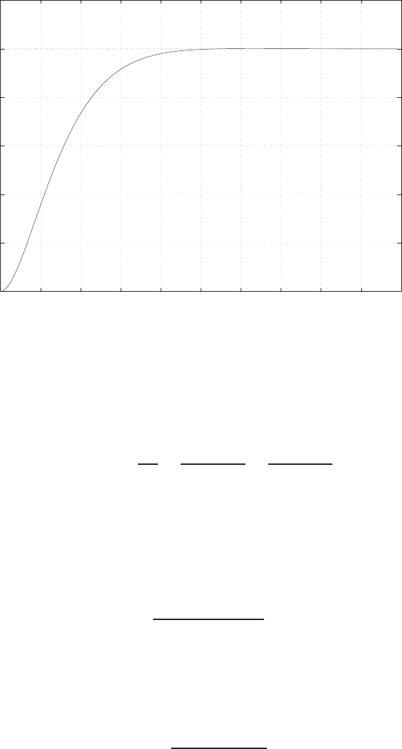
530 CHAPTER 10 The Design of Feedback Control Systems

0.2

0.4

0.6

0.8

1.2

0 0.5 1 1.5 2 2.5 3 3.5 4 4.5 5

Time (secs)

Amplitude

FIGURE E10.17

Step response for the deadbeat system.

E10.18 Consider the PI controller

Gc(s) = Kp+KI

s=Kps+KI

s=30s+ 300

and the preﬁlter

Gp(s) = 10 .

Then, the closed-loop system is

T(s) = 300s+ 3000

s2+ 280s+ 3000 .

The percent overshoot is P.O. = 9.2% and the settling time Ts= 0.16

seconds. The steady-state tracking error to a unit step is zero, as desired.

E10.19 Consider the PID controller

Gc(s) = 29s2+ 10s+ 100

from the publisher prior to any prohibited reproduction, storage in a retrieval system, or transmission in any form or by any means, electronic, mechanical, photocopying,

recording, or likewise. For information regarding permission(s), write to: Rights and Permissions Department, Pearson Education, Inc., Upper Saddle River, NJ 07458.

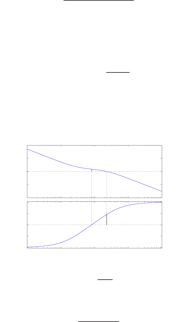
Exercises 531

The closed-loop transfer function is

T(s) = 29(s2+ 10s+ 100)

s3+ 24s2+ 290s+ 2900 .

The settling time to a unit step is Ts= 0.94 seconds.

E10.20 Consider the PD controller

Gc(s) = KDs+Kp= 3s+ 1 .

The loop transfer function is

L(s) = Gc(s)G(s) = 3s+ 1

s(s−2) .

The Bode plot is shown in Figure E10.20. The phase margin is P.M. =

40.4◦. This is a situation where decreasing the gain leads to instability. The

Bode plot shows a negative gain margin indicating that the system gain

can be decreased up to -3.5 dB before the closed-loop becomes unstable.

−40

−20

Magnitude (dB)

10−2 10−1 100101102

−270

−225

−180

−135

−90

Phase (deg)

Bode Diagram

Gm = −3.52 dB (at 0.816 rad/sec) , Pm = 40.4 deg (at 2.28 rad/sec)

Frequency (rad/sec)

FIGURE E10.20

Bode plot for the loop transfer function L(s) = 3s+1

s(s−2) .

E10.21 The transfer function from Td(s) to Y(s) is

T(s) = 1

s2+ 4.4s+K.

from the publisher prior to any prohibited reproduction, storage in a retrieval system, or transmission in any form or by any means, electronic, mechanical, photocopying,

recording, or likewise. For information regarding permission(s), write to: Rights and Permissions Department, Pearson Education, Inc., Upper Saddle River, NJ 07458.

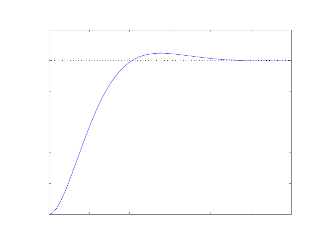
532 CHAPTER 10 The Design of Feedback Control Systems

The tracking error is E(s) = R(s)−Y(s). When R(s) = 0, then E(s) =

−Y(s). The ﬁnal value of the output to a unit step disturbance is ess =

1/K. If we want the tracking error to be less than 0.1, then we require

K > 10. When K= 10, we have the disturbance response shown in

Figure E10.21.

0 0.5 1 1.5 2 2.5 3

0.02

0.04

0.06

0.08

0.1

0.12

Step Response

Time (sec)

Amplitude

FIGURE E10.21

Disturbance response for K= 10.

from the publisher prior to any prohibited reproduction, storage in a retrieval system, or transmission in any form or by any means, electronic, mechanical, photocopying,

recording, or likewise. For information regarding permission(s), write to: Rights and Permissions Department, Pearson Education, Inc., Upper Saddle River, NJ 07458.

Problems 533

Problems

P10.1 (a) The loop transfer function is

L(s) = Gc(s)G(s)H(s) = (1 + ατs)K1K2

α(1 + τs)(Js2).

We desire ζ= 0.6, Ts≤2.5 or ζωn≥1.6. The uncompensated closed-

loop system is

T(s) = K

s2+K,

where K=K1K2/J and K=ω2

n. We can select K= 20, and then

ζωn>1.6. First, plot the Bode diagram for

G(s)H(s) = 20

where K1K2/αJ = 20. The phase margin of the uncompensated sys-

tem is 0o. We need to add phase at ωc. After several iterations, we

choose to add 40ophase at ωc, so

sin 40o=α−1

α+ 1 = 0.64 .

Therefore, α= 4.6. Then,

10 log α= 10 log 4.6 = 6.63dB .

We determine the frequency where magnitude is -6.63 dB to be ωm=

6.6 rad/sec. Then,

p=ωn√α= 14.1 and z=p/α = 3.07 .

The compensated loop transfer function (see Figure P10.1a) is

Gc(s)G(s)H(s) = 20 s

3.07 + 1

s2s

14.1+ 1.

(b) Since we desire ζωn≥1.6, we place the compensator zero at z= 1.6.

Then, we place the compensator pole far in the left half-plane; in this

case, we selected p= 20. Thus, the compensator is

Gc(s) = s+ 1.6

s+ 20 .

The root locus is shown in Figure P10.1b. To satisfy the ζ= 0.6

requirement, we ﬁnd K= 250, and the compensated loop transfer

from the publisher prior to any prohibited reproduction, storage in a retrieval system, or transmission in any form or by any means, electronic, mechanical, photocopying,

recording, or likewise. For information regarding permission(s), write to: Rights and Permissions Department, Pearson Education, Inc., Upper Saddle River, NJ 07458.

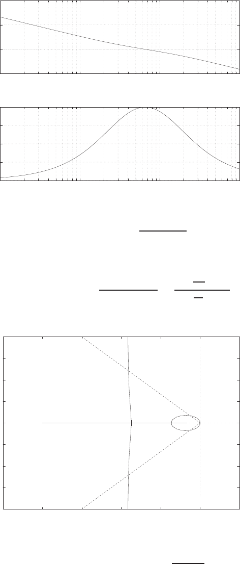
534 CHAPTER 10 The Design of Feedback Control Systems

-50

100

10-1 100101102

Frequency (rad/sec)

Gain dB

-180

-170

-160

-150

-140

10-1 100101102

Frequency (rad/sec)

Phase deg

FIGURE P10.1

(a) Compensated Bode plot for Gc(s)G(s)H(s) = 20(s/3.07+1)

s2(s/14.1+1) .

function is

Gc(s)G(s)H(s) = 250(s+ 1.6)

s2(s+ 20) =20 s

1.6+ 1

s2s

20 + 1.

-20

-15

-10

-5

-25 -20 -15 -10 -5 0 5

xxx o

Real Axis

Imag Axis

FIGURE P10.1

CONTINUED: (b) Root locus for Gc(s)G(s)H(s) = 1 + Ks+1.6

s2(s+20) .

from the publisher prior to any prohibited reproduction, storage in a retrieval system, or transmission in any form or by any means, electronic, mechanical, photocopying,

recording, or likewise. For information regarding permission(s), write to: Rights and Permissions Department, Pearson Education, Inc., Upper Saddle River, NJ 07458.

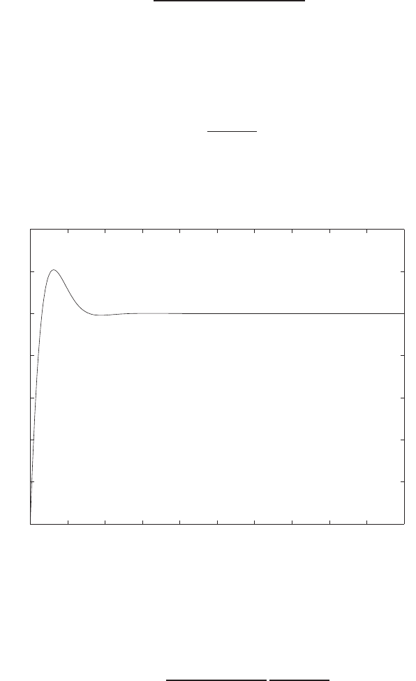
Problems 535

P10.2 The transfer function of the system is

G(s) = 1.0e+ 14

s3+ 2000s2+ 1e+ 11s,

where we use the system parameters given in P7.11 with the following

modiﬁcations: τ1=τ1= 0 and K1= 1. Also we have scaled the transfer

function so that the time units are seconds. The parameters in P7.11 are

given for time in milliseconds. A suitable compensator is

Gc(s) = s+ 500

s+ 1 .

The closed-loop system response is shown in Figure P10.2. The percent

overshoot is P.O. ≈20% and the time to settle is Ts<0.01 second.

0 0.005 0.01 0.015 0.02 0.025 0.03 0.035 0.04 0.045 0.05

0.2

0.4

0.6

0.8

1.2

1.4

Time (secs)

Amplitude

FIGURE P10.2

Step response.

P10.3 The loop transfer function is

Gc(s)G(s) = 16(s+ 1)

s(s2+ 2s+ 16)

K(s+z)

(s+p).

We desire dominant roots with Ts<5 sec and P.O. < 5%, so use ζ= 0.69

and ζωn= 0.8. One solution is to select z= 1.1 (i.e. to the left of the

from the publisher prior to any prohibited reproduction, storage in a retrieval system, or transmission in any form or by any means, electronic, mechanical, photocopying,

recording, or likewise. For information regarding permission(s), write to: Rights and Permissions Department, Pearson Education, Inc., Upper Saddle River, NJ 07458.

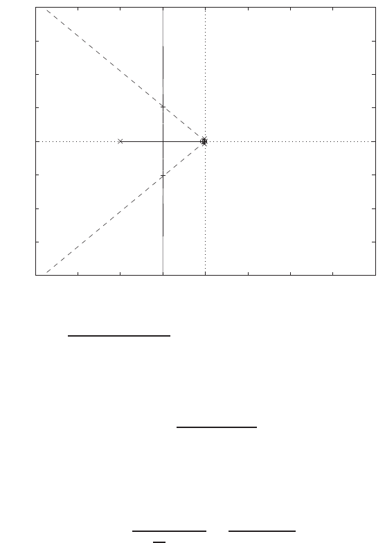
536 CHAPTER 10 The Design of Feedback Control Systems

existing zero at s=−1) and determine the pole pand gain Kfor dominant

roots with ζ= 0.69. After iteration, we can select p= 100, so that the

root locus has the form shown in Figure P10.3. Then, we select K= 320,

-200 -150 -100 -50 0 50 100 150 200

-200

-150

-100

-50

100

150

200

Real Axis

Imag Axis

FIGURE P10.3

Root locus for 1 + K16(s+1)(s+1.1)

s(s2+2s+16)(s+100) = 0.

so that ζ= 0.69. The ﬁnal compensator is

Gc(s) = 320(s+ 1.1)

s+ 100 .

The design speciﬁcations are satisﬁed with this compensator.

P10.4 The uncompensated loop transfer function is

G(s) = 1

s2(1

40 s+ 1) =40

s2(s+ 40) .

We desire 10% < P.O. < 20%, so 0.58 < ζ < 0.65, and Ts<2 implies

ζωn<2. We will utilize a PD compensator Ka(s+a). We select a= 2,

to obtain the root locus shown in Figure P10.4. Then with Ka= 23.5, we

have the desired root location, and

Gc(s) = 23.5(s+ 2) .

The design speciﬁcations are satisﬁed with the PD compensator.

from the publisher prior to any prohibited reproduction, storage in a retrieval system, or transmission in any form or by any means, electronic, mechanical, photocopying,

recording, or likewise. For information regarding permission(s), write to: Rights and Permissions Department, Pearson Education, Inc., Upper Saddle River, NJ 07458.

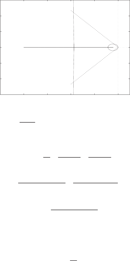
Problems 537

-30

-20

-10

-50 -40 -30 -20 -10 0

xxx o

Real Axis

Imag Axis

FIGURE P10.4

Root locus for 1 + Ka40(s+2)

s2(s+40) = 0.

P10.5 We desire P.O. < 10% and Ts<1.5 sec. The compensator is a PI-type,

given by

Gc(s) = K2+K3

s=K2s+K3

s=K2(s+a)

where a=K3/K2. So, ess = 0 for a step input and

G(s) = 3.75Ka

(s+ 0.15)(0.15s+ 1) =25Ka

(s+ 0.15)(s+ 6.67) .

The loop transfer function is

Gc(s)G(s) = 25KaK2(s+a)

s(s+ 0.15)(s+ 6.67) .

Using root locus methods, we select a= 0.2 (after several iterations) and

determine KaK2to yield ζ= 0.65. This results in KaK2= 1. The root

locus is shown in Figure P10.5. The design speciﬁcations are met. The

actual percent overshoot and settling time are P.O. = 7.4% and Ts= 1.3

s. The controller is

Gc(s) = 1 + 0.2

from the publisher prior to any prohibited reproduction, storage in a retrieval system, or transmission in any form or by any means, electronic, mechanical, photocopying,

recording, or likewise. For information regarding permission(s), write to: Rights and Permissions Department, Pearson Education, Inc., Upper Saddle River, NJ 07458.

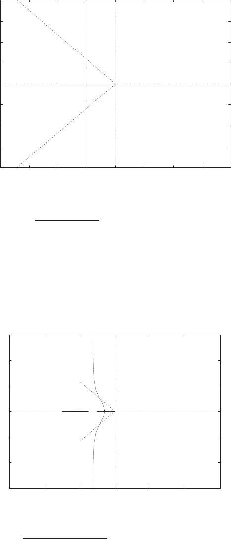
538 CHAPTER 10 The Design of Feedback Control Systems

-20

-15

-10

-5

-20 -15 -10 -5 0 5 10 15 20

xxx o

Real Axis

Imag Axis

FIGURE P10.5

Root locus for 1 + KaK225(s+0.2)

s(s+0.15)(s+6.67) = 0.

P10.6 As in P10.5, using root locus we ﬁnd that placing z= 15 and p= 30 yields

a root locus shape (see Figure P10.6) where the loop transfer function is

-60

-40

-20

-60 -40 -20 0 20 40 60

x x xo

Real Axis

Imag Axis

FIGURE P10.6

Root locus for 1 + Ka25(s+15)

(s+0.15)(s+6.67)(s+30) = 0.

from the publisher prior to any prohibited reproduction, storage in a retrieval system, or transmission in any form or by any means, electronic, mechanical, photocopying,

recording, or likewise. For information regarding permission(s), write to: Rights and Permissions Department, Pearson Education, Inc., Upper Saddle River, NJ 07458.

Problems 539

Gc(s)G(s) = 25Ka(s+z)

(s+p)(s+ 0.15)(s+ 6.67) .

and where z, p and Kaare the parameters to be determined. Properly

choosing the parameter values allows us to increase ζωnof the dominant

roots (compared to the PI compensator of P10.5). Then, with Ka= 3.7,

the dominant roots have ζ= 0.65. The design speciﬁcations are met with

the compensator.

P10.7 The plant transfer function is

G(s) = e−50s

(40s+ 1)2.

The steady-state error is

ess =A

1 + Kp

<0.1A .

Therefore, Kp>9. Insert an ampliﬁer with the compensator with a dc

gain = 9, as follows

Gc(s)G(s) = 9e−50s(s+ 2)

(40s+ 1)2(s+p).

The system is unstable without compensation, and it is very diﬃcult to

compensate such a time delay system with a lead compensator. Consider

a lag network

Gc(s) = s+z

s+p

where z > p. Let

z= 10p.

Then, a plot of the P.M. versus pis shown in Figure P10.8a. Suitable

system performance can be obtained with P.M. > 45o, so choose

p= 0.0001.

The Bode plot of the compensated and uncompensated systems is shown

in Figure P10.7c, where we have selected z= 0.001 and p= 0.0001. The

compensated system has

P.M. = 62oand Ts= 9 minutes .

The step response is shown in Figure P10.7b.

from the publisher prior to any prohibited reproduction, storage in a retrieval system, or transmission in any form or by any means, electronic, mechanical, photocopying,

recording, or likewise. For information regarding permission(s), write to: Rights and Permissions Department, Pearson Education, Inc., Upper Saddle River, NJ 07458.

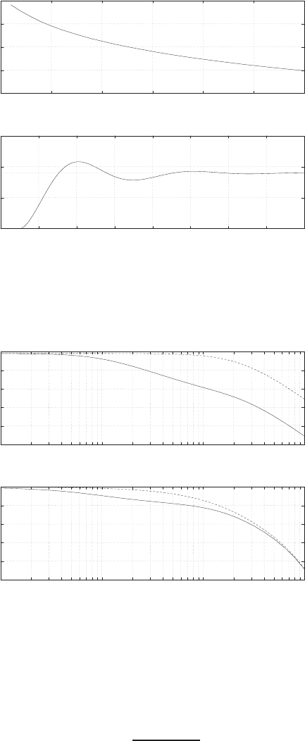
540 CHAPTER 10 The Design of Feedback Control Systems

0.5

1.5

0100 200 300 400 500 600 700 800

Time (secs)

Amplitude

(b)

-50

100

150

00.5 1 1.5 2 2.5 3

x10-3

Phase Margin (deg)

(a)

FIGURE P10.7

(a) Phase margin versus p. (b) Step response with p= 0.0001 and z= 0.001.

-30

-20

-10

10-4 10-3 10-2 10-1

Frequency (rad/sec)

Gain dB

-500

-400

-300

-200

-100

10-4 10-3 10-2 10-1

Frequency (rad/sec)

Phase deg

FIGURE P10.7

CONTINUED: (c) Bode plot for the compensated system (solid lines) and the uncompen-

sated system (dashed line).

P10.8 The transfer function is

G(s) = 5000

s(s+ 10)2.

To meet the steady-state accuracy, we need Kv>40. The uncompensated

from the publisher prior to any prohibited reproduction, storage in a retrieval system, or transmission in any form or by any means, electronic, mechanical, photocopying,

recording, or likewise. For information regarding permission(s), write to: Rights and Permissions Department, Pearson Education, Inc., Upper Saddle River, NJ 07458.

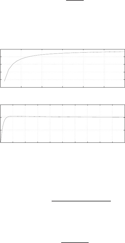
Problems 541

Kv= 50, so the steady-state accuracy can be met.

(a) Using the Bode method, we need P.M. = 70% (to meet P.O. < 5%

speciﬁcation). Let

Gc(s) = bs + 1

as + 1 .

The plot of P.M. versus bis shown in Figure P10.8a, where we set

a= 50b. Choosing b= 20 should satisfy the P.O. speciﬁcation. The

Bode plot is shown in Figure P10.8c. Thus,

0.5

1.5

05 10 15 20 25 30 35 40 45 50

Time (secs)

Amplitude

(b)

0 5 10 15 20 25 30

Phase Margin (deg)

(a)

FIGURE P10.8

(a) Phase margin versus b; (b) Step response for lag compensator designed with Bode where

a= 1000 and b= 20.

Gc(s)G(s) = 5000(20s+ 1)

s(s+ 10)2(1000s+ 1) .

The step response is shown in Figure P10.8b.

(b) We require that ζ= 0.7 to meet the P.O. speciﬁcations. Let

Gc(s) = K(bs + 1)

(as + 1) .

Using root locus methods, we ﬁx aand b, and then determine Kfor

ζ= 0.7. Let a= 50band select b= 10 (other values will work). The

root locus is shown in Figure P10.8d. We ﬁnd K= 2.5 when ζ= 0.7.

Now, Kv= 125, so the steady-state accuracy requirement is satisﬁed

for the step response as shown in Figure P10.8e.

from the publisher prior to any prohibited reproduction, storage in a retrieval system, or transmission in any form or by any means, electronic, mechanical, photocopying,

recording, or likewise. For information regarding permission(s), write to: Rights and Permissions Department, Pearson Education, Inc., Upper Saddle River, NJ 07458.

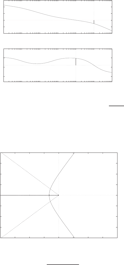
542 CHAPTER 10 The Design of Feedback Control Systems

-100

-50

100

150

10-4 10-3 10-2 10-1 100101102

Frequency (rad/sec)

Gain dB

-300

-200

-100

10-4 10-3 10-2 10-1 100101102

Frequency (rad/sec)

Phase deg

FIGURE P10.8

CONTINUED: (c) Bode plot for the compensated system with Gc(s) = 20s+1

1000s+1 .

-20

-15

-10

-5

-20 -15 -10 -5 0 5 10 15 20

xxx xo

Real Axis

Imag Axis

FIGURE P10.8

CONTINUED: (d) Root locus for 1 + K5000(10s+1)

s(s+10)2(500s+1) .

from the publisher prior to any prohibited reproduction, storage in a retrieval system, or transmission in any form or by any means, electronic, mechanical, photocopying,

recording, or likewise. For information regarding permission(s), write to: Rights and Permissions Department, Pearson Education, Inc., Upper Saddle River, NJ 07458.

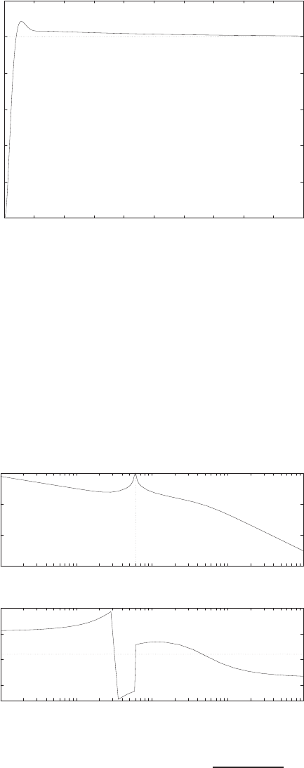
Problems 543

0.2

0.4

0.6

0.8

1.2

0 2 4 6 8 10 12 14 16 18 20

Time (secs)

Amplitude

FIGURE P10.8

CONTINUED: (e) Step response for lag compensator designed with root locus methods,

where K= 2.5.

P10.9 We desire a small response for a disturbance at 6 rad/sec. The Bode plot

of Gc(s)G(s) is shown in Figure P10.9a where we consider a compensator

-150

-100

-50

10-1 100101102103

Frequency (rad/sec)

Gain dB

-300

-200

-100

10-1 100101102103

Frequency (rad/sec)

Phase deg

FIGURE P10.9

(a) Bode plot for the compensated system with Gc(s) = 10(s2+4s+10)

s2+36 .

from the publisher prior to any prohibited reproduction, storage in a retrieval system, or transmission in any form or by any means, electronic, mechanical, photocopying,

recording, or likewise. For information regarding permission(s), write to: Rights and Permissions Department, Pearson Education, Inc., Upper Saddle River, NJ 07458.

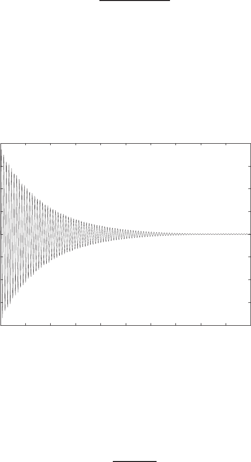
544 CHAPTER 10 The Design of Feedback Control Systems

of the form

Gc(s) = K(s2+as +b)

s2+ 36 .

Notice that the magnitude is large at ω= 6, as desired. We select

a= 4, b = 10 and K= 10 .

The response to a sinusoidal disturbance at 6 rad/sec is shown in Fig-

ure P10.9b. Notice that the eﬀect of the disturbance is virtually eliminated

in steady-state.

-0.02

-0.015

-0.01

-0.005

0.005

0.01

0.015

0.02

0 10 20 30 40 50 60 70 80 90 100

Time (secs)

Amplitude

FIGURE P10.9

CONTINUED: (b) Disturbance response for a sinusoidal disturbance at 6 rad/sec.

P10.10 The step response with Gc(s) = 1 is shown in Figure P10.10. A suitable

lag compensator is

Gc(s) = s+ 0.05

s+ 0.005 .

The step response of the compensated system is also shown in Figure P10.10.

The settling time of the compensated system is

Ts= 28 seconds .

from the publisher prior to any prohibited reproduction, storage in a retrieval system, or transmission in any form or by any means, electronic, mechanical, photocopying,

recording, or likewise. For information regarding permission(s), write to: Rights and Permissions Department, Pearson Education, Inc., Upper Saddle River, NJ 07458.

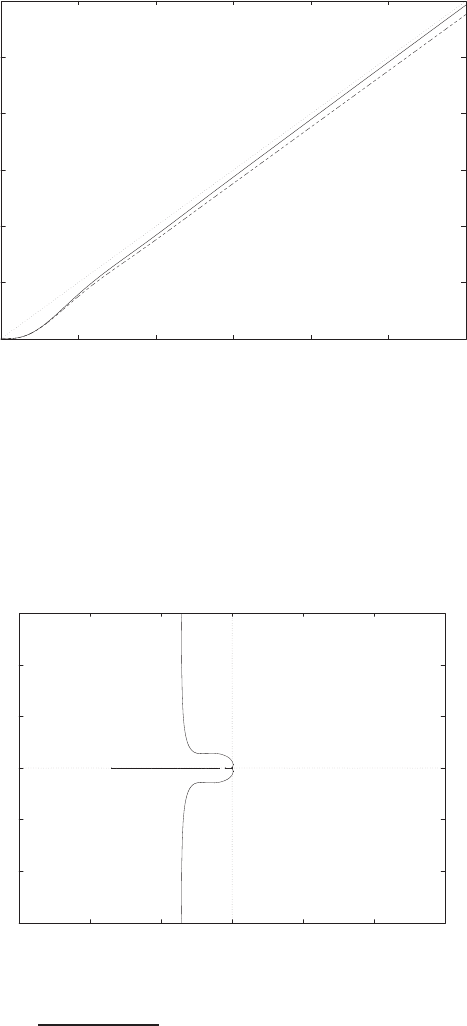
Problems 545

0 5 10 15 20 25 30

Time (sec)

Amplitude

Input (dotted line)

Compensated system (solid) & Uncompensated system (dashed)

FIGURE P10.10

Step response of uncompensated and compensated systems.

P10.11 The root locus is shown in Figure P10.11 where a suitable lead-lag com-

-300

-200

-100

100

200

300

-300 -200 -100 0 100 200 300

xxxx oo

Real Axis

Imag Axis

FIGURE P10.11

Root locus for 1 + K160(s+17)(s+10)

s2(s+170)(s+1) = 0.

from the publisher prior to any prohibited reproduction, storage in a retrieval system, or transmission in any form or by any means, electronic, mechanical, photocopying,

recording, or likewise. For information regarding permission(s), write to: Rights and Permissions Department, Pearson Education, Inc., Upper Saddle River, NJ 07458.

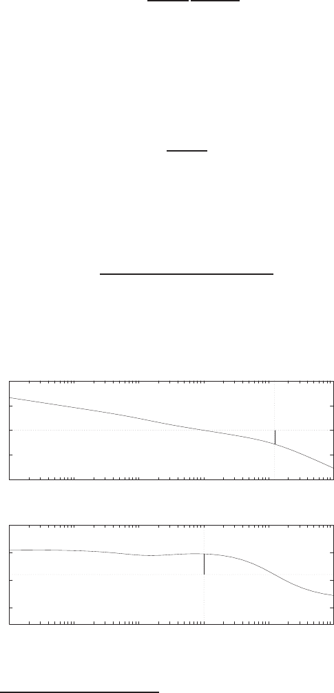
546 CHAPTER 10 The Design of Feedback Control Systems

pensator is

Gc(s) = Ks+ 10

s+ 1

s+ 17

s+ 170 .

The selected gain is K= 57, so that the damping of the complex roots

is about ζ= 0.7. For this particular design, the closed-loop system zeros

will aﬀect the system response and the percent overshoot speciﬁcation

may not be satisﬁed. Some design iteration may be necessary or apreﬁlter

can be utilized. A suitable preﬁlter is

Gp(s) = 17

s+ 17 .

The acceleration constant is Ka= 9120.

P10.12 We choose K= 10. This yields a velocity constant Kv= 20K= 200, as

desired. A suitable two-stage lead compensaator is

Gc(s) = (0.05s+ 1)(0.05s+ 1)

(0.0008s+ 1)(0.0008s+ 1) .

The Bode plot is shown in Figure P10.12. The phase margin is P.M. =

75.06o.

-100

-50

100

10-1 100101102103104

Frequency (rad/sec)

Gain dB

-300

-200

-100

10-1 100101102103104

Frequency (rad/sec)

Phase deg

Phase margin=75.06 deg

FIGURE P10.12

Bode plot for 200(0.05s+1)2

s(0.1s+1)(0.05s+1)(0.0008s+1)2.

from the publisher prior to any prohibited reproduction, storage in a retrieval system, or transmission in any form or by any means, electronic, mechanical, photocopying,

recording, or likewise. For information regarding permission(s), write to: Rights and Permissions Department, Pearson Education, Inc., Upper Saddle River, NJ 07458.

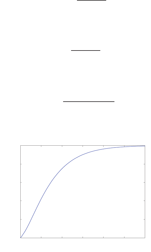
Problems 547

P10.13 (a) When

Gc(s) = K= 0.288 ,

the phase margin is P.M. = 49.3oand the bandwidth is ωB= 0.95

rad/sec.

(b) A suitable lag compensator is

Gc(s) = 25s+ 1

113.6s+ 1 .

The compensated system phase margin is P.M. = 52.21oand Kv= 2,

as desired.

P10.14 A suitable lead compensator is

Gc(s) = 1.155s+ 1

0.032s+ 1 .

The compensated system phase margin is P.M. = 50oand Kv= 2, as

desired. The settling time is Ts= 3.82 seconds.

P10.15 One possible solution is

Gc(s) = K(s+ 12)(s+ 15)

(s+ 120)(s+ 150) ,

where K= 900. The disturbance response is shown in Figure P10.15.

0 0.1 0.2 0.3 0.4 0.5 0.6

0.02

0.04

0.06

0.08

0.1

Step Response

Time

(

sec

)

Amplitude

FIGURE P10.15

Compensated system disturbance response.

from the publisher prior to any prohibited reproduction, storage in a retrieval system, or transmission in any form or by any means, electronic, mechanical, photocopying,

recording, or likewise. For information regarding permission(s), write to: Rights and Permissions Department, Pearson Education, Inc., Upper Saddle River, NJ 07458.

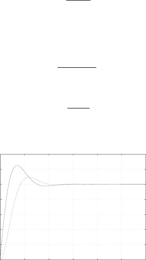
548 CHAPTER 10 The Design of Feedback Control Systems

P10.16 The PI controller is given by

Gc(s) = K(s+b)

where Kand bare to be determined. To meet the design speciﬁcations,

we need

ζ= 0.6 and ωn= 6.67 rad/sec .

The closed-loop transfer function is

T(s) = K(s+b)

s2+Ks +bK .

Solving for the gains yields K= 2ζωn= 8 and b=ω2

n/K = 5.55. A

suitable preﬁlter is

Gp(s) = 5.55

s+ 5.55 .

The step response, with and without the preﬁlter, is shown in Figure P10.16.

0.2

0.4

0.6

0.8

1.2

1.4

0 0.5 1 1.5 2 2.5 3

Without prelter (solid) & with prelter (dashed)

Time (sec)

Amplitude

FIGURE P10.16

Compensated system response with and without a preﬁlter.

from the publisher prior to any prohibited reproduction, storage in a retrieval system, or transmission in any form or by any means, electronic, mechanical, photocopying,

recording, or likewise. For information regarding permission(s), write to: Rights and Permissions Department, Pearson Education, Inc., Upper Saddle River, NJ 07458.

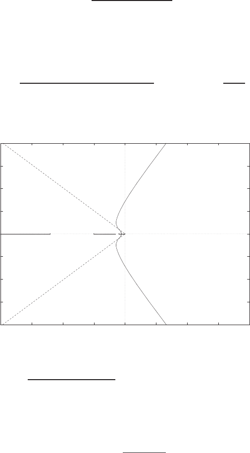
Problems 549

P10.17 The plant transfer function is

G(s) = K

s(s+ 10)(s+ 50) .

We desire ζωn>10 to meet Ts<0.4 sec and ζ= 0.65 to meet P.O. <

7.5%. Try a pole at s=−120. The root locus is shown in Figure P10.17.

The gain K= 6000 for ζ= 0.65. Thus,

Gc(s)G(s) = 6000(s/15 + 1)

s(s+ 10)(s+ 50)(s/120 + 1) and Kv=6000

500 = 12 .

-200

-150

-100

-50

100

150

200

-200 -150 -100 -50 0 50 100 150 200

xxx xo

Real Axis

Imag Axis

* * *

FIGURE P10.17

Root locus for 1 + Ks/15+1

s(s+10)(s+50)(s/120+1) .

P10.18 (a) The loop transfer function is

L(s) = K1e−2T s

0.25s+ 1

where T= 1.28. The phase angle is

φ=−2.56ω−tan 0.25ω .

So, ω= 1.12 rad/sec when φ=−180o. However, the break frequency

from the publisher prior to any prohibited reproduction, storage in a retrieval system, or transmission in any form or by any means, electronic, mechanical, photocopying,

recording, or likewise. For information regarding permission(s), write to: Rights and Permissions Department, Pearson Education, Inc., Upper Saddle River, NJ 07458.

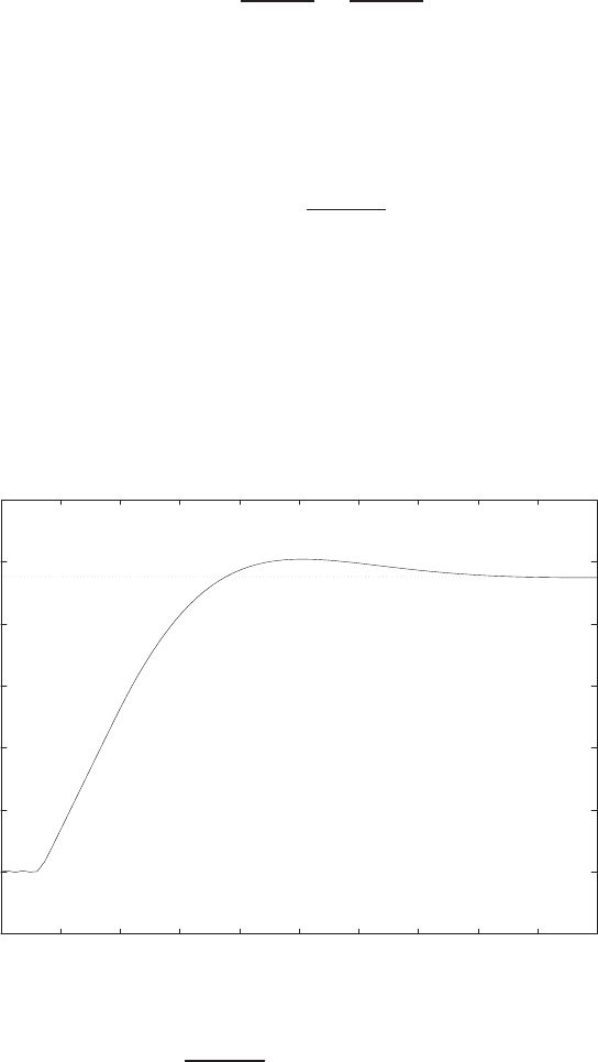
550 CHAPTER 10 The Design of Feedback Control Systems

is 4 rad/sec. Therefore, you cannot achieve P.M. = 30oand have the

system be stable for K1<1. The steady-state error is

ess =A

1 + Kp

1 + K1

since K1=Kp.

(b) Set K1= 20, then Kp= 20 and this yields a 5% steady-state error.

Without compensation, the system is now unstable. Let

Gc(s) = s/b + 1

s/a + 1

where b= 5 and a= 0.01. Then, the system is stable with

P.M. = 63o.

The system response is shown in Figure P10.18.

-0.2

0.2

0.4

0.6

0.8

1.2

02 4 6 8 10 12 14 16 18 20

Time (secs)

Amplitude

FIGURE P10.18

Unit step response with Gc(s) = 20(s/5+1)

s/0.01+1 .

from the publisher prior to any prohibited reproduction, storage in a retrieval system, or transmission in any form or by any means, electronic, mechanical, photocopying,

recording, or likewise. For information regarding permission(s), write to: Rights and Permissions Department, Pearson Education, Inc., Upper Saddle River, NJ 07458.

Problems 551

P10.19 (a) The open-loop transfer function is

G(s) = Ke−sT

(s+ 1)(s+ 3) ,

where T= 0.5 sec. We desire P.O. < 30%, thus ζ > 0.36. We will

design for ζ= 0.4, which implies P.M. = 40o. Then

φ=−tan−1ω−tan−1ω

3−0.5ω(57.3o).

At ωc= 1.75, the phase margin is P.M. = 40o, and solving

|G(jω)|=K

[(3 −ω2)2+ (4ω)2]1

= 1

at ω= 1.75 yields K= 7. Then ess = 0.3.

(b) We want ess <0.12, so use ess = 0.10 as the goal. Then

Gc(s)G(s) = Ke−0.5s(s+ 2)

(s+ 1)(s+ 3)(s+b),

and

ess =1

1 + Kp

where Kp=2K

3b. If b= 0.1 then Kp= 6.7Kand

ess =1

1 + 6.7K.

So, we need 6.7K= 9, or K= 1.35. We need a lag compensator (i.e.

b < 2) to meet ess <12% and have stability.

P10.20 We desire Kv= 20, P.M. = 45oand ωB>4 rad/sec. Thus, we set K= 20,

and

G(s) = 20

ss

2+ 1s

6+ 1.

Then, the Bode plot yields P.M. =−21ouncompensated at ωc= 5.2

rad/sec. The phase lead compensator must add 66 oplus phase lead to

account for the shift of the crossover to a higher frequency with the phase

lead compensator. Consider

Gc(s) = 1 + ατs

1 + τs 2

from the publisher prior to any prohibited reproduction, storage in a retrieval system, or transmission in any form or by any means, electronic, mechanical, photocopying,

recording, or likewise. For information regarding permission(s), write to: Rights and Permissions Department, Pearson Education, Inc., Upper Saddle River, NJ 07458.

552 CHAPTER 10 The Design of Feedback Control Systems

One solution is to use

α= 10

τ= 1/67 .

Then

Gc(s) = 100(s+ 6.7)2

(s+ 67)2.

The compensator has two zeros at ω= 6.7, two poles at ω= 67 yielding

P.M. = 47o,ωc= 7.3 and ωB= 12 rad/sec.

P10.21 We desire Kv= 20, P.M. = 45oand ωB≥2. The lag compensator is

Gc(jω) = 1 + jωτ

1 + jωατ

where α > 1. From the Bode plot, φ=−135oat ω∼

=1.3. So, at ω= 1.3,

we need to lower the magnitude by 22 dB to cause ω= 1.3 to be ω′

c, the

new crossover frequency. Thus, solving

22 = 20 log α

yields α= 14. We select the zero one decade below ω′

cor 1

τ= 0.13.

Therefore,

ατ =0.13

14 = 0.0093 .

Then, the lag compensator is given by

Gc(s) = 1 + s

0.13

1 + s

0.0093

=s+ 0.13

14(s+ 0.0093) .

The new crossover is ω′

c= 1.3, and ωB= 2.14 rad/sec.

P10.22 We desire P.M. = 45o,Kv= 20 and 2 ≤ωB≤10. The lead-lag compen-

sator is

Gc(s) = 1 + s

1 + s

10b·1 + s

10a

1 + s

Since ωB∼

=1.5ωc, we design for a new crossover frequency ω′

cso that

1.4< ω′

c<7.

Try for ω′

c= 4. The phase φ=−190oat ω= 4, so we need to add phase

lead of 55oplus phase to account for lag part of network at ω′

c. Use α= 10

and bracket ω= 4 with the lead network. Put the zero at ω= 0.8 = b

from the publisher prior to any prohibited reproduction, storage in a retrieval system, or transmission in any form or by any means, electronic, mechanical, photocopying,

recording, or likewise. For information regarding permission(s), write to: Rights and Permissions Department, Pearson Education, Inc., Upper Saddle River, NJ 07458.

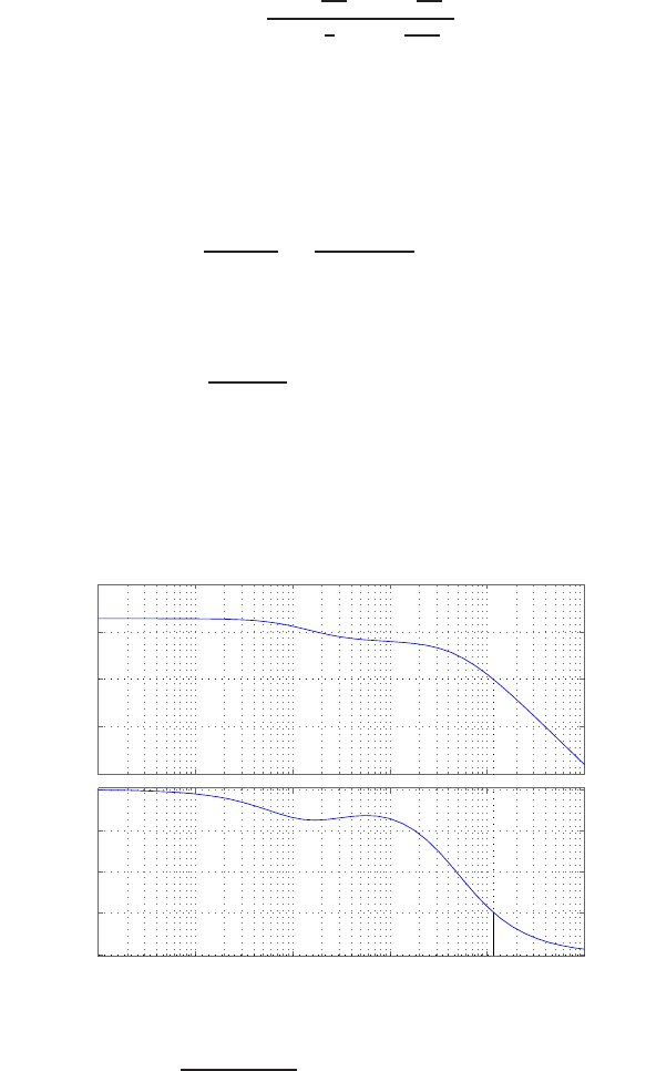
Problems 553

and the pole at ω= 8. For the lag compensator, put the zero at a lower

frequency than ω′

c/10. So try a zero at ω= 0.2 = 10aand a pole at

ω= 0.02 = a. Then, the lead-lag compensator is

Gc(s) = 1 + s

0.81 + s

0.2

1 + s

81 + s

0.02 .

The compensated Bode plot yields

ω′

c= 3.5 rad/sec, P.M. = 50oand ωB= 6.2 rad/sec .

P10.23 The steady-state error is

ess =1

1 + Kp

1 + K/25 = 0.05 .

So, we need K/25 ≥19 or K≥475. One possible solution is

Gc(s) = 4s+ 1

12s+ 1 and K= 475 .

The compensated Bode plot is shown in Figure P10.23. The phase margin

is P.M. = 46o.

−40

−20

Magnitude (dB)

10−3 10−2 10−1 100101102

−180

−135

−90

−45

Phase (deg)

Bode Diagram

Gm = Inf dB (at Inf rad/sec) , Pm = 46 deg (at 11.5 rad/sec)

Frequency (rad/sec)

FIGURE P10.23

Bode plot for Gc(s)G(s) = 475(4s+1)

(s+5)2(12s+1) .

from the publisher prior to any prohibited reproduction, storage in a retrieval system, or transmission in any form or by any means, electronic, mechanical, photocopying,

recording, or likewise. For information regarding permission(s), write to: Rights and Permissions Department, Pearson Education, Inc., Upper Saddle River, NJ 07458.

554 CHAPTER 10 The Design of Feedback Control Systems

P10.24 The arm-rotating dynamics are represented by

G(s) = 80

ss2

4900 +s

70 + 1.

We desire Kv= 20, and P.O. < 10%. One possible solution is the lead-lag

compensator

Gc(s) = (s+ 50)(s+ 0.48)

4(s+ 400)(s+ 0.06) .

With this compensator, we have

P.O. = 9.5% and Kv= 20 .

P10.25 Neglect the pole of the airgap feedback loop at s= 200. The characteristic

equation is

1 + ¯

K(s+ 20)(s+c)

s3= 0 ,

where

K=K

K1+K2

c=K2b

K1+K2

Choose

c= 10

to attain the root locus structure shown in Figure P10.25. The gain

K= 38.87

insures the damping ratio of ζ= 0.5. Then, solving for K1and byields

K1=K

38.87 −K2

and

b=0.1K

38.87K2

For given values of Kand K2(unspeciﬁed in the problem), we can com-

pute K1and b.

from the publisher prior to any prohibited reproduction, storage in a retrieval system, or transmission in any form or by any means, electronic, mechanical, photocopying,

recording, or likewise. For information regarding permission(s), write to: Rights and Permissions Department, Pearson Education, Inc., Upper Saddle River, NJ 07458.

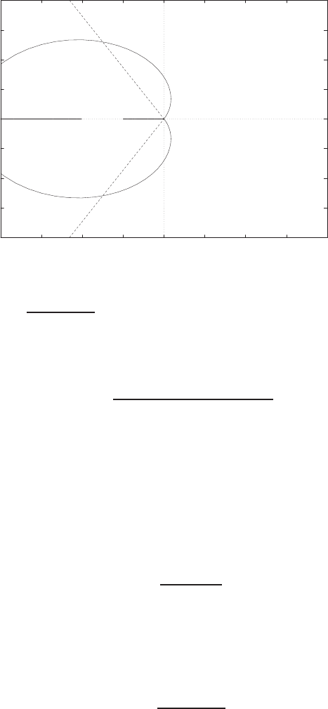
Problems 555

-40

-30

-20

-10

-40 -30 -20 -10 0 10 20 30 40

xxxo o

Real Axis

Imag Axis

FIGURE P10.25

Root locus for 1 + ¯

K(s+20)(s+10)

s3= 0.

P10.26 The loop transfer function is

Gc(s)G(s) = 0.15K(10as + 1)

s(s+ 1)(5s+ 1)(as + 1) ,

where Kand aare to be selected to meet the design speciﬁcations. Suit-

able values are

K= 6.25 and a= 0.15 .

Then, the phase margin is P.M. = 30.79oand the bandwidth is ωB=

0.746 rad/sec. The lead compensator is

Gc(s) = 6.25 1.5s+ 1

0.15s+ 1 .

P10.27 (a) Let Gc(s) = K= 11. Then the phase margin is P.M. = 50oand the

performance summary is shown in Table P10.27.

(b) Let

Gc(s) = K(s+ 12)

(s+ 20) ,

where K= 32. Then, the phase margin is P.M. = 50oand the per-

formance summary is given in Table P10.27.

from the publisher prior to any prohibited reproduction, storage in a retrieval system, or transmission in any form or by any means, electronic, mechanical, photocopying,

recording, or likewise. For information regarding permission(s), write to: Rights and Permissions Department, Pearson Education, Inc., Upper Saddle River, NJ 07458.

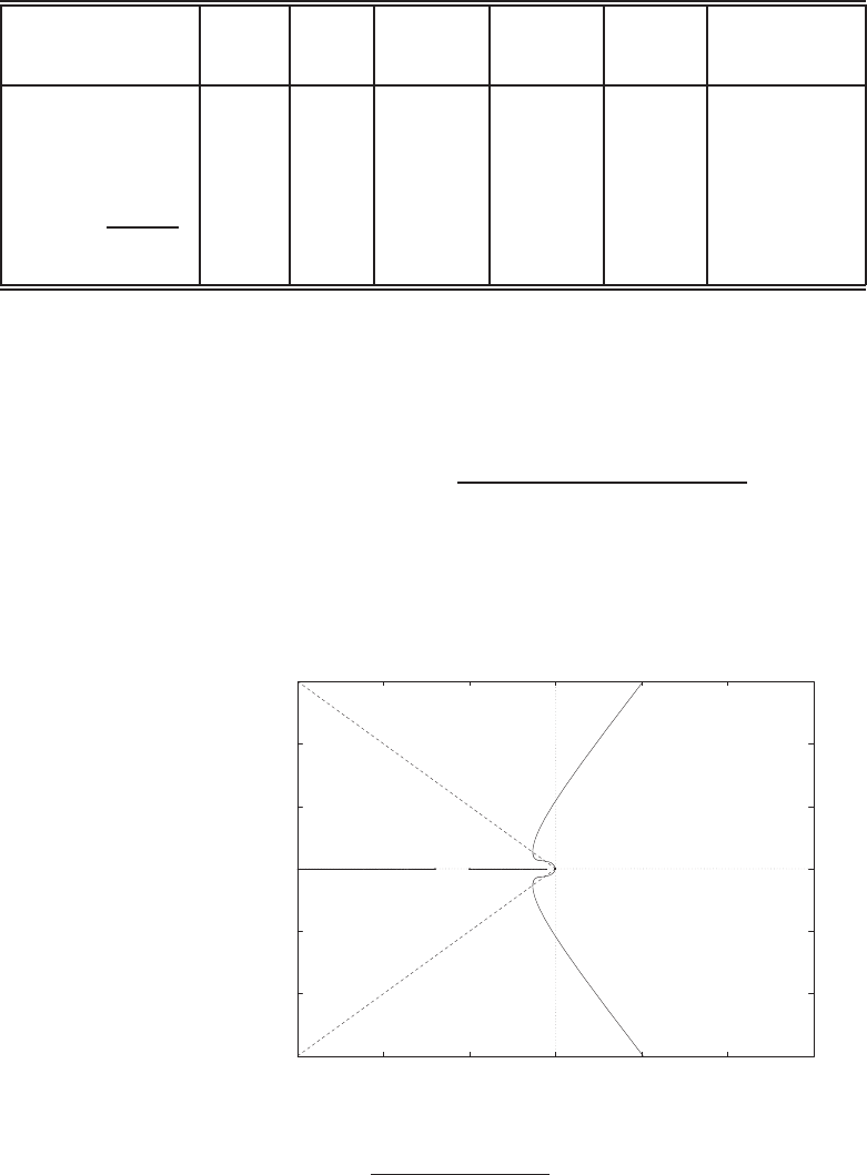
556 CHAPTER 10 The Design of Feedback Control Systems

compensator P.M. P.O. TpTsMpωωB

Gc(s) = K= 11 50o18% 0.34 sec 0.78 sec 1.5 dB 13.9 rad/sec

Gc(s) = 32(s+12)

s+20 50o18% 0.20 sec 0.47 sec 1.5 dB 26.3 rad/sec

TABLE P10.27 Performance Summary.

P10.28 The loop transfer function is

Gc(s)G(s) = K(as + 1)

s(s+ 10)(s+ 14)(10as + 1) ,

where Kand aare to be selected to meet the design speciﬁcations, and

we have set α= 10. The root locus is shown in Figure P10.28a. To satisfy

-30

-20

-10

-30 -20 -10 0 10 20 30

xxx xo

Real Axis

Imag Axis

FIGURE P10.28

(a) Root locus for 1 + K1400(s+1)

s(s+10)(s+14)(10s+1) = 0.

from the publisher prior to any prohibited reproduction, storage in a retrieval system, or transmission in any form or by any means, electronic, mechanical, photocopying,

recording, or likewise. For information regarding permission(s), write to: Rights and Permissions Department, Pearson Education, Inc., Upper Saddle River, NJ 07458.

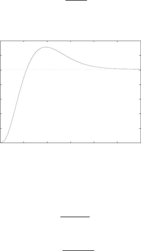
Problems 557

the steady-state tracking error we must select

K > 1400 .

Suitable values for the lag compensator are

K= 4060 and a= 1 .

Then, the percent overshoot is P.O. = 31% and the settling time is Ts=

2.34 sec. The lag compensator is

Gc(s) = s+ 1

10s+ 1 .

The step response is shown in Figure P10.28b.

0.2

0.4

0.6

0.8

1.2

1.4

00.5 1 1.5 2 2.5 3

Time (secs)

Amplitude

FIGURE P10.28

CONTINUED: (b) Step response.

P10.29 The plant transfer function is

G(s) = 10e−0.05s

s2(s+ 10) .

The lead network

Gc(s) = 16(s+ 0.7)

(s+ 9)

from the publisher prior to any prohibited reproduction, storage in a retrieval system, or transmission in any form or by any means, electronic, mechanical, photocopying,

recording, or likewise. For information regarding permission(s), write to: Rights and Permissions Department, Pearson Education, Inc., Upper Saddle River, NJ 07458.

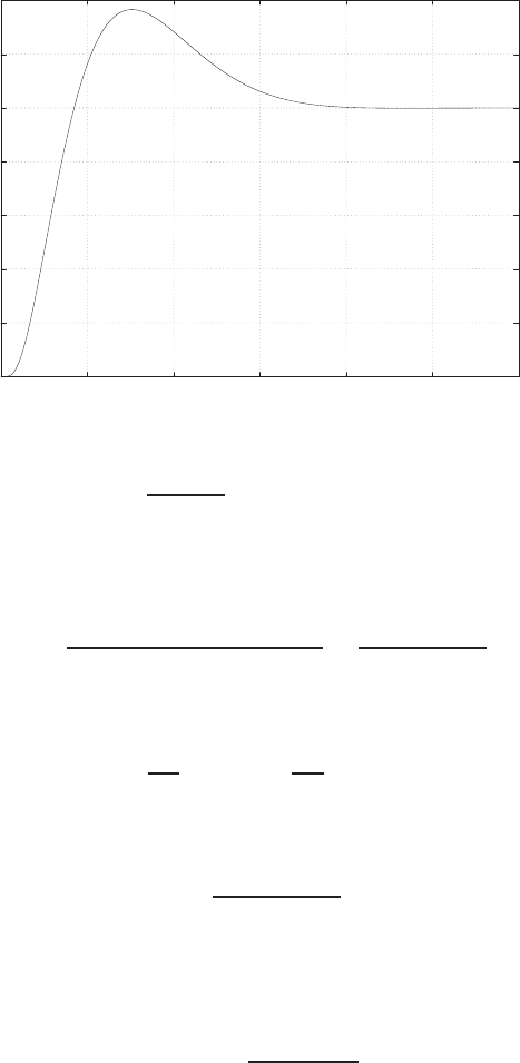
558 CHAPTER 10 The Design of Feedback Control Systems

provides Mpω= 3.4 dB and ωr= 1.39 rad/sec. The step response is shown

in Figure P10.29. The overshoot is P.O. = 37% and Ts= 3.5 sec.

0.2

0.4

0.6

0.8

1.2

1.4

01 2 3 4 5 6

Time (secs)

Amplitude

FIGURE P10.29

Unit step response with Gc(s) = 16(s+0.7)

s+9 .

P10.30 The vehicle is represented by

G(s) = K

s(0.04s+ 1)(0.001s+ 1) ≈K

s(0.04s+ 1) .

For a ramp input, we want

ess

A= 0.01 = 1

So, let

G(s) = 100

s(0.04s+ 1) .

The uncompensated P.M. = 28oat ωc= 47 rad/sec. We need to add 17o.

Case (1) Phase lead compensation:

Gc(s) = 1 + 0.021s

1 + 0.01s.

The phase margin is P.M. = 45o.

from the publisher prior to any prohibited reproduction, storage in a retrieval system, or transmission in any form or by any means, electronic, mechanical, photocopying,

recording, or likewise. For information regarding permission(s), write to: Rights and Permissions Department, Pearson Education, Inc., Upper Saddle River, NJ 07458.

Problems 559

Case (2) Phase lead compensation:

Gc(s) = 1 + 0.04s

1 + 0.005s.

The phase margin is P.M. = 65o.

For Case 1, we have

P.O. = 25% , Ts= 0.13 sec and Tp= 0.05 sec .

For Case 2, we have

P.O. = 4% , Ts= 0.04 sec and Tp= 0.03 sec .

P10.31 As in P10.30, the plant is given by

G(s) = 100

s(0.04s+ 1) .

The uncompensated P.M. = 28o. We need P.M. = 50o. The phase lag

compensator

Gc(s) = 1 + 0.5s

1 + 2.5s

results in P.M. = 50o. The P.O. = 21%, Ts= 0.72 sec and Tp= 0.17 sec.

P10.32 (a) To obtain Kv= 100, we have

Gc(s)G(s) = 43.33(s+ 500)

s(s+ 0.0325)(s2+ 2.57s+ 6667) .

With K= 43.33, we have

P.M. = 1.2o, Mpω= 26 dB , ωr= 1.8 rad/sec and ωB= 3.7 rad/sec .

The Bode plot is shown in Figure P10.32.

(b) Let

Gc(s) = 0.35s+ 1

0.001s+ 1 ,

and K= 43.33 (as before). Then,

P.M. = 36o, Mpω= 5.4 dB , ωr= 1.7 rad/sec and ωB= 3.0 rad/sec .

from the publisher prior to any prohibited reproduction, storage in a retrieval system, or transmission in any form or by any means, electronic, mechanical, photocopying,

recording, or likewise. For information regarding permission(s), write to: Rights and Permissions Department, Pearson Education, Inc., Upper Saddle River, NJ 07458.

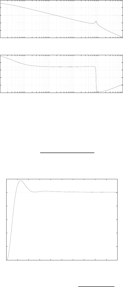
560 CHAPTER 10 The Design of Feedback Control Systems

-150

-100

-50

100

10-2 10-1 100101102103

Frequency (rad/sec)

Gain dB

-350

-300

-250

-200

-150

-100

10-2 10-1 100101102103

Frequency (rad/sec)

Phase deg

FIGURE P10.32

Bode plot with Gc(s) = K= 43.33.

P10.33 The step response is shown in Figure P10.33, where

Gc(s) = 10(s+ 0.71)(s+ 0.02)

(s+ 0.0017)(s+ 10) .

0.2

0.4

0.6

0.8

1.2

0 0.5 1 1.5 2 2.5 3 3.5 4 4.5 5

Time (secs)

Amplitude

FIGURE P10.33

Step response with the lead-lag compensator Gc(s) = 10(s+0.71)(s+0.02)

(s+0.0017)(s+10) .

from the publisher prior to any prohibited reproduction, storage in a retrieval system, or transmission in any form or by any means, electronic, mechanical, photocopying,

recording, or likewise. For information regarding permission(s), write to: Rights and Permissions Department, Pearson Education, Inc., Upper Saddle River, NJ 07458.

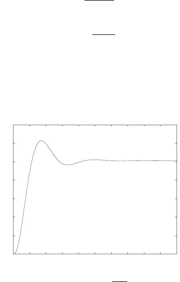
Problems 561

Then,

Kv= 80

and P.O. = 17%, Ts= 1.8 sec, and ζ= 0.54.

P10.34 The process model is

G(s) = 1

s2(s+ 10) ,

and we consider the lead compensator

Gc(s) = K1 + sατ

1 + sτ ,

where α= 100, τ= 0.4 and K= 0.5. Then, P.M. = 46.4o. The step

response is shown in Figure P10.34. The system performance is

P.O. = 22.7%

Ts= 5.2 sec

Tp= 1.72 sec .

0 1 2 3 4 5 6 7 8 9 10

0.2

0.4

0.6

0.8

1.2

1.4

Time (secs)

Amplitude

FIGURE P10.34

Step response with the lead compensator Gc(s) = 0.540s+1

0.4s+1 .

from the publisher prior to any prohibited reproduction, storage in a retrieval system, or transmission in any form or by any means, electronic, mechanical, photocopying,

recording, or likewise. For information regarding permission(s), write to: Rights and Permissions Department, Pearson Education, Inc., Upper Saddle River, NJ 07458.

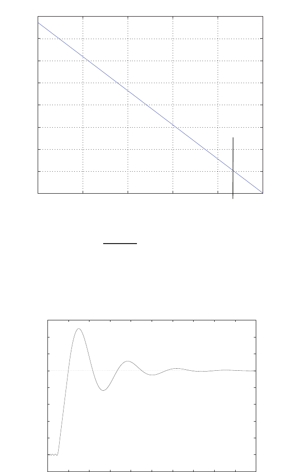
562 CHAPTER 10 The Design of Feedback Control Systems

P10.35 The phase margin is shown in Figure P10.35. As the time delay increases,

the phase margin decreases. The system is unstable when T > 2.1843 s.

0 0.5 1 1.5 2 2.5

−20

100

120

140

Time delay (s)

Phase margin (deg)

Stability boundary

T=2.1843 s

FIGURE P10.35

Step response with Gc(s)G(s) = 2s+0.54

s(s+1.76) e−T s, where 0≤T≤2.5.

P10.36 One possible solution is the integral controller Gc(s) = 2/s. The step

response is shown in Figure P10.36. The steady-state tracking error to a

-0.2

0.2

0.4

0.6

0.8

1.2

1.4

1.6

012345678910

Time (secs)

Amplitude

FIGURE P10.36

Step response with the integral controller Gc(s) = 2/s.

from the publisher prior to any prohibited reproduction, storage in a retrieval system, or transmission in any form or by any means, electronic, mechanical, photocopying,

recording, or likewise. For information regarding permission(s), write to: Rights and Permissions Department, Pearson Education, Inc., Upper Saddle River, NJ 07458.

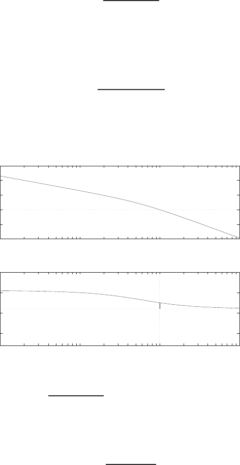
Problems 563

step input is zero since the system is type-1. The phase margin is P.M. =

32.8◦and the bandwidth is ωB= 4.3 rad/s .

P10.37 One possible solution is

Gc(s) = 1600(s+ 1)

25s+ 1 .

The overshoot to a unit step is P.O. = 4.75% and the steady-state error

to a step input is ess = 1%. The system bandwidth is ωB= 9.7 rad/sec.

P10.38 The lead compensator is

Gc(s) = 2.88(s+ 2.04)

s+ 5.88 .

The Bode plot is shown in Figure P10.38. The phase margin is P.M. =

30.4oat ωc= 9.95 rad/sec and the bandwidth is ωB= 17.43 rad/sec.

-40

-20

10-1 100101102

Frequency (rad/sec)

Gain dB

-300

-200

-100

10-1 100101102

Frequency (rad/sec)

Phase deg

FIGURE P10.38

Bode plot for Gc(s)G(s) = 115.29(s+2.04)

s(s+2)(s+5.88) .

P10.39 The lag compensator is

Gc(s) = 1 + 1.48s

1 + 11.08s.

The Bode plot is shown in Figure P10.39. The steady-state error speciﬁ-

cation is satisﬁed since Kv= 20. The phase margin is P.M. = 28.85oat

from the publisher prior to any prohibited reproduction, storage in a retrieval system, or transmission in any form or by any means, electronic, mechanical, photocopying,

recording, or likewise. For information regarding permission(s), write to: Rights and Permissions Department, Pearson Education, Inc., Upper Saddle River, NJ 07458.

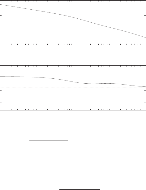
564 CHAPTER 10 The Design of Feedback Control Systems

-50

100

10-3 10-2 10-1 100101

Frequency (rad/sec)

Gain dB

-300

-200

-100

10-3 10-2 10-1 100101

Frequency (rad/sec)

Phase deg

FIGURE P10.39

Bode plot for Gc(s)G(s) = 40(1+1.48s)

s(s+2)(1+11.08s).

ωc= 2 rad/sec and the bandwidth is ωB= 3.57 rad/sec.

P10.40 The lag compensator is

Gc(s) = 2.5(1 + 1.64s)

1 + 30.5s.

The Bode plot is shown in Figure P10.40. The steady-state error speciﬁ-

cation is satisﬁed since

Kv= 50 .

The phase margin is

P.M. = 28.93o

at ωc= 1.98 rad/sec and the bandwidth is

ωB= 3.59 rad/sec.

from the publisher prior to any prohibited reproduction, storage in a retrieval system, or transmission in any form or by any means, electronic, mechanical, photocopying,

recording, or likewise. For information regarding permission(s), write to: Rights and Permissions Department, Pearson Education, Inc., Upper Saddle River, NJ 07458.

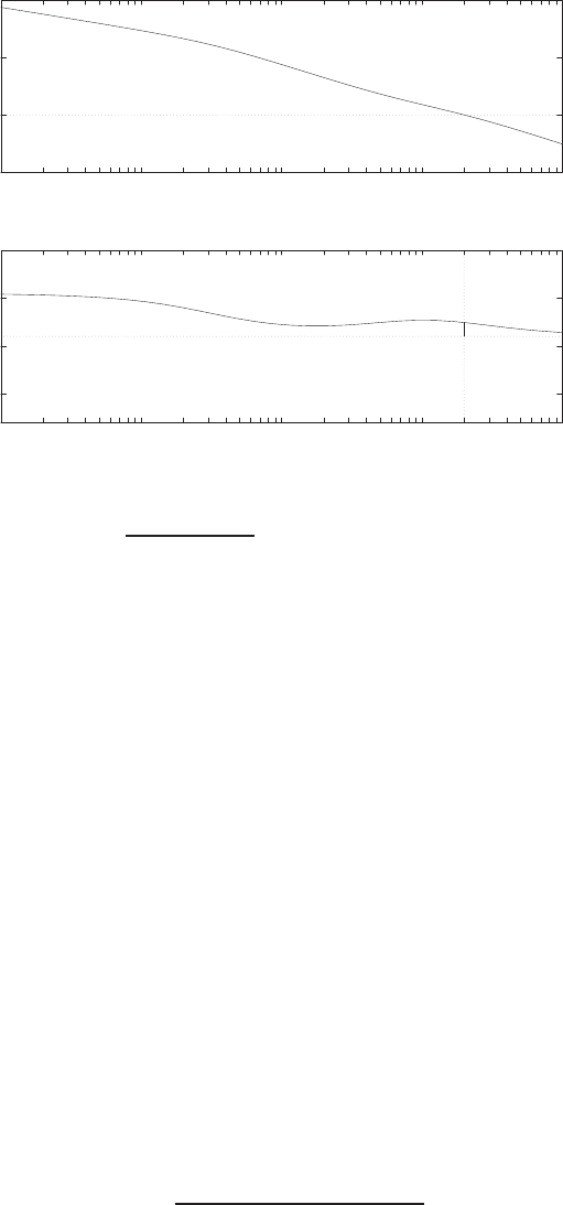
Problems 565

-50

100

10-3 10-2 10-1 100101

Frequency (rad/sec)

Gain dB

-300

-200

-100

10-3 10-2 10-1 100101

Frequency (rad/sec)

Phase deg

FIGURE P10.40

Bode plot for Gc(s)G(s) = 100(1+1.64s)

s(s+2)(1+30.5s).

P10.41 We use Table 10.2 in Dorf & Bishop to determine the required coeﬃcients

α= 1.9 and β= 2.2.

Also,

ωnTr= 4.32 implies ωn= 4.32,

since we require

Tr= 1 second.

The characteristic equation is

s3+ 8.21s2+ 41.06s+ 80.62 = s3+ (1 + p)s2+ (K+p)s+Kz = 0 .

Equating coeﬃcients and solving yields

p= 7.21 K= 33.85 z= 2.38 .

P10.42 From Example 10.4 in Dorf & Bishop, we have the closed-loop transfer

function

T(s) = 96.5(s+ 4)

(s2+ 8s+ 80)(s+ 4.83) .

from the publisher prior to any prohibited reproduction, storage in a retrieval system, or transmission in any form or by any means, electronic, mechanical, photocopying,

recording, or likewise. For information regarding permission(s), write to: Rights and Permissions Department, Pearson Education, Inc., Upper Saddle River, NJ 07458.

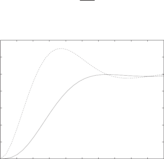
566 CHAPTER 10 The Design of Feedback Control Systems

A suitable preﬁlter is

Gp(s) = 4

s+ 4 .

The step response (with and without the preﬁlter) is shown in Figure P10.42.

0.2

0.4

0.6

0.8

1.2

1.4

0 0.1 0.2 0.3 0.4 0.5 0.6 0.7 0.8 0.9 1

With prelter (solid) & without prelter (dashed)

Time (sec)

Amplitude

FIGURE P10.42

Step response with and without the preﬁlter.

P10.43 Let

K= 100.

The Bode plot is shown in Figure P10.43a and the response to a simusoidal

noise input with

ω= 100 rad/s

is shown in Figure P10.43b.

from the publisher prior to any prohibited reproduction, storage in a retrieval system, or transmission in any form or by any means, electronic, mechanical, photocopying,

recording, or likewise. For information regarding permission(s), write to: Rights and Permissions Department, Pearson Education, Inc., Upper Saddle River, NJ 07458.

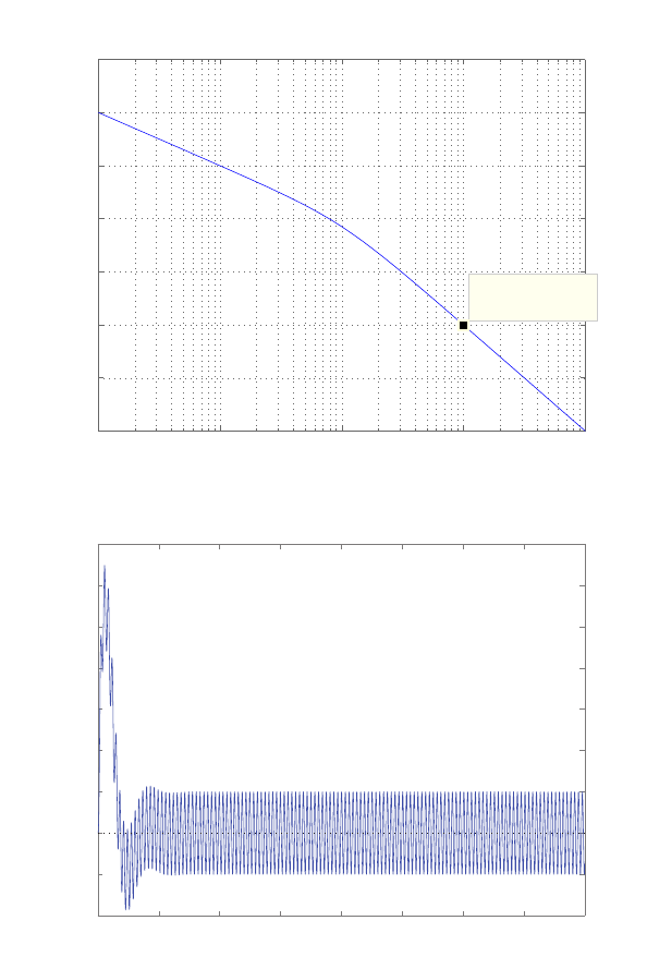
Problems 567

Bode Diagram

Frequency (rad/sec)

10−1 100101102103

−80

−60

−40

−20

System: sysg

Frequency (rad/sec): 100

Magnitude (dB): −40.1

Magnitude (dB)

012345678

−0.02

−0.01

0.01

0.02

0.03

0.04

0.05

0.06

0.07

Time (sec)

Amplitude

FIGURE P10.43

(a) Bode magnitude plot. (b) Response to a noise input.

P10.44 For 0.129 < K ≤69.87, the system is unstable. The percent overshoot is

shown in Figure P10.44 .

from the publisher prior to any prohibited reproduction, storage in a retrieval system, or transmission in any form or by any means, electronic, mechanical, photocopying,

recording, or likewise. For information regarding permission(s), write to: Rights and Permissions Department, Pearson Education, Inc., Upper Saddle River, NJ 07458.

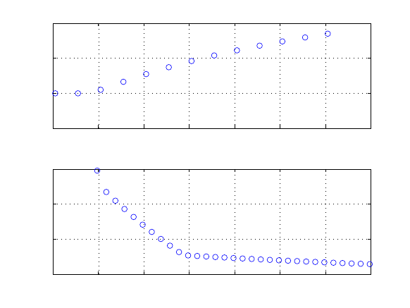
568 CHAPTER 10 The Design of Feedback Control Systems

0 0.02 0.04 0.06 0.08 0.1 0.12 0.14

−50

100

Percent Overshoot

65 70 75 80 85 90 95 100

100

120

140

160

Percent Overshoot

FIGURE P10.44

Percent overshoot.

from the publisher prior to any prohibited reproduction, storage in a retrieval system, or transmission in any form or by any means, electronic, mechanical, photocopying,

recording, or likewise. For information regarding permission(s), write to: Rights and Permissions Department, Pearson Education, Inc., Upper Saddle River, NJ 07458.

Advanced Problems 569

Advanced Problems

AP10.1 (a) With

Gc(s) = K ,

the closed-loop transfer function is

T(s) = K

s3+ 5s2+ 4s+K.

When K= 2.05, the characteristic equation is

s3+ 5s2+ 4s+ 2.05 = 0

with poles at s=−4.1563 and s=−0.4219 ±j0.5615. Therefore

ζ= 0.6, and the predicted overshoot is

P.O. = 100e−π0.6/√1−0.62= 9.5% <13% .

The actual overshoot is P.O. = 9.3% and Ts= 8.7 seconds.

(b) When

Gc(s) = 82.3(s+ 1.114)

s+ 11.46

the closed-loop transfer function is

T(s) = 82.3(s+ 1.114)

s4+ 16.46s3+ 61.3s2+ 128.14s+ 91.6822

=82.3(s+ 1.114)

(s+ 1.196)(s+ 12.26)(s+ 1.5±j2) .

Therefore ζ= 0.6 and the predicted overshoot is P.O. = 9.5% <13%.

The actual overshoot is P.O. = 12% and Ts= 2.5 seconds.

AP10.2 The lag network is given by

Gc=K(s+a1)

s+a2

The closed-loop transfer function is

T(s) = Ks+a1

s4+ (5 + a2)s3+ (4 + 5a2)s2+ (4a2+K)s+Ka1

from the publisher prior to any prohibited reproduction, storage in a retrieval system, or transmission in any form or by any means, electronic, mechanical, photocopying,

recording, or likewise. For information regarding permission(s), write to: Rights and Permissions Department, Pearson Education, Inc., Upper Saddle River, NJ 07458.

570 CHAPTER 10 The Design of Feedback Control Systems

Computing the steady-state tracking error yields

ess = lim

s→0

s4+ (5 + a2)s3+ (4 + 5a2)s2+ 4a2s

s5+ (5 + a2)s4+ (4 + 5a2)s3+ (4a2+K)s2+Ka1s

=4a2

a1K<0.125 .

If we select K= 2.05 (as in AP10.1), then

a1>15.61a2.

So, take a2=a1/16. The lag compensator can now be written as

Gc(s) = 2.05 s+a1

s+a1/16 .

Select a1= 0.018. Then, the closed-loop transfer function is

T(s) = 2.05(s+ 0.018)

s4+ 5.0011s3+ 4.0056s2+ 2.0545s+ 0.0369 .

The performance results are P.O. = 13% and Ts= 29.6 seconds for a step

input, and ess = 0.12 for a ramp input.

AP10.3 The plant transfer function is

G(s) = 1

s(s+ 1)(s+ 4)

and the PI controller is given by

Gc(s) = Kps+KI

The closed-loop transfer function is

T(s) = Kps+KI

s4+ 5s3+ 4s2+Kps+KI

For a unit ramp, the steady-state tracking error is

ess = lim

s→0

s4+ 5s3+ 4s2

s5+ 5s4+ 4s3+Kps2+KIs= 0 .

Any KI>0 and Kp>0 (such that the system is stable) is suitable and

will track a ramp with zero steady-state error. Since we want P.O. <

13%, the damping of the dominant roots should be ζ≈0.6. One suitable

from the publisher prior to any prohibited reproduction, storage in a retrieval system, or transmission in any form or by any means, electronic, mechanical, photocopying,

recording, or likewise. For information regarding permission(s), write to: Rights and Permissions Department, Pearson Education, Inc., Upper Saddle River, NJ 07458.

Advanced Problems 571

solution is to place the zero at s=−0.01 and select the PI controller

Gc(s) = 2.05(s+ 0.01)

Therefore, Kp= 2.05 and KI= 0.0205. The closed-loop transfer function

T(s) = 2.05(s+ 0.01)

s4+ 5s3+ 4s2+ 2.05s+ 0.0205 .

The performance results are P.O. = 11.5% and Ts= 9.8 seconds for a

step input, and ess = 0 for a unit ramp.

AP10.4 The closed-loop transfer function is

T(s) = 10K1

s2+ 10(1 + K1K2)s+ 10K1

From the performance speciﬁcations, we determine that the natural fre-

quency and damping of the dominant poles should be ωn= 5.79 and

ζ= 0.69. So,

s2+ 8(1 + K1K2)s+ 8K1=s2+ 2ζωns+ω2

n=s2+ 7.99s+ 33.52 .

Solving for the gains yields K1= 4.19 and K2= 0. The closed-loop

transfer function is

T(s) = 33.52

s2+ 8s+ 33.52 .

The performance results are P.O. = 5% and Ts= 1 second.

AP10.5 (a) From the overshoot speciﬁcation P.O. = 10%. The plant transfer

function is

G(s) = 1

s(s+ 1)(s+ 10) .

Let Gp= 1. A suitable compensator is

Gc=Ks+ 0.5

s+ 10 .

Using root locus methods, we determine that K= 45 yields P.O. ≈

10%. The closed-loop poles are s1,2=−2.5±j5.1, s3=−15.48, and

s4=−0.45.

(b) The closed-loop transfer function is

T(s) = 450(s+ 0.5)

s4+ 21s3+ 120s2+ 550s+ 225 .

from the publisher prior to any prohibited reproduction, storage in a retrieval system, or transmission in any form or by any means, electronic, mechanical, photocopying,

recording, or likewise. For information regarding permission(s), write to: Rights and Permissions Department, Pearson Education, Inc., Upper Saddle River, NJ 07458.

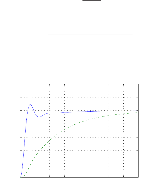
572 CHAPTER 10 The Design of Feedback Control Systems

The step response is shown in Figure AP10.5. The overshoot and

settling time are P.O. = 9.5% and Ts= 3.4 seconds.

Gp(s) = 0.5

s+ 0.5.

The closed-loop transfer function is

T(s) = 225

s4+ 21s3+ 120s2+ 550s+ 225 .

The step response is shown in Figure AP10.5. The overshoot and

settling time are P.O. = 0% and Ts= 6.85 seconds.

012345678

0.2

0.4

0.6

0.8

1.2

1.4

Time (sec)

Amplitude

FIGURE AP10.5

Step response with preﬁlter (dashed line) and without preﬁlter (solid line).

AP10.6 From Example 10.12 in Dorf & Bishop, we have the relationship

ωnTs= 4.04 .

Thereore, minimizing Tsimplies maximizing ωn. Using Table 10.2 in Dorf

& Bishop, we equate the desired and actual characteristic polynomials

q(s) = s3+ 1.9ωns2+ 2.2ω2

ns+ω3

n=s3+ (1 + p)s2+ (K+p)s+Kz .

from the publisher prior to any prohibited reproduction, storage in a retrieval system, or transmission in any form or by any means, electronic, mechanical, photocopying,

recording, or likewise. For information regarding permission(s), write to: Rights and Permissions Department, Pearson Education, Inc., Upper Saddle River, NJ 07458.

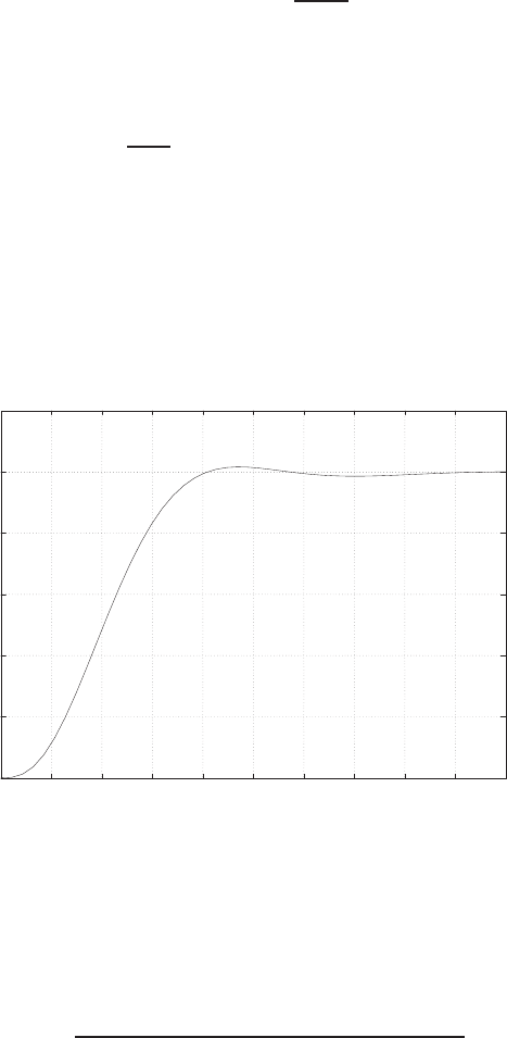
Advanced Problems 573

Comparing coeﬃcients yields

(1 + p) = 1.9ωn, K +p= 2.21 + p

1.92

, Kz =ω3

So, from the ﬁrst relationship we see that maximizing ωnimplies maxi-

mizing p. Solving for pwhile maintaining K < 52

K=2.2

3.61(p2+ 2p+ 1) −p < 52

we determine that

−9.3643 < p < 9.005 .

The largest p= 9. Therefore, K= 51.94 and z= 2.81. The step response

is shown in Figure AP10.6. The settling time is Ts= 0.77 second.

0.2

0.4

0.6

0.8

1.2

0 0.2 0.4 0.6 0.8 1 1.2 1.4 1.6 1.8 2

Time (secs)

Amplitude

FIGURE AP10.6

Step response with minimum settling time.

AP10.7 Let Gp= 1. The closed-loop transfer function is

T(s) = K(s+ 3)

s4+ 38s3+ 296s2+ (K+ 448)s+ 3K.

When K= 311, the characteristic equation

s4+ 38s3+ 296s2+ 759s+ 933 = 0

from the publisher prior to any prohibited reproduction, storage in a retrieval system, or transmission in any form or by any means, electronic, mechanical, photocopying,

recording, or likewise. For information regarding permission(s), write to: Rights and Permissions Department, Pearson Education, Inc., Upper Saddle River, NJ 07458.

574 CHAPTER 10 The Design of Feedback Control Systems

has poles at s=−1.619±j1.617 (ζ= 1/√2), s=−6.25, and s=−28.51.

(a) When Gp(s) = 1 and K= 311, the closed-loop transfer function is

T(s) = 311(s+ 3)

s4+ 38s3+ 296s2+ 759s+ 933 .

The step input performance is P.O. = 6.5%, Ts= 2.5 seconds, and

Tr= 1.6 seconds. With the preﬁlter

Gp(s) = 3

s+ 3

and K= 311, the closed-loop transfer function is

T(s) = 933

s4+ 38s3+ 296s2+ 759s+ 933 .

In this case, the step response is P.O. = 3.9%, Ts= 2.8 seconds, and

Tr= 1.3 seconds.

(b) Now, consider the preﬁlter

Gp(s) = 1.8

s+ 1.8

and K= 311. The closed-loop transfer function is

(s) = 559.8(s+ 3)

s5+ 39.8s4+ 364.4s3+ 1291.8s2+ 2299.2s+ 1679.4.

The step input response is P.O. = 0.7%, Ts= 2.14 seconds and

Tr= 1.3 seconds.

AP10.8 The plant transfer function is

G(s) = 250

s(s+ 2)(s+ 40)(s+ 45) .

The performance speciﬁcations are P.O. < 20%, Tr<0.5 second, Ts<1.2

seconds and Kv≥10. A suitable lead compensator is

Gc= 1483.7s+ 3.5

s+ 33.75 .

The closed-loop transfer function is

T(s) = 250(1483.7)(s+ 35)

s(s+ 2)(s+ 40)(s+ 45)(s+ 33.75) + 250(1483.7)(s+ 3.5)

The actual step input performance (see Figure AP10.8) is P.O. = 18%,

Ts= 0.88 second, Tr= 0.18 second, and Kv= 10.7.

from the publisher prior to any prohibited reproduction, storage in a retrieval system, or transmission in any form or by any means, electronic, mechanical, photocopying,

recording, or likewise. For information regarding permission(s), write to: Rights and Permissions Department, Pearson Education, Inc., Upper Saddle River, NJ 07458.

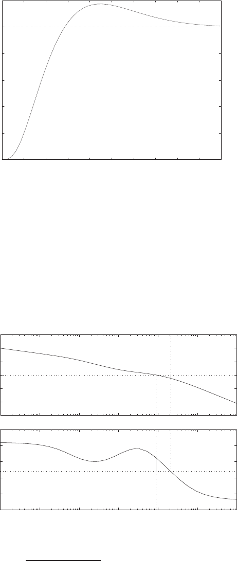
Advanced Problems 575

0.2

0.4

0.6

0.8

1.2

0 0.1 0.2 0.3 0.4 0.5 0.6 0.7 0.8 0.9 1

Time (secs)

Amplitude

FIGURE AP10.8

Step response with lead compensator.

AP10.9 The frequency response is shown in Figure AP10.9.

Frequency (rad/sec)

Phase (deg); Magnitude (dB)

Bode Diagrams

-150

-100

-50

100

150

Gm=12.4 dB (Wcg=20.9); Pm=42.0 deg. (Wcp=9.0)

10-3 10-2 10-1 100101102103

-300

-250

-200

-150

-100

-50

FIGURE AP10.9

Bode plot with Gc(s) = (s+2.5)(s+0.9871)

(s+36.54)(s+0.0675)

from the publisher prior to any prohibited reproduction, storage in a retrieval system, or transmission in any form or by any means, electronic, mechanical, photocopying,

recording, or likewise. For information regarding permission(s), write to: Rights and Permissions Department, Pearson Education, Inc., Upper Saddle River, NJ 07458.

576 CHAPTER 10 The Design of Feedback Control Systems

One lead-lag compensator that satisﬁes the speciﬁcations is

Gc(s) = (s+ 2.5)(s+ 0.9871)

(s+ 36.54)(s+ 0.0675) .

The gain and phase margins are Gm = 12.35 dB and P m = 41.8◦, re-

spectively. The velocity error constant is Kv= 100. Therefore, all speci-

ﬁcations are satisﬁed.

from the publisher prior to any prohibited reproduction, storage in a retrieval system, or transmission in any form or by any means, electronic, mechanical, photocopying,

recording, or likewise. For information regarding permission(s), write to: Rights and Permissions Department, Pearson Education, Inc., Upper Saddle River, NJ 07458.

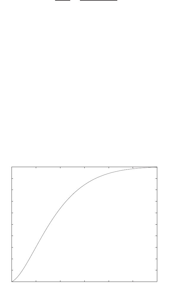
Design Problems 577

Design Problems

The plant model with parameters given in Table CDP2.1 in Dorf andCDP10.1

Bishop is given by:

θ(s)

Va(s)=26.035

s(s+ 33.142) ,

where we neglect the motor inductance Lmand where we switch oﬀ the

tachometer feedback (see Figure CDP4.1 in Dorf and Bishop). With a PD

controller the closed-loop system characteristic equation is

s2+ (33.142 + 26.035KD)s+ 26.035Kp= 0 .

Using Table 10.2 in Dorf and Bishop we determine that for a second-order

system with a deadbeat response we have α= 1.82 and ωnTs= 4.82. Since

we desire Ts<0.25 seconds, we choose ωn= 19.28. Equating the actual

characteristic equation with the desired characteristic equation we obtain

s2+ωnαs +ω2

n=s2+ (33.142 + 26.035KD)s+ 26.035Kp.

Solving for Kpand KDyields the PD controller:

Gc(s) = 14.28 + 0.075s .

The step response is shown below. The settling time is Ts= 0.24 second.

0 0.05 0.1 0.15 0.2 0.25 0.3

0.1

0.2

0.3

0.4

0.5

0.6

0.7

0.8

0.9

Time (secs)

Amplitude

from the publisher prior to any prohibited reproduction, storage in a retrieval system, or transmission in any form or by any means, electronic, mechanical, photocopying,

recording, or likewise. For information regarding permission(s), write to: Rights and Permissions Department, Pearson Education, Inc., Upper Saddle River, NJ 07458.

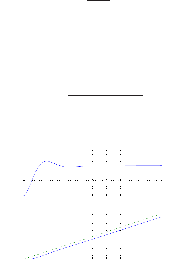
578 CHAPTER 10 The Design of Feedback Control Systems

DP10.1 The plant is given as

G(s) = 20

s(s+ 2) .

One possible lead compensator is

Gclead (s) = 50(s+ 1)

s+ 20 .

Similarly, a suitable lag compensator is

Gclag (s) = s+ 0.1

s+ 0.022 .

The loop transfer function with the lead-lag compensator is

Gc(s)G(s) = 1000(s+ 1)(s+ 0.1)

s(s+ 2) (s+ 0.022)(s+ 20) .

The step response and ramp response are shown in Figure DP10.1. The

velocity constant is Kv= 50, so the steady-state error speciﬁcation is

satisﬁed.

0 0.1 0.2 0.3 0.4 0.5 0.6 0.7 0.8 0.9 1

0.5

1.5

Time (sec)

Step response

0 0.1 0.2 0.3 0.4 0.5 0.6 0.7 0.8 0.9 1

0.2

0.4

0.6

0.8

Time (sec)

Ramp response

FIGURE DP10.1

Step response and ramp response.

from the publisher prior to any prohibited reproduction, storage in a retrieval system, or transmission in any form or by any means, electronic, mechanical, photocopying,

recording, or likewise. For information regarding permission(s), write to: Rights and Permissions Department, Pearson Education, Inc., Upper Saddle River, NJ 07458.

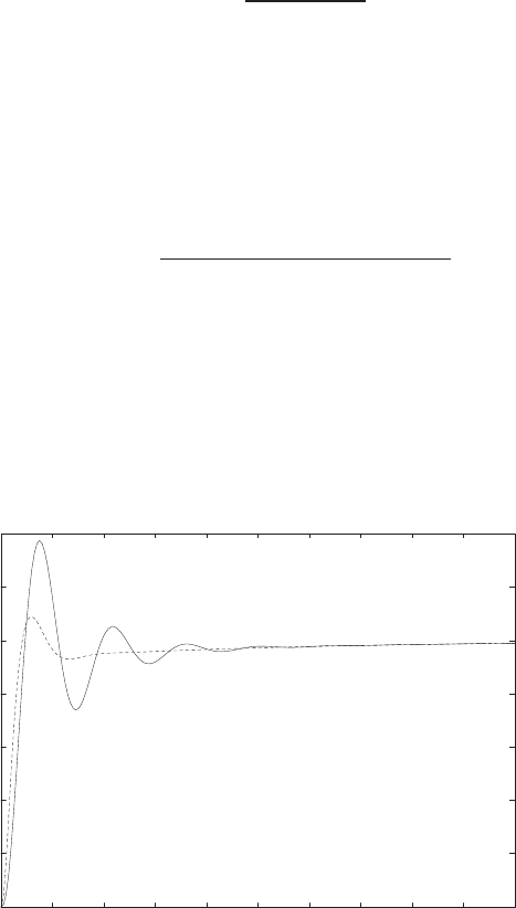
Design Problems 579

DP10.2 (a) When Gc(s) = K, we require K > 20 to meet the steady-state track-

ing speciﬁcation of less than 5%.

(b) The system is unstable for K > 20.

Gc1(s) = 1 + 0.49s

1 + 0.0035s.

With this compensator, the bandwidth is

ωB= 68.9 rad/sec

and the phase margin is P.M. = 28.57o.

(d) A two stage lead compensator is

Gc2(s) = (1 + 0.0185s)(1 + 0.49s)

(1 + 0.00263s)(1 + 0.0035s).

With the two stage compensator, the bandwidth is

ωB= 83.6 rad/sec

and the phase margin is P.M. = 56.79o. The step response for the

two compensators is shown in Figure DP10.2.

0.2

0.4

0.6

0.8

1.2

1.4

00.1 0.2 0.3 0.4 0.5 0.6 0.7 0.8 0.9 1

Single stage (solid) & two stage (dashed)

Time (sec)

Amplitude

FIGURE DP10.2

Step response for one- and two-stage lead compensators.

from the publisher prior to any prohibited reproduction, storage in a retrieval system, or transmission in any form or by any means, electronic, mechanical, photocopying,

recording, or likewise. For information regarding permission(s), write to: Rights and Permissions Department, Pearson Education, Inc., Upper Saddle River, NJ 07458.

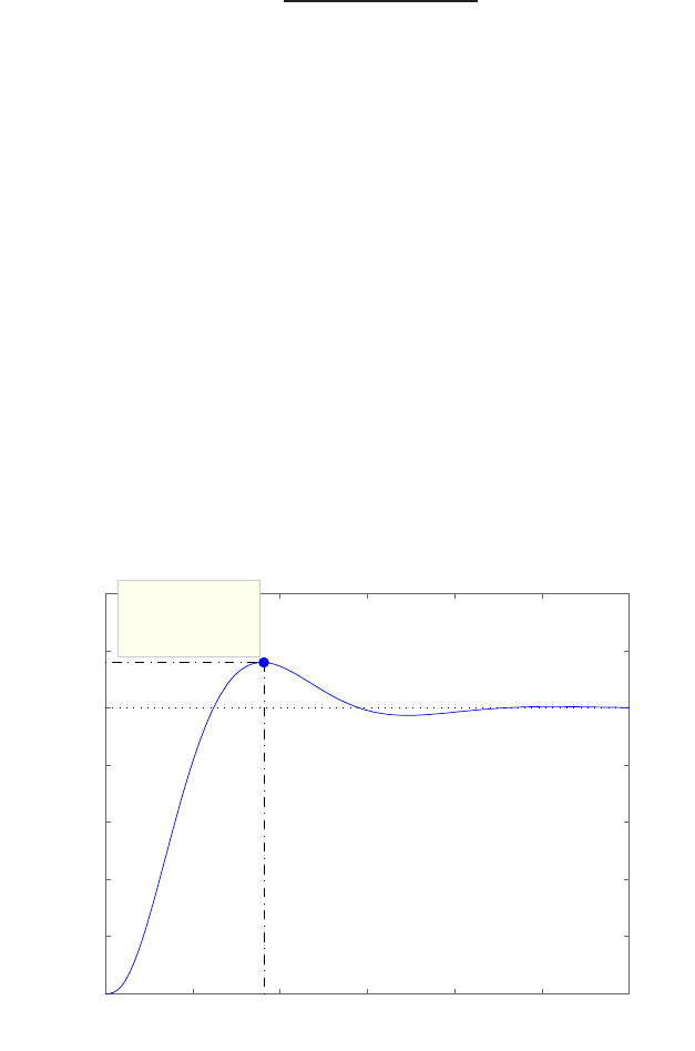
580 CHAPTER 10 The Design of Feedback Control Systems

DP10.3 The mast ﬂight system is modeled as

G(s) = 6

s(s+ 1.5)(s+ 3.9) .

Consider the proportional controller

Gc(s) = K= 0.85 .

The system step response is shown in Figure DP10.3. The percent over-

shoot is

P.O. = 15.9%,

the rise time is

Tr= 3.63 seconds,

and the phase margin is

P.M. = 52o.

Step Response

Time (sec)

Amplitude

0 2 4 6 8 10 12

0.2

0.4

0.6

0.8

1.2

1.4 System: syscl

Peak amplitude: 1.16

Overshoot (%): 15.9

At time (sec): 3.63

FIGURE DP10.3

Step response for the mast ﬂight system.

from the publisher prior to any prohibited reproduction, storage in a retrieval system, or transmission in any form or by any means, electronic, mechanical, photocopying,

recording, or likewise. For information regarding permission(s), write to: Rights and Permissions Department, Pearson Education, Inc., Upper Saddle River, NJ 07458.

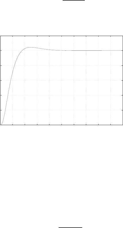
Design Problems 581

DP10.4 One possible compensator is

Gc(s) = 5682s+ 12.6

s+ 87.3.

The step response is shown in Figure DP10.4. The performance results

0.2

0.4

0.6

0.8

1.2

00.1 0.2 0.3 0.4 0.5 0.6 0.7 0.8 0.9 1

Time (sec)

Amplitude

FIGURE DP10.4

Step response for the high speed train system.

are

P.O. = 4.44% Ts= 0.36 sec Kv= 14.1.

DP10.5 The design speciﬁcations are Kv>200; Ts<12 ms and percent overshoot

P.O. < 10%. The step response is shown in Figure DP10.5. A suitable

compensator is

Gc(s) = Ks+ 403

s+ 2336 ,

where

K= 1.9476e+ 13.

Then,

P.O. = 9.5% Ts= 10 ms Kv= 560 .

from the publisher prior to any prohibited reproduction, storage in a retrieval system, or transmission in any form or by any means, electronic, mechanical, photocopying,

recording, or likewise. For information regarding permission(s), write to: Rights and Permissions Department, Pearson Education, Inc., Upper Saddle River, NJ 07458.

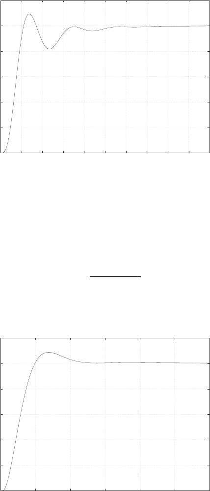
582 CHAPTER 10 The Design of Feedback Control Systems

0.2

0.4

0.6

0.8

1.2

0 2 4 6 8 10 12 14 16 18 20

Time (ms)

Amplitude

FIGURE DP10.5

Step response for the tape transport system.

DP10.6 A solution to the problem is the PI controller

Gc(s) = 4.21s+ 1.2

The step response is shown in Figure DP10.6.

0.2

0.4

0.6

0.8

1.2

0 1 2 3 4 5 6

Time (sec)

Amplitude

FIGURE DP10.6

Step response for the engine control system.

from the publisher prior to any prohibited reproduction, storage in a retrieval system, or transmission in any form or by any means, electronic, mechanical, photocopying,

recording, or likewise. For information regarding permission(s), write to: Rights and Permissions Department, Pearson Education, Inc., Upper Saddle River, NJ 07458.

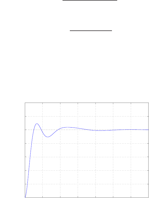
Design Problems 583

The performance results are

P.O. = 8.8% and Ts= 2.14 .

The system is a type-1, so the steady-state error for a step input is zero,

as desired.

DP10.7 The jet aircraft roll angle motion is represented by the transfer function

G(s) = 10

(s+ 10)(s2+ 2s+ 20) .

A good controls solution is obtained with a PID controller

Gc(s) = 10s2+ 20s+ 150

The system is type-1, so the steady-state tracking error is zero for a step

input. The performance results are

P.O. = 9.13% and Ts= 1.56 .

0 0.5 1 1.5 2 2.5 3 3.5

0.2

0.4

0.6

0.8

1.2

1.4

Step Response

Time (sec)

Amplitude

FIGURE DP10.7

Step response for the jet aircraft roll control system.

from the publisher prior to any prohibited reproduction, storage in a retrieval system, or transmission in any form or by any means, electronic, mechanical, photocopying,

recording, or likewise. For information regarding permission(s), write to: Rights and Permissions Department, Pearson Education, Inc., Upper Saddle River, NJ 07458.

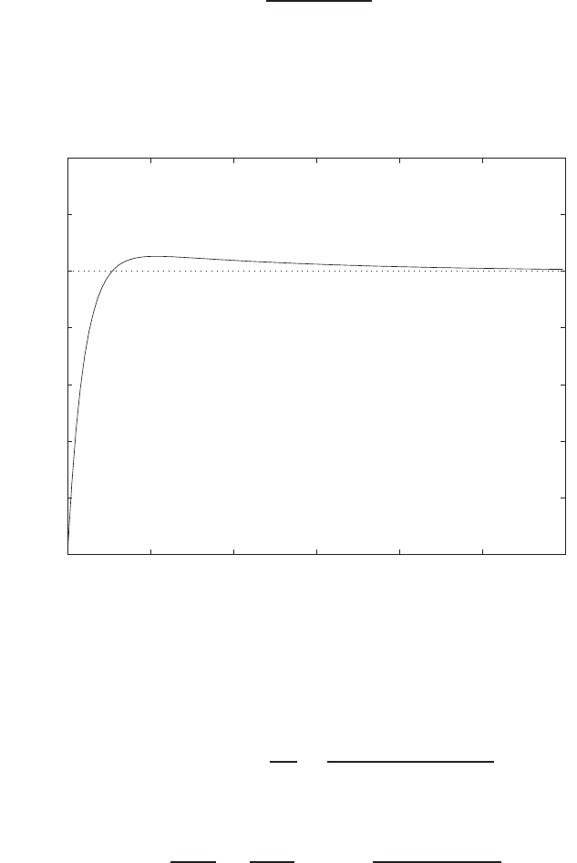
584 CHAPTER 10 The Design of Feedback Control Systems

DP10.8 One good solution is obtained with the following PI controller

Gc(s) = 27.35(s+ 2)

The system is type-1, so the steady-state tracking error is zero for a step

input. The step response is shown in Figure DP10.8.

Time (sec.)

Amplitude

Step Response

0 0.2 0.4 0.6 0.8 1 1.2

0.2

0.4

0.6

0.8

1.2

1.4

From: U(1)

To: Y(1)

FIGURE DP10.8

Step response for the windmill radiometer.

DP10.9 Consider the PID controller

Gc(s) = Kp+KDs+KI

s=1.554s2+ 1.08s+ 1

and the lead-lag controller

Gc(s) = Ks+a

s+bs+c

s+d= 6.04(s+ 10)(s+ 2)

(s+ 1)(s+ 5) .

Both are stabilizing in the presence of a T= 0.1 second time delay. For the

PID controller the phase margin is P.M. = 40o. For the lead-lag controller

the phase margin is P.M. = 45o. We ﬁnd (for these particular designs)

from the publisher prior to any prohibited reproduction, storage in a retrieval system, or transmission in any form or by any means, electronic, mechanical, photocopying,

recording, or likewise. For information regarding permission(s), write to: Rights and Permissions Department, Pearson Education, Inc., Upper Saddle River, NJ 07458.

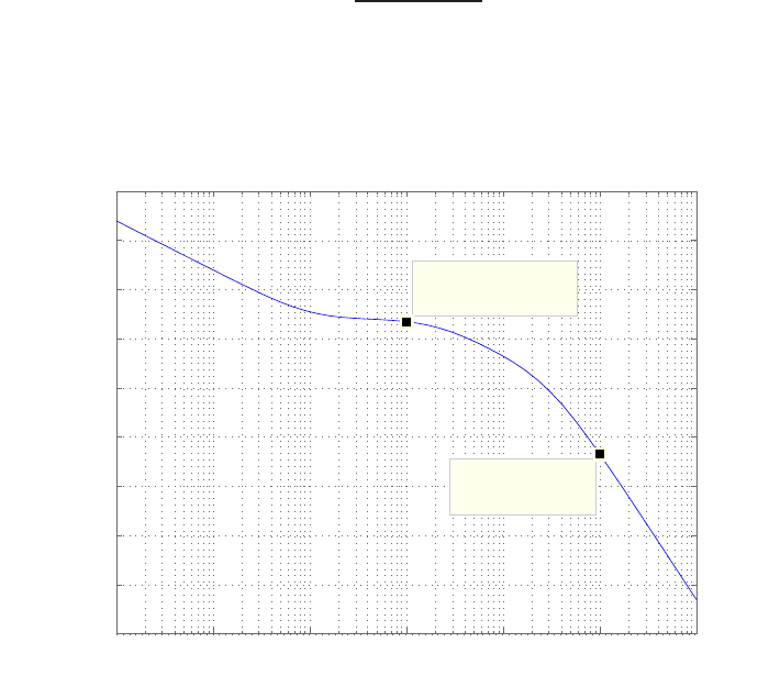
Design Problems 585

that the lead-lag controller is more able to remain stable in the process

of increasing time delay. For a time-delay of T= 0.2 seconds, the lead-lag

compensator has a phase margin of P.M. = 22o, while the PID controller

is unstable.

DP10.10 One solution is

Gc(s) = 50(s+ 0.01)

s+ 2 .

The Bode magnitude is shown in Figure DP10.10. You want high gain at

Bode Diagram

Frequency (rad/sec)

10−4 10−3 10−2 10−1 100101102

−100

−80

−60

−40

−20

System: sys

Frequency (rad/sec): 10

Magnitude (dB): −26.9

System: sys

Frequency (rad/sec): 0.101

Magnitude (dB): 26.9

Magnitude (dB)

FIGURE DP10.10

Step response for the windmill radiometer.

low frequency to improve disturbance rejection and decrease sensitivity to

plant changes and low gain at high frequency to attenuate measurement

noise.

DP10.11 One solution is the PD controller

Gc(s) = 0008(s+ 10) .

The step response is shown in Figure DP10.11. The closed-loop transfer

from the publisher prior to any prohibited reproduction, storage in a retrieval system, or transmission in any form or by any means, electronic, mechanical, photocopying,

recording, or likewise. For information regarding permission(s), write to: Rights and Permissions Department, Pearson Education, Inc., Upper Saddle River, NJ 07458.

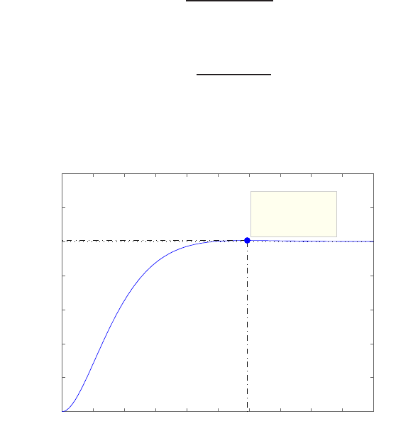
586 CHAPTER 10 The Design of Feedback Control Systems

function is

T(s) = 4

s2+ 3.4s+ 4,

where we use the preﬁlter

Gp(s) = 4

0.36s+ 3.6.

Step Response

Time (sec)

Amplitude

0 0.5 1 1.5 2 2.5 3 3.5 4 4.5 5

0.2

0.4

0.6

0.8

1.2

1.4

System: sys_cl

Peak amplitude: 1.01

Overshoot (%): 0.637

At time (sec): 2.97

FIGURE DP10.11

Step response for the polymerase chain reaction system.

from the publisher prior to any prohibited reproduction, storage in a retrieval system, or transmission in any form or by any means, electronic, mechanical, photocopying,

recording, or likewise. For information regarding permission(s), write to: Rights and Permissions Department, Pearson Education, Inc., Upper Saddle River, NJ 07458.

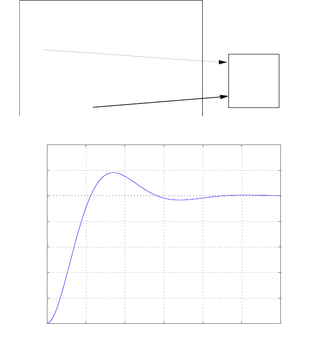
Computer Problems 587

Computer Problems

CP10.1 The m-ﬁle script and step response is shown in Figure CP10.1. The phase

margin and percent overshoot are

P.M. = 50o

P.O. ≈18% ,

respectively.

nnumc=[110]; denc=[1 0]; sysc = tf(numc,denc);

numg=[1]; deng=[1 10]; sysg = tf(numg,deng);

syss = series(sysc,sysg);

[Gm,Pm]=margin(syss);

sys_cl = feedback(syss,1);

[y,t]=step(sys_cl);

step(sys_cl); grid

S=stepinfo(y,t);

PO=S.Overshoot

Pm =

49.9158

PO =

17.5724

0 0.2 0.4 0.6 0.8 1 1.2

0.2

0.4

0.6

0.8

1.2

1.4

Step Response

Time (sec)

Amplitude

FIGURE CP10.1

Phase margin and step response for the closed-loop system.

from the publisher prior to any prohibited reproduction, storage in a retrieval system, or transmission in any form or by any means, electronic, mechanical, photocopying,

recording, or likewise. For information regarding permission(s), write to: Rights and Permissions Department, Pearson Education, Inc., Upper Saddle River, NJ 07458.

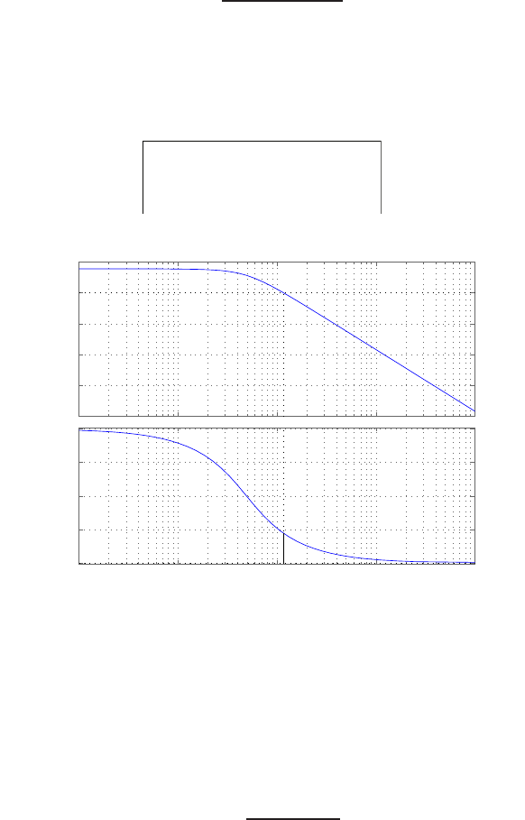
588 CHAPTER 10 The Design of Feedback Control Systems

CP10.2 Using a proportional controller the closed-loop characteristic equation is

1 + K24.2

s2+ 8s+ 24.2.

A simple m-ﬁle script which computes the P.M. as a function of the gain

Kyields the proportional controller gain K= 6. Checking the phase

margin of the system reveals that P.M. ≈40◦, as desired.

n=24.2; d=[1 8 24.2]; sys = tf(n,d);

K=6;

margin(K*sys), grid

−80

−60

−40

−20

Magnitude (dB)

10−1 100101102103

−180

−135

−90

−45

Phase (deg)

Bode Diagram

Gm = Inf dB (at Inf rad/sec) , Pm = 39.9 deg (at 11.6 rad/sec)

Frequency (rad/sec)

FIGURE CP10.2

Bode plot with a proportional controller K= 6 in the loop.

CP10.3 The uncompensated system is type-1. To realize a zero steady-state error

to a ramp input we need to increase the system type by one. One controller

that does this is the PI controller:

Gc(s) = KPs+KD

The step response is shown in Figure CP10.3 where it can be seen in the

tracking error plot that the settling time is Ts<5 seconds. The actual

settling time is

Ts= 3.6 seconds .

from the publisher prior to any prohibited reproduction, storage in a retrieval system, or transmission in any form or by any means, electronic, mechanical, photocopying,

recording, or likewise. For information regarding permission(s), write to: Rights and Permissions Department, Pearson Education, Inc., Upper Saddle River, NJ 07458.

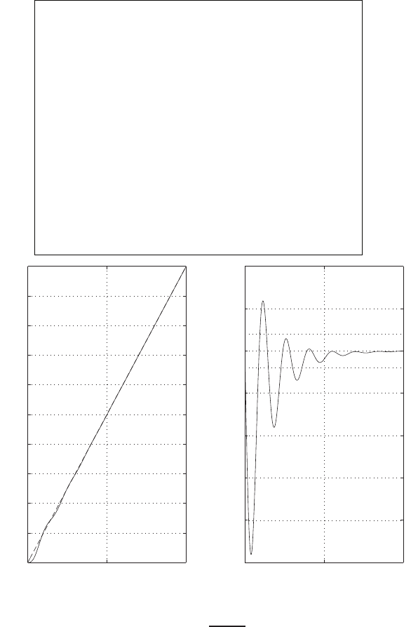
Computer Problems 589

KP=20; KD=10;

nc=[KP KD]; dc=[1 0]; sysc = tf(nc,dc);

n=1; d=[1 2 0]; sys = tf(n,d);

sys_o = series(sysc,sys);

sys_cl = feedback(sys_o,[1]);

t=[0:0.001:10];

sys1 = tf([1],[1 0]); sys_cl1 = series(sys_cl,sys1);

subplot(121)

y=step(sys_cl1,t);

plot(t,y,t,t,'--'), grid

xlabel('Time (sec)'), ylabel('Ramp response')

e=y-t'; L=nd(abs(e)>0.02);

Ts=t(L(length(L)))

subplot(122)

plot(t,e,[0 10],[0.02 0.02],':',[0 10],[-0.02 -0.02],':')

xlabel('Time (sec)'), ylabel('Tracking error')

grid

0 5 10

Time (sec)

Ramp response

0 5 10

-0.25

-0.2

-0.15

-0.1

-0.05

0.05

0.1

Time (sec)

Tracking error

FIGURE CP10.3

Ramp response with a PI controller Gc(s) = 20s+10

sin the loop.

CP10.4 From the percent overshoot spec we determine that P.O. < 10% implies

ζ > 0.6. So, we target a phase margin P.M. = 100ζ= 60o. The m-ﬁle

script which generates the uncompensated Bode plot is shown in Fig-

ure CP10.4a.

from the publisher prior to any prohibited reproduction, storage in a retrieval system, or transmission in any form or by any means, electronic, mechanical, photocopying,

recording, or likewise. For information regarding permission(s), write to: Rights and Permissions Department, Pearson Education, Inc., Upper Saddle River, NJ 07458.

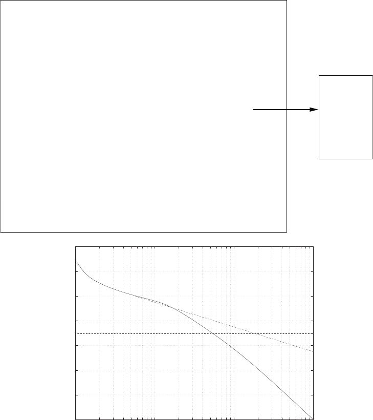
590 CHAPTER 10 The Design of Feedback Control Systems

Phi =

56.2111

Pm =

3.7889

alpha =

10.8408

numg = 100*conv([1 1],[1 0.01]);

deng = conv([1 10],conv([1 2 2],[1 0.02 0.0101]));

sysg = tf(numg,deng)

w=logspace(-1,2,200);

[mag,phase,w]=bode(sysg,w);

[Gm,Pm,Wcg,Wcp]=margin(mag,phase,w);

Phi=60-Pm

Phi=(60-Pm)*pi/180;

alpha=(1+sin(Phi))/(1-sin(Phi))

M=-10*log10(alpha)*ones(length(w),1);

[mag,phase,w]=bode(sysg,w);

for i = 1:length(w),

magdB(i) = 20*log10(mag(1,1,i));

end

semilogx(w,magdB,w,M), grid

xlabel('Frequency (rad/sec)'), ylabel('mag [dB]')

title('Uncompensated Bode Plot')

hold on

semilogx([.56072 5.6072 56.072 560.72],[20 0 -20 -40],'--')

-80

-60

-40

-20

10-1 100101102

Frequency (rad/sec)

mag [dB]

Uncompensated Bode Plot

FIGURE CP10.4

(a) Uncompensated Bode plot.

We assume that K= 1 and raise the gain at a later step to meet settling

time requirement. The uncompensated phase margin is P.M. = 3.7o, so

that the lead compensator needs to add φ= 56.2o. The script also cal-

culates α= 10.84. Following the design procedure outlined in Dorf &

Bishop, we locate the compensator zero at ω= 2 rad/sec (see dashed line

in Figure CP10.4a). Then, p=αz implies p= 21.68. After several iter-

from the publisher prior to any prohibited reproduction, storage in a retrieval system, or transmission in any form or by any means, electronic, mechanical, photocopying,

recording, or likewise. For information regarding permission(s), write to: Rights and Permissions Department, Pearson Education, Inc., Upper Saddle River, NJ 07458.

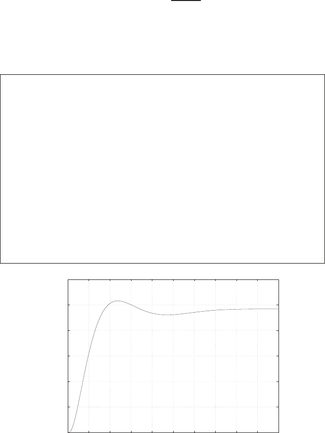
Computer Problems 591

ations, we converge on K= 4 as a “good” value. The lead compensator

Gc(s) = 4 s+ 2

s+ 22 .

The step response is shown in Figure CP10.4b. The compensated Bode is

shown in Figure CP10.4c.

K=4;

numg = 100*conv([1 1],[1 0.01]);

deng = conv([1 10],conv([1 2 2],[1 0.02 0.0101]));

sysg = tf(numg,deng)

numc=K*[1 2]; denc=[1 22]; sysc = tf(numc,denc);

sys_o = series(sysc,sysg);

sys_cl = feedback(sys_o,[1]);

t=[0:0.01:5];

f=10*pi/180;

[y,t,x]=step(f*sys_cl,t);

plot(t,y*180/pi), grid

xlabel('Time (sec)')

ylabel('Attitude rate (deg/sec)'), pause

w=logspace(-1,2,200);

[mag,phase,w]=bode(sys_o,w);

[Gm,Pm,Wcg,Wcp]=margin(mag,phase,w);

bode(sys_o)

title(['Gain Margin = ',num2str(Gm),' Phase Margin = ',num2str(Pm)])

0 0.5 1 1.5 2 2.5 3 3.5 4 4.5 5

Time (sec)

Attitude rate (deg/sec)

FIGURE CP10.4

CONTINUED: (b) Step response.

from the publisher prior to any prohibited reproduction, storage in a retrieval system, or transmission in any form or by any means, electronic, mechanical, photocopying,

recording, or likewise. For information regarding permission(s), write to: Rights and Permissions Department, Pearson Education, Inc., Upper Saddle River, NJ 07458.

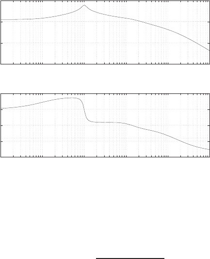
592 CHAPTER 10 The Design of Feedback Control Systems

-100

-50

10-3 10-2 10-1 100101102

Frequency (rad/sec)

Gain dB

-300

-200

-100

100

10-3 10-2 10-1 100101102

Frequency (rad/sec)

Phase deg

Gain Margin = 14.96 Phase Margin = 60.49

FIGURE CP10.4

CONTINUED: (c) Bode plot with lead compensator.

CP10.5 The closed-loop transfer function is

θ(s)/θd(s) = ¯

K1+¯

K2s

s2+¯

K2s+¯

where ¯

K1=K1/J and ¯

K2=K2/J. A percent overshoot P.O. ≤20%

requires ζ > 0.45. Select as the initial damping

ζ= 0.7 (initial selection) .

For a second-order system with ζ= 0.7, we ﬁnd that ω/ωn≈0.9 when

|θ(s)/θd(s)|= 0.7. So, we select

ωn=ωB/0.9

as a starting choice. Therefore, since ωB= 10, we have

ωn= 11 .

The m-ﬁle script is shown in Figure CP10.5a. After several iterations, we

ﬁnd a set of “good” values for

ζ= 0.8 and ωn= 4.5 (ﬁnal selection) .

The step response and closed-loop Bode plot are shown in Figures CP10.5b

and CP10.5c.

from the publisher prior to any prohibited reproduction, storage in a retrieval system, or transmission in any form or by any means, electronic, mechanical, photocopying,

recording, or likewise. For information regarding permission(s), write to: Rights and Permissions Department, Pearson Education, Inc., Upper Saddle River, NJ 07458.

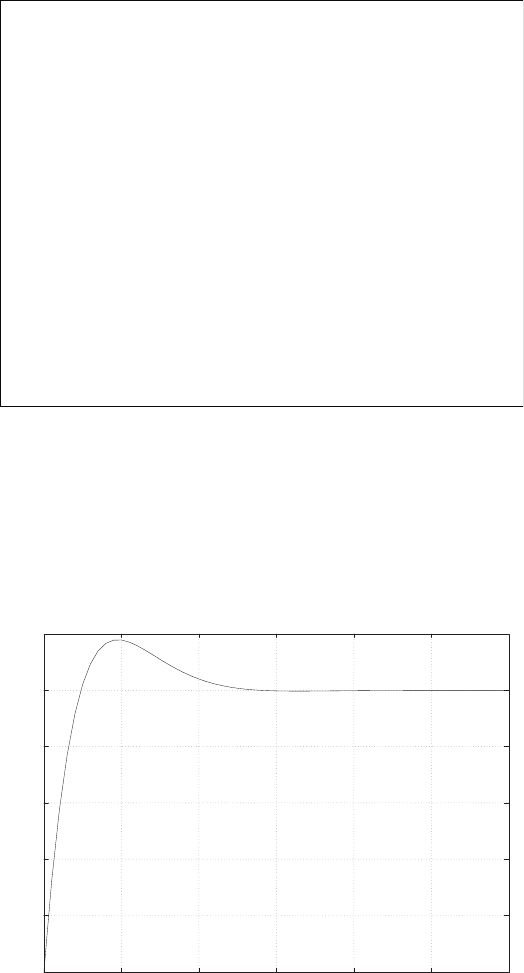
Computer Problems 593

% Part (a)

wn=4.5; zeta=0.8; K2=2*zeta*wn; K1=wn^2;

% Part (b)

num=[K2 K1]; den=[1 0 0]; sys = tf(num,den);

sys_cl = feedback(sys,[1]);

f=10*pi/180; % set-up for 10 deg step input

t=[0:.05:3];

[y,t,x]=step(f*sys_cl,t);

plot(t,y*180/pi), xlabel('time [sec]'), ylabel('theta [deg]'),

grid, pause

% Part (c)

w=logspace(-1,2,400);

[mag,phase,w]=bode(sys_cl,w);

for i = 1:length(w),

magdB(i) = 20*log10(mag(1,1,i));

end

semilogx(w,magdB,[w(1) w(length(w))],[-3 -3]), grid

xlabel('Frequency (rad/sec)')

ylabel('Gain dB')

FIGURE CP10.5

(a) Script to generate the step response and the closed-loop Bode plot.

0 0.5 1 1.5 2 2.5 3

time [sec]

theta [deg]

FIGURE CP10.5

CONTINUED: (b) Step response.

from the publisher prior to any prohibited reproduction, storage in a retrieval system, or transmission in any form or by any means, electronic, mechanical, photocopying,

recording, or likewise. For information regarding permission(s), write to: Rights and Permissions Department, Pearson Education, Inc., Upper Saddle River, NJ 07458.

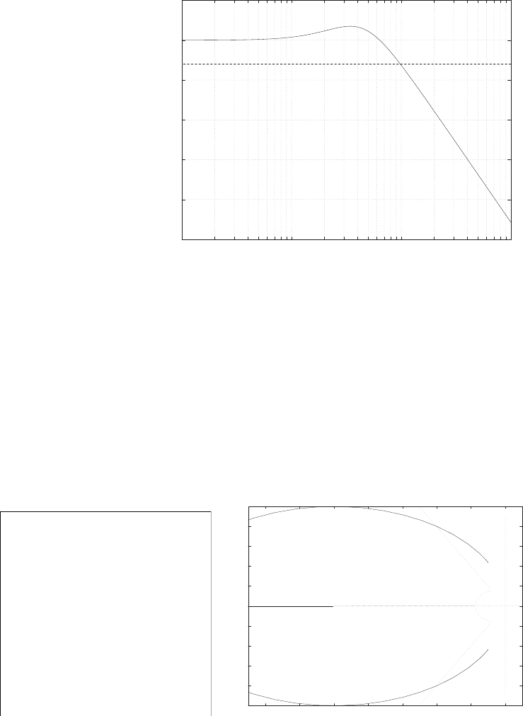
594 CHAPTER 10 The Design of Feedback Control Systems

-25

-20

-15

-10

-5

10-1 100101102

Frequency (rad/sec)

Gain dB

FIGURE CP10.5

CONTINUED: (c) Closed-loop Bode plot.

CP10.6 The settling time and phase margin speciﬁcations require that the dom-

inant closed-loop poles have natural frequency and damping of ζ≥0.45

and ωn≥1.78. The uncompensated roots locus is shown in Figure CP10.6a.

numg=[1 10]; deng=[1 2 20];

sysg = tf(numg,deng);

axis([-15,1,-10,10]);

rlocus(sysg); hold on

zeta=0.45; wn=1.7778;

x=[-10:0.1:-zeta*wn];

y=-(sqrt(1-zeta^2)/zeta)*x;

xc=[-10:0.1:-zeta*wn];

c=sqrt(wn^2-xc.^2);

plot(x,y,':',x,-y,':',xc,c,':',xc,-c,':')

rlocnd(sysg),

hold o

-10

-8

-6

-4

-2

-14 -12 -10 -8 -6 -4 -2 0

Real Axis

Imag Axis

K=10

FIGURE CP10.6

(a) Uncompensated root locus.

from the publisher prior to any prohibited reproduction, storage in a retrieval system, or transmission in any form or by any means, electronic, mechanical, photocopying,

recording, or likewise. For information regarding permission(s), write to: Rights and Permissions Department, Pearson Education, Inc., Upper Saddle River, NJ 07458.

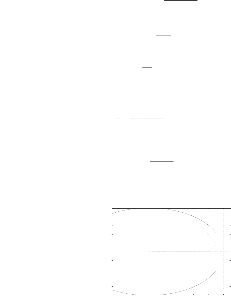
Computer Problems 595

From the ﬁnal value theorem, we determine that

lim

s→0=sE(s)≤0.1Aimplies A

1 + GGc(s)= 0.1A .

Therefore, the compensated Kpcomp ≥9. With the compensator

Gc(s) = Ks+z

s+p

we ﬁnd that

Kpcomp =Kz

pKpuncomp .

But Kpuncomp = 0.5 and (from the uncompensated root locus) a gain of

K= 10 results in roots of the characteristic equation in the desired region.

Solving for

p=1

Kpcomp

Kpuncomp ≈2.

Select z= 0.5 to minimize changing the root locus. Then, p= 0.25, and

the compensator is

Gc(s) = 10 s+ 0.5

s+ 0.25 .

The compensated root locus is shown in Figure CP10.6b and the step re-

sponse is shown in Figure CP10.6c. The phase margin of the compensated

numg=[1 10]; deng=[1 2 20];

sysg = tf(numg,deng);

numc=[1 0.5]; denc=[1 0.25];

sysc = tf(numc,denc);

sys_o = series(sysc,sysg);

axis([-15,1,-10,10]);

rlocus(sys_o); hold on

zeta=0.45; wn=1.7778;

x=[-10:0.1:-zeta*wn];

y=-(sqrt(1-zeta^2)/zeta)*x;

xc=[-10:0.1:-zeta*wn];

c=sqrt(wn^2-xc.^2);

plot(x,y,':',x,-y,':',xc,c,':',xc,-c,':')

rlocnd(sys_o)

hold o

-10

-8

-6

-4

-2

-14 -12 -10 -8 -6 -4 -2 0

xo o

Real Axis

Imag Axis

FIGURE CP10.6

CONTINUED: (b) Compensated root locus.

from the publisher prior to any prohibited reproduction, storage in a retrieval system, or transmission in any form or by any means, electronic, mechanical, photocopying,

recording, or likewise. For information regarding permission(s), write to: Rights and Permissions Department, Pearson Education, Inc., Upper Saddle River, NJ 07458.

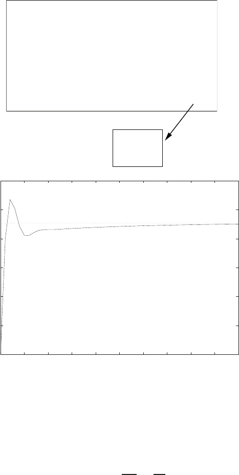
596 CHAPTER 10 The Design of Feedback Control Systems

system is P.M. = 62.3oand the settling time Ts<5 seconds.

pm =

62.3201

numg=[1 10]; deng=[1 2 20];

sysg = tf(numg,deng);

numgc=10*[1 0.5]; dengc=[1 0.25];

sysc = tf(numgc,dengc);

sys_o = series(sysc,sysg);

sys_cl = feedback(sys_o,[1]);

t=[0:0.1:5]; step(sys_cl,t)

[mag,phase,w]=bode(sys_o);

[gm,pm,w1,w2]=margin(mag,phase,w); pm

0.2

0.4

0.6

0.8

1.2

0 0.5 1 1.5 2 2.5 3 3.5 4 4.5 5

Time (secs)

Amplitude

FIGURE CP10.6

CONTINUED: (c) Step response and phase margin veriﬁcation.

CP10.7 Both design speciﬁcations can be satisﬁed with an integral controller

Gc(s) = K1+K2

s=10

The simulation results and m-ﬁle script are shown in Figures CP10.7a

and b.

from the publisher prior to any prohibited reproduction, storage in a retrieval system, or transmission in any form or by any means, electronic, mechanical, photocopying,

recording, or likewise. For information regarding permission(s), write to: Rights and Permissions Department, Pearson Education, Inc., Upper Saddle River, NJ 07458.

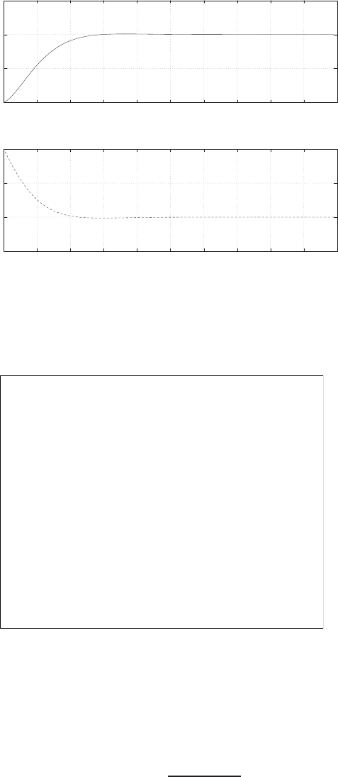
Computer Problems 597

0.5

1.5

00.1 0.2 0.3 0.4 0.5 0.6 0.7 0.8 0.9 1

Time (sec)

Phi dot

Unit Step Response

-0.15

-0.1

-0.05

00.1 0.2 0.3 0.4 0.5 0.6 0.7 0.8 0.9 1

Time (sec)

Tracking error

Unit Ramp Response

FIGURE CP10.7

(a) Simulation results.

K1=0; K2=10;

numc=[K1 K2]; denc=[1 0]; sysc = tf(numc,denc);

numg=[23]; deng=[1 23]; sysg = tf(numg,deng);

sys_o = series(sysc,sysg);

sys_cl = feedback(sys_o,[1]);

t=[0:0.01:1];

ys=step(sys_cl,t);

subplot(211)

plot(t,ys), xlabel('Time (sec)'), ylabel('Phi dot')

title('Unit Step Response'), grid

u=t;

yr=lsim(sys_cl,u,t);

subplot(212)

plot(t,yr-u','--')

xlabel('Time (sec)'), ylabel('Tracking error')

title('Unit Ramp Response'), grid

FIGURE CP10.7

CONTINUED: (b) M-ﬁle design script.

CP10.8 From Example 10.3, we have that the loop transfer function is

Gc(s)G(s) = 8.1(s+z)

s2(s+ 3.6),

from the publisher prior to any prohibited reproduction, storage in a retrieval system, or transmission in any form or by any means, electronic, mechanical, photocopying,

recording, or likewise. For information regarding permission(s), write to: Rights and Permissions Department, Pearson Education, Inc., Upper Saddle River, NJ 07458.

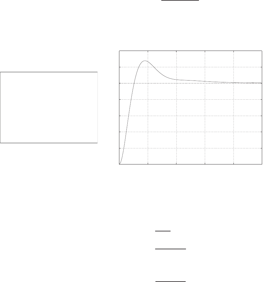
598 CHAPTER 10 The Design of Feedback Control Systems

where z= 1. We want to determine a value of zso the the percent

overshoot is reduced from 46% to less than 32%. A valid design is

Gc(s)G(s) = 8.1(s+ 0.45)

s2(s+ 3.6) .

The m-ﬁle script and step response are shown in Figure CP10.8. The

percent overshoot is P.O.=27.7 %.

K1 = 8.1;

numg = [K1]; deng = [1 0 0];

sysg = tf(numg,deng);

numc = [1 0.45]; denc = [1 3.6];

sysc = tf(numc,denc);

sys_o = series(sysc,sysg);

sys_cl = feedback(sys_o,[1]);

step(sys_cl)

y=step(sys_cl);

po=100*(max(y)-1)

Time (sec.)

Amplitude

Step Response

0 1.6 3.2 4.8 6.4 8

0.2

0.4

0.6

0.8

1.2

1.4

From: U(1)

To: Y(1)

FIGURE CP10.8

Response of system with new lead compensator design.

CP10.9 From AP10.10, we have the transfer function is

T(s) = Vo(s)

Vi(s)

=1 + R2C2s

1 + R1C1s.

Substituting C1= 0.1µF ,C2= 1 mF ,R1= 10 kΩ, and R2= 10 Ω yields

T(s) = 1 + 0.01s

1 + 0.001s.

The frequency response is shown in Figure CP10.9.

from the publisher prior to any prohibited reproduction, storage in a retrieval system, or transmission in any form or by any means, electronic, mechanical, photocopying,

recording, or likewise. For information regarding permission(s), write to: Rights and Permissions Department, Pearson Education, Inc., Upper Saddle River, NJ 07458.

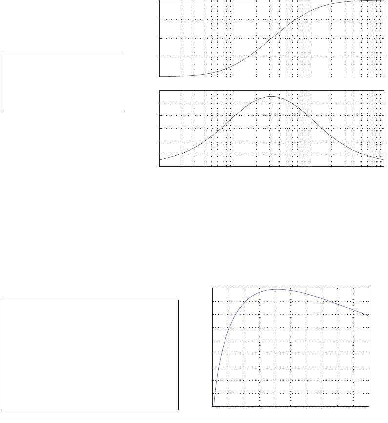
Computer Problems 599

c1=0.0000001; c2=0.001;

r1=10000; r2=10;

n=[c2*r2 1]; d=[c1*r1 1];

sys=tf(n,d)

bode(sys)

Frequency (rad/sec)

Phase (deg); Magnitude (dB)

Bode Diagrams

101102103104

FIGURE CP10.9

Op-amp circuit frequency response.

CP10.10 The plot of Kversus phase margin is shown in Figure CP10.10. The value

of Kthat maximizes the phase margin is K= 4.15.

K=[0.1:0.01:10];

T=0.2;

[np,dp]=pade(T,6); sysp=tf(np,dp);

for i=1:length(K)

ng=K(i)*[1 0.2]; dg=[1 6 0 0]; sysg=tf(ng,dg);

[gm,pm]=margin(sysg*sysp);

PM(i)=pm;

end

plot(K,PM), grid

[P,n]=max(PM); K(n)

xlabel('K'), ylabel('P.M.')

012345678910

P.M.

FIGURE CP10.10

Plot of Kversus phase margin.

from the publisher prior to any prohibited reproduction, storage in a retrieval system, or transmission in any form or by any means, electronic, mechanical, photocopying,

recording, or likewise. For information regarding permission(s), write to: Rights and Permissions Department, Pearson Education, Inc., Upper Saddle River, NJ 07458.

C H A P T E R 1 1

The Design of State Variable

Feedback Systems

Exercises

E11.1 The system is given by

x=Ax +Bu

u=Kx

where

A=



0 1

−1 0 

B=



1 0

0 1 

and K=

−k0

0−2k

.

Then, with u=Kx, we have

x=

−k1

−1−2k

x.

The characteristic equation is

det[sI−A] = det 



s+k−1

1s+ 2k

=s2+ 3ks + 2k2+ 1

=s2+ 2ζωns+ω2

n= 0 .

Solving for kwhere ω2

n= 2k2+ 1 and ζ= 1 (critical damping) yields

k= 2.

600

from the publisher prior to any prohibited reproduction, storage in a retrieval system, or transmission in any form or by any means, electronic, mechanical, photocopying,

recording, or likewise. For information regarding permission(s), write to: Rights and Permissions Department, Pearson Education, Inc., Upper Saddle River, NJ 07458.

Exercises 601

E11.2 Let

u=−k1x1−k2x2+r .

Then,

x=



0 1

9−k1−k2

x+



1

r ,

and

det(sI−A) = s2+k2s+k1−9 = 0 .

We want ζ= 1, so the desired characteristic equation is

pd(s) = (s+co)2,

where cois to be determined to meet Ts= 4 and where k2= 2coand

k1=c2

o+ 9. Solving for the state response of x1(t) to a unit step input

we ﬁnd

x1(t) = 1 −e−cot−cote−cot.

When t≥Ts= 4 sec we want x1(t)≥0.98. Solving for coat t=Tsyields

co= 1.459, k1= 11.13,and k2= 2.92 .

E11.3 The controllability matrix is

Pc=hB AB i=



0 1

1−3

,

and det Pc6= 0, therefore the system is controllable. The observability

matrix is

Po=



CA 

=



0 2

0−6

,

and det Po= 0; therefore the system is unobservable.

E11.4 The controllability matrix is

Pc=hB AB i=



0 0

2−4

,

from the publisher prior to any prohibited reproduction, storage in a retrieval system, or transmission in any form or by any means, electronic, mechanical, photocopying,

recording, or likewise. For information regarding permission(s), write to: Rights and Permissions Department, Pearson Education, Inc., Upper Saddle River, NJ 07458.

602 CHAPTER 11 The Design of State Variable Feedback Systems

and the det Pc= 0; therefore the system is uncontrollable. The observ-

ability matrix is

Po=



CA 

=



1 0

−10 0 

,

and det Po= 0; therefore the system is also unobservable.

E11.5 The controllability matrix is

Pc=hB AB i=



1−2

−2 3 

,

and det Pc=−16= 0; therefore the system is controllable. The observ-

ability matrix is

Po=



CA 

=



1 0

0 1 

,

and det Po= 1 6= 0; therefore the system is observable.

E11.6 The controllability matrix is

Pc=hB AB i=



0 1

1−2

,

and det Pc6= 0; therefore the system is controllable. The observability

matrix is

Po=



CA 

=



1 0

0 1 

,

and det Po6= 0; therefore the system is observable.

from the publisher prior to any prohibited reproduction, storage in a retrieval system, or transmission in any form or by any means, electronic, mechanical, photocopying,

recording, or likewise. For information regarding permission(s), write to: Rights and Permissions Department, Pearson Education, Inc., Upper Saddle River, NJ 07458.

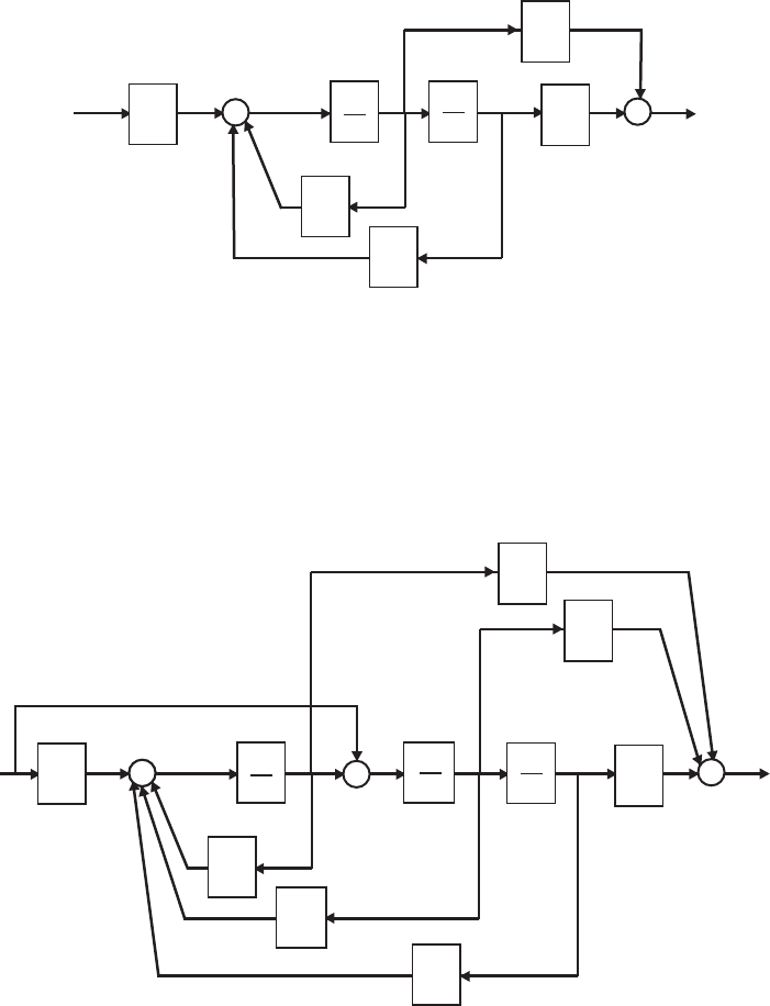
Exercises 603

E11.7 The block diagram is shown in Fig. E11.7.

U(s)Y(s)

2+-

FIGURE E11.7

The block diagram for E11.7.

E11.8 The block diagram is shown in Fig. E11.8.

U(s)Y(s)

2++

FIGURE E11.8

The block diagram for E11.8.

from the publisher prior to any prohibited reproduction, storage in a retrieval system, or transmission in any form or by any means, electronic, mechanical, photocopying,

recording, or likewise. For information regarding permission(s), write to: Rights and Permissions Department, Pearson Education, Inc., Upper Saddle River, NJ 07458.

604 CHAPTER 11 The Design of State Variable Feedback Systems

E11.9 The controllability matrix is

Pc=hB AB i=



k1k1−k2

k2−k1+k2

,

and det Pc=−k2

1+k2

2. So, the condition for complete controllability is

16=k2

E11.10 A matrix diﬀerential equation representation is

x=





010

001

−10 −6−3







x+











y= [−3 4 2]x+ [0]u .

E11.11 The system is given by

x=Ax +Bu

y=Cx +Du

where

A=





0 1 0

0 0 1

−2 0 −7







,B=











,C=h1 2 0 i,and D= [1] .

The controllability matrix is

Pc=hB AB A2Bi=





0 0 1

0 1 −7

1−7 49







and det Pc=−16= 0; therefore the system is controllable. The observ-

ability matrix is

Po=





CA2







=





1 2 0

0 1 2

−4 0 −13







from the publisher prior to any prohibited reproduction, storage in a retrieval system, or transmission in any form or by any means, electronic, mechanical, photocopying,

recording, or likewise. For information regarding permission(s), write to: Rights and Permissions Department, Pearson Education, Inc., Upper Saddle River, NJ 07458.

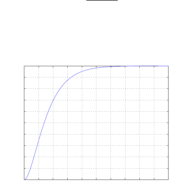
Exercises 605

and det Po=−29 6= 0; therefore the system is observable.

E11.12 The transfer function is

G(s) = 6

s2+ 5s+ 6 .

The response of the system to a unit step is

y(t) = 1 −3e−2t+ 2e−3t.

The step response is shown in Figure E11.12

0 0.5 1 1.5 2 2.5 3 3.5 4 4.5 5

0.1

0.2

0.3

0.4

0.5

0.6

0.7

0.8

0.9

Time (s)

Step Response

FIGURE E11.12

Unit step response.

from the publisher prior to any prohibited reproduction, storage in a retrieval system, or transmission in any form or by any means, electronic, mechanical, photocopying,

recording, or likewise. For information regarding permission(s), write to: Rights and Permissions Department, Pearson Education, Inc., Upper Saddle River, NJ 07458.

606 CHAPTER 11 The Design of State Variable Feedback Systems

Problems

P11.1 Consider the system

˙x=x+u

u=−kx .

So,

˙x=x−kx = (1 −k)x

and

x(t) = e(1−k)tx(0) .

The system is stable if k > 1. Computing the value of J(assuming k > 1)

yields

J=Z∞

e2(1−k)tx2(0)dt =1

k−1.

Thus, Jis minimum when k→ ∞. This is not physically realizable. Select

k= 35. Then, the value of the performance index Jis

J=1

34 .

The system is not stable without feedback.

P11.2 (a) The performance index is given

J=Z∞

(x2+λu2)dt .

The system is

˙x=x+u

u=−kx .

So,

J=Z∞

(x2+λk2x2)dt =Z∞

(1 + λk2)x2dt = (1 + λk2)Z∞

x2dt .

Carrying out the integration (assuming k > 1) yields

J= (1 + λk2)1

k−1.

We want to determine kthat minimizes J. Taking the partial of J

from the publisher prior to any prohibited reproduction, storage in a retrieval system, or transmission in any form or by any means, electronic, mechanical, photocopying,

recording, or likewise. For information regarding permission(s), write to: Rights and Permissions Department, Pearson Education, Inc., Upper Saddle River, NJ 07458.

Problems 607

with respect to kand setting the result to zero yields

∂J

∂k =λk2−2λk −1

(k−1)2= 0 ,

λk2−2λk −1 = 0 .

Solving for kyields

k= 1 + r1 + 1

λ,

where we reject the solution k= 1 −q1 + 1

λ, since we require k > 1.

(b) For λ= 2, we determine that k= 2.2 and Jmin = 8.9.

P11.3 The system is given by

x=



1 0

−1 2 

x+



1

u

u=−k(x1+x2) = −k[1 1]x.

Then, with feedback applied, the system is

x=



(1 −k)−k

−(1 + k) (2 −k)

x.

Solving

HTP+PH =−I

yields

2p11(1 −k)−2p12(k+ 1) = −1

p12(3 −2k)−p11k−p22(k+ 1) = 0

−2kp12 + 2p22(2 −k) = −1.

Solving for p11, p12 and p22 yields

p11 =−(2k2−6k+ 7)

4(4k2−8k+ 3)

p12 =2k2−2k−1

4(4k2−8k+ 3)

from the publisher prior to any prohibited reproduction, storage in a retrieval system, or transmission in any form or by any means, electronic, mechanical, photocopying,

recording, or likewise. For information regarding permission(s), write to: Rights and Permissions Department, Pearson Education, Inc., Upper Saddle River, NJ 07458.

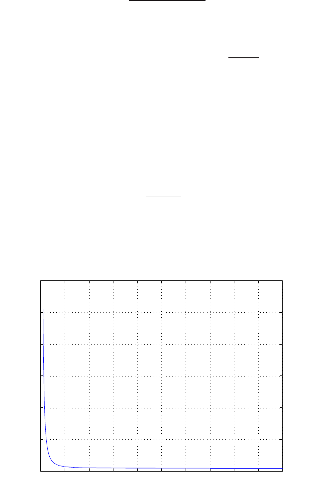
608 CHAPTER 11 The Design of State Variable Feedback Systems

p22 =−(2k2−6k+ 3)

4(4k2−8k+ 3) .

The performance index is computed to be

J=xT(0)Px(0) = p11 + 2p12 +p22 =1

2k−1,

when x(0) = [1 1]T. So as k→ ∞,J→0. The system is unstable without

feedback.

P11.4 The performance index is

J=xT(0)Px(0) = p11 −2p12 +p22 .

From Example 11.12 in Dorf and Bishop, we determine that

J=2k2+ 1

2k2.

So, when k→ ∞, the performance index J→1. The plot of Jversus k

is shown in Figure P11.4.

0 1 2 3 4 5 6 7 8 9 10

FIGURE P11.4

The performance index Jversus k.

from the publisher prior to any prohibited reproduction, storage in a retrieval system, or transmission in any form or by any means, electronic, mechanical, photocopying,

recording, or likewise. For information regarding permission(s), write to: Rights and Permissions Department, Pearson Education, Inc., Upper Saddle River, NJ 07458.

Problems 609

P11.5 The system is given by

x=



0 1

0 0 

x+



0 0

1 1 

u

u=−kx.

The performance index is

J=Z∞

(xTx+uTu)dt =Z∞

(1 + k2)(xTx)dt .

First, we solve

HTP+PH =−(1 + k2)I,

yielding,

p12 =(1 + k2)

p22 =k3+k2+k+ 1

2k2

p11 =2k3+k2+ 2k+ 1

2k.

The performance index is then given by

J=p11 + 2p12 +p22 =2k4+ 4k3+ 3k2+ 4k+ 1

2k2.

Taking the partial of Jwith respect to k, setting the result to zero and

solving for kyields

∂J

∂k =2k4+ 2k3−2k−1

k3= 0

2k4+ 2k3−2k−1 = 0 .

Solving for kyields k= 0.90. The plot of Jversus kis shown in Fig-

ure P11.5. The value of the performance index is

J= 6.95

when k= 0.90.

from the publisher prior to any prohibited reproduction, storage in a retrieval system, or transmission in any form or by any means, electronic, mechanical, photocopying,

recording, or likewise. For information regarding permission(s), write to: Rights and Permissions Department, Pearson Education, Inc., Upper Saddle River, NJ 07458.

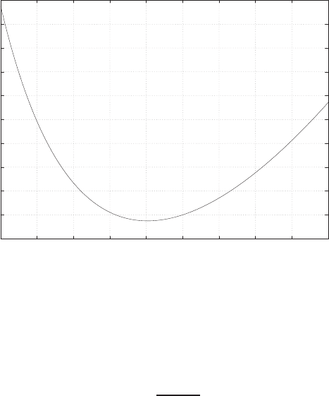
610 CHAPTER 11 The Design of State Variable Feedback Systems

6.8

7.2

7.4

7.6

7.8

8.2

8.4

8.6

8.8

0.5 0.6 0.7 0.8 0.9 1 1.1 1.2 1.3 1.4

FIGURE P11.5

The performance index Jversus k.

P11.6 (a) For P11.3, we have

J=1

2k−1.

So, as k→ ∞, then J→0. But k=∞is not a practical solution, so

select k= 10. Then, J= 1/19, and

x=

−9−10

−11 −8

x=Ax .

The closed-loop system roots are determined by solving

det[sI−A] = s2+ 17s−38 = 0 ,

which yields s=−19 and s2= 2. The system is unstable. The original

system was unstable, and it remains unstable with the feedback. In

general,

x=



(1 −k)−k

−(1 + k) (2 −k)

x=Ax

and det[sI−A] = s2+s(2k−3) + (2 −4k) = 0. A Routh-Hurwitz

analysis reveals that the system is unstable for all k.

from the publisher prior to any prohibited reproduction, storage in a retrieval system, or transmission in any form or by any means, electronic, mechanical, photocopying,

recording, or likewise. For information regarding permission(s), write to: Rights and Permissions Department, Pearson Education, Inc., Upper Saddle River, NJ 07458.

Problems 611

(b) For P11.4, we have

x=



0 1

−k−k

x=Ax ,

and

det[sI−A] = s2+ks +k= 0 .

The performance index was found to be

J= 1 + 4k+ 1

2k2.

As k→ ∞, we have J→0. But k=∞is not a practical choice for

k. Select k= 10. Then,

det[sI−A] = s2+ 10s+ 10 = (s+ 1.13)(s+ 8.87) .

The closed-loop system is stable.

x=



0 1

−k−k

x

and

det[sI−A] = s2+ks +k=s2+ 0.9s+ 0.9

= (s+ 0.45 + j0.835)(s+ 0.45 −j0.835) .

P11.7 The closed-loop system is

x=



0 1

−k1−k2

x=Hx ,

and

det[sI−H] = s2+k2s+k1=s2+ 2ζωns+ω2

n= 0 .

We desire ωn= 2, so set k1= 4. With xT(0) = [1,0], we have J=p11,

and solving

HTP+PH =−I

from the publisher prior to any prohibited reproduction, storage in a retrieval system, or transmission in any form or by any means, electronic, mechanical, photocopying,

recording, or likewise. For information regarding permission(s), write to: Rights and Permissions Department, Pearson Education, Inc., Upper Saddle River, NJ 07458.

612 CHAPTER 11 The Design of State Variable Feedback Systems

yields





0−4

1−k2





p11 p12

p12 p22 

+



p11 p12

p12 p22 





0 1

−4−k2



=

−1 0

0−1

,

and

p11 =k2

8+20

8k2

=k2

2+ 20

8k2

Select

k2=√20

for Jmin, where Jmin =√5

2. Then

det[sI−H] = s2+√20s+ 4 = 0 ,

and ωn= 2 and ζ= 1.12. The system is overdamped.

P11.8 From Example 11.11 in Dorf and Bishop, we have

P=



2+2

2k2



.

So,

J=xT(0)Px(0) = k2

2+ 2

2k2

when xT(0) = [1 0]. Taking the partial of Jwith respect to k2and setting

the result to zero yields

∂J

∂k2

= 1 −k2

2+ 2

2k2

= 0 .

Solving for the optimum value of k2yields

k2=√2.

P11.9 Let x1=φand x2=ω. We have that

ω=dφ

dt .

from the publisher prior to any prohibited reproduction, storage in a retrieval system, or transmission in any form or by any means, electronic, mechanical, photocopying,

recording, or likewise. For information regarding permission(s), write to: Rights and Permissions Department, Pearson Education, Inc., Upper Saddle River, NJ 07458.

Problems 613

The state equations are

˙x1=x2

˙x2=Ku .

Select a feedback such that

u=−x1−K1x2+r

when r(t) is the reference input. Then,

x=



0 1

−K−KK1

x+



K

r ,

and

det[sI −A] = s2+K1Ks +K .

We desire ζ=1

√2, so that the overshoot is 4%. Since Ts= 1 = 4

ζωn, we

require ζωn= 4 or ωn= 4√2. Then, s2+ 8s+ 32 = s2+K1Ks +K, or

K= 32 and K1=8

32 =1

P11.10 The system with feedback is given by

x=Ax =

−10 −25

1 0 

x,

where x1(0) = 1, and x2(0) = −1. The characteristic equation is

det[sI−A] = det 



s+ 10 25

−1s

=s(s+ 10) + 25 = s2+ 10s+ 25 = 0 .

The roots are s1,2=−5. The solution is

x(t) = 



φ11 φ12

φ21 φ22 

x(0) = 



φ11 −φ12

φ21 −φ22 



since x1(0) = 1 and x2(0) = −1. We compute the elements of the state

transition matrix as follows:

φ22(t) = (1 + 5t)e−5tand φ21(t) = te−5t,

therefore

x2(t) = −(1 + 4t)e−5t.

from the publisher prior to any prohibited reproduction, storage in a retrieval system, or transmission in any form or by any means, electronic, mechanical, photocopying,

recording, or likewise. For information regarding permission(s), write to: Rights and Permissions Department, Pearson Education, Inc., Upper Saddle River, NJ 07458.

614 CHAPTER 11 The Design of State Variable Feedback Systems

Similarly,

φ11(t) = (1 −5t)e−5tand φ12 = −25e−5t.

Therefore,

x1(t) = (1 + 20t)e−5t.

P11.11 Let

u=−k1x1−k2x2+αr

where r(t) is the command input. A state variable representation of the

plant is

x=

−5−2

2 0 

x+



0.5

0

u

y=h0 1 ix+h0iu .

The closed-loop transfer function is

T(s) = α

s2+ (k1/2 + 5)s+ 4 + k2

To meet the performance speciﬁcations we need ωn= 4.8 and ζ= 0.826.

Therefore, the desired characteristic polynomial is

q(s) = s2+ 2(0.826)4.8s+ 23 = s2+ 8s+ 23 .

Equating coeﬃcients and solving for k1and k2yields k2= 19 and k1= 6.

Select α= 23 to obtain zero steady-state error to a step input.

P11.12 A state variable representation of the dc motor is







−3−2−0.75 0 0

3 0 0 0 0

0 2 0 0 0

0 0 1 0 0

0 0 0 2 0



















y= [0 0 0 0 2.75]x.

from the publisher prior to any prohibited reproduction, storage in a retrieval system, or transmission in any form or by any means, electronic, mechanical, photocopying,

recording, or likewise. For information regarding permission(s), write to: Rights and Permissions Department, Pearson Education, Inc., Upper Saddle River, NJ 07458.

Problems 615

The controllability matrix is

Pc=







1−3 3 4.5−18

0 3 −9 9 13.5

006−18 18

0 0 0 6 −18

0 0 0 0 12







and the det Pc6= 0, so the system is controllable. The observability matrix

Po=







0 0 0 0 2.75

0 0 0 5.5 0

0 0 5.5 0 0

0 11 0 0 0

33 0 0 0 0







and the det Po6= 0, so the system is observable.

P11.13 To meet the Kv= 35 speciﬁcation, we need K= 2450. A state variable

representation is

x=



0 1

0−70 

x+



2450 

u

y= [1 0]x.

Let

u=−k1x1−k2x2.

Then, the closed-loop characteristic equation is

q(s) = s2+ (2450k2+ 70)s+ 2450k1= 0 .

The desired characteristic polynomial is

s2+ 72.73s+ 2644.63 = 0

where we select ζ= 0.707 and ωn= 51.42 to meet the performance

speciﬁcations. Equating coeﬃcients and solving for the gains yields k1=

from the publisher prior to any prohibited reproduction, storage in a retrieval system, or transmission in any form or by any means, electronic, mechanical, photocopying,

recording, or likewise. For information regarding permission(s), write to: Rights and Permissions Department, Pearson Education, Inc., Upper Saddle River, NJ 07458.

616 CHAPTER 11 The Design of State Variable Feedback Systems

1.08 and k2= 0.0011.

P11.14 Let

u=−k1x1−k2x2−k3r

where r(t) is the command input. Then, the closed-loop system in state

variable form is

x=

−10 −k1−k2

1 0 

x+



0

r

y= [0 1]x.

To meet the performance speciﬁcations, we want the closed-loop charac-

teristic polynomial to be

q(s) = s2+ 8s+ 45.96 = 0

where ζ= 0.59 and ωn= 6.78. The actual characteristic polynomial is

det(sI−A) = s2+ (10 + k1)s+k2= 0 .

Equating coeﬃcients and solving for the gains yields k2= 45.96 and

k1=−2. Select k3=k2= 45.96 to obtain a zero steady-state error to a

step input. This results in a settling time of Ts= 0.87 s and a percent

overshoot of P.O. = 10%.

P11.15 The transfer function is

G(s) = C(sI−A)−1B=1

s+ 1 .

The system is not controllable and not observable.

P11.16 Let

u=−Kx .

Then, Ackermann’s formula is

K= [0,0, ..., 1]P−1

cq(A)

where q(s) is the desired characteristic polynomial, which in this case is

q(s) = s2+ 2s+ 10 .

from the publisher prior to any prohibited reproduction, storage in a retrieval system, or transmission in any form or by any means, electronic, mechanical, photocopying,

recording, or likewise. For information regarding permission(s), write to: Rights and Permissions Department, Pearson Education, Inc., Upper Saddle River, NJ 07458.

Problems 617

A state-space representation of the limb motion dynamics is

x=

−4 0

1−1

x+



0

u .

The controllability matrix is

Pc= [B AB] = 



1−4

0 1 



and

P−1

c=



1 4

0 1 

.

Also, we have

q(A) = A2+ 2A+ 10I=



18 0

−3 9 

.

Using Ackermann’s formula, we have

K= [−3 9] .

P11.17 The system is either uncontrollable or unobservable if a= 5 or a= 8.

Both of these values correspond to system real poles. So, if atakes on

either value, a pole-zero cancellation occurs in the transfer function.

P11.18 A matrix diﬀerential equation representation is

x=



0 1

−1−2

x+



1

u

y= [1 0]x.

Let u(t) = −k1x1−k2x2. Then, the closed-loop characteristic equation is

q(s) = s2+ (2 + k2)s+ 1 + k1= 0 .

We desire the characteristic equation

s2+ 2√2s+ 2 = 0 .

from the publisher prior to any prohibited reproduction, storage in a retrieval system, or transmission in any form or by any means, electronic, mechanical, photocopying,

recording, or likewise. For information regarding permission(s), write to: Rights and Permissions Department, Pearson Education, Inc., Upper Saddle River, NJ 07458.

618 CHAPTER 11 The Design of State Variable Feedback Systems

Equating coeﬃcients and solving for the gains yields k1= 1 and k2=

2√2−2 = 0.828.

P11.19 A state space representation is

x=



0 1

3−2

x+



1

r

y= [3 1]x.

The controllability matrix is

Pc=



0 1

1−2

,

and det Pc6= 0, so the system is controllable. The observability matrix is

Po=



3 1

3 1 

,

and the det Po= 0, so the system is not observable.

P11.20 The characteristic equation associated with Ais

s2(s2+ 0.2s+ 0.0015) = 0 .

There are two roots at the origin, so the system is unstable. The system

can be stabilized with

δ=−k1x1−k3x3= 20x1−10x3.

P11.21 (a) Let x1=i1,x2=i2and u=v. Then, the state equation is

x=



−(R1+R3)

L2−(R3+R2)



x+



0

u.

Also,

y=vo,

but

y= [R3−R3]x.

from the publisher prior to any prohibited reproduction, storage in a retrieval system, or transmission in any form or by any means, electronic, mechanical, photocopying,

recording, or likewise. For information regarding permission(s), write to: Rights and Permissions Department, Pearson Education, Inc., Upper Saddle River, NJ 07458.

Problems 619

(b) The observability matrix is

Po=



CA 

=



R3−R3

−R1R3

L1−R2

31

L1+1

L2R2R3

L2+R2

31

L1+1

L2



and

det Po=R2

L2−R1

L1R2

So, when

=R2

det Po= 0 and the system is not observable.

a=R1+R3

and

b=R3+R2

Then

det[sI−A] = det 



(s+a)−R3

−R3

L2(s+b)



="(s+a)(s+b) + R2

L1L2#= (s+r)2

=s2+ (a+b)s+ab +R2

L1L2

The system has two equal roots when

(a+b)2−4 ab +R2

L1L2!

R1+R3

+R3+R2

L22

−4(R1+R3)(R3+R2)+R2

L1L2

= 0 .

from the publisher prior to any prohibited reproduction, storage in a retrieval system, or transmission in any form or by any means, electronic, mechanical, photocopying,

recording, or likewise. For information regarding permission(s), write to: Rights and Permissions Department, Pearson Education, Inc., Upper Saddle River, NJ 07458.

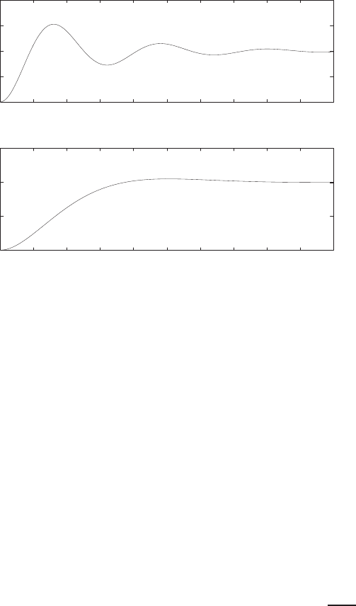
620 CHAPTER 11 The Design of State Variable Feedback Systems

P11.22 (a) Without state feedback the state diﬀerential equation is given by

x=

−0.4−1

1 0 

x+



0

u

y=h0 1 ix.

The step response is shown in Figure P11.22a.

0.5

1.5

02 4 6 8 10 12 14 16 18 20

Time (sec)

(a) Without state feedback

0.5

1.5

00.2 0.4 0.6 0.8 1 1.2 1.4 1.6 1.8 2

Time (sec)

(b) With state feedback

FIGURE P11.22

Step response (a) without state feedback, and (b) with state feedback.

(b) Consider state feedback

u=−K(ax2+bx1) + cr

where ris the reference input and K, a, b and care to be determined.

Then, the state diﬀerential equation is

x=

−0.4−Kb −1−Ka

1 0 

x+



0

r

y=h0 1 ix,

and det(sI−A) = s2+ (0.4 + Kb)s+ (1 + Ka) = 0. Our speciﬁcations

are P.O. = 5% and Ts= 1.35 sec. So, ζ= 0.69 and ωn=4

ζ1.35 = 4.3.

from the publisher prior to any prohibited reproduction, storage in a retrieval system, or transmission in any form or by any means, electronic, mechanical, photocopying,

recording, or likewise. For information regarding permission(s), write to: Rights and Permissions Department, Pearson Education, Inc., Upper Saddle River, NJ 07458.

Problems 621

Solving for K, a and byields

Ka =ω2

n−1

and

Kb = 2ζωn−0.4.

Select K= 1. Then, a= 17.49 and b= 5.53. Select c= 1 + Ka to

achieve a zero steady-state tracking error.

state feedback.

P11.23 Using the internal model design method for step inputs, we have





˙e

z

=





0 1 0

0 0 1

0 0 0









z

+











w ,

where we choose

w=−K1e−K2z.

To place the poles at s=−10 and s=−2±jwe use Ackermann’s formula

to compute

K1= 50

K2= [45 14] .

The compensator has the form shown in Figure 11.14 in Dorf and Bishop.

P11.24 Using the internal model design method for ramp inputs, we have







˙e

¨e













0 1 0 0

0 0 1 0

0 0 0 1

0 0 0 0













˙e



















where we choose

w=−K1e−K2˙e−K3z.

To place the poles at s=−20 and s=−2±2jwe can use Ackermann’s

formula. We also need an additional pole (must be a stable pole); select

from the publisher prior to any prohibited reproduction, storage in a retrieval system, or transmission in any form or by any means, electronic, mechanical, photocopying,

recording, or likewise. For information regarding permission(s), write to: Rights and Permissions Department, Pearson Education, Inc., Upper Saddle River, NJ 07458.

622 CHAPTER 11 The Design of State Variable Feedback Systems

s=−20 as the fourth pole. Then,

K1= 3200

K2= 1920

K3= [568 44] .

The compensator has the form shown in Figure 11.16 in Dorf and Bishop.

P11.25 The observability matrix is

Po=



CA 

=



1−4

21 −36 

,

and det Po= 48 6= 0; therefore the system is completely observable. The

desired poles of the observer are s1,2=−1. This implies that the desired

characteristic polynomial is

pd(s) = s2+ 2s+ 1 .

The actual characteristic polynomial is

det |λI−(A−LC)|= det 

λ−1 + L1−4−4L1

5 + L2λ−10 −4L2

=λ2+ (L1−4L2−11)λ+ 10L1+ 8L2+ 30 = 0 .

Solving for L1and L2yields

L=



L2

=

−0.25

−3.3125 

.

Checking we ﬁnd that det(λI−(A−LC)) = s2+ 2s+ 1. The response of

the estimation error is shown in Figure P11.25, where e(0) = [ 1 1 ]T.

from the publisher prior to any prohibited reproduction, storage in a retrieval system, or transmission in any form or by any means, electronic, mechanical, photocopying,

recording, or likewise. For information regarding permission(s), write to: Rights and Permissions Department, Pearson Education, Inc., Upper Saddle River, NJ 07458.

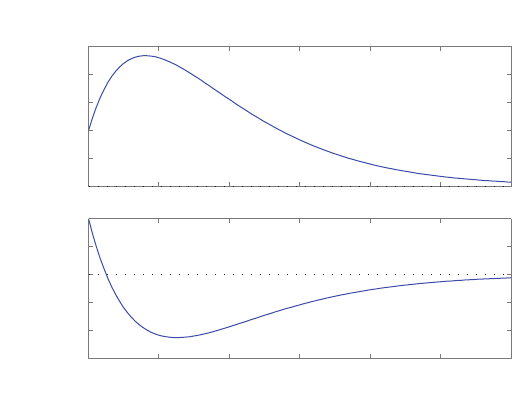
Problems 623

0.5

1.5

2.5

To: Out(1)

0 1 2 3 4 5 6

-1.5

?-1

-0.5

0.5

To: Out(2)

Response to Initial Conditions

Time

(

sec

)

Amplitude

FIGURE P11.25

Estimation error response to an initial condition.

P11.26 The observability matrix is

Po=





CA2







=





2−4 0

0 2 −4

32 20 14







The det Po= 728 6= 0, hence the system is observable. The gain matrix

L=





0.14

−0.93

0.79







results in the observer poles at s1,2=−1±jand s3=−5, as desired.

P11.27 The observability matrix is

Po=



CA 

=



1 0

1 0 

.

The det Po= 0, hence the system is not completely observable. So, we

cannot ﬁnd an observer gain matrix that places the observer poles at the

desired locations.

from the publisher prior to any prohibited reproduction, storage in a retrieval system, or transmission in any form or by any means, electronic, mechanical, photocopying,

recording, or likewise. For information regarding permission(s), write to: Rights and Permissions Department, Pearson Education, Inc., Upper Saddle River, NJ 07458.

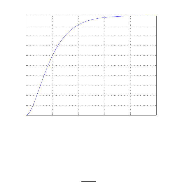
624 CHAPTER 11 The Design of State Variable Feedback Systems

P11.28 Selecting K= 16 yields a zero steady-state error to a unit step input.

The step response is shown in Figure P11.28.

0 0.5 1 1.5 2 2.5

0.1

0.2

0.3

0.4

0.5

0.6

0.7

0.8

0.9

Step Response

Time (sec)

Amplitude

FIGURE P11.28

Estimation error response to an initial condition.

P11.29 The system transfer function is

Y(s) = 2

s+ 3U(s).

The associated state variable model is

˙x=−3x+ 2u

y=x .

from the publisher prior to any prohibited reproduction, storage in a retrieval system, or transmission in any form or by any means, electronic, mechanical, photocopying,

recording, or likewise. For information regarding permission(s), write to: Rights and Permissions Department, Pearson Education, Inc., Upper Saddle River, NJ 07458.

Advanced Problems 625

Advanced Problems

AP11.1 The closed loop system in state-space form is given by







˙x1

˙x2

˙x3







=





0 1 0

0−1 2

−2KK1−2KK2−4−2KK3



















+











y=h1 0 0 i











The closed-loop transfer function is

T(s) = 4K

s3+ (2KK3+ 5)s2+ (4KK2+ 2KK3+ 4)s+ 4KK1

Setting the steady-state error to zero, we determine that

ess = 1 −T(0) = 1 −1

Solving for K1yields

K1= 0.5.

Choosing

K2= 0.5 and K3= 1.5

results in a percent overshoot of P.O. = 2.82%.

AP11.2 A state variable representation is given by

x=Ax +Bu

where

A=





−3−1−1

4 0 0

0 1 0







,B=











from the publisher prior to any prohibited reproduction, storage in a retrieval system, or transmission in any form or by any means, electronic, mechanical, photocopying,

recording, or likewise. For information regarding permission(s), write to: Rights and Permissions Department, Pearson Education, Inc., Upper Saddle River, NJ 07458.

626 CHAPTER 11 The Design of State Variable Feedback Systems

Let

u=−Kx .

Then, with

K=h4.00 24.33 39.67 i,

the closed-loop system poles are s=−4,−5, and −6.

AP11.3 Given

A=



0 1

−1−2

,and B=



b2

,

we compute the determinant of the controllability matrix as

det Pc= det[B AB] = −(b1+b2).

The system is controllable if and only if the determinant is non-zero. So,

for the system to be controllable, we require that b26=−b1.

AP11.4 Consider the state variable feedback law

u=−Kx .

Using Ackermann’s formula, we determine that

K= [−14.2045 −17.0455 −94.0045 −31.0455]

results in the closed-loop system characteristic roots at s=−2±j,s=−5

and s=−5.

AP11.5 The closed-loop transfer function for the system is

T(s) = 2Kp

s3+ (9 + 2K3)s2+ (26 + 2K2+ 10K3)s+ (26 + 6K2+ 12K3).

Setting the steady-state error for a step input to zero yields

ess = 1 −2Kp

26 + 6K2+ 12K3

= 0 .

Solving for Kpin terms of K2and K3yields

Kp= 13 + 3K2+ 12K3.

Now, choosing

K2= 5

from the publisher prior to any prohibited reproduction, storage in a retrieval system, or transmission in any form or by any means, electronic, mechanical, photocopying,

recording, or likewise. For information regarding permission(s), write to: Rights and Permissions Department, Pearson Education, Inc., Upper Saddle River, NJ 07458.

Advanced Problems 627

K3= 2

results in the closed-loop characteristic roots at

s1=−4s2=−4s3=−5.

Also, the preﬁlter gain is

Kp= 52 .

AP11.6 (a) A state variable representation is given by

A=



0 1

−1−2

,B=



1

,

C=h1 0 i.

Since the determinant of the controllability matrix det[B AB]6= 0,

the system is controllable.

(b) The state variable representation is

x=Ax +Bu ,





˙x1

˙x2

=



0 1

−1−2





x2

+



−1

u.

The determinant of the controllability matrix

det Pc= det[B AB] = 0 .

Therefore, the system is uncontrollable.

AP11.7 The closed-loop transfer function is

T(s) = 120

s3+ (10 + 60K3)s2+ (16 + 120(K3+K2))s+ 120 .

The state feedback gains

K2= 0.283 and K3= 0.15

place the poles at the desired locations. The plot of the roll output for a

unit step disturbance is shown in Figure AP11.7.

from the publisher prior to any prohibited reproduction, storage in a retrieval system, or transmission in any form or by any means, electronic, mechanical, photocopying,

recording, or likewise. For information regarding permission(s), write to: Rights and Permissions Department, Pearson Education, Inc., Upper Saddle River, NJ 07458.

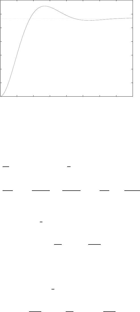
628 CHAPTER 11 The Design of State Variable Feedback Systems

0.05

0.1

0.15

0.2

0.25

0.3

0.35

00.5 1 1.5 2 2.5 3 3.5 4

Time (secs)

Amplitude

FIGURE AP11.7

Roll angle response to a step disturbance.

AP11.8 The state equations are (using the parameters of P3.36 in Dorf and

Bishop)

h= ˙x1=1

50[80θ−50h] = −x1+8

5x2

θ= ˙x2=ω=x3

˙ω= ˙x3=Km

Jia=−KmKb

JRa

ω+KmKa

JRa

vi=−353

30 x3+25000

3vi.

In state variable form we have (without feedback)

x=





−18

0 0 1

0 0 −353







x+





25000







vi.

(a) In this case we have vi=−kh +ar =−kx1+ar, where kand aare

the parameters to be determined and ris the reference input. With

the feedback of h(t) we have

x=





−18

0 0 1

−25000

3k0−353







x+





a25000







r .

from the publisher prior to any prohibited reproduction, storage in a retrieval system, or transmission in any form or by any means, electronic, mechanical, photocopying,

recording, or likewise. For information regarding permission(s), write to: Rights and Permissions Department, Pearson Education, Inc., Upper Saddle River, NJ 07458.

Advanced Problems 629

Since we only have one parameter to adjust, namely k, we will proba-

bly not be able to simultaneously meet both design speciﬁcations, In

fact with

k= 0.00056

we obtain the percent overshoot P.O. = 9.89%. The settling time cri-

terion cannot simultaneously be met—the best that can be obtained

is Ts≈7.5 seconds. In this case, we choose a= 0.00056 to make the

steady-state value of h(t) = 1.

(b) In this case we have vi=−k1h−k2θ+ar =−k1x1−k2x2+ar,

where k1,k2, and aare the parameters to be determined and ris the

reference input. Since we have two parameter to adjust, namely k1

and k2we will probably be able to simultaneously meet both design

speciﬁcations. In fact with

k1= 0.00056 and k2= 0.001

we obtain the percent overshoot P.O. = 4.35%. The settling time

criterion is easily met— Ts≈5 seconds. In this case, we choose a=

0.0012 to make the steady-state value of h(t) = 1.

AP11.9 (a) The state vector diﬀerential equation is







0 1 0 0

−2 0 1 0

0 0 0 1

1 0 −1 0



















where x1=z,x2= ˙z,x3=yand x4= ˙y.

(b) The characteristic equation is

s4+ 3s2+ 1 = (s+j0.618)(s−j0.618)(s+j1.618)(s−j1.618) = 0 .

So, the system is oscillatory.

s4+ks3+ 3s2+ 2ks + 1 = 0

which is stable if k > 0.

(d) Rewrite the characteristic equation as

1 + ks(s2+ 2)

s4+ 3s2+ 1 = 0 .

from the publisher prior to any prohibited reproduction, storage in a retrieval system, or transmission in any form or by any means, electronic, mechanical, photocopying,

recording, or likewise. For information regarding permission(s), write to: Rights and Permissions Department, Pearson Education, Inc., Upper Saddle River, NJ 07458.

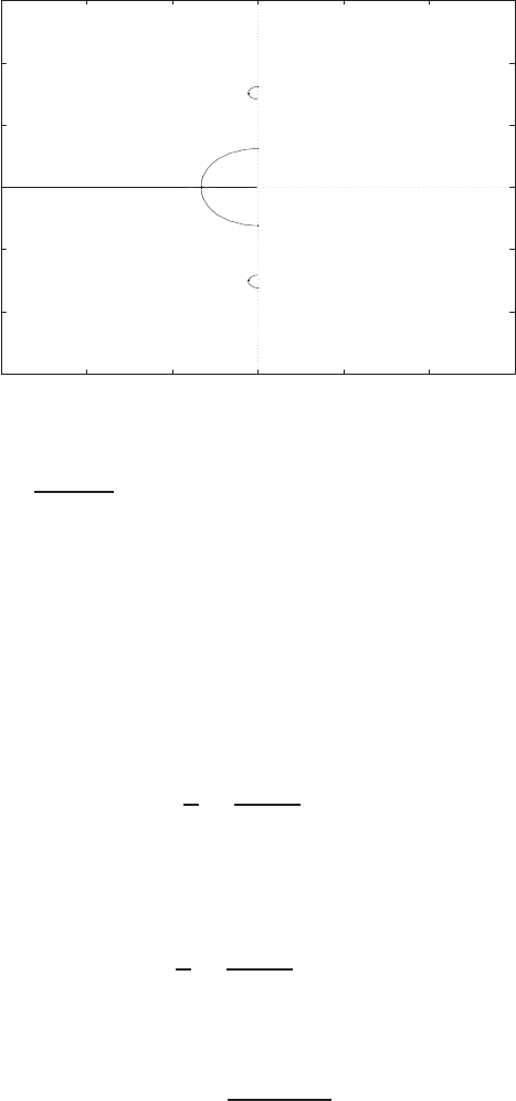
630 CHAPTER 11 The Design of State Variable Feedback Systems

The root locus is shown in Figure AP11.9. A reasonable solution for

kis k= 1.35.

-3

-2

-1

-3 -2 -1 0 1 2 3

Real Axis

Imag Axis

FIGURE AP11.9

Root locus for 1 + ks(s2+2)

s4+3s2+1 = 0.

AP11.10 The state diﬀerential equation is

¨y=ky +αu

where kand αdepend on the system parameters, such as mass and length.

The transfer function is

u=α

s2−k

which is unstable at the top of the arc. Since we can only use ˙yfor

feedback, we have

˙y

u=sα

s2−k.

Let

Gc(s) = K1s+K2

from the publisher prior to any prohibited reproduction, storage in a retrieval system, or transmission in any form or by any means, electronic, mechanical, photocopying,

recording, or likewise. For information regarding permission(s), write to: Rights and Permissions Department, Pearson Education, Inc., Upper Saddle River, NJ 07458.

Advanced Problems 631

Then

GGc(s) = α(K1s+K2)

(s2−k)

and the closed-loop characteristic equation is

αK1s+αK2+s2−k= 0

s2+αK1s+αK2−k= 0 .

Select αK2−k > 0 and αK1>0 for stability.

AP11.11 The state-space representation of the plant is

x=Ax +Bu

y=Cx

where

A=



0 1

−2−3

,B=



1

,and C=h1 0 i.

With the intermediate variables deﬁned as

z=˙

xand w= ˙u

we have





˙e

z

=





010

001

0−2−3











z

+











where

e=y−r .

To meet the design speciﬁcations, we require the closed-loop poles to lie

to the left of the line in the complex plane deﬁned by s=−0.8. We choose

K2= [10 3]

and

Gc(s) = 8

from the publisher prior to any prohibited reproduction, storage in a retrieval system, or transmission in any form or by any means, electronic, mechanical, photocopying,

recording, or likewise. For information regarding permission(s), write to: Rights and Permissions Department, Pearson Education, Inc., Upper Saddle River, NJ 07458.

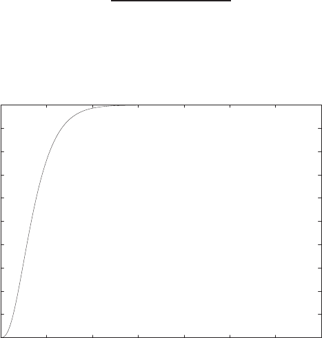
632 CHAPTER 11 The Design of State Variable Feedback Systems

This places the closed-loop poles at s=−2,−2 and −2. The closed-loop

transfer function with the internal model controller is

T(s) = 8

s3+ 6s2+ 12s+ 8 .

The step response is shown on Figure AP11.11.

0.1

0.2

0.3

0.4

0.5

0.6

0.7

0.8

0.9

0 2 4 6 8 10 12 14

Time (secs)

Amplitude

FIGURE AP11.11

Internal model controller step response.

AP11.12 The state-space representation of the plant is

x=Ax +Bu

y=Cx

where

A=



0 1

−2−3

,B=



1

,and C=h1 0 i.

With the intermediate variables deﬁned as

z=¨

xand w= ¨u

from the publisher prior to any prohibited reproduction, storage in a retrieval system, or transmission in any form or by any means, electronic, mechanical, photocopying,

recording, or likewise. For information regarding permission(s), write to: Rights and Permissions Department, Pearson Education, Inc., Upper Saddle River, NJ 07458.

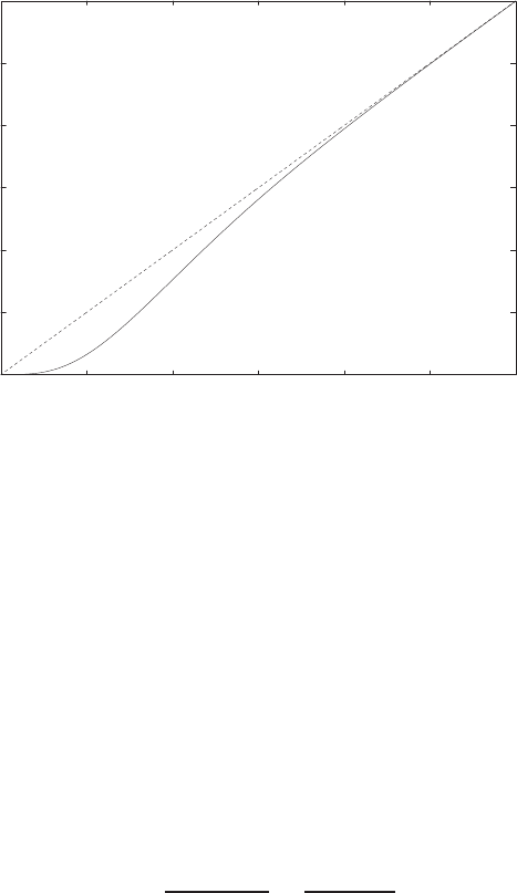
Advanced Problems 633

we have







˙e

¨e













0 1 0 0

0 0 1 0

0 0 0 1

0 0 −2−3













˙e



















where e=y−r.

0 1 2 3 4 5 6

Time (secs)

Amplitude

FIGURE AP11.12

Internal model controller ramp response.

To meet the design speciﬁcations, we require the closed-loop poles to lie

to the left of the line in the complex plane deﬁned by s=−0.67. We

choose

w=−[K1K2K3]





˙e







=−[16 32 22 5] 





˙e







Then,

Gc(s) = K1+K2s

s2=16 + 32s

s2.

from the publisher prior to any prohibited reproduction, storage in a retrieval system, or transmission in any form or by any means, electronic, mechanical, photocopying,

recording, or likewise. For information regarding permission(s), write to: Rights and Permissions Department, Pearson Education, Inc., Upper Saddle River, NJ 07458.

634 CHAPTER 11 The Design of State Variable Feedback Systems

The closed-loop transfer function with the internal model controller is

T(s) = 32s+ 16

s4+ 8s3+ 24s2+ 32s+ 16 .

This places the closed-loop poles at s=−2,−2,−2 and −2. The ramp

response is shown in Figure AP11.12.

AP11.13 The controllability matrix is

Pc=

−5−3

1 18 



and the observability matrix is

Po=



4−3

22 44 

.

Computing the determinants yields

det Pc=−87 6= 0 and det P0= 242 6= 0 ,

hence the system is controllable and observable. The controller gain ma-

trix

K=h3.02 6.11 i

places the closed-loop poles at the desired locations. Similarly, the ob-

server gain matrix

L=



2.38

−1.16 



places the observer poles at the desired locations.

AP11.14 The controllability matrix is

Pc=





0 0 4

0 4 −12

4−12 24







from the publisher prior to any prohibited reproduction, storage in a retrieval system, or transmission in any form or by any means, electronic, mechanical, photocopying,

recording, or likewise. For information regarding permission(s), write to: Rights and Permissions Department, Pearson Education, Inc., Upper Saddle River, NJ 07458.

Advanced Problems 635

and the observability matrix is

Po=





2−9 2

−16 −4−15

120 29 41







Computing the determinants yields

det Pc=−64 6= 0 and det P0= 10870 6= 0 ,

hence the system is controllable and observable. The controller gain ma-

trix

K=h−0.5 1.25 0.5i

and the observer gain matrix

L=





57.43

−16.11

−104.43







yields the desired closed-loop system poles and observer poles, respec-

tively.

AP11.15 The state-variable representation of the system is

x=



0 1

−7−2

x+



1

u

y= [ 1 4 ]x+ [0]u .

The observability matrix is

P0=



1 4

−28 −7

,

and det P0= 105 6= 0, hence the system is observable. The observer gain

matrix

L=

−7.18

6.29 



places the observer poles at s1,2=−10 ±10, as desired.

from the publisher prior to any prohibited reproduction, storage in a retrieval system, or transmission in any form or by any means, electronic, mechanical, photocopying,

recording, or likewise. For information regarding permission(s), write to: Rights and Permissions Department, Pearson Education, Inc., Upper Saddle River, NJ 07458.

636 CHAPTER 11 The Design of State Variable Feedback Systems

Design Problems

A state variable representation isCDP11.1

x=



0 1

0−33.14 

x+



0.827 

va

y=h1 0 ix

where x1=xand x2= ˙x. Note that we are neglecting the motor induc-

tance and assuming that the position x(t) is the output. Assume that we

have available for feedback the angle θand angle rate ˙

θ(see CDP4.1), so

that

va=−k1

rx1−k2

rx2+au

where u(t) is the reference input (that is, the desired position x(t)), the

gains k1and k2and the scaling parameter aare to be determined. Recall

that

x=rθ = 0.03175θ .

With the feedback in the loop we have

x=



0 1

−26.03k1−33.14 −26.03k2

x+



0.827a

u

y=h1 0 ix

Choosing k1= 50, k2= 1 and a= 1574.1 results in

P.O. = 1.1% and Ts= 0.11 second .

The closed-loop poles are s1,2=−29.59 ±20.65j.

DP11.1 The governing diﬀerential equation is

¨y−2000y=−20i .

In state variable form, the system is described by

x=



0 1

2000 0 

x+



−20 

i .

from the publisher prior to any prohibited reproduction, storage in a retrieval system, or transmission in any form or by any means, electronic, mechanical, photocopying,

recording, or likewise. For information regarding permission(s), write to: Rights and Permissions Department, Pearson Education, Inc., Upper Saddle River, NJ 07458.

Design Problems 637

Consider the state feedback

i=−k1x1−k2x2+βr

where r(t) is the reference input and k1, k2and βare to be determined.

Then, the closed-loop system is

x=



0 1

2000 −20k1−20k2

x+



−20β

r .

The characteristic equation is

s2+ 20k2s−2000 + 20k1= 0 .

For stability, let 20k1−2000 >0. Select k1= 125. Then, ωn= 22.36

rad/sec, and

k2=2ζωn

20 .

Let ζ= 0.59 to meet 10% overshoot speciﬁcation. Thus,

k2=2(0.59)(22.36)

20 = 1.32 .

The closed-loop transfer function is

T(s) = −20β

s2+ 26.4s+ 500 .

Choose β=−25 so that

T(s) = 500

s2+ 26.4s+ 500 .

The feedback law is

i= 125x1+ 1.32x2−25r .

DP11.2 The automobile engine control system (see DP10.8 in Dorf and Bishop)

is modeled as

G(s) = 2e−sT

(0.21s+ 1)(4s+ 1) .

In this case, we will assume the delay is negligible. Therefore, T= 0. A

from the publisher prior to any prohibited reproduction, storage in a retrieval system, or transmission in any form or by any means, electronic, mechanical, photocopying,

recording, or likewise. For information regarding permission(s), write to: Rights and Permissions Department, Pearson Education, Inc., Upper Saddle River, NJ 07458.

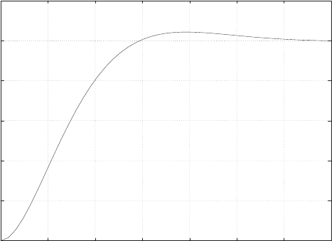
638 CHAPTER 11 The Design of State Variable Feedback Systems

state variable representation of the system is

x=



0 1

−1.19 −5.01 

x+



1.19 

r

y= [1 0]x.

Let

r(t) = −k1x1−k2x2+k3u

where u(t) is the command input. Using ITAE methods, our desired char-

acteristic polynomial is

q(s) = s2+ 1.4ωns+ω2

n= 0 .

Select ωn= 11.315 to obtain a settling time Ts<0.5 seconds. The char-

acteristic polynomial of the closed-loop system is

s2+ (5.01 + 1.19k2)s+ (1.19 + 1.19k1) = 0 .

Equating coeﬃcients and solving for the gains yields

k1= 106.59 and k2= 9.235 .

Select k3= 107.59 to yield a zero steady-state error to a step input.

0.2

0.4

0.6

0.8

1.2

0 0.1 0.2 0.3 0.4 0.5 0.6 0.7

Time (secs)

Amplitude

FIGURE DP11.2

The step response of the engine control system.

from the publisher prior to any prohibited reproduction, storage in a retrieval system, or transmission in any form or by any means, electronic, mechanical, photocopying,

recording, or likewise. For information regarding permission(s), write to: Rights and Permissions Department, Pearson Education, Inc., Upper Saddle River, NJ 07458.

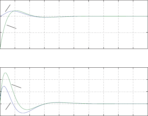
Design Problems 639

DP11.3 The compensator is

x= [A−BK −LC]ˆ

x+Ly+Mr

˜u=−Kˆ

where

A−BK −LC =

−28.7 1

−365.19 −20 

,M=



200 

,

N= 363.64 ,K=h344.55 15.82 i,and L=



28.7

165.19 

.

We selected the desired eigenvalues of A−BK at p=−10 ±10jand the

desired eigenvalues of A−LC at q=−20 ±10j. For initial conditions we

let x(0) = [1 1] and ˆ

x(0) = [0 0].

0 0.1 0.2 0.3 0.4 0.5 0.6 0.7 0.8 0.9 1

0.5

1.5

Time (s)

0 0.1 0.2 0.3 0.4 0.5 0.6 0.7 0.8 0.9 1

−2

Time (s)

Actual x1

Actual x2

Estimated x1

Estimated x2

FIGURE DP11.3

The step response showing the actual and estimated states.

DP11.4 The design speciﬁcations are

(a) Percent overshoot <20%

(b) Ts<1.5s, and

from the publisher prior to any prohibited reproduction, storage in a retrieval system, or transmission in any form or by any means, electronic, mechanical, photocopying,

recording, or likewise. For information regarding permission(s), write to: Rights and Permissions Department, Pearson Education, Inc., Upper Saddle River, NJ 07458.

640 CHAPTER 11 The Design of State Variable Feedback Systems

The state diﬀerential equation is

x=Ax +Bu

y=Cx

where

A=





0 1 0

0−σ1−α1

g−α2−σ2







=





0 1 0

0−0.415 −0.0111

9.8−1.43 −0.0198







B=











=





6.27

9.8







and C=h1 0 0 i.

The transfer function is

θ(s)

δ(s)=ns +nσ2−α1g

s3+ (σ1+σ2)s2+ (σ1σ2−α1α2)s+α1g

=6.27s+ 0.0154

s3+ 0.435s2−0.0077 + 0.109 .

Let u=−K1x1−K2x2−K3x3. Then the closed-loop system matrix is

A−BK =





0 1 0

−nK1−σ1−nK2−α1−nK3

g−gK1−α2−gK2−σ2−gK3







where K= [K1K2K3]. From the design speciﬁcations, we have the

desired roots at

s3+a2s2+a1s+ao=s3+36s2+225s+1350 = (s+30)(s+3+j6)(s+3−j6) = 0 .

The actual characteristic equation is

s3+ (gK3+K2n+σ1+σ2)s2+ (−α1α2−α1gK2+K1n−α2nK3

+gK3σ1+K2nσ2+σ1σ2)s

+α1g−α1gK1+gK3n+σ2nK1= 0 .

from the publisher prior to any prohibited reproduction, storage in a retrieval system, or transmission in any form or by any means, electronic, mechanical, photocopying,

recording, or likewise. For information regarding permission(s), write to: Rights and Permissions Department, Pearson Education, Inc., Upper Saddle River, NJ 07458.

Design Problems 641

Comparing coeﬃcients yields







0n g

n nσ2−α1g−α2n+gσ1

−α1g+σ2n0gn



















=





a2−σ1−σ2

a1+α1α2−σ1σ2

a0−α1g







where

a2= 36

a1= 225

a0= 1350 .

The solution for Kis

K= [53.11 −28.64 21.96] .

DP11.5 The controllability and observability matrices are

Pc=



0.05 −0.04

0.001 −0.001 

and

P0=



1 0

−0.8 0.02 

,respectively.

Computing the determinants yields

det Pc=−1.002e−05 6= 0 and Po= 0.02 6= 0 ,

hence the system is controllable and observable. The feedback gain matrix

K= [ 3820 −179620 ]

yields the desired closed-loop poles. The observer gain matrix

L=



120

180000 



yields the desired observer poles. The integrated system is shown in Fig-

ure DP11.5.

from the publisher prior to any prohibited reproduction, storage in a retrieval system, or transmission in any form or by any means, electronic, mechanical, photocopying,

recording, or likewise. For information regarding permission(s), write to: Rights and Permissions Department, Pearson Education, Inc., Upper Saddle River, NJ 07458.

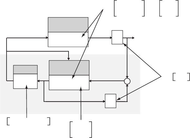
642 CHAPTER 11 The Design of State Variable Feedback Systems

System Model

x=Ax+Bu

Observer

Control Law

-K x=Ax+Bu+Ly

^ ^ ~y=y-Cx

A= -0.8 0.02

-0.02 0 B= 0.05

0.001

C= 1 0

K= 3820 -179620

L= 120

180000

FIGURE DP11.5

Integrated controller and observer.

DP11.6 (a) The characteristic equation associated with the system matrix is

q(s) = s2+ (12 + K2)s+ (36 + K1) = 0 ,

where we have assumed state feedback of the form

u=−K1x1−K2x2.

The deadbeat control characteristic equation is

s2+αωns+ω2

n= 0 ,

where α= 1.82 and we use ωn= 9.64 to meet the settling time

speciﬁcation. Then, equating coeﬃcients and solving for the gains

yields

K1= 56.93 and K2= 5.54 .

(b) Since the closed-loop poles are located at s1,2=−8.77 ±4, we can

select the observer poles to be about ten times farther in the left-half

plane, or

s1,2=−88,−88 .

from the publisher prior to any prohibited reproduction, storage in a retrieval system, or transmission in any form or by any means, electronic, mechanical, photocopying,

recording, or likewise. For information regarding permission(s), write to: Rights and Permissions Department, Pearson Education, Inc., Upper Saddle River, NJ 07458.

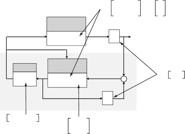
Design Problems 643

Then the observer gains are

L=



164

5740 

.

System Model

x=Ax+Bu

Observer

Control Law

-K x=Ax+Bu+Ly

^ ^ ~y=y-Cx

A= 0 1

-36 -12 B= 0

C= 1 0

K= 56.93 5.54

L= 164

5740

FIGURE DP11.6

Block diagram for integrated controller and observer.

DP11.7 The compensator is

x= [A−LC]ˆ

x+Ly+Bu

u=−Kˆ

where

A−LC =





−60 1 0

−1095 0 1

−3750 −5−10







from the publisher prior to any prohibited reproduction, storage in a retrieval system, or transmission in any form or by any means, electronic, mechanical, photocopying,

recording, or likewise. For information regarding permission(s), write to: Rights and Permissions Department, Pearson Education, Inc., Upper Saddle River, NJ 07458.

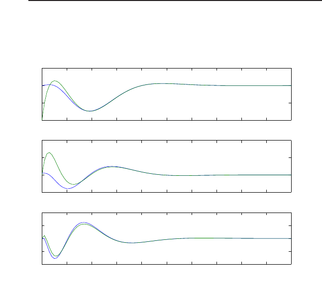
644 CHAPTER 11 The Design of State Variable Feedback Systems

N= 4000 ,K=h3998 595 30 i,and L=





1095

3748







We selected the desired eigenvalues of A−BK at p1,2=−10 ±10j,

p3=−20 and the desired eigenvalues of A−LC at q1,2=−20 ±10j,

q3=−30. For initial conditions we let x(0) = [1 1 1] and ˆ

x(0) = [0 0 0].

The transfer function from rto yis

T(s) = 4000s3+ 2.8e05s2+ 6.8e06s+ 6e07

s6+ 110s5+ 5100s4+ 1.29e05s3+ 1.9e06s2+ 1.58e07s+ 6e07 .

The bandwidth is 11.7 rad/s.

0 0.1 0.2 0.3 0.4 0.5 0.6 0.7 0.8 0.9 1

0.5

1.5

0 0.1 0.2 0.3 0.4 0.5 0.6 0.7 0.8 0.9 1

−10

0 0.1 0.2 0.3 0.4 0.5 0.6 0.7 0.8 0.9 1

−200

−100

100

200

FIGURE DP11.7

The step response showing the actual and estimated states.

from the publisher prior to any prohibited reproduction, storage in a retrieval system, or transmission in any form or by any means, electronic, mechanical, photocopying,

recording, or likewise. For information regarding permission(s), write to: Rights and Permissions Department, Pearson Education, Inc., Upper Saddle River, NJ 07458.

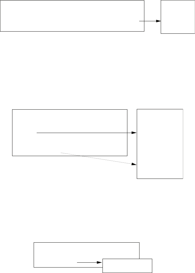
Computer Problems 645

Computer Problems

CP11.1 The controllability and observablity matrices have nonzero determinants,

as shown in Figure CP11.1. Therefore, the system is observable and con-

trollable.

A=[-6 2 0;4 0 7;-10 1 11]; b=[5;0;1]; c=[ 1 2 1]; d=[0];

sys = ss(A,b,c,d);

Co=ctrb(sys); dt_Co=det(Co)

Ob=obsv(sys); dt_Ob=det(Ob)

dt_Co =

-84933

dt_Ob =

-3.6030e+03

FIGURE CP11.1

Determining controllability and observability.

CP11.2 The system is controllable since the determinant of the controllability

matrix is nonzero , as shown in Figure CP11.2.

a=[0 1;-6 -5]; b=[0;6]; c=[1 0]; d=[0];

sys_ss = ss(a,b,c,d);

Pc=ctrb(sys_ss);

dt_Pc=det(Pc)

Ob=obsv(sys_ss);

dt_Ob=det(Ob)

sys_tf=tf(sys_ss)

dt_Pc =

-36

dt_Ob =

Transfer function:

-------------

s^2 + 5 s + 6

FIGURE CP11.2

M-ﬁle script to determine controllability and to compute equivalent transfer function model.

CP11.3 The gain matrix (computed as shown in Figure CP11.3) is K=h0.5 0.5i.

a=[0 1;-1 -2]; b=[1;1]; c=[1 -1]; d=[0];

p=[-1;-2];

K=acker(a,b,p)K =

0.5000 0.5000

FIGURE CP11.3

M-ﬁle script to place the closed-loop system poles using state feedback.

from the publisher prior to any prohibited reproduction, storage in a retrieval system, or transmission in any form or by any means, electronic, mechanical, photocopying,

recording, or likewise. For information regarding permission(s), write to: Rights and Permissions Department, Pearson Education, Inc., Upper Saddle River, NJ 07458.

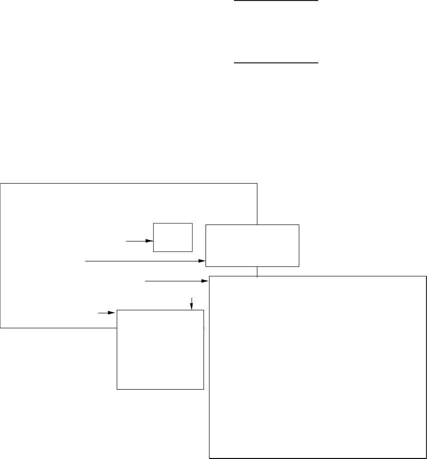
646 CHAPTER 11 The Design of State Variable Feedback Systems

CP11.4 The constant velocity guided missile is not controllable since the control-

lablity matrix, Co, has a zero determinant, as shown in Figure CP11.4.

Using the tf function (see Figure CP11.4), we determine that the transfer

function is

G(s) = 5s

s5+ 0.5s4+ 0.1s3.

Cancelling common terms in the transfer function yields

G(s) = 5

s4+ 0.5s3+ 0.1s2.

Then, using the ss function, we determine a state-space representation of

G(s). As shown in Figure CP11.4, the state-space representation is

x=Ax +Bu

y=Cx

A=[0 1 0 0 0;-0.1 -0.5 0 0 0;0.5 0 0 0 0;0 0 10 0 0;0.5 1 0 0 0];

b=[0;1;0;0;0];

c=[0 0 0 1 0];

d=[0];

sys_ss = ss(A,b,c,d);

% Part (a)

Co=ctrb(sys_ss); dt_Co=det(Co)

% Part (b)

sys_tf = tf(sys_ss)

sys_new = minreal(sys_tf);

sys_new_ss=ss(sys_new)

% Part (c)

Co_new=ctrb(sys_new_ss); dt_Co_new=det(Co_new)

% Part (d)

evalues=eig(sys_new_ss)

dt_Co_new =

evalues =

-0.2500 + 0.1936i

-0.2500 - 0.1936i

a =

x1 x2 x3 x4

x1 -0.50000 -0.10000 0 0

x2 1.00000 0 0 0

x3 0 1.00000 0 0

x4 0 0 2.00000 0

b =

x1 2.00000

x2 0

x3 0

x4 0

c =

x1 x2 x3 x4

y1 0 0 0 1.25000

d =

y1 0

Continuous-time system.

Transfer function:

5 s

-----------------------

s^5 + 0.5 s^4 + 0.1 s^3

dt_Co =

FIGURE CP11.4

Analysis of the constant velocity guided missile state-space model.

from the publisher prior to any prohibited reproduction, storage in a retrieval system, or transmission in any form or by any means, electronic, mechanical, photocopying,

recording, or likewise. For information regarding permission(s), write to: Rights and Permissions Department, Pearson Education, Inc., Upper Saddle River, NJ 07458.

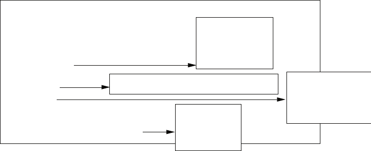
Computer Problems 647

where







−0.5−0.100

1 0 0 0

0 1 0 0

0 0 2 0



















and C=h0 0 0 1.25 i.

The reduced system is controllable but not stable, since there are two poles

at the origin. Systems that are not controllable have too many states.

After eliminating unnecessary states, a controllable system of minimal

complexity (i.e. states) is obtained. In this case, the number of states is

reduced from ﬁve to four.

CP11.5 The eigenvalues of Aare

e1=−2.0727

e2=−0.2354

e3,4= 0.2761 ±0.2593j

The system is unstable since there are two eigenvalues in the right half-

plane, see Figure CP11.5. The characteristic polynomial is

A = [-0.0389 0.0271 0.0188 -0.4555; 0.0482 -1.0100 0.0019 -4.0208;

0.1024 0.3681 -0.7070 1.4200; 0 0 1 0];

b1 = [0.4422;3.5446;-6.0214;0];

b2 = [0.1291;-7.5922;4.4900;0];

% Part (a)

evalues = eig(A)

%part (b)

p = poly(A)

r = roots(p)

% Part (c)

Co1 = ctrb(A,b1); dt1 = det(Co1)

Co2 = ctrb(A,b2); dt2 = det(Co2)

evalues =

0.2761 + 0.2593i

0.2761 - 0.2593i

-0.2354

-2.0727

p =

r =

1.0000 1.7559 -0.6431 0.0618 0.0700 -2.0727

0.2761 + 0.2593i

0.2761 - 0.2593i

-0.2354

dt1 =

-1.8451e+03

dt2 =

-90.6354

FIGURE CP11.5

Analysis of the VTOL aircraft model.

p(s) = s4+ 1.7559s3−0.6431s2+ 0.0618s+ 0.0700 .

The roots of the characteristic equation are the same as the eigenvalues.

Also, the system is controllable from either u1or u2. If the aircraft should

lose the control of the vertical motion through u1, then the control u2can

from the publisher prior to any prohibited reproduction, storage in a retrieval system, or transmission in any form or by any means, electronic, mechanical, photocopying,

recording, or likewise. For information regarding permission(s), write to: Rights and Permissions Department, Pearson Education, Inc., Upper Saddle River, NJ 07458.

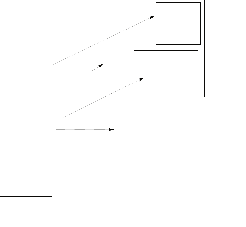
648 CHAPTER 11 The Design of State Variable Feedback Systems

be used to control both vertical and horizontal motion, and vice versa.

CP11.6 The m-ﬁle script to analyze the translunar halo orbit problem is shown

in Figure CP11.6. The translunar equilibrium point is not a stable point

dt1 =

dt2 =

dt3 =

A=[0 0 0 1 0 0;0 0 0 0 1 0; 0 0 0 0 0 1;7.3809 0 0 0 2 0;

0 -2.1904 0 -2 0 0; 0 0 -3.1904 0 0 0];

c=[0 1 0 0 0 0];d=[0];

b1=[0;0;0;1;0;0];

b2=[0;0;0;0;1;0];

b3=[0;0;0;0;0;1];

sys_ss_1 = ss(A,b1,c,d);

sys_ss_2 = ss(A,b2,c,d);

sys_ss_3 = ss(A,b3,c,d);

% Part (a)

evalues=eig(A)

% Part (b)

Cb1=ctrb(sys_ss_1); dt1=det(Cb1)

% Part (c)

Cb2=ctrb(sys_ss_2); dt2=det(Cb2)

% Part (d)

Cb3=ctrb(sys_ss_3); dt3=det(Cb3)

% Part (e)

sys_tf = tf(sys_ss_2);

sys_tf=minreal(sys_tf)

% Part (f)

sys_ss=ss(sys_tf);

Co=ctrb(sys_ss); dt_Co=det(Co)

if dt_Co ~= 0

disp('System is completelly Controllable')

else

disp('System in uncontrollable')

end

% Part (g)

P = [-1+i; -1-i;-10;-10];

[A,B]=ssdata(sys_ss);

K = acker(A,B,P)

evalues =

2.1587

-2.1587

0 + 1.8626i

0 - 1.8626i

0 + 1.7862i

0 - 1.7862i

Transfer function:

s^2 - 7.381

----------------------------

s^4 - 1.19 s^2 - 16.17

dt_Co =

System is completelly Controllable

a =

x1 x2 x3 x4

x1 0 0.59525 0 2.02089

x2 2.00000 0 0 0

x3 0 2.00000 0 0

x4 0 0 2.00000 0

b =

x1 1.00000

x2 0

x3 0

x4 0

c =

x1 x2 x3 x4

y1 0 0.50000 0 -0.92261

d =

y1 0

FIGURE CP11.6

Analysis of the translunar satellite halo orbit.

as evidenced by the eigenvalues of Ain the right half-plane; the system is

not completely controllable from any uiindividually. The transfer function

from the publisher prior to any prohibited reproduction, storage in a retrieval system, or transmission in any form or by any means, electronic, mechanical, photocopying,

recording, or likewise. For information regarding permission(s), write to: Rights and Permissions Department, Pearson Education, Inc., Upper Saddle River, NJ 07458.

Computer Problems 649

from u2to ηis

T(s) = s4−4.191s2−23.55

s6+ 2s4−19.97s2−51.58 .

A careful analysis reveals that T(s) can be reduced by eliminating com-

mon factors. The common factors are s2+ 3.1834. The reduced transfer

function is

T(s) = s2−7.3815

s4−1.1837s2−16.2030 .

Using state feedback

u2=−Kx

the gain matrix Kwhich places the desired poles (using Ackermann’s

formula) is

K=h22 71.56 60 27.02 i.

CP11.7 The m-ﬁle script to determine the initial state is shown in Figure CP11.7a.

Given three data points at t= 0,2,4, we construct the three equations

A=[0 1 0;0 0 1;-2 -4 -6];

b=[0;0;0]; c=[1 0 0]; d=[0];

sys=ss(A,b,c,d);

% Part (b)

v1=c*expm(0*A); v2=c*expm(2*A); v3=c*expm(4*A);

V=[v1;v2;v3]; Vi=inv(V);

n=[1;-0.0256;-0.2522];

x0=Vi*n

% Part (c)

t=[0:0.1:4]; u=0.0*t;

[y,x]=lsim(sys,u,t,x0');

plot(t,y,[0 2 4],[1;-0.0256;-0.2522],'*'), grid

xlabel('Time (sec)'), ylabel('y(t)')

title('Data points denoted by *')

FIGURE CP11.7

(a) Script to determine the initial state from three observations.

y(0) = 1 = Ce0Ax0

y(2) = −0.0256 = Ce2Ax0

from the publisher prior to any prohibited reproduction, storage in a retrieval system, or transmission in any form or by any means, electronic, mechanical, photocopying,

recording, or likewise. For information regarding permission(s), write to: Rights and Permissions Department, Pearson Education, Inc., Upper Saddle River, NJ 07458.

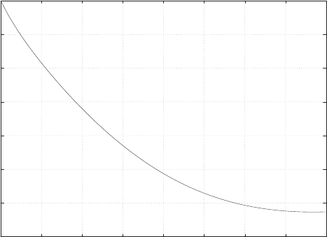
650 CHAPTER 11 The Design of State Variable Feedback Systems

y(4) = −0.2522 = Ce4Ax0

or, in matrix form







Ce0A

Ce2A

Ce4A







x0=





−0.0256

−0.2522







The problem is solvable if the matrix







Ce0A

Ce2A

Ce4A







is invertible. In this case, the inverse does exist and the solution is

x0=





−1

1.9998







The simulation is shown in Figure CP11.7b.

-0.4

-0.2

0.2

0.4

0.6

0.8

00.5 1 1.5 2 2.5 3 3.5 4

Time (sec)

y(t)

Data points denoted by *

FIGURE CP11.7

CONTINUED: (b) System simulation using computed initial state.

from the publisher prior to any prohibited reproduction, storage in a retrieval system, or transmission in any form or by any means, electronic, mechanical, photocopying,

recording, or likewise. For information regarding permission(s), write to: Rights and Permissions Department, Pearson Education, Inc., Upper Saddle River, NJ 07458.

Computer Problems 651

CP11.8 Suppose we are given

A=



0 1

−1 0 

B=



1



and the feedback

u=−Kx =−[K1K2]x.

Solving HTP+PH =−Ifor Pyields

p11 =K2

2+K2

1+ 3K1+ 2

2(K1+ 1)K2

p12 =1

2(K1+ 1)

p22 =K1+ 2

2(K1+ 1)K2

Then, with xoT= [1,0] we ﬁnd that

J=xoTPxo=p11 .

Computing the partial of Jwith respect to K2yields

∂J

∂K2

21

K1+ 1 −K1+ 2

2.

Setting

∂J

∂K2

= 0

and solving for K2, we ﬁnd that

K2=q(K1+ 2)(K1+ 1) .

For a given value of K1, the value of K2that minimizes Jcan be computed

via the above equation. With K2given as above, we can compute Jto be

J=sK1+ 2

K1+ 1 .

A plot of Jversus K1(with K2equal to the minimizing value) is shown

in Figure CP11.8. As K1increases, the performance index Jdecreases.

However, we see that the rate of decrease slows considerably after K1>

20. Also, K2increases as K1increases. We want to keep both gains as

from the publisher prior to any prohibited reproduction, storage in a retrieval system, or transmission in any form or by any means, electronic, mechanical, photocopying,

recording, or likewise. For information regarding permission(s), write to: Rights and Permissions Department, Pearson Education, Inc., Upper Saddle River, NJ 07458.

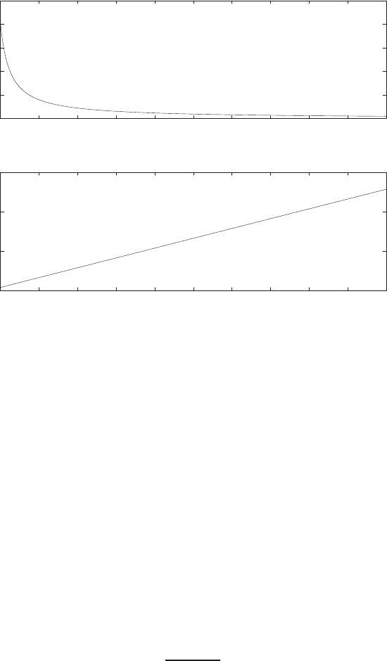
652 CHAPTER 11 The Design of State Variable Feedback Systems

small as possible, while still having a small J. A reasonable selection is

K1= 20 and K2= 21.5.

1.1

1.2

1.3

1.4

1.5

0 5 10 15 20 25 30 35 40 45 50

Performance index J versus K1

0 5 10 15 20 25 30 35 40 45 50

K2 versus K1

FIGURE CP11.8

Performance index as a function of K1and K2.

CP11.9 In this problem, A=−1 and B= 1. Computing Qyields

Q= (1 + λ(−k)2) = 1 + λk2.

Deﬁne

H=A−Bk =−1−k .

Solving

HTP+P H =−Q

yields

p=1 + λk2

2(k+ 1) .

from the publisher prior to any prohibited reproduction, storage in a retrieval system, or transmission in any form or by any means, electronic, mechanical, photocopying,

recording, or likewise. For information regarding permission(s), write to: Rights and Permissions Department, Pearson Education, Inc., Upper Saddle River, NJ 07458.

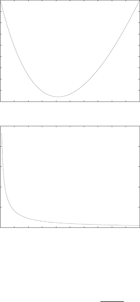
Computer Problems 653

0.41

0.42

0.43

0.44

0.45

0.46

0.47

0.48

0.49

0.5

0 0.1 0.2 0.3 0.4 0.5 0.6 0.7 0.8 0.9 1

J/x0^2

0.5

1.5

2.5

0 1 2 3 4 5 6 7 8 9 10

lambda

k min

FIGURE CP11.9

Plot of J/x2

0versus kand the minimizing kversus λ.

The performance index is

J=x2

0pwhich implies J/x2

0=1 + λk2

2(k+ 1) .

The plot of J/x2

0versus kis shown in Figure CP11.9. The minimum value

is achieved when k= 0.41. To arrive at this result analytically, take the

from the publisher prior to any prohibited reproduction, storage in a retrieval system, or transmission in any form or by any means, electronic, mechanical, photocopying,

recording, or likewise. For information regarding permission(s), write to: Rights and Permissions Department, Pearson Education, Inc., Upper Saddle River, NJ 07458.

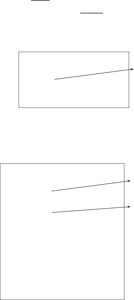
654 CHAPTER 11 The Design of State Variable Feedback Systems

partial of J/x2

0with respect to k, set the result to zero and solve for k:

∂J/x2

∂k = 0 when k2+ 2K−1/λ = 0 .

Solving for kyields k=−1±p1 + 1/λ. So, when λ= 1, k= 0.41. The

plot of kmin versus λis shown in Figure CP11.9.

CP11.10 The m-ﬁle is shown in Figure CP11.10.

A=[0 1;-18.7 -10.4]; B=[10.1; 24.6]; C=[1 0]; D=[0];

% Controller Gains

p=[-2;-2 ];

K=acker(A,B,p)

% Observer Gains

q=[-20+4*j;-20-4*j];

L = acker(A',C',q); L=L

K =

-0.3081 -0.1337

L =

29.6000

89.4600

FIGURE CP11.10

Using the acker function to compute the controller gains and the observer gains.

CP11.11 The m-ﬁle is shown in Figure CP11.11(a). The compensator can be rep-

A=[0 1 0;0 0 1;-4.3 -1.7 -6.7]; B=[0;0;0.35]; C=[0 1 0]; D=[0];

% Controller Gains

p=[-1.4+1.4*j;-1.4-1.4*j;-2];

K=acker(A,B,p)

% Observer Gains

q=[-18+5*j;-18-5*j;-20];

L = acker(A',C', q); L=L'

% Simulation of closed-loop system with the observer

Ac=[A -B*K;L*C A-B*K-L*C];

Bc=[zeros(6,1)];

Cc=eye(6);

Dc=zeros(6,1);

sys=ss(Ac,Bc,Cc,Dc);

x0=[1;0;0;0.5;0.1;0.1]; t=[0:0.001:3.5];

[y,t]=initial(sys,x0,t);

subplot(311)

plot(t,y(:,1),t,y(:,4),'--'), grid

subplot(312)

plot(t,y(:,2),t,y(:,5),'--'), grid

subplot(313)

plot(t,y(:,3),t,y(:,6),'--'), grid

K =

10.1143 22.3429 -5.4286

L =

1.0e+003 *

-1.6223

0.0493

0.7370

FIGURE CP11.11

(a) M-ﬁle.

from the publisher prior to any prohibited reproduction, storage in a retrieval system, or transmission in any form or by any means, electronic, mechanical, photocopying,

recording, or likewise. For information regarding permission(s), write to: Rights and Permissions Department, Pearson Education, Inc., Upper Saddle River, NJ 07458.

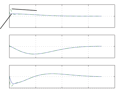
Computer Problems 655

resented as

x= (A−BK −LC)ˆ

x+Lyand u=−Kˆ

Since y=Cx, we can write

x= (A−BK −LC)ˆ

x+LCx .

Similarly, with

x=Ax +Buand u = −Kˆ

we obtain

x=Ax −BKˆ

In matrix form, we have





x

=



A−BK

LC A −BK −LC 





x

,

with initial conditions

hx(0)Tˆ

x(0)TiT=h1 0 0 0.5 0.1 0.1iT.

The response of the system is shown in Figure CP11.11(b).

0 1 2 3 4

Estimated state (dashed line)

True state

(solid line)

Time (sec)

FIGURE CP11.11

CONTINUED: (b) Response of system to an initial condition.

from the publisher prior to any prohibited reproduction, storage in a retrieval system, or transmission in any form or by any means, electronic, mechanical, photocopying,

recording, or likewise. For information regarding permission(s), write to: Rights and Permissions Department, Pearson Education, Inc., Upper Saddle River, NJ 07458.

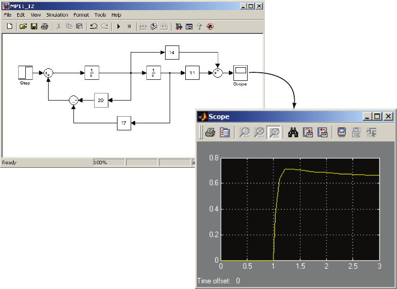
656 CHAPTER 11 The Design of State Variable Feedback Systems

CP11.12 The Simulink block diagram is shown in Figure CP11.12.

FIGURE CP11.12

Simulink block diagram.

CP11.13 The m-ﬁle to design the compensator is shown in Figure CP11.13(a). The

Simulink simulation is shown in Figure CP11.13(b). The output shown

on the x-y graph depicts the state xof the system. The initial conditions

selected for the simulation are

x(0) =













and ˆ

x(0) =







0.5

0.1







from the publisher prior to any prohibited reproduction, storage in a retrieval system, or transmission in any form or by any means, electronic, mechanical, photocopying,

recording, or likewise. For information regarding permission(s), write to: Rights and Permissions Department, Pearson Education, Inc., Upper Saddle River, NJ 07458.

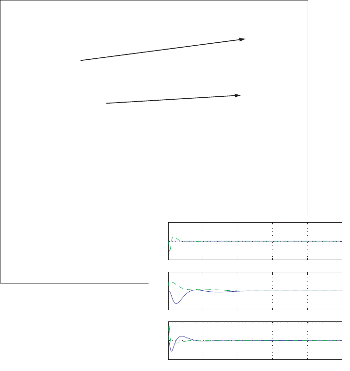
Computer Problems 657

0 2 4 6 8 10

?100

100

0 2 4 6 8 10

?10

A=[0 1 0 0;0 0 1 0;0 0 0 1;-2 -5 -1 -13]; B=[0;0;0;1]; C=[1 0 0 0]; D=[0];

% Controller Gains

p=[-1.4+1.4*j;-1.4-1.4*j;-2+j;-2-j];

K=acker(A,B,p)

% Observer Gains

q=[-18+5*j;-18-5*j;-20;-20];

L = acker(A',C',q); L=L'

% Simulation of closed-loop system with the observer

Ac=[A -B*K;L*C A-B*K-L*C];

Bc=[zeros(8,1)];

Cc=eye(8);

Dc=zeros(8,1);

sys=ss(Ac,Bc,Cc,Dc);

x0=[1;0;0;0;0.5;0.1;0.1;0.1]; t=[0:0.001:10];

[y,t]=initial(sys,x0,t);

subplot(311)

plot(t,y(:,1),t,y(:,4),'--'), grid

subplot(312)

plot(t,y(:,2),t,y(:,5),'--'), grid

subplot(313)

plot(t,y(:,3),t,y(:,6),'--'), grid

K =

17.6000 24.6800 19.1200 -6.2000

L =

1369

10495

1479

FIGURE CP11.13

(a) M-ﬁle to design the compensator, including the observer.

from the publisher prior to any prohibited reproduction, storage in a retrieval system, or transmission in any form or by any means, electronic, mechanical, photocopying,

recording, or likewise. For information regarding permission(s), write to: Rights and Permissions Department, Pearson Education, Inc., Upper Saddle River, NJ 07458.

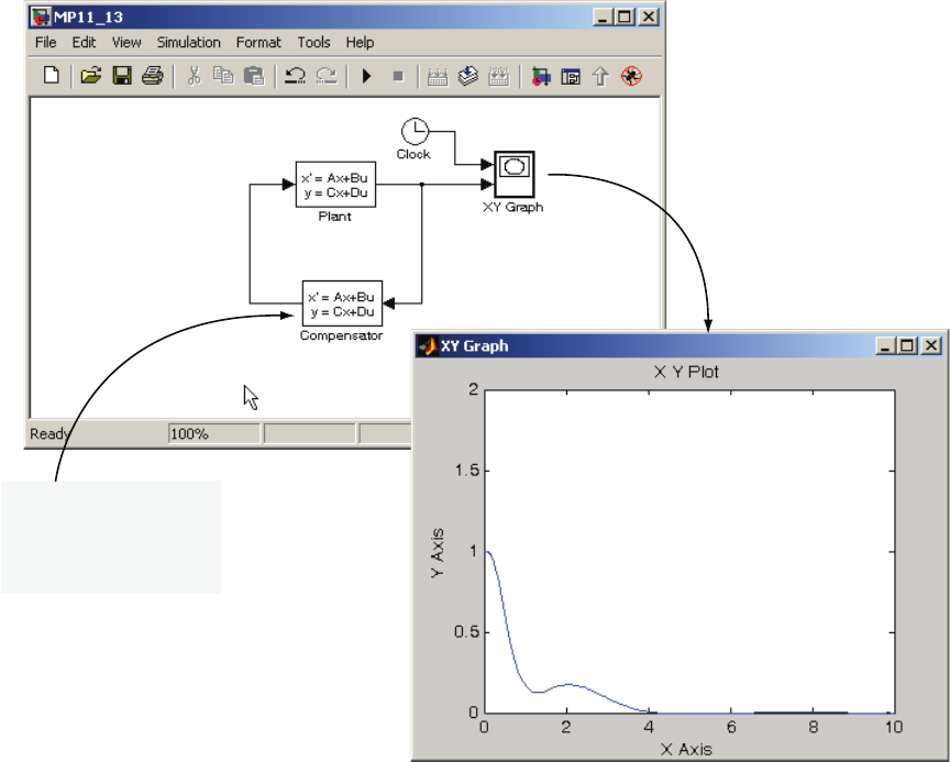
658 CHAPTER 11 The Design of State Variable Feedback Systems

x=[A-BK-LC]x+Ly

^ ^

u=-Kx

FIGURE CP11.13

CONTINUED (b) The Simulink simulation.

from the publisher prior to any prohibited reproduction, storage in a retrieval system, or transmission in any form or by any means, electronic, mechanical, photocopying,

recording, or likewise. For information regarding permission(s), write to: Rights and Permissions Department, Pearson Education, Inc., Upper Saddle River, NJ 07458.

C H A P T E R 1 2

Robust Control Systems

Exercises

E12.1 The plant transfer function is

G(s) = 3

s+ 3 .

Try a PI controller, given by

Gc=K1+K2

The ITAE characteristic equation is

s2+ 1.4ωns+ω2

where ωn= 30. Then

K1= 13 and K2= 300 .

Without a preﬁlter, the closed-loop system is

Y(s)

R(s)=39s+ 900

s2+ 42s+ 900 ,

and with a preﬁlter, the closed-loop system is

Y(s)

R(s)=900

s2+ 42s+ 900 ,

where

Gp(s) = 23.07

s+ 23.07 .

The step response, with and without the preﬁlter, is shown in Figure E12.1.

659

from the publisher prior to any prohibited reproduction, storage in a retrieval system, or transmission in any form or by any means, electronic, mechanical, photocopying,

recording, or likewise. For information regarding permission(s), write to: Rights and Permissions Department, Pearson Education, Inc., Upper Saddle River, NJ 07458.

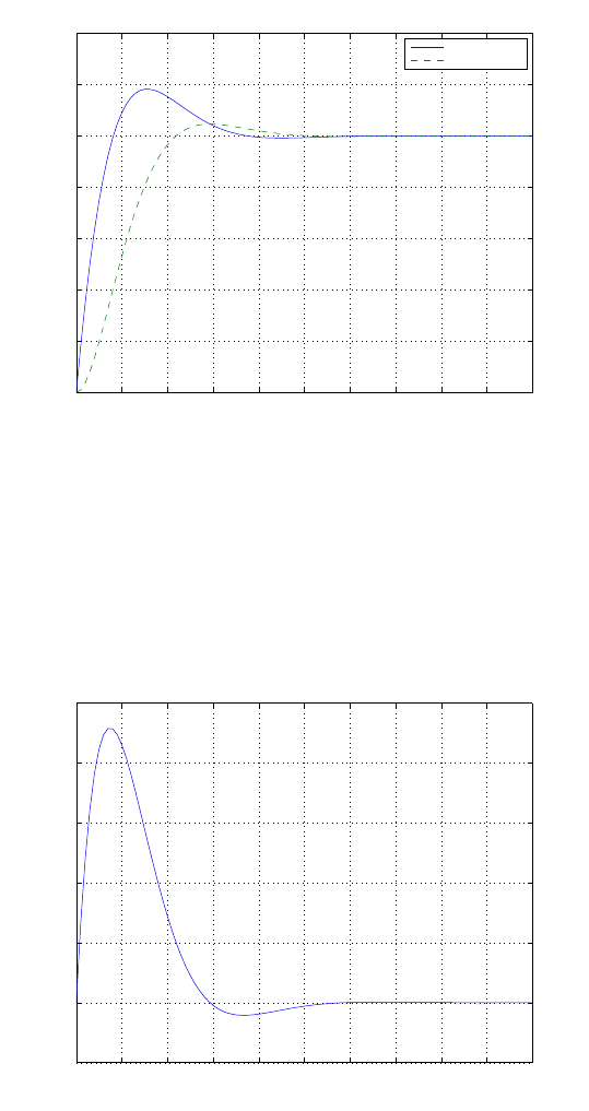
660 CHAPTER 12 Robust Control Systems

0 0.05 0.1 0.15 0.2 0.25 0.3 0.35 0.4 0.45 0.5

0.2

0.4

0.6

0.8

1.2

1.4

Time (sec)

y(t)

Without prefilter

With prefilter

FIGURE E12.1

Step response: (a) w/o preﬁlter (solid line), and (b) w/preﬁlter (dashed line).

E12.2 The disturbance response is shown in Figure E12.2.

0 0.05 0.1 0.15 0.2 0.25 0.3 0.35 0.4 0.45 0.5

−0.01

0.01

0.02

0.03

0.04

0.05

Time (sec)

y(t)

FIGURE E12.2

Disturbance response for system in E12.1.

from the publisher prior to any prohibited reproduction, storage in a retrieval system, or transmission in any form or by any means, electronic, mechanical, photocopying,

recording, or likewise. For information regarding permission(s), write to: Rights and Permissions Department, Pearson Education, Inc., Upper Saddle River, NJ 07458.

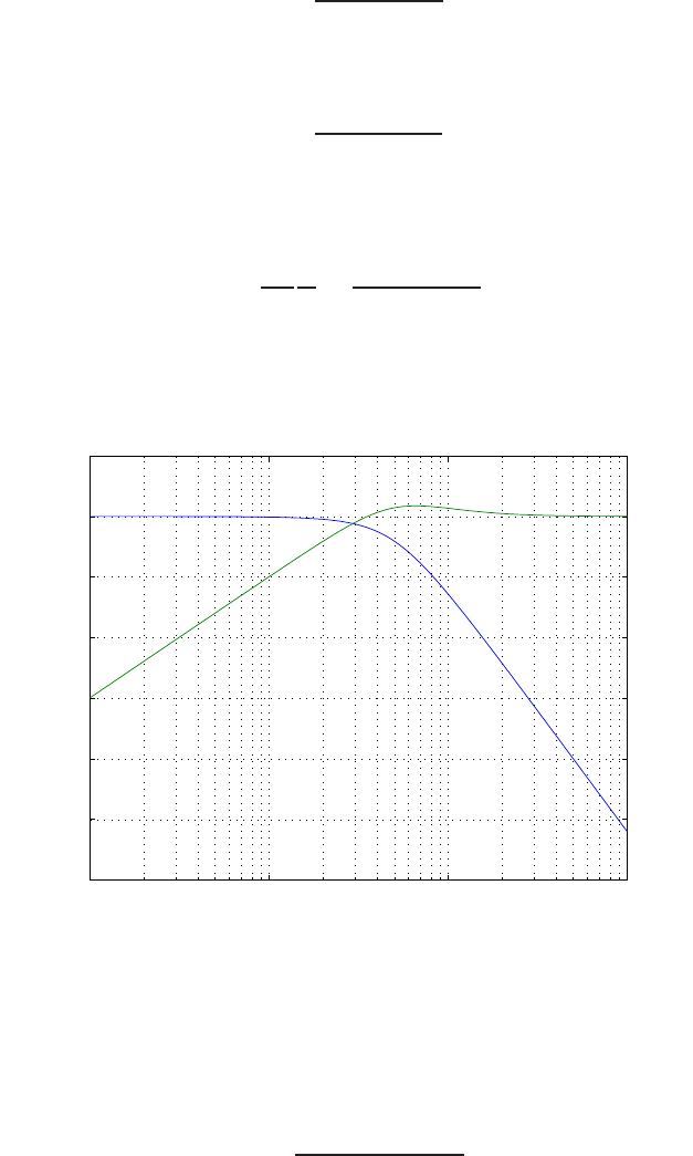
Exercises 661

E12.3 The closed-loop transfer function is

T(s) = 25

s2+bs + 25 ,

and the sensitivity function is

S(s) = s2+bs

s2+bs + 25 ,

where b= 8, nominally. The sensitivity of Tto changes in bis determined

to be

b=∂T

∂b

T=−bs

s2+bs + 25 .

The plot of T(s) and S(s) is shown in Figure E12.3, where b= 8.

10−1 100101102

−60

−50

−40

−30

−20

−10

Frequency (rad/sec)

Gain dB

20log|T|

20log|S|

FIGURE E12.3

Plot of T(s)and the sensitivity function S(s).

E12.4 The plant transfer function is

G(s) = 1

(s+ 20)(s+ 36) ,

from the publisher prior to any prohibited reproduction, storage in a retrieval system, or transmission in any form or by any means, electronic, mechanical, photocopying,

recording, or likewise. For information regarding permission(s), write to: Rights and Permissions Department, Pearson Education, Inc., Upper Saddle River, NJ 07458.

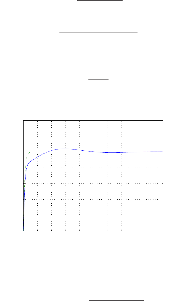
662 CHAPTER 12 Robust Control Systems

and the PID controller is given by

Gc(s) = K3(s+a)(s+b)

Let a=20, b=500, and K3= 200. Then, the closed-loop system is

T(s) = 200s2+ 4000s+ 100000

s3+ 256s2+ 4720s+ 100000 .

The closed-loop poles are s1=-237.93 and s2,3=−9.04 ±j18.5 and the

zeros are s1,2=−10±j20. Therefore, there is an approximate cancellation

of the complex poles and zeros and the approximate system is

T(s) = 238

s+ 238 .

The actual response and approximation are shown in Figure E12.4.

0 0.05 0.1 0.15 0.2 0.25 0.3 0.35 0.4 0.45 0.5

0.2

0.4

0.6

0.8

1.2

1.4

Time (sec)

y(t)

approximation

actual

FIGURE E12.4

Step response for closed-loop actual and approximate transfer functions.

E12.5 The loop transfer function is

L(s) = Gc(s)G(s) = 10KD(s+KP/KD)

s(s+ 3)(s+ 10) .

from the publisher prior to any prohibited reproduction, storage in a retrieval system, or transmission in any form or by any means, electronic, mechanical, photocopying,

recording, or likewise. For information regarding permission(s), write to: Rights and Permissions Department, Pearson Education, Inc., Upper Saddle River, NJ 07458.

Exercises 663

Select KP/KD= 10. Then

L(s) = Gc(s)G(s) = 10KD

s(s+ 3) ,

and the closed-loop transfer function is

T(s) = 10KD

s2+ 3s+ 10KD

Let ζ= 0.69, which implies P.O. < 5%. Also, 2ζωn= 3, so ωn= 2.17.

Thus,

10KD=ω2

n= 4.72 .

Thus, the controller is Gc(s) = 0.47(s+ 10). The settling time is Ts= 2.8

s and the percent overshoot is P.O. = 4.6%. As Kincreases, the per-

cent overshoot increases from 0% to 16% and the settling time generally

decreases from 3.8 sec to 2.6 sec.

E12.6 The loop transfer function with the PID controller is

Gc(s)Gs(s) = KDs2+KPs+KI

(s+ 5)2.

The ITAE step response requires

s3+ 1.75ωns2+ 2.15ω2

ns+ω3

n=s3+ (10 + KD)s2+ (25 + KP)s+KI.

For n= 3 we estimate the normalized settling time to be

ωnTs≈8 seconds.

Thus, ωn≈6, and

KD= 0.5, KP= 52.4,and KI= 216.

The step response is shown in Figure E12.6. The transfer function from

the disturbance to the output is

Y(s)

Td(s)=G(s)

1 + Gc(s)G(s)=s

s3+ 10.5s2+ 77.4s+ 216 .

The disturbance response is shown in Figure E12.6. The system is eﬀective

in reducing the eﬀects of the disturbance, and the maximum output is

reduced by 1/100 for a step disturbance.

from the publisher prior to any prohibited reproduction, storage in a retrieval system, or transmission in any form or by any means, electronic, mechanical, photocopying,

recording, or likewise. For information regarding permission(s), write to: Rights and Permissions Department, Pearson Education, Inc., Upper Saddle River, NJ 07458.

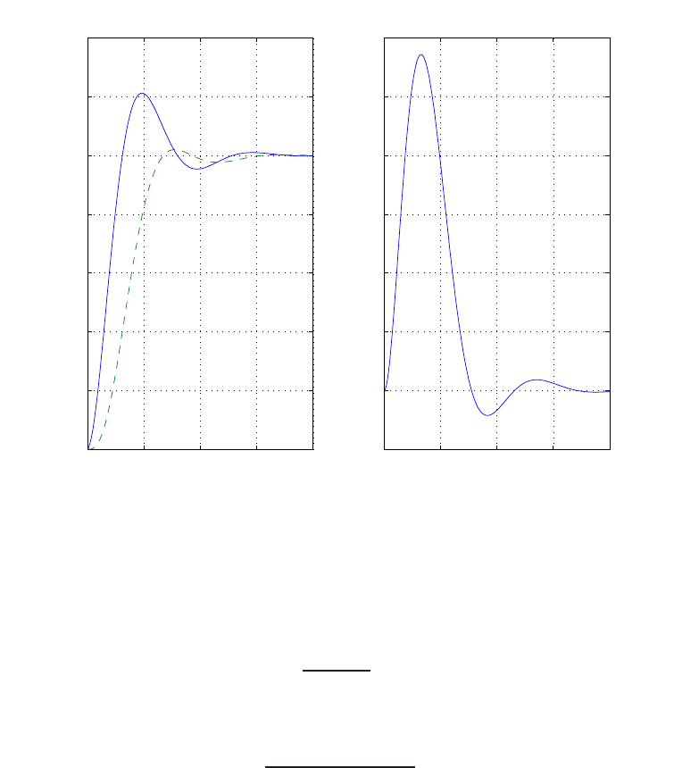
664 CHAPTER 12 Robust Control Systems

0 0.5 1 1.5 2

0.2

0.4

0.6

0.8

1.2

1.4

TIme (s)

(a) Step response

y(t)

0 0.5 1 1.5 2

−2

12 x 10−3

TIme (s)

(b) Disturbance response

y(t)

FIGURE E12.6

(a) Step response: w/o preﬁlter (solid line) and w/preﬁlter (dashed line); and (b) distur-

bance response.

E12.7 The plant transfer function is

G(s) = 1

(s+ 4)2,

and the PID controller is

Gc(s) = K1s+K2+K3s2

Using the ITAE criteria and selecting ωn= 10 yields

K3= 9.5K2= 1000 and K1= 199 .

The step response is shown in Figure E12.7. The disturbance response is

also shown in Figure E12.7. The maximum y(t) = 0.0041, so the system

is eﬀective in rejecting the step disturbance.

from the publisher prior to any prohibited reproduction, storage in a retrieval system, or transmission in any form or by any means, electronic, mechanical, photocopying,

recording, or likewise. For information regarding permission(s), write to: Rights and Permissions Department, Pearson Education, Inc., Upper Saddle River, NJ 07458.

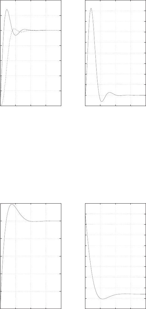
Exercises 665

0.2

0.4

0.6

0.8

1.2

1.4

00.5 1 1.5 2

Time (sec)

y(t)

(a) step response

-0.5

0.5

1.5

2.5

3.5

4.5

x10-3

00.5 1 1.5 2

Time (sec)

y(t)

(b) disturbance

FIGURE E12.7

(a) Step response: w/o preﬁlter (solid line) and w/preﬁlter (dashed line); and (b) distur-

bance response.

E12.8 The maximum ωn= 60. Then K1= 3600 and K2= 80. The maximum

control input is max |u(t)| ≈ 80. The plot of the step response and the

control input u(t) is shown in Figure E12.8.

0.2

0.4

0.6

0.8

1.2

0 0.05 0.1 0.15 0.2

Time (sec)

y(t)

(a) step response

-10

0 0.05 0.1 0.15 0.2

Time (sec)

u(t)

(b) control input u(t)

FIGURE E12.8

Step response w/o preﬁlter; and (b) control input u(t).

from the publisher prior to any prohibited reproduction, storage in a retrieval system, or transmission in any form or by any means, electronic, mechanical, photocopying,

recording, or likewise. For information regarding permission(s), write to: Rights and Permissions Department, Pearson Education, Inc., Upper Saddle River, NJ 07458.

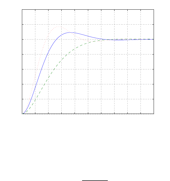
666 CHAPTER 12 Robust Control Systems

E12.9 One possible PD controller is

Gc(s) = 27.6s+ 8.25s .

When

K= 1 ,

the system roots are

s1,2=−3.2±j4.3

s3=−9.5.

The step response is shown in Figure E12.9 for K= 0.5,1, and 1.5.

0 0.2 0.4 0.6 0.8 1 1.2 1.4 1.6 1.8 2

0.2

0.4

0.6

0.8

1.2

1.4

Time (sec)

y(t)

K=1 (solid); K=0.5 (dashed); and K=1.5 (dotted)

FIGURE E12.9

Step response for K= 0.5,1, and 1.5.

E12.10 One possible PI controller is

Gc(s) = 2.2s+ 22

When K= 1, the system roots are s1,2=−1.31 ±j1.31, and s3=−6.37.

The step response is shown in Figure E12.10.

from the publisher prior to any prohibited reproduction, storage in a retrieval system, or transmission in any form or by any means, electronic, mechanical, photocopying,

recording, or likewise. For information regarding permission(s), write to: Rights and Permissions Department, Pearson Education, Inc., Upper Saddle River, NJ 07458.

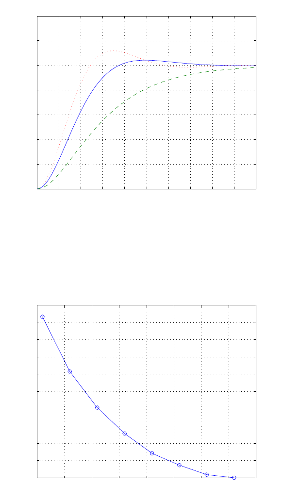
Exercises 667

0 0.5 1 1.5 2 2.5 3 3.5 4 4.5 5

0.2

0.4

0.6

0.8

1.2

1.4

Time (sec)

y(t)

K=1 (solid); K=0.5 (dashed); and K=1.5 (dotted)

FIGURE E12.10

Step response for K= 0.5,1, and 1.5.

E12.11 The plot is shown in Figure E12.11.

0 0.5 1 1.5 2 2.5 3 3.5 4

100

Time (sec)

P.O. (%)

FIGURE E12.11

Percent overshoot as a function of kin the interval 0.1≤k≤4.

from the publisher prior to any prohibited reproduction, storage in a retrieval system, or transmission in any form or by any means, electronic, mechanical, photocopying,

recording, or likewise. For information regarding permission(s), write to: Rights and Permissions Department, Pearson Education, Inc., Upper Saddle River, NJ 07458.

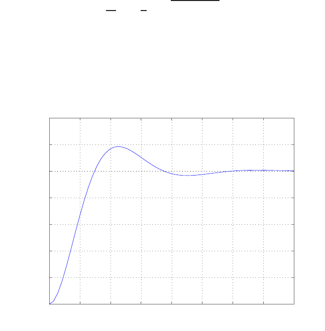
668 CHAPTER 12 Robust Control Systems

E12.12 The controllability matrix is

Pc=



c1c2

c2−ac1−bc2



and

det Pc=c2

2+ [bc1]c2+ac2

For controllability we require det Pc6= 0, hence

2+ [bc1]c2+ac2

16= 0

implies

c16=−b

2±q(b/2)2−a

where (b/2)2−a≥0. For real-valued c1and c2, if (b/2)2−a < 0, all real

values of c1and c2are valid. Valid values of the constants are c1= 0,

c2= 10, a= 10, and b= 3. The step response is shown in Figure E12.12.

0 0.5 1 1.5 2 2.5 3 3.5 4

0.2

0.4

0.6

0.8

1.2

1.4

Step Response

Time (sec)

Amplitude

FIGURE E12.12

Step response with c1= 0,c2= 10,a= 10, and b= 3.

from the publisher prior to any prohibited reproduction, storage in a retrieval system, or transmission in any form or by any means, electronic, mechanical, photocopying,

recording, or likewise. For information regarding permission(s), write to: Rights and Permissions Department, Pearson Education, Inc., Upper Saddle River, NJ 07458.

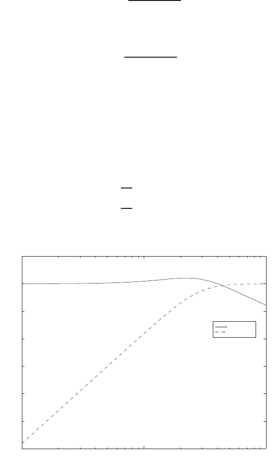
Problems 669

Problems

P12.1 The closed-loop transfer function is

T(s) = 4(s+ 2)

s2+ 4s+ 8

and the sensitivity function is

S(s) = s2

s2+ 4s+ 8 .

The plot of 20 log |T|and 20 log |S|is shown in Figure P12.1. The band-

width is

ωB= 6.31 rad/sec .

Then

|ST

K|ωB= 0.98

|ST

K|ωB

2= 0.78

|ST

K|ωB

4= 0.30 .

20log|T|

20log|S|

10-1 100101

-60

-50

-40

-30

-20

-10

Frequency (rad/sec)

Gain dB

FIGURE P12.1

Plot of T(s)and the sensitivity function S(s).

from the publisher prior to any prohibited reproduction, storage in a retrieval system, or transmission in any form or by any means, electronic, mechanical, photocopying,

recording, or likewise. For information regarding permission(s), write to: Rights and Permissions Department, Pearson Education, Inc., Upper Saddle River, NJ 07458.

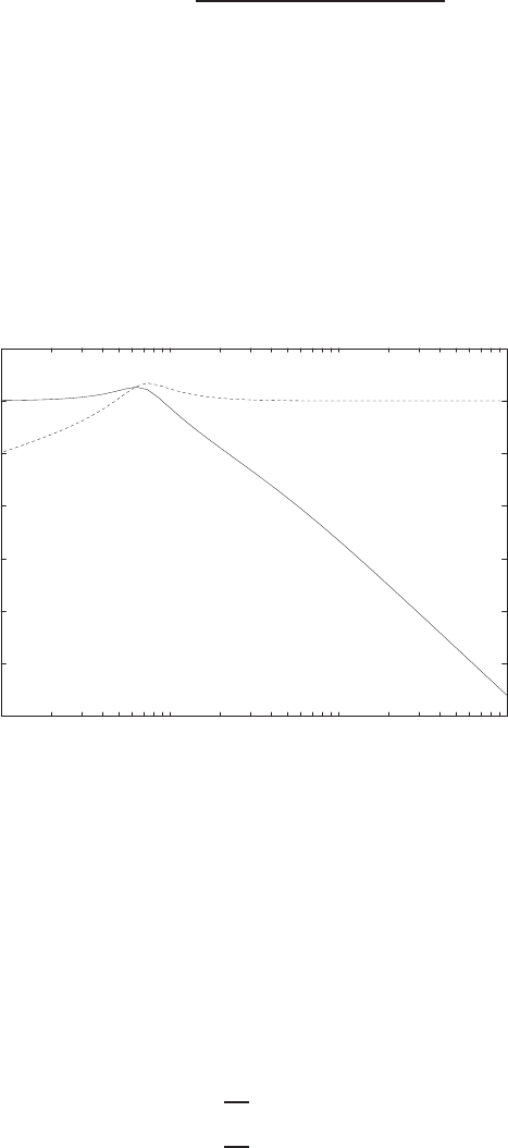
670 CHAPTER 12 Robust Control Systems

P12.2 (a) The loop transfer function is given by

Gc(s)G(s) = K

s(0.02s+ 1)(0.002s+ 1) .

When

K= 100 ,

the peak magnitude is

Mpω= 1.84 .

(b) The plot of 20 log |T|and 20 log |S|is shown in Figure P12.2a.

-120

-100

-80

-60

-40

-20

101102103104

20log|T|

20log|S|

Frequency (rad/sec)

Gain dB

FIGURE P12.2

(a) Plot of T(s)and the sensitivity function S(s).

ωB= 117 rad/sec ,

and

|ST

K|ωB= 1.47

|ST

K|ωB

4= 0.39

|ST

K|ωB

2= 1.62 .

from the publisher prior to any prohibited reproduction, storage in a retrieval system, or transmission in any form or by any means, electronic, mechanical, photocopying,

recording, or likewise. For information regarding permission(s), write to: Rights and Permissions Department, Pearson Education, Inc., Upper Saddle River, NJ 07458.

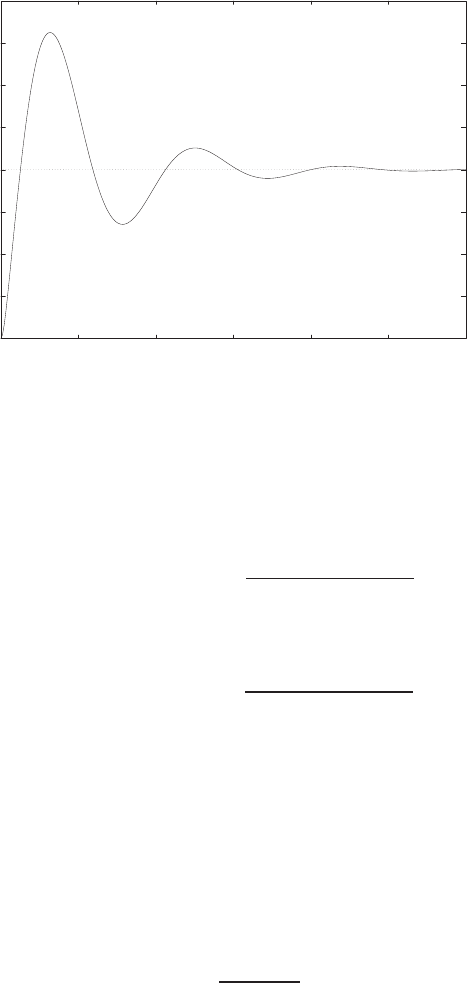
Problems 671

x10-7

0 0.05 0.1 0.15 0.2 0.25 0.3

Time (secs)

Amplitude

FIGURE P12.2

CONTINUED: (b) Disturbance response for K= 100.

P12.3 (a) The loop transfer function is

L(s) = Gc(s)G(s) = K(s−4)(s−1)

(s+ 0.02)(s+ 2)2.

The characteristic equation is

1 + Gc(s)G(s) = 1 + K(s−4)(s−1)

(s+ 0.02)(s+ 2)2= 0

s3+ (4.02 + K)s2+ (4.08 −5K)s+ 0.08 + 4K= 0 .

Using Routh-Hurwitz we ﬁnd that the system is stable for

−4.6987 < K < 0.6947 .

(b) The steady-state error is

ess =1

1 + 50K.

Select K= 0.18 to obtain a steady-state error to a unit step of 0.1.

from the publisher prior to any prohibited reproduction, storage in a retrieval system, or transmission in any form or by any means, electronic, mechanical, photocopying,

recording, or likewise. For information regarding permission(s), write to: Rights and Permissions Department, Pearson Education, Inc., Upper Saddle River, NJ 07458.

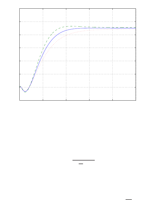
672 CHAPTER 12 Robust Control Systems

(c,d) The plots of y(t) for

K= 0.18 (nominal)

K= 0.21 (+15%)

K= 0.15 (−15%)

are shown in Figure P12.3.

0 5 10 15 20 25

−0.2

0.2

0.4

0.6

0.8

1.2

Time (sec)

y(t)

K=0.18 (solid) & K=0.21 (dashed) & K=0.15 (dotted)

FIGURE P12.3

Step input response for K= 0.18,K= 0.21 and K= 0.15.

P12.4 (a) The plant is given by

G=1

ss

25 + 1.

We desire P.O. < 10% and Ts<100 ms. Using a PD controller

Gc(s) = 100 + 2.2s ,

we determine that P.O. = 7%, Ts<100 ms and ess =A

100 for a ramp

input. The plot of y(t) is shown in Figure P12.4.

from the publisher prior to any prohibited reproduction, storage in a retrieval system, or transmission in any form or by any means, electronic, mechanical, photocopying,

recording, or likewise. For information regarding permission(s), write to: Rights and Permissions Department, Pearson Education, Inc., Upper Saddle River, NJ 07458.

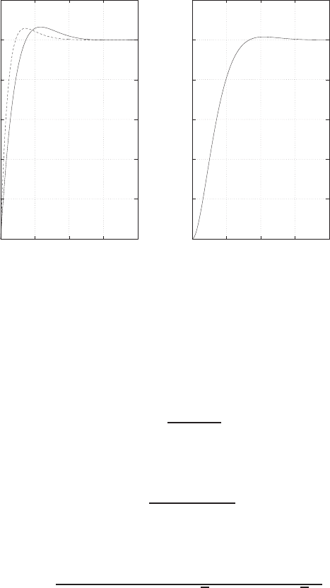
Problems 673

(b) The sensitivity is

|Sr

K1|= 27.95

when K1= 1.

is shown in Figure P12.4.

(d) The disturbance response is shown in Figure P12.4.

0.2

0.4

0.6

0.8

1.2

0 0.05 0.1 0.15 0.2

Time (sec)

y(t)

(a) step response

0.002

0.004

0.006

0.008

0.01

0.012

0 0.05 0.1 0.15 0.2

Time (sec)

y(t)

(b) disturbance

FIGURE P12.4

(a) Step response: K1= 1 (solid line) and K1= 2 (dashed line); and (b) disturbance

response.

P12.5 (a) The plant is given by

G(s) = 1

s(s+p)

where p= 2, nominally. One solution is

Gc(s) = 18.7(s+ 2.9)

(s+ 5.4) .

Then,

T(s) = 18.7(s+ 2.9)

(s+ 3.41)(s+ 2 + 2√3j)(s+ 2 −2√3j).

from the publisher prior to any prohibited reproduction, storage in a retrieval system, or transmission in any form or by any means, electronic, mechanical, photocopying,

recording, or likewise. For information regarding permission(s), write to: Rights and Permissions Department, Pearson Education, Inc., Upper Saddle River, NJ 07458.

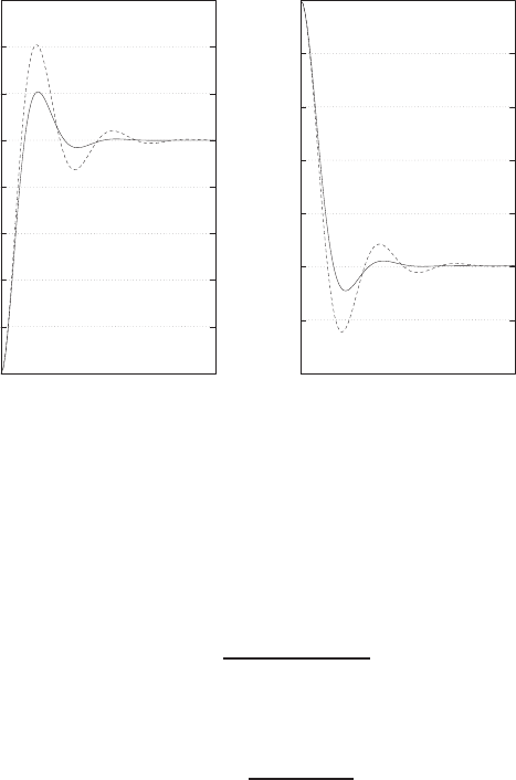
674 CHAPTER 12 Robust Control Systems

(b,d) The step responses are shown in Figure P12.5 for p= 2 and p= 1.

(c,d) The disturbance responses are shown in Figure P12.5 for p= 2 and

p= 1.

0.2

0.4

0.6

0.8

1.2

1.4

1.6

0 5

Time (sec)

y(t)

(a) step response

-0.14

-0.12

-0.1

-0.08

-0.06

-0.04

-0.02

0 5

Time (sec)

y(t)

(b) disturbance

FIGURE P12.5

(a) Step response: p= 2 (solid line) and p= 1 (dashed line); and (b) disturbance response:

p= 2 (solid line) and p= 1 (dashed line).

P12.6 (a) The plant is given by

G(s) = 1

s(s2+ 4s+ 5) ,

and the PID controller is

Gc(s) = K(s+z)2

When

z= 1.25

and

K= 4 ,

all roots are

s=−1±j1.22 .

from the publisher prior to any prohibited reproduction, storage in a retrieval system, or transmission in any form or by any means, electronic, mechanical, photocopying,

recording, or likewise. For information regarding permission(s), write to: Rights and Permissions Department, Pearson Education, Inc., Upper Saddle River, NJ 07458.

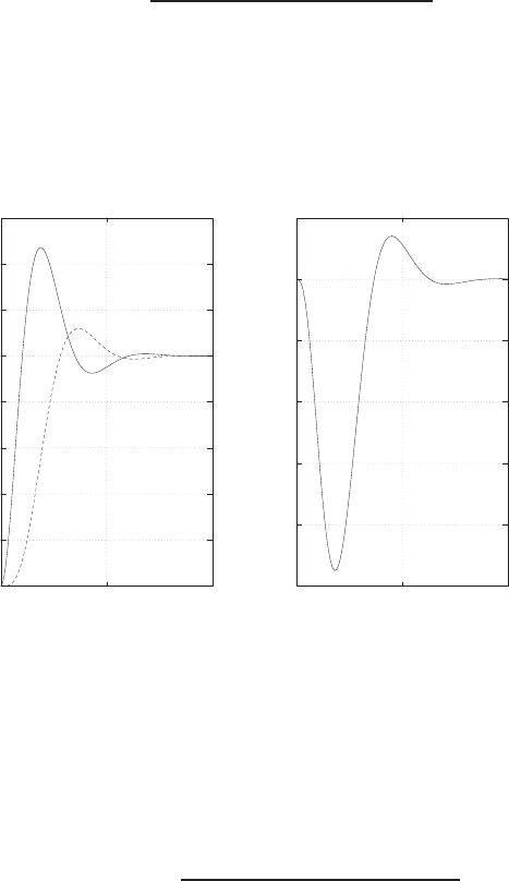
Problems 675

Then, the closed-loop transfer function is

T(s) = 4(s+ 1.25)2

s4+ 4s3+ 9s2+ 10s+ 6.25 .

(b,c) The step responses with and without a preﬁlter are shown in Fig-

ure P12.6.

(d) The disturbance response is shown in Figure P12.6.

0.2

0.4

0.6

0.8

1.2

1.4

1.6

0 5 10

Time (sec)

y(t)

(a) step response

-0.1

-0.08

-0.06

-0.04

-0.02

0.02

0 5 10

Time (sec)

y(t)

(b) disturbance

FIGURE P12.6

(a) Step response: w/o preﬁlter (solid line) and w/preﬁlter (dashed line); and (b) distur-

bance response.

P12.7 (a) The loop transfer function is

Gc(s)G(s) = 10Ka(5s+ 500 + 0.0475s2)

s3.

When

Ka= 374.5,

the phase margin is

P.M. = 40o.

(b) The root locus is shown in Figure P12.7a.

from the publisher prior to any prohibited reproduction, storage in a retrieval system, or transmission in any form or by any means, electronic, mechanical, photocopying,

recording, or likewise. For information regarding permission(s), write to: Rights and Permissions Department, Pearson Education, Inc., Upper Saddle River, NJ 07458.

676 CHAPTER 12 Robust Control Systems

-150

-100

-50

100

150

-150 -100 -50 0 50 100 150

xxx

Real Axis

Imag Axis

FIGURE P12.7

(a) Root locus for 1 + Ka10(0.0475s2+5s+500)

s3= 0.

When

Ka= 374.5,

the roots are

s1=−139.8

s2,3=−19.1±j114.2.

Y(s)

Td(s)=−s

s3+ 182s2+ 19150s+ 1915000 .

The maximum is

max |y(t)|= 0.0000389 .

(d) The step responses, with and without a preﬁlter, are shown in Fig-

ure P12.7b.

P12.8 The polynomial under investigation is

s3+ 3s2+ 3s+ 4 = 0 .

from the publisher prior to any prohibited reproduction, storage in a retrieval system, or transmission in any form or by any means, electronic, mechanical, photocopying,

recording, or likewise. For information regarding permission(s), write to: Rights and Permissions Department, Pearson Education, Inc., Upper Saddle River, NJ 07458.

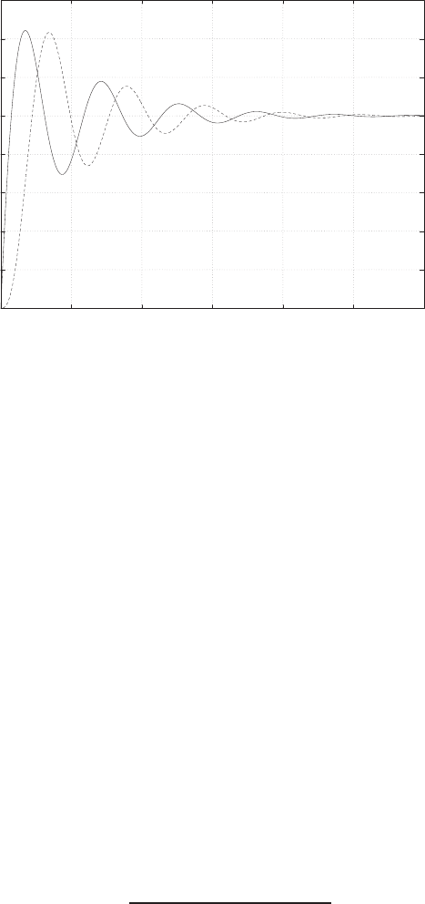
Problems 677

0.2

0.4

0.6

0.8

1.2

1.4

1.6

0 0.05 0.1 0.15 0.2 0.25 0.3

Time (sec)

y(t)

FIGURE P12.7

CONTINUED: (b) Step response: w/o preﬁlter (solid line) and w/preﬁlter (dashed line).

From the uncertainty bounds on the coeﬃcients, we deﬁne

α0= 4 β0= 5

α1= 1 β1= 4

α2= 2 β2= 4

Then, we must examine the four polynomials:

s3+ 2s2+ 4s+ 5 = 0

s3+ 4s2+s+ 4 = 0

s3+ 4s2+ 4s+ 4 = 0

s3+ 2s2+s+ 5 = 0

The fourth polynomial is not stable—therefore, the system is not stable

for the uncertain parameters.

P12.9 One possible PID controller is

Gc(s) = 0.058s2+ 2.17s+ 16.95

A ﬁrst-order Pade approximation was used in the design to account for

the delay system. The step input response is shown in Figure P12.9. A

preﬁlter should also be used with the PID controller. A suitable preﬁlter

from the publisher prior to any prohibited reproduction, storage in a retrieval system, or transmission in any form or by any means, electronic, mechanical, photocopying,

recording, or likewise. For information regarding permission(s), write to: Rights and Permissions Department, Pearson Education, Inc., Upper Saddle River, NJ 07458.

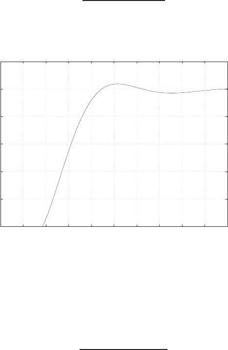
678 CHAPTER 12 Robust Control Systems

Gp(s) = K2

K3s2+K1s+K2

0.2

0.4

0.6

0.8

1.2

0 0.05 0.1 0.15 0.2 0.25 0.3 0.35 0.4 0.45 0.5

Time (sec)

y(t)

FIGURE P12.9

Step response with the PID controller and preﬁlter.

P12.10 The PID controller is given by

Gc(s) = KDs2+KPs+KI

Using the ITAE method, we desire the characteristic polynomial to be

q(s) = s3+ 1.75ωns2+ 2.15ω2

ns+ω3

n= 0 ,

where we select ωn= 4 to obtain a peak time of Tp= 1 second. Here we

use the approximation for ITAE third-order systems that ωnTp≈4 from

Figure 5.30(c) in Dorf and Bishop. The actual characteristic equation is

s3+ 25KDs2+ 25KPs+ 25KI= 0 .

Equating coeﬃcients and solving for the gains yields

KP= 1.376 , KD= 0.28 ,and KI= 2.56 .

from the publisher prior to any prohibited reproduction, storage in a retrieval system, or transmission in any form or by any means, electronic, mechanical, photocopying,

recording, or likewise. For information regarding permission(s), write to: Rights and Permissions Department, Pearson Education, Inc., Upper Saddle River, NJ 07458.

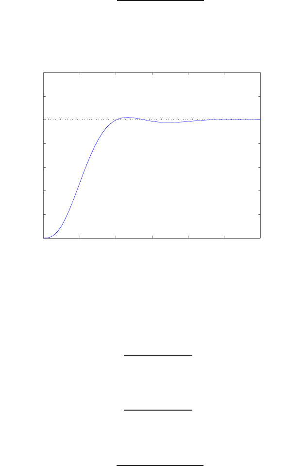
Problems 679

The step response is shown in Figure P12.10, with the preﬁlter

Gp(s) = KI

KDs2+KPs+KI

0 0.5 1 1.5 2 2.5 3

0.2

0.4

0.6

0.8

1.2

1.4

Step Response

Time (sec)

Amplitude

FIGURE P12.10

Step response with the PID controller and preﬁlter.

P12.11 We will design for the case where K= 1 and p= 1. The design plant is

G(s) = 1

s(s+ 1)(s+ 4) .

The nominal plant is given by

G(s) = 2.5

s(s+ 2)(s+ 4) ,

and the PID controller is

Gc(s) = KDs2+KPs+KI

Using the ITAE method, we desire the characteristic polynomial to be

q(s) = s4+ 2.1ωns3+ 3.4ω2

ns2+ 2.7ω3

ns+ω4

n= 0 ,

from the publisher prior to any prohibited reproduction, storage in a retrieval system, or transmission in any form or by any means, electronic, mechanical, photocopying,

recording, or likewise. For information regarding permission(s), write to: Rights and Permissions Department, Pearson Education, Inc., Upper Saddle River, NJ 07458.

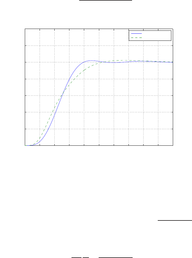
680 CHAPTER 12 Robust Control Systems

where we select ωn= 2.38 to obtain a peak time around Tp= 3 seconds.

The actual characteristic equation (with the worst-case plant) is

s4+ 5s3+ (4 + KD)s2+KPs+KI= 0 .

Equating coeﬃcients and solving for the gains yields KP= 36.40, KI=

32.08, and KD= 15.26. The step response is shown in Figure P12.11,

with the preﬁlter

Gp(s) = KI

KDs2+KPs+KI

0 0.5 1 1.5 2 2.5 3 3.5 4 4.5 5

0.2

0.4

0.6

0.8

1.2

1.4

Time (sec)

y(t)

Worst−case plant

Nominal plant

FIGURE P12.11

Step response with the preﬁlter: nominal plant (dashed line) & worst-case plant (solid line).

P12.12 The transfer function is

G(s) = C(sI−A)−1B=h2 0 i



s−3

5s+K





1

=−6

s2+Ks + 5 .

The sensitivity is

K=∂G

∂K

G=−Ks

s2+Ks +5.

from the publisher prior to any prohibited reproduction, storage in a retrieval system, or transmission in any form or by any means, electronic, mechanical, photocopying,

recording, or likewise. For information regarding permission(s), write to: Rights and Permissions Department, Pearson Education, Inc., Upper Saddle River, NJ 07458.

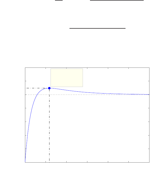
Advanced Problems 681

Advanced Problems

AP12.1 Let Gp(s) = 1. A viable PID controller is

Gc(s) = KP+KI

s+KDs=1000s2+ 3000s+ 100

The loop transfer function is

Gc(s)G(s) = 1000s2+ 3000s+ 100)

s(50s2+ 1) .

We can check that Kv= 100, as desired. The step response is shown in

Figure AP12.1.

Step Response

Time (sec)

Amplitude

0 0.2 0.4 0.6 0.8 1 1.2

0.2

0.4

0.6

0.8

1.2

1.4

System: syscl

Peak amplitude: 1.1

Overshoot (%): 9.5

At time (sec): 0.234

FIGURE AP12.1

Step response with PID controller.

AP12.2 For all three controllers, choose K= 1 as the design value. Also, use

as the nominal points a= 2 and b= 5 for each design. ITAE methods

were employed in all designs, although this did not work well for the PI

controller.

(a) PI controller: Let

Gp(s) = 1 .

Not all speciﬁcations could be met simultaneously with a PI con-

from the publisher prior to any prohibited reproduction, storage in a retrieval system, or transmission in any form or by any means, electronic, mechanical, photocopying,

recording, or likewise. For information regarding permission(s), write to: Rights and Permissions Department, Pearson Education, Inc., Upper Saddle River, NJ 07458.

682 CHAPTER 12 Robust Control Systems

troller. The best over-all results are achieved when using a= 3 and

b= 4.5 as the design values. An acceptable PI controller is

Gc(s) = 1.2 + 3.96

Controller P.O. TsTp|u(t)|max

PI 0% 2.29s n.a. 4.43

PD 4.6% 1.72s 1.26s 12.25

PID 1.97% 0.65s 0.47s 37.25

TABLE AP12.2 PI, PD, and PID controller performance summary.

The ﬁnal design is based on root locus methods since the ITAE meth-

ods did not produce an eﬀective controller. The closed-loop transfer

function is

T(s) = 1.2s+ 3.96

s3+ 3s2+ 5.7s+ 3.96 .

(b) PD controller: Let

Gp(s) = 12.25

7.25 + 2.9s.

The closed-loop transfer function is

T(s) = 7.25 + 2.9s

s2+ 4.9s+ 12.25 ,

where the PD controller (based on ITAE methods) is

Gc(s) = 7.25 + 2.9s .

from the publisher prior to any prohibited reproduction, storage in a retrieval system, or transmission in any form or by any means, electronic, mechanical, photocopying,

recording, or likewise. For information regarding permission(s), write to: Rights and Permissions Department, Pearson Education, Inc., Upper Saddle River, NJ 07458.

Advanced Problems 683

Gp(s) = 1000

15.5s2+ 210s+ 1000 .

The closed-loop transfer function is

T(s) = 15.5s2+ 210s+ 1000

s3+ 17.5s2+ 215s+ 1000 .

And the PID controller (based on ITAE methods) is

Gc(s) = 15.5s2+ 210s+ 1000

The performance of each controller is summarized in Table AP12.2.

AP12.3 (a) The PID controller is

Gc(s) = KDs2+KP

KDs+KI

KD

Since we want P.O. < 4% and Ts<1s, we choose the dominant

closed-loop poles to have ωn= 6 and ζ= 0.8. Therefore, we place the

zeros at

s2+KP

s+KI

=s2+ 10s+ 36 .

Solving for the constants yields,

= 10 ,KI

= 36 .

Then, using root locus methods, we choose KD= 91 to place the

roots near the zeros. The PID controller gains are computed to be

KP= 910, KI= 3276 and KD= 91.

(b) The loop transfer function is

Gc(s)G(s) = KDs2+KPs+KI

s2(s2+ 5s+ 4) .

The closed-loop system characteristic equation is

s3+ 5s2+ 4s+KDs2+KPs+KI= 0 .

Solving for the PID gains yields KP= 73.4, KI= 216 and KD= 5.5.

from the publisher prior to any prohibited reproduction, storage in a retrieval system, or transmission in any form or by any means, electronic, mechanical, photocopying,

recording, or likewise. For information regarding permission(s), write to: Rights and Permissions Department, Pearson Education, Inc., Upper Saddle River, NJ 07458.

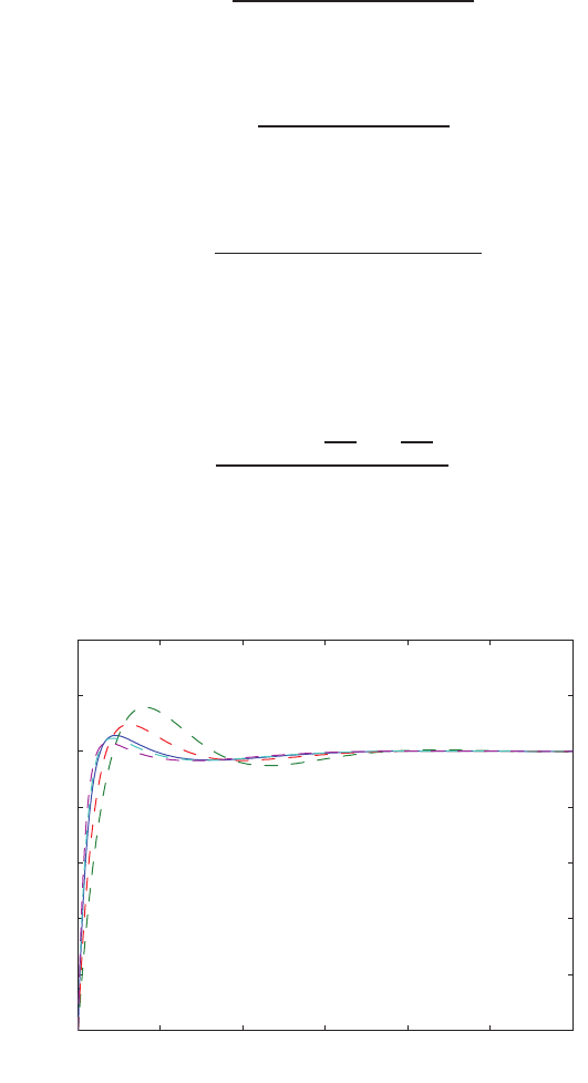
684 CHAPTER 12 Robust Control Systems

Therefore, the controller is

Gc(s) = 5.5(s2+ 13.35s+ 39.3)

Using the preﬁlter

Gp(s) = 39.3

s2+ 13.35s+ 39.3,

we obtain the closed-loop transfer function

T(s) = 216

s3+ 10.5s2+ 77.4s+ 216 .

The percent overshoot is P.O. ≈3.5% and the settling time is Ts≈

1.67 sec.

AP12.4 The PID controller is

Gc(s) = KDs2+KP

KDs+KI

KD

The bounds 1 ≤a≤2 and 4 ≤b≤12 imply that 2 ≤ωn≤3.46

and 0.5≤ζωn≤1. One solution is to place the PID controller zeros at

0 0.5 1 1.5 2 2.5 3

0.2

0.4

0.6

0.8

1.2

1.4

Time (sec)

Amplitude

FIGURE AP12.4

Family of step response with PID controller with nominal case (a, b) = (1.5,9) denoted by

the solid line.

from the publisher prior to any prohibited reproduction, storage in a retrieval system, or transmission in any form or by any means, electronic, mechanical, photocopying,

recording, or likewise. For information regarding permission(s), write to: Rights and Permissions Department, Pearson Education, Inc., Upper Saddle River, NJ 07458.

Advanced Problems 685

s=−1±j√8 (i.e. ζωn= 1 and ωn= 3). So,

s2+KP

s+KI

=s2+ 2ζωns+ω2

n=s2+ 4s+ 9 .

The nominal case for design is chosen to be a= 1.5 and b= 9. Using

root locus, we select KD= 2.1 to place the closed-loop characteristic

roots near the zeros. Then, the PID controller gains are computed to be

KP= 8.4, KI= 18.9, and KD= 2.1. The plot of the response to a step

input is shown in Figure AP12.4. The oﬀ-nominal cases shown in the

simulations are (a, b) = (1.2,4), (1.4,6), (1.6,10), and (1.8,12).

AP12.5 To obtain a phase margin of P.M. = 49.77o, select K= 1.5, b= 36 and

choose Gp(s) = 1. The PID controller is

Gc(s) = 1.5(s2+ 20s+ 36)

When K1= 0.75, the phase margin is reduced to P.M. = 45.45o; and

when K1= 1.25, the phase margin is increased to P.M. = 52.75o.

AP12.6 With the settling time Ts= 1 and percent overshoot P.O. < 10% speciﬁ-

cations, we target for dominant closed-loop poles with ωn= 10. Here we

estimate ωnTs≈10 associated with the ITAE performance. The closed-

loop transfer function is

T(s) = Gp(s)1.5(KDs2+KPs+KI)

(1 + 1.5KD)s2+ 1.5KPs+ 1.5KI

where we have neglected τ. Using the ITAE method, the desired charac-

teristic polynomial is

s2+√2ωns+ω2

n=s2+1.5Kp

1 + 1.5KD

s+1.5KI

1 + 1.5KD

Let KD= 0.25. Then solving for the remaining PID gains yields KP=

12.96 and KI= 91.67. The pre-ﬁlter is

Gp(s) = 137.5

0.375s2+ 19.45s+ 137.5.

Then the closed-loop transfer function (with τ= 0.001) is

T(s) = 137.5

0.001s3+ 1.375s2+ 19.45s+ 137.5.

The transfer function from the disturbance to the output is

Y(s)/Td(s) = 1.5s

0.001s3+ 1.375s2+ 19.45s+ 137.5.

from the publisher prior to any prohibited reproduction, storage in a retrieval system, or transmission in any form or by any means, electronic, mechanical, photocopying,

recording, or likewise. For information regarding permission(s), write to: Rights and Permissions Department, Pearson Education, Inc., Upper Saddle River, NJ 07458.

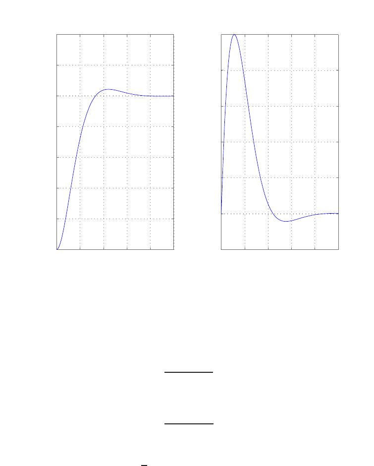
686 CHAPTER 12 Robust Control Systems

The step input response and disturbance response are shown in Fig-

ure AP12.6.

0 0.2 0.4 0.6 0.8 1

0.2

0.4

0.6

0.8

1.2

1.4

(a)

Time (sec)

Amplitude

0 0.2 0.4 0.6 0.8 1

−0.01

0.01

0.02

0.03

0.04

0.05

(b)

Time (sec)

Amplitude

FIGURE AP12.6

(a) Input response; (b) Disturbance response.

AP12.7 The PI controller is given by

Gc(s) = KPs+KI

We will also use the preﬁlter

Gp(s) = KI

KPs+KI

Using the ITAE method, we determine that

KP=√2ωnand KI=ω2

Let ωn= 2.2. Then KP= 3.11 and KI= 4.8. The step response and

control u(t) are shown in Figure AP12.7.

from the publisher prior to any prohibited reproduction, storage in a retrieval system, or transmission in any form or by any means, electronic, mechanical, photocopying,

recording, or likewise. For information regarding permission(s), write to: Rights and Permissions Department, Pearson Education, Inc., Upper Saddle River, NJ 07458.

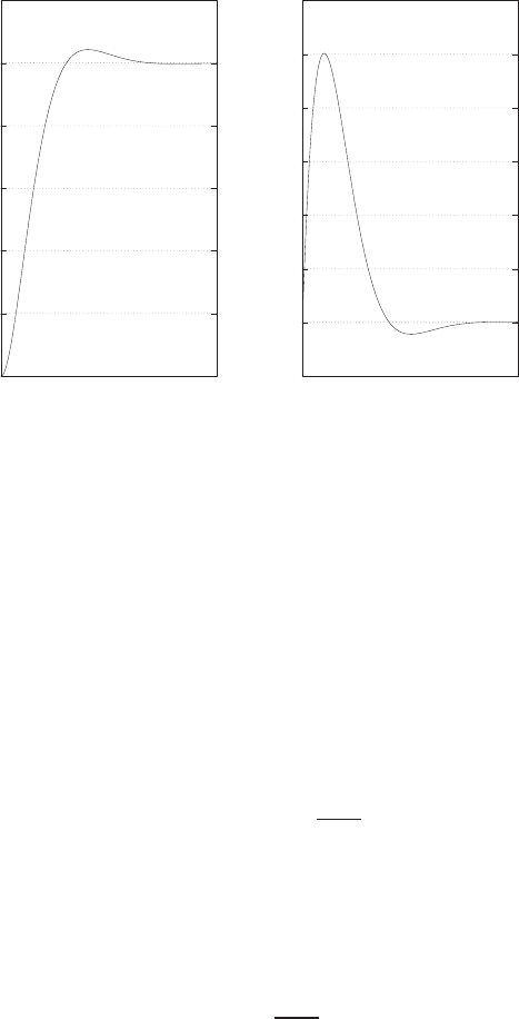
Advanced Problems 687

0.2

0.4

0.6

0.8

1.2

0 5

Time (secs)

Amplitude

(a)

-0.2

0.2

0.4

0.6

0.8

1.2

0 5

Time (secs)

Amplitude

(b)

FIGURE AP12.7

(a) Input response; (b) Control history u(t).

AP12.8 (a) A suitable PD controller is given by

Gc(s) = 0.6 + 0.4s .

The percent overshoot is P.O. = 18.8% and the peak time is Tp= 2.4

sec.

(b) A suitable PI controller is given by

Gc(s) = 0.15 + 0.01

The percent overshoot is P.O. = 23.7% and the peak time is Tp= 7.8

sec.

Gc(s) = 0.6 + 0.01

s+ 0.4s .

The percent overshoot is P.O. = 19.9% and the peak time is Tp= 2.5

sec.

(d) The PD or PID controllers are the best choices.

AP12.9 A robust PID controller designed with ITAE methods will be a suitable

controller. From the settling time speciﬁcation we select ωn= 10, where

from the publisher prior to any prohibited reproduction, storage in a retrieval system, or transmission in any form or by any means, electronic, mechanical, photocopying,

recording, or likewise. For information regarding permission(s), write to: Rights and Permissions Department, Pearson Education, Inc., Upper Saddle River, NJ 07458.

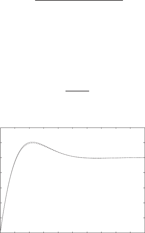
688 CHAPTER 12 Robust Control Systems

we have used ζ= 0.8. The worst case is

a= 1 and K= 2 .

The desired closed-loop transfer function is

T(s) = ω3

s3+ 1.75ωns2+ 2.15ω2

ns+ω3

and the actual characteristic equation is

q(s) = s3+ (2a+KKD)s2+ (a2+KKP)s+KKI.

Equating like terms, we ﬁnd that

KP= 107 KI= 500 KD= 7.75 .

AP12.10 We use as the design plant

G(s) = s+ 2

s(s+ 3) .

0.2

0.4

0.6

0.8

1.2

1.4

0 0.01 0.02 0.03 0.04 0.05 0.06 0.07 0.08 0.09 0.1

Time(sec)

Amplitude

FIGURE AP12.10

Family of step responses with the design plant (p, q, r) = (3,0,2) denoted by the solid line.

Select

p1= 2 and z1= 3

from the publisher prior to any prohibited reproduction, storage in a retrieval system, or transmission in any form or by any means, electronic, mechanical, photocopying,

recording, or likewise. For information regarding permission(s), write to: Rights and Permissions Department, Pearson Education, Inc., Upper Saddle River, NJ 07458.

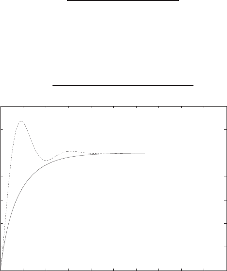
Advanced Problems 689

to cancel a design plant pole and zero. Then, choose p2= 0 to have

zero steady-state error to a unit step. The remaining variables Kand

z2are selected based on ITAE methods, where ωn= 100. A suitable

compensator is

Gc(s) = 141.42(s+ 3)(s+ 70.71)

s(s+ 2) .

A plot of the step responses for various values of p, q and ris shown in

Figure AP12.10.

AP12.11 A suitable compensator is

Gc(s) = 1000(s+ 1.8)(s+ 3.5)(s+ 5.5)

s(s+ 600) .

0.2

0.4

0.6

0.8

1.2

1.4

012345678910

Time (sec)

Amplitude

FIGURE AP12.11

Step responses with nominal plant (solid line) and oﬀ-nominal plant with all poles reduced

by 50% (dashed line).

from the publisher prior to any prohibited reproduction, storage in a retrieval system, or transmission in any form or by any means, electronic, mechanical, photocopying,

recording, or likewise. For information regarding permission(s), write to: Rights and Permissions Department, Pearson Education, Inc., Upper Saddle River, NJ 07458.

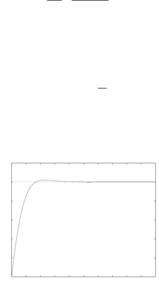
690 CHAPTER 12 Robust Control Systems

Design Problems

The plant model with parameters given in Table CDP2.1 in Dorf andCDP12.1

Bishop is given by:

θ(s)

Va(s)=26.035

s(s+ 33.142) ,

where we neglect the motor inductance Lmand where we switch oﬀ the

tachometer feedback (see Figure CDP4.1 in Dorf and Bishop). With a

PID controller ,the closed-loop system characteristic equation is

s3+ (33.142 + 26.035KD)s2+ 26.035KPs+ 26.035KI= 0 .

A suitable PID controller is

Gc(s) = 50 + s+0.1

This PID controller places the closed-loop system poles to the left of

the −ζωnline necessary to meet the settling time requirement. The step

response is shown below. The settling time is Ts= 0.12 second. In the

steady-state the error due to a step disturbance is zero.

0 0.05 0.1 0.15 0.2 0.25 0.3 0.35 0.4 0.45 0.5

0.2

0.4

0.6

0.8

1.2

Time (secs)

Amplitude

from the publisher prior to any prohibited reproduction, storage in a retrieval system, or transmission in any form or by any means, electronic, mechanical, photocopying,

recording, or likewise. For information regarding permission(s), write to: Rights and Permissions Department, Pearson Education, Inc., Upper Saddle River, NJ 07458.

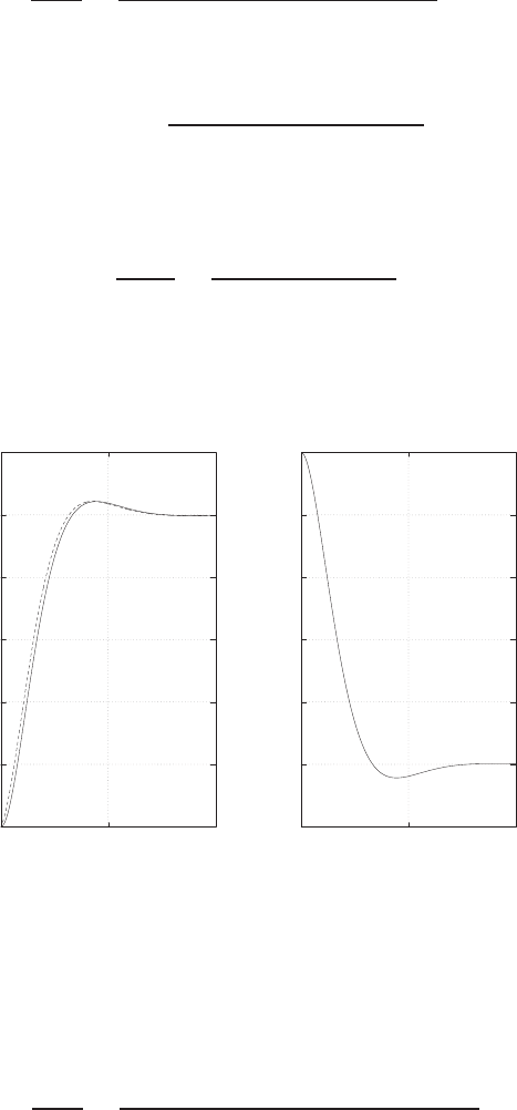
Design Problems 691

DP12.1 The closed-loop transfer function is

Y(s)

R(s)=KmGc(s)

s2+ (2 + KmK1)s+Gc(s)Km

(a) When Gc=K, we have

T(s) = 15K

s2+ (2 + 15K1)s+ 15K,

where Km= 15. Using ITAE criteria and ωn= 10, we determine that

K1= 0.81 and K= 6.67. For the disturbance, we have

Y(s)

TL(s)=−1

s2+ 14.14s+ 100 .

The input and disturbance responses are shown in Figure DP12.1,

without preﬁlters.

0.2

0.4

0.6

0.8

1.2

0 0.5 1

Time (sec)

y(t)

(a) Step response

-0.012

-0.01

-0.008

-0.006

-0.004

-0.002

0 0.5 1

Time (sec)

y(t)

(b) Disturbance response

FIGURE DP12.1

(a) Step response: Gc(s) = K(solid line) and Gc(s) = KP+KDs(dashed line); and (b)

disturbance response (same for both compensators).

(b) When Gc=KP+KDs, we have

Y(s)

R(s)=15(KP+KDs)

s2+ (2 + 15K1+ 15KD)s+ 15KP

For ωn= 10 and with the ITAE criteria, we determine that (with

from the publisher prior to any prohibited reproduction, storage in a retrieval system, or transmission in any form or by any means, electronic, mechanical, photocopying,

recording, or likewise. For information regarding permission(s), write to: Rights and Permissions Department, Pearson Education, Inc., Upper Saddle River, NJ 07458.

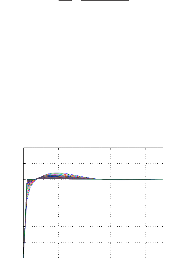
692 CHAPTER 12 Robust Control Systems

KD= 0.1)

Y(s)

R(s)=15(6.67 + 0.1s)

s2+ 14.14s+ 100 .

DP12.2 The nominal plant is given by

G(s) = 1

s(s+ 5) .

The closed-loop transfer function is

T(s) = K(KDs2+KPs+KI)

s3+ (5 + KKD)s2+KKPs+KKI

Let

KP= 450 , KI= 750 ,and KD= 150 .

A family of responses is shown in Figure DP12.2 a for various values of

K. The percent overshoot for 0.1≤K≤2 is shown in Figure DP12.2b.

0 0.5 1 1.5 2 2.5 3 3.5 4

0.2

0.4

0.6

0.8

1.2

1.4

Time (s)

Step response

FIGURE DP12.2

(a) Family of step responses for various values of K.

from the publisher prior to any prohibited reproduction, storage in a retrieval system, or transmission in any form or by any means, electronic, mechanical, photocopying,

recording, or likewise. For information regarding permission(s), write to: Rights and Permissions Department, Pearson Education, Inc., Upper Saddle River, NJ 07458.

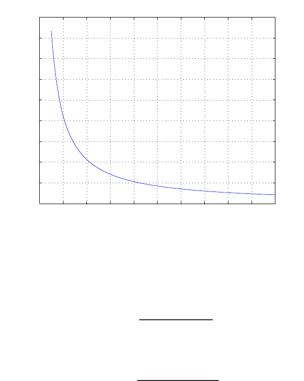
Design Problems 693

0 0.2 0.4 0.6 0.8 1 1.2 1.4 1.6 1.8 2

Percent overshoot

FIGURE DP12.2

CONTINUED: (b) Percent overshoot for various values of K.

DP12.3 (a) The dexterous hand model is given by

G(s) = Km

s(s+ 5)(s+ 10) ,

where Km= 1, nominally. The PID controller is

Gc(s) = KD(s2+ 6s+ 18)

The root locus is shown in Figure DP12.3a. If we select

KD= 90 ,

the roots are

s1,2=−5.47 ±j6.6

s3,4=−2.03 ±j4.23 .

Thus, all roots have

ζωn>4/3

from the publisher prior to any prohibited reproduction, storage in a retrieval system, or transmission in any form or by any means, electronic, mechanical, photocopying,

recording, or likewise. For information regarding permission(s), write to: Rights and Permissions Department, Pearson Education, Inc., Upper Saddle River, NJ 07458.

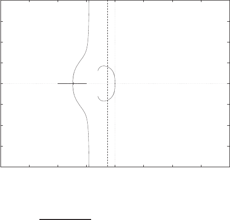
694 CHAPTER 12 Robust Control Systems

to meet the design speciﬁcation

Ts<3 sec .

(b) The step responses for

Km= 1

and

Km= 1/2

are shown in Figure DP12.3b. When

K= 1/2,

an oﬀ-nominal value, the settling time speciﬁcation is no longer sat-

isﬁed.

-20

-15

-10

-5

-20 -15 -10 -5 0 5 10 15 20

xxxx

Real Axis

Imag Axis

FIGURE DP12.3

(a) Root locus for 1 + KDs2+6s+18

s2(s+5)(s+10) = 0.

from the publisher prior to any prohibited reproduction, storage in a retrieval system, or transmission in any form or by any means, electronic, mechanical, photocopying,

recording, or likewise. For information regarding permission(s), write to: Rights and Permissions Department, Pearson Education, Inc., Upper Saddle River, NJ 07458.

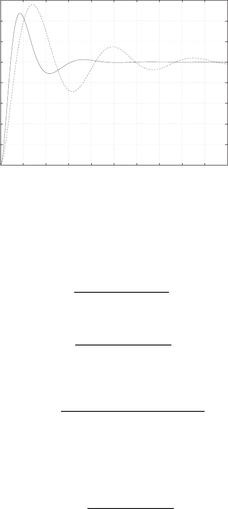
Design Problems 695

0.2

0.4

0.6

0.8

1.2

1.4

1.6

0 0.5 1 1.5 2 2.5 3 3.5 4 4.5 5

Time (sec)

y(t)

FIGURE DP12.3

CONTINUED: (b) Step response (without preﬁlters): PID with K3= 90 and Km= 1

(solid line) and PID with K3= 90 and Km= 0.5(dashed line).

DP12.4 The nominal plant is

G(s) = 17640

s(s2+ 59.4s+ 1764) ,

and the PID controller is

Gc(s) = KI(τ1s+ 1)(τ2s+ 1)

(a) Using ITAE methods, we determine that ωn= 28.29, KI= 36.28,

τ1+τ2= 0.0954 and τ1τ2= 0.00149. So,

Gc(s) = 36.28(0.00149s2+ 0.0954s+ 1)

(b) The step response for the nominal plant and the PID controller is

shown in Figure DP12.4a, with and without a preﬁlter.

(d) The oﬀ-nominal plant is

G(s) = 16000

s(s2+ 40s+ 1600) .

The step response for the oﬀ-nominal plant is shown in Figure DP12.4a.

from the publisher prior to any prohibited reproduction, storage in a retrieval system, or transmission in any form or by any means, electronic, mechanical, photocopying,

recording, or likewise. For information regarding permission(s), write to: Rights and Permissions Department, Pearson Education, Inc., Upper Saddle River, NJ 07458.

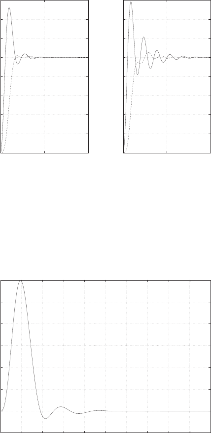
696 CHAPTER 12 Robust Control Systems

0.2

0.4

0.6

0.8

1.2

1.4

1.6

00.5 1

Time (sec)

y(t)

(a) nominal plant

0.2

0.4

0.6

0.8

1.2

1.4

1.6

00.5 1

Time (sec)

y(t)

(b) o-nominal plant

FIGURE DP12.4

(a) Step response for (i) nominal plant: w/o preﬁlter (solid line) and w/preﬁlter (dashed

line); and (ii) for oﬀ-nominal plant: w/o preﬁlter (solid line) and w/preﬁlter (dashed line).

-0.05

0.05

0.1

0.15

0.2

0.25

0.3

0 0.1 0.2 0.3 0.4 0.5 0.6 0.7 0.8 0.9 1

Time (sec)

y(t)

disturbance response

FIGURE DP12.4

CONTINUED: (b) Disturbance response for the nominal plant.

from the publisher prior to any prohibited reproduction, storage in a retrieval system, or transmission in any form or by any means, electronic, mechanical, photocopying,

recording, or likewise. For information regarding permission(s), write to: Rights and Permissions Department, Pearson Education, Inc., Upper Saddle River, NJ 07458.

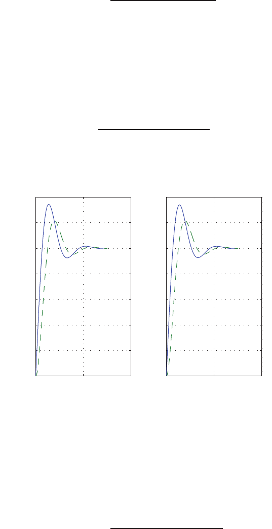
Design Problems 697

DP12.5 One possible solution is

Gc(s) = 0.08(0.01s+ 1)(0.99s+ 1)

The phase margin with this controller is

P.M. = 45.5o.

The step response is shown in Figure DP12.5 for the nominal plant (with

and without a preﬁlter); the step response for the oﬀ-nominal plant is also

shown in Figure DP12.5. The preﬁlter is

Gp(s) = 1411

13.97s2+ 1411s+ 1411 .

0 10 20

0.2

0.4

0.6

0.8

1.2

1.4

Time (sec)

y(t)

(a) nominal plant

0 10 20

0.2

0.4

0.6

0.8

1.2

1.4

Time (sec)

y(t)

(b) o nominal plant

FIGURE DP12.5

(a) Step response for nominal plant: w/o preﬁlter (solid line) and w/preﬁlter (dashed line);

and (b) for oﬀ-nominal plant: w/o preﬁlter (solid line) and w/preﬁlter (dashed line).

DP12.6 Using ITAE methods, three controllers are designed for the nominal plant:

(i) PID controller:

Gc(s) = 0.225s2+ 0.535s+ 34.3

from the publisher prior to any prohibited reproduction, storage in a retrieval system, or transmission in any form or by any means, electronic, mechanical, photocopying,

recording, or likewise. For information regarding permission(s), write to: Rights and Permissions Department, Pearson Education, Inc., Upper Saddle River, NJ 07458.

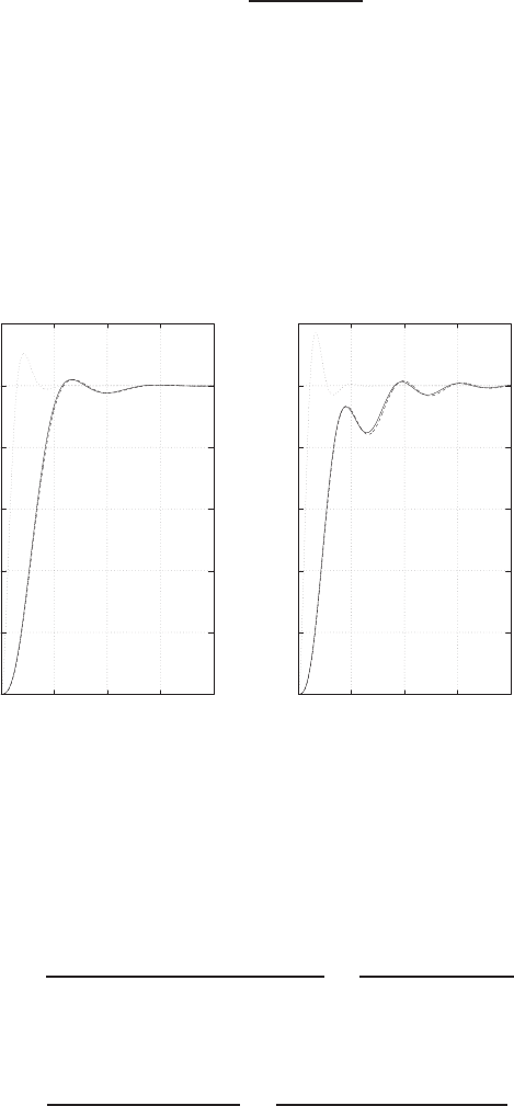
698 CHAPTER 12 Robust Control Systems

(ii) PI controller:

Gc(s) = 0.9s+ 22.5

(iii) PD controller:

Gc(s) = 0.9s+ 22.5

The step responses for each controller is shown in Figure DP12.6. The

responses for the PID and PI controller are the same since the gains were

selected to obtain the same ITAE characteristic equation. An appropriate

preﬁlter is used in all cases.

0.2

0.4

0.6

0.8

1.2

0 0.5 1 1.5 2

Time (sec)

y(t)

(a) nominal plant

0.2

0.4

0.6

0.8

1.2

0 0.5 1 1.5 2

Time (sec)

y(t)

(b) o-nominal plant

FIGURE DP12.6

(a) Step response for nominal plant: PID (solid line); PI (dashed line); and PD (dotted

line); (b) for oﬀ-nominal plant: PID (solid line); PI (dashed line); and PD (dotted line).

DP12.7 The loop transfer function is

G(s) = KaKm

(0.5s+ 1)(τfs+ 1)s(s+ 1) =K

s(s+ 2)(s+ 1)

since τfis negligible. A suitable PID controller is

Gc(s) = KKD(s2+as +b)

s=300(s2+ 2.236s+ 2.5)

The step response is shown in Figure DP12.7. The percent overshoot is

from the publisher prior to any prohibited reproduction, storage in a retrieval system, or transmission in any form or by any means, electronic, mechanical, photocopying,

recording, or likewise. For information regarding permission(s), write to: Rights and Permissions Department, Pearson Education, Inc., Upper Saddle River, NJ 07458.

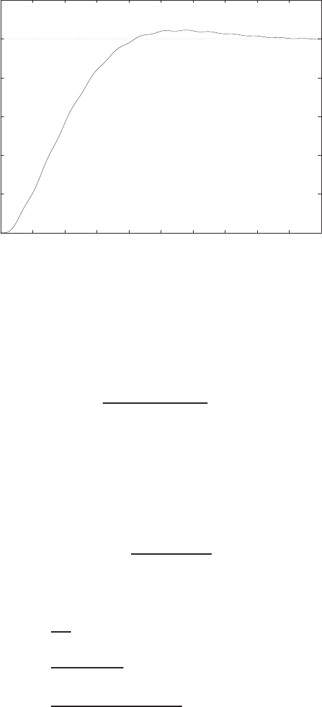
Design Problems 699

P.O. = 4.6% and the settling time is Ts= 3.74 seconds.

0.2

0.4

0.6

0.8

1.2

0 0.5 1 1.5 2 2.5 3 3.5 4 4.5 5

Time (secs)

Amplitude

FIGURE DP12.7

Step response for the elevator position control.

DP12.8 The system transfer function is

Y(s) = G(s)Gc(s)Gp(s)

1 + G(s)Gc(s)R(s).

We are given

G(s) = e−sT where T = 1 second .

Using a second-order Pade approximation yields

G(s)≈s2−6s+ 12

s2+ 6s+ 12 .

Three controllers that meet the speciﬁcations are

Gc1(s) = 0.5

s(Integral controller)

Gc2(s) = 0.04s+ 0.4

s(PI controller)

Gc3(s) = 0.01s2+ 0.04s+ 0.4

s(PID controller) .

from the publisher prior to any prohibited reproduction, storage in a retrieval system, or transmission in any form or by any means, electronic, mechanical, photocopying,

recording, or likewise. For information regarding permission(s), write to: Rights and Permissions Department, Pearson Education, Inc., Upper Saddle River, NJ 07458.

700 CHAPTER 12 Robust Control Systems

In all cases, the steady-state error is zero.

Integral PI PID

P.O.(%) 4.05 0 0

Ts(sec) 6.03 6.12 6.02

Tp(sec) 4.75 N/A N/A

|V(t)|max (volts) 1.04 1 1

The preﬁlter Gp(s) = 1 is used in all designs. To compute the voltage,

the transfer function is

V(s) = Gp(s)Gc(s)

1 + Gc(s)G(s)R(s).

DP12.9 The space robot transfer function is

G(s) = 1

s(s+ 10) .

(a) Consider Gc(s) = K. Then

T(s) = Gc(s)G(s)

1 + Gc(s)G(s)=K

s2+ 10s+K.

We determine that K= 50.73 for ζ= 0.702. Thus, we expect P.O. <

4.5%. So,

Gc(s) = 50.73 .

(b) Consider the PD controller

Gc(s) = KP+KDs .

Then

T(s) = KP+KDs

s2+ (10 + KD)s+KP

Using the ITAE method, we compute

KP= 100 and KD= 4 .

Thus,

Gc(s) = 4s+ 100 ,

from the publisher prior to any prohibited reproduction, storage in a retrieval system, or transmission in any form or by any means, electronic, mechanical, photocopying,

recording, or likewise. For information regarding permission(s), write to: Rights and Permissions Department, Pearson Education, Inc., Upper Saddle River, NJ 07458.

Design Problems 701

and the preﬁlter is

Gp(s) = 100

4s+ 100 .

Gc(s) = KP+KI

s=KPs+KI

Then,

T(s) = KPs+KI

s3+ 10s2+KPs+KI

Using the ITAE method, we have

ωn= 5.7KP= 70.2 and KI= 186.59 .

Thus,

Gc(s) = 70.2 + 186.59/s ,

and the preﬁlter is

Gp(s) = 186.59

70.2s+ 186.59 .

(d) Consider the PID controller

Gc(s) = KDs2+KPs+KI

Then,

T(s) = KDs2+KPs+KI

s3+ 10s2+KDs2+KPs+KI

Using the ITAE method with ωn= 10, we have

KD= 7.5KP= 215 and KI= 1000 .

Thus,

Gc(s) = 7.5s2+ 215s+ 1000

and the preﬁlter is

Gp(s) = 1000

7.5s2+ 215s+ 1000 .

from the publisher prior to any prohibited reproduction, storage in a retrieval system, or transmission in any form or by any means, electronic, mechanical, photocopying,

recording, or likewise. For information regarding permission(s), write to: Rights and Permissions Department, Pearson Education, Inc., Upper Saddle River, NJ 07458.

702 CHAPTER 12 Robust Control Systems

A summary of the performance is given in Table DP12.9.

Gc(s)P.O. tptsyss max|y(t)|

K4.5% 0.62 s 0.84 s 0 0.026

PD 5.2% 0.39 s 0.56s 0 0.010

PI 1.98% 0.81 s 1.32s 0 0.013

PID 1.98% 0.46 s 0.75 s 0 0.004

TABLE DP12.9 A summary of performance to a disturbance input.

from the publisher prior to any prohibited reproduction, storage in a retrieval system, or transmission in any form or by any means, electronic, mechanical, photocopying,

recording, or likewise. For information regarding permission(s), write to: Rights and Permissions Department, Pearson Education, Inc., Upper Saddle River, NJ 07458.

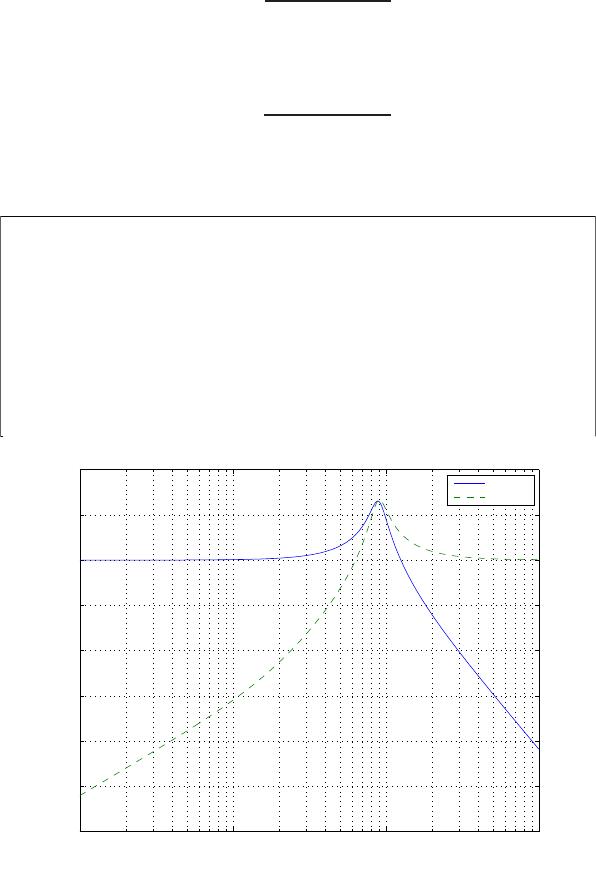
Computer Problems 703

Computer Problems

CP12.1 The closed-loop transfer function is

T(s) = 8K

s2+ 2s+ 8K,

and the sensitivity function, ST

K, is

S(s) = s2+s

s2+ 2s+ 8K.

The plot of T(s) and S(s) is shown in Figure CP12.1, where K= 10.

nt=[80]; dt=[1 2 80]; syst = tf(nt,dt);

ns=[1 2 0];ds=[1 2 80]; syss = tf(ns,ds);

w=logspace(-1,2,400);

[magt,phaset]=bode(syst,w);magtdB(1,:) = 20*log10(magt(1,1,:));

[mags,phases]=bode(syss,w); magsdB(1,:) = 20*log10(mags(1,1,:));

semilogx(w,magtdB,w,magsdB,'--')

legend('20log|T|','20log|S|')

xlabel('Frequency (rad/sec)')

ylabel('Gain dB')

grid

10−1 100101102

−60

−50

−40

−30

−20

−10

Frequency (rad/sec)

Gain dB

20log|T|

20log|S|

FIGURE CP12.1

Plot of T(s)and the sensitivity function S(s).

from the publisher prior to any prohibited reproduction, storage in a retrieval system, or transmission in any form or by any means, electronic, mechanical, photocopying,

recording, or likewise. For information regarding permission(s), write to: Rights and Permissions Department, Pearson Education, Inc., Upper Saddle River, NJ 07458.

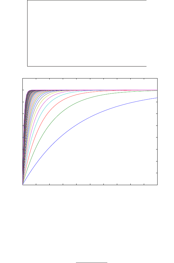
704 CHAPTER 12 Robust Control Systems

CP12.2 A reasonable value of the gain K= 4. The family of step responses is

shown in Figure CP12.2.

p=[0.5:0.5:20]; K=4;

t=[0:0.01:1];

for i=1:length(p)

n=[K*p(i)]; d=[1 p(i)]; sys = tf(n,d);

sys_cl = feedback(sys,[1]);

y=step(sys_cl,t); Y(:,i)=y;

[y2,t2]=step(sys_cl);

S=stepinfo(y2,t2); Ts(i)=S.SettlingTime;

end

plot(t,Y) , xlabel('Time (sec)'), ylabel('Step response')

0 0.1 0.2 0.3 0.4 0.5 0.6 0.7 0.8 0.9 1

0.1

0.2

0.3

0.4

0.5

0.6

0.7

0.8

0.9

Time (sec)

Step response

FIGURE CP12.2

Family of step responses for 0.5< p < 20.

CP12.3 The closed-loop characteristic equation is

1 + KD

s2+as +b

Js3= 0

where

a=KP/KD

b=KI/KD.

from the publisher prior to any prohibited reproduction, storage in a retrieval system, or transmission in any form or by any means, electronic, mechanical, photocopying,

recording, or likewise. For information regarding permission(s), write to: Rights and Permissions Department, Pearson Education, Inc., Upper Saddle River, NJ 07458.

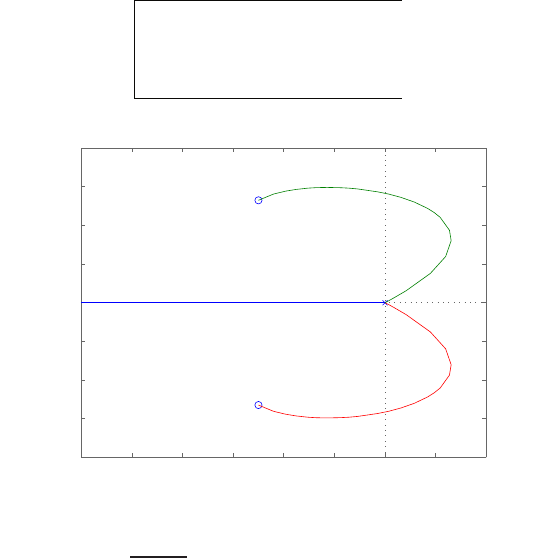
Computer Problems 705

We select

a= 1 and b= 2

to move the root locus into the left hand-plane (see Figure CP12.3a).

Then, we choose

KD= 71

from the root locus using the rlocﬁnd function. The closed-loop Bode

plot in Figure CP12.3b veriﬁes that the bandwidth

ωB<5 rad/sec.

Also, the phase margin is

P.M. = 45.7o,

which meets the design speciﬁcation. The plot of phase margin versus J

is shown in Figure CP12.3c. We see that as Jincreases, the phase margin

decreases.

J=25; a=1; b=2;

ng=[1];dg=[J 0 0]; sysg=tf(ng,dg);

nc=[1 a b]; dc=[1 0]; sysc=tf(nc,dc);

sys=series(sysc,sysg); rlocus(sys)

−1.2 −1 −0.8 −0.6 −0.4 −0.2 0 0.2 0.4

−2

−1.5

−1

−0.5

0.5

1.5

Root Locus

Real Axis

Imaginary Axis

FIGURE CP12.3

(a) Root locus for 1 + KDs2+s+2

10s3= 0.

from the publisher prior to any prohibited reproduction, storage in a retrieval system, or transmission in any form or by any means, electronic, mechanical, photocopying,

recording, or likewise. For information regarding permission(s), write to: Rights and Permissions Department, Pearson Education, Inc., Upper Saddle River, NJ 07458.

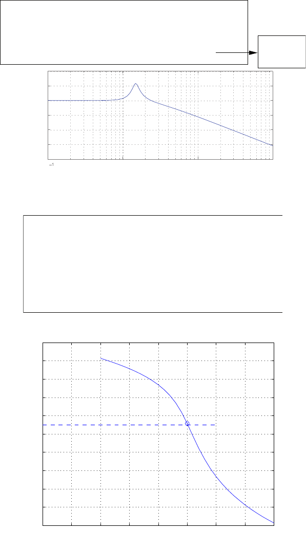
706 CHAPTER 12 Robust Control Systems

PM =

45.7093

J=25; a=1; b=2; KD=71; KP=a*KD; KI=b*KD;

ng=[1]; dg=[J 0 0]; sysg=tf(ng,dg);

nc=[KD KP KI]; dc=[1 0]; sysc = tf(nc,dc);

sys=series(sysc,sysg); sys_cl = feedback(sys,[1]);

bode(sys_cl);

[GM,PM]=margin(sys); PM

−30

−20

−10

Magnitude (dB)

10 100101102

Frequency (rad/sec)

FIGURE CP12.3

CONTINUED: (b) Closed-loop Bode plot with ωB<5rad/sec.

Ji=[10:1:40];

for i=1:length(Ji)

numc=[KD KP KI]; denc=[Ji(i) 0 0 0]; sysc = tf(numc,denc);

[gm,pm]=margin(sysc);

Pm(i)=pm;

end

plot(Ji,Pm), grid

xlabel('J'), ylabel('Phase Margin (deg)')

0 5 10 15 20 25 30 35 40

−10

Phase Margin (deg)

FIGURE CP12.3

CONTINUED: (c) Phase margin versus J.

from the publisher prior to any prohibited reproduction, storage in a retrieval system, or transmission in any form or by any means, electronic, mechanical, photocopying,

recording, or likewise. For information regarding permission(s), write to: Rights and Permissions Department, Pearson Education, Inc., Upper Saddle River, NJ 07458.

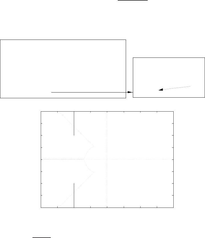
Computer Problems 707

CP12.4 The closed-loop characteristic equation is

1 + K1

s2+bs +a= 0

where a= 8 and the nominal value of b= 4. The root locus is shown in

Figure CP12.4a.

ÈSelect a point in the graphics window

selected_point =

-2.0165 + 2.5426i

ans =

2.4659

clf, hold o

a=8; b=4;

num=[1]; den=[1 b a]; sys = tf(num,den);

rlocus(sys), hold on

zeta=0.59; wn=1.35;

x=[-10:0.1:-zeta*wn]; y=-(sqrt(1-zeta^2)/zeta)*x;

xc=[-10:0.1:-zeta*wn];c=sqrt(wn^2-xc.^2);

plot(x,y,':',x,-y,':',xc,c,':',xc,-c,':')

rlocnd(sys)

-4

-3

-2

-1

-4 -3 -2 -1 0 1 2 3 4

Real Axis

Imag Axis

FIGURE CP12.4

(a) Root locus for 1 + K1

s2+4s+8 .

The performance region is speciﬁed by

ζ= 0.59 and ωn= 1.35 ,

which derives from the design speciﬁcations

Ts<5 sec and P.O. < 10% .

from the publisher prior to any prohibited reproduction, storage in a retrieval system, or transmission in any form or by any means, electronic, mechanical, photocopying,

recording, or likewise. For information regarding permission(s), write to: Rights and Permissions Department, Pearson Education, Inc., Upper Saddle River, NJ 07458.

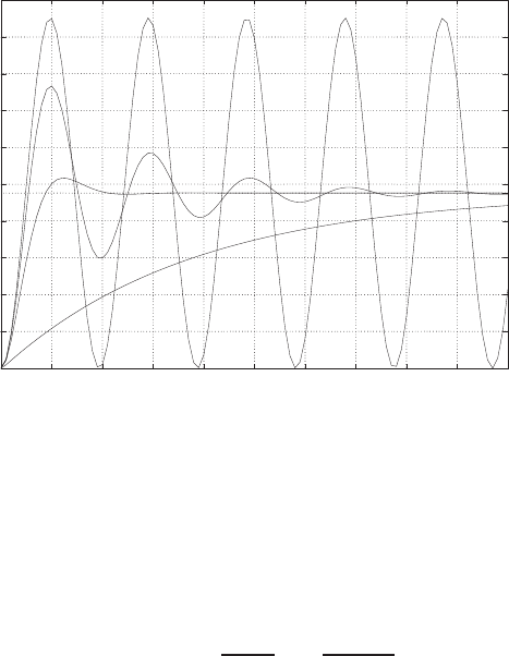
708 CHAPTER 12 Robust Control Systems

Using an m-ﬁle, the value of

K= 2.5

is selected with the rlocﬁnd function. The step responses for b= 0,1,4

and b= 40 are shown in Figure CP12.4b. When b= 0, the system is

marginally stable; b= 1 results in a stable system with unsatisfactory

performance. The nominal case b= 4 is stable and all performance specs

are satisﬁed. When b= 40, the system is heavily damped: the percent

overshoot speciﬁcation is satisﬁed, but the settling time is too long.

0.05

0.1

0.15

0.2

0.25

0.3

0.35

0.4

0.45

0.5

01 2 3 4 5 6 7 8 9 10

Time (secs)

Amplitude

Time (secs)

Amplitude

Time (secs)

Amplitude

Time (secs)

Amplitude

b=0

b=1

b=40

b=4

FIGURE CP12.4

CONTINUED: (b) Step responses for b= 0,1,4and 40.

CP12.5 (a) An acceptable lead compensator (designed with root locus methods)

Gc(s) = Ks+a

s+b= 5s+ 0.3

s+ 2 .

The compensated root locus is shown in Figure CP12.5a, where

K= 5

is selected to place the closed-loop poles in the performance region.

(b) The step responses for ζ= 0,0.005,0.1 and 1 are shown in Fig-

ure CP12.5b.

from the publisher prior to any prohibited reproduction, storage in a retrieval system, or transmission in any form or by any means, electronic, mechanical, photocopying,

recording, or likewise. For information regarding permission(s), write to: Rights and Permissions Department, Pearson Education, Inc., Upper Saddle River, NJ 07458.

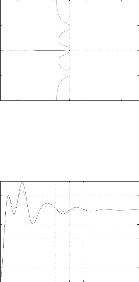
Computer Problems 709

-4

-3

-2

-1

-4 -3 -2 -1 0 1 2 3 4

xxx

Real Axis

Imag Axis

FIGURE CP12.5

(a) Compensated root locus.

design value, if it must be diﬀerent at all.

0.2

0.4

0.6

0.8

1.2

1.4

02 4 6 8 10 12 14 16 18 20

Time (sec)

Amplitude

zeta=0,0.005 (solid); zeta=0.1 (dashed); zeta=1 (dotted)

FIGURE CP12.5

CONTINUED: (b) Step responses for ζ= 0,0.005,0.1and 1.

from the publisher prior to any prohibited reproduction, storage in a retrieval system, or transmission in any form or by any means, electronic, mechanical, photocopying,

recording, or likewise. For information regarding permission(s), write to: Rights and Permissions Department, Pearson Education, Inc., Upper Saddle River, NJ 07458.

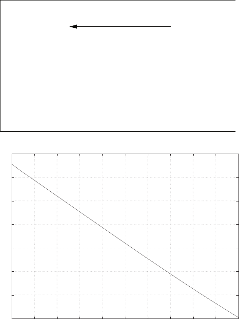
710 CHAPTER 12 Robust Control Systems

CP12.6 The m-ﬁle script which computes the phase margin as a function of the

time delay (using the pade function) is shown in Figure CP12.6. The

maximum time delay (for stability) is td= 4.3 seconds.

time delay vector

K=5;

numg=K*[1]; deng=[1 10 2]; sysg = tf(numg,deng);

td=[0:0.1:5];

for i=1:length(td)

[ndelay,ddelay]=pade(td(i),2); sysd = tf(ndelay,ddelay);

sys = series(sysg,sysd);

[mag,phase,w]=bode(sys);

[gm,pm,w1,w2]=margin(mag,phase,w);

pmv(i)=pm;

end

plot(td,pmv), grid

xlabel('time delay [sec]')

ylabel('phase margin [deg]')

-20

100

120

00.5 1 1.5 2 2.5 3 3.5 4 4.5 5

time delay [sec]

phase margin [deg]

FIGURE CP12.6

Phase margin versus time delay.

CP12.7 The m-ﬁle script is shown in Figure CP12.7a. The steady-state error

(shown in Figure CP12.7b) is zero when

a= 0.5

and increases rapidly as aincreases past a= 0.5. The maximum initial

undershoot is shown in Figure CP12.7c. As aincreases, the initial under-

shoot increases linearly. The gain margin is shown in Figure CP12.7d. It

from the publisher prior to any prohibited reproduction, storage in a retrieval system, or transmission in any form or by any means, electronic, mechanical, photocopying,

recording, or likewise. For information regarding permission(s), write to: Rights and Permissions Department, Pearson Education, Inc., Upper Saddle River, NJ 07458.

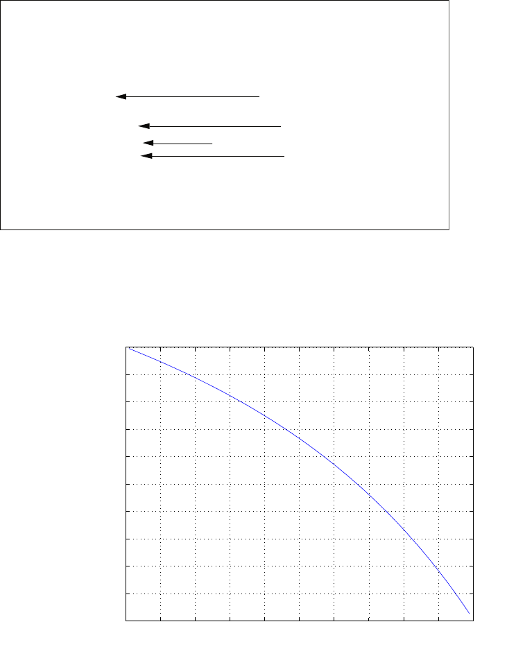
Computer Problems 711

can be seen that as aincreases, the gain margin decreases very rapidly.

gain margin

negative unit step input

max initial undershoot

steady-state tracking error

a=[0.01:0.01:0.99];

t=[0:0.1:30];

for i=1:length(a)

num=a(i)*[1 -0.5]; den=[1 2 1]; sys_o = tf(num,den);

[mag,phase,w]=bode(sys_o);

[gm,pm,w1,w2]=margin(mag,phase,w);

gmv(i)=gm;

sys_cl = feedback(sys_o,[1]);

[y,x]=step(-sys_cl,t);

yf(i)=1-y(length(t));

ym(i)=-min(y)*100;

end

gure(1), plot(a,gmv), grid, xlabel('a'), ylabel('gm')

gure(2), plot(a,yf), grid, xlabel('a'), ylabel('steady-state error')

gure(3), plot(a,ym), grid, xlabel('a'), ylabel('maximum initial undershoot [%]')

FIGURE CP12.7

Script to generate all the plots.

0 0.1 0.2 0.3 0.4 0.5 0.6 0.7 0.8 0.9 1

0.1

0.2

0.3

0.4

0.5

0.6

0.7

0.8

0.9

steady−state error

FIGURE CP12.7

CONTINUED: (b) Steady-state tracking error.

from the publisher prior to any prohibited reproduction, storage in a retrieval system, or transmission in any form or by any means, electronic, mechanical, photocopying,

recording, or likewise. For information regarding permission(s), write to: Rights and Permissions Department, Pearson Education, Inc., Upper Saddle River, NJ 07458.

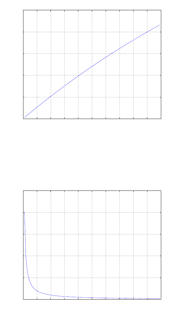
712 CHAPTER 12 Robust Control Systems

0 0.1 0.2 0.3 0.4 0.5 0.6 0.7 0.8 0.9 1

maximum initial undershoot [%]

FIGURE CP12.7

CONTINUED: (c) Maximum initial undershoot.

0 0.1 0.2 0.3 0.4 0.5 0.6 0.7 0.8 0.9 1

100

150

200

250

FIGURE CP12.7

CONTINUED: (d) Gain margin.

from the publisher prior to any prohibited reproduction, storage in a retrieval system, or transmission in any form or by any means, electronic, mechanical, photocopying,

recording, or likewise. For information regarding permission(s), write to: Rights and Permissions Department, Pearson Education, Inc., Upper Saddle River, NJ 07458.

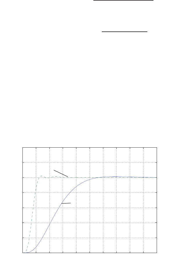
Computer Problems 713

CP12.8 The plant (balloon and canister dynamics plus motor) is given by

G(s) = 1

(s+ 2)(s+ 4)(s+ 10) ,

and the PID controller is

Gc(s) = KD(s2+as +b)

Let a= 6. Then using the root locus methods, we determine that with

KD= 12.5 and b= 10

we have the roots

s1=−8.4

s2=−4.7

s3,4=−1.43 ±j1.05 .

Thus, ζ= 0.8. The plot of y(t) is shown in Figure CP12.8. The percent

overshoot is less that 3%, as desired.

0 0.5 1 1.5 2 2.5 3 3.5 4 4.5 5

0.2

0.4

0.6

0.8

1.2

1.4

Time (sec)

y(t)

With prefilter

Without prefilter

FIGURE CP12.8

Simulation of the GRID device.

from the publisher prior to any prohibited reproduction, storage in a retrieval system, or transmission in any form or by any means, electronic, mechanical, photocopying,

recording, or likewise. For information regarding permission(s), write to: Rights and Permissions Department, Pearson Education, Inc., Upper Saddle River, NJ 07458.

C H A P T E R 1 3

Digital Control Systems

Exercises

E13.1 (a) Elevation contours on a map are discrete signals. (b) Temperature in

a room is a continuous signal. (c) A digital clock display is a discrete

signal. (d) The score of a basketball game is a discrete signal. (e) The

output of a loudspeaker is a continuous signal.

E13.2 (a) Using long-division we determine that

Y(z) = z−1+ 3z−2+ 7z−3+ 15z−4+···

Therefore, with

Y(z) = ∞

k=0

y(kT )z−k

we have

y(0) = 0 y(T) = 1 y(2T) = 3 y(3T) = 7 y(4T) = 15 .

(b) The exact solution is

y(kT ) = ekln 2 −1.

E13.3 For the system response

y(kT ) = kT

where k≥0, we have

Y(z) = T z

(z−1)2.

E13.4 The partial fraction expansion of Y(s) is

Y(s) = 5

s(s+ 2)(s+ 10) =0.25

s+0.0625

s+ 10 −0.3125

s+ 2 .

714

from the publisher prior to any prohibited reproduction, storage in a retrieval system, or transmission in any form or by any means, electronic, mechanical, photocopying,

recording, or likewise. For information regarding permission(s), write to: Rights and Permissions Department, Pearson Education, Inc., Upper Saddle River, NJ 07458.

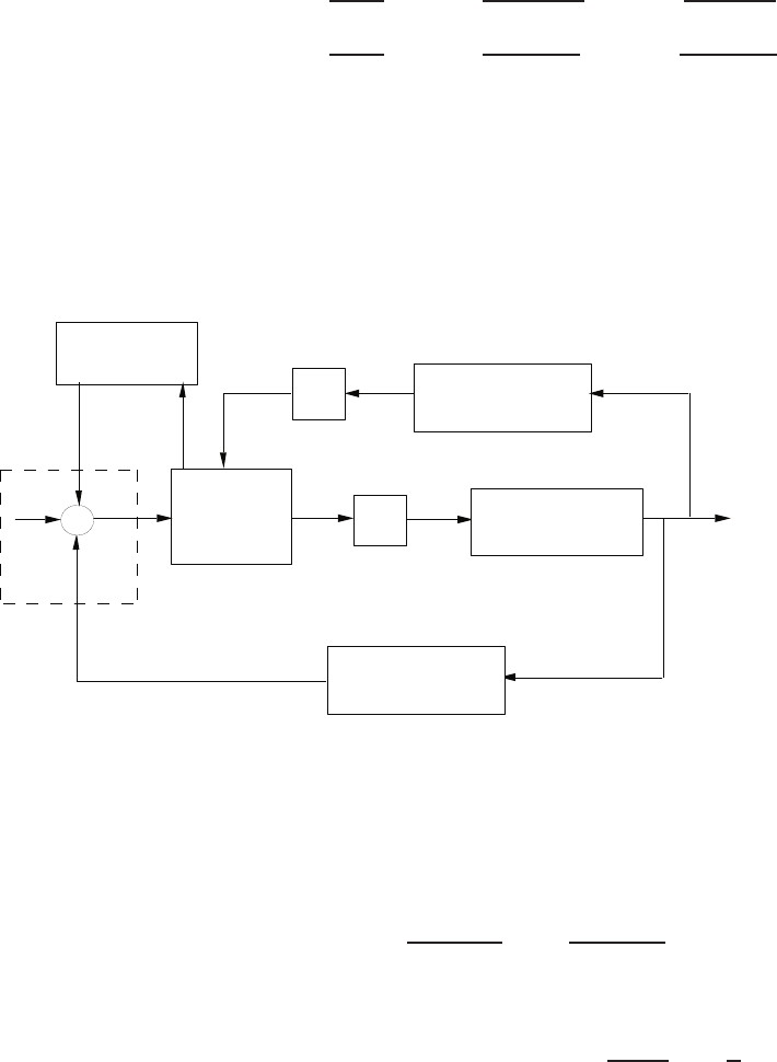
Exercises 715

Then, using Table 13.1 in Dorf and Bishop, we determine that

Y(z) = 0.25 z

z−1+ 0.0625 z

z−e−10T−0.3125 z

z−e−2T

= 0.25 z

z−1+ 0.0625 z

z−0.135 −0.3125 z

z−0.670 ,

where T= 0.1.

E13.5 The Space Shuttle and robot arm control block diagram is shown in Fig-

ure E13.5. The human operator uses information from the computer gen-

erated data display and visual sensory data from the TV monitor and by

looking out the window. He/she commands the robot arm via a joystick

command to the computer.

+Computer D/A Robot arm

& motors/gears

TV monitor

& window view

measurement

joint angle &

rate sensors

measurement

A/D

human

operator

data

display

digital analog

analog

digital

ref.

joystick

command tip

position

FIGURE E13.5

The Space Shuttle/robot arm control block diagram.

E13.6 From Section 10.8 in Dorf and Bishop, we ﬁnd that the design resulted

in the compensator

Gc(s) = 6.66s+ 1

66.6s+ 1 = 0.1s+ 0.15

s+ 0.015 .

Using the relationships

A=e−aT , B =e−bT ,and C1−A

1−B=Ka

we compute

A=e−0.15(0.001) = 0.99985 , B =e−0.015(0.001) = 0.999985 ,and C= 0.1.

from the publisher prior to any prohibited reproduction, storage in a retrieval system, or transmission in any form or by any means, electronic, mechanical, photocopying,

recording, or likewise. For information regarding permission(s), write to: Rights and Permissions Department, Pearson Education, Inc., Upper Saddle River, NJ 07458.

716 CHAPTER 13 Digital Control Systems

Therefore,

D(z) = Cz−A

z−B= 0.1z−0.99985

z−0.999985 .

E13.7 Using long-division, we determine that

Y(z) = 1 + 3.5z−1+ 5.75z−2+ 6.875z−3+···

Therefore, with

Y(z) = ∞

k=0

y(kT )z−k

we have

y(0) = 1 y(T) = 3.5y(2T) = 5.75 y(3T) = 6.875 .

E13.8 The closed-loop system with

T(z) = z

z2+ 0.2z−1.0

is unstable since one of the poles of the transfer function (z=−1.1 and

z= 0.90) lies outside the unit circle in the z-plane.

E13.9 (a) Using long-division we determine that

Y(z) = z−1+z−2+z−3+z−4+···

Therefore, with

Y(z) = ∞

k=0

y(kT )z−k

we have

y(0) = 0 y(T) = 1 y(2T) = 1 y(3T) = 1 y(4T) = 1 .

(b) The exact solution is

y(kT ) = 1 −δ(k)

where δ(k) = 1 when k= 0 and δ(k) = 0 when k6= 0.

E13.10 We compute T/τ = 1.25.

(a) Using Figure 13.19 in Dorf and Bishop, we determine that Kτ = 0.8

which implies K= 100.

(b) Using Figure 13.21 in Dorf and Bishop, we determine that ess = 0.75.

from the publisher prior to any prohibited reproduction, storage in a retrieval system, or transmission in any form or by any means, electronic, mechanical, photocopying,

recording, or likewise. For information regarding permission(s), write to: Rights and Permissions Department, Pearson Education, Inc., Upper Saddle River, NJ 07458.

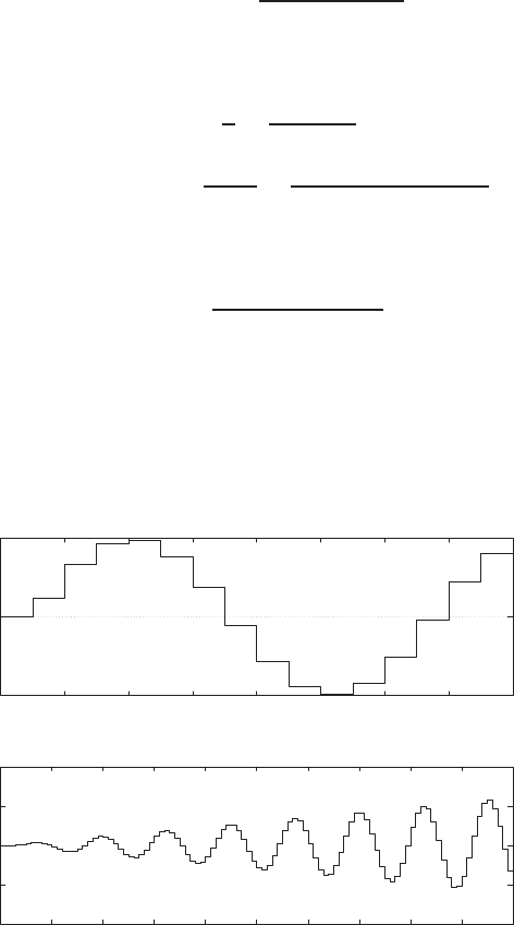
Exercises 717

which implies K= 88.

E13.11 (a) The transfer function (including the zero-order hold) is

Go(s)Gp(s) = 100(1 −e−sT )

s(s2+ 100) .

Expanding into partial fractions yields

G(z) = (1 −z−1)Z1

s−s

s2+ 100

= (1 −z−1)z

z−1−z(z−cos 10T)

z2−2 cos 10T z + 1 .

When T= 0.05 we ha,ve

G(z) = 0.1224(z+ 1)

z2−1.7552z+ 1 .

(b) The system is marginally stable since the system poles, z=−0.8776±

0.4794j, are on the unit circle.

Figure E13.11.

-0.5

0.5

02 4 6 8 10 12 14 16

No. of Samples

Amplitude

-40

-20

010 20 30 40 50 60 70 80 90 100

No. of Samples

Amplitude

FIGURE E13.11

Impulse and sinusoidal (natural frequency) input response.

from the publisher prior to any prohibited reproduction, storage in a retrieval system, or transmission in any form or by any means, electronic, mechanical, photocopying,

recording, or likewise. For information regarding permission(s), write to: Rights and Permissions Department, Pearson Education, Inc., Upper Saddle River, NJ 07458.

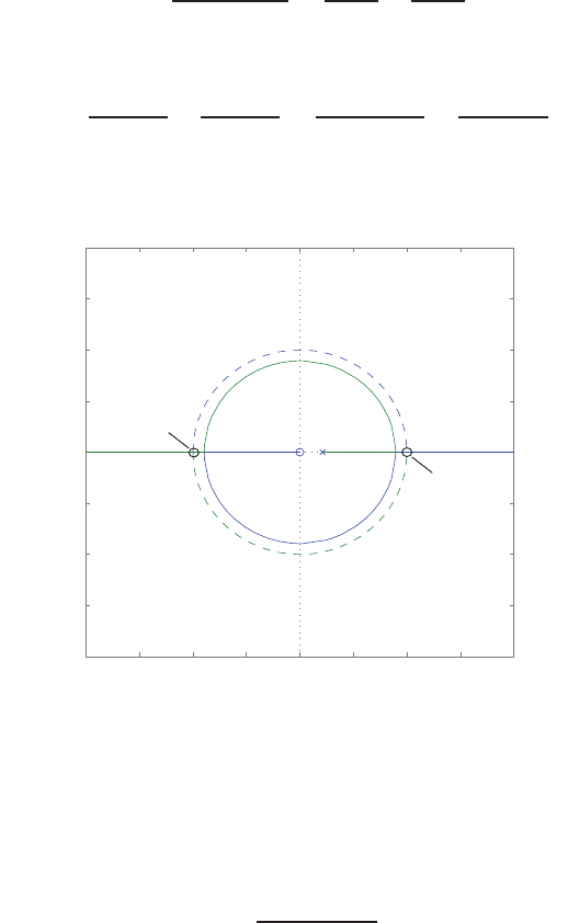
718 CHAPTER 13 Digital Control Systems

E13.12 The partial fraction expansion of X(s) is

X(s) = s+ 1

s2+ 5s+ 6 =2

s+ 3 −1

s+ 2 .

Then, with T= 1, we have

X(z) = 2z

z−e−3−z

z−e−2=2z

z−0.0498 −z

z−1353 .

E13.13 The root locus is shown in Figure E13.13. For stability: 2.2< K < 5.8.

−2 −1.5 −1 −0.5 0 0.5 1 1.5 2

−2

−1.5

−1

−0.5

0.5

1.5

K=5.8

K=2.2

Root Locus

Real Axis

Imaginary Axis

FIGURE E13.13

Root locus with unit circle (dashed curve).

E13.14 Given Gp(s), we determine that (with K= 5)

G(z) = 5(1 −e−1)z

z(z−e−1).

The closed-loop characteristic equation is

z2+ 1.792z+ 0.368 = 0

and the system is unstable, since there is a pole at z=−1.55. The

system is stable for

0< K < 4.32 .

from the publisher prior to any prohibited reproduction, storage in a retrieval system, or transmission in any form or by any means, electronic, mechanical, photocopying,

recording, or likewise. For information regarding permission(s), write to: Rights and Permissions Department, Pearson Education, Inc., Upper Saddle River, NJ 07458.

Exercises 719

E13.15 The transfer function G(z) is

G(z) = 0.1289z+ 0.02624

z2−0.3862z+ 0.006738 .

The sampling time is T= 1 s.

E13.16 The transfer function G(z) is

G(z) = 0.2759z+ 0.1982

z2−1.368z+ 0.3679 .

The sampling time is T= 0.5 s.

from the publisher prior to any prohibited reproduction, storage in a retrieval system, or transmission in any form or by any means, electronic, mechanical, photocopying,

recording, or likewise. For information regarding permission(s), write to: Rights and Permissions Department, Pearson Education, Inc., Upper Saddle River, NJ 07458.

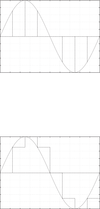
720 CHAPTER 13 Digital Control Systems

Problems

P13.1 The plot of the input to the sampler and the output r∗(t) is shown in

Figure P13.1.

-1

-0.8

-0.6

-0.4

-0.2

0.2

0.4

0.6

0.8

0 0.2 0.4 0.6 0.8 1 1.2 1.4 1.6 1.8 2

Time (sec)

r(t), r*(t)

FIGURE P13.1

Plot of r(t) = sin(ωt)and r∗(t).

P13.2 The plot of the input and the output is shown in Figure P13.2.

-1

-0.8

-0.6

-0.4

-0.2

0.2

0.4

0.6

0.8

0 0.2 0.4 0.6 0.8 1 1.2 1.4 1.6 1.8 2

Time (sec)

r(t)

FIGURE P13.2

Plot of r(t) = sin(ωt)and output of sample and hold.

from the publisher prior to any prohibited reproduction, storage in a retrieval system, or transmission in any form or by any means, electronic, mechanical, photocopying,

recording, or likewise. For information regarding permission(s), write to: Rights and Permissions Department, Pearson Education, Inc., Upper Saddle River, NJ 07458.

Problems 721

P13.3 The transfer function

Y(z)/R∗(z) = G(z) = z

z−e−T.

The ramp input is represented by

R(z) = T z

(z−1)2.

The output Y(z) = G(z)R(z) is obtained by long division:

Y(z) = T z−1+T(2 + e−T)z−2−Th(1 + 2e−T)−(2 + e−T)2iz−3

+The−T+ (1 + 2e−T)(2 + e−T)

−(2 + e−T)(1 + 2e−T)−(2 + e−T)2iz−4+···

P13.4 The transfer function

Y(s)/R∗(s) = 1−e−sT

s(s+ 2) .

The partial fraction expansion (with T= 1) yields

G(z) = (1 −z−1)Z0.5

s−0.5

s+ 2= (1 −z−1)0.5z

z−1−0.5z

z−0.1353 

=0.4323

z−0.1353 .

P13.5 The step input is

R(z) = z

z−1.

Also,

T(z) = G(z)

1 + G(z)=0.6321

z+ 0.2643 .

So,

Y(z) = T(z)R(z) = 0.6321

z+ 0.2643

z−1=0.6321z

z2−0.7357z−0.2643 .

Using long-division we determine that

Y(z) = 0.6321z−1+ 0.4650z−2+ 0.5092z−3+ 0.4975z−4+ 0.5006z−5+···

from the publisher prior to any prohibited reproduction, storage in a retrieval system, or transmission in any form or by any means, electronic, mechanical, photocopying,

recording, or likewise. For information regarding permission(s), write to: Rights and Permissions Department, Pearson Education, Inc., Upper Saddle River, NJ 07458.

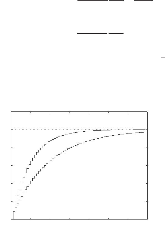
722 CHAPTER 13 Digital Control Systems

Therefore, with

Y(z) = ∞

k=0

y(kT )z−k

we have y(0) = 0, y(T) = 0.6321, y(2T) = 0.4650, y(3T) = 0.5092,

y(4T) = 0.4975, and y(5T) = 0.5006.

P13.6 Using the ﬁnal value theorem (see Table 13.1 in Dorf and Bishop), we

determine that (for a step input)

Yss = lim

z→1(z−1)Y(z) = lim

z→1(z−1) 0.6321

z+ 0.2643

z−1=0.6321

1.2643 = 0.5.

And using the initial value theorem, we compute

Yo= lim

z→∞ Y(z) = lim

z→∞

0.6321

z+ 0.2643

z−1= 0 .

P13.7 Using Figures 13.19 and 13.21 in Dorf and Bishop, we determine that

the performance speciﬁcations are satisﬁed when Kτ = 0.5 and T

τ= 2.

Computing Kand T(with τ= 0.5) yields K= 1 and T= 1.

P13.8 We can select K= 1 and r= 0.2. The step responses for the compensated

and uncompensated systems are shown in Figure P13.8.

0 10 20 30 40 50 60 70

0.2

0.4

0.6

0.8

1.2

No. of Samples

Amplitude

Uncompensated

Compensated

FIGURE P13.8

Plot of compensated and uncompensated systems.

from the publisher prior to any prohibited reproduction, storage in a retrieval system, or transmission in any form or by any means, electronic, mechanical, photocopying,

recording, or likewise. For information regarding permission(s), write to: Rights and Permissions Department, Pearson Education, Inc., Upper Saddle River, NJ 07458.

Problems 723

P13.9 Consider the compensator

Gc(s) = Ks+a

s+b.

Then, using Bode methods we can select a= 1, b= 4, and K= 1. The

compensated system phase margin is P.M. = 50oand the gain margin is

G.M. = 15dB. The crossover frequency is ωc= 2.15 rad/sec. Utilizing the

Gc(s)-to-D(z) method and selecting T= 0.01 second, we determine

D(z) = Cz−A

z−B=z−0.99

z−0.96 .

We use the relationships

A=e−aT , B =e−bT ,and C1−A

1−B=Ka

to compute A=e−0.01 = 0.99, B=e−0.04 = 0.96, and C= 1.

P13.10 (a) The transfer function G(z)D(z) is

G(z)D(z) = K0.0037z+ 0.0026

z2−1.368z+ 0.3679 .

(b) The closed-loop system characteristic equation is

1 + K0.0037z+ 0.0026

z2−1.368z+ 0.3679 = 0 .

Kmax = 239.

(d) Using Figure 13.19 in Dorf and Bishop for T /τ = 1 and a maximum

overshoot of 0.3, we ﬁnd that K= 75. (e) The closed-loop transfer

function (with K= 75) is

T(z) = 0.2759z+ 0.1982

z2−1.092z+ 0.5661 .

The step response is shown in Figure P13.10.

(f) The closed-loop poles with K= 119.5 are z= 0.4641 ±0.6843j. The

overshoot is 0.55.

(g) The step response is shown in Figure P13.10 (for K= 119.5).

from the publisher prior to any prohibited reproduction, storage in a retrieval system, or transmission in any form or by any means, electronic, mechanical, photocopying,

recording, or likewise. For information regarding permission(s), write to: Rights and Permissions Department, Pearson Education, Inc., Upper Saddle River, NJ 07458.

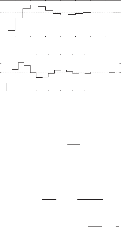
724 CHAPTER 13 Digital Control Systems

0.5

1.5

02 4 6 8 10 12 14 16

No. of Samples

Amplitude

K=75

0.5

1.5

0 2 4 6 8 10 12 14 16 18 20

No. of Samples

Amplitude

K=119.5

FIGURE P13.10

Step response for K= 75 and K= 119.5.

P13.11 (a) Consider the compensator

Gc(s) = Ks+a

s+b.

Then, using Bode methods we can select a= 0.7, b= 0.1, and K=

150. The compensated system overshoot and steady-state tracking

error (for a ramp input) are P.O. = 30% and ess <0.01.

(b) Utilizing the Gc(s)-to-D(z) method (with T= 0.1 second), we deter-

mine

D(z) = Cz−A

z−B= 155.3z−0.9324

z−0.99 .

We use the relationships

A=e−aT , B =e−bT ,and C1−A

1−B=Ka

to compute

A=e−0.007 = 0.9324 , B =e−0.01 = 0.99 ,and C= 155.3.

and for the discrete system with D(z) in part (b) is shown in Fig-

ure P13.11a.

(d) Utilizing the Gc(s)-to-D(z) method (with T= 0.01 second), we de-

from the publisher prior to any prohibited reproduction, storage in a retrieval system, or transmission in any form or by any means, electronic, mechanical, photocopying,

recording, or likewise. For information regarding permission(s), write to: Rights and Permissions Department, Pearson Education, Inc., Upper Saddle River, NJ 07458.

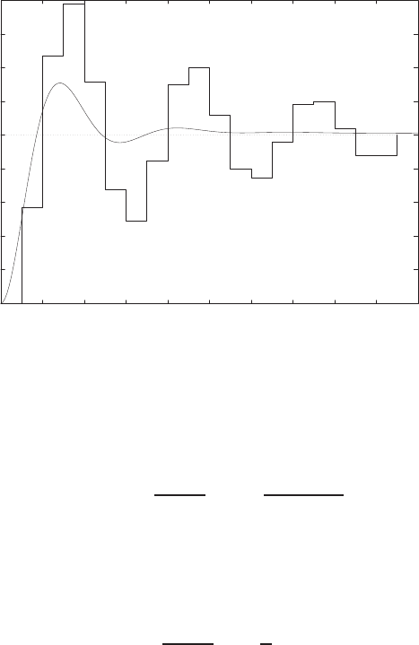
Problems 725

0.2

0.4

0.6

0.8

1.2

1.4

1.6

1.8

0 2 4 6 8 10 12 14 16 18 20

No. of Samples

Amplitude

T=0.1 sec

FIGURE P13.11

(a) Step response for continuous and discrete systems (T=0.1s) in Parts (a) and (b).

termine

D(z) = Cz−A

z−B= 150z−0.993

z−0.999 .

We use the relationships

A=e−aT

B=e−bT

C1−A

1−B=Ka

to compute

A=e−0.07 = 0.993

B=e−0.001 = 0.999

C= 150 .

The step response for the continuous system with Gc(s) in part(a)

and for the discrete system with D(z) in part (d) is shown in Fig-

ure P13.11b.

(e) The ramp response for the continuous system with Gc(s) in part(a)

and for the discrete system with D(z) in part (b) is shown in Fig-

ure P13.11c.

from the publisher prior to any prohibited reproduction, storage in a retrieval system, or transmission in any form or by any means, electronic, mechanical, photocopying,

recording, or likewise. For information regarding permission(s), write to: Rights and Permissions Department, Pearson Education, Inc., Upper Saddle River, NJ 07458.

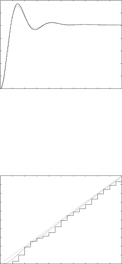
726 CHAPTER 13 Digital Control Systems

0.2

0.4

0.6

0.8

1.2

1.4

0 20 40 60 80 100 120 140 160 180 200

No. of Samples

Amplitude

T=0.01 sec

FIGURE P13.11

CONTINUED: (b) Step response for continuous and discrete systems (T=0.01s) in Parts

(a) and (d).

0.2

0.4

0.6

0.8

1.2

1.4

1.6

1.8

0 2 4 6 8 10 12 14 16 18 20

No. of Samples

Amplitude

T=0.1 sec

Ramp input (dashed line)

FIGURE P13.11

CONTINUED: (c) Ramp response for continuous and discrete systems (T=0.1s) in Parts

(a) and (b).

from the publisher prior to any prohibited reproduction, storage in a retrieval system, or transmission in any form or by any means, electronic, mechanical, photocopying,

recording, or likewise. For information regarding permission(s), write to: Rights and Permissions Department, Pearson Education, Inc., Upper Saddle River, NJ 07458.

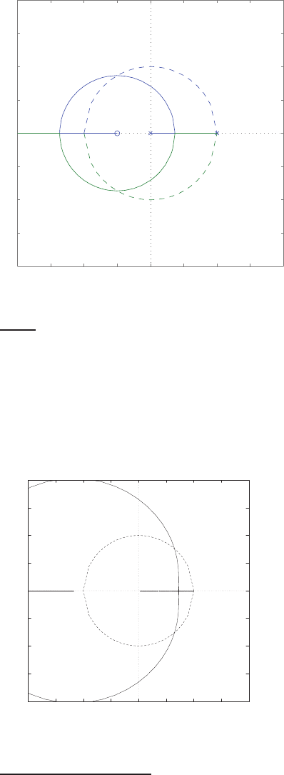
Problems 727

P13.12 The root locus is shown in Figure P13.12. For stability: 0 < K < 2.

Real Axis

Imaginary Axis

−2 −1.5 −1 −0.5 0 0.5 1 1.5 2

−2

−1.5

−1

−0.5

0.5

1.5

Unit circle (dashed line)

FIGURE P13.12

Root locus for 1 + Kz+0.5

z(z−1) = 0.

P13.13 The root locus is shown in Figure P13.13. When K= 0.027, the char-

acteristic equation has two equal roots: z1,2= 0.7247 and z3= 0.2593.

-2

-1.5

-1

-0.5

0.5

1.5

-2 -1.5 -1 -0.5 0 0.5 1 1.5 2

xxxo o

Real Axis

Imag Axis

Unit circle (dashed line)

FIGURE P13.13

Root locus for 1 + Kz2+1.1206z−0.0364

z3−1.7358z2+0.8711z−0.1353 = 0.

from the publisher prior to any prohibited reproduction, storage in a retrieval system, or transmission in any form or by any means, electronic, mechanical, photocopying,

recording, or likewise. For information regarding permission(s), write to: Rights and Permissions Department, Pearson Education, Inc., Upper Saddle River, NJ 07458.

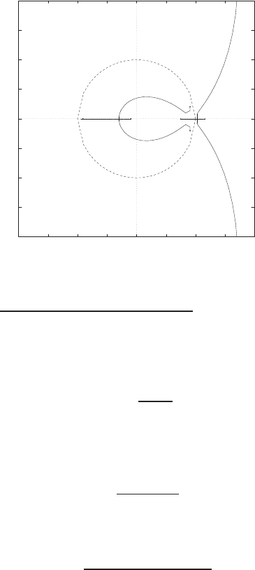
728 CHAPTER 13 Digital Control Systems

P13.14 The root locus is shown in Figure P13.14. When K= 9.5655 ×10−5, the

two real roots break away from the real axis at z= 0.99. For stability:

K < 9.7×10−5.

-2

-1.5

-1

-0.5

0.5

1.5

-2 -1.5 -1 -0.5 0 0.5 1 1.5 2

xo o

Real Axis

Imag Axis

Unit circle (dashed line)

FIGURE P13.14

Root locus for 1 + Kz3+10.3614z2+9.758z+0.8353

z4−3.7123z3+5.1644z2−3.195z+0.7408 = 0.

P13.15 Given

Gp(s) = 20

s−5

and the sample and hold (T=0.1s) as shown in Figure 13.18 in Dorf and

Bishop, we determine that

G(z) = 2.595

z−1.649 .

Then, with R(z) = z/(z−1), we have

Y(z) = 2.595z

(z−1)(z+ 0.9462) .

Therefore, Y(z) = 2.59z−1+ 0.14z−2+ 2.46z−3+ 0.26z−4+···.

from the publisher prior to any prohibited reproduction, storage in a retrieval system, or transmission in any form or by any means, electronic, mechanical, photocopying,

recording, or likewise. For information regarding permission(s), write to: Rights and Permissions Department, Pearson Education, Inc., Upper Saddle River, NJ 07458.

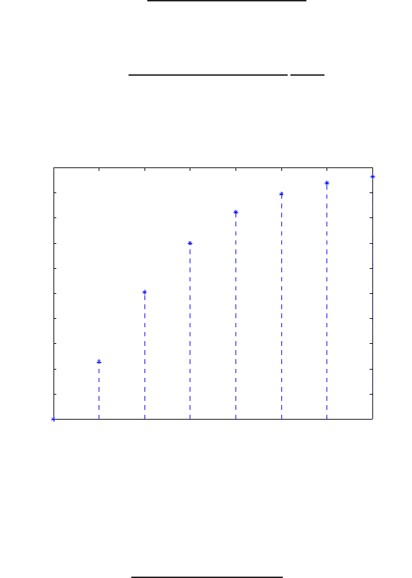
Problems 729

P13.16 Given Gp(s) and the sample and hold (T=1s) as shown in Figure 13.18

in Dorf and Bishop, we determine that

G(z) = 0.22775z+ 0.088984

z2−1.0498z+ 0.049787 .

Then, with R(z) = z/(z−1), we have

Y(z) = 0.22775z+ 0.088984

z2−0.82203z+ 0.13877

z−1.

The plot of y(kT ) is shown in Figure P13.16.

12345678

0.1

0.2

0.3

0.4

0.5

0.6

0.7

0.8

0.9

y(kT)

FIGURE P13.16

Plot of y(kT )for a step input.

P13.17 The root locus is shown in Figure P13.17 for

1 + K0.39532z+ 0.30819

z2−1.4724z+ 0.47237 = 0 .

The limiting value of the gain for stability is K= 1.71.

from the publisher prior to any prohibited reproduction, storage in a retrieval system, or transmission in any form or by any means, electronic, mechanical, photocopying,

recording, or likewise. For information regarding permission(s), write to: Rights and Permissions Department, Pearson Education, Inc., Upper Saddle River, NJ 07458.

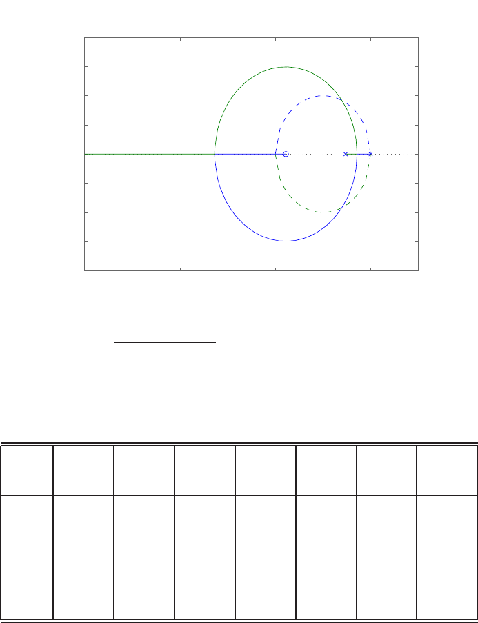
730 CHAPTER 13 Digital Control Systems

−5 −4 −3 −2 −1 0 1 2

−2

−1.5

−1

−0.5

0.5

1.5

Unit circle (dashed line)

Root Locus

Real Axis

Imaginary Axis

FIGURE P13.17

Root locus for 1 + K0.39532z+0.30819

z2−1.4724z+0.47237 = 0.

P13.18 The plot of the step responses for 0 ≤T≤1.2 is shown in Figure P13.18.

The overshoot and settling time summary is given in Table P13.18.

T0 0.2 0.4 0.6 0.8 1.0 1.2

P.O. 16.3% 20.6% 25.6% 31.3% 36.9% 40.0% 51.0%

Ts8.1 8.4 8.8 11.4 14.4 16.0 19.2

TABLE P13.18 Performance summary.

from the publisher prior to any prohibited reproduction, storage in a retrieval system, or transmission in any form or by any means, electronic, mechanical, photocopying,

recording, or likewise. For information regarding permission(s), write to: Rights and Permissions Department, Pearson Education, Inc., Upper Saddle River, NJ 07458.

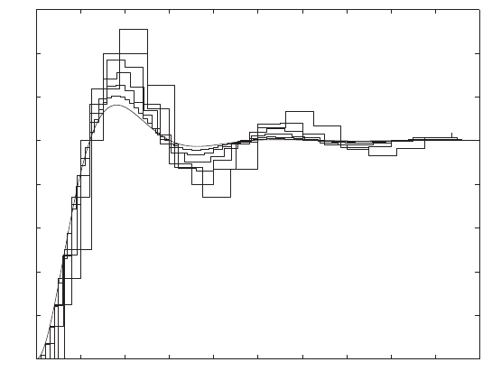
Problems 731

0 10 20 30 40 50 60 70 80 90 100

0.2

0.4

0.6

0.8

1.2

1.4

1.6

Amplitude

No. of Samples

FIGURE P13.18

Step responses for 0≤T≤1.2.

from the publisher prior to any prohibited reproduction, storage in a retrieval system, or transmission in any form or by any means, electronic, mechanical, photocopying,

recording, or likewise. For information regarding permission(s), write to: Rights and Permissions Department, Pearson Education, Inc., Upper Saddle River, NJ 07458.

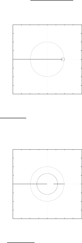
732 CHAPTER 13 Digital Control Systems

Advanced Problems

AP13.1 Given the sample and hold with Gp(s), we determine that

G(z) = 10.5K(z−0.9048)

(z−1)2.

The root locus is shown in Figure AP13.1. For stability: 0 < K < 0.2.

-2

-1.5

-1

-0.5

0.5

1.5

-2 -1.5 -1 -0.5 0 0.5 1 1.5 2

xxo

Real Axis

Imag Axis

Unit circle (dashed line)

FIGURE AP13.1

Root locus for 1 + K10.5(z−0.9048)

(z−1)2= 0 with unit circle (dashed line).

AP13.2 The root locus is shown in Figure AP13.2a. The loop transfer function is

-2

-1.5

-1

-0.5

0.5

1.5

-2 -1.5 -1 -0.5 0 0.5 1 1.5 2

xxo

Real Axis

Imag Axis

Unit circle (dashed line)

FIGURE AP13.2

(a) Root locus for 1 + K0.0379z

(z−1)(z−0.368) = 0.

from the publisher prior to any prohibited reproduction, storage in a retrieval system, or transmission in any form or by any means, electronic, mechanical, photocopying,

recording, or likewise. For information regarding permission(s), write to: Rights and Permissions Department, Pearson Education, Inc., Upper Saddle River, NJ 07458.

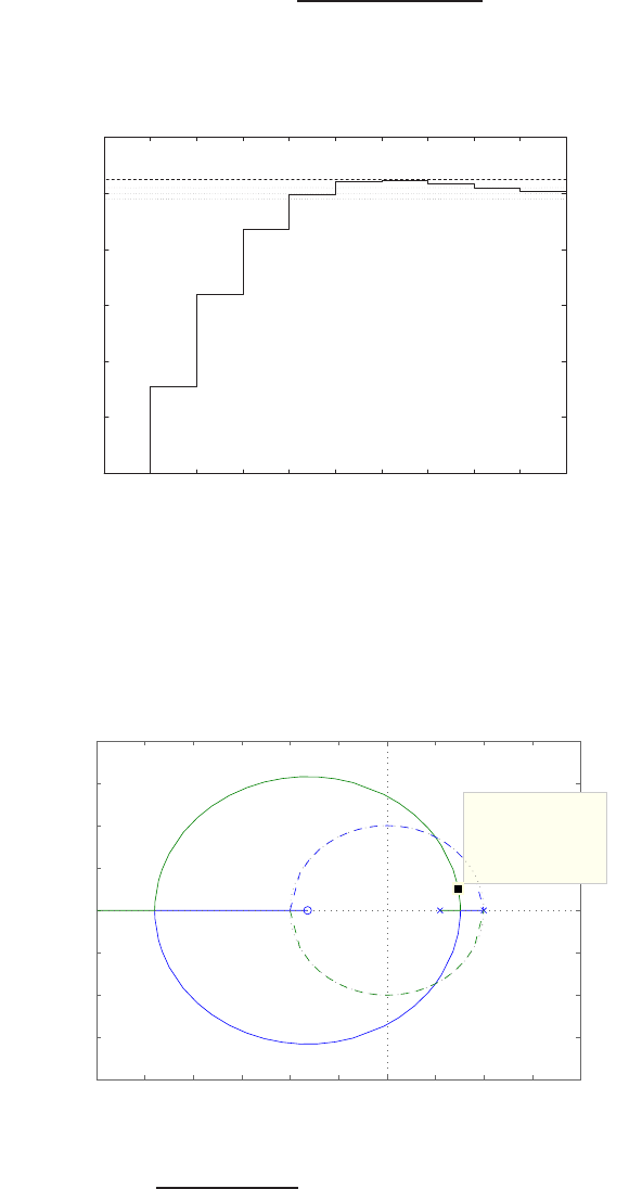
Advanced Problems 733

G(z)D(z) = K0.0379z

(z−1)(z−0.368) .

For stability: Kmax = 72. We select K= 8.2. The step response is shown

in Figure AP13.2b.

0.2

0.4

0.6

0.8

1.2

0 1 2 3 4 5 6 7 8 9 10

No. of Samples

Amplitude

FIGURE AP13.2

CONTINUED: (b) Step response with K= 8.2.

AP13.3 The root locus is shown in Figure AP13.3a. The maximum gain for

−3 −2.5 −2 −1.5 −1 −0.5 0 0.5 1 1.5 2

−2

−1.5

−1

−0.5

0.5

1.5

System: sysz

Gain: 5.99

Pole: 0.736 + 0.257i

Damping: 0.596

Overshoot (%): 9.74

Frequency (rad/sec): 8.36

Unit circle (dashed line)

Root Locus

Real Axis

Imaginary Axis

FIGURE AP13.3

(a) Root locus for 1 + K0.07441z+0.06095

z2−1.474z+0.6098 = 0.

from the publisher prior to any prohibited reproduction, storage in a retrieval system, or transmission in any form or by any means, electronic, mechanical, photocopying,

recording, or likewise. For information regarding permission(s), write to: Rights and Permissions Department, Pearson Education, Inc., Upper Saddle River, NJ 07458.

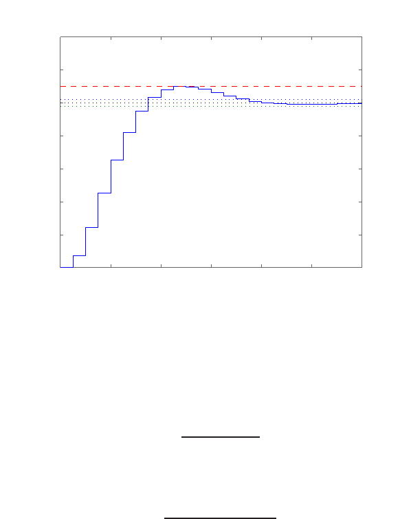
734 CHAPTER 13 Digital Control Systems

stability is Kmax = 44.3. We select K= 6. The step response is shown in

Figure AP13.3b.

0 0.2 0.4 0.6 0.8 1 1.2

0.2

0.4

0.6

0.8

1.2

1.4

Step Response

Time (sec)

Amplitude

FIGURE AP13.3

CONTINUED: (b) Step response with K= 6.

AP13.4 The loop transfer function is

G(z) = 10(1 −e−T)

z−e−T,

and the closed-loop transfer function is

T(z) = 10(1 −e−T)

z−(11e−T−10) .

For stability, we require

|11e−T−10|<1.

Solving for Tyields

0< T < 0.2.

Selecting T= 0.1s provides a stable system with rapid response; the

settling time is Ts= 0.2s. The step response is shown in Figure AP13.4.

from the publisher prior to any prohibited reproduction, storage in a retrieval system, or transmission in any form or by any means, electronic, mechanical, photocopying,

recording, or likewise. For information regarding permission(s), write to: Rights and Permissions Department, Pearson Education, Inc., Upper Saddle River, NJ 07458.

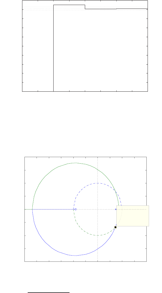
Advanced Problems 735

0.1

0.2

0.3

0.4

0.5

0.6

0.7

0.8

0.9

0 0.5 1 1.5 2 2.5 3 3.5 4

No. of Samples

Amplitude

FIGURE AP13.4

Step response with T= 0.1s.

AP13.5 The maximum gain for stability is Kmax = 63.15.

Root Locus

Real Axis

Imaginary Axis

−3 −2.5 −2 −1.5 −1 −0.5 0 0.5 1 1.5 2

−2

−1.5

−1

−0.5

0.5

1.5

System: sysz

Gain: 63.2

Pole: 0.725 − 0.686i

Damping: 0.00308

Overshoot (%): 99

Frequency (rad/sec): 7.58

Unit circle (dashed line)

FIGURE AP13.5

Root locus for 1 + K0.004535z+0.004104

z2−1.741z+0.7408 = 0.

from the publisher prior to any prohibited reproduction, storage in a retrieval system, or transmission in any form or by any means, electronic, mechanical, photocopying,

recording, or likewise. For information regarding permission(s), write to: Rights and Permissions Department, Pearson Education, Inc., Upper Saddle River, NJ 07458.

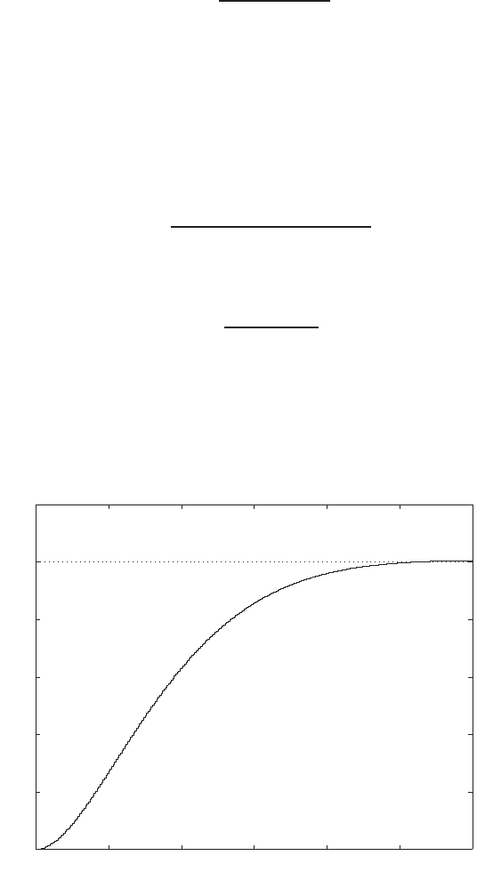
736 CHAPTER 13 Digital Control Systems

Design Problems

The plant model with parameters given in Table CDP2.1 in Dorf andCDP13.1

Bishop is given by:

Gp(s) = 26.035

s(s+ 33.142) ,

where we neglect the motor inductance Lmand where we switch oﬀ the

tachometer feedback (see Figure CDP4.1 in Dorf and Bishop). Letting

G(z) = ZG≀(∫)G√(∫)

we obtain

G(z) = 1.2875e−05(z+ 0.989)

(z−1)(z−0.9674) .

A suitable controller is

D(z) = 20(z−0.5)

z+ 0.25 .

The step response is shown below. The settling time is under 250 samples.

With each sample being 1 ms this means that Ts<250 ms, as desired.

Also, the percent overshoot is P.O. < 5%.

0 50 100 150 200 250 300

0.2

0.4

0.6

0.8

1.2

No. of Samples

Amplitude

from the publisher prior to any prohibited reproduction, storage in a retrieval system, or transmission in any form or by any means, electronic, mechanical, photocopying,

recording, or likewise. For information regarding permission(s), write to: Rights and Permissions Department, Pearson Education, Inc., Upper Saddle River, NJ 07458.

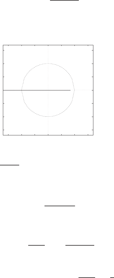
Design Problems 737

DP13.1 (a) Given the sample and hold with Gp(s), we determine that

KG(z) = K0.1228

z−0.8465 .

The root locus is shown in Figure DP13.1a. For stablity: 0 ≤K < 15.

-1.5

-1

-0.5

0.5

1.5

-1.5 -1 -0.5 0 0.5 1 1.5

Real Axis

Imag Axis

Unit circle (dashed line)

FIGURE DP13.1

(a) Root locus for 1 + K0.1228

z−0.8465 = 0 with unit circle (dashed line).

(b) A suitable compensator is

Gc(s) = 15(s+ 0.5)

s+ 5 .

Utilizing the Gc(s)-to-D(z) method (with T= 0.5 second), we deter-

mine

D(z) = Cz−A

z−B= 6.22z−0.7788

z−0.0821 .

We use the relationships

A=e−aT , B =e−bT ,and C1−A

1−B=Ka

to compute

A=e−0.5(0.5) = 0.7788 , B =e−0.5(5) = 0.0821 ,and C= 6.22 .

from the publisher prior to any prohibited reproduction, storage in a retrieval system, or transmission in any form or by any means, electronic, mechanical, photocopying,

recording, or likewise. For information regarding permission(s), write to: Rights and Permissions Department, Pearson Education, Inc., Upper Saddle River, NJ 07458.

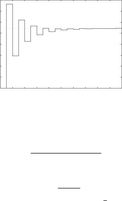
738 CHAPTER 13 Digital Control Systems

0.1

0.2

0.3

0.4

0.5

0.6

0.7

0.8

0 2 4 6 8 10 12 14 16 18 20

No. of Samples

Amplitude

FIGURE DP13.1

CONTINUED: (b) Closed-loop system step response.

DP13.2 With the sample and hold (T=10ms), we have

G(z) = 0.00044579z+ 0.00044453

z2−1.9136z+ 0.99154 .

A suitable compensator is

D(z) = Kz−0.75

z+ 0.5,

where Kis determined so that ζof the system is 1/√2. The root locus is

shown in Figure DP13.2. We choose K= 1400.

from the publisher prior to any prohibited reproduction, storage in a retrieval system, or transmission in any form or by any means, electronic, mechanical, photocopying,

recording, or likewise. For information regarding permission(s), write to: Rights and Permissions Department, Pearson Education, Inc., Upper Saddle River, NJ 07458.

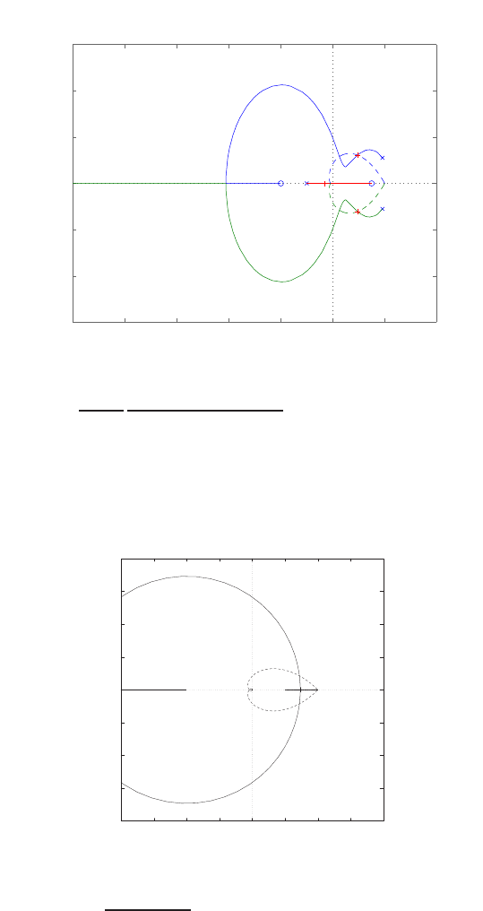
Design Problems 739

−5 −4 −3 −2 −1 0 1 2

−1.5

−1

−0.5

0.5

1.5

Curve of constant zeta=0.707 (dashed line)

Root Locus

Real Axis

Imaginary Axis

FIGURE DP13.2

Root locus for 1 + Kz−0.75

z+0.50.00044579z+0.00044453

z2−1.9136z+0.99154 = 0.

DP13.3 The root locus is shown in Figure DP13.3a.

-2

-1.5

-1

-0.5

0.5

1.5

-2 -1.5 -1 -0.5 0 0.5 1 1.5 2

xxo

Real Axis

Imag Axis

Curve of constant zeta=0.707 (dashed line)

FIGURE DP13.3

(a) Root locus for 1 + Kz+1

(z−1)(z−0.5) = 0.

The gain for ζ= 0.707 is K= 0.0627. The step response is shown in

Figure DP13.3b. The settling time is Ts= 14T= 1.4s and P.O. = 5%.

from the publisher prior to any prohibited reproduction, storage in a retrieval system, or transmission in any form or by any means, electronic, mechanical, photocopying,

recording, or likewise. For information regarding permission(s), write to: Rights and Permissions Department, Pearson Education, Inc., Upper Saddle River, NJ 07458.

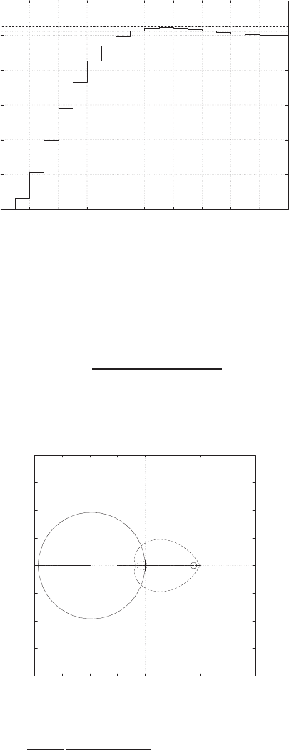
740 CHAPTER 13 Digital Control Systems

0.2

0.4

0.6

0.8

1.2

02 4 6 8 10 12 14 16 18 20

No. of Samples

Amplitude

FIGURE DP13.3

CONTINUED: (b) Step response with K= 0.0627.

DP13.4 With the sample and hold (T=1s), we have

G(z) = 0.484(z+ 0.9672)

(z−1)(z−0.9048) .

-2

-1.5

-1

-0.5

0.5

1.5

-2 -1.5 -1 -0.5 0 0.5 1 1.5 2

xxxo o

Real Axis

Imag Axis

Curve of constant zeta=0.5 (dashed line)

FIGURE DP13.4

(a) Root locus for 1 + Kz−0.88

z+0.5

0.484(z+0.9672)

(z−1)(z−0.9048) = 0.

from the publisher prior to any prohibited reproduction, storage in a retrieval system, or transmission in any form or by any means, electronic, mechanical, photocopying,

recording, or likewise. For information regarding permission(s), write to: Rights and Permissions Department, Pearson Education, Inc., Upper Saddle River, NJ 07458.

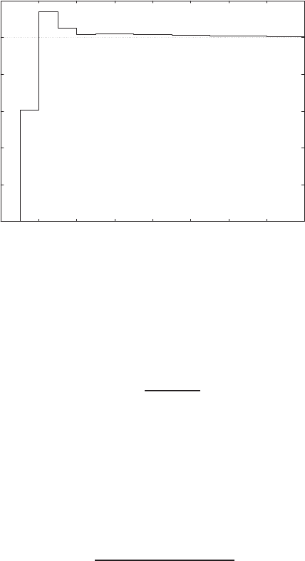
Design Problems 741

0.2

0.4

0.6

0.8

1.2

0 2 4 6 8 10 12 14 16

No. of Samples

Amplitude

FIGURE DP13.4

CONTINUED: (b) Step response for K= 12.5.

A suitable compensator is

D(z) = Kz−0.88

z+ 0.5,

where Kis determined so that ζof the system is 0.5. The root locus

is shown in Figure DP13.4a. We choose K= 12.5. The step response

is shown in Figure DP13.4b. Also, Kv= 1, so the steady-state error

speciﬁcation is satisﬁed.

DP13.5 Select T= 1 second. With the sample and hold, we have

G(z) = 0.2838z+ 0.1485

z2−1.135z+ 0.1353 .

The root locus is shown in Figure DP13.5. To meet the percent overshoot

speciﬁcation, we choose Kso that ζof the system is 0.7. This results in

K= 1. The step response has an overshoot of P.O. = 4.6%. Also, from

Figure 13.21 in Dorf and Bishop, we determine that the steady-state error

to a ramp input is ess = 2 (since T/τ = 2, and Kτ = 0.3).

from the publisher prior to any prohibited reproduction, storage in a retrieval system, or transmission in any form or by any means, electronic, mechanical, photocopying,

recording, or likewise. For information regarding permission(s), write to: Rights and Permissions Department, Pearson Education, Inc., Upper Saddle River, NJ 07458.

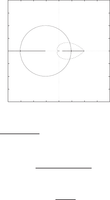
742 CHAPTER 13 Digital Control Systems

-2

-1.5

-1

-0.5

0.5

1.5

-2 -1.5 -1 -0.5 0 0.5 1 1.5 2

xxo

Real Axis

Imag Axis

Curve of constant zeta=0.7 (dashed line)

FIGURE DP13.5

Root locus for 1 + K0.2838z+0.1485

z2−1.135z+0.1353 = 0.

DP13.6 With the sample and hold at T= 1 , we have

G(z) = 0.298z+ 0.296

z2−1.98z+ 0.9802 .

Consider the digital controller

Dz) = Kz−0.9

z+ 0.6.

The root locus is shown in Figure DP13.6. To meet the percent overshoot

speciﬁcation, we choose Kso that ζof the system is greater than 0.52.

We select K= 2. The step response has an overshoot of P.O. = 11.9%

and the settling time is Ts= 17.8s.

from the publisher prior to any prohibited reproduction, storage in a retrieval system, or transmission in any form or by any means, electronic, mechanical, photocopying,

recording, or likewise. For information regarding permission(s), write to: Rights and Permissions Department, Pearson Education, Inc., Upper Saddle River, NJ 07458.

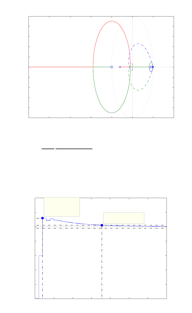
Design Problems 743

−5 −4 −3 −2 −1 0 1 2

−1

−0.8

−0.6

−0.4

−0.2

0.2

0.4

0.6

0.8

Root Locus

Real Axis

Imaginary Axis

FIGURE DP13.6

Root locus for 1 + Kz−0.9

z+0.60.298z+0.296

z2−1.98z+0.9802 = 0.

Step Response

Time (sec)

Amplitude

0 5 10 15 20 25 30 35

0.2

0.4

0.6

0.8

1.2

1.4 System: syscl

Peak amplitude: 1.12

Overshoot (%): 11.9

At time (sec): 2 System: syscl

Settling Time (sec): 17.8

FIGURE DP13.6

CONTINUED: (b) Step response for K= 2.

from the publisher prior to any prohibited reproduction, storage in a retrieval system, or transmission in any form or by any means, electronic, mechanical, photocopying,

recording, or likewise. For information regarding permission(s), write to: Rights and Permissions Department, Pearson Education, Inc., Upper Saddle River, NJ 07458.

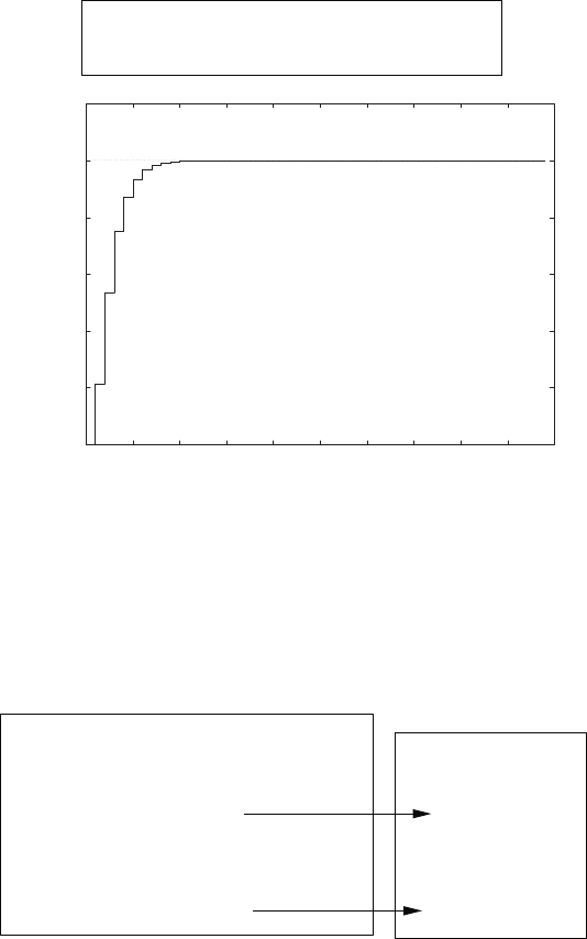
744 CHAPTER 13 Digital Control Systems

Computer Problems

CP13.1 The m-ﬁle script and unit step response are shown in Figure CP13.1.

num=[0.2145 0.1609]; den=[1 -0.75 0.125];

sysd = tf(num,den,1);

step(sysd,0:1:50)

0.2

0.4

0.6

0.8

1.2

05 10 15 20 25 30 35 40 45 50

No. of Samples

Amplitude

FIGURE CP13.1

Step response.

CP13.2 The m-ﬁle script utilizing the c2d function is shown in Figure CP13.2.

% Part (a)

num = [1]; den = [1 0]; T = 1;

sys = tf(num,den);

sys_d = c2d(sys,T,'zoh')

% Part (b)

num = [1 0]; den = [1 0 2]; T = 1;

sys = tf(num,den);

sys_d=c2d(sys,T,'zoh')

Transfer function:

-----

z - 1

Transfer function:

0.6985 z - 0.6985

------------------

z^2 - 0.3119 z + 1

FIGURE CP13.2

Script utilizing the c2d function for (a) and (b).

from the publisher prior to any prohibited reproduction, storage in a retrieval system, or transmission in any form or by any means, electronic, mechanical, photocopying,

recording, or likewise. For information regarding permission(s), write to: Rights and Permissions Department, Pearson Education, Inc., Upper Saddle River, NJ 07458.

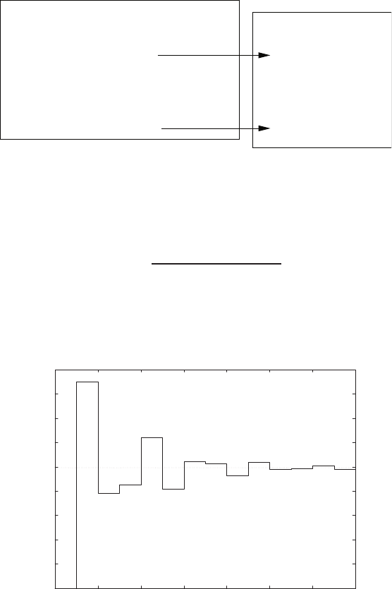
Computer Problems 745

% Part (c)

num = [1 4]; den = [1 3]; T = 1;

sys = tf(num,den);

sys_d = c2d(sys,T,'zoh')

% Part (d)

num = [1]; den = [1 8 0]; T = 1;

sys = tf(num,den);

sys_d = c2d(sys,T,'zoh')

Transfer function:

z + 0.267

-----------

z - 0.04979

Transfer function:

0.1094 z + 0.01558

-------------------

z^2 - z + 0.0003355

FIGURE CP13.2

CONTINUED: Script utilizing the c2d function for (c) and (d).

CP13.3 The continuous system transfer function (with T= 0.1 sec) is

T(s) = 13.37s+ 563.1

s2+ 6.931s+ 567.2.

The step response using the dstep function is shown in Figure CP13.3a.

The contrinuous system step response is shown in Figure CP13.3b.

0.2

0.4

0.6

0.8

1.2

1.4

1.6

1.8

0 2 4 6 8 10 12 14

No. of Samples

Amplitude

FIGURE CP13.3

(a) Unit step response using the dstep function.

from the publisher prior to any prohibited reproduction, storage in a retrieval system, or transmission in any form or by any means, electronic, mechanical, photocopying,

recording, or likewise. For information regarding permission(s), write to: Rights and Permissions Department, Pearson Education, Inc., Upper Saddle River, NJ 07458.

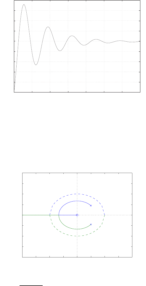
746 CHAPTER 13 Digital Control Systems

0.2

0.4

0.6

0.8

1.2

1.4

1.6

1.8

0 0.2 0.4 0.6 0.8 1 1.2 1.4

*****

FIGURE CP13.3

CONTINUED: (b) Continuous system step response (* denote sampled-data step response).

CP13.4 The root locus in shown in Figure CP13.4. For stability: 0 < K < 2.45.

−2 −1.5 −1 −0.5 0 0.5 1 1.5 2

−2

−1.5

−1

−0.5

0.5

1.5

Root Locus

Real Axis

Imaginary Axis

FIGURE CP13.4

Root locus for 1 + Kz

z2−z+0.45 = 0.

from the publisher prior to any prohibited reproduction, storage in a retrieval system, or transmission in any form or by any means, electronic, mechanical, photocopying,

recording, or likewise. For information regarding permission(s), write to: Rights and Permissions Department, Pearson Education, Inc., Upper Saddle River, NJ 07458.

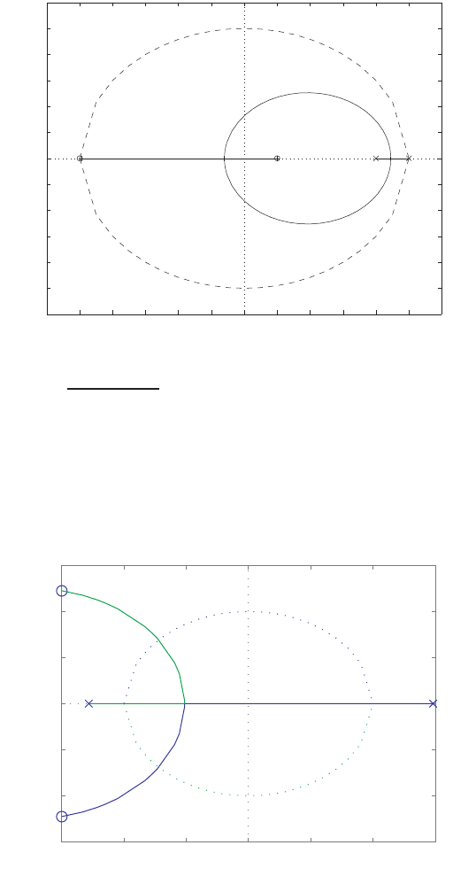
Computer Problems 747

CP13.5 The root locus in shown in Figure CP13.5. For stability: 0 < K < ∞.

-1 -0.8 -0.6 -0.4 -0.2 0 0.2 0.4 0.6 0.8 1

-1

-0.8

-0.6

-0.4

-0.2

0.2

0.4

0.6

0.8

Real Axis

Imag Axis

FIGURE CP13.5

Root locus for 1 + K(z−0.2)(z+1)

(z−0.08)(z−1) = 0

CP13.6 The root locus is shown in Figure CP13.6.

1.5 1 0.5 0 0.5 1 1.5

1.5

0.5

1.5

Root Locus

Real Axis

Imaginary Axis

FIGURE CP13.6

Root locus.

from the publisher prior to any prohibited reproduction, storage in a retrieval system, or transmission in any form or by any means, electronic, mechanical, photocopying,

recording, or likewise. For information regarding permission(s), write to: Rights and Permissions Department, Pearson Education, Inc., Upper Saddle River, NJ 07458.

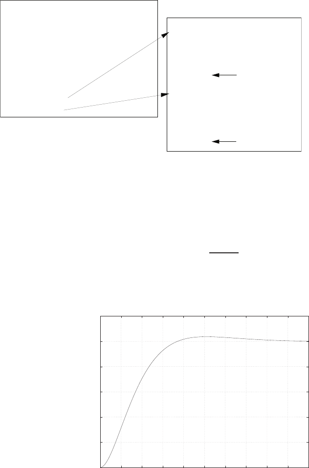
748 CHAPTER 13 Digital Control Systems

We determine the range of Kfor stability is 0.4< K < 1.06.

ÈSelect a point in the graphics window

selected_point =

-0.8278 + 0.5202i

ans =

0.7444

Select a point in the graphics window

selected_point =

-0.9745 - 0.0072i

ans =

0.3481 Kmin

Kmax

% Part (a)

num=[1 4 4.25 ]; den=[1 -0.1 -1.5];

sys = tf(num,den);

rlocus(sys), hold on

xc=[-1:0.1:1];c=sqrt(1-xc.^2);

plot(xc,c,':',xc,-c,':')

hold off

% Part (b)

rlocfind(sys)

FIGURE CP13.6

CONTINUED: Using the rlocus and rlocﬁnd functions.

CP13.7 Using root locus methods, we determine that an acceptable compensator

Gc(s) = 11.7s+ 6

s+ 20 .

With a zero-order hold and T= 0.02 sec, we ﬁnd that

0.2

0.4

0.6

0.8

1.2

00.1 0.2 0.3 0.4 0.5 0.6 0.7 0.8 0.9 1

************************************

Time (sec)

Amplitude

FIGURE CP13.7

System step response (* denotes sampled-data response).

from the publisher prior to any prohibited reproduction, storage in a retrieval system, or transmission in any form or by any means, electronic, mechanical, photocopying,

recording, or likewise. For information regarding permission(s), write to: Rights and Permissions Department, Pearson Education, Inc., Upper Saddle River, NJ 07458.

Computer Problems 749

D(z) = 11.7z−10.54

z−0.6703 .

The closed-loop step response is shown in Figure CP13.7.

from the publisher prior to any prohibited reproduction, storage in a retrieval system, or transmission in any form or by any means, electronic, mechanical, photocopying,

recording, or likewise. For information regarding permission(s), write to: Rights and Permissions Department, Pearson Education, Inc., Upper Saddle River, NJ 07458.

Instructor's Solutions Manual For Modern Control Systems, 12th Ed Systems Edition

Navigation menu

Versions of this User Manual:

Views

Navigation