NGPM A NSGA II Program In Matlab Manual V1.4
NGPM%20manual%20v1.4
User Manual: Pdf
Open the PDF directly: View PDF ![]() .
.
Page Count: 20

NGPM -- A NSGA-II Program in Matlab
Version 1.4
LIN Song
Aerospace Structural Dynamics Research Laboratory
College of Astronautics, Northwestern Polytechnical University, China
Email: lsssswc@163.com
2011-07-26
Contents
Contents...................................................................................................................................... i
1. Introduction ....................................................................................................................... 1
2. How to run the code? ........................................................................................................ 1
2.1. ‘CONSTR’ test problem description..................................................................... 1
2.2. Step1: Specified optimization model .................................................................... 1
2.3. Step2: Create a objective function......................................................................... 2
2.4. Results ................................................................................................................... 3
3. NGPM Options .................................................................................................................. 5
3.1. Coding ................................................................................................................... 5
3.2. Population options................................................................................................. 5
3.3. Population initialization ........................................................................................ 6
3.4. Selection................................................................................................................ 7
3.5. Crossover............................................................................................................... 7
3.6. Mutation ................................................................................................................ 8
3.7. Constraint handling ............................................................................................... 8
3.8. Stopping Criteria ................................................................................................... 8
3.9. Output function ..................................................................................................... 9
3.10. GUI control ........................................................................................................... 9
3.11. Plot interval ......................................................................................................... 11
3.12. Parallel computation............................................................................................ 11
4. R-NSGA-II: Reference-point-based NSGA-II.............................................................. 12
4.1. Introduction ......................................................................................................... 12
4.2. Using the R-NSGA-II.......................................................................................... 12
5. Test Problems................................................................................................................... 13
5.1. TP1: KUR............................................................................................................ 13
5.2. TP2: TNK............................................................................................................ 14
6. Disclaimer ........................................................................................................................ 17
7. Appendix A: Version history .......................................................................................... 17
i

NGPM -- A NSGA-II Program in Matlab
1. Introduction
This document gives a brief description about NGPM. NGPM is the abbreviation of “A
NSGA-II Program in Matlab”, which is the implementation of NSGA-II in Matlab. NSGA-II
is a multi-objective genetic algorithm developed by K. Deb[1] . The details of NSGA-II are
not described in this document; please refer to [1] . From version 1.3, R-NSGA-II — a
modified procedure of NSGA-II — is implemented, the details of R-NSGA-II please refer to
[2] .
2. How to run the code?
To use this program to solve a function optimization problem. Optimization model such
as number of design variables, number of objectives, number of constraints, should be
specified in the NSGA-II optimization options structure1 which is created by function
nsgaopt(). The objective function must be created as a function file (*.m), and specify the
function handle options.objfun to this function. The Matlab file TP_CONSTR.m is a script file
which solves a constrained test function. This test problem is 'CONSTR' in [1] .
2.1. ‘CONSTR’ test problem description
(1) Objectives: 2
11
22
()
() (1 )/
fx x
1
f
xxx
(1)
(2) Design variables: 2
12
[0.1,1.0], [0,5]xx
(2)
(3) Constraints: 2
121
221
() 9 6
() 9 1
gx x x
gx x x
(3)
Two steps should be done to solve this problem.
2.2. Step1: Specified optimization model
The file TP_CONSTR.m is a script file which specified the optimization model.
1 In this document, all of the italic options is the structure created by nsgaopt().
1

NGPM -- A NSGA-II Program in Matlab
% TP_CONSTR.m file
% 'CONSTR' test problem
clc; clear; close all
options = nsgaopt(); % create default options structure
options.popsize = 50; % population size
options.maxGen = 100; % max generation
options.numObj = 2; % number of objectives
options.numVar = 2; % number of design variables
options.numCons = 2; % number of constraints
options.lb = [0.1 0]; % lower bound of x
options.ub = [1 5]; % upper bound of x
options.objfun = @objfun; % objective function handle
result = nsga2(options); % start the optimization progress
2.3. Step2: Create a objective function
The file TP_CONSTR_objfun.m is a function file which specified the objective function
evaluation. The objective function is specified by options.objfun parameter created by the
function nsgaopt(). Its prototype is:
[y, cons] = objfun(x, varvargin)
x : Design variables vector, its length must equals options.numVar.
y : Objective values vector, its length must equals options.numObj.
cons : Constraint violations vector. Its length must equals options.numCons. If there is
no constraint, return empty vector [].
varargin : Any variable(s) which are passed to nsga2 function will be finally passed to
this objective function. For example, if you call
result = nsga2(opt, model, param)
The two addition parameter passed to nsga2 — model and param — will be passed to
the objective function as
[y, const]=objfun(x, model, param)
2

NGPM -- A NSGA-II Program in Matlab
In this function optimization problem, there is no other parameter.
function [y, cons] = objfun(x)
% TP_CONSTR_objfun.m file
% 'CONSTR' test problem
y = [0,0];
cons = [0,0];
y(1) = x(1);
y(2) = (1+x(2)) / x(1);
% calculate the constraint violations
c = x(2) + 9*x(1) - 6;
if(c<0)
cons(1) = abs(c);
end
c = -x(2) + 9*x(1) - 1;
if(c<0)
cons(2) = abs(c);
end
2.4. Results
Run the script file TP_CONSTR.m, and you will get the optimization result store in the
result structure. The population will be plotted in a GUI figure. The x-axis is the first
objective, and the y-axis is the second. If user specifies the names of objectives in
options.nameObj, then they will be displayed in the x and y labels.
On the GUI window ‘plotnsga’, the optimization progress could be paused or stop by
press the corresponding buttons. Note that, the progress of optimization would pause or stop
only when the current population evaluation is done!
The Pareto front (or population distribution) of generation 1 and 100 was plot in Fig. 1.
The populations of each generation were outputted to the file ‘populations.txt’ in current path.
3

NGPM -- A NSGA-II Program in Matlab
0.1 0.2 0.3 0.4 0.5 0.6 0.7 0.8 0.9 1
0
5
10
15
20
25
30
objective 1
objective 2
Generation 1 / 100
0.4 0.5 0.6 0.7 0.8 0.9 1
1
2
3
4
5
6
7
8
9
objective 1
objective 2
Generation 100 / 100
Fig. 1: Optimization results
In the population file, there is a head section in the beginning which saves some
information of optimization model. The head section begins with “#NSGA2” line, and ends
with “#end” line. And there is a state section in the front of each generation of population,
which begins with “#Generation” line and ends with “#end” line.
Populations.txt file example:
#NSGA2
popsize 50
maxGen 100
numVar 2
numObj 2
numCons 2
stateFieldNames currentGen evaluateCount totalTime firstFrontCount
frontCount avgEvalTime
#end
#Generation 1 / 100
currentGen 1
evaluateCount 50
totalTime 0.534723
firstFrontCount 7
frontCount 22
avgEvalTime 5.4181e-005
#end
4

NGPM -- A NSGA-II Program in Matlab
Var1 Var2 Obj1 Obj2 Cons1 Cons2
0.833251 4.52896 0.833251 6.6354 0 0
0.214288 4.56688 0.214288 25.9785 0 3.63829
0.669123 0.487702 0.669123 2.22336 0 0
0.350648 2.73441 0.350648 10.65 0.109757 0.578572
0.961756 4.82444 0.961756 6.05605 0 0
0.241852 4.85296 0.241852 24.2006 0 3.6763
…
3. NGPM Options
This program is written for finite element optimization problem, the “Intermediate
crossover” and “Gaussian mutation” is adequate for my use. Thus, I don’t implement other
genetic operators into NGPM. The real/integer coding, the binary tournament selection, the
Gaussian mutation operator and the intermediate crossover operator work well in my
application. If you want to use other genetic operators, try to modify the code yourself.
The following genetic operators and capabilities are supported in NGPM:
3.1. Coding
Real and integer coding are both supported. If the coding types of design variables are
not specified in options.vartype vector, real coding is use as default.
options.vartype: integer vector, the length must equal to the number of design variables.
1=real, 2=integer. For example, [1 1 2] represents that the first two variables are real, and the
third variable is integer.
3.2. Population options
options.popsize : even integer, population size.
options.numVar : integer, number of design variables.
options.numOb : integer, number of objectives.
options.numCons : integer, number of constraints.
options.lb : vector, lower bound of design variables, the length must equal to
numVar.
options.ub : vector, upper bound of design variables , the length must equal to
numVar.
5

NGPM -- A NSGA-II Program in Matlab
3.3. Population initialization
There are three ways to initialize the population:
(1) (default) Using uniform distribution random number between the lower and upper
bounds.
(2) Using population file generated in previous optimization.
(3) Using the population result structure in previous optimization.
All these approach are specified in the options.initfun cell array parameter.
3.3.1. Uniform initialization
options.initfun = {@initpop}
Description:
Create a random initial population with a uniform distribution. This is the default
approach.
3.3.2. From exist population file
options.initfun={@initpop, strFileName, ngen}
strFileName : string, the optimization result file name.
ngen : (optional) integer, the generation of population would be used. If this
parameter is not specified, the last population would be used.
Description:
Load population from exist population file and use the last population. If the popsize of
the population from file less than the popsize of current optimization model, then uniform
initialization would be used to fill the whole population.
Example:
options.initfun={@initpop, 'pops.txt'} % Restart from the last generation
options.initfun={@initpop, 'pops.txt', 100} % Restart from the 100 generation
3.3.3. From exist optimization result
options.initfun={@initpop, oldresult, ngen}
oldresult : structure, the optimization result structure in the workspace.
ngen : (optional) integer, the generation of population would be used. If this
parameter is not specified, the last population would be used.
6

NGPM -- A NSGA-II Program in Matlab
Description: Load population from previous optimization result structure. The result
structure can be:
1. The result generated by last optimization procedure.
2. The result loaded from file by loadpopfile(‘pop.txt’) function.
3. The oldresult generated in the global workspace by the plotnsga(‘pop.txt’)
function. (The plotnsga function calls loadpopfile function too.)
Example:
oldresult=loadpopfile(‘pop.txt’);
options.initfun={@initpop, oldresult} % Restart from the last generation
options.initfun={@initpop, oldresult, 100} % Restart from the 100 generation
3.4. Selection
Only binary tournament selection is supported.
3.5. Crossover
Only intermediate crossover[3] (which also names arithmetic crossover) is supported in
the current version.
3.5.1. Crossover fraction
options.crossoverFraction: scalar or string, crossover fraction of variables of an
individual. If ‘auto’ string is specified, NGPM would used 2/numVar as the
crossoverFraction.
NOTE: All of the individuals in the population would be processed by crossover
operator, and only crossoverFraction of all variables would do crossover.
3.5.2. Intermediate crossover
options.crossover={'intermediate', ratio};
Intermediate crossover [3] creates two children from two parents: parent1 and parent2.
child1 = parent1 + rand×ratio×(parent2 - parent1)
child2 = parent2 - rand×ratio× (parent2 - parent1)
ratio: scalar. If it lies in the range [0, 1], the children created are within the two parent. If
algorithm is premature, try to set ratio larger than 1.0.
7

NGPM -- A NSGA-II Program in Matlab
3.6. Mutation
Only Gaussian mutation (which also names normal mutation) is supported in the current
version.
3.6.1. Mutation fraction
options.mutaionFraction: scalar or string, mutation fraction of variables of an individual.
If ‘auto’ string is specified, NGPM would use 2/numVar as the mutaionFraction.
NOTE: It’s similar to the crossoverFraction parameter described before. All of the
individuals in the population would be processed, and only mutaionFraction of all variables
would do mutation.
3.6.2. Gaussian mutation
options.mutation = {'gaussian', scale, shrink}
Gaussian mutation[3] adds a normally distributed random number to each variable:
child =parent + S × randn×(ub-lb);
S = scale×(1 - shrink×currGen / maxGen);
scale: scalar, the scale parameter determines the standard deviation of the random
number generated.
shrink: scalar, [0,1]. As the optimization progress goes forward, decrease the mutation
range (for example, shrink∈[0.5, 1.0]) is usually used for local search. If the optimization
problem has many different local Pareto-optimal fronts, such as ZDT4 problem[1] , a large
mutation range is require getting out of the local Pareto-optimal fronts. It means a zero shrink
should be used.
3.7. Constraint handling
NGPM uses binary tournament selection based on constraint-dominate definition to
handle constraint which proposed by Deb[1] .
3.8. Stopping Criteria
Only maximum generation specified by options.maxGen is supported currently.
Example:
options.maxGen=500;
8

NGPM -- A NSGA-II Program in Matlab
3.9. Output function
3.9.1. Output function
In current version NGPM, the only output function is output2file which outputs the
whole population includes design variables, objectives and constraint violations (if exist) into
the specified file (options.outputfile).
options.outputfuns: cell array, the first element must be the output function handle, such
as @output2file. The other parameter will be passed to this function as variable length input
argument. The output function has the prototype:
function output (opt, state, pop, type, varargin)
opt : the options structure.
state : the state structure.
pop : the current population.
type : use to identify if this call is the last call.
-1 = the last call, use for closing the opened file or other operations.
others(or no exist) = normal output
varargin : the parameter specified in the options.outputfuns cell array. There is no
parameter for the default output function output2file.
3.9.2. Output interval
options.outputInterval : integer, interval between two calls of output function. This
parameter can be assigned a large value for efficiency.
Example:
options.outputInterval = 10;
3.10. GUI control
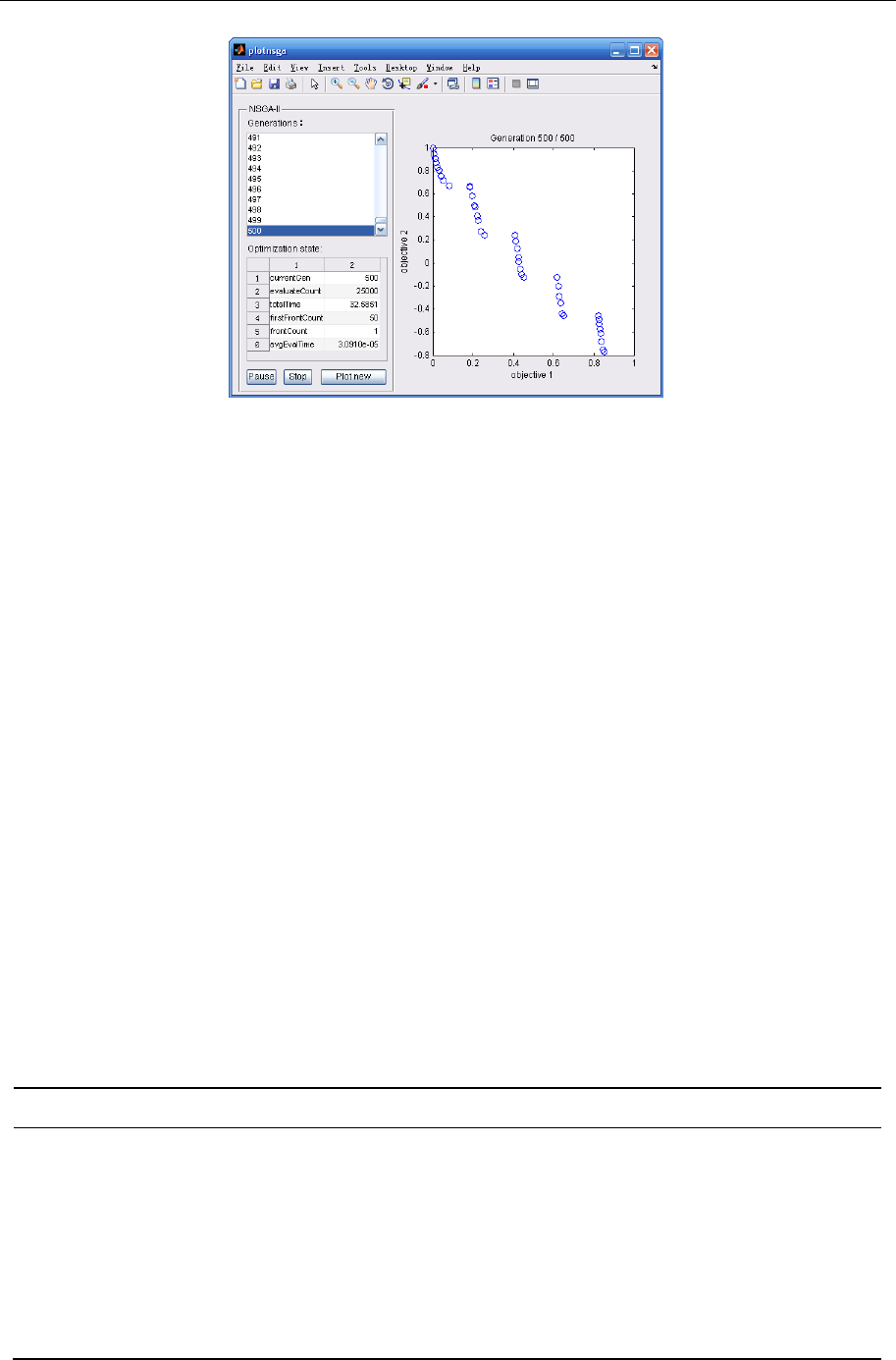
The GUI window ‘plognsga’ (Fig. 2) is use to plot the result populations or control the
optimization progress. Call plotnsga function to plot the populations:
plotnsga(result)
plotnsga(strPopFile)
result : structure created by nsga2() function.
strPopFile : population file name.
9
NGPM -- A NSGA-II Program in Matlab
Fig. 2: plotnsga GUI window
3.10.1. Pause, stop
Press “Pause” button to pause the optimization progress, and the button title would be
changed to “Continue”. Then, press “Continue” button to continue the optimization.
Press “Stop” button to stop the optimization progress. This operation would stop the
nsga2 iteration and closed the output file if specified.
NOTE: When ‘pause’ or ‘stop’ button is pressed, the program would response until the
current generation of optimization progress is finished.
3.10.2. Plot in new window
Press “Plot new” button to plot the selected population in a new figure window. This
function is designed to save the figure as EMF file (because the window could not be saved
as EMF file if there is any GUI control on the figure window).
3.10.3. Optimization state
The optimization state list-box lists all fields of the state structure of selected generation.
Table 1: Optimization states
Name Description
currentGen The selected generation ID, begin with 1.
evaluateCount The objective function evaluation count from the beginning.
totalTime The elapsed time from optimization progress start.
firstFrontCount The number of individuals in the first front.
frontCount The number of fronts in current population.
avgEvalTime The average evaluation time of current generation.
10

NGPM -- A NSGA-II Program in Matlab
3.10.4. Load from result
plotnsga(strPopFile)
strPopFile : string, the optimization result file name.
Description:
The function plotnsga will first call loadpopfile() function to read the specified
optimization result file. A global variable named "oldresult" which contains the optimization
result in the file would be created in global workspace. Then the population loaded from file
would be plotted in the GUI window, and the file name was showed in the figure title.
Example:
plotnsga(‘populations.txt’)
3.11. Plot interval
options.plotInterval : integer, interval between two calls of "plotnsga".
Description:
The overhead of plot in Matlab is very expensive. And it’s not necessary to plot every
generation for function optimization, a large interval value could speedup the optimization.
3.12. Parallel computation
options.useParallel : string, {‘yes’, ‘no’}, specified if parallel computation is used.
options.poolsize : scalar, the number of worker processes. If you have a quat-core
processor, poolsize could be set to 3, then you can do other things when the optimization is
progressing.
Description:
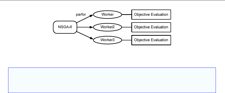
The parallel computation is very useful when the evaluation of objective function is very
time-expensive and you have a multicore/multiple processor(s) computer. If
options.useParallel is specified as ‘yes’, the program would start multiple worker processes
and use parfor to calculate each objective function (Parallel Computation Toolbox in Matlab
is required). This procedure is showed in Fig. 3. Refer Matlab helps for details about parallel
computation.
11
NGPM -- A NSGA-II Program in Matlab
Fig. 3: Parallel computation in NGPM
Example:
options.useParallel = 'yes';
options.poolsize = 2;
4. R-NSGA-II: Reference-point-based NSGA-II
4.1. Introduction
The two objectives of multi-objective optimization are:
(1) Find the whole Pareto-optimal front.
(2) Get a well-distributed solution set in the front.
NSGA-II could do this well. But at last, only one or several solutions may be chose.
Deb[2] proposed a modified procedure — R-NSGA-II — based on NSGA-II to get
preference solutions by specified reference points. This procedure provides the
decision-maker with a set of solutions near the preference solution(s), so that a better and a
more reliable decision can be made.
4.2. Using the R-NSGA-II
The parameters below would be used in R-NSGA-II:
options.refPoints : matrix, Reference point(s) used to specify preference. Each row is
a reference point in objective space.
options.refWeight : vector, weight factor used in the calculation of Euclidean distance.
If no value is specified, all objectives have the same weight factor 1.0. It’s the in Eq.
i
w(4).
options.refEpsilon : scalar, a parameter used in epsilon-based selection strategy to
control the spread of solution. All solutions having a weighted normalized Euclidean distance
equal or less than ε would have a large preference distance in the next selection procedure. A
large number (such as 0.01) would get a wide spread solution set near reference points, while
a small value (such as 0.0001) would get a narrow spread solution set.
options. refUseNormDistance : string, {'front', 'ever', 'no'}, specify which approach
12

NGPM -- A NSGA-II Program in Matlab
would be used to calculate the preference distance in R-NSGA-II.
"front" : (default) Use maximum and minimum objectives in the front as normalized
factor. It means the max
i
f
and min
i
f
in Eq. (4) are the maximum and minimum objective
values in the front.
"ever": Use maximum and minimum objectives ever found as normalized factor. It
means the max
i
f
and min
i
f
in Eq. (4) are the maximum and minimum objective values ever
found begin from the initialization population. In many test problems, it’s similar to "front"
parameter.
"no": Do not use normalized factor, only use Euclidean distance. It means
.
max min 1
ii
ff
2
max min
1
()
M
ii
ij i
iii
fz
dw
ff
x
(4)
Example:
options.refPoints = [0.1 0.6; 0.3 0.6; 0.5 0.2; 0.7 0.2; 0.9 0;];
options.refWeight = [0.2 0.8];
options.refEpsilon = 0.001;
options.refUseNormDistance = 'no'
A test example ZDT1 can be find in “TP_R-NSGA2” folder.
5. Test Problems
5.1. TP1: KUR
File: TP_KUR.m, TP_KUR_fun.m
The KUR[1] problem has two objective function and no constraint except for bound
constraints.
2
22
11 2 3 1
1
3
0.8 3
2123
1
min . ( , , ) 10 exp 0.2
(, , ) | | 5sin
s.t. 5 5, 1,2,3
ii
i
ii
i
i
fxxx x x
fxxx x x
xi
(5)
13
NGPM -- A NSGA-II Program in Matlab
Some of the optimization parameters were showed in Table 2.
Table 2: Optimization parameters
Parameter Value
Population size 50
Maximum generation 100
Crossover operator Intermediate, ratio=1.2
Mutation operator Gaussian, scale=0.1, shrink=0.5
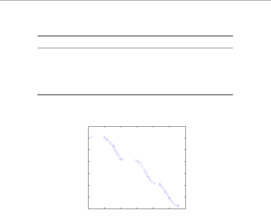
Fig. 4 shows the whole population of generation 100.
-20 -19 -18 -17 -16 -15 -14
-12
-10
-8
-6
-4
-2
0
2
objective 1
objective 2
Generation 100 / 100
Fig. 4: The last population of problem KUR
5.2. TP2: TNK
File: TP_TNK.m, TP_TNK_objfun.m
The TNK[1] problem has two simple objective function and two complicated
constraints except for bound constraints.
(6)
112 1
212 2
22
112 12
22
21 2
min . ( , )
(, )
s.t. ( ) 1 0.1cos(16arctan( / )) 0
() ( 0.5) ( 0.5) 0.5
[0, ], 1,2
i
fxx x
fxx x
gx x x x x
gx x x
xi
The optimization parameters are showed in Table 2. Parallel computation is enabled, and
poolsize is assigned 2. Actually, parallel computation is no essential here, and parallel
computation cost more time then serial computation, since the overhead of interprocess
communication exceeds the save time benefit from parallel computation. In my dual-core
computer, the total time of parallel computation is 24.0s, while serial computation costs
14

NGPM -- A NSGA-II Program in Matlab
12.5s.
Fig. 5 shows the whole population of generation 100.
00.2 0.4 0.6 0.8 11.2 1.4
0
0.2
0.4
0.6
0.8
1
1.2
1.4
obj 1 : f1=x1
obj 2 : f2=x2
Generation 100 / 100
Fig. 5: The last population of problem TNK
5.3. TP3: Three-objective DTLZ2 — R-NSGA-II
File: TPR_DTLZ2_3obj.m, TPR_DTLZ2_objfun_3obj.m
The DTLZ [4] (Deb-Thiele-Laumanns-Zitzler) test problems are a set of MOPs for
testing and comparing MOEAs. They are scalable to a user defined number of objectives.
(7)
1122
2122
3122
11
min. ( ) (1 ( ))cos( / 2)cos( / 2) cos( / 2) cos( / 2)
( ) (1 ( ))cos( / 2)cos( / 2) cos( / 2)sin( / 2)
( ) (1 ( ))cos( / 2)cos( / 2) sin( / 2)
() (1 ( ))cos( /2)
MM
MM
MM
MM
fx g x x x x
fx g x x x x
fx g x x x
fx g x
x
x
x
x
2
2
1
sin( / 2)
() (1 ( ))sin( /2)
. . 0 1, 1, 2,...,
() ( 0.5)
iM
MM
i
Mi
x
x
fx g x
st x i n
where g x
x
x
x
1
1
M
M
where M is the number of objectives, n is the number of variables,
M
x represents i
x
for . It is recommended that [,]iMn9nM
. For DTLZ2 problem, Pareto-optimal
solutions satisfy , and
2
11
M
i
if
0.5
i
x
for [,]niM
.
Here, optimization parameters below were used. There are two reference points:
(0.2,0.2,0.6) and (0.8,0.6,1.0). The definition of ε is different from the Deb's definition, thus
ε=0.002 was used instead of 0.01 in [2] .
options.popsize = 200; % populaion size
options.maxGen = 200; % max generation
15
NGPM -- A NSGA-II Program in Matlab
options.refPoints = [0.2 0.2 0.6; 0.8 0.6 1.0];
options.refEpsilon = 0.002;
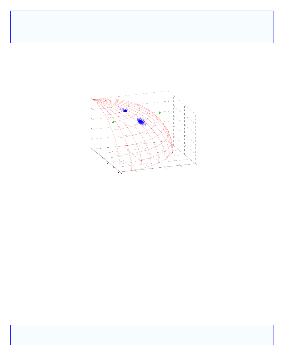
Fig. 6 shows the last population of three objective DTLZ2 problem and the true Pareto
front.
0
0.2
0.4
0.6
0.8
100.2 0.4 0.6 0.8 1
0
0.2
0.4
0.6
0.8
1
objective 2
Generation 200 / 200
objective 1
objective 3
Fig. 6: The last population of three objective DTLZ2 problem
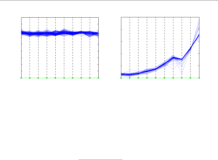
5.4. TP4: 10-objective DTLZ2 — R-NSGA-II
bj.m
point: 0.25f for all
1,i[2]
reference point. This is not true when normalized Euclidean
not conce
File: TPR_DTLZ2_10obj.m, TPR_DTLZ2_objfun_10o
For 10-objective DTLZ2 problem, we used reference i
distance is used: the points do
2,...,10 . In Deb's paper , it's said that the solution with fi=0.316 is closest to the
ntrates near fi =0.316. If you want to get similar results as ref [2] ,
options.refUseNormDistance must be specified as 'no':
options.refUseNormDistance = 'no';
Then, similar result would be get as showed in Fig. 7(a). If options.refUseNormDistance
was specified as default value 'front', you will get the result showed in Fig. 7(b).
16
NGPM -- A NSGA-II Program in Matlab
12345678910
0.25
0.26
0.27
0.28
0.29
0.3
0.31
0.32
0.33
0.34
Objective number
Objective value
Generation 200 / 200
12345678910
0.25
0.3
0.35
0.4
0.45
0.5
Objective number
Objective value
Generation 200 / 200
(a) refUseNormDistance='no' (b) refUseNormDistance='front'
Fig. 7: 10-objective DTLZ2 problem with different refUseNormDistance parameter
6. Disclaimer
This code is distributed for academic purposes only. If you have any comments or find
any bugs, please send an email to lsssswc@163.com.
7. Appendix A: Version history
v1.4 [2011-07-26]
1. Add: Support three or more objectives visualization display in "plotnsga".
2. Add: R-NSGA-II problem: DTLZ2.
3. Improve efficiency for large generation.
v1.3 [2011-07-15]
1. Add: Implement reference-point-based NSGA-II procedure -- R-NSGA-II.
2. Add: NSGA-II test problem: ZDT1, ZDT2, ZDT3 and ZDT6.
3. Improve: Improve the efficiency of "ndsort" function, get a 48% speedup for TP_CONSTR
problem.
4. Improve: Save the output file ID to options structure for no explicit clear in optimization
script file.
5. Modify: Modify the crossover and mutation strategy from individuals to variables.
v1.1 [2011-07-01]
17

NGPM -- A NSGA-II Program in Matlab
18
1. Add: Load and plot population from previous optimization result file.
2. Add: Initialize population using exist optimization result or file.
v1.0 [2011-04-23]
The first version distributed.
Reference:
[1] Deb K, Pratap A, Agarwal S, et al. A fast and elitist multiobjective genetic algorithm
NSGA-II[J]. Evolutionary Computation. 2002, 6(2): 182-197.
[2] Deb K, Sundar J, U B R N, et al. Reference point based multi-objective optimization
using evolutionary algorithms[J]. International Journal of Computational Intelligence
Research. 2006, 2(3): 273-286.
[3] Matlab Help, Global optimization toolbox.
[4] Deb K, Thiele L, Laumanns M, et al. Scalable Test Problems for Evolutionary
Multi-Objective Optimization[C]. Piscataway, New Jersey: 2002.
