Cassandra: The Definitive Guide OReilly.Cassandra.The.Definitive.Guide.2nd.Edition.1491933666
User Manual: Pdf
Open the PDF directly: View PDF ![]() .
.
Page Count: 369 [warning: Documents this large are best viewed by clicking the View PDF Link!]
- Cover
- Copyright
- Table of Contents
- Foreword
- Foreword
- Preface
- Chapter 1. Beyond Relational Databases
- Chapter 2. Introducing Cassandra
- Chapter 3. Installing Cassandra
- Chapter 4. The Cassandra Query Language
- Chapter 5. Data Modeling
- Chapter 6. The Cassandra Architecture
- Data Centers and Racks
- Gossip and Failure Detection
- Snitches
- Rings and Tokens
- Virtual Nodes
- Partitioners
- Replication Strategies
- Consistency Levels
- Queries and Coordinator Nodes
- Memtables, SSTables, and Commit Logs
- Caching
- Hinted Handoff
- Lightweight Transactions and Paxos
- Tombstones
- Bloom Filters
- Compaction
- Anti-Entropy, Repair, and Merkle Trees
- Staged Event-Driven Architecture (SEDA)
- Managers and Services
- System Keyspaces
- Summary
- Chapter 7. Configuring Cassandra
- Chapter 8. Clients
- Chapter 9. Reading and Writing Data
- Chapter 10. Monitoring
- Chapter 11. Maintenance
- Chapter 12. Performance Tuning
- Chapter 13. Security
- Chapter 14. Deploying and Integrating
- Index
- About the Authors
- Colophon

Je Carpenter & Eben Hewitt
Cassandra
The Definitive Guide
DISTRIBUTED DATA AT WEB SCALE
2nd Edition

Je Carpenter and Eben Hewitt
Cassandra: The Denitive Guide
SECOND EDITION
Boston Farnham Sebastopol Tokyo
Beijing Boston Farnham Sebastopol Tokyo
Beijing
978-1-491-93366-4
[LSI]
Cassandra: The Denitive Guide
by Jeff Carpenter and Eben Hewitt
Copyright © 2016 Jeff Carpenter, Eben Hewitt. All rights reserved.
Printed in the United States of America.
Published by O’Reilly Media, Inc., 1005 Gravenstein Highway North, Sebastopol, CA 95472.
O’Reilly books may be purchased for educational, business, or sales promotional use. Online editions are
also available for most titles (http://oreilly.com/safari). For more information, contact our corporate/insti‐
tutional sales department: 800-998-9938 or corporate@oreilly.com.
Editors: Mike Loukides and Marie Beaugureau
Production Editor: Colleen Cole
Copyeditor: Jasmine Kwityn
Proofreader: James Fraleigh
Indexer: Ellen Troutman-Zaig
Interior Designer: David Futato
Cover Designer: Karen Montgomery
Illustrator: Rebecca Demarest
June 2016: Second Edition
Revision History for the Second Edition
2010-11-12: First Release
2016-06-27: Second Release
2017-04-07: Third Release
See http://oreilly.com/catalog/errata.csp?isbn=9781491933664 for release details.
The O’Reilly logo is a registered trademark of O’Reilly Media, Inc. Cassandra: e Denitive Guide, the
cover image, and related trade dress are trademarks of O’Reilly Media, Inc.
While the publisher and the authors have used good faith efforts to ensure that the information and
instructions contained in this work are accurate, the publisher and the authors disclaim all responsibility
for errors or omissions, including without limitation responsibility for damages resulting from the use of
or reliance on this work. Use of the information and instructions contained in this work is at your own
risk. If any code samples or other technology this work contains or describes is subject to open source
licenses or the intellectual property rights of others, it is your responsibility to ensure that your use
thereof complies with such licenses and/or rights.
is book is dedicated to my sweetheart, Alison Brown.
I can hear the sound of violins, long before it begins.
—E.H.
For Stephanie, my inspiration, unfailing support,
and the love of my life.
—J.C.

Table of Contents
Foreword. . . . . . . . . . . . . . . . . . . . . . . . . . . . . . . . . . . . . . . . . . . . . . . . . . . . . . . . . . . . . . . . . . . . xiii
Foreword. . . . . . . . . . . . . . . . . . . . . . . . . . . . . . . . . . . . . . . . . . . . . . . . . . . . . . . . . . . . . . . . . . . . . xv
Preface. . . . . . . . . . . . . . . . . . . . . . . . . . . . . . . . . . . . . . . . . . . . . . . . . . . . . . . . . . . . . . . . . . . . . . xvii
1. Beyond Relational Databases. . . . . . . . . . . . . . . . . . . . . . . . . . . . . . . . . . . . . . . . . . . . . . . . . 1
What’s Wrong with Relational Databases? 1
A Quick Review of Relational Databases 5
RDBMSs: The Awesome and the Not-So-Much 5
Web Scale 12
The Rise of NoSQL 13
Summary 15
2. Introducing Cassandra. . . . . . . . . . . . . . . . . . . . . . . . . . . . . . . . . . . . . . . . . . . . . . . . . . . . . . 17
The Cassandra Elevator Pitch 17
Cassandra in 50 Words or Less 17
Distributed and Decentralized 18
Elastic Scalability 19
High Availability and Fault Tolerance 19
Tuneable Consistency 20
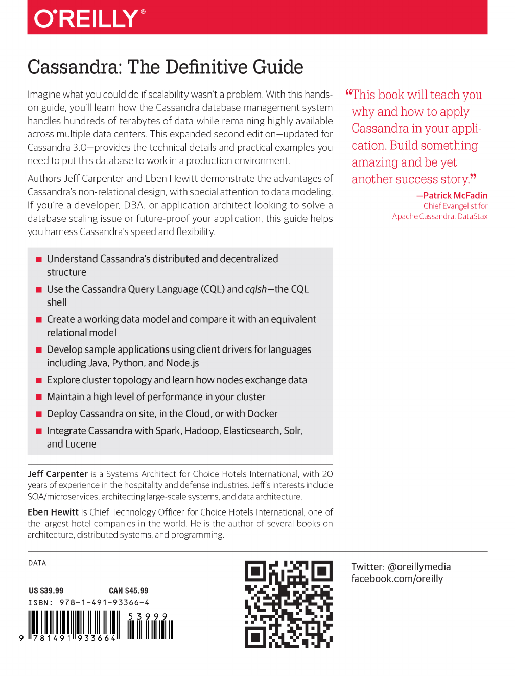
Brewer’s CAP Theorem 23
Row-Oriented 26
High Performance 28
Where Did Cassandra Come From? 28
Release History 30
Is Cassandra a Good Fit for My Project? 35
Large Deployments 35
v

Lots of Writes, Statistics, and Analysis 36
Geographical Distribution 36
Evolving Applications 36
Getting Involved 36
Summary 38
3. Installing Cassandra. . . . . . . . . . . . . . . . . . . . . . . . . . . . . . . . . . . . . . . . . . . . . . . . . . . . . . . . 39
Installing the Apache Distribution 39
Extracting the Download 39
What’s In There? 40
Building from Source 41
Additional Build Targets 43
Running Cassandra 43
On Windows 44
On Linux 45
Starting the Server 45
Stopping Cassandra 47
Other Cassandra Distributions 48
Running the CQL Shell 49
Basic cqlsh Commands 50
cqlsh Help 50
Describing the Environment in cqlsh 51
Creating a Keyspace and Table in cqlsh 52
Writing and Reading Data in cqlsh 55
Summary 56
4. The Cassandra Query Language. . . . . . . . . . . . . . . . . . . . . . . . . . . . . . . . . . . . . . . . . . . . . . . 57
The Relational Data Model 57
Cassandra’s Data Model 58
Clusters 61
Keyspaces 61
Tables 61
Columns 63
CQL Types 65
Numeric Data Types 66
Textual Data Types 67
Time and Identity Data Types 67
Other Simple Data Types 69
Collections 70
User-Defined Types 73
Secondary Indexes 76
Summary 78
vi | Table of Contents

5. Data Modeling. . . . . . . . . . . . . . . . . . . . . . . . . . . . . . . . . . . . . . . . . . . . . . . . . . . . . . . . . . . . . 79
Conceptual Data Modeling 79
RDBMS Design 80
Design Differences Between RDBMS and Cassandra 81
Defining Application Queries 84
Logical Data Modeling 85
Hotel Logical Data Model 87
Reservation Logical Data Model 89
Physical Data Modeling 91
Hotel Physical Data Model 92
Reservation Physical Data Model 93
Materialized Views 94
Evaluating and Refining 96
Calculating Partition Size 96
Calculating Size on Disk 97
Breaking Up Large Partitions 99
Defining Database Schema 100
DataStax DevCenter 102
Summary 103
6. The Cassandra Architecture. . . . . . . . . . . . . . . . . . . . . . . . . . . . . . . . . . . . . . . . . . . . . . . . . 105
Data Centers and Racks 105
Gossip and Failure Detection 106
Snitches 108
Rings and Tokens 109
Virtual Nodes 110
Partitioners 111
Replication Strategies 112
Consistency Levels 113
Queries and Coordinator Nodes 114
Memtables, SSTables, and Commit Logs 115
Caching 117
Hinted Handoff 117
Lightweight Transactions and Paxos 118
Tombstones 120
Bloom Filters 120
Compaction 121
Anti-Entropy, Repair, and Merkle Trees 122
Staged Event-Driven Architecture (SEDA) 124
Managers and Services 125
Cassandra Daemon 125
Storage Engine 126
Table of Contents | vii

Storage Service 126
Storage Proxy 126
Messaging Service 127
Stream Manager 127
CQL Native Transport Server 127
System Keyspaces 128
Summary 130
7. Conguring Cassandra. . . . . . . . . . . . . . . . . . . . . . . . . . . . . . . . . . . . . . . . . . . . . . . . . . . . . 131
Cassandra Cluster Manager 131
Creating a Cluster 132
Seed Nodes 135
Partitioners 136
Murmur3 Partitioner 136
Random Partitioner 137
Order-Preserving Partitioner 137
ByteOrderedPartitioner 137
Snitches 138
Simple Snitch 138
Property File Snitch 138
Gossiping Property File Snitch 139
Rack Inferring Snitch 139
Cloud Snitches 140
Dynamic Snitch 140
Node Configuration 140
Tokens and Virtual Nodes 141
Network Interfaces 142
Data Storage 143
Startup and JVM Settings 144
Adding Nodes to a Cluster 144
Dynamic Ring Participation 146
Replication Strategies 147
SimpleStrategy 147
NetworkTopologyStrategy 148
Changing the Replication Factor 150
Summary 150
8. Clients. . . . . . . . . . . . . . . . . . . . . . . . . . . . . . . . . . . . . . . . . . . . . . . . . . . . . . . . . . . . . . . . . . . 151
Hector, Astyanax, and Other Legacy Clients 151
DataStax Java Driver 152
Development Environment Configuration 152
Clusters and Contact Points 153
viii | Table of Contents

Sessions and Connection Pooling 155
Statements 156
Policies 164
Metadata 167
Debugging and Monitoring 171
DataStax Python Driver 172
DataStax Node.js Driver 173
DataStax Ruby Driver 174
DataStax C# Driver 175
DataStax C/C++ Driver 176
DataStax PHP Driver 177
Summary 177
9. Reading and Writing Data. . . . . . . . . . . . . . . . . . . . . . . . . . . . . . . . . . . . . . . . . . . . . . . . . . 179
Writing 179
Write Consistency Levels 180
The Cassandra Write Path 181
Writing Files to Disk 183
Lightweight Transactions 185
Batches 188
Reading 190
Read Consistency Levels 191
The Cassandra Read Path 192
Read Repair 195
Range Queries, Ordering and Filtering 195
Functions and Aggregates 198
Paging 202
Speculative Retry 205
Deleting 205
Summary 206
10. Monitoring. . . . . . . . . . . . . . . . . . . . . . . . . . . . . . . . . . . . . . . . . . . . . . . . . . . . . . . . . . . . . . . 207
Logging 207
Tailing 209
Examining Log Files 210
Monitoring Cassandra with JMX 211
Connecting to Cassandra via JConsole 213
Overview of MBeans 215
Cassandra’s MBeans 219
Database MBeans 222
Networking MBeans 226
Metrics MBeans 227
Table of Contents | ix

Threading MBeans 228
Service MBeans 228
Security MBeans 228
Monitoring with nodetool 229
Getting Cluster Information 230
Getting Statistics 232
Summary 234
11. Maintenance. . . . . . . . . . . . . . . . . . . . . . . . . . . . . . . . . . . . . . . . . . . . . . . . . . . . . . . . . . . . . 235
Health Check 235
Basic Maintenance 236
Flush 236
Cleanup 237
Repair 238
Rebuilding Indexes 242
Moving Tokens 243
Adding Nodes 243
Adding Nodes to an Existing Data Center 243
Adding a Data Center to a Cluster 244
Handling Node Failure 246
Repairing Nodes 246
Replacing Nodes 247
Removing Nodes 248
Upgrading Cassandra 251
Backup and Recovery 252
Taking a Snapshot 253
Clearing a Snapshot 255
Enabling Incremental Backup 255
Restoring from Snapshot 255
SSTable Utilities 256
Maintenance Tools 257
DataStax OpsCenter 257
Netflix Priam 260
Summary 260
12. Performance Tuning. . . . . . . . . . . . . . . . . . . . . . . . . . . . . . . . . . . . . . . . . . . . . . . . . . . . . . . 261
Managing Performance 261
Setting Performance Goals 261
Monitoring Performance 262
Analyzing Performance Issues 264
Tracing 265
Tuning Methodology 268
x | Table of Contents

Caching 268
Key Cache 269
Row Cache 269
Counter Cache 270
Saved Cache Settings 270
Memtables 271
Commit Logs 272
SSTables 273
Hinted Handoff 274
Compaction 275
Concurrency and Threading 278
Networking and Timeouts 279
JVM Settings 280
Memory 281
Garbage Collection 281
Using cassandra-stress 283
Summary 286
13. Security. . . . . . . . . . . . . . . . . . . . . . . . . . . . . . . . . . . . . . . . . . . . . . . . . . . . . . . . . . . . . . . . . . 287
Authentication and Authorization 289
Password Authenticator 289
Using CassandraAuthorizer 292
Role-Based Access Control 293
Encryption 294
SSL, TLS, and Certificates 295
Node-to-Node Encryption 296
Client-to-Node Encryption 298
JMX Security 299
Securing JMX Access 299
Security MBeans 301
Summary 301
14. Deploying and Integrating. . . . . . . . . . . . . . . . . . . . . . . . . . . . . . . . . . . . . . . . . . . . . . . . . . 303
Planning a Cluster Deployment 303
Sizing Your Cluster 303
Selecting Instances 305
Storage 306
Network 307
Cloud Deployment 308
Amazon Web Services 308
Microsoft Azure 310
Google Cloud Platform 311
Table of Contents | xi


Foreword
Cassandra was open-sourced by Facebook in July 2008. This original version of
Cassandra was written primarily by an ex-employee from Amazon and one from
Microsoft. It was strongly influenced by Dynamo, Amazon’s pioneering distributed
key/value database. Cassandra implements a Dynamo-style replication model with no
single point of failure, but adds a more powerful “column family” data model.
I became involved in December of that year, when Rackspace asked me to build them
a scalable database. This was good timing, because all of today’s important open
source scalable databases were available for evaluation. Despite initially having only a
single major use case, Cassandra’s underlying architecture was the strongest, and I
directed my efforts toward improving the code and building a community.
Cassandra was accepted into the Apache Incubator, and by the time it graduated in
March 2010, it had become a true open source success story, with committers from
Rackspace, Digg, Twitter, and other companies that wouldn’t have written their own
database from scratch, but together built something important.
Today’s Cassandra is much more than the early system that powered (and still pow‐
ers) Facebook’s inbox search; it has become “the hands-down winner for transaction
processing performance,” to quote Tony Bain, with a deserved reputation for reliabil‐
ity and performance at scale.
As Cassandra matured and began attracting more mainstream users, it became clear
that there was a need for commercial support; thus, Matt Pfeil and I cofounded Rip‐
tano in April 2010. Helping drive Cassandra adoption has been very rewarding, espe‐
cially seeing the uses that don’t get discussed in public.
Another need has been a book like this one. Like many open source projects, Cassan‐
dra’s documentation has historically been weak. And even when the documentation
ultimately improves, a book-length treatment like this will remain useful.
xiii

Thanks to Eben for tackling the difficult task of distilling the art and science of devel‐
oping against and deploying Cassandra. You, the reader, have the opportunity to
learn these new concepts in an organized fashion.
— Jonathan Ellis
Project Chair, Apache Cassandra, and
Cofounder and CTO, DataStax
xiv | Foreword

Foreword
I am so excited to be writing the foreword for the new edition of Cassandra: e
Denitive Guide. Why? Because there is a new edition! When the original version of
this book was written, Apache Cassandra was a brand new project. Over the years, so
much has changed that users from that time would barely recognize the database
today. It’s notoriously hard to keep track of fast moving projects like Apache Cassan‐
dra, and I’m very thankful to Jeff for taking on this task and communicating the latest
to the world.
One of the most important updates to the new edition is the content on modeling
your data. I have said this many times in public: a data model can be the difference
between a successful Apache Cassandra project and a failed one. A good portion of
this book is now devoted to understanding how to do it right. Operations folks, you
haven’t been left out either. Modern Apache Cassandra includes things such as virtual
nodes and many new options to maintain data consistency, which are all explained in
the second edition. There’s so much ground to cover—it’s a good thing you got the
definitive guide!
Whatever your focus, you have made a great choice in learning more about Apache
Cassandra. There is no better time to add this skill to your toolbox. Or, for experi‐
enced users, maintaining your knowledge by keeping current with changes will give
you an edge. As recent surveys have shown, Apache Cassandra skills are some of the
highest paying and most sought after in the world of application development and
infrastructure. This also shows a very clear trend in our industry. When organiza‐
tions need a highly scaling, always-on, multi-datacenter database, you can’t find a bet‐
ter choice than Apache Cassandra. A quick search will yield hundreds of companies
that have staked their success on our favorite database. This trust is well founded, as
you will see as you read on. As applications are moving to the cloud by default, Cas‐
sandra keeps up with dynamic and global data needs. This book will teach you why
and how to apply it in your application. Build something amazing and be yet another
success story.
xv

And finally, I invite you to join our thriving Apache Cassandra community. World‐
wide, the community has been one of the strongest non-technical assets for new
users. We are lucky to have a thriving Cassandra community, and collaboration
among our members has made Apache Cassandra a stronger database. There are
many ways you can participate. You can start with simple things like attending meet‐
ups or conferences, where you can network with your peers. Eventually you may
want to make more involved contributions like writing blog posts or giving presenta‐
tions, which can add to the group intelligence and help new users following behind
you. And, the most critical part of an open source project, make technical contribu‐
tions. Write some code to fix a bug or add a feature. Submit a bug report or feature
request in a JIRA. These contributions are a great measurement of the health and
vibrancy of a project. You don’t need any special status, just create an account and go!
And when you need help, refer back to this book, or reach out to our community. We
are here to help you be successful.
Excited yet? Good!
Enough of me talking, it’s time for you to turn the page and start learning.
— Patrick McFadin
Chief Evangelist for
Apache Cassandra, DataStax
xvi | Foreword

Preface
Why Apache Cassandra?
Apache Cassandra is a free, open source, distributed data storage system that differs
sharply from relational database management systems (RDBMSs).
Cassandra first started as an Incubator project at Apache in January of 2009. Shortly
thereafter, the committers, led by Apache Cassandra Project Chair Jonathan Ellis,
released version 0.3 of Cassandra, and have steadily made releases ever since. Cassan‐
dra is being used in production by some of the biggest companies on the Web, includ‐
ing Facebook, Twitter, and Netflix.
Its popularity is due in large part to the outstanding technical features it provides. It is
durable, seamlessly scalable, and tuneably consistent. It performs blazingly fast writes,
can store hundreds of terabytes of data, and is decentralized and symmetrical so
there’s no single point of failure. It is highly available and offers a data model based on
the Cassandra Query Language (CQL).
Is This Book for You?
This book is intended for a variety of audiences. It should be useful to you if you are:
•A developer working with large-scale, high-volume applications, such as Web 2.0
social applications or ecommerce sites
•An application architect or data architect who needs to understand the available
options for high-performance, decentralized, elastic data stores
•A database administrator or database developer currently working with standard
relational database systems who needs to understand how to implement a fault-
tolerant, eventually consistent data store
xvii

•A manager who wants to understand the advantages (and disadvantages) of Cas‐
sandra and related columnar databases to help make decisions about technology
strategy
•A student, analyst, or researcher who is designing a project related to Cassandra
or other non-relational data store options
This book is a technical guide. In many ways, Cassandra represents a new way of
thinking about data. Many developers who gained their professional chops in the last
15–20 years have become well versed in thinking about data in purely relational or
object-oriented terms. Cassandra’s data model is very different and can be difficult to
wrap your mind around at first, especially for those of us with entrenched ideas about
what a database is (and should be).
Using Cassandra does not mean that you have to be a Java developer. However, Cas‐
sandra is written in Java, so if you’re going to dive into the source code, a solid under‐
standing of Java is crucial. Although it’s not strictly necessary to know Java, it can
help you to better understand exceptions, how to build the source code, and how to
use some of the popular clients. Many of the examples in this book are in Java. But
because of the interface used to access Cassandra, you can use Cassandra from a wide
variety of languages, including C#, Python, node.js, PHP, and Ruby.
Finally, it is assumed that you have a good understanding of how the Web works, can
use an integrated development environment (IDE), and are somewhat familiar with
the typical concerns of data-driven applications. You might be a well-seasoned devel‐
oper or administrator but still, on occasion, encounter tools used in the Cassandra
world that you’re not familiar with. For example, Apache Ant is used to build Cassan‐
dra, and the Cassandra source code is available via Git. In cases where we speculate
that you’ll need to do a little setup of your own in order to work with the examples,
we try to support that.
What’s in This Book?
This book is designed with the chapters acting, to a reasonable extent, as standalone
guides. This is important for a book on Cassandra, which has a variety of audiences
and is changing rapidly. To borrow from the software world, the book is designed to
be “modular.” If you’re new to Cassandra, it makes sense to read the book in order; if
you’ve passed the introductory stages, you will still find value in later chapters, which
you can read as standalone guides.
Here is how the book is organized:
Chapter 1, Beyond Relational Databases
This chapter reviews the history of the enormously successful relational database
and the recent rise of non-relational database technologies like Cassandra.
xviii | Preface

Chapter 2, Introducing Cassandra
This chapter introduces Cassandra and discusses what’s exciting and different
about it, where it came from, and what its advantages are.
Chapter 3, Installing Cassandra
This chapter walks you through installing Cassandra, getting it running, and try‐
ing out some of its basic features.
Chapter 4, e Cassandra Query Language
Here we look at Cassandra’s data model, highlighting how it differs from the tra‐
ditional relational model. We also explore how this data model is expressed in the
Cassandra Query Language (CQL).
Chapter 5, Data Modeling
This chapter introduces principles and processes for data modeling in Cassandra.
We analyze a well-understood domain to produce a working schema.
Chapter 6, e Cassandra Architecture
This chapter helps you understand what happens during read and write opera‐
tions and how the database accomplishes some of its notable aspects, such as
durability and high availability. We go under the hood to understand some of the
more complex inner workings, such as the gossip protocol, hinted handoffs, read
repairs, Merkle trees, and more.
Chapter 7, Conguring Cassandra
This chapter shows you how to specify partitioners, replica placement strategies,
and snitches. We set up a cluster and see the implications of different configura‐
tion choices.
Chapter 8, Clients
There are a variety of clients available for different languages, including Java,
Python, node.js, Ruby, C#, and PHP, in order to abstract Cassandra’s lower-level
API. We help you understand common driver features.
Chapter 9, Reading and Writing Data
We build on the previous chapters to learn how Cassandra works “under the cov‐
ers” to read and write data. We’ll also discuss concepts such as batches, light‐
weight transactions, and paging.
Chapter 10, Monitoring
Once your cluster is up and running, you’ll want to monitor its usage, memory
patterns, and thread patterns, and understand its general activity. Cassandra has
a rich Java Management Extensions (JMX) interface baked in, which we put to
use to monitor all of these and more.
Preface | xix

Chapter 11, Maintenance
The ongoing maintenance of a Cassandra cluster is made somewhat easier by
some tools that ship with the server. We see how to decommission a node, load
balance the cluster, get statistics, and perform other routine operational tasks.
Chapter 12, Performance Tuning
One of Cassandra’s most notable features is its speed—it’s very fast. But there are
a number of things, including memory settings, data storage, hardware choices,
caching, and buffer sizes, that you can tune to squeeze out even more perfor‐
mance.
Chapter 13, Security
NoSQL technologies are often slighted as being weak on security. Thankfully,
Cassandra provides authentication, authorization, and encryption features,
which we’ll learn how to configure in this chapter.
Chapter 14, Deploying and Integrating
We close the book with a discussion of considerations for planning cluster
deployments, including cloud deployments using providers such as Amazon,
Microsoft, and Google. We also introduce several technologies that are frequently
paired with Cassandra to extend its capabilities.
Cassandra Versions Used in This Book
This book was developed using Apache Cassandra 3.0 and the
DataStax Java Driver version 3.0. The formatting and content of
tool output, log files, configuration files, and error messages are as
they appear in the 3.0 release, and may change in future releases.
When discussing features added in releases 2.0 and later, we cite
the release in which the feature was added for readers who may be
using earlier versions and are considering whether to upgrade.
New for the Second Edition
The first edition of Cassandra: e Denitive Guide was the first book published on
Cassandra, and has remained highly regarded over the years. However, the Cassandra
landscape has changed significantly since 2010, both in terms of the technology itself
and the community that develops and supports that technology. Here’s a summary of
the key updates we’ve made to bring the book up to date:
A sense of history
The first edition was written against the 0.7 release in 2010. As of 2016, we’re up
to the 3.X series. The most significant change has been the introduction of CQL
and deprecation of the old Thrift API. Other new architectural features include
xx | Preface

secondary indexes, materialized views, and lightweight transactions. We provide
a summary release history in Chapter 2 to help guide you through the changes.
As we introduce new features throughout the text, we frequently cite the releases
in which these features were added.
Giving developers a leg up
Development and testing with Cassandra has changed a lot over the years, with
the introduction of the CQL shell (cqlsh) and the gradual replacement of
community-developed clients with the drivers provided by DataStax. We give in-
depth treatment to cqlsh in Chapters 3 and 4, and the drivers in Chapters 8 and
9. We also provide an expanded description of Cassandra’s read path and write
path in Chapter 9 to enhance your understanding of the internals and help you
understand the impact of decisions.
Maturing Cassandra operations
As more and more individuals and organizations have deployed Cassandra in
production environments, the knowledge base of production challenges and best
practices to meet those challenges has increased. We’ve added entirely new chap‐
ters on security (Chapter 13) and deployment and integration (Chapter 14), and
greatly expanded the monitoring, maintenance, and performance tuning chap‐
ters (Chapters 10 through 12) in order to relate this collected wisdom.
Conventions Used in This Book
The following typographical conventions are used in this book:
Italic
Indicates new terms, URLs, email addresses, filenames, and file extensions.
Constant width
Used for program listings, as well as within paragraphs to refer to program ele‐
ments such as variable or function names, databases, data types, environment
variables, statements, and keywords.
Constant width bold
Shows commands or other text that should be typed literally by the user.
Constant width italic
Shows text that should be replaced with user-supplied values or by values deter‐
mined by context.
Preface | xxi

This element signifies a tip or suggestion.
This element signifies a general note.
This element indicates a warning or caution.
Using Code Examples
The code examples found in this book are available for download at https://
github.com/jereyscarpenter/cassandra-guide.
This book is here to help you get your job done. In general, you may use the code in
this book in your programs and documentation. You do not need to contact us for
permission unless you’re reproducing a significant portion of the code. For example,
writing a program that uses several chunks of code from this book does not require
permission. Selling or distributing a CD-ROM of examples from O’Reilly books does
require permission. Answering a question by citing this book and quoting example
code does not require permission. Incorporating a significant amount of example
code from this book into your product’s documentation does require permission.
We appreciate, but do not require, attribution. An attribution usually includes the
title, author, publisher, and ISBN. For example: “Cassandra: e Denitive Guide, Sec‐
ond Edition, by Jeff Carpenter. Copyright 2016 Jeff Carpenter, 978-1-491-93366-4.”
If you feel your use of code examples falls outside fair use or the permission given
here, feel free to contact us at permissions@oreilly.com.
O’Reilly Safari
Safari (formerly Safari Books Online) is a membership-based
training and reference platform for enterprise, government,
educators, and individuals.
xxii | Preface

Members have access to thousands of books, training videos, Learning Paths, interac‐
tive tutorials, and curated playlists from over 250 publishers, including O’Reilly
Media, Harvard Business Review, Prentice Hall Professional, Addison-Wesley Profes‐
sional, Microsoft Press, Sams, Que, Peachpit Press, Adobe, Focal Press, Cisco Press,
John Wiley & Sons, Syngress, Morgan Kaufmann, IBM Redbooks, Packt, Adobe
Press, FT Press, Apress, Manning, New Riders, McGraw-Hill, Jones & Bartlett, and
Course Technology, among others.
For more information, please visit http://oreilly.com/safari.
How to Contact Us
Please address comments and questions concerning this book to the publisher:
O’Reilly Media, Inc.
1005 Gravenstein Highway North
Sebastopol, CA 95472
800-998-9938 (in the United States or Canada)
707-829-0515 (international or local)
707-829-0104 (fax)
We have a web page for this book, where we list errata, examples, and any additional
information. You can access this page at http://bit.ly/cassandra2e.
To comment or ask technical questions about this book, send email to bookques‐
tions@oreilly.com.
For more information about our books, courses, conferences, and news, see our web‐
site at http://www.oreilly.com.
Find us on Facebook: http://facebook.com/oreilly
Follow us on Twitter: http://twitter.com/oreillymedia
Watch us on YouTube: http://www.youtube.com/oreillymedia
Acknowledgments
There are many wonderful people to whom we are grateful for helping bring this
book to life.
Thank you to our technical reviewers: Stu Hood, Robert Schneider, and Gary Dusba‐
bek contributed thoughtful reviews to the first edition, while Andrew Baker, Ewan
Elliot, Kirk Damron, Corey Cole, Jeff Jirsa, and Patrick McFadin reviewed the second
edition. Chris Judson’s feedback was key to the maturation of Chapter 14.
Preface | xxiii

Thank you to Jonathan Ellis and Patrick McFadin for writing forewords for the first
and second editions, respectively. Thanks also to Patrick for his contributions to the
Spark integration section in Chapter 14.
Thanks to our editors, Mike Loukides and Marie Beaugureau, for their constant sup‐
port and making this a better book.
Jeff would like to thank Eben for entrusting him with the opportunity to update such
a well-regarded, foundational text, and for Eben’s encouragement from start to finish.
Finally, we’ve been inspired by the many terrific developers who have contributed to
Cassandra. Hats off for making such an elegant and powerful database.
xxiv | Preface

CHAPTER 1
Beyond Relational Databases
If at rst the idea is not absurd, then there is no hope for it.
—Albert Einstein
Welcome to Cassandra: e Denitive Guide. The aim of this book is to help develop‐
ers and database administrators understand this important database technology.
During the course of this book, we will explore how Cassandra compares to tradi‐
tional relational database management systems, and help you put it to work in your
own environment.
What’s Wrong with Relational Databases?
If I had asked people what they wanted, they would have said faster horses.
—Henry Ford
We ask you to consider a certain model for data, invented by a small team at a com‐
pany with thousands of employees. It was accessible over a TCP/IP interface and was
available from a variety of languages, including Java and web services. This model
was difficult at first for all but the most advanced computer scientists to understand,
until broader adoption helped make the concepts clearer. Using the database built
around this model required learning new terms and thinking about data storage in a
different way. But as products sprang up around it, more businesses and government
agencies put it to use, in no small part because it was fast—capable of processing
thousands of operations a second. The revenue it generated was tremendous.
And then a new model came along.
The new model was threatening, chiefly for two reasons. First, the new model was
very different from the old model, which it pointedly controverted. It was threatening
because it can be hard to understand something different and new. Ensuing debates
1

can help entrench people stubbornly further in their views—views that might have
been largely inherited from the climate in which they learned their craft and the cir‐
cumstances in which they work. Second, and perhaps more importantly, as a barrier,
the new model was threatening because businesses had made considerable invest‐
ments in the old model and were making lots of money with it. Changing course
seemed ridiculous, even impossible.
Of course, we are talking about the Information Management System (IMS) hierarch‐
ical database, invented in 1966 at IBM.
IMS was built for use in the Saturn V moon rocket. Its architect was Vern Watts, who
dedicated his career to it. Many of us are familiar with IBM’s database DB2. IBM’s
wildly popular DB2 database gets its name as the successor to DB1—the product built
around the hierarchical data model IMS. IMS was released in 1968, and subsequently
enjoyed success in Customer Information Control System (CICS) and other applica‐
tions. It is still used today.
But in the years following the invention of IMS, the new model, the disruptive model,
the threatening model, was the relational database.
In his 1970 paper “A Relational Model of Data for Large Shared Data Banks,” Dr.
Edgar F. Codd, also at advanced his theory of the relational model for data while
working at IBM’s San Jose research laboratory. This paper, still available at http://
www.seas.upenn.edu/~zives/03f/cis550/codd.pdf, became the foundational work for
relational database management systems.
Codd’s work was antithetical to the hierarchical structure of IMS. Understanding and
working with a relational database required learning new terms, including “relations,”
“tuples,” and “normal form,” all of which must have sounded very strange indeed to
users of IMS. It presented certain key advantages over its predecessor, such as the
ability to express complex relationships between multiple entities, well beyond what
could be represented by hierarchical databases.
While these ideas and their application have evolved in four decades, the relational
database still is clearly one of the most successful software applications in history. It’s
used in the form of Microsoft Access in sole proprietorships, and in giant multina‐
tional corporations with clusters of hundreds of finely tuned instances representing
multi-terabyte data warehouses. Relational databases store invoices, customer
records, product catalogues, accounting ledgers, user authentication schemes—the
very world, it might appear. There is no question that the relational database is a key
facet of the modern technology and business landscape, and one that will be with us
in its various forms for many years to come, as will IMS in its various forms. The
relational model presented an alternative to IMS, and each has its uses.
So the short answer to the question, “What’s wrong with relational databases?” is
“Nothing.”
2 | Chapter 1: Beyond Relational Databases

There is, however, a rather longer answer, which says that every once in a while an
idea is born that ostensibly changes things, and engenders a revolution of sorts. And
yet, in another way, such revolutions, viewed structurally, are simply history’s busi‐
ness as usual. IMS, RDBMSs, NoSQL. The horse, the car, the plane. They each build
on prior art, they each attempt to solve certain problems, and so they’re each good at
certain things—and less good at others. They each coexist, even now.
So let’s examine for a moment why, at this point, we might consider an alternative to
the relational database, just as Codd himself four decades ago looked at the Informa‐
tion Management System and thought that maybe it wasn’t the only legitimate way of
organizing information and solving data problems, and that maybe, for certain prob‐
lems, it might prove fruitful to consider an alternative.
We encounter scalability problems when our relational applications become success‐
ful and usage goes up. Joins are inherent in any relatively normalized relational data‐
base of even modest size, and joins can be slow. The way that databases gain
consistency is typically through the use of transactions, which require locking some
portion of the database so it’s not available to other clients. This can become untena‐
ble under very heavy loads, as the locks mean that competing users start queuing up,
waiting for their turn to read or write the data.
We typically address these problems in one or more of the following ways, sometimes
in this order:
•Throw hardware at the problem by adding more memory, adding faster process‐
ors, and upgrading disks. This is known as vertical scaling. This can relieve you
for a time.
•When the problems arise again, the answer appears to be similar: now that one
box is maxed out, you add hardware in the form of additional boxes in a database
cluster. Now you have the problem of data replication and consistency during
regular usage and in failover scenarios. You didn’t have that problem before.
•Now we need to update the configuration of the database management system.
This might mean optimizing the channels the database uses to write to the
underlying filesystem. We turn off logging or journaling, which frequently is not
a desirable (or, depending on your situation, legal) option.
•Having put what attention we could into the database system, we turn to our
application. We try to improve our indexes. We optimize the queries. But pre‐
sumably at this scale we weren’t wholly ignorant of index and query optimiza‐
tion, and already had them in pretty good shape. So this becomes a painful
process of picking through the data access code to find any opportunities for
fine-tuning. This might include reducing or reorganizing joins, throwing out
resource-intensive features such as XML processing within a stored procedure,
and so forth. Of course, presumably we were doing that XML processing for a
What’s Wrong with Relational Databases? | 3

reason, so if we have to do it somewhere, we move that problem to the applica‐
tion layer, hoping to solve it there and crossing our fingers that we don’t break
something else in the meantime.
•We employ a caching layer. For larger systems, this might include distributed
caches such as memcached, Redis, Riak, EHCache, or other related products.
Now we have a consistency problem between updates in the cache and updates in
the database, which is exacerbated over a cluster.
•We turn our attention to the database again and decide that, now that the appli‐
cation is built and we understand the primary query paths, we can duplicate
some of the data to make it look more like the queries that access it. This process,
called denormalization, is antithetical to the five normal forms that characterize
the relational model, and violates Codd’s 12 Rules for relational data. We remind
ourselves that we live in this world, and not in some theoretical cloud, and then
undertake to do what we must to make the application start responding at
acceptable levels again, even if it’s no longer “pure.”
Codd’s Twelve Rules
Codd provided a list of 12 rules (there are actually 13, numbered 0
to 12) formalizing his definition of the relational model as a
response to the divergence of commercial databases from his origi‐
nal concepts. Codd introduced his rules in a pair of articles in
CompuWorld magazine in October 1985, and formalized them in
the second edition of his book e Relational Model for Database
Management, which is now out of print.
This likely sounds familiar to you. At web scale, engineers may legitimately ponder
whether this situation isn’t similar to Henry Ford’s assertion that at a certain point, it’s
not simply a faster horse that you want. And they’ve done some impressive, interest‐
ing work.
We must therefore begin here in recognition that the relational model is simply a
model. That is, it’s intended to be a useful way of looking at the world, applicable to
certain problems. It does not purport to be exhaustive, closing the case on all other
ways of representing data, never again to be examined, leaving no room for alterna‐
tives. If we take the long view of history, Dr. Codd’s model was a rather disruptive one
in its time. It was new, with strange new vocabulary and terms such as “tuples”—
familiar words used in a new and different manner. The relational model was held up
to suspicion, and doubtless suffered its vehement detractors. It encountered opposi‐
tion even in the form of Dr. Codd’s own employer, IBM, which had a very lucrative
product set around IMS and didn’t need a young upstart cutting into its pie.
4 | Chapter 1: Beyond Relational Databases

But the relational model now arguably enjoys the best seat in the house within the
data world. SQL is widely supported and well understood. It is taught in introductory
university courses. There are open source databases that come installed and ready to
use with a $4.95 monthly web hosting plan. Cloud-based Platform-as-a-Service
(PaaS) providers such as Amazon Web Services, Google Cloud Platform, Rackspace,
and Microsoft Azure provide relational database access as a service, including auto‐
mated monitoring and maintenance features. Often the database we end up using is
dictated to us by architectural standards within our organization. Even absent such
standards, it’s prudent to learn whatever your organization already has for a database
platform. Our colleagues in development and infrastructure have considerable hard-
won knowledge.
If by nothing more than osmosis (or inertia), we have learned over the years that a
relational database is a one-size-fits-all solution.
So perhaps a better question is not, “What’s wrong with relational databases?” but
rather, “What problem do you have?”
That is, you want to ensure that your solution matches the problem that you have.
There are certain problems that relational databases solve very well. But the explosion
of the Web, and in particular social networks, means a corresponding explosion in
the sheer volume of data we must deal with. When Tim Berners-Lee first worked on
the Web in the early 1990s, it was for the purpose of exchanging scientific documents
between PhDs at a physics laboratory. Now, of course, the Web has become so ubiqui‐
tous that it’s used by everyone, from those same scientists to legions of five-year-olds
exchanging emoticons about kittens. That means in part that it must support enor‐
mous volumes of data; the fact that it does stands as a monument to the ingenious
architecture of the Web.
But some of this infrastructure is starting to bend under the weight.
A Quick Review of Relational Databases
Though you are likely familiar with them, let’s briefly turn our attention to some of
the foundational concepts in relational databases. This will give us a basis on which to
consider more recent advances in thought around the trade-offs inherent in dis‐
tributed data systems, especially very large distributed data systems, such as those
that are required at web scale.
RDBMSs: The Awesome and the Not-So-Much
There are many reasons that the relational database has become so overwhelmingly
popular over the last four decades. An important one is the Structured Query Lan‐
guage (SQL), which is feature-rich and uses a simple, declarative syntax. SQL was first
officially adopted as an ANSI standard in 1986; since that time, it’s gone through sev‐
A Quick Review of Relational Databases | 5

eral revisions and has also been extended with vendor proprietary syntax such as
Microsoft’s T-SQL and Oracle’s PL/SQL to provide additional implementation-
specific features.
SQL is powerful for a variety of reasons. It allows the user to represent complex rela‐
tionships with the data, using statements that form the Data Manipulation Language
(DML) to insert, select, update, delete, truncate, and merge data. You can perform a
rich variety of operations using functions based on relational algebra to find a maxi‐
mum or minimum value in a set, for example, or to filter and order results. SQL state‐
ments support grouping aggregate values and executing summary functions. SQL
provides a means of directly creating, altering, and dropping schema structures at
runtime using Data Definition Language (DDL). SQL also allows you to grant and
revoke rights for users and groups of users using the same syntax.
SQL is easy to use. The basic syntax can be learned quickly, and conceptually SQL
and RDBMSs offer a low barrier to entry. Junior developers can become proficient
readily, and as is often the case in an industry beset by rapid changes, tight deadlines,
and exploding budgets, ease of use can be very important. And it’s not just the syntax
that’s easy to use; there are many robust tools that include intuitive graphical inter‐
faces for viewing and working with your database.
In part because it’s a standard, SQL allows you to easily integrate your RDBMS with a
wide variety of systems. All you need is a driver for your application language, and
you’re off to the races in a very portable way. If you decide to change your application
implementation language (or your RDBMS vendor), you can often do that painlessly,
assuming you haven’t backed yourself into a corner using lots of proprietary exten‐
sions.
Transactions, ACID-ity, and two-phase commit
In addition to the features mentioned already, RDBMSs and SQL also support trans‐
actions. A key feature of transactions is that they execute virtually at first, allowing
the programmer to undo (using rollback) any changes that may have gone awry dur‐
ing execution; if all has gone well, the transaction can be reliably committed. As Jim
Gray puts it, a transaction is “a transformation of state” that has the ACID properties
(see “The Transaction Concept: Virtues and Limitations”).
ACID is an acronym for Atomic, Consistent, Isolated, Durable, which are the gauges
we can use to assess that a transaction has executed properly and that it was success‐
ful:
Atomic
Atomic means “all or nothing”; that is, when a statement is executed, every
update within the transaction must succeed in order to be called successful.
There is no partial failure where one update was successful and another related
6 | Chapter 1: Beyond Relational Databases

update failed. The common example here is with monetary transfers at an ATM:
the transfer requires subtracting money from one account and adding it to
another account. This operation cannot be subdivided; they must both succeed.
Consistent
Consistent means that data moves from one correct state to another correct state,
with no possibility that readers could view different values that don’t make sense
together. For example, if a transaction attempts to delete a customer and her
order history, it cannot leave order rows that reference the deleted customer’s
primary key; this is an inconsistent state that would cause errors if someone tried
to read those order records.
Isolated
Isolated means that transactions executing concurrently will not become entan‐
gled with each other; they each execute in their own space. That is, if two differ‐
ent transactions attempt to modify the same data at the same time, then one of
them will have to wait for the other to complete.
Durable
Once a transaction has succeeded, the changes will not be lost. This doesn’t imply
another transaction won’t later modify the same data; it just means that writers
can be confident that the changes are available for the next transaction to work
with as necessary.
The debate about support for transactions comes up very quickly as a sore spot in
conversations around non-relational data stores, so let’s take a moment to revisit what
this really means. On the surface, ACID properties seem so obviously desirable as to
not even merit conversation. Presumably no one who runs a database would suggest
that data updates don’t have to endure for some length of time; that’s the very point of
making updates—that they’re there for others to read. However, a more subtle exami‐
nation might lead us to want to find a way to tune these properties a bit and control
them slightly. There is, as they say, no free lunch on the Internet, and once we see how
we’re paying for our transactions, we may start to wonder whether there’s an alterna‐
tive.
Transactions become difficult under heavy load. When you first attempt to horizon‐
tally scale a relational database, making it distributed, you must now account for dis‐
tributed transactions, where the transaction isn’t simply operating inside a single table
or a single database, but is spread across multiple systems. In order to continue to
honor the ACID properties of transactions, you now need a transaction manager to
orchestrate across the multiple nodes.
In order to account for successful completion across multiple hosts, the idea of a two-
phase commit (sometimes referred to as “2PC”) is introduced. But then, because
two-phase commit locks all associated resources, it is useful only for operations that
A Quick Review of Relational Databases | 7

can complete very quickly. Although it may often be the case that your distributed
operations can complete in sub-second time, it is certainly not always the case. Some
use cases require coordination between multiple hosts that you may not control your‐
self. Operations coordinating several different but related activities can take hours to
update.
Two-phase commit blocks; that is, clients (“competing consumers”) must wait for a
prior transaction to finish before they can access the blocked resource. The protocol
will wait for a node to respond, even if it has died. It’s possible to avoid waiting for‐
ever in this event, because a timeout can be set that allows the transaction coordinator
node to decide that the node isn’t going to respond and that it should abort the trans‐
action. However, an infinite loop is still possible with 2PC; that’s because a node can
send a message to the transaction coordinator node agreeing that it’s OK for the coor‐
dinator to commit the entire transaction. The node will then wait for the coordinator
to send a commit response (or a rollback response if, say, a different node can’t com‐
mit); if the coordinator is down in this scenario, that node conceivably will wait for‐
ever.
So in order to account for these shortcomings in two-phase commit of distributed
transactions, the database world turned to the idea of compensation. Compensation,
often used in web services, means in simple terms that the operation is immediately
committed, and then in the event that some error is reported, a new operation is
invoked to restore proper state.
There are a few basic, well-known patterns for compensatory action that architects
frequently have to consider as an alternative to two-phase commit. These include
writing off the transaction if it fails, deciding to discard erroneous transactions and
reconciling later. Another alternative is to retry failed operations later on notification.
In a reservation system or a stock sales ticker, these are not likely to meet your
requirements. For other kinds of applications, such as billing or ticketing applica‐
tions, this can be acceptable.
The Problem with Two-Phase Commit
Gregor Hohpe, a Google architect, wrote a wonderful and often-
cited blog entry called “Starbucks Does Not Use Two-Phase Com‐
mit”. It shows in real-world terms how difficult it is to scale two-
phase commit and highlights some of the alternatives that are
mentioned here. It’s an easy, fun, and enlightening read.
The problems that 2PC introduces for application developers include loss of availabil‐
ity and higher latency during partial failures. Neither of these is desirable. So once
you’ve had the good fortune of being successful enough to necessitate scaling your
database past a single machine, you now have to figure out how to handle transac‐
8 | Chapter 1: Beyond Relational Databases

tions across multiple machines and still make the ACID properties apply. Whether
you have 10 or 100 or 1,000 database machines, atomicity is still required in transac‐
tions as if you were working on a single node. But it’s now a much, much bigger pill
to swallow.
Schema
One often-lauded feature of relational database systems is the rich schemas they
afford. You can represent your domain objects in a relational model. A whole indus‐
try has sprung up around (expensive) tools such as the CA ERWin Data Modeler to
support this effort. In order to create a properly normalized schema, however, you are
forced to create tables that don’t exist as business objects in your domain. For exam‐
ple, a schema for a university database might require a “student” table and a “course”
table. But because of the “many-to-many” relationship here (one student can take
many courses at the same time, and one course has many students at the same time),
you have to create a join table. This pollutes a pristine data model, where we’d prefer
to just have students and courses. It also forces us to create more complex SQL state‐
ments to join these tables together. The join statements, in turn, can be slow.
Again, in a system of modest size, this isn’t much of a problem. But complex queries
and multiple joins can become burdensomely slow once you have a large number of
rows in many tables to handle.
Finally, not all schemas map well to the relational model. One type of system that has
risen in popularity in the last decade is the complex event processing system, which
represents state changes in a very fast stream. It’s often useful to contextualize events
at runtime against other events that might be related in order to infer some conclu‐
sion to support business decision making. Although event streams could be repre‐
sented in terms of a relational database, it is an uncomfortable stretch.
And if you’re an application developer, you’ll no doubt be familiar with the many
object-relational mapping (ORM) frameworks that have sprung up in recent years to
help ease the difficulty in mapping application objects to a relational model. Again,
for small systems, ORM can be a relief. But it also introduces new problems of its
own, such as extended memory requirements, and it often pollutes the application
code with increasingly unwieldy mapping code. Here’s an example of a Java method
using Hibernate to “ease the burden” of having to write the SQL code:
@CollectionOfElements
@JoinTable(name="store_description",
joinColumns = @JoinColumn(name="store_code"))
@MapKey(columns={@Column(name="for_store",length=3)})
@Column(name="description")
private Map<String, String> getMap() {
return this.map;
}
//... etc.
A Quick Review of Relational Databases | 9

Is it certain that we’ve done anything but move the problem here? Of course, with
some systems, such as those that make extensive use of document exchange, as with
services or XML-based applications, there are not always clear mappings to a rela‐
tional database. This exacerbates the problem.
Sharding and shared-nothing architecture
If you can’t split it, you can’t scale it.
—Randy Shoup, Distinguished Architect, eBay
Another way to attempt to scale a relational database is to introduce sharding to your
architecture. This has been used to good effect at large websites such as eBay, which
supports billions of SQL queries a day, and in other modern web applications. The
idea here is that you split the data so that instead of hosting all of it on a single server
or replicating all of the data on all of the servers in a cluster, you divide up portions of
the data horizontally and host them each separately.
For example, consider a large customer table in a relational database. The least dis‐
ruptive thing (for the programming staff, anyway) is to vertically scale by adding
CPU, adding memory, and getting faster hard drives, but if you continue to be suc‐
cessful and add more customers, at some point (perhaps into the tens of millions of
rows), you’ll likely have to start thinking about how you can add more machines.
When you do so, do you just copy the data so that all of the machines have it? Or do
you instead divide up that single customer table so that each database has only some
of the records, with their order preserved? Then, when clients execute queries, they
put load only on the machine that has the record they’re looking for, with no load on
the other machines.
It seems clear that in order to shard, you need to find a good key by which to order
your records. For example, you could divide your customer records across 26
machines, one for each letter of the alphabet, with each hosting only the records for
customers whose last names start with that particular letter. It’s likely this is not a
good strategy, however—there probably aren’t many last names that begin with “Q”
or “Z,” so those machines will sit idle while the “J,” “M,” and “S” machines spike. You
could shard according to something numeric, like phone number, “member since”
date, or the name of the customer’s state. It all depends on how your specific data is
likely to be distributed.
10 | Chapter 1: Beyond Relational Databases

There are three basic strategies for determining shard structure:
Feature-based shard or functional segmentation
This is the approach taken by Randy Shoup, Distinguished Architect at eBay,
who in 2006 helped bring the site’s architecture into maturity to support many
billions of queries per day. Using this strategy, the data is split not by dividing
records in a single table (as in the customer example discussed earlier), but rather
by splitting into separate databases the features that don’t overlap with each other
very much. For example, at eBay, the users are in one shard, and the items for
sale are in another. At Flixster, movie ratings are in one shard and comments are
in another. This approach depends on understanding your domain so that you
can segment data cleanly.
Key-based sharding
In this approach, you find a key in your data that will evenly distribute it across
shards. So instead of simply storing one letter of the alphabet for each server as in
the (naive and improper) earlier example, you use a one-way hash on a key data
element and distribute data across machines according to the hash. It is common
in this strategy to find time-based or numeric keys to hash on.
Lookup table
In this approach, one of the nodes in the cluster acts as a “yellow pages” directory
and looks up which node has the data you’re trying to access. This has two obvi‐
ous disadvantages. The first is that you’ll take a performance hit every time you
have to go through the lookup table as an additional hop. The second is that the
lookup table not only becomes a bottleneck, but a single point of failure.
Sharding can minimize contention depending on your strategy and allows you not
just to scale horizontally, but then to scale more precisely, as you can add power to
the particular shards that need it.
Sharding could be termed a kind of “shared-nothing” architecture that’s specific to
databases. A shared-nothing architecture is one in which there is no centralized
(shared) state, but each node in a distributed system is independent, so there is no
client contention for shared resources. The term was first coined by Michael Stone‐
braker at the University of California at Berkeley in his 1986 paper “The Case for
Shared Nothing.”
Shared-nothing architecture was more recently popularized by Google, which has
written systems such as its Bigtable database and its MapReduce implementation that
do not share state, and are therefore capable of near-infinite scaling. The Cassandra
database is a shared-nothing architecture, as it has no central controller and no
notion of master/slave; all of its nodes are the same.
A Quick Review of Relational Databases | 11

More on Shared-Nothing Architecture
You can read the 1986 paper “The Case for Shared Nothing” online
at http://db.cs.berkeley.edu/papers/hpts85-nothing.pdf. It’s only a few
pages. If you take a look, you’ll see that many of the features of
shared-nothing distributed data architecture, such as ease of high
availability and the ability to scale to a very large number of
machines, are the very things that Cassandra excels at.
MongoDB also provides auto-sharding capabilities to manage failover and node bal‐
ancing. That many non-relational databases offer this automatically and out of the
box is very handy; creating and maintaining custom data shards by hand is a wicked
proposition. It’s good to understand sharding in terms of data architecture in general,
but especially in terms of Cassandra more specifically, as it can take an approach sim‐
ilar to key-based sharding to distribute data across nodes, but does so automatically.
Web Scale
In summary, relational databases are very good at solving certain data storage prob‐
lems, but because of their focus, they also can create problems of their own when it’s
time to scale. Then, you often need to find a way to get rid of your joins, which means
denormalizing the data, which means maintaining multiple copies of data and seri‐
ously disrupting your design, both in the database and in your application. Further,
you almost certainly need to find a way around distributed transactions, which will
quickly become a bottleneck. These compensatory actions are not directly supported
in any but the most expensive RDBMSs. And even if you can write such a huge check,
you still need to carefully choose partitioning keys to the point where you can never
entirely ignore the limitation.
Perhaps more importantly, as we see some of the limitations of RDBMSs and conse‐
quently some of the strategies that architects have used to mitigate their scaling
issues, a picture slowly starts to emerge. It’s a picture that makes some NoSQL solu‐
tions seem perhaps less radical and less scary than we may have thought at first, and
more like a natural expression and encapsulation of some of the work that was
already being done to manage very large databases.
Because of some of the inherent design decisions in RDBMSs, it is not always as easy
to scale as some other, more recent possibilities that take the structure of the Web into
consideration. However, it’s not only the structure of the Web we need to consider,
but also its phenomenal growth, because as more and more data becomes available,
we need architectures that allow our organizations to take advantage of this data in
near real time to support decision making and to offer new and more powerful fea‐
tures and capabilities to our customers.
12 | Chapter 1: Beyond Relational Databases

Data Scale, Then and Now
It has been said, though it is hard to verify, that the 17th-century
English poet John Milton had actually read every published book
on the face of the earth. Milton knew many languages (he was even
learning Navajo at the time of his death), and given that the total
number of published books at that time was in the thousands, this
would have been possible. The size of the world’s data stores have
grown somewhat since then.
With the rapid growth in the Web, there is great variety to the kinds of data that need
to be stored, processed, and queried, and some variety to the businesses that use such
data. Consider not only customer data at familiar retailers or suppliers, and not only
digital video content, but also the required move to digital television and the explo‐
sive growth of email, messaging, mobile phones, RFID, Voice Over IP (VoIP) usage,
and the Internet of Things (IoT). As we have departed from physical consumer media
storage, companies that provide content—and the third-party value-add businesses
built around them—require very scalable data solutions. Consider too that as a typi‐
cal business application developer or database administrator, we may be used to
thinking of relational databases as the center of our universe. You might then be sur‐
prised to learn that within corporations, around 80% of data is unstructured.
The Rise of NoSQL
The recent interest in non-relational databases reflects the growing sense of need in
the software development community for web scale data solutions. The term
“NoSQL” began gaining popularity around 2009 as a shorthand way of describing
these databases. The term has historically been the subject of much debate, but a con‐
sensus has emerged that the term refers to non-relational databases that support “not
only SQL” semantics.
Various experts have attempted to organize these databases in a few broad categories;
we’ll examine a few of the most common:
Key-value stores
In a key-value store, the data items are keys that have a set of attributes. All data
relevant to a key is stored with the key; data is frequently duplicated. Popular
key-value stores include Amazon’s Dynamo DB, Riak, and Voldemort. Addition‐
ally, many popular caching technologies act as key-value stores, including Oracle
Coherence, Redis, and MemcacheD.
Column stores
Column stores are also frequently known as wide-column stores. Google’s
Bigtable served as the inspiration for implementations including Cassandra,
Hypertable, and Apache Hadoop’s HBase.
The Rise of NoSQL | 13

Document stores
The basic unit of storage in a document database is the complete document,
often stored in a format such as JSON, XML, or YAML. Popular document stores
include MongoDB and CouchDB.
Graph databases
Graph databases represent data as a graph—a network of nodes and edges that
connect the nodes. Both nodes and edges can have properties. Because they give
heightened importance to relationships, graph databases such as FlockDB, Neo4J,
and Polyglot have proven popular for building social networking and semantic
web applications.
Object databases
Object databases store data not in terms of relations and columns and rows, but
in terms of the objects themselves, making it straightforward to use the database
from an object-oriented application. Object databases such as db4o and InterSys‐
tems Caché allow you to avoid techniques like stored procedures and object-
relational mapping (ORM) tools.
XML databases
XML databases are a special form of document databases, optimized specifically
for working with XML. So-called “XML native” databases include Tamino from
Software AG and eXist.
For a comprehensive list of NoSQL databases, see the site http://nosql-database.org.
There is wide variety in the goals and features of these databases, but they tend to
share a set of common characteristics. The most obvious of these is implied by the
name NoSQL—these databases support data models, data definition languages
(DDLs), and interfaces beyond the standard SQL available in popular relational data‐
bases. In addition, these databases are typically distributed systems without central‐
ized control. They emphasize horizontal scalability and high availability, in some
cases at the cost of strong consistency and ACID semantics. They tend to support
rapid development and deployment. They take flexible approaches to schema defini‐
tion, in some cases not requiring any schema to be defined up front. They provide
support for Big Data and analytics use cases.
Over the past several years, there have been a large number of open source and com‐
mercial offerings in the NoSQL space. The adoption and quality of these have varied
widely, but leaders have emerged in the categories just discussed, and many have
become mature technologies with large installation bases and commercial support.
We’re happy to report that Cassandra is one of those technologies, as we’ll dig into
more in the next chapter.
14 | Chapter 1: Beyond Relational Databases

Summary
The relational model has served the software industry well over the past four decades,
but the level of availability and scalability required for modern applications has
stretched relational database technology to the breaking point.
The intention of this book is not to convince you by clever argument to adopt a non-
relational database such as Apache Cassandra. It is only our intention to present what
Cassandra can do and how it does it so that you can make an informed decision and
get started working with it in practical ways if you find it applies.
Perhaps the ultimate question, then, is not “What’s wrong with relational databases?”
but rather, “What kinds of things would I do with data if it wasn’t a problem?” In a
world now working at web scale and looking to the future, Apache Cassandra might
be one part of the answer.
Summary | 15

CHAPTER 2
Introducing Cassandra
An invention has to make sense in the world in which it is nished,
not the world in which it is started.
—Ray Kurzweil
In the previous chapter, we discussed the emergence of non-relational database tech‐
nologies in order to meet the increasing demands of modern web scale applications.
In this chapter, we’ll focus on Cassandra’s value proposition and key tenets to show
how it rises to the challenge. You’ll also learn about Cassandra’s history and how you
can get involved in the open source community that maintains Cassandra.
The Cassandra Elevator Pitch
Hollywood screenwriters and software startups are often advised to have their “eleva‐
tor pitch” ready. This is a summary of exactly what their product is all about—con‐
cise, clear, and brief enough to deliver in just a minute or two, in the lucky event that
they find themselves sharing an elevator with an executive, agent, or investor who
might consider funding their project. Cassandra has a compelling story, so let’s boil it
down to an elevator pitch that you can present to your manager or colleagues should
the occasion arise.
Cassandra in 50 Words or Less
“Apache Cassandra is an open source, distributed, decentralized, elastically scalable,
highly available, fault-tolerant, tuneably consistent, row-oriented database that bases
its distribution design on Amazon’s Dynamo and its data model on Google’s Bigtable.
Created at Facebook, it is now used at some of the most popular sites on the Web.”
That’s exactly 50 words.
17

Of course, if you were to recite that to your boss in the elevator, you’d probably get a
blank look in return. So let’s break down the key points in the following sections.
Distributed and Decentralized
Cassandra is distributed, which means that it is capable of running on multiple
machines while appearing to users as a unified whole. In fact, there is little point in
running a single Cassandra node. Although you can do it, and that’s acceptable for
getting up to speed on how it works, you quickly realize that you’ll need multiple
machines to really realize any benefit from running Cassandra. Much of its design
and code base is specifically engineered toward not only making it work across many
different machines, but also for optimizing performance across multiple data center
racks, and even for a single Cassandra cluster running across geographically dis‐
persed data centers. You can confidently write data to anywhere in the cluster and
Cassandra will get it.
Once you start to scale many other data stores (MySQL, Bigtable), some nodes need
to be set up as masters in order to organize other nodes, which are set up as slaves.
Cassandra, however, is decentralized, meaning that every node is identical; no Cas‐
sandra node performs certain organizing operations distinct from any other node.
Instead, Cassandra features a peer-to-peer protocol and uses gossip to maintain and
keep in sync a list of nodes that are alive or dead.
The fact that Cassandra is decentralized means that there is no single point of failure.
All of the nodes in a Cassandra cluster function exactly the same. This is sometimes
referred to as “server symmetry.” Because they are all doing the same thing, by defini‐
tion there can’t be a special host that is coordinating activities, as with the master/
slave setup that you see in MySQL, Bigtable, and so many others.
In many distributed data solutions (such as RDBMS clusters), you set up multiple
copies of data on different servers in a process called replication, which copies the
data to multiple machines so that they can all serve simultaneous requests and
improve performance. Typically this process is not decentralized, as in Cassandra, but
is rather performed by defining a master/slave relationship. That is, all of the servers
in this kind of cluster don’t function in the same way. You configure your cluster by
designating one server as the master and others as slaves. The master acts as the
authoritative source of the data, and operates in a unidirectional relationship with the
slave nodes, which must synchronize their copies. If the master node fails, the whole
database is in jeopardy. The decentralized design is therefore one of the keys to Cas‐
sandra’s high availability. Note that while we frequently understand master/slave rep‐
lication in the RDBMS world, there are NoSQL databases such as MongoDB that
follow the master/slave scheme as well.
Decentralization, therefore, has two key advantages: it’s simpler to use than master/
slave, and it helps you avoid outages. It can be easier to operate and maintain a decen‐
18 | Chapter 2: Introducing Cassandra

tralized store than a master/slave store because all nodes are the same. That means
that you don’t need any special knowledge to scale; setting up 50 nodes isn’t much dif‐
ferent from setting up one. There’s next to no configuration required to support it.
Moreover, in a master/slave setup, the master can become a single point of failure
(SPOF). To avoid this, you often need to add some complexity to the environment in
the form of multiple masters. Because all of the replicas in Cassandra are identical,
failures of a node won’t disrupt service.
In short, because Cassandra is distributed and decentralized, there is no single point
of failure, which supports high availability.
Elastic Scalability
Scalability is an architectural feature of a system that can continue serving a greater
number of requests with little degradation in performance. Vertical scaling—simply
adding more hardware capacity and memory to your existing machine—is the easiest
way to achieve this. Horizontal scaling means adding more machines that have all or
some of the data on them so that no one machine has to bear the entire burden of
serving requests. But then the software itself must have an internal mechanism for
keeping its data in sync with the other nodes in the cluster.
Elastic scalability refers to a special property of horizontal scalability. It means that
your cluster can seamlessly scale up and scale back down. To do this, the cluster must
be able to accept new nodes that can begin participating by getting a copy of some or
all of the data and start serving new user requests without major disruption or recon‐
figuration of the entire cluster. You don’t have to restart your process. You don’t have
to change your application queries. You don’t have to manually rebalance the data
yourself. Just add another machine—Cassandra will find it and start sending it work.
Scaling down, of course, means removing some of the processing capacity from your
cluster. You might do this for business reasons, such as adjusting to seasonal work‐
loads in retail or travel applications. Or perhaps there will be technical reasons such
as moving parts of your application to another platform. As much as we try to mini‐
mize these situations, they still happen. But when they do, you won’t need to upset the
entire apple cart to scale back.
High Availability and Fault Tolerance
In general architecture terms, the availability of a system is measured according to its
ability to fulfill requests. But computers can experience all manner of failure, from
hardware component failure to network disruption to corruption. Any computer is
susceptible to these kinds of failure. There are of course very sophisticated (and often
prohibitively expensive) computers that can themselves mitigate many of these cir‐
cumstances, as they include internal hardware redundancies and facilities to send
notification of failure events and hot swap components. But anyone can accidentally
The Cassandra Elevator Pitch | 19

break an Ethernet cable, and catastrophic events can beset a single data center. So for
a system to be highly available, it must typically include multiple networked comput‐
ers, and the software they’re running must then be capable of operating in a cluster
and have some facility for recognizing node failures and failing over requests to
another part of the system.
Cassandra is highly available. You can replace failed nodes in the cluster with no
downtime, and you can replicate data to multiple data centers to offer improved local
performance and prevent downtime if one data center experiences a catastrophe such
as fire or flood.
Tuneable Consistency
Consistency essentially means that a read always returns the most recently written
value. Consider two customers are attempting to put the same item into their shop‐
ping carts on an ecommerce site. If I place the last item in stock into my cart an
instant after you do, you should get the item added to your cart, and I should be
informed that the item is no longer available for purchase. This is guaranteed to hap‐
pen when the state of a write is consistent among all nodes that have that data.
But as we’ll see later, scaling data stores means making certain trade-offs between data
consistency, node availability, and partition tolerance. Cassandra is frequently called
“eventually consistent,” which is a bit misleading. Out of the box, Cassandra trades
some consistency in order to achieve total availability. But Cassandra is more accu‐
rately termed “tuneably consistent,” which means it allows you to easily decide the
level of consistency you require, in balance with the level of availability.
Let’s take a moment to unpack this, as the term “eventual consistency” has caused
some uproar in the industry. Some practitioners hesitate to use a system that is
described as “eventually consistent.”
For detractors of eventual consistency, the broad argument goes something like this:
eventual consistency is maybe OK for social web applications where data doesn’t
really matter. After all, you’re just posting to Mom what little Billy ate for breakfast,
and if it gets lost, it doesn’t really matter. But the data I have is actually really
important, and it’s ridiculous to think that I could allow eventual consistency in my
model.
Set aside the fact that all of the most popular web applications (Amazon, Facebook,
Google, Twitter) are using this model, and that perhaps there’s something to it. Pre‐
sumably such data is very important indeed to the companies running these
applications, because that data is their primary product, and they are multibillion-
dollar companies with billions of users to satisfy in a sharply competitive world. It
may be possible to gain guaranteed, immediate, and perfect consistency throughout a
20 | Chapter 2: Introducing Cassandra

highly trafficked system running in parallel on a variety of networks, but if you want
clients to get their results sometime this year, it’s a very tricky proposition.
The detractors claim that some Big Data databases such as Cassandra have merely
eventual consistency, and that all other distributed systems have strict consistency. As
with so many things in the world, however, the reality is not so black and white, and
the binary opposition between consistent and not-consistent is not truly reflected in
practice. There are instead degrees of consistency, and in the real world they are very
susceptible to external circumstance.
Eventual consistency is one of several consistency models available to architects. Let’s
take a look at these models so we can understand the trade-offs:
Strict consistency
This is sometimes called sequential consistency, and is the most stringent level of
consistency. It requires that any read will always return the most recently written
value. That sounds perfect, and it’s exactly what I’m looking for. I’ll take it! How‐
ever, upon closer examination, what do we find? What precisely is meant by
“most recently written”? Most recently to whom? In one single-processor
machine, this is no problem to observe, as the sequence of operations is known
to the one clock. But in a system executing across a variety of geographically dis‐
persed data centers, it becomes much more slippery. Achieving this implies some
sort of global clock that is capable of timestamping all operations, regardless of
the location of the data or the user requesting it or how many (possibly disparate)
services are required to determine the response.
Causal consistency
This is a slightly weaker form of strict consistency. It does away with the fantasy
of the single global clock that can magically synchronize all operations without
creating an unbearable bottleneck. Instead of relying on timestamps, causal con‐
sistency instead takes a more semantic approach, attempting to determine the
cause of events to create some consistency in their order. It means that writes that
are potentially related must be read in sequence. If two different, unrelated oper‐
ations suddenly write to the same field, then those writes are inferred not to be
causally related. But if one write occurs after another, we might infer that they
are causally related. Causal consistency dictates that causal writes must be read in
sequence.
Weak (eventual) consistency
Eventual consistency means on the surface that all updates will propagate
throughout all of the replicas in a distributed system, but that this may take some
time. Eventually, all replicas will be consistent.
Eventual consistency becomes suddenly very attractive when you consider what is
required to achieve stronger forms of consistency.
The Cassandra Elevator Pitch | 21

1“Dynamo: Amazon’s Highly Distributed Key-Value Store”, 207.
When considering consistency, availability, and partition tolerance, we can achieve
only two of these goals in a given distributed system, a trade-off known as the CAP
theorem (we explore this theorem in more depth in “Brewer’s CAP Theorem” on
page 23). At the center of the problem is data update replication. To achieve a strict
consistency, all update operations will be performed synchronously, meaning that
they must block, locking all replicas until the operation is complete, and forcing com‐
peting clients to wait. A side effect of such a design is that during a failure, some of
the data will be entirely unavailable. As Amazon CTO Werner Vogels puts it, “rather
than dealing with the uncertainty of the correctness of an answer, the data is made
unavailable until it is absolutely certain that it is correct.”1
We could alternatively take an optimistic approach to replication, propagating
updates to all replicas in the background in order to avoid blowing up on the client.
The difficulty this approach presents is that now we are forced into the situation of
detecting and resolving conflicts. A design approach must decide whether to resolve
these conflicts at one of two possible times: during reads or during writes. That is, a
distributed database designer must choose to make the system either always readable
or always writable.
Dynamo and Cassandra choose to be always writable, opting to defer the complexity
of reconciliation to read operations, and realize tremendous performance gains. The
alternative is to reject updates amidst network and server failures.
In Cassandra, consistency is not an all-or-nothing proposition. We might more accu‐
rately term it “tuneable consistency” because the client can control the number of
replicas to block on for all updates. This is done by setting the consistency level
against the replication factor.
The replication factor lets you decide how much you want to pay in performance to
gain more consistency. You set the replication factor to the number of nodes in the
cluster you want the updates to propagate to (remember that an update means any
add, update, or delete operation).
The consistency level is a setting that clients must specify on every operation and that
allows you to decide how many replicas in the cluster must acknowledge a write oper‐
ation or respond to a read operation in order to be considered successful. That’s the
part where Cassandra has pushed the decision for determining consistency out to the
client.
So if you like, you could set the consistency level to a number equal to the replication
factor, and gain stronger consistency at the cost of synchronous blocking operations
that wait for all nodes to be updated and declare success before returning. This is not
22 | Chapter 2: Introducing Cassandra

often done in practice with Cassandra, however, for reasons that should be clear (it
defeats the availability goal, would impact performance, and generally goes against
the grain of why you’d want to use Cassandra in the first place). So if the client sets
the consistency level to a value less than the replication factor, the update is consid‐
ered successful even if some nodes are down.
Brewer’s CAP Theorem
In order to understand Cassandra’s design and its label as an “eventually consistent”
database, we need to understand the CAP theorem. The CAP theorem is sometimes
called Brewer’s theorem after its author, Eric Brewer.
While working at the University of California at Berkeley, Eric Brewer posited his
CAP theorem in 2000 at the ACM Symposium on the Principles of Distributed Com‐
puting. The theorem states that within a large-scale distributed data system, there are
three requirements that have a relationship of sliding dependency:
Consistency
All database clients will read the same value for the same query, even given con‐
current updates.
Availability
All database clients will always be able to read and write data.
Partition tolerance
The database can be split into multiple machines; it can continue functioning in
the face of network segmentation breaks.
Brewer’s theorem is that in any given system, you can strongly support only two of
the three. This is analogous to the saying you may have heard in software develop‐
ment: “You can have it good, you can have it fast, you can have it cheap: pick two.”
We have to choose between them because of this sliding mutual dependency. The
more consistency you demand from your system, for example, the less partition-
tolerant you’re likely to be able to make it, unless you make some concessions around
availability.
The CAP theorem was formally proved to be true by Seth Gilbert and Nancy Lynch
of MIT in 2002. In distributed systems, however, it is very likely that you will have
network partitioning, and that at some point, machines will fail and cause others to
become unreachable. Networking issues such as packet loss or high latency are nearly
inevitable and have the potential to cause temporary partitions. This leads us to the
conclusion that a distributed system must do its best to continue operating in the face
of network partitions (to be partition tolerant), leaving us with only two real options
to compromise on: availability and consistency.
The Cassandra Elevator Pitch | 23
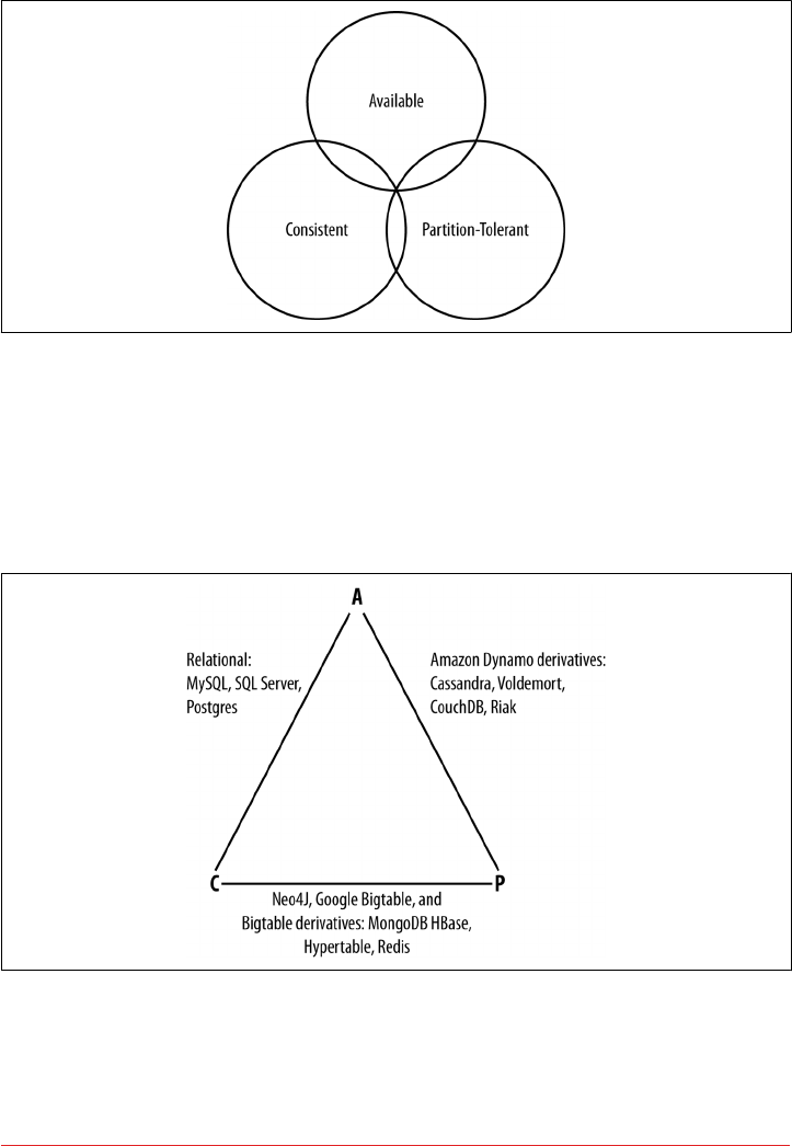
Figure 2-1 illustrates visually that there is no overlapping segment where all three are
obtainable.
Figure 2-1. CAP theorem indicates that you can realize only two of these properties at
once
It might prove useful at this point to see a graphical depiction of where each of the
non-relational data stores we’ll look at falls within the CAP spectrum. The graphic in
Figure 2-2 was inspired by a slide in a 2009 talk given by Dwight Merriman, CEO and
founder of MongoDB, to the MySQL User Group in New York City. However, we
have modified the placement of some systems based on research.
Figure 2-2. Where dierent databases appear on the CAP continuum
Figure 2-2 shows the general focus of some of the different databases we discuss in
this chapter. Note that placement of the databases in this chart could change based on
24 | Chapter 2: Introducing Cassandra

configuration. As Stu Hood points out, a distributed MySQL database can count as a
consistent system only if you’re using Google’s synchronous replication patches;
otherwise, it can only be available and partition tolerant (AP).
It’s interesting to note that the design of the system around CAP placement is inde‐
pendent of the orientation of the data storage mechanism; for example, the CP edge is
populated by graph databases and document-oriented databases alike.
In this depiction, relational databases are on the line between consistency and availa‐
bility, which means that they can fail in the event of a network failure (including a
cable breaking). This is typically achieved by defining a single master server, which
could itself go down, or an array of servers that simply don’t have sufficient mecha‐
nisms built in to continue functioning in the case of network partitions.
Graph databases such as Neo4J and the set of databases derived at least in part from
the design of Google’s Bigtable database (such as MongoDB, HBase, Hypertable, and
Redis) all are focused slightly less on availability and more on ensuring consistency
and partition tolerance.
Finally, the databases derived from Amazon’s Dynamo design include Cassandra,
Project Voldemort, CouchDB, and Riak. These are more focused on availability and
partition tolerance. However, this does not mean that they dismiss consistency as
unimportant, any more than Bigtable dismisses availability. According to the Bigtable
paper, the average percentage of server hours that “some data” was unavailable is
0.0047% (section 4), so this is relative, as we’re talking about very robust systems
already. If you think of each of these letters (C, A, P) as knobs you can tune to arrive
at the system you want, Dynamo derivatives are intended for employment in the
many use cases where “eventual consistency” is tolerable and where “eventual” is a
matter of milliseconds, read repairs mean that reads will return consistent values, and
you can achieve strong consistency if you want to.
So what does it mean in practical terms to support only two of the three facets of
CAP?
CA To primarily support consistency and availability means that you’re likely using
two-phase commit for distributed transactions. It means that the system will
block when a network partition occurs, so it may be that your system is limited to
a single data center cluster in an attempt to mitigate this. If your application
needs only this level of scale, this is easy to manage and allows you to rely on
familiar, simple structures.
CP To primarily support consistency and partition tolerance, you may try to
advance your architecture by setting up data shards in order to scale. Your data
The Cassandra Elevator Pitch | 25

will be consistent, but you still run the risk of some data becoming unavailable if
nodes fail.
AP To primarily support availability and partition tolerance, your system may return
inaccurate data, but the system will always be available, even in the face of net‐
work partitioning. DNS is perhaps the most popular example of a system that is
massively scalable, highly available, and partition tolerant.
Note that this depiction is intended to offer an overview that helps draw distinctions
between the broader contours in these systems; it is not strictly precise. For example,
it’s not entirely clear where Google’s Bigtable should be placed on such a continuum.
The Google paper describes Bigtable as “highly available,” but later goes on to say that
if Chubby (the Bigtable persistent lock service) “becomes unavailable for an extended
period of time [caused by Chubby outages or network issues], Bigtable becomes
unavailable” (section 4). On the matter of data reads, the paper says that “we do not
consider the possibility of multiple copies of the same data, possibly in alternate
forms due to views or indices.” Finally, the paper indicates that “centralized control
and Byzantine fault tolerance are not Bigtable goals” (section 10). Given such variable
information, you can see that determining where a database falls on this sliding scale
is not an exact science.
An Updated Perspective on CAP
In February 2012, Eric Brewer provided an updated perspective on his CAP theorem
in the article “CAP Twelve Years Later: How the ‘Rules’ Have Changed” in IEEE’s
Computer. Brewer now describes the “2 out of 3” axiom as somewhat misleading. He
notes that designers only need sacrifice consistency or availability in the presence of
partitions, and that advances in partition recovery techniques have made it possible
for designers to achieve high levels of both consistency and availability.
These advances in partition recovery certainly would include Cassandra’s usage of
mechanisms such as hinted handoff and read repair. We’ll explore these in Chapter 6.
However, it is important to recognize that these partition recovery mechanisms are
not infallible. There is still immense value in Cassandra’s tuneable consistency, allow‐
ing Cassandra to function effectively in a diverse set of deployments in which it is not
possible to completely prevent partitions.
Row-Oriented
Cassandra’s data model can be described as a partitioned row store, in which data is
stored in sparse multidimensional hashtables. “Sparse” means that for any given row
you can have one or more columns, but each row doesn’t need to have all the same
columns as other rows like it (as in a relational model). “Partitioned” means that each
26 | Chapter 2: Introducing Cassandra

row has a unique key which makes its data accessible, and the keys are used to dis‐
tribute the rows across multiple data stores.
Row-Oriented Versus Column-Oriented
Cassandra has frequently been referred to as a “column-oriented”
database, which has proved to be the source of some confusion. A
column-oriented database is one in which the data is actually
stored by columns, as opposed to relational databases, which store
data in rows. Part of the confusion that occurs in classifying data‐
bases is that there can be a difference between the API exposed by
the database and the underlying storage on disk. So Cassandra is
not really column-oriented, in that its data store is not organized
primarily around columns.
In the relational storage model, all of the columns for a table are defined beforehand
and space is allocated for each column whether it is populated or not. In contrast,
Cassandra stores data in a multidimensional, sorted hash table. As data is stored in
each column, it is stored as a separate entry in the hash table. Column values are
stored according to a consistent sort order, omitting columns that are not populated,
which enables more efficient storage and query processing. We’ll examine Cassandra’s
data model in more detail in Chapter 4.
Is Cassandra “Schema-Free”?
In its early versions. Cassandra was faithful to the original Bigtable whitepaper in
supporting a “schema-free” data model in which new columns can be defined dynam‐
ically. Schema-free databases such as Bigtable and MongoDB have the advantage of
being very extensible and highly performant in accessing large amounts of data. The
major drawback of schema-free databases is the difficulty in determining the meaning
and format of data, which limits the ability to perform complex queries. These disad‐
vantages proved a barrier to adoption for many, especially as startup projects which
benefitted from the initial flexibility matured into more complex enterprises involv‐
ing multiple developers and administrators.
The solution for those users was the introduction of the Cassandra Query Language
(CQL), which provides a way to define schema via a syntax similar to the Structured
Query Language (SQL) familiar to those coming from a relational background. Ini‐
tially, CQL was provided as another interface to Cassandra alongside the schema-free
interface based on the Apache Thrift project. During this transitional phase, the term
“Schema-optional” was used to describe that data models could be defined by schema
using CQL, but could also be dynamically extended to add new columns via the
Thrift API. During this period, the underlying data storage continued to be based on
the Bigtable model.
The Cassandra Elevator Pitch | 27

Starting with the 3.0 release, the Thrift-based API that supported dynamic column
creation has been deprecated, and Cassandra’s underlying storage has been re-
implemented to more closely align with CQL. Cassandra does not entirely limit the
ability to dynamically extend the schema on the fly, but the way it works is signifi‐
cantly different. CQL collections such as lists, sets, and especially maps provide the
ability to add content in a less structured form that can be leveraged to extend an
existing schema. CQL also provides the ability to change the type of columns in cer‐
tain instances, and facilities to support the storage of JSON-formatted text.
So perhaps the best way to describe Cassandra’s current posture is that it supports
“flexible schema.”
High Performance
Cassandra was designed specifically from the ground up to take full advantage of
multiprocessor/multi-core machines, and to run across many dozens of these
machines housed in multiple data centers. It scales consistently and seamlessly to
hundreds of terabytes. Cassandra has been shown to perform exceptionally well
under heavy load. It consistently can show very fast throughput for writes per second
on basic commodity computers, whether physical hardware or virtual machines. As
you add more servers, you can maintain all of Cassandra’s desirable properties
without sacrificing performance.
Where Did Cassandra Come From?
The Cassandra data store is an open source Apache project. Cassandra originated at
Facebook in 2007 to solve its inbox search problem—the company had to deal with
large volumes of data in a way that was difficult to scale with traditional methods.
Specifically, the team had requirements to handle huge volumes of data in the form of
message copies, reverse indices of messages, and many random reads and many
simultaneous random writes.
The team was led by Jeff Hammerbacher, with Avinash Lakshman, Karthik Rangana‐
than, and Facebook engineer on the Search Team Prashant Malik as key engineers.
The code was released as an open source Google Code project in July 2008. During its
tenure as a Google Code project in 2008, the code was updatable only by Facebook
engineers, and little community was built around it as a result. So in March 2009, it
was moved to an Apache Incubator project, and on February 17, 2010, it was voted
into a top-level project. On the Apache Cassandra Wiki, you can find a list of the
committers, many of whom have been with the project since 2010/2011. The commit‐
ters represent companies including Twitter, LinkedIn, Apple, as well as independent
developers.
28 | Chapter 2: Introducing Cassandra

The Paper that Introduced Cassandra to the World
“A Decentralized Structured Storage System” by Facebook’s Laksh‐
man and Malik was a central paper on Cassandra. An updated
commentary on this paper was provided by Jonathan Ellis corre‐
sponding to the 2.0 release, noting changes to the technology since
the transition to Apache. We’ll unpack some of these changes in
more detail in “Release History” on page 30.
How Did Cassandra Get Its Name?
In Greek mythology, Cassandra was the daughter of King Priam and Queen Hecuba
of Troy. Cassandra was so beautiful that the god Apollo gave her the ability to see the
future. But when she refused his amorous advances, he cursed her such that she
would still be able to accurately predict everything that would happen—but no one
would believe her. Cassandra foresaw the destruction of her city of Troy, but was
powerless to stop it. The Cassandra distributed database is named for her. We specu‐
late that it is also named as kind of a joke on the Oracle at Delphi, another seer for
whom a database is named.
As commercial interest in Cassandra grew, the need for production support became
apparent. Jonathan Ellis, the Apache Project Chair for Cassandra, and his colleague
Matt Pfeil formed a services company called DataStax (originally known as Riptano)
in April of 2010. DataStax has provided leadership and support for the Cassandra
project, employing several Cassandra committers.
DataStax provides free products including Cassandra drivers for various languages
and tools for development and administration of Cassandra. Paid product offerings
include enterprise versions of the Cassandra server and tools, integrations with other
data technologies, and product support. Unlike some other open source projects that
have commercial backing, changes are added first to the Apache open source project,
and then rolled into the commercial offering shortly after each Apache release.
DataStax also provides the Planet Cassandra website as a resource to the Cassandra
community. This site is a great location to learn about the ever-growing list of compa‐
nies and organizations that are using Cassandra in industry and academia. Industries
represented run the gamut: financial services, telecommunications, education, social
media, entertainment, marketing, retail, hospitality, transportation, healthcare,
energy, philanthropy, aerospace, defense, and technology. Chances are that you will
find a number of case studies here that are relevant to your needs.
Where Did Cassandra Come From? | 29

Release History
Now that we’ve learned about the people and organizations that have shaped Cassan‐
dra, let’s take a look at how Cassandra has matured through its various releases since
becoming an official Apache project. If you’re new to Cassandra, don’t worry if some
of these concepts and terms are new to you—we’ll dive into them in more depth in
due time. You can return to this list later to get a sense of the trajectory of how Cas‐
sandra has matured over time and its future directions. If you’ve used Cassandra in
the past, this summary will give you a quick primer on what’s changed.
Performance and Reliability Improvements
This list focuses primarily on features that have been added over
the course of Cassandra’s lifespan. This is not to discount the steady
and substantial improvements in reliability and read/write perfor‐
mance.
Release 0.6
This was the first release after Cassandra graduated from the Apache Incubator
to a top-level project. Releases in this series ran from 0.6.0 in April 2010 through
0.6.13 in April 2011. Features in this series included:
•Integration with Apache Hadoop, allowing easy data retrieval from Cassan‐
dra via MapReduce
•Integrated row caching, which helped eliminate the need for applications to
deploy other caching technologies alongside Cassandra
Release 0.7
Releases in this series ran from 0.7.0 in January 2011 through 0.7.10 in October
2011. Key features and improvements included:
• Secondary indexes—that is, indexes on non-primary columns
• Support for large rows, containing up to two billion columns
•Online schema changes, including adding, renaming, and removing keyspa‐
ces and column families in live clusters without a restart, via the Thrift API
•Expiring columns, via specification of a time-to-live (TTL) per column
•The NetworkTopologyStrategy was introduced to support multi-data center
deployments, allowing a separate replication factor per data center, per key‐
space
•Configuration files were converted from XML to the more readable YAML
format
30 | Chapter 2: Introducing Cassandra

Release 0.8
This release began a major shift in Cassandra APIs with the introduction of CQL.
Releases in this series ran from 0.8.0 in June 2011 through 0.8.10 in February
2012. Key features and improvements included:
•Distributed counters were added as a new data type that incrementally
counts up or down
•The sstableloader tool was introduced to support bulk loading of data into
Cassandra clusters
•An off-heap row cache was provided to allow usage of native memory
instead of the JVM heap
•Concurrent compaction allowed for multi-threaded execution and throttling
control of SSTable compaction
•Improved memory configuration parameters allowed more flexible control
over the size of memtables
Release 1.0
In keeping with common version numbering practice, this is officially the first
production release of Cassandra, although many companies were using Cassan‐
dra in production well before this point. Releases in this series ran from 1.0.0 in
October 2011 through 1.0.12 in October 2012. In keeping with the focus on pro‐
duction readiness, improvements focused on performance and enhancements to
existing features:
•CQL 2 added several improvements, including the ability to alter tables and
columns, support for counters and TTL, and the ability to retrieve the count
of items matching a query
•The leveled compaction strategy was introduced as an alternative to the orig‐
inal size-tiered compaction strategy, allowing for faster reads at the expense
of more I/O on writes
•Compression of SSTable files, configurable on a per-table level
Release 1.1
Releases in this series ran from 1.1.0 in April 2011 through 1.1.12 in May 2013.
Key features and improvements included:
•CQL 3 added the timeuuid type, and the ability to create tables with com‐
pound primary keys including clustering keys. Clustering keys support
“order by” semantics to allow sorting. This was a much anticipated feature
that allowed the creation of “wide rows” via CQL.
•Support for importing and exporting comma-separated values (CSV) files
via cqlsh
•Flexible data storage settings allow the storage of data in SSDs or magnetic
storage, selectable by table
Where Did Cassandra Come From? | 31

•The schema update mechanism was reimplemented to allow concurrent
changes and improve reliability. Schema are now stored in tables in the
system keyspace.
•Caching was updated to provide more straightforward configuration of
cache sizes
•A utility to leverage the bulk loader from Hadoop, allowing efficient export
of data from Hadoop to Cassandra
•Row-level isolation was added to assure that when multiple columns are
updated on a write, it is not possible for a read to get a mix of new and old
column values
Release 1.2
Releases in this series ran from 1.2.0 in January 2013 through 1.2.19 in Septem‐
ber 2014. Notable features and improvements included:
•CQL 3 added collection types (sets, lists, and maps), prepared statements,
and a binary protocol as a replacement for Thrift
•Virtual nodes spread data more evenly across the nodes in a cluster, improv‐
ing performance, especially when adding or replacing nodes
•Atomic batches ensure that all writes in a batch succeed or fail as a unit
•The system keyspace contains the local table containing information about
the local node and the peers table describing other nodes in the cluster
•Request tracing can be enabled to allow clients to see the interactions
between nodes for reads and writes. Tracing provides valuable insight into
what is going on behind the scenes and can help developers understand the
implications of various table design options.
• Most data structures were moved off of the JVM heap to native memory
•Disk failure policies allow flexible configuration of behaviors, including
removing a node from the cluster on disk failure or making a best effort to
access data from memory, even if stale
Release 2.0
The 2.0 release was an especially significant milestone in the history of Cassan‐
dra, as it marked the culmination of the CQL capability, as well as a new level of
production maturity. This included significant performance improvements and
cleanup of the codebase to pay down 5 years of accumulated technical debt.
Releases in this series ran from 2.0.0 in September 2013 through 2.0.16 in June
2015. Highlights included:
• Lightweight transactions were added using the Paxos consensus protocol
•CQL3 improvements included the addition of DROP semantics on the
ALTER command, conditional schema modifications (IF EXISTS, IF NOT
32 | Chapter 2: Introducing Cassandra

EXISTS), and the ability to create secondary indexes on primary key col‐
umns
•Native CQL protocol improvements began to make CQL demonstrably more
performant than Thrift
•A prototype implementation of triggers was added, providing an extensible
way to react to write operations. Triggers can be implemented in any JVM
language.
• Java 7 was required for the first time
• Static columns were added in the 2.0.6 release
Release 2.1
Releases in this series ran from 2.1.0 in September 2014 through 2.1.8 in June
2015. Key features and improvements included:
•CQL3 added user-defined types (UDT), and the ability to create secondary
indexes on collections
•Configuration options were added to move memtable data off heap to native
memory
•Row caching was made more configurable to allow setting the number of
cached rows per partition
• Counters were re-implemented to improve performance and reliability
Release 2.2
The original release plan outlined by the Cassandra developers did not contain a
2.2 release. The intent was to do some major “under the covers” rework for a 3.0
release to follow the 2.1 series. However, due to the amount and complexity of
the changes involved, it was decided to release some of completed features sepa‐
rately in order to make them available while allowing some of the more complex
changes time to mature. Release 2.2.0 became available in July 2015, and support
releases are scheduled through fall 2016. Notable features and improvements in
this series included:
•CQL3 improvements, including support for JSON-formatted input/output
and user-defined functions
•With this release, Windows became a fully supported operating system.
Although Cassandra still performs best on Linux systems, improvements in
file I/O and scripting have made it much easier to run Cassandra on Win‐
dows.
•The Date Tiered Compaction Strategy (DTCS) was introduced to improve
performance of time series data
Where Did Cassandra Come From? | 33

•Role-based access control (RBAC) was introduced to allow more flexible
management of authorization
Tick-Tock Releases
In June 2015, the Cassandra team announced plans to adopt a tick-tock release model
as part of increased emphasis on improving agility and the quality of releases.
The tick-tock release model popularized by Intel was originally intended for chip
design, and referred to changing chip architecture and production processes in alter‐
nate builds. You can read more about this approach at http://www.intel.com/
content/www/us/en/silicon-innovations/intel-tick-tock-model-general.html.
The tick-tock approach has proven to be useful in software development as well.
Starting with the Cassandra 3.0 release, even-numbered releases are feature releases
with some bug fixes, while odd-numbered releases are focused on bug fixes, with the
goal of releasing each month.
Release 3.0 (Feature release - November 2015)
•The underlying storage engine was rewritten to more closely match CQL con‐
structs
• Support for materialized views (sometimes also called global indexes) was added
• Java 8 is now the supported version
• The Thrift-based command-line interface (CLI) was removed
Release 3.1 (Bug x release - December 2015)
Release 3.2 (Feature release - January 2016)
•The way in which Cassandra allocates SSTable file storage across multiple disk in
“just a bunch of disks” or JBOD configurations was reworked to improve reliabil‐
ity and performance and to enable backup and restore of individual disks
• The ability to compress and encrypt hints was added
Release 3.3 (Bug x release - February 2016)
Release 3.4 (Feature release - March 2016)
•SSTableAttachedSecondaryIndex, or “SASI” for short, is an implementation of
Cassandra’s SecondaryIndex interface that can be used as an alternative to the
existing implementations.
Release 3.5 (Bug x release - April 2016)
The 4.0 release series is scheduled to begin in Fall 2016.
34 | Chapter 2: Introducing Cassandra

As you will have noticed, the trends in these releases include:
• Continuous improvement in the capabilities of CQL
•A growing list of clients for popular languages built on a common set of
metaphors
•Exposure of configuration options to tune performance and optimize resource
usage
• Performance and reliability improvements, and reduction of technical debt
Supported Releases
There are two officially supported releases of Cassandra at any one
time: the latest stable release, which is considered appropriate for
production, and the latest development release. You can see the
officially supported versions on the project’s download page.
Users of Cassandra are strongly recommended to track the latest
stable release in production. Anecdotally, a substantial majority of
issues and questions posted to the Cassandra-users email list per‐
tain to releases that are no longer supported. Cassandra experts are
very gracious in answering questions and diagnosing issues with
these unsupported releases, but more often than not the recom‐
mendation is to upgrade as soon as possible to a release that
addresses the issue.
Is Cassandra a Good Fit for My Project?
We have now unpacked the elevator pitch and have an understanding of Cassandra’s
advantages. Despite Cassandra’s sophisticated design and smart features, it is not the
right tool for every job. So in this section, let’s take a quick look at what kind of
projects Cassandra is a good fit for.
Large Deployments
You probably don’t drive a semitruck to pick up your dry cleaning; semis aren’t well
suited for that sort of task. Lots of careful engineering has gone into Cassandra’s high
availability, tuneable consistency, peer-to-peer protocol, and seamless scaling, which
are its main selling points. None of these qualities is even meaningful in a single-node
deployment, let alone allowed to realize its full potential.
There are, however, a wide variety of situations where a single-node relational data‐
base is all we may need. So do some measuring. Consider your expected traffic,
throughput needs, and SLAs. There are no hard-and-fast rules here, but if you expect
that you can reliably serve traffic with an acceptable level of performance with just a
Is Cassandra a Good Fit for My Project? | 35

few relational databases, it might be a better choice to do so, simply because RDBMSs
are easier to run on a single machine and are more familiar.
If you think you’ll need at least several nodes to support your efforts, however, Cas‐
sandra might be a good fit. If your application is expected to require dozens of nodes,
Cassandra might be a great fit.
Lots of Writes, Statistics, and Analysis
Consider your application from the perspective of the ratio of reads to writes. Cassan‐
dra is optimized for excellent throughput on writes.
Many of the early production deployments of Cassandra involve storing user activity
updates, social network usage, recommendations/reviews, and application statistics.
These are strong use cases for Cassandra because they involve lots of writing with less
predictable read operations, and because updates can occur unevenly with sudden
spikes. In fact, the ability to handle application workloads that require high perfor‐
mance at significant write volumes with many concurrent client threads is one of the
primary features of Cassandra.
According to the project wiki, Cassandra has been used to create a variety of applica‐
tions, including a windowed time-series store, an inverted index for document
searching, and a distributed job priority queue.
Geographical Distribution
Cassandra has out-of-the-box support for geographical distribution of data. You can
easily configure Cassandra to replicate data across multiple data centers. If you have a
globally deployed application that could see a performance benefit from putting the
data near the user, Cassandra could be a great fit.
Evolving Applications
If your application is evolving rapidly and you’re in “startup mode,” Cassandra might
be a good fit given its support for flexible schemas. This makes it easy to keep your
database in step with application changes as you rapidly deploy.
Getting Involved
The strength and relevance of any technology depend on the investment of individu‐
als in a vibrant community environment. Thankfully, the Cassandra community is
active and healthy, offering a number of ways for you to participate. We’ll start with a
few steps in Chapter 3 such as downloading Cassandra and building from the source.
Here are a few other ways to get involved:
36 | Chapter 2: Introducing Cassandra

Chat
Many of the Cassandra developers and community members hang out in the
#cassandra channel on webchat.freenode.net. This informal environment is a
great place to get your questions answered or offer up some answers of your own.
Mailing lists
The Apache project hosts several mailing lists to which you can subscribe to learn
about various topics of interest:
•user@cassandra.apache.org provides a general discussion list for users and is
frequently used by new users or those needing assistance.
•dev@cassandra.apache.org is used by developers to discuss changes, prioritize
work, and approve releases.
•client-dev@cassandra.apache.org is used for discussion specific to develop‐
ment of Cassandra clients for various programming languages.
•commits@cassandra.apache.org tracks Cassandra code commits. This is a
fairly high volume list and is primarily of interest to committers.
Releases are typically announced to both the developer and user mailing lists.
Issues
If you encounter issues using Cassandra and feel you have discovered a defect,
you should feel free to submit an issue to the Cassandra JIRA. In fact, users who
identify defects on the user@cassandra.apache.org list are frequently encouraged
to create JIRA issues.
Blogs
The DataStax developer blog features posts on using Cassandra, announcements
of Apache Cassandra and DataStax product releases, as well as occasional deep-
dive technical articles on Cassandra implementation details and features under
development. The Planet Cassandra blog provides similar technical content, but
has a greater focus on profiling companies using Cassandra.
The Apache Cassandra Wiki provides helpful articles on getting started and con‐
figuration, but note that some content may not be fully up to date with current
releases.
Meetups
A meetup group is a local community of people who meet face to face to discuss
topics of common interest. These groups provide an excellent opportunity to
network, learn, or share your knowledge by offering a presentation of your own.
There are Cassandra meetups on every continent, so you stand a good chance of
being able to find one in your area.
Getting Involved | 37

Training and conferences
DataStax offers online training, and in June 2015 announced a partnership with
O’Reilly Media to produce Cassandra certifications. DataStax also hosts annual
Cassandra Summits in locations around the world.
A Marketable Skill
There continues to be increased demand for Cassandra developers
and administrators. A 2015 Dice.com salary survey placed Cassan‐
dra as the second most highly compensated skill set.
Summary
In this chapter, we’ve taken an introductory look at Cassandra’s defining characteris‐
tics, history, and major features. We have learned about the Cassandra user commu‐
nity and how companies are using Cassandra. Now we’re ready to start getting some
hands-on experience.
38 | Chapter 2: Introducing Cassandra

CHAPTER 3
Installing Cassandra
For those among us who like instant gratification, we’ll start by installing Cassandra.
Because Cassandra introduces a lot of new vocabulary, there might be some unfami‐
liar terms as we walk through this. That’s OK; the idea here is to get set up quickly in
a simple configuration to make sure everything is running properly. This will serve as
an orientation. Then, we’ll take a step back and understand Cassandra in its larger
context.
Installing the Apache Distribution
Cassandra is available for download from the Web at http://cassandra.apache.org. Just
click the link on the home page to download a version as a gzipped tarball. Typically
two versions of Cassandra are provided. The latest release is recommended for those
starting new projects not yet in production. The most stable release is the one recom‐
mended for production usage. For all releases, the prebuilt binary is named apache-
cassandra-x.x.x-bin.tar.gz, where x.x.x represents the version number. The download
is around 23MB.
Extracting the Download
The simplest way to get started is to download the prebuilt binary. You can unpack
the compressed file using any regular ZIP utility. On Unix-based systems such as
Linux or MacOS, GZip extraction utilities should be preinstalled; on Windows, you’ll
need to get a program such as WinZip, which is commercial, or something like 7-Zip,
which is freeware.
Open your extracting program. You might have to extract the ZIP file and the TAR
file in separate steps. Once you have a folder on your filesystem called apache-
cassandra-x.x.x, you’re ready to run Cassandra.
39

What’s In There?
Once you decompress the tarball, you’ll see that the Cassandra binary distribution
includes several files and directories.
The files include the NEWS.txt file, which includes the release notes describing fea‐
tures included in the current and prior releases, and the CHANGES.txt, which is simi‐
lar but focuses on bug fixes. You’ll want to make sure to review these files whenever
you are upgrading to a new version so you know what changes to expect.
Let’s take a moment to look around in the directories and see what we have.
bin This directory contains the executables to run Cassandra as well as clients,
including the query language shell (cqlsh) and the command-line interface
(CLI) client. It also has scripts to run the nodetool, which is a utility for inspect‐
ing a cluster to determine whether it is properly configured, and to perform a
variety of maintenance operations. We look at nodetool in depth later. The direc‐
tory also contains several utilities for performing operations on SSTables, includ‐
ing listing the keys of an SSTable (sstablekeys), bulk extraction and restoration
of SSTable contents (sstableloader), and upgrading SSTables to a new version
of Cassandra (sstableupgrade).
confThis directory contains the files for configuring your Cassandra instance. The
required configuration files include: the cassandra.yaml file, which is the primary
configuration for running Cassandra; and the logback.xml file, which lets you
change the logging settings to suit your needs. Additional files can optionally be
used to configure the network topology, archival and restore commands, and
triggers. We see how to use these configuration files when we discuss configura‐
tion in Chapter 7.
interface
This directory contains a single file, called cassandra.thri. This file defines a leg‐
acy Remote Procedure Call (RPC) API based on the Thrift syntax. The Thrift
interface was used to create clients in Java, C++, PHP, Ruby, Python, Perl, and C#
prior to the creation of CQL. The Thrift API has been officially marked as depre‐
cated in the 3.2 release and will be deleted in the 4.0 release.
javadoc
This directory contains a documentation website generated using Java’s JavaDoc
tool. Note that JavaDoc reflects only the comments that are stored directly in the
Java code, and as such does not represent comprehensive documentation. It’s
helpful if you want to see how the code is laid out. Moreover, Cassandra is a
wonderful project, but the code contains relatively few comments, so you might
40 | Chapter 3: Installing Cassandra

find the JavaDoc’s usefulness limited. It may be more fruitful to simply read the
class files directly if you’re familiar with Java. Nonetheless, to read the JavaDoc,
open the javadoc/index.html file in a browser.
lib This directory contains all of the external libraries that Cassandra needs to run.
For example, it uses two different JSON serialization libraries, the Google collec‐
tions project, and several Apache Commons libraries.
pylib
This directory contains Python libraries that are used by cqlsh.
toolsThis directory contains tools that are used to maintain your Cassandra nodes.
We’ll look at these tools in Chapter 11.
Additional Directories
If you’ve already run Cassandra using the default configuration,
you will notice two additional directories under the main Cassan‐
dra directory: data and log. We’ll discuss the contents of these
directories momentarily.
Building from Source
Cassandra uses Apache Ant for its build scripting language and Maven for depend‐
ency management.
Downloading Ant
You can download Ant from http://ant.apache.org. You don’t need
to download Maven separately just to build Cassandra.
Building from source requires a complete Java 7 or 8 JDK, not just the JRE. If you see
a message about how Ant is missing tools.jar, either you don’t have the full JDK or
you’re pointing to the wrong path in your environment variables. Maven downloads
files from the Internet so if your connection is invalid or Maven cannot determine the
proxy, the build will fail.
Building from Source | 41

Downloading Development Builds
If you want to download the most cutting-edge builds, you can get
the source from Jenkins, which the Cassandra project uses as its
Continuous Integration tool. See http://cassci.datastax.com for the
latest builds and test coverage information.
If you are a Git fan, you can get a read-only trunk version of the Cassandra source
using this command:
$ git clone git://git.apache.org/cassandra.git
What Is Git?
Git is a source code management system created by Linus Torvalds
to manage development of the Linux kernel. It’s increasingly popu‐
lar and is used by projects such as Android, Fedora, Ruby on Rails,
Perl, and many Cassandra clients (as we’ll see in Chapter 8). If
you’re on a Linux distribution such as Ubuntu, it couldn’t be easier
to get Git. At a console, just type >apt-get install git and it will be
installed and ready for commands. For more information, visit
http://git-scm.com.
Because Maven takes care of all the dependencies, it’s easy to build Cassandra once
you have the source. Just make sure you’re in the root directory of your source down‐
load and execute the ant program, which will look for a file called build.xml in the
current directory and execute the default build target. Ant and Maven take care of the
rest. To execute the Ant program and start compiling the source, just type:
$ ant
That’s it. Maven will retrieve all of the necessary dependencies, and Ant will build the
hundreds of source files and execute the tests. If all went well, you should see a BUILD
SUCCESSFUL message. If all did not go well, make sure that your path settings are all
correct, that you have the most recent versions of the required programs, and that
you downloaded a stable Cassandra build. You can check the Jenkins report to make
sure that the source you downloaded actually can compile.
More Build Output
If you want to see detailed information on what is happening dur‐
ing the build, you can pass Ant the -v option to cause it to output
verbose details regarding each operation it performs.
42 | Chapter 3: Installing Cassandra

Additional Build Targets
To compile the server, you can simply execute ant as shown previously. This com‐
mand executes the default target, jar. This target will perform a complete build
including unit tests and output a file into the build directory called apache-cassandra-
x.x.x.jar.
If you want to see a list of all of the targets supported by the build file, simply pass
Ant the -p option to get a description of each target. Here are a few others you might
be interested in:
test Users will probably find this the most helpful, as it executes the battery of unit
tests. You can also check out the unit test sources themselves for some useful
examples of how to interact with Cassandra.
stress-build
This target builds the Cassandra stress tool, which we will try out in Chapter 12.
clean
This target removes locally created artifacts such as generated source files and
classes and unit test results. The related target realclean performs a clean and
additionally removes the Cassandra distribution JAR files and JAR files downloa‐
ded by Maven.
Running Cassandra
In earlier versions of Cassandra, before you could start the server there were some
required steps to edit configuration files and set environment variables. But the devel‐
opers have done a terrific job of making it very easy to start using Cassandra immedi‐
ately. We’ll note some of the available configuration options as we go.
Required Java Version
Cassandra requires a Java 7 or 8 JVM, preferably the latest stable
version. It has been tested on both the Open JDK and Oracle’s JDK.
You can check your installed Java version by opening a command
prompt and executing java -version. If you need a JDK, you can
get one at http://www.oracle.com/technetwork/java/javase/down‐
loads/index.html.
Running Cassandra | 43

On Windows
Once you have the binary or the source downloaded and compiled, you’re ready to
start the database server.
Setting the JAVA_HOME environment variable is recommended. To do this on
Windows 7, click the Start button and then right-click on Computer. Click Advanced
System Settings, and then click the Environment Variables... button. Click New... to
create a new system variable. In the Variable Name field, type JAVA_HOME. In the Vari‐
able Value field, type the path to your Java installation. This is probably something
like C:\Program Files\Java\jre7 if running Java 7 or C:\Program Files\Java\jre1.8.0_25
if running Java 8.
Remember that if you create a new environment variable, you’ll need to reopen any
currently open terminals in order for the system to become aware of the new variable.
To make sure your environment variable is set correctly and that Cassandra can sub‐
sequently find Java on Windows, execute this command in a new terminal: echo
%JAVA_HOME%. This prints the value of your environment variable.
You can also define an environment variable called CASSANDRA_HOME that points to the
top-level directory where you have placed or built Cassandra, so you don’t have to
pay as much attention to where you’re starting Cassandra from. This is useful for
other tools besides the database server, such as nodetool and cqlsh.
Once you’ve started the server for the first time, Cassandra will add directories to
your system to store its data files. The default configuration creates these directories
under the CASSANDRA_HOME directory.
dataThis directory is where Cassandra stores its data. By default, there are three sub-
directories under the data directory, corresponding to the various data files Cas‐
sandra uses: commitlog, data, and saved_caches. We’ll explore the significance of
each of these data files in Chapter 6. If you’ve been trying different versions of the
database and aren’t worried about losing data, you can delete these directories
and restart the server as a last resort.
logs This directory is where Cassandra stores its logs in a file called system.log. If you
encounter any difficulties, consult the log to see what might have happened.
44 | Chapter 3: Installing Cassandra
Data File Locations
The data file locations are configurable in the cassandra.yaml file,
located in the conf directory. The properties are called
data_file_directories, commit_log_directory, and saved_
caches_directory. We’ll discuss the recommended configuration
of these directories in Chapter 7.
On Linux
The process on Linux and other *nix operating systems (including Mac OS) is similar
to that on Windows. Make sure that your JAVA_HOME variable is properly set, accord‐
ing to the earlier description. Then, you need to extract the Cassandra gzipped tarball
using gunzip. Many users prefer to use the /var/lib directory for data storage. If you
are changing this configuration, you will need to edit the conf/cassandra.yaml file and
create the referenced directories for Cassandra to store its data and logs, making sure
to configure write permissions for the user that will be running Cassandra:
$ sudo mkdir -p /var/lib/cassandra
$ sudo chown -R username /var/lib/cassandra
Instead of username, substitute your own username, of course.
Starting the Server
To start the Cassandra server on any OS, open a command prompt or terminal win‐
dow, navigate to the <cassandra-directory>/bin where you unpacked Cassandra, and
run the command cassandra -f to start your server.
Starting Cassandra in the Foreground
Using the -f switch tells Cassandra to stay in the foreground
instead of running as a background process, so that all of the server
logs will print to standard out and you can see them in your termi‐
nal window, which is useful for testing. In either case, the logs will
append to the system.log file, described earlier.
In a clean installation, you should see quite a few log statements as the server gets
running. The exact syntax of logging statements will vary depending on the release
you’re using, but there are a few highlights we can look for. If you search for “cassan‐
dra.yaml”, you’ll quickly run into the following:
DEBUG [main] 2015-12-08 06:02:38,677 YamlConfigurationLoader.java:104 -
Loading settings from file:/.../conf/cassandra.yaml
INFO [main] 2015-12-08 06:02:38,781 YamlConfigurationLoader.java:179 -
Node configuration:[authenticator=AllowAllAuthenticator;
Running Cassandra | 45

authorizer=AllowAllAuthorizer; auto_bootstrap=false; auto_snapshot=true;
batch_size_fail_threshold_in_kb=50; ...
These log statements indicate the location of the cassandra.yaml file containing the
configured settings. The Node configuration statement lists out the settings from
the config file.
Now search for “JVM” and you’ll find something like this:
INFO [main] 2015-12-08 06:02:39,239 CassandraDaemon.java:436 -
JVM vendor/version: Java HotSpot(TM) 64-Bit Server VM/1.8.0_60
INFO [main] 2015-12-08 06:02:39,239 CassandraDaemon.java:437 -
Heap size: 519045120/519045120
These log statements provide information describing the JVM being used, including
memory settings.
Next, search for versions in use—“Cassandra version”, “Thrift API Version”, “CQL
supported versions”:
INFO [main] 2015-12-08 06:02:43,931 StorageService.java:586 -
Cassandra version: 3.0.0
INFO [main] 2015-12-08 06:02:43,932 StorageService.java:587 -
Thrift API version: 20.1.0
INFO [main] 2015-12-08 06:02:43,932 StorageService.java:588 -
CQL supported versions: 3.3.1 (default: 3.3.1)
We can also find statements where Cassandra is initializing internal data structures
such as caches:
INFO [main] 2015-12-08 06:02:43,633 CacheService.java:115 -
Initializing key cache with capacity of 24 MBs.
INFO [main] 2015-12-08 06:02:43,679 CacheService.java:137 -
Initializing row cache with capacity of 0 MBs
INFO [main] 2015-12-08 06:02:43,686 CacheService.java:166 -
Initializing counter cache with capacity of 12 MBs
If we search for terms like “JMX”, “gossip”, and “clients”, we can find statements like
the following:
WARN [main] 2015-12-08 06:08:06,078 StartupChecks.java:147 -
JMX is not enabled to receive remote connections.
Please see cassandra-env.sh for more info.
INFO [main] 2015-12-08 06:08:18,463 StorageService.java:790 -
Starting up server gossip
INFO [main] 2015-12-08 06:02:48,171 Server.java:162 -
Starting listening for CQL clients on /127.0.0.1:9042 (unencrypted)
These log statements indicate the server is beginning to initiate communications with
other servers in the cluster and expose publicly available interfaces. By default, the
management interface via the Java Management Extensions (JMX) is disabled for
remote access. We’ll explore the management interface in Chapter 10.
46 | Chapter 3: Installing Cassandra

Finally, search for “state jump” and you’ll see the following:
INFO [main] 2015-12-08 06:02:47,351 StorageService.java:1936 -
Node /127.0.0.1 state jump to normal
Congratulations! Now your Cassandra server should be up and running with a new
single node cluster called Test Cluster listening on port 9160. If you continue to mon‐
itor the output, you’ll begin to see periodic output such as memtable flushing and
compaction, which we’ll learn about soon.
Starting Over
The committers work hard to ensure that data is readable from one
minor dot release to the next and from one major version to the
next. The commit log, however, needs to be completely cleared out
from version to version (even minor versions).
If you have any previous versions of Cassandra installed, you may
want to clear out the data directories for now, just to get up and
running. If you’ve messed up your Cassandra installation and want
to get started cleanly again, you can delete the data folders.
Stopping Cassandra
Now that we’ve successfully started a Cassandra server, you may be wondering how to
stop it. You may have noticed the stop-server command in the bin directory. Let’s
try running that command. Here’s what you’ll see on Unix systems:
$ ./stop-server
please read the stop-server script before use
So you see that our server has not been stopped, but instead we are directed to read
the script. Taking a look inside with our favorite code editor, you’ll learn that the way
to stop Cassandra is to kill the JVM process that is running Cassandra. The file sug‐
gests a couple of different techniques by which you can identify the JVM process and
kill it.
The first technique is to start Cassandra using the -p option, which provides Cassan‐
dra with the name of a file to which it should write the process identifier (PID) upon
starting up. This is arguably the most straightforward approach to making sure we
kill the right process.
However, because we did not start Cassandra with the -p option, we’ll need to find
the process ourselves and kill it. The script suggests using pgrep to locate processes
for the current user containing the term “cassandra”:
user=`whoami`
pgrep -u $user -f cassandra | xargs kill -9
Running Cassandra | 47

Stopping Cassandra on Windows
On Windows installations, you can find the JVM process and kill it
using the Task Manager.
Other Cassandra Distributions
The instructions we just reviewed showed us how to install the Apache distribution of
Cassandra. In addition to the Apache distribution, there are a couple of other ways to
get Cassandra:
DataStax Community Edition
This free distribution is provided by DataStax via the Planet Cassandra website.
Installation options for various platforms include RPM and Debian (Linux), MSI
(Windows), and a MacOS library. The community edition provides additional
tools, including an integrated development environment (IDE) known as Dev‐
Center, and the OpsCenter monitoring tool. Another useful feature is the ability
to configure Cassandra as an OS-managed service on Windows. Releases of the
community edition generally track the Apache releases, with availability soon
after each Apache release.
DataStax Enterprise Edition
DataStax also provides a fully supported version certified for production use. The
product line provides an integrated database platform with support for comple‐
mentary data technologies such as Hadoop and Apache Spark. We’ll explore
some of these integrations in Chapter 14.
Virtual machine images
A frequent model for deployment of Cassandra is to package one of the preced‐
ing distributions in a virtual machine image. For example, multiple such images
are available in the Amazon Web Services (AWS) Marketplace.
We’ll take a deeper look at several options for deploying Cassandra in production
environments, including cloud computing environments, in Chapter 14.
Selecting the right distribution will depend on your deployment environment; your
needs for scale, stability, and support; and your development and maintenance budg‐
ets. Having both open source and commercial deployment options provides the flexi‐
bility to make the right choice for your organization.
48 | Chapter 3: Installing Cassandra

Running the CQL Shell
Now that you have a Cassandra installation up and running, let’s give it a quick try to
make sure everything is set up properly. We’ll use the CQL shell (cqlsh) to connect to
our server and have a look around.
Deprecation of the CLI
If you’ve used Cassandra in releases prior to 3.0, you may also be
familiar with the command-line client interface known as
cassandra-cli. The CLI was removed in the 3.0 release because it
depends on the legacy Thrift API.
To run the shell, create a new terminal window, change to the Cassandra home direc‐
tory, and type the following command (you should see output similar to that shown
here):
$ bin/cqlsh
Connected to Test Cluster at 127.0.0.1:9042.
[cqlsh 5.0.1 | Cassandra 3.0.0 | CQL spec 3.3.1 | Native protocol v4]
Use HELP for help.
cqlsh>
Because we did not specify a node to which we wanted to connect, the shell helpfully
checks for a node running on the local host, and finds the node we started earlier. The
shell also indicates that you’re connected to a Cassandra server cluster called “Test
Cluster”. That’s because this cluster of one node at localhost is set up for you by
default.
Renaming the Default Cluster
In a production environment, be sure to change the cluster name
to something more suitable to your application.
To connect to a specific node, specify the hostname and port on the command line.
For example, the following will connect to our local node:
$ bin/cqlsh localhost 9042
Another alternative for configuring the cqlsh connection is to set the environment
variables $CQLSH_HOST and $CQLSH_PORT. This approach is useful if you will be fre‐
quently connecting to a specific node on another host. The environment variables
will be overriden if you specify the host and port on the command line.
Running the CQL Shell | 49
Connection Errors
Have you run into an error like this while trying to connect to a
server?
Exception connecting to localhost/9160. Reason:
Connection refused.
If so, make sure that a Cassandra instance is started at that host and
port, and that you can ping the host you’re trying to reach. There
may be firewall rules preventing you from connecting.
To see a complete list of the command-line options supported by cqlsh, type the
command cqlsh -help.
Basic cqlsh Commands
Let’s take a quick tour of cqlsh to learn what kinds of commands you can send to the
server. We’ll see how to use the basic environment commands and how to do a
round-trip of inserting and retrieving some data.
Case in cqlsh
The cqlsh commands are all case insensitive. For our examples,
we’ll adopt the convention of uppercase to be consistent with the
way the shell describes its own commands in help topics and out‐
put.
cqlsh Help
To get help for cqlsh, type HELP or ? to see the list of available commands:
cqlsh> HELP
Documented shell commands:
===========================
CAPTURE COPY DESCRIBE EXPAND PAGING SOURCE
CONSISTENCY DESC EXIT HELP SHOW TRACING
CQL help topics:
================
ALTER CREATE_TABLE_TYPES PERMISSIONS
ALTER_ADD CREATE_USER REVOKE
ALTER_ALTER DATE_INPUT REVOKE_ROLE
ALTER_DROP DELETE SELECT
ALTER_RENAME DELETE_COLUMNS SELECT_COLUMNFAMILY
ALTER_USER DELETE_USING SELECT_EXPR
ALTER_WITH DELETE_WHERE SELECT_LIMIT
APPLY DROP SELECT_TABLE
ASCII_OUTPUT DROP_AGGREGATE SELECT_WHERE
50 | Chapter 3: Installing Cassandra

BEGIN DROP_COLUMNFAMILY TEXT_OUTPUT
BLOB_INPUT DROP_FUNCTION TIMESTAMP_INPUT
BOOLEAN_INPUT DROP_INDEX TIMESTAMP_OUTPUT
COMPOUND_PRIMARY_KEYS DROP_KEYSPACE TIME_INPUT
CREATE DROP_ROLE TRUNCATE
CREATE_AGGREGATE DROP_TABLE TYPES
CREATE_COLUMNFAMILY DROP_USER UPDATE
CREATE_COLUMNFAMILY_OPTIONS GRANT UPDATE_COUNTERS
CREATE_COLUMNFAMILY_TYPES GRANT_ROLE UPDATE_SET
CREATE_FUNCTION INSERT UPDATE_USING
CREATE_INDEX INT_INPUT UPDATE_WHERE
CREATE_KEYSPACE LIST USE
CREATE_ROLE LIST_PERMISSIONS UUID_INPUT
CREATE_TABLE LIST_ROLES
CREATE_TABLE_OPTIONS LIST_USERS
cqlsh Help Topics
You’ll notice that the help topics listed differ slightly from the
actual command syntax. The CREATE_TABLE help topic describes
how to use the syntax > CREATE TABLE ..., for example.
To get additional documentation about a particular command, type HELP <command>.
Many cqlsh commands may be used with no parameters, in which case they print
out the current setting. Examples include CONSISTENCY, EXPAND, and PAGING.
Describing the Environment in cqlsh
After connecting to your Cassandra instance Test Cluster, if you’re using the binary
distribution, an empty keyspace, or Cassandra database, is set up for you to test with.
To learn about the current cluster you’re working in, type:
cqlsh> DESCRIBE CLUSTER;
Cluster: Test Cluster
Partitioner: Murmur3Partitioner
...
For releases 3.0 and later, this command also prints out a list of token ranges owned
by each node in the cluster, which have been omitted here for brevity.
To see which keyspaces are available in the cluster, issue this command:
cqlsh> DESCRIBE KEYSPACES;
system_auth system_distributed system_schema
system system_traces
Initially this list will consist of several system keyspaces. Once you have created your
own keyspaces, they will be shown as well. The system keyspaces are managed inter‐
nally by Cassandra, and aren’t for us to put data into. In this way, these keyspaces are
Basic cqlsh Commands | 51

similar to the master and temp databases in Microsoft SQL Server. Cassandra uses
these keyspaces to store the schema, tracing, and security information. We’ll learn
more about these keyspaces in Chapter 6.
You can use the following command to learn the client, server, and protocol versions
in use:
cqlsh> SHOW VERSION;
[cqlsh 5.0.1 | Cassandra 3.0.0 | CQL spec 3.3.1 | Native protocol v4]
You may have noticed that this version info is printed out when cqlsh starts. There
are a variety of other commands with which you can experiment. For now, let’s add
some data to the database and get it back out again.
Creating a Keyspace and Table in cqlsh
A Cassandra keyspace is sort of like a relational database. It defines one or more
tables or “column families.” When you start cqlsh without specifying a keyspace, the
prompt will look like this: cqlsh>, with no keyspace specified.
Let’s create our own keyspace so we have something to write data to. In creating our
keyspace, there are some required options. To walk through these options, we could
use the command HELP CREATE_KEYSPACE, but instead we’ll use the helpful
command-completion features of cqlsh. Type the following and then hit the Tab key:
cqlsh> CREATE KEYSPACE my_keyspace WITH
When you hit the Tab key, cqlsh begins completing the syntax of our command:
cqlsh> CREATE KEYSPACE my_keyspace WITH replication = {'class': '
This is informing us that in order to specify a keyspace, we also need to specify a rep‐
lication strategy. Let’s Tab again to see what options we have:
cqlsh> CREATE KEYSPACE my_keyspace WITH replication = {'class': '
NetworkTopologyStrategy SimpleStrategy
OldNetworkTopologyStrategy
Now cqlsh is giving us three strategies to choose from. We’ll learn more about these
strategies in Chapter 6. For now, we will choose the SimpleStrategy by typing the
name. We’ll indicate we’re done with a closing quote and Tab again:
cqlsh> CREATE KEYSPACE my_keyspace WITH replication = {'class':
'SimpleStrategy', 'replication_factor':
The next option we’re presented with is a replication factor. For the simple strategy,
this indicates how many nodes the data in this keyspace will be written to. For a pro‐
duction deployment, we’d want copies of our data stored on multiple nodes, but
because we’re just running a single node at the moment, we’ll ask for a single copy.
Let’s specify a value of “1” and Tab again:
52 | Chapter 3: Installing Cassandra

cqlsh> CREATE KEYSPACE my_keyspace WITH replication = {'class':
'SimpleStrategy', 'replication_factor': 1};
We see that cqlsh has now added a closing bracket, indicating we’ve completed all of
the required options. Let’s complete our command with a semicolon and return, and
our keyspace will be created.
Keyspace Creation Options
For a production keyspace, we would probably never want to use a
value of 1 for the replication factor. There are additional options on
creating a keyspace depending on the replication strategy that is
chosen. The command completion feature will walk through the
different options.
Let’s have a look at our keyspace using theDESCRIBE KEYSPACE command:
cqlsh> DESCRIBE KEYSPACE my_keyspace
CREATE KEYSPACE my_keyspace WITH replication = {'class':
'SimpleStrategy', 'replication_factor': '1'} AND
durable_writes = true;
We see that the table has been created with the SimpleStrategy, a replication_fac
tor of one, and durable writes. Notice that our keyspace is described in much the
same syntax that we used to create it, with one additional option that we did not spec‐
ify: durable_writes = true. Don’t worry about these settings now; we’ll look at
them in detail later.
After you have created your own keyspace, you can switch to it in the shell by typing:
cqlsh> USE my_keyspace;
cqlsh:my_keyspace>
Notice that the prompt has changed to indicate that we’re using the keyspace.
Using Snake Case
You may have wondered why we chose to name our keyspace in “snake case”
(my_keyspace) as opposed to “camel case” (MyKeyspace), which is familiar to devel‐
opers using Java and other languages.
As it turns out, Cassandra naturally handles keyspace, table, and column names as
lowercase. When you enter names in mixed case, Cassandra stores them as all lower‐
case.
This behavior can be overridden by enclosing your names in double quotes (e.g.,
CREATE KEYSPACE "MyKeyspace"...). However, it tends to be a lot simpler to use
snake case than to go against the grain.
Basic cqlsh Commands | 53

Now that we have a keyspace, we can create a table in our keyspace. To do this in
cqlsh, use the following command:
cqlsh:my_keyspace> CREATE TABLE user ( first_name text ,
last_name text, PRIMARY KEY (first_name)) ;
This creates a new table called “user” in our current keyspace with two columns to
store first and last names, both of type text. The text and varchar types are synony‐
mous and are used to store strings. We’ve specified the first_name column as our
primary key and taken the defaults for other table options.
Using Keyspace Names in cqlsh
We could have also created this table without switching to our key‐
space by using the syntax CREATE TABLE my_keyspace.user (... .
We can use cqlsh to get a description of a the table we just created using the
DESCRIBE TABLE command:
cqlsh:my_keyspace> DESCRIBE TABLE user;
CREATE TABLE my_keyspace.user (
first_name text PRIMARY KEY,
last_name text
) WITH bloom_filter_fp_chance = 0.01
AND caching = {'keys': 'ALL', 'rows_per_partition': 'NONE'}
AND comment = ''
AND compaction = {'class': 'org.apache.cassandra.db.compaction.
SizeTieredCompactionStrategy', 'max_threshold': '32',
'min_threshold': '4'}
AND compression = {'chunk_length_in_kb': '64', 'class':
'org.apache.cassandra.io.compress.LZ4Compressor'}
AND crc_check_chance = 1.0
AND dclocal_read_repair_chance = 0.1
AND default_time_to_live = 0
AND gc_grace_seconds = 864000
AND max_index_interval = 2048
AND memtable_flush_period_in_ms = 0
AND min_index_interval = 128
AND read_repair_chance = 0.0
AND speculative_retry = '99PERCENTILE';
You’ll notice that cqlsh prints a nicely formatted version of the CREATE TABLE com‐
mand that we just typed in but also includes values for all of the available table
options that we did not specify. These values are the defaults, as we did not specify
them. We’ll worry about these settings later. For now, we have enough to get started.
54 | Chapter 3: Installing Cassandra

Writing and Reading Data in cqlsh
Now that we have a keyspace and a table, we’ll write some data to the database and
read it back out again. It’s OK at this point not to know quite what’s going on. We’ll
come to understand Cassandra’s data model in depth later. For now, you have a key‐
space (database), which has a table, which holds columns, the atomic unit of data
storage.
To write a value, use the INSERT command:
cqlsh:my_keyspace> INSERT INTO user (first_name, last_name )
VALUES ('Bill', 'Nguyen');
Here we have created a new row with two columns for the key Bill, to store a set of
related values. The column names are first_name and last_name. We can use the
SELECT COUNT command to make sure that the row was written:
cqlsh:my_keyspace> SELECT COUNT (*) FROM user;
count
-------
1
(1 rows)
Now that we know the data is there, let’s read it, using the SELECT command:
cqlsh:my_keyspace> SELECT * FROM user WHERE first_name='Bill';
first_name | last_name
------------+-----------
Bill | Nguyen
(1 rows)
In this command, we requested to return rows matching the primary key Bill
including all columns. You can delete a column using the DELETE command. Here we
will delete the last_name column for the Bill row key:
cqlsh:my_keyspace> DELETE last_name FROM USER WHERE
first_name='Bill';
To make sure that it’s removed, we can query again:
cqlsh:my_keyspace> SELECT * FROM user WHERE first_name='Bill';
first_name | last_name
------------+-----------
Bill | null
(1 rows)
Basic cqlsh Commands | 55

Now we’ll clean up after ourselves by deleting the entire row. It’s the same command,
but we don’t specify a column name:
cqlsh:my_keyspace> DELETE FROM USER WHERE first_name='Bill';
To make sure that it’s removed, we can query again:
cqlsh:my_keyspace> SELECT * FROM user WHERE first_name='Bill';
first_name | last_name
------------+-----------
(0 rows)
If we really want to clean up after ourselves, we can remove all data from the table
using the TRUNCATE command, or even delete the table schema using the DROP TABLE
command.
cqlsh:my_keyspace> TRUNCATE user;
cqlsh:my_keyspace> DROP TABLE user;
cqlsh Command History
Now that you’ve been using cqlsh for a while, you may have
noticed that you can navigate through commands you’ve executed
previously with the up and down arrow key. This history is stored
in a file called cqlsh_history, which is located in a hidden directory
called .cassandra within your home directory. This acts like your
bash shell history, listing the commands in a plain-text file in the
order Cassandra executed them. Nice!
Summary
Now you should have a Cassandra installation up and running. You’ve worked with
the cqlsh client to insert and retrieve some data, and you’re ready to take a step back
and get the big picture on Cassandra before really diving into the details.
56 | Chapter 3: Installing Cassandra

CHAPTER 4
The Cassandra Query Language
In this chapter, you’ll gain an understanding of Cassandra’s data model and how that
data model is implemented by the Cassandra Query Language (CQL). We’ll show
how CQL supports Cassandra’s design goals and look at some general behavior char‐
acteristics.
For developers and administrators coming from the relational world, the Cassandra
data model can be difficult to understand initially. Some terms, such as “keyspace,”
are completely new, and some, such as “column,” exist in both worlds but have
slightly different meanings. The syntax of CQL is similar in many ways to SQL, but
with some important differences. For those familiar with NoSQL technologies such as
Dynamo or Bigtable, it can also be confusing, because although Cassandra may be
based on those technologies, its own data model is significantly different.
So in this chapter, we start from relational database terminology and introduce
Cassandra’s view of the world. Along the way we’ll get more familiar with CQL and
learn how it implements this data model.
The Relational Data Model
In a relational database, we have the database itself, which is the outermost container
that might correspond to a single application. The database contains tables. Tables
have names and contain one or more columns, which also have names. When we add
data to a table, we specify a value for every column defined; if we don’t have a value
for a particular column, we use null. This new entry adds a row to the table, which
we can later read if we know the row’s unique identifier (primary key), or by using a
SQL statement that expresses some criteria that row might meet. If we want to update
values in the table, we can update all of the rows or just some of them, depending on
the filter we use in a “where” clause of our SQL statement.
57

Now that we’ve had this review, we’re in good shape to look at Cassandra’s data model
in terms of its similarities and differences.
Cassandra’s Data Model
In this section, we’ll take a bottom-up approach to understanding Cassandra’s data
model.
The simplest data store you would conceivably want to work with might be an array
or list. It would look like Figure 4-1.
Figure 4-1. A list of values
If you persisted this list, you could query it later, but you would have to either exam‐
ine each value in order to know what it represented, or always store each value in the
same place in the list and then externally maintain documentation about which cell in
the array holds which values. That would mean you might have to supply empty
placeholder values (nulls) in order to keep the predetermined size of the array in case
you didn’t have a value for an optional attribute (such as a fax number or apartment
number). An array is a clearly useful data structure, but not semantically rich.
So we’d like to add a second dimension to this list: names to match the values. We’ll
give names to each cell, and now we have a map structure, as shown in Figure 4-2.
Figure 4-2. A map of name/value pairs
This is an improvement because we can know the names of our values. So if we deci‐
ded that our map would hold User information, we could have column names like
first_name, last_name, phone, email, and so on. This is a somewhat richer structure
to work with.
But the structure we’ve built so far works only if we have one instance of a given
entity, such as a single person, user, hotel, or tweet. It doesn’t give us much if we want
to store multiple entities with the same structure, which is certainly what we want to
do. There’s nothing to unify some collection of name/value pairs, and no way to
repeat the same column names. So we need something that will group some of the
column values together in a distinctly addressable group. We need a key to reference
58 | Chapter 4: The Cassandra Query Language
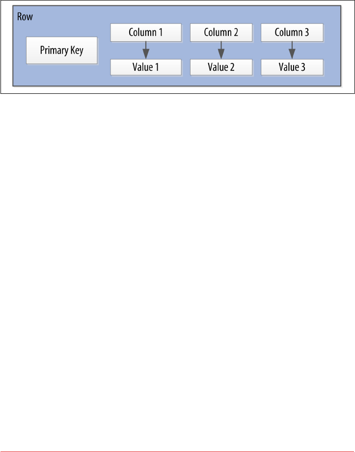
a group of columns that should be treated together as a set. We need rows. Then, if we
get a single row, we can get all of the name/value pairs for a single entity at once, or
just get the values for the names we’re interested in. We could call these name/value
pairs columns. We could call each separate entity that holds some set of columns rows.
And the unique identifier for each row could be called a row key or primary key.
Figure 4-3 shows the contents of a simple row: a primary key, which is itself one or
more columns, and additional columns.
Figure 4-3. A Cassandra row
Cassandra defines a table to be a logical division that associates similar data. For
example, we might have a user table, a hotel table, an address book table, and so
on. In this way, a Cassandra table is analogous to a table in the relational world.
Now we don’t need to store a value for every column every time we store a new entity.
Maybe we don’t know the values for every column for a given entity. For example,
some people have a second phone number and some don’t, and in an online form
backed by Cassandra, there may be some fields that are optional and some that are
required. That’s OK. Instead of storing null for those values we don’t know, which
would waste space, we just won’t store that column at all for that row. So now we have
a sparse, multidimensional array structure that looks like Figure 4-4.
When designing a table in a traditional relational database, you’re typically dealing
with “entities,” or the set of attributes that describe a particular noun (hotel, user,
product, etc.). Not much thought is given to the size of the rows themselves, because
row size isn’t negotiable once you’ve decided what noun your table represents. How‐
ever, when you’re working with Cassandra, you actually have a decision to make
about the size of your rows: they can be wide or skinny, depending on the number of
columns the row contains.
A wide row means a row that has lots and lots (perhaps tens of thousands or even
millions) of columns. Typically there is a smaller number of rows that go along with
so many columns. Conversely, you could have something closer to a relational model,
where you define a smaller number of columns and use many different rows—that’s
the skinny model. We’ve already seen a skinny model in Figure 4-4.
Cassandra’s Data Model | 59
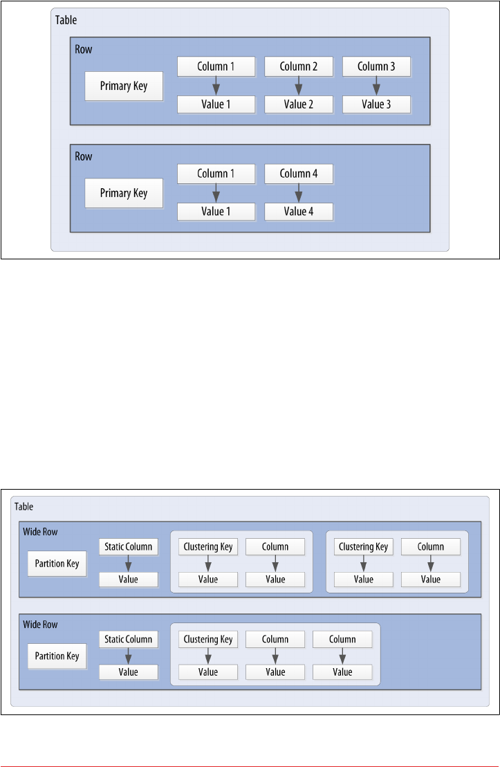
Figure 4-4. A Cassandra table
Cassandra uses a special primary key called a composite key (or compound key) to
represent wide rows, also called partitions. The composite key consists of a partition
key, plus an optional set of clustering columns. The partition key is used to determine
the nodes on which rows are stored and can itself consist of multiple columns. The
clustering columns are used to control how data is sorted for storage within a parti‐
tion. Cassandra also supports an additional construct called a static column, which is
for storing data that is not part of the primary key but is shared by every row in a
partition.
Figure 4-5 shows how each partition is uniquely identified by a partition key, and
how the clustering keys are used to uniquely identify the rows within a partition.
Figure 4-5. A Cassandra wide row
60 | Chapter 4: The Cassandra Query Language

For this chapter, we will concern ourselves with simple primary keys consisting of a
single column. In these cases, the primary key and the partition key are the same,
because we have no clustering columns. We’ll examine more complex primary keys in
Chapter 5.
Putting this all together, we have the basic Cassandra data structures:
•The column, which is a name/value pair
• The row, which is a container for columns referenced by a primary key
• The table, which is a container for rows
• The keyspace, which is a container for tables
•The cluster, which is a container for keyspaces that spans one or more nodes
So that’s the bottom-up approach to looking at Cassandra’s data model. Now that we
know the basic terminology, let’s examine each structure in more detail.
Clusters
As previously mentioned, the Cassandra database is specifically designed to be dis‐
tributed over several machines operating together that appear as a single instance to
the end user. So the outermost structure in Cassandra is the cluster, sometimes called
the ring, because Cassandra assigns data to nodes in the cluster by arranging them in
a ring.
Keyspaces
A cluster is a container for keyspaces. A keyspace is the outermost container for data
in Cassandra, corresponding closely to a relational database. In the same way that a
database is a container for tables in the relational model, a keyspace is a container for
tables in the Cassandra data model. Like a relational database, a keyspace has a name
and a set of attributes that define keyspace-wide behavior.
Because we’re currently focusing on the data model, we’ll leave questions about set‐
ting up and configuring clusters and keyspaces until later. We’ll examine these topics
in Chapter 7.
Tables
A table is a container for an ordered collection of rows, each of which is itself an
ordered collection of columns. The ordering is determined by the columns, which are
identified as keys. We’ll soon see how Cassandra uses additional keys beyond the pri‐
mary key.
When you write data to a table in Cassandra, you specify values for one or more col‐
umns. That collection of values is called a row. At least one of the values you specify
must be a primary key that serves as the unique identifier for that row.
Cassandra’s Data Model | 61

Let’s go back to the user table we created in the previous chapter. Remember how we
wrote a row of data and then read it using the SELECT command in cqlsh:
cqlsh:my_keyspace> SELECT * FROM user WHERE first_name='Bill';
first_name | last_name
------------+-----------
Bill | Nguyen
(1 rows)
You’ll notice in the last row that the shell tells us that one row was returned. It turns
out to be the row identified by the first_name “Bill”. This is the primary key that
identifies this row.
Data Access Requires a Primary Key
This is an important detail—the SELECT, INSERT, UPDATE, and
DELETE commands in CQL all operate in terms of rows.
As we stated earlier, we don’t need to include a value for every column when we add a
new row to the table. Let’s test this out with our user table using the ALTER TABLE
command and then view the results using the DESCRIBE TABLE command:
cqlsh:my_keyspace> ALTER TABLE user ADD title text;
cqlsh:my_keyspace> DESCRIBE TABLE user;
CREATE TABLE my_keyspace.user (
first_name text PRIMARY KEY,
last_name text,
title text
) ...
We see that the title column has been added. Note that we’ve shortened the output
to omit the various table settings. You’ll learn more about these settings and how to
configure them in Chapter 7.
Now, let’s write a couple of rows, populate different columns for each, and view the
results:
cqlsh:my_keyspace> INSERT INTO user (first_name, last_name, title)
VALUES ('Bill', 'Nguyen', 'Mr.');
cqlsh:my_keyspace> INSERT INTO user (first_name, last_name) VALUES
('Mary', 'Rodriguez');
cqlsh:my_keyspace> SELECT * FROM user;
first_name | last_name | title
------------+-----------+-------
Mary | Rodriguez | null
Bill | Nguyen | Mr.
62 | Chapter 4: The Cassandra Query Language

(2 rows)
Now that we’ve learned more about the structure of a table and done some data mod‐
eling, let’s dive deeper into columns.
Columns
A column is the most basic unit of data structure in the Cassandra data model. So far
we’ve seen that a column contains a name and a value. We constrain each of the val‐
ues to be of a particular type when we define the column. We’ll want to dig into the
various types that are available for each column, but first let’s take a look into some
other attributes of a column that we haven’t discussed yet: timestamps and time to
live. These attributes are key to understanding how Cassandra uses time to keep data
current.
Timestamps
Each time you write data into Cassandra, a timestamp is generated for each column
value that is updated. Internally, Cassandra uses these timestamps for resolving any
conflicting changes that are made to the same value. Generally, the last timestamp
wins.
Let’s view the timestamps that were generated for our previous writes by adding the
writetime() function to our SELECT command. We’ll do this on the lastname col‐
umn and include a couple of other values for context:
cqlsh:my_keyspace> SELECT first_name, last_name,
writetime(last_name) FROM user;
first_name | last_name | writetime(last_name)
------------+-----------+----------------------
Mary | Rodriguez | 1434591198790252
Bill | Nguyen | 1434591198798235
(2 rows)
We might expect that if we ask for the timestamp on first_name we’d get a similar
result. However, it turns out we’re not allowed to ask for the timestamp on primary
key columns:
cqlsh:my_keyspace> SELECT WRITETIME(first_name) FROM user;
InvalidRequest: code=2200 [Invalid query] message="Cannot use
selection function writeTime on PRIMARY KEY part first_name"
Cassandra’s Data Model | 63

Cassandra also allows us to specify a timestamp we want to use when performing
writes. To do this, we’ll use the CQL UPDATE command for the first time. We’ll use the
optional USING TIMESTAMP option to manually set a timestamp (note that the time‐
stamp must be later than the one from our SELECT command, or the UPDATE will be
ignored):
cqlsh:my_keyspace> UPDATE user USING TIMESTAMP 1434373756626000
SET last_name = 'Boateng' WHERE first_name = 'Mary' ;
cqlsh:my_keyspace> SELECT first_name, last_name,
WRITETIME(last_name) FROM user WHERE first_name = 'Mary';
first_name | last_name | writetime(last_name)
------------+-------------+---------------------
Mary | Boateng | 1434373756626000
(1 rows)
This statement has the effect of adding the last name column to the row identified by
the primary key “Mary”, and setting the timestamp to the value we provided.
Working with Timestamps
Setting the timestamp is not required for writes. This functionality
is typically used for writes in which there is a concern that some of
the writes may cause fresh data to be overwritten with stale data.
This is advanced behavior and should be used with caution.
There is currently not a way to convert timestamps produced by
writetime() into a more friendly format in cqlsh.
Time to live (TTL)
One very powerful feature that Cassandra provides is the ability to expire data that is
no longer needed. This expiration is very flexible and works at the level of individual
column values. The time to live (or TTL) is a value that Cassandra stores for each
column value to indicate how long to keep the value.
The TTL value defaults to null, meaning that data that is written will not expire. Let’s
show this by adding the TTL() function to a SELECT command in cqlsh to see the
TTL value for Mary’s last name:
cqlsh:my_keyspace> SELECT first_name, last_name, TTL(last_name)
FROM user WHERE first_name = 'Mary';
first_name | last_name | ttl(last_name)
------------+-----------+----------------
Mary | Boateng | null
(1 rows)
64 | Chapter 4: The Cassandra Query Language

Now let’s set the TTL on the last name column to an hour (3,600 seconds) by adding
the USING TTL option to our UPDATE command:
cqlsh:my_keyspace> UPDATE user USING TTL 3600 SET last_name =
'McDonald' WHERE first_name = 'Mary' ;
cqlsh:my_keyspace> SELECT first_name, last_name, TTL(last_name)
FROM user WHERE first_name = 'Mary';
first_name | last_name | ttl(last_name)
------------+-------------+---------------
Mary | McDonald | 3588
(1 rows)
As you can see, the clock is already counting down our TTL, reflecting the several
seconds it took to type the second command. If we run this command again in an
hour, Mary’s last_name will be set to null. We can also set TTL on INSERTS using the
same USING TTL option.
Using TTL
Remember that TTL is stored on a per-column level. There is cur‐
rently no mechanism for setting TTL at a row level directly. As
with the timestamp, there is no way to obtain or set the TTL value
of a primary key column, and the TTL can only be set for a column
when we provide a value for the column.
If we want to set TTL across an entire row, we must provide a value for every non-
primary key column in our INSERT or UPDATE command.
CQL Types
Now that we’ve taken a deeper dive into how Cassandra represents columns including
time-based metadata, let’s look at the various types that are available to us for our val‐
ues.
As we’ve seen in our exploration so far, each column in our table is of a specified type.
Up until this point, we’ve only used the varchar type, but there are plenty of other
options available to us in CQL, so let’s explore them.
CQL supports a flexible set of data types, including simple character and numeric
types, collections, and user-defined types. We’ll describe these data types and provide
some examples of how they might be used to help you learn to make the right choice
for your data model.
CQL Types | 65

Numeric Data Types
CQL supports the numeric types you’d expect, including integer and floating-point
numbers. These types are similar to standard types in Java and other languages:
int
A 32-bit signed integer (as in Java)
bigint
A 64-bit signed long integer (equivalent to a Java long)
smallint
A 16-bit signed integer (equivalent to a Java short)
tinyint
An 8-bit signed integer (as in Java)
varint
A variable precision signed integer (equivalent to java.math.BigInteger)
float
A 32-bit IEEE-754 floating point (as in Java)
double
A 64-bit IEEE-754 floating point (as in Java)
decimal
A variable precision decimal (equivalent to java.math.BigDecimal)
Additional Integer Types
The smallint and tinyint types were added in the Cassandra 2.2
release.
While enumerated types are common in many languages, there is no direct equiva‐
lent in CQL. A common practice is to store enumerated values as strings. For exam‐
ple, using the Enum.name() method to convert an enumerated value to a String for
writing to Cassandra as text, and the Enum.valueOf() method to convert from text
back to the enumerated value.
66 | Chapter 4: The Cassandra Query Language

Textual Data Types
CQL provides two data types for representing text, one of which we’ve made quite a
bit of use of already (text):
text, varchar
Synonyms for a UTF-8 character string
ascii
An ASCII character string
UTF-8 is the more recent and widely used text standard and supports internationali‐
zation, so we recommend using text over ascii when building tables for new data.
The ascii type is most useful if you are dealing with legacy data that is in ASCII for‐
mat.
Setting the Locale in cqlsh
By default, cqlsh prints out control and other unprintable charac‐
ters using a backslash escape. You can control how cqlsh displays
non-ASCII characters by setting the locale via the $LANG environ‐
ment variable before running the tool. See the cqlsh command
HELP TEXT_OUTPUT for more information.
Time and Identity Data Types
The identity of data elements such as rows and partitions is important in any data
model in order to be able to access the data. Cassandra provides several types which
prove quite useful in defining unique partition keys. Let’s take some time (pun
intended) to dig into these:
timestamp
While we noted earlier that each column has a timestamp indicating when it was
last modified, you can also use a timestamp as the value of a column itself. The
time can be encoded as a 64-bit signed integer, but it is typically much more use‐
ful to input a timestamp using one of several supported ISO 8601 date formats.
For example:
2015-06-15 20:05-0700
2015-06-15 20:05:07-0700
2015-06-15 20:05:07.013-0700
2015-06-15T20:05-0700
2015-06-15T20:05:07-0700
2015-06-15T20:05:07.013+-0700
CQL Types | 67

The best practice is to always provide time zones rather than relying on the oper‐
ating system time zone configuration.
date, time
Releases through Cassandra 2.1 only had the timestamp type to represent times,
which included both a date and a time of day. The 2.2 release introduced date
and time types that allowed these to be represented independently; that is, a date
without a time, and a time of day without reference to a specific date. As with
timestamp, these types support ISO 8601 formats.
Although there are new java.time types available in Java 8, the date type maps
to a custom type in Cassandra in order to preserve compatibility with older
JDKs. The time type maps to a Java long representing the number of nanosec‐
onds since midnight.
uuid
A universally unique identier (UUID) is a 128-bit value in which the bits con‐
form to one of several types, of which the most commonly used are known as
Type 1 and Type 4. The CQL uuid type is a Type 4 UUID, which is based entirely
on random numbers. UUIDs are typically represented as dash-separated sequen‐
ces of hex digits. For example:
1a6300ca-0572-4736-a393-c0b7229e193e
The uuid type is often used as a surrogate key, either by itself or in combination
with other values.
Because UUIDs are of a finite length, they are not absolutely guaranteed to be
unique. However, most operating systems and programming languages provide
utilities to generate IDs that provide adequate uniqueness, and cqlsh does as
well. You can obtain a Type 4 UUID value via the uuid() function and use this
value in an INSERT or UPDATE.
timeuuid
This is a Type 1 UUID, which is based on the MAC address of the computer, the
system time, and a sequence number used to prevent duplicates. This type is fre‐
quently used as a conflict-free timestamp. cqlsh provides several convenience
functions for interacting with the timeuuid type: now(), dateOf() and
unixTimestampOf().
The availability of these convenience functions is one reason why timeuuid tends
to be used more frequently than uuid.
68 | Chapter 4: The Cassandra Query Language

Building on our previous examples, we might determine that we’d like to assign a
unique ID to each user, as first_name is perhaps not a sufficiently unique key for our
user table. After all, it’s very likely that we’ll run into users with the same first name at
some point. If we were starting from scratch, we might have chosen to make this
identifier our primary key, but for now we’ll add it as another column.
Primary Keys Are Forever
After you create a table, there is no way to modify the primary key,
because this controls how data is distributed within the cluster, and
even more importantly, how it is stored on disk.
Let’s add the identifier using a uuid :
cqlsh:my_keyspace> ALTER TABLE user ADD id uuid;
Next, we’ll insert an ID for Mary using the uuid() function and then view the results:
cqlsh:my_keyspace> UPDATE user SET id = uuid() WHERE first_name =
'Mary';
cqlsh:my_keyspace> SELECT first_name, id FROM user WHERE
first_name = 'Mary';
first_name | id
------------+--------------------------------------
Mary | e43abc5d-6650-4d13-867a-70cbad7feda9
(1 rows)
Notice that the id is in UUID format.
Now we have a more robust table design, which we can extend with even more col‐
umns as we learn about more types.
Other Simple Data Types
CQL provides several other simple data types that don’t fall nicely into one of the cat‐
egories we’ve looked at already:
boolean
This is a simple true/false value. The cqlsh is case insensitive in accepting these
values but outputs True or False.
blob
A binary large object (blob) is a colloquial computing term for an arbitrary array
of bytes. The CQL blob type is useful for storing media or other binary file types.
Cassandra does not validate or examine the bytes in a blob. CQL represents the
data as hexadecimal digits—for example, 0x00000ab83cf0. If you want to encode
CQL Types | 69

arbitrary textual data into the blob you can use the textAsBlob() function in
order to specify values for entry. See the cqlsh help function HELP BLOB_INPUT
for more information.
inet
This type represents IPv4 or IPv6 Internet addresses. cqlsh accepts any legal for‐
mat for defining IPv4 addresses, including dotted or non-dotted representations
containing decimal, octal, or hexadecimal values. However, the values are repre‐
sented using the dotted decimal format in cqlsh output—for example,
192.0.2.235.
IPv6 addresses are represented as eight groups of four hexadecimal digits, separa‐
ted by colons—for example, 2001:0db8:85a3:0000:0000:8a2e:0370:7334. The
IPv6 specification allows the collapsing of consecutive zero hex values, so the
preceding value is rendered as follows when read using SELECT: 2001:
db8:85a3:a::8a2e:370:7334.
counter
The counter data type provides 64-bit signed integer, whose value cannot be set
directly, but only incremented or decremented. Cassandra is one of the few data‐
bases that provides race-free increments across data centers. Counters are fre‐
quently used for tracking statistics such as numbers of page views, tweets, log
messages, and so on. The counter type has some special restrictions. It cannot be
used as part of a primary key. If a counter is used, all of the columns other than
primary key columns must be counters.
A Warning About Counters
Remember: the increment and decrement operators are not
idempotent. There is no operation to reset a counter directly,
but you can approximate a reset by reading the counter value
and decrementing by that value. Unfortunately, this is not
guaranteed to work perfectly, as the counter may have been
changed elsewhere in between reading and writing.
Collections
Let’s say we wanted to extend our user table to support multiple email addresses.
One way to do this would be to create additional columns such as email2, email3, and
so on. While this is an approach that will work, it does not scale very well and might
cause a lot of rework. It is much simpler to deal with the email addresses as a group or
“collection.” CQL provides three collection types to help us out with these situations:
sets, lists, and maps. Let’s now take a look at each of them:
70 | Chapter 4: The Cassandra Query Language

set
The set data type stores a collection of elements. The elements are unordered,
but cqlsh returns the elements in sorted order. For example, text values are
returned in alphabetical order. Sets can contain the simple types we reviewed ear‐
lier as well as user-defined types (which we’ll discuss momentarily) and even
other collections. One advantage of using set is the ability to insert additional
items without having to read the contents first.
Let’s modify our user table to add a set of email addresses:
cqlsh:my_keyspace> ALTER TABLE user ADD emails set<text>;
Then we’ll add an email address for Mary and check that it was added success‐
fully:
cqlsh:my_keyspace> UPDATE user SET emails = {
'mary@example.com' } WHERE first_name = 'Mary';
cqlsh:my_keyspace> SELECT emails FROM user WHERE first_name =
'Mary';
emails
----------------------
{'mary@example.com'}
(1 rows)
Note that in adding that first email address, we replaced the previous contents of
the set, which in this case was null. We can add another email address later
without replacing the whole set by using concatenation:
cqlsh:my_keyspace> UPDATE user SET emails = emails + {
'mary.mcdonald.AZ@gmail.com' } WHERE first_name = 'Mary';
cqlsh:my_keyspace> SELECT emails FROM user WHERE first_name =
'Mary';
emails
---------------------------------------------------
{'mary.mcdonald.AZ@gmail.com', 'mary@example.com'}
(1 rows)
Other Set Operations
We can also clear items from the set by using the subtraction
operator: SET emails = emails - {'mary@example.com'}.
Alternatively, we could clear out the entire set by using the
empty set notation: SET emails = {}.
CQL Types | 71

list
The list data type contains an ordered list of elements. By default, the values are
stored in order of insertion. Let’s modify our user table to add a list of phone
numbers:
cqlsh:my_keyspace> ALTER TABLE user ADD
phone_numbers list<text>;
Then we’ll add a phone number for Mary and check that it was added success‐
fully:
cqlsh:my_keyspace> UPDATE user SET phone_numbers = [
'1-800-999-9999' ] WHERE first_name = 'Mary';
cqlsh:my_keyspace> SELECT phone_numbers FROM user WHERE
first_name = 'Mary';
phone_numbers
--------------------
['1-800-999-9999']
(1 rows)
Let’s add a second number by appending it:
cqlsh:my_keyspace> UPDATE user SET phone_numbers =
phone_numbers + [ '480-111-1111' ] WHERE first_name = 'Mary';
cqlsh:my_keyspace> SELECT phone_numbers FROM user WHERE
first_name = 'Mary';
phone_numbers
------------------------------------
['1-800-999-9999', '480-111-1111']
(1 rows)
The second number we added now appears at the end of the list.
We could also have prepended the number to the front of the
list by reversing the order of our values: SET phone_numbers =
[‘4801234567’] + phone_numbers.
We can replace an individual item in the list when we reference it by its index:
cqlsh:my_keyspace> UPDATE user SET phone_numbers[1] =
'480-111-1111' WHERE first_name = 'Mary';
72 | Chapter 4: The Cassandra Query Language

As with sets, we can also use the subtraction operator to remove items that match
a specified value:
cqlsh:my_keyspace> UPDATE user SET phone_numbers =
phone_numbers - [ '480-111-1111' ] WHERE first_name = 'Mary';
Finally, we can delete a specific item directly using its index:
cqlsh:my_keyspace> DELETE phone_numbers[0] from user WHERE
first_name = 'Mary';
map
The map data type contains a collection of key/value pairs. The keys and the val‐
ues can be of any type except counter. Let’s try this out by using a map to store
information about user logins. We’ll create a column to track login session time
in seconds, with a timeuuid as the key:
cqlsh:my_keyspace> ALTER TABLE user ADD
login_sessions map<timeuuid, int>;
Then we’ll add a couple of login sessions for Mary and see the results:
cqlsh:my_keyspace> UPDATE user SET login_sessions =
{ now(): 13, now(): 18} WHERE first_name = 'Mary';
cqlsh:my_keyspace> SELECT login_sessions FROM user WHERE
first_name = 'Mary';
login_sessions
-----------------------------------------------
{6061b850-14f8-11e5-899a-a9fac1d00bce: 13,
6061b851-14f8-11e5-899a-a9fac1d00bce: 18}
(1 rows)
We can also reference an individual item in the map by using its key.
Collection types are very useful in cases where we need to store a variable number of
elements within a single column.
User-Dened Types
Now we might decide that we need to keep track of physical addresses for our users.
We could just use a single text column to store these values, but that would put the
burden of parsing the various components of the address on the application. It would
be better if we could define a structure in which to store the addresses to maintain the
integrity of the different components.
CQL Types | 73

Fortunately, Cassandra gives us a way to define our own types. We can then create
columns of these user-defined types (UDTs). Let’s create our own address type,
inserting some line breaks in our command for readability:
cqlsh:my_keyspace> CREATE TYPE address (
... street text,
... city text,
... state text,
... zip_code int);
A UDT is scoped by the keyspace in which it is defined. We could have written
CREATE TYPE my_keyspace.address. If you run the command DESCRIBE KEYSPACE
my_keyspace, you’ll see that the address type is part of the keyspace definition.
Now that we have defined our address type, we’ll try to use it in our user table, but we
immediately run into a problem:
cqlsh:my_keyspace> ALTER TABLE user ADD
addresses map<text, address>;
InvalidRequest: code=2200 [Invalid query] message="Non-frozen
collections are not allowed inside collections: map<text,
address>"
What is going on here? It turns out that a user-defined data type is considered a col‐
lection, as its implementation is similar to a set, list, or map.
Freezing Collections
Cassandra releases prior to 2.2 do not fully support the nesting of
collections. Specifically, the ability to access individual attributes of
a nested collection is not yet supported, because the nested collec‐
tion is serialized as a single object by the implementation.
Freezing is a concept that the Cassandra community has intro‐
duced as a forward compatibility mechanism. For now, you can
nest a collection within another collection by marking it as frozen.
In the future, when nested collections are fully supported, there
will be a mechanism to “unfreeze” the nested collections, allowing
the individual attributes to be accessed.
You can also use a collection as a primary key if it is frozen.
Now that we’ve taken a short detour to discuss freezing and nested tables, let’s get
back to modifying our table, this time marking the address as frozen:
cqlsh:my_keyspace> ALTER TABLE user ADD addresses map<text,
frozen<address>>;
74 | Chapter 4: The Cassandra Query Language

Now let’s add a home address for Mary:
cqlsh:my_keyspace> UPDATE user SET addresses = addresses +
{'home': { street: '7712 E. Broadway', city: 'Tucson',
state: 'AZ', zip_code: 85715} } WHERE first_name = 'Mary';
Now that we’ve finished learning about the various types, let’s take a step back and
look at the tables we’ve created so far by describing my_keyspace:
cqlsh:my_keyspace> DESCRIBE KEYSPACE my_keyspace ;
CREATE KEYSPACE my_keyspace WITH replication = {'class':
'SimpleStrategy', 'replication_factor': '1'} AND
durable_writes = true;
CREATE TYPE my_keyspace.address (
street text,
city text,
state text,
zip_code int
);
CREATE TABLE my_keyspace.user (
first_name text PRIMARY KEY,
addresses map<text, frozen<address>>,
emails set<text>,
id uuid,
last_name text,
login_sessions map<timeuuid, int>,
phone_numbers list<text>,
title text
) WITH bloom_filter_fp_chance = 0.01
AND caching = '{'keys':'ALL', 'rows_per_partition':'NONE'}'
AND comment = ''
AND compaction = {'min_threshold': '4', 'class':
'org.apache.cassandra.db.compaction.
SizeTieredCompactionStrategy', 'max_threshold': '32'}
AND compression = {'sstable_compression':
'org.apache.cassandra.io.compress.LZ4Compressor'}
AND dclocal_read_repair_chance = 0.1
AND default_time_to_live = 0
AND gc_grace_seconds = 864000
AND max_index_interval = 2048
AND memtable_flush_period_in_ms = 0
AND min_index_interval = 128
AND read_repair_chance = 0.0
AND speculative_retry = '99.0PERCENTILE';
CQL Types | 75

Secondary Indexes
If you try to query on column in a Cassandra table that is not part of the primary key,
you’ll soon realize that this is not allowed. For example, consider our user table from
the previous chapter, which uses first_name as the primary key. Attempting to query
by last_name results in the following output:
cqlsh:my_keyspace> SELECT * FROM user WHERE last_name = 'Nguyen';
InvalidRequest: code=2200 [Invalid query] message="No supported
secondary index found for the non primary key columns restrictions"
As the error message instructs us, we need to create a secondary index for the
last_name column. A secondary index is an index on a column that is not part of the
primary key:
cqlsh:my_keyspace> CREATE INDEX ON user ( last_name );
We can also give an optional name to the index with the syntax CREATE INDEX
<name> ON.... If you don’t specify a name, cqlsh creates a name automatically
according to the form <table name>_<column name>_idx. For example, we can learn
the name of the index we just created using DESCRIBE KEYSPACE:
cqlsh:my_keyspace> DESCRIBE KEYSPACE;
...
CREATE INDEX user_last_name_idx ON my_keyspace.user (last_name);
Now that we’ve created the index, our query will work as expected:
cqlsh:my_keyspace> SELECT * FROM user WHERE last_name = 'Nguyen';
first_name | last_name
------------+-----------
Bill | Nguyen
(1 rows)
We’re not limited just to indexes based only on simple type columns. It’s also possible
to create indexes that are based on values in collections. For example, we might wish
to be able to search based on user addresses, emails, or phone numbers, which we
have implemented using map, set, and list, respectively:
cqlsh:my_keyspace> CREATE INDEX ON user ( addresses );
cqlsh:my_keyspace> CREATE INDEX ON user ( emails );
cqlsh:my_keyspace> CREATE INDEX ON user ( phone_numbers );
Note that for maps in particular, we have the option of indexing either the keys (via
the syntax KEYS(addresses)) or the values (which is the default), or both (in Cassan‐
dra 2.2 or later).
76 | Chapter 4: The Cassandra Query Language

Finally, we can use the DROP INDEX command to remove an index:
cqlsh:my_keyspace> DROP INDEX user_last_name_idx;
Secondary Index Pitfalls
Because Cassandra partitions data across multiple nodes, each
node must maintain its own copy of a secondary index based on
the data stored in partitions it owns. For this reason, queries
involving a secondary index typically involve more nodes, making
them significantly more expensive.
Secondary indexes are not recommended for several specific cases:
•Columns with high cardinality. For example, indexing on the
user.addresses column could be very expensive, as the vast
majority of addresses are unique.
•Columns with very low data cardinality. For example, it would
make little sense to index on the user.title column in order
to support a query for every “Mrs.” in the user table, as this
would result in a massive row in the index.
•Columns that are frequently updated or deleted. Indexes built
on these columns can generate errors if the amount of deleted
data (tombstones) builds up more quickly than the compac‐
tion process can handle.
For optimal read performance, denormalized table designs or materialized views are
generally preferred to using secondary indexes. We’ll learn more about these in Chap‐
ter 5. However, secondary indexes can be a useful way of supporting queries that were
not considered in the initial data model design.
Secondary Indexes | 77

SASI: A New Secondary Index Implementation
The Cassandra 3.4 release included an alternative implementation of secondary
indexes known as the SSTable Attached Secondary Index (SASI). SASI was developed
by Apple and released as an open source implementation of Cassandra’s secondary
index API. As the name implies, SASI indexes are calculated and stored as part of
each SSTable file, differing from the original Cassandra implementation, which stores
indexes in separate, “hidden” tables.
The SASI implementation exists alongside traditional secondary indexes, and you can
create a SASI index with the CQL CREATE CUSTOM INDEX command:
CREATE CUSTOM INDEX user_last_name_sasi_idx ON user (last_name)
USING 'org.apache.cassandra.index.sasi.SASIIndex';
SASI indexes do offer functionality beyond the traditional secondary index imple‐
mentation, such as the ability to do inequality (greater than or less than) searches on
indexed columns. You can also use the new CQL LIKE keyword to do text searches
against indexed columns. For example, you could use the following query to find
users whose last name begins with “N”:
SELECT * FROM user WHERE last_name LIKE 'N%';
While SASI indexes do perform better than traditional indexes by eliminating the
need to read from additional tables, they still require reads from a greater number of
nodes than a denormalized design.
Summary
In this chapter, we took a quick tour of Cassandra’s data model of clusters, keyspaces,
tables, keys, rows, and columns. In the process, we learned a lot of CQL syntax and
gained more experience working with tables and columns in cqlsh. If you’re interes‐
ted in diving deeper on CQL, you can read the full language specification.
78 | Chapter 4: The Cassandra Query Language

CHAPTER 5
Data Modeling
In this chapter, you’ll learn how to design data models for Cassandra, including a data
modeling process and notation. To apply this knowledge, we’ll design the data model
for a sample application, which we’ll build over the next several chapters. This will
help show how all the parts fit together. Along the way, we’ll use a tool to help us
manage our CQL scripts.
Conceptual Data Modeling
First, let’s create a simple domain model that is easy to understand in the relational
world, and then see how we might map it from a relational to a distributed hashtable
model in Cassandra.
To create the example, we want to use something that is complex enough to show the
various data structures and design patterns, but not something that will bog you
down with details. Also, a domain that’s familiar to everyone will allow you to con‐
centrate on how to work with Cassandra, not on what the application domain is all
about.
For our example, we’ll use a domain that is easily understood and that everyone can
relate to: making hotel reservations.
Our conceptual domain includes hotels, guests that stay in the hotels, a collection of
rooms for each hotel, the rates and availability of those rooms, and a record of reser‐
vations booked for guests. Hotels typically also maintain a collection of “points of
interest,” which are parks, museums, shopping galleries, monuments, or other places
near the hotel that guests might want to visit during their stay. Both hotels and points
of interest need to maintain geolocation data so that they can be found on maps for
mashups, and to calculate distances.
79
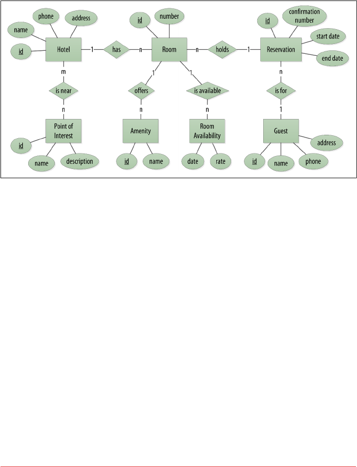
We depict our conceptual domain in Figure 5-1 using the entity–relationship model
popularized by Peter Chen. This simple diagram represents the entities in our
domain with rectangles, and attributes of those entities with ovals. Attributes that
represent unique identifiers for items are underlined. Relationships between entities
are represented as diamonds, and the connectors between the relationship and each
entity show the multiplicity of the connection.
Figure 5-1. Hotel domain entity–relationship diagram
Obviously, in the real world, there would be many more considerations and much
more complexity. For example, hotel rates are notoriously dynamic, and calculating
them involves a wide array of factors. Here we’re defining something complex enough
to be interesting and touch on the important points, but simple enough to maintain
the focus on learning Cassandra.
RDBMS Design
When you set out to build a new data-driven application that will use a relational
database, you might start by modeling the domain as a set of properly normalized
tables and use foreign keys to reference related data in other tables.
Figure 5-2 shows how we might represent the data storage for our application using a
relational database model. The relational model includes a couple of “join” tables in
order to realize the many-to-many relationships from our conceptual model of
hotels-to-points of interest, rooms-to-amenities, rooms-to-availability, and guests-to-
rooms (via a reservation).
80 | Chapter 5: Data Modeling
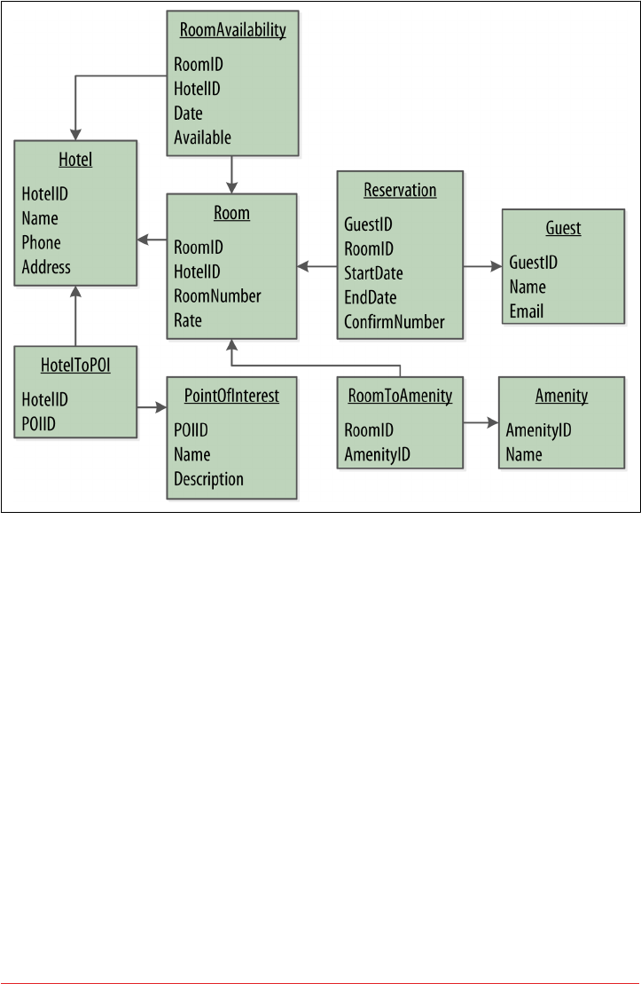
Figure 5-2. A simple hotel search system using RDBMS
Design Dierences Between RDBMS and Cassandra
Of course, because this is a Cassandra book, what we really want is to model our data
so we can store it in Cassandra. Before we start creating our Cassandra data model,
let’s take a minute to highlight some of the key differences in doing data modeling for
Cassandra versus a relational database.
No joins
You cannot perform joins in Cassandra. If you have designed a data model and find
that you need something like a join, you’ll have to either do the work on the client
side, or create a denormalized second table that represents the join results for you.
This latter option is preferred in Cassandra data modeling. Performing joins on the
client should be a very rare case; you really want to duplicate (denormalize) the data
instead.
RDBMS Design | 81

No referential integrity
Although Cassandra supports features such as lightweight transactions and batches,
Cassandra itself has no concept of referential integrity across tables. In a relational
database, you could specify foreign keys in a table to reference the primary key of a
record in another table. But Cassandra does not enforce this. It is still a common
design requirement to store IDs related to other entities in your tables, but operations
such as cascading deletes are not available.
Denormalization
In relational database design, we are often taught the importance of normalization.
This is not an advantage when working with Cassandra because it performs best
when the data model is denormalized. It is often the case that companies end up
denormalizing data in relational databases as well. There are two common reasons for
this. One is performance. Companies simply can’t get the performance they need
when they have to do so many joins on years’ worth of data, so they denormalize
along the lines of known queries. This ends up working, but goes against the grain of
how relational databases are intended to be designed, and ultimately makes one ques‐
tion whether using a relational database is the best approach in these circumstances.
A second reason that relational databases get denormalized on purpose is a business
document structure that requires retention. That is, you have an enclosing table that
refers to a lot of external tables whose data could change over time, but you need to
preserve the enclosing document as a snapshot in history. The common example here
is with invoices. You already have customer and product tables, and you’d think that
you could just make an invoice that refers to those tables. But this should never be
done in practice. Customer or price information could change, and then you would
lose the integrity of the invoice document as it was on the invoice date, which could
violate audits, reports, or laws, and cause other problems.
In the relational world, denormalization violates Codd’s normal forms, and we try to
avoid it. But in Cassandra, denormalization is, well, perfectly normal. It’s not required
if your data model is simple. But don’t be afraid of it.
Server-Side Denormalization with Materialized Views
Historically, denormalization in Cassandra has required designing
and managing multiple tables using techniques we will introduce
momentarily. Beginning with the 3.0 release, Cassandra provides a
feature known as materialized views which allows us to create mul‐
tiple denormalized views of data based on a base table design. Cas‐
sandra manages materialized views on the server, including the
work of keeping the views in sync with the table. In this chapter,
we’ll see examples of both classic denormalization and materialized
views.
82 | Chapter 5: Data Modeling

Query-rst design
Relational modeling, in simple terms, means that you start from the conceptual
domain and then represent the nouns in the domain in tables. You then assign pri‐
mary keys and foreign keys to model relationships. When you have a many-to-many
relationship, you create the join tables that represent just those keys. The join tables
don’t exist in the real world, and are a necessary side effect of the way relational mod‐
els work. After you have all your tables laid out, you can start writing queries that pull
together disparate data using the relationships defined by the keys. The queries in the
relational world are very much secondary. It is assumed that you can always get the
data you want as long as you have your tables modeled properly. Even if you have to
use several complex subqueries or join statements, this is usually true.
By contrast, in Cassandra you don’t start with the data model; you start with the
query model. Instead of modeling the data first and then writing queries, with Cas‐
sandra you model the queries and let the data be organized around them. Think of
the most common query paths your application will use, and then create the tables
that you need to support them.
Detractors have suggested that designing the queries first is overly constraining on
application design, not to mention database modeling. But it is perfectly reasonable to
expect that you should think hard about the queries in your application, just as you
would, presumably, think hard about your relational domain. You may get it wrong,
and then you’ll have problems in either world. Or your query needs might change
over time, and then you’ll have to work to update your data set. But this is no differ‐
ent from defining the wrong tables, or needing additional tables, in an RDBMS.
Designing for optimal storage
In a relational database, it is frequently transparent to the user how tables are stored
on disk, and it is rare to hear of recommendations about data modeling based on how
the RDBMS might store tables on disk. However, that is an important consideration
in Cassandra. Because Cassandra tables are each stored in separate files on disk, it’s
important to keep related columns defined together in the same table.
A key goal that we will see as we begin creating data models in Cassandra is to mini‐
mize the number of partitions that must be searched in order to satisfy a given query.
Because the partition is a unit of storage that does not get divided across nodes, a
query that searches a single partition will typically yield the best performance.
Sorting is a design decision
In an RDBMS, you can easily change the order in which records are returned to you
by using ORDER BY in your query. The default sort order is not configurable; by
default, records are returned in the order in which they are written. If you want to
RDBMS Design | 83

change the order, you just modify your query, and you can sort by any list of col‐
umns.
In Cassandra, however, sorting is treated differently; it is a design decision. The sort
order available on queries is fixed, and is determined entirely by the selection of clus‐
tering columns you supply in the CREATE TABLE command. The CQL SELECT state‐
ment does support ORDER BY semantics, but only in the order specified by the
clustering columns.
Dening Application Queries
Let’s try the query-first approach to start designing the data model for our hotel
application. The user interface design for the application is often a great artifact to use
to begin identifying queries. Let’s assume that we’ve talked with the project stakehold‐
ers and our UX designers have produced user interface designs or wireframes for the
key use cases. We’ll likely have a list of shopping queries like the following:
• Q1. Find hotels near a given point of interest.
• Q2. Find information about a given hotel, such as its name and location.
• Q3. Find points of interest near a given hotel.
•Q4. Find an available room in a given date range.
• Q5. Find the rate and amenities for a room.
Number Your Queries
It is often helpful to be able to refer to queries by a shorthand num‐
ber rather that explaining them in full. The queries listed here are
numbered Q1, Q2, and so on, which is how we will reference them
in diagrams as we move throughout our example.
Now if our application is to be a success, we’ll certainly want our customers to be able
to book reservations at our hotels. This includes steps such as selecting an available
room and entering their guest information. So clearly we will also need some queries
that address the reservation and guest entities from our conceptual data model. Even
here, however, we’ll want to think not only from the customer perspective in terms of
how the data is written, but also in terms of how the data will be queried by down‐
stream use cases.
Our natural tendency as data modelers would be to focus first on designing the tables
to store reservation and guest records, and only then start thinking about the queries
that would access them. You may have felt a similar tension already when we began
discussing the shopping queries before, thinking “but where did the hotel and point
of interest data come from?” Don’t worry, we will get to this soon enough. Here are
some queries that describe how our users will access reservations:
84 | Chapter 5: Data Modeling
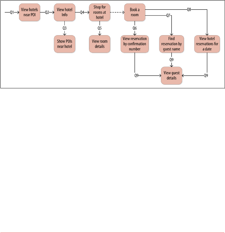
• Q6. Lookup a reservation by confirmation number.
• Q7. Lookup a reservation by hotel, date, and guest name.
• Q8. Lookup all reservations by guest name.
•Q9. View guest details.
We show all of our queries in the context of the workflow of our application in
Figure 5-3. Each box on the diagram represents a step in the application workflow,
with arrows indicating the flows between steps and the associated query. If we’ve
modeled our application well, each step of the workflow accomplishes a task that
“unlocks” subsequent steps. For example, the “View hotels near POI” task helps the
application learn about several hotels, including their unique keys. The key for a
selected hotel may be used as part of Q2, in order to obtain detailed description of the
hotel. The act of booking a room creates a reservation record that may be accessed by
the guest and hotel staff at a later time through various additional queries.
Figure 5-3. Hotel application queries
Logical Data Modeling
Now that we have defined our queries, we’re ready to begin designing our Cassandra
tables. First, we’ll create a logical model containing a table for each query, capturing
entities and relationships from the conceptual model.
To name each table, we’ll identify the primary entity type for which we are querying
and use that to start the entity name. If we are querying by attributes of other related
entities, we append those to the table name, separated with _by_. For example,
hotels_by_poi.
Next, we identify the primary key for the table, adding partition key columns based
on the required query attributes, and clustering columns in order to guarantee
uniqueness and support desired sort ordering.
Logical Data Modeling | 85
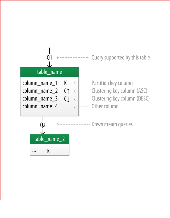
We complete each table by adding any additional attributes identified by the query. If
any of these additional attributes are the same for every instance of the partition key,
we mark the column as static.
Now that was a pretty quick description of a fairly involved process, so it will be
worth our time to work through a detailed example. First, let’s introduce a notation
that we can use to represent our logical models.
Introducing Chebotko Diagrams
Several individuals within the Cassandra community have proposed notations for
capturing data models in diagrammatic form. We’ve elected to use a notation popu‐
larized by Artem Chebotko which provides a simple, informative way to visualize the
relationships between queries and tables in our designs. Figure 5-4 shows the Che‐
botko notation for a logical data model.
Figure 5-4. A Chebotko logical diagram
Each table is shown with its title and a list of columns. Primary key columns are iden‐
tified via symbols such as K for partition key columns and C↑ or C↓ to represent clus‐
tering columns. Lines are shown entering tables or between tables to indicate the
queries that each table is designed to support.
86 | Chapter 5: Data Modeling
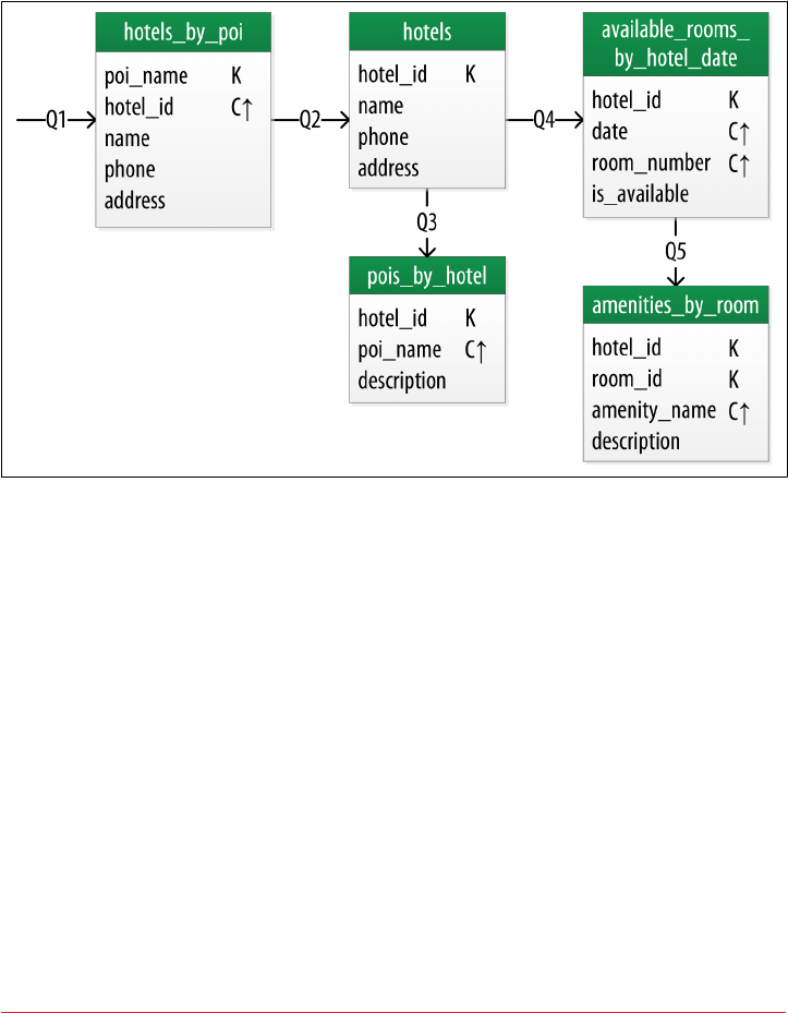
Hotel Logical Data Model
Figure 5-5 shows a Chebotko logical data model for the queries involving hotels,
points of interest, rooms, and amenities. One thing we notice immediately is that our
Cassandra design doesn’t include dedicated tables for rooms or amenities, as we had
in the relational design. This is because our workflow didn’t identify any queries
requiring this direct access.
Figure 5-5. Hotel domain logical model
Let’s explore the details of each of these tables.
Our first query Q1 is to find hotels near a point of interest, so we’ll call our table
hotels_by_poi. We’re searching by a named point of interest, so that is a clue that the
point of interest should be a part of our primary key. Let’s reference the point of inter‐
est by name, because according to our workflow that is how our users will start their
search.
You’ll note that we certainly could have more than one hotel near a given point of
interest, so we’ll need another component in our primary key in order to make sure
we have a unique partition for each hotel. So we add the hotel key as a clustering col‐
umn.
Logical Data Modeling | 87

Make Your Primary Keys Unique
An important consideration in designing your table’s primary key
is making sure that it defines a unique data element. Otherwise you
run the risk of accidentally overwriting data.
Now for our second query (Q2), we’ll need a table to get information about a specific
hotel. One approach would have been to put all of the attributes of a hotel in the
hotels_by_poi table, but we chose to add only those attributes that were required by
our application workflow.
From our workflow diagram, we know that the hotels_by_poi table is used to dis‐
play a list of hotels with basic information on each hotel, and the application knows
the unique identifiers of the hotels returned. When the user selects a hotel to view
details, we can then use Q2, which is used to obtain details about the hotel. Because
we already have the hotel_id from Q1, we use that as our reference to the hotel we’re
looking for. Therefore our second table is just called hotels.
Another option would have been to store a set of poi_names in the hotels table. This
is an equally valid approach. You’ll learn through experience which approach is best
for your application.
Using Unique Identiers as References
You’ll find that it’s often helpful to use unique IDs to uniquely ref‐
erence elements, and to use these uuids as references in tables rep‐
resenting other entities. This helps to minimize coupling between
different entity types. This may prove especially helpful if you are
using a microservice architectural style for your application, in
which there are separate services responsible for each entity type.
For the purposes of this book, however, we’ll use mostly text
attributes as identifiers, to keep our samples simple and readable.
For example, a common convention in the hospitality industry is to
reference properties by short codes like “AZ123” or “NY229”. We’ll
use these values for our hotel_ids, while acknowledging they are
not necessarily globally unique.
Q3 is just a reverse of Q1—looking for points of interest near a hotel, rather than
hotels near a point of interest. This time, however, we need to access the details of
each point of interest, as represented by the pois_by_hotel table. As we have done
previously, we add the point of interest name as a clustering key to guarantee unique‐
ness.
88 | Chapter 5: Data Modeling
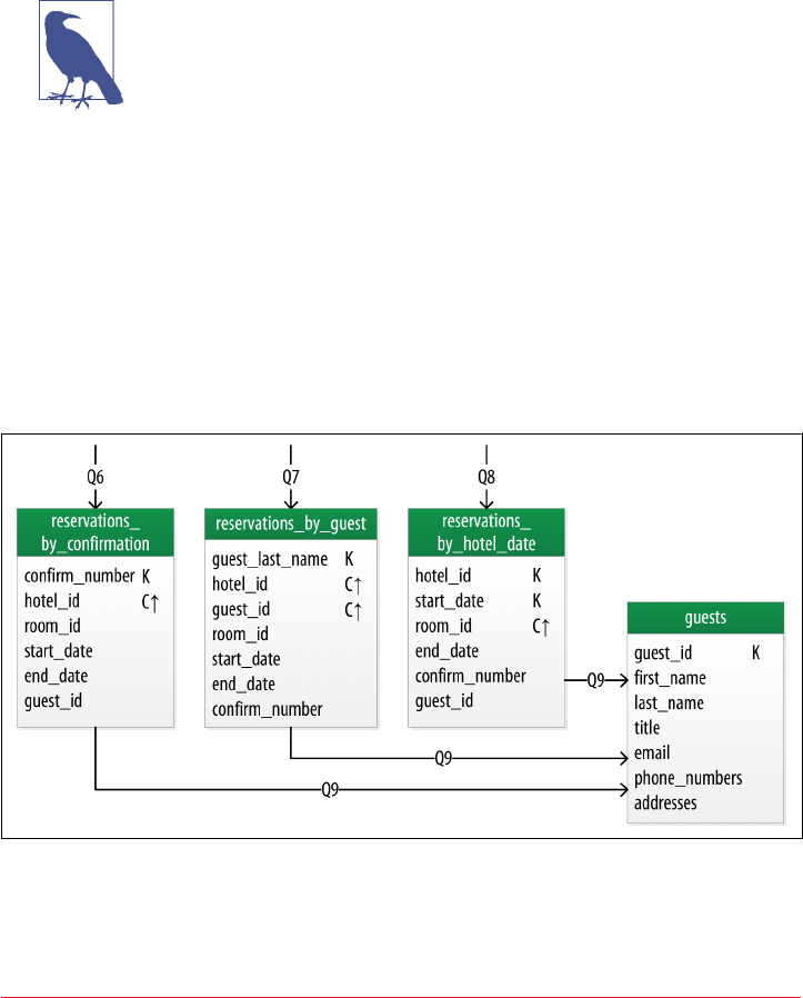
At this point, let’s now consider how to support query Q4 to help our user find avail‐
able rooms at a selected hotel for the nights they are interested in staying. Note that
this query involves both a start date and an end date. Because we’re querying over a
range instead of a single date, we know that we’ll need to use the date as a clustering
key. We use the hotel_id as a primary key to group room data for each hotel on a
single partition, which should help our search be super fast. Let’s call this the
available_rooms_by_hotel_date table.
Searching Over a Range
Use clustering columns to store attributes that you need to access
in a range query. Remember that the order of the clustering col‐
umns is important. We’ll learn more about range queries in Chap‐
ter 9.
In order to round out the shopping portion of our data model, we add the
amenities_by_room table to support Q5. This will allow our user to view the ameni‐
ties of one of the rooms that is available for the desired stay dates.
Reservation Logical Data Model
Now we switch gears to look at the reservation queries. Figure 5-6 shows a logical
data model for reservations. You’ll notice that these tables represent a denormalized
design; the same data appears in multiple tables, with differing keys.
Figure 5-6. A denormalized logical model for reservations
Logical Data Modeling | 89

In order to satisfy Q6, the reservations_by_confirmation table supports the look
up of reservations by a unique confirmation number provided to the customer at the
time of booking.
If the guest doesn’t have the confirmation number, the reservations_by_guest table
can be used to look up the reservation by guest name. We could envision query Q7
being used on behalf of a guest on a self-serve website or a call center agent trying to
assist the guest. Because the guest name might not be unique, we include the guest ID
here as a clustering column as well.
The hotel staff might wish to see a record of upcoming reservations by date in order
to get insight into how the hotel is performing, such as what dates the hotel is sold out
or undersold. Q8 supports the retrieval of reservations for a given hotel by date.
Finally, we create a guests table. You’ll notice that it has similar attributes to our user
table from Chapter 4. This provides a single location that we can use to store our
guests. In this case, we specify a separate unique identifier for our guest records, as it
is not uncommon for guests to have the same name. In many organizations, a cus‐
tomer database such as our guests table would be part of a separate customer man‐
agement application, which is why we’ve omitted other guest access patterns from our
example.
Design Queries for All Stakeholders
Q8 and Q9 in particular help to remind us that we need to create
queries that support various stakeholders of our application, not
just customers but staff as well, and perhaps even the analytics
team, suppliers, and so on.
Patterns and Anti-Patterns
As with other types of software design, there are some well-known patterns and anti-
patterns for data modeling in Cassandra. We’ve already used one of the most com‐
mon patterns in our hotel model—the wide row.
The time series pattern is an extension of the wide row pattern. In this pattern, a ser‐
ies of measurements at specific time intervals are stored in a wide row, where the
measurement time is used as part of the partition key. This pattern is frequently used
in domains including business analysis, sensor data management, and scientific
experiments.
The time series pattern is also useful for data other than measurements. Consider the
example of a banking application. We could store each customer’s balance in a row,
but that might lead to a lot of read and write contention as various customers check
their balance or make transactions. We’d probably be tempted to wrap a transaction
around our writes just to protect the balance from being updated in error. In contrast,
90 | Chapter 5: Data Modeling

a time series–style design would store each transaction as a timestamped row and
leave the work of calculating the current balance to the application.
One design trap that many new users fall into is attempting to use Cassandra as a
queue. Each item in the queue is stored with a timestamp in a wide row. Items are
appended to the end of the queue and read from the front, being deleted after they are
read. This is a design that seems attractive, especially given its apparent similarity to
the time series pattern. The problem with this approach is that the deleted items are
now tombstones that Cassandra must scan past in order to read from the front of the
queue. Over time, a growing number of tombstones begins to degrade read perfor‐
mance.
The queue anti-pattern serves as a reminder that any design that relies on the deletion
of data is potentially a poorly performing design.
Physical Data Modeling
Once we have a logical data model defined, creating the physical model is a relatively
simple process.
We walk through each of our logical model tables, assigning types to each item. We
can use any of the types we covered in Chapter 4, including the basic types, collec‐
tions, and user-defined types. We may identify additional user-defined types that can
be created to simplify our design.
After we’ve assigned our data types, we analyze our model by performing size calcula‐
tions and testing out how the model works. We may make some adjustments based
on our findings. Once again we’ll cover the data modeling process in more detail by
working through our example.
Before we get started, let’s look at a few additions to the Chebotko notation for physi‐
cal data models.
Chebotko Physical Diagrams
To draw physical models, we need to be able to add the typing information for each
column. Figure 5-7 shows the addition of a type for each column in a sample table.
The figure includes a designation of the keyspace containing each table and visual
cues for columns represented using collections and user-defined types. We also note
the designation of static columns and secondary index columns. There is no restric‐
tion on assigning these as part of a logical model, but they are typically more of a
physical data modeling concern.
Physical Data Modeling | 91
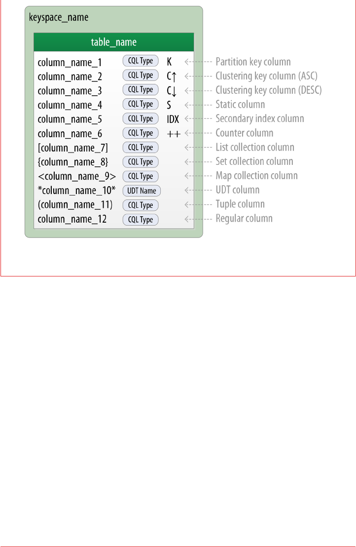
Figure 5-7. Extending the Chebotko notation for physical data models
Hotel Physical Data Model
Now let’s get to work on our physical model. First, we need keyspaces for our tables.
To keep the design relatively simple, we’ll create a hotel keyspace to contain our
tables for hotel and availability data, and a reservation keyspace to contain tables for
reservation and guest data. In a real system, we might divide the tables across even
more keyspaces in order to separate concerns.
For our hotels table, we’ll use Cassandra’s text type to represent the hotel’s id. For
the address, we’ll use the address type that we created in Chapter 4. We use the text
type to represent the phone number, as there is considerable variance in the format‐
ting of numbers between countries.
As we work to create physical representations of various tables in our logical hotel
data model, we use the same approach. The resulting design is shown in Figure 5-8.
92 | Chapter 5: Data Modeling
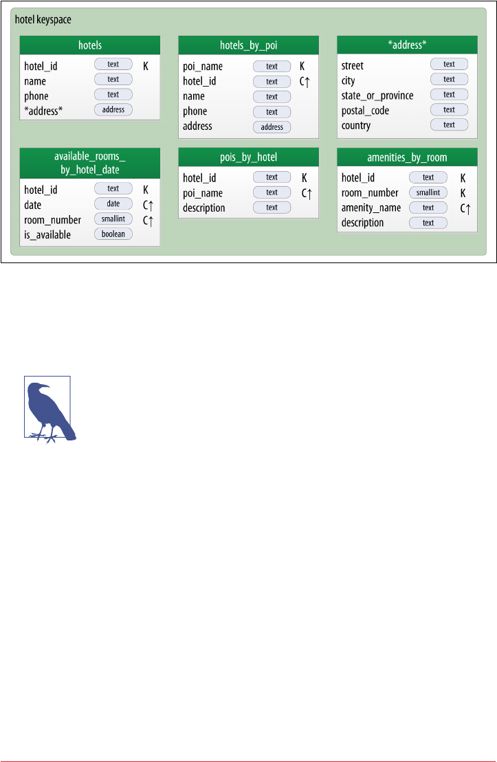
Figure 5-8. Hotel physical model
Note that we have also included the address type in our design. It is designated with
an asterisk to denote that it is a user-defined type, and has no primary key columns
identified. We make use of this type in the hotels and hotels_by_poi tables.
Taking Advantage of User-Dened Types
It is often helpful to make use of user-defined types to help reduce
duplication of non-primary key columns, as we have done with the
address user-defined type. This can reduce complexity in the
design.
Remember that the scope of a UDT is the keyspace in which it is
defined. To use address in the reservation keyspace we’re about
to design, we’ll have to declare it again. This is just one of the many
trade-offs we have to make in data model design.
Reservation Physical Data Model
Now, let’s turn our attention to the reservation tables in our design. Remember that
our logical model contained three denormalized tables to support queries for reserva‐
tions by confirmation number, guest, and hotel and date. As we work to implement
these different designs, we’ll want to consider whether to manage the denormaliza‐
tion manually or use Cassandra’s materialized view capability.
The design shown for the reservation keyspace in Figure 5-9 uses both approaches.
We chose to implement reservations_by_hotel_date and reservations_by_guest
as regular tables, and reservations_by_confirmation as a materialized view on the
Physical Data Modeling | 93
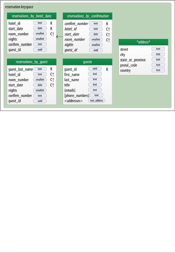
reservations_by_hotel_date table. We’ll discuss the reasoning behind this design
choice momentarily.
Figure 5-9. Reservation physical model
Note that we have reproduced the address type in this keyspace and modeled the
guest_id as a uuid type in all of our tables.
Materialized Views
Materialized views were introduced to help address some of the shortcomings of sec‐
ondary indexes, which we discussed in Chapter 4. Creating indexes on columns with
high cardinality tends to result in poor performance, because most or all of the nodes
in the ring need are queried.
Materialized views address this problem by storing preconfigured views that support
queries on additional columns which are not part of the original clustering key. Mate‐
rialized views simplify application development: instead of the application having to
keep multiple denormalized tables in sync, Cassandra takes on the responsibility of
updating views in order to keep them consistent with the base table.
Materialized views incur a small performance impact on writes in order to maintain
this consistency. However, materialized views demonstrate more efficient perfor‐
mance compared to managing denormalized tables in application clients. Internally,
materialized view updates are implemented using batching, which we will discuss in
Chapter 9.
94 | Chapter 5: Data Modeling

Similar to secondary indexes, materialized views can be created on existing tables.
To understand the syntax and constraints associated with materialized views, we’ll
take a look at the CQL command that creates the reservations_by_confirmation
table from the reservation physical model:
cqlsh> CREATE MATERIALIZED VIEW reservation.reservations_by_confirmation
AS SELECT *
FROM reservation.reservations_by_hotel_date
WHERE confirm_number IS NOT NULL and hotel_id IS NOT NULL and
start_date IS NOT NULL and room_number IS NOT NULL
PRIMARY KEY (confirm_number, hotel_id, start_date, room_number);
The order of the clauses in the CREATE MATERIALIZED VIEW command can appear
somewhat inverted, so we’ll walk through these clauses in an order that is a bit easier
to process.
The first parameter after the command is the name of the materialized view—in this
case, reservations_by_confirmation. The FROM clause identifies the base table for
the materialized view, reservations_by_hotel_date.
The PRIMARY KEY clause identifies the primary key for the materialized view, which
must include all of the columns in the primary key of the base table. This restriction
keeps Cassandra from collapsing multiple rows in the base table into a single row in
the materialized view, which would greatly increase the complexity of managing
updates.
The grouping of the primary key columns uses the same syntax as an ordinary table.
The most common usage is to place the additional column first as the partition key,
followed by the base table primary key columns, used as clustering columns for pur‐
poses of the materialized view.
The WHERE clause provides support for filtering.Note that a filter must be specified for
every primary key column of the materialized view, even if it is as simple as designat‐
ing that the value IS NOT NULL.
The AS SELECT clause identifies the columns from the base table that we want our
materialized view to contain. We can reference individual columns, but in this case
have chosen for all columns to be part of the view by using the wildcard *.
Physical Data Modeling | 95

Enhanced Materialized View Capabilities
The initial implementation of materialized views in the 3.0 release
has some limitations on the selection of primary key columns and
filters. There are several JIRA issues in progress to add capabilities
such as multiple non-primary key columns in materialized view
primary keys CASSANDRA-9928 or using aggregates in material‐
ized views CASSANDRA-9778. If you’re interested in these fea‐
tures, track the JIRA issues to see when they will be included in a
release.
Now that we have a better understanding of the design and use of materialized views,
we can revisit the prior decision made for the reservation physical design. Specifically,
reservations_by_confirmation is a good candidate for implementation as a mate‐
rialized view due to the high cardinality of the confirmation numbers—after all, you
can’t get any higher cardinality than a unique value per reservation.
An alternate design would have been to use reservations_by_confirmation as the
base table and reservations_by_hotel_date as a materialized view. However,
because we cannot (at least in early 3.X releases) create a materialized view with mul‐
tiple non-primary key column from the base table, this would have required us to
designate either hotel_id or date as a clustering column in reservations_by_con
firmation. Both designs are acceptable, but this should give some insight into the
trade-offs you’ll want to consider in selecting which of several denormalized table
designs to use as the base table.
Evaluating and Rening
Once we’ve created our physical model, there are some steps we’ll want to take to
evaluate and refine our table designs to help ensure optimal performance.
Calculating Partition Size
The first thing that we want to look for is whether our tables will have partitions that
will be overly large, or to put it another way, partitions that are too wide. Partition
size is measured by the number of cells (values) that are stored in the partition. Cas‐
sandra’s hard limit is 2 billion cells per partition, but we’ll likely run into performance
issues before reaching that limit.
In order to calculate the size of our partitions, we use the following formula:
Nv=NrNc−Npk −Ns+Ns
The number of values (or cells) in the partition (Nv) is equal to the number of static
columns (Ns) plus the product of the number of rows (Nr) and the number of of val‐
96 | Chapter 5: Data Modeling
ues per row. The number of values per row is defined as the number of columns (Nc)
minus the number of primary key columns (Npk) and static columns (Ns).
The number of columns tends to be relatively static, although as we have seen it is
quite possible to alter tables at runtime. For this reason, a primary driver of partition
size is the number of rows in the partition. This is a key factor that you must consider
in determining whether a partition has the potential to get too large. Two billion val‐
ues sounds like a lot, but in a sensor system where tens or hundreds of values are
measured every millisecond, the number of values starts to add up pretty fast.
Let’s take a look at one of our tables to analyze the partition size. Because it has a wide
row design with a partition per hotel, we’ll choose the available_rooms_
by_hotel_date table. The table has four columns total (Nc = 4), including three pri‐
mary key columns (Npk = 3) and no static columns (Ns = 0). Plugging these values
into our formula, we get:
Nv=Nr4 − 3 − 0 + 0 = 1Nr
So the number of values for this table is equal to the number of rows. We still need to
determine a number of rows. To do this, we make some estimates based on the appli‐
cation we’re designing. Our table is storing a record for each room, in each of our
hotels, for every night. Let’s assume that our system will be used to store two years of
inventory at a time, and there are 5,000 hotels in our system, with an average of 100
rooms in each hotel.
Since there is a partition for each hotel, our estimated number of rows per partition is
as follows:
Nr= 100 rooms/hotel × 730 days = 73, 000 rows
This relatively small number of rows per partition is not going to get us in too much
trouble, but if we start storing more dates of inventory, or don’t manage the size of
our inventory well using TTL, we could start having issues. We still might want to
look at breaking up this large partition, which we’ll do shortly.
Estimate for the Worst Case
When performing sizing calculations, it is tempting to assume the
nominal or average case for variables such as the number of rows.
Consider calculating the worst case as well, as these sorts of predic‐
tions have a way of coming true in successful systems.
Calculating Size on Disk
In addition to calculating the size of our partition, it is also an excellent idea for us to
estimate the amount of disk space that will be required for each table we plan to store
Evaluating and Rening | 97

in the cluster. In order to determine the size, we use the following formula to deter‐
mine the size St of a partition:
St=∑
isizeOf cki+∑
jsizeOf csj+Nr×∑
ksizeOf crk+∑
lsizeOf ccl+
Nv×sizeOf tavg
This is a bit more complex than our previous formula, but we’ll break it down a bit at
a time. Let’s take a look at the notation first:
• In this formula, ck refers to partition key columns, cs to static columns, cr to regu‐
lar columns, and cc to clustering columns.
•The term tavg refers to the average number of bytes of metadata stored per cell,
such as timestamps. It is typical to use an estimate of 8 bytes for this value.
•We recognize the number of rows Nr and number of values Nv from our previous
calculations.
•The sizeOf() function refers to the size in bytes of the CQL data type of each ref‐
erenced column.
The first term asks us to sum the size of the partition key columns. For our example,
the available_rooms_by_hotel_date table has a single partition key column, the
hotel_id, which we chose to make of type text. Assuming our hotel identifiers are
simple 5-character codes, we have a 5-byte value, so the sum of our partition key col‐
umn sizes is 5 bytes.
The second term asks us to sum the size of our static columns. Our table has no static
columns, so in our case this is 0 bytes.
The third term is the most involved, and for good reason—it is calculating the size of
the cells in the partition. We sum the size of the clustering columns and regular col‐
umns. Our two clustering columns are the date, which we assume is 4 bytes, and the
room_number, which is a 2-byte short integer, giving us a sum of 6 bytes. There is only
a single regular column, the boolean is_available, which is 1 byte in size. Summing
the regular column size (1 byte) plus the clustering column size (6 bytes) gives us a
total of 7 bytes. To finish up the term, we multiply this value by the number of rows
(73,000), giving us 511,000 bytes (0.51 MB).
The fourth term is simply counting the metadata that that Cassandra stores for each
cell. In the storage format used by Cassandra 3.0 and later, the amount of metadata
for a given cell varies based on the type of data being stored, and whether or not cus‐
tom timestamp or TTL values are specified for individual cells. For our table, we
reuse the number of values from our previous calculation (73,000) and multiply by 8,
which gives us 0.58 MB.
Adding these terms together, we get our final estimate:
98 | Chapter 5: Data Modeling

Partition size = 16 bytes + 0 bytes + 0.51 MB + 0.58 MB = 1.1 MB
This formula is an approximation of the actual size of a partition on disk, but is accu‐
rate enough to be quite useful. Remembering that the partition must be able to fit on
a single node, it looks like our table design will not put a lot of strain on our disk
storage.
A More Compact Storage Format
As mentioned in Chapter 2, Cassandra’s storage engine was re-
implemented for the 3.0 release, including a new format for
SSTable files. The previous format stored a separate copy of the
clustering columns as part of the record for each cell. The newer
format eliminates this duplication, which reduces the size of stored
data and simplifies the formula for computing that size.
Keep in mind also that this estimate only counts a single replica of our data. We will
need to multiply the value obtained here by the number of partitions and the number
of replicas specified by the keyspace’s replication strategy in order to determine the
total required total capacity for each table. This will come in handy when we discuss
how to plan our clusters in Chapter 14.
Breaking Up Large Partitions
As discussed previously, our goal is to design tables that can provide the data we need
with queries that touch a single partition, or failing that, the minimum possible num‐
ber of partitions. However, as we have seen in our examples, it is quite possible to
design wide row-style tables that approach Cassandra’s built-in limits. Performing siz‐
ing analysis on tables may reveal partitions that are potentially too large, either in
number of values, size on disk, or both.
The technique for splitting a large partition is straightforward: add an additional col‐
umn to the partition key. In most cases, moving one of the existing columns into the
partition key will be sufficient. Another option is to introduce an additional column
to the table to act as a sharding key, but this requires additional application logic.
Continuing to examine our available rooms example, if we add the date column to
the partition key for the available_rooms_by_hotel_date table, each partition
would then represent the availability of rooms at a specific hotel on a specific date.
This will certainly yield partitions that are significantly smaller, perhaps too small, as
the data for consecutive days will likely be on separate nodes.
Another technique known as bucketing is often used to break the data into moderate-
size partitions. For example, we could bucketize our available_rooms_
by_hotel_date table by adding a month column to the partition key. While this col‐
Evaluating and Rening | 99

umn is partially duplicative of the date, it provides a nice way of grouping related
data in a partition that will not get too large.
If we really felt strongly about preserving a wide row design, we could instead add the
room_id to the partition key, so that each partition would represent the availability of
the room across all dates. Because we haven’t identified a query that involves search‐
ing availability of a specific room, the first or second design approach is most suitable
to our application needs.
Dening Database Schema
Once we have finished evaluating and refining our physical model, we’re ready to
implement the schema in CQL. Here is the schema for the hotel keyspace, using
CQL’s comment feature to document the query pattern supported by each table:
CREATE KEYSPACE hotel
WITH replication = {'class': 'SimpleStrategy', 'replication_factor' : 3};
CREATE TYPE hotel.address (
street text,
city text,
state_or_province text,
postal_code text,
country text
);
CREATE TABLE hotel.hotels_by_poi (
poi_name text,
hotel_id text,
name text,
phone text,
address frozen<address>,
PRIMARY KEY ((poi_name), hotel_id)
) WITH comment = 'Q1. Find hotels near given poi'
AND CLUSTERING ORDER BY (hotel_id ASC) ;
CREATE TABLE hotel.hotels (
id text PRIMARY KEY,
name text,
phone text,
address frozen<address>,
pois set<text>
) WITH comment = 'Q2. Find information about a hotel';
CREATE TABLE hotel.pois_by_hotel (
poi_name text,
hotel_id text,
description text,
PRIMARY KEY ((hotel_id), poi_name)
) WITH comment = 'Q3. Find pois near a hotel';
100 | Chapter 5: Data Modeling

CREATE TABLE hotel.available_rooms_by_hotel_date (
hotel_id text,
date date,
room_number smallint,
is_available boolean,
PRIMARY KEY ((hotel_id), date, room_number)
) WITH comment = 'Q4. Find available rooms by hotel / date';
CREATE TABLE hotel.amenities_by_room (
hotel_id text,
room_number smallint,
amenity_name text,
description text,
PRIMARY KEY ((hotel_id, room_number), amenity_name)
) WITH comment = 'Q5. Find amenities for a room';
Identify Partition Keys Explicitly
We chose to represent our tables by surrounding the elements of
our partition key with parentheses, even though the partition key
consists of the single column poi_name. This is a best practice that
makes our selection of partition key more explicit to others reading
our CQL.
Similarly, here is the schema for the reservation keyspace:
CREATE KEYSPACE reservation
WITH replication = {'class': 'SimpleStrategy', 'replication_factor' : 3};
CREATE TYPE reservation.address (
street text,
city text,
state_or_province text,
postal_code text,
country text
);
CREATE TABLE reservation.reservations_by_hotel_date (
hotel_id text,
start_date date,
end_date date,
room_number smallint,
confirm_number text,
guest_id uuid,
PRIMARY KEY ((hotel_id, start_date), room_number)
) WITH comment = 'Q7. Find reservations by hotel and date';
CREATE MATERIALIZED VIEW reservation.reservations_by_confirmation AS
SELECT * FROM reservation.reservations_by_hotel_date
WHERE confirm_number IS NOT NULL and hotel_id IS NOT NULL and
Dening Database Schema | 101

start_date IS NOT NULL and room_number IS NOT NULL
PRIMARY KEY (confirm_number, hotel_id, start_date, room_number);
CREATE TABLE reservation.reservations_by_guest (
guest_last_name text,
hotel_id text,
start_date date,
end_date date,
room_number smallint,
confirm_number text,
guest_id uuid,
PRIMARY KEY ((guest_last_name), hotel_id)
) WITH comment = 'Q8. Find reservations by guest name';
CREATE TABLE reservation.guests (
guest_id uuid PRIMARY KEY,
first_name text,
last_name text,
title text,
emails set<text>,
phone_numbers list<text>,
addresses map<text, frozen<address>>,
confirm_number text
) WITH comment = 'Q9. Find guest by ID';
DataStax DevCenter
We’ve already had quite a bit of practice creating schema using cqlsh, but now that
we’re starting to create an application data model with more tables, it starts to be
more of a challenge to keep track of all of that CQL.
Thankfully, there is a great development tool provided by DataStax called DevCenter.
This tool is available as a free download from the DataStax Academy. Figure 5-10
shows the hotel schema being edited in DevCenter.
The middle pane shows the currently selected CQL file, featuring syntax highlighting
for CQL commands, CQL types, and name literals. DevCenter provides command
completion as you type out CQL commands and interprets the commands you type,
highlighting any errors you make. The tool provides panes for managing multiple
CQL scripts and connections to multiple clusters. The connections are used to run
CQL commands against live clusters and view the results.
102 | Chapter 5: Data Modeling
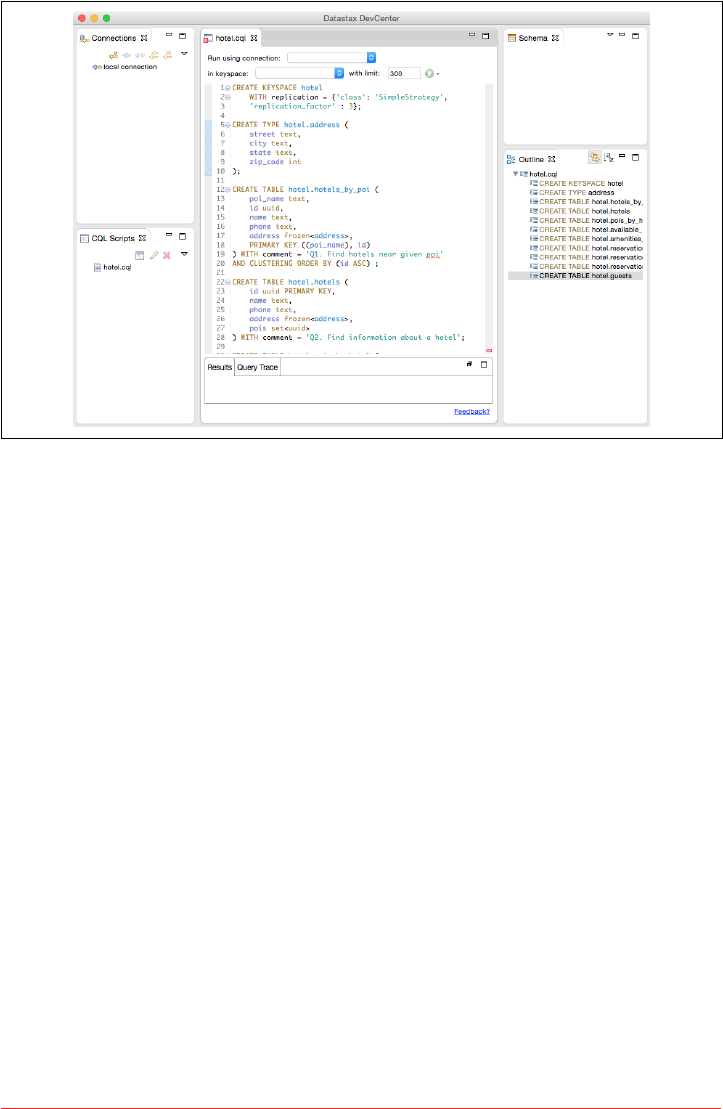
Figure 5-10. Editing the Hotel schema in DataStax DevCenter
Summary
In this chapter, we saw how to create a complete, working Cassandra data model and
compared it with an equivalent relational model. We represented our data model in
both logical and physical forms and learned a new tool for realizing our data models
in CQL. Now that we have a working data model, we’ll continue building our hotel
application in the coming chapters.
Summary | 103

CHAPTER 6
The Cassandra Architecture
3.2 Architecture - fundamental concepts or properties of a system in its environment embod‐
ied in its elements, relationships, and in the principles of its design and evolution.
—ISO/IEC/IEEE 42010
In this chapter, we examine several aspects of Cassandra’s architecture in order to
understand how it does its job. We’ll explain the topology of a cluster, and how nodes
interact in a peer-to-peer design to maintain the health of the cluster and exchange
data, using techniques like gossip, anti-entropy, and hinted handoff. Looking inside
the design of a node, we examine architecture techniques Cassandra uses to support
reading, writing, and deleting data, and examine how these choices affect architec‐
tural considerations such as scalability, durability, availability, manageability, and
more. We also discuss Cassandra’s adoption of a Staged Event-Driven Architecture,
which acts as the platform for request delegation.
As we introduce these topics, we also provide references to where you can find their
implementations in the Cassandra source code.
Data Centers and Racks
Cassandra is frequently used in systems spanning physically separate locations. Cas‐
sandra provides two levels of grouping that are used to describe the topology of a
cluster: data center and rack. A rack is a logical set of nodes in close proximity to each
other, perhaps on physical machines in a single rack of equipment. A data center is a
logical set of racks, perhaps located in the same building and connected by reliable
network. A sample topology with multiple data centers and racks is shown in
Figure 6-1.
105
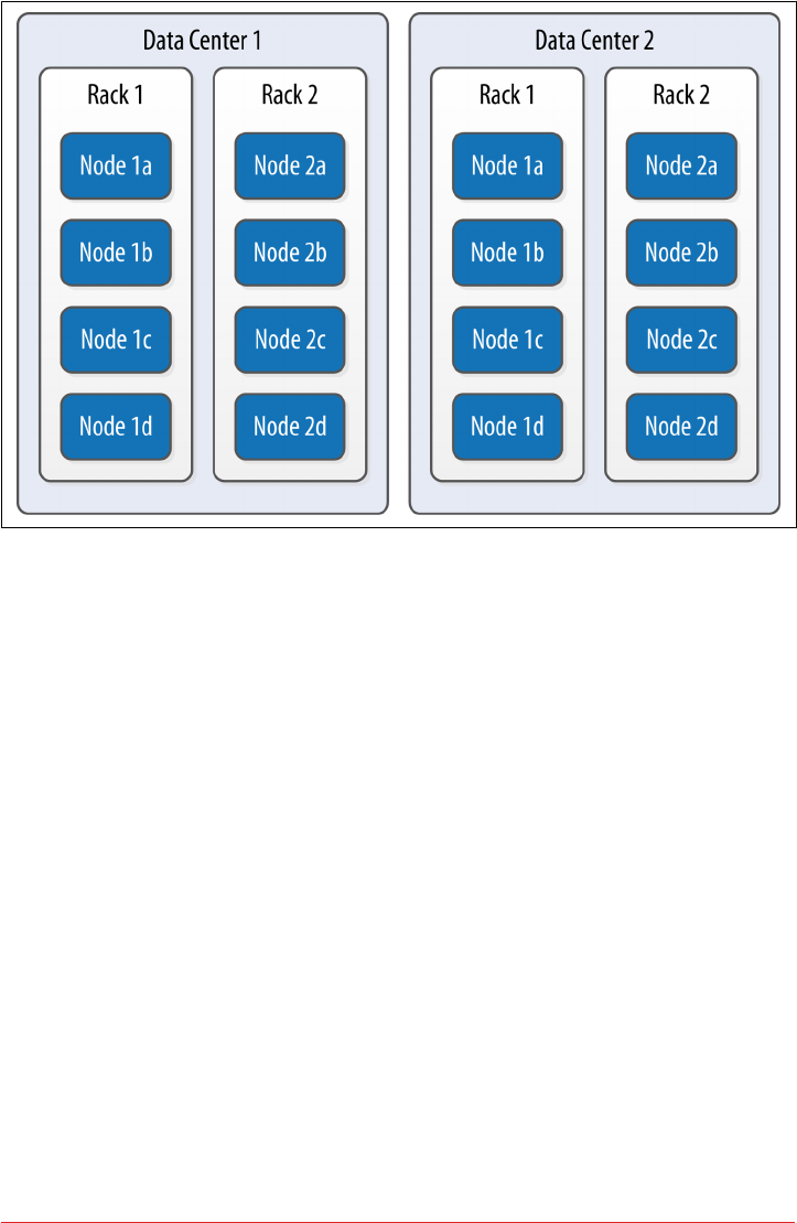
Figure 6-1. Topology of a sample cluster with data centers, racks, and nodes
Out of the box, Cassandra comes with a default configuration of a single data center
("DC1") containing a single rack ("RAC1"). We’ll learn in Chapter 7 how to build a
larger cluster and define its topology.
Cassandra leverages the information you provide about your cluster’s topology to
determine where to store data, and how to route queries efficiently. Cassandra tries to
store copies of your data in multiple data centers to maximize availability and parti‐
tion tolerance, while preferring to route queries to nodes in the local data center to
maximize performance.
Gossip and Failure Detection
To support decentralization and partition tolerance, Cassandra uses a gossip protocol
that allows each node to keep track of state information about the other nodes in the
cluster. The gossiper runs every second on a timer.
Gossip protocols (sometimes called “epidemic protocols”) generally assume a faulty
network, are commonly employed in very large, decentralized network systems, and
are often used as an automatic mechanism for replication in distributed databases.
They take their name from the concept of human gossip, a form of communication in
which peers can choose with whom they want to exchange information.
106 | Chapter 6: The Cassandra Architecture

The Origin of “Gossip Protocol”
The term “gossip protocol” was originally coined in 1987 by Alan
Demers, a researcher at Xerox’s Palo Alto Research Center, who
was studying ways to route information through unreliable net‐
works.
The gossip protocol in Cassandra is primarily implemented by the org.apache.cas
sandra.gms.Gossiper class, which is responsible for managing gossip for the local
node. When a server node is started, it registers itself with the gossiper to receive
endpoint state information.
Because Cassandra gossip is used for failure detection, the Gossiper class maintains a
list of nodes that are alive and dead.
Here is how the gossiper works:
1. Once per second, the gossiper will choose a random node in the cluster and initi‐
alize a gossip session with it. Each round of gossip requires three messages.
2. The gossip initiator sends its chosen friend a GossipDigestSynMessage.
3. When the friend receives this message, it returns a GossipDigestAckMessage.
4. When the initiator receives the ack message from the friend, it sends the friend a
GossipDigestAck2Message to complete the round of gossip.
When the gossiper determines that another endpoint is dead, it “convicts” that end‐
point by marking it as dead in its local list and logging that fact.
Cassandra has robust support for failure detection, as specified by a popular algo‐
rithm for distributed computing called Phi Accrual Failure Detection. This manner of
failure detection originated at the Advanced Institute of Science and Technology in
Japan in 2004.
Accrual failure detection is based on two primary ideas. The first general idea is that
failure detection should be flexible, which is achieved by decoupling it from the appli‐
cation being monitored. The second and more novel idea challenges the notion of
traditional failure detectors, which are implemented by simple “heartbeats” and
decide whether a node is dead or not dead based on whether a heartbeat is received
or not. But accrual failure detection decides that this approach is naive, and finds a
place in between the extremes of dead and alive—a suspicion level.
Therefore, the failure monitoring system outputs a continuous level of “suspicion”
regarding how confident it is that a node has failed. This is desirable because it can
take into account fluctuations in the network environment. For example, just because
one connection gets caught up doesn’t necessarily mean that the whole node is dead.
So suspicion offers a more fluid and proactive indication of the weaker or stronger
Gossip and Failure Detection | 107

possibility of failure based on interpretation (the sampling of heartbeats), as opposed
to a simple binary assessment.
Phi Threshold and Accrual Failure Detectors
Accrual Failure Detectors output a value associated with each process (or node). This
value is called Phi. The value is output in a manner that is designed from the ground
up to be adaptive in the face of volatile network conditions, so it’s not a binary condi‐
tion that simply checks whether a server is up or down.
The Phi convict threshold in the configuration adjusts the sensitivity of the failure
detector. Lower values increase the sensitivity and higher values decrease it, but not in
a linear fashion.
The Phi value refers to a level of suspicion that a server might be down. Applications
such as Cassandra that employ an AFD can specify variable conditions for the Phi
value they emit. Cassandra can generally detect a failed node in about 10 seconds
using this mechanism.
You can read the original Phi Accrual Failure Detection paper by Naohiro Hayashi‐
bara et al. at http://www.jaist.ac.jp/~defago/les/pdf/IS_RR_2004_010.pdf.
Failure detection is implemented in Cassandra by the org.apache.cassandra.gms.
FailureDetector class, which implements the org.apache.cassandra.gms.IFailur
eDetector interface. Together, they allow operations including:
isAlive(InetAddress)
What the detector will report about a given node’s alive-ness.
interpret(InetAddress)
Used by the gossiper to help it decide whether a node is alive or not based on
suspicion level reached by calculating Phi (as described in the Hayashibara
paper).
report(InetAddress)
When a node receives a heartbeat, it invokes this method.
Snitches
The job of a snitch is to determine relative host proximity for each node in a cluster,
which is used to determine which nodes to read and write from. Snitches gather
information about your network topology so that Cassandra can efficiently route
requests. The snitch will figure out where nodes are in relation to other nodes.
108 | Chapter 6: The Cassandra Architecture

As an example, let’s examine how the snitch participates in a read operation. When
Cassandra performs a read, it must contact a number of replicas determined by the
consistency level. In order to support the maximum speed for reads, Cassandra
selects a single replica to query for the full object, and asks additional replicas for
hash values in order to ensure the latest version of the requested data is returned. The
role of the snitch is to help identify the replica that will return the fastest, and this is
the replica which is queried for the full data.
The default snitch (the SimpleSnitch) is topology unaware; that is, it does not know
about the racks and data centers in a cluster, which makes it unsuitable for multi-data
center deployments. For this reason, Cassandra comes with several snitches for dif‐
ferent cloud environments including Amazon EC2, Google Cloud, and Apache
Cloudstack.
The snitches can be found in the package org.apache.cassandra.locator. Each
snitch implements the IEndpointSnitch interface. We’ll learn how to select and con‐
figure an appropriate snitch for your environment in Chapter 7.
While Cassandra provides a pluggable way to statically describe your cluster’s topol‐
ogy, it also provides a feature called dynamic snitching that helps optimize the routing
of reads and writes over time. Here’s how it works. Your selected snitch is wrapped
with another snitch called the DynamicEndpointSnitch. The dynamic snitch gets its
basic understanding of the topology from the selected snitch. It then monitors the
performance of requests to the other nodes, even keeping track of things like which
nodes are performing compaction. The performance data is used to select the best
replica for each query. This enables Cassandra to avoid routing requests to replicas
that are performing poorly.
The dynamic snitching implementation uses a modified version of the Phi failure
detection mechanism used by gossip. The “badness threshold” is a configurable
parameter that determines how much worse a preferred node must perform than the
best-performing node in order to lose its preferential status. The scores of each node
are reset periodically in order to allow a poorly performing node to demonstrate that
it has recovered and reclaim its preferred status.
Rings and Tokens
So far we’ve been focusing on how Cassandra keeps track of the physical layout of
nodes in a cluster. Let’s shift gears and look at how Cassandra distributes data across
these nodes.
Cassandra represents the data managed by a cluster as a ring. Each node in the ring is
assigned one or more ranges of data described by a token, which determines its posi‐
tion in the ring. A token is a 64-bit integer ID used to identify each partition. This
gives a possible range for tokens from –263 to 263–1.
Rings and Tokens | 109
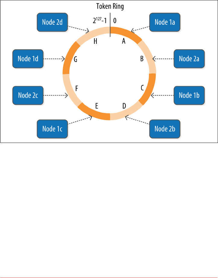
A node claims ownership of the range of values less than or equal to each token and
greater than the token of the previous node. The node with lowest token owns the
range less than or equal to its token and the range greater than the highest token,
which is also known as the “wrapping range.” In this way, the tokens specify a com‐
plete ring. Figure 6-2 shows a notional ring layout including the nodes in a single
data center. This particular arrangement is structured such that consecutive token
ranges are spread across nodes in different racks.
Figure 6-2. Example ring arrangement of nodes in a data center
Data is assigned to nodes by using a hash function to calculate a token for the parti‐
tion key. This partition key token is compared to the token values for the various
nodes to identify the range, and therefore the node, that owns the data.
Token ranges are represented by the org.apache.cassandra.dht.Range class.
Virtual Nodes
Early versions of Cassandra assigned a single token to each node, in a fairly static
manner, requiring you to calculate tokens for each node. Although there are tools
available to calculate tokens based on a given number of nodes, it was still a manual
process to configure the initial_token property for each node in the cassandra.yaml
file. This also made adding or replacing a node an expensive operation, as rebalanc‐
ing the cluster required moving a lot of data.
110 | Chapter 6: The Cassandra Architecture

Cassandra’s 1.2 release introduced the concept of virtual nodes, also called vnodes for
short. Instead of assigning a single token to a node, the token range is broken up into
multiple smaller ranges. Each physical node is then assigned multiple tokens. By
default, each node will be assigned 256 of these tokens, meaning that it contains 256
virtual nodes. Virtual nodes have been enabled by default since 2.0.
Vnodes make it easier to maintain a cluster containing heterogeneous machines. For
nodes in your cluster that have more computing resources available to them, you can
increase the number of vnodes by setting the num_tokens property in the cassan‐
dra.yaml file. Conversely, you might set num_tokens lower to decrease the number of
vnodes for less capable machines.
Cassandra automatically handles the calculation of token ranges for each node in the
cluster in proportion to their num_tokens value. Token assignments for vnodes are
calculated by the org.apache.cassandra.dht.tokenallocator.ReplicationAware
TokenAllocator class.
A further advantage of virtual nodes is that they speed up some of the more heavy‐
weight Cassandra operations such as bootstrapping a new node, decommissioning a
node, and repairing a node. This is because the load associated with operations on
multiple smaller ranges is spread more evenly across the nodes in the cluster.
Partitioners
A partitioner determines how data is distributed across the nodes in the cluster. As we
learned in Chapter 5, Cassandra stores data in wide rows, or “partitions.” Each row
has a partition key that is used to identify the partition. A partitioner, then, is a hash
function for computing the token of a partition key. Each row of data is distributed
within the ring according to the value of the partition key token.
Cassandra provides several different partitioners in the org.apache.cassandra.dht
package (DHT stands for “distributed hash table”). The Murmur3Partitioner was
added in 1.2 and has been the default partitioner since then; it is an efficient Java
implementation on the murmur algorithm developed by Austin Appleby. It generates
64-bit hashes. The previous default was the RandomPartitioner.
Because of Cassandra’s generally pluggable design, you can also create your own par‐
titioner by implementing the org.apache.cassandra.dht.IPartitioner class and
placing it on Cassandra’s classpath.
Partitioners | 111

Replication Strategies
A node serves as a replica for different ranges of data. If one node goes down, other
replicas can respond to queries for that range of data. Cassandra replicates data across
nodes in a manner transparent to the user, and the replication factor is the number of
nodes in your cluster that will receive copies (replicas) of the same data. If your repli‐
cation factor is 3, then three nodes in the ring will have copies of each row.
The first replica will always be the node that claims the range in which the token falls,
but the remainder of the replicas are placed according to the replication strategy
(sometimes also referred to as the replica placement strategy).
For determining replica placement, Cassandra implements the Gang of Four Strategy
pattern, which is outlined in the common abstract class org.apache.cassandra.loca
tor.AbstractReplicationStrategy, allowing different implementations of an algo‐
rithm (different strategies for accomplishing the same work). Each algorithm
implementation is encapsulated inside a single class that extends the AbstractRepli
cationStrategy.
Out of the box, Cassandra provides two primary implementations of this interface
(extensions of the abstract class): SimpleStrategy and NetworkTopologyStrategy.
The SimpleStrategy places replicas at consecutive nodes around the ring, starting
with the node indicated by the partitioner. The NetworkTopologyStrategy allows you
to specify a different replication factor for each data center. Within a data center, it
allocates replicas to different racks in order to maximize availability.
Legacy Replication Strategies
A third strategy, OldNetworkTopologyStrategy, is provided for
backward compatibility. It was previously known as the RackAware
Strategy, while the SimpleStrategy was previously known as the
RackUnawareStrategy. NetworkTopologyStrategy was previously
known as DataCenterShardStrategy. These changes were effective
in the 0.7 release.
The strategy is set independently for each keyspace and is a required option to create
a keyspace, as we saw in Chapter 5.
112 | Chapter 6: The Cassandra Architecture

Consistency Levels
In Chapter 2, we discussed Brewer’s CAP theorem, in which consistency, availability,
and partition tolerance are traded off against one another. Cassandra provides tunea‐
ble consistency levels that allow you to make these trade-offs at a fine-grained level.
You specify a consistency level on each read or write query that indicates how much
consistency you require. A higher consistency level means that more nodes need to
respond to a read or write query, giving you more assurance that the values present
on each replica are the same.
For read queries, the consistency level specifies how many replica nodes must
respond to a read request before returning the data. For write operations, the consis‐
tency level specifies how many replica nodes must respond for the write to be
reported as successful to the client. Because Cassandra is eventually consistent,
updates to other replica nodes may continue in the background.
The available consistency levels include ONE, TWO, and THREE, each of which specify an
absolute number of replica nodes that must respond to a request. The QUORUM consis‐
tency level requires a response from a majority of the replica nodes (sometimes
expressed as “replication factor / 2 + 1”). The ALL consistency level requires a
response from all of the replicas. We’ll examine these consistency levels and others in
more detail in Chapter 9.
For both reads and writes, the consistency levels of ANY, ONE, TWO, and THREE are con‐
sidered weak, whereas QUORUM and ALL are considered strong. Consistency is tuneable
in Cassandra because clients can specify the desired consistency level on both reads
and writes. There is an equation that is popularly used to represent the way to achieve
strong consistency in Cassandra: R + W > N = strong consistency. In this equation, R,
W, and N are the read replica count, the write replica count, and the replication fac‐
tor, respectively; all client reads will see the most recent write in this scenario, and
you will have strong consistency.
Distinguishing Consistency Levels and Replication Factors
If you’re new to Cassandra, the replication factor can sometimes be
confused with the consistency level. The replication factor is set per
keyspace. The consistency level is specified per query, by the client.
The replication factor indicates how many nodes you want to use
to store a value during each write operation. The consistency level
specifies how many nodes the client has decided must respond in
order to feel confident of a successful read or write operation. The
confusion arises because the consistency level is based on the repli‐
cation factor, not on the number of nodes in the system.
Consistency Levels | 113

Queries and Coordinator Nodes
Let’s bring these concepts together to discuss how Cassandra nodes interact to sup‐
port reads and writes from client applications. Figure 6-3 shows the typical path of
interactions with Cassandra.
Figure 6-3. Clients, coordinator nodes, and replicas
A client may connect to any node in the cluster to initiate a read or write query. This
node is known as the coordinator node. The coordinator identifies which nodes are
replicas for the data that is being written or read and forwards the queries to them.
For a write, the coordinator node contacts all replicas, as determined by the consis‐
tency level and replication factor, and considers the write successful when a number
of replicas commensurate with the consistency level acknowledge the write.
For a read, the coordinator contacts enough replicas to ensure the required consis‐
tency level is met, and returns the data to the client.
These, of course, are the “happy path” descriptions of how Cassandra works. We’ll
soon discuss some of Cassandra’s high availability mechanisms, including hinted
handoff.
114 | Chapter 6: The Cassandra Architecture
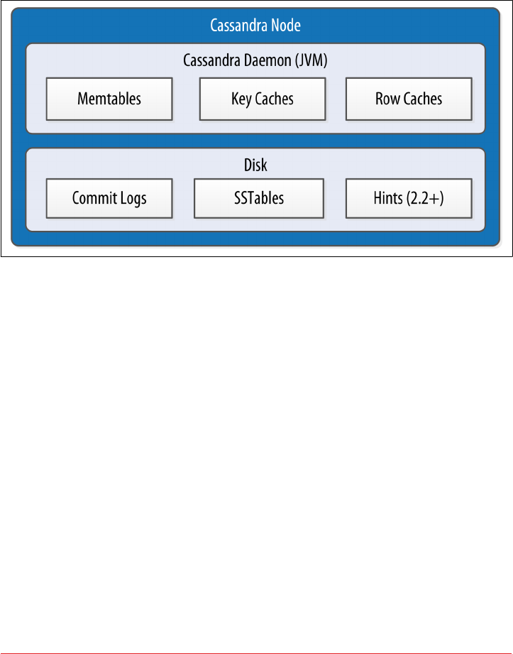
Memtables, SSTables, and Commit Logs
Now let’s take a look at some of Cassandra’s internal data structures and files, sum‐
marized in Figure 6-4. Cassandra stores data both in memory and on disk to provide
both high performance and durability. In this section, we’ll focus on Cassandra’s use
of constructs called memtables, SSTables, and commit logs to support the writing and
reading of data from tables.
Figure 6-4. Internal data structures and les of a Cassandra node
When you perform a write operation, it’s immediately written to a commit log. The
commit log is a crash-recovery mechanism that supports Cassandra’s durability goals.
A write will not count as successful until it’s written to the commit log, to ensure that
if a write operation does not make it to the in-memory store (the memtable, dis‐
cussed in a moment), it will still be possible to recover the data. If you shut down the
database or it crashes unexpectedly, the commit log can ensure that data is not lost.
That’s because the next time you start the node, the commit log gets replayed. In fact,
that’s the only time the commit log is read; clients never read from it.
After it’s written to the commit log, the value is written to a memory-resident data
structure called the memtable. Each memtable contains data for a specific table. In
early implementations of Cassandra, memtables were stored on the JVM heap, but
improvements starting with the 2.1 release have moved the majority of memtable data
to native memory. This makes Cassandra less susceptible to fluctuations in perfor‐
mance due to Java garbage collection.
When the number of objects stored in the memtable reaches a threshold, the contents
of the memtable are flushed to disk in a file called an SSTable. A new memtable is
then created. This flushing is a non-blocking operation; multiple memtables may
Memtables, SSTables, and Commit Logs | 115

exist for a single table, one current and the rest waiting to be flushed. They typically
should not have to wait very long, as the node should flush them very quickly unless
it is overloaded.
Each commit log maintains an internal bit flag to indicate whether it needs flushing.
When a write operation is first received, it is written to the commit log and its bit flag
is set to 1. There is only one bit flag per table, because only one commit log is ever
being written to across the entire server. All writes to all tables will go into the same
commit log, so the bit flag indicates whether a particular commit log contains any‐
thing that hasn’t been flushed for a particular table. Once the memtable has been
properly flushed to disk, the corresponding commit log’s bit flag is set to 0, indicating
that the commit log no longer has to maintain that data for durability purposes. Like
regular logfiles, commit logs have a configurable rollover threshold, and once this file
size threshold is reached, the log will roll over, carrying with it any extant dirty bit
flags.
The SSTable is a concept borrowed from Google’s Bigtable. Once a memtable is
flushed to disk as an SSTable, it is immutable and cannot be changed by the applica‐
tion. Despite the fact that SSTables are compacted, this compaction changes only
their on-disk representation; it essentially performs the “merge” step of a mergesort
into new files and removes the old files on success.
Why Are They Called “SSTables”?
The idea that “SSTable” is a compaction of “Sorted String Table” is
somewhat inaccurate for Cassandra, because the data is not stored
as strings on disk.
Since the 1.0 release, Cassandra has supported the compression of SSTables in order
to maximize use of the available storage. This compression is configurable per table.
Each SSTable also has an associated Bloom filter, which is used as an additional per‐
formance enhancer (see “Bloom Filters” on page 120).
All writes are sequential, which is the primary reason that writes perform so well in
Cassandra. No reads or seeks of any kind are required for writing a value to Cassan‐
dra because all writes are append operations. This makes one key limitation on per‐
formance the speed of your disk. Compaction is intended to amortize the
reorganization of data, but it uses sequential I/O to do so. So the performance benefit
is gained by splitting; the write operation is just an immediate append, and then com‐
paction helps to organize for better future read performance. If Cassandra naively
inserted values where they ultimately belonged, writing clients would pay for seeks up
front.
116 | Chapter 6: The Cassandra Architecture

On reads, Cassandra will read both SSTables and memtables to find data values, as
the memtable may contain values that have not yet been flushed to disk. Memtables
are implemented by the org.apache.cassandra.db.Memtable class.
Caching
As we saw in Figure 6-4, Cassandra provides three forms of caching:
•The key cache stores a map of partition keys to row index entries, facilitating
faster read access into SSTables stored on disk. The key cache is stored on the
JVM heap.
•The row cache caches entire rows and can greatly speed up read access for fre‐
quently accessed rows, at the cost of more memory usage. The row cache is
stored in off-heap memory.
•The counter cache was added in the 2.1 release to improve counter performance
by reducing lock contention for the most frequently accessed counters.
By default, key and counter caching are enabled, while row caching is disabled, as it
requires more memory. Cassandra saves its caches to disk periodically in order to
warm them up more quickly on a node restart. We’ll investigate how to tune these
caches in Chapter 12.
Hinted Hando
Consider the following scenario: a write request is sent to Cassandra, but a replica
node where the write properly belongs is not available due to network partition,
hardware failure, or some other reason. In order to ensure general availability of the
ring in such a situation, Cassandra implements a feature called hinted hando. You
might think of a hint as a little Post-it note that contains the information from the
write request. If the replica node where the write belongs has failed, the coordinator
will create a hint, which is a small reminder that says, “I have the write information
that is intended for node B. I’m going to hang onto this write, and I’ll notice when
node B comes back online; when it does, I’ll send it the write request.” That is, once it
detects via gossip that node B is back online, node A will “hand off” to node B the
“hint” regarding the write. Cassandra holds a separate hint for each partition that is to
be written.
This allows Cassandra to be always available for writes, and generally enables a clus‐
ter to sustain the same write load even when some of the nodes are down. It also
reduces the time that a failed node will be inconsistent after it does come back online.
In general, hints do not count as writes for the purposes of consistency level. The
exception is the consistency level ANY, which was added in 0.6. This consistency level
means that a hinted handoff alone will count as sufficient toward the success of a
Caching | 117

write operation. That is, even if only a hint was able to be recorded, the write still
counts as successful. Note that the write is considered durable, but the data may not
be readable until the hint is delivered to the target replica.
Hinted Hando and Guaranteed Delivery
Hinted handoff is used in Amazon’s Dynamo and is familiar to
those who are aware of the concept of guaranteed delivery in mes‐
saging systems such as the Java Message Service (JMS). In a durable
guaranteed-delivery JMS queue, if a message cannot be delivered to
a receiver, JMS will wait for a given interval and then resend the
request until the message is received.
There is a practical problem with hinted handoffs (and guaranteed delivery
approaches, for that matter): if a node is offline for some time, the hints can build up
considerably on other nodes. Then, when the other nodes notice that the failed node
has come back online, they tend to flood that node with requests, just at the moment
it is most vulnerable (when it is struggling to come back into play after a failure). To
address this problem, Cassandra limits the storage of hints to a configurable time
window. It is also possible to disable hinted handoff entirely.
As its name suggests, org.apache.cassandra.db.HintedHandOffManager is the class
that manages hinted handoffs internally.
Although hinted handoff helps increase Cassandra’s availability, it does not fully
replace the need for manual repair to ensure consistency.
Lightweight Transactions and Paxos
As we discussed in Chapter 2, Cassandra provides tuneable consistency, including the
ability to achieve strong consistency by specifying sufficiently high consistency levels.
However, strong consistency is not enough to prevent race conditions in cases where
clients need to read, then write data.
To help explain this with an example, let’s revisit our my_keyspace.user table from
Chapter 5. Imagine we are building a client that wants to manage user records as part
of an account management application. In creating a new user account, we’d like to
make sure that the user record doesn’t already exist, lest we unintentionally overwrite
existing user data. So we do a read to see if the record exists first, and then only per‐
form the create if the record doesn’t exist.
The behavior we’re looking for is called linearizable consistency, meaning that we’d
like to guarantee that no other client can come in between our read and write queries
with their own modification. Since the 2.0 release, Cassandra supports a lightweight
transaction (or “LWT”) mechanism that provides linearizable consistency.
118 | Chapter 6: The Cassandra Architecture

Cassandra’s LWT implementation is based on Paxos. Paxos is a consensus algorithm
that allows distributed peer nodes to agree on a proposal, without requiring a master
to coordinate a transaction. Paxos and other consensus algorithms emerged as alter‐
natives to traditional two-phase commit based approaches to distributed transactions
(reference the note on Two-Phase Commit in The Problem with Two-Phase Com‐
mit).
The basic Paxos algorithm consists of two stages: prepare/promise, and propose/
accept. To modify data, a coordinator node can propose a new value to the replica
nodes, taking on the role of leader. Other nodes may act as leaders simultaneously for
other modifications. Each replica node checks the proposal, and if the proposal is the
latest it has seen, it promises to not accept proposals associated with any prior pro‐
posals. Each replica node also returns the last proposal it received that is still in pro‐
gress. If the proposal is approved by a majority of replicas, the leader commits the
proposal, but with the caveat that it must first commit any in-progress proposals that
preceded its own proposal.
The Cassandra implementation extends the basic Paxos algorithm in order to support
the desired read-before-write semantics (also known as “check-and-set”), and to
allow the state to be reset between transactions. It does this by inserting two addi‐
tional phases into the algorithm, so that it works as follows:
1. Prepare/Promise
2. Read/Results
3. Propose/Accept
4. Commit/Ack
Thus, a successful transaction requires four round-trips between the coordinator
node and replicas. This is more expensive than a regular write, which is why you
should think carefully about your use case before using LWTs.
More on Paxos
Several papers have been written about the Paxos protocol. One of
the best explanations available is Leslie Lamport’s “Paxos Made
Simple”.
Cassandra’s lightweight transactions are limited to a single partition. Internally, Cas‐
sandra stores a Paxos state for each partition. This ensures that transactions on differ‐
ent partitions cannot interfere with each other.
You can find Cassandra’s implementation of the Paxos algorithm in the package
org.apache.cassandra.service.paxos. These classes are leveraged by the Storage
Service, which we will learn about soon.
Lightweight Transactions and Paxos | 119

Tombstones
In the relational world, you might be accustomed to the idea of a “soft delete.” Instead
of actually executing a delete SQL statement, the application will issue an update
statement that changes a value in a column called something like “deleted.” Program‐
mers sometimes do this to support audit trails, for example.
There’s a similar concept in Cassandra called a tombstone. This is how all deletes work
and is therefore automatically handled for you. When you execute a delete operation,
the data is not immediately deleted. Instead, it’s treated as an update operation that
places a tombstone on the value. A tombstone is a deletion marker that is required to
suppress older data in SSTables until compaction can run.
There’s a related setting called Garbage Collection Grace Seconds. This is the amount
of time that the server will wait to garbage-collect a tombstone. By default, it’s set to
864,000 seconds, the equivalent of 10 days. Cassandra keeps track of tombstone age,
and once a tombstone is older than GCGraceSeconds, it will be garbage-collected. The
purpose of this delay is to give a node that is unavailable time to recover; if a node is
down longer than this value, then it is treated as failed and replaced.
Bloom Filters
Bloom filters are used to boost the performance of reads. They are named for their
inventor, Burton Bloom. Bloom filters are very fast, non-deterministic algorithms for
testing whether an element is a member of a set. They are non-deterministic because
it is possible to get a false-positive read from a Bloom filter, but not a false-negative.
Bloom filters work by mapping the values in a data set into a bit array and condens‐
ing a larger data set into a digest string using a hash function. The digest, by defini‐
tion, uses a much smaller amount of memory than the original data would. The filters
are stored in memory and are used to improve performance by reducing the need for
disk access on key lookups. Disk access is typically much slower than memory access.
So, in a way, a Bloom filter is a special kind of cache. When a query is performed, the
Bloom filter is checked first before accessing disk. Because false-negatives are not
possible, if the filter indicates that the element does not exist in the set, it certainly
doesn’t; but if the filter thinks that the element is in the set, the disk is accessed to
make sure.
Bloom filters are implemented by the org.apache.cassandra.utils.BloomFilter
class. Cassandra provides the ability to increase Bloom filter accuracy (reducing the
number of false positives) by increasing the filter size, at the cost of more memory.
This false positive chance is tuneable per table.
120 | Chapter 6: The Cassandra Architecture

Other Uses of Bloom Filters
Bloom filters are used in other distributed database and caching
technologies, including Apache Hadoop, Google Bigtable, and
Squid Proxy Cache.
Compaction
As we already discussed, SSTables are immutable, which helps Cassandra achieve
such high write speeds. However, periodic compaction of these SSTables is important
in order to support fast read performance and clean out stale data values. A compac‐
tion operation in Cassandra is performed in order to merge SSTables. During com‐
paction, the data in SSTables is merged: the keys are merged, columns are combined,
tombstones are discarded, and a new index is created.
Compaction is the process of freeing up space by merging large accumulated data‐
files. This is roughly analogous to rebuilding a table in the relational world. But the
primary difference in Cassandra is that it is intended as a transparent operation that
is amortized across the life of the server.
On compaction, the merged data is sorted, a new index is created over the sorted
data, and the freshly merged, sorted, and indexed data is written to a single new
SSTable (each SSTable consists of multiple files including: Data, Index, and Filter).
This process is managed by the class org.apache.cassandra.db.compaction.Compac
tionManager.
Another important function of compaction is to improve performance by reducing
the number of required seeks. There are a bounded number of SSTables to inspect to
find the column data for a given key. If a key is frequently mutated, it’s very likely that
the mutations will all end up in flushed SSTables. Compacting them prevents the
database from having to perform a seek to pull the data from each SSTable in order to
locate the current value of each column requested in a read request.
When compaction is performed, there is a temporary spike in disk I/O and the size of
data on disk while old SSTables are read and new SSTables are being written.
Cassandra supports multiple algorithms for compaction via the strategy pattern. The
compaction strategy is an option that is set for each table. The compaction strategy
extends the AbstractCompactionStrategy class. The available strategies include:
•SizeTieredCompactionStrategy (STCS) is the default compaction strategy and
is recommended for write-intensive tables
•LeveledCompactionStrategy (LCS) is recommended for read-intensive tables
•DateTieredCompactionStrategy (DTCS), which is intended for time series or
otherwise date-based data.
Compaction | 121
We’ll revisit these strategies in Chapter 12 to discuss selecting the best strategy for
each table.
One interesting feature of compaction relates to its intersection with incremental
repair. A feature called anticompaction was added in 2.1. As the name implies, anti‐
compaction is somewhat of an opposite operation to regular compaction in that the
result is the division of an SSTable into two SSTables, one containing repaired data,
and the other containing unrepaired data.
The trade-off is that more complexity is introduced into the compaction strategies,
which must handle repaired and unrepaired SSTables separately so that they are not
merged together.
What About Major Compaction?
Users with prior experience may recall that Cassandra exposes an
administrative operation called major compaction (also known as
full compaction) that consolidates multiple SSTables into a single
SSTable. While this feature is still available, the utility of perform‐
ing a major compaction has been greatly reduced over time. In fact,
usage is actually discouraged in production environments, as it
tends to limit Cassandra’s ability to remove stale data. We’ll learn
more about this and other administrative operations on SSTables
available via nodetool in Chapter 11.
Anti-Entropy, Repair, and Merkle Trees
Cassandra uses an anti-entropy protocol, which is a type of gossip protocol for repair‐
ing replicated data. Anti-entropy protocols work by comparing replicas of data and
reconciling differences observed between the replicas. Anti-entropy is used in Ama‐
zon’s Dynamo, and Cassandra’s implementation is modeled on that (see Section 4.7 of
the Dynamo paper).
Anti-Entropy in Cassandra
In Cassandra, the term anti-entropy is often used in two slightly dif‐
ferent contexts, with meanings that have some overlap:
•The term is often used as a shorthand for the replica synchro‐
nization mechanism for ensuring that data on different nodes
is updated to the newest version.
•At other times, Cassandra is described as having an anti-
entropy capability that includes replica synchronization as well
as hinted handoff, which is a write-time anti-entropy mecha‐
nism we read about in “Hinted Handoff” on page 117.
122 | Chapter 6: The Cassandra Architecture

Replica synchronization is supported via two different modes known as read repair
and anti-entropy repair. Read repair refers to the synchronization of replicas as data
is read. Cassandra reads data from multiple replicas in order to achieve the requested
consistency level, and detects if any replicas have out of date values. If an insufficient
number of nodes have the latest value, a read repair is performed immediately to
update the out of date replicas. Otherwise, the repairs can be performed in the back‐
ground after the read returns. This design is observed by Cassandra as well as by
straight key/value stores such as Project Voldemort and Riak.
Anti-entropy repair (sometimes called manual repair) is a manually initiated opera‐
tion performed on nodes as part of a regular maintenance process. This type of repair
is executed by using a tool called nodetool, as we’ll learn about in Chapter 11. Run‐
ning nodetool repair causes Cassandra to execute a major compaction (see “Com‐
paction” on page 121). During a major compaction, the server initiates a
TreeRequest/TreeReponse conversation to exchange Merkle trees with neighboring
nodes. The Merkle tree is a hash representing the data in that table. If the trees from
the different nodes don’t match, they have to be reconciled (or “repaired”) to deter‐
mine the latest data values they should all be set to. This tree comparison validation is
the responsibility of the org.apache.cassandra.service.AbstractReadExecutor
class.
What’s a Merkle Tree?
A Merkle tree, named for its inventor, Ralph Merkle, is also known as a “hash tree.”
It’s a data structure represented as a binary tree, and it’s useful because it summarizes
in short form the data in a larger data set. In a hash tree, the leaves are the data blocks
(typically files on a filesystem) to be summarized. Every parent node in the tree is a
hash of its direct child node, which tightly compacts the summary.
In Cassandra, the Merkle tree is implemented in the org.apache.cassandra.utils
.MerkleTree class.
Merkle trees are used in Cassandra to ensure that the peer-to-peer network of nodes
receives data blocks unaltered and unharmed. They are also used in cryptography to
verify the contents of files and transmissions.
Both Cassandra and Dynamo use Merkle trees for anti-entropy, but their implemen‐
tations are a little different. In Cassandra, each table has its own Merkle tree; the tree
is created as a snapshot during a major compaction, and is kept only as long as is
required to send it to the neighboring nodes on the ring. The advantage of this imple‐
mentation is that it reduces network I/O.
Anti-Entropy, Repair, and Merkle Trees | 123

Staged Event-Driven Architecture (SEDA)
Cassandra’s design was influenced by Staged Event-Driven Architecture (SEDA).
SEDA is a general architecture for highly concurrent Internet services, originally pro‐
posed in a 2001 paper called “SEDA: An Architecture for Well-Conditioned, Scalable
Internet Services” by Matt Welsh, David Culler, and Eric Brewer (who you might
recall from our discussion of the CAP theorem). You can read the original SEDA
paper at http://www.eecs.harvard.edu/~mdw/proj/seda.
In a typical application, a single unit of work is often performed within the confines
of a single thread. A write operation, for example, will start and end within the same
thread. Cassandra, however, is different: its concurrency model is based on SEDA, so
a single operation may start with one thread, which then hands off the work to
another thread, which may hand it off to other threads. But it’s not up to the current
thread to hand off the work to another thread. Instead, work is subdivided into what
are called stages, and the thread pool (really, a java.util.concurrent.Execu
torService) associated with the stage determines execution.
A stage is a basic unit of work, and a single operation may internally state-transition
from one stage to the next. Because each stage can be handled by a different thread
pool, Cassandra experiences a massive performance improvement. This design also
means that Cassandra is better able to manage its own resources internally because
different operations might require disk I/O, or they might be CPU-bound, or they
might be network operations, and so on, so the pools can manage their work accord‐
ing to the availability of these resources.
A stage consists of an incoming event queue, an event handler, and an associated
thread pool. Stages are managed by a controller that determines scheduling and
thread allocation; Cassandra implements this kind of concurrency model using the
thread pool java.util.concurrent.ExecutorService. To see specifically how this
works, check out the org.apache.cassandra.concurrent.StageManager class. The
following operations are represented as stages in Cassandra, including many of the
concepts we’ve discussed in this chapter:
•Read (local reads)
• Mutation (local writes)
• Gossip
•Request/response (interactions with other nodes)
• Anti-entropy (nodetool repair)
• Read repair
• Migration (making schema changes)
• Hinted handoff
124 | Chapter 6: The Cassandra Architecture

You can observe the thread pools associated with each of these stages by using the
nodetool tpstats command, which we’ll learn about in Chapter 10.
A few additional operations are also implemented as stages, such as operations on
memtables including flushing data out to SSTables and freeing memory. The stages
implement the IVerbHandler interface to support the functionality for a given verb.
Because the idea of mutation is represented as a stage, it can play a role in both insert
and delete operations.
A Pragmatic Approach to SEDA
Over time, developers of Cassandra and other technologies based
on the SEDA architecture article have encountered performance
issues due to the inefficiencies of requiring separate thread pools
for each stage and event queues between each stage, even for short-
lived stages. These challenges were acknowledged by Matt Welsh in
the follow-up blog post “A Retrospective on SEDA”.
Over time, Cassandra’s developers have relaxed the strict SEDA
conventions, collapsing some stages into the same thread pool to
improve throughput. However, the basic principles of separating
work into stages and using queues and thread pools to manage
these stages are still in evidence in the code.
Managers and Services
There is a set of classes that form Cassandra’s basic internal control mechanisms.
We’ve encountered a few of them already in this chapter, including the Hinted Han
dOffManager, the CompactionManager, and the StageManager. We’ll present a brief
overview of a few other classes here so that you can become familiar with some of the
more important ones. Many of these expose MBeans via the Java Management Exten‐
sion (JMX) in order to report status and metrics, and in some cases to allow configu‐
ration and control of their activities. We’ll learn more about interacting with these
MBeans in Chapter 10.
Cassandra Daemon
The org.apache.cassandra.service.CassandraDaemon interface represents the life
cycle of the Cassandra service running on a single node. It includes the typical life
cycle operations that you might expect: start, stop, activate, deactivate, and
destroy.
You can also create an in-memory Cassandra instance programmatically by using the
class org.apache.cassandra.service.EmbeddedCassandraService. Creating an
embedded instance can be useful for unit testing programs using Cassandra.
Managers and Services | 125

Storage Engine
Cassandra’s core data storage functionality is commonly referred to as the storage
engine, which consists primarily of classes in the org.apache.cassandra.db package.
The main entry point is the ColumnFamilyStore class, which manages all aspects of
table storage, including commit logs, memtables, SSTables, and indexes.
Major Changes to the Storage Engine
The storage engine was largely rewritten for the 3.0 release to bring
Cassandra’s in-memory and on-disk representations of data in
alignment with the CQL. An excellent summary of the changes is
provided in the CASSANDRA-8099 JIRA issue.
The storage engine rewrite was a precursor for many other
changes, most importantly, support for materialized views, which
was implemented under CASSANDRA-6477. These two JIRA
issues make for interesting reading if you want to better under‐
stand the changes required “under the hood” to enable these pow‐
erful new features.
Storage Service
Cassandra wraps the storage engine with a service represented by the
org.apache.cassandra.service.StorageService class. The storage service con‐
tains the node’s token, which is a marker indicating the range of data that the node is
responsible for.
The server starts up with a call to the initServer method of this class, upon which
the server registers the SEDA verb handlers, makes some determinations about its
state (such as whether it was bootstrapped or not, and what its partitioner is), and
registers an MBean with the JMX server.
Storage Proxy
The org.apache.cassandra.service.StorageProxy sits in front of the
StorageService to handle the work of responding to client requests. It coordinates
with other nodes to store and retrieve data, including storage of hints when needed.
The StorageProxy also helps manage lightweight transaction processing.
Direct Invocation of the Storage Proxy
Although it is possible to invoke the StorageProxy programmati‐
cally, as an in-memory instance, note that this is not considered an
officially supported API for Cassandra and therefore has under‐
gone changes between releases.
126 | Chapter 6: The Cassandra Architecture

Messaging Service
The purpose of org.apache.cassandra.net.MessagingService is to create socket
listeners for message exchange; inbound and outbound messages from this node
come through this service. The MessagingService.listen method creates a thread.
Each incoming connection then dips into the ExecutorService thread pool using
org.apache.cassandra.net.IncomingTcpConnection (a class that extends Thread)
to deserialize the message. The message is validated, and then routed to the appropri‐
ate handler.
Because the MessagingService also makes heavy use of stages and the pool it main‐
tains is wrapped with an MBean, you can find out a lot about how this service is work‐
ing (whether reads are getting backed up and so forth) through JMX.
Stream Manager
Streaming is Cassandra’s optimized way of sending sections of SSTable files from one
node to another via a persistent TCP connection; all other communication between
nodes occurs via serialized messages. The org.apache.cassandra.streaming.
Stream Manager handles these streaming messages, including connection manage‐
ment, message compression, progress tracking, and statistics.
CQL Native Transport Server
The CQL Native Protocol is the binary protocol used by clients to communicate with
Cassandra. The org.apache.cassandra.transport package contains the classes that
implement this protocol, including the Server. This native transport server manages
client connections and routes incoming requests, delegating the work of performing
queries to the StorageProxy.
There are several other classes that manage key features of Cassandra. Here are a few
to investigate if you’re interested:
Key feature Class
Repair org.apache.cassandra.service.ActiveRepairService
Caching org.apache.cassandra.service.CachingService
Migration org.apache.cassandra.service.MigrationManager
Materialized views org.apache.cassandra.db.view.MaterializedViewManager
Secondary indexes org.apache.cassandra.db.index.SecondaryIndexManager
Authorization org.apache.cassandra.auth.CassandraRoleManager
Managers and Services | 127

System Keyspaces
In true “dogfooding” style, Cassandra makes use of its own storage to keep track of
metadata about the cluster and local node. This is similar to the way in which Micro‐
soft SQL Server maintains the meta-databases master and tempdb. The master is used
to keep information about disk space, usage, system settings, and general server
installation notes; the tempdb is used as a workspace to store intermediate results and
perform general tasks. The Oracle database always has a tablespace called SYSTEM,
used for similar purposes. The Cassandra system keyspaces are used much like these.
Let’s go back to cqlsh to have a quick peek at the tables in Cassandra’s system key‐
space:
cqlsh> DESCRIBE TABLES;
Keyspace system_traces
----------------------
events sessions
Keyspace system_schema
----------------------
materialized_views functions aggregates types columns
tables triggers keyspaces dropped_columns
Keyspace system_auth
--------------------
resource_role_permissons_index role_permissions role_members
roles
Keyspace system
---------------
available_ranges sstable_activity local
range_xfers peer_events hints
materialized_views_builds_in_progress paxos
"IndexInfo" batchlog
peers size_estimates
built_materialized_views compaction_history
Keyspace system_distributed
---------------------------
repair_history parent_repair_history
128 | Chapter 6: The Cassandra Architecture

Seeing Dierent System Keyspaces?
If you’re using a version of Cassandra prior to 2.2, you may not see
some of these keyspaces listed. While the basic system keyspace
has been around since the beginning, the system_traces keyspace
was added in 1.2 to support request tracing. The system_auth and
system_distributed keyspaces were added in 2.2 to support role-
based access control (RBAC) and persistence of repair data, respec‐
tively. Finally, tables related to schema definition were migrated
from system to the system_schema keyspace in 3.0.
Looking over these tables, we see that many of them are related to the concepts dis‐
cussed in this chapter:
•Information about the structure of the cluster communicated via gossip is stored
in system.local and system.peers. These tables hold information about the
local node and other nodes in the cluster including IP addresses, locations by
data center and rack, CQL, and protocol versions.
•The system.range_xfers and system.available_ranges track token ranges
managed by each node and any ranges needing allocation.
•The system_schema.keyspaces, system_schema.tables, and system_
schema.columns store the definitions of the keyspaces, tables, and indexes
defined for the cluster.
•The construction of materialized views is tracked in the system.materialized_
views_builds_in_progress and system.built_materialized_views tables,
resulting in the views available in system_schema.materialized_views.
•User-provided extensions such as system_schema.types for user-defined types,
system_schema.triggers for triggers configured per table, system_schema.
functions for user-defined functions, and system_schema.aggregates for user-
defined aggregates.
•The system.paxos table stores the status of transactions in progress, while the
system.batchlog table stores the status of atomic batches.
• The system.size_estimates stores the estimated number of partitions per table,
which is used for Hadoop integration.
Removal of the system.hints Table
Hinted handoffs have traditionally been stored in the
system.hints table. As thoughtful developers have noted, the fact
that hints are really messages to be kept for a short time and
deleted means this usage is really an instance of the well-known
anti-pattern of using Cassandra as a queue, which we discussed in
Chapter 5. Hint storage was moved to flat files in the 3.0 release.
System Keyspaces | 129

Let’s go back to cqlsh to have a quick peek at the attributes of Cassandra’s system
keyspace:
cqlsh> USE system;
cqlsh:system> DESCRIBE KEYSPACE;
CREATE KEYSPACE system WITH replication =
{'class': 'LocalStrategy'} AND durable_writes = true;
...
We’ve truncated the output here because it lists the complete structure of each table.
Looking at the first statement in the output, we see that the system keyspace is using
the replication strategy LocalStrategy, meaning that this information is intended for
internal use and not replicated to other nodes.
Immutability of the System Keyspace
Describing the system keyspaces produces similar output to
describing any other keyspace, in that the tables are described using
the CREATE TABLE command syntax. This may be somewhat mis‐
leading, as you cannot modify the schema of the system keyspaces.
Summary
In this chapter, we examined the main pillars of Cassandra’s architecture, including
gossip, snitches, partitioners, replication, consistency, anti-entropy, hinted handoff,
and lightweight transactions, and how the use of a Staged Event-Driven Architecture
maximizes performance. We also looked at some of Cassandra’s internal data struc‐
tures, including memtables, SSTables, and commit logs, and how it executes various
operations, such as tombstones and compaction. Finally, we surveyed some of the
major classes and interfaces, pointing out key points of interest in case you want to
dive deeper into the code base.
130 | Chapter 6: The Cassandra Architecture

CHAPTER 7
Conguring Cassandra
In this chapter, we’ll build our first cluster and look at the available options for con‐
figuring Cassandra. Out of the box, Cassandra works with no configuration at all; you
can simply download and decompress, and then execute the program to start the
server with its default configuration. However, one of the things that makes Cassan‐
dra such a powerful technology is its emphasis on configurability and customization.
At the same time, the number of options may seem confusing at first.
We will focus on aspects of Cassandra that affect node behavior in a cluster and meta-
operations such as partitioning, snitches, and replication. Performance tuning and
security are additional configuration topics that get their own treatment in Chapters
12 and 13.
Cassandra Cluster Manager
In order to get practice in building and configuring a cluster, we’ll take advantage of a
tool called the Cassandra Cluster Manager or ccm. Built by Sylvain Lebresne and sev‐
eral other contributors, this tool is a set of Python scripts that allow you to run a
multi-node cluster on a single machine. This allows you to quickly configure a cluster
without having to provision additional hardware.
The tool is available on GitHub. A quick way to get started is to clone the repository
using Git. We’ll open a terminal window and navigate to a directory where we want to
create our clone and run the following command:
$ git clone https://github.com/pcmanus/ccm.git
Then we can to run the installation script with administrative-level privileges:
$ sudo ./setup.py install
131

ccm Installation Updates
We’ve provide a simplified view of instructions here for getting
started with ccm. You’ll want to check the webpage for dependen‐
cies and special instructions for platforms such as Windows and
MacOS X. Because ccm is an actively maintained tool, these details
may change over time.
Once you’ve installed ccm, it should be on the system path. To get a list of supported
commands, you can type ccm or ccm –help. If you need more information on the
options for a specific cluster command, type ccm <command> -h. We’ll use several of
these commands in the following sections as we create and configure a cluster.
You can dig into the Python script files to learn more about what ccm is doing. You
can also invoke the scripts directly from automated test suites.
Creating a Cluster
You can run Cassandra on a single machine, which is fine for getting started as you
learn how to read and write data. But Cassandra is specifically engineered to be used
in a cluster of many machines that can share the load in very high-volume situations.
In this section, we’ll learn about the configuration required to get multiple Cassandra
instances to talk to each other in a ring. The key file for configuring each node in a
cluster is the cassandra.yaml file, which you can find in the conf directory under your
Cassandra installation.
The key values in configuring a cluster are the cluster name, the partitioner, the
snitch, and the seed nodes. The cluster name, partitioner, and snitch must be the
same in all of the nodes participating in the cluster. The seed nodes are not strictly
required to be exactly the same for every node across the cluster, but it is a good idea
to do so; we’ll learn about the best practices for configuration momentarily.
Cassandra clusters are given names in order to prevent machines in one cluster from
joining another that you don’t want them to be a part of. The name of the default
cluster in the cassandra.yaml file is “Test Cluster.” You can change the name of the
cluster by updating the cluster_name property—just make sure that you have done
this on all nodes that you want to participate in this cluster.
Changing the Cluster Name
If you have written data to an existing Cassandra cluster and then
change the cluster name, Cassandra will warn you with a cluster
name mismatch error as it tries to read the datafiles on startup, and
then it will shut down.
132 | Chapter 7: Conguring Cassandra

Let’s try creating a cluster using ccm:
$ ccm create -v 3.0.0 -n 3 my_cluster --vnodes
Downloading http://archive.apache.org/dist/cassandra/3.0.0/
apache-cassandra-3.0.0-src.tar.gz to
/var/folders/63/6h7dm1k51bd6phvm7fbngskc0000gt/T/
ccm-z2kHp0.tar.gz (22.934MB)
24048379 [100.00%]
Extracting /var/folders/63/6h7dm1k51bd6phvm7fbngskc0000gt/T/
ccm-z2kHp0.tar.gz as version 3.0.0 ...
Compiling Cassandra 3.0.0 ...
Current cluster is now: my_cluster
This command creates a cluster based on the version of Cassandra we selected—in
this case, 3.0.0. The cluster is named my_cluster and has three nodes. We specify that
we want to use virtual nodes, because ccm defaults to creating single token nodes. ccm
designates our cluster as the current cluster that will be used for subsequent com‐
mands. You’ll notice that ccm downloads the source for the version requested to run
and compiles it. This is because ccm needs to make some minor modifications to the
Cassandra source in order to support running multiple nodes on a single machine.
We could also have used the copy of the source that we downloaded in Chapter 3. If
you’d like to investigate additional options for creating a cluster, run the command
ccm create -h.
Once we’ve created the cluster, we can see it is the only cluster in our list of clusters
(and marked as the default), and we can learn about its status:
$ ccm list
*my_cluster
$ ccm status
Cluster: 'my_cluster'
---------------------
node1: DOWN (Not initialized)
node3: DOWN (Not initialized)
node2: DOWN (Not initialized)
At this point, none of the nodes have been initialized. Let’s start our cluster and then
check status again:
$ ccm start
$ ccm status
Cluster: 'my_cluster'
---------------------
node1: UP
node3: UP
node2: UP
Creating a Cluster | 133

This is the equivalent of starting each individual node using the bin/cassandra script
(or service start cassandra for package installations). To dig deeper on the status
of an individual node, we’ll enter the following command:
$ ccm node1 status
Datacenter: datacenter1
=======================
Status=Up/Down
|/ State=Normal/Leaving/Joining/Moving
-- Address Load Tokens Owns Host ID Rack
UN 127.0.0.1 193.2 KB 256 ? e5a6b739-... rack1
UN 127.0.0.2 68.45 KB 256 ? 48843ab4-... rack1
UN 127.0.0.3 68.5 KB 256 ? dd728f0b-... rack1
This is equivalent to running the command nodetool status on the individual
node. The output shows that all of the nodes are up and reporting normal status
(UN). Each of the nodes has 256 tokens, and owns no data, as we haven’t inserted any
data yet. (We’ve shortened the host ID somewhat for brevity.)
We can run the nodetool ring command in order to get a list of the tokens owned
by each node. To do this in ccm, we enter the command:
$ ccm node1 ring
Datacenter: datacenter1
==========
Address Rack Status State ... Token
9205346612887953633
127.0.0.1 rack1 Up Normal ... -9211073930147845649
127.0.0.3 rack1 Up Normal ... -9114803904447515108
127.0.0.3 rack1 Up Normal ... -9091620194155459357
127.0.0.1 rack1 Up Normal ... -9068215598443754923
127.0.0.2 rack1 Up Normal ... -9063205907969085747
The command requires us to specify a node. This doesn’t affect the output; it just
indicates what node nodetool is connecting to in order to get the ring information.
As you can see, the tokens are allocated randomly across our three nodes. (As before,
we’ve abbreviated the output and omitted the Owns and Load columns for brevity.)
134 | Chapter 7: Conguring Cassandra

A Closer Look at Cluster Conguration
It’s quite interesting to take a look under the covers to see what configuration changes
ccm makes in order to get a cluster running on our local machine. By default, ccm
stores metadata and configuration files for your cluster in a directory under your
home directory called .ccm; it also uses this directory to store the source files for ver‐
sions of Cassandra you have run. Let’s take a look in this directory to see what we can
find there:
$ cd ~/.ccm; ls
CURRENT my_cluster repository
The repository directory contains the source that ccm downloaded. Diving deeper into
the my_cluster directory, we’ll see a directory for each node:
$ cd my_cluster; ls
cluster.conf node1 node2 node3
The cluster.conf file contains a list of options we selected when creating the cluster. To
see the configuration options that are different between nodes, try using the diff
command to compare the contents of the directories. For example:
$ cd ~/.ccm/my_cluster
$ diff node1/conf/ node2/conf/
The output highlights the differences in the configuration files, including the directo‐
ries used for storage of data, commit logs and output logs, the listen and RPC
addresses used for network communications, and the JMX port exposed for remote
management. We’ll examine these settings in more detail as we proceed through the
rest of the chapter.
Seed Nodes
A new node in a cluster needs what’s called a seed node. A seed node is used as a con‐
tact point for other nodes, so Cassandra can learn the topology of the cluster—that is,
what hosts have what ranges. For example, if node A acts as a seed for node B, when
node B comes online, it will use node A as a reference point from which to get data.
This process is known as bootstrapping or sometimes auto bootstrapping because it is
an operation that Cassandra performs automatically. Seed nodes do not auto boot‐
strap because it is assumed that they will be the first nodes in the cluster.
By default, the cassandra.yaml file will have only a single seed entry set to the local‐
host:
- seeds: "127.0.0.1"
Seed Nodes | 135

To add more seed nodes to a cluster, we just add another seed element. We can set
multiple servers to be seeds just by indicating the IP address or hostname of the node.
For an example, if we look in the cassandra.yaml file for one of our ccm nodes, we’ll
find the following:
- seeds: 127.0.0.1, 127.0.0.2, 127.0.0.3
In a production cluster, these would be the IP addresses of other hosts rather than
loopback addresses. To ensure high availability of Cassandra’s bootstrapping process,
it is considered a best practice to have at least two seed nodes per data center. This
increases the likelihood of having at least one seed node available should one of the
local seed nodes go down during a network partition between data centers.
As you may have noticed if you looked in the cassandra.yaml file, the list of seeds is
actually part of a larger definition of the seed provider. The org.apache.cassandra.
locator.SeedProvider interface specifies the contract that must be implemented.
Cassandra provides the SimpleSeedProvider as the default implementation, which
loads the IP addresses of the seed nodes from the cassandra.yaml file.
Partitioners
The purpose of the partitioner is to allow you to specify how partition keys should be
sorted, which has a significant impact on how data will be distributed across your
nodes. It also has an effect on the options available for querying ranges of rows. You
set the partitioner by updating the value of the partitioner property in the cassan‐
dra.yaml file. There are a few different partitioners you can use, which we look at
now.
Changing the Partitioner
You can’t change the partitioner once you’ve inserted data into a
cluster, so take care before deviating from the default!
Murmur3 Partitioner
The default partitioner is org.apache.cassandra.dht.Murmur3Partitioner. The
Murmur3Partitioner uses the murmur hash algorithm to generate tokens. This has
the advantage of spreading your keys evenly across your cluster, because the distribu‐
tion is random. It has the disadvantage of causing inefficient range queries, because
keys within a specified range might be placed in a variety of disparate locations in the
ring, and key range queries will return data in an essentially random order.
In general, new clusters should always use the Murmur3Partitioner. However, Cas‐
sandra provides several older partitioners for backward compatibility.
136 | Chapter 7: Conguring Cassandra

Random Partitioner
The random partitioner is implemented by org.apache.cassandra.dht.Ran
domPartitioner and was Cassandra’s default in Cassandra 1.1 and earlier. It uses a
BigIntegerToken with an MD5 cryptographic hash applied to it to determine where
to place the keys on the node ring. Although the RandomPartitioner and Murmur3Par
titioner are both based on random hash functions, the cryptographic hash used by
RandomPartitioner is considerably slower, which is why the Murmur3Partitioner
replaced it as the default.
Order-Preserving Partitioner
The order-preserving partitioner is implemented by org.apache.cassandra.dht.
OrderPreservingPartitioner. Using this type of partitioner, the token is a UTF-8
string, based on a key. Rows are therefore stored by key order, aligning the physical
structure of the data with your sort order. Configuring your column family to use
order-preserving partitioning (OPP) allows you to perform range slices.
It’s worth noting that OPP isn’t more efficient for range queries than random parti‐
tioning—it just provides ordering. It has the disadvantage of creating a ring that is
potentially very lopsided, because real-world data typically is not written to evenly. As
an example, consider the value assigned to letters in a Scrabble game. Q and Z are
rarely used, so they get a high value. With OPP, you’ll likely eventually end up with
lots of data on some nodes and much less data on other nodes. The nodes on which
lots of data is stored, making the ring lopsided, are often referred to as hotspots.
Because of the ordering aspect, users are sometimes attracted to OPP. However, using
OPP means in practice that your operations team needed to manually rebalance
nodes more frequently using nodetool loadbalance or move operations. Because of
these factors, usage of order preserving partitioners is discouraged. Instead, use
indexes.
ByteOrderedPartitioner
The ByteOrderedPartitioner is an order-preserving partitioner that treats the data
as raw bytes, instead of converting them to strings the way the order-preserving parti‐
tioner and collating order-preserving partitioner do. If you need an order-preserving
partitioner that doesn’t validate your keys as being strings, BOP is recommended for
the performance improvement.
Partitioners | 137

Avoiding Partition Hotspots
Although Murmur3Partitioner selects tokens randomly, it can still
be susceptible to hotspots; however, the problem is significantly
reduced compared to the order preserving partitioners. It turns out
that in order to minimize hotspots, additional knowledge of the
topology is required. An improvement to token selection was
added in 3.0 to address this issue. Configuring the allocate_
tokens_ keyspace property in cassandra.yaml with the name of a
specific keyspace instructs the partitioner to optimize token selec‐
tion based on the replication strategy of that keyspace. This is most
useful in cases where you have a single keyspace for the cluster or
all of the keyspaces have the same replication strategy. As of the 3.0
release, this option is only available for the Murmur3Partitioner.
Snitches
The job of a snitch is simply to determine relative host proximity. Snitches gather
some information about your network topology so that Cassandra can efficiently
route requests. The snitch will figure out where nodes are in relation to other nodes.
Inferring data centers is the job of the replication strategy. You configure the endpoint
snitch implementation to use by updating the endpoint_snitch property in the cas‐
sandra.yaml file.
Simple Snitch
By default, Cassandra uses org.apache.cassandra.locator.SimpleSnitch. This
snitch is not rack-aware (a term we’ll explain in just a minute), which makes it
unsuitable for multi-data center deployments. If you choose to use this snitch, you
should also use the SimpleStrategy replication strategy for your keyspaces.
Property File Snitch
The org.apache.cassandra.locator.PropertyFileSnitch is what is known as a
rack-aware snitch, meaning that it uses information you provide about the topology
of your cluster in a standard Java key/value properties file called cassandra-
topology.properties. The default configuration of cassandra-topology.properties looks
like this:
# Cassandra Node IP=Data Center:Rack
192.168.1.100=DC1:RAC1
192.168.2.200=DC2:RAC2
10.0.0.10=DC1:RAC1
10.0.0.11=DC1:RAC1
10.0.0.12=DC1:RAC2
138 | Chapter 7: Conguring Cassandra

10.20.114.10=DC2:RAC1
10.20.114.11=DC2:RAC1
10.21.119.13=DC3:RAC1
10.21.119.10=DC3:RAC1
10.0.0.13=DC1:RAC2
10.21.119.14=DC3:RAC2
10.20.114.15=DC2:RAC2
# default for unknown nodes
default=DC1:r1
Here we see that there are three data centers (DC1, DC2, and DC3), each with two racks
(RAC1 and RAC2). Any nodes that aren’t identified here will be assumed to be in the
default data center and rack (DC1, r1).
If you choose to use this snitch or one of the other rack-aware snitches, these are the
same rack and data names that you will use in configuring the NetworkTopology
Strategy settings per data center for your keyspace replication strategies.
Update the values in this file to record each node in your cluster to specify which rack
contains the node with that IP and which data center it’s in. Although this may seem
difficult to maintain if you expect to add or remove nodes with some frequency,
remember that it’s one alternative, and it trades away a little flexibility and ease of
maintenance in order to give you more control and better runtime performance, as
Cassandra doesn’t have to figure out where nodes are. Instead, you just tell it where
they are.
Gossiping Property File Snitch
The org.apache.cassandra.locator.GossipingPropertyFileSnitch is another
rack-aware snitch. The data exchanges information about its own rack and data cen‐
ter location with other nodes via gossip. The rack and data center locations are
defined in the cassandra-rackdc.properties file. The GossipingPropertyFileSnitch
also uses the cassandra-topology.properties file, if present.
Rack Inferring Snitch
The org.apache.cassandra.locator.RackInferringSnitch assumes that nodes in
the cluster are laid out in a consistent network scheme. It operates by simply com‐
paring different octets in the IP addresses of each node. If two hosts have the same
value in the second octet of their IP addresses, then they are determined to be in the
same data center. If two hosts have the same value in the third octet of their IP
addresses, then they are determined to be in the same rack. “Determined to be” really
Snitches | 139

means that Cassandra has to guess based on an assumption of how your servers are
located in different VLANs or subnets.
Cloud Snitches
Cassandra comes with several snitches designed for use in cloud deployments:
•The org.apache.cassandra.locator.Ec2Snitch and Ec2MultiRegionSnitch
are designed for use in Amazon’s Elastic Compute Cloud (EC2), part of Amazon
Web Services (AWS). The Ec2Snitch is useful for a deployment in a single AWS
region or multi-region deployments in which the regions are on the same virtual
network. The Ec2MultiRegionSnitch is designed for multi-region deployments
in which the regions are connected via public Internet.
•The org.apache.cassandra.locator.GoogleCloudSnitch may be used across
one region or multiple regions on the Google Cloud Platform.
•The org.apache.cassandra.locator.CloudstackSnitch is designed for use in
public or private cloud deployments based on the Apache Cloudstack project.
The EC2 and Google Cloud snitches use the cassandra-rackdc.properties file, with
rack and data center naming conventions that vary based on the environment. We’ll
revisit these snitches in Chapter 14.
Dynamic Snitch
As we discussed in Chapter 6, Cassandra wraps your selected snitch with a
org.apache.cassandra.locator.DynamicEndpointSnitch in order to select the
highest performing nodes for queries. The dynamic_snitch_badness_threshold
property defines a threshold for changing the preferred node. The default value of 0.1
means that the preferred node must perform 10% worse than the fastest node in
order to be lose its status. The dynamic snitch updates this status according to the
dynamic_snitch_update_interval_in_ms property, and resets its calculations at the
duration specified by the dynamic_snitch_reset_interval_in_ms property. The
reset interval should be a much longer interval than the update interval because it is a
more expensive operation, but it does allow a node to regain its preferred status
without having to demonstrate performance superior to the badness threshold.
Node Conguration
Besides the cluster-related settings we discussed earlier, there are many other proper‐
ties that can be set in the cassandra.yaml file. We’ll look at a few highlights related to
networking and disk usage in this chapter, and save some of the others for treatment
in Chapters 12 and 13.
140 | Chapter 7: Conguring Cassandra

A Guided Tour of the cassandra.yaml File
We recommend checking the DataStax documentation for your
release, which provides a helpful guide to configuring the various
settings in the cassandra.yaml file. This guide builds from the most
commonly configured settings toward more advanced configura‐
tion options.
Tokens and Virtual Nodes
By default, Cassandra is configured to use virtual nodes (vnodes). The number of
tokens that a given node will service is set by the num_tokens property. Generally this
should be left at the default value (currently 256, but see the note that follows), but
may be increased to allocate more tokens to more capable machines, or decreased to
allocate fewer tokens to less capable machines.
How Many vnodes?
Many Cassandra experts have begun to recommend that the default
num_tokens be changed from 256 to 32. They argue that having 32
tokens per node provides adequate balance between token ranges,
while requiring significantly less bandwidth to maintain. Look for a
possible change to this default in a future release.
To disable vnodes and configure the more traditional token ranges, you’ll first need to
set num_tokens to 1, or you may also comment out the property entirely. Then you’ll
also need to set the initial_token property to indicate the range of tokens that will
be owned by the node. This will be a different value for each node in the cluster.
Cassandra releases prior to 3.0 provide a tool called token-generator that you can
use to calculate initial token values for the nodes in the cluster. For example, let’s run
it for cluster consisting of a single data center of three nodes:
$ cd $CASSANDRA_HOME/tools/bin
$ ./token-generator 3
DC #1:
Node #1: -9223372036854775808
Node #2: -3074457345618258603
Node #3: 3074457345618258602
For configurations with multiple data centers, just provide multiple integer values
corresponding to the number of nodes in each data center. By default, token-
generator generates initial tokens for the Murmur3Partitioner, but it can also gener‐
ate tokens for the RandomPartitioner with the --random option. If you’re determined
to use initial tokens and the token-generator is not available in your release, there is a
Node Conguration | 141

handy calculator available at http://www.geroba.com/cassandra/cassandra-token-
calculator.
In general, it is highly recommended to use vnodes, due to the additional burden of
calculating tokens and manual configuration steps required to rebalance the cluster
when adding or deleting single-token nodes.
Network Interfaces
There are several properties in the cassandra.yaml file that relate to the networking of
the node in terms of ports and protocols used for communications with clients and
other nodes:
$ cd ~/.ccm
$ find . -name cassandra.yaml -exec grep -H 'listen_address' {} \;
./node1/conf/cassandra.yaml:listen_address: 127.0.0.1
./node2/conf/cassandra.yaml:listen_address: 127.0.0.2
./node3/conf/cassandra.yaml:listen_address: 127.0.0.3
If you’d prefer to bind via an interface name, you can use the listen_interface
property instead of listen_address. For example, listen_interface=eth0. You
may not set both of these properties.
The storage_port property designates the port used for inter-node communications,
typically 7000. If you will be using Cassandra in a network environment that traverses
public networks, or multiple regions in a cloud deployment, you should configure the
ssl_storage_port (typically 7001). Configuring the secure port also requires the
configuration of inter-node encryption options, which we’ll discuss in Chapter 14.
Historically, Cassandra has supported two different client interfaces: the original
Thrift API, also known as the Remote Procedure Call (RPC) interface, and the CQL
interface first added in 0.8, also known as the native transport. For releases through
2.2, both interfaces were supported and enabled by default. Starting with the 3.0
release, Thrift is disabled by default and will be removed entirely in a future release.
The native transport is enabled or disabled by the start_native_transport prop‐
erty, which defaults to true. The native transport uses port 9042, as specified by the
native_transport_port property.
The cassandra.yaml file contains a similar set of properties for configuring the RPC
interface. RPC defaults to port 9160, as defined by the rpc_port property. If you have
existing clients using Thrift, you may need to enable this interface. However, given
that CQL has been available in its current form (CQL3) since 1.1, you should make
every effort to upgrade clients to CQL.
There is one property, rpc_keepalive, which is used by both the RPC and native
interfaces. The default value true means that Cassandra will allow clients to hold
142 | Chapter 7: Conguring Cassandra

connections open across multiple requests. Other properties are available to limit the
threads, connections, and frame size, which we’ll examine in Chapter 12.
Data Storage
Cassandra allows you to configure how and where its various data files are stored on
disk, including data files, commit logs, and saved caches. The default is the data
directory under your Cassandra installation ($CASSANDRA_HOME/data or %CAS‐
SANDRA_HOME%/data). Older releases and some Linux package distributions use
the directory /var/lib/cassandra/data.
You’ll remember from Chapter 6 that the commit log is used as short-term storage for
incoming writes. As Cassandra receives updates, every write value is written immedi‐
ately to the commit log in the form of raw sequential file appends. If you shut down
the database or it crashes unexpectedly, the commit log can ensure that data is not
lost. That’s because the next time you start the node, the commit log gets replayed. In
fact, that’s the only time the commit log is read; clients never read from it. But the
normal write operation to the commit log blocks, so it would damage performance to
require clients to wait for the write to finish. Commit logs are stored in the location
specified by the commitlog_directory property.
The datale represents the Sorted String Tables (SSTables). Unlike the commit log,
data is written to this file asynchronously. The SSTables are periodically merged dur‐
ing major compactions to free up space. To do this, Cassandra will merge keys, com‐
bine columns, and delete tombstones.
Data files are stored in the location specified by the data_file_directories prop‐
erty. You can specify multiple values if you wish, and Cassandra will spread the data
files evenly across them. This is how Cassandra supports a “just a bunch of disks” or
JBOD deployment, where each directory represents a different disk mount point.
Storage File Locations on Windows
You don’t need to update the default storage file locations for Win‐
dows, because Windows will automatically adjust the path separa‐
tor and place them under C:\. Of course, in a real environment, it’s
a good idea to specify them separately, as indicated.
For testing, you might not see a need to change these locations. However, in produc‐
tion environments using spinning disks, it’s recommended that you store the datafiles
and the commit logs on separate disks for maximum performance and availability.
Cassandra is robust enough to handle loss of one or more disks without an entire
node going down, but gives you several options to specify the desired behavior of
nodes on disk failure. The behavior on disk failure impacting data files is specified by
Node Conguration | 143

the disk_failure_policy property, while failure response for commit logs is speci‐
fied by commit_failure_policy. The default behavior stop is to disable client inter‐
faces while remaining alive for inspection via JMX. Other options include die, which
stops the node entirely (JVM exit), and ignore, which means that filesystem errors
are logged and ignored. Use of ignore is not recommended. An additional option
best_effort is available for data files, allowing operations on SSTables stored on
disks that are still available.
Startup and JVM Settings
We’ve spent most of our time in this chapter so far examining settings in the cassan‐
dra.yaml file, but there are other configuration files we should examine as well.
Cassandra’s startup scripts embody a lot of hard-won logic to optimize configuration
of the various JVM options. The key file to look at is the environment script conf/
cassandra.env.sh (or conf/cassandra.env.ps1 PowerShell script on Windows). This file
contains settings to configure the JVM version (if multiple versions are available on
your system), heap size, and other JVM options. Most of these options you’ll rarely
need to change from their default settings, with the possible exception of the JMX set‐
tings. The environment script allows you to set the JMX port and configure security
settings for remote JMX access.
Cassandra’s logging configuration is found in the conf/logback.xml file. This file
includes settings such as the log level, message formatting, and log file settings
including locations, maximum sizes, and rotation. Cassandra uses the Logback log‐
ging framework, which you can learn more about at http://logback.qos.ch. The logging
implementation was changed from Log4J to Logback in the 2.1 release.
We’ll examine logging and JMX configuration in more detail in Chapter 10 and JVM
memory configuration in Chapter 12.
Adding Nodes to a Cluster
Now that you have an understanding of what goes into configuring each node of a
Cassandra cluster, you’re ready to learn how to add nodes. As we’ve already discussed,
to add a new node manually, we need to configure the cassandra.yaml file for the new
node to set the seed nodes, partitioner, snitch, and network ports. If you’ve elected to
create single token nodes, you’ll also need to calculate the token range for the new
node and make adjustments to the ranges of other nodes.
Because we’re using ccm, the process of adding a new node is quite simple. We run the
following command:
$ ccm add node4 -i 127.0.0.4 -j 7400
144 | Chapter 7: Conguring Cassandra

This creates a new node, node4, with another loopback address and JMX port set to
7400. To see additional options for this command you can type ccm add –h. Now that
we’ve added a node, let’s check the status of our cluster:
$ ccm status
Cluster: 'my_cluster'
---------------------
node1: UP
node3: UP
node2: UP
node4: DOWN (Not initialized)
The new node has been added but has not been started yet. If you run the nodetool
ring command again, you’ll see that no changes have been made to the tokens. Now
we’re ready to start the new node by typing ccm node4 start (after double-checking
that the additional loopback address is enabled). If you run the nodetool ring com‐
mand once more, you’ll see output similar to the following:
Datacenter: datacenter1
==========
Address Rack Status State ... Token
9218701579919475223
127.0.0.1 rack1 Up Normal ... -9211073930147845649
127.0.0.4 rack1 Up Normal ... -9190530381068170163
...
If you compare this with the previous output, you’ll notice a couple of things. First,
the tokens have been reallocated across all of the nodes, including our new node. Sec‐
ond, the token values have changed representing smaller ranges. In order to give our
new node its 256 tokens (num_tokens), we now have 1,024 total tokens in the cluster.
We can observe what it looks like to other nodes when node4 starts up by examining
the log file. On a standalone node, you might look at the system.log file in /var/log/
cassandra (or $CASSANDRA_HOME/logs), depending on your configuration.
Because we’re using ccm, there is a handy command that we can use to examine the
log files from any node. We’ll look at the node1 log using the command: ccm node1
showlog. This brings up a view similar to the standard unix more command that
allows us to page through or search the log file contents. Searching for gossip-related
statements in the log file near the end, we find the following:
INFO [GossipStage:1] 2015-08-24 20:02:24,377 Gossiper.java:1005 –
Node /127.0.0.4 is now part of the cluster
INFO [HANDSHAKE-/127.0.0.4] 2015-08-24 20:02:24,380
OutboundTcpConnection.java:494 - Handshaking version with /127.0.0.4
INFO [SharedPool-Worker-1] 2015-08-24 20:02:24,383
Gossiper.java:970 - InetAddress /127.0.0.4 is now UP
Adding Nodes to a Cluster | 145

These statements show node1 successfully gossiping with node4 and that node4 is
considered up and part of the cluster. At this point, the bootstrapping process begins
to allocate tokens to node4 and stream any data associated with those tokens to node4.
Dynamic Ring Participation
Nodes in a Cassandra cluster can be brought down and brought back up without dis‐
ruption to the rest of the cluster (assuming a reasonable replication factor and consis‐
tency level). Say that we have started a two-node cluster as described earlier in
“Creating a Cluster” on page 132. We can cause an error to occur that will take down
one of the nodes, and then make sure that the rest of the cluster is still OK.
We’ll simulate this by taking one of our nodes down using the ccm node4 stop com‐
mand. We can run the ccm status to verify the node is down, and then check a log
file as we did earlier via the command ccm node1 showlog. Examining the log file
we’ll see some lines like the following:
INFO [GossipStage:1] 2015-08-27 19:31:24,196 Gossiper.java:984 -
InetAddress /127.0.0.4 is now DOWN
INFO [HANDSHAKE-/127.0.0.4] 2015-08-27 19:31:24,745
OutboundTcpConnection.java:494 - Handshaking version with /127.0.0.4
Now we bring node4 back up and recheck the logs at node1. Sure enough, Cassandra
has automatically detected that the other participant has returned to the cluster and is
again open for business:
INFO [HANDSHAKE-/127.0.0.4] 2015-08-27 19:32:56,733 OutboundTcpConnection
.java:494 - Handshaking version with /127.0.0.4
INFO [GossipStage:1] 2015-08-27 19:32:57,574 Gossiper.java:1003 -
Node /127.0.0.4 has restarted, now UP
INFO [SharedPool-Worker-1] 2015-08-27 19:32:57,652 Gossiper.java:970 -
InetAddress /127.0.0.4 is now UP
INFO [GossipStage:1] 2015-08-27 19:32:58,115 StorageService.java:1886 -
Node /127.0.0.4 state jump to normal
The state jump to normal for node4 indicates that it’s part of the cluster again. As a
final check, we run the status command again and see that the node is back up:
$ ccm status
Cluster: 'my_cluster'
---------------------
node1: UP
node2: UP
node3: UP
node4: UP
146 | Chapter 7: Conguring Cassandra

Replication Strategies
While we’ve spent a good amount of time learning about the various configuration
options for our cluster and nodes, Cassandra also provides flexible configuration of
keyspaces and tables. These values are accessed using cqlsh, or they may also be
accessed via the client driver in use, which we’ll learn about in Chapter 8.
cqlsh> DESCRIBE KEYSPACE my_keyspace ;
CREATE KEYSPACE my_keyspace WITH replication =
{'class': 'SimpleStrategy',
'replication_factor': '1'} AND durable_writes = true;
What Are Durable Writes?
The durable_writes property allows you to bypass writing to the
commit log for the keyspace. This value defaults to true, meaning
that the commit log will be updated on modifications. Setting the
value to false increases the speed of writes, but also has the risk of
losing data if the node goes down before the data is flushed from
memtables into SSTables.
Choosing the right replication strategy is important because the strategy determines
which nodes are responsible for which key ranges. The implication is that you’re also
determining which nodes should receive which write operations, which can have a
big impact on efficiency in different scenarios. If you set up your cluster such that all
writes are going to two data centers—one in Australia and one in Reston, Virginia—
you will see a matching performance degradation. The selection of pluggable strate‐
gies allows you greater flexibility, so that you can tune Cassandra according to your
network topology and needs.
The first replica will always be the node that claims the range in which the token falls,
but the remainder of the replicas are placed according to the replication strategy you
use.
As we learned in Chapter 6, Cassandra provides two replication strategies, the
SimpleStrategy and the NetworkTopologyStrategy.
SimpleStrategy
The SimpleStrategy places replicas in a single data center, in a manner that is not
aware of their placement on a data center rack. This means that the implementation is
theoretically fast, but not if the next node that has the given key is in a different rack
than others. This is shown in Figure 7-1.
Replication Strategies | 147
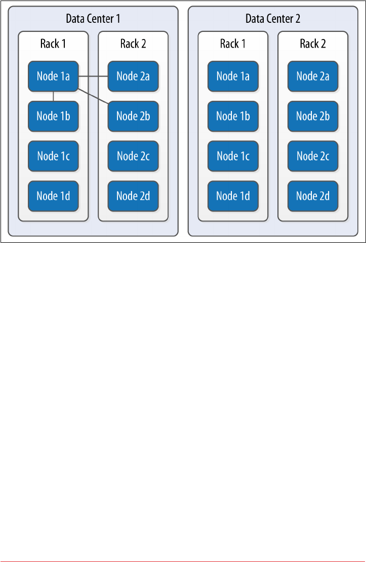
Figure 7-1. e SimpleStrategy places replicas in a single data center, without respect to
topology
What’s happening here is that the next N nodes on the ring are chosen to hold repli‐
cas, and the strategy has no notion of data centers. A second data center is shown in
the diagram to highlight the fact that the strategy is unaware of it.
NetworkTopologyStrategy
Now let’s say you want to spread replicas across multiple centers in case one of the
data centers suffers some kind of catastrophic failure or network outage. The Network
TopologyStrategy allows you to request that some replicas be placed in DC1, and
some in DC2. Within each data center, the NetworkTopologyStrategy distributes
replicas on distinct racks, as nodes in the same rack (or similar physical grouping)
often fail at the same time due to power, cooling, or network issues.
The NetworkTopologyStrategy distributes the replicas as follows: the first replica is
replaced according to the selected partitioner. Subsequent replicas are placed by tra‐
versing the nodes in the ring, skipping nodes in the same rack until a node in another
rack is found. The process repeats for additional replicas, placing them on separate
racks. Once a replica has been placed in each rack, the skipped nodes are used to
place replicas until the replication factor has been met.
148 | Chapter 7: Conguring Cassandra
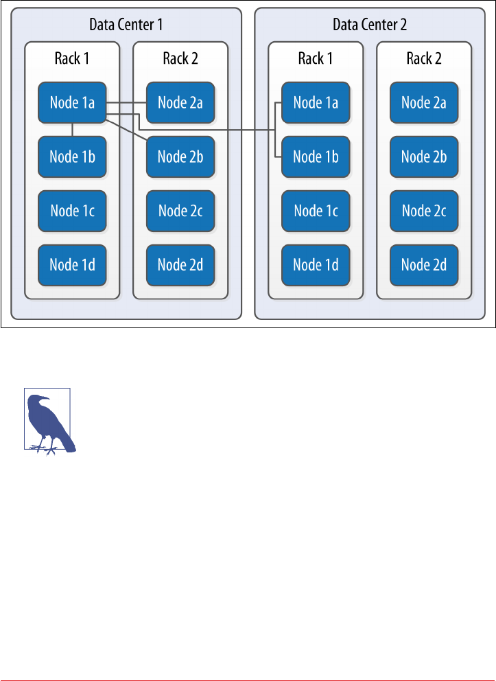
The NetworkTopologyStrategy allows you to specify a replication factor for each
data center. Thus, the total number of replicas that will be stored is equal to the sum
of the replication factors for each data center. The results of the NetworkTopology
Strategy are depicted in Figure 7-2.
Figure 7-2. e NetworkTopologyStrategy places replicas in multiple data centers accord‐
ing to the specied replication factor per data center
Additional Replication Strategies
Careful observers will note that there are actually two additional
replication strategies that ship with Cassandra: the OldNet
workTopologyStrategy and the LocalStrategy.
The OldNetworkTopologyStrategy is similar to the NetworkTopol
ogyStrategy in that it places replicas in multiple data centers, but
its algorithm is less sophisticated. It places the second replica in a
different data center from the first, the third replica in a different
rack in the first data center, and any remaining replicas by travers‐
ing subsequent nodes on the ring.
The LocalStrategy is reserved for Cassandra’s own internal use.
As the name implies, the LocalStrategy keeps data only on the
local node and does not replicate this data to other nodes. Cassan‐
dra uses this strategy for system keyspaces that store metadata
about the local node and other nodes in the cluster.
Replication Strategies | 149

Changing the Replication Factor
You can change the replication factor for an existing keyspace via cqlsh or another
client. For the change to fully take effect, you’ll need to run a nodetool command on
each of the affected nodes. If you increase the replication factor for a cluster (or data
center), run the nodetool repair command on each of the nodes in the cluster (or
data center) to make sure Cassandra generates the additional replicas. For as long as
the repair takes, it is possible that some clients will receive a notice that data does not
exist if they connect to a replica that doesn’t have the data yet.
If you decrease the replication factor for a cluster (or data center), run the nodetool
clean command on each of the nodes in the cluster (or data center) so that Cassan‐
dra frees up the space associated with unneeded replicas. We’ll learn more about
repair, clean, and other nodetool commands in Chapter 11.
As a general guideline, you can anticipate that your write throughput capacity will be
the number of nodes divided by your replication factor. So in a 10-node cluster that
typically does 10,000 writes per second with a replication factor of 1, if you increase
the replication factor to 2, you can expect to do around 5,000 writes per second.
Summary
In this chapter, we looked at how to create Cassandra clusters and add additional
nodes to a cluster. We learned how to configure Cassandra nodes via the cassan‐
dra.yaml file, including setting the seed nodes, the partitioner, the snitch, and other
settings. We also learned how to configure replication for a keyspace and how to
select an appropriate replication strategy.
150 | Chapter 7: Conguring Cassandra

CHAPTER 8
Clients
We’re used to connecting to relational databases using drivers. For example, in Java,
JDBC is an API that abstracts the vendor implementation of the relational database to
present a consistent way of storing and retrieving data using Statements, Prepared
Statements, ResultSets, and so forth. To interact with the database, you get a driver
that works with the particular database you’re using, such as Oracle, SQL Server, or
MySQL; the implementation details of this interaction are hidden from the developer.
Drivers are typically provided for a wide variety of programming languages to con‐
nect to a wide variety of databases.
There are a number of client drivers available for Cassandra as well, including sup‐
port for most popular languages. There are benefits to these clients, in that you can
easily embed them in your own applications (which we’ll see how to do) and that they
frequently offer more features than the CQL native interface does, including connec‐
tion pooling and JMX integration and monitoring. In the following sections, we’ll
learn about the various clients available and the features they offer.
Hector, Astyanax, and Other Legacy Clients
In the early days of Cassandra, the community produced a number of client drivers
for different languages. These contributions were a key enabler of Cassandra adop‐
tion. Some of the most notable early drivers included Hector and Astyanax.
Named after Cassandra’s brother, a warrior of Troy in Greek mythology, Hector was
one of the first Cassandra clients. Hector provided a simple Java interface that helped
many early developers avoid the challenges of writing to the Thrift API, and served as
the inspiration for several other drivers. The project is no longer active, but you can
access it at https://github.com/hector-client/hector.
151

Astyanax was a Java client originally built by Netflix on top of the Thrift API as a log‐
ical successor to the Hector driver (Astyanax was Hector’s son). Once the DataStax
Java driver was introduced, Netflix adapted Astyanax to support the Java driver in
addition to the original Thrift implementation. This helped many users transition
from Thrift to CQL. However, as the Java driver gained prominence, activity on
Astyanax slowed considerably, and the project was retired in February, 2016. You can
still access the project at https://github.com/Netix/astyanax.
Other clients included Pycassa for Python, Perlcassa for Perl, Helenus for Node.js,
and Cassandra-Sharp for the Microsoft .NET framework and C#. Most of these cli‐
ents are no longer actively maintained, as they were based on the now-deprecated
Thrift interface. You can find a comprehensive list of both current and legacy drivers
at http://www.planetcassandra.org/client-drivers-tools.
DataStax Java Driver
The introduction of CQL was the impetus for a major shift in the landscape of Cas‐
sandra client drivers. The simplicity and familiar syntax of CQL made the develop‐
ment of client programs similar to traditional relational database drivers. DataStax
made a strategic investment of open source drivers for Java and several additional
languages in order to continue to fuel Cassandra adoption. These drivers quickly
became the de facto standard for new development projects. You can access the driv‐
ers as well as additional connectors and tools at https://github.com/datastax.
More Information on DataStax Drivers
Visit the driver matrix page to access documentation and identify
driver versions that are compatible with your server version.
The DataStax Java driver is the oldest and most mature of these drivers. For this rea‐
son, we’ll focus on using the Java driver and use this as an opportunity to learn about
the features that are provided by the DataStax drivers across multiple languages.
Development Environment Conguration
First, we’ll need to access the driver in our development environment. We could
download the driver directly from the URL listed before and manage the dependen‐
cies manually, but it is more typical in modern Java development to use a tool like
Maven to manage dependencies. If you’re using Maven, you’ll need to add something
like the following to your project pom.xml file:
<dependency>
<groupId>com.datastax.cassandra</groupId>
<artifactId>cassandra-driver-core</artifactId>
152 | Chapter 8: Clients

<version>3.0.0</version>
</dependency>
You can find the Javadoc for the Java driver at http://docs.datastax.com/en/drivers/
java/3.0/index.html. Alternatively, the Javadocs are also part of the source distribu‐
tion.
All of the DataStax drivers are managed as open source projects on GitHub. If you’re
interested in seeing the Java driver source, you can get a read-only trunk version
using this command:
$ git clone https://github.com/datastax/java-driver.git
Clusters and Contact Points
Once we’ve configured our environment, we’re ready to start coding. We’ll create a
client application based on the hotel data model we created in Chapter 5. All of the
source code used in this chapter and throughout the rest of the book is available at
https://github.com/jereyscarpenter/cassandra-guide.
To start building our application, we’ll use the driver’s API to connect to our cluster.
In the Java driver, this is represented by the com.datastax.driver.core.Cluster
and Session classes.
The Cluster class is the main entry point of the driver. It supports a fluent-style API
using the builder pattern. For example, the following lines create a connection to a
node running on the local host:
Cluster cluster = Cluster.builder().
addContactPoint("127.0.0.1").build();
This one statement represents the minimum required information to create a cluster:
a single contact point. We can also specify multiple contact points. Contact points are
similar to the concept seed nodes that a Cassandra node uses to connect to other
nodes in the same cluster.
Creating a Custom Cluster Initializer
The Cluster.Builder class implements an interface called
Cluster.Initializer. This allows us to plug in a different
mechanism to initialize a Cluster using the static method Clus
ter.buildFrom(Initializer initializer). This could be useful
if we wanted to load the connection information from a configura‐
tion file, for example.
There are several other options that we can configure on a Cluster, such as a metrics,
default query options, and policies for reconnection, retry, and speculative execution.
DataStax Java Driver | 153

We’ll examine each of these options in later sections after we take a look at some
other connection-related options: protocol version, compression, and authentication.
Protocol version
The driver supports multiple versions of the CQL native protocol. Cassandra 3.0 sup‐
ports version 4, as we learned in our overview of Cassandra’s release history in Chap‐
ter 2.
By default, the driver uses the protocol version supported by the first node it connects
to. While in most cases this is sufficient, you may need to override this behavior if
you’re working with a cluster based on an older version of Cassandra. You can select
your protocol version by passing the desired value from the com.datastax.
driver.core.ProtocolVersion enumeration to the Cluster.Builder.withProtocol
Version() operation.
Compression
The driver provides the option of compressing messages between your client and
Cassandra nodes, taking advantage of the compression options supported by the
CQL native protocol. Enabling compression reduces network bandwidth consumed
by the driver, at the cost of additional CPU usage for the client and server.
Currently there are two compression algorithms available, LZ4 and SNAPPY, as defined
by the com.datastax.driver.core.ProtocolOptions.Compression enumeration.
The compression defaults to NONE but can be overridden by calling the Cluster.
Builder.withCompression() operation.
Authentication and encryption
The driver provides a pluggable authentication mechanism that can be used to sup‐
port a simple username/password login, or integration with other authentication sys‐
tems. By default, no authentication is performed. You can select an authentication
provider by passing an implementation of the com.datastax.driver.core.AuthPro
vider interface such as the PlainTextAuthProvider to the Cluster.Builder.with
AuthProvider() operation.
The driver can also encrypt its communications with the server to ensure privacy.
Client-server encryption options are specified by each node in its cassandra.yaml file.
The driver complies with the encryption settings specified by each node.
We’ll examine authentication, authorization, and encryption from both the client and
server perspective in more detail in Chapter 13.
154 | Chapter 8: Clients

Sessions and Connection Pooling
After we create our Cluster instance, it is not connected to any Cassandra nodes
until we initialize it by calling the init() method:
cluster.init();
When this method is invoked, the driver connects to one of the configured contact
points in order to obtain metadata about the cluster. This operation will throw a
NoHostAvailableException if none of the contact points is available, or an Authenti
cationException if authentication fails. We’ll discuss authentication in more detail in
Chapter 13.
Once we have initialized our Cluster object, we need to establish a session in order
to formulate our queries. We can obtain a com.datastax.driver.core.Session
object by calling one of the Cluster.connect() operations. You can optionally pro‐
vide the name of a keyspace to connect to, as we do in this example that connects to
the hotel keyspace:
Session session = cluster.connect("hotel");
There is also a connect() operation with no parameters, which creates a Session that
can be used with multiple keyspaces. If you choose this option, you’ll have to qualify
every table reference in your queries with the appropriate keyspace name. Note that it
is not strictly required to call Cluster.init() explicitly, as it is also invoked behind
the scenes when we call connect().
Each Session manages connections to a Cassandra cluster, which are used to execute
queries and control operations using the Cassandra native protocol. The session con‐
tains a pool of TCP connections for each host.
Sessions Are Expensive
Because a session maintains connection pools for multiple nodes, it
is a relatively heavyweight object. In most cases, you’ll want to cre‐
ate a single Session and reuse it throughout your application,
rather than continually building up and tearing down Sessions.
Another acceptable option is to create a Session per keyspace, if
your application is accessing multiple keyspaces.
Because the CQL native protocol is asynchronous, it allows multiple simultaneous
requests per connection; the maximum is 128 simultaneous requests in protocol v2,
while v3 and v4 allow up to 32,768 simultaneous requests. Because of this larger
number of simultaneous requests, fewer connections per node are required. In fact,
the default is a single connection per node.
DataStax Java Driver | 155

The driver supports the ability to scale the number of connections up or down based
on the number of requests per connection. These connection pool settings are config‐
urable via the PoolingOptions class, which sets the maximum and minimum (or
“core”) number of connections to use for local and remote hosts. If the core and max‐
imum values are different, the driver scales the size of the connection pool for each
node up or down depending on the amount of requests made by the client. The set‐
tings of minimum and maximum thresholds of requests per connection are used to
determine when new connections are created, and when underused connections can
be reclaimed. There is also a buffer period to prevent the continual building up and
tearing down of connections.
The PoolingOptions can be set when creating the Cluster using ClusterBuilder.
withPoolingOptions(), or manipulated after the Cluster is created using Cluster.
getConfiguration().getPoolingOptions(). Here is an example of creating a Clus
ter that limits the maximum number of connections to remote nodes to one:
PoolingOptions poolingOptions = new PoolingOptions().
setMaxConnectionsPerHost(HostDistance.REMOTE, 1);
Cluster cluster = Cluster.builder().
addContactPoint("127.0.0.1").
withPoolingOptions(poolingOptions).build();
The driver provides a connection heartbeat which is used to make sure that connec‐
tions are not closed prematurely by intervening network devices. This defaults to 30
seconds but can be overridden using the operation PoolingOptions.setHeartbeat
IntervalSeconds(). However, this only applies to connections established after the
value is set, so you’ll most likely want to configure this when creating your Cluster.
Statements
Up until this point, we have only configured our connection to the cluster, and
haven’t yet performed any reads or writes. To begin doing some real application work,
we’ll create and execute statements using the com.datastax.driver.core.Statement
class and its various subclasses. Statement is an abstract class with several implemen‐
tations, including SimpleStatement, PreparedStatement, BoundStatement, Batch
Statement, and BuiltStatement.
The simplest way to create and execute a statement is to call the Session.execute()
operation with a string representing the statement. Here’s an example of a statement
that will return the entire contents of our hotels table:
session.execute("SELECT * from hotel.hotels");
156 | Chapter 8: Clients

This statement creates and executes a query in a single method call. In practice, this
could turn out to be a very expensive query to execute in a large database, but it does
serve as a useful example of a very simple query. Most queries we need to build will
be more complex, as we’ll have search criteria to specify or specific values to insert.
We can certainly use Java’s various string utilities to build up the syntax of our query
by hand, but this of course is error prone. It may even expose our application to injec‐
tion attacks, if we’re not careful to sanitize strings that come from end users.
Simple statement
Thankfully, we needn’t make things so hard on ourselves. The Java driver provides the
SimpleStatement class to help construct parameterized statements. As it turns out,
the execute() operation we saw before is actually a convenience method for creating
a SimpleStatement.
Let’s try building a query by asking our Session object to create a SimpleStatement.
Here’s an example of a statement that will insert a row in our hotels table, which we
can then execute:
SimpleStatement hotelInsert = session.newSimpleStatement(
"INSERT INTO hotels (hotel_id, name, phone) VALUES (?, ?, ?)",
"AZ123", "Super Hotel at WestWorld", "1-888-999-9999");
session.execute(hotelInsert);
The first parameter to the call is the basic syntax of our query, indicating the table
and columns we are interested in. The question marks are used to indicate values that
we’ll be providing in additional parameters. We use simple strings to hold the values
of the hotel ID, name, and phone number.
If we’ve created our statement correctly, the insert will execute successfully (and
silently). Now let’s create another statement to read back the row we just inserted:
SimpleStatement hotelSelect = session.newSimpleStatement(
"SELECT * FROM hotels WHERE id=?", "AZ123");
ResultSet hotelSelectResult = session.execute(hotelSelect);
Again, we make use of parameterization to provide the ID for our search. This time,
when we execute the query, we make sure to receive the ResultSet which is returned
from the execute() method. We can iterate through the rows returned by the Result
Set as follows:
for (Row row : hotelSelectResult) {
System.out.format("hotel_id: %s, name: %s, phone: %s\n",
row.getString("hotel_id"), row.getString("name"), row.getString("phone"));
}
This code uses the ResultSet.iterator() option to get an Iterator over the rows
in the result set and loop over each row, printing out the desired column values. Note
that we use special accessors to obtain the value of each column depending on the
DataStax Java Driver | 157

desired type—in this case, Row.getString(). As we might expect, this will print out a
result such as:
hotel_id: AZ123, name: Super Hotel at WestWorld, phone: 1-888-999-9999
Using a Custom Codec
As we already noted, we need to know the type of the columns we are requesting
when interacting with the Rows in our ResultSets. If we were to request the id col‐
umn using Row.getString(), we would receive a CodecNotFoundException, indicat‐
ing that the driver does not know how to map the CQL type uuid to java.lang.
String.
What is happening here is that the driver maintains a default list of mappings
between Java and CQL types called a codec, which it uses to translate back and forth
between your application and Cassandra. The driver provides a way to add additional
mappings by extending the class com.datastax.driver.core.TypeCodec<T> and reg‐
istering it with the CodecRegistry managed by the Cluster:
cluster.getConfiguration().getCodecRegistry().
register(myCustomCodec)
The custom codec mechanism is very flexible, as demonstrated by the following use
cases:
•Mapping to alternate date/time formats (e.g., Joda time for pre-Java 8 users)
• Mapping string data to/from formats such as XML and JSON
• Mapping lists, sets, and maps to various Java collection types
You can find code samples for working with SimpleStatements in the example
com.cassandraguide.clients.SimpleStatementExample.
Asynchronous execution
The Session.execute() operation is synchronous, which means that it blocks until a
result is obtained or an error occurs, such as a network timeout. The driver also pro‐
vides the asynchronous executeAsync() operation to support non-blocking interac‐
tions with Cassandra. These non-blocking requests can make it simpler to send
multiple queries in parallel to speed performance of your client application.
Let’s take our operation from before and modify it to use the asynchronous operation:
ResultSetFuture result = session.executeAsync(statement);
The result is of the type ResultSetFuture, which is an implementation of the
java.util.concurrent.Future interface. A Future is a Java generic type used to
capture the result of an asynchronous operation. Each Future can be checked to see
158 | Chapter 8: Clients

whether the operation has completed, and then queried for the result of the operation
according to the bound type. There are also blocking wait() operations to wait for
the result. A Future can also be cancelled if the caller is no longer interested in the
result of the operation. The Future class is a useful tool for implementing asynchro‐
nous programming patterns, but requires either blocking or polling to wait for the
operation to complete.
To address this drawback, the Java driver leverages the ListenableFuture interface
from Google’s Guava framework. The ListenableFuture interface extends Future,
and adds an addListener() operation that allows the client to register a callback
method that is invoked when the Future completes. The callback method is invoked
in a thread managed by the driver, so it is important that the method complete
quickly to avoid tying up driver resources. The ResultSetFuture is bound to the
ResultSet type.
Additional Asynchronous Operations
In addition to the Session.executeAsync() operation, the driver
supports several other asynchronous operations, including
Cluster.closeAsync(), Session.prepareAsync(), and several
operations on the object mapper.
Prepared statement
While SimpleStatements are quite useful for creating ad hoc queries, most applica‐
tions tend to perform the same set of queries repeatedly. The PreparedStatement is
designed to handle these queries more efficiently. The structure of the statement
is sent to nodes a single time for preparation, and a handle for the statement is
returned. To use the prepared statement, only the handle and the parameters need to
be sent.
As you’re building your application, you’ll typically create PreparedStatements for
reading data, corresponding to each access pattern you derive in your data model,
plus others for writing data to your tables to support those access patterns.
Let’s create some PreparedStatements to represent the same hotel queries as before,
using the Session.prepare() operation:
PreparedStatement hotelInsertPrepared = session.prepare(
"INSERT INTO hotels (hotel_id, name, phone) VALUES (?, ?, ?)");
PreparedStatement hotelSelectPrepared = session.prepare(
"SELECT * FROM hotels WHERE hotel_id=?");
Note that the PreparedStatement uses the same parameterized syntax we used earlier
for our SimpleStatement. A key difference, however, is that a PreparedStatement is
DataStax Java Driver | 159

not a subtype of Statement. This prevents the error of trying to pass an unbound
PreparedStatement to the session to execute.
Before we get to that, however, let’s take a step back and discuss what is happening
behind the scenes of the Session.prepare() operation. The driver passes the con‐
tents of our PreparedStatement to a Cassandra node and gets back a unique identi‐
fier for the statement. This unique identifier is referenced when you create a
BoundStatement. If you’re curious, you can actually see this reference by calling
PreparedStatement.getPreparedID().
You can think of a PreparedStatement as a template for creating queries. In addition
to specifying the form of our query, there are other attributes that we can set on a
PreparedStatement that will be used as defaults for statements it is used to create,
including a default consistency level, retry policy, and tracing.
In addition to improving efficiency, PreparedStatements also improve security by
separating the query logic of CQL from the data. This provides protection against
injection attacks, which attempt to embed commands into data fields in order to gain
unauthorized access.
Bound statement
Now our PreparedStatement is available for us to use to create queries. In order to
make use of a PreparedStatement, we bind it with actual values by calling the bind()
operation. For example, we can bind the SELECT statement we created earlier as fol‐
lows:
BoundStatement hotelSelectBound = hotelSelectPrepared.bind("AZ123");
The bind() operation we’ve used here allows us to provide values that match each
variable in the PreparedStatement. It is possible to provide the first n bound values,
in which case the remaining values must be bound separately before executing the
statement. There is also a version of bind() which takes no parameters, in which case
all of the parameters must be bound separately. There are several set() operations
provided by BoundStatement that can be used to bind values of different types. For
example, we can take our INSERT prepared statement from above and bind the name
and phone values using the setString() operation:
BoundStatement hotelInsertBound = hotelInsertPrepared.bind("AZ123");
hotelInsertBound.setString("name", "Super Hotel at WestWorld");
hotelInsertBound.setString("phone", "1-888-999-9999");
Once we have bound all of the values, we execute a BoundStatement using
Session.execute(). If we have failed to bind any of the values, they will be ignored
on the server side, if protocol v4 (Cassandra 3.0 or later) is in use. The driver behav‐
160 | Chapter 8: Clients

ior for older protocol versions is to throw an IllegalStateException if there are any
unbound values.
You can find code samples for working with PreparedStatement and BoundState
ment in the example com.cassandraguide.clients.PreparedStatementExample.
Built statement and the Query Builder
The driver also provides the com.datastax.driver.core.querybuilder.Query
Builder class, which provides a fluent-style API for building queries. This is suitable
for cases where there is variation in the query structure (such as optional parameters)
that would make using PreparedStatements difficult. Similar to PreparedStatement,
it also provides some protection against injection attacks.
We construct a QueryBuilder using a simple constructor that takes our Cluster
object:
QueryBuilder queryBuilder = new QueryBuilder(cluster);
The QueryBuilder produces queries that are represented using the BuiltStatement
class and its subclasses. The methods on each class return instances of
BuiltStatement that represent content added to a query as it is being built up. You’ll
likely find your IDE quite useful in helping to identify the allowed operations as
you’re building queries.
Let’s reproduce the queries from before using the QueryBuilder to see how it works.
First, we’ll build a CQL INSERT query:
BuiltStatement hotelInsertBuilt =
queryBuilder.insertInto("hotels")
.value("hotel_id", "AZ123")
.value("name", "Super Hotel at WestWorld")
.value("phone", "1-888-999-9999");
The first operation calls the QueryBuilder.insertInto() operation to create an
Insert statement for the hotels table. If desired, we could then add a CQL USING
clause to our statement with Insert.using(), but instead we choose to start adding
values to our query. The Insert.value() operation continues returning Insert
statements as we add values. The resulting Insert can be executed like any other
Statement using Session.execute() or executeAsync().
The construction of the CQL SELECT command is similar:
BuiltStatement hotelSelectBuilt = queryBuilder.select()
.all()
.from("hotels")
.where(eq("hotel_id", "AZ123"));
DataStax Java Driver | 161

For this query, we call QueryBuilder.select() to create a Select statement. We use
the Select.all() operation to select all columns, although we could also have used
the column() operation to select specific columns. We add a CQL WHERE clause via the
Select.where() operation, which accepts an instance of the Clause class. We create
Clauses using static operations provided by the QueryBuilder. In this case, we use
the eq() operation to check for equality with our ID.
To access these static operations, we need to add additional import statements to our
Java source files such as:
import static com.datastax.driver.core.querybuilder.QueryBuilder.eq;
For a complete code sample using the QueryBuilder and BuiltStatement, see the
class com.cassandraguide.clients.QueryBuilderExample.
Object mapper
We’ve explored several techniques for creating and executing query statements with
the driver. There is one final technique that we’ll look at that provides a bit more
abstraction. The Java driver provides an object mapper that allows you to focus on
developing and interacting with domain models (or data types used on APIs). The
object mapper works off of annotations in source code that are used to map Java
classes to tables or user-defined types (UDTs).
The object mapping API is provided as a separate library from the rest of the driver
in the cassandra-driver-mapping.jar file, so you will need to include this additional
Maven dependency in order to use Mapper in your project:
<dependency>
<groupId>com.datastax.cassandra</groupId>
<artifactId>cassandra-driver-mapping</artifactId>
<version>3.0.0</version>
</dependency>
For example, let’s create and annotate a Hotel domain model class corresponding to
our hotels table:
import com.datastax.driver.mapping.annotations.Column;
import com.datastax.driver.mapping.annotations.PartitionKey;
import com.datastax.driver.mapping.annotations.Table;
@Table(keyspace = "hotel", name = "hotels")
public class Hotel {
@PartitionKey
private String id;
@Column (name = "name")
private String name;
162 | Chapter 8: Clients

@Column (name = "phone")
private String phone;
@Column (name = "address")
private String address;
@Column (name = "pois")
private Set<String> pointsOfInterest;
// constructors, get/set methods, hashcode, equals
}
Now we use the com.datastax.driver.mapping.MappingManager to attach to our
Session and create a Mapper for our annotated domain model class:
MappingManager mappingManager = new MappingManager(session);
Mapper<Hotel> hotelMapper = MappingManager.mapper(Hotel.class);
Let’s assume the Hotel class has a simple constructor that just takes a UUID, name,
and phone number, which we’ll use to create a simple hotel that we can save using the
object mapper:
Hotel hotel = new Hotel("AZ123", "Super Hotel at WestWorld”,
"1-888-999-9999");
hotelMapper.save(hotel);
The Mapper.save() operation is all we need to execute to perform a CQL INSERT or
UPDATE, as these are really the same operation to Cassandra. The Mapper builds and
executes the statement on our behalf.
To retrieve an object, we use the Mapper.get() operation, passing in an argument list
that matches the elements of the partition key:
Hotel retrievedHotel = hotelMapper.get(hotelId);
The syntax for deleting an object is similar:
hotelMapper.delete(hotelId);
As with the save() operation, get() and delete() completely handle the details of
executing statements with the driver on our behalf. There are also saveAsync(),
getAsync() and deleteAsync() operations that support asynchronous execution
using the ListenableFuture interface we discussed earlier.
If you want to be able to configure the queries before they are executed, there are also
operations on the Mapper that return Statements: saveQuery(), getQuery(), and
deleteQuery().
The object mapper is a useful tool for abstracting some of the details of interacting
with your code, especially if you have an existing domain model. If your domain
model contains classes that reference other classes, you can annotate the referenced
DataStax Java Driver | 163

classes as user-defined types with the @UDT annotation. The object mapper processes
objects recursively using your annotated types.
Achilles: An Advanced Object Mapper
DuyHai Doan has developed an advanced object mapper for Java
called Achilles. Achilles provides support for more advanced func‐
tionality such as complex key mappings, lightweight transactions,
user defined functions, and more. You can check it out at https://
github.com/doanduyhai/Achilles.
Policies
The Java driver provides several policy interfaces that can be used to tune the behav‐
ior of the driver. These include policies for load balancing, retrying requests, and
managing connections to nodes in the cluster.
Load balancing policy
As we learned in Chapter 6, a query can be made to any node in a cluster, which is
then known as the coordinator node for that query. Depending on the contents of the
query, the coordinator may communicate with other nodes in order to satisfy the
query. If a client were to direct all of its queries at the same node, this would produce
an unbalanced load on the cluster, especially if other clients are doing the same.
To get around this issue, the driver provides a pluggable mechanism to balance the
query load across multiple nodes. Load balancing is implemented by selecting an
implementation of the com.datastax.driver.core.policies.LoadBalancing
Policy interface.
Each LoadBalancingPolicy must provide a distance() operation to classify each
node in the cluster as local, remote, or ignored, according to the HostDistance enu‐
meration. The driver prefers interactions with local nodes and maintains more con‐
nections to local nodes than remote nodes. The other key operation is
newQueryPlan(), which returns a list of nodes in the order they should be queried.
The LoadBalancingPolicy interface also contains operations that are used to inform
the policy when nodes are added or removed, or go up or down. These operations
help the policy avoid including down or removed nodes in query plans.
The driver provides two basic load balancing implementations: the RoundRobin
Policy, which is the default, and the DCAwareRoundRobinPolicy.
The RoundRobinPolicy allocates requests across the nodes in the cluster in a repeat‐
ing pattern to spread the processing load. The DCAwareRoundRobinPolicy is similar,
but focuses its query plans on nodes in the local data center. This policy can add a
164 | Chapter 8: Clients

configurable number of nodes in remote data centers to query plans, but the remote
nodes will always come after local nodes in priority. The local data center can be iden‐
tified explicitly, or you can allow the driver to discover it automatically.
A second mode is token awareness, which uses the token value of the partition key in
order to select a node which is a replica for the desired data, thus minimizing the
number of nodes that must be queried. This is implemented by wrapping the selected
policy with a TokenAwarePolicy.
The LoadBalancingPolicy is set on the Cluster when it is built. For example, the fol‐
lowing statement will initialize a Cluster to have token awareness and to prefer
nodes in the local data center:
Cluster.builder().withLoadBalancingPolicy(
new TokenAwarePolicy(new DCAwareRoundRobinPolicy.Builder().build());
Retry policy
When Cassandra nodes fail or become unreachable, the driver automatically and
transparently tries other nodes and schedules reconnection to the dead nodes in the
background. Because temporary changes in network conditions can also make nodes
appear offline, the driver also provides a mechanism to retry queries that fail due to
network-related errors. This removes the need to write retry logic in client code.
The driver retries failed queries according to the provided implementation of the
com.datastax.driver.core.RetryPolicy interface. The onReadTimeout(), onWrite
Timeout(), and onUnavailable() operations define the behavior that should be
taken when a query fails with the network-related exceptions ReadTimeoutExcep
tion, WriteTimeoutException, or UnavailableException, respectively.
DataStax Java Driver Exceptions
The various exceptions and errors that can be generated by the Java
driver are collected in the com.datastax.driver.core.excep
tions package.
The RetryPolicy operations return a RetryDecision, which indicates whether the
query should be retried, and if so, at what consistency level. If the exception is not
retried, it can be rethrown, or ignored, in which case the query operation will return
an empty ResultSet.
The Java driver provides several RetryPolicy implementations:
•The DefaultRetryPolicy is a conservative implementation that only retries
queries under a narrow set of conditions.
DataStax Java Driver | 165

• The FallthroughRetryPolicy never recommends a retry, always recommending
that the exception be rethrown.
•The DowngradingConsistencyRetryPolicy is a more aggressive policy which
downgrades the consistency level required, as an attempt to get the query to suc‐
ceed.
A Word on DowngradingConsistencyRetryPolicy
This policy comes with a warning attached: if you are willing to
accept a downgraded consistency level under some circumstances,
do you really require a higher consistency level for the general
case?
The RetryPolicy can be set on a Cluster when it is built, as shown by the following
statement, which selects the DowngradingConsistencyRetryPolicy and wraps it with
a LoggingRetryPolicy so that each retry attempt will be logged:
Cluster.builder().withRetryPolicy(new LoggingRetryPolicy(
DowngradingConsistencyRetryPolicy.INSTANCE));
The RetryPolicy on a cluster will be used for all queries executed on that cluster,
unless overridden on any individual query via the Statement.setRetryPolicy()
operation.
Speculative execution policy
While it’s great to have a retry mechanism that automates our response to network
timeouts, we don’t often have the luxury of being able to wait for timeouts or even
long garbage collection pauses. To speed things up, the driver provides a speculative
execution mechanism. If the original coordinator node for a query fails to respond in
a predetermined interval, the driver preemptively starts an additional execution of
the query against a different coordinator node. When one of the queries returns, the
driver provides that response and cancels any other outstanding queries.
The speculative execution behavior is set on a Cluster by specifying an implementa‐
tion of com.datastax.driver.core.policies.SpeculativeExecutionPolicy.
The default is the NoSpeculativeExecutionPolicy, which does not schedule any
speculative executions. There is also a ConstantSpeculativeExecutionPolicy,
which schedules up to a maximum number of retries with a fixed delay in milli‐
seconds. The PercentileSpeculativeExecutionPolicy is a newer policy that is still
considered a Beta as of the 3.0 driver release. It triggers speculative executions at a
delay based on the observed latency to the original coordinator node.
166 | Chapter 8: Clients

The policy is set using the Cluster.Builder, for example:
Cluster.builder().withSpeculativeExecutionPolicy(
new ConstantSpeculativeExecutionPolicy (
200, // delay in ms
3 // max number of speculative executions
);
This policy cannot be changed later, or overridden on individual Statements.
Address translator
In the examples we’ve seen so far, each node is identified by the IP address configured
as the node’s rpc_address in its cassandra.yaml file. In some deployments, that
address may not be reachable by the client. To handle this case, the driver provides a
pluggable capability to translate addresses via the com.datastax.driver.core.
policies.AddressTranslator interface (in versions of the driver prior to 3.0,
“translator” is misspelled as “translater” throughout the API).
For example, the Java driver comes with the IdentityTranslator, a default translator
that leaves the IP address unchanged, and the EC2MultiRegionAddressTranslator,
which is useful for Amazon EC2 environments. This translator is useful in cases
where a client may need to access a node in another data center via a public IP
address. We’ll discuss EC2 deployments in more detail in Chapter 14.
Metadata
To access the cluster metadata, we invoke the Cluster.getMetadata() method. The
com.datastax.driver.core.Metadata class provides information about the cluster
including the cluster name, the schema including keyspaces and tables, and the
known hosts in the cluster. We can obtain the name of the cluster via the following
code:
Metadata metadata = cluster.getMetadata();
System.out.printf("Connected to cluster: %s\n",
metadata.getClusterName(), cluster.getClusterName());
DataStax Java Driver | 167

Assigning a Cluster Name
Somewhat confusingly, the Cluster.Builder class allows us to
assign a name to the Cluster instance as it is being built. This
name is really just a way for the client to keep track of multiple
Cluster objects, and can be different than the name known by the
nodes within the actual Cassandra cluster. This second cluster
name is the one we obtain via the Metadata class.
If we do not specify a name for the Cluster on construction, it is
assigned a default name such as “cluster1”, “cluster2”, and so on (if
multiple clusters are created). You can see this value if you modify
the example from before to change metadata.getClusterName()
to cluster.getClusterName().
Node discovery
A Cluster object maintains a permanent connection to one of the contact points,
which it uses to maintain information on the state and topology of the cluster. Using
this connection, the driver will discover all the nodes currently in the cluster. The
driver uses the com.datastax.driver.core.Host class to represent each node. The
following code shows an example of iterating over the hosts to print out their infor‐
mation:
for (Host host : cluster.getMetadata.getAllHosts())
{
System.out.printf("Data Center: %s; Rack: %s; Host: %s\n",
host.getDatacenter(), host.getRack(), host.getAddress());
}
You can find this code in the class com.cassandraguide.clients.SimpleConnection
Example.
If we’re running a multi-node cluster such as the one we created in Chapter 7 using
the Cassandra Cluster Manager (ccm), the output of this program will look something
like the following:
Connected to cluster: my_cluster
Data Center: datacenter1; Rack: rack1; Host: /127.0.0.1
Data Center: datacenter1; Rack: rack1; Host: /127.0.0.2
Data Center: datacenter1; Rack: rack1; Host: /127.0.0.3
Using the connection, the driver can also discover all the nodes currently in the clus‐
ter. The driver also can detect when new nodes are added to a cluster. You can register
a listener to do this by implementing the Host.StateListener interface. This
requires us to implement several operations such as onAdd() and onRemove(), which
are called when nodes are added or removed from the cluster, as well as onUp() and
onDown(), which indicate when nodes go up or down. Let’s look at a portion of a sam‐
ple class that registers a listener with the cluster:
168 | Chapter 8: Clients

public class ConnectionListenerExample implements Host.StateListener {
public String getHostString(Host host) {
return new StringBuilder("Data Center: " + host.getDatacenter() +
" Rack: " + host.getRack() +
" Host: " + host.getAddress().toString() +
" Version: " + host.getCassandraVersion() +
" State: " + host.getState());
}
public void onUp(Host host) {
System.out.printf("Node is up: %s\n", getHostString(host));
}
public void onDown(Host host) {
System.out.printf("Node is down: %s\n", getHostString(host));
}
// other required methods omitted...
public static void main(String[] args) {
List<Host.StateListener> list =
ArrayList<Host.StateListener>();
list.add(new ConnectionListenerExample());
Cluster cluster = Cluster.builder().
addContactPoint("127.0.0.1").
withInitialListeners(list).
build();
cluster.init();
}
}
This code simply prints out a status message when a node goes up or down. You’ll
note that we make use of a bit more information about each node than our previous
example, including the Cassandra version in use by each of the nodes. You can find
the full code listing in the class com.cassandraguide.clients.ConnectionListener
Example.
Let’s run this sample program. Because our listener was added before calling init(),
we immediately get the following output:
Node added: Data Center: datacenter1 Rack: rack1
Host: /127.0.0.1 Version: 3.0.0 State: UP
Node added: Data Center: datacenter1 Rack: rack1
Host: /127.0.0.2 Version: 3.0.0 State: UP
Node added: Data Center: datacenter1 Rack: rack1
Host: /127.0.0.3 Version: 3.0.0 State: UP
DataStax Java Driver | 169

Now let’s use the ccm stop command to shut down one of our nodes, and we’ll see
something like the following:
Node is down: Data Center: datacenter1 Rack: rack1
Host: /127.0.0.1 Version: 3.0.0 State: DOWN
Similarly, if we bring the node back up, we’ll see a notification that the node is back
online:
Node is up: Data Center: datacenter1 Rack: rack1
Host: /127.0.0.1 Version: 3.0.0 State: UP
Schema access
The Metadata class also allows the client to learn about the schema in a cluster. The
exportSchemaAsString() operation creates a String describing all of the keyspaces
and tables defined in the cluster, including the system keyspaces. This output is
equivalent to the cqlsh command DESCRIBE FULL SCHEMA. Additional operations
support browsing the contents of individual keyspaces and tables.
We’ve previously discussed Cassandra’s support for eventual consistency at great
length in Chapter 2. Because schema information is itself stored using Cassandra, it is
also eventually consistent, and as a result it is possible for different nodes to have dif‐
ferent versions of the schema. As of the 3.0 release, the Java driver does not expose
the schema version directly, but you can see an example by running the nodetool
describecluster command:
$ ccm node1 nodetool describecluster
Cluster Information:
Name: test_cluster
Snitch: org.apache.cassandra.locator.DynamicEndpointSnitch
Partitioner: org.apache.cassandra.dht.Murmur3Partitioner
Schema versions:
ea46580a-4ab4-3e70-b68f-5e57da189ac5:
[127.0.0.1, 127.0.0.2, 127.0.0.3]
This output shows us a couple of things. First, we see that the schema version is a
UUID value. This value is calculated based on a hash of all of the keyspace and table
definitions a node knows about. The fact that all three nodes share the same schema
version means that they all have the same schema defined.
Of course, the schema version in use can change over time as keyspaces and tables are
created, altered, and deleted. The driver provides a notification mechanism for clients
to learn about these changes by registering a com.datastax.driver.core.Schema
ChangeListener with the Cluster.
You can find an example of these calls by running the example com.cassandra
guide.clients.SimpleSchemaExample.
170 | Chapter 8: Clients

In addition to the schema access we’ve just examined in the Metadata class, the Java
driver also provides a facility for managing schema in the com.datastax.
driver.core.schemabuilder package. The SchemaBuilder provides a fluent-style
API for creating SchemaStatements representing operations such as CREATE, ALTER,
and DROP operations on keyspaces, tables, indexes, and user-defined types (UDTs).
For example, the following code could be used to create our hotels keyspace:
SchemaStatement hotelSchemaStatement = SchemaBuilder.createTable("hotels").
addPartitionKey("id", DataType.text()).
addColumn("name", DataType.text()).
addColumn("phone", DataType.text()).
addColumn("address", DataType.text()).
addColumn("pois", DataType.set(DataType.text()));
session.execute(hotelSchemaStatement);
We also import com.datastax.driver.core.DataType so that we can leverage its
static operations to define the data types of each column.
Avoid Conicts When Using Programmatic Schema Denition
Many developers have noted that this programmatic schema man‐
agement capability can be used as a “lazy initialization” technique
for simplified application deployment: if the schema our applica‐
tion uses doesn’t exist, we can simply create it programmatically.
However, this technique is not recommended when running multi‐
ple clients, even with IF NOT EXISTS semantics. CREATE TABLE or
ALTER TABLE statements from multiple concurrent clients can
result in inconsistent state between nodes, requiring manual
repairs.
Debugging and Monitoring
The driver provides features for monitoring and debugging your client’s use of Cas‐
sandra, including facilities for logging and metrics. There is also a query tracing
capability, which we’ll learn about in Chapter 12.
Logging
As we will learn in Chapter 10, Cassandra uses a logging API called Simple Logging
Facade for Java (SLF4J). The Java driver uses the SLF4J API as well. In order to enable
logging on your Java client application, you need to provide a compliant SLF4J imple‐
mentation on the classpath.
Here’s an example of a dependency we can add to our Maven POM file to select the
Logback project as the implementation:
DataStax Java Driver | 171

<dependency>
<groupId>ch.qos.logback</groupId>
<artifactId>logback-classic</artifactId>
<version>1.1.3</version>
</dependency>
You can learn more about Logback at http://logback.qos.ch/.
By default, the Java driver is set to use the DEBUG logging level, which is fairly verbose.
We can configure logging by taking advantage of Logback’s configuration mecha‐
nism, which supports separate configuration for test and production environments.
Logback inspects the classpath first for the file logback-test.xml representing the test
configuration, and then if no test configuration is found, it searches for the file log‐
back.xml.
For more detail on Logback configuration, including sample configuration files for
test and production environments, see the configuration page.
Metrics
Sometimes it can be helpful to monitor the behavior of client applications over time
in order to detect abnormal conditions and debug errors. The Java driver collects
metrics on its activities and makes these available using the Dropwizard Metrics
library. The driver reports metrics on connections, task queues, queries, and errors
such as connection errors, read and write timeouts, retries, and speculative execu‐
tions.
You can access the Java driver metrics locally via the Cluster.getMetrics() opera‐
tion. The Metrics library also integrates with the Java Management Extensions (JMX)
to allow remote monitoring of metrics. JMX reporting is enabled by default, but this
can be overridden in the Configuration provided when building a Cluster.
DataStax Python Driver
The most popular early Python client was Pycassa, which was built on the Thrift
interface. The Pycassa project is no longer maintained, however, and the recommen‐
dation is to use the DataStax Python Driver for all new development.
The first full version of the DataStax Python Driver was introduced January 2014 and
provided session management, node discovery, connection pooling, synchronous/
asynchronous queries, load balancing, query tracing, metrics (using the Scales
library), logging, authentication and SSL. Features such as support for Cassandra 2.1
and later paging, lightweight transactions, and Python 3 support were added in the
2.0 release in May 2014. The Python Driver is compatible with Cassandra releases 1.2
and later and runs on Python 2.6, 2.7, 3.3, and 3.4. The driver runs on Linux, Mac OS,
and Windows.
172 | Chapter 8: Clients

The official documentation for the driver is available at the DataStax website, while
the source driver is available on GitHub. You can install the driver by running the
Python installer pip:
$ pip install cassandra-driver
Installing Python and PIP
To use the example code, you’ll need a compatible version of
Python for your platform (as listed earlier), and pip. You can install
pip by downloading the script https://bootstrap.pypa.io/get-pip.py
and running the command python get-pip.py. You may need to
run this command via sudo on Unix systems.
Here’s a simple example of connecting to a cluster and inserting a row in the hotels
table:
from cassandra.cluster import Cluster
cluster = Cluster(['127.0.0.1'])
session = cluster.connect('hotel')
session.execute("""
insert into hotels (id, name, phone)
values (%s, %s, %s)
"""
('AZ123', 'Super Hotel at WestWorld', '1-888-999-9999')
)
The Python driver includes an object mapper called cqlengine, which is accessed
through the cassandra.cqlengine.models.Model class. The Python driver also
makes use of third party libraries for performance, compression, and metrics. Some C
extensions using Cython are used to speed up performance. The driver may also be
run on PyPy, an alternative Python runtime that uses a JIT compiler. The reduced
CPU consumption leads to improved throughput, up to two times better than regular
Python. Compression requires installation of either the lz4 or python-snappy libra‐
ries, depending on the desired algorithm.
DataStax Node.js Driver
The original Thrift-based client bindings for Node.js were provided by Helenus, and
the node-cassandra-cql package by Jorge Bay subsequently provided a CQL native cli‐
ent.
The DataStax Node.js driver, which was officially available in October 2014, is based
on node-cassandra-cql, adding in the standard features common across the other
DataStax drivers for Apache Cassandra. You can access the driver at https://
github.com/datastax/nodejs-driver.
DataStax Node.js Driver | 173

The Node.js driver is installed via the node package manager (NPM):
$ npm install cassandra-driver
Installing the Node.js Runtime and Package Manager
If you don’t have experience using Node, you can get an installation
for your platform at https://nodejs.org that includes both Node.js
and NPM. These are typically installed at /usr/local/bin/node
and /usr/local/bin/npm on Unix systems.
The syntax is a bit different, in that you access a Client object instead of a Cluster as
in other language drivers. The other constructs are very similar:
var cassandra = require('cassandra-driver');
var client = new cassandra.Client({ contactPoints: ['127.0.0.1'],
keyspace: 'hotel'});
Building and executing a parameterized query looks like this:
var query = 'SELECT * FROM hotels WHERE id=?';
client.execute(query, ['AZ123'], function(err, result) {
assert.ifError(err);
console.log('got hotel with name ' + result.rows[0].name);
});
DataStax Ruby Driver
Fauna was an early Thrift-based Ruby client created for Cassandra by Twitter. Start‐
ing in early 2013, Theo Hultberg led development of the cql-rb gem, which became
the basis of the DataStax Ruby Driver released in November 2014. You can access the
Ruby driver at https://github.com/datastax/ruby-driver.
You can install the driver using Ruby Gems:
$ gem install cassandra-driver
Here’s an example of creating a cluster and session and executing a simple asynchro‐
nous query that iterates over the contents of our hotels table:
require 'cassandra'
cluster = Cassandra.cluster(hosts: ['127.0.0.1'])
session = cluster.connect('hotel')
future = session.execute_async('SELECT * FROM hotels')
future.on_success do |rows|
rows.each do |row|
puts "Hotel: #{row['id']} Name: #{row['name']}"
end
174 | Chapter 8: Clients

end
future.join
The Ruby driver runs on standard Ruby, but can also be run on JRuby 1.7 or later for
improved performance. The driver runs on Linux, Mac OS, but Windows is not sup‐
ported.
DataStax C# Driver
First released in July 2013, the DataStax C# driver provides support for Windows cli‐
ents using the .NET framework. For this reason, it is also frequently referred to as the
“.NET Driver.”
The C# Driver is available on NuGet, the package manager for the Microsoft develop‐
ment platform. Within PowerShell, run the following command at the Package Man‐
ager Console:
PM> Install-Package CassandraCSharpDriver
To use the driver, create a new project in Visual Studio and add a using directive that
references the Cassandra namespace. The following example connects to our hotel
keyspace and inserts a new record into the hotels table:
Cluster Cluster = Cluster.Builder()
.AddContactPoint("127.0.0.1") .Build();
ISession Session = Cluster.Connect("hotel");
Session.Execute(
"INSERT INTO hotels (id, name, phone) " +
"VALUES (" +
"'AZ123'," +
"'Super Hotel at WestWorld'," +
"'1-888-999-9999'," +
";");
The C# driver integrates with Language Integrated Query (LINQ), a Microsoft .NET
Framework component that adds query capabilities to .NET languages; there is a sep‐
arate object mapper available as well.
A Sample Application: KillrVideo
Luke Tillman, Patrick McFadin, and others have created a video
sharing application called KillrVideo. KillrVideo is an open
source .NET application built using the DataStax C# driver and
deployed to Microsoft’s Azure cloud. It also makes use of DataStax
Enterprise features such as integration with Apache Spark and
Apache SOLR. You can download the source on GitHub.
DataStax C# Driver | 175

DataStax C/C++ Driver
The DataStax C/C++ Driver was released in February 2014. You can access the driver
at https://github.com/datastax/cpp-driver, and the documentation at http://data‐
stax.github.io/cpp-driver.
The C/C++ Driver is a bit different than the other drivers in that its API focuses on
asynchronous operations to the exclusion of synchronous operations. For example,
creating a session is an asynchronous operation which returns a future:
#include <cassandra.h>
#include <stdio.h>
int main() {
CassFuture* connect_future = NULL;
CassCluster* cluster = cass_cluster_new();
CassSession* session = cass_session_new();
cass_cluster_set_contact_points(cluster, "127.0.0.1");
connect_future = cass_session_connect(session, cluster);
if (cass_future_error_code(connect_future) == CASS_OK) {
/* proceed with processing... */
As shown in the example, however, synchronous semantics are easily supported by
immediately blocking on the future. Building and executing a simple query looks like
this:
CassStatement* select_statement
= cass_statement_new("SELECT * "
"FROM hotel.hotels", 0);
CassFuture* hotel_select_future =
cass_session_execute(session, select_statement);
if(cass_future_error_code(result_future) == CASS_OK) {
const CassResult* result = cass_future_get_result(result_future);
CassIterator* rows = cass_iterator_from_result(result);
while(cass_iterator_next(rows)) {
const CassRow* row = cass_iterator_get_row(rows);
const CassValue* value =
cass_row_get_column_by_name(row, "name");
const char* name;
size_t name_length;
cass_value_get_string(value, &name, &name_length);
printf("Hotel_name: '%.*s'\n", (int)name_length, name);
176 | Chapter 8: Clients

}
}
Remember that memory management is very important in C/C++ programs; we’ve
omitted statements to free objects such as clusters, sessions, futures, and results for
brevity.
The C/C++ driver uses the libuv library for asynchronous I/O operations, and
optionally uses the OpenSSL library if needed for encrypted client-node connections.
Instructions for compilation and linking vary by platform, so see the driver docu‐
mentation for details.
DataStax PHP Driver
The DataStax PHP driver supports the PHP server side scripting language. Released
in 2015, the driver wraps the DataStax C/C++ Driver and supports both Unix and
Windows environments.
There are multiple installation options for the driver, but the simplest is to use the
PECL repository:
pecl install cassandra
The following short example selects rows from the hotels table and prints out their
values using the asynchronous API:
<?php
$keyspace = 'hotel';
$session = $cluster->connect($keyspace);
$statement = new Cassandra\SimpleStatement(
'SELECT * FROM hotels'
);
$future = $session->executeAsync($statement);
$result = $future->get();
foreach ($result as $row) {
printf("id: %s, name: %s, phone: %s\n",
$row['id'], $row['name'], $row['phone']);
}
You can access the PHP driver documentation at https://github.com/datastax/php-
driver, and the source code at https://datastax.github.io/php-driver.
Summary
You should now have an understanding of the various client interfaces available for
Cassandra, the features they provide, and how to install and use them. We gave par‐
ticular attention to the DataStax Java driver in order to get some hands-on experi‐
DataStax PHP Driver | 177

ence, which should serve you well even if you choose to use one of the other DataStax
drivers. We’ll continue to use the DataStax Java driver in the coming chapters as we
do more reading and writing.
178 | Chapter 8: Clients

CHAPTER 9
Reading and Writing Data
Now that we understand the data model and how to use a simple client, we’ll dig
deeper into the different kinds of queries you can perform in Cassandra to read and
write data. We’ll also take a look behind the scenes to see how Cassandra handles
your read and write queries.
As with the previous chapter, we’ve included code samples using the DataStax Java
Driver to help illustrate how these concepts work in practice.
Writing
Let’s start by noting some basic properties of writing data to Cassandra. First, writing
data is very fast in Cassandra, because its design does not require performing disk
reads or seeks. The memtables and SSTables save Cassandra from having to perform
these operations on writes, which slow down many databases. All writes in Cassandra
are append-only.
Because of the database commit log and hinted handoff design, the database is always
writable, and within a column family, writes are always atomic.
Insert, Update, and Upsert
Because Cassandra uses an append model, there is no fundamental
difference between the insert and update operations. If you insert a
row that has the same primary key as an existing row, the row is
replaced. If you update a row and the primary key does not exist,
Cassandra creates it.
For this reason, it is often said that Cassandra supports upsert,
meaning that inserts and updates are treated the same, with one
minor exception which we’ll see on lightweight transactions.
179

Write Consistency Levels
Cassandra’s tuneable consistency levels mean that you can specify in your queries
how much consistency you require on writes. A higher consistency level means that
more replica nodes need to respond, indicating that the write has completed. Higher
consistency levels also come with a reduction in availability, as more nodes must be
operational for the write to succeed. The implications of using the different consis‐
tency levels on writes are shown in Table 9-1.
Table 9-1. Write consistency levels
Consistency level Implication
ANY Ensure that the value is written to a minimum of one replica node before returning to the client,
allowing hints to count as a write.
ONE, TWO, THREE Ensure that the value is written to the commit log and memtable of at least one, two, or three nodes
before returning to the client.
LOCAL_ONE Similar to ONE, with the additional requirement that the responding node is in the local data center.
QUORUM Ensure that the write was received by at least a majority of replicas ((replication factor / 2) +
1).
LOCAL_QUORUM Similar to QUORUM, where the responding nodes are in the local data center.
EACH_QUORUM Ensure that a QUORUM of nodes respond in each data center.
ALL Ensure that the number of nodes specied by replication factor received the write before
returning to the client. If even one replica is unresponsive to the write operation, fail the operation.
The most notable consistency level for writes is the ANY level. This level means that
the write is guaranteed to reach at least one node, but it allows a hint to count as a
successful write. That is, if you perform a write operation and the node that the opera‐
tion targets for that value is down, the server will make a note to itself, called a hint,
which it will store until that node comes back up. Once the node is up, the server will
detect this, look to see whether it has any writes that it saved for later in the form of a
hint, and then write the value to the revived node. In many cases, the node that makes
the hint actually isn’t the node that stores it; instead, it sends it off to one of the non‐
replica neighbors of the node that is down.
Using the consistency level of ONE on writes means that the write operation will be
written to both the commit log and the memtable. That means that writes at ONE are
durable, so this level is the minimum level to use to achieve fast performance and
durability. If this node goes down immediately after the write operation, the value will
have been written to the commit log, which can be replayed when the server is
brought back up to ensure that it still has the value.
180 | Chapter 9: Reading and Writing Data

Default Consistency Levels
Cassandra clients typically support setting a default consistency level for all queries,
as well as a specific level for individual queries. For example, in cqlsh you can check
and set the default consistency level using the CONSISTENCY command:
cqlsh> CONSISTENCY;
Current consistency level is ONE.
cqlsh> CONSISTENCY LOCAL_ONE;
Consistency level set to LOCAL_ONE.
In the DataStax Java Driver, the default consistency level can be set on the Cluster.
Builder by providing a com.datastax.driver.core.QueryOptions object:
QueryOptions queryOptions = new QueryOptions();
queryOptions.setConsistencyLevel(ConsistencyLevel.LOCAL_ONE);
Cluster cluster = Cluster.builder().addContactPoint("127.0.0.1").
withQueryOptions(queryOptions).build();
The default consistency level can be overridden on an individual statement:
Statement statement = ...
statement.setConsistencyLevel(ConsistencyLevel.LOCAL_ONE);
The Cassandra Write Path
The write path describes how data modification queries initiated by clients are pro‐
cessed, eventually resulting in the data being stored on disk. We’ll examine the write
path both in terms of interactions between nodes, and the internal process of storing
data on an individual node. An overview of the write path interactions between nodes
in a multi-data center cluster is shown in Figure 9-1.
The write path begins when a client initiates a write query to a Cassandra node which
serves as the coordinator for this request. The coordinator node uses the partitioner
to identify which nodes in the cluster are replicas, according to the replication factor
for the keyspace. The coordinator node may itself be a replica, especially if the client
is using a token-aware driver. If the coordinator knows that there are not enough rep‐
licas up to satisfy the requested consistency level, it returns an error immediately.
Next, the coordinator node sends simultaneous write requests to all replicas for the
data being written. This ensures that all nodes will get the write as long as they are up.
Nodes that are down will not have consistent data, but they will be repaired via one of
the anti-entropy mechanisms: hinted handoff, read repair, or anti-entropy repair.
Writing | 181
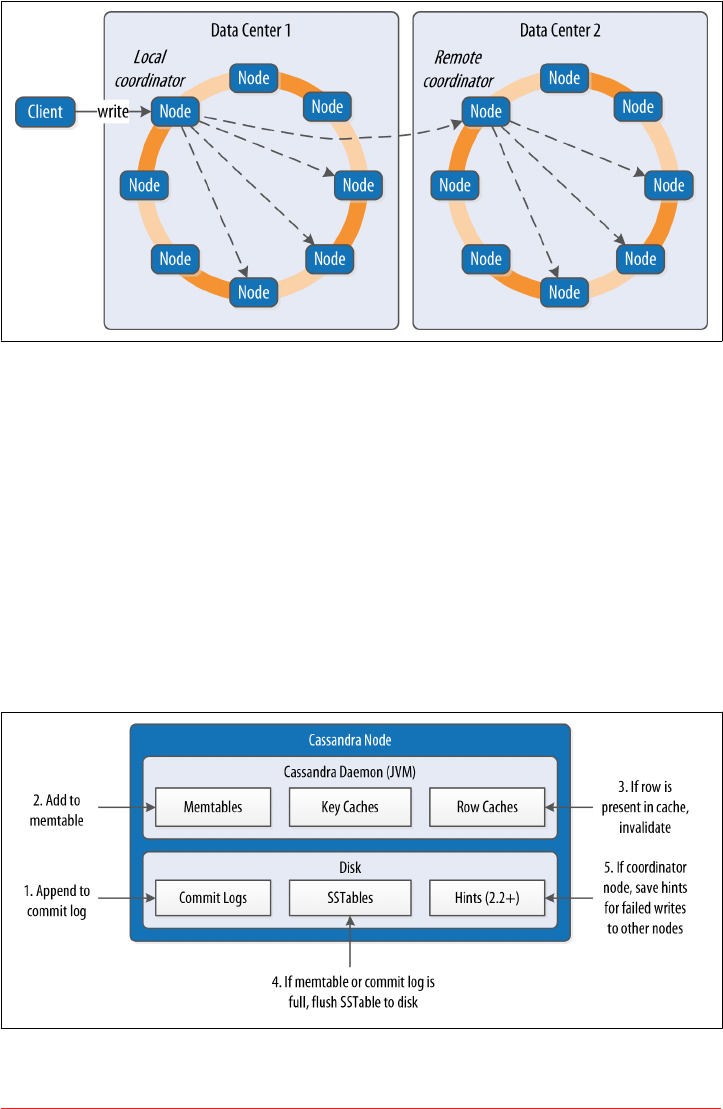
Figure 9-1. Interactions between nodes on the write path
If the cluster spans multiple data centers, the local coordinator node selects a remote
coordinator in each of the other data centers to coordinate the write to the replicas in
that data center. Each of the remote replicas responds directly to the original coordi‐
nator node.
The coordinator waits for the replicas to respond. Once a sufficient number of repli‐
cas have responded to satisfy the consistency level, the coordinator acknowledges the
write to the client. If a replica doesn’t respond within the timeout, it is presumed to be
down, and a hint is stored for the write. A hint does not count as successful replica
write unless the consistency level ANY is used.
Figure 9-2 depicts the interactions that take place within each replica node to process
a write request.
Figure 9-2. Interactions within a node on the write path
182 | Chapter 9: Reading and Writing Data

First, the replica node receives the write request and immediately writes the data to
the commit log. Next, the replica node writes the data to a memtable. If row caching
is used and the row is in the cache, the row is invalidated. We’ll discuss caching in
more detail under the read path.
If the write causes either the commit log or memtable to pass their maximum thresh‐
olds, a flush is scheduled to run. We’ll learn how to tune these thresholds in Chap‐
ter 12.
At this point, the write is considered to have succeeded and the node can reply to the
coordinator node or client.
After returning, the node executes a flush if one was scheduled. The contents of each
memtable are stored as SSTables on disk and the commit log is cleared. After the
flush completes, additional tasks are scheduled to check if compaction is needed and
then a compaction is performed if necessary.
More Detail on the Write Path
Of course, this is a simple overview of the write path that doesn’t
take into account variants such as counter modifications and mate‐
rialized views. Writes to tables with materialized views are more
complex because partitions must be locked. Cassandra leverages
logged batches internally in order to maintain materialized views.
For a more in-depth treatment of the write path, consult Michael
Edge’s excellent description on the Apache Cassandra Wiki at
https://wiki.apache.org/cassandra/WritePathForUsers.
Writing Files to Disk
Let’s examine a few more details on the files Cassandra writes to disk, including com‐
mit logs and SSTables.
Commit log les
Cassandra writes commit logs to the filesystem as binary files. The commit log files
are found under the $CASSANDRA_HOME/data/commitlog directory.
Commit log files are named according to the pattern CommitLog-<version>-
<timestamp>.log. For example: CommitLog-6-1451831400468.log. The version is an
integer representing the commit log format. For example, the version for the 3.0
release is 6. You can find the versions in use by release in the org.apache.cassandra
.db.commitlog.CommitLogDescriptor class.
Writing | 183

SSTable les
When SSTables are written to the filesystem during a flush, there are actually several
files that are written per SSTable. Let’s take a look at the $CASSANDRA_HOME/data/
data directory to see how the files are organized on disk.
Forcing SSTables to Disk
If you’re following along with the exercises in this book on a real
Cassandra node, you may want to execute the nodetool flush
command at this point, as you may not have entered enough data
yet for Cassandra to have flushed data to disk automatically. We’ll
learn more about this command in Chapter 11.
Looking in the data directory, you’ll see a directory for each keyspace. These directo‐
ries, in turn, contain a directory for each table, consisting of the table name plus a
UUID. The purpose of the UUID is to distinguish between multiple schema versions,
because the schema of a table can be altered over time.
Each of these directories contain SSTable files which contain the stored data. Here is
an example directory path: hotel/hotels-3677bbb0155811e5899aa9fac1d00bce.
Each SSTable is represented by multiple files that share a common naming scheme.
The files are named according to the pattern <version>-<generation>-
<implementation>-<component>.db. The significance of the pattern is as follows:
•The version is a two-character sequence representing the major/minor version of
the SSTable format. For example, the version for the 3.0 release is ma. You can
learn more about various versions in the org.apache.cassandra.io.sstable.
Descriptor class.
•The generation is an index number which is incremented every time a new
SSTable is created for a table.
•The implementation is a reference to the implementation of the org.apache.cas
sandra.io.sstable.format.SSTableWriter interface in use. As of the 3.0
release the value is “big”, which references the “Bigtable format” found in the
org.apache.cassandra.io.sstable.format.big.BigFormat class.
184 | Chapter 9: Reading and Writing Data

Each SSTable is broken up into multiple files or components. These are the compo‐
nents as of the 3.0 release:
*-Data.db
These are the files that store the actual data and are the only files that are pre‐
served by Cassandra’s backup mechanisms, which we’ll learn about in Chap‐
ter 11.
*-CompressionInfo.db
Provides metadata about the compression of the Data.db file.
*-Digest.adler32
Contains a checksum for the *-Data.db file. (Releases prior to 3.0 use CRC 32
checksums and the .crc32 extension.)
*-Filter.db
Contains the bloom filter for this SSTable.
*-Index.db
Provides row and column offsets within the corresponding *-Data.db file.
Summary.db
A sample of the index for even faster reads.
Statistics.db
Stores statistics about the SSTable which are used by the nodetool tablehisto
grams command.
TOC.txt
Lists the file components for this SSTable.
Older releases support different versions and filenames. Releases prior to 2.2 prepend
the keyspace and table name to each file, while 2.2 and later leave these out because
they can be inferred from the directory name.
We’ll investigate some tools for working with SSTable files in Chapter 11.
Lightweight Transactions
As we’ve discussed previously in Chapter 1, Cassandra and many other NoSQL data‐
bases do not support transactions with full ACID semantics supported by relational
databases. However, Cassandra does provide two mechanisms that offer some trans‐
actional behavior: lightweight transactions and batches.
Cassandra’s lightweight transaction (LWT) mechanism uses the Paxos algorithm
described in Chapter 6. LWTs were introduced in the 2.0 release. LWTs support the
following semantics:
Writing | 185

• The scope of each transaction is limited to a single partition.
•Each transaction consists of both a read and a write, also known as a “compare
and set” operation. The set is only performed if the comparison is successful.
•If a transaction fails because the existing values did not match the one you
expected, Cassandra will include the current ones so you can decide whether to
retry or abort without needing to make an extra request.
•The USING TIMESTAMP option is not supported.
Let’s say we wanted to create a record for a new hotel, using the data model we intro‐
duced in Chapter 5. We want to make sure that we’re not overwriting a hotel with the
same ID, so we add the IF NOT EXISTS syntax to our insert command:
cqlsh> INSERT INTO hotel.hotels (id, name, phone) VALUES (
'AZ123', 'Super Hotel at WestWorld', '1-888-999-9999') IF NOT EXISTS;
[applied]
-----------
True
This command checks to see if there is a record with the partition key, which for this
table consists of the hotel_id. So let’s find out what happens when we execute this
command a second time:
cqlsh> INSERT INTO hotel.hotels (id, name, phone) VALUES (
'AZ123', 'Super Hotel at WestWorld', '1-888-999-9999') IF NOT EXISTS;
[applied] | id | address | name | phone | pois
-----------+-------+---------+--------------------------+----------------+------
False | AZ123 | null | Super Hotel at WestWorld | 1-888-999-9999 | null
In this case, the transaction fails, as there is already a hotel with the ID “AZ123”, and
cqlsh helpfully echoes back a row containing a failure indication and the values we
tried to enter.
It works in a similar way for updates. For example, we might use the following state‐
ment to make sure we’re changing the name for this hotel:
cqlsh> UPDATE hotel.hotels SET name='Super Hotel Suites at WestWorld'
... WHERE id='AZ123' IF name='Super Hotel at WestWorld';
[applied]
-----------
True
cqlsh> UPDATE hotel.hotels SET name='Super Hotel Suites at WestWorld'
... WHERE id='AZ123' IF name='Super Hotel at WestWorld';
[applied] | name
-----------+---------------------------------
False | Super Hotel Suites at WestWorld
186 | Chapter 9: Reading and Writing Data

Similar to what we saw with multiple INSERT statements, entering the same UPDATE
statement again fails because the value has already been set. Because of Cassandra’s
upsert model, the IF NOT EXISTS syntax available on INSERT and the IF x=y syntax
on UPDATE represent the only semantic difference between these two operations.
Using Transactions on Schema Creation
CQL also supports the use of the IF NOT EXISTS option on the cre‐
ation of keyspaces and tables. This is especially useful if you are
scripting multiple schema updates.
Let’s implement the hotel creation example from before using the DataStax Java
Driver. When executing a conditional statement the ResultSet will contain a single
Row with a column named applied of type boolean. This tells whether the condi‐
tional statement was successful or not. We can also use the wasApplied() operation
on the statement:
SimpleStatement hotelInsert = session.newSimpleStatement(
"INSERT INTO hotels (id, name, phone) VALUES (?, ?, ?) IF NOT EXISTS",
"AZ123", "Super Hotel at WestWorld", "1-888-999-9999");
ResultSet hotelInsertResult = session.execute(hotelInsert);
boolean wasApplied = hotelInsertResult.wasApplied());
if (wasApplied) {
Row row = hotelInsertResult.one();
row.getBool("applied");
}
Conditional write statements can have a serial consistency level in addition to the reg‐
ular consistency level. The serial consistency level determines the number of nodes
that must reply in the Paxos phase of the write, when the participating nodes are
negotiating about the proposed write. The two available options are shown in
Table 9-2.
Table 9-2. Serial consistency levels
Consistency level Implication
SERIAL This is the default serial consistency level, indicating that a quorum of nodes must respond.
LOCAL_SERIAL Similar to SERIAL, but indicates that the transaction will only involve nodes in the local data center.
The serial consistency level can apply on reads as well. If Cassandra detects that a
query is reading data that is part of an uncommitted transaction, it commits the
transaction as part of the read, according to the specified serial consistency level.
Writing | 187

You can set a default serial consistency level for all statements in cqlsh using the
SERIAL CONSISTENCY statement, or in the DataStax Java Driver using the Query
Options.setSerialConsistencyLevel() operation.
Batches
While lightweight transactions are limited to a single partition, Cassandra provides a
batch mechanism that allows you to group modifications to multiple partitions into a
single statement.
The semantics of the batch operation are as follows:
•Only modification statements (INSERT, UPDATE, or DELETE) may be included in a
batch.
•Batches are atomic—that is, if the batch is accepted, all of the statements in a
batch will succeed eventually. This is why Cassandra’s batches are sometimes
referred to as atomic batches or logged batches.
•All updates in a batch belonging to a given partition key are performed in isola‐
tion, but there is no isolation guarantee across partitions. This means that modi‐
fications to different partitions may be read before the batch completes.
•Batches are not a transaction mechanism, but you can include lightweight trans‐
action statements in a batch. Multiple lightweight transactions in a batch must
apply to the same partition.
•Counter modifications are only allowed within a special form of batch known as
a counter batch. A counter batch can only contain counter modifications.
Deprecation of Unlogged Batches
In releases prior to 3.0, Cassandra supported unlogged batches, or
batches in which the steps involving the batchlog were skipped.
The drawback of unlogged batches was that there was no guarantee
that batches would complete successfully, which could leave the
database in an inconsistent state.
Using a batch saves back and forth traffic between the client and the coordinator
node, as the client is able to group multiple statements in a single query. However, the
batch places additional work on the coordinator to orchestrate the execution of the
various statements.
Cassandra’s batches are a good fit for use cases such as making multiple updates to a
single partition, or keeping multiple tables in sync. A good example is making modi‐
fications to denormalized tables that store the same data for different access patterns.
188 | Chapter 9: Reading and Writing Data

Batches Aren’t for Bulk Loading
First time users often confuse batches for a way to get faster perfor‐
mance for bulk updates. This is definitely not the case—batches
actually decrease performance and can cause garbage collection
pressure.
Let’s look at an example batch that we might use to insert a new hotel in our denor‐
malized table design. We use the CQL BEGIN BATCH and APPLY BATCH keywords to
surround the statements in our batch:
cqlsh> BEGIN BATCH
INSERT INTO hotel.hotels (id, name, phone)
VALUES ('AZ123', 'Super Hotel at WestWorld', '1-888-999-9999');
INSERT INTO hotel.hotels_by_poi (poi_name, id, name, phone)
VALUES ('West World', 'AZ123', 'Super Hotel at WestWorld',
'1-888-999-9999');
APPLY BATCH;
The DataStax Java driver supports batches through the com.datastax.
driver.core.BatchStatement class. Here’s an example of what the same batch would
look like in a Java client:
SimpleStatement hotelInsert = session.newSimpleStatement(
"INSERT INTO hotels (id, name, phone) VALUES (?, ?, ?)",
"AZ123", "Super Hotel at WestWorld", "1-888-999-9999");
SimpleStatement hotelsByPoiInsert = session.newSimpleStatement(
"INSERT INTO hotels_by_poi (poi_name, id, name, phone)
VALUES (?, ?, ?, ?)", "WestWorld", "AZ123",
"Super Hotel at WestWorld", "1-888-999-9999");
BatchStatement hotelBatch = new BatchStatement();
hotelBatch.add(hotelsByPoiInsert);
hotelBatch.add(hotelInsert);
ResultSet hotelInsertResult = session.execute(hotelBatch);
You can also create batches using the QueryBuilder.batch() operation by passing
other Statements. You can find code samples for working with BatchStatement and
com.cassandraguide.readwrite.BatchStatementExample.
Creating Counter Batches in DataStax Drivers
The DataStax drivers do not provide separate mechanisms for
counter batches. Instead, you must simply remember to create
batches that include only counter modifications or only non-
counter modifications.
Writing | 189

Here’s how a batch works under the covers: the coordinator sends a copy of the batch
called a batchlog to two other nodes, where it is stored in the system.batchlog table.
The coordinator then executes all of the statements in the batch, and deletes the
batchlog from the other nodes after the statements are completed.
If the coordinator should fail to complete the batch, the other nodes have a copy in
their batchlog and are therefore able to replay the batch. Each node checks its
batchlog once a minute to see if there are any batches that should have completed. To
give ample time for the coordinator to complete any in-progress batches, Cassandra
uses a grace period from the timestamp on the batch statement equal to twice the
value of the write_request_timeout_in_ms property. Any batches that are older
than this grace period will be replayed and then deleted from the remaining node.
The second batchlog node provides an additional layer of redundancy, ensuring high
reliability of the batch mechanism.
Cassandra enforces limits on the size of batch statements to prevent them from
becoming arbitrarily large and impacting the performance and stability of the cluster.
The cassandra.yaml file contains two properties that control how this works: the
batch_size_warn_threshold_in_kb property defines the level at which a node will
log at the WARN log level that it has received a large batch, while any batch exceeding
the value set batch_size_fail_threshold_in_kb will be rejected and result in error
notification to the client. The batch size is measured in terms of the length of the
CQL query statement. The warning threshold defaults to 5KB, while the fail threshold
defaults to 50KB.
Reading
There are a few basic properties of Cassandra’s read capability that are worth noting.
First, it’s easy to read data because clients can connect to any node in the cluster to
perform reads, without having to know whether a particular node acts as a replica for
that data. If a client connects to a node that doesn’t have the data it’s trying to read,
the node it’s connected to will act as coordinator node to read the data from a node
that does have it, identified by token ranges.
In Cassandra, reads are generally slower than writes. To fulfill read operations, Cas‐
sandra typically has to perform seeks, but you may be able to keep more data in
memory by adding nodes, using compute instances with more memory, and using
Cassandra’s caches. Cassandra also has to wait for responses synchronously on reads
(based on consistency level and replication factor), and then perform read repairs as
necessary.
190 | Chapter 9: Reading and Writing Data

Read Consistency Levels
The consistency levels for read operations are similar to the write consistency levels,
but their meanings are slightly different. A higher consistency level means that more
nodes need to respond to the query, giving you more assurance that the values
present on each replica are the same. If two nodes respond with different timestamps,
the newest value wins, and that’s what will be returned to the client. In the back‐
ground, Cassandra will then perform what’s called a read repair: it takes notice of the
fact that one or more replicas responded to a query with an outdated value, and
updates those replicas with the most current value so that they are all consistent.
The possible consistency levels, and the implications of specifying each one for read
queries, are shown in Table 9-3.
Table 9-3. Read consistency levels
Consistency level Implication
ONE, TWO, THREE Immediately return the record held by the rst node(s) that respond to the query. A background thread
is created to check that record against the same record on other replicas. If any are out of date, a read
repair is then performed to sync them all to the most recent value.
LOCAL_ONE Similar to ONE, with the additional requirement that the responding node is in the local data center.
QUORUM Query all nodes. Once a majority of replicas ((replication factor / 2) + 1) respond, return to
the client the value with the most recent timestamp. Then, if necessary, perform a read repair in the
background on all remaining replicas.
LOCAL_QUORUM Similar to QUORUM, where the responding nodes are in the local data center.
EACH_QUORUM Ensure that a QUORUM of nodes respond in each data center.
ALL Query all nodes. Wait for all nodes to respond, and return to the client the record with the most recent
timestamp. Then, if necessary, perform a read repair in the background. If any nodes fail to respond, fail
the read operation.
As you can see from the table, the ANY consistency level is not supported for read
operations. Notice that the implication of consistency level ONE is that the first node
to respond to the read operation is the value that the client will get—even if it is out
of date. The read repair operation is performed after the record is returned, so any
subsequent reads will all have a consistent value, regardless of the responding node.
Another item worth noting is in the case of consistency level ALL. If you specify ALL,
then you’re saying that you require all replicas to respond, so if any node with that
record is down or otherwise fails to respond before the timeout, the read operation
fails. A node is considered unresponsive if it does not respond to a query before the
value specified by rpc_timeout_in_ms in the configuration file. The default is 10 sec‐
onds.
Reading | 191
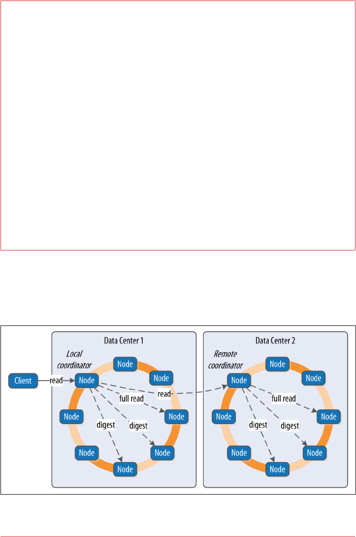
Aligning Read and Write Consistency Levels
The read and write consistency levels you choose to use in your applications are an
example of the flexibility Cassandra provides us to make trade-offs between consis‐
tency, availability, and performance.
As we learned in Chapter 6, Cassandra can guarantee strong consistency on reads by
using read and write consistency levels whose sum exceeds the replication factor. One
simple way to achieve this is to require QUORUM for reads and writes. For example, on
a keyspace with a replication factor of 3, QUORUM represents a response from 2 out of
three nodes. Because 2 + 2 > 3, strong consistency is guaranteed.
If you are willing to sacrifice strong consistency in order to support increased
throughput and more tolerance for downed nodes, you can use lesser consistency lev‐
els. For example, using QUORUM for writes and ONE for reads doesn’t guarantee strong
consistency, as 2 + 1 is merely equal to 3.
Thinking this through practically, if you are only guaranteed writes to two out of
three replicas, there is certainly a chance that one of the replicas did not receive the
write and has not yet been repaired, and a read at consistency level ONE could go to
that very node.
The Cassandra Read Path
Now let’s take a look at what happens when a client requests data. This is known as
the read path. We’ll describe the read path from the perspective of a query for a single
partition key, starting with the interactions between nodes shown in Figure 9-3.
Figure 9-3. Interactions between nodes on the read path
192 | Chapter 9: Reading and Writing Data
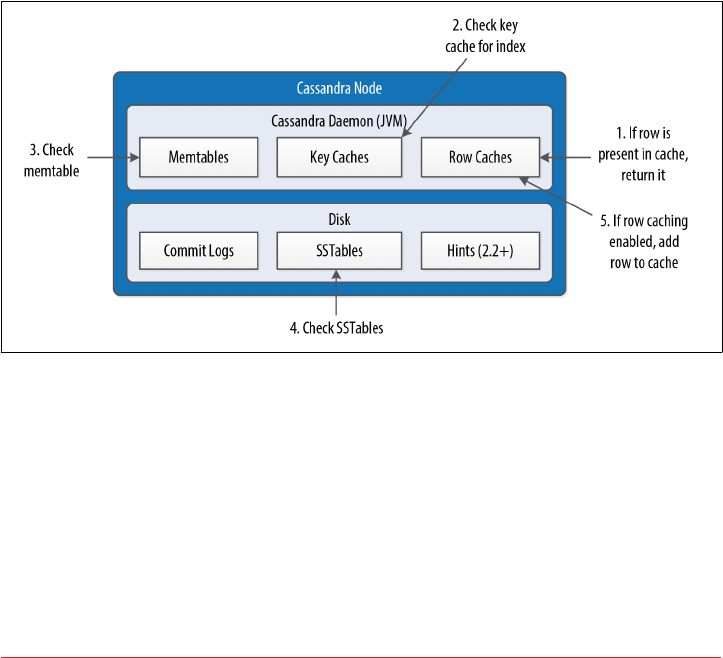
The read path begins when a client initiates a read query to the coordinator node. As
on the write path, the coordinator uses the partitioner to determine the replicas and
checks that there are enough replicas up to satisfy the requested consistency level.
Another similarity to the write path is that a remote coordinator is selected per data
center for any read queries that involve multiple data centers.
If the coordinator is not itself a replica, the coordinator then sends a read request to
the fastest replica, as determined by the dynamic snitch. The coordinator node also
sends a digest request to the other replicas. A digest request is similar to a standard
read request, except the replicas return a digest, or hash, of the requested data.
The coordinator calculates the digest hash for data returned from the fastest replica
and compares it to the digests returned from the other replicas. If the digests are con‐
sistent, and the desired consistency level has been met, then the data from the fastest
replica can be returned. If the digests are not consistent, then the coordinator must
perform a read repair, as discussed in the following section.
Figure 9-4 shows the interactions that take place within each replica node to process
read requests.
Figure 9-4. Interactions within a node on the read path
When the replica node receives the read request, it first checks the row cache. If the
row cache contains the data, it can be returned immediately. The row cache helps
speed read performance for rows that are accessed frequently. We’ll discuss the pros
and cons of row caching in Chapter 12.
If the data is not in the row cache, the replica node searches for the data in memtables
and SSTables. There is only a single memtable for a given table, so that part of the
search is straightforward. However, there are potentially many physical SSTables for a
single Cassandra table, each of which may contain a portion of the requested data.
Reading | 193

Cassandra implements several features to optimize the SSTable search: key caching,
Bloom filters, SSTable indexes, and summary indexes.
The first step in searching SSTables on disk is to use a Bloom filter to determine
whether requested partition does not exist in a given SSTable, which would make it
unnecessary to search that SSTable.
Tuning Bloom Filters
Cassandra maintains a copy of Bloom filters in memory, although
you may remember from our earlier discussion of files from above
that the Bloom filters are stored in files alongside the SSTable data
files so that they don’t have to be recalculated if the node is restar‐
ted.
The Bloom filter does not guarantee that the SSTable contains the
partition, only that it might contain it. You can set the bloom_fil
ter_fp_chance property on each table to control the percentage of
false positives that the Bloom filter reports. This increased accuracy
comes at the cost of additional memory use.
If the SSTable passes the Bloom filter, Cassandra checks the key cache to see if it con‐
tains the offset of the partition key in the SSTable. The key cache is implemented as a
map structure in which the keys are a combination of the SSTable file descriptor and
partition key, and the values are offset locations into SSTable files. The key cache
helps to eliminate seeks within SSTable files for frequently accessed data, because the
data can be read directly.
If the offset is not obtained from the key cache, Cassandra uses a two-level index
stored on disk in order to locate the offset. The first level index is the partition sum‐
mary, which is used to obtain an offset for searching for the partition key within the
second level index, the partition index. The partition index is where the offset into the
SSTable for the partition key is stored.
If the offset for the partition key is found, Cassandra accesses the SSTable at the speci‐
fied offset and starts reading data.
Once data has been obtained from all of the SSTables, Cassandra merges the SSTable
data and memtable data by selecting the value with the latest timestamp for each
requested column. Any tombstones encountered are ignored.
Finally, the merged data can be added to the row cache (if enabled) and returned to
the client or coordinator node. A digest request is handled in much the same way as a
regular read request, with the additional step that a digest is calculated on the result
data and returned instead of the data itself.
194 | Chapter 9: Reading and Writing Data

More Detail on the Read Path
For more detail on the read path, consult the Apache Cassandra
Wiki.
Read Repair
Here’s how read repair works: the coordinator makes a full read request from all of
the replica nodes. The coordinator node merges the data by selecting a value for each
requested column. It compares the values returned from the replicas and returns the
value that has the latest timestamp. If Cassandra finds different values stored with the
same timestamp, it will compare the values lexicographically and choose the one that
has the greater value. This case should be exceedingly rare. The merged data is the
value that is returned to the client.
Asynchronously, the coordinator identifies any replicas that return obsolete data and
issues a read-repair request to each of these replicas to update their data based on the
merged data.
The read repair may be performed either before or after the return to the client. If
you are using one of the two stronger consistency levels (QUORUM or ALL), then the
read repair happens before data is returned to the client. If the client specifies a weak
consistency level (such as ONE), then the read repair is optionally performed in the
background after returning to the client. The percentage of reads that result in back‐
ground repairs for a given table is determined by the read_repair_chance and
dc_local_read_repair_chance options for the table.
Range Queries, Ordering and Filtering
So far in our travels we’ve confined our read queries to very simple examples. Let’s
take a look at more of the options that Cassandra provides on the SELECT command,
such as the WHERE and ORDER BY clauses.
First, let’s examine how to use the WHERE clause that Cassandra provides for reading
ranges of data within a partition, sometimes called slices.
In order to do a range query, however, it will help to have some data to work with.
Although we don’t have a lot of data yet, we can quickly get some by using one of
Cassandra’s bulk loading tools.
Reading | 195

Bulk Loading Options
In using Cassandra, you’ll often find it useful to be able to load test or reference data
into a cluster. Fortunately, there are a couple of easy ways to bulk load formatted data
to and from Cassandra.
cqlsh supports loading and unloading of comma-separated variable (CSV) files via
the COPY command.
For example, the following command could be used to save the contents of our hotels
table to a file:
cqlsh:hotel> COPY hotels TO 'hotels.csv' WITH HEADER=TRUE;
The TO value specifies the file to write to, and the HEADER option to TRUE causes the
column names to be printed in our output file. We could edit this file and read the
contents back in with this command:
cqlsh:hotel> COPY hotels FROM 'hotels.csv' WITH HEADER=true;
The COPY command supports other options to configure how quotes, escapes, and
times are represented.
Brian Hess has created a command-line tool called the Cassandra Loader that loads
and unloads CSV files as well as other delimited files, and is flexible enough to handle
using the comma as the decimal separator.
We can use cqlsh to load some sample hotel inventory data into our cluster. You can
access a simple .csv file in the GitHub repository for this book. The avail‐
able_rooms.csv file contains a month’s worth of inventory for two small hotels with
five rooms each. Let’s load the data into the cluster:
cqlsh:hotel> COPY available_rooms_by_hotel_date FROM
'available_rooms.csv' WITH HEADER=true;
310 rows imported in 0.789 seconds.
If you do a quick query to read some of this data, you’ll find that we have data for two
hotels: “AZ123” and “NY229”.
Now let’s consider how to support the query we labeled “Q4. Find an available room
in a given date range” from Chapter 5. Remember that we designed the
available_rooms_by_hotel_date table to support this query, with the primary
key:
PRIMARY KEY (hotel_id, date, room_number)
196 | Chapter 9: Reading and Writing Data

This means that the hotel_id is the partition key, while date and room_number are
clustering columns.
Here’s a CQL statement that allows us to search for hotel rooms for a specific hotel
and date range:
cqlsh:hotel> SELECT * FROM available_rooms_by_hotel_date
WHERE hotel_id='AZ123' and date>'2016-01-05' and date<'2016-01-12';
hotel_id | date | room_number | is_available
----------+------------+-------------+--------------
AZ123 | 2016-01-06 | 101 | True
AZ123 | 2016-01-06 | 102 | True
AZ123 | 2016-01-06 | 103 | True
AZ123 | 2016-01-06 | 104 | True
AZ123 | 2016-01-06 | 105 | True
...
(60 rows)
Note that this query involves the partition key hotel_id and a range of values repre‐
senting the start and end of our search over the clustering key date.
If we wanted to try to find the records for room number 101 at hotel AZ123, we
might attempt a query like the following:
cqlsh:hotel> SELECT * FROM available_rooms_by_hotel_date
WHERE hotel_id='AZ123' and room_number=101;
InvalidRequest: code=2200 [Invalid query] message="PRIMARY KEY column
"room_number" cannot be restricted as preceding column "date" is not
restricted"
As you can see, this query results in an error, because we have attempted to restrict
the value of the second clustering key while not limiting the value of the first cluster‐
ing key.
The syntax of the WHERE clause involves the following rules:
•All elements of the partition key must be identified
•A given clustering key may only be restricted if all previous clustering keys are
restricted
These restrictions are based on how Cassandra stores data on disk, which is based on
the clustering columns and sort order specified on the CREATE TABLE command. The
conditions on the clustering column are restricted to those that allow Cassandra to
select a contiguous ordering of rows.
The exception to this rule is the ALLOW FILTERING keyword, which allows us to omit a
partition key element. For example, we can search the room status across multiple
hotels for rooms on a specific date with this query:
Reading | 197

cqlsh:hotel> SELECT * FROM available_rooms_by_hotel_date
WHERE date='2016-01-25' ALLOW FILTERING;
hotel_id | date | room_number | is_available
----------+------------+-------------+--------------
AZ123 | 2016-01-25 | 101 | True
AZ123 | 2016-01-25 | 102 | True
AZ123 | 2016-01-25 | 103 | True
AZ123 | 2016-01-25 | 104 | True
AZ123 | 2016-01-25 | 105 | True
NY229 | 2016-01-25 | 101 | True
NY229 | 2016-01-25 | 102 | True
NY229 | 2016-01-25 | 103 | True
NY229 | 2016-01-25 | 104 | True
NY229 | 2016-01-25 | 105 | True
(10 rows)
Usage of ALLOW FILTERING is not recommended, however, as it has the potential to
result in very expensive queries. If you find yourself needing such a query, you will
want to revisit your data model to make sure you have designed tables that support
your queries.
The IN clause can be used to test equality with multiple possible values for a column.
For example, we could use the following to find inventory on two dates a week apart
with the command:
cqlsh:hotel> SELECT * FROM available_rooms_by_hotel_date
WHERE hotel_id='AZ123' AND date IN ('2016-01-05', '2016-01-12');
Note that using the IN clause can result in slower performance on queries, as the
specified column values may correspond to non-contiguous areas within the row.
Finally, the SELECT command allows us to override the sort order which has been
specified on the columns when we created the table. For example, we could obtain the
rooms in descending order by date for any of our previous queries using the ORDER
BY syntax:
cqlsh:hotel> SELECT * FROM available_rooms_by_hotel_date
WHERE hotel_id='AZ123' and date>'2016-01-05' and date<'2016-01-12'
ORDER BY date DESC;
Functions and Aggregates
Cassandra 2.2 introduced two features that allow clients to shift some processing
work to the coordinator node: user-defined functions (UDFs) and user-defined
aggregates (UDAs). Using these features can improve performance in some situations
by reducing the amount of data that has to be returned to the client and reducing
processing load on the client, at the cost of additional processing on the server.
198 | Chapter 9: Reading and Writing Data

User-dened functions
UDFs are functions that are applied on Cassandra nodes to stored data as part of
query processing. Before using UDFs in your cluster, they must be enabled in the
cassandra.yaml file on each node:
enable_user_defined_functions: true
Here’s a quick summary of how this works: we create a UDF using the CQL CREATE
FUNCTION command, which causes the function to be propagated to every node in the
cluster. When you execute a query that references the UDF, it is applied to each row
of the query result.
Let’s create an example UDF to count the number of available rooms in our
available_rooms_by_hotel_date table:
cqlsh:hotel> CREATE FUNCTION count_if_true(input boolean)
RETURNS NULL ON NULL INPUT
RETURNS int
LANGUAGE java AS 'if (input) return 1; else return 0;';
We’ll dissect this command a bit at a time. We’ve created a UDF named
count_if_true which operates on a boolean parameter and returns an integer.
We’ve also included a null check to make sure the function works effectively just in
case the value is not defined. Note that if a UDF fails, execution of the query is abor‐
ted, so this can be an important check.
UDF Security
The 3.0 release added a security feature to run UDF code in a sepa‐
rate sandbox to limit the ability for a malicious function to gain
unauthorized access to a node’s Java runtime.
Next, note that we’ve declared this to be a Java implementation with the LANGUAGE
clause. Cassandra natively supports functions and aggregates defined in Java and
JavaScript. They can also be implemented using any language supported by the Java
Scripting API specified in JSR 223, including Python, Ruby, and Scala. Functions
defined in these languages require adding additional scripting engine JAR files to
Cassandra’s Java CLASSPATH.
Finally, we include the actual Java syntax of the function with the AS clause. Now this
function is somewhat trivial by itself, because all we’re doing is counting true values
as 1. We’ll do something more powerful with this UDF in a bit.
First, however, let’s try our UDF out on our available_rooms_by_hotel_date table
to see how it works:
cqlsh:hotel> SELECT room_number, count_if_true(is_available)
FROM available_rooms_by_hotel_date
Reading | 199

WHERE hotel_id='AZ123' and date='2016-01-05';
room_number | hotel.count_if_true(is_available)
-------------+-----------------------------------
101 | 1
102 | 1
103 | 1
104 | 1
105 | 1
(5 rows)
As you can see, the column with our function result is qualified with the hotel key‐
space name. This is because each UDF is associated with a specific keyspace. If we
were to execute a similar query in the DataStax Java Driver, we would find a Column
in each Row with the name hotel_count_if_true_is_available.
User-dened aggregates
As we’ve just learned, user-defined functions operate on a single row. In order to per‐
form operations across multiple rows, we create a user-defined aggregate. The UDA
leverages two UDFs: a state function and an optional final function. A state function
is executed against every row, while the final function, if present, operates on the
results of the state function.
Let’s look at a simple example to help investigate how this works. First, we’ll need a
state function. The count_if_true function is close to what we need, but we need to
make a small change to allow the available count to be summed across multiple rows.
Let’s create a new function that allows a running total to be passed in, incremented
and returned:
cqlsh:hotel> CREATE FUNCTION state_count_if_true(total int, input boolean)
RETURNS NULL ON NULL INPUT
RETURNS int
LANGUAGE java AS 'if (input) return total+1; else return total;';
Note that the total parameter is passed as the first parameter, with its type matching
the return type of the function (int). For a UDF to be used as a state function, the
first parameter type and return types must match. The second parameter is the
boolean which we had in our original count_if_true UDF.
Now we can create an aggregate that uses this state function:
cqlsh:hotel> CREATE AGGREGATE total_available (boolean)
SFUNC state_count_if_true
STYPE int
INITCOND 0;
Let’s break down this statement piece by piece: first, we’ve declared a UDA called
total_available, which operates on columns of type boolean.
200 | Chapter 9: Reading and Writing Data

The SFUNC clause identifies the state function used by this query—in this case,
state_count_if_true.
Next, we identify the type that is used to accumulate results from the state function by
the STYPE clause. Cassandra maintains a value of this type, which it passes to the state
function as it is called on each successive row. The STYPE must be the same as the first
parameter and return type of the state function. The INITCOND clause allows us to set
the initial value of the result; here, we set the initial count to zero.
In this case, we’ve chosen to omit the final function, but we could have included a
function that took an argument of the STYPE and returned any other type, such as a
function that accepts an integer argument and returns a boolean indicating if the
inventory is at a low level that should generate an alert.
Now let’s use our aggregate to get a count of available rooms returned by one of our
previous queries. Note that our query must only include the UDA, with no other col‐
umns or functions:
cqlsh:hotel> SELECT total_available(is_available)
FROM available_rooms_by_hotel_date
WHERE hotel_id='AZ123' and date='2016-01-05';
hotel.total_available(is_available)
-------------------------------------
5
(1 rows)
As you can see, this query yields a result of five available rooms for the specified hotel
and date.
Additional UDF/UDA Command Options
You can use the familiar IF NOT EXISTS syntax when creating
UDFs and UDAs to avoid error messages for attempts to create
functions and aggregates with duplicate signatures. Alternatively,
you can use the CREATE OR REPLACE syntax when you can actually
intend to override the current function or aggregate.
Use the DESCRIBE FUNCTIONS command or the DESCRIBE
AGGREGATES command to learn which UDFs and UDAs have been
defined already. This can be especially useful when there are func‐
tions with the same name but different signatures.
Finally, you can delete UDFs and UDAs using the DROP FUNCTION
and DROP AGGREGATE commands.
Reading | 201

Built-in functions and aggregates
In addition to user-defined functions and aggregates, Cassandra also provides some
built-in, or native functions and aggregates that we can use:
COUNT
The COUNT function is used to count the number of rows returned by a query. For
example, to count the number of hotels in our database:
SELECT COUNT(*) FROM hotel.hotels;
This command can also can be used to count the number of non-null values of a
specified column. For example, the following could be used to count how many
guests provided an email address:
SELECT COUNT(emails) FROM reservation.guests;
MIN and MAX
The MIN and MAX functions can be used to compute the minimum and maximum
value returned by a query for a given column. For example, this query could be
used to determine the minimum and maximum stay lengths (in nights) for reser‐
vations at a given hotel and arrival date:
SELECT MIN(nights), MAX(nights) FROM reservations_by_hotel_date
WHERE hotel_id='AZ123' AND start_date='2016-09-09';
sum
The sum function can be used to sum up all the values returned by a query for a
given column. We could sum the number of nights to be stayed across multiple
reservations as follows:
SELECT SUM(nights) FROM reservations_by_hotel_date
WHERE hotel_id='AZ123' AND start_date='2016-09-09';
avg
The avg function can be used to compute the average of all the values returned
by a query for a given column. To get the average stay length in nights, we might
execute a query like:
SELECT AVG(nights) FROM reservations_by_hotel_date
WHERE hotel_id='AZ123' AND start_date='2016-09-09';
These built-in aggregates are technically part of the system keyspace. Therefore, the
column name containing results of our last query would be system_avg_nights.
Paging
In early releases of Cassandra, clients had to make sure to carefully limit the amount
of data requested at a time. For a large result set, it is possible to overwhelm both
nodes and clients even to the point of running out of memory.
202 | Chapter 9: Reading and Writing Data

Thankfully, Cassandra provides a paging mechanism that allows retrieval of result
sets incrementally. A simple example of this is shown by use of the CQL keyword
LIMIT. For example, the following command will return no more than 100 hotels:
cqlsh> SELECT * FROM hotel.hotels LIMIT 100;
Of course, the limitation of the LIMIT keyword (pun intended) is that there’s no way
to obtain additional pages containing the additional rows beyond the requested
quantity.
The 2.0 release of Cassandra introduced a feature known as automatic paging. Auto‐
matic paging allows clients to request a subset of the data that would be returned by a
query. The server breaks the result into pages that are returned as the client requests
them.
You can view paging status in cqlsh via the PAGING command. The following output
shows a sequence of checking paging status, changing the fetch size (page size), and
disabling paging:
cqlsh> PAGING;
Query paging is currently enabled. Use PAGING OFF to disable
Page size: 100
cqlsh> PAGING 1000;
Page size: 1000
cqlsh> PAGING OFF;
Disabled Query paging.
cqlsh> PAGING ON;
Now Query paging is enabled
Now let’s see how paging works in the DataStax Java Driver. You can set a default
fetch size globally for a Cluster instance:
Cluster cluster = Cluster.builder().addContactPoint("127.0.0.1").
withQueryOptions(new QueryOptions().setFetchSize(2000)).build();
The fetch size can also be set on an individual statement, overriding the default value:
Statement statement = new SimpleStatement("...");
statement.setFetchSize(2000);
If the fetch size is set on a statement, it will take precedence; otherwise, the cluster-
wide value (which defaults to 5,000) will be used. Note that setting a fetch size doesn’t
mean that Cassandra will always return the exact number of rows requested; it is pos‐
sible that it returns slightly more or less results.
The driver handles automatic paging on our behalf, allowing us to iterate over a
ResultSet without requiring knowledge of the paging mechanism. For example,
consider the following code sample for iterating over a query for hotels:
SimpleStatement hotelSelect = session.newSimpleStatement(
"SELECT * FROM hotels");
Reading | 203

ResultSet resultSet = session.execute(hotelSelect);
for (Row row : resultSet) {
// process the row
}
What happens behind the scenes is as follows: when our application invokes the
session.execute() operation, the driver performs our query to Cassandra, request‐
ing the first page of results. Our application iterates over the results as shown in the
for loop, and when the driver detects that there are no more items remaining on the
current page, it requests the next page.
It is possible that the small pause of requesting the next page would affect the perfor‐
mance and user experience of our application, so the ResultSet provides additional
operations that allow more fine grained control over paging. Here’s an example of
how we could extend our application to do some pre-fetching of rows:
for (Row row : resultSet) {
if (resultSet.getAvailableWithoutFetching() < 100 &&
!resultSet.isFullyFetched())
resultSet.fetchMoreResults();
// process the row
}
This additional statement checks to see if there are less than 100 rows remaining on
the current page using getAvailableWithoutFetching(). If there is another page to
be retrieved, which we determine by checking isFullyFetched(), we initiate an
asynchronous call to obtain the extra rows via fetchMoreResults().
The driver also exposes the ability to access the paging state more directly so it can be
saved and reused later. This could be useful if your application is a stateless web ser‐
vice that doesn’t sustain a session across multiple invocations.
We can access the paging state through the ExecutionInfo of the ResultSet:
PagingState nextPage = resultSet.getExecutionInfo().getPagingState();
We can then save this state within our application, or return it to clients. The Paging
State can be converted to a string using toString(), or a byte array using
toBytes().
Note that in either string or byte array form, the state is not something you should try
to manipulate or reuse with a different statement. Doing so will result in a Paging
StateException.
To resume a query from a given PagingState, we set it on the Statement:
SimpleStatement hotelSelect = session.newSimpleStatement(
"SELECT * FROM hotels");
hotelSelect.setPagingState(pagingState);
204 | Chapter 9: Reading and Writing Data

Speculative Retry
We’ve previously discussed in Chapter 8 the SpeculativeExecutionPolicy provided
by the DataStax Java Driver, which pre-emptively retries read queries using different
nodes if the initial node does not respond in a configurable amount of time.
The same behavior is available for us to configure on each node so that when the
node acts as a coordinator, it can initiate speculative requests to alternate nodes. This
behavior is configurable on each table via the speculative_retry property, which
allows the following values:
ALWAYS
Retry reads of all replicas.
<X>PERCENTILE
Initiate retries if a response isn’t received within the Xth percentile response time.
<Y>ms
Retry if no response is received in Y milliseconds.
NONE
Do not retry reads.
The default value is 99.0PERCENTILE. This achieves a good balance by speeding up
the “outlier” slow performing requests without flooding the cluster with a large num‐
ber of duplicate read requests.
This feature is also known as rapid read protection, and was introduced in release
2.0.2. Note that it has no effect for queries at consistency level ALL, as there are no
additional nodes to retry.
Deleting
Deleting data is not the same in Cassandra as it is in a relational database. In an
RDBMS, you simply issue a delete statement that identifies the row or rows you want
to delete. In Cassandra, a delete does not actually remove the data immediately.
There’s a simple reason for this: Cassandra’s durable, eventually consistent, dis‐
tributed design. If Cassandra had a traditional design for deletes, any nodes that were
down at the time of a delete would not receive the delete. Once one of these nodes
came back online, it would mistakenly think that all of the nodes that had received
the delete had actually missed a write (the data that it still has because it missed the
delete), and it would start repairing all of the other nodes. So Cassandra needs a more
sophisticated mechanism to support deletes. That mechanism is called a tombstone.
A tombstone is a special marker issued in a delete that overwrites the deleted values,
acting as a placeholder. If any replica did not receive the delete operation, the tomb‐
Deleting | 205

stone can later be propagated to those replicas when they are available again. The net
effect of this design is that your data store will not immediately shrink in size follow‐
ing a delete. Each node keeps track of the age of all its tombstones. Once they reach
the age as configured in gc_grace_seconds (which is 10 days by default), then a com‐
paction is run, the tombstones are garbage-collected, and the corresponding disk
space is recovered.
Because SSTables are immutable, the data is not deleted from the SSTable. On com‐
paction, tombstones are accounted for, merged data is sorted, a new index is created
over the sorted data, and the freshly merged, sorted, and indexed data is written to a
single new file. The assumption is that 10 days is plenty of time for you to bring a
failed node back online before compaction runs. If you feel comfortable doing so, you
can reduce that grace period to reclaim disk space more quickly.
A simple delete of an entire row in the DataStax Java Driver looks like this:
SimpleStatement hotelDelete = session.newSimpleStatement(
"DELETE * FROM hotels WHERE id=?", "AZ123");
ResultSet hotelDeleteResult = session.execute(hotelDelete);
You can delete non-primary key columns by identifying them by name in the query.
You can also delete data using PreparedStatements, the QueryBuilder, and the
MappingManager.
Here is an example of deleting an entire row using the QueryBuilder:
BuiltStatement hotelDeleteBuilt = queryBuilder.delete().all().
from("hotels").where(eq("id", "AZ123"));
session.execute(hotelDeleteBuilt);
Consistency Levels for Deletion
Because a delete is a form of write, the consistency levels available
for deletes are the same as those listed for writes.
Summary
In this chapter, we saw how to read, write, and delete data using both cqlsh and client
drivers. We also took a peek behind the scenes to learn how Cassandra implements
these operations, which should help us to make more informed decisions as we
design, implement, deploy and maintain applications using Cassandra.
206 | Chapter 9: Reading and Writing Data

CHAPTER 10
Monitoring
In this chapter, you’ll learn how to use a variety of tools to monitor and understand
important events in the life cycle of your Cassandra cluster. We’ll look at some simple
ways to see what’s going on, such as changing the logging levels and understanding
the output.
Cassandra also features built-in support for Java Management Extensions (JMX),
which offers a rich way to monitor your Cassandra nodes and their underlying Java
environment. Through JMX, we can see the health of the database and ongoing
events, and even interact with it remotely to tune certain values. JMX is an important
part of Cassandra, and we’ll spend some time to make sure we know how it works
and what exactly Cassandra makes available for monitoring and management with
JMX. Let’s get started!
Logging
The simplest way to get a picture of what’s happening in your database is to just
change the logging level to make the output more verbose. This is great for develop‐
ment and for learning what Cassandra is doing under the hood.
Cassandra uses the Simple Logging Facade for Java (SLF4J) API for logging, with
Logback as the implementation. SLF4J provides a facade over various logging frame‐
works such as Logback, Log4J, and Java’s built-in logger (java.util.logging). You can
learn more about Logback at http://logback.qos.ch/.
By default, the Cassandra server log level is set at INFO, which doesn’t give you much
detail about what work Cassandra is doing at any given time. It just outputs basic sta‐
tus updates, such as the following:
INFO [main] 2015-09-19 09:40:20,215 CassandraDaemon.java:149 -
Hostname: Carp-iMac27.local
207

INFO [main] 2015-09-19 09:40:20,233 YamlConfigurationLoader.java:92 -
Loading settings from file:/Users/jeff/Cassandra/
apache-cassandra-2.1.8/conf/cassandra.yaml
INFO [main] 2015-09-19 09:40:20,333 YamlConfigurationLoader.java:135 -
Node configuration
...
When you start Cassandra in a terminal, you keep this output running in the termi‐
nal window by passing the program the -f flag (to keep output visible in the fore‐
ground of the terminal window). But Cassandra is also writing these logs to physical
files for you to examine later.
By changing the logging level to DEBUG, we can see much more clearly what activity
the server is working on, instead of seeing only these stage updates.
To change the logging level, open the file <cassandra-home>/conf/logback.xml
and find the section that looks like this:
<root level="INFO">
<appender-ref ref="FILE" />
<appender-ref ref="STDOUT" />
</root>
Change the first line so it looks like this:
<root level="DEBUG">
Once we have made this change and saved the file, Cassandra will shortly begin print‐
ing DEBUG-level logging statements. This is because the default logging is configured
to scan the configuration file once a minute, as set by the line:
<configuration scan="true">
Now we can see a lot more activity as Cassandra does its work. This allows you to see
exactly what Cassandra is doing and when, which is very helpful in troubleshooting.
But it’s also helpful in simply understanding what Cassandra does to maintain itself.
Tuning Logging in Production
Of course, in production you’ll want to tune the logging level back
up to WARN or ERROR, as the verbose output will slow things down
considerably.
By default, Cassandra’s log files are stored in the logs directory underneath the Cas‐
sandra installation directory.
If you want to change the location of the logs directory, just find the following entry
in the logback.xml file and chose a different filename:
<file>${cassandra.logdir}/system.log</file>
208 | Chapter 10: Monitoring

Missing Log Files
If you don’t see any logfiles in the location specified, make sure that
you are the owner of the directories, or at least that proper read
and write permissions are set. Cassandra won’t tell you if it can’t
write the log; it just won’t write. Same for the datafiles.
Other settings in the logback.xml file support rolling log files. By default, the sys‐
tem.log file is rolled to an archive once it reaches a size of 20 MB. Each log file archive
is compressed in zip format and named according to the pattern system.log.1.zip, sys‐
tem.log.2.zip, and so on.
Tailing
You don’t need to start Cassandra using the foreground switch in order to see the
rolling log. You can also simply start it without the -f option and then tail the logs.
Tailing is not specific to Cassandra; it’s a small program available in Linux distribu‐
tions to see new values printed to a console as they are appended to a file.
To tail the logs, start Cassandra like this:
$ bin/cassandra
Then open a second console, enter the tail command, and pass it the location of the
particular file you want to tail, like this:
$ tail -f $CASSANDRA_HOME/logs/system.log
The -f option means “follow,” and as Cassandra outputs information to the physical
logfile, tail will output it to the screen. To stop tailing, just press Ctrl-C.
You can do the same thing if you’re using Windows, but Windows doesn’t include a
tail program natively. So to achieve this, you’ll need to download and install Cygwin,
which is a free and open source Bash shell emulator. Cygwin allows you to have a
Linux-style interface and use a variety of Linux tools on Windows.
Then you can start Cassandra regularly and tail the logfile using this command:
$ tail -f %CASSANDRA_HOME%\\logs\\system.log
This will show the output in the console in the same way as if it were foregrounded.
Logging | 209

Examining Log Files
Once you’re running the server with debug logging enabled, you can see a lot more
happening that can help during debugging. For example, here we can see the output
when writing a simple value to the database using cqlsh:
cqlsh> INSERT INTO hotel.hotels (id, name, phone, address)
... VALUES ( 'AZ123', 'Comfort Suites Old Town Scottsdale',
... '(480) 946-1111', { street : '3275 N. Drinkwater Blvd.',
... city : 'Scottsdale', state : 'AZ', zip_code : 85251 });
DEBUG [SharedPool-Worker-1] 2015-09-30 06:21:41,410 Message.java:506 -
Received: OPTIONS, v=4
DEBUG [SharedPool-Worker-1] 2015-09-30 06:21:41,410 Message.java:525 -
Responding: SUPPORTED {COMPRESSION=[snappy, lz4],
CQL_VERSION=[3.3.1]}, v=4
DEBUG [SharedPool-Worker-1] 2015-09-30 06:21:42,082 Message.java:506 -
Received: QUERY INSERT INTO hotel.hotels (id, name, phone, address)
VALUES ( 'AZ123', 'Comfort Suites Old Town Scottsdale',
'(480) 946-1111', { street : '3275 N. Drinkwater Blvd.',
city : 'Scottsdale', state : 'AZ', zip_code : 85251 });
[pageSize = 100], v=4
DEBUG [SharedPool-Worker-1] 2015-09-30 06:21:42,086
AbstractReplicationStrategy.java:87 - clearing cached endpoints
DEBUG [SharedPool-Worker-1] 2015-09-30 06:21:42,087 Tracing.java:155 -
request complete
DEBUG [SharedPool-Worker-1] 2015-09-30 06:21:42,087 Message.java:525 -
Responding: EMPTY RESULT, v=4
This particular output is less expressive than it could otherwise be, given that it was
run on a single node cluster.
If we then load the row via a simple query:
cqlsh> SELECT * from hotel.hotels;
The server log records this query as follows:
DEBUG [SharedPool-Worker-1] 2015-09-30 06:27:27,392 Message.java:506 -
Received: QUERY SELECT * from hotel.hotels;[pageSize = 100], v=4
DEBUG [SharedPool-Worker-1] 2015-09-30 06:27:27,395
StorageProxy.java:2021 - Estimated result rows per range: 0.0;
requested rows: 100, ranges.size(): 257; concurrent range requests: 1
DEBUG [SharedPool-Worker-1] 2015-09-30 06:27:27,401
ReadCallback.java:141 - Read: 0 ms.
DEBUG [SharedPool-Worker-1] 2015-09-30 06:27:27,401 Tracing.java:155 -
request complete
DEBUG [SharedPool-Worker-1] 2015-09-30 06:27:27,401 Message.java:525 -
Responding: ROWS [id(hotel, hotels),
org.apache.cassandra.db.marshal.UUIDType][address(hotel, hotels),
org.apache.cassandra.db.marshal.UserType(hotel,61646472657373,
737472656574:org.apache.cassandra.db.marshal.UTF8Type,
210 | Chapter 10: Monitoring

63697479:org.apache.cassandra.db.marshal.UTF8Type,7374617465:
org.apache.cassandra.db.marshal.UTF8Type,7a69705f636f6465:
org.apache.cassandra.db.marshal.Int32Type)][name(hotel, hotels),
org.apache.cassandra.db.marshal.UTF8Type][phone(hotel, hotels),
org.apache.cassandra.db.marshal.UTF8Type][pois(hotel, hotels),
org.apache.cassandra.db.marshal.SetType(org.apache.cassandra.db.
marshal.UUIDType)]
| 452d27e1-804e-479b-aeaf-61d1fa31090f | 3275 N. Drinkwater Blvd.:
Scottsdale:AZ:85251 | Comfort Suites Old Town Scottsdale |
(480) 946-1111 | null
As you can see, the server loads each of the columns we requested via a class respon‐
sible for marshalling data from the on-disk format.
The DEBUG log level should give you enough information to follow along with what
the server’s doing as you work.
Monitoring Cassandra with JMX
In this section, we explore how Cassandra makes use of Java Management Extensions
(JMX) to enable remote management of your servers. JMX started as Java Specifica‐
tion Request (JSR) 160 and has been a core part of Java since version 5.0.
More on JMX
You can read more about the JMX implementation in Java by
examining the java.lang.management package.
JMX is a Java API that provides management of applications in two key ways. First,
JMX allows you to understand your application’s health and overall performance in
terms of memory, threads, and CPU usage—things that are generally applicable to
any Java application. Second, JMX allows you to work with specific aspects of your
application that you have instrumented.
Instrumentation refers to putting a wrapper around application code that provides
hooks from the application to the JVM in order to allow the JVM to gather data that
external tools can use. Such tools include monitoring agents, data analysis tools, pro‐
filers, and more. JMX allows you not only to view such data but also, if the applica‐
tion enables it, to manage your application at runtime by updating values.
JMX is commonly used for a variety of application control operations, including:
•Low available memory detection, including the size of each generation space on
the heap
•Thread information such as deadlock detection, peak number of threads, and
current live threads
Monitoring Cassandra with JMX | 211
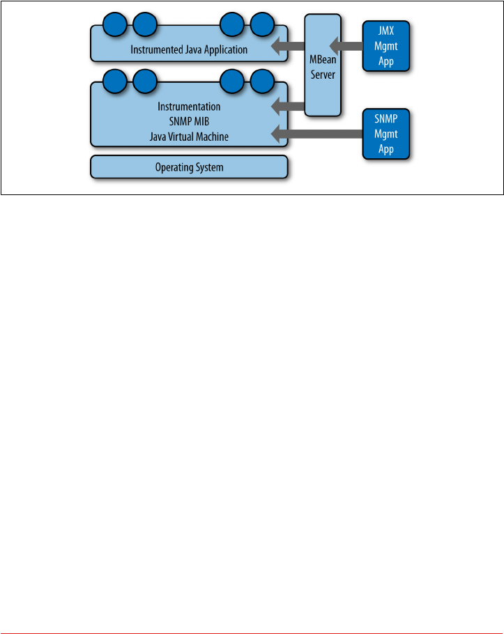
• Verbose classloader tracing
• Log level control
• General information such as application uptime and the active classpath
Many popular Java applications are instrumented using JMX, including the JVM
itself, the Tomcat application server, and Cassandra. A depiction of the JMX architec‐
ture is shown in Figure 10-1.
Figure 10-1. e JMX architecture
The JMX architecture is simple. The JVM collects information from the underlying
operating system. The JVM itself is instrumented, so many of its features are exposed
for management as described earlier. An instrumented Java application (such as Cas‐
sandra) runs on top of this, also exposing some of its features as manageable objects.
The JDK includes an MBean server that makes the instrumented features available
over a remote protocol to a JMX Management Application. The JVM also offers man‐
agement capabilities via Simple Network Monitoring Protocol (SNMP), which may
be useful if you are using SMTP monitoring tools such as Nagios or Zenoss.
But within a given application, you can manage only what the application developers
have made available for you to manage. Luckily, the Cassandra developers have
instrumented large parts of the database engine, making management via JMX fairly
straightforward.
This instrumentation of a Java application is performed by wrapping the application
code that you want JMX to hook into with managed beans.
212 | Chapter 10: Monitoring
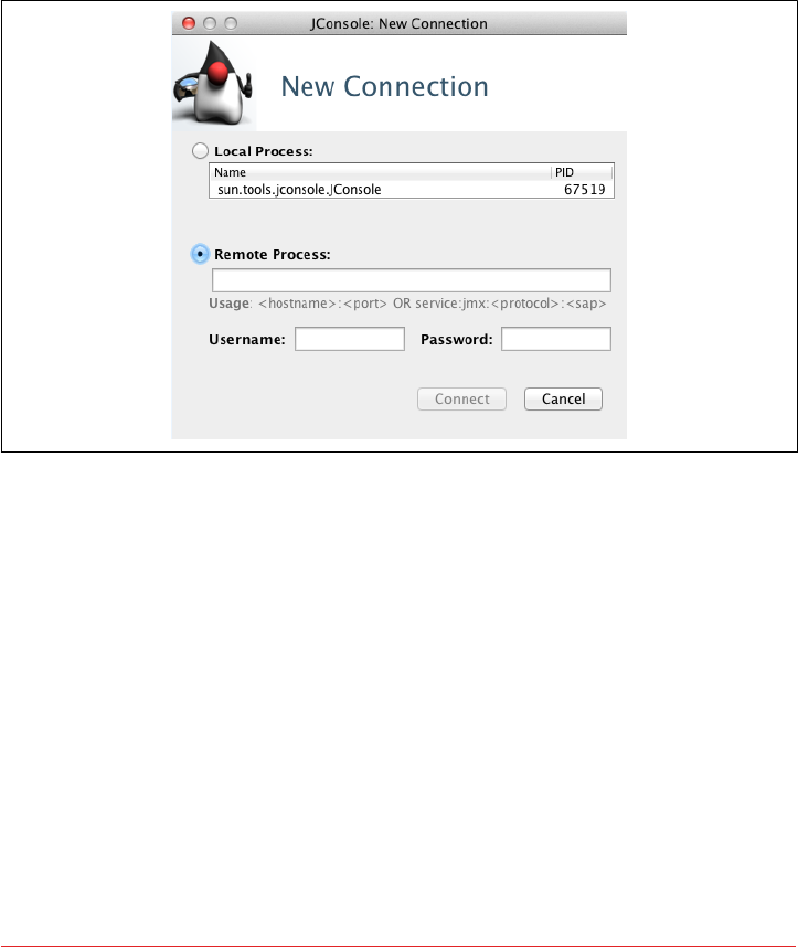
Connecting to Cassandra via JConsole
The jconsole tool ships with the standard Java Development Kit. It provides a
graphical user interface client for working with MBeans and can be used for local or
remote management. Let’s connect to Cassandra on its JMX port using JConsole. To
do so, open a new terminal and type the following:
>jconsole
When you run jconsole, you’ll see a login screen similar to that in Figure 10-2.
Figure 10-2. e jconsole login
From here, you can simply double-click on the value org.apache.cassandra.
service.CassandraDaemon under the Local Process section if you’re monitoring a
node on the same machine. If you want to monitor a node on a different machine,
check the Remote Process radio button, then enter the host and port you want to
connect to. Cassandra JMX by default broadcasts on port 7199, so you can enter a
value like the one shown here and then hit Connect:
>lucky:7199
Monitoring Cassandra with JMX | 213

Connecting Remotely via JMX
By default, Cassandra runs with JMX enabled for local access only.
To enable remote access, edit the file <cassandra-home>/cassandra-
env.sh (or cassandra.ps1 on Windows). Search for “JMX” to find the
section of the file with options to control the JMX port and other
local/remote connection settings.
Once you’ve connected to a server, the default view includes four major categories
about your server’s state, which are updated constantly:
Heap memory usage
This shows the total memory available to the Cassandra program, as well as how
much it’s using right now.
reads
This is the number of live threads Cassandra is using.
Classes
The number of classes that Cassandra has loaded. This number is relatively small
for such a powerful program; Cassandra typically requires under 3,000 classes
out of the box. Compare this to a program such as Oracle WebLogic, which typi‐
cally loads around 24,000 classes.
CPU usage
This shows the percentage of the processor that the Cassandra program is cur‐
rently using.
You can use the selector to adjust the time range shown in the charts.
If you want to see a more detailed view of how Cassandra is using the Java heap and
non-heap memory, click the Memory tab. By changing the chart value in the drop-
down, you can see in detail the graduations in which Cassandra is using its memory.
You can also (try to) force a garbage collection if you think it’s necessary.
You can connect to more than one JMX agent at once. Just choose File → New Con‐
nection... and repeat the steps to connect to another running Cassandra node to view
multiple servers at once.
214 | Chapter 10: Monitoring

Other JMX Clients
JConsole is an easy choice when you’re looking for a JMX client, because it’s easy to
use and ships with the JDK. But this is only one possible JMX client—there are plenty
of others available. Here are a few examples of clients that might meet your needs:
Oracle Java Mission Control and Visual VM
These tools also ship with the Oracle JDK and provide more robust metrics,
diagnostics, and visualizations for memory usage, threads, garbage collection,
and others. The main comparison between the two is that Visual VM is an open
source project available under the GNU license, while Mission Control provides
a deeper level of integration with the Oracle JVM via a framework called Flight
Control.
Java Mission Control can be run via the command $JAVA_HOME/bin/jmc, and
Visual VM via the command $JAVA_HOME/bin/jvisualvm. Both are suitable for
usage in both development and production environments.
MX4J
The Management Extensions for Java (MX4J) project provides an open source
implementation of JMX, including tooling such as an embedded web interface to
JMX using HTTP/HTML. This allows interactions with JMX via a standard web
browser.
To integrate MX4J into a Cassandra installation, download the mx4j_tools.jar
library, save the JAR file in the lib directory of your Cassandra installation, and
configure the MX4J_ADDRESS and MX4J_PORT options in conf/cassandra-env.sh.
Jmxterm
Jmxterm is a command-line JMX client that allows access to a JMX server
without a graphical interface. This can be especially useful when working in
cloud environments, as the graphical tools are typically more resource intensive.
Jmxterm is an open source Java project available from the Cyclops Group.
IDE Integrations
You can also find JMX clients that integrate with popular IDEs; for example,
eclipse-jmx.
Overview of MBeans
A managed bean, or MBean, is a special type of Java bean that represents a single
manageable resource inside the JVM. MBeans interact with an MBean server to make
their functions remotely available.
A view of JConsole is provided in Figure 10-3.
Monitoring Cassandra with JMX | 215
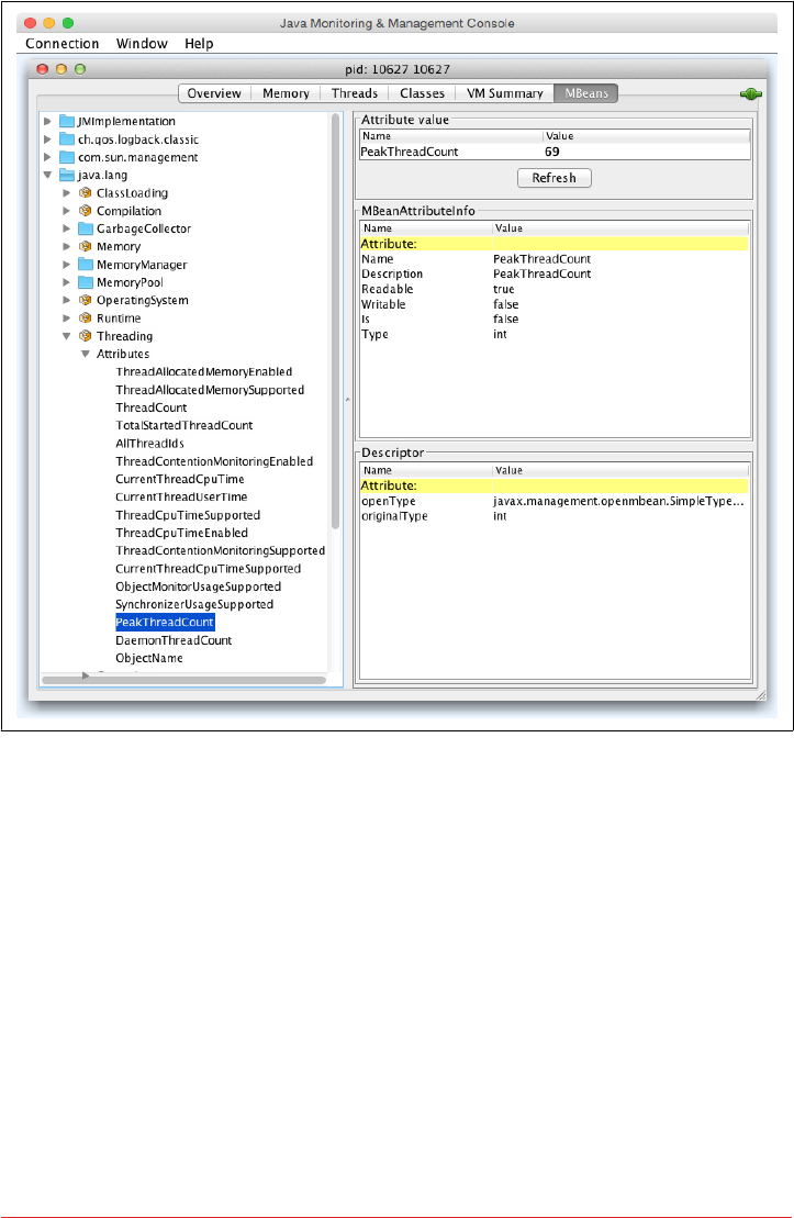
Figure 10-3. JConsole showing the peak thread count for a Cassandra daemon
In this figure, you can see tabbed windows that offer general views about threads,
memory, and CPU that every application will have, and a more detailed MBeans tab
that exposes the ability to interact in more detail with MBeans exposed by the appli‐
cation. For example, in the figure, we’ve selected to view the peak thread count value.
You can see that many other instrumented aspects of the application are also avail‐
able.
There are many aspects of an application or the JVM that can be instrumented but
that may be disabled. Thread Contention is one example of a potentially useful
MBean that is turned off by default in the JVM. These aspects can be very useful for
debugging, so if you see an MBean that you think might help you hunt down a prob‐
lem, go ahead and enable it. But keep in mind that nothing comes for free, and it’s a
good idea to read the JavaDoc on the MBean you want to enable in order to under‐
216 | Chapter 10: Monitoring

stand the potential impact on performance. For example, measuring CPU time per
thread is an example of a useful, but expensive, MBean operation.
MBean Object Name Conventions
When an MBean is registered with the MBean server, it specifies an
object name that is used to identify the MBean to JMX clients. An
object name consists of a domain followed by a list of key-value
pairs, at least one of which must identify a type. The typical con‐
vention is to choose a domain name that is similar to the Java pack‐
age name of the MBean, and to name the type after the MBean
interface name (minus the “MBean”), but this is not strictly
required.
For example, the threading attributes we looked at earlier appear
under the java.lang.Threading heading in JConsole, and are
exposed by a class implementing the java.lang.management.
ThreadMXBean interface, which registers the MBean with the object
name java.lang.type=Threading.
As we discuss various MBeans in this chapter, we’ll identify both
the MBean object name and the interface to help you navigate
between JMX clients and the Cassandra source code.
Some simple values in the application are exposed as attributes. An example of this is
Threading > PeakThreadCount, which just reports the value that the MBean has
stored for the greatest number of threads the application used at a single point in
time. You can refresh to see the most recent value, but that’s pretty much all you can
do with it. Because such a value is maintained internally in the JVM, it doesn’t make
sense to set it externally (it’s derived from actual events, and not configurable).
But other MBeans are configurable. They make operations available to the JMX agent
that let you get and set values. You can tell whether the MBean will let you set a value
by looking at the value for writable. If it’s false, you will see a label indicating the
read-only value; if it’s true, you will see a set of one or more fields to add your new
value and a button to update it. An example of this is the ch.qos.logback.classic.
jmx.JMXConfigurator bean, as shown in Figure 10-4.
Monitoring Cassandra with JMX | 217
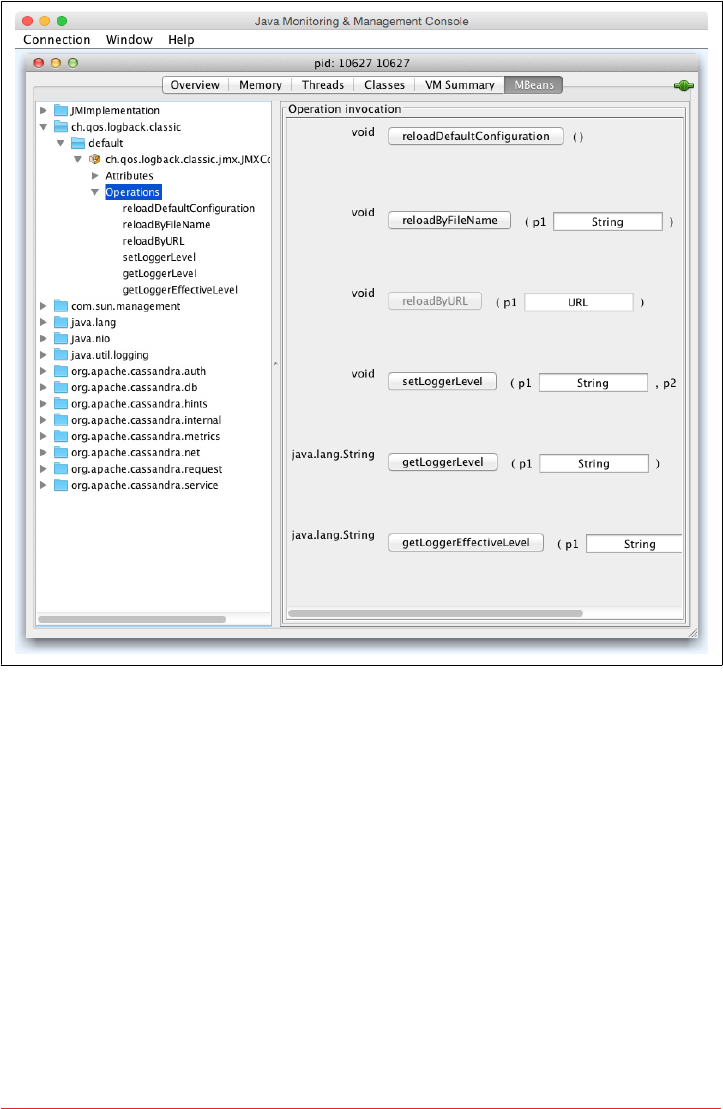
Figure 10-4. e JMXCongurator MBean allows you to set a logger’s log level
Note that the parameter names are not available to the JMX agent; they’re just labeled
as p0, p1, and so on. That’s because the Java compiler “erased” the parameter names
during compilation. So in order to know what parameters to set on an operation,
you’ll need to look at the JavaDoc for the particular MBean you’re working with.
In the case of JMXConfigurator, this class implements an interface called
JMXConfiguratorMBean, which wraps it for instrumentation. To find out what the
right parameters are for the setLoggerLevel operation, we examine the JavaDoc for
this interface, available at http://logback.qos.ch/apidocs/ch/qos/logback/classic/jmx/
JMXConguratorMBean.html. Looking at the documentation, you’ll see that p0 rep‐
resents the name of the logger you want to change, and p1 describes the logging level
you want to set that logger to.
218 | Chapter 10: Monitoring

Some MBeans return an attribute value of javax.management.openmbean.Composite
DataSupport. That means that these are not simple values that can be displayed in a
single field, such as LoadedClassCount, but are instead multivalued. One example is
Memory > HeapMemoryUsage, which offers several data points and therefore has its
own view.
Another type of MBean operation is one that doesn’t simply show a value or allow
you to set a value, but instead lets you execute some useful action. dumpAllThreads
and resetPeakThreadCount are two such operations.
Now we’ll quickly get set up to start monitoring and managing Cassandra specifically.
Cassandra’s MBeans
Once you’ve connected with a JMX agent such as JConsole, you can manage Cassan‐
dra using the MBeans it exposes. To do so, click the MBeans tab. Other than the stan‐
dard Java items available to every agent, there are several Cassandra packages that
contain manageable beans, organized by their package names, which start with
org.apache.cassandra. We won’t go into detail on all of them here, but there are
several of interest that we’ll take a look at.
Many classes in Cassandra are exposed as MBeans, which means in practical terms
that they implement a custom interface that describes the operations that need to be
implemented and for which the JMX agent will provide hooks. The steps are basically
the same for getting any MBean to work. If you’d like to JMX-enable something that
isn’t already enabled, modify the source code following this general outline and you’ll
be in business.
For example, we look at Cassandra’s CompactionManager from the org.apache.
cassandra.db.compaction package and how it uses MBeans. Here’s the definition
of the CompactionManagerMBean class, with comments omitted for brevity:
public interface CompactionManagerMBean
{
public List<Map<String, String>> getCompactions();
public List<String> getCompactionSummary();
public TabularData getCompactionHistory();
public void forceUserDefinedCompaction(String dataFiles);
public void stopCompaction(String type);
public void stopCompactionById(String compactionId);
public int getCoreCompactorThreads();
public void setCoreCompactorThreads(int number);
public int getMaximumCompactorThreads();
public void setMaximumCompactorThreads(int number);
Cassandra’s MBeans | 219

public int getCoreValidationThreads();
public void setCoreValidationThreads(int number);
public int getMaximumValidatorThreads();
public void setMaximumValidatorThreads(int number);
}
As you can see by this MBean interface definition, there’s no magic going on. This is
just a regular interface defining the set of operations that will be exposed to JMX that
the CompactionManager implementation must support. This typically means main‐
taining additional metadata as the regular operations do their work.
The CompactionManager class implements this interface and must do the work of
directly supporting JMX. The CompactionManager class itself registers and unregi‐
sters with the MBean server for the JMX properties that it maintains locally:
public static final String MBEAN_OBJECT_NAME =
"org.apache.cassandra.db:type=CompactionManager";
// ...
static
{
instance = new CompactionManager();
MBeanServer mbs = ManagementFactory.getPlatformMBeanServer();
try
{
mbs.registerMBean(instance,
new ObjectName(MBEAN_OBJECT_NAME));
}
catch (Exception e)
{
throw new RuntimeException(e);
}
}
Note that the MBean is registered in the domain org.apache.cassandra.db with a
type of CompactionManager. The attributes and operations exposed by this MBean
appear under org.apache.cassandra.db > CompactionManager in JMX clients. The
implementation does all of the work that it is intended to do, and then has implemen‐
tations of the methods that are only necessary for talking to the MBean server. For
example, here is the CompactionManager implementation of the stopCompaction()
operation:
public void stopCompaction(String type)
{
OperationType operation = OperationType.valueOf(type);
for (Holder holder : CompactionMetrics.getCompactions())
{
if (holder.getCompactionInfo().getTaskType() == operation)
holder.stop();
220 | Chapter 10: Monitoring
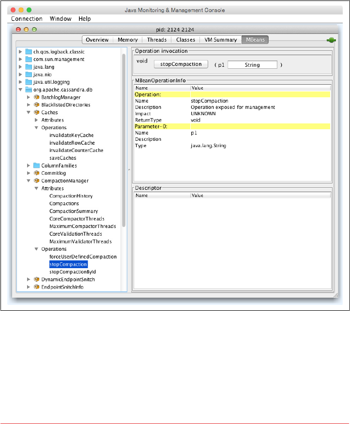
}
}
The CompactionManager iterates through the compactions in progress, stopping each
one that is of the specified type. The Javadoc lets us know that the valid types are
COMPACTION, VALIDATION, CLEANUP, SCRUB, and INDEX_BUILD.
When we view the CompactionManagerMBean in JConsole we can select the opera‐
tions and view the stopCompaction() operation, as shown in Figure 10-5. We can
enter one of the preceding types and request that the compactions be stopped.
Figure 10-5. e CompactionManager stopCompaction() operation
In the following sections, we see what features are available for monitoring and
management via JMX.
Cassandra’s MBeans | 221

Database MBeans
These are the Cassandra classes related to the core database itself that are exposed to
clients in the org.apache.cassandra.db domain. There are many MBeans in this
domain, but we’ll focus on a few key ones related to storage, caching, the commit log,
and table stores.
Storage Service MBean
Because Cassandra is a database, it’s essentially a very sophisticated storage program;
therefore, one of the first places you’ll want to look when you encounter problems is
the org.apache.cassandra.service.StorageServiceMBean. This allows you to
inspect your OperationMode, which reports normal if everything is going smoothly
(other possible states are leaving, joining, decommissioned, and client).
You can also view the current set of live nodes, as well as the set of unreachable nodes
in the cluster. If any nodes are unreachable, Cassandra will tell you their IP addresses
in the UnreachableNodes attribute.
If you want to change Cassandra’s log level at runtime without interrupting service (as
we saw earlier in the general example), you can invoke the setLoggingLevel(String
classQualifier, String level) method. For example, say that you have set Cas‐
sandra’s log level to DEBUG because you’re troubleshooting an issue. You can use some
of the methods described here to try to help fix your problem, then you might want
to change the log level to something less taxing on the system. To do this, navigate to
the StorageService MBean in a JMX client such as JConsole. We’ll change the value
for a particularly chatty class: the Gossiper. The first parameter to this operation is
the name of the class you want to set the log level for, and the second parameter is the
level you want to set it to. Enter org.apache.cassandra.gms.Gossiper and INFO,
and click the button labeled setLoggingLevel. You should see the following output in
your logs (assuming your level was already debug):
INFO 03:08:20 set log level to INFO for classes under
'org.apache.cassandra.gms.Gossiper' (if the level doesn't look
like 'INFO' then the logger couldn't parse 'INFO')
After invoking the setLoggingLevel operation, we get the INFO output and no more
DEBUG-level statements.
To get an understanding of how much data is stored on each node, you can use the
getLoadMap() method, which will return to you a Java Map with keys of IP addresses
with values of their corresponding storage loads. You can also use the effec
tiveOwnership(String keyspace) operation to access the percentage of the data in
a keyspace owned by each node.
222 | Chapter 10: Monitoring

If you’re looking for a certain key, you can use the getNaturalEndpoints(String
table, byte[] key) operation. Pass it the table name and the key for which you
want to find the endpoint value, and it will return a list of IP addresses that are
responsible for storing this key.
You can also use the getRangeToEndpointMap operation to get a map of range to end
points describing your ring topology.
If you’re feeling brave, you can invoke the truncate() operation for a given table in a
given keyspace. If all of the nodes are available, this operation will delete all data from
the table but leave its definition intact.
There are many standard maintenance operations that the StorageServiceMBean
affords you, including resumeBootstrap(), joinRing(), repairAsync(), drain(),
removeNode(), decommission(), and operations to start and stop gossip, the native
transport, and Thrift (until Thrift is finally removed). Understanding the available
maintenance operations is important to keeping your cluster in good health, and we’ll
dig more into these in Chapter 11.
Storage Proxy MBean
As we learned in Chapter 6, the org.apache.cassandra.service.StorageProxy pro‐
vides a layer on top of the StorageService to handle client requests and inter-node
communications. The StorageProxyMBean provides the ability to check and set time‐
out values for various operations including read and write.
This MBean also provides access to hinted handoff settings such as the maximum
time window for storing hints. Hinted handoff statistics include getTotalHints()
and getHintsInProgress(). You can disable hints for a particular node with the dis
ableHintsForDC() operation.
You can also turn this node’s participation in hinted handoff on or off via setHinted
HandoffEnabled(), or check the current status via getHintedHandoffEnabled().
These are used by nodetool’s enablehandoff, disablehandoff, and statushandoff
commands, respectively.
The reloadTriggerClasses() operation allows you to install a new trigger without
having to restart a node.
ColumnFamilyStoreMBean
Cassandra registers an instance of the org.apache.cassandra.db.ColumnFamily
StoreMBean for each table stored in the node under org.apache.cassandra.db >
Tables (previously ColumnFamilies).
Cassandra’s MBeans | 223

The ColumnFamilyStoreMBean provides access to the compaction and compression
settings for each table. This allows you to temporarily override these settings on a
specific node. The values will be reset to those configured on the table schema when
the node is restarted.
The MBean also exposes a lot of information about the node’s storage of data for this
table on disk. The getSSTableCountPerLevel() operation provides a list of how
many SStables are in each tier. The estimateKeys() operation provides an estimate
of the number of partitions stored on this node. Taken together, this information can
give you some insight as to whether invoking the forceMajorCompaction() opera‐
tion for this table might help free space on this node and increase read performance.
There is also a trueSnapshotsSize() operation that allows you to determine the size
of SSTable shapshots which are no longer active. A large value here indicates that you
should consider deleting these snapshots, possibly after making an archive copy.
Because Cassandra stores indexes as tables, there is also a ColumnFamilyStoreMBean
instance for each indexed column, available under org.apache.cassandra.db >
IndexTables (previously IndexColumnFamilies), with the same attributes and opera‐
tions.
CacheServiceMBean
The org.apache.cassandra.service.CacheServiceMBean provides access to Cas‐
sandra’s key cache, row cache, and counter cache under the domain org.apache.
cassandra.db > Caches. The information available for each cache includes the
maximum size and time duration to cache items, and the ability to invalidate each
cache.
CommitLogMBean
The org.apache.cassandra.db.commitlog.CommitLogMBean exposes attributes and
operations that allow you to learn about the current state of commit logs. The Commit
LogMBean also exposes the recover() operation which can be used to restore database
state from archived commit log files.
The default settings that control commit log recovery are specified in the conf/commi‐
tlog_archiving.properties file, but can be overridden via the MBean. We’ll learn more
about data recovery in Chapter 11.
Compaction Manager MBean
We’ve already taken a peek inside the source of the org.apache.cassandra.db.com
paction.CompactionManagerMBean to see how it interacts with JMX, but we didn’t
really talk about its purpose. This MBean allows us to get statistics about compactions
224 | Chapter 10: Monitoring

performed in the past, and the ability to force compaction of specific SSTable files we
identify by calling the forceUserDefinedCompaction method of the CompactionMan
ager class. This MBean is leveraged by nodetool commands including compact,
compactionhistory, and compactionstats.
Snitch MBeans
Cassandra provides two MBeans to monitor and configure behavior of the snitch.
The org.apache.cassandra.locator.EndpointSnitchInfoMBean provides the name
of the rack and data center for a given host, as well as the name of the snitch in use.
If you’re using the DynamicEndpointSnitch, the org.apache.cassandra.locator.
DynamicEndpointSnitchMBean is registered. This MBean exposes the ability to reset
the badness threshold used by the snitch for marking nodes as offline, as well as
allowing you to see the scores for various nodes.
HintedHandoManagerMBean
In addition to the hinted handoff operations on the StorageServiceMBean men‐
tioned earlier, Cassandra provides more fine grained control of hinted handoff via the
org.apache.cassandra.db.HintedHandOffManagerMBean. The MBean exposes the
ability to list nodes for which hints are stored by calling listEndpointsPending
Hints(). You can then force delivery of hints to a node via scheduleHintDelivery(),
or delete hints that are stored up for a specific node with deleteHintsForEnd
point().
Additionally, you can pause and resume hint delivery to all nodes with pauseHint
Delivery() or delete stored hints for all nodes with the truncateAllHints() opera‐
tion. These are used by nodetool’s pausehandoff, resumehandoff, and truncate
hints commands, respectively.
Duplicative Hinted Hando Management
The org.apache.cassandra.hints.HintsService exposes the
HintsServiceMBean under the domain org.apache.cassandra
.hints > HintsService. This MBean provides operations to
pause and resume hinted handoff, and to delete hints stored for all
nodes, or for a specific node identified by IP address.
Because there is a lot of overlap between the StorageService
MBean, HintedHandOffManagerMBean, and HintsServiceMBean,
there is likely to be some consolidation of these operations in
future releases.
Cassandra’s MBeans | 225

Networking MBeans
The org.apache.cassandra.net domain contains MBeans to help manage Cassan‐
dra’s network-related activities, including Phi failure detection and gossip, the Mes‐
saging Service, and Stream Manager.
FailureDetectorMBean
The org.apache.cassandra.gms.FailureDetectorMBean provides attributes
describing the states and Phi scores of other nodes, as well as the Phi conviction
threshold.
GossiperMBean
The org.apache.cassandra.gms.GossiperMBean provides access to the work of the
Gossiper.
We’ve already discussed how the StorageServiceMBean reports which nodes are
unreachable. Based on that list, you can call the getEndpointDowntime() operation
on the GossiperMBean to determine how long a given node has been down. The
downtime is measured from the perspective of the node whose MBean we’re inspect‐
ing, and the value resets when the node comes back online. Cassandra uses this oper‐
ation internally to know how long it can wait to discard hints.
The getCurrentGenerationNumber() operation returns the generation number asso‐
ciated with a specific node. The generation number is included in gossip messages
exchanged between nodes and is used to distinguish the current state of a node from
the state prior to a restart. The generation number remains the same while the node is
alive and is incremented each time the node restarts. It’s maintained by the Gossiper
using a timestamp.
The assassinateEndpoint() operation attempts to remove a node from the ring by
telling the other nodes that the node has been permanently removed, similar to the
concept of “character assassination” in human gossip. Assassinating a node is a main‐
tenance step of last resort when a node cannot be removed from the cluster normally.
This operation is used by the nodetool assassinate command.
StreamManagerMBean
The org.apache.cassandra.streaming.StreamManagerMBean allows us to see the
streaming activities that occur between a node and its peers. There are two basic ideas
here: a stream source and a stream destination. Each node can stream its data to
another node in order to perform load balancing, and the StreamManager class sup‐
ports these operations. The StreamManagerMBean gives necessary view into the data
that is moving between nodes in the cluster.
226 | Chapter 10: Monitoring

The StreamManagerMBean supports two modes of operation. The getCurrent
Streams() operation provides a snapshot of the current incoming and outgoing
streams, and the MBean also publishes notifications associated with stream state
changes, such as initialization, completion or failure. You can subscribe to these noti‐
fications in your JMX client in order to watch the streaming operations as they occur.
So in conjunction with the StorageServiceMBean, if you’re concerned that a node is
not receiving data as it should, or that a node is unbalanced or even down, these two
MBeans working together can give you very rich insight into exactly what’s happen‐
ing in your cluster.
Metrics MBeans
The ability to access metrics related to application performance, health, and key activ‐
ities has become an essential tool for maintaining web-scale applications. Fortunately,
Cassandra collects a wide range of metrics on its own activities to help us understand
the behavior.
The metrics reported by Cassandra include the following:
•Buer pool metrics describing Cassandra’s use of memory.
•CQL metrics including the number of prepared and regular statement executions.
•Cache metrics for key, row, and counter caches such as the number of entries ver‐
sus capacity, as well as hit and miss rates.
•Client metrics including the number of connected clients, and information about
client requests such as latency, failures, and timeouts.
•Commit log metrics including the commit log size and statistics on pending and
completed tasks.
•Compaction metrics including the total bytes compacted and statistics on pending
and completed compactions.
•Connection metrics to each node in the cluster including gossip.
•Dropped message metrics which are used as part of nodetool tpstats.
•Read repair metrics describing the number of background versus blocking read
repairs performed over time.
•Storage metrics, including counts of hints in progress and total hints.
•read pool metrics, including active, completed, and blocked tasks for each
thread pool.
•Table metrics, including caches, memtables, SSTables, and Bloom filter usage and
the latency of various read and write operations, reported at one, five, and fifteen
minute intervals.
•Keyspace metrics that aggregate the metrics for the tables in each keyspace.
To make these metrics accessible via JMX, Cassandra uses the Dropwizard Metrics
open source Java library. Cassandra registers its metrics with the Metrics library,
Cassandra’s MBeans | 227

which in turn exposes them as MBeans in the org.apache.cassandra.metrics
domain.
Many of these metrics are used by nodetool commands such as tpstats, tablehisto
grams, and proxyhistograms. For example, tpstats is simply a presentation of the
thread pool and dropped message metrics.
Threading MBeans
The org.apache.cassandra.internal domain houses MBeans that allow you to
configure the thread pools associated with each stage in Cassandra’s Staged Event-
Driven Architecture (SEDA). The stages include AntiEntropyStage, GossipStage,
InternalResponseStage, MigrationStage, and others.
Read Repair MBean
For historical reasons, the ReadRepairStage MBean is located
under the org.apache.cassandra.request domain instead of
org.apache.cassandra.internal.
The thread pools are implemented via the JMXEnabledThreadPoolExecutor and
JMXEnabledScheduledThreadPoolExecutor classes in the org.apache.cassandra
.concurrent package. The MBeans for each stage implement the JMXEnabledSchedu
ledThreadPoolExecutorMBean interface, which allows you to view and configure the
number of core threads in each thread pool as well as the maximum number of
threads.
Service MBeans
The GCInspectorMXBean exposes a single operation getAndResetStats() which
retrieves and then resets garbage collection metrics that Cassandra collects on its
JVM. This MBean appears in the org.apache.cassandra.service domain. This
MBean is accessed by the nodetool gcstats command.
Security MBeans
The org.apache.cassandra.auth domain contains security-related MBeans that are
grouped according to the same Java package name. As of the 3.0 release, this consists
of a single MBean, the PermissionsCacheMBean, exposed to clients as org.apache.
cassandra.auth.PermissionsCache. We’ll discuss this MBean in Chapter 13.
228 | Chapter 10: Monitoring

Monitoring with nodetool
We’ve already explored a few of the commands offered by nodetool in previous chap‐
ters, but let’s take this opportunity to get properly introduced.
nodetool ships with Cassandra and can be found in <cassandra-home>/bin. This is a
command-line program that offers a rich array of ways to look at your cluster, under‐
stand its activity, and modify it. nodetool lets you get limited statistics about the clus‐
ter, see the ranges each node maintains, move data from one node to another,
decommission a node, and even repair a node that’s having trouble.
Overlap of nodetool and JMX
Many of the tasks in nodetool overlap with functions available in
the JMX interface. This is because, behind the scenes, nodetool is
invoking JMX using a helper class called org.apache .cassandra
.tools.NodeProbe. So JMX is doing the real work, the NodeProbe
class is used to connect to the JMX agent and retrieve the data, and
the NodeCmd class is used to present it in an interactive command-
line interface.
nodetool uses the same environment settings as the Cassandra daemon: bin/cassan‐
dra.in.sh and conf/cassandra-env.sh on Unix (or bin/cassandra.in.bat and conf/
cassandra-env.ps1 on Windows). The logging settings are found in the conf/logback-
tools.xml file; these work the same way as the Cassandra daemon logging settings
found in conf/logback.xml.
Starting nodetool is a breeze. Just open a terminal, navigate to <cassandra-home>,
and enter the following command:
$ bin/nodetool help
This causes the program to print a list of available commands, several of which we
will cover momentarily. Running nodetool with no arguments is equivalent to the
help command. You can also execute help with the name of a specific command to
get additional details.
Monitoring with nodetool | 229

Connecting to a Specic Node
With the exception of the help command, nodetool must connect
to a Cassandra node in order to access information about that node
or the cluster as a whole.
You can use the -h option to identify the IP address of the node to
connect to with nodetool. If no IP address is specified, the tool
attempts to connect to the default port on the local machine, which
is the approach we’ll take for examples in this chapter.
Getting Cluster Information
There is a variety of information you can get about the cluster and its nodes, which
we look at in this section. You can get basic information on an individual node or on
all the nodes participating in a ring.
describecluster
The describecluster command prints out basic information about the cluster,
including the name, snitch, and partitioner:
$ bin/nodetool describecluster
Cluster Information:
Name: Test Cluster
Snitch: org.apache.cassandra.locator.DynamicEndpointSnitch
Partitioner: org.apache.cassandra.dht.Murmur3Partitioner
Schema versions:
2d4043cb-2124-3589-b2d0-375759b9dd0a: [127.0.0.1, 127.0.0.2, 127.0.0.3]]
The last part of the output is especially important for identifying any disagreements
in table definitions, or “schema,” between nodes. As Cassandra propagates schema
changes through a cluster, any differences are typically resolved quickly, so any lin‐
gering schema differences usually indicate a node that is down or unreachable that
needs to be restarted.
status
A more direct way to identify the nodes in your cluster and what state they’re in, is to
use the status command:
$ bin/nodetool status
Datacenter: datacenter1
=======================
Status=Up/Down
|/ State=Normal/Leaving/Joining/Moving
-- Address Load Tokens Owns Host ID
UN 127.0.0.1 103.82 KB 256 ? 31d9042b-6603-4040-8aac-fef0a235570b
UN 127.0.0.2 110.9 KB 256 ? caad1573-4157-43d2-a9fa-88f79344683d
UN 127.0.0.3 109.6 KB 256 ? e78529c8-ee9f-46a4-8bc1-3479f99a1860
230 | Chapter 10: Monitoring

The status is organized by data center and rack. Each node’s status is identified by a
two-character code, in which the first character indicates whether the node is up
(currently available and ready for queries) or down, and the second character indi‐
cates the state or operational mode of the node. The load column represents the byte
count of the data each node is holding.
The owns column indidates the effective percentage of the token range owned by the
node, taking replication into account. Because we did not specify a keyspace and the
various keyspaces in this cluster have differing replication strategies, nodetool is not
able to calculate a meaningful ownership percentage.
info
The info command tells nodetool to connect with a single node and get basic data
about its current state. Just pass it the address of the node you want info for:
$ bin/nodetool -h 192.168.2.7 info
ID : 197efa22-ecaa-40dc-a010-6c105819bf5e
Gossip active : true
Thrift active : false
Native Transport active: true
Load : 301.17 MB
Generation No : 1447444152
Uptime (seconds) : 1901668
Heap Memory (MB) : 395.03 / 989.88
Off Heap Memory (MB) : 2.94
Data Center : datacenter1
Rack : rack1
Exceptions : 0
Key Cache : entries 85, size 8.38 KB, capacity 49 MB,
47958 hits, 48038 requests, 0.998 recent hit rate, 14400 save
period in seconds
Row Cache : entries 0, size 0 bytes, capacity 0 bytes,
0 hits, 0 requests, NaN recent hit rate, 0 save period in seconds
Counter Cache : entries 0, size 0 bytes, capacity 24 MB,
0 hits, 0 requests, NaN recent hit rate, 7200 save period in seconds
Token : (invoke with -T/--tokens to see all 256 tokens)
The information reported includes the memory and disk usage (“Load”) of the node
and the status of various services offered by Cassandra. You can also check the status
of individual services by the nodetool commands statusgossip, statusthrift,
statusbinary, and statushandoff (note that handoff status is not part of info).
ring
To determine what nodes are in your ring and what state they’re in, use the ring com‐
mand on nodetool, like this:
$ bin/nodetool ring
Datacenter: datacenter1
Monitoring with nodetool | 231

==========
Address Rack Status State Load Owns Token
9208237582789476801
192.168.2.5 rack1 Up Normal 243.6 KB ? -9203905334627395805
192.168.2.6 rack1 Up Normal 243.6 KB ? -9145503818225306830
192.168.2.7 rack1 Up Normal 243.6 KB ? -9091015424710319286
...
This output is organized in terms of vnodes. Here we see the IP addresses of all the
nodes in the ring. In this case, we have three nodes, all of which are up (currently
available and ready for queries). The load column represents the byte count of the
data each node is holding. The output of the describering command is similar but is
organized around token ranges.
Other useful status commands provided by nodetool include:
•The getLoggingLevels and setLoggingLevels commands allow dynamic con‐
figuration of logging levels, using the Logback JMXConfiguratorMBean we dis‐
cussed previously.
•The gossipinfo command prints the parameters this node communicates about
itself to other nodes via gossip.
•The version command prints the version of Cassandra this node is running.
Getting Statistics
nodetool also lets you gather statistics about the state of your server in the aggregate
level as well as down to the level of specific keyspaces and tables. Two of the most
frequently used commands are tpstats and tablestats, both of which we examine
now.
Using tpstats
The tpstats tool gives us information on the thread pools that Cassandra maintains.
Cassandra is highly concurrent, and optimized for multiprocessor/multicore
machines. Moreover, Cassandra employs a Staged Event-Driven Architecture (SEDA)
internally, so understanding the behavior and health of the thread pools is important
to good Cassandra maintenance.
To find statistics on the thread pools, execute nodetool with the tpstats command:
$ bin/nodetool tpstats
Pool Name Active Pending Completed Blocked All time
blocked
ReadStage 0 0 216 0 0
MutationStage 1 0 3637 0 0
CounterMutationStage 0 0 0 0 0
ViewMutationStage 0 0 0 0 0
GossipStage 0 0 0 0 0
232 | Chapter 10: Monitoring

RequestResponseStage 0 0 0 0 0
AntiEntropyStage 0 0 0 0 0
MigrationStage 0 0 2 0 0
MiscStage 0 0 0 0 0
InternalResponseStage 0 0 2 0 0
ReadRepairStage 0 0 0 0 0
Message type Dropped
READ 0
RANGE_SLICE 0
_TRACE 0
HINT 0
MUTATION 0
COUNTER_MUTATION 0
BATCH_STORE 0
BATCH_REMOVE 0
REQUEST_RESPONSE 0
PAGED_RANGE 0
READ_REPAIR 0
The top portion of the output presents data on tasks in each of Cassandra’s thread
pools. You can see directly how many operations are in what stage, and whether they
are active, pending, or completed. This output was captured during a write operation,
and therefore shows that there is an active task in the MutationStage.
The bottom portion of the output indicates the number of dropped messages for the
node. Dropped messages are an indicator of Cassandra’s load shedding implementa‐
tion, which each node uses to defend itself when it receives more requests than it can
handle. For example, internode messages that are received by a node but not pro‐
cessed within the rpc_timeout are dropped, rather than processed, as the coordinator
node will no longer be waiting for a response.
Seeing lots of zeros in the output for blocked tasks and dropped messages means that
you either have very little activity on the server or that Cassandra is doing an excep‐
tional job of keeping up with the load. Lots of non-zero values is indicative of situa‐
tions where Cassandra is having a hard time keeping up, and may indicate a need for
some of the techniques described in Chapter 12.
Using tablestats
To see overview statistics for keyspaces and tables, you can use the tablestats com‐
mand. You may also recognize this command from its previous name cfstats. Here
is sample output on the hotel keyspace:
$ bin/nodetool tablestats hotel
Keyspace: hotel
Read Count: 8
Read Latency: 0.617 ms.
Write Count: 13
Write Latency: 0.13330769230769232 ms.
Monitoring with nodetool | 233

Pending Flushes: 0
Table: hotels
SSTable count: 3
Space used (live): 16601
Space used (total): 16601
Space used by snapshots (total): 0
Off heap memory used (total): 140
SSTable Compression Ratio: 0.6277372262773723
Number of keys (estimate): 19
Memtable cell count: 8
Memtable data size: 792
Memtable off heap memory used: 0
Memtable switch count: 1
Local read count: 8
Local read latency: 0.680 ms
Local write count: 13
Local write latency: 0.148 ms
Pending flushes: 0
Bloom filter false positives: 0
Bloom filter false ratio: 0.00000
Bloom filter space used: 56
Bloom filter off heap memory used: 32
Index summary off heap memory used: 84
Compression metadata off heap memory used: 24
Compacted partition minimum bytes: 30
Compacted partition maximum bytes: 149
Compacted partition mean bytes: 87
Average live cells per slice (last five minutes): 1.0
Maximum live cells per slice (last five minutes): 1
Average tombstones per slice (last five minutes): 1.0
Maximum tombstones per slice (last five minutes): 1
Here we have omitted output for other tables in the keyspace so we can focus on the
hotels table; the same statistics are generated for each table. We can see the read and
write latency and total number of reads and writes at the keyspace and table level. We
can also see detailed information about Cassandra’s internal structures for each table,
including memtables, Bloom filters and SSTables.
Summary
In this chapter, we looked at ways you can monitor and manage your Cassandra clus‐
ter. In particular, we went into some detail on JMX and learned the rich variety of
operations Cassandra makes available to the MBean server. We saw how to use JCon‐
sole and nodetool to view what’s happening in your Cassandra cluster. You are now
ready to learn how to perform routine maintenance tasks to help keep your Cassan‐
dra cluster healthy.
234 | Chapter 10: Monitoring

CHAPTER 11
Maintenance
In this chapter, we look at some things you can do to keep your Cassandra cluster
healthy. Our goal here is to provide an overview of the various maintenance tasks
available. Because the specific procedures for these tasks tend to change slightly from
release to release, you’ll want to make sure to consult the DataStax documentation for
the release you’re using to make sure you’re not missing any new steps.
Let’s put our operations hats on and get started!
Health Check
There are some basic things that you’ll want to look for to ensure that nodes in your
cluster are healthy:
•Use nodetool status to make sure all of the nodes are up and reporting normal
status. Check the load on each node to make sure the cluster is well balanced. An
uneven number of nodes per rack can lead to an imbalanced cluster.
•Check nodetool tpstats on your nodes for dropped messages, especially muta‐
tions, as this indicates that data writes may be lost. A growing number of blocked
flush writers indicates the node is ingesting data into memory faster than it can
be flushed to disk. Both of these conditions can indicate that Cassandra is having
trouble keeping up with the load. As is usual with databases, once these problems
begin, they tend to continue in a downward spiral. Three things that can improve
the situation are a decreased load, scaling up (adding more hardware), or scaling
out (adding another node and rebalancing).
235

If these checks indicate issues, you may need to dig deeper to get more information
about what is going on:
•Check the logs to see that nothing is reporting at ERROR or WARN level (e.g., an
OutOfMemoryError). Cassandra generates warning logs when it detects bad or
obsolete configuration settings, operations that did not complete successfully,
and memory or data storage issues.
•Review the configuration of the cassandra.yaml and cassandra-env.sh files for
your Cassandra nodes to make sure that they match your intended settings. For
example, the heap should be set to its recommended size of 8 GB.
•Verify keyspace and table configuration settings. For example, a frequent config‐
uration error is to forget to update keyspace replication strategies when adding a
new data center.
•Beyond the health of your Cassandra nodes, it is always helpful to have a sense of
the overall health and configuration of your system, including ensuring network
connectivity and that Network Time Protocol (NTP) servers are functioning cor‐
rectly.
These are a few of the most important things that experienced Cassandra operators
have learned to look for. As you gain experience with your own deployments, you can
augment this list with additional health checks that are appropriate for your own
environment.
Basic Maintenance
There are a few tasks that you’ll need to perform before or after more impactful tasks.
For example, it makes sense to take a snapshot only after you’ve performed a flush. So
in this section we look at some of these basic maintenance tasks.
Many of the tasks we look at in this chapter work somewhat differently depending on
whether you’re using virtual nodes or single token nodes. Because vnodes are the
default, we’ll focus primarily on maintenance of those nodes, but provide pointers if
you’re using single token nodes.
Flush
To force Cassandra to write data from its memtables to SSTables on the filesystem,
you use the flush command on nodetool, like this:
$ nodetool flush
236 | Chapter 11: Maintenance

If you check the server logs, you’ll see a series of output statements similar to this, one
per table stored on the node:
DEBUG [RMI TCP Connection(297)-127.0.0.1] 2015-12-21 19:20:50,794
StorageService.java:2847 - Forcing flush on keyspace hotel,
CF reservations_by_hotel_date
You can selectively flush specific keyspaces or even specific tables within a keyspace
by naming them on the command line:
$ nodetool flush hotel
$ nodetool flush hotel reservations_by_hotel_date hotels_by_poi
Running flush also allows Cassandra to clear commitlog segments, as the data has
been written to SSTables.
The nodetool drain command is similar to flush. This command actually performs
a flush and then directs Cassandra to stop listening to commands from the client and
other nodes. The drain command is typically used as part of an orderly shutdown of
a Cassandra node and helps the node startup to run more quickly, as there is no com‐
mitlog to replay.
Cleanup
The cleanup command scans all of the data on a node and discards any data that is no
longer owned by the node. You might ask why a node would have any data that it
doesn’t own.
Say that you’ve had a cluster running for some time, and you want to change the rep‐
lication factor or the replication strategy. If you decrease the number of replicas for
any data center, then there will be nodes in that data center that no longer serve as
replicas for secondary ranges.
Or perhaps you’ve added a node to a cluster and reduced the size of the token
range(s) owned by each node. Then each node may contain data from portions of
token ranges it no longer owns.
In both of these cases, Cassandra does not immediately delete the excess data, in case
a node goes down while you’re in the middle of your maintenance. Instead, the nor‐
mal compaction processes will eventually discard this data.
However, you may wish to reclaim the disk space used by this excess data more
quickly to reduce the strain on your cluster. To do this, you can the nodetool
cleanup command.
As with the flush command, you can select to cleanup specific keyspaces and tables.
You don’t need to automate running cleanup, as you will only need to run it if you
have performed one of the actions described earlier.
Basic Maintenance | 237

Repair
As we discussed in Chapter 6, Cassandra’s tuneable consistency means that it is possi‐
ble for nodes in a cluster to get out of sync over time. For example, writes at consis‐
tency levels less than ALL may succeed even if some of the nodes don’t respond,
especially when a cluster is under heavy load. It’s also possible for a node to miss
mutations if it is down or unreachable for longer than the time window for which
hints are stored. The result is that different replicas for a different partition may have
different versions of our data.
This is especially challenging when the missed mutations are deletions. A node that is
down when the deletion occurs and remains offline for longer than the gc_grace_
seconds defined for the table in question can “resurrect” the data when it is brought
back online.
Fortunately, Cassandra provides multiple anti-entropy mechanisms to help mitigate
against inconsistency. We’ve already discussed how read repair and higher consis‐
tency levels on reads can be used to increase consistency. The final key element of
Cassandra’s arsenal is the anti-entropy repair or manual repair, which we perform
using the nodetool repair command.
We can execute a basic repair as follows:
$ nodetool repair
[2016-01-01 14:47:59,010] Nothing to repair for keyspace 'hotel'
[2016-01-01 14:47:59,018] Nothing to repair for keyspace 'system_auth'
[2016-01-01 14:47:59,129] Starting repair command #1, repairing
keyspace system_traces with repair options (parallelism: parallel,
primary range: false, incremental: true, job threads: 1,
ColumnFamilies: [], dataCenters: [], hosts: [], # of ranges: 510)
...
The output of this will vary, of course, based on the current state of your cluster. This
particular command iterates over all of the keyspaces and tables in our cluster, repair‐
ing each one. We can also specify specific keyspaces and even one or more specific
tables to repair via the syntax: nodetool repair <keyspace> {<table(s)>}. For
example: nodetool repair hotel hotels_by_poi.
Limiting Repair Scope
The repair command can be restricted to run in the local data cen‐
ter via the -local option (which you may also specify via the
longer form --in-local-dc), or in a named data center via the -dc
<name> option (or --in-dc <name>).
Let’s look at what is happening behind the scenes when you run nodetool repair on
a node. The node on which the command is run serves as the coordinator node for
238 | Chapter 11: Maintenance

the request. The org.apache.cassandra.service.ActiveRepairService class is
responsible for managing repairs on the coordinator node and processes the incom‐
ing request. The ActiveRepairService first executes a read-only version of a major
compaction, also known as a validation compaction. During a validation compaction,
the node examines its local data store and creates Merkle trees containing hash values
representing the data in one of the tables under repair. This part of the process is gen‐
erally expensive in terms of disk I/O and memory usage.
Next, the node initiates a TreeRequest/TreeResponse conversation to exchange Mer‐
kle trees with neighboring nodes. If the trees from the different nodes don’t match,
they have to be reconciled in order to determine the latest data values they should all
be set to. If any differences are found, the nodes stream data to each other for the
ranges that don’t agree. When a node receives data for repair, it stores it in SSTables.
Note that if you have a lot of data in a table, the resolution of Merkle trees will not go
down to the individual partition. For example, in a node with a million partitions,
each leaf node of the Merkle tree will represent about 30 partitions. Each of these par‐
titions will have to be streamed even if only a single partition requires repair. This
behavior is known as overstreaming. For this reason, the streaming part of the process
is generally expensive in terms of network I/O, and can result in duplicate storage of
data that did not actually need repair.
This process is repeated on each node, for each included keyspace and table, until all
of the token ranges in the cluster have been repaired.
Although repair can be an expensive operation, Cassandra provides several options to
give you flexibility in how the work is spread out.
Full repair, incremental repair, and anti-compaction
In Cassandra releases prior to 2.1, performing a repair meant that all SSTables in a
node were examined in a repair, which is now referred to as a full repair. The 2.1
release introduced incremental repair. With incremental repairs, data that has been
repaired is separated from data that has not been repaired, a process known as anti-
compaction.
This incremental approach improves the performance of the repair process, as there
are fewer SSTables to search on each repair. Also the reduced search means that fewer
partitions are in scope, leading to smaller Merkle trees and less overstreaming.
Cassandra adds a bit of metadata to each SSTable file in order to keep track of its
repair status. You can view the repair time by using the sstablemetadata tool. For
example, examining an SSTable for our hotel data indicates the data it contains has
not been repaired:
$ tools/bin/sstablemetadata data/data/hotel/
hotels-d089fec0677411e59f0ba9fac1d00bce/ma-5-big-Data.db
Basic Maintenance | 239

SSTable: data/data/hotel/hotels-d089fec0677411e59f0ba9fac1d00bce/ma-5-big
Partitioner: org.apache.cassandra.dht.Murmur3Partitioner
Bloom Filter FP chance: 0.010000
Minimum timestamp: 1443619302081305
Maximum timestamp: 1448201891587000
SSTable max local deletion time: 2147483647
Compression ratio: -1.0
Estimated droppable tombstones: 0.0
SSTable Level: 0
Repaired at: 0
ReplayPosition(segmentId=1449353006197, position=326)
Estimated tombstone drop times:
2147483647: 37
...
Transitioning to Incremental Repair
Incremental repair became the default in the 2.2 release, and you
must use the -full option to request a full repair. If you are using a
version of Cassandra prior to 2.2, make sure to consult the release
documentation for any additional steps to prepare your cluster for
incremental repair.
Sequential and parallel repair
A sequential repair works on repairing one node at a time, while parallel repair works
on repairing multiple nodes with the same data simultaneously. Sequential repair was
the default for releases through 2.1, and parallel repair became the default in the 2.2
release.
When a sequential repair is initiated using the -seq option, a snapshot of data is
taken on the coordinator node and each replica node, and the snapshots are used to
construct Merkle trees. The repairs are performed between the coordinator node and
each replica in sequence. During sequential repairs, Cassandra’s dynamic snitch helps
maintain performance. Because replicas that aren’t actively involved in the current
repair are able to respond more quickly to requests, the dynamic snitch will tend to
route requests to these nodes.
A parallel repair is initiated using the -par option. In a parallel repair, all replicas are
involved in repair simultaneously, and no snapshots are needed. Parallel repair places
a more intensive load on the cluster than sequential repair, but also allows the repair
to complete more quickly.
Partitioner range repair
When you run repair on a node, by default Cassandra repairs all of the token ranges
for which the node is a replica. This is appropriate for the situation where you have a
240 | Chapter 11: Maintenance

single node that is in need of repair—for example, a node that has been down and is
being prepared to bring back online.
However, if you are doing regular repairs for preventative maintenance, as recom‐
mended, repairing all of the token ranges for each node means that you will be doing
multiple repairs over each range. For this reason, the nodetool repair command
provides the -pr option, which allows you to repair only the primary token range or
partitioner range. If you repair each node’s primary range, the whole ring will be
repaired.
Subrange repair
Even with the -pr option, a repair can still be an expensive operation, as the primary
range of a node can represent a large amount of data. For this reason, Cassandra sup‐
ports the ability to repair by breaking the token range of a node into smaller chunks,
a process known as subrange repair.
Subrange repair also addresses the issue of overstreaming. Because the full resolution
of a Merkle tree is applied to a smaller range, Cassandra can precisely identify indi‐
vidual rows that need repair.
To initiate a subrange repair operation, you will need the start token (-st) and end
token (-et) of the range to be repaired.
$ nodetool repair -st <start token> -et <end token>
You can obtain tokens for a range programmatically via the DataStax Cassandra driv‐
ers. For example, the Java driver provides operations to get the token ranges for a
given host and keyspace, and to split a token range into subranges. You could use
these operations to automate a repair request for each subrange, or just print out the
ranges, as we do in this example:
for (Host host : cluster.getMetadata().getAllHosts())
{
for (TokenRange tokenRange :
cluster.getMetadata().getTokenRanges("hotel", host))
{
for (TokenRange splitRange : tokenRange.splitEvenly(SPLIT_SIZE))
{
System.out.println("Start: " + splitRange.getStart().getValue() +
", End: " + splitRange.getEnd().getValue());
}
}
}
A similar algorithm using subrange repair is implemented by the OpsCenter Repair
Service, which we’ll examine momentarily.
Basic Maintenance | 241

Best Practices for Repair
In practice, selecting and executing the proper repair strategy is one of the more diffi‐
cult tasks in maintaining a Cassandra cluster. Here’s a checklist to help guide your
decision making:
Repair frequency
Remember that the data consistency your applications will observe depends on
the read and write consistency levels you use, but also on the repair strategy you
put in place. If you’re willing to use read/write consistency levels that don’t guar‐
antee immediate consistency, you’ll want to do more frequent repairs.
Repair scheduling
Minimize the impact of repairs on your application by scheduling them at off-
peak times for your application. Alternatively, spread the process out by using
subrange repairs or stagger repairs for various keyspaces and tables at different
start times.
Operations requiring repair
Don’t forget that some operations—such as changing the snitch on a cluster or
changing the replication factor on a keyspace—will require a full repair.
Avoiding conicting repairs
Cassandra does not allow multiple simultaneous repairs over a given token
range, as repair by definition involves interactions between nodes. For this rea‐
son, it’s best to manage repairs from a single location external to the cluster,
rather than trying to implement automated processes on each node to repair
their locally owned ranges.
Until a more robust repair status mechanism is put in place (for example, see the
JIRA issue CASSANDRA-10302), you can monitor repairs in progress using
nodetool netstats.
Rebuilding Indexes
If you’re using secondary indexes, they can get out of sync just like any other data.
While it is true that Cassandra stores secondary indexes as tables behind the scenes,
the index tables only reference values stored on the local node. For this reason, Cas‐
sandra’s repair mechanisms aren’t helpful for keeping indexes up to date.
Because secondary indexes can’t be repaired and there is no simple way to check their
validity, Cassandra provides the ability to rebuild them from scratch using nodetool’s
rebuild_index command. It is a good idea to rebuild an index after repairing the
table on which it is based, as the columns on which the index is based could have
242 | Chapter 11: Maintenance

been represented among the values repaired. As with repair, remember that rebuild‐
ing indexes is a CPU- and I/O-intensive procedure.
Moving Tokens
If you have configured your cluster to use vnodes (which has been the default config‐
uration since the 2.0. release), Cassandra handles the assignment of token ranges to
each of the nodes in your cluster. This includes changing these assignments when
nodes are added or removed from the cluster. However, if you’re using single token
nodes, you’ll need to reconfigure the tokens manually.
To do this, you first need to recalculate the token ranges for each node using the tech‐
nique described in Chapter 7. Then we use the nodetool move command to assign
the ranges. The move command takes a single argument, which is the new start token
for the node:
$ nodetool move 3074457345618258600
After adjusting the token of each node, complete the process by running nodetool
cleanup on each node.
Adding Nodes
We learned briefly in Chapter 7 how to add a node using the Cassandra Cluster Man‐
ager (ccm), which was a great way for us to get started quickly. Now let’s dig a little
deeper to discuss some of the motivations and procedures for adding new nodes and
data centers.
Adding Nodes to an Existing Data Center
If your application is successful, sooner or later you’ll arrive at the point where you
need to add nodes to your cluster. This might be as part of a planned increase in
capacity, or it might be in reaction to something you’ve observed in a health check
such as running low on storage space, or nodes that are experiencing high memory
and CPU utilization, or increasing read and write latencies.
Whatever the motivation for your expansion, you’ll start by installing and configur‐
ing Cassandra on the machines that will host the new nodes. The process is similar to
what we outlined in Chapter 7, but keep the following in mind:
•The Cassandra version must be the same as the existing nodes in the cluster. If
you want to do a version upgrade, upgrade the existing nodes to the new version
first and then add new nodes.
Adding Nodes | 243

•You’ll want to use the same configuration values as you did for other nodes in
files such as cassandra.yaml and cassandra-env.sh, including the cluster_name,
dynamic_snitch, partitioner, and listen_address.
•Use the same seed nodes as in the other nodes. Typically, the new nodes you add
won’t be seed nodes, so there is no need to add the new nodes to the seeds list in
your previously existing nodes.
•If you have multiple racks in your configuration, it’s a good idea to add nodes to
each rack at the same time to keep the number of nodes in each rack balanced.
For some reason, this always reminds me of the rule in the classic board game
Monopoly that requires houses to be spread evenly across properties.
•If you’re using single token nodes, you’ll have to manually calculate the token
range that will be assigned to each node as we discussed in “Moving Tokens” on
page 243. A simple and effective way to keep the cluster balanced is to divide
each token range in half, doubling the number of nodes in the cluster.
•In most cases, you’ll want to configure your new nodes to begin bootstrapping
immediately—that is, claiming token ranges and streaming the data for those
ranges from other nodes. This is controlled by the autobootstrap property,
which defaults to true. You can add this to your cassandra.yaml file to explicitly
enable or disable auto bootstrapping.
Once the nodes are configured, you can start them, and use nodetool status to
determine when they are fully initialized.
You can also watch the progress of a bootstrap operation on a node by running the
nodetool bootstrap command. If you’ve started a node with auto bootstrapping
disabled, you can also kick off bootstrapping remotely at the time of your choosing
with the command nodetool bootstrap resume.
After all new nodes are running, make sure to run a nodetool cleanup on each of
the previously existing nodes to clear out data that is no longer managed by those
nodes.
Adding a Data Center to a Cluster
There are several reasons you might want to add an entirely new data center to your
cluster. For example, let’s say that you are deploying your application to a new data
center in order to reduce network latency for clients in a new market. Or perhaps you
need an active-active configuration in order to support disaster recovery require‐
ments for your application. A third popular use case is to create a separate data center
that can be used for analytics without impacting online customer transactions.
We’ll explore some of these deployments further in Chapter 14, but for now let’s focus
on how we can extend our cluster to a new data center.
244 | Chapter 11: Maintenance

The same basic steps we followed for adding a node in an existing data center apply
to adding nodes in a new data center. Here are a few additional things you’ll want to
consider as you configure the cassandra.yaml file for each node:
•Make sure to configure an appropriate snitch for your deployment environment
using the endpoint_snitch property and any configuration files associated with
the snitch. Hopefully you planned for this when first setting up your cluster, but
if not, you will need to change the snitch in the initial data center. If you do need
to change the snitch, you’ll first want to change it on nodes in the existing data
center and perform a repair before adding the new data center.
•Select a couple of the nodes in the new data center to be seeds, and configure the
seeds property in the other nodes accordingly. Each data center should have its
own seeds independent of the other data centers.
•The new data center is not required to have the same token range configuration
as any existing data centers within the cluster. You can select a different number
of vnodes or use single-token nodes if so desired.
•Disable auto bootstrapping by finding (or adding) the autobootstrap option and
setting it to false. This will prevent our new nodes from attempting to stream
data before we’re ready.
After all of the nodes in the new data center have been brought online, you then con‐
figure replication options for the NetworkTopologyStrategy for all keyspaces that
you wish to replicate to the new data center.
For example, to extend our hotel keyspace into an additional data center, we might
execute the command:
cqlsh> ALTER KEYSPACE hotel WITH REPLICATION =
{'class' : 'NetworkTopologyStrategy', 'dc1' : 3, 'dc2' : 2};
Note that the NetworkTopologyStrategy allows us to specify a different number of
replicas for each data center.
Next, run the nodetool rebuild command on each node in the new data center. For
example, the following command causes a node to rebuild its data by streaming from
data center dc1:
$ nodetool rebuild -- dc1
You can rebuild multiple nodes in parallel if desired; just remember to consider the
impact on your cluster before doing this.
Once the rebuilding is complete, your new data center is ready to use. Don’t forget to
reconfigure the cassandra.yaml file for each node in the new data center to remove
the autobootstrap: false option, so that the nodes will recover successfully if
restarted.
Adding Nodes | 245

Don’t Forget Your Clients
You’ll also want to consider how adding another data center affects
your existing clients and their usage of LOCAL_* and EACH_* consis‐
tency levels. For example, if you have clients using the QUORUM con‐
sistency level for reads or writes, queries that used to be confined to
a single data center will now involve multiple data centers. You may
wish to switch to LOCAL_QUORUM to limit latency, or to EACH_QUORUM
to ensure strong consistency in each data center.
Handling Node Failure
From time to time, a Cassandra node may fail. Failure can occur for a variety of rea‐
sons, including: hardware failure, a crashed Cassandra process, or a virtual machine
that has been stopped or destroyed. A node that is experiencing network connectivity
issues may be marked as failed in gossip and reported as down in nodetool status,
although it may come back online if connectivity improves.
In this section, we’ll examine how to repair or replace failed nodes, as well as how to
gracefully remove nodes from a cluster.
Repairing Nodes
The first thing to do when you observe there is a failed node is to try to determine
how long the node has been down. Here is a quick rule of thumb to know if repair or
replacement may be required:
•If the node has been down for less than the hints delivery window specified by
the max_hint_window_in_ms property, the hinted handoff mechanism should be
able to recover the node. Restart the node and see whether it is able to recover.
You can watch the node’s logs or track its progress using nodetool status.
•If the node has been down for less than the repair window defined lowest value
of gc_grace_seconds for any of its contained tables, then restart the node. If it
comes up successfully, run a nodetool repair.
•If the node has been down for longer than the repair window, it should be
replaced, in order to avoid tombstone resurrection.
Recovering from disk failure
A disk failure is one form of hardware failure from which a node may be able to
recover. If your node is configured to use Cassandra with multiple disks (JBOD), the
disk_failure_policy setting determines what action is taken when a disk failure
occurs, and how you may be able to detect the failure:
246 | Chapter 11: Maintenance

•If the policy is set to the default (stop), the node will stop gossiping, which will
cause it to appear as a downed node in nodetool status. You can still connect to
the node via JMX.
•If the policy is set to die, the JVM exits and the node will appear as a downed
node in nodetool status.
• If the policy is set to ignore, there’s no immediate way to detect the failure.
•If the policy is set to best_effort, Cassandra continues to operate using the
other disks, but a WARN log entry is written, which can be detected if you are
using a log aggregation tool. Alternatively, you can use a JMX monitoring tool to
monitor the state of the org.apache.cassandra.db.BlacklistedDirectories
MBean, which lists the directories for which the node has recorded failures.
•If a disk failure is detected on node startup and the policy is anything besides
best_effort, the node writes an ERROR log entry and exits.
Once you’ve detected a disk failure, you may want to try restarting the Cassandra
process or rebooting the server. But if the failure persists, you’ll have to replace the
disk and delete the contents of the data/system directory in the remaining disks so
that when you restart the node, it comes up in a consistent state. When the node is
up, run a repair.
Replacing Nodes
If you’ve determined that a node can’t be repaired, you will most likely want to
replace it in order to keep your cluster balanced and maintain the same capacity.
While we could replace a node by removing the old node (as in the next section) and
adding a new node, this is not a very efficient approach. Removing and then adding
nodes results in excess streaming of data, first to move data away from the old node
and then to move it back to the new node.
The more efficient approach is to add a node that takes over the token ranges of an
existing node. To do this, we follow the previously outlined procedure for adding a
node, with one addition. Edit the cassandra-env.sh file for the new node to add the
following JVM option (where <address> is the IP address or hostname of the node
that is being replaced):
JVM_OPTS="$JVM_OPTS -Dcassandra.replace_address=<address>"
After the replacement node finishes bootstrapping, you can remove this option, as it
is not required for any subsequent restarts of the node.
If you’re using a snitch that uses a properties file to record the cluster topology, such
as the GossipingPropertyFileSnitch or the PropertyFileSnitch, you’ll need to
add the address of your new node to the properties file on each node and do a rolling
Handling Node Failure | 247

restart of the nodes in your cluster. It is recommended that you wait 72 hours before
removing the address of the old node to avoid confusing the gossiper.
Replacing a Seed Node
If the node you’re replacing is a seed node, select an existing non-
seed node to promote to a seed node. You’ll need to add the pro‐
moted seed node to the seeds property in the cassandra.yaml file of
existing nodes.
Typically, these will be nodes in the same data center, assuming you
follow the recommendation of using a different seed list per data
center. In this way, the new node we create will be a non-seed node
and can bootstrap normally.
There are some additional details if you are using a package installation of Cassandra;
consult the documentation for your specific release for additional details.
Removing Nodes
If you decide not to replace a downed node right away, or just want to shrink the size
of your cluster, you’ll need to remove or decommission the node. The proper techni‐
que for removal depends on whether the node being removed is online or able to be
brought online. We’ll look at three techniques, in order of preference: decommission,
remove, and assassinate.
Decommissioning a node
If the node is reporting as up, we decommission the node. Decommissioning a node
means pulling it out of service. When you execute the nodetool decommission com‐
mand, you’re calling the decommission operation on Cassandra’s StorageService
class. The decommission operation assigns the token ranges that the node was
responsible for to other nodes and then streams the data to those nodes. This is effec‐
tively the opposite of the bootstrapping operation.
While the decommission is running, the node will report that it is in a leaving state in
nodetool status via the code UL (up, leaving):
$ nodetool status
Datacenter: datacenter1
=======================
Status=Up/Down
|/ State=Normal/Leaving/Joining/Moving
-- Address Load Tokens Owns Host ID Rack
UN 127.0.0.1 340.25 KB 256 ? 31d9042b-6603-4040-8aac-... rack1
UN 127.0.0.2 254.31 KB 256 ? caad1573-4157-43d2-a9fa-... rack1
248 | Chapter 11: Maintenance

UN 127.0.0.3 259.45 KB 256 ? e78529c8-ee9f-46a4-8bc1-... rack1
UL 127.0.0.4 116.33 KB 256 ? 706a2d42-32b8-4a3a-85b7-... rack1
You can examine the server log of the decommissioned node to see the progress. For
example, you’ll see a series of statements like this indicating the new home for each
token range:
DEBUG [RMI TCP Connection(4)-127.0.0.1] 2016-01-07 06:00:20,923
StorageService.java:2369 - Range (-1517961367820069851,-1490120499577273657]
will be responsibility of /127.0.0.3
After this, you’ll see another log statement indicating the beginning of streaming data
to other nodes:
INFO [RMI TCP Connection(4)-127.0.0.1] 2016-01-07 06:00:21,274
StorageService.java:1191 - LEAVING: replaying batch log and
streaming data to other nodes
You can also use nodetool netstats to monitor the progress of data streaming to the
new replicas.
When the streaming is complete, the node announces its departure to the rest of the
cluster for a period of 30 seconds, and then stops:
INFO [RMI TCP Connection(4)-127.0.0.1] 2016-01-07 06:00:22,526
StorageService.java:3425 - Announcing that I have left the ring for 30000ms
...
WARN [RMI TCP Connection(4)-127.0.0.1] 2016-01-07 06:00:52,529
Gossiper.java:1461 - No local state or state is in silent shutdown, not
announcing shutdown
Finally, the decommission is complete:
INFO [RMI TCP Connection(4)-127.0.0.1] 2016-01-07 06:00:52,662
StorageService.java:1191 - DECOMMISSIONED
If you call decommission on a node that can’t be decommissioned (i.e., one that isn’t
part of the ring yet, or on the only node available), you’ll see an error message to that
effect.
Decommissioning Does Not Remove Data Files
Be warned that data is not automatically removed from a decom‐
missioned node. If you decide that you want to reintroduce a previ‐
ously decommissioned node into the ring with a different range,
you’ll need to manually delete its data first.
Handling Node Failure | 249

Removing a node
If the node is down, you’ll have to use the nodetool removenode command instead of
decommission. If your cluster uses vnodes, the removenode command causes Cassan‐
dra to recalculate new token ranges for the remaining nodes and stream data from
current replicas to the new owner of each token range.
If your cluster does not use vnodes, you’ll need to manually adjust the token ranges
assigned to each remaining node (as discussed in “Moving Tokens” on page 243)
prior to running removenode to perform the streaming. The removenode command
also provides a -- status option to allow you to monitor the progress of streaming.
Most nodetool commands operate directly on the node identified via the -h flag. The
syntax of the removenode command is a bit different, because it has to run on a node
which is not the one being removed. Rather than the IP address, the target node is
identified via its host ID, which you can obtain via the nodetool status command:
$ nodetool status
Datacenter: datacenter1
=======================
Status=Up/Down
|/ State=Normal/Leaving/Joining/Moving
-- Address Load Tokens Owns Host ID
UN 127.0.0.1 244.71 KB 256 ? 31d9042b-6603-4040-8aac-fef0a235570b
UN 127.0.0.2 224.96 KB 256 ? caad1573-4157-43d2-a9fa-88f79344683d
DN 127.0.0.3 230.37 KB 256 ? e78529c8-ee9f-46a4-8bc1-3479f99a1860
$ nodetool removenode e78529c8-ee9f-46a4-8bc1-3479f99a1860
Assassinating a node
If the nodetool removenode operation fails, you can also run nodetool assassinate
as a last resort. The assassinate command is similar to removenode, except that it
does not re-replicate the removed node’s data. This leaves your cluster in a state
where repair is needed.
Another key difference from removenode is that the assassinate command takes the
IP address of the node to assassinate, rather than the host ID:
$ nodetool assassinate 127.0.0.3
Don’t Forget to Clean Up Seed Node Conguration
Whenever you remove a seed node, make sure you update the cas‐
sandra.yaml files on remaining nodes to remove the IP address of
the node that was removed. You’ll also want to make sure you still
have an adequate number of seed nodes (at least two per data cen‐
ter).
250 | Chapter 11: Maintenance

Upgrading Cassandra
Because Cassandra is a technology that continues to thrive and grow, new releases are
made available on a regular basis, offering new features, improved performance, and
bug fixes. Just as the Apache community has established a rhythm for its regular
releases, you’ll also want to plan your adoption of these releases.
Finding a Cassandra Version That Is “Just Right”
You’ll want to avoid the extremes of being “too hot” and “too cold” in selecting your
Cassandra version.
For example, it’s best to avoid deploying major version number releases when they are
first available. Historically, major new features tend to be unstable when first released,
and you may not want to volunteer your production systems to help shake out the
issues.
On the other hand, you don’t want to get too far behind either, as the upgrade path
becomes more and more complex the longer you wait. The Cassandra email list
archives are awash in issues and questions raised against older versions, when fixes
are frequently available in newer releases.
When you determine it is time for an upgrade, be careful to consult the NEWS.txt file
found in the base directory of the new release and follow the upgrade instructions for
releases between your current and new releases. An upgrade can be a complex pro‐
cess and it’s easy to cause a lot of damage to your cluster if the instructions aren’t fol‐
lowed carefully.
You should also consult the overall upgrade guide published by DataStax. This guide
provides an excellent overview of the upgrade process and a summary of any inter‐
mediate upgrades that may be required in order to update to and from various ver‐
sions.
A Cassandra cluster is upgraded via a process known as a rolling upgrade, as each
node is upgraded one at a time. To perform a rolling upgrade, use the following steps:
1. First, run a nodetool drain on the node to clear out any writes that still need to
be flushed to disk and stop receiving new writes.
2. Stop the node.
3. Make a backup copy of configuration files such as cassandra.yaml and cassandra-
env.sh so they don’t get overwritten.
4. Install the new version.
5. Update the configuration files to match your specific deployment.
Upgrading Cassandra | 251

Best Practices for Updating Conguration Files
If you’re upgrading your version of Cassandra, you may be tempted to try to reuse the
cassandra.yaml from your previous deployment. The problem with this approach is
that most releases provide some additional configuration options. In addition, default
values of configuration parameters occasionally change. In both of these cases, you
won’t be able to take advantage of the changes. If you are making a significant jump,
there’s even a chance that Cassandra won’t function correctly with your old configura‐
tion file.
The best practice for an upgrade is to start with the cassandra.yaml file that comes
with the new release and merge custom changes you’ve made for your environment
from your old configuration file such as the cluster name, seeds list, and the parti‐
tioner. Remember that the partitioner cannot be changed on a cluster that has data in
it.
If you are on a Unix-based system, the merge can typically be done fairly simply by
hand by using the diff command to identify the changes. Alternatively, you can use
merge tools provided by your source code configuration tool or integrated develop‐
ment environment (IDE).
Upgrading a major version number (and some minor version upgrades) requires you
to run the nodetool upgradesstables command to convert your stored data files to
the latest format. As with other nodetool commands we’ve examined, you can specify
a keyspace or even tables within a keyspace to be upgraded, but in general you’ll need
to upgrade all of the node’s tables. You can also update a node’s tables when it is off‐
line via the bin/sstableupgrade script.
These steps are repeated for each node in the cluster. Although the cluster remains
operational while the rolling upgrade is in process, you should carefully plan your
upgrade schedule, taking into account the size of the cluster. While the cluster is still
being upgraded, you should avoid making schema changes or run any repairs.
Backup and Recovery
Cassandra is built to be highly resilient to failure, with its support for configurable
replication and multiple data centers. However, there are still a number of good rea‐
sons for backing up data:
•Defects in application logic could cause good data to be overwritten and replica‐
ted to all nodes before the situation becomes known.
• SSTables can become corrupted.
252 | Chapter 11: Maintenance

• A multi–data center failure could wipe out your disaster recovery plan.
Cassandra provides two mechanisms for backing up data: snapshots and incremental
backups. Snapshots provide a full backup, while incremental backups provide a way
to back up changes a little at a time.
Full, Incremental, and Dierential Backups
Database backup approaches typically take one of three forms:
•A full backup includes the entire state of a database (or specific tables within a
database) and are the most expensive to create.
• An incremental backup includes the changes made over a period of time, typically
the period of time since the last incremental backup. Taken together, a series of
incremental backups provides a differential backup.
•A dierential backup includes all of the changes made since the previous full
backup.
Note that Cassandra does not provide a built-in differential backup mechanism,
focusing instead on full and incremental backups.
Cassandra’s snapshots and backups are complementary techniques that are used
together to support a robust backup and recovery approach.
Both the snapshot and backup mechanisms create hard links to SSTable files, which
avoids creating extra files in the short term. However, these files can accumulate over
time as compaction occurs and files that are deleted from the data directory are still
preserved via the hard links.
The tasks of copying these files to another location and deleting them so they do not
fill up disk space are left to the user. However, these tasks are easy to automate and
there are various tools that support this such as DataStax OpsCenter, which we’ll
introduce momentarily. An open source example is Jeremy Grosser’s Tablesnap.
Taking a Snapshot
The purpose of a snapshot is to make a copy of some or all of the keyspaces and tables
in a node and save it to what is essentially a separate database file. This means that
you can back up the keyspaces elsewhere or leave them where they are in case you
need to restore them later. When you take a snapshot, Cassandra first performs a
flush, and then makes a hard link for each SSTable file.
Backup and Recovery | 253

Taking a snapshot is straightforward:
$ nodetool snapshot
Requested creating snapshot(s) for [all keyspaces] with snapshot name
[1452265846037]
Snapshot directory: 1452265846037
Here, a snapshot has been taken for all of the keyspaces on the server, including Cas‐
sandra’s internal system keyspace. If you want to specify only a single keyspace to
take a snapshot of, you can pass it as an additional argument: nodetool snapshot
hotel. Alternatively, you can use the -cf option to list the name of a specific table.
We can list the snapshots that have been taken with the nodetool listsnapshots
command:
$ nodetool listsnapshots
Snapshot name Keyspace name Column family name True size Size on disk
1452265846037 hotel pois_by_hotel 0 bytes 13 bytes
1452265846037 hotel hotels 0 bytes 13 bytes
...
Total TrueDiskSpaceUsed: 0 bytes
To find these snapshots on the filesystem, remember that the contents of the data
directory are organized in subdirectories for keyspaces and tables. There is a snap‐
shots directory under each table’s directory, and each snapshot is stored in a directory
named for the timestamp at which it was taken. For example, we can find the hotels
table snapshot at:
$CASSANDRA_HOME/data/data/hotel/hotels-b9282710a78a11e5a0a51a2efd47/
snapshots/1452265846037/
Each snapshot also contains a manifest.json file, that lists the SSTable files which are
included in the snapshot. This is used to make sure that the entire contents of a snap‐
shot are present.
Point-in-Time Snapshots Across Multiple Nodes
The nodetool snapshot command only operates on a single
server. You will need to run this command at the same time on
multiple servers if you want a point-in-time snapshot, using a par‐
allel ssh tool such as pssh.
Cassandra also provides an auto snapshot capability that takes a snapshot on every
DROP KEYSPACE, DROP TABLE, or TRUNCATE operation. This capability is enabled by
default via the auto_snapshot property in the cassandra.yaml file to prevent against
accidental data loss. There is an additional property, snapshot_before_compaction,
which defaults to false.
254 | Chapter 11: Maintenance

Clearing a Snapshot
You can also delete any snapshots you’ve made, say, after you’ve backed them up to
permanent storage elsewhere. It is a good idea to delete old snapshots before creating
a new one.
To clear your snapshots, you can manually delete the files, or use the nodetool clear
snapshot command, which takes an optional keyspace option.
Enabling Incremental Backup
After you perform a snapshot, you can enable Cassandra’s incremental backup using
the nodetool enablebackup command. This command applies to all keyspaces and
tables in the node.
You can also check whether incremental backups are enabled with nodetool status
backup and disable incremental backups with nodetool disablebackup.
When incremental backups are enabled, Cassandra creates backups as part of the
process of flushing SSTables to disk. The backup consists of a hard link to each data
file Cassandra writes under a backups directory—for example:
$CASSANDRA_HOME/data/data/hotel/hotels-b9282710a78a11e5a0a51a2efd47/
backups/
To enable backups across a restart of the node, set the incremental_backups prop‐
erty to true in the cassandra.yaml file.
You can safely clear incremental backups after you perform a snapshot and save the
snapshot to permanent storage.
Restoring from Snapshot
The process of restoring a node from backups begins with collecting the most recent
snapshot plus any incremental backups since the snapshot. There is no difference in
how data files from snapshots and backups are treated.
Before starting a restore operation on a node, you will most likely want to truncate
the tables to clear any data changes made since the snapshot.
Don’t Forget to Restore the Schema!
Be aware that Cassandra does not include the database schema as
part of snapshots and backups. You will need to make sure that the
schema is in place before doing any restore operations. Fortunately,
this is easy to do using the cqlsh’s DESCRIBE TABLES operation,
which can easily be scripted.
Backup and Recovery | 255

If your cluster topology is the same as when the snapshots were taken, there have
been no changes to the token ranges for each node, and there are no changes to the
replication factor for the tables in question, you can copy the SSTable data files into
the data directory for each node. If the nodes are already running, running the node
tool refresh command will cause Cassandra to load the data.
If there has been a change to the topology, token ranges, or replication, you’ll need to
use a tool called sstableloader to load the data. In some ways, the sstableloader
behaves like a Cassandra node: it uses the gossip protocol to learn about the nodes in
a cluster, but it does not register itself as a node. It uses Cassandra’s streaming libra‐
ries to push SSTables to nodes. The sstableloader does not copy SSTable files
directly to every node, but inserts the data in each SSTable into the cluster, allowing
the partitioner and replication strategy of the cluster to do their work.
The sstableloader is also useful for moving data between clusters.
SSTable Utilities
There are several utilities found in the bin and tools/bin directories that operate
directly on SSTable data files on the filesystem of a Cassandra node. These files have
a .db extension. For example:
$CASSANDRA_HOME/data/hotels-b9282710a78a11e5a0a51a2efd47/
ma-1-big-Data.db
In addition to the sstablemetadata, sstableloader, and sstableupgrade tools
we’ve seen already, here are a few other SSTable utilities:
• The sstableutil utility will list the SSTable files for a provided table name.
• The sstablekeys utility lists the partition keys that are stored in a given SSTable.
•The sstableverify utility will verify the SSTable files for a provided keyspace
and table name, identifying any files that exhibit errors or data corruption. This
is an offline version of the nodetool verify command.
•The sstablescrub utility is an offline version of the nodetool scrub command.
Because it runs offline, it can be more effective at removing corrupted data from
SSTable files. If the tool removes any corrupt rows, you will need to run a repair.
•The sstablerepairedset is used to mark specific SSTables as repaired or unre‐
paired to enable transitioning a node to incremental repair. Because incremental
repair is the default as of the 2.2 release, clusters that have been created on 2.2 or
later will have no need to use this tool.
256 | Chapter 11: Maintenance

Several of the utilities help assist in managing compaction, which we’ll examine fur‐
ther in Chapter 12:
•The sstableexpiredblockers utility will reveal blocking SSTables that prevent
an SSTable from being deleted. This class outputs all SSTables that are blocking
other SSTables from getting dropped so you can determine why a given SSTable
is still on disk.
• The sstablelevelreset utility will reset the level to 0 on a given set of SSTables,
which will force the SSTable to be compacted as part of the next compaction
operation.
•The sstableofflinerelevel utility will reassign SSTable levels for tables using
the LeveledCompactionStrategy. This is useful when a large amount of data is
ingested quickly, such as with a bulk import.
• The sstablesplit utility is used to split SSTables files into multiple SSTables of a
maximum designated size. This is useful if a major compaction has generated
large tables that otherwise would not be compacted for a long time.
Under normal circumstances, you probably won’t need to use these tools very often,
but they can be quite useful in debugging and gaining a greater understanding of how
Cassandra’s data storage works. Utilities that modify SSTables such as sstablelevel
reset, sstablerepairedset, sstablesplit, sstableofflinerelevel must be run
when Cassandra is not running on the local host.
Maintenance Tools
While it is certainly possible to maintain a Cassandra cluster entirely via nodetool,
many organizations, especially those with larger installations, have found it helpful to
make use of advanced tools that provide automated maintenance features and
improved visualizations.
Let’s take a quick look at the capabilities provided by two of these tools: DataStax
OpsCenter and Netflix Priam.
DataStax OpsCenter
DataStax OpsCenter is a web-based management and monitoring solution for Cas‐
sandra that automates maintenance tasks including those we discussed in this chap‐
ter. OpsCenter comes in two editions: the free Community Edition, which manages
clusters built on the Apache Cassandra distribution, and the Enterprise version,
which manages DataStax Enterprise clusters.
The core of OpsCenter is the dashboard, which provides an immediate visual sum‐
mary of the health of your cluster, as shown in Figure 11-1.
Maintenance Tools | 257
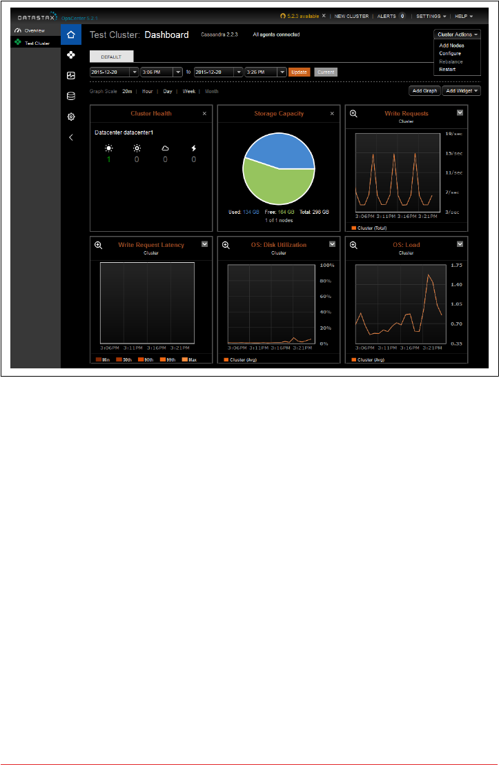
Figure 11-1. DataStax OpsCenter Dashboard for the Test Cluster
In addition to cluster health, the dashboard includes metrics to track capacity and
write latency. You can customize the dashboard to add graphs to monitor many other
metrics reported by Cassandra via JMX. The Enterprise Edition also allows you to
configure thresholds on these metrics for generation of alerts and email notifications.
Operations that can be performed on a cluster are shown at the upper right of the
figure and include adding nodes, configuring cassandra.yaml settings for all nodes,
and restarting the cluster. There is also a “Rebalance” command that can be used to
automatically reallocate token ranges in clusters not using vnodes.
DataStax Enterprise Edition also provides a Repair Service which automates repairs
across the cluster. The Repair Service runs continuously, using incremental repairs to
repair subranges of the cluster. The Repair Service monitors the progress of these
subrange repairs and throttles its repairs to minimize impact to the cluster. Once all
subranges have been repaired, a new repair cycle is started.
The OpsCenter Nodes view provides a helpful graphical representation of the nodes
in the cluster in a ring configuration, as shown in Figure 11-2.
258 | Chapter 11: Maintenance
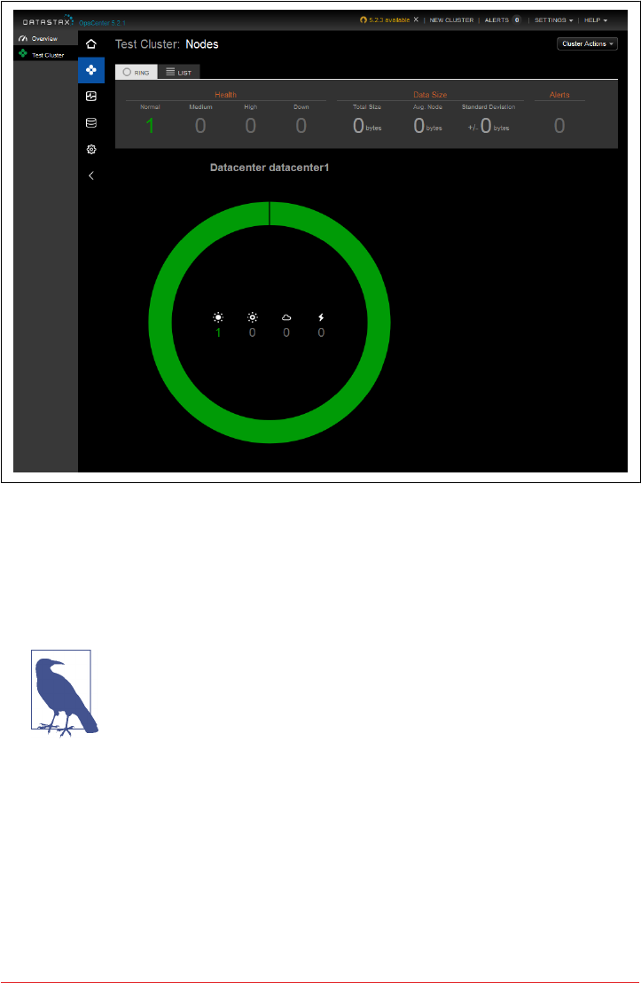
Figure 11-2. DataStax OpsCenter Nodes View
From the Nodes view, we can select an individual node by its position on the ring and
view statistics on the node’s memory, storage capacity, load, tpstats info, and other
metrics. We can also start and stop nodes and perform maintenance actions such as
cleanup, compaction, flush, repair, decommission, and drain.
Use a Separate Cluster for OpsCenter Data
Behind the scenes, OpsCenter uses Cassandra to store metadata
and metrics for the clusters it is managing. While it is possible to
configure OpsCenter to put its tables in an existing cluster, the rec‐
ommended configuration is to create a separate cluster for Ops‐
Center to store its data. By following this guideline, you will avoid
impacting your production clusters.
Maintenance Tools | 259

Netix Priam
Priam is a tool built by Netflix to help manage its Cassandra clusters. Priam was the
King of Troy in Greek mythology, and the father of Cassandra. Priam automates the
deployment, starting, and stopping of nodes, as well as backup and restore opera‐
tions.
Priam is also well integrated with the Amazon Web Services (AWS) cloud environ‐
ment, although AWS deployment is not required. For example, Priam supports
deployment of Cassandra in auto-scaling groups (ASGs), automated backup of snap‐
shots to the Simple Storage Service (S3), and configuration of networking and secu‐
rity groups for Cassandra clusters that span multiple regions.
While Priam does not include a user interface, it does provide a RESTful API that you
can use to build your own frontend or access directly via curl. The API provides the
ability to start and stop nodes, access nodetool commands (with JSON-formatted
output), and perform backup and restore operations.
Summary
In this chapter, we looked at some of the ways you can interact with Cassandra to per‐
form routine maintenance tasks; add, remove, and replace nodes; back up and
recover data with snapshots, and more. We also looked at some tools that help auto‐
mate these tasks to speed up maintenance and reduce errors.
260 | Chapter 11: Maintenance

CHAPTER 12
Performance Tuning
In this chapter, we look at how to tune Cassandra to improve performance. There are
a variety of settings in the configuration file and on individual tables. Although the
default settings are appropriate for many use cases, there might be circumstances in
which you need to change them. In this chapter, we look at how and why to make
these changes.
We also see how to use the cassandra-stress test tool that ships with Cassandra to
generate load against Cassandra and quickly see how it behaves under stress test cir‐
cumstances. We can then tune Cassandra appropriately and feel confident that we’re
ready to deploy to a production environment.
Managing Performance
To be effective at achieving and maintaining a high level of performance in your clus‐
ter, it’s helpful to think of managing performance as a process that begins with the
architecture of your application and continues through development and operations.
Setting Performance Goals
Before beginning any performance tuning effort, it is important to have clear goals in
mind, whether you are just getting started on deploying an application on Cassandra,
or maintaining an existing application.
When planning a cluster, it’s important to understand how the cluster will be used:
the number of clients, intended usage patterns, expected peak hours, and so on. This
will be useful in planning the initial cluster capacity and for planning cluster growth,
as we’ll discuss further in Chapter 14.
261

An important part of this planning effort is to identify clear performance goals in
terms of both throughput (the number of queries serviced per unit time) and latency
(the time to complete a given query).
For example, let’s say that we’re building an ecommerce website that uses the hotel
data model we designed in Chapter 5. We might set a performance goal such as the
following for shopping operations on our cluster:
The cluster must support 30,000 read operations per second from the available_
rooms_by_hotel_date table with a 95th percentile read latency of 3 ms.
This is a statement that includes both throughput and latency goals. We’ll learn how
to measure this using nodetool tablestats.
Regardless of your specific performance goals, it’s important to remember that per‐
formance tuning is all about trade-offs. Having well-defined performance goals will
help you articulate what trade-offs are acceptable for your application. For example:
•Enabling SSTable compression in order to conserve disk space, at the cost of
additional CPU processing.
•Throttling network usage and threads, which can be used to keep network and
CPU utilization under control, at the cost of reduced throughput and increased
latency.
•Increasing or decreasing number of threads allocated to specific tasks such as
reads, writes, or compaction in order to affect the priority relative to other tasks
or to support additional clients.
• Increasing heap size in order to decrease query times.
These are just a few of the trade-offs that you will find yourself considering in perfor‐
mance tuning. We’ll highlight others throughout the rest of this chapter.
Monitoring Performance
As the size of your cluster grows, the number of clients increases, and more keyspaces
and tables are added, the demands on your cluster will begin to pull in different
directions. Taking frequent baselines to measure the performance of your cluster
against its goals will become increasingly important.
We learned in Chapter 10 about the various metrics that are exposed via JMX, includ‐
ing performance-related metrics for Cassandra’s StorageProxy and individual tables.
In that chapter, we also examined nodetool commands that publish performance-
related statistics such as nodetool tpstats and nodetool tablestats and discussed
how these can help identify loading and latency issues.
262 | Chapter 12: Performance Tuning

Now we’ll look at two additional nodetool commands that present performance sta‐
tistics formatted as histograms: proxyhistograms and tablehistograms. First, let’s
examine the output of the nodetool proxyhistograms command:
$ nodetool proxyhistograms
proxy histograms
Percentile Read Latency Write Latency Range Latency
(micros) (micros) (micros)
50% 654.95 0.00 1629.72
75% 943.13 0.00 5839.59
95% 4055.27 0.00 62479.63
98% 62479.63 0.00 107964.79
99% 107964.79 0.00 129557.75
Min 263.21 0.00 545.79
Max 107964.79 0.00 155469.30
The output shows the latency of reads, writes, and range requests for which the
requested node has served as the coordinator. The output is expressed in terms of
percentile rank as well as minimum and maximum values in microseconds. Running
this command on multiple nodes can help identify the presence of slow nodes in the
cluster. A large range latency (in the hundreds of milliseconds or more) can be an
indicator of clients using inefficient range queries, such as those requiring the ALLOW
FILTERING clause or index lookups.
While the view provided by proxyhistograms is useful for identifying general perfor‐
mance issues, we’ll frequently need to focus on performance of specific tables. This is
what nodetool tablehistograms allows us to do. Let’s look at the output of this
command against the available_rooms_by_hotel_date table:
nodetool tablehistograms hotel available_rooms_by_hotel_date
hotel/available_rooms_by_hotel_date histograms
Percentile SSTables Write Latency Read Latency Partition Size Cell Count
(micros) (micros) (bytes)
50% 0.00 0.00 0.00 2759 179
75% 0.00 0.00 0.00 2759 179
95% 0.00 0.00 0.00 2759 179
98% 0.00 0.00 0.00 2759 179
99% 0.00 0.00 0.00 2759 179
Min 0.00 0.00 0.00 2300 150
Max 0.00 0.00 0.00 2759 179
The output of this command is similar. It omits the range latency statistics and
instead provides counts of SSTables read per query. The partition size and cell count
are provided, and this provides another way of identifying large partitions.
Managing Performance | 263

Resetting Metrics
Note that in Cassandra releases through the 3.X series, the metrics
reported are lifetime metrics since the node was started. To reset
the metrics on a node, you have to restart it. The JIRA issue
CASSANDRA-8433 requests the ability to reset the metrics via
JMX and nodetool.
Once you’ve gained familiarity with these metrics and what they tell you about your
cluster, you should identify key metrics to monitor and even implement automated
alerts that indicate your performance goals are not being met. You can accomplish
this via DataStax OpsCenter or any JMX-based metrics framework.
Analyzing Performance Issues
It’s not unusual for the performance of a cluster that has been working well to begin
to degrade over time. When you’ve detected a performance issue, you’ll want to begin
analyzing it quickly to ensure the performance doesn’t continue to deteriorate. Your
goal in these circumstances should be to determine the root cause and address it.
In this chapter, we’ll be looking at many configuration settings that can be used to
tune the performance of each node in a cluster as a whole, across all keyspaces and
tables. It’s also important to try to narrow performance issues down to specific tables
and even queries.
In fact, the quality of the data model is usually the most influential factor in the per‐
formance of a Cassandra cluster. For example, a table design that results in partitions
with a growing number of rows can begin to degrade the performance of the cluster
and manifest in failed repairs, or streaming failures on addition of new nodes. Con‐
versely, partitions with partition keys that are too restrictive can result in rows that
are too narrow, requiring many partitions to be read to satisfy a simple query.
Beware the Large Partition
In addition to the nodetool tablehistograms discussed earlier,
you can detect large partitions by searching logs for WARN mes‐
sages that reference “Writing large partition” or “Compacting large
partition”. The threshold for warning on compaction of large parti‐
tions is set by the compaction_large_partition_warning_ thres
hold_mb property in the cassandra.yaml file.
You’ll also want to learn to recognize instances of the anti-patterns discussed in
Chapter 5 such as queues, or other design approaches that generate a large amount of
tombstones.
264 | Chapter 12: Performance Tuning

Tracing
If you can narrow your search down to a specific table and query of concern, you can
use tracing to gain detailed insight. Tracing is an invaluable tool for understanding
the communications between clients and nodes involved in each query and the time
spent in each step. This helps us see the performance implications of design decisions
we make in our data models and choice of replication factors and consistency levels.
There are several ways to access trace data. We’ll start by looking at how tracing
works in cqlsh. First we’ll enable tracing, and then execute a simple command:
cqlsh:hotel> TRACING ON
Now Tracing is enabled
cqlsh:hotel> SELECT * from hotels where id='AZ123';
id | address | name | phone | pois
-------+---------+---------------------------------+----------------+------
AZ123 | null | Super Hotel Suites at WestWorld | 1-888-999-9999 | null
(1 rows)
Tracing session: 6669f210-de99-11e5-bdb9-59bbf54c4f73
activity | timestamp | source | source_elapsed
--------------------+----------------------------+-----------+----------------
Execute CQL3 query | 2016-02-28 21:03:33.503000 | 127.0.0.1 | 0
Parsing SELECT *... | 2016-02-28 21:03:33.505000 | 127.0.0.1 | 41491
...
We’ve truncated the output quite a bit for brevity, but if you run a command like this,
you’ll see activities such as preparing statements, read repair, key cache searches, data
lookups in memtables and SSTables, interactions between nodes, and the time associ‐
ated with each step in microseconds.
You’ll want to be on the lookout for queries that require a lot of inter-node interac‐
tion, as these may indicate a problem with your schema design. For example, a query
based on a secondary index will likely involve interactions with most or all of the
nodes in the cluster.
Once you are done using tracing in cqlsh, you can turn it off using the TRACING OFF
command.
Tracing information is also available to clients using the DataStax drivers. Let’s mod‐
ify one of our examples from Chapter 8 to see how to interact with traces via the
DataStax Java Driver. The highlighted code enables tracing on a query and prints out
the trace results:
SimpleStatement hotelSelect = session.newSimpleStatement(
"SELECT * FROM hotels WHERE id='AZ123'");
hotelSelect.enableTracing();
Managing Performance | 265

ResultSet hotelSelectResult = session.execute(hotelSelect);
QueryTrace queryTrace = hotelSelectResult.getExecutionInfo().getQueryTrace();
System.out.printf("Trace id: %s\n\n", queryTrace.getTraceId());
System.out.printf("%-42s | %-12s | %-10s \n", "activity",
"timestamp", "source");
System.out.println("-------------------------------------------"
+ "--------------+------------");
SimpleDateFormat dateFormat = new SimpleDateFormat("HH:mm:ss.SSS");
for (QueryTrace.Event event : queryTrace.getEvents()) {
System.out.printf("%42s | %12s | %10s\n",
event.getDescription(),
dateFormat.format((event.getTimestamp())),
event.getSource());
}
Tracing is individually enabled on each Statement or PreparedStatement using the
enableTracing() operation. To obtain the trace of a query, we look at the query
results. You may have noticed in our previous examples that the Session.execute()
operation always returns a ResultSet object, even for queries other than SELECT
queries. This enables us to obtain metadata about the request via an ExecutionInfo
object, even when there are no results to be returned. This metadata includes the con‐
sistency level that was achieved, the coordinator node and other nodes involved in
the query, and information about tracing and paging.
Executing this code produces output that is quite similar to what we saw in cqlsh:
Trace id: 58b22960-90cb-11e5-897a-a9fac1d00bce
activity | timestamp | source
-------------------------------------------+--------------+------------
Parsing SELECT * FROM hotels WHERE id=? | 20:44:34.550 | 127.0.0.1
Preparing statement | 20:44:34.550 | 127.0.0.1
Read-repair DC_LOCAL | 20:44:34.551 | 127.0.0.1
Executing single-partition query on hotels | 20:44:34.551 | 127.0.0.1
Acquiring sstable references | 20:44:34.551 | 127.0.0.1
Merging memtable contents | 20:44:34.551 | 127.0.0.1
Merging data from sstable 3 | 20:44:34.552 | 127.0.0.1
Bloom filter allows skipping sstable 3 | 20:44:34.552 | 127.0.0.1
Merging data from sstable 2 | 20:44:34.552 | 127.0.0.1
Bloom filter allows skipping sstable 2 | 20:44:34.552 | 127.0.0.1
Read 1 live and 0 tombstone cells | 20:44:34.552 | 127.0.0.1
Tracing is also supported in DataStax DevCenter, where it is enabled by default. You
can immediately view the trace of any request you make in DevCenter by selecting
the “Query Trace” tab in the lower middle of the screen, as shown in Figure 12-1.
266 | Chapter 12: Performance Tuning
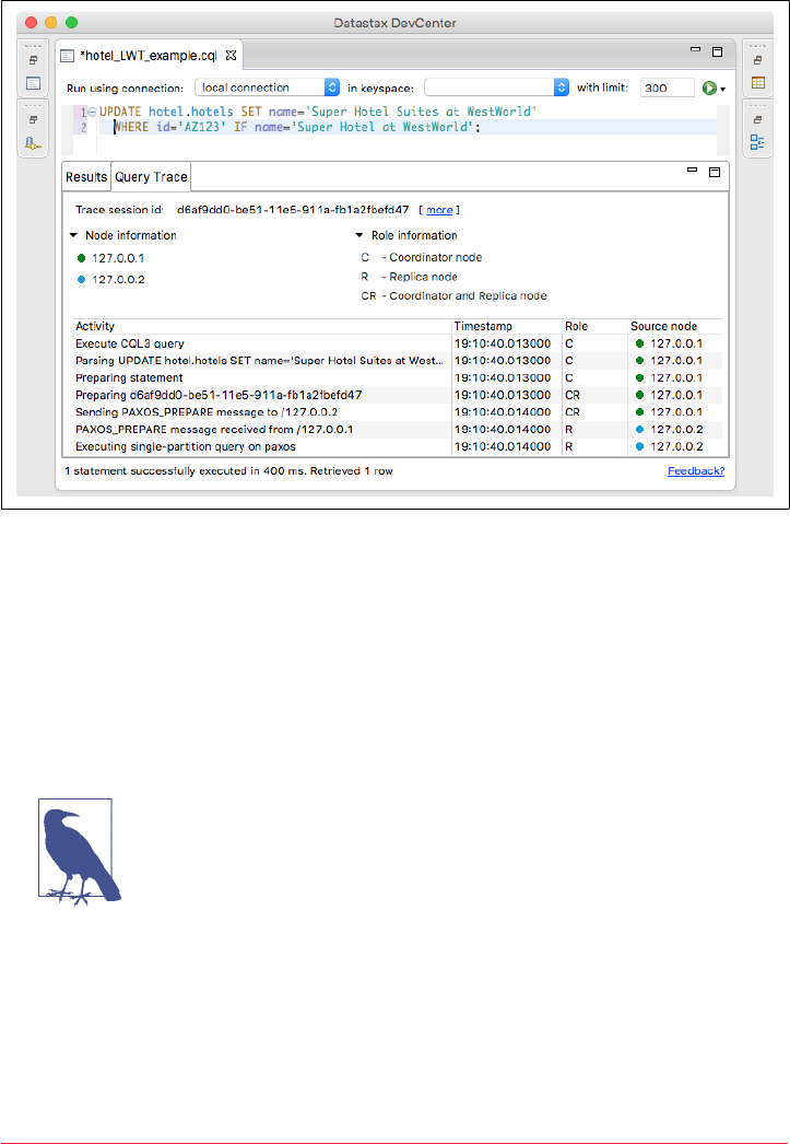
(The “Connection”, “CQL Scripts”, “Schema”, and “Outline” panels have been mini‐
mized to enable readability.)
Figure 12-1. Viewing query traces in DataStax DevCenter
You can configure individual nodes to trace some or all of their queries via the node
tool settraceprobability command. This command takes a number between 0.0
(the default) and 1.0, where 0.0 disables tracing and 1.0 traces every query. This does
not affect tracing of individual queries as requested by clients. Exercise care in chang‐
ing the trace probability, as a typical trace session involves 10 or more writes. Setting
a trace level of 1.0 could easily overload a busy cluster, so a value such as 0.01 or 0.001
is typically appropriate.
Traces Aren’t Forever
Cassandra stores query trace results in the system_traces key‐
space. Since the 2.2 release, Cassandra also uses tracing to store the
results of repair operations. Cassandra limits the TTL on these
tables to prevent them from filling up your disk over time. You can
configure these TTL values by editing the tracetype_query_ttl
and tracetype_repair_ttl properties in the cassandra.yaml file.
Managing Performance | 267

Tuning Methodology
Once you’ve identified the root cause of performance issues related to one of your
established goals, it’s time to begin tuning performance. The suggested methodology
for tuning Cassandra performance is to change one configuration parameter at a time
and test the results.
It is important to limit the amount of configuration changes you make when tuning
so that you can clearly identify the impact of each change. You may need to repeat the
change process multiple times until you’ve reached the desired performance goal.
In some cases, it may be that you can get the performance back in line simply by
adding more resources such as memory or extra nodes, but make sure that you aren’t
simply masking underlying design or configuration issues. In other cases, you may
find that you can’t reach your desired goals through tuning alone, and that design
changes are needed.
With this methodology in mind, let’s look at some of the various options that you can
configure to tune your Cassandra clusters. We’ll highlight node configuration proper‐
ties in the cassandra.yaml and cassandra-env.sh files as well as options that are config‐
ured on individual tables using CQL.
Caching
Caches are used to improve responsiveness to read operations. Additional memory is
used to hold data, to minimize the number of disk reads that must be performed. As
the cache size increases, so does the number of “hits” that can be served from mem‐
ory.
There are three caches built into Cassandra: the key cache, row cache, and counter
cache. The row cache caches a configurable number of rows per partition. If you are
using a row cache for a given table, you will not need to use a key cache on it as well.
Your caching strategy should therefore be tuned in accordance with a few factors:
•Consider your queries, and use the cache type that best fits your queries.
•Consider the ratio of your heap size to your cache size, and do not allow the
cache to overwhelm your heap.
•Consider the size of your rows against the size of your keys. Typically keys will be
much smaller than entire rows.
Let’s consider some specific tuning and configuration options for each cache.
268 | Chapter 12: Performance Tuning

Key Cache
Cassandra’s key cache stores a map of partition keys to row index entries, facilitating
faster read access into SSTables stored on disk. We can configure usage of the key
cache on a per-table basis. For example, let’s use cqlsh to examine the caching set‐
tings on our hotels table:
cqlsh:hotel> DESCRIBE TABLE hotels;
CREATE TABLE hotel.hotels (
id text PRIMARY KEY,
address frozen<address>,
name text,
phone text,
pois set<text>
) WITH bloom_filter_fp_chance = 0.01
AND caching = {'keys': 'ALL', 'rows_per_partition': 'NONE'}
...
Because the key cache greatly increases reads without consuming a lot of additional
memory, it is enabled by default; that is, key caching is enabled if you don’t specify a
value when creating the table. We can disable key caching for this table with the
ALTER TABLE command:
cqlsh:hotel> ALTER TABLE hotels
WITH caching = { 'keys' : 'NONE', 'rows_per_partition' : 'NONE' };
The legal options for the keys attribute are ALL or NONE.
The key_cache_size_in_mb setting indicates the maximum amount of memory that
will be devoted to the key cache, which is shared across all tables. The default value is
either 5% of the total JVM heap, or 100 MB, whichever is less.
Row Cache
The row cache caches entire rows and can speed up read access for frequently
accessed rows, at the cost of more memory usage.
You’ll want to use the row cache size setting carefully, as this can easily lead to more
performance issues than it solves. In many cases, a row cache can yield impressive
performance results for small data sets when all the rows are in memory, only to
degrade on larger data sets when the data must be read from disk.
If your table gets far more reads than writes, then configuring an overly large row
cache will needlessly consume considerable server resources. If your table has a lower
ratio of reads to writes, but has rows with lots of data in them (hundreds of columns),
then you’ll need to do some math before setting the row cache size. And unless you
have certain rows that get hit a lot and others that get hit very little, you’re not going
to see much of a boost here.
Caching | 269

For these reasons, row caching tends to yield fewer benefits than key caching. You
may want to explore file caching features supported by your operating system as an
alternative to row caching.
As with key caching, we can configure usage of the row cache on a per-table basis.
The rows_per_partition setting specifies the number of rows that will be cached per
partition. By default, this value is set to NONE, meaning that no rows will be cached.
Other available options are positive integers or ALL. The following CQL statement
sets the row cache to 200 rows:
cqlsh:hotel> ALTER TABLE hotels
WITH caching = { 'keys' : 'NONE', 'rows_per_partition' : '200' };
The implementation of the row cache is pluggable via the row_cache_class_name
property. This defaults to the off-heap cache provider implemented by the
org.apache.cassandra.OHCProvider class. The previous implementation was the
SerializingCacheProvider.
Counter Cache
The counter cache improves counter performance by reducing lock contention for
the most frequently accessed counters. There is no per-table option for configuration
of the counter cache.
The counter_cache_size_in_mb setting determines the maximum amount of mem‐
ory that will be devoted to the counter cache, which is shared across all tables. The
default value is either 2.5% of the total JVM heap, or 50 MB, whichever is less.
Saved Cache Settings
Cassandra provides the ability to periodically save caches to disk, so that they can be
read on startup as a way to quickly warm the cache. The saved cache settings are sim‐
ilar across all three cache types:
•Cache files are saved under the directory specified by the saved_caches property.
The files are written at the interval in seconds specified by the key_ cache_
save_period, row_cache_save_period, and counter_cache_ save_period,
which default to 14000 (4 hours), 0 (disabled), and 7200 (2 hours), respectively.
•Caches are indexed by key values. The number of keys to save in the file are indi‐
cated by the key_cache_keys_to_save, row_cache_keys_to_save, and counter_
cache_keys_to_save properties.
270 | Chapter 12: Performance Tuning

Managing Caches via nodetool
Cassandra also provides capabilities for managing caching via node
tool:
•You can clear caches using the invalidatekeycache, invalid
aterowcache, and invalidatecountercache commands.
•Use the setcachecapacity command to override the config‐
ured settings for key and row cache capacity.
•Use the setcachekeystosave command to override the con‐
figured settings for how many key and row cache elements to
save to a file.
Remember that these settings will revert to the values set in the cas‐
sandra.yaml file on a node restart.
Memtables
Cassandra uses memtables to speed up writes, holding a memtable corresponding to
each table it stores. Cassandra flushes memtables to disk as SSTables when either the
commit log threshold or memtable threshold has been reached.
Cassandra stores memtables either on the Java heap, off-heap (native) memory, or
both. The limits on heap and off-heap memory can be set via the properties
memtable_heap_space_in_mb and memtable_offheap_space_in_mb, respectively.
By default, Cassandra sets each of these values to 1/4 of the total heap size set in the
cassandra-env.sh file. Allocating memory for memtables reduces the memory avail‐
able for caching and other internal Cassandra structures, so tune carefully and in
small increments.
You can influence how Cassandra allocates and manages memory via the
memtable_allocation_type property. This property configures another of Cassan‐
dra’s pluggable interfaces, selecting which implementation of the abstract class
org.apache.cassandra.utils.memory.MemtablePool is used to control the memory
used by each memtable. The default value heap_buffers causes Cassandra to allocate
memtables on the heap using the Java New I/O (NIO) API, while offheap_buffers
uses Java NIO to allocate a portion of each memtable both on and off the heap. The
offheap_objects uses native memory directly, making Cassandra entirely responsi‐
ble for memory management and garbage collection of memtable memory. This is a
less-well documented feature, so it’s best to stick with the default here until you can
gain more experience.
Another element related to tuning the memtables is memtable_flush_writers. This
setting, which is 2 by default, indicates the number of threads used to write out the
memtables when it becomes necessary. If your data directories are backed by SSD,
Memtables | 271

you should increase this to the number of cores, without exceeding the maximum
value of 8. If you have a very large heap, it can improve performance to set this count
higher, as these threads are blocked during disk I/O.
You can also enable metered flushing on each table via the CQL CREATE TABLE or
ALTER TABLE command. The memtable_flush_period_in_ms option sets the interval
at which the memtable will be flushed to disk.
Setting this property results in more predictable write I/O, but will also result in more
SSTables and more frequent compactions, possibly impacting read performance. The
default value of 0 means that periodic flushing is disabled, and flushes will only occur
based on the commit log threshold or memtable threshold being reached.
Commit Logs
There are two sets of files that Cassandra writes to as part of handling update opera‐
tions: the commit log and the SSTable files. Their different purposes need to be con‐
sidered in order to understand how to treat them during configuration.
Remember that the commit log can be thought of as short-term storage that helps
ensure that data is not lost if a node crashes or is shut down before memtables can be
flushed to disk. That’s because when a node is restarted, the commit log gets replayed.
In fact, that’s the only time the commit log is read; clients never read from it. But the
normal write operation to the commit log blocks, so it would damage performance to
require clients to wait for the write to finish.
You can set the value for how large the commit log is allowed to grow before it stops
appending new writes to a file and creates a new one. This value is set with the
commitlog_segment_size_in_mb property. By default, the value is 32 MB. This is
similar to setting log rotation on a logging engine such as Log4J or Logback.
The total space allocated to the commit log is specified by the commitlog_total_
space_in_mb property. Setting this to a larger value means that Cassandra will need
to flush tables to disk less frequently.
The commit logs are periodically removed, following a successful flush of all their
appended data to the dedicated SSTable files. For this reason, the commit logs will not
grow to anywhere near the size of the SSTable files, so the disks don’t need to be as
large; this is something to consider during hardware selection.
To increase the amount of writes that the commit log can hold, you’ll want to enable
log compression via the commitlog_compression property. The supported compres‐
sion algorithms are LZ4, Snappy, and Deflate. Using compression comes at the cost of
additional CPU time to perform the compression.
272 | Chapter 12: Performance Tuning

Additional settings relate to the commit log sync operation, represented by the
commitlog_sync element. There are two possible settings for this: periodic and
batch. The default is periodic, meaning that the server will make writes durable only
at specified intervals. The interval is specified by the commitlog_sync_period_in_ms
property, which defaults to 10000 (10 seconds).
In order to guarantee durability for your Cassandra cluster, you may want to examine
this setting. When the server is set to make writes durable periodically, you can
potentially lose the data that has not yet been synced to disk from the write-behind
cache.
If your commit log is set to batch, it will block until the write is synced to disk
(Cassandra will not acknowledge write operations until the commit log has been
completely synced to disk). Changing this value will require taking some perfor‐
mance metrics, as there is a necessary trade-off here: forcing Cassandra to write more
immediately constrains its freedom to manage its own resources. If you do set
commitlog_sync to batch, you need to provide a suitable value for commit_ log_
sync_batch_window_in_ms, where ms is the number of milliseconds between each
sync effort.
SSTables
Unlike the commit log, Cassandra writes SSTable files to disk asynchronously. If
you’re using hard disk drives, it’s recommended that you store the datafiles and the
commit logs on separate disks for maximum performance. If you’re deploying on
solid state drives (SSDs), it is fine to use the same disk.
Cassandra, like many databases, is particularly dependent on the speed of the hard
disk and the speed of the CPUs. It’s more important to have several processing cores
than one or two very fast ones, to take advantage of Cassandra’s highly concurrent
construction. So make sure for QA and production environments to get the fastest
disks you can—SSDs if you can afford them. If you’re using hard disks, make sure
there are at least two so that you can store commit log files and the datafiles on sepa‐
rate disks and avoid competition for I/O time.
When reading SSTable files from disk, Cassandra uses a buer cache (also known as a
buer pool), to help reduce database file I/O. This cache uses off-heap memory, but its
size defaults to either 512 MB, or 1/4 of the Java heap, whichever is smaller. You can
set the cache size using the file_cache_size_in_mb property in cassandra.yaml. You
can also allow Cassandra to use the Java heap for buffers once the off-heap cache is
full by setting buffer_pool_use_heap_if_exhausted to true.
As we discussed in Chapter 9, Cassandra maintains SSTable index summaries in
memory in order to speed access into SSTable files. By default, Cassandra allocates
SSTables | 273

5% of the Java heap to these indexes, but you can override this via the
index_summary_capacity_in_mb property in cassandra.yaml. In order to stay
within the allocated limit, Cassandra will shrink indexes associated with tables that
are read less frequently. Because read rates may change over time, Cassandra also
resamples indexes from files stored on disk at the frequency specified by the index_
summary_resize_interval_in_minutes property, which defaults to 60.
Cassandra also provides a mechanism to influence the relative amount of space allo‐
cated to indexes for different tables. This is accomplished via the min_index_inter
val and max_index_interval properties, which can be set per via the CQL CREATE
TABLE or ALTER TABLE commands. These values specify the minimum and maximum
number of index entries to store per SSTable.
Hinted Hando
Hinted handoff is one of several mechanisms that Cassandra provides to keep data in
sync across the cluster. As we’ve learned previously, a coordinator node can keep a
copy of data on behalf of a node that is down for some amount of time. We can tune
hinted handoff in terms of the amount of disk space we’re willing to use to store hints,
and how quickly hints will be delivered when a node comes back online.
We can control the bandwidth utilization of hint delivery using the property
hinted_handoff_throttle_in_kb, or at runtime via nodetool sethintedhandoff
throttlekb.
This throttling limit has a default value of 1024, or 1 MB/second, and is used to set an
upper threshold on the bandwidth that would be required of a node receiving hints.
For example, in a cluster of three nodes, each of the two nodes delivering hints to a
third node would throttle its hint delivery to half of this value, or 512KB/second.
Note that configuring this throttle is a bit different than configuring other Cassandra
features, as the behavior that will be observed by a node receiving hints is entirely
based on property settings on other nodes. You’ll definitely want to use the same val‐
ues for these settings in sync across the cluster to avoid confusion.
In releases prior to 3.0, Cassandra stores hints in a table which is not replicated to
other nodes, but starting with the 3.0 release, Cassandra stores hints in a directory
specified by the hints_directory property, which defaults to the data/hints directory
under the Cassandra installation. You can set a cap on the amount of disk space devo‐
ted to hints via the max_hints_file_size_in_mb property.
You can clear out any hints awaiting delivery to one or more nodes using the node
tool truncatehints command with a list of IP addresses or hostnames. Hints even‐
tually expire after the value expressed by the max_hint_window_in_ms property.
274 | Chapter 12: Performance Tuning

It’s also possible to enable or disable hinted handoff entirely, as we learned in Chap‐
ter 10. While some would use this as a way to conserve disk and bandwidth, in gen‐
eral the hinted handoff mechanism does not consume a lot of resources in
comparison to the extra layer of consistency it helps to provide, especially compared
to the cost of repairing a node.
Compaction
Cassandra provides configuration options for compaction including the resources
used by compaction on a node, and the compaction strategy to be used for each table.
Choosing the right compaction strategy for a table can certainly be a factor in
improving performance. Let’s review the available strategies and discuss when they
should be used.
SizeTieredCompactionStrategy
The SizeTieredCompactionStrategy (STCS) is the default compaction strategy,
and it should be used in most cases. This strategy groups SSTables into tiers
organized by size. When there are a sufficient number of SSTables in a tier (4 or
more by default), a compaction is run to combine them into a larger SSTable. As
the amount of data grows, more and more tiers are created. STCS performs espe‐
cially well for write-intensive tables, but less so for read-intensive tables, as the
data for a particular row may be spread across an average of 10 or so SSTables.
LeveledCompactionStrategy
The LeveledCompactionStrategy (LCS) creates SSTables of a fixed size (5 MB by
default) and groups them into levels, with each level holding 10 times as many
SSTables as the previous level. LCS guarantees that a given row appears in at most
one SSTable per level. LCS spends additional effort on I/O to minimize the num‐
ber of SSTables a row appears in; the average number of SSTables for a given row
is 1.11. This strategy should be used if there is a high ratio of reads to writes or
predictable latency is required. LCS will tend to not perform as well if a cluster is
already I/O bound. If writes dominate reads, Cassandra may struggle to keep up.
DateTieredCompactionStrategy
The DateTieredCompactionStrategy (DTCS) was introduced in the 2.0.11 and
2.1.1 releases. It is intended to improve read performance for time series data,
specifically for access patterns that involve accessing the most recently written
data. It works by grouping SSTables in windows organized by the write time of
the data. Compaction is only performed within these windows. Because DTCS is
relatively new and targeted at a very specific use case, make sure you research
carefully before making use of it.
Compaction | 275

Each strategy has its own specific parameters that can be tuned. Check the documen‐
tation for your release for further details.
Testing Compaction Strategies with Write Survey Mode
If you’d like to test out using a different compaction strategy for a table, you don’t
have to change it on the whole cluster in order to see how it works. Instead, you can
create a test node running in write survey mode to see how the new compaction strat‐
egy will work.
To do this, add the following options to the cassandra-env.sh file for the test node:
JVM_OPTS="$JVM_OPTS -Dcassandra.write_survey=true"
JVM_OPTS="$JVM_OPTS -Djoin_ring=false"
Once the node is up, you can then access the org.apache.cassandra.db.Col
umnFamilyStoreMBean for the table under org.apache.cassandra.db > Tables in
order to configure the compaction strategy. Set the CompactionStrategyClass
attribute to the fully qualified compaction strategy class name.
After this configuration change, add the node to the ring via nodetool join so that it
can start receiving writes. Writes to the test node place a minimal additional load on
the cluster and do not count toward consistency levels. You can now monitor the per‐
formance of writes to the node using nodetool tablestats and tablehistograms.
You can test the impact of new compaction strategy on reads by stopping the node,
bringing it up as a standalone machine, and then testing read performance on the
node.
Write survey mode is also useful for testing out other configuration changes or even a
new version of Cassandra.
Another per-table setting is the compaction threshold. The compaction threshold
refers to the number of SSTables that are in the queue to be compacted before a
minor compaction is actually kicked off. By default, the minimum number is 4 and
the maximum is 32. You don’t want this number to be too small, or Cassandra will
spend time fighting with clients for resources to perform many frequent, unnecessary
compactions. You also don’t want this number to be too large, or Cassandra could
spend a lot of resources performing many compactions at once, and therefore will
have fewer resources available for clients.
The compaction threshold is set per table using the CQL CREATE TABLE or ALTER
TABLE commands. However, you can inspect or override this setting for a particular
node using the nodetool getcompactionthreshold or setcompactionthreshold
commands:
276 | Chapter 12: Performance Tuning

$ nodetool getcompactionthreshold hotel hotels
Current compaction thresholds for hotel/hotels:
min = 4, max = 32
$ nodetool setcompactionthreshold hotel hotels 8 32
Compaction can be intensive in terms of I/O and CPU, so Cassandra provides the
ability to monitor the compaction process and influence when compaction occurs.
You can monitor the status of compaction on a node using the nodetool compaction
stats command, which lists the completed and total bytes for each active compac‐
tion (we’ve omitted the ID column for brevity):
$ nodetool compactionstats
pending tasks: 1
id compaction type keyspace table completed total unit progress
... Compaction hotel hotels 57957241 127536780 bytes 45.44%
Active compaction remaining time : 0h00m12s
If you see that the pending compactions are starting to stack up, you can use the node
tool commands getcompactionthroughput and setcompactionthroughput to check
and set the throttle that Cassandra applies to compactions across the cluster. This
corresponds to the property compaction_throughput_mb_per_sec in the cassan‐
dra.yaml file. Setting this value to 0 disables throttling entirely, but the default value
of 16 MB/s is sufficient for most non-write-intensive cases.
If this does not fix the issue, you can increase the number of threads dedicated to
compaction by setting the concurrent_compactors property in cassandra.yaml file,
or at runtime via the CompactionManagerMBean. This property defaults to the mini‐
mum of the number of disks and number of cores, with a minimum of 2 and a maxi‐
mum of 8.
Although it is not very common, a large compaction could negatively impact the per‐
formance of the cluster. You can use the nodetool stop command to stop all active
compactions on a node. You can also identify a specific compaction to stop by ID,
where the ID is obtained from the compactionstats output. Cassandra will resched‐
ule any stopped compactions to run later.
You can force a major compaction via the nodetool compact command. Before kick‐
ing off a major compaction manually, remember that this is an expensive operation.
The behavior of nodetool compact during compaction varies depending on the com‐
paction strategy in use. We’ll discuss the implications of each compaction strategy on
disk usage in Chapter 14.
The nodetool compactionhistory command prints statistics about completed com‐
pactions, including the size of data before and after compaction and the number of
rows merged. The output is pretty verbose, so we’ve omitted it here.
Compaction | 277

Concurrency and Threading
Cassandra differs from many data stores in that it offers much faster write perfor‐
mance than read performance. There are two settings related to how many threads
can perform read and write operations: concurrent_reads and concurrent_writes.
In general, the defaults provided by Cassandra out of the box are very good.
The concurrent_reads setting determines how many simultaneous read requests the
node can service. This defaults to 32, but should be set to the number of drives used
for data storage × 16. This is because when your data sets are larger than available
memory, the read operation is I/O bound.
The concurrent_writes setting behaves somewhat differently. This should correlate
to the number of clients that will write concurrently to the server. If Cassandra is
backing a web application server, you can tune this setting from its default of 32 to
match the number of threads the application server has available to connect to Cas‐
sandra. It is common in Java application servers to prefer database connection pools
no larger than 20 or 30, but if you’re using several application servers in a cluster,
you’ll need to factor that in as well.
Two additional settings—concurrent_counter_writes and concurrent_material
ized_view_writes—are available for tuning special forms of writes. Because counter
and materialized view writes both involve a read before write, it is best to set this to
the lower of concurrent_reads and concurrent_writes.
There are several other properties in the cassandra.yaml file which control the num‐
ber of threads allocated to the thread pools which implement various stages in Cas‐
sandra’s SEDA approach. We’ve looked at some of these already, but here is a
summary:
max_hints_delivery_threads
Maximum number of threads devoted to hint delivery
memtable_flush_writers
Number of threads devoted to flushing memtables to disk
concurrent_compactors
Number of threads devoted to running compaction
native_transport_max_threads
Maximum number of threads devoted to processing incoming CQL requests
(you may also notice the similar properties rpc_min_threads and rpc_ max_
threads, which are for the deprecated Thrift interface)
Note that some of these properties allow Cassandra to dynamically allocate and deal‐
locate threads up to a maximum value, while others specify a static number of
278 | Chapter 12: Performance Tuning

threads. Tuning these properties up or down affects how Cassandra uses its CPU time
and how much I/O capacity it can devote to various activities.
Networking and Timeouts
As Cassandra is a distributed system, it provides mechanisms for dealing with net‐
work and node issues including retries, timeouts, and throttling. We’ve already dis‐
cussed a couple of the ways Cassandra implements retry logic, such as the
RetryPolicy in the DataStax client drivers, and speculative read execution in drivers
and nodes.
Now let’s take a look at the timeout mechanisms that Cassandra provides to help it
avoid hanging indefinitely waiting for other nodes to respond. The timeout proper‐
ties listed in Table 12-1 are set in the cassandra.yaml file.
Table 12-1. Cassandra node timeouts
Property Name Default Value Description
read_request_timeout_in_ms 5000 (5 seconds) How long the coordinator waits for read
operations to complete
range_request_timeout_in_ms 10000 (10
seconds)
How long the coordinator should wait for
range reads to complete
write_request_timeout_in_ms 2000 (2 seconds) How long the coordinator should wait for
writes to complete
counter_write_request_timeout_in_ms 5000 (5 seconds) How long the coordinator should wait for
counter writes to complete
cas_contention_timeout_in_ms 1000 (1 second) How long a coordinator should continue to
retry a lightweight transaction
truncate_request_timeout_in_ms 60000 (1 minute) How long the coordinator should wait for
truncates to complete (including snapshot)
streaming_socket_timeout_in_ms 3600000 (1 hour) How long a node waits for streaming to
complete
request_timeout_in_ms 10000 (10
seconds)
The default timeout for other, miscellaneous
operations
The values for these timeouts are generally acceptable, but you may need to adjust
them for your network environment.
Another property related to timeouts is cross_node_timeout, which defaults to
false. If you have NTP configured in your environment, consider enabling this so
that nodes can more accurately estimate when the coordinator has timed out on long-
running requests and release resources more quickly.
Networking and Timeouts | 279

Cassandra also provides several properties that allow you to throttle the amount of
network bandwidth it will use for various operations. Tuning these allows you to pre‐
vent Cassandra from swamping your network, at the cost of longer time to complete
these tasks. For example, the stream_throughput_outbound_megabits_per_sec and
inter_dc_stream_throughput_outbound_megabits_per_sec properties specify a
per-thread throttle on streaming file transfers to other nodes in the local and remote
data centers, respectively.
The throttles for hinted handoff and batchlog replay work slightly differently. The
values specified by hinted_handoff_throttle_in_kb and batchlog_replay_ throt
tle_in_kb are considered maximum throughput values for the cluster and are there‐
fore spread proportionally across nodes according to the formula:
Tx=Tt
Nn− 1
That is, the throughput of a node x (Tx) is equal to the total throughput (Tt) divided
by one less than the number of nodes in the cluster (Nn).
Finally, there are several properties that you can use to limit traffic to the native CQL
port on each node. These may be useful in situations where you don’t have direct con‐
trol over the client applications of your cluster. The default maximum frame size
specified by the native_transport_max_frame_size_in_mb property is 256. Frame
requests larger than this will be rejected by the node.
The node can also limit the maximum number of simultaneous client connections,
via the native_transport_max_concurrent_connections property, but the default is
-1 (unlimited). If you configure this value, you’ll want to make sure it makes sense in
light of the concurrent_readers and concurrent_writers properties.
To limit the number of simultaneous connections from a single source IP address,
configure the native_transport_max_concurrent_connections_per_ip property,
which defaults to -1 (unlimited).
JVM Settings
Cassandra allows you to configure a variety of options for how the server JVM should
start up, how much Java memory should be allocated, and so forth. In this section, we
look at how to tune the startup.
If you’re using Windows, the startup script is called cassandra.bat, and on Linux it’s
cassandra.sh. You can start the server by simply executing this file, which sets several
defaults. But there’s another file in the conf directory that allows you to configure a
variety of settings related to how Cassandra starts. This file is called cassandra-env.sh
(cassandra-env.ps1 on Windows) and it separates certain options, such as the JVM
settings, into a different file to make it easier to update.
280 | Chapter 12: Performance Tuning

Try tuning the options passed to the JVM at startup for better performance. The key
JVM options included in cassandra-env.sh and guidelines for how you might tweak
them are discussed momentarily. If you want to change any of these values, simply
open the cassandra-env.sh file in a text editor, change the values, and restart.
The jvm.options File
The Cassandra 3.0 release introduced another settings file in the
conf directory called jvm.options. The purpose of this file is to move
JVM settings related to heap size and garbage collection out of cas‐
sandra.in.sh file to a separate file, as these are the attributes that are
tuned most frequently. The jvm.options and cassandra.in.sh are
included (sourced) by the cassandra-env.sh file.
Memory
By default, Cassandra uses the following algorithm to set the JVM heap size: if the
machine has less than 1 GB of RAM, the heap is set to 50% of RAM. If the machine
has more than 4 GB of RAM, the heap is set to 25% of RAM, with a cap of 8 GB. To
tune the minimum and maximum heap size, use the -Xms and -Xmx flags. These
should be set to the same value to allow the entire heap to be locked in memory and
not swapped out by the OS. It is not recommended to set the heap larger than 8GB if
you are using the Concurrent Mark Sweep (CMS) garbage collector, as heap sizes
larger than this value tend to lead to longer GC pauses.
When performance tuning, it’s a good idea to set only the heap min and max options,
and nothing else at first. Only after real-world usage in your environment and some
performance benchmarking with the aid of heap analysis tools and observation of
your specific application’s behavior should you dive into tuning the more advanced
JVM settings. If you tune your JVM options and see some success, don’t get too exci‐
ted. You need to test under real-world conditions.
In general, you’ll probably want to make sure that you’ve instructed the heap to dump
its state if it hits an out-of-memory error, which is the default in cassandra-env.sh, set
by the -XX:+HeapDumpOnOutOfMemory option. This is just good practice if you start
experiencing out-of-memory errors.
Garbage Collection
The Java heap is broadly divided into two object spaces: young and old. The young
space is subdivided into one for new object allocation (called “eden space”) and
another for new objects that are still in use (the “survivor space”).
Cassandra uses the parallel copying collector in the young generation; this is set via
the -XX:+UseParNewGC option. Older objects still have some reference, and have
JVM Settings | 281

therefore survived a few garbage collections, so the Survivor Ratio is the ratio of eden
space to survivor space in the young object part of the heap. Increasing the ratio
makes sense for applications with lots of new object creation and low object preserva‐
tion; decreasing it makes sense for applications with longer-living objects. Cassandra
sets this value to 8 via the -XX:SurvivorRatio option, meaning that the ratio of eden
to survivor space is 1:8 (each survivor space will be 1/8 the size of eden). This is fairly
low, because the objects are living longer in the memtables.
Every Java object has an age field in its header, indicating how many times it has been
copied within the young generation space. Objects are copied into a new space when
they survive a young generation garbage collection, and this copying has a cost.
Because long-living objects may be copied many times, tuning this value can improve
performance. By default, Cassandra has this value set at 1 via the
-XX:MaxTenuringThreshold option. Set it to 0 to immediately move an object that
survives a young generation collection to the old generation. Tune the survivor ratio
together along with the tenuring threshold.
By default, modern Cassandra releases use the Concurrent Mark Sweep (CMS)
garbage collector for the old generation; this is set via the -XX:+UseConcMarkSweepGC
option. This setting uses more RAM and CPU power to do frequent garbage collec‐
tions while the application is running, in order to keep the GC pause time to a mini‐
mum. When using this strategy, it’s important to set the heap min and max values to
the same value, in order to prevent the JVM from having to spend a lot of time grow‐
ing the heap initially.
Moving to the Garbage First Garbage Collector
The Garbage First garbage collector (also known as G1GC) was introduced in Java 7
as an improvement and eventual replacement for CMS GC, especially on multiproc‐
essor machines with more memory.
G1GC divides the heap into multiple equal size regions and allocates these to eden,
survivor, and old generations dynamically, so that each generation is a logical collec‐
tion of regions that need not be consecutive regions in memory. This approach ena‐
bles garbage collection to run continually and require fewer of the “stop the world”
pauses that characterize traditional garbage collectors.
G1GC generally requires fewer tuning decisions; the intended usage is that you need
only define the min and max heap size and a pause time goal. A lower pause time will
cause GC to occur more frequently.
G1GC was on course to become the default for the Cassandra 3.0 release, but was
backed out as part of the JIRA issue CASSANDRA-10403, due to the fact that it did
not perform as well as the CMS for heap sizes smaller than 8 GB.
282 | Chapter 12: Performance Tuning

If you’d like to experiment with using G1GC and a larger heap size on a Cassandra 2.2
or later release, the settings are readily available in the cassandra-env.sh file (or
jvm.options) file.
Look for G1GC to become the default in a future Cassandra release, most likely in
conjunction with support for Java 9, in which G1GC will become the Java default.
To get more insight on garbage collection activity in your Cassandra nodes, there are
a couple of options. The gc_warn_threshold_in_ms setting in the cassandra.yaml file
determines the pause length that will cause Cassandra to generate log messages at the
WARN logging level. This value defaults to 1000 ms (1 second). You can also instruct
the JVM to print garbage-collection details by setting options in the cassandra-env.sh
or jvm.options file.
Using cassandra-stress
Cassandra ships with a utility called cassandra-stress that you can use to run a
stress test on your Cassandra cluster. To run cassandra-stress, navigate to the
<cassandra-home>/tools/bin directory and run the command:
$ cassandra-stress write n=1000000
Connected to cluster: test-cluster
Datatacenter: datacenter1; Host: localhost/127.0.0.1; Rack: rack1
Datatacenter: datacenter1; Host: /127.0.0.2; Rack: rack1
Datatacenter: datacenter1; Host: /127.0.0.3; Rack: rack1
Created keyspaces. Sleeping 1s for propagation.
Sleeping 2s...
Warming up WRITE with 50000 iterations...
Running WRITE with 200 threads for 1000000 iteration
...
The output lists the nodes to which the tool is connected (in this case, a cluster cre‐
ated using ccm) and creates a sample keyspace and table to which it can write data.
The test is warmed up by doing 50,000 writes, and then the tool begins to output
metrics as it continues to write, which we’ve omitted for brevity. The tool creates a
pool of threads (defaulting on my system to 200) that perform one write after
another, until it inserts one million rows. Finally, it prints a summary of results:
Results:
op rate : 7620 [WRITE:7620]
partition rate : 7620 [WRITE:7620]
row rate : 7620 [WRITE:7620]
latency mean : 26.2 [WRITE:26.2]
latency median : 2.6 [WRITE:2.6]
latency 95th percentile : 138.4 [WRITE:138.4]
latency 99th percentile : 278.8 [WRITE:278.8]
latency 99.9th percentile : 393.3 [WRITE:393.3]
latency max : 820.9 [WRITE:820.9]
Using cassandra-stress | 283

Total partitions : 1000000 [WRITE:1000000]
Total errors : 0 [WRITE:0]
total gc count : 0
total gc mb : 0
total gc time (s) : 0
avg gc time(ms) : NaN
stdev gc time(ms) : 0
Total operation time : 00:02:11
Let’s unpack this a bit. What we’ve done is generated and inserted one million values
into a completely untuned three-node cluster in a little over two minutes, which rep‐
resents a rate of 7,620 writes per second. The median latency per operation is 2.6
milliseconds, although a small number of writes took longer.
Now that we have all of this data in the database, let’s use the test to read some values
too:
$ cassandra-stress read n=200000
...
Running with 4 threadCount
Running READ with 4 threads for 200000 iteration
If you examine the output, you will see that it starts out with a small number of
threads and ramps up. On one test run, it peaked at over 600 threads, as shown here:
Results:
op rate : 13828 [READ:13828]
partition rate : 13828 [READ:13828]
row rate : 13828 [READ:13828]
latency mean : 67.1 [READ:67.1]
latency median : 9.9 [READ:9.9]
latency 95th percentile : 333.2 [READ:333.2]
latency 99th percentile : 471.1 [READ:471.1]
latency 99.9th percentile : 627.9 [READ:627.9]
latency max : 1060.5 [READ:1060.5]
Total partitions : 200000 [READ:200000]
Total errors : 0 [READ:0]
total gc count : 0
total gc mb : 0
total gc time (s) : 0
avg gc time(ms) : NaN
stdev gc time(ms) : 0
Total operation time : 00:00:14
Improvement over 609 threadCount: 7%
The tool periodically prints out statistics about the last several writes. The preceding
output came from the last block of statistics. As you can see, Cassandra doesn’t read
nearly as fast as it writes; the mean read latency was around 10 ms. Remember,
though, that this is out of the box, untuned, single-threaded, on a regular workstation
running other programs, and the database is approximately 2 GB in size. Regardless,
284 | Chapter 12: Performance Tuning

this is a great tool to help you do performance tuning for your environment and to
get a set of numbers that indicates what to expect in your cluster.
We can also run cassandra-stress on our own tables by creating a specification in a
yaml file. For example, we could create a cqlstress-hotel.yaml file to describe queries
that read from tables in our hotel keyspace. This file defines queries that we would
use to stress the available_rooms_by_hotel_date table:
keyspace: hotel
table: available_rooms_by_hotel_date
columnspec:
- name: date
cluster: uniform(20..40)
insert:
partitions: uniform(1..50)
batchtype: LOGGED
select: uniform(1..10)/10
queries:
simple1:
cql: select * from available_rooms_by_hotel_date
where hotel_id = ? and date = ?
fields: samerow
range1:
cql: select * from available_rooms_by_hotel_date
where hotel_id = ? and date >= ? and date <= ?
fields: multirow
We can then execute these queries in a run of cassandra-stress. For example, we
might run a mixed load of writes, single item queries, and range queries, as follows:
$ cassandra-stress user profile=~/cqlstress-hotel.yaml
ops\(simple1=2,range1=1,insert=1\) no-warmup
The numbers associated with each query indicate the desired ratio of usage. This
command performs three reads for every write.
Additional Help on cassandra-stress
There are a number of options. You can execute cassandra-stress
help to get the list of supported commands and options, and
cassandra-stress help <command> to get more information on a
specific command.
Using cassandra-stress | 285

You may also want to investigate cstar_perf, an open source performance testing
platform for Cassandra provided by DataStax. This tool supports automation of stress
testing, including the ability to spin up clusters and run performance tests across
multiple Cassandra versions, or separate clusters with different configuration settings
for the purpose of comparison. It provides a web-based user interface for creating and
running test scripts and viewing test results. You can download cstar_perf and read
the documentation at http://datastax.github.io/cstar_perf/setup_cstar_perf_tool.html.
Summary
In this chapter, we looked at managing Cassandra performance and the settings avail‐
able in Cassandra to aid in performance tuning, including caching settings, memory
settings, and hardware concerns. We also set up and used the cassandra-stress test
tool to write and then read one million rows of data.
If you’re somewhat new to Linux systems and you want to run Cassandra on Linux
(which is recommended), you may want to check out Al Tobey’s blog post on tuning
Cassandra. This walks through several Linux performance monitoring tools to help
you understand the performance of your underlying platform so that you can trou‐
bleshoot in the right place. Although the post references Cassandra 2.1, the advice it
contains is broadly applicable.
286 | Chapter 12: Performance Tuning

CHAPTER 13
Security
Making data accessible has been one of the key tenets of the Big Data movement, ena‐
bling huge strides in data analytics and bringing tangible benefits to business, aca‐
demia, and the general public. At the same time, this data accessibility is held in
tension with growing security and privacy demands. Internet scale systems are
exposed to an ever-changing collection of attacks, with the data held by these systems
being the most common target. We’re all aware of multiple high-profile breaches
resulting in significant losses of data, including personal data, payment information,
military intelligence, and corporate trade secrets. And these are just the breaches that
have made the news.
One result of this heightened threat environment has been increased regulatory and
compliance regimens in many industries:
•The U.S. Health Insurance Portability and Accountability Act (HIPAA) of 1996
prescribes controls for the protection and handling of individual health informa‐
tion.
•Germany’s Federal Data Protection Act (known as Bundesdatenschutzgesetz or
BDSG) was revised in 2009 to regulate the collection and transfer of personally
identifiable information (PII), including restrictions on movement of such data
outside of Germany and the European Union.
•The Payment Card Industry Data Security Standard (PCI DSS), first released in
2006, is an industry-defined set of standards for the secure handling of payment
card data.
•The U.S. Sarbanes-Oxley Act of 2002 regulates corporate auditing and reporting,
including data retention, protection, and auditing.
These are just a few examples of regulatory and compliance standards. Even if none
of these examples apply directly to your application, chances are there are regulatory
guidelines of some kind that impact your system.
287
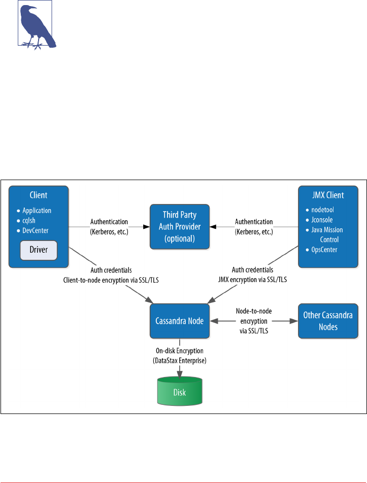
All of this publicity and regulatory rigor has resulted in a much increased level of vis‐
ibility on enterprise application security in general, and more pertinently for our dis‐
cussions, on NoSQL database security. Although a database is by definition only a
part of an application, it certainly forms a vital part of the attack surface of the appli‐
cation, because it serves as the repository of the application’s data.
Is Security a Weakness of NoSQL?
A 2012 Information Week report took the NoSQL community to
task for a perceived complacency and lack of prioritization of secu‐
rity features in NoSQL databases. While the security of many
NoSQL technologies, including Cassandra, has improved signifi‐
cantly since then, the paper serves as a healthy reminder of our
responsibilities and the need for continued vigilance.
Fortunately, the Cassandra community has demonstrated a commitment to continu‐
ous improvement in security over its relatively short lifespan, as we’ve seen already in
the release history in Chapter 2.
Cassandra’s security features include authentication, role-based authorization, and
encryption, as shown in Figure 13-1.
Figure 13-1. Cassandra’s security features
288 | Chapter 13: Security

In this chapter, we’ll explore these security features and how to access them via cqlsh
and other clients, with some thoughts along the way for how Cassandra fits into a
broader application security strategy.
Authentication and Authorization
Let’s take a look at Cassandra’s authentication and authorization features.
Password Authenticator
By default, Cassandra allows any client on your network to connect to your cluster.
This does not mean that no security is set up out of the box, but rather that Cassandra
is configured to use an authentication mechanism that allows all clients, without
requiring that they provide credentials. The security mechanism is pluggable, which
means that you can easily swap out one authentication method for another, or write
your own.
The authenticator that’s plugged in by default is the org.apache.cassandra. auth.
AllowAllAuthenticator. If you want to force clients to provide credentials, another
alternative ships with Cassandra, the org.apache.cassandra.auth.PasswordAuthen
ticator. In this section, we see how to use this second authenticator.
Conguring the authenticator
First, let’s shut down our cluster so that we can change the security configuration.
We’ll open the cassandra.yaml file and search for “authenticator”. You’ll find the fol‐
lowing line:
authenticator: AllowAllAuthenticator
Let’s change this line to use the PasswordAuthenticator:
authenticator: PasswordAuthenticator
If you’re using Cassandra 2.2 or later, you’ll see a note in the cassandra.yaml file indi‐
cating that the CassandraRoleManager must be used if the PasswordAuthenticator is
used. The CassandraRoleManager is part of Cassandra’s authorization capability and
we’ll discuss it in more depth momentarily.
Additional authentication providers
You can provide your own method of authenticating to Cassandra, such as a Ker‐
beros ticket, or if you want to store passwords in a different location, such as an
LDAP directory. In order to create your own authentication scheme, simply imple‐
ment the IAuthenticator interface. DataStax Enterprise Edition provides additional
authentication integrations.
Authentication and Authorization | 289

Cassandra also supports pluggable authentication between nodes via the IInternode
Authenticator interface. The default implementation AllowAllInternodeAuthenti
cator performs no authentication, but you are free to implement your own authenti‐
cator as a way to protect a node from making connections to untrusted nodes.
Adding users
Now we’ll save the cassandra.yaml file and restart our node or cluster, and try logging
in with cqlsh. Immediately we run into a problem:
$ bin/cqlsh
Connection error: ('Unable to connect to any servers',
{'127.0.0.1': AuthenticationFailed('Remote end requires
authentication.',)})
Prior versions of Cassandra might allow login, but would not allow any access. Ver‐
sions of Cassandra 2.2 and later require a password even to log in. Cassandra comes
with a default user known as cassandra, with “cassandra” as the password. Let’s try
logging in again with these credentials:
$ bin/cqlsh -u cassandra -p cassandra
Connected to Test Cluster at 127.0.0.1:9042.
[cqlsh 5.0.1 | Cassandra 3.0.0-rc1 | CQL spec 3.3.1 |
Native protocol v4]
Use HELP for help.
cassandra@cqlsh>
Once we’ve logged in successfully, we see that the prompt indicates that we are logged
in as the user cassandra. One of the first things we’ll want to do to begin securing our
installation is to change the password for this very important user. We’ve used a ran‐
dom password generator here as an example:
cassandra@cqlsh> ALTER USER cassandra WITH PASSWORD 'Kxl0*nGpB6'
Make sure to store the cassandra user’s password in a secure location.
Now, let’s create a new user account. We’ll specify a username and password. The
password is optional, but of course recommended.
cassandra@cqlsh> CREATE USER jeff WITH PASSWORD 'i6XJsj!k#9';
The CREATE USER command also supports the IF NOT EXISTS syntax to avoid errors
on multiple attempts to create a user. Now, we’ll check to see that we’ve created the
user successfully by using the LIST USERS command:
cassandra@cqlsh> LIST USERS;
name | super
-----------+-------
cassandra | True
jeff | False
290 | Chapter 13: Security

(2 rows)
You’ll note that the user cassandra is listed as being a superuser. The superuser desig‐
nates the ability to perform all supported actions. Only a superuser can create other
users. We’ve already changed the password for the built-in user cassandra. You may
also want to create another superuser and remove the cassandra account’s superuser
status for additional security.
Conguring Automatic Login
To avoid having to enter a username and password on every login
to cqlsh, create a file in your home directory called .cqlshrc. You
can enter login credentials through lines like this:
; Sample ~/.cqlshrc file.
[authentication]
username = jeff
password = i6XJsj!k#9
Obviously, you’ll want to make sure this file is secure so that only
authorized users (such as your account) have access to the pass‐
word.
Other operations on users include the ALTER USER command, which allows us to
change a user’s password or superuser status, as well as the DROP USER command,
which we use to delete a user. A non-superuser can alter their own password using
the ALTER USER command, but all other operations require superuser status.
We can use the LOGIN command to switch users within cqlsh without restart:
cassandra@cqlsh> login jeff 'i6XJsj!k#9'
jeff@cqlsh>
You may choose to omit the password from the command, in which case cqlsh will
prompt you to enter the password. It’s preferable to enter passwords at the shell
prompt, rather than the command line, as cqlsh saves all of your commands to a file
called .cassandra/cqlsh_history under your home directory, including any passwords
you include on the command line when using the LOGIN command.
Authenticating via the DataStax Java driver
Of course, your applications don’t use cqlsh to access Cassandra, so it will be helpful
for us to learn how to authenticate to the client using the DataStax client drivers.
Building on the simple Java driver example from Chapter 8, let’s use the Cluster.
Builder.withCredentials() operation to provide the user name and password
when we construct our Cluster instance:
Authentication and Authorization | 291

Cluster cluster = Cluster.builder().addContactPoint("127.0.0.1").
withCredentials("jeff", "i6XJsj!k#9").
build();
This is a simple example that hardcodes the login credentials, but you could just as
easily use values stored in a secure configuration file or provided by an application
user. The login syntax is quite similar for the other DataStax drivers.
If you’ve configured an authenticator on your nodes other than the default, you’ll also
need to configure a compatible authenticator in your clients as well. Client authenti‐
cation providers implement the com.datastax.driver.core.AuthProvider inter‐
face. The default implementation is the PlainTextAuthProvider class, an instance of
which is registered when we call the Cluster.Builder.withCredentials() opera‐
tion.
Other implementations provided with the driver are found in the com.datastax.
driver.auth package. These include the DseAuthProvider for connecting to Data‐
Stax Enterprise clusters, and the KerberosAuthenticator.
You select these providers when constructing your Cluster object by calling the
Cluster.Builder.withAuthProvider() operation.
Using CassandraAuthorizer
It is certainly possible to only use authentication, although in most cases you’ll want
to make use of Cassandra’s authorization capabilities as well. Cassandra’s out-of-the-
box configuration authorizes all clients to access all keyspaces and tables in your clus‐
ter. As with authentication, the authentication mechanism is pluggable.
The authorizer that’s plugged in by default is the org.apache.cassandra.auth.Allow
AllAuthorizer. To enable Cassandra’s role-based access control, we’ll need to config‐
ure the org.apache.cassandra.auth.CassandraAuthorizer.
Again, we’ll shut down the cluster to enable us to change the authorizer. In the cas‐
sandra.yaml file, we’ll search for “authorizer”. We’ll find the line:
authorizer: AllowAllAuthorizer
and change it to:
authorizer: CassandraAuthorizer
Once we restart our cluster, we can log into cqlsh again as our regular user to see
what we can access, making use of the hotel data we’ve stored in our cluster in previ‐
ous chapters:
$ cqlsh -u jeff –p 'i6XJsj!k#9'
...
jeff@cqlsh> DESCRIBE KEYSPACES;
292 | Chapter 13: Security

hotel system_schema system_auth system system_distributed
system_traces
jeff@cqlsh> USE hotel;
jeff@cqlsh:hotel> DESCRIBE TABLES;
hotels
jeff@cqlsh:hotel> select * from hotels;
Unauthorized: code=2100 [Unauthorized] message="User jeff has no
SELECT permission on <table hotel.hotels> or any of its parents"
As you can see, we are able to navigate through cqlsh to view the names of the vari‐
ous keyspaces and tables, but once we attempt to access data, we are denied access.
To fix this, we’ll need to switch back into a superuser role and grant our user some
permissions. For example, let’s allow our user to access the hotels table:
cassandra@cqlsh> GRANT SELECT ON hotel.hotels TO jeff;
Now, if we log back in as our regular user and run our SELECT command again, we’ll
see the data we’ve stored in our hotel table previously.
Getting Help with Permissions
Use the cqlsh commands HELP GRANT and HELP PERMISSIONS to
get additional information on configuring permissions.
Role-Based Access Control
In a large Cassandra cluster, there might be a lot of different keyspaces and tables,
with many different potential users. It would be difficult to keep track of the permis‐
sions assigned to many different users. While it’s tempting to share login information
with multiple support staff, there is a better way.
Starting with the 2.2 release, Cassandra provides a role-based access control (RBAC)
capability. This allows us to create roles and assign permissions to these roles. Roles
can be granted to individual users in any combination. Roles can themselves contain
other roles.
To see how this works, let’s create a hotel management role and grant it all permis‐
sions to all of the tables in the hotel keyspace:
cassandra@cqlsh> CREATE ROLE hotel_management;
cassandra@cqlsh> GRANT ALL ON KEYSPACE hotel TO hotel_management;
We’ve created a simple role here to which you can’t log in to directly. You can also
create roles that have superuser privileges, and roles that support login and take a
password.
Authentication and Authorization | 293

Now we’ll apply this role to our regular user:
cassandra@cqlsh> GRANT hotel_management TO jeff;
Roles are additive in Cassandra, meaning that if any of the roles granted to a user
have a specific permission granted, then that permission is granted to the user.
Behind the scenes, Cassandra stores users and roles in the system_auth keyspace. If
we’ve configured authorization for our cluster, only administrative users can access
this keyspace, so let’s examine its contents in cqlsh using our administrator login:
cassandra@cqlsh> DESCRIBE KEYSPACE system_auth
CREATE KEYSPACE system_auth WITH replication = {'class': 'SimpleStrategy',
'replication_factor': '1'} AND durable_writes = true;
...
We’ve truncated the output, but if you run this command, you’ll see the tables that
store the roles, their permissions, and role assignments. There is actually no separate
concept of a user at the database level—Cassandra uses the role concept to track both
users and roles.
Changing the system_auth replication Factor
It’s important to note that the system_auth keyspace is configured
out of the box to use the SimpleStrategy with a replication factor
of one.
This means that by default, any users, roles, and permissions we
configure will not be distributed across the cluster until we recon‐
figure the replication strategy of the system_auth keyspace to
match our cluster topology.
Encryption
Protecting user privacy is an important aspect of many systems, especially with
respect to health, financial, and other personal data. Typically we protect privacy by
encrypting data, so that if the data is intercepted, it is unusable to an attacker who
does not have the encryption key. Data can be encrypted as it moves around the pub‐
lic Internet and within our internal systems, also known as data in motion, or it can
be encrypted on systems where it is persisted. This is known as data at rest.
As of the 3.0 release, Cassandra secures data in motion via encryption between clients
and servers (nodes) and encryption between nodes. As of Cassandra 3.0, encryption
of data files (data at rest) is only supported in DataStax Enterprise releases of Cassan‐
dra.
294 | Chapter 13: Security

Data File Encryption Roadmap
There are several Cassandra JIRA requests targeted for the 3.X
release series that provide encryption features. For example, the
following were added in the 3.4 release:
•CASSANDRA-11040 - encryption of hints
•CASSANDRA-6018 - encryption of commit logs
See also CASSANDRA-9633 on encryption of SSTables, and
CASSANDRA-7922, which serves as an umbrella ticket for file-
level encryption requests.
Before we start configuring nodes to enable encryption, we have some preparation
work to do to create security certificates that are a key part of the machinery.
SSL, TLS, and Certicates
Cassandra uses Transport Layer Security (TLS) for encrypting data in motion. TLS is
often referenced by the name of its predecessor, Secure Sockets Layer (SSL). TLS is a
cryptographic protocol for securing communications between computers to prevent
eavesdropping and tampering. More specifically, TLS makes use of public key cryp‐
tography (also known as asymmetric cryptography), in which a pair of keys is used to
encrypt and decrypt messages between two endpoints: a client and a server.
Prior to establishing a connection, each endpoint must possess a certificate contain‐
ing a public and private key pair. Public keys are exchanged with communication
partners, while private keys are not shared with anyone.
To establish a connection, the client sends a request to the server indicating the
cipher suites it supports. The server selects a cipher suite from the list that it also sup‐
ports and replies with a certificate that contains its public key. The client optionally
validates the server’s public key. The server may also require that the client provide its
public key in order to perform two-way validation. The client uses the server’s public
key to encrypt a message to the server in order to negotiate a session key. The session
key is a symmetric key generated by the selected cipher suite which is used for subse‐
quent communications.
For many applications of public key cryptography, the certificates are obtained from a
certificate authority, but because we typically control both the clients and our Cassan‐
dra nodes, we don’t need quite that level of validation. For our purposes, we can gen‐
erate our certificates with a simple tool that is provided with Java, the keytool.
The following command gives an example of how we can use the -genkey switch on
keytool to generate a public/private key pair:
Encryption | 295

$ keytool -genkey -keyalg RSA -alias node1 -keystore node1.keystore
-storepass cassandra -keypass cassandra
-dname "CN=Jeff Carpenter, OU=None, O=None, L=Scottsdale, C=USA"
This command generates the keypair for one of our Cassandra nodes, which we’ll call
“node1”, and places the keypair in a file called a keystore. We call our keystore
node1.keystore. We provide passwords for the keystore and for the keypair, and a dis‐
tinguished name specified according to the Lightweight Directory Access Prototol
(LDAP) format.
The example command we’ve shown here provides the bare minimum set of
attributes for generating a key. We could also provide fewer attributes on the com‐
mand line and allow keytool to prompt us for the remaining ones, which is more
secure for entering passwords.
Then we export the public key of each certificate to a separate file that we can share
with others:
$ keytool -export -alias node1 -file node0.cer -keystore node1.keystore
Enter keystore password:
Certificate stored in file <node0.cer>
We identify the key we want to export from the keystore via the same alias as before,
and provide the name of the output file. keytool prompts us for the keystore pass‐
word and generates the certificate file.
We repeat this procedure to generate keys for each node and client.
Node-to-Node Encryption
Now that we have keys for each of our Cassandra nodes, we are ready to enable node-
to-node configuration by setting the server_encryption_options in the cassan‐
dra.yaml file:
server_encryption_options:
internode_encryption: none
keystore: conf/.keystore
keystore_password: cassandra
truststore: conf/.truststore
truststore_password: cassandra
# More advanced defaults below:
# protocol: TLS
# algorithm: SunX509
# store_type: JKS
# cipher_suites: [TLS_RSA_WITH_AES_128_CBC_SHA,...]
# require_client_auth: false
First, we set the internode_encryption option. We can select all to encrypt all inter-
node communications, dc to encrypt between data centers, and rack to encrypt
296 | Chapter 13: Security

between racks. We provide the password for the keystore and set its path, or we can
place the keystore file we created earlier at the default locations in the conf directory.
Next, we configure options for a file similar to the keystore called the truststore. We
generate a truststore for each node containing the public keys of all the other nodes in
our cluster. For example, to add the certificate for node 1 to the keystore for node
two, we would use the command:
$ keytool -import -v -trustcacerts -alias node1 -file node1.cer
-keystore node2.truststore
Enter keystore password:
Re-enter new password:
Owner: CN=Jeff Carpenter, OU=None, O=None, L=Scottsdale, C=USA
Issuer: CN=Jeff Carpenter, OU=None, O=None, L=Scottsdale, C=USA
Serial number: 52cf9209
Valid from: Thu Dec 17 17:01:03 MST 2015 until: Wed Mar 16 17:01:03 MST 2016
Certificate fingerprints:
MD5: E2:B6:07:C0:AA:BB:71:E8:47:8A:2A:81:FE:48:2F:AB
SHA1: 42:3E:9F:85:0D:87:02:50:A7:CD:C5:EF:DD:D1:6B:C2:78:2F:B0:E7
SHA256: C1:F0:51:5B:B6:C7:B5:8A:57:7F:D0:F2:F7:89:C7:34:30:79:30:
98:0B:65:75:CE:03:AB:AA:A6:E5:F5:6E:C0
Signature algorithm name: SHA256withRSA
Version: 3
Extensions:
#1: ObjectId: 2.5.29.14 Criticality=false
SubjectKeyIdentifier [
KeyIdentifier [
0000: C2 32 58 D0 55 27 5C D2 FB 1E 50 C9 76 21 30 5C .2X.U'\...P.v!0\
0010: E6 1A 7D CF ....
]
]
Trust this certificate? [no]: y
Certificate was added to keystore
[Storing truststore.node1]
keytool prompts us to enter a password for the new truststore and then prints out
summary information about the key we’re importing.
The cassandra.yaml file also presents us with a series of “advanced” options to config‐
ure the cryptography. These options provide you the ability to select from Java’s menu
of supported cryptographic algorithms and libraries. For example, for Java 8, you can
find the descriptions of these items at http://docs.oracle.com/javase/8/docs/technotes/
guides/security/StandardNames.html.
The defaults will be sufficient in most cases, but it’s helpful to understand what
options are available. We can see how these options are used in Cassandra by examin‐
Encryption | 297

ing the class org.apache.cassandra.security.SSLFactory, which Cassandra uses
to generate secure sockets.
The protocol option specifies the protocol suite that will be used to instantiate a
javax.net.ssl.SSLContext. As of Java 8, the supported values include SSLv2,
SSLv3, TLSv1, TLSv1.1, or TLSv1.2. You can also use the shortcuts SSL or TLS to get
the latest supported version of either suite.
The algorithm option specifies the setting provided to obtain an instance of
javax.net.ssl.TrustManagerFactory. This defaults to the X.509 certificate.
The store_type option specifies the setting provided to obtain an instance of java.
security.KeyStore. The default value jks indicates a keystore built by keytool,
which is exactly what we have.
The cipher_suites option is a list of encryption algorithms in order of preference.
The cipher suite to use is determined by the client and server in negotiating their
connection, based on the priority specified in this list. The same technique is used by
your browser in negotiating with web servers when you visit websites using https:
URLs. As demonstrated by the defaults, you’ll typically want to prefer stronger cipher
suites by placing them at the front of the list. If you don’t have total control over your
clients, you may even wish to remove weaker suites entirely to eliminate the threat of
a downgrade attack.
Finally, we can also enable two-way certificate authentication in which the client
authenticates the server as well by setting require_client_auth to true.
Client-to-Node Encryption
Client-to-node encryption protects data as it moves from client machines to nodes in
the cluster. The client_encryption_options in the cassandra.yaml file are quite sim‐
ilar to the node-to-node options:
# enable or disable client/server encryption.
client_encryption_options:
enabled: false
optional: false
keystore: conf/.keystore
keystore_password: cassandra
# require_client_auth: false
# Set truststore and truststore_password if require_client_auth is true
# truststore: conf/.truststore
# truststore_password: cassandra
# More advanced defaults below:
# protocol: TLS
# algorithm: SunX509
# store_type: JKS
# cipher_suites: [TLS_RSA_WITH_AES_128_CBC_SHA,...]
298 | Chapter 13: Security

The primary differences from the server_encryption_options are the enabled
option, which serves as the on/off switch for client-to-node encryption, and the
optional option, which indicates whether clients may choose either encrypted or
unencrypted connections.
The keystore and truststore settings will typically be the same as those in the
server_encryption_options, although it is possible to have separate files for the cli‐
ent options.
Note that setting require_client_auth for clients means that the truststore for each
node will need to have a public key for each client that will be using a encrypted con‐
nection.
Simplied Certicate Management
Configuring truststores for Cassandra nodes can become something of a logistical
problem if you’re adding nodes to your cluster or additional clients on a regular basis.
A common practice is to reuse the same certificate for all of the nodes in a cluster, and
a second certificate for all of the clients.
This approach simplifies the process of managing your cluster greatly as you won’t
have to reconfigure truststores and restart nodes in order to add nodes and clients.
This comes at the cost of fine-grained control over the trust you assign to individual
nodes and clients.
Whatever scheme you choose to manage your certificates, the overall security of your
Cassandra cluster depends on limiting access to the computers on which your nodes
are running so that the configuration can’t be tampered with.
JMX Security
We learned how Cassandra exposes a monitoring and management capability via
JMX in Chapter 10. In this section, we’ll learn how to make that management inter‐
face secure, and what security-related options we can configure using JMX.
Securing JMX Access
By default, Cassandra only makes JMX accessible from localhost. This is fine for sit‐
uations where you have direct machine access, but if you’re running a large cluster, it
may not be practical to log in to the machine hosting each node in order to access
with tools such as nodetool or OpsCenter.
For this reason, Cassandra provides the ability to expose its JMX interface for remote
access. Of course, it would be a waste to invest our efforts in securing access to Cas‐
JMX Security | 299

sandra via the native transport, and leave a major attack surface like JMX vulnerable.
So let’s see how to enable remote JMX access in a way that is secure.
First, we’ll stop our node or cluster and edit the conf/cassandra-env.sh file (or
cassandra-env.ps1 on Windows). Look for the setting LOCAL_JMX, and change it as fol‐
lows:
LOCAL_JMX=no
Setting this value to anything other than “yes” causes several additional properties to
be set, including properties that enable the JMX port to be accessed remotely:
JVM_OPTS="$JVM_OPTS -Dcom.sun.management.jmxremote.port=$JMX_PORT"
JVM_OPTS="$JVM_OPTS -Dcom.sun.management.jmxremote.rmi.port=$JMX_PORT"
Next, there is a property that configures whether SSL is used to encrypt JMX connec‐
tions (we’ll discuss it in more depth momentarily):
JVM_OPTS="$JVM_OPTS -Dcom.sun.management.jmxremote.ssl=false"
Finally, there are properties that configure remote authentication for JMX:
JVM_OPTS="$JVM_OPTS -Dcom.sun.management.jmxremote.authenticate=true"
JVM_OPTS="$JVM_OPTS -Dcom.sun.management.jmxremote.password.file=
/etc/cassandra/jmxremote.password"
The location of the jmxremote.password file is entirely up to you. Keep in mind that
you’ll want to specify a location for the file that is accessible only to users that you
intend to have access. We’ll configure the jmxremote.password file in just a minute,
but first let’s finish up our configuration edits by saving the cassandra-env.sh file.
Your JRE installation comes with a template jmxremote.password file under the jre/lib/
management directory. Typically you will find installed JREs under C:\Program Files
\Java on Windows, /Library/Java/JavaVirtualMachines on Mac OS, and /usr/lib/java
on Linux. Copy the jmxremote.password file to the location you set previously in
cassandra-env.sh and edit the file, adding a line with our administrator username and
password, as shown in bold here:
...
# monitorRole QED
# controlRole R&D
cassandra cassandra
We’ll also edit the jmxremote.access file under the jre/lib/management directory to add
read and write MBean access for our administrative user:
monitorRole readonly
controlRole readwrite \
create javax.management.monitor.*,javax.management.timer.* \
unregister
cassandra readwrite
300 | Chapter 13: Security

Configure the permissions on the jmxremote.password and jmxremote.access. Ideally,
the account under which you run Cassandra should have read-only access to this file,
and other non-administrative users should have no access.
Finally, we restart Cassandra and test that we’ve configured secure access correctly by
calling nodetool:
$ nodetool status -u cassandra -pw cassandra
We can also configure SSL for our JMX connection. To do this, we need to add a few
more JVM options in the cassandra-env file:
JVM_OPTS="${JVM_OPTS} -Dcom.sun.management.jmxremote.ssl=true"
JVM_OPTS="${JVM_OPTS} -Djavax.net.ssl.keyStore=conf/node1.keystore"
JVM_OPTS="${JVM_OPTS} -Djavax.net.ssl.keyStorePassword=cassandra"
JVM_OPTS="${JVM_OPTS} -Djavax.net.ssl.trustStore=conf/node1.truststore"
JVM_OPTS="${JVM_OPTS} -Djavax.net.ssl.trustStorePassword=cassandra"
JVM_OPTS="${JVM_OPTS} -Dcom.sun.management.jmxremote.ssl.need.client.auth=true"
Security MBeans
We learned about the various MBeans exposed by Cassandra in Chapter 10. For
understandable reasons, there are not many security-related configuration parame‐
ters that are accessible remotely via JMX, but there are some capabilities exposed via
the org.apache.cassandra.auth domain.
PermissionsCacheMBean
By default, Cassandra caches information about roles and permissions as a perfor‐
mance optimization. The amount of time permissions are cached is set in the cassan‐
dra.yaml file by the permissions_validity_in_ms property, defaulting to 2 seconds.
The PermissionsCacheMBean allows you to override this value to extend or shorten
the cache time, and also provides a command to invalidate all of the permissions in
cache. This could be a useful operation if you need to change permissions in your
cluster and need them to take effect immediately.
Summary
Cassandra is just one part of an enterprise application, but performs an important
part nonetheless. In this chapter, we learned how to configure Cassandra’s pluggable
authentication and authorization capabilities, and how to manage and grant permis‐
sions to users and roles. We enabled encryption between clients and nodes and
learned how to secure the JMX interface for remote access.
Summary | 301

CHAPTER 14
Deploying and Integrating
In this, our final chapter, it’s time to share a few last pieces of advice as you work
toward deploying Cassandra in production. We’ll discuss options to consider in plan‐
ning deployments and explore options for deploying Cassandra in various cloud
environments. We’ll close with a few thoughts on some technologies that complement
Cassandra well.
Planning a Cluster Deployment
A successful deployment of Cassandra starts with good planning. You’ll want to con‐
sider the amount of data that the cluster will hold, the network environment in which
the cluster will be deployed, and the computing resources (whether physical or vir‐
tual) on which the instances will run.
Sizing Your Cluster
An important first step in planning your cluster is to consider the amount of data that
it will need to store. You will, of course, be able to add and remove nodes from your
cluster in order to adjust its capacity over time, but calculating the initial and planned
size over time will help you better anticipate costs and make sound decisions as you
plan your cluster configuration.
In order to calculate the required size of the cluster, you’ll first need to determine the
storage size of each of the supported tables using the formulas we introduced in
Chapter 5. This calculation is based on the columns within each table as well as the
estimated number of rows and results in an estimated size of one copy of your data
on disk.
In order to estimate the actual physical amount of disk storage required for a given
table across your cluster, you’ll also need to consider the replication factor for the
303

table’s keyspace and the compaction strategy in use. The resulting formula for the
total size Tt is as follows:
Tt=St*RFk*CSFt
Where St is the size of the table calculated using the formula referenced above, RFk is
the replication factor of the keyspace, and CSFt is a factor representing the compac‐
tion strategy of the table, whose value is as follows:
•2 for the SizeTieredCompactionStrategy. The worst case scenario for this strat‐
egy is that there is a second copy of all of the data required for a major compac‐
tion.
•1.25 for other compaction strategies, which have been estimated to require an
extra 20% overhead during a major compaction.
Once we know the total physical disk size of the data for all tables, we can sum those
values across all keyspaces and tables to arrive at the total for our cluster.
We can then divide this total by the amount of usable storage space per disk to esti‐
mate a required number of disks. A reasonable estimate for the usable storage space
of a disk is 90% of the disk size.
Note that this calculation is based on the assumption of providing enough overhead
on each disk to handle a major compaction of all keyspaces and tables. It’s possible to
reduce the required overhead if you can ensure such a major compaction will never
be executed by an operations team, but this seems like a risky assumption.
Sizing Cassandra’s System Keyspaces
Alert readers may wonder about the disk space devoted to Cassan‐
dra’s internal data storage in the various system keyspaces. This is
typically insignificant when compared to the size of the disk. We
created a three-node cluster and measured the size of each node’s
data storage at about 18 MB with no additional keyspaces.
Although this could certainly grow considerably if you are making
frequent use of tracing, the system_traces tables do use TTL to
allow trace data to expire, preventing these tables from overwhelm‐
ing your data storage over time.
Once you’ve made calculations of the required size and number of nodes, you’ll be in
a better position to decide on an initial cluster size. The amount of capacity you build
into your cluster is dependent on how quickly you anticipate growth, which must be
balanced against cost of additional hardware, whether it be physical or virtual.
304 | Chapter 14: Deploying and Integrating

Selecting Instances
It is important to choose the right computing resources for your Cassandra nodes,
whether you are running on physical hardware or in a virtualized cloud environment.
The recommended computing resources for modern Cassandra releases (2.0 and
later) tend to differ for development versus production environments:
Development environments
Cassandra nodes in development environments should generally have CPUs with
at least two cores and 8 GB of memory. Although Cassandra has been success‐
fully run on smaller processors such as Raspberry Pi with 512 MB of memory,
this does require a significant performance-tuning effort.
Production environments
Cassandra nodes in production environments should have CPUs with at least
eight cores (although four cores are acceptable for virtual machines), and any‐
where from 16 MB to 64 MB of memory.
Docker and Other Container Deployments
Another deployment option that has been rapidly gaining in popularity, especially in
the Linux community, is software containers such as Docker.
The value proposition of containers is often phrased as “build once, deploy any‐
where.” Container engines support the ability to create lightweight, portable contain‐
ers for software that can be easily moved and deployed on a wide variety of hardware
platforms.
In Docker, each container is a lightweight virtual machine that provides process isola‐
tion, and a separate filesystem and network adapter. The Docker engine sits between
the application and the OS.
The primary challenges in deploying Cassandra in Docker have to do with network‐
ing and data directories. The default deployment in Docker uses software-defined
routing. At the time of writing, the performance of this layer currently reduces Cas‐
sandra throughput by somewhere around 50%, so the recommended configuration is
to use the host network stack directly. This limits the deployment to a single Cassan‐
dra node per container.
If you do attempt to run multiple Cassandra instances in a container, this is really
only appropriate for a development environment. You’ll want to carefully consider
the memory settings we discussed in Chapter 12.
From a data management perspective, you will want to configure data directories to
be outside of the container itself. This will allow you to preserve your data when you
want to upgrade or stop containers.
Planning a Cluster Deployment | 305

These same considerations apply in other container technologies, although the details
will be slightly different. This is an emerging area that is likely to see continuing
change over the coming months and years.
Storage
There are a few factors to consider when selecting and configuring storage, including
the type and quantities of drives to use:
HDDs versus SSDs
Cassandra supports both hard disk drives (HDDs, also called “spinning drives”)
and solid state drives (SSDs) for storage. Although Cassandra’s usage of append-
based writes is conducive to sequential writes on spinning drives, SSDs provide
higher performance overall because of their support for low-latency random
reads.
Historically, HDDs have been the more cost-effective storage option, but the cost
of using SSDs has continued to come down, especially as more and more cloud
platform providers support this as a storage option.
Disk conguration
If you’re using spinning disks, it’s best to use separate disks for data and commit
log files. If you’re using SSDs, the data and commit log files can be stored on the
same disk.
JBOD versus RAID
Traditionally, the Cassandra community has recommended using multiple disks
for data files, with the disks configured as a Redundant Array of Independent
Disks (RAID). Because Cassandra uses replication to achieve redundancy across
multiple nodes, the RAID 0 (or “striped volume”) configuration is considered
sufficient.
More recently, Cassandra users have been using a Just a Bunch of Disks (JBOD)
deployment style. The JBOD approach provides better performance and is a
good choice if you have the ability to replace individual disks.
Avoid shared storage
When selecting storage, avoid using Storage Area Networks (SAN) and Network
Attached Storage (NAS). Neither of these storage technologies scale well—they
consume additional network bandwidth in order to access the physical storage
over the network, and they require additional I/O wait time on both reads and
writes.
306 | Chapter 14: Deploying and Integrating

Network
Because Cassandra relies on a distributed architecture involving multiple networked
nodes, here are a few things you’ll need to consider:
roughput
First, make sure your network is sufficiently robust to handle the traffic associ‐
ated with distributing data across multiple nodes. The recommended network
bandwidth is 1 GB or higher.
Network conguration
Make sure that you’ve correctly configured firewall rules and IP addresses for
your nodes and network appliances to allow traffic on the ports used for the CQL
native transport, inter-node communication (the listen_address), JMX, and so
on. This includes networking between data centers (we’ll discuss cluster topology
momentarily).
The clocks on all nodes should be synchronized using Network Time Protocol
(NTP) or other methods. Remember that Cassandra only overwrites columns if
the timestamp for the new value is more recent than the timestamp of the exist‐
ing value. Without synchronized clocks, writes from nodes that lag behind can be
lost.
Avoid load balancers
Load balancers are a feature of many computing environments. While these are
frequently useful to spread incoming traffic across multiple service or application
instances, it’s not recommended to use load balancers with Cassandra. Cassandra
already provides its own mechanisms to balance network traffic between nodes,
and the DataStax drivers spread client queries across replicas, so strictly speaking
a load balancer won’t offer any additional help. Besides this, putting a load bal‐
ancer in front of your Cassandra nodes actually introduces a potential single
point of failure, which could reduce the availability of your cluster.
Timeouts
If you’re building a cluster that spans multiple data centers, it’s a good idea to
measure the latency between data centers and tune timeout values in the cassan‐
dra.yaml file accordingly.
A proper network configuration is key to a successful Cassandra deployment,
whether it is in a private data center, a public cloud spanning multiple data centers, or
even a hybrid cloud environment.
Planning a Cluster Deployment | 307

Cloud Deployment
Now that we’ve learned the basics of planning a cluster deployment, let’s examine our
options for deploying Cassandra in three of the most popular public cloud providers.
There are a couple of key advantages that you can realize by using commercial cloud
computing providers. First, you can select from multiple data centers in order to
maintain high availability. If you extend your cluster to multiple data centers in an
active-active configuration and implement a sound backup strategy, you can avoid
having to create a separate disaster recovery system.
Second, using commercial cloud providers allows you to situate your data in data
centers that are closer to your customer base, thus improving application response
time. If your application’s usage profile is seasonal, you can expand and shrink your
clusters in each data center according to the current demands.
You may want to save time by using a prebuilt image that already contains Cassandra.
There are also companies that provide Cassandra as a managed service in a Software-
as-a-Service (SaaS) offering.
Don’t Forget Cloud Resource Costs
In planning a public cloud deployment, you’ll want to make sure to
estimate the cost to operate your cluster. Don’t forget to account for
resources including compute services, node and backup storage,
and networking.
Amazon Web Services
Amazon Web Services (AWS) has been a popular deployment option for Cassandra,
as evidenced by the presence of AWS-specific extensions in the Cassandra project
such as the Ec2Snitch, Ec2MultiRegionSnitch, and the EC2MultiRegion Address
Translator in the DataStax Java Driver.
Cluster layout
AWS is organized around the concepts of regions and availability zones, which
are typically mapped to the Cassandra constructs of data centers and racks,
respectively. A sample AWS cluster topology spanning the us-east-1 (Virginia)
and eu-west-1 (Ireland) regions is shown in Figure 14-1. The node names are
notional—this naming is not a required convention.
308 | Chapter 14: Deploying and Integrating
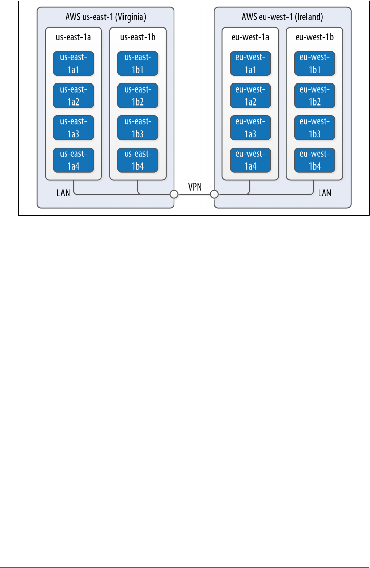
Figure 14-1. Topology of a cluster in two AWS regions
EC2 instances
The Amazon Elastic Compute Cloud (EC2) provides a variety of different virtual
hardware instances grouped according to various classes. The two classes most
frequently recommended for Cassandra deployments are the M-class and the I-
class.
M-class instances are general-purpose instances that balance compute, memory,
and network resources and are generally acceptable for development and light
production environments. Later M-class instances such as M3 and M4 are SSD-
backed.
The I-class instances are all SSD-backed and designed for high I/O. These instan‐
ces come at a higher cost that generally pays off for heavily loaded production
clusters.
You can find more information about the various instance types available at
https://aws.amazon.com/ec2/instance-types.
DataStax Enterprise provides a prebuilt Amazon Machine Image (AMI) to sim‐
plify deployment (an AMI for DataStax Community Edition was discontinued
after the Cassandra 2.1 release).
Data storage
Historically, the recommended disk option in AWS was to use ephemeral storage
attached to each instance. The drawback of this is that if an instance on which a
node is running is terminated (as happens occasionally in AWS), the data is lost.
Cloud Deployment | 309

By late 2015, the network-attached storage known as Elastic Block Store (EBS)
has been proven to provide a reliable place to store data that doesn’t go away
when EC2 instances are dropped, at the cost of additional latency.
AWS Services such as S3 and Glacier are a good option for short- to medium-
term and long-term storage of backups, respectively.
Networking
If you’re running a multi-region configuration, you’ll want to make sure you have
adequate networking between the regions. Many have found that using elements
of the AWS Virtual Private Cloud (VPC) provides an effective way of achieving
reliable, high-throughput connections between regions. AWS Direct Connect
provides dedicated private networks, and there are virtual private network (VPN)
options available as well. These services of course come at an additional cost.
If you have a single region deployment or a multi-region deployment using VPN
connections between regions, use the Ec2Snitch. If you have a multi-region
deployment that uses public IP between regions, use the Ec2MultiRegionSnitch.
For either snitch, increasing the phi_convict_threshold value in the cassan‐
dra.yaml file to 12 is generally recommended in the AWS network environment.
Microsoft Azure
DataStax and Microsoft have partnered together to help improve deployment of Cas‐
sandra in Microsoft’s Azure on both Windows and Ubuntu Linux OSs.
Cluster layout
Azure provides data centers in locations worldwide, using the same term “region”
as AWS. The concept of availability sets is used to manage collections of VMs.
Azure manages the assignment of the VMs in an availability set across update
domains, which equate to Cassandra’s racks.
Virtual machine instances
Similar to AWS, Azure provides several classes of VMs. The D series, D series v2,
and G series machines are all SSD-backed instances appropriate for Cassandra
deployments. The G series VMs provide additional memory as required for inte‐
grations such as those described next. You can find more information about
Azure VM types at https://azure.microso.com/en-us/pricing/details/virtual-
machines.
Data storage
Azure provides a standard SSD capability on the previously mentioned instances.
In addition, you can upgrade to use Premium Storage, which provides network-
attached SSDs in larger sizes up to 1 TB.
310 | Chapter 14: Deploying and Integrating

Networking
Public IP addresses are recommended for both single-region and multi-region
deployments. Use the GossipingPropertyFileSnitch to allow your nodes to
detect the cluster topology. Networking options between regions include VPN
Gateways and the Express Route, which provides up to 2 GB/s throughput.
Google Cloud Platform
Google Cloud Platform provides cloud computing, application hosting, networking,
storage, and various Software-as-a-Service (SaaS) offerings such as Google’s Translate
and Prediction APIs.
Cluster layout
The Google Compute Environment (GCE) provides regions and zones, corre‐
sponding to Cassandra’s data centers and racks, respectively.
Virtual machine instances
GCE’s n1-standard and n1-highmemory machine types are recommended for
Cassandra deployments. You can launch Cassandra quickly on the Google Cloud
Platform using the Cloud Launcher. For example if you search the launcher at
https://cloud.google.com/launcher/?q=cassandra, you’ll find options for creating a
cluster in just a few button clicks.
Data storage
GCE provides both spinning disk (pd-hdd) and solid state disk options for both
ephemeral drives (local-ssd) and network-attached drives (pd-ssd). There are
three storage options that can be used to store Cassandra backups, each with dif‐
ferent cost and availability profiles: Standard, Durable Reduced Availability
(DRA), and Nearline.
Networking
The GoogleCloudSnitch is a custom snitch designed just for the GCE. VPN net‐
working is available between regions.
Cloud Deployment | 311

Integrations
As we learned in Chapter 2, Cassandra is a great solution for many applications, but
that doesn’t guarantee that it provides everything you need for your application or
enterprise. In this section, we’ll discuss several technologies that can be paired with
Cassandra in order to provide more robust solutions for features such as searching
and analytics.
Apache Lucene, SOLR, and Elasticsearch
One of the features that is commonly required in applications built on top of Cassan‐
dra is full text searching. This capability can be added to Cassandra via Apache
Lucene, which provides an engine for distributed indexing and searching, and its
subproject, Apache Solr, which adds REST and JSON APIs to the Lucene search
engine.
Elasticsearch is another popular open source search framework built on top of
Apache Lucene. It supports multitenancy and provides Java and JSON over HTTP
APIs.
Stratio has provided a plugin that can be used to replace Cassandra’s standard secon‐
dary index implementation with a Lucene index. When using this integration, there is
a Lucene index available on each Cassandra node that provides high performance
search capability.
Apache Hadoop
Apache Hadoop is a framework that provides distributed storage and processing of
large data sets on commodity hardware. This work originated at Google in the early
2000s. Google found that several internal groups had been implementing similar
functionality for data processing, and that these tools commonly had two phases: a
map phase and a reduce phase. A map function operates over raw data and produces
intermediate values. A reduce function distills those intermediate values, producing
the final output. In 2006, Doug Cutting wrote open source implementations of the
Google File System, and MapReduce, and thus, Hadoop was born.
Similar to Cassandra, Hadoop uses a distributed architecture with nodes organized in
clusters. The typical integration is to install Hadoop on each Cassandra node that will
be used to provide data. You can use Cassandra as a data source by running a Hadoop
Task Tracker and Data Node on each Cassandra node. Then, when a MapReduce job
is initiated (typically on a node external to the Cassandra cluster), the Job Tracker can
query Cassandra for data as it tracks map and reduce tasks, as shown in Figure 14-2.
312 | Chapter 14: Deploying and Integrating
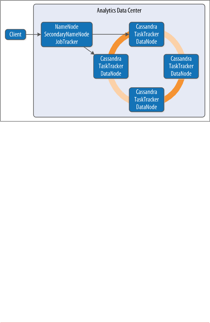
Figure 14-2. Topology of a Hadoop-Cassandra cluster
Starting in the late 2000s, Hadoop has been a huge driver of interest and growth in
the Big Data community. Due to its popularity, a large ecosystem of extensions has
developed around Hadoop, such as Apache Pig, which provides a framework and lan‐
guage for data analysis, and Apache Hive, a data warehouse tool. The Hadoop com‐
munity has begun moving away from MapReduce because of its relatively slow
performance (all data is written to disk, even for intermediate processing steps), high
memory use, non-intuitive API, and batch-only processing mode. For this reason, the
emergence of the Apache Spark project has been a significant development.
Apache Spark
with Patrick McFadin
Apache Spark is an emerging data analytics framework that provides a massively par‐
allel processing framework to enable simple API calls across large volumes of data.
Originally developed in 2009 at UC Berkeley as an improvement to MapReduce,
Spark was open sourced in 2010, and became an Apache project in 2014.
Unlike Hadoop, which writes intermediate results to disk, the Spark core processing
engine is designed to maximize memory usage while minimizing disk and network
access. Spark uses streaming instead of batch-oriented processing to achieve process‐
ing speeds up to 100 times faster than Hadoop. In addition, Spark’s API is much sim‐
pler to use than Hadoop.
Integrations | 313

The basic unit of data representation in Spark is the Resilient Distributed Dataset
(RDD). The RDD is a description of the data to be processed, such as a file or data
collection. Once an RDD is created, the data contained can be transformed with API
calls as if all of the data were contained in a single machine. However, in reality, the
RDD can span many nodes in the network by partitioning. Each partition can be
operated on in parallel to produce a final result. The RDD supports the familiar map
and reduce operations plus additional operations such as count, filter, union, and
distinct. For a full list of transformations, see the Spark documentation.
In addition to the core engine, Spark includes further libraries for different types of
processing requirements. These are included as subprojects that are managed sepa‐
rately from Spark core, but follow a similar release schedule:
•SparkSQL provides familiar SQL syntax and relational queries over structured
data.
•MLlib is Spark’s machine learning library.
• SparkR provides support for using the R statistics language in Spark jobs.
• GraphX is Spark’s library for graph and collection analytics.
• Spark Streaming provides near real-time processing of live data streams.
Use cases for Spark with Cassandra
As we’ve discussed in this book, Apache Cassandra is a great choice for transactional
workloads that require high scale and maximum availability. Apache Spark is a great
choice for analyzing large volumes of data at scale. Combining the two enables many
interesting use cases that exploit the power of both technologies.
An example use case is high-volume time-series data. A system for ingesting weather
data from thousands of sensors with variable volume is a perfect fit for Cassandra.
Once the data is collected, further analysis on data stored in Cassandra may be diffi‐
cult given that the analytics capabilities available using CQL are limited. At this point,
adding Spark to the solution will open many new uses for the collected data. For
example, we can pre-build aggregations from the raw sensor data and store those
results in Cassandra tables for use in frontend applications. This brings analytics
closer to users without the need to run complex data warehouse queries at runtime.
Or consider the hotel application we’ve been using throughout this book. We could
use Spark to implement various analytic tasks on our reservation and guest data, such
as generating reports on revenue trends, or demographic analysis of anonymized
guest records.
One use case to avoid is using Spark-Cassandra integration as an alternative to a
Hadoop workload. Cassandra is suited for transactional workloads at high volume
and shouldn’t be considered as a data warehouse. When approaching a use case where
both technologies might be needed, first apply Cassandra to solving a problem suited
314 | Chapter 14: Deploying and Integrating
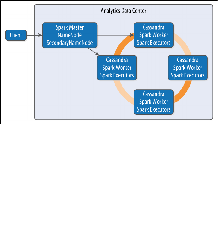
for Cassandra, such as those we discuss in Chapter 2. Then consider incorporating
Spark as a way to analyze and enrich the data stored in Cassandra without the cost
and complexity of extract, transform, and load (ETL) processing.
Deploying Spark with Cassandra
Cassandra places data per node based on token assignment. This existing data distri‐
bution can be used as an advantage to parallelize Spark jobs. Because each node con‐
tains a subset of the cluster’s data, the recommended configuration for Spark-
Cassandra integrations is to co-locate a Spark Worker on each Cassandra node in a
data center, as shown in Figure 14-3.
Figure 14-3. Topology of a Spark-Cassandra cluster
When a job is submitted to the Spark Master, the Spark Workers on each node spawn
Spark Executors to complete the work. Using the spark-cassandra-connector as a
conduit, he data required for each job is sourced from the local node as much as pos‐
sible. We’ll learn more about the connector momentarily.
Because each node contains a portion of the entire data in the cluster, each Spark
Worker will only need to process that local subset of data. An example is a count
action on a table. Each node will have a range of the table’s data. The count is calcula‐
ted locally and then merged from every node to produce the total count.
This design maximizes data locality, resulting in improved throughput and lower
resource utilization for analytic jobs. The Spark Executors only communicate over
Integrations | 315

the network when data needs to be merged from other nodes. As cluster sizes get
larger, the efficiency gains of this design are much more pronounced.
Using a Separate Data Center for Analytics
A common deployment model for Cassandra and analytics toolsets such as Spark is
to create a separate data center for analytic processing. This has the advantage of iso‐
lating the performance impact of analytics workloads from the rest of the cluster. The
analytics data center can be constructed as a “virtual” data center where the actual
hardware exists in the same physical location as another data center within the clus‐
ter. Using the NetworkTopologyStrategy, you can specify a lower replication factor
for the analytics data center, as your required availability in this data center will typi‐
cally be lower.
The spark-cassandra-connector
The spark-cassandra-connector is an open source project sponsored by DataStax
on GitHub. The connector can be used by clients as a conduit to read and write data
from Cassandra tables via Spark. The connector provides features including SQL
queries and server-side filtering. The connector is implemented in Scala, but a Java
API is available as well. API calls from the spark-cassandra-connector provide
direct access to data in Cassandra in a context related to the underlying data. As
Spark accesses data, the connector translates to and from Cassandra as the data
source.
To start using the spark-cassandra-connector, you’ll need to download both the
connector and Spark. Although a detailed installation guide is beyond our scope here,
we’ll give a quick summary. For a more fulsome introduction, we suggest the O’Reilly
book Learning Spark. You can download either a pre-built version of Spark, or you
can build Spark yourself from the source.
If you’re building an application in Java or Scala and using Maven, you’ll want to add
dependencies such as the following to your project’s pom.xml file to access the Spark
core and connector:
<dependency>
<groupId>org.apache.spark</groupId>
<artifactId>spark-core_2.10</artifactId>
<version>1.5.2</version>
</dependency>
<dependency>
<groupId>com.datastax.spark</groupId>
<artifactId>spark-cassandra-connector_2.10</artifactId>
<version>1.5.0</version>
</dependency>
316 | Chapter 14: Deploying and Integrating

Spark supports two modes of deployment: local and cluster. Cluster mode involves a
central Spark Master and many compute nodes. Local mode runs entirely on the local
host; this mode is best suited for development. For this example, we will run in local
mode, but clustering requires only a few more steps.
Let’s review the common API elements used for most Spark jobs accessing data in
Cassandra. In this section, we’ve chosen to write our examples in Scala because of its
simplicity and readability, as well as the fact that Spark and many Spark applications
are written in Scala. The Java API is similar but quite a bit more verbose; we’ve pro‐
vided a Java version of this example code in the GitHub repository for this book. To
connect your Spark application to Cassandra, you will first need to create a SparkCon
text containing connection parameters:
val conf = new SparkConf(true)
.set("spark.cassandra.connection.host", "127.0.0.1")
.setMaster("local[*]")
.setAppName(getClass.getName)
// Optionally
.set("cassandra.username", "cassandra")
.set("cassandra.password", "cassandra")
val sc = new SparkContext(conf)
Establishing a connection between Cassandra and Spark is simply the process of
pointing to the running Cassandra cluster and Spark Master. This example configura‐
tion shows how to connect to a local Cassandra node and Spark Master. You can also
provide Cassandra login credentials if required.
Once the SparkContext is created, you can then operate on Cassandra data by creat‐
ing an RDD representing a Cassandra table. For example, let’s create an RDD repre‐
senting the reservations_by_hotel_date table from the reservation keyspace
introduced in Chapter 5:
val rdd = sc.cassandraTable("reservation",
"reservations_by_hotel_date")
Once you’ve created an RDD, you can perform transformations and actions on it. For
example, to get the total number of reservations, create the following action to count
every record in the table:
println("Number of reservations: " + rdd.count)
Because this is running as an analytics job in parallel with Cassandra, it is much more
efficient than running a SELECT count(*) FROM reservations from cqlsh.
As the underlying structure of the RDD is a Cassandra table, you can use CQL to fil‐
ter the data and select rows. In Cassandra, filter queries using native CQL require a
partition key to be efficient, but that restriction is removed when running queries as
Spark jobs.
Integrations | 317

For example, you might derive a use case to produce a report listing reservations by
end date, so that each hotel can know who is checking out on a given day. In this
example, end_date is not a partition key or clustering column, but you can scan the
entire cluster’s data looking for reservations with a checkout date of September 8,
2016:
val rdd = sc.cassandraTable("reservation",
"reservations_by_hotel_date")
.select("hotel_id", "confirm_number")
.where("end_date = ?", "2016-09-08")
// Invoke the action to run the spark job
rdd.toArray.foreach(println)
Finding and retrieving data is only half of the functionality available—you can also
save data back to Cassandra. Traditionally, data in a transactional database would
require extraction to a separate location in order to perform analytics. With the
spark-cassandra-connector, you can extract data, transform in place, and save it
directly back to a Cassandra table, eliminating the costly and error-prone ETL pro‐
cess. Saving data back to a Cassandra table is amazingly easy:
// Create a collection of guests with simple identifiers
val collection = sc.parallelize(Seq(("1", "Delaney", "McFadin"),
("2", "Quinn", "McFadin")))
// Save to the guests table
collection.saveToCassandra("reservation", "guests",
SomeColumns("guest_id", "first_name", "last_name"))
This is a simple example, but the basic syntax applies to any data. A more advanced
example would be to calculate the average daily revenue for a hotel and write the
results to a new Cassandra table. In a sensor application, you might calculate high
and low temperatures for a given day and write those results back out to Cassandra.
Querying data is not just limited to Spark APIs. With SparkSQL, you can use familiar
SQL syntax to perform complex queries on data in Cassandra, including query
options not available in CQL. It’s easy to create enhanced queries such as aggrega‐
tions, ordering, and joins.
To embed SQL queries inside your code, you need to create a CassandraSQLContext:
// Use the SparkContext to create a CassandraSQLContext
val cc = new CassandraSQLContext(sc)
// Set the keyspace
cc.setKeyspace("reservation")
val rdd = cc.cassandraSql("
SELECT hotel_id, confirm_number
FROM reservations_by_hotel_date
WHERE end_date = '2016-09-08'
318 | Chapter 14: Deploying and Integrating

ORDER BY hotel_id")
// Perform action to run SQL job
rdd.collect().foreach(println)
The SQL syntax is similar to the Spark job from before, but is more familiar to users
with a traditional database background. To explore data outside of writing Spark jobs,
you can also use the spark-sql shell, which is available under the bin directory in
your Spark installation.
Integrations in DataStax Enterprise
DataStax Enterprise is a productized version of Cassandra that supports many of the
integrations described in this chapter. Specifically, DSE Search provides integration
with Solr, while DSE Analytics provides integration with Apache Spark and elements
of the Hadoop ecosystem such as MapReduce, Hive, and Pig.
Additional DSE features include additional security provider plugins and an in-
memory configuration suitable for applications that require extremely fast response
times.
Summary
In this chapter, we’ve just scratched the surface of the many deployment and integra‐
tion options available for Cassandra. Hopefully we’ve piqued your interest in the wide
range of directions you can take your applications using Cassandra and related tech‐
nologies.
And now we’ve come to the end of our journey together. If we’ve achieved our goal,
you now have an in-depth understanding of the right problems to solve using Cas‐
sandra, and how to design, implement, deploy, and maintain successful applications.
Summary | 319

Index
Symbols
2PC (see two-phase commit)
? command, getting help in cqlsh, 50
A
AbstractCompactionStrategy, 121
AbstractReplicationStrategy, 112
accrual failure detection, 107
ACID (atomic, consistent, isolated, durable), 6
ActiveRepairService, 239
AddressTranslator interface, 167
aggregates, 198, 200-202
built-in, 202
defined in Java and JavaScript, native sup‐
port for, 199
user-defined, 129, 200
ALL consistency level, 113, 180, 191
speculative retry and, 205
allocate_tokens_keyspace property, 138
ALLOW FILTERING keyword, 197, 263
AllowAllAuthenticator, 289
AllowAllAuthorizer, 292
AllowAllInternodeAuthenticator, 290
ALTER TABLE command, 62
ALTER USER command, 291
Amazon Dynamo, 17, 22
Amazon EC2, 109, 140
Amazon Web Services (AWS), 5
Cassandra deployment on, 308
Priam, integration with, 260
snitches for, 140
analysis, using Cassandra for, 36
analytics
Apache Spark, 313
using a separate data center for, 316
Antadditional build targets, 43
downloading, 41
executing and compiling Cassandra source,
42
more build output with -v option, 42
anti-compaction, 239
anti-entropy, 122
meaning in Cassandra, 122
node repair via, 181
anti-entropy repair, 123
anticompaction, 122
ANY consistency level, 117, 180, 182
AP, primarily supporting availability and parti‐
tion tolerance, 26
Apache Cassandra (see Cassandra)
Apache Cassandra Wiki, 37
Apache Cloudstack, 109, 140
Apache Hadoop, 30, 312
Apache Lucene, 312
Apache Solr, 312
Apache Spark (see Spark)
append-only writes, 179
APPLY BATCH command, 189
architecture (Cassandra), 105-130
anti-entropy, repair, and Merkle trees, 122
Bloom filters, 120
compaction, 121
consistency levels, 113
data centers and racks, 105
gossip and failure detection, 106-108
hinted handoff, 117
managers and services, 125-128
321

memtables, SSTables, and commit logs,
115-117
queries and coordinator nodes, 114
replication strategies, 112
rings and tokens, 109
snitches, 108
staged event-driven architecture (SEDA),
124-125
system keyspaces, 128-130
tombstones, 120
AS SELECT clause (CREATE MATERIALIZED
VIEW), 95
ascii type, 67
assassinating nodes, 250
Astyanax (client), 152
asynchronous execution
CQL native protocol, 155
DataStax Java driver requests, 158
atomic batches, 188
atomicity (transactions), 6
in distributed systems, 9
attributes (JMX), 217
authentication, 289-294
DataStax Java driver support for, 154
password authenticator, 289-292
adding users, 290
additional authentication providers, 289
authenticating via DataStax Java driver,
291
configuring automatic login, 291
configuring the authenticator, 289
remote authentication for JMX, 300
two-way certificate authentication, 298
authorization
role-based access control, 293
using CassandraAuthorizer, 292
AuthProvider interface, 292
auto bootstrapping, 135
auto snapshot capability, 254
auto-scaling groups (ASGs), 260
autobootstrap property, 244, 245
automatic paging, 203
auto_snapshot property, 254
availability
consistency levels and, 180
high availability and fault tolerance with
Cassandra, 19
in CAP theorem, 23
avg function, 202
B
backup and recovery, 252-256
clearing a snapshot, 255
enabling incremental backup, 255
full, incremental, and differential backups,
253
restoring from snapshot, 255
taking a snapshot, 253
Bash shell emulator (Cygwin), 209
batches, 188-190
bulk loading and, 189
deprecation of unlogged batches, 188
example, inserting hotel into table, 189
limits on size of batch statements, 190
semantics of batch operation, 188
system.batchlog table, 129
batchlog, 190
BEGIN BATCH command, 189
bigint type, 66
Bigtable, 17
databases derived from, in CAP spectrum,
25
placement in CAP spectrum, 26
schema-free database, 27
bin directory, 40
binary large objects (see blob type)
BlacklistedDirectoriesMBean, 247
blob type, 69
blocking (two-phase commits), 8
blogs for Cassandra community, 37
Bloom filters, 116, 120
determining if partition exists in SSTables,
194
information about, 234
other uses of, 121
tuning, 194
Bloom, Burton, 120
boolean type, 69
bootstrapping, 135
configuring nodes for, 244
disabling autobootstrap option, 245
bound statement, DataStax Java driver, 160
Brewer, Eric, 23, 124
bucketing, 99
buffer cache, 273
building Cassandra from source, 41-43
built-in functions and aggregates, 202
BuiltStatement class, 161
bulk loading, 196
322 | Index

ByteOrderPartitioner, 137
C
C# and .NET framework, 152
DataStax C# driver, 175
C/C++ driver, 176
CA, primarily supporting consistency and
availability, 25
CacheServiceMBean, 224
caching, 268-271
buffer cache, tuning, 273
forms of caching in Cassandra, 117
information about roles and permissions,
301
key cache, 194
configuring and tuning, 269
log statements on, 46
managing caches with nodetool, 271
read requests and, 193
row cache, configuring and tuning, 269
saved cache settings, 270
tuning your caching strategy, 268
writes and, 183
caching layer, 4
CAP theorem, 23-26
databases, placement in CAP spectrum, 24
updated perspective on, 26
case
in cqlsh, 50
snake case for keyspace, table, and column
names, 53
“The Case for Shared Nothing”, 11
Cassandra
community, involvement with, 36
distributed and decentralized, 18
elastic scalability, 19
elevator pitch for, 17
origins of, 28
projects it's a fit for, 35
release history, 30
sharding and shared-nothing architecture,
11
cassandra -f command, 45
cassandra -p command, 47
Cassandra Cluster Manager (see ccm)
Cassandra Loader, 196
Cassandra Query Language (see CQL)
cassandra-env.sh file, 236
cassandra-rackdc.properties file, 139, 140
Cassandra-Sharp client, Microsoft .NET frame‐
work and C#, 152
cassandra-stress, 283-286
cassandra-topology.properties file, 138
cassandra.thrift file, 40
cassandra.yaml file, 40
data file locations, configuring, 45
guide to configuring settings, 141
networking of nodes, 142
reviewing in node health check, 236
CassandraAuthorizer, 292
CassandraDaemon interface, 125
CassandraRoleManager, 289
CassandraSQLContext, 318
CASSANDRA_HOME environment variable,
44
causal consistency, 21
ccm (Cassandra Cluster Manager), 131
adding nodes to a cluster, 144
checking cluster status, 145
checking status of individual nodes, 134
closer look at cluster configuration, 135
creating a cluster, 133
examining log files from any node, 145
listing clusters, 133
listing tokens owned by each node, 134
starting a new node, 145
starting a node and checking log file, 146
starting cluster and checking status, 133
stopping a node and checking log file, 146
cells (values), number in a partition, 96
certificates, 295
simplified management of, 299
two-way certificate authentication, 298
chat, Cassandra community, 37
Chebotko diagrams, 86
for physical data models, 91
check-and-set semantics, 119
cipher_suites option, 298
classes
in Cassandra, exposed as MBeans, 219
number loaded by Cassandra, 214
clean (build target), 43
CLI (command-line interface) client, 40
deprecation of cassandra-cli, 49
client interfaces, 142
client-to-node encryption, 298
clients, 40, 151-178
Index | 323

considering effects of adding another data
center, 246
current and legacy, comprehensive list of,
152
DataStax C# driver, 175
DataStax C/C++ driver, 176
DataStax Java driver, 152-172
accessing cluster metadata, 167-171
authenticating via, 291
batch support, 189
clusters and contact points, 153-154
debugging and monitoring, 171
development environment configura‐
tion, 152
exceptions, 165
paging in, 203
policies, 164-167
sessions and connection pooling, 155
setting default consistency level, 181
statements, 156-164
DataStax Node.js driver, 173
DataStax PHP driver, 177
DataStax Python driver, 172
DataStax Ruby driver, 174
determining version in cqlsh, 52
JMX, 215
legacy clients, Hector, Astyanax, and others,
151
logging information on, 46
support for reads and writes from, 114
tracing information for, 265
client_encryption_options, 298
cloud environments
cloud resource costs, 308
deployment in, 308-312
Amazon Web Services, 308
Google Cloud Platform, 311
Microsoft Azure, 310
Platform-as-a-Service (PaaS) providers, 5
snitches for, 109, 140
CloudstackSnitch, 140
cluster.conf file (ccm), 135
clustering columns, 60, 197
determining sort order, 84
using to store attributes for range query, 89
clustering keys, 60
clusters, 61
adding a data center to, 244
adding nodes to, 144
cluster layout in AWS, 308
cluster layout in Microsoft Azure, 310
creating, 132-135
cluster configuration with ccm, 135
cluster name, 132
using ccm, 133
custer layout in GCE, 311
describing current cluster in cqlsh, 51
getting information about with nodetool,
230
information about, in system keyspace
tables, 129
interaction with, DataStax Java driver,
153-154
creating custom cluster initializer, 153
metadata, accessing with DataStax Java
driver, 167-171
seed nodes, 135
sizing, 303
topology of, 138
upgrade guide, 251
cluster_name property, 132
Codd, Edgar F., 2
Twelve Rules for relational data, 4
codec, custom, using with DataStax Java driver,
158
collections, 70-73
freezing, 74
list data type, 72
map data type, 73
set data type, 71
column stores, 13
column-oriented versus row-oriented data‐
bases, 27
ColumnFamilyStore class, 126
ColumnFamilyStoreMBean, 224
columns
clustering, 60
in a partition, 97
in Cassandra, 59, 61, 63-65
timestamps for updated values, 63
TTL values for data, 64
names of, 53
static, 60
commit logs, 115, 143
replay, 115, 272
tuning, 272
writing to filesystem, 183
CommitLogMBean, 224
324 | Index

commitlog_directory property, 143
commitlog_sync property, 273
commit_failure_policy property, 144
compaction, 121, 206
anti-compaction, 239
large partitions, 264
settings, 224
SSTable utilities assisting in managing, 257
tuning, 275
validation compaction, 239
compaction strategies, 121, 275, 304
testing with write survey mode, 276
compaction threshold, 276
CompactionManager class, 121, 219
implementation of stopCompaction() oper‐
ation, 220
CompactionManagerMBean class, 219, 224,
277
compensation, 8
composite key, 60
compression
commitlog_compression property, 272
DataStax Java driver, client/server messages,
154
DataStax Python driver, 173
log files, 209
settings for tables, 224
SSTables, 116, 262
conceptual data modeling, 79
hotel domain entity-relationship diagram,
80
concurrency, 278
concurrency model, 124
Concurrent Mark Sweep (CMS) garbage collec‐
tor, 282
concurrent_compactors property, 277
conditional write statements, 186
conf directory, 40
conferences, Cassandra community, 38
configuration files, 132
(see also cassadra.env.sh file; cassandra.yaml
file)
backing up, 251
updating for Cassandra upgrade, 252
configuring Cassandra, 131-150
adding nodes to a cluster, 144
Cassandra Cluster Manager (ccm), 131
creating a cluster, 132-135
dynamic ring participation, 146
node configuration, 140-144
partitioners, 136, 138
replication strategies, 147-150
seed nodes, 135
snitches, 138-140
connection errors, 50
connection heartbeat, DataStax Java driver, 156
connection pooling
CQL native interface, 151
sessions and, 155
consensus algorithms, 119
consistency, 3
in ACID semantics, 7
in CAP theorem, 23
lightweight transactions and Paxos, 118
models of, 21
tuneable, 20
CONSISTENCY command, 181
consistency levels, 22, 113
default, 181
for clients after adding a new data center,
246
for deletes, 206
for reads, 191
for writes, 180
hinted handoff and, 117
read and write, aligning, 192
read repair and, 195
replication factors versus, 113
serial, 187
container deployments, 305
coordinator nodes, 114
in lightweight transactions, 119
read path interactions, 193
write path, interactons with other nodes,
181
COPY command, 196
COUNT function, 202
counter batches, 188
creating in DataStax drivers, 189
counter cache, 117, 270
counter type, 70
counters
improving performance with counter cache,
270
writes and, 183
CP, primarily supporting consistency and parti‐
tion tolerance, 25
CPU usage, Cassandra program, 214
Index | 325

CQL (Cassandra Query Language), 27, 57-78
Cassandra's data model, 58-65
data types, 65-76
secondary indexes, 76-78
CQL interface, 142
CQL native protocol, 127
allowing multiple simultaneous request per
connection, 155
DataStax Java Driver support for, 154
CQL shell (cqlsh), 40
basic commands, 50-56
case insensitivity of commands, 50
command history, 56
creating a keyspace and table, 52-54
describing the environment, 51
HELP or ?, 50
used with no parameters, 51
writing and reading data, 55
running, 49
connecting to a specific node, 49
connection errors, 50
setting the locale in, 67
tracing in, 265
cql-rb gem, 174
$CQLSH_HOST environment variable, 49
$CQLSH_PORT environment variable, 49
CREATE AGGREGATE statement, 200
CREATE CUSTOM INDEX command, 78
CREATE FUNCTION command, 199
LANGUAGE clause, 199
CREATE INDEX ON command, 76
CREATE KEYSPACE command (cqlsh), 52
CREATE MATERIALIZED VIEW command,
95
CREATE OR REPLACE syntax, 201
CREATE TABLE command, 54, 197
CREATE TYPE command, 74
CREATE USER command, 290
cryptography
cryptographic algorithms and libraries, 297
cryptographic hash used by RandomParti‐
tioner, 137
cstar_perf performance testing platform, 286
CSV (comma-separated values) files, loading
and unloading, 196
Culler, David, 124
Cygwin, 209
D
data centers, 105, 139
adding nodes to existing data center, 243
adding to a cluster, 244
in EC2 and Google Cloud snitches, 140
in GossipingPropertyFileSnitch, 139
limiting nodetool repair to specific, 238
seed nodes, 136
using a separate data center for analytics,
316
data consistency (see consistency)
Data Definition Language (DDL), 6
data directory, 44
data file locations, configuring, 45
data modeling, 79-103
anti-patterns, learning to recognize, 264
conceptual, 79
defining a database schema, 100-102
defining application queries, 84
design differences between RDBMS and
Cassandra, 81-84
evaluating and refining, 96-100
breaking up large partitions, 99
calculating partition size, 96
calculating size on disk, 98
logical, 85-91
hotel domain logical model, 87
reservation logical data model, 89
patterns and anti-patterns for, 90
physical, 91-96
materialized views, 94-96
RDBMS design, 80
data models, 1
Cassandra's data model, 58-65
basic data structures, 61
clusters, 61
columns, 63-65
keyspaces, 61
tables, 61
relational data model, 57
data storage
AWS options for, 309
configuring, 143
GCE options for, 311
Microsoft Azure options for, 310
data types
DataStax Java driver DataType class, 171
mapping between Java and CQL, 158
object mappers for, 162
326 | Index

return type for state function, 201
data types in CQL, 65-76
boolean type, 69
collections, 70-73
counter type, 70
inet type, 70
numeric types, 66
textual types, 67
time and identity types, 67
user-defined types, 73-76
database MBeans, 222-225
CacheServiceMBean, 224
ColumnFamilyStoreMBean, 224
CommitLogMBean, 224
CompactionManagerMBean, 224
HintedHandoffManagerMBean, 225
snitch MBeans, 225
StorageProxyMBean, 223
StorageServiceMBean, 222
databases
focus on CAP theorem facets, 24
row-oriented versus column-oriented, 27
datafiles, 143
DataStax, 29
C# driver, 175
C/C++ driver, 176
Community Edition Cassandra distribution,
48
cstar_perf, 286
DevCenter, 102
tracing support, 266
driver information, 152
Enterprise Edition Cassandra distribution,
48
Java driver, 152-172
authenticating via, 291
batch support, 189
default consistency level, setting, 181
hotel creation example, 187
paging in, 203
traces, interacting with, 265
Node.js driver, 173
OpsCenter, 257
PHP driver, 177
Python driver, 172
Ruby driver, 174
DataStax Enterprise, 319
data_file_directories property, 143
date type, 68
dateOf() function, 68
dates and time
synchronization of clocks on all nodes, 307
time and identity data types, 67
DateTieredCompactionStrategy (DTCS), 121,
275
DCAwareRoundRobinPolicy, 164
DEBUG logging level, 208
debugging, DataStax Java client, 171
decentralized, 18
"A Decentralized Structured Storage System",
29
decimal type, 66
decommissioning nodes, 248
not removing data files, 249
DELETE command (cqlsh), 55
deleting data, 205
soft deletes, 120
tombstones, 120, 205
denormalization, 4
Cassandra vs. RDBMS data model, 82
logical model for hotel reservations, 89
server-side, with materialized views, 82
deployment, 303-311
cloud, 308
Amazon Web Services, 308
Google Cloud Platform, 311
Microsoft Azure, 310
deploying Spark with Cassandra, 315
Docker and other container deployments,
305
planning a cluster deployment, 303-307
network, 307
selecting instances, 305
sizing your cluster, 303
storage, 306
DESCRIBE AGGREGATES command, 201
DESCRIBE command, 51
DESCRIBE FUNCTIONS command, 201
DESCRIBE KEYSPACE command, 53, 74
DESCRIBE TABLE command, 54, 62
DevCenter
editing a database schema in, 102
tracing support, 266
development builds, downloading, 42
development environments, 305
configuring for DataStax Java driver, 152
diff command, 135, 252
differential backups, 253
Index | 327

digest requests, 193, 194
disk reads and seeks, on writes, 179
disks
configuration, 306
JBOD versus RAID, 306
disk_failure_policy property, 143, 246
distributed transactions, 7
Docker, deploying Cassandra in, 305
document exchange systems, ORM and, 10
document stores, 14
double type, 66
DowngradingConsistencyRetryPolicy, 166
drives, type and quantities to use, 306
DROP AGGREGATE command, 201
DROP FUNCTION command, 201
DROP INDEX command, 77
DROP TABLE command, 56
DROP USER command, 291
Dropwizard Metrics, 227
DseAuthProvider, 292
DTCS (DateTieredCompactionStrategy), 121,
275
durability (transactions), 7
durable writes, 147, 180
dynamic snitching, 109
DynamicEndpointSnitch, 140, 225
DynamicEndpointSnitchMBean, 225
Dynamo, 17, 22
databases derived from, in CAP spectrum,
25
E
EACH_QUORUM consistency level, 180, 191,
246
EC2 (Elastic Compute Cloud) instances, 309
Ec2MultiRegionSnitch, 140, 310
Ec2Snitch, 140, 310
eden space, 281
Elastic Block Store (EBS), 309
elastic scalability, 19
Elasticsearch, 312
elevator pitch for Cassandra, 17
Ellis, Jonathan, 29
EmbeddedCassandraService, 125
encryption, 294-299
client-to-node, 298
data file encryption roadmap, 295
DataStax Java driver, 154
node-to-node, 296
SSL, TLS, and certificates, 295
EndpointSnitchInfoMBean, 225
endpoint_snitch property, 138, 245
entity-relationship model, 80
enumerated types, CQL and, 66
enumerated values, converting to/from strings,
66
environment script, 144
epidemic protocols (see gossip protocol)
ERROR logging level, 208
eventual consistency, 20, 21
schema information, 170
evolving applications, using Cassandra, 36
exceptions
CompactionManager and, 220
connection errors, 50
DataStax Java driver, 165
sessions and connection pooling, 155
ExecutorService class, 124
extraction utilities for Cassandra installation,
39
F
-f (foreground) flag, starting Cassandra with,
208
Facebook, 20
Cassandra origins, 28
failure detection
by Gossiper class, 107
implementation in Cassandra, 108
Phi Accrual Failure Detection algorithm,
107
FailureDetector class, 108
FailureDetectorMBean, 226
fault tolerance, 19
feature-based shards, 11
file_cache_size_in_mb property, 273
filtering, 197, 263
float type, 66
foreground (-f) switch, starting Cassandra
with, 208
freezing collections, 74
FROM clause, CREATE MATERIALIZED
VIEW, 95
full backups, 253
full compaction, 122
full repair, 239
functions, 198-202
built-in, 202
328 | Index

user-defined, 129, 199
using in user-defined aggregate, 200
Futures, 158
returned by creating session with DataStax
C/C++ driver, 176
G
G1GC (Garbage First garbage collector), 282
Gang of Four Strategy pattern, 112
garbage collection, 206
moving to G1GC, 282
tuning, 281
Garbage Collection Grace Seconds, 120
Garbage First garbage collector (G1GC), 282
GCInspectorMXBean, 228
gc_grace_seconds property, 246
gc_warn_threshold_in_ms, 283
geographical distribution of data, Cassandra
support for, 36
Gitcloning ccm repository, 131
DataStax drivers on GitHub, 153
read-only trunk version of Cassandra
source, 42
Google Bigtable, 13, 17
databases derived from, in CAP spectrum,
25
schema-free database, 27
Google Cloud Platform, 5, 109, 311
Google Compute Environment (GCE) , 311
Google, popularization of shared-nothing
architecture, 11
GoogleCloudSnitch, 140, 311
gossip protocol, 106
failure detection by gossiper, 107
gossip-related statements in log file, 145
nodetool gossipinfo command, 232
Gossiper class, 107
GossiperMBean, 226
GossipingPropertyFileSnitch, 139, 247
graph databases, 14
placement in CAP spectrum, 25
guaranteed delivery, hinted handoff and, 118
H
Hadoop, 30, 312
handoffs, hinted (see hinted handoff)
hard disk drives (HDDs), 306
hash trees, 123
health checks, 235
heap memory
available amount and current use by Cas‐
sandra, 214
for buffers, 273
for memtables, 271
JVM heap object spaces, 281
setting JVM heap size, 281
Hector (client), 151
Helenus client, 152, 173
HELP BLOB_INPUT command, 69
HELP command (cqlsh), 50
help topics (cqlsh), 51
hierarchical databases, 2
high availability, 20
hinted handoff, 117, 181
and guaranteed delivery, 118
duplicative management, 225
recovering a node, 246
removal of system.hints table, 129
settings access by StorageProxyMBean, 223
tuning, 274
HintedHandOffManager class, 118
HintedHandOffManagerMBean, 225
hints, 117
HintsServiceMBean, 225
hints_directory property, 274
histograms, nodetool commands presenting,
263
horizontal scaling
in NoSQL databases, 14
in relational databases, 7
Host.StateListener interface, 168
hosts
Host class, DataStax Java driver, 168
two-phase commits across multiple hosts, 8
hotel application (example)
conceptual data modeling, 79
defining database schema, 100-102
defining queries, 84
entity-relationship diagram of hotel
domain, 80
examining a table to analyze partition size,
97
hotel logical data model, 87
hotel physical data model, 92
RDBMS data model design, 80
reservation logical data model, 89
reservation physical data model, 93
Index | 329

reservations materialized view, 96
hotspots, 137
I
IAuthenticator interface, 289
identifier data types, 68
IDEs (integrated development environments)
JMX clients that integrate with, 215
IEndpointSnitch interface, 109
IF NOT EXISTS syntax
CREATE USER command, 290
INSERT command, 186
using to create user-defined functions and
aggregates, 201
IFailureDetector interface, 108
IInternodeAuthenticator interface, 290
IN clause, 198
IncomingTcpConnection class, 127
incremental backups, 253
enabling, 255
incremental repair, 239
transitioning to, 240
incremental_backups property, 255
index optimization, 3
indexes
created for merged SSTables, 121
defined in a cluster, definitions of, 129
index summaries for SSTables, 273
partition summary and partition index, 194
rebuilding, 242
replacing secorndary indexes with Lucene
index, 312
secondary, 76-78
space allocation to, 274
inet type, 70
infinite loops with two-phase commits, 8
INFO logging level, 207
Information Management System (IMS) data‐
bases, 2
initial_token property, 110, 141
INSERT command, 55
building with QueryBuilder, 161
IF NOT EXISTS syntax, 186
USING TTL option, 65
inserts, 179
installing Cassandra, 39-48
binary distribution, files and directories, 40
building from source, 41-43
distrubutions other than Apache Cassandra,
48
downloading gzipped tarball, 39
extracting download, 39
instrumentation, 211
of Java applications, 212
Int type, 66
integrations, 312-319
Apache Hadoop, 312
Apache Lucene, Solr, and Elasticsearch, 312
Apache Spark, 313-319
deploying Spark with Cassandra, 315
spark-cassandra-connector, 316-319
uses cases for, 314
in DataStack Enterprise, 319
interface directory, 40
internode_encryption option, 296
IP addresses
for seed nodes, 136
RackInferringSnitch and, 139
translation with AddressTranslator, 167
IPartitioner interface, 111
IPv4 or IPv6 Internet addresses, 70
ISO 8601 date formats, 67
isolation (transactions), 7
issues (Cassandra JIRA), 37
IVerbHandler interface, 125
J
jar (build target), 43
Java
DataStax client driver, 152
functions defined in, 199
required version for Cassandra, 43
Scripting API, languages supported, 199
java.lang.management.ThreadMXBean, 217
java.lang.Threading, 217
java.util.concurrent.ExecutorService, 124
java.util.logging, 207
Javadocs
for DataStax Java driver, 153
javadoc directory, 40
JavaScript, functions defined in, 199
JAVA_HOME environment variable, 44
JBOD (just a bunch of disks) deployment, 143,
306
JConsole, 213-215
JDBC (Java Database Connectivity), 151
JDK (Java Development Kit)
330 | Index

for building Cassandra from source, 41
jconsole, 213
JMX (Java Management Extensions)
application control operations, 211
architecture, 212
clients other than JConsole, 215
connecting to Cassandra via JConsole,
213-214
categories about server's state, 214
enabling remote access to Cassandra, 214
getting information on MessagingService,
127
logging information on, 46
managers exposing MBeans via, 125
MBeans, 215-219
Metrics library integration with, 172
monitoring with, 207
overlap with nodetool, 229
security, 299-301
remote access, 299
security MBeans, 301
settings in environment script, 144
JMXConfigurator bean, 217
JMXEnabledScheduledThreadPoolExecutor,
228
JMXEnabledThreadPoolExecutor, 228
jmxremote.access file, 300
jmxremote.password file, 300
Jmxterm, 215
joins, Cassandra and, 81
JRuby, 175
just a bunch of disks (JBOD) deployment, 143,
306
JVM (Java Virtual Machine)
configuring settings, 144
instrumentation with JMX, 212
killing process running Cassandra, 47
logging information on, 46
management capabilities throuh SNMP, 212
options in cassandra-env file, 301
required version for Cassandra, 43
settings, 280
garbage collection, 281
memory, 281
jvm.options file, 281
K
KerberosAuthenticator, 292
key cache, 117
tuning and configuration options, 269
key-based sharding, 11
key-value stores, 13
key/value pairs, 58
keys attribute, 269
keys, in saved cache settings, 270
keyspaces, 61
allocate_tokens_keyspace property, 138
creating in cqlsh, 52
definitions of, in system kesypace, 129
determining available keyspaces in a cluster,
51
flushing, 237
getting statistics about with nodetool, 233
names of, 53
snapshots of, 253
switching to, in cqlsh, 53
user-defined functions in, 200
user-defined types in, 74
keystore, 296, 298
settings in client encryption options, 299
keytool utility, 295
key_cache_size_in_mb, 269
KillrVideo, 175
L
Lakshman, Avinash, 29
Lamport, Leslie, 119
LANGUAGE clause, CREATE FUNCTION,
199
Language Integrated Query (LINQ), 175
large deployments, using Cassandra for, 35
legacy clients, 151
LeveledCompactionStrategy (LCS), 121, 275
lib directory, 41
Lightweight Directory Access Prototol (LDAP),
296
lightweight transactions (LWT), 118, 185-188
LIMIT keyword, 203
linearizable consistency, 118
Linux, 33
DataStax Community Edition of Cassandra
on, 48
Git, 42
GZip extraction utilities, 39
running Cassandra on, 45
tuning Cassandra on, 286
list type, 72
LIST USERS command, 290
Index | 331

ListenableFuture interface, 159
listen_address property, 142
listen_interface property, 142
load balancers, avoiding, 307
load balancing policy, DataStax Java driver, 164
local coordinator node, 182
locale, setting in cqlsh, 67
LocalStrategy, 130, 149
LOCAL_JMX setting, 300
LOCAL_ONE consistency level, 180, 191
LOCAL_QUORUM consistency level, 180, 191,
246
LOCAL_SERIAL consistency level, 187
Log4J, 144
Logback logging framework, 144, 171, 207
logback.xml file, 40, 209
logged batches, 188
logging, 207-211
Cassandra logging configuration, 144
changing logging level, 208, 222
checking for reporting at ERROR or WARN
level, 236
checking log file after starting a node, 146
cleaning out commit log for Cassandra ver‐
sions, 47
examining log file after starting new node,
145
examining log file after stopping a node, 146
examining log files, 210-211
getting and setting log levels with nodetool,
232
log statements when running server, 45
missing log files, 209
nodetool logging settings, 229
Simple Logging Facade for Java (SLF4J), 171
tailing, 209
tuning in production, 208
LoggingRetryPolicy, 166
logical data modeling, 85-91
Chebotko diagrams, 86
hotel domain logical model, 87
reservation logical data model, 89
login
as superuser, 290
configuring automatic login, 291
LOGIN command, 291
logs directory, 44
lookup tables, use in sharding, 11
LWT (see lightweight transactions)
LZ4 compression, 154
M
mailing lists for Cassandra, 37
maintenance, 235-260
adding nodes to existing data center, 243
backup and recovery, 252-256
basic, 236-243
cleanup of data on a node, 237
flushing memtables and SSTables, 236
moving tokens, 243
rebuilding indexes, 242
repair, 238-242
handling node failure, 246-251
SSTable utilities, 256
tools for, 257
DataStax OpsCenter, 257
Netflix Priam, 260
upgrading Cassandra, 251-252
major compaction, 122
execution using nodetool repair, 123
Malik, Prashant, 29
managed beans (see MBeans)
Management Extensions for Java (MX4J), 215
managers, 125
other manager classes, 127
StreamManager class, 127
manifest.json file, 254
manual repair (see anti-entropy repair)
map type, 73
Mapper class, 162
master database (SQL Server), 128
master/slave relationship, 18
materialized views, 82, 94-96, 126
construction of, tracking in system key‐
space, 129
enhanced capabilities, 96
writes to tables with, 183
Maven, 42
max_hint_window_in_ms property, 246
MBeans, 125
BlacklistedDirectoriesMBean, 247
Cassandra's, 219-228
database MBeans, 222-225
metrics MBeans, 227
networking MBeans, 226
security MBeans, 228
service MBeans, 228
threading MBeans, 228
332 | Index

overview, 215-219
configurable MBeans, 217
object name conventions, 217
security-related, 301
MD5 cryptographic hash, 137
meetups, Cassandra community, 37
memory
allocated to counter cache, 270
buffer cache, 273
heap and off-heap, for memtables, 271
HeapMemoryUsage, 219
JVM settings, 281
MemtablePool, 271
memtables, 115
forcing flush to filesystem, 236
operations on, implemented as stages, 125
read requests and, 193
statistics on, 234
tuning, 271
memtable_allocation_type, 271
memtable_flush_period_in_ms, 272
memtable_flush_writers, 271
memtable_heap_space_in_mb, 271
memtable_offheap_space_in_mb, 271
Merkle trees, 123
reconciling, 239
Merkle, Ralph, 123
MessagingService class, 127
metadata
cluster, accessing with DataStax Java driver,
167-171
node discovery, 168-170
schema access, 170
repair status for SSTable files, 239
metrics
collection by DataStax Java driver, 172
garbage collection, 228
reported by Cassandra, 227
resetting, 264
Microsoft Azure, 5
deploying Cassandra to, 310
Microsoft SQL Server, meta-databases, 128
Milton, John, 13
MIN and MAX functions, 202
Mission Control, 215
MongoDB, 27
auto-sharding capabilities, 12
monitoring, 207-234
logging, 207-211
performance, 262
using Cassandra's MBeans, 219-228
using JMX, 211-219
using nodetool, 229-234
getting cluster information, 230
getting statistics, 232
oerlap with JMX, 229
Murmur3Partitioner, 111, 136
avoiding partition hotspots, 138
initial token generation for, 141
MX4J (Management Extensions for Java), 215
N
native protocol, 154
(see also CQL native protocol)
native transport, 142
properties for, 280
native_transport_port property, 142
nesting collections, 74
.NET framework, 152
DataStax C# driver, 175
Netflix
Astyanax client, 152
Priam tool, 260
Network Attached Storage (NAS), 306
Network Time Protocol (NTP), 307
network, planning for cluster deployment, 307
networking
GCE, 311
health check for, 236
in Microsoft Azure deployment, 311
network interfaces for nodes, 142
tuning, 279
networking MBeans, 226
networks, 307
NetworkTopologyStrategy class, 112, 139, 148,
245
Node configuration log statement, 46
node-to-node encryption, 296
Node.js
DataStax Node.js driver, 173
Helenus client, 152
NodeProbe class, 229
nodes
adding to a cluster, 144
adding to existing data center, 243
configuring, 140-144
data storage, 143
network interfaces, 142
Index | 333

startup and JVM settings, 144
tokens and virtual nodes, 141
handling node failure, 246-251
removing nodes, 248
repairing nodes, 246
replacing nodes, 247
health checks, 235
node discovery with DataStax Java driver,
168-170
read path interactions, 192
seed nodes for new node, 135
stopping and starting without disrupting
cluster, 146
virtual (vnodes), 110
write path interactions between, 181
nodetool, 40
accessing commands with Priam, 260
cache management commands, 271
compaction threshold commands, 276
hinted handoff commands, 274
monitoring with, 229-234
getting cluster information, 230
overlap with JMX, 229
printing commands, 229
nodetool assassinate command, 250
nodetool bootstrap command, 244
nodetool bootstrap resume command, 244
nodetool clean command, 150
nodetool cleanup command, 237
nodetool clearsnapshot command, 255
nodetool compact command, 277
nodetool compactionhistory command, 277
nodetool compactionstats command, 277
nodetool decommission command, 248
nodetool describecluster command, 230
nodetool describering command, 232
nodetool disablebackup command, 255
nodetool drain command, 237, 251
nodetool enablebackup command, 255
nodetool flush command, 184, 236
nodetool info command, 231
nodetool join command, 276
nodetool listsnapshots command, 254
nodetool loadbalance command, 137
nodetool move command, 243
nodetool netstats command, 249
nodetool proxyhistograms command, 263
nodetool rebuild_index command, 242
nodetool refresh command, 256
nodetool removenode command, 250
nodetool repair command, 123, 150, 238, 246
-par option, 240
-pr option, 241
-seq option, 240
-st and -et options, 241
limiting repair scope, 238
nodetool ring command, 134, 145, 231
nodetool settraceprobability command, 267
nodetool snapshot command, 254
nodetool status command, 134, 230, 235
leaving state, 248
nodetool statusbackup command, 255
nodetool tablehistograms command, 263, 276
nodetool tablestats command, 233, 262, 276
nodetool tpstats command, 125, 232, 235
nodetool upgradesstables command, 252
NoSQL
rise of, 13
types of databases, 13
now() function, 68
numeric data types, 66
num_tokens property, 111, 141
O
object databases, 14
object mappers
DataStax Java driver, 162
DataStax Python driver, 173
object-relational mapping (ORM) frameworks,
9
objects
JVM heap object spaces, 281
MBean, naming conventions, 217
off-heap cache provider (OHCProvider), 270
OldNetworkTopologyStrategy, 112, 149
ONE consistency level, 113, 180, 191
using on reads, 192
using on writes, 180
operating systems
extraction utilities, 39
starting Cassandra server on, 45
OperationMode, 222
operations (MBean), 217
OPP (order-preserving partitioning), 137
OpsCenter, 257
using separate cluster for data, 259
Oracle
Coherence, 13
334 | Index

JDK, 43
PL/SQL, 6
SYSTEM tablespace in databases, 128
Oracle Java Mission Control and Visual VM,
215
ORDER BY clause, SELECT command, 198
OrderPreservingPartitioner, 137
org.apache.cassandra.db package, 126
org.apache.cassandra.dht package, 111
org.apache.cassandra.internal, 228
org.apache.cassandra.locator package, 109
org.apache.cassandra.metrics, 228
org.apache.cassandra.service.paxos package,
119
org.apache.cassandra.transport package, 127
org.apache.cassandra.concurrent package, 228
ORM (object-relational mapping) frameworks,
9
overstreaming, 239
P
PaaS (Platform-as-a-Service), 5
paging, 202
PAGING command, 203
PagingState, 204
parallel repair, 240
parallel ssh tools, 254
partition index, 194
partition keys, 60, 197
adding additional column to, 99
identifying explicitly, 101
partition summary, 194
partition tolerance
in CAP theorem, 23
AP databases, 26
CP databases, 25
maximization in Cassandra, 106
tradeoffs between data consistency, node
availability and, 20
partitioner range repair, 241
partitioners, 111, 132, 136-138
avoiding partition hotspots, 138
ByteOrderPartitioner, 137
Cassandra upgrades and, 252
Murmur3Partitioner, 136
RandomPartitioner, 137
OrderPreservingPartitioner, 137
partitions, 60
advances in partition recovery, 26
avoiding large partitions, 264
breaking up large partitions, 99
calculating size of, 96
esitmating for worst case, 97
calculating size of cells in, 98
calculating size on disk, 98
estimates of number per table, 129
lightweight transactions and Paxos, 119
minimizing number to search for queries,
83
passwords
jmxremote.password file, 300
with LOGIN command, 291
PasswordAuthenticator, 289-292
patterns and anti-patterns for data modeling,
90
Paxos consensus algorithm, 119
system.paxos table, 129
"Paxos Made Simple", 119
performance
high performance, Cassandra design for, 28
improvements over Cassandra releases, 30
materialized views and, 94
performance tuning, 261-286
caching, 268-271
commit logs, 272
compaction, 275
concurrency and threading, 278
hinted handoff, 274
JVM settings, 280
managing performance, 261-268
analyzing performance issues, 264
monitoring performance, 262
setting performance goals, 261
tracing, 265
tuning methodology, 268
memtables, 271
networking and timeouts, 279
SSTables, 273
using cassandra-stress, 283-286
Perl, Perlcassa client, 152
permissions, 293
role-based access control, 293
PermissionsCacheMBean, 228, 301
pgrep tool, 47
Phi Accrual Failure Detection, 107
Phi threshold, Accrual Failure Detectors, 108
PHP, DataStax PHP driver, 177
physical data modeling, 91-96
Index | 335

Chebotko diagrams, 91
hotel physical data model, 92
materialized views, 94-96
reservation physical data model, 93
pip (Python installer), 173
PlainTextAuthProvider, 292
Planet Cassandra website, 29
Platform-as-a-Service (PaaS), 5
policies, DataStax Java driver, 164-167
RetryPolicy, 165
SpeculativeExecutionPolicy, 166
PoolingOptions class, 156
prepared statements
DataStax Java driver, 159
binding values to, 160
support in CQL, 32
Priam, 260
PRIMARY KEY clause (CREATE MATERIAL‐
IZED VIEW), 95
primary keys, 59, 196
for rows in Cassandra, 61
frozen collections as, 74
immutability of, 69
making unique, 88
process identifiers (PIDs), 47
production environments, 305
PropertyFileSnitch, 138, 247
protocols
CQL native protocol
DataStax Java driver support for, 154
determining protocol versions in cqlsh, 52
public key, 295
public/private key pair, generating, 295
Pycassa (Python driver), 172
Python, 199
ccm tool, 131
DataStax Python driver, 172
installing, 173
Pycassa client, 152
pylib directory, 41
Q
queries, 157
(see also statements)
client queries and coordinator nodes, 114
defining for hotel application, 84
designing for all stakeholders in an applica‐
tion, 90
relationships between tables and, 85
query language shell (see cqlsh client)
query optimization, 3
query-first design, 83
QueryBuilder class, 161
using to delete data, 206
queue anti-pattern in data modeling, 91
QUORUM consistency level, 113, 180, 191
for reads and writes, 192
R
rack-aware snitches, 138
rack-unaware, 147
RackInferringSnitch, 139
racks, 105, 139
in EC2 and Google Cloud snitches, 140
in GossipingPropertyFileSnitch, 139
RAID (Redundant Array of Independent
Disks), 306
RandomPartitioner, 111, 137
initial token generation for, 141
ranges
range queries, 195, 263
searching over, 89
token ranges, 110, 129
rapid read protection, 205
RDBMS (see relational databases)
read repair, 123, 181, 195
read-before-write semantics, 119
reading/writing operations, 179-206
clients, coordinator nodes, and replicas, 114
concurrent_reads and concurrent_writes,
278
deleting data, 205
durable writes, 147
in cqlsh, 55
reading, 190-205
Cassandra read path, 192-195
paging, 202
range queries, ordering and filtering,
195-198
read consistency levels, 191
read repair, 195
speculative retry, 205
using functions and aggregates, 198-202
using Cassandra for lots of writes, 36
writing, 179-190
batches, 188-190
Cassandra write path, 181-183
files to disks, 183-185
336 | Index

lightweight transactions, 185-188
write consistency levels, 180
ReadRepairStageMBean, 228
recovery (see backup and recovery)
referential integrity, Cassandra and, 82
relational data model, 57
relational database management systems (see
relational databases)
relational databases, 2
client drivers, 151
data modeling, design differences between
Cassandra and, 80-84
placement in CAP spectrum, 25
problems with, 3
scaling issues with, 12
schemas, 9
SQL and, 5
tables in, 59
transactions, ACID-ity, and two-phase com‐
mit, 6
uses of, 2
“A Relational Model of Data for Large Shared
Data Banks”, 2
release history, 30
supported releases, 35
tick-tock release model, 34
remote coordinator, 182
Remote Procedure Call (RPC) interface, 142
removing nodes, 248
Repair Service, 258
repairs, 238-242
anti-entropy and Merkle trees, 122
anti-entropy mechanisms for, 181
best practices, 242
full repair, incremental repair, and anti-
compaction, 239
nodetool repair, 238
partitioner range repair, 240
repairing nodes, 246
sequential and parallel repair, 240
subrange repair, 241
replacing nodes, 247
replica placement strategy (see replication
strategies)
replica synchronization, 123
replicas
coordinator nodes for client reads/writes,
114
replica nodes in lightweight transactions,
119
replica nodes on read path, 193
replica nodes on write path, 181
replication, 18
and consistency, problems in relational
databases, 3
replication factor, 22, 112, 304
changing, 150
changing for system_auth keyspace, 294
consistency levels versus, 113
creating keyspace in cqlsh, 52
replication strategies, 112, 147-150
changing replication factor, 150
choosing when creating keyspace in cqlsh,
52
in system keyspace, 130
legacy, 112
LocalStrategy, 149
NetworkTopologyStrategy, 139, 148, 245
OldNetworkTopologyStrategy, 149
SimpleStrategy, 138, 147
ReplicationAwareTokenAllocator class, 111
reservations
logical data model for, 89
materialized view implementation, 96
physical data model, 93
Resilient Distributed Dataset (RDD), 314
creating, 317
result sets
from DataStax JavaDriver SimpleStatement,
157
iterating over, using automatic paging, 203
RetryDecision, 165
RetryPolicy, 165
DowngradingConsistencyRetryPolicy,
warning about, 166
implementations, 165
rings, 109
dynamic ring participation, 146
getting information about with nodetool,
231
role-based access control (RBAC), 293
rolling upgrade, 251
RoundRobinPolicy, 164
row cache, 117
configuring and tuning, 269
row-oriented databases, 26
rows
Index | 337

CQL commands operating in terms of, 62
in Cassandra, 58, 61, 61
number in a partition, 96
rows_per_partition, 270
row_cache_class_name property, 270
rpc_address property, 167
rpc_keepalive property, 142
rpc_port property, 142
rpc_timeout_in_ms property, 191
Ruby, DataStax Ruby driver, 174
running Cassandra, 43-48
on Linux, 45
on Windows, 44
required Java version, 43
starting the server, 45
S
SASI indexes, 78
saved_caches property, 270
Scala, 199
scalability, 19
problems with relational databases, 3
scaling
horizontal scalability in NoSQL databases,
14
in relational databases, problems with, 12
Web scale, 13
Web scale data solutions, 12
SchemaBuilder, 171
SchemaChangeListener, 170
schemas
accessing schema in a cluster, 170
avoiding conflics using programmatic defi‐
nition, 171
defining a database schema, 100-102
identifying conflicts in, 230
in relational databases, 9
restoring, 255
schema-free data model, Cassandra and, 27
using transactions on schema creation, 187
SchemaStatement, 171
secondary indexes, 76-78
materialized views and, 94
rebuilding, 242
security, 287-301
authentication and authorization, 289-294
Cassandra's security features, 288
encryption, 294-299
JMX, 299-301
security MBeans, 301
MBeans, 228
possible weakness of NoSQL, 288
regulatory and compliance concerns, 287
SEDA (staged event-driven architecture),
124-125, 228
“SEDA: An Architecture for Well-Conditioned,
Scalable Internet Services”, 124
seed nodes, 132, 135, 245
removing, 250
replacing, 248
SeedProvider interface, 136
SELECT command, 55, 62
building with QueryBuilder, 161
range queries, ordering and filtering,
195-198
using TTL() function with, 64
SELECT COUNT command, 55
sequential consistency (see strict consistency)
sequential repair, 240
serial consistency levels, 187
SerializingCacheProvider, 270
server version, determining in cqlsh, 52
servers
setting to be seeds, 136
starting the Cassandra server, 45-47
stopping the Cassandra server, 47
server_encryption_options, 296, 299
services
CassandraDaemon, 125
EmbeddedCassandraService, 125
MessagingService class, 127
service MBeans, 228
StorageProxy class, 126
StorageService class, 126
session key, 295
sessions
creating using DataStax C/C++ driver, 176
creating using DataStax Java driver, 155
creating using DataStax Ruby driver, 174
set type, 71
other set operations, 71
sets, testing if element is a member of, 120
sharding, 10
as shared-nothing architecture, 11
strategies for determining shard structure,
11
shared storage, avoiding, 306
shared-nothing architecture, 11
338 | Index

SHOW VERSION command (cqlsh), 52
Simple Logging Facade for Java (SLF4J), 171,
207
Simple Network Monitoring Protocol (SNMP),
212
SimpleSeedProvider class, 136
SimpleSnitch class, 138
SimpleStrategy class, 112, 138, 147
single point of failure, avoiding, 19
sizeOf() function, 98
SizeTieredCompactionStrategy (STCS), 121,
275, 304
skill set (Cassandra), salary for, 38
skinny rows, 59
slices, 195
smallint type, 66
snake case, 53
SNAPPY compression, 154
snapshots, 253
clearing, 255
finding on the filesystem, 254
listing, 254
point-in-time, across multiple nodes, 254
restoring from, 255
SSTables, 224
taking, 253
snapshot_before_compaction property, 254
snitches, 108, 132, 138-140
configuring for deployment environment,
245
dynamic snitching, 109
DynamicEndpointSnitch, 140
for cloud environments, 140
GossipingPropertyFileSnitch, 139
PropertyFileSnitch, 138
RackInferringSnitch, 139
SimpleSnitch, 138
snitch MBeans, 225
using properties file, 247
soft deletes, 120
solid state drives (SSDs), deploying in, 273, 306
sorting, in RDBMS versus Cassandra, 83
Spark, 313-319
deploying with Cassandra, 315
spark-cassandra-connector, 316-319
use cases for Spark with Cassandra, 314
spark-cassandra-connector, 316-319
speculative retry, 205
SpeculativeExecutionPolicy, 166
speculative_retry property, 205
SQL (Structured Query Language), 5
CQL and, 57
role in popularity of relational databases, 5
SparkSQL, 318
SSL (Secure Sockets Layer), 295
for encrypting JMX connections, 300
SSLContext object, 298
SSLFactory class, 298
ssl_storage_port property, 142
SSTable Attached Secondary Index (SASI), 78
sstableloader, 256
sstablemetadata tool, 239
SSTables, 115
anticompaction, 122
compaction of, 121
compression of, 116
data files representing, 143
deletion and, 206
files or components in, 185
flushing to disk, backups created, 255
forcing flush to filesystem, 236
information about, 224, 234
major compaction of, 122
repair status metadata, 239
searching in read requests, 193
tuning and configuration options, 273
upgrading, 252
utilities for, 40, 256
writing files to disk, 184
sstableupgrade script, 252
SSTableWriter, 184
staged event-driven architecture (SEDA),
124-125, 228
thread allocation for stages, 278
stages, 124
operations in Cassandra represented as, 124
startup scripts, 144
start_native_transport property, 142
state function, 201
statements
DataStax Java driver, 156-164
asynchronous execution, 158
BoundStatement, 160
PreparedStatement, 159
SimpleStatement, 157
SchemaStatements, 171
tracing enabled on, 266
static columns, 60
Index | 339

number in a partition, 96
statistics
getting with nodetool, 232
using Cassandra for, 36
status commands (nodetool), 231
STCS (SizeTieredCompactionStrategy), 121
Stonebreaker, Michael, 11
stop-server command, 47
stopping Cassandra, 47
storage
configuring data storage, 143
designing for optimal storage, 83
selecting and configuring, 306
Storage Area Networks (SAN), 306
storage engine, 126
major changes to, 126
StorageProxy class, 126
StorageProxyMBean, 223
StorageService class, 126
calling decommission operation on, 248
StorageServiceMBean, 222, 227
storage_port property, 142
streaming, 127
overstreaming, 239
StreamManager class, 127
StreamManagerMBean, 226
stress-build target (ant), 43
strict consistency, 21
strings
converting between enumerated values and,
66
storage in text and varchar types, 54
strong consistency
achieving in Cassandra, 113
on reads, 192
subrange repair, 241
sum function, 202
superuser, 291
supported releases, 35
survivor space, 281
suspicion level, 107
system keyspaces, 51, 128-130
and Cassandra versions, 129
describing attributes of, 130
describing tables in, 128
immutability of, 130
sizing, 304
system.log file, 145, 209
system_auth keyspace, 294
T
tables
calculating size of, 98
creating in cqlsh, 54
definitions of, in system kesypace, 129
describing in cqlsh, 54
designing for optimal storage, 83
flushing specific tables in a keyspace, 237
getting statistics about with nodetool, 233
in Cassandra, 59, 61, 61
names of, 53
performance data for specific tables, 263
relationships between queries and, 85
Tablesnap, 253
tailing, 209
tempdb (SQL Server), 128
test (build target), 43
text type, 67
using text attributes as identifiers, 88
textAsBlob() function, 69
textual types, 67
thread pools, 228
getting statistics about with nodetool, 232,
235
thread allocation for SEDA stages, 278
threading MBeans, 228
Threading object, 217
threading, concurrency and, 278
ThreadMXBean, 217
threads, 124
number in use by Cassandra, 214
THREE consistency level, 113, 180, 191
Thrift API (deprecated), 27, 142
cassandra.thrift file, 40
legacy clients built on, 151
throttling, 280
tick-tock releases, 34
time series pattern, 90
time to live (TTL), 64
for traces, 267
time type, 68
timeouts, 279, 307
Cassandra node timeouts, properties for,
279
timestamp type, 67
timestamps, 63
counting for each cell, 98
working with, 64
timeuuid type, 68, 73
340 | Index

tinyint type, 66
TLS (Transport Layer Security), 295
token ranges, 129
subrange repair, 241
token-generator tool, 141
TokenAwarePolicy, 165
tokens, 109
allocate_tokens_keyspace property, 138
calculating for nodes, 110
listing tokens owned by each node, 134
moving, 243
num_tokens property, 141
reallocation across nodes, 145
tombstones, 120, 205
tools directory, 41
tracing, 265
nodetool settraceprobability command, 267
support in DataStax DevCenter, 266
TRACING OFF command, 265
TTL for traces, 267
training and conferences, 38
transactions, 6
ACID-ity, 6
lightweight transactions and batches, 185
two-phase commit, 7
problem with, 8
Transport Layer Security (TLS), 295
transport server, 127
triggers, 129
TRUNCATE command, 56
TrustManagerFactory, 298
truststore, 297
logistical problems with, 299
settings in client encryption options, 299
TTL() function, 64
tuneable consistency, 20
TWO consistency level, 113, 180, 191
two-phase commit (2PC), 7, 119
problem with, 8
types (see data types in CQL)
U
UDAs (see user-defined aggregates)
UDFs (see user-defined functions)
UDTs (see user-defined types)
universally unique identifiers (UUIDs), 68
unixTimestampOf() function, 68
unlogged batches, 188
UnreachableNodes attribute, 222
UPDATE command
compared with INSERT, 179
in lightweight transactions, 186
USING TIMESTAMP option, 64
USING TTL option, 65
upgrading Cassandra, 251-252
Cassandra version, 251
performing a rolling upgrade, 251
upserts, 179, 187
user-defined aggregates, 200
additional command options, 201
user-defined functions, 199
additional command options, 201
security, 199
using in user-defined aggregate, 200
user-defined types, 73-76
mapping Java classes to, 162
using to reduce duplication of non-primary
key columns, 93
users
adding, 290
ALTER USER and DROP USER commands,
291
granting permissions to, 293
role-based access control, 293
USING TIMESTAMP option, UPDATE com‐
mand, 64
USING TTL option
with INSERT command, 65
with UPDATE command, 65
uuid type, 68
using uuids as references, 88
uuid() function, 68
V
validation compaction, 239
values (or cells), number in a partition, 96
varchar type, 67
varint type, 66
versions
choosing right Cassandra version, 251
client, server, and protocol, determining in
cqlsh, 52
getting logging information on, 46
nodetool version command, 232
vertical scaling, 3
virtual machine images, Cassandra distribu‐
tions, 48
virtual machine instances, 311
Index | 341

virtual nodes (vnodes), 110, 141
disabling and configuring token ranges, 141
recommended use instead of tokens, 142
using in ccm cluster creation, 133
Visual VM, 215
W
Walsh, Matt, 124
WARN logging level, 208, 283
weak consistency, 21
(see also eventual consistency)
Web scale data solutions, 12
Web, explosion of data on, 5
WHERE clause
adding to SELECT via QueryBuilder, 162
in CREATE MATERIALIZED VIEW, 95
in SELECT statements
ALLOW FILTERING with, 197
IN clause to check equality, 198
rules for, 197
wide rows, 59, 90
wide-column stores (see column stores)
Windows systems
DataStax Community Edition of Cassandra,
48
GZip extraction utilities, 39
running Cassandra on, 33, 44
stopping Cassandra on, 48
storage file locations, 143
tailing, 209
write survey mode, 276
writetime() function, 64
X
XML databases, 14
342 | Index

About the Authors
Eben Hewitt is Chief Technology Officer for Choice Hotels International, one of the
largest hotel companies in the world. He is the author of several books on architec‐
ture, distributed systems, and programming. He has consulted for venture capital
firms, and is a frequently invited speaker on technology and strategy.
Je Carpenter is a Systems Architect for Choice Hotels International, with 20 years
of experience in the hospitality and defense industries. Jeff’s interests include SOA/
microservices, architecting large-scale systems, and data architecture. He has worked
on projects ranging from complex battle planning systems to a cloud-based hotel res‐
ervation system. Jeff is passionate about disruptive projects that change industries,
mentoring architects and developers, and the next challenge.
Colophon
The bird on the cover of Cassandra: e Denitive Guide is a paradise flycatcher. Part
of the family of monarch flycatchers (Monarchidae), paradise flycatchers are passer‐
ine (perching) insectivores. They’re the most widely distributed of the monarch fly‐
catchers and can be found from sub-Saharan Africa to Southeast Asia and on many
Pacific islands. While most species are resident, others, including the Japanese para‐
dise flycatcher and the Satin flycatcher, are migratory.
Most species of paradise flycatcher are sexually dimorphic, meaning that males and
females look different. Females of most species tend to be less brilliantly colored than
their male counterparts, which are also characterized by long tail feathers that vary in
length according to species. For example, the male Asian paradise flycatcher’s tail
streamers can be approximately 15 inches long. Female flycatchers are believed to
select their mate based on tail length. Paradise flycatchers are monogamous, which
makes their distinctive coloring and plumage unusual, as this form of sexual display
is usually reserved for non-monogamous species.
Because they’re so widely distributed, paradise flycatchers can be found in a variety of
habitats, including savannas, bamboo groves, rain forests, deciduous forests, and even
cultivated gardens. Most species catch their food on the wing, thanks in part to their
quick reflexes and sharp eyesight.
The cover image is from Cassell’s Natural History, Vol. IV. The cover fonts are URW
Typewriter and Guardian Sans. The text font is Adobe Minion Pro; the heading font
is Adobe Myriad Condensed; and the code font is Dalton Maag’s Ubuntu Mono.
