NVIDIA OptiX 5.0 Programming Guide Opti X 5.0.0

User Manual: Pdf

Open the PDF directly: View PDF .
Page Count: 115 [warning: Documents this large are best viewed by clicking the View PDF Link!]

OptiX overview
Programming model
Host API
Programs
Motion blur
Post-processing framework
Building with OptiX
Interoperability with OpenGL
- Opengl interop
  - Buffer objects
  - Textures and render buffers
Interoperability with CUDA
- Primary CUDA contexts
- Sharing CUDA device pointers
OptiXpp: C++ wrapper for the OptiX C API
- OptiXpp objects
OptiX Prime: low-level ray tracing API
OptiX Prime++: C++ wrapper for the OptiX Prime API
- OptiX Prime++ objects
Performance guidelines
Caveats
Appendix: Texture formats

NVIDIA OptiX 5.0

Programming Guide

14 December 2017

Version 5.0

This document is protected under copyright law. The contents of this document may not be

translated, copied or duplicated in any form, in whole or in part, without the express written

permission of NVIDIA Corporation.

The information contained in this document is subject to change without notice. NVIDIA

Corporation and its employees shall not be responsible for incidental or consequential

damages resulting from the use of this material or liable for technical or editorial omissions

made herein.

NVIDIA, the NVIDIA logo, and OptiX are trademarks and/or registered trademarks of

NVIDIA Corporation. Other product names mentioned in this document may be trademarks

or registered trademarks of their respective companies and are hereby acknowledged.

Document build number 300255

Contents

1OptiX overview ..................................................... 1

1.1 Motivation ..................................................... 1

1.2 Programming model ............................................. 1

1.3 Ray tracing basics ............................................... 2

2Programming model ................................................. 5

2.1 Object model ................................................... 5

2.2 Programs ...................................................... 6

2.3 Variables ...................................................... 6

2.4 Execution model ................................................ 7

3Host API .......................................................... 9

3.1 Context ....................................................... 9

3.1.1 Entry points ................................................ 9

3.1.2 Ray types .................................................. 10

3.1.3 Global state ................................................ 12

3.2 Buffers ........................................................ 14

3.2.1 Buffers of buffer ids .......................................... 16

3.3 Textures ....................................................... 18

3.4 Graph nodes ................................................... 20

3.4.1 Geometry .................................................. 21

3.4.2 Material ................................................... 22

3.4.3 GeometryInstance ........................................... 23

3.4.4 GeometryGroup ............................................ 23

3.4.5 Group .................................................... 24

3.4.6 Transform ................................................. 24

3.4.7 Selector ................................................... 25

3.5 Acceleration structures for ray tracing ............................... 25

3.5.1 Acceleration objects in the node graph ........................... 26

3.5.2 Acceleration structure builders ................................. 27

3.5.3 Acceleration structure properties ............................... 29

3.5.4 Acceleration structure builds .................................. 30

3.5.5 Shared acceleration structures .................................. 30

3.6 Rendering on the VCA ........................................... 31

3.6.1 Remote launches ............................................ 32

3.6.2 Parallelization .............................................. 32

3.6.3 Remote devices ............................................. 32

3.6.4 Progressive launches ......................................... 32

3.6.5 Stream buffers .............................................. 33

3.6.6 Device code ................................................ 34

3.6.7 Limitations ................................................ 34

3.6.8 Example ................................................... 35

4Programs .......................................................... 37

4.1 OptiX program objects ........................................... 37

4.1.1 Managing program objects .................................... 37

4.1.2 Communication through variables .............................. 38

4.1.3 Internally provided semantics ................................. 39

4.1.4 Attribute variables .......................................... 39

4.1.5 Program variable scoping ..................................... 40

4.1.6 Program variable transformation ............................... 41

4.2 The program scope of API function calls ............................. 42

4.3 Ray generation programs ......................................... 42

4.3.1 Entry point indices .......................................... 43

4.3.2 Launching a ray generation program ............................ 43

4.3.3 Ray generation program function signature ....................... 43

4.3.4 Example ray generation program ............................... 44

4.4 Exception programs ............................................. 44

4.4.1 Exception program entry point association ....................... 45

4.4.2 Exception types ............................................. 45

4.4.3 Exception program function signature ........................... 46

4.4.4 Example exception program ................................... 46

4.5 Closest hit programs ............................................. 46

4.5.1 Closest hit program material association ......................... 47

4.5.2 Closest hit program function signature .......................... 47

4.5.3 Recursion in a closest hit program .............................. 47

4.5.4 Example closest hit program ................................... 47

4.6 Any hit programs ............................................... 48

4.6.1 Any hit program material association ............................ 48

4.6.2 Termination in an any hit program .............................. 48

4.6.3 Any hit program function signature ............................. 48

4.6.4 Example any hit program ..................................... 48

4.7 Miss programs .................................................. 49

4.7.1 Miss program function signature ............................... 49

4.7.2 Example miss program ....................................... 49

4.8 Intersection and bounding box programs ............................. 50

4.8.1 Intersection and bounding box program function signatures ......... 50

4.8.2 Reporting intersections ....................................... 50

4.8.3 Specifying bounding boxes .................................... 51

4.8.4 Example intersection and bounding box programs ................. 51

4.9 Selector programs ............................................... 52

4.9.1 Selector visit program function signature ......................... 52

4.9.2 Example visit program ....................................... 53

4.10 Callable programs .............................................. 53

4.10.1 Deﬁning a callable program in CUDA .......................... 53

4.10.2 Using a callable program variable in CUDA ...................... 54

4.10.3 Setting a callable program on the host .......................... 55

4.10.4 Bound versus bindless callable programs ........................ 57

5Motion blur ........................................................ 59

5.1 Motion in Geometry nodes ........................................ 59

5.1.1 Deﬁning motion range for Geometry nodes ....................... 60

5.1.2 Bounding boxes for motion blur ................................ 60

5.1.3 Border modes .............................................. 61

5.1.4 Acquiring motion parameter values ............................. 61

5.2 Motion in Acceleration nodes ...................................... 61

5.3 Motion in Transform nodes ........................................ 62

5.3.1 Key types .................................................. 62

5.3.1.1 Key type RT_MOTIONKEYTYPE_MATRIX_FLOAT12 .......... 62

5.3.1.2 Key type RT_MOTIONKEYTYPE_SRT_FLOAT16 .............. 62

5.3.2 Border modes for Transform nodes ............................. 63

5.3.3 Acquiring motion parameter values ............................. 64

5.4 Examples of motion transforms .................................... 64

5.5 Motion in user programs .......................................... 64

6Post-processing framework ............................................ 67

6.1 Overview ...................................................... 67

6.2 Post-processing stage ............................................ 67

6.2.1 Creating a post-processing stage ................................ 67

6.2.2 Querying variables .......................................... 68

6.2.2.1 Declaring a named variable ............................... 68

6.2.2.2 Getting a named variable ................................. 68

6.2.2.3 Iterating over existing variables ............................ 69

6.3 Command List .................................................. 69

6.3.1 Creating a command list ...................................... 69

6.3.2 Adding a post-processing stage to a command list ................. 69

6.3.3 Appending a launch to a command list .......................... 69

6.3.4 Finalizing a command list ..................................... 70

6.3.5 Running a command list ...................................... 70

6.4 Built-In Post-Processing Stages ..................................... 71

6.4.1 Deep-learning based Denoiser ................................. 71

6.4.1.1 Performance ........................................... 73

6.4.1.2 Limitations ............................................ 73

6.4.2 Simple Tone Mapper ......................................... 73

7Building with OptiX ................................................. 75

7.1 Libraries ....................................................... 75

7.2 Header ﬁles .................................................... 75

7.3 PTX generation ................................................. 76

7.4 SDK build ..................................................... 77

8Interoperability with OpenGL .......................................... 79

8.1 Opengl interop ................................................. 79

8.1.1 Buffer objects ............................................... 79

8.1.2 Textures and render buffers ................................... 79

9Interoperability with CUDA ........................................... 81

9.1 Primary CUDA contexts .......................................... 81

9.2 Sharing CUDA device pointers ..................................... 81

9.2.1 Buffer synchronization ....................................... 82

9.2.1.1 Automatic single-pointer synchronization .................... 82

9.2.1.2 Manual single-pointer synchronization ...................... 82

9.2.1.3 Multi-pointer synchronization ............................. 82

9.2.2 Restrictions ................................................ 82

9.2.3 Zero-copy pointers .......................................... 83

10 OptiXpp: C++ wrapper for the OptiX C API ............................. 85

10.1 OptiXpp objects ................................................ 85

10.1.1 Handle class ............................................... 85

10.1.2 Attribute classes ........................................... 86

10.1.2.1 API attribute .......................................... 86

10.1.2.2 Destroyable attribute .................................... 86

10.1.2.3 Scoped attribute ........................................ 86

10.1.2.4 Attributes of OptiXpp objects ............................. 87

10.1.3 API objects ................................................ 87

10.1.3.1 Context .............................................. 87

10.1.3.2 Buffer ................................................ 88

10.1.3.3 Variable .............................................. 88

10.1.3.4 TextureSampler ........................................ 88

10.1.3.5 Group and GeometryGroup .............................. 88

10.1.3.6 GeometryInstance ...................................... 88

10.1.3.7 Geometry ............................................. 88

10.1.3.8 Material .............................................. 88

10.1.3.9 Transform ............................................ 89

10.1.3.10 Selector ............................................. 89

10.1.4 Exceptions ................................................ 89

11 OptiX Prime: low-level ray tracing API ................................. 91

11.1 Overview ..................................................... 91

11.2 Context ...................................................... 91

11.3 Buffer descriptor ............................................... 92

11.4 Model ........................................................ 93

11.4.1 Triangle models ............................................ 93

11.4.2 Instancing ................................................ 94

11.4.3 Masking .................................................. 95

11.5 Query ........................................................ 95

11.6 Utility functions ................................................ 96

11.6.1 Page-locked buffers ......................................... 96

11.6.2 Error reporting ............................................. 96

11.7 Multi-threading ................................................ 96

11.8 Streams ...................................................... 97

12 OptiX Prime++: C++ wrapper for the OptiX Prime API ..................... 99

12.1 OptiX Prime++ objects .......................................... 99

12.1.1 Context object ............................................. 99

12.1.2 BufferDesc object ...........................................100

12.1.3 Model object .............................................. 100

12.1.4 Query object .............................................. 100

12.1.5 Exception class ............................................100

13 Performance guidelines ..............................................101

14 Caveats ..........................................................105

15 Appendix: Texture formats ...........................................107

1 OptiX overview

GPUs are best at exploiting very high degrees of parallelism, and ray tracing ﬁts that

requirement perfectly. However, typical ray tracing algorithms can be highly irregular, which

poses serious challenges for anyone trying to exploit the full raw computational potential of a

GPU. The NVIDIA®OptiX™ ray tracing engine and API address those challenges and

provide a framework for harnessing the enormous computational power of both current- and

future-generation graphics hardware to incorporate ray tracing into interactive applications.

By using OptiX together with NVIDIA®CUDA®architecture, interactive ray tracing is ﬁnally

feasible for developers without a Ph.D. in computer graphics and a team of ray tracing

engineers.

OptiX is not itself a renderer. Instead, it is a scalable framework for building ray tracing based

applications. The OptiX engine is composed of two symbiotic parts: 1) a host-based API that

deﬁnes data structures for ray tracing, and 2) a CUDA C++-based programming system that

can produce new rays, intersect rays with surfaces, and respond to those intersections.

Together, these two pieces provide low-level support for “raw ray tracing.” This allows

user-written applications that use ray tracing for graphics, collision detection, sound

propagation, visibility determination, etc.

1.1 Motivation

By abstracting the execution model of a generic ray tracer, OptiX makes it easier to assemble a

ray tracing system, leveraging custom-built algorithms for object traversal, shader dispatch

and memory management. Furthermore, the resulting system will be able to take advantage

of future evolution in GPU hardware and OptiX SDK releases — similar to the manner that

OpenGL and Direct3D provide an abstraction for the rasterization pipeline.

Wherever possible, the OptiX engine avoids speciﬁcation of ray tracing behaviors and instead

provides mechanisms to execute user- provided CUDA C code to implement shading

(including recursive rays), camera models, and even color representations. Consequently, the

OptiX engine can be used for Whitted-style ray tracing, path tracing, collision detection,

photon mapping, or any other ray tracing-based algorithm. It is designed to operate either

standalone or in conjunction with an OpenGL or DirectX application for hybrid ray

tracing-rasterization applications.

1.2 Programming model

At the core of OptiX is a simple but powerful abstract model of a ray tracer. This ray tracer

employs user-provided programs to control the initiation of rays, intersection of rays with

surfaces, shading with materials, and spawning of new rays. Rays carry user-speciﬁed

payloads that describe per-ray variables such as color, recursion depth, importance, or other

attributes. Developers provide these functions to OptiX in the form of CUDA C-based

functions. Because ray tracing is an inherently recursive algorithm, OptiX allows user

programs to recursively spawn new rays, and the internal execution mechanism manages all

the details of a recursion stack. OptiX also provides ﬂexible dynamic function dispatch and a

1 OptiX overview 1.3 Ray tracing basics

sophisticated variable inheritance mechanism so that ray tracing systems can be written very

generically and compactly.

1.3 Ray tracing basics

“Ray tracing” is an overloaded term whose meaning can depend on context. Sometimes it

refers to the computation of the intersection points between a 3D line and a set of 3D objects

such as spheres. Sometimes it refers to a speciﬁc algorithm such as Whitted’s method of

generating pictures or the oil exploration industry’s algorithm for simulating ground wave

propagation. Other times it refers to a family of algorithms that include Whitted’s algorithm

along with others such as distribution ray tracing. OptiX is a ray tracing engine in the ﬁrst

sense of the word: it allows the user to intersect rays and 3D objects. As such it can be used to

build programs that ﬁt the other use of “ray tracing” such as Whitted’s algorithm. In addition

OptiX provides the ability for users to write their own programs to generate rays and to

deﬁne behavior for when rays hit objects.

For graphics, ray tracing was originally proposed by Arthur Appel in 1968 for rendering solid

objects. In 1980, Turner Whitted pursued the idea further by introducing recursion to enable

reﬂective and refractive effects. Subsequent advances in ray tracing increased accuracy by

introducing effects for depth of ﬁeld, diffuse inter- reﬂection, soft shadows, motion blur, and

other optical effects. Simultaneously, numerous researchers have improved the performance

of ray tracing using new algorithms for indexing the objects in the scene.

Realistic rendering algorithms based on ray tracing have been used to accurately simulate

light transport. Some of these algorithms simulate the propagation of photons in a virtual

environment. Others follow adjoint photons “backward” from a virtual camera to determine

where they originated. Still other algorithms use bidirectional methods. OptiX operates at a

level below such algorithmic decisions, so can be used to build any of those algorithms.

Ray tracing has often been used for non-graphics applications. In the computer-aided design

community, ray tracing has been used to estimate the volume of complex parts. This is

accomplished by sending a set of parallel rays at the part; the fraction of rays that hit the part

gives the cross-sectional area, and the average length that those rays are inside the part gives

the average depth. Ray tracing has also often been used to determine proximity (including

collision) for complex moving objects. This is usually done by sending “feeler” rays from the

surfaces of objects to “see” what is nearby. Rays are also commonly used for mouse-based

object selection to determine what object is seen in a pixel, and for projectile-object collision in

games. OptiX can be used for any of those applications.

The common feature in ray tracing algorithms is that they compute the intersection points of

3D rays (an origin and a propagation direction) and a collection of 3D surfaces (the “model”

or “scene”). In rendering applications, the optical properties of the point where the ray

intersects the model determine what happens to the ray (e.g., it might be reﬂected, absorbed

or refracted). Other applications might not care about information other than where the

intersection happens, or even if an intersection occurs at all. This variety of needs means it is

desirable for OptiX to support a variety of ray-scene queries and user-deﬁned behavior when

rays intersect the scene.

One of ray tracing’s nice features is that it is easy to support any geometric object that can be

intersected with a 3D line. For example, it is straightforward to support spheres natively with

no tessellation. Another nice feature is that ray tracing’s execution is normally “sub-linear” in

the number of objects—doubling the number of objects in the scene should less than double

1.3 Ray tracing basics 1 OptiX overview

the running time. This is accomplished by organizing the objects into an acceleration

structure that can quickly reject whole groups of primitives as not candidates for intersection

with any given ray. For static parts of the scene, this structure can be reused for the life of the

application. For dynamic parts of the scene, OptiX supports rebuilding the acceleration

structure when needed. The structure only queries the bounding box of any geometric objects

it contains, so new types of primitives can be added and the acceleration structures will

continue to work without modiﬁcation, so long as the new primitives can provide a bounding

box.

For graphics applications, ray tracing has advantages over rasterization. One of these is that

general camera models are easy to support; the user can associate points on the screen with

any direction they want, and there is no requirement that rays originate at the same point.

Another advantage is that important optical effects such as reﬂection and refraction can be

supported with only a few lines of code. Hard shadows are easy to produce with none of the

artifacts typically associated with shadow maps, and soft shadows are not much harder.

Furthermore, ray tracing can be added to more traditional graphics programs as a pass that

produces a texture, letting the developer leverage the best of both worlds. For example, just

the specular reﬂections could be computed by using points in the depth buffer as ray origins.

There are a number of such “hybrid algorithms” that use both z-buffer and ray tracing

techniques.

1 OptiX overview 1.3 Ray tracing basics

2 Programming model

The OptiX programming model consists of two halves: the host code and the GPU device

programs. This chapter introduces the objects, programs, and variables that are deﬁned in

host code and used on the device.

2.1 Object model

OptiX is an object-based C API that implements a simple retained mode object hierarchy. This

object-oriented host interface is augmented with programs that execute on the GPU. The

main objects in the system are:

Context

An instance of a running OptiX engine

Program

A CUDA C function, compiled to NVIDIA’s PTX virtual assembly language

Variable

A name used to pass data from C to OptiX programs

Buffer

A multidimensional array that can be bound to a variable

TextureSampler

One or more buffers bound with an interpolation mechanism

Geometry

One or more primitives that a ray can be intersected with, such as triangles or other

user-deﬁned types

Material

A set of programs executed when a ray intersects with the closest primitive or potentially

closest primitive.

GeometryInstance

A binding between Geometry and Material objects.

Group

A set of objects arranged in a hierarchy

GeometryGroup

A set of GeometryInstance objects

Transform

A hierarchy node that geometrically transforms rays, so as to transform the geometric

objects

Selector

A programmable hierarchy node that selects which children to traverse

Acceleration

An acceleration structure object that can be bound to a hierarchy node

2 Programming model 2.3 Variables

Remote Device

A network connection for optional remote rendering.

These objects are created, destroyed, modiﬁed and bound with the C API and are further

detailed in Chapter 3. The behavior of OptiX can be controlled by assembling these objects

into any number of different conﬁgurations.

2.2 Programs

The ray tracing pipeline provided by OptiX contains several programmable components.

These programs are invoked on the GPU at speciﬁc points during the execution of a generic

ray tracing algorithm. There are eight types of programs:

Ray generation

The entry point into the ray tracing pipeline, invoked by the system in parallel for each

pixel, sample, or other user-deﬁned work assignment

Exception

Exception handler, invoked for conditions such as stack overﬂow and other errors

Closest hit

Called when a traced ray ﬁnds the closest intersection point, such as for material shading

Any hit

Called when a traced ray ﬁnds a new potentially closest intersection point, such as for

shadow computation

Intersection

Implements a ray-primitive intersection test, invoked during traversal

Bounding box

Computes a primitive’s world space bounding box, called when the system builds a new

acceleration structure over the geometry

Miss

Called when a traced ray misses all scene geometry

Visit

Called during traversal of a Selector node to determine the children a ray will traverse

The input language for these programs is PTX. The OptiX SDK also provides a set of wrapper

classes and headers for use with the NVIDIA C Compiler (nvcc) that enable the use of CUDA

C as a way of generating appropriate PTX.

These programs are further detailed in <a href="optix_programs.htm">Programs</a>.

2.3 Variables

OptiX features a ﬂexible and powerful variable system for communicating data to programs.

When an OptiX program references a variable, there is a well-deﬁned set of scopes that will

be queried for a deﬁnition of that variable. This enables dynamic overrides of variable

deﬁnitions based on which scopes are queried for deﬁnitions.

For example, a closest hit program may reference a variable called color. This program may

then be attached to multiple Material objects, which are, in turn, attached to

GeometryInstance objects. Variables in closest hit programs ﬁrst look for deﬁnitions directly

2.4 Execution model 2 Programming model

attached to their Program object, followed by GeometryInstance,Material and Context

objects, in that order. This enables a default color deﬁnition to exist on the Material object but

speciﬁc instances using that material to override the default color deﬁnition.

See the “Graph nodes” section (page 93) for more information.

2.4 Execution model

Once all of these objects, programs and variables are assembled into a valid context, ray

generation programs may be launched. Launches take dimensionality and size parameters

and invoke the ray generation program a number of times equal to the speciﬁed size.

Once the ray generation program is invoked, a special semantic variable may be queried to

provide a runtime index identifying the ray generation program invocation. For example, a

common use case is to launch a two-dimensional invocation with a width and height equal to

the size, in pixels, of an image to be rendered.

See the “Launching a ray generation program” section (page 50) for more information on

launching ray generation programs from a context.

2 Programming model 2.4 Execution model

3 Host API

3.1 Context

An OptiX context provides an interface for controlling the setup and subsequent launch of the

ray tracing engine. Contexts are created with the rtContextCreate function. A context object

encapsulates all OptiX resources — textures, geometry, user-deﬁned programs, etc. The

destruction of a context, via the rtContextDestroy function, will clean up all of these

resources and invalidate any existing handles to them.

The functions rtContextLaunch1D,rtContextLaunch2D and rtContextLaunch3D (collectively

known as rtContextLaunch) serve as entry points to ray engine computation. The launch

function takes an entry point parameter, discussed in the “Entry points” section (page 93), as

well as one, two or three grid dimension parameters. The dimensions establish a logical

computation grid. Upon a call to rtContextLaunch, any necessary preprocessing is

performed and then the ray generation program associated with the provided entry point

index is invoked once per computational grid cell. The launch precomputation includes state

validation and, if necessary, acceleration structure generation and kernel compilation. Output

from the launch is passed back via OptiX buffers, typically but not necessarily of the same

dimensionality as the computation grid.

RTcontext context;

rtContextCreate( &context );

unsigned int entry_point = ...;

unsigned int width = ...;

unsigned int height = ...;

// Set up context state and scene description

...

rtContextLaunch2D( context, entry_point, width, height );

rtContextDestroy( context );

While multiple contexts can be active at one time in limited cases, this is usually unnecessary

as a single context object can leverage multiple hardware devices. The devices to be used can

be speciﬁed with rtContextSetDevices. By default, the highest compute capable set of

compatible OptiX-capable devices is used. The following set of rules is used to determine

device compatibility. These rules could change in the future. If incompatible devices are

selected an error is returned from rtContextSetDevices.

3.1.1 Entry points

Each context may have multiple computation entry points. A context entry point is associated

with a single ray generation program as well as an exception program. The total number of

entry points for a given context can be set with rtContextSetEntryPointCount. Each entry

point’s associated programs are set by rtContextSetRayGenerationProgram and

3 Host API 3.1 Context

rtContextSetExceptionProgram and are queried by rtContextGetRayGenerationProgram

and rtContextGetExceptionProgram. Each entry point must be assigned a ray generation

program before use; however, the exception program is an optional program that allows users

to specify behavior upon various error conditions. The multiple entry point mechanism

allows switching between multiple rendering algorithms as well as efﬁcient implementation

of techniques such as multi-pass rendering on a single OptiX context.

RTcontext context = ...;

rtContextSetEntryPointCount( context, 2 );

RTprogram pinhole_camera = ...;

RTprogram thin_lens_camera = ...;

RTprogram exception = ...;

rtContextSetRayGenerationProgram( context, 0, pinhole_camera );

rtContextSetRayGenerationProgram( context, 1, thin_lens_camera );

rtContextSetExceptionProgram( context, 0, exception );

rtContextSetExceptionProgram( context, 1, exception );

3.1.2 Ray types

OptiX supports the notion of ray types, which is useful to distinguish between rays that are

traced for different purposes. For example, a renderer might distinguish between rays used to

compute color values and rays used exclusively for determining visibility of light sources

(shadow rays). Proper separation of such conceptually different ray types not only increases

program modularity, but also enables OptiX to operate more efﬁciently.

Both the number of different ray types as well as their behavior is entirely deﬁned by the

application. The number of ray types to be used is set with rtContextSetRayTypeCount.

The following properties may differ among ray types:

•The ray payload

•The closest hit program of each individual material

•The any hit program of each individual material

•The miss program

The ray payload is an arbitrary user-deﬁned data structure associated with each ray. This is

commonly used, for example, to store a result color, the ray’s recursion depth, a shadow

attenuation factor, and so on. It can be regarded as the result a ray delivers after having been

traced, but it can also be used to store and propagate data between ray generations during

recursive ray tracing.

The closest hit and any hit programs assigned to materials correspond roughly to shaders in

conventional rendering systems: they are invoked when an intersection between a ray and a

geometric primitive is found. Since those programs are assigned to materials per ray type, not

all ray types must deﬁne behavior for both program types. See the “Closest hit programs”

section (page 50) and the “Any hit programs” section (page 48) for a more detailed discussion

of material programs.

3.1 Context 3 Host API

The miss program is executed when a traced ray is determined to not hit any geometry. A

miss program could, for example, return a constant sky color or sample from an environment

map.

As an example of how to make use of ray types, a Whitted-style recursive ray tracer might

deﬁne the ray types listed in Table 1:

Use Radiance Shadow

Payload RadiancePL ShadowPL

Closest hit Compute color, keep track of

recursion depth

—

Any hit — Compute shadow attenuation and

terminate ray if opaque

Miss Environment map lookup —

Table 1 – Example ray types

The ray payload data structures in the above example might look as follows:

// Payload for ray type 0: radiance rays

struct RadiancePL

{

float3 color;

int recursion_depth;

};

// Payload for ray type 1: shadow rays

struct ShadowPL

{

float attenuation;

};

Upon a call to rtContextLaunch, the ray generation program traces radiance rays into the

scene, and writes the delivered results (found in the color ﬁeld of the payload) into an output

buffer for display:

RadiancePL payload;

payload.color = make_float3( 0.f, 0.f, 0.f );

payload.recursion_depth = 0; // Initialize recursion depth

Ray ray = ... // Some camera code creates the ray

ray.ray_type = 0; // Make this a radiance ray

rtTrace( top_object, ray, payload );

// Write result to output buffer

writeOutput( payload.color );

3 Host API 3.1 Context

A primitive intersected by a radiance ray would execute a closest hit program which

computes the ray’s color and potentially traces shadow rays and reﬂection rays. The shadow

ray part is shown in the following code snippet:

ShadowPL shadow_payload;

shadow_payload.attenuation = 1.0f; // initialize to visible

Ray shadow_ray = ... // create a ray to light source

shadow_ray.ray_type = 1; // make this a shadow ray

rtTrace( top_object, shadow_ray, shadow_payload );

// Attenuate incoming light (’light’ is some user-defined

// variable describing the light source)

float3 rad = light.radiance * shadow_payload.attenuation;

// Add the contribution to the current radiance ray’s

// payload (assumed to be declared as ’payload’)

payload.color += rad;

To properly attenuate shadow rays, all materials use an any hit program which adjusts the

attenuation and terminates ray traversal. The following code sets the attenuation to zero,

assuming an opaque material:

shadow_payload.attenuation = 0; // Assume opaque material

rtTerminateRay(); // It won’t get any darker, so terminate

3.1.3 Global state

Aside from ray type and entry point counts, there are several other global settings

encapsulated within OptiX contexts.

Each context holds a number of attributes that can be queried and set using

rtContext{Get|Set}Attribute. For example, the amount of memory an OptiX context has

allocated on the host can be queried by specifying

RT_CONTEXT_ATTRIBUTE_USED_HOST_MEMORY as attribute parameter.

To support recursion, OptiX uses a small stack of memory associated with each thread of

execution. rtContext{Get|Set}StackSize allows for setting and querying the size of this

stack. The stack size should be set with care as unnecessarily large stacks will result in

performance degradation while overly small stacks will cause overﬂows within the ray

engine. Stack overﬂow errors can be handled with user deﬁned exception programs.

The rtContextSetPrint* functions are used to enable C-style printf printing from within

OptiX programs, allowing these programs to be more easily debugged. The CUDA C

function rtContextSetPrintEnabled turns on or off printing globally while

rtContextSetPrintLaunchIndex toggles printing for individual computation grid cells. Print

statements have no adverse effect on performance while printing is globally disabled, which

is the default behavior.

Print requests are buffered in an internal buffer, the size of which can be speciﬁed with

rtContextSetPrintBufferSize. Overﬂow of this buffer will cause truncation of the output

3.1 Context 3 Host API

stream. The output stream is printed to the standard output after all computation has

completed but before rtContextLaunch has returned.

RTcontext context = ...;

rtContextSetPrintEnabled( context, 1 );

rtContextSetPrintBufferSize( context, 4096 );

Within an OptiX program, the rtPrintf function works similarly to C’s printf. Each

invocation of rtPrintf will be atomically deposited into the print output buffer, but separate

invocations by the same thread or by different threads will be interleaved arbitrarily.

rtDeclareVariable(uint2, launch_idx ,rtLaunchIndex, );

RT_PROGRAM void any_hit()

{

rtPrintf( "Hello from index %u, %u!\n", launch_idx.x, launch_idx.y );

}

The context also serves as the outermost scope for OptiX variables. Variables declared via

rtContextDeclareVariable are available to all OptiX objects associated with the given

context. To avoid name conﬂicts, existing variables may be queried with either

rtContextQueryVariable (by name) or rtContextGetVariable (by index), and removed

with rtContextRemoveVariable.

rtContextValidate can be used at any point in the setup process to check the state validity of

a context and all of its associated OptiX objects. This will include checks for the presence of

necessary programs (e.g., an intersection program for a geometry node), invalid internal state

such as unspeciﬁed children in graph nodes and the presence of variables referred to by all

speciﬁed programs. Validation is always implicitly performed upon a context launch.

rtContextSetTimeoutCallback speciﬁes a callback function of type RTtimeoutcallback that

is called at a speciﬁed maximum frequency from OptiX API calls that can run long, such as

acceleration structure builds, compilation, and kernel launches. This allows the application to

update its interface or perform other tasks. The callback function may also ask OptiX to cease

its current work and return control to the application. This request is complied with as soon

as possible. Output buffers expected to be written to by an rtContextLaunch are left in an

undeﬁned state, but otherwise OptiX tracks what tasks still need to be performed and

resumes cleanly in subsequent API calls.

// Return 1 to ask for abort, 0 to continue.

// An RTtimeoutcallback.

int timeout_callback()

{

update_gui();

return check_gui_status();

}

...

// Call timeout_callback() at most once every 100 ms.

rtContextSetTimeoutCallback( context, timeout_callback, 0.1 );

3 Host API 3.2 Buers

rtContextGetErrorString can be used to get a description of any failures occurring during

context state setup, validation, or launch execution.

3.2 Buers

OptiX uses buffers to pass data between the host and the device. Buffers are created by the

host prior to invocation of rtContextLaunch using the rtBufferCreate function. This

function also sets the buffer type as well as optional ﬂags. The type and ﬂags are speciﬁed as

a bitwise OR combination.

The buffer type determines the direction of data ﬂow between host and device. Its options are

enumerated by RTbuffertype:

RT_BUFFER_INPUT

Only the host may write to the buffer. Data is transferred from host to device and device

access is restricted to be read-only.

RT_BUFFER_OUTPUT

The converse of RT_BUFFER_INPUT. Only the device may write to the buffer. Data is

transferred from device to host.

RT_BUFFER_INPUT_OUTPUT

Allows read-write access from both the host and the device.

RT_BUFFER_PROGRESSIVE_STREAM

The automatically updated output of a progressive launch. Can be streamed efﬁciently

over network connections. (See the “Progressive launches” section (page 32).)

Buffer ﬂags specify certain buffer characteristics and are enumerated by RTbufferflags:

RT_BUFFER_GPU_LOCAL

Can only be used in combination with RT_BUFFER_INPUT_OUTPUT. This restricts the host

to write operations as the buffer is not copied back from the device to the host. The device

is allowed read-write access. However, writes from multiple devices are not coherent, as

a separate copy of the buffer resides on each device.

RT_BUFFER_LAYERED

If RT_BUFFER_LAYERED ﬂag is set, buffer depth speciﬁes the number of layers, not the

depth of a 3D buffer, when it is used as a texture buffer.

RT_BUFFER_CUBEMAP

If RT_BUFFER_CUBEMAP ﬂag is set, buffer depth speciﬁes the number of cube faces, not the

depth of a 3D buffer.

Before using a buffer, its size, dimensionality and element format must be speciﬁed. The

format can be set and queried with rtBuffer{Get|Set}Format. Format options are

enumerated by the RTformat type. Formats exist for C and CUDA C data types such as

unsigned int and float3. Buffers of arbitrary elements can be created by choosing the

format RT_FORMAT_USER and specifying an element size with the rtBufferSetElementSize

function. The size of the buffer is set with rtBufferSetSize{1,2,3}D which also speciﬁes the

dimensionality implicitly. rtBufferGetMipLevelSize can be used to get the size of a mip

level of a texture buffer, given the mip level number.

RTcontext context = ...;

RTbuffer buffer;

3.2 Buers 3 Host API

typedef struct { float r; float g; float b; } rgb;

rtBufferCreate( context, RT_BUFFER_INPUT_OUTPUT, &buffer );

rtBufferSetFormat( RT_FORMAT_USER );

rtBufferSetElementSize( sizeof(rgb) );

rtBufferSetSize2D( buffer, 512, 512 );

Host access to the data stored within a buffer is performed with the rtBufferMap function.

This function returns a pointer to a one dimensional array representation of the buffer data.

All buffers must be unmapped via rtBufferUnmap before context validation will succeed.

// Using the buffer created above

unsigned int width, height;

rtBufferGetSize2D( buffer, &width, &height );

void* data;

rtBufferMap( buffer, &data );

rgb* rgb_data = (rgb*)data;

for( unsigned int i = 0; i < width*height; ++I ) {

rgb_data[i].r = rgb_data[i].g = rgb_data[i].b =0.0f;

}

rtBufferUnmap( buffer );

rtBufferMapEx and rtBufferUnmapEx set the contents of a mip mapped texture buffer.

// Using the buffer created above

unsigned int width, height;

rtBufferGetMipLevelSize2D( buffer, &width, &height, level+1 );

rgb *dL, *dNextL;

rtBufferMapEx( buffer, RT_BUFFER_MAP_READ_WRITE, level, 0, &dL );

rtBufferMapEx( buffer, RT_BUFFER_MAP_READ_WRITE, level+1, 0, &dNextL );

unsigned int width2 = width*2;

for ( unsigned int y = 0; y < height; ++y ) {

for ( unsigned int x = 0; x < width; ++x ) {

dNextL[x+width*y] = 0.25f *

(dL[x*2+width2*y*2] +

dL[x*2+1+width2*y*2] +

dL[x*2+width2*(y*2+1)] +

dL[x*2+1+width2*(y*2+1)]);

}

rtBufferUnmapEx( buffer, level );

rtBufferUnmapEx( buffer, level+1 );

3 Host API 3.2 Buers

Access to buffers within OptiX programs uses a simple array syntax. The two template

arguments in the declaration below are the element type and the dimensionality, respectively.

rtBuffer<rgb, 2> buffer;

...

uint2 index = ...;

float r = buffer[index].r;

3.2.1 Buers of buer ids

Beginning in OptiX 3.5, buffers may contain IDs to buffers. From the host side, an input

buffer is declared with format RT_FORMAT_BUFFER_ID. The buffer is then ﬁlled with buffer IDs

obtained through the use of either rtBufferGetId or OptiX::Buffer::getId. A special

sentinel value, RT_BUFFER_ID_NULL, can be used to distinguish between valid and invalid

buffer IDs. RT_BUFFER_ID_NULL will never be returned as a valid buffer ID.

The following example that creates two input buffers; the ﬁrst contains the data, and the

second contains the buffer IDs.

Buffer inputBuffer0 =

context->createBuffer( RT_BUFFER_INPUT, RT_FORMAT_INT, 3 );

Buffer inputBuffers =

context->createBuffer( RT_BUFFER_INPUT, RT_FORMAT_BUFFER_ID, 1);

int* buffers = static_cast<int*>(inputBuffers->map());

buffers[0] = inputBuffer0->getId();

inputBuffers->unmap();

From the device side, buffers of buffer IDs are declared using rtBuffer with a template

argument type of rtBufferId. The identiﬁers stored in the buffer are implicitly cast to buffer

handles when used on the device. This example creates a one dimensional buffer whose

elements are themselves one dimensional buffers that contain integers.

rtBuffer<rtBufferId<int,1>, 1> input_buffers;

Accessing the buffer is done the same way as with regular buffers:

// Grab the first element of the first buffer in

// ’input_buffers’

int value = input_buffers[buf_index][0];

The size of the buffer can also be queried to loop over the contents:

for(size_t i = 0; k < input_buffers.size(); ++i)

result += input_buffers[i];

Buffers may nest arbitrarily deeply, though there is memory access overhead per nesting level.

Multiple buffer lookups may be avoided by using references or copies of the rtBufferId.

3.2 Buers 3 Host API

rtBuffer<rtBufferId<rtBufferId<int,1>, 1>, 1> input_buffers3;

...

rtBufferId<int,1>& buffer = input_buffers[buf_index1][buf_index2];

size_t size = buffer.size();

for(size_t i = 0; i < size; ++i)

value += buffer[i];

Currently only non-interop buffers of type RT_BUFFER_INPUT may contain buffer IDs and they

may only contain IDs of buffers that match in element format and dimensionality, though

they may have varying sizes.

The RTbuffer object associated with a given buffer ID can be queried with the function

rtContextGetBufferFromId or if using the C++ interface,

OptiX::Context::getBufferFromId.

In addition to storing buffer IDs in other buffers, you can store buffer IDs in arbitrary structs

or RTvariables or as data members in the ray payload as well as pass them as arguments to

callable programs. An rtBufferId object can be constructed using the buffer ID as a

constructor argument.

rtDeclareVariable(int, id, ,);

rtDeclareVariable(int, index, ,);

...

int value = rtBufferId<int,1>(id)[index];

An example of passing to a callable program:

#include <OptiX_world.h>

using namespace OptiX;

struct BufInfo {

int index;

rtBufferId<int, 1> data;

};

rtCallableProgram(int, getValue, (BufInfo));

RT_CALLABLE_PROGRAM

int getVal( BufInfo bufInfo )

{

return bufInfo.data[bufInfo.index];

}

rtBuffer<int,1> result;

rtDeclareVariable(BufInfo, buf_info, ,);

RT_PROGRAM void bindlessCall()

{

int value = getValue(buf_info);

3 Host API 3.3 Textures

result[0] = value;

}

Note that because rtCallProgram and rtDeclareVariable are macros, typedefs or structs

should be used instead of using the templated type directly in order to work around the C

preprocessor’s limitations.

typedef rtBufferId<int,1> RTB;

rtDeclareVariable(RTB, buf, ,);

There is a deﬁnition for rtBufferId in OptiXpp_namespace.h that mirrors the device side

declaration to enable declaring types that can be used in both host and device code.

Here is an example of the use of the BufInfo struct from the host side:

BufInfo buf_info;

buf_info.index = 0;

buf_info.data = rtBufferId<int,1>(inputBuf0->getId());

context["buf_info"]->setUserData(sizeof(buf_info), &buf_info);

3.3 Textures

OptiX textures provide support for common texture mapping functionality including texture

ﬁltering, various wrap modes, and texture sampling. rtTextureSamplerCreate is used to

create texture objects. Each texture object is associated with one or more buffers containing

the texture data. The buffers may be 1D, 2D or 3D and can be set with

rtTextureSamplerSetBuffer.

rtTextureSamplerSetFilteringModes can be used to set the ﬁltering methods for

miniﬁcation, magniﬁcation and mipmapping. Wrapping for texture coordinates outside of [0,

1] can be speciﬁed per-dimension with rtTextureSamplerSetWrapMode. The maximum

anisotropy for a given texture can be set with rtTextureSamplerSetMaxAnisotropy. A value

greater than 0 will enable anisotropic ﬁltering at the speciﬁed value.

rtTextureSamplerSetReadMode can be used to request all texture read results be

automatically converted to normalized ﬂoat values.

RTcontext context = ...;

RTbuffer tex_buffer = ...; // 2D buffer

RTtexturesampler tex_sampler;

rtTextureSamplerCreate( context, &tex_sampler );

rtTextureSamplerSetWrapMode( tex_sampler, 0, RT_WRAP_CLAMP_TO_EDGE);

rtTextureSamplerSetWrapMode( tex_sampler, 1, RT_WRAP_CLAMP_TO_EDGE);

rtTextureSamplerSetFilteringModes(

tex_sampler, RT_FILTER_LINEAR, RT_FILTER_LINEAR, RT_FILTER_NONE );

rtTextureSamplerSetIndexingMode(

tex_sampler, RT_TEXTURE_INDEX_NORMALIZED_COORDINATES );

rtTextureSamplerSetReadMode(

tex_sampler, RT_TEXTURE_READ_NORMALIZED_FLOAT );

rtTextureSamplerSetMaxAnisotropy( tex_sampler, 1.0f );

rtTextureSamplerSetBuffer( tex_sampler, 0, 0, tex_buffer );

3.3 Textures 3 Host API

As of version 3.9, OptiX supports cube, layered, and mipmapped textures using new API

calls rtBufferMapEx,rtBufferUnmapEx,rtBufferSetMipLevelCount.1Layered textures are

equivalent to CUDA layered textures and OpenGL texture arrays. They are created by calling

rtBufferCreate with RT_BUFFER_LAYERED and cube maps by passing RT_BUFFER_CUBEMAP. In

both cases the buffer’s depth dimension is used to specify the number of layers or cube faces,

not the depth of a 3D buffer.

OptiX programs can access texture data with CUDA C’s built-in tex1D,tex2D and tex3D

functions.

rtTextureSampler<uchar4, 2, cudaReadModeNormalizedFloat> t;

...

float2 tex_coord = ...;

float4 value = tex2D( t, tex_coord.x, tex_coord.y );

As of version 3.0, OptiX supports bindless textures. Bindless textures allow OptiX programs

to reference textures without having to bind them to speciﬁc variables. This is accomplished

through the use of texture IDs.

Using bindless textures, it is possible to dynamically switch between multiple textures

without the need to explicitly declare all possible textures in a program and without having

to manually implement switching code. The set of textures being switched on can have

varying attributes, such as wrap mode, and varying sizes, providing increased ﬂexibility over

texture arrays.

To obtain a device handle from an existing texture sampler, rtTextureSamplerGetId can be

used:

RTtexturesampler tex_sampler = ...;

int tex_id;

rtTextureSamplerGetId( tex_sampler, &tex_id );

A texture ID value is immutable and is valid until the destruction of its associated texture

sampler. Make texture IDs available to OptiX programs by using input buffers or OptiX

variables:

RTbuffer tex_id_buffer = ...; // 1D buffer

unsigned int index = ...;

void* tex_id_data;

rtBufferMap( tex_id_buffer, &tex_id_data );

((int*)tex_id_data)[index] = tex_id;

rtBufferUnmap( tex_id_buffer );

1rtTextureSamplerSetArraySize and rtTextureSamplerSetMipLevelCount were never implemented and

are deprecated.

3 Host API 3.4 Graph nodes

Similar to CUDA C’s texture functions, OptiX programs can access textures in a bindless way

with rtTex1D<>,rtTex2D<>, and rtTex3D<>. functions:

rtBuffer<int, 1> tex_id_buffer;

unsigned int index = ...;

int tex_id = tex_id_buffer[index];

float2 tex_coord = ...;

float4 value = rtTex2D<float4>( tex_id, tex_coord.x, tex_coord.y );

Textures may also be sampled by providing a level of detail for mip mapping or gradients for

anisotropic ﬁltering. An integer layer number is required for layered textures (arrays of

textures):

float4 v;

if( mip_mode == MIP_DISABLE )

v = rtTex2DLayeredLod<float4>( tex, uv.x, uv.y, tex_layer );

else if( mip_mode == MIP_LEVEL )

v = rtTex2DLayeredLod<float4>( tex, uv.x, uv.y, tex_layer, lod );

else if( mip_mode == MIP_GRAD )

v = rtTex2DLayeredGrad<float4>(

tex, uv.x, uv.y, tex_layer, dpdx, dpdy );

3.4 Graph nodes

When a ray is traced from a program using the rtTrace function, a node is given that

speciﬁes the root of the graph. The host application creates this graph by assembling various

types of nodes provided by the OptiX API. The basic structure of the graph is a hierarchy,

with nodes describing geometric objects at the bottom, and collections of objects at the top.

The graph structure is not meant to be a scene graph in the classical sense. Instead, it serves

as a way of binding different programs or actions to portions of the scene. Since each

invocation of rtTrace speciﬁes a root node, different trees or subtrees may be used. For

example, shadowing objects or reﬂective objects may use a different representation — for

performance or for artistic effect.

Graph nodes are created via rt*Create calls, which take the Context as a parameter. Since

these graph node objects are owned by the context, rather than by their parent node in the

graph, a call to rt*Destroy will delete that object’s variables, but not do any reference

counting or automatic freeing of its child nodes.

Figure 3.1 (page 21) shows an example of what a graph might look like. The following

sections will describe the individual node types.

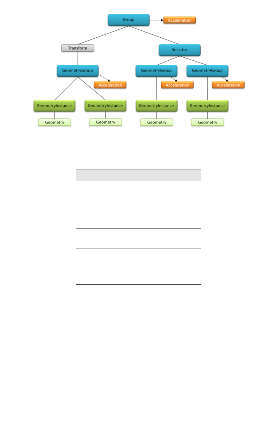
3.4 Graph nodes 3 Host API

Fig. 3.1 – A sample graph

Table 2 indicates which nodes can be children of other nodes including association with

acceleration structure nodes.

Parent node type Child node types

Geometry

Material

Acceleration

none

GeometryInstance Geometry

Material

GeometryGroup GeometryInstance

Acceleration

Transform

Selector

GeometryGroup

Group

Selector

Transform

Group

GeometryGroup

Group

Selector

Transform

Acceleration

Table 2 – Parent nodes and the types of nodes allowed as children

3.4.1 Geometry

A geometry node is the fundamental node to describe a geometric object: a collection of

user-deﬁned primitives against which rays can be intersected. The number of primitives

contained in a geometry node is speciﬁed using rtGeometrySetPrimitiveCount.

To deﬁne the primitives, an intersection program is assigned to the geometry node using

rtGeometrySetIntersectionProgram. The input parameters to an intersection program are a

primitive index and a ray, and it is the program’s job to return the intersection between the

two. In combination with program variables, this provides the necessary mechanisms to

3 Host API 3.4 Graph nodes

deﬁne any primitive type that can be intersected against a ray. A common example is a

triangle mesh, where the intersection program reads a triangle’s vertex data out of a buffer

(passed to the program via a variable) and performs a ray-triangle intersection.

In order to build an acceleration structure over arbitrary geometry, it is necessary for OptiX to

query the bounds of individual primitives. For this reason, a separate bounds program must

be provided using rtGeometrySetBoundingBoxProgram. This program simply computes

bounding boxes of the requested primitives, which are then used by OptiX as the basis for

acceleration structure construction.

The following example shows how to construct a geometry object describing a sphere, using a

single primitive. The intersection and bounding box program are assumed to depend on a

single parameter variable specifying the sphere radius:

RTgeometry geometry;

RTvariable variable;

// Set up geometry object.

rtGeometryCreate( context, &geometry );

rtGeometrySetPrimitiveCount( geometry, 1 );

rtGeometrySetIntersectionProgram( geometry, sphere_intersection );

rtGeometrySetBoundingBoxProgram( geometry, sphere_bounds );

// Declare and set the radius variable.

rtGeometryDeclareVariable( geometry, "radius", &variable );

rtVariableSet1f( variable, 10.0f );

3.4.2 Material

A material encapsulates the actions that are taken when a ray intersects a primitive associated

with a given material. Examples for such actions include: computing a reﬂectance color,

tracing additional rays, ignoring an intersection, and terminating a ray. Arbitrary parameters

can be provided to materials by declaring program variables.

Two types of programs may be assigned to a material, closest hit programs and any hit

programs. The two types differ in when and how often they are executed. The closest hit

program, which is similar to a shader in a classical rendering system, is executed at most once

per ray, for the closest intersection of a ray with the scene. It typically performs actions that

involve texture lookups, reﬂectance color computations, light source sampling, recursive ray

tracing, and so on, and stores the results in a ray payload data structure.

The any hit program is executed for each potential closest intersection found during ray

traversal. The intersections for which the program is executed may not be ordered along the

ray, but eventually all intersections of a ray with the scene can be enumerated if required (by

calling rtIgnoreIntersection on each of them). Typical uses of the any hit program include

early termination of shadow rays (using rtTerminateRay) and binary transparency, e.g., by

ignoring intersections based on a texture lookup.

It is important to note that both types of programs are assigned to materials per ray type,

which means that each material can actually hold more than one closest hit or any hit

program. This is useful if an application can identify that a certain kind of ray only performs

speciﬁc actions. For example, a separate ray type may be used for shadow rays, which are

3.4 Graph nodes 3 Host API

only used to determine binary visibility between two points in the scene. In this case, a

simple any hit program attached to all materials under that ray type index can immediately

terminate such rays, and the closest hit program can be omitted entirely. This concept allows

for highly efﬁcient specialization of individual ray types.

The closest hit program is assigned to the material by calling

rtMaterialSetClosestHitProgram, and the any hit program is assigned with

rtMaterialSetAnyHitProgram. If a program is omitted, an empty program is the default.

3.4.3 GeometryInstance

A geometry instance represents a coupling of a single geometry node with a set of materials.

The geometry object the instance refers to is speciﬁed using

rtGeometryInstanceSetGeometry. The number of materials associated with the instance is

set by rtGeometryInstanceSetMaterialCount, and the individual materials are assigned

with rtGeometryInstanceSetMaterial. The number of materials that must be assigned to a

geometry instance is determined by the highest material index that may be reported by an

intersection program of the referenced geometry.

Note that multiple geometry instances are allowed to refer to a single geometry object,

enabling instancing of a geometric object with different materials. Likewise, materials can be

reused between different geometry instances.

This example conﬁgures a geometry instance so that its ﬁrst material index is mat_phong and

the second one is mat_diffuse, both of which are assumed to be rtMaterial objects with

appropriate programs assigned. The instance is made to refer to the rtGeometry object

triangle_mesh.

RTgeometryinstance ginst;

rtGeometryInstanceCreate( context, &ginst );

rtGeometryInstanceSetGeometry( ginst, triangle_mesh );

rtGeometryInstanceSetMaterialCount( ginst, 2 );

rtGeometryInstanceSetMaterial( ginst, 0, mat_phong );

rtGeometryInstanceSetMaterial( ginst, 1, mat_diffuse);

3.4.4 GeometryGroup

A geometry group is a container for an arbitrary number of geometry instances. The number

of contained geometry instances is set using rtGeometryGroupSetChildCount, and the

instances are assigned with rtGeometryGroupSetChild. Each geometry group must also be

assigned an acceleration structure using rtGeometryGroupSetAcceleration. (See the

“Acceleration structures for ray tracing” section (page 25).)

The minimal sample use case for a geometry group is to assign it a single geometry instance:

RTgeometrygroup geomgroup;

rtGeometryGroupCreate( context, &geomgroup );

rtGeometryGroupSetChildCount( geomgroup, 1 );

rtGeometryGroupSetChild( geomgroup, 0, geometry_instance );

3 Host API 3.4 Graph nodes

Multiple geometry groups are allowed to share children, that is, a geometry instance can be a

child of more than one geometry group.

3.4.5 Group

A group represents a collection of higher level nodes in the graph. They are used to compile

the graph structure which is eventually passed to rtTrace for intersection with a ray.

A group can contain an arbitrary number of child nodes, which must themselves be of type

rtGroup,rtGeometryGroup,rtTransform, or rtSelector. The number of children in a group

is set by rtGroupSetChildCount, and the individual children are assigned using

rtGroupSetChild. Every group must also be assigned an acceleration structure via

rtGroupSetAcceleration.

A common use case for groups is to collect several geometry groups which dynamically move

relative to each other. The individual position, rotation, and scaling parameters can be

represented by transform nodes, so the only acceleration structure that needs to be rebuilt

between calls to rtContextLaunch is the one for the top level group. This will usually be

much cheaper than updating acceleration structures for the entire scene.

Note that the children of a group can be shared with other groups, that is, each child node can

also be the child of another group (or of any other graph node for which it is a valid child).

This allows for very ﬂexible and lightweight instancing scenarios, especially in combination

with shared acceleration structures. (See the “Acceleration structures for ray tracing” section

(page 25).)

3.4.6 Transform

A transform node is used to represent a projective transformation of its underlying scene

geometry. The transform must be assigned exactly one child of type rtGroup,

rtGeometryGroup,rtTransform, or rtSelector, using rtTransformSetChild. That is, the

nodes below a transform may simply be geometry in the form of a geometry group, or a

whole new subgraph of the scene.

The transformation itself is speciﬁed by passing a 4x4 ﬂoating point matrix (speciﬁed as a

16-element one-dimensional array) to rtTransformSetMatrix. Conceptually, it can be seen as

if the matrix were applied to all the underlying geometry. However, the effect is instead

achieved by transforming the rays themselves during traversal. This means that OptiX does

not rebuild any acceleration structures when the transform changes.

This example shows how a transform object with a simple translation matrix is created:

RTtransform transform;

const float x=10.0f, y=20.0f, z=30.0f;

// Matrices are row-major.

const float m[16] = { 1, 0, 0, x,

0, 1, 0, y,

0, 0, 1, z,

0, 0, 0, 1 };

rtTransformCreate( context, &transform );

3.5 Acceleration structures for ray tracing 3 Host API

rtTransformSetMatrix( transform, 0, m, 0 );

Note that the transform child node may be shared with other graph nodes. That is, a child

node of a transform may be a child of another node at the same time. This is often useful for

instancing geometry.

Transform nodes should be used sparingly as they cost performance during ray tracing. In

particular, it is highly recommended for node graphs to not exceed a single level of transform

depth.

3.4.7 Selector

A selector is similar to a group in that it is a collection of higher level graph nodes. The

number of nodes in the collection is set by rtSelectorSetChildCount, and the individual

children are assigned with rtSelectorSetChild. Valid child types are rtGroup,

rtGeometryGroup,rtTransform, and rtSelector.

The main difference between selectors and groups is that selectors do not have an

acceleration structure associated with them. Instead, a visit program is speciﬁed with

rtSelectorSetVisitProgram. This program is executed every time a ray encounters the

selector node during graph traversal. The program speciﬁes which children the ray should

continue traversal through by calling rtIntersectChild.

A typical use case for a selector is dynamic (i.e. per-ray) level of detail: an object in the scene

may be represented by a number of geometry nodes, each containing a different level of detail

version of the object. The geometry groups containing these different representations can be

assigned as children of a selector. The visit program can select which child to intersect using

any criterion (e.g. based on the footprint or length of the current ray), and ignore the others.

As for groups and other graph nodes, child nodes of a selector can be shared with other graph

nodes to allow ﬂexible instancing.

3.5 Acceleration structures for ray tracing

Acceleration structures are an important tool for speeding up the traversal and intersection

queries for ray tracing, especially for large scene databases. Most successful acceleration

structures represent a hierarchical decomposition of the scene geometry. This hierarchy is

then used to quickly cull regions of space not intersected by the ray.

There are different types of acceleration structures, each with their own advantages and

drawbacks. Furthermore, different scenes require different kinds of acceleration structures for

optimal performance (e.g., static vs. dynamic scenes, generic primitives vs. triangles, and so

on). The most common tradeoff is construction speed vs. ray tracing performance, but other

factors such as memory consumption can play a role as well.

No single type of acceleration structure is optimal for all scenes. To allow an application to

balance the tradeoffs, OptiX lets you choose between several kinds of supported structures.

You can even mix and match different types of acceleration structures within the same node

graph.

3 Host API 3.5 Acceleration structures for ray tracing

3.5.1 Acceleration objects in the node graph

Acceleration structures are individual API objects in OptiX, called rtAcceleration. Once an

acceleration object is created with rtAccelerationCreate, it is assigned to either a group

(using rtGroupSetAcceleration) or a geometry group (using

rtGeometryGroupSetAcceleration) Every group and geometry group in the node graph

needs to have an acceleration object assigned for ray traversal to intersect those nodes.

This example creates a geometry group and an acceleration structure and connects the two:

RTgeometrygroup geomgroup;

RTacceleration accel;

rtGeometryGroupCreate( context, &geomgroup );

rtAccelerationCreate( context, &accel );

rtGeometryGroupSetAcceleration( geomgroup, accel );

By making use of groups and geometry groups when assembling the node graph, the

application has a high level of control over how acceleration structures are constructed over

the scene geometry. If one considers the case of several geometry instances in a scene, there

are a number of ways they can be placed in groups or geometry groups to ﬁt the application’s

use case.

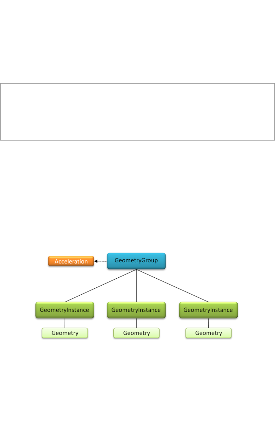
For example, Figure 3.2 places all the geometry instances in a single geometry group. An

acceleration structure on a geometry group will be constructed over the individual primitives

deﬁned by the collection of child geometry instances. This will allow OptiX to build an

acceleration structure which is as efﬁcient as if the geometries of the individual instances had

been merged into a single object.

Fig. 3.2 – Multiple geometry instances in a geometry group

A different approach to managing multiple geometry instances is shown in Figure 3.4

(page 31). Each instance is placed in its own geometry group, i.e. there is a separate

acceleration structure for each instance. The resulting collection of geometry groups is

aggregated in a top level group, which itself has an acceleration structure. Acceleration

structures on groups are constructed over the bounding volumes of the child nodes. Because

the number of child nodes is usually relatively low, high level structures are typically quick to

update. The advantage of this approach is that when one of the geometry instances is

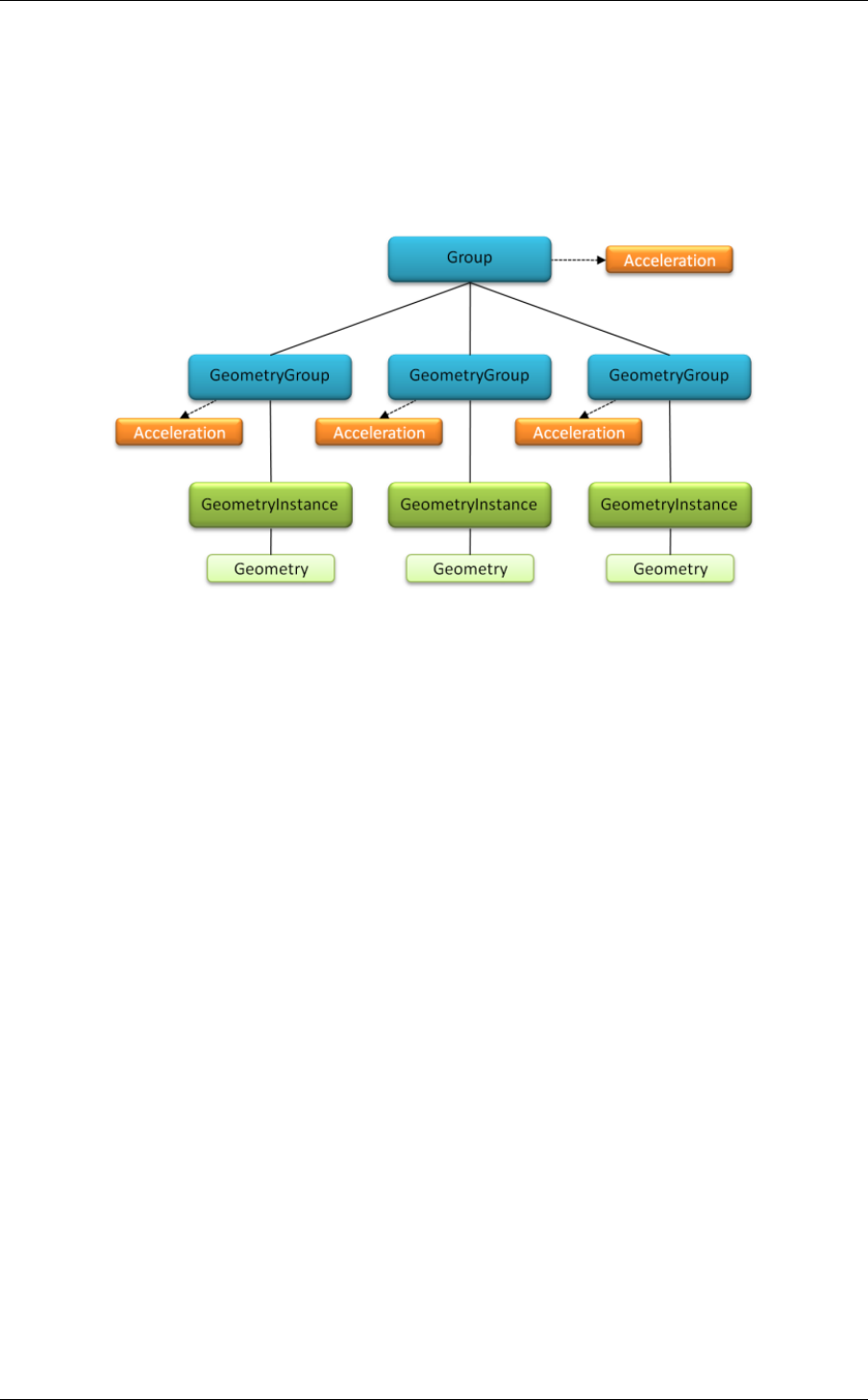
3.5 Acceleration structures for ray tracing 3 Host API

modiﬁed, the acceleration structures of the other instances need not be rebuilt. However,

because higher level acceleration structures introduce an additional level of complexity and

are built only on the coarse bounds of their group’s children, the graph in Figure 3 will likely

not be as efﬁcient to traverse as the one in Figure 2. Again, this is a tradeoff the application

needs to balance, e.g. in this case by considering how frequently individual geometry

instances will be modiﬁed.

Fig. 3.3 – Multiple geometry instances, each in a separate geometry group

3.5.2 Acceleration structure builders

An rtAcceleration has a builder. The builder is responsible for collecting input geometry

(in most cases, this geometry is the bounding boxes created by geometry nodes’ bounding

box programs) and computing a data structure that allows for accelerated ray-scene

intersection query. Builders are not application-deﬁned programs. Instead, the application

chooses an appropriate builder from Table 3.

3 Host API 3.5 Acceleration structures for ray tracing

Builder Description

Trbvh The Trbvh2. builder performs a very fast GPU-based BVH build. Its ray

tracing performance is usually within a few percent of SBVH, yet its build

time is generally the fastest. This builder should be strongly considered for

all datasets. Trbvh uses a modest amount of extra memory beyond that

required for the ﬁnal BVH. When the extra memory is not available on the

GPU, Trbvh may automatically fallback to build on the CPU.

Sbvh The Split-BVH (SBVH) is a high quality bounding volume hierarchy. While

build times are highest, it was traditionally the method of choice for static

geometry due to its high ray tracing performance, but may be superseded

by Trbvh. Improvements over regular BVHs are especially visible if the

geometry is non-uniform (e.g. triangles of different sizes). This builder can

be used for any type of geometry, but for optimal performance with

triangle geometry, specialized properties should be set (see Table 4)3.

Bvh The Bvh builder constructs a classic bounding volume hierarchy. It has

relatively good traversal performance and does not focus on fast

construction performance, but it supports reﬁtting for fast incremental

updates (Table 4).

Bvh is often the best choice for acceleration structures built over groups.

NoAccel This is a dummy builder which does not construct an actual acceleration

structure. Traversal loops over all elements and intersects each one with

the ray. This is very inefﬁcient for anything but very simple cases, but can

sometimes outperform real acceleration structures, for example, on a

group with very few child nodes.

Table 3 – Supported builders

Table 3 shows the builders currently available in OptiX. A builder is set using

rtAccelerationSetBuilder. The builder can be changed at any time; switching builders will

cause an acceleration structure to be ﬂagged for rebuild.

This example shows a typical initialization of an acceleration object:

RTacceleration accel;

rtAccelerationCreate( context, &accel );

rtAccelerationSetBuilder( accel, "Trbvh" );

2See Tero Karras and Timo Aila, Fast Parallel Construction of High-Quality Bounding Volume Hierarchies.http:

//highperformancegraphics.org/wp-content/uploads/Karras-BVH.pdf

3See Martin Stich, Heiko Friedrich, Andreas Dietrich. Spatial Splits in Bounding Volume Hierarchies.http://

www.nvidia.com/object/nvidia_research_pub_012.html

3.5 Acceleration structures for ray tracing 3 Host API

3.5.3 Acceleration structure properties

Fine-tuning acceleration structure construction can be useful depending on the situation. For

this purpose, builders expose various named properties, which are listed in Table 4:

Property Available Description

refit Bvh

Trbvh

If set to 1, the builder will only readjust the node

bounds of the bounding volume hierarchy instead of

constructing it from scratch. Reﬁt is only effective if

there is an initial BVH already in place, and the

underlying geometry has undergone relatively modest

deformation. In this case, the builder delivers a very

fast BVH update without sacriﬁcing too much ray

tracing performance.

The default is 0.

vertex_buffer_name Bvh

Trbvh

The name of the buffer variable holding triangle vertex

data. Each vertex consists of 3 ﬂoats. Mandatory for

TriangleKdTree, optional for Sbvh (but recommended

if the geometry consists of triangles).

The default is vertex_buffer.

vertex_buffer_stride Bvh

Trbvh

The offset between two vertices in the vertex buffer,

given in bytes.

The default value is 0, which assumes the vertices are

tightly packed.

index_buffer_name Bvh

Trbvh

The name of the buffer variable holding vertex index

data. The entries in this buffer are indices of type int,

where each index refers to one entry in the vertex buffer.

A sequence of three indices represents one triangle. If

no index buffer is given, the vertices in the vertex buffer

are assumed to be a list of triangles, i.e. every 3 vertices

in a row form a triangle.

The default is index_buffer.

index_buffer_stride Bvh

Trbvh

The offset between two indices in the index buffer,

given in bytes.

The default value is 0, which assumes the indices are

tightly packed.

chunk_size Trbvh Number of bytes to be used for a partitioned

acceleration structure build. If no chunk size is set, or

set to 0, the chunk size is chosen automatically. If set to

-1, the chunk size is unlimited. The minimum chunk

size is currently 64MB. Please note that specifying a

small chunk size reduces the peak-memory footprint of

the Trbvh, but can result in slower rendering

performance.

Table 4 – Acceleration structure properties

3 Host API 3.5 Acceleration structures for ray tracing

Properties are speciﬁed using rtAccelerationSetProperty. Their values are given as strings,

which are parsed by OptiX. Properties take effect only when an acceleration structure is

actually rebuilt. Setting or changing the property does not itself mark the acceleration

structure for rebuild; see the next section for details on how to do that. Properties not

recognized by a builder will be silently ignored.

// Enable fast refitting on a BVH acceleration.

rtAccelerationSetProperty( accel, "refit", "1" );

3.5.4 Acceleration structure builds

In OptiX, acceleration structures are ﬂagged (marked “dirty”) when they need to be rebuilt.

During rtContextLaunch, all ﬂagged acceleration structures are built before ray tracing

begins. Every newly created rtAcceleration object is initially ﬂagged dirty.

An application can decide at any time to explicitly mark an acceleration structure for rebuild.

For example, if the underlying geometry of a geometry group changes, the acceleration

structure attached to the geometry group must be recreated. This is achieved by calling

rtAccelerationMarkDirty. This is also required if, for example, new child geometry

instances are added to the geometry group, or if children are removed from it.

The same is true for acceleration structures on groups: adding or removing children,

changing transforms below the group, etc., are operations which require the group’s

acceleration to be marked as dirty. As a rule of thumb, every operation that causes a

modiﬁcation to the underlying geometry over which the structure is built (in the case of a

group, that geometry is the children’s axis-aligned bounding boxes) requires a rebuild.

However, no rebuild is required if, for example, some parts of the graph change further down

the tree, without affecting the bounding boxes of the immediate children of the group.

Note that the application decides independently for each single acceleration structure in the

graph whether a rebuild is necessary. OptiX will not attempt to automatically detect changes,

and marking one acceleration structure as dirty will not propagate the dirty ﬂag to any other

acceleration structures. Failure to mark acceleration structures as dirty when necessary may

result in unexpected behavior — usually missing intersections or performance degradation.

3.5.5 Shared acceleration structures

Mechanisms such as a graph node being attached as a child to multiple other graph nodes

make composing the node graph ﬂexible, and enable interesting instancing applications.

Instancing can be seen as inexpensive reuse of scene objects or parts of the graph by

referencing nodes multiple times instead of duplicating them.

OptiX decouples acceleration structures as separate objects from other graph nodes. Hence,

acceleration structures can naturally be shared between several groups or geometry groups,

as long as the underlying geometry on which the structure is built is the same:

// Attach one acceleration to multiple groups.

rtGroupSetAcceleration( group1, accel );

rtGroupSetAcceleration( group2, accel );

rtGroupSetAcceleration( group3, accel );

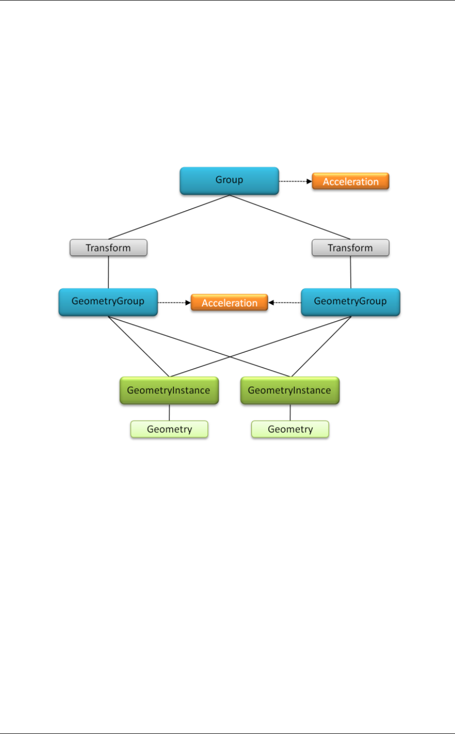
3.6 Rendering on the VCA 3 Host API

Note that the application must ensure that each node sharing the acceleration structure has

matching underlying geometry. Failure to do so will result in undeﬁned behavior. Also,

acceleration structures cannot be shared between groups and geometry groups.

The capability of sharing acceleration structures is a powerful concept to maximize efﬁciency,

as shown in Figure 4. The acceleration node in the center of the ﬁgure is attached to both

geometry groups, and both geometry groups reference the same geometry objects. This reuse

of geometry and acceleration structure data minimizes both memory footprint and

acceleration construction time. Additional geometry groups could be added in the same

manner at very little overhead.

Fig. 3.4 – Two geometry groups sharing an acceleration structure and the underlying

geometry objects.

3.6 Rendering on the VCA

OptiX 3.8 introduced remote network rendering as well as a new type of launch called the

progressive launch. Using these APIs, common progressive rendering algorithms can be

implemented easily and executed efﬁciently on NVIDIA’s Visual Computing Appliance

servers (VCAs). All OptiX computation can happen remotely on the VCA, with the rendered

result being sent back to the client as a video stream. This allows even relatively

low-performance client computers to run heavyweight OptiX applications efﬁciently, using

the substantial computational resources provided by tens or hundreds of GPUs in a VCA

cluster.

The Progressive Launch API mainly serves to address the following aspects not covered by

the traditional OptiX API:

3 Host API 3.6 Rendering on the VCA

3.6.1 Remote launches

The rtContextLaunch calls offered by traditional OptiX work for remote rendering but are

not well suited to it. Because the API calls are synchronous, each launch/display cycle incurs

the full network roundtrip latency, and thus performance is usually not acceptable over

standard network connections. Progressive launches, on the other hand, are asynchronous,

and can achieve smooth application performance even over a high latency connection.

3.6.2 Parallelization

OptiX can parallelize work across a small number of local GPUs. To enable ﬁrst class support

for VCA clusters, however, the system needs to be able to scale to potentially hundreds of

GPUs efﬁciently. Progressive renderers, such as path tracers, are one of the most common use

cases of OptiX. The fact that the image samples they compute are independent of each other

provides a natural way to parallelize the problem. The Progressive Launch API therefore

combines the assumption that work can be split into many independent parts with the

capability to launch kernels asynchronously.

Note that the Progressive Launch API may be used to render on local devices, as well as

remotely on the VCA. Except for the code that sets up the RemoteDevice (see the “Remote

devices” section (page 32)), whether rendering happens locally or remotely is transparent to

the application. For applications that are amenable to the progressive launch programming

model an advantage of using this model all the time, rather than traditional synchronous

launches is that adapting the application to the VCA with full performance is virtually

automatic.

3.6.3 Remote devices

The connection to a VCA (or cluster of VCAs) is represented by the RTremotedevice API

object. On creation, the network connection is established given the URL of the cluster

manager (in form of a WebSockets address) and user credentials. Information about the

device can then be queried using rtRemoteDeviceGetAttribute. A VCA cluster consists of a

number of nodes, of which a subset can be reserved for rendering using

rtRemoteDeviceReserve. Since several server conﬁgurations may be available, that call also

selects which one to use.

After node reservation has been initiated, the application must wait for the nodes to be ready

by polling the RT_REMOTEDEVICE_STATUS attribute. Once that ﬂag reports

RT_REMOTEDEVICE_STATUS_READY, the device can be used for rendering.

To execute OptiX commands on the remote device, the device must be assigned to a context

using rtContextSetRemoteDevice. Note that only newly created contexts can be used with

remote devices. That is, the call to rtContextSetRemoteDevice should immediately follow

the call to rtContextCreate.

3.6.4 Progressive launches

While most existing OptiX applications will work unchanged when run on a remote device

(see the “Limitations” section (page 34) for caveats), progressive launches must be used

instead of rtContextLaunch for optimal performance.

Instead of requesting the generation of a single frame, a progressive launch, triggered by

rtContextLaunchProgressive2D, requests multiple subframes at once. A subframe is output

3.6 Rendering on the VCA 3 Host API

buffer content which is composited with other subframes to yield the ﬁnal frame. In most

progressive renderers, this means that a subframe simply contains a single sample per pixel.

Progressive launch calls are non-blocking. An application typically executes a progressive

launch, and then continuously polls the stream buffers associated with its output, using

rtBufferGetProgressiveUpdateReady. If that call reports that an update is available, the

stream buffer can be mapped and the content displayed.

If any OptiX API functions are called while a progressive launch is in progress, the launch

will stop generating subframes until the next time a progressive launch is triggered (the

exception is the API calls to poll and map the stream buffers). This way, state changes to

OptiX, such as setting variables using rtVariableSet, can be made easily and efﬁciently in

combination with a render loop that polls for stream updates and executes a progressive

launch. This method is outlined in the example pseudocode below.

3.6.5 Stream buers

Accessing the results of a progressive launch is typically done through a new type of buffer

called a stream buffer. Stream buffers allow the remotely rendered frames to be sent to the

application client using compressed video streaming, greatly improving response times while

still allowing the application to use the result frame in the same way as with a non-stream

output buffer.

Stream buffers are created using rtBufferCreate with the type set to

RT_BUFFER_PROGRESSIVE_STREAM. A stream buffer must be bound to a regular output buffer

via rtBufferBindProgressiveStream in order to deﬁne its data source.

By executing the bind operation, the system enables automatic compositing for the output

buffer. That is, any values written to the output buffer by device code will be averaged into

the stream buffer, rather than overwriting the previous value as in regular output buffers.

Compositing happens automatically and potentially in parallel across many devices on the

network, or locally if remote rendering is not used.

Several conﬁguration options are available for stream buffers, such as the video stream

format to use, and parameters to trade off quality versus speed. Those options can be set

using rtBufferSetAttribute. Note that some of the options only take effect if rendering

happens on a remote device, and are a no-op when rendering locally. This is because stream

buffers don’t undergo video compression when they don’t have to be sent across a network.

In addition to automatic compositing, the system also tonemaps and quantizes the averaged

output before writing it into a stream. Tonemapping is performed using a simple built-in

operator with a user- deﬁned gamma value (speciﬁed using rtBufferSetAttribute). The

tonemap operator is deﬁned as:

final_value = clamp( pow( hdr_value, 1/gamma ), 0, 1 )

Accessing a progressive stream happens by mapping the stream buffer, just like any regular

buffer, and reading out the frame data. The data is uncompressed, if necessary, when

mapped. The data available for reading will always represent the most recent update to the

stream if a progressive launch is in progress, so a frame that is not read on time may be

skipped (e.g., if polling happens at a low frequency).

3 Host API 3.6 Rendering on the VCA

It is also possible to map an output buffer that is bound as a data source for a stream buffer.

This can be useful to access “ﬁnal frame” data, i.e. the uncompressed and unquantized

accumulated output. Note that mapping a non-stream buffer will cause the progressive

launch to stop generating subframes, and that such a map operation is much slower than

mapping a stream.

3.6.6 Device code

In OptiX device code, the subframe index used for progressive rendering is exposed as a

semantic variable of type unsigned int. Its value is guaranteed to be unique for each subframe

in the current progressive launch, starting at zero for the ﬁrst subframe and increasing by one

with each subsequent subframe. For example, an application performing stochastic sampling

may use this variable to seed a random number generator. (For a description of semantic

variables, see the “Communication through variables” section (page 38).)

The current subframe index can be accessed in shader programs by declaring the following

variable:

rtDeclareVariable(unsigned int, index, rtSubframeIndex,);

Computed pixel values can be written to an output buffer, just like for non-progressive

rendering. Output buffers that are bound as sources to stream buffers will then be averaged

automatically and processed (as described in the “Buffers” section (page 14)).

Note in particular that device code does not use stream buffers directly.

3.6.7 Limitations

•OpenGL interoperability is limited with remote rendering, and using it is discouraged

for performance reasons. See the “Interoperability with OpenGL” section (page 79) for

more information. Direct3D and CUDA interop are not supported.

•Using buffers of type RT_BUFFER_INPUT_OUTPUT in combination with remote rendering

yields undeﬁned results.

•rtPrintf and associated host functions are not supported in combination with remote

rendering.

•rtContextSetTimeoutCallback is not supported in combination with remote

rendering.

•Error codes and messages returned by API calls may apply to errors encountered on

prior API calls, rather than the current call since return codes are streamed back

asynchronously from the VCA.

•Output buffers used as data sources for progressive stream buffers must be of

RT_FORMAT_FLOAT3 or RT_FORMAT_FLOAT4 format. For performance reasons, using

RT_FORMAT_FLOAT4 is strongly recommended.

•Stream buffers must be of RT_FORMAT_UNSIGNED_BYTE4 format.

3.6 Rendering on the VCA 3 Host API

3.6.8 Example

For complete example applications using remote rendering and progressive launches, please

refer to the “progressive” and “queryRemote” examples in the SDK. The following illustrates

basic API usage in pseudocode.

// Set up the remote device. To use progressive rendering locally,

// simply skip this and the call to rtContextSetRemoteDevice.

RTremotedevice rdev;

rtRemoteDeviceCreate(

"wss://myvcacluster.example.com:443", "user", "password", &rdev );

// Reserve 1 VCA node with config #0

rtRemoteDeviceReserve( rdev, 1, 0 );

// Wait until the VCA is ready

int ready;

bool first = true;

do {

if (first)

first = false;

else

sleep(1); // poll once per second.

rtRemoteDeviceGetAttribute(

rdev, RT_REMOTEDEVICE_ATTRIBUTE_STATUS, sizeof(int), &ready ) );

} while( ready != RT_REMOTEDEVICE_STATUS_READY );

// Set up the OptiX context

RTcontext context;

rtContextCreate( &context );

// Enable rendering on the remote device.

// Must immediately follow context creation.

rtContextSetRemoteDevice( context, rdev );

// Set up a stream buffer/output buffer pair

RTbuffer output_buffer, stream_buffer;

rtBufferCreate( context, RT_BUFFER_OUTPUT, &output_buffer );

rtBufferCreate( context, RT_BUFFER_PROGRESSIVE_STREAM, &stream_buffer );

rtBufferSetSize2D( output_buffer, width, height );

rtBufferSetSize2D( stream_buffer, width, height );

rtBufferSetFormat( output_buffer, RT_FORMAT_FLOAT4 );

rtBufferSetFormat( stream_buffer, RT_FORMAT_UNSIGNED_BYTE4 );

rtBufferBindProgressiveStream( stream_buffer, output_buffer );

// [The usual OptiX scene setup goes here. Geometries, acceleration

// structures, materials, programs, etc.]

3 Host API 3.6 Rendering on the VCA

// Non-blocking launch, request infinite number of subframes

rtContextLaunchProgressive2D( context, width, height, 0 );

while( !finished )

{

// Poll stream buffer for updates from the progressive launch

int ready;

rtBufferGetProgressiveUpdateReady( stream_buffer, &ready, 0, 0 );

if( ready )

{

// Map and display the stream. This won’t interrupt rendering.

rtBufferMap( stream_buffer, &data );

display( data );

rtBufferUnmap( stream_buffer );

}

// Check whether scene has changed, e.g. because of user input

if( scene_changed() )

{

// [Update OptiX state here, e.g. by calling rtVariableSet

// or other OptiX functions. This will cause the server to

// stop generating subframes, so we call launch again below].

rtVariableSet( ... );

}

// Start a new progressive launch, in case the OptiX state has been

// changed above. If it hasn’t, then this is a no-op and the

// previous launch just continues running, accumulating further

// subframes into the stream.

rtContextLaunchProgressive2D( context, width, height, 0 );

}

// Clean up.

rtContextDestroy( context );

rtRemoteDeviceRelease( rdev );

rtRemoteDeviceDestroy( rdev );

4 Programs

This chapter describes the different kinds of OptiX programs, which provide programmatic

control over ray intersection, shading, and other general computation in OptiX ray tracing

kernels. OptiX programs are associated with binding points serving different semantic roles

during a ray tracing computation. Like other concepts, OptiX abstracts programs through its

object model as program objects.

4.1 OptiX program objects

The central theme of the OptiX API is programmability. OptiX programs are written in

CUDA C, and speciﬁed to the API through a string or ﬁle containing PTX, the parallel thread

execution virtual assembly language associated with CUDA. The nvcc compiler that is

distributed with the CUDA SDK is used to create PTX in conjunction with the OptiX header

ﬁles.

These PTX ﬁles are then bound to Program objects via the host API. Program objects can be

used for any of the OptiX program types discussed later in this section.

4.1.1 Managing program objects

OptiX provides two API entry points for creating Program objects:

rtProgramCreateFromPTXString, and rtProgramCreateFromPTXFile. The former creates a

new Program object from a string of PTX source code. The latter creates a new Program object

from a ﬁle of PTX source on disk:

RTcontext context = ...;

const char *ptx_filename = ...;

const char *program_name = ...;

RTprogram program = ...;

rtProgramCreateFromPTXFile(

context, ptx_filename, function_name, &program );

In this example, ptx_filename names a ﬁle of PTX source on disk, and function_name names

a particular function of interest within that source. If the program is ill-formed and cannot

compile, these entry points return an error code.

Program objects may be checked for completeness using the rtProgramValidate function, as

the following example demonstrates:

if ( rtProgramValidate(context, program)!=RT_SUCCESS ) {

printf( "Program is not complete." );

}

An error code returned from rtProgramValidate indicates an error condition due to the

program object or any other objects bound to it.

4 Programs 4.1 OptiX program objects

Finally, the rtProgramGetContext function reports the context object owning the program

object, while rtProgramDestroy invalidates the object and frees all resources related to it.

4.1.2 Communication through variables

OptiX program objects communicate with the host program through variables. Variables are

declared in an OptiX program using the rtDeclareVariable macro:

rtDeclareVariable( float, x, , );

This declaration creates a variable named xof type float which is available to both the host

program through the OptiX variable object API, and to the device program code through

usual C language semantics. Notice that the last two arguments are left blank in this example.

The commas must still be speciﬁed.

Taking the address of a variable on the device is not supported. This means that pointers and

references to x in the above example are not allowed. If, for instance, you needed to pass x

into a function taking a float* argument you would need to ﬁrst copy x into a stack variable

and then pass in the address of this local variable:

void my_func( float* my_float) {...}

RT_PROGRAM call_my_func()

{

my_func(&x); // not allowed

float local_x = x;

my_func(&local_x); // allowed

}

Variables declared in this way may be read and written by the host program through the

rtVariableGet* and rtVariableSet* family of functions. When variables are declared this

way, they are implicitly const-qualiﬁed from the device program’s perspective. If

communication from the program to the host is necessary, an rtBuffer should be used

instead.

As of OptiX 2.0, variables may be declared inside arbitrarily nested namespaces to avoid

name conﬂicts. References from the host program to namespace-enclosed OptiX variables

will need to include the full namespace.

Program variables may also be declared with semantics. Declaring a variable with a semantic

binds the variable to a special value which OptiX manages internally over the lifetime of the

ray tracing kernel. For example, declaring a variable with the rtCurrentRay semantic creates

a special read-only program variable that mirrors the value of the Ray currently being traced

through the program ﬂow:

rtDeclareVariable( OptiX::Ray, ray, rtCurrentRay, );

Variables declared with a built-in semantic exist only during ray tracing kernel runtime and

may not be modiﬁed or queried by the host program. Unlike regular variables, some

semantic variables may be modiﬁed by the device program.

4.1 OptiX program objects 4 Programs

Declaring a variable with an annotation associates with it a read-only string which, for

example, may be interpreted by the host program as a human-readable description of the

variable. For example:

rtDeclareVariable( float, shininess, , "The shininess of the sphere" );

A variable’s annotation is the fourth argument of rtDeclareVariable, following the

variable’s optional semantic argument. The host program may query a variable’s annotation

with the rtVariableGetAnnotation function.

4.1.3 Internally provided semantics

OptiX manages ﬁve internal semantics for program variable binding. Table 5 summarizes in

which types of program these semantics are available, along with their access rules from

device programs and a brief description of their meaning.

Name Access Description

Ray generation

Exception

Closest hit

Any hit

Miss

Intersection

Bounding box

Visit

rtLaunchIndex read only

The unique index identifying

each thread launched by

rtContextLaunch{1|2|3}D.

XXXXXX X

rtCurrentRay read only The state of the current ray. XXXX X

rtPayload read/write The state of the current ray’s

payload of user-deﬁned data. X X X X

rtIntersection-

Distance read only

The parametric distance from

the current ray’s origin to the

closest intersection point yet

discovered.

X X X X

rtSubframeIndex read only

The unique index identifying

each subframe in a

progressive launch. Zero for

non-progressive launches.

XXXXXX X

Table 5 – Semantic variables

4.1.4 Attribute variables

In addition to the semantics provided by OptiX, variables may also be declared with

user-deﬁned semantics called attributes. Unlike built-in semantics, the value of variables

declared in this way must be managed by the programmer. Attribute variables provide a

mechanism for communicating data between the intersection program and the shading

programs (e.g., surface normal, texture coordinates). Attribute variables may only be written

in an intersection program between calls to rtPotentialIntersection and

rtReportIntersection. Although OptiX may not ﬁnd all object intersections in order along

4 Programs 4.1 OptiX program objects

the ray, the value of the attribute variable is guaranteed to reﬂect the value at the closest

intersection at the time that the closest hit program is invoked.

Note: Because intersections may not be found in order, programs should use attribute

variables (as opposed to the ray payload) to communicate information about the local

hit point between intersection and shading programs.

The following example declares an attribute variable of type float3 named normal. The

semantic association of the attribute is speciﬁed with the user-deﬁned name normal_vec. This

name is arbitrary, and is the link between the variable declared here and another variable

declared in the closest hit program. The two attribute variables need not have the same name

as long as their attribute names match.

rtDeclareVariable( float3, normal, attribute normal_vec, );

4.1.5 Program variable scoping

OptiX program variables can have their values deﬁned in two ways: static initializations, and

(more typically) by variable declarations attached to API objects. A variable declared with a

static initializer will only use that value if it does not ﬁnd a deﬁnition attached to an API

object. A declaration with static initialization is written:

rtDeclareVariable( float, x, , ) = 5.0f;

The OptiX variable scoping rules provide a valuable inheritance mechanism that is designed

to create compact representations of material and object parameters. To enable this, each

program type also has an ordered list of scopes through which it will search for variable

deﬁnitions in order. For example, a closest hit program that refers to a variable named color

will search the Program,GeometryInstance,Material and Context API objects for

deﬁnitions created with the rt* functions, in that order. Similar to scoping rules in a

programming language, variables in one scope will shadow those in another scope.

summarizes the scopes that are searched for variable declarations for each type of program.

Program type Search order

Closest hit

Any hit

Intersection

Bounding box

Program GeometryInstance Geometry Context

Ray generation

Exception

Miss

Program Context

Visit Program Node

Table 6 – Scope search order for each type of program (from left to right)

It is possible for a program to ﬁnd multiple deﬁnitions for a variable in its scopes depending

upon where the program is called. For example, a closest hit program may be attached to

4.1 OptiX program objects 4 Programs

several Material objects and reference a variable named shininess. We can attach a variable

deﬁnition to the Material object as well as attach a variable deﬁnition to speciﬁc

GeometryInstance objects that we create that reference that Material.

During execution of a speciﬁc GeometryInstance’ closest hit program, the value of shininess

depends on whether the particular instance has a deﬁnition attached: if the

GeometryInstance deﬁnes shininess, then that value will be used. Otherwise, the value will

be taken from the Material object. As you can see from Table 6 above, the program searches

the GeometryInstance scope before the Material scope. Variables with deﬁnitions in

multiple scopes are said to be dynamic and may incur a performance penalty. Dynamic

variables are therefore best used sparingly.

4.1.6 Program variable transformation

Recall that rays have a projective transformation applied to them upon encountering

Transform nodes during traversal. The transformed ray is said to be in object space, while the

original ray is said to be in world space.

Programs with access to the rtCurrentRay semantic operate in the spaces summarized in

Table 7:

Program type Space

Closest hit world

Any hit object

Miss world

Intersection object

Visit object

Table 7 – Space of rtCurrentRay for each program type

To facilitate transforming variables from one space to another, OptiX’s CUDA C API provides

a set of functions:

__device__ float3 rtTransformPoint(

RTtransformkind kind, const float3& p )

__device__ float3 rtTransformVector(

RTtransformkind kind, const float3& v )

__device__ float3 rtTransformNormal(

RTtransformkind kind, const float3& n )

__device__ void rtGetTransform(

RTtransformkind kind, float matrix[16] )

The ﬁrst three functions transform a float3, interpreted as a point, vector, or normal vector,

from object to world space or vice versa depending on the value of a RTtransformkind ﬂag

passed as an argument. rtGetTransform returns the four-by-four matrix representing the

current transformation from object to world space (or vice versa depending on the

RTtransformkind argument). For best performance, use the rtTransform* functions rather

than performing your own explicit matrix multiplication with the result of rtGetTransform.

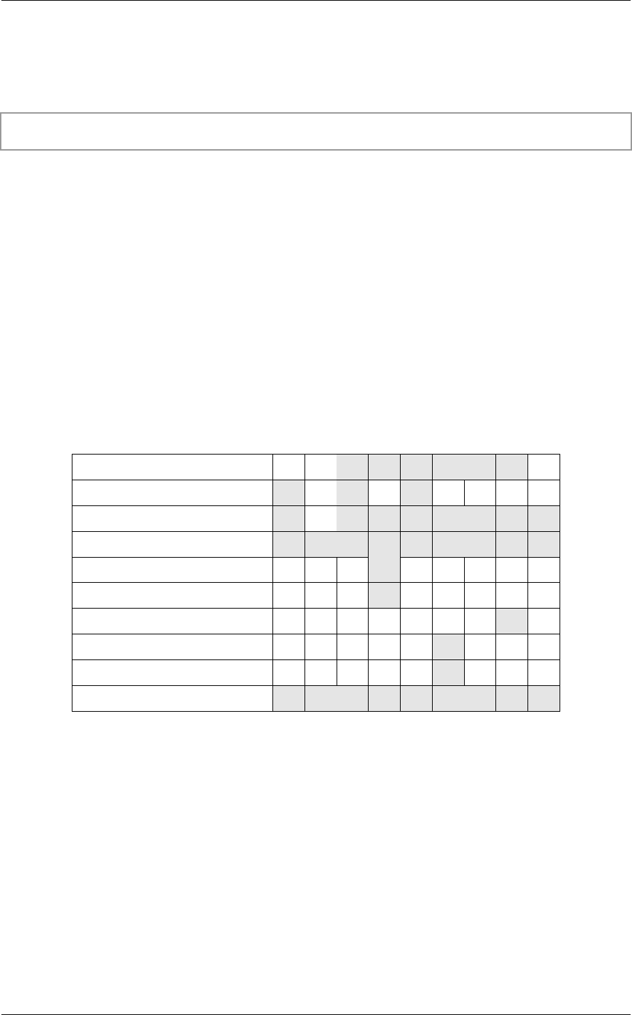
4 Programs 4.3 Ray generation programs

A common use case of variable transformation occurs when interpreting attributes passed

from the intersection program to the closest hit program. Intersection programs often produce

attributes, such as normal vectors, in object space. Should a closest hit program wish to

consume that attribute, it often must transform the attribute from object space to world space:

float3 n = rtTransformNormal( RT_OBJECT_TO_WORLD, normal );

4.2 The program scope of API function calls

Not all OptiX function calls are supported in all types of user-provided programs. For

example, it doesn’t make sense to spawn a new ray inside an intersection program, so this

behavior is disallowed. A complete table of what device-side functions are allowed is given

below. (Callable programs are described in the “Callable programs” section (page 93).)

Ray generation

Exception

Closest hit

Any hit

Miss

Intersection

Bounding box

Visit

Bindless callable program

rtTransform* X X X X X X

rtTrace X X X

rtThrow X X X X X X X X

rtPrintf XXXXXXXXX

rtTerminateRay X

rtIgnoreIntersection X

rtIntersectChild X

rtPotentialIntersection X

rtReportIntersection X

Callable program XXXXXXXXX

Table 8 – Scopes allowed for device-side API functions

4.3 Ray generation programs

Aray generation program serves as the ﬁrst point of entry upon a call to

rtContextLaunch{1|2|3}D. As such, it serves a role analogous to the main function of a C

program. Like C’s main function, any subsequent computation performed by the kernel, from

casting rays to reading and writing from buffers, is spawned by the ray generation program.

However, unlike a serial C program, an OptiX ray generation program is executed many

times in parallel — once for each thread implied by rtContextLaunch{1|2|3}D’s parameters.

4.3 Ray generation programs 4 Programs

Each thread is assigned a unique rtLaunchIndex. The value of this variable may be used to

distinguish it from its neighbors for the purpose of, e.g., writing to a unique location in an

rtBuffer:

rtBuffer<float, 1> output_buffer;

rtDeclareVariable( unsigned int, index, rtLaunchIndex, );

...;

float result = ...;

output_buffer[index] = result;

In this case, the result is written to a unique location in the output buffer. In general, a ray

generation program may write to any location in output buffers, as long as care is taken to

avoid race conditions between buffer writes.

4.3.1 Entry point indices

To conﬁgure a ray tracing kernel launch, the programmer must specify the desired ray

generation program using an entry point index. The total number of entry points for a

context is speciﬁed with rtContextSetEntryPointCount:

RTcontext context = ...;

unsigned int num_entry_points = ...;

rtContextSetEntryPointCount( context, num_entry_points );

OptiX requires that each entry point index created in this manner have a ray generation

program associated with it. A ray generation program may be associated with multiple

indices. Use the rtContextSetRayGenerationProgram function to associate a ray generation

program with an entry point index in the range [0, num_entry_points).

RTprogram prog = ...;

// index is >= 0 and < num_entry_points

unsigned int index = ...;

rtContextSetRayGenerationProgram( context, index, prog );

4.3.2 Launching a ray generation program

rtContextLaunch{1|2|3}Dtakes as a parameter the entry point index of the ray generation

program to launch:

RTsize width = ...;

rtContextLaunch1D( context, index, width );

If no ray generation program has been associated with the entry point index speciﬁed by

rtContextLaunch{1|2|3}D’s parameter, the launch will fail.

4.3.3 Ray generation program function signature

In CUDA C, ray generation programs return void and take no parameters. Like all OptiX

programs, ray generation programs written in CUDA C must be tagged with the RT_PROGRAM

4 Programs 4.4 Exception programs

qualiﬁer. The following snippet shows an example ray generation program function

prototype:

RT_PROGRAM void ray_generation_program( void );

4.3.4 Example ray generation program

The following example ray generation program implements a pinhole camera model in a

rendering application. This example demonstrates that ray generation programs act as the

gateway to all ray tracing computation by initiating traversal through the rtTrace function,

and often store the result of a ray tracing computation to an output buffer.

Note the variables eye,U,V, and W. Together, these four variables allow the host API to specify

the position and orientation of the camera.

rtBuffer<uchar4, 2> output_buffer;

rtDeclareVariable( uint2, index, rtLaunchIndex, );

rtDeclareVariable( rtObject, top_object, , );

rtDeclareVariable(float3, eye, , );

rtDeclareVariable(float3, U, , );

rtDeclareVariable(float3, V, , );

rtDeclareVariable(float3, W, , );

struct Payload

{

uchar4 result;

};

RT_PROGRAM void pinhole_camera( void )

{

uint2 screen = output_buffer.size();

float2 d = (make_float2( index ) / make_float2( screen )) * 2.f - 1.f;

float3 origin = eye;

float3 direction = normalize( d.x*U + d.y*V + W );

OptiX::Ray ray =

OptiX::make_Ray( origin, direction, 0, 0.05f, RT_DEFAULT_MAX );

Payload payload;

rtTrace( top_object, ray, payload );

output_buffer[index] = payload.result;

}

4.4 Exception programs

OptiX ray tracing kernels invoke an exception program when certain types of serious errors

are encountered. Exception programs provide a means of communicating to the host

4.4 Exception programs 4 Programs

program that something has gone wrong during a launch. The information an exception

program provides may be useful in avoiding an error state in a future launch or for

debugging during application development.

4.4.1 Exception program entry point association

An exception program is associated with an entry point using the

rtContextSetExceptionProgram function:

RTcontext context = ...;

RTprogram program = ...;

// index is >= 0 and < num_entry_points

unsigned int index = ...;

rtContextSetExceptionProgram( context, index, program );

Unlike with ray generation programs, the programmer need not associate an exception

program with an entry point. By default, entry points are associated with an internally

provided exception program that silently ignores errors.

As with ray generation programs, a single exception program may be associated with many

different entry points.

4.4.2 Exception types

OptiX detects a number of different error conditions that result in exception programs being

invoked. An exception is identiﬁed by its code, which is an integer deﬁned by the OptiX API.

For example, the exception code for the stack overﬂow exception is

RT_EXCEPTION_STACK_OVERFLOW.

The type or code of a caught exception can be queried by calling rtGetExceptionCode from

the exception program. More detailed information on the exception can be printed to the

standard output using rtPrintExceptionDetails.

In addition to the built in exception types, OptiX provides means to introduce user-deﬁned

exceptions. Exception codes between RT_EXCEPTION_USER (0x400) and 0xFFFF are reserved

for user exceptions. To trigger such an exception, rtThrow is used:

// Define user-specified exception codes.

#define MY_EXCEPTION_0 RT_EXCEPTION_USER + 0

#define MY_EXCEPTION_1 RT_EXCEPTION_USER + 1

RT_PROGRAM void some_program()

{

...

// Throw user exceptions from within a program.

if( condition0 )

rtThrow( MY_EXCEPTION_0 );

if( condition1 )

rtThrow( MY_EXCEPTION_1 );

...

}

4 Programs 4.5 Closest hit programs

In order to control the runtime overhead involved in checking for error conditions, individual

types of exceptions may be switched on or off using rtContextSetExceptionEnabled.

Disabling exceptions usually results in faster performance, but is less safe. By default, only

RT_EXCEPTION_STACK_OVERFLOW is enabled. During debugging, it is often useful to turn on all

available exceptions. This can be achieved with a single call:

...

rtContextSetExceptionEnabled(context, RT_EXCEPTION_ALL, 1);

...

4.4.3 Exception program function signature

In CUDA C, exception programs return void, take no parameters, and use the

RT_PROGRAM qualiﬁer:

RT_PROGRAM void exception_program( void );

4.4.4 Example exception program

The following example code demonstrates a simple exception program which indicates a

stack overﬂow error by outputting a special value to an output buffer which is otherwise

used as a buffer of pixels. In this way, the exception program indicates the rtLaunchIndex of

the failed thread by marking its location in a buffer of pixels with a known color. Exceptions

which are not caused by a stack overﬂow are reported by printing their details to the console.

rtDeclareVariable( int, launch_index, rtLaunchIndex, );

rtDeclareVariable( float3, error, , ) = make_float3(1,0,0);

rtBuffer<float3, 2> output_buffer;

RT_PROGRAM void exception_program( void )

{

const unsigned int code = rtGetExceptionCode();

if( code == RT_EXCEPTION_STACK_OVERFLOW )

output_buffer[launch_index] = error;

else

rtPrintExceptionDetails();

}

4.5 Closest hit programs

After a call to the rtTrace function, OptiX invokes a closest hit program once it identiﬁes the

nearest primitive intersected along the ray from its origin. Closest hit programs are useful for

performing primitive-dependent processing that should occur once a ray’s visibility has been

established. A closest hit program may communicate the results of its computation by

modifying per-ray data or writing to an output buffer. It may also recursively call the

rtTrace function. For example, a computer graphics application might implement a surface

shading algorithm with a closest hit program.

4.5 Closest hit programs 4 Programs

4.5.1 Closest hit program material association

A closest hit program is associated with each (material,ray_type) pair. Each pair’s default

program is a no-op. This is convenient when an OptiX application requires many types of

rays but only a small number of those types require special closest hit processing.

The programmer may change an association with the rtMaterialSetClosestHitProgram

function:

RTmaterial material = ...;

RTprogram program = ...;

unsigned int type = ...;

rtMaterialSetClosestHitProgram( material, type, program );

4.5.2 Closest hit program function signature

In CUDA C, closest hit programs return void, take no parameters, and use the RT_PROGRAM

qualiﬁer:

RT_PROGRAM void closest_hit_program( void );

4.5.3 Recursion in a closest hit program

Though the rtTrace function is available to all programs with access to the rtLaunchIndex

semantic, a common use case of closest hit programs is to perform recursion by tracing more

rays upon identiﬁcation of the closest surface intersected by a ray. For example, a computer

graphics application might implement Whitted- style ray tracing by recursive invocation of

rtTrace and closest hit programs. Care must be used to limit the recursion depth to avoid

stack overﬂow.

4.5.4 Example closest hit program

The following code example demonstrates a closest hit program that transforms the normal

vector computed by an intersection program (not shown) from the intersected primitive’s

local coordinate system to a global coordinate system. The transformed normal vector is

returned to the calling function through a variable declared with the rtPayload semantic.

Note that this program is quite trivial; normally the transformed normal vector would be

used by the closest hit program to perform some calculation (e.g., lighting). See the document

Introductory tutorials in the OptiX documentation set for examples.

rtDeclareVariable( float3, normal, attribute normal_vec, );

struct Payload

{

float3 result;

};

rtDeclareVariable( Payload, ray_data, rtPayload, );

RT_PROGRAM void closest_hit_program( void )

{

float3 norm;

4 Programs 4.6 Any hit programs

norm = rtTransformNormal( RT_OBJECT_TO_WORLD, normal );

norm = normalize( norm );

ray_data.result = norm;

}

4.6 Any hit programs

Instead of the closest intersected primitive, an application may wish to perform some

computation for any primitive intersection that occurs along a ray cast during the rtTrace

function; this usage model can be implemented using any hit programs. For example, a

rendering application may require some value to be accumulated along a ray at each surface

intersection.

4.6.1 Any hit program material association

Like closest hit programs, an any hit program is associated with each (material,ray_type)

pair. Each pair’s default association is with an internally-provided any hit program which

implements a no-op.

The rtMaterialSetAnyHitProgram function changes the association of a (material,

ray_type) pair:

RTmaterial material = ...;

RTprogram program = ...;

unsigned int type = ...;

rtMaterialSetAnyHitProgram( material, type, program );

4.6.2 Termination in an any hit program

A common OptiX usage pattern is for an any hit program to halt ray traversal upon discovery

of an intersection. The any hit program can do this by calling rtTerminateRay. This

technique can increase performance by eliminating redundant traversal computations when

an application only needs to determine whether any intersection occurs and identiﬁcation of

the nearest intersection is irrelevant. For example, a rendering application might use this

technique to implement shadow ray casting, which is often a binary true or false computation.

4.6.3 Any hit program function signature

In CUDA C, any hit programs return void, take no parameters, and use the RT_PROGRAM

qualiﬁer:

RT_PROGRAM void any_hit_program( void );

4.6.4 Example any hit program

The following code example demonstrates an any hit program that implements early

termination of shadow ray traversal upon intersection. The program also sets the value of a

per-ray payload member, attenuation, to zero to indicate the material associated with the

program is totally opaque.

4.7 Miss programs 4 Programs

struct Payload

{

float attenuation;

};

rtDeclareVariable( Payload, payload, rtPayload, );

RT_PROGRAM void any_hit_program( void )

{

payload.attenuation = 0.f;

rtTerminateRay();

}

4.7 Miss programs

When a ray traced by the rtTrace function intersects no primitive, a miss program is

invoked. Miss programs may access variables declared with the rtPayload semantic in the

same way as closest hit and any hit programs.

4.7.1 Miss program function signature

In CUDA C, miss programs return void, take no parameters, and use the RT_PROGRAM

qualiﬁer:

RT_PROGRAM void miss_program( void );

4.7.2 Example miss program

In a computer graphics application, the miss program may implement an environment

mapping algorithm using a simple gradient, as this example demonstrates:

rtDeclareVariable( float3, environment_light, , );

rtDeclareVariable( float3, environment_dark, , );

rtDeclareVariable( float3, up, , );

struct Payload

{

float3 result;

};

rtDeclareVariable( Payload, payload, rtPayload, );

rtDeclareVariable( OptiX::Ray, ray, rtCurrentRay, );

RT_PROGRAM void miss(void)

{

float t = max( dot( ray.direction, up ), 0.0f );

payload.result = lerp( environment_light, environment_dark, t );

}

4 Programs 4.8 Intersection and bounding box programs

4.8 Intersection and bounding box programs

Intersection and bounding box programs represents geometry by implementing

ray-primitive intersection and bounding algorithms. These program types are associated with

and queried from Geometry objects using rtGeometrySetIntersectionProgram,

rtGeometryGetIntersectionProgram,rtGeometrySetBoundingBoxProgram, and

rtGeometryGetBoundingBoxProgram.

4.8.1 Intersection and bounding box program function signatures

Like the previously discussed OptiX programs, in CUDA C, intersection and bounding box

programs return void and use the RT_PROGRAM qualiﬁer. Because Geometry objects are

collections of primitives, these functions require a parameter to specify the index of the

primitive of interest to the computation. This parameter is always in the range [0, N), where

N is given by the argument to the rtGeometrySetPrimitiveCount function.

Additionally, the bounding box program requires an array of ﬂoats to store the result of the

bounding box computation, yielding these function signatures:

RT_PROGRAM void intersection_program( int prim_index);

RT_PROGRAM void bounding_box_program( int prim_index, float result[6]);

4.8.2 Reporting intersections

Ray traversal invokes an intersection program when the current ray encounters one of a

Geometry object’s primitives. It is the responsibility of an intersection program to compute

whether the ray intersects with the primitive, and to report the parametric t-value of the

intersection. Additionally, the intersection program is responsible for computing and

reporting any details of the intersection, such as surface normal vectors, through attribute

variables.

Once the intersection program has determined the t-value of a ray- primitive intersection, it

must report the result by calling a pair of OptiX functions, rtPotentialIntersection and

rtReportIntersection:

__device__ bool rtPotentialIntersection( float tmin )

__device__ bool rtReportIntersection( unsigned int material )

rtPotentialIntersection takes the intersection’s t-value as an argument. If the t-value

could potentially be the closest intersection of the current traversal the function narrows the

t-interval of the current ray accordingly and returns true. If the t-value lies outside the

t-interval the function returns false, whereupon the intersection program may trivially

return.

If rtPotentialIntersection returns true, the intersection program may then set any

attribute variable values and must subsequently call rtReportIntersection. This function

takes an unsigned int specifying the index of a material that must be associated with an any

hit and closest hit program. This material index can be used to support primitives of several

different materials ﬂattened into a single Geometry object. Traversal then immediately

invokes the corresponding any hit program. Should that any hit program invalidate the

4.8 Intersection and bounding box programs 4 Programs

intersection via the rtIgnoreIntersection function, then rtReportIntersection will return

false. Otherwise, it will return true.

The values of attribute variables must be modiﬁed only between the call to

rtPotentialIntersection and the call to rtReportIntersection. The result of writing to an

attribute variable outside the bounds of these two calls is undeﬁned. The values of attribute

variables written in this way are accessible by any hit and closest hit programs.

If the any hit program invokes rtIgnoreIntersection, any attributes computed will be reset

to their previous values and the previous t-interval will be restored.

If no intersection exists between the current ray and the primitive, an intersection program

need only return.

4.8.3 Specifying bounding boxes

Acceleration structures use bounding boxes to bound the spatial extent of scene primitives to

accelerate the performance of ray traversal. A bounding box program’s responsibility is to

describe the minimal three dimensional axis-aligned bounding box that contains the primitive

speciﬁed by its ﬁrst argument and store the result in its second argument. Bounding boxes are

always speciﬁed in object space, so the user should not apply any transformations to them.

For correct results bounding boxes must merely contain the primitive. For best performance

bounding boxes should be as tight as possible.

4.8.4 Example intersection and bounding box programs

The following code demonstrates how an intersection and bounding box program combine to

describe a simple geometric primitive. The sphere is a simple analytic shape with a

well-known ray intersection algorithm. In the following code example, the sphere variable

encodes the center and radius of a three-dimensional sphere in a float4:

rtDeclareVariable( float4, sphere, , );

rtDeclareVariable( OptiX::Ray, ray, rtCurrentRay, );

rtDeclareVariable( float3, normal, attribute normal );

RT_PROGRAM void intersect_sphere( int prim_index )

{

float3 center = make_float3( sphere.x, sphere.y, sphere.z );

float radius = sphere.w;

float3 O = ray.origin - center;

float b = dot( O, ray.direction );

float c = dot( O, O ) - radius*radius;

float disc = b*b - c;

if ( disc > 0.0f ) {

float sdisc = sqrtf( disc );

float root1 = (-b - sdisc);

bool check_second = true;

if( rtPotentialIntersection( root1 ) ) {

normal = (O + root1*D) / radius;

if( rtReportIntersection( 0 ) )

check_second = false;

4 Programs 4.9 Selector programs

}

if ( check_second ) {

float root2 = (-b + sdisc);

if( rtPotentialIntersection( root2 ) ) {

normal = (O + root2*D) / radius;

rtReportIntersection( 0 );

}

Note that this intersection program ignores its prim_index argument and passes a material

index of 0 to rtReportIntersection; it represents only the single primitive of its

corresponding Geometry object.

The bounding box program for the sphere is very simple:

RT_PROGRAM void bound_sphere( int, float result[6] )

{

float3 cen = make_float3( sphere.x, sphere.y, sphere.z );

float3 rad = make_float3( sphere.w, sphere.w, sphere.w );

// Compute the minimal and maximal corners of

// the axis-aligned bounding box

float3 min = cen - rad;

float3 max = cen + rad;

// Store results in order

result[0] = min.x;

result[1] = min.y;

result[2] = min.z;

result[3] = max.x;

result[4] = max.y;

result[5] = max.z;

}

4.9 Selector programs

Ray traversal invokes selector visit programs upon encountering a Selector node to

programmatically select which of the node’s children the ray shall visit. A visit program

dispatches the current ray to a particular child by calling the rtIntersectChild function. The

argument to rtIntersectChild selects the child by specifying its index in the range [0, N),

where N is given by the argument to rtSelectorSetChildCount.

4.9.1 Selector visit program function signature

In CUDA C, visit programs return void, take no parameters, and use the RT_PROGRAM

qualiﬁer:

RT_PROGRAM void visit_program( void );

4.10 Callable programs 4 Programs

4.9.2 Example visit program

Visit programs may implement, for example, sophisticated level-of- detail systems or simple

selections based on ray direction. The following code sample demonstrates an example visit

program that selects between two children based on the direction of the current ray:

rtDeclareVariable( OptiX::Ray, ray, rtCurrentRay, );

RT_PROGRAM void visit( void )

{

unsigned int index = (unsigned int)( ray.direction.y < 0 );

rtIntersectChild( index );

}

4.10 Callable programs

Callable programs allow for additional programmability within the standard set of OptiX

programs. Callable programs are referenced by handles that are set via RTvariables or

RTbuffers on the host. This allows the changing of the target of a function call at runtime to

achieve, for example, different shading effects in response to user input or customize a more

general program based on the scene setup. Also, if you have a function that is invoked from

many different places in your OptiX node graph, making it an RT_CALLABLE_PROGRAM can

reduce code replication and compile time, and potentially improve runtime through

increased warp utilization.

There are three pieces of callable programs. The ﬁrst is the program you wish to call. The

second is a declaration of a proxy function used to call the callable program. The third is the

host code used to associate a callable program with the proxy function that will call it within

the OptiX node graph.

Callable programs come in two variants, bound and bindless. Bound programs are invoked

by direct use of a program bound to a variable through the host API and inherit the semantic

type and variable scope lookup as the calling program. Bindless programs are called via an

ID obtained from the RTprogram on the host and unlike bound programs do not inherit the

semantic type or scope lookup of the calling program

4.10.1 Defining a callable program in CUDA

Deﬁning an RT_CALLABLE_PROGRAM is similar to deﬁning an RT_PROGRAM:

RT_CALLABLE_PROGRAM float3 get_color( float3 input_color, float scale)

{

uint2 tile_size = make_uint2(launch_dim.x/N, launch_dim.y/N);

if (launch_index.x/tile_size.x ˆ launch_index.y/tile_size.y)

return input_color;

else

return input_color * scale;

}

RT_CALLABLE_PROGRAMs can take arguments and return values just like other functions in

CUDA, whereas RT_PROGRAMs must return void.

4 Programs 4.10 Callable programs

4.10.2 Using a callable program variable in CUDA

To invoke an RT_CALLABLE_PROGRAM from inside another RT_PROGRAM, you must ﬁrst declare

its handle. The handles can be one of two types, rtCallableProgramId or

rtCallableProgramX. Both of these types are templated on the return type followed by the

argument types (up to 10 arguments are supported as of OptiX 3.6). The difference between

these two will be discussed later in this section.

typedef rtCallableProgramId<int(int)> callT;

rtDeclareVariable(callT, do_work, ,);

typedef rtCallableProgramX<float(int,int)> call2T;

rtDeclareVariable(call2T, do_more_work, ,);

OptiX versions 3.5 and older declared callable programs via the rtCallableProgram macro.

This macro still works for compatibility, but for SM_20 and newer targets rtCallableProgram

now creates a declaration similar to rtCallableProgramX.

rtCallableProgram(return_type, function_name, (argument_list) );

Note: The third argument must be contained in parentheses.

It is recommended to replace all uses of the macro version of rtCallableProgram with the

templated version, rtCallableProgramX. In addition, if the preprocessor macro

RT_USE_TEMPLATED_RTCALLABLEPROGRAM is deﬁned then the old rtCallableProgram macro is

supplanted by a deﬁnition that uses rtCallableProgramX.

// Before

#include <optix_world.h>

rtCallableProgram(int, func, (int,float));

// After

#define RT_USE_TEMPLATED_RTCALLABLEPROGRAM

#include <optix_world.h>

rtDeclareVariable(rtCallableProgram<int(int,float)>, func, , );

Once the program variable is declared, your OptiX program may invoke function_name as if

it were a standard CUDA function. For example:

rtDeclareVariable(

rtCallableProgramId<float3(float3,float)>, get_color,,);

RT_PROGRAM camera()

{

float3 initial_color, fi

nal_color;

// ... trace a ray, get the initial color ...

final_color = get_color( initial_color, 0.5f );

// ... write new final color to output buffer ...

4.10 Callable programs 4 Programs

}

Because the target of the get_color program variable is speciﬁed at runtime by the host, the

camera function does not need to take into accoun how its colors are being modiﬁed by the

get_color function.

In addition to declaring single rtCallableProgramId variables, you can also declare a buffer

of them, as follows.

rtCallableProgram(float3, get_color, (float3, float));

RT_PROGRAM camera()

{

float3 initial_color, final_color;

// ... trace a ray, get the initial color ...

final_color = get_color( initial_color, 0.5f );

// ... write new final color to output buffer ...

}

You can also pass rtCallableProgramId objects to other functions and store them for later

use.

4.10.3 Setting a callable program on the host

To set up an RT_CALLABLE_PROGRAM in your host code, load the PTX function using

rtProgramCreateFromPTXFile, just like you would any other OptiX program. The resulting

RTprogram object can be used in one of two ways. You can use the object directly to set an

RTvariable via rtVariableSetObject. This is done for rtCallableProgramX and

rtCallableProgram declared variables.

Alternatively, an ID for the RTprogram can be obtained through rtProgramGetId. This ID can

be used to set the value of a rtCallableProgramId typed RTvariable (via

rtVariableSetInt) or the values in a RTbuffer declared with type RT_FORMAT_PROGRAM_ID.

For example:

RTprogram color_program;

RTvariable color_program_variable;

rtProgramCreateFromPTXFile(

context, ptx_path, "my_color_program", &color_program );

rtProgramDeclareVariable(

camera_program, "get_color", &color_program_variable );

// for rtCallableProgramX and rtCallableProgram

rtVariableSetObject( color_program_variable, color_program );

// For rtCallableProgramId

int id;

rtProgramGetId( color_program, &id );

rtVariableSetInt( color_program_variable, id );

4 Programs 4.10 Callable programs

// For convenience the C++ wrapper has a Variable::setProgramId method

// that gets the ID and sets the variable with it

camera_program["get_color"]->setProgramId( color_program );

Here is an example of creating a buffer of rtCallableProgramIds using the C++ API. This

sets up several programs one of which (times_multiplier) makes use of a locally deﬁned

RTvariable called multiplier that is unique to each instance of the program.

Program plus10 =

context->createProgramFromPTXFile( ptx_path, "plus10" );

Program minus10 =

context->createProgramFromPTXFile( ptx_path, "minus10" );

Program times_multiplier2 =

context->createProgramFromPTXFile( ptx_path, "times_multiplier" );

times_multiplier2["multiplier"]->setInt(2);

Program times_multiplier3 =

context->createProgramFromPTXFile( ptx_path, "times_multiplier" );

times_multiplier3["multiplier"]->setInt(3);

Buffer functions =

context->createBuffer( RT_BUFFER_INPUT, RT_FORMAT_PROGRAM_ID, 5 );

context["functions"]->set( functions );

// Here you can use the host defined type of callableProgramId<> or int

callableProgramId<int(int)>* f_data =

static_cast<callableProgramId<int(int)>*>(functions->map());

f_data[0] = callableProgramId<int(int)>(plus10->getId());

f_data[1] = callableProgramId<int(int)>(plus10->getId());

f_data[2] = callableProgramId<int(int)>(times_multiplier2->getId());

f_data[3] = callableProgramId<int(int)>(minus10->getId());

f_data[4] = callableProgramId<int(int)>(times_multiplier3->getId());

functions->unmap();

int* f_data_int = static_cast<int*>(functions->map());

f_data_int[0] = plus10->getId();

f_data_int[1] = plus10->getId();

f_data_int[2] = times_multiplier2->getId();

f_data_int[3] = minus10->getId();

f_data_int[4] = times_multiplier3->getId();

functions->unmap();

Buffers created using RT_FORMAT_PROGRAM_ID can either cast the mapped pointer to a

callableProgramId type or to int as seen above.

4.10 Callable programs 4 Programs

4.10.4 Bound versus bindless callable programs

Bound callable programs are deﬁned using either the rtCallableProgramX templated class or

with the backward compatible rtCallableProgram macro. Bound programs are referred to as

bound because you bind an RTprogram directly to an RTvariable that is then used to call the

program. Binding a program to a variable enables OptiX to extend certain features to the

program. Bound programs can be thought of as an extension to the caller, inheriting the

semantic type as well as the RTvariable lookup scope based on where the program variable is

called from. For example, if a callable program is called from a closest hit program then

attributes are available to the callable program as well as being able to call functions such as

rtTrace. Additionally, OptiX will look up identiﬁers in your callable program in the same

scopes as the OptiX programs that invoke it. For example, if invoked from a closest hit

program the lookup scopes will be program, geometry instance, material, then context where

the program scope is the callable program itself instead of the caller’s.

Bindless callable programs, on the other hand, inherit neither a program semantic type nor

scope. Their scope is always itself (the RTprogram object) then the context regardless of where

the program is invoked from. This is to enable calling these programs from arbitray locations.

Obtaining the ID via rtProgramGetId will mark the RTprogram as bindless and this

RTprogram object can no longer be bound to an RTvariable (used with rtCallableProgramX

or rtCallableProgram) Bindless programs can only call callable programs, rtPrintf,

rtThrow, and inlineable CUDA functions. Buffer, texture, and variable accesses also work.

Where the callable program variable is attached to the OptiX node graph determines which

callable program is invoked when called from another OptiX program. This follows the same

variable lookup method that other rtVariables employ. The only difference is that you

cannot specify a default initializer.

4 Programs 4.10 Callable programs

5 Motion blur

The previous chapters have described the software structures and functions that OptiX

provides as a foundation for implementing a ray-tracing application. A ray generation

program (page 42) is responsible for deﬁning pixels in the output image from the result of

rays traced into the scene. It is useful to think of this as analogous to a camera. For example,

the “Example ray generation program” section (page 93) presents a simple pinhole camera

model.

However, a photographic image is not made instantaneously; it is created by exposing ﬁlm to

light for a ﬁnite period of time. Objects moving quickly enough with respect to the shutter

duration will appear as streaks in the photograph. This streaking effect is called motion blur.

To create “photorealistic” images — images that look like photographs — the camera model

must also simulate the artifact of motion blur.

The OptiX API as previously described provides two places where motion blur can be

implemented:

1. The ray generation program can deﬁne a starting time and a duration for a simulated

camera shutter, sampling at random times within the shutter duration.

2. The primitive intersection program can deﬁne animated primitives by storing multiple

positions and interpolating between them, given a random sampling time. However,

there is a gap between the time of ray generation and primitive intersection; some parts

of scene traversal triggered by rtTrace are, for efﬁciency, not programmable and

remain internal to OptiX.

Beginning with OptiX version 5.0, programmers can specify motion data for Transform and

Geometry nodes; OptiX automatically builds Acceleration structures that respect this

motion.

The rtTrace call was also extended in version 5.0 to take an optional time argument for the

ray. OptiX automatically evaluates Transform and Geometry motion at this time when

traversing the scene. The time value is then available to user programs for intersection and

shading.

In the mathematical expressions of this chapter, lowercase letters represent scalars and

vectors, uppercase letters represent matrices. A name in the C++ API is written in a

fixed-font typeface. A product of a scalar with a scalar or vector is represented by dot, as in

a·v, a vector multiplied by a matrix is represented by ×, as in v×T, and matrix

multiplications is represented by adjacency, as in SRT for the the multiplication of Sby Rand

then by T.

5.1 Motion in Geometry nodes

The motion blur implementation in OptiX adds functions to deﬁne the simulated camera

shutter and a variation of the bounding-box program described in the “Intersection and

bounding box programs” section (page 50).

5 Motion blur 5.1 Motion in Geometry nodes

5.1.1 Defining motion range for Geometry nodes

The interval within which the simulated shutter is open is deﬁned in OptiX by including time

as a factor in the ray generation program. A related concept is the time interval during which

aGeometry node moves. This interval is called the Geometry node’s motion range. These two

intervals may not correspond; for example, the motion range may be larger than necessary to

allow later adjustments to the shutter interval within the motion range.

The motion range for a Geometry node is is deﬁned by rtGeometrySetMotionRange.

RTresult RTAPI rtGeometrySetMotionRange(

RTgeometry geometry, float timeBegin, float timeEnd );

The time range is inclusive, with timeBegin ≤timeEnd. It defaults to the range [0.0, 1.0]if not

set.

The Geometry node’s motion within the motion range is deﬁned by two or more positions

through which the node moves, similar to key frames in traditional animation. These

positions are called motion steps and are deﬁned by rtGeometrySetMotionSteps.

RTresult RTAPI rtGeometrySetMotionSteps(

RTgeometry geometry, unsigned int n );

If rtGeometrySetMotionSteps is not called, or is passed a value of 1, then the Geometry node

remains static and the time range is ignored during traversal. Note that both here and in

Transform nodes, motion is speciﬁed with a set of keys representing the end points of

connected segments. The simplest deﬁnition of motion therefore requires two keys.

5.1.2 Bounding boxes for motion blur

Without motion blur, the bounding box program has the following signature.

RT_PROGRAM void bounding_box_program (

int prim_index, float result[6]);

When motion blur is enabled, the bounding box program adds an integer argument for the

motion index as the second argument:

RT_PROGRAM void motion_blur_bounding_box_program (

int prim_index, int motion_index, float result[6]);

The motion_index argument is an integer in the range [0, motion-steps - 1], where motion-steps

has been deﬁned by rtGeometrySetMotionSteps. The relationship of motion-steps to time tis:

t=motion-index ·time-end −time-begin

motion-steps (1)

AGeometry node with more than one motion step must have a bounds program that takes

this argument for the motion index. This requirement is enforced during context validation.

However, static geometry can use either form of the bounding-box program.

5.2 Motion in Acceleration nodes 5 Motion blur

The bounding-box program is responsible for returning the bounding box at the motion

index. The set of bounding boxes for a given primitive will be interpolated linearly by OptiX

when building and traversing a bounding volume hierarchy. If you want to do something

other than linear interpolation later in the intersection program, you must pad the bounding

boxes so that when linearly interpolated during traversal, they still bound the nonlinear

motion path of the primitive.

Currently only custom primitives can have motion, not “built-in” triangles used optionally

for some builders, for example, the Trbvh builder.

5.1.3 Border modes

OptiX deﬁnes the treatment of Geometry nodes evaluated outside its time range using border

modes:

RTresult RTAPI rtGeometrySetMotionBorderMode(

RTgeometry geometry,

RTmotionbordermode beginMode, RTmotionbordermode endMode );

The two border modes can be applied separately for timeBegin and timeEnd:

RT_MOTIONBORDERMODE_CLAMP

This is the default border mode. The Geometry node exists at times less than timeBegin

or greater than timeEnd, with the associated bounding box clamped to its value at

timeBegin or timeEnd, respectively.

RT_MOTIONBORDERMODE_VANISH

The geometry vanishes for times less than timeBegin or greater than timeEnd.

5.1.4 Acquiring motion parameter values

The following functions return the values of motion parameters set on Geometry nodes:

•rtGeometryGetMotionSteps

•rtGeometryGetMotionBorderMode

•rtGeometryGetMotionRange

5.2 Motion in Acceleration nodes

An Acceleration attached to a GeometryGroup automatically becomes a motion BVH (or

NoAccel) if any of its Geometry has more than one motion step. A top level Acceleration for

aGroup becomes a motion BVH if anything in the scene under it (Transform or Geometry

nodes) has motion. Not all types of Acceleration support motion; those that do not will

throw an exception.

OptiX by default will use two motion steps for a motion BVH even if input Geometry or

Transform nodes have more than two motion steps. Users can change this value via the

motion_steps property. For example, to use three motion steps in the BVH:

rtAccelerationSetProperty( accel, motion_steps, "3" );

5 Motion blur 5.3 Motion in Transform nodes

The value of the motion_steps property has several performance implications:

•The value of motion_steps must be an integer greater than 0. Setting motion_steps to 1

is valid and will produce a static BVH over the union of input bounding boxes.

•Device memory for the BVH scales linearly with motion_steps.

•The internal time range for the BVH is the maximum time range over all the child

Geometry and Transform nodes, and cannot be overridden. For performance reasons, it

may be better for you to split parts of the scene with different time ranges into different

Acceleration objects, to minimize empty space in each, but OptiX does not require this.

5.3 Motion in Transform nodes

Motion is added to Transform nodes using a set of keys uniformly distributed over a time

range. The function rtTransformSetMotionKeys deﬁnes the key values.

RTresult RTAPI rtTransformSetMotionKeys(

RTtransform transform, unsigned int n, RTmotionkeytype type,

const float* keys );

The beginning and ending times within which the motion keys are in effect are deﬁned by the

function rtTransformSetMotionRange.

RTresult RTAPI rtTransformSetMotionRange(

RTtransform transform, float timeBegin, float timeEnd );

Motion keys are set by a single assignment and replace any existing data set with previous

calls to rtTransformSetMatrix or rtTransformSetMotionKeys.

5.3.1 Key types

A motion key is deﬁned by either a 3 ×4 matrix or by a 16-element array that encodes scaling,

rotation, and translation.

5.3.1.1 Key type RT_MOTIONKEYTYPE_MATRIX_FLOAT12

ART_MOTIONKEYTYPE_MATRIX_FLOAT12 key is a 12-ﬂoat 3 ×4 matrix in row major order (3

rows, 4 columns). When transforming points, vectors and normals at time tduring scene

traversal, OptiX will linearly interpolate the two matrices that bracket tto get a matrix M,

then apply M,M−1, or their transposes.

5.3.1.2 Key type RT_MOTIONKEYTYPE_SRT_FLOAT16

ART_MOTIONKEYTYPE_SRT_FLOAT16 key can represent a smooth rotation with fewer keys.

Each key is constructed from elements taken from a matrix, a quaternion, and a translation.

A scaling matrix S

The upper nine elements of an upper triangular 4 ×4 matrix in row-major order. This

matrix can include scale, shear, and a translation. The translation can, for example, deﬁne

a pivot point for rotation, speciﬁed as pxpypzin matrix S:

5.3 Motion in Transform nodes 5 Motion blur







sxa b px

0syc py

0 0 szpz

0 0 0 1







(2)

A quaternion R

A rotation by an angle θin quaternion format with angular component qw =cos(θ/2)

and other components qxqyqz=sin(θ/2)·axayazwhere the axis axayazis

normalized.

R=hqxqyqzqwi(3)

A translation matrix T

A translation deﬁned by tx,ty, and tzcomponents to be applied after the rotation.







100tx

010ty

001tz

0 0 0 1







(4)

The transformations are applied in the order S, then R, then T. For column vectors pand p0,

p0=T×R×S×p.

OptiX will store and interpolate Ras a quaternion. Other components are interpolated

linearly during traversal. For this type, the dimension of the keys array is 16 ×Nfor Nkeys.

A single key would have these components that refer to the elements of S,R, and T.

key =hsxa b pxsyc pyszpzqxqyqzqwtxtytzi

Note that the order of the elements in this key is based on a serialization of the component

values of S(ﬁrst nine, by row), R, and T.

When transforming points, vectors, and normals at time t, OptiX will effectively ﬁrst

interpolate S,T, and R, then build a combined transform C=T×R×Sat time t, then apply

C,C−1, or their transposes.

5.3.2 Border modes for Transform nodes

As with Geometry nodes, you also can deﬁne how a Transform node is evaluated outside its

time range. For example, a time value of 1.2 is passed to rtTrace but the Transform node has

a time range of [0.0, 1.0].

RTresult RTAPI rtTransformSetMotionBorderMode( RTtransform transform,

RTmotionbordermode beginMode, RTmotionbordermode endMode );

The arguments are the same as for Geometry:RT_MOTIONBORDERMODE_CLAMP or

RT_MOTIONBORDERMODE_VANISH. For transforms, RT_MOTIONBORDERMODE_VANISH means that

5 Motion blur 5.5 Motion in user programs

the sub-tree under the transform is ignored when the speciﬁed time is outside the motion

time range.

5.3.3 Acquiring motion parameter values

The following functions return the values of motion parameters set on Transform nodes:

•rtTransformGetMotionBorderMode

•rtTransformGetMotionKeyCount

•rtTransformGetMotionKeys

•rtTransformGetMotionKeyType

•rtTransformGetMotionRange

5.4 Examples of motion transforms

The hollowing are examples of the use of motion transforms.

Case 1: Translation by txtytz

Use the MATRIX_FLOAT12 key type with two keys. Set the ﬁrst key to the identity matrix

and the second key to a 3 ×4 translation matrix with txtytzas the rightmost column.

Case 2: Rotation about the origin, with spherical interpolation

Use the SRT_FLOAT16 key type with two keys. Set the ﬁrst key to identity values. For the

second key, deﬁne a quaternion from an axis and angle, for example, a 60-degree rotation

about the zaxis is given by:

q=h0 0 sin(π/6)cos(π/6)i(5)

Case 3: Rotation about a pivot point, with spherical interpolation of rotation

Use the SRT_FLOAT16 key type with two keys. Set the ﬁrst key to identity values.

Represent the pivot as a translation P, and deﬁne the second key as follows:

S0=PinvS(6)

T0=TP (7)

p0=T0RS0×p(8)

Case 4: Scaling about a pivot point

Represent the pivot as a translation G=GxGyGzand modify the pivot point

described above:

x=Px+ (−Sx·Gx+Gx)

y=Py+ (−Sy·Gy+Gy)

z=Pz+ (−Sz·Gz+Gz)

(9)

5.5 Motion in user programs

A variant of the rtTrace function sets the time for the traced ray through an additional

argument.

rtTrace( ..., float time = rtCurrentTime );

5.5 Motion in user programs 5 Motion blur

Time is not necessarily in the interval of [0.0, 1.0]; the interpretation as a relative or absolute

time is up to the application. If time is not given, it defaults to one of the following:

•The time of the parent ray that triggered the program

•0.0 if there is no parent ray, for example, in a ray-generation program

In typical use, the sample time is ﬁxed for an entire ray tree. To achieve this, the

ray-generation program would specify a sample time for each primary ray traced, but

closest-hit programs would not need to specify a time when tracing secondary rays.

The time deﬁned for the current ray can be read from the rtCurrentTime semantic variable.

Reading rtCurrentTime is supported in all programs where rtCurrentRay is supported.

The value for the current time is also used by these four functions that set or acquire

transform values:

•rtTransformPoint

•rtTransformNormal

•rtTransformVector

•rtGetTransform

5 Motion blur 5.5 Motion in user programs

6 Post-processing framework

6.1 Overview

Starting with OptiX 5.0 a post-processing framework has been added to OptiX. The

post-processing framework allows to post-process images rendered by an OptiX based

renderer. The post-processing framework introduces two new types of objects to the OptiX

API:

•Post-processing stage — A post-processing stage usually transforms at least one input

buffer into an output buffer by post-processing it. The current version of OptiX features

two post-processing stage types built into OptiX:

•Deep-learning based denoiser

•Simple tonemapper

•Command lists — A command list is an ordered list of post-processing stages and OptiX

launches

The post-processing framework can be used by instantiating any number of built-in

post-processing stages. Those stages and additionally OptiX launches can then be added to a

command list. Command lists can later be executed and will execute the launches and all the

post-processing stages in the command list, eventually producing one or more output buffers.

Each post-processing stage operates on a number of inputs and produces at least one output.

Subsequent post-processing stages can then take the outputs of a post-processing stage which

is earlier in the command list and operate on them. Input and outputs are given as OptiX

variables of arbitrary types and are managed by the user.

Post-processing stages can be conﬁgured using a ﬁxed set of input and output variables with

speciﬁc names. Note that those variables, even though they are builtin, must still be declared

in the application like any other OptiX variable.

The available variables are described in the description of the respective post-processing

stages. API calls support iteration over the set of pre-deﬁned variables of a stage as well as

direct access to them by name.

A simple command list would start with a launch command which outputs to an RTBuffer

object. After that a post-processing stage would be added. The variable named input_buffer

would be set to the RTBuffer which holds the output of the launch command. A variable

named output_buffer would be set to a new RTBuffer. When a second post-processing

stage would be added after the ﬁrst one, its input_buffer variable would be set to the same

RTBuffer as the output_buffer of the ﬁrst stage.

6.2 Post-processing stage

6.2.1 Creating a post-processing stage

To create a post-processing stage, use rtPostProcessingStageCreateBuiltin.

6 Post-processing framework 6.2 Post-processing stage

Input parameters:

context

The OptiX context to which the post-processing stage belongs. The post-processing stage

can only be added to a command list belongs to the same context.

builtin_name

The name of the post-processing stage type. See the description of the currently existing

built-in post-processing stages for supported names.

Output parameter:

stage

If the call is successful, the created post-processing stage is stored here.

The call returns an error code.

6.2.2 Querying variables

6.2.2.1 Declaring a named variable

Before getting a named variable, you must ﬁrst declare it using

rtPostProcessingStageDeclareVariable.

Input parameters:

stage

The post-processing stage to get the variable from.

name

The name of the variable.

Output parameter:

vIf the call is successful, a handle to the newly declared variable is returned.

The call returns an error code.

6.2.2.2 Getting a named variable

To get a named variable, use rtPostProcessingStageQueryVariable.

Input parameters:

stage

The post-processing stage to get the variable from.

name

The name of the variable.

Output parameter:

variable

If the call is successful, the variable is stored here.

The call returns an error code.

After obtaining a variable, you can set it to a value that matches the expected type.

6.3 Command List 6 Post-processing framework

6.2.2.3 Iterating over existing variables

To iterate over all existing variables of a post-processing stage, use

rtPostProcessingStageGetVariableCount and rtPostProcessingStageGetVariable. After

obtaining a variable, you can query the name and the type of the variable.

Note: You can only iterate over variables declared by the application. You cannot use

these API calls to ﬁnd out which variables are supported.

6.3 Command List

6.3.1 Creating a command list

To create a command list, use rtCommandListCreate.

Input parameter:

context

The OptiX context to which the command list belongs. Only post-processing stages

belonging to the same context can be added to the command list.

Output parameter:

list

If the call is successful, the created command list will be stored here

The call returns an error code.

You can create any number of post-processing stages and use them in the same or different

command lists.

6.3.2 Adding a post-processing stage to a command list

To add a post-processing stage to a command list, use the API call

rtCommandListAppendPostprocessingStage.

Input parameters:

list

The command list to append to.

stage

The post-processing stage to append to the command list.

launch_width

This is a hint for the width of the launch dimensions to use for this stage.

launch_height

This is a hint for the height of the launch dimensions to use for this stage.

The call returns an error code.

6.3.3 Appending a launch to a command list

To append a launch to a command list, use rtCommandListAppendLaunch2D.

6 Post-processing framework 6.3 Command List

Appending a launch to a command list has the same effect as calling rtContextLaunch2D

directly except that the launch is executed as part of the command list and at the position in

the command list deﬁned by the order in which stages and launches were added to the

command list.

Input parameters:

list

The command list to append to.

entry_point_index

The initial entry point into the kernel.

launch_width

Width of the computation grid.

launch_height

Height of the computation grid.

The call returns an error code.

6.3.4 Finalizing a command list

After adding all stages and launches to the command list, ﬁnalize the command list using

rtCommandListFinalize. This call prepares the command list for execution.

Note: After calling ﬁnalize it is still possible to set and change the input and output

variables. However it is no longer possible to add stages or launches.

6.3.5 Running a command list

To run a command list, use rtCommandListExecute. This function can only be called after

rtCommandListFinalize has been called. The execution operation runs all launches and

stages in an order that is compatible with the command list. Later stages and launches can

rely on the previous stages to be ﬁnished if they use output variables written to by the earlier

stages and launches.

Running a command list will ﬁrst validate the command list. If the setup of the command list

is not valid, then execution fails. This can be the case, for example, when necessary variables

have not been set or when the type of the variables is not matching the set of expected types.

For example, it is not possible to set a variable to a ﬂoat type if the expected type is a buffer.

After the execution call has returned, the output variables can be read and used for their

respective purposes, for example a rendered image can be displayed.

Note: Variable contents must not be changed during the execution of a command list.

Doing this will result in undeﬁned behavior. Also note that a command list can be

executed any number of times, but only one execution may be active at a time.

See the new optixDenoiser example. It demonstrates a full post-processing pipeline with a

rendering followed by tone mapping and then denoising.

6.4 Built-In Post-Processing Stages 6 Post-processing framework

6.4 Built-In Post-Processing Stages

The following sections describe the current built-in post-processing stages.

6.4.1 Deep-learning based Denoiser

Image areas that have not yet fully converged during rendering will often exhibit pixel-scale

grainy noise due to the insufﬁcient amount of color information gathered by the renderer.

OptiX provides a method for estimating the converged image from a partially converged one,

a process called denoising. Instead of further improving image quality through a large number

of path tracing iterations, the denoiser can produce images of acceptable quality with far

fewer iterations by post-processing the image.

The OptiX type name for denoising used as an argument to

rtPostProcessingStageCreateBuiltin is DLDenoiser.

The OptiX denoiser comes with a built-in pre-trained model. The model, represented by a

binary blob called training data, is the result of training the underlying Deep Learning system

with a large group of rendered images in different stages of convergence. Since training needs

signiﬁcant computational resources and obtaining a sufﬁcient amount of image pairs can be

difﬁcult, a general-purpose model is provided with OptiX. This model is suitable for many

renderers in practice, but might not always lead to optimal results when applied to images

produced by renderers with different noise characteristics compared to those that were

present in the original training data.

You can also create a custom model by training the denoiser with your own set of images and

use the resulting training data in OptiX, but this process is not provided as part of OptiX

itself. To learn how to generate your own training data based on your renderer’s images you

can attend the course Rendered Image Denoising using Autoencoders, which is part of the

NVIDIA Deep Learning Institute.

In general, the pixel color space of an image that is used as input for the denoiser should

match that of the images it was trained on, although slight variations such as substituting

sRGB with a simple gamma curve, should not have a noticeable impact. The images of the

training model provided with the OptiX distribution were rendered using a gamma value of

2.2.

Using the denoiser is only possible if an additional shared library is available at runtime. This

shared library is delivered with the OptiX installer and is named denoiser.dll on Windows

and denoiser.so on Linux. In addition the cudnn shared library is needed at runtime which

is installed with the OptiX SDK as well. If the application you are building does not require

denoising, then it is possible to not deliver the shared libraries. In that case creating a

denoising stage would fail.

The denoiser pre-deﬁnes the following variables:

input_buffer

A buffer of type RTBuffer which contains values of type float4 representing a noisy

image that is to be denoised. The fourth (alpha) channel of the image is not changed by

the denoiser. Note that this buffer must contain values between 0 and 1 for each of the

6 Post-processing framework 6.4 Built-In Post-Processing Stages

three color channels (i.e., a tone mapped image) and should be encoded in sRGB or

gamma space with a gamma value of 2.2.

Note:

•An image in linear color space can be tone mapped and converted into the

correct gamma space, for example, using the Simple Tone Mapper

post-processing stage with gamma set to 2.2, before denoising the image.

•Applying image blur techniques before denoising an image can have

detrimental effects on the quality of the denoised image, especially for very

small blur kernels that change the characteristics of the noise. It is therefore

recommended to apply image-space techniques only after denoising.

output_buffer

ARTBuffer of type float4. It must have the same dimensions as the input buffer as it

will be used to store the denoised image.

input_albedo_buffer optional

The albedo image represents an approximation of the color of the surface of the object,

independent of view direction and lighting conditions. In physical terms, the albedo is a

single color value approximating the ratio of radiant exitance to the irradiance under

uniform lighting. The albedo value can be approximated for simple materials by using

the diffuse color of the ﬁrst hit, or for layered materials by using a weighted sum of the

individual BRDFs’ albedo values. For some objects such as perfect mirrors, the quality of

the result might be improved by using the albedo value of a subsequent hit instead. The

fourth channel of this buffer is ignored, but must have the same type and dimensions as

the input buffer.

input_normal_buffer optional

This buffer is expected to contain the surface normals of the primary hit in camera space.

The camera space is assumed to be right handed such that the camera is looking down

the negative z axis, and the up direction is along the y axis. The x axis points to the right.

The normal buffer can only be speciﬁed if the albedo buffer is present. The fourth channel

of this buffer is ignored. It must have the same type and dimensions as the input buffer.

training_data_buffer optional

It speciﬁes an custom training set to be used for denoising. This must be an RTBuffer of

type byte. If this is not set, the built-in training set will be used.

blend optional

The blend variable is a value of type float between 0.0 and 1.0. A value of 0.0 means the

fully denoised image is written to the output buffer. A value of 1.0 means that the

original image is written to the output buffer. A value in between will produce a blend

between original image and denoised image. This can be used for example to reduce the

effect of denoising for early iterations and increase it over time. Use this if denoising

early iterations produces unacceptable artifacts with your renderer.

6.4 Built-In Post-Processing Stages 6 Post-processing framework

6.4.1.1 Performance

For HD and 4K images, denoising produced the following memory footprints and timings:

Size GPU Memory Time

1920x1080 GV100 732 MB 19 ms

P6000 635 MB 49 ms

P5000 635 MB 70 ms

3840x2160 GV100 2.9 GB 74 ms

P6000 2.5 GB 193 ms

P5000 2.5 GB 282 ms

6.4.1.2 Limitations

In Optix 5.0, the denoiser has the following limitations:

•The denoiser runs under the ﬁrst GPU found by the system. A different GPU can be

selected by calling the functions cudaSetDevice()4.

•There is no CPU fallback for denoising.

•Objects behind transparent surfaces (for example, simulations of glass) will not denoise

correctly.

•Denoising produces ﬂickering in a series of images rendered as an animation.

6.4.2 Simple Tone Mapper

The stage implements a simple tone mapper and optionally provides gamma correction. It is

suitable for example to tone map an image for later use with the denoiser.

The tone mapper pre-deﬁnes the following variables:

input_buffer

This should be an image rendered by a renderer, for example a path tracer. It must be of

type RTBuffer which contains values of type float4.

output_buffer

This must be an RTBuffer of type float4. It must have the same dimensions as the input

buffer as it will be used to store the tone mapped image.

gamma

This is a variable of ﬂoat type and controls the gamma correction, applied to the ﬁrst

three channels of the output values of the tone mapper. This operation is implemented as

pow(value, 1 / gamma). The default value is 1.0, i.e., no gamma correction is applied.

exposure

This is a variable of ﬂoat type and acts as a simple multiplier that is applied to the ﬁrst

three channels of the input values. The default value is 1.0.

4http://docs.nvidia.com/cuda/cuda-c-programming-guide/index.html#device-enumeration

6 Post-processing framework 6.4 Built-In Post-Processing Stages

7 Building with OptiX

7.1 Libraries

OptiX comes with several header ﬁles and supporting libraries, primarily optix and optixu.

On Windows, these libraries are statically linked against the C runtime libraries and are

suitable for use in any version of Microsoft Visual Studio, though only the subset of versions

listed in the OptiX release notes are tested. If you wish to distribute the OptiX libraries with

your application, the VS redistributables are not required by our DLL.

The OptiX libraries are numbered not by release version, but by binary compatibility.

Incrementing this number means that a library will not work in place of an earlier version

(e.g. optix.2.dll will not work when an optix.1.dll is requested). On Linux, you will ﬁnd

liboptix.so which is a soft link to liboptix.so.1 which is a soft link to

liboptix.so.Z.Y.Z, the actual library of OptiX version X.Y.Z. liboptix.so.1 is the binary

compatibility number similar to optix.1.dll. On MacOS X, liboptix.X.Y.Z.dylib is the

actual library, and you will also ﬁnd a soft link named liboptix.1.dylib (again, with the 1

indicating the level of binary compatibility), as well as liboptix.dylib.

In addition to the OptiX libraries, the installation includes networking and video/image

decoding libraries required by the VCA remote rendering functionality. The main networking

library is libdice. It is not required to include these libraries in a distribution if remote

rendering is not used by the application. See the “Rendering on the VCA” section (page 93)

for more information.

7.2 Header files

There are two principal methods to gain access to the OptiX API. Including <optix.h> in host

and device code will give access strictly to the C API. Using <optix_world.h> in host and

device code will provide access to the C and C++ API as well as importing additional helper

classes, functions, and types into the OptiX namespace (including wrappers for CUDA’s

vector types such as ﬂoat3).

Sample 5 from the SDK provides two identical implementations using both the C (<optix.h>)

and C++ (<optixpp_namespace.h>) API, respectively. Understanding this example should

give you a good sense of how the C++ wrappers work.

The optixu include directory contains several headers that augment the C API. The

namespace versions of the header ﬁles (see the list of ﬁles below) place all the classes,

functions, and types into the optix namespace. This allows better integration into systems

which would have had conﬂicts within the global namespace. Backward compatibility is

maintained if you include the old headers. It is not recommended to mix the old global

namespace versions of the headers with the new optix namespace versions of the headers in

the same project. Doing so can result in linker errors and type confusion.

<optix_world.h>

General include ﬁle for the C/C++ APIs for host and device code, plus various helper

classes, functions, and types all wrapped in the optix namespace.

7 Building with OptiX 7.3 PTX generation

<optix.h>

General include ﬁle for the C API for host and device code.

Provides additional operators for CUDA’s vector types as well as additional functions

such as fminf,refract, and an ortho normal basis class.

C++ API for OptiX (backward compatibility with OptiXu:: namespace is provided in

<optixpp.h>).

Templated multi- dimensional matrix class with certain operations specialized for speciﬁc

dimensions.

Axis- Aligned Bounding box class.

Standard template library stream operators for CUDA’s vector types.

Wrapper around CUDA’s <vector_types.h> header that deﬁnes the CUDA vector types

in the OptiX namespace.

Wrapper around CUDA’s <vector_functions.h> header that deﬁnes CUDA’s vector

functions (e.g. make_float3) into the optix namespace.

7.3 PTX generation

Programs supplied to the OptiX API must be written in PTX. This PTX could be generated

from any mechanism, but the most common method is to use the CUDA Toolkit’s nvcc

compiler to generate PTX from CUDA C/C++ code.

When nvcc is used, make sure the device code bitness is targeted by using the -m64 ﬂag. The

bitness of all PTX given to the OptiX API must be 64-bit.

When using nvcc to generate PTX output specify the -ptx ﬂag. Note that any host code in the

CUDA ﬁle will not be present in the generated PTX ﬁle. Your CUDA ﬁles should include

<OptiX_world.h> to gain access to functions and deﬁnitions required by OptiX and many

useful operations for vector types and ray tracing.

OptiX is not guaranteed to parse all debug information inserted by nvcc into PTX ﬁles. We

recommend avoiding the --device-debug ﬂag of nvcc. Note that this ﬂag is set by default on

debug builds in Visual Studio.

OptiX supports running with NVIDIA Nsight, but does not currently support kernel

debugging in Nsight. In addition, it is not recommended to compile PTX code using any -G

(debug) ﬂags to nvcc.

In order to provide better support for compilation of PTX to different SM targets, OptiX uses

the .target information found in the PTX code to determine compatibility with the currently

utilized devices. If you wish your code to run an sm_20 device, compiling the PTX with

-arch sm_30 will generate an error even if no sm_30 features are present in the code.

Compiling to sm_20 will run on sm_20 and higher targets.

7.4 SDK build 7 Building with OptiX

7.4 SDK build

Our SDK samples’ build environment is generated by CMake. CMake is a cross platform tool

that generates several types of build systems, such as Visual Studio projects and makeﬁles.

The SDK comes with three text ﬁles describing the installation procedures on Windows,

Macintosh, and Linux, currently named INSTALL-WIN.txt,INSTALL-MAC.txt and

INSTALL-LINUX.txt respectively. See the appropriate ﬁle for your operating system for

details on how to compile the example source code provided as part of the OptiX SDK.

7 Building with OptiX 7.4 SDK build

8 Interoperability with OpenGL

OptiX supports the sharing of data between OpenGL applications and both rtBuffers and

rtTextureSamplers. This way, OptiX applications can read data directly from objects such as

vertex and pixel buffers, and can also write arbitrary data for direct consumption by graphics

shaders. This sharing is referred to as interoperability or by the abbreviation interop.

8.1 Opengl interop

OptiX supports interop for OpenGL buffer objects, textures, and render buffers. OpenGL

buffer objects can be read and written by OptiX program objects, whereas textures and render

buffers can only be read.

Note that OpenGL interop in combination with VCA remote rendering is only available in

limited form (only regular buffers are allowed, not textures). Interop use is discouraged with

remote rendering for performance reasons.

8.1.1 Buer objects

OpenGL buffer objects like PBOs and VBOs can be encapsulated for use in OptiX with

rtBufferCreateFromGLBO. The resulting buffer is only a reference to the OpenGL data; the

size of the OptiX buffer as well as the format have to be set via rtBufferSetSize and

rtBufferSetFormat. When the OptiX buffer is destroyed, the state of the OpenGL buffer

object is unaltered. Once an OptiX buffer is created, the original GL buffer object is

immutable, meaning the properties of the GL object like its size cannot be changed while

registered with OptiX. However, it is still possible to read and write buffer data to the GL

buffer object using the appropriate GL functions. If it is necessary to change properties of an

object, ﬁrst call rtBufferGLUnregister before making changes. After the changes are made

the object has to be registered again with rtBufferGLRegister. This is necessary to allow OptiX

to access the objects data again. Registration and unregistration calls are expensive and

should be avoided if possible.

8.1.2 Textures and render buers

OpenGL texture and render buffer objects must be encapsulated for use in OptiX with

rtTextureSamplerCreateFromGLImage. This call may return

RT_ERROR_MEMORY_ALLOCATION_FAILED for textures that have a size of 0. Once an OptiX

texture sampler is created, the original GL texture is immutable, meaning the properties of the

GL texture like its size cannot be changed while registered with OptiX. However, it is still

possible to read and write pixel data to the GL texture using the appropriate GL functions. If

it is necessary to change properties of a GL texture, ﬁrst call rtTextureSamplerGLUnregister

before making changes. After the changes are made the texture has to be registered again with

rtTextureSamplerGLRegister. This is necessary to allow OptiX to access the textures data

again. Registration and unregistration calls are expensive and should be avoided if possible.

Only textures with the following GL targets are supported:

8 Interoperability with OpenGL 8.1 Opengl interop

•GL_TEXTURE_1D

•GL_TEXTURE_2D

•GL_TEXTURE_2D_RECT

•GL_TEXTURE_3D

•GL_TEXTURE_1D_ARRAY

•GL_TEXTURE_2D_ARRAY

•GL_TEXTURE_CUBE_MAP

•GL_TEXTURE_CUBE_MAP_ARRAY

Supported attachment points for render buffers are:

•GL_COLOR_ATTACHMENT<NUM>

Not all OpenGL texture formats are supported by OptiX. A table that lists the supported

texture formats can be found in Appendix A.

OptiX automatically detects the size, texture format, and number of mipmap levels of a

texture. rtTextureSampler( cannot be called for OptiX interop texture samplers and will

return RT_ERROR_INVALID_VALUE.

9 Interoperability with CUDA

General purpose CUDA programs can be used with OptiX-based ray tracing. For example,

you might use a CUDA program before launching OptiX to determine which rays to trace, or

to tabulate reﬂection properties for a material, or to compute geometry. In addition, you may

wish to write a CUDA program that post-processes the output of OptiX, especially if OptiX is

being used to generate data structures rather than just a rendered image, e.g. computing

object or character movement based on visibility and collision rays. These usage scenarios are

possible using the OptiX-CUDA interoperability functions described in this chapter.

Note that CUDA interop is not available with VCA remote rendering.

9.1 Primary CUDA contexts

In order for CUDA and OptiX to interoperate, it is necessary for OptiX and the application to

use the same CUDA context. Similar to the CUDA Runtime, OptiX will use the primary

context for each device, creating it on demand if necessary. Any device pointers that are

communicated to and from OptiX will be valid in the primary context. This enables

straightforward interoperability of OptiX with both CUDA Runtime API and CUDA Driver

API based applications.

Please refer to the CUDA documentation for detailed information about primary contexts.

9.2 Sharing CUDA device pointers

An OptiX buffer internally maintains a CUDA device pointer for each device used by the

OptiX context. A buffer device pointer can be retrieved by calling

rtBufferGetDevicePointer. An application can also provide a device pointer for the buffer

to use with rtBufferSetDevicePointer. A buffer device pointer can be used by CUDA to

update the contents of an OptiX input buffer before launch or to read the contents of an OptiX

output buffer after launch. The following example shows how a CUDA kernel can write data

to the device pointer retrieved from a buffer:

rtBufferGetDevicePointer( buffer, optix_device_ordinal, &device_ptr );

rtDeviceGetAttribute(

optix_device_ordinal, RT_DEVICE_ATTRIBUTE_CUDA_DEVICE_ORDINAL,

sizeof(int), &cuda_device_oridinal );

cudaSetDevice( cuda_device_ordinal );

writeData<<< blockDim, threadDim >>>( device_ptr );

Note that each device is assigned an OptiX device ordinal. rtDeviceGetDeviceCount can be

used to query the number of devices available to OptiX and rtDeviceGetAttribute can be

used to determine the corresponding CUDA device ordinal for each one (using

RT_DEVICE_ATTRIBUTE_CUDA_DEVICE_ORDINAL)

9 Interoperability with CUDA 9.2 Sharing CUDA device pointers

9.2.1 Buer synchronization

Copies of an OptiX buffer’s contents may exist on multiple devices and on the host. These

copies need to be properly synchronized. For example, if the host copy of a buffer’s contents

are not up-to-date, a call to rtBufferMap may require a copy from a device. If the buffer is an

input or input/output buffer, then sometime between the call to rtBufferUnmap and

rtContextLaunch modiﬁed host data must be copied to each device used by OptiX. With a

multi-GPU OptiX context, getting or setting a buffer pointer for a single device may also

require copies to other devices to synchronize buffer data.

9.2.1.1 Automatic single-pointer synchronization

If an application gets or sets a pointer for a single device only, OptiX always assumes that the

application has modiﬁed the contents of the device pointer and will perform any required

synchronizations to other devices automatically. The only exception to this assumption is

after a call to rtBufferUnmap. If synchronization from the host data to the devices is required,

it will override synchronization between devices. Therefore, an application should not

modify the contents of a buffer device pointer between a call to rtBufferUnmap on the buffer

and the next call to rtContextLaunch.

9.2.1.2 Manual single-pointer synchronization

If a buffer’s contents are not changing for every launch, then the per-launch copies of the

automatic synchronization are not necessary. Automatic synchronization can be disabled

when creating a buffer by specifying the RT_BUFFER_COPY_ON_DIRTY ﬂag. With this ﬂag, an

application must call rtBufferMarkDirty for synchronizations to take place. Calling

rtBufferMarkDirty after rtBufferUnmap will cause a synchronization from the buffer device

pointer at launch and override any pending synchronization from the host.

9.2.1.3 Multi-pointer synchronization

If OptiX is using multiple devices it performs no synchronization when an application

retrieves/provides buffer pointers for all the devices. OptiX assumes that the application will

manage the synchronization of the contents of a buffer’s device pointers.

9.2.2 Restrictions

An application must retrieve or provide device pointers for either one or all of the devices

used by a buffer’s OptiX context. Getting or setting pointers for any other number of devices

is an error. Getting pointers for some devices and setting them for others on the same buffer is

not allowed.

Calling rtBufferMap or rtBufferMarkDirty on a buffer with pointers retrieved/set on all of

multiple devices is not allowed. Calling rtBufferSetDevicePointer on output or

input/output buffers is not allowed.

Setting buffer device pointers for devices which are not used by the buffer’s OptiX context is

not allowed. An application that needs to copy data to/from a CUDA device that is not part

of the OptiX context can do so manually using CUDA, e.g. by calling cudaMemcpyPeer or

cudaMemcpyPeerAsync.

9.2 Sharing CUDA device pointers 9 Interoperability with CUDA

9.2.3 Zero-copy pointers

With a multi-GPU OptiX context and output or input/output buffers, it is necessary to

combine the outputs of each used device. Currently one way OptiX accomplishes this is by

using CUDA zero-copy memory. Therefore, rtBufferGetDevicePointer may return a

pointer to zero-copy memory. Data written to the pointer will automatically be visible to

other devices. Zero-copy memory may incur a performance penalty because accesses take

place over the PCIe bus.

9 Interoperability with CUDA 9.2 Sharing CUDA device pointers

10 OptiXpp: C++ wrapper for the OptiX C API

OptiXpp wraps each OptiX C API opaque type in a C++ class and provides relevant

operations on that type. Most of the OptiXpp class member functions map directly to C API

function calls. For example, VariableObj::getContext wraps rtVariableGetContext and

ContextObj::createBuffer wraps rtBufferCreate.

Some functions perform slightly more complex sequences of C API calls. For example

ContextObj::createBuffer(unsigned int type, RTformat format, RTsize width)

provides in one call the functionality of

rtBufferCreate

rtBufferSetFormat

rtBufferSetSize1D

See the API reference in the OptiX documentation set or the header ﬁle OptiXpp_namespace.h

for a full list of the available OptiXpp functions. The usage of the API is described below.

10.1 OptiXpp objects

The OptiXpp classes consist of a Handle class, a class for each API opaque type, and three

classes that provide attributes to these objects.

10.1.1 Handle class

All classes are manipulated via the reference counted Handle class. Rather than working with

aContextObj directly you would use a Context instead, which is simply a typedef for

Handle<ContextObj>.

In addition to providing reference counting and automatic destruction when the reference

count reaches zero, the Handle class provides a mechanism to create a handle from a C API

opaque type, as follows:

RTtransform t;

rtTransformCreate( my_context, &t );

Transform Tr = Transform::take( t );

The converse of take is get, which returns the underlying C API opaque type, but does not

decrement the reference count within the handle.

Transform Tr;

...

rtTransformDestroy( Tr->get( ) );

10 OptiXpp: C++ wrapper for the OptiX C API 10.1 OptiXpp objects

These functions are typically used when calling C API functions, though such is rarely

necessary since OptiXpp provides nearly all OptiX functionality.

10.1.2 Attribute classes

The attributes are API, Destroyable, and Scoped.

10.1.2.1 API attribute

All object types have the API attribute. This attribute provides the following functions to

objects:

getContext

Return the context to which this object belongs

checkError

Check the given result code and throw an error with appropriate message if the code is

not RTsuccess.checkError is often used as a wrapper around a call to a function that

makes OptiX API calls:

my_context->checkError( sutilDisplayFilePPM( ... ) );

10.1.2.2 Destroyable attribute

This attribute provides the following functions to objects:

destroy

Equivalent to rt*

validate

Equivalent to rt*

10.1.2.3 Scoped attribute

This attribute applies only to API objects that are containers for RTvariables. It provides

functions for accessing the contained variables. The most basic access is via operator[], as

follows:

my_context["new_variable"]->setFloat( 1.0f );

This access returns the variable, but ﬁrst creates it within the containing object if it does not

already exist.

This array operator syntax with the string variable name argument is probably the most

powerful feature of OptiXpp, as it greatly reduces the amount of code necessary to access a

variable.

The following functions are also available to Scoped objects:

declareVariable

Declare a variable associated with this object

queryVariable

Query a variable associated with this object by name

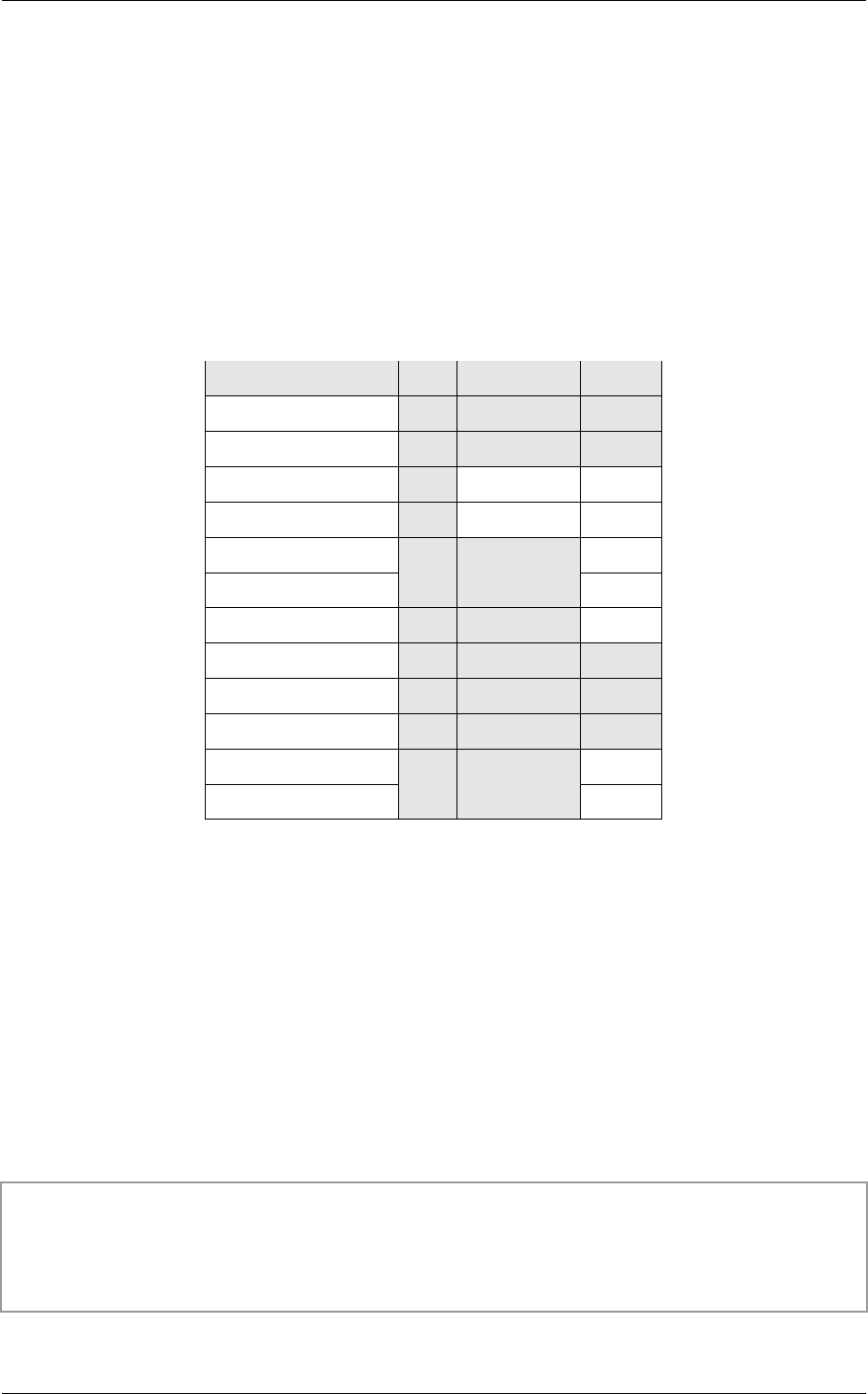
10.1 OptiXpp objects 10 OptiXpp: C++ wrapper for the OptiX C API

removeVariable

Remove a variable associated with this object

getVariableCount

Query the number of variables associated with this object, typically so as to iterate over

them

getVariable

Query variable by index, typically while iterating over them

10.1.2.4 Attributes of OptiXpp objects

The following table lists all of the OptiXpp objects and their attributes.

Object API Destroyable Scoped

Context X X X

Program X X X

Buffer X

Variable X

TextureSampler X X

Group X X

GeometryGroup X X

GeometryInstance X X X

Geometry X X X

Material X X X

Transform X X

Selector X X

Table 9 – OptiXpp opaque types and their attributes

10.1.3 API objects

In addition to the methods provided by the attribute classes that give commonality to the

different API objects each object type also has a unique set of methods. These functions cover

the complete set of functionality from the C API, although not all methods will be described

here. See OptiXpp_namespace.h for the complete set.

10.1.3.1 Context

The Context object provides create* functions for creating all other opaque types. These are

owned by the context and handles to the created object are returned:

Context my_context;

Buffer Buf =

my_context->createBuffer(

RT_BUFFER_INPUT, RT_FORMAT_FLOAT4, 1024, 1024);

10 OptiXpp: C++ wrapper for the OptiX C API 10.1 OptiXpp objects

Context also provides launch functions, with overloads for 1D, 2D, and 3D kernel launches. It

provides many other functions that wrap rtContext* C API calls.

10.1.3.2 Buer

The Buffer class provides a map call that returns a pointer to the buffer data, and provides an

unmap call. It also provides set and get functions for the buffer format, element size, and

1D, 2D, and 3D buffer size. Finally, it provides registerGLBuffer and unregisterGLBuffer.

10.1.3.3 Variable

The Variable class provides getName,getAnnotation,getType, and getSize functions for

returning properties of the variable. It also contains a multitude of set* functions that set the

value of the variable and its type, if the type is not already set:

my_context["my_dim3"]->setInt( 512, 512, 1024 );

The Variable object also offers set functions for setting its value to an API object, and provides

setUserData and getUserData.

10.1.3.4 TextureSampler

The TextureSampler class provides functions to set and get the attributes of an

RTtexturesampler, such as setWrapMode,setMipLevelCount, etc.

It also provides setBuffer,getBuffer,registerGLTexture, and unregisterGLTexture.

10.1.3.5 Group and GeometryGroup

The remaining API object classes are for OptiX node types. They offer member functions for

setting and querying the nodes to which they attach.

The Group class provides setAcceleration,getAcceleration,setChildCount,

getChildCount,setChild, and getChild.

10.1.3.6 GeometryInstance

RTgeometryinstance is a binding of Geometry and Material. Thus, GeometryInstance

provides functions to set and get both the Geometry and the Materials. This includes

addMaterial, which increments the material count and appends the given Material to the list.

10.1.3.7 Geometry

The unique functions provided by the Geometry class set and get the BoundingBoxProgram,

the IntersectionProgram and the PrimitiveCount. It also offers markDirty and isDirty.

10.1.3.8 Material

A Material consists of a ClosestHitProgram and an AnyHitProgram, and is a container for the

variables appertaining to these programs. It contains set and get functions for these programs.

10.1 OptiXpp objects 10 OptiXpp: C++ wrapper for the OptiX C API

10.1.3.9 Transform

An RTtransform node applies a transformation matrix to its child, so the Transform class

offers setChild,getChild,setMatrix, and getMatrix methods.

10.1.3.10 Selector

A Selector node applies a Visit program to operate on its multiple children. Thus, the Selector

class includes functions to set and get the VisitProgram,ChildCount, and Child.

10.1.4 Exceptions

The Exception class of OptiXpp encapsulates an error message. These errors are often the

direct result of a failed OptiX C API function call and subsequent rtContextGetErrorString

call. Nearly all methods of all object types can throw an exception using the Exception class.

Likewise, the checkError function can throw an Exception.

Additionally, the Exception class can be used explicitly by user code as a convenient way to

throw exceptions of the same type as OptiXpp.

Call Exception::makeException to create an Exception.

Call getErrorString to return an std::string for the error message as returned by

rtContextGetErrorString.

10 OptiXpp: C++ wrapper for the OptiX C API 10.1 OptiXpp objects

11 OptiX Prime: low-level ray tracing API

11.1 Overview

OptiX is generally used to represent an entire algorithm implementation, whether that be

rendering, visibility, radiation transfer, or anything else. The many user programmable

portions of OptiX allow the application to express complex operations, such as shading, that

are tightly intermingled, often recursively, with the ray tracing operations and expressed in a

single-ray programming model. By encapsulating the programmable portions of the

algorithm and owning the entire algorithm, OptiX can execute the entire algorithm on the

GPU and optimize the execution for each new GPU as it is released or for other platforms

such as cloud rendering on the NVIDIA VCA.

Sometimes the algorithm as a whole does not beneﬁt from this tight coupling of user code

and ray tracing code, and only the ray tracing functionality is needed. Visibility, trivial ray

casting rendering, and ray tracing very large batches of rays in phases may have this

property. OptiX Prime is a set of OptiX APIs designed for these use cases. Prime is specialized

to deliver high performance for intersecting a set of rays against a set of triangles. Prime is a

thinner, simpler API, since programmable operations, such as shading, are excluded. Prime is

also suitable for some quick experimentation and hobby projects.

The OptiX Prime API consist of three main objects:

BufferDesc

Wraps application managed buffers and provides descriptive information about them.

Context

Manages resource allocation.

Model

Represents a set of triangles and an acceleration structure.

Query

Coordinates the intersection of rays with a model.

11.2 Context

An OptiX Prime context performs two main functions. The ﬁrst function is to manage objects

created by the API. The context can create objects, some of which can also create other objects.

All of these objects are registered with the context and will be destroyed when the context is

destroyed. The second function is to encapsulate a particular backend that performs the

actual computation.

Currently the following context types are supported:

•RTP_CONTEXT_TYPE_CPU

•RTP_CONTEXT_TYPE_CUDA

11 OptiX Prime: low-level ray tracing API 11.3 Buer descriptor

RTP_CONTEXT_TYPE_CPU is intended to be used as a fallback when an acceptable CUDA device

is not available. It will allow an application to run, despite the absence of CUDA-capable

GPUs, but will have lower performance. In certain situations it might also make sense to use

CPU and CUDA contexts in parallel.

RTP_CONTEXT_TYPE_CUDA by default will only use the fastest available device. It is also

possible to specify a speciﬁc device (or a list of devices) to be used by the context by

supplying a list of device numbers to rtpContextSetCudaDevices. The fastest device in this

list is used as the primary device. Acceleration structures will be built on that primary device

and copied to the others. Speciﬁed devices must feature compute capability SM 3.0 or greater.

All devices will be used for ray tracing with work being distributed proportionally to each

device’s computational power. Note that this distribution can be rather costly if the rays are

stored in device memory though. For maximum efﬁciency it is recommended to only ever

select one device per context. The CUDA context of the primary device is made current after

a call to rtpContextCreate or rtpContextSetDevices.

The following code demonstrates how to create a context and specify which devices to use. In

this example, a CPU context is created as a fallback.

RTPcontext context;

if(rtpContextCreate( RTP_CONTEXT_TYPE_CUDA, &context ) == RTP_SUCCESS ) {

int deviceNumbers[] = {0,1};

rtpContextSetCudaDeviceNumbers( 2, deviceNumbers );

}

else {

rtpContextCreate( RTP_CONTEXT_TYPE_CPU, &context );

}

11.3 Buer descriptor

The buffers used to send and receive data from OptiX Prime are managed by the application.

A buffer descriptor is an object that provides information about a buffer, such as its format

and location, as well as the pointer to the buffer’s data. OptiX Prime supports the following

buffer types:

•RTP_BUFFER_TYPE_HOST

•RTP_BUFFER_TYPE_CUDA_LINEAR

A buffer descriptor is created by calling rtpBufferDescCreate. A buffer of type

RTP_BUFFER_TYPE_CUDA_LINEAR is assumed to reside on the current CUDA device. The

device number for the buffer can be speciﬁed explicitly by calling

rtpBufferDescSetCudaDeviceNumber.

The portion of the buffer to use for input or output is speciﬁed by calling

rtpBufferDescSetRange. The range is speciﬁed in terms of the number of elements.

For buffers containing vertex data, it is possible to specify a stride in bytes between each

element. This is useful for vertex buffers that contain interleaved vertex attributes, as shown

in the following example:

struct Vertex {

float3 pos, normal, color;

11.4 Model 11 OptiX Prime: low-level ray tracing API

};

...

RTPbufferdesc vertsBD;

rtpBufferDescCreate(

context, RTP_BUFFER_FORMAT_VERTEX_FLOAT3, RTP_BUFFER_TYPE_HOST,

verts, &vertsBD);

rtpBufferDescSetRange(vertsBD, 0, numVerts);

rtpBufferDescSetStride(vertsBD, sizeof(Vertex));

The functions that accept buffer descriptors as parameters have copy semantics. This means,

for example, when a buffer descriptor is used in a call to set the rays to be queried and

afterwards the range of the buffer descriptor is changed, the changes to the buffer descriptor

will not be visible to the query. However, changing the contents of the buffer itself could

affect the query.

Buffer descriptors are lightweight objects and can be created and destroyed as needed.

Buffers of any type can be passed to OptiX Prime functions and the will automatically be

copied to the appropriate location. For example, a vertex buffer on the host will be copied to

the primary device when the context is of type RTP_CONTEXT_TYPE_CUDA. While convenient,

this automatic copying may require the allocation of memory on the device and can

negatively impact performance. For best performance it is recommended that the following

buffer and context types be used together:

Context type Buffer type

RTP_CONTEXT_TYPE_CPU RTP_BUFFER_TYPE_HOST

RTP_CONTEXT_TYPE_CUDA RTP_BUFFER_TYPE_CUDA_LINEAR (on the primary device)

11.4 Model

A model represents either a set of triangles or a group of model instances, in addition to an

acceleration structure built over the triangles or instances. A model is created with an

associated context by calling rtpModelCreate, and can be destroyed with rtpModelDestroy.

11.4.1 Triangle models

Triangle data for the model is supplied by calling rtpModelSetTriangles with a vertex buffer

descriptor and an optional index buffer descriptor. If no index buffer is supplied then the

vertex buffer is considered to be a ﬂat list of triangle vertices, with every set of three vertices

forming a triangle (i.e., a triangle soup).

rtpModelUpdate creates the acceleration structure over the triangles. It is important that the

vertex and index buffers speciﬁed in rtpModelSetTriangles remain valid until

rtpModelUpdate is ﬁnished. If the ﬂag RTP_MODEL_HINT_ASYNC is speciﬁed, some or all of the

acceleration structure update may run asynchronously and rtpModelUpdate may return

before the update is ﬁnished. rtpModelFinish blocks the calling thread until the update is

ﬁnished. rtpModelGetFinished can be used to poll until the update is ﬁnished. Once the

update has ﬁnished, the input buffers can be modiﬁed.

11 OptiX Prime: low-level ray tracing API 11.4 Model

The following code demonstrates how to create a model from a vertex buffer with an

asynchronous update. The code assumes that a vertex buffer descriptor vertsBD already

exists:

RTPmodel model;

rtpModelCreate(context, &model);

rtpModelSetTriangles(model, 0, vertsBD);

rtpModelUpdate(model, RTP_MODEL_HINT_ASYNC);

// ... do useful work on CPU while GPU is busy

rtpModelFinish(model);

// safe to modify vertex buffer

For some use cases, the user may wish to have explicit control over multi-GPU computation

rather than using the automatic multi-GPU support provided by OptiX Prime. A context can

be created for each device and work can be distributed manually to each context. OptiX

Prime provides rtpModelCopy to copy a model from one context to another so that it is not

necessary to create and update the model in each context. rtpModelCopy can also be used to

build multiple models in parallel on different devices, then broadcast the results to each

device. When using older devices, rtpModelCopy can be used to build an acceleration

structure in a CPU context and copy it to the context that uses the devices.

Beyond the memory used by the ﬁnal acceleration structure, some additional memory is

needed during rtpModelUpdate. The amount used may be controlled by calling

rtpModelSetBuilderParameter. The RTP_BUILDER_PARAM_CHUNK_SIZE controls the amount

of scratch space used while building. The minimum scratch space is currently 64MB, and the

default scratch space is 10available video memory for CUDA contexts, and 512MB for CPU

contexts. A chunk size of -1 signiﬁes unlimited. In this case about 152 bytes per triangle are

used while building the acceleration structure.

RTP_BUILDER_PARAM_USE_CALLER_TRIANGLES controls whether to create a possibly

transformed copy of the vertex buffer data, or to use the buffer supplied by the user, thus

saving memory. If a model is copied, and the source model is using the user supplied triangle

data to save memory, the user triangles will be automatically copied as well. If this is not

intended, it is necessary to set RTP_BUILDER_PARAM_USE_CALLER_TRIANGLES on the

destination model as well, before the copy is performed. Afterward, rtpModelSetTriangles

must be called to supply the user triangles on the destination model.

11.4.2 Instancing

Using instancing, it is possible to compose complex scenes using existing triangle models

(compare section the “Triangle models” section (page 93)). Instancing data for a model is

supplied by calling rtpModelSetInstances with an instance buffer descriptor and a

transformation buffer descriptor. The ranges for these buffer descriptors must be identical.

The type of the instance buffer descriptor must be RTP_BUFFER_TYPE_HOST, and the format

RTP_BUFFER_FORMAT_INSTANCE_MODEL. For transformations, the buffer descriptor format can

be either RTP_BUFFER_FORMAT_TRANSFORM_FLOAT4x4 or

RTP_BUFFER_FORMAT_TRANSFORM_FLOAT4x3. If a stride is speciﬁed for the transformations, it

must be a multiple of 16 bytes. Furthermore, the matrices must be stored in row-major order.

11.5 Query 11 OptiX Prime: low-level ray tracing API

Please note that only afﬁne transformations are supported, and that the last row is always

assumed to be [0.0, 0.0, 0.0, 1.0].

In contrast to triangle models, instance models can not be copied.

For an example of instancing please refer to the primeInstancing sample which ships with the

OptiX SDK.

11.4.3 Masking

With masking, it is possible to specify per triangle visibility information in combination with

a per ray mask. In order to use masking, triangle data must be speciﬁed with the

RTP_BUFFER_FORMAT_INDICES_INT3_MASK_INT buffer format. Furthermore the user-triangle

build parameter must be set, as well as ray format

RTP_BUFFER_FORMAT_RAY_ORIGIN_MASK_DIRECTION_TMAX must be used. The per triangle

visibility ﬂags are evaluated by a bitwise AND operation with the currently processed ray’s

MASK ﬁeld before a ray-triangle intersection is performed. If the result is non-zero, the

ray-triangle intersection test is skipped. The combination of a per triangle mask with a per

ray mask e.g. allows to exclude triangles based on different ray generations.

If the per triangle mask values need to be updated, rtpModelSetTriangles must be called

again, with a successive call to rtpModelUpdate. Using the RTP_MODEL_HINT_MASK_UPDATE

ﬂag indicates that only the per triangle mask has changed, but that no rebuild of the

acceleration structure is needed.

For an example of masking, please refer to the primeMasking sample which ships with the

OptiX SDK.

11.5 Query

A query is used to perform the actual ray tracing against a model. The query is created from a

model using rtpQueryCreate. The following types of queries are supported:

•RTP_QUERY_TYPE_ANY

•RTP_QUERY_TYPE_CLOSEST

Along any given ray there may be a number of intersection points. RTP_QUERY_TYPE_CLOSEST

returns the ﬁrst hit along the ray. RTP_QUERY_TYPE_ANY returns the ﬁrst hit found, whether it

is the closest or not. The query takes a buffer of rays to intersect and a buffer to store the

resulting hits. There are several formats for the rays and hits. The main advantage of the

different formats is that some require less storage than others. This is important for

minimizing the transfer time of rays and hit data between the host and the device and

between devices.

Once the ray and hit buffers have been speciﬁed, the query can be executed by calling

rtpQueryExecute. The ray buffer must not be modiﬁed until after this function returns. If the

ﬂag RTP_QUERY_HINT_ASYNC is speciﬁed, rtpQueryExecute may return before the query is

actually ﬁnished. rtpQueryFinish can be called to block the current thread until the query is

ﬁnished, or rtpQueryGetFinished can be used to poll until the query is ﬁnished. At this point

all of the hits are guaranteed to have been returned, and it is safe to modify the ray buffer.

The following code demonstrates how to execute a query using ray and hit buffers:

RTPquery query;

11 OptiX Prime: low-level ray tracing API 11.7 Multi-threading

RTPbufferdesc raysBD, hitsBD;

// fill in raysBD with rays

rtpQueryCreate(model, RTP_QUERY_TYPE_CLOSEST, &query);

rtpQuerySetRays(query, raysBD);

rtpQuerySetHits(hits, hitsBD);

rtpQueryExecute(query, 0);

// safe to modify ray buffer and process hits

With rtpQuerySetCudaStream, it is possible to specify a speciﬁc CUDA stream which can be

used to synchronize (asynchronous) queries and user CUDA kernel launches. If no stream is

speciﬁed, the CUDA default stream is used.

A query may be executed multiple times. Note that rtpQueryFinish and

rtpQueryGetFinished only apply to the stream corresponding to the last call to

rtpQueryExecute. Therefore, if the stream has been changed between asynchronous calls to

rtpQueryExecute it may be necessary to manually synchronize the streams, i.e. by calling

cudaStreamSynchronize or using CUDA events (see the CUDA Programming Guide).

11.6 Utility functions

In addition to the basic objects and their functions, OptiX Prime has several utility functions.

11.6.1 Page-locked buers

The performance of transfers between devices and the host can be improved by page-locking

the host memory. Functions for page-locking already allocated memory are provided in the

CUDA runtime. For convenience, OptiX Prime provides the functions rtpHostBufferLock

and rtpHostBufferUnlock so that it is possible to achieve better performance with host

buffers without having to invoke CUDA functions directly. Note that page- locking excessive

amounts of memory may degrade system performance, since it reduces the amount of

memory available to the system for paging. As a result, this function is best used sparingly to

11.6.2 Error reporting

All functions in OptiX Prime return an error code. The function rtpGetErrorString

translates an error code into a string. rtpContextGetLastErrorString returns an error string

for the last error encountered. This error string may contain additional information beyond a

simple error code. Note that this function may also return errors from previous asynchronous

launches, or from other threads.

11.7 Multi-threading

The OptiX Prime API is thread safe. It is possible to share a single context among multiple

host threads. However only one thread may access a context (or objects associated with it) at

a time. Therefore to avoid locking other threads out of the API for extensive periods of time,

the asynchronous APIs should be used. Care must also be taken to synchronize state changes

to API objects. For example, if two threads try to set the ray buffer on the same query at the

same time, a race condition can occur.

11.8 Streams 11 OptiX Prime: low-level ray tracing API

11.8 Streams

By default, all computation in OptiX Prime (e.g. updating models and executing queries)

takes place within the default CUDA stream of the primary device. However, with

rtpQuerySetCudaStream it is possible to specify a speciﬁc CUDA stream which can be used

to synchronize (asynchronous) queries and user CUDA kernel launches.

11 OptiX Prime: low-level ray tracing API 11.8 Streams

12 OptiX Prime++: C++ wrapper for the OptiX Prime API

OptiX Prime++ wraps each OptiX Prime C API opaque type in a C++ class and provides

relevant operations on that type. Most of the OptiX Prime++ class member functions map

directly to C API function calls. For example, ContextObj::setCudaDeviceNumbers maps

directly to rtpContextSetCudaDeviceNumbers.

Some functions perform slightly more complex sequences of C API calls. For example

ModelObj::setTriangles

provides in one call the functionality of

rtpBufferDescCreate

rtpBufferDescSetRange

rtpBufferDescSetStride

rtpModelSetTriangles

rtpBufferDescDestroy

See the OptiX API Reference.pdf or OptiX_primepp.h for a full list of the available OptiX

Prime++ functions. The usage of the API is described below.

12.1 OptiX Prime++ objects

Manipulation of OptiX Prime objects is performed via reference counted Handle classes

which encapsulate all OptiX Prime objects functionalities.

All classes are manipulated via the reference counted Handle class. Rather than working with

aContextObj directly you would use a Context instead, which is simply a typedef for

Handle<ContextObj>.

12.1.1 Context object

The Context object wraps the OptiX Prime C API RTPcontext opaque type and its associated

function set representing an OptiX Prime context.Its constructor requires a

RTPcontexttype type in order to specify the type of the context to be created (CPU or GPU).

By default, only the fastest GPU will be used. A different device (or a list of devices) can be

selected by using ContextObj::setCudaDeviceNumbers. Note that for maximum efﬁciency it

is recommended to only ever select one device per context.

Context context( Context::create(contextType) );

For all objects the following pattern is also possible:

Context context;

12 OptiX Prime++: C++ wrapper for the OptiX Prime API 12.1 OptiX Prime++ objects

context = Context::create(contextType);

The Context also provides functions to create OptiX Prime objects directly owned by it.

ContextObj::createBufferDesc

ContextObj::createModel

ContextObj::createQuery

12.1.2 BuerDesc object

The BufferDesc object wraps a RTPbufferdesc object opaque type and its associated function

set representing an OptiX Prime buffer descriptor.

The creation of a BufferDesc object is demanded to an owning Context object since each

BufferDesc object needs to be assigned to an OptiX Prime context.

12.1.3 Model object

The Model object wraps a RTPmodel object opaque type and its associated function set

representing an OptiX Prime model.

The creation of a Model object is demanded to an owning Context object since each Model

object needs to be assigned to an OptiX Prime context.

Variants of the setTriangles functions are provided to allow creating a model by either a

custom-format triangle soup , with a supplied indices buffer descriptor or directly from a

supplied vertices buffer descriptor.

12.1.4 Query object

The Query object wraps a RTPquery object opaque type and its associated function set

representing an OptiX Prime query.

The creation of a Query object is demanded to an owning Context object since each Query

object needs to be assigned to an OptiX Prime context.

Variants of the setRays and setHits functions are provided to allow setting the rays and the

hits for a query from either a custom-format user supplied buffer or from a buffer descriptor.

12.1.5 Exception class

The Exception class provides methods to deal with OptiX Prime exceptions. Both error code

and error description methods are provided as well as a wrapper for the

rtpContextGetLastErrorString function

catch ( Exception& e ) {

std::cerr << "An error occurred with error code "

<< e.getErrorCode() << " and message "

<< e.getErrorString() << std::endl;

}

13 Performance guidelines

Subtle changes in your code can dramatically alter performance. This list of performance tips

should help when using OptiX.

•Where possible use ﬂoats instead of doubles. This also extends to the use of literals and

math functions. For example, use 0.5f instead of 0.5 and sinf instead of sin to prevent

automatic type promotion. To check for automatic type promotion, search the PTX ﬁles

for the .f64 instruction modiﬁer.

•OptiX will try to partition thread launches into tiles that are the same dimensionality as

the launch. To have maximal coherency between the threads of a tile you should choose

a launch dimensionality that is the same as the coherence dimensionality of your

problem. For example, the common problem of rendering an image has 2D coherency

(adjacent pixels both horizontally and vertically look at the same part of the scene), so a

2D launch is appropriate. Conversely, a collision detection problem with many agents

each looking in many directions may appear to be 2D (the agents in one dimension and

the ray directions in another), but there is rarely coherence between different agents, so

the coherence dimensionality is one, and performance will be better by using a 1D

launch.

•Do not build an articulate scene graph with Groups,Transforms and

GeometryInstances. Try to make the topology as shallow and minimal as possible. For

example, for static scenes the fastest performance is achieved by having a single

GeometryGroup, where transforms are ﬂattened to the geometry. For scenes where

Transforms are changing all the static geometry should go in one GeometryGroup and

each Transform should have a single GeometryGroup. Also, if possible, combine

multiple meshes into a single mesh.

•Each new Program object can introduce execution divergence. Try to reuse the same

program with different variable values. However, don’t take this idea too far and

attempt to create an “über shader.” This will create execution divergence within the

program. Experiment with your scene to ﬁnd the right balance.

•Try to minimize live state across calls to rtTrace in programs. For example, in a closest

hit program temporary values used after a recursive call to rtTrace should be computed

after the call to rtTrace, rather than before, since these values must be saved and

restored when calling rtTrace, impacting performance. RTvariables declared outside

of the program body are exempt from this rule.

•In multi-GPU environments INPUT_OUTPUT and OUTPUT buffers are stored on the host. In

order to optimize writes to these buffers, types of either 4 bytes or 16 bytes (e.g. float,

uint, or float4) should be used when possible. One might be tempted to make an

output buffer used for the screen out of float3’ (RGB), however using a float4 buffer

will result in improved performance (e.g.

output_buffer[launch_index] = make_float4( result_color )). This also affects

deﬁned types (see the progressivePhotonMap sample for an example of accessing user

deﬁned structs with float4s)

13 Performance guidelines

•Memory accesses to structs containing four-vectors, such as ﬂoat4, need to be 16-byte

aligned for optimal performance. Do so by placing the largest aligned variables ﬁrst in

structs.

•In multi-GPU environments, INPUT_OUTPUT buffers may be stored on the device, with a

separate copy per device by using the RT_BUFFER_GPU_LOCAL buffer attribute. This is

useful for avoiding the slower reads and writes by the device to host memory.

RT_BUFFER_GPU_LOCAL is useful for scratch buffers, such as random number seed

buffers and variance buffers.

•Use iteration instead of recursion where possible (e.g. path tracing with no ray

branching). See the path_tracer sample for an example of how to use iteration instead of

recursion when tracing secondary rays.

•For best performance, use the rtTransform* functions rather than explicitly

transforming by the matrix returned by rtGetTransform.

•Disable exceptions that are not needed. While it is recommended to turn on all available

exception types during development and for debugging, the error checking involved

e.g. to validate buffer index bounds is usually not necessary in the ﬁnal product.

•Avoid recompiling the OptiX kernel. These recompiles can be triggered when certain

changes to the input programs or variables occur. For example, swapping the

ClosestHit program of a Material between two programs will cause a recompile on each

swap because the kernel consists of different code, whereas creating two Materials, one

with each program, and swapping between the two Materials will not cause a recompile

because only the node graph is changing, not the code. Creating dummy nodes with the

alternate programs is one way to provide all of the code at once. Also avoid changing

the layout of variables attached to scope objects.

•It is possible for a program to ﬁnd multiple deﬁnitions for a variable in its scopes

depending upon where the program is called. Variables with deﬁnitions in multiple

scopes are said to be dynamic and may incur a performance penalty.

•Uninitialized variables can increase register pressure and negatively impact

performance.

•When creating PTX code using nvcc, adding --use-fast-math as a compile option can

reduce code size and increase the performance for most OptiX programs. This can come

at the price of slightly decreased numerical ﬂoating point accuracy. See the nvcc

documentation5for more details.

•Avoid using OpenGL interop in combination with VCA remote rendering.

•Use output buffers in ﬂoat4 format for VCA remote rendering, even if only three

components are needed.

The following performance guidelines apply to OptiX Prime:

•Use page-locked host memory for host buffers to improve performance when using

contexts of type RTP_CONTEXT_TYPE_CUDA. Asynchronous API calls involving host

buffers can may not actually be asynchronous if the host memory is not page-locked.

•Multi-GPU contexts, while convenient, are limited by PCIe bandwidth. That is because

ray and hit buffers reside in a single location (either the host or a device) and must be

copied over the PCIe bus to multiple devices. It is possible to obtain better performance

5http://docs.nvidia.com/cuda/cuda-compiler-driver-nvcc/index.html

13 Performance guidelines

by managing multiple GPUs manually. By allocating a context for each device and

generating rays and consuming hits on the device, transfers can be avoided.

•For maximum concurrency with model updates, it is best to use a separate context for

each device, each running in its own host thread. There are currently some limitations

on the amount of concurrency that can be achieved from a single host thread which will

be addressed in a future release.

•Prime contexts allocate a small amount of page-locked host memory. Because the

allocation of page-locked memory can sometimes block when other kernels are running,

it is best to initialize contexts when no long-running kernels are active.

•With the current implementation, the performance of queries created from a multi-GPU

context are generally better when used with buffers residing in page-locked host

memory rather than on a device.

•Use the asynchronous API when using Prime in a multi-threaded setting to achieve

better concurrency.

13 Performance guidelines

14 Caveats

Keep in mind the following caveats when using OptiX.

•Setting a large stack size will consume GPU device memory. Try to minimize the stack

as much as possible. Start with a small stack and with the use of an exception program

that will make it obvious you have exceeded your memory, increase the stack size until

the stack is sufﬁciently large.

•The use of __shared__ memory within a program is not allowed.

•The use of PTX bar or CUDA syncthreads within a program is not allowed.

•threadIdx in CUDA can map to multiple launch indices (e.g. pixels). Use the

rtLaunchIndex semantic instead.

•Use of the CUDA malloc,free, and printf functions within a program is not

supported. Attempts to use these functions will result in an illegal symbol error.

•Currently, the OptiX host API is not guaranteed to be thread-safe. While it may be

successful in some applications to use OptiX contexts in different host threads, it may

fail in others. OptiX should therefore only be used from within a single host thread.

•On Fermi architecture the number of cube, layered, and half ﬂoat textures is limited to

127. Mip levels of textures over the 127 limit are stripped to one level.

14 Caveats

15 Appendix: Texture formats

OpenGL texture format

GL_RGBA8

GL_RGBA16

GL_R32F

GL_RG32F

GL_RGBA32F

GL_R8I

GL_R8UI

GL_R16I

GL_R16UI

GL_R32I

GL_R32UI

GL_RG8I

GL_RG8UI

GL_RG16I

GL_RG16UI

GL_RG32I

GL_RG32UI

GL_RGBA8I

GL_RGBA8UI

GL_RGBA16I

GL_RGBA16UI

GL_RGBA32I

GL_RGBA32UI

NVIDIA OptiX 5.0 Programming Guide Opti X 5.0.0

Navigation menu

Versions of this User Manual:

Views

Navigation