Oracle 11g A Beginner's Guide
User Manual: Pdf
Open the PDF directly: View PDF ![]() .
.
Page Count: 433 [warning: Documents this large are best viewed by clicking the View PDF Link!]
- Contents
- Acknowledgments
- Introduction
- 1 Database Fundamentals
- Critical Skill 1.1 Define a Database
- Critical Skill 1.2 Learn the Oracle Database 11g Architecture
- Project 1-1 Review the Oracle Database 11g Architecture
- Critical Skill 1.3 Learn the Basic Oracle Database 11g Data Types
- Critical Skill 1.4 Work with Tables
- Critical Skill 1.5 Work with Stored Programmed Objects
- Critical Skill 1.6 Become Familiar with Other Important Items in Oracle Database 11g
- Critical Skill 1.7 Work with Object and System Privileges
- Critical Skill 1.8 Introduce Yourself to the Grid
- Critical Skill 1.9 Tie It All Together
- Chapter 1 Mastery Check
- 2 Installing Oracle
- 3 Connecting to Oracle
- Critical Skill 3.1 Use Oracle Net Services
- Critical Skill 3.2 Learn the Difference Between Dedicated and Shared Server Architectures
- Critical Skill 3.3 Define Connections
- Critical Skill 3.4 Use the Oracle Net Listener
- Critical Skill 3.5 Learn Naming Methods
- Critical Skill 3.6 Use Oracle Configuration Files
- Critical Skill 3.7 Use Administration Tools
- Project 3-1 Test a Connection
- Critical Skill 3.8 Use Profiles
- Critical Skill 3.9 Network in a Multi-tiered Environment
- Critical Skill 3.10 Install the Oracle 11g Client Software
- Chapter 3 Mastery Check
- 4 SQL: Structured Query Language
- Critical Skill 4.1 Learn the SQL Statement Components
- Critical Skill 4.2 Use Basic Insert and Select Statements
- Critical Skill 4.3 Use Simple Where Clauses
- Critical Skill 4.4 Use Basic Update and Delete Statements
- Critical Skill 4.5 Order Data
- Critical Skill 4.6 Employ Functions: String, Numeric, Aggregate (No Grouping)
- Critical Skill 4.7 Use Dates and Data Functions (Formatting and Chronological)
- Critical Skill 4.8 Employ Joins (ANSI vs. Oracle): Inner, Outer, Self
- Project 4-1 Join Data Using Inner and Outer Joins
- Project 4-2 Join Data Using ANSI SQL Joins
- Critical Skill 4.9 Learn the Group By and Having Clauses
- Project 4-3 Group Data in Your Select Statements
- Critical Skill 4.10 Learn Subqueries: Simple and Correlated Comparison with Joins
- Critical Skill 4.11 Use Set Operators: Union, Intersect, Minus
- Project 4-4 Use the Union Function in Your SQL
- Critical Skill 4.12 Use Views
- Critical Skill 4.13 Learn Sequences: Just Simple Stuff
- Critical Skill 4.14 Employ Constraints: Linkage to Entity Models, Types, Deferred, Enforced, Gathering Exceptions
- Critical Skill 4.15 Format Your Output with SQL*Plus
- Project 4-5 Format Your SQL Output
- Chapter 4 Mastery Check
- 5 PL/SQL
- Critical Skill 5.1 Define PL/SQL and Learn Why We Use It
- Critical Skill 5.2 Describe the Basic PL/SQL Program Structure
- Critical Skill 5.3 Define PL/SQL Data Types
- Critical Skill 5.4 Write PL/SQL Programs in SQL*Plus
- Project 5-1 Create a PL/SQL Program
- Critical Skill 5.5 Handle Error Conditions in PL/SQL
- Critical Skill 5.6 Include Conditions in Your Programs
- Project 5-2 Use Conditions and Loops in PL/SQL
- Critical Skill 5.7 Create Stored Procedures—How and Why
- Critical Skill 5.8 Create and Use Functions
- Project 5-3 Create and Use a Function
- Critical Skill 5.9 Call PL/SQL Programs
- Chapter 5 Mastery Check
- 6 The Database Administrator
- Critical Skill 6.1 Learn What a DBA Does
- Critical Skill 6.2 Perform Day-to-Day Operations
- Critical Skill 6.3 Understand the Oracle Database 11g Infrastructure
- Critical Skill 6.4 Operate Modes of an Oracle Database 11g
- Critical Skill 6.5 Get Started with Oracle Enterprise Manager
- Critical Skill 6.6 Manage Database Objects
- Critical Skill 6.7 Manage Space
- Critical Skill 6.8 Manage Users
- Critical Skill 6.9 Manage Privileges for Database Users
- Project 6-1 Create Essential Objects
- Chapter 6 Mastery Check
- 7 Backup and Recovery
- Critical Skill 7.1 Understand Oracle Backup and Recovery Fundamentals
- Critical Skill 7.2 Learn about Oracle User-Managed Backup and Recovery
- Critical Skill 7.3 Write a Database Backup
- Critical Skill 7.4 Back Up Archived Redo Logs
- Critical Skill 7.5 Get Started with Oracle Data Pump
- Critical Skill 7.6 Use Oracle Data Pump Export
- Critical Skill 7.7 Work with Oracle Data Pump Import
- Critical Skill 7.8 Use Traditional Export and Import
- Critical Skill 7.9 Get Started with Recovery Manager
- Project 7-1 RMAN End to End
- Chapter 7 Mastery Check
- 8 High Availability: RAC, ASM, and Data Guard
- Critical Skill 8.1 Define High Availability
- Critical Skill 8.2 Understand Real Application Clusters
- Critical Skill 8.3 Install RAC
- Critical Skill 8.4 Test RAC
- Critical Skill 8.5 Set Up the ASM Instance
- Critical Skill 8.6 Create ASM Disk Groups
- Project 8-2 Create Disk Groups
- Critical Skill 8.7 Use ASMCMD and ASMLIB
- Critical Skill 8.8 Convert an Existing Database to ASM
- Critical Skill 8.9 Understand Data Guard
- Critical Skill 8.10 Explain Data Guard Protection Modes
- Critical Skill 8.11 Create a Physical Standby Server
- Project 8-3 Create a Physical Standby Server
- Chapter 8 Mastery Check
- 9 Large Database Features
- Critical Skill 9.1 Learn to Identify a Very Large Database
- Critical Skill 9.2 Why and How to Use Data Partitioning
- Project 9-1 Create a Range-Partitioned Table and a Local-Partitioned Index
- Critical Skill 9.3 Compress Your Data
- Critical Skill 9.4 Use Parallel Processing to Improve Performance
- Critical Skill 9.5 Use Materialized Views
- Critical Skill 9.6 Use SQL Aggregate and Analysis Functions
- Critical Skill 9.7 Create SQL Models
- Project 9-2 Use Analytic SQL Functions and Models
- Chapter 9 Mastery Check
- A: Mastery Check Answers
- Chapter 1: Database Fundamentals
- Chapter 2: Installing Oracle
- Chapter 3: Connecting to Oracle
- Chapter 4: SQL: Structured Query Language
- Chapter 5: PL/SQL
- Chapter 6: The Database Administrator
- Chapter 7: Backup and Recovery
- Chapter 8: High Availability: RAC, ASM, and Data Guard
- Chapter 9: Large Database Features
- Index

Oracle Database 11g:
A Beginner’s Guide
Ian Abramson
Michael Abbey
Michael J. Corey
Michelle Malcher
New York Chicago San Francisco
Lisbon London Madrid Mexico City Milan
New Delhi San Juan Seoul Singapore Sydney Toronto

Copyright © 2009 by The McGraw-Hill Companies, Inc. All rights reserved. Except as permitted under the United States Copyright Act
of 1976, no part of this publication may be reproduced or distributed in any form or by any means, or stored in a database or retrieval sys-
tem, without the prior written permission of the publisher.
ISBN: 978-0-07-160460-4
MHID: 0-07-160460-X
The material in this eBook also appears in the print version of this title: ISBN: 978-0-07-160459-8, MHID: 0-07-160459-6.
All trademarks are trademarks of their respective owners. Rather than put a trademark symbol after every occurrence of a trademarked
name, we use names in an editorial fashion only, and to the benefit of the trademark owner, with no intention of infringement of the trade-
mark. Where such designations appear in this book, they have been printed with initial caps.
McGraw-Hill eBooks are available at special quantity discounts to use as premiums and sales promotions, or for use in corporate training
programs. To contact a representative please e-mail us at bulksales@mcgraw-hill.com.
Information has been obtained by Publisher from sources believed to be reliable. However, because of the possibility of human or mechan-
ical error by our sources, Publisher, or others, Publisher does not guarantee to the accuracy, adequacy, or completeness of any information
included in this work and is not responsible for any errors or omissions or the results obtained from the use of such information.
Oracle Corporation does not make any representations or warranties as to the accuracy, adequacy, or completeness of any information con-
tained in this Work, and is not responsible for any errors or omissions.
TERMS OF USE
This is a copyrighted work and The McGraw-Hill Companies, Inc. (“McGraw-Hill”) and its licensors reserve all rights in and to the work.
Use of this work is subject to these terms. Except as permitted under the Copyright Act of 1976 and the right to store and retrieve one copy
of the work, you may not decompile, disassemble, reverse engineer, reproduce, modify, create derivative works based upon, transmit, dis-
tribute, disseminate, sell, publish or sublicense the work or any part of it without McGraw-Hill’s prior consent. You may use the work for
your own noncommercial and personal use; any other use of the work is strictly prohibited. Your right to use the work may be terminated
if you fail to comply with these terms.
THE WORK IS PROVIDED “AS IS.” McGRAW-HILL AND ITS LICENSORS MAKE NO GUARANTEES OR WARRANTIES AS TO
THE ACCURACY, ADEQUACY OR COMPLETENESS OF OR RESULTS TO BE OBTAINED FROM USING THE WORK, INCLUD-
ING ANY INFORMATION THAT CAN BE ACCESSED THROUGH THE WORK VIA HYPERLINK OR OTHERWISE, AND
EXPRESSLY DISCLAIM ANY WARRANTY, EXPRESS OR IMPLIED, INCLUDING BUT NOT LIMITED TO IMPLIED WAR-
RANTIES OF MERCHANTABILITY OR FITNESS FOR A PARTICULAR PURPOSE. McGraw-Hill and its licensors do not warrant or
guarantee that the functions contained in the work will meet your requirements or that its operation will be uninterrupted or error free.
Neither McGraw-Hill nor its licensors shall be liable to you or anyone else for any inaccuracy, error or omission, regardless of cause, in
the work or for any damages resulting therefrom. McGraw-Hill has no responsibility for the content of any information accessed through
the work. Under no circumstances shall McGraw-Hill and/or its licensors be liable for any indirect, incidental, special, punitive,
consequential or similar damages that result from the use of or inability to use the work, even if any of them has been advised of the pos-
sibility of such damages. This limitation of liability shall apply to any claim or cause whatsoever whether such claim or cause arises in
contract, tort or otherwise.
This book is dedicated to all those who have
helped us learn and become better professionals.
We share this with all of you.

About the Authors
Ian Abramson is the current president for the Independent Oracle Users Group
(IOUG). Based in Toronto, Canada, he is an experienced industry and technical
consultant, providing expert guidance in implementing solutions for clients in
telecommunications, CRM, utilities, and other industries. His focus includes the
Oracle product set, as well as other leading technologies and their use in optimizing
data warehouse design and deployment. He is also a regular speaker at various
technology conferences, including COLLABORATE, Oracle OpenWorld, and
other local and regional events.
Michael Abbey is a recognized authority on database administration, installation,
development, application migration, performance tuning, and implementation.
Working with Ian Abramson and Michael Corey, he has coauthored works in
the Oracle Press series for over 14 years. Active in the international Oracle user
community, Abbey is a frequent presenter at COLLABORATE, Oracle OpenWorld,
and regional user group meetings.
Michael J. Corey is the founder and CEO of Ntirety—The Database Administration
Experts. Michael’s roots go back to Oracle version 3.0. Michael is a past president of the
Independent Oracle Users group (www.ioug.org) and the original Oracle Press author.
Michael is a frequent speaker at business and technology events and has presented all
over the world. Check out Michael’s blog at http://michaelcorey.ntirety.com.
Michelle Malcher is a Senior Database Administrator with
over ten years’ experience in database development, design,
and administration. She has expertise in performance tuning,
security, data modeling, and database architecture of very large database
environments. She is a contributing author for the IOUG Best Practices Tip
Booklet. Michelle is enthusiastically involved with the Independent Oracle
User Group and is director of Special Interest Groups. She enjoys presenting and
sharing ideas about Oracle Database topics at technology conferences and user
group meetings. She can be reached at michelle_malcher@ioug.org.
About the Reviewers
Carl Dudley has worked closely with Oracle for a number of years and presents regularly at international
conferences on Oracle database technology. He is currently a consultant database administrator and has
research interests in database performance, disaster planning, and security. Carl is a director of the UK
Oracle User Group, received Oracle Magazine’s Editors’ Choice Award for Database Administrator of the
Year in 2003 for services to the Oracle community, and achieved Oracle ACE status in 2007.
Ted Falcon, based in Toronto, Canada, is CEO of BDR Business Data Reporting Inc. He has ten
years’ experience in business intelligence reporting systems, specializing in the Cognos suite of tools.

Contents
ACKNOWLEDGMENTS . . . . . . . . . . . . . . . . . . . . . . . . . . . . . . . . . . . xiii
INTRODUCTION . . . . . . . . . . . . . . . . . . . . . . . . . . . . . . . . . . . . . . . . xv
1 Database Fundamentals . . . . . . . . . . . . . . . . . . . . . . . . . . . . . . . . . . . . 1
Critical Skill 1.1 Define a Database . . . . . . . . . . . . . . . . . . . . . . . . . . . 2
Critical Skill 1.2 Learn the Oracle Database 11gArchitecture . . . . . . . 4
The Control Files . . . . . . . . . . . . . . . . . . . . . . . . . . . . . . . . . . . . . . 5
The Online Redo Logs . . . . . . . . . . . . . . . . . . . . . . . . . . . . . . . . . . 5
The System Tablespace . . . . . . . . . . . . . . . . . . . . . . . . . . . . . . . . . 5
The Sysaux Tablespace . . . . . . . . . . . . . . . . . . . . . . . . . . . . . . . . . 6
Default Temporary Tablespace . . . . . . . . . . . . . . . . . . . . . . . . . . . 6
Undo Tablespace . . . . . . . . . . . . . . . . . . . . . . . . . . . . . . . . . . . . . 6
The Server Parameter File . . . . . . . . . . . . . . . . . . . . . . . . . . . . . . . 6
Background Processes . . . . . . . . . . . . . . . . . . . . . . . . . . . . . . . . . . 7
Project 1-1 Review the Oracle Database 11gArchitecture . . . . . . . . . 9
The Database Administrator . . . . . . . . . . . . . . . . . . . . . . . . . . . . . 10
Critical Skill 1.3 Learn the Basic Oracle Database 11gData Types . . . 11
varchar2 . . . . . . . . . . . . . . . . . . . . . . . . . . . . . . . . . . . . . . . . . . . . 12
number . . . . . . . . . . . . . . . . . . . . . . . . . . . . . . . . . . . . . . . . . . . . . 12
date . . . . . . . . . . . . . . . . . . . . . . . . . . . . . . . . . . . . . . . . . . . . . . . . 13
timestamp . . . . . . . . . . . . . . . . . . . . . . . . . . . . . . . . . . . . . . . . . . . 13
clob . . . . . . . . . . . . . . . . . . . . . . . . . . . . . . . . . . . . . . . . . . . . . . . . 13
blob . . . . . . . . . . . . . . . . . . . . . . . . . . . . . . . . . . . . . . . . . . . . . . . . 14
Critical Skill 1.4 Work with Tables . . . . . . . . . . . . . . . . . . . . . . . . . . . . 14
Tables Related to part_master . . . . . . . . . . . . . . . . . . . . . . . . . . . . 14
Critical Skill 1.5 Work with Stored Programmed Objects . . . . . . . . . . . 16
Views . . . . . . . . . . . . . . . . . . . . . . . . . . . . . . . . . . . . . . . . . . . . . . 16
Triggers . . . . . . . . . . . . . . . . . . . . . . . . . . . . . . . . . . . . . . . . . . . . . 18
Procedures . . . . . . . . . . . . . . . . . . . . . . . . . . . . . . . . . . . . . . . . . . 18
Functions . . . . . . . . . . . . . . . . . . . . . . . . . . . . . . . . . . . . . . . . . . . . 18
Packages . . . . . . . . . . . . . . . . . . . . . . . . . . . . . . . . . . . . . . . . . . . . 19
v
Critical Skill 1.6 Become Familiar with Other Important Items
in Oracle Database 11g . . . . . . . . . . . . . . . . . . . . . . . . . . . . . . . . . . 21
Indexes . . . . . . . . . . . . . . . . . . . . . . . . . . . . . . . . . . . . . . . . . . . . . 21
Users . . . . . . . . . . . . . . . . . . . . . . . . . . . . . . . . . . . . . . . . . . . . . . . 22
Tablespace Quotas . . . . . . . . . . . . . . . . . . . . . . . . . . . . . . . . . . . . 22
Synonyms . . . . . . . . . . . . . . . . . . . . . . . . . . . . . . . . . . . . . . . . . . . 23
Roles . . . . . . . . . . . . . . . . . . . . . . . . . . . . . . . . . . . . . . . . . . . . . . . 24
Default User Environments . . . . . . . . . . . . . . . . . . . . . . . . . . . . . . 24
Critical Skill 1.7 Work with Object and System Privileges . . . . . . . . . . 25
Select . . . . . . . . . . . . . . . . . . . . . . . . . . . . . . . . . . . . . . . . . . . . . . 25
Insert . . . . . . . . . . . . . . . . . . . . . . . . . . . . . . . . . . . . . . . . . . . . . . . 26
Update . . . . . . . . . . . . . . . . . . . . . . . . . . . . . . . . . . . . . . . . . . . . . 26
Delete . . . . . . . . . . . . . . . . . . . . . . . . . . . . . . . . . . . . . . . . . . . . . . 26
System Privileges . . . . . . . . . . . . . . . . . . . . . . . . . . . . . . . . . . . . . . 26
Critical Skill 1.8 Introduce Yourself to the Grid . . . . . . . . . . . . . . . . . . 27
Critical Skill 1.9 Tie It All Together . . . . . . . . . . . . . . . . . . . . . . . . . . . 31
Chapter 1 Mastery Check. . . . . . . . . . . . . . . . . . . . . . . . . . . . . . . . . . . . 32
2 Installing Oracle . . . . . . . . . . . . . . . . . . . . . . . . . . . . . . . . . . . . . . . . . . 35
Critical Skill 2.1 Research and Plan the Installation . . . . . . . . . . . . . . . 36
Define System Requirements . . . . . . . . . . . . . . . . . . . . . . . . . . . . . 37
Linux Installation . . . . . . . . . . . . . . . . . . . . . . . . . . . . . . . . . . . . . . 37
Critical Skill 2.2 Set Up the Operating System . . . . . . . . . . . . . . . . . . . 42
Project 2-1 Configure Kernel Parameters . . . . . . . . . . . . . . . . . . . . . . 44
Critical Skill 2.3 Get Familiar with Linux . . . . . . . . . . . . . . . . . . . . . . . 47
Critical Skill 2.4 Choose Components to Install . . . . . . . . . . . . . . . . . . 48
Critical Skill 2.5 Install the Oracle Software . . . . . . . . . . . . . . . . . . . . . 49
Database Configuration Assistant . . . . . . . . . . . . . . . . . . . . . . . . . . 57
Verify the Installation . . . . . . . . . . . . . . . . . . . . . . . . . . . . . . . . . . . 61
Chapter 2 Mastery Check. . . . . . . . . . . . . . . . . . . . . . . . . . . . . . . . . . . . 63
3 Connecting to Oracle . . . . . . . . . . . . . . . . . . . . . . . . . . . . . . . . . . . . . . 65
Critical Skill 3.1 Use Oracle Net Services . . . . . . . . . . . . . . . . . . . . . . 66
Network Protocols . . . . . . . . . . . . . . . . . . . . . . . . . . . . . . . . . . . . . 67
Optimize Network Bandwidth . . . . . . . . . . . . . . . . . . . . . . . . . . . . 67
Connections . . . . . . . . . . . . . . . . . . . . . . . . . . . . . . . . . . . . . . . . . 68
Maintain Connections . . . . . . . . . . . . . . . . . . . . . . . . . . . . . . . . . . 69
Define a Location . . . . . . . . . . . . . . . . . . . . . . . . . . . . . . . . . . . . . 70
Critical Skill 3.2 Learn the Difference Between Dedicated
and Shared Server Architectures . . . . . . . . . . . . . . . . . . . . . . . . . . . 71
Dedicated Server . . . . . . . . . . . . . . . . . . . . . . . . . . . . . . . . . . . . . . 71
Shared Server . . . . . . . . . . . . . . . . . . . . . . . . . . . . . . . . . . . . . . . . 72
Set Dispatchers . . . . . . . . . . . . . . . . . . . . . . . . . . . . . . . . . . . . . . . 74
Views to Monitor the Shared Server . . . . . . . . . . . . . . . . . . . . . . . . 76
Critical Skill 3.3 Define Connections . . . . . . . . . . . . . . . . . . . . . . . . . . 77
vi Oracle Database 11g: A Beginner’s Guide
A Connect Descriptor . . . . . . . . . . . . . . . . . . . . . . . . . . . . . . . . . . 77
Define a Connect Descriptor . . . . . . . . . . . . . . . . . . . . . . . . . . . . . 77
The Oracle Connection Manager . . . . . . . . . . . . . . . . . . . . . . . . . . 78
Session Multiplexing . . . . . . . . . . . . . . . . . . . . . . . . . . . . . . . . . . . 79
Firewall Access Control . . . . . . . . . . . . . . . . . . . . . . . . . . . . . . . . . 79
Critical Skill 3.4 Use the Oracle Net Listener . . . . . . . . . . . . . . . . . . . . 80
Password Authentication . . . . . . . . . . . . . . . . . . . . . . . . . . . . . . . . 82
Multiple Listeners . . . . . . . . . . . . . . . . . . . . . . . . . . . . . . . . . . . . . 82
Connection Pooling . . . . . . . . . . . . . . . . . . . . . . . . . . . . . . . . . . . . 83
Critical Skill 3.5 Learn Naming Methods . . . . . . . . . . . . . . . . . . . . . . . 83
Directory Naming Method . . . . . . . . . . . . . . . . . . . . . . . . . . . . . . . 83
Directory Information Trees . . . . . . . . . . . . . . . . . . . . . . . . . . . . . . 84
Distinguished Names . . . . . . . . . . . . . . . . . . . . . . . . . . . . . . . . . . . 85
How to Find the Directory Naming Information . . . . . . . . . . . . . . 85
Net Service Alias Entries . . . . . . . . . . . . . . . . . . . . . . . . . . . . . . . . 86
The Local Naming Method . . . . . . . . . . . . . . . . . . . . . . . . . . . . . . 86
The Easy Naming Method . . . . . . . . . . . . . . . . . . . . . . . . . . . . . . . 87
The External Naming Method . . . . . . . . . . . . . . . . . . . . . . . . . . . . 87
Which Naming Method to Use . . . . . . . . . . . . . . . . . . . . . . . . . . . 87
Critical Skill 3.6 Use Oracle Configuration Files . . . . . . . . . . . . . . . . . 87
Critical Skill 3.7 Use Administration Tools . . . . . . . . . . . . . . . . . . . . . . 89
The Oracle Enterprise Manager/Grid Control . . . . . . . . . . . . . . . . . 89
The Oracle Net Manager . . . . . . . . . . . . . . . . . . . . . . . . . . . . . . . . 90
The OEM Console . . . . . . . . . . . . . . . . . . . . . . . . . . . . . . . . . . . . . 91
The OEM Components . . . . . . . . . . . . . . . . . . . . . . . . . . . . . . . . . 91
The Oracle Net Configuration Assistant . . . . . . . . . . . . . . . . . . . . . 91
The Oracle Internet Directory Configuration Assistant . . . . . . . . . . 92
Command-Line Utilities . . . . . . . . . . . . . . . . . . . . . . . . . . . . . . . . . 92
The Oracle Advanced Security Option . . . . . . . . . . . . . . . . . . . . . 94
Dispatchers . . . . . . . . . . . . . . . . . . . . . . . . . . . . . . . . . . . . . . . . . . 94
Project 3-1 Test a Connection . . . . . . . . . . . . . . . . . . . . . . . . . . . . . . 95
Critical Skill 3.8 Use Profiles . . . . . . . . . . . . . . . . . . . . . . . . . . . . . . . . 97
Critical Skill 3.9 Network in a Multi-tiered Environment . . . . . . . . . . . 98
Critical Skill 3.10 Install the Oracle 11gClient Software . . . . . . . . . . . 99
Chapter 3 Mastery Check. . . . . . . . . . . . . . . . . . . . . . . . . . . . . . . . . . . . 104
4 SQL: Structured Query Language . . . . . . . . . . . . . . . . . . . . . . . . . . . 105
Critical Skill 4.1 Learn the SQL Statement Components . . . . . . . . . . . . 106
DDL . . . . . . . . . . . . . . . . . . . . . . . . . . . . . . . . . . . . . . . . . . . . . . . 106
DML . . . . . . . . . . . . . . . . . . . . . . . . . . . . . . . . . . . . . . . . . . . . . . . 107
Critical Skill 4.2 Use Basic Insert and Select Statements . . . . . . . . . . . . 108
Insert . . . . . . . . . . . . . . . . . . . . . . . . . . . . . . . . . . . . . . . . . . . . . . . 108
Select . . . . . . . . . . . . . . . . . . . . . . . . . . . . . . . . . . . . . . . . . . . . . . 109
Critical Skill 4.3 Use Simple Where Clauses . . . . . . . . . . . . . . . . . . . . 111
A Where Clause with and/or . . . . . . . . . . . . . . . . . . . . . . . . . . . . . 113
Contents vii
The Where Clause with NOT . . . . . . . . . . . . . . . . . . . . . . . . . . . . 115
The Where Clause with a Range Search . . . . . . . . . . . . . . . . . . . . 115
The Where Clause with a Search List . . . . . . . . . . . . . . . . . . . . . . . 116
The Where Clause with a Pattern Search . . . . . . . . . . . . . . . . . . . . 116
The Where Clause: Common Operators . . . . . . . . . . . . . . . . . . . . 117
Critical Skill 4.4 Use Basic Update and Delete Statements . . . . . . . . . . 118
Update . . . . . . . . . . . . . . . . . . . . . . . . . . . . . . . . . . . . . . . . . . . . . 119
Delete . . . . . . . . . . . . . . . . . . . . . . . . . . . . . . . . . . . . . . . . . . . . . . 120
Critical Skill 4.5 Order Data . . . . . . . . . . . . . . . . . . . . . . . . . . . . . . . . . 122
Critical Skill 4.6 Employ Functions: String, Numeric, Aggregate
(No Grouping) . . . . . . . . . . . . . . . . . . . . . . . . . . . . . . . . . . . . . . . . . 124
String Functions . . . . . . . . . . . . . . . . . . . . . . . . . . . . . . . . . . . . . . . 124
Numeric Functions . . . . . . . . . . . . . . . . . . . . . . . . . . . . . . . . . . . . 124
Aggregate Functions . . . . . . . . . . . . . . . . . . . . . . . . . . . . . . . . . . . 124
Critical Skill 4.7 Use Dates and Data Functions (Formatting and
Chronological) . . . . . . . . . . . . . . . . . . . . . . . . . . . . . . . . . . . . . . . . . 126
Date Functions . . . . . . . . . . . . . . . . . . . . . . . . . . . . . . . . . . . . . . . 126
Special Formats with the Date Data Type . . . . . . . . . . . . . . . . . . . 127
Nested Functions . . . . . . . . . . . . . . . . . . . . . . . . . . . . . . . . . . . . . . 128
Critical Skill 4.8 Employ Joins (ANSI vs. Oracle): Inner, Outer, Self . . . 129
Inner Joins . . . . . . . . . . . . . . . . . . . . . . . . . . . . . . . . . . . . . . . . . . . 129
Outer Joins . . . . . . . . . . . . . . . . . . . . . . . . . . . . . . . . . . . . . . . . . . 134
Project 4-1 Join Data Using Inner and Outer Joins . . . . . . . . . . . . . . . 134
Project 4-2 Join Data Using ANSI SQL Joins . . . . . . . . . . . . . . . . . . . 137
Self-Joins . . . . . . . . . . . . . . . . . . . . . . . . . . . . . . . . . . . . . . . . . . . . 139
Critical Skill 4.9 Learn the Group By and Having Clauses . . . . . . . . . . 140
Group By . . . . . . . . . . . . . . . . . . . . . . . . . . . . . . . . . . . . . . . . . . . . 140
Having . . . . . . . . . . . . . . . . . . . . . . . . . . . . . . . . . . . . . . . . . . . . . 141
Project 4-3 Group Data in Your Select Statements . . . . . . . . . . . . . . . 141
Critical Skill 4.10 Learn Subqueries: Simple and Correlated
Comparison with Joins . . . . . . . . . . . . . . . . . . . . . . . . . . . . . . . . . . . 145
Simple Subquery . . . . . . . . . . . . . . . . . . . . . . . . . . . . . . . . . . . . . . 145
Correlated Subqueries with Joins . . . . . . . . . . . . . . . . . . . . . . . . . . 146
Critical Skill 4.11 Use Set Operators: Union, Intersect, Minus . . . . . . . 147
Union . . . . . . . . . . . . . . . . . . . . . . . . . . . . . . . . . . . . . . . . . . . . . . 147
Union All . . . . . . . . . . . . . . . . . . . . . . . . . . . . . . . . . . . . . . . . . . . 148
Intersect . . . . . . . . . . . . . . . . . . . . . . . . . . . . . . . . . . . . . . . . . . . . . 148
Minus . . . . . . . . . . . . . . . . . . . . . . . . . . . . . . . . . . . . . . . . . . . . . . 149
Project 4-4 Use the Union Function in Your SQL . . . . . . . . . . . . . . . . 149
Critical Skill 4.12 Use Views . . . . . . . . . . . . . . . . . . . . . . . . . . . . . . . . 150
Critical Skill 4.13 Learn Sequences: Just Simple Stuff . . . . . . . . . . . . . . 152
Critical Skill 4.14 Employ Constraints: Linkage to Entity Models, Types,
Deferred, Enforced, Gathering Exceptions . . . . . . . . . . . . . . . . . . . . 153
Linkage to Entity Models . . . . . . . . . . . . . . . . . . . . . . . . . . . . . . . . 154
viii Oracle Database 11g: A Beginner’s Guide
Types . . . . . . . . . . . . . . . . . . . . . . . . . . . . . . . . . . . . . . . . . . . . . . . 154
Deferred . . . . . . . . . . . . . . . . . . . . . . . . . . . . . . . . . . . . . . . . . . . . 156
Critical Skill 4.15 Format Your Output with SQL*Plus . . . . . . . . . . . . . 156
Page and Line Size . . . . . . . . . . . . . . . . . . . . . . . . . . . . . . . . . . . . 157
Page Titles . . . . . . . . . . . . . . . . . . . . . . . . . . . . . . . . . . . . . . . . . . . 157
Page Footers . . . . . . . . . . . . . . . . . . . . . . . . . . . . . . . . . . . . . . . . . 157
Formatting Columns . . . . . . . . . . . . . . . . . . . . . . . . . . . . . . . . . . . 157
Project 4-5 Format Your SQL Output . . . . . . . . . . . . . . . . . . . . . . . . . 157
Writing SQL*Plus Output to a File . . . . . . . . . . . . . . . . . . . . . . . . . 160
Chapter 4 Mastery Check. . . . . . . . . . . . . . . . . . . . . . . . . . . . . . . . . . . . 160
5 PL/SQL . . . . . . . . . . . . . . . . . . . . . . . . . . . . . . . . . . . . . . . . . . . . . . . . . 163
Critical Skill 5.1 Define PL/SQL and Learn Why We Use It . . . . . . . . . 164
Critical Skill 5.2 Describe the Basic PL/SQL Program Structure . . . . . . 166
Critical Skill 5.3 Define PL/SQL Data Types . . . . . . . . . . . . . . . . . . . . . 168
Valid Characters . . . . . . . . . . . . . . . . . . . . . . . . . . . . . . . . . . . . . . 168
Arithmetic Operators . . . . . . . . . . . . . . . . . . . . . . . . . . . . . . . . . . . 168
The varchar2 Data Type . . . . . . . . . . . . . . . . . . . . . . . . . . . . . . . . 171
The Number Data Type . . . . . . . . . . . . . . . . . . . . . . . . . . . . . . . . . 171
The Date Data Type . . . . . . . . . . . . . . . . . . . . . . . . . . . . . . . . . . . 172
The Boolean Data Type . . . . . . . . . . . . . . . . . . . . . . . . . . . . . . . . . 173
Critical Skill 5.4 Write PL/SQL Programs in SQL*Plus . . . . . . . . . . . . . 174
Project 5-1 Create a PL/SQL Program . . . . . . . . . . . . . . . . . . . . . . . . . 176
SQL in Your PL/SQL Programs . . . . . . . . . . . . . . . . . . . . . . . . . . . . 177
PL/SQL Cursors . . . . . . . . . . . . . . . . . . . . . . . . . . . . . . . . . . . . . . . 177
The Cursor FOR Loop . . . . . . . . . . . . . . . . . . . . . . . . . . . . . . . . . . 179
Critical Skill 5.5 Handle Error Conditions in PL/SQL . . . . . . . . . . . . . . 181
Error Handling Using Oracle-Supplied Variables . . . . . . . . . . . . . . 185
Critical Skill 5.6 Include Conditions in Your Programs . . . . . . . . . . . . . 187
Program Control . . . . . . . . . . . . . . . . . . . . . . . . . . . . . . . . . . . . . . 187
Project 5-2 Use Conditions and Loops in PL/SQL . . . . . . . . . . . . . . . . 195
Critical Skill 5.7 Create Stored Procedures—How and Why . . . . . . . . . 196
Critical Skill 5.8 Create and Use Functions . . . . . . . . . . . . . . . . . . . . . 201
Project 5-3 Create and Use a Function . . . . . . . . . . . . . . . . . . . . . . . . 201
Critical Skill 5.9 Call PL/SQL Programs . . . . . . . . . . . . . . . . . . . . . . . . 203
Chapter 5 Mastery Check. . . . . . . . . . . . . . . . . . . . . . . . . . . . . . . . . . . . 204
6 The Database Administrator . . . . . . . . . . . . . . . . . . . . . . . . . . . . . . . 207
Critical Skill 6.1 Learn What a DBA Does . . . . . . . . . . . . . . . . . . . . . . 208
Critical Skill 6.2 Perform Day-to-Day Operations . . . . . . . . . . . . . . . . . 209
Architecture and Design . . . . . . . . . . . . . . . . . . . . . . . . . . . . . . . . 209
Capacity Planning . . . . . . . . . . . . . . . . . . . . . . . . . . . . . . . . . . . . . 209
Backup and Recovery . . . . . . . . . . . . . . . . . . . . . . . . . . . . . . . . . . 210
Security . . . . . . . . . . . . . . . . . . . . . . . . . . . . . . . . . . . . . . . . . . . . . 210
Performance and Tuning . . . . . . . . . . . . . . . . . . . . . . . . . . . . . . . . 210
Contents ix
Managing Database Objects . . . . . . . . . . . . . . . . . . . . . . . . . . . . . 210
Storage Management . . . . . . . . . . . . . . . . . . . . . . . . . . . . . . . . . . . 211
Change Management . . . . . . . . . . . . . . . . . . . . . . . . . . . . . . . . . . . 211
Schedule Jobs . . . . . . . . . . . . . . . . . . . . . . . . . . . . . . . . . . . . . . . . 211
Network Management . . . . . . . . . . . . . . . . . . . . . . . . . . . . . . . . . . 211
Troubleshooting . . . . . . . . . . . . . . . . . . . . . . . . . . . . . . . . . . . . . . 211
Critical Skill 6.3 Understand the Oracle Database 11gInfrastructure . . 212
Schemas . . . . . . . . . . . . . . . . . . . . . . . . . . . . . . . . . . . . . . . . . . . . 212
Storage Structures . . . . . . . . . . . . . . . . . . . . . . . . . . . . . . . . . . . . . 215
Critical Skill 6.4 Operate Modes of an Oracle Database 11g. . . . . . . . 216
Modes of Operation . . . . . . . . . . . . . . . . . . . . . . . . . . . . . . . . . . . 216
Database and Instance Shutdown . . . . . . . . . . . . . . . . . . . . . . . . . 217
Critical Skill 6.5 Get Started with Oracle Enterprise Manager . . . . . . . . 219
Instance Configuration . . . . . . . . . . . . . . . . . . . . . . . . . . . . . . . . . . 219
User Sessions . . . . . . . . . . . . . . . . . . . . . . . . . . . . . . . . . . . . . . . . . 220
Resource Consumer Groups . . . . . . . . . . . . . . . . . . . . . . . . . . . . . 220
Schema, Security, and Storage Management . . . . . . . . . . . . . . . . . 221
Distributed Management . . . . . . . . . . . . . . . . . . . . . . . . . . . . . . . . 222
Warehouse Features . . . . . . . . . . . . . . . . . . . . . . . . . . . . . . . . . . . 222
Other Tools . . . . . . . . . . . . . . . . . . . . . . . . . . . . . . . . . . . . . . . . . . 222
Critical Skill 6.6 Manage Database Objects . . . . . . . . . . . . . . . . . . . . . 223
Control Files . . . . . . . . . . . . . . . . . . . . . . . . . . . . . . . . . . . . . . . . . 223
Redo Logs . . . . . . . . . . . . . . . . . . . . . . . . . . . . . . . . . . . . . . . . . . . 223
Undo Management . . . . . . . . . . . . . . . . . . . . . . . . . . . . . . . . . . . . 224
Schema Objects . . . . . . . . . . . . . . . . . . . . . . . . . . . . . . . . . . . . . . 225
Critical Skill 6.7 Manage Space . . . . . . . . . . . . . . . . . . . . . . . . . . . . . . 226
Archive Logs . . . . . . . . . . . . . . . . . . . . . . . . . . . . . . . . . . . . . . . . . 227
Tablespaces and Data Files . . . . . . . . . . . . . . . . . . . . . . . . . . . . . . 227
Critical Skill 6.8 Manage Users . . . . . . . . . . . . . . . . . . . . . . . . . . . . . . 229
Create a User . . . . . . . . . . . . . . . . . . . . . . . . . . . . . . . . . . . . . . . . . 229
Edit Users . . . . . . . . . . . . . . . . . . . . . . . . . . . . . . . . . . . . . . . . . . . 230
Critical Skill 6.9 Manage Privileges for Database Users . . . . . . . . . . . . 231
Grant Authority . . . . . . . . . . . . . . . . . . . . . . . . . . . . . . . . . . . . . . . 232
Roles . . . . . . . . . . . . . . . . . . . . . . . . . . . . . . . . . . . . . . . . . . . . . . . 233
Profiles . . . . . . . . . . . . . . . . . . . . . . . . . . . . . . . . . . . . . . . . . . . . . 234
Project 6-1 Create Essential Objects . . . . . . . . . . . . . . . . . . . . . . . . . . 235
Chapter 6 Mastery Check. . . . . . . . . . . . . . . . . . . . . . . . . . . . . . . . . . . . 237
7 Backup and Recovery . . . . . . . . . . . . . . . . . . . . . . . . . . . . . . . . . . . . . . . 239
Critical Skill 7.1 Understand Oracle Backup and Recovery
Fundamentals . . . . . . . . . . . . . . . . . . . . . . . . . . . . . . . . . . . . . . . . . . 240
Where Do I Start? . . . . . . . . . . . . . . . . . . . . . . . . . . . . . . . . . . . . . . 240
Backup Architecture . . . . . . . . . . . . . . . . . . . . . . . . . . . . . . . . . . . . 241
Oracle Binaries . . . . . . . . . . . . . . . . . . . . . . . . . . . . . . . . . . . . . . . . 242
Parameter Files . . . . . . . . . . . . . . . . . . . . . . . . . . . . . . . . . . . . . . . . 242
xOracle Database 11g: A Beginner’s Guide
Control Files . . . . . . . . . . . . . . . . . . . . . . . . . . . . . . . . . . . . . . . . . . 242
Redo Logs . . . . . . . . . . . . . . . . . . . . . . . . . . . . . . . . . . . . . . . . . . . . 243
Undo Segments . . . . . . . . . . . . . . . . . . . . . . . . . . . . . . . . . . . . . . . . 243
Checkpoints . . . . . . . . . . . . . . . . . . . . . . . . . . . . . . . . . . . . . . . . . . 244
Archive Logs . . . . . . . . . . . . . . . . . . . . . . . . . . . . . . . . . . . . . . . . . . 244
Data Files, Tablespaces, Segments, Extents, and Blocks . . . . . . . . . . 245
Dump Files . . . . . . . . . . . . . . . . . . . . . . . . . . . . . . . . . . . . . . . . . . . 247
Critical Skill 7.2 Learn about Oracle User-Managed Backup
and Recovery. . . . . . . . . . . . . . . . . . . . . . . . . . . . . . . . . . . . . . . . . . . 248
Types of User-Managed Backups. . . . . . . . . . . . . . . . . . . . . . . . . . . 248
Cold Backups . . . . . . . . . . . . . . . . . . . . . . . . . . . . . . . . . . . . . . . . . 248
Hot Backups . . . . . . . . . . . . . . . . . . . . . . . . . . . . . . . . . . . . . . . . . . 249
Recovery from a Cold Backup . . . . . . . . . . . . . . . . . . . . . . . . . . . . . 251
Recovery from a Hot Backup. . . . . . . . . . . . . . . . . . . . . . . . . . . . . . 252
Seven Steps to Recovery . . . . . . . . . . . . . . . . . . . . . . . . . . . . . . . . . 252
Recovery Using Backup Control Files . . . . . . . . . . . . . . . . . . . . . . . 253
Critical Skill 7.3 Write a Database Backup. . . . . . . . . . . . . . . . . . . . . . . 254
Critical Skill 7.4 Back Up Archived Redo Logs. . . . . . . . . . . . . . . . . . . . 256
Critical Skill 7.5 Get Started with Oracle Data Pump . . . . . . . . . . . . . . . 257
Critical Skill 7.6 Use Oracle Data Pump Export . . . . . . . . . . . . . . . . . . . 258
Critical Skill 7.7 Work with Oracle Data Pump Import. . . . . . . . . . . . . . 264
Critical Skill 7.8 Use Traditional Export and Import . . . . . . . . . . . . . . . . 269
Critical Skill 7.9 Get Started with Recovery Manager . . . . . . . . . . . . . . . 270
RMAN Architecture. . . . . . . . . . . . . . . . . . . . . . . . . . . . . . . . . . . . . 271
Set Up a Recovery Catalog and Target Database . . . . . . . . . . . . . . . 274
Key RMAN Features . . . . . . . . . . . . . . . . . . . . . . . . . . . . . . . . . . . . 274
Backups. . . . . . . . . . . . . . . . . . . . . . . . . . . . . . . . . . . . . . . . . . . . . . 277
RMAN Using Enterprise Manager . . . . . . . . . . . . . . . . . . . . . . . . . . 278
Performing Backups. . . . . . . . . . . . . . . . . . . . . . . . . . . . . . . . . . . . . 281
Restore and Recovery . . . . . . . . . . . . . . . . . . . . . . . . . . . . . . . . . . . 282
Project 7-1 RMAN End to End . . . . . . . . . . . . . . . . . . . . . . . . . . . . . . . 283
Chapter 7 Mastery Check. . . . . . . . . . . . . . . . . . . . . . . . . . . . . . . . . . . . 285
8 High Availability: RAC, ASM, and Data Guard . . . . . . . . . . . . . . . . . 287
Critical Skill 8.1 Define High Availability . . . . . . . . . . . . . . . . . . . . . . . 288
Critical Skill 8.2 Understand Real Application Clusters . . . . . . . . . . . . 289
Critical Skill 8.3 Install RAC . . . . . . . . . . . . . . . . . . . . . . . . . . . . . . . . . 290
Critical Skill 8.4 Test RAC . . . . . . . . . . . . . . . . . . . . . . . . . . . . . . . . . . 295
Workload Manager . . . . . . . . . . . . . . . . . . . . . . . . . . . . . . . . . . . . 296
ASM . . . . . . . . . . . . . . . . . . . . . . . . . . . . . . . . . . . . . . . . . . . . . . . 297
Critical Skill 8.5 Set Up the ASM Instance . . . . . . . . . . . . . . . . . . . . . . 297
Project 8-1 Install ASMLib . . . . . . . . . . . . . . . . . . . . . . . . . . . . . . . . . 301
Critical Skill 8.6 Create ASM Disk Groups . . . . . . . . . . . . . . . . . . . . . . 302
Project 8-2 Create Disk Groups . . . . . . . . . . . . . . . . . . . . . . . . . . . . . 303
Critical Skill 8.7 Use ASMCMD and ASMLIB . . . . . . . . . . . . . . . . . . . . 304
Contents xi
Critical Skill 8.8 Convert an Existing Database to ASM . . . . . . . . . . . . . 306
Critical Skill 8.9 Understand Data Guard . . . . . . . . . . . . . . . . . . . . . . . 308
Critical Skill 8.10 Explain Data Guard Protection Modes . . . . . . . . . . . 309
Critical Skill 8.11 Create a Physical Standby Server . . . . . . . . . . . . . . . 312
Project 8-3 Create a Physical Standby Server . . . . . . . . . . . . . . . . . . . 313
Chapter 8 Mastery Check. . . . . . . . . . . . . . . . . . . . . . . . . . . . . . . . . . . . 315
9 Large Database Features . . . . . . . . . . . . . . . . . . . . . . . . . . . . . . . . . . . 317
Critical Skill 9.1 Learn to Identify a Very Large Database . . . . . . . . . . . 318
Critical Skill 9.2 Why and How to Use Data Partitioning . . . . . . . . . . . 319
Why Use Data Partitioning . . . . . . . . . . . . . . . . . . . . . . . . . . . . . . 319
Implement Data Partitioning . . . . . . . . . . . . . . . . . . . . . . . . . . . . . 323
Project 9-1 Create a Range-Partitioned Table and
a Local-Partitioned Index . . . . . . . . . . . . . . . . . . . . . . . . . . . . . . . . 340
Critical Skill 9.3 Compress Your Data . . . . . . . . . . . . . . . . . . . . . . . . . 344
Data Compression . . . . . . . . . . . . . . . . . . . . . . . . . . . . . . . . . . . . . 344
Index Key Compression . . . . . . . . . . . . . . . . . . . . . . . . . . . . . . . . . 346
Critical Skill 9.4 Use Parallel Processing to Improve Performance . . . . 347
Parallel Processing Database Components . . . . . . . . . . . . . . . . . . . 347
Parallel Processing Configuration . . . . . . . . . . . . . . . . . . . . . . . . . 348
Invoke Parallel Execution . . . . . . . . . . . . . . . . . . . . . . . . . . . . . . . 350
Critical Skill 9.5 Use Materialized Views . . . . . . . . . . . . . . . . . . . . . . . 351
Uses for Materialized Views . . . . . . . . . . . . . . . . . . . . . . . . . . . . . 352
Query Rewrite . . . . . . . . . . . . . . . . . . . . . . . . . . . . . . . . . . . . . . . . 353
When to Create Materialized Views . . . . . . . . . . . . . . . . . . . . . . . 354
Create Materialized Views . . . . . . . . . . . . . . . . . . . . . . . . . . . . . . . 355
Critical Skill 9.6 Use SQL Aggregate and Analysis Functions . . . . . . . . 356
Aggregation Functions . . . . . . . . . . . . . . . . . . . . . . . . . . . . . . . . . . 356
Analysis Functions . . . . . . . . . . . . . . . . . . . . . . . . . . . . . . . . . . . . . 359
Other Functions . . . . . . . . . . . . . . . . . . . . . . . . . . . . . . . . . . . . . . . 367
Critical Skill 9.7 Create SQL Models . . . . . . . . . . . . . . . . . . . . . . . . . . 367
Project 9-2 Use Analytic SQL Functions and Models . . . . . . . . . . . . . 370
Chapter 9 Mastery Check. . . . . . . . . . . . . . . . . . . . . . . . . . . . . . . . . . . . 372
A Mastery Check Answers . . . . . . . . . . . . . . . . . . . . . . . . . . . . . . . . . . . . 375
Chapter 1: Database Fundamentals . . . . . . . . . . . . . . . . . . . . . . . . . . . 376
Chapter 2: Installing Oracle . . . . . . . . . . . . . . . . . . . . . . . . . . . . . . . . . 379
Chapter 3: Connecting to Oracle . . . . . . . . . . . . . . . . . . . . . . . . . . . . . 380
Chapter 4: SQL: Structured Query Language . . . . . . . . . . . . . . . . . . . . 381
Chapter 5: PL/SQL . . . . . . . . . . . . . . . . . . . . . . . . . . . . . . . . . . . . . . . . 384
Chapter 6: The Database Administrator . . . . . . . . . . . . . . . . . . . . . . . . 385
Chapter 7: Backup and Recovery . . . . . . . . . . . . . . . . . . . . . . . . . . . . . 387
Chapter 8: High Availability: RAC, ASM, and Data Guard . . . . . . . . . . 390
Chapter 9: Large Database Features . . . . . . . . . . . . . . . . . . . . . . . . . . . 391
Index . . . . . . . . . . . . . . . . . . . . . . . . . . . . . . . . . . . . . . . . . . . . . . . . . . 395
xii Oracle Database 11g: A Beginner’s Guide

Acknowledgments
Ian Abramson: I would like to thank all of those who are part of my life
and who have been part of this great adventure. I would like to thank
my family: my wife, Susan, is my true partner who puts up with me being
me; and of course my two joys in life, my daughters Baila and Jillian—
they have become two wonderful and intelligent women, and I am so
proud and expect that their dreams will all be within their reach. To my friends, the
people who are part of my everyday journey and whom I am so lucky to have as part
of my life: Michael Brown, Chris Clarke, Marc Allaire, Marshall Lucatch, Jim Boutin,
Kevin Larose, Al Murphy, Ken Sheppard, Terry Butts, Andrew Allaire, Mark Kerzner,
Michael Abbey, Michael Corey, Ted Falcon, Moti Fishman, Tom Tishler, Carol McGury
and everyone at the IOUG, and Jack Chadirdjian—you are all an important part of my
life, and I am honored to know each of you and call you all friends.
Michael Abbey: Thanks to my wife, Sandy; and my children, Ben, Naomi, Nathan,
and Jordan; as well as two new-found wonders of my life—a granddaughter named
Annabelle and a daughter-in-law Lindsay.
Michael Corey: Special thanks to my friend, Ian Abramson, whose hard work
and efforts made this book happen.
Michelle Malcher: I would like to thank my junior DBAs, Mandy and Emily, for
their fun breaks from work to enjoy life. Thanks to my husband for putting up with
the long hours I spend sitting in front of a computer. Special thanks to Ian Abramson
for getting me involved with this book and his support and encouragement. Thanks
to all involved in the IOUG; keep sharing ideas and working with each other to
sharpen each others’ skills and grow careers.
Ted Falcon: I would like to acknowledge those people whose love and support
have allowed me to get to where I am today. First and foremost are my wife, Vanessa;
and our 3 children, Mya, Matthew, and Noah. Thank you for everything that you do
to enrich and fulfill my life. I love you all more than you know. To my parents, Mel
and Tita, thank you for your continued guidance and love. To my brother, Adrian,
our battles on the basketball court are legendary. Your quest to one day beat me is
xiii
xiv Oracle Database 11g: A Beginner’s Guide
inspiring. I love you, little brother. To my huge extended family, thank you for your
love and support. To my friends—you are all family, especially Bruha. To my friend
Garth Gray, who guided me through the halls of U of T Scarborough and to this
crazy world of IT. Thank you for the advice, the support, and the drives down to ITI.
Finally, to my friends and colleagues whom I’ve met throughout my career, especially
Ian Abramson; thank you for your friendship, guidance, Raptor tickets, and for
allowing me to be a part of this book.

Introduction
The release of Oracle Database 11gis one that comes with much
anticipation. We are at a time when data is exploding and the cost
of operations must be reduced. Oracle 11gis a release that addresses
many of these concerns and provides a database that can help
organizations move forward without boundaries. With the release of
Oracle Database 11g: A Beginner’s Guide, we bring back together the Abramson,
Abbey, and Corey team that has been writing these books for over 13 years. That
time slice is pale compared to the length of time the Oracle database software has
been embracing the information highway. Recently Oracle celebrated its 30th
anniversary with the customary hoopla and fanfare…justifiably so.
One cannot rub shoulders with fellow information technologists without experiencing
Oracle’s technology, and quite a piece of technology it is! In the beginning, there was a
database, and then came development tools. The Oracle product line added components
at an ever more accelerating rate. This book is all about the foundation underneath just
about everything running the Oracle technology stack—the database. Regardless of what
corner of the technology you work with, being familiar with the underpinnings of the
database technology makes you a better practitioner.
Where has Oracle been, and where is it going? The former question is not that hard
to answer, the latter a mystery until it unfolds. In 1979 we saw the first commercial SQL
RDBMS offering from a new company in Redwood Shores, California—Software
Development Laboratories. Close to two years later, the company morphed into
Relational Software, Inc. in Menlo Park, not far from its origin. The VAX hardware
platform was the initial home of the database offering. The rest of the story of this
company, now known as Oracle Corporation, is revolutionary—all the way from the
first read-consistent database (1984), through its first full suite of applications (1992),
to the first web database offering (1997). The calendar year 2000 saw the first Internet
development suite, followed not long thereafter by the release of Enterprise Grid
computing with Database 10gin 2003. The acquisitions path emerged strongly in
2004 with the purchase of PeopleSoft, and it did not stop there. Significant technology
xv
xvi Oracle Database 11g: A Beginner’s Guide
acquisitions are now common for this software giant, with Stellent Inc., Hyperion
Solutions Corporation, and, more recently, BEA Systems. As of the publication date of
this book, Oracle has acquired over 40 companies, making their products a significant
component of its growth strategy.
The database will always be the backbone of Oracle’s product line—hence the
fifth release of this successful suite of works: Oracle Database 11g: A Beginner’s
Guide. What many people find so fascinating about the Oracle technology stack
is how you can bury yourself in such a small part of the database offering. The part
that you are familiar with compared to the complete technology stack can be likened
to a little itty-bitty street corner compared to the network of intersections in a
thriving urban metropolis. Many of us live and breathe our piece of the database
technology, never having the opportunity to experience the features and functionality
leveraged elsewhere. That is why we wrote this Beginner’s Guide. Our main audience
is just that, the beginner, but there are also chapters in this book that cater to the
information needs of seasoned veterans with the technology.
In the earliest days of the Beginner’s Guide, we continually heard two dramatically
opposing opinions about the same thing. On one hand, some people said “One
thing I really like about the Oracle database software is that it’s so easy to tune”; on
the other hand, some claimed “One thing I really hate the Oracle database software
is that it’s so hard to tune.” Exactly where you align yourself as you get further and
further into this book remains to be seen; suffice it to say, the material covered in
Oracle Database 11g: A Beginner’s Guide will help you make more informed
decisions and adopt better best practices now and in the future. Oracle Database
is a powerful tool, and this book will be your first step toward empowerment and
your future of becoming an Oracle expert.
This book features the following elements, which enable you to check your
progress and understanding of the concepts and details of the product:
■Critical Skills listed at the beginning of each chapter highlight what you will
learn by the end of the chapter.
■Step-by-step Projects reinforce the concepts and skills learned in each
chapter, enabling you to apply your newly acquired knowledge and skills
immediately.
■Ask the Expert questions and answers appear throughout the chapters to
make the subject more interactive and personal.
■Progress Checks are quick, numbered self-assessment sections where you
can easily check your progress by answering questions and getting immediate
feedback with the provided answers.
■Mastery Checks at the end of each chapter test proficiency in concepts
and technology details covered in the chapter through multiple-choice,
fill-in-the blank, true/false, and short-answer questions.
This book introduces you to many aspects of the Oracle database software.
Chapter 1 starts with the concept of a database and how Oracle is structured so
that you understand the fundamentals. Chapter 2 covers installing the software that
you are going to need to try things out. We have provided a step-by-step guide to
installing the software on Linux, but if you wish to install it on another platform, this
chapter will help you understand the choices that you need to make when installing
the database.
Once your database is installed, you will need to communicate with it; in order
to do this, you may need to install Oracle client software to access the database.
Chapter 3 on connecting to Oracle will guide you through the tasks that can often
be complex, but we provide information on how to keep it simple.
Once the database is installed and you can communicate with it, you need to
speak the languages that the database understands. We provide you with a solid
introduction to Structured Query Language (SQL) in Chapter 4, as well as Oracle’s
own programming language, PL/SQL, in Chapter 5. These two chapters will help
you create robust interactions with the database to get data into and out of your
database.
The administration of the Oracle database is largely a function of the people who
work closely with Oracle’s software. Thus, we provide you with a deep introduction
to these functions and features. In Chapter 6 we will show you what database
administrators (DBAs) do on a daily, weekly, and other basis. In Chapter 7 we
provide guidance on how to do backups and, in case things really go wrong with
your database, how to restore your old database.
Oracle 11ghas many features that are at the leading edge of technology, and
Oracle Rapid Application Clusters (RAC) and Automatic Storage Management (ASM)
are important technology in the order to support the high-availability needs of
today’s applications. Take time in Chapter 8 to become familiar with all of this
technology to ensure that you understand how today’s databases are deployed and
optimized for performance and availability.
Finally, in Chapter 9 we discuss features that apply to large databases. As you
will learn or are already aware, databases are growing at an exponential rate. We
need to use the facilities of the database that address this growth and ensure that we
optimize the investment an organization makes in its Oracle software. This book
closes by discussing many of the features that will become everyday necessities in
your Oracle job.
There is one thing you must keep in mind as you travel around the pages of this
book: Oracle Database 11gis a complex product with many, many more features
and facilities than we can discuss here. We have chosen topics based on our own
experiences of what Oracle customers use 90% of the time, but realize that this is
just the start of a very interesting journey. As we say, “You have to start
somewhere.”
Oracle Database is an exciting product, and one that will provide you with
limitless chances to learn more about it. This book is one of your first steps; we
hope you take from it the curiosity to dig deeper into the topics.
Introduction xvii
This page intentionally left blank

Chapter
1
Database Fundamentals
CRITICAL SKILLS
1.1 Define a Database
1.2 Learn the Oracle Database 11g
Architecture
1.3 Learn the Basic Oracle Database
11gData Types
1.4 Work with Tables
1.5 Work with Stored Programmed
Objects
1.6 Become Familiar with Other
Important Items in Oracle
Database 11g
1.7 Work with Object and System
Privileges
1.8 Introduce Yourself to the Grid
1.9 Tie It All Together

2Oracle Database 11g: A Beginner’s Guide
his chapter is the start of your Oracle Database 11gjourney. The
Oracle database is a complex product and you will need to learn the
basics first. From this point forward, we will walk you through the
skills that you’ll need to begin working with Oracle Database 11g.
We’ll begin at the core of this product, with the fundamentals of a
database. This chapter will also give you an understanding of the contents of your
database and prepare you to move into the more complex areas of Oracle Database
11gtechnology.
CRITICAL SKILL 1.1
Define a Database
Oracle Database 11gis the latest offering from Oracle. Perhaps you have heard a lot
of hype about Oracle Database 11g, and perhaps not. Regardless of your experience, 11g
is a rich, full-featured software intended to revolutionize the way many companies
do their database business. Think of a database as the Fort Knox for your information.
A database is an electronic collection of information designed to meet a handful of
needs:
1. What is a database? Databases provide one-stop shopping for all your
data storage requirements, no matter whether the information has to do
with human resources, finance, inventory, sales, or something else. The
database can contain any amount of data, from very little to very big. Data
volumes in excess of many hundreds of gigabytes are commonplace in this
day and age, where a gigabyte is 1,073,741,824 bytes.
2. What must it be able to do? Databases must provide mechanisms for
retrieving data quickly as applications interact with their contents. It is one
thing to store tax information for the 300 million citizens of a country, but it’s
another kettle of fish to retrieve that data, as required, in a short time period.
3. How is it suitable for corporate data? Databases allow the sharing of
corporate data such that personnel data is shared amongst one’s payroll,
benefits, and pension systems. A familiar adage in the database industry
is “write once, read many.” Databases are a manifestation of that
saying—one’s name, address, and other basic personnel information are
stored in one place and read by as many systems requiring these details.
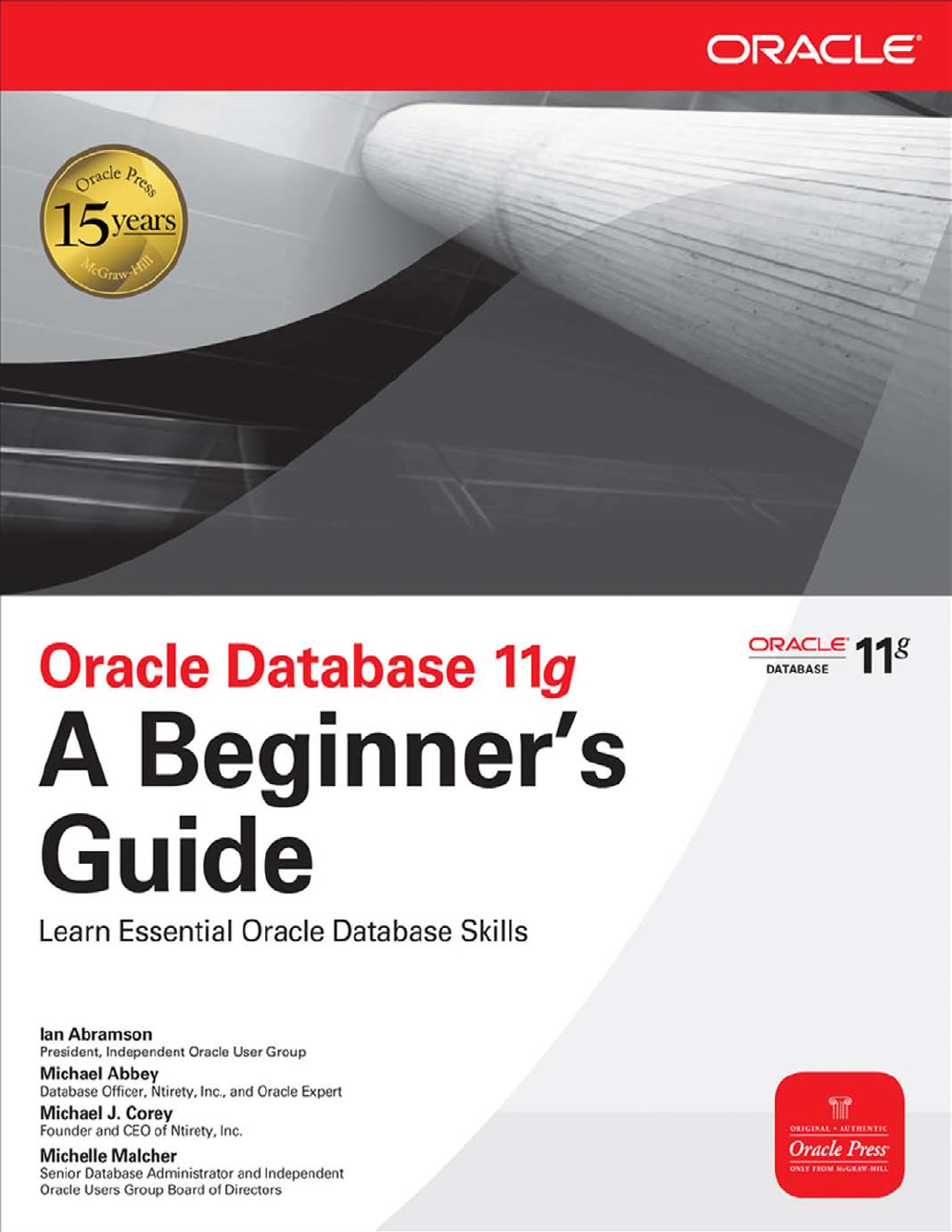
Figure 1-1 shows, in a nutshell, the components that come together to deliver the
corporate database management solution affectionately called Oracle Database 11g.
There is a great deal of academic interest in the database industry, because the
theory of the relational database is founded in relational algebra. As data is entered
into and stored in Oracle Database 11g, the relationships it has to other data are
T
Chapter 1: Database Fundamentals 3
defined as well. This allows the assembling of required data as applications run.
These relationships can be described in plain English for a fictitious computer parts
store in the following example:
■Each geographical location that the store does business in is uniquely
identified by a quad_id.
■Each manufacturer that supplies parts is uniquely identified by a ten-character
manufacturer_id. When a new manufacturer is registered with the system, it
is assigned a quad_id based on its location.
■Each item in the store’s inventory is uniquely identified by a ten-character
part_id and must be associated with a valid manufacturer_id.
Based on these three points, practitioners commonly develop statements similar to
the following to describe the relationships between locations, manufacturers, and parts:
■A one-to-many relationship Locations and manufacturers— more than
one manufacturer can reside in a specified location.
■A many-to-many relationship Manufacturers and computer parts—the
store purchases many different parts from each manufacturer.
These two relationships are established as data is captured in the store’s database
and other relationships can be deduced as a result—for example, one can safely say
FIGURE 1-1. The players in the Oracle Database 11g solution

4Oracle Database 11g: A Beginner’s Guide
“parts are manufactured in one or more locations based on the fact that there are
many manufacturers supplying many different products.” Oracle has always been a
relational database product, commanding a significant percentage of market share
compared to its major competition. Let’s get started and look at the Oracle Database
11garchitecture.
CRITICAL SKILL 1.2
Learn the Oracle Database 11gArchitecture
As with many new software experiences, there is some jargon that we should get
out of the way before starting this section.
■Startup This is the act of issuing the appropriate commands to make an
Oracle Database 11gaccessible to applications. After a startup activity
completes, the database is referred to as opened. Once opened, the
database moves to the next step where it is started. At this point, the
database is ready to use.
■Shutdown This is the act of stopping Oracle Database 11g. When Oracle
Database 11gis shut down, nobody can access the data in its files.
■Instance This is a set of processes that run in a computer’s memory and
provide access to the many files that come together to define themselves as
Oracle Database 11g.
■Background processes These are processes that support access to an
Oracle Database 11gthat has been started, playing a vital role in Oracle’s
database implementation. Various background processes are spawned
when the database is started and each performs a handful of tasks until a
database is shut down.
Let’s look at the assortment of files and background processes that support
Oracle Database 11g.
NOTE
In order to work with the code snippets and the sample
schemas we discuss throughout this book, you will need
to have the Oracle Database 11gsoftware installed and
the first database successfully created. The Database
Configuration Assistant (dbca) is the fastest way to set up
your first database. Most of the time you simply accept
the defaults suggested on the dbca screens. If you have
any problems with either the software installation or the
dbca, please either consult a more senior colleague or
surf MetaLink (http://metalink.oracle.com) to get
assistance (after supplying appropriate login credentials).
Chapter 1: Database Fundamentals 5
The Control Files
Oracle’s control files are binary files containing information about the assortment of
files that come together to support Oracle Database 11g. They contain information
that describes the names, locations, and sizes of the database files. Oracle insists
there is only one control file, but knowledgeable technicians have two or three and
sometimes more. As Oracle Database 11gis started, the control files are read and the
files described therein are opened to support the running database.
The Online Redo Logs
As sessions interact with Oracle Database 11g, the details of their activities are
recorded in the online redo logs. Redo logs may be thought of as transaction logs;
these logs collect transactions. A transaction is a unit of work, passed to the database
for processing. The following listing shows a few activities that can be referred to as
two transactions:
-- Begin of transaction #1
create some new information
update some existing information
create some more new information
delete some information
save all the work that has been accomplished
-- End of transaction #1
-- Begin transaction #2
update some information
back out the update by not saving the changed data
-- End transaction #2
Oracle Database 11ginsists that there are at least two online redo logs to
support the instance. In fact, most databases have two or more redo log groups
with each group having the same number of equally sized members.
The System Tablespace
Tablespace is a fancy Oracle Database 11gname for a database file. Think of it as a
space where a table resides. As an Oracle Database 11gis created, a system tablespace
is built that contains Oracle’s data dictionary. As Oracle Database 11goperates, it
continually gets operational information out of its data dictionary. As records are
created, this system tablespace defines attributes of the data it stores, such as
■Data types These are the characteristics of data stored in the database.
Are they numeric, alphanumeric, or perhaps binary of some video or audio
format?
■Field size This is the maximum allowable size for fields as they are
populated by the applications. This is where, for example, a country
description is defined as from 1 to 30 characters long, containing only letters.
6Oracle Database 11g: A Beginner’s Guide
■Ownership Who owns the information as the database data files are
populated?
■Viewing and manipulation rights Who is allowed to look at the data and
what are the types of activities that each database user can perform on that
data?
The system tablespace is a very close cousin of the sysaux tablespace discussed
next.
The Sysaux Tablespace
Many of the tools and options that support the Oracle Database 11gactivities store
their objects in this sysaux tablespace. This is mandatory as a database is created.
The Oracle Enterprise Manager (OEM) Grid Control repository used to go in its own
oem_repository tablespace, but with Oracle Database 11g(and its predecessors), its
objects now reside in sysaux.
Default Temporary Tablespace
As the dbca does its thing, a tablespace is created that serves as the default location
for intermediary objects Oracle Database 11gbuilds as it processes SQL statements.
SQL stands for structured query language, an industry standard in the database
arena, which is used to retrieve, create, change, and update data. Most of the work
Oracle does to assemble a result set for a query operation is done in memory. A
result set is a collection of data that qualifies for inclusion in a query passed to
Oracle. If the amount of memory allocated for query processing is insufficient to
accommodate all the activities required to assemble data, Oracle uses this default
temporary tablespace as its secondary work area for many activities, including sorting.
Undo Tablespace
As sessions interact with Oracle Database 11g, they create, change, and delete data.
Undo is the act of restoring data to a previous state. Suppose one’s address
is changed from 123 Any Street to 456 New Street via a screen in the personnel
application. The user who is making the change has not yet saved the transaction.
Until that transaction is saved (referred to as committed in the world of Oracle
Database 11g) or abandoned (referred to as rolled back in the same world), Oracle
maintains a copy of the changed data in its undo tablespace.
The Server Parameter File
Oracle Database 11gsometimes calls the server parameter file its spfile. This is
where its startup parameters are defined and the values in this file determine the
Chapter 1: Database Fundamentals 7
environment that database operates in. As one starts an Oracle instance, the spfile is
read and various memory structures are allocated based on its contents.
Background Processes
Essentially, background processes facilitate access to Oracle Database 11gand
support the instance while it is running. These are the main background processes;
many of their names haven’t changed over the past few releases prior to Oracle
Database 11g.
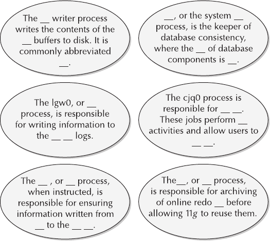
■The database writer (dbw0) process This process (named dbwr in earlier
versions of Oracle Database) is responsible for writing the contents of
database buffers to disk. As sessions interact with Oracle Database 11g, all
the information they use passes through Oracle’s database buffers, a segment
of memory allocated for this activity.
■The log writer (lgw0) process This process (named lgwr in previous
versions of Oracle Database) manages the writing of information to the
online redo logs. A log buffer area is set aside in memory where information
destined for the online redo logs is staged. The transfer of this information
from memory to disk is handled by this process.
■The checkpoint process (ckpt) This is responsible for updating information
in Oracle Database 11g’s files during a checkpoint activity. A checkpoint is
the activity of writing information from memory to the appropriate locations
in Oracle Database 11g. Think of a checkpoint as a stake in the ground
allowing the restoration of a system to a specific point in time. The checkpoint
process may trigger lgw0 and dbw0 to do their specialized tasks.
■The system monitor (smon) process This is the gatekeeper of consistency
as Oracle Database 11gruns. Consistency defines the interrelatedness of
the database components with one another. A consistent instance must be
established every time Oracle Database 11gstarts, and it is smon’s job to
continually enforce and reestablish this consistency. Plainly put: an
inconsistent database is trouble!
■The process monitor (pmon) This is responsible for cleaning up any
resources that may have been tied up by aborted sessions interacting with
the database. The famous CTRL-ALT-DEL that people tend to use to reboot a
personal computer can leave resources tied up in Oracle Database 11g. It is
pmon’s job to free up these resources.
■The job queue coordination (cjq0) process This is responsible for
spawning job processes from Oracle Database 11g’s internal job queue.
Oracle Database 11gdoes some self-management using its job queue, and
users of the database can create jobs and have them submitted to this cjq0
coordinator.
■The archiver (arc0) process This is responsible for copying online redo
logs to a secondary storage location before they are reused by the next set
of transactions. In the “Online Redo Logs” section of this chapter, we
discuss how Oracle Database 11ginsists there are at least two online redo
logs. Suppose we call these groups A and B. Oracle Database 11guses
these two groups in a cyclical fashion, moving back and forth from A to B
to A to B and so on. The arc0 process, when and if instructed, will make a
copy of a file from log group A before allowing it to be reused.
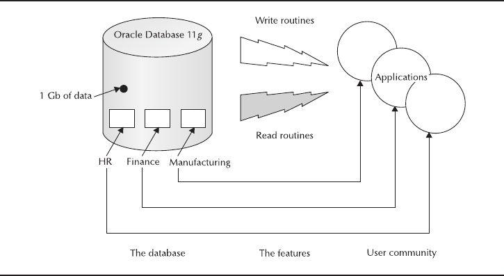
Figure 1-2 illustrates the way the architecture components we have described
come together to support Oracle Database 11g. Oracle Database 11gis opened and
then started, and the control files are read to get its bearings. Then the online redo
logs and the assortment of tablespaces listed in the control files are acquired. As the
instance comes to life, the background processes take over and manage the
operations of the database from there.
8Oracle Database 11g: A Beginner’s Guide
FIGURE 1-2. Tablespaces, support processes, and infrastructure files
Project 1-1 Review the Oracle Database 11g
Architecture
There are many types of files that come together to support Oracle Database 11g.
In this section, we have discussed control files, online redo logs, the system
tablespace, and an assortment of datafiles and tablespaces that support the database.
As well, we have looked at the series of background processes that allow users to
interact with Oracle Database 11g. In this brief project, you will apply what you
have learned about the processes that support Oracle Database 11g. As you descend
into the land of Oracle Database 11g, you’ll find that this information is crucial to
your understanding of this remarkable software solution.
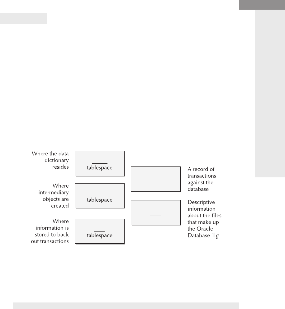
Step by Step
1. There are a few pieces missing in the following diagram of the infrastructure
of files that support Oracle Database 11g. Fill in the missing text where
required.
2. The second diagram shows a partial makeup of the background processes
with Oracle Database 11g. Complete the missing text where indicated
by broken lines.
Chapter 1: Database Fundamentals 9
Review the Oracle Database 11gArchitecture
Project 1-1
(continued)
10 Oracle Database 11g: A Beginner’s Guide
Project Summary
You don’t need to master Oracle Database 11garchitecture to become fluent with
the software. Just as an electrician needs the assistance of a good set of blueprints, the
Oracle Database 11gtechnical person should understand some of the inner
workings of the software. A peek under the covers, as brief as it may have been in
this section, is a good path to follow while becoming familiar with what Oracle
Database 11gis all about.
Before moving on to discuss Oracle Database 11gdata types, let’s spend a
minute looking at the database administrator, the ultimate director of the operations
of the database.
The Database Administrator
This privileged user of Oracle Database 11gis commonly the most experienced
technician in the shop, with some exceptions. Often, recent adopters of the Oracle
technology have little or no in-house experience, and one or more employees may find
themselves targets of the familiar directive “So, you’re the new Oracle Database 11g
DBA!” One scrambles to find sources for technical knowledge when thrust into this
role. What better place to be than reading Oracle Database 11g: A Beginner’s Guide?
The following list outlines common responsibilities of the Oracle Database 11gDBA:
■Installation and configuration The DBA must install and customize the
Oracle Database 11gsoftware and any assorted programs that will run
alongside and access the database.

Chapter 1: Database Fundamentals 11
■Create datafiles and tablespaces The DBA decides which application the
data will reside in.
■Create and manage accounts The DBA sets up the accounts with the
usernames and passwords that interact with the database.
■Tuning The DBA tweaks the environment that Oracle Database 11g
operates in by adjusting initialization parameters using the system parameter
file.
■Configure backups Alongside recovery testing, the DBA performs this
activity to ensure the usability and integrity of system backups.
■Work with developers This is an ongoing process for DBAs, to ensure that
the code they write is optimal and that they use the server’s resources as
efficiently as possible.
■Stay current DBAs keep abreast of the emerging technology and are
involved in scoping out future directions based on the enhancements
delivered with new software releases.
■Work with Oracle Support Services DBAs initiate service requests (SRs) to
engage support engineers in problem-solving endeavors. The front-end of
the SR creation process is called MetaLink (described earlier in the chapter).
■Maximize resource efficiency The DBA must tune Oracle Database 11g
so that applications can coexist with one another on the same server and
share that machine’s resources efficiently.
■Liaise with the system administrators DBAs must ensure that the appropriate
disk space and processor power are available and properly utilized.
As with most lists, after reading the preceding bullet points, you may wonder
what else DBAs do with their time. As you work with Oracle Database 11g, you’ll
experience other activities that will plug any loopholes that may exist in the
previous list.
CRITICAL SKILL 1.3
Learn the Basic Oracle
Database 11gData Types
Very early in one’s journey through the world of Oracle Database 11g, it becomes
time to learn its common data types. Regardless of your past experience in information
technology, data types are nothing new. Let’s look at the most common type of data
that can be stored in Oracle Database 11g; keep in mind that the list is much longer
than the one presented here.

varchar2
By far the most common data type, varchar2 allows storage of just about any
character that can be entered from a computer keyboard. In earlier software
solutions, this was commonly referred to as alphanumeric data. The maximum
length of varchar2 is 4000 bytes or characters, and it possible to store numeric data
in this data type. This is a variable length character string, with no storing of trailing
insignificant white space:
create table ... (
name varchar2(30),
city varchar2(30),
...
...
state varchar2(2));
If a program or SQL statement tries to store a set of characters in a varchar2 field
that is longer than the field’s specification, an error is returned, and the statement
stops running and returns control back to you.
number
The number data type allows the storing of integer as well as integer/decimal digits.
When non-integer data is stored, the total number of significant digits of the number
is referred to as precision, while the portion to the right is called scale or decimal
places. For example, the number 29.1963 has a precision of 6 and a scale of 4. The
maximum precision is 38 and the maximum scale is 127. The confusing part of the
specification of a number data type comes into play when storing non-integer
information. Table 1-1 illustrates this concept.
When defining a number data type with decimal places, it’s important to know
that the maximum integer portion of the number data type is the difference between
the two numbers specified. The specification (6,3) allows for two, not six, integer
12 Oracle Database 11g: A Beginner’s Guide
Number Specification Column Length (Precision) Decimal Digits (Scale)
(3,2) 3 2
(6,3) 6 3
(17,12) 17 12
TABLE 1-1. Number Data Type Specification
Chapter 1: Database Fundamentals 13
digits. If more decimal digits are received than the column definition permits, it
rounds the value before storage.
date
The date data type stores time and date information, with the time component
rounded to the nearest full second.
There are many, many functions available to be performed on date fields as they
are extracted from an Oracle Database 11g.
When date columns are selected from Oracle Database 11g, it is common to
perform a function on their values to make them more readable. By default, the time
component of a date column is not displayed without manipulating its contents using
a to_char function, described in Chapter 4. By default the general display format for a
date is DD-MON-YY (day, month, and year). This format may be changed via the
NLS_DATE_FORMAT parameter or by using a display format function.
timestamp
The timestamp data type is a close relative of date. The major advantage is that the
timestamp stores information about the second to a much higher accuracy. In this
time when every subsecond counts, the timestamp can be a valuable asset. There is
a time component in this data type, displayed with the data without the need for the
to_char function. This listing illustrates this concept:
SQL> create table timestamp_test (ts timestamp);
Table created.
SQL> insert into timestamp_test values (sysdate);
1 row created.
SQL> select * from timestamp_test;
TS
--------------------------------------------------------------------------
14-DEC-09 05.25.07.000000 PM
SQL> create table date_test (d date);
Table created.
SQL> insert into date_test values (sysdate);
1 row created.
SQL> select * from date_test;
TS
---------
14-DEC-06
clob
The clob data type allows storage of very large objects in excess of four gigabytes in
size. Since this is a true character data type, it is very similar to the varchar2 data
type except for its much larger maximum size.

blob
The blob data type permits storage of large unstructured binary objects. Sound and
video are examples of blob data.
It’s now time to have a look at the most common object in Oracle Database
11g: the table. After that, we will have a look at a few types of programming units
written using SQL, which a person can store in Oracle Database 11g.
CRITICAL SKILL 1.4
Work with Tables
The best way to think of a table in a relational database such as Oracle Database
11gis to see it as a spreadsheet with rows and columns. With this in mind, note the
following:
■Rows are often referred to as records.
■Each column has a name unique to the table that it resides in.
■The intersection of each row and column, referred to as a cell in a
spreadsheet, is called a field in Oracle Database 11g.
Picture the following SQL statement, which creates a table (the line numbers are
not part of the code):
1- create table part_master (
2- id number(8) not null,
3- manufacturer_code number(4) not null,
4- inception date not null,
5- description varchar2(60) not null,
6- unit_price number(6,2) not null,
7- in_stock varchar2(1));
Let’s pick apart the code and highlight the main points in Table 1-2.
Table 1-2 mentions the concept of a relational database. Let’s inspect a few
other tables and see how they are related to one another.
Tables Related to part_master
The manufacturer_code column in part_master points to a record in manufacturer.
Also, some columns in manufacturer may end up being related to column values
in other tables. Figure 1-3 illustrates these relationship concepts, the heart of the
Oracle Database 11gimplementation.
14 Oracle Database 11g: A Beginner’s Guide
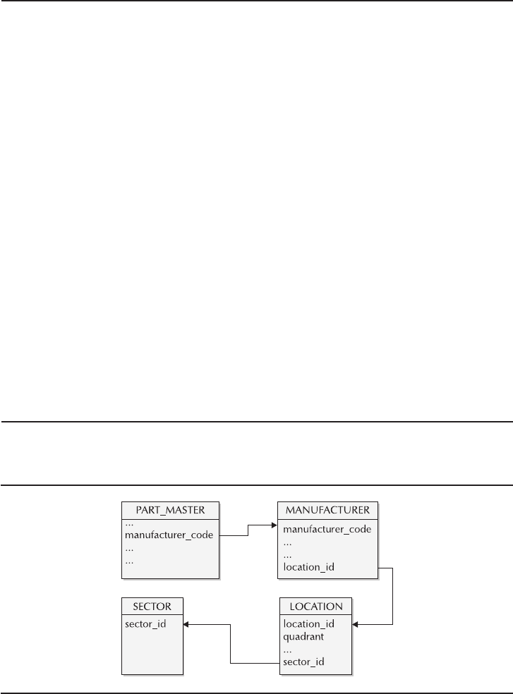
Chapter 1: Database Fundamentals 15
Line Important Points
1 The table has a unique name, from 1 to 30 characters. It is stored in
Oracle Database’s data dictionary in uppercase.
2 The ID column is numeric with anywhere from one to eight digits. The
application that creates and keeps track of parts may insist that the first
character of the ID be a digit between 1 and 9. Since the field is defined
as numeric, if the leading digit were a 0, the part ID would only be
seven digits long.
3 The manufacturer_code is the only manufacturer information stored in
part_master. Further information about who made the product is in a
related table—hence, the terminology relational database.
4 inception, as a date field, contains a date and time specification, though it
will display a default month abbreviation and a two-character year unless
some manual manipulation is performed (for example, 12-NOV-05).
5 description is a free-form field with a variable length of up to 30 characters.
6 unit_price can accommodate up to four integer and two decimal digits.
7 in_stock is a one-character flag of sorts; thus, the system designers can
decide to use an indicator like a “1” or “X” to represent items that are in
stock. Notice how this is the only one of seven fields in the
PART_MASTER table that can be left blank.
TABLE 1-2. part_master Table Definitions
FIGURE 1-3. Relationships to part_master

16 Oracle Database 11g: A Beginner’s Guide
Suppose someone wanted to know where in the country a certain part was
manufactured. By looking at Figure 1-3, that information is not readily available in
part_master. However, part_master has a manufacturer_code. So, a person would
traverse to manufacturer using manufacturer_code to get a location_id. Armed with
that value, one then proceeds to location to get a quadrant column value. After this
navigation is complete, a person would know where a specific part is built. Table
1-3 maps out this journey.
As illustrated in Table 1-3, you can deduce that part 33499909 comes from the
Pacific Northwest—a deduction that is made by following the relationships between
matching columns in the three tables in question.
CRITICAL SKILL 1.5
Work with Stored Programmed Objects
Oracle Database 11goffers the ability to store user-defined programming units in
the data dictionary, called stored objects. These programming units are written in
PL/SQL, the topic of Chapter 5. Without worrying about what goes inside these
objects, let’s do an overview of what they are all about.
Views
Views are predefined subsets of data from an Oracle Database 11gtable. The SQL
query that builds the view is stored in the data dictionary and need not be reassembled
every time the view is used. Suppose a personnel application stores the location of
all employees in its EMPLOYEE_MASTER table in the loc_id column. With Oracle
Database 11g, you can define a view called emp_hq as follows:
create or replace view emp_hq
as select * from employee_master
where loc_id = '2';
EMP_HQ becomes a valid object of the select statement just as if it were a table
of its own.
Table Part Number Column Value Related Column Value
part_master 33499909 manufacturer_code 3490
manufacturer 3490 location_id 5
location 5 quadrant Pacific Northwest
TABLE 1-3. Following Relationships Between Tables

Chapter 1: Database Fundamentals 17
NOTE
At this point, you should realize that views are
generally built based on more than one table. A view
provides the perfect environment to predefine join
conditions between tables to ensure that they adhere
to business rules and perform at an optimal level.
Ask the Expert
Q: What is the major difference between the clob and blob data types in
Oracle Database 11g?
A: The clob stores only alphanumeric data, whereas the blob can
accommodate any type of data, including sound and video.
Q: When specifying the number data type, how is the total length of the
field determined?
A: The total length of a numeric field is determined by the digit(s) to the left
of the comma if the specification includes an integer and decimal component.
For example, number(4,1) denotes a maximum of four digits, of which one
digit can be stored to the right of the decimal point.
Q: Which of the Oracle Database 11gbackground processes is responsible
for writing information from memory into the database files?
A: This is the job of the database writer, or dbw0, process.
Q: Where does Oracle Database 11gread its environment from as it is started?
A: The startup parameters are read from the system parameter file, which can
be a binary file stored in Oracle Database 11g.
Q: As sessions interact with the data in Oracle Database 11g, what role
does the undo tablespace play in the architecture of the software?
A: When transactions change the contents of information in Oracle Database
11g’s tables, this special tablespace keeps a “before image” of the changes in
case the operator decides to back out before saving newly entered
information.

18 Oracle Database 11g: A Beginner’s Guide
Triggers
Just as their name implies, triggers are stored objects that fire based on the execution
of certain events. Suppose a payroll application wants to audit salary increases: a
trigger is created that fires when the salary column in hr_master is updated. The
trigger could do the following:
1. Create a record in sal_audit.
2. Trap the time and date of the transaction.
3. Place the user’s login ID in the doer column.
4. Place the old salary value in the old_sal column.
5. Place the new salary value in the new_sal column.
Code in the trigger traps the event by specifying on update. While triggers are
commonly used for auditing, the types of activities they can initiate are endless.
NOTE
Triggers cannot exist independently of an Oracle
Database 11gtable. They are associated with one
and only one table and, if a table is dropped, so is
the trigger.
Triggers, as well as procedures, packages, and functions described next, are
most commonly written using PL/SQL. The PL/SQL programming language is the
topic of Chapter 5.
Procedures
Procedures perform specific tasks as applications interact with Oracle Database
11g. If there are a number of interrelated activities to carry out in one place, a
procedure is an ideal way to do this. Procedures can accept parameters when
invoked and can interact with objects in Oracle Database 11g. They encapsulate
related activities into single programming units that simplify logic and share data
values as they perform various activities. They offer extremely flexible features,
many of which are not available with triggers.
Functions
Functions are very close relatives of procedures, except that they return a value to
the code that called them. Oracle Database 11gdelivers many functions out of the

box and developers can create their own functions to augment what is delivered
with the software. Suppose you want to strip all the vowels out of a name with a
function. You can pass in a name (for instance, Bellissimo) and gets back the text
“Bllssm” when the function completes its work. Let’s look at the get_age function,
which operates based on the following logic:
given a date of birth (format DD-MON-YYYY)
using an SQL function
get the months between today's date and the date passed in
divide the number of months by 12
truncate the results (giving the span in years between the 2 dates)
pass integer back
Packages
Packages roll functions and procedures together into a cohesive programming unit.
Often, developers prefer to bundle like functionality together since it makes logical
sense to call one larger unit and have it perform a series of tasks. Let’s look at the
CREATE_EMPLOYEE package in Table 1-4.
Chapter 1: Database Fundamentals 19
Component Name Type Work Accomplished
give_holidays Procedure Creates the default holiday quota based
on the new person’s rank in the company.
notify_benefits Procedure Creates a record in the BEN_QUEUE
table to alert the benefits people of the
new employee.
is_under_25 Function Returns a “1” if the new employee is
under 25 years old as of December 31
of the year they were hired.
is_over_59 Function Returns a “1” if the new employee is 60
years old or older as of the calendar date
of hire.
TABLE 1-4. Members of the CREATE_EMPLOYEE Package

Progress Check
1. Oracle Database 11gis referred to as a relational database.Why is the
word relational used?
2. What is the maximum length of a varchar2 data type that can be stored in
Oracle Database 11g?
3. What is data consistency when referred to as a feature of Oracle Database
11g? Give an example.
4. What types of stored objects can be encapsulated into an Oracle Database
11gpackage?
5. What is the fundamental difference between a procedure and a function in
Oracle Database 11g?
6. Data in the system tablespace is often referred to as metadata—or data
about data. Name at least two types of metadata in the system tablespace.
7. What is the difference between the timestamp and date data types?
8. What type of information and data ends up being stored in the sysaux
tablespace?
20 Oracle Database 11g: A Beginner’s Guide
Progress Check Answers
1. The word relational is used because Oracle Database 11gdefines the relationships between
tables. It is these relationships that allow applications to navigate an assortment of tables and
assemble results from more than one table.
2. The varchar2 data type can accommodate up to 4000 characters.
3. Data consistency refers to the ability to ensure that related items of information are manipulated
in a similar fashion. Suppose an application assigns a department to a new employee as a two-digit
number field. Sometime down the road, due to company growth, the department identifier is changed
to three digits. All the data where this used-to-be two-character identifier is stored must be changed
to reflect the expansion of the department codes.
4. Packages can contain a mixture of one or more functions and procedures.
5. A procedure receives from zero to many parameters as it is invoked and then goes about its
business until the end of its code segment. A function, on the other hand, accepts one or more
parameters as it is called and returns a value to the code from where it was invoked. The procedure
passes nothing back to its caller.
6. Metadata defines items such as the names of tables in the database, the owners of the tables, the
data types of the columns in each table, and who is allowed to look at what data.
7. When columns are displayed, they use the date data type, containing a day/month/year component,
whereas, by default, the timestamp data type columns contain a time-of-day component as well.
8. The sysaux tablespace contains tables required to manage Oracle Database, such as the items
required to support OEM Grid Control.

Chapter 1: Database Fundamentals 21
CRITICAL SKILL 1.6
Become Familiar with Other Important Items
in Oracle Database 11g
So far, you’ve had a brief look at tables, views, tablespaces, and a handful of stored
objects, such as views, triggers, procedures, packages, and functions. Let’s round
out this introduction to Oracle Database 11garchitecture by covering a few other
items commonly encountered. The following discussion is a hodgepodge of things
that are necessary for a person’s understanding of the Oracle Database 11g
architecture and operations. Keep in mind that you must also spend a bit of time
looking at the role of the database administrator, affectionately called the DBA, who
is the gatekeeper of the database and the person responsible for its smooth
operation.
NOTE
You’ll get a more detailed look at the DBA in
Chapter 6, with more information on how DBAs go
about carrying out their administrative chores.
Indexes
Tables are made up of rows and columns, which are the basis of all objects in
Oracle Database 11g. As applications interact with the database, they often retrieve
vast amounts of data. Suppose MyYP, a fictitious Internet company, provided
Yellow Pages listings for North America, and the data was stored primarily in a table
called YP_MASTER. Each row in the YP_MASTER table is uniquely identified by
a combination of company name, municipality, and geographic location (state
or province). As words are retrieved from the database to satisfy online queries,
indexes would provide a quick access path to the qualifying data. Specific index
characteristics are relevant to the power they deliver in Oracle Database 11g. For
instance:
■They are built on one or more columns in a table using simple SQL
statements.
■They are separate from the tables that they are built on and can be dropped
without affecting the data in the table itself. On the contrary, when a table
is dropped, any indexes it has disappear with the table.
■The function they perform can be likened to the index in a book. If one
were looking for a specific topic in a textbook, the best place to start would
be the index—it provides a shortcut to the information being sought. If one
imagined that YP_MASTER were a book rather than a table, finding Y&M
Plumbing in Pensacola, Florida would be faster using the index than reading
the book from the start to the 25th letter of the alphabet. The names on the
corner of the pages in a phone book are like an index.

22 Oracle Database 11g: A Beginner’s Guide
■Indexes occupy space in the database; even though there are ways to keep
their space to a minimum, extra space is required and must be pre-allocated.
Users
Most of us are familiar with usernames and passwords from our experience logging
into corporate networks and other secure systems. Oracle Database 11gimplements
the same mechanism with login credentials and privileges given out by the database
administrator. Once accounts are created, people initiate connections to Oracle
Database 11gand work with their own data and other users’ data where the
appropriate privileges have been given out. We discuss object privileges in the
“Work with Object and System Privileges” section immediately following this one.
NOTE
With Oracle Database 11g, the terminology user,
account, and schema are used synonymously.
Once an account is created, it is often given the rights to occupy space in one or
more Oracle Database 11gtablespaces. This is discussed in the next section.
Tablespace Quotas
As additional nonsystem tablespaces are created, the database administrator gives
out quotas that allow users to occupy space therein. Tablespace quotas are given
out using an SQL statement with three parts:
■The username to whom the quota is being given.
■The name of the tablespace within which the username is being permitted
to create tables.
■The amount of that quota—whether it’s mentioned in absolute bytes (for
example, 500,000) or more commonly in quantities of megabytes (500MB,
for instance). Unlimited quotas can be allowed using the keyword
unlimited.
Regardless of how a quota is given out, the SQL statement passed to Oracle
Database 11gresembles the following:
SQL*Plus: Release 11.1.0.1.0 - Production on Sun Mar 11 10:29:42 2009
Copyright (c) 1982, 2007, Oracle. All rights reserved.
Connected to:
Oracle11g Enterprise Edition Release 11.1.0.1.0 – Production
With the Partitioning, OLAP and Data Mining options

Chapter 1: Database Fundamentals 23
SQL> alter user hr quota 500m on hr_data;
User altered.
SQL> alter user ap quota unlimited on ap_idx;
User altered.
Synonyms
You’ll remember that in the “Work with Tables” section we discussed that the key
was passing Oracle Database 11gthe create table keywords. In a nutshell, table
creation is undertaken after establishing a successful connection to the database,
and then, with appropriate privileges in place, defining a table. One of the key
concepts with all database management systems is sharing data. Since it is key to
only have one copy of a table and to have its contents shared amongst applications,
synonyms are a way to reference other people’s data.
Suppose you wanted to use the PART_MASTER table in an application owned
by a user other than the owner. That owner would permit us to work with the table’s
data, and then we would create a synonym to reference its contents. The code
would resemble the following:
SQL*Plus: Release 11.1.0.1.0 - Production on Sun Mar 11 10:29:42 2009
Copyright (c) 1982, 2007, Oracle. All rights reserved.
Connected to:
Oracle11g Enterprise Edition Release 11.1.0.1.0 – Production
With the Partitioning, OLAP and Data Mining options
SQL> create synonym part_master for inv.part_master;
Synonym created.
SQL> select count(*)
2 from
part_master
3 where in_stock is not null;
COUNT(*)
-------------
13442
The preceding SQL statement references an object called part_master. Depending
on how your access is defined, the way that you reach the physical table may be
different. When you are the owner of the table and you use the table’s name in the
from clause, Oracle understands that you would like to use your own table. If you
do not own a table by that name, Oracle then looks in a list of table synonyms or
pointers to a table with that name owned by someone else. This process of using
synonyms is a transparent operation. If you do not own the table by the name or no
synonym exists, you will receive an error. There are actually two kinds of synonyms:
■Private synonyms are created in one account and are only usable by the
creator.
■Public synonyms are created by a central privileged user and are available
to anyone able to connect to Oracle Database 11g.

24 Oracle Database 11g: A Beginner’s Guide
NOTE
One needs the appropriate object privileges to be
able to work with someone else’s data using a
private or public synonym. The synonym itself does
not imply that the appropriate privileges can be
circumvented.
Roles
Often it makes sense to group similar users together to streamline the organization
of people who use Oracle Database 11g. Using roles, the DBA can logically lump
personnel together and give out object privileges to roles rather than individual users.
Roles can be password protected, though in most implementations they do not have
this level of complexity.
Default User Environments
As accounts are created by the DBA, users are given a default environment to use
unless some specifics are coded as they interact with Oracle Database 11g. Users
are commonly set up with the following default environment settings:
■The default tablespace is where tables are placed unless the create table
statement explicitly points at a nondefault tablespace that the user has a
quota for.
■Temporary tablespaces are the tablespaces where users perform sort and
merge operations while the Oracle Database 11gengine is processing
queries.
Users can be given membership in one or more roles and have their default
profile changed as well. As users are created, they do not automatically inherit a
default tablespace; one must be manually given out during or following the user
creation statement. Users do automatically point at a temporary tablespace, as
discussed in the “Default Temporary Tablespace” section of this chapter, unless
manually pointed elsewhere.
NOTE
With Oracle Database 11gone is now able to set
the default tablespace for the entire database
instance. This is done via an “ALTER DATABASE
DEFAULT TABLESPACE tablespace-name;”
command. You will need to have the privileges
to be able to perform this operation.

Progress Check
1. Name at least four tasks handled by the Oracle Database 11gadministrator.
2. What is the difference between public and private synonyms?
3. What is meant by a user’s default tablespace?
4. What two units of measurement are commonly used to specify a tablespace
quota?
5. Where do DBAs go to create iTARs, where assistance is requested from
Oracle’s support organization?
6. Which of the following—procedures, packages, or triggers—cannot exist
independent of a table to which they belong?
CRITICAL SKILL 1.7
Work with Object and System Privileges
It’s next to impossible to work with data in Oracle Database 11gwithout looking at
object privileges. In this section, we are going to look at these privileges as well as a
suite of system privileges closely related to managing Oracle Database 11g. The
four main object privileges are select, insert, update, and delete, all discussed in the
next four sections. Oracle Database 11guses the term grant when referring to giving
out both object and system privileges.
Select
This is the primary and most commonly used privilege, permitting other users to
view your data. There are three parts to grant statements:
■The keywords grant select on.
■The name of the object upon which the privileges are being given out.
■The recipient of the grant.
Chapter 1: Database Fundamentals 25
Progress Check Answers
1. Installation, upgrades, tuning, and environment setup are four of many tasks performed by the DBA.
2. A private synonym can only be referenced in a SQL statement by the user who created and owns
the synonym. A public synonym, created by a centralized user such as a DBA, is available to all users.
3. The default tablespace is the one within which users occupy space by default, unless another
tablespace is mentioned as a table is created.
4. Quota on tablespaces is usually given out using bytes or megabytes as units of measurement.
5. The DBA goes to MetaLink to request assistance from Oracle’s support organization.
6. Triggers cannot exist on their own without association with an Oracle Database 11gtable.
26 Oracle Database 11g: A Beginner’s Guide
Once the select privilege has been given out, the recipients, using a private or
public synonym as described earlier in the “Synonyms” section of this chapter, can
reference your objects in their SQL statements.
Insert
This privilege allows users to create rows in tables belonging to other users. The
creator of new rows in other users’ objects is bound by the same rules used if they
owned the objects themselves. They must adhere to the boundaries defined by the
data types of the columns in the rows they create. For example, when rows are
inserted into a table that has a column defined as type DATE, they must ensure that
valid date type data is placed in the column so defined. As rows are created in an
Oracle Database 11gtable, the transaction must be committed to the database
before the row becomes part of the information available to other users. With
Oracle Database 11g, we use the term commit the same way the word save is
used with other types of software.
Update
This privilege allows a person to change the contents of columns in rows belonging
to other tables. The SQL update statement can change the value of data in one or
more columns. As with insert activity, the update transactions need to commit their
work to make it permanent in the Oracle Database 11gfiles.
Delete
Delete operations interact with one or more rows in Oracle Database 11gtables
and must be followed by a commit as well to write the results of the transaction to
the database files.
You will see more in Chapter 4 about how SQL statements are constructed using
the four keywords in the previous sections. SQL statements are subject to rigorous
syntax requirements which, if not followed, return an assortment of Oracle errors.
Just as with other programming languages you may be familiar with, the SQL statement
processing engine is very strict with reserved words and the placement of the pieces
that come together to form an SQL transaction. Let’s briefly discuss system privileges
that allow certain users of Oracle Database 11gto perform secure activities.
System Privileges
We have mentioned the database administrator in a number of places in this
introductory chapter. Classically, secure operations are performed by the DBAs;
however, one can grant system privileges to specified users so that they can perform

Chapter 1: Database Fundamentals 27
selected activities themselves. The following list illustrates a few examples of these
secure operations:
■Alter system There are a number of modes that Oracle Database 11gcan
operate from. The modes are toggled using alter system. For example, this
privilege can be given out to Jane by issuing the command grant alter
system to jane.
■Create user/alter user Often, the DBA wants to partition some of the user
creation activities between a handful of users of Oracle Database 11g. This
is done by giving out the create user system privilege. Once new users are
created, you often don’t want to tweak their environment; this can be
accomplished by issuing the grant alter user statement to one or more users
of the database.
■Create session/table/trigger Sometimes when new users are created, they
are given the create session system privilege which allows them to connect
to Oracle Database 11g. In many cases, depending on how new users are
created, they are not allowed to build any objects until they receive the
create table system privilege. As well, many users are not capable of
defining triggers until they receive the create trigger system privilege.
System privileges were introduced with early releases of Oracle7 (circa 1993)
and have played a useful role in the division of labor in the database since their
inception. Now it’s time to get into the meat of the seventh letter of the alphabet,
g, that throughout this chapter has followed the two-digit version number of this
software release—11.
CRITICAL SKILL 1.8
Introduce Yourself to the Grid
As many have heard, the “g” in Oracle Database 11gstands for grid. Grid computing
is a technology that allows for seamless and massively scalable access to a distributed
network of diverse yet homogenous computer types. Oracle Database 11gis the
glue permitting different vendors’ computers to work together providing a seemingly
endless supply of shared computer resources. Oracle sees the grid as revolutionizing
the way companies go about doing their business. Grid computing targets the
delivery of information as a utility, similar to the way electrical and telephone
services are currently delivered to the public—hence the term grid. The industry
as a whole, but Oracle in particular, sees a delivery method from the grid such
that consumers will only pay for what they use. Interlaced computers will allow idle

28 Oracle Database 11g: A Beginner’s Guide
capacity to be leveraged by the grid to provide for a form of parallel processing on
steroids. The following are the major players that enable the Oracle grid technology:
■Real Application Clusters (RAC) Involves a suite of networked computers
sharing a common Oracle Database 11gand running platform-independent
clusterware, the glue that makes the interconnect between the clustered
nodes so transparent.
■Automatic Storage Management (ASM) A front-end management system
that can group disks from an assortment of manufacturers together to form a
Ask the Expert
Q: Name the four main object privileges used in Oracle Database 11g.
A: The four most common privileges are select, insert, update, and delete.
Q: Placing an Oracle Database 11gin a state where it can be accessed by
applications is referred to as what activity?
A: Putting an Oracle Database 11gin a normal operating mode for
day-to-day access by a company’s applications is referred to as startup.
Q: How many integer and decimal digits can a field defined in the data
dictionary as number(10,2) accommodate?
A: The field would be able to store up to eight integer digits and two decimal
digits.
Q: When Oracle Database 11gis passed the value “Beginner ” for storage
in a varchar2 column, how does it deal with trailing insignificant spaces?
A: The trailing spaces are trimmed before the information is stored in the
database. Though not as common as varchar2, the char data type can be used
to store trailing spaces.
Q: What would Oracle Database 11gstore as a value in a number(6,2) field
when passed the value 9.8882?
A: It would store 9.89 in a number(6,2) field when passed 9.8882.
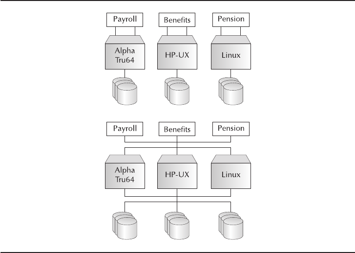
suite of disks that is available to all computers on the grid. ASM encapsulates
the complete life cycle of disk management and allocation into a centralized
GUI interface.
■Oracle Resource Manager Provides a framework within which administrators
can control the computing resources of nodes on the grid.
■Oracle Scheduler Allows the handing out of jobs to members of the grid
to facilitate the execution of business tasks anywhere and everywhere
where idle resources exist.
■Oracle Streams Assists the processing requirements whereby copies of
data need to be streamed between nodes in the grid, providing the
mechanisms to keep data in sync on one database with the database from
which the data originated. Oracle Streams’ tight integration with the Oracle
Database 11gengine facilitates this synchronization and delivers a
preferred method of replication.
Figure 1-4 illustrates the primary differences between grid computing and
traditional approaches to providing computer services.
Chapter 1: Database Fundamentals 29
FIGURE 1-4. Differences between traditional and grid computing

The following points reinforce the details of the two scenarios depicted in
Figure 1-4:
■The three applications at the top of the figure each have a dedicated server,
each with its own dedicated disk. If the Linux server were to go out of
service, the pension application would grind to a halt. There is no built-in
mechanism for pension system processing to carry on another server.
■The three applications at the bottom are interlaced with one another. The
benefits application can be hosted on from one to three of the available
servers. As well, the database files that support these three applications can
reside upon (and be read from) any of the nine disks in the grid’s disk farm.
The browser-based OEM Grid Control holds the whole thing together. With the
implementation of the ASM component of Oracle Database 11g, disks are managed
by OEM, database instances are managed by OEM, clusterware is managed through
OEM; the list is endless. Figure 1-5 shows the first OEM screen that appears after
entering appropriate login credentials.
NOTE
There is an OEM configuration program (called
emca) that must be successfully run before you can
access the browser-based OEM. The screen shown
in your version of Oracle Database 11gmay be
somewhat different than the one shown in Figure
1-4. The look and feel of the OEM Grid Control
screens can change significantly between minor
releases of the software.
30 Oracle Database 11g: A Beginner’s Guide
FIGURE 1-5. OEM startup

Chapter 1: Database Fundamentals 31
CRITICAL SKILL 1.9
Tie It All Together
Now that was quite a journey! We have covered database fundamentals, with an
Oracle Database 11gflavor. Relational database management systems have been
around for a few decades, and the release of Oracle Database 11gis a landmark
in the industry. There have been many academic discussions about the grid
technology— some claim Oracle Database 11gis a grid implementation, while
others don’t. Regardless of which side of the fence you’re on, Oracle Database 11g
is a big step. Let’s pull it all together and spend a bit of time on the big picture.
Oracle Database 11gis a collection of special files created using its database
configuration assistant and then completing the work using OEM Grid Control.
Access to these database files is facilitated by a set of shared memory processes
referred to as an instance. Many technicians use this term synonymously with
database. There is nothing wrong with that because, even though they are
technically different pieces, they cannot survive without each other.
Relationships between objects in the database are defined in the data
dictionary— hence the familiar term relational database. It is these relationships that
provide the power and allow Oracle Database 11gto store vast amounts of data.
Storing that data is one thing—retrieving it for applications in a quick and complete
fashion is another story. Data retrieval is one of the strengths of the Oracle Database
11gengine.
Over the next eight chapters, we will be delving into more details of the Oracle
Database 11goffering, paying specific attention to the following:
■Installing Oracle In order to become productive with Oracle, it is
valuable to learn the steps that are necessary to install and connect to the
database. This will help you get started as well as prepare you for the
samples within the book.
■Networking The glue that holds many systems together and allows
computers to communicate with one another in widely diverse and
separated locations.
■SQL—Structured Query Language This is the way we communicate with
Oracle Database 11g. Whatever the programming language (from C to
Java), SQL is all the database engine understands.
■PL/SQL A programming language native to the Oracle Database 11g
engine, providing more procedural capabilities that can amplify and
enhance the functionality of SQL.
■The Database Administrator The person who is the gatekeeper of Oracle
Database 11gand the one responsible for its smooth operation and optimal
performance.
32 Oracle Database 11g: A Beginner’s Guide
■Backup and Recovery Two areas critical to the smooth operation of
Oracle Database 11g. Oracle Database 11g’s Recovery Manager (referred
to as RMAN) is the fundamental building block in its backup and recovery
implementation. In addition, your backup and recovery strategy is one that
will need to be considered as input to your Disaster Recovery strategy.
■High Availability The need to support databases and applications for
extended and uninterrupted times requires Oracle to be able to support
these demands. This chapter focuses on Rapid Application Clusters (RAC)
and Automatic Storage Management (ASM) to serve as the foundation to
your high availability solutions.
■Large Database Features Oracle Database 11gexpands on an already
solid offering in this area. With Oracle9i, they boasted the ability to support
a database of up to 500 petabytes. Oracle Database 11gexpands that upper
limit to many exabytes, a staggering number, to say the least—where an
exabyte is 1,152,921,504,606,846,976 bytes—or about one trillion million!
þChapter 1 Mastery Check
1. The __________ background process is primarily responsible for writing
information to the Oracle Database 11gfiles.
2. How many online redo log groups are required to start an Oracle Database
11g?
A. 3
B. 2
C. 4
D. 1
3. Of the following four items of information, which one is not stored in
Oracle Database 11g’s control files?
A. The name of the database files
B. The creator of the database
C. The location of the database files
D. The sizes of the database files
4. What is the function of a default temporary tablespace in the support of
Oracle Database 11g?
Chapter 1: Database Fundamentals 33
5. Differentiate between an Oracle Database 11gand an instance.
6. Activities such as allocating space in the database and user management
are commonly performed by the DBA. What feature in Oracle Database
11gallows some of these secure operations to be carried out by non-DBA
users? How are these rights given out?
7. As a user of Oracle Database 11gis created, you often specify a default
tablespace. In this context, what does default tablespace mean?
A. The system tablespace
B. A tablespace the user can occupy space in without a private or public
synonym
C. The tablespace within which objects are created if a location
(tablespace) is not explicitly mentioned as a table is created
8. The __________ GUI interface is used to create a new database.
9. What happens when one tries to store the text “Madagascar” in a field with
a specification of varchar2(8)?
10. What is the most common way one uses triggers in Oracle Database 11g?
Give an example of this activity.
11. What programming language, native to Oracle Database 11g, is used to
create stored objects such as triggers and functions?
A. SQL*Plus
B. OEM Grid Control
C. Basic
D. PL/SQL
12. What is the role of the sysaux tablespace in Oracle Database 11g?
13. The clob and blob data types differ in all but one of the following three
ways. Which one does not apply to the differences between the two data
types?
A. The clob holds standard alphanumeric data, whereas the blob may store
binary information.
B. The blob contains a time (hour/minute) component, but the clob does not.
C. The blob contains unstructured free-form data, whereas the rules
governing the type of information that can be stored in the clob are
more stringent.
14. There are many ways to replicate data from one node to another. What
main feature does Oracle Streams provide that is missing from many other
methods?
15. What does the acronym SQL stand for?
A. Structured Query Language
B. Simple Query Language
C. Straightforward Question-based Learning
34 Oracle Database 11g: A Beginner’s Guide

Chapter
2
Installing Oracle
CRITICAL SKILLS
2.1 Research and Plan the Installation
2.2 Set Up the Operating System
2.3 Get Familiar with Linux
2.4 Choose Components to Install
2.5 Install the Oracle Software

36 Oracle Database 11g: A Beginner’s Guide
nowledge of the technology behind Oracle and an understanding its
tables and columns are basic skills needed for working with Oracle;
however, you need to install the software to take advantage of all of
the functionality of the product. There are many product options and
features that you will need to select during installation and for this
chapter we suggest you consider installing all options for your educational use of
the product. Are you ready to install the Oracle software? You are probably not as
ready as you think, unless you have already done some research and prepared the
environment. Downloading or obtaining the media for the Oracle software is the
easy part, but do you know which operating system you are using and have you
set up the configurations for Oracle?
Oracle has a proven track record on a variety of operating systems. Oracle 11g
was first released on the Linux platform (among other Unix-based platforms), then
followed closely by a release for Windows, which is the normal pattern in which
Oracle develops and releases products. We suggest that you get the latest version of
the software from the Oracle Technology Network (otn.oracle.com) for your chosen
platform.
It is also critical to be able to configure or verify the operating system configuration
for successful installs and, ultimately, well-running and performing systems. We
recommend, therefore, that you have administrator access to the server that you plan to
install the software on. Being able to tune or discuss the issues regarding the operating
system comes in handy when you’re looking at configurations for the system as a whole;
deciding when the minimum is not enough and starting to understand where the
dependencies are is a valuable part of successful implementations. This chapter will
walk you through some basic steps for installing the Oracle software on Linux, including
gathering the information needed for the system requirements as well as completing a
checklist for a Linux installation.
CRITICAL SKILL 2.1
Research and Plan the Installation
Oracle provides some critical information needed for installing the Oracle software,
both with the software itself and in the Oracle support site MetaLink notes. These
are important documents for successful installs that can help you with the planning
and research (for example, the Quick Installation Guide, Database Readme, and
Database Release Notes) and they contain hardware requirements, prerequisites, and
the setup to be done before and after installation. Also, information on installation
issues for Oracle software can be obtained from most recent release notes, which
contain possible workarounds or updated steps for the installs.
Gathering information on what is required to install the software and running it
effectively is a very important first step. Neglecting to do this by going straight to the
install can mean a lot more work, due to the potential need for uninstalling and
K
Chapter 2: Installing Oracle 37
reinstalling parts of the software. Important information you’ll want to watch for:
what is needed for the operating system to be configured for Oracle to run and the
fact that the initial settings are minimum values to be adjusted for larger systems.
With Linux and Unix environments, there are kernel parameters and settings that
need to be adjusted when the system starts up. The uses for these parameters range
from being able to allocate shared memory for Oracle to the number of processes
that are allowed to run on the server. Failure to set parameters and verify the needed
system requirements may allow the software to be installed, but it could prevent the
database from starting up because it is unable to get the system resources that are
needed. Each operating system has a particular set of configurations that it needs.
There are also patches that need to be in synch with the version of Oracle that is
to be installed. So, knowing the requirements that are needed and gathering the
needed patches and parameter values for application to the operating system are
critical to the install.
Define System Requirements
Hardware minimum requirements are related to processors, memory, and the disk
needed to install OS and Oracle software. For Oracle 11g, at least 1GB of RAM is
required and the Oracle software requires 3.5 to 5GB of disk space. The processors
themselves can be verified in pre-installation checks. Other hardware requirements,
such as network adapters or additional disks, all depend on the environment that is
being set up: for example, systems with Real Application Clusters or other additional
features.
In taking a closer look at how to prepare the operating system for an Oracle
install, let’s use Linux as an example from installation to configuration. You’ll start
the Linux installation by obtaining the media and starting up the server with the
Linux CDs inserted. Oracle Enterprise Linux has included all the needed packages
with the standard install. After a bootup of the server, the install screens will come
up and walk you through the simple process of setting up the operating system. The
following figures and comments explain the Linux install screens, as well as a basic
configuration to get started with Oracle on Linux.
Linux Installation
Most of the beginning screens simply step through and configure the language
and very basic server settings. The first install screen that might require additional
information is disk partition, which has two options: to leave as is or customize.
These include partitions for swap, root, tmp, or other file system mount points. The
file system mount points are the disk mounts for the directories where the software
will be installed and the databases will eventually be created. Bare minimum
partitions are swap and another device for the file mount points. Figure 2-1 shows
the install screen with the standard disk partitions, which is definitely enough to get
you started with the Oracle install on Linux.
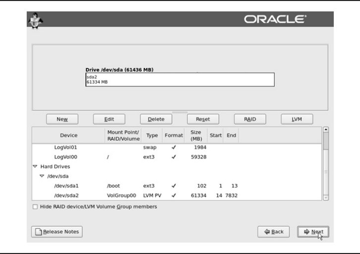
38 Oracle Database 11g: A Beginner’s Guide
In Figure 2-1, you can see one logical device for the swap space, which is the
memory area on the disk allowing for programs to swap to virtual memory when
they need more memory than the physical memory contains. There is another
device for the boot area, the initial partition of the disk, and then the rest of the disk
under the root directory can be used for creating the directories for tmp, var, home,
oracle, and so on. Even if it isn’t defined on separate devices, the directories that
Linux needs, such as the tmp and var directories, will be created during install.
However, you will need to create a directory for the Oracle software before you
install it.
As shown in Figure 2-1, the devices are configured based on the disk available
to the server, and the values and sizes can be adjusted at this point. The swap space
can be adjusted later, but it is just as easy to configure here. Also, new mount points
or file systems can be created on the root directory, depending on your needs. After
setting the values and mount points, click on Next for the next configuration screen.
After the disk partitions install screen, you need to make a choice about boot
loaders. In Linux, a boot loader is the piece that loads the operating system into
memory (there are usually a couple of them in use). The boot loaders in this case
are LILO, Linux Loader, and Grand Unified Bootloader (GRUB). The GRUB boot
loader is the default for RedHat and Oracle Linux and can be selected if needed.
FIGURE 2-1. Linux install disk partitions
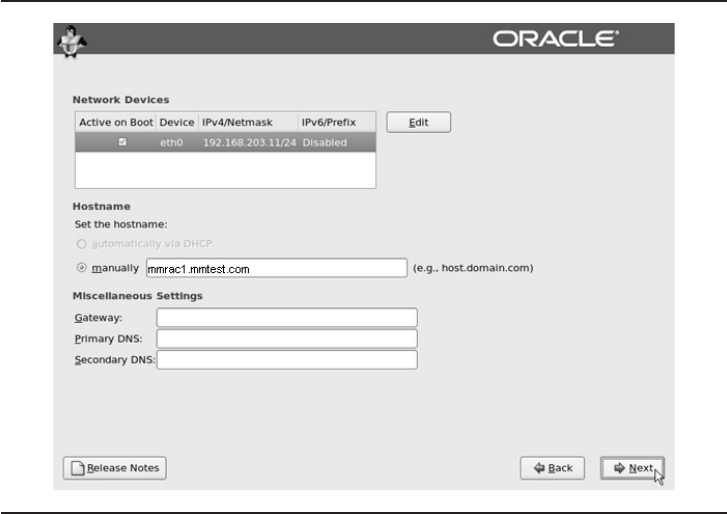
Chapter 2: Installing Oracle 39
The network configuration and devices are the next step. Plug in the IP address
and edit the network device on the installation screen, shown in Figure 2-2. This
can also be done after installation, using the network settings. This is where the host
name is defined as shown with the domain name; the miscellaneous settings are
dependent on the network settings and configurations. Figure 2-2 also shows where
to manually enter the server name with the domain and the miscellaneous settings
with the Gateway, Primary, and Secondary DNS.
The next couple of installation screens go through the root password and time
zone information; the proper time zone for your location just needs to be chosen
when going through the installation. Choose and remember the root password
carefully. At this point, there is no other way to login to the OS without the root
password. The default install will include packages for generic use, but it should
also be selected to support software development for this system. The option to
customize can be done here or the needed packages can also be installed afterward.
During the install, the packages can just be selected and then verified after the
install to ensure that they are completed. The required packages for Oracle
Enterprise Linux 5.0 (based on the current installation guide) are as follows:
■binutils-2.17.50.0.6-2.e15
■compat-libstdc++-33-3.2.3-61
FIGURE 2-2. Linux network
40 Oracle Database 11g: A Beginner’s Guide
■elfutils-libelf-0.125-3.e15
■elfutils-libelf-devel-0.125
■glibc-2.5-12
■glibc-common-2.5-12
■glibc-devel-2.5-12
■glibc-headers-2.5-12
■gcc-4.1.1-52
■gcc-c++-4.1.1-52
■libaio-0.3.106
■libaio-devel-0.3.106
■libgcc-4.1.1-52
■libstdc++-4.1.1
■libstdc++-devel-4.1.1-52.e15
■make-3.81-1.1
■sysstat-7.0.0
■unixODBC-2.2.11
■unixODBC-devel-2.2.11
After the installation, the packages should be verified by running the command
at the Linux prompt:
rpm –q unixODBC-devel-2.2.11
If the packages were not installed or if the installation failed, then the following
commands can be run to install packages as needed from the Linux source files.
Here is an example install command for this package:
rpm –ivh unixODBC-devel-2*rpm
These steps are seen in Figure 2-3; the rpm –q used to verify the packages shows
that the unixODBC package was not installed, so executing the command to install
the package completes this step. This step is repeated for each of the packages that
are required.
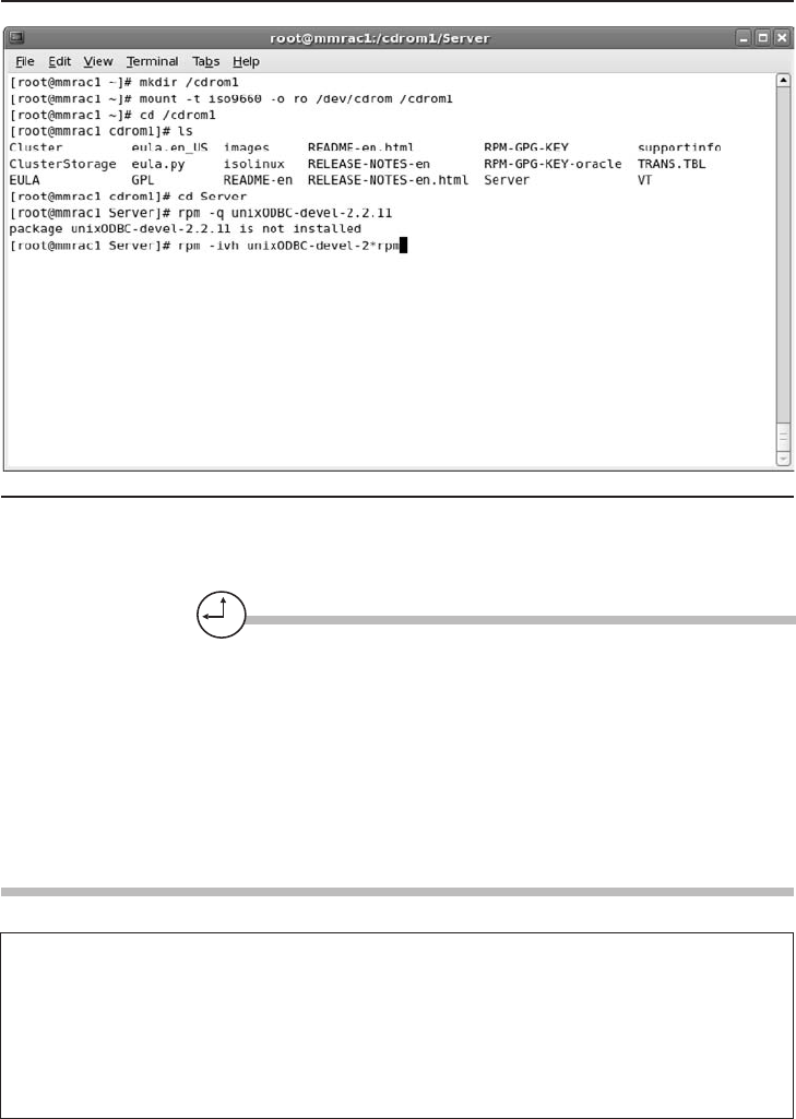
Chapter 2: Installing Oracle 41
Progress Check
1. What documents are provided for system requirements and installation
instructions by Oracle?
2. What is an important first step for installing Oracle software?
3. When installing Linux, which devices are needed when configuring the disk?
4. What is the command for verifying that a package is installed?
5. How much RAM is required for Oracle 11g?
FIGURE 2-3. Linux package install
Progress Check Answers
1. Quick Installation Guide, Database Readme, Database Release Notes
2. Gathering information on system requirements
3. You need two disk devices: swap and / (root) for the file mount points
4. rpm –q package_name
5. 1GB
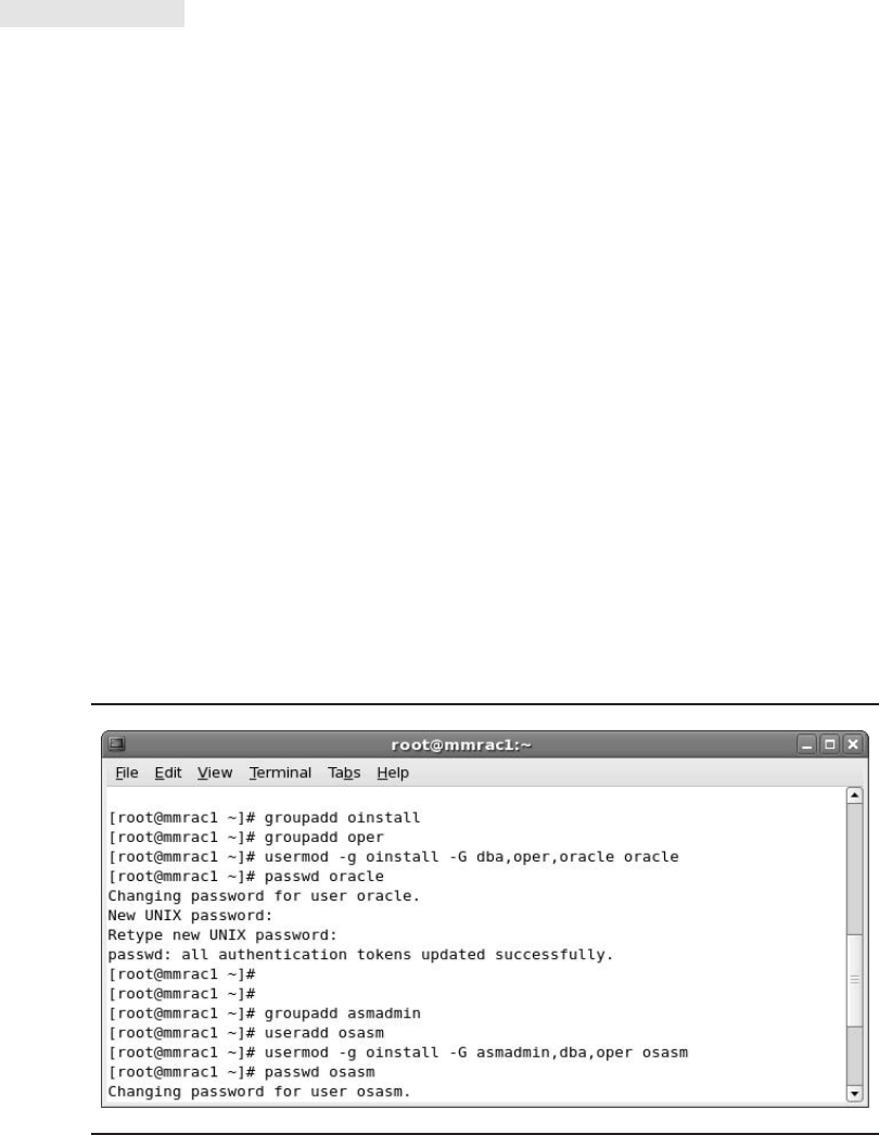
CRITICAL SKILL 2.2
Set Up the Operating System
After Linux is installed and rebooted, information screens walk you through the
license information and an option to create a user. Taking this opportunity to create
another user besides root is a recommended practice. This is because the Oracle
user is needed along with groups for the Oracle software inventory and dba group.
Oracle software should be installed under the Oracle user created here, but
additional users can also be created now, as needed, for supporting different
pieces of the software or for different options that may be installed.
Figure 2-4 shows the creation of groups using command line in the terminal
window that is needed for Oracle installs. The groups are created using the groupadd
command and then associated with a user id using usermod with the listed parameters
and options. Also seen in this figure are the ways that the passwords for the user can
be easily changed with the passwd command. Adding another ID, such as osasm to
manage the Automatic Storage Management instance, can be accomplished with
the command useradd.
The users and groups can be reviewed and managed using the User Manager in
System Tools. This interface is also available for creating new users and for associating
the groups to the user instead of using the command line in the terminal window.
Any users created using this tool and even the users created by the command line,
as in Figure 2-4, also have a home directory that is created for them at the same
time they are created. The Add User and Add Group in the User Management Tool
do the same task as the useradd and groupadd commands; the tools in Linux make
it easy to perform these tasks in a way that is most familiar, with either the command
lines or user interfaces.
42 Oracle Database 11g: A Beginner’s Guide
FIGURE 2-4. Create groups and users

Chapter 2: Installing Oracle 43
The Oracle user needs certain other permissions along with resource permissions
for the software to run well. This is done by adding the Oracle user to the
/etc/security/limits.conf and session information to the /etc/pam.d/login file. The
file limits.conf, as listed next, shows that the Oracle user has been added with
resources to nproc and nofile parameters at the end of the file. These files can be
edited with Notepad or a similar editing program when you open the files by using
Explorer windows:
limits.conf file:
#<domain> <type> <item> <value>
#
oracle soft nproc 2047
oracle hard nproc 16384
oracle soft nofile 1024
oracle hard nofile 65536
# End of file
/etc/pam.d/login file:
#%PAM-1.0
auth [user_unknown=ignore success=ok ignore=ignore default=bad]
pam_security.so
auth include system-auth
account required pam_nologin.so
account include system-auth
password include system-auth
Ask the Expert
Q: Are there security concerns with adding users? Do you really need any
other users besides root and oracle?
A: Security for the operating system is important. Make sure that logins are
created for users to install the Oracle software and that additional users are
created for the purpose of allowing database administrators to log in and
maintain Oracle and the database. Anyone logging into the system should have
their own user ID; use of the Oracle login should be limited to installation and
patching of the software. Different users should have permissions to access only
areas that they should be allowed to access in order to perform tasks as needed.
File system permissions should only be granted to the groups and users that
need the access, and should be limited where possible. Research best practices
for security and don’t share logins or root passwords. Keep the environment
secure by limiting access to the Oracle software directories; make sure it is not
open to just any user who is able to log into the server.

44 Oracle Database 11g: A Beginner’s Guide
# pam_selinux.so close should be the first session rule
session required pam_selinux.so close
session include system-auth
session required pam_loginuid.so
session optional pam_console.so
# pam_selinux.so open should only be followed by sessions to be
executed in the user context
session required pam_selinux.so open
session optional pam_keyinit.so force revoke
session required /lib/security/pam-limits.so
session required pam_limits.so
Now the operating system is installed and users and groups are created and
configured with the needed permissions. You still need to verify (and possibly
update) some configurations needed by the kernel parameters so that they match at
least the minimum requirements for Oracle. The Oracle Quick Installation Guide is
the reference for these requirements. We hope that you are starting to see the
importance of these documents and why these pieces of information should be
gathered before you start the installs.
Project 2-1 Configure Kernel Parameters
The default install of the Linux operating system has values set for the kernel parameters,
but the Oracle requirements may need you to adjust these settings. This project will
walk you through step by step to change the kernel parameters and show the values
of these settings.
Step by Step
1. Get the minimum values from the installation guide. Here is a quick list:
Semmsl 250
Semmns 32000
Semopm 100
Semmni 128
Shmall 2097152
Shmmax The lesser of the two: either half the size of the
physical memory or 4GB
Shmmni 4096
file-max 512*PROCESSES
ip_local_port_range Min: 1024, max: 650000

rmem_default 4194304
rmem_max 4194304
wmem_default 262144
wmem_max 262144
2. Verify the parameters that are currently set. There may be values already set
above the minimum value, so these would not need to be changed. At the
command line type the following:
# /sbin/sysctl –a | grep <param-name>
3. Substitute the parameter name for param-name. For example, shm will
show the values for the semaphore parameters:
# /sbin/sysctl –a | grep shm
kernel.shmmni = 4096
kernel.shmall = 2097152
kernel.shmmax = 2147483648
4. Edit the /etc/sysctl.conf to adjust the kernel parameter values. Use vi or
another text editor to add the line as listed under #ORACLE 11gR1 kernel
parameters to the end of the file. The other parameter that was changed was
kernel.shmmax. Here is the example /etc/sysctl.conf file; the areas that need
to change or be added are in bold:
sysctl.conf edits:
# Controls the maximum size of a message, in bytes
kernel.msgmnb = 65536
# Controls the default maximum size of a message queue
kernel.msgmax = 65536
# Controls for maximum shared segment size, in bytes
# CHANGED FOR ORACLE 11g # kernel.shmmax = 1073740324
kernel.shmmax = 2147483648
# Controls the maximum number of shared memory segments, in pages
kernel.shmall = 2097152
#ORACLE 11gR1 Kernel Parameters – add the following lines
fs.file-max = 6553600
kernel.shmmni = 4096
kernel.sem = 250 32000 100 128
net.ipv4.ip_local_port_range = 1024 65000
net.core.rmem_default = 4194304
net.core.rmem_max = 4194304
net.core.wmem_default = 262144
net.core.wmem_max = 262144
Chapter 2: Installing Oracle 45
Configure Kernel Parameters
Project 2-1
(continued)
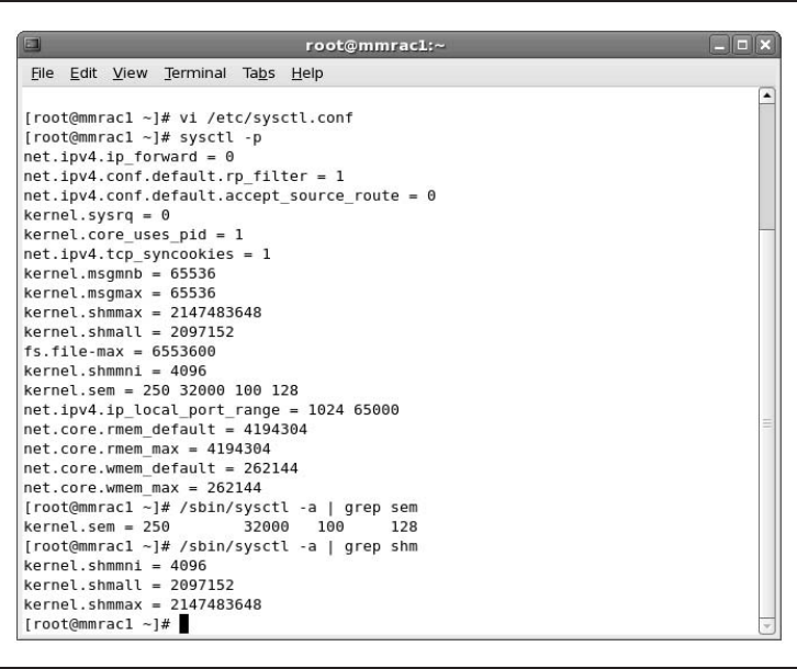
5. Reload the kernel parameters for the new values to take effect. This can be
done by restarting the server or by using the following command to reload:
# /sbin/syctl –p
The execution of this command and its output are shown in Figure 2-5.
Project Summary
In walking through this project, you now know how to see the kernel parameters,
make changes to the parameters, and verify those changes. In changing the kernel
parameters, you are making the necessary optimizations for the Oracle software to
run on the Linux platform.
46 Oracle Database 11g: A Beginner’s Guide
FIGURE 2-5. Verify the kernel parameters using sysctl –p

CRITICAL SKILL 2.3
Get Familiar with Linux
Having the user interface and the terminal window for access to the command line
means that there are a couple of ways to navigate through Linux and do what needs to
be done. With previous examples of using the command line, files were edited, users
were added, and parameters were set up. In managing some of the Oracle files and
directories, it is useful to know some of the basic commands or how to look up the
option for the commands. Changing directories, copying and moving files, editing, and
being able to look at the content of the file are all basic commands in Linux (and almost
the same as what is used in Unix, with a couple of possible differences in the parameter
options). The following are some useful Linux commands, with a brief definition:
■pwd This shows the current directory (print working directory).
■more filename This lists the file.
■ls This lists the files in the directory.
■echo $VAR This shows value of variables or echoes back the text.
■mv filename newfilename This renames a file.
■cp filename /newdirectory This copies a file.
■rm filename This removes (deletes) a file; wildcards can be used but are
not recommended for a root directory.
Manual pages are available to provide details for commands as well as available
options. There are also examples for how to use the commands in the details. This
information can be accessed by typing man and then the command. Here is an
example of the command, and Figure 2-6 show the results of this command and
what can be found in the man pages.
$man grep
Progress Check
1. How are kernel parameters verified on Linux?
2. What is the Linux command to view the manual pages for grep?
3. What is the command to create a Unix group?
Chapter 2: Installing Oracle 47
Progress Check Answers
1. sysctl –p
2. man grep
3. group add oinstall
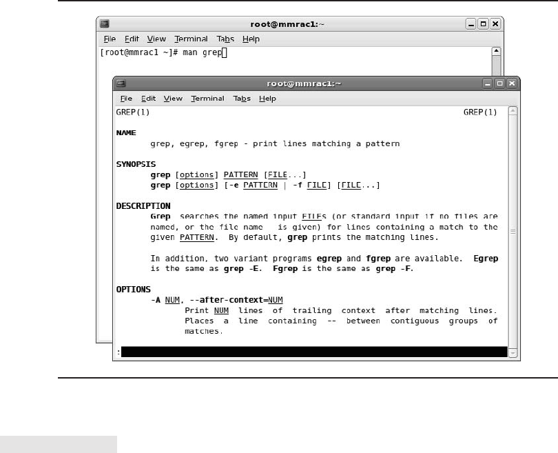
48 Oracle Database 11g: A Beginner’s Guide
CRITICAL SKILL 2.4
Choose Components to Install
Various components of the Oracle software are automatically installed; some are
available on the companion CDs or as additional downloads. With Oracle 11g, the
following products are now installed by default with the database:
■Oracle Database Vault
■Oracle SQL Developer
■Oracle Configuration Manager
■Oracle Application Express
■Oracle Warehouse Builder
This section is not going to turn into a discussion of licensing for standard or
enterprise editions and of the different products that are available; however, there
FIGURE 2-6. OUTPUT of man commands
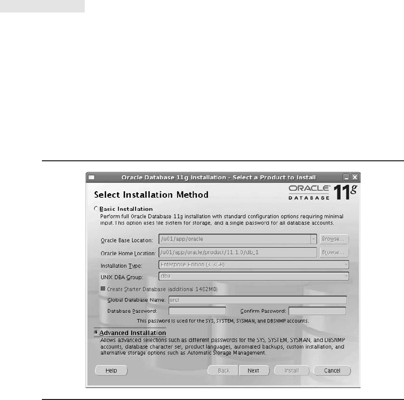
are products that provide benefits for different needs. Reviewing the products and
versions to match them with business needs before installing is helpful for performing
the install of these products at the same time as the initial install. It is possible to add
products by running through the install again and choosing the options that have
not yet been installed.
The Oracle Universal Installer allows for the Basic install, which is just going to
install the default options for Oracle. There is an Advanced option available for
deselecting or selecting other available options.
CRITICAL SKILL 2.5
Install the Oracle Software
To begin, run the Oracle Universal Installer as oracle, either from the DVDs or from
the downloaded software that has been unzipped on the file system:
[oracle@mmrac1 database]$ ./runInstaller
If the ORACLE_HOME environment variable is set before running the Installer,
information will already be populated with these details. Starting with Figure 2-7,
let’s walk through some of the screens of the Oracle Universal Installer. Each of the
illustrations following provides some detail about what options to select and
information to provide while installing the Oracle software.
Chapter 2: Installing Oracle 49
FIGURE 2-7. Basic vs. advanced install
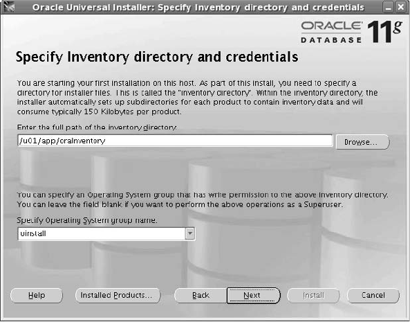
50 Oracle Database 11g: A Beginner’s Guide
The Basic install will start up the database configuration assistant in order to
create a database instance after installing the software. Certain configurations are
not available, such as Automatic Storage Management (ASM), but the Basic install
will install the default components without walking through the options. The
Advanced install will allow you to pick and choose from the available options.
Advanced install was chosen in Figure 2-7, and the following illustrations for this
install will show the options available with the advanced option.
It’s a good idea to start to document the options that are chosen for the checklist
for the install, so that future installs of the Oracle software will have the same
components installed as needed. A checklist will be useful for creating consistent
environments and ensuring that the same components are being installed across test
to production systems.
The group that was defined on the operating system for the Oracle install is
needed for the permissions to the OraInventory directory. This is normally a group
such as oinstall, as seen in the following illustration. The OraInventory will contain
the information about what was installed and the versions used. OraInventory is
used for when the binaries need to be patched and when needing to add or remove
components.
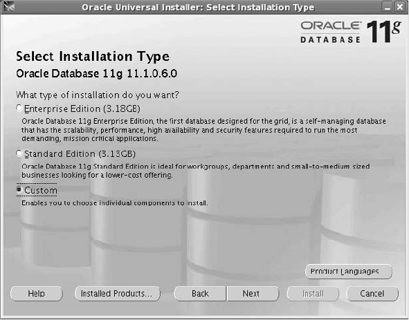
Chapter 2: Installing Oracle 51
As seen in the next illustration, there are three types of installs: Enterprise,
Standard, or Custom. Choosing Enterprise or Standard will install the default
products for those versions. Obviously, the Enterprise and Standard versions
have different licensing issues, and limitations are set on the Standard edition
for CPUs and the options that can be added. There are several product options
that come with installing a default type of Standard or Enterprise. Some may
argue that you should install only what is needed, while others may suggest
that for a development environment, you should install everything to allow
developers to test and try out different options. For most systems, we recommend
that you use the Custom option to select only options that are needed. Standardize
the install so that it can repeated when you are ready for a production
environment.
On a server, there can be several home directories with different versions,
options, and patch sets installed. The following illustration shows an example of
what the base directory and home directory should be set to. If doing a new install
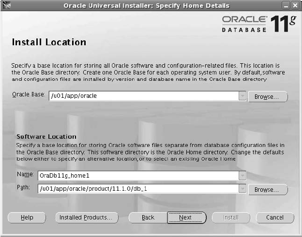
and for additional components or patching existing ones, Oracle home directory
should be used.
The following illustration shows the install screen running through checks for
kernel parameters, memory, and patch sets for the operating system, as well as
other requirements that are needed to install and run the Oracle software. If
the verification of the operating system was done as part of the planning, these
checks should all pass. If there are failures here, they need to be corrected before
continuing with the install.
52 Oracle Database 11g: A Beginner’s Guide
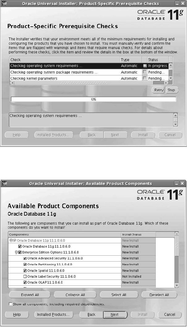
Chapter 2: Installing Oracle 53
As discussed when using the custom install, there are options for what to install,
as shown in the following illustration. Look through the available options and check
the components that are desired or uncheck those components not needed.
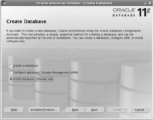
After the software is installed, the installer will open up the database configuration
assistant to create a database or to configure ASM. See the following illustration,
which shows these choices; in this case, only software has been selected. If you are
just installing the software, the database creation assistant can be used at another time
for creating databases and ASM instances. The steps for the database configuration
assistant are listed in the next section, “Database Configuration Assistant.”
During the last step before the actual install, you still have the opportunity to go
back and modify any directories or options for the install. The following illustration
shows the screen with this summary information, which has the directories where it
is to be installed, installation type, and its space requirements. At this step, take time
to review to make sure the information is correct.
54 Oracle Database 11g: A Beginner’s Guide
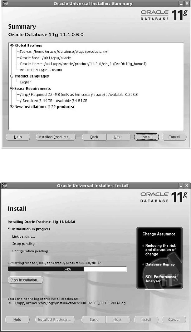
Chapter 2: Installing Oracle 55
The following illustration shows the files are being copied and installed. Note
the location of the log file. If any issues or errors come up, this would be the first
place to look for more information.
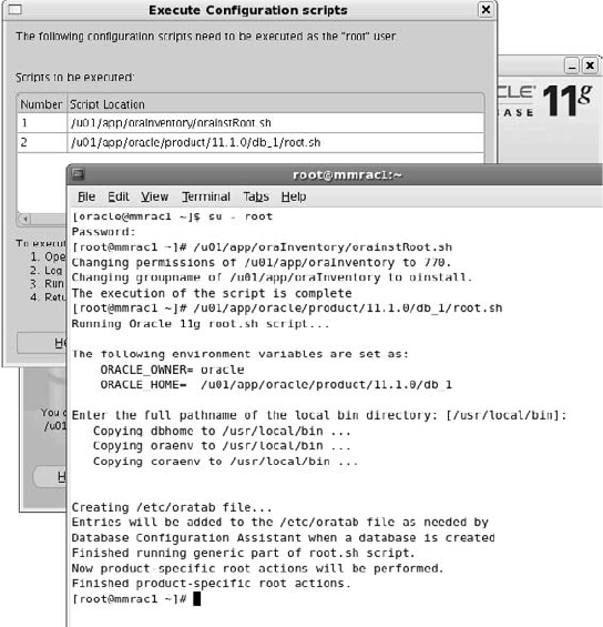
Your last steps are demonstrated in the following illustration. To complete the
installation, you will need to make changes regarding permissions and directories
that are owned by root. There are two scripts that need to be executed by the root
owner to make these changes. Have the operating system administrator log in and
run orainstRoot.sh and root.sh (as shown in the illustration).
This final illustration is always a good screen to see because it means that the
installation of the Oracle software has completed successfully. The installation went
through the listener configuration and the instance configuration, so the database is
now up and available for use. The listener configuration will be covered in more
detail in the next chapter, but for reference here, it is important to have the listener
service started to be able to connect to the database instance from another server.
This configuration is completed with a default listener name and port as well as
starting of the service which will allow the connections to the database.
56 Oracle Database 11g: A Beginner’s Guide
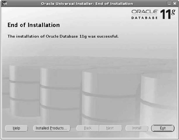
Database Configuration Assistant
As part of the installation, the database configuration assistant (dbca) can be configured
to start up after the initial software install. Otherwise, the assistant can be started any
time to create a new database instance. The dbca has standard templates to be used for
different types of databases; the templates have some parameter settings for memory and
others based on the type of instance. The passwords and directories for the tablespaces
can use the default values or be customized. As part of the planning process, these
configurations should be decided on depending on the directory structures and
templates to be used. A checklist needs to be kept to determine which templates,
parameter settings, and other choices are to be made within the assistant. The advantage
is that even after the database instance is created, parameters and file locations can
be adjusted. However, some adjustments are easier than others, and with Oracle 11g,
there are even more dynamic parameters that can be changed while the database is up
and available, instead of having to restart the database instance to make the change in
value for the parameter.
As shown in Figure 2-8, the database can be created or an existing database can
be dropped. There is also the option to create an Automatic Storage Management
(ASM) instance, which will be described in more detail in Chapter 8. Choosing this
option for ASM will only install an ASM instance, while running through dbca will
be required in order to install a database instance.
Chapter 2: Installing Oracle 57
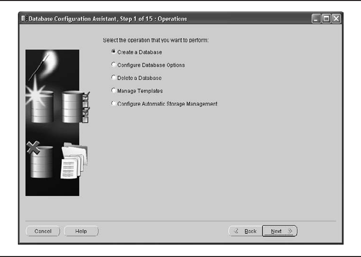
58 Oracle Database 11g: A Beginner’s Guide
The next dbac screen has three default options to choose for the databases:
General Purpose, Custom Database, and Data Warehouse. For following along
with examples that will be used in the rest of the book, it would be useful to install
a General Purpose database with the sample schemas. The SH schema that is used
for examples is included with other sample schemas.
In stepping through the screens, the next step would be to name the database
instance. Passwords should be set for SYS and SYSTEM. All of the system passwords
can be the same or they can all be different. The main thing is that these passwords
should not be set with a default value as they have in the past. Anyone who knows
about installing Oracle and default passwords would be able to log into the
database if the default was not changed. For now, the choices to be made with the
database install can be kept to defaults or basic choices. As you learn more about
FIGURE 2-8. Option for install of database
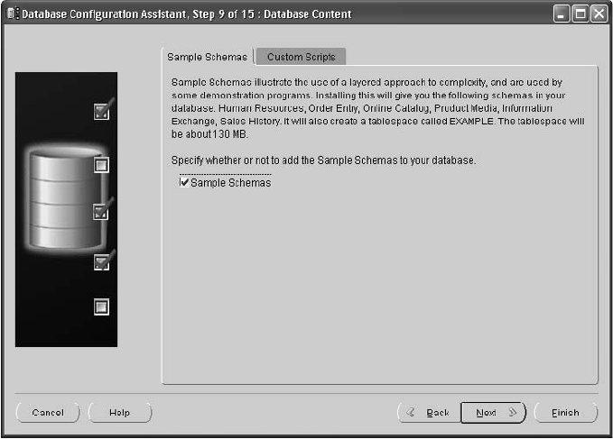
Chapter 2: Installing Oracle 59
what the system is to be used for, you can make more adjustments with parameters
and configurations.
For a test database instance with schemas and to work through the examples,
check Sample Schemas, as shown here.
The initialization parameters can be configured as you create the database. The
following illustration shows step 10 of the database configuration assistant, where
these parameters can be configured. The memory can be customized or default
values can be taken, based on a percentage of overall available memory. The
character set should also be set up; it is more difficult to change, unlike the memory
settings, so verifying the character set for the database is important. The character
sets are important for databases with international characters and globalization of
the characters. When dealing with international characters, it is suggested to use a
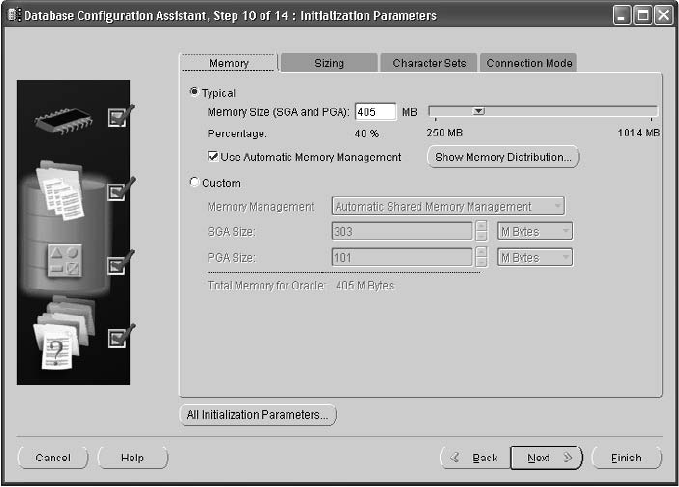
60 Oracle Database 11g: A Beginner’s Guide
character set that allows for these values. Unicode character sets support characters
with different sizes and in multiple languages.
Creating the database, creating the scripts, and developing a template are the
final steps before the database is actually created. The following illustration shows
the option to save the database as a template and to generate database creation
scripts. Having scripts is a valuable tool for creating another similar database, or
when needing to create the database again without the assistant. The templates will
be added to the creation process of other databases in this Oracle home, again,
making it easier to create another database that is similar in nature.
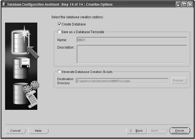
Chapter 2: Installing Oracle 61
Verify the Installation
The operating system is now configured, the Oracle software is installed, and an
initial database has been created. Now the system should be reviewed to confirm
that everything is in the right place and that everything is working as expected.
Looking through the directories and log directories of the database to verify the
install is very useful. Check the install log file, which was the log file that was listed
during the install of the software. See Figure 2-9 for example output of the log file.
Review the alert logs of the database and check the logs for any issues with
the startup or parameters of the database. The default location for the log files are
$ORACLE_BASE\admin\SID. This information can also be retrieved by queries
to the database and selecting the value from v$parameter where the name =
'background_dump_dest'. Look at the file systems to make sure that the datafiles
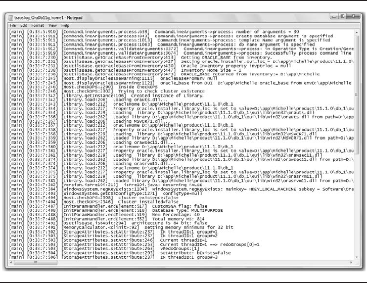
62 Oracle Database 11g: A Beginner’s Guide
are going to the directory that is expected. Again, a quick query against the database,
such as select file_name from dba_data_files, will show all of the current data files.
Log into Oracle Enterprise Manager (OEM) and make sure the database can be
accessed. Several of these checks are listed in greater detail in later chapters of the
book and will show more details about Oracle Enterprise Manager as well as
information about tablespaces and data files. Check the memory usage on the
operating system level to ensure that the right amount of memory was configured
for Oracle and that there is space available for user processes too. Use commands
like top to see what the top processes are and to view memory usage for the processes.
The file systems should also have enough space; you should verify this after
installing Oracle and creating the database.
After these initial checks the system should be ready to use, allowing you to install
the front-end application, add users, and set up monitoring and backups. Setting up
backups and monitoring help also verify that the system is ready to go and might be
a good step to complete before allowing other users to access the database.
FIGURE 2-9. Log file details
Tie It All Together
When doing an Oracle install, the upfront planning and research is important.
Gathering business requirements in order to match up database options and
versions is also a critical first step to doing the installations. A basic understanding
of an operating system is needed to work through the install and to ensure that the
user permissions, required system, and hardware components are available. Oracle
Enterprise Linux has a standard install, with packages that match up to the database
requirements. Gathering documents that provide the latest information about issues
and needed prerequisites will make the overall installation go smoothly plus give
the added bonus of starting an install process that would be repeatable in the
production environment.
þChapter 2 Mastery Check
1. How much disk space is needed for installing Oracle software on Linux?
2. What users and groups are used for installing the Oracle software?
3. True or false: Installing Oracle software will automatically install an Oracle
database.
4. What are the prerequisites for installing Oracle software?
5. What are the types of installation options for the Oracle software?
6. What is the Oracle home directory? Can there be more than one?
7. Besides the database, what are some of the other products that are installed
by default?
8. What is the tool for creating a database, after the Oracle software install?
9. What is the default password for SYS and SYSTEM users in the database?
10. Which scripts need to be run by root (system administrator) after the install
of the software?
Chapter 2: Installing Oracle 63
This page intentionally left blank

Chapter
3
Connecting to Oracle
CRITICAL SKILLS
3.1 Use Oracle Net Services
3.2 Learn the Difference Between
Dedicated and Shared Server
Architectures
3.3 Define Connections
3.4 Use the Oracle Net Listener
3.5 Learn Naming Methods
3.6 Use Oracle Configuration Files
3.7 Use Administration Tools
3.8 Use Profiles
3.9 Network in a Multi-tiered
Environment
3.10 Install the Oracle 11gClient
Software

66 Oracle Database 11g: A Beginner’s Guide
his chapter introduces Oracle Net Services, which allows database
applications running on remote systems to access an Oracle
database. It creates and maintains the network connection, and
also exchanges data between the application and the database.
Oracle networking plays a critical role in performance and
availability. Each new version of Oracle is designed to support more data and users
than the previous release. This increased amount of database activity and network
traffic needs to be addressed from an availability and performance perspective
and should be managed by the DBA. A DBA also has to be able to determine if a
performance issue is due to networking, and if so, then they must be able to resolve
any network performance issues from a database configuration perspective.
Throughout this chapter we will refer to DBAs, which in this context means
anyone that is performing networking administration operations to make the
database connectivity work. These days, more developers are managing their own
development databases and performing operations traditionally reserved for DBAs.
NOTE
Oracle Net Services is a large topic. The emphasis
in this chapter is to introduce DBAs to Oracle
Net Services terminology and concepts,
feature/functionality, and key components and
tools. Once a beginning DBA reads this section,
they should be able to understand the Oracle
networking references and be capable of performing
simple operations using the Oracle GUI tools and
wizards for Oracle Net Services.
CRITICAL SKILL 3.1
Use Oracle Net Services
Oracle Net Services is the software component that allows enterprise connectivity
across heterogeneous environments. Oracle Net is the part of Oracle Net Services
that manages data communication between a remote application and the Oracle
database; it runs on top of a network protocol like TCP/IP. The software used by
Oracle Net software resides on the remote system and the Oracle database platform.
A listener process must be running on the database server to receive the network
request. (A listener is a program that listens on a port for incoming network requests
and then hands the request to another program for processing.) The listener then
determines the appropriate type of process to handle the request.
The network protocol sends a request to the Oracle Protocol layer, which sends
the information to the Oracle Net Foundation layer, which in turn communicates
with the database server. The Oracle network communication stack, shown in
Figure 3-1, is similar on both the client and server sides.
T
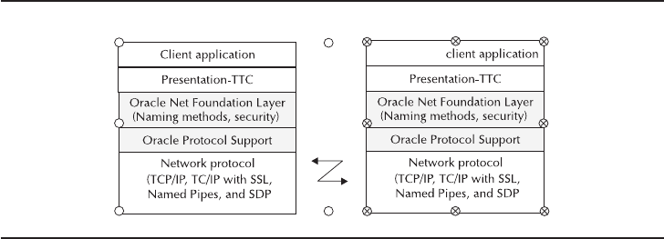
Chapter 3: Connecting to Oracle 67
Oracle Net (Oracle Net Foundation Layer and Oracle Protocol Support) fits into
the session layer of the Open Systems Interconnect (OSI) model (visit www.ietf.org
for more information about the OSI model).
Network Protocols
Oracle supports a number of industry standard protocols. These protocols transport
the data between the remote platform and the database server platform. The protocols
also display how users need to work with data differently than they did a few years
ago. Oracle-supporting protocols like SDP, HTTP, FTP, and WebDAV show that
Oracle Database 11genhances network performance and offers increased flexibility
for users working with data. In this section, the term application server will be used
to address both web and application server services available in the middle tier.
Table 3-1 lists the supported industry-standard protocols.
Optimize Network Bandwidth
Multi-tiered architectures need to maximize the bandwidth between the application
server and the database server platforms. Oracle Net Services supports the high-speed
networks of InfiniBand, a channel-based, high-speed interconnect technology
designed to optimize performance between different platforms. It’s used for server
clustering and for network interfaces to storage area networks (SANs) and local area
networks (LANs). Vendors such as Hewlett-Packard, IBM, Sun Microsystems, Dell,
and Microsoft support InfiniBand technology; the SDP protocol, an industry-standard
wire protocol, is also used with the InfiniBand network. Highly active multi-tiered
environments should consider using high-speed interconnects between the application
server and the database server.
Server-based
ServerClient
FIGURE 3-1. The Oracle network communication stack

68 Oracle Database 11g: A Beginner’s Guide
Connections
Aconnection is an Oracle communication path between a user process and the
Oracle database server. If this communication path is dropped, a user must establish
a new session. The current transaction is rolled back if the connection for its session
is lost. A session is a specific connection for a user between the user process and the
Oracle database server.
Protocol Description
TCP/IP The Transmission Control Protocol/Internet Protocol (TCP/IP) is
the standard protocol used in client server environments.
TCP/IP
with SSL
TCP/IP with Secure Sockets Layer (SSL) provides authentication
(certificates and private keys) encryption. The Oracle Advanced
Security option is required for this protocol.
SDP The Sockets Directory Protocol (SDP) is an industry-standard
high-speed protocol. SDP is used with an InfiniBand network. The
InfiniBand network takes the messaging burden off the CPU and
onto the network hardware. This network reduces the overhead
of TCP/IP, providing increased bandwidth.
Named pipes This supports inter-process communication between remote
platforms and the database server platform using pipes. A pipe
is opened on one end and information is sent down the pipe to
allow I/O between the platforms.
HTTP The Hypertext Transport Protocol (HTTP) is an industry- standard
protocol that is primarily used between clients and application
servers. Oracle can also start up an HTTP listener to handle a
request over HTTP directly.
FTP File Transfer Protocol (FTP) is a standard method for transferring files
across the Internet. It makes it easy to transfer files back and forth
between different platforms. A server that can receive an FTP
connection is referred to as an FTP server or FTP site. FTP addresses
looks similar to HTTP; ftp://ftp.beginner.com is an example of an FTP
server address.
WebDAV The Web-based Distributed Authoring and Versioning (WebDAV)
protocol supports collaborative authoring over the Internet. The
benefits of WebDAV include locking mechanisms, interoperable
publishing with HTTP and XML support, writing over the Web
with embedded devices, versioning, and Access Control Lists.
TABLE 3-1. Standard Industry Network Protocols
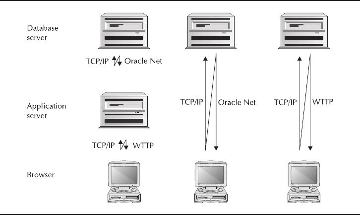
If a connection cannot be made, it is important to be able to troubleshoot these
issues and problems. In the Automatic Diagnostic Repository (ADR) for Oracle 11g,
the network information is also captured. The repository holds trace files and other
errors collected into a standard place. This troubleshooting facility for diagnosing
network problems is the same as the one you will use to analyze and diagnose
database problems. With tools like this it will be easier to find connection issues
or avoid problems.
Maintain Connections
The Oracle Net Foundation Layer establishes and maintains connections with the
database server. Transparent Network Substrate (TNS) is the common interface
between all the industry-standard protocols. Oracle Protocol Support maps the
industry-standard protocols (TCP/IP, TCP/IP with SSL, SDP and Named Pipes) used
in the connection.
Figure 3-2 shows us how Oracle Net works. Oracle Net software will reside on
the database server platform and the platform that is running the Oracle applications.
With an application server, HTTP runs on top of a network protocol between the
browser platform and the application server platform. Oracle Net then runs on top
of a network protocol between the application server and the database server. For
a client/server configuration, Oracle Net will reside on the client platform and the
database server platform, and will run on top of a network protocol between the
client and the database server platforms.
Chapter 3: Connecting to Oracle 69
FIGURE 3-2. An Oracle network overview

If Java programs are running, a Java Database Connectivity (JDBC) OCI, or Thin
driver, will communicate with Oracle Net to process the database request. A JDBC
OCI driver requires Oracle Net on the remote platform and the database server. A
Thin driver doesn’t require a full Oracle Client to be installed and uses network
calls to connect to a database. So, a JDBC Thin driver written entirely in Java uses
JavaNet to communicate, and requires Oracle Net only on the server platform.
Define a Location
Locations need to be defined so a remote application can find the correct Oracle
database server on the network. A service name, such as customer.us.beginner.com,
is used to define the unique location of each database server. In the preceding
example, customer is the database name and us.beginner.com is the domain name.
On the plus side, if the physical location of the database is changed, the service
name can stay the same while the definition or settings of the name can change
underneath.
A database can support multiple services. The service name, defined with the
initialization parameter SERVICE_NAMES, makes the physical location of the database
transparent and will default to the global database name (the name of your database),
which uses the format database_name.database_domain, as in customer.us.beginner.com.
The database domain name is the domain where the database is located, and is
made up of the initialization parameters DB_NAME and DB_DOMAIN. The combination
of the DB_NAME and DB_DOMAIN (customer.us.beginner.com) name distinguishes
one database from another, as shown in the following examples:
DB_NAME=customer
DB_DOMAIN=us.beginner.com
70 Oracle Database 11g: A Beginner’s Guide
Ask the Expert
Q: Why is it important for DBAs to understand the networking setup and
configuration for Oracle Database 11g?
A: Often as systems interact with the database, networking bottlenecks
surface that require attention from DBA personnel in addition to those who
manage the applications. Familiarity if not fluency with setting up Oracle Net
services and its configuration files arms the DBA with the skills required to
intervene.

Chapter 3: Connecting to Oracle 71
CRITICAL SKILL 3.2
Learn the Difference Between Dedicated and
Shared Server Architectures
An Oracle database server can be configured to run either a dedicated or shared
server architecture. This decision determines how the listener processes requests
and how server processes work for an Oracle instance. Server processes are the
interface between the Oracle database server and user processes, the latter of which
must go through a server process that handles the database communication between
the user process and the database. Server processes can
■Process database requests, access data, and return the results.
■Perform data translations and conversions between the application and
database server environments.
■Protect the database server from illegal operations by the user processes. A
server process accesses Oracle database and memory structures on behalf
of the user process. This separates user process activity from direct access to
Oracle’s internal memory.
Dedicated Server
A dedicated server environment uses a “dedicated” server process for each user
process. The benefit of this is that each user process has a dedicated server process
to handle all of its database requests. If there are a hundred separate sessions, there
will be a hundred dedicated server processes running on the same platform as the
database server.
The problem is that each dedicated server process is often idle a large
percentage of the time. This takes up a lot of operating system resources for server
processes that are sitting idle and creates issues when large numbers of users are
accessing a system. Oracle databases that allow access from the Internet can have
tremendous spikes of activity that generate a large number of dedicated server
processes. The dedicated server architecture also does not support FTP, HTTP, or
WebDAV clients.
Figure 3-3 illustrates the way that dedicated server processes run on the database
server platform. A dedicated server process will be run for each user session.
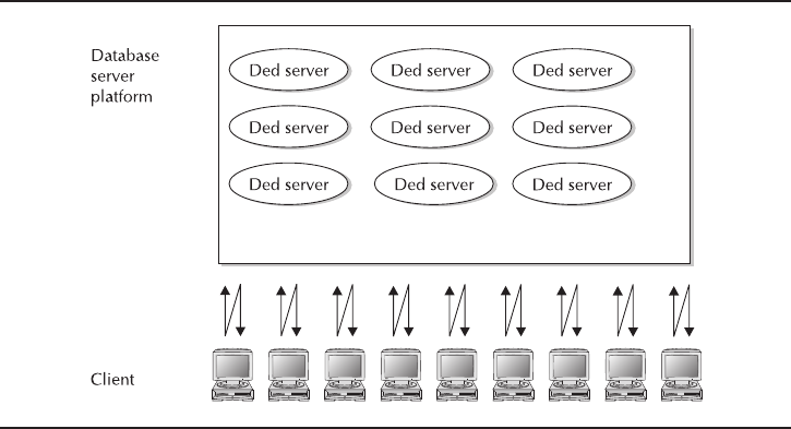
72 Oracle Database 11g: A Beginner’s Guide
Shared Server
A shared server architecture offers increased scalability for a large number of users.
This is possible because a single server process can be “shared” among a number of
user processes, allowing a single server process to be able to support a large number
of user processes. If there are 100 separate sessions, there may in turn be 20 shared
server processes supporting them. Having a small pool of server processes that can
support a large number of sessions increases scalability. This shared server architecture
is much more scalable than a dedicated architecture as the number of users for a
system increase. The shared server process can also handle large spikes of user
activity much better than a dedicated server process configuration.
When a user request arrives, the listener will route the request to a dispatcher,
which then processes and routes the request to a common queue. From a pool of
shared server processes, an idle shared server will see if there is work in the common
queue. Requests are processed on a first-in first-out basis. The shared server then
processes the request and puts the results in a response queue (each dispatcher has
one) that a dispatcher can return to the user process. Afterward, the dispatcher
returns the results from its response queue to the appropriate user process.
A dispatcher supports multiple connections with virtual circuits, which are
sections of shared memory that contain the information necessary for client
communication. The dispatcher puts the virtual circuit on the common (request)
queue accessed by the server process.
There are some administration operations that cannot be performed through a
dispatcher, however. To perform these restricted administration operations in a shared
FIGURE 3-3. The dedicated server architecture
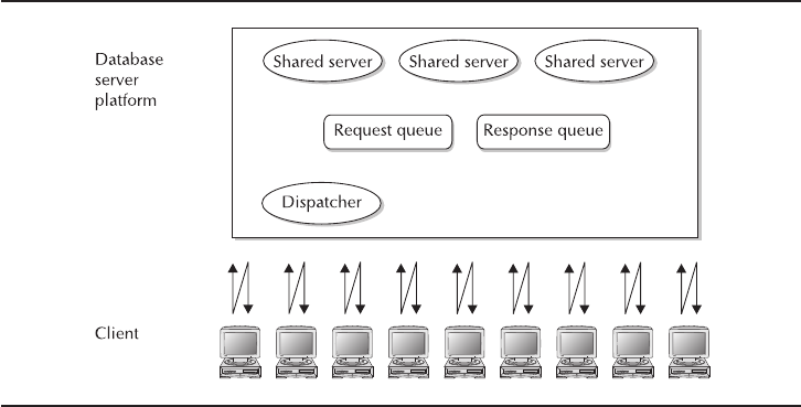
server environment, the DBA needs to connect with a dedicated server process instead
of a dispatcher process. The restricted operation needs a connect descriptor with a
setting of SERVER=DEDICATED, defined in the CONNECT_DATA section of the
tnsnames.ora file: (CONNECT_DATA = (SERVER = DEDICATED)(SERVICE_NAME =
MMDEV1)). Restricted operations include the following:
■Starting up an instance
■Shutting down an instance
■Media recovery
As Figure 3-4 shows, a shared server process can support multiple user sessions.
Table 3-2 illustrates the initialization parameters that are used to configure the
shared server architecture. Possible values for these parameters are dependent on
the level of user activity and the types of operations the server processes are
executing.
Oracle recommends starting with one shared server process for every ten
connections. It then automatically increases the number of shared servers based
upon the workload up to the MAX_SHARED_SERVERS that are defined. The PMON
process is responsible for adding and removing shared servers; the number of shared
servers will never drop below the value contained in the SHARED_SERVERS parameter.
You should also note that the parameters that control the minimum and maximum
number of these shared servers can be set dynamically; therefore you can always
ensure that you can react quickly to shared server issues.
Chapter 3: Connecting to Oracle 73
FIGURE 3-4. The shared server architecture

74 Oracle Database 11g: A Beginner’s Guide
Set Dispatchers
To set the number of dispatchers, determine the maximum number of concurrent
sessions and divide this by the number of connections per dispatcher. Then,
dependent upon the level of activity, the number of dispatchers may need to be
Oracle Initialization Parameter Definition
DISPATCHERS This defines the number of dispatcher
processes to start in a shared server
architecture. The number of dispatchers can
be dynamically added or reduced. There
must be at least one dispatcher for each
network protocol. Additional dispatchers
can be defined based upon the workload.
MAX_DISPATCHERS This defines the maximum number of
dispatchers. This is not a fixed limit. In this
release, this value can be dynamically
exceeded at runtime.
SHARED_SERVERS This defines the number of shared servers to
invoke on database startup in a shared server
architecture.
MAX_SHARED_SERVERS This defines the maximum number of shared
server processes.
SESSIONS This defines the maximum number of
sessions that can be active in a system.
SHARED_SERVER__SESSIONS This defines the maximum number of shared
server sessions that can be started in a
system. It also allows dedicated sessions to
be reserved in a shared server environment.
Sessions started above this limit will use
dedicated server processes.
CIRCUITS This defines the maximum number of virtual
circuits.
LARGE_POOL_SIZE This defines the size of the large pool area in
the SGA. If a large pool exists, the session
information will be stored in the large pool,
not the shared pool area.
TABLE 3-2. Initialization Parameters Used by Shared Servers
Chapter 3: Connecting to Oracle 75
increased or decreased. A single dispatcher can handle a large number of shared
server processes, but the number of dispatchers per shared server is dependent upon
the activity of the shared server processes.
One of the following attributes—PROTOCOL, ADDRESS, or DESCRIPTION—can
be set with dispatchers. PROTOCOL defines the network protocol to use, ADDRESS
defines the network protocol address on which the dispatchers listen, and
DESCRIPTION is the network description. Default values are used if the attributes
are not defined, and additional network options can be defined if the ADDRESS or
DESCRIPTION attribute is set.
Additional attributes that can be set with ADDRESS or DESCRIPTION include
the following:
■SESSIONS This defines the maximum number of network sessions per
dispatcher.
■CONNECTIONS This defines the maximum number of network
connections per dispatcher.
■TICKS This defines the length of a network tick (seconds). A tick defines
the length of time for a message to get from the client to the database server
or from the database server to the client.
■POOL This defines the timeout in ticks for incoming (IN=15) and outgoing
(OUT=20) connections, and whether connection pooling is enabled. The
number of ticks multiplied by the POOL value determines the total
connection pool timeout.
■MULTIPLEX This defines if multiplexing with the Connection Manager is
set for incoming and outgoing connections. Multiplexing allows multiple
sessions to transport over a single network connection. This is used to
increase the network capacity for a large number of sessions.
■LISTENER This defines the network name of an address for the listener.
■SERVICE This defines the server names that dispatchers determine with
the listeners.
■INDEX This defines which dispatcher should be modified.
In your init.ora file, you will define the dispatchers. The following are examples
of different types of entries that will typically be created to support shared servers.
Define the number of dispatchers to start:
DISPATCHERS='(PROTOCOL=TCP)(DISPATCHERS=5)'
Define a dispatcher to start on a specific port:
DISPATCHERS='(ADDRESS=(PROTOCOL=TCP)(DISPATCHERS=5))'
76 Oracle Database 11g: A Beginner’s Guide
Define a dispatcher with more options:
DISPATCHERS="(DESCRIPTION=(ADDRESS=(PROTOCOL=TCP)
(HOST=eclipse)(PORT=1521)(QUEUESIZE=20)))
(DISPATCHERS=2)
(SERVICE = customer.us.beginner.com)
(SESSIONS=2000)
(CONNECTIONS = 2000)
(MULTIPLEX = ON)
(POOL = ON)
(TICK = 5)"
As you can see, there are numerous options that may be used, depending on the
configuration methods that you select when configuring the dispatcher.
Views to Monitor the Shared Server
The following views can be used to monitor the load on the dispatchers:
■V$DISPATCHER
■V$DISPATCHER_RATE
■V$QUEUE
■V$DISPATCHER_CONFIG
The following views can be used to monitor the load on the shared servers:
■V$SHARED_SERVER
■V$SHARED_SERVER_MONITOR
■V$QUEUE
The V$CIRCUIT view can be used to monitor virtual circuits.
The following views can be used to monitor the SGA memory associated with
the shared server environment:
■V$SGA
■V$SGASTAT
■V$SHARED_POOL_RESERVED
These views provide you with the ability to monitor your database and the
activity related to your shared servers and database. We encourage you to take a
look at the data in these tables before and after you implement shared servers, to
see how they change your database and how it functions.

Chapter 3: Connecting to Oracle 77
CRITICAL SKILL 3.3
Define Connections
This section will discuss the core components required to handle Oracle connections.
A Connect Descriptor
Aconnect descriptor is used to define the service name and the location of the
database. The address component of a connect descriptor defines the protocol, host
name, and port number. Though port numbers can be between 1 to 65535, those
from 1 to 1024 are usually reserved for special processes. The default port for
Oracle Listener is 1521. The connect data component of the description describes
the service to which you want to connect. If you do not include the instance_name
in your descriptor, it will default to the Oracle SID.
A sample connect descriptor for customer.us.beginner.com looks like the
following:
(DESCRIPTION =
(ADDRESS=(PROTOCOL=tcp)(HOST=eclipse)(PORT=1521))
(CONNECT_DATA=
(SERVICE_NAME=customer.us.beginner.com)))
A specific connect descriptor can be defined for a specific service handler. For
example, in a shared server architecture, a dedicated service handler can be chosen,
which can be set to dedicated (SERVER=dedicated) or shared (SERVER=shared). If
no dispatchers are available, a dedicated server will be used and the default service
handler is shared:
(DESCRIPTION =
(ADDRESS=(PROTOCOL=tcp)(HOST=eclipse)(PORT=1521))
(CONNECT_DATA=
(SERVICE_NAME=customer.us.beginner.com)
(SERVER=dedicated)))
Define a Connect Descriptor
When establishing a connection, you have two choices: a detailed connect descriptor
can be defined or a manual name that maps to a connect descriptor can be used.
The following example shows you how to define a manual connect descriptor or
name a connection descriptor name:
-- Manual definition of a connection descriptor
CONNECT
username/password@(DESCRIPTION = (ADDRESS=(PROTOCOL=tcp) (HOST=eclipse)
(PORT=1521)) (CONNECT_DATA= (SERVICE_NAME=customer.us.beginner.com)))
-- Connect using a pre-defined descriptor
CONNECT username/password@cust
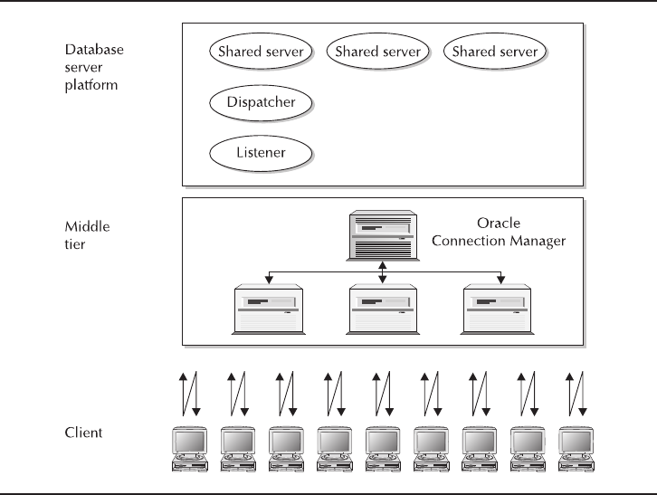
The Oracle Connection Manager
The Oracle Connection Manager processes and filters requests to the database
server. It can also optimize network performance for a large number of sessions.
Figure 3-5 illustrates the various layers between the users and the database that
need to be controlled by the manager.
The Oracle Connection Manager Control utility allows administration of the
Oracle Connection Manager. The syntax is
cmctl {command} [parameter1 ... parameterN] {-c instance_name}
{-p password}
Connection Manager commands can be executed from within the utility, as
shown here:
cmctl
CMCTL> startup –c cman0
The Oracle Connection Manager can offload network I/O from the application
servers.
78 Oracle Database 11g: A Beginner’s Guide
FIGURE 3-5. The Oracle Connection Manager architecture

We will now move on and look at the Oracle Connection Manager options to
include session multiplexing and firewall access control.
Session Multiplexing
The Oracle Connection Manager allows a number of different client network sessions
to be shared (multiplexed) through a single network connection to the database
server. Multiplexing sessions increases the number of network sessions that can be
supported. Similarly, multiple Connection Managers can be used to handle hundreds
or thousands of concurrent users; they run on the application server platform in
order to multiplex sessions to the Oracle database server.
Firewall Access Control
The Oracle Connection Manager can define filtering rules to grant or deny access to
the database server; this is done via the Oracle Net Firewall Proxy. The Oracle Net
Firewall Proxy is software that provides Oracle Connection Manager features through
different firewall vendors.
Progress Check
1. The protocol ____________________ supports collaborative authoring over
the Internet.
2. True or False: The SDP protocol adds advanced network security features.
3. True or False: A virtual circuit is a section of shared memory that contains
information for client communication.
4. True or False: Port numbers from 1 to 1024 are usually reserved for SSL.
5. The ___________ server architecture does not support FTP, HTTP, or
WebDAV clients.
6. True or False: The Oracle Connection Manager supports multiplexing sessions.
Chapter 3: Connecting to Oracle 79
Progress Check Answers
1. The protocol WebDAV supports collaborative authoring over the internet.
2. False. The SDP protocol is used with high-speed networks.
3. True. A virtual circuit is a section of shared memory that contains information for client
communication.
4. False. Ports 1 to 1024 are used for special processes. They are not reserved for SSL.
5. The dedicated server architecture does not support FTP, HTTP, or WebDAV clients.
6. True. Yes, this is one of the advantages of using the Oracle Connection Manager.

80 Oracle Database 11g: A Beginner’s Guide
CRITICAL SKILL 3.4
Use the Oracle Net Listener
The Oracle Net Listener (listener) listens on a network port (listening endpoints) for
incoming database requests. A listening endpoint defines the protocol addresses the
listener is defined to listen on. Listening endpoints include HTTP, FTP, WebDAV,
and Oracle XML. Look at the ORACLE XML DB Developer’s Guide for more detail
on registering FTP, HTTP, and WebDAV listening points.
The process is fairly simple. The listener receives a request and hands the
request to a service handler, which is a server process that runs on the same
platform as the Oracle database server. The service handler can be a dedicated
server or a dispatcher, the latter of which works with shared servers.
The PMON background process registers the service information to the listener.
During registration, PMON gives the listener information on the database services and
instance information. PMON then tries to register with the listener once the listener has
been started. Dynamic registration is supported with the alter system register command.
If PMON has not registered with the listener, a TNS listener error will occur. View the
Oracle Database 11gError Messages reference manual for more details.
The listener will receive the database request and spawn a dedicated server
process if the environment is configured for the dedicated server architecture. The
listener will hand the request over to a dispatcher if running a shared server architecture.
A client application can bypass the listener if it is running on the same platform as
the database server. Once the listener hands off the request it will resume listening
for additional network requests.
A default listener (named listener) is configured at installation with the Oracle
Net Configuration Assistant making it easy to start up the default listener when a
system is first built. An additional ICP protocol address is defined for external routes
(EXTPROC) during installation.
The following is a sample listener.ora file:
LISTENER =
(DESCRIPTION_LIST =
(DESCRIPTION =
(ADDRESS_LIST =
(ADDRESS = (PROTOCOL = IPC)(KEY = EXTPROC0))
)
(ADDRESS_LIST =
(ADDRESS = (PROTOCOL = TCP)(HOST = eclipse)(PORT = 1521))
)
)
)

Chapter 3: Connecting to Oracle 81
Table 3-3 illustrates the contents of the listener.ora file.
In the following, host defines the server name, PORT defines the port number,
SERVER defines the host server name, PIPE defines the pipe name, and KEY defines
a unique name for the service. It is recommended that you use the Oracle SID value
for the key.
Table 3-4 defines the components of the protocol definition.
Parameter Description
DESCRIPTION This defines a connect descriptor for a net service name.
DESCRIPTION_LIST This defines a list of connect descriptors.
LISTENER This defines the listener alias.
ADDRESS This defines the listener protocol address.
ADDRESS_LIST This defines a list of protocol addresses that contain
common behavior.
TABLE 3-3. Listener.ora File Formats
Protocol Example
TCP (PROTOCOL=tcp)(host=eclipse)(PORT=1521)
TCP/IP with SSL (PROTOCOL=tcps)(host=eclipse)(PORT=2484)
IPC (PROTOCOL=ipc)(KEY=cust)
Named pipes (PROTOCOL=nmp)(SERVER=eclipse)(PIPE=pipe01)
SDP (PROTOCOL=sdp)(host=eclipse)(PORT=1521)
TABLE 3-4. Protocol Examples in the listener.ora File
After installation, the Oracle Net Manager can be used to modify the listener
configuration. Some of the values that can be configured for the listener include the
following:
■If the default port of 1521 is not specified, the LOCAL_LISTENER initialization
parameter needs to be defined through a naming method. The LOCAL_LISTENER
parameter is dynamic and can be set with the alter system command.
■Be careful, because the LISTENER parameter overrides the
LOCAL_LISTENER parameter. A host system can have multiple IP
addresses, and a listener can be configured to listen on them.
■The I/O buffer size for send and receive operations can be defined.
■Heterogeneous services can be set to support additional services such as
external routines.
■The QUEUESIZE parameter can be defined for environments that may
have a large number of concurrent connection requests for a listener on
a listening endpoint.
Password Authentication
In Oracle 11g, the listener administration is secure through the operating system
authentication. So the administration is then restricted to the account that started
the listener. Another option is to set a password for the listener. Also for remote
administration of the listener a password is required. The change_password command
can be used to change a password or set a new password. If a password is not set,
someone can accidentally impact the availability of the database—for example,
accidentally shutting down the listener. If you don’t have a listener, new sessions cannot
be established. It is important that a DBA protect access to listener management.
Using the listener utility, lsnrctl, listener configurations can be managed. The
following example sets the listener password:
> lsnrctl
lsnrctl> change_password
Old password: <enter>
New password: newpassword
Reenter new password: newpassword
lsnrctl> save_config
Multiple Listeners
Multiple listeners can be defined for a service and can offer a number of advantages
for more complex environments. These advantages include the following:
82 Oracle Database 11g: A Beginner’s Guide

■Failover
■Transparent application failover
■Load balancing
The following is a sample connect descriptor for a listener:
(DESCRIPTION =
(ADDRESS_LIST=
(ADDRESS=(PROTOCOL=tcp)(HOST=eclipse)(PORT=1521))
(CONNECT_DATA=
(SERVICE_NAME=customer.us.beginner.com)))
Connection Pooling
A shared server architecture is used to improve user scalability. So, it is assumed
that if this architecture is being used, there is a potential for a large number of users.
As mentioned previously, at any point in time there can be a large percentage of
idle processes. Connection pooling allows the database server to time out sessions
that are idle and then use the connection to support an active session. These
sessions remain open but in an idle state. When they become active again, a
connection is reestablished.
CRITICAL SKILL 3.5
Learn Naming Methods
Anaming method defines the type of repository used to configure Oracle network
information. This repository is accessed to define where the Oracle database server
is located.
Oracle supports various types of naming methods, such as:
■Directory naming (centralized configuration)
■Local naming (client configuration)
■External naming (external configuration)
■Easy naming (manual configuration)
Directory Naming Method
For centralized network management, Oracle Net Services uses a Lightweight Directory
Access Protocol (LDAP) directory server as the repository. LDAP uses hierarchical
structures (directories) that contain different components of a communication path.
The LDAP directory stores all database network information, policies, security, and
Chapter 3: Connecting to Oracle 83
authentication information in this centralized repository. Remote applications will go to
the centralized repository to find network configuration information. The results are then
returned containing the communication path to the Oracle database server.
Different vendors provide their own LDAP directory server. The Oracle LDAP
directory, for instance, is named the Oracle Internet Directory (OID). (The Microsoft
version of this is named Microsoft Active Directory.)
You should note that there are some restrictions when using the Microsoft Active
Directory. The Oracle Net Configuration Assistant may be used with the Microsoft
Active Directory; however, the Oracle Internet Directory Configuration tool cannot
be used with the Microsoft Active Directory.
Security has been a focus of Oracle 11g, and with directories such as the LDAP
directory, there are areas that need to be more secure than others. The method of
authentication of lookups through parameters in the directory users can be validated
and authorized first, which would protect sensitive Net Services information. A
simple authenticated user is defined by just a login and a password; in comparison,
strong authentication includes encryption. Modification of the directory via Oracle
Net Manager or lookups in the directory can be configured securely through simple
or strong authentication.
Storing network information in a centralized location is much more efficient
from an administration perspective. Make a change in one place, and it is reflected
everywhere. It’s also better from a security perspective because the database
location is stored in a centralized repository instead of a file on a local machine.
Directory Information Trees
LDAP directory servers store information in a hierarchical tree structure called a
Directory Information Tree (DIT). DITs are typically organized in a Domain Name
Space (DNS) structure (usually along corporate or geographical lines), and are
defined by the Oracle Internet Directory Configuration Assistant. Every node in
the tree is referred to as an entry, each of which can be modified with the Oracle
Enterprise Manager or the Oracle Net Manager. The following example shows how
a connect descriptor maps to a DIT:
(DESCRIPTION =
(ADDRESS=(PROTOCOL=tcp)(HOST=eclipse)(PORT=1521))
(CONNECT_DATA=
(SERVICE_NAME=customer.us.beginner.com)))
Figure 3-6 illustrates how the directories are organized and may be navigated
when using the Oracle Internet Directory Configuration Assistant. It is important to
know your directory trees to ensure that you correctly move through your hierarchy.
84 Oracle Database 11g: A Beginner’s Guide
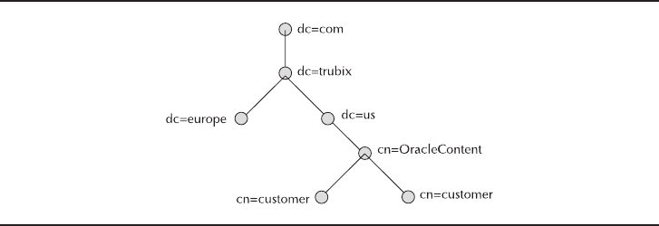
Distinguished Names
A distinguished name (DN) defines where an entry resides in the directory path,
and begins at the lowest entry. The DN for the customer distinguished name is
dn:cn=customer, cn=OracleContext, dc=us, dc=beginner, and dc=com. Relative
distinguished names (RDNs), on the other hand, define the sequences within the
path. An RDN contains an attribute that defines the RDN. An important RDN is
the Oracle Context, which defines the default location for connect identifiers. An
identity management realm, meanwhile, defines a set of identities that share the
same administration policies.
How to Find the Directory Naming Information
With this naming method, a client needs to find the centralized information that is
stored in the LDAP repository to be able to connect to the database server. There are
two ways to find the centralized directory naming information stored on a separate
system:
■The static method, which works via a local ldap.ora file.
■The dynamic method, which works via a domain name server (DNS).
An ldap.ora file is a statically configured file containing the location of the LDAP
server. DNS uses name servers to map names and IP addresses for systems. If the
latter changes, the next time the name is looked for on the domain name server, it
will map to the new IP address.
Chapter 3: Connecting to Oracle 85
FIGURE 3-6. A directory information tree

86 Oracle Database 11g: A Beginner’s Guide
Net Service Alias Entries
Anet service alias entry is another name for a net service name. A net service alias
references the directory location and the name cust in the directory information tree
is a net service alias. Aliases simplify management by using a short alias instead of
having to specify the full path.
The Local Naming Method
The local naming method uses a local configuration file called tnsnames.ora. The
tnsnames.ora file stores net service names and connect descriptors and it resides
on the platform running the database application. It also contains the information
required to find and connect to the Oracle database server. The following definition
defines the address (protocol, host, port number) along with the dedicated server
environment and which service to connect to:
CUST =
(DESCRIPTION =
(ADDRESS_LIST =
(ADDRESS = (PROTOCOL = TCP)(HOST = eclipse)(PORT = 1521))
)
(CONNECT_DATA =
(SERVER = DEDICATED)
(SERVICE_NAME = CUST)
)
)
This is a simple file to configure. The problem is that if you have 1000 users,
you need to make sure the tnsnames.ora file has been updated for all of the client
machines. From a security perspective, it is not ideal to allow clients access to a
server location and the connection information.
Ask the Expert:
Q: Should I be prepared to implement non-TCP/IP-based network
transports with my Database 11ginstallations?
A: Most sites leverage the TCP/IP protocol for network services from Oracle
and other vendors that play a role in getting information from the client to the
database back end. In most of your travels around the Oracle technology, you
too will use the TCP/IP standard almost all the time. Familiarity with other
protocols is wise if and when called upon to administer non-TCP/IP networks.

Chapter 3: Connecting to Oracle 87
The Easy Naming Method
The easy naming method explicitly defines the connect information. The connect
information contains the host, port, service name, and instance name. This allows
someone to connect in a specific way without going through the configuration
effort. The format is
CONNECT username/password@eclipse:1521/customer.us.beginner.com/cust
An advantage of the easy naming method is that it is easy to configure. The user
need only provide minimal information to get a connection. As a result, no other
naming methods need to be configured. This method cannot be used if more
advanced features are required.
The External Naming Method
The external naming method uses net service names that are defined in a non-Oracle
environment. This naming method works well for administrators that want to use
their native naming service and allows them to use native tools and utilities with
which they have experience. The disadvantage of this approach is that Oracle Net
tools cannot be used for these native naming methods. Supported non-Oracle
services include the Network Information Service (NIS) or Cell Directory Services
(CDS). CDS is part of a Distributed Computing Environment (DCE). DCE is an
integrated distributed environment designed to resolve interoperability issues with
heterogeneous environments. DCE is maintained by the Open Systems Foundation
(OSF).
Which Naming Method to Use
The local naming method (tnsnames.ora) has traditionally been the most popular
method. However, there are a number of administration and security issues in
stored local configuration with a tnsnames.ora file. The directory (centralized)
naming method is more scalable and has less administration than the local naming
method. For large systems, the directory method is becoming more popular.
CRITICAL SKILL 3.6
Use Oracle Configuration Files
Remote applications will look for Oracle Net configuration files to determine
how to access the Oracle database server. Configuration files can be found in the
ORACLE_HOME/network/admin directory location. Table 3-5 defines the primary
configuration files.

88 Oracle Database 11g: A Beginner’s Guide
DBAs can use the management tools to modify Oracle Net Services configurations.
However, since the configuration files have a simple syntax, it is easy to modify the
configuration files directly. The following is an example of the listener.ora file:
# LISTENER.ORA Date: 04/25/2009
LISTENER =
(DESCRIPTION_LIST =
(DESCRIPTION =
(ADDRESS_LIST =
(ADDRESS = (PROTOCOL = IPC)(KEY = EXTPROC0))
)
(ADDRESS_LIST =
(ADDRESS = (PROTOCOL = TCP)(HOST = eclipse)(PORT = 1521))
)
)
)
Should a DBA want to modify the files directly, the following syntax rules must
be followed:
Network Configuration
Filename Description
listener.ora The listener.ora file defines how the listeners are
configured on the database server.
sqlnet.ora The sqlnet.ora file resides on the database server and
the local platform. Profile information is stored in the
sqlnet.ora file. This file defines information on service
names, naming methods, external naming information,
Advanced Security parameters, and database access
information. The TNS_ADMIN environmental variable
can override the default location of these files.
tnsnames.ora Resides on the local system and is used with the local
naming method. This defines net service names and
connect descriptor information.
cman.ora The configuration file for the Oracle Connection
Manager. This file resides on the same platform where
the Oracle Connection Manager runs.
ldap.ora The directory usage file is created by the Oracle
Internet Directory Configuration Assistant.
TABLE 3-5. Primary Configuration Files for Oracle Net Services

Chapter 3: Connecting to Oracle 89
■Comments must begin with a pound sign (#). Anything following the pound
sign is treated as a comment.
■Keywords are not case sensitive and cannot contain spaces.
■Spaces are optional around equal (=) signs.
■Values can only contain spaces if they are surrounded by quotes. The
values may be case sensitive depending on the operating system and
protocol.
■A connect descriptor can be no more than 4KB in length.
■All characters must be part of the network set.
■Care must be taken with parentheses when editing. Troubleshooting a
connection problem might be necessary because a simple edit was made
to the file and close or open parenthesis was dropped.
CRITICAL SKILL 3.7
Use Administration Tools
Oracle Net Services contains a number of user interfaces and tools that simplify the
management of the Oracle network, including the following:
■Oracle Enterprise Manager (OEM) / Grid Control
■The OEM console
■Oracle Net Manager
■Oracle Net Configuration Assistant
■Oracle Connection Manager
■Oracle Internet Directory Configuration Assistant
■Command-line utilities
■Oracle Advanced Security
The Oracle Enterprise Manager/Grid Control
Along with database administration, OEM allows configuration of Oracle Net
Services. OEM can be used to perform the following administration features:
■The configuration of listeners
■The configuration of naming definitions such as connect descriptors

The Oracle Net Manager
The Oracle Net Manager allows the configuration of Oracle Net Services and can
be started from the OEM console, by choosing Tools | Service Management | Oracle
Net Manager.
The Oracle Net Manager provides the following administration support:
■Listeners This supports creating and configuring listeners.
■Naming This supports defining simple names. Simple names specify
information for connect descriptors and service location information.
■Naming methods This supports the definition of naming methods.
Some of the functionality in OEM is also available in the Oracle Net Manager.
Table 3-6 shows the overlapping functionality and the differences between the two
tools.
The following can be used to start Oracle Net Manager manually through UNIX:
$ $ORACLE_HOME/bin/netmgr
Oracle Net Manager can also be started manually through Windows by
selecting Start | Programs | Oracle—OraHome11 | Configuration and Migration
Tools | Net Manager.
90 Oracle Database 11g: A Beginner’s Guide
Oracle Enterprise Manager Oracle Net Manager
Local naming (tnsnames.ora) Local naming (tnsnames.ora)
Directory naming Directory naming
Listeners Listeners
Oracle home support for multiple hosts Oracle home support for a single host
Search capability on local and directory
names
Profiles
Export directory entries to tnsnames.ora
file
Changing tracing and logging settings
TABLE 3-6. Common Features and Differences Between OEM and Oracle Net
Manager
Chapter 3: Connecting to Oracle 91
The OEM Console
The Oracle Enterprise Manager Central Console is a web-based interface for
managing the entire enterprise from the console. It offers a lot more functionality
than the standard Oracle Enterprise Manager that comes with a typical database
install. The default ports for running in a nonsecure mode are 7777-7877; default
ports for running in a secure mode are 4443-4533.
You can access the OEM Central Console from the following URLs: http://<oms
hostname>.<domain>.<port>/em and https://<oms hostname>.<domain>.<port>/
em. The OEM Central Console requires the Oracle Management Service unless the
Oracle Management Agent is installed separately.
The OEM Components
The OEM console uses the following components installed with the Oracle
application server:
■The Oracle Management Service This is a web-based application that
runs on the Oracle application server. It provides the user interface for the
OEM console, and interfaces with the management agents to process and
monitor information.
■The Oracle Management Agent This monitors information from sites that
need to be managed and that are loaded into the management service.
■The Oracle Management Repository This contains all the information
managed by the Oracle Enterprise Manager.
Before installing the Complete Enterprise Manager, make sure to read the
requirements for the complete installation that includes the Oracle Application
Server 11g, Web Cache, and the Management Service application as well as
verifying additional licensing requirements.
The Oracle Net Configuration Assistant
The Oracle Net Configuration Assistant is used during installation to configure the
basic network components. The Oracle Net Configuration Assistant can also be run
standalone to modify the same values configured during installation. Configurable
components include the following:
■Naming methods
■Net service names (tnsnames.ora)
■Listener names and protocol addresses
■Directory server usage
92 Oracle Database 11g: A Beginner’s Guide
The following can be used to start the Oracle Net Configuration Assistant
manually through UNIX:
$ $ORACLE_HOME/bin/netca
The Oracle Net Configuration Assistant can also be started manually through
Windows by selecting Start | Programs | Oracle—OraHome11 | Configuration and
Migration Tools | Net Configuration Assistant.
The Oracle Internet Directory
Configuration Assistant
The Oracle Internet Directory Configuration Assistant can be used to configure
the Oracle Internet Directory. The directory configuration file ldap.ora can be
configured with the Oracle Internet Directory Configuration Assistant or the Oracle
Net Configuration Assistant. The ldap.ora file can reside in different locations
depending on which tool created the ldap.ora file:
■If created by the OID Configuration Assistant, the ldap.ora file is stored in
the ORACLE_HOME/ldap/admin directory.
■If created by the Oracle Net Configuration Assistant, the ldap.ora file is
stored in the ORACLE_HOME/network/admin directory.
■The ldap.ora file location can be manually specified with the
LDAP_ADMIN or TNS_ADMIN environmental variables.
Command-Line Utilities
The Listener Control utility can be used to start and stop listeners, check their status,
and perform tracing and other management operations. The syntax is
lsnrctl command [listener_name]
Listener commands can also be executed from within the Listener Control utility.
The listener name is the one defined in the listener.ora file, but a default listener
named LISTENER can be used instead. If LISTENER is used, a listener name does not
need to be specified.
The following shows how to stop the listener. Here, executing the lsnrctl
command generates an LSNRCTL prompt:
$ lsnrctl
LSNRCTL> stop
Connecting to (DESCRIPTION=(ADDRESS=(PROTOCOL=IPC)(KEY=EXTPROC0)))
The command completed successfully
Chapter 3: Connecting to Oracle 93
The next example shows a sample of the type of information displayed when
starting the listener:
LSNRCTL> start
starting tnslsnr: please wait...
TNSLSNR for 32-bit Windows: Version 11.1.0.6.0 -
System parameter file is C:\oracle\ora11\network\admin\listener.ora
Log messages written to C:\oracle\ora11\network\log\listener.log
Listening on: (DESCRIPTION=(ADDRESS=(PROTOCOL=tcp)(HOST=eclipse)
(PORT=1521)))
Connecting to (DESCRIPTION=(ADDRESS=(PROTOCOL=IPC)(KEY=EXTPROC0)))
STATUS of the LISTENER
------------------------
Alias LISTENER
Version TNSLSNR for 32-bit Windows:Version 11.1.0.6.0
Start Date 03-FEB-2009 21:26:56
Uptime 0 days 0 hr. 0 min. 2 sec
Trace Level off
Security OFF
SNMP OFF
Listener Parameter File C:\oracle\ora11\network\admin\listener.ora
Listener Log File C:\oracle\ora11\network\log\listener.log
Listening Endpoints Summary...
(DESCRIPTION=(ADDRESS=(PROTOCOL=tcp)(HOST=eclipse)(PORT=1521)))
Services Summary...
Service "cust" has 1 instance(s).
Instance "cust", status UNKNOWN, has 1 handler(s) for this service...
The command completed successfully
The status command displays detailed information on the status of the listener.
Information includes the start time of the listener, the location of log and
configuration files, and so on.
LSNRCTL> status
The services command lists dispatchers in a shared server environment and
dedicated servers in a dedicated server environment:
LSNRCTL> services
Here is a list of listener commands:
■change_password
■exit
■help
94 Oracle Database 11g: A Beginner’s Guide
■quit
■reload
■save_config
■services
■set
■show
■spawn
■start
■status
■stop
■trace
■version
The set command can be used to modify different parameter values for a
listener. The set command, by itself, will display the parameter values that can be
modified:
LSNRCTL> set
password rawmode
displaymode trc_file
trc_directory trc_level
log_file log_directory
log_status current_listener
inbound_connect_timeout startup_waittime
save_config_on_stop
The Oracle Advanced Security Option
The Oracle Advanced Security option supports data encryption, enhanced
authentication, integrity checking, single sign-on, and the Distributed Computing
Environment (DCE). The Oracle Net Manager is used to configure Oracle Advanced
Security options.
Dispatchers
The DISPATCHERS parameter can be set to define how dispatchers will work with
the shared server architecture. Dispatchers must be defined to work with different
protocols, as shown in the following:

DISPATCHERS="(PROTOCOL=tcp)(DISPATCHERS=6)(CONNECTIONS=1000)"
DISPATCHERS="(PROTOCOL=tcps)(DISPATCHERS=6)(CONNECTIONS=1000)"
Connection pooling can also be defined as shown next:
DISPATCHERS="(PROTOCOL=tcp)(DISPATCHERS=6)(POOL=on) (TICK=1)
(CONNECTIONS=1000)(SESSIONS=5000)"
DISPATCHERS="(PROTOCOL=tcps)(DISPATCHERS=6)(POOL=on) (TICK=1)
(CONNECTIONS=1000)(SESSIONS=5000)"
NOTE
TICK is the amount of time for a message to be sent
from the server to the client; for fast networks,
recommended value is 1, but default is 15.
Project 3-1 Test a Connection
The following project will walk you through the steps of testing a connection to an
Oracle database server.
Step by Step
The first step is to test the network connectivity between the remote system and the
Oracle database server. The ping command will verify network access. If ping is
successful, the remote system can resolve the name of the host server name. The
host server name should be defined in the hosts file for the operating system.
The hosts file in UNIX is in the /etc directory; the hosts file in Windows is in
the\winnt directory. The following is an example hosts file entry:
eclipse customer.us.beginner.com
1. Ping the host server name:
ping eclipse
2. If the ping is not successful using the host server name then use the IP
address to verify that the remote system can access the host server through
the network:
ping 122.23.20.24
3. Start the listener. If the listener does not start, check the listener.ora file for
the proper entries. The listener.ora file can be found in the ORACLE_
HOME/ network/ admin directory:
lsnrctl start listener_name
Chapter 3: Connecting to Oracle 95
Test a Connection
Project 3-1
(continued)
96 Oracle Database 11g: A Beginner’s Guide
4. Verify that the service registration has been completed and that the listener
is ready to handle requests:
lsnrctl services listener_name
5. Service registration is impacted by a number of initialization parameters.
They include SERVICE_NAMES (cust.us.acme.com) and INSTANCE_NAME
(cust). The SERVICE_NAMES parameter defaults to the global database
name. The global database name is made up of the DB_NAME and
DB_DOMAIN parameters.
6. The remote system now needs to be configured. The Oracle Net Configuration
Assistant can be used for configuration. Start the Oracle Net Configuration
Assistant.
7. Of the four configuration options on the Welcome page, select the Local
Net Service Name configuration.
8. Select Add and then click Next.
9. Enter the service name (cust) and click Next.
10. Select the protocol (TCP/IP) and click Next.
11. Select the host name and port number and then click Next.
12. Select Yes, perform a test, and then click Next. If the test fails, check
whether the instance and listener are running. If they are, check the
protocol information, and if it still fails, double-check the username and
password used for the test.
13. Enter the net service name and click Next.
14. Select No when asked if you would like to configure another net service
name, and then click Next.
15. At the Congratulations screen, select Next, and then click Finish.
16. The local naming method will create a connect descriptor in the
tnsnames.ora file similar to this one:
cust=
(DESCRIPTION =
(ADDRESS=(PROTOCOL=tcp)(HOST=eclipse)(PORT=1521))
(CONNECT_DATA=
(SERVICE_NAME=customer.us.beginner.com)))
17. For the final test, log into Oracle and see if you can connect using the new
net service name:
SQL> CONNECT username/password@cust

18. The tnsping utility can also be used to test a service. If unsuccessful, it will
return the error that occurred. tnsping requires the net service name found
in the tnsnames.ora file. The count parameter defines how many attempts
are made to reach the server.
tnsping net_service_name [count]
19. If unable to connect, the trcroute utility can be used to get more detailed
error information. The trcroute utility tracks the TNS address of every node
it accesses in the path.
trcroute net_service_name
Project Summary
This project walked you through the steps a DBA will go through to test a simple
connection for an Oracle database server using the local naming method.
CRITICAL SKILL 3.8
Use Profiles
A profile contains a set of parameters that define Oracle Net options on the remote
or database server. Profiles are stored in the sqlnet.ora file and can be used to
■Route connections to specific processes
■Control access through protocol-specific parameters
■Prioritize naming methods
■Control logging and tracing features
■Configure for external naming
■Define how the client domain should append to unqualified names
During installation, the priority order for the naming methods will be defined.
If the first naming method cannot resolve the connect identifier, the next naming
method will be checked. The results will then be stored in the sqlnet.ora file, as
shown in the following example:
NAMES.DIRECTORY_PATH=(ezconnect, tnsnames)
After installation, Oracle Net Manager can be used to modify the sqlnet.ora
configuration file.
The sqlnet.ora file can be used to grant or deny access to the Oracle database
server. Table 3-7 displays sqlnet.ora parameters that control access.
Chapter 3: Connecting to Oracle 97
Test a Connection
Project 3-1

The Oracle Net Manager is used to define database access control. To define
database access control, perform the following steps using Oracle Net Manager:
1. After starting Net Manager, select Local | Profile.
2. Choose General.
3. Select Access Rights.
4. Choose Check TCP/IP Client Access Rights.
5. In the Clients Excluded From Access and the Clients Allowed To Access
fields, access control can now be defined.
CRITICAL SKILL 3.9
Network in a Multi-tiered Environment
Although the Oracle Database 11ghas additional features that simplify database
administration, the environment the database server runs in is becoming more
complex. The following areas continue to increase the complexity of Oracle
networking environments:
■Oracle Database 11g–supporting HTTP, FTP, and WebDAV protocols are
changing how data is used and accessed.
■The OEM Central Console is changing how Oracle DBAs perform
administration across multiple databases.
98 Oracle Database 11g: A Beginner’s Guide
sqlnet.ora Parameter Name Description
TCP.VALIDNODE_CHECKING Determines where to control access to
the database. If this parameter is set, the
following parameters will be used to
define the access.
TCP.EXCLUDED_NODES Defines which systems are denied access
to the database.
TCP.INVITED_NODES Defines which systems are granted access
to the database.
TABLE 3-7. sqlnet.ora Parameters

■Multi-tiered architectures are placing increasing demands on network
performance and security.
Traditionally, most Oracle networks have been set with the local naming
method. In the future, more Oracle networking environments will work with
multi-tiered architectures, the Oracle OEM Central Console, encryption, and the
directory naming method. Companies are going to need people with skills to
manage these complex environments. This chapter introduced you to the main
components of Oracle Net Services. To begin working with Oracle Net Services,
you may want to look at the following areas in the following order in terms of
developing your skills:
■Strengthen your understanding of the Oracle Net Services architecture.
■Obtain a solid understanding of configuring dedicated and shared server
environments.
■Become comfortable working with listeners and the local naming method.
■Get comfortable working with the directory naming method.
■Be able to work with the OEM Central Console and the environment
required to support it.
This list should be able to keep you busy for a few days. After that, developing
skill in tuning and troubleshooting the Oracle Net Services environment will be
important. Not included in these discussions, but also very important, is the ability
to troubleshoot and tune the network from an operating system perspective.
CRITICAL SKILL 3.10
Install the Oracle 11gClient Software
Before moving on from Oracle’s networking offering, you are going to get a quick
look at the Oracle 11gclient software. Classically, this piece of the puzzle goes on
a desktop computer, but in a 3-tier client-server model, it is often put on the middle
tier. This architecture makes it accessible to multiple client computers and often
eases management and maintenance tasks for the administrator. The journey begins
at technet.oracle.com in the download area of the site, as shown in the following
illustration.
Chapter 3: Connecting to Oracle 99
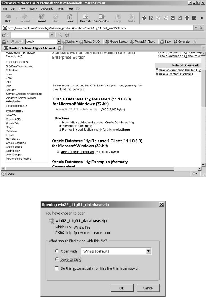
100 Oracle Database 11g: A Beginner’s Guide
Click on the name of the client software and choose the Save to Disk option as
your web browser prepares to download the file for you, as shown next.
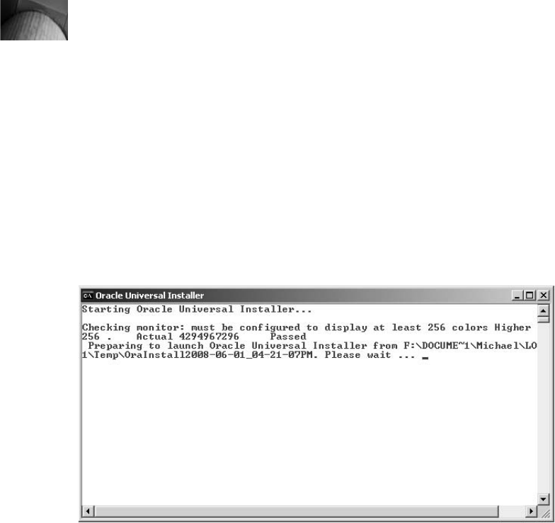
Chapter 3: Connecting to Oracle 101
NOTE
You will need a valid username and password to
download the Oracle software discussed in the next
few sections. The Oracle software contains several
components that can be installed, and along with
these components, several more options are
available as part of the downloaded software. The
material we discuss here is an overview of a simple
client install; a mere tip-of-the-iceberg so to speak.
With the file downloaded, using WinZIP or the Windows compressed folders
feature, uncompress the file in preparation for the client install. Proceed to the
location where the media was unzipped and double-click the setup.exe program.
A DOS window appears as soon as the setup is invoked, as shown in the following
illustration.
As the first screen appears, click the Advanced Installation radio button as
shown in the following illustration, and then click Next. When asked for an
Installation type on the next screen, choose Custom, and then click Next. On the
Installation location screen, you can overwrite the suggested Oracle Base or leave
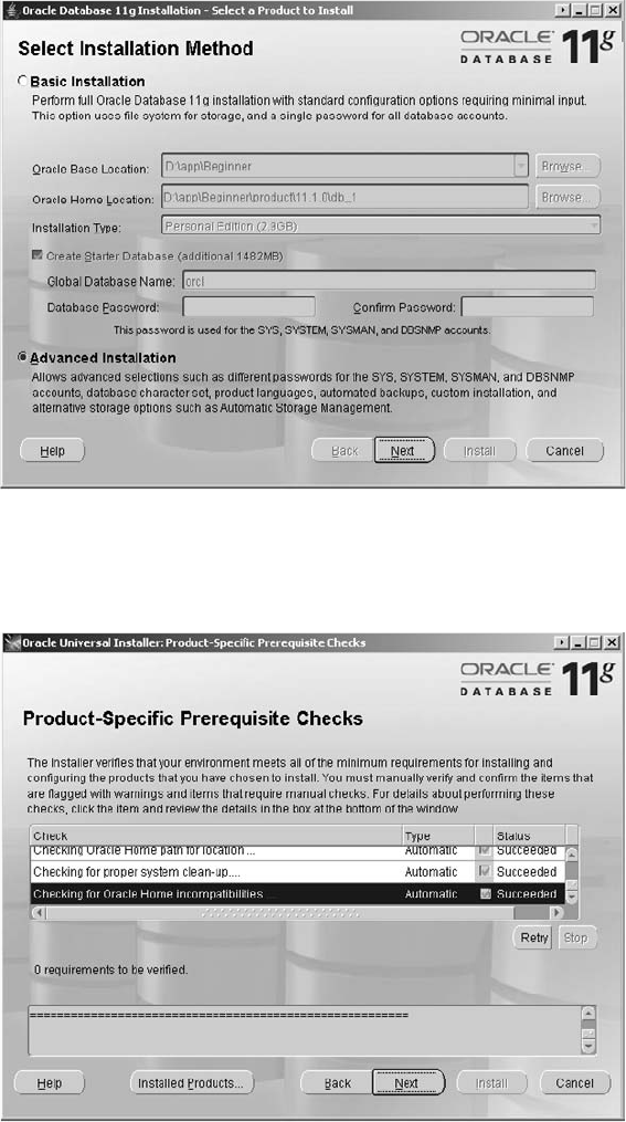
102 Oracle Database 11g: A Beginner’s Guide
the default as suggested by the installer. Once you’re happy with the Oracle Base
location, click Next.
The next screen to appear, as shown in the following illustration, does a quick
series of Product-Specific Prerequisite Checks. This ensures that the environment
where the 11gclient is to be installed can support the software. Once the installer
completes its checks, click Next to continue.
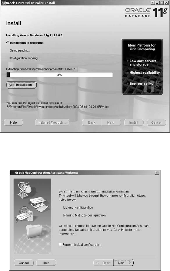
Chapter 3: Connecting to Oracle 103
You will then be positioned on the Available Product Components screen. This
tree lists the products that can be installed from the download. All of the products in
the tree should be de-selected, except for Oracle Net Services (including the Oracle
Net Listener and Oracle Connection Manager). Click Next to display the installation
summary screen before the process commences. A progress screen appears with
messages about what is being installed and a progress indicator as shown here.
Once the installer completes its work, it will bring up a Configuration Assistant
notification screen followed by starting the Oracle Net Configuration Assistant, as
shown in the following illustration.
Proceed as follows with the next few screens and the questions they ask,
clicking Next to move from one screen to the next:
■When a listener name is suggested, accept the default LISTENER.
■In the Available Protocols/Selected Protocols, ensure TCP-IP is in the
Selected Protocols list.
■Allow it to use the standard port 1521 for the listener.
■When asked about configuring another listener, say No.
■When asked if you want to configure additional naming methods, answer No.
You are then done with the network configuration. You will be returned to the
setup completion screen, at which point it is safe to shut down the installer.
þChapter 3 Mastery Check
1. The __________ background process registers the service information to the
listener.
2. True or false: The LOCAL_LISTENER parameter should be set to work with
port 1521.
3. The _______________________ is used during installation to configure
Oracle Net Services.
4. The _____________ file can be used to define, grant, or deny access to the
Oracle database server.
5. The ________________ utility can also be used to test a service.
6. A __________________ contains a set of parameters that define Oracle Net
options on the remote or database server.
7. The ldap.ora file location can be manually specified with the ____________
or TNS_ADMIN environmental variables.
8. True or false: The easy naming method is a valid naming method.
9. The Oracle LDAP directory is called the _______________.
10. True or false: The Oracle Management Service is a repository of information
generated by the Management Agent.
104 Oracle Database 11g: A Beginner’s Guide

Chapter
4
SQL: Structured Query
Language
CRITICAL SKILLS
4.1 Learn the SQL Statement Components
4.2 Use Basic Insert and Select Statements
4.3 Use Simple Where Clauses
4.4 Use Basic Update and Delete
Statements
4.5 Order Data
4.6 Employ Functions: String, Numeric,
Aggregate (No Grouping)
4.7 Use Dates and Data Functions
(Formatting and Chronological)
4.8 Employ Joins (ANSI vs. Oracle): Inner,
Outer, Self
4.9 Learn the Group By and Having
Clauses
4.10 Learn Subqueries: Simple and
Correlated Comparison with Joins
4.11 Use Set Operators: Union, Intersect,
Minus
4.12 Use Views
4.13 Learn Sequences: Just Simple Stuff
4.14 Employ Constraints: Linkage to Entity
Models, Types, Deferred, Enforced,
Gathering Exceptions
4.15 Format Your Output with SQL*Plus

106 Oracle Database 11g: A Beginner’s Guide
QL is the fundamental access tool of Oracle Database; in fact, it is
the fundamental access tool of all relational databases. SQL is used
to build database objects and it is also used to query and manipulate
both these objects and the data they may contain. You cannot insert
a row of data into an Oracle database unless you have first issued
some basic SQL statements to create the underlying tables. While Oracle provides
SQL*Plus, a SQL tool that enables you to interact with the database, there are also
many GUI tools that can be used, which can then issue SQL statements on your
behalf behind the scenes. However you decide to access the database, you will
need to understand the fundamentals of SQL. SQL will become your connection to
your data and it is an important starting point for all Oracle professionals to master.
CRITICAL SKILL 4.1
Learn the SQL Statement Components
Before you learn the many SQL commands that you will use frequently, you should
take a look at the two different categories that SQL statements are classified into.
They are DDL, or data definition language, and DML, or data manipulation
language. The majority of this chapter will deal with the latter.
DDL
DDL is the set of SQL statements that define or delete database objects such as
tables or views. For the purposes of this chapter, you will concentrate on dealing
with tables. Examples of DDL are any SQL statements that begin with create, alter,
and drop: all of these commands would act upon a database object like a table,
view, or trigger, among many others. Table 4-1 is a sample list of some DDL statements.
It does not completely represent the many varied statements that all have a unique
purpose and value.
The following SQL statements are examples of DDL create and drop statements
in action:
SQL> create table b
2 (colb char(1));
SQL> drop table b;
Table dropped.
SQL> create table state
2 (state_cd char(2) not null,
3 state_name varchar2(30));
Table created.
After you have created your table, you should confirm that it was created as you
expected. To display a description of a table, the describe command is used. Our
S

Chapter 4: SQL: Structured Query Language 107
experience suggests that you will find it very useful to be able to describe tables
within the database after you create them or any time you need to know the exact
nature of the table. You should take a closer look at the state table that you created
in the previous example:
SQL> desc state;
Name Null? Type
----------------------------------------- -------- -------------------
STATE_CD NOT NULL CHAR(2)
STATE_NAME VARCHAR2(30)
DML
DML is any SQL statement that begins with select, insert, update, or delete. The
remainder of this chapter will deal primarily with DML. Every DML SQL statement
consists of a few basic components. The following three items form the basic
foundation of most DML statements:
■Each DML statement begins with either a select, insert, update, or delete
command:
■select is used when you want to retrieve data from an Oracle database.
It is the most common SQL statement you will see.
SQL Command Purpose
create table Creates a table
create index Creates an index
alter table Adds a column, redefines an existing column, changes
storage allocation
drop table Drops a table
grant Grants privileges or roles to a user or another role
truncate Removes all rows from a table
revoke Removes privileges from a user or a role
analyze Gathers performance statistics on database objects for use by
the cost-based optimizer (although we recommend that you
use the Oracle built-in package named DBMS_STATS for the
most robust statistic collection)
TABLE 4-1. Common Formats for Date Type Data

■insert is used when you want to add rows into an Oracle table.
■update commands are used to change one or more records in a table.
■delete commands are issued when you want to remove one or more
records from a table.
■All DML commands require reference to an object that will be
manipulated. More often than not, the object being referenced is a table.
■A conditional statement can be added to any select, update, or delete
command. Absence of a conditional statement means that the command
will be performed against every record in the object. A conditional
statement is used when the DML command is intended to only act upon a
group of records that meet a specific condition. The where clause will be
discussed a little later in this chapter.
More optional DML statements will be described later in this chapter. For now,
you should concentrate on understanding the fundamental structure of each DML
statement starting with the insert and select statements.
CRITICAL SKILL 4.2
Use Basic Insert and Select Statements
Getting data into and out of a database are two of the most important features of a
database. Oracle provides two basic features that help you do just that. To get data
into the database, use the insert command; to get it back out, use the select command.
You must master these commands because they form the basics for most data access
to your Oracle database. In this section you’ll first learn how to get data into your
database and then how to get data out.
Insert
Using the state table created in the DDL example, the following is an illustration of
using the insert statement in its simplest form:
SQL> insert into state values ('AZ','Arizona');
1 row created.
Each time you execute an insert command, you receive the message “1 row
created.” Thus, you get immediate feedback that you are populating the given table
with data. When you load data into a table, you may also specify the column to
load it into. This ensures that there is no mistaking where you want the data to be
placed. In the next example, the columns are specified after the insert command:
108 Oracle Database 11g: A Beginner’s Guide
SQL> insert into state (state_cd, state_name)
2> values ('NJ','New Jersey');
1 row created.
SQL> insert into state (state_cd, state_name)
2> values ('CA','California');
1 row created.
SQL> insert into state (state_cd, state_name)
2> values ('TX','Texas');
1 row created.
SQL> insert into state (state_cd, state_name)
2> values ('FL','Florida');
1 row created.
SQL> insert into state (state_cd, state_name)
2> values ('ME','Maine');
1 row created.
Select
As mentioned earlier, the select statement is used to retrieve data from the database.
This is the commonest SQL statement you will use. The five basic parts of the SQL
statement are as follows:
■First is the keyword select, followed by what you want to retrieve from the
database. The names of the columns to be retrieved are listed here. The
select clause is mandatory.
■The word from is the next part of the SQL statement. Reference to the
object that the data is being retrieved from is made here. This is usually
a table name. The from clause is mandatory.
■As mentioned before, a conditional statement is optional for select statements.
The word where, followed by the conditions, would be the next part of the
SQL statement. (See Critical Skill 4.3 for more details on the where clause.)
■A group by clause is another optional component of the select statement.
This topic will be covered in more detail in Critical Skill 4.9, once we have
had the opportunity to discuss functions.
■The final component of a select statement is the order by clause. This will
also be discussed in more detail later on in this chapter. This is an optional
component, which will sort the results of the query before they are presented
back to you.
Chapter 4: SQL: Structured Query Language 109
110 Oracle Database 11g: A Beginner’s Guide
You should now issue your first select statement against the state table you just
populated in the insert statement examples:
SQL> select *
2 from state;
ST STATE_NAME
-- ------------------------------
AZ Arizona
NJ New Jersey
CA California
TX Texas
FL Florida
MN Maine
6 rows selected.
Notice the use of the asterisk in the select statement. The asterisk means “retrieve
data from all the columns” of the state table. (select * from emp,dept retrieves all
columns from the table.)
Rather than using the asterisk as you did in the previous example, you can specify
one or more columns after the select command in a comma-separated list. You
should rewrite the previous query and only select the state_name column this time:
SQL> select state_name
2 from state;
STATE_NAME
------------------------------
Arizona
New Jersey
California
Texas
Florida
Maine
6 rows selected.
The semicolons in the two SQL examples force the immediate execution of the
SQL statement within SQL*Plus. There are two ways to signify you have finished
and that the SQL statement can be executed in SQL*Plus:
■The semicolon at the end of a line
■The slash on a separate line
Until SQL*Plus encounters either of these characters, it assumes you need an
additional line. The following example highlights this point. Notice the use of the
slash and semicolon.

Chapter 4: SQL: Structured Query Language 111
SQL> select *
2 from a;
SQL> select *
2 from a
3 /
The absence of the semicolon in the second example resulted in a new line. In
these cases, the semicolon and slash on a separate line would force the execution of
the statement.
CRITICAL SKILL 4.3
Use Simple Where Clauses
Up to now, you have seen how the select command can be used to retrieve records
from a table. However, our basic examples have all retrieved every record from the
table. If you want to see only certain rows, you must add a where clause.
Since the previous examples returned every record in the table, you created a
simple table with a few rows in it for illustration purposes. Had you chosen to
illustrate the select command against the large sample tables provided by Oracle,
you would have returned thousands of rows—far too many for listing in this chapter.
Now that you are introducing the where clause, you will be able to control the
output. As a result, the remaining examples in this chapter will now use the
customers, products, sales, and costs tables that are part of the Oracle sample
database; they can be found in the SH schema that is included when you install the
sample databases with a default installation. Let’s describe each of these tables in
the SH schema. This may be done in SQL*Plus or in a GUI that provides this type
of table interface:
SQL> desc customers;
Name Null? Type
----------------------------------------- -------- -------------------
CUST_ID NOT NULL NUMBER
CUST_FIRST_NAME NOT NULL VARCHAR2(20)
CUST_LAST_NAME NOT NULL VARCHAR2(40)
CUST_GENDER NOT NULL CHAR(1)
CUST_YEAR_OF_BIRTH NOT NULL NUMBER(4)
CUST_MARITAL_STATUS VARCHAR2(20)
CUST_STREET_ADDRESS NOT NULL VARCHAR2(40)
CUST_POSTAL_CODE NOT NULL VARCHAR2(10)
CUST_CITY NOT NULL VARCHAR2(30)
CUST_CITY_ID NOT NULL NUMBER
CUST_STATE_PROVINCE NOT NULL VARCHAR2(40)
CUST_STATE_PROVINCE_ID NOT NULL NUMBER
COUNTRY_ID NOT NULL NUMBER
CUST_MAIN_PHONE_NUMBER NOT NULL VARCHAR2(25)
CUST_INCOME_LEVEL VARCHAR2(30)
CUST_CREDIT_LIMIT NUMBER
CUST_EMAIL VARCHAR2(30)
CUST_TOTAL NOT NULL VARCHAR2(14)
CUST_TOTAL_ID NOT NULL NUMBER
CUST_SRC_ID NUMBER
CUST_EFF_FROM DATE
CUST_EFF_TO DATE
CUST_VALID VARCHAR2(1)
SQL> desc products;
Name Null? Type
----------------------------------------- -------- -------------------
PROD_ID NOT NULL NUMBER(6)
PROD_NAME NOT NULL VARCHAR2(50)
PROD_DESC NOT NULL VARCHAR2(4000)
PROD_SUBCATEGORY NOT NULL VARCHAR2(50)
PROD_SUBCATEGORY_ID NOT NULL NUMBER
PROD_SUBCATEGORY_DESC NOT NULL VARCHAR2(2000)
PROD_CATEGORY NOT NULL VARCHAR2(50)
PROD_CATEGORY_ID NOT NULL NUMBER
PROD_CATEGORY_DESC NOT NULL VARCHAR2(2000)
PROD_WEIGHT_CLASS NOT NULL NUMBER(3)
PROD_UNIT_OF_MEASURE VARCHAR2(20)
PROD_PACK_SIZE NOT NULL VARCHAR2(30)
SUPPLIER_ID NOT NULL NUMBER(6)
PROD_STATUS NOT NULL VARCHAR2(20)
PROD_LIST_PRICE NOT NULL NUMBER(8,2)
PROD_MIN_PRICE NOT NULL NUMBER(8,2)
PROD_TOTAL NOT NULL VARCHAR2(13)
PROD_TOTAL_ID NOT NULL NUMBER
PROD_SRC_ID NUMBER
PROD_EFF_FROM DATE
PROD_EFF_TO DATE
PROD_VALID VARCHAR2(1)
SQL> desc sales;
Name Null? Type
----------------------------------------- -------- -------------------
PROD_ID NOT NULL NUMBER
CUST_ID NOT NULL NUMBER
TIME_ID NOT NULL DATE
CHANNEL_ID NOT NULL NUMBER
PROMO_ID NOT NULL NUMBER
QUANTITY_SOLD NOT NULL NUMBER(10,2)
AMOUNT_SOLD NOT NULL NUMBER(10,2)
112 Oracle Database 11g: A Beginner’s Guide
SQL> desc costs;
Name Null? Type
----------------------------------------- -------- -------------------
PROD_ID NOT NULL NUMBER
TIME_ID NOT NULL DATE
PROMO_ID NOT NULL NUMBER
CHANNEL_ID NOT NULL NUMBER
UNIT_COST NOT NULL NUMBER(10,2)
UNIT_PRICE NOT NULL NUMBER(10,2)
SQL> desc promotions
Name Null? Type
------------------------------------- -------- -----------------------
PROMO_ID NOT NULL NUMBER(6)
PROMO_NAME NOT NULL VARCHAR2(30)
PROMO_SUBCATEGORY NOT NULL VARCHAR2(30)
PROMO_SUBCATEGORY_ID NOT NULL NUMBER
PROMO_CATEGORY NOT NULL VARCHAR2(30)
PROMO_CATEGORY_ID NOT NULL NUMBER
PROMO_COST NOT NULL NUMBER(10,2)
PROMO_BEGIN_DATE NOT NULL DATE
PROMO_END_DATE NOT NULL DATE
PROMO_TOTAL NOT NULL VARCHAR2(15)
PROMO_TOTAL_ID NOT NULL NUMBER
The PRODUCTS table contains more than 70 products for sale. The following
select statement will retrieve only one record for product ID (prod_id) 117, which
is the use of the simplest of where clauses. In this case, you will perform an exact
query to find product ID number 117, which is the product ID for a pack of CD-Rs:
SQL> select prod_id, prod_name, prod_category, prod_list_price PRC
2 from products
3 where prod_id = 117;
PROD_ID PROD_NAME PROD_CATEGORY PRC
---------- ---------------------------------- ---------------- ------
117 CD-R, Profess. Grade, Pack of 10 Software/Other 8.99
A Where Clause with and/or
A where clause instructs Oracle to search the data in a table and then return only
those rows that meet the criteria that you have defined. In the preceding example,
you searched the products table for one specific record with a product ID equal to
117. This was accomplished with where prod_id = 117;.
You will often be interested in retrieving rows that meet multiple criteria—for
example, if you want to retrieve a list of customers from Utah who also have a
Chapter 4: SQL: Structured Query Language 113

credit limit greater than $10,000. The SQL statement would produce the following
output:
SQL> select cust_id, cust_state_province, cust_credit_limit
2 from customers
3 where cust_state_province = 'UT'
4 and cust_credit_limit > 10000;
CUST_ID CUST_STATE_PROVINCE CUST_CREDIT_LIMIT
---------- ---------------------------------------- -----------------
50601 UT 11000
24830 UT 15000
28983 UT 15000
100267 UT 11000
100207 UT 11000
103007 UT 15000
6 rows selected.
In the previous example, you retrieved records that met all the criteria. You may
be interested in retrieving records that meet one criterion or another. For example,
if you wanted to find all the product IDs in the products table that are either in the
Hardware product category or have a weight class of 4, you would generate the
following SQL statement and output:
SQL> select prod_id, prod_category, prod_weight_class WGT
2 from products
3 where prod_category = 'Hardware'
4 or prod_weight_class = 4;
PROD_ID PROD_CATEGORY WGT
---------- -------------------------------------------------- ---------
15 Hardware 1
18 Hardware 1
139 Electronics 4
114 Oracle Database 11g: A Beginner’s Guide
Ask the Expert
Q: Why is hardware in quotes in the sample statement?
A: When a character column is used in a where clause, it is necessary to use
the single quotes around the value to be compared.
The and condition and the or condition are known as logical operators. They are
used to tell the query how the multiple criteria affect each other. Compound conditions
connected by the and keyword all have to evaluate to true for records to be retrieved.
Records are returned by compound conditions connected by the or keyword when
either one of the conditions is true. If you mix your and and or conditions, you must
carefully evaluate how the these two types will interact.
The Where Clause with NOT
The ability also exists within Oracle to retrieve records with negative criteria. The
“not equals” operator is != or may also use <>. For example, you might want to see
all the products that are not in weight class 1. The following query and its output
illustrate this example:
SQL> select prod_id, prod_category, prod_weight_class WGT
2 from products
3 where prod_weight_class != 1;
PROD_ID PROD_CATEGORY WGT
---------- -------------------------------------------------- ---------
139 Electronics 4
The Where Clause with a Range Search
Oracle also supports range searches so you can query for records that are between
two values. If you want to find all male customers in Connecticut who were born
between 1936 and 1939, you would write a query with three conditions joined by
the and keyword (all three need to evaluate to true), and one of the conditions
would use the range search between keyword. The following example illustrates
the query and resulting output:
SQL> select cust_id, cust_gender, cust_year_of_birth
2 from customers
3 where cust_state_province = 'CT'
4 and cust_gender = 'M'
5 and cust_year_of_birth between 1936 and 1939;
CUST_ID C CUST_YEAR_OF_BIRTH
---------- - ------------------
20058 M 1937
17139 M 1936
1218 M 1938
3985 M 1939
Chapter 4: SQL: Structured Query Language 115
116 Oracle Database 11g: A Beginner’s Guide
The Where Clause with a Search List
Oracle also supports searching for records that meet criteria within a list. If you
wanted to find all customers in Utah and Connecticut with a credit limit of $15,000,
this can be done with a search list. The following query represents a search list
condition:
SQL> select cust_id, cust_state_province, cust_credit_limit
2 from customers
3 where cust_credit_limit = 15000
4 and cust_state_province in ('UT','CT');
CUST_ID CUST_STATE_PROVINCE CUST_CREDIT_LIMIT
---------- ---------------------------------------- -----------------
24830 UT 15000
28983 UT 15000
101798 CT 15000
103171 CT 15000
102579 CT 15000
102238 CT 15000
101515 CT 15000
103007 UT 15000
104381 CT 15000
9 rows selected.
The Where Clause with a Pattern Search
The like command exists within Oracle to search for records that match a pattern.
The wildcard operator for pattern searches is the % sign. To search for all customers
whose last name begins with the letter Q, the following query would produce these
results:
SQL> select cust_last_name, cust_credit_limit
2 from customers
3 where cust_last_name like 'Q%';
CUST_LAST_NAME CUST_CREDIT_LIMIT
---------------------------------------- -----------------
Quinlan 9000
Quinn 11000

Chapter 4: SQL: Structured Query Language 117
You could also ask Oracle to retrieve customers whose last names contain “inl”
by using the wildcard at the beginning and end of the pattern search. The query and
output would resemble the following:
SQL> select cust_last_name
2 from customers
3 where cust_last_name like '%inl%';
CUST_LAST_NAME
----------------------------------------
Quinlan
The Where Clause: Common Operators
As you can see from the preceding examples, Oracle has a very powerful set of
operators when it comes to restricting the rows retrieved. Table 4-2 is a partial list
of operators you can use in the where clause.
Ask the Expert
Q: Are character searches case-sensitive?
A: Yes. Character columns can contain upper- or lowercase alphas. If
you searched the CUSTOMERS table for all instances of “INL” in the last
names, you would not have retrieved any records.
Q: The percent (%) sign appears to be a multicharacter wildcard.
Is there a single character wildcard available for pattern searches?
A: Yes. The underscore (_) symbol serves as the single character
wildcard.

118 Oracle Database 11g: A Beginner’s Guide
CRITICAL SKILL 4.4
Use Basic Update and Delete Statements
While select will likely be the command you use the most; you’ll use the update
and delete commands regularly, too. As you will see in Chapter 5, your programs
Operator Purpose Example
= Tests for equality. select * from customers where
cust_state_province = 'UT';
!= Tests for inequality. select * from customers where
cust_state_province != 'UT';
^= Same as !=. select * from customers where
cust_state_province ^= 'UT';
<> Same as !=. select * from customers where
cust_state_province <> 'UT';
< Less than. select * from sales where
amount_sold < 100;
> Greater than. select * from sales where
amount_sold > 100;
<= Less than or equal to. select * from sales where
amount_sold <= 500;
>= Greater than or equal to. select * from sales where
amount_sold >= 600;
In Equal to any member in
parentheses.
select * from customers where
cust_state_ province is in
('UT','CA','TX');
not in Not equal to any member in
parentheses.
select * from customers where
cust_state_ province is not in
('UT','CA','TX');
between A and B Greater than or equal to A and
less than or equal to B.
select * from sales where
amount_sold is between 100
and 500;
not between A and B Not greater than or equal to A,
and not less than or equal to B.
select * from sales where
amount_sold is not between
100 and 500;
like '%tin%' Contains given text (for
example, 'tin').
select * from customer where
cust_last_name is like '%tin%';
TABLE 4-2. Common Comparison Operators
will have a mixture of DML statements. In this section, you’ll take a closer look at
the update and delete commands.
Update
It is often necessary to change data already stored within a table. This is done using
the update command. There are three parts to this command:
1. The word update followed by the table to which you want to apply the
change. This part is mandatory.
2. The word set followed by one or more columns in which you want to
change the values. This part is also mandatory.
3. A where clause followed by selection criteria. This is optional.
Imagine that one of our customers has requested an increase in their credit limit
and our accounting department has approved it. An update statement will have to
be executed to alter the credit limit. For illustration purposes, a customer record will
be displayed before and after the update. The following example illustrates a simple
update for one customer:
SQL> select cust_id, cust_credit_limit
2 from customers
3 where cust_id = 28983;
CUST_ID CUST_CREDIT_LIMIT
---------- -----------------
28983 15000
SQL> update customers
2 set cust_credit_limit = 20000
3 where cust_id = 28983;
1 row updated.
SQL> select cust_id, cust_credit_limit
2 from customers
3 where cust_id = 28983;
CUST_ID CUST_CREDIT_LIMIT
---------- -----------------
28983 20000
This example reveals that customer 28983 had a $15,000 credit limit before
the update statement was executed. The update statement is written against the
CUSTOMERS table with a set clause issued against the column to be changed,
Chapter 4: SQL: Structured Query Language 119

cust_credit_limit, and a where clause to make the change only for customer 28983.
After the command is executed, a select statement reveals that the customer now
has a credit limit of $20,000. The update statement is a very powerful tool. It can be
used against one record, multiple records meeting simple or complex criteria, or all
records in a table.
Delete
Use the delete statement when you want to remove one or more rows of data from a
table. The command has two parts:
1. The keywords delete from followed by the table name you want to remove
records from. This is mandatory.
2. A where clause followed by the record selection criteria. This is optional.
As with the update, absence of a where clause will remove every record
from the table.
If you want to remove all the customers from the CUSTOMERS table, you would
issue the SQL statement delete from customer;. As you become more familiar with
Oracle, you will learn that the truncate customer; command will also remove every
record, but this doesn’t allow you to roll back the changes if you make a mistake.
It’s very easy to accidentally drop all the records in a table. As with the update
statement, be very careful when issuing the delete or truncate commands.
120 Oracle Database 11g: A Beginner’s Guide
Ask the Expert
Q: Can you use a where clause with every type of DML statement?
A: The where clause can be used only with select, update, and delete
statements. The insert statement can never have a where clause.
Q: You mentioned that a where clause is optional for update statements.
What would happen if one isn’t used during an update?
A: If a where clause isn’t used with an update statement, every record in the
table will be updated.
Let us now illustrate a deletion of all customers in the province of Delhi. The
code listing will first show a count of customers in Delhi, introducing count(*) for
the first time. This is being used to illustrate the number of records you expect to
delete when you issue the command. The second SQL statement issues the delete
from command, which confirms the number of records deleted. The final SQL
statement is a repeat of the first one to illustrate that there are no records remaining
for the province of Delhi. In order to continue to use these records for later examples,
you will rollback the changes so that they never get permanently committed to the
database and re-run the first SQL statement one more time to confirm that the records
have been restored:
SQL> select count(*)
2 from customers
3 where cust_state_province = 'Delhi';
COUNT(*)
----------
34
SQL> delete from customers
2 where cust_state_province = 'Delhi';
34 rows deleted.
SQL> select count(*)
2 from customers
3 where cust_state_province = 'Delhi';
COUNT(*)
----------
0
SQL> rollback;
Rollback complete.
SQL> select count(*)
2 from customers
3 where cust_state_province = 'Delhi';
COUNT(*)
----------
34
Chapter 4: SQL: Structured Query Language 121

Progress Check
1. Of the following four items, which one is not a DML keyword?
A. select
B. insert
C. create
D. update
2. How can the current column definitions of the CUSTOMERS table be
displayed?
3. In order to retrieve data from the database, there are two keywords that are
mandatory. Name them.
4. Write a SQL statement to select the customer last name and city for all
customers in Florida (FL) with a credit limit less than $5000.
CRITICAL SKILL 4.5
Order Data
So far, all of your select queries have returned records in random order. Earlier, you
selected records from the customer table, where the customer was located in either
Connecticut or Utah and had a credit limit of $15,000. The results came back in no
apparent order. It is often desirable to order the result set on one or more of the
selected columns. This ordering of data is known as sorting. Sorting will provide
guidance to the reader on how they can direct and manage their data review and
analysis. In this case, it probably would have been easier to interpret the results if
122 Oracle Database 11g: A Beginner’s Guide
Progress Check Answers
1. C. The four DML keywords are select, insert, update, and delete.
2. The following code listing displays the defined columns for the CUSTOMERS table:
desc customers;
3. Every SQL statement that retrieves data from the database will have both the select and from keywords.
4. The following SQL statement is a correct answer:
SQL> select cust_last_name, cust_city
2 from customers
3 where cust_state_province = 'UT'
4 and cust_credit_limit < 5000;
they were sorted by state, and within that state were then sorted by customer ID.
You should take a look at the query syntax and resulting output:
SQL> select cust_id, cust_state_province, cust_credit_limit
2 from customers
3 where cust_credit_limit = 15000
4 and cust_state_province in ('UT','CT')
5 order by cust_state_province, cust_id;
CUST_ID CUST_STATE_PROVINCE CUST_CREDIT_LIMIT
---------- ---------------------------------------- -----------------
101515 CT 15000
101798 CT 15000
102238 CT 15000
102579 CT 15000
103171 CT 15000
104381 CT 15000
24830 UT 15000
103007 UT 15000
8 rows selected.
Any column specified in the order by statement could be sorted either in ascending
or descending order. By default, Oracle will sort each column in ascending order. In
order to sort a column in descending order, the use of desc following the order by
column will accomplish this. You should look at the previous example one more
time with the customer IDs sorted in descending order:
SQL> select cust_id, cust_state_province, cust_credit_limit
2 from customers
3 where cust_credit_limit = 15000
4 and cust_state_province in ('UT','CT')
5 order by cust_state_province, cust_id desc;
CUST_ID CUST_STATE_PROVINCE CUST_CREDIT_LIMIT
---------- ---------------------------------------- -----------------
104381 CT 15000
103171 CT 15000
102579 CT 15000
102238 CT 15000
101798 CT 15000
101515 CT 15000
103007 UT 15000
24830 UT 15000
8 rows selected.
Chapter 4: SQL: Structured Query Language 123

CRITICAL SKILL 4.6
Employ Functions: String, Numeric, Aggregate
(No Grouping)
Up to now, you have illustrated a number of fairly simplistic DML statements.
You’ve selected some records from different tables using criteria, you’ve updated
existing rows, and you’ve even inserted and deleted some records.
Oracle provides us with many functions that allow us to analyze and aggregate
the data, returning results that differ greatly from the result sets you’ve seen so far. A
function manipulates the contents of a column in a SQL statement. You can find
what the largest credit limit is in the CUSTOMERS table and you can round numbers
or pad results with characters. In fact, when you ran a count of customers that were
in the province of Delhi before and after deleting these records, you took a sneak
peek ahead at functions.
This section will introduce you to three different types of functions: string (or
character), numeric, and aggregate.
String Functions
String functions, also known as character functions, can be categorized in two
types: those that return character values and those that return numeric values.
Table 4-3 represents the most common functions you will perform with the
character data type; it’s only a partial list. The examples that follow all use the dual
table. The dual table is an internal Oracle table and is useful in SQL and PL/SQL for
performing functions that return a single row. It can be used to return the current
system date and time, to perform arithmetic functions, or to obtain a generated
sequential number (more on this later in the chapter).
Numeric Functions
Table 4-4 illustrates some common numeric functions, their syntax, and the results
they produce. These are only a few of the many functions available.
Aggregate Functions
Unlike the character or numeric functions, which act on a single row, aggregate
functions act on an entire column of data. Aggregate functions save the developer
from having to write a lot of code to determine the maximum column value in a set
of records or an average, for example. A single result row is returned by aggregate
functions based on the group of rows. Table 4-5 illustrates the more commonly used
aggregate functions but is only a partial list. As simple as these are, we’re sure you’ll
agree that they are indeed quite powerful.
124 Oracle Database 11g: A Beginner’s Guide

Chapter 4: SQL: Structured Query Language 125
Function Action Example Displays
lower(char) Converts the entire string
to lowercase.
select lower('DAliA') from
dual;
dalia
replace(char,str1,str2) Replaces every occurrence
of str1 in char with str2.
select replace('Scott', 'S',
'Boy') from dual;
Boycott
substr(char,m,n) Extracts the characters
from char starting in
position mfor n
characters.
select substr('ABCDEF',4,2)
from dual;
DE
length(char) Returns the length of char. select length('Marissa')
from dual;
7
rpad(expr1,n,expr2) Pads expr1 with expr2 to
the right for ncharacters.
Often used for space
padding in the creation
of a fixed-length record.
select rpad('Amanda', 10, '1')
from dual;
Amanda1111
initcap(char) Changes the first character
of each element in char to
uppercase.
select initcap('shane k.')
from dual;
Shane K.
TABLE 4-3. Common String Functions
Function Action Example Displays
ceil(n) Returns nearest whole number
greater than or equal to n.
select ceil(12.3) from dual; 13
floor(n) Returns nearest whole number
less than or equal to n.
select floor(127.6) from dual; 127
round(n,m) Rounds nto mplaces to the
right of the decimal point.
select round(579.34886,3)
from dual;
579.349
power(m,n) Multiplies mto the power n. select power(5,3) from dual; 125
mod(m,n) Returns the remainder of the
division of mby n. If n=0, then
0 is returned. If n>m, then mis
returned.
select mod(9,5) from dual;
select mod(10,5) from dual;
select mod(6,7) from dual;
4
0
6
sqrt(n) Returns the square root of n. select sqrt(9) from dual; 3
TABLE 4-4. Common Numeric Functions

126 Oracle Database 11g: A Beginner’s Guide
CRITICAL SKILL 4.7
Use Dates and Data Functions (Formatting
and Chronological)
Date is the next commonest type of data you’ll find in an Oracle database after
character and numeric data. The date data type consists of two principal elements:
date and time. It’s important to keep in mind that the date data type includes time
when comparing two dates with each other for equality.
The default date format in many Oracle databases is DD-MON-YY, where DD
represents the day, MON is the month, and YY is the two-digit year. A date can be
inserted into a table without specifying either the four-digit year or a value for the
time element. Oracle will default the century to 20 for years 00–49 and 19 for years
50–99. Without a specific time being specified during an insert, the time will default
to midnight, which is represented as 00:00:00.
Date Functions
As with the numeric and character data types, Oracle has provided many date
functions to help with the manipulation of date data. If you were to routinely print
customized letters to your best customers offering them a special deal that expires
Function Action Example Displays
count(expr) Returns a count of
non-null column
values for each row
retrieved.
select count(cust_id)
from customers
where cust_state_ province = 'NY';
694
avg(expr) Returns the average
for the column values
and rows selected.
select avg(amount_sold) from sales
where prod_id = 117;
9.92712978
sum(expr) Returns the sum of the
column values for all
the retrieved rows.
select sum(amount_sold) from sales
where prod_id = 117;
170270.13
min(expr) Returns the minimum
value for the column
and rows retrieved.
select min(prod_list_price) from
products;
6.99
max(expr) Returns the maximum
value for the column
and rows retrieved.
select max(prod_list_price) from
products;
1299.99
TABLE 4-5. Common Aggregate Functions

on the last day of the month, the last_day function could be used to automatically
generate the expiration date for the offer. Table 4-6 shows the commonest date
functions.
Special Formats with the Date Data Type
Date formats are used to change the display format of a date. This is done using the
to_char conversion function along with the date and format mask. Table 4-7 shows
a sample of the commoner date formats and their output.
Chapter 4: SQL: Structured Query Language 127
Function Action Example Displays
Sysdate Returns current
system date. Time
could also be
retrieved using the
to_char function,
which is discussed
in the next section.
select sysdate from dual; 17-MAR-08 on
March 17, 2008
last_day(date) Returns last day of
the month for date.
select
last_day('17-MAR-08')
from dual;
31-MAR-08
add_months(d,n) Adds nor subtracts
-nmonths from
date d.
select add_
months('21-APR-08', 2)
from dual;
21-JUN-08
months_between(d1,d2) Returns difference
in months between
date d1 and
date d2.
select months_
between('17-MAR-61',
'21-APR-62') from dual;
-13.129032
next_day(d,day) Returns the date
that corresponds
with the day of the
week after date d.
select
next_day('01-FEB-08',
'Saturday') from dual;
07-FEB-08
current_timestamp Returns the current
timestamp along
with the time
zone offset.
select sessiontimezone,
current_timestamp
from dual;
01-NOV-08
01.17.56.917550
PM -05:00
TABLE 4-6. Common Date Functions

128 Oracle Database 11g: A Beginner’s Guide
Nested Functions
It is also common to nest functions within functions. Using the months_between
example from Table 4-7, it would be possible to round the number of months
between the two dates. The following statement and output illustrates this example.
SQL> select round(months_between('17-MAR-61','21-APR-62'))
2 from dual;
ROUND(MONTHS_BETWEEN('17-MAR-61','21-APR-62'))
----------------------------------------------
-13
The inner function is evaluated first, and then the outer function is evaluated
second. This is true for all nested functions and as this example illustrates, different
function types can be combined. Pay special notice to the parentheses for the outer
Format Mask Returns Example Displays
Y or YY or YYY Last one, two, or three
digits of year
select to_char(sysdate,'YYY')
from dual;
004 for all dates in 2004
YEAR Year spelled out select
to_char(sysdate,'YEAR')
from dual;
TWO THOUSAND FOUR
in 2004
Q Quarter of year select to_char(sysdate,'Q')
from dual;
3 for all dates in August
MM Month select to_char(sysdate,'MM')
from dual;
12 for all dates in December
Month Name of month as a
nine-character name
select
to_char(sysdate,'Month')
from dual;
March followed by 4 spaces
for all dates in March
WW Week of year select to_char(sysdate,'WW')
from dual;
29 on July 15, 2004
W Week of the month select to_char(sysdate,'W')
from dual;
3 on May 15, 2004
DDD Day of the year select
to_char(sysdate,'DDD')
from dual;
359 on December 25 in
non-leap years
DD Day of the month select to_char(sysdate,'DD')
from dual;
09 on September 9 in
any year
D Day of the week
(1 through 7)
select to_char(sysdate,'D')
from dual;
5 on January 29, 2004
TABLE 4-7. Common Formats of Date Type Data

and inner functions. For illustration purposes, this example nests only one function
within another. However, it is possible to nest many functions within each other.
Just be careful; the order of the functions is important, and the complexity of
debugging nested functions increases with each additional nested function.
CRITICAL SKILL 4.8
Employ Joins (ANSI vs. Oracle):
Inner, Outer, Self
Up until now, all of the examples in this chapter have selected data from only one
table. In actual fact, much of the data that you need is in two or more tables. The
true power of a relational database (and the source of its name) comes from the
ability to relate different tables and their data together. Understanding this concept
is critical to harvesting the information held within the database. This is more
commonly known as joining two or more tables.
With Oracle Database 11g, queries can be written using either Oracle’s SQL
syntax or ANSI syntax. While Oracle hasn’t made ANSI syntax available until
recently, it has been used in non-Oracle environments for some time. Many
third-party tools accept ANSI SQL and, as you’ll see shortly, the joins are quite
different.
Inner Joins
An inner join, also known simply as join, occurs when records are selected from
two tables and the values in one column from the first table are also found in a
similar column in the second table. In effect, two or more tables are joined together
based on common fields. These common fields are known as keys. There are two
types of keys:
■Aprimary key is what makes a row of data unique within a table. In the
CUSTOMERS table, CUST_ID is the primary key.
■Aforeign key is the primary key of one table that is stored inside another
table. The foreign key connects the two tables together. The SALES table
also contains CUST_ID, which in the case of the SALES table, is a foreign
key back to the CUSTOMERS table.
Oracle Inner Joins
The tables to be joined are listed in the from clause and then related together in the
where clause. Whenever two or more tables are found in the from clause, a join
happens. Additional conditions can still be specified in the where clause to limit
which rows will be returned by the join. For example, when you queried the SALES
Chapter 4: SQL: Structured Query Language 129

130 Oracle Database 11g: A Beginner’s Guide
table on its own, the only customer information available to us was the CUST_ID.
However, if you join each record, you retrieve from the SALES table by the
CUST_ID to the same column in the CUSTOMERS table, and all the customer
information becomes available to you instantly.
This first join example displays both the city and state details for each customer
who has purchased a particular product under a specific promotion. The product ID
and quantity sold are also displayed:
SQL> select prod_id, quantity_sold, cust_city, cust_state_province
2 from sales, customers
3 where sales.cust_id = customers.cust_id
4 and prod_id = 117;
PROD_ID QUANTITY_SOLD CUST_CITY CUST_STATE_PROVINCE
---------- ------------- --------------- -------------------
117 1 Fort Klamath OR
117 1 San Mateo CA
117 1 Frederick CO
. . .
The from clause identified two tables and the where clause joins them with
table_name.column_name syntax. Later on in this chapter, you’ll take a brief look at
the report formatting capabilities of SQL*Plus, which will allow you to control the
look of the output.
NOTE
The reason you must adopt the table_name.column_
name construct is to tell Oracle exactly which tables
and columns to join. This is to avoid any ambiguity
when different tables have columns that are named
the same.
SQL statements can become quite confusing once you start joining tables,
especially when you’re joining more than two. Oracle also allows you to give the
tables an alternate name known as a table alias. You should present this query
again using “s” as the table alias for the SALES table and “c” as the table alias for
the CUSTOMERS table:
select prod_id, quantity_sold, cust_city, cust_state_province
from sales s, customers c
where s.cust_id = c.cust_id
and prod_id = 117
You should take this join example one step further. cust_id is the column you
are using to join the two tables, and therefore it is found in both the SALES and
CUSTOMERS tables. If you want to display cust_id as part of the select list, you
would need to prefix it with the table alias:
select s.prod_id, s.quantity_sold, c.cust_id, c.cust_city,
c.cust_state_province
from sales s, customers c
where s.cust_id = c.cust_id
and s.prod_id = 117
All the column names in this example were prefixed with the table alias qualifier.
While it’s only necessary for columns that appear in more than one table, it enhances
the readability of the SQL statement as the statements become more complex and
include more than one table join.
This leads you into the final example, which presents the concept of joining more
than two tables. In addition to joining the CUSTOMERS table to the SALES table as
you have in all of the preceding examples, you are also joining the CUSTOMERS
table to the PRODUCTS and PROMOTIONS tables so you can pull in columns from
those tables, as well:
select c.country_id, p1.promo_name, p2.prod_category, s.quantity_sold,
from sales s,
customers c,
promotions p1,
products p2
where s.cust_id = c.cust_id
and s.promo_id = p1.promo_id
and s.prod_id = p2.prod_id
and s.prod_id = 117
It’s that simple to join a bunch of tables together. Name each of the tables in the
from clause, alias them, and then join them to each other in your where clause using
the foreign key relationships.
Chapter 4: SQL: Structured Query Language 131
ANSI Inner Joins
With ANSI joins, the join criteria is found in the from portion of the SQL statement.
The where clause only lists the selection criteria for the rows. There are a couple of
different ways to join the tables together with ANSI syntax.
ANSI on/using A simple join can be specified with an on or using statement. The
columns to be joined on will be listed, while the where clause can list additional
selection criteria. The following two examples illustrate the on syntax followed by
the using syntax:
select c.cust_id, c.cust_state_province,
s.quantity_sold, s.prod_category
from sales s join customers c
on s.cust_id = c.cust_id
where prod_id = 117;
select cust_id, c.cust_state_province,
s.quantity_sold, s.prod_category
from sales s join customers c
using (cust_id)
where prod_id = 117;
The ANSI syntax also allows for two or more tables to be joined. This can be
accomplished with multiple join on or multiple join using statements in the from
section of the SQL statement. The following are two examples:
select c.cust_id, c.cust_state_province,
s.quantity_sold, p.prod_name
from sales s
join customers c
on s.cust_id = c.cust_id
join products
on s.prod_id = p.prod_id
where p.prod_id = 117
and c.country_id = 52790;
select cust_id, c.cust_state_province,
s.quantity_sold, p.prod_name
from sales s
join customers c using (cust_id)
join products p using (prod_id)
where p.prod_id = 117
and c.country_id = 52790;
132 Oracle Database 11g: A Beginner’s Guide

ANSI Natural Join ANSI SQL also gives us a third join alternative: the natural join.
In this case, the columns to be joined are not specified but rather are resolved by
Oracle. They must be similarly named in the tables to be joined. As always,
additional selection criteria can be specified in the where clause:
select cust_id, c.cust_state_province,
s.quantity_sold, p.prod_name
from sales s
natural join customers c
natural join products p
where prod_id = 117;
As you found out with the using syntax, you couldn’t use the table alias qualifier
on the cust_id column. If you did, you would get an “ORA-25155: column used in
NATURAL join cannot have qualifier” error message.
Although it would be very poor database design, it’s entirely possible that a
similarly named column could exist in different tables but have no relationship to
each other. Be careful while naturally joining tables to make sure that it makes
sense to join them. While this could just as easily happen with a regular Oracle
join, the simple act of having to specify which columns to join could force you to
go through this thought process. It’s an important fact to know your tables and what
you want to accomplish with the joins.
Chapter 4: SQL: Structured Query Language 133
Ask the Expert
Q: Why does the cust_id column in the ANSI on join have a table prefix
qualifier while the cust_id column in the ANSI using join does not?
A: The on join syntax tells Oracle which columns to use in the table join. Like
the Oracle inner join examples, the table prefix is required for cust_id within
both the select list of columns and the table join. The using syntax declares
only the column name and allows Oracle to resolve the join. The table
qualifiers for the cust_id column are absent from the join portion of the SQL
statement and need to be kept out of the select list as well. If you forget, don’t
worry, Oracle will return an “ORA-25154: column part of USING clause
cannot have a qualifier” error message.

134 Oracle Database 11g: A Beginner’s Guide
Outer Joins
Unlike an inner join, which only returned records that had matching values for a
specific column in both tables, an outer join can return results from one table where
the corresponding table did not have a matching value.
In our sample set of data, there are a number of customers that haven’t recorded
any sales. There are also a number of products that haven’t been sold either. These
examples will be used in the following explanation of Oracle and ANSI outer joins.
Oracle Outer Joins
In order to find rows from one table that don’t match rows in another, known as an
outer join, Oracle presents you with the “(+)” notation. The “(+)” is used in the where
clause on either of the tables where nonmatching rows are to be returned.
You have found that cust_id = 1 does not have any sales, while cust_id = 80 has
exactly two. Now take a look at what happens when you select these two customers
from the CUSTOMERS table and request some SALES table details if they exist:
SQL> select c.cust_id, c.cust_last_name, s.prod_id, s.quantity_sold
2 from customers c, sales s
3 where c.cust_id = s.cust_id(+)
4 and c.cust_id in (1,80);
CUST_ID CUST_LAST_NAME PROD_ID QUANTITY_SOLD
---------- ---------------------------------- ---------- -------------
1 Kessel
80 Carpenter 127 1
80 Carpenter 36 1
The outer join allows you to display the CUSTOMERS columns alongside the
nulls for the nonmatched rows’ SALES records. A simple join would have only
returned the two records for cust_id 80.
Project 4-1 Join Data Using Inner and Outer Joins
With the sample tables Oracle has provided, there are no outer join examples. When
you learn about referential integrity and constraints later in this chapter, this will
become a little clearer. Suffice it to say that the customers, products, and promotions
in the sales table all exist in their respective tables. In this project, you’re going to
create your own simple tables where you can better demonstrate outer joins. Once
you discuss the ANSI version of joins, you’ll revisit this project and introduce a new
concept available only with the ANSI syntax.
Step by Step
You should start by creating and populating two very simple tables that will join on
a common column. Open up a SQL*Plus session and issue the following commands:
1. create table temp1 (id number(3), desc1 char(5));

Projec
2. create table temp2 (id number(3), desc2 char(5));
3. insert into temp1 values (123, 'ABCDE');
4. insert into temp1 values (456, 'FGHIJ');
5. insert into temp2 values (456, 'ZZZZZ');
6. insert into temp2 values (789, 'MMMMM');
Table temp1 and temp2 each have two records. The two tables join with each
other on the “ID” column, and they have one ID in common: 456. You should
continue now by displaying all the records from temp1 and temp2 followed by
writing an inner, right outer, and left outer join. In SQL*Plus, enter the code from
the following code listings and check that you get the same output.
1. Display the records from temp1 (remember to use select * when doing so):
ID DESC1
---------- -----
123 ABCDE
456 FGHIJ
2. Next, display the records from temp2:
ID DESC2
---------- -----
456 ZZZZZ
789 MMMMM
3. Use an inner join to join the two:
SQL> select a.id, a.desc1, b.desc2
2 from temp1 a, temp2 b
3 where a.id = b.id;
ID DESC1 DESC2
---------- ----- -----
456 FGHIJ ZZZZZ
4. Create an outer join table called temp2, as in the following:
SQL> select a.id, a.desc1, b.id, b.desc2
2 from temp1 a, temp2 b
3 where a.id = b.id(+);
ID DESC1 ID DESC2
---------- ----- ---------- -----
123 ABCDE
456 FGHIJ 456 ZZZZZ
Chapter 4: SQL: Structured Query Language 135
Join Data Using Inner and Outer Joins
Project 4-1
(continued)
5. Generate outer join table temp1:
SQL> select a.id, a.desc1, b.id, b.desc2
2 from temp1 a, temp2 b
3 where a.id(+) = b.id;
ID DESC1 ID DESC2
---------- ----- ---------- -----
456 FGHIJ 456 ZZZZZ
789 MMMMM
6. Now, outer join both sides, as in the following:
SQL> select a.id, a.desc1, b.id, b.desc2
2 from temp1 a, temp2 b
3 where a.id(+) = b.id(+);
where a.id(+) = b.id(+)
*
ERROR at line 3:
ORA-01468: a predicate may reference only one outer-joined table
Project Summary
The outer join of table temp2 returned all records from temp1 even if they had
nonmatching rows in temp2. The outer join of table temp1 returned all records from
temp2 whether or not they had matching rows in temp1. Lastly, you tried an outer
join on both sides to see what would happen. This syntax would not work, and
Oracle gave us a helpful error message (that’s not always the case!). When you
learn the union critical point later on in this chapter, you’ll see that there’s a way to
do this with Oracle’s syntax. However, you should move on to the ANSI outer join
examples now, where you’ll see that it is possible without writing a lot of code
(that’s a good thing!).
ANSI Outer Joins
With Oracle9i, Oracle began down the journey to fully support ANSI SQL standards.
To meet this goal, Oracle started the support of ANSI joins as discussed previously.
You are now presented with ANSI outer joins. As was just alluded to in Project 4-1,
the ANSI outer join syntax allows you to perform right outer joins, left outer joins,
and full outer joins.
ANSI Right Outer Joins As with the ANSI inner joins, the ANSI outer joins have
moved the join to the from clause. A right outer join can be written with keywords
right outer join or right join since outer is redundant. Rewriting our SALES and
CUSTOMERS example from before with the ANSI syntax would produce the
following:
136 Oracle Database 11g: A Beginner’s Guide

Projec
SQL> select c.cust_id, c.cust_last_name, s.prod_id, s.quantity_sold
2 from sales s right join customers c
3 on c.cust_id = s.cust_id
4 where c.cust_id in (1,80);
CUST_ID CUST_LAST_NAME PROD_ID QUANTITY_SOLD
---------- ----------------------------------- ---------- -------------
1 Kessel
80 Carpenter 127 1
80 Carpenter 36 1
As with the Oracle example, the SALES table nonmatched rows are returned.
The main difference was that s.cust_id had the (+) notation before; now you state
that SALES will be right joined to CUSTOMERS. The join syntax is in the from
clause, while the where clause contains only the selection criteria (in this case, only
customer 1’s and 80’s records). This query can also be written with using or natural
right join ANSI syntax. Go ahead and try that on your own. Make sure you get the
exact same results as you did with the on example from the preceding example.
ANSI Left Outer Joins The ANSI left outer join works exactly the same as the right
outer join and can be written using either left outer join or left join. As with the right
outer join, the join on, join using, or natural left join styles are all available. Any of
the combinations will produce exactly the same results. Hold off on the left outer
join example until you revisit the outer join idea later in Project 4-4.
ANSI Full Outer Joins A full outer join is possible when using the ANSI syntax
without having to write too much code. With a full outer join, you will be able to
return both the right outer join and left outer join results from the same query.
The full outer join queries can be written as full outer join or full join and once
again, the on, using, or natural joins are all possible. You should revisit the Outer
Joins Project and try the ANSI syntax out.
Project 4-2 Join Data Using ANSI SQL Joins
Using the temp1 and temp2 tables you created and populated, try out the ANSI
right, left, and full outer joins.
Step by Step
You’ve just learned that you can write the ANSI outer joins with or without the outer
keyword in each of the ANSI right, left, and full outer joins. You also learned that
the ANSI on, using, and natural join syntax is available as well. The following
step-by-step instructions use a combination of these for illustration purposes. Feel
Chapter 4: SQL: Structured Query Language 137
Join Data Using ANSI SQL Joins
Project 4-2
(continued)
free to try alternate syntax, but we encourage you to adopt a consistent style to
allow your code to be self-documenting and traceable by other developers.
1. Use the ANSI right outer join:
SQL> select id, desc1, desc2
2 from temp2 right outer join temp1
3 using (id);
ID DESC1 DESC2
---------- ----- -----
456 EFGH ZZZZ
123 ABCD
2. Use the ANSI left outer join, shown in the following:
SQL> select id, desc1, desc2
2 from temp2 b natural left join temp1 a;
ID DESC1 DESC2
---------- ----- -----
456 EFGH ZZZZ
789 MMMM
3. Use the ANSI full outer join to complete the syntax:
SQL> select a.id, a.desc1, b.id, b.desc2
2 from temp1 a full join temp2 b
3 on a.id = b.id;
ID DESC1 ID DESC2
---------- ----- ---------- -----
456 EFGH 456 ZZZZ
123 ABCD 789 MMMM
Project Summary
The three examples in this project show an alternate way of performing outer joins
using ANSI SQL. Our first join, the right outer join, returns all of the rows from the
table listed on the right side of the from clause, temp1, regardless of whether or not
they match to a row from the other table, temp2.
The second example switches the logic. The table on the left, temp2, returns all
rows with a left outer join specified as natural left join.
The final example introduces the full outer join concept available with ANSI
SQL. In this case, all rows are returned from each table regardless of whether or
not a match was made.
138 Oracle Database 11g: A Beginner’s Guide
Self-Joins
A self-join is used for a relationship within a single table. Rows are joined back to
the same table instead of joining them to a related second table as you have seen
with the many CUSTOMERS and SALES tables examples throughout this chapter.
A common example involves hierarchical relationships where all of the records
and related records are stored within the same table. A family tree is one such
hierarchy that best illustrates the self-join. You should take a look at the FAMILY
table that you have defined for this concept:
SQL> desc family
Name Null? Type
----------------------------------------- -------- --------------
NAME NOT NULL CHAR(10)
BIRTH_YEAR NOT NULL NUMBER(4)
FATHER CHAR(10)
The table contains columns for a person’s name and birth year as well as their
father’s name. The fathers each have their own row in the table with their respective
birth years and names. This table could be filled out with every known relationship
in the family tree. For this example, Moishe, born in 1894, has a son, Joseph, who was
born in 1930. Joseph has three children: Michael, born in 1957; David, born in 1959;
and Ian, born in 1963. You can see that Ian then had two children. The example first
takes a look at all of the records in the table followed by your hierarchical self-join
example. In the first record, we show you all of the data we created. You can
simulate this example by creating your own insert statements into the family table:
SQL> select * from family;
NAME BIRTH_YEAR FATHER
---------- ---------- ----------
Moishe 1894
Joseph 1930 Moishe
Michael 1957 Joseph
Davi 1959 Joseph
Ian 1963 Joseph
Baila 1989 Ian
Jillian 1991 Ian
SQL> select a.name, a.birth_year,
2 a.father, b.birth_year
3 from family a, family b, family c
4 where a.father = b.name;
NAME BIRTH_YEAR FATHER BIRTH_YEAR
---------- ---------- ---------- ----------
Joseph 1930 Moishe 1894
Chapter 4: SQL: Structured Query Language 139

140 Oracle Database 11g: A Beginner’s Guide
Michael 1957 Joseph 1930
David 1959 Joseph 1930
Ian 1963 Joseph 1930
Baila 1989 Ian 1963
Jillian 1991 Ian 1963
The FAMILY table is found in the from clause twice with table aliases of a and b.
The table is joined back to itself to retrieve the father’s details. In order to accomplish
this, the value found in the father column for each retrieved record (a.father) is
joined back to the table to obtain a match on the name column (b.name), which
will return the father’s details—in this case, his year of birth (b.birth_year). Although
this appears complex on the surface, you will find that connecting information
together whether from multiple tables or one table back to itself is a regular way
for you to view your data in a more meaningful manner.
CRITICAL SKILL 4.9
Learn the Group By and Having Clauses
Earlier, you learned about functions that can work on sets of rows. You can also
group sets of rows to lump similar types of information together and return summary
information, also referred to as aggregated information. A large number of queries
you write will perform group functions as the data is retrieved from the database.
Mastering the use of functions and grouping is fundamental to understanding the
full power of SQL.
Group By
You can use many of the functions you were presented with earlier with or without
the group by clause; but, when you use them without it, Oracle treats all of the
selected rows as one group. For example, the following query, when written without
a group by clause, returns the average amount sold for products within the Electronics
category:
SQL> select avg(amount_sold)
2 from sales s, products p
3 where s.prod_id = p.prod_id
4 and prod_category = 'Electronics';
AVG(AMOUNT_SOLD)
----------------
125.551667
The entire Electronics category was treated as one group. If you wanted to see
the average amount sold for each subcategory within the Electronics category, you
will need to use a group by clause in your query, lumping each of the Electronics
subcategories together before calculating the average. Each group by clause is

Chapter 4: SQL: Structured Query Language 141
Projec
accomplished by putting the column or columns to group by in the select list
followed by one or more functions. A group by statement follows the where clause,
and it must include each of the select list columns that are not acted upon by a
group function. You should take a look at an example:
SQL> select prod_subcategory, avg(amount_sold)
2 from sales s, products p
3 where s.prod_id = p.prod_id
4 and prod_category = 'Electronics'
5 group by prod_subcategory;
PROD_SUBCATEGORY AVG(AMOUNT_SOLD)
-------------------------------------------------- ----------------
Game Consoles 300.523928
Y Box Accessories 18.7803303
Home Audio 582.175922
Y Box Games 22.640670
This group by example illustrates a column and function in the select list and the
repetition of the column again in the group by clause.
Having
Just as you have used selection criteria to reduce the result set, you can apply the
having clause to summarized data from a group by operation to restrict the groups
returned. Using the previous example, suppose you only wanted to see the Product
Subcategory groups that had an average amount sold greater than 300. The following
is a having clause executed against the avg(amount_sold) aggregation example:
SQL> select prod_subcategory, avg(amount_sold)
2 from sales s, products p
3 where s.prod_id = p.prod_id
4 and prod_category = 'Electronics'
5 group by prod_subcategory
6 having avg(amount_sold) > 300;
PROD_SUBCATEGORY AVG(AMOUNT_SOLD)
-------------------------------------------------- ----------------
Game Consoles 300.523928
Home Audio 582.175922
Project 4-3 Group Data in Your Select Statements
One final example will demonstrate the grouping of multiple columns and more
than one function being performed for each group. As you build on this example,
you will be introduced to column aliases, the round function combined with an avg
Group Data in Your Select Statements
Project 4-3
(continued)
142 Oracle Database 11g: A Beginner’s Guide
function, and the use of a substr function, which will serve to select only a specified
number of characters for the product subcategories and names results.
Step by Step
Start with the preceding group by example and build on it as you introduce some
formatting and intermediate concepts. Look at the output each time and see how
you are transforming it along the way. A final output listing has been provided at the
end for you to compare against:
1. Start SQL*Plus and re-execute the preceding group by example:
select prod_subcategory, avg(amount_sold)
from sales s, products p
where s.prod_id = p.prod_id
and prod_category = 'Electronics'
group by prod_subcategory;
2. Add the product name to the select list. Don’t forget to add it to the group
by also:
select prod_subcategory, prod_name, avg(amount_sold)
from sales s, products p
where s.prod_id = p.prod_id
and prod_category = 'Electronics'
group by prod_subcategory, prod_name;
3. Rewrite the query to use a natural join, remove the table aliases, and
exclude the 'Home Audio' subcategory from the selection:
select prod_subcategory, prod_name, avg(amount_sold)
from sales natural join products
where prod_category = 'Electronics'
and prod_subcategory != 'Home Audio'
group by prod_subcategory, prod_name;
4. Add a max function calculation on the amount_sold to the query:
select prod_subcategory, prod_name, max(amount_sold), avg(amount_sold)
from sales natural join products
where prod_category = 'Electronics'
and prod_subcategory != 'Home Audio'
group by prod_subcategory, prod_name;
5. Add a substr function to both the prod_subcategory and prod_name,
selecting the first 18 and 25 characters, respectively, to shorten the
displayed results. Don’t forget to change the group by at the same time:
select substr(prod_subcategory,1,18),
substr(prod_name,1,25),
max(amount_sold),
avg(amount_sold)

from sales natural join products
where prod_category = 'Electronics'
and prod_subcategory != 'Home Audio'
group by substr(prod_subcategory,1,18),
substr(prod_name,1,25);
6. Add a round function to the avg(amount_sold) function. In this step, you
should also give the column names aliases to make the results more readable:
select substr(prod_subcategory,1,18) Subcategory,
substr(prod_name,1,25) Product_Name,
max(amount_sold) Max_Amt_Sold,
round(avg(amount_sold),2) AvgAmt
from sales natural join products
where prod_category = 'Electronics'
and prod_subcategory != 'Home Audio'
group by substr(prod_subcategory,1,18),
substr(prod_name,1,25);
7. Add a having clause to return aggregated rows that have both a maximum
amount sold and an average amount sold greater than 10. As one final
measure, you should also add an order by:
select substr(prod_subcategory,1,18) Subcategory,
substr(prod_name,1,25) Product_Name,
max(amount_sold) Max_Amt_Sold,
round(avg(amount_sold),2) AvgAmt
from sales natural join products
where prod_category = 'Electronics'
and prod_subcategory != 'Home Audio'
group by substr(prod_subcategory,1,18),
substr(prod_name,1,25)
having max(amount_sold) > 10
and avg(amount_sold) > 10
order by substr(prod_subcategory,1,18),
substr(prod_name,1,25);
8. Your final output should look like this:
SUBCATEGORY PRODUCT_NAME MAX_AMT_SOLD AVGAMT
------------------ ------------------------ ------------ ------
Game Consoles Y Box 326.39 300.52
Y Box Accessories Xtend Memory 29.8 24.15
Y Box Games Adventures with Numbers 17.03 13.78
Y Box Games Bounce 25.55 21.13
Y Box Games Comic Book Heroes 25.76 22.14
Y Box Games Endurance Racing 42.58 34.29
Y Box Games Finding Fido 16.6 12.79
Chapter 4: SQL: Structured Query Language 143
Group Data in Your Select Statements
Project 4-3
Group Data in Your Select Statements
Project 4-3
(continued)

Y Box Games Martial Arts Champions 25.76 22.14
Y Box Games Smash up Boxing 38.64 33.2
9 rows selected.
Project Summary
While the final example, and a few transformations along the way, could be considered
more along the lines of intermediate SQL, take some time to study each of the steps
and the resulting changes to the output. Once you understand the different components
of the SQL statement that evolved in this project, you’ll be well on your way to
unleashing the power of SQL.
Progress Check
1. Retrieve a list of all product categories, subcategories, names, and list prices
where the list price is greater than $100. Order this query by product category,
subcategory, and name.
2. List the aggregate total sales for every product category and subcategory
group using the ANSI natural join syntax.
3. Retrieve a list of all customers IDs and last names where the customer only
has one entry in the SALES table.
144 Oracle Database 11g: A Beginner’s Guide
Progress Check Answers
1. An ordered list of all product categories, subcategories, names, and list prices greater than $100 is
returned by the following query:
SQL> select prod_category, prod_subcategory, prod_name, prod_list_price
2 from products
3 where prod_list_price > 100
4 order by prod_category, prod_subcategory, prod_name;
2. The SQL statement that will return the aggregate amount sold for every product category and
subcategory using the ANSI SQL natural join is shown here:
SQL> select prod_category, prod_subcategory, sum(amount_sold)
2 from products natural join sales
3 group by prod_category, prod_subcategory;
3. The list of all customer IDs and last names for customers that only had one sale is returned by the
following SQL statement:
SQL> select c.cust_id, cust_last_name, count(*)
2 from customers c, sales s
3 where c.cust_id = s.cust_id
4 group by c.cust_id, cust_last_name
5 having count(*) = 1;

CRITICAL SKILL 4.10
Learn Subqueries: Simple and Correlated
Comparison with Joins
Within SQL, functionality exists to create subqueries, which are essentially queries
within queries. This power capability makes it possible to produce results based on
another result or set of results. You should explore this concept a little further.
Simple Subquery
Without the functionality of subqueries, it would take a couple SQL queries to
retrieve product information for the product with the maximum list price. The first
query would have to find the value of max(prod_list_price). A subsequent query
would have to use the value resolved for max(prod_list_price) to find the product
details. You should take a look at how you can resolve this with a subquery
embedded in the where clause of the main query:
select prod_id, prod_name, prod_category
from products
where prod_list_price = (select max(prod_list_price)
from products);
The subquery is enclosed in parentheses and is part of the where clause. The main
query is resolved based on the results of the subquery; in this case, the maximum
product list price. As you can see, the ability to have a query within a query is very
powerful.
Running SQL queries with embedded subqueries can affect performance. As
your experience with subqueries increases, you will find that you will need to work
closely with your database administrator, more commonly referred to as a DBA, to
optimize statements with subquery processing.
Chapter 4: SQL: Structured Query Language 145
Ask the Expert
Q: What would happen if the subquery returned multiple values?
A: Since the subquery in the example could return only a single value, it was
acceptable for it to be written with the equals (=) operand. If multiple values
are expected from the subquery, the in list operand should be used.
146 Oracle Database 11g: A Beginner’s Guide
Correlated Subqueries with Joins
A correlated subquery is a query that references a column from the main query. In
the example that follows, you are able to first retrieve the average list price for each
product category and then join it back (correlate it) to the product category in the
outer query. You should take a look at the example and its output:
SQL> select substr(prod_category,1,22) Category,
2 substr(prod_name,1,39) Product,
3 prod_list_price List
4 from products p
5 where prod_list_price > (select avg(prod_list_price)
6 from products
7 where p.prod_category = prod_category)
8 order by substr(prod_category,1,22), prod_list_price desc;
CATEGORY PRODUCT LIST
---------------------- --------------------------------------- --------
Electronics Home Theatre Package with DVD-Audio/Vid 599.99
Electronics 8.3 Minitower Speaker 499.99
Electronics Y Box 299.99
Hardware Envoy Ambassador 1299.99
Peripherals and Access 17" LCD w/built-in HDTV Tuner 999.99
Peripherals and Access 18" Flat Panel Graphics Monitor 899.99
Peripherals and Access Model NM500X High Yield Toner Cartridge 192.99
Peripherals and Access SIMM- 16MB PCMCIAII card 149.99
Photo Mini DV Camcorder with 3.5" Swivel LCD 1099.99
Photo 5MP Telephoto Digital Camera 899.99
Software/Other Unix/Windows 1-user pack 199.99
Software/Other Laptop carrying case 55.99
Software/Other DVD-R Discs, 4.7GB, Pack of 5 49.99
Software/Other O/S Documentation Set - English 44.99
Software/Other O/S Documentation Set - German 44.99
Software/Other O/S Documentation Set - French 44.99
Software/Other O/S Documentation Set - Spanish 44.99
Software/Other O/S Documentation Set - Italian 44.99
Software/Other O/S Documentation Set - Kanji 44.99
19 rows selected.
The main query retrieves the Category, Product, and List Price details for each
product that is greater than the average list price of all products within its category.
This wouldn’t be possible without the subquery. Data from the subquery’s product
category is joined with the main query’s product category and referenced by the
main query’s table alias.
Notice as well that the order by exists on the outer query. If it were placed in the
subquery, it wouldn’t work. The displayed results are what you want to order, not
the subquery results.

CRITICAL SKILL 4.11
Use Set Operators: Union, Intersect, Minus
One of the nice things about a relational database is that SQL queries act upon sets
of data versus a single row of data. Oracle provides us with a series of set functions
that can be used to bring data sets together. The set functions will be discussed in
the next few sections using two single column tables: table x and table y. Before
proceeding to the discussion on the set functions, you should first take a look at the
contents of these tables.
Table x:
SQL> select * from x;
COL
---
1
2
3
4
5
6
6 rows selected.
Table y:
SQL> select * from y;
COL
---
5
6
7
3 rows selected.
Union
When you use this operator in SQL*Plus, it returns all the rows in both tables without
any duplicates. This is done by Oracle with a sort operation. In the preceding table
listings, both tables have columns with values of 5 and 6. A closer look at the union
query and resulting output is shown here:
SQL> select * from x
2 union
3 select * from y;
Chapter 4: SQL: Structured Query Language 147
148 Oracle Database 11g: A Beginner’s Guide
COL
---
1
2
3
4
5
6
7
7 rows selected.
Union All
The union all set function is similar to the union query with the exception that it
returns all rows from both tables with duplicates. The following example is a rewrite
of the preceding union example using union all:
SQL> select * from x
2 union all
3 select * from y;
COL
---
1
2
3
4
5
6
5
6
7
9 rows selected.
Intersect
The intersect operator will return all the rows in one table that also reside in the
other. Column values 5 and 6 exist in both the tables. The following example
demonstrates the intersect set function:
SQL> select * from x
2 intersect
3 select * from y;
COL
---
5
6

Projec
NOTE
Please be aware that the intersect set operator can
introduce major performance problems. If you are
venturing down this path, weigh the alternatives
first.
Minus
The minus set function returns all the rows in the first table minus the rows in the
first table that are also in the second table. The order of the tables is important. Pay
close attention to the order of the tables and the different results in these two query
examples:
SQL> select * from x
2 minus
3 select * from y;
COL
---
1
2
3
4
SQL> select * from y
2 minus
3 select * from x;
COL
---
7
Project 4-4 Use the Union Function in Your SQL
During the discussion of Oracle outer joins and the associated Project 4-1, you
learned that a full outer join wasn’t readily available using the Oracle syntax. You
also learned about the union set function, and you took a moment to revisit creating
an outer join without using ANSI SQL syntax.
Step by Step
You should first recall the Oracle right outer join and left outer join examples you
were working on in Project 4-1.
1. Start by using the right outer join example from Project 4-1:
SQL> select a.id, a.desc1, b.id, b.desc2
2 from temp1 a, temp2 b
Chapter 4: SQL: Structured Query Language 149
Use the Union Function in Your SQL
Project 4-4
(continued)

150 Oracle Database 11g: A Beginner’s Guide
3 where a.id = b.id(+);
ID DESC1 ID DESC2
---------- ----- ---------- -----
123 ABCDE
456 FGHIJ 456 ZZZZZ
2. Now, use the left outer join example from Project 4-1:
SQL> select a.id, a.desc1, b.id, b.desc2
2 from temp1 a, temp2 b
3 where a.id(+) = b.id;
ID DESC1 ID DESC2
---------- ----- ---------- -----
456 FGHIJ 456 ZZZZZ
789 MMMMM
3. Now, put the two together with a full outer join using union. ANSI SQL
outer join syntax provided you with a full outer join option that wasn’t
available with Oracle’s standard SQL. With the union set function in your
Oracle tool belt, you have another way to solve this problem. So now, take
the two queries from the recalled examples and union them together:
SQL> select a.id, a.desc1, b.id, b.desc2
2 from temp1 a, temp2 b
3 where a.id = b.id(+)
4 union
5 select a.id, a.desc1, b.id, b.desc2
6 from temp1 a, temp2 b
7 where a.id(+) = b.id;
ID DESC1 ID DESC2
---------- ----- ---------- -----
123 ABCDE
456 FGHIJ 456 ZZZZZ
789 MMMMM
Project Summary
In this project, by combining the right and left outer join Oracle statements together
with a union set operator, you were able to mimic the ANSI SQL full outer join
functionality.
CRITICAL SKILL 4.12
Use Views
Views are database objects that are based on one or more tables. They allow the
user to create a pseudo-table that has no data. The view consists solely of a SQL
query that retrieves specific columns and rows. The data that is retrieved by a view
is presented like a table.
Views can provide a level of security, making only certain rows and columns from
one or more tables available to the end user. You could hide the underlying tables,
CUSTOMERS and SALES, from all the users in our organization and only make
available the data for states they are entitled to see. In the following example, you are
creating a view to show only specific details about Utah-based customer sales:
SQL> create view utah_sales
2 as
3 select c.cust_id ID,
4 substr(cust_last_name,1,20) Name,
5 substr(cust_city,1,20) City,
6 substr(cust_state_province,1,5) State,
7 sum(amount_sold) Total
8 from customers c, sales s
9 where c.cust_id = s.cust_id
10 and cust_state_province = 'UT'
11 group by c.cust_id,
12 substr(cust_last_name,1,20),
13 substr(cust_city,1,20),
14 substr(cust_state_province,1,5);
View created.
The create view statement names the view and then uses keywords as select to
define the select list, tables, and selection criteria that the view will be based upon.
The following code listing issues a desc statement to demonstrate that the view
looks just like a table. Notice that the column names have been changed from their
original ones and were instead created using the column aliases from the select
statement in the preceding view creation DDL:
SQL> desc utah_sales
Name Null? Type
----------------------------------------- -------- -------------------
ID NOT NULL NUMBER
NAME VARCHAR2(20)
CITY VARCHAR2(20)
STATE VARCHAR2(5)
TOTAL NUMBER
The view looks like a table as demonstrated by the preceding code listing, so
you should now issue a couple of queries against it. The first one that follows selects
all rows and columns from this view. The second example selects only the name
and total columns for customers whose sales are greater than 20,000. Keep in mind,
this is still only for Utah customers:
SQL> select *
2 from utah_sales;
Chapter 4: SQL: Structured Query Language 151

152 Oracle Database 11g: A Beginner’s Guide
ID NAME CITY STATE TOTAL
---------- -------------------- -------------------- ----- ----------
118 Kuehler Farmington UT 23258.4
392 Eubank Farmington UT 21297.49
411 Vankirk Farmington UT 19279.94
462 Nielley Farmington UT 64509.91
599 Robbinette Farmington UT 11167.65
7003 Bane Farmington UT 62605.42
100207 Campbell Farmington UT 11.99
100267 Desai Farmington UT 240.95
100308 Wilbur Farmington UT 190.96
9 rows selected.
SQL> select name, total
2 from utah_sales
3 where total > 20000;
NAME TOTAL
-------------------- ----------
Kuehler 23258.4
Eubank 21297.49
Nielley 64509.91
Bane 62605.42
It’s easy to see how you could keep certain users in our company from accessing
sales information from more than the states they are granted access to. If this sample
database had sale representatives with assigned territories, one could imagine how
the use of territory-based views could keep one salesperson from viewing the sales
and commissions of another territory representative.
You have demonstrated here that views contain no data. All the data for the
view example in this section resides in the underlying tables. In Chapter 9, we will
introduce you to materialized views: a physical implementation of a view that is
used to improve performance when you have a significant amount of data.
CRITICAL SKILL 4.13
Learn Sequences: Just Simple Stuff
Quite often, primary keys in tables are simply generated numeric values that are
sequential. In the sample database that you’ve used throughout this chapter, cust_id
and prod_id in the CUSTOMERS and PRODUCTS tables are likely candidates for
creation using a sequence.
Sequences are objects in the database that can be used to provide sequentially
generated integers. Without these valuable objects available to users, generating
values sequentially would only be possible through the use of programs.
Sequences are generally created and named by a DBA. Among the attributes
that can be defined when creating a sequence are a minimum value, a maximum

value, a number to increment by, and a number to start with. They are then made
available to the systems applications and users that would need to generate them.
For the following example, you will have established a cust_id_seq sequence,
which increments by one each time it’s called. When you created the sequence,
you specified that 104501 should be the number to start with. For demonstration
purposes, you’ll use the DUAL table to select the next two sequence numbers. More
often than not, an application will retrieve and assign the sequence numbers as
records are inserted into the associated table:
SQL> create sequence cust_id_seq
2 start with 104501;
Sequence created
SQL> select cust_id_seq.nextval
2 from dual;
NEXTVAL
----------
104501
SQL> select cust_id_seq.nextval
2 from dual;
NEXTVAL
----------
104502
CRITICAL SKILL 4.14
Employ Constraints: Linkage to Entity Models,
Types, Deferred, Enforced, Gathering
Exceptions
In the section on joins in this chapter, you were introduced to the concept of primary
and foreign keys. These were, in fact, constraints on the tables. Constraints preserve
the integrity of the database by enforcing business rules.
The primary key for the PROMOTIONS table in the sample schema is an integrity
constraint. It requires that each value in promo_id be unique. You should see what
would happen if you tried to insert a row in this table with a promo_id value that
already exists:
SQL> insert into promotions
2 (promo_id,
3 promo_name,
4 promo_subcategory,
5 promo_subcategory_id,
Chapter 4: SQL: Structured Query Language 153
154 Oracle Database 11g: A Beginner’s Guide
6 promo_category,
7 promo_category_id,
8 promo_cost,
9 promo_begin_date,
10 promo_end_date,
11 promo_total,
12 promo_total_id)
13 values
14 (36,
15 'Thanksgiving Sale',
16 'Newspaper',
17 28,
18 'ad news',
19 4,
20 250,
21 '23-NOV-03',
22 '27-NOV-03',
23 'Promotion Total',
24 5);
insert into promotions
*
ERROR at line 1:
ORA-00001: unique constraint (SH.PROMO_PK) violated
Since the value 36 already existed for promo_id, the unique constraint was
violated when you tried to insert another row in the table with the same value. This
constraint preserved the integrity of the data by enforcing the business rule that
every promotion must be identified uniquely.
Linkage to Entity Models
Many organizations have complex databases and, as a result, they use entity models
to document each system’s database objects and constraints. These models of the
organizations’ database schemas graphically represent the relationships between objects.
The function of database design could be the responsibility of the developer,
DBA, or a database designer. Among other uses, entity-modeling software allows
the database designer to graphically define and link tables to each other. The result
is a data model with tables, columns, primary keys, and foreign keys. Throughout
this chapter, you have issued DDL to create tables. Typically, entity-modeling
software will generate the DDL in a script that can be executed against the
database. This makes the job of defining and maintaining database objects (and
their associated constraints and relationships with each other) a lot easier.
Types
There are a number of different types of integrity constraints. The following is a list
of the integrity constraints that are available in Oracle Database:
■NULL constraints are defined on a single column and dictate whether or
not the column must contain a value. If a column is defined as NOT NULL,
it must contain values in each and every record.
■UNIQUE constraints allow a value in a column to be inserted or updated
providing it contains a unique value.
■PRIMARY KEY constraints require that the key uniquely identifies each
row in the table. The key may consist of one column or a combination
of columns.
■FOREIGN KEY constraints define the relationships between tables. This is
commonly referred to as referential integrity. These are rules that are based
on a key in one table that assure that the values exist in the key of the
referenced table.
■CHECK constraints enable users to define and enforce rules on columns.
Acceptable values are defined for a column and insert, update, and delete
commands are interrogated and are then accepted or rejected based on
whether or not the values are specifically allowed. A separate check
constraint definition is required if the requirement exists to perform either
similar or different checks on more than one column. The following
example illustrates the creation of a table with a single check constraint,
followed by an insert with an acceptable value and an attempted insert
with a disallowed value:
SQL> create table check_constraint_example
2 (col1 char(1)
3 constraint check_col1
4 check (col1 in ('B','G','N')));
Table created.
SQL> insert into check_constraint_example values ('B');
1 row created.
SQL> insert into check_constraint_example values ('C');
insert into check_constraint_example values ('C')
*
ERROR at line 1:
ORA-02290: check constraint (SH.CHECK_COL1) violated
Chapter 4: SQL: Structured Query Language 155

Deferred
When constraints are created, they can be created either as deferrable or not
deferrable. A constraint that is not deferred is checked immediately upon execution
of each statement and, if the constraint is violated, it is immediately rolled back. A
constraint that is deferred will not be checked until a commit statement is issued. This
is useful when inserting rows or updating values that reference other values that do
not exist but are part of the overall batch of statements. By deferring the constraint
checking until the commit is issued, you can complete the entire batch of entries
before determining if there are any constraint violations.
CRITICAL SKILL 4.15
Format Your Output with SQL*Plus
Throughout this chapter, you’ve seen the results of many SQL queries. In some, you
added functions like substr to reduce the size of the columns and keep the results
confined within one line. In SQL*Plus, there are many parameters that can be set
to control how the output is displayed. A list of all of the available settings is easily
obtained by issuing the show all command within SQL*Plus. Alternatively, if
156 Oracle Database 11g: A Beginner’s Guide
Ask the Expert
Q: Is a single space an acceptable entry into a NOT NULL constrained column?
A: Yes. Oracle will allow you to enter a space as the sole character in a NOT
NULL constrained column. Be careful though. The single space will look like
a NULL value when a select statement retrieves and displays this row. The
space is very different than a NULL.
Ask the Expert
Q: Once I set parameters, do I ever have to set them again?
A: Yes. Parameters are good only for the current setting. The parameters
always reset to their default settings when you start up a new SQL*Plus
session. However, the parameter defaults can be overwritten at the start of
each SQL*Plus session by entering and saving them in the login.sql file.

you know the parameter and want to see its current value, the command show
parameter_name will give you the answer. Before we close out this chapter, you
should visit a number of the more useful SQL*Plus parameters.
Page and Line Size
The set linesize command tells Oracle how wide the line output is before wrapping
the results to the next line. To set the line size to 100, enter the command set linesize
100. There is no semicolon required to end set commands.
The set pagesize command determines the length of the page. The default page
size is 14 lines. If you don’t want to repeat the result headings every 14 lines, use
this command. If you want your page to be 50 lines long, issue the command set
pagesize 50.
Page Titles
The ttitle (for top title) command includes a number of options. The default settings
return the date and page number on every page followed by the title text centered
on the next line. Multiple headings can also be produced by separating the text with
the vertical bar character. The command ttitle 'Customer List | Utah' centers the text
“Customer List” on the first line followed by “Utah” on the second line.
Page Footers
The btitle command will center text at the bottom of the page. The command btitle
'sample.sql' places the text “sample.sql” at the bottom center of the output listing.
The command btitle left 'sample.sql' results in the footer text “sample.sql” being
placed at the left edge of the footer.
Formatting Columns
Quite often, you’ll need to format the actual column data. The column command
is used to accomplish this. Suppose you are going to select the last name from the
CUSTOMERS table along with a number of other columns. You know that, by
default, the last name data will take up more space than it needs. The command
column cust_last_name format a12 wrap heading 'Last | Name' tells SQL*Plus that
there should be only 12 characters of the last name displayed and that the column
title “Last Name” should be displayed on two separate lines.
Project 4-5 Format Your SQL Output
Now put these SQL*Plus concepts together and format the output of a SQL query.
The following step-by-step instructions will lead you through a few of these basic
formatting commands.
Format Your SQL Output
Project 4-5
Chapter 4: SQL: Structured Query Language 157
Format Your SQL Output
Project 4-5
(continued)
Step by Step
In this project, you’re going to select some customer and sales information for the
customers from Utah. Now first take a look at our sample SQL query and output
before any formatting kicks in:
SQL> select cust_last_name, cust_city, sum(amount_sold)
2 from customers natural join sales
3 where cust_state_province = 'UT'
4 group by cust_last_name, cust_city;
CUST_LAST_NAME CUST_CITY SUM(AMOUNT_SOLD)
----------------- --------------- ----------------
Bane Farmington 62605.42
Desai Farmington 240.95
Eubank Farmington 21297.49
Wilbur Farmington 190.96
Kuehler Farmington 23258.40
Nielley Farmington 64509.91
Vankirk Farmington 19279.94
Campbell Farmington 11.99
Robbinette Farmington 11167.65
9 rows selected.
The following steps correspond to the set commands in the code listing that
follows them. The original SQL query will also be executed a second time with
much nicer formatting results.
1. Set the page size to 15. (You’ll probably never have such a small page size,
but you’re doing this to illustrate multiple pages with this small result set.)
2. Set the line size to 70.
3. Add a title at the top of the page with “Customer Sales Report” and “Utah
Region” in the first and second lines, respectively.
4. Add a footer with “CONFIDENTIAL REPORT” displayed.
5. Format the last name to be exactly 12 characters long and with a title “Last
Name” listed on two separate lines.
6. Format the city with “City” as the title and the data fixed at 15 characters long.
7. Format the summed amount sold with a two-line title “Total Sales.” Format
the data to include a dollar sign, two digits following the decimal point, and
a comma to denote thousands.
158 Oracle Database 11g: A Beginner’s Guide

SQL> set pagesize 15
SQL> set linesize 64
SQL> ttitle 'Customer Sales Report | Utah Region'
SQL> btitle 'CONFIDENTIAL REPORT'
SQL> column cust_last_name format a12 wrap heading 'Last | Name'
SQL> column cust_city format a15 heading 'City'
SQL> column sum(amount_sold) format $999,999.99 wrap
SQL> column sum(amount_sold) heading 'Total | Sales'
SQL> select cust_last_name, cust_city, sum(amount_sold)
2 from customers natural join sales
3 where cust_state_province = 'UT'
4 group by cust_last_name, cust_city;
Mon Jan 12 page 1
Customer Sales Report
Utah Region
Last Total
Name City Sales
------------ --------------- ------------
Bane Farmington $62,605.42
Desai Farmington $240.95
Eubank Farmington $21,297.49
Wilbur Farmington $190.96
Kuehler Farmington $23,258.40
Nielley Farmington $64,509.91
CONFIDENTIAL REPORT
Mon Jan 12 page 2
Customer Sales Report
Utah Region
Last Total
Name City Sales
------------ --------------- ------------
Vankirk Farmington $19,279.94
Campbell Farmington $11.99
Robbinette Farmington $11,167.65
CONFIDENTIAL REPORT
9 rows selected.
Chapter 4: SQL: Structured Query Language 159
Format Your SQL Output
Project 4-5
Format Your SQL Output
Project 4-5
(continued)
Project Summary
With some simple formatting commands available within SQL*Plus, you were
able to transform the unformatted, difficult-to-read output into a simple and
effective report. SQL*Plus has many formatting options available above and
beyond the few you have seen demonstrated here. As you become more familiar
with SQL and SQL*Plus, take the time to research and try more of the available
formatting options. We think you’ll agree that SQL*Plus is an effective query tool
and report formatter.
Writing SQL*Plus Output to a File
The spool command will save the output to a data file. If your database is on a
Windows operating system, the command spool c:\reports\output.dat would
capture the output of the query execution in the “output.dat” file.
þChapter 4 Mastery Check
1. DDL and DML translate to _________ and ________, respectively.
2. Which of the following descriptions is true about insert statements?
A. Insert statements must always have a where clause.
B. Insert statements can never have a where clause.
C. Insert statements can optionally include a where clause.
3. In addition to the two mandatory keywords required to retrieve data from
the database, there are three optional keywords. Name them.
4. Write a SQL statement to select the customer last name, city, state, and
amount sold for the customer represented by customer ID 100895.
5. Retrieve a list of all product categories, subcategories, names, and list prices
where the list price is greater than $100 while displaying the results for the
product category all in uppercase.
6. Rewrite the query from the previous question and round the amount sold so
that there are no cents in the display of the list prices.
7. Retrieve a list of all customer IDs and last names where the customer has
more than 200 entries in the SALES table in SH schema.
8. Display the product name of all products that have the lowest list price.
160 Oracle Database 11g: A Beginner’s Guide
9. Create a view that contains all products in the Electronics category.
10. Sequences provide __________ generated integers.
11. This referential integrity constraint defines the relationship between two
tables. Name it.
12. Check constraints enable users to define and enforce rules for:
A. One or more tables
B. No more than one column
C. One or more columns
D. Only one table
13. Deferred constraints are not checked until the __________ statement is
issued.
Chapter 4: SQL: Structured Query Language 161
This page intentionally left blank

Chapter
5
PL/SQL
CRITICAL SKILLS
5.1 Define PL/SQL and Learn Why We
Use It
5.2 Describe the Basic PL/SQL Program
Structure
5.3 Define PL/SQL Data Types
5.4 Write PL/SQL Programs in SQL*Plus
5.5 Handle Error Conditions in PL/SQL
5.6 Include Conditions in Your
Programs
5.7 Create Stored Procedures—How
and Why
5.8 Create and Use Functions
5.9 Call PL/SQL Programs

he basic way we access data with Oracle is via SQL. It provides us
with the ability to manage both the database and the information.
However, you generally will find that SQL cannot do everything that
the programmer needs to do. SQL has an inherent lack of procedural
control of the output; it has no array handling, looping constructs,
and other programming language features. PL/SQL can be regarded as an extension
to SQL for fine control of database data processing. To address this need, Oracle
developed Procedural Language for Structured Query Language (PL/SQL), Oracle’s
proprietary programming language.
PL/SQL, Oracle’s contribution to the programming world, is a programming
environment that resides directly in the database. You’ll learn about its architecture
later in this chapter. First, some background about this powerful programming
environment.
PL/SQL first appeared in Oracle Version 6 in 1985. It was primarily used within
Oracle’s user interface product SQL*Forms to allow for the inclusion of complex
logic within the forms; it replaced an odd step-method for logical control. It also
provided a reasonably simple block-structured programming language that resembles
ADA and C. You can use PL/SQL to read your data, perform logical tasks, populate
your database, create stored objects, move data within the database, and even to
create and display web pages. PL/SQL has certainly developed into a mature
technology, and Oracle has shown a very strong dedication to the language, as
illustrated by its use of PL/SQL in many of its products (such as Oracle Applications).
Oracle also uses the web extensions of PL/SQL quite extensively in many other
applications and products. Even products like Oracle Warehouse Builder produce
PL/SQL code to move data from one Oracle data source to another. PL/SQL is
indeed a powerful language that serves all Oracle professionals who need to interact
with the database and the data.
In this chapter, we’ll discuss the basic concepts and constructs of PL/SQL so that
you’ll understand how to create your own PL/SQL programs. There is a lot to cover,
but as important as it is to learn SQL, you will need to know PL/SQL as well; if
you’re looking to become a DBA or an Oracle database developer, you must have
knowledge of PL/SQL in your database toolkit.
CRITICAL SKILL 5.1
Define PL/SQL and Learn Why We Use It
Oracle Database 11gis more than just a database management system—it’s also
an engine for many programming languages. Not only does it serve as a Java
engine with the built-in Java Virtual Machine (JVM), it’s a PL/SQL engine as well.
This means that the code you write may be stored in a database and then run as
required.
164 Oracle Database 11g: A Beginner’s Guide
T
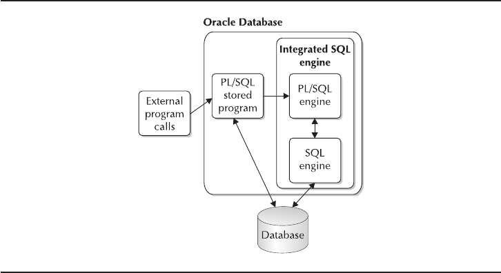
The PL/SQL engine is bundled together with the database, and is an integral part
of the Oracle server, providing you with a powerful language to empower your
logic and data. Let’s look at how PL/SQL fits into the Oracle server. Figure 5-1
shows you how PL/SQL works from both within and without the database.
At the center of the Oracle Database 11gserver in Figure 5-1 is the primary
engine for the database, which serves as the coordinator for all calls to and from the
database. This means that when a call is made from a program to the server to run a
PL/SQL program, the Oracle server loads the compiled program into memory and
then the PL/SQL engine and SQL engine execute the program. The PL/SQL engine
will handle the program’s memory structures and logical program flow and then the
SQL engine issues data requests to the database. It is a closed system and one that
allows for very efficient programming.
PL/SQL is used in numerous Oracle products, including the following:
■Oracle Database Server
■Application Express
■Oracle Data Miner
■Oracle Warehouse Builder
■Oracle eBusiness Suite
■Oracle Portal
Chapter 5: PL/SQL 165
FIGURE 5-1. PL/SQL architecture

166 Oracle Database 11g: A Beginner’s Guide
All of these programs use PL/SQL to some extent. If you look at the internals of
Oracle applications, you’ll see that there can be as many as five million lines of
PL/SQL code contained within it. PL/SQL interfaces can be developed and utilized
from these Oracle development environments:
■SQL*Plus
■Oracle Grid Control/Oracle Enterprise Manager
■Oracle Pre-compilers (such as Pro*C, Pro*COBOL, and so on)
■Oracle Call Interface (OCI)
■Server Manager
■Oracle Application Server 11g
■jDeveloper
As you can see, PL/SQL is well established within Oracle’s line of products. The
reasons for using PL/SQL are primarily its tight integration with the database server
and its ease of use. You will find that there are few tasks that PL/SQL cannot handle.
TIP
Use PL/SQL to program complex tasks or for
program elements that may be used over and
over again.
CRITICAL SKILL 5.2
Describe the Basic PL/SQL Program Structure
The structure you use in PL/SQL is the foundation for the language as a whole. Once
you’ve mastered it, you will then be able to move forward; however, if you do not
take the time to get this first step right, your journey will be difficult. Thankfully, it’s
quite simple.
The structure is quite basic. You will have areas for your program parameters
(these are used to pass values from outside a program to the program itself), your
internal variables, the main program code and logic, and various ways to deal with
problem situations. Let’s look at the basic form of a PL/SQL block:
[DECLARE]
-- Put Variables Here
BEGIN
-- Put Program Here
[EXCEPTION]

-- Put exception handlers here
END;
/
That’s it: the basic structure of every PL/SQL program. When we talk about PL/SQL
programs, they are referred to as PL/SQL blocks. PL/SQL blocks are simply programs
that are complete and that are programmed to run successfully. A PL/SQL program
is comprised of one or more of these blocks, which you can think of as routines. So
at the basic level, you only need one block for a valid PL/SQL program, but as you
consider writing a more complex program, you will find it easiest if each block
addresses a particular task or subtask; it is these structures that you will use in all of
your PL/SQL programs to create the most robust code possible. The PL/SQL block
structures form the basis for any program you shall be writing in PL/SQL. This
chapter builds upon that fundamental form, each section helping you move
toward more complex programs.
In its basic form, you will usually need to declare variables in your PL/SQL program.
It is these variables used in the PL/SQL that hold the declarative or working storage
area (including constants, local program variables, select statements, data arrays,
and such) within your program. These variables are then available for use in your
program. So if you need a counter, a data array, data variables, or even Boolean
variables, you will declare them here.
Next is the program body or executable section. It is the only section you really
need to include in your PL/SQL block, since you could write a program without
variables or exception handling. It is in this section that you build your program
logic and database access. That is why you must always remember BEGIN and
END; these are your PL/SQL bookends. It is between these two lines that your
program logic is contained.
The final section is the exception section. It is within this section that you will
find all the error handling needed for your program. This section is an optional
portion of the PL/SQL block. However, it is recommended that all programs include
the use of exception handling to ensure a controlled run of your programs.
Chapter 5: PL/SQL 167
Ask the Expert
Q: What are the only lines of the PL/SQL block that are required to create a
functional program?
A: The only lines of the basic PL/SQL block that are required to create a
functional program are BEGIN and END.

CRITICAL SKILL 5.3
Define PL/SQL Data Types
The use of local variables within a PL/SQL program is an important knowledge point
for everyone using the language. It is a basic component of each program, and as
such, it is invaluable for gaining the knowledge of what is available and how best to
use it. You can now look at how you use and define variables and working storage
within your PL/SQL programs.
As with all programming languages, there are characters that you use to write
your programs. Each language has its own rules and restrictions when it comes to
the valid characters. In the following sections, we will show you
■Valid characters when programming in PL/SQL
■Arithmetic operators
■Relational operators
Valid Characters
When programming in PL/SQL, you may use only characters as defined here:
■Characters can be typed in either upper- or lowercase. PL/SQL is case
insensitive.
■All digits between 0 and 9.
■The following symbols: ( ) + - * / < > = ! ~ ; : . @ % , " ' # ^ & _ | { } ? [ ]
Some of these characters are for program commands; others serve as relational
or arithmetic operators. Together they form a program.
Arithmetic Operators
Table 5-1 shows the common arithmetic operators used in PL/SQL. They are listed
in the order of precedence in which they are executed (that is, by priority). When
the functions appear in the same line, it means that they are executed with the same
168 Oracle Database 11g: A Beginner’s Guide
Operator Meaning
** Exponent
*,/ Multiplication, Division
+,-, || Addition, Subtraction, Concatenation
TABLE 5-1. Arithmetic Operators

level of precedence, so the position of the expression determines which goes first in
the operational execution.
Table 5-2 shows the common relational operators used in PL/SQL. These are the
logical variables that are used to compare data. As with any comparison, they need
to conform to logic hierarchies, especially when using multiple operators in your
conditional clauses.
The use of variables in a PL/SQL program is usually something that is required to
truly leverage the power of the language. It is here that you define how your data is
to be held while you work it through your program. These variables can be the
same types you have already learned about in the SQL language. However, in
addition to these standard data types, there are some special ones that have been
created specifically for the PL/SQL language.
NOTE
All SQL within Oracle is supported directly
with PL/SQL.
One of the important features of Oracle Database 11gis the tight integration
of the SQL and PL/SQL engines into one system. This means that from Oracle9i
forward you can run the same commands in PL/SQL that you use in SQL. This was
not true in earlier versions of PL/SQL, so take care if using these versions (it may be
time to consider an upgrade). That would also qualify you as more than a beginner.
Now you can move on to the most common data types that you will use when
writing PL/SQL programs:
■varchar2
■number
■date
■Boolean
Chapter 5: PL/SQL 169
Operator Meaning
= Equal
<> or != Not equal
> Greater than
< Less than
>= Greater than or equal to
<= Less than or equal to
TABLE 5-2. Relational Operators

You’ll use these variables in PL/SQL the same way that you would use them in
SQL. Assigning values to variables is very important when programming in PL/SQL
or any other programming language. You can assign values to variables in any
section of your program code, and you can also assign values to variables in the
declare section. Defining your variable in the declare section is done to initialize
values in advance of their use in the program or to define values that will be used as
constants in your program. To assign a value to a variable in the declaration section,
you would use the following format:
Variable_name variable_type := value;
NOTE
The important item that you should notice here is
that you use the := to assign a value. This is the
standard used in PL/SQL.
You may also define variable values in the execution and exception sections of
your PL/SQL program. Within the program, you would use the following format to
assign a value to a variable:
Variable_name := value;
To assign values to variables you use, let’s look at a small program that assigns
values in each section of a program:
-- Declaration section of the program
declare
l_counter number := 0; -- initiate value to 0
l_today date := sysdate; -- assign system date to variable
l_name varchar2(50); -- variable is defined but has no value
l_seq_val number := ian_seq.nextval; -- assigns the next sequence
value to the variable
--
-- Execution section of the program
begin l_counter := l_counter + 1; -- add one to current value of counter
l_name := 'LUCY THE CAT'; -- set a value to character variable
-- Error (EXCEPTION) handling section of the program
exception
-- Generic error handling to handle any type of error
when others then
-- print out an error message
raise_application_error (-20100, 'error#' || sqlcode || ' desc: ' sqlerrm)
end;
170 Oracle Database 11g: A Beginner’s Guide

Chapter 5: PL/SQL 171
NOTE
Oracle has some special variables that may be used
in a PL/SQL program. In the example, we used the
sqlcode and sqlerrm variables. These variables
represent the Oracle error number and the Oracle
error message respectively. You may use these
variables to capture Oracle errors in your program.
The varchar2 Data Type
varchar2 is a variable-length alphanumeric data type. In PL/SQL, it may have a
length up to 32,767 bytes. When you define the varchar2 variable in the declare
section, remember to terminate the line with a semicolon (;). The following is the
form of varchar2 variable declarations:
Variable_name varchar2(max_length);
where the max_length is a positive integer, as in
l_name varchar2(30);
You may also set an initial or default value for the variable. This is done on the
same line as the variable declaration in the declare section of your program. You
can do this by using the following syntax:
L_name varchar2(30) := 'ABRAMSON';
The preceding statement will set that value of the variable L_name to the value of
ABRAMSON.
The Number Data Type
The number data type is used to represent all numeric data. The format of the
declaration is
Number_field number(length, decimal_places);
where the length can be from 1 to 38 numerical positions, and decimal_places
represents the positions for numerical precision of the decimal place for the
variable. Keep this in mind when you define your numerical variable, as in
L_average_amount number(12,2);
This describes a variable that may hold up to ten digits (Length(12) - decimal_
places(2)) and up to two decimal places. This means the variable may hold a
number up to a value of 9,999,999,999.99. The number data type has a number of

supported subtypes. These include DECIMAL, FLOAT, REAL, and others. These are
quite familiar to people who use other languages to program for their business needs.
The Date Data Type
The date data type variable is used to store date and datetime values. The following
is the format of the date declaration:
Date_variable date;
By default, Oracle displays values using the format DD-MON-YY. So a value of
14-JAN-08 would be the equivalent of saying January 14, 2008. When programming
in PL/SQL, you should always use this data type when performing date manipulation.
It is possible when combining this data type with some built-in Oracle functions to
extend the flexibility of your date manipulations. For example, let’s say that you
create a variable for a start date and you want to place values into this variable.
Let’s see how this may be done:
Declare
L_start_date date;
Begin L_start_date := '29-SEP-05'; -- Sets variable
-- to September 29, 2009.
L_start_date := to_date('29-SEP-2083 ', 'DD-MON-YYYY');
-- Sets variable to September 29, 2083
L_start_date := to_date('09-JUN-91:13:01 ', 'DD-MON-YY:HH24:MI');
-- Sets variable to June 9, 1991, 1:01 p.m.
End;
So here you have set the date variable in three different forms. The first is the
simplest, while the second is more complex (since it uses the to_date function),
though it does allow for more flexible data declarations, since you can use a
four-digit year definition. The final example shows you how to put a datetime into
the variable. Again you’ll use the to_date function, but you’ll include the time in the
value and then define it with the date mask definition.
NOTE
For more information on other Oracle built-in
functions, see “Oracle Database SQL Reference,”
in the Oracle Database 11gdocumentation.
You should also familiarize yourself with the variations of the date data type.
This includes the timestamp data type, which provides additional date support that
may not be available with the simple date data type.
172 Oracle Database 11g: A Beginner’s Guide

The Boolean Data Type
The final basic data type we will discuss is the Boolean data type. Simply put, this
variable will hold a value of either true or false.When you use this data type, you
must test its status and then do one thing if it is true and another if it is false. You
can use a Boolean expression to compare arithmetic expressions or character
expressions. So, if you have the following arithmetic values, you’ll get
L_record_goals := 91;
L_season_goals := 77;
-- Therefore the following expression will be true
L_record_goals > l_season_goals
-- However the next is false
l_record_goals <= l_season_goals
If you wish to compare character strings, the same may be done. Here’s an example:
l_Cognos_developer := 'Falcon';
l_Oracle_dba := 'Ruxpinnah';
-- The following expression will be true in a true Boolean value
l_Cognos_developer <> l_oracle_dba
It is important to understand that these comparisons provide Boolean results that
may then be used during conditional program control, so you should take the time
to know the difference between true and false.There are numerous other data types,
but by mastering these simple ones you can already build some complex programs.
In C++ and other languages, Booleans can be represented as either true/false or 1/0.
In PL/SQL, the value is assigned only true or false.
Chapter 5: PL/SQL 173
Ask the Expert
Q: How do you let Oracle set the definition of a variable within PL/SQL
programs based on a table’s column definition?
A: The use of dynamic variable definitions based on column definitions is a
very important feature that you should always utilize within PL/SQL. This ties
the variable definition to a table within the database. When defining your
variable, use the name of the table, the column, and the special string of
%TYPE. The following is an example of using the product table’s prod_id
as a variable data definition:
v_product_id products.prod_id%TYPE
By using the %TYPE variable type, we have freed our program of the need
to ever redefine this field. So if the column’s definition changes, so will the
variable within your program.

Progress Check
1. Name four programs or facilities where you can use PL/SQL.
2. Name three sections that may be contained in a PL/SQL block.
3. What is the only required section in a PL/SQL block?
4. What data type would you use to store each of the following?
A. 12344.50
B. True
C. April 11, 1963
D. “PINK FLOYD”
E. 42
CRITICAL SKILL 5.4
Write PL/SQL Programs in SQL*Plus
When you write PL/SQL programs, you have a couple of options for how to run a
program. A program may be run directly in SQL*Plus (or some other SQL environment
such as SQL Developer), or it can be stored in the database and then run from a
174 Oracle Database 11g: A Beginner’s Guide
Progress Check Answers
1. Any four from among the following would be acceptable answers: Oracle Forms, Reports,
Warehouse Builder, Oracle Applications, Oracle Portal, SQL*Plus, Oracle Grid Control, Oracle
Pre-compilers, and Oracle Application Server.
2. The three sections that may be contained in a PL/SQL block are the Declaration, Execution, and
Exception sections.
3. The Execution section is the only required section in a PL/SQL block.
4. The data types used to store each of the variables would be
A. Number or number(8,2). The storage of a number should always be done in a number data
type. You can specify the precision or simply define it as a number with no precision, when you
do not know the exact nature of your data.
B. Boolean. The boolean data type is used to store true and false information.
C. Date. The date data type stores date and time information.
D. Varchar2(10). Character values should be stored in the varchar2 data type. This is more
effective for storing the data, yet it has a limit of 4000 bytes. If you need more than 4000 bytes,
you should then use the LONG data type, which allows you to store up to 2GB of data.
E. Number or number(2). These are the preferred data types for numbers when no decimal places
are required (integers).
Chapter 5: PL/SQL 175
SQL environment or a program. When you store a program in the database, it’s
called a stored program or stored object. (We’ll cover this later in the chapter.) For
now, let’s discuss how to write a program using SQL*Plus. While we illustrate this
example from within the SQL*Plus environment, these programs may also be run
using other SQL interfaces such as SQL Developer, TOAD, or any other product that
you may prefer.
When first writing a program, you can create and modify it using the command
line in SQL*Plus. To do this:
1. Log into SQL*Plus. Depending on your environment you may need to
issue a sqlplus command on the command line. You should note that
with Oracle Database 11g, the Windows version of SQL*Plus has been
deprecated, so if you wish you may also perform this exercise using
SQL Developer.
2. Type in your program via the command line.
3. For each line you write, press ENTER to get to the next line.
4. When you finish typing in your program, remember to terminate it with a “/”
character. This tells Oracle to run the program that you just finished entering.
5. Monitor Oracle to see if your program ran successfully. If your program
does run without errors (syntax errors), you will see the message “PL/SQL
procedure successfully completed.” If you see anything else, this is an
indication that an error occurred.
6. To see the errors created by your program (if you have created a stored
object as we will discuss later in this chapter), type in Show errors.
SQL*Plus will display the errors it encountered during the current run
of your program.
7. Should you receive an error, you will need to edit your program. If your
SQL*Plus and Oracle environment is set up correctly, you should be
able to simply enter edit on the command line and your program will
be loaded into an editor where you can then fix it. Once you exit the
editor, the program will be reloaded into the SQL buffer and may be
run again.
Now let’s move on to an illustration for how to construct a PL/SQL program and
get some output of our results.

176 Oracle Database 11g: A Beginner’s Guide
Project 5-1 Create a PL/SQL Program
This will be the first PL/SQL program that you will create. The concept is straightforward;
you will first declare some variables, place some values into them, and then output
the data to the screen with SQL*Plus.
Step by Step
1. Log into SQL*Plus.
2. At the SQL> prompt, enter the serveroutput command: set serveroutput on;.
3. Enter the following PL/SQL program:
Declare
L_start_date date;
Begin L_start_date := '29-SEP-2005';
dbms_output.putline (l_start_date); --show date
End;
/
4. You should now see the following output on your screen:
SQL> /
29-SEP-05
PL/SQL procedure successfully completed.
5. You have now completed your first PL/SQL program.
Ask the Expert
Q: How can I get feedback/output from my PL/SQL programs?
A: Oracle provides a built-in package named dbms_output for this purpose.
Oracle supplies many of these packages that provide users with additional
functionality, such as outputting data to the screen. By placing the
dbms_output.put_line command into your programs, Oracle PL/SQL can
then provide information to the user as shown in this chapter’s examples.
To actually see this information, you must enable screen output by entering
SET SERVEROUTPUT ON at the SQL> prompt before executing your PL/SQL
routine.

6. Take the time to add to the program and add lines that use other date
formats or perform some date addition. For example, you may wish to
add the following code and see the results that they provide:
L_start_date := to_date('14-JAN-2063', 'DD-MON-YYYY');
dbms_output.put_line (l_start_date);
L_start_date := to_date('09-JUN-91:13:01', 'DD-MON-YY:HH24:MI');
dbms_output.put_line (l_start_date);
Next, we need to discuss how to include database data within your PL/SQL
programs.
Project Summary
This project enables you to see how to construct a PL/SQL program. You now have
seen how to create, run, and then re-run it, allowing you to see the output. This is a
simple example, presented to show you the basis of all PL/SQL programs.
SQL in Your PL/SQL Programs
We have looked at a lot of structure up until now. You should know that a PL/SQL
program will always have a BEGIN and END statement. It may have variables, loops,
or logic control, but now you need to get real database data into your programs. What
gives PL/SQL its power is its tight integration with SQL. You may want the information
so that you can create a report, update data, create new data, delete old data, or
perform just about any other function you can think of. It is very important for you
to see how you can integrate data into PL/SQL code. Without data, PL/SQL is just PL.
PL/SQL Cursors
How do you get data to your programs? Simple—select it from the database. This is
the easiest way to use SQL in your program. Thus, inserting a line like the following
will provide you with the ability to access data in the database:
select prod_name
into v_prod_name
from products
Let’s break down the statement and look at what it means to the program. As
you look at the select statement, you can see that it looks very similar to a standard
select statement. However, you should also have noticed the word into in the
statement. You may be wondering what it’s for? This is how you put a value into
a variable using a select statement.
The following example illustrates how you include a SQL statement in your
PL/SQL program:
1 declare
2 v_prod_name varchar2(80);
Chapter 5: PL/SQL 177
Create a PL/SQL Program
Project 5-1

3 begin
4 select prod_name
5 into v_prod_name
6 from products
7 where rownum = 1;
8 dbms_output.put_line(v_prod_name);
9* end;
10 /
In addition to selecting one value from the database, you also have the ability to
select more than one value and add conditions that you want to include. To do this,
use the following cursor format:
select prod_name, prod_list_price, prod_min_price from products
where rownum < 10
You can use any SQL statement you want within your program. It can be a
select, insert, update, or delete statement. All of these will be supported. When
you use a select statement like you did in the preceding example, this is called an
implicit cursor. An implicit cursor is a SQL statement that is contained within the
executable section of the program and has an into statement (as in the case of a
select statement). With an implicit cursor, Oracle will handle everything for you, but
there is a cost to doing this: the program will run slower. You need to understand
what you’re doing because though it may not be the best way to perform a select
statement, you must use an implicit cursor when you want to run a delete, update,
or insert statement. So, let’s move on to see a better way of doing the same thing.
We will revisit your previous example so that you can compare the two.
The better way is to create an explicit cursor. An explicit cursor is a select
statement that is declared in the declare section of a program. You do this so that
Oracle will then prepare your SQL statement in advance of running your program.
178 Oracle Database 11g: A Beginner’s Guide
Ask the Expert
Q: Why did we include rownum = 1 in our select statement?
A: The reason we include rownum = 1 when using an implicit cursor is that
in this particular case the select statement will return more than 1 row. This
will result in an Oracle error that terminates the processing of this PL/SQL
block. To avoid this situation, we include the rownum = 1 condition.

This makes for very efficient use of memory by the program. Let’s look at what the
program would look like with an explicit cursor:
1 declare
2 v_prod_name varchar2(80);
3 cursor get_data is
4 select prod_name
5 from products;
6 begin
7 open get_data;
8 fetch get_data into v_prod_name;
9 dbms_output.put_line(v_prod_name);
10 close get_data;
11* end;
In the previous code, we converted the initial example into one that uses an
explicit cursor. Notice that the select statement is now contained in the declaration
section. There is also no longer an into clause. This functionality is moved into the
execution section, where it is used in the fetch command.
You will also note that we introduced three new PL/SQL commands: open,
fetch,and close. With these three simple commands, you can get data from your
database using SQL cursors. The open command tells Oracle to reserve memory
that will need to be used by the select statement. The fetch command, meanwhile,
pulls the data from the first row of the result set, and the close command returns the
memory back to Oracle for other uses.
NOTE
Always remember to close your cursors when you
are done with them. If you don’t, you may start
getting memory problems, or you could get results
that you don’t expect.
The Cursor FOR Loop
You get a better sense of the power of the cursor by combining it with a loop. The
cursor FOR loop is the result of combining the select cursor with a FOR loop (we’ll
go into additional detail about this loop in the next section). This allows you to
retrieve multiple rows from the database if your result set should do this. It also is
simpler to program, and you don’t have to worry about opening or closing your
cursor; Oracle handles all that within the loop. Let’s look at an example of the
cursor FOR loop. The important lines have been highlighted for you:
SQL> set serveroutput on
SQL> declare
2 v_prod_name varchar2(80);
3 cursor cur_get_data is
Chapter 5: PL/SQL 179

180 Oracle Database 11g: A Beginner’s Guide
4 select prod_name
5 from products;
6 begin
7 for i in cur_get_data
8 LOOP
9 dbms_output.put_line(i.prod_name);
10 END LOOP;
11 end;
12 /
5MP Telephoto Digital Camera
17" LCD w/built-in HDTV Tuner
Envoy 256MB - 40GB
Y Box
Mini DV Camcorder with 3.5" Swivel LCD
Envoy Ambassador
Laptop carrying case
Home Theatre Package with DVD-Audio/Video Play ...
NOTE
To reference columns during a FOR loop, use the
name of the loop and concatenate it with the name
of the column as defined within the cursor
declaration. Thus, your result will be a variable
named cursor_name.fieldname (in our example,
we did this using the variable i.prod_name).
The cursor FOR loop is truly PL/SQL power in action. It provides you with the
ability to easily move through the result set of a select statement and perform the
logic and manipulations you need to be successful.
We have just touched the surface of getting information from PL/SQL. One
concept that you will need to get comfortable with is the debugging of PL/SQL
programs, which can be a very complex task. Experience has taught us that finding
our errors can never be taken lightly or ignored. Using a simple facility like
dbms_output,you have a way of tracking the progress of your program.
NOTE
Another available facility is dbms_profiler. This
package analyzes how your program is running and
collects statistics on how long each line takes to
execute. This helps you find code that runs slowly
or inefficiently. When you need to access more
advanced statistics about your programs, take the
time to investigate this package and how to integrate
it into your PL/SQL code. Since this is a beginner’s
guide, we’ll only direct you to an important feature
when you need its functionality.

Chapter 5: PL/SQL 181
Having seen how to write and debug programs, you can now make those
programs more complex.
CRITICAL SKILL 5.5
Handle Error Conditions in PL/SQL
As you have seen in the previous section, bad things happen to good programs.
However, you also have to deal with bad or problematic data as well. To deal with
problems during the processing of data, PL/SQL provides us with the robust ability
to handle these types of errors. We call this type of program code exception
handling.
To raise an error from within a PL/SQL program, use the built-in procedure
named raise_application_error.The procedure requires two arguments: one is for
the error number and must be between –20000 and –20999, whereas the second
argument is the error that you want the user to see.
As with all exception handling, this program code is placed into the EXCEPTION
section of your PL/SQL program. Thus, your program structure will now be
BEGIN
-- Put Program Here
EXCEPTION
-- Put exception handlers here
END;
/
Table 5-3 gives you some examples of the most common errors that Oracle can
help you handle.
NOTE
You must always make the Others error handle the
last one in your program, since Oracle will not
process any exception handles after this one. In
addition, the WHEN OTHERS exception should be
a last resort and should not be used as a catch-all,
error-handling mechanism.
The following is the line that your program may contain to provide feedback to
the user:
raise_application_error (-20123, 'This is an error, you have done a bad thing');

182 Oracle Database 11g: A Beginner’s Guide
So let’s see how these all come together in a single program:
SQL> run
1 declare
2 l_emp_count number;
3 i number; -- We will use this as our counter
Exception Name Explanation Oracle Error
No_data_found When a select statement returns
no rows, this error may be raised.
It usually occurs when you use
an implicit cursor and perform
a SELECT INTO.
ORA-01403
Too_many_rows When a case that should only
return a single row returns multiple
rows, this exception is raised.
ORA-01422
Dup_val_on_index This exception is raised when you
try to insert a record into a table
that has a primary key on it and
the record that you are inserting is
a duplicate of one that already
exists in the table.
ORA-00001
Value_error This error occurs when you
attempt to put a value into
a variable, but the value is
incompatible (for example,
inserting a value of 'MICHAEL
BROWN' into a numerical field).
It also occurs when you input a
value that is too large to be held
in the defined field (for instance,
inputting 'JILLIAN ABRAMSON'
into a character variable that is
only ten characters long).
ORA-06502
Zero_divide This error is encountered when
you attempt to divide by zero.
ORA-01476
Others This exception is used to catch any
errors not handled by specific error
handles.
Non-specific
TABLE 5-3. Built-in PL/SQL Exceptions
Chapter 5: PL/SQL 183
4 l_row employee%rowtype;
5 begin
6 select *
7 into l_row
8 from employee
9 order by emp_name;
10 EXCEPTION
11 WHEN no_data_found then
12 raise_application_error (-20052,'Sorry no data in this table. TRY AGAIN!');
13 WHEN others then
14 raise_application_error (-20999,'Something has gone really wrong...you better
guess');
15* end;
declare
*
ERROR at line 1:
ORA-20052: Sorry no data in this table. TRY AGAIN!
ORA-06512: at line 12
This program will handle instances where no data is found, as well as anything
else that happens that is not a result of lack of data. So, with these simple techniques
you may now handle problems that might occur in your programs.
You may also extend the functionality of the Oracle exception handling facility
with your own user-defined exceptions.
User-defined exceptions are defined within your program code. There are three
components to defining and using this exception type. They include
■Declaring the exception
■Raising the exception during program execution
■The exception handle itself
These three items must all be in place for an exception to be valid and to be
used within the program. This differs from the Oracle-defined exceptions, which
may be used within a program without declaring them or even raising an error
condition. So let’s see how this all comes together in a program:
Declare
L_counter number := 0;
L_name employee.employee_name%type;
Cursor get_employee_name is
Select employee_name
From employee;
excep_old_friend Exception;
never_met_them Exception;
Begin Open get_employee_name;
Fetch get_employee_name into l_name;
If l_name = 'CARL DUDLEY' then
Raise excep_old_friend;

184 Oracle Database 11g: A Beginner’s Guide
Else Raise excep_never_met_them;
End if;
Close get_employee_name;
Exception
When excep_old_friend then
Dbms_output.put_line('I know this person');
When excep_old_friend then
Dbms_output.put_line('I do not know this person');
End;
As you can see in this program, the definition and use of a user-defined exception
is really driven by your needs. In this case, you select data from the employee table.
Should the name of the person you retrieve be Carl Dudley, then you raise the
exception that you defined called excep_old_friend. In any other case, you would
raise excep_never_met_them. Based on this decision, you raise the exception that
you want to handle for the situation.
So, let’s look at the three components you need to use this exception you’ve
created specially. First, there is the declaration of the exceptions. These go into the
Declaration section. You simply name the exception and tell Oracle that they are of
the type exception, just as we have done in the following lines of program code:
excep_old_friend Exception;
never_met_them Exception;
Next, you need to call the appropriate exception within the program code.
You’ll want to call the exception when something occurs—in this case, when
you obtain the name of a friend or the name of a stranger.
NOTE
User-defined exceptions may be raised to handle an
error or to handle a condition that may not be seen
by Oracle as an error.
In your case, you are not concerned with an error; you just want to deal with a
situation. Therefore, in your program code all that is needed to call a user-defined
exception is to simply use the raise command followed by the name of the
exception, as in the following code snippet:
Raise excep_old_friend;
You have taken the first two steps toward defining and calling your own
exception (Declaration and Execution sections); all that’s left is to define what the
exception is going to do. This is done in the Exception section of your program. To
do this, simply include the exception in the Exception section:
Chapter 5: PL/SQL 185
Exception
When excep_old_friend then
Dbms_output.put_line('I know this person');
In your case, you simply will output that you know this person.
This example has shown you how to set up user-defined exceptions and how
to use them. The way in which you implement exceptions is limited only by your
imagination.
Error Handling Using Oracle-Supplied Variables
As well as being able to define your own exceptions within your PL/SQL program,
Oracle also provides some standard variables that may be used in your PL/SQL
programs. These variables are available to you in many different forms depending on
where you use them in your program. These variables are known as pseudo-columns.
A pseudo-column is a column that may be used in a select statement or during the
processing of data. We use the term pseudo-column so that you can consider their
use similarly to the way you would use a column. They include
■Current system date (sysdate)
■Row number (rownum)
■Oracle error number (sqlcode)
■Oracle error message (sqlerrm)
In this section, we will only look at the last two, which in exception handling
are the two that are often used. They provide you with access to the Oracle error
number and message and will therefore allow you to write programs that may
always end successfully. Even though they may still encounter an error, it’s handled
in a manner that is quite robust and manageable. Let’s look at the same program,
except this time you will add another exception handle for when any error occurs.
You do this by adding the when others exception:
Declare
L_counter number := 0;
L_name employee.employee_name%type;
Cursor get_employee_name is
Select employee_name
From employee;
excep_old_friend Exception;
never_met_them Exception;
Begin Open get_employee_name;
Fetch get_employee_name into l_name;
If l_name = 'CHRISTINE LECKMAN' then
Raise excep_old_friend;

Else Raise excep_never_met_them;
End if;
Close get_employee_name;
Exception
When excep_old_friend then
Dbms_output.put_line('I know this person');
When excep_never_met_them then
Dbms_output.put_line('I do not know this person');
When others then
Dbms_output.put_line('Oracle Error: ' || sqlcode);
Dbms_output.put_line('Oracle error message is: '|| sqlerrm);
End;
As you can see, you have now added an extra error-handling condition. The one
you have added to the program is the infamous when others exception. As previously
discussed, this exception may be used to handle any error that occurs for which no
other exception has been defined. Most importantly, it must also be the last exception
in your exception section, since Oracle stops processing when it encounters an
exception that meets the criteria. Therefore, if this exception is first, Oracle will stop
once it hits the when others condition. As we mentioned before, this is a dangerous
practice; you need to handle this error carefully and might even consider not
utilizing the when others condition because it could mask the real issues with
your program.
In our example, we have now used the functions sqlcode and sqlerrm. You
should always consider using these variables in your program code to ensure your
PL/SQL program completes in a manageable manner and provides the necessary
feedback for diagnosing potential problems and errors.
Progress Check
1. What facility do you use to get output from within a PL/SQL program?
2. What is wrong with the following cursor declaration?
Cursor get_data is;
Select cust_id, cust_last_name
From customers;
3. What are the two basic types of exception handles within PL/SQL?
4. To call an exception, what PL/SQL command should you use?
5. Name two pseudo-columns that help with exception feedback?
186 Oracle Database 11g: A Beginner’s Guide

CRITICAL SKILL 5.6
Include Conditions in Your Programs
The inclusion of conditions in your programs is the heart of all advanced programming
languages. In the previous section, you actually included some statements for
performing these types of tasks and you may have noticed IF statements and loops.
It is in this section that we now illustrate how to construct them by providing you
with a step-by-step guide. Since programs are written to handle a number of
different situations, the manner in which different conditions are detected and dealt
with is the biggest part of program control. This section will provide you with details
on the following topics:
■Program control
■Various types of IF logic structures
■CASE expressions
■Various types of looping structures
Program Control
Program control is governed by the status of the variables that it uses and the data
it reads and writes from the database. As an example, picture yourself going to the
Department of Motor Vehicles to renew your driver’s license. Upon entering the
office, you are presented with a number of directional signs. One sign is “Drivers
Testing”; for this you go to the 2nd floor. Another sign tells you that “License
Renewals” are on the 3rd floor. So, since you are here for a renewal, you proceed to
the 3rd floor. Once you arrive in the renewal office, you are once again faced with
some new choices—after all, this is a government office; it’s not going to be a
simple exercise. So, now you have to decide if you are going to pay by cash or
credit card. Cash payments are being accepted to the right and credit cards are to
the left. Noting that you have enough cash, you head to the payment wicket on the
right. Let’s look at Table 5-4 and see how the program control influenced your choices.
Chapter 5: PL/SQL 187
Progress Check Answers
1. The dbms_output package can be used to get output from within a PL/SQL program.
2. The extra “;” on line 1 of the cursor should not be there.
3. Built-in exceptions like when others and when no_data_found are the two basic types of
exception handles within PL/SQL.
4. The raise command is used.
5. Two pseudo-columns that help with exception feedback are sqlcode and sqlerrm.

188 Oracle Database 11g: A Beginner’s Guide
IF Logic Structures
When you are writing computer programs, situations present themselves in which
you must test a condition. So, when you ask a question in your program, you are
usually presented with one of two answers. First, it may be true or it may be false;
computer programs are quite black and white. So, in computer logic there can only
be true or false answers to our questions, no maybes here. PL/SQL provides you
with three distinctive IF logic structures that allow you to test for true and false
conditions. In everyday life, you are presented with decisions that you need to
make. The following sections show you how to do this using PL/SQL.
IF/THEN The IF/THEN construct tests the simplest type of condition. If the condition
evaluates to TRUE, then one or more lines of program code will be executed. If the
condition evaluates as FALSE, then no action is taken. The following code snippet
illustrates how this is performed with a PL/SQL program:
IF l_date > '11-APR-63' then
l_salary := l_salary * 1.15; -- Increase salary by 15%
END IF;
Step # Process or Decision to Make Next Steps
1 Here for a driver’s license
transaction
Yes = 2 No = 4
2 Here for a driving test Yes = 5 No = 3
3 Here for a license renewal Yes = 6 No = 4
4 Ask for help Right place = 1 Wrong place = 13
5 Go to 2nd floor 7
6 Go to 3rd floor 9
7 Line up for driver’s test 8
8 Pass test (we hope) 6
9 Payment method Cash = 10 Credit = 11
10 Cash payment wicket 12
11 Credit-card payment wicket 12
12 Receive new license 13
13 Leave building, head home
TABLE 5-4. Logical Flow

Chapter 5: PL/SQL 189
In this case, you are asking that if the value of the variable l_date is greater than
(>) April 11, 1963, then the salary should increase by 15 percent. This statement
may also be restated using the following:
IF not(l_date <= '11-APR-63') then
l_salary := l_salary * 1.15; -- Increase salary by 15%
END IF;
You may nest IF/THEN statements to increase the power of your statements. So,
let’s add an additional condition to limit who gets the raise:
IF l_date > '11-APR-63' then
IF l_last_name = 'PAKMAN' then
l_salary := l_salary * 1.15; -- Increase salary by 15%
END IF;
END IF;
So, not only must the date be greater than April 11th, 1963, but your last name
must be equal to 'PAKMAN' in order to get the raise. This is a method we use to make
sure that human resource programs ensure that programmers get a raise every year.
What you should also notice in this code is that there are now two END IF
statements. This is a required construct, since you must always pair up an IF statement
with an END IF. So, if you are going to have nested IF statements, you must ensure
that each is paired with a matching END IF.
NOTE
Each IF statement block must have at least one line
of program code. If you wish to do nothing within
your program code, then simply use the NULL;
command.
IF/THEN/ELSE The IF/THEN/ELSE construct is similar to the simple IF/THEN construct.
The difference here is that if the condition executes as FALSE, you perform the
program statements that follow the ELSE statement. The following code illustrates
this logic within PL/SQL:
IF l_date > '11-APR-63' then
l_salary := l_salary * 1.15; -- Increase salary by 15%
ELSE
l_salary := l_salary * 1.05; -- Increase salary by 5%
END IF;
In this code listing, you see the condition that if the date is greater than April 11,
1963, you will get a 15 percent salary increase. However, when the date is less than
or equal to this date, you only receive a five percent increase.
190 Oracle Database 11g: A Beginner’s Guide
As with the simple for of the IF/THEN construct, you may nest the IF/THEN/ELSE
construct. Let’s look at how this might appear in your PL/SQL program:
IF l_date > '11-APR-63' then
If l_last_name = 'PAKMAN' then
l_salary := l_salary * 1.15; -- Increase salary by 15%
ELSE l_salary := l_salary * 1.10; -- Increase salary by 10%
END IF;
ELSE l_salary := l_salary * 1.05; -- Increase salary by 5%
END IF;
This leads us to another two points on using the IF statement within PL/SQL:
■There may only be one ELSE statement within every IF statement construct.
■There is no semicolon (;) on the line starting with ELSE.
IF/THEN/ELSIF The final IF construct that we will show you is the IF/THEN/ELSIF
one. In this case, you provide yourself with the option to test another condition
where the condition is evaluated as FALSE. So, should you want to test for more
than one condition without using nested IF statements, this is the type of statement
you might use:
IF l_last_name = 'PAKMAN' then
l_salary := l_salary * 1.15; -- Increase salary by 15%
ELSIF l_last_name = 'ASTROFF' then
l_salary := l_salary * 1.10; -- Increase salary by 10%
ELSE l_salary := l_salary * 1.05; -- Increase salary by 5%
END IF;
In this statement, if your last name is Pakman, you get a 15 percent raise. If it is
Astroff, you get 10 percent, and the rest of us get only a 5 percent raise.
Note that there is no limit to the number of ELSIF conditions you may use within
this construct. The following shows an example of using multiple ELSIF statements
within the construct:
IF l_city = 'OTTAWA' then
L_team_name := 'SENATORS';
ELSIF l_city = 'BOSTON' then
L_team_name := 'BRUINS';
ELSIF l_city = 'MONTREAL' then
L_team_name := 'CANADIENS'
ELSIF l_city = 'TORONTO' then
L_team_name := 'MAPLE LEAFS';
END IF;

Chapter 5: PL/SQL 191
NOTE
There is no matching END IF statement for each
ELSIF. Only a single END IF is required within this
construct.
When writing your PL/SQL program, you should use indentation to simplify the
reading of the program. Notice in our code segments that we use indentation to
make it easier for you to read the code statements. As a rule, you should line up
each IF/THEN/ELSE statement and indent the program code that lies between each
of these words.
CASE Statements
The next logical step from the IF statement is the CASE statement. The CASE statement
was introduced with Oracle9iand is an evolution in logical control. It differs from
the IF/THEN/ELSE constructs in that we now can use a simple structure to logically
select from a list of values. More important, it may be used to set the value of a
variable. Let’s explore how this is done.
First, let’s look at the format you will need to follow:
CASE variable
WHEN expression1 then value1
WHEN expression2 then value2
WHEN expression3 then value3
WHEN expression4 then value4
ELSE value5
END;
There is no limit to the number of expressions that may be defined in a CASE
statement. The following is an example of the use of the CASE expression:
SQL> run
1 declare
2 val varchar2(100);
3 city varchar2(20) := 'TORONTO';
4 begin
5 val := CASE city
6 WHEN 'TORONTO' then 'RAPTORS'
7 WHEN 'LOS ANGELES' then 'LAKERS'
8 WHEN 'BOSTON' then 'CELTICS'
9 WHEN 'CHICAGO' then 'BULLS'
10 ELSE 'NO TEAM'
11 END;
12
13 dbms_output.put_line(val); -- output to the screen
14* end;
RAPTORS
PL/SQL procedure successfully completed.

192 Oracle Database 11g: A Beginner’s Guide
Although you may have been able to use the IF/ELSIF/THEN/ELSE construct to
achieve the same purpose, the CASE statement is easier to read and is more efficient
with the database.
Loops
When was the last time that you visited an amusement park? Well, if you have been
to one in recent years, you will surely have seen a roller coaster. That roller coaster,
if it’s a really good roller coaster, probably had one or more loops. PL/SQL is that
kind of ride. It is a ride that includes loops. Loops are control structures that allow
you to repeat a set of commands until you decide that it is time to stop the looping.
Generally, the format that all loops take is the following:
LOOP Executable statements;
END LOOP;
Each time the loop is executed, the statements within the loop are executed, and
the program returns to the top of the LOOP structure to do it all over again. However,
if you ever want this processing to stop, you need to learn about the EXIT statement.
The EXIT statement allows you to stop executing within a loop without a
condition. It then passes control back to the program and continues on after the
LOOP statements.
The following is how to get out of a tight LOOP:
LOOP IF l_bank_balance >= 0 then EXIT;
ELSE L_decision := 'ACCOUNT OVERDRAWN';
END IF;
END LOOP;
Ask the Expert
Q: How do I add comments to my PL/SQL programs?
A: To add comments to your code, simply start a comment with a /* and end
it with a */ or use the -- (as we have done previously). If you use the --, you
need to make sure you put it on its own line, or after your program code if you
place it on the same line. The following are examples of valid comments:
/* This is a comment */
-- This is also a comment

Chapter 5: PL/SQL 193
NOTE
Without an EXIT statement in a simple LOOP, the
loop will be infinite.
There are many other kinds of loops, some of which provide more control over
your looping. Each has its use in PL/SQL programming and each should be learned
in order to give your programming the greatest flexibility.
The WHILE Loop
The WHILE loop will continue to execute as long as the condition that you have
defined continues to be true. When and if the condition becomes false, then you
exit your loop. If your condition is never satisfied you will end up in a loop that will
never exit. Let’s look at an example:
WHILE l_sales_total < 100000 LOOP
Select sales_amount into l_sale_amount from daily_sales;
l_sales_total := l_sales_total + l_sale_amount;
END LOOP;
Although you may have used the EXIT command to do the same thing, it is
better form to use the WHILE expression.
The FOR Loop
The FOR loop is one of the most common loops you will encounter in your PL/SQL
programming and it allows you to control the number of times a loop executes. In
the case of the WHILE loop, you are never quite sure how many times a loop is
executed, since it will continue to loop until a condition is met. However, in the
case of the FOR loop, this isn’t true.
The FOR loop allows you to define the number of times to loop when you program
the loop itself. You will define the value that starts your loop, as well as the value
that terminates it. Let’s look at its syntax:
FOR l_counter IN 1 .. 10
LOOP Statements;
END LOOP;
So, what is important to note in the preceding statement? First, you need to
know that the variable l_counter will hold the value between 1 and 10. How do you
know it will be between 1 and 10? Well, after the IN word, you place the counter’s
range. In this case, you want the counter to start at 1 (the low bound), and then
continue to 10. You should also note that between the two integer values (1 and 10)
194 Oracle Database 11g: A Beginner’s Guide
you place two dots (..). You do this to tell Oracle that you would like it to count
between these two numbers. You should also notice that we have not shown you
any type of declaration section, as they are not explicitly defined, since LOOP
counters are defined when they are used. You also have the ability to count
backwards using the REVERSE clause. This listing shows you how the REVERSE
clause may be used:
declare
l_counter number;
begin
FOR l_counter IN REVERSE 1..5
LOOP dbms_output.put_line(l_counter);
END LOOP;
end;
/
5
4
3
2
1
PL/SQL procedure successfully completed.
Now you can see how simple it is to use simple loops. But don’t be
fooled—loops have a lot of power, some of which you will see later. When you use
loops like the WHILE loop or the FOR loop, you have the ability to use variables
instead of hard-coded values. This allows you to have the greatest possible
flexibility since you can have the database or external data provide you with the
limits within your loop. Let’s look at how this might work. The following example
illustrates the simplest form of the FOR loop. In this case, you select the number of
employees you have in your employee table and then simply show how the counter
counts from 1 to the number of employees in your small company:
SQL> run
1 declare
2 l_emp_count number;
3 i number; -- We will use this as our counter
4 begin
5 -- Select the number of employees in the l_emp_count variable
6 select count(*) into l_emp_count from employee;
7
8 FOR i IN 1 .. l_emp_count LOOP
9 dbms_output.put_line('Employee ' || i);
10 END LOOP;
11* end;

Employee 1
Employee 2
Employee 3
Employee 4
Employee 5
Employee 6
PL/SQL procedure successfully completed.
So, as you might have guessed, you have six employees in your company. It
may be small, but it’s very good. However, the important thing to know is that you
may use variables in your loops. The other line you may have noticed was the select
statement contained in the PL/SQL block.
Project 5-2 Use Conditions and Loops in PL/SQL
In this project, you will create a PL/SQL program that will read the data in the
products table and then print out the products that are priced above $50.
Step by Step
1. Log into SQL*Plus.
2. At the SQL> prompt, enter the serveroutput command: set serveroutput on.
3. Enter the following PL/SQL program:
1 declare
2 cursor get_data is
3 select prod_name, prod_list_price
4 from products;
5 begin
6 for i in get_data
7 LOOP
8 if i.prod_list_price > 50 then
9 dbms_output.put_line(i.prod_name||' Price: '|| i.prod_list_price);
10 end if;
11 END LOOP;
12* end;
4. You should now see the following output on your screen:
SQL> /
5MP Telephoto Digital Camera Price: 899.99
17" LCD w/built-in HDTV Tuner Price: 999.99
Envoy 256MB - 40GB Price: 999.99
Y Box Price: 299.99
Mini DV Camcorder with 3.5" Swivel LCD Price: 1099.99
Chapter 5: PL/SQL 195
Use Conditions and Loops in PL/SQL
Project 5-2
(continued)

196 Oracle Database 11g: A Beginner’s Guide
Envoy Ambassador Price: 1299.99
Laptop carrying case Price: 55.99
Home Theatre Package with DVD-Audio/Video Play Price: 599.99
18" Flat Panel Graphics Monitor Price: 899.99
SIMM- 8MB PCMCIAII card Price: 112.99
SIMM- 16MB PCMCIAII card Price: 149.99
Unix/Windows 1-user pack Price: 199.99
8.3 Minitower Speaker Price: 499.99
Multimedia speakers- 5" cones Price: 67.99
Envoy External 8X CD-ROM Price: 54.99
Model NM500X High Yield Toner Cartridge Price: 192.99
Model A3827H Black Image Cartridge Price: 89.99
128MB Memory Card Price: 52.99
256MB Memory Card Price: 69.99
PL/SQL procedure successfully completed.
5. You may now change the criteria we have used so that we print out
messages for products under $50. This is done by adding the following text
in the right place in the code:
else
dbms_output.put_line(i.prod_name || ' Product under 50');
6. More output will appear, including that of all the products.
Project Summary
This project illustrates how to use loops and conditional clauses and how you can
easily select data and use it within a PL/SQL program.
CRITICAL SKILL 6.7
Create Stored Procedures—How and Why
PL/SQL is a very powerful language; one of its most important features is the ability
to store programs in the database and share them with others. We generally refer to
these as stored objects or stored sub/programs. There are four distinct types: procedures,
functions, triggers, and packages. Up until now in this chapter, you have looked at
anonymous PL/SQL blocks. Stored PL/SQL programs differ from these since they are
named objects that are stored inside the database. Anonymous blocks are not stored
in the database and must be loaded each time you want to run them.
You create stored programs for a number of reasons. The most important reason
to create programs that are stored and named instead of anonymous ones is that it
provides you with the ability to share programs and optimize performance. By
storing programs, you can grant many different users the privilege of running your
program. You can also simplify them and have different programs perform specific
functions. These programs can then be called from a central program, which can

Chapter 5: PL/SQL 197
optimize performance and programming time. This concept is very familiar to
object-oriented programmers and is known as modularity.
If you are to truly take advantage of PL/SQL within the confines of your Oracle
database, you will need to understand how to create and maintain PL/SQL stored
objects. Let’s look at the various types of PL/SQL stored programs.
The first stored object is called a stored procedure. A stored procedure is a
PL/SQL program-adding construct that tells the database you want to store an
object. Just as you do when you create a table, a procedure is created or updated
with the create procedure command. By adding this at the beginning of a PL/SQL
block, you create an object in the database known as a procedure.Another feature
of stored procedures, provided to you at no extra cost, is the ability to pass values in
and out of a procedure.
NOTE
You should put create or replace procedure in your
create procedure commands. If you do not use the
replace portion of the command, you will need to
drop your procedure before trying to re-create it. By
including replace, the procedure will be created if it
does not exist or will be replaced if it does.
Let’s look at one of the programs you have already created and convert it to a
stored procedure:
1 create or replace procedure print_products
2 as
3 declare
4 cursor get_data is
5 select prod_name, prod_list_price
6 from products;
7 begin
8 for i in get_data
9 LOOP
10 if i.prod_list_price > 50 then
11 dbms_output.put_line(i.prod_name || ' Price: ' || i.prod_MIN_price);
12 else
13 dbms_output.put_line(i.prod_name || ' Product under 50');
14 end if;
15 END LOOP;
16* end;
Warning: Procedure created with compilation errors.
Now it looks like we have a couple of errors. Even authors get errors when we
write PL/SQL. To see what errors you have received from your program, simply
enter show errors. Oracle will then show you the errors that have occurred during
the compiling of your program. Let’s see what we did wrong:
SQL> show errors
198 Oracle Database 11g: A Beginner’s Guide
Errors for PROCEDURE PRINT_PRODUCTS:
LINE/COL ERROR
-------- -----------------------------------------------------------------
3/1 PLS-00103: Encountered the symbol "DECLARE" when expecting one of
the following:
begin function package pragma procedure subtype type use
<an identifier> <a double-quoted delimited-identifier> form
current cursor external language
The symbol "begin" was substituted for "DECLARE" to continue.
16/4 PLS-00103: Encountered the symbol "end-of-file" when expecting
one of the following:
begin case declare end exception exit for goto if loop mod
null pragma raise return select update while with
<an identifier> <a double-quoted delimited-identifier>
<a bind variable> << close current delete fetch lock insert
open rollback savepoint set sql execute commit forall merge
<a single-quoted SQL string> pipe
<an alternatively-quoted SQL string>
It looks like we have errors on lines 3 and 16. When creating a stored object,
you do not always need to include the declare statement since PL/SQL understands
that, based on the way the program is structured, after a create statement it expects
to see the reserved word as, which will be followed by the Declaration section. So
you can think of it this way: as replaces declare when creating a stored object. Let’s
now look at the repaired PL/SQL code. The lines we changed are highlighted in bold:
1 create or replace procedure print_products
2as
3 cursor get_data is
4 select prod_name, prod_list_price
5 from products;
6 begin
7 for i in get_data
8 LOOP
9 if i.prod_list_price > 50 then
10 dbms_output.put_line(i.prod_name ||' Price: '|| i.prod_LIST_price);
11 else
12 dbms_output.put_line(i.prod_name || ' Product under 50');
13 end if;
14 END LOOP;
15* end;
SQL> /
Procedure created.
That’s good news. The program has compiled and will now run when we call it.
Let’s look at how to call a procedure from SQL*Plus. Using the execute command,
you may run a stored program:
SQL>> execute print_products
PL/SQL procedure successfully completed.

You have added a parameter to your program to show you how to get information
into it. You use parameters within the program when you supply data to the procedure,
and you can then return a value to the program that calls it through another output
parameter. It is also possible to define parameters as both input and output. However,
to simplify our parameters, you usually define them for only one of the two purposes.
In this case, you will use SQL*Plus to call your procedure since it works. Your
example will input a character that will be used to find only products that begin
with the input string:
1 create or replace procedure print_products
2 (FIRST_CHARACTER IN VARCHAR)
3 as
4 cursor get_data is
5 select prod_name, prod_list_price
6 from products
7where prod_name like FIRST_CHARACTER || '%';
8 begin
9 for i in get_data
10 LOOP
11 if i.prod_list_price > 50 then
12 dbms_output.put_line(i.prod_name ||' Price: '|| i.prod_LiST_price);
13 else
14 dbms_output.put_line(i.prod_name || ' Product under 50');
15 end if;
16 END LOOP;
17* end print_products;
Chapter 5: PL/SQL 199
Ask the Expert
Q: I get an error “ORA-20000: ORU-10027: buffer overflow, limit of 2000
bytes” when running my PL/SQL programs that use dbms_output. How can I
fix this problem?
A: The default buffer size for the DBMS__OUTPUT package is 2000 bytes.
This is usually sufficient for most testing purposes. However, if you need to
increase this, you can do it through the serveroutput command. One
parameter it has is size, whose value may be set to between 2000 and
1,000,000 bytes. You perform this by issuing the following command:
SQL> set serveroutput on size 100000

200 Oracle Database 11g: A Beginner’s Guide
Now, let’s see how to describe your procedure, as indicated by the bold text
in the next listing. Here, you learn the name of the program and get a list of any
parameters you may need to pass:
SQL> describe print_products
PROCEDURE print_products
Argument Name Type In/Out Default?
------------------------------ ----------------------- ------ --------
FIRST_CHARACTER VARCHAR2 IN
Next, you need to run the procedure. In this case, you are running it in SQL*Plus.
When in this facility, if you want to receive data from a program, you need to
declare a variable. This is done in the first line of the following listing. You will then
run the program with the execute command:
SQL> exec print_products ('A');
Adventures with Numbers Product under 50
PL/SQL procedure successfully completed.
As you can tell, the program was called print_products. You want to print the
products that begin with an “A.” The results show you that you only have one
product that begins with the character “A.” As you may have gleaned from the
results, the program has functioned as expected.
Now that you have learned to create stored objects in Oracle Database 11g,
let’s look at a specialized program, called a function, which can extend the
functionality of the database.
Progress Check
1. What type of IF structure should be used if you had a single test and only
one alternate choice?
2. What is wrong with the following IF structure? What other way can this
type of logic be implemented with Oracle Database 11g?
IF surname = 'ABRAMSON' then
Salary = salary * 1.12;
IF surname = 'ABBEY' then
Salary = salary * 1.22;
IF surname = 'COREY' then
Salary = salary * 2.5;
END IF;

3. True or False: When naming your stored programs, you must follow the
same rules as naming a table.
4. What are the three types of procedure parameters you can have?
5. What SQL*Plus command do you use to run your stored programs?
CRITICAL SKILL 5.8
Create and Use Functions
You may also create stored objects that can be used within a select command.
Oracle provides us with functions. There are functions to trim spaces from a field, or
replace one character with another. All of these provide us with an ability to extend
the capabilities of Oracle itself.
Functions are very much like stored procedures. The main difference is that
functions may be used within a select statement in the column list or may also be
used in the where clause.
When creating a function, you perform a create or replace function command.
You can have variables input to the function and return a value to the calling statement.
A function must return a value. The data type of the returned value must be defined
when creating the function. This is how a function differs from a procedure. The
function will then perform its task during regular processing, allowing you to utilize
the results along with your regular data, thus extending the value of your data and
your database.
Project 5-3 Create and Use a Function
The following project will walk you through the process of defining a function.
Then, use the function in two select statements. The first will use the function in the
returned columns and the next will use it as a data constraint. The function that you
Chapter 5: PL/SQL 201
Create and Use a Function
Project 5-3
Progress Check Answers
1. You would use the IF/THEN/ELSE structure.
2. We should not use chained IF statements, but instead use ELSIF in the secondary IF statements.
The best way to implement this type of logic is to employ a CASE statement.
3. True. When naming your stored programs you must follow the same rules as naming a table.
4. You can have any or all of the following: INPUT, OUTPUT, or INPUT&OUTPUT.
5. Use the execute command to run your stored programs.
(continued)
202 Oracle Database 11g: A Beginner’s Guide
create will perform the simple task of adding a 15 percent tax to the list price, giving
the price with taxes included.
Step by Step
1. Log into SQL*Plus.
2. At the SQL> prompt, type in the following command:
create or replace function GetProductTaxIn
(in_product_id number)
return number
is v_price number;
cursor get_price_tax is
select nvl(round(prod_list_price * 1.15,2),0)
from products
where prod_id = in_product_id;
begin open get_price_tax;
fetch get_price_tax into v_price;
return v_price;
exception
when others then v_price := 0;
return v_price;
end;
Function created.
3. If you receive any errors, you will need to fix them before you move on.
4. Create a select statement that uses the function in the columns
specification. The following is an example:
select prod_id, prod_list_price, GetProductTaxIn(Prod_id)
from products
5. Your results may look similar to this:
PROD_ID PROD_LIST_PRICE GETPRODUCTTAXIN(PROD_ID)
---------- --------------- ------------------------
13 899.99 1034.99
14 999.99 1149.99
15 999.99 1149.99
16 299.99 344.99
17 1099.99 1264.99
18 1299.99 1494.99
19 55.99 64.39

20 599.99 689.99
21 899.99 1034.99
22 24.99 28.74
23 21.99 25.29
...
6. Now use the function in the where clause of a SQL statement. The
following is an example of using the function within a where clause:
select prod_id, prod_list_price, GetProductTaxIn(Prod_id)
from products
where GetProductTaxIn(Prod_id)>= 500
Project Summary
This project illustrates how you can extend the functionality of your database as
well as add value to your organization by building standard rules that can be
utilized by everyone using your database.
Functions provide us all with the ability to define standard rules and derivations
for our user community and ensure that programs perform predictably and optimally.
CRITICAL SKILL 5.9
Call PL/SQL Programs
Up to this point in the chapter, you have done the following:
■Defined a PL/SQL block
■Defined a PL/SQL program
■Created a stored program
■Debugged your code
This is fine if you want to write every program and have it run as a simple
standalone program. However, as with many programming languages it is important
to write a number of separate programs that perform specific tasks, rather than a
single program that performs all of your tasks. So, when writing PL/SQL programs,
you should think the same way. Have programs that perform table maintenance,
that perform complex logic, or simply read data from tables or files. This leads you
to how to call programs from other programs, a process similar to calling subroutines
within C programs. Procedures may be called from programs ranging from Oracle
Forms to perl scripts, but for this section we will simply show you how to call
procedures from each other.
Chapter 5: PL/SQL 203
Create and Use a Function
Project 5-3
To call a procedure from another, you can use your previous procedure, named
print_products.Let’s create another procedure that calls this procedure:
create or replace procedure call_print_prods
as
begin
for l_alpha IN 65 .. 90
LOOP
print_products(chr(l_alpha));
END LOOP;
end;
/
You have created a new procedure. It loops through the values of 65 to 90, the
ASCII values for A to Z. Using the CHR function, you can convert the value to an
ASCII character. You need to do this because you cannot loop through character
values. So, the procedure will loop through the values calling the print_products
procedure each time. This calling of programs can be looped extensively and can
be organized into efficient and simple program units. This is similar to
modularization seen in object-oriented programming language.
As you can tell, Oracle’s PL/SQL is a powerful and deep language. In this chapter,
we’ve helped provide you with the ability to start writing programs and to incorporate
some complex logic using the basic features of the language. As with any language,
you can achieve a significant amount of productivity with only a limited number of
commands. We encourage you to use this as a starting point and build upon it to
ultimately create the programs you and your organization will need.
þChapter 5 Mastery Check
1. Where is PL/SQL executed?
2. Which type of PL/SQL statement would you use to increase the price values
by 15 percent for items with more than 1500 in stock and by 20 percent for
items with fewer than 500 in stock?
A. A cursor FOR loop
B. An IF/THEN/ELSE command
C. An insert statement
D. An update statement
3. What is the fetch command used for?
204 Oracle Database 11g: A Beginner’s Guide
4. What will the following command do?
V_PRICE_TOLERANCE := 500;
5. What is wrong with this function definition?
CREATE OR REPLACE FUNCTION raise_price
(original_price IN NUMBER)
RETURN number
IS
BEGIN
RETURN (original_price * 1.25);
END lower_price;
6. What is the advantage of using the %TYPE attribute when defining PL/SQL
variables?
7. What Oracle Database 11gfacility, besides PL/SQL, supports exception
handling based on error numbers?
8. A commit that is issued in a PL/SQL program will commit what?
Chapter 5: PL/SQL 205
This page intentionally left blank

Chapter
6
The Database Administrator
CRITICAL SKILLS
6.1 Learn What a DBA Does
6.2 Perform Day-to-Day Operations
6.3 Understand the Oracle Database
11gInfrastructure
6.4 Operate Modes for an Oracle
Database 11g
6.5 Get Started with Oracle Enterprise
Manager
6.6 Manage Database Objects
6.7 Manage Space
6.8 Manage Users
6.9 Manage Privileges for Database
Users

208 Oracle Database 11g: A Beginner’s Guide
o, you’ve decided to be a Database Administrator (DBA). Great
choice! On top of that, you’ve chosen Oracle as the Database
Management System (DBMS) that you want to work with. Even
better! All you need to figure out now is what to learn in order to do
the job. Reading this book is a great start. However, a DBA’s job
cannot be learned entirely in a few short months. It is a work in progress and it can
take several years to become really good at it. Don’t get us wrong—you can learn
the basics that will make you a productive DBA in a few short months. However,
there is a great deal to learn, and you won’t become really good at this job until
you’ve actually run the utility, executed the SQL, or performed the task. In other
words, don’t just read this book—try out the examples and don’t be afraid to make
mistakes.
CRITICAL SKILL 6.1
Learn What a DBA Does
The role of a DBA is more of a career than just a job. Those of us who have been
doing this for many years are always learning new things and are just trying to keep
up! That’s the exciting thing about being a DBA: the job keeps changing. Databases
are growing at a phenomenal pace, the number of users is increasing, availability
requirements are striving for that magical 24/7 mark, and security has become a
much greater concern. As you will see in this book, databases now include more
than just data. Knowledge of databases also encompasses the Internet, grid computing,
XML, storage management, clustering, and Java. So, how long will it take you to
learn how to be a DBA? The answer is for as long as you’re planning to practice
this career.
There are some concrete steps that you can take to jumpstart your learning
process. Undertaking an Oracle Certification will provide you with a structured
program offering you clear steps for learning the details of the job. Instructor-led
courses as well as CD- and Internet-based classes can help you through the process.
Getting involved in user groups in order to learn from other DBA experiences is
highly recommended. Also, read as much as you can and then get your hands on
a test database and practice what you’ve learned.
Applications come and go, but data stays around. All of the information that
makes your company valuable is (or should be) stored in a database. Customer,
vendor, employee, and financial data, as well as every other kind of corporate data,
is stored in a database; your company would have great difficulty surviving if any of
that data was lost. Learn your job well. People are depending on you.
There is good news for DBAs: Oracle has tools to help you do your job and
manage your databases. These tools have existed for many versions of Oracle and
have improved with each release to the point where the Oracle Database 11g
offerings are extensive. You will have the option of doing your job using either a
graphical user interface (GUI) or a command-line interface. We recommend
S

Chapter 6: The Database Administrator 209
learning both. In many cases, you will need to use the command-line interface to
schedule work through scripts. The GUI, on the other hand, can be used for
performing day-to-day operations and can also be used as a great learning tool the
first time you perform an operation. Often you will be able to generate the low-level
commands from the GUI and can then copy them to a file to be used later on.
Either with the command line or with GUI tools, DBAs will need to perform
many tasks, from managing users to backing up the database. Performing some tasks
might have gotten easier with the improved management tools; however, areas such
as high availability, securing the database from data to backups, and managing new
features of the database have gotten more complex. A DBA’s skill set now must
include understanding these areas and how to design the architecture of the
database environment to meet requirements coming from the business.
As we’ve mentioned previously, there is a great deal that you will need to know
in order to be able to provide well-rounded coverage of your Oracle environment.
Because of this, we have categorized the specialized areas of database management
so that you will be aware of the whole picture and can break your work into
well-defined groupings.
CRITICAL SKILL 6.2
Perform Day-to-Day Operations
In order to properly perform the role of Database Administrator, you will need to
develop and implement solutions that cover all areas of this discipline. The amazing
part of this job is that you may be asked to do many, or perhaps all, of the different
aspects of your job on any given day. Your daily tasks will vary from doing high-level
architecture and design to performing low-level tasks. Let’s take a look at the things
that you will be getting involved in.
Architecture and Design
DBAs should be involved with the architecture and design of new applications,
databases, and even technical infrastructure changes. Decisions made here will
have a large impact on database performance and scalability, while database
knowledge will help you choose a better technical implementation. Data design
tools such as Oracle Designer can assist the DBA.
Capacity Planning
Short- and long-range planning needs to be performed on your databases and
applications. You should focus on performance and sizing characteristics of your
systems that will help to determine upcoming storage, CPU, memory, and network
needs. This is an area that is often neglected and can lead to big problems if it is not
done properly.
210 Oracle Database 11g: A Beginner’s Guide
Backup and Recovery
A backup and recovery plan is, of course, critical for protecting your corporate data.
You need to ensure that the data can be recovered quickly to the nearest point in
time as possible. There is also a performance aspect to this, since backups must be
performed using minimal resources while the database is up and running and
recoveries need to be performed within a time limit predefined by Service Level
Agreements (SLAs) developed to meet customers’ requirements. A complete backup
and recovery implementation should include local recovery and remote recovery
that is also referred to as disaster recovery planning (DRP). You will see more on
backup and recovery in Chapter 7.
Security
This is an area that has become very sensitive due to the number of users that can
access your databases and the amount of external, web-based access. Database
users need to be authenticated so that you know with certainty who is accessing
your database. The users must then be given authorization to use the resources that
they need to do their job by being granting access to the objects in Oracle. However,
despite this need for permissions and access in order to do their jobs, a best practice
is to only grant the minimum amount of permissions and access for the role or user.
This can be managed with Oracle Enterprise Manager, as you’ll see in some examples
of this later in this chapter. External users require extra web-based security that is
beyond the scope of this book.
Performance and Tuning
Performance and tuning is arguably the most exciting area of database management.
Changes here are noticed almost immediately and every experienced DBA has stories
about small changes they’ve made that resulted in large performance gains. On the
other hand, every performance glitch in the environment will be blamed on the
database and you will need to learn how to deal with this. Automatic Workload
Repository (AWR) Reports, Statspack, OEM Performance Management, and third-party
tools will assist you in this area. There is a lot to learn here, but the proper tools will
simplify this considerably.
Managing Database Objects
You need to manage all schema objects, such as tables, indexes, views, synonyms,
sequences, and clusters, as well as source types, such as packages, procedures,
functions, and triggers, to ensure they are valid and organized in a fashion that will
deliver adequate performance and have adequate space. The space requirements of
schema objects are directly related to the tablespaces and data files that are growing
at incredible rates. Using OEM, this can be simplified, something you’ll see
examples of later in this chapter.

Chapter 6: The Database Administrator 211
Storage Management
Databases are growing at incredible rates. You need to carefully manage space and
pay particular attention to the space used by data files and archive logs. Online
utilities are supported to help with reorganization of indexes and tables while they
remain online. Reorgs use considerable resources, however, so do not perform these
operations unless it is necessary. See the section “Manage Space,” later in the
chapter, for more on this.
TIP
Do not reorg your database unless you absolutely
need to.
Change Management
Being able to upgrade or change the database is a skill that requires knowledge of
many areas. Upgrades to the database schema, the procedural logic in the database,
and the database software must all be performed in a controlled manner. Change
control procedures and tools such as Oracle’s Change Manager and third-party
offerings will assist you.
Schedule Jobs
Oracle Database 11gcomes with a new scheduler that allows you to schedule a job
for a specific date and time, and to categorize jobs into job classes that can then be
prioritized. This means that resources can be controlled by job class. Of course, other
native scheduling systems such as Task Scheduler in Windows and crontab in UNIX
can be used, as well as other third-party offerings.
Jobs can include any of the database maintenance tasks such as backups and
monitoring scripts. Grouping the monitoring and maintenance jobs into a job class
can give them a lower priority as opposed to an application batch job that needs to
finish in a short batch window.
Network Management
Oracle Networking is a fundamental component of the database that you will need
to become comfortable with. Database connectivity options like tnsnames, the Oracle
Internet Directory (OID), and the Oracle Listener require planning to ensure that
performance and security requirements are met in a way that is simple to manage.
Details of this are discussed in Chapter 3.
Troubleshooting
Though troubleshooting may not be what you’d consider a classic area of Database
Management, it is one area that you will encounter daily. You will need tools to
help you with this. Oracle MetaLink technical support, available to customers who
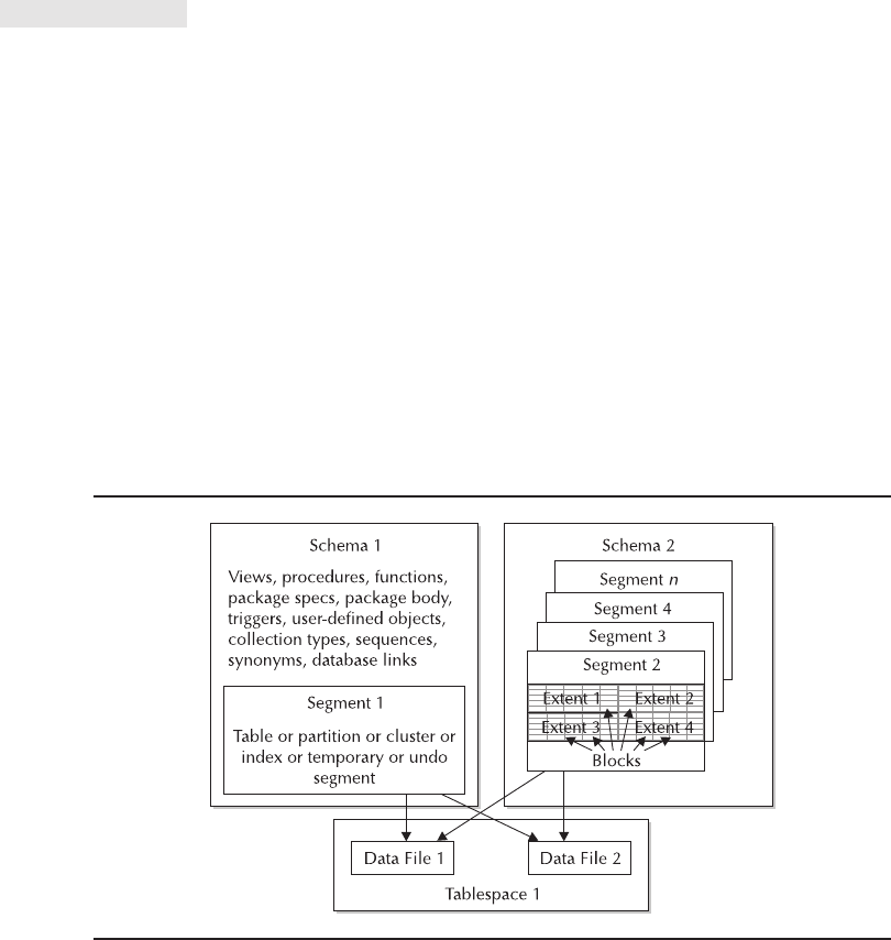
purchase the service, is invaluable. Oracle alert logs and dump files will also help
you greatly. Experience will be your biggest ally here and the sooner you dive into
database support, the faster you will progress.
You’ve seen the areas of database management that need to be handled; now
it’s time to look at the Oracle schema and storage infrastructure.
CRITICAL SKILL 6.3
Understand the Oracle Database 11g
Infrastructure
Oracle’s memory and process infrastructure have already been discussed in Chapter 1.
In this section, you will take a look at the Oracle schema and storage infrastructure,
since these are a large part of what you will be required to manage.
Schemas
An Oracle database can have many schemas contained in it. The schema is a logical
structure that contains objects like segments, views, procedures, functions, packages,
triggers, user-defined objects, collection types, sequences, synonyms, and database
links. A segment is a data structure that can be a table, index, or temporary or undo
segment. The schema name is the user that controls the schema. Examples of schemas
are the SYSTEM, SYS, SCOTT, and SH schemas. Figure 6-1 shows the relationship
between these schema objects.
212 Oracle Database 11g: A Beginner’s Guide
FIGURE 6-1. The database and user schemas
Chapter 6: The Database Administrator 213
Segments, Extents, and Blocks
As you can see in Figure 6-1, a schema can have many segments and many segment
types. Each segment is a single instance of a table, partition, cluster, index, or
temporary or undo segment. So, for example, a table with two indexes is implemented
as three segments in the schema. A segment is broken down further into extents,
which are a collection of contiguous data blocks. As data is added to Oracle, it will
first fill the blocks in the allocated extents and once those extents are full, new extents
can be added to the segment as long as space allows. Oracle segment types are
listed here:
■Tables. This is where the data is kept in rows and columns. This is the heart
of your database with tables implemented in one schema and one tablespace.
The exception to this is a special type of table called a partitioned table,
where the table can be split into different ranges or sets of values called
apartition, with each partition implemented in a different tablespace.
Remember, however, that each partition is itself a segment and each
segment can only reside in one tablespace. Clustered tables are another
special case where two tables with a close link between them can have
their data stored together in a single block to improve join operations.
■Indexes. These are optionally built on tables for performance reasons and to
help implement integrity constraints such as primary keys and uniqueness.
■Temporary segments. Oracle uses these as a temporary storage area to run
a SQL statement. For example, they may be used for sorting data and then
discarded once a query or transaction is complete.
■Undo segments. These are used to manage the before image of changes,
which allows data to roll back if needed and helps provide data consistency
for users querying data that is being changed. You’ll learn more about this
in Chapter 7.
Segments can be thought of as physical structures since they actually are used to
store data that is kept in a tablespace (although some of this is temporary in nature).
There are other structures stored in the schema that are more logical in nature.
Logical Schema Structures
Not everything stored in a database and schema is data. Oracle also manages
source modules and supporting structures (such as sequences) that are used to
populate new unique and primary key values when inserting data into the database.
These objects belong to a schema and are stored in the Oracle Catalog. These, as
well as view properties of the objects, can all be easily managed through OEM, as
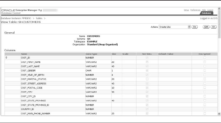
214 Oracle Database 11g: A Beginner’s Guide
shown in Figure 6-2. Take a look at the following for a brief description of these
logical structures:
■Views. These give you the capability of subsetting a table and combining
multiple tables through a single named object. They can be thought of as
astored query. With the exception of a special type of view called a
materialized view, which is used for data warehousing, data is not stored
in views. They are simply a new way of defining access to the underlying
tables. These can be used for security, performance, and ease-of-use.
■Synonyms. These are used to create a new name or alias for another
database object such as a table, view, another synonym, and sources such
as a procedure, package, function, java class, and so on. They can be used
to simplify access. As with views, data is not stored in a synonym.
■Sequences. These are used to generate new unique numbers that can be
used by applications when inserting data into tables.
■Source programs. These can be stored in the catalog and written either in
Oracle’s proprietary PL/SQL or in Java. PL/SQL source types include business
logic that can be written as Packages, Procedures, and Functions. Triggers
can also be used to implement business logic, but are often used to implement
data integrity since they are not executed directly by a user or source
program, but rather are automatically executed when an action is performed
on the database. Java Sources and Java Classes are also implemented directly
in Oracle. This server-side support of application logic improves performance
since the logic resides with the data and it also improves performance.
FIGURE 6-2. Enterprise Manager table definition view

■User types. These can be created by you to support object-oriented
development. Array types, Object types, and Table types can all be created
by you. Also, the Oracle XML Schema Processor supports XML processing
by adding data types to XML documents that can be used to ensure the
integrity of data in XML documents.
So now that you have seen all of the schema objects, it’s time to tie these
together to your storage architecture.
Storage Structures
As shown earlier in Figure 6-1, the physical schema objects are stored as segments
in the database. Each segment can only be stored in a single tablespace, with a
tablespace being made up of one or more data files. If a tablespace is running out
of space, you can expand the data files it is made up of, or you can also add a new
data file to the tablespace. A data file can only store data for a single tablespace.
A single tablespace can store data for multiple segments and in fact for several
segment types. Segments from multiple schemas can also exist in the same tablespace.
So, for example, table_a from schema1 and index_b from schema2 can both be
implemented in the same tablespace. Oh, and by the way, a tablespace can only
store data for a single database.
The logical structures such as views and source code are stored in the Oracle
catalog, but are part of a schema. So, this means that the Oracle-supplied SH
schema can contain all of the objects that it needs to run the entire application
under its own schema name. This provides strong security and management benefits.
Progress Check
1. Name five areas that you will need to address as a DBA.
2. What is a schema and what does it contain?
3. Can a tablespace store more than one segment type?
4. List an example of nondata structures or logical structures in a database.
Chapter 6: The Database Administrator 215
Progress Check Answers
1. As a DBA, you will need to address architecture, capacity planning, backup and recovery, security,
and performance, among other things.
2. Aschema is a logical structure that contains objects like segments, views, procedures, functions,
packages, triggers, user-defined objects, collection types, sequences, synonyms, and database links.
3. A single tablespace can store data for multiple segments and different segment types. Segments
from multiple schemas can also exist in the same tablespace. So, for example, table_a from schema1
and index_b from schema2 can be implemented as two segments in the same tablespace.
4. Source programs such as triggers, stored procedures, functions, and packages are logical
structures. Other examples include views, synonyms, sequences, and types.

216 Oracle Database 11g: A Beginner’s Guide
CRITICAL SKILL 6.4
Operate Modes of an Oracle Database 11g
Oracle is a software package like many others that you may have used. However,
when you run most programs, they run one and only one way. So, when I open my
accounting software, I run it the same way all the time. However, you have options
with Oracle. This section discusses the many ways that you can run Oracle. Some
of these methods will be important to administrators, while others will allow for full
use. This feature is important when you need to perform both critical and noncritical
activities, and not interfere with your users or your data.
Modes of Operation
Oracle has several modes of operation. In most cases, when you start Oracle, you
will simply issue the command:
> Startup;
This command actually takes Oracle through three distinct startup phases
automatically, though you can also choose to explicitly step through these phases:
1. nomount phase In this phase, the database reads the spfile or the init.ora
parameter file and starts up the Oracle memory structures as well as the
background processes. The instance is started, but the database is not yet
associated with the newly started instance. This is usually used in cases where
you need to re-create the control file. The command to perform this is
> startup nomount;
2. mount phase You use this phase in order to associate a database with the
instance; the instance “mounts” the database. The previously read parameter
file is used to find those control files, which contain the name of the data
files and redo logs. The database is then mounted to allow some maintenance
activities to be performed. Data files and redo logs are not opened when
the database is in mount mode, so the database is not yet accessible by end
users for normal tasks. Commands to mount a database are
> startup mount;
> alter database mount;
3. open phase This is when Oracle opens the data files and redo logs, making
the database available for normal operations. Your redo logs must exist in
order for the database to open. If they do not, the resetlogs command must
be used to create new redo logs in the location specified in the control files:
> Startup {open} {resetlogs};
> alter database open;

Chapter 6: The Database Administrator 217
Other Ways to Open the Database
There are other options for opening a database. For example, you may want to open
it in read-only mode so that no database changes (inserts, updates, or deletes) can
be performed. There are also the upgrade/downgrade options that allow a database to
be opened to perform a downgrade or upgrade to another version of Oracle:
> alter database open read only;
A common option you will use to perform maintenance will be to open the
database in restricted mode. When you issue the command startup restrict, only
users with both the create session and restricted session privileges will be able to
use the database. So, as a DBA this is a helpful way to open the database that only
you can use:
> startup restrict;
The database can be placed in a state where only the sys and system users can
query the database without stopping the database and performing a subsequent
startup restrict. The activities of other users continue until they become inactive.
This can be performed using the quiesce option of alter system when the Database
Resource Manager option has been set up:
> alter system quiesce restrict;
> alter system unquiesce;
Forcing a Startup
Over time, you will run into situations where Oracle has not shut down properly and
you are unable to restart it. In these rare instances, you will need to use the force
option of the startup command. This will first perform a “shutdown abort,” which
forces the database to shut down (see the next section for more information on this)
followed by a database startup:
> startup force
Database and Instance Shutdown
When shutting down an instance, perform these steps, which are the reverse from
those you just saw when opening a database:
1. Close the database (including the data files and redo logs), so that it is no
longer usable for normal tasks.
2. Unmount the database from the instance so that only the instance memory
structures and background tasks are left running without a database
associated with them.
3. Shut down the instance to close the control files.
218 Oracle Database 11g: A Beginner’s Guide
In order to shut down a database, four different approaches can be used:
shutdown normal, immediate, transactional, and abort.
■Normal is, in a sense, the perfect way to shut down, since this approach
will wait for all users to disconnect from the database and all transactions
to complete before the shutdown occurs. Once this command has been
issued, new users are not allowed into the system. This can be impractical
in cases where users remain on the system for long periods of time:
> shutdown normal;
■Immediate is a practical shutdown approach that also leaves the database
in a consistent state. When the database is put through a “shutdown
immediate,” all current transactions are rolled back and users are
disconnected. No new transactions are allowed into the system. This will
be relatively quick if the rollback operations are small and it’s an excellent
way to shut down the database before performing a database backup:
> shutdown immediate;
■Atransactional shutdown is similar to the immediate variety except that
running transactions are allowed to complete. So, once transactions have
been committed, the user running it is disconnected. This is useful in cases
where you do not want to shut down until currently running transactions
have finished or in cases where it will be quicker to complete existing
transactions than it will be to roll them back:
> shutdown transactional;
■Abort is the least graceful shutdown option of the four. When this is used,
all transactions are ended immediately without waiting for a rollback or
commit and all users are instantly disconnected while the database is
brought down. Use this only if you are experiencing problems shutting
down the database using one of the three options described previously or in
cases where you need to shut down the database immediately. The
database needs to go through recovery procedures the next time it is
restarted. After a shutdown abort has been performed, you should try to
immediately start up the database so that you can then perform a shutdown
(normal, immediate, or transactional) to bring the database down in the
proper manner:
> shutdown abort;
OEM can help with instance and database startup and shutdown, as shown in
Figure 6-3. First, open OEM in a web browser. Then, on the Home tab under the
General section, choose Shutdown (or Startup, depending on if the database is
currently running). The advanced options allow for the different types of shutdown.
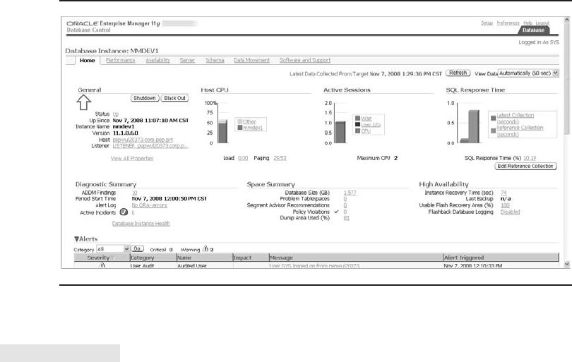
CRITICAL SKILL 6.5
Get Started with Oracle Enterprise Manager
Oracle Enterprise Manager (OEM) is a great tool for assisting the beginner DBA to
become an experienced one. You should, however, also learn the low-level
commands that will allow you to do your job through an interface like SQL*Plus.
OEM can help you with this by showing you the SQL that it has generated when you
select the Show Sql button that exists on many windows. Given how many options
OEM has to help you do your job as a DBA, you should take a quick look at them
here.
Oracle Enterprise Manager can be used to manage all of the aspects of the
databases. As shown in Figure 6-3, you can see the Home page of Enterprise
Manager and details about the current state of the database. The tabs show the
different areas of database that can be managed for performance, availability,
server, schema, and data movement.
Instance Configuration
Figure 6-3 shows you the state of an instance and server. By selecting the Server tab
from the Home page (shown later in Figure 6-6), you can see different areas to
manage the parameters, memory settings, recovery options, resource monitors in
effect, and undo information.
Chapter 6: The Database Administrator 219
FIGURE 6-3. Enterprise Manager Home page view

User Sessions
Now that you have a good handle on managing instances and databases, you can
drill down to your user sessions to see exactly what is going on inside the database.
By choosing a session, you can see some general information such as the user
session ID, when the user logged in, and what the OS username and terminal name
are for this user. As you can see from Figure 6-4, you can also see the SQL that is
currently running, along with the explain plan being used. You can follow the order
that each explain step is being performed in by the Step # column and can step
through the plan or see it in a graphical layout using the far right column. You can
also manage sessions and disconnect users by right-clicking the username and
issuing the kill session command. The command name may sound a bit harsh,
but it does get the idea across.
Resource Consumer Groups
Next, you can select the Resource Consumer Groups item to see all of the groups
that exist. A resource consumer group provides a way to group together users so
that they can share similar processing requirements. The DATABASE_RESOURCE_
MANAGER package is used to allocate the maximum amount of CPU that a session
can use or to set a limit for parallel execution for a session or to set the number of
sessions that can be active for a consumer group as a few examples of this capability.
OEM can assist in managing these groups by giving you an easy way to add new
220 Oracle Database 10g: A Beginner’s Guide
FIGURE 6-4. SQL explain plan
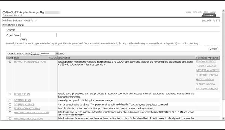
groups and edit those that exist. This panel allows you to enter a description of the
group and attach users and database roles to a group. If you look at Figure 6-5,
you will see all of the resource consumer groups listed. If you select one of these
consumer groups, you will be presented with the capabilities to manage users, roles,
and general information about the group.
A resource plan builds on the resource consumer groups by providing a way to
define the way that system resources will be allocated to the resource consumer
groups that we just discussed. Figure 6-5 shows a list of the groups and subplans
that can be set up here. Also in the figure you can see the tabs to define other
options, such as maximum parallelism, concurrently active sessions in the session
pool, undo pool space, and execution time limits for the group. Group switching
allows for a session to change groups after a predefined amount of execution time
has been reached. Presumably, you would move the user to a lower priority group
to free resources to other sessions. The resource plan schedule can be used to set
daily schedules to enable and disable resource plans.
Schema, Security, and Storage Management
The next items on the OEM console are schema, security, and storage management.
We will visit these in Critical Skill sections 6.6, 6.7, and 6.8–6.9, respectively. It is
worth mentioning now, however, that all three of these can be completely managed
through OEM.
Chapter 6: The Database Administrator 221
FIGURE 6-5. Enterprise Manager resource group view
222 Oracle Database 11g: A Beginner’s Guide
Distributed Management
Some Oracle distributed capabilities are handled through the Distributed option.
These include the ability to
■Manage in-doubt transactions that can result from two-phase commit.
■Create, edit, and drop database links.
■Use streams to implement messaging.
■Use advanced queues and replication to pass messages and data to applications.
This can be a difficult area to manage and having a tool such as the OEM
Console to help you out with this is a very welcome feature.
Warehouse Features
Warehouse options such as summary management, materialized views, and
dimensions can all be dealt with through OEM, as was shown in Figure 6-5.
Other Tools
The Server tab from the Home page, shown in Figure 6-6, will take you to a list of
different tools. This includes more advanced tools for managing the environment.
Let’s very quickly review the tools that are included here:
■Database tools enable you to analyze data and performance, and manage
tablespaces and parameters. The backup and recovery tools are available
under the Availability tab. Statistics management is also an important
area for running statistics and getting information about the workload
repository.
■Oracle Scheduler provides tools to set up jobs and manage schedules. Job
classes can be set up here, as well as standard maintenance jobs to be
automated.
■Tuning facilities such as performance manager, outline management, and
tablespace maps are provided through Query Optimizer.
As you can see from this overview of OEM console capabilities, many of the
tools that you need to perform your day-to-day tasks can be found in this one
console. Now that you have confidence that there’s a toolset to support you,
let’s take a quick look at what you need to think about when managing database
objects.
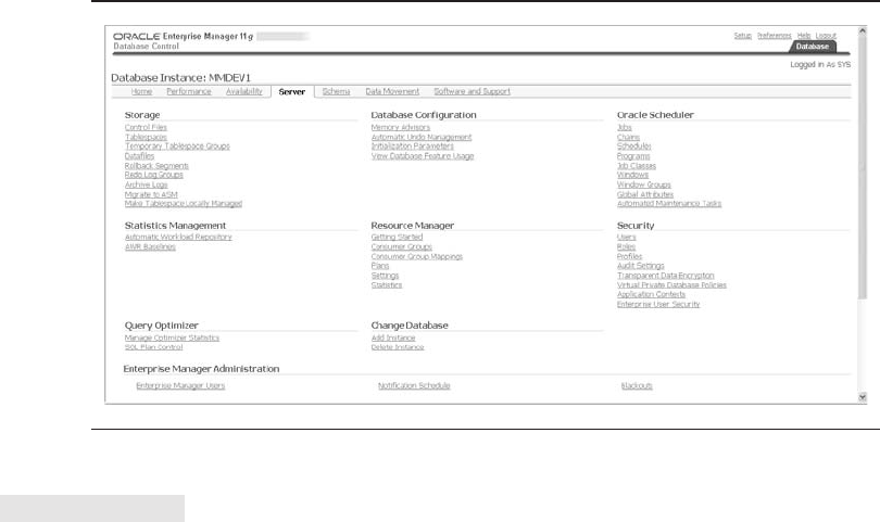
CRITICAL SKILL 6.6
Manage Database Objects
A large part of your job as a DBA will be to manage the objects that exist in a
database. Let’s look at the objects that you need to concern yourself with and
discuss the main management issues that you will have in each of these areas.
Control Files
It is critical to the database that you have at least one valid control file for your
database. These are small files and can be multiplexed by the Oracle instance.
Ensuring that you have at least three copies of the control files (remember, they
are small), as well as text and binary backups whenever a data file, log file, or
tablespace is changed and on a regularly scheduled basis (at least daily), will go a
long way towards ensuring that your control files are in good shape. Control files
will be discussed in more detail in Chapter 7.
Redo Logs
Redo logs are necessary to ensure database integrity and should be duplexed in
Oracle. Oracle mirroring helps even if your redo logs are mirrored by your storage
subsystem since Oracle will use the alternate redo log if one should become
corrupt. You will need to ensure that you have enough redo logs and that they are
sized properly to support database performance. How large should your redo logs
be? They should be large enough that a log switch does not usually occur more than
once every 15 minutes due to the checkpointing that occurs during a log switch and
the overhead that is incurred during this operation. How many redo logs should you
Chapter 6: The Database Administrator 223
FIGURE 6-6. Enterprise Manager Server tab view with configuration options
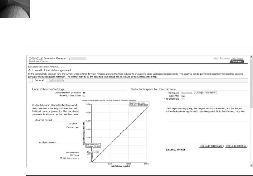
have? You should have enough redo logs that the system will not wrap around to a
log that has not yet completed a checkpoint or completed archiving (for systems in
archivelog mode). Redo logs can be added, deleted, and switched through OEM.
Undo Management
The Undo segment is where the before images of changed rows are stored. Oracle
will manage your undo segments for you, but you need to determine how large to
make the tablespace that the Undo segment is stored in. The size that you make this
depends on the length of time that you want the undo information to be available to
you. If you look at Figure 6-7, you will see how OEM helps you determine the
length of time that Undo can be retained, based on the system activity and Undo
tablespace. This is in the Configuration section for an instance. If the tablespace is
not the correct size, it can be changed using the Storage feature of OEM, which you
will see later in this chapter.
If you choose to implement user-managed rollback segments, then these can be
managed in the Storage section of OEM by choosing Rollback Segments and then
selecting the segment name that you want to manage.
NOTE
When using user-managed rollback segments, the
system rollback segment will always exist, but
should never be used as a rollback segment for
user processes.
224 Oracle Database 11g: A Beginner’s Guide
FIGURE 6-7. Enterprise Manager Automatic Undo Management view

Chapter 6: The Database Administrator 225
Schema Objects
Schema objects were discussed earlier in this chapter where you saw that you can
manage schema objects through OEM. There are also some things that you may
want to do with your own SQL scripts that run as scheduled jobs. When managing
schemas, you need to ensure that those physical objects that take up a great deal of
space do in fact have enough space to grow. These include tables, indexes, clusters,
and partitioned tables. Manage these objects through the tablespaces where they are
implemented and ensure that there is enough room to grow. Just because an object
may have hundreds of extents doesn’t mean that a reorganization of the object is
necessary. You only need to reorg if there are a large number of chained or
migrated rows. It is also possible for the reorgs to gain back unused space. Indexes,
on the other hand, will need to be rebuilt more frequently and do provide some
performance benefits. These rebuilds and reorganizations of indexes can normally
be done online and are easy to take care of during a time when there is not much
going on in the database. You will find out more about managing space
in the next section.
Figure 6-2, seen earlier, is an example of how the SH.Customers table can be
managed through OEM. Note the Storage tab that allows you to change the table’s
storage parameters. You should also try to maintain statistics on your tables and
indexes so they are up-to-date. This will assist the optimizer make better decisions
when choosing access paths for your queries and can be used to validate the
structures. In Oracle Database 11g, a scheduler job called gather_stats_job will run
during a maintenance window between 10:00 P.M. and 6:00 A.M., by default, and
will run statistics for those objects in cases where they have not been collected yet
or are stale, which are statistics that are old due to recent changes in data. Setting
the Oracle Database 11ginitialization parameter statistics_level to typical (the
default) will allow Oracle to automatically update statistics as a background task on
a regular basis and is the recommended approach for gathering statistics. In
pre–Oracle Database 11greleases, the DBMS_STATS package should be run
manually or it can be turned on at a table level by using the Monitoring keyword in
a CREATE or ALTER table. Monitoring is a deprecated feature in Oracle Database
11gand the keyword (along with “nomonitoring”) will be ignored.
Triggers, views, synonyms, procedures, functions, and packages are logical
schema objects that do not take up a lot of space in the tablespace; however, these
objects need to be watched to ensure they are not invalid. They can become invalid
with an ALTER table statement or changes in structure to any dependent objects.
These objects should be valid, and you can check this with the SQL statement that
follows:
select owner, object_name, object_type
from dba_objects where status ^= 'VALID';
You’ve looked at many of the database objects that will require your attention. Let’s
now explore one area that requires special attention due to the size of today’s databases.

226 Oracle Database 11g: A Beginner’s Guide
CRITICAL SKILL 6.7
Manage Space
The challenge of managing data in your Oracle Database 11gis one that provides
you with options. In this section, you will look at the methods that have been used
in the many versions of the database to manage your information. Today’s version
of the database provides you with options. The first that you will discuss is managing
your data and the files in which they reside in a manual way. Another option,
Automatic Storage Management, is discussed in Chapter 8.
Ask the Expert
Q: Why is it important for DBAs to get involved with the architecture and
design of a new system?
A: Decisions made on the technical infrastructure as well as data and
application designs will have a large impact on database performance and
scalability. Database knowledge will help choose a better technical
implementation. Once chosen, these can be difficult to change.
Q: Which method do you normally use to shut down a database?
A: Although the shutdown normal operation is a recommended approach, it is
often impractical since you need users to disconnect themselves. The approach
that we prefer is to perform a checkpoint using the command alter system
checkpoint, which will write data out to data files and speed up the restart.
Then perform a shutdown abort, immediately followed by a startup restrict and
shutdown immediate. This is a fast, guaranteed shutdown that leaves the database
in a consistent state once all of the steps have been completed.
Q: What is the best way to become a good Oracle DBA quickly and then to
keep improving?
A: There are many things that you will need to do and many skills that you’ll
need to develop to do this job. First, learning the basic DBA skills, which you can
get from books such as this, as well as from courses, will give you a head start.
Practicing what you see is probably the quickest and most practical way to learn.
Getting involved in supporting some databases in development and production
will force you to learn very quickly. Then, working on development systems for
different types of applications will help to round out your skills. Keep reading
and learning and never assume that you know it all and you will do very well.
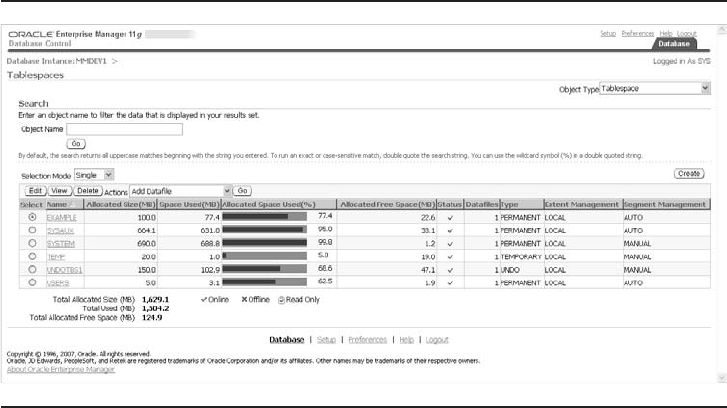
Archive Logs
When you put the database in archive logging mode, the redo logs are written out
to a directory that is named in the SPFILE. If that directory becomes full and the
database attempts to write another archive log, the database activity will be suspended
until sufficient space is made available for the new file. Create a large directory and
schedule jobs to move the archive log files from online storage to tape before you
encounter a space issue. Recovery Manager (RMAN), a utility used for backup and
recovery, does a nice job of helping you manage this. Please see Chapter 7 for more
information on backing up the archive log files to tape and managing these files.
Tablespaces and Data Files
Space should be managed at the data file and tablespace level rather than at a lower
level such as a table or index. Using locally managed tablespaces with uniform extent
sizes will simplify your management. Do not worry that you have multiple extents
in a tablespace or for an object. This does not create a performance issue since the
extents contain a number of blocks that must be contiguous, and the extents will be
reused and created as needed. You can see the amount of space available in your
data files or tablespaces in OEM, as in Figure 6-8. This shows the amount of free
space available in the currently allocated space. If you have used the autoextend
feature to allow a data file to extend in size when more space is needed, the extra
space is not shown in this graph.
Chapter 6: The Database Administrator 227
FIGURE 6-8. Tablespace view in Enterprise Manager

TIP
Do not autoextend temporary and undo tablespaces,
since they will quickly grow to use all of the space
to which they can autoextend.
What do you do if you run out of space in a data file? Just enter OEM, click the
data file, and choose the Storage tab. Once there, you can change the autoextend
feature and enter the size of the extensions that you would like. Do not forget to
limit the size of the data file so that it doesn’t grow until it uses all of your space.
After you’ve completed this, click Apply and you’re done. If you select the Show
SQL button, you can see the alter database syntax, which is also shown next:
alter database datafile '/u01/oradata/ora11g/example01.dbf'
autoextend on next 50M maxsize 5000M;
You can write your own scripts to compare the amount of allocated space for
a data file in view dba_data_files to the amount of free space, as shown in view
dba_free_space.
OEM also provides you with a more detailed map of how space is used. In
OEM, select a tablespace and then navigate from Tools to Tuning Features, finally
choosing Tablespace Map. This opens a graphical layout showing each segment in
the tablespace. From the tablespace map, you can choose the Tablespace Analysis
Report tab for a written report on the space being used.
Managing the database objects discussed earlier will be a large part of your role
as a DBA. In the next section, you’ll take a look at setting up and managing users.
After all, without database users, there is no point in doing any of this!
Progress Check
1. What’s better: shutdown transactional or shutdown immediate?
2. Do you only need to worry about logical schema objects that take up a
large amount of space?
3. What happens if your archive log directory becomes full?
4. Why would you want to use a command-line interface rather than a GUI to
perform your tasks as a DBA?
5. Under what circumstances would you bother to start up the database in
nomount mode?
228 Oracle Database 11g: A Beginner’s Guide

CRITICAL SKILL 6.8
Manage Users
Before you can do anything in Oracle, you need to have a user ID created to enable
you to log into Oracle. As a DBA, you will begin with the SYS or SYSTEM accounts
since these accounts both have the DBA role and exist in all Oracle databases. They
are often used to perform database administration tasks. The SYS account is also
granted the sysdba privilege and is the schema that the Oracle catalog is stored in.
You should only use the SYS account when you need to perform a task as SYS or
need the sysdba privilege. If your database was created using the Database
Configuration Assistant (dbca), then you will also automatically get the SYSMAN
and DBSNMP accounts. SYSMAN is used to administer Oracle Enterprise Manager
(OEM) and DBSNMP is used by the agent that OEM employs to monitor Oracle
databases. Several other accounts will also be set up for the “example” schemas,
such as the Sales History ('SH') user that you will see utilized throughout this book.
The OUTLN schema will be created to allow you to use query plan stability through
the stored outline feature.
Depending on the options you choose when creating your database, other
accounts may be set up for you. For example, if you install the OLAP option, the
OLAPSYS account will be created.
Create a User
When you create a user, you can use either the create user syntax or the OEM,
which is an easier approach. In order to create a user, you will need to decide the
following:
■The default tablespace where segments created by this user will be placed
unless a tablespace name is used in the DDL to override this.
Chapter 6: The Database Administrator 229
Progress Check Answers
1. Both leave your database in a consistent state. It depends on how long your transactions will take
to complete or roll back. If all things are equal, and you think that it will take as long to commit the
transactions that are already running, then you should use “shutdown transactional” since commits
will be allowed to complete and no data will be lost.
2. No; logical schema objects also need to be watched to ensure they are in a valid state.
3. If database attempts to write an archive log after the directory has become full, the database
activity will be suspended until sufficient space is made available for the new file.
4. You may want to place the command in a script that is scheduled or run as a repetitive task.
5. When started in nomount mode, the parameter file is read, and memory structures and processes
are started for the instance. The database is not yet associated with the instance. You would use this
in circumstances when you need to re-create the control file.

230 Oracle Database 11g: A Beginner’s Guide
■Whether to expire the password so that the user needs to change it the first
time they log into Oracle.
■A temporary tablespace to store internal data used by Oracle while queries
are running. Sort operations make use of the temporary tablespace if there
is not enough room in the SGA to perform the sort operation.
■Whether to employ user quotas on tablespaces, which put a limit on the
amount of space that a user’s objects can take up in that tablespace.
■The authentication type, which allows you to specify whether you want
Oracle to force the user to specify a password when they log in, or you
can trust the operating system to do this for you.
■The initial password that the user will log in with. The user must change
this during the first logon if you chose to expire the password in advance
of the user’s first logon.
■Privileges to grant to the user. These can be direct privileges or roles. You’ll
see these discussed in the next section.
■A profile for the user, which can be employed to manage the user’s session
by limiting resources that sessions can use, and that help implement
corporate password policies. You will also see this in the next section.
■The account status of the user (lock or unlock) as it is created.
The OEM console in Figure 6-9 shows the options available to you to create and
edit a user. For each user, there are eight separate tabs that allow you to easily enter
a user’s information. You can see the SQL that will be generated by selecting the
Show SQL button at the bottom of the panel. Another great option allows you to
model a user and create another user like one that already exists. To do this, click
the user that you want to model, select Object from the top of the panel, and then
select the Create Like option.
Here is a sample CREATE USER statement:
CREATE USER "NEWUSER" PROFILE "DEFAULT" IDENTIFIED BY "newpassword"
PASSWORD EXPIRE DEFAULT TABLESPACE "USERS" TEMPORARY TABLESPACE "TEMP"
QUOTA UNLIMITED ON TEMP QUOTA UNLIMITED ON USERS
ACCOUNT UNLOCK;
GRANT "CONNECT" TO "NEWUSER";
Edit Users
Once a user has been created, you will be asked at different times to alter it in order
to change quotas or reset passwords or unlock an account. This can be easily performed
through OEM by selecting the User, choosing the option you want to change through
the GUI, and then applying the change.
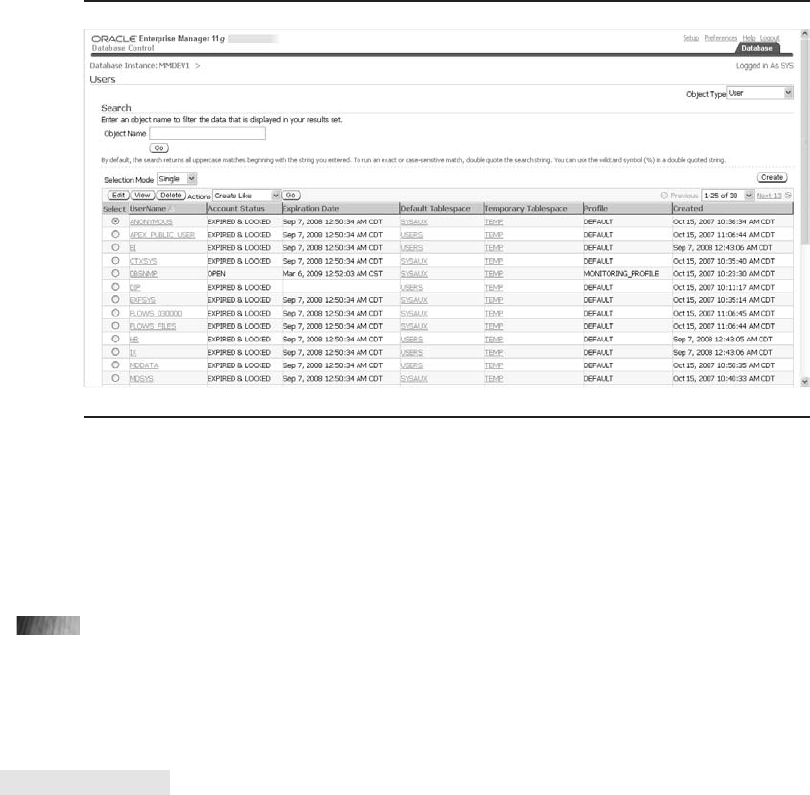
Editing users can also be performed using the ALTER USER statement, as shown
next, where a user account is unlocked, the password is changed, and a tablespace
quota is increased:
ALTER USER "username" IDENTIFIED BY "newpwd" QUOTA UNLIMITED
ON TOOLS ACCOUNT UNLOCK;
You’ve now created a user and it’s time to grant them some privileges. Let’s see
how you do this in the next section.
CRITICAL SKILL 6.9
Manage Privileges for Database Users
Creating a user in Oracle has accomplished the first part of user setup, which is
authentication. You have a user ID and password and have authorized this user to
use an Oracle database. Once the user logs in, however, they will not be able to do
very much because they will not have privileges that allow them to access any objects.
This leads you to the second step of setting up a user: authorization. In order to
authorize a user to perform their tasks, you need to grant access.
Chapter 6: The Database Administrator 231
FIGURE 6-9. User Management view

232 Oracle Database 11g: A Beginner’s Guide
Grant Authority
You now need to give permission to the user to do things in Oracle. Actions like
accessing a table or executing a procedure or running a utility require you to “grant”
the authority to that user. When you perform a grant, you can specify four things:
■The user that is being granted the authority.
■The object that is being granted. Examples of these are a table, procedure,
or role.
■The type of access being granted, such as select, insert, update, or delete on
a table, or execute on a procedure, function, or package.
■Whether this user has authority to then grant the same authority to other users.
By default, they do not, but this can be added by using the With Grant option.
Here are two examples that grant a user “NEWUSER” access to a table and then
to a package:
GRANT SELECT ON "TABLE_NAME" TO "NEWUSER" WITH GRANT OPTION;
GRANT INSERT ON "TABLE_NAME" TO "NEWUSER" WITH GRANT OPTION;
GRANT EXECUTE ON "PROCEDURE_NAME" TO "NEWUSER"
Types of Grants
There are two types of grants that can be given to a user: system privileges and
object privileges.
■System privileges are predefined Oracle privileges granting authority to
overall system objects; for example, using ANY or ability to execute types of
statements rather than relating to an individual object or schema. The ability
to perform a create tablespace, create session, or alter system or to back up
any table are just a few examples of some system-level privileges that can be
granted to a user. There are over 150 different system privileges, which can
be viewed by looking at the DBA_SYS_PRIVS view.
■Object privileges are a lower-level authority where a named object is
granted to a user. So, the ability to perform an operation on a particular
table, or execute an individual function, package, or procedure is an object
privilege, as opposed to the ability to execute any procedure or select any
table, which is a system-level privilege.
Take Away Authority
What is given can be taken away. In order to take privileges away from a user, you
use the REVOKE command; the syntax is very similar to the syntax you use when
issuing a grant. Here are two examples of a REVOKE operation:

Chapter 6: The Database Administrator 233
REVOKE INSERT ON "TABLE_NAME" FROM "NEWUSER";
REVOKE EXECUTE ON "TABLE_NAME" FROM "NEWUSER";
Roles
When you think of the number of privileges that need to be managed in situations
where you have thousands of database objects as well as thousands of users, you
quickly realize that it would be nice to organize the privileges into groups that can
be easily managed. This is where roles come into play.
A “role” is used to group privileges together into a predefined group that can be
granted to users. So, rather than granting object and system privileges individually to
every user in your system, you can grant them to a role, which in turn is granted to
the user. With the amount of system privileges that can be granted as well as several
thousand objects that could be in a schema, using roles makes it at least a little easier
to manage grants and permissions.
Oracle-defined Roles
Some special roles are created by Oracle through the install process or by running
Oracle-supplied scripts. The DBA, Connect, Resource, Imp_Full_Database, and
Select_Catalog_Role are some examples of roles that are supplied by Oracle and
should not be changed.
Create and Grant a Role
Roles are created using the create statement in the same manner as creating users.
You can also revoke privileges from roles and drop roles when they are no longer
needed. Roles can also be granted to other roles. You can see an example of this
next where the Oracle role CONNECT is granted to the newly created role TESTROLE,
along with a system and object privilege:
CREATE ROLE "TESTROLE";
GRANT CONNECT TO "TESTROLE"
GRANT EXECUTE ANY PROCEDURE TO "TESTROLE"
GRANT SELECT ON "table_name" TO "TESTROLE"
The new role can then be granted to a user as shown next, where TESTROLE is
granted to user TESTUSER:
Grant "TESTROLE" to "TESTUSER";
The TESTROLE is then dropped since it is no longer required:
DROP ROLE "TESTROLE";
Now that you’ve created users and roles, you can fine-tune our management of
these by implementing some user policies through profiles, which you will explore next.

234 Oracle Database 11g: A Beginner’s Guide
Profiles
A profile can be used to implement the management for strong passwords as well as
establish limits in resources for a user. When you created the user NEWUSER earlier,
a password was supplied along with the DEFAULT profile. Using this DEFAULT
profile, the user never needs to change their password and there are no limits placed
on any system resources. You can create new profiles to implement your corporate
password policies in Oracle. For example, you can specify the number of days after
which a user must change their password. You can also establish a rule where a
password cannot be reused within a certain period of time and must contain a
certain number of changes. A function can be used to ensure that a complex password
is created by the user. For example, you may require that a password be more than
eight characters long, use alpha, numeric, and special characters, and that it does
not repeat a character more than twice. This can all be implemented in a function.
An account can be locked after a specified number of login attempts and can
remain locked for the number of days defined in the profile.
System limits for a user can also be implemented by a profile. These include
limiting system resources such as those for CPU, connect, and idle time as well as
the number of sessions employed by the user, limits on reads, and the SGA used.
You should note, however, that the Database Resource Manager is the preferred
way to limit resources and that you should use profiles to manage passwords.
The following is an example of the creation of a new profile that will lock an
account after three failed login attempts and will keep the account locked indefinitely.
The password needs to be changed every 60 days and the new password will be
verified by your custom function COMPLEX_PASSWORD. The old password cannot
be reused for 120 days:
CREATE PROFILE "NEWPOLICY"
FAILED_LOGIN_ATTEMPTS 3
PASSWORD_LOCK_TIME UNLIMITED
PASSWORD_LIFE_TIME 60
PASSWORD_REUSE_TIME 120
PASSWORD_VERIFY_FUNCTION COMPLEX_PASSWORD
Now, let’s add this profile to user NEWUSER:
ALTER USER NEWUSER PROFILE NEWPOLICY;
Tie It All Together
As you have seen in this chapter, there is a great deal that a DBA needs to be aware
of to properly manage a database. The good news is that you will have tools such as
OEM to help you. Do your best to keep your environment as simple as you possibly
can! You will be glad that you did as your overall database environment continues
to grow.

Project 6-1 Create Essential Objects
This project will walk you through the creation of the essential storage and schema
objects after a database has been created, which in this project will be called
ora11g. You will create a new tablespace called NEW_TS and will then add a user
NEW_USER who will be given a quota for this tablespace in order to be able to
create objects in the tablespace. You will then create a role called NEW_ROLE and
grant privileges to it. Afterward, you’ll grant this role to the new user. A table and
index will be created on this tablespace by the new user. Lastly, you will resize the
undo tablespace to make it larger. You will see how to do this in OEM and the
generated SQL will also be shown to you so you can do this in SQL*Plus.
Step by Step
1. You have been asked to create a new user named NEW_USER who will
need to create objects in a new tablespace called NEW_TS that should be
sized at 5MB. Your first step will be to create the tablespace. In OEM, log
in as user SYSTEM, go to database ora11g, choose storage, then choose
tablespace and select an existing tablespace to model. Under Objects in the
toolbar, select the Create Like option to model your new tablespace after
the existing one. Enter the new tablespace name, data file name, and all
properties including the size. Make this a locally managed tablespace 5MB
in size with uniform extents 96KB in size. If you choose the Show SQL
button, you will see the generated SQL. It should look something like the
following SQL. You can either apply the change in OEM or you can copy
and paste the generated SQL and run it in SQL*Plus:
CREATE TABLESPACE "NEW_TS" LOGGING
DATAFILE 'C:\ORACLE\ORA11\ORA11g\NEW_TS1.ora' SIZE 2M
REUSE AUTOEXTEND ON
NEXT 1280K MAXSIZE 32767M EXTENT MANAGEMENT LOCAL
UNIFORM SIZE 96K SEGMENT SPACE MANAGEMENT AUTO;
2. Now you will create NEW_USER. As with the preceding tablespace creation,
you can model an existing user. In OEM, go to Security and then to User,
choose an existing user to model, and select Object from the toolbar. Once
again, use the Create Like feature. The user should now have a password of
new_password, which will be unlocked. Set the default tablespace to NEW_TS:
CREATE USER "NEW_USER" PROFILE "DEFAULT" IDENTIFIED
BY "new_password" PASSWORD EXPIRE DEFAULT TABLESPACE "NEW_TS"
TEMPORARY TABLESPACE "TEMP" QUOTA UNLIMITED ON "TEMP";
3. Create a role called NEW_ROLE. In OEM, go to security, and then choose
Role. Under Object in the toolbar, select Create and enter the role name:
CREATE ROLE "NEW_ROLE" NOT IDENTIFIED;
Chapter 6: The Database Administrator 235
Create Essential Objects
Project 6-1
(continued)
4. Grant the CREATE TABLE system privilege, the OLAP_USER role, and
the object privilege SELECT on table SQLPLUS_PRODUCT_PROFILE to
NEW_ROLE. In OEM, go to Role and choose NEW_ROLE. Use the tabs
System, Object, and Role to choose the objects listed here. Click the Apply
button to make the changes. The generated SQL will look like the three
grants listed next:
GRANT CREATE TABLE TO "NEW_ROLE";
GRANT SELECT ON "SYSTEM"."SQLPLUS_PRODUCT_PROFILE"
TO "NEW_ROLE";
GRANT "OLAP_USER" TO "NEW_ROLE";
5. Grant NEW_ROLE and connect to NEW_USER. Also, give NEW_USER
an unlimited quota on NEW_TS to allow for objects to be created in the
tablespace. In OEM, navigate to Users and choose NEW_USER. Once
there, choose the Role tab and select NEW_ROLE, and then select the
down arrow. Click the Apply button to make the change:
GRANT "NEW_ROLE" TO "NEW_USER";
ALTER USER "NEW_USER" DEFAULT ROLE ALL;
ALTER USER "NEW_USER" QUOTA UNLIMITED ON "NEW_TS";
6. You will now log into the database as NEW_USER and can use OEM with
the NEW_USER account. Once in OEM, you will create a table called
NEW_TABLE with columns col01 as number(15) and col02 as varchar2(30).
In OEM, in the toolbar, select Object and under that choose Create, and
then choose Table. Make sure the table is created in NEW_TS. Follow the
screens to add col01 and col02. You will then create a primary key called
NEW_TABLE_PK using col01. Follow the screens and choose the options
you would like. We recommend that you name any keys and constraints
rather than relying on system defaults. Choose Finish and you have created
a new table with a primary key!
CREATE TABLE "NEW_USER"."NEW_TABLE"
("COL01" NUMBER(15) NOT NULL,
"COL02" VARCHAR2(30) NOT NULL,
CONSTRAINT "NEW_TABLE_PK" PRIMARY KEY("COL01"),
CONSTRAINT "NEW_TABLE_U1" UNIQUE("COL01"))
TABLESPACE "NEW_TS";
7. You now have one last task: resizing the undo tablespace to add 100MB to
it. Log into OEM as user System and choose the data file under the undo
tablespace. Enter the new size and click Apply. It’s as easy as that. The SQL
to increase this from 50MB to 150MB is shown here:
ALTER DATABASE DATAFILE '/u01/oradata/ORA11g/UNDOTBS01.DBF'
RESIZE 150M;
236 Oracle Database 11g: A Beginner’s Guide

Project Summary
This project has taken you through the basic steps of creating an environment for a
new user, including using roles and granting privileges. You’ve seen how to manage
users as well as space and have even created objects. Armed with these capabilities,
you are now on your way to being a productive DBA. Congratulations!
þChapter 6 Mastery Check
1. What is the benefit of a role?
2. Should a table that is in tens or hundreds of extents be reorganized?
3. What is the preferred method for collecting object statistics?
4. What is a segment?
5. What is an extent?
6. Name two reasons for implementing an index.
7. How can you place a database in maintenance mode without first shutting
it down?
8. How can you limit the resources that a particular user can consume, and
how does this work?
9. When managing undo segments, what are the things that you need to think
about?
10. What is likely to happen if you turn on the autoextend property for undo
and temporary tablespaces with a maxsize set to unlimited?
11. What is special about the SYS user account, and how does it differ from
SYSTEM?
12. What are temporary tablespaces used for?
13. What are the two aspects of security that are covered in Oracle’s
implementation?
14. Name and describe the types of privileges that can be granted to a user.
15. How would you implement your corporate password policy in Oracle?
Chapter 6: The Database Administrator 237
Create Essential Objects
Project 6-1
This page intentionally left blank

Chapter
7
Backup and Recovery
CRITICAL SKILLS
7.1 Understand Oracle Backup and
Recovery Fundamentals
7.2 Learn about Oracle User-managed
Backup and Recovery
7.3 Write a Database Backup
7.4 Back Up Archived Redo Logs
7.5 Get Started with Oracle Data Pump
7.6 Use Oracle Data Pump Export
7.7 Work with Oracle Data Pump
Import
7.8 Use Traditional Export and Import
7.9 Get Started with Recovery Manager

his chapter discusses many concepts that are very important to
Oracle DBAs and to Oracle users. Backing up your data is crucial,
and in this chapter you’ll learn how to do this, as well as how to
recover when things go wrong. As we have said before, the best way
to learn is to do, and backup and recovery are tasks that every DBA
must learn and, more importantly, practice. Just remember, if you do plan to perform
the exercises and examples in this chapter, do it on a database that is not being used
or create one just for this purpose…just in case.
CRITICAL SKILL 7.1
Understand Oracle Backup and Recovery
Fundamentals
As you should already know, data is a valuable asset. To ensure that you can protect
your investment, it is important to insure your valuable property and Oracle
Database 11gprovides numerous features to enable you to protect your investment.
The ability to back up your data in case of a failure is invaluable; now you have the
chance to back up your data without interruption to your business processes. Just
as important as backing up your data is the ability to recover quickly from a failure.
Whether you lose data due to hardware, software, or human failures, the time needed
for recovery costs businesses opportunity and money. This chapter introduces you to
the ways Oracle supports the backing up and recovering of data.
Where Do I Start?
Oracle’s implementation of backup and recovery is an extensive one that provides
you with the advantage of having many options that you can use. This is a good
thing, but can leave you wondering, “Where should I start and which options are
best for me?” This chapter will take you on a quick tour of backup and recovery and
should leave you with a good understanding of how this is implemented in Oracle.
As you review the backup and recovery utilities presented in this chapter, keep in
mind that we strongly recommend using Recovery Manager (RMAN) for performing
backup and recovery (we’ll explain why later).
One of the most important elements of an advanced database management
system (DBMS) is the capability to perform backup and recovery in a manner that
guarantees data will not be lost. Oracle provides you with many options, from basic
backup and recovery through advanced facilities to keep the database up in a
high-availability environment. As a DBA, when you need to deal with a situation
where the database is corrupted and needs to be recovered, there is nothing more
comforting than knowing that you have valid backups for recovery and that you
know how to use them!
240 Oracle Database 11g: A Beginner’s Guide
T

Chapter 7: Backup and Recovery 241
In this chapter, you will see basic approaches and sound practices for performing
backup and recovery. We will cover some examples and provide you with scripts
you can use to start implementing your own backup and recovery procedures.
Three fundamental types of backups and recoveries can be performed in Oracle:
■Physical backup and recovery This is performed on the entire database,
tablespaces, or even at the data file level without regard for the underlying
logical data structures such as tables or schemas. All of the database files
are backed up together so they may be recovered simultaneously. These are
often referred to as hot or cold backups and they will be covered in more
detail later on in the chapter.
■Logical backup and recovery This is performed by choosing specific
logical database structures such as named tables, indexes, and perhaps
even schemas. They allow you to restore the database in a more granular
fashion than is possible with a physical backup. Logical backups are
implemented by tools such as Oracle’s Data Pump Export and Data Pump
Import facilities. You should note that you cannot use a logical backup for
a recovery; you can only use it for a restore.
■Recovery Manager (RMAN) This Oracle tool allows you to perform physical
database backups in a more controlled manner. With RMAN, the backups
and recoveries are managed for you through the RMAN toolset, as well as
with a GUI interface using Enterprise Management. Syntax is simplified and
the scripting is powerful and consistent across platforms. This is the toolset
that Oracle has been investing in and moving toward since Oracle 8 and it
is the recovery toolset that we recommend you use.
TIP
Which types of backups should you use: physical or
logical? That’s easy! Use both, whenever possible.
Always try to have more than one way to restore or
recover data when faced with this task. Having a
logical and physical backup on hand provides you,
the DBA, with more options when presented with a
recovery scenario.
Backup Architecture
There are many types of failures and corruptions that can occur and impact the
database, including server, network, and media failures that may render the database
inoperable. They can come in the form of data corruptions caused by software failures
in the OS, in Oracle, or in the application. Human error can also create problems
with the database (but these errors are never the result of the DBA, of course).

242 Oracle Database 11g: A Beginner’s Guide
In order to understand the type of backup and recovery needed for a given
situation, it’s important to understand Oracle’s database architecture fundamentals.
The database architecture, as it relates to backup and recovery principles, includes
many components. Let’s examine those structures critical to performing Oracle
backup and recovery.
Oracle Binaries
Oracle binaries are the programs that make up Oracle software and perform the
logic of the Oracle database. This should be backed up after the install of every
release and product patch. A patch is software containing fixes for known problems
and, in some cases, enhancements to major versions or releases of the database.
Patches are installed over the top of a release and, in some cases, after other patches
have already been applied.
Though you can always reinstall the software, you should back up your Oracle
binaries for the following reasons:
■Installs of software are slower than file restores.
■CDs and web sites that contain the software for download may not be
available.
■You may not remember the exact patch level applied to a particular server.
This means that the Oracle binaries should be backed up after every software
change and on a regularly scheduled basis. At a minimum, there should be a
weekly backup.
Parameter Files
The text-based init.ora parameter file and executable Server Parameter file (spfile)
contain a list of directives for how the instance will operate once it has been started.
All parameters that define the database are either stored in these files, derived from
parameters that are stored here, or set to system defaults. These files are not volatile,
but should be backed up so that the current state of the database can be re-created
from a consistent set of backups. Not having a backed-up parameter file forces you
to guess which parameters the database is using.
TIP
Back up the init.ora file and spfile on a nightly basis.
Control Files
Introduced in Chapter 1, the control file contains information that assists the
recovery process. The history of archive logs, the name of the current online redo
log file, and data file header checkpoint data are some of the types of information

Chapter 7: Backup and Recovery 243
maintained by the control file. This is a small but critical piece of the database
without which Oracle cannot run! Because of this, control files should be
multiplexed so that at least three copies are used. A text version of this file and
a binary version should both be backed up.
TIP
Back up a text and binary version of the control files
with your regular database backups, as well as every
time you alter a data file, tablespace, or redo log.
alter database backup controlfile to trace; --text backup
alter database backup controlfile to '/directory/file'; --binary backup
Redo Logs
When data is changed in Oracle, data buffers are changed to reflect the change in
tables and indexes. For performance purposes, these are usually not written out to
the physical disk immediately. In order to protect the data, change records are
written out to allow changes to be undone (undo records) when a transaction is
rolled back, or redone (redo records) for the purpose of forward recovery. At
transaction commit time, all redo records that make up the transaction have been
written to the redo log files along with a unique system change number (scn) and
the time of the change. Once redo logs have been written, data protection is
guaranteed. The changes to the data files are in the buffer and can be written out
at a later time. Multiple log files in a database are used in a round-robin format.
So, once one redo log file fills up, the next redo log will then be used until it is full,
followed by the next one and so on until finally the first redo log will be used again;
this is a continuous cycle. Redo logs should be multiplexed so that each redo log
can be a group of two or more identical members. In this manner, if there is a
problem with one file being corrupted, the database can still operate as long as the
other file(s) remain intact. The redo logs are absolutely required by Oracle to ensure
that changes to the data aren’t lost.
Figure 7-1 shows how the redo logs are being used and cycling through each
log. Starting at the left side of Figure 7-1, you can see that after the redo log file is
full, it moves to the next log group. It will continue to cycle through all of the log
groups. Each group has two files in the group, and the LGWR process will write to
both, creating a copy. The archive process copies the log files to the archive log files
so that the redo file is available to be overwritten as it cycles through.
Undo Segments
When data is changed, as mentioned earlier, “before images” of the data are created
to allow a transaction to roll back. This is accomplished through undo records being
written to undo segments (also called rollback segments) and undo tablespaces.
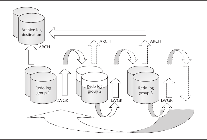
244 Oracle Database 11g: A Beginner’s Guide
Undo tablespaces are managed in the same way as any other tablespace and the
data is subsequently logged as redo logs. Rollback segments allow changes to be
undone, either for system reasons, perhaps due to a transaction that has failed, or
because the application has explicitly requested that a rollback be performed. Undo
or rollback tablespaces need to be included as part of your backup strategy.
Checkpoints
As you’ve seen, the redo logs and database data are not written out at the same time.
The redo logs are guaranteed to be written out at commit time, but the data is not
written to disk simultaneously. If that’s the case, just when is the data written from the
buffers to the data files? This is determined by an Oracle process called the database
writer (dbw0) process, which manages the writing of information to the database.
dbw0 writes changes to the data files to free up dirty buffers (buffers that have
changed data in them) to allow more changes to occur. A checkpoint is a background
event that ensures all of the changed data has been written to the data files.
Archive Logs
Archive logs are the mechanism used to provide continuous availability to an Oracle
database by allowing you to back up the database while it is running. This is known as
ahot backup. They also allow you to recover databases by performing a “roll-forward”
FIGURE 7-1. Redo logs

of changes using redo logs up to either the current point in time or a time that you
specify the database should be rolled forward to. This cannot be done with online redo
logs, because they are written to sequentially and eventually wrapped-around. When
that occurs, the previous records that existed in the wrapped redo file are overwritten.
By placing the database in archive log mode, online redo logs can be written out to files
to be kept indefinitely. The files can then be named with sequential incrementing names
so that you know the order they should be applied in. As with redo logs, archive logs
can be multiplexed. In other words, more than one copy of each archive log can be
written to different locations. Refer back to Figure 7-1, as it also demonstrates the redo
logs being written to the archive log location.
Data Files, Tablespaces, Segments,
Extents, and Blocks
Data files are the low-level structures that make up what you probably think of as a
database. To put it simply, the tables and indexes that make up your applications are
stored in tablespaces and each tablespace is created on one or more data files. A
particular data file will store data for one tablespace and a tablespace can contain
many tables and indexes. Tables and indexes are a subset of a type of database object
called a segment. Examples of segments are indexes, tables, rollback/undos, clusters,
Chapter 7: Backup and Recovery 245
Ask the Expert
Q: What would happen if I restored the redo logs before I performed a
point-in-time recovery? It seems like this is the best approach to use.
A: There is an end-of-redo marker on the online redo logs that will stop the
recovery immediately. Oracle will think the forward recovery is complete and
archive logs will not be applied. The current redo logs should also not be
overwritten by the backups because the current redo logs contain the last pieces
of the recovery information. This means that the recovery will not be restored
completely and an incomplete recovery will need to be done.
Q: How can I find out the state of a file when a backup control file was
taken? I need to know which files are read-write, read-only, or offline, but
how can I do that?
A: Whenever you back up a control file, run a sql script that queries
dba_data_files and writes the status of all of your data files to a separate file
that is kept with the backup control file. We will show you an example of this
in the following section.
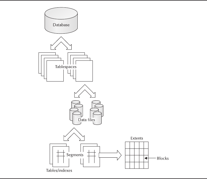
lobindexes, and lobsegments. A segment is made up of extents that are a collection of
contiguous blocks. Take a look at Figure 7-2 for a picture of these breakdowns of the
storage structure. So, to put this into a single sentence, a tablespace is created on one
or more data files and consists of one or more segments made up of one or more
extents that are a contiguous collection of blocks. Got it? Good. It’s an important
set of relationships to understand.
From a backup and recovery point-of-view, it’s important to be aware of the
relationship between tables, tablespaces, and data files. You should employ a naming
standard that makes it easy to determine the tablespace that a data file supports.
Whenever you perform a backup where you are not backing up the entire database at
the same time, it is important to consider any referential integrity constraints enforced
by the backup or application that must be honored. If you’re just backing up a set of
tables, or one tablespace but not another, are you getting all that is needed for valid
restore of the application?
246 Oracle Database 11g: A Beginner’s Guide
FIGURE 7-2. A database’s storage structure is not just made up of tables, but
tablespaces that are comprised of data files that are made up of
segments built of blocks.

Dump Files
There are three types of dump files that contain information about errors that occur
in the database. Background dumps are written out by Oracle background processes
when an error occurs. User dumps are files written for user processes for the purpose
of debugging. Core dumps are a place where Oracle dumps core files in a UNIX
environment. These may be worth backing up as a history of problems that have
occurred to help you troubleshoot future issues. One particular file that should be
backed up regularly is a special trace file called an alert log. This file reports on a
great deal of activity, such as when the database is stopped and started, when
checkpoints occurred, and the system change number (or scn, a unique number
given to every change in the database), where the current incarnation or version of
the database began. This is all valuable information that can be of great assistance
when it comes time to recover your database.
TIP
Back up your alert log with your regular database
backups. The location of the alert log can be
found by looking at the value of the parameter
background_dump_dest. Since this is a regular file,
a file system backup of this directory is a valid
option and would back up the alert log.
You have now seen the structures that are critical to your backup and recovery
operations. Armed with this knowledge, you are ready to learn about user-manager
backup and recovery.
Progress Check
1. Name some files that should be backed up as part of your strategy.
2. What does multiplexing mean and which objects should be multiplexed?
3. Why would you want to use archive logging?
Chapter 7: Backup and Recovery 247
Progress Check Answers
1. Some files that should be backed up include parameter, control, undo, archive log, data, online
redo, dump, and trace files.
2. Multiplexing is a term to describe data that’s written to more than one location or file at the same
time. Redo logs, archive logs, and control files should be multiplexed and each copy should go to a
different disk to protect against the loss of one disk.
3. Archive logging allows you to perform full recovery of the database. Without archive logs, no
recovery is possible (only restores can be performed). Also, the database can be backed up while it
is up and running. It is needed to deliver high availability.

248 Oracle Database 11g: A Beginner’s Guide
CRITICAL SKILL 7.2
Learn about Oracle User-Managed
Backup and Recovery
Oracle supports backing up data in a number of ways. This section discusses how
and why to use user-managed backups. These backups are by nature handled more
mechanically than other methods and are just as effective. The information presented
here is also needed to recover your first database. Please remember that you should
try this on test databases before trying your first backup and ultimate recovery on a
business database.
Types of User-Managed Backups
User-managed database backups can be performed as either cold or hot physical
backups. A cold backup means that all users are disconnected from the database
and it is shut down in order to perform the backup. A hot backup is performed
while the database is up and end users can remain connected to the database. In
fact, they can be changing the very data that is being backed up! Let’s examine
these two situations in more detail.
Cold Backups
Cold backups are the simplest type of backup operation you can perform. Cold
backups are performed with the database completely shut down so that the data
files are in a consistent state and nothing is being accessed or changed. Once that
is done, all database files should be backed up to disk or tape. Once the file copies
are complete, the database can be started and users can resume their activity.
The database does not need to be in archive log mode in order to perform a cold
backup, but without archive logging, the database can only be restored to the point
in time that the cold backup was done. Cold backups are a simple option and are
limited in the way they must be run, but once you have a cold backup, it can be
easier to work with and can provide a fair degree of functionality.
In order to perform a cold backup, the database must be shut down in a consistent
manner. In other words, the database should be shut down by issuing one of the
following commands:
■shutdown normal
■shutdown immediate
■shutdown transactional
Do not perform a cold backup of the database immediately after a shutdown
abort. If you must shut down the database in this manner, follow it up with a startup
restrict (to not allow user access), so that the recovery process of the transactions

Chapter 7: Backup and Recovery 249
that were in progress before the abort can complete. Then execute a shutdown
[immediate, transactional, normal]. In this way, you can be confident that you have
a database wherein all of the transactions have completed or rolled back and the
data is in a consistent state. When the database has been shut down, copy the files
to another location on disk or to tape. The files that you should back up include
■All database data files and tablespaces including system, temp, and
rollback/undo
■Control files, backup binary control files, and text control files
■Archive logs if they are being used
■Alert logs
■Oracle password files if they exist
■Parameter files init<SID>.ora and spfile
■Redo logs—but you should be careful whenever restoring redo logs since the
restore of a redo log could overwrite existing current redo logs containing the
final entries in the redo stream needed to complete the recovery. Because of
this, Oracle recommends that you do not back up redo logs.
Once the backups have been completed, the database can be restarted. If the
backups were made to disk, these files can later be backed up to tape after the
database is restarted.
Hot Backups
A hot backup is a backup done while the database is up and running. The entire
database can be backed up or a subset of the tablespaces or data files can be backed
up at one time. While this is happening, end users can continue to perform all of
their normal operations against it. In order to do this, the database must be running
in archivelog mode. This is done by setting the parameter log_archive_start = true
and then running the sql statement alter database archivelog while the database is
mounted. The tablespaces to be backed up are put in backup mode with the alter
tablespace tablespace_name begin backup command. The whole database can also
be put into backup mode at the same time with alter database begin backup and
end backup. But when at a tablespace level it is recommended to put the tablespaces
into backup mode one at a time. The data files are then copied using OS copies,
and the backup is completed with the alter tablespace tablespace_name end backup
command. This looks like the following:
alter tablespace <tablespace_name> begin backup;
[os file copy command such as cp in unix or ocopy in Windows]
alter tablespace <tablespace_name> end backup;

250 Oracle Database 11g: A Beginner’s Guide
Once the backup is complete, you will need to ensure that all of the log records
created during the backup operation have been subsequently archived. Do this with
the sql statement archive log current.This command ensures that all redo logs have
been archived and it will wait for the archive to complete. You should note that the
ocopy utility is required in Windows environments to allow a file to be shared
between the copy utility and Oracle. Ocopy is a command-line utility used to back
up files to disk when the database is down or tablespace is offline. It is not needed
in UNIX environments.
After a hot backup has been successfully completed, the database can be recovered
to a particular point in time by restoring the data files from the hot backup and rolling
forward archive logs to the time required. Online redo logs should never be backed
up during a hot backup. Rather, you should archive the current redo logs and back
those up. As a result, you will create the redo logs at the end of recovery when an
alter database open resetlogs is performed (resetlogs is discussed later in this chapter,
in the section “Recovery Using Backup Control Files”).
In order to recover from a hot or cold backup, it is important to remember that
all of the files that make up the database must be recovered to the same point in
time in order to keep the entire database consistent. The exception to this rule is that
read-only tablespaces can be restored to the point that they were made read-only.
This makes sense since the tablespace cannot be changed once it has been made
read-only. In order to recover a tablespace that is open for read-write operations to
a point in time that is different from the rest of the database, a special operation
called Tablespace Point In Time Recovery (TSPITR) must be performed. However,
this operation requires a clone database and is beyond the scope of this chapter.
Whenever a tablespace status changes to read-only or read-write, it should be
backed up. You will need to keep track of these backups so that you know where
they are when it comes time to use them in a recovery situation. Consider backing
up “read only” tablespaces periodically to deal with potential expiry dates on tape,
as well as other tape management problems that could result from older tapes.
TIP
Run hot backups when the system is not busy. Also,
only put one tablespace between the begin and end
backup operations to reduce the amount of system
overhead associated with this activity, since system
logging is increased on tablespaces that are in
backup mode. You can group multiple tablespaces
together in cases where change activity will not be
high on them during the backup.
Hot backups and archivelogs will be a requirement of every system that has true
high-availability requirements.

Recovery from a Cold Backup
Database recovery can be broken into two distinct steps: the first step involves file
restores where files are copied from tape or a disk backup to a location on disk
where the actual database resides. This is the location of files pointed to by the
control files. The second step is forward recovery, where the archive logs can be
processed and applied to the database, making the data as current as possible. In
the case of the database in noarchivelog mode (which is often the case where cold
backups are concerned), there are no logs to recover with, so all data files, control
files, and redo logs are simply restored to their proper location. Other files, such as
the init.ora and spfile parameter files, as well as password files, must also be in the
proper place.
Restoring a database from a cold backup is one of the simpler things you can do
as a DBA; this simplicity is perhaps the biggest benefit of performing a cold backup.
A cold backup of a database that is in archivelog mode can be recovered, but there
is no recovery from a hot backup that isn’t in archivelog mode (note that a hot backup
is only performed on databases in archivelog mode): there are only file restores.
Once these files have been restored, the database can be started. That’s it!
Chapter 7: Backup and Recovery 251
Ask the Expert
Q: Why would I ever want to use cold backups if hot backups are so
powerful?
A: There are situations when you only need to restore a database from a cold
backup and high availability is not a concern. In these cases, you can consider
using a cold backup.
Q: What is the downside to performing hot backups and running in
archivelog mode, if any?
A: You will need to manage the archive log files, but RMAN can help you
with this (more information can be found later in this chapter in the “Archive
Log Management” section). There is also extra logging that occurs when a
tablespace is placed in the backup mode. This can be overcome by scheduling
backups when the database is not busy or by using RMAN, which does not
place tablespaces in backup mode. Restorations from hot backup require more
care and practice, but the benefits to hot backups outweigh the disadvantages
by a great deal.

252 Oracle Database 11g: A Beginner’s Guide
Recovery from a Hot Backup
This is one of the places where you will earn your stripes as a DBA, since you will
always need to perform recovery from a hot backup. To clarify this point, recovery
can be performed on any database that is in archivelog mode, whether the backup
was a hot or cold one, but hot backups always require that recovery be performed.
There are two fundamental types of recovery: complete recovery and incomplete
recovery.
Complete recovery describes a recovery where the database is restored and then
recovered forward using all available archive logs. You are performing as complete
a recovery as you can, with no data loss. Complete recovery can be performed at
the database, tablespace, data file, or block level.
Incomplete or point-in-time recovery is where the database is restored and then
optionally rolled forward to a predetermined point in time or system change number
(scn) by applying some, but not all, of the logs. This produces a version of the
database that is not current and is often done to bring the database back to a time
before a problem occurred. There are three fundamental types of incomplete recovery:
■Cancel-based recovery runs until you issue a cancel command.
■Timestamp recovery applies to all of the logs until a timestamp you enter is
reached.
■Change-based recovery applies to all of the logs until a scn you enter is
reached.
Examples of these are shown next:
SQL> recover database until cancel;
SQL> recover database until change 1234567;
SQL> recover database until time '2004-04-15:14:33:00';
TIP
When performing a recovery, always try to recover
as much data as possible by running a complete
recovery or by applying archive logs to the latest
timestamp or scn that you possibly can.
Seven Steps to Recovery
The fundamental steps for performing a recovery are summed up here:
1. Restore data files from tape or a backup location on disk to the location
where the database file should reside.

Chapter 7: Backup and Recovery 253
2. Startup nomount. This step reads the parameter file, allocates the memory
structure of the SGA, and starts the background Oracle processes. Also, the
alert log and trace files are opened. Note that the data files are not open
during a Startup nomount. (This step has to be performed if the control file
needs to be rebuilt.)
3. Create the control file. This step is optional and only needed if the control
file is unavailable. A text version of the control file should be used to create
a new binary version of the control file.
4. Ensure that all the data files to recover are online. Read-only data files once
restored do not need to be recovered since no data will have changed in
these files.
5. Mount the database. This step associates a database with the instance that
was started in step 2. The database, however, is not opened at this time.
The control file listed in the parameter file is opened and all database files
are located.
6. Recover the database by locating and applying the archive logs.
7. Open the database. The database, including the redo logs and data files, is
opened with the Startup Open command.
In some cases, you only need to recover a single tablespace or data file without
touching the rest of the database. These must be complete recoveries and the tablespace
or data file must be taken offline to perform this. A block level recovery can also be
performed, but only by RMAN and only with the data file online. This feature allows
you to recover a small number of corrupt blocks of a data file and is one of the great
reasons to use RMAN!
TIP
If a database crashes in the middle of a hot backup,
and the data file is still in backup mode, it will
appear that the data file will need recovery.
However, it will just need to be changed out of
backup mode to allow the database to come up
properly and continue. Check the status of the data
file in v$backup before performing a recovery.
Recovery Using Backup Control Files
You can create both a text version of the control file and a binary version of the
control file as backups. When recovering the database, you should try to use the
current control file. If that is not possible, then your next option should be to try to

254 Oracle Database 11g: A Beginner’s Guide
use a backup control file since it contains useful information that assists recovery
that is not included in the text-based control file. With a backup control file, you
will need to perform media recovery and use the using backup control file syntax
when performing the recover database command. A resetlogs command will then
need to be performed when the database is opened, which will create new redo
logs as well as a new version, or incarnation,of the database. You also need to
know the status of data files when the backup control file was created. If a data file
had a status of read-write when the backup control file was created (but should be
opened as a read-only file), then it should be taken offline before recovery begins.
Backup control files are a useful and sometimes required feature, but can
complicate your database recovery.
TIP
Always back up the database after performing an
incomplete recovery and opening the database
with the Resetlogs option. The backups before this
recovery are not easily useable, so taking another
backup after the resetlogs option will make a simple
restore possible if there is a need to recover after this
point.
CRITICAL SKILL 7.3
Write a Database Backup
When you decide to use a user-managed backup strategy rather than RMAN, you
will need to develop scripts to perform hot or cold backups. One of the most
important things you should do to simplify your maintenance requirements is to
develop scripts that are generated from the Oracle catalog. If done properly, you
won’t need to change your backup scripts every time you add a new file or change
the location of a file.
TIP
Automate your backups with scripts that are
generated from the Oracle Catalog.
Whenever you perform a backup, it is extremely useful to know the status of
your database including the data files and parameters in effect. Information such as
which data files are open in read-only mode at backup time is invaluable, as is a
listing of the file locations and sizes. Next we’ll show you a simple example of some
SQL queries that provide information about the state of a database when you need
to restore:

Chapter 7: Backup and Recovery 255
select * from dba_tablespaces; -- Tablespace Information
select * from dba_data_files; -- Data file Information
select * from v$datafile; -- More data file information
select * from v$logfile; -- log file information
select * from v$log; -- more log file information
select * from v$controlfile; -- control file information
select * from v$parameter; -- database parameters in effect
select * from v$nls_parameters; -- language characters in effect
-- Get the log history information for the past 3 days
select * from v$log_history where first_time > sysdate - 3;
The preceding should be spooled to the backup directory and kept with your
backups. You can list the specific columns you want to see in the previous queries,
but when it comes to needing information during a high-pressure recovery, we
would rather you err on the side of having a little too much information than risk
missing a piece of information that would be useful. Once you have this information,
your backup can be performed. The following is an example of a hot backup SQL
script. This script must be executed on a database running in archivelog mode:
set echo on;
spool /u02/backup/ora11g/hotBackup1.lst;
alter system archive log current;
alter tablespace INDX begin backup;
! cp /u01/oradata/ora11g/indx01.dbf /u02/backup/ora11g
alter tablespace INDX end backup;
alter tablespace TABLESPACE_n begin backup;
! cp /u01/oradata/ora11g/tablespace_n01.dbf /u02/backup/ora11g
! cp /u01/oradata/ora11g/tablespace_n02.dbf /u02/backup/ora11g
alter tablespace TABLESPACE_n end backup;
... more tablespaces ...
alter tablespace SYSTEM begin backup;
! cp /u01/oradata/ora11g/system01.dbf /u02/backup/ora11g
alter tablespace SYSTEM end backup;
-- Backup the log file
alter system archive log current;
-- Create 3 copies of a binary controlfile backup.
alter database backup controlfile to
/u02/backup/ora11g/CONTROL01.CTL' reuse;
alter database backup controlfile to
/u02/backup/ora11g/CONTROL02.CTL' reuse;
alter database backup controlfile to
/u02/backup/ora11g/CONTROL03.CTL' reuse;
-- Create a text version of a controlfile backup
alter database backup controlfile to trace;
spool off;
exit;

256 Oracle Database 11g: A Beginner’s Guide
This is a SQL script that can be run from a UNIX shell script or a Windows
command file. To run this in Windows environments, the file copies are performed
using the host start /wait c:\oracle\ora11g\bin\ocopy.exe command rather than
with the UNIX ! cp command, which hosts out and runs the UNIX version of copy.
The ocopy command is an Oracle copy utility that must be run under Windows to
allow file sharing to occur during hot backups. The standard DOS copy command
does not allow this.
Cold backups are similar to the preceding except that the begin backup and
end backup commands are not needed. The copy commands are surrounded by a
consistent database shutdown before the copies have started, with a startup after the
copies have completed. Note that in Windows environments, you should use the
standard “copy” utility for cold backups.
You should also add your parameter files, dump files, alert logs, and your own
DBA scripts that perform backup, recovery, and monitoring to your backups. Once
you’ve added those, you’ll have everything backed up except for your archive logs.
Let’s see how to manage those next.
CRITICAL SKILL 7.4
Back Up Archived Redo Logs
Managing archive logs is one of the more difficult tasks on a busy Oracle database.
You will want to have archive logs available to you in case they are needed for a
database recovery. At the same time, the archive logs must be written to disk and
if disk space fills up, the instance will stop processing requests until more space
becomes available. Trying to balance both of these competing requirements can
be tricky, especially if your system writes a large number of log records.
To meet the first requirement of having the archive logs available to your online
system in the event of a recovery, try to keep archive logs since the last backup (or,
even better, the last two backups) on disk. If you are unable to keep archive logs
online due to space issues, then you will need to write a script that regularly backs
up the archive logs to tape and deletes them from disk. An example of a space
management script that backs up archive logs once the archive directory is over
50 percent full is shown next:
#Pseudo-shell-code for free archive log space
# Check used and free space: this is a very simple script
# df –k (on linux: location of fields varies by platform)
# Filesystem 1k-blocks Used Available Use% Mounted on
# /dev/hda3 3763404 102676 3469556 3% /
Log_arch_dest='/u01/oradata/db01/arch'
arch_dir_mountPoint=`df -k ${log_arch_dest}|grep -v blocks|
awk '{print $6}'`
arch_dir_freeSpace=`df -k ${log_arch_dest}|grep -v blocks|
awk '{print $4}'`
arch_dir_used=`df -k ${LOG_ARCH_DEST}|grep -v blocks|

Chapter 7: Backup and Recovery 257
awk '{print $3}'`
if [${arch_dir_freeSpace} -le ${arch_dir_Used}]; then
echo "Place archiving logic here"
fi
All of this is unnecessary when you use RMAN, since it will back up archive logs
to tape, delete the files on disk, and manage the tape files in the RMAN repository.
You will see more of this later in the “Get Started with Recovery Manager” section.
CRITICAL SKILL 7.5
Get Started with Oracle Data Pump
Oracle Data Pump is a utility available since Oracle Database 10gthat can be used
to move data and metadata from one database to another. (Metadata is the “data
about the data,” or in Oracle terms, the catalog information.) In earlier versions of
Oracle, Export and Import were the utilities for this; their interface is similar to the
new utilities, Data Pump Export and Data Pump Import, though they are completely
separate utilities. The performance of Oracle’s new utilities Data Pump Export and
Data Pump Import will increase greatly over the old Export and Import utilities and
can also take advantage of parallelism to accomplish this. The Data Pump Export
and Import utilities use the expdp and impdp commands, respectively. You are
encouraged to use these rather than the pre–Oracle Database 10gexp and imp
utilities, since those do not support all Oracle Database 11gfeatures, while the
Data Pump utilities do.
The Data Pump output files are written in a proprietary format that can only be
read by the Data Pump Import utility. Now with Oracle 11g, the export files can be
encrypted and compressed as they are exported. The compression of the export file
can shrink the file from 10–15 percent. Encryption of the export can be done at a
file level—or even at the level of table columns—to protect the sensitive data in
these tables.
Data Pump will allow a subset of data and metadata to be moved through filters
implemented in the Export and Import parameters. The Data Pump Export utility
unloads data, metadata, and control information from the database into one or more
operating system files that are called dump files. These can be imported into a target
database that resides on another server and a totally different operating system.
The Data Pump Import utility can read these dump files and load a target
database with metadata, data, and all objects that have been previously exported.
For example, table DDL, security in the form of grants, objects such as triggers,
stored procedures, and views can also be imported, among other things. In fact, an
entire target database can be created from a Data Pump Full Export using the Import
utility. Some useful options provided through Data Pump are
■The ability to view object DDL without running it using the SQLFILE parameter
■The network import, which allows a Data Pump Import to occur using a
source database rather than a dump file set

258 Oracle Database 11g: A Beginner’s Guide
■The ability to restart Data Pump jobs using the start_job parameter to restart
import jobs
■Using the Parallel parameter to define the maximum number of threads and
degrees of parallelism for export and import jobs
■The ability to monitor jobs by detaching and reattaching to running jobs
■The ability to estimate the amount of space an export file will occupy by
using the estimate_only clause
The Data Pump Export and Import for data and metadata are performed using
the Data Pump application programming interface (API) and use procedures in the
DBMS_DATAPUMP PL/SQL package. The metadata API is implemented through the
DBMS_METADATA package. This package retrieves metadata in an XML format
that can be used in many ways. For example, XML can be transformed into DDL
or Extensible Stylesheet Language Transformation (XSLT) and the XML itself can be
used to create an object. There is a new Remap attribute that allows the attributes
of an object to be changed; for example, schema names can be changed using this
feature. The Data Pump API supports all objects needed to perform a full export.
There are three ways to perform Data Pump Export and Import utilities. There
is the command-line interface, where export and import parameters are listed on a
command line or in a script. A variation of the command-line interface is to add a
parameter file using the parfile parameter, which points to a different file where all
of the import or export parameters are listed. An interactive-command interface can
also be used by entering CTRL-C during an import or export run which will then allow
you to enter commands when prompted.
Let’s now explore some details about actually running Data Pump exports and
imports.
CRITICAL SKILL 7.6
Use Oracle Data Pump Export
There are five mutually exclusive modes for performing the Oracle Data Pump Export:
■Full Export is where the entire database is exported using the full
parameter. This can be used to completely rebuild the database if needed.
■Schema Export is the default mode; it allows you to export one or more
schemas in the database. The schemas parameter is used to run this. Please
note that objects in other schemas related or dependent on objects in this
schema are not exported unless the other schema is also mentioned in the
schema list.
■Table Export allows for the export of tables or partitions and their
dependent objects using the tables parameter.

Chapter 7: Backup and Recovery 259
■Tablespace Export can be used to unload all of the tables that have been
created in the given tablespace set using the tablespaces parameter.
■Transportable Tablespace mode differs from the preceding bullet in that
only the metadata is exported from the database for a given tablespace set.
This uses the transport_tablespaces parameter.
The exp_full_database role must be granted to a user performing a full or
tablespace export or, alternatively, an export of a schema or table that is outside
of the user’s schema.
A feature of the Data Pump Export is that filters can be used on both data and
metadata. The data filters are applied with the query parameter, and the filter is
executed once per table per job. For metadata, either the exclude or include
parameters can be used and are mutually exclusive commands. When filters are
applied to metadata, the objects that are included will also have their dependent
objects. For example, tables will also have indexes, triggers, grants, and constraints
included with them. You can use the datapump_paths view to see which objects
can be filtered on. When multiple filters are applied to an object, they are processed
with an and condition between them. When using filters, we recommend using the
parfile parameter and placing all parameters in the parfile including the filter
operators.
The parameters for the Data Pump Export command can be seen using the
command expdp help=y. A subset of the output from this, which contains the
parameters along with a brief description, is shown next.
C:\Users\iabramson>expdp help=y
The Data Pump export utility provides a mechanism for transferring
data objects between Oracle databases. The utility is invoked with
the following command:
Example: expdp scott/tiger DIRECTORY=dmpdir DUMPFILE=scott.dmp
You can control how Export runs by entering the 'expdp' command
followed by various parameters. To specify parameters, you use
keywords:
Format: expdp KEYWORD=value
or KEYWORD=(value1,value2,...,valueN)
Example: expdp scott/tiger DUMPFILE=scott.dmp
DIRECTORY=dmpdir SCHEMAS=scott
or TABLES=(T1:P1,T1:P2), if T1 is partitioned table
USERID must be the first parameter on the command line.
Keyword Description (Default)
----------------------------------------------------------------------
ATTACH Attach to existing job, e.g. ATTACH [=job name].
260 Oracle Database 11g: A Beginner’s Guide
COMPRESSION Reduce size of dumpfile contents where valid
keyword values are: ALL, (METADATA_ONLY),
DATA_ONLY and NONE.
CONTENT Specifies data to unload where the valid keyword
values are: (ALL), DATA_ONLY, and METADATA_ONLY.
DATA_OPTIONS Data layer flags where the only valid value is:
XML_CLOBS-write XML datatype in CLOB format
DIRECTORY Directory object to be used for dumpfiles
and logfiles.
DUMPFILE List of destination dump files (expdat.dmp),
e.g. DUMPFILE=scott1.dmp, scott2.dmp,
dmpdir:scott3.dmp.
ENCRYPTION Encrypt part or all of the dump file where valid
keyword values are: ALL, DATA_ONLY,
METADATA_ONLY,ENCRYPTED_COLUMNS_ONLY, or NONE.
ENCRYPTION_ALGORITHM Specify how encryption should be done where valid
keyword values are: (AES128), AES192, and AES256.
ENCRYPTION_MODE Method of generating encryption key where valid
keyword values are: DUAL, PASSWORD,
and (TRANSPARENT).
ENCRYPTION_PASSWORD Password key for creating encrypted column data.
ESTIMATE Calculate job estimates where the valid keyword
values are: (BLOCKS) and STATISTICS.
ESTIMATE_ONLY Calculate job estimates without performing the
export.
EXCLUDE Exclude specific object types,
e.g. EXCLUDE=TABLE:EMP.
FILESIZE Specify the size of each dumpfile in units of
bytes.
FLASHBACK_SCN SCN used to set session snapshot back to.
FLASHBACK_TIME Time used to get the SCN closest to the specified
time.
FULL Export entire database (N).
HELP Display Help messages (N).
INCLUDE Include specific object types,
e.g. INCLUDE=TABLE_DATA.
JOB_NAME Name of export job to create.
LOGFILE Log file name (export.log).
NETWORK_LINK Name of remote database link to the
source system.
NOLOGFILE Do not write logfile (N).
PARALLEL Change the number of active workers for current
job.
PARFILE Specify parameter file.
QUERY Predicate clause used to export a subset of a
table.
REMAP_DATA Specify a data conversion function,
e.g. REMAP_DATA=EMP.EMPNO:REMAPPKG.EMPNO.
REUSE_DUMPFILES Overwrite destination dump file if it exists (N).
SAMPLE Percentage of data to be exported;
Chapter 7: Backup and Recovery 261
SCHEMAS List of schemas to export (login schema).
STATUS Frequency (secs) job status is to be monitored
where the default (0) will show new status when
available.
TABLES Identifies a list of tables to export - one
schema only.
TABLESPACES Identifies a list of tablespaces to export.
TRANSPORTABLE Specify whether transportable method can be
used where valid keyword values are:
ALWAYS, (NEVER).
TRANSPORT_FULL_CHECK Verify storage segments of all tables (N).
TRANSPORT_TABLESPACES List of tablespaces from which metadata will be
unloaded.
VERSION Version of objects to export where
valid keywords are:
(COMPATIBLE), LATEST, or any valid
database version.
The following commands are valid while in interactive mode.
Note: abbreviations are allowed
Command Description
----------------------------------------------------------------------
ADD_FILE Add dumpfile to dumpfile set.
CONTINUE_CLIENT Return to logging mode. Job will be re-started
if idle.
EXIT_CLIENT Quit client session and leave job running.
FILESIZE Default filesize (bytes) for subsequent ADD_FILE
commands.
HELP Summarize interactive commands.
KILL_JOB Detach and delete job.
PARALLEL Change the number of active workers for current
job. PARALLEL=<number of workers>.
REUSE_DUMPFILES Overwrite destination dump file if it exists (N).
START_JOB Start/resume current job.
STATUS Frequency (secs) job status is to be monitored
where the default (0) will show new status when
available. STATUS[=interval]
STOP_JOB Orderly shutdown of job execution and exits the
client.
STOP_JOB=IMMEDIATE performs an immediate
shutdown of the Data Pump job.
The values in brackets in the preceding list are the default values in use for the
parameter. Some parameters worth noting are explored further in the following
bullet points:
■DIRECTORY is the directory that is created using the sql create directory
syntax in Oracle and it’s the location that the dump file is written to. The
262 Oracle Database 11g: A Beginner’s Guide
default name is DPUMP_DIR. Without a directory the export will fail; the
directory is where the dump file and log file will be stored. For example,
set this as follows:
create or replace directory DPUMP_DIR as '\u01\';
grant read, write on dpump_dir to export_user;
■ESTIMATE allows you to see how much disk space each table in the export
job will consume. The options for ESTIMATE include BLOCK and
STATISTICS, which specify if Data Pump will use either a sample of blocks
or table statistics to determine the size of the export.
■EXCLUDE can be used to exclude metadata, dependent objects, and data to
be exported or imported. The exclude parameter can exclude tables,
constraints, stored procedures, grants, and schemas. This doesn’t exclude
data from a table; to exclude data, you must use data filtering through a
query and where clause.
■FLASHBACK_SCN and _TIME directs the export to unload data that is
consistent with the time or scn listed.
■INCLUDE is used to list metadata objects and dependent data that will be
exported. This can include object types and object names. Only objects
explicitly listed in the INCLUDE statement will be exported.
■NETWORK_LINK allows an import into a target database directly from a
source database rather than from a dump file.
■PARALLEL is a performance option that can be used to specify the maximum
number of threads that can be used to speed up an export by running it in
parallel.
■PARFILE can be included to point to another file that includes export
parameters. Use this when filtering data and metadata using the exclude,
include, or query parameters.
■QUERY can be used to apply syntax similar to qualifiers that you would use
in a select…where clause to filter the rows to be exported.
■TRANSPORT_TABLESPACES (TTS) is the parameter used to specify the
tablespaces that will have their metadata exported during a transportable
tablespace operation. When this is done, the tablespaces in the source
database should be placed in read-only mode and their underlying data files
copied to a new location. The data file copies are performed at the OS level.
The only exportx is that of the metadata. The data file copies and exported
metadata can be used to plug in the tablespaces to a target database. The
tablespaces must be a self-contained set and the transport_full_check
parameter can be used to ensure this is the case.

Chapter 7: Backup and Recovery 263
■ADD_FILE is valuable if an export operation fills the current dump file. If
working in interactive mode when this occurs, you will be prompted to add
a new dump file and will be able to do so. Otherwise, additional files can
be added when the job is defined.
■START_ JOB allows you to start a job to which you are attached. This
allows you to restart an export after a previous failure and is valuable
for long-running jobs.
Next we’ll cover some examples. To perform a full database export and
compress the full export file using Data Pump, run the following:
expdp system/manager DUMPFILE=expdat.dmp FULL=y LOGFILE=export.log
COMPRESSION=ALL
A Schema Level Export of the Sales History (SH) schema can be performed as
follows:
expdp system/manager DUMPFILE=expdat.dmp SCHEMAS=sh LOGFILE=export.log
A single table can be exported, as shown next with the sh.customers table:
expdp system/manager DUMPFILE=expdat.dmp TABLES=sh.customers
LOGFILE=export.log
Here is an example of data filtering where the tables in the SH schema are
exported, except for the PROMOTIONS table and CUSTOMERS table which has
one row exported:
expdp sh/sh parfile=exp.par
The contents of the exp.par file are shown here:
DIRECTORY=DPUMP_DIR
DUMPFILE=testsh.dmp
CONTENT=DATA_ONLY
EXCLUDE=TABLE:"in ('PROMOTIONS')"
QUERY=customers:"where cust_id=1"
The Data Pump Export utility is valuable for performing backups of a database
or objects in a database, as well as for moving data from one database to another.
Experiment with the different parameters and test your exports by performing
imports to another database to ensure that the entire export and import stream is
working properly.

264 Oracle Database 11g: A Beginner’s Guide
CRITICAL SKILL 7.7
Work with Oracle Data Pump Import
You’ve successfully performed exports and they seem to have worked, but that’s
only half of the job. You now need to perform the ultimate test of whether those
exports worked by performing Data Pump Imports.
Imports are performed using the impdp command, which is new since Oracle
Database 10g. As with Data Pump Export, this utility has similar functionality with
the import utility found in pre–Oracle Database 10gversions. There are five modes
for performing the Oracle Data Pump Import, described next. The modes correspond
to the export modes, but an import can be run using an export of the exact same
mode or an export mode that is a higher level in the hierarchy. For example, a
table-mode import can be performed using a source that is a Full, Schema, Tablespace,
or Table mode export dump file as well as a Network_Link. These modes are
mutually exclusive and explained in detail next:
■Full Import The entire database is imported using the FULL parameter.
This can be used to completely rebuild the database if needed. This can be
run using a source dump file or a source database using a Network_Link.
■Schema Import The default mode allows you to import one or more
schemas in the database using the SCHEMAS parameter. Objects in other
schemas that are dependent on objects in this schema are not imported
unless the other schema is also mentioned in the schema list. The source
for this can be a full export dump file or a schema level export dump file
or another database using a Network_Link.
■Table Import This allows for the import of tables or partitions and their
dependent objects using the TABLES parameter. To import tables that are
not in your schema, the imp_full_database role must be granted to you. The
source for this can be a Full, Schema, Table, or Tablespace level dump file,
or another database using a Network_Link.
■Tablespace Import This can be used to load all of the tables that have
been created in the given tablespace set using the TABLESPACES parameter.
The source for this can be a Full, Schema, Table, or Tablespace level dump
file, or another database using a Network_Link.
■Transportable Tablespace (TTS) This differs from its siblings in that only
the metadata is imported to the database for a given tablespace set, and it
uses the TRANSPORT_TABLESPACES parameter. The metadata that was
exported using a TTS export are imported into the target database and the
data files need to be copied into the correct location as specified by the
metadata (note that the paths can be changed). The source for this can be a
transportable tablespace export dump file or a source database.

Chapter 7: Backup and Recovery 265
The parameters available with Data Pump Import can be seen using the
command impdp help=y. A subset of the output from this, which contains the
parameters along with a brief description, is shown next.
>impdp help=y
Keyword Description (Default)
---------------------------------------------------------------------
ATTACH Attach to existing job, e.g., ATTACH [=job name].
CONTENT Specifies data to load where the valid keywords
are (ALL), DATA_ONLY, and METADATA_ONLY.
DIRECTORY Directory object to be used for dump, log, and
sql files.
DUMPFILE List of dumpfiles to import from (expdat.dmp),
e.g., DUMPFILE=scott1.dmp, scott2.dmp,
dmpdir:scott3.dmp.
ESTIMATE Calculate job estimates where the valid keywords
are (BLOCKS), SAMPLING, and STATISTICS.
EXCLUDE Exclude specific object types, e.g.,
EXCLUDE=TABLE:EMP.
FLASHBACK_SCN SCN used to reset the session snapshot.
FLASHBACK_TIME Time used to get the SCN closest to the
specified time.
FULL Import everything from source (Y).
HELP Display help messages (N).
INCLUDE Include specific object types, e.g.,
INCLUDE=TABLE_DATA.
JOB_NAME Name of import job to create.
LOGFILE Log file name (import.log).
NETWORK_LINK Name of remote database link to the source
system.
NOLOGFILE Do not write logfile.
PARALLEL Change the number of active workers for current
job.
PARFILE Specify parameter file.
QUERY Predicate clause used to import a subset
of a table.
REMAP_DATAFILE Redefine datafile references in all DDL
statements.
REMAP_SCHEMA Objects from one schema are loaded into
another schema.
REMAP_TABLESPACE Tablespace object is remapped to another
tablespace.
REUSE_DATAFILES Tablespace will be initialized if it already
exists (N).
SCHEMAS List of schemas to import.
SKIP_UNUSABLE_INDEXES Skip indexes that were set to the Index Unusable
state.
SQLFILE Write all the SQL DDL to a specified file.
266 Oracle Database 11g: A Beginner’s Guide
STATUS Frequency (secs) job status is to be monitored
where the default (0) will show new status when
available.
TABLE_EXISTS_ACTION Action to take if imported object already exists.
Valid keywords: (SKIP), APPEND, REPLACE, and
TRUNCATE.
TABLES Identifies a list of tables to import.
TABLESPACES Identifies a list of tablespaces to import.
TRANSFORM Metadata transform to apply (Y/N) to specific
objects. Valid transform keywords:
SEGMENT_ATTRIBUTES and STORAGE.
e.g., TRANSFORM=SEGMENT_ATTRIBUTES:N:TABLE.
TRANSPORT_DATAFILES List of datafiles to be imported by
transportable mode.
TRANSPORT_FULL_CHECK Verify storage segments of all tables (N).
TRANSPORT_TABLESPACES List of tablespaces from which metadata will be
loaded. Only valid in NETWORK_LINK mode import
operations.
VERSION Version of objects to export where valid keywords
are (COMPATIBLE), LATEST, or any valid database
version. Only valid for NETWORK_LINK and SQLFILE.
The following commands are valid while in interactive mode.
Command Description (Default)
----------------------------------------------------------------------
CONTINUE_CLIENT Return to logging mode. Job will be re-started if
idle.
EXIT_CLIENT Quit client session and leave job running.
HELP Summarize interactive commands.
KILL_JOB Detach and delete job.
PARALLEL Change the number of active workers for current
job. PARALLEL=<number of workers>.
START_JOB Start/resume current job.
STATUS Frequency (secs) job status is to be monitored
where the default (0) will show new status when
available STATUS=[interval]
STOP_JOB Stops job execution and exits the client.
The values in brackets in the preceding list are the default values in use for the
parameter. Some parameters worth noting are as follows:
■EXCLUDE can be used to exclude metadata and dependent objects and
data to be imported. To exclude data only, you must use data filtering
through a query. Once an object has been excluded, all of its dependent
objects will also be excluded.
■FLASHBACK_SCN and _TIME specify the system change number (scn) or
time that the import will use as a point of consistency. In other words, the
import will be performed in a manner in which the data is consistent with
the time or scn listed. This is only used with a Network_Link, and specifies
the scn or time from the source database.
■INCLUDE is used to include metadata objects and dependent data during
an import. This can include object types as well as object names. Only
objects explicitly listed in the include statement will be imported. Employ
a parfile when using this option.
■NETWORK_LINK allows for an import into a target database directly from a
source database rather than from a dump file that was previously exported.
■PARALLEL is a performance option that specifies the maximum number of
threads that can be used to speed up an import by running it in parallel.
■PARFILE can be included to point to another file that includes import
parameters. Use this when filtering data and metadata using the exclude,
include, or query parameters.
■QUERY is used to apply syntax similar to qualifiers that you would use in
a select…where clause to filter rows to be imported. Use a parfile with this
parameter.
■Remap parameters include REMAP_DATAFILE, REMAP_SCHEMA,
REMAP_TABLESPACE, and REMAP_DATAFILES. These allow you to
change the names of data files, schemas, and tablespaces when moving
objects from one database to another.
■REUSE_DATAFILES should be used with extreme caution. When set to Y,
existing data files will be used and data will be overwritten when a Create
Tablespace operation is performed. The default is N, and a create
tablespace command will fail when a dependent data file exists.
■SQLFILE names a file where all of the DDL that would be executed will be
written. So, rather than executing the DDL, it writes the statements to the
SQLFILE named here.
■TRANSPORT_TABLESPACES (TTS) specifies tablespaces that will have their
metadata imported during a TTS operation. The data file copies and previously
exported metadata can be used to plug in the tablespaces to a target database.
When exporting and importing, filters can be used on both data and metadata to
restrict the rows to be imported. For data, restrictions on the rows to be imported are
implemented with the query parameter, and the filter is executed once per table per
job. For metadata, either the exclude or include parameters can be used and these
are mutually exclusive commands. When filters are applied to metadata, the objects
that are included will also have their dependent objects included.
Let’s look at an example of data filtering where all data from all tables in the
SH schema are exported except for the SALES table. We will then use the dump file
Chapter 7: Backup and Recovery 267

268 Oracle Database 11g: A Beginner’s Guide
created by this export in a separate import job that renames the schema and only
imports one table. Here are the export script and parameter files:
expdp system/manager parfile=exp.par
Contents of the exp.par parameter file are shown here:
DIRECTORY=DPUMP_DIR
DUMPFILE=testsh.dmp
SCHEMAS=SH
EXCLUDE=TABLE:"in ('SALES')"
An import that uses the preceding dump file is shown next. Notice that we
are importing a single table into a different schema SHNEW as specified by the
REMAP_SCHEMA command. If the table already exists, then this will be skipped
and the import will continue through the TABLE_EXISTS_ACTION parameter.
Note that the SHNEW schema must already exist in the database with the proper
authority to create all of the objects in it since this was a schema level export. In
order to create the SHNEW schema with Data Pump Import, a full export would
need to be run:
impdp system/manager parfile=imp.par
Contents of the imp.par file are shown here:
DIRECTORY=DPUMP_DIR
DUMPFILE=testsh.dmp
REMAP_SCHEMA=SH:SHNEW
TABLES=SH.PRODUCTS
TABLE_EXISTS_ACTION=SKIP
Progress Check
1. Describe the data and metadata that is exported with the following command:
expdb system/manager dumpfile=testsh.dmp schemas=sh
logfile = testsh.txt compression=DATA_ONLY
2. What is the result of the following export?
expdb system/manager dumpfile=testsh.dmp full=Y
EXCLUDE=TABLE:"LIKE'%'"
3. Why would you run a Data Pump export rather than an original Oracle export?
4. How does a transportable tablespace export and import differ from the others?
5. What makes the metadata export and import so useful and flexible?

Chapter 7: Backup and Recovery 269
CRITICAL SKILL 7.8
Use Traditional Export and Import
The original (non–Data Pump) Export and Import utilities that were used in previous
versions can be found in Oracle Database 11g. However, we strongly recommend
that you use the new Data Pump utilities, since they support all Oracle Database
11gfeatures and will increase performance. Here, we’ll briefly review the original
Export and Import utilities since you’ll be using them with earlier versions of Oracle.
Before running the original export and import, the catexp.sql catalog script needs
to be run to prepare Oracle for these utilities and is invoked from the catalog.sql
script. These scripts can be found in the ORACLE_HOME/rdbms/admin directory.
Once the catalog has been set up for export and import, you are ready to run the
utilities. As with Data Pump, these utilities can be run as a command-line interface,
by using parameter files or interactive commands.
To run an original export, issue the exp executable in a manner similar to using
Data Pump. Use the following syntax to run a command-line export or an export
using a parameter file or an interactive export, respectively:
exp user/password@SID parameter_list
exp PARFILE
exp system/manager full=y grants=y rows=y triggers=y buffer=10000000
direct=n consistent=Y constraints=Y compress=Y file=shexp.dmp
log=shexp.log
This can be transformed to a user export by replacing full=y with the owner
parameter:
exp (and respond interactively to the export requests)
To find all of the export and import syntax, issue the following command:
exp help=y
Progress Check Answers
1. The entire schema, including metadata and all table data, is exported to file testsh.dmp.
2. Although the FULL=Y option is used, all tables were excluded through the wildcard LIKE '%'. No
tables were exported, nor were any table dependencies and metadata.
3. The Data Pump export provides considerable performance enhancements such as parallelism,
and it supports all Oracle Database 11gfeatures.
4. Data is not exported and imported using Transportable Tablespaces (TTS). Rather, all of the
metadata associated with the objects are exported from the source database and imported into the
target. The data files in the source database are placed in read-only mode and the files are copied to
the target location before the TTS Import step begins.
5. The metadata is retrieved in XML format that can be used in many different ways. The
REMAP_SCHEMA parameter facilitates object renames.

270 Oracle Database 11g: A Beginner’s Guide
To run an original import, issue the imp executable in a manner similar to using
Data Pump. Use the same syntax as for export in the previous example, except that
the utility to be run is imp. The three types of import can be run as shown next:
imp user/password@SID parameter_list
imp PARFILE
imp system/manager FROMUSER=SH TOUSER=SHNEW ignore=y compile=y
destroy=n grants=y rows=y buffer=10000000 constraints=y
file=shexp.dmp log=shimp.log
imp (and respond interactively to the export requests)
To find all of the export syntax, issue the following command:
imp help=y
The parameters for export and import are a little different than the Data Pump
ones, but as with Data Pump, these can be run in different, mutually exclusive
modes. They are
■Full export and import
■User export and import
■Table export and import
■transportable_tablespace export and import
These utilities can also be run in Direct Path or Conventional Path mode.
Conventional Path performs the utilities as SQL statements that are more versatile than
Direct Path exports. These can be used to move data across different server platform
types or different Oracle versions. Direct path exports and imports are much faster
than conventional ones, but they are also less versatile. A direct path export and
import needs to be run on the same Oracle version and the same server platform.
Conventional is the default and Direct is run with the DIRECT=Y parameter.
CRITICAL SKILL 7.9
Get Started with Recovery Manager
You have seen different ways to provide backup and recovery in this section as a
matter of background and completeness. We will now look into the method that
Oracle recommends you should be using or at least migrating to. This is Recovery
Manager (RMAN). The RMAN utility has been available since Oracle8iand has
been improving steadily with each new release. With Oracle 11g, there are
significant improvements with performance of RMAN, as well as enhancements
to features that make validation of backup sets and copying of databases simpler.
Chapter 7: Backup and Recovery 271
RMAN is an Oracle tool that manages all backup and recovery activities, including
backup, copy, restore and recovery of data files, control files, and archived redo
logs. It is included with the Oracle server at no extra charge; Enterprise Manager’s
backup and recovery is based on RMAN. RMAN provides many benefits over other
types of Oracle backup and recovery. It can
■Perform full and incremental backups
■Create backup scripting and automation
■Use its powerful reporting capabilities
■Be used in either a GUI or command-line mode
■Compress backups so that only blocks that have been written to are included
■Keep tablespaces from being put into backup mode, so no extra redo is
generated.
■Verify backups and detect corrupt blocks
■Parallel and verify backups
■Back up data files, control files, archive redo logs, backup pieces, and spfiles
■Allow online restores of corrupt blocks
■Clone a database using the DUPLICATE command
RMAN Architecture
The RMAN architecture, shown in Figure 7-3, includes a target database, repository,
and Media Management Layer, as well as Server Processes, Channels, Backup Sets,
and Backup Pieces. The target database is the database that is either being backed
up or restored. RMAN connects to the target database using server sessions.
The repository is a separate database or schema that contains the metadata
about your target database, as well as all of the backup and recovery information
connected with that database for maintenance purposes. It can keep track of all
of the information about every backup that you perform, including all of the file
information, the time of the backup, and the database incarnation (the database
version) at the time of the backup. This information can all be used to restore files
and recover the database by issuing very simple restore and recovery commands.
All of the information needed to complete these operations is stored in the
repository. This repository can be implemented in one of two ways:
■By using control files
■As a recovery catalog database

272 Oracle Database 11g: A Beginner’s Guide
Control files are the default option for implementing a repository since backup
information is written to control files making the recovery catalog optional. Using a
control file, however, limits the functionality of RMAN, while a recovery catalog
provides you with the use of all RMAN features (this option is strongly recommended).
Some of the advantages that a recovery catalog gives include the following:
■The catalog will store the physical structure of the target database, as well
as backups of data files, control files, and archive logs.
■You can store scripts of common tasks.
■Multiple databases can be managed from one location.
■Complete reporting capabilities
■Access to a longer history of backups and metadata
■Ability to perform recovery when control files are lost
FIGURE 7-3. RMAN architecture

Chapter 7: Backup and Recovery 273
■A complete set of options when you try to restore from previous backup sets
■More recovery flexibility and options
One disadvantage of using an RMAN recovery is that it needs to be managed
itself. However, this is a small database or schema, so maintenance is minimal.
Also, one RMAN catalog can manage multiple databases. Backups can be
performed easily through a hot backup or database export. You also need to keep
the recovery catalog in sync with the control files, which is performed with the
RMAN-provided resync command.
TIP
When using RMAN, use the recovery catalog if it
provides you with specific needed features that are
above and beyond those provided by the control file.
The Media Management Layer (MML) is the third-party software that manages the
reading, writing, loading, and labeling of backups to tape. This can be integrated with
RMAN to streamline the process of backup, restore, and recovery from the database
through to the tape library and keeps track of where files are cataloged on tape.
Oracle publishes a media management API that third-party vendors use to build
software that works with RMAN. Tapes will, over time, become unavailable to the
system after backups have been performed; the RMAN MML option will perform
crosschecks to determine if backup pieces are still available to the system. Missing
backups will be marked as “Expired.” This can be run as follows:
RMAN> crosscheck backup;
The preceding code checks that the RMAN catalog is in sync with the backup
files on disk or the media management catalog.
Channels are server processes that are used to read and write backup files, connect
to your target database and to the catalog, and to allocate and open an I/O channel
for backup or recovery using tape (called sbt in RMAN) or disk. Many configuration
options can be set up through channels, such as implementing a degree of parallelism
for a backup operation or configuring default settings to be used for a specific channel.
Allocating a channel starts a server process at the target server and establishes a
connection between the RMAN and the target. A channel can do things such as
determine the maximum size of files, the maximum rate files are read, the maximum
number of files open at one time, the number of processes accessing a device
simultaneously, or the type of I/O device disk or sbt_tape. A channel will be allocated
for you automatically using default options unless you explicitly allocate a channel
and specify overriding options for the channel in effect.
Backup sets are a complete set of backup pieces that constitute a full or incremental
backup of the objects specified in the Backup command. Each backup creates a

274 Oracle Database 11g: A Beginner’s Guide
backup set that is composed of one or more backup pieces which are just the backups
of a number of data files. The backup sets are in an RMAN proprietary format.
Set Up a Recovery Catalog and Target Database
Setting up a recovery catalog is a very simple process. This can be done through the
Enterprise Manager GUI or through some simple commands in SQL*Plus and the
RMAN command-line interface. In SQL*Plus, all you need to do is to create a
tablespace to store the catalog data in, create an RMAN user, and then grant the
recovery_catalog_owner role to the RMAN user. In RMAN, run the create catalog
statement:
SQL>create tablespace rcatts datafile '/u01/oradata/rcatts.dbf'
size 1024M;
SQL>create user rcat identified by rcat temporary tablespace temp
default tablespace rcatts quota unlimited on rcatts;
SQL>grant connect, resource, recovery_catalog_owner to rcat;
In the RMAN command-line interface, log in and create the catalog:
$ rman catalog=rmancat/rmancat
RMAN> create catalog
Now you need to register the target database in the catalog. To do this, connect
to the target and the catalog database and then register the target database in the
catalog. This can be done from either location. The target connection must have a
user ID with sysdba privileges, so an Oracle password file must be created using
the orapwd utility. As described in Chapter 3, you also need to create the Oracle
networking configuration using tnsnames or an equivalent for both the target and
recovery catalog instances:
$ rman
RMAN> connect catalog rmancat/rmancat@sid
RMAN> connect target sys/pwd@sid
RMAN> register database;
Key RMAN Features
You are now ready to start using RMAN, but before going too far, let’s take a quick
tour of some RMAN features.
Stored Scripts
Astored script is a set of RMAN commands that are stored in the recovery catalog.
These can be used to perform tasks such as backup restore, recovery, or reporting.
This option allows you to develop, test, and save commands, as well as minimize
the potential for operator errors. Each script relates to one target database only.
The following is a sample stored script that allocates a channel and performs an

Chapter 7: Backup and Recovery 275
incremental level 0 full database backup. The current log is archived and all archive
logs are then backed up and deleted:
RMAN> create script b_whole_l1 {
allocate channel c1 type disk;
backupincremental level 0
format "/u01/backup/b_t%t_s%s_p%p"
database plus archivelog;
}
Archive Log Management
As shown in the preceding script, RMAN can back up archive logs to tape and then
delete the online versions once they have been successfully backed up. This is a
great space saver!
Backup and Restore Optimization
RMAN can optimize backups so files that have not changed are not backed up. This
will save you from performing repeated backups of read-only files. Also, new with
Oracle 11g, the data in the UNDO tablespace that is already committed and is not
needed for recovery is not backed up. In the same manner, restores are optimized
so that online files that have not been changed since the last backup will not be
restored. This also allows restores to be restartable because the changes are tracked
and the restore process can continue where it left off.
configure backup optimization {ON | OFF | CLEAR}
Corruption and Verification Checks
When RMAN moves a backup piece to another location, it verifies that the backup
piece is not corrupt; a multiplexed copy will be used if a corruption is found. Archive
logs are also checked in the same manner, with another archive log location used if
a corruption is found. As part of backup, RMAN checks every data file block, performs
verification checks, and logs the corrupted blocks. These can be viewed in the views
v$backup_corruption for backup command; if the copy command is used, any
corrupt block information will be in v$copy_corruption view. Each corrupt block
encountered is also recorded in the control file and alert log. RMAN will not allow
an unusable backup or corrupt restore to be performed.
Using VALIDATE, block corruption can be detected on backup sets and data
files. On a restore the backup set can even be verified that there is no corruption
before running the restore. VALIDATE can be run against the database, backup sets,
or data files:
RMAN > validate database;
RMAN > validate backupset 7;
RMAN > validate datafile 10;

276 Oracle Database 11g: A Beginner’s Guide
The validate command can also be used with the backup command to check
for physical corruptions in the database as RMAN is backing up the data. The same
thing is done with the restore command to make sure that the backup set can be
used to restore the database. If there are no errors that appear after using validate
restore, you should be able to use that backup set successfully. Otherwise, errors
will appear either because of corruption to the backup set or because of missing
data files that are needed for the recovery:
RMAN > backup validate database archive log all;
RMAN > restore database validate;
RMAN > restore archive log all validate;
Configuration and Default Settings
RMAN allows you to set defaults once for all of your backup and recovery jobs
using the configure command. (These can be overridden when needed.) The
configure settings are stored in the control file and recovery catalog once synched,
and can all be displayed with the show all command in RMAN. An example of an
extremely valuable setting is the one that follows which directs RMAN to automatically
back up the control file after every backup, or every copy in RMAN, or in a Run block:
configure controlfile autobackup;
Channels can be allocated automatically by RMAN, and when configuration
defaults are applied to a channel these can also be applied automatically. To
configure a channel to have a default file format, a configure command such as the
one listed next can be issued:
Configure channel 1 device type disk format
'/orarecover/backup/db01/tp_%U';
Redundancy vs. Recovery Windows
An important backup management consideration is to determine how long backups
should be kept and then to automate the implementation of your policy. RMAN
helps you with this through the mutually exclusive commands redundancy and
recovery window. Redundancy specifies the number of backups to be kept before
RMAN will start to delete backup files. This is very good for controlling disk space.
For example, to start deleting backups after four backups have been taken, issue the
following command:
configure retention policy to redundancy 4;
A recovery window specifies the amount of time that point-in-time recovery
should be able to go back to, which is specified in days. To make point-in-time
recovery possible up to the last 15 days and to make backups taken more than
14 days ago obsolete, issue the following command:

Chapter 7: Backup and Recovery 277
configure retention policy to recovery window of 15 days;
Block Media Recovery
Individual blocks can now be recovered from backups and this option is only
available with RMAN. The database stays up while the blocks are being recovered
but the blocks being recovered remain unavailable until the recovery is complete.
This speeds up recovery if only a small number of blocks need to be recovered. The
DBA specifies which block to recover by entering a corrupt block address that can
be found in the v$backup_corruption view, the v$copy_corruption view, or in the
alert log.
Trial Recovery
A trial recovery can be performed, which lets you find all of the corrupt blocks in a
database. You perform a trial recovery by adding the parameter test to the end of a
recover command.
Reporting
A major advantage of RMAN is that it gives you the ability to run lists and reports on
the repository. Lists allow you to display the contents of the RMAN repository, such
as image copies (exact copy of a data file), archive log files, or control files that can
be used for a recovery or creating different incarnations of the database, among
other things. Reports provide a more detailed analysis and can help you determine
what should be done. Reports help identify objects that have not been backed up
lately, backups that are obsolete and can be deleted, or data files that are not
recoverable, to mention a few. Such reports and lists are valuable in managing
your backup and recovery environment.
To list backup sets and their detailed files and pieces, run the following:
List backup by file
To report on backups that are no longer needed because they exceed the
retention policy:
Report obsolete
Along with the LIST command for seeing the information about the backup sets,
you can also preview the restore and see the summary for the restore:
Restore database preview summary
Backups
Oracle RMAN backups can be performed either as image copies or as backups.
Image copies are a complete copy of the binary data files used in the database and
can be used by both RMAN or user-managed backup and recovery. Backup sets, on
the other hand, are in a proprietary RMAN format, with each set consisting of one or
more files called backup pieces. These backups can only be used by RMAN, but
have the advantage of performing unused block compression and incremental backups.
Image copies can only be made to disk, while backup sets can be made to disk or tape.
When performing database backups, RMAN supports both full and incremental
backups. A full backup will copy all used blocks in the data files specified. An
incremental backup, on the other hand, only backs up those blocks that have
changed since the previous incremental backup. Incremental backups require a
level 0 backup, which is similar to a full backup except that it serves as a baseline
to allow future incremental backups. Incremental backups can save recovery time
when compared to the time that may be needed to apply archive logs, and they take
up less disk space and network resources than full backups. Believe it or not, before
Oracle Database 11g, incremental backups ran as slow as or slower than full backups
because table scans needed to be performed to find the blocks that had changed.
This has changed with Oracle Database 11gand has continued to improve because
a block-change tracking file consisting of bitmaps is used, rather than performing
full table scans to discover changed blocks.
In order to back up a database, the target database must be either open or
mounted so that RMAN can access the control file before performing a backup. If
the database is mounted, it needs to have a consistent backup (that is, it must NOT
have been abnormally terminated), and the control file must be current. Backups
can be performed as either offline or online, and the target database must be placed
in archivelog mode to allow you to perform online backups.
■Offline Backup This performs an immediate or normal shutdown,
followed by a startup mount. This does not require archivelog mode.
■Online Backup For this to be done, the database must be open and in
archivelog mode.
To help manage your backup and recovery space, a Flash Recovery Area should
be created as the storage area for most of your backup and recovery files. Archive
logs can be placed here; if possible, the Flash Recovery Area should be large
enough to handle two complete backup cycles for your database, including the
archive logs. The backup retention policy for either recovery window or redundancy
is used to manage space in the Flash Recovery Area. The Flash Recovery Area is an
Oracle-managed area that can be used to store all of the files required for backup and
recovery, including RMAN backups.
RMAN Using Enterprise Manager
We just walked you through some basic setup and features of RMAN; using RMAN
in Enterprise Manager is just as simple. Under backup settings (see the following
illustration), you can choose whether backups go to disk or tape, the level of
278 Oracle Database 11g: A Beginner’s Guide
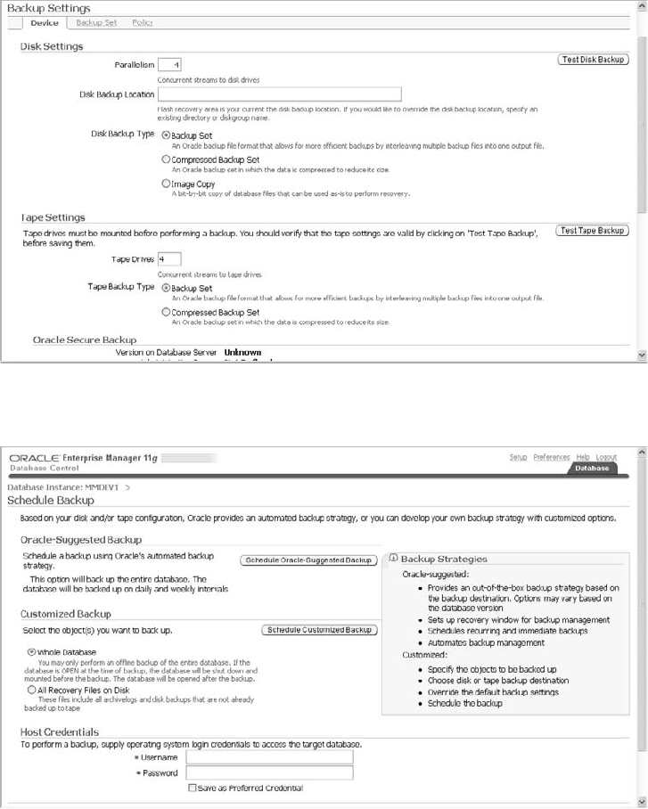
parallelism, and whether they are compressed or an image copy. The backups can
be tested here as well.
Scheduling the backups can be planned on the Schedule Backup screen (shown
next) after configuring what is to be backed up and where.
Just as with using the list or preview of the RMAN backup sets, you can manage
Oracle backups under Enterprise Manager in the following screen. You can review the
backup sets that are available and what is current. Settings are available for backup
Chapter 7: Backup and Recovery 279

sets as well as for image copies. It is also a good way to manage obsolete and expired
sets and files. Crosschecking is an option here too, which will resynchronize the
RMAN catalog with the available files.
Performing a recovery using Oracle Enterprise Manager, as shown in the following
illustration, allows for either complete recovery or point in time. There is also an
advisor to help manage the recovery process and help you detect to what point the
database might need recovery.
280 Oracle Database 11g: A Beginner’s Guide

Chapter 7: Backup and Recovery 281
Now that you’re familiar with the options available through RMAN as well as
some of the features available through Oracle Enterprise Manager, you’re ready to
back up a database.
Performing Backups
There are a number of ways that RMAN backups can be performed. In this section,
you will see several examples of the basic set of backups. Namely, you will see an
example of a database, data file, tablespace, and incremental backup, as well as an
image copy.
Database Backup
An RMAN database backup can be as simple or as complex as you want to make it.
In its simplest form, you can preconfigure channel defaults as discussed previously,
connect to the catalog and the target, and then run the backup command:
RMAN > connect catalog rmancat/rmancat@test2
RMAN > connect target sys/lexus4me@TEST1
RMAN > backup database;
Data File Backup
It doesn’t get any easier than that! Let’s now look at a backup that allocates one
channel and backs up three data files using parallelism. The archive logs are then
backed up:
RMAN > run {
RMAN > configure device type disk parallelism 3;
RMAN > allocate channel c1 type disk;
RMAN > allocate channel c2 type disk;
RMAN > allocate channel c3 type disk;
RMAN > backup database plus archivelog;}
Tablespace Backup
A tablespace backup is performed along with a backup of the control file and
archivelog. Of course, the tablespace backup is implemented by RMAN as a series
of data file backups:
RMAN > backup tablespace EXAMPLE include controlfile plus archivelog;
Incremental Backup
You can configure default settings for a channel and then perform an incremental
level 1 backup. You need to perform an incremental level 0 backup first to provide
a baseline for this incremental to be compared to. If an incremental level 0 does not
exist, then this level 1 backup will be changed to level 0. Check the output of your
backup run to make sure that the backup ran exactly as you expected it to. Backup

282
Oracle Database 11g: A Beginner’s Guide
optimization will be used to ignore any data files that have not changed since the
last backup was performed. A backup script will be used in this example:
replace script BackupTEST1 {
configure backup optimization on;
configure channel device type disk;
sql 'alter system archive log current';
backup database incremental 2 cumulative database;
release channel d1;
}
run {execute script BackupTEST1;}
Image Copy
An image copy can be performed using the RMAN copy command. Next you’ll see
a copy of a system data file to a named location. As you can see, there are no begin
backup and end backup statements. The syntax is simple and RMAN performs the
copy without incurring extra logging overhead:
RMAN > run { allocate channel c1 type disk;
RMAN > copy datafile 1 to '/u01/back/system.dbf';}
You’ve only done the first part of the job, but as you can see, the commands
are relatively simple. We now need to think about how to use these backups in a
recovery situation. Fortunately, the RMAN toolset also simplifies our restores and
recoveries a great deal! Let’s take a look at an example of how we can recover a
database with RMAN.
Restore and Recovery
RMAN can automate file restores and can be used to restore data files, control files,
and archived redo logs. In this example, you will see a full restore and recovery where
the control file is restored from backup and the archive logs that we need are also
restored. We have changed the archive log directory destination to write the archive
log restores to. Notice that there is no mention of file names in this script. The recovery
catalog has kept track of all of the files for us and if files were stored on tape, the
Media Management Layer software may have also assisted with this:
RMAN> connect catalog rmancat/rmancat@ora11g
RMAN> connect target sys/change_on_install@ora11g
MAN> replace script fullRestoreTEST1 {
allocate channel ch1 type disk;
# Set a new location for logs
set archivelog destination to '/TD70/sandbox/TEST1/arch';
startup nomount;
restore controlfile;
alter database mount;
restore database;

recover database;
alter database open resetlogs;
release channel ch1;
}
host 'echo "start `date`"';
run {execute script fullRestoreTEST1;}
host 'echo "stop `date`"';
exit
That’s it! This script is simple and very powerful. We’ve now covered some basic
RMAN backup options to give you an overview of how you can use RMAN on your
databases. You should now test out various backup and recovery options to see how
they function and how well the different options work in your environment. The
settings that you use on one set of servers may not be the ones you will use on another,
so testing your RMAN backup and recovery setup is essential!
Project 7-1 RMAN End to End
This project will have you using RMAN from start to finish. We will first assume that
you have two Oracle databases to work with: the target database will be called
ora11g in this project and the catalog database will be called oracat. You will first
set up the RMAN catalog and then connect to the target database and register that
database in the catalog. A full database backup will be performed, and once that
has been successfully completed, you will use that backup to perform a full
database restore using RMAN. Look carefully at the output that RMAN produces to
help better understand what is going on behind the scenes. Once you’ve completed
this project, you will have used RMAN from end to end and will be comfortable
with basic RMAN functionality.
Step by Step
1. In SQL*Plus, create the RMAN tablespace, catalog, and user named rcat.
Grant the authority that user rcat needs to perform all RMAN operations:
> export ORACLE_SID=oracat
SQL> sqlplus /nolog
SQL> connect sys/change_on_install as sysdba
SQL> create tablespace rcatts datafile
'/u01/oradata/oracat/rcatts.dbf' size 50M;
SQL> create user rcat identified by rcat temporary tablespace
temp default
SQL> tablespace rcatts quota unlimited on rcat;
SQL> grant connect, resource, recovery_catalog_owner to rcat;
SQL> exit
Chapter 7: Backup and Recovery 283
RMAN End to End
Project 7-1
(continued)
284 Oracle Database 11g: A Beginner’s Guide
2. Your RMAN environment and user have now been created, so you need
to go into RMAN to create the recovery catalog. Note that you are using
a recovery catalog here rather than the control file; we strongly encourage
using this approach. You first log into the catalog, connect with the rcat
user, and then run the create catalog command:
> rman catalog=rcat/rcat@oracat
RMAN> catalog rcat/rcat@oracat
RMAN> create catalog;
RMAN> exit;
3. Register the target database ora11g with the RMAN catalog. Once you’ve
completed this, you will be connected to both the target database and a
fully functional catalog and will be ready to begin issuing RMAN commands:
RMAN> connect catalog rcat/rcat@oracat
RMAN> connect target sys/manager@ora11g
RMAN> register database;
4. It’s now time to back up your entire database. You’ll start by applying a
couple of configuration settings to set the default backup device to disk and
to state that you always want to back up the control file and spfile with every
backup. The spfile is automatically included with control file backups. Once
these are configured, you can back up the database, archivelogs, control file,
and spfile. This sounds like a lot of work, but just look at how easy this is to
do with RMAN:
RMAN> configure default device type to disk;
RMAN> configure controlfile autobackup on;
RMAN> backup database plus archivelog;
RMAN> exit;
5. Once the backup has completed successfully, you’ll want to set up the
environment for a restore. To do this, shut down the database and delete all
of the data files, archive logs, control files, and the spfile SPFILEORA11G.ora
for the target database.
6. Now for the big test! The database restore and recovery is the one thing that
absolutely tests how well we’ve done everything so far. Once again in RMAN,
connect to the catalog and target and then put the database in nomount
mode. Once that’s done, restore the archive logs and control files, and then
mount the database. You should now see these files in their proper location.
Restore the database and watch the files being created in another window.
Once that’s complete, recover the database and open it up:
RMAN> connect catalog rcat/rcat@oracat
RMAN> connect target sys/manager@ora11g
RMAN> startup nomount;
RMAN> restore archivelog all;
RMAN> restore controlfile;
Chapter 7: Backup and Recovery 285
RMAN> alter database mount;
RMAN> restore database;
RMAN> recover database;
RMAN> alter database open resetlogs;
The resetlogs step at the end of the listing is needed to create new log files. This
creates a new incarnation (that is, version) of the database and it should be backed
up immediately.
Project Summary
This project has taken you from the very first step of setting up RMAN through a full
backup, restore, and recovery. Congratulations! You have successfully completed
the RMAN fundamentals and are now ready to explore it further and exploit this
powerful tool in your own environment.
þChapter 7 Mastery Check
1. What are some advantages of cold backups, and when would you use them?
2. What are disadvantages of cold backups?
3. Describe the difference between a logical and a physical backup.
4. Name three different types of backups.
5. What is the difference between an RMAN backup and an RMAN image copy?
6. Under what situations should redo logs be restored in a recovery situation?
7. Name three interfaces that can be used to perform a Data Pump Export and
Import.
8. List some advantages of using RMAN.
9. Why would RMAN’s recovery catalog be used to implement the repository
rather than a control file?
10. Are there any disadvantages to an RMAN recovery catalog?
11. How can default settings be set up by you for future runs of RMAN?
12. What is an RMAN backup set and how does it relate to a backup piece?
13. Describe the ways in which corrupt blocks can be detected and recovered.
14. What are some advantages to incremental image copies?
15. When performing a recovery from a hot backup, do all files and tablespaces
need to be brought forward to the same point in time?
This page intentionally left blank

Chapter
8
High Availability: RAC,
ASM, and Data Guard
CRITICAL SKILLS
8.1 Define High Availability
8.2 Understand Real Application
Clusters
8.3 Install RAC
8.4 Test RAC
8.5 Set Up the ASM Instance
8.6 Create ASM Disk Groups
8.7 Use ASMCMD and ASMLIB
8.8 Convert an Existing Database
to ASM
8.9 Understand Data Guard
8.10 Explain Data Guard Protection
Modes
8.11 Create a Physical Standby Server

288 Oracle Database 11g: A Beginner’s Guide
igh availability and reducing planned (or even unplanned) downtime
is a goal of database systems, especially in environments that require
accessibility 24x7. It is unacceptable to have databases go down for
maintenance or even for hardware failures, since these outages can
cause significant losses to the business. Luckily, Oracle 11gis here to
save the day with high availability features such as Real Application Clusters (RAC),
Automatic Storage Management (ASM), and Data Guard. In architecting database
environments, the combinations of RAC and Data Guard will provide instance
failover and even disaster recovery to an offsite standby server. In planning the
configurations and combinations, you must look at cost-effective ways to provide
the business with the availability that they require. Examining the features and how to
implement them will assist you in providing a plan for a reliable, scalable, and stable
environment that can handle the loss of a piece of hardware or be recoverable in the
event of an unplanned circumstance. Let’s also not forget the need for maintenance of
the databases in Oracle 11g. With the rolling patches working by patching one node
of a cluster and then continuing to the next node so at least one node is available
while patching, even the planned maintenance window now becomes smaller.
CRITICAL SKILL 8.1
Define High Availability
What does high availability mean to the business? What is the level of risk tolerance?
How much data loss is acceptable? Are there current issues with backups or reporting?
These are all questions that need to be asked to start mapping out the components
that are needed. You may decide that absolutely no data loss can be tolerated or,
alternatively, that it is fine if the application is down for a day or two.
Also, it helps to look at what kind of outages can happen and then build in fault
tolerance for these situations. Examples of unplanned outages are hardware failures,
such as disk or server failures; human error, such as dropping a data file or making a
bad change; and network and site failures. Then, add on to these examples the
planned outages needed for applying patches, database changes and migrations,
and application changes that might include table and database object changes and
upgrades. Look for the areas in the system with single points of failure and then
match up solutions to start to eliminate those areas.
This chapter just touches on a couple of areas necessary for building a highly
available environment: Real Application Clusters, Automatic Storage Management,
and Data Guard. Understanding these components, plus researching other Oracle
options such as Flashback Query, Transaction and Database, Flash Recovery Area,
Data Recovery Advisor, and Secure Backups, will assist in synching up the environment
with the business needs in the area of availability.
So, in looking at the application and the business needs, if there are planned
outages for maintenance to allow for downtime to patch the environment, rolling
patches might not be as much of a concern. Instead, a solution for testing application
H

Chapter 8: High Availability: RAC, ASM, and Data Guard 289
changes as well as the patches might be possible via Flashback technologies or the
ability to test application changes on a production-like server. If the business doesn’t
allow for downtime or a regular maintenance window, and you know each minute
down will cost the company a serious amount of money, you can use a combination
of components for the solution: rolling patches, prevention of outages from hardware
failures, having failover servers through clusters, and Data Guard.
Working with the business teams and having some understanding of different
options available for architecting a solution that meets budget restrictions and
business needs will take some discussions and planning. The rest of this chapter will
give you an understanding of some of these areas and what it takes to implement them.
CRITICAL SKILL 8.2
Understand Real Application Clusters
Oracle Real Application Clusters (RAC) provides a database environment that is
highly available as well as scalable. If a server in the cluster fails, the database
instance will continue to run on the remaining servers or nodes in the cluster. With
Oracle 11gClusterware, implementing a new cluster node is made simple. RAC
provides possibilities for scaling applications further than the resources of a single
server, which means that the environment can start with what is currently needed
and then servers can be added as necessary. Oracle 9iintroduced the Oracle Real
Application Clusters; with each subsequent release, management as well as
implementation of RAC have become more straightforward, with new features
providing a stable and good performance environment.
In Oracle 11g, Oracle introduced rolling patches for the RAC environment.
Previously, it was possible to provide ways to minimize downtime by failing over to
another node for patching, but it would still require an outage to finish patching all
of the nodes in a cluster. Now with Oracle 11g, the patches can be applied allowing
other servers to continue working even with the non-patched version. Reducing any
outages, planned or unplanned, in companies with 24x7 operations is key. Along the
same lines of the rolling patches, the deployment of new RAC instances and nodes
has been significantly enhanced in 11g. The Oracle Clusterware is the piece that
helps in setting up new servers and can clone an existing ORACLE_HOME and
database instances. Also, it can convert a single node Oracle database into a RAC
environment with multiple nodes.
The RAC environment consists of one or more server nodes; of course a single
server cluster doesn’t provide high availability, because there is nowhere to failover
to. The servers or nodes are connected through a private network, also referred to as
an interconnect. The nodes share the same set of disks, and if one node fails, the
other nodes in a cluster take over.
A typical RAC environment has a set of disks that are shared by all servers; each
server has at least two network ports: one for outside connections and one for the
interconnect (the private network between nodes and a cluster manager). The shared
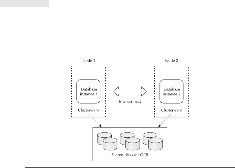
disk cannot just be a simple file system because it needs to be cluster aware, which
is the reason for Oracle Clusterware. Oracle 11gmade several improvements with
the Oracle Clusterware, which now provides several interfaces for managing the
cluster. RAC still supports third-party cluster managers, but the Oracle Clusterware
provides the hooks for the new features for provisioning or deployment of new
nodes and the rolling patches. The Oracle Clusterware is also necessary for Automatic
Storage Management (ASM), which will be discussed in the later part of this chapter.
The shared disk for the clusterware is comprised of two components: a voting
disk for recording disk membership and an Oracle Cluster Registry (OCR) that
contains the cluster configurations. The voting disk needs to be shared and can be
raw devices, Oracle Cluster File System files, ASM, or NTFS partitions. The Oracle
Clusterware is the key piece that allows all of the servers to operate together.
Without the interconnect, the servers do not have a way to talk to each other;
without the clustered disk they have no way to have another node to access the
same information. As seen in Figure 8-1, this is a basic setup with these key
components. Next we will look at how to set up and install these pieces of the
RAC environment.
CRITICAL SKILL 8.3
Install RAC
Before runInstaller or setup.exe is even executed, a checklist of pre-installation steps
needs to be completed. These vary from network setup to making sure the proper
disk is in place. Also before the database is even installed on one of the nodes for
290 Oracle Database 11g: A Beginner’s Guide
FIGURE 8-1. RAC components

Chapter 8: High Availability: RAC, ASM, and Data Guard 291
RAC, the clusterware needs to be present. Several of these steps only need to be
done once to set up the backbone of the RAC environment no matter how many
nodes are being installed. Then tools for cloning the configuration can be used for
deployment of new nodes in the cluster.
Each server needs to be set up with the needed kernel parameters and system
parameters that are required for the operating system. (Please refer back to Chapter
2 for more details on installing Oracle.) Just as there were steps that needed to be
completed for that install, network addresses and the shared disks need to be
configured before Clusterware is installed.
Configurations for network addresses and connections are different from a
standalone database. There are three different IP addresses that are needed: the
virtual network, the private network (interconnect), and the normal or public
network. The hosts need a non-domain name listed for each node in the /etc/hosts
files on the nodes as well as the IP addresses. That is, each host will have at least
three listings in the /etc/hosts files, and each one will have its own unique IP address
and alias or name for the host.
cat /etc/hosts
#eth0 – Public Network
mmrac1.domain1.com mmrac1
mmrac2.domain1.com mmrac2
#eth1 – Private/Interconnect Network
10.0.0.1 mmrac1priv.domain1.com mmrac1priv
10.0.0.2 mmrac2priv.domain1.com mmrac2priv
#VIPs – Virtual Nework
192.168.10.104 mmrac1vip.domain1.com mmrac1vip
192.168.10.05 mmrac2vip.domain1.com mmrac2vip
The public and private networks need to be configured on the same adapter for
all of the nodes. So from the example host file, all of the nodes in the cluster must
have eth0 set to the public network and eth1 to the private. These nodes should be
tested and reachable by pinging them. The interconnect network should be reserved
for traffic between the nodes only, and it is even recommended that it have its own
physically separate network. (This means with hardware setup there should have
been at least two network adaptors installed.) This will certainly help with the
performance of the cache fusion, which is the memory sharing of the buffer caches
between the nodes.
The shared disk needs to be available to be able record the configuration about
the cluster being installed. This disk will house the Oracle Cluster Registry and the
cluster membership.
There should be multiple voting disks available to the Oracle Cluster; if not
added at installation, disks can be added, backed up, and restored if necessary. To
add disks, the following must be run as root; the path is the fully qualified name for
the disk that is being added:
crsctl add votedisk css path –force

Verify by pulling a current list of voting disks:
crsctl query css votedisk
To back up voting disks in Linux/Unix, run the following:
dd if=voting_disk_name of=backup_file_name
In Windows, use the following:
ocopy voting_disk_name backup_file_name
To restore voting disks in Linux/Unix, run the following:
dd if=backup_file_name of=voting_disk_name
In Windows, use the following:
ocopy backup_file_name voting_disk_name
With all of these different pieces needed before RAC can even be installed, the
importance of verifying and checking the configurations is extremely high. When
installing the clusterware, it is critical that the initial configuration of the virtual and
private networks is set up properly. Verifying the network, disk, operating system,
and hardware prerequisites is the first step for installation. The clusterware will not
install properly if any of these requirements is missing. The option to install the
Real Application Cluster when installing the Oracle software will not be available
if the clusterware is not installed or installed correctly.
The Cluster Verification Utility (CVU) assists in this area and should be run before
attempting to install the clusterware. It will verify the hardware and operating system
prerequisites as well as the network configurations. From the software install directory
run the following:
./runcluvfy.sh stage –pre crsinst –n mmrac1, mmrac2
Unknown outputs could mean that the user doesn’t have privileges it needs to
run the check, or a node is unavailable or having resource errors. Running cluvfy
checks after clusterware is installed to verify the install and other prerequisites
before the Oracle database install. Failures should be addressed here before
attempting the database install, otherwise you may find yourself uninstalling
and reinstalling many more times than necessary.
292 Oracle Database 11g: A Beginner’s Guide

NOTE
Setting up users for the installs of Oracle Software,
it might be wise to plan to have different logins for
Clusterware and ASM. Using ASM and Clusterware,
they should be set up in different Oracle homes from
the instance and can have separate Oracle Software
owners, which would be a best practice for security.
You can create users such as crs, asm, and oracle,
but they must share the same Oracle Software
Inventory and have the oinstall group as primary.
Now that the requirements are in place, the installation of the clusterware is
ready to go; by using the Oracle installer, the option should be available to install
clusterware. If the installation of clusterware does not come up, then go back
through and run the Cluster Verification Utility and fix any issues first. Figure 8-2
shows the network information that was configured for the three network addresses
as well as the name of the cluster being defined.
Chapter 8: High Availability: RAC, ASM, and Data Guard 293
FIGURE 8-2. Clusterware install
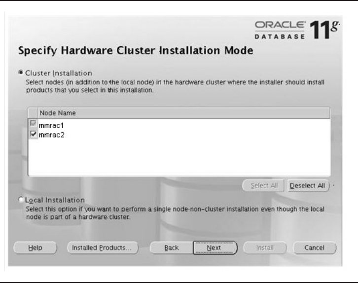
294 Oracle Database 11g: A Beginner’s Guide
After your clusterware is successfully installed, it’s time to install Oracle
Database because the framework has already been completed on the nodes.
From the first node in the cluster, run the Oracle installer (runInstaller on linux/unix,
setup.exe on Windows). Install the Enterprise Edition, which follows along the same
path as a single instance, except for the Cluster installation choices (see Figure 8-3)
after the location of the install information. The recommended path would be to just
do a software install without creating the database, so that the software install can
first be verified. Then, you can use the database configuration assistance to create
the database on the nodes of the cluster.
FIGURE 8-3. RAC install

Chapter 8: High Availability: RAC, ASM, and Data Guard 295
Progress Check
1. How does RAC provide high availability?
2. What does the clusterware use the shared disks for?
3. What is the Cluster Verification Utility?
4. True or False: RAC components are shared disk, with at least two network
connections and clusterware.
5. What is the private network used for in the RAC environment?
CRITICAL SKILL 8.4
Test RAC
RAC environments should first be created for testing and proving concepts for how
the failover works for different applications. The RAC test environments should
continue to be available for testing for production systems, because different workloads
and failover can’t be tested as against a single node. After the installs of the clusterware
and database nodes, it’s useful to test several different scenarios of failover in order
to verify the install as well as to determine how the application fails over.
Create a test list and establish the pieces of the application that need to be part
of that testing. Testing should include hardware, interconnect, disk, and operating
system failures. Simulations of most of these failures are possible in the environment.
Here is an example test list:
■Interconnect Disconnect network cable from network adapter.
Progress Check Answers
1. Failover to another node when there are hardware issues with one of the nodes.
2. Oracle Cluster Registry and voting disk.
3. The utility you run to verify the environment before running the clusterware install.
4. TRUE
5. The private network is used for the interconnect, which allows the nodes to talk to each other
directly and does a health check of the nodes.

■Transaction failover when node fails Connect to one node, run the
transaction, and then shut down the node; try with selects, inserts, updates
and deletes.
■Backups and restores
■Loss of a data file or disk
■Test load balancing of transactions Verify that the services are valid and
are allowing for work load balancing.
Workload Manager
Using RAC databases on the backend of applications doesn’t necessarily mean that
the application is RAC aware. The application as a whole may not fail over, even
though the database is failing over current transactions and connections. There might
be a small outage when one of the nodes needs to fail over. However, with server
calls about the failover, these events can be used to trigger automated processes for
reconnecting or restarting application pieces. These are the Fast Application
Notification events and can be used for failover and for workload balancing.
In Oracle 10g, having different pieces of the application connect to different
nodes helped with load balancing in some ways, but now, thanks to the improvements
in Oracle 11g, the Oracle Clusterware and the Load Balancing Advisor workload
can be distributed across the RAC environment more effectively. Application
workloads connect via a service, and it is by these services that load balancing
as well as the failover is handled. The services are designed to be integrated with
several areas of the database, and not just CPU resources. The advisor bases
information on SERVICE_TIME and THROUGHPUT.
296 Oracle Database 11g: A Beginner’s Guide
Ask the Expert
Q: Is tuning a RAC environment different than tuning single instances?
A: For a first look at tuning the RAC performance, the beginning steps are the
same as with a single instance. The next step would be to look at interconnect
performance and issues. The tools available to tune single instances are RAC
aware, such as Automatic Workload Repository (AWR) reports, which detail
the information collected about performance statistics, waits, long running
SQL statements, and other details about how the database resources are being
used. Oracle Enterprise Manager also provides good insight into issues, enabling
you to see things at a cluster level.

Chapter 8: High Availability: RAC, ASM, and Data Guard 297
ASM
As mentioned with the RAC environment, Automatic Storage Management (ASM)
is both the file and disk manager for the Oracle database files. Now you might be
thinking that this seems like a more advanced topic, and possibly too detailed for a
beginner’s guide. However, ASM is an important component in a highly available
database environment and for addressing performance issues and management of
Oracle files. Even after years of working with applications and databases, there is
always I/O contention, and reading and writing to disk is a main part of what a
database does. So, a database administrator ends up understanding more about disk,
mirroring, and striping than they might really want to know. Debating different RAID
strategies and optimizing I/O may seem like intermediate topics, but even some of
these areas are handled by ASM and have simplified the management of the Oracle
disk and file needs.
There are several more in-depth discussions and topics revolving around
ASM, but this chapter will provide only a general introduction as well as the basic
configuration and how to get started with ASM.
In large databases, the number of data files for an instance can grow out of control;
even a tablespace for a large environment can become unmanageable. Then, any
disk migrations or moving of tablespaces becomes a very difficult task and leaves
areas of vulnerabilities open due to the sheer number of data files. ASM manages
the files using disk groups, and disks are added to the disk groups even while the
database is open and running and the ASM instance is being accessed.
CRITICAL SKILL 8.5
Set Up the ASM Instance
In Oracle 11g, the ASM instance can now be set up as a cluster for providing rolling
patches, and one ASM instance manages the files for one RAC node or one single
Oracle server. An ASM instance can manage the following files for all of the instances
on each cluster node: control files, data files, tempfiles, spfiles, redo logs, archive
logs, RMAN backups, Data Pump dumpsets, and flashback logs. Just as with the
RAC instance, the ASM instance will fail over to the other nodes in the cluster and
continue to manage the disk.
RAC is not necessary for using ASM. In fact, ASM can be installed on a single server
as well as used in a RAC environment. However, an ASM instance is needed for each
server. In Figure 8-4, you’ll see two standalone servers, each with their own ASM
instance. Even though each server needs its own ASM instance, one ASM instance
can manage the files for more than one database instance on that server. Each of the
databases for that ASM instance on that server has access to all of the disk groups,
which are the available disks that have been allocated by creating groups.
As you can see in Figure 8-5, the difference with ASM instances in the RAC
environment is that they are also instances that are available for failover; this means
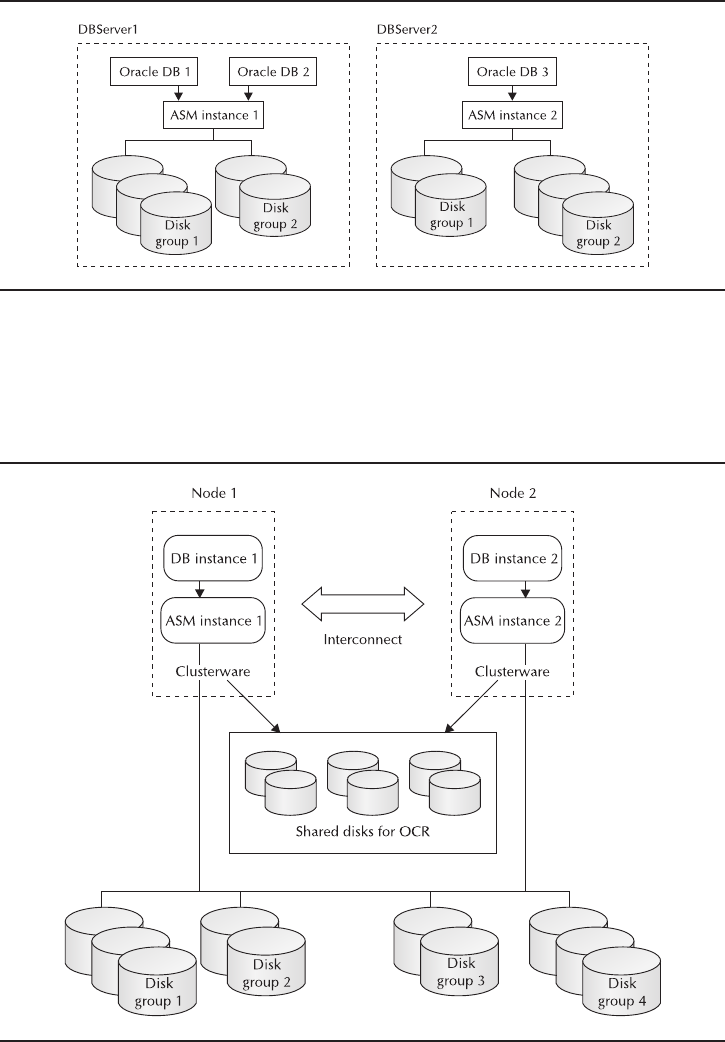
that RAC components need to be available to manage the failover. An ASM instance
is still created on each node, but the instances manage the disk groups and files
across all of the nodes.
298 Oracle Database 11g: A Beginner’s Guide
FIGURE 8-4. ASM instance standalone
FIGURE 8-5. ASM instance RAC
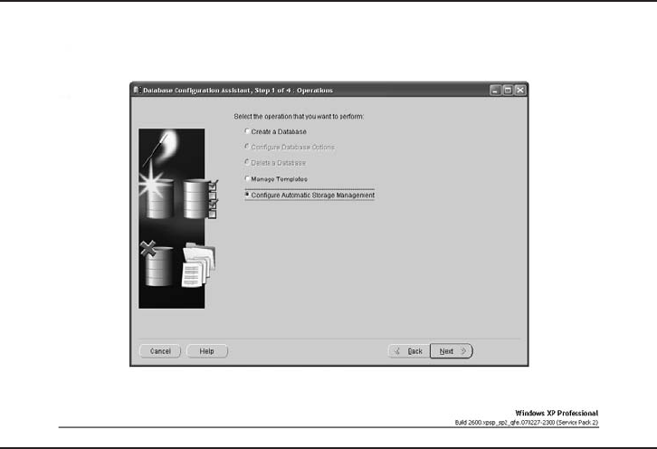
An ASM instance is a small database instance because it is basically the memory
structures, and this provides the framework for managing disk groups. The disk groups
contain several physical disks and can be from different disk formats. The formats
can be a raw disk partition, LUNS (hardware RAID), LVM (redundant functionality),
or NFS (can load balance over NFS system and doesn’t depend on the OS to support
NFS). However, the advantage of ASM is using raw devices which bypass any OS
buffering.
The ASM instance can be created on installation of the Oracle software or by
using Database Configuration Assistant (dbca). The name of the instance normally
starts with +ASM, and then the Oracle Cluster Synchronization Server (CSS) must be
configured. This service is added with the localconfig script, which will add the
OCR repository that is necessary for ASM. Also, there is a new role to log in as
administrator of the ASM instance, SYSASM. The OS group of OSASM goes along
with this new role.
The following are screenshots from creating the ASM instance using the Database
Configuration Assistant or dbca. In walking through the configuration of a database,
you have a choice to create a regular database or to configure Automatic Storage
Management. If you want to create a database using ASM, the ASM instance needs
to be created first. However, you can also migrate an existing database to ASM,
allowing the instance to be created for that migration as well. Either way, the dbca
(see Figure 8-6) provides an easy way to get the ASM instance created.
Chapter 8: High Availability: RAC, ASM, and Data Guard 299
FIGURE 8-6. Creating ASM instance in dbca
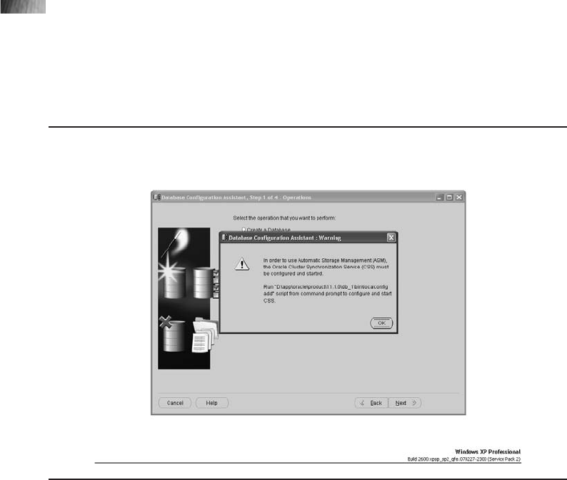
If the Oracle Cluster Synchronization Server (CSS) has not yet been started, a
message will come up that says it needs to be running in order to configure ASM.
Another window can be opened to start this; the command is provided in the
pop-up window as shown in Figure 8-7.
Now the ASM instance is ready to be created, so a click on OK, as shown in
Figure 8-8, will create the ASM instance. Now you’ll just need to configure the
parameters for finding the available disks and the disk groups.
In order for the ASM instance to discover the available disks, an initialization
parameter is used: ASM_DISKSTRING. Other parameters include ASM_DISKGROUPS,
which specifics which files are managed by ASM, and ASM_POWER_LIMIT, which
is the default value for disk rebalancing. INSTANCE_TYPE is set to indicate that the
instance is an ASM instance and not a database:
Parameters:
ASM_DISKGROUPS = CONTROLFILE, DATAFILE, LOGFILE
ASM_DISKSTRING = /dev/rdsk/*
ASM_POWER_LIMIT = 0 /* 0 to 11 0 disables and 11 to enable
rebalancing more quickly */
INSTANCE_TYPE = ASM
300 Oracle Database 11g: A Beginner’s Guide
FIGURE 8-7. Creating ASM instance (CSS)

Disk groups can be created during instance creation. After the instance is
created, sqlplus is used to start up ASM.
Project 8-1 Install ASMLib
For Linux, there is an option for using raw devices or ASMLib to manage the
available disks for Automatic Storage Management. ASMLib is a tool that will
need to be installed as a Linux operating system package.
Step by Step
1. After installing the packages as the root user, the Linux software, and the
Oracle software, the following packages are needed for the ASMLib:
# rpm –Uvh oracleasm-support-2.0.1.-1.i386.rpm
# rpm –Uvh oracleasmlib-2.0.1.-1.i386.rpm
# rpm –Uvh oracleasm-2.6.9-34.ELsmp-2.0.1-1.i686.rpm
2. Verify that the package is installed:
# rpm –q oracleasm*
Chapter 8: High Availability: RAC, ASM, and Data Guard 301
Install ASMLib
Project 8-1
FIGURE 8-8. Creating ASM instance (Completion)
(continued)

302 Oracle Database 11g: A Beginner’s Guide
3. The previous step installed the ASMLib software. Now, to configure, run the
following:
# /etc/init.d/oracleasm configure
4. With the ASMLib software installed, the available partitions can be used to
create ASM disks:
# /etc/init.d/oracleasm createdisk VOL1 /dev/disk1
# /etc/init.d/oracleasm createdisk VOL2 /dev/disk2
5. To view the disks from the OS level that were just created:
# /etc/init.d/oracleasm listdisks
VOL1
VOL2
Project Summary
This project has taken you through the steps to install the package needed for the
ASMLib utility, as well as demonstrated some of the tasks that can be completed
using this command-line utility. Having ASMLib configured will be useful for
managing ASM disks and files.
CRITICAL SKILL 8.6
Create ASM Disk Groups
Starting up the ASM instance is very similar to a database instance. Instead of
connecting as SYSDBA, SYASM should be used:
ORACLE_SID=+ASM
SQLPLUS /NOLOG
SQL> connect SYS as SYSASM
Enter password: sys_password
Connected to an idle instance.
SQL> STARTUP
ASM instance started
Shutdown is also similar to database instances, but the IMMEDIATE clause
checks for databases that are still connected to the ASM instance and returns an
error if this is the case. Any databases connected to the ASM instance during a
shutdown abort will also abort:
SQL> SHUTDOWN NORMAL\IMMEDIATE\ABORT
The redundancy type for a DISKGROUP is specified when the group is created
and cannot be changed. However new groups can be created with different redundancy
types and then migrated to. There are three types of redundancy: EXTERNAL, NORMAL,

and HIGH. With EXTERNAL, ASM is not providing any redundancy, and is assuming
that an outside source is such as the storage array is providing fault tolerance. NORMAL
requires two groups for failover and will handle the failure of one group. HIGH
redundancy provides three-way failover and needs three groups. The NORMAL
and HIGH redundancies also eliminate the single point of failure for the ASM disk.
A small number of disk groups can normally be used even for a large database.
Project 8-2 Create Disk Groups
The next steps will give the commands for creating disk groups with external
redundancy or normal redundancy. Once the groups are created they are available
to create tablespaces.
Step by Step
1. Create disk groups by using the following:
SQL> create diskgroup DGEXT1 external redundancy disk '/dev/rdsk1/disk1';
SQL> create diskgroup DGNORM1 normal redundancy disk
FAILGROUP controller1 DISK
'/dev/rdsk/disk1' name disk1,
'/dev/rdsk/disk2' name disk2
FAILGROUP controller2 DISK
'/dev/rdsk/disk3' name disk3,
'/dev/rdsk/disk4' name disk4;
2. Now that you’ve created the disk groups, validate them by looking at the
views that give you information about disks and disk groups:
■V$ASM_DISKS Available disks reflect values in the parameter
ASM_DISKSTRING:
select * from v$asm_disks;
■V$ASM_DISKGROUPS Available disk groups and details on
redundancy type:
select name, state from v$asm_diskgroups;
NAME STATE
---------------------- -------------------DGEXT1 MOUNTED
DGNORM1 MOUNTED
3. Adding disks to the disk groups can be done as needed to be able to grow
space for the databases:
alter DISKGROUP DGNORM1 add DISK
'/dev/rdsk/disk5' name disk5,
'/dev/rdsk/disk6' name disk6;
Chapter 8: High Availability: RAC, ASM, and Data Guard 303
Create Disk Groups
Project 8-2
(continued)
4. After ASM is started and disk groups are created it is as simple as saying
CREATE TABLESPACE ts_data1, or the disk group name can be used in
place of the data file name as used in a non-ASM database:
Create tablespace DATATBS1 datafile '+DGNORM1' size 1024M;
Project Summary
This project walked through how to create and alter disk groups. After the creation
of the disk groups, steps were taken to verify the disk groups were created or altered
as expected.
Progress Check
1. What is a typical name for an ASM instance?
2. What does ASM stand for?
3. What are the three types of redundancy for disk groups?
4. What is the initialization parameter for ASM to discover the available disks?
5. How is the ASM Instance created?
CRITICAL SKILL 8.7
Use ASMCMD and ASMLIB
Managing ASM instances can be done through Oracle Enterprise Manager, as well
as using the command line in sqlplus and ASMCMD, which is the ASM command-
line utility. Oracle 11gASMCMD has new commands to copy files, back up and
restore metadata, and list and remap ASM files.
There are several new commands for the ASMCMD with Oracle 11g. The new
commands are listed next:
■cp This copies files between ASM disk groups and copies files from disk
groups to the operating system, for example:
ASMCMD >cp +DISKGRP1/MMDB.CTF1 /backups
304 Oracle Database 11g: A Beginner’s Guide
Progress Check Answers
1. +ASM
2. Automatic Storage Management
3. NORMAL, HIGH, and EXTERNAL
4. ASM_DISKSTRING
5. Using the Database Configuration Assistant (dbca)

Chapter 8: High Availability: RAC, ASM, and Data Guard 305
■Lsdsk This lists disk information, which is good for creating a list of disks
an ASM instance uses.
■md_backup This creates a backup file containing the metadata for one or
more disk groups to enable you to re-create the disk groups in the future.
■md_restore This restores a disk group using the backup from md_backup.
■remap This recovers bad blocks on a disk by moving a good copy to a
different location on disk.
Next are other commands; this is not a complete list and you will start to see
these are similar to linux/unix commands:
■cd This changes the directory.
■du This displays the total disk space.
■exit This exits out of ASMCMD command line.
■find This lists occurrences for the specified name.
■ls This lists the contents of the ASM directory (when logging into ASM, it
starts in the / root directory).
■mkdir This creates ASM directories.
■pwd This displays the path of the current directory.
■lsct This lists information about current ASM clients.
Along with managing the ASM instances, there are performance improvements
with Oracle 11gASM, such as the Fast Mirror Resync. The time to recover from a
failure is reduced because of improvements here. There are attributes for disk groups
for these settings. DISK_REPAIR_TIME has a default of 3.6 hours, with the value
determining how much faster the recovery time of the disks is. Faster rebalancing is
also possible using RESTRICTED mode for the disk groups. ASM can be configured
to read from a preferred mirror copy, which in a RAC environment means that nodes
can read from their local storage mirrors instead of possibly having to go through a
network with higher latencies.
As mentioned earlier, the rolling patching can be applied to the ASM instances
as well as database instances when clustering ASM instances. Since ASM is dependent
on the Oracle Clusterware, the clusterware must first be upgraded on all nodes
before upgrading ASM. During the patching, normal database functions are possible,
but changes to the disk group configurations are limited:
To start patching:
SQLPLUS> ALTER SYSTEM START ROLLING MIGRATION TO 11.1.2;
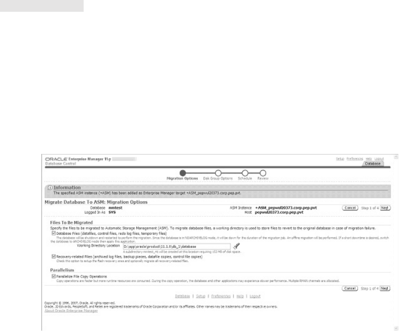
/*Then each ASM instance can be taken down and upgraded. After all the
upgrades have been completed the migration just needs to be stopped.*/
SQLPLUS> ALTER SYSTEM STOP ROLLING MIGRATION;
CRITICAL SKILL 8.8
Convert an Existing Database to ASM
Taking an instance from regular storage to ASM is actually a simple task, but this
is making the assumption that the ASM instance has already been created. Using
Oracle Enterprise Manager is probably the most straightforward way to do this.
Start by opening up Oracle Enterprise Manager and choosing the option to
migrate to ASM. The screen shown in the following illustration is what comes up
after you select to migrate to ASM. Migration requires to you to first choose the
files to be migrated, which of course include database files, but can also include
recovery type files, such as archive logs, backup, and control file copies. If not
chosen, the log files and control files will remain on the current disk.
The next screen has options for choosing the disk groups that this database
should migrate to.
306 Oracle Database 11g: A Beginner’s Guide
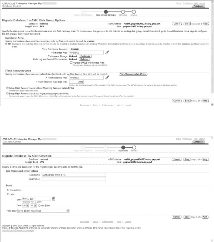
The job can be scheduled to run as needed with the settings in the following
screen. This does require some downtime of the database to run the migration.
Chapter 8: High Availability: RAC, ASM, and Data Guard 307
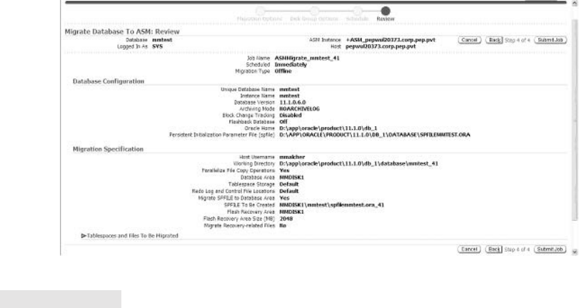
308 Oracle Database 11g: A Beginner’s Guide
The next step summarizes the selections, and then the final step is to submit the
job, as shown next. The migration job can be monitored in OEM.
CRITICAL SKILL 8.9
Understand Data Guard
Providing highly available, recoverable, and secure stable environments is definitely
a goal that needs several components for handling different areas. We have already
discussed RAC and ASM; the Oracle Data Guard environment offers an additional
piece to this architecture. Cluster servers normally reside in the same data center
because of the requirements for the interconnect and clusters share disk. Because of
this, there is potential for failure of this environment. Also, what about restores and
disaster recovery sites? Data Guard can provide solutions in this area, as well as help
offload some of the intense resource consumers such as hot backups, exports, and
reporting. With Data Guard 11g, the standby server can be an active server that can
be used to offload reporting and backups, as well as continue to operate in its
standard role for failover and provide a disaster recovery server. Using Data Guard,
one or more standby servers could be at different locations to allow for failover to a
different site. So, for high availability, Data Guard provides solutions on both fronts
of failover and recovery.
Data Guard has been available in some form since Oracle 8i; however, with
11gthe secondary database can recover while it is open for reading. This means
that ad hoc queries (ones that probably haven’t been tuned and are resource hogs),

reports, backups, and exports can be off-loaded to this system. Being able to use
the failover hardware for useful business purposes makes it a cost-effective part of
a disaster recovery plan.
The Data Guard manager provides a practical way to manage the primary and
secondary servers. It can allow for manual failover, set up the automatic failover,
and place the secondary in snapshot mode. The snapshot mode actually puts the
database in read and write mode so that testing can be done against a current set
of production data. More on this snapshot mode in a little bit, but first let’s walk
through some of the architecture and setup for Data Guard.
CRITICAL SKILL 8.10
Explain Data Guard Protection Modes
The different modes of setup for Data Guard allow for different configurations that
are adaptive and that are dependent on available hardware, processes, and ultimately
business needs.
The modes for the Data Guard configuration include maximum protection,
maximum availability, and maximum performance. The Data Guard configuration
can also have more than one standby database. Having multiple standby databases
is even recommended in modes like maximum protection, in order to make sure at
least one standby is available.
Maximum protection is designed for zero data loss, while the redo transport
is synchronous. Synchronous transport means that you’re applying the database
transactions at the same time on the primary and secondary database servers. The
primary waits for a response telling it that the transaction has been applied to the
standby database before it commits the transaction. Having two standbys or even
a RAC setup on the secondary site would be recommended in this situation, because
if the standby fails, the primary will be halted in this mode.
Maximum availability also has the goal for zero data loss (again with the redo
transport being synchronous). The difference is that if the standby fails or if there
is a connectivity issue, it will allow the primary to continue and the standby to fall
slightly behind. It is not as critical to have more than one standby for this mode
because of the fault tolerance.
Maximum performance has the possibility of minimal data loss, but the
performance is the concern on the primary. This is because the redo transport is
done asynchronously and it doesn’t have to check back with the primary before
the primary does a commit. So, if transport is a concern for slowing down the
primary database and the performance risk is higher than any data loss, the
maximum performance mode will allow for that.
Chapter 8: High Availability: RAC, ASM, and Data Guard 309

310 Oracle Database 11g: A Beginner’s Guide
NOTE
It can be especially hard with discussions regarding
costs and business expectations to come to an
agreement on which mode to use. It is probably
simplest to set the protection mode; the ability to
use the standby server in very practical ways should
help defray concerns. To set the protection mode
for the database, issue the following statement:
ALTER DATABASE SET STANDBY DATABASE TO MAXIMIZE
(PROTECTION | AVAILABILITY | PERFORMANCE);
As discussed earlier, each mode has different services that take care of the
transport and application:
■Transport Services are the pieces that handle the synchronous and
asynchronous transport. These services move the log or transactions to
available standby servers and verify that they are being applied to these
servers. Synchronous transports validate that transactions have been applied
on both primary and standby servers before committing the transactions.
The asynchronous transport will validate that transactions have been sent,
but transactions will be committed on the primary even if not completed
on the standby.
■Apply Services take care of the SQL Apply or the Redo Apply. Apply Services
take the SQL statements or redo logs and control applying them to the standby
databases. SQL Apply takes the redo and transforms it into SQL statements.
After running the SQL statements on primary and standby databases, the
standby matches the primary database and can be used as a logical standby
database. Redo logs are used for keeping the physical standby database
consistent with the primary database. Redo information is applied to the
standby databases by Redo Apply and controlled by the Apply Services.
■Role Management Service is for the switching of the standby to primary.
This is used either for a planned switchover or for the failover due to an
outage of one of the servers.
Figure 8-9 shows a configuration of the Data Guard environment and how the
primary and standby servers do not even need to be in the same location. The
servers can be in the same data center, down the street, or cities apart from each
other, depending on the purpose and need. Having the servers in a different city
provides high availability even in an event of a disaster in the location of the primary
database. Also in Figure 8-9, notice the options that are available for uses of the
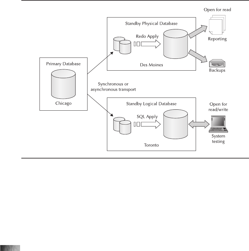
standby server, such as reporting, system testing, or even running backups to take
this type of load off of the primary server.
With Redo Apply, the standby database can be opened for read-only queries.
The recovery on the standby is canceled and the database is then opened. If you’re
using the Active Data Guard option, the Redo Apply can be started again to allow
the standby to have real-time data while having the database open. This can be
done in sqlplus on the standby database:
SQLPLUS> ALTER DATABASE RECOVER MANAGED STANDBY DATABASE CANCEL;
SQLPLUS> ALTER DATABASE OPEN READ ONLY; And then to start applying
the redo again:
SQLPLUS> ALTER DATABASE RECOVER MANAGED STANDBY DATABASE
USING CURRENT LOGFILE DISCONNECT;
/* The database is still open for read-only queries and reporting as
the logs are being applied. */
Another option for using the standby database is as a snapshot database that can
be updated and used for testing. During this time, no logs are applied. After testing,
Chapter 8: High Availability: RAC, ASM, and Data Guard 311
FIGURE 8-9. Data Guard configuration

the snapshot database is converted back to standby database by using a restore
point with flashback database:
Create Snapshot:
SQLPLUS> ALTER DATABASE CONVERT TO SNAPSHOT STANDBY;
Convert back to Standby:
SQLPLUS> ALTER DATABASE CONVERT TO PHYSICAL STANDBY DATABASE;
When using a snapshot database with SQL Apply, stopping the apply of the SQL
statements is not necessary. This is because the standby is kept synchronized by
having the same SQL being applied on the primary applied on the standby as well.
So, while the standby is still being synchronized, it is also available for queries,
running reports, or backups. The commands for setting up the standby for read
access shown here are not necessary, but are done during the initial setup to show
that SQL Apply is being used:
SQLPLUS> ALTER DATABASE START LOGICAL STANDBY APPLY IMMEDIATE;
Progress Check
1. What service handles the failover from primary to standby?
2. What protection mode will cause the primary to wait on new transactions if
it is not able to apply logs to at least one of the standbys?
3. How many protection modes are there?
CRITICAL SKILL 8.11
Create a Physical Standby Server
All of the databases, whether physical or logical, must be created as a physical standby
first. The tools used to create the standby are RMAN, Data Guard Broker, or Oracle
Grid Control. Steps must be completed on both primary and standby servers. However,
the steps on the primary database only need to be done once, no matter how many
standby servers are being created. Oracle 11gRMAN provides a simple command
for creating the standby database and backing up the database at the same time.
312 Oracle Database 11g: A Beginner’s Guide
Progress Check Answers
1. Role Management Service
2. Maximum protection mode
3. Three: maximum protection, maximum availability, and maximum performance

Project 8-3 Create a Physical Standby Server
Step by Step
1. Complete the following steps on the primary server:
select FORCE_LOGGING from v$database;
alter database force logging;
-- forces all changes to be logged even if nologging
might be set on an object
2. Configure the redo transport authentication; use a remote login password
file.
3. Add standby logfiles to the primary. The logs on the standby need to be the
same size or larger than on the primary in order for the primary redo to be
applied to the standby redo logs.
alter database add standby logfile '/u...' size 50M;
4. Set initialization parameters on the primary server:
DB_NAME =
DB_UNIQUE_NAME (Doesn't change even if the standby becomes the primary)
CONTROL_FILES
LOG_ARCHIVE_CONFIG='dg_config=(DG01,DG02)'
LOG_ARCHIVE_DEST_1='LOCATION=/u01/oraarch/DG01' ## local archive directory
LOG_ARCHIVE_DEST_2='service=DG01 ASYNC
VALID_FOR=(ONLINE_LOGFILE,PRIMARY_ROLE) db_unique_name=DG01' ## sets the type
of transport and used for physical standby
REMOTE_LOGIN_PASSWORDFILE = Exclusive
LOG_ARCHIVE_DEST_STATE_n
5. Put the primary server in archive log mode.
6. The network configurations for the standby database need to be configured
on both the primary and secondary servers. Using Oracle Net Manager on
both servers will help configure this. (Refer to the discussion in Chapter 3.)
In configuring a service name, use the unique_db name for the standby
server. After setting up the listener and service on both servers, verify that
the password file has been copied over and the directories for adump,
bdump, flashback, and so on have been created.
7. Creating the standby database over the network, start up the standby
database in NOMOUNT mode.
Chapter 8: High Availability: RAC, ASM, and Data Guard 313
Create a Physical Standby Server
Project 8-3
(continued)
314 Oracle Database 11g: A Beginner’s Guide
8. On the primary server, issue the RMAN command and connect as sysdba:
RMAN> connect auxiliary sys/password@DG02
RMAN> run {
allocate channel disk1 type disk;
allocate auxiliary channel stby type disk;
duplicate target database for standby from active database
spfile
parameter_value_convert 'DG01','DG02'
set db_unique_name='DG02'
set db_file_name_convert='/dg01/','/dg02/'
set log_file_name_convert='/dg01/','/dg02/'
set control_files='/u01/app/oradata/controlfiles/dg02.ctl'
set log_archive_max_processes='5'
set fal_client='dg02' ## FAL (fetch archive log) client and is used if
roles are switched
set fal_server='dg01'
set standby_file_management='AUTO'
set log_archive_config='dg_config=(dg01,dg02)'
set log_archive_dest_1='service=dg01 ASYNC
valid_for=(ONLINE_LOGFILE,PRIMARY_ROLE) db_unique_name=DG01'
;}
9. Log into the primary server and switch the logfile:
SQLPLUS>alter system switch logfile;
10. Start the recovery process on the standby server:
SQLPLUS> alter database recover managed standby database
using current logfile disconnect;
Primary and standby servers have been created and now should be verified.
Project Summary
In this project, primary and standby databases were created. The configuration of
the parameters and starting up the instances all need to be completed before the
recovery process on the standby server starts. Following these steps should give
you a good idea what it takes to create a standby server.
To manage the Data Guard system, the Data Guard Broker (command line)
or Oracle Enterprise Manager Grid Control can be used. In order to use the Data
Guard Broker, the parameter DG_BROKER_START needs to be set to TRUE and the
listener needs to have the databases with broker services added. DGMRGL is the
command to invoke the broker. For Oracle Grid Control, once the database targets
are added to the Grid, the Data Guard management is possible. These tools provide
a way to failover the database to the standby and back again to primary. They hold
the configurations and allow modifications as well as managing and monitoring the
Data Guard environment.
Chapter 8: High Availability: RAC, ASM, and Data Guard 315
Tie It All Together
High availability is an important topic for database systems with the effort to remove
all single points of failure in business critical applications. There are several
components of Oracle 11gwhich, either standing alone or in combination, provide
highly available solutions. Oracle Real Application Clusters (RAC) along with Data
Guard provides a very fast failover system with the capabilities of an off-site standby
database for disaster recovery. Automatic Storage Management (ASM) offers several
advancements for managing the database files and disk in order to provide a stable
environment that can minimize maintenance windows and downtime. Planning
with your business and reviewing these as well as other database features should
assist you in developing and implementing a well-architected, highly available
database system.
þChapter 8 Mastery Check
1. Which component is not part of a RAC environment?
A. Interconnect
B. Clusterware
C. DGMGRL
D. OCR
2. True or false: The Cluster Verification Utility is run after the RAC database is
created to verify that the interconnect is running properly.
3. In a RAC environment, OCR stands for
A. Oracle Cluster Registry
B. Oracle Connection Repository
C. Oracle Clusterware Record
D. Oracle Cluster Recovery
4. In a RAC environment, how many IP addresses are needed for a server?
5. What is the command-line interface that can be used to copy, back up, and
list the files in ASM directories?
6. True or false: ASM redundancy types are EXTERNAL, HIGH, and LOW.
7. When shutdown abort is used to shut down the ASM instance, what
happens to the database instances connecting to that ASM instance?
8. What is the administrator’s login role on the ASM instance?
9. What does the following sqlplus command do? Does it run against the
primary or standby server?
SQLPLUS> alter database recover managed standby database using current
logfile disconnect;
10. True or false: Asynchronous transport of redo logs means that the redo is
being written to the primary and standby locations at the same time.
11. Which of the following is not a characteristic of the Data Guard Protection
mode of maximum protection?
A. Synchronous transport
B. Zero data loss
C. Standby fails, primary is halted
D. Performance is the biggest concern
12. Which tools can be used to manage the Data Guard environment?
316 Oracle Database 11g: A Beginner’s Guide

Chapter
9
Large Database Features
CRITICAL SKILLS
9.1 Learn to Identify a Very Large
Database
9.2 How and Why to Use Data
Partitioning
9.3 Compress Your Data
9.4 Use Parallel Processing to Improve
Performance
9.5 Use Materialized Views
9.6 Use SQL Aggregate and Analysis
Functions
9.7 Create SQL Models

318 Oracle Database 11g: A Beginner’s Guide
n this chapter, you will be exploring the topics and features available
in Oracle Database 11g that you’ll need to be familiar with when
working with large databases. These features are among the more
advanced that you will encounter, but they’re necessary because
databases continue to grow larger and larger. When you start working
with Oracle, you will find yourself facing the trials and tribulations associated with
large databases sooner rather than later. The quicker you understand the features and
know where and when to use them, the more effective you will be. Of course, these
features are not just valuable for large databases; they provide value to everyone who
is looking to optimize their Oracle database environment.
CRITICAL SKILL 9.1
Learn to Identify a Very Large Database
Let’s start by describing what we mean by a very large database (VLDB). Large is a
relative term that changes over time. What was considered large five or ten years
ago is small by today’s standards, and what is large today will be peanuts a few
years from now. How many people remember buying a computer with 20MB of
storage and wondering how they could ever fill it up? Today, personal computers
may come with more than a terabyte of storage; with the types of information you
store, you know that you will fill these storage systems to capacity sooner or later.
Each release of Oracle has included new features and enhancements for addressing
the need to store more and more data. For example, Oracle8iwas released in 1999
and could handle databases with terabytes (1024 gigabytes) of data. In 2001, Oracle9i
was released and could deal with up to 500 petabytes (1024 terabytes). Oracle
Database 11gnow offers support for exabyte (1024 petabytes) databases. You won’t
come across too many databases with exabytes of data right now, but in the future
at least you know Oracle will support them. In addition, Oracle produces a new
high-performance hardware and software solution called “The Database Machine,”
which will provide speed improvements and large amounts of storage as the
importance of large databases continues to expand and evolve over time.
The most obvious examples of large database implementations are data warehouses
and decision support systems. These environments usually have tables with millions
or billions of rows or wide tables with large numbers of columns and many rows.
There are also many OLTP systems that are very large and can benefit from the
features you are about to explore. Since you have many topics to get through, let’s
jump right in and start with data partitioning.
NOTE
Many of the topics discussed in this chapter could
take an entire book to cover completely. Since this is
an introductory book, specifics for some topics have
been omitted. Real-world experiences and additional
reading will build on the material presented here.
I

Chapter 9: Large Database Features 319
CRITICAL SKILL 9.2
Why and How to Use Data Partitioning
As user communities require more and more detailed information to remain
competitive, it has fallen to database designers and administrators to help ensure
that the information is managed effectively and can be retrieved for analysis
efficiently. In this section, we will discuss partitioning data and the reasons why it
is so important for working with large databases. Afterwards, you’ll follow the steps
required to make it all work.
Why Use Data Partitioning
Let’s start by defining data partitioning. In its simplest form, it is a way of breaking
up or subsetting data into smaller units that can be managed and accessed separately.
It has been around for a long time, both as a design technique and as a technology.
Let’s look at some of the issues that gave rise to the need for partitioning and the
solutions to these issues.
Tables containing very large numbers of rows have always posed problems and
challenges for DBAs, application developers, and end users alike. For the DBA, the
problems are centered on the maintenance and manageability of the underlying
data files that contain the data for these tables. For the application developers and
end users, the issues are query performance and data availability.
To mitigate these issues, the standard database design technique was to create
physically separate tables, identical in structure (for example, columns), but each
containing a subset of the total data (this design technique will be referred to as
non-partitioned here). These tables could be referred to directly or through a series
of views. This technique solved some of the problems, but still meant maintenance
for the DBA with regard to creating new tables and/or views as new subsets of data
were acquired. In addition, if access to the entire dataset was required, a view was
needed to join all subsets together.
Figure 9-1 illustrates a non-partitioned design. In this sample, separate tables
with identical structures have been created to hold monthly sales information for
2005. Views have also been defined to group the monthly information into quarters
using a union query. The quarterly views themselves are then grouped together into
a view that represents the entire year. The same structures would be created for
each year of data. In order to obtain data for a particular month or quarter, an end
user would have to know which table or view to use.
Similar to the technique illustrated in Figure 9-1, the partitioning technology
offered by Oracle Database 11gis a method of breaking up large amounts of data
into smaller, more manageable chunks, with each of the partitions having their own
unique name and their own storage definitions. But, like the non-partitioned technique,
it is transparent to the end user, offering improved performance and reduced
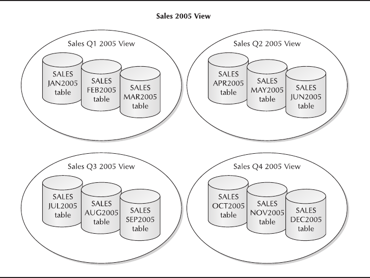
320 Oracle Database 11g: A Beginner’s Guide
maintenance. Figure 9-2 illustrates the same SALES table, but implemented using
Oracle Database 11g’s partitioning option. From the end user’s perspective, there is
only one table called SALES and all that is required to access data from the correct
partition is a date (or a month and year).
Oracle partitioning was first introduced in Oracle8, is only available with the
Enterprise Edition, and is an additional option to the version. As previously suggested,
it is one database option that is a must-have for anyone with a large volume of data
that needs to be quickly retrievable or with a need for speedy data archiving. Many
improvements have been made since then, and Oracle Database 11gcontains all
of the latest features. The remainder of this section discusses these features in more
detail.
Manageability
When administering large databases, DBAs are required to determine the most
efficient and effective ways to configure the underlying data files that support
the tables in the database. The decisions made at this time will affect your data
accessibility and availability as well as backup and recovery.
FIGURE 9-1. Partitioning using physically separate tables (non-partitioned)
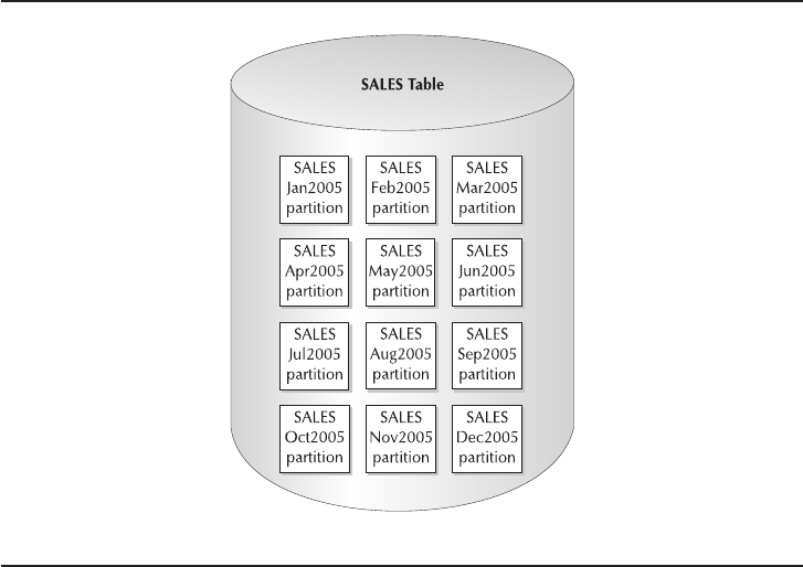
Chapter 9: Large Database Features 321
Some of the benefits for database manageability when using partitioned tables
include the following:
■The size of each underlying data file is generally smaller for partitioned
tables than for non-partitioned tables. This allows for easier and quicker
data selections and smaller backups.
■Historical partitions can be made read-only and will not need to be backed
up more than once. This also means faster backups. With partitions, you
can move data to lower cost storage by either moving the tablespace,
sending it to an archive via an export (datapump), or some other method.
■The structure of a partitioned table needs to be defined only once. As new
subsets of data are acquired they will be assigned to the correct partition,
based on the partitioning method chosen. In addition, with Oracle 11gyou
now have the ability to define intervals that allow you to define only the
partitions that you need. It also allows Oracle to automatically add partitions
based on data arriving in the database. This is an important feature for
DBAs, who currently spend time manually adding partitions to their tables.
FIGURE 9-2. Partitioning using Oracle 11gpartitioning

■Individual tablespaces and/or their data files can be taken offline for
maintenance or archiving without affecting access to other subsets of data.
For example, assuming data for a table is partitioned by month (later in this
chapter, you’ll learn about the different types of partitioning) and only 13
months of data is to be kept online at any one time, the earliest month is
archived and dropped from the table when a new month is acquired. This
is accomplished using the command alter table abc drop partition xyz and
does not affect access to the remaining 12 months of data.
■Other commands that would normally apply at the table level can also
be applied to a particular partition of the table. These include, but are not
limited to: delete, insert, select, truncate, and update. You should review
the Oracle 11gPartitioning Guide for a complete list of the commands that
are available with partitions and subpartitions.
Performance
One of the main reasons for partitioning a table is to improve I/O response time
when selecting data from the table. Having a table’s data partitioned into subsets
can yield much faster query results when you are looking for data that is contained
within one subset of the total. Let’s look at an illustrative example.
Assume the SALES table contains 100 million records representing daily sales
revenue for the three years 2005 to 2008 inclusive. You want to know what the total
revenue is for February 2008. Your query might look something like this:
select sum(amount_sold)
from sales
where time_id between to_date('2008-02-01', 'YYYY-MM-DD')
and to_date('2008-02-28', 'YYYY-MM-DD');
322 Oracle Database 11g: A Beginner’s Guide
Ask the Expert
Q: Can you use the analyze table command to gather statistics on
partitioned tables?
A: No, at least not correctly. The supplied DBMS_STATS package should
be used to gather statistics on partitioned tables instead. The analyze table
command does not gather all required statistics for partitioned tables (in
particular, global statistics). In addition, the analyze command will eventually
be phased out (for all types of table and indexes) and only those statistics
gathered by the DBMS_STATS package will be used by the cost-based
optimizer.

Using a non-partitioned table design, all 100 million rows would need to be
scanned to determine if they belong to the date criteria. Using a partitioned table
design based on monthly partitions, with about 2.8 million rows for each month,
only those rows in the February 2008 partition (and therefore only about 2.8 million
rows) would be scanned. The process of eliminating data not belonging to the
subset defined by the query criteria is referred to as partition pruning.
With the basic concepts of partitioning and why you use it under your belt, you
can now learn about the finer details of how to implement partitioning.
Implement Data Partitioning
Implementing data partitioning in Oracle Database 11gis a process that requires
careful planning to ensure success. You will need to understand your database
environment, hardware, structures, and data before you can make the appropriate
decisions. The next few sections will outline the steps you will take when
partitioning. Let’s start by looking at the characteristics of the candidate table.
Analyze the Candidate Table
The first step in the partitioning process is to analyze and understand the candidate
table, its environment, and its uses. Following are some criteria to consider.
Table Structure and Data Contents You will need to look at the attributes that are
available and the distribution of the data within each attribute. You must consider
currently available data as well as projected future data. The distribution of data
over each attribute is important because you want to ensure that the resulting data
subsets are evenly distributed across the defined partitions.
Consider a table called PHONE_USAGE that contains detailed mobile phone
call records with over 300 million records per month. It has many attributes,
including the toll type (toll_type_cd) and the date of call (call_date). Table 9-1
shows a sample row count for a month by toll_type_cd. As you can see, using this
attribute would probably not be an ideal choice for creating subsets because the
distribution is heavily skewed toward LOCAL calls.
Chapter 9: Large Database Features 323
toll_type_cd Record Count (Sample Month)
INTNL 27,296,802
CONTNL US 52,227,998
LOCAL 189,554,584
NRTH AMRCA 36,367,841
TABLE 9-1. Toll Type and Record Counts

Table 9-2 looks at the distribution of the same data by the day of the week (for
example, Sunday to Saturday based on call_date).
You can see that the day of the week provides a relatively even distribution that
is more suitable for partitioning. Having a relatively equal data distribution of your
data across the partitions will result in better performance during queries, as processing
can be spread equally across the partitions. When a table is skewed to one partition,
this can result in a very large data set within your table, which would defeat the
purpose of partitioning the table in the first place.
How the Data Will Be Accessed To access the data, you will need to know what
the commonest data selection criteria are. This is perhaps the most important part of
the analysis because, as stated earlier, query performance is the most noticeable gain
of data partitioning. In order for this to be realized, your data subsets need to be
defined according to the commonest selection criteria so that unnecessary partitions
can be pruned from the result set. The selection criteria will be determined largely
by your user community and can be determined using historical query patterns (if
available) or consulting business requirements.
Referring to the SALES table example, your analysis of query patterns for a
three-month period (averaging 400 queries per month) yields the results shown
in Table 9-3.
The analysis tells you that time_id and promo_id are both frequently used as
query predicates. You could use this information along with the corresponding row
distribution to determine which attribute would result in the better partitioning strategy.
Hardware Configuration Factors such as the number of physical disks and disk
controllers will contribute to the effectiveness of your partitioning strategy. Generally,
the greater the number of disks and/or controllers, the better—you can spread the
partitions over more hardware to improve I/O performance.
324 Oracle Database 11g: A Beginner’s Guide
Day of the Week (Based on call_date) Record Count (Sample Month)
SUN 41,635,356
MON 44,235,019
TUE 42,875,502
WED 43,235,721
THU 43,922,997
FRI 45,005,293
SAT 44,537,337
TABLE 9-2. Counts Based on Day of the Week

Chapter 9: Large Database Features 325
Identify the Partition Key
Once you understand the characteristics of your candidate table, the next step in the
partitioning process is to select the attribute(s) of the candidate table that will define
the partition subsets and how the subsets will be defined. The selected attributes
will form the partition key. Only one set of attributes can be chosen to partition the
data. This is an important decision, since it will affect the manageability and usability
of the table.
The results of your analysis of the candidate table should provide you with a good
idea of the attributes to use. The best attributes will be those that satisfy the most criteria.
Keep in mind, though, that the adage “you can satisfy some of the criteria some of the
time, but you can’t satisfy all of the criteria all of the time” applies here. Despite your
best efforts and planning, there will still be situations when the table will be treated as
if it were non-partitioned. Take, for example, a perfectly valid query submitted by the
user community that does not include the attributes of the partition key as part of the
selection criteria or groups by the partition key. In this case, data from the entire table
(that is, all partitions) would be scanned in order to satisfy the request.
Select the Type of Partitioning
After you have selected the partition key, the next step in the partitioning process is
to decide which type of partitioning you want to implement on the candidate table.
Oracle Database 11gprovides seven ways to partition data:
■Range partitioning
■List partitioning
■Hash partitioning
Attribute
Times Used in Query Selection Criteria
(Average/Month)
prod_id 33
cust_id 40
time_id 355
channel_id 55
promo_id 298
quantity_sold 25
amount_sold 20
TABLE 9-3. Query Counts Based on Data Attributes

326 Oracle Database 11g: A Beginner’s Guide
■Composite partitioning
■Reference partitioning
■Virtual column-based partitioning
■Interval partitioning
The type of partitioning you choose will depend on the results of your analysis
of the candidate table. The commonest type of partitioning is range partitioning and
this will be covered in the most detail. Let’s look at the characteristics of each type
of partitioning.
Range Partitioning Range partitioning has been around the longest of all partitioning
types and is the one implemented most often. In most cases, the ranges are based on
some date column, such as quarters, months or, in the case of very large data volumes,
days. (Theoretically, you can go down to any level of time—hours, minutes, and so
on—assuming you have a time component. But the maintenance implications of
defining this many partitions make it unrealistic.) The ranges selected will again be
based on the results of your analysis of the table, using dates, numeric values, or
character values. Following is an example based on the SALES table you saw earlier
in the chapter.
NOTE
The partitioning examples presented in this chapter
do not address all of the command options available.
They are meant to give you a taste of what is available.
To create your SALES table as non-partitioned, you would use the standard
create table statement as shown in this listing:
create table sales (
prod_id number not null,
cust_id number not null,
time_id date not null,
channel_id number not null,
promo_id number not null,
quantity_sold number (10,2) not null,
amount_sold number (10,2) not null)
tablespace example_tblspc_1;
Based on the analysis of the usage patterns and row distribution, you have
decided that the optimal partition strategy for this table is based on sales month.
You will now redefine the SALES table using time_id as your partition key to create
monthly partitions for January 2007 to December 2009, inclusive. Creation of data
partitions is accomplished using extensions of the create table statement. The
following listing shows the creation of the table with range partitions. Explanations
of the important lines are given in Table 9-4.

1 create table sales (
2 prod_id number not null,
3 cust_id number not null,
4 time_id date not null,
5 channel_id number not null,
6 promo_id number not null,
7 quantity_sold number (10,2) not null,
8 amount_sold number (10,2) not null)
9 storage (initial 65536 minextents 1 maxextents 2147483645)
10 partition by range (time_id)
11 (partition sales_200701 values less than
12 (to_date('2007-02-01','YYYY-MM-DD'))
13 tablespace sales_ts_200501,
14 partition sales_200702 values less than
15 (to_date('2007-03-01','YYYY-MM-DD'))
16 tablespace sales_ts_200502,
17 partition sales_200703 values less than
18 (to_date('2007-04-01','YYYY-MM-DD'))
19 tablespace sales_ts_200503,
...
113 partition sales_200811 values less than
114 (to_date('2008-12-01','YYYY-MM-DD'))
115 tablespace sales_ts_200711,
116 partition sales_200812 values less than
117 (to_date('2009-01-01','YYYY-MM-DD'))
118 tablespace sales_ts_200712,
119 partition sales_max values less than (maxvalue)
120 tablespace sales_ts_max);
Chapter 9: Large Database Features 327
Lines Important Points
9 This defines the default table-level storage parameters that will apply to
all partitions. It is possible to override these defaults at the partition level
in favor of specific parameters required for a particular partition.
10 This defines the type of partitioning (for example, range) and the
partition key (for instance, time_id).
11–118 Define each partition based on the values of time_id (repetitive lines for
Apr 2007 to Oct 2009 omitted for brevity’s sake). For each partition, the
upper boundary of the partition key value is specified (as defined by the
values less than clause), as well as the name of the tablespace where
the subset is to be stored. Values must be specified in ascending order
and cannot overlap. It is good practice to give meaningful names to both
the partitions and tablespaces.
TABLE 9-4. Explanation of Range Partitioning Syntax

NOTE
Lines 11 to 13 define the first partition to hold data
where time_id is less than February 1, 2007. The
intention in this example is that this first partition
will only hold data for January 2007 (our data
analysis tells us that there is no data before this
date). However, if there happens to be data prior to
January 2007, it will also be placed in this partition
and may skew the row distribution by placing many
more rows than intended in this partition.
That completes the discussion on range partitioning. Let’s now have a look at list
and hash partitioning.
List Partitioning There may be cases when, after your analysis of a candidate
table, you decide that range partitioning is not the best fit for your table. Another
way to subset your data is to use list partitioning, where you group a set of discrete
partition key values and assign them to their own tablespace. By using this type of
partitioning, you can control the placement of the records in specified partitions,
thereby allowing you to group related records together that may not otherwise have
a relationship.
As an example, assume you have an INS_COVERAGE table that contains
insurance coverages. Your analysis of this table and its usage leads you to decide
that you should partition, based on the attribute COV_TYPE_CD, into the buckets
shown in Table 9-5.
328 Oracle Database 11g: A Beginner’s Guide
COV_TYPE_CD Grouping
TERM 65 Life
UL Life
ADB Life
COLA GIB
GPO GIB
WP Disability
DIS Disability
MF Investment
TABLE 9-5. Insurance Coverage Groupings

The syntax of the create table statement is similar to that for range partitioning.
An explanation is provided in Table 9-6:
1 create table ins_coverage (
2 plan_id number not null,
3 cust_id number not null,
4 time_id date not null,
5 dist_channel_id number not null,
6 cov_type_cd varchar2(50) not null,
7 cov_amt number (10,2) not null,
8 prem_amt number (10,2) not null)
9 storage (initial 65536 minextents 1 maxextents 2147483645)
10 partition by list (cov_type_cd)
11 (partition cov_life values ('TERM 65', 'UL', 'ADB')
12 tablespace cov_life_ts,
13 partition cov_gib values ('COLA', 'GIB')
14 tablespace cov_gib_ts,
15 partition cov_dis values ('WP', 'DIS')
16 tablespace cov_dis_ts,
17 partition cov_inv values ('MF')
18 tablespace cov_inv_ts
19 partition cov_other values(default));
TIP
If you discover missing partition keys values that
need to be added to existing partition definitions
after the table has been created, you can issue and
alter table abc modify partition xyz add values
('value1', …).
Chapter 9: Large Database Features 329
Lines Important Points
10 This defines the type of partitioning (for example, list) and
the partition key (cov_type_cd, for instance). Note that with
list partitioning, only one attribute from the table can be
chosen as the partition key—in other words, multicolumn
partition keys are not permitted.
11–18 This defines each partition based on the groups of values of
cov_type_cd.
TABLE 9-6. Explanation of List Partitioning Syntax

Hash Partitioning If you determine from your table analysis that neither range nor
list partitioning is appropriate for your table, but you still want to reap the benefits
offered by partitioning, Oracle Database 11gprovides a third partitioning option
called hash partitioning. With hash partitioning, you define up to 16 partition key
attributes as well as the number of partitions you want to spread the data across. As
long as each partition is on its own physical device and most of the queries use the
partition key as a predicate, you should see performance gains. Hash partitioning is
useful if the distribution of data is unknown or unpredictable.
The following listing is an example of hash partitioning. Table 9-7 explains the
important lines:
1 create table sub_activations (
2 sub_id number not null,
3 dist_channel_id number not null,
4 act_date date not null,
5 deact_date date not null,
6 sales_rep_id number not null)
7 partition by hash (sub_id)
8 partitions 4
9 store in (subact_ts1, subact_ts2, subact_ts3, subact_ts4);
It is beyond the scope of this book to discuss the hashing algorithm used by
Oracle Database 11g. However, it is based on the number of attributes in the
partition key and the number of partitions selected.
Composite Partitioning The final method of partitioning that you will read about
here is a combination of two of the previous types. Combining two types of
partitioning is called composite partitioning. There are a few basic combinations:
range with hash, range with range, and range with list and others. Using composite
partitioning allows you to take advantage of the features of either hash or list
partitioning within the higher groupings of ranges.
330 Oracle Database 11g: A Beginner’s Guide
Lines Important Points
7 This defines the type of partitioning (for instance, hash) and the
partition key (for example, sub_id).
8 This specifies the number of partitions over which to spread the data.
9 This specifies the tablespaces into which the partitions will be placed.
TABLE 9-7. Explanation of Hash Partitioning Syntax

A good example of where this type of partitioning is used would be the
PHONE_USAGE table you saw in your candidate table analysis. In this case, you
have a table that is being loaded with 300 million records per month. You could
choose to implement range partitioning by month and then subdivide the monthly
partitions into four hash partitions. The following listing shows the SQL syntax that
accomplishes this, and Table 9-8 provides the explanation of the important lines:
1 create table phone_usage
2 (sub_id number,
3 call_date date,
4 call_type_id number,
5 called_location varchar2(50),
6 service_carrier_id number)
7 storage (initial 65536? minextents 1 maxextents 2147483645)
8 partition by range (call_date)
9 subpartition by hash(sub_id)
10 subpartition template(
11 subpartition sub1 tablespace ph_usg_ts1,
12 subpartition sub2 tablespace ph_usg_ts2,
13 subpartition sub3 tablespace ph_usg_ts3,
14 subpartition sub4 tablespace ph_usg_ts4)
15 (partition phoneusg_200601 values less than
16 (to_date('2006-02-01','YYYY-MM-DD')),
17 partition phoneusg_200602 values less than
18 (to_date('2006-03-01','YYYY-MM-DD')),
19 partition phoneusg_200603 values less than
20 (to_date('2006-04-01','YYYY-MM-DD')),
21 partition phoneusg_200604 values less than
22 (to_date('2006-05-01','YYYY-MM-DD')),
23 partition phoneusg_200605 values less than
24 (to_date('2006-06-01','YYYY-MM-DD')),
25 partition phoneusg_200606 values less than
26 (to_date('2006-07-01','YYYY-MM-DD')),
27 partition phoneusg_max values less than (maxvalue));
Chapter 9: Large Database Features 331
Ask the Expert
Q: If the partition key of record in a partitioned table is updated and the
new value means that the data belongs to a different partition, does Oracle
Database 11gautomatically move the record to the appropriate partition?
A: Yes, but the table must have the enable row movement option before
the update is made. This option is invoked as either part of the create table
statement or using an alter table statement. Otherwise, the update statement
will generate an Oracle error.

332 Oracle Database 11g: A Beginner’s Guide
Reference Partitioning Reference partitioning is one of the latest methods that
Oracle has provided you for partitioning your data in Oracle 11g. The method
used by reference partitioning allows you to partition data based upon referential
constraints. As previously discussed, referential integrity in a database allows data to
be correct and to be consistent. The idea is that you would not have any order line
items without an order. RI is implemented to ensure data is correct, complete, and
consistent. This leads you to the challenge of partitioning data in a productive
manner, such that you may have consistent partitioning between parent and child
tables. So, if you partition ORDERS by date range, you want the ORDER_ITEMS to
follow the same method. Before its introduction in Oracle 11g, you could achieve this
in a manual way, which may include adding additional attributes to child records
(ORDER_ITEMS) to allow you to provide the same partition keys. With reference
partitioning, you can now equipartition parent and child tables without the need to
duplicate keys. In addition, partition maintenance tasks will cascade from parent to
child to reduce errors or omissions in the two tables.
Let’s look at an example of how you could set up a reference partitioned table.
First, you should define the parent table:
CREATE TABLE orders
( order_id NUMBER(12),
Lines Important Points
8 This defines the higher-level partitioning type (for example,
range) and its partition key (for instance, call_date).
9 This specifies the secondary partitioning type (in this case,
hash) and its partition key (here, sub_id).
10–14 This specifies a template that will be used to define the
tablespace names for each subpartition, as well as the
tablespace names. The name of each subpartition will be
composed of the higher-level partition name concatenated
with an underscore, then the subpartition name specified in
the template. For example, data for January 2006 will be
placed in tablespace ph_usg_ts1 and divided into four
subpartitions called PHONEUSG_200601_SUB1,
PHONEUSG_200601_SUB2, PHONEUSG_200601_SUB3,
and PHONEUSG_200601_SUB4.
15–27 This specifies the ranges for the higher-level partition based on
the call_date partition key.
TABLE 9-8. Explanation of Composite Partitioning Syntax

Chapter 9: Large Database Features 333
order_date DATE,
order_meth VARCHAR2(8),
customer_id NUMBER(6),
order_status NUMBER(2),
order_tot NUMBER(8,2),
sales_rep_id NUMBER(6),
campaign_id NUMBER(6),
CONSTRAINT orders_pk PRIMARY KEY(order_id)
)
PARTITION BY RANGE(order_date)
( PARTITION Q1_2008 VALUES
LESS THAN (TO_DATE('01-APR-2008','DD-MON-YYYY')),
PARTITION Q2_2008 VALUES
LESS THAN (TO_DATE('01-JUL-2008','DD-MON-YYYY')),
PARTITION Q3_2008 VALUES
LESS THAN (TO_DATE('01-OCT-2008','DD-MON-YYYY')),
PARTITION Q4_2008 VALUES
LESS THAN (TO_DATE('01-JAN-2009','DD-MON-YYYY')),
PARTITION UNCLASSIFIED_ORDER VALUES (DEFAULT) )
/
Now that you have the parent ORDERS table defined, you should take the time
to notice that you defined a primary key constraint within the table definition. This
is a requirement for the next step. Oracle reference partitioning depends solely on
the definition of this integrity between entities, so consider this when deciding to
utilize this method of partitioning. Now you can move on to the child table
definition. In this case, you will define the table and then reference back to the
parent table so that the partitioning is now based upon the parent’s partitioning
methods, ultimately leveraging the database’s defined referential integrity:
CREATE TABLE order_items
( order_id NUMBER(12) NOT NULL,
line_item_id NUMBER(3) NOT NULL,
product_id NUMBER(6) NOT NULL,
unit_price NUMBER(8,2),
quantity NUMBER(8),
CONSTRAINT order_items_fk
FOREIGN KEY(order_id) REFERENCES orders(order_id)
)
PARTITION BY REFERENCE(order_items_fk)
/
As can see in the previous listing, this is a powerful method for partitioning data
in a manner that logically follows the way that you store and read your data in a
parent-child type relationship. Although you define only one partitioning method,
this will reduce your workload because it really defines the method used by two or
more tables, ultimately reducing the maintenance of your database. This method
should be considered in operational and more relationship-oriented data sets.

334 Oracle Database 11g: A Beginner’s Guide
Virtual Column-based Partitioning Earlier in the book we discussed the theory of
virtual columns. Virtual columns are columns that are defined in metadata and are
provided with the ability to create in-table derivations. This is valuable to many
applications. To extend the virtual column idea to partitioning is the next logical
extension of this functionality. Beginning in the Oracle 11gversion of the database
Oracle provides us with virtual column-based partitioning. By implementing this
method of partitioning you can now use value derivations.
Before we discuss this method, we need to discuss the concept of the INTERVAL
clause. The INTERVAL clause is used by Oracle to calculate the range of partitions.
In our example we will use a one-month interval, but this range can be set to other
values. Let’s look at an example of how a table is partitioned using this method:
CREATE TABLE sales
( prod_id NUMBER(6) NOT NULL
, cust_id NUMBER NOT NULL
, time_id DATE NOT NULL
, channel_id CHAR(1) NOT NULL
, promo_id NUMBER(6) NOT NULL
, quantity_sold NUMBER(3) NOT NULL
, amount_sold NUMBER(10,2) NOT NULL
, total_amount AS (quantity_sold * amount_sold)
)
PARTITION BY RANGE (time_id) INTERVAL (NUMTOYMINTERVAL(1,'MONTH'))
SUBPARTITION BY RANGE (total_amount)
SUBPARTITION TEMPLATE
( SUBPARTITION p_small VALUES LESS THAN (1000)
, SUBPARTITION p_medium VALUES LESS THAN (5000)
, SUBPARTITION p_large VALUES LESS THAN (10000)
, SUBPARTITION p_extreme VALUES LESS THAN (MAXVALUE)
)
(PARTITION sales_before_2007 VALUES LESS THAN
(TO_DATE('01-JAN-2007','dd-MON-yyyy'))
ENABLE ROW MOVEMENT
PARALLEL NOLOGGING;
The previous example provides you with a few partitioning features. The first is
the use of the virtual column partitioning. As you can see, the virtual column total
amount is the column that will be used in the subpartitions. Subpartitions are used
in secondary partitioning. This is known as composite partitioning, or the combining
of two types of partitioning providing two layers of partitioned data. In this example
you are combining range on date and range on the virtual column. The power of
virtual columns is focused on providing a complete control over how and where
data is stored to optimize performance.
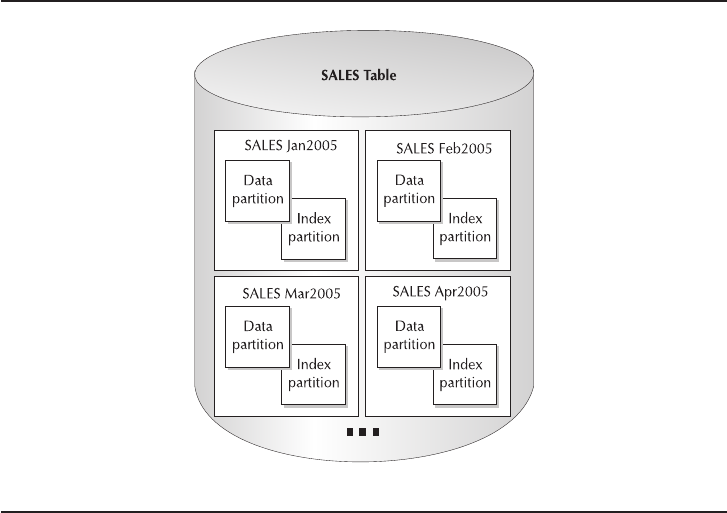
Define the Partitioned Indexing Strategy
Okay, so now you have decided how you are going to partition your data. To really
get the most out of partitioning, you will need to look at some indexing strategies.
There are two types of indexes applicable to partitioned tables: local and global.
Let’s take a brief look at each.
Local Partitioned Indexes Local partitioned indexes are indexes that are partitioned
in the exact same manner as the data in their associated table—that is, they have a
direct one-to-one relationship with the data partitions and use the same partition
key. This association is illustrated in Figure 9-3; as you can see, each partition has
its own associated “local” index. This drawing is based on Figure 9-2, which you
saw at the beginning of the chapter. It shows how the data and indexes for each
monthly subset are related and then joins it with the concept of the local index.
Because of this relationship, the following points apply to local indexes:
■You cannot explicitly add or drop a partition to/from a local index. Oracle
Database 11gautomatically adds or drops index partitions when related
data partitions are added or dropped. Looking at Figure 9-3, if you dropped
Chapter 9: Large Database Features 335
FIGURE 9-3. Local partitioned indexes

336 Oracle Database 11g: A Beginner’s Guide
the data partition for January 2005, the corresponding index partition would
automatically be dropped as well. Likewise, if you added a new data
partition for January 2006, a new index partition would automatically
be created.
■One of the advantages of partitioning data is to allow access to other subsets
while maintenance is being carried out on another partition. Since local
index partitions are in line with the data partitions, this advantage still exists.
■Local partitioned indexes require less maintenance than global indexes as
you will see later in this chapter.
The SQL syntax for creating a local index is presented in the next listing, which
refers to the SALES table you created in the “Range Partitioning” section. Table 9-9
contains an explanation of the syntax:
1 create index sales_idx_l1 on sales (time_id)
2 local
3 (partition sales_idx_200501 tablespace sales_ts_idx_200501,
4 partition sales_idx_200502 tablespace sales_ts_idx_200502,
5 partition sales_idx_200503 tablespace sales_ts_idx_200503,
...
37 partition sales_idx_200711 tablespace sales_ts_idx_200711,
38 partition sales_idx_200712 tablespace sales_ts_idx_200712,
39 partition sales_idx_max tablespace sales_ts_idx_max);
Lines Important Points
2 This specifies that the index is to be local. This line alone tells
Oracle Database 11gthat the index is to be partitioned along
the same ranges as the data.
3–39 This defines the partition names and tablespaces for each
partition. These lines are optional, but without them, Oracle
Database 11gwould use the same partition names as the data
and would also place the index in the same tablespaces as the
data—a situation that is less than ideal for performance!
TABLE 9-9. Syntax Highlights

Chapter 9: Large Database Features 337
Some other points about local partitioned indexes:
■They can be unique, but only if the data partition key is part of the index
key attributes.
■Bitmap indexes on partitioned tables must be local.
■Subpartitioned indexes are always local.
■They are best suited for data warehouses and decision support systems.
■Local unique indexes also work well in OLTP environments.
Ask the Expert
Q: After a table and its local indexes have been defined using range
partitioning with a default maxvalue partition, how can you add more
partitions as new subsets of data are received?
A: Use an alter table statement to split the default data partitions, adding your
new partition ranges. For example, to add a data partition for January 2008 data
in the SALES table in the previous listing, issue the following command:
alter table sales
split partition sales_max at (to_date('2008-02-01','YYYY-MM-DD'))
into (partition sales_200801 tablespace sales_ts_200801,
partition sales_max tablespace sales_ts_max);
This alter table command will split the default index partition for sales_idx_l1.
However, it will use the data partition names (for example, sales_200801) and
tablespaces (sales_ts_200801, for instance); remember in the local index example
you explicitly specified the partition names and tablespaces for the index.
Therefore, the partition names and tablespaces will need to be adjusted using
alter index commands, as follows:
alter index sales_idx_l1
rename partition sales_200801 to sales_idx_200801;
alter index sales_idx_l1
rebuild partition sales_idx_200801 tablespace sales_ts_idx_200801;
alter index sales_idx_l1
rebuild partition sales_idx_max tablespace sales_ts_idx_max;
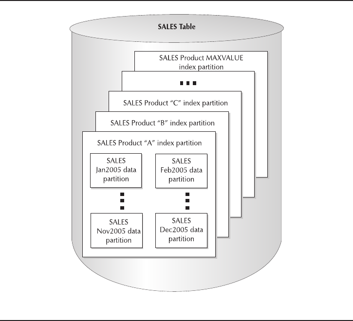
Global Partitioned Indexes Global partitioned indexes are indexes that are not
directly associated with the data partitions. Instead, their partitions are defined
independently, with the partition key sometimes different from the data partition
key. This association is illustrated in Figure 9-4. (This figure is again based on Figure
9-2, seen at the beginning of the chapter.) It shows that the data is partitioned by
monthly ranges, with a global index partitioned by product.
One advantage of global indexes is that if partition pruning cannot occur for the
data partitions due to the predicates of a query, index partition pruning may still be
possible with the global partition index. Global partitioned indexes are available as
either range-based or hash-based. When using range-based global indexes, you
must specify a default partition with maxvalue. Let’s look at an example for creating
a global partitioned index and then discuss how it would be used.
338 Oracle Database 11g: A Beginner’s Guide
FIGURE 9-4. Global partitioned indexes

Referring again to the PHONE_USAGE table you created in the Composite
Partitioning section, you should now create a global index on the call_type_id. The
following listing is the SQL for this, with the explanation presented in Table 9-10:
1 create index phone_usg_idx_g1 on phone_usage (call_type_id)
2 global
3 partition by range (call_type_id)
4 (partition ph_usg_idx_g1 values less than (2)
5 tablespace ph_usg_ts_idx_1,
6 partition ph_usg_idx_g2 values less than (3)
7 tablespace ph_usg_ts_idx_2,
8 partition ph_usg_idx_g3 values less than (4)
9 tablespace ph_usg_ts_idx_3,
10 partition ph_usg_idx_g4 values less than (5)
11 tablespace ph_usg_ts_idx_4,
12 partition ph_usg_idx_gmax values less than (maxvalue)
13 tablespace ph_usg_ts_idx_max);
Now, assume the following query is executed against the PHONE_USAGE table:
select count(*)
from phone_usage
where call_type_id = 3;
Without the global index you just defined, no partition pruning would occur
since the query predicate does not refer to the data partition key call_date. But, with
the global index, only the index entries from the partition ph_usg_idx_g3 would be
scanned and therefore only data records related to those entries would be used in
the result set.
Some other points on global partitioned indexes:
■They require more maintenance than local indexes, especially when you
drop data partitions because the indexes become invalid and will require
rebuilding before they are available for use.
■They can be unique.
Chapter 9: Large Database Features 339
Lines Important Points
2 This specifies that the index is to be global.
3 This defines the type of partitioning (here, range) for this index and
the partition key (call_type_id, in this case).
4–13 This defines the partition names and tablespaces for each partition.
TABLE 9-10. Explanation for Global Partitioned Index Syntax

340 Oracle Database 11g: A Beginner’s Guide
■They cannot be bitmap indexes.
■They are best suited for OLTP systems for direct access to specific records.
Prefixed and Nonprefixed Partition Indexes In your travels through the world of
partitioning, you will hear the terms prefixed and nonprefixed partition indexes.
These terms apply to both local and global indexes. An index is prefixed when the
leftmost column of the index key is the same as the leftmost column of the index
partition key. If the columns are not the same, the index is nonprefixed. That’s all
well and good, but what effect does it have?
It is a matter of performance: nonprefixed indexes cost more, from a query
perspective, than prefixed indexes. When a query is submitted against a partitioned
table and the predicate(s) of the query include the index keys of a prefixed index,
pruning of the index partition can occur. If the same index is nonprefixed instead,
all index partitions may need to be scanned. (Scanning of all index partitions will
depend on the predicate in the query and the type of index: global or local. If the
data partition key is included as a predicate and the index is local, then the index
partitions to be scanned will be based on pruned data partitions.)
Project 9-1 Create a Range-Partitioned Table and a
Local-Partitioned Index
Data and index partitioning are an important part in maintaining large databases. We
have discussed the reasons for partitioning and shown the steps to implement it. In
this project, you will create a range-partitioned table and a related local-partitioned
index.
Step by Step
1. Create two tablespaces called inv_ts_2007q1 and inv_2007q2 using the
following SQL statements. These will be used to store data partitions:
create tablespace inv_ts_2007q1
datafile 'inv_ts_2007q1_1.dat' size 10m;
create tablespace inv_ts_2007q2
datafile 'inv_ts_2007q2_1.dat' size 10m;
2. Create two tablespaces called inv_idx_ts_2007q1 and inv_idx_2007q2
using the following SQL statements. These will be used to store index
partitions:
create tablespace inv_idx_ts_2007q1
datafile 'inv_idx_ts_2007q1_f1.dat' size 10m;

create tablespace inv_idx_ts_2007q2
datafile 'inv_idx_ts_2007q2_f1.dat' size 10m;
3. Create a partitioned table called INVOICE using the following listing, based
on the following information:
a. Define the table with the columns identified in Table 9-11.
b. Use order_date as the partition key and then subset the data into the first
and second calendar quarters 2007.
c. Define the table with the data partitions and tablespaces identified in
Table 9-12.
d. Use the enable row movement option:
create table invoice (
invoice_id number,
customer_id number,
order_date date,
ship_date date)
partition by range (order_date)
(partition INV_2007Q1 values less than
(to_date(2007-04-01','YYYY-MM-DD'))
tablespace inv_ts_2007Q1,
partition INV_2007Q2 values less than
(to_date('2007-07-01','YYYY-MM-DD'))
tablespace inv_ts_2007Q2,
partition inv_max values less than (maxvalue)
tablespace inv_ts_max)
enable row movement;
Chapter 9: Large Database Features 341
Create a Range-Partitioned Table and a Local-Partitioned
Index
Project 9-1
Column Name Data Type
INVOICE_ID NUMBER
CUSTOMER_ID NUMBER
ORDER_DATE DATE
SHIP_DATE DATE
TABLE 9-11. INVOICE Table Columns
(continued)

342 Oracle Database 11g: A Beginner’s Guide
4. Create a local partitioned index called inv_order_dt_idx on call_date
using the following listing as well as the index partitions and tablespaces
identified in Table 9-12.
create index inv_order_dt_idx on invoice(order_date)
local
(partition inv_idx_2007q1 tablespace inv_idx_ts_2007q1,
partition inv_idx_2007q2 tablespace inv_idx_ts_2007q2,
partition inv_idx_max tablespace inv_idx_ts_max);
Project Summary
The steps in this project reinforce some of the more common scenarios you will
encounter: range-based partitioning and prefixed local partitioned indexes. Separate
tablespaces were used for data and indexes, quarterly partitions were defined, a
local index was defined, and the enable row movement was used to allow the
database to automatically redistribute rows to their related partitions in the event
of an update to the partition key.
Well, you have certainly covered a lot in this section. Having the background
information on these topics will serve you well when maintaining and tuning large
databases. Before you move on to the next section, let’s take a quick progress check
to make sure it all sank in.
Partition Name Tablespace Name Upper Range Limit
Data Partitions INV_2007Q1 INV_TS_2007Q1 Apr 1, 2007
INV_2007Q2 INV_TS_2007Q2 July 1, 2007
INV_MAX INV_TS_MAX MAXVALUE
Index Partitions INV_IDX_2007Q1 INV_IDX_TS_2007Q1 Apr 1, 2007
INV_IDX_2007Q2 INV_IDX_TS_2007Q2 July 1, 2007
INV_IDX_MAX INV_IDX_TS_MAX MAXVALUE
TABLE 9-12. INVOICE Table Data and Index Partitions

Chapter 9: Large Database Features 343
Progress Check
1. List at least three DML commands that can be applied to partitions as well
as tables.
2. What does partition pruning mean?
3. How many table attributes can be used to define the partition key in list
partitioning?
4. Which type of partitioning is most commonly used with a date-based
partition key?
5. Which partitioning types cannot be combined together for composite
partitioning?
6. How many partition keys can be defined for a partitioned table?
7. Which type of partitioned index has a one-to-one relationship between the
data and index partitions?
8. What is meant by a prefixed partitioned index?
Progress Check Answers
1. The following DML commands can be applied to partitions as well as tables: delete, insert, select,
truncate, and update.
2. Partition pruning is the process of eliminating data not belonging to the subset defined by the
criteria of a query.
3. Only one table attribute can be used to define the partition key in list partitioning.
4. Range partitioning is most commonly used with a date-based partition key.
5. List and hash partitioning cannot be combined for composite partitioning.
6. Only one partition key may be defined.
7. Local partitioned indexes have a one-to-one relationship between data and index partitions.
8. A partitioned index is prefixed when the leftmost column of the index key is the same as the
leftmost column of the index partition key.

344 Oracle Database 11g: A Beginner’s Guide
CRITICAL SKILL 9.3
Compress Your Data
As you load more and more data into your database, performance and storage
maintenance can quickly become concerns. Usually at the start of an implementation
of a database, data volumes are estimated and projected a year or two ahead.
However, oftentimes these estimates turn out to be on the low side and you find
yourself scrambling for more space in order to load new data. In addition to the
partitioning abilities discussed in the previous section, Oracle Database 11ghas
the ability to compress your data and indexes to further address the concerns of
performance and maintenance.
Compression can be performed at the data or index levels. In this section, you’ll
learn about the options available with Oracle Database 11gand the impacts these
options have on your database.
Data Compression
With data compression, duplicate values in a database block are removed, leaving
only a reference to the removed value, which is placed at the beginning of the
block. All of the information required to rebuild the data in a block is contained
within the block.
By compressing data, physical disk space required is reduced; disk I/O and
memory usage are also reduced, thereby improving performance. However, there
are some cases when data compression is not appropriate. The following should be
considered when looking at whether or not to compress data:
■Does the table exist in an OLTP or data warehousing environment? Data
compression is best suited for data that is updated infrequently or, better
yet, is read-only. Since most data in a data warehouse is considered
read-only, data compression is more compatible with this type of environment.
■Does the table have many foreign keys? Foreign keys result in a lot of
duplicate values in data. Tables with these structures are ideal candidates
for data compression.
■How will data be loaded into the table? Even when compression is enabled,
data is only compressed during bulk loading (for example, SQL*Loader). If
data is loaded using a standard insert into statement, the data will not be
compressed.
Compression can be specified for various data-related objects using the create or
alter object commands. Table 9-13 identifies these objects and their first-level parent
object, from which default compression properties are inherited if not specified for
the base object. For example, if no compression property is specified for a table, it

will inherit the property from its tablespace. The same applies to a data partition—if
not specified at the partition level, the default property from the table will be used.
The following listing demonstrates the creation of a table with compression
enabled. Line 7 contains the keyword compress to tell Oracle that data compression
is to be enabled:
1 create table commission (
2 sales_rep_id number,
3 prod_id number,
4 comm_date date,
5 comm_amt number(10,2))
6 tablespace comm_ts pctfree 5 initrans 1 maxtrans 255
7 compress;
Because compression can be enabled or disabled at different points in an
object’s lifetime (say, by using an alter command), and because the compression
action only occurs on new data being loaded, it is possible for an object to contain
both compressed and uncompressed data at the same time.
Chapter 9: Large Database Features 345
Object Type Compression Property Inheritance Parent
Table Tablespace
Materialized View Tablespace
Partition Table
TABLE 9-13. Compression Property Inheritance
Ask the Expert
Q: Can existing data in a table be compressed and uncompressed?
A: Yes. There are two methods. The first is by using an alter table statement
such as
alter table sales
move compress;
The second method is by using the utilities contained in the dbms_redefinition
package.

346 Oracle Database 11g: A Beginner’s Guide
Index Key Compression
Index key compression works in a similar manner to data compression in that
duplicated values are removed from the index entries. It’s a little more complicated,
however, because it has more restrictions and considerations than data compression,
partly due to the way indexes are structured. Since the details of these structures are
beyond the scope of this book, you will focus on the benefits of, and the mechanisms
for, defining index compression.
Compressing indexes offers the same benefits as data compression—that is,
reduced storage and improved (usually) performance. However, performance may
suffer during index scans as the burden on the CPU is increased in order to rebuild
the key values. One restriction we should mention is that index compression cannot
be used on a unique index that has only one attribute.
Enabling index compression is done using the create index statement. If you
need to compress or uncompress an existing index, you must drop the index first
and then re-create it with or without the compression option enabled. The following
listing illustrates the syntax for creating a compressed index. Table 9-14 provides an
explanation of the syntax:
1 create index comm_sr_prod_idx
2 on commission (sales_rep_id, prod_id)
3 compress 1;
Using data and index compression can provide substantial benefits in the areas
of storage and performance. In the next section, you will see how to improve query
performance using Oracle Database 11g’s parallel processing options.
Lines Important Points
1–2 This specifies that the index is to be created on columns
sales_rep_id and prod_id.
3 This specifies that the index is to be compressed, with the
number of prefixing (leading) columns to compress. In this
case, you used a value of 1 to indicate that duplicate values
of the first column, sales_rep_id, are to be removed.
TABLE 9-14. Explanation of Index Compression Syntax

Chapter 9: Large Database Features 347
CRITICAL SKILL 9.4
Use Parallel Processing to Improve
Performance
Improving performance (and by this we usually mean query performance) is always
a hot item with database administrators and users. One of the best and easiest ways
to boost performance is to take advantage of the parallel processing option offered
by Oracle Database 11g(Enterprise Edition only).
Using normal (that is, serial) processing, the data involved in a single request (for
example, user query) is handled by one database process. Using parallel processing,
the request is broken down into multiple units to be worked on by multiple database
processes. Each process looks at only a portion of the total data for the request.
Serial and parallel processing are illustrated in Figures 9-5 and 9-6, respectively.
Parallel processing can help improve performance in situations where large
amounts of data need to be examined or processed, such as scanning large tables,
joining large tables, creating large indexes, and scanning partitioned indexes. In
order to realize the benefits of parallel processing, your database environment
should not already be running at, or near, capacity. Parallel processing requires more
processing, memory, and I/O resources than serial processing. Before implementing
parallel processing, you may need to add hardware resources. Let’s forge ahead by
looking at the Oracle Database 11gcomponents involved in parallel processing.
Parallel Processing Database Components
Oracle Database 11g’s parallel processing components are the parallel execution
coordinator and the parallel execution servers. The parallel execution coordinator is
responsible for breaking down the request into as many processes as specified by the
request. Each process is passed to a parallel execution server for execution during
which only a portion of the total data is worked on. The coordinator then assembles
the results from each server and presents the complete results to the requester.
FIGURE 9-5. Oracle serial processing

Parallel Processing Configuration
Generally, not much configuration is required for Oracle Database 11gto perform
parallel processing. There are, however, a number of configuration options that are
required and will affect the effectiveness of parallelism.
To begin with, parallel processing is enabled by default for DDL (for example,
create and alter) and query (for example, select) commands, but disabled for DML
(say, insert, update, delete, merge) commands. If you wish to execute a DML
command in parallel mode, you must first issue the following command for the
session in which the command is to be executed, as in the following:
alter session enable parallel dml;
Several database initialization parameters affect parallel processing. These are
shown next. When an Oracle instance starts, the parameters in the initialization file
are used to define or specify the settings for the instance. Table 9-15 identifies the
initialization parameters that affect parallel processing. In many cases, the default
values will provide adequate results for your large database. Specifics of your own
environment will influence your decisions on the best values to use.
348 Oracle Database 11g: A Beginner’s Guide
FIGURE 9-6. Oracle parallel processing

As you can see from Table 9-15, there are dependencies between parameters.
Modifying one may necessitate modifying others. If you modify any of the parallel
processing parameters, you may also have to modify the following database/instance
parameters:
■INSTANCE GROUPS
■PROCESSES
Chapter 9: Large Database Features 349
Parameter Default Setting Comment
PARALLEL_ADAPTIVE_MULTI_USER True When set to True, this enables an
adaptive algorithm designed to
improve performance in
multiuser environments that use
parallel processing.
PARALLEL_AUTOMATIC_TUNING False This is no longer used. Exists for
backward compatibility only.
PARALLEL_EXECUTION_MESSAGE_SIZE Installation Dependent This specifies the byte size of
messages for parallel
processing.
PARALLEL_INSTANCE_GROUP Installation Dependent This is used in Real Application
Cluster environments to restrict
parallel query operations to a
limited number of database
instances.
PARALLEL_MAX_SERVERS # of CPUs available to
the database instance
This specifies maximum number
of parallel processes for the
database instance.
PARALLEL_MIN_PERCENT 0 This specifies minimum
percentage of parallel processes
required for parallel processing.
Value is a percentage of
PARALLEL_MAX_SERVERS.
PARALLEL_MIN_SERVERS 0 This specifies minimum number
of parallel processes for the
database instance. Cannot be
greater than value of
PARALLEL_MAX_SERVERS.
PARALLEL_THREADS_PER_CPU Usually set to 2,
depending on
operating system
This specifies the number of
parallel processes per CPU.
TABLE 9-15. Initialization Parameters Affecting Parallel Processing

350 Oracle Database 11g: A Beginner’s Guide
■SESSIONS
■TRANSACTIONS
Invoke Parallel Execution
Parallel execution can be applied to tables, views, and materialized views. Assuming
all necessary configurations have been made, there are several ways to invoke
parallel execution. The first way is during table creation (including materialized
views), using the parallel clause. If the table is being created using the results of a
subquery, the loading of the table will be parallelized. In addition, by default, all
queries that are executed against the table will be parallelized to the same extent.
The next listing shows an example of specifying the parallel option for a table creation:
1 create table commission (
2 sales_rep_id number,
3 prod_id number,
4 comm_date date,
5 comm_amt number(10,2))
6 tablespace comm_ts
7 parallel;
The important line here is Line 7, specifying the parallel clause. This line could
also have included an integer to specify the degree of parallelism—that is, the number
of processes that are to be used to execute the parallel process. As the degree of
parallelism is omitted in this example, the number of processes used will be
calculated as the number of CPUs the value of the PARALLEL_THREADS_PER_CPU
initialization parameter. The degree of parallelism for a table or materialized view
can be changed using an alter statement.
Parallel processing can also be invoked when the parallel hint is used in a select
statement. This hint will override any default parallel processing options specified
during table creation. The following listing illustrates the use of the parallel hint.
Line 1 contains the parallel hint, specifying the table to be parallelized (commission)
and the degree of parallelism (4):
1 select /*+ parallel (commission, 4) */
2 prod_id, sum(comm_amt), count(*)
3 from commission
4 group by prod_id;
In some cases, Oracle Database 11gwill alter how, or if, parallel processing is
executed. Examples of these include the following:
■Parallel processing will be disabled for DML commands (for example,
insert, update, delete, and merge) on tables with triggers or referential
integrity constraints.

Chapter 9: Large Database Features 351
■If a table has a bitmap index, DML commands are always executed using
serial processing if the table is non-partitioned. If the table is partitioned,
parallel processing will occur, but Oracle will limit the degree of parallelism
to the number of partitions affected by the command.
Parallel processing can have a significant positive impact on performance.
Impacts on performance are even greater when you combine range- or hash-based
partitioning with parallel processing. With this configuration, each parallel process
can act on a particular partition. For example, if you had a table partitioned by
month, the parallel execution coordinator could divide the work up according to
those partitions. This way, partitioning and parallelism work together to provide
results even faster.
CRITICAL SKILL 9.5
Use Materialized Views
So far, you have reviewed several features and techniques at your disposal for
improving performance in large databases. In this section, we will discuss another
feature of Oracle Database 11gthat you can include in your arsenal: materialized
views.
Originally called snapshots, materialized views were introduced in Oracle8
and are only available in the Enterprise Edition. Like a regular view, the data in a
materialized view are the results of a query. However, the results of a regular view
are transitory—they are lost once the query is complete and if needed again, the
query must be re-executed. In contrast, the results from a materialized view are kept
and physically stored in a database object that resembles a table. This feature means
that the underlying query only needs to be executed once and then the results are
available to all who need them.
From a database perspective, materialized views are treated like tables:
■You can perform most DML and query commands such as insert, delete,
update and select.
■They can be partitioned.
■They can be compressed.
■They can be parallelized.
■You can create indexes on them.
Materialized views are different in other ways and have some interesting features
associated with them. Before we talk about those, let’s look at some ways to use
materialized views.
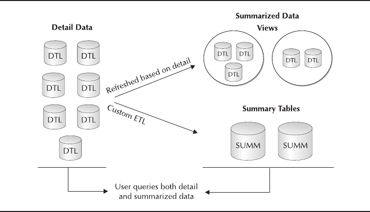
Uses for Materialized Views
Materialized views are used as a performance enhancing technique. Following are
some usage examples. In this section, you will learn about the first four uses, as they
are applicable to the topic of large databases.
■Performing data summarization (for example, sums, averages)
■Prejoining tables
■Performing CPU-intensive calculations
■Replicating and distributing data
In large databases, particularly data warehousing environments, there is always
a need to summarize, join, perform calculations, or do all three at once on large
numbers of records for the purposes of reporting and analysis. To improve
performance in the past, a combination of views and physical tables were usually
implemented that contained the results of these operations. The summary tables
would require some type of extraction, transformation, and load (ETL) process to
populate and refresh them. In addition to the base tables containing the detailed
data, the users would need to know which combinations of the views and/or
summary tables to use. These structures are illustrated in Figure 9-7.
352 Oracle Database 11g: A Beginner’s Guide
FIGURE 9-7. Summarization using views and summary tables
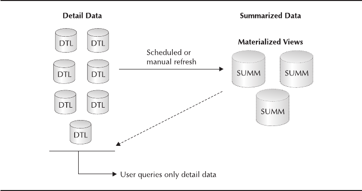
Using materialized views has several advantages over more traditional methods.
These include the following:
■Materialized views have a built-in data refresh process, which can provide
an automatic update or repopulation of a materialized view without any
programming on the part of the DBA.
■As mentioned earlier, the data in materialized views can be partitioned,
using the same techniques that apply to tables.
■Materialized views are transparent to the users. This is probably the most
attractive feature of using materialized views, and we will expand more on
this in the next section when we discuss automatic query rewriting.
Figure 9-8 illustrates summarization using materialized views.
Query Rewrite
Earlier, you learned that one of the benefits of using materialized views was that
they are transparent to the users. But what exactly does that mean and how can they
be used if the users can’t see them? In fact, because materialized views are so much
like tables, you can give the users access to materialized views, though generally
this is not done.
Chapter 9: Large Database Features 353
FIGURE 9-8. Summarization using materialized views

354 Oracle Database 11g: A Beginner’s Guide
Instead, as indicated in Figure 9-8, the users always query the tables with the
detail data—they don’t usually query the materialized views directly. This is because
the query optimizer in Oracle Database 11gknows about the materialized views
and their relationships to the detail tables and can rewrite the query on the fly to
access the materialized views instead. This results in huge performance gains without
the user having to do anything special—just query the detail data. There is a
maintenance benefit of this feature for the user as well: the queries do not have to
change to point to different summary tables, as is the case with the more traditional
summarization approach.
In order for the query to be rewritten, the structure of the materialized view must
satisfy the criteria of the query. The following two listings demonstrate the query
rewrite process. Let’s assume you need to summarize the COMMISSION table you
saw in the data compression section using the following query:
select prod_id, to_char(comm_date, 'YYYY-MM'), count(*), sum(comm_amt)
from commission
group by prod_id, to_char(comm_date, 'YYYY-MM');
Assume further that a materialized view (called comm_prod_mv) exists that
contains summarized commission data by sales_rep_id, prod_id, and comm_date
(full date). In this case, the query would be automatically rewritten as follows:
select prod_id, to_char(comm_date, 'YYYY-MM'), count(*), sum(comm_amt)
from comm_prod_mv
group by prod_id, to_char(comm_date, 'YYYY-MM');
By rewriting the query to use the materialized view instead, a large amount of
data-crunching has been saved and the results will return much more quickly. Now
turn your attention to determining what materialized views should be created.
When to Create Materialized Views
At this point, you may be asking yourself: “How do I determine what materialized
views to create and at what level of summarization?” Oracle Database 11ghas
some utilities to help. These utilities are collectively called the SQLAccess Advisor
and will recommend materialized views based on historical queries, or based on
theoretical scenarios. They can be run from the Oracle Enterprise Manager Grid
Control (OEM) or by calling the dbms_advisor package.

Chapter 9: Large Database Features 355
Create Materialized Views
Materialized views are created using a create materialized view statement, which
is similar to a create table statement. This can be performed using SQL Developer,
SQL*Plus, or OEM. The following listing shows a simple example of how to create
the comm_prod_mv materialized view mentioned earlier and Table 9-16 provides
an explanation of the syntax:
1 create materialized view comm_prod_mv
2 tablespace comm_prod_mv_ts
3 storage (initial 50k next 50k)
4 refresh complete next sysdate + 7
5 enable query rewrite
6 as select sales_rep_id, prod_id, comm_date, count(*), sum(comm_amt)
7 from commission
8 group by sales_rep_id, prod_id, comm_date;
In the next three sections, you will learn about some higher-level concepts: Real
Application Clusters, Automatic Storage Management, and Grid Computing. But
first, complete this progress check.
Lines Important Points
2–3 This specifies the tablespace and storage parameters.
4 This specifies how and when to refresh the data. In
this case, the materialized view will be populated
immediately and be completely refreshed every seven
days thereafter.
5 This specifies that query rewrite is to be enabled.
6–8 This specifies the query that will act as the source of
the data.
TABLE 9-16. Explanation of Materialized View Creation Syntax

Progress Check
1. True or False: Tables with many foreign keys are good candidates for
compression.
2. Name the two processing components involved in Oracle Database 11g’s
parallel processing.
3. What is the function of the SQLAccess Advisor?
4. True or False: In order to access the data in a materialized view, a user or
application must query the materialized view directly?
5. List the ways in which parallel processing can be invoked.
6. In what situation can index key compression not be used on a unique index?
CRITICAL SKILL 9.6
Use SQL Aggregate and Analysis Functions
Once your database has been loaded with data, your users or applications will, of
course, want to use that data to run queries, perform analysis, produce reports, extract
data, and so forth. Oracle Database 11gprovides many sophisticated aggregation
and analysis functions that can help ease the pain sometimes associated with
analyzing data in large databases.
Aggregation Functions
Oracle Database 11gprovides extensions to the standard SQL group by clause of
the select statement that generate other totals as part of the result set that previously
required multiple queries, nested subqueries, or importing into spreadsheet type
applications. These extensions are rollup and cube.
356 Oracle Database 11g: A Beginner’s Guide
Progress Check Answers
1. True.
2. The parallel execution coordinator and the parallel execution servers.
3. The SQLAccess Advisor recommends potential materialized views based on historical or
theoretical scenarios.
4. False. While the end user or application can query the materialized view directly, usually the
target of a query is the detail data and Oracle’s query rewrite capabilities will automatically return
the results from the materialized view instead of the detail table (assuming the materialized view
meets the query criteria).
5. Parallel processing can be invoked based on the parallelism specified for a table at the time of its
creation, or by providing the parallel hint in a select query.
6. If the unique index has only one attribute, key compression cannot be used.

Chapter 9: Large Database Features 357
rollup
The rollup extension generates subtotals for attributes specified in the group by
clause, plus another row representing the grand total. The following is an example
of the rollup extension, using the SALES table you have seen throughout this chapter:
select c.cust_gender gender,
b.channel_class channel_class,
to_char(a.time_id, 'yyyy-mm') month,
count(*) unit_count,
sum(a.amount_sold) amount_sold
from sales a, channels b, customers c
where a.channel_id = b.channel_id
and a.cust_id = c.cust_id
and to_char(a.time_id, 'yyyy-mm') between '2001-01' and '2001-02'
group by rollup(c.cust_gender,
b.channel_class,
to_char(a.time_id, 'yyyy-mm'));
GENDER CHANNEL_CLASS MONTH UNIT_COUNT AMOUNT_SOLD
------ -------------------- ------- ---------- -----------
F Direct 2001-01 4001 387000.9
F Direct 2001-02 3208 365860.13
F Direct 7209 752861.03
F Others 2001-01 2486 242615.9
F Others 2001-02 2056 229633.52
F Others 4542 472249.42
F Indirect 2001-01 1053 138395.21
F Indirect 2001-02 1470 189425.88
F Indirect 2523 327821.09
F 14274 1552931.54
M Direct 2001-01 7038 719146.28
M Direct 2001-02 6180 641192.61
M Direct 13218 1360338.89
M Others 2001-01 4310 414603.03
M Others 2001-02 3751 391792.61
M Others 8061 806395.64
M Indirect 2001-01 1851 211947.81
M Indirect 2001-02 2520 285219.79
M Indirect 4371 497167.6
M 25650 2663902.13
39924 4216833.67
In the results, we can see that counts and sums of amount_sold are returned at
the following levels:
■By GENDER, CHANNEL_CLASS, and MONTH
■Subtotals by CHANNEL_CLASS within GENDER

358 Oracle Database 11g: A Beginner’s Guide
■Subtotals by GENDER
■Grand total
cube
The cube extension takes rollup a step further by generating subtotals for each
combination of the group by attributes, totals by attribute, and the grand total. The
following is an example of the cube extension, using the same query you used for
rollup:
select c.cust_gender gender,
b.channel_class channel_class,
to_char(a.time_id, 'yyyy-mm') month,
count(*) unit_count,
sum(a.amount_sold) amount_sold
from sales a, channels b, customers c
where a.channel_id = b.channel_id
and a.cust_id = c.cust_id
and to_char(a.time_id, 'yyyy-mm') between '2001-01' and '2001-02'
group by cube(c.cust_gender,
b.channel_class,
to_char(a.time_id, 'yyyy-mm'));
GENDER CHANNEL_CLASS MONTH UNIT_COUNT AMOUNT_SOLD
------ -------------------- ------- ---------- -----------
39924 4216833.67
2001-01 20739 2113709.13
2001-02 19185 2103124.54
Direct 20427 2113199.92
Direct 2001-01 11039 1106147.18
Direct 2001-02 9388 1007052.74
Others 12603 1278645.06
Others 2001-01 6796 657218.93
Others 2001-02 5807 621426.13
Indirect 6894 824988.69
Indirect 2001-01 2904 350343.02
Indirect 2001-02 3990 474645.67
F 14274 1552931.54
F 2001-01 7540 768012.01
F 2001-02 6734 784919.53
F Direct 7209 752861.03
F Direct 2001-01 4001 387000.9
F Direct 2001-02 3208 365860.13
F Others 4542 472249.42
F Others 2001-01 2486 242615.9
F Others 2001-02 2056 229633.52
F Indirect 2523 327821.09

Chapter 9: Large Database Features 359
F Indirect 2001-01 1053 138395.21
F Indirect 2001-02 1470 189425.88
M 25650 2663902.13
M 2001-01 13199 1345697.12
M 2001-02 12451 1318205.01
M Direct 13218 1360338.89
M Direct 2001-01 7038 719146.28
M Direct 2001-02 6180 641192.61
M Others 8061 806395.64
M Others 2001-01 4310 414603.03
M Others 2001-02 3751 391792.61
M Indirect 4371 497167.6
M Indirect 2001-01 1851 211947.81
M Indirect 2001-02 2520 285219.79
In the results, you can see that counts and sums of amount_sold are returned at
the following levels:
■By GENDER, CHANNEL_CLASS, and MONTH
■Subtotals by MONTH within CHANNEL_CLASS
■Subtotals by MONTH within GENDER
■Subtotals by CHANNEL_CLASS within GENDER
■Subtotals by MONTH
■Subtotals by CHANNEL_CLASS
■Subtotals by GENDER
■Grand total
Analysis Functions
Oracle Database 11gprovides a number of ranking and statistical functions that
previously would have required some pretty heavy SQL to perform or an extract
to a third-party application. In this section, you will look at the analysis function
available and examine examples of their use where appropriate.
NOTE
Some of the functions in this section are based on
complex statistical calculations. Don’t be worried if
you are unfamiliar with these concepts. It is more
important for you to know that these functions exist
than it is to understand the theory behind them.

360 Oracle Database 11g: A Beginner’s Guide
Ranking Functions
Ranking functions provide the ability to rank a row of a query result relative to the
other rows in the result set. Common examples of uses for these functions include
identifying the top ten selling products for a period, or classifying or grouping a
salesperson’s commissions into one of four buckets. The ranking functions included
in Oracle Database 11gare
■rank
■dense_rank
■cume_dist
■percent_rank
■ntile
■row_number
rank and dense_rank Functions The simplest ranking functions are rank and
dense_rank. These functions are very similar and determine the ordinal position of
each row within the query result set. The difference between these two functions is
that rank will leave a gap in the sequence when there is a tie for position, whereas
dense_rank does not leave a gap. The results of the following listing illustrate the
difference between the two:
select prod_id,
sum(quantity_sold),
rank () over (order by sum(quantity_sold) desc) as rank,
dense_rank () over (order by sum(quantity_sold) desc) as dense_rank
from sales
where to_char(time_id, 'yyyy-mm') = '2001-06'
group by prod_id;
PROD_ID SUM(QUANTITY_SOLD) RANK DENSE_RANK
---------- ------------------ ---------- ----------
24 762 1 1
30 627 2 2
147 578 3 3
33 552 4 4
40 550 5 5
133 550 5 5
48 541 7 6
120 538 8 7
23 535 9 8
119 512 10 9
124 503 11 10
140 484 12 11
148 472 13 12
139 464 14 13

Chapter 9: Large Database Features 361
123 459 15 14
131 447 16 15
25 420 17 16
135 415 18 17
137 407 19 18
146 401 20 19
As you can see, the ordinal position 6 does not exist as a value for rank, but it
does for dense_rank. If from this result set you wanted to see the top ten listings for
prod_id, you would use the original query as a subquery, as in the following listing:
select * from
(select prod_id,
sum(quantity_sold),
rank () over (order by sum(quantity_sold) desc) as rank,
dense_rank () over (order by sum(quantity_sold) desc) as dense_rank
from sales
where to_char(time_id, 'yyyy-mm') = '2001-06'
group by prod_id)
where rank < 11;
To see the bottom ten prod_ids, use the same query, but change the order by
option from descending (desc) to ascending (asc). The next two functions, cume_dist
and percent_rank, are statistical in nature but still part of the family of ranking
functions, so the important feature is that these functions properly handle ties in
the rankings.
cume_dist and percent_rank Functions The cume_dist function calculates the
cumulative distribution of a value in a group of values. Since this is not a statistics
beginner’s guide, we will not attempt to provide the theoretical background on
cumulative distribution. However, we can offer these points:
■The range of values returned by cume_dist is always between 0 and 1.
■The value returned by cume_dist is always the same in the case of tie
values in the group.
■The formula for cumulative distribution is
# of rows with values <= value of row being evaluated
# of rows being evaluated
Looking at the query y used when discussing rank, the following listing
calculates the cumulative distribution for quantity_sold. The results immediately
follow the listing:
select prod_id,
sum(quantity_sold),
cume_dist () over (order by sum(quantity_sold) asc) as cume_dist

362 Oracle Database 11g: A Beginner’s Guide
from sales
where to_char(time_id, 'yyyy-mm') = '2001-06'
group by prod_id
order by sum(quantity_sold) desc;
PROD_ID SUM(QUANTITY_SOLD) CUME_DIST
---------- ------------------ ----------
24 762 1
30 627 .985915493
147 578 .971830986
33 552 .957746479
40 550 .943661972
133 550 .943661972
48 541 .915492958
120 538 .901408451
23 535 .887323944
119 512 .873239437
124 503 .85915493
140 484 .845070423
148 472 .830985915
139 464 .816901408
123 459 .802816901
131 447 .788732394
25 420 .774647887
135 415 .76056338
137 407 .746478873
146 401 .732394366
The percent_rank function is similar to the cume_dist function, but calculates a
percentage ranking of a value relative to its group. Again, without getting into the
theory, we can make some points about percent_rank:
■The range of values returned by the function is always between 0 and 1.
■The row with a rank of 1 will have a percent rank of 0.
■The formula for calculating percent rank is
rank of row within its group – 1
# of rows in the group – 1
The next listing and its results demonstrate the percent_rank function using the
base query you have been using in this section:
select prod_id,
sum(quantity_sold),
rank () over (order by sum(quantity_sold) desc) as rank,
percent_rank ()
over (order by sum(quantity_sold) asc) as percent_rank

Chapter 9: Large Database Features 363
from sales
where to_char(time_id, 'yyyy-mm') = '2001-06'
group by prod_id
order by sum(quantity_sold) desc;
PROD_ID SUM(QUANTITY_SOLD) RANK PERCENT_RANK
---------- ------------------ ---------- ------------
24 762 1 1
30 627 2 .985714286
147 578 3 .971428571
33 552 4 .957142857
40 550 5 .928571429
133 550 5 .928571429
48 541 7 .914285714
120 538 8 .9
23 535 9 .885714286
119 512 10 .871428571
124 503 11 .857142857
140 484 12 .842857143
148 472 13 .828571429
139 464 14 .814285714
123 459 15 .8
131 447 16 .785714286
25 420 17 .771428571
135 415 18 .757142857
137 407 19 .742857143
146 401 20 .728571429
The ntile Function The ntile function divides a result set into a number of buckets
specified at query time by the user, and then assigns each row in the result set a
bucket number. The most common number of buckets used are 3 (tertiles), 4 (quartiles),
and 10 (deciles). Each bucket will have the same number of rows, except in the case
when the number of rows does not divide evenly by the number of buckets. In this
case, each of the leftover rows will be assigned to buckets with the lowest bucket
numbers until all leftover rows are assigned. For example, if four buckets were
specified and the number of rows in the result set was 98, buckets 1 and 2 would
have 25 rows each and buckets 3 and 4 would have 24 rows each.
Let’s look at an example. Using your base query of amount_sold in the SALES
table, you want to look at amount_sold by product subcategory and rank the
amounts into four buckets. Here’s the SQL:
select b.prod_subcategory,
sum(a.quantity_sold),
ntile(4) over (ORDER BY SUM(a.quantity_sold) desc) as quartile
from sales a, products b
where a.prod_id = b.prod_id
and to_char(a.time_id, 'yyyy-mm') = '2001-06'
group by b.prod_subcategory;

364 Oracle Database 11g: A Beginner’s Guide
As you can see in the following results, the number of product subcategories
was not evenly divisible by the number of buckets specified (in this case, 4).
Therefore, six subcategories were assigned to the first quartile (bucket 1) and five
subcategories were assigned to the second, third, and fourth quartiles.
PROD_SUBCATEGORY COUNT(*) SUM(A.QUANTITY_SOLD) QUARTILE
--------------------------- ---------- -------------------- ----------
Accessories 3230 3230 1
Y Box Games 2572 2572 1
Recordable CDs 2278 2278 1
Camera Batteries 2192 2192 1
Recordable DVD Discs 2115 2115 1
Documentation 1931 1931 1
Modems/Fax 1314 1314 2
CD-ROM 1076 1076 2
Y Box Accessories 1050 1050 2
Printer Supplies 956 956 2
Memory 748 748 2
Camera Media 664 664 3
Home Audio 370 370 3
Game Consoles 352 352 3
Operating Systems 343 343 3
Bulk Pack Diskettes 270 270 3
Portable PCs 215 215 4
Desktop PCs 214 214 4
Camcorders 196 196 4
Monitors 178 178 4
Cameras 173 173 4
row_number Function The row_number function is a simple function that assigns
a unique number to each row in a result set. The numbers are sequential, starting at
1, and are based on the order by clause of the query.
You will again use your SALES table query as an example. Using the query from
your ntile example and adding a new column using row_count, you get
select b.prod_subcategory,
sum(a.quantity_sold),
ntile(4) over (ORDER BY SUM(a.quantity_sold) desc) as quartile,
row_number () over (order by sum(quantity_sold) desc) as rownumber
from sales a, products b
where a.prod_id = b.prod_id
and to_char(a.time_id, 'yyyy-mm') = '2001-06'
group by b.prod_subcategory;
In the following results, each row is assigned a number, depending on its
position defined by the order by clause. As you can observe, the ROWNUMBER
is simply the row position in the list without any intelligence, whereas quartile is
a calculated field and could have repeating values:

Chapter 9: Large Database Features 365
PROD_SUBCATEGORY SUM(A.QUANTITY_SOLD) QUARTILE ROWNUMBER
------------------------- -------------------- ---------- ----------
Accessories 3230 1 1
Y Box Games 2572 1 2
Recordable CDs 2278 1 3
Camera Batteries 2192 1 4
Recordable DVD Discs 2115 1 5
Documentation 1931 1 6
Modems/Fax 1314 2 7
CD-ROM 1076 2 8
Y Box Accessories 1050 2 9
Printer Supplies 956 2 10
Memory 748 2 11
Camera Media 664 3 12
Home Audio 370 3 13
Game Consoles 352 3 14
Operating Systems 343 3 15
Bulk Pack Diskettes 270 3 16
Portable PCs 215 4 17
Desktop PCs 214 4 18
Camcorders 196 4 19
Monitors 178 4 20
Cameras 173 4 21
Windowing Functions
Before you get into the details, you need to learn a couple of terms: analytic partitioning
and analytic window.
■Analytic partitioning is the division of the results of an analytic function into
groups within which the analytic function operates. This is accomplished
using the partition by clause of the analytic function. Do not confuse this
partitioning with data partitioning discussed earlier in this chapter. Analytic
partitioning can be used with any of the analytic functions we have
discussed so far.
■An analytic window is a subset of an analytic partition in which the values
of each row depend on the values of other rows in the window. There are
two types of windows: physical and logical. A physical window is defined
by a specified number of rows. A logical window is defined by the order by
values.
Windowing functions can only be used in the select and order by clauses. They
can be used to calculate the following:
■Moving sum
■Moving average

366 Oracle Database 11g: A Beginner’s Guide
■Moving min/max
■Cumulative sum
■Statistical functions
Now look at an example of a moving sum function. The following shows the
listing and results for calculating the moving sum from the SALES table by product
category for a six-month period:
select b.prod_category,
to_char(a.time_id, 'yyyy-mm'),
sum(a.quantity_sold),
sum(sum(a.quantity_sold)) over (partition by b.prod_category
order by to_char(a.time_id, 'yyyy-mm')
rows unbounded preceding) as cume_sum
from sales a, products b
where a.prod_id = b.prod_id
and b.prod_category_id between 202 and 204
and to_char(a.time_id, 'yyyy-mm') between '2001-01' and '2001-06'
group by b.prod_category, to_char(a.time_id, 'yyyy-mm')
order by b.prod_category, to_char(a.time_id, 'yyyy-mm');
PROD_CATEGORY TO_CHAR SUM(A.QUANTITY_SOLD) CUME_SUM
------------------------------ ------- -------------------- ----------
Hardware 2001-01 281 281
Hardware 2001-02 306 587
Hardware 2001-03 442 1029
Hardware 2001-04 439 1468
Hardware 2001-05 413 1881
Hardware 2001-06 429 2310
Peripherals and Accessories 2001-01 5439 5439
Peripherals and Accessories 2001-02 5984 11423
Peripherals and Accessories 2001-03 5104 16527
Peripherals and Accessories 2001-04 5619 22146
Peripherals and Accessories 2001-05 4955 27101
Peripherals and Accessories 2001-06 5486 32587
Photo 2001-01 2802 2802
Photo 2001-02 2220 5022
Photo 2001-03 2982 8004
Photo 2001-04 2824 10828
Photo 2001-05 2359 13187
Photo 2001-06 3225 16412
As you can see in the results, the moving sum is contained within each product
category and resets when a new product category starts. In the past, windowing
analysis used to require third-party products such as spreadsheet applications.
Having the capabilities to perform these functions right in the database can
streamline analysis and report generation efforts.

Other Functions
There are many other functions included with Oracle Database 11gthat can be
used to analyze data in large databases. While we will not be going into any detail
for these, they are listed here for completeness:
■Statistical functions, including:
■Linear regression functions
■Descriptive statistics functions
■Hypothetical testing and crosstab statistics functions (contained a new
PL/SQL package called dbms_statistics)
■first/last functions
■lag/lead functions
■Reporting aggregate functions
■Inverse percentile functions
■Hypothetical rank and distribution functions
As was stated earlier, database administrators do not have to know the theory
behind the functions provided by Oracle Database 11gor even how to use their
results. However, you should be able to let your users know what capabilities are
available. Knowing this, your users will be able to take advantage of these functions
and construct efficient queries. In the next section, you’ll learn about a new feature
in Oracle Database 11g—SQL models.
CRITICAL SKILL 9.7
Create SQL Models
One of the more powerful data analysis features introduced in Oracle Database 11g
is SQL models. SQL models allow a user to create multidimensional arrays from query
results. Formulas, both simple and complex, can then be applied to the arrays to
generate results in which the user is interested. SQL models allow inter-row calculations
to be applied without doing expensive self-joins.
SQL models are similar to other multidimensional structures used in business
intelligence applications. However, because they are part of the database, they can
take advantage of Oracle Database 11g’s built-in features of scalability, manageability
security, and so on. In addition, using SQL models, there is no need to transfer large
amounts of data to external business intelligence applications.
Chapter 9: Large Database Features 367

368 Oracle Database 11g: A Beginner’s Guide
A SQL model is defined by the model extension of the select statement.
Columns of a query result are classified into one of three groups:
■Partitioning This is the same as the analytic partitioning defined in the
Windowing Functions section.
■Dimensions These are the attributes used to describe or fully qualify a
measure within a partition. Examples could include product, sales rep id,
and phone call type.
■Measures These are the numeric (usually) values to which calculations are
applied. Examples could include quantity sold, commission amount, and
call duration.
One of the main applications of SQL models is projecting or forecasting measures
based on existing measures. Let’s look at an example of the model clause to illustrate.
The listing and its results show an aggregate query using the SALES table:
select c.channel_desc, p.prod_category, t.calendar_year year,
sum(s.quantity_sold) quantity_sold
from sales s, products p, channels c, times t
where s.prod_id = p.prod_id
and s.channel_id = c.channel_id
and s.time_id = t.time_id
and c.channel_desc = 'Direct Sales'
group by c.channel_desc, p.prod_category, t.calendar_year
order by c.channel_desc, p.prod_category, t.calendar_year;
CHANNEL_DESC PROD_CATEGORY YEAR QUANTITY_SOLD
---------------- ------------------------------ ------ -------------
Direct Sales Electronics 1998 7758
Direct Sales Electronics 1999 15007
...
Direct Sales Hardware 2000 1970
Direct Sales Hardware 2001 2399
Direct Sales Peripherals and Accessories 1998 44258
...
Direct Sales Software/Other 2000 64483
Direct Sales Software/Other 2001 49146
In the results, you can see the historical aggregate quantity_sold for each year
by product category for the Direct Sales channel. You can use the model clause to
project the quantity_sold. In the following listing, you’ll project values for 2002 for
the product category Hardware in the channel. The quantity_sold will be based on
the previous year’s value (2001), plus 10 percent. Table 9-17 explains the syntax
of the listing:

1 select channel_desc, prod_category, year, quantity_sold
2 from
3 (select c.channel_desc, p.prod_category, t.calendar_year year,
4 sum(s.quantity_sold) quantity_sold
5 from sales s, products p, channels c, times t
6 where s.prod_id = p.prod_id
7 and s.channel_id = c.channel_id
8 and s.time_id = t.time_id
9 group by c.channel_desc, p.prod_category, t.calendar_year) sales
10 where channel_desc = 'Direct Sales'
11 model
12 partition by (channel_desc)
13 dimension by (prod_category, year)
14 measures (quantity_sold)
15 rules (quantity_sold['Hardware', 2002]
16 = quantity_sold['Hardware', 2001] * 1.10)
17 order by channel_desc, prod_category, year;
Chapter 9: Large Database Features 369
Lines Important Points
3–9 This defines an in-line select that will be the source for the
query. It is basically the same query you started with before
the model clause.
10 This specifies that you are only going to look at Direct Sales
channels.
11 This specifies the model clause.
12 This specifies the partition by clause (in this case,
channel_desc).
13 This specifies the dimension by clause (here, prod_category
and year). These elements will fully qualify the measure
within the channel_desc partition.
14 This specifies the measures clause (quantity_sold).
15–16 This specifies the rules clause—that is, calculations you
want to perform on the measure. In this example, we are
referring to a specific cell of quantity_sold, described by the
dimensions prod_category (Hardware) and year (2002).
TABLE 9-17. Explanation of Model Clause Syntax

370 Oracle Database 11g: A Beginner’s Guide
Following are the results of the previous query. Notice that a new row has been
added for Hardware in 2002. Its quantity_sold is 2638.9, which is the previous
year’s value (2399) plus 10 percent:
CHANNEL_DESC PROD_CATEGORY YEAR QUANTITY_SOLD
---------------- ------------------------------ ------ -------------
Direct Sales Electronics 1998 7758
Direct Sales Electronics 1999 15007
...
Direct Sales Hardware 2000 1970
Direct Sales Hardware 2001 2399
Direct Sales Hardware 2002 2638.9
Direct Sales Peripherals and Accessories 1998 44258
...
Direct Sales Software/Other 2000 64483
Direct Sales Software/Other 2001 49146
The model clause has many variations and allows for very powerful
calculations. Let’s point out some of the characteristics and/or features you should
be aware of. Supported functionalities include the following:
■Looping (for example, FOR loops)
■Recursive calculations
■Regression calculations
■Nested cell references
■Dimension wildcards and ranges
■The model clause does not update any base table, although in theory you
could create a table or materialized view from the results of the query using
the model clause.
Restrictions include the following:
■The rules clause cannot include any analytic SQL or windowing functions.
■A maximum of 20,000 rules may be specified. This may seem like plenty,
but a FOR loop is expanded into many single-cell rules at execution time.
Project 9-2 Use Analytic SQL Functions and Models
Once all the database structures have been put in place and data has been loaded,
the users will want to analyze it. Knowing what functions are available is important,
and so is their use as well, at least to some extent. So, in this project you will walk
through a more complex analytical example that includes using the lag function and
creating a SQL model.

Step by Step
1. Create a view of the SALES table using the following listing. (The SALES
table should have been created during your Oracle installation process.)
This view will calculate the percentage change (called percent_chng) of
quantity_sold from one year to the next using the lag function, summarized
by prod_category, channel_desc, and calendar_year:
create or replace view sales_trends
as
select p.prod_category, c.channel_desc, t.calendar_year year,
sum(s.quantity_sold) quantity_sold,
round((sum(s.quantity_sold) -
lag(sum(s.quantity_sold),1)
over (partition by p.prod_category, c.channel_desc
order by t.calendar_year)) /
lag(sum(s.quantity_sold),1)
over (partition by p.prod_category, c.channel_desc
order by t.calendar_year) *
100 ,2) as percent_chng
from sales s, products p, channels c, times t
where s.prod_id = p.prod_id
and s.channel_id = c.channel_id
and s.time_id = t.time_id
group by p.prod_category, c.channel_desc, t.calendar_year;
2. Select from the sales_trends view using the following listing. Notice that
quantity_sold and percent_chng reset after each channel_desc. This is a
result of the lag function’s partition by clauses in the view definition:
select prod_category, channel_desc, year, quantity_sold,
percent_chng
from sales_trends
where prod_category = 'Electronics'
order by prod_category, channel_desc, year;
3. Select from the sales_trends view using the following listing that contains a
model clause. In this query, you are projecting quantity_sold and percent_chng
according to the following rules:
a. Filter the prod_category to only select Electronics.
b. Project for years 2002 to 2006 inclusive.
c. The projected quantity_sold is calculated as the previous year’s value
plus the average percent_chng over the previous three years.
Chapter 9: Large Database Features 371
Use Analytic SQL Functions and Models
Project 9-2
(continued)
372 Oracle Database 11g: A Beginner’s Guide
d. The projected percent_chng is the average percent_chng over the
previous three years:
select prod_category, channel_desc, year, quantity_sold, percent_chng
from sales_trends
where prod_category = 'Electronics'
model
partition by (prod_category, channel_desc)
dimension by (year)
measures (quantity_sold, percent_chng)
rules (
percent_chng[for year from 2002 to 2006 increment 1] =
round(avg(percent_chng)[year between currentv()-3 and
currentv()-1], 2),
quantity_sold[for year from 2002 to 2006 increment 1] =
round(quantity_sold[currentv()-1] *
(1 + (round(avg(percent_chng)[year between currentv()-3 and
currentv()-1] ,2) / 100))))
order by prod_category, channel_desc, year;
4. Notice the projected values for 2002 to 2006 for each channel_desc.
Project Summary
The steps in this project build on the discussions you’ve had on Oracle Database
11g’s analytic capabilities. You used the lag function to calculate percentage
change and used the model clause of the select statement to project sales five years
into the future based on past trends. By going to the next level of examples, you can
start to appreciate the significance of these functions and how they can be used.
Oracle Database 11g’s analytic functions provide powerful and efficient analysis
capabilities that would otherwise require complex SQL and/or third-party tools. All
of these functions are part of the core database—ready and waiting to be exploited
by your users.
So, now you have come to the end of your exploration of large database
features. A great deal of material has been presented in this chapter and you have
really only seen the tip of the iceberg! However, you can feel confident that with
this background information, you are primed to tackle almost any large database
environment out there.
þChapter 9 Mastery Check
1. What data population methods can be used on a compressed table that
results in the data being compressed?
2. What are the three basic types of partitioning?
3. _____________ partitioned indexes are defined independently of the data
partitions, and _____________ partitioned indexes have a one-to-one
relationship with the data partitions.
4. Explain the functions of the parallel execution coordinator in parallel
processing.
5. For which of the following SQL commands is parallel processing not
enabled by default?
A. select
B. insert
C. create
D. alter
6. What is meant by “degree of parallelism”?
7. What analytic feature can be used to forecast values based on existing
measures?
8. What two methods can be used to run the SQLAccess Advisor utilities for
materialized views?
9. _____________ partitioning allows you to control the placement of records
in specified partitions based on sets of partition key values.
10. What analytic function would you use to assign each row from a query to
one of five buckets?
11. What are the two types of windows that can be used in analytic functions?
12. The _____________ automatically collects workload and performance
statistics used for database self-management activities.
13. When creating partitioned tables, what option should you use to ensure that
rows are redistributed to their correct partition if their partition key is updated?
Chapter 9: Large Database Features 373
This page intentionally left blank

Appendix
Mastery Check Answers
376 Oracle Database 11g: A Beginner’s Guide
Chapter 1: Database Fundamentals
1. The __________ background process is primarily responsible for writing
information to the Oracle Database 11gfiles.
The database writer, or dbw0, background process is primarily responsible
for writing information to the Oracle Database 11gfiles.
2. How many online redo log groups are required to start an Oracle
Database 11g?
A. 3
B. 2
C. 4
D. 1
B.
Explanation The minimum number of redo log groups required to start an
Oracle Database 11gis two, though many DBAs add more groups than
that. This increases the fault tolerance of the database.
3. Of the following four items of information, which one is not stored in
Oracle Database 11g’s control files?
A. The name of the database files
B. The creator of the database
C. The location of the database files
D. The sizes of the database files
B.
Explanation The creator of the database is not stored anywhere in the
assortment of Oracle Database 11gsupport files.
4. What is the function of a default temporary tablespace in the support of
Oracle Database 11g?
The default temporary tablespace is the location where sessions build
intermediary objects to satisfy queries and perform sort operations.
5. Differentiate between an Oracle Database 11gand an instance.
Appendix: Mastery Check Answers 377
The database is a collection of files, whereas an instance is a handful of
processes working in conjunction with a computer’s memory to support
access to those files.
6. Activities such as allocating space in the database and user management are
commonly performed by the DBA. What feature in Oracle Database 11g
allows some of these secure operations to be carried out by non-DBA users?
How are these rights given out?
System privileges allow the DBA to give out rights for performing selected
secure operations to other Oracle Database 11gusers. These privileges are
given out with a grant statement.
7. As a user of Oracle Database 11gis created, you often specify a default
tablespace. In this context, what does default tablespace mean?
A. The system tablespace
B. A tablespace that the user can occupy space in, without a private or
public synonym
C. The tablespace that objects are created in if a location (tablespace) is
not explicitly mentioned as a table is created
C.
Explanation Often, when one creates a table, the tablespace that the table
resides in is not mentioned. The default tablespace feature ensures that
tables created in this way always end up in the correct location.
8. The __________ GUI interface is used to create a new database.
The Database Configuration Assistant (or dbca) GUI interface is used to
create a new database.
9. What happens when one tries to store the text “Madagascar” in a field
with a specification of varchar2(8)?
An Oracle error is returned and processing of the offending SQL statement
terminates.
10. What is the most common way one uses triggers in Oracle Database 11g?
Give an example of this activity.
Triggers are most commonly used to perform auditing operations. When an
employee’s salary is changed, a trigger could record the time, date, and name
of the operator who performed the changes.
378 Oracle Database 11g: A Beginner’s Guide
11. What programming language, native to Oracle Database 11g, is used to
create stored objects such as triggers and functions?
A. SQL*Plus
B. OEM Grid Control
C. Basic
D. PL/SQL
D.
Explanation PL/SQL, the Oracle Database 11gprocedural programming
language, is what you use to code items such as triggers and stored procedures.
12. What is the role of the sysaux tablespace in Oracle Database 11g?
The sysaux tablespace is a mandatory container holding an assortment
of tables that support some of the administrative tasks related to Oracle
Database 11g.
13. The clob and blob data types differ in all but one of the following three ways.
Which one does not apply to the differences between the two data types?
A. The clob holds standard alphanumeric data, whereas the blob may store
binary information.
B. The blob contains a time (hour/minute) component, but the clob does not.
C. The blob contains unstructured freeform data, whereas the rules governing
the type of information that can be stored in the clob are more stringent.
C.
Explanation As much as possible, system architects stick with the clob
data type. It is much easier to work with than its close relative—the blob
data type.
14. There are many ways to replicate data from one node to another. What
main feature does Oracle Streams provide that is missing from many other
methods?
Oracle Streams can keep one node’s data in sync with another, which is an
almost insurmountable chore in many do-it-yourself solutions.
15. What does the acronym SQL stand for?
A. Structured Query Language
B. Simple Query Language
C. Straightforward Question-based Learning
Appendix: Mastery Check Answers 379
A.
Explanation SQL is the industry standard for many relational database
systems. Interestingly enough, as you become more familiar with its syntax,
it reads very much like plain and simple English. This makes it even more
attractive as a data retrieval language.
Chapter 2: Installing Oracle
1. How much disk space is needed for installing Oracle software on Linux?
The software requires between 3.5 to 5GB, just for the binaries. You also
need to add space for your data needs.
2. What users and groups are used for installing the Oracle software?
The user that is needed is the oracle user. The groups that are needed
include oinstall and dba.
3. True or false: Installing Oracle software will automatically install an
Oracle database.
False.
Explanation This is an option and is not automatic.
4. What are the prerequisites for installing Oracle software?
You need to review OS requirements, hardware requirements (1GB RAM),
disk space, kernel parameters, and needed OS packages before installing
the Oracle software and database.
5. What are the types of installation options for the Oracle software?
Standard, Enterprise, and Custom
6. What is the Oracle home directory? Can there be more than one?
The Oracle home directory is where the Oracle software is installed. Yes,
there could be a different Oracle Home for each version of the Oracle
software or different options that are installed in each Oracle Home.
7. Besides the database, what are some of the other products that are
installed by default?
SQL Developer, Database Vault, Configuration Manager, Application Express,
and Warehouse Builder are installed during the standard installation of the
Oracle database.
380 Oracle Database 11g: A Beginner’s Guide
8. What is the tool for creating a database, after the Oracle software install?
The tool that is provided to create a database is named the Database
Configuration Assistant (dbca).
9. What is the default password for SYS and SYSTEM users in the database?
Whatever password is chosen for the database during creation will be the
password for these accounts; the passwords can all be set the same or they
can be each be different and may be changed after logging into the database.
10. Which scripts need to be run by root (system administrator) after the
install of the software?
The scripts that need to be run after installing the Oracle software on Linux
or UNIX are named: root.sh and orainstRoot.sh.
Chapter 3: Connecting to Oracle
1. The __________ background process registers the service information to
the listener.
The PMON background process registers the service information to the listener.
2. True or false: The LOCAL_LISTENER parameter should be set to work with
port 1521.
False.
Explanation The LOCAL_LISTENER parameter is defined when port 1521
is not used.
3. The _______________________ is used during installation to configure
Oracle Net Services.
The Oracle Net Configuration Assistant is used during installation to
configure Oracle Net Services.
4. The _____________ file can be used to define grant or deny access to the
Oracle database server.
The sqlnet.ora file can be used to define, grant, or deny access to the
Oracle database server.
5. The ________________ utility can also be used to test a service.
The tnsping utility can also be used to test a service.
6. A __________________ contains a set of parameters that define Oracle Net
options on the remote or database server.
Appendix: Mastery Check Answers 381
A profile contains a set of parameters that define Oracle Net options on the
remote or database server.
7. The ldap.ora file location can be manually specified with the ____________
or TNS_ADMIN environmental variables.
The ldap.ora file location can be manually specified with the
LDAP_ADMIN or TNS_ADMIN environmental variables.
8. True or false: The easy naming method is a valid naming method.
True.
Explanation The easy naming method is a valid naming method.
9. The Oracle LDAP directory is called the _______________.
The Oracle LDAP directory is called the Oracle Internet Directory.
10. True or false: The Oracle Management Service is a repository of
information generated by the Management Agent.
False.
Explanation The Oracle Management Service interfaces with the
management agents to process and monitor information. It is not the
repository.
Chapter 4: SQL: Structured Query
Language
1. DDL and DML translate to _________ and _________, respectively.
DDL stands for Data Definition Language. DML stands for Data
Manipulation Language.
2. Which of the following descriptions is true about insert statements?
A. Insert statements must always have a where clause.
B. Insert statements can never have a where clause.
C. Insert statements can optionally include a where clause.
B.
Explanation Insert statements can never have a where clause. Every insert
will create a row, providing it doesn’t violate any constraints.
382 Oracle Database 11g: A Beginner’s Guide
3. In addition to the two mandatory keywords required to retrieve data from
the database, there are three optional keywords. Name them.
The optional parts of a select statement are the where clause, an order by
clause, and a group by clause.
4. Write a SQL statement to select the customer last name, city, state, and
amount sold for the customer represented by customer ID 100895.
Possible solutions include any of the Oracle and ANSI join options. The
following SQL statement joins the CUSTOMERS and SALES tables using a
simple Oracle join:
SQL> select cust_last_name, cust_city, cust_state_province,
2 amount_sold
3 from customers c, sales s
4 where c.cust_id = s.cust_id
5 and c.cust_id = 100895;
5. Retrieve a list of all product categories, subcategories, names, and list
prices where the list price is greater than $100 while displaying the results
for the product category all in uppercase.
The following statement returns a list of all product categories,
subcategories, and names for products with list prices greater than $100.
The product categories are also all output in uppercase:
SQL> select UPPER(prod_category),
2 prod_subcategory,
3 prod_name,
4 prod_list_price
5 from products
6 where prod_list_price > 100;
6. Rewrite the query from the previous question and round the amount sold
so that there are no cents in the display of the list prices.
The following SQL statement alters the previous answer to return the list
price without cents:
SQL> select UPPER(prod_category),
2 prod_subcategory,
3 prod_name,
4 round(prod_list_price,0)
5 from products
6 where prod_list_price > 100;
7. Retrieve a list of all customer IDs and last names where the customer has
more than 200 entries in the SALES table.
The list of all customer IDs and last names for customers that had more than
200 sales is returned by the following SQL statement:
Appendix: Mastery Check Answers 383
SQL> select c.cust_id, cust_last_name, count(*)
2 from customers c, sales s
3 where c.cust_id = s.cust_id
4 group by c.cust_id, cust_last_name
5 having count(*) > 200;
8. Display the product name of all products that have the lowest list price.
To display all the product names that have the lowest list price, the
following SQL statement would be used:
SQL> select prod_name
2 from products
3 where prod_list_price = (select min(prod_list_price)
4 from products);
9. Create a view that contains all products in the Electronics category.
The DDL to create a view with only Electronics products could be created
this way:
SQL> create view electronics_products
2 as
3 select prod_name
4 from products
5 where prod_category = 'Electronics';
10. Sequences provide __________ generated integers.
Sequences provide sequentially generated integers. Without this
valuable object, sequentially generated numbers could only be
produced programmatically.
11. This referential integrity constraint defines the relationship between two
tables. Name it.
A foreign key is the referential integrity constraint that relates two tables to
each other.
12. Check constraints enable users to define and enforce rules for:
A. One or more tables
B. No more than one column
C. One or more columns
D. Only one table
C.
Explanation Check constraints enable users to define and enforce rules
individually for one or more columns within a table.
13. Deferred constraints are not checked until the __________ statement is issued.
384 Oracle Database 11g: A Beginner’s Guide
Deferred constraints are not checked until the commit keyword statement is
executed.
Chapter 5: PL/SQL
1. Where is PL/SQL executed?
PL/SQL is executed within the confines of the database. It will receive
parameters and return data, but all program execution is performed in the
database.
2. Which type of PL/SQL statement would you use to increase the price
values by 15 percent for items with more than 1500 in stock and by 20
percent for items with fewer than 500 in stock?
A. A cursor FOR loop
B. An IF/THEN/ELSE command
C. An insert statement
D. An update statement
B.
Explanation To be able to perform a validation of your data and then
perform one task if the condition is met and another when the condition
is not met, you must use the IF/THEN/ELSE construct.
3. What is the fetch command used for?
The fetch command is used to retrieve data from an open cursor that had
been opened previously.
4. What will the following command do?
V_PRICE_TOLERANCE := 500;
It will set the value of the variable to 500.
5. What is wrong with this function definition?
CREATE OR REPLACE FUNCTION raise_price
(original_price IN NUMBER)
RETURN number
IS
BEGIN
RETURN (original_price * 1.25);
END lower_price;
The END clause needs to have the same name as the name of the
procedure. This value should be raise_price, not lower_price.
Appendix: Mastery Check Answers 385
6. What is the advantage of using the %TYPE attribute when defining PL/SQL
variables?
The advantage of using the %TYPE attribute when defining PL/SQL
variables is that it links the definition of the variable to the database
definition. It also allows a program to adjust for changes to database
structures while impacting the execution of the PL/SQL program.
7. What Oracle Database 11gfacility, besides PL/SQL, supports exception
handling based on error numbers?
No other Oracle Database 11gfacility besides PL/SQL supports exception
handling based on error numbers.
8. A commit that is issued in a PL/SQL program will commit what?
All transactions that are currently pending will be committed, unless the
commit is issued within an autonomous transaction.
Chapter 6: The Database Administrator
1. What is the benefit of a role?
Arole is used to group privileges together so that the group (called a role)
can be granted to Oracle. Beyond the management savings, think about the
savings that are achieved in the catalog. If we give the same 2000 grants to
3000 users, we would have 6,000,000 grants stored in the database. If they
were put into a single role, however, there would be only 3000 grants. An
extreme example perhaps, but it illustrates the point.
2. Should a table that is in tens or hundreds of extents be reorganized?
No.
Explanation Do not reorganize (reorg) tables unless you need to. The
tables’ extents are a contiguous set of blocks and if these are large enough,
having many extents will not impact performance. You only need to reorg a
table when there are a large number of chained rows. You can also consider
reorging once your table is in thousands of extents.
3. What is the preferred method for collecting object statistics?
In Oracle Database 11g, use an automatic statistics collection whenever
possible.
Explanation Setting the Oracle Database 11ginitialization parameter
statistics_level to typical (the default) allows Oracle to automatically update
statistics as a background task. In pre–Oracle Database 10greleases, the
DBMS_STATS package should be run manually.
386 Oracle Database 11g: A Beginner’s Guide
4. What is a segment?
Each segment is a single instance of a table, partition, cluster, or index or a
temporary or undo segment. A segment is broken down further into extents.
5. What is an extent?
An extent is a collection of contiguous data blocks that all belong to the
same segment. One or more extents can exist for a single segment. New
extents can be added to the segment as long as space allows.
6. Name two reasons for implementing an index.
Indexes are optional objects built on tables to improve performance and/or to
help implement integrity constraints such as primary keys and uniqueness.
7. How can you place a database in maintenance mode without first shutting
it down?
SYS and SYSTEM users can query the database without stopping the database
and performing a subsequent startup restrict using the command alter session
quiesce restrict when the Database Resource Manager option has been set
up. The activities of other users continue until they become inactive.
8. How can you limit the resources that a particular user can consume and
how does this work?
You can use the Profile feature to do some of this, but profiles are now being
used more to manage password policies than system resources. The preferred
approach is to use the Database_Resource_Manager package to limit
system resources such as CPU, parallelism, undo pool space, execution
time limits, and the number of sessions that can be active for a group.
A resource plan schedule can be used to schedule when groups will be
enabled and disabled. Group switching can move a user to another group
once a specified threshold has been met.
9. When managing undo segments, what are the things that you need to
think about?
You need to first determine the length of time that undo will need to be
retained for. Once you have decided this, you’ll need to calculate the undo
tablespace size based on system activity.
10. What is likely to happen if you turn on the autoextend property for undo
and temporary tablespaces with a maxsize set to unlimited?
They will continue to grow indefinitely until they eventually use up all of
the space in the directory.
11. What is special about the SYS user account and how does it differ from
SYSTEM?
Appendix: Mastery Check Answers 387
The SYS account is used as the schema to store the Oracle catalog. This has
the DBA role as well as the SYSDBA privilege. The SYSTEM account also
has the DBA role but not the SYSDBA privilege.
12. What are temporary tablespaces used for?
They store internal data used by Oracle while queries are running. Sort
operations make use of the temporary tablespace if there is not enough room
in the SGA to perform the sort operation. Data in temporary tablespaces is
transient and not persistent. As soon as a transaction has completed, the data
in the temporary tablespace can no longer be used. It can be thought of as a
scratch pad area for Oracle.
13. What are the two aspects of security that are covered in Oracle’s
implementation?
Two key security aspects that must be implemented are authentication and
authorization. Creating a distinct user in Oracle accomplishes authentication
in that the user must be authenticated when they enter the database and
we must know who they are. Once in the database, they still need to be
authorized to access objects and resources. This is accomplished by granting
privileges to the user.
14. Name and describe the types of privileges that can be granted to a user.
Two types of privileges can be given to a user: system and object. System
privileges are used to give authority to overall system objects rather than
individual ones. The ability to perform a create tablespace is an example of
this. Object privileges are a lower-level authority where a named object is
granted to a user. Granting select on an individual table is an example of an
object privilege.
15. How would you implement your corporate password policy in Oracle?
A profile can be used to implement a password management policy as well
as to limit resources for a user. You can specify the number of days after
which a user must change their password. You can also establish a policy
where a password cannot be used again before a specified number of days
has elapsed, and/or the new password must differ from the old by a certain
number of changes. A function can also be used to ensure that the user will
create a complex password.
Chapter 7: Backup and Recovery
1. What are some advantages of cold backups, and when would you use them?
Cold backups are consistent and very simple to implement. They are useful
in situations where the database can be brought down to perform a backup.
388 Oracle Database 11g: A Beginner’s Guide
No recovery is required after a restore from a cold backup, if you choose
not to perform one. You can also perform a cold backup of a database in
archivelog mode and perform a recovery of that database. These deliver
simplicity and flexibility in cases where you can take a database down to
back it up.
2. What is a disadvantage of cold backups?
The database is not available during the backup.
3. Describe the difference between a logical and a physical backup.
A physical backup is performed by utilities such as RMAN or by a hot or
cold backup and operates on the underlying database data files. A logical
backup, on the other hand, is performed by utilities such as Data Pump
Export or Import and allows for a backup or restore to be performed on
logical database structures such as tables or indexes.
4. Name three different types of backups.
Three different types of backups are physical, hot and cold backups; logical
backups as implemented by Data Pump Export/Import; and RMAN backups.
5. What is the difference between an RMAN backup and an RMAN image copy?
Image copies are complete copies of binary data files as they exist in the
database. They can be created through a hot or cold backup or by RMAN.
Backups are created by RMAN and can only be used by RMAN since they
are in a proprietary format. Backups compress unused data blocks, while
image copies do not.
6. Under what situations should redo logs be restored in a recovery situation?
Redo logs can be restored where a cold backup of a database without
archive logging was performed; otherwise, they should not be restored.
7. Name three interfaces that can be used to perform a Data Pump Export
and Import.
The three interfaces that can be used to perform Data Pump Exports and
Imports are the command-line interface, a command-line interface that
uses a parameter file called parfile, and an interactive interface.
8. List some advantages of using RMAN.
RMAN has many advantages, including the following:
■The ability to perform incremental backups.
■The ability to create backup scripts.
■The ability to compress backups so that only blocks that were written
to are backed up.
Appendix: Mastery Check Answers 389
■Its tablespaces are not put into backup mode, so no extra redo is
generated.
■Simplified scripting and management of both files and archive logs.
9. Why would RMAN’s recovery catalog be used to implement the repository
rather than a control file?
RMAN’s recovery catalog has many advantages over using a control file.
Some of these are:
■Scripts of common tasks can be created and stored.
■All backup information, including file names, is stored in the catalog
for a longer period of time if needed.
■Complete reporting capabilities.
■The ability to recover a control file if it has been lost.
■Multiple databases can be managed from one backup location.
10. Are there any disadvantages to an RMAN recovery catalog?
One disadvantage to the recovery catalog is that it must be backed up itself.
This is simple since it is a very small schema.
11. How can default settings be set up by you for future runs of RMAN?
Default settings can be set up by you with the RMAN configure command.
Channels can be configured to achieve optimal performance and other
backup configurations can be created to simplify backup and recovery scripts.
12. What is an RMAN backup set, and how does it relate to a backup piece?
A backup set is made up of one or more backup pieces and constitutes a
full or incremental backup. A backup piece is a file that is managed
by RMAN.
13. Describe the ways in which corrupt blocks can be detected and recovered.
Individual data blocks can be recovered while the database is online and
available to users. You need to specify which block can be recovered,
which can be found in the alert log or the v$backup_corruption or
v$copy_corruption views. Block media recovery is only available with RMAN.
14. What are some advantages to incremental image copies?
Incremental image copies save disk space and network resources since the
backup files are smaller. They can also speed up recovery when compared
to applying archive logs.
390 Oracle Database 11g: A Beginner’s Guide
15. When performing a recovery from a hot backup, do all files and
tablespaces need to be brought forward to the same point in time?
All files and tablespaces (except for files in read-only tablespaces) need to
be brought forward to the same point in time.
Chapter 8: High Availability: RAC, ASM,
and Data Guard
1. Which component is not part of a RAC environment?
A. Interconnect
B. Clusterware
C. DGMGRL
D. OCR
C.
Explanation DGMGRL is the command for accessing the Data Guard Broker.
2. True or false: The Cluster Verification Utility is run after the RAC database
is created to verify that the interconnect is running properly.
False.
Explanation Cluster Verification Utility is run before the install of the
Clusterware. This verifies that the environment is configured to have
Clusterware installed.
3. In a RAC environment, OCR stands for
A. Oracle Cluster Registry
B. Oracle Connection Repository
C. Oracle Clusterware Record
D. Oracle Cluster Recovery
A.
4. In a RAC environment, how many IP addresses are needed for a server?
Three. One for each of the following networks: Public, Private, and Virtual.
5. What is the command-line interface that can be used to copy, back up,
and list the files in ASM directories?
ASMCMD
Appendix: Mastery Check Answers 391
6. True or false: ASM redundancy types are EXTERNAL, HIGH, and LOW.
False.
Explanation EXTERNAL, HIGH, and NORMAL
7. When shutdown abort is used to shut down the ASM instance, what
happens to the database instances connecting to that ASM instance?
They will also shutdown abort.
8. What is the administrator’s login role on the ASM instance?
SYSASM
9. What does the following sqlplus command do? Does it run against the
primary or standby server?
SQLPLUS> alter database recover managed standby database using
current logfile disconnect;
10. True or false: Asynchronous transport of redo logs means that the redo is
being written to the primary and standby locations at the same time.
False. That is true for synchronous transport.
11. Which of the following is not a characteristic of the Data Guard
Protection mode of maximum protection?
A. Synchronous transport
B. Zero data loss
C. Standby fails, primary is halted
D. Performance is the biggest concern
D.
Explanation The biggest concern is the data and changes.
12. Which tools can be used to manage the Data Guard environment?
OEM Grid Control or DGMGRL (Data Guard Broker)
Chapter 9: Large Database Features
1. What data population methods can be used on a compressed table that
results in the data being compressed?
For data to be compressed, you must either bulk load it into the table or
issue an alter table statement to compress existing data.
392 Oracle Database 11g: A Beginner’s Guide
2. What are the three basic types of partitioning?
RANGE, HASH, and LIST
3. _____________ partitioned indexes are defined independently of the data
partitions, and _____________ partitioned indexes have a one-to-one
relationship with the data partitions.
Global partitioned indexes are defined independently of data partitions,
and local partitioned indexes have a one-to-one relationship with the data
partitions.
4. Explain the functions of the parallel execution coordinator in parallel
processing.
The parallel execution coordinator is responsible for breaking down a request
into as many processes as specified by the request. After the processes are
complete, it then assembles all of the results and presents the complete data
set to the requester.
5. For which of the following SQL commands is parallel processing not
enabled by default?
A. select
B. insert
C. create
D. alter
B.
Explanation Parallel processing is not enabled by default for insert.
6. What is meant by “degree of parallelism”?
“Degree of parallelism” refers to the number of processes that are to be
used to execute a parallel process.
7. What analytic feature can be used to forecast values based on existing
measures?
The SQL model clause in a select statement can be used to forecast values
based on existing measures.
8. What two methods can be used to run the SQLAccess Advisor utilities for
materialized views?
OEM or dbms_advisor package can be used to run the SQLAccess Advisor
utilities for materialized views.
9. _____________ partitioning allows you to control the placement of records
in specified partitions based on sets of partition key values.
List partitioning allows you to control the placement of records in specified
partitions based on sets of partition key values.
10. What analytic function would you use to assign each row from a query to
one of five buckets?
ntile is used to assign each row from a query to one of five buckets.
11. What are the two types of windows that can be used in analytic functions?
Physical and logical windows are the two types of windows that can be
used in analytic functions.
12. The _____________ automatically collects workload and performance
statistics used for database self-management activities.
The Automatic Workload Repository automatically collects workload and
performance statistics used for database self-management activities.
13. When creating partitioned tables, what option should you use to ensure
that rows are redistributed to their correct partition if their partition key
is updated?
Use enable row movement in the create table or alter table statements to
ensure that rows are redistributed to their correct partition if their partition
key is updated.
Appendix: Mastery Check Answers 393
This page intentionally left blank

Index
Symbols
* (asterisk), in SQL select
statements, 110
/ (forward slash), to terminate
PL/SQL programs, 175
!= (not equals) operator, where
clause with, 115
<> (not equals) operator, where
clause with, 115
% (percent sign), 116–117
+ (plus sign), in Oracle outer
joins, 134
; (semicolon), in SQL
statements, 110–111
_ (underscore), wildcard, 116
A
abort shutdowns, 218, 248–249
access control, firewalls, 79
Active Data Guard, 311
Add Group, User Management
Tool, 42
Add User, User Management
Tool, 42
ADD_FILE parameter, Data
Pump Export, 263
ADDRESS attribute,
dispatchers, 75
administration tools, 89–97
command-line utilities,
92–93
OEM components, 91
OEM Console, 91
OEM/Grid Control, 89
Oracle Advanced Security
option, 94
Oracle Internet Directory
Configuration Assistant, 92
Oracle Net Configuration
Assistant, 91–92
Oracle Net Manager, 90
overview of, 89
ADR (Automatic Diagnostic
Repository), 69
Advanced Install, Oracle
Universal Installer, 49–50
aggregate functions, SQL, 124,
126, 356–359
alert logs, 247
aliases
net service, 86
table, 130–131
alphanumeric data, 12
alter database default tablespace
command, 24
alter system privilege, 27
alter table statement
adding new partition
ranges, 337
compressing existing table
data, 345
managing schema
objects, 225
alter tablespace
tablespace_name end backup
command, hot backups, 249
alter user statement, editing
users, 231
alter user system privilege, 27
analysis functions, SQL, 359–366
other functions, 366
overview of, 359
ranking functions, 360
using SQL models and,
370–372
analytic partitioning, 365–366
analytic window, 365–366
analyze table command, 322
and condition, where clause
with, 113–115
ANSI
inner joins, 132–133
natural joins, 133, 144
outer joins, 136–138
answers, review questions
mastery checks. See review
Q & A, mastery checks
progress checks. See review
Q & A, progress checks
application servers, 67–68
Apply Services, Data Guard, 310
architecture
backup, 241–242
DBA managing database,
209, 226
395

architecture (continued)
Oracle Database 11g, 4–10
PL/SQL, 165
RMAN, 271–274
archive log current command, hot
backups, 250
archive log management
backing up redo logs, 256–257
cold backups, 249, 251
as database administration
function, 227–228
hot backups, 244–245,
249–251
multiplexing, 247
performing recovery, 253
reasons to use, 247
RMAN corruption and
verification checks,
275–276
archiver (arc0) process, 8
arithmetic operators, PL/SQL,
168–169
ASM (Automatic Storage
Management)
converting existing database
to, 306–308
creating disk groups, 302–304
creating with database
configuration assistant, 57
defined, 28–29
installing ASMLib, 301–302
overview of, 297
review Q & A, progress
check, 304
setting up instance, 297–301
setting up login for, 293
using ASMCMD and ASMLIB,
304–306
ASMCMD commands, 304–306
ASMLib, installing, 301–302
asterisk (*), SQL select
statements, 110
asynchronous transports, Data
Guard, 310
attributes
defining partition keys,
325, 343
dispatcher, 75
system tablespace, 5–6
authentication
creating users, 230
managing database, 210
authority, granting to users,
232–233
Automatic Diagnostic Repository
(ADR), 69
Automatic Storage Management.
See ASM (Automatic Storage
Management)
Automatic Workload Repository
(AWR) reports, 296
AWR (Automatic Workload
Repository) reports, 296
B
background dumps, 247
background processes
defined, 4
overview of, 7–8
review, 9–10
writing information from
memory, 17
backup and recovery, 239–285
archive logs, 244–245
back up archived redo logs,
256–257
backup architecture, 241–242
checkpoints, 244
control files, 242–243
data files, tablespaces,
segments, extents, and
blocks, 245–246
dump files, 247
fundamentals of, 239–240
getting started with Oracle
Data Pump, 257–258
managing database, 210
Oracle binaries, 242
parameter files, 242
redo logs, 243–244
review Q & A, mastery check,
285, 387–389
review Q & A, progress
checks, 247, 268
undo segments, 243–244
user-managed, 248–254
using Oracle Data Pump
Export, 258–263
using Oracle Data Pump
Import, 264–268
using Recovery Manager. See
RMAN (Recovery Manager)
using traditional (non–Data
Pump) export and import,
269–270
writing database backup,
254–256
backup sets, RMAN
architecture, 273–274
running backups as, 277–278
using OEM, 279–280
backups, RMAN, 277–283
corruption and verification
checks, 275–276
optimization for, 275
overview of, 277–278
performing, 281–282
using Enterprise Manager,
278–281
bandwidth, optimizing network,
67–68
Basic Install, Oracle Universal
Installer, 49–50
BEGIN, PL/SQL programs, 167, 177
bitmap indexes, and parallel
processing, 351
blob data types, 14, 17
block media recovery, RMAN, 277
blocks
backup and recovery,
245–246
PL/SQL. See programs,
PL/SQL
schema segment, 213
Boolean data type, PL/SQL,
173, 174
boot area, Linux installation, 38
boot loaders, Linux installation, 38
btitle command, SQL*Plus, 157
bulk loading, and data
compression, 344
C
cancel-based incomplete
recovery, 252
candidate table, data partitioning,
323–325
capacity planning, 211
case-sensitivity, character
searches, 117
CASE statements, 191–192
cd command, ASMCMD, 305
396 Oracle Database 11g: A Beginner’s Guide
CDS (Cell Directory Services), 87
Cell Directory Services (CDS), 87
change-based incomplete
recovery, 252
change, managing database, 211
change_password command,
listener, 83
channels, RMAN, 273, 276
character columns, where
clause, 114
character (string) functions,
124–125
characters, valid PL/SQL, 168
CHECK constraints, 155
checklists
database configuration
assistant, 57
Oracle installation, 50
checkpoints
backup and recovery, 244
checkpoint (ckpt) process, 7–8
CIRCUITS, shared server
parameter, 74
clients, installing Oracle 11g
software, 99–104
clob data types, 13, 17
close command, PL/SQL, 179
Cluster Synchronization Server
(CSS), creating ASM instance,
299–301
Cluster Verification Utility (CVU),
292, 295
Clusterware
installing for RAC, 290–294
understanding in RAC
environment, 289–290
workload balancing, 296
cold backups, 248–249, 251
collaborative authoring, with
WebDAV, 68, 79
columns
formatting in SQL*Plus, 157
names of, 14
command line
managing database from,
208–209, 228
performing Data Pump Export
and Import from, 258
writing PL/SQL programs in
SQL*Plus from, 175
commands, Linux, 47
comments, adding to PL/SQL
programs, 192
complete recovery, 252
components
choosing for Oracle
installation, 48–49
connecting to Oracle, 77–79
OEM administration, 91
Oracle Universal Installer,
50, 53
parallel processing, 347–348
composite partitioning,
330–332, 334
compound conditions, 115
compression
of data for large databases,
344–346
Data Pump, 257
conditional statement, SQL select
statement, 109
conditions, PL/SQL programs,
187–196
CASE statements, 191–192
IF logic structures, 188–191
looping structures, 192–195
program control, 187–188
using loops and, 195–196
connect descriptors
configuring with OEM, 89
overview of, 77
connecting to Oracle, 65–104
administration tools for. See
administration tools
components to handle,
77–79
dedicated vs. shared server
architectures, 72–76
installing Oracle 11gclient
software, 99–104
naming methods, 83–87
networking in multi-tiered
environment, 98–99
review Q & A, mastery check,
104, 380–381
review Q & A, progress
check, 79
testing connection, 95–97
using Oracle configuration
files, 87–89
using Oracle Net Listener,
80–83
using Oracle Net Services,
66–70
using profiles, 97–98
connection pooling, 83
connections
defining, 68–69
maintaining, 69–70
consistency, 7–8, 20
constraints
deferred, 156
linkage to entity models, 154
overview of, 153–154
types of, 154–155
control files
backup and recovery of,
242–243
cold backups, performing, 249
cold backups, recovery
from, 251
managing, 223
multiplexing, 247
overview of, 5
recovery of, 253–254
RMAN, recovery and restore
using, 282–283
RMAN repository,
implementing with, 271–272
copy command, RMAN, 282
core dumps, 247
corporate databases, 2
correlated subqueries, with
joins, 146
corruption checks, RMAN,
275–276
cp command, ASMCMD, 304
CPU, managing, 209
create function statement, 201–203
create index statement, 346
create materialized view
statement, 355
create procedure, 197
create role statement, 233
create session system privilege
statement, 27
create table statement, 326
create table system privilege
statement, 27
create trigger system privilege
statement, 27
create user syntax statement,
229–230
Index 397

create user system privilege, 27
create view statement, 151
CSS (Cluster Synchronization
Server), creating ASM instance,
299–301
CTRL-ALT-DEL, 7
cube extension, SQL, 358–359
cume_dist function, 361–363
cursors, PL/SQL
combining with FOR loop,
179–180
overview of, 177–179
review Q & A, progress
check, 186
Custom install, 51
CVU (Cluster Verification Utility),
292, 295
D
data
compression of large
databases, 344–346
partitioning. See partitioning,
data
summarization, with
materialized views,
352–353
data data types
blob, 14
clob, 13
common formats of, 126–127
date, 13
date functions, 126–127
number, 12–13
PL/SQL, 172, 174
system tablespace defining, 5
timestamp, 13
varchar2, 12
data definition language. See DDL
(data definition language)
data files
backup and recovery of,
245–246
backups with RMAN, 281
cold backups of, 249
Data Pump Export filters
for, 259
hot backups, and crashing
of, 253
hot backups, restoring, 250
managing space in, 227–228
recovery of, 252–253
recovery using RMAN,
282–283
types to back up, 247
Data Guard, 308–315
creating physical standby
server, 312–315
protection modes, 309–312
understanding, 308–309
data manipulation language. See
DML (data manipulation
language)
Data Pump Export utility
getting started with, 257–258
using, 258–263
versus traditional export, 269
Data Pump Import utility
getting started with, 257–258
review Q & A, progress
check, 268
versus traditional import, 269
working with, 264–268
data types, PL/SQL, 168–174
data warehouses
data compression for, 344
managing options with
OEM, 222
as very large databases, 318
database administrators. See DBAs
(database administrators)
Database Configuration Assistant.
See dbca (Database
Configuration Assistant)
database fundamentals, 1–34
administrator, 10–11
default user environments,
24–25
defining database, 2–4
grid computing, 27–30
indexes, 21–22
object and system privileges,
25–27
Oracle Database 11g
architecture, 4–10
Oracle Database 11gdata
types, 11–14
review Q & A, mastery check,
32–34, 376–379
review Q & A, progress
checks, 20, 25
roles, 24
stored programmed objects,
16–19
synonyms, 23–24
tables, 14–16
tablespace quotas, 22–23
users, 22
Database Readme, 36, 41
Database Release Notes, 36, 41
database shutdown. See
shutdown, database
Database Tools, OEM, 222
database writer (dbw0) process,
7–8, 17, 244
DATABASE_RESOURCE_
MANAGER package, 220
date-based partitioning keys,
326, 343
date data type
common date functions,
126–128
overview of, 13
timestamp data type vs., 20
date functions, 126–128
day-to-day operations, of DBAs,
209–212
DBAs (database administrators),
207–238
creating and naming
sequences, 152–153
critical skills, 207
database and instance
shutdown, 217–218
day-to-day operations of,
209–212
getting started with OEM,
219–223
managing database objects,
223–226
managing privileges for
database users, 231–234
managing space, 226–228
managing users, 229–231
modes of operation,
216–217
networking configuration and
setup, 66, 70
optimizing statements with
subquery processing, 145
responsibilities of, 10–11,
208–209, 226
review Q & A, mastery check,
237, 385–387
398 Oracle Database 11g: A Beginner’s Guide

review Q & A, progress
checks, 215, 228–229
schemas, 212–215
storage structures, 215
tasks handled by, 25
using partitioned tables for
manageability, 320–323
dbca (Database Configuration
Assistant)
creating ASM instance,
299–301
creating database, 57–61
setting up first database using, 4
specifying for Oracle install, 53
dbms_advisor package,
materialized views, 354
dbms_datapump PL/SQL
package, 258
dbms_metadata package, 258
dbms_output package, 199
dbms_profiler, 180
dbms_redefinition package, 345
dbw0 (database writer) process,
7–8, 17, 244
dbwr process. See dbw0 (database
writer) process
DCE (Distributed Computing
Environment), 87
DD-MON-YY format, 126
DDL (data definition language)
Data Pump options for
viewing, 257–258
parallel processing
configuration and,
348–350
SQL statements, 106–107
debugging PL/SQL programs
dbms_profiler, 180
handling error conditions,
181–187
decimal places, number data type,
12–13
decision support systems, as very
large databases, 318
dedicated servers
architecture of, 71–72
connect descriptors for, 77
performing restricted
administration, 72–73
protocols not supported by, 79
default settings, RMAN, 276
default tablespace, user, 24, 25
default user environments, 24–25
deferred constraints, 156
degree of parallelism, 350
delete command, tables and
partitions, 322, 343
delete privilege, 26
delete statement, SQL, 120–121
dense_rank function, 360–361
describe command, DDL SQL
statements, 376–377
DESCRIPTION attribute,
dispatchers, 75
design, managing database, 209
dimensions, SQL model, 368
directories
naming method, 83–84, 99
root, changing for Oracle
install, 56
Directory Information Trees
(DITs), 84–85
DIRECTORY parameter, Data
Pump Export, 261–262
disk groups, ASM, 299, 302–305
disk partitions, Linux installation,
37–38
disk space, reducing, 344
disks
configuring during Linux
installation, 41
Oracle installation
requirements, 37
in RAC environment, 290
dispatchers
setting number of, 74–76
in shared server architecture,
72–73
DISPATCHERS parameter,
94–95
distinguished names (DNs), 85
Distributed Computing
Environment (DCE), 87
distributed management,
managing with OEM, 222
DITs (Directory Information
Trees), 84–85
DML (data manipulation
language)
altering parallel processing,
350–351
keywords, 122
SQL statements, 107–108
DNs (distinguished names), 85
documentation, of Oracle
installation components, 50
domain names, and database
server location, 70
du command, ASMCMD, 305
dual tables, 124–125
dump files
Oracle Data Pump and, 257
overview of, 247
Dup_val_on_index exception,
PL/SQL, 182
dynamic method, for directory
names, 85
E
easy naming method, 87
edit command, 175
editing users, 230–231
emca configuration program, 30
encryption, Data Pump, 257
End Of Installation page, Oracle
Universal Installer, 56–57
END, PL/SQL programs, 167, 177
Enterprise install, 51
entity models, linkage to, 154
errors, handling PL/SQL, 175,
181–187
ESTIMATE parameter, Data Pump
Export, 262
/etc/hosts files, 291
/etc/pam.d/login file, 43
/etc/security/limits.conf file, 43
exception handling, PL/SQL
defined, 167
overview of, 181–185
review, 186
using Oracle-supplied
variables, 185–187
EXCLUDE parameter, Data Pump
Export, 262
EXCLUDE parameter, Data Pump
Import, 266
executable section, PL/SQL, 167
execute command, stored
programs, 198, 201
exit command, ASMCMD, 305
expdp command, 257
exp_full_database role, Data
Pump Export, 259
explain plan, SQL, 220
Index 399

explicit cursors, 178–179
export utilities
Data Pump. See Data Pump
Export utility
traditional, 269–270
extents
backup and recovery,
245–246
schema segment, 213
external naming method, 87
F
failover
with Data Guard, 308–312
in RAC, 289, 293
setting up ASM instances for,
297–298
testing RAC for, 295–297
Fast Application Notification
events, RAC, 296
Fast Mirror Resync, 305
feedback, PL/SQL program, 176
fetch command, PL/SQL, 179
fields
defined, 14
joining tables based on.
See joins
system tablespace size, 5
file system permissions, 43
File Transfer Protocol (FTP), 68
filters
Data Pump Export, 259
Data Pump Import, 267
find command, ASMCMD, 305
firewalls, access control, 79
Flash Recovery Area, RMAN, 278
FLASHBACK_SCN parameter,
Data Pump Export, 262
FLASHBACK_SCN parameter,
Data Pump Import, 266–267
FLASHBACK_TIME parameter,
Data Pump Export, 262
FLASHBACK_TIME parameter,
Data Pump Import,
266–267
footers, SQL*Plus, 157
FOR loop, PL/SQL cursor,
179–180, 193–195
foreign keys, 355
for compression, 344, 356
constraints, 153–156
for joins, 129
formats
columns in SQL*Plus, 157
date data type, 126–127
outputs with SQL*Plus,
156–160
forward slash (/), to terminate
PL/SQL programs, 175
from clause
Oracle inner joins using,
129–131
retrieving data with, 122
SQL select statements
with, 109
FTP (File Transfer Protocol), 68
full backups, RMAN, 278
Full Export mode, Data Pump
Export, 258
Full Import mode, Data Pump
Import, 264
functions
dates and data, 126–128
nested, 128–129
overview of, 18–19
PL/SQL, 201–203
procedures vs., 20, 201
schema object, 225
SQL aggregate, 356–359
SQL analysis. See analysis
functions, SQL
G
global partitioned indexes, 340
Grand Unified Bootloader
(GRUB), 38
granting authority, to users,
232–233
graphical user interface (GUI),
managing database with,
208–209, 228
grid computing, 27–30
Grid Control, 312–315
group by clause, SQL, 109,
140–144
groupadd command, 42
groups
creating Unix, 47
defining for Oracle install,
42–44
managing with OEM,
220–221
permissions to OraInventory
directory, 50
GRUB (Grand Unified
Bootloader), 38
GUI (graphical user interface),
managing database with,
208–209, 228
H
hardware
configuring candidate tables,
324–325
Oracle installation
requirements, 37
hash partitioning, 330, 338
having clause, SQL, 140–141
high availability, 287–316
ASM, converting existing
database to, 306–308
ASM, creating disk groups,
302–304
ASM instances, setting up,
297–301
ASMCMD and ASMLIB, using,
304–306
creating physical standby
server, 312–315
Data Guard, protection
modes, 309–312
Data Guard, understanding,
308–309
defining, 288–289
installing ASMLib, 301–302
RAC, installing, 290–294
RAC, testing, 295–297
RAC, understanding, 289–290
review Q & A, mastery check,
315–316, 390–391
review Q & A, progress
checks, 295, 312
high-speed networks, using SDP
protocol, 68, 79
hot backups
archive logs and, 244–245
defined, 248
overview of, 249–250
pros and cons of, 251
recovery from, 252
400 Oracle Database 11g: A Beginner’s Guide

HTTP (Hypertext Transfer
Protocol), 68
Hypertext Transfer Protocol
(HTTP), 68
I
IF logic structures, PL/SQL
programs, 188–191, 200
IF/THEN construct, PL/SQL,
188–189
IF/THEN/ELSE construct, PL/SQL,
189–190
IF/THEN/ELSIF construct, PL/SQL,
190–191
image copies, RMAN,
277–278, 282
immediate shutdown
in cold backups, 248
defined, 218
transactional shutdown vs., 228
impdp command, 257, 264
implicit cursors, 178
import utilities
Data Pump. See Data Pump
Import utility
traditional, 269–270
incarnation, database, 271
INCLUDE parameter, Data Pump
Export, 262
INCLUDE parameter, Data Pump
Import, 267
incomplete recovery, 252
incremental backups, RMAN, 278,
281–282
index key compression, 346–347
indexes
enabling compression,
346–347
overview of, 21–22
as segment type, 213
indexes, partitioned, 335–341
creating range-partitioned
table and local, 340–342
global, 338–340
local, 335–337, 343
prefixed and nonprefixed, 340
Infiniband technology, 67
initialization parameters
parallel processing, 348–350
shared services, 73–74
init.ora file, 75, 242
inner joins
ANSI, 132–133
Oracle, 129–131
overview of, 129
using outer and, 134–136
input parameters, procedures, 199
insert command, tables and
partitions, 322, 343
insert privilege, 26
insert statement, SQL, 108–109
Installation In Progress page,
Oracle Universal Installer,
55, 103
installing Oracle, 35–64
choosing components, 48–49
configuring database
configuration assistant
(dbca), 57–61
creating ASM instance
while, 299
installing Real Application
Clusters, 291
operating system setup, 42–46
researching and planning for,
36–41
review Q & A, mastery check,
63–64, 379–380
review Q & A, progress
checks, 41, 47
summary review, 63
understanding Linux, 47–48
using Oracle Universal
Installer. See Oracle
Universal Installer
verifying installation, 61–62
installing, Oracle 11gclient
software, 99–104
instances
configuring with OEM, 219
defined, 4
shutting down, 217
used synonymously with
database, 30
instances, ASM
applying rolling patching,
305–306
converting existing database
to ASM, 306–308
managing using ASMCMD
and ASMLIB, 304–306
setting up in RAC
environment, 297–301
integrity constraints. See
constraints
interconnect, RAC
environment, 289
intersect set function, 148
INTERVAL clause, 334
IP addresses, RAC installation, 291
J
job queue coordination (cjq0)
process, 7–8
job scheduler, 211, 307–308
joins, 129–140
ANSI SQL outer, 136–138
correlated subqueries with, 146
inner, 129–133
outer, 134
self-joins, 139–140
using inner and outer, 134–136
K
kernel parameters, 44–47
kill session command, 220
L
large database features, 317–374
compressing data, 344–346
creating SQL models, 367–372
critical skills, 317
data partitioning for. See
partitioning, data
identifying, 318
improving performance with
parallel processing,
347–351
review Q & A, mastery check,
372–373, 391–393
review Q & A, progress
checks, 343, 356
using materialized views,
351–356
using SQL aggregate and
analysis functions, 356–367
LARGE_POOL_SIZE parameter, 74
Index 401

LDAP (Lightweight Directory
Access Protocol), directory
naming, 83–84
lgw0 (log writer) process, 7–8
lgwr process. See lgw0 (log writer
process)
linesize command, SQL*Plus, 157
Linux
getting familiar with, 47
installation, 37–39
list partitions, selecting, 328–329
listener control (lsnrctl) utility, 83,
92–94
LISTENER parameter, 82
listener.ora file, 80–81
listeners
configuring with OEM, 89
configuring with Oracle Net
Manager, 90
connection pooling, 83
multiple, 82–83
password authentication, 82
receiving network requests, 66
shared server architecture, 72
using, 80–82
listening endpoints, 80
Load Balancing Advisor
workload, 296
local naming method, 86, 99
local partitioned indexes
creating range-partitioned
table and, 340–343
one-to-one relationship with
data partitions, 343
overview of, 335–337
prefixed and nonprefixed, 340
LOCAL_LISTENER parameter, 82
location
connect descriptor defining
database, 77
defining database, 70
specifying Oracle install, 51–52
log files
managing archiving of,
227–228
verifying Oracle installation,
61–62
log writer (lgw0) process, 7–8
logical analytic windows, 365
logical backup and recovery, 241
logical operators, 115
logical structures, schemas,
213–215
login
for Clusterware and ASM, 293
security and, 43
user, 22
loops
FOR loop, 193–195
overview of, 192–193
in PL/SQL programs, 192–195
using conditions and,
195–196
WHILE loop, 193
ls command, ASMCMD, 305
lsct command, ASMCMD, 305
Lsdsk command, ASMCMD, 305
lsnrctl (listener control) utility, 83,
92–94
M
man commands, 47–48
manufacturer_id, 3
many-to-many relationship, 3
mastery checks. See review Q &
A, mastery checks
materialized views, 351–356
creating, 355–356
overview of, 351–352
query rewrite capabilities,
353–354, 356
uses for, 351–352
when to create, 354
MAX_DISPATCHERS parameter, 74
maximum availability mode, Data
Guard, 309, 312
maximum performance mode,
Data Guard, 309, 312
maximum protection mode, Data
Guard, 312
overview of, 309
setting, 310
MAX_SHARED_SERVERS
parameter, 73–74
md_backup command,
ASMCMD, 305
md_restore command,
ASMCMD, 305
measures, SQL models
forecasting, 368
Media Management Layer (MML),
RMAN, 273
memory usage
managing, 209
reducing with data
compression, 344
verifying Oracle installation, 62
metadata
Data Pump Export filters
for, 259
export and import of,
267–268
moving with Oracle Data
Pump, 257–258
system tablespace, 20
MetaLink technical support, 4, 25,
36, 211–212
Microsoft Active Directory, as
LDAP directory server, 84
minus set function, 149
mkdir command, ASMCMD, 305
MML (Media Management Layer),
RMAN, 273
modes of operation, 216–217
modularity, 197
monitoring, shared servers, 75
mount mode, 216
mount points, 37–38
multi-tiered environment
networking in, 98–99
optimizing network
bandwidth, 67–68
multiple listeners, 82–83
multiplexing, 247
N
named listener, 80
named pipes, 68
naming conventions
ASM instances, 299
defining location of database
servers, 70
joined tables, 130–131
naming methods, 83–87
choosing, 87
configuring with Oracle Net
Manager, 90
directory, 83–84
Directory Information Trees,
84–85
402 Oracle Database 11g: A Beginner’s Guide

distinguished names, 85
easy naming method, 87
external, 87
finding directory naming
information, 85
local, 86
in multi-tiered environment, 99
net service alias entries, 86
overview of, 83
natural joins, ANSI, 133, 144
net service alias entries, 86
network communication stack,
Oracle, 66–67
Network Information Service
(NIS), 87
NETWORK_LINK parameter, Data
Pump Export, 262
NETWORK_LINK parameter, Data
Pump Import, 267
networks
addresses in RAC
installation, 291
Linux configuration, 39
managing, 211
multi-tiered, 98–99
protocols, 67–68
NIS (Network Information
Service), 87
noarchivelog mode, 251
No_data_found exception,
PL/SQL, 182
nomount mode
overview of, 216
performing recovery,
228, 253
non-partitioned design,
319–320, 323
nonprefixed partition indexes, 340
normal shutdown, 218, 248
not equals (!= or <>) operator,
where clause with, 115
NOT NULL constrained columns,
155–156
ntile function, 363–364
NULL constraints, 155
number data type
determining total length of
field, 17
overview of, 12–13
PL/SQL, 171–172, 174
storing integer and decimal
digits, 28
numeric functions, SQL, 124–125
O
object privileges
granting to users, 232
main types of, 28
overview of, 25–26
objects, managing database, 210,
223–226
ocopy utility, 250, 256
OCR (Oracle Cluster Registry), 290
OEM (Oracle Enterprise Manager)
converting existing database
to ASM, 306–308
creating materialized
views, 354
creating users, 229–230
editing users, 230–231
getting started with, 219–223
Oracle Net Manager vs., 90
RMAN using, 278–280
startup and shutdown
using, 218
verifying Oracle installation
by viewing, 62
OEM (Oracle Enterprise Manager)
Grid Control
as administration tool, 89
defined, 6
functions of, 30
offline backups, RMAN, 278
OID (Oracle Internet Directory), 84
on join statement, ANSI, 132–133
one-to-many relationship, 3
online backups, RMAN, 278
online redo logs, 5, 8
open command, PL/SQL, 179
open mode of operation, 216
operate modes, 216–217
operators
logical, 115
PL/SQL arithmetic, 168–169
PL/SQL relational, 169
SQL where clause, 117–118
using set, 147–150
or condition, where clause with,
113–115
Oracle
Advanced Security option, 94
binaries, backup and
recovery, 242
Cluster Synchronization
Server, 299–301
Clusterware. See Clusterware
Data Guard. See Data Guard
inner joins, 129–131, 134–136
installing 11gclient software,
99–104
outer joins, 134–136
Real Application Clusters. See
RAC (Real Application
Clusters)
roles, 233
Oracle Catalog, 213
Oracle Cluster Registry (OCR), 290
Oracle Connection Manager,
78–79
Oracle Data Pump, 257–258
Oracle Database 11gError
Messages reference manual, 80
Oracle Enterprise Manager. See
OEM (Oracle Enterprise
Manager)
Oracle Internet Directory
Configuration Assistant,
84–85, 92
Oracle Internet Directory
(OID), 84
Oracle Management Agent, 91
Oracle Management Repository, 91
Oracle Management Service, 91
Oracle Net Configuration
Assistant, 91–92
Oracle Net Foundation layer,
66, 69–70
Oracle Net Listener. See listeners
Oracle Net Manager, 90, 97–98
Oracle Net Services
administration tools. See
administration tools
configuration files, 87–89
connections, 68–69
defining location, 70
maintaining connections, 69–70
network protocols, 67
optimizing network
bandwidth, 67–68
overview of, 66–67
Index 403

Oracle Network Configuration
Assistant, 103
Oracle Quick Installation Guide,44
Oracle Resource Manager, 29
Oracle Scheduler, 29, 222
Oracle Streams, 29
Oracle Universal Installer
changing
permissions/directories, 56
creating database, 54
documenting Oracle
installation, 50
End Of Installation page, 56–57
Installation In Progress page, 55
installing Oracle using, 49–57
permissions to OraInventory
directory, 50
product components, 53
Product-Specific Prerequisite
Checks page, 53
selecting installation method,
49–50
selecting installation type, 51
specifying installation
location, 51–52
specifying inventory
directory/credentials, 50
Summary page, 55
Oracle XML DB Developer’s
Guide, 80
OraInventory directory, 50
order by clause, 109, 365
ordering data (sorting),
122–123, 144
others exception, PL/SQL, 182
outer joins, 134–138
output parameters, procedures, 199
output, PL/SQL program, 176, 186
ownership, system tablespace, 6
P
packages
managing schema objects, 225
overview of, 19
selecting during Linux
installation, 39–40
stored objects encapsulated
into, 20
verifying installation of, 41
pagesize command, SQL*Plus, 157
parallel clause, parallel
execution, 350
parallel execution coordinator,
347–348, 356
parallel execution server,
347–348, 356
parallel hint, 350
PARALLEL parameter, Data
Pump, 258
PARALLEL parameter, Data Pump
Export, 262
PARALLEL parameter, Data Pump
Import, 267
parallel processing, 347–351
components, 347–348, 356
configuration, 348–349
invoking parallel execution,
350–351, 356
overview of, 347
parameters
backing up init.ora file, 242
Data Pump Export, 259–263
Data Pump Import, 265–267
export and import, 270
performing cold backups
for, 249
performing Data Pump Export
and Import from, 258
procedure, 201
setting SQL*Plus, 156–157
PARFILE parameter, Data Pump
Export, 262
PARFILE parameter, Data Pump
Import, 267
parition pruning, 323, 343
part_id, 3
partition keys
composite partitioning and,
330–332
defining for partitioned
tables, 343
hash partitioning and, 330
identifying, 325
list partitioning and, 328–329
range partitioning and,
326–328
reference partitioning and,
332–333
updating records in partition
tables and, 331
virtual column-based
partitioning and, 334
partition pruning, 323
partitioning, data, 319–343
analyzing candidate table,
323–325
creating range-partitioned
table and local-partitioned
index, 340–343
defining, 319
defining indexing strategy. See
indexes, partitioned
identifying partition key, 325
in Linux installation, 37–38
reasons for using, 319–323
SQL models and, 368
partitioning, selecting type of,
325–334
composite partitioning,
330–332
hash partitioning, 330
list partitioning, 328–329
overview of, 325–326
range partitioning, 326–328
reference partitioning, 332–333
virtual column-based
partitioning, 334
part_master, tables related to, 14–16
passwd command, 42
passwords
changing user, 42
creating user, 230
installing Oracle 11g
software, 101
listener authentication, 82
performing cold backups
for, 249
using database configuration
assistant, 58
patches
applying to ASM instances,
305–306
for RAC environment, 289
percent sign (%), 116–117
percent_rank function, 361–363
performance, improving
ASM, 305
data compression, 344
data partitioning,
319–320, 322
managing, 210
materialized views, 352–353
maximum performance mode,
Data Guard, 309–312
404 Oracle Database 11g: A Beginner’s Guide

parallel processing, 347–351
tuning RAC, 296
permissions
changing root, for Oracle
install, 56
granting user, 43
OraInventory, 50
physical analytic windows, 365
physical backup and
recovery, 241
physical standby server, 312–315
PL/SQL (Procedural Language for
Structured Query Language),
163–206
adding comments, 192
applications of, 165–166, 174
basic program structure of,
166–167
calling programs, 203–204
conditions. See conditions,
PL/SQL programs
creating and using functions,
201–203
creating stored procedures,
196–201
critical skills, 163
cursors, 177–178
defining, 164–165
defining data types,
168–174
handling error conditions,
181–187
overview of, 164
review Q & A, mastery check,
204–205, 384–385
review Q & A, progress
checks, 174, 186–187,
200–201
writing programs in SQL*Plus,
174–181
plus sign (+), Oracle outer
joins, 134
PMON background process,
listener, 80
port numbers
OEM Console, 91
reserved for special processes,
77, 79
precision, number data type, 12
prefixed partitioned index,
340, 343
PRIMARY KEY constraints, 155
primary keys, 129, 153–156
primary server, 308, 313–315
private network, RAC,
291, 295
private synonyms, 23, 25
privileges
creating users, 230
managing users, 22,
231–234
object and system, 25–27
synonyms, 24
procedures
calling PL/SQL programs,
202–203
creating stored, 196–201
functions as, 18–19
functions vs., 20, 201
overview of, 18
process monitor (pmon), 7–8
Product-Specific Prerequisite
Checks, Oracle Universal
Installer, 53, 102
profiles
creating user, 230, 234
overview of, 97–98
program body, PL/SQL, 167
program control, PL/SQL
CASE statements, 191–192
IF logic structures, 188–191
loops, 192–196
overview of, 187–188
programs, PL/SQL
basic structure, 166–167
calling, 203–204
conditions. See conditions,
PL/SQL programs
sections, 174
writing in SQL*Plus, 174–181
progress checks. See review Q &
A, progress checks
protection modes, Data Guard,
309–312
PROTOCOL attribute,
dispatchers, 75
protocols
listener.ora file, 81
network, 67–68
pseudo-columns, PL/SQL,
185–186
public network, RAC, 291
public synonyms, 23, 25
pwd command, ASMCMD, 305
Q
quad_id, 3
QUERY parameter, Data Pump
Export, 262
QUERY parameter, Data Pump
Import, 267
query rewrite, materialized views,
353–354, 356
questions, review
mastery check. See review
Q & A, mastery checks
progress checks. See review
Q & A, progress checks
QUEUESIZE parameter, listener, 82
Quick Installation Guide, 36, 41
R
RAC (Real Application Clusters)
defined, 28
failovers to another node,
289, 295
installing, 290–294
testing, 295–297
understanding, 289–290
raise command, PL/SQL, 184
raise_application_error procedure,
PL/SQL, 181
RAM, Oracle installation, 37, 41
range partitioning
adding new partition
ranges, 337
creating local-partitioned
index and table for, 340–343
in global partitioned
indexes, 338
selecting, 326–328
range searches, 115
rank function, 360–361
ranking functions
cume_dist and percent_rank,
361–363
ntile, 363–364
rank and dense_rank,
360–361
row_number, 364–365
windowing, 365–366
RDNs (relative distinguished
names), 85
read-only mode of operation, 217
Index 405

read-only tablespaces, backing
up, 250
Real Application Clusters. See
RAC (Real Application Clusters)
records
defined, 14
deleting, 26, 120–121
inserting into tables of other
users, 26
retrieving only specific. See
where clauses, SQL
retrieving with select
statements, 109–111
updating, 26, 119–121
recovery. See also backup and
recovery
with archive logging,
244–245, 247
assisted by control files,
242–243
from cold backups,
248–249, 251
with Data Guard, 308–312
fundamentals of, 240–241
from hot backups, 252
seven steps to, 252–253
types of, 241
using backup control files,
253–254
using RMAN, 282–283
recovery catalog, RMAN
architecture, 271–273
overview of, 282
setting up, 282
Recovery Manager. See RMAN
(Recovery Manager)
recovery windows, RMAN,
276–277
Redo Apply, Data Guard, 310, 311
redo logs
backing up archived,
243–244, 256–257
cold backups and, 249
hot backups and, 250
managing, 223–224
multiplexing, 247
restore and recovery using
RMAN, 282–283
redundancy, RMAN, 276
reference partitioning, 332–333
relational algebra, 2–4
relational databases
defined, 30
founded in algebra, 2–4
reasons for using term, 20
relational operators, PL/SQL, 169
relative distinguished names
(RDNs), 85
release notes, installation issues, 36
remap command, ASMCMD, 305
remap parameters, Data Pump
Import, 267
replace function command,
201–203
replace procedure, 197
reports, advantage of RMAN, 277
repository, RMAN architecture,
271–272
research, Oracle installation, 36–41
resource consumer groups,
managing, 220–221
restore, RMAN, 275, 282–283
restricted mode of operation, 217
result sets, 6
resync command, RMAN, 273
REUSE_DATAFILES parameter,
Data Pump Import, 267
review Q & A, mastery checks
backup and recovery, 285,
387–390
connecting to Oracle, 104,
380–381
database administrator, 237,
385–387
database fundamentals,
32–34, 376–379
high availability, 315–316,
390–391
installing Oracle, 63–64,
379–380
large database features,
372–373, 391–393
PL/SQL, 204–205, 384–385
SQL, 160–161, 381–384
review Q & A, progress checks
backup and recovery, 247, 268
connecting to Oracle, 79
database administrator, 215,
228–229
database fundamentals, 20, 25
high availability, 295, 312
installing Oracle, 41, 47
large database features,
343, 356
PL/SQL, 174, 186–187,
200–201
SQL, 122, 144
revoke command, 232–233
rights, system tablespace, 5–6
RMAN (Recovery Manager),
270–285
architecture, 271–274
backups, 277–283
creating physical standby
server, 312–315
key features of, 274–277
overview of, 241, 270–271
recommended for backup and
recovery, 240
restore and recovery, 282–283
setting up recovery catalog
and target database, 274
using from start to finish,
283–285
Role Management Service, Data
Guard, 310, 312
roles
creating and granting, 233–234
grouping privileges in, 233
overview of, 24
rollback segments, 243
rollup extension, SQL, 357–358
root passwords, Linux
installation, 39
root users, changing
permissions/directories, 56
routines, PL/SQL, 167
rownum (row number), 185–186
row_number function, 364–365
rows. See records
rpm -q command, 40, 41
S
scalability
with RAC. See RAC (Real
Application Clusters)
of shared server
architecture, 72
schedule jobs
managing for database, 211
RMAN using OEM for
backups, 279
406 Oracle Database 11g: A Beginner’s Guide
Schema Export mode, Data Pump
Export, 258
Schema Import mode, Data Pump
Import, 264
schemas
creating essential objects,
235–236
defining, 215
logical structures, 213–215
managing objects, 225
managing with OEM, 221
name, 212
overview of, 212–213
segments, extents and
blocks, 213
scripts
RMAN stored, 274–275
writing database backup, 254
SDP (Sockets Directory Protocol)
for high-speed networks, 79
Oracle support for, 68
using with Infiniband, 67
search lists, with where clause, 116
Secure Sockets Layer (SSL), 68
security
adding users, 43
directory naming method, 84
managing database, 210
managing with OEM, 221
Oracle Advanced Security, 94
using views for, 151
segments, schema
backup and recovery,
245–246
creating users, 229
overview of, 212–213
storage capacity of, 215
select clause, SQL
defined, 109
retrieving data with, 122
for tables and partitions,
322, 343
using window functions
in, 365
Select Installation Method, Oracle
Universal Installer, 102
select privilege, 25–26
select statement, SQL, 109–111
self-joins, 139–140
semicolons (;), SQL statements,
110–111
sequences
as logical schema
structure, 214
SQL, 152–153
server nodes, in RAC
environment, 289
server parameter file (spfile), 6–7
server processes, 71–76
dedicated servers, 71–72
overview of, 71
set dispatchers, 74–76
shared servers, 72–74
views to monitor shared
servers, 76
Server tab, OEM, 222
service names
connect descriptor defining, 77
defining location of database
server with, 70
session multiplexing, 79
SESSIONS parameter, 74
set keyword, update and delete
commands, 119–120
set linesize command,
SQL*Plus, 157
set operators, SQL, 147–150
set pagesize command,
SQL*Plus, 157
set serveroutput on command,
SQL*Plus, 176
setup.exe program, 101
shared disks, RAC components,
291–292, 295
shared servers, 72–76
architecture of, 72–74
connect descriptor for, 77
connection pooling in, 83
views to monitor, 76
SHARED_SERVERS parameter,
73–74
SHARED_SERVER_SESSIONS
parameter, 74
show errors command, 197–198
Show Sql button, 219
shutdown, database
approaches to, 218, 226, 228
for cold backups, 248–249
defined, 4
shutdown, instance, 217–218
single quotes (' '), where clause, 114
slqnet.ora file, profiles, 380–381
smon (system monitor)
process, 7–8
snapshot database, Data Guard,
311–312
snapshots. See materialized views
Sockets Directory Protocol. See
SDP (Sockets Directory
Protocol)
sorting data, 122–123, 144
source programs, as logical
schema structure, 214
space, managing, 226–228
spfile (server parameter file), 6–7
SQL Apply, Data Guard, 310, 312
SQL models, 367–372
creating, 367–370
using analytic SQL functions
and, 370–372
SQL (structured query language),
105–162. See also PL/SQL
(Procedural Language for
Structured Query Language)
aggregate functions, 356–359
analysis functions. See
analysis functions, SQL
constraints, 153–156
creating global partitioned
indexes, 339
creating local partitioned
indexes, 336
critical skills, 105
date function, 126–128
DDL, 106–107
default temporary tablespace
and, 6
delete statement, 120–121
DML, 107–108
formatting output with
SQL*Plus, 156–160
group by clause, 140–144
having clause, 140–141
insert statement, 108–109
joins. See joins
nested functions, 128–129
ordering data (sorting),
122–123
in PL/SQL programs, 177
review Q & A, mastery check,
160–161, 381–384
review Q & A, progress
checks, 122, 144
Index 407

SQL (continued)
select statement, 109–111
sequences, 152–153
set operators, 147–150
string, numeric, and aggregate
functions, 124–126
subqueries, 145–146
update statement, 119–120
views, 150–152
where clauses. See where
clauses, SQL
SQLAccess Advisor, 354, 356
sqlcode (Oracle error number),
185–186
sqlerrm (Oracle error message),
185–186
SQLFILE parameter, Data Pump
Import, 267
SQL*Forms, 164
SQL*Plus
forcing execution of SQL
statement, 110–111
formatting SQL output with,
157–160
overview of, 156–157
setting up recovery catalog
using, 274
use of union operator in, 148
writing PL/SQL programs in,
174–181
SSL (Secure Sockets Layer), 68
Standard install, 51
standby server
creating physical, 312–315
with Data Guard, 308
Role Management Service
for switching to primary
server, 308
setting protection mode
for, 310
START_ JOB parameter, Data
Pump Export, 263
startup
defined, 4, 28
forcing, 217
static method, directory
naming, 85
storage
creating essential objects,
235–236
managing database, 209
managing with OEM, 221
understanding structures, 215
stored objects
defined, 175
encapsulated into
packages, 20
in PL/SQL programs, 196–201
review Q & A, progress
check, 201
stored procedures
creating in PL/SQL, 196–201
review Q & A, progress
check, 201
stored programmed objects,
16–19
stored scripts, RMAN,
274–275
string functions, SQL, 124–125
structured query language. See
SQL (structured query language)
subqueries, SQL, 145–146
summarization, with materialized
views, 352–353
Summary page, Oracle Universal
Installer, 55
swap space, 38
SYASM role, ASM instances, 299,
302–304
synchronous transport, Data
Guard, 309
synonyms, 23–24, 214
sysaux tablespace
background processes for, 8
information and data stored
in, 20
overview of, 6
sysdate (current system date),
185–186
system
gathering information on
requirements, 37, 41
installation documents for
operating, 41
privileges, 26–27, 232
setting up operating, 42–46
system monitor (smon)
process, 7–8
system tablespace
background processes for, 8
overview of, 5–6
types of metadata in, 20
T
table alias, 130–131
Table Export mode, Data Pump
Export, 258
Table Import mode, Data Pump
Import, 264
table_name.column_name
syntax, 130
tables
analyzing candidate, 323–324
joining. See joins
materialized views vs., 351
retrieving records, 109–111
as segment type, 213
updating and deleting records,
119–121
using views based on, 150
working with, 14–16
Tablespace Export mode, Data
Pump Export, 259
Tablespace Import mode, Data
Pump Import, 264
Tablespace Point in Time
Recovery (TSPITR), 250
tablespace quotas
creating users, 230
overview of, 22–23
units of measurement
specifying, 25
tablespaces
background processes for, 8
backup and recovery for,
245–246
creating users with, 229
DBA managing space in,
227–228
default temporary, 6
defined, 5
performing RMAN backups
for, 281
review, 9
sysaux, 6
system, 5–6
undo, 6
target database, RMAN
architecture, 271–272
opening or mounting for
backups, 278
registering in recovery
catalog, 274
408 Oracle Database 11g: A Beginner’s Guide

TCP/IP (Transmission Control
Protocol/Internet Protocol)
frequent implementation of, 86
Oracle support for, 68
with SSL, 68
templates, saving databases as,
57–61
temporary segments, 213
temporary tablespaces
background processes for, 8
creating users, 230
defined, 24
overview of, 6
testing RAC, 295–297
time element, date data type, 126
time zone information, Linux
installation, 39
timestamp data type, 13, 20
timestamp incomplete
recovery, 252
titles, SQL*Plus, 157
tnsnames.ora file, 86
Too_many_rows exception,
PL/SQL, 182
traditional computing, grid vs., 29
trailing spaces, varchar2 data type,
12, 28
transactional shutdown
in cold backups, 248
defined, 218
immediate shutdown vs., 228
transactions, defined, 5
Transmission Control
Protocol/Internet Protocol. See
TCP/IP (Transmission Control
Protocol/Internet Protocol)
Transport Services, Data
Guard, 310
Transportable Tablespace (TTS)
mode, Data Pump Export, 259
Transportable Tablespace (TTS)
mode, Data Pump Import, 264
TRANSPORT_TABLESPACES
(TTS) parameter, Data Pump
Export, 262
TRANSPORT_TABLESPACES
(TTS) parameter, Data Pump
Import, 267
trial recovery, RMAN, 277
triggers
associated with tables, 25
managing schema objects, 225
overview of, 18
troubleshooting
connections, 69
managing database, 211–212
truncate command, tables and
partitions, 322, 343
TSPITR (Tablespace Point in Time
Recovery), 250
ttitle command, SQL*Plus, 157
tuning
managing database, 210
managing with OEM, 222
RAC performance, 296
U
underscore ( _ ), wildcard, 116
undo segments
backup and recovery,
243–244
database administrator
managing, 224
defined, 213
undo tablespace
background processes for, 8
defined, 6
RMAN backup and restore
optimization, 275
role of, 17
union all set function, 148
union set function, 147–150
UNIQUE constraints, 155
update command, tables and
partitions, 322, 343
update privilege, 26
update statement, SQL, 119–120
user-defined exceptions, PL/SQL,
183–184
user dumps, 247
user-managed backups, 248–254
cold backups, 248–249
hot backups, 249–250
recovery from cold
backups, 251
recovery from hot backups, 252
recovery using backup control
files, 253–254
seven steps to recovery,
252–253
types of, 248
user-managed rollback segments,
managing, 224
User Manager, 42
user sessions, managing, 220
user types, as logical schema
structure, 215
usermod command, 42
usernames, installing Oracle 11g
software, 101
users
creating, 229–230
creating profiles, 234
database privileges, 231–234
default environment settings
for, 24
defining for Oracle install,
42–44
editing, 230–231
managing, 229
overview of, 22
using statement, ANSI, 132–133
V
validate command, RMAN, 276
Value_error exception, PL/SQL, 182
varchar2 data type
maximum length of, 20
overview of, 12
PL/SQL, 171, 174
storing trailing spaces, 28
variables, PL/SQL programs
based on table column
definitions, 173
declaring, 167
defining data types, 168–174
error handling using, 185–186
verification
Oracle installation, 61
using RMAN, 275–276
views
as logical schema
structure, 214
materialized, 347–351
monitoring shared servers, 75
SQL, 150–152
working with, 16–17
virtual column-based
partitioning, 334
virtual network, RAC
environment, 291
Index 409

VLDB (very large database), 338.
See also large database features
voting disks, Oracle Clusterware,
290–292
W
warehouses. See data warehouses
Web-based Distributed Authoring
and Versioning (WebDAV)
protocol, 68, 79
WebDAV (Web-based Distributed
Authoring and Versioning)
protocol, 68, 79
where clauses, SQL, 111–118
and/or with, 113–115
common operators for,
117–118
NOT with, 115
Oracle inner joins using,
129–131
overview of, 111–113
pattern search with, 116–117
range search with, 115
search list with, 116
update statement with,
119–120
WHILE loop, 193
wildcards
multicharacter, 116
single character, 117
windowing functions, 365–366
workload balancing, 296
Z
ZERO_DIVIDE exception,
PL/SQL, 182
410 Oracle Database 11g: A Beginner’s Guide


t 6QUPEBUFJOGPSNBUJPOPO0SBDMF%BUBCBTF0SBDMF"QQMJDBUJPO4FSWFS
8FCEFWFMPQNFOUFOUFSQSJTFHSJEDPNQVUJOHEBUBCBTFUFDIOPMPHZ
BOECVTJOFTTUSFOET
t 5IJSEQBSUZOFXTBOEBOOPVODFNFOUT
t 5FDIOJDBMBSUJDMFTPO0SBDMFBOEQBSUOFSQSPEVDUTUFDIOPMPHJFT
BOEPQFSBUJOHFOWJSPONFOUT
t %FWFMPQNFOUBOEBENJOJTUSBUJPOUJQT
t 3FBMXPSMEDVTUPNFSTUPSJFT
If there are other Oracle users at
your location who would like to
receive their own subscription to
Oracle Magazine, please photo-
copy this form and pass it along.
Three easy ways to subscribe:
Web
7JTJUPVS8FCTJUFBU oracle.com/oraclemagazine
:PVMMGJOEBTVCTDSJQUJPOGPSNUIFSFQMVTNVDINPSF
Fax
$PNQMFUFUIFRVFTUJPOOBJSFPOUIFCBDLPGUIJTDBSE
BOEGBYUIFRVFTUJPOOBJSFTJEFPOMZUP+1.847.763.9638
Mail
$PNQMFUFUIFRVFTUJPOOBJSFPOUIFCBDLPGUIJTDBSE
BOENBJMJUUP P.O. Box 1263, Skokie, IL 60076-8263
1
2
3
FREE SUBSCRIPTION
GET
YOUR
TO ORACLE MAGAZINE
Oracle Magazine is essential gear for today’s information technology professionals.
Stay informed and increase your productivity with every issue of Oracle Magazine.
Inside each free bimonthly issue you’ll get:
Copyright © 2008, Oracle and/or its affiliates. All rights reserved. Oracle is a registered trademark of Oracle Corporation and/or its affiliates. Other names may be trademarks of their respective owners.
WHAT IS THE PRIMARY BUSINESS ACTIVITY
OF YOUR FIRM AT THIS LOCATION? (check
one only)
o01 Aerospace and Defense Manufacturing
o02 Application Service Provider
o03 Automotive Manufacturing
o04 Chemicals
o05 Media and Entertainment
o06 Construction/Engineering
o07 Consumer Sector/Consumer Packaged
Goods
o08 Education
o09 Financial Services/Insurance
o10 Health Care
o11 High Technology Manufacturing, OEM
o12 Industrial Manufacturing
o13 Independent Software Vendor
o14 Life Sciences (biotech, pharmaceuticals)
o15 Natural Resources
o16 Oil and Gas
o17 Professional Services
o18 Public Sector (government)
o19 Research
o20 Retail/Wholesale/Distribution
o21 Systems Integrator, VAR/VAD
o22 Telecommunications
o23 Travel and Transportation
o24 Utilities (electric, gas, sanitation, water)
o98 O t he r B u sin e ss a n d S er v i ce s _________
WHICH OF THE FOLLOWING BEST DESCRIBES
YOUR PRIMARY JOB FUNCTION?
(check one only)
CORPORATE MANAGEMENT/STAFF
o01 Executive Management (President, Chair,
CEO, CFO, Owner, Partner, Principal)
o02 Finance/Administrative Management
(VP/Director/ Manager/Controller,
Purchasing, Administration)
o03 Sales/Marketing Management
(VP/Director/Manager)
o04 Computer Systems/Operations
Management
(CIO/VP/Director/Manager MIS/IS/IT, Ops)
IS/IT STAFF
o05 Application Development/Programming
Management
o06 Application Development/Programming
Staff
o07 Consulting
o08 DBA/Systems Administrator
o09 Education/Training
o10 Technical Support Director/Manager
o11 Other Technical Management/Staff
o98 Other
WHAT IS YOUR CURRENT PRIMARY OPERATING
PLATFORM (check all that apply)
o01 Digital Equipment Corp UNIX/VAX/VMS
o02 HP UNIX
o03 IBM AIX
o04 IBM UNIX
o05 Linux (Red Hat)
o06 Linux (SUSE)
o07 Linux (Oracle Enterprise)
o08 Linux (other)
o09 Macintosh
o10 MVS
o11 Netware
o12 Network Computing
o13 SCO UNIX
o14 Sun Solaris/SunOS
o15 Windows
o16 Other UNIX
o98 Other
99 oNone of the Above
DO YOU EVALUATE, SPECIFY, RECOMMEND,
OR AUTHORIZE THE PURCHASE OF ANY OF
THE FOLLOWING? (check all that apply)
o01 Hardware
o02 Business Applications (ERP, CRM, etc.)
o03 Application Development Tools
o04 Database Products
o05 Internet or Intranet Products
o06 Other Software
o07 Middleware Products
99 oNone of the Above
IN YOUR JOB, DO YOU USE OR PLAN TO PUR-
CHASE ANY OF THE FOLLOWING PRODUCTS?
(check all that apply)
SOFTWARE
o01 CAD/CAE/CAM
o02 Collaboration Software
o03 Communications
o04 Database Management
o05 File Management
o06 Finance
o07 Java
o08 Multimedia Authoring
o09 Networking
o10 Programming
o11 Project Management
o12 Scientific and Engineering
o13 Systems Management
o14 Workflow
HARDWARE
o15 Macintosh
o16 Mainframe
o17 Massively Parallel Processing
o18 Minicomputer
o19 Intel x86(32)
o20 Intel x86(64)
o21 Network Computer
o22 Symmetric Multiprocessing
o23 Workstation Services
SERVICES
o24 Consulting
o25 Education/Training
o26 Maintenance
o27 Online Database
o28 Support
o29 Technology-Based Training
o30 Other
99 oNone of the Above
WHAT IS YOUR COMPANY’S SIZE?
(check one only)
o01 More than 25,000 Employees
o02 10,001 to 25,000 Employees
o03 5,001 to 10,000 Employees
o04 1,001 to 5,000 Employees
o05 101 to 1,000 Employees
o06 Fewer than 100 Employees
DURING THE NEXT 12 MONTHS, HOW MUCH
DO YOU ANTICIPATE YOUR ORGANIZATION
WILL SPEND ON COMPUTER HARDWARE,
SOFTWARE, PERIPHERALS, AND SERVICES FOR
YOUR LOCATION? (check one only)
o01 Less than $10,000
o02 $10,000 to $49,999
o03 $50,000 to $99,999
o04 $100,000 to $499,999
o05 $500,000 to $999,999
o06 $1,000,000 and Over
WHAT IS YOUR COMPANY’S YEARLY SALES
REVENUE? (check one only)
o01 $500, 000, 000 and above
o02 $100, 000, 000 to $500, 000, 000
o03 $50, 000, 000 to $100, 000, 000
o04 $5, 000, 000 to $50, 000, 000
o05 $1, 000, 000 to $5, 000, 000
WHAT LANGUAGES AND FRAMEWORKS DO
YOU USE? (check all that apply)
o01 Ajax o13 Python
o02 C o14 Ruby/Rails
o03 C++ o15 Spring
o04 C# o16 Struts
o05 Hibernate o17 SQL
o06 J++/J# o18 Visual Basic
o07 Java o98 Other
o08 JSP
o09 .NET
o10 Perl
o11 PHP
o12 PL/SQL
WHAT ORACLE PRODUCTS ARE IN USE AT YOUR
SITE? (check all that apply)
ORACLE DATABASE
o01 Oracle Database 11
g
o02 Oracle Database 10
g
o03 Oracle9
i
Database
o04 Oracle Embedded Database
(Oracle Lite, Times Ten, Berkeley DB)
o05 Other Oracle Database Release
ORACLE FUSION MIDDLEWARE
o06 Oracle Application Server
o07 Oracle Portal
o08 Oracle Enterprise Manager
o09 Oracle BPEL Process Manager
o10 Oracle Identity Management
o11 Oracle SOA Suite
o12 Oracle Data Hubs
ORACLE DEVELOPMENT TOOLS
o13 Oracle JDeveloper
o14 Oracle Forms
o15 Oracle Reports
o16 Oracle Designer
o17 Oracle Discoverer
o18 Oracle BI Beans
o19 Oracle Warehouse Builder
o20 Oracle WebCenter
o21 Oracle Application Express
ORACLE APPLICATIONS
o22 Oracle E-Business Suite
o23 PeopleSoft Enterprise
o24 JD Edwards EnterpriseOne
o25 JD Edwards World
o26 Oracle Fusion
o27 Hyperion
o28 Siebel CRM
ORACLE SERVICES
o28 Oracle E-Business Suite On Demand
o29 Oracle Technology On Demand
o30 Siebel CRM On Demand
o31 Oracle Consulting
o32 Oracle Education
o33 Oracle Support
o98 Other
99 oNone of the Above
YOU MUST ANSWER ALL 10 QUESTIONS BELOW.
1
2
3
4
5
6
7
8
9
08014004
signature (required) date
x
From time to time, Oracle Publishing allows our partners
exclusive access to our e-mail addresses for special promo-
tions and announcements. To be included in this program,
please check this circle. If you do not wish to be included, you
will only receive notices about your subscription via e-mail.
Oracle Publishing allows sharing of our postal mailing list with
selected third parties. If you prefer your mailing address not to
be included in this program, please check this circle.
If at any time you would like to be removed from either mailing list, please contact
Customer Service at +1.847.763.9635 or send an e-mail to oracle@halldata.com.
If you opt in to the sharing of information, Oracle may also provide you with
e-mail related to Oracle products, services, and events. If you want to completely
unsubscribe from any e-mail communication from Oracle, please send an e-mail to:
unsubscribe@oracle-mail.com with the following in the subject line: REMOVE [your
e-mail address]. For complete information on Oracle Publishing’s privacy practices,
please visit oracle.com/html/privacy/html
name title
company e-mail address
street/p.o. box
city/state/zip or postal code telephone
country fax
Want your own FREE subscription?
Yes, please send me a FREE subscription Oracle Magazine. No.
Would you like to receive your free subscription in digital format instead of print if it becomes available? Yes No
To receive a free subscription to Oracle Magazine, you must fill out the entire card, sign it, and date
it (incomplete cards cannot be processed or acknowledged). You can also fax your application to
+1.847.763.9638. Or subscribe at our Web site at oracle.com/oraclemagazine
10
