Packtpub.Pentaho.3.2.Data.Integration.Beginners.Guide.Apr.2010
User Manual: Pdf
Open the PDF directly: View PDF ![]() .
.
Page Count: 493 [warning: Documents this large are best viewed by clicking the View PDF Link!]
- Cover
- Copyright
- Credits
- Foreword
- The Kettle Project
- About the Author
- About the Reviewers
- Table of Contents
- Preface
- Chapter 1: Getting started with Pentaho Data Integration
- Pentaho Data Integration and Pentaho BI Suite
- Pentaho Data Integration
- Installing PDI
- Time for action – installing PDI
- Launching the PDI graphical designer: Spoon
- Time for action – starting and customizing Spoon
- Time for action – creating a hello world transformation
- Time for action – running and previewing the hello_world
- transformation
- Installing MySQL
- Time for action – installing MySQL on Windows
- Time for action – installing MySQL on Ubuntu
- Summary
- Chapter 2: Getting Started with Transformations
- Reading data from files
- Time for action – reading results of football matches from files
- Time for action – reading all your files at a time using a single
- Text file input step
- Time for action – reading all your files at a time using a single
- Text file input step and regular expressions
- Sending data to files
- Time for action – sending the results of matches to a plain file
- Getting system information
- Time for action – updating a file with news about examinations
- Time for action – running the examination transformation from
- a terminal window
- XML files
- Time for action – getting data from an XML file with information
- about countries
- Summary
- Chapter 3: Basic data manipulation
- Basic calculations
- Time for action – reviewing examinations by using the
- Calculator step
- Time for action – reviewing examinations by using the
- Formula step
- Calculations on groups of rows
- Time for action – calculating World Cup statistics by
- grouping data
- Filtering
- Time for action – counting frequent words by filtering
- Looking up data
- Time for action – finding out which language people speak
- Summary
- Chapter 4: Controlling the Flow of Data
- Splitting streams
- Time for action – browsing new PDI features by copying
- a dataset
- Time for action – assigning tasks by distributing
- Splitting the stream based on conditions
- Time for action – assigning tasks by filtering priorities with the
- Filter rows step
- Time for action – assigning tasks by filtering priorities with the
- Switch/ Case step
- Merging streams
- Time for action – gathering progress and merging all together
- Time for action – giving priority to Bouchard by using
- Append Stream
- Summary
- Chapter 5: Transforming Your Data with JavaScript Code and the JavaScript Step
- Doing simple tasks with the JavaScript step
- Time for action – calculating scores with JavaScript
- Time for action – testing the calculation of averages
- Enriching the code
- Time for action – calculating flexible scores by using variables
- Reading and parsing unstructured files
- Time for action – changing a list of house descriptions with
- JavaScript
- Avoiding coding by using purpose-built steps
- Summary
- Chapter 6: Transforming the Row Set
- Converting rows to columns
- Time for action – enhancing a films file by converting
- rows to columns
- Time for action – calculating total scores by performances
- by country
- Normalizing data
- Time for action – enhancing the matches file by normalizing
- the dataset
- Generating a custom time dimension dataset by using Kettle variables
- Time for action – creating the time dimension dataset
- Time for action – getting variables for setting the default
- starting date
- Summary
- Chapter 7: Validating Data and Handling Errors
- Capturing errors
- Time for action – capturing errors while calculating the age
- of a film
- Time for action – aborting when there are too many errors
- Time for action – treating errors that may appear
- Avoiding unexpected errors by validating data
- Time for action – validating genres with a Regex Evaluation step
- Time for action – checking films file with the Data Validator
- Summary
- Chapter 8: Working with Databases
- Introducing the Steel Wheels sample database
- Time for action – creating a connection with the Steel Wheels
- database
- Time for action – exploring the sample database
- Querying a database
- Time for action – getting data about shipped orders
- Time for action – getting orders in a range of dates by using
- parameters
- Time for action – getting orders in a range of dates by using
- variables
- Sending data to a database
- Time for action – loading a table with a list of manufacturers
- Time for action – inserting new products or updating
- existent ones
- Time for action – testing the update of existing products
- Eliminating data from a database
- Time for action – deleting data about discontinued items
- Summary
- Chapter 9: Performing Advanced Operations with Databases
- Preparing the environment
- Time for action – populating the Jigsaw database
- Looking up data in a database
- Time for action – using a Database lookup step to create a list
- of products to buy
- Time for action – using a Database join step to create a list of
- suggested products to buy
- Introducing dimensional modeling
- Loading dimensions with data
- Time for action – loading a region dimension with a
- Combination lookup/update step
- Time for action – testing the transformation that loads the
- region dimension
- Time for action – keeping a history of product changes with the
- Dimension lookup/update step
- Time for action – testing the transformation that keeps a history
- of product changes
- Summary
- Chapter 10: Creating Basic Task Flows
- Introducing PDI jobs
- Time for action – creating a simple hello world job
- Receiving arguments and parameters in a job
- Time for action – customizing the hello world file with
- arguments and parameters
- Running jobs from a terminal window
- Time for action – executing the hello world job from a terminal
- window
- Using named parameters and command-line arguments in transformations
- Time for action – calling the hello world transformation with
- fixed arguments and parameters
- Deciding between the use of a command-line argument and a named parameter
- Running job entries under conditions
- Time for action – sending a sales report and warning the
- administrator if something is wrong
- Summary
- Chapter 11: Creating Advanced Transformations and Jobs
- Enhancing your processes with the use of variables
- Time for action – updating a file with news about examinations
- by setting a variable with the name of the file
- Enhancing the design of your processes
- Time for action – generating files with top scores
- Time for action – calculating the top scores with a
- subtransformation
- Time for action – splitting the generation of top scores by
- copying and getting rows
- Time for action – generating the files with top scores by
- nesting jobs
- Iterating jobs and transformations
- Time for action – generating custom files by executing a
- transformation for every input row
- Summary
- Chapter 12: Developing and Implementing a Simple Datamart
- Exploring the sales datamart
- Loading the dimensions
- Time for action – loading dimensions for the sales datamart
- Extending the sales datamart model
- Loading a fact table with aggregated data
- Time for action – loading the sales fact table by looking up
- dimensions
- Getting facts and dimensions together
- Time for action – loading the fact table using a range of dates
- obtained from the command line
- Time for action – loading the sales star
- Getting rid of administrative tasks
- Time for action – automating the loading of the sales datamart
- Summary
- Chapter 13: Taking it Further
- Appendix A: Working with Repositories
- Creating a repository
- Time for action – creating a PDI repository
- Working with the repository storage system
- Time for action – logging into a repository
- Examining and modifying the contents of a repository with the Repository explorer
- Migrating from a file-based system to a repository-based system and vice-versa
- Summary
- Appendix B: Pan and Kitchen: Launching Transformations and Jobs from the Command Line
- Appendix C: Quick Reference: Steps and Job Entries
- Appendix D: Spoon Shortcuts
- Appendix E: Introducing PDI 4 Features
- Appendix F: Pop Quiz Answers
- Index

Pentaho 3.2 Data Integration
Beginner's Guide
Explore, transform, validate, and integrate your data with ease
María Carina Roldán
BIRMINGHAM - MUMBAI
Pentaho 3.2 Data Integration
Beginner's Guide
Copyright © 2010 Packt Publishing
All rights reserved. No part of this book may be reproduced, stored in a retrieval system,
or transmied in any form or by any means, without the prior wrien permission of the
publisher, except in the case of brief quotaons embedded in crical arcles or reviews.
Every eort has been made in the preparaon of this book to ensure the accuracy of the
informaon presented. However, the informaon contained in this book is sold without
warranty, either express or implied. Neither the author, Packt Publishing, nor its dealers or
distributors will be held liable for any damages caused or alleged to be caused directly or
indirectly by this book.
Packt Publishing has endeavored to provide trademark informaon about all the companies
and products menoned in this book by the appropriate use of capitals. However, Packt
Publishing cannot guarantee the accuracy of this informaon.
First published: April 2010
Producon Reference: 1050410
Published by Packt Publishing Ltd.
32 Lincoln Road
Olton
Birmingham, B27 6PA, UK.
ISBN 978-1-847199-54-6
www.packtpub.com
Cover Image by Parag Kadam (paragvkadam@gmail.com)

Credits
Author
María Carina Roldán
Reviewers
Jens Bleuel
Roland Bouman
Ma Casters
James Dixon
Will Gorman
Gretchen Moran
Acquision Editor
Usha Iyer
Development Editor
Reshma Sundaresan
Technical Editors
Gaurav Datar
Rukhsana Khambaa
Copy Editor
Sanchari Mukherjee
Editorial Team Leader
Gagandeep Singh
Project Team Leader
Lata Basantani
Project Coordinator
Poorvi Nair
Proofreader
Sandra Hopper
Indexer
Rekha Nair
Graphics
Geetanjali Sawant
Producon Coordinator
Shantanu Zagade
Cover Work
Shantanu Zagade
Foreword
If we look back at what has happened in the data integraon market over the last 10
years we can see a lot of change. In the rst half of that decade there was an explosion
in the number of data integraon tools and in the second half there was a big wave of
consolidaons. This consolidaon wave put an ever growing amount of data integraon
power in the hands of only a few large billion dollar companies. For any person, company
or project in need of data integraon, this meant either paying large amounts of money or
doing hand-coding of their soluon.
During that exact same period, we saw web servers, programming languages, operang
systems, and even relaonal databases turn into a commodity in the ICT market place. This
was driven among other things by the availability of open source soware such as Apache,
GNU, Linux, MySQL, and many others. For the ICT market, this meant that more services
could be deployed at a lower cost. If you look closely at what has been going on in those last
10 years, you will noce that most companies increasingly deployed more ICT services to
end-users. These services get more and more connected over an ever growing network.
Prey much anything ranging from ny mobile devices to huge cloud-based infrastructure
is being deployed and all those can contain data that is valuable to an organizaon.
The job of any person that needs to integrate all this data is not easy. Complexity of
informaon services technology usually increases exponenally with the number of systems
involved. Because of this, integrang all these systems can be a daunng and scary task that
is never complete. Any piece of code lives in what can be described as a soware ecosystem
that is always in a state of ux. Like in nature, certain ecosystems evolve extremely fast
where others change very slowly over me. However, like in nature all ICT systems change.
What is needed is another wave of commodicaon in the area of data integraon and
business intelligence in general. This is where Pentaho comes in.
Pentaho tries to provide answers to these problems by making the integraon soware
available as open source, accessible, easy to use, and easy to maintain for users and
developers alike. Every release of our soware we try to make things easier, beer, and
faster. However, even if things can be done with nice user interfaces, there are sll a huge
amount of possibilies and opons to choose from.
As the founder of the project I've always liked the fact that Kele users had a lot of choice.
Choice translates into creavity, and creavity oen delivers good soluons that are
comfortable to the person implemenng them. However, this choice can be daunng to any
beginning Kele developer. With thousands of opons to choose from, it can be very hard to
get started.
This is above all others the reason why I'm very happy to see this book come to life. It will
be a great and indispensable help for everyone that is taking steps into the wonderful world
of data integraon with Kele. As such, I hope you see this book as an open invitaon to get
started with Kele in the wonderful world of data integraon.
Ma Casters
Chief Data Integraon at Pentaho
Kele founder
The Kettle Project
Whether there is a migraon to do, an ETL process to run, or a need for massively loading
data into a database, you have several soware tools, ranging from expensive and
sophiscated to free open source and friendly ones, which help you accomplish the task.
Ten years ago, the scenario was clearly dierent. By 2000, Ma Casters, a Belgian business
intelligent consultant, had been working for a while as a datawarehouse architect and
administrator. As such, he was one of quite a number of people who, no maer if the
company they worked for was big or small, had to deal with the dicules that involve
bridging the gap between informaon technology and business needs. What made it even
worse at that me was that ETL tools were prohibively expensive and everything had to
be craed done. The last employer he worked for, didn't think that wring a new ETL tool
would be a good idea. This was one of the movaons for Ma to become an independent
contractor and to start his own company. That was in June 2001.
At the end of that year, he told his wife that he was going to write a new piece of soware
for himself to do ETL tasks. It was going to take up some me le and right in the evenings
and weekends. Surprised, she asked how long it would take you to get it done. He replied
that it would probably take ve years and that he perhaps would have something working
in three.
Working on that started in early 2003. Ma's main goals for wring the soware included
learning about databases, ETL processes, and data warehousing. This would in turn improve
his chances on a job market that was prey volale. Ulmately, it would allow him to work
full me on the soware.
Another important goal was to understand what the tool had to do. Ma wanted a scalable
and parallel tool, and wanted to isolate rows of data as much as possible.
The last but not least goal was to pick the right technology that would support the tool. The
rst idea was to build it on top of KDE, the popular Unix desktop environment. Trolltech, the
people behind Qt, the core UI library of KDE, had released database plans to create drivers
for popular databases. However, the lack of decent drivers for those databases drove Ma
to change plans and use Java. He picked Java because he had some prior experience as he
had wrien a Japanese Chess (Shogi) database program when Java 1.0 was released. To
Sun's credit, this soware sll runs and is available at http://ibridge.be/shogi/.
Aer a year of development, the tool was capable of reading text les, reading from
databases, wring to databases and it was very exible. The experience with Java was not
100% posive though. The code had grown unstructured, crashes occurred all too oen, and
it was hard to get something going with the Java graphic library used at that moment, the
Abstract Window Toolkit (AWT); it looked bad and it was slow.
As for the library, Ma decided to start using the newly released Standard Widget Toolkit
(SWT), which helped solve part of the problem. As for the rest, Kele was a complete mess.
It was me to ask for help. The help came in hands of Wim De Clercq, a senior enterprise
Java architect, co-owner of Ixor (www.ixor.be) and also friend of Ma. At various intervals
over the next few years, Wim involved himself in the project, giving advices to Ma about
good pracces in Java programming. Listening to that advice meant performing massive
amounts of code changes. As a consequence, it was not unusual to spend weekends doing
nothing but refactoring code and xing thousands of errors because of that. But, bit by bit,
things kept going in the right direcon.
At that same me, Ma also showed the results to his peers, colleagues, and other senior
BI consultants to hear what they thought of Kele. That was how he got in touch with the
Flemish Trac Centre (www.verkeerscentrum.be/verkeersinfo/kaart) where billions
of rows of data had to be integrated from thousands of data sources all over Belgium. All of
a sudden, he was being paid to deploy and improve Kele to handle that job. The diversity of
test cases at the trac center helped to improve Kele dramacally. That was somewhere in
2004 and Kele was by its version 1.2.
While working at Flemish, Ma also posted messages on Javaforge (www.javaforge.com)
to let people know they could download a free copy of Kele for their own use. He got a
few reacons. Despite some of them being remarkably negave, most were posive. The
most interesng response came from a nice guy called Jens Bleuel in Germany who asked if
it was possible to integrate third-party soware into Kele. In his specic case, he needed a
connector to link Kele with the German SAP soware (www.sap.com). Kele didn't have a
plugin architecture, so Jens' queson made Ma think about a plugin system, and that was
the main movaon for developing version 2.0.
For various reasons including the birth of Ma's son Sam and a lot of consultancy work,
it took around a year to release Kele version 2.0. It was a fairly complete release with
advanced support for slowly changing dimensions and junk dimensions (Chapter 9 explains
those concepts), ability to connect to thirteen dierent databases, and the most important
fact being support for plugins. Ma contacted Jens to let him know the news and Jens was
really interested. It was a very memorable moment for Ma and Jens as it took them only a
few hours to get a new plugin going that read data from an SAP/R3 server. There was a lot
of excitement, and they agreed to start promong the sales of Kele from the Kettle.be
website and from Prorao (www.proratio.de), the company Jens worked for.
Those were days of improvements, requests, people interested in the project. However, it
became too much to handle. Doing development and sales all by themselves was no fun
aer a while. As such, Ma thought about open sourcing Kele early in 2005 and by late
summer he made his decision. Jens and Prorao didn't mind and the decision was nal.
When they nally open sourced Kele on December 2005, the response was massive. The
downloadable package put up on Javaforge got downloaded around 35000 mes during rst
week only. The news got spread all over the world prey quickly.
What followed was a ood of messages, both private and on the forum. At its peak in March
2006, Ma got over 300 messages a day concerning Kele.
In no me, he was answering quesons like crazy, allowing people to join the development
team and working as a consultant at the same me. Added to this, the birth of his daughter
Hannelore in February 2006 was too much to deal with.
Fortunately, good mes came. While Ma was trying to handle all that, a discussion was
taking place at the Pentaho forum (http://forums.pentaho.org/) concerning the ETL
tool that Pentaho should support. They had selected Enhydra Octopus, a Java-based ETL
soware, but they didn't have a strong reliance on a specic tool.
While Jens was evaluang all sorts of open source BI packages, he came across that thread.
Ma replied immediately persuading people at Pentaho to consider including Kele. And
he must be convincing because the answer came quickly and was posive. James Dixon,
Pentaho founder and CTO, opened Kele the possibility to be the premier and only ETL
tool supported by Pentaho. Later on, Ma came in touch with one of the other Pentaho
founders, Richard Daley, who oered him a job. That allowed Ma to focus full-me on
Kele. Four years later, he's sll happily working for Pentaho as chief architect for data
integraon, doing the best eort to deliver Kele 4.0. Jens Bleuel, who collaborated with
Ma since the early versions, is now also part of the Pentaho team.

About the Author
María Carina was born in a small town in the Patagonia region in Argenna. She earned
her Bachelor degree in Computer Science at UNLP in La Plata and then moved to Buenos
Aires where she has lived since 1994 working in IT.
She has been working as a BI consultant for the last 10 years. At the beginning she worked
with Cognos suite. However, over the last three years, she has been dedicated, full me, to
developing Pentaho BI soluons both for local and several Lan-American companies, as well
as for a French automove company in the last months.
She is also an acve contributor to the Pentaho community.
At present, she lives in Buenos Aires, Argenna, with her husband Adrián and children
Camila and Nicolás.
Wring my rst book in a foreign language and working on a full me job
at the same me, not to menon the upbringing of two small kids, was
denitely a big challenge. Now I can tell that it's not impossible.
I dedicate this book to my husband and kids; I'd like to thank them for all
their support and tolerance over the last year. I'd also like to thank my
colleagues and friends who gave me encouraging words throughout the
wring process.
Special thanks to the people at Packt; working with them has been
really pleasant.
I'd also like to thank the Pentaho community and developers for making
Kele the incredible tool it is. Thanks to the technical reviewers who,
with their very crical eye, contributed to make this a book suited to
the audience.
Finally, I'd like to thank Ma Casters who, despite his busy schedule, was
willing to help me from the rst moment he knew about this book.
About the Reviewers
Jens Bleuel is a Senior Consultant and Engineer at Pentaho. He is also working as a project
leader, trainer, and product specialist in the services and support department. Before he
joined Pentaho in mid 2007, he was soware developer and project leader, and his main
business was Data Warehousing and the architecture along with designing and developing of
user friendly tools. He studied business economics, was on a grammar school for electronics,
and has been programming in a wide area of environments such as Assembler, C, Visual
Basic, Delphi, .NET, and these days mainly in Java. His customer focus is on the wholesale
market and consumer goods industries. Jens is 40 years old and lives with his wife and two
boys in Mainz, Germany (near the nice Rhine river). In his spare me, he pracces Tai-Chi,
Qigong, and photography.
Roland Bouman has been working in the IT industry since 1998, mostly as a database and
web applicaon developer. He has also worked for MySQL AB (later Sun Microsystems) as
cercaon developer and as curriculum developer.
Roland mainly focuses on open source web technology, databases, and Business Intelligence.
He's an acve member of the MySQL and Pentaho communies and can oen be found
speaking at worldwide conferences and events such as the MySQL user conference, the
O'Reilly Open Source conference (OSCON), and at Pentaho community events.
Roland is co-author of the MySQL 5.1 Cluster DBA Cercaon Study Guide (Vervante,
ISBN: 595352502) and Pentaho Soluons: Business Intelligence and Data Warehousing with
Pentaho and MySQL (Wiley, ISBN: 978-0-470-48432-6). He also writes on a regular basis for
the Dutch Database Magazine (DBM).
Roland is @rolandbouman on Twier and maintains a blog at
http://rpbouman.blogspot.com/.

Ma Casters has been an independent senior BI consultant for almost two decades. In that
period he led, designed, and implemented numerous data warehouses and BI soluons for
large and small companies. In that capacity, he always had the need for ETL in some form
or another. Almost out of pure necessity, he has been busy wring the ETL tool called Kele
(a.k.a. Pentaho Data Integraon) for the past eight years. First, he developed the tool mostly
on his own. Since the end of 2005 when Kele was declared an open source technology,
development took place with the help of a large community.
Since the Kele project was acquired by Pentaho in early 2006, he has been Chief of Data
Integraon at Pentaho as the lead architect, head of development, and spokesperson for the
Kele community.
I would like to personally thank the complete community for their help
in making Kele the success it is today. In parcular, I would like to thank
Maria for taking the me to write this nice book as well as the many
arcles on the Pentaho wiki (for example, the Kele tutorials), and her
appreciated parcipaon on the forum. Many thanks also go to my
employer Pentaho, for their large investment in open source BI in
general and Kele in parcular.
James Dixon is the Chief Geek and one of the co-founders of Pentaho Corporaon—the
leading commercial open source Business Intelligence company. He has worked in the
business intelligence market since graduang in 1992 from Southampton University with a
degree in Computer Science. He has served as Soware Engineer, Development Manager,
Engineering VP, and CTO at mulple business intelligence soware companies. He regularly
uses Pentaho Data Integraon for internal projects and was involved in the architectural
design of PDI V3.0.
He lives in Orlando, Florida, with his wife Tami and son Samuel.
I would like to thank my co-founders, my parents, and my wife Tami for all
their support and tolerance of my odd working hours.
I would like to thank my son Samuel for all the opportunies he gives me to
prove I'm not as clever as I think I am.

Will Gorman is an Engineering Team Lead at Pentaho. He works on a variety of Pentaho's
products, including Reporng, Analysis, Dashboards, Metadata, and the BI Server. Will
started his career at GE Research and earned his Masters degree in Computer Science at
Rensselaer Polytechnic Instute in Troy, New York. Will is the author of Pentaho Reporng
3.5 for Java Developers (ISBN: 3193), published by Packt Publishing.
Gretchen Moran is a graduate of University of Wisconsin – Stevens Point with a Bachelor's
degree in Computer Informaon Systems with a minor in Data Communicaons. Gretchen
began her career as a corporate data warehouse developer in the insurance industry and
joined Arbor Soware/Hyperion Soluons in 1999 as a commercial developer for the
Hyperion Analyzer and Web Analycs team. Gretchen has been a key player with Pentaho
Corporaon since its incepon in 2004. As Community Leader and core developer, Gretchen
managed the explosive growth of Pentaho's open source community for her rst 2 years
with the company. Gretchen has contributed to many of the Pentaho projects, including the
Pentaho BI Server, Pentaho Data Integraon, Pentaho Metadata Editor, Pentaho Reporng,
Pentaho Charng, and others.
Thanks Doug, Anthony, Isabella and Baby Jack for giving me my favorite
challenges and crowning achievements—being a wife and mom.

Table of Contents
Preface 1
Chapter 1: Geng started with Pentaho Data Integraon 7
Pentaho Data Integraon and Pentaho BI Suite 7
Exploring the Pentaho Demo 9
Pentaho Data Integraon 9
Using PDI in real world scenarios 11
Loading data warehouses or data marts 11
Integrang data 12
Data cleansing 12
Migrang informaon 13
Exporng data 13
Integrang PDI using Pentaho BI 13
Installing PDI 14
Time for acon – installing PDI 14
Launching the PDI graphical designer: Spoon 15
Time for acon – starng and customizing Spoon 15
Spoon 18
Seng preferences in the Opons window 18
Storing transformaons and jobs in a repository 19
Creang your rst transformaon 20
Time for acon – creang a hello world transformaon 20
Direcng the Kele engine with transformaons 25
Exploring the Spoon interface 26
Running and previewing the transformaon 27
Time for acon – running and previewing the
hello_world transformaon 27
Installing MySQL 29
Time for acon – installing MySQL on Windows 29
Time for acon – installing MySQL on Ubuntu 32
Summary 34

Table of Contents
[ ii ]
Chapter 2: Geng Started with Transformaons 35
Reading data from les 35
Time for acon – reading results of football matches from les 36
Input les 41
Input steps 41
Reading several les at once 42
Time for acon – reading all your les at a me using a single
Text le input step 42
Time for acon – reading all your les at a me using a single
Text le input step and regular expressions 43
Regular expressions 44
Grids 46
Sending data to les 47
Time for acon – sending the results of matches to a plain le 47
Output les 49
Output steps 50
Some data denions 50
Rowset 50
Streams 51
The Select values step 52
Geng system informaon 52
Time for acon – updang a le with news about examinaons 53
Geng informaon by using Get System Info step 57
Data types 58
Date elds 58
Numeric elds 59
Running transformaons from a terminal window 60
Time for acon – running the examinaon transformaon from
a terminal window 60
XML les 62
Time for acon – geng data from an XML le with informaon
about countries 62
What is XML 67
PDI transformaon les 68
Geng data from XML les 68
XPath 68
Conguring the Get data from XML step 69
Kele variables 70
How and when you can use variables 70
Summary 72

Table of Contents
[ iii ]
Chapter 3: Basic data manipulaon 73
Basic calculaons 73
Time for acon – reviewing examinaons by using the Calculator step 74
Adding or modifying elds by using dierent PDI steps 82
The Calculator step 83
The Formula step 84
Time for acon – reviewing examinaons by using the Formula step 84
Calculaons on groups of rows 88
Time for acon – calculang World Cup stascs by grouping data 89
Group by step 94
Filtering 97
Time for acon – counng frequent words by ltering 97
Filtering rows using the Filter rows step 103
Looking up data 105
Time for acon – nding out which language people speak 105
The Stream lookup step 109
Summary 112
Chapter 4: Controlling the Flow of Data 113
Spling streams 113
Time for acon – browsing new PDI features by copying a dataset 114
Copying rows 119
Distribung rows 120
Time for acon – assigning tasks by distribung 121
Spling the stream based on condions 125
Time for acon – assigning tasks by ltering priories with the Filter rows step 126
PDI steps for spling the stream based on condions 128
Time for acon – assigning tasks by ltering priories with the Switch/ Case step 129
Merging streams 131
Time for acon – gathering progress and merging all together 132
PDI opons for merging streams 134
Time for acon – giving priority to Bouchard by using Append Stream 137
Summary 139
Chapter 5: Transforming Your Data with JavaScript Code and
the JavaScript Step 141
Doing simple tasks with the JavaScript step 141
Time for acon – calculang scores with JavaScript 142
Using the JavaScript language in PDI 147
Inserng JavaScript code using the Modied Java Script Value step 148
Adding elds 150

Table of Contents
[ iv ]
Modifying elds 150
Turning on the compability switch 151
Tesng your code 151
Time for acon – tesng the calculaon of averages 152
Tesng the script using the Test script buon 153
Enriching the code 154
Time for acon – calculang exible scores by using variables 154
Using named parameters 158
Using the special Start, Main, and End scripts 159
Using transformaon predened constants 159
Reading and parsing unstructured les 162
Time for acon – changing a list of house descripons with JavaScript 162
Looking at previous rows 164
Avoiding coding by using purpose-built steps 165
Summary 167
Chapter 6: Transforming the Row Set 169
Converng rows to columns 169
Time for acon – enhancing a lms le by converng rows to columns 170
Converng row data to column data by using the Row denormalizer step 173
Aggregang data with a Row denormalizer step 176
Time for acon – calculang total scores by performances by country 177
Using Row denormalizer for aggregang data 178
Normalizing data 180
Time for acon – enhancing the matches le by normalizing the dataset 180
Modifying the dataset with a Row Normalizer step 182
Summarizing the PDI steps that operate on sets of rows 184
Generang a custom me dimension dataset by using Kele variables 186
Time for acon – creang the me dimension dataset 187
Geng variables 191
Time for acon – geng variables for seng the default starng date 192
Using the Get Variables step 193
Summary 194
Chapter 7: Validang Data and Handling Errors 195
Capturing errors 195
Time for acon – capturing errors while calculang the age of a lm 196
Using PDI error handling funconality 200
Aborng a transformaon 201
Time for acon – aborng when there are too many errors 202
Aborng a transformaon using the Abort step 203
Fixing captured errors 203

Table of Contents
[ v ]
Time for acon – treang errors that may appear 203
Treang rows coming to the error stream 205
Avoiding unexpected errors by validang data 206
Time for acon – validang genres with a Regex Evaluaon step 206
Validang data 208
Time for acon – checking lms le with the Data Validator 209
Dening simple validaon rules using the Data Validator 211
Cleansing data 213
Summary 215
Chapter 8: Working with Databases 217
Introducing the Steel Wheels sample database 217
Connecng to the Steel Wheels database 219
Time for acon – creang a connecon with the Steel Wheels database 219
Connecng with Relaonal Database Management Systems 222
Exploring the Steel Wheels database 223
Time for acon – exploring the sample database 224
A brief word about SQL 225
Exploring any congured database with the PDI Database explorer 228
Querying a database 229
Time for acon – geng data about shipped orders 229
Geng data from the database with the Table input step 231
Using the SELECT statement for generang a new dataset 232
Making exible queries by using parameters 234
Time for acon – geng orders in a range of dates by using parameters 234
Making exible queries by using Kele variables 236
Time for acon – geng orders in a range of dates by using variables 237
Sending data to a database 239
Time for acon – loading a table with a list of manufacturers 239
Inserng new data into a database table with the Table output step 245
Inserng or updang data by using other PDI steps 246
Time for acon – inserng new products or updang existent ones 246
Time for acon – tesng the update of exisng products 249
Inserng or updang data with the Insert/Update step 251
Eliminang data from a database 256
Time for acon – deleng data about disconnued items 256
Deleng records of a database table with the Delete step 259
Summary 260
Chapter 9: Performing Advanced Operaons with Databases 261
Preparing the environment 261
Time for acon – populang the Jigsaw database 261
Exploring the Jigsaw database model 264

Table of Contents
[ vi ]
Looking up data in a database 266
Doing simple lookups 266
Time for acon – using a Database lookup step to create a list of products to buy 266
Looking up values in a database with the Database lookup step 268
Doing complex lookups 270
Time for acon – using a Database join step to create a list of
suggested products to buy 270
Joining data from the database to the stream data by using a Database join step 272
Introducing dimensional modeling 275
Loading dimensions with data 276
Time for acon – loading a region dimension with a
Combinaon lookup/update step 276
Time for acon – tesng the transformaon that loads the region dimension 279
Describing data with dimensions 281
Loading Type I SCD with a Combinaon lookup/update step 282
Keeping a history of changes 286
Time for acon – keeping a history of product changes with the
Dimension lookup/update step 286
Time for acon – tesng the transformaon that keeps a history
of product changes 288
Keeping an enre history of data with a Type II slowly changing dimension 289
Loading Type II SCDs with the Dimension lookup/update step 291
Summary 296
Chapter 10: Creang Basic Task Flows 297
Introducing PDI jobs 297
Time for acon – creang a simple hello world job 298
Execung processes with PDI jobs 305
Using Spoon to design and run jobs 306
Using the transformaon job entry 307
Receiving arguments and parameters in a job 309
Time for acon – customizing the hello world le with
arguments and parameters 309
Using named parameters in jobs 312
Running jobs from a terminal window 312
Time for acon – execung the hello world job from a terminal window 313
Using named parameters and command-line arguments in transformaons 314
Time for acon – calling the hello world transformaon with
xed arguments and parameters 315
Deciding between the use of a command-line argument and a named parameter 317
Running job entries under condions 318

Table of Contents
[ vii ]
Time for acon – sending a sales report and warning the
administrator if something is wrong 318
Changing the ow of execuon on the basis of condions 324
Creang and using a le results list 326
Summary 327
Chapter 11: Creang Advanced Transformaons and Jobs 329
Enhancing your processes with the use of variables 329
Time for acon – updang a le with news about examinaons by seng
a variable with the name of the le 330
Seng variables inside a transformaon 335
Enhancing the design of your processes 337
Time for acon – generang les with top scores 337
Reusing part of your transformaons 341
Time for acon – calculang the top scores with a subtransformaon 341
Creang and using subtransformaons 345
Creang a job as a process ow 348
Time for acon – spling the generaon of top scores by
copying and geng rows 348
Transferring data between transformaons by using the copy /get rows mechanism 352
Nesng jobs 354
Time for acon – generang the les with top scores by nesng jobs 354
Running a job inside another job with a job entry 355
Understanding the scope of variables 356
Iterang jobs and transformaons 357
Time for acon – generang custom les by execung a transformaon
for every input row 358
Execung for each row 361
Summary 366
Chapter 12: Developing and Implemenng a Simple Datamart 367
Exploring the sales datamart 367
Deciding the level of granularity 370
Loading the dimensions 370
Time for acon – loading dimensions for the sales datamart 371
Extending the sales datamart model 376
Loading a fact table with aggregated data 378
Time for acon – loading the sales fact table by looking up dimensions 378
Geng the informaon from the source with SQL queries 384
Translang the business keys into surrogate keys 388
Obtaining the surrogate key for a Type I SCD 388
Obtaining the surrogate key for a Type II SCD 389
Obtaining the surrogate key for the Junk dimension 391
Obtaining the surrogate key for the Time dimension 391

Table of Contents
[ viii ]
Geng facts and dimensions together 394
Time for acon – loading the fact table using a range of dates obtained
from the command line 394
Time for acon – loading the sales star 396
Geng rid of administrave tasks 399
Time for acon – automang the loading of the sales datamart 399
Summary 403
Chapter 13: Taking it Further 405
PDI best pracces 405
Geng the most out of PDI 408
Extending Kele with plugins 408
Overcoming real world risks with some remote execuon 410
Scaling out to overcome bigger risks 411
Integrang PDI and the Pentaho BI suite 412
PDI as a process acon 412
PDI as a datasource 413
More about the Pentaho suite 414
PDI Enterprise Edion and Kele Developer Support 415
Summary 416
Appendix A: Working with Repositories 417
Creang a repository 418
Time for acon – creang a PDI repository 418
Creang repositories to store your transformaons and jobs 420
Working with the repository storage system 421
Time for acon – logging into a repository 421
Logging into a repository by using credenals 422
Dening repository user accounts 422
Creang transformaons and jobs in repository folders 423
Creang database connecons, parons, servers, and clusters 424
Backing up and restoring a repository 424
Examining and modifying the contents of a repository with
the Repository explorer 424
Migrang from a le-based system to a repository-based system and
vice-versa 426
Summary 427
Appendix B: Pan and Kitchen: Launching Transformaons and
Jobs from the Command Line 429
Running transformaons and jobs stored in les 429
Running transformaons and jobs from a repository 430
Specifying command line opons 431

Table of Contents
[ ix ]
Checking the exit code 432
Providing opons when running Pan and Kitchen 432
Log details 433
Named parameters 433
Arguments 433
Variables 433
Appendix C: Quick Reference: Steps and Job Entries 435
Transformaon steps 436
Job entries 440
Appendix D: Spoon Shortcuts 443
General shortcuts 443
Designing transformaons and jobs 444
Grids 445
Repositories 445
Appendix E: Introducing PDI 4 Features 447
Agile BI 447
Visual improvements for designing transformaons and jobs 447
Experiencing the mouse-over assistance 447
Time for acon – creang a hop with the mouse-over assistance 448
Using the mouse-over assistance toolbar 448
Experiencing the sni-tesng feature 449
Experiencing the job drill-down feature 449
Experiencing even more visual changes 450
Enterprise features 450
Summary 450
Appendix F: Pop Quiz Answers 451
Chapter 1 451
PDI data sources 451
PDI prerequisites 451
PDI basics 451
Chapter 2 452
formang data 452
Chapter 3 452
concatenang strings 452
Chapter 4 452
data movement (copying and distribung) 452
spling a stream 452
Chapter 5 453
nding the seven errors 453

Table of Contents
[ x ]
Chapter 6 453
using Kele variables inside transformaons 453
Chapter 7 453
PDI error handling 453
Chapter 8 454
dening database connecons 454
database datatypes versus PDI datatypes 454
Insert/Update step versus Table Output/Update steps 454
ltering the rst 10 rows 454
Chapter 9 454
loading slowly changing dimensions 454
loading type III slowly changing dimensions 455
Chapter 10 455
dening PDI jobs 455
Chapter 11 455
using the Add sequence step 455
deciding the scope of variables 455
Chapter 12 456
modifying a star model and loading the star with PDI 456
Chapter 13 456
remote execuon and clustering 456
Index 457
Preface
Pentaho Data Integraon (aka Kele) is an engine along with a suite of tools responsible
for the processes of Extracng, Transforming, and Loading—beer known as the ETL
processes. PDI not only serves as an ETL tool, but it's also used for other purposes such as
migrang data between applicaons or databases, exporng data from databases to at
les, data cleansing, and much more. PDI has an intuive, graphical, drag-and-drop design
environment, and its ETL capabilies are powerful. However, geng started with PDI can be
dicult or confusing. This book provides the guidance needed to overcome that diculty,
covering the key features of PDI. Each chapter introduces new features, allowing you to
gradually get involved with the tool.
By the end of the book, you will have not only experimented with all kinds of examples, but
will also have built a basic but complete datamart with the help of PDI.
How to read this book
Although it is recommended that you read all the chapters, you don't need to. The book
allows you to tailor the PDI learning process according to your parcular needs.
The rst four chapters, along with Chapter 7 and Chapter 10, cover the core concepts. If
you don't know PDI and want to learn just the basics, reading those chapters would suce.
Besides, if you need to work with databases, you could include Chapter 8 in the roadmap.
If you already know the basics, you can improve your PDI knowledge by reading chapters 5,
6, and 11.
Finally, if you already know PDI and want to learn how to use it to load or maintain a
datawarehouse or datamart, you will nd all that you need in chapters 9 and 12.
While Chapter 13 is useful for anyone who is willing to take it further, all the appendices are
valuable resources for anyone who reads this book.

Preface
[ 2 ]
What this book covers
Chapter 1, Geng started with Pentaho Data Integraon serves as the most basic
introducon to PDI, presenng the tool. The chapter includes instrucons for installing PDI
and gives you the opportunity to play with the graphical designer (Spoon). The chapter also
includes instrucons for installing a MySQL server.
Chapter 2, Geng Started with Transformaons introduces one of the basic components
of PDI—transformaons. Then, it focuses on the explanaon of how to work with les. It
explains how to get data from simple input sources such as txt, csv, xml, and so on, do a
preview of the data, and send the data back to any of these common output formats. The
chapter also explains how to read command-line parameters and system informaon.
Chapter 3, Basic Data Manipulaon explains the simplest and most commonly used ways of
transforming data, including performing calculaons, adding constants, counng, ltering,
ordering, and looking for data.
Chapter 4—Controlling the Flow of Data explains dierent opons that PDI oers to combine
or split ows of data.
Chapter 5, Transforming Your Data with JavaScript Code and the JavaScript Step explains how
JavaScript coding can help in the treatment of data. It shows why you need to code inside
PDI, and explains in detail how to do it.
Chapter 6, Transforming the Row Set explains the ability of PDI to deal with some
sophiscated problems, such as normalizing data from pivoted tables, in a simple fashion.
Chapter 7, Validang Data and Handling Errors explains the dierent opons that PDI has to
validate data, and how to treat the errors that may appear.
Chapter 8, Working with Databases explains how to use PDI to work with databases. The
list of topics covered includes connecng to a database, previewing and geng data, and
inserng, updang, and deleng data. As database knowledge is not presumed, the chapter
also covers fundamental concepts of databases and the SQL language.
Chapter 9, Performing Advanced Operaons with Databases explains how to perform
advanced operaons with databases, including those specially designed to load
datawarehouses. A primer on datawarehouse concepts is also given in case you are not
familiar with the subject.
Chapter 10, Creang Basic Task Flow serves as an introducon to processes in PDI. Through
the creaon of simple jobs, you will learn what jobs are and what they are used for.
Chapter 11, Creang Advanced Transformaons and Jobs deals with advanced concepts that
will allow you to build complex PDI projects. The list of covered topics includes nesng jobs,
iterang on jobs and transformaons, and creang subtransformaons.

Preface
[ 3 ]
Chapter 12, Developing and implemenng a simple datamart presents a simple datamart
project, and guides you to build the datamart by using all the concepts learned throughout
the book.
Chapter 13, Taking it Further gives a list of best PDI pracces and recommendaons for
going beyond.
Appendix A, Working with repositories guides you step by step in the creaon of a PDI
database repository and then gives instrucons to work with it.
Appendix B, Pan and Kitchen: Launching Transformaons and Jobs from the Command Line is
a quick reference for running transformaons and jobs from the command line.
Appendix C, Quick Reference: Steps and Job Entries serves as a quick reference to steps and
job entries used throughout the book.
Appendix D, Spoon Shortcuts is an extensive list of Spoon shortcuts useful for saving me
when designing and running PDI jobs and transformaons.
Appendix E, Introducing PDI 4 features quickly introduces you to the architectural and
funconal features included in Kele 4—the version that was under development while
wring this book.
Appendix F, Pop Quiz Answers, contains answers to pop quiz quesons.
What you need for this book
PDI is a mulplaorm tool. This means no maer what your operang system is, you will
be able to work with the tool. The only prerequisite is to have JVM 1.5 or a higher version
installed. It is also useful to have Excel or Calc along with a nice text editor.
Having an Internet connecon while reading is extremely useful as well. Several links are
provided throughout the book that complement what is explained. Besides, there is the
PDI forum where you may search or post doubts if you are stuck with something.
Who this book is for
This book is for soware developers, database administrators, IT students, and everyone
involved or interested in developing ETL soluons or, more generally, doing any kind of data
manipulaon. If you have never used PDI before, this will be a perfect book to start with.
You will nd this book to be a good starng point if you are a database administrator, a data
warehouse designer, an architect, or any person who is responsible for data warehouse
projects and need to load data into them.
Preface
[ 4 ]
You don't need to have any prior data warehouse or database experience to read this book.
Fundamental database and data warehouse technical terms and concepts are explained in
an easy-to-understand language.
Conventions
In this book, you will nd a number of styles of text that disnguish between dierent
kinds of informaon. Here are some examples of these styles, and an explanaon of
their meaning.
Code words in text are shown as follows: "You read the examination.txt le, and did
some calculaons to see how the students did."
New terms and important words are shown in bold. Words that you see on the screen, in
menus or dialog boxes for example, appear in our text like this: "Edit the Sort rows step by
double-clicking it, click the Get Fields buon, and adjust the grid."
Warnings or important notes appear in a box like this.
Tips and tricks appear like this.
Reader feedback
Feedback from our readers is always welcome. Let us know what you think about this book—
what you liked or may have disliked. Reader feedback is important for us to develop tles
that you really get the most out of.
To send us general feedback, simply drop an email to feedback@packtpub.com, and
menon the book tle in the subject of your message.
If there is a book that you need and would like to see us publish, please send us a note in the
SUGGEST A TITLE form on www.packtpub.com or email suggest@packtpub.com.
If there is a topic that you have experse in and you are interested in either wring or
contribung to a book, see our author guide on www.packtpub.com/authors.

Preface
[ 5 ]
Customer support
Now that you are the proud owner of a Packt book, we have a number of things to help you
to get the most from your purchase.
Downloading the example code for the book
Visit http://www.packtpub.com/files/code/9546_Code.zip to
directly download the example code.
The downloadable les contain instrucons on how to use them.
Errata
Although we have taken every care to ensure the accuracy of our contents, mistakes do
happen. If you nd a mistake in one of our books—maybe a mistake in text or code—we
would be grateful if you would report this to us. By doing so, you can save other readers
from frustraon, and help us to improve subsequent versions of this book. If you nd any
errata, please report them by vising http://www.packtpub.com/support, selecng
your book, clicking on the let us know link, and entering the details of your errata.
Once your errata are veried, your submission will be accepted and the errata added
to any list of exisng errata. Any exisng errata can be viewed by selecng your tle
from http://www.packtpub.com/support.
Piracy
Piracy of copyright material on the Internet is an ongoing problem across all media. At Packt,
we take the protecon of our copyright and licenses very seriously. If you come across any
illegal copies of our works in any form on the Internet, please provide us with the locaon
address or website name immediately so that we can pursue a remedy.
Please contact us at copyright@packtpub.com with a link to the suspected pirated material.
We appreciate your help in protecng our authors, and our ability to bring you
valuable content.
Questions
You can contact us at questions@packtpub.com if you are having a problem with any
aspect of the book, and we will do our best to address it.

1
Getting Started with Pentaho
Data Integration
Pentaho Data Integraon is an engine along with a suite of tools responsible
for the processes of extracng, transforming, and loading—best known as the
ETL processes. This book is meant to teach you how to use PDI.
In this chapter you will:
Learn what Pentaho Data Integraon is
Install the soware and start working with the PDI graphical designer
Install MySQL, a database engine that you will use when you start working
with databases
Pentaho Data Integration and Pentaho BI Suite
Before introducing PDI, let's talk about Pentaho BI Suite. The Pentaho Business Intelligence
Suite is a collecon of soware applicaons intended to create and deliver soluons for
decision making. The main funconal areas covered by the suite are:
Analysis: The analysis engine serves muldimensional analysis. It's provided by the
Mondrian OLAP server and the JPivot library for navigaon and exploring.
Geng Started with Pentaho Data Integraon
[ 8 ]
Reporng: The reporng engine allows designing, creang, and distribung reports
in various known formats (HTML, PDF, and so on) from dierent kinds of sources.
The reports created in Pentaho are based mainly in the JFreeReport library, but it's
possible to integrate reports created with external reporng libraries such as Jasper
Reports or BIRT.
Data Mining: Data mining is running data through algorithms in order to understand
the business and do predicve analysis. Data mining is possible thanks to the
Weka Project.
Dashboards: Dashboards are used to monitor and analyze Key Performance
Indicators (KPIs). A set of tools incorporated to the BI Suite in the latest version
allows users to create interesng dashboards, including graphs, reports, analysis
views, and other Pentaho content, without much eort.
Data integraon: Data integraon is used to integrate scaered informaon
from dierent sources (applicaons, databases, les) and make the integrated
informaon available to the nal user. Pentaho Data Integraon—our main
concern—is the engine that provides this funconality.
All this funconality can be used standalone as well as integrated. In order to run analysis,
reports, and so on integrated as a suite, you have to use the Pentaho BI Plaorm. The
plaorm has a soluon engine, and oers crical services such as authencaon,
scheduling, security, and web services.

Chapter 1
[ 9 ]
This set of soware and services forms a complete BI Plaorm, which makes Pentaho Suite
the world's leading open source Business Intelligence Suite.
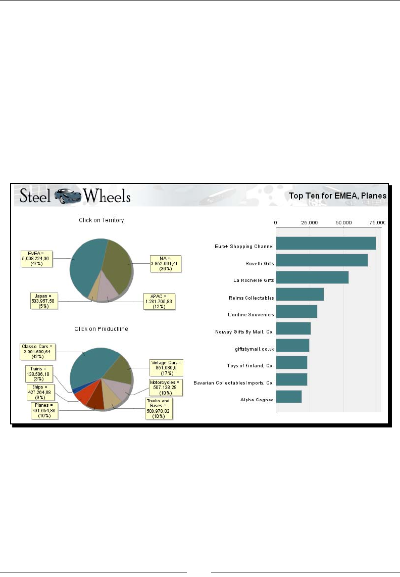
Exploring the Pentaho Demo
Despite being out of the scope of this book, it's worth to briey introduce the Pentaho
Demo. The Pentaho BI Plaorm Demo is a precongured installaon that lets you explore
several capabilies of the Pentaho plaorm. It includes sample reports, cubes, and
dashboards for Steel Wheels. Steel Wheels is a conal store that sells all kind of scale
replicas of vehicles.
The demo can be downloaded from http://sourceforge.net/projects/pentaho/
files/. Under the Business Intelligence Server folder, look for the latest stable
version. The le you have to download is named biserver-ce-3.5.2.stable.zip for
Windows and biserver-ce-3.5.2.stable.tar.gz for other systems.
In the same folder you will nd a le named biserver-getting_started-ce-
3.5.0.pdf. The le is a guide that introduces you the plaorm and gives you some
guidance on how to install and run it. The guide even includes a mini tutorial on building
a simple PDI input-output transformaon.
You can nd more about Pentaho BI Suite at www.pentaho.org.
Pentaho Data Integration
Most of the Pentaho engines, including the engines menoned earlier, were created as
community projects and later adopted by Pentaho. The PDI engine is no excepon—Pentaho
Data Integraon is the new denominaon for the business intelligence tool born as Kele.
The name Kele didn't come from the recursive acronym Kele Extracon,
Transportaon, Transformaon, and Loading Environment it has now, but from
KDE Extracon, Transportaon, Transformaon and Loading Environment,
as the tool was planned to be wrien on top of KDE, as menoned in the
introducon of the book.
In April 2006 the Kele project was acquired by the Pentaho Corporaon and Ma Casters,
Kele's founder, also joined the Pentaho team as a Data Integraon Architect.

Geng Started with Pentaho Data Integraon
[ 10 ]
When Pentaho announced the acquision, James Dixon, the Chief Technology Ocer, said:
We reviewed many alternaves for open source data integraon, and Kele clearly
had the best architecture, richest funconality, and most mature user interface.
The open architecture and superior technology of the Pentaho BI Plaorm
and Kele allowed us to deliver integraon in only a few days, and make that
integraon available to the community.
By joining forces with Pentaho, Kele beneted from a huge developer community, as well
as from a company that would support the future of the project.
From that moment the tool has grown constantly. Every few months a new release is
available, bringing to the users, improvements in performance and exisng funconality,
new funconality, ease of use, and great changes in look and feel. The following is a meline
of the major events related to PDI since its acquision by Pentaho:
June 2006: PDI 2.3 is released. Numerous developers had joined the project and
there were bug xes provided by people in various regions of the world. Among
other changes, the version included enhancements for large scale environments
and mullingual capabilies.
February 2007: Almost seven months aer the last major revision, PDI 2.4 is
released including remote execuon and clustering support (more on this in
Chapter 13), enhanced database support, and a single designer for the two
main elements you design in Kele—jobs and transformaons.
May 2007: PDI 2.5 is released including many new features, the main feature being
the advanced error handling.
November 2007: PDI 3.0 emerges totally redesigned. Its major library changed to
gain massive performance. The look and feel also changed completely.
October 2008: PDI 3.1 comes with an easier-to-use tool, along with a lot of new
funconalies as well.
April 2009: PDI 3.2 is released with a really large number of changes for a
minor version—new funconality, visualizaon improvements, performance
improvements, and a huge pile of bug xes. The main change in this version was the
incorporaon of dynamic clustering (see Chapter 13 for details).
In 2010 PDI 4.0 will be released, delivering mostly improvements with regard to
enterprise features such as version control.
Most users sll refer to PDI as Kele, its further name. Therefore, the names PDI,
Pentaho Data Integraon, and Kele will be used interchangeably throughout
the book.

Chapter 1
[ 11 ]
Using PDI in real world scenarios
Paying aenon to its name, Pentaho Data Integraon, you could think of PDI as a tool to
integrate data.
In you look at its original name, K.E.T.T.L.E., then you must conclude that it is a tool used
for ETL processes which, as you may know, are most frequently seen in data warehouse
environments.
In fact, PDI not only serves as a data integrator or an ETL tool, but is such a powerful tool
that it is common to see it used for those and for many other purposes. Here you have
some examples.
Loading datawarehouses or datamarts
The loading of a datawarehouse or a datamart involves many steps, and there are many
variants depending on business area or business rules. However, in every case, the process
involves the following steps:
Extracng informaon from one or dierent databases, text les, and other sources.
The extracon process may include the task of validang and discarding data that
doesn't match expected paerns or rules.
Transforming the obtained data to meet the business and technical needs required
on the target. Transformaon implies tasks such as converng data types, doing
some calculaons, ltering irrelevant data, and summarizing.
Loading the transformed data into the target database. Depending on the
requirements, the loading may overwrite the exisng informaon, or may
add new informaon each me it is executed.
Geng Started with Pentaho Data Integraon
[ 12 ]
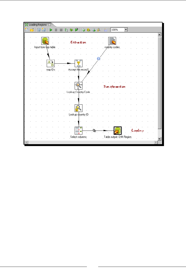
Kele comes ready to do every stage of this loading process. The following sample
screenshot shows a simple ETL designed with Kele:
Integrating data
Imagine two similar companies that need to merge their databases in order to have a unied
view of the data, or a single company that has to combine informaon from a main ERP
applicaon and a CRM applicaon, though they're not connected. These are just two of
hundreds of examples where data integraon is needed. Integrang data is not just a maer
of gathering and mixing data; some conversions, validaon, and transport of data has to be
done. Kele is meant to do all those tasks.
Data cleansing
Why do we need that data be correct and accurate? There are many reasons—for the
eciency of business, to generate trusted conclusions in data mining or stascal studies,
to succeed when integrang data, and so on. Data cleansing is about ensuring that the
data is correct and precise. This can be ensured by verifying if the data meets certain rules,
discarding or correcng those that don't follow the expected paern, seng default values
for missing data, eliminang informaon that is duplicated, normalizing data to conform
minimum and maximum values, and so on—tasks that Kele makes possible, thanks to its
vast set of transformaon and validaon capabilies.

Chapter 1
[ 13 ]
Migrating information
Think of a company of any size that uses a commercial ERP applicaon. One day the owners
realize that the licences are consuming an important share of its budget and so they decide
to migrate to an open source ERP. The company will no longer have to pay licences, but if
they want to do the change, they will have to migrate the informaon. Obviously it is not an
opon to start from scratch, or type the informaon by hand. Kele makes the migraon
possible, thanks to its ability to interact with most kinds of sources and desnaons such as
plain les, and commercial and free databases and spreadsheets.
Exporting data
Somemes you are forced by government regulaons to export certain data to be processed
by legacy systems. You can't just print and deliver some reports containing the required data.
The data has to have a rigid format, with columns that have to obey some rules (size, format,
content), dierent records for heading and tail, just to name some common demands. Kele
has the power to take crude data from the source and generate these kinds of ad hoc reports.
Integrating PDI using Pentaho BI
The previous examples show typical uses of PDI as a standalone applicaon. However, Kele
may be used as part of a process inside the Pentaho BI Plaorm. There are many things
embedded in the Pentaho applicaon that Kele can do—preprocessing data for an on-line
report, sending mails in a schedule fashion, or generang spreadsheet reports.
You'll nd more on this in Chapter 13. However, the use of PDI integrated
with the BI Suite is beyond the scope of this book.
Pop quiz – PDI data sources
Which of the following aren't valid sources in Kele:
1. Spreadsheets
2. Free database engines
3. Commercial database engines
4. Flat les
5. None of the above
Geng Started with Pentaho Data Integraon
[ 14 ]
Installing PDI
In order to work with PDI you need to install the soware. It's a simple task; let's do it.
Time for action – installing PDI
These are the instrucons to install Kele, whatever your operang system.
The only prerequisite to install PDI is to have JRE 5.0 or higher installed. If you don't have it,
please download it from http://www.javasoft.com/ and install it before proceeding.
Once you have checked the prerequisite, follow these steps:
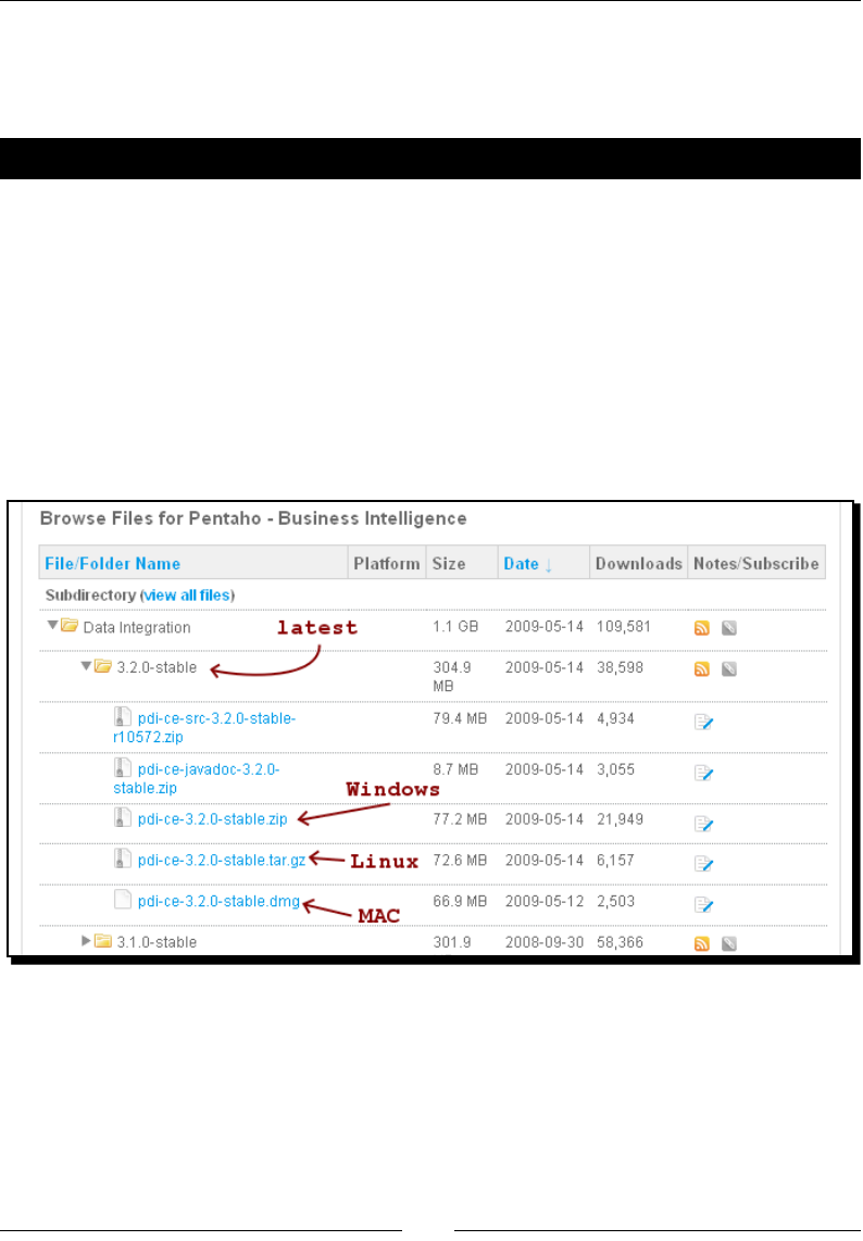
1. From http://community.pentaho.com/sourceforge/ follow the link to
Pentaho Data Integraon (Kele). Alternavely, go directly to the download page
http://sourceforge.net/projects/pentaho/files/Data Integration.
2. Choose the newest stable release. At this me, it is 3.2.0.
3. Download the le that matches your plaorm. The preceding screenshot should
help you.
4. Unzip the downloaded le in a folder of your choice
—C:/Kettle or /home/your_dir/kettle.

Chapter 1
[ 15 ]
5. If your system is Windows, you're done. Under UNIX-like environments, it's
recommended that you make the scripts executable. Assuming that you
chose Kele as the installaon folder, execute the following command:
cd Kettle
chmod +x *.sh
What just happened?
You have installed the tool in just a few minutes. Now you have all you need to start working.
Pop quiz – PDI prerequisites
Which of the following are mandatory to run PDI? You may choose more than one opon.
1. Kele
2. Pentaho BI plaorm
3. JRE
4. A database engine
Launching the PDI graphical designer: Spoon
Now that you've installed PDI, you must be eager to do some stu with data. That will be
possible only inside a graphical environment. PDI has a desktop designer tool named Spoon.
Let's see how it feels to work with it.
Time for action – starting and customizing Spoon
In this tutorial you're going to launch the PDI graphical designer and get familiarized with itsn this tutorial you're going to launch the PDI graphical designer and get familiarized with its
main features.
1. Start Spoon.
If your system is Windows, type the following command:
Spoon.bat
In other plaorms such as Unix, Linux, and so on, type:
Spoon.sh
If you didn't make spoon.sh executable, you may type:
sh Spoon.sh
Geng Started with Pentaho Data Integraon
[ 16 ]
2. As soon as Spoon starts, a dialog window appears asking for the repository
connecon data. Click the No Repository buon. The main window appears. You
will see a small window with the p of the day. Aer reading it, close that window.
3. A welcome! window appears with some useful links for you to see.
4. Close the welcome window. You can open that window later from the main menu.
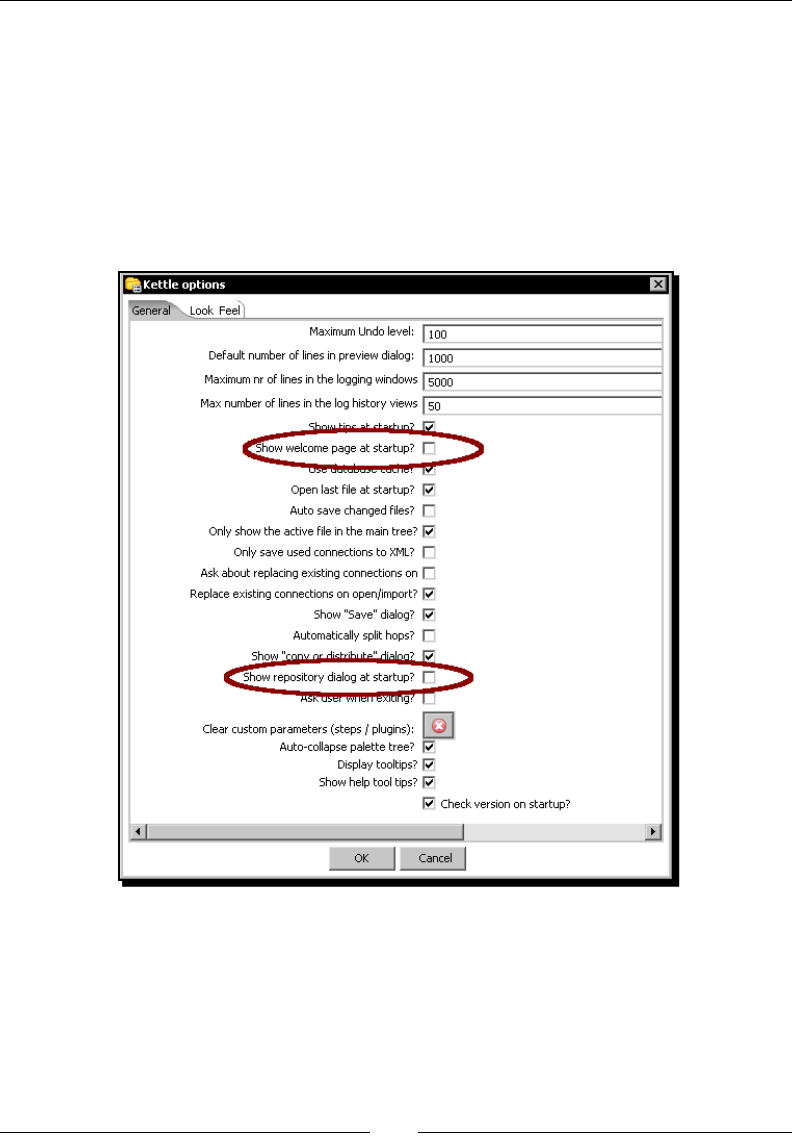
5. Click Opons... from the Edit menu. A window appears where you can change
various general and visual characteriscs. Uncheck the circled checkboxes:
6. Select the tab window Look Feel.
Chapter 1
[ 17 ]
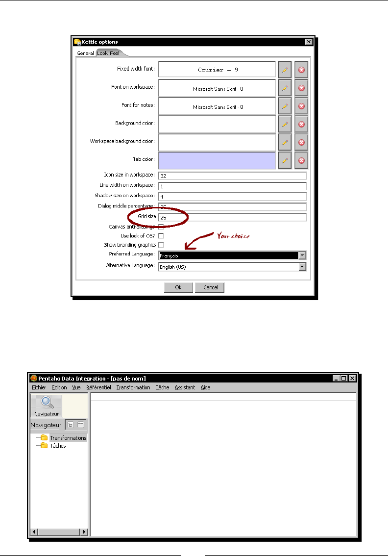
7. Change the Grid size and Preferred Language sengs as follows:
8. Click the OK buon.
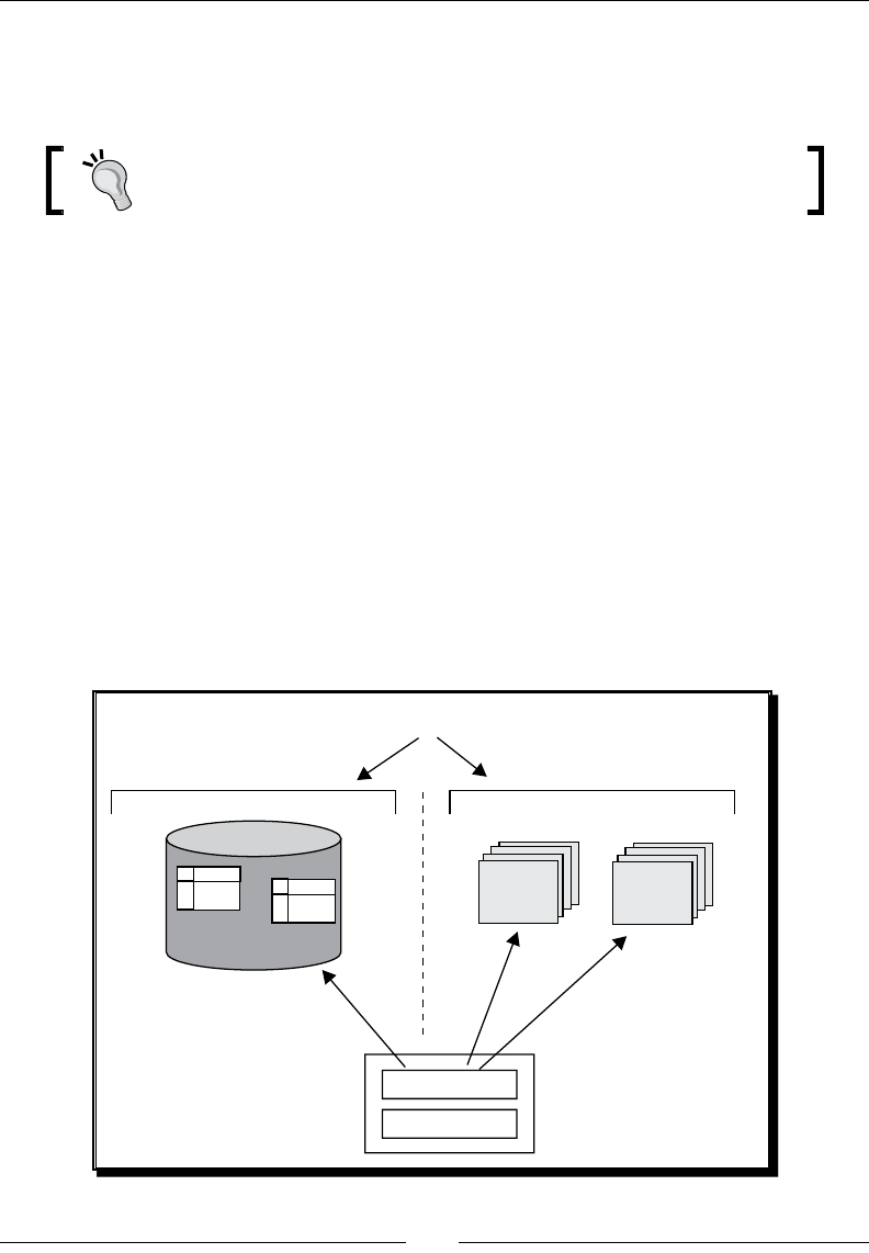
9. Restart Spoon in order to apply the changes. You should neither see the repository
dialog, nor the welcome window. You should see the following screen instead:

Geng Started with Pentaho Data Integraon
[ 18 ]
What just happened?
You ran for the rst me the graphical designer of PDI Spoon, and applied some
custom conguraon.
From the Look Feel conguraon window, you changed the size of the doed grid that
appears in the canvas area while you are working. You also changed the preferred language.
In the Opon tab window, you chose not to show either the repository dialog or the
welcome window at startup. These changes were applied as you restarted the tool, not
before.
The second me you launched the tool, the repository dialog didn't show up. When the
main window appeared, all the visible texts were shown in French, which was the selected
language, and instead of the welcome window, there was a blank screen.
Spoon
This tool that you're exploring in this secon is the PDI's desktop design tool. With Spoon you
design, preview, and test all your work, that is, transformaons and jobs. When you see PDI
screenshots, what you are really seeing are Spoon screenshots. The other PDI components
that you will meet in the following chapters are executed from terminal windows.
Setting preferences in the Options window
In the tutorial you changed some preferences in the Opons window. There are several look
and feel characteriscs you can change beyond those you changed. Feel free to experiment
with this seng.
Remember to restart Spoon in order to see the changes applied.
If you choose any language as preferred language other than English, you
should select a dierent language as alternave. If you do so, every name or
descripon not translated to your preferred language will be shown in the
alternave language.
Just for the curious people: Italian and French are the overall winners of the list of languages
to which the tool has been translated from English. Below them follow Korean, Argennean
Spanish, Japanese, and Chinese.
Chapter 1
[ 19 ]
One of the sengs you changed was the appearance of the welcome window at start up.
The welcome window has many useful links, all related with the tool: wiki pages, news,
forum access, and more. It's worth exploring them.
You don't have to change the sengs again to see the welcome window.
You can open it from the menu Help | Show the Welcome Screen.
Storing transformations and jobs in a repository
The rst me you launched Spoon, you chose No Repository. Aer that, you congured
Spoon to stop asking you for the Repository opon. You must be curious about what the
repository is and why not to use it. Let's explain it.
As said, the results of working with PDI are Transformaons and Jobs. In order to save the
Transformaons and Jobs, PDI oers two methods:
Repository: When you use the repository method you save jobs and
transformaons in a repository. A repository is a relaonal database specially
designed for this purpose.
Files: The les method consists of saving jobs and transformaons as regular XML
les in the lesystem, with extension kjb and ktr respecvely.
The following diagram summarizes this:
exclusive
REPOSITORY FILE SYSTEM
.ktr .kjb
Design, Preview, Run
SPOON
Kettle Engine KETTLE
Transfor
mations Jobs
Transformations Jobs
Design, Preview, Run

Geng Started with Pentaho Data Integraon
[ 20 ]
You cannot mix the two methods (les and repository) in the same project. Therefore, you
must choose the method when you start the tool.
Why did we choose not to work with repository, or in other words, to work with les? This is
mainly for the following two reasons:
Working with les is more natural and praccal for most users.
Working with repository requires minimum database knowledge and that you also
have access to a database engine from your computer. Having both precondions
would allow you to learn working with both methods. However, it's probable that
you haven't.
Throughout this book, we will use the le method. For details of working with repositories,
please refer to Appendix A.
Creating your rst transformation
Unl now, you've seen the very basic elements of Spoon. For sure, you must be waing to do
some interesng task beyond looking around. It's me to create your rst transformaon.
Time for action – creating a hello world transformation
How about starng by saying Hello to the World? Not original but enough for a very rst
praccal exercise. Here is how you do it:
1. Create a folder named pdi_labs under the folder of your choice.
2. Open Spoon.
3. From the main menu select File | New Transformaon.
4. At the le-hand side of the screen, you'll see a tree of Steps. Expand the Input
branch by double-clicking it.
5. Le-click the Generate Rows icon.

Chapter 1
[ 21 ]
6. Without releasing the buon, drag-and-drop the selected icon to the main canvas.
The screen will look like this:
7. Double-click the Generate Rows step that you just put in the canvas and ll the text
boxes and grid as follows:
8. From the Steps tree, double-click the Flow step.
9. Click the Dummy icon and drag-and-drop it to the main canvas.
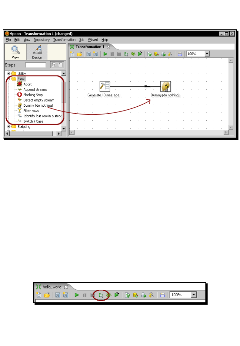
Geng Started with Pentaho Data Integraon
[ 22 ]
10. Click the Generate Rows step and holding the Shi key down, drag the cursor
towards the Dummy step. Release the buon. The screen should look like this:
11. Right-click somewhere on the canvas to bring up a contextual menu.
12. Select New note. A note editor appears.
13. Type some descripon such as Hello World! and click OK.
14. From the main menu, select Transformaon | Conguraon. A window appears
to specify transformaon properes. Fill the Transformaon name with a simple
name as hello_world. Fill the Descripon eld with a short descripon such as
My rst transformaon. Finally provide a more clear explanaon in the Extended
descripon text box and click OK.
15. From the main menu, select File | Save.
16. Save the transformaon in the folder pdi_labs with the name hello_world.
17. Select the Dummy step by le-clicking it.
18. Click on the Preview buon in the menu above the main canvas.
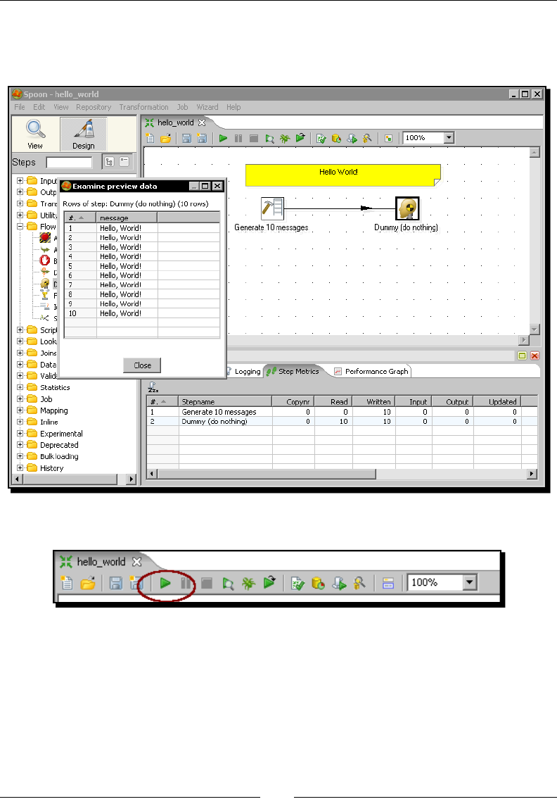
Chapter 1
[ 23 ]
19. A debug window appears. Click the Quick Launch buon.
20. The following window appears to preview the data generated by the transformaon:
21. Close the preview window and click the Run buon.
22. A window appears. Click Launch.
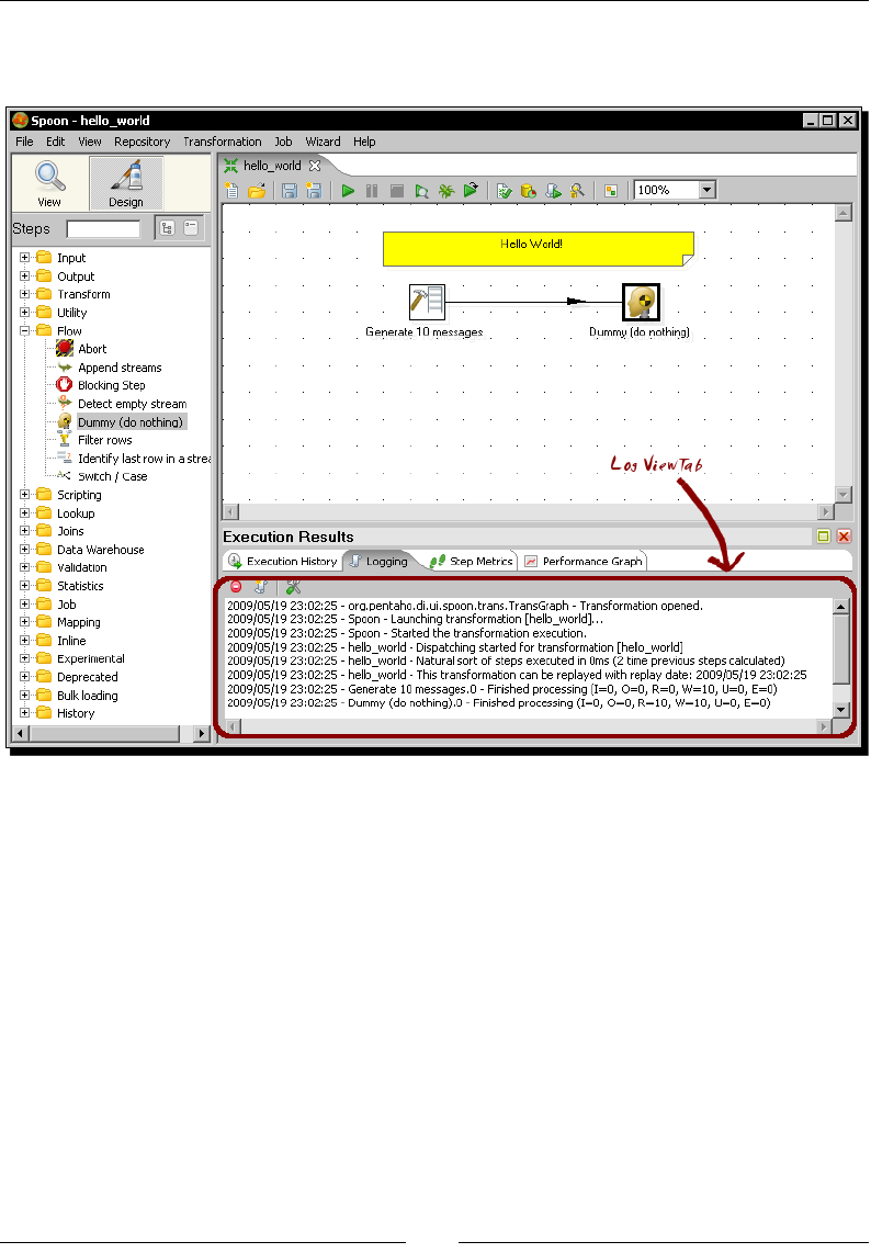
Geng Started with Pentaho Data Integraon
[ 24 ]
23. The execuon results are shown in the boom of the screen. The Logging tab
should look as follows:
What just happened?
You've just created your rst transformaon.
First, you created a new transformaon. From the tree on the le, you dragged two steps
and drop them into the canvas. Finally, you linked them with a hop.
With the Generate Rows step, you created 10 rows of data with the message Hello World!.
The Dummy step simply served as a desnaon of those rows.
Aer creang the transformaon, you did a preview. The preview allowed you to see the
content of the created data, this is, the 10 rows with the message Hello World!
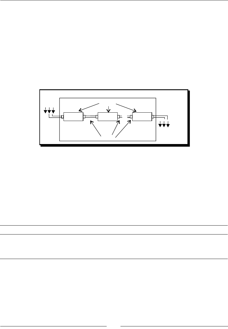
Chapter 1
[ 25 ]
Finally, you ran the transformaon. You could see the results of the execuon at the boom
of the windows. There is a tab named Step Metrics with informaon about what happens
with each steps in the transformaon. There is also a Logging tab showing a complete detail
of what happened.
Directing the Kettle engine with transformations
As shown in the following diagram, transformaon is an enty made of steps linked by hops.
These steps and hops build paths through which data ows. The data enters or is created in a
step, the step applies some kind of transformaon to it, and nally the data leaves that step.
Therefore, it's said that a transformaon is data-ow oriented.
Steps
Transformation
Output
Input
Hops
Step1 Step2 StepN
...
A transformaon itself is not a program nor an executable le. It is just plain XML. The
transformaon contains metadata that tells the Kele engine what to do.
A step is the minimal unit inside a transformaon. A big set of steps is available. These steps
are grouped in categories such as the input and ow categories that you saw in the example.
Each step is conceived to accomplish a specic funcon, going from reading a parameter to
normalizing a dataset. Each step has a conguraon window. These windows vary according
to the funconality of the steps and the category to which they belong. What all steps have
in common are the name and descripon:
Step property Descripon
Name A representative name inside the transformation.
Description A brief explanation that allows you to clarify the purpose of the step.
It's not mandatory but it is useful.
A hop is a graphical representaon of data owing between two steps—an origin and a
desnaon. The data that ows through that hop constutes the output data of the origin
step and the input data of the desnaon step.
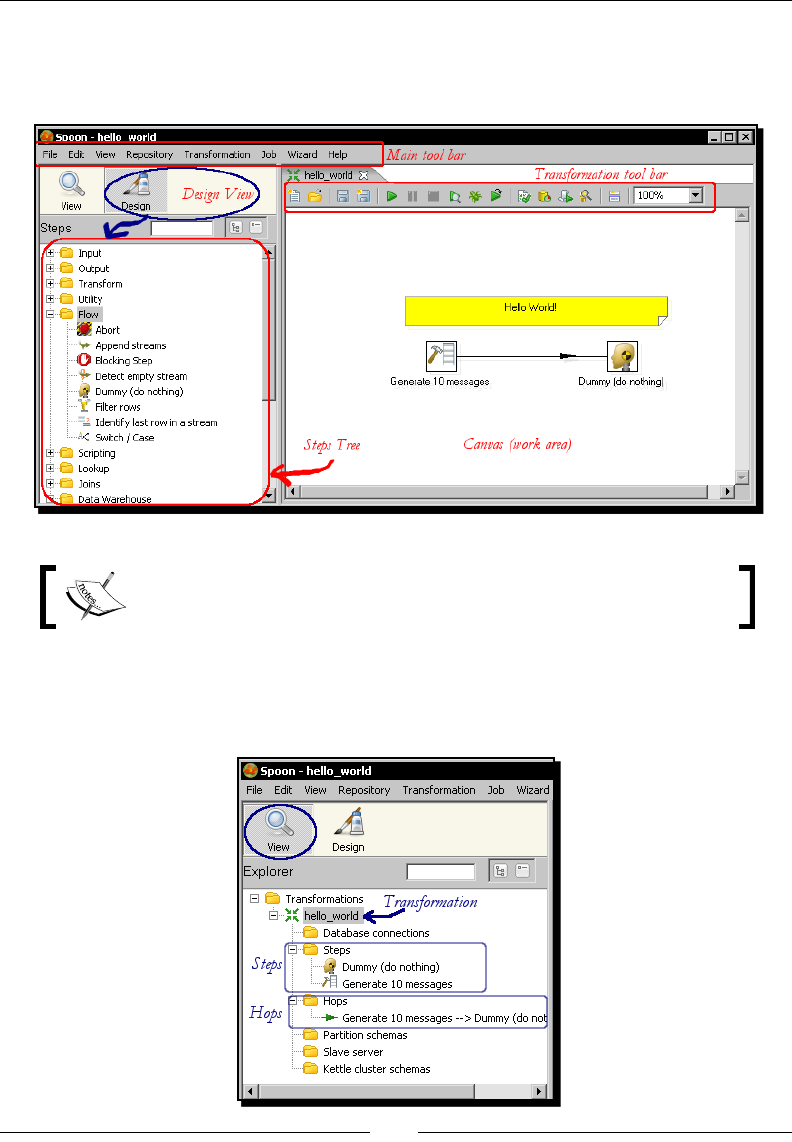
Geng Started with Pentaho Data Integraon
[ 26 ]
Exploring the Spoon interface
As you just saw, the Spoon is the tool using which you create, preview, and run
transformaons. The following screenshot shows you the basic work areas:
The words canvas and work area will be used interchangeably throughout
the book.
Viewing the transformation structure
If you click the View icon in the upper le corner of the screen, the tree will change to show
the structure of the transformaon currently being edited.
Download from Wow! eBook <www.wowebook.com>
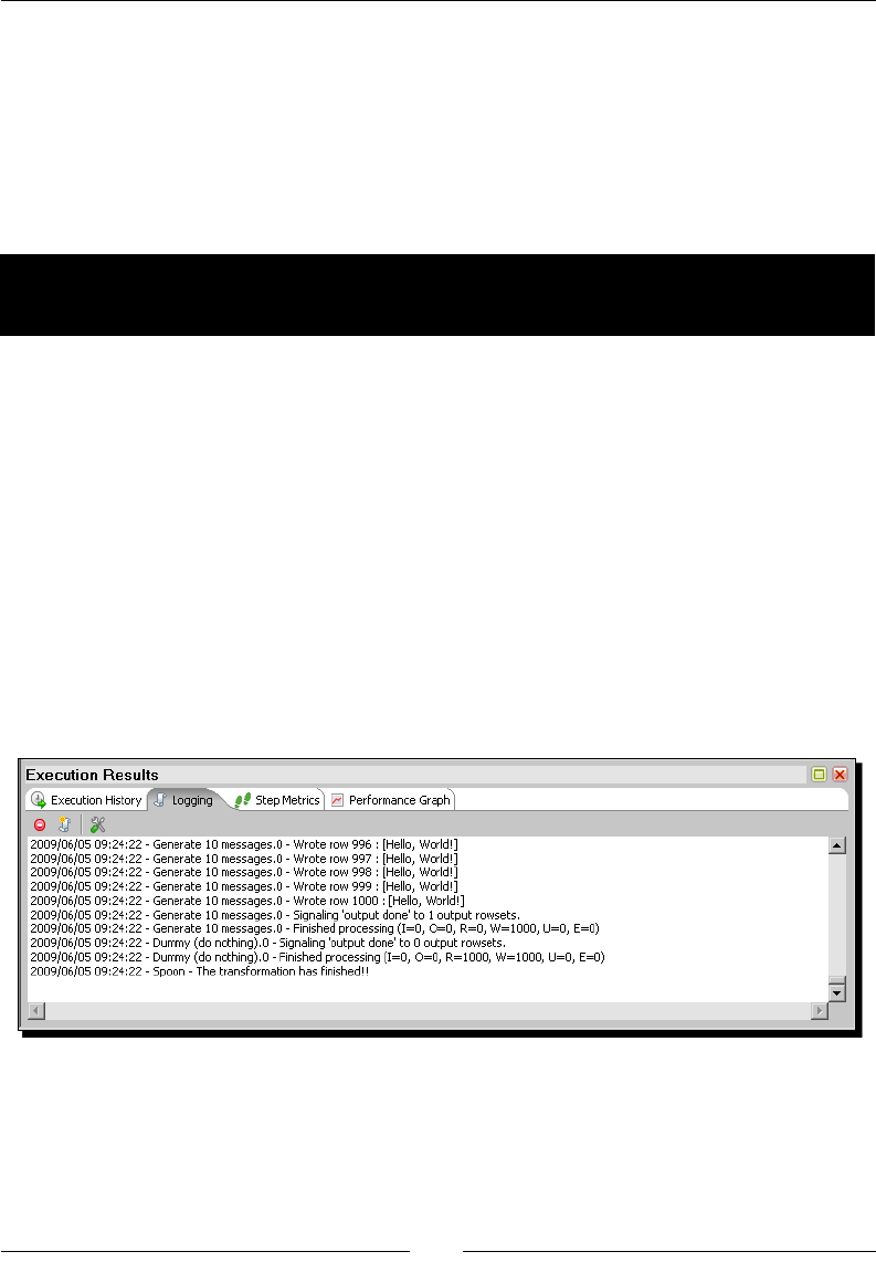
Chapter 1
[ 27 ]
Running and previewing the transformation
The Preview funconality allows you to see a sample of the data produced for selected steps.
In the previous example, you previewed the output of the Dummy Step. The Run opon
eecvely runs the whole transformaon.
Whether you preview or run a transformaon, you'll get an execuon results window
showing what happened. Let's explain it through an example.
Time for action – running and previewing the hello_world
transformation
Let's do some tesng and explore the results:
1. Open the hello_world transformaon.
2. Edit the Generate Rows step, and change the limit from 10 to 1000 so that it
generates 1,000 rows.
3. Select the Logging tab window at the boom of the screen.
4. Click on Run.
5. In the Log level drop-down list, select RowLevel detail.
6. Click on Launch.
7. You can see how the logging window shows every task in a very detailed way.
8. Edit the Generate Rows step, and change the limit to 10,000 so that it generates
10,000 rows.
9. Select the Step Metrics.
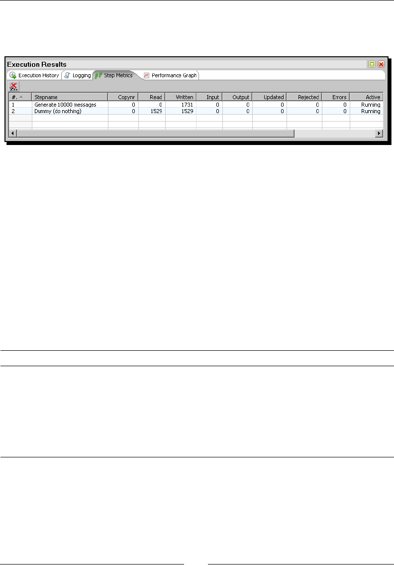
Geng Started with Pentaho Data Integraon
[ 28 ]
10. Run the transformaon.
11. You can see how the numbers change as the rows travel through the steps.
What just happened?
You did some tests with the hello_world transformaon and saw the results in the
Execuon Results window.
Previewing the results in the Execution Results window
The Execuon Results window shows you what is happening while you preview or run
a transformaon.
The Logging tab shows the execuon of your transformaon, step by step. By default, the
level of the logging detail is Basic but you can change it to see dierent levels of detail—from
a minimal logging (level Minimal) to a very detailed one (level RowLevel).
The Step Metrics tab shows, for each step of the transformaon, the executed operaons
and several status and informaon columns. You may be interested in the following columns:
Column Descripon
Read Contains the number of rows coming from previous steps
Written Contains the number of rows leaving from this step toward the next
Input Number of rows read from a le or table
Output Number of rows written to a le or table
Errors Errors in the execution. If there are errors, the whole row becomes red
Active Tells the current status of the execution
In the example, you can see that the Generate Rows step writes rows, which then are read
by the Dummy step. The Dummy step also writes the same rows, but in this case those
go nowhere.

Chapter 1
[ 29 ]
Pop quiz – PDI basics
For each of the following, decide if the sentence is true or false:
1. There are several graphical tools in PDI, but Spoon is the most used.
2. You can choose to save Transformaons either in les or in a database.
3. To run a Transformaon, an executable le has to be generated from Spoon.
4. The grid size opon in the Look and Feel windows allows you to resize the work area.
5. To create a transformaon, you have to provide external data.
Installing MySQL
Before skipping to the next chapter, let's devote some minutes to the installaon of MySQL.
In Chapter 8 you will begin working with databases from PDI. In order to do that, you will
need access to some database engine. As MySQL is the world's most popular open source
database, it was the database engine chosen for the database-related tutorials in the book.
In this secon you will learn to install the MySQL database engine both in Windows and
Ubuntu, the most popular distribuon of Linux these days. As the procedures for installing
the soware are dierent, a separate explanaon is given for each system.
Time for action – installing MySQL on Windows
In order to install MySQL on your Windows system, please follow these instrucons:
1. Open an internet browser and type http://dev.mysql.com/downloads/mysql/.
2. Select the Microso Windows plaorm and download the mysql-essenal package
that matches your system: 32-bit or 64-bit.
3. Double-click the downloaded le. A wizard will guide you through the process.
4. When asked about the setup type, select Typical.
5. Several screens follow. When the wizard is complete you'll have the opon to
congure the server. Check Congure the MySQL Server now and click Finish.
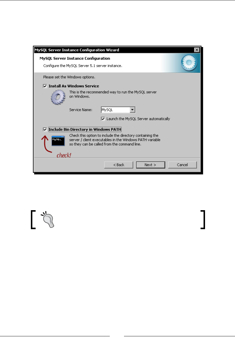
Geng Started with Pentaho Data Integraon
[ 30 ]
6. A new wizard will be launched that lets you congure the server.
7. When asked about the conguraon type, select Standard Conguraon.
8. When prompted, set the Windows opons as shown in the next screenshot:
9. When prompted for the security opons, provide a password for the root user.
You'll have to retype the password.
Provide a password that you can remember. You'll need it
later to connect to the MySQL server.
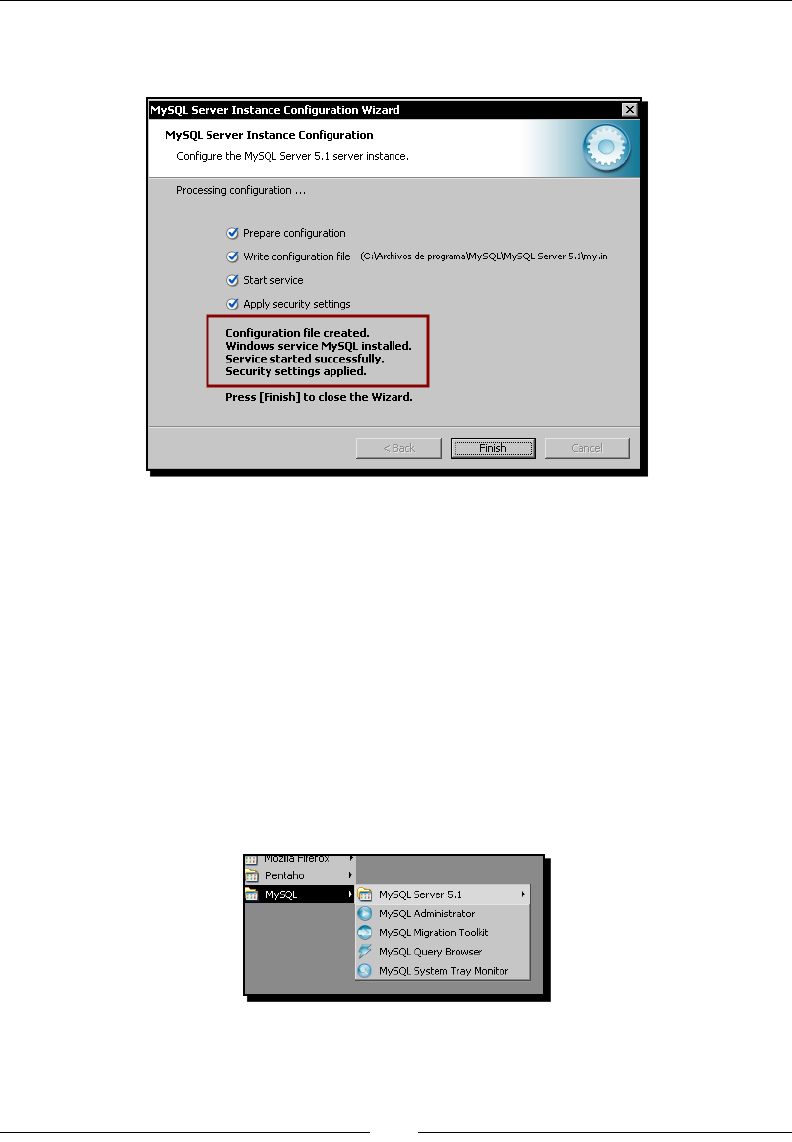
Chapter 1
[ 31 ]
10. In the next window click on Execute to proceed with the conguraon. When the
conguraon is done, you'll see this:
11. Click on Finish. Aer installing MySQL it is recommended that you install the GUI
tools for administering and querying the database.
12. Open an Internet browser and type
http://dev.mysql.com/downloads/gui-tools/.
13. Look for the Windows downloads and download the Windows (x86) package.
14. Double-click the downloaded le. A wizard will guide you through the process.
15. When asked about the setup type, select Complete.
16. Several screens follow. Just follow the wizard instrucons.
17. When the wizard ends, you'll have the GUI tools added to the MySQL menu.
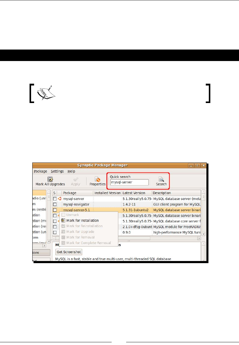
Geng Started with Pentaho Data Integraon
[ 32 ]
What just happened?
You downloaded and installed MySQL on your Windows system. You also installed MySQL
GUI tools, a soware package that includes an administrator and a query browser ulity and
that will make your life easier when working with the database.
Time for action – installing MySQL on Ubuntu
This tutorial shows you the procedure to install MySQL on Ubuntu.
In order to follow the tutorial you need to be connected to
the Internet.
Please follow these instrucons:
1. Check that you have access to the Internet.
2. Open the Synapc package manager from System | Administraon | Synapc
Package Manager.
3. Under Quick search type mysql-server and click on the Search buon.
4. Among the results, locate mysql-server-5.1, click in the ny square to the le,
and select Mark for Installaon.
5. You'll be prompted for conrmaon. Click on Mark.
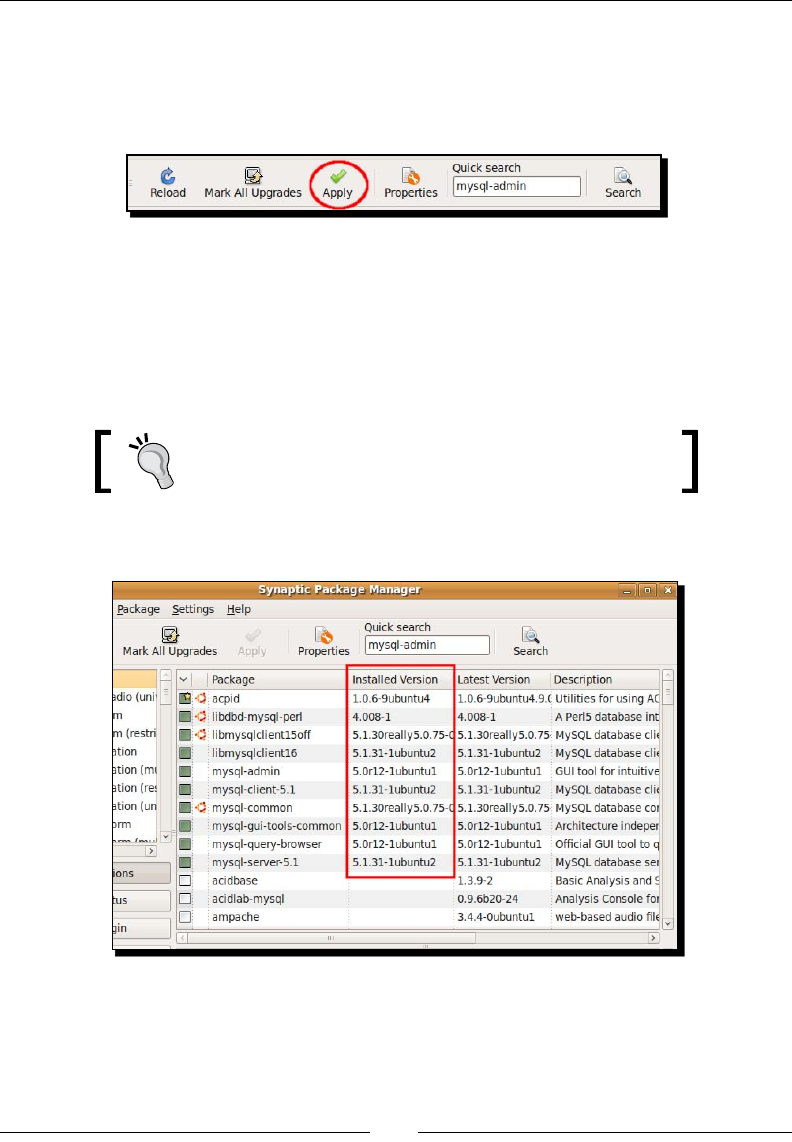
Chapter 1
[ 33 ]
6. Now search for a package named mysql-admin.
7. When found, mark it for installaon in the same way.
8. Click on Apply on the main toolbar.
9. A window shows up asking for conrmaon. Click on Mark again. What follows is
the download process followed by the installaon process.
10. At a parcular moment a window appears asking you for a password for the root
user—the administrator of the database. Enter a password of your choice. You'll
have to enter it twice.
Think of a password that you can remember. You'll need it
later to connect to the MySQL server.
11. When the process ends, you will see the changes applied.
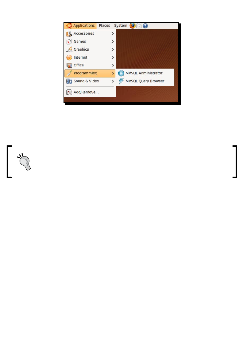
Geng Started with Pentaho Data Integraon
[ 34 ]
12. Under Applicaons a new menu will also be added to access the GUI tools.
What just happened?
You installed MySQL server and GUI Tools in your Ubuntu system.
The previous direcons are for standard installaons. For custom installaons,
instrucons related to other operang systems, or for troubleshoong, please
check the MySQL documentaon at—http://dev.mysql.com/doc/
refman/5.1/en/installing.html.
Summary
In this rst chapter, you were introduced to Pentaho Data Integraon. Specically, you learned
what Pentaho Data Integraon is and you installed the tool. You were also introduced to
Spoon, the graphical designer of PDI, and you created your rst transformaon.
As an addional exercise, you installed a MySQL server and the MySQL GUI tools. You will
need this soware when you start working with databases in Chapter 8.
Now that you've learned the basics, you're ready to begin creang your own transformaons
to explore real data. That is the topic of the next chapter.

2
Getting Started with Transformations
In the previous chapter you used the graphical designer Spoon to create
your rst transformaon: Hello world. Now you will start creang your own
transformaons to explore data from the real world. Data is everywhere; in
parcular you will nd data in les. Product lists, logs, survey results, and
stascal informaon are just a sample of the dierent kinds of informaon
usually stored in les. In this chapter you will create transformaons to get
data from les, and also to send data back to les. This in turn will allow you to
learn the basic PDI terminology related to data.
Reading data from les
Despite being the most primive format used to store data, les are broadly used and they
exist in several avors as xed width, comma-separated values, spreadsheet, or even free
format les. PDI has the ability to read data from all types of les; in this rst tutorial let's
see how to use PDI to get data from text les.

Geng Started with Transformaons
[ 36 ]
Time for action – reading results of football matches from les
Suppose you have collected several football stascs in plain les. Your les look like this:
Group|Date|Home Team |Results|Away Team|Notes
Group 1|02/June|Italy|2-1|France|
Group 1|02/June|Argentina|2-1|Hungary
Group 1|06/June|Italy|3-1|Hungary
Group 1|06/June|Argentina|2-1|France
Group 1|10/June|France|3-1|Hungary
Group 1|10/June|Italy|1-0|Argentina
-------------------------------------------
World Cup 78
Group 1
You don't have one, but many les, all with the same structure. You now want to unify all the
informaon in one single le. Let's begin by reading the les.
1. Create the folder named pdi_files. Inside it, create the input and
output subfolders.
2. By using any text editor, type the le shown and save it under the name
group1.txt in the folder named input, which you just created. You can also
download the le from Packt's ocial website.
3. Start Spoon.
4. From the main menu select File | New Transformaon.
5. Expand the Input branch of the steps tree.
6. Drag the Text le input icon to the canvas.
7. Double-click the text input le icon and give a name to the step.
8. Click the Browse... buon and search the le group1.txt.
9. Select the le. The textbox File or directory will be temporarily populated with the full
path of the le—for example, C:\pdi_files\input\group1.txt.
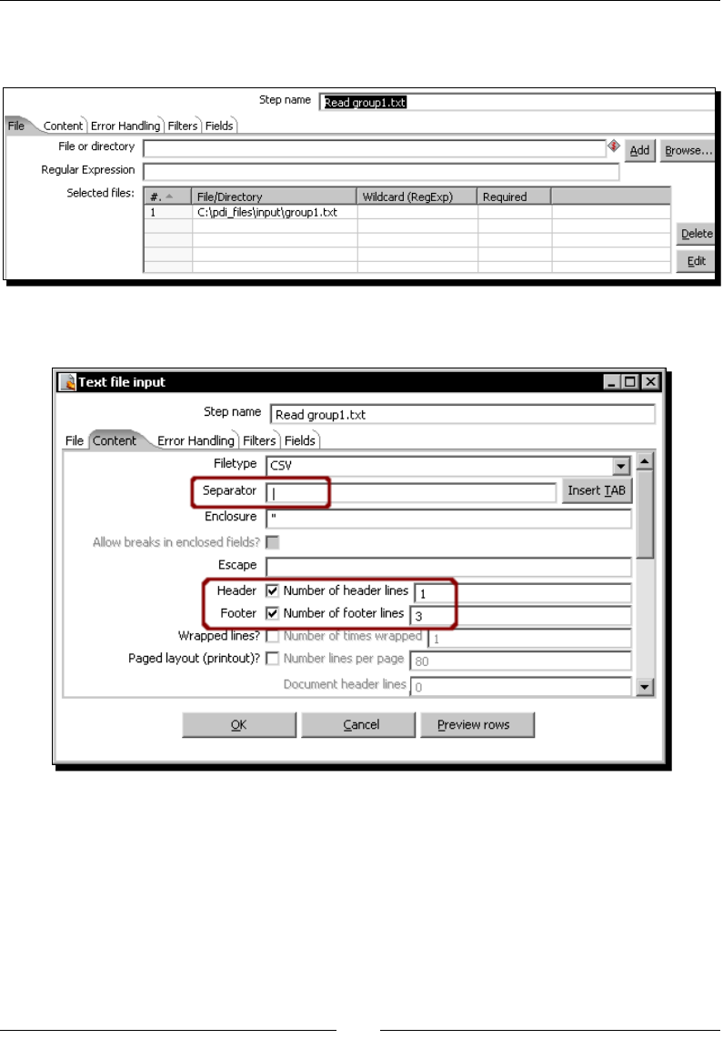
Chapter 2
[ 37 ]
10. Click the Add buon. The full text will be moved from the File or directory textbox to the
grid. The conguraon window should look as follows:
11. Select the Content tab and ll it like this:
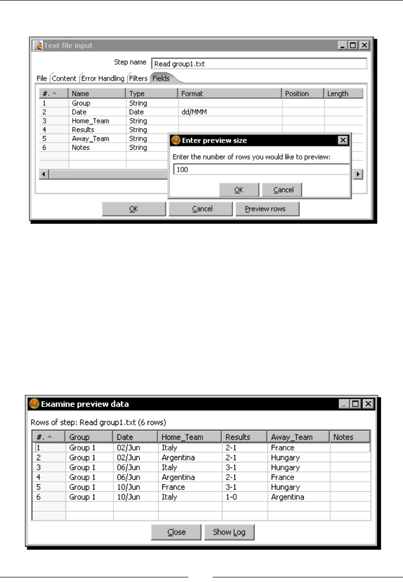
Geng Started with Transformaons
[ 38 ]
12. Select the Fields tab. Click the Get Fields buon. The screen should look like this:
13. In the small window that proposes you a number of sample lines, click OK.
14. Close the scan results window.
15. Change the second row. Under the Type column select Date, and under the Format
column, type dd/MMM.
16. The result value is text, not a number, so change the fourth row too. Under the Type
column select String.
17. Click the Preview rows buon, and then the OK buon.
18. The previewed data should look like the following:
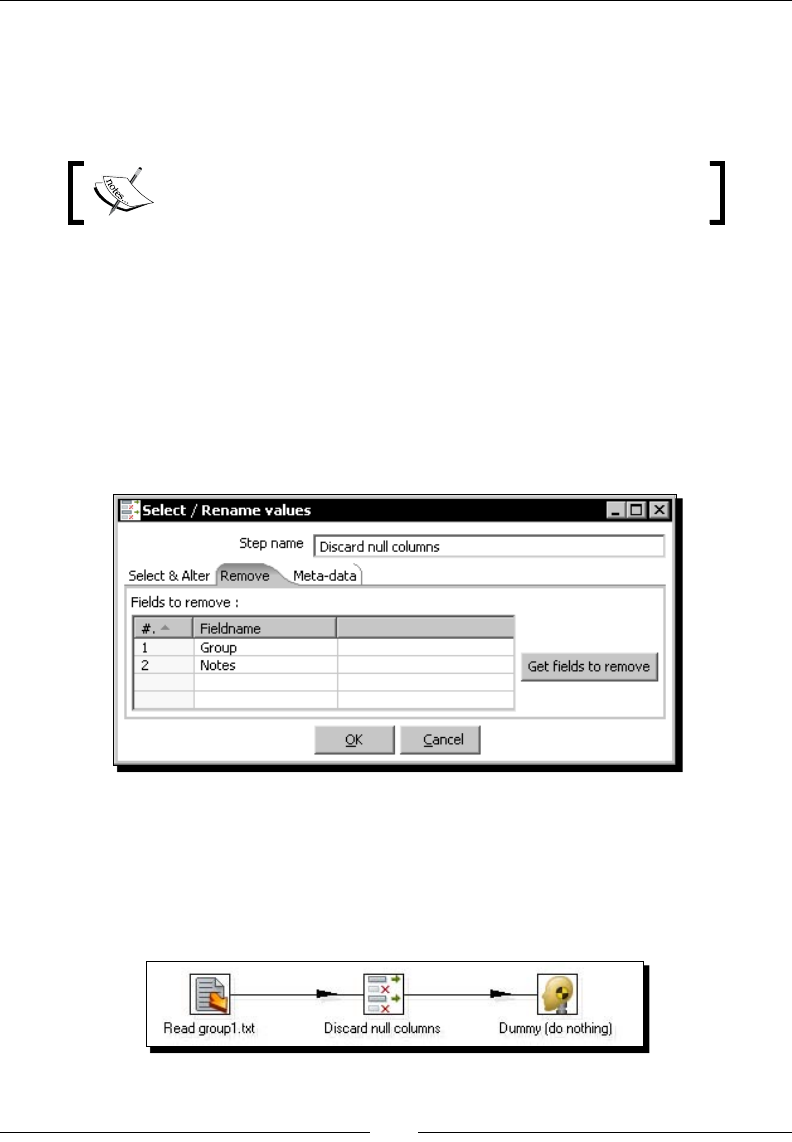
Chapter 2
[ 39 ]
19. Expand the Transform branch of the steps tree.
20. Drag the Select values icon to the canvas.
21. Create a hop from the Text le input step to the Select values step.
Remember that you do it by selecng the rst step, then dragging
toward the second while holding down the Shi key.
22. Double-click the Select values step icon and give a name to the step.
23. Select the Remove tab.
24. Click the Get elds to remove buon.
25. Delete every row except the rst and the last one by le-clicking them and
pressing Delete.
26. The tab window looks like this:
27. Click OK.
28. From the Flow branch of the steps tree, drag the Dummy icon to the canvas.
29. Create a hop from the Select values step to the Dummy step. Your transformaon
should look like the following:
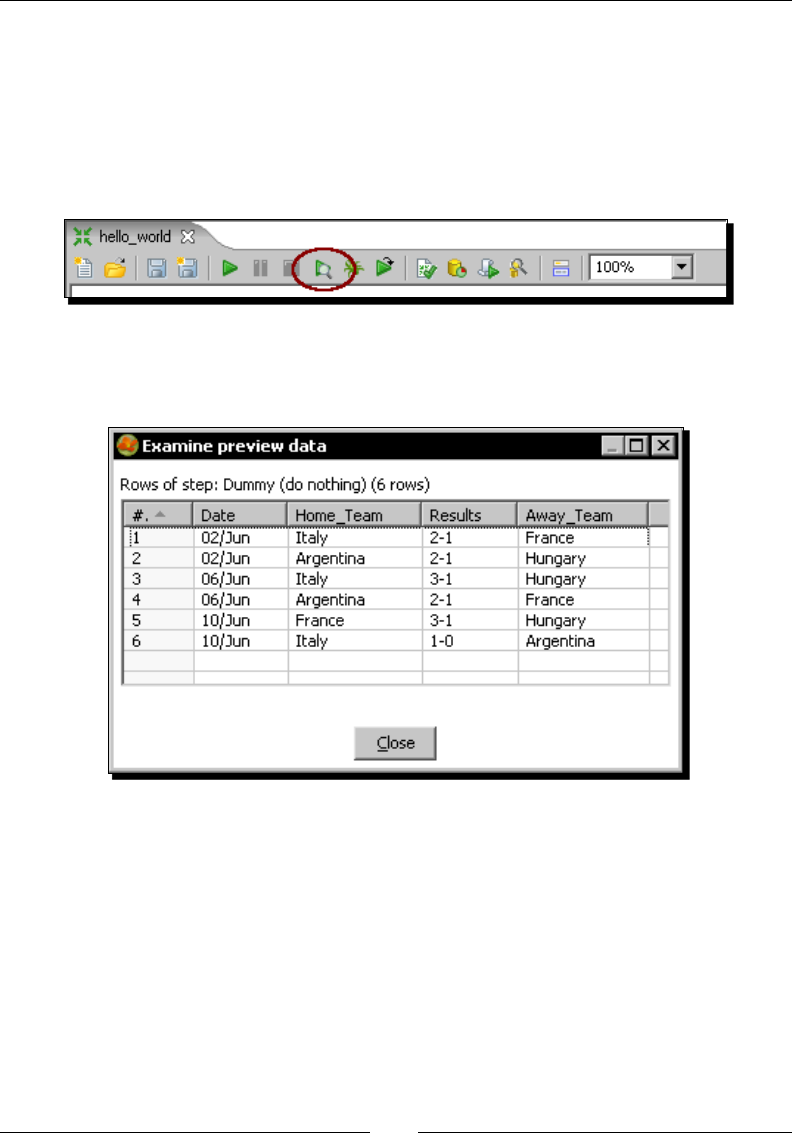
Geng Started with Transformaons
[ 40 ]
30. Congure the transformaon by pressing Ctrl+T and giving a name and a descripon to
the transformaon.
31. Save the transformaon by pressing Ctrl+S.
32. Select the Dummy step.
33. Click the Preview buon located on the transformaon toolbar:
34. Click the Quick Launch buon.
35. The following window appears, showing the nal data:
What just happened?
You read your plain le with results of football matches into a transformaon.
By using a Text le input step, you told Kele the full path to your le, along with the
characteriscs of the le so that Kele was able to read the data correctly—you specied
that the le had a header, had three rows at the end that should be ignored, and specied
the name and type of the columns.
Aer reading the le, you used a Select values step to remove columns you didn't need— the
rst and the last column.

Chapter 2
[ 41 ]
With those two simple steps, you were able to preview the data in your le from inside
the transformaon.
Another thing you may have noced is the use of shortcuts instead of the menu opons—for
example, to save the transformaon.
Many of the menu opons can be accessed more quickly by using shortcuts. The
available shortcuts for the menu opons are menoned as part of the name of
the operaon—for example, Run F9.
For a full shortcut reference please check Appendix D.
Input les
Files are one of the most used input sources. PDI can take data from several types of les,
with very few limitaons.
When you have a le to work with, the rst thing you have to do is to specify where the le
is, how it looks, and what kinds of values it contains. That is exactly what you did in the rst
tutorial of this chapter.
With the informaon you provide, Kele can create the dataset to work within the
current transformaon.
Input steps
There are several steps that allow you to take a le as the input data. All those steps such as
Text le input, Fixed le input, Excel Input, and so on are under the Input step category.
Despite the obvious dierences that exist between these types of les, the ways to congure
the steps have much in common. The following are the main properes you have to specify
for an input step:
Name of the step: It is mandatory and must be dierent for every step in
the transformaon.
Name and locaon of the le: These must be specied of course. At the moment
you create the transformaon, it's not mandatory that the le exists. However, if it
does, you will nd it easier to congure this step.
Content type: This data includes delimiter character, type of encoding, whether a
header is present, and so on. The list depends on the kind of le chosen. In every
case, Kele propose default values, so you don't have to enter too much data.
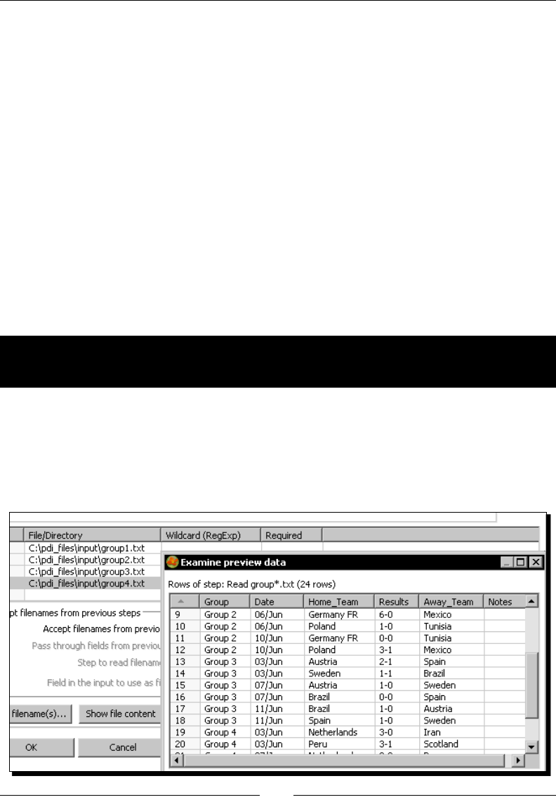
Geng Started with Transformaons
[ 42 ]
Fields: Kele has the facility to get the denions automacally by clicking the Get
Fields buon. However, Kele doesn't always guess the data types, size, or format
as expected. So, aer geng the elds you may change what you consider more
appropriate, as you did in the tutorial.
Filtering: Some steps allow you to lter the data—skip blank rows, read only the rst
n rows, and so on.
Aer conguring an input step, you can preview the data just as you did, by Clicking
the Preview Rows buon. This is useful to discover if there is something wrong in the
conguraon. In that case, you can make the adjustments and preview again, unl your
data looks ne.
Reading several les at once
Unl now you used an input step to read one le. But you have several les, all with the very
same structure. That will not be a problem because with Kele it is possible to read more
than a le at a me.
Time for action – reading all your les at a time using a single
Text le input step
To read all your les follow the next steps:
1. Open the transformaon, double-click the input step, and add the other les in the
same way you added the rst.
2. Aer Clicking the Preview rows buon, you will see this:
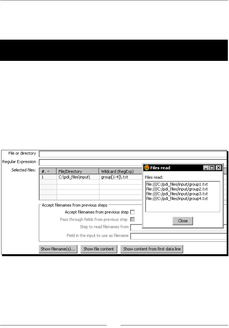
Chapter 2
[ 43 ]
What just happened?
You read several les at once. By pung in the grid the names of all the input les, you could
get the content of every specied le one aer the other.
Time for action – reading all your les at a time using a single
Text le input step and regular expressions
You could do the same thing you did above by using a dierent notaon.
Follow these instrucons:
1. Open the transformaon and edit the conguraon windows of the input step.
2. Delete the lines with the names of the les.
3. In the rst row of the grid, type C:\pdi_files\input\ under the File/Directory
column, and group[1-4]\.txt under the Wildcard (Reg.Exp.) column.
4. Click the Show lename(s)... buon. You'll see the list of les that match
the expression.
5. Close the ny window and click Preview rows to conrm that the rows shown
belong to the four les that match the expression you typed.
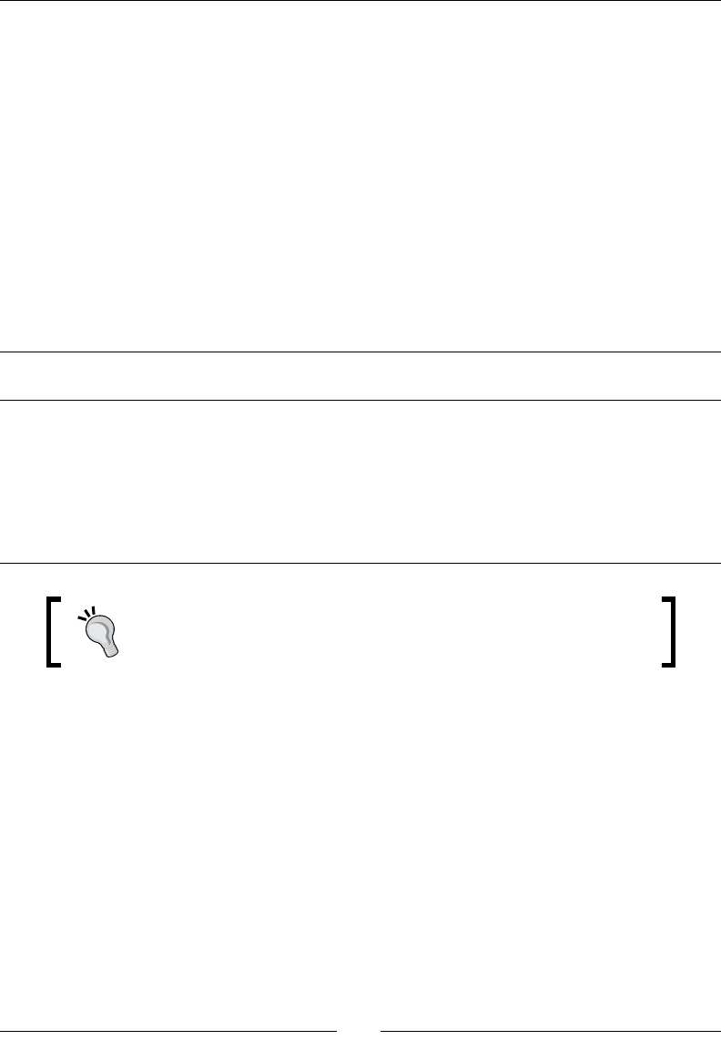
Geng Started with Transformaons
[ 44 ]
What just happened?
In this parcular case, all lenames follow a paern—group1.txt, group2.txt, and so
on. In order to specify the names of the les, you used a regular expression. In the column
File/Directory you put the stac part of the names, while in the Wildcard (Reg.Exp.) column
you put the regular expression with the paern that a le must follow to be considered:
the text group followed by a number between 1 and 4, and then .txt. Then, all les that
matched the expression were considered as input les.
Regular expressions
There are many places inside Kele where you may or have to provide a regular expression.
A regular expression is much more than specifying the known wildcards ? and *.
Here you have some examples of regular expressions you may use to specify lenames:
The following regular
expression ...
Matches ... Examples
.*\.txt Any txt le thisisaValidExample.
txt
test(19|20)\d\d-
(0[1-9]|1[012])\.txt
Any txt le beginning with test
followed by a date using the format
yyyy-mm
test2009-12.txt
test2009-01.txt
(?i)test.+\.txt Any txt le beginning with test,
upper or lower case
TeSTcaseinsensitive.
tXt
Please note that the * wildcard doesn't work the same as it does on
the command line. If you want to match any character, the * has to be
preceded by a dot.
Here are some useful links in case you want to know more about regular expressions:
Regular Expression Quick Start:
http://www.regular-expressions.info/quickstart.html
The Java Regular Expression Tutorial:
http://java.sun.com/docs/books/tutorial/essential/regex/
Java Regular Expression Paern Syntax: http://java.sun.com/javase/6/
docs/api/java/util/regex/Pattern.html

Chapter 2
[ 45 ]
Troubleshooting reading les
Despite the simplicity of reading les with PDI, obstacles and errors appear. Many mes
the soluon is simple but dicult to nd if you are new to PDI. Here you have a list of
common problems and possible soluons for you to take into account while reading and
previewing a le:
Problem Diagnosc Possible soluons
You get the message
Sorry, no rows found to
be previewed.
This happens when the input le
doesn't exist or is empty.
It also may happen if you
specied the input les with
regular expressions and there
is no le that matches the
expression.
Check the name of the input les.
Verify the syntax used, check that
you didn't put spaces or any strange
character as part of the name.
If you used regular expressions, check
the syntax.
Also verify that you put the lename
in the grid. If you just put it in the File
or directory textbox, Kele will not
read it.
When you preview the
data you see a grid with
blank lines
The le contains empty lines, or
you forgot to get the elds.
Check the content of the le.
Also check that you got the elds in the
Fields tab.
You see the whole line
under the rst dened
eld.
You didn't set the proper
separator and Kele couldn't split
the dierent elds.
Check and x the separator in the
Content tab.
You see strange
characters.
You le the default content but
your le has a dierent format or
encoding.
Check and x the Format and Encoding
in the Content tab.
If you are not sure of the format, you
can specify mixed.
You don't see all the
lines you have in the le
You are previewing just a sample
(100 lines by default).
Or you put a limit to the number
of rows to get.
Another problem may be that you
set the wrong number of header
or footer lines.
When you preview, you see just a
sample. This is not a problem.
If you raise the previewed number of
rows and sll have few lines, check the
Header, Footer and Limit opons in
the Content tab.

Geng Started with Transformaons
[ 46 ]
Problem Diagnosc Possible soluons
Instead of rows of
data, you get a window
headed ERROR with an
extract of the log
Dierent errors may happen, but
the most common has to do with
problems in the denion of the
elds.
You could try to understand the log
and x the denion accordingly. For
example if you see:
Couldn't parse eld [Integer] with
value [Italy].
The error is that PDI found the text
Italy in a eld that you dened as
Integer.
If you made a mistake, you could x
it. On the other hand, if the le has
errors, you could read all elds as
String and you will not get the error
again. In chapter 7 you will learn how
to overcome these situaons.
Grids
Grids are tables used in many Spoon places to enter or display informaon. You already saw
grids in several conguraon windows—Text le input, Text le output, and Select values.
Many grids contain eld informaon. Examples of these grids are the Field tab window in the
Text Input and Output steps, or the main conguraon window of the Select Values step. In
these cases, the grids are usually accompanied by a Get Fields buon. The Get Fields buon
is a facility to avoid typing. When you press that buon, Kele lls the grid with all the
available elds.
For example, when reading a le, the Get Fields buon lls the grid with the columns of the
incoming le. When using a Select Values step or a File output step, the Get Fields buon
lls the grid with all the elds entering from a previous step.
Every me you see a Get Fields buon, consider it as a shortcut to avoid typing.
Kele will bring the elds available to the grid; you will only have to check the
informaon brought and make minimal changes.
There are many places in Spoon where the grid serves also to edit other kinds of informaon.
One example of that is the grid where you specify the list of les in a Text File Input step. No
maer what kind of grid you are eding, there is always a contextual menu, which you may
access by right-clicking on a row. That menu oers eding opons to copy, paste, or move
rows of the grid.

Chapter 2
[ 47 ]
When the number of rows in the grid is big, use shortcuts! Most of the eding
opons of a grid have shortcuts that make the eding work easier and quicker.
You'll nd a full list of shortcuts for eding grids in Appendix E.
Have a go hero – explore your own les
Try to read your own text les from Kele. You must have several les with dierent kinds of
data, dierent separators, and with or without header or footer. You can also search for les
over the Internet; there are plenty of les there to download and play with. Aer conguring
the input step, do a preview. If the data is not shown properly, x the conguraon and
preview again unl you are sure that the data is read as expected. If you have trouble
reading the les, please refer to the Troubleshoong reading les secon seen earlier for
diagnosis and possible ways to solve the problems.
Sending data to les
Now you know how to bring data into Kele. You didn't bring the data just to preview it; you
probably want to do some transformaon on the data, to nally send it to a nal desnaon
such as another plain le. Let's learn how to do this last task.
Time for action – sending the results of matches to a plain le
In the previous tutorial, you read all your "results of matches" les. Now you want to send
the data coming from all les to a single output le.
1. Create a new transformaon.
2. Drag a Text le input step to the canvas and congure it just as you did in the
previous tutorial.
3. Drag a Select values step to the canvas and create a hop from the Text le input
step to the Select values step.
4. Double-click the Select values step.
5. Click the Get elds to select buon.
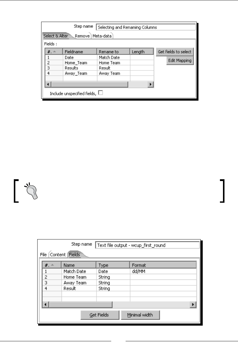
Geng Started with Transformaons
[ 48 ]
6. Modify the elds as follows:
7. Expand the Output branch of the steps tree.
8. Drag the Text le output icon to the canvas.
9. Create a hop from the Select values step to the Text le output step.
10. Double-click the Text le output step and give it a name.
11. In the le name type: C:/pdi_files/output/wcup_first_round.
Note that the path contains forward slashes. If your system is Windows,
you may use back or forward slashes. PDI will recognize both notaons.
12. In the Content tab, leave the default values.
13. Select the Fields tab and congure it as follows:
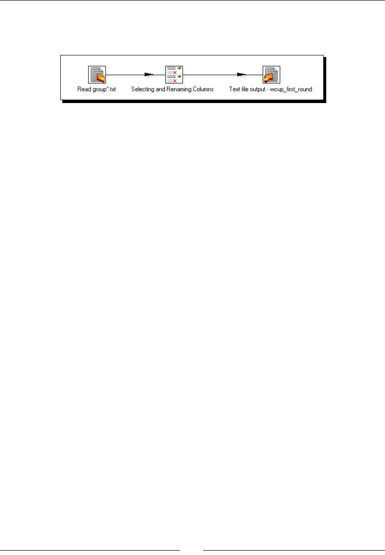
Chapter 2
[ 49 ]
14. Click OK.
15. Give a name and descripon to the transformaon.
16. Save the transformaon.
17. Click Run and then Launch.
18. Once the transformaon is nished, check the le generated. It should have been
created as C:/pdi_files/output/wcup_first_round.txt and should look
like this:
Match Date;Home Team;Away Team;Result
02/06;Italy;France;2-1
02/06;Argentina;Hungary;2-1
06/06;Italy;Hungary;3-1
06/06;Argentina;France;2-1
10/06;France;Hungary;3-1
10/06;Italy;Argentina;1-0
01/06;Germany FR;Poland;0-0
02/06;Tunisia;Mexico;3-1
06/06;Germany FR;Mexico;6-0
…
What just happened?
You gathered informaon from several les and sent all the data to a single le. Before
sending the data out, you used a Select Value step to select the data you wanted for the le
and to rename the elds so that the header of the desnaon le looks clearer.
Output les
We saw that PDI could take data from several types of les. The same applies to output data.
The data you have in a transformaon can be sent to dierent types of les. All you have to
do is redirect the ow of data towards an Output step.

Geng Started with Transformaons
[ 50 ]
Output steps
There are several steps that allow you to send the data to a le. All those steps are under the
Output step category: Text le output and Excel Output are examples of them.
For an Output step, just like you do for an Input step, you also have to dene:
Name of the step: It is mandatory and must be dierent for every step in
the transformaon.
Name and locaon of the le: These must be specied. If you specify an exisng
le, the le will be replaced by a new one (unless you check the Append checkbox
present in some of the output steps).
Content type: This data includes delimiter character, type of encoding, whether to
put a header, and so on. The list depends on the kind of le chosen. If you check
Header, the header will be built with the names of the elds.
If you don't like the names of the elds as header names in your le,
you may use a Select values step just to rename those elds.
Fields: Here you specify the list of elds that has to be sent to the le, and provide
some format instrucons. Just like in the input steps, you may use the Get Fields
buon to ll the grid. In this case, the grid is going to be lled based on the data
that arrives from the previous step. You are not forced to send every piece of data
coming to the output step, nor to send the elds in the same order.
Some data denitions
From the Kele's point of view, data can be anything ready to be processed by soware (for
example les or data in databases). Whichever the subject or origin of the data, whichever
its format, Kele transformaons can get the data for further processing and delivering.
Rowset
Transformaons deals with datasets, that is, data presented in a tabular form, where:
Each column represents a eld. A eld has a name and a data type. The data type
can be any of the common data types—number (oat), string, date, Boolean, integer,
or big number.
Each row corresponds to a given member of the dataset. All rows in a dataset have
the same structure, that is, all rows have the same elds, in the same order. A eld
in a row may be null, but it has to be present.
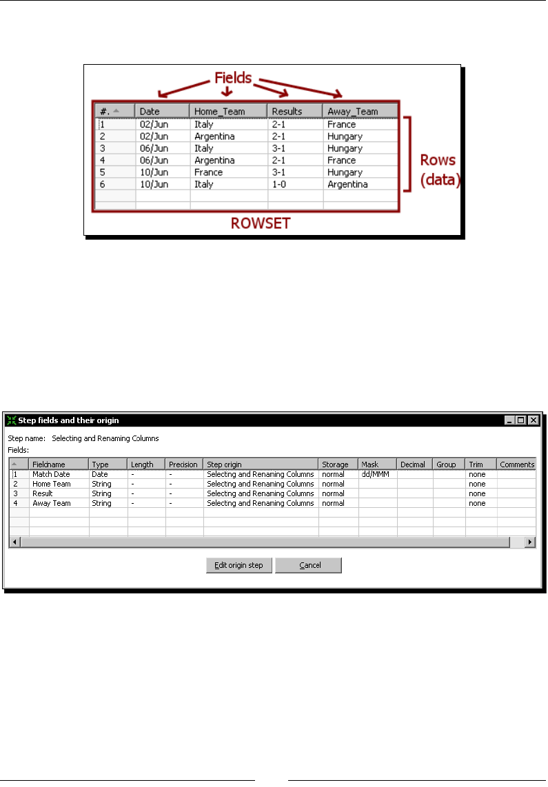
Chapter 2
[ 51 ]
The dataset is called rowset. The following is an example of rowset. It is the rowset
generated in the World Cup tutorial:
Streams
Once the data is read, it travels from step to step, through the hops that link those steps.
Nothing happens in the hops except data owing. The real manipulaon of data, as well as
the modicaon of a stream by adding or removing columns, occurs in the steps.
Right-click on the Select values step of the transformaon you created. In the contextual
menu select Show output elds. You'll see this:
This window shows the metadata of the data that leaves this step, this is, name, type, and
other properes of each eld leaving this step towards the following step.
In the same way, if you select Show input elds, you will see the metadata of the data that
le the previous step.
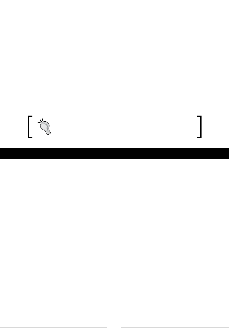
Geng Started with Transformaons
[ 52 ]
The Select values step
The Select values step allows you to select, rename, and delete elds, or change the
metadata of a eld. The step has three tabs:
Select & Alter: This tab is also used to rename the elds or reorder them. This is
how we used it in the last exercise.
Remove: This tab is useful to discard undesirable elds. We used it in the matches
exercise to drop the rst and last elds. Alternavely, we could use the Select &
Alter tab, and specify the elds that you want to keep. Both are equivalent for
that purpose.
Meta-data: This tab is used when you want to change the denion of a eld such
as telling Kele to interpret a string eld as a date. We will see examples of this later
in this book.
You may use only one of the Select Values step tabs at a
me. Kele will not restrain you from lling more than one
tab, but that could lead to unexpected behavior.
Have a go hero – extending your transformations by writing output les
Suppose you read your own les in the previous secon, modify your transformaons by
wring some or all the data back into les, however, changing the format, headers, number
or order of elds, and so on this me around. The objecve is to get some experience to see
what happens. Aer some tests, you will feel condent with input and output les, and be
ready to move forward.
Getting system information
Unl now, you have learned how to read data from known les, and send data back to les.
What if you don't know beforehand the name of the le to process? There are several ways
to handle this with Kele. Let's learn the simplest.

Chapter 2
[ 53 ]
Time for action – updating a le with news about examinations
Imagine you are responsible to collect the results of an annual examinaon that is being
taken in a language school. The examinaon evaluates wring, reading, speaking, and
listening skills. Every professor gives the exam to the students, the students take the
examinaon, the professors grade the examinaons in the scale 0-100 for each skill, and
write the results in a text le, like the following:
student_code;name;writing;reading;speaking;listening
80711-85;William Miller;81;83;80;90
20362-34;Jennifer Martin;87;76;70;80
75283-17;Margaret Wilson;99;94;90;80
83714-28;Helen Thomas;89;97;80;80
61666-55;Maria Thomas;88;77;70;80
All the les follow that paern.
When a professor has the le ready, he/she sends it to you, and you have to integrate the
results in a global list. Let's do it with Kele.
1. Before starng, be sure to have a le ready to read. Type it or download the sample les
from the Packt's ocial website.
2. Create the le where the news will be appended. Type this:
---------------------------------------------------------
Annual Language Examinations
Testing writing, reading, speaking and listening skills
---------------------------------------------------------
student_code;name;writing;reading;speaking;listening;file_
processed;process_date
Save the le as C:/pdi_files/output/examination.txt.
3. Create a new transformaon.
4. Expand the Input branch of the steps tree.
5. Drag the Get System Info and Text le input icons to the canvas.
6. Expand the Output branch of the steps tree, and drag a Text le output step to
the canvas.
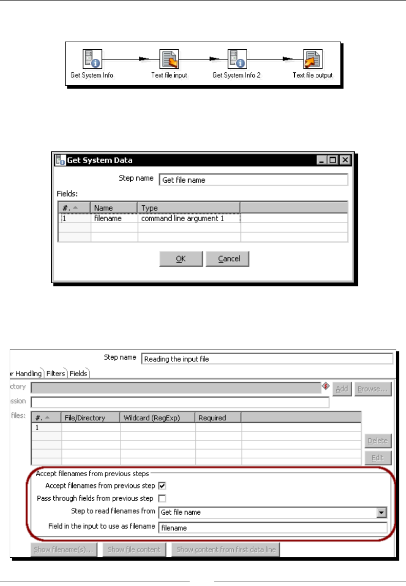
Geng Started with Transformaons
[ 54 ]
7. Link the steps as follows:
8. Double-click the rst Get System Info step icon and give it a name.
9. Fill the grid as follows:
10. Click OK.
11. Double-click the Text le Input step icon and congure it like here:
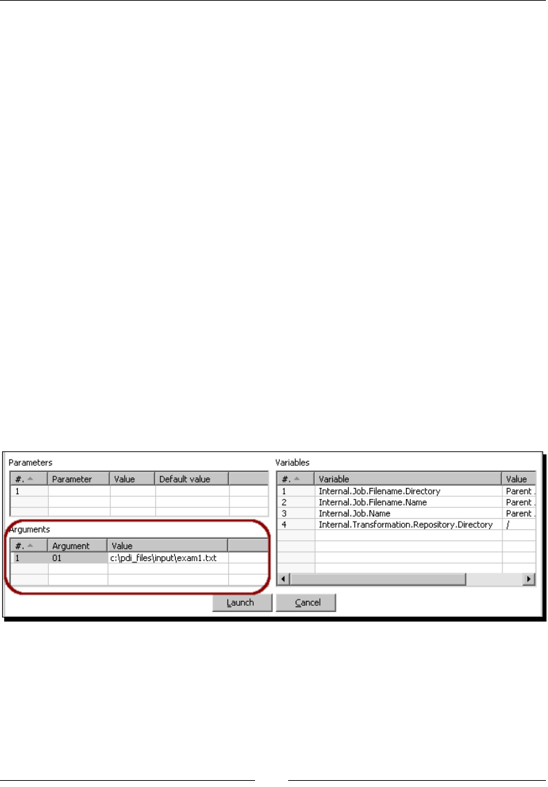
Chapter 2
[ 55 ]
12. Select the Content tab.
13. Check the Include lename in output? checkbox and type file_processed in the
Filename eldname textbox.
14. Check the Add lenames to result checkbox.
15. Select the Fields tab and Click the Get Fields buon to ll the grid.
16. Click OK.
17. Double-click the second Get System Info step icon and give it a name.
18. Add a eld named process_date, and from the list of choices select system
date (xed).
19. Double-click the Text le output step icon and give it a name.
20. Type C:/pdi_files/output/examination as the lename.
21. In the Fields tab, press the Get Fields buon to ll the grid.
22. Change the format of the Date row to yy/MM/dd.
23. Give a name and descripon to the transformaon and save it.
24. Press F9 to run the transformaon.
25. Fill in the argument grid, wring the full path of the le created.
26. Click Launch.

Geng Started with Transformaons
[ 56 ]
27. The output le should look like this:
---------------------------------------------------------
Annual Language Examinations
Testing writing, reading, speaking and listening skills
---------------------------------------------------------
student_code;name;writing;reading;speaking;listening;file_
processed;process_date
80711-85;William Miller;81;83;80;90;C:\exams\exam1.txt;28-05-2009
20362-34;Jennifer Martin;87;76;70;80;C:\exams\exam1.txt;28-05-2009
75283-17;Margaret Wilson;99;94;90;80;C:\exams\exam1.txt;28-05-2009
83714-28;Helen Thomas;89;97;80;80;C:\exams\exam1.txt;28-05-2009
61666-55;Maria Thomas;88;77;70;80;C:\exams\exam1.txt;28-05-2009
28. Run the transformaon again.
29. This me ll the argument grid with the name of a second le.
30. Click Launch.
31. Verify that the data from this second le was appended to the previous data in the
output le.
What just happened?
You read a le whose name is known at runme, and fed a desnaon le by appending the
contents of the input le.
The rst Get System Info step tells Kele to take the rst command line argument, and
assume that it is the name of the le to read.
In the Text File Input step, you didn't specify the name of the le, but told Kele to take as
the name of the le, the eld coming from the previous step, which is the read argument.
With the second Get System Info step you just took from the system, the date, which you
used later to enrich the data sent to the desnaon le.
The desnaon le is appended with new data every me you run the transformaon.
Beyond the basic required data (student code and grades), the name of the processed le
and the date on which the data is being appended are added as part of the data.
When you don't specify the name and locaon of a le (like in this example), or
when the real le is not available at design me, you won't be able to use the
Get Fields buon, nor preview to see if the step is well congured. The trick is
to congure the step by using a real le idencal to the expected one. Aer the
step is congured, change the name and locaon of the le as needed.

Chapter 2
[ 57 ]
Getting information by using Get System Info step
The Get System Info step allows you to get dierent informaon from the system. In this
exercise, you took the system date and an argument. If you look to the available list, you
will see more than just these two opons.
Here we used the step in two dierent ways:
As a resource to take the name of the le from the command line
To add a eld to the dataset
The use of this step will be clearer with a picture.
In this example, the Text File Input doesn't know the name or the locaon of the le. It takes
it from the previous step, which is a Get System Info Step. As the Get System Info serves as
a supplier of informaon, the hop that leaves the step changes its look and feel to show
the situaon.

Geng Started with Transformaons
[ 58 ]
The second me the Get System Info is used, its funcon is simply to add a eld to the
incoming dataset.
Data types
Every eld must have a data type. The data type can be any of the common data
types—number (oat), string, date, Boolean, integer, or big number. Strings are simple,
just text for which you may specify a length. Date and numeric elds have more variants,
and are worthy of while a separate explanaon.
Date elds
Date is one the main data types available in Kele. In the matches tutorial, you have an
example of date eld—the match date eld. Its values were 2/Jun, 6/Jun, 10/Jun. Take a
look at how you dened that eld in the Text le input step. You dened the eld as a date
eld with format dd/MMM. What does it mean? To Kele it means that it has to interpret the
eld as a date, where the rst two posions represent the day, then there is a slash, and
nally there is the month in leers (that's the meaning of the three last posions).
Generally speaking, when a date eld is created, like the text input eld of the example, you
have to dene the format of the data so that Kele can recognize in the eld the dierent
components of the date. There are several formats that may be dened for a date, all of
them combinaons of leers that represents date or me components. Here are the most
basic ones:
Leers Meaning
yYear
M Month
d Day
H Hour (0-23)
m Minutes
s Seconds
Now let's see the other end of the same transformaon—the output step. Here you set
another format for the same eld: dd/MM. According the table, this means the date has to
have two posions for the day, then a slash, and then two posions for the month. Here, the
format specicaon represents the mask you want to apply when the date is shown. Instead
of 2/Jun, 6/Jun, 10/Jun, in the output le, you expect to see 02/06, 06/06, 10/06.
In the examinaon tutorial, you also have a Date eld—the process date. When you created
it, you didn't specify a format because you took the system date which, by denion, is a
date and Kele knows it. But when wring this date to the output le, again you dened a
format, in this case it was yyyy/MM/dd.

Chapter 2
[ 59 ]
In general, when you are wring a date, the format aribute is used of format the data
before sending it to the desnaon. In case you don't specify a format, Kele sets a
default format.
As said earlier, there are more combinaons to dene the format to a date eld.
For a complete reference, check the Sun Java API documentaon located at
http://java.sun.com/javase/6/docs/api/java/text/SimpleDateFormat.html.
Numeric elds
Numeric elds are present in almost all Kele transformaons. In the Examinaon example,
you encountered numeric elds for the rst me. The input le had four numeric elds.
As the numbers were all integer, you didn't set a specic format. When you have more
elaborate elds such as numbers with separators, dollar signs, and so on, you should specify
a format to tell Kele how to interpret the number. If you don't, Kele will do its best to
interpret the number, but this could lead to unexpected results.
At the other extreme of the ow, when wring to the output le text, you may specify the
format in which you want the number to be shown.
There are several formats you may apply to a numeric eld. The format is basically a
combinaon of predened symbols, each with a special meaning. The following are
the most used symbols:
Symbol Meaning
#Digit Leading zeros are not shown
0 Digit If the digit is not present, zero is displayed in its place
. Decimal separator
- Minus sign
%Field has to be mulplied by 100 and shown as a percentage
These symbols are not used alone. In order to specify the format of your numbers, you
have to combine them. Suppose that you have a numeric eld whose value is 99.55; the
following table shows you the same value aer applying dierent formats to it:
Format Result
# 100
0 100
#.# 99.6
#.## 99.55
#.000 99.550
000.000 099.550

Geng Started with Transformaons
[ 60 ]
If you don't specify a format for your numbers, you may sll provide a Length and
Precision. Length is the total number of signicant gures, while precision is the number
of oang-point digits.
If you neither specify format nor length or precision, Kele behaves as follow. While reading,
it does its best to interpret the incoming number, and when wring, it sends the data as it
comes without applying any format.
For a complete reference on number formats, you can check the Sun Java API
documentaon available at http://java.sun.com/javase/6/docs/api/java/text/
DecimalFormat.html.
Running transformations from a terminal window
In the examinaon exercise, you specied that the name of the input le will be taken
from the rst command-line argument. That means when execung the transformaon,
the lename has to be supplied as an argument. Unl now, you only ran transformaons
from inside Spoon. In the last exercise, you provided the argument by typing it in a dialog
window. Now it is me to learn how to run transformaons with or without arguments from
a terminal window.
Time for action – running the examination transformation from
a terminal window
Before execung the transformaon from a terminal window, make sure that you have a new
examinaon le to process, let's say exam3.txt. Then follow these instrucons:
1. Open a terminal window and go to the directory where Kele is installed.
On Windows systems type:
C:\pdi-ce>pan.bat /file:c:\pdi_labs\examinations.ktr c:\
pdi_files\input\exam3.txt
On Unix, Linux, and other Unix-based systems type:
/home/yourself/pdi-ce/pan.sh /file:/home/yourself/pdi_labs/
examinations.ktr c:/pdi_files/input/exam3.txt
If your transformaon is in another folder, modify the command
accordingly.
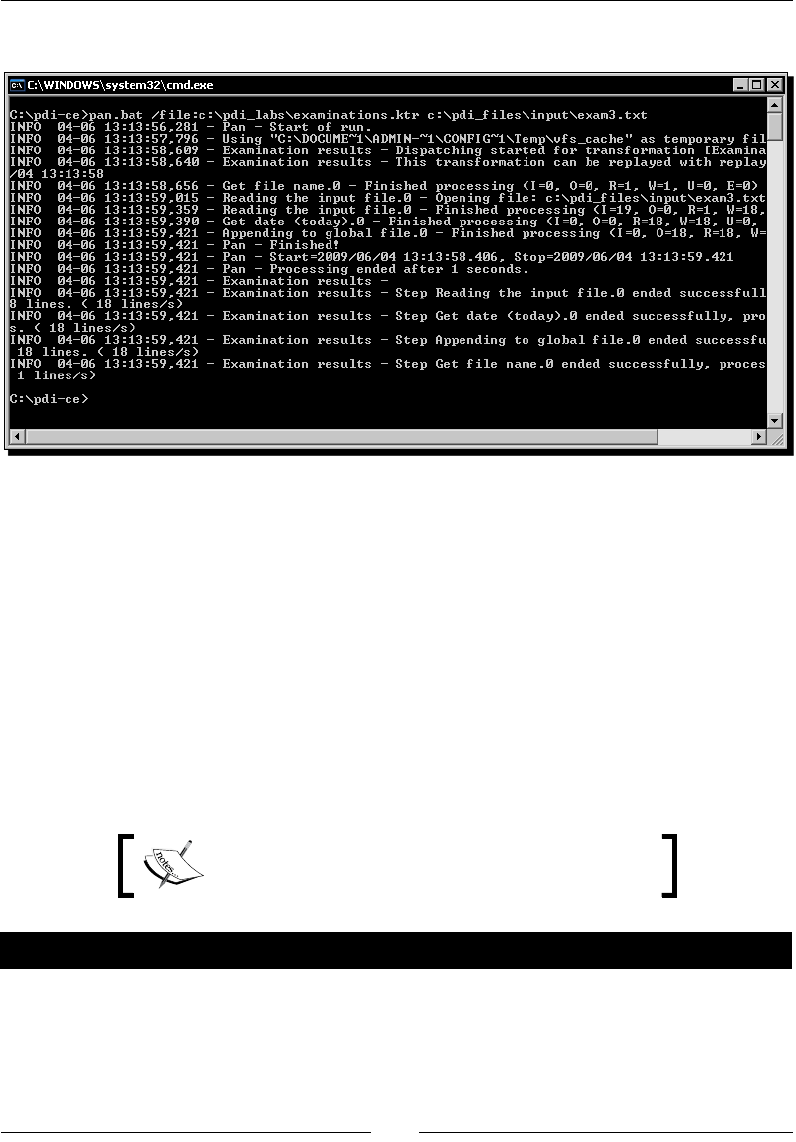
Chapter 2
[ 61 ]
2. You will see how the transformaon runs, showing you the log in the terminal.
3. Check the output le. The contents of exam3.txt should be at the end of the le.
What just happened?
You executed a transformaon with Pan, the program that runs transformaons from
terminal windows. As part of the command, you specied the name of the transformaon
le and provided the name of the le to process, which was the only argument expected by
the transformaon. As a result, you got the same as if you had run the transformaon from
Spoon—a small le appended to the global le.
When you are designing transformaons, you run them with Spoon; you don't use Pan. Pan
is mainly used as part of batch processes, for example processes that run every night in a
scheduled fashion.
Appendix B tells you all the details about using Pan.
Have a go hero – using different date formats
Change the main transformaon of the last tutorial so that the process_date is saved with
a full format, that is, including day of week (Monday, Tuesday, and so on), month in leers
(January, February, and so on), and me.

Geng Started with Transformaons
[ 62 ]
Go for a hero – formatting 99.55
Create a transformaon to see for yourself the dierent formats for the number 99.55. Test
the formats shown in the Numeric elds secon and try some other opons as well.
To test this, you will need a dataset with a single row and a single eld—the
number. You can generate it with a Generate rows step.
Pop quiz–formatting data
Suppose that you read a le where the rst column is a numeric idener: 1, 2, 3, and so on.
You read the eld as a Number. Now you want to send the data back to a le. Despite being
a number, this eld is regular text to you because it is a code. How do you dene the eld in
the Text output step (you may choose more than one opon):
a. As a Number. In the format, you put #.
b. As a String. In the format, you put #.
c. As a String. You leave the format blank.
XML les
Even if you're not a system developer, you must have heard about XML les. XML les
or documents are not only used to store data, but also to exchange data between
heterogeneous systems over the Internet. PDI has many features that enable you to
manipulate XML les. In this secon you will learn to get data from those les.
Time for action – getting data from an XML le with information
about countries
In this tutorial you will build an Excel le with basic informaon about countries. The source
will be an XML le that you can download from the Packt website.
1. If you work under Windows, open the kettle.properties le located in the
C:/Documents and Settings/yourself/.kettle folder and add the
following line:
LABSOUTPUT=c:/pdi_files/output
Chapter 2
[ 63 ]
On the other hand, if you work under Linux (or similar), open the kettle.
properties le located in the /home/yourself/.kettle folder and add the
following line:
LABSOUTPUT=/home/yourself/pdi_files/output
2. Make sure that the directory specied in kettle.properties exists.
3. Save the le.
4. Restart Spoon.
5. Create a new transformaon.
6. Give a name to the transformaon and save it in the same directory you have all the
other transformaons.
7. From the Packt website, download the resources folder containing a file named
countries.xml. Save the folder in your working directory. For example, if your
transformaons are in pdi_labs, the le will be in pdi_labs/resources/.
The last two steps are important. Don't skip them! If you do,
some of the following steps will fail.
8. Take a look at the le. You can edit it with any text editor, or you can double-click it to
see it within an explorer. In any case, you will see informaon about countries. This is
just the extract for a single country:
<?xml version="1.0" encoding="UTF-8"?>
<world>
...
<country>
<name>Argentina</name>
<capital>Buenos Aires</capital>
<language isofficial="T">
<name>Spanish</name>
<percentage>96.8</percentage>
</language>
<language isofficial="F">
<name>Italian</name>
<percentage>1.7</percentage>
</language>
<language isofficial="F">
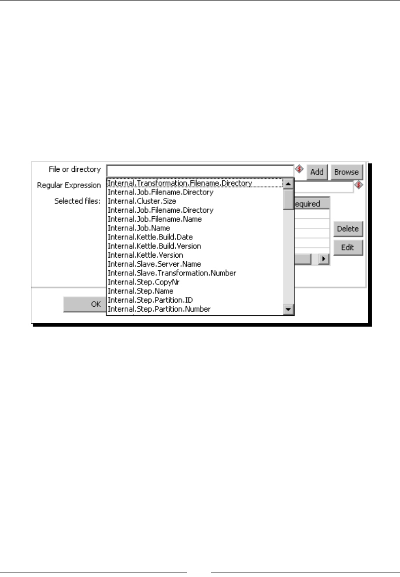
Geng Started with Transformaons
[ 64 ]
<name>Indian Languages</name>
<percentage>0.3</percentage>
</language>
</country>
...
</world>
9. From the Input steps, drag a Get data from XML step to the canvas.
10. Open the conguraon window for this step by double-clicking it.
11. In the File or directory textbox, press Ctrl+Space. A drop-down list appears as shown in
the next screenshot:
12. Select Internal.Transformation.Filename.Directory. The textbox gets lled
with this text.
13. Complete the text so that you can read ${Internal.Transformation.Filename.
Directory}/resources/countries.xml.
14. Click on the Add buon. The full path is moved to the grid.
15. Select the Content tab and click Get XPath nodes.
16. In the list that appears, select /world/country/language.
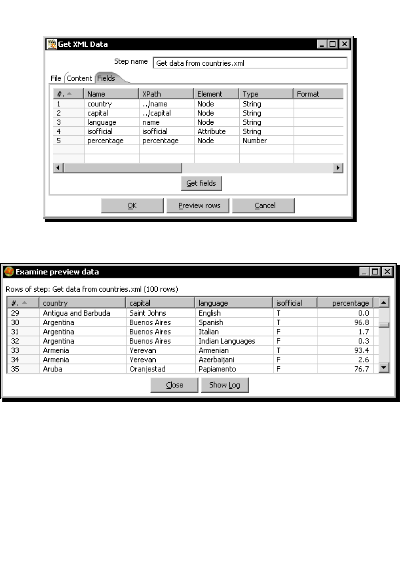
Chapter 2
[ 65 ]
17. Select the Fields tab and ll the grid as follows:
18. Click Preview rows, and you should see something like this:
19. Click OK.
20. From the Output steps, drag an Excel Output step to the canvas.
21. Create a hop from the Get data from XML step to the Excel Output step.
22. Open the conguraon window for this step by double-clicking it.
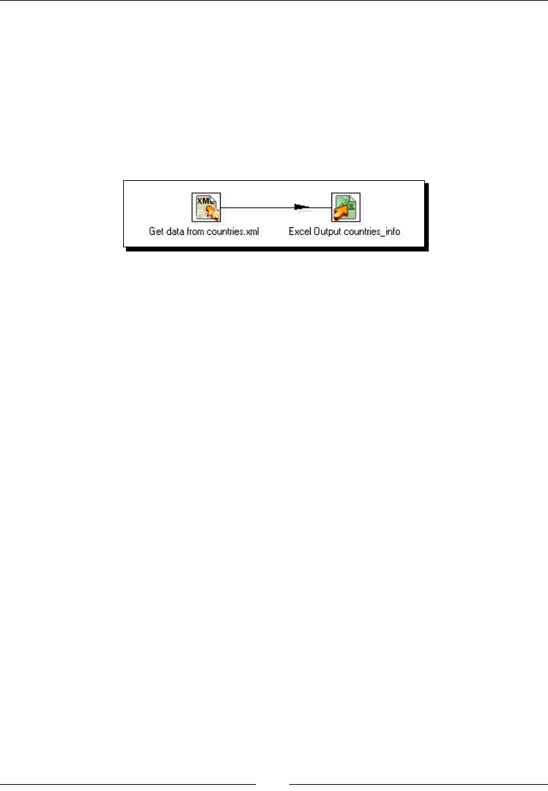
Geng Started with Transformaons
[ 66 ]
23. In the Filename textbox press Ctrl+Space.
24. From the drop-down list, select ${LABSOUTPUT}.
25. By the side of that text type /countries_info. The complete text should be
${LABSOUTPUT}/countries_info.
26. Select the Fields tab and click the Get Fields buon to ll the grid.
27. Click OK. This is your nal transformaon.
28. Save the transformaon.
29. Run the transformaon.
30. Check that the countries_info.xls le has been created in the output directory
and contains the informaon you previewed in the input step.
What just happened?
You got informaon about countries from an XML le and saved it in a more readable
format—an Excel spreadsheet—for the common people.
To get the informaon, you used a Get data from XML step. As the source le was
taken from a folder relave to the folder where you stored the transformaon, you set
the directory to ${Internal.Transformation.Filename.Directory}. When
the transformaon ran, Kele replaced ${Internal.Transformation.Filename.
Directory} with the real path of the transformaon: c:/pdi_labs/.
In the same way, you didn't put a xed value for the path of the nal Excel le. As directory,
you used ${LABSOUTPUT}. When the transformaon ran, Kele replaced ${LABSOUTPUT}
with the value you wrote in the kettle.properties le. The output le was then saved in
that folder: c:/pdi_files/output.

Chapter 2
[ 67 ]
What is XML
XML stands for EXtensible Markup Language. It is basically a language designed to describe
data. XML les or documents contain informaon wrapped in tags. Look at this piece of XML
taken from the countries le:
<?xml version="1.0" encoding="UTF-8"?>
<world>
...
<country>
<name>Argentina</name>
<capital>Buenos Aires</capital>
<language isofficial="T">
<name>Spanish</name>
<percentage>96.8</percentage>
</language>
<language isofficial="F">
<name>Italian</name>
<percentage>1.7</percentage>
</language>
<language isofficial="F">
<name>Indian Languages</name>
<percentage>0.3</percentage>
</language>
</country>
...
</world>
The rst line in the document is the XML declaraon. It denes the XML version of the
document, and should always be present.
Below the declaraon is the body of the document. The body is a set of nested elements.
An element is a logical piece enclosed by a start-tag and a matching end-tag—for example,
<country> </country>.
Within the start-tag of an element, you may have aributes. An aribute is a markup
construct consisng of a name/value pair—for example, isofficial="F".
These are the most basic terminology related to XML les. If you want to know more about
XML, you can visit http://www.w3schools.com/xml/.

Geng Started with Transformaons
[ 68 ]
PDI transformation les
Despite the .ktr extension, PDI transformaons are just XML les. As such, you are able to
explore them inside and recognize dierent XML elements. Look the following sample text:
<?xml version="1.0" encoding="UTF-8"?>
<transformation>
<info>
<name>hello_world</name>
<description>My first transformation</description>
<extended_description>
This transformation generates 10 rows
with the message Hello World.
</extended_description>
...
</transformation>
This is an extract from the hello_world.ktr le. Here you can see the root element
named transformation, and some inner elements such as info and name.
Note that if you copy a step by selecng it in the Spoon canvas and pressing Ctrl+C , and then
pass it to a text editor, you can see its XML denion. If you copy it back to the canvas, a new
idencal step will be added to your transformaon.
Getting data from XML les
In order to get data from an XML le, you have to use the Get Data From XML input step.
To tell PDI which informaon to get from the le, it is required that you use a parcular
notaon named XPath.
XPath
XPath is a set of rules used for geng informaon from an XML document. In XPath, XML
documents are treated as trees of nodes. There are several types of nodes; elements,
aributes, and texts are some of them. As an example, world, country, and isofficial
are some of the nodes in the sample le.
Among the nodes there are relaonships. A node has a parent, zero or more children,
siblings, ancestors, and descendants depending on where the other nodes are in
the hierarchy.
In the sample countries le, country is the the parent of the elements name, capital, and
language. These three elements are children of country.
To select a node in an XML document, you have to use a path expression relave to a
current node.
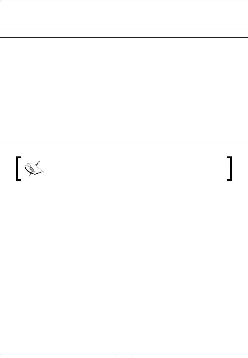
Chapter 2
[ 69 ]
The following table has some examples of path expressions that you may use to specify
elds. The examples assume that the current node is language.
Path expression Descripon Sample expression
node_name Selects all child nodes of the
node named node_name.
percentage
This expression selects all child nodes of
the node percentage. It looks for the node
percentage inside the current node language.
.Selects the current node language
.. Selects the parent of the
current node
../capital
This expression selects all child nodes of the
node capital. It doesn't look in the current
node (language), but inside its parent, which
is country.
@Selects an aribute @isofficial
This expression gets the aribute isofficial
in the current node language.
Note that the expressions name and ../name are not the same. The
rst selects the name of the language, while the second selects the
name of the country.
For more informaon on XPath, follow this link: http://www.w3schools.com/XPath/.
Conguring the Get data from XML step
In order to specify the name and locaon of an XML le, you have to ll the File tab just as
you do in any le input step. What is dierent here is how you get the data.
The rst thing you have to do is select the path that will idenfy the current node. You do
it by lling the Loop XPath textbox in the Content tab. You can type it by hand, or you can
select it from the list of available paths by Clicking the Get XPath nodes buon.
Once you have selected a path, PDI will generate one row of data for every found path.
In the tutorial you selected /world/country/language. Then PDI generates one row for
each /world/country/language element in the le.
Aer selecng the loop XPath, you have to specify the elds to get. In order to do that,
you have to ll the grid in the Fields tab by using XPath notaon as explained in the
preceding secon.

Geng Started with Transformaons
[ 70 ]
Note that if you click the Get elds buon, PDI will ll the grid with the child nodes of the
current node. If you want to get some other node, you have to type its XPath by hand.
Also note the notaon for the aributes. To get an aribute, you can use the @ notaon as
explained, or you can simply type the name of the aribute without @ and select Aribute
under the Element column, as you did in the tutorial.
Kettle variables
In the last tutorial, you used the string ${Internal.Transformation.Filename.
Directory} to idenfy the folder where the current transformaon was saved. You also
used the string ${LABSOUTPUT} to dene the desnaon folder of the output le.
Both strings, ${Internal.Transformation.Filename.Directory} and
${LABSOUTPUT}, are Kele variables, that is, keywords linked to a value. You use the
name of a variable, and when the transformaon runs, the name of the variable is
replaced by its value.
The rst of these two variables is an environment variable, and it is not the only available.
Other known environment variables are ${user.home}, ${java.io.tmpdir}, and
${java.home}. All these variables are ready to use any me you need.
The second variable is a variable you dened in the kettle.properties le. In this le
you may dene as many variables as you want. The only thing you have to keep in mind is
that those variables will be available inside Spoon aer you restart it.
These two kinds of variables—environment variables and variables dened in the
kettle.properties le—are the most primive kinds of variables found in PDI.
All of these variables are string variables and their scope is the Java virtual machine.
How and when you can use variables
Any me you see a red dollar sign by the side of a textbox, you may use a variable. Inside the
textbox you can mix variable names with stac text, as you did in the tutorial when you put
the name of the desnaon as ${LABSOUTPUT}/countries_info.
To see all the available variables, you have to posion the cursor in the textbox, press
Ctrl+Space, and a full list is displayed for you to select the variable of your choice. If you put
the mouse cursor over any of the variables for a second, the actual value of the variable will
be shown.
If you know the name of the variable, you don't need to select it from the list. You may type
its name, by using either of these notaons—${<name>} or %%<name>%%.
Chapter 2
[ 71 ]
Have a go hero – exploring XML les
Now you can explore by yourself. On the Packt website there are some sample XML les.
Download them and try this:
• Read the customer.xml le and create a list of customers.
• Read the tomcat-users.xml le and get the users and their passwords.
• Read the areachart.xml and get the color palee, that is, the list of colors used.
The customer le is included in the Pentaho Report Designer soware package.
The others come with the Pentaho BI package. This soware has many XML les
for you to use. If you are interested you can download the soware from
http://sourceforge.net/projects/pentaho/files/.
Have a go hero – enhancing the output countries le
Modify the transformaon in the tutorial so that the Excel output uses a template. The
template will be an Excel le with the header and format already applied, and will be located
in a folder inside the pdi_labs folder.
Templates are congured in the Content tab of the Excel conguraon window.
In order to set the name for the template, use internal variables.
Have a go hero – documenting your work
As explained, transformaons are nothing dierent than XML les. Now you'll create a new
transformaon that will take as input the transformaons you've created so far, and will
create a simple Excel spreadsheet with the name and descripon of all your transformaons.
If you keep this sheet updated by running the transformaon on a regular basis, it will be
easier to nd a parcular transformaon you created in the past.
To get data from the transformaons les, use the Get data from XML step.
As wildcard, use .*\.ktr. Doing so, you'll get all the les.
On the other hand, as Loop XPath, use /transformation/info.

Geng Started with Transformaons
[ 72 ]
Summary
In this chapter you learned how to get data from les and put data back into les.
Specically, you learned how to:
Get data from plain les and also from XML les
Put data into text les and Excel les
Get informaon from the operang system such as command-line arguments and
system date
We also discussed the following:
The main PDI terminology related to data, for example datasets, data types,
and streams
The Select values step, a commonly used step for selecng, reordering, removing
and changing data
How and when to use Kele variables
How to run transformaons from a terminal with the Pan command
Now that you know how to get data into a transformaon, you are ready to start
manipulang data. This is going to happen in the next chapter.
3
Basic Data Manipulation
In the previous chapter, you learned how to get data into PDI. Now you're ready to
begin transforming that data. This chapter explains the simplest and most used ways
of transforming data. We will cover the following:
Execung basic operaons
Filtering and sorng of data
Looking up data outside the main stream of data
By the end of this chapter, you will be able to do simple but meaningful transformaons on
dierent types of data.
Basic calculations
You already know how to create a transformaon and read data from an external source.
Now, taking that data as a starng point, you will begin to do basic calculaons.

Basic Data Manipulaon
[ 74 ]
Time for action – reviewing examinations by using the
Calculator step
Can you recollect the exercise about examinaons you did in the previous chapter? You
created an incremental le with examinaon results. The nal le looked like the following:
---------------------------------------------------------
Annual Language Examinations
Testing writing, reading, speaking and listening skills
---------------------------------------------------------
student_code;name;writing;reading;speaking;listening;file_
processed;process_date
80711-85;William Miller; 81;83;80;90;C:\pdi_files\input\first_turn.
txt;28-05-2009
20362-34;Jennifer Martin; 87;76;70;80;C:\pdi_files\input\first_turn.
txt;28-05-2009
75283-17;Margaret Wilson; 99;94;90;80;C:\pdi_files\input\first_turn.
txt;28-05-2009
83714-28;Helen Thomas; 89;97;80;80;C:\pdi_files\input\first_turn.
txt;28-05-2009
61666-55;Maria Thomas; 88;77;70;80;C:\pdi_files\input\first_turn.
txt;28-05-2009
...
Now you want to convert all grades in the scale 0-100 to a new scale from 0 to 5. Also, you
want to take the average grade to see how the students did.
1. Create a new transformaon, give it a name and descripon, and save it.
2. By using a Text le input step, read the examination.txt le. Give the name and
locaon of the le, check the Content tab to see that everything matches your le, and
ll the Fields tab as here:

Chapter 3
[ 75 ]
3. Do a preview just to conrm that the step is well congured.
Noce that you have several lines as header. Because the
names of the elds are not in the rst row, you won't be able
to use the Get Fields buon successfully. You will have to write
the elds manually, or you can avoid it by doing the following:
Congure the step with a copy of the le that doesn't have the
extra heading, just the heading row with the names of the elds.
Then, restore the name of your le in the File tab, adjust the
number of headings in the Content tab, and your step is ready.
4. Use the Select values step to remove the elds you will not use—file_processed
and process_date.
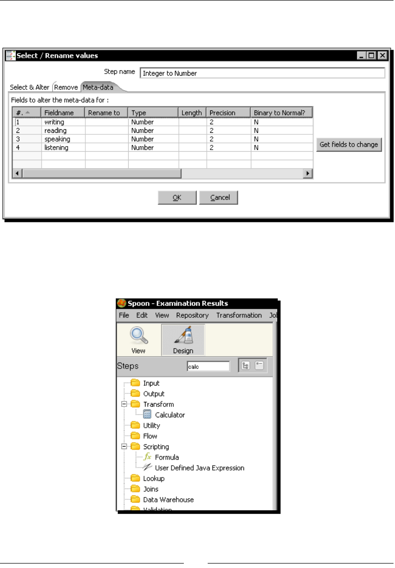
Basic Data Manipulaon
[ 76 ]
5. Drag another Select values step to the canvas. Select the Meta-data tab and change the
meta-data of the numeric elds like here:
6. Near the upper-le corner of the screen, above the step tree, there is a textbox for
searching. Type calc in the textbox. While you type, a lter is applied to show you only
the steps that contain, in their name or descripon, the text you typed. You should be
seeing this:
7. Among the steps you see, select the Calculator step and drag it to the canvas.

Chapter 3
[ 77 ]
8. To remove the lter, clear the typed text.
9. Create a hop from the Text le input step to the Calculator step.
10. Edit the Calculator step and ll the grid as follows:
11. To ll the Calculaon column, simply select the operaon from the list provided. Be sure
to ll every column in the grid like shown in the screenshot.
You don't have to feel like you are doing data entry instead
of learning PDI. You can avoid typing by copying and pasng
similar rows, and then xing the values properly. Appendix D
has a list of shortcuts you can use when eding grids like these.
12. Leave the Calculator step selected and click the Preview this transformaon buon
followed by the Quick Launch buon. You should see something similar to the
following screenshot:
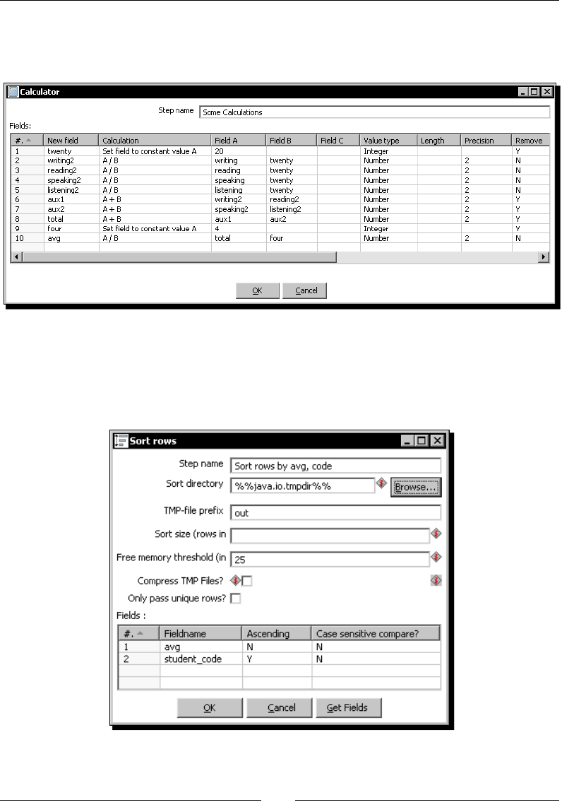
Basic Data Manipulaon
[ 78 ]
The numbers may vary according to the contents of your le.
13. Edit the calculator again and change the content of the Remove column like here:
14. From the Transform category of steps, add a Sort rows step and create a hop from the
Calculator step to this new step.
15. Edit the Sort rows step by double-clicking it, click the Get Fields buon, and adjust the
grid as follows:
16. Click OK.
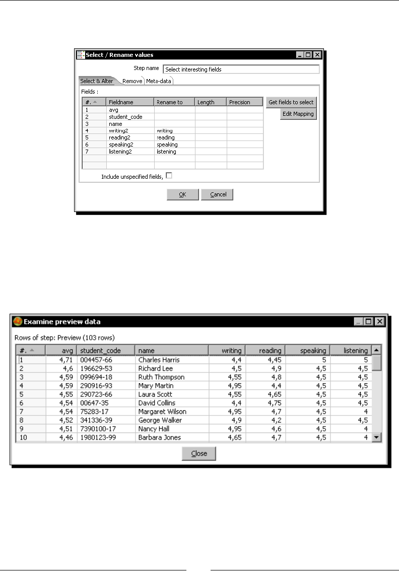
Chapter 3
[ 79 ]
17. Drag a third Select values step, create a hop from the Sort rows step to this new step,
and use it to keep only the elds by which you ordered the data:
18. From the Flow category of steps, add a Dummy step and create a hop from the last
Select values step to this.
19. Select the Dummy step and do a preview.
20. The nal preview looks like the following screenshot:

Basic Data Manipulaon
[ 80 ]
If you get an error or a dierent result, review the explanaon and make
sure that you followed the instrucons correctly. Do a preview on each
step to discover in which one you have the problem. If you realize that
the problem is in any of the steps that read the input les, please refer
to the Troubleshoong reading les secon in Chapter 2.
What just happened?
You read the examination.txt le, and did some calculaons to see how the students did.
You did the calculaons by using the Calculator step.
First of all, you removed the elds you didn't need from the stream of data.
Aer that, you did the following calculaons:
By dividing by 20, you converted all grades from the scale 0-100 to the scale 0-5.
Then, you calculated the average of the grades for the four skills—wring, reading, listening,
and speaking. You created two auxiliary elds, aux1 and aux2, to calculate paral sums. Aer
that, you created the eld total with the sum of aux1 and aux2, another auxiliary eld with
the number 4, and nally the avg as the division of the total by the eld four.
In order to obtain the new grades, as well as the average with two decimal posions, you
need the result of the operaon to be of a numeric type with precision 2. Therefore, you
had to change the metadata, by adding a Select values step before the Calculator. With the
Select values you changed the type of the numeric elds from integer to number, that is,
oat numbers. If you didn't, the quoents would have been rounded to integer numbers.
You can try and see for yourself!
The rst me you edited the calculator, you set the eld Remove to N for every row in the
calculator grid. By doing this, you could preview every eld created in the calculator, even
the auxiliary ones such as the elds twenty, aux1, and aux2. You then changed the eld to
Y so that the auxiliary elds didn't pass to the next step.
Aer doing the calculaons, you sorted the data by using a Sort rows step. You specied the
order by avg descending, then by student_code ascending.

Chapter 3
[ 81 ]
Sorng data
For small datasets, the sorng algorithm runs mainly using the JVM memory.
When the number of rows exceeds 5,000, it works dierently. Every ve
thousand rows, the process sorts them and writes them to a temporary le.
When there are no more rows, it does a merge sort on all those les and gives
you back the sorted dataset. You can conclude that for huge datasets a lot
of reading and wring operaons are done on your disk, which slows down
the whole transformaon. Fortunately, you can change the number of rows
in memory (5,000 by default) by seng a new value in the Sort size (rows in
memory) textbox. The bigger this number, the faster the sorng process.
Note that a sort size that works in your system may not work in a machine with
a dierent conguraon. To avoid that risk, you can use a dierent approach.
In the Sort rows conguraon window, you can set a Free memory threshold
(in %) value. The process begins to use temporary les when the percentage
of available memory drops below the indicated threshold. The lower the
percentage, the faster the process.
As it's not possible to know the exact amount of free memory, it's not
recommended to set a very small free memory threshold. You denitely
shouldn't use that opon in complex transformaons or when there is more
than one sort going on, as you could sll run out of memory.
The two nal steps were added to keep only the elds of interest, and to preview the result
of the transformaon. You can change the Dummy step for any of the output steps you
already know.
You've used the Dummy step several mes but sll nothing has been said
about it. Mainly it was because it does nothing! However, you can use it as a
placeholder for tesng purposes as in the last exercise.
Note that in this tutorial you used the Select values step in three dierent ways:
To remove elds by using the Remove tab.
To change the meta-data of some elds by using the Meta-data tab.
To select and rename elds by using the Select tab.
Remember that the Select values step's tabs are exclusive! You can't use more
than one in the same step!

Basic Data Manipulaon
[ 82 ]
Besides calculaon, in this tutorial you did something you hadn't before—searching the
step tree.
When you don't remember where a step is in the steps tree, or when you just
want to nd if there is a step that does some kind of operaon, you could simply
type the search criterion in the textbox above the steps tree. PDI does a search
and lters all the steps that have that text as part of their name or descripon.
Adding or modifying elds by using different PDI steps
In this tutorial you used the Calculator step to create new elds and add them to
your dataset. The Calculator is one the many steps that PDI has to create new elds by
combining existent ones. Usually you will nd these steps under the Transform category
of the steps tree. The following table describes some of them (the examples refer to the
examinaon le):
Step Descripon Example
Split Fields Split a single eld into two
or more. You have to give
the character that acts as
separator.
Split the name into two elds: Name and
Last Name. The separator would be a space
character.
Add constants Add one or more constants
to the input rows
Add two constants: four and twenty. Then
you could use them in the Calculator step
without dening the auxiliary elds.
Replace in string Replace all occurrences of
a text in a string eld with
another text
Replace the – in the student code by a /.
For example: 108418-95 would become
108418/95.
Number range Create a new eld based on
ranges of values. Applies to
a numeric eld.
Create a new eld called exam_range with
two ranges: Range A with the students with
average grade below 3.5, and Range B with
students with average grade greater or equal
to 3.5.
Value Mapper Creates a correspondence
between the values of
a eld and a new set of
values.
Suppose you calculated the average grade as
an integer number ranging from 0 to 5. You can
map the average to A, B, C, D, like this:
Old value: 5; New value: A
Old value: 3, 4; New value: B
Old value: 1, 2; New value: C
Old value: 0; New value: D

Chapter 3
[ 83 ]
Step Descripon Example
User Dened Java
Expression
Creates a new eld by
using a Java expression that
involves one or more elds.
This step may eventually
replace any of the above
but it's only recommended
for those familiar with Java.
Create a ag (a Boolean eld) that tells if a
student passed. A student passes if his/her
average grade is above 4.5.
The expression to use could be:
(((writing+reading+speaking+
listening)/4)>4.5)?true:false
Any of these steps when added to your transformaon, are executed for every row in the
stream. It takes the row, idenes the elds needed to do its tasks, calculates the new
eld(s), and adds it to the dataset.
For details on a parcular step, don't hesitate to visit the Wiki page for steps:
http://wiki.pentaho.com/display/EAI/Pentaho+Data+Integration+v3.2.+St
eps
The Calculator step
The Calculator step you used in the tutorial, allows you to do simple calculaons not only
on numeric elds, but also on data and text. The Calculator step is not the only means to do
calculaons, but it is the simplest. It allows you to do simple calculaons in a quick fashion.
The step has a grid where you can add all the elds you want to. Every row represents
an operaon that involves from one up to three operands (depending on the selected
operaon). When you select an operaon, the descripon of the operaon itself tells you
which argument it needs. For example:
If you select Set constant eld to value A, you have to provide a constant value
under the column name A.
If you select A/B, the operaon needs two arguments, and you have to provide
them by indicang the elds to use in the columns named A and B respecvely.
The result of every operaon becomes a new eld in your dataset, unless you set the
Remove column to Y. The name of the new eld is the one you type under the New
eld column.
For each and every row of the data set, the operaons dened in the Calculator are
calculated in the order in which they appear. Therefore, you may create auxiliary elds and
then use them in rows of the Calculator grid that are below them. That is what you did in
the tutorial when you dened the auxiliary elds aux1 and aux2 and then used them in the
eld total.
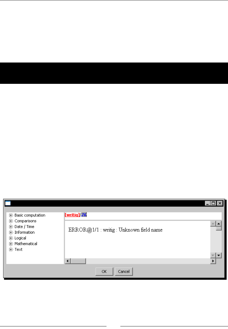
Basic Data Manipulaon
[ 84 ]
Just like every grid in Kele, you have a contextual menu (and its corresponding shortcuts)
that lets you manipulate the rows by deleng, moving, copying and pasng, and so on.
The Formula step
The Formula step is another step you can use for doing calculaons. Let's give it a try by
using it in the examinaon tutorial.
Time for action – reviewing examinations by using the
Formula step
In this tutorial you will redo the previous exercise, but this me you will do the calculaons
with the Formula step.
1. Open the transformaon you just nished.
2. Delete from the transformaon the Calculator step, and put in its place a Formula
step. You will nd it under the Scripng category of steps.
3. Add a eld named writing.
4. When you click the cell under the Formula column, a window appears to edit the
formula for the new eld.
5. In the upper area of the window, type [writing]/20. You will noce that the
sentence is red if it is incomplete or the syntax is incorrect. In that case, the error is
shown below the eding area, like in the following example:
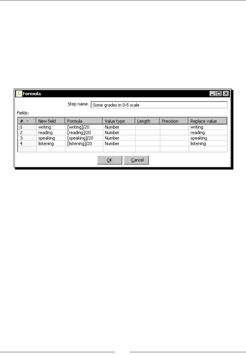
Chapter 3
[ 85 ]
6. As soon as the formula is complete and correct, the red color disappears.
7. Click OK.
8. The formula you typed will be displayed in the cell you clicked.
9. Set Number as the type for the new eld, and type writing in the Replace value
column.
10. Add three more elds to the grid in the same way you added this eld so that the
grid looks like the following:
11. Click OK.
12. Add a second Formula step.
13. Add a eld named avg and click the Formula cell to edit it.
14. Expand the Mathemacal category of funcons to the leside of the window, and click
the AVERAGE funcon.
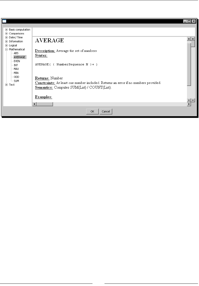
Basic Data Manipulaon
[ 86 ]
15. The explanaon of the selected funcon appears to guide you.
16. In the eding area, type average([writing];[reading];[speaking];
[listening]).
17. Click OK.
18. Set the Value type to Number.
19. Click OK.
20. Create a hop from this step to the Sort rows step.
21. Edit the last Select values step.
22. Click Get elds to select.
23. A queson appears to ask you what to do. Click Clear and add all.
24. The grid is reloaded with the modied elds.
25. Click on the Dummy step and do a preview.
26. There should be no dierence with what you had in the Calculator version of
the tutorial:
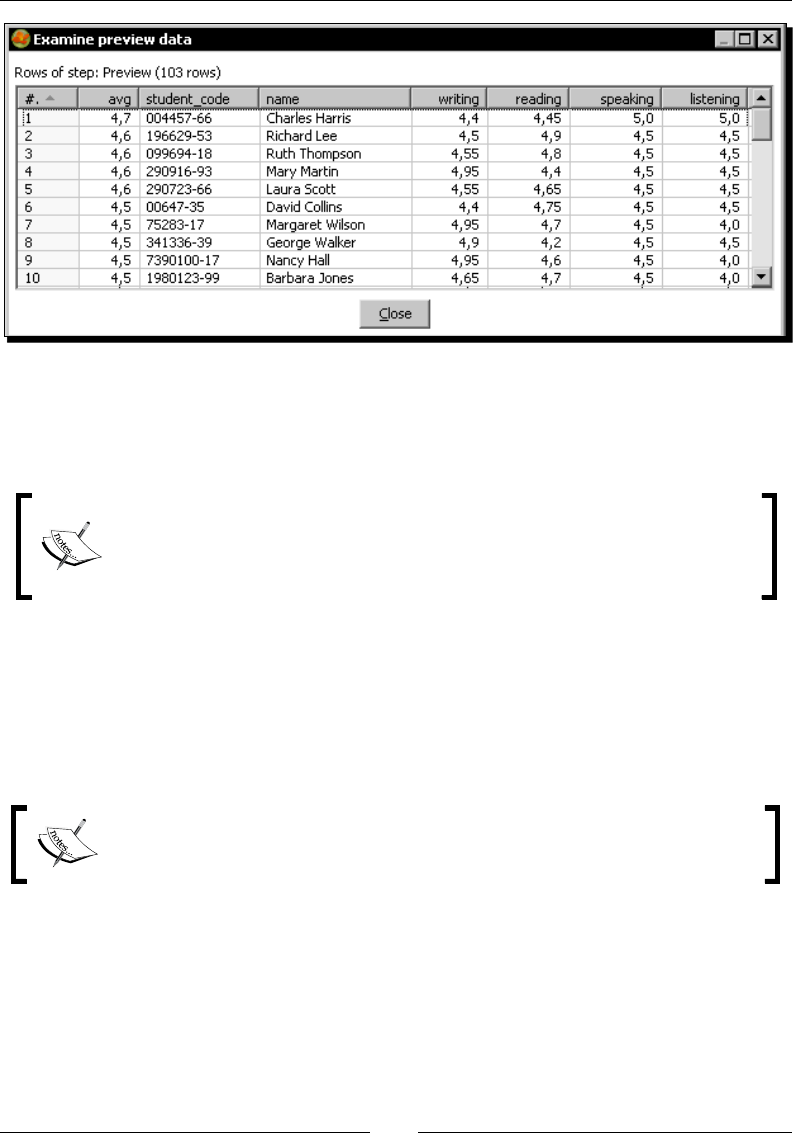
Chapter 3
[ 87 ]
What just happened?
You read the examination.txt le, and did some calculaons using the Formula step to
see how the students did.
It may happen that the preview window shows you less decimal posions than
expected. This is a preview issue. One of the ways you have to see the numbers
with more decimals is to send the numbers to an output le with a proper
format and see the numbers in the le.
As you saw, you have quite a lot of funcons available for building formulas and expressions.
To reference a eld you have to use square brackets, like in [writing]. You may reference
only the current elds of the row. You have no way to access previous rows of the grid as
you have in the Calculator step and so you needed two Formula steps to replace a single
Calculator. But you saved auxiliary elds because the Formula allows you to type complex
formulas in a single eld without using paral calculaons.
When the calculaons are not simple, that is, they require resolving a complex
formula or involve many operands, then you might prefer the Formula step over
the Calculator.
The Formula step uses the library Libformula. The syntax used in LibFormula is based
on the OpenFormula standard. For more informaon on OpenFormula, you may visit
http://wiki.oasis-open.org/office/About_OpenFormula.

Basic Data Manipulaon
[ 88 ]
Have a go hero – listing students and their examinations results
Let's play a lile with the examinaon le. Suppose you decide that only those students
whose average grade was above 3.9 will pass the examinaon; the others will not. List the
students ordered by average (desc.), last name (asc.), and name (asc.). The output list should
have the following elds:
Student code
Name
Last Name
Passed (yes/no)
average grade
Pop quiz – concatenating strings
Suppose that you want to create a new eld as the student_code plus the name of the
student separated by a space, as for example 867432-94 Linda Rodriguez. Which of the
following are possible soluons for your problem:
a. Use a Calculator, using the calculaon a+b+c, where a is student_code, b is a
space, and c is the name eld.
b. Use a Formula, using as formula [student_code]+" "+[name]
c. Use a Formula, using as formula [student_code]&" "&[name]
You may choose more than one opon.
Calculations on groups of rows
You just learned to do simple operaons for every row of a dataset. Now you are ready to
go beyond. Suppose you have a list of daily temperatures of a given country over a year. You
may want to know the overall average temperature, the average temperature by region,
or the coldest day of the year. When you work with data, these types of calculaons are a
common requirement. In this secon you will learn to address those requirements with PDI.
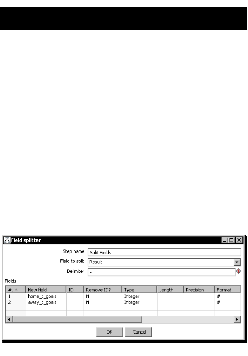
Chapter 3
[ 89 ]
Time for action – calculating World Cup statistics by
grouping data
Let's forget the examinaons for a while, and retake the World Cup tutorial from the
previous chapter. The le you obtained from that tutorial was a list of results of football
matches. These are sample rows of the nal le:
Match Date;Home Team;Away Team;Result
02/06;Italy;France;2-1
02/06;Argentina;Hungary;2-1
06/06;Italy;Hungary;3-1
06/06;Argentina;France;2-1
10/06;France;Hungary;3-1
10/06;Italy;Argentina;1-0
...
Now you want to take that informaon to obtain some stascs such as the maximum
number of goals per match in a given day. To do it, follow these instrucons:
1. Create a new transformaon, give it a name and descripon, and save it.
2. By using a Text le input step, read the wcup_first_round.txt le you generated
in Chapter 2. Give the name and locaon of the le, check the Content tab to see that
everything matches your le, and ll the Fields tab.
3. Do a preview just to conrm that the step is well congured.
4. From the Transform category of step, select a Split Fields step, drag it to the work area,
and create a hop from the Text le input to this step.
5. Double-click the Split Fields steps and ll the grid like done in the following screenshot:
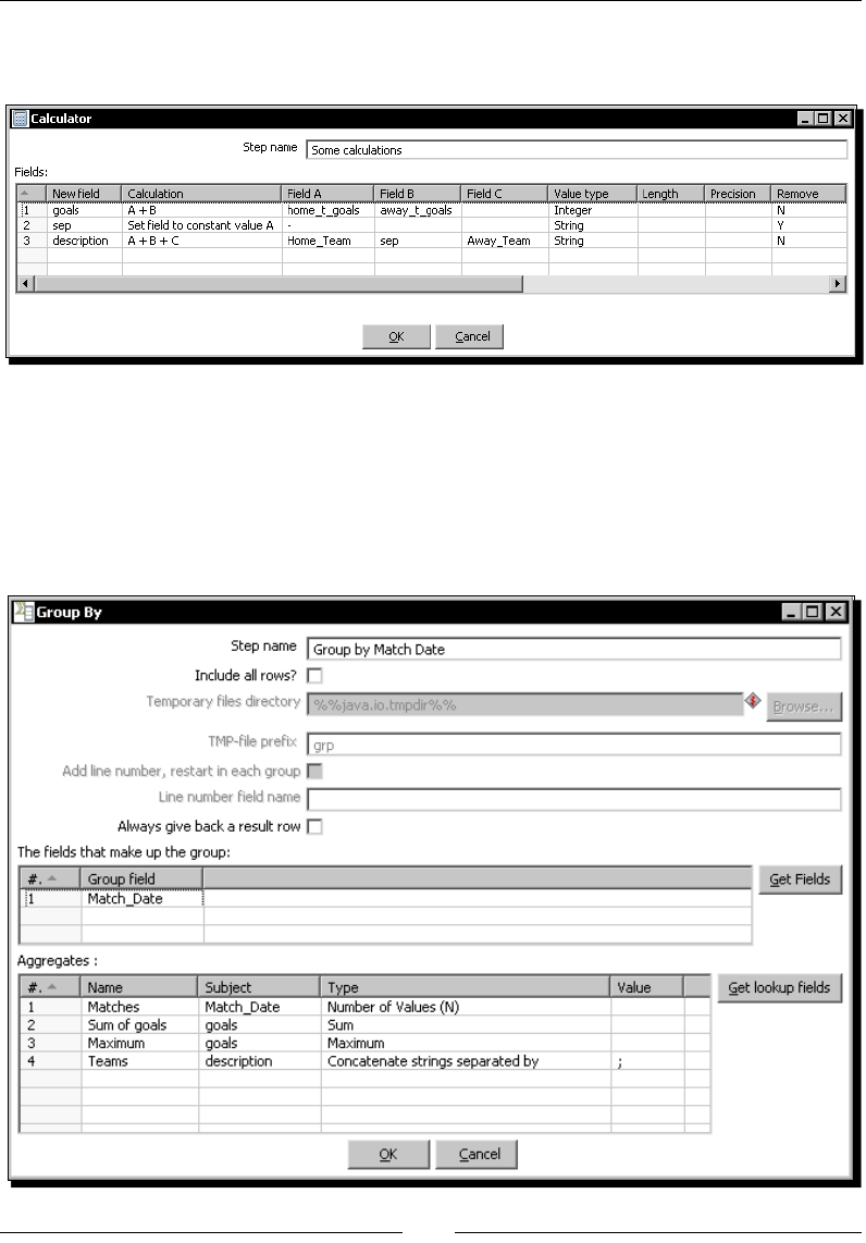
Basic Data Manipulaon
[ 90 ]
6. Add a Calculator step to the transformaon and create a hop from the Split Fields step
to this step and edit the step to create the following new elds:
7. Add a Sort rows step to the transformaon, create a hop from the Calculator step to this
step, and sort the elds by Match_Date.
8. Expand the Stascs category of steps, and drag a Group by step to the canvas. Create a
hop from the Sort rows step to this new step.
9. Edit the Group by step and ll the conguraon window as shown next:
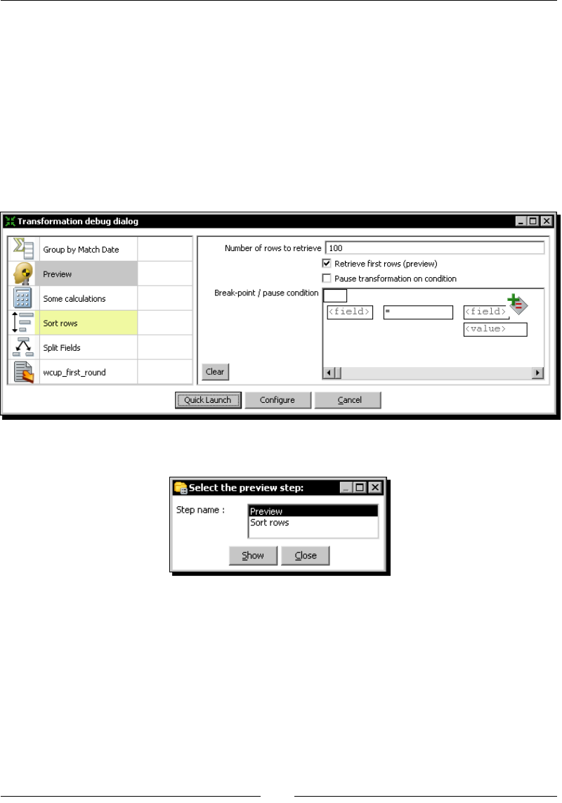
Chapter 3
[ 91 ]
10. When you click the OK buon, a window appears to warn you that this step
needs the input to be sorted on the specied keys—the Range eld in this case.
Click I understand, and don't worry because you already sorted the data in the
previous step.
11. Add a nal Dummy step.
12. Select the Dummy and the Group by steps, le-click one and holding down the Shi
key, le-click the other.
13. Click the Preview this transformaon buon. You will see the the following:
14. Click Quick Launch. The following window appears:
15. Double-click the Sort rows step. A window appears with the data coming out of the Sort
rows step.
16. Double-click the Dummy step. A window appears with the data coming out of the
Dummy step.
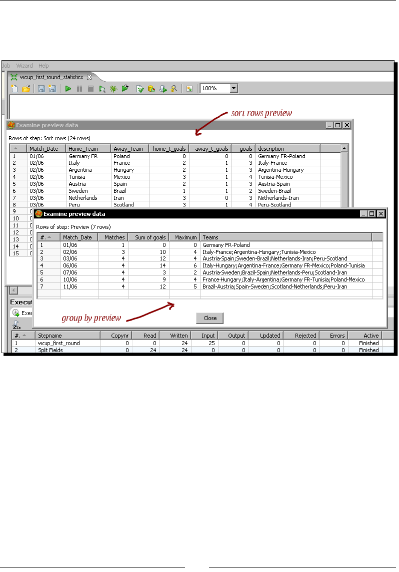
Basic Data Manipulaon
[ 92 ]
17. If you rearrange the preview windows, you can see both preview windows at a me, and
understand beer what happened with the numbers. The following would be the data
shown in the windows:
What just happened?
You opened a le with results from several matches and got some stascs from it.
In the le, there was a column with the match result in the format n-m, with n being the
goals of the home team and m being the goals of the away team. With the Split Fields step,
you split this eld in two—one with each of these two numbers.
With the Calculator you did two things:
You created a new eld with the total number of goals for each match.
You created a descripon for the match.
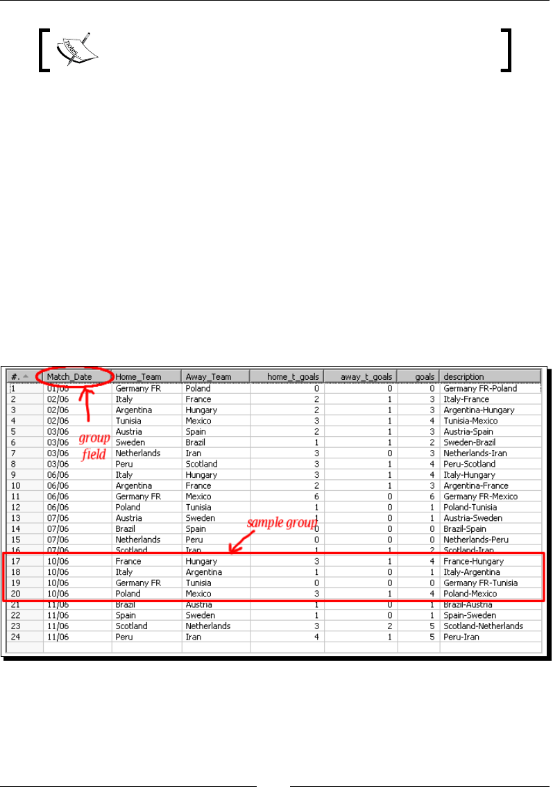
Chapter 3
[ 93 ]
Note that in order to create a descripon, you used the + operator to
concatenate string rather than add numbers.
Aer that, you ordered the data by match date with a Sort rows step.
In the preview window of the Sort rows step, you could see all the calculated elds: home
team goals, away team goals, match goals, and descripon.
Finally, you did some stascal calculaons:
First, you grouped the rows by match date. You did this by typing Match_Date in the
upper grid of the Group by step.
Then, for every match date, you calculated some stascs. You did the calculaons by
adding rows in the lower grid of the step, one for every stasc you needed.
Let's see how it works. Because the Group by step was preceded by a Sort rows step, the
rows came to the step already ordered. When the rows arrive to the Group by step, Kele
creates groups based on the eld(s) indicated in the upper grid—the Match_Date eld in this
case. The following drawing shows this idea:
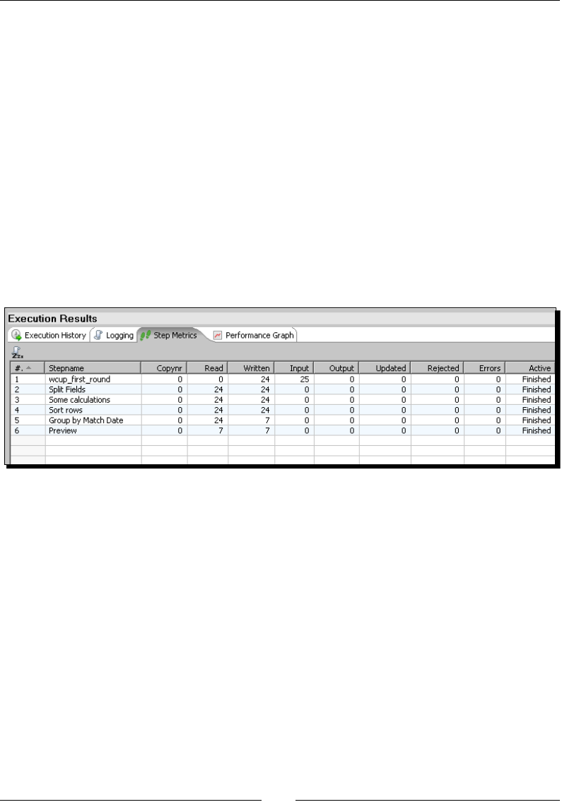
Basic Data Manipulaon
[ 94 ]
Then, for every group, the elds that you put in the lower grid are calculated. Let's see, for
example, the group for the match date 03/06. For the rows in this group, Kele calculated
the following:
Matches: The number of matches played on 03/06. There were 4.
Sum of goals: The total number of goals converted on 03/06. There were 3+2+3+4=12.
Maximum: The maximum number of goals converted in a single match played on 03/06.
The maximum among 3, 2, 3, and 4 was 4.
Teams: The descripons of the teams which played on 03/06, separated by ; : Austria-
Spain; Sweden-Brazil; Netherlands-Iran; Peru-Scotland.
The same calculaons were made for every group. You can verify the details by looking in the
preview window.
Look at the Step Metrics tab in the Execuon Results area of the screen:
Note that 24 rows entered the Group by step and only 7 came out of that step towards the
Dummy step. That is because aer the grouping, you no longer have the detail of matches.
The output of the Group by step is your new data now—one row for every group created.
Group by step
The Group by step allows you to create groups of rows and calculate new elds over
those groups.
In order to dene the groups, you have to specify which eld(s) are the keys. For every
combinaon of values for those elds, Kele builds a new group.
In the tutorial you grouped by a single eld Match_date. Then for every value of
Match_date, Kele created a dierent group.
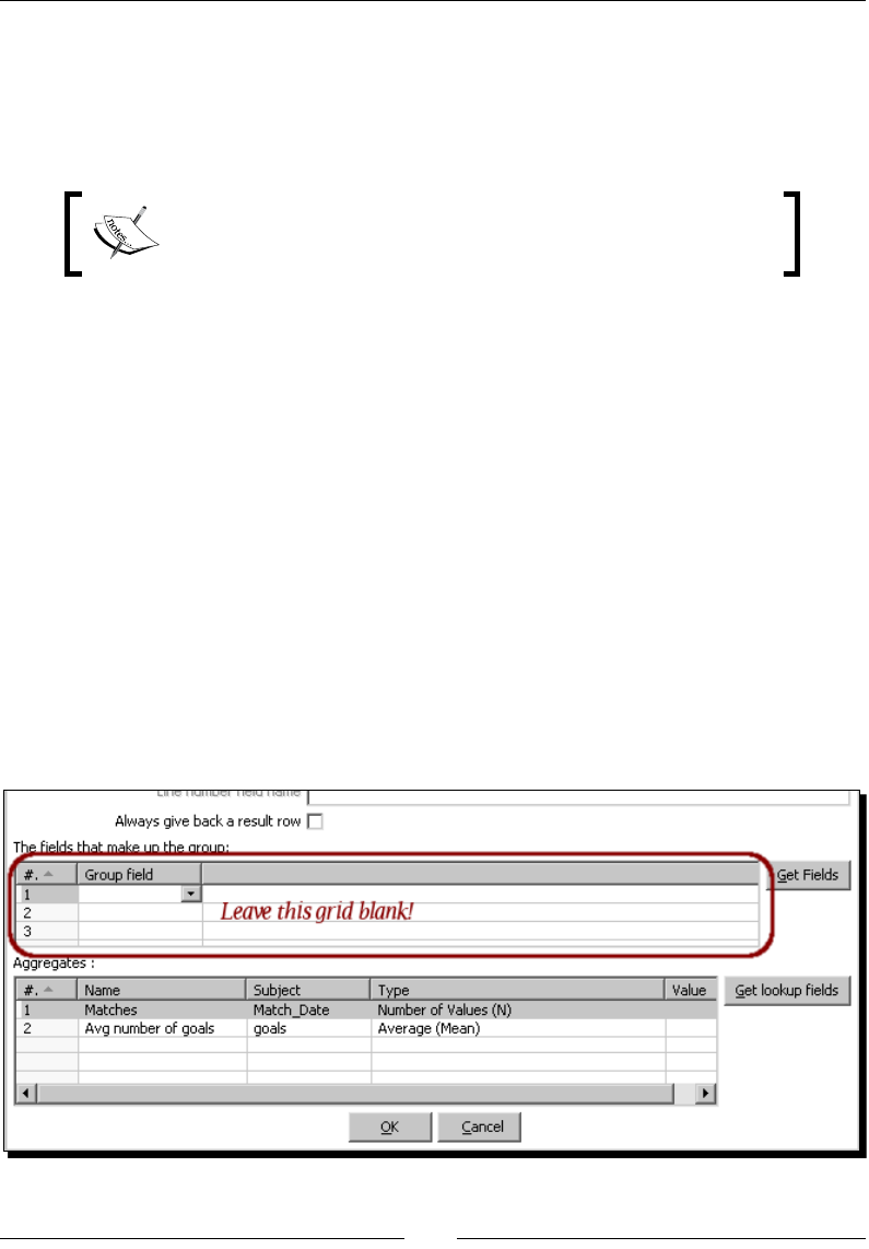
Chapter 3
[ 95 ]
The Group by step operates on consecuve rows. Suppose that the rows are already sorted
by date, but those with date 10/06 are above the rest. The step traverses the dataset and
each me the value for any of the grouping eld changes, it creates a new group. If you
see it this way, you will noce that the step will work even if the data is not sorted by the
grouping eld.
As you probably don't know how the data is ordered, it is safer and
recommended that you sort the data by using a Sort rows step just
before using a Group by step.
Once you have dened the groups, you are free to specify new elds to be calculated
for every group. Every new eld is dened as an aggregate funcon over some of the
existent elds.
Let's review some of the elds you created in the tutorial:
The Matches eld is the result of applying the Number of values funcon over
the eld Match_date.
The Sum of goals eld is the result of applying the Sum funcon over the
eld goals.
The Maximum eld is the result of applying the Maximum funcon over the
eld goals.
Finally, you have the opon to calculate aggregate funcons over the whole dataset. You do
this by leaving the upper grid blank. Following the same example, you could calculate the
total number of matches and the average number of goals for all those matches. This is how
you do it:
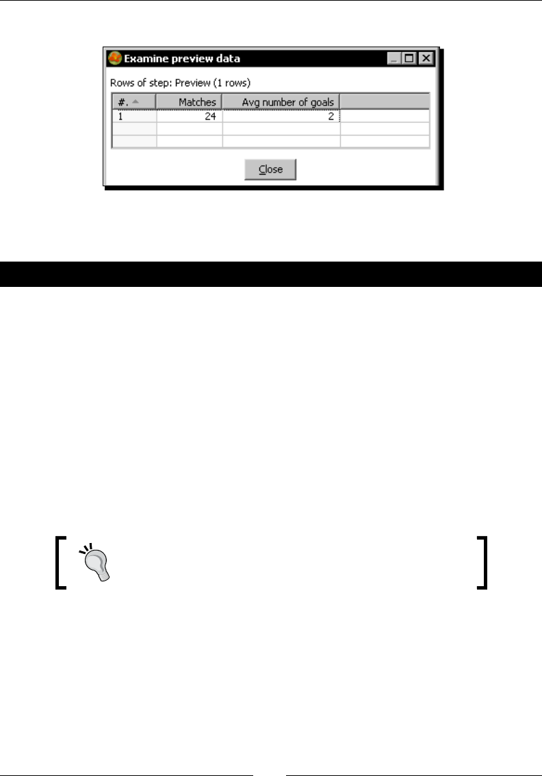
Basic Data Manipulaon
[ 96 ]
The following is what you get:
In any case, as a result of the Group by step, you will no longer have the detailed rows,
unless you check the Include all rows? checkbox.
Have a go hero – calculating statistics for the examinations
Here you have one more task related with the examinaons le. Create a new
transformaon, read the le, and calculate:
The number of students who passed
The number of students who failed
The average wring, reading, speaking, and listening grade obtained by students
who passed
The average wring, reading, speaking, and listening grade obtained by students
who failed
The minimum and maximum average grade among students who passed
The minimum and maximum average grade among students who failed
Use the Number range step to dene the range of the average
grade; then use a Group by step to calculate the stascs.
Chapter 3
[ 97 ]
Have a go hero – listing the languages spoken by country
Read the le with countries' informaon you used in Chapter 2. Build a le where each row
has two columns—the name of a country and the list of spoken languages in that country.
As aggregate, use the opon Concatenate strings separated by.
Filtering
Unl now you learned how to accomplish several kinds of calculaons that enriched the set
of data. There is sll another kind of operaon that is frequently used, and does not have to
do with enriching the data but with discarding data. It is ltering unwanted data. Now you
will learn how to discard rows under given condions.
Time for action – counting frequent words by ltering
Let's suppose, you have some plain text les, and you want to know what is said in them. You
don't want to read them, so you decide to count the mes that words appear in the text, and
see the most frequent ones to get an idea of what the les are about.
Before starng, you'll need at least one text le to play with. The text le used in
this tutorial is named smcng10.txt and is available for you to download from
the Packt website.
Let's work:
1. Create a new transformaon.
2. By using a Text le input step, read your le. The trick here is to put as a separator
a sign you are not expecng in the le, for example |. By doing so, the enre line
would be recognized as a single eld. Congure the Fields tab by dening a single
string eld named line.
3. From the Transform category of step, drag to the canvas a Split eld to rows step,
and create a hop from Text le input step to this new step.
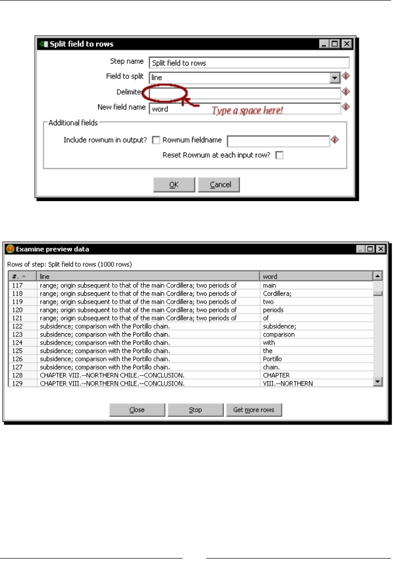
Basic Data Manipulaon
[ 98 ]
4. Congure the step like this:
5. With this last step selected, do a preview. Your preview window should look like this:
6. Close the preview window.
7. Expand the Flow category of steps, and drag a Filter rows step to the work area.
8. Create a hop from the last step to the Filter rows step.
9. Edit the Filter rows step by double-clicking it.
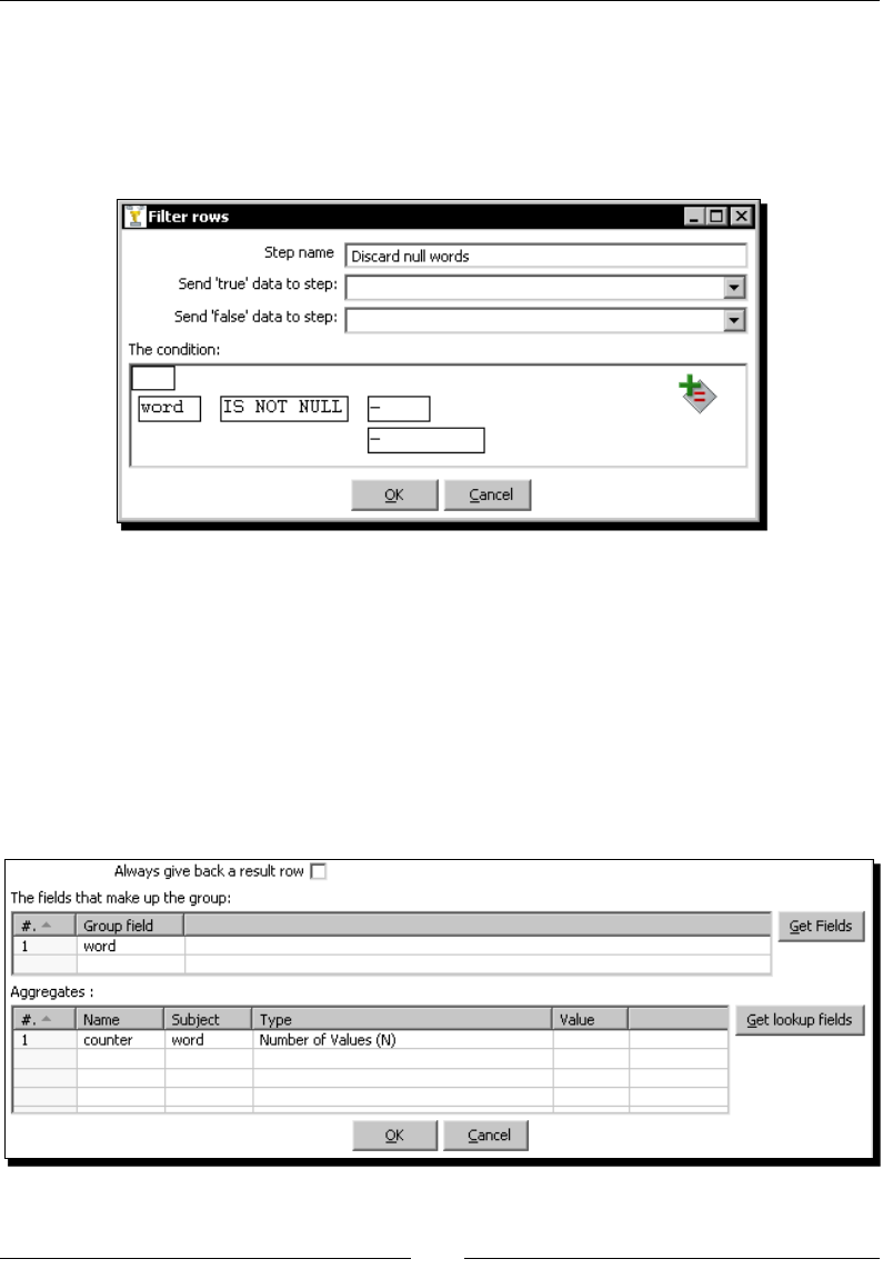
Chapter 3
[ 99 ]
10. Click the <field> textbox to the le of the = sign. The list of elds appears.
Select word.
11. Click the = sign. A list of operaons appears. Select IS NOT NULL.
12. The window looks like the following:
13. Click OK.
14. From the Transform category of steps drag a Sort rows step to the canvas, and
create a hop from the Filter rows step to this new step.
15. Sort the rows by word.
16. From the Stascs category, drag a Group by step, and create a hop from the Sort
rows step to this step.
17. Congure the grids in the Group by conguraon window like shown:
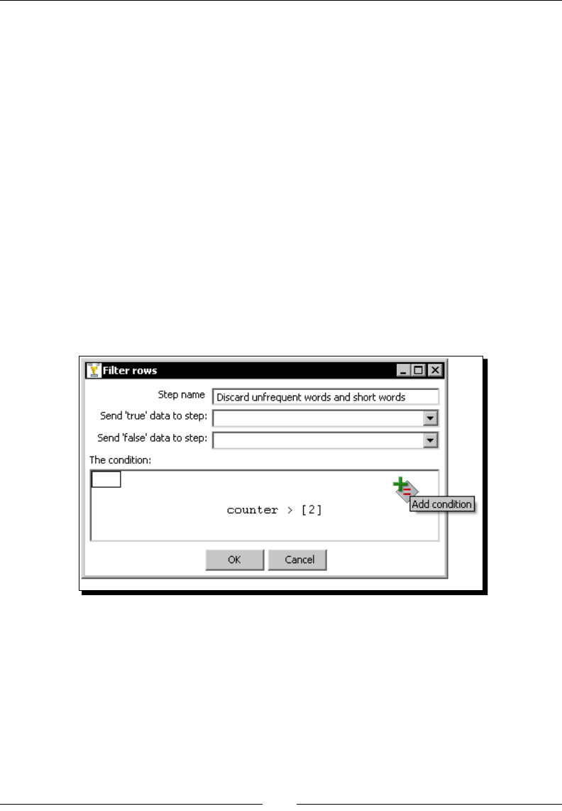
Basic Data Manipulaon
[ 100 ]
18. Add a Calculator step, create a hop from the last step to this, and calculate the new
eld len_word represenng the length of the words. For that, use the calculator
funcon Return the length of a string A and select word from the
drop-down menu for Field A.
19. Expand the Flow category and drag another Filter rows step to the canvas.
20. Create a hop from the Calculator step to this step and edit it.
21. Click <field> and select counter.
22. Click the = sign, and select >.
23. Click <value>. A small window appears.
24. In the Value textbox of the lile window, enter 2.
25. Click OK.
26. Posion the mouse cursor over the icon in the upper-right corner of the window.
When the text Add condion shows up, click on the icon.
27. A new blank condion is shown below the one you created.
28. Click on null = [] and create the condion len_word>3, in the same way you
created the condion counter>2.
29. Click OK.

Chapter 3
[ 101 ]
30. The nal condion looks like this:
31. Add one more Filter rows step to the transformaon and create a hop from the last
step to this new step.
32. On the le side of the condion, select word.
33. As comparator select IN LIST.
34. At the end of the condion, inside the textbox value, type the following:
a;an;and;the;that;this;there;these.
35. Click the upper-le square above the condion and the word NOT will appear.
36. The condion looks like the following:
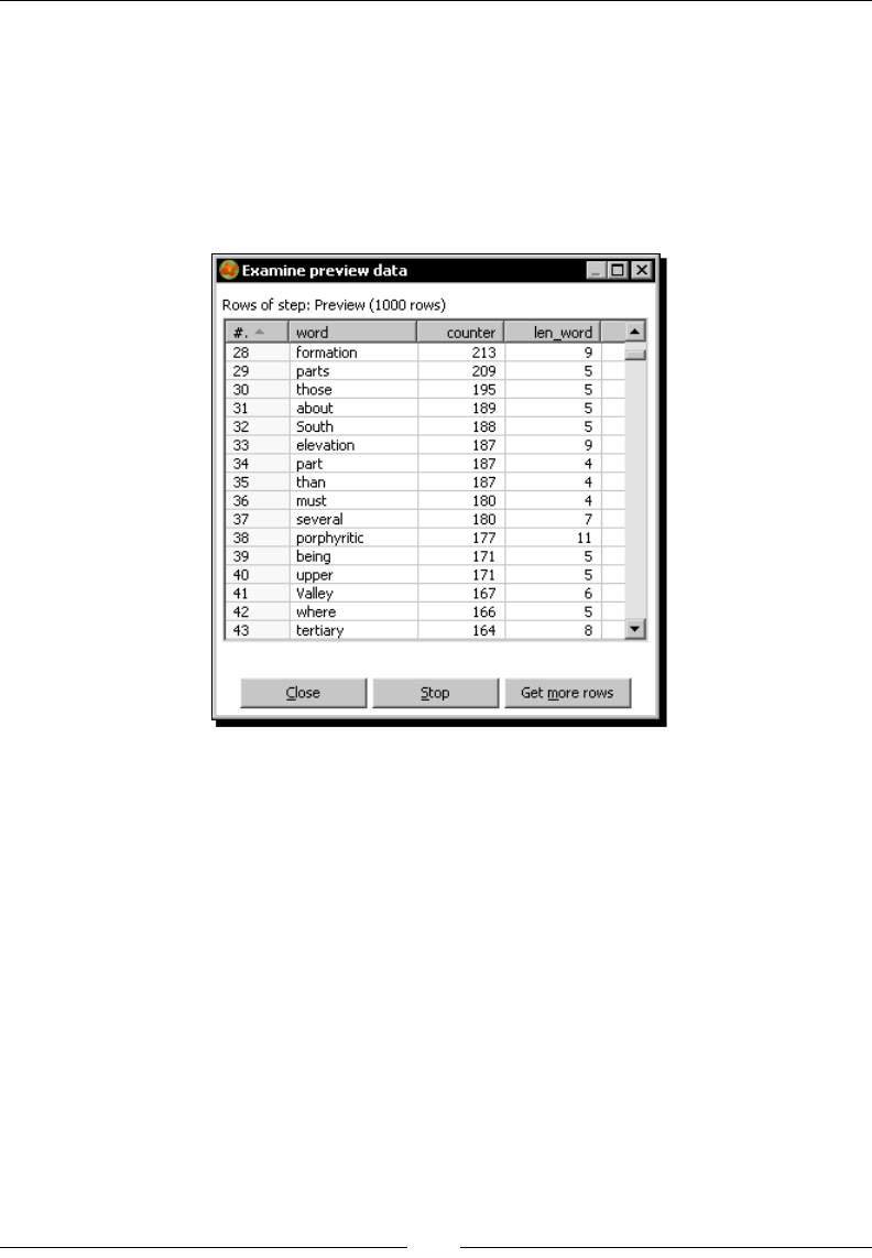
Basic Data Manipulaon
[ 102 ]
37. Add a Sort rows step, create a hop from the previous step to this step, and sort the
rows in the descending order of counter.
38. Add a Dummy step at the end of the transformaon, create a hop from the last step
to the Dummy step.
39. With the Dummy step selected, preview the transformaon. The following is what
you should see now:
What just happened?
You read a regular plain le and arranged the words that appear in the le in some
parcular fashion.
The rst thing you did was to read the plain le and split the lines so that every word became
a new row in the dataset. Consider, for example, the following line:
subsidence; comparison with the Portillo chain.
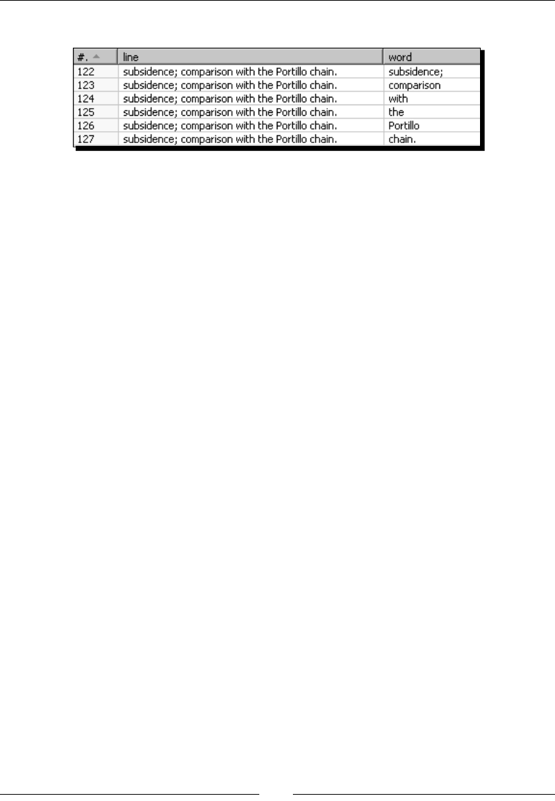
Chapter 3
[ 103 ]
The spling of this line resulted in the following rows being generated:
Thus, a new eld named word became the basis for your transformaon.
First of all, you discarded rows with null words. You did it by using a lter with the condion
word IS NOT NULL. Then, you counted the words by using the Group by step you learned
in the previous tutorial. Once you counted the words, you discarded those rows where the
word was too short (length less than 4) or too common (comparing to a list you typed).
Once you applied all those lters, you sorted the rows in the descending order of
the number of mes the word appeared in the le so that you could see the most
frequent words.
Scrolling down a lile the preview window to skip some preposions, pronouns, and other
very common words that have nothing to do with a specic subject, you found words such
as shells, strata, formaon, South, elevaon, porphyric, Valley, terary, calcareous, plain,
North, rocks, and so on. If you had to guess, you would say that this was a book or arcle
about geology, and you would be right. The text taken for this exercise was Geological
Observaons on South America by Charles Darwin.
Filtering rows using the Filter rows step
The Filter rows step allows you to lter rows based on condions and comparisons.
The step checks the condion for every row. Then it applies a lter leng pass only the rows
for which the condion is true. The other rows are lost.
In the counng words exercise, you used the Filter rows step several mes so you already
have an idea of how it works. Let's review it.

Basic Data Manipulaon
[ 104 ]
In the Filter rows seng window you have to enter a condion. The following table
summarizes the dierent kinds of condions you may enter:
Condion Descripon Example
A single eld followed by IS NULL or
IS NOT NULL
Checks whether the value of a
eld in the stream is null
word IS NOT NULL
A eld, a comparator, and a constant Compares a eld in the stream
against a constant value.
counter > 2
Two elds separated by a comparator Compares two elds in the
stream
line CONTAINS
word
You can combine condions as shown here:
counter > 2
AND
len_word>3
You can also create subcondions such as:
(
counter > 2
AND
len_word>3
)
OR
(word in list geology; sun)
In this last example, the condion lets the word geology pass even if it appears only once. It
also lets the word sun pass, despite its length.
When eding condions, you always have a contextual menu which allows you to add and
delete sub-condions, change the order of existent condions, and more.
Maybe you wonder what the Send 'true' data to step: and Send 'false' data to step: textboxes
are for. Be paent, you will learn how to use them in Chapter 4.
Have a go hero – playing with lters
Now it is your turn to try ltering rows. Modify the counng_words transformaon in the
following way:
Alter the Filter rows steps. By using a Formula step create a ag (a Boolean eld)
that evaluates the dierent condions (counter>2, and so on). Then use only one
Filter rows step that lters the rows for which the ag is true. Test it and verify that
the results are the same as before the change.

Chapter 3
[ 105 ]
In the Formula eding window, use the opons under the Logic category.
Then in the Filter rows step, you can type true or Y as the value against which
you compare the ag.
Add a sub-condion to avoid excluding some words, just like the one in the example:
(word in list geology; sun). Change the list of words and test the lter to see
that the results are as expected.
Have a go hero – counting words and discarding those that are
commonly used
If you take a look at the results in the tutorial, you may noce that some words appear more
than once in the nal list because of special signs such as . , ) or ", or because of lower
or upper case leers. For example, look how many mes the word rock appears: rock (99
occurrences) - rock,(51 occurrences) – rock. (11 occurrences) – rock." (1 occurrence)
- rock: (6 occurrences) - rock; - (2 occurrences). You can x this and make the word rock
appear only once: Before grouping the words, remove all extra signs and convert all words to
lower case or upper case, so they are grouped as expected.
Try one or more of the following steps: Formula, Calculator, Replace in string.
Looking up data
Unl now, you have been working with a single stream of data. When you did calculaons or
created condions to compare elds, you only involved elds of your stream. Usually, this is
not enough, and you need data from other sources. In this secon you will learn to look up
data outside your stream.
Time for action – nding out which language people speak
An Internaonal Musical Contest will take place and 24 countries will parcipate, each
presenng a duet. Your task is to hire interpreters so the contestants can communicate in
their nave language. In order to do that, you need to nd out the language they speak:
1. Create a new transformaon.
2. By using a Get Data From XML step, read the countries.xml le that contains
informaon about countries that you used in Chapter 2.
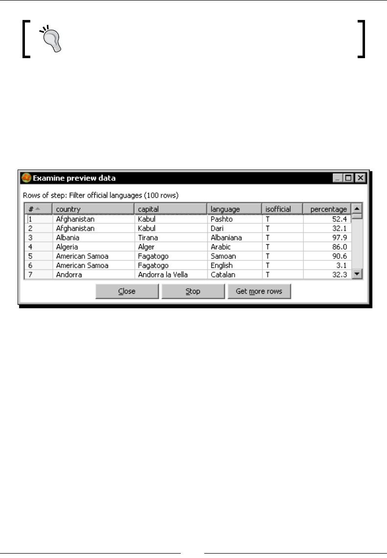
Basic Data Manipulaon
[ 106 ]
To avoid conguring the step again, you can open the transformaon
that reads this le, copy the Get data from XML step, and paste it here.
3. Drag a Filter rows step to the canvas.
4. Create a hop from the Get data from XML step to the Filter rows step.
5. Edit the Filter rows step and create the condion- isofficial= T.
6. Click the Filter rows step and do a preview. The list of previewed rows will show the
countries along with the ocial languages:
Now let's create the main ow of data:
7. From the book website download the list of contestants. It looks like this:
ID;Country;Duet
1;Russia;Mikhail Davydova
;;Anastasia Davydova
2;Spain;Carmen Rodriguez
;;Francisco Delgado
3;Japan;Natsuki Harada
;;Emiko Suzuki
4;China;Lin Jiang
;;Wei Chiu
5;United States;Chelsea Thompson
;;Cassandra Sullivan
6;Canada;Mackenzie Martin
;;Nathan Gauthier
7;Italy;Giovanni Lombardi
;;Federica Lombardi
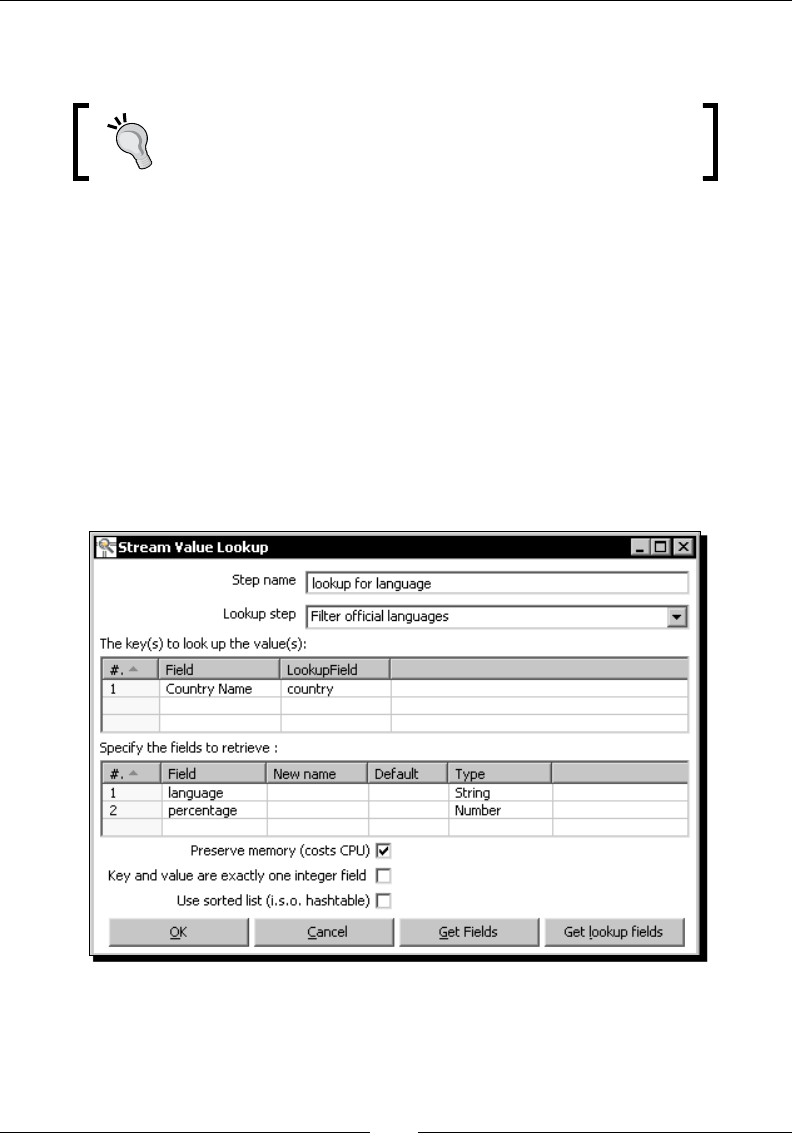
Chapter 3
[ 107 ]
8. In the same transformaon, drag a Text le Input step to the canvas and read the
downloaded le.
The ID and country have values only in the rst of the two
lines for each country. In order to repeat the values in the
second line use the ag Repeat in the Fields tab. Set it to Y.
9. Expand the Lookup category of steps.
10. Drag a Stream lookup step to the canvas.
11. Create a hop from the Text le input you just created, to the Stream lookup step.
12. Create another hop from the Filter rows step to the Stream lookup step.
13. Edit the Stream lookup step by double-clicking it.
14. In the Lookup step drop-down list, select Filter ocial languages, the step that brings
the list of languages.
15. Fill the grids in the conguraon window as follows:
Note that Country Name is a eld coming from the text le stream, while the country
eld comes from the countries stream.
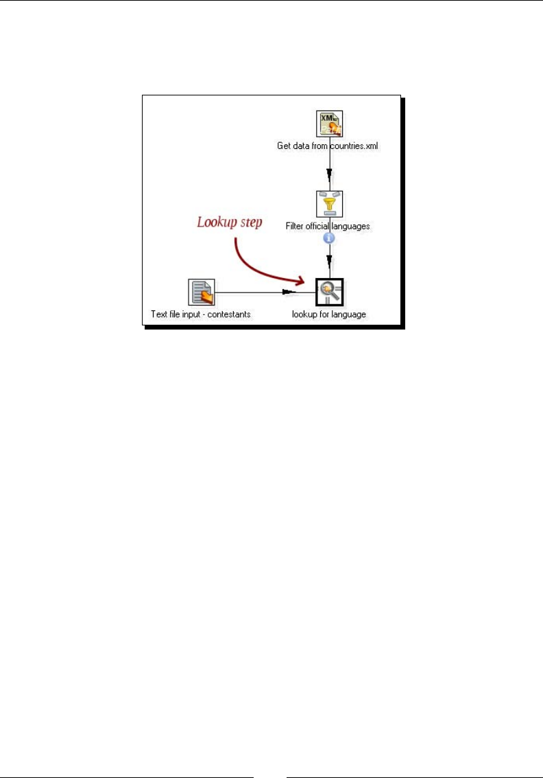
Basic Data Manipulaon
[ 108 ]
16. Click OK.
17. The hop that goes from the Filter rows step to the Stream lookup step changes its look
and feel, to show that this is the stream where the Stream lookup is going to look:
18. Aer the Stream lookup, add a Filter rows step.
19. In the Filter rows step, type the condion language-IS NOT NULL.
20. By using a Select values step, rename the elds Duet, Country Name and
language to Name, Country, and Language.
21. Drag a Text le output step to the canvas and create the le
people_and_languages.txt with the selected elds.
22. Save the transformaon.
23. Run the transformaon and check the nal le, which should look like this:
Name|Country|Language
Mikhail Davydova|Russia|
Anastasia Davydova|Russia|
Carmen Rodriguez|Spain|Spanish
Francisco Delgado|Spain|Spanish
Natsuki Harada|Japan|Japanese
Emiko Suzuki|Japan|Japanese

Chapter 3
[ 109 ]
Lin Jiang|China|Chinese
Wei Chiu|China|Chinese
Chelsea Thompson|United States|English
Cassandra Sullivan|United States|English
Mackenzie Martin|Canada|French
Nathan Gauthier|Canada|French
Giovanni Lombardi|Italy|Italian
Federica Lombardi|Italy|Italian
What just happened?
First of all, you read a le with informaon about countries and the languages spoken in
those countries.
Then you read a list of people along with the country they come from. For every row in this
list, you told Kele to look for the country (Country Name eld) in the countries stream
(country eld), and to give you back a language and the percentage of people that speaks
that language (language and percentage elds). Let's explain it with a sample row: The
row for Francisco Delgado from Spain. When this row gets to the Stream lookup step,
Kele looks in the list of countries for a row with the country Spain. It nds it. Then, it
returns the value of the columns language and percentage: Spanish and 74.4.
Now take another sample row—the row with the country Russia. When the row gets to the
Stream lookup step, Kele looks for it in the list of countries, but it doesn't nd it. So what
you get as language is a null string.
Whether the country is found or not, two new elds are added to your stream—language
and percentage.
Aer the Stream lookup step, you discarded the rows where language is null, that is, those
whose country wasn't found in the list of countries.
With the successful rows you generated an output le.
The Stream lookup step
The Stream lookup step allows you to look up data in a secondary stream.
You tell Kele which of the incoming streams is the stream used to look up, by selecng the
right choice in the Lookup step list.
The upper grid in the conguraon window allows you to specify the names of the elds that
are used to look up.
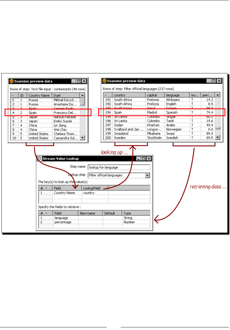
Basic Data Manipulaon
[ 110 ]
In the le column, Field, you indicate the eld of your main stream. You can ll this
column by using the Get Fields buon, and deleng all the elds you don't want to use
for the search.
In the right column, Lookup Field, you indicate the eld of the secondary stream.
When a row of data comes to the step, a lookup is made to see if there is a row in the
secondary stream for which, every pair (Field, LookupField) in the grid has the value of
Field equal to the value of LookupField. If there is one, the look up will be successful.
In the lower grid, you specify the names of the secondary stream elds that you want back
as a result of the look up. You can ll this column by using the Get lookup elds buon, and
deleng all the elds you don't want to retrieve.
Aer the lookup, new elds are added to your dataset—one for every row of this grid.
For the rows for which the look up is successful, the values for the new elds will be taken
from the lookup stream.
For the others, the elds will remain null, unless you set a default value.

Chapter 3
[ 111 ]
When you use a Stream lookup, all lookup data is loaded into memory. Then the stream
lookup is made using a hash table algorithm. Even if you don't know how this algorithm
works, it is important that you know the implicaons of using this step:
First, if the data where you look is huge, you take the risk of running out
of memory.
Second, only one row is returned per key. If the key you are looking for is present
more than once in the lookup stream, only one will be returned—for example, in the
tutorial where there are more than one ocial languages spoken in a country, you
get just one. Somemes you don't care, but on some occasions this is not acceptable
and you have to try some other methods. You'll learn other ways to do this later in
the book.
Have a go hero – counting words more precisely
The tutorial where you counted the words in a le worked prey well, but you may have
noced that it has some details you can x or enhance.
You discarded a very small list of words, but there are much more that are quite usual
in English—preposions, pronouns, auxiliary verbs, and many more. So here is the challenge:
Get a list of commonly used words and save it in a le. Instead of excluding words from a
small list as you did with a Filter rows step, exclude the words that are in your common
words le.
Use a Stream lookup step.
Test the transformaon with the same le, and also with other les, and verify
that you get beer results with all these changes.

Basic Data Manipulaon
[ 112 ]
Summary
This chapter covered the simplest and most common ways of transforming data. Specically,
it covered how to:
Use dierent transformaon steps to calculate new elds
Use the Calculator and the Formula steps
Filter and sort data
Calculate stascs on groups of rows
Look up data
Aer learning basic manipulaon of data, you may now create more complex
transformaons, where the streams begin to split and merge. That is the core
subject of the next chapter.

4
Controlling the Flow of Data
In the previous chapter, you learned the basics of transforming data. Basically
you read data from some le, did some transformaon to the data, and sent
the data back to a dierent output. This is the simplest scenario. Think of
a dierent situaon. Suppose you collect results from a survey. You receive
several les with the data and those les have dierent formats. You have to
merge those les somehow and generate a unied view of the informaon.
You also want to put aside the rows of data whose content is irrelevant. Finally,
based on the rows that interest you, you want to create another le with some
stascs. This kind of requirement is very common. In this chapter you will
learn how to implement it with PDI.
Splitting streams
Unl now, you have been working with simple, straight ows of data. When you deal with
real problems, those simple ows are not enough. Many mes, the rows of your dataset
have to take dierent paths. This situaon is handled very easily, and you will learn how to
do it in this secon.
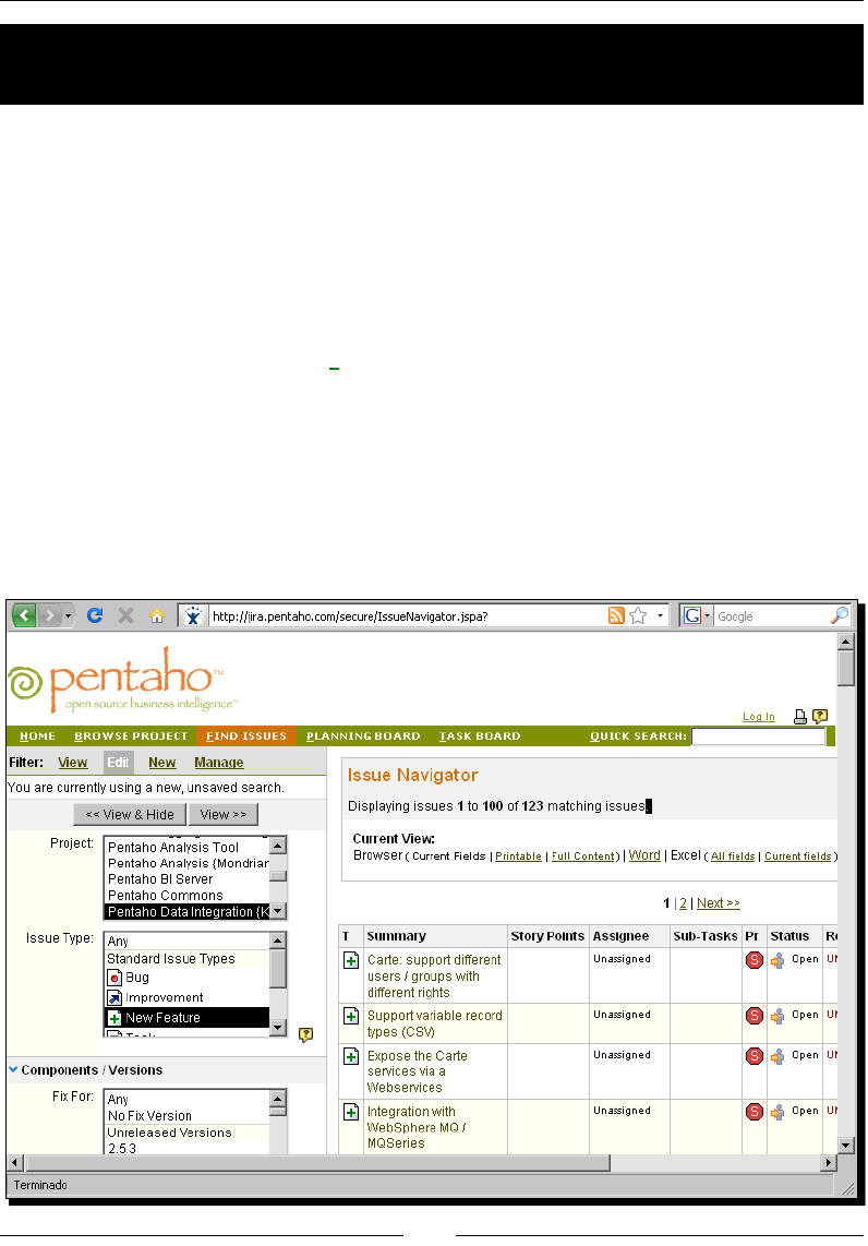
Controlling the Flow of Data
[ 114 ]
Time for action – browsing new PDI features by copying
a dataset
Before starng, let's introduce the Pentaho BI Plaorm Tracking site. At the tracking site you
can see the current Pentaho roadmap and browse their issue tracking system. The PDI page
for that site is http://jira.pentaho.com/browse/PDI.
In this exercise, you will export the list of proposed new features for PDI from the site, and
generate detailed and summarized les from that informaon.
1. Access the main Pentaho tracking site page: http://jira.pentaho.com.
2. In the main menu, click on FIND ISSUES.
3. On the le side, select the following lters:
Project: Pentaho Data Integraon {Kele}
Issue Type: New Feature
Status: Open
4. At the boom of the lter list, click View >>. A list of found issues will appear.
Download from Wow! eBook <www.wowebook.com>
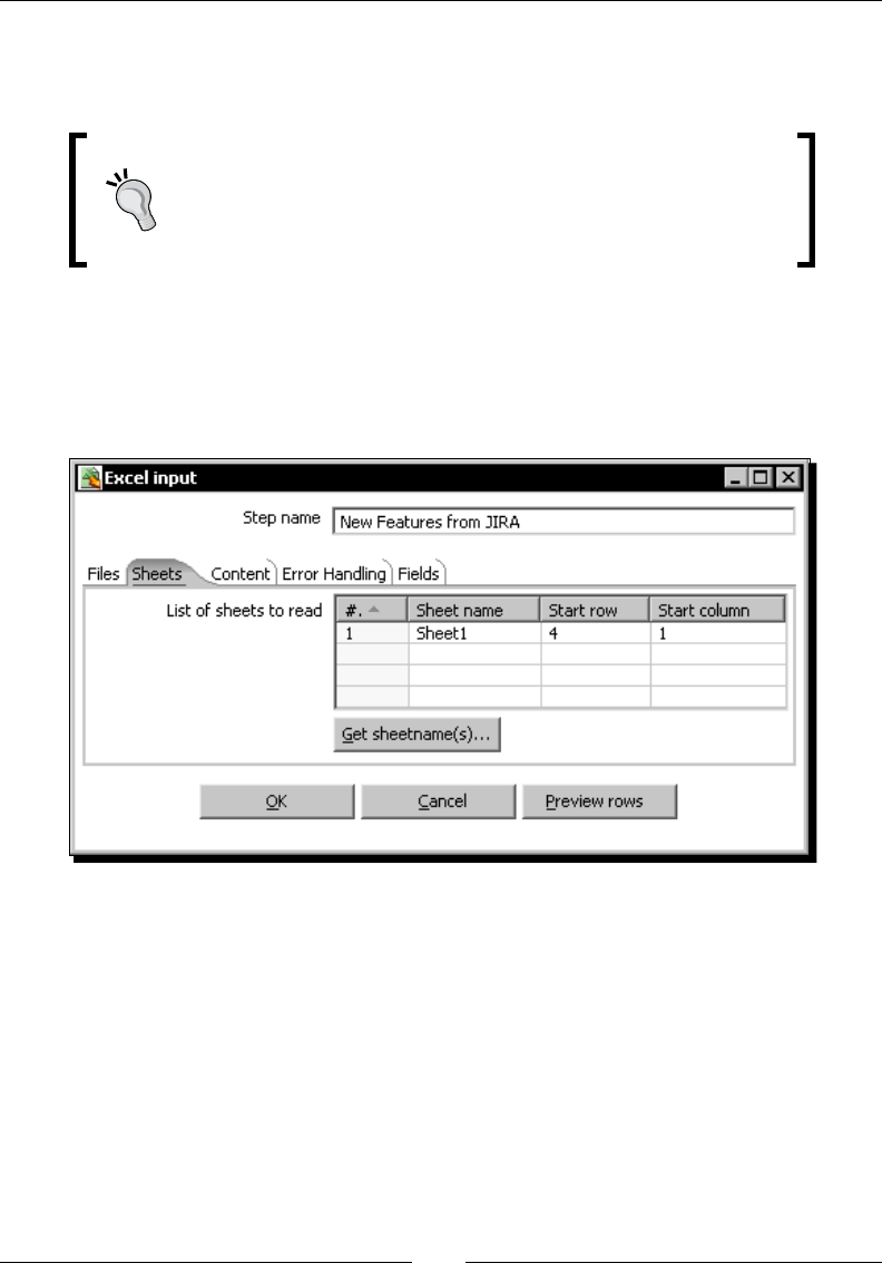
Chapter 4
[ 115 ]
5. Above the list, select Current eld to export the list to an Excel le.
6. Save the le to the folder of your choice.
The Excel le exported from the JIRA site is a Microso Excel 97-
2003 Worksheet. PDI doesn't recognize this version of worksheets.
So, before proceeding, open the le with Excel or Calc and convert
it to Excel 97/2000/XP.
7. Create a transformaon.
8. Read the le by using an Excel Input step. Aer selecng the le, click on the Sheets
tab, and ll it as shown in the next screenshot so that it skips the header rows and
the rst column:
9. Click the Fields tab and ll the grid by clicking the Get elds from header
row... buon.
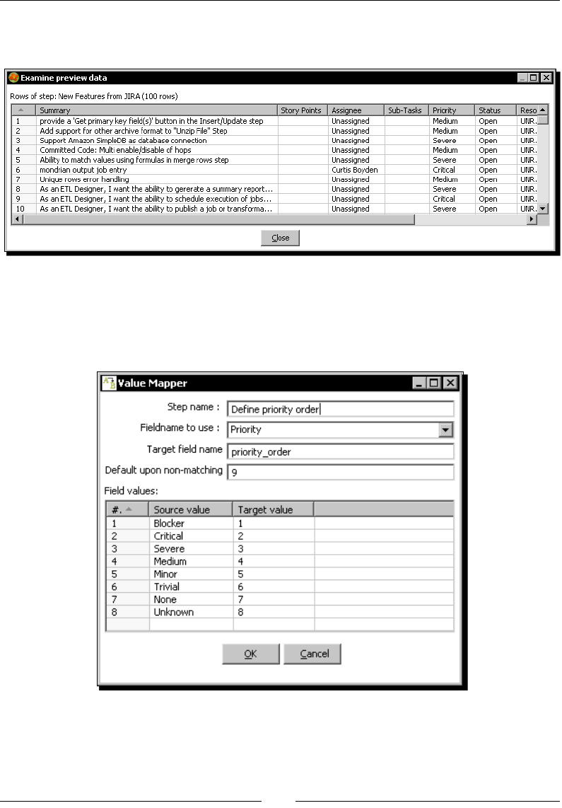
Controlling the Flow of Data
[ 116 ]
10. Click the Preview rows just to be sure that you are reading the le properly. You
should see all the contents of the Excel le except the three heading lines.
11. Click OK.
12. Add a Filter rows step to drop the rows where the Summary eld is null.
13. Aer the Filter rows step, add a Value Mapper step and ll it like here:
14. Aer the Value Mapper step, add a Sort rows step and order the rows by
priority_order (asc.), Summary (asc.).
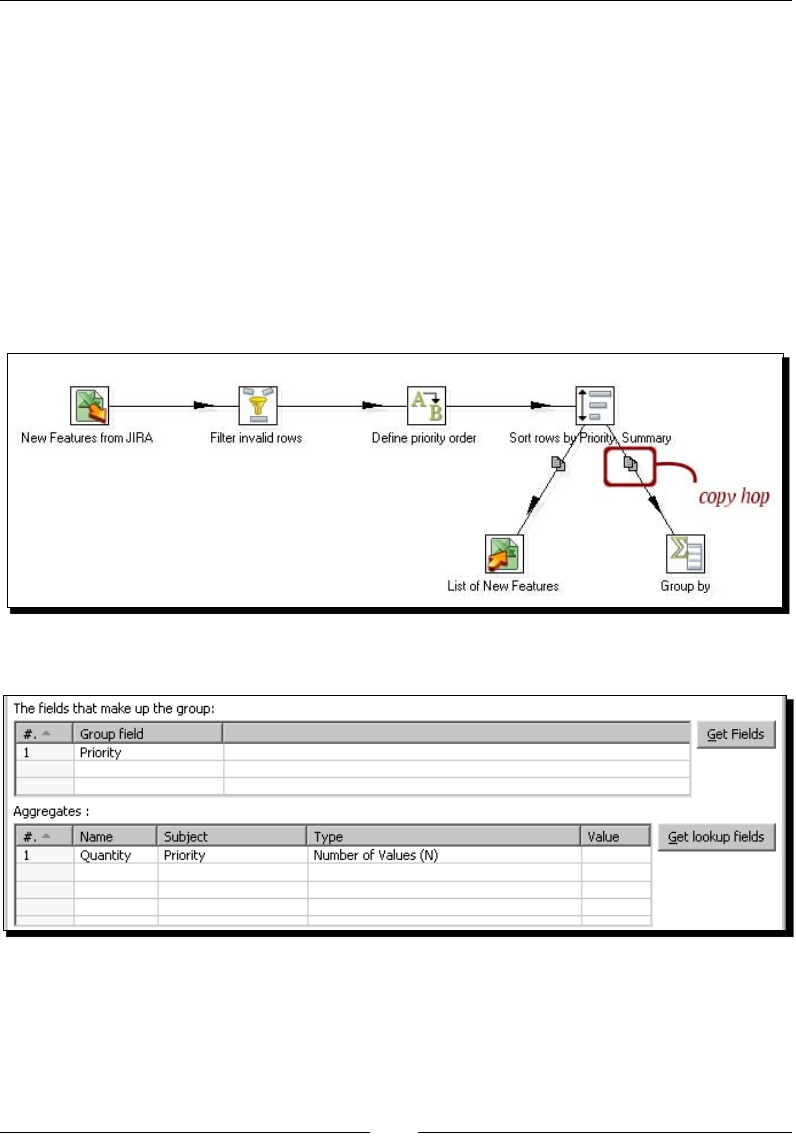
Chapter 4
[ 117 ]
15. Aer that add an Excel Output step, and congure it to send the priority_order
and Summary elds to an Excel le named new_features.xls.
16. Drag a Group by step to the canvas.
17. Create a new hop from the Sort rows step to the Group by step.
18. A warning window appears asking you to decide whether you wish to Copy or
Distribute.
19. Click Copy to send the rows toward both output steps.
20. The hops leaving the Sort rows step change to show you the decision you made. So
far you have this:
21. Congure the Group by steps like shown:
22. Add a new Excel Output step to the canvas and create a hop from the Group by step
to this new step.
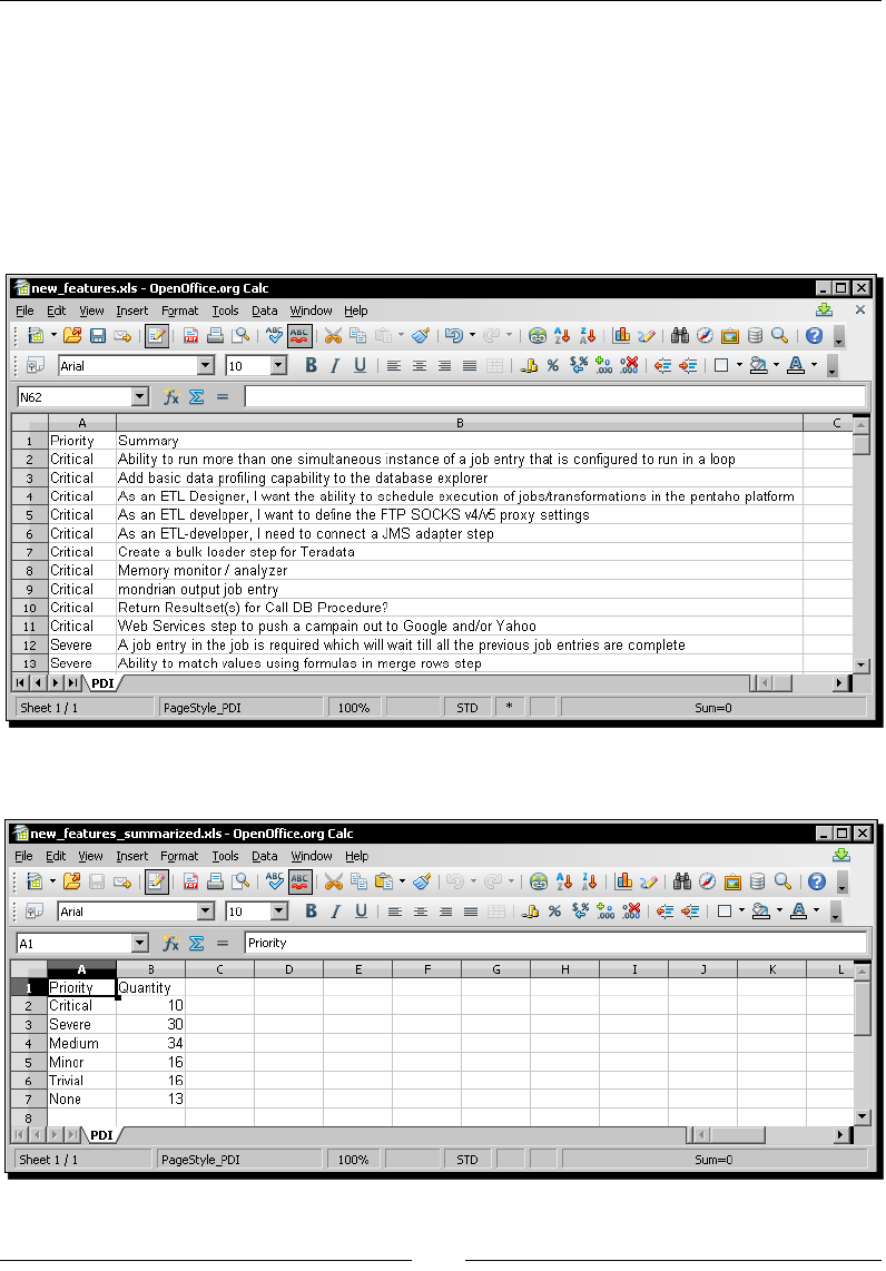
Controlling the Flow of Data
[ 118 ]
23. Congure the Excel Output step to send the Priority and Quantity elds to an
Excel le named new_features_summarized.xls.
24. Save the transformaon and run it.
25. Verify that both les, new_features.xls and new_features_summarized.xls,
have been created.
26. The rst le should look like this:
27. And the second le should look like this:

Chapter 4
[ 119 ]
What just happened?
Aer exporng an Excel le with the PDI new features from the JIRA site, you read the le and
created two Excel les—one with a list of the issues and the other with a summary of the list.
The rst steps of the transformaon are well known—read a le, lter null rows, map a eld,
and sort.
Note that the mapping creates a new eld to give an order to the Priority
eld so that the more severe issues are rst in the list, while the minor priories
remain at the end of the list.
You linked the Sort rows step to two dierent steps. This caused PDI to ask you what to
do with the rows leaving the step. By answering Copy, you told PDI to create a copy of
the dataset. Aer that, two idencal copies le the Sort rows step, each to a dierent
desnaon step.
From the moment you copied the dataset, those copies became independent, each following
its way. The rst copy was sent to a detailed Excel le. The other copy was used to create a
summary of the elds, which then was sent to another Excel le.
Copying rows
At any place in a transformaon, you may decide to split the main stream into two or more
streams. When you do so, you have to decide what to do with the data that leaves the last
step—copy or distribute.
To copy means that the whole dataset is copied to each of the desnaon steps. Once the
rows are sent to those steps, each follows its own way.
When you copy, the hops that leave the step from which you are copying change visually to
indicate the copy acon.
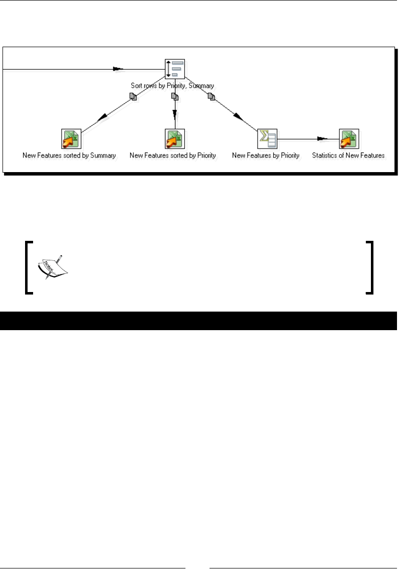
Controlling the Flow of Data
[ 120 ]
In the tutorial, you created two copies of the main dataset. You could have created more
than two, like in this example:
When you split the stream into two or more streams, you can do whatever you want with
each one as if they had never been the same. The transformaons you apply to any of those
output streams will not modify the data in the others.
You shouldn't assume a parcular order in the execuon of the output
streams of a step. All the output streams receive the rows in synch and
you don't have control over the order in which they are executed.
Have a go hero – recalculating statistics
Do you remember the exercise from Chapter 3 where you calculated some stascs? You
created two transformaons. One was to generate a le with students that failed. The other
was to create a le with some stascs such as average grade, number of students who
failed, and so.
Now you can do all that work in a single transformaon, reading the le once.
Distributing rows
As said, when you split a stream, you can copy or distribute the rows. You already saw that
copy is about creang copies of the whole dataset and sending each of them to each output
stream. To distribute means the rows of the dataset are distributed among the desnaon
steps. Let's see how it works through a modied exercise.
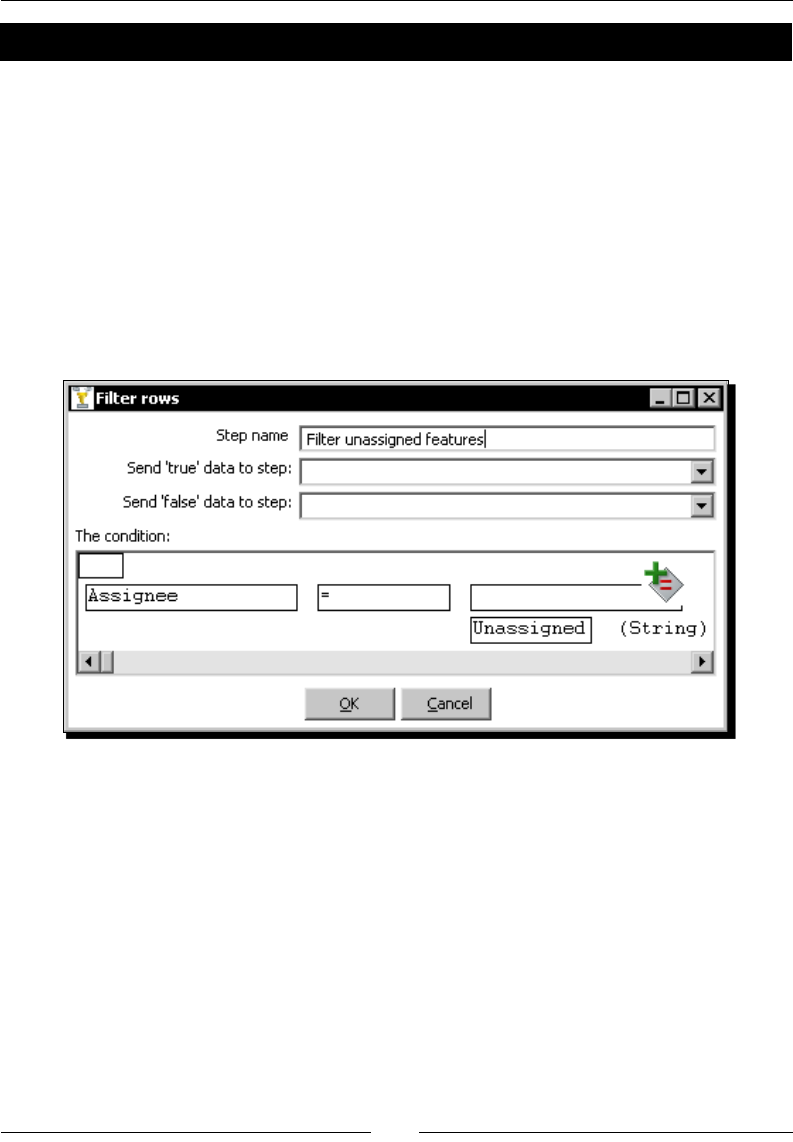
Chapter 4
[ 121 ]
Time for action – assigning tasks by distributing
Let's suppose you want to distribute the issues among three programmers so that each of
them implements a subset of the new features.
1. Select Transformaon | Copy transformaon to clipboard in the main menu.
Close the transformaon and select Transformaon | Paste transformaon from
clipboard. A new transformaon is created idencal to the one you copied. Change
the descripon and save the transformaon under a dierent name.
2. Now delete all the steps aer the Sort rows step.
3. Change the lter step to keep only the unassigned issues: Assignee eld equal to
the string Unassigned. The condion looks like the next screenshot:
4. From the Transform category of steps, drag an Add sequence step to the canvas and
create a hop from the Sort rows step to this new step.
5. Double-click the Add sequence step and replace the content of the Name of value
textbox with nr.
6. Drag three Excel Output steps to the canvas.
7. Link the Add sequence step to one of these steps.
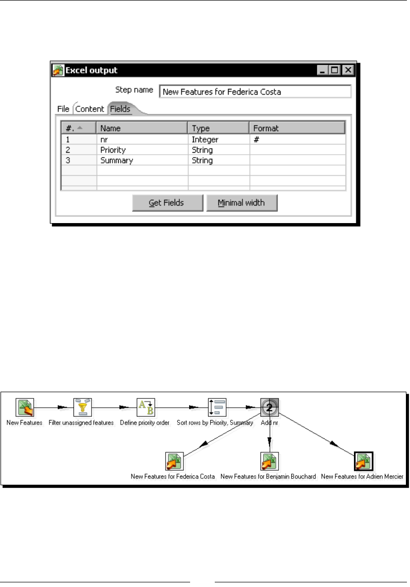
Controlling the Flow of Data
[ 122 ]
Congure the Excel Output step to send the elds nr, Priority, and Summary to an Excel
le named f_costa.xls (the name of one of the programmers). The Fields tab should look
like this:
8. Create a hop from the Add sequence step to the second Excel Output step. When
asked to decide between Copy and Distribute, select Distribute.
9. Congure the step like before, but name the le as b_bouchard.xls
(the second programmer).
10. Create a hop from the Add sequence step to the last Excel Output step.
11. Congure this last step like before, but name the le as a_mercier.xls
(the last programmer).
12. The transformaon should look like the following:
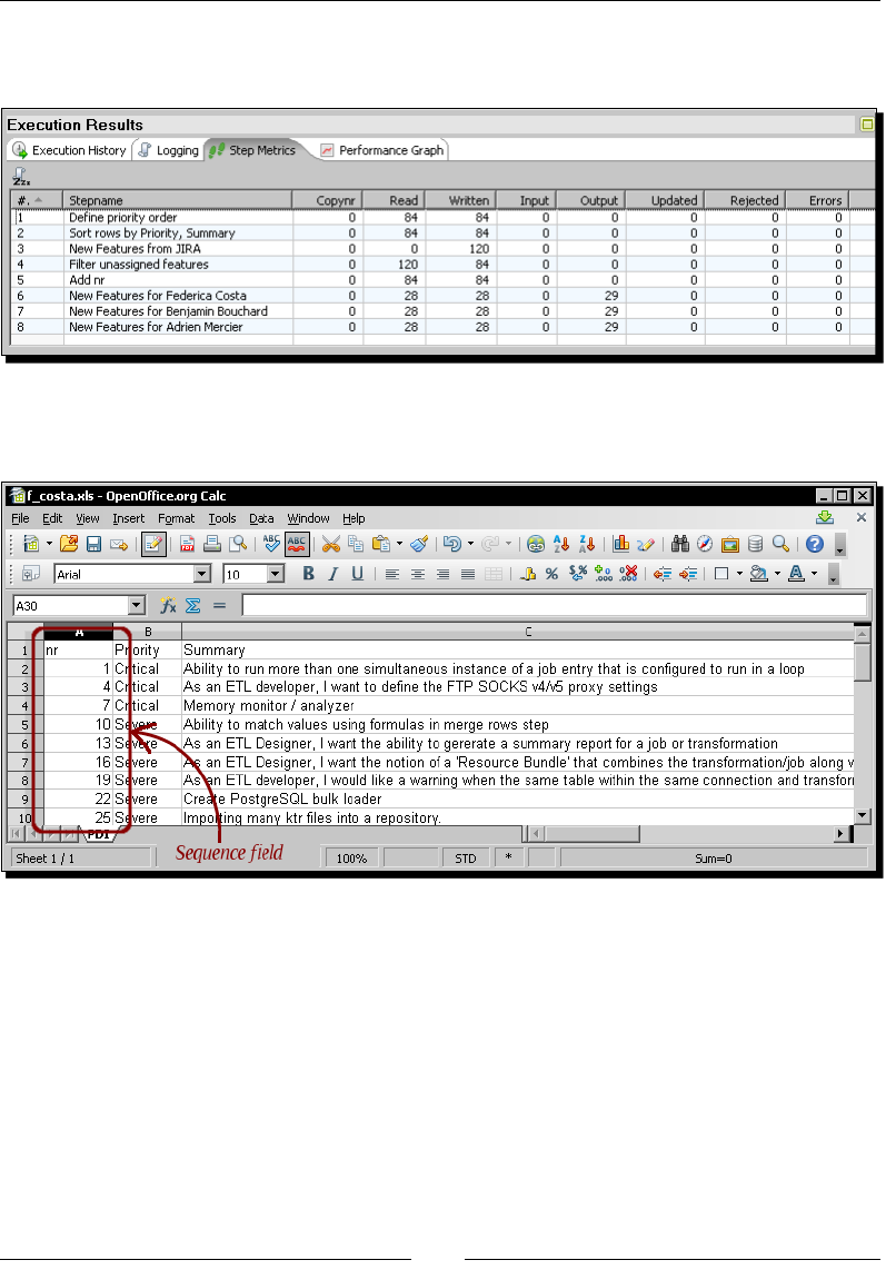
Chapter 4
[ 123 ]
13. Run the transformaon and look at the execuon tab window to see
what happened:
14. To see which rows belong to which of the created les, open any of them. It should
look like this:
What just happened?
You distributed the issues among three programmers.
In the execuon window, you could see that 84 rows leave the Add sequence step, and 28
arrive to each of the Excel Output steps, that is, a third of the number of rows to each of
them. You veried that when you explored the Excel les.
In the transformaon, you added an Add sequence step that did nothing more than adding
a sequenal number to the rows. This sequence helps you recognize that one out of every
three rows were distributed to every le.
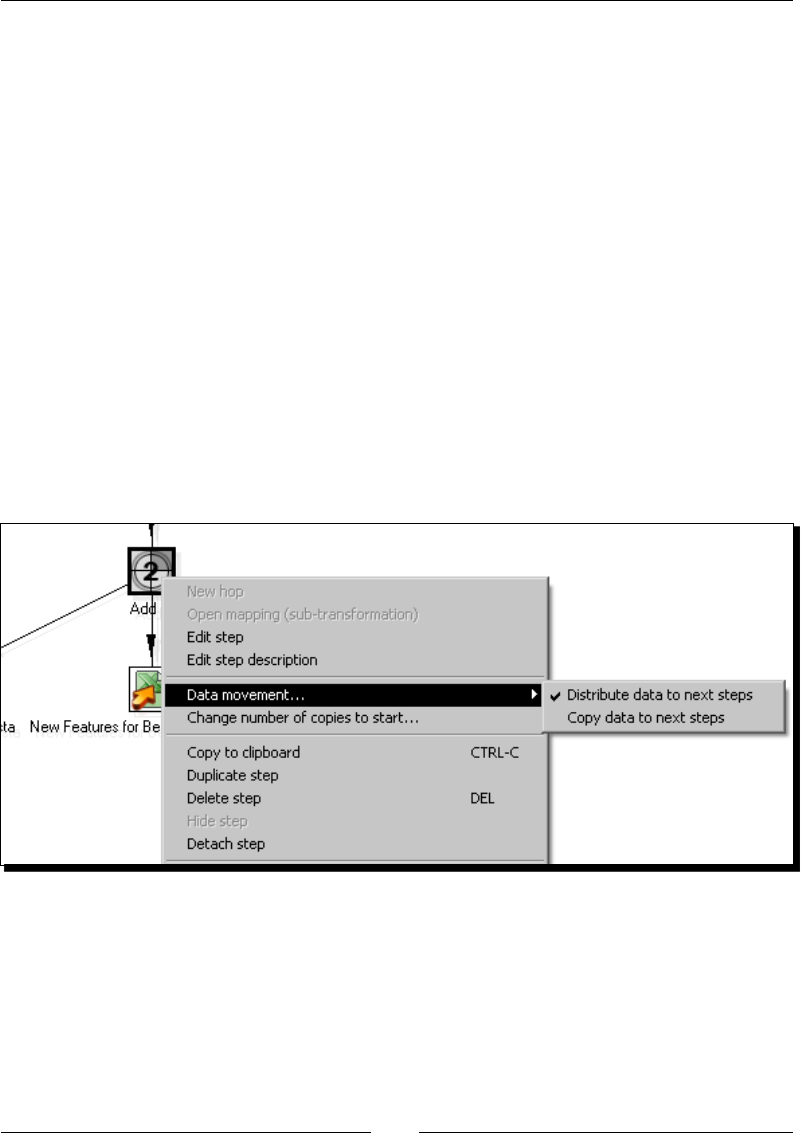
Controlling the Flow of Data
[ 124 ]
Here you saw a praccal example for the distribung opon. When you distribute, the
desnaon steps receive the rows in turn. For example, if you have three target steps, the
rst row goes to the rst target step, the second row goes to the second step, the third row
goes to the third step, the fourth row now goes to the rst step, and so on.
As you could see, when distribung, the hop leaving the step from which you distribute is
plain; it doesn't change its look and feel.
Despite this example showing clearly how the Distribute… method works, this is not how
you will regularly use this opon. The Distribute… opon is mainly used for performance
reasons. Throughout this book you will always use the Copy… opon. To avoid being asked
for the acon to take every me you create more that one hop leaving a step, you can set
the Copy… opon as default; you do this by opening the PDI opons window (Edit|Opons
… from the main menu) and unchecking the opon Show "copy or distribute" dialog?.
Remember that to see the change applied, you will have to restart Spoon.
Once you have changed this opon, the default method is copying rows. If you want to
distribute rows, you can change the acon by right-clicking the step from which you want
to copy or distribute, selecng Data Movement... in the contextual menu that appears, and
then selecng the desired opon.
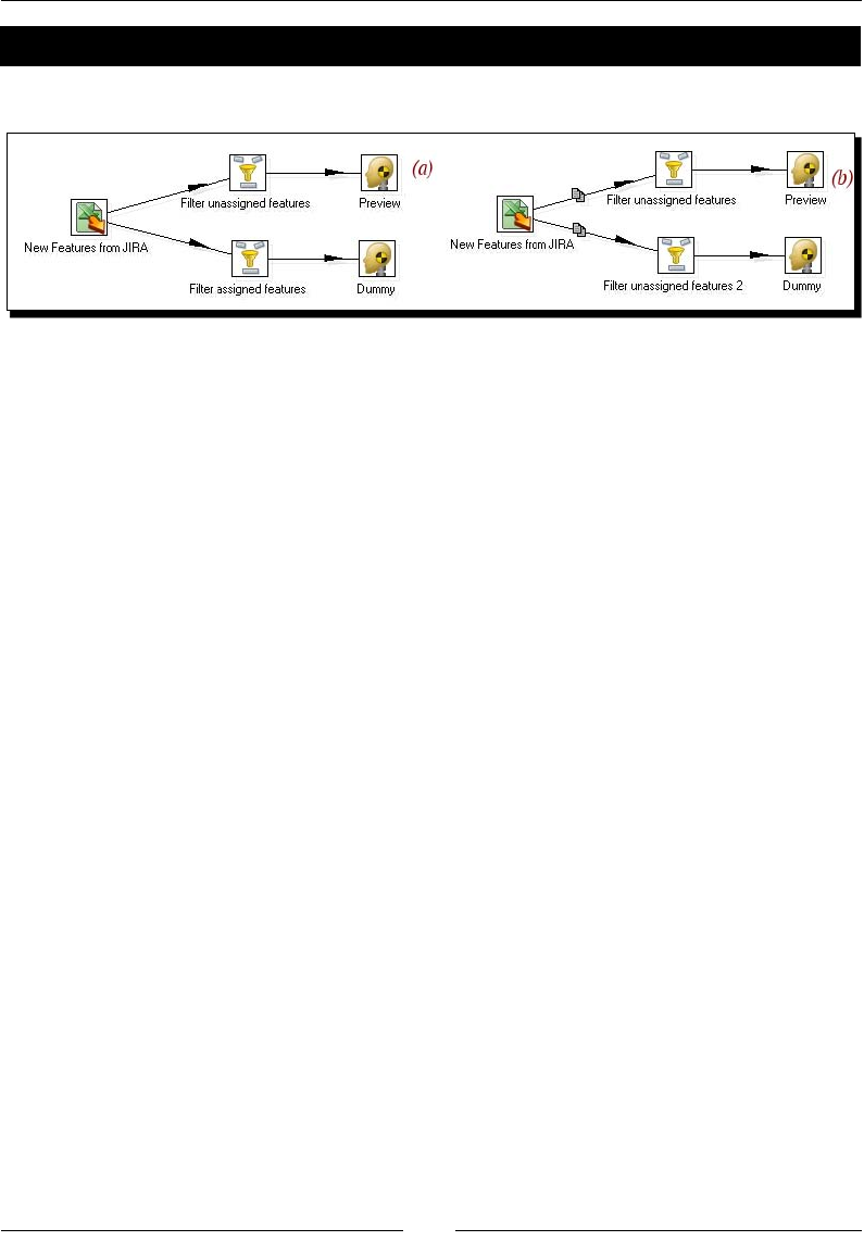
Chapter 4
[ 125 ]
Pop quiz – data movement (copying and distributing)
Look at the following transformaons:
If you do a preview on the Steps named Preview, which of the following is true:
a. The number of rows you see in (a) is greater or equal than the number of rows you
see in (b)
b. The number of rows you see in (b) is greater or equal than the number of rows you
see in (a)
c. The dataset you see in (a) is exactly the same as you see in (b) no maer what data
you have in the Excel le.
You can create a transformaon and test each opon to check the results for yourself. To
be sure you understand correctly where and when the rows take one or other way, you can
preview every step in the transformaon, not just the last one.
Splitting the stream based on conditions
In the previous secon you learned to split the main stream of data into two or more
streams. The whole dataset was copied or distributed among the desnaon steps. Now
you will learn how to put condions so that the rows take one way or another depending
on the condions.
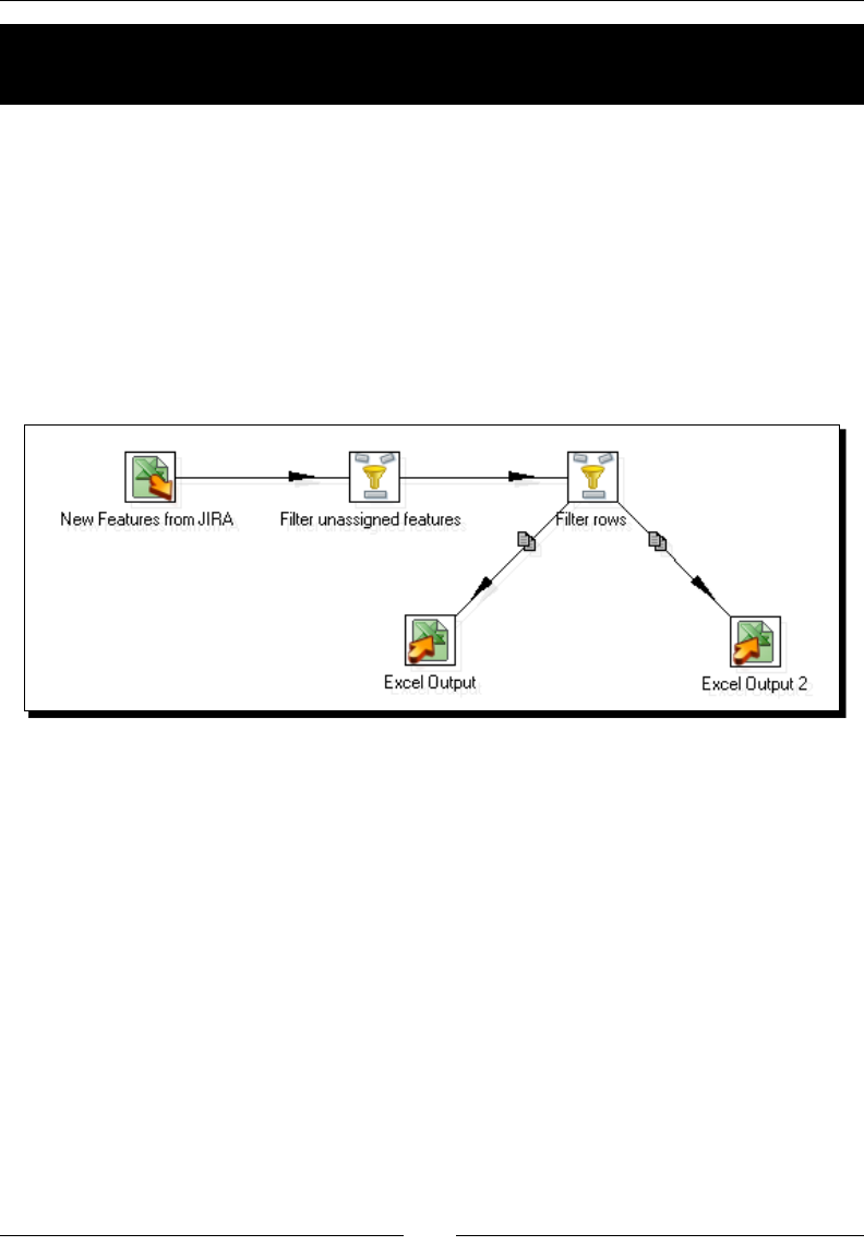
Controlling the Flow of Data
[ 126 ]
Time for action – assigning tasks by ltering priorities with the
Filter rows step
Following with the JIRA subject, let's do a more realisc distribuon of tasks among
programmers. Let's assign the serious task to our most experienced programmer,
and the remaining tasks to others.
1. Create a new transformaon.
2. Read the JIRA le and lter the unassigned tasks, just as you did in the
previous tutorial.
3. Add a Filter rows step and two Excel Output steps to the canvas, and link them to
the other steps as follows:
4. Congure one of the Excel Output steps to send the elds, Priority and Summary,
to an Excel le named b_bouchard.xls (the name of the senior programmer).
5. Congure the other Excel Output step to send the elds Priority and Summary to
an Excel le named new_features_to_develop.xls.
6. Double-click the Filter row step to edit it.
7. Enter the condion Priority = Critical OR Priority = Severe.
8. From the rst drop-down list, Send 'true' data to step, select the step that creates
the b_bouchard.xls Excel le.
9. From the other drop-down list, Send 'false' data to step, select the step that creates
the Excel new_features_to_develop.xls Excel le.
10. Click OK.
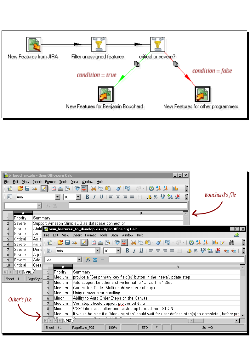
Chapter 4
[ 127 ]
11. The hops leaving the Filter rows step change to show which way a row will take,
depending on the result of the condion.
12. Save the transformaon.
13. Run the transformaon, and verify that the two Excel les were created.
14. The les should look like this:
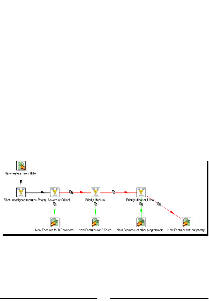
Controlling the Flow of Data
[ 128 ]
What just happened?
You sent the list of PDI new features to two Excel les—one le with the crical issues and
the other le with the rest of the issues.
In the Filter row step, you put a condion to evaluate if the priority of a task was severe
or crical. For every row coming to the lter, the condion was evaluated. The rows that
had a severe or crical priority were sent toward the Excel Output step that creates the
b_bouchard.xls le. The rows with another priority were sent towards the other Excel
Output step, the one that creates the new_features_to_develop.xls le.
PDI steps for splitting the stream based on conditions
When you have to make a decision, and upon that decision split the stream in two, you can
use the Filter row step as you did in this last exercise. In this case, the Filter rows step acts as a
decision maker. It has a condion and two possible desnaons. For every row coming to the
lter, the step evaluates the condion. Then if the result of the condion is true, it decides
to send the row toward the step selected in the rst drop-down list of the conguraon
window—Send 'true' data to step.
If the result of the condion is false, it sends the row toward the step selected in the second
drop-down list of the conguraon window: Send 'false' data to step.
Somemes you have to make nested decisions; consider the next gure for example:
In the transformaon shown in the preceding diagram, the condions are as simple as tesng
if a eld is equal to a value. In situaons like this you have a simpler way for accomplishing
the same..
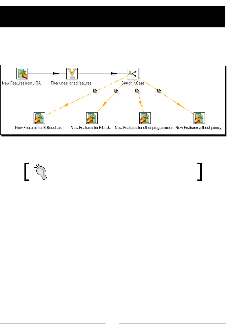
Chapter 4
[ 129 ]
Time for action – assigning tasks by ltering priorities with the
Switch/ Case step
Let's use a Switch/Case step to replace the nested Filter Rows steps shown in the
preceding diagram
1. Create a transformaon like the following:
2. You will nd the Switch/Case step in the Flow category of steps.
To save me, you can take the last transformaon you created
as the starng point.
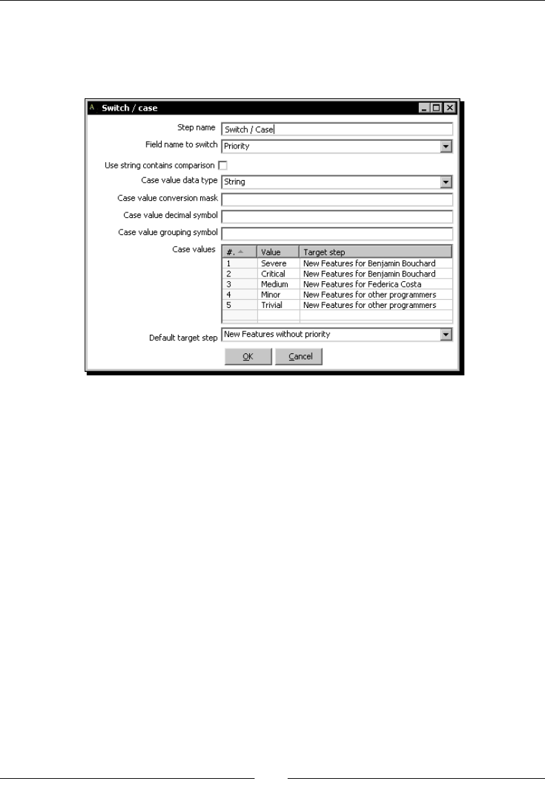
Controlling the Flow of Data
[ 130 ]
3. Note that the hops arriving to the Excel Output steps look strange. They are doed
orange lines. This look and feel shows you that the target steps are unreachable. In
this case, it means that you sll have to congure the Switch/Case step. Double-click
it and ll it like here:
4. Save the transformaon and run it
5. Open the Excel les generated to see that the transformaon distributed the task among
the les based on the given condions.
What just happened?
In this tutorial you learned to use the Switch/Case step. This step routes rows of data to one
or more target steps based on the value encountered in a given eld.
In the Switch/Case step conguraon window, you told Kele where to send the row
depending on a condion. The condion to evaluate was the equality of the eld set in Field
name to switch and the value indicated in the grid. In this case, the eld name to switch
is Priority, and the values against which it will be compared are the dierent values for
priories: Severe, Crical, and so on. Depending on the values of the Priority eld, the rows
will be sent to any of the target steps. For example, the rows where Priority=Medium, will be
sent toward the target step New Features for Federica Costa.
Note that it is possible to specify the same target step more than once.
The Default target step represents the step where the rows that don't match any of the case
values are sent. In this example, the rows with a priority not present in the list will be sent to
the step New Features without priority.

Chapter 4
[ 131 ]
Have a go hero – listing languages and countries
Open the transformaon you created in the Finding out which language people speak
tutorial in Chapter 3. If you run the transformaon and check the content of the output le,
you'll noce that there are missing languages. Modify the transformaon so that it generates
two les—one with the rows where there is a language, that is, the rows for which the
lookup didn't fail, and another le with the list of countries not found in the countries.
xml le.
Pop quiz – splitting a stream
Connuing with the contestant exercise, suppose that the number of interpreters you will
hire depends on the number of people that speak each language:
Number of people that speaks the language Number of interpreters
Less than 3 1
Between 3 and 6 2
More that 6 3
You want to create a le with the languages with a single interpreter, another le with the
languages with two interpreters, and a nal le with the languages with three interpreters.
Which of the following would solve your situaon when it comes to spling the languages
into three output streams:
a. A Number range step followed by a Switch/Case step.
b. A Switch/Case step.
c. Both
In order to gure out the answer, create a transformaon and count the number
of people that speak each language. You'll have to use a Sort rows step followed
by a Group by step. Aer that, try to develop each alternave soluon and see
what happens.
Merging streams
You've just seen how the rows of a dataset can take dierent paths. Here you will learn the
opposite—how data coming from dierent places is merged into a single stream.
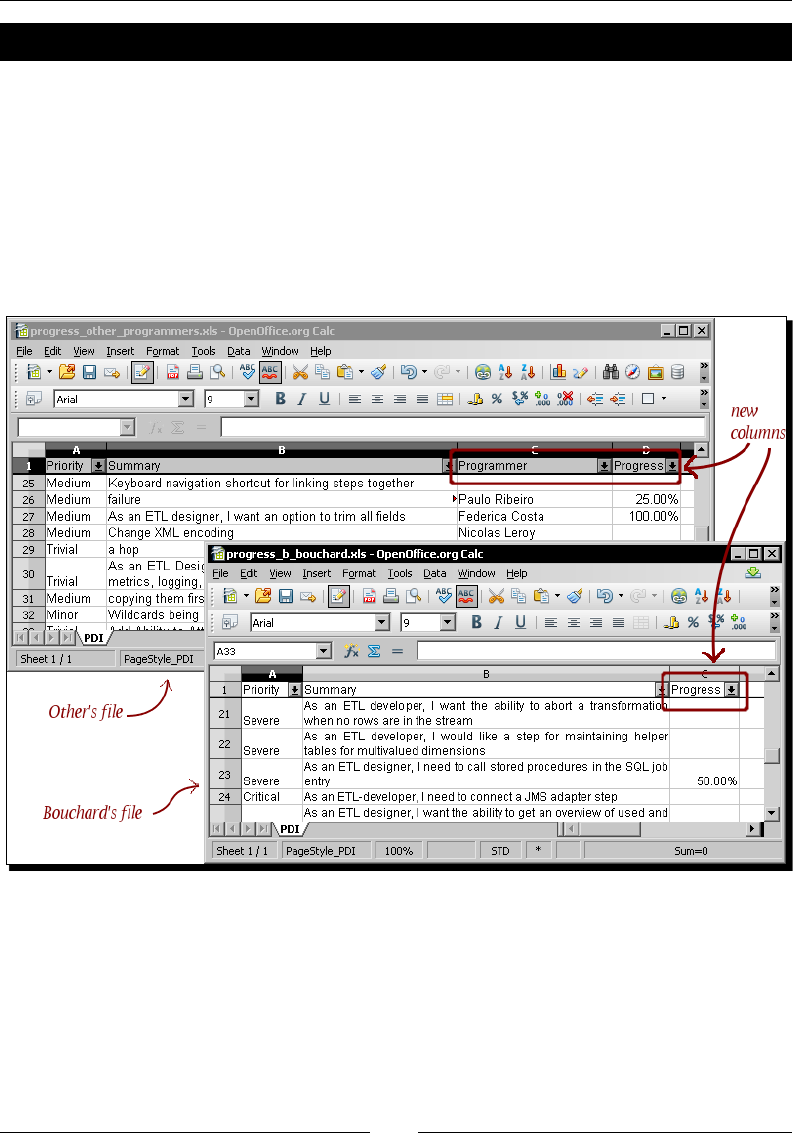
Controlling the Flow of Data
[ 132 ]
Time for action – gathering progress and merging all together
Suppose that you delivered the Excel les you generated in the Assigning tasks by ltering
priories tutorial earlier in the chapter. You gave the b_bouchard.xls to Benjamin
Bouchard, the senior programmer. You also gave the other Excel le to a project leader who
is going to assign the tasks to dierent programmers. Now they are giving you back the
worksheets, with a new column indicang the progress of the development. In the case of
the shared le, there is also a column with the name of the programmer who is working on
every issue. Your task is now to unify those sheets.
Here is what the Excel les look like:
1. Create a new transformaon.
2. Drag an Excel Input step to the canvas and read one of the les.
3. Add a Filter row step to keep only the rows where the progress is not null, that is,
the rows belonging to tasks whose development has been started.
4. Aer the lter, add a Sort rows step, and congure it to order the elds by
Progress, in descending order.

Chapter 4
[ 133 ]
5. Add another Excel Input step, read the other le, and lter and sort the rows just
like you did before. Your transformaon should look like this:
6. From the Transform category of steps, select the Add Constants step and drag it
onto the canvas.
7. Link the step to the stream that reads the B. Bouchard's le; edit the step and add a
new eld named Programmer, with type string and value Benjamin Bouchard.
8. Aer this step, add a Select values step and reorder the elds so that they remain
in a specic order Priority, Summary, Programmer, Progress—to resemble the
other stream.
9. Now, from the Transform category add an Add sequence step, name the new eld
ID, and link the step with the Select values step.
10. Create a hop from the Sort rows step of the other stream to the Add sequence step.
Your transformaon should look like the one shown next:
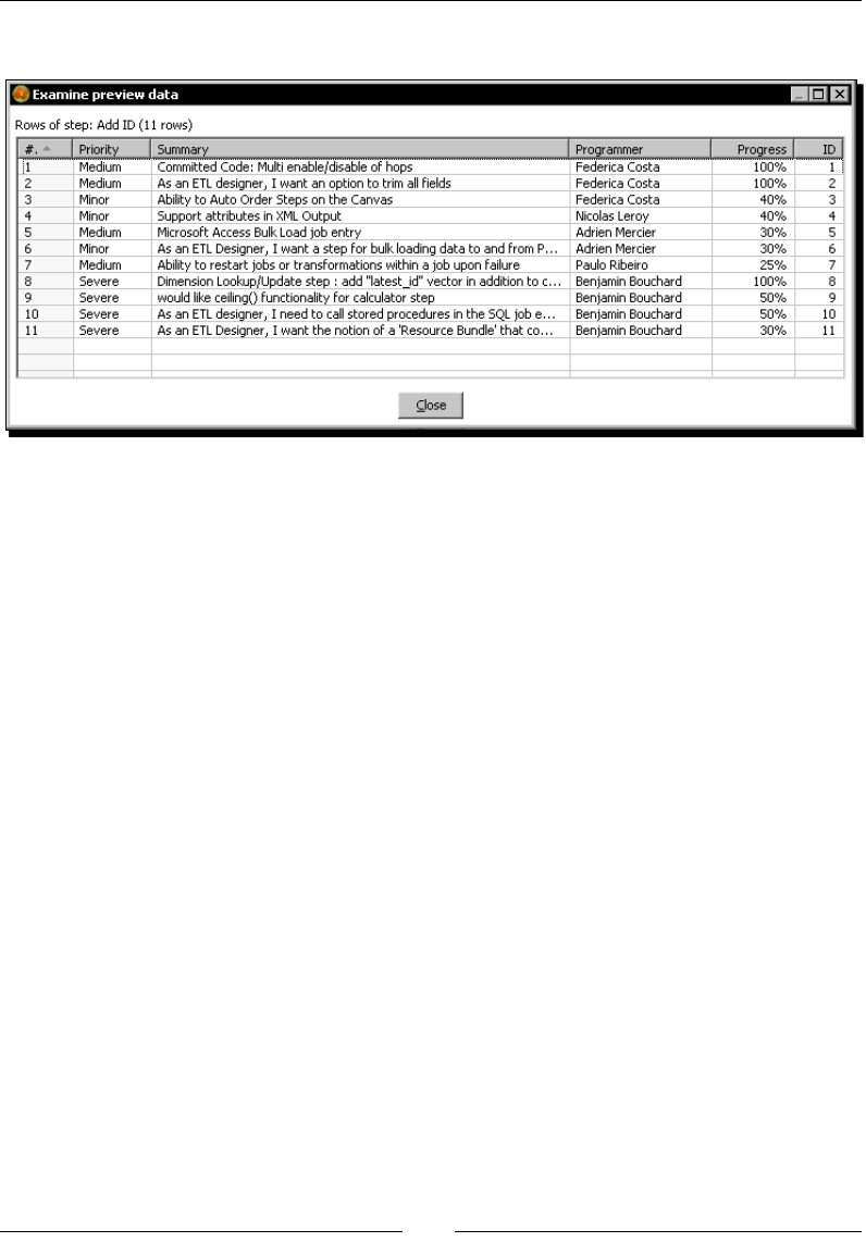
Controlling the Flow of Data
[ 134 ]
11. Select the Add sequence step and do a preview. You will see this:
What just happened?
You read two similar Excel les and merged them into one single dataset.
First of all, you read, ltered, and sorted the les as usual. Then you altered the stream
belonging to B. Bouchard, so it looked similar to the other. You added the eld Programmer,
and reordered the elds.
Aer that, you used an Add sequence step to create a single dataset containing the rows of
both streams, with the rows numbered.
PDI options for merging streams
You can create a union of two or more streams anywhere in your transformaon. To create a
union of two or more data streams, you can use any step. The step unies the data, takes the
incoming streams in any order, and then it completes its task in the same way as if the data
came from a single stream.
In the example, you used an Add sequence step as the step to join two streams. The step
gathered the rows from the two streams, and then proceeded to numerate the rows with
the sequence name ID.
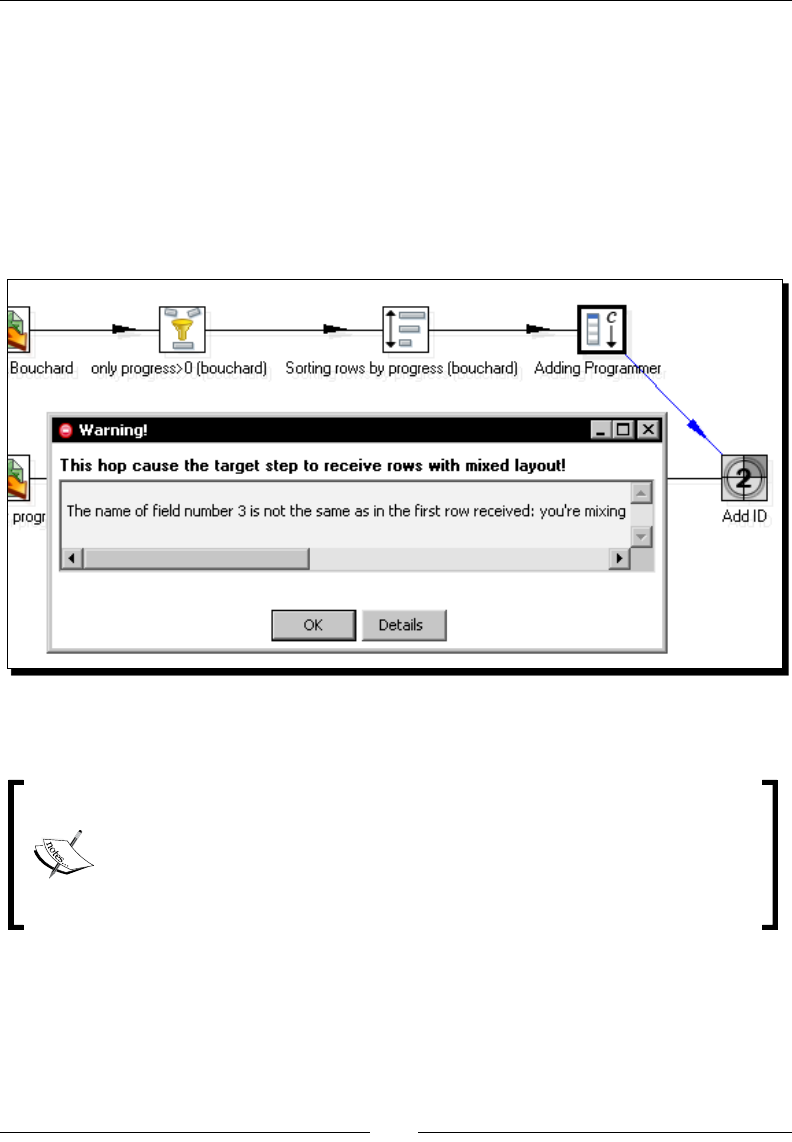
Chapter 4
[ 135 ]
This is only one example of how you can mix streams together. As said, any step can be used
to unify two streams. Whichever the step, the most important thing you have to have in
mind is that you cannot mix rows that have a dierent layout. The rows have to have the
same lengths, the same data types, and the same elds in the same order.
Fortunately, there is a trap detector that provides warnings at design me if a step is
receiving mixed layouts.
You can try this out. Delete the Select values step. Create a hop from the Add constants step
to the Add sequence step. A warning message appears as shown next:
In this case, the third eld of the rst stream, Programmer (String), does not have the
same name or the same type as the third eld of the second stream, Progress (Number).
Note that PDI warns you but it doesn't prevent you from mixing row layouts
when creang the transformaon.
If you want Kele to prevent you from running transformaons with mixed row
layouts, you can check the opon Enable safe mode in the window that shows
up when you dispatch the transformaon. Have in mind that doing this will
cause a performance drop.

Controlling the Flow of Data
[ 136 ]
When you use an arbitrary step to unify, the rows remain in the same order as they
were in their original stream, but the streams are joined in any order. Take a look at the
example's preview. The rows of the Bouchard's stream as well as the rows of the other
stream remained sorted within its original group. However, whether the Bouchard's stream
appeared before or aer the rows of the other stream was just a maer of chance. You
didn't decide the order of the streams; PDI decided it for you. If you care about the order in
which the union is made, there are some steps that can help you. Here are the opons
you have:
If you want to ... You can do this ...
Append two or more streams, and
don't care about the order
Use any step. The selected step will take all the incoming
streams in any order, and then will proceed with its specic
task.
Append two streams in a given order Use the Append streams step from the Flow category. It
helps to decide which stream goes rst.
Merge two streams ordered by one or
more elds
Use a Sorted Merge step from the Joins category. This
step allows you to decide on which eld(s) to order the
incoming rows before sending them to the desnaon
step(s). The input streams must be sorted on that eld(s).
Merge two streams keeping the newest
when there are duplicates
Use a Merge Rows (di) step from the Joins category.
You tell PDI the key elds, that is, the elds that say that
a row is the same in both streams. You also give PDI the
elds to compare when the row is found in both streams.
PDI tries to match rows of both streams, based on the key
elds. Then it creates a eld that will act as a ag, and lls
it as follows:
If a row was only found in the rst stream, the
ag is set to deleted.
If a row was only found in the second stream, the
ag is set to new.
If the row was found in both streams, and the
elds to compare are the same, the ag is set to
identical.
If the row was found in both streams, and at least
one of the elds to compare is dierent, the ag
is set to changed.
Let's try one of these opons.
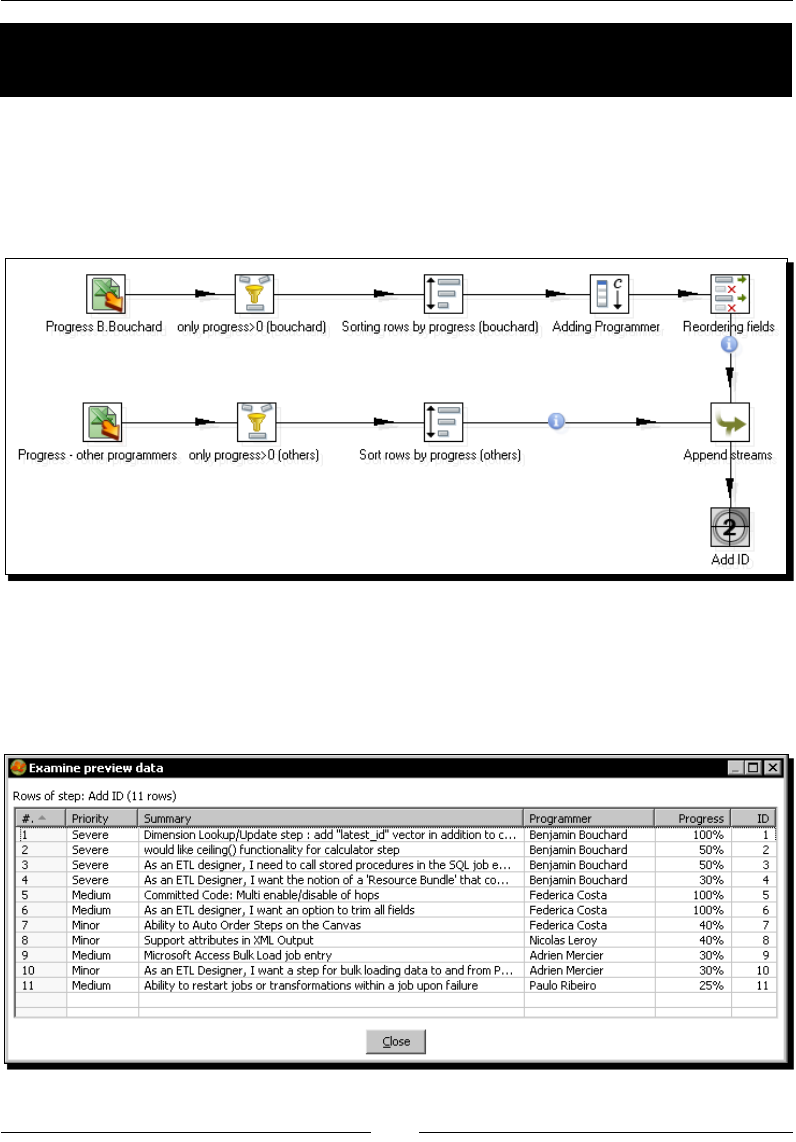
Chapter 4
[ 137 ]
Time for action – giving priority to Bouchard by using
Append Stream
Suppose you want the Bouchard's row before the other rows. You can modify the
transformaon as follows:
1. From the Flow category of steps, drag an Append Streams step to the canvas.
Rearrange the steps and hops so the transformaon looks like this:
2. Edit the Append streams step and select as the Head hop the one belonging to the
Bouchard's rows, and as the Tail hop the other. Doing this, you indicate toPDI how it
has to order the streams.
3. Do a preview on the Add sequence step. You should see this:
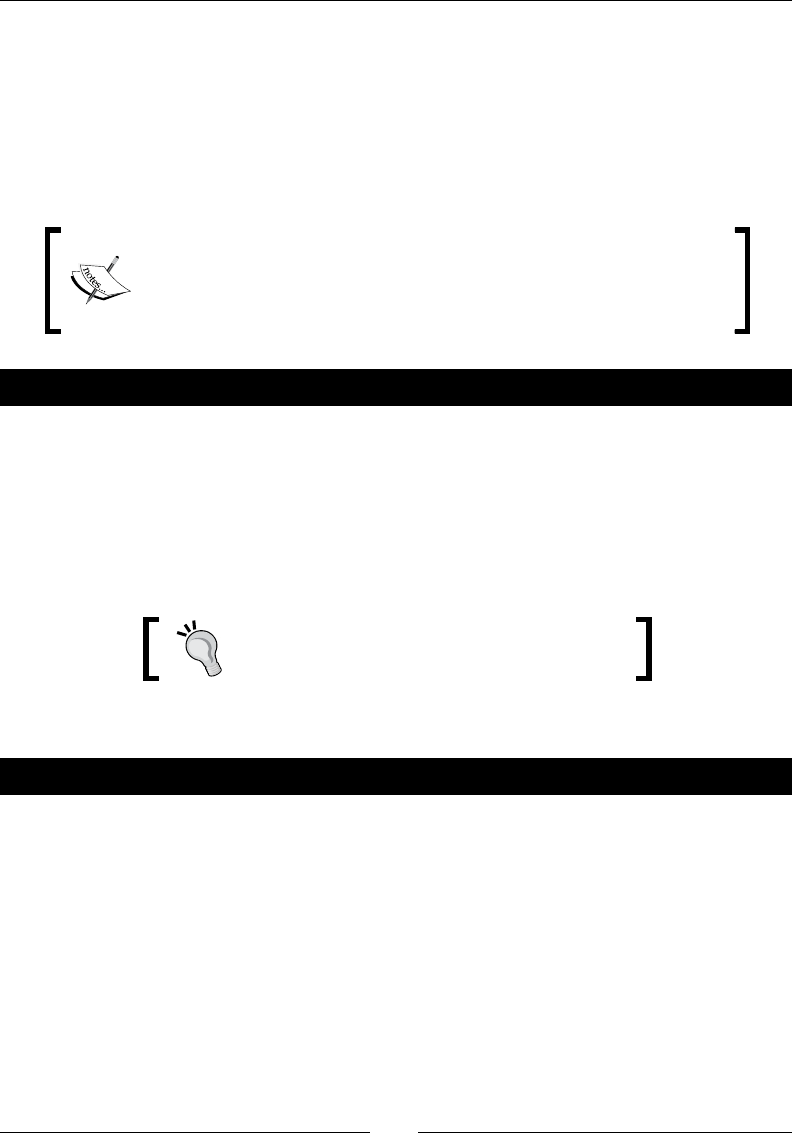
Controlling the Flow of Data
[ 138 ]
What just happened?
You changed the transformaon to give priority to Bouchard's issues.
You made it by using the Append Streams step. By telling that the head hop was the one coming
from the Bouchard's le, you got the expected order—rst the rows with the tasks assigned
to Bouchard, sorted by progress descending, and then the rows with the tasks assigned to
other programmers, also sorted by progress descending.
Whether you use arbitrary steps or some of the special steps menoned
here to merge streams, don't forget to verify the layouts of the streams
you are merging. Pay aenon to the warnings of the trap detector and
avoid mixing row layouts.
Have a go hero – sorting and merging all tasks
Modify the previous exercise so that the nal output is sorted by priority. Try two possible
soluons:
Sort the input streams on their own and then use a Sorted Merge step.
Merge the stream with a Dummy step and then sort.
Which one do you think would give the best performance?
Refer to the Sort rows step issues in Chapter 3.
In which circumstances would you use the other opon?
Have a go hero – trying to nd missing countries
As you saw in the countries exercises, there are missing countries in the countries.xml
le. In fact, the countries are there, but with dierent names. For example, Russia in the
contestant le is Russian Federation in the XML le. Modify the transformaon that
looks for the language. Split the stream in two—one for the rows where a language was
found and the other for the rows where no language was found. For this last stream, use a
Value Mapper step to rename the countries you idened as wrong, that is, rename Russia
as Russian Federation. Then look again for a language now with the new name. Finally,
merge the two streams and create the output le with the result.

Chapter 4
[ 139 ]
Summary
In this chapter, you learned dierent opons that PDI oers to combine or split ows of data.
The chapter covered the following:
Copying and distribung rows
Spling streams based on condions
Merging independent streams in dierent ways
With the concepts you learned in the inial chapters, the range of tasks you are able to
perform is already broad. In the next chapter, you will learn how to insert JavaScript code in
your transformaons not only as an alternave to perform some of those tasks, but also as
a way to accomplish other tasks that are complicated or even unthinkable to carry out with
regular PDI steps.

5
Transforming Your Data
with JavaScript Code and the
JavaScript Step
Whichever transformaon you need to do on your data, you have a big chance
of nding that PDI steps are able to do the job. Despite that, it may happen that
there are not proper steps that serve your requirements, or that an apparently
minor transformaon consumes a lot of steps linked in a very confusing
arrangement dicult to test or understand. Pung colorful icons here and
there is funny and praccal, but there are some situaons like the ones
described above where you inevitably will have to code. This chapter explains
how to do it with JavaScript and the special JavaScript step.
In this chapter you will learn how to:
Insert and test JavaScript code in your transformaons
Disnguish situaons where coding is the best opon, from those where there are
beer alternaves
Doing simple tasks with the JavaScript step
One of the tradional steps inside PDI is the JavaScript step that allows you to code inside
PDI. In this secon you will learn how to use it for doing simple tasks.
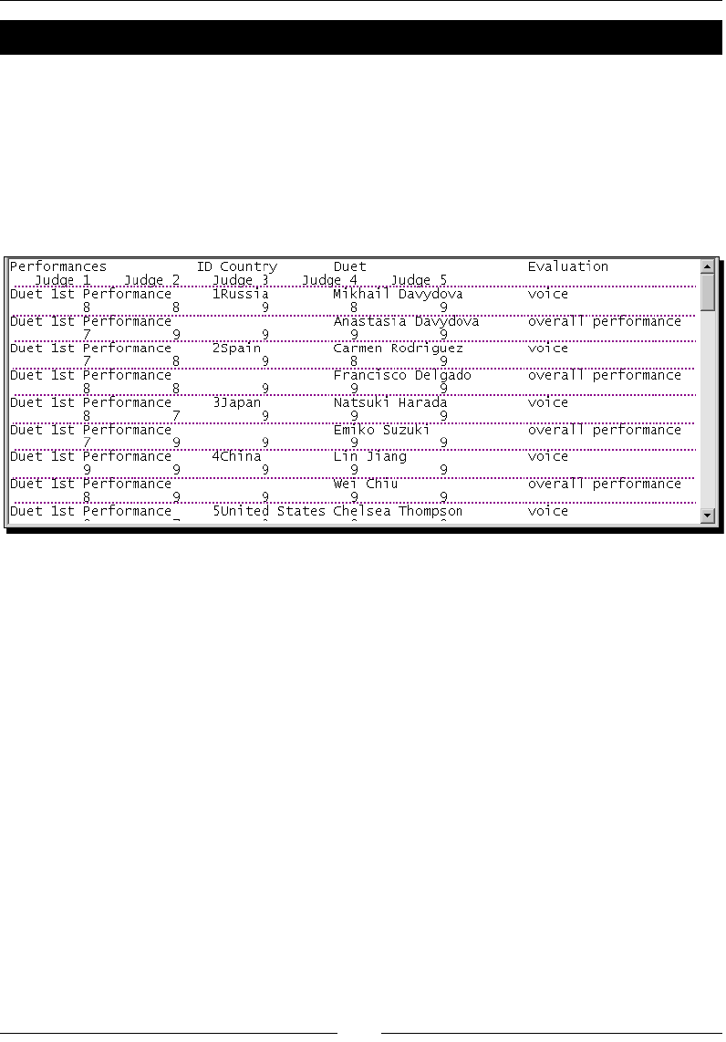
Transforming Your Data with JavaScript Code and the JavaScript Step
[ 142 ]
Time for action – calculating scores with JavaScript
The Internaonal Musical Contest menoned in Chapter 4 has already taken place. Each duet
performed twice. The rst me technical skills were evaluated, while in the second, the focus
was on arsc performance.
Each performance was assessed by a panel of ve judges who awarded a mark out of a
possible 10.
The following is the detailed list of scores:
Note that the elds don't t in the screen, so the lines are wrapped and doed lines are
added for you to disnguish each line.
Now you have to calculate, for each evaluated skill, the overall score as well as an
average score.
1. Download the sample le from the Packt website.
2. Create a transformaon and drag a Fixed le input step to the canvas to read
the le.

Chapter 5
[ 143 ]
3. Fill the conguraon window as follows:
4. Press the Get Fields buon. A window appears to help you dene the columns.
5. Click between the elds to add markers that dene the limits. The window will look
like this:
6. Click on Next >. A new window appears for you to congure the elds.
7. Click on the rst eld at the le of the window and change the name to Performance.
Verify that the type is set to String.

Transforming Your Data with JavaScript Code and the JavaScript Step
[ 144 ]
8. To the right, you will see a preview of the data for the eld.
9. Select each eld to the le of the window, change the names, and adjust the types. Set
ID, Country, Duet, and Skill elds as String, and elds from Judge 1 to Judge
5 as Integer.
10. Go back and forth between these two windows as many mes as you need unl you are
done with the denions of the elds.
11. Click on Finish.
12. The grid at the boom is now lled.
13. Set the column Trim type to both for every eld.
14. The window should look like the following:
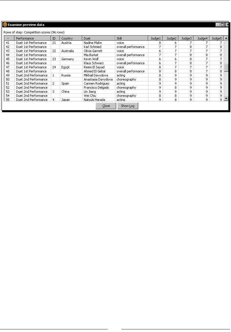
Chapter 5
[ 145 ]
15. Click on Preview the transformaon. You should see this:
16. From the Scripng category of steps, select a Modied JavaScript Value step and drag it
to the canvas.
17. Link the step to the Fixed le input step, and double-click it to congure it.
18. Most of the conguraon window is blank, which is the eding area. Type the following
text in it:
var totalScore;
var wAverage;
totalScore = Judge1 + Judge2 + Judge3 + Judge4 + Judge5;
wAverage = 0.35 * Judge1 + 0.35 * Judge2
+ 0.10 * Judge3 + 0.10 * Judge4 + 0.10 * Judge5;
19. Click on the Get variables buon.
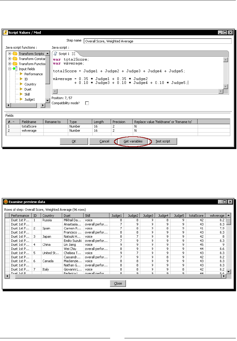
Transforming Your Data with JavaScript Code and the JavaScript Step
[ 146 ]
20. The grid under the eding area gets lled with the two variables dened in the code.
The window looks like this:
21. Click on OK.
22. Keep the JavaScript step selected and do a preview.
23. This is how the nal data looks like:

Chapter 5
[ 147 ]
What just happened?
You read the detailed list of scores and added two elds with the overall score and an
average score for each evaluated skill.
In order to read the le, you used a step you hadn't used before—the Fixed le input step.
You congured the step with the help of a wizard. You could have also lled the eld grid
manually if you wanted to.
Aer reading the le, you used a JavaScript step to create new elds. The code you typed
was pure JavaScript code. In this case, you typed a simple code to calculate the total score
and a weighted average combining the elds from Judge 1 to Judge 5.
Note that the average was dened by giving more weight, that is, more importance, to the
scores coming from Judge 1 and Judge 2.
For example, consider the rst line of the le. This is how the new elds were calculated:
totalScore = Judge1 + Judge2 + Judge3 + Judge4 + Judge5 = 8+8+9+8+9
= 42
wAverage = 0.35*Judge1 + 0.35*Judge2+ 0.10*Judge3 + 0.10*Judge4 +
0.10*Judge5 = 0.35*8 + 0.35*8+ 0.10*8 + 0.10*8 + 0.10*8 = 8.2
In order to add these new elds to your dataset, you brought them to the grid at the boom
of the window.
Note that this is not the only way to do calculaons in PDI. All you did with the JavaScript
step can also be done with other steps.
Using the JavaScript language in PDI
JavaScript is a scripng language primarily used in website development. However, inside PDI
you use just the core language; you neither run a web browser nor do you care about HTML.
There are many available JavaScript engines. PDI uses the Rhino engine, from Mozilla. Rhino
is an open source implementaon of the core JavaScript language; it doesn't contain objects
or methods related to manipulaon of web pages. If you are interested in knowing more
about Rhino, you can visit https://developer.mozilla.org/en/Rhino_Overview.
The core language is not too dierent from other languages you might know. It has basic
statements, block statements (statements enclosed by curly brackets), condional statements
(if..else and switch case), and loop statements ( for, do..while, and while). If you
are interested in the language itself, you can access a good JavaScript guide following this link:
https://developer.mozilla.org/En/Core_JavaScript_1.5_Guide.
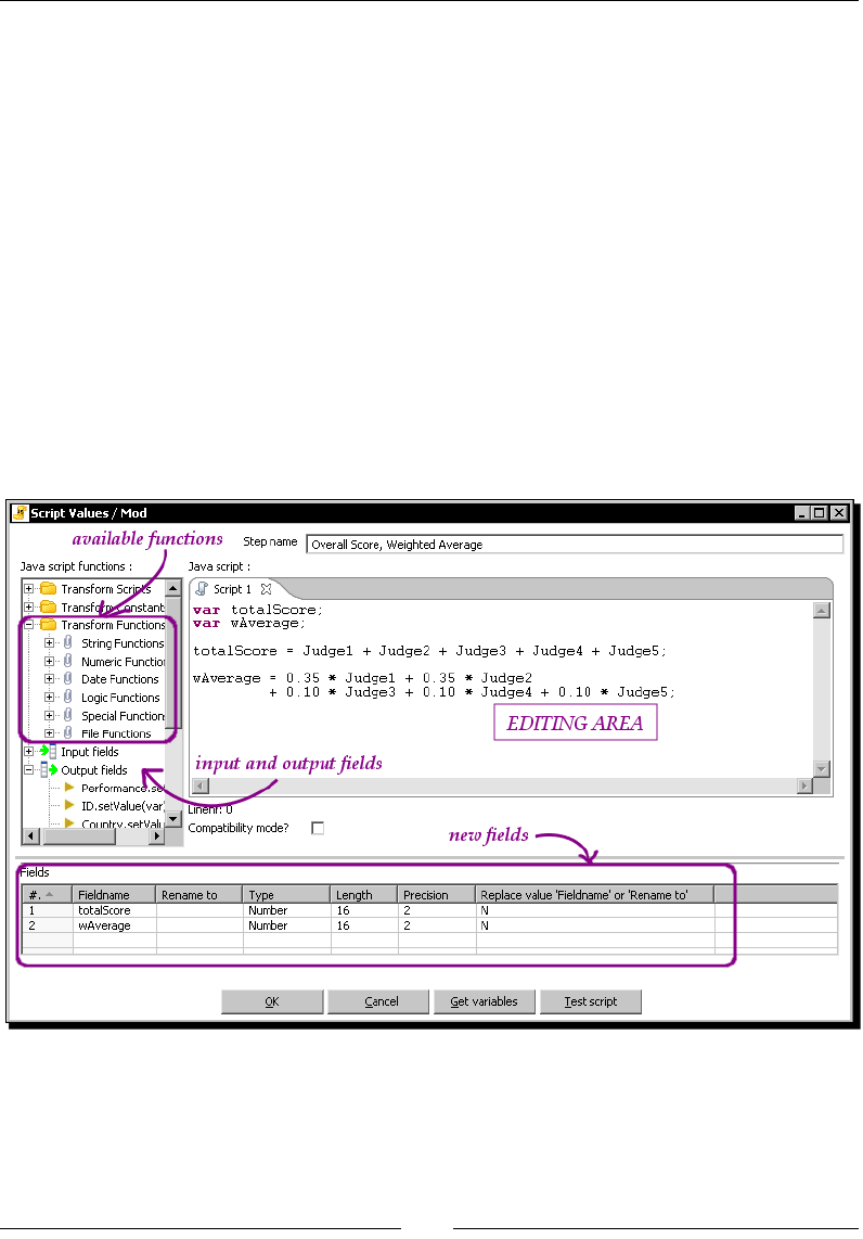
Transforming Your Data with JavaScript Code and the JavaScript Step
[ 148 ]
Besides the basics, an interesng feature included in the PDI implementaon is E4X, a
programming language extension that allows you to manipulate XML objects inside JavaScript.
You can nd an E4X tutorial as well as a reference manual at https://developer.
mozilla.org/En/E4X/Processing_XML_with_E4X.
Finally, there is a complete tutorial and reference at http://www.w3schools.com/
js/. Despite being quite oriented to web development, which is not your concern, it is clear,
complete, and has plenty of examples.
Inserting JavaScript code using the Modied Java Script
Value step
The Modied Java Script Value step (JavaScript step in short) allows you to insert JavaScript
code inside your transformaon. The code you type here is executed once per row coming to
the step.
Let's explore its dialog window.
Most of the window is occupied by the eding area. It's there that you write JavaScript code
using the standard syntax of the language and the funcons and elds from the tree
to the le of the window.
The Transform Funcons branch of the tree contains a rich list of funcons, ready to use.
Chapter 5
[ 149 ]
The funcons are grouped by category.
String, Numeric, Date, and Logic categories contain usual JavaScript funcons.
This is not a full list of JavaScript funcons. You are allowed to
use JavaScript funcons even if they are not in this list.
The Special category contains a mix of ulity funcons. Most of them are not
JavaScript funcons but Kele funcons. You will use some of them later in
this chapter.
Finally, the File category, as its name suggests, contains a list of funcons that
do simple vericaons or acons related to les and folders—for example,
fileExist() or createFolder().
To add a funcon to your script, simply double-click on it, and drag it to the locaon in your
script where you wish to use it, or just type it.
If you are not sure about how to use a parcular funcon or what a
funcon does, just right-click on the funcon and select Sample. A new
script window appears with a descripon of the funcon and sample code
showing how to use it.
The Input elds branch contains the list of the elds coming from previous steps. To see and
use the value of a eld for the current row, you need to double-click on it or drag it to the
code area. You can also type it by hand as you did in the tutorial.
When you use one of these elds in the code, it is treated as a JavaScript variable. As such,
the name of the eld has to follow the convenons for a variable name—for example, it
cannot contain dots, nor can it start with non-character symbols.
As Kele is quite permissive with names, you can have elds in your stream whose names
are not valid to be used inside JavaScript code.
If you intend to use a eld with a name that doesn't follow the name rules,
rename it just before the JavaScript step with a Select values step. If you use
that eld without renaming it, you will not be warned when coding, but you'll
get an error or unexpected results when you execute the transformaon.
The Output elds is a list of the elds that will leave the step.
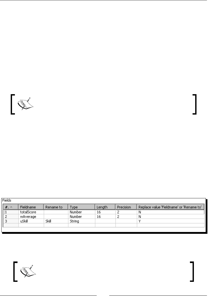
Transforming Your Data with JavaScript Code and the JavaScript Step
[ 150 ]
Adding elds
At the boom of the window, there is a grid where you put the elds you created in the
code. This is how you add a new eld:
1. Dene the eld as a variable in the code—for example, var totalScore.
2. Fill the grid manually or by clicking the Get variables buon. A new row will be lled
for every variable you dened in the code.
That was exactly what you did for the new elds, totalScore and wAverage.
In the JavaScript code you can create and use all variables you need without declaring them.
However, if you intend to add a variable as a eld in your stream, the declaraon with the
var sentence is mandatory.
The variables you dene in the JavaScript code are not Kele variables.
JavaScript variables are local to the step, and have nothing to do with the
Kele variables you know.
Modifying elds
Instead of adding a eld, you may want to change the value and eventually the data type of
an existent eld. You can do that but not directly in the code.
Imagine that you wanted to change the eld Skill, converng it to uppercase. To
accomplish this, double-click the JavaScript step and add the following two lines:
var uSkill;
uSkill = upper(Skill);
Add the new field to the grid at the bottom:
By renaming uSkill to Skill and seng the Replace value 'Fieldname' or 'Rename to' to
Y, the uSkill eld is renamed to Skill and replaces the old Skill eld.
Don't use the setValue() funcon to change existent elds. It may
cause problems and remains just for compability reasons.

Chapter 5
[ 151 ]
Turning on the compatibility switch
In the JavaScript window, you might have seen the Compability mode checkbox. This
checkbox, unchecked by default, causes JavaScript to work like it did in version 2.5 of the
JavaScript engine. With that version, you could modify the values and their types directly in
the code, which allows mixing data types, thus causing many problems.
Old JavaScript programs run in compability mode. However, when creang new code,
you should make use of the new engine; that is, you should leave the compability mode
turned o.
Do not check the compability switch. Leaving it unchecked, you will have a
cleaner, faster, and safer code.
Have a go hero – adding and modifying elds to the contest data
Take the contest le as source and do the following:
Add a eld named average. For the rst performance, calculate the average as
a weighted average, just like you did in the tutorial. For the second performance,
calculate the eld as a regular average, that is, the sum of the ve scores divided
by ve.
Modify the Performance eld. Replace Duet 1st Performance and Duet 2nd
Performance by 1st and 2nd.
There is no single way to code this, but here you have a list of funcons or sentences you can
use: if..then...else, indexOf(), substr()
Testing your code
Aer you type a script, you may want to test it. You can do it from inside the JavaScript
conguraon window. Let's try it:
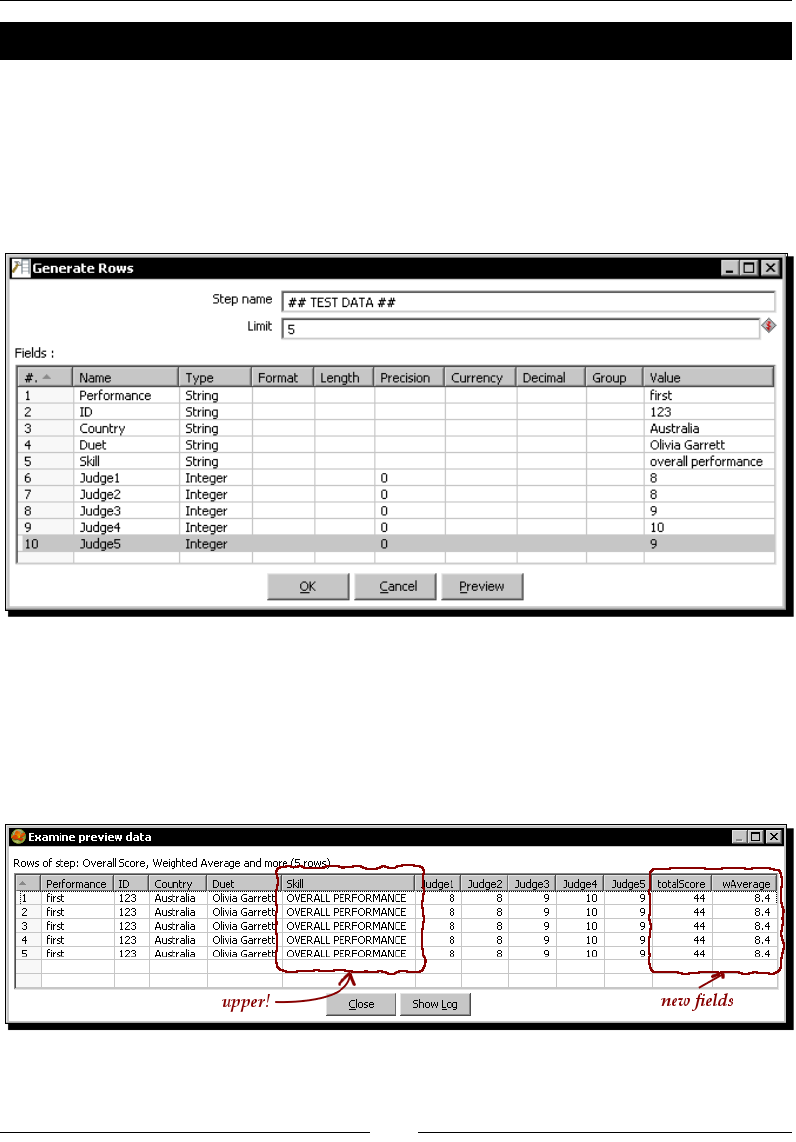
Transforming Your Data with JavaScript Code and the JavaScript Step
[ 152 ]
Time for action – testing the calculation of averages
Let's test the code you've just created.
1. Double-click the JavaScript step.
2. Click on the Test script buon.
3. A window appears to create a set of rows for tesng. Fill it like here:
4. Click on Preview the transformaon. A window appears showing ve idencal rows
with the provided sample values. Close the preview window.
5. Click on OK to test the code.
A window appears with the result that will appear when we execute the script with
the test data.

Chapter 5
[ 153 ]
What just happened?
You tested the code of the JavaScript step.
You clicked on the Test script buon, and created a dataset that served as the basis for
tesng the script. You previewed the test dataset.
Aer that, you did the test itself. A window appeared showing you how the created dataset
looks like aer the execuon of the script—the totalScore and wAverage elds were
added, and the skill eld was converted to uppercase.
Testing the script using the Test script button
The Test script buon allows you to check that the script does what it is intended to do.
It actually generates a transformaon in the back with two steps—a Generate Rows step
sending data to a copy of the JavaScript step. Just aer clicking on the buon, you are
allowed to ll the Generates Rows window with the test dataset.
The rst thing that the test funcon does is to verify that the code is properly wrien; that is,
that there are no syntax errors in the code. Try deleng the last parenthesis in the code and
click on the Test script buon. When you click OK to see the result of the execuon, instead
of a dataset you will see an error window.
If the script is syntaccally correct, what follows is the preview of the JavaScript for the
transformaon in the back, that is, the JavaScript code applied to the test dataset.
If you don't see any error and the previewed data shows the expected results, you are
done. If not, you can check the code, x it, and test it again unl you see that the step
works properly.
Have a go hero – testing the new calculation of the average
Open the transformaon of the previous Hero secon, and test:
The weighted average code
The regular code
To test one or the other, simply change the test data. Don't
touch your code!
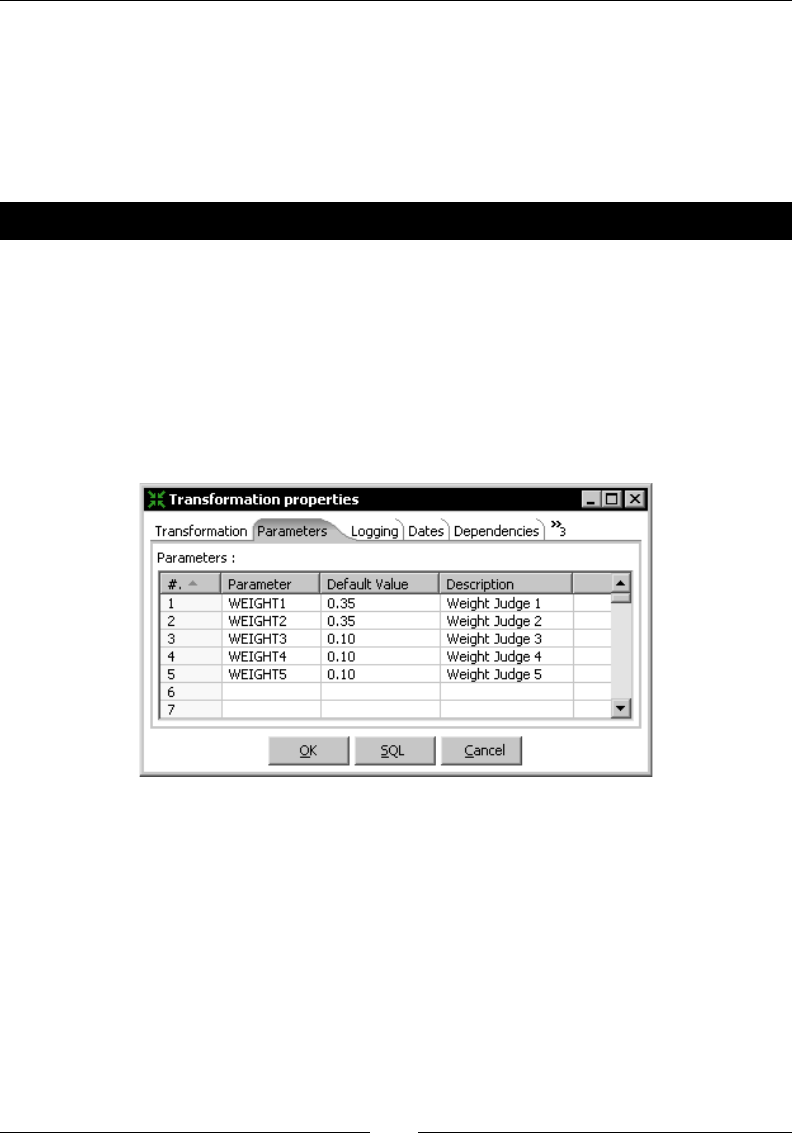
Transforming Your Data with JavaScript Code and the JavaScript Step
[ 154 ]
Enriching the code
In the previous secon, you learned how to insert code in your transformaon by using
a JavaScript step. In this secon, you will see how to use variables from outside to give
exibility to your code. You also will learn how to take control of the rows from inside the
JavaScript step.
Time for action – calculating exible scores by using variables
Suppose that by the me you are creang the transformaon, the weights for calculang
the weighted average are unknown. You can modify the transformaon by using parameters.
Let's do it:
1. Open the transformaon of the previous secon and save it with a new name.
2. Press Ctrl+T to open the Transformaon properes dialog window.
3. Select the Parameters tab and ll it like here:
4. Replace the JavaScript step by a new one and double-click it.
5. Expand the Transform Scripts branch of the tree at the le of the window.
6. Right-click the script named Script 1, select Rename, and type main as the
new name.
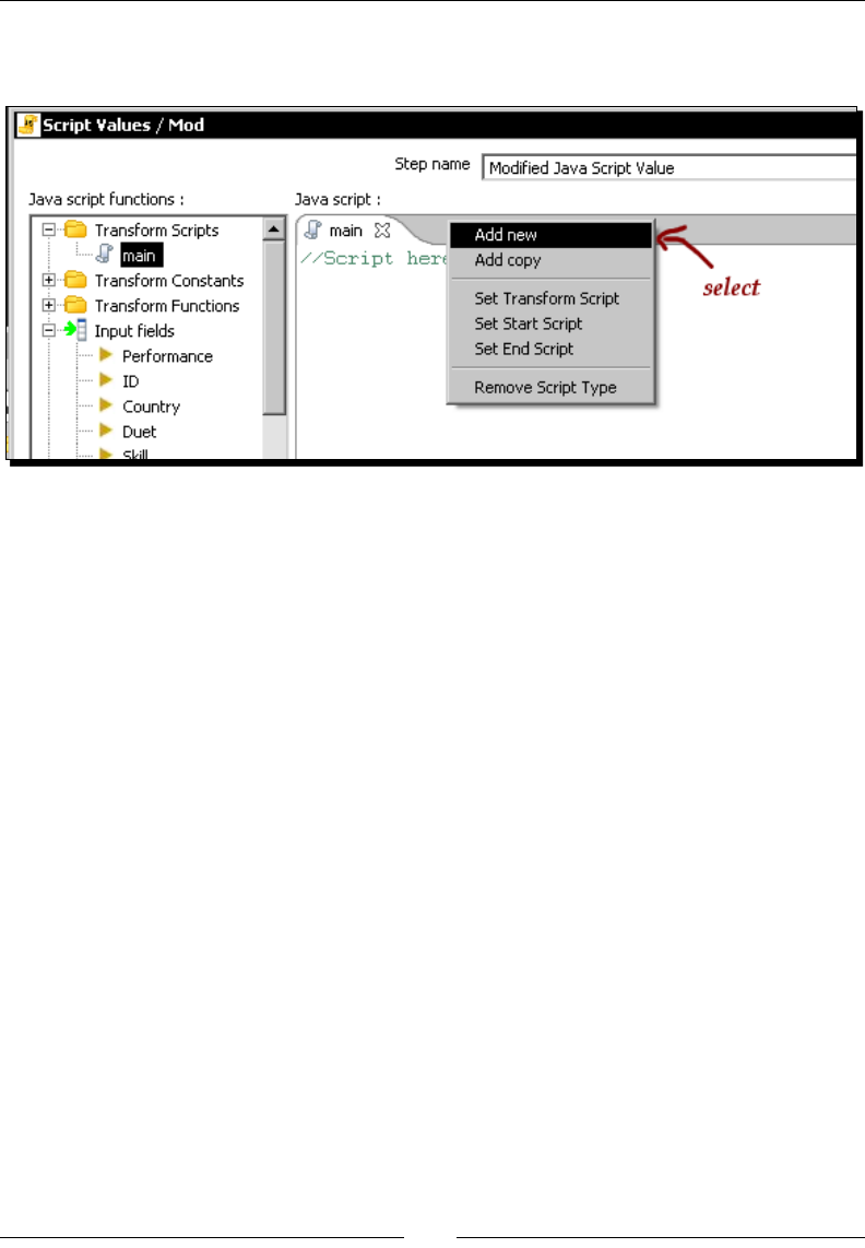
Chapter 5
[ 155 ]
7. Posion the mouse cursor over the eding window and right-click to bring up the
following contextual menu:
8. Select Add new to add the script, which will execute before your main code.
9. A new script window appears. The script is added to the list of scripts under
Transform Scripts.
10. Bring up the contextual menu again, but this me clicking on the tle of the new script.
Select Set Start Script.
11. Right-click the script in the tree list, and rename the new script as Start.
12. In the eding area of the new script, type the following code to bring the
transformaon parameters to the JavaScript code:
w1 = str2num(getVariable('WEIGHT1',0));
w2 = str2num(getVariable('WEIGHT2',0));
w3 = str2num(getVariable('WEIGHT3',0));
w4 = str2num(getVariable('WEIGHT4',0));
w5 = str2num(getVariable('WEIGHT5',0));
writeToLog('Getting weights...');
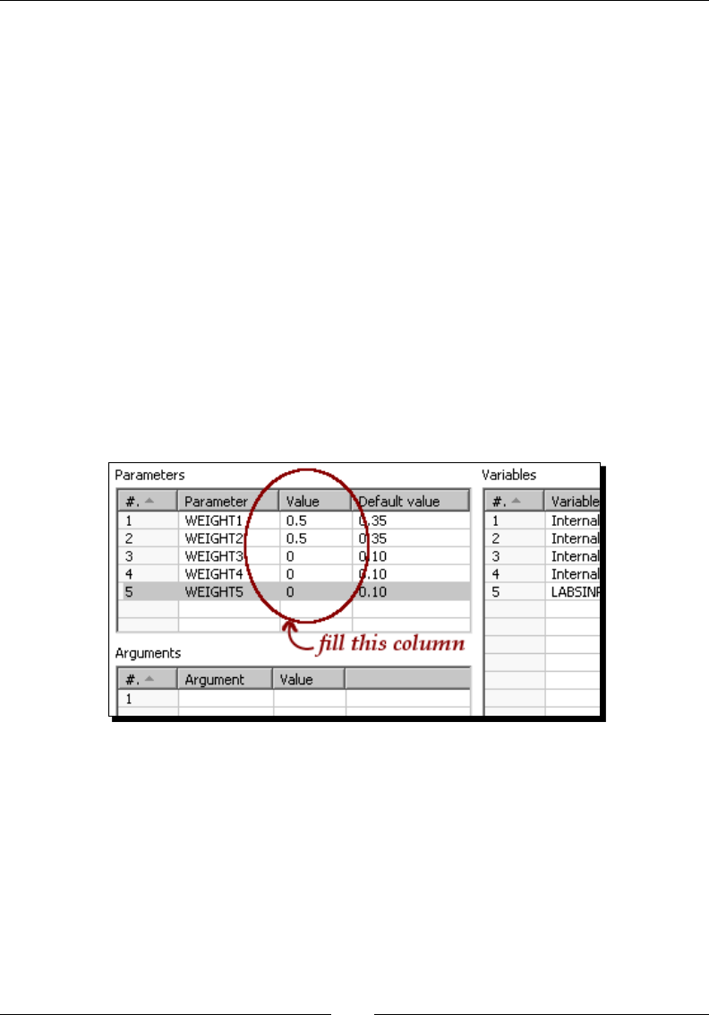
Transforming Your Data with JavaScript Code and the JavaScript Step
[ 156 ]
13. Select the main script by clicking on its tle and type the following code:
var wAverage;
wAverage = w1 * Judge1 + w2 * Judge2
+ w3 * Judge3 + w4 * Judge4 + w5 * Judge5;
writeToLog('row:' + getProcessCount('r') + ' wAverage:' +
num2str(wAverage));
if (wAverage >=7)
trans_Status = CONTINUE_TRANSFORMATION;
else
trans_Status = SKIP_TRANSFORMATION;
14. Click Get variables to add the wAverage variable to the grid.
15. Close the JavaScript window.
16. With the JavaScript step selected, click on the Preview this transformaon buon.
17. When the preview window appears, click on Congure.
18. In the window that shows up, modify the parameters as follows:
19. Click Launch.
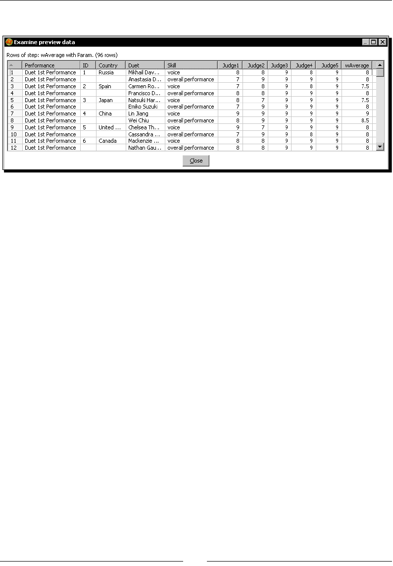
Chapter 5
[ 157 ]
20. The preview window shows this data:
21. The log window shows this:
...
2009/07/23 14:46:54 - wAverage with Param..0 - Getting weights...
2009/07/23 14:46:54 - wAverage with Param..0 - row:1 wAverage:8
2009/07/23 14:46:54 - wAverage with Param..0 - row:2 wAverage:8
2009/07/23 14:46:54 - wAverage with Param..0 - row:3 wAverage:7.5
2009/07/23 14:46:54 - wAverage with Param..0 - row:4 wAverage:8
2009/07/23 14:46:54 - wAverage with Param..0 - row:5 wAverage:7.5
...
What just happened?
You modied the code of the JavaScript step to use parameters.
First, you created four parameters for the transformaon, containing the weights for
the calculaon.
Then in the JavaScript step, you created a Start script to read the variables. That script
executed once, before the main script. Note that you didn't declare the variables. You could
have done it, but it's not mandatory unless you intend to add them as output elds.
In the main script, the script that is executed for every row, you typed the code to calculate
the average by using those variables instead of xed numbers.
Aer the calculaon of the average, you kept only the rows for which the average was
greater or equal to 7. You did it by seng the value of trans_Status to CONTINUE_
TRANSFORMATION for the rows you wanted to keep, and to SKIP_TRANSFORMATION
for the rows you wanted to discard.

Transforming Your Data with JavaScript Code and the JavaScript Step
[ 158 ]
In the preview window, you could see that the average was calculated as a weighted
average of the scores you provided, and that only the rows with an average greater or
equal to 7 were kept.
Using named parameters
The parameters that you put in the transformaon dialog window are called named
parameters. They can be used through the transformaon as regular variables, as if you
had created them before—for example, in the kettle.properties le.
From the point of view of the transformaon, the main dierence between
variables dened in the kettle.properties le and named parameters is
that the named parameters have a default value that can be changed at the me
you run the transformaon.
In this case, the default values for the variables dened as named parameters WEIGHT1 to
WEIGHT5 were 0.35, 0.35, 0.10, 0.10, and 0.10—the same that you had used in previous
exercises. But when you executed, you changed the default and used 0.50, 0.50, 0, 0, and 0
instead. This caused the formula for calculang the weighted average to work as an average
of the rst two scores. Take, for example, the numbers for the rst row of the le. Consider
the following code line:
wAverage = w1 * Judge1 + w2 * Judge2 + w3 * Judge3 + w4 * Judge4 + w5
* Judge5;
It was calculated as:
wAverage = 0.50 * 8 + 0.50 * 8 + 0 * 9 + 0 * 8 + 0 * 9;
giving a weighted average equal to 8.
Note that the named parameters are ready to use through the transformaon as regular
variables. You can see and use them at any place where the icon with the dollar sign
is present.
If you want to use a named parameter or any other Kele variable such as LABSINPUT or
java.io.tmpdir inside the JavaScript code, you have to use the getVariable() funcon
as you did in the Start script.
When you run the transformaon from the command line, you also have the possibility to
specify values for named parameters. For details about this, check Appendix B.
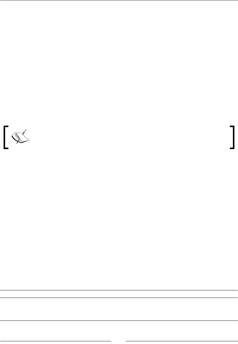
Chapter 5
[ 159 ]
Using the special Start, Main, and End scripts
The JavaScript step allows you to create mulple scripts. The Transformaon Script list
displays a list with all scripts of the step.
In the tutorial, you added a special script named Start and used it to read the variables.
The Start Script is a script that executes only once, before the execuon of the main script
you already know.
The Main script, the script that is created by default, executes for every row. As this script
is executed aer the start script, all variables dened in the main script there are accessible
here. As an example of this, in the tutorial you used the start script to set values for the
variables w1 through w5. Then in the main script you used those variables.
It is also possible to have an End Script that executes at the end of the execuon of the step,
that is, aer the main script has been executed for all rows.
When you create a Start or an End script, don't forget to give it a name so
that you can recognize it. If you don't, you may get confused because nothing in
the step shows you the type of the scripts.
Beyond main, start, and end scripts, you can use extra scripts to avoid overloading the main
script with code. The code in the extra scripts will be available aer the execuon of the
special funcon LoadScriptFromTab().
Note that in the exercises, you wrote some text to the log by using the writeToLog()
funcon. That had the only purpose of showing you that the start script executed at the
beginning and the main script executed for every row. You can see this sequence in the
execuon log.
Using transformation predened constants
In the tree to the le-hand side of the JavaScript window, under Transformaon Constants,
you have a list of predened constants. You can use those constants to change the value of
the predened variable, trans_Status, such as:
trans_Status = SKIP_TRANSFORMATION
Here is how it works:
Value of the trans_Status variable Eect on the current row
SKIP_TRANSFORMATION The current row is removed from the dataset
CONTINUE_TRANSFORMATION The current row is retained
ERROR_TRANSFORMATION The current row causes aboron of the transformaon
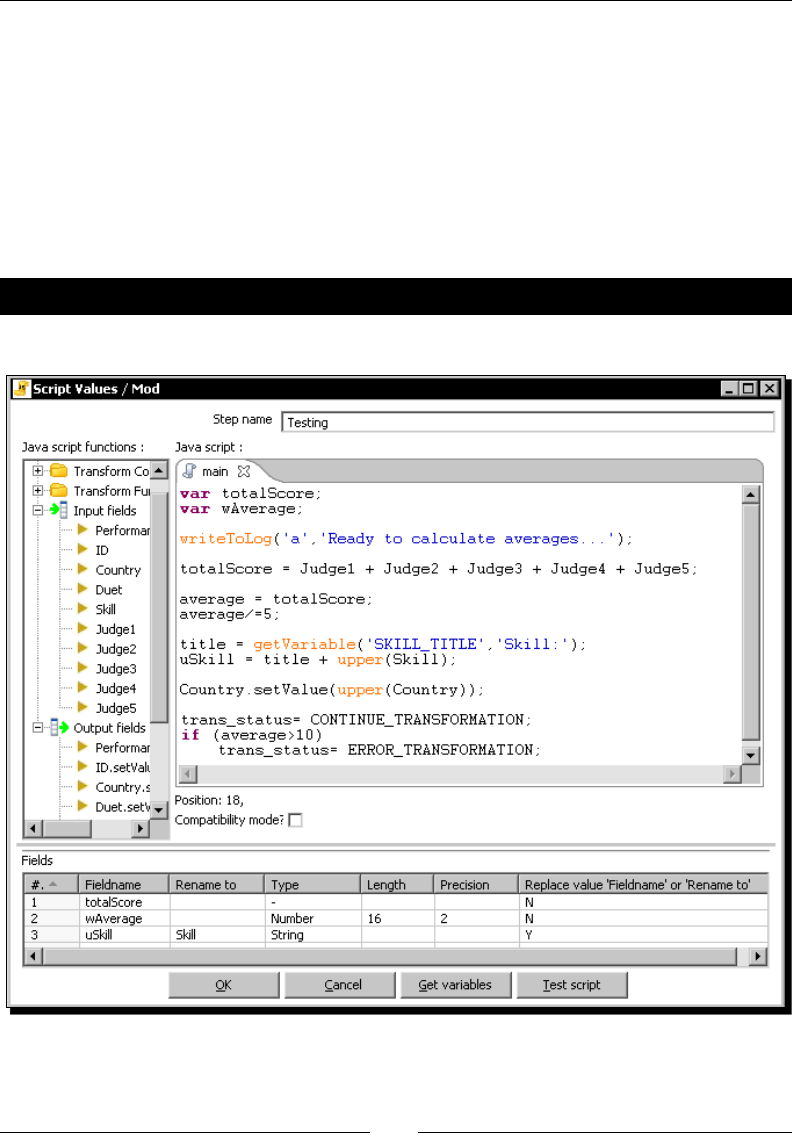
Transforming Your Data with JavaScript Code and the JavaScript Step
[ 160 ]
In other words, you can use that constant to control what will happen to the rows. In the
exercise you put:
if (wAverage >=7)
trans_Status = CONTINUE_TRANSFORMATION;
else
trans_Status = SKIP_TRANSFORMATION;
This means a row where the average is greater than or equal to 7 will connue its way to the
following steps. On the contrary, a row with a lower average will be discarded.
Pop quiz – nding the 7 errors
Look at the following screenshot:

Chapter 5
[ 161 ]
Does it look good? Well, it is not. There are seven errors in it. Can you nd them?
Have a go hero – keeping the top 10 performances
Modify the last tutorial. By using a JavaScript step, keep the top 10 performances, that is,
the 10 performances with the best average.
Sort the data using a regular Sort rows step. Give the
getProcessCount() funcon a try.
Have a go hero – calculating scores with Java code
If you are a Java programmer, or just curious, you will like to know that you can access
Java libraries from inside the JavaScript step. On the book site there is a JAR le named
pdi_chapter_5.jar. The JAR le contains a class with two methods—w_average()
and r_average(), for calculang a weighted average and a regular average.
Here is what you have to do:
1. Download the le from Packt's site, copy it to the libext folder inside the PDI
installaon folder, and restart Spoon.
2. Replace the JavaScript calculaon of the averages by a call to one of these
methods. You'll have to specify the complete name of the class. Consider the
next line for example:
wAverage = Packages.Averages.w_average(Judge1, Judge2, Judge3,
Judge4, Judge5);
3. Preview the transformaon and verify that it works properly.
The Java le is available as well. You can change it by adding new methods and trying them
from PDI.
Likewise, you can try using any Java objects, as long as they are in PDI's classpath. Don't
forget to type the complete name as in the following examples:
java.lang.Character.isDigit(c);
var my_date = new java.util.Date();
var val = Math.floor(Math.random()*100);

Transforming Your Data with JavaScript Code and the JavaScript Step
[ 162 ]
Reading and parsing unstructured les
It is marvelous to have input les where the informaon is well formed; that is, the number
of columns and the type of its data is precise, all rows follow the same paern, and so on.
However, it is common to nd input les where the informaon has lile or no structure, or
the structure doesn't follow the matrix (n rows by m columns) you expect. In this secon you
will learn how to deal with such les.
Time for action – changing a list of house descriptions with
JavaScript
You won the loery and decided to invest the money in a new house. You asked a real-estate
agency for a list of candidate houses for you and it gave you this:
...
Property Code: MCX-011
Status: Active
5 bedrooms
5 baths
Style: Contemporary
Basement
Laundry room
Fireplace
2 car garage
Central air conditioning
More Features: Attic, Clothes dryer, Clothes washer, Dishwasher
Property Code: MCX-012
4 bedrooms
3 baths
Fireplace
Attached parking
More Features: Alarm System, Eat in Kitchen, Powder Room
Property Code: MCX-013
3 bedrooms
...
Chapter 5
[ 163 ]
You want to compare the properes before vising them, but you're nding it hard to do so
because the le doesn't have a precise structure. Fortunately, you have the JavaScript step,
which will help you to give the le some structure.
1. Create a new transformaon.
2. Get the sample le from Packt site and read it with a Text le input step. Uncheck
the Header checkbox and create a single eld named text.
3. Do a preview. You should see the content of the le under a single column named
text. Add a JavaScript step aer the input step and double-click it to edit it.
4. In the eding area, type the following JavaScript code to create a eld with the code
of the property:
var prop_code;
posCod = indexOf(text,'Property Code:');
if (posCod>=0)
prop_code = trim(substr(text,posCod+15));
5. Click Get variables to add the prop_code variable to the grid under the code.
6. Click OK.
7. With the JavaScript step selected, do a preview. You should see this:
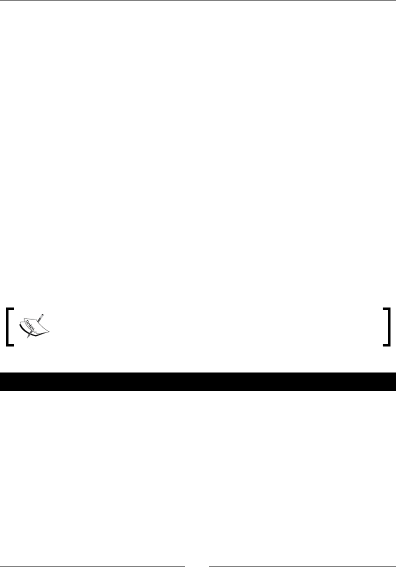
Transforming Your Data with JavaScript Code and the JavaScript Step
[ 164 ]
What just happened?
You read a le where each house was described in several rows. You added to every row
the code of the house to which that row belonged. In order to obtain the property code,
you idened the lines with a code, and then you cut the Property Code: text with the
substr funcon and discarded the leading spaces with trim.
Looking at previous rows
The code you wrote may seem a lile strange at the beginning, but it is not. It
creates a variable named prod_code, which will be used to create a new eld to
idenfy the properes. When the JavaScript code detects a property header row such
as Property Code: MCX-002, it sets the variable prop_code to the code it nds
in that line—MCX – 002 in this case.
Unl a new header row appears, the prop_code variable keeps that value. Thus all the
rows following a row like the one shown above will have the same value for the variable
prop_code.
The variable is then used to create a new eld, which will contain for every row, the code for
the house to which it belongs.
This is an example of when you can keep values from previous rows to be used in the
current row.
Note that here you use JavaScript to see and use values from previous rows, but
you can't modify them! JavaScript always works on the current row.
Have a go hero – enhancing the houses le
Modify the exercise from the tutorial by doing the following:
1. Aer keeping the property code, discard the rows that headed each property
descripon.
2. Create two new elds named feature and description. Fill the feature eld
with the feature described in the row (Exterior construcon) and the description
eld with the descripon of that feature (Brick). If you think that is not worth
keeping some features (Living Room), you may discard some rows. Discard also the
original eld text. Here you have a sample house descripon showing a possible
output aer the changes:

Chapter 5
[ 165 ]
prop_code; Feature; Description
MCX-023;bedrooms;4
MCX-023;baths;4
MCX-023;Style;Colonial
MCX-023;family room;yes
MCX-023;basement;yes
MCX-023;fireplace;yes
MCX-023;Heating features;Hot Water Heater
MCX-023;Central air conditioning present;yes
MCX-023;Exterior construction;Stucco
MCX-023;Waterview;yes
MCX-023;More Features;Attic, Living/Dining Room, Eat-In-Kitchen
Have a go hero – ll gaps in the contest le
Take a look at the contest le. Each performance occupies two rows, one showing each
evaluated skill. The name of the country appeared only in the rst row.
Open the rst version of the contest transformaon and modify it to ll the column Country
where it is blank.
Avoiding coding by using purpose-built steps
You saw through the exercises how powerful the JavaScript step is for helping you in your
transformaons. In older versions of PDI, coding JavaScript was the only means you had for
doing specic tasks. In the latest releases of PDI, actual steps appeared that eliminate the
need for coding in many cases. Here you have some examples of that:
Formula: You saw it in Chapter 3. Before the appearance of this step,
there were a lot of funcons such as the text funcons that you could only
solve with JavaScript.
Analyc Query: This step oers a way to retrieve informaon from rows before or
aer the current.
Split eld to rows: The step is used to create several rows from a single string value.
You used this step in Chapter 3 to create a new row for each word found in a le.
Analyc Query and Split elds to row are examples of where not only the need for coding
was eliminated, they also eliminated the need for accessing internal objects and funcons
such as Clone() or putRow() that you probably saw in old sample code or when browsing
the PDI forum. The use of those objects and funcons can lead to odd behavior and data
corrupon, and so their use is strongly discouraged.

Transforming Your Data with JavaScript Code and the JavaScript Step
[ 166 ]
Despite the appearance of new steps, you sll have the choice to do the tasks with code.
In fact, quite a lot of tasks you do with regular PDI steps may also be done with JavaScript,
by using the JavaScript step. This is a temptaon to programmers who end up with
transformaons having plenty of JavaScript steps.
Whenever there is a step that does what you want to do, you should
prefer that step to coding.
Why should you prefer to use a specic step rather than code? Here are some reasons:
To code takes more me to develop. You don't have to waste your me coding if
there are steps that can solve your problem.
Code is hard to maintain. If you have to modify or x a transformaon, it will be
much easier to tackle the change if the transformaon is a bunch of colorful steps
with meaningful names than if the transformaon consists of just a couple of
JavaScript icons.
A bunch of icons is self documented. A JavaScript step is like Pandora's box. Unl
you open it, you don't know exactly what it does, or whether it contains just a line of
code or thousands.
JavaScript is inherently slow. Faster alternaves for simple expressions are the User
Dened Java Expression and Calculator steps. They are typically more than twice
as fast. The next PDI release will feature a User Dened Java Class step. One of the
purposes of this step, intended to be used by Java developers, is to overcome the
drawbacks of JavaScript.
On the contrary, there are situaons where you may prefer or have to use JavaScript. Let's
enumerate some of them:
To handle unstructured input data
For accessing Java libraries
When you need to use a funcon provided by the JavaScript language that is not
provided by any of the regular PDI steps
When the JavaScript code saves a lot of regular PDI steps (as well as screen space),
and you think it is not worth showing the details of what those steps do
In the end, it is up to you to choose one or the other opon. The following exercise will help
you a lile in the recognion of pros and cons.

Chapter 5
[ 167 ]
Have a go hero – creating alternative solutions
Redo the following Hero exercises you did in this chapter:
Adding and modifying elds to the contest data
Keeping the top 10 performances
Enhancing the houses le
Filling gaps in the contest le
Do these exercises without using JavaScript when possible. In each case, compare both
versions, having in mind the following:
Time to develop
Maintenance
Documentaon
Capability to handle unstructured data
Number of steps required
Performance
Decide which opon you would choose if you had to decide.
To keep the 10 rst performances, use an Add Sequence step.
To ll the gaps, use an Analyc Query step.
Summary
In this chapter, you learned to code JavaScript into PDI. Specically, you learned:
What the JavaScript step is and how to use it
How to modify elds and add new elds to your dataset from inside your
JavaScript step
How to deal with unstructured input data
You also considered the pros and cons of coding JavaScript inside your transformaons, as
well as alternave ways to do things, avoiding wring code when possible.
As a bonus, you learned the concept of named parameters.
If you feel condent with all you've learned unl now, you are certainly ready to move on to
the next chapter, where you will learn in a simple fashion how to solve some sophiscated
problems such as normalizing data from pivot tables.

6
Transforming the Row Set
So far, you have been working with simple datasets, that is, datasets where
the each row represented a dierent enty (for example a student) and each
column represented a dierent aribute for that enty (for example student
name). There are occasions when your dataset doesn’t resemble such a simple
format, and working with it as is, may be complicate or even impossible. In
other occasions your data simply does not have the structure you like or the
structure you need.
Whichever your situaon, you have to transform the dataset in an appropriate format and
the soluon is not always about changing or adding elds, or about ltering or adding rows.
Somemes it has to do with twisng the whole dataset. In this chapter you will learn how to:
Convert rows to columns
Convert columns to rows
Operate on sets of rows
You will also be introduced to a core subject in data warehousing: Time dimensions.
Converting rows to columns
In most datasets each row belongs to a dierent element such as a dierent match or
a dierent student. However, there are datasets where a single row doesn't completely
describe one element. Take, for example, the real-estate le from Chapter 5. Every
house was described through several rows. A single row gave incomplete informaon
about the house. The ideal situaon would be one in which all the aributes for the
house were in a single row. With PDI you can convert the data into this alternave
format. You will learn how to do it in this secon.

Transforming the Row Set
[ 170 ]
Time for action – enhancing a lms le by converting
rows to columns
In this tutorial we will work with a le that contains list of all French movies ever made. Each
movie is described through several rows. This is how it looks like:
...
Caché
Year: 2005
Director:Michael Haneke
Cast: Daniel Auteuil, Juliette Binoche, Maurice Bénichou
Jean de Florette
Year: 1986
Genre: Historical drama
Director: Claude Berri
Produced by: Pierre Grunstein
Cast: Yves Montand, Gérard Depardieu, Daniel Auteuil
Le Ballon rouge
Year: 1956
Genre: Fantasy | Comedy | Drama
...
In order to process the informaon of the le, it would be beer if the rows belonging to
each movie were merged into a single row. Let's work on that.
1. Download the le from the Packt website.
2. Create a transformaon and read the le with a Text le input step.
3. In the Content tab of the Text le input step put : as separator. Also uncheck the
Header and the No empty rows opons.
4. In the Fields tab enter two string elds—feature and description. Do a preview of
the input le to see if it is well congured. You should see two columns—feature with
the texts to the le of the semicolons, and description with the text to the right of
the semicolons.
5. Add a JavaScript step and type the following code that will create the film eld:
var film;
if (getProcessCount('r') == 1) film = '';
if (feature == null)
film = '';
else if (film == '')
film = feature;
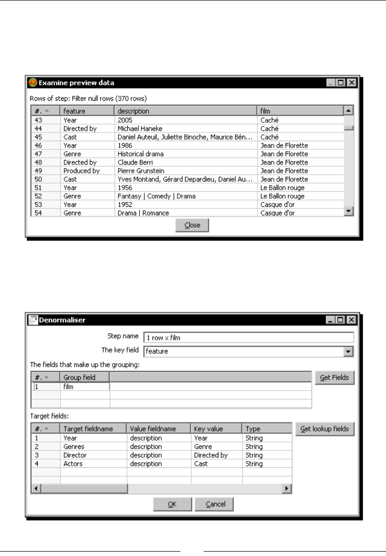
Chapter 6
[ 171 ]
6. Click on the Get variables buon to add to the dataset the eld film.
7. Add a Filter rows step with the condion description IS NOT NULL.
8. With the Filter rows step selected, do a preview. This is what you should see:
9. Aer the lter step, add a Row denormalizer step. You can nd it under the
Transform category.
10. Double-click the step and ll it like here:
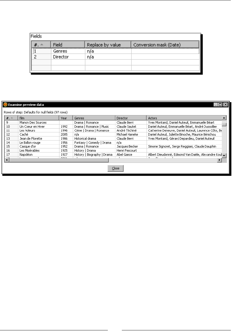
Transforming the Row Set
[ 172 ]
11. From the Ulity category select an If eld value is null step.
12. Double-click it , check the Select elds opon, and ll the Fields grid as follows:
13. With this last step selected, do a preview. You will see this:
What just happened?
You read a le with a selecon of lms in which each lm was described through
several rows.
First of all, you created a new eld with the name of the lm by using a small piece of
JavaScript code. If you look at the code, you will note that the empty rows are key for
calculang the new eld. They are used in order to disnguish between one lm and the
next and that is the reason for unchecking the No empty rows opon. When the code
executes for an empty row, it sets the lm to an empty value. Then, when it executes for the
rst line of a lm (film == '' in the code), it sets the new value for the film eld. When
the code executes for other lines, it does nothing but the lm already has the right value.
Aer that, you used a Row denormalizer step to translate the descripon of lms from rows
to columns, so the nal dataset had a single row by lm.
Finally, you used a new step to replace some null elds with the text n/a.
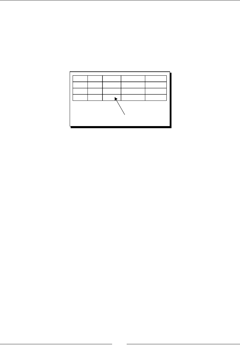
Chapter 6
[ 173 ]
Converting row data to column data by using the Row
denormalizer step
The Row denormaliser step converts the incoming dataset into a new dataset by moving
informaon from rows to columns according to the values of a key eld.
To understand how the Row denormaliser works, let's do a sketch of the desired
nal dataset:
FILM YEAR GENRE DIRECTOR ACTORS
1 film
by row
Here, a lm is described by using a single row. On the contrary, in your input le the
descripon for every lm was spread over several rows.
To tell PDI how to combine a group of rows into a single one, there are three things you have
to think about:
Among the input elds there must be a key eld. Depending on the value of that key
eld, you decide how the new elds will be lled. In your example, the key eld is
feature. Depending on the value of the column feature, you will send the value
of the eld description to some of the new elds: Year, Genres, Director,
or Actors.
You have to decide which eld or elds make up the groups of rows. In our example,
that eld is film. All rows with the same value for the eld film make up a
dierent group.
Decide the rules that have to be applied in order to ll the new target elds. All rules
follow this paern:
If the value for the key eld is equal to A, then put the value of the
eld B into the new eld C.
A sample rule could be: If the value for the eld feature
(our key eld) is equal to Directed by, put the value of the
eld description into the new eld Director.
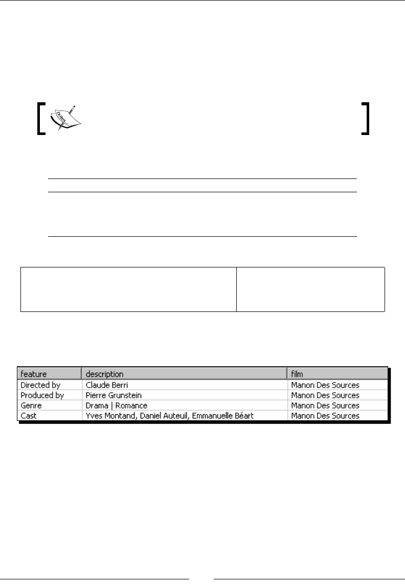
Transforming the Row Set
[ 174 ]
Once you are clear about these three things, all you have to do is ll the Row denormaliser
conguraon window to tell PDI how to do this task.
1. Fill the key eld textbox with the name of the key eld. In the example, the eld
is feature.
2. Fill the upper grid with the elds that make up the grouping. In this case, it is film.
The dataset must be sorted on the grouping elds. If not, you will
get unexpected results.
3. Finally, ll the lower grid. This grid contains the rules for the new elds. Fill it
following this example:
To add this rule ... Fill a row like this ...
If the value for the key eld is equal to A, put the
value of the eld B into the new eld C.
Key value: A
Value eldname: B
Target eldname: C
This is how you ll the row for the sample rule:
If the value for the eld feature (our key eld) is
equal to 'Directed by,' put the value of the eld
description into the new eld Director.
Key value: Directed by
Value eldname: description
Target eldname: Director
For every rule you must ll a dierent row in the target elds' grid.
Let's see how the Row denormalizer works for the following sample rows:
PDI creates an output row for the lm Manon Des Sources. Then it processes every row
looking for values to ll the new elds.
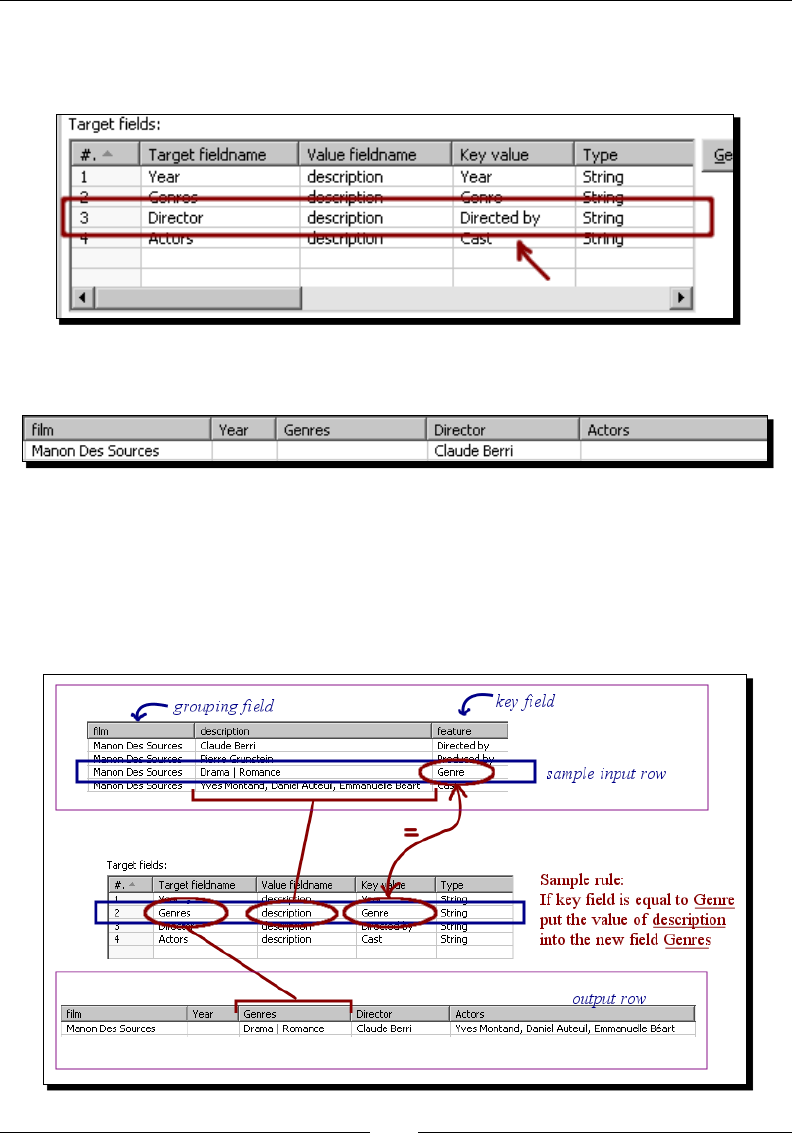
Chapter 6
[ 175 ]
Let's take the rst row. The value for the key eld feature is Directed by. PDI searches
in the target elds' grid to see if there is an entry where the Key value is Directed by; it
nds it.
Then it puts the value of the eld description as the content for the target eld
Director. The output row is now like this:
Now take the second row. The value for the key eld feature is 'Produced by.'
PDI searches in the target elds' grid to see if there is an entry where the Key value is
Produced by. It cannot nd it, and the informaon for this row is lost.
The following screenshot shows the rule applied to the third sample row. It also shows how
the nal output row looks like:
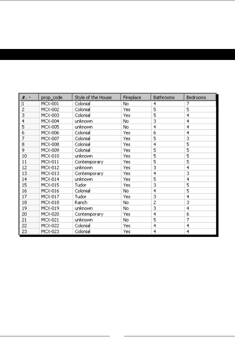
Transforming the Row Set
[ 176 ]
Note that the presence of rows is not mandatory for every key value entered in the target
elds' grid. If an entry in the grid is not used, the target eld is created anyway but it
remains empty.
In this sample lm, the year was not present. Then the eld Year remained empty.
Have a go hero – houses revisited
Take the output le for the Hero exercise to enhance the houses le from the previous
chapter. You can also download the sample le from the Packt site. Create a transformaon
that reads that le and generates the following output:
Aggregating data with a Row denormalizer step
In the previous secon, you learned how to use the Row denormalizer step to combine
several rows into one. The Row denormalizer step can also be used to take as input a dataset
and generate as output a new dataset with aggregated or consolidated data. Let's see it with
an example.
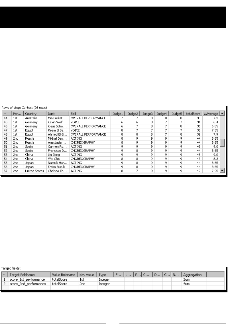
Chapter 6
[ 177 ]
Time for action – calculating total scores by performances
by country
Let's work now with the contest le from Chapter 5. You will need the output le for the
Hero exercise. Fill gaps in the contest le from that chapter. If you don't have it, you can
download it from the Packt website.
In this tutorial, we will calculate the total score for each performance by country.
1. Create a new transformaon.
2. Read the le with a Text le input step and do a preview to see that the step is well
congured. You should see this:
3. With a Select values step, keep only the following columns: Country, Performance,
and totalScore.
4. With a Sort Rows step sort the data by Country ascendant.
5. Aer the Sort Rows step, put a Row denormalizer step.
6. Double-click this last step to congure it.
7. As the key eld put Performance, and as group elds put Country.
8. Fill the target elds' grid like shown:
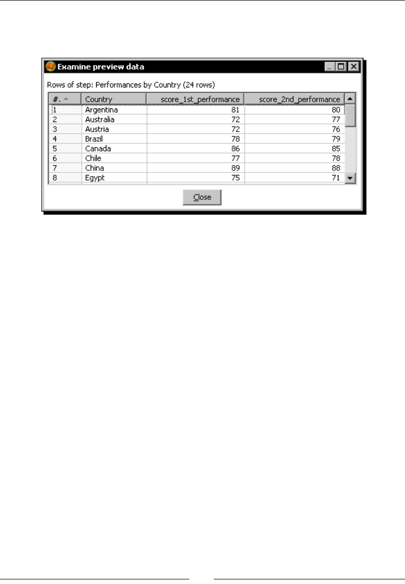
Transforming the Row Set
[ 178 ]
9. Close the window.
10. With the Row denormalizer step selected, do a preview. You will see this:
What just happened?
You read the contest le, grouped the data by country, and then created a new column
for every performance. As values for those new elds you put the sum of the scores by
performance and by country.
Using Row denormalizer for aggregating data
The purpose for which you used the Row denormaliser step in this tutorial was dierent
from the purpose in the previous tutorial. In this case, you put the countries in rows, the
performances in columns, and in the cells you put sums. The nal dataset was kind of a cross
tab like those you create with the DataPilot tool in Open Oce, or the Pivot in Excel. The
big dierence is that here the nal dataset is not interacve because, in essence, PDI is not.
Another dierence is that here you have to know the names or elements for the columns
in advance.
Let's explain how the Row denormalizer step works in these cases. Basically, the way it
works is quite the same as before:
The step groups the rows by the grouping elds and creates a new output row for
each group.
The novelty here is the aggregaon of values. When more than one row in the group
matches the value for the key eld, PDI calculates the new output eld as the result of
applying an aggregate funcon to all the values. The aggregate funcons available are the
same you already saw when you learned the Group by step—sum, minimum, rst value,
and so on. Take a look at the following sample rows:
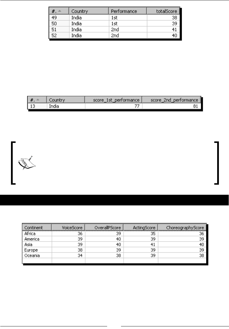
Chapter 6
[ 179 ]
The rst two rows had 1st as the value for the key eld Performance. According to the rule
of the Row denormaliser step, the values for the eld totalScore of these two rows go to
the new target eld score_1st_performance. As the rule applies for two rows, the values
for those rows have to be added, as Sum was the selected aggregaon funcon.
So, the output data for this sample group is this:
The value for the new eld score_1st_performance is 77 and is the sum of 38 and 39,
the values of the eld totalScore for the input rows where Performance was "1st."
Please note the dierence between the Row denormaliser and the Group
by step for aggregang. With the Row denormaliser step, you generate
another new eld for each interesng key value. Using the Group by step
for the tutorial, you couldn't have created the two columns shown in the
preceding screenshot—score_1st_performance and score_2nd_
performance.
Have a go hero – calculating scores by skill by continent
Create a new transformaon. Read the contest le and generate the following output:
To get the connent for each country, download the countries.txt le from the Packt
website and get the informaon with a Stream lookup step.

Transforming the Row Set
[ 180 ]
Normalizing data
Some datasets are nice to see but complicate to process further. Take a look at the matches
le we saw in Chapter 3:
Match Date;Home Team;Away Team;Result
02/06;Italy;France;2-1
02/06;Argentina;Hungary;2-1
06/06;Italy;Hungary;3-1
06/06;Argentina;France;2-1
10/06;France;Hungary;3-1
10/06;Italy;Argentina;1-0
...
Imagine you want to answer these quesons:
1. How many teams played?
2. Which team converted most goals?
3. Which team won all matches it played?
The dataset is not prepared to answer those quesons, at least in an easy way. If you want
to answer those quesons in a simple way, you will rst have to normalize the data, that is,
convert it to a suitable format before proceeding. Let's work on it.
Time for action – enhancing the matches le by normalizing
the dataset
Now you will convert the matches le you generated in Chapter 2 to a format suitable for
answering the proposed quesons.
1. Search on your disk for the le you created in Chapter 2, or download it from the
Packt website.
2. Create a new transformaon and read the le by using a Text le input step.
3. With a Split Fields step, split the Result eld in two: home_t_goals and
away_t_goals. (Do you remember having done this in chapter 3?)
4. From the Transform category of steps, drag a Row Normalizer step to the canvas.
5. Create a hop from the last step to this new one.
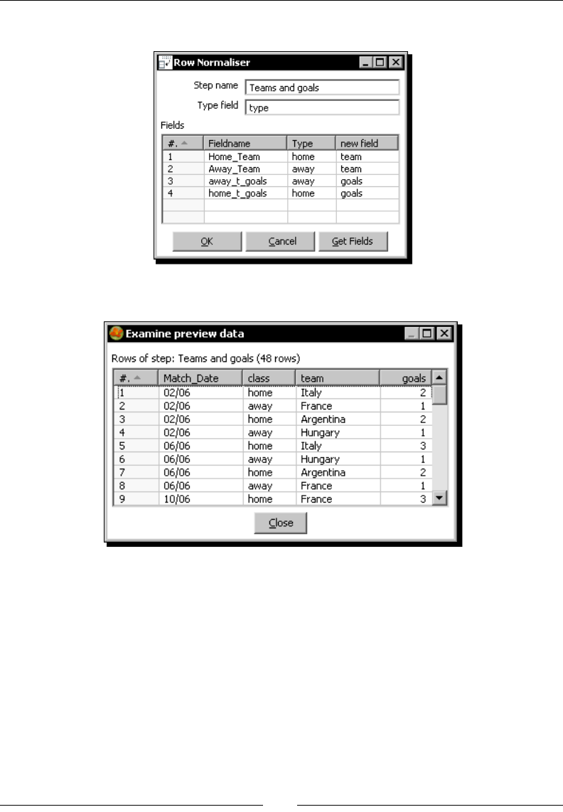
Chapter 6
[ 181 ]
6. Double-click the Row Normalizer step to edit it and ll the window as follows:
7. With the Row Normalizer selected, do a preview. You should see this:
What just happened?
You read the matches le and converted the dataset to a new one where both the home
team and the away team appeared under a new column named team, together with another
new column named goals holding the goals converted by each team. With this new format,
it is really easy now to answer the quesons proposed at the beginning of the secon.
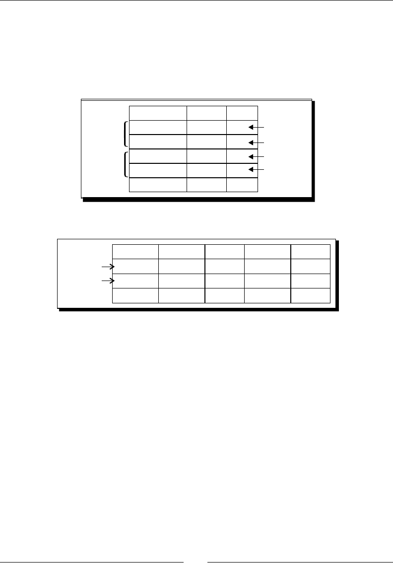
Transforming the Row Set
[ 182 ]
Modifying the dataset with a Row Normalizer step
The Row Normalizer step modies your dataset, so it becomes more suitable for processing.
Usually this involves transforming columns into rows.
To understand how it works, let's take as example the le from the tutorial. Here is a sketch
of what we want to have at the end:
MATCH DATE TEAM GOALS
1st Match
2nd Match
02/06
Italy
France
Hungary
2
1Away Team
02/06
02/06
02/06
Argentina
2
1
... ... ...
Away Team
Home Team
Home Team
What we have now is this:
1st Match
2nd Match
Match Date Home Team Goals Away Team
02/06
Italy
Argentina
France
Hungary
2
1
Goals
02/06
2
1
... ... ... ... ...
Now it is just a maer of creang a correspondence between the old columns and the
new ones.
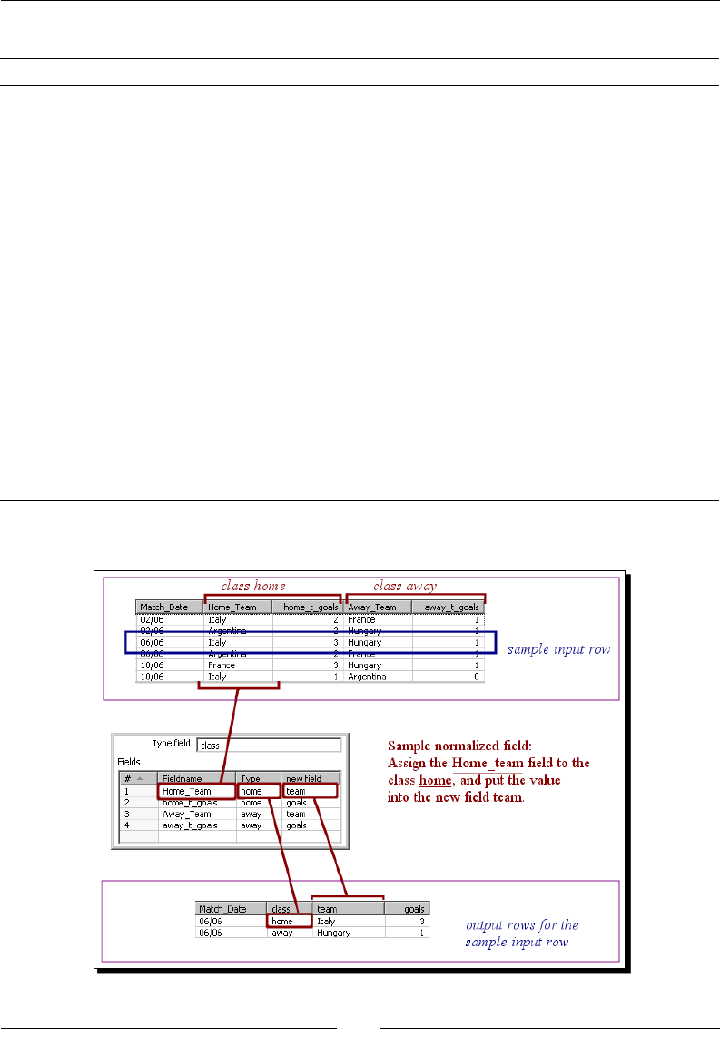
Chapter 6
[ 183 ]
Just follow these steps and you have the work done:
Step Example
Idenfy the new desired elds. Give them a name. team, goals.
Look at the old elds and idenfy which ones you
want to translate to the new elds.
Home_Team, home_t_goals, Away_Team,
away_t_goals.
From that list, idenfy the columns you want to
keep together in the same row, creang a sort
of classicaon of the elds. Give each group a
name. Also, give a name to the classicaon.
You want to keep together the elds Home_
Team and home_t_goals. So, you create a
group with those elds, and name it home.
Likewise, you create a group named away with
the elds Away_Team and away_t_goals.
Name the classicaon as class.
Dene a correspondence between the elds
idened above, and the new elds.
The old eld Home_Team goes to the new
eld team.
The old eld home_t_goals goes to the new
eld goals.
The old eld Away_Team goes to the new
eld team.
The old eld away_t_goals goes to the new
eld goals.
Transcript all these denions to the Row Normalizer conguraon window as shown below:

Transforming the Row Set
[ 184 ]
In the elds grid, insert one row for each of the elds you want to normalize.
Once you normalize, you have a new dataset where the elds for the groups you dened
were converted to rows.
The number of rows in the new dataset is equal to the number of groups dened by the
number of rows in the old dataset. In the tutorial, the nal number is 24 rows x 2
groups = 48 rows.
Note that the elds not menoned in the conguraon of the Row Normalizer (Match_Date
eld in the example) are kept without changes. They are simply duplicated for each new row.
In the tutorial, every group was made by two elds: Home_Team and home_t_goals for the
rst group, and Away_Team and away_t_goals for the second. When you normalize, a group
may have just one eld, two elds (as in this example), or more than two elds.
Summarizing the PDI steps that operate on sets of rows
The Row Normaliser and Row denormalizer steps you learned in this chapter are some of
the PDI steps which, rather than treang single rows, operate on sets of rows. The following
table gives you an overview of the main PDI steps that fall into this parcular group of steps:
Step Purpose
Group by Builds aggregates such as Sum, Maximum, and so on, on groups of rows.
Univariate
Stascs
Computes some simple stascs. It complements the Group by. It has less
capabilies than that step but provides more aggregate funcons such as
median and percentiles.
Split Fields Splits a single eld into more than one. Actually it doesn't operate on a set of
rows, but it's common to use it combined with some of the steps in this table.
For example: You could use a Group by step to concatenate a eld, followed by
a Split Fields step that splits that concatenated eld into several columns.
Row Normaliser Transforms columns into rows making the dataset more suitable for processing.
Row denormaliser Moves informaon from rows to columns according to the values of a key eld.
Row aener Flaens consecuve rows. You could achieve the same by using a Group by to
concatenate the eld to aen, followed by a Split Field step.
Sort rows Sorts rows based on eld values. Alternavely, it can keep only unique rows.
Split eld to rows Splits a single string eld and creates a new row for each split term.
Unique rows Removes double consecuve rows and leaves only unique occurrences.
For examples on using these steps or for geng more informaon about them, please refer
to Appendix C, Quick reference: Steps and Job Entries.
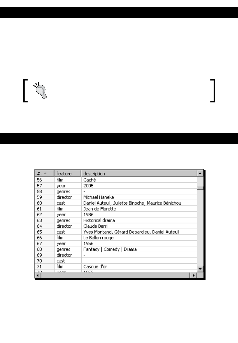
Chapter 6
[ 185 ]
Have a go hero – verifying the benets of normalization
Extend the transformaon and answer the quesons proposed at the beginning of
the secon:
How many teams played?
Which team converted most goals?
Which team won all matches it played?
For answering the third queson, you'll have to modify the Row
Normalizer step as well.
If you are not convinced that the normalizer process makes the work easier, you can try to
answer the quesons without normalizing. That eort will denively convince you!
Have a go hero – normalizing the Films le
Consider the output of the rst Time for acon secon in this chapter. Generate the
following output:
You have two opons here:
To modify the tutorial by sending the output to a new le. Then to use that new le
to do this exercise.
To extend the stream in the original transformaon by adding new steps aer the
Row Denormalizer step.
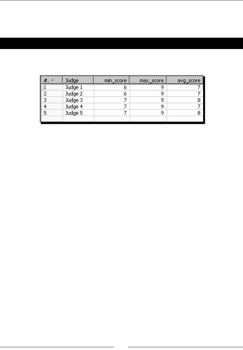
Transforming the Row Set
[ 186 ]
Aer doing the exercise, think about this: Does it make sense to denormalize and then
normalize again? What is the dierence between the original le and the output of this
exercise? Could you have done the same without denormalizing and normalizing?
Have a go hero – calculating scores by judge
Take the contest le and generate the following output, where the columns represent the
minimum, maximum, and average score given by every judge:
This exercise may appear dicult at rst, but here's a clue: Aer reading the le, use a Group
by step to calculate all the values you need for your nal output. Leave the group eld empty
so that the step groups all rows in the dataset.
Generating a custom time dimension dataset by using
Kettle variables
Dimensions are sets of aributes useful for describing a business. A list of products along
with their shape, color, or size is a typical example of dimension. The me dimension is a
special dimension used for describing a business in terms of when things happened. Just
think of a me dimension as a list of dates along with aributes describing those dates. For
example, given the date 05/08/2009, you know that it is a day of August, it belongs to the
third quarter and it is Wednesday. These are some of the aributes for that date.
In the following tutorial you will create a transformaon that generates the dataset for a
me dimension. The dataset for a me dimension has one row for every date in a given
range of dates and one column for each aribute of the date.
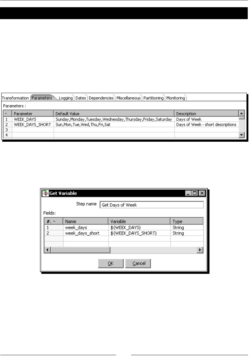
Chapter 6
[ 187 ]
Time for action – creating the time dimension dataset
In this tutorial we will create a simple dataset for a me dimension.
First we will create a stream with the days of the week:
1. Create a new transformaon.
2. Press Ctrl+T to access the Transformaon sengs window.
3. Select the Parameters tab and ll it like shown in the next screenshot:
4. Expand the Job category of steps.
5. Drag a Get Variables step to the canvas, double-click the step, and ll the window
like here:
6. Aer the Get Variables step, add a Split Fields step and use it to split the eld
week_days into seven String elds named sun, mon, tue, wed, thu, fri, and
sat. As Delimiter, set a comma (,).
7. Add one more Split Fields step and use it to split the eld week_days_short into
seven String elds named sun_sh, mon_sh, tue_sh, wed_sh, thu_sh, fri_sh,
and sat_sh. As Delimiter, set a comma (,).
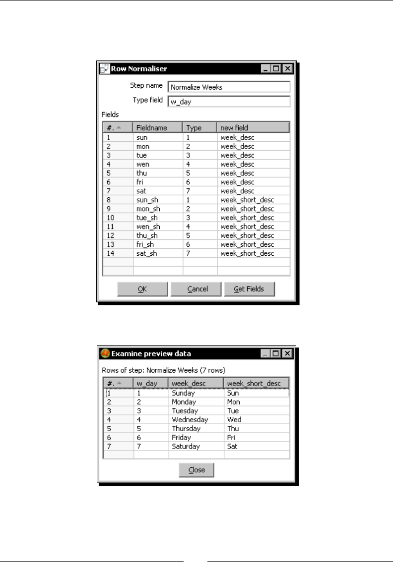
Transforming the Row Set
[ 188 ]
8. Aer this last step, add a Row Normalizer step.
9. Double-click the Row Normalizer step and ll it as follows:
10. Keep the Row Normalizer step selected and do a preview. You will see this:
Now let's build the main stream:
1. Drag a Generate Rows step, an Add sequence step, a Calculator step, and a Filter
rows step to the canvas.
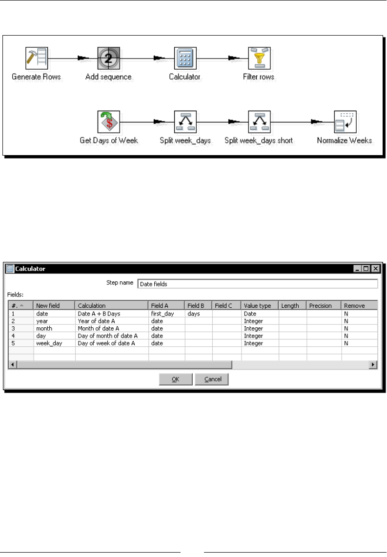
Chapter 6
[ 189 ]
2. Link them so you get this:
3. Double-click the Generate Rows step and use it to generate 45000 lines. Add a single
Date eld named first_day. As Format select yyyyMMdd and as Value write
19000101.
4. Double-click the Add sequence step. In the Name of value textbox, type days.
5. Double-click the Calculator step and ll the window as shown next:
6. Double-click the Filter rows step and add the lter date <= 31/12/2020. When you
enter the date 31/12/2020, make sure to set the Type to Date and the Conversion
format to dd/MM/yyyy. Aer the Filter rows step add a Stream lookup step.
7. Create two hops—one from the Filter rows step to the Stream lookup step and the
other from the Row Normalizer step to the Stream lookup step.
8. Double-click the Stream lookup step. In the upper grid add a row, seng week_day
under the Field column and w_day under the LookupField column. Use the lower grid
to retrieve the String elds week_desc and week_short_desc. Finally, aer the
Stream lookup step, add a Select values step.
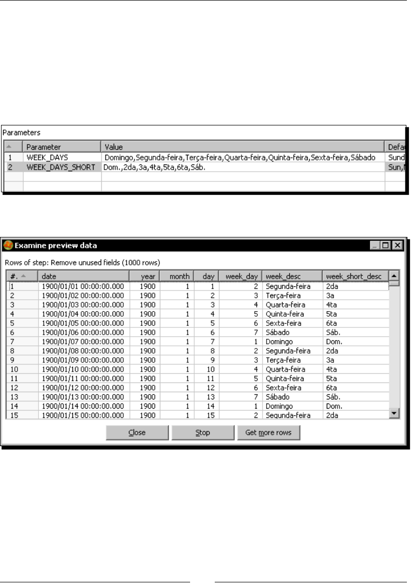
Transforming the Row Set
[ 190 ]
9. Use the Select values step to remove the unused elds first_day and days. Create a
hop from the Stream lookup step to this step.
10. With the Select values step selected, click the preview buon.
11. When the preview window appears click on Congure.
12. Fill the column value in the Parameters grid of the transformaon execuon window
as follows:
13. Click the Launch buon. You will see this:
What just happened?
You generated data for a me dimension with dates ranging from 01/01/1900 through
31/12/2020. Time dimensions are meant to answer quesons related with me such as: Do
I sell more on Mondays or on Fridays? Am I selling more this quarter than the same quarter
last year? The list of aributes you need to include in your me dimension depends on the
kind of queson you want to answer. Typical elds in a me dimension include: year, month
(a number between 1 and 12), descripon of month, day of month, week day, and quarter.
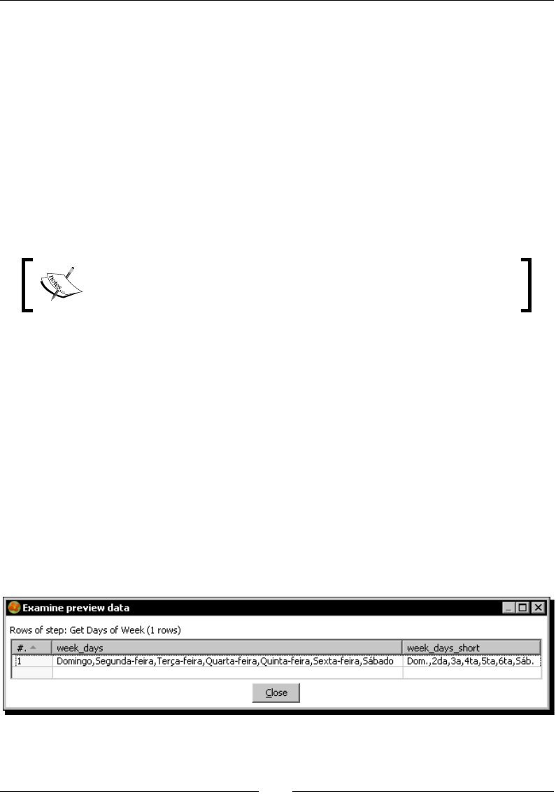
Chapter 6
[ 191 ]
In the tutorial you created a few aributes, but you could have added much more. Among
the aributes included you had the week day. The week descripons were taken from
named parameters, which allowed you to set the language of the week descripons at the
me you ran the transformaon. In the tutorial you specied Portuguese descripons. If
you had le the parameters grid empty, the transformaon would have used the English
descripons that you put as default.
Let's explain how you build the stream with the number and descripons for the days of
the week. First, you created a dataset by geng the variables with the descripons for the
days of the week. Aer creang the dataset, you split the descripons and by using the Row
Normalize step, you converted that row into a list of rows, one for every day of the week.
In other words, you created a single row with all the descripons for the days of the week.
Then you normalized it to create the list of days.
This method used for creang the list of days of a week is very useful when
you have to create a very small dataset. It avoids the creaon of external
les to hold that data.
The transformaon you created was inspired by the sample transformaon
General - Populate date dimension.ktr found in the samples/transformations
folder inside the PDI installaon folder. You can take a look at that transformaon. It builds
the dataset in a slightly dierent way, also by using Row Normalizer steps.
Getting variables
To create the secondary stream of the tutorial, you used a Get Variables step. The Get
Variables step allows you to get the value of one or more variables. In this tutorial you
read two variables that had been dened as named parameters.
When put as the rst step of a stream like in this case, this step creates a dataset with one
single row and as many elds as read variables.
The following is the dataset created by the Get Variables step in the me dimension tutorial:
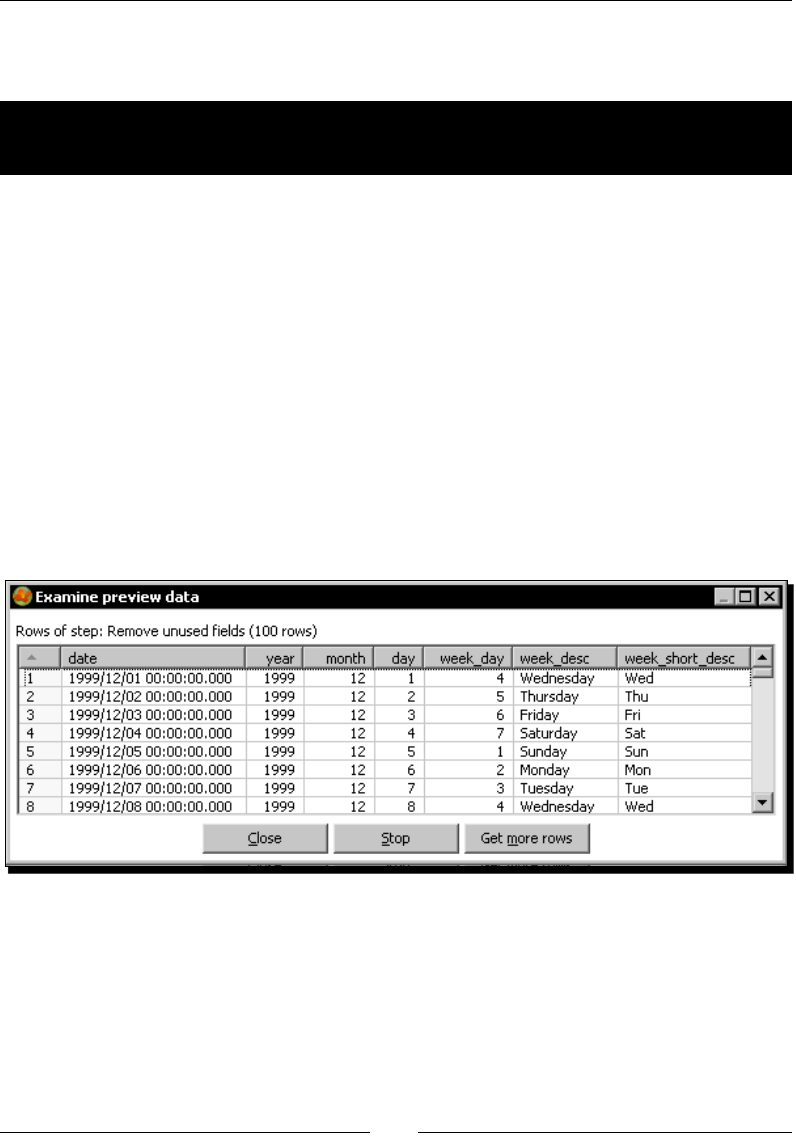
Transforming the Row Set
[ 192 ]
When put in the middle of a stream, this step adds to the incoming dataset, as many elds as
the number of variables it reads. Let's see how it works.
Time for action – getting variables for setting the default
starting date
Let's modify the transformaon so that the starng date depends on a parameter.
1. Press Ctrl+T to open the transformaon sengs window.
2. Add a parameter named START_DATE with default value 01/12/1999.
3. Add a Get variables step between the Calculator step and the Filter rows step .
4. Edit the Get variables step and a new eld named start_date. Under Variable write
${START_DATE}. As Type select Date, and under Format select or type dd/MM/yyyy.
5. Modify the lter step so the condion is now: date>=start_date and
date<=31/12/2020.
6. Modify the Select values step to remove the start_date eld.
7. With the Select values step selected do a preview. You will see this:
What just happened?
You added a starng date as a named parameter. Then you read that variable into a new eld
and used it to keep only the dates that are greater or equal to its value.
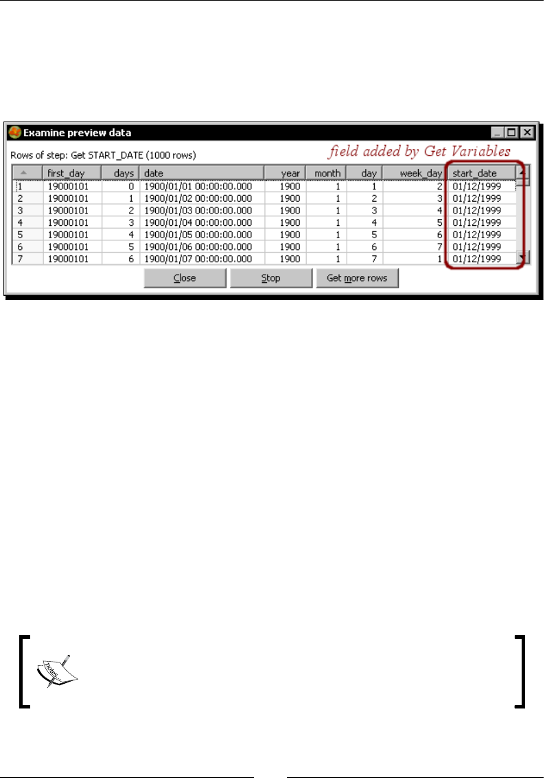
Chapter 6
[ 193 ]
Using the Get Variables step
As you just saw, the Get Variables step allows you to get the value of one or more variables. In
the main tutorial you saw how to use the step at the beginning of a stream. Now you saw how
to use it in the middle. The following is the dataset aer the Get Variables step for this
last exercise:
With the Get Variables step, you can read any Kele variable—variables dened in the
kettle.properties le, internal variables as for example ${user.dir}, named parameters
as in this tutorial, or variables dened in another transformaon (you haven't yet learned about
these variables but you will soon).
As you know, the type of Kele variables is String by default. However, at the me you get a
variable, you can change its metadata. As an example of that, in this last exercise you converted
${START_DATE} to a Date by using the mask dd/MM/yyyy.
Note that you specied the variables as ${name of the variable}. You could have used
%%name of the variable%% also. The full specicaon of the name of a variable allows you
to mix variables with plain text.
Suppose that instead of a date you create a parameter named YEAR with default value 1950.
In the Get variables step you may specify 01/01/${YEAR} as the value.
When you execute the transformaon, this text will be expanded to 01/01/1950 or to
01/01/ plus the year you enter if you overwrite the default value.
Note that the purpose of using the Get Variable step is to have the values of
variables as elds in the dataset. Otherwise, you don't need to use this step
for using a variable. You just use it wherever you see a dollar sign icon.

Transforming the Row Set
[ 194 ]
Have a go hero – enhancing the time dimension
Modify the me dimension generaon by doing the following:
Add the following elds to the dataset, taking as model the generaon of weeks:
Name of month, Short name of month, and Quarter.
Add two more parameters: start_year and end_year. Modify the transformaon
so that it generates dates only between those years. In other words, you have
to discard dates out of that range. You may assume that the parameters will be
between 1900 and 2020.
Pop quiz – using Kettle variables inside transformations
There are some Kele predened variables that hold informaon about the logged in user:
user.country, user.language, etc. The following tasks involve the use of some of those
variables. Which of the tasks can be accomplished without using a Get Variables step or a
JavaScript step (Remember from the previous chapter that you can also get the value for a
Kele variable with a Javascript step):
a. Create a le named hello_<user>.txt, where <user> is the name of the
logged user.
b. Create a le named hello.txt that contains a single line with the text Hello,
<user>!, <user> being is the name of the logged user.
c. Write to the log (by using the Write to log step) a greeng message like Hello,
user!. The message has to be wrien in a dierent language depending on the
language of the logged user.
d. All of the above
e. None of the above
Summary
In this chapter, you learned to transform your dataset by applying two magical steps: Row
Normalizer and Row denormalizer. These two steps aren't the kind of steps you use every
day such as a Filter Rows or a Select values step. But when you need to do the kind of task
they achieve, you are really grateful that these steps exist. They do a complex task in a quite
simple way. You also learned what a me dimension is and how to create a dataset for a
me dimension.
So far, you've been learning to transform data. In the next chapter, you will set that kind of
learning aside for a while. The chapter will be devoted to an essenal subject when it comes
to working in producve environments and dealing with real data—data validaon and
error handling.

7
Validating Data and Handling Errors
So far, you have been working alone in front of your own computer. In
the "Time for acon" exercises, the step-by-step instrucons along with the
error-free sample data helped you create and run transformaons free of errors.
During the "Have a go hero" exercises, you likely encountered numerous errors,
but ps and troubleshoong notes were there to help you get rid of them.
This is quite dierent from real scenarios, mainly for two reasons:
Real data has errors—a fact that can't be avoided. If you fail to heed it, the
transformaons that run with your sample data will probably crash when
running with real data.
In most cases, who runs your nal work is decided by an automated process and is
not user dened. Therefore, if a transformaon crashes, there will be nobody to x
the problem.
In this chapter you will learn about the opons that PDI oers to treat errors and validate
data so that your transformaons are well prepared to be run in a producve environment.
Capturing errors
Suppose that you are running or previewing a transformaon from Spoon. As you already
know, if an error occurs it is shown in the Logging window inside the Execuon Results
pane. As a consequence, you can look at the error, try to x it, and run the transformaon
again. This is far from what happens in real life. As said, transformaons in real scenarios
are supposed to be automated. Therefore, it is not acceptable to have a transformaon that
crashes without someone who noces it and reacts to that situaon. On the contrary, it's
your duty to do everything you can to trap errors that may happen, avoiding unexpected
crashes when possible. In this secon you will learn how to do that.
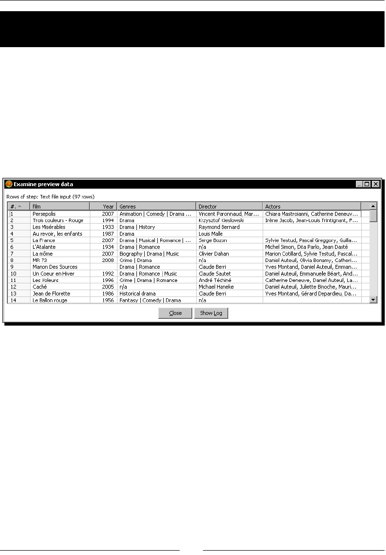
Validang Data and Handling Errors
[ 196 ]
Time for action – capturing errors while calculating the age
of a lm
In this tutorial you will use the output of the denormalizing process from the previous
chapter. You will calculate the age of the lms and classify them according to their age.
1. Get the le with the lms. You can take the transformaon that denormalized the
data and generate the le with a Text le output step, or you can take a sample le
from the Packt website.
2. Create a new transformaon and read the le with a Text le input step.
3. Do a preview of the data. You will see the following:
4. Aer the Text le input step, add a Get System Info step.
5. Edit the step, add a new eld named today, and choose Today 00:00:00 as
its value.
6. Add a JavaScript step.
7. Edit the step and type the following piece of code:
var diff;
film_date = str2date('01/01/' + Year, 'dd/MM/yyyy');
diff = dateDiff(film_date,today,”y”);
8. Click on Get variables to add diff as a new eld.
Download from Wow! eBook <www.wowebook.com>
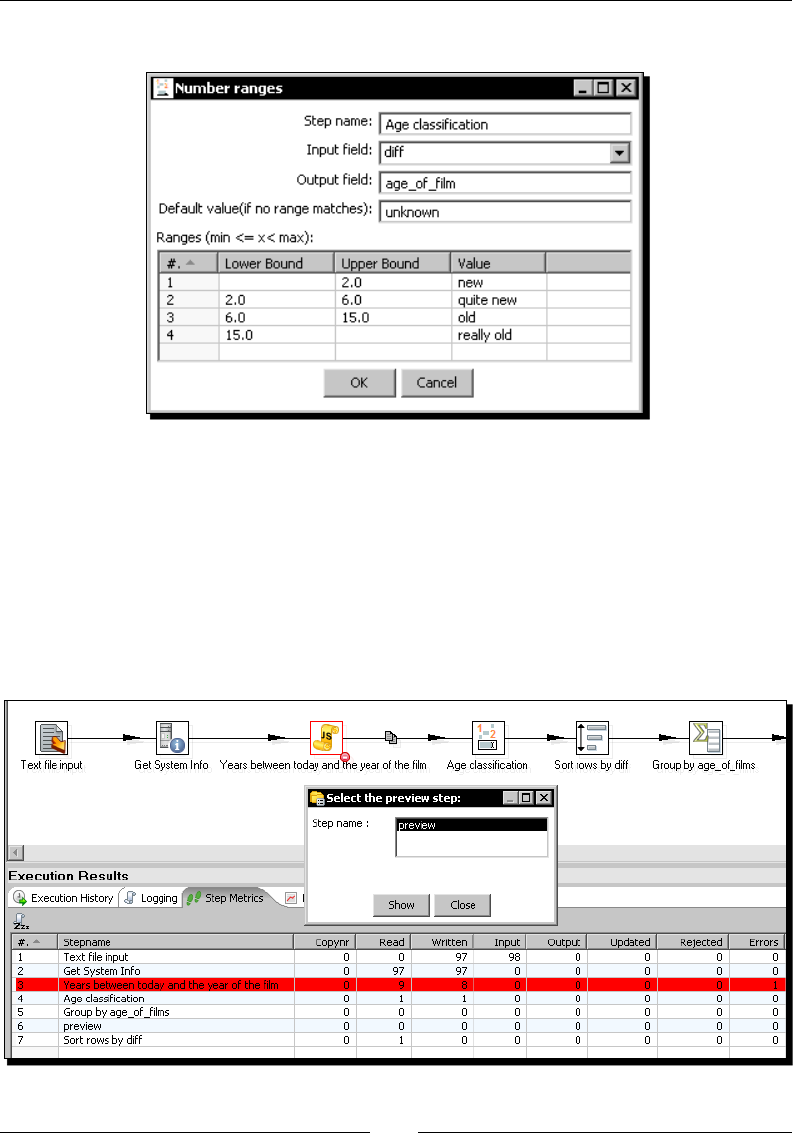
Chapter 7
[ 197 ]
9. Add a Number range step, edit it, and ll its window as follows:
10. With a Sort rows step, sort the data by diff.
11. Finally, add a Group by step and double-click to edit it.
12. As group eld put age_of_film. In the Aggregates grid create a eld named
number_of_films to hold the number of lms with that age. Put film as the
Subject and select Number of values (N) as the Type.
13. Add a Dummy step at the end and do a preview. You will be surprised by an error
like this:
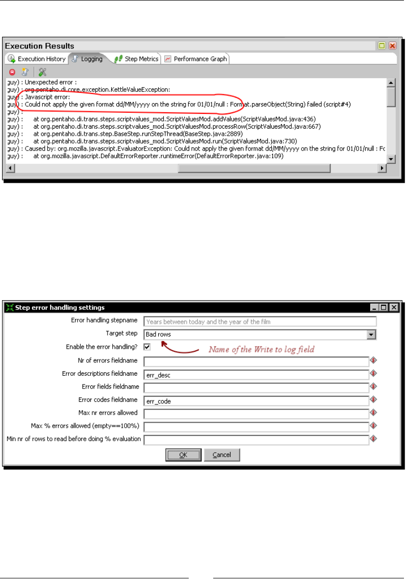
Validang Data and Handling Errors
[ 198 ]
14. Look at the logging window. It looks like this:
15. Now drag Write to log step to the canvas from the Ulity category.
16. Create a hop from the JavaScript step to this new step.
17. Select the JavaScript step, right-click it to bring up a contextual menu, and select
Dene error handling....
18. The error handling sengs window appears. Fill it like shown:
19. Click on OK.
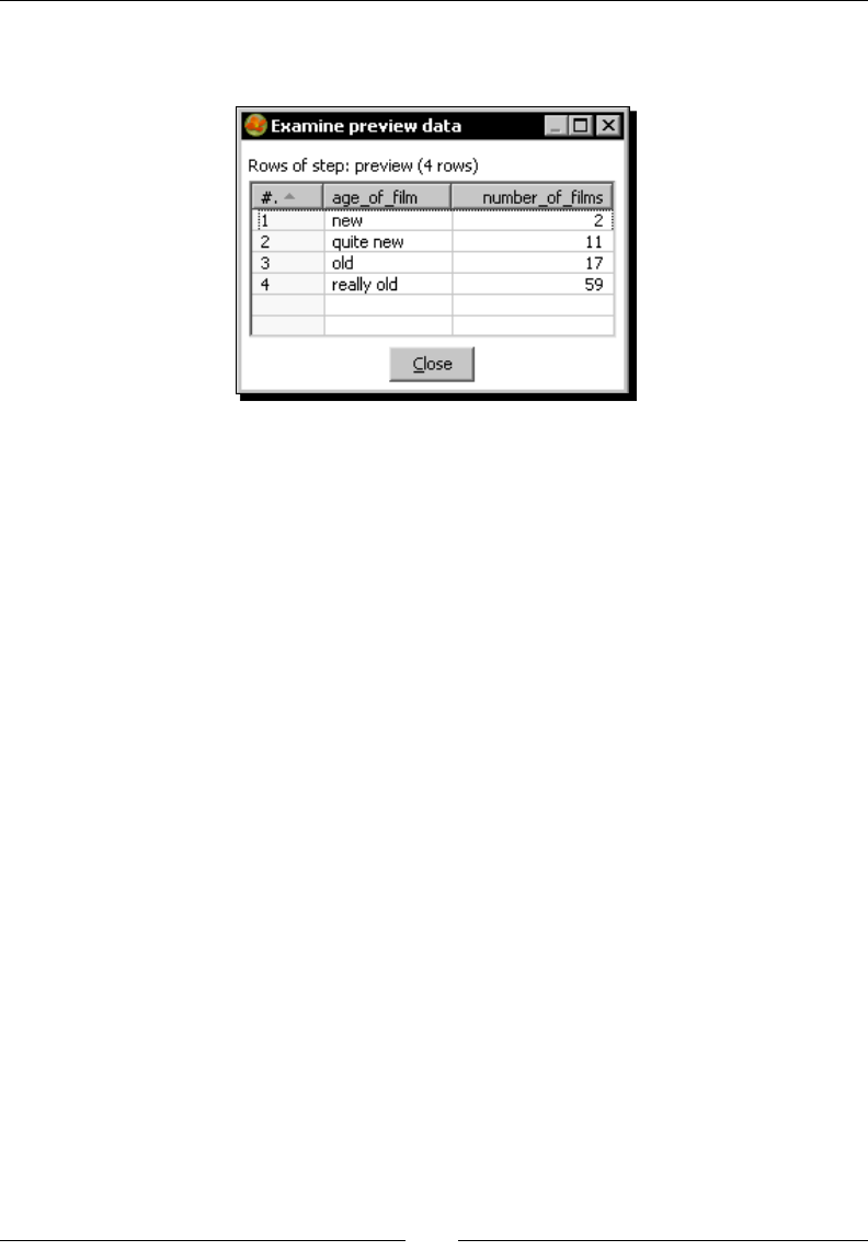
Chapter 7
[ 199 ]
20. Save the transformaon and do a new preview on the Dummy step. You will
see this:
21. The logging window will show you this:
... - Bad rows.0 -
... - Bad rows.0 - ------------> Linenr 1-------------------------
... - Bad rows.0 - null
... - Bad rows.0 -
... - Bad rows.0 - Javascript error:
... - Bad rows.0 - Could not apply the given format dd/MM/yyyy
on the string for 01/01/null : Format.parseObject(String) failed
(script#4)
... - Bad rows.0 -
... - Bad rows.0 - --> 4:0
... - Bad rows.0 - SCR-001
... - Bad rows.0 -
... - Bad rows.0 - ====================
... - Bad rows.0 -
... - Bad rows.0 - ------------> Linenr 2-------------------------
... - Bad rows.0 - null
... - Bad rows.0 -
... - Bad rows.0 - Javascript error:
... - Bad rows.0 - Could not apply the given format dd/MM/yyyy
on the string for 01/01/null : Format.parseObject(String) failed
(script#4)
... - Bad rows.0 -
... - Bad rows.0 - --> 4:0
...
The date was cut from the log for clarity of the log messages.
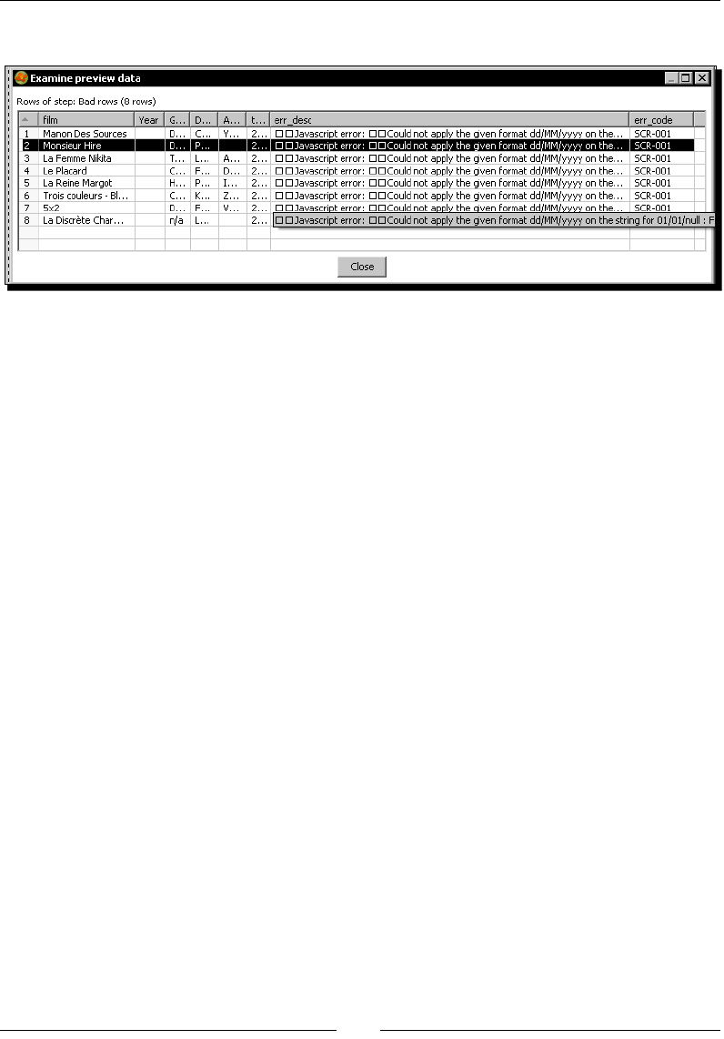
Validang Data and Handling Errors
[ 200 ]
22. Now do a preview on the Write to log step. This is what you see:
What just happened?
You created a transformaon to read a list of lms and group them according to their age,
that is, how old the movie is. You were surprised by an unexpected error caused by the rows
in which the year was undened. Then you implemented error handling to capture that error
and to avoid the aboron of the transformaon. With the treatment of the error, you split
the stream in two:
The rows that caused the error went to a new stream that wrote to the log
informaon about the error
The rows that passed the JavaScript step without problem went through the
main path
Using PDI error handling functionality
With the error handling funconality, you can capture errors that otherwise would cause
the transformaon to halt. Instead of aborng, the rows that cause the errors are sent to a
dierent stream for further treatment.
You don't need to implement error handling in every step, but in those where it's more
likely to have errors when running the transformaon. A typical situaon where you should
consider handling errors is in a JavaScript step. A code that works perfectly when designing
might fail while execung against real data, where the most common errors are related to
data type conversions or indexes out of range. Another common use of error handling is
when working with databases (you will see more on this later in the book).
To congure the error handling, you have to right-click the step and select Dene
Error handling.

Chapter 7
[ 201 ]
Note that not all steps support error handling. The Dene Error handling opon
is available only when clicking on steps that support it.
Aer opening the sengs window, you have to ll it just as you did in the tutorial. You have
to specify the target step for the bad rows along with the name of the extra elds being
added, as part of the treatment of errors:
Field Descripon
Nr of errors eldname Name for the eld that will have the number of errors
Error elds eldname Name for the eld that will have the name of the eld(s) that
caused the errors
Error codes eldname Name for the eld that will have the error code
Error descripons eldname Name for the eld that will have the error descripon
The rst two are trivial. The last two deserve an explanaon. The values for the error code
and descripon elds are the same as those you see in the Logging tab when you don't trap
the error. In the tutorial there was a JavaScript error with code SCR-001 and descripon
JavaScript error: Could not apply the given format.... You saw this
code as well as its descripon in the Logging tab when you didn't trap the error and the
transformaon crashed, and in the preview you made at the end of the error stream. This
parcular error was a JavaScript one, but the kind of error you get depends always on the
kind of step where it occurs.
You are not forced to ll all the textboxes in the error seng window. Only the elds for
which you provide a name will be added to the dataset. By doing a preview on the target
step, you can see the extra elds that were added.
Aborting a transformation
You can handle the errors by detecng and sending bad rows to an extra stream. But when
the errors are too many or when the errors are severe, the best opon is to cancel the whole
transformaon. Let's see how to force the aboron of a transformaon in such a situaon.
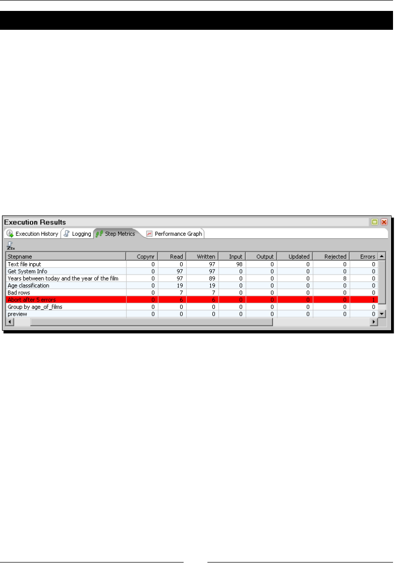
Validang Data and Handling Errors
[ 202 ]
Time for action – aborting when there are too many errors
1. Open the transformaon from the previous tutorial and save it under a
dierent name.
2. From the Flow category, drag an Abort step to the canvas.
3. Create a hop from the Write to log step to the Abort step.
4. Double-click the Abort step. Enter 5 as Abort threshold. As Abort message, type
Too many errors calculating age of film!.
5. Click OK.
6. Select the Dummy step and do a preview. As a result, a warning window shows up
informing you that there were no rows to display. In the Step Metrics tab, the Abort
aer 5 errors line becomes red to show you that there was an error:
7. The log looks like this:
... - Bad rows.0 -
... - Bad rows.0 - ====================
... - Abort after 5 errors.0 - Row nr 6 causing abort :
[Trois couleurs - Blanc], [null], [Comedy | Drama],
[Krzysztof Kieslowski], [Zbigniew Zamachowski, Julie Delpy],
[2009/08/18 00:00:00.000], [
... - Abort after 5 errors.0 - Javascript error:
... - Abort after 5 errors.0 - Could not apply the given
format dd/MM/yyyy on the string for 01/01/null : Format.
parseObject(String) failed (script#4)
... - Abort after 5 errors.0 -
... - Abort after 5 errors.0 - --> 4:0], [SCR-001]
... - Abort after 5 errors.0 - Too many errors calculating age of
film!
... - Abort after 5 errors.0 - Finished processing (I=0, O=0, R=6,
W=6, U=0, E=1)

Chapter 7
[ 203 ]
...
... - Spoon - The transformation has finished!!
... - error_handling_with_abort - ERROR (version 3.2.0-GA, build
10572 from 2009-05-12 08.45.26 by buildguy) : Errors detected!
What just happened?
You forced the aboron of a transformaon aer ve erroneous rows.
Aborting a transformation using the Abort step
Through the use of the Abort step, you force the aboron of a transformaon. Its main use is
in error handling.
You can use the Abort step to force the aboron as soon as a row arrives to it, or aer a
certain number of rows as you did in the tutorial. To decide between one and the other
opon, you use the Abort threshold opon. If threshold is 0, the Abort step will abort
aer the rst row arrives. If threshold is N, the Abort step will cause the aboron of the
transformaon when the row number N+1 arrives at it.
Beyond the error handling situaon, you may use the Abort step in any unexpected
situaon. Examples of that could be when you expect parameters and they are not present
or when an incoming le is empty when it shouldn't be. In situaons like these, you can force
an abnormal ending of the execuon just by adding an Abort step aer the step that detects
the anomaly.
Fixing captured errors
In the Time for acon—capturing errors while calculang the age of a lm secon of this
chapter, you sent the bad rows to the log. However, when you capture errors, you can send
the bad rows toward any step as long as the step knows how to treat those rows. Let's see
an example of that.
Time for action – treating errors that may appear
1. Open the transformaon from the tutorial and save it under a dierent name.
2. From the Transform category, drag the Add constants step to the canvas.
3. Create a hop from the Write to log step to the Add constants step.
4. Add an Integer constant named diff with value 999, and a String constant
named age_of_film with value unknown.
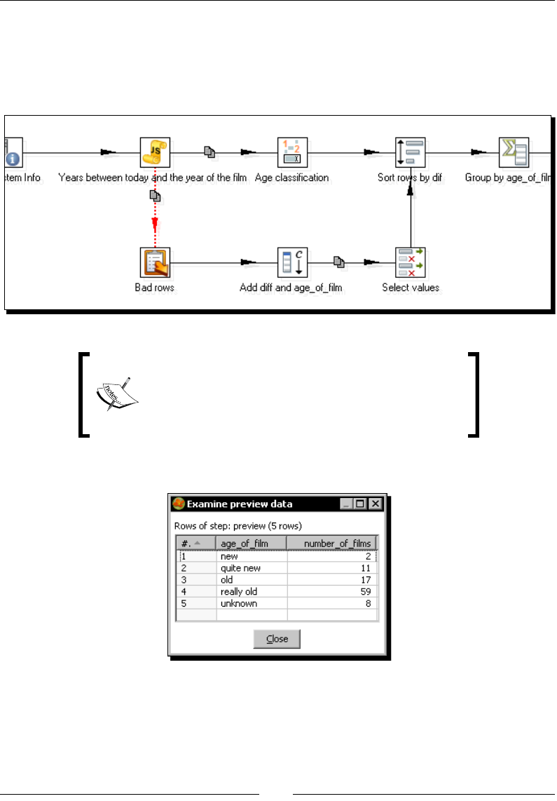
Validang Data and Handling Errors
[ 204 ]
5. Aer the Add constants step, add a Select values step and use it to remove the
elds err_code and err_desc.
6. Create a hop from the Select values step to the Sort rows step. Your transformaon
should look like this:
Note that you are merging two streams. Those
streams must have the same metadata. If you get a
trap detector warning, please verify that you executed
these instrucons exactly as explained.
7. Select the Dummy step and do a preview. You will see this:
What just happened?
You modied the transformaon so that you didn't end up discarding the erroneous rows. In
the error stream (the stream aer the red doed line), you xed the rows by pung default
values for the new elds. Aer that you returned the rows to the main stream.

Chapter 7
[ 205 ]
Treating rows coming to the error stream
If the errors are not severe enough to discard the rows, if you can somehow guess
what data was supposed to be there instead of the error, or if you have default values for
erroneous data, you can do your best to x the errors and send the rows back to the
main stream.
What you did instead of discarding the rows with no year informaon was to x the rows
and send them back to the main stream. The Group by step grouped them under a separate
category named unknown.
There are no rules for what to do with bad rows where you handle errors. You always have
the opon to discard the bad rows or try to x them. Somemes you can x only a few and
discard the rest of them. It always depends on your parcular data or business rules.
Pop quiz – PDI error handling
What does the PDI error-handling funconality do:
a. Avoids the happening of unexpected errors
b. Captures errors that happen and discards erroneous rows so you can connue
working with valid data
c. Captures errors that happen and sends erroneous rows to a new stream, leng you
decide what to do with them
Have a go hero – capturing errors while seeing who wins
On the Packt website you will nd a modied football match le named
wcup_modified.txt. This modied le has some intenonal errors.
Download the le and do the following:
1. Create a transformaon, read the le with a Text le input step. Set all elds
as string.
2. Add a JavaScript step and type the following code in it:
var result_desc;
result_split = Result.split('-');
home_g = str2num(result_split[0]);
away_g = str2num(result_split[1]);
if (home_g > away_g)
result_desc = Home_Team + ' wins';
else if (home_g < away_g)
result_desc = Away_Team + ' wins';
else result_desc = 'Nobody wins';

Validang Data and Handling Errors
[ 206 ]
3. In the grid below the code, add the string variable result_desc.
4. Do a preview on the JavaScript step and see what happens.
5. Now try any of the following two soluons:
Handle the errors and discard the rows that cause those errors.
Abort if there are more than 10 errors.
Handle the errors and x the transformaon by seng a default
result descripon for the rows that cause the errors.
Avoiding unexpected errors by validating data
To avoid unexpected errors that happen or just to meet your requirements is a common
pracce to validate your data before processing it. Let's do some validaons.
Time for action – validating genres with a Regex Evaluation step
In this tutorial you will read the modied lms le and validate the genres eld.
1. Create a new transformaon.
2. Read the modied lms le just as you did in the previous tutorial.
3. In the Content tab, check the Rownum in output? opon and ll the Rownum
eldname with the text rownum.
4. Do a preview. You should see this:
5. Aer the Text le input step, add a Regex Evaluaon step. You will nd it under the
Scripng category of steps.
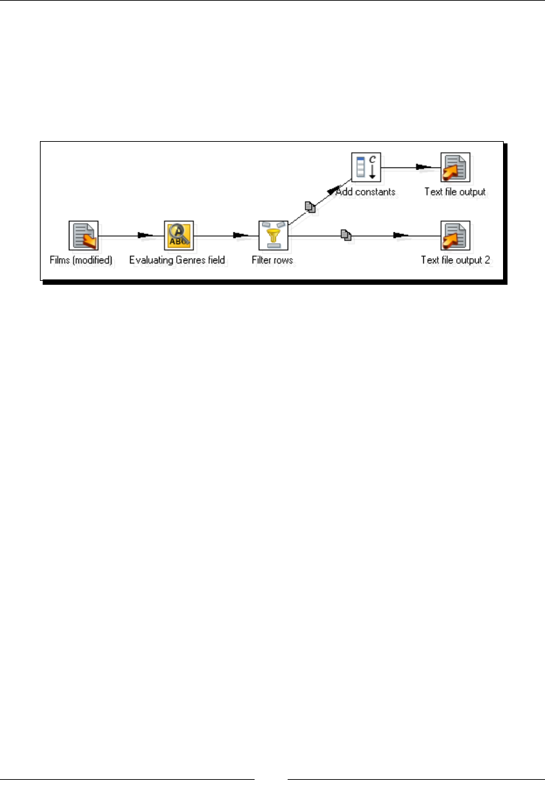
Chapter 7
[ 207 ]
6. Under the Step sengs box, select Genres as the Field to evaluate, and type
genres_ok as the Result Fieldname.
7. In the Regular expression textbox type [A-Za-z\s\-]*(\|[A-Za-z\s\-]*)* .
8. Add the Filter rows step, an Add constants step, and two Text le output steps and
link them as shown next:
9. Edit the Add constants step.
10. Add a String constant named err_code with value GEN_INV and a String constant
named err_desc with value Invalid list of genres.
11. Congure the Text le output step aer the Add constant step to create the
${LABSOUTPUT}/films_err.txt le, with the elds rownum, err_code, and
err_desc.
12. Congure the other Text le output step to create the ${LABSOUTPUT}/films_
ok.txt le, with the elds film, Year, Genres, Director, and Actors.
13. Double-click the Filter rows step and add the condion genres_ok = Y, Y being a
Boolean value. Send true data to the stream that generates the films_ok.txt
le. Send false data to the other stream.
14. Run the transformaon.
15. Check the generated les. The films_err.txt le looks like the following:
rownum;err_code;err_desc
12;GEN_INV;Invalid list of genres
18;GEN_INV;Invalid list of genres
20;GEN_INV;Invalid list of genres
21;GEN_INV;Invalid list of genres
22;GEN_INV;Invalid list of genres
33;GEN_INV;Invalid list of genres
34;GEN_INV;Invalid list of genres
...

Validang Data and Handling Errors
[ 208 ]
The films_ok.txt le looks like this:
film;Year;Genres;Director;Actors
Persepolis;2007;Animation | Comedy | Drama | History;Vincent
Paronnaud, Marjane Satrapi;Chiara Mastroianni, Catherine Deneuve,
Danielle Darrieux
Trois couleurs - Rouge;1994;Drama;Krzysztof Kieslowski;Irène
Jacob, Jean-Louis Trintignant, Frédérique Feder, Jean-Pierre
Lorit, Samuel Le Bihan
Les Misérables;1933;Drama | History;Raymond Bernard;
...
What just happened?
You read the lms le and checked that the Genres eld was a list of strings separated by |.
You created two les:
One le with the valid rows.
Another le with the rows with an invalid Genres eld. Note that the rownum eld
you added when you read the le is used here for idenfying the wrong lines.
In order to check the validity of the Genres eld, you used a regular expression. The
expression you typed accepts any combinaon of characters, spaces, or hyphens separated
by a pipe. The * symbol allows empty genres as well. For a detailed explanaon of regular
expressions, please refer to Chapter 2.
Validating data
As said, you would validate data mainly for two reasons:
To prevent the transformaon from aborng because of unexpected errors
To check that your data meets some pre-exisng requirements
For example, consider some of the sample data from previous chapters:
In the match le, the results eld had to be a string formed by two numbers
separated by a -
In the real estate le, the ag for Fireplace had to be Yes or No
In the contest le the name of the country had to be a valid country, not a
random string
If your data doesn't meet these requirements, it is possible that you don't have errors but
you will sll be working with invalid data.
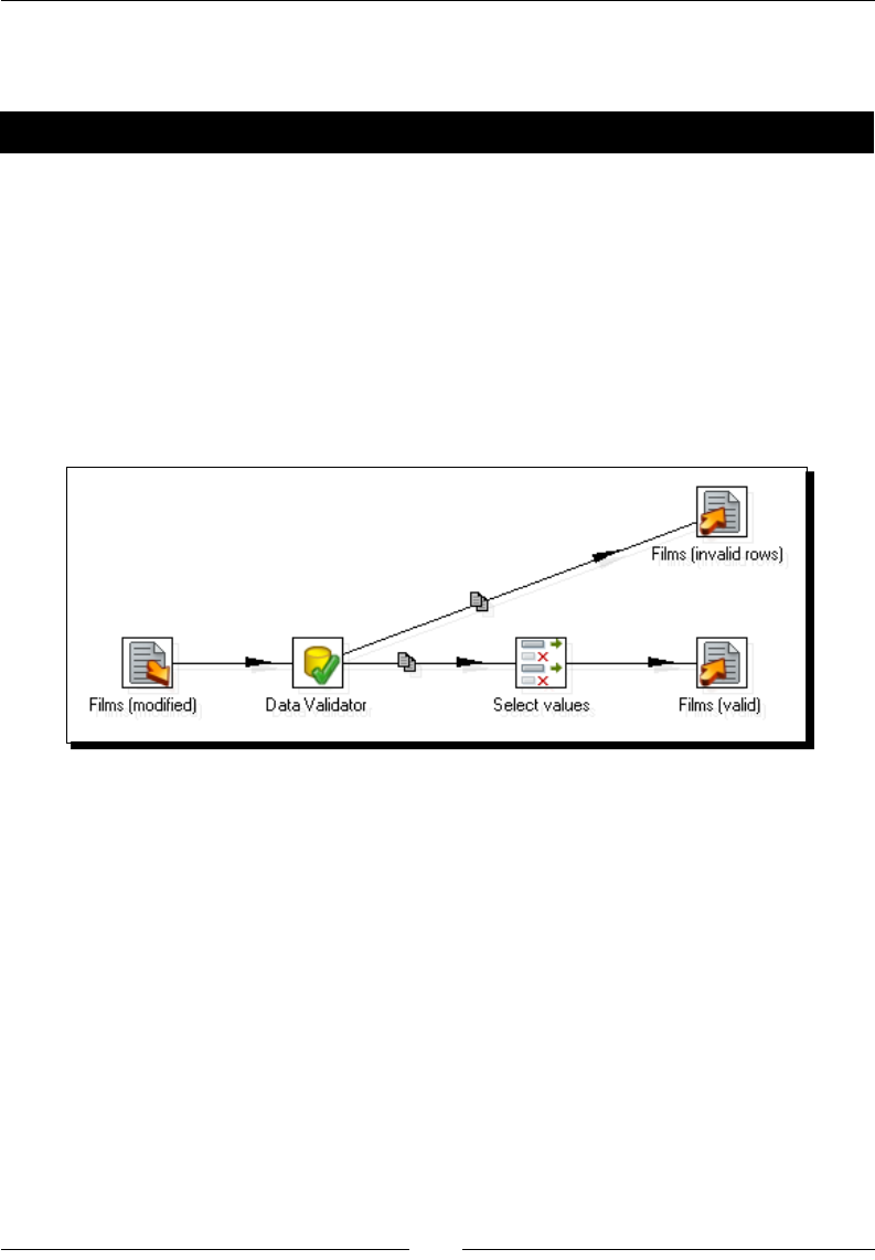
Chapter 7
[ 209 ]
In the last tutorial you just validated one of the elds. If you want to validate more than one
eld, you have a specic step that simplies that work: The Data Validator.
Time for action – checking lms le with the Data Validator
Let's validate not only the Genres eld, but also the Year eld.
1. Open the last transformaon and save it under a new name.
2. Delete all steps except the Text le input and Text le output steps.
3. In the Fields tab of the Text le input step, change the Type of the Year from
Integer to String.
4. From the Validaon category add a Data Validator step. Also add a Select values
step. Link all steps as follows:
5. Double-click the Data Validator step.
6. Check the Report all errors, not only the rst opon found on at the top of the
window. This will enable the Output one row, concatenate errors with separator
opon. Check this opon too, and ll the textbox to the right with a slash /. Click on
New validaon and type genres as the name of the validaon rule.
7. Click on OK.
8. Click on genres. The right half of the window is lled with checkboxes and textboxes
where you will dene the rule.
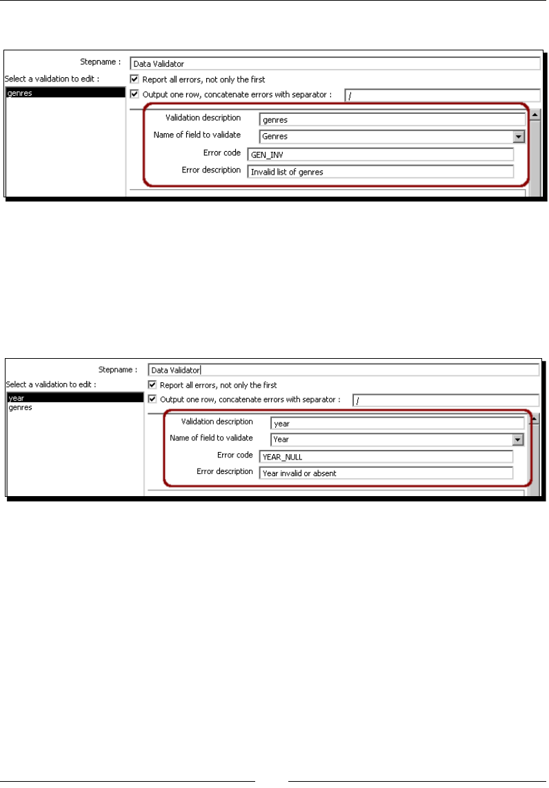
Validang Data and Handling Errors
[ 210 ]
9. Fill the header of the rule denion as follows:
10. In the Regular expression expected to match textbox, type
[A-Za-z\s\-]*(\|[A-Za-z\s\-]*)*
11. Click on New validaon and type year as the name of the validaon rule.
12. Click on OK.
13. Click on year and ll the header of the rule denion as follows:
14. In the data block, select the Only numeric data expected checkbox opon.
15. Click on OK.
16. Right-click the Data Validator step and select Dene error handling....
17. Fill the error handling sengs window as follows: As Target step, select the step that
generates the le with invalid rows. Check the Enable the error handling? checkbox.
Type err_desc as Error descripon eld name, err_field as Error elds, and
err_code as Error codes. Click on OK.
18. Use the Select values step to change the metadata for the Year from String
to Integer.
19. Save the transformaon and run it.

Chapter 7
[ 211 ]
20. Check the generated les. The films_err.txt le now has more detail, as you
validated two elds.
rownum;err_code;err_desc
9;YEAR_NULL;Year invalid or absent
12;GEN_INV;Invalid list of genres
18;GEN_INV;Invalid list of genres
20;GEN_INV;Invalid list of genres
21;GEN_INV;Invalid list of genres
22;GEN_INV;Invalid list of genres
33;GEN_INV;Invalid list of genres
34;GEN_INV;Invalid list of genres
47;YEAR_NULL/GEN_INV;Year invalid or absent/Invalid list of genres
48;YEAR_NULL/GEN_INV;Year invalid or absent/Invalid list of genres
49;YEAR_NULL;Year invalid or absent
...
21. The films_ok.txt le should have less rows instead, as the lms with year invalid
or absent are no longer sent to this le.
What just happened?
You used the Data Validator step to validate both the genres list and the year. You created
a le with the good rows, and another le with the informaon to show you which errors
were found.
Dening simple validation rules using the Data Validator
The Data Validator step, or DV for short, allows you to dene simple validaon rules to
describe the expected characteriscs for the incoming elds. The good thing about the DV
step is that it concentrates several validaons into a single step, and obviously it supports
error handling.
For every validaon rule, you have to specify these elds:
Field Descripon
Name of the eld to validate Name of the incoming eld whose value will be
validated with this rule
Error code The error code to pass to error handling. If
omied, a default is set
Error descripon The error descripon to pass to error handling. If
omied, a default is set

Validang Data and Handling Errors
[ 212 ]
The error code and error descripon are useful to idenfy which eld was erroneous when
you have more than one validaon rule in a single DV step.
It is possible for more than one eld to cause a row pass to error handling. In that case,
you can generate one output row per error or a single row with all error descripons
concatenated. In the tutorial you chose this last opon.
In the sengs window, once you select a validaon rule, you have two blocks of sengs—
the Data block where you dene the expected data for a eld and the Type block where you
validate if a eld matches a given type or not.
In the Data block you set the actual validaon rule for a eld.
The following table summarizes the kinds of validaons you may apply in this block:
Validaon Data block opons
Allowing (only) null values Null allowed? / Only null values allowed?
Making sure that the length of the selected
eld is between a range of values
Max string length / Min string length.
You may use one or both at the same me.
Making sure that the value of the selected
eld is between a range of values
Maximum value / Minimum value
You may use one or both at the same me.
Making sure that the selected eld matches
a paern
Only numeric data expected
Expected start string
Expected end string
Regular expression expected to match
Making sure that the selected eld doesn't
match a paern
Not allowed start string
Not allowed end string
Regular expression not allowed
to match
Making sure that the selected eld is one of
the values in a given list
Allowed values (when you have a
xed list)
Read allowed values from another step?
(when the list comes from
another stream)
In the tutorial, you used just a couple from this long list of opons. For the validaon of the
genres, you used a regular expression that the eld had to match. For the year, you checked
that the eld wasn't null and that it contained only numeric data.
Let's briey explain what you did to validate the year. You read the year as a String. Then
with the DV you checked that it contained only numeric data. If the data was valid, you
changed the metadata to Integer aer the row le the DV step.

Chapter 7
[ 213 ]
Why didn't you simply validate whether the year was an Integer? This is because the type
validaon just checks that the year is an integer eld, rather than checking if it can be
converted into an integer. In this case, the year is of type String because you read it
as a String in the Text le input step.
What would happen if you read the year as an Integer? The invalid elds would cause
an error in the Text le input step, and the row would never arrive to the DV step to
be validated.
The type block allows you to validate the type of an incoming eld. This just
checks the real data type, rather than checking if the eld can be converted
into a given data type.
Have a go hero – validating the football matches le
From the Packt website, download the valid_countries.txt le. Modify the
transformaon from the previous "Hero" secon doing the following things.
Aer reading the le, apply the following validaon rules:
Field Validaon rule
Match_Date dd/mm, where dd/mm is a valid date.
Home_Team Belongs to the list of countries in the valid_countries.txt le.
Away_Team Belongs to the list of countries in the valid_countries.txt le.
Result n-n where n is a number.
Also validate that Home_Team is dierent from Away_Team.
Use a Data Validator step when possible.
Send the bad rows to a le of invalid data and the good rows to the JavaScript step.
Test your transformaon and check that every validaon rule is applied as expected.
Cleansing data
While validaon means mainly rejecng data, data cleansing detects and tries to x not only
invalid data, but also data considered illegal or inaccurate in a specic domain.
For example, consider a eld represenng a year. A year containing non-numeric symbols
should always be considered invalid and then rejected.

Validang Data and Handling Errors
[ 214 ]
Now look at the lms example. In this specic case, the year might not be important to you.
If you nd a non-numeric value, you could just replace it by a null year meaning unknown
and keep the data.
On the contrary, the simple rule that looks for numeric values is not enough. A year equal to
1084 should also be considered invalid as it is impossible to have a lm made at that me.
However, as it is a common error to type 0 instead of 9, you may assume that there was a
human mistake and you could replace the 0 in 1084 by a 9 automacally.
Doing data cleansing actually involves trying to detect and deal with these kinds of
situaons, knowing in advance the rules that apply.
Data cleansing, also known as data cleaning or data scrubbing, may be done manually
or automacally depending on the complexity of the cleansing. With PDI you can use the
automated opon. For the validang part of the process, you can use any of the steps or
mechanisms explained above. While for the cleaning part you can use any PDI step that suits,
there are some steps that are parcularly useful.
Step Purpose
If eld value is null If a eld is null, it changes its value to a constant. It can be applied to all elds
of the same data type, or to parcular elds.
Null if... Sets a eld value to null if it is equal to a constant value.
Number range Creates ranges based on a numeric eld. An example of use is converng
oang numbers to a discrete scale such as 0, 0.25, 0.50, and so on.
Value Mapper Maps values of a eld from one value to another. For example, you can use
this step to convert yes/no, true/false, or 0/1 values to Y/N.
Stream lookup Looks up values coming from another stream. In data cleansing, you can use
it to set a default value if your eld is not in a given list.
Database lookup Same as Stream lookup but looking in a database table.
Unique rows Removes double consecuve rows and leaves only unique occurrences.
For examples that use these steps or for geng more informaon about them, please refer
to Appendix C, Job Entries and Steps Reference.
Have a go hero – cleansing lms data
From the Packt's website, download the fix_genres.txt le. The le has the
following lines:
erroneous;fixed
commedy;comedy
sci-fi; science fiction
science-fiction; science fiction
musical;music
historical;history

Chapter 7
[ 215 ]
Create a new transformaon and do the following:
Read the modied lms le that you have used throughout the chapter. Validate that the
genre is a list of strings separated by |. Send the bad rows to a le of bad rows. So far,
this is the same as you did in the last two tutorials. Now clean the genres in the lists.
For every genre:
1. Check that it is not null. If it is null, discard it.
2. Split composed genres in two. For example, Historical drama becomes
historical and drama.
3. Standardize the descripons:
Remove trailing spaces.
Change the descripons to lower case.
4. Check that it is not misspelled. For doing that, use the miss_genres.txt le. If
the genre is in the list, replace the text by the correct descripon.
5. Aer all this cleaning add a Dummy step and preview the results.
To validate each genre, you can split the Genres eld into rows. Aer the
cleansing, you can recover the original lines by grouping the rows, using as
aggregate Concatenate strings separated by | to concatenate
the validated genres.
Summary
In this chapter, you learned two essenal subjects when it comes to the running of
transformaons by nontechnical users, in producve environments, with real data—
validang data and handling errors.
In the next chapter, we go back to the development, this me with a subject that most of
you must be waing for since Chapter 1—working with databases.

8
Working with Databases
Database systems are the main mechanism used by most organizaons to store
and administer organizaonal data. Online sales, bank-related operaons,
customer service history, and credit card transacons are some examples of
data stored in databases.
This is the rst of two chapters fully dedicated to working with databases. This chapter
provides an overview of the main database concepts. It also covers the following topics:
Connecng to databases
Previewing and geng data from a database
Inserng, updang, and deleng data from a database
Introducing the Steel Wheels sample database
As you were told in the rst chapter, there is a Pentaho Demo that includes data for a
conal store named Steel Wheels and you can download it from the Internet. This data is
stored in a database that is going to be the starng point for you to learn how to work with
databases in PDI. Before beginning to work on databases, let's briey introduce the Steel
Wheels database along with some database denions.

Working with Databases
[ 218 ]
A relaonal database is a collecon of items stored in tables. Typically, all items stored in a
table belong to a parcular type of data. The following table lists some of the tables in the
Steel Wheels database:
Table Content
CUSTOMERS Steel Wheels' customers
EMPLOYEES Steel Wheels' employees
PRODUCTS Products sold by Steel Wheels
OFFICES Steel Wheels' oces
ORDERS Informaon about sales orders
ORDERDETAILS Details about the sales orders
The items stored in the tables represent an enty or a concept in the real world. As an
example, the CUSTOMERS table stores items represenng customers. The ORDERS table
stores items that represent sales orders in the real world.
In technical terms, a table is uniquely idened by a name such as CUSTOMERS, and contains
columns and rows of data.
You can think of a table as a PDI dataset. You have elds (the columns of the table) and rows
(the records of the table).
The columns, just like the elds in a PDI dataset, have a metadata describing their name, type,
and length. The records hold the data for those columns; each record represents a dierent
instance of the items in the table. As an example, the table CUSTOMERS describes the
customers with the columns CUSTOMERNUMBER, CUSTOMERNAME, CONTACTLASTNAME and so
forth. Each record of the table CUSTOMERS belongs to a dierent Steel Wheels' customer.
A table usually has a primary key. A primary key or PK is a combinaon of one or more
columns that uniquely idenfy each record of the table. In the sample table, CUSTOMERS,
the primary key is made up of a single column—CUSTOMERNUMBER. This means there cannot
be two customers with the same customer number.
Tables in a relaonal database are usually related to one another. For example, the
CUSTOMERS and ORDERS tables are related to convey the fact that real-world customers
have placed one or more real-world orders. In the database, the ORDERS table has a column
named CUSTOMERNUMBER with the number of the customer who placed the order. As said,
CUSTOMERNUMBER is the column that uniquely idenes a customer in the CUSTOMERS
table. Thus, there is a relaonship between both tables. This kind of relaonship between
columns in two tables is called foreign key or FK.
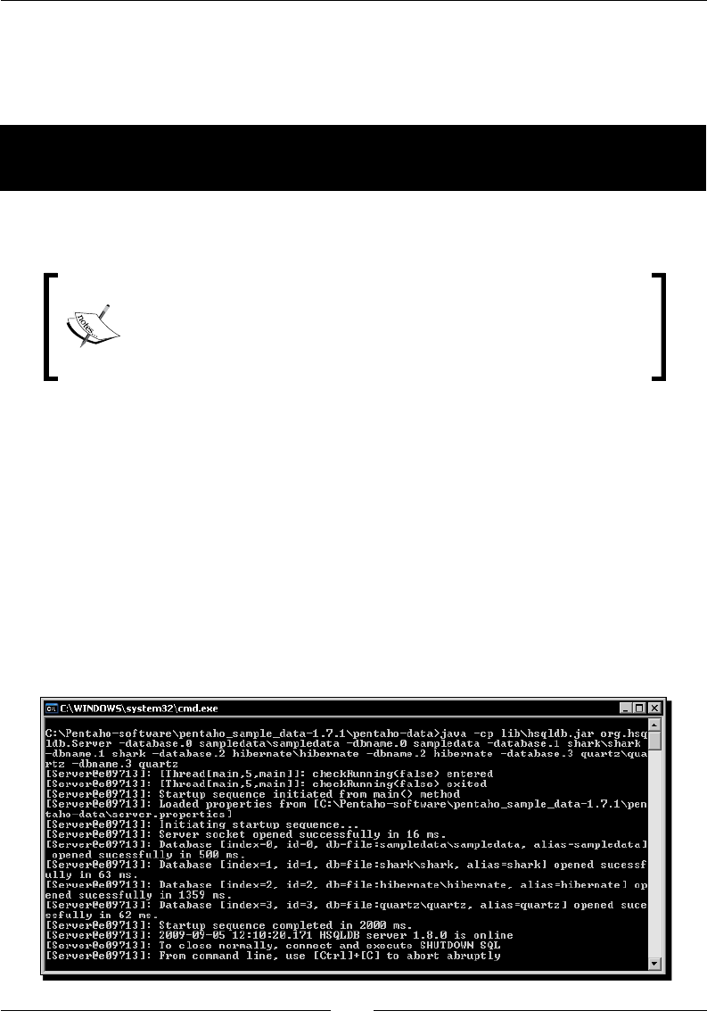
Chapter 8
[ 219 ]
Connecting to the Steel Wheels database
The rst thing you have to do in order to work with a database is tell PDI how to access the
database. Let's learn how to do it.
Time for action – creating a connection with the Steel Wheels
database
In this rst database tutorial, you will download the sample database and create a
connecon for accessing it from PDI.
The Pentaho BI demo includes the sample data. So, if you have already
downloaded the demo as explained in Chapter 1, just skip the rst
three steps. If the Pentaho BI demo is running on your machine, the
database server is running as well. In that case, skip the rst four steps.
1. Go to the Pentaho Download site: http://sourceforge.net/projects/
pentaho/files/.
2. Under the Business Intelligence Server | 1.7.1-stable, look for the le namedlook for the le named
pentaho_sample_data-1.7.1.zip and download it.
3. Unzip the downloaded le.
4. Run start_hypersonic.bat under Windows or start_hypersonic.sh under
Unix-based operang systems. If you download the sample data, you will nd
these scripts in the folder named pentaho-data. If you download the Pentaho BI
server instead, you will nd them in the folder named data. The following screen is
displayed when the database server starts:
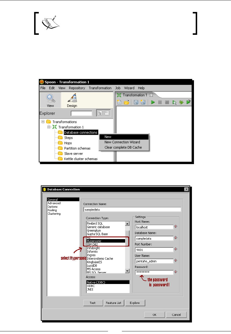
Working with Databases
[ 220 ]
Don't close this window. It would cause the database
server to stop.
5. Open Spoon and create a new transformaon.
6. Click on the View opon that appears in the upper-le corner of the screen.
7. Right-click the Database connecons opon and click on New.
8. Fill the Database Connecon dialog window as follows:
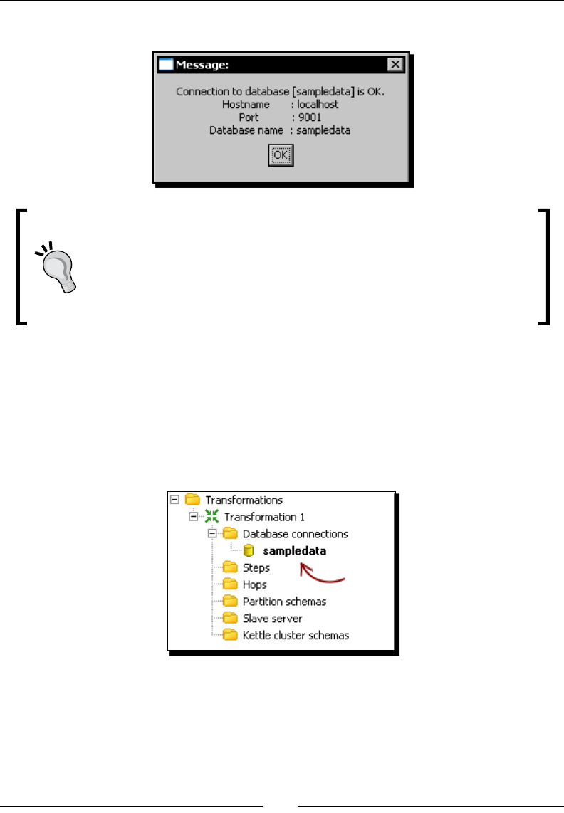
Chapter 8
[ 221 ]
9. Click on the Test buon. The following window shows up:
If you get an error message instead of the Message window shown in the
previous screenshot, please recheck the data you entered in the connecon
window. Also verify that the database is running, that is, the terminal window
is sll opened and doesn't show an error message. If you see an error, or if
you don't see the terminal, please start the database server again as explained
at the beginning of the tutorial.
10. Click on OK to close the test window.
11. Click on OK again to close the database denion window. A new database
connecon is added to the tree.
12. Right-click on the database connecon and click on Share. The connecon
is available in all transformaons you create from now onwards. The shared
connecons are shown in bold leers.
13. Save the transformaon.
What just happened?
You created and tested a connecon to the Pentaho Sample database. Finally, you shared the
connecon so that it could be reused in other transformaons.
Working with Databases
[ 222 ]
Connecting with Relational Database Management Systems
Even if you've never worked with databases, you must have heard terms such as MySQL, Oracle,
DB2, or MS SQL server. These are just some of many Relaonal Database Management
Systems (RDBMS) on the market. An RDBMS is a soware that lets you create and administer
relaonal databases.
In the tutorial you worked with HyperSQL DataBase (HSQLDB), just another RDBMS formerly
known as Hypersonic DB. HSQLDB has a small, fast database engine wrien in Java. HSQLDB
is currently being used in many open source soware projects such as OpenOce.org 3.1
as well as in commercial projects and products such as Mathemaca. You can get more
informaon about HSQLDB at http://hsqldb.org/.
PDI has the ability to connect with both commercial RDBMSes such as Oracle or MS SQL
server and free RDBMSes such as MySQL. In order to get connected to a parcular database,
you have to dene a connecon to it.
A database connecon describes all parameters needed to connect PDI to a database.
To create a connecon, you must give the connecon a name and ll at least the
general sengs:
Seng Descripon Steel Wheels sample
Connecon
type
Type of database system: HSQLDB, Oracle, MySQL,
Firebird, and so on.
HSQLDB
Method of
access
Nave (JDBC), ODBC, JNDI, or OCI. The available opons
depend on the type of DB.
Native (JDBC)
Host name Name or IP address for the host where the database is. localhost
Database
name
Idenes the database to which you want to connect. sampledata
Port number PDI sets as default the most usual port number for the
selected type of database. You can change it of course.
9001
User Name /
Password
Name of the user and password to connect to the
database.
pentaho_admin /
password
If you don't nd your database engine in the list, you will sll be able to connect
to it by specifying as connecon type, the Generic database opon. In that case,
you have to provide a connecon URL and the driver class name.
Aer creang a connecon, you can click the Test buon to check that the connecon has
been dened correctly and that you can reach them from PDI.

Chapter 8
[ 223 ]
The database connecons will be available just in the transformaon where you dened
them, unless you share it for reuse as you did in the tutorial. Normally, you share
connecons because you know that you will use them later in many transformaons.
The informaon about shared connecons is stored in a le named shared.xml, located in the
same folder as the kettle.properties le.
When you have shared connecons and you save the transformaon, the connecon
informaon is saved in the transformaon itself.
If there is more than one shared connecon, all of them will be saved
along with the transformaon, even if the transformaon doesn't use
them all. To avoid this, go to the eding opons and check the Only
save used connecons to XML? opon. This opon limits the XML
content of a transformaon to just the used connecons.
Pop quiz – dening database connections
Which opons do you have to connect to the same database in several transformaons:
a. Dene the connecon in each transformaon that needs it
b. Dene a connecon once and share it
c. Either of the above opons
d. Neither of the above opons
Have a go hero – connecting to your own databases
You must have access to a database, whether local or in the network to which you are logged
in. Get the connecon informaon for the database. From PDI create a connecon to the
database and test it to verify that you can access it from PDI.
Exploring the Steel Wheels database
In the previous secon, you learned about what RDBMSs are and how to connect to an
RDBMS from PDI. Before beginning to work with the data in a database, it would be useful to
get familiarized with that database. In this secon, you will learn to explore databases with
the PDI Database explorer.
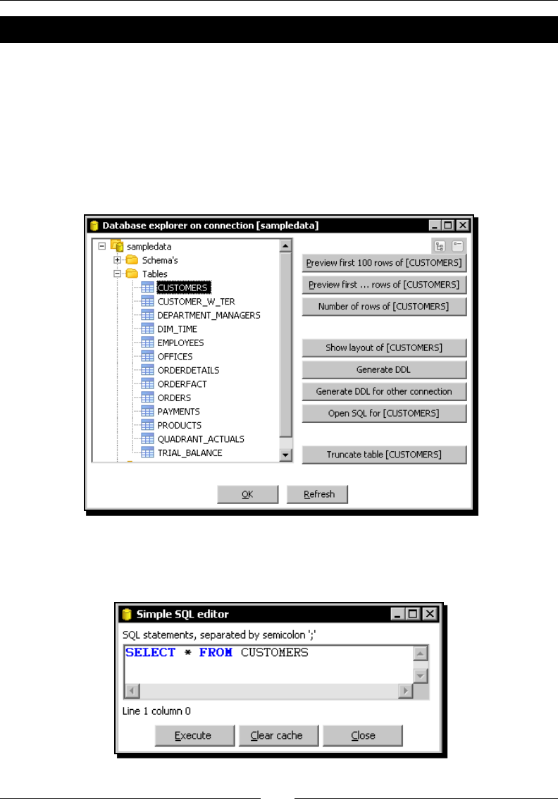
Working with Databases
[ 224 ]
Time for action – exploring the sample database
Let's explore the sample database:
1. Open the transformaon you just created.
2. Right-click the connecon in the Database connecons list and select Explore in the
contextual menu. The Database explorer on connecon window opens.
3. Expand the Tables node of the tree and select CUSTOMERS. This is how the
explorer looks:
4. Click on the Open SQL for [CUSTOMERS] opon.
5. The following SQL editor window appears:
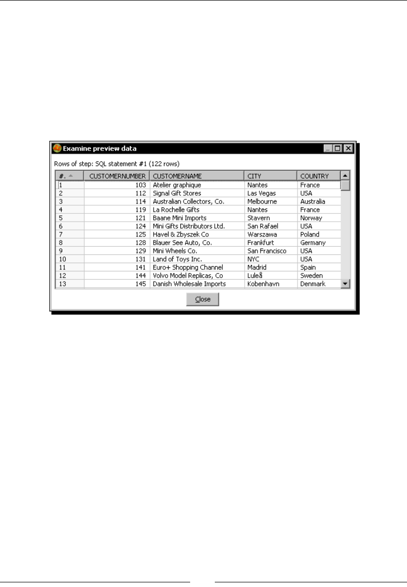
Chapter 8
[ 225 ]
6. Modify the text in the window so that you have the following:
SELECT
CUSTOMERNUMBER
, CUSTOMERNAME
, CITY
, COUNTRY
FROM CUSTOMERS
7. Click on Execute. You will see the following result:
8. Close the preview window (the window that tells the result of the execuon) and
the SQL editor window.
9. Click on OK to close the database explorer window.
What just happened?
You explored the Pentaho sample database with the PDI Database explorer.
A brief word about SQL
Before explaining the details of the database explorer, it's worth giving an introducon to
SQL—a central topic in relaonal database terminology.
SQL, that is, Structured Query Language is the language that lets you access and manipulate
databases in a RDBMS.
SQL can be divided into two parts—DDL and DML.

Working with Databases
[ 226 ]
The DDL, that is, Data Denion Language is the branch of the language that basically allows
creang or deleng databases and tables.
The following is an example of DDL. It is the DDL statement that creates the
CUSTOMERS table.
CREATE TABLE CUSTOMERS
(
CUSTOMERNUMBER INTEGER
, CUSTOMERNAME VARCHAR(50)
, CONTACTLASTNAME VARCHAR(50)
, CONTACTFIRSTNAME VARCHAR(50)
, PHONE VARCHAR(50)
, ADDRESSLINE1 VARCHAR(50)
, ADDRESSLINE2 VARCHAR(50)
, CITY VARCHAR(50)
, STATE VARCHAR(50)
, POSTALCODE VARCHAR(15)
, COUNTRY VARCHAR(50)
, SALESREPEMPLOYEENUMBER INTEGER
, CREDITLIMIT BIGINT
)
;
This DDL statement tells the database to create the table CUSTOMERS with the columns
CUSTOMERNUMBER of the type INTEGER, the column CUSTOMERNAME of the type VARCHAR
with length 50, and so on.
Note that INTEGER, VARCHAR, and BIGINT are HSQLDB types of data, not PDI ones. The
DML, that is, Data Manipulaon Language allows you to retrieve data from a database. It
also lets you insert, update, or delete data from the database.
The statement you typed in the SQL editor is an example of DML:
SELECT
CUSTOMERNUMBER
, CUSTOMERNAME
, CITY
, COUNTRY
FROM CUSTOMERS

Chapter 8
[ 227 ]
This statement is asking the database to retrieve all the rows for the CUSTOMERS table,
showing only CUSTOMERNUMBER, CUSTOMERNAME, CITY, and COUNTRY columns. Aer you
clicked Execute, PDI queried the database and showed you a window with the data you had
asked for.
If you were to leave the following statement:
SELECT * FROM CUSTOMERS
the window would have showed you all columns for the CUSTOMERS table.
SELECT is the statement that allows you to retrieve data from one or more tables. It is the
most commonly used DML statement and you're going to use it a lot when working with
databases in PDI. You will learn more about the SELECT statement in the next secon of
this chapter.
Other important DML statements are:
INSERT: This allows you to insert rows in a table
UPDATE : This allows you to update the values in rows of a table
DELETE: This statement is used to remove rows from a table
It is important to understand the meaning of these basic statements, but you are not
forced to learn them as PDI oers you ways to insert, update, and delete without typing
any SQL statement.
Although SQL is a standard, each database engine has its own version of the SQL language.
However, all database engines support the main commands.
When you type SQL statements in PDI, try to keep the code within the
standard. Your transformaons will then be reusable in case you have
to change the database engine.
If you are interested in learning more about SQL, there are a lot of tutorials on the Internet.
The following are a few useful links with tutorials and SQL references:
http://www.sqlcourse.com/
http://www.w3schools.com/SQl/
http://sqlzoo.net/
Unl now, you have used only HSQLDB. In the tutorials to come, you will also work with the
MySQL database engine. So, you may be interested in specic documentaon for MySQL,
which you can nd at http://dev.mysql.com/doc/. You can nd even more informaon
in books; there are plenty of books available about both SQL language and MySQL databases.
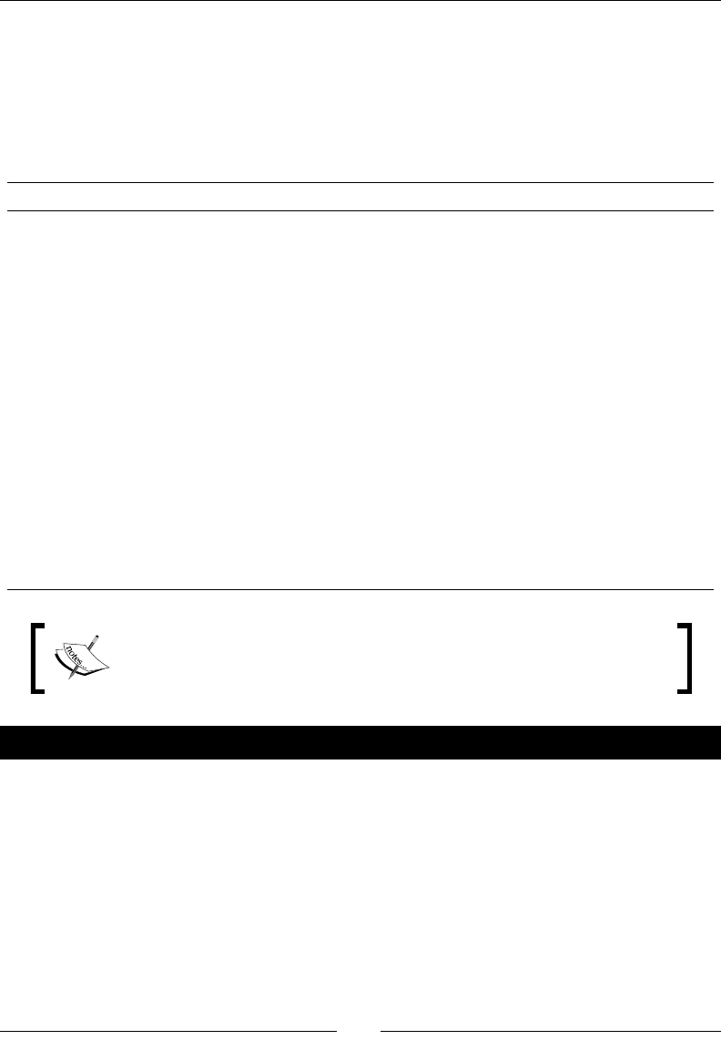
Working with Databases
[ 228 ]
Exploring any congured database with the PDI Database explorer
The database explorer allows you to explore any congured database. When you open the
database explorer, the rst thing you see is a tree with the dierent objects of the database.
As soon as you select a database table, all buons to the right side become available for you
to explore that table. The following are the funcons oered by the buons at the right side
of the database explorer:
Opon Meaning
Preview rst 100 rows of ... Return the rst 100 rows of the selected table, or all the rows
if the table has less that 100. This opon shows all columns of
the table.
Preview rst...rows of ... The same as the previous opon, but here you decide the
number of rows to show.
Number of rows of ... Tells you the total number of records in the table.
Show layout of ... Shows you the metadata for the columns of the table.
Generate DDL Shows you the DDL statement that creates the selected table.
Generate DDL for other
connecon
It lets you select another existent connecon. Then it shows
you the DDL just like the previous opon. The dierence is that
the DDL is wrien with the syntax of the database engine of the
selected connecon.
Open SQL for ... Lets you edit a SELECT statement to query the table. Here you
decide which columns and rows to retrieve.
Truncate table Deletes all rows from the selected table.
In the tutorial you opened the Database explorer from the contextual
menu in the Database connecons tree. You can also open it by clicking
the Explore opon in the database denion window.
Have a go hero – exploring the sample data in depth
In the tutorial you just tried the Open SQL buon. Feel free to try other buons to
explore not only the CUSTOMERS table but also the rest of the tables found in the Steel
Wheels database.

Chapter 8
[ 229 ]
Have a go hero – exploring your own databases
In the previous secon, there was a Hero exercise that asked you to connect to your own
databases. If you have done that, then use a database connecon dened by you and
explore the database. See if you can recognize the dierent objects of the database. Run
some previews to verify that everything looks as expected.
Querying a database
So far you have just connected to a database. You haven't yet worked with the data. Now is
the me to do that.
Time for action – getting data about shipped orders
Let's connue working with the sample data.
1. Create a new transformaon.
2. Select the Design view.
3. Expand the input category of steps and drag a Table Input step to the canvas.
4. Double-click the step.
5. Click on the Get SQL select statement... buon. The database explorer
window appears.
6. Expand the tables list and select ORDERS.
7. Click on OK.
8. PDI asks if you want to include the eld names in the SQL. Answer Yes.
9. The SQL box gets lled with a SELECT SQL statement.
SELECT
ORDERNUMBER
, ORDERDATE
, REQUIREDDATE
, SHIPPEDDATE
, STATUS
, COMMENTS
, CUSTOMERNUMBER
FROM ORDERS
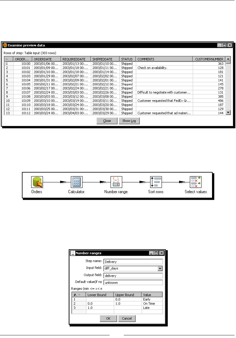
Working with Databases
[ 230 ]
10. At the end of the SQL statement, add the following clause:
WHERE STATUS = 'Shipped'
11. Click Preview and then OK. The following window appears:
12. Close the window and click OK to close the step conguraon window.
13. Aer the Table input step add a Calculator step, a Number Range step, a Sort step,
and a Select values step and link them as follows:
14. With the Calculator step, add an Integer eld to calculate the dierence between
the shipped date and the required date. Use the calculaon Date A – Date B
(in days) and name the eld diff_days. Use the Number ranges step to classify
the delays in delivery.
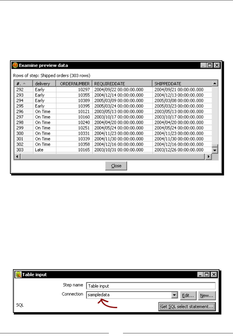
Chapter 8
[ 231 ]
15. Use the Sort rows step to sort the rows by the diff_days eld.
16. Use the Select values step to select the delivery, ORDERNUMBER, REQUIREDDATE,
and SHIPPEDDATE elds.
17. With the Select values step selected, do a preview. The following is how the nal
data will look:
What just happened?
From the sample database, you got informaon about shipped orders. Aer you read
the data from the database, you classied the orders based on the me it took to do
the shipment.
Getting data from the database with the Table input step
The Table input step is the main step to get data from a database. In order to use it, you have
to specify the connecon with the database. In the tutorial you didn't explicitly specify one
because there was just one connecon and PDI put it as the default value.
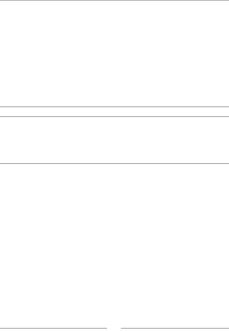
Working with Databases
[ 232 ]
The connecon was available because you shared it before. If you hadn't, you should have
created here again.
The output of a Table Input step is a regular dataset. Each column of the SQL query leads
to a new eld and the rows generated by the execuon of the query become the rows of
the dataset.
As the data types of the databases are not exactly the same as the PDI data types, when
geng data from a table, PDI implicitly converts the metadata of the new elds.
For example, consider the ORDERS table. Open the Database Explorer and look at the DDL
denion for the table. Then right-click the Table input step and select Show output elds to
see the metadata of the created dataset. The following table shows you how the metadata
was translated:
Table columns Database data type PDI metadata
ORDERNUMBER,
CUSTOMERNUMBER
INTEGER Integer(9)
ORDERDATE, REQUIREDDATE,
SHIPPEDDATE
TIMESTAMP Date
STATUS VARCHAR(15) String(15)
COMMENTS TEXT String(214748364)
Once the data comes out of the Table input step and the metadata is adjusted, PDI forgets
that it comes from a database. It treats it just as regular data, no maer if it came from a
database or any other data source.
Using the SELECT statement for generating a new dataset
The SQL area of a Table input step is where you write the SELECT statement that will
generate the new dataset. As said before, SELECT is the statement that you use to retrieve
data from one or more tables in your database.
The simplest SELECT statement is as follows:
SELECT <values>
FROM <table name>
Here <table name> is the name of the table that will be queried to get the result set and
<values> is the list of the desired columns of that table, separated by commas.
This is another simple SELECT statement:
SELECT ORDERNUMBER, ORDERDATE, STATUS
FROM ORDERS

Chapter 8
[ 233 ]
If you want to select all columns, you can just put a * as here:
SELECT *
FROM ORDERS
There are some oponal clauses that you can add to a SELECT statement. The most
commonly used among the oponal clauses are WHERE and ORDER BY. The WHERE clause
limits the list of retrieved records, while ORDER BY is used to retrieve the rows sorted by
one or more columns.
Another common clause is DISTINCT that can be used to return only dierent records.
Let's see some sample SELECT statements:
Sample statement Output
SELECT ORDERNUMBER, ORDERDATE
FROM ORDERS
WHERE SHIPPEDDATE IS NULL
Returns the number and order date for the orders
that have not been shipped.
SELECT *
FROM EMPLOYEES
WHERE JOBTITLE = 'Sales Rep'
ORDER BY LASTNAME, FIRSTNAME
Returns all columns for the employees whose job
is sales representave, ordered by last name and
rst name.
SELECT PRODUCTNAME
FROM PRODUCTS
WHERE PRODUCTLINE LIKE '%Cars%'
Returns the list of products whose product line
contains cars—for example, Classic cars and
Vintage cars.
SELECT DISTINCT CUSTOMERNUMBER
FROM PAYMENTS
WHERE AMOUNT > 80000
Returns the list of customer numbers who have
made payments with checks above USD80,000.
The customers who have paid more than once
with a check above USD80,000 appear more than
once in the PAYMENTS table, but only once in this
result set.
You can try these statements in the database explorer to check that the result sets are
as explained.
When you add a Table input step, it comes with a default SELECT statement for you
to complete.
SELECT <values> FROM <table name> WHERE <conditions>
If you need to query a single table, you can take advantage of the Get SQL select
statement... buon that generates the full statement for you. Aer you get the statement,
you can modify it at your will by adding, say, WHERE or ORDER clauses just as you did in the
tutorial. If you need to write more complex queries, you will have to do it manually.

Working with Databases
[ 234 ]
You can write any SELECT query as long as it is a valid SQL statement for
the selected type of database. Remember that every database engine has
its own dialect of the language.
Whether simple or complex, you may need to pass some parameters to the query. You can
do it in a couple of ways. Let's explain this with two praccal examples.
Making exible queries by using parameters
One of the ways you have to make your queries more exible is by passing it through some
parameters. In the following tutorial you will learn how to do it.
Time for action – getting orders in a range of dates by using
parameters
Now you will modify your transformaon so that it shows orders in a range of dates.
1. Open the transformaon from the previous tutorial and save it under a new name.
2. From the Input category, add a Get System Info step.
3. Double-click it and use the step to get the command line argument 1 and command
line argument 2 values. Name the elds as date_from and date_to respecvely.
Create a hop from the Get System Info step to the Table input step.
4. Double-click the Table input step.
5. Modify the SELECT statement as follows:
SELECT
ORDERNUMBER
, ORDERDATE
, REQUIREDDATE
, SHIPPEDDATE
FROM ORDERS
WHERE STATUS = 'Shipped'
AND ORDERDATE BETWEEN ? AND ?
6. In the drop-down list to the right side of Insert data from step, select the
incoming step.
7. Click OK.
8. With the Select values step selected, click the Preview buon.
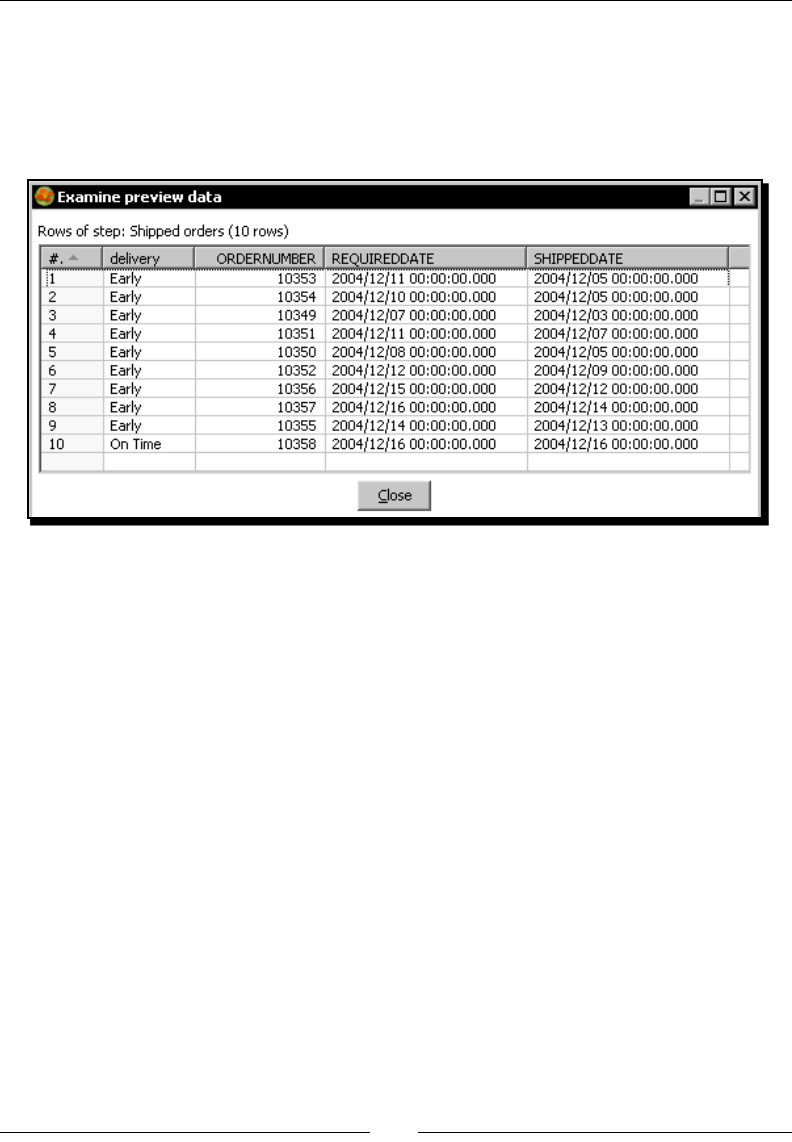
Chapter 8
[ 235 ]
9. Click on Congure.
10. Fill the Arguments grid. To the right of the argument 01, type 2004-12-01. To the
right of the argument 02, type 2004-12-10.
11. Click OK. The following window appears:
What just happened?
You modied the transformaon from the previous tutorial to get orders in a range of dates
coming from the command line.
Adding parameters to your queries
You can make your queries more exible by adding parameters. Let's explain how you do it.
The rst thing to do is obtain the elds that will be plugged as parameters. You can get them
from any source by using any number of steps, as long as you create a hop from the last step
toward the Table input step.
In the tutorial you just used a Get System Info step that read the parameters from the
command line.
Once you have the parameters for the query, you have to change the Table input step
conguraon. In the Insert data from step opon, you have to select the name of the step
that the parameters will come from. In the query, you have to put a queson mark (?) for
each incoming parameter.
When you execute the transformaon, the queson marks are replaced, one by one, with
the data that comes to the Table input step.
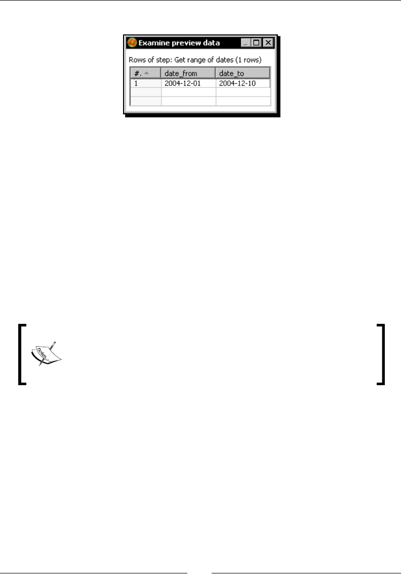
Working with Databases
[ 236 ]
Let's see how it works in the tutorial. The following is the output of the Get System Info step:
In the SQL statement, you have two queson marks. The rst is replaced by the value of the
date_from eld and the second is replaced by the value of the date_to eld. Now the SQL
statement becomes:
SELECT
ORDERNUMBER
, ORDERDATE
, REQUIREDDATE
, SHIPPEDDATE
FROM ORDERS
WHERE STATUS = 'Shipped'
AND ORDERDATE BETWEEN '2004-12-01' AND '2004-12-10'
Here 2004-12-01 and 2004-12-10 are the values you entered as arguments for
the transformaon.
The replacement of the markers respects the order of the incoming elds.
When you use queson marks to parameterize a query, you can't forget
the following—the number of elds coming to a Table input step must be
exactly the same as the number of queson marks found in the query.
Making exible queries by using Kettle variables
Another way you have to make your queries exible is by using Kele variables. Let's explain
how you do it using an example.
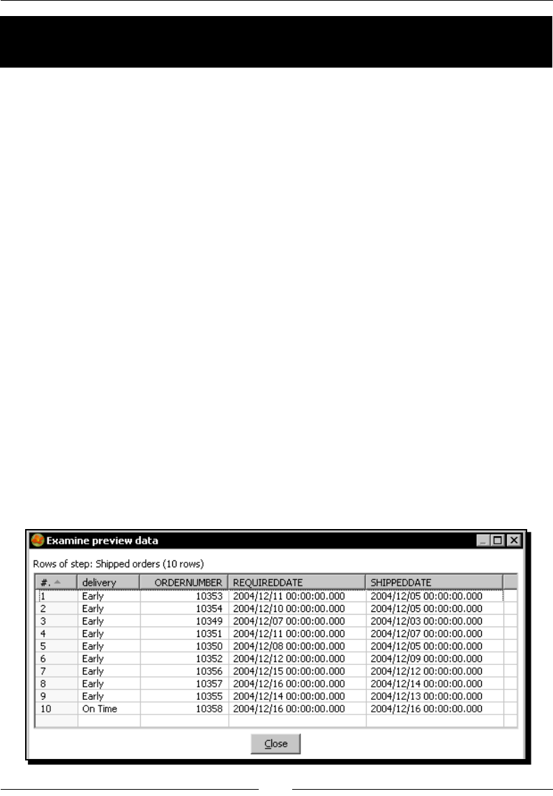
Chapter 8
[ 237 ]
Time for action – getting orders in a range of dates by using
variables
In this tutorial you will do the same as you did in the previous tutorial, but another method
will be explained to you.
1. Open the main transformaon we created in the Time for acon–geng
data about shipped orders secon and save it under a new name.
2. Double-click the Table input step.
3. Modify the SELECT statement as follows:
SELECT
ORDERNUMBER
, ORDERDATE
, REQUIREDDATE
, SHIPPEDDATE
FROM ORDERS
WHERE STATUS = 'Shipped'
AND ORDERDATE BETWEEN '${DATE_FROM}' AND '${DATE_TO}'
4. Tick the Replace variables in script? checkbox.
5. Save the transformaon.
6. With the Select values step selected, click the Preview buon.
7. Click on Congure.
8. Fill the Variables grid in the sengs dialog window—type 2004-12-01 to the right
of the DATE_FROM opon and 2004-12-10 to the right of the DATE_TO opon.
9. Click OK. This following window appears:

Working with Databases
[ 238 ]
What just happened?
You modied the transformaon from the previous tutorial, so the range of dates is taken
from two variables—DATE_FROM and DATE_TO. The nal result set was exactly the same you
got in the previous version of the transformaon.
Using Kettle variables in your queries
As an alternave to the use of posional parameters, you can use Kele variables. Instead
of geng the parameters from an incoming step, you check the opon Replace variables in
script? and replace the queson marks by names of variables. The nal result is the same.
PDI replaces the names of the variables by their values. Only aer that, it sends the SQL
statement to the database engine to be evaluated.
The advantage of using posional parameters over the variables is quite obvious—you don't
have to dene the variables in advance.
On the contrary, Kele variables have several advantages over the use of queson marks:
You can use the same variable more than once in the same query.
You can use variables for any poron of the query, not just the values. For example,
you could have the following query:
SELECT ORDERNUMBER FROM ${ORDER_TABLE}
Then the result will vary upon the content of the variable ${ORDER_TABLE}. In the
case of this example, the variable could be ORDERS or ORDERDETAILS.
A query with variables is easier to understand and less error prone than a query
with posional parameters. When you use posional parameters, it's quite common
to get confused and make mistakes.
Note that in order to provide parameters to a statement in a
Table input step, it's perfectly possible to combine both methods:
posional parameters and Kele variables.
Pop quiz – database datatypes versus PDI datatypes
Aer you read data from the database with a Table Input step, what happens to the data
types of that data:
a. They remain unchanged
b. PDI converts the database data types to internal data types
c. It depends on how you dened the database connecon

Chapter 8
[ 239 ]
Have a go hero – querying the sample data
Based on the sample data:
Create a transformaon to list the oces of Steel Wheels located in USA. Modify the
transformaon so that the country is entered by command line.
Create a transformaon that lists the contact informaon of clients whose credit
limit is above USD100,000. Modify the transformaon so that the threshold is
100000 by default, but can be modied when you run the transformaon.
(Hint: Use named parameters.)
Create a transformaon that generates two Excel les—one with a list of planes
and the other with a list of ships. Include the code, name, and descripon of
the products.
Sending data to a database
By now you know how to get data from a database. Now you will learn how to insert data
into it. For the next tutorials we will use a MySQL database, so before proceeding make sure
you have MySQL installed ad running.
If you haven't yet installed MySQL, please refer to Chapter 1. It has
basic instrucons on installing MySQL, both on Windows and on
Linux operang systems.
Time for action – loading a table with a list of manufacturers
Suppose you love jigsaw puzzles and decided to open a store for selling them. You have
made all the arrangements and the only missing thing is the soware. You have already
acquired a soware to handle your business, but you sll have one hard task to do—insert
data into the database, that is, load the database with the basic informaon about the
products you are about to sell.
As this is the rst of several tutorials in which you will interact with that database, the rst
thing you have to do is to create the database.
For MySQL-specic tasks such as the creaon of a database, we will use
the MySQL Query Browser, included in the MySQL GUI Tools soware. If
you don't have it or don't like it, you can accomplish the same tasks by
using the MySQL Command Line Client or any other GUI Tool.

Working with Databases
[ 240 ]
1. From the Packt website, download the script le js.sql.
2. Launch the MySQL Query Browser.
3. A dialog window appears asking you for the connecon informaon. Enter
localhost as Server Host, and as Username and Password, enter the name
and password of the user you created when you installed the soware .
4. Click on OK.
5. From the File menu, select Open Script....
6. Locate the downloaded le and open it.
7. Click on the Execute buon or press Ctrl+Enter.
8. In the Schemata tab window, a new database, js, appears.
9. Right-click the name of the database and select Make Default Schema.
10. In the Schemata tab window, expand the js tree and you will see the tables of
the database.
11. Close the script window.
Now that the database has been created, let's load some data into it:
1. From the Packt website, download the manufacturers.xls le.
2. Open Spoon and create a new transformaon.
3. Create a connecon to the created database. Under Connecon Type, select
MySQL. In the Sengs frame, insert the same values you provided for the
connecon in MySQL Query Browser—enter localhost as Host Name and
js (the database you just created) as Database Name, and as User Name
and Password, enter the name and password of the user you created when
you installed MySQL. For other sengs in the window, leave the default
values. Test the connecon to see if it has been properly created.
The main reason for a failed test is either erroneous data provided
in the seng window or the non-funconing of the server. If the
test fails, please read the error message to know exactly what the
error was and act accordingly.
4. Right-click the database connecon and share it.
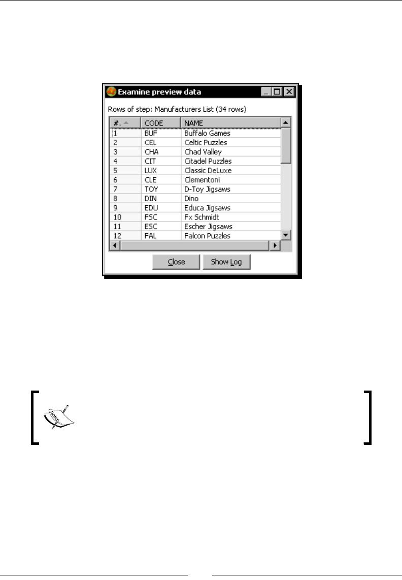
Chapter 8
[ 241 ]
5. Drag an Excel Input step to the canvas and use it to read the
manufacturers.xls le.
6. Click on Preview Rows to check that you are reading the le properly. You should
see the following:
7. From the Output category of steps, drag a Table Output step to the canvas.
8. Create a hop from the Excel Input step to the Table output step.
9. Double-click the Table output step and ll the main sengs window as
follows—select js as Connecon, as Target table, browse and select the
table manufacturers or type it. Check the Specify database elds opon.
It is not mandatory but recommended in this parcular exercise that
you also check the Truncate table opon. Otherwise, the output
table will have duplicate records if you run the transformaon more
than once.
10. Select the Database elds tab.
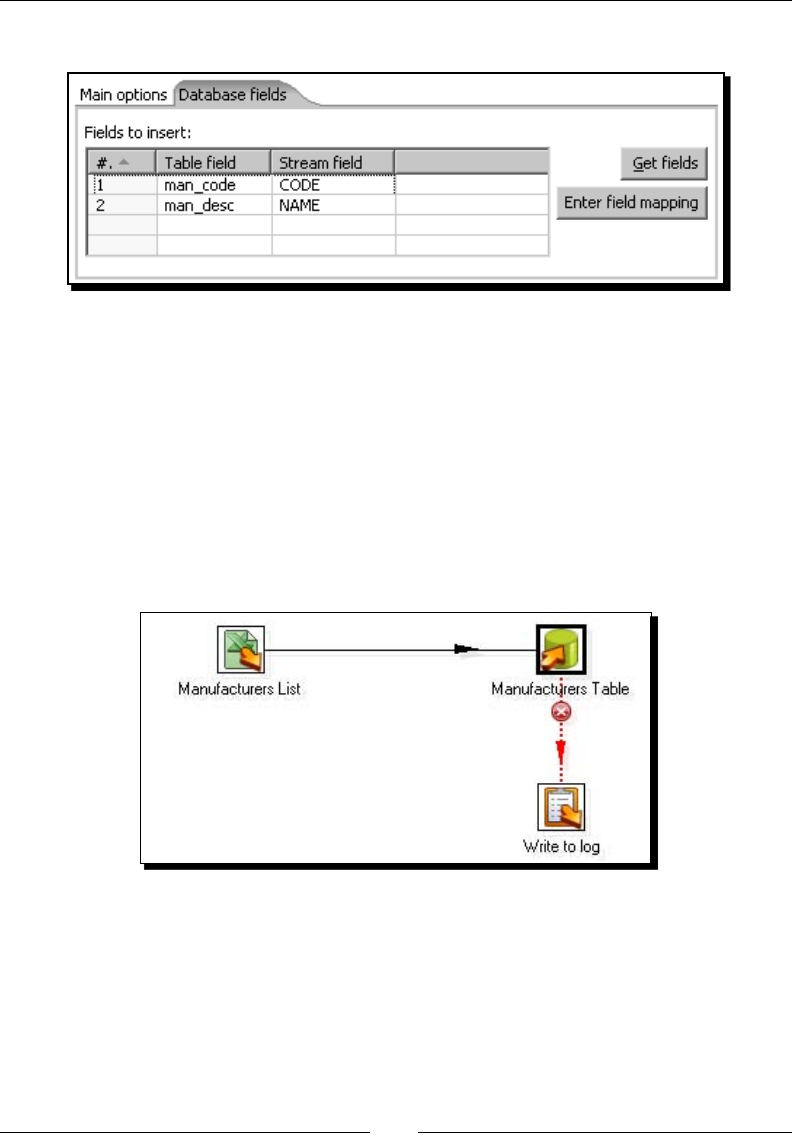
Working with Databases
[ 242 ]
11. Fill the grid as follows:
12. Click OK.
13. Aer the Table output step, add a Write to log step.
14. Right-click the Table output step and select Dene error handling....
15. Fill the error handling sengs window. As Target step, select the
Write to log step. Check the Enable the error handling? opon. Enter
db_err_desc as Error descripons eldname, db_err_field as
Error elds eldname, and db_err_cod as Error codes eldname.
16. Click OK. The following is your nal transformaon:
17. Save the transformaon and run it.
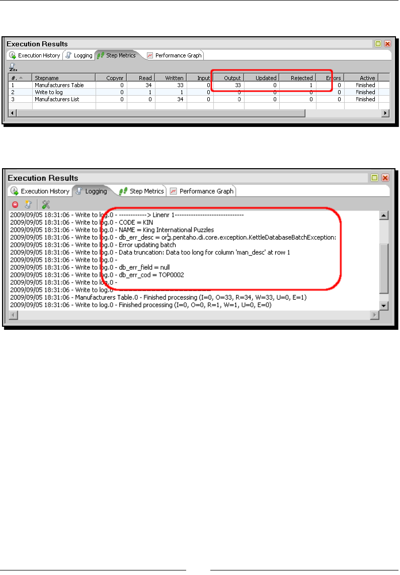
Chapter 8
[ 243 ]
18. Take a look at the Steps Metrics tab window. You will see the following:
19. Now look at the Logging tab window. The following is what you see:
20. Switch to MySQL Query Browser.
21. In the Schemata window, double-click the manufacturers table.
22. The query entry box is lled with a basic SELECT statement for that table such as:
SELECT * FROM manufacturers m;
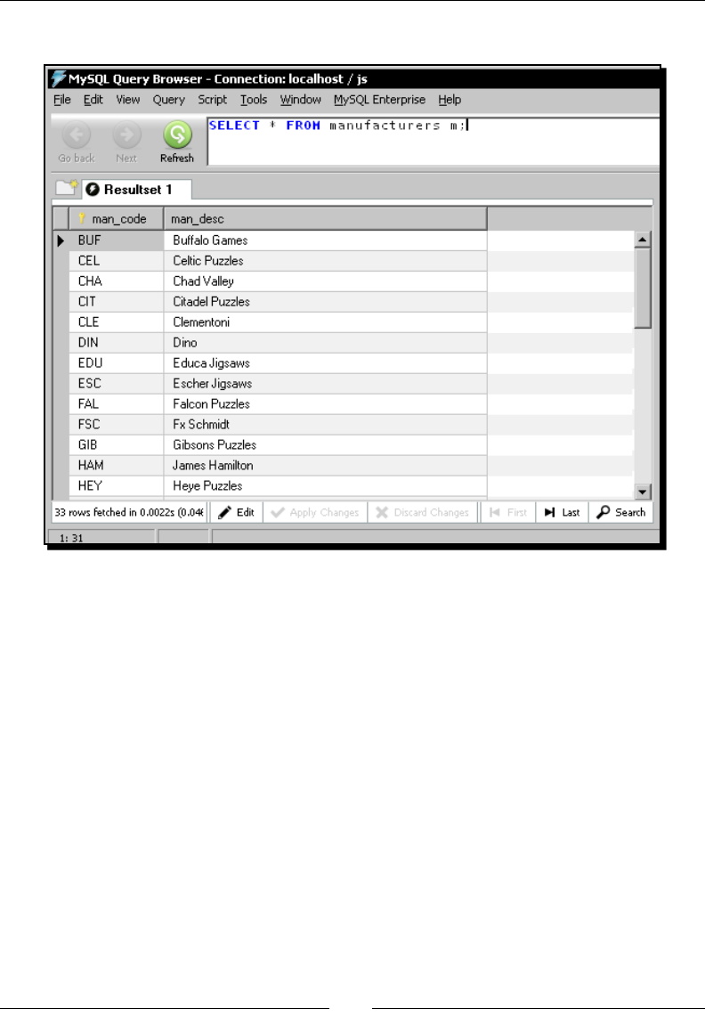
Working with Databases
[ 244 ]
23. Click Execute. The following result set is shown:
What just happened?
In the rst part of the tutorial, you created the Jigsaw Puzzle database.
In Spoon, you created a connecon to the new database.
Finally, you created a transformaon that read an Excel le with a list of puzzle
manufacturers and inserted that data into the manufacturers table. Note that not
all rows were inserted. The row that couldn't be inserted was reported in the log.
In the data for the tutorial, there was a descripon too long to be inserted in the table. That
was properly reported in the log because you implemented error handling. Doing that, you
avoided the aboron of the transformaon due to errors like that. As you learned in the
previous chapter, when a row causes an error, it is up to you to decide what to do with that
row. In this case, the row was sent to the log and wasn't inserted. Other possible opons
for you are:

Chapter 8
[ 245 ]
Fixing the problem in the Excel le and rerunning the transformaon
Validang the data and xing it properly (for example, cung the descripons)
before the data arrives to the Table output step
Sending the full data for the erroneous rows to a le, xing manually the data in the
le, and creang a transformaon that inserts only this data
Inserting new data into a database table with the Table
output step
The Table output step is the main PDI step for inserng new data into a database table.
The use of this step is simple. You have to enter the name of the database connecon
and the name of the table where you want to insert data. The names for the connecon
and the table are mandatory, but as you can see, there are some extra sengs for the
Table output step.
The database eld tab lets you specify the mapping between the dataset stream elds and
the table elds.
In the tutorial the dataset had two elds—CODE and NAME. The table has two columns
named man_code and man_desc.
As the names are dierent, you have to explicitly indicate that the CODE eld is to be wrien
in the table eld named man_code, and that the NAME eld is to be wrien in the table eld
named man_desc.
The following are some important ps and warnings about the use of the Table output step:
If the names of the elds in the PDI stream are equal to the names of the columns
in the table, you don't have to specify the mapping. In that case, you have to leave
the Specify database elds checkbox unchecked and make sure that all the elds
coming to the Table output step exist in the table.
Before sending data to the Table output step, check your transformaon against the
denion of the table. All the mandatory columns that don't have a default value
must have a corresponding eld in the PDI stream coming to the Table output step.
Check the data types for the elds you are sending to the table. It is possible
that a PDI eld type and the table column data type don’t match. In that case, x
the problem before sending the data to the table. You can, for example, use the
Metadata tab of a Select values step to change the data type of the data.
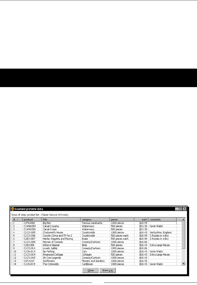
Working with Databases
[ 246 ]
In the Table output step, you may have noted a buon named SQL. This buon generates
the DDL to create the output table. In the tutorial, the output table, manufacturers,
already existed. But if you want to create the table from scratch, this buon allows you
to do it based on the database elds you provided in the step.
Inserting or updating data by using other PDI steps
The Table output step provides the simplest but not the only way to insert data into a
database table. In this secon, you will learn some alternaves for feeding a table with PDI.
Time for action – inserting new products or updating
existent ones
So far, you created the Jigsaw Puzzles database and loaded a list of puzzles manufacturers.
It's me to start loading informaon about the products you will sell— puzzles.
Suppose, in order to show you what they are selling, the suppliers provide you with the lists
of products made by the manufacturers themselves. Fortunately, they don't give you the lists
in the form of papers, but they give you either plain les or spreadsheets. In this tutorial, you
will take the list of products oered by the manufacturer Classic DeLuxe and load it into the
puzzles table.
1. From the Packt website, download the sample lists of products.
2. Open Spoon and create a new transformaon.
3. Add a Text le input step and congure it to read the
productlist_LUX_200908.txt le.
Pay aenon to the each eld. It's the price of the product and must be congured
as a Number with format $0.00.
4. Preview the le. You should see the following:
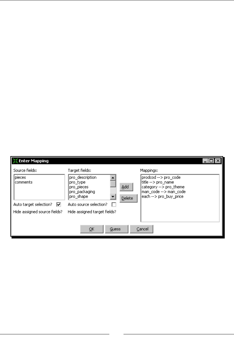
Chapter 8
[ 247 ]
5. In the Selected Files grid, replace the text productlist_
LUX_200908.txt by ${PRODUCTLISTFILE}.
6. Click on OK.
7. Aer the Text le input step, add an Add constants step.
8. Use it to add a String constant named man_code with value LUX.
9. From the Output category of steps, drag an Insert/Update step to the
canvas. Create a hop from the Add constants step to this new step.
10. Double-click the step. Select js as Connecon. As Target table,
browse and select products. In the upper grid of the window, add the
condions pro_code = prodcod and man_code = man_code. Click
the Edit mapping buon. The mapping dialog window shows up.
11. Under the Source elds list, click on prodcod, under the Target elds list click
on pro_code, and then click the Add buon. Again, under the Source elds
list click on title, under the Target elds list click on pro_name, and then
nally click Add. Proceed with the mapping unl you get the following:
12. Click OK.
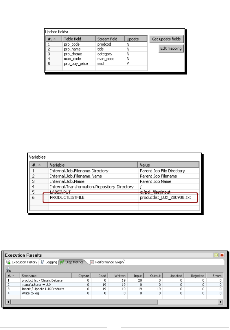
Working with Databases
[ 248 ]
13. Fill the Update column for the price row with the value Y. Fill the rest of the
column with the value N. The following is how the nal grid looks like:
14. Aer the Insert/Update step, add a Write to log step.
15. Right-click the Insert/Update step and select Dene error handling....
16. Fill the error handling sengs window just as you did in the previous tutorial.
17. Save the transformaon and run it by pressing the F9 key.
18. In the sengs window, assign the PRODUCTLISTFILE variable
with the value productlist_LUX_200908.txt.
19. Click on Launch.
20. When the transformaon ends, check the Step Metrics. You will see the following:
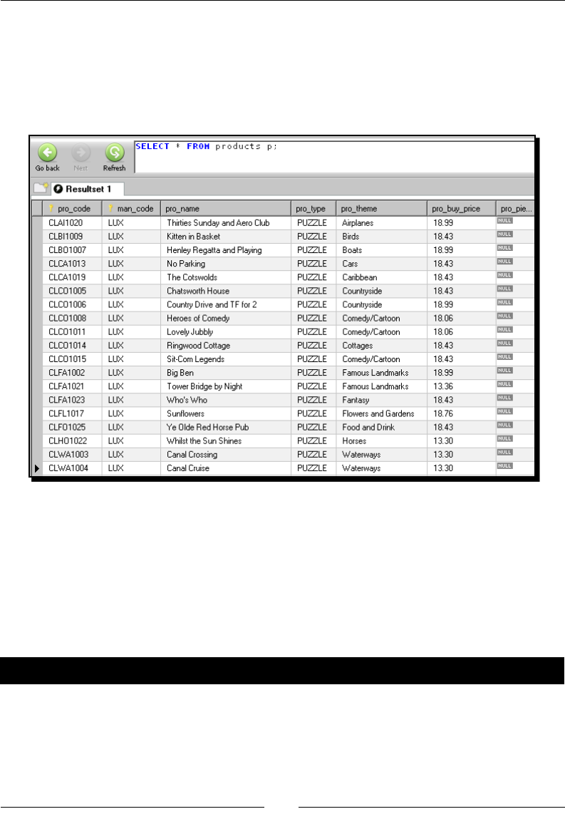
Chapter 8
[ 249 ]
21. Switch to the SQL Query Browser applicaon.
22. Type the following in the query entry box:
SELECT * FROM products p;
23. Click on Execute. The following result set is shown:
What just happened?
You populated the products table with data found in text les. For inserng the data, you
used the Insert/Update step.
As this was the rst me you dealt with the products table, before you ran the
transformaon, the table was empty. Aer running the transformaon, you could
see how all products in the le were inserted in the table.
Time for action – testing the update of existing products
In the preceding tutorial, you used an Insert/Update step, but only inserted records. Let's try
the transformaon again to see how the update opon works.
1. If you closed the transformaon, please open it.
2. Press F9 to launch the transformaon again.
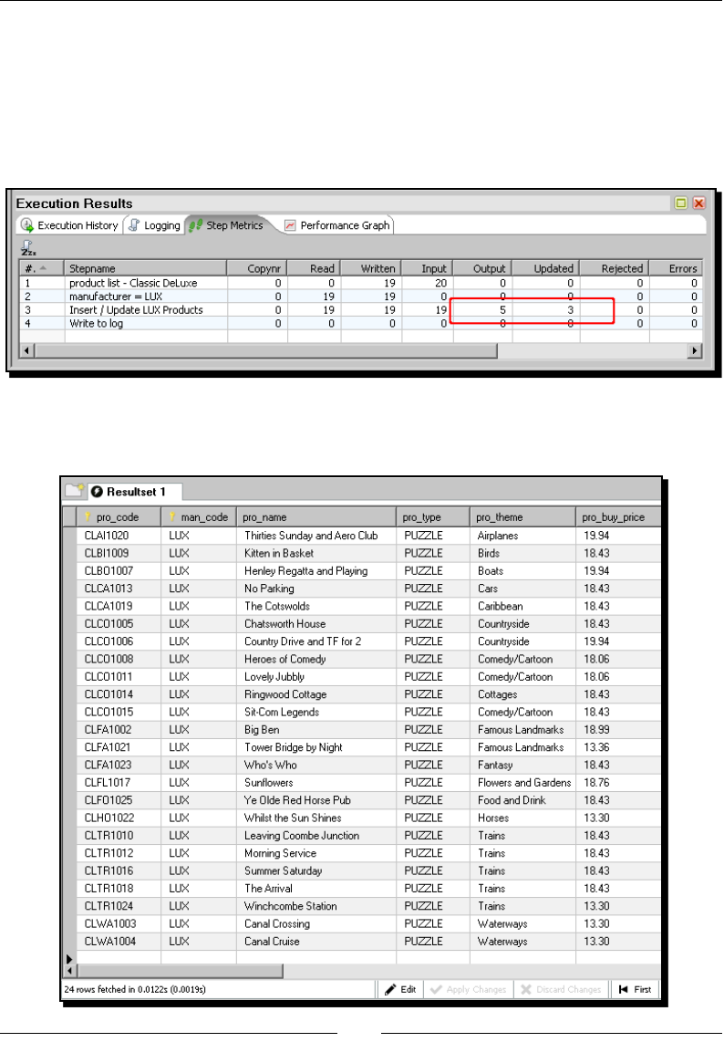
Working with Databases
[ 250 ]
3. As the value for the PRODUCTLISTFILE variable,
insert productlist_LUX_200909.txt.
4. Click Launch.
5. When the transformaon ends, check the Step Metrics tab. You will see
the following:
6. Switch to the SQL Query Browser applicaon and click Execute to run the query
again. This me you will see this:

Chapter 8
[ 251 ]
What just happened?
You reran the transformaon that was created in the previous tutorial, this me using a
dierent input le. In this le there were new products and some products were removed
from the list, whereas some had their descripons, categories, and prices modied.
When you ran the transformaon for the second me, the new products were added to
the table. Also, the modied prices of the products were updated. In the Step Metrics tab
window, you can see the number of inserted records (Output column) and the number of
updated ones (Update column).
Note that as the supplier may give you updated lists of products with dierent
names of les, for the name of the le you used a variable. Doing so, you were
able to reuse the transformaon for reading dierent les each me.
Inserting or updating data with the Insert/Update step
While the Table output step allows you to insert brand new data, the Insert/Update step
allows you to do both, insert and update data in a single step.
The rows coming to the Insert/Update step can be new data or can be data that already
exists in the table. Depending on the case, the Insert/Update step behaves dierently. Let's
see each case in detail:
For each incoming row, the rst thing the step does is use the lookup condion you put in
the upper grid to check if the row already exists in the table.
In the tutorial you wrote two condions: pro_code = prodcod and man_code = man_
code. Doing so, you told the step to look for a row in the products table for which the table
column pro_code is equal to the eld prodcod of your row, and the table column
man_code is equal to the eld with the same name of your row.
If the lookup fails, that is, the row doesn't exist, the step inserts the row in the table by using
the mapping you put in the lower grid.
The rst me you ran the tutorial transformaon, the table was empty. There were no
rows against which to compare. In this case, all the lookups failed and, consequently, all
rows were inserted.
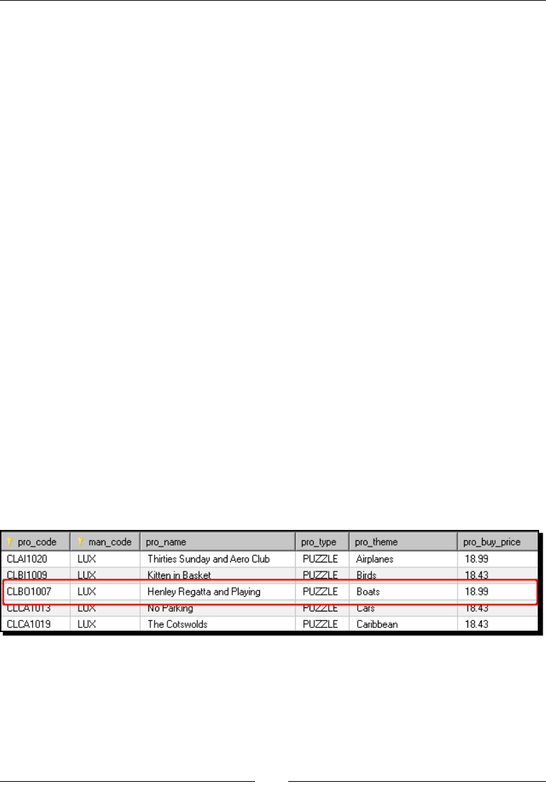
Working with Databases
[ 252 ]
This insert operaon is exactly the same that you could have done with a Table output step.
That implies that here you also have to be careful about the following:
All the mandatory columns that don't have a default value must be present in the
Update Field grid, including the keys you used in the upper grid
The data types for the elds you are sending to the table must match the data type
for the columns of the table
If the lookup succeeds, the step updates the table replacing the old values with the new
ones. This update is made only for the elds where you put Y as the value for the Update
column in the lower grid.
If you don't want to perform any update operaon, you can check the Don't perform any
updates opon.
The second me you ran the tutorial, you had two types of products in the le—products
that already existed in the database and new products. For example, consider the following
row found in the second le:
CLTR1001|A Saint at Radley|Trains|500 pieces|$13.30|Peter Webster
PDI looks for a row in the table where the prod_code is equal to CLTR1001 and man_code
is equal to LUX (the eld added with the Add constants step). It doesnt nd it. Then it
inserts a new row with the data coming from the le.
Take another sample row:
CLBO1007|Henley Regatta & Playing|Boats|500 pieces each|$19.94|2
Puzzles in a Box
PDI looks for a row in the table where the prod_code is equal to CLBO1007 and man_code
equal to LUX. It nds the following:
There are two dierences between the old and the new versions of the product. Both the
name and the price have changed.
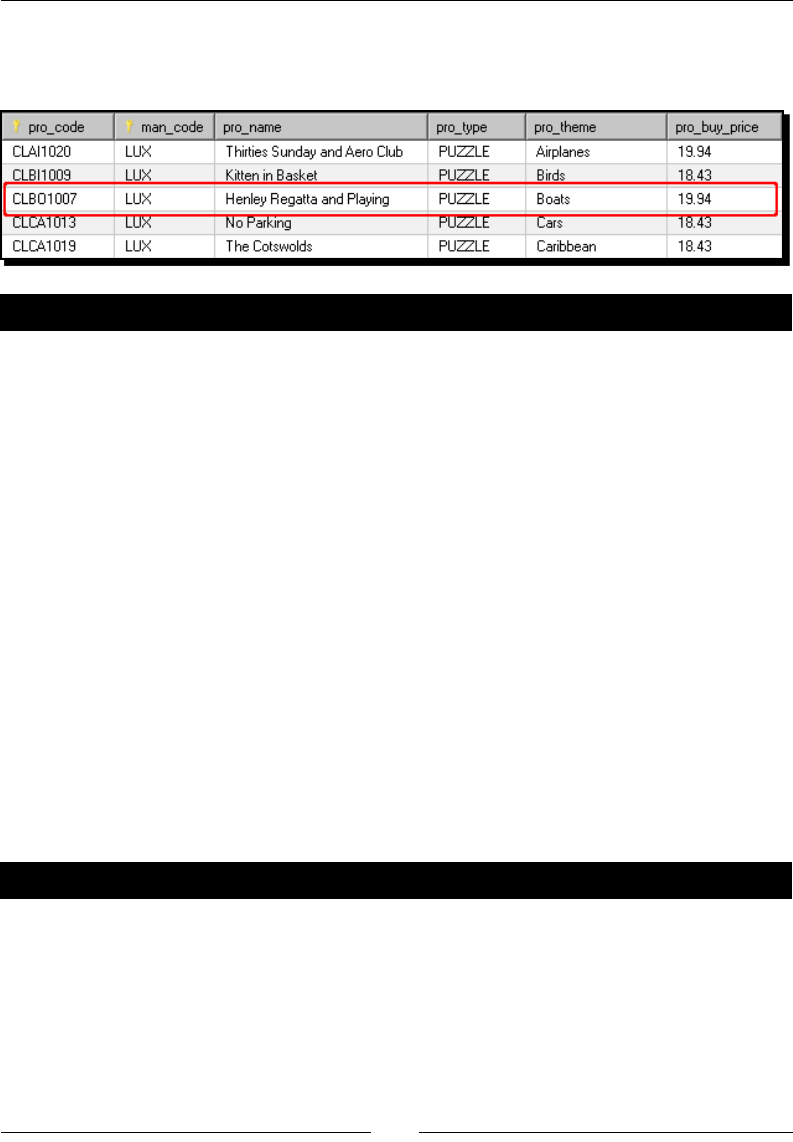
Chapter 8
[ 253 ]
As you congured the Insert/Update step to update only the price column, the update
operaon does so. The new record in the table aer the execuon of the transformaon
is this:
Have a go hero – populating a lms database
From the Packt website, download the films.sql script le. Run the script In MySQL. A
new database will be created to hold lm data.
Browse the folder where you have the les for Chapter 7 and get the French lms le.
You will use it to populate the following tables of the films database: GENRES, PEOPLE,
and FILMS.
Now follow these instrucons:
Create a connecon to the database.
In order to populate the GENRES table, you have to build a list of genres, no
duplicates! For the primary key, GEN_ID, you don't have a value in the le. Create
the key with an Add sequence step.
The table, PEOPLE, will have the names of both actors and directors. In order to
populate that table, you will have to create a single list of people, no duplicates here
either! To generate the primary key, use the same method as before.
4. Finally, populate the FILMS table with the whole list of lms found in the le.
Don't forget to handle errors so that you can detect bad rows.
Have a go hero – creating the time dimension
Now you're going to nish what you started back in Chapter 6—the creaon of a
me dimension.
From the Packt website, download the js_dw.sql script le. Run the script in MySQL.
A new database named js_dw will be created.
Now you are going to modify the time_dimension.ktr transformaon to load the me
dataset into the lk_time table.
1.
2.
3.
Working with Databases
[ 254 ]
The following are some ps:
Create a connecon to the created database
Find a correspondence between each eld in the dataset and each column in the
LK_TIME table
Use a Table output step to send the dataset to the table
Aer running the transformaon, check if all rows were inserted as expected.
Pay aenon to the main eld in the me dimension—date.
In the transformaon the date is a eld whose type is Date.
However, in the table the type for the date eld is CHAR(8). This column
is meant to hold the date as a String with the format YYYYMMDD—for
example 20090915.
As explained, the data types of the data you sent to the table have to match
the data types in the table. In this case, as the types don't match, you will
have to use a Select values step and change the metadata of the date eld
from Date to String.
Have a go hero – populating the products table
This exercise has two parts. The rst is intended to enrich the transformaon you created
in the tutorial. The transformaon processed the product list les supplied by the Classics
DeLuxe manufacturer. In the le, there was some extra informaon that you could put in the
table such as the number of pieces of a puzzle. However, the data didn't come ready to use.
Consider, for example, this text: 500 pieces each. In order to get the number of pieces, you
need to do some transformaon. Modify the transformaon so that you can enrich the data
in the products table.
The second part of the exercise has to do with populang the products table with products
from other manufacturers. Unfortunately, you can't expect that all manufacturers to share
the same structure for the list of products. Not only the structure changes, but also the
kind of informaon they give you can vary. On the Packt website, you have several sample
product les belonging to dierent manufactures. Explore them, analyze them to see if you
can idenfy the dierent data you need for the products table, and load all the products
into the database by using a dierent transformaon for each manufacturer.
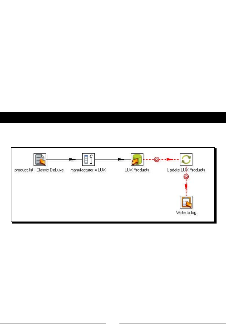
Chapter 8
[ 255 ]
The following are some ps:
Take as a model the transformaon for the tutorial. You may reuse most of it.
You don't have to worry about the stock columns or the pro_type column
because they already have default values.
Use the comments in the le to idenfy potenal values for the pro_packaging,
pro_shape and pro_style columns. Use the pro_packaging eld for values
such as 2 puzzles in a box. Use the pro_shape eld for values such as
Panoramic Puzzle or 3D Puzzle. Use the puzzle_type eld for values
such as Glow in the Dark or Wooden Puzzle.
You can leave the pro_description empty or put in it whatever you feel that
ts—a x string such as Best in market!, or the full comment found in the le,
or whatever your imaginaon says.
Pop quiz – Insert/Update step versus Table Output/Update steps
In the last tutorial you read a le and used an Insert/Update step to populate the products
table. Look at the following variant of the transformaon:
Suppose you use this transformaon instead of the original. Compared to the results you got
in the tutorial, aer the execuon of this version of the transformaon, the products table
will have:
a. The same number of records
b. More records
c. Less records
d. It depends on the contents of the le
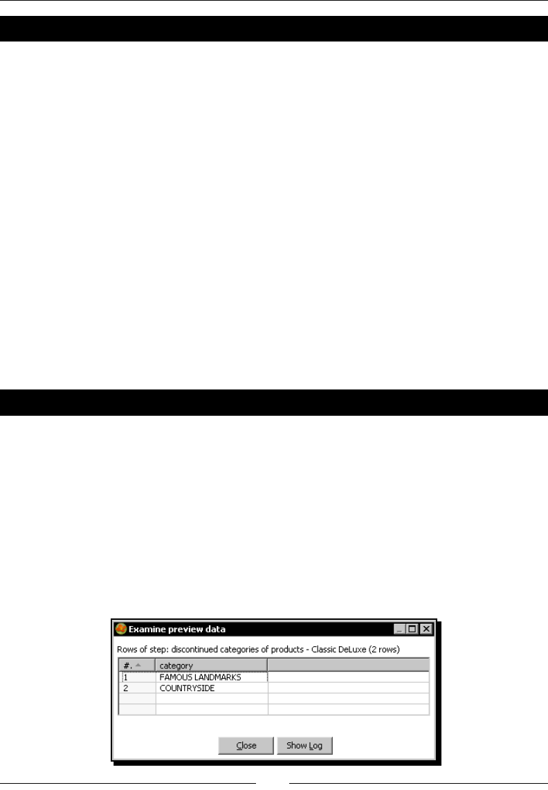
Working with Databases
[ 256 ]
Pop quiz – ltering the rst 10 rows
The following SELECT statement:
SELECT TOP 10 * FROM CUSTOMERS
gives you the rst ten customers in the CUSTOMERS table of the sample database.
Suppose you want to get the rst ten products in the PRODUCTS table of the Jigsaw Puzzles
database. Which of the following statements would do that:
a. SELECT TOP 10 * FROM product
b. SELECT * FROM product WHERE ROWNUM<11
c. SELECT * FROM product LIMIT 10
d. Any of the above statements
Eliminating data from a database
Deleng informaon from a database is not the most common operaon with databases, but
it is an important one. Now you will learn how to do it with PDI.
Time for action – deleting data about discontinued items
Suppose a manufacturer informs you about the categories of products that will no longer be
available. You don't want to have in your database products something that you will not sell.
Then you use PDI to delete them.
1. From the Packt website, download the LUX_discontinued.txt le.
2. Create a new transformaon.
3. With a Text le input step, read the le.
4. Preview the le. You will see the following:
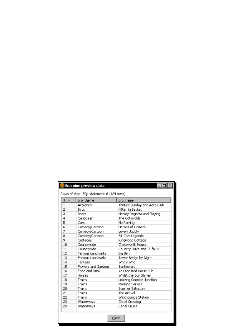
Chapter 8
[ 257 ]
5. Aer the Text le input step, add an Add constants step to add
a String constant named man_code with value LUX.
6. Expand the Output category of steps and drag a Delete step to the canvas.
7. Create a hop from the Add constants step to the Delete step.
8. Double-click the Delete step. Select js as Connecon and, as Target table, browse
and select products. In the grid add the condions man_code = man_code and
pro_theme LIKE category. Aer the Delete step, add a Write to log step.
9. Right-click the Delete step and dene the error handling just like you did in each of
the previous tutorials in this chapter.
10. Save the transformaon.
11. Before running the transformaon, open the Database Explorer.
12. Under the js connecon, locate the products table and click
Open SQL for [products].
13. In the simple SQL editor type:
SELECT pro_theme, pro_name FROM js.products p
ORDER BY pro_theme, pro_name;
14. Click on Execute. You will see the following result set:

Working with Databases
[ 258 ]
15. Close the preview data window and the results of the SQL window.
16. Minimize the database explorer window.
17. The database explorer is collapsed at the boom of the Spoon window.
18. Run the transformaon.
19. Look at the Step Metrics. The following is what you should see:
20. Maximize the database explorer window.
21. In the SQL editor window click Execute again. This me you will see this:
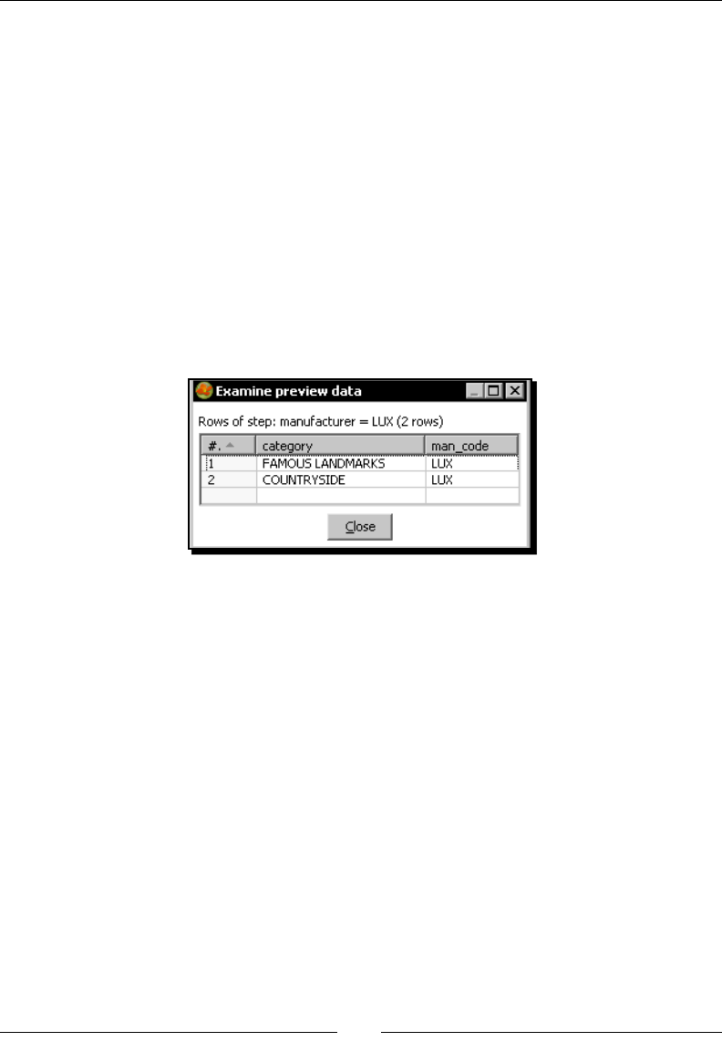
Chapter 8
[ 259 ]
What just happened?
You deleted from the products table all products belonging to the categories found in the
LUX_discontinued.txt le.
Note that to query the list of products, you used the PDI Database explorer. You could have
done the same by using MySQL Query Browser.
Deleting records of a database table with the Delete step
The Delete step allows you to delete records of a database table based on a given condion.
For each row coming to the step, PDI deletes the records that match the condion set in its
conguraon window.
Let's see how it worked in the tutorial. The following is the dataset coming to the
Delete step:
For each of these two rows PDI performs a new delete operaon.
For the rst row, the records deleted from the products table are those where man_code is
equal to LUX and pro_theme is like FAMOUS LANDMARKS.
For the second row, the records deleted from the products table are those where
man_code is equal to LUX and pro_theme is like COUNTRYSIDE.
You can verify the performed operaons by comparing the result sets you got in the
database explorer before and aer running the transformaon.
Just for your informaon, you could have done the same task with the following
DELETE statements:
DELETE FROM products
WHERE man_code = 'LUX' and pro_theme LIKE 'FAMOUS LANDMARKS'
DELETE FROM products
WHERE man_code = 'LUX' and pro_theme LIKE 'COUNTRYSIDE'

Working with Databases
[ 260 ]
In the Step Metrics result, you may noce that the updated column for the Delete step has
value 2. This number is the number of delete operaons, not the number of deleted records,
which was actually a bigger number.
Have a go hero – deleting old orders
Create a transformaon that asks for a date from the command line and deletes all orders
from the Steel Wheels database whose order dates are before the given date.
Summary
This chapter discussed how to use PDI to work with databases. Specically, the chapter
covered the following:
Introducon to the Pentaho Sample Data Steel Wheels—the starng point for you
to learn basic database theory
Creang connecons from PDI to dierent database engines
Exploring databases with the PDI Database explorer
Basics of SQL
Performing CRUD (Create, Read, Update, and Delete) operaons on databases
In the next chapter you will connue working with databases. You will learn some advanced
concepts, including datawarehouse-specic operaons.

9
Performing Advanced Operations
with Databases
In this chapter you will learn about advanced operaons with databases. The rst part of the
chapter includes:
Populang the Jigsaw puzzle database so that it is prepared for the rest of the
acvies in the chapter
Doing simple lookups in a database
Doing complex lookups
The second part of the chapter is fully devoted to datawarehouse-related concepts. The list
of the topics that will be covered includes:
Introducing dimensional modeling
Loading dimensions
Preparing the environment
In order to learn the concepts of this chapter, a database with lile or no data is useless.
Therefore, the rst thing you'll do is populang your Jigsaw puzzle database.
Time for action – populating the Jigsaw database
To load data massively into your Jigsaw database, you must have the Jigsaw database
created and the MySQL server running. You already know how to do this. If not, please
refer to Chapter 1 for the installaon of MySQL and Chapter 8 for the creaon of the
Jigsaw database.

Performing Advanced Operaons with Databases
[ 262 ]
This tutorial will overwrite all your data in the js database. If you don't
want to overwrite the data in your js database, you could simply create a new
database with a dierent name and run the js.sql script to create the tables
in your new database.
Aer checking that everything is in order, follow these instrucons:
1. From Packt's website download the js_data.sql script le.
2. Launch the MySQL query browser.
3. From the File menu select Open Script....
4. Locate the downloaded le and open it.
5. At the beginning of the script le you will see this line:
USE js;
If you created a new database, replace the name js by the name of your new
database.
6. Click on the Execute buon.
7. At the boom of the screen, you'll see a progress message.
8. When the script execuon ends, verify that the database has been populated.
Execute some SELECT statements such as:
SELECT * FROM cities
All tables must have records.
Having populated the database, let's prepare the Spoon environment:
1. Edit the kettle.properties le located in the PDI home directory. Add the
following variables: DB_HOST, DB_NAME, DB_USER, DB_PASS, and DB_PORT. As
values put the seng for your connecon to the Jigsaw database. Use the following
lines as a guide:
DB_HOST=localhost
DB_NAME=js
DB_USER=root
DB_PASS=1234
DB_PORT=3306
Chapter 9
[ 263 ]
2. Add the following variables: DW_HOST, DW_NAME, DW_USER, DW_PASS, and
DW_PORT. As values, put the seng for your connecon to the js_dw
database—the database you created in Chapter 8 to load the me dimension.
Here are some sample lines for you to use:
DW_HOST=localhost
DW_NAME=js_dw
DW_USER=root
DW_PASS=1234
DW_PORT=3306
Save the le.
3. Included in the downloaded material is a le named shared.xml. Copy it to your
PDI home directory (the same directory where the kettle.properties le is)
overwring the exisng le.
Before overwring the le, please take a backup, as this will
delete any share connecons you might have created.
4. Launch Spoon. If it was running, restart it so that it recognizes the changes in the
kettle.properties le.
5. Create a new transformaon.
If you don't see the shared database connecons js and
dw, please verify that you copied the shared.xml le to
the right folder.
6. Right-click the js database connecon and select Edit. In the Sengs frame, instead
of xed values, you will see variables: ${DS_HOST} for Host Name, ${DS_NAME} for
Database Name, and so on.
7. Test the connecon.
8. Repeat the steps for the js_dw shared connecon: Right-click the database
connecon and select Edit. In the Sengs frame, you will see the variables you
dened in the kettle.properties le—${DW_HOST}, ${DW_NAME}, and so on.
9. Test the dw_js connecon.
Performing Advanced Operaons with Databases
[ 264 ]
If any of the database tests fail, please check that the connecon
variables you put in the kettle.properties le are correct.
Also check that MySQL is running database.
What just happened?
In this tutorial you prepared the environment for working in the rest of the chapter.
You did two dierent things:
First, you ran a script that emped all the js database tables and loaded data into them.
Then, you redened the database connecons to the databases js and js_dw.
Note that the names for the connecon don't have to match the
names of the databases. This can benet you in the following way: If
you created a database with a dierent name for the Jigsaw database
puzzle, your connecon may sll be named js, and all code you
download from the Packt website should work without touching
anything but the kettle.properties le.
You edited the kettle.properties le by adding variables with the database connecon
values such as host name, database name, and so on. Then you edited the database
connecons. There you saw that the database sengs didn't have values but variable
names—the variables you had dened in the kettle.properties le. For shared
connecons, PDI takes the database denion from the shared.xml le.
Note that you didn't save the transformaon you created. That was
intenonal. The only purpose for creang it was to be able to see the
shared connecons.
Exploring the Jigsaw database model
The informaon in this secon allows you to understand the organizaon of the data in the
Jigsaw database. In the rst place, you have a DER. A DER or enty relaonship diagram is
a graphical representaon that allows you to see how the tables in a database are related to
each other. The following is the DER for the js database:
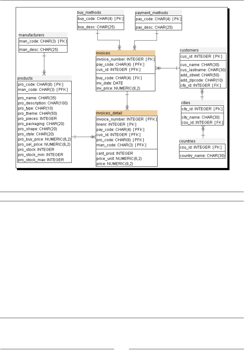
Chapter 9
[ 265 ]
The following table contains a brief explanaon of what each table is for:
Table name Content
manufacturers Informaon about manufacturers of the products.
products It is about the products you sell such as puzzles and accessories. The
table has descripve informaon and data about prices and stock. The
pro_type column has the type of product—puzzle, glue, and so on.
Several of the columns apply only to puzzles, such as shape or pieces.
buy_methods It contains informaon about the list of methods for buying—for
example, in store, by telephone, and so on.
payment_methods Informaon about list of methods of payment such as cash, check,
credit card, and so on.
countries The list of countries.
cities The list of cies.
customers A list of customers. A customer has a number, a name, and an address.
invoices The header of invoices including date, customer number, and total
amount. The invoices dates range from 2004 to 2010.
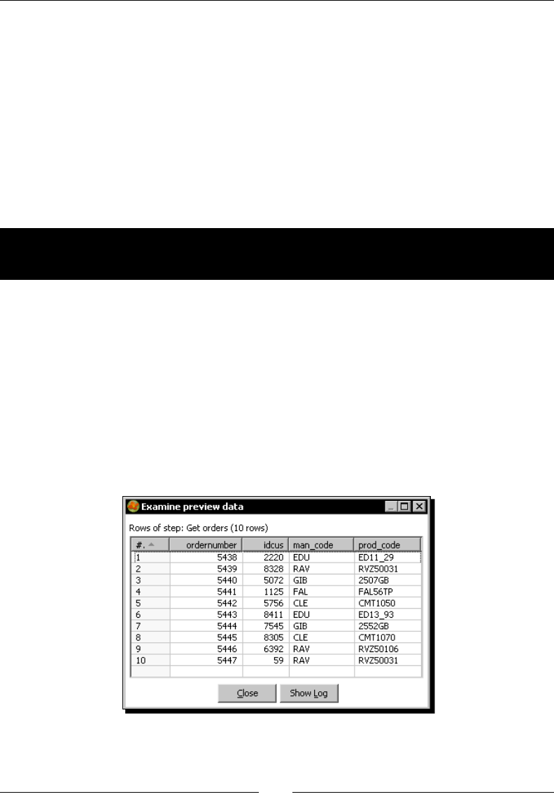
Performing Advanced Operaons with Databases
[ 266 ]
Looking up data in a database
You already know how to create, update, and delete data from a database. It's now me to
learn to look up data. Lookup is the act of searching for informaon in a database. You can
look up a column of a single table or you can do more complex lookups. Let's begin with the
simplest way of looking up.
Doing simple lookups
Somemes you need to get informaon from a database table based on the data you have in
your main stream. Let's see how you can do it.
Time for action – using a Database lookup step to create a list
of products to buy
Suppose you have an online system for your customers to order products. On a daily basis,
the system creates a le with the orders informaon. Now you will check if you have stock
for the ordered products and make a list of the products you'll have to buy.
1. Create a new transformaon.
2. From the Input category of steps, drag a Get data from XML step to the canvas.
3. Use it to read the orders.xml le. In the Content tab, ll the Loop XPath opon
with the /orders/order string. In the Fields tab get the elds.
4. Do a preview. You will see the following:
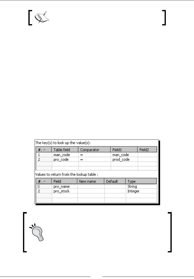
Chapter 9
[ 267 ]
To keep this exercise simple, the le contains a single
product by order.
5. Add a Sort rows step and use it to sort the data by man_code, prod_code.
6. Add a Group by step and double-click it.
7. Use the upper grid for grouping by man_code and prod_code.
8. Use the lower grid for adding a eld with the number of orders in each group. As
Name write quantity, as Subject ordernumber, and as Type write Number of
Values (N). Expand the Lookup category of steps.
9. Drag a Database lookup step to the canvas and create a hop from the Group by step
toward this step.
10. Double-click the Database lookup step.
11. As Connecon, select js and in Lookup table, browse the database and select
products or just type its name.
12. Fill the grids as follows:
If you don't see both grids, just resize the window. This is
one of the few conguraon steps that lack the scrollbar to
the right side.
Also remember that with all grids in PDI, you always have
the opon to populate the grids by using the Get Fields and
Get lookup elds buons respecvely.

Performing Advanced Operaons with Databases
[ 268 ]
13. Click on OK.
14. Add a lter step to pass only the rows where pro_stock<quantity.
15. Add a Text le output step to send the manufacturer code, the product code, the
product name, and the ordered quanty to a le named products_to_buy.txt.
16. Run the transformaon.
17. The le should have the following content:
man_code;prod_code;pro_name;quantity
EDU;ED13_93;Times Square;1
RAV;RVZ50031;Disney World Map;2
RAV;RVZ50106;Star Wars Clone Wars;1
What just happened?
You processed a le with orders. You grouped and counted the ordered products by product
code. Then with the Database lookup step, you looked up the product table for the record
belonging to the ordered product. You added to your stream, the name and stock for the
products. Aer that, you kept only the rows for which the stock was lower than the units
your customers ordered. With the rows that passed, you created a list of products to buy.
Looking up values in a database with the Database lookup step
The Database lookup step allows you to look up values in a database table. In the upper grid of
the seng window, you specify the keys to look up. In the example you look for a record that
has the same product code and manufacturer code as the codes coming in the stream.
In the lower grid you put the name of the table columns you want back. Those elds are
added to the output stream. In this case, you added the name and the stock of the product.
The step returns only one row even if it doesn't nd a matching record or if it nds more
than one. When the step doesn't nd a record with the given condions, it returns null for
all the added elds, unless you specify a default value for those new elds.
Note that this behavior is quite similar to the Stream lookup step's behavior. You search for
a match and, if a record is found, the step returns you the specied elds. If not, the new
elds are lled with default values. Besides the fact that the data is searched in a database,
the new thing here is that you specify the comparator to be used: =, <, >, and so on. The
Stream lookup step looks only for equal values. As all the products in the le existed in your
database, the step found a record for every row, adding to your stream two elds: the name
and the stock for the product. You can check it by doing a preview on the Database lookup
step. Aer the Database lookup setup, you used a Filter rows step to discard the rows where
the stock was lower than the required quanty of products. You can avoid adding this step

Chapter 9
[ 269 ]
by rening the lookup conguraon. In the upper grid you could add the condion pro_
stock<quantity and check the Do not pass the row if the lookup fails checkbox; you now
get a dierent result. The step will look not only for the product, but also for the condion
pro_stock<quantity. If it doesn't nd a record that matches, that is, the lookup fails, the
check Do not pass the row if the lookup fails does its work—lters the row. Doing these
changes, you don't have to use the extra Filter rows step, nor add the pro_stock eld to
the stream unless you need it for another use.
As a nal remark—if the lookup returns more than one row, only the rst is returned. You
have the opon to abort the whole transformaon if this happens—simply check the Fail on
mulple results? checkbox.
Making a performance dierence when looking up data in a database
Database lookups are costly and can severely impact transformaon
performance. However, performance can be signicantly improved by using the
cache feature of the Database lookup step. To enable the cache feature, just
check the Enable cache? opon.
This is how it works: Think of the cache as a buer of high-speed memory that
temporarily holds frequently requested data. By enabling the cache opon,
Kele will look rst in the cache and then in the database.
If the table where you look up has few records, you could preload the cache with
all the data in the lookup table. You do it by checking the Load all data from
table opon. This will give you the best performance.
On the contrary, if the number of rows in the lookup table is too large to t enrely
into memory, instead of caching the whole table you can tell Kele the maximum
number of rows to hold in cache. You do it by specifying the number in the Cache
size in rows textbox. The bigger this number, the faster the lookup process.
Be careful when seng the cache opons. If you have a large table
or don't have much memory, you risk running out of memory.
Have a go hero – preparing the delivery of the products
Create a new transformaon and do the following. Taking as source the orders le, create a
list of the customers who ordered products. Include their name, last name, and full address.
Order the data by country name.
You will need two Database lookup steps—one for geng the customers'
informaon and the other to get the name of the country.

Performing Advanced Operaons with Databases
[ 270 ]
Have a go hero – rening the transformation
Modify the original transformaon. As the le may have been manipulated, it may contain
invalid data. Apply the following treatment:
Verify that there is a customer with the given number. If the customer doesn't exist,
discard the row. Use the Do not pass the row if the lookup fails checkbox.
In the rows that passed, verify that there is a product with the given manufacturer and
product codes. If the data is valid, check the stock and proceed. If not, make a list so that
the cases can be handled later by the customer care department.
Doing complex lookups
The Database lookup step is very useful and quite simple, but it lets you search only
for columns of a specic table. Let's now try a step that allows you to do more
complex searches.
Time for action – using a Database join step to create a list of
suggested products to buy
If your customers ordered a product that is out of stock and you don't want to let them
down, you will suggest them some alternave puzzles to buy.
1. Open the transformaon of the previous tutorial and save it under a new name.
2. Delete the Text le output step.
3. Double-click the Group by step and add an aggregated eld named customers with
the list of customers separated by (,). Under Subject, select idcus and as Type,
select Concatenate strings separated by ,.
4. Double-click the Database lookup step. In the Values to return from the lookup
table grid, add pro_theme as value in the String eld.
5. Add a Select values step. Use it to select the elds customers, quantity,
pro_theme, and pro_name. Also rename quantity as quantity_param and
pro_theme as theme_param. From the Lookup category, drag a Database join
step to the canvas. Create a hop from the Select values step to this step.
6. Double-click the Database join step.
7. Select js as Connecon.
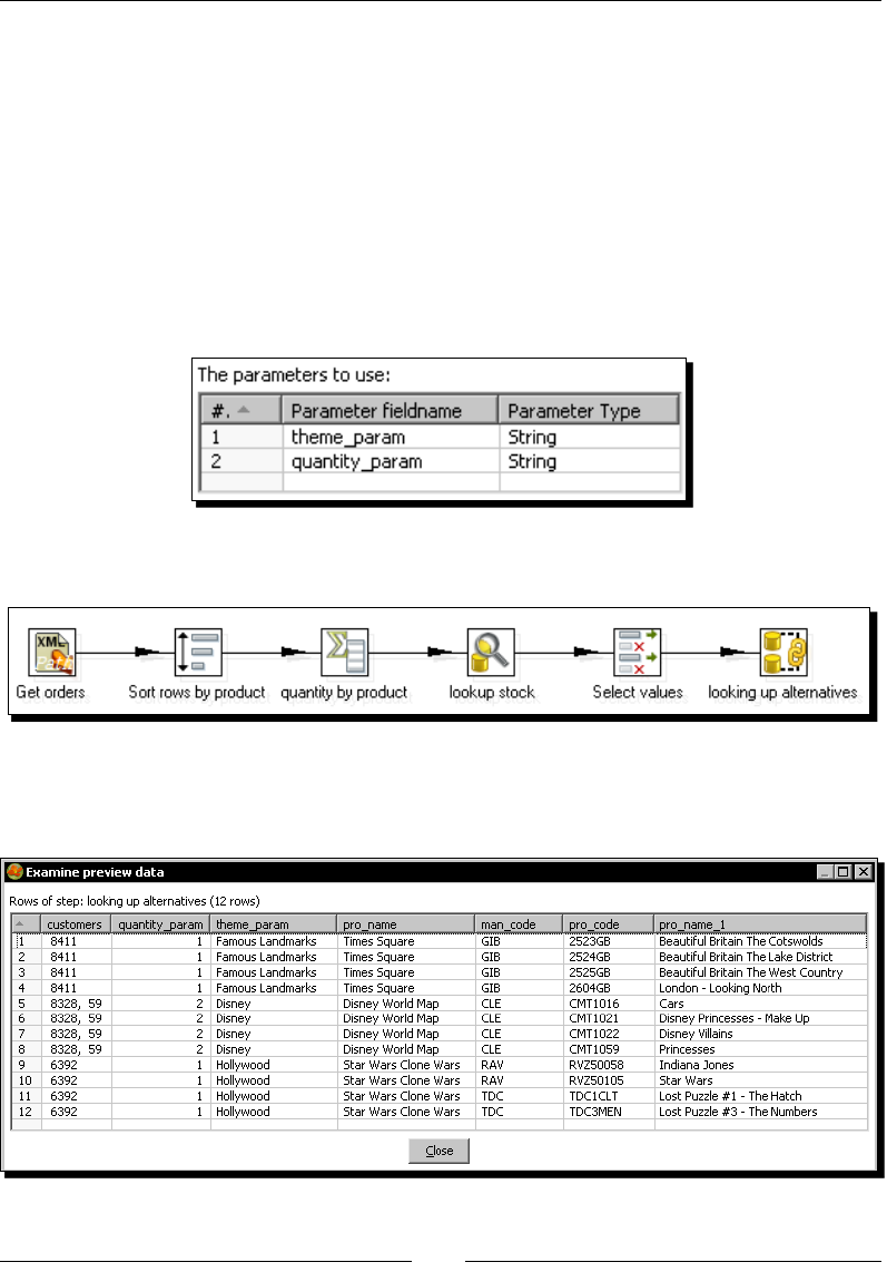
Chapter 9
[ 271 ]
8. In the SQL frame type the following statement:
SELECT man_code
, pro_code
, pro_name
FROM products
WHERE pro_theme like ?
AND pro_stock>=?
9. In the Number of rows to return textbox, type 4.
10. Fill the grid as shown:
11. Click on OK. The transformaon looks like this:
12. With the last step selected, do a Preview.
13. You should see this:
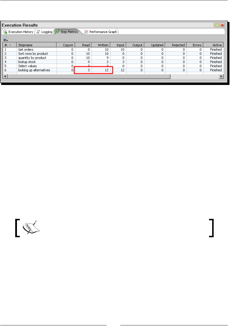
Performing Advanced Operaons with Databases
[ 272 ]
14. In the Step Metrics you should see this:
What just happened?
You took the list of orders and ltered those for which you ran out of products. For the
customers that ordered those products you built a list of four alternave puzzles to buy.
The selecon of the puzzles was based on the theme. To lter the suggested puzzles, you
used the theme of the ordered product.
The second parameter in the Database join step, the ordered quanty, was used to oer only
alternaves for products for which there is a sucient stock.
Joining data from the database to the stream data by using a Database
join step
With the Database join step, you can combine your incoming stream with data from your
database, based on given condions. The condions are put as parameters in the query you
write in the Database join step.
Note that this is not really a database join as the name suggests; it is a
join of data from the database to the stream data.
In the tutorial you used two parameters—the theme and the quanty ordered. With those
parameters, you queried the list of products with the same theme:
where pro_theme like ?
and for which you have stock:
and pro_stock>=?
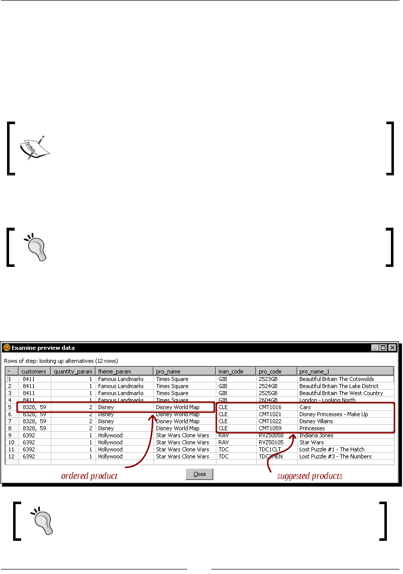
Chapter 9
[ 273 ]
You set the parameters as queson marks. This works like the queson marks in a Table
input step you learned in the last chapter—the parameters are replaced posionally. The
dierence is that here you dene the list and the order of the parameters. You do it in the
small grid at the boom of the sengs window. This means you aren't forced to use all the
incoming elds as parameters, and that you also may change the order.
Just as you do in a Table input step, instead of using posional parameters, you can use
Kele variables by using the ${} notaon and checking the Replace variables checkbox.
You don't need to add the Select values step to discard elds and rename the
parameters. You did it just to have fewer elds in the nal screenshot so that it
was easier to understand the output of the Database join step.
The step will give you back the manufacturer code, the product code, and the product name
for the matching records.
As you cannot do a preview here, you can write and try your query inside a
Table input step or in MySQL Query Browser. When you are done, just copy
and paste the query here.
So far, you did the same you could have done with Database lookup step—looking for a
record with a given condion, and adding new elds to the stream. However, there is a big
dierence here—you put 4 as the Number of rows to return. This means for each incoming
row, the step will give you back up to four results. The following shows you this:
Note that if you had le the Number of rows to return empty, the step would
have returned all found rows.

Performing Advanced Operaons with Databases
[ 274 ]
You may need to use a Database join step in several situaons:
When, as the result of the lookup, there is more than one row for each incoming row.
This was the case in the tutorial.
When you have to look in a combinaon of tables. Look at the following SQL statement:
SELECT co.country_name
FROM customers cu
, cities ci
, countries co
WHERE cu.city_id = ci.city_id
AND ci.cou_id = co.cou_id
AND cu.cus_id = 1000
This statement returns the name of the country where the customer with id 1000
lives. If you want to look up the countries where a list of customers live, you can do
it with a sentence like this by using a Database join step.
When you want to look for an aggregate result. Look at this sample query:
SELECT pro_theme
, count(*) quant
FROM products
GROUP BY pro_theme
ORDER BY pro_theme
This statement returns the number of puzzles by theme. If you have a list of themes
and you want to nd out how many puzzles you have for each theme, you can use a
query like this also by using a Database join step.
The last opon in the list can also be developed without using the Database join step.
You could execute the SELECT statement with a Table Input step, and then look for the
calculated quanty by using a Stream lookup step.
As you can see, this is another situaon where PDI oers more that one
way to do the same thing. Somemes it is a maer of taste. In general, you
should test each opon and choose the method which gives you the best
performance.

Chapter 9
[ 275 ]
Have a go hero – rebuilding the list of customers
Redo the Hero exercise preparing the delivery of the products, this me using a Database
join step. Try to discover which one is preferable from the point of view of performance. If
you don't see any dierence, try with a bigger number of records in the main stream. You
will have to create your own dataset for this test.
Introducing dimensional modeling
So far you have dealt with the Jigsaw puzzles database, a database used for daily operaonal
work. In the real-world, a database like this is maintained by an On-Line Transacon
Processing (OLTP) system. The users of an OLTP system perform operaonal tasks—sell
products, process orders, control stock, and so on.
As a counterpart, a datawarehouse is a nonoperaonal database; it is a specialized database
designed for decision support purposes. Users of a datawarehouse analyze the data, and
they do it from dierent points of view.
The most used technique for delivering data to datawarehouse users is dimensional
modeling. This technique makes databases simple and understandable.
The primary table in a dimensional model is the fact table. A fact table stores numerical
measurements of the business such as quanty of products sold, amount represented by the
sold products, discounts, taxes, number of invoices, number of claims, and anything that can
be measured. These measurements are referred as facts.
A fact is useless without the dimension tables. Dimension tables contain the textual
descriptors of the business. Typical dimensions are product, me, customers, and regions.
The fact along with all the surrounding dimension tables make a star-like structure oen
called a star schema.
Datawarehouse is a very broad concept. In this book we will deal with datamarts. While a
datawarehouse represents a global vision of an enterprise, a datamart holds the data from a
single business process .
Data stored in datawarehouses and datamarts usually comes from dierent sources, the
operaonal database being the main. The process that takes the informaon from the source,
transforms it in several ways, and nally loads the data into the datamart or datawarehouse is
the already menoned ETL process. As said, PDI is a perfect tool for accomplishing that task.
In the rest of this chapter, you will learn how to load dimension tables with PDI. This will build
the basis for the nal project of the book: Loading a full datamart.

Performing Advanced Operaons with Databases
[ 276 ]
Through the tutorials you will learn more about this. However, the terminology introduced
here constutes just a preamble to dimensional modeling. There is much more you
can learn. If you are really interested in the subject, you should start by reading The
Data Warehouse Toolkit (Second Edion) by Ralph Kimball and Margy Ross. The book is
undoubtedly the best guide to dimensional modeling.
Loading dimensions with data
A dimension is an enty that describes your business—customers and products are examples
of dimensions. A very special dimension is the me dimension that you already know. A
dimension table (no surprises here) is a table that contains informaon about a dimension.
In this secon you will learn to load dimension tables, that is, ll dimension tables with data.
Time for action – loading a region dimension with a
Combination lookup/update step
In this tutorial you will load a dimension that stores geographical informaon.
1. Launch Spoon.
2. Create a new transformaon.
3. Drag a Table input step to the canvas and double-click it.
4. As connecon select js.
5. In the SQL area type the following query:
SELECT ci.city_id, city_name, country_name
FROM cities ci, countries co
WHERE ci.cou_id = co.cou_id
6. Click on OK.
7. Expand the Data Warehouse category of steps.
8. Select the Combinaon lookup/update step and drag it to the canvas.
9. Create a hop from the Table input step to this new step.
10. Double-click the Combinaon lookup/update step.
11. As Connecon select dw.

Chapter 9
[ 277 ]
12. As Target table browse and select lk_regions or simply type it.
13. Enter id as Technical key eld and lastupdate as Date of last update eld.
14. Click OK.
15. Aer the Combinaon lookup/update step, add an Update step.
16. Double-click the Update step.
17. Select dw as Connecon and lk_regions as Target table.
18. Fill the upper grid adding the condion id = id. The id to the le is the table id,
while the id to the right is the stream id.
19. Fill the lower grid: Add one row with the values city and city_name. Add a
second row with the values country and country_name. This will update the
table columns city and country with the values city_name and country_name
coming in the stream.
20. Now create another stream: Add to the canvas a Generate Rows step, a Table
output step, and a Dummy step.
21. Link the steps in the order you added them.
22. Edit the Generate Rows step and set Limit to 1.
23. Add four elds in this order: An Integer eld named id with value 0, a String
eld named city with value N/A, another String named country with value
N/A, and an Integer eld named id_js with value 0. Double-click the Table
Output step.
24. Select dw as Connecon and lk_regions as Target table.
25. Click on OK.
26. In the Table output step, enable error handling and send the bad rows to the
Dummy step.
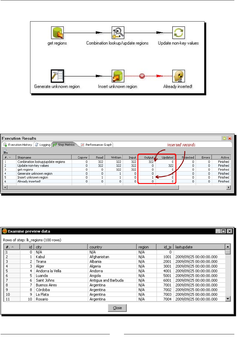
Performing Advanced Operaons with Databases
[ 278 ]
27. The transformaon looks like this:
28. Save the transformaon and run it.
29. The Step metrics looks like this:
30. Explore the js_dw database and do a preview of the lk_regions table. You should
see this:
Download from Wow! eBook <www.wowebook.com>

Chapter 9
[ 279 ]
What just happened?
You loaded the region dimension with geographical informaon—cies and countries.
Note that you took informaon from the operaonal database
js and loaded a table in another database js_dw.
Before running the transformaon, the dimension table lk_region was empty. When the
transformaon ran, all cies were inserted in the dimension table.
Besides the records with cies from the cities table, you also inserted a special record
with values n/a for the descripve elds. You did it in the second stream added to the
transformaon.
Note that the dimension table lk_regions has a column named region that you didn't
update because you don't have data for that column. The column is lled with a default
value set in the DDL denion of the table.
Time for action – testing the transformation that loads the
region dimension
1. In the previous tutorial you loaded a dimension that stores geographical
informaon. You ran it once, causing the inseron of one record for each city and a
special record with values n/a for the descripve elds. Let's apply some changes in
the operaonal database, and run the transformaon again to see what happens.
2. Launch MySQL Query Browser.
3. Type the following sentence to change the names of the countries to upper case:
UPDATE countries SET country_name = UCASE(country_name)
4. Execute it.
5. If the transformaon created in the last tutorial is not open, open it again.
6. Run the transformaon.
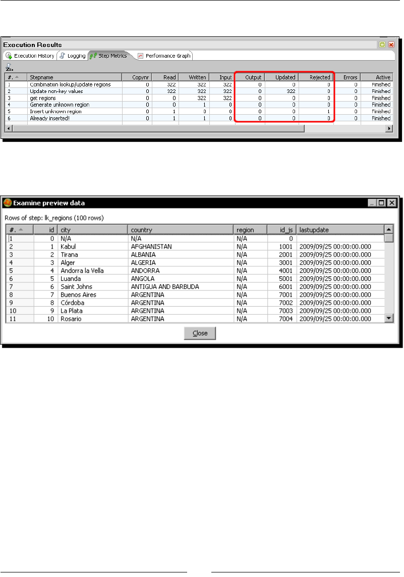
Performing Advanced Operaons with Databases
[ 280 ]
7. The Step Metrics looks like this:
8. Explore the js_dw database again and do a preview of the lk_regions table. This
me you will see the following:
What just happened?
Aer changing the leer case for the names of the countries in the transaconal database
js, you again ran the transformaon that updates the Regions dimension. This me the
descripons for the dimension table were updated.
As for the special record with values n/a for the descripve elds, it had been created the
rst me the transformaon ran. This me, as the record already existed, the row passed by
to the Dummy step.
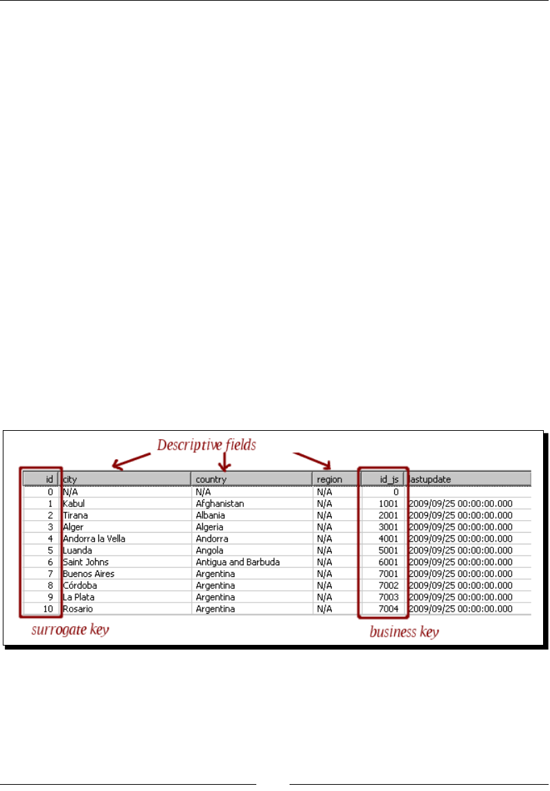
Chapter 9
[ 281 ]
Describing data with dimensions
A dimension table contains descripons about a parcular enty or category of your
business. Dimensions are one of the basic blocks of a datawarehouse or a datamart.
A dimension has the purpose of grouping, ltering, and describing data.
Think of a typical report you would like to have—sales grouped by region, by customer, by
method of payment ordered by date. The by word lets you idenfy potenal dimensions—
regions, customers, method of payments, and date.
Best pracces say that a dimension table must have its own technical key column dierent
to the business key column used in the operaonal database. This technical key is known
as a surrogate key. In the lk_region dimension table the surrogate key is the column
named id.
While in the operaonal database the key may be a string such as the manufacturer code in
the manufacturers table, surrogate keys are always integers. Another good pracce is to have
a special record for unavailable data. In the case of the regions example, this implies that
besides one record for every city, you should have a record with key equal to zero, and n/a
or unknown or something that represents invalid data for all the descripve aributes.
Along with the descripve aributes that you save in a dimension, you usually keep the
business key so that you can match the data in the dimension table with the data in the
source database. The following screenshot depicts typical columns in a dimension table:
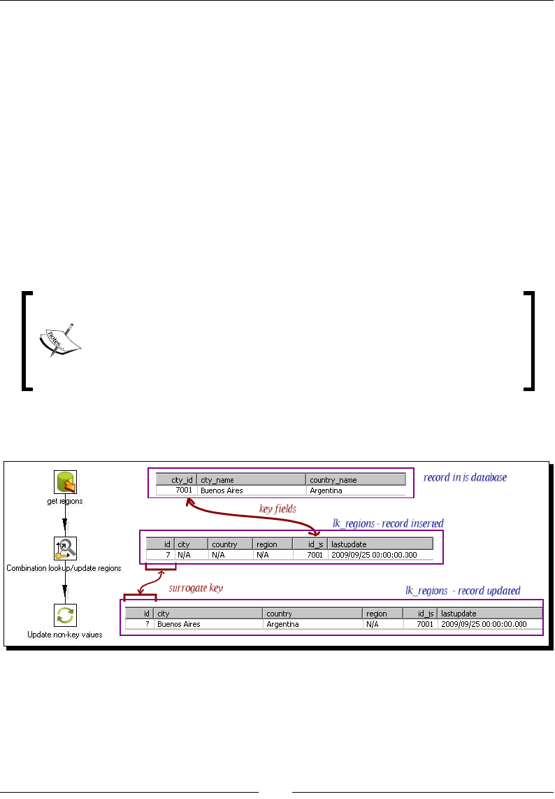
Performing Advanced Operaons with Databases
[ 282 ]
In the tutorial, you took informaon from the cities and countries tables and used that
data to load the regions dimension. When there were changes in the transaconal database,
the changes were translated to the dimension table overwring the old values. A dimension
where changes may occur from me to me is called a Slowly Changing Dimension or SCD
for short. If, when you update an SCD dimension, you don't preserve historical values but the
old values, the dimension is called Type I slowly changing dimension (Type I SCD).
Loading Type I SCD with a Combination lookup/update step
In the tutorial, you loaded a Type I SCD by using a Combinaon lookup/update step. The
Combinaon lookup/update or Combinaon L/U for short, looks in the dimension table
for a record that matches the key elds you put in the upper grid in the sengs window. If
the combinaon exists, the step returns the surrogate key of the found record. If it doesn't
exist, the step generates a new surrogate key and inserts a row with the key elds and the
generated surrogate key. In any case, the surrogate key is added to the output stream.
Be aware that in the Combinaon Lookup/update step the following opons
do not refer to elds in the stream, but to columns in the table: Dimension
eld, Technical key eld, and Date of last update eld. You should read
Dimension column, Technical key column, and Date of last update column.
Also note that the term Technical refers to the surrogate key.
Let's see how the Combinaon lookup/update step works with an example. Look at the
following screenshot:
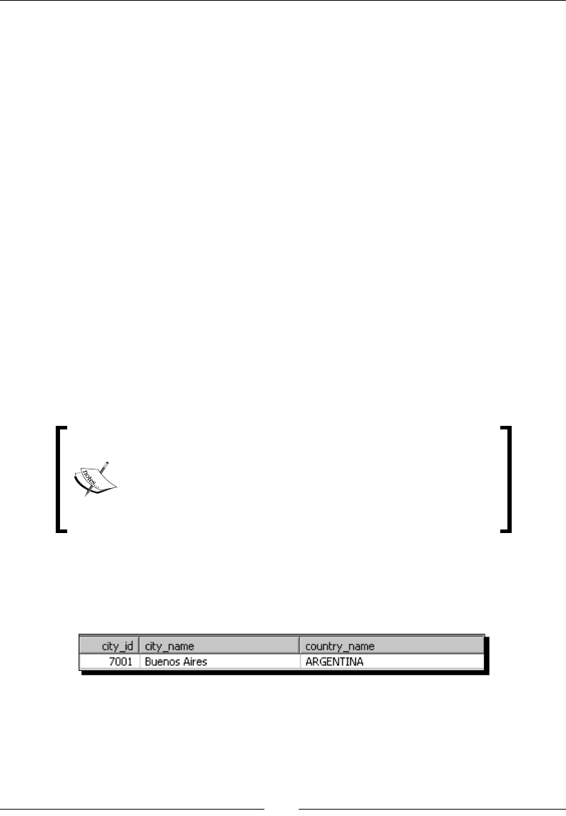
Chapter 9
[ 283 ]
The record to the right of the Table input icon is a sample city among the cies that the Table
input step gets from the js database.
With the Combinaon L/U step, PDI looks for a record in the lk_region table in the dw
database, where id_js is equal to the eld city_id in the incoming stream, which is 7001.
The rst me you run the transformaon, the dimension table is empty, so the lookup fails.
This causes PDI to generate a new surrogate key according to what you put in the Technical
key eld area of the sengs window.
You told PDI that the column that holds the surrogate key is the column named id. You also
told PDI that in order to generate the key, the value should be equal to the maximum key
found in the target table plus one. In this example, it generates a key equal to 7. You may
also use a sequence or an auto increment eld if the database engine allows it. If that is not
the case, those opons are disabled.
Then PDI generates the key and inserts the record you can see to the right of the
Combinaon L/U step in the draw. Note that the record contains only values for the key
elds and the technical key eld.
The Combinaon L/U step put the returned technical key in the output stream. Then you
used that key for updang the descripons for city and country with the use of an Update
step. Aer that step, the record is fully generated, as shown in the record to the right of
the Update icon.
As the Combinaon L/U only maintains the key informaon, if
you have non-key columns in the table you must update them
with an extra Update step.
Note that those values must have a default value or must
allow null values. If none of these condions is true, the insert
operaon will fail.
Aer converng to upper case, all the country names in the source database, you run the
transformaon again.
This me the incoming record for the same city is this:
PDI looks for a record in the lk_region table, in the dw database, where id_js is equal
to 7001. It nds it. It is the record inserted the rst me you ran the transformaon, as
explained above.
Then, the Combinaon L/U simply returns the key eld adding it to the output stream.

Performing Advanced Operaons with Databases
[ 284 ]
Then you use the key that the step added to update the descripons for city and country.
Aer the Update step, the old values for city and country name are overwrien by the
new ones:
Have a go hero – adding regions to the Region Dimension
Modify the transformaon that loads the Region dimension to ll the region column. Get
the values from the regions.xls le you can nd among the downloaded material for this
chapter. To add the region informaon to your stream, use a Stream lookup step.
While you are playing with dimensions, you may want to throw away all the
inserted data and start over again. For doing that, simply explore the database
and use the Truncate table opon. You can do the same in MySQL Query
Explorer. For the lk_regions dimension, you could execute any of
the following:
DELETE FROM lk_regions or TRUNCATE TABLE lk_regions
Have a go hero – loading the manufacturers dimension
Create a transformaon that loads the manufacturers dimension—lk_manufacturers.
Here you have the table denion and some guidance for loading:
Column Descripon
id Surrogate key.
name Name of the manufacturer.
id_js Business key. Here you have to store the manufacturer's code
(man_code eld of the source table manufacturers).
lastupdate Date of dimension update—system date.

Chapter 9
[ 285 ]
Have a go hero – loading a mini-dimension
A mini-dimension is a dimension where you store the frequently analyzed or frequently
changing aributes of a large dimension. Look at the products in the Jigsaw puzzles
database. There are several puzzle aributes you may be interested in, for example, when
you analyze the sales—number of puzzles in a single pack, number of pieces of the puzzles,
material of the product, and so on. Instead of creang a big dimension with all puzzle
aributes, you can create a mini-dimension that stores only a selecon of aributes. There
would be one row in this mini-dimension for each unique combinaon of the selected
aributes encountered in the products table, not one row per puzzle.
In this exercise, you'll have to load a mini-dimension with puzzle aributes. Here you have
the denion of the table that will hold the mini-dimension data:
Column Descripon
id Surrogate key
glowsInDark Y/N
is3D Y/N
wooden Y/N
isPanoramic Y/N
nrPuzzles Number of puzzles in a single pack
nrPieces Number of pieces of the puzzle
Take as a starng point the following query:
SELECT DISTINCT pro_type
, pro_packaging
, pro_shape
, pro_style
FROM products
WHERE pro_type = 'PUZZLE'
Use the output stream for creang the elds you need for the dimension—for example,
for the eld is3D, you'll have to check the value of the pro_shape eld.
Once you have all the elds you need, insert the records in the dimension table by using a
Combinaon L/U step. In this mini-dimension, the key is made by all the elds of the table.
As a consequence, you don’t need an extra Update step.

Performing Advanced Operaons with Databases
[ 286 ]
Keeping a history of changes
The Region dimension is a typical Type I SCD dimension. If some descripon changes, as
the country names did, it makes no sense to keep the old values. The new values simply
overwrite the old ones. This is not always the best choice. Somemes you would like to
keep a history of the changes. Now you will learn to load a dimension that keeps a history.
Time for action – keeping a history of product changes with the
Dimension lookup/update step
Let's load a puzzles dimension along with the history of the changes in puzzle aributes:
1. Create a new transformaon.
2. Drag a Table input step to the work area and double-click it.
3. Select js as Connecon.
4. Type the following query in the SQL area:
SELECT pro_code
, man_code
, pro_name
, pro_theme
FROM products
WHERE pro_type LIKE 'PUZZLE'
5. Click on OK.
6. Add an Add constants step, and create a hop from the Table input, step toward it.
7. Use the step to add a Date eld named changedate. As Format type dd/MM/
yyyy, and as Value, type 01/10/2009.
8. Expand the Data Warehouse category of steps.
9. Select the Dimension lookup/update step and drag it to the canvas.
10. Create a hop from the Add constants step to this new step.
11. Double-click the Dimension lookup/update step.
12. As Connecon select dw.
13. As Target table type lk_puzzles.
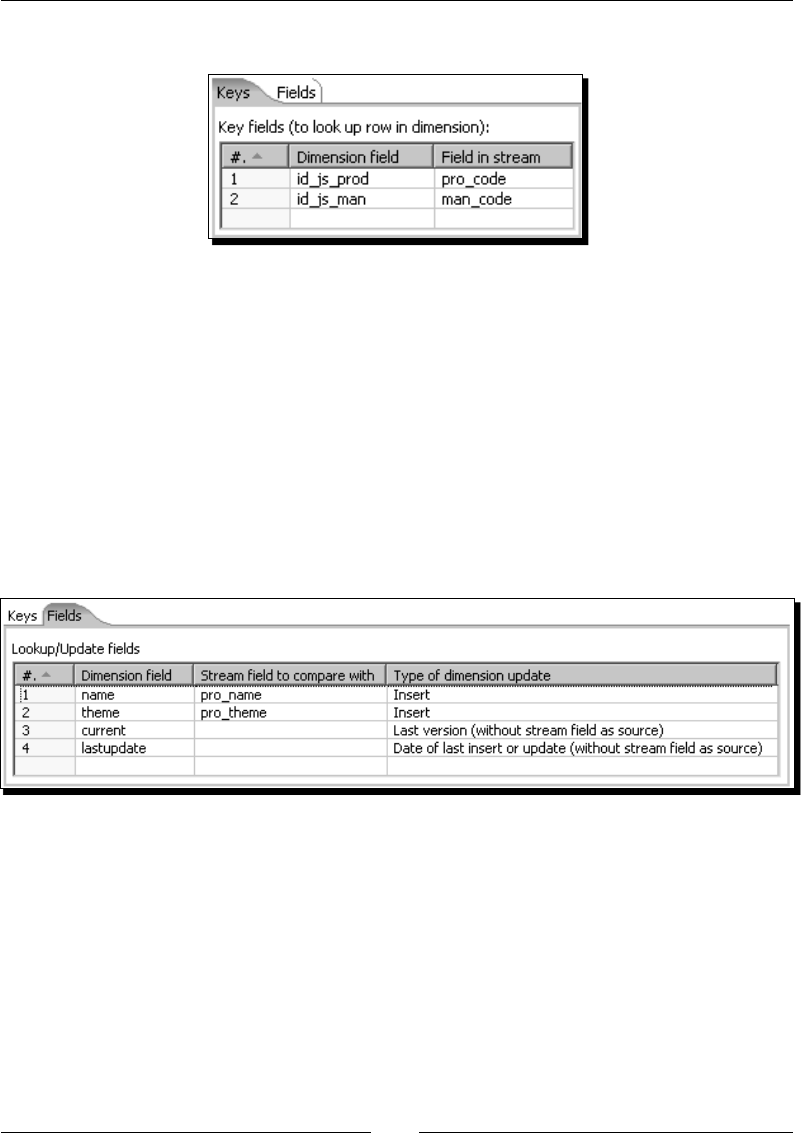
Chapter 9
[ 287 ]
14. Fill the Key elds as shown:
15. Select id as Technical key eld.
16. In the frame Creaon of technical key, leave the default to
Use table maximum + 1.
17. As Version eld, select version.
18. As Stream Dateeld, select changedate.
19. As Date range start eld, select start_date.
20. As Table daterange end, select end_date.
21. Select the Fields tab and ll it like this:
22. Close the sengs window.
23. Save the transformaon, and run it.
24. Explore the js_dw database and do a preview of the lk_puzzles table.
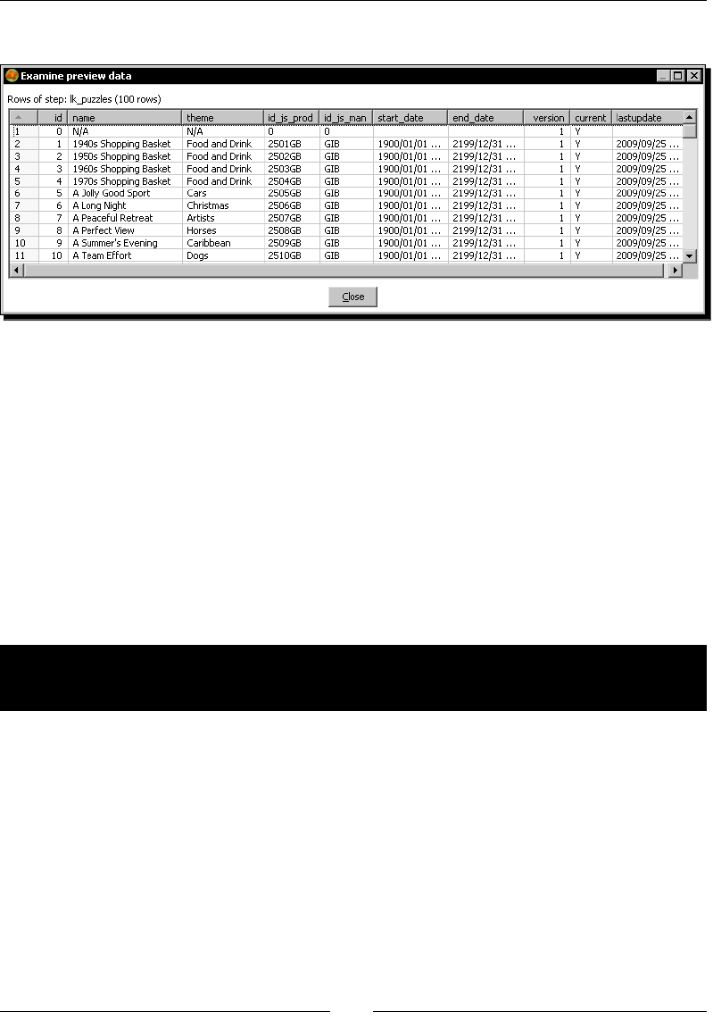
Performing Advanced Operaons with Databases
[ 288 ]
25. You should see this:
What just happened?
You loaded the puzzle dimension with the name and theme of the puzzles you sell. The
dimension table has the usual columns for a dimension—technical id (eld id), elds that
store the key elds in the table of the operaonal database (prod_code and man_code),
and columns for the puzzle aributes (name and theme). It also has some extra elds
specially designed to keep history.
When you ran the transformaon, all records were inserted in the dimension table. Also a
special record was automacally inserted for unavailable data.
So far, there is nothing new except for a few extra columns with dates. In the next tutorial,
you will learn more about those columns.
Time for action – testing the transformation that keeps a history
of product changes
1. In the previous tutorial you loaded a dimension with products by using a Dimension
lookup/update step. You ran the transformaon once, causing the inseron of one
record for each product and a special record with values n/a for the descripve elds.
Let's apply some changes in the operaonal database, and run the transformaon again
to see how the Dimension lookup/update step keeps history.
2. In MySQL Query Browser, open the script update_jumbo_products.sql and
run it.
3. Switch to Spoon.
4. If the transformaon created in the last tutorial is not open, open it again.
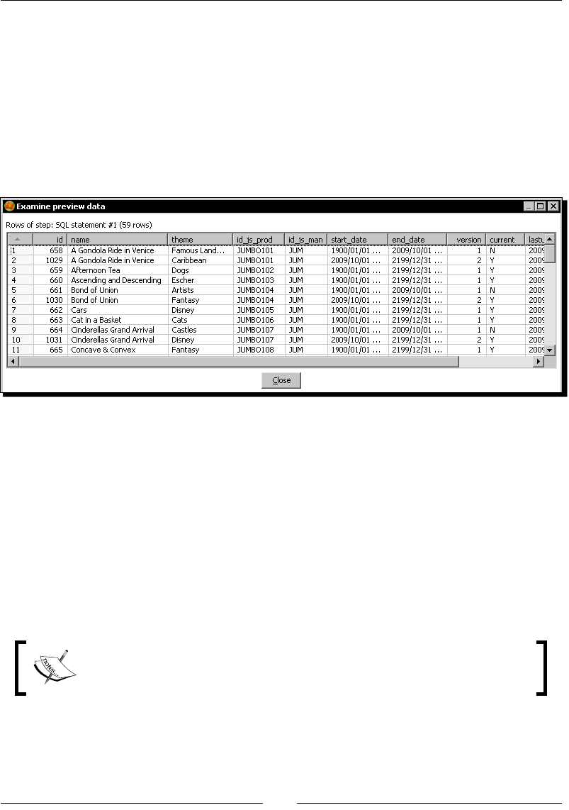
Chapter 9
[ 289 ]
5. Run the transformaon. Explore the js_dw database again. Press Open SQL for
[lk_puzzles] and type the following sentence:
SELECT *
FROM lk_puzzles
WHERE id_js_man = 'JUM'
ORDER BY id_js_prod
, version
6. You will see this:
What just happened?
Aer making some changes in the operaonal database, you ran the transformaon for a
second me. The modicaons you made caused the inseron of new records recreang the
history of the puzzle aributes.
Keeping an entire history of data with a Type II slowly changing dimension
Type II SCDs dier from Type I SCDs in that a Type II keeps the whole history of the data of
your dimension. Typical examples of aributes for which you would like to keep a history are
sales territories that change over me, categories of products that are reclassied from me
to me, and promoons that you apply to products and are valid in a given range of dates.
There are no rules that dictate whether or not you keep/retain the history in a
dimension. It's the nal user who decides based on his requirements.
Performing Advanced Operaons with Databases
[ 290 ]
In the puzzle dimension, you kept informaon about the changes for the name and theme
aributes. Let's see how the history is kept for this sample dimension.
Each puzzle is to be represented by one or more records, each with the informaon valid
during a certain period of me, as in the following example:
01
1900 2199
31
12
VERSION : 1
To :
01-01-1900
664
Castles
01-10-2009
JUM, JUMB0107
Valid From :
Surrogate Key :
Business Key :
Fields :
Name :
Theme :
Cindrellas Grand Arrival
01-10-2009
JUM, JUMB0107
31-12-2199
1031
Disney
VERSION : 2 (current)
To :
Valid From :
Surrogate Key :
Business Key :
Fields :
Name :
Theme :
Cindrellas Grand Arrival
01
01
1900
10
The history is kept in three extra elds in the dimension table—version, date_from,
and date_to.
The version eld is an automacally incremented value that maintains a revision number of
the records for a parcular puzzle.
The date range is used to indicate the period of applicability of the data.
In the tutorial you also had a current eld, that acted as a ag to show if a record is the
record valid in the present day.
The sample puzzle, Cinderellas Grand Arrival, was classied in the category Castles unl
October 1, 2009. Aer that date, the puzzle was reclassied as a Disney puzzle. This is the
second version of the puzzle, as indicated by the column version. It's also the current
version, as indicated by the column current.
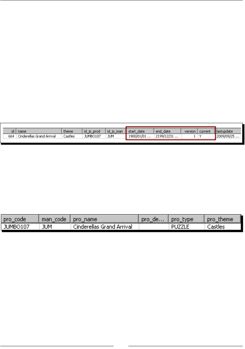
Chapter 9
[ 291 ]
In general, if you have to implement a Type II SCD with PDI, your dimension table
must have the rst three elds—version, date from, and date to. The current ag
is oponal.
Loading Type II SCDs with the Dimension lookup/update step
Type II SCDs can be loaded by using the Dimension lookup/update step. The Dimension
lookup/update or Dimension L/U for short, looks in the dimension for a record that matches
the informaon you put in the Keys grid of the sengs window.
If the lookup fails, it inserts a new record. If a record is found, the step inserts or updates
records depending on how you congured the step.
Let's explain how the Dimension L/U works with the following sample puzzle in the
js database:
The rst me you run the transformaon, the step looks in the dimension for a record where
id_js_prod is equal to JUMBO107and id_js_man is equal to JUM. Not only that, the
period from start_date to end_date of the found record must contain the value of the
stream datefield, which is 01/10/2009.
Because you never loaded this table before, the table was empty and so the lookup failed.
As a result, the step inserts the following record:
Note the values that the step put for the special elds:
The version for the new record is 1, the current ag is set to true, and the start_date and
end_date take as values the dates you put in the Min.year and Max.year: 01/01/1900
and 31/12/2199.
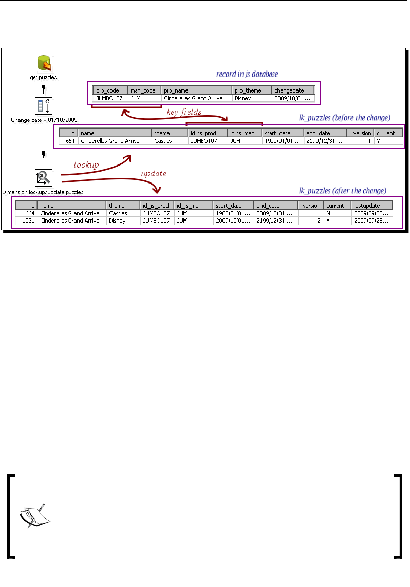
Performing Advanced Operaons with Databases
[ 292 ]
Aer making some modicaons to the operaonal database, you ran the transformaon
again. Look at the following screenshot:
The puzzle informaon changed. As you see to the right of the Table input step, the puzzle is
now classied as a Disney puzzle.
This me the lookup succeeds. There is a record for which the keys match and the period
from start_date to end_date of the found record, 01/01/1900 to 31/12/2199,
obviously contains the value of the stream datefield, 01/10/2009.
Once found, the step compares the elds you put in the Fields tab—name and theme in the
dimension table against pro_name and pro_theme in the incoming stream.
As there is a dierence in the theme eld, the step inserts a new record, and modies the
current—it changes the validity dates and sets the current ag to false. Now this puzzle has
two versions in the dimension table, as you see below the Dimension L/U icon in the drawing.
These update and insert operaons are made for all records that changed.
For the records that didn't change, dimension records are found but as nothing changed,
nothing is inserted or updated.
Take a note about the stream date: The eld you put here is key to the loading
process of the dimension, as its value is interpreted by PDI as the eecve
date of the change. In the tutorial, you put a xed date—01/10/2009. In
real situaons you should use the eecve or last changed date of the data if
that date is available. If it is not available, leave the eld blank. PDI will use the
system date.

Chapter 9
[ 293 ]
In this example, you lled the column Type of SCD update with the opon Insert for every
eld. Doing so, you loaded a pure Type II SCD, that is, a dimension that keeps track of all
changes in all elds.
In the sample puzzles dimension, you kept a history of changes both in the theme and in
the name. For the sample puzzle, the theme was changed from Castles to Disney. If, aer
some me, you query the sales and noce that the sales for that puzzle increased aer the
change, then you may conclude that the customers are more interested in Disney puzzles
than in castle puzzles. The possibility of creang these kinds of reports is a good reason for
maintaining a Type II SCD.
On the other hand, if the name of the puzzle changes, you may not be so interested in
knowing what the name was before. Fortunately, you may change the conguraon and
create a Hybrid SCD. Instead of selecng Insert for every eld, you may select Update
or Punch through:
When there is a change in a eld for which you chose Update, the new value
overwrites the old value in the last dimension record version, this being the usual
behavior in Type I SCDs.
When there is a change in a eld for which you chose Punch through, the new
data overwrites the old value in all record versions.
Note that selecng Punch through for all the elds, the Dimension L/U step allows you
to load a Type I SCD dimension. When you build Type I SCD you are not interested in range
dates. Thus, you can leave the Stream dateeld textbox empty. The current date is assumed
by default.
In pracce both Type I, Type II, and Hybrid SCDs are used. The choice of the type of SCD
depends on the business needs.
Besides all those inserts and updates operaons, the Dimension L/U automacally inserts in
the dimension a record for unavailable data.
In order to insert the special record with key equal to zero, all elds must have
default values or allow nulls. If none of these condions are true, the automac
inseron will fail.
In order to load a dimension with the Dimension L/U step, your table has to have columns
for the version, date from, and date to. The step automacally maintains those columns.
You simply have to put their names in the right textbox in the sengs window.
Besides those elds, your dimension table may have a column for the current ag, and
another column for the date of last insert or update. To ll those oponal columns, you
have to add them in the Fields tab as you did in the tutorial.
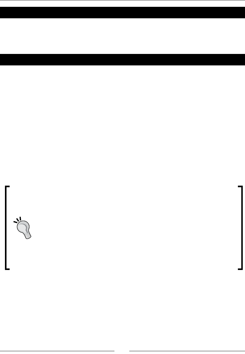
Performing Advanced Operaons with Databases
[ 294 ]
Have a go hero – keeping a history just for the theme of a product
Modify the loading of the products dimension so that it only keeps a history of the theme. If
the name of the product changes, just overwrite the old values. Modify some data in the js
database and run your transformaon to conrm that it works as expected.
Have a go hero – loading a Type II SCD dimension
As you saw in the Hero exercise to add regions to the Region Dimension, the countries were
grouped in three: Spain, Rest of Europe, Rest of the World.
As the sales rose in several countries of the world, you decided to regroup the countries in
more than three groups. However, you want to do it starng in 2008. For older sales you
prefer to keep seeing the sales grouped by the original categories.
This is what you will do: Use the table named lk_regions_2 to create a Type II Region
dimension. Here is a guide to follow:
Create a transformaon that loads the dimension. You will take the stream date (the date
you use for loading the dimension) from the command line. If the command line argument is
empty, use the present day.
As the name for the sheet with the region denion, use a named parameter.
Stream date
If the command line argument is present, remember to change it to Date
before using it. You do that with a Select values step.
Note that you have to dene the format of the entered data in advance.
Suppose that you want to enter as argument the date January 1, 2008. If
you chose the format dd-mm-yyyy, you'll have to enter the argument as
01-01-2008.
In case the command line argument is absent, you can get the default with
a Get System Info step. Note that the system date you add with this step is
already a Date eld.

Chapter 9
[ 295 ]
Now just follow these steps:
1. Run the transformaon by using the regions.xls le. Don't worry about the
command line argument. Check that the dimension was loaded as expected. There
has to be a single record for every city.
2. Run the transformaon again. This me use the regions2008.xls le as source
for the region column. As command line, enter January 1st, 2008. Remember to type
the date in the expected format (check the preceding p). Explore the dimension
table. There has to be two records for each country—one valid before 2008 and
one valid aer that date.
3. Modify the sheet to create a new grouping for the American countries. Use your
imaginaon for this task! Run the transformaon for the third me. This me use
the sheet you created and as date, type the present day (or leave the argument
blank). Explore the dimension table. Now each city for the countries you regrouped
has to have three versions, where the current is the version you created. The other
cies should connue to have two versions each, because nothing related to those
cies changed.
Pop quiz – loading slowly changing dimensions
Suppose you have DVDs with the French lms in the catalog you've created so far. You
rent those DVDs and keep the rental informaon in the database. Now you will design a
dimensional model for that data.
1. You begin by designing a dimension to store the names of the lms. How do you
create the Films dimension:
a. As a Type I SCD
b. As a Type II SCD
c. You will decide when you have rented enough lms so you make the
right decision.
2. In order to create that dimension, you could use:
a. A Dimension L/U step
b. A Combinaon L/U step
c. Either of the above
d. Neither of the above

Performing Advanced Operaons with Databases
[ 296 ]
Pop quiz – loading type III slowly changing dimensions
Type III SCD are dimensions that store the immediately preceding and current value for a
descripve eld of the dimension. Each enty is stored in a single record. The eld for which
you want to keep the previous value has two columns assigned in the record: One for the
current value and the other for the old. Somemes, it is possible to have a third column
holding the date of eecve change.
Type III SCDs are appropriate when you don't want to keep all the history, but mainly when
you need to support two views of the aribute simultaneously—the previous and the
current. Suppose you have an Employees dimension. Among the aributes you have their
posion. People are promoted from me to me and you want to keep these changes in the
dimension; however, you are not interested in knowing all the intermediate posions the
employees have been through. In this case, you may implement a Type III SCD.
The queson is, how would you load a Type III SCD with PDI:
a. With a Dimension L/U step conguring it properly
b. By using a Database lookup step to get the previous value. Then with a Dimension
L/U step or a Combinaon L/U step to insert or update the records.
c. You can't load Type III SCDs with PDI
It's worth saying that type III SCD are used rather infrequently and not always can be
automated. Somemes they are used to represent human-applied changes and the
implementaon has to be made manually.
Summary
In this chapter you learned to perform some advanced operaons on databases.
First, you populated the Jigsaw database in order to have data for the acvies in the
chapter. Then, you learned to do simple and complex searches in a database.
Then you were introduced to dimensional concepts and learned what dimensions are
and how to load them with PDI. You learned about Type I, Type II, Type III SCDs and
mini-dimensions. You sll have to learn when and how to use those dimensions. You
will do so in Chapter 12.
The steps you learned in this and the preceding chapter are far from being the full list of
steps that PDI oers to work with databases. However, taking into account all you learned,
you are now ready to use PDI for implemenng most of your database requirements. In the
next chapter, you will switch to a totally dierent yet core subject needed to work with
PDI—jobs.

10
Creating Basic Task Flows
So far you have been working with data. You got data from a le, a sheet, or a
database, transformed it somehow, and sent it back to some le or table in a
database. You did it by using PDI transformaons. A PDI transformaon does
not run in isolaon. Usually, it is embedded in a bigger process. Here are
some examples:
Download a le, clean it, load the informaon of the le in a database,
and ll an audit le with the result of the operaon.
Generate a daily report and transfer the report to a shared repository.
Update a datawarehouse. If something goes wrong, nofy the
administrator by e-mail.
All these examples are typical processes of which a transformaon is only a piece. These
types of processes can be implemented by PDI Jobs. In this chapter, you will learn to build
basic jobs. These are the topics that will be covered:
Introducon to jobs
Execung tasks depending upon condions
Introducing PDI jobs
A PDI job is analogous to a process. As with processes in real life, there are basic jobs and
there are jobs that do really complex tasks. Let's start by creang a job in the rst group—a
hello world job.
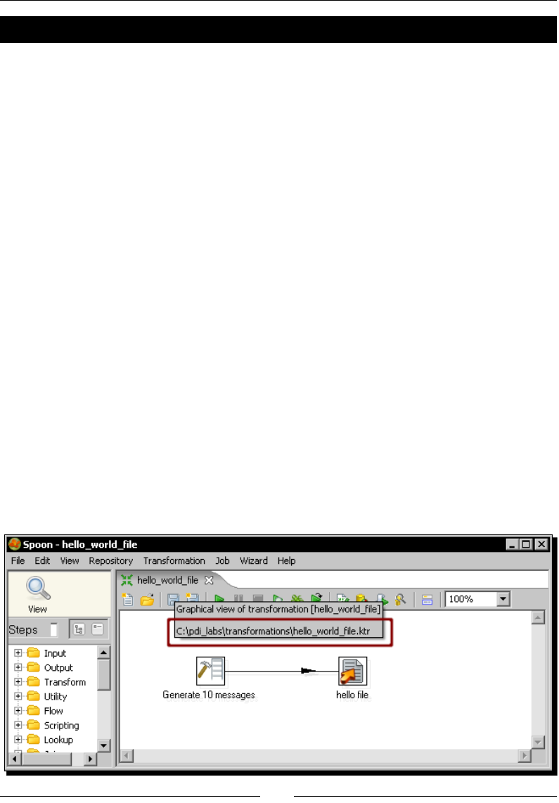
Creang Basic Task Flows
[ 298 ]
Time for action – creating a simple hello world job
In this tutorial, you will create a very simple job so that you get an idea of what jobs
are about.
Although you will now learn how to create a job, for this tutorial you rst have to create
a transformaon.
1. Open Spoon.
2. Create a new transformaon.
3. Drag a Generate rows step to the canvas and double-click it.
4. Add a String value named message, with the value Hello, World!.
5. Click on OK.
6. Add a Text le output step and create a hop from the Generate rows step to this
new step.
7. Double-click the step.
8. Type ${LABSOUTPUT}/chapter10/hello as lename.
9. In the Fields tab, add the only eld in the stream—message.
10. Click on OK.
11. Inside the folder where you save your work, create a folder named
transformations.
12. Save the transformaon with the name hello_world_file.ktr in the folder you
just created. The following is your nal transformaon:

Chapter 10
[ 299 ]
Now you are ready to create the main job.
13. Select File | New | Job or press Ctrl+Alt+N. A new job is created.
14. Press Ctrl+J. The Job properes window appears.
15. Give a name and descripon to the job.
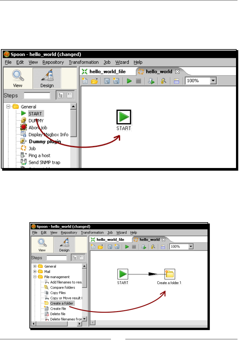
Creang Basic Task Flows
[ 300 ]
16. Save the job in the folder where you created the transformations folder, with
the name hello_world.kjb.
17. To the le of the screen, there is a tree with job entries. Expand the General
category of job entries, select the START entry, and drag it to the work area.
18. Expand the File management category, select the Create a folder entry, and drag it
to the canvas.
19. Select both entries. With the mouse cursor over the second entry, right-click and
select New hop. A new hop is created.
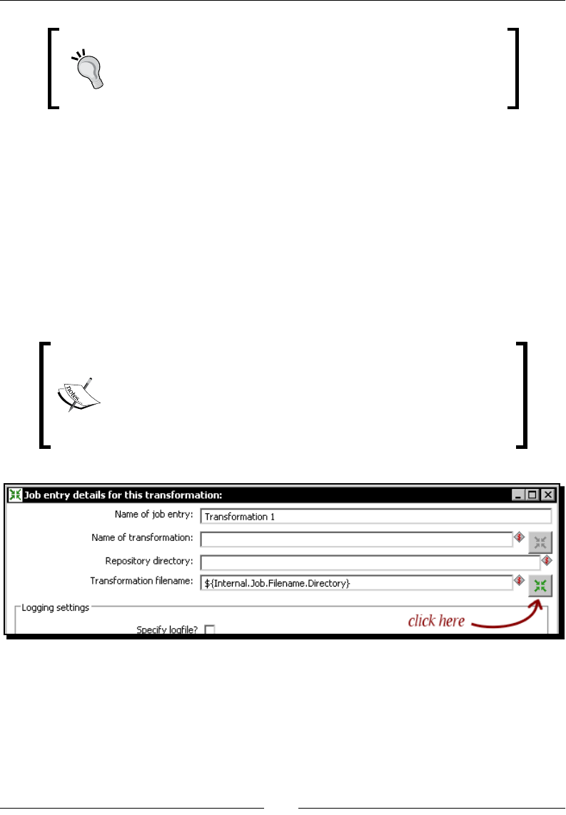
Chapter 10
[ 301 ]
Just like in a transformaon, you have several ways to create hops.
For more detail, please refer to the Time for acon – creang a
Hello Word transformaon secon in Chapter 1 where hops were
introduced or to Appendix D, Spoon Shortcuts.
20. Double-click the Create a folder...icon.
21. In the textbox next to the Folder name opon, type ${LABSOUTPUT}/chapter10
and click on OK. From the General category, drag a transformaon job entry to
the canvas.
22. Create a hop from the Create a folder entry to the transformaon entry.
23. Double-click the transformaon job entry.
24. Posion the cursor in the Transformaon lename textbox, press Ctrl+Space, and
select ${Internal.Job.Filename.Directory}.
This variable is the counterpart to the variable {Internal.
Transformation.Filename.Directory} you already know.
{Internal.Job.Filename.Directory} evaluates the
directory where the job resides.
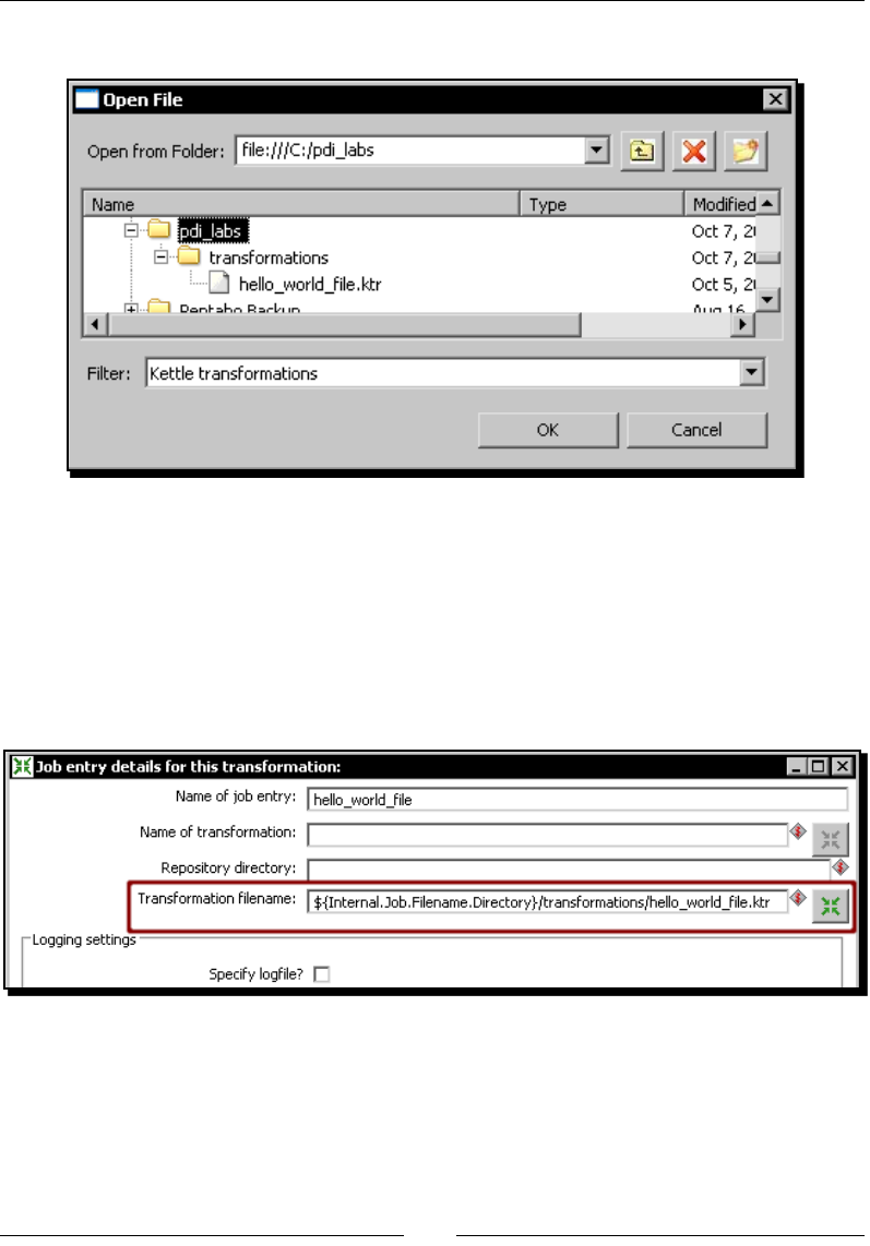
Creang Basic Task Flows
[ 302 ]
25. Click on the icon to the right of the textbox. The following dialog window shows up:
26. As you can see, the {Internal.Job.Filename.Directory} variable provides
a convenient starng place for looking up the transformaon le. Select the
hello_world_file.ktr transformaon and click OK.
27. Now the Transformaon lename has the full path to the transformaon.
Replace the full job path back to ${Internal.Job.Filename.Directory}
so that the nal text for the Transformaon lename eld is as shown in the
following screenshot:
28. Click on OK.
29. Press Ctrl+S to save the job.
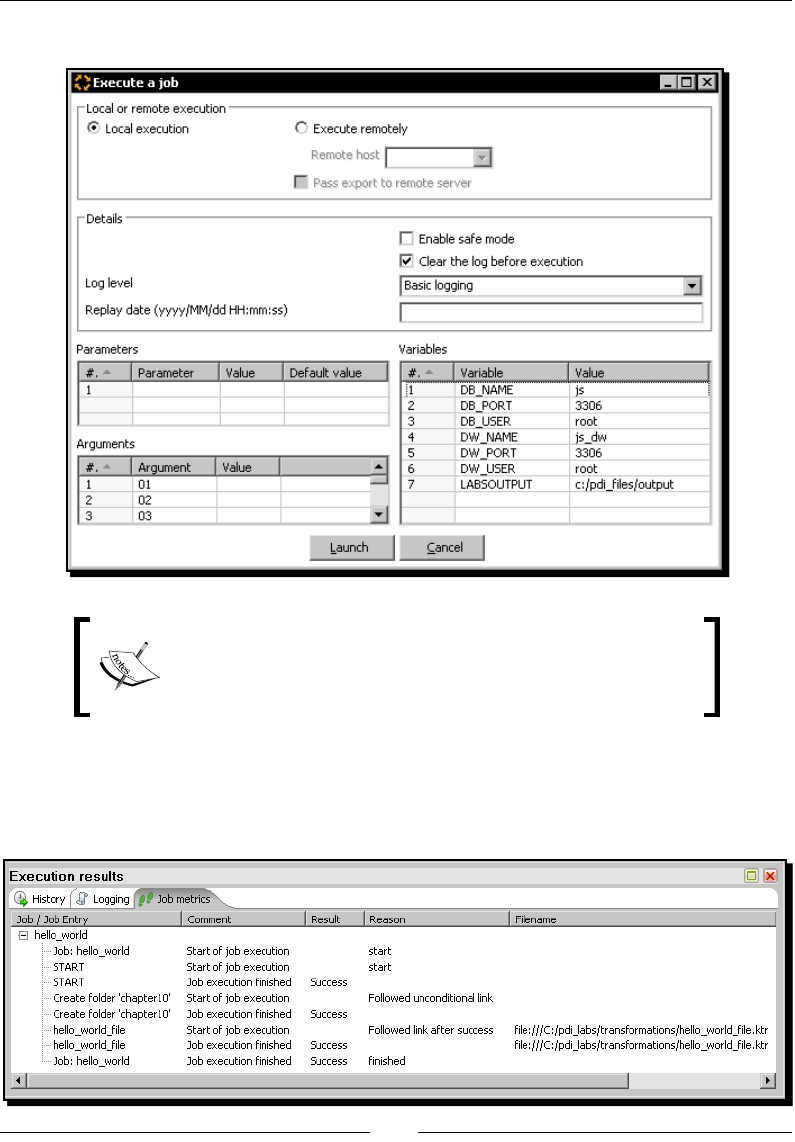
Chapter 10
[ 303 ]
30. Press F9 to run the job. The following window shows up:
Remember that in the inial chapters, you dened the
LABSOUTPUT variable in the kettle.properties le. You
should see its value in the Variables grid. If you removed the
variable from that le, provide a value here.
31. Click on Launch.
32. At the boom of the screen, you'll see the Execuon results. The Job metrics screen
looks as follows:
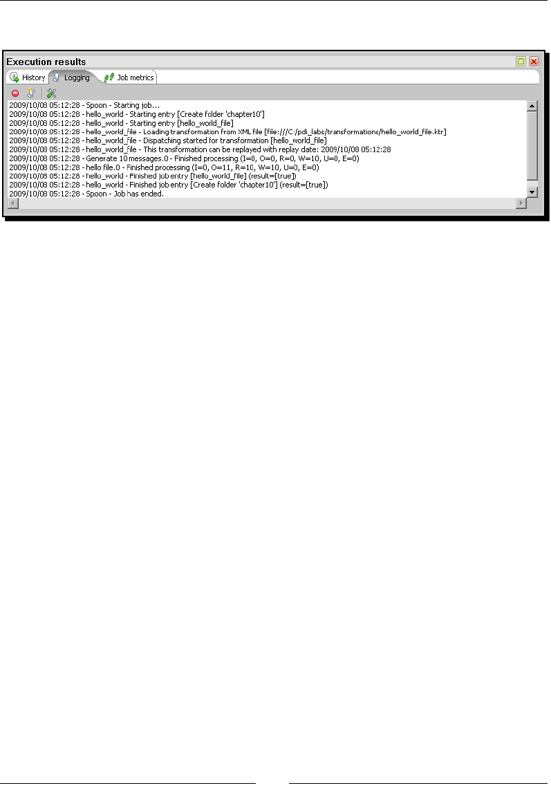
Creang Basic Task Flows
[ 304 ]
33. Select the Logging tab. It looks like this:
34. Explore the folder pointed to by your ${LABSOUTPUT} variable—for example, c:/
pdi_files/output. You should see a new folder named chapter10.
35. Inside the chapter10 folder, you should see a le named hello.txt.
36. Explore the le. It should have the following content:
Message
Hello, World!
Hello, World!
Hello, World!
Hello, World!
What just happened?
First of all, you created a transformaon that generated a simple le with the message
Hello, World!. The le was congured to be created in a folder named chapter10.
Aer that, you created a PDI Job. The job was built to create a folder named chapter10
and then to execute the hello_world transformaon.
When you ran the job, the chapter10 folder was created, and inside it, a le with the
Hello, World! message was generated.

Chapter 10
[ 305 ]
Executing processes with PDI jobs
A Job is a PDI enty designed for the execuon of processes. In the tutorial, you ran a
simple process that created a folder and then generated a le in that folder. A more complex
example could be the one that truncates all the tables in a database and loads data in all the
tables from a set of text les. Other examples involve sending e-mails, transferring les, and
execung shell scripts.
The unit of execuon inside a job is called a job entry. In Spoon you can see the entries
grouped into categories according to the purpose of the entries. In the tutorial, you used
job entries from two of those categories: General and File management.
Most of the job entries in the File management category have a self-explanatory name such
as Create a folder, and their use is quite intuive. Feel free to experiment with them!
As to the General category, it contains many of the most used entries. Among them is the
START job entry that you used. A job must start with a START job entry.
Don't forget to start your sequence of job entries with a START. A job
can have any mix of job entries and hops, as long as they start with this
special kind of job entry.
A Hop is a graphical representaon that links two job entries. The direcon of the hop
denes the order of execuon of the job entries it links. Besides, the execuon of the
desnaon job entry does not begin unl the job entry that precedes it has nished. Look,
for example, at the job in the tutorial. There is an entry that creates a folder, followed by an
entry that executes a transformaon. First of all, the job creates the folder. Once the folder
has been created, the execuon of the transformaon begins. This allows the transformaon
to assume that the folder exists. So, it safely creates a le in that folder.
A hop connects only two job entries. However, a job entry may be reached by more than one
hop. Also, more than one hop may leave a job entry.
A job, like a transformaon, is neither a program nor an executable le. It is simply
plain XML. The job contains metadata that tells the Kele engine which processes to
run and the order of execuon of those processes. Therefore, it is said that a job is
ow-control oriented.
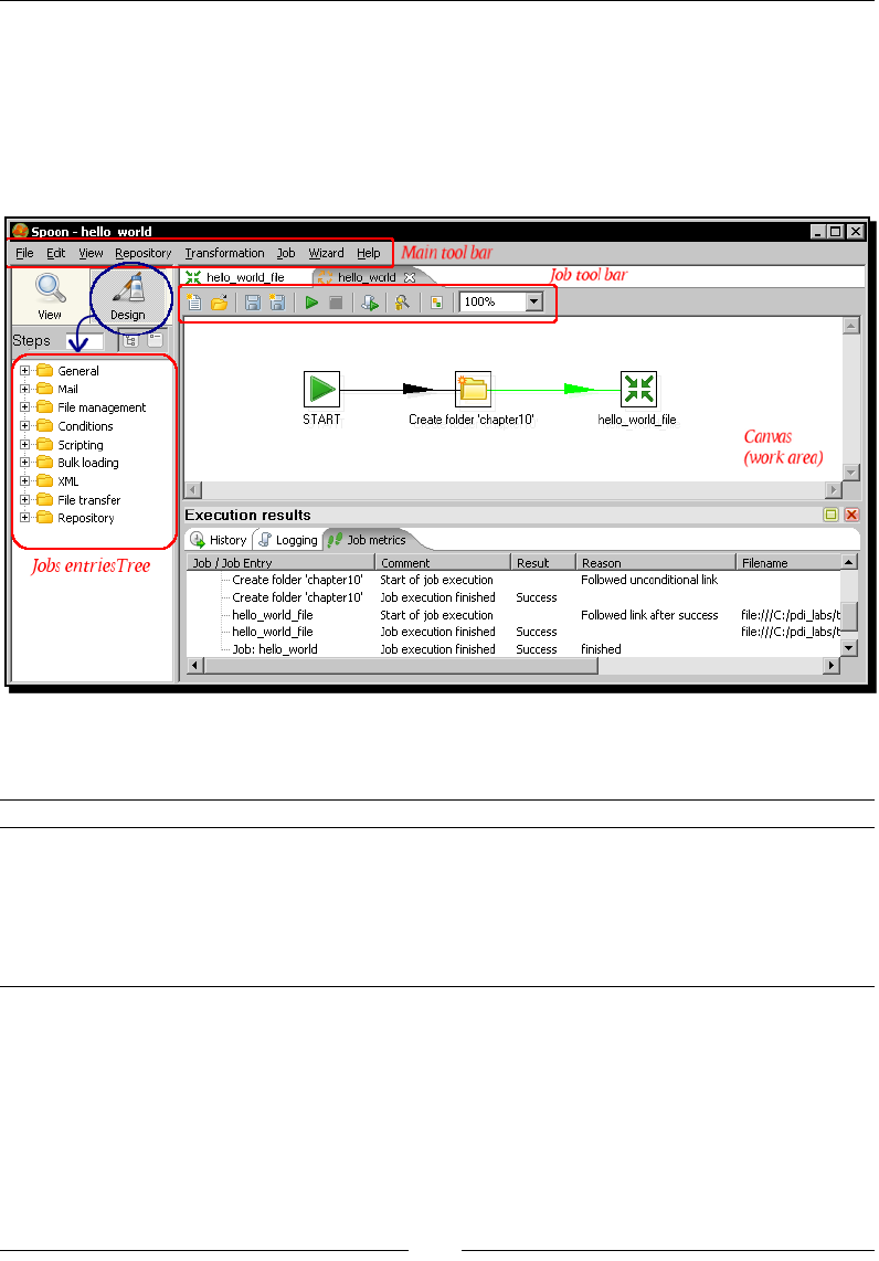
Creang Basic Task Flows
[ 306 ]
Using Spoon to design and run jobs
As you just saw, with Spoon you not only create, preview, and run transformaons, but you
also create and run jobs.
You are already familiar with this graphical tool, so you don't need too much explanaon
about the basic work areas. So, let's do a brief review.
The following table describes the main dierences you will noce while designing a job
compared to designing a transformaon:
Area Descripon
Design tree You don’t see a list of steps but a list of job entries (despite on top of
the list you see the word Steps).
Job menu You no longer see some opons that only have sense while working
with datasets. One of them is the Preview buon.
Job metrics tab
(Execuon results window)
Instead of a Step Metrics, you have this tab. Here you can see metrics
for each job entry.
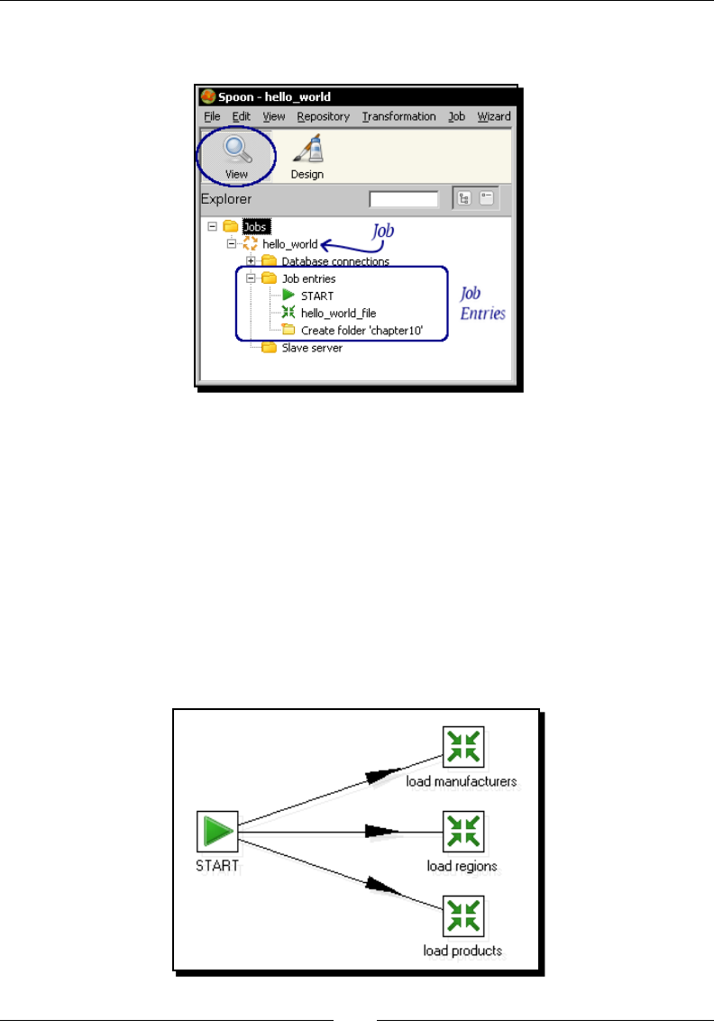
Chapter 10
[ 307 ]
If you click the View icon in the upper-le corner of the screen, the tree will change to show
the structure of the job currently being edited.
Using the transformation job entry
The transformaon job entry allows you to call a transformaon from a job.transformaon job entry allows you to call a transformaon from a job. job entry allows you to call a transformaon from a job.
There are several situaons where you may need to use a transformaon job entry.
In the tutorial, you had a transformaon that generated a le in a given folder. You called the
transformaon from a job that created that folder in advance. In this case, the job and the
transformaon performed complementary tasks.
Somemes the job just keeps your work organized. Consider the transformaons that loaded
the dimension tables for the js database. As you will usually run them together, you can
embed them into a single job as shown in this gure:
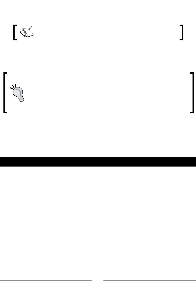
Creang Basic Task Flows
[ 308 ]
The only task done by this job is to keep the transformaons together. Although the picture Although the picture
implies the entries are run simultaneoulsy, that is not the case.
Job entries typically execute sequenally, this being one of the central
dierences between jobs and transformaons.
When you link two entries with a hop, you force an order of execuon. On the contrary,
when you create a job as shown in this preceding gure, you needn't give an order and the
entries sll run in sequence, one entry aer another depending on the creaon sequence.
Launching job entries in parallel
As the transformaons that load dimensions are not dependent on each other,
as an opon, you can ask the START entry to launch them simultaneously. For
doing that, right-click the START entry and select Launch next entries in parallel.
Once selected, the arrows to the next job entries will be shown in dashed lines.
This opon is available in any entry, not just in the START entry.
The jobs explained earlier are just two examples of how and when you use a transformaon
job entry. Note that many transformaons perform their tasks by themselves. In that
case you are not forced to embed them into jobs. It makes no sense to have a job with
just a START entry, followed by a transformaon job entry. You can sll execute those
transformaons alone, as you used to do unl now.
Pop quiz – dening PDI jobs
1. A job is:
a. A big transformaon that groups smaller transformaons
b. An ordered group of task denions
c. An unordered group of task denions
2. For each of the following sentences select True or False. A job allows you to:
a. Send e-mails
b. Compare folders
c. Run transformaons
d. Truncate database tables
e. Transfer les with FTP

Chapter 10
[ 309 ]
Have a go hero – loading the dimension tables
Create a job that loads the main dimension tables in the Jigsaw database—manufacturers,
products, and regions. Test the job.
Receiving arguments and parameters in a job
Jobs, as well as transformaons, are more exible when receiving parameters from outside.
You already learned to parameterize your transformaons by using named parameters and
command-line arguments. Let's extend these concepts to jobs.
Time for action – customizing the hello world le with
arguments and parameters
Let's create a more exible version of the job you did in the previous secon.
1. Create a new transformaon.
2. Press Ctrl+T to bring up the Transformaon properes window.
3. Select the Parameters tab.
4. Add a named parameter HELLOFOLDER. Insert chapter10 as the default value.
5. Click on OK.
6. Drag a Get System Info step to the canvas .
7. Double-click the step.
8. Add a eld named yourname. Select command line argument 1 as the Type.
9. Click on OK.
10. Now add a Formula step located in the Scripng category of steps.
11. Use the step to add a String eld named message. As Formula, type "Hello, "
& [yourname] & "!".
12. Finally, add a Text le output step.
13. Use the step to send the message data to a le. Enter ${LABSOUTPUT}/
${HELLOFOLDER}/hello as the name of the le.
14. Save the transformaon in the transformations folder you created in the
previous tutorial, under the name hello_world_param.ktr.
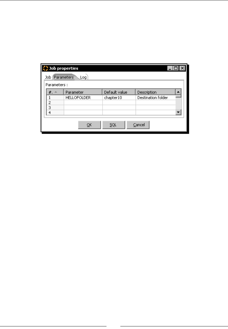
Creang Basic Task Flows
[ 310 ]
15. Open the hello_world.kjb job you created in the previous tutorial and save it
under a new job named hello_world_param.kjb.
16. Press Ctrl+J to open the Job properes window.
17. Select the Parameters tab.
18. Add the same named parameter you added in the transformaon.
19. Click on OK.
20. Double-click the Create a folder entry.
21. Change the Folder name textbox content to ${LABSOUTPUT}/${HELLOFOLDER}.
22. Double-click the Transformaon entry.
23. Change the transformaon lename textbox to point to the new transformaon:
${Internal.Job.Filename.Directory}/transformations/hello_world_
param.ktr.
24. Click on OK.
25. Save the job and run it.
26. Fill the dialog window with a value for the named parameter and a value for the
command-line argument.
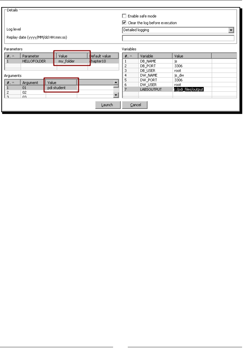
Chapter 10
[ 311 ]
27. Click on Launch.
28. When the execuon nishes, check the output folder. The folder named
my_folder, which you inially specied as a named parameter, should be created.
29. Inside that folder there should be a le named hello.txt. This me the content of
the le has been customized with the name you provided:
Hello, pdi student!
What just happened?
You created a transformaon that generated a hello.txt le in a folder given as the
named parameter. The content of the le is a customized "Hello" message that gets the
name of the reader from the command line.
In the main job you also dened a named parameter, the same that you dened in the
transformaon. The job needs the parameter to create the folder.
When you run the job, you provided both the command-line argument and the named
parameter in the job dialog window that shows up when you launch the execuon. Then
a folder was created with the name you gave, and a le was generated with the name you
typed as argument.
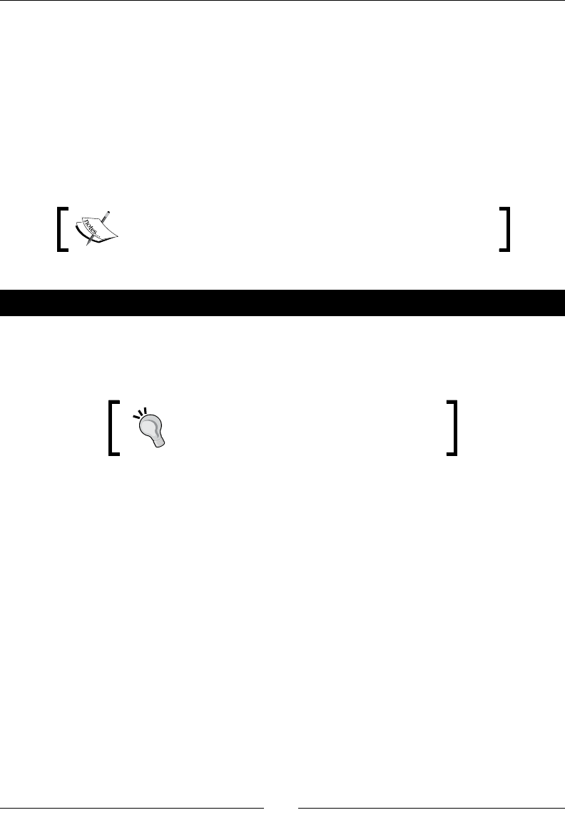
Creang Basic Task Flows
[ 312 ]
Using named parameters in jobs
You can use named parameters in jobs in the same way you do in transformaons. You
dene them in the Job properes window. You provide names and default values, and then
you use them just as regular variables. The places where you can use variables, just as in a
transformaon, are idened with a dollar sign to the right of the textboxes. In the tutorial,
you used a named parameter in the Create a folder job entry. In this parcular example,
you used the same named parameter both in the main job and in the transformaon called
by the job. So, you dened the named parameter HELLOFOLDER in two places—in the Job
sengs window and in the Transformaon properes window.
If a named parameter is used only in the transformaon, you
don't need to dene it in the job that calls the transformaon.
Have a go hero – backing up your work
Suppose you want to back up your output les regularly, that is, the les in your
${LABSOUTPUT} directory. Build a job that creates a ZIP le with all your output les. For
the name and locaon of the ZIP le, use two named parameters.
Use the Zip le job entry located in the File
management category.
Running jobs from a terminal window
In the main tutorial of this secon, both the job and the transformaon called by the job
used a named parameter. The transformaon also required a command-line argument.
When you executed the job from Spoon, you provided both the parameter and the
argument in the job dialog window. You will now learn to launch the job and provide
that informaon from a terminal window.
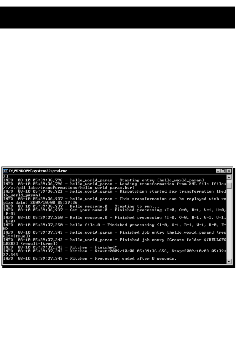
Chapter 10
[ 313 ]
Time for action – executing the hello world job from a terminal
window
In order to run the job from a terminal window, follow these instrucons:
1. Open a terminal window.
2. Go to the directory where Kele is installed.
On Windows systems type:
C:\pdi-ce>kitchen /file:c:/pdi_labs/hello_world_param.kjb
Maria -param:"HELLOFOLDER=my_work" /norep
On Unix, Linux, and other Unix-like systems type:
/home/yourself/pdi-ce/kitchen.sh /file:/home/yourself/
pdi_labs/hello_world_param.kjb Maria -param:"HELLOFOLDER=
my_work" /norep
3. If your job is in another folder, modify the command accordingly. You may also
replace the name Maria with your name, of course. If your name has spaces,
enclose the whole argument within "".
4. You will see how the job runs, following the log in the terminal:
5. Go to the output folder—the folder pointed by your LABS_OUTPUT variable.
6. A folder named my_work should have been created.
7. Check the content of the folder. A le named hello.txt should be there. Edit the
le. You should see the following:
Hello,Maria!

Creang Basic Task Flows
[ 314 ]
What just happened?
You ran the job with Kitchen, the program that executes jobs from the terminal window.
Aer the name of the command, kitchen.bat or kitchen.sh, depending on the
plaorm, you provided the following:
The full path to the job le: /file:c:/pdi_labs/hello_world_param.kjb
A command-line argument: Maria.
A named parameter, and a -param:"HELLOFOLDER=my_work"
The switch /norep to tell Kele not to connect to a repository
Aer running the job, you could see that the folder had been created and a le with a
custom "Hello" message had been generated.
Here you used some of the opons available when you run Kitchen. Appendix B tells you all
the details about using Kitchen for running jobs.
Have a go hero – experiencing Kitchen
Run the hello_world_param.kjb job from Kitchen, with and without providing
arguments and parameters. See what happens in each case.
Using named parameters and command-line arguments
in transformations
As you know, transformaons accept both arguments from the command line and named
parameters. When you run a transformaon from Spoon, you supply the values for
arguments and named parameters in the transformaon dialog window that shows up
when you launch the execuon. From a terminal window, you provide those values in the
Pan command line.
In this chapter you learned to run a transformaon embedded in a job. Here, the methods
you have for supplying named parameters and arguments needed by the transformaon
are quite similar. From Spoon you supply the values in the job dialog window that shows up
when you launch the job execuon. From the terminal window you provide the values in the
Kitchen command line.
Whether you run a job from Spoon or from Kitchen, the named parameters
and arguments you provide are unique and shared by the main job and
all transformaons called by that job. Each transformaon, as well as the
main job, may or may not use them according to their needs.
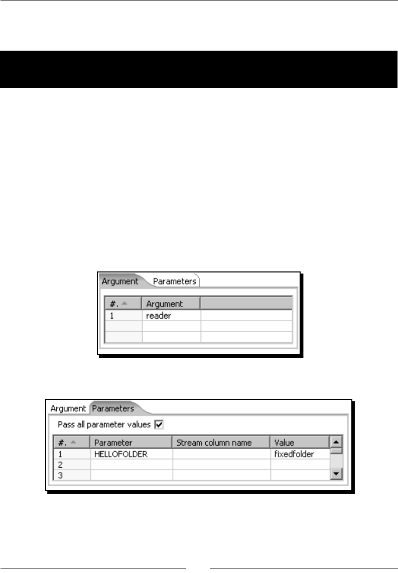
Chapter 10
[ 315 ]
There is sll another way in which you can pass parameters and arguments to a
transformaon. Let's see it by example.
Time for action – calling the hello world transformation with
xed arguments and parameters
This me you will call the parameterized transformaon from a new job.
1. Open the hello_world.kjb job you created in the rst secon and save it as
hello_world_fixedvalues.kjb.
2. Double-click the Create a folder job entry.
3. Replace the chapter10 string by the string fixedfolder.
4. Double-click the transformaon job entry.
5. Change the Transformaon lename as ${Internal.Job.Filename.
Directory}/transformations/hello_world_param.ktr.
6. Fill the Argument tab as follows.
7. Click the Parameters tab and ll it as follows:
8. Click on OK.
9. Save the job.

Creang Basic Task Flows
[ 316 ]
10. Open a terminal window and go to the directory where Kele is installed.
On Windows systems type:
C:\pdi-ce>kitchen /file:c:/pdi_labs/
hello_world_param.kjb /norep
On Unix, Linux, and other Unix-like systems type:
/home/yourself/pdi-ce/kitchen.sh /file:/home/yourself/
pdi_labs/hello_world_param.kjb /norep
11. When the execuon nishes, check the output folder. A folder named
fixedfolder has been created.
12. In that folder, you can see a hello.txt with the following content:
Hello, reader!
What just happened?
You reused the transformaon that expects an argument and a named parameter from the
command line. This me you created a job that called the transformaon and set both the
parameter and the argument in the transformaon job entry seng window.
Then you ran the job from a terminal window, without typing any arguments or parameters.
It didn't make any dierence for the transformaon. Whether you provide parameters and
arguments from the command line or you set constant values in a transformaon job entry,
the transformaon does its job—creang a le with a custom message in the folder with the
name given by the ${HELLOFOLDER}parameter.
Instead of running from the terminal window, you could have run the
job by pressing F9 and then clicking Launch, without typing anything
in either the parameter or the argument grid. The nal result should
be exactly the same.
Have a go hero – saying hello again and again
Modify the hello_world_param.kjb job so that it generates three les in the default
${HELLOFOLDER}, each saying "hello" to a dierent person.
Aer the creaon of the folder, use three transformaon job entries.
Provide dierent arguments for each.
Run the job to see that it works as expected.

Chapter 10
[ 317 ]
Have a go hero – loading the time dimension from a job
In Chapter 6, you built a transformaon that created the data for a me dimension. Then in
Chapter 8, you nished the transformaon loading the data into a me dimension table.
The transformaon had several named parameters, one of them being START_DATE.
Create a job that loads a me dimension with dates starng at 01/01/2000. In
technical jargon, create a job that calls your transformaon and passes it a value for
the START_DATE parameter.
Deciding between the use of a command-line argument
and a named parameter
Both command-line arguments and named parameters are means for creang more exible
jobs and transformaons. The following table summarizes the dierences and the reasons
for using one or the other. In the rst column, the word argument refers to the external
value you will use in your job or transformaon. That argument could be implemented
as a named parameter or as a command-line argument.
Situaon Soluon using named
parameters
Soluon using arguments
It is desirable to have a
default for the argument
Named parameters are
perfect in this case. You
provide default values at the
me you dene them.
Before using the command-line
argument, you have to evaluate if it
was provided in the command line. If
not, you have to set the default value
at that moment.
The argument is
mandatory
You don't have means
to determine if the user
provided a value for the
named parameter.
To know if the user provided a value
for the command-line argument, you
just get the command-line argument
and compare it to a null value.
You need several
arguments but it is
probable that not all of
them are present.
If you don't have a value for a
named parameter, you are not
forced to enter it when you
run the job or transformaon.
Let's suppose that you expect three
command line arguments. If you
have a value only for the third, you
sll have to provide empty values for
the rst and the second.
You need several
arguments and it is
highly probable that all
of them are present.
The command line would be
too long. It will help explain
clearly the purpose of each
parameter, but typing the
command line would be
tedious.
The command-line is simple as you
just list the values one aer the
other. However, there is a risk—you
may unintenonally enter the values
unordered, which could lead to
unexpected results.

Creang Basic Task Flows
[ 318 ]
Situaon Soluon using named
parameters
Soluon using arguments
You want to use the
argument in several places
You can do it, but you must
assure that the value will not be
overwrien in the middle of the
execuon.
You can get the command-line
argument by using a Get System Info
step as many mes as you need.
You need to use the value
in a place where a variable
is needed
Named parameters are ready to
be used as Kele variables.
First, you need to set a variable with
the command-line argument value.
Usually this requires creang addional
transformaons to be run before any
other job or transformaon.
Depending on your parcular situaon, you would prefer one or the other soluon. Note
that you can mix both as you did in the previous tutorials.
Have a go hero – analysing the use of arguments and named parameters
In the Time for acon – customizing the hello world le with xed arguments and parameters
secon, you created a transformaon that used an argument and a named parameter. Based
on this preceding table, try to understand why the folder was dened as named parameter
and the name of the person you want to say Hello to was dened as command-line
argument. Would you have applied the same approach?
Running job entries under conditions
A job may contain any number of entries. Not all of them execute always. Some of them
execute depending on the result of previous entries in the ow. Let's see it in pracce.
Time for action – sending a sales report and warning the
administrator if something is wrong
Now you will build a sales report and send it by e-mail. In order to follow the tutorial, you
will need two simple prerequisites:
As the report will be based on the Jigsaw database you created in Chapter 8, you will
need the MySQL server running.
In order to send e-mails, you will need at least one valid Gmail account. Sign up for
an account. Alternavely, if you are familiar with you own SMTP conguraon, you
could use it instead.

Chapter 10
[ 319 ]
Once you've checked these prerequisites, you are ready to start.
1. Create a new transformaon.
2. Add a Get System Info step. Use it to add a eld named today. As Type, select
Today 00:00:00.
3. Now add a Table input step.
4. Double-click the step.
5. As Connecon, select js—the name of the connecon to the jigsaw
puzzles database.
Note that if the connecon is not shared, you will have to
dene it.
6. In the SQL frame, type the following statement:
SELECT pay_code
, COUNT(*) quantity
, SUM(inv_price) amount
FROM invoices
WHERE inv_date = ?
GROUP BY pay_code
7. In the drop-down list to the right of Insert data from step, select the name of the
Get System Info step.
8. Finally, add an Excel Output step.
9. Double-click the step.
10. Enter type ${LABSOUTPUT}/sales_ as Filename.
11. Check the Specify Date me format opon. In the Date me format drop-down list,
select yyyyMMdd.
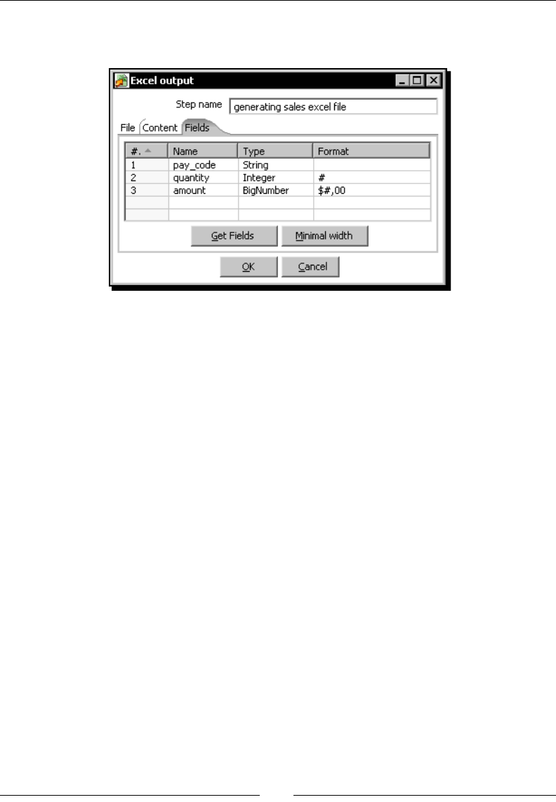
Creang Basic Task Flows
[ 320 ]
12. Make sure you don't uncheck the Add lenames to result opon. Click on OK. Fill
the Fields tab as here:
13. Save the transformaon under the transformations folder you created in a
previous tutorial, with the name sales_report.ktr.
14. Create a new job by pressing Ctrl+Alt+N.
15. Add a START job entry.
16. Aer the START entry, add a Transformaon entry.
17. Double-click the Transformaon entry.
18. Enter ${Internal.Job.Filename.Directory}/transformations/sales_
report.ktr as the transformaon lename, either by hand or by browsing the
folder and selecng the le.
19. Click on OK.
20. Expand the Mail category of entries and drag a Mail entry to the canvas.
21. Create a hop from the transformaon entry to the Mail entry.
22. Double-click the Mail entry.
23. Fill the main tab Addresses with the desnaon and the sender e-mail addresses,
that is, provide values for the Desnaon address, Sender name, and Sender
address textboxes. If you have two accounts to play with, put one of them as
desnaon and the other as sender. If not, use the same e-mail twice.
24. Select the Server tab and ll the SMTP Server frame as follows—enter smtp.gmail.
com as SMTP Server and 465 as Port.
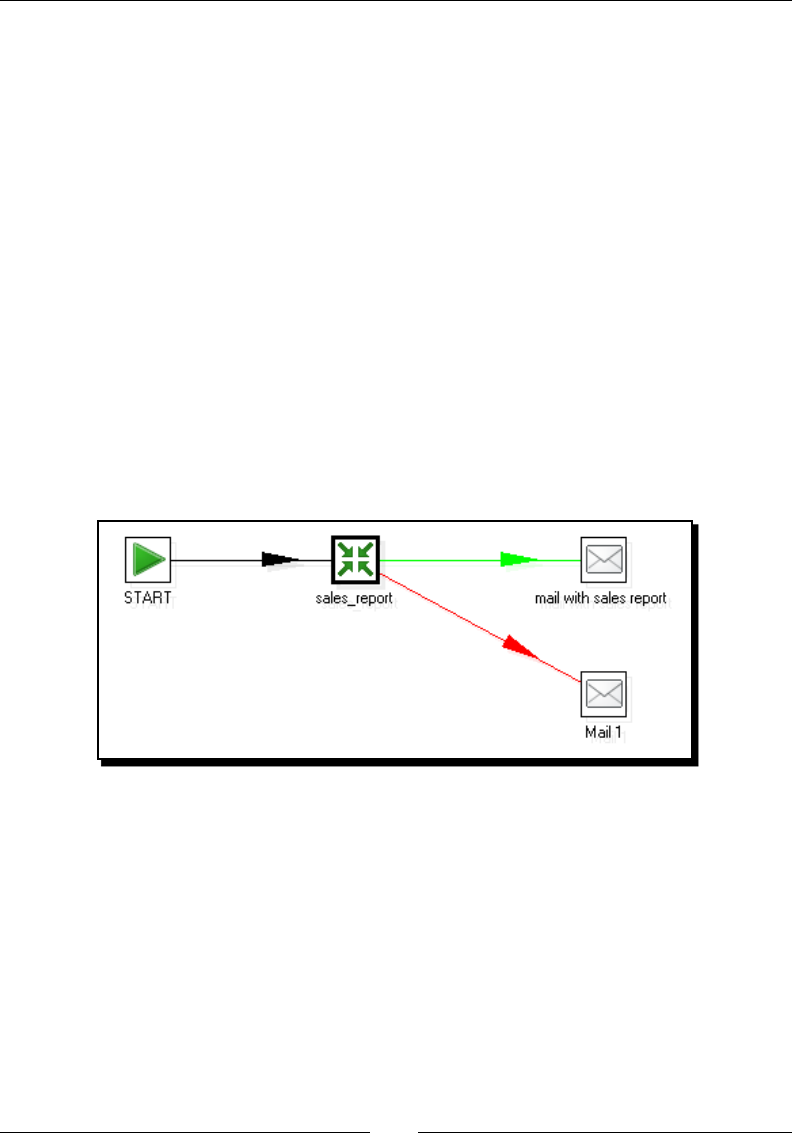
Chapter 10
[ 321 ]
25. Fill the Authencaon frame. Check the Use authencaon? checkbox. Fill the
Authencaon user and Authencaon password textboxes. For example, if your
account is pdi_account@gmail.com, then as user enter pdi_account and as
password provide your e-mail password.
26. Check the Use secure authencaon? opon. In Secure connecon type, leave the
default to SSL. Select the Email Message tab. In the Message Sengs frame, check
the Only send comment in mail body? opon.
27. Fill the Message frame, providing a subject and a comment for the e-mail—enter
Sales report as Subject and Please check the aachment as Comment. Select the
Aached Files tab and check the Aach le(s) to message? opon.
28. In the Select le type list, select the type General.
29. Click OK.
30. Drag another Mail job entry to the canvas.
31. Create a hop from the transformaon entry to this new entry. This hop will appear
in red.
32. Double-click the new entry.
33. Fill the Desnaon and Sender frames with desnaon and sender e-mail
addresses. If you have another account to use as desnaon, use it here. Select the
Server tab and ll it exactly as you did in the other Mail entry.
34. Select the Email Message tab. In the Subject textbox, type Error generating
sales report.
35. Click on OK.
36. Save the job and run it.
37. Once the job nished, log into your account. You should have received a mail!
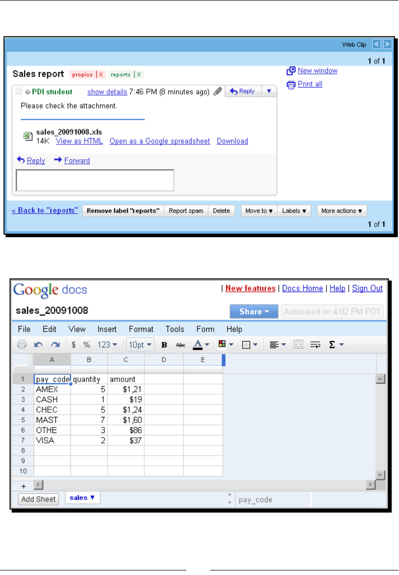
Creang Basic Task Flows
[ 322 ]
38. Open the e-mail. This is what you should see:
39. Click on the Open as a Google spreadsheet opon. You will see the following:
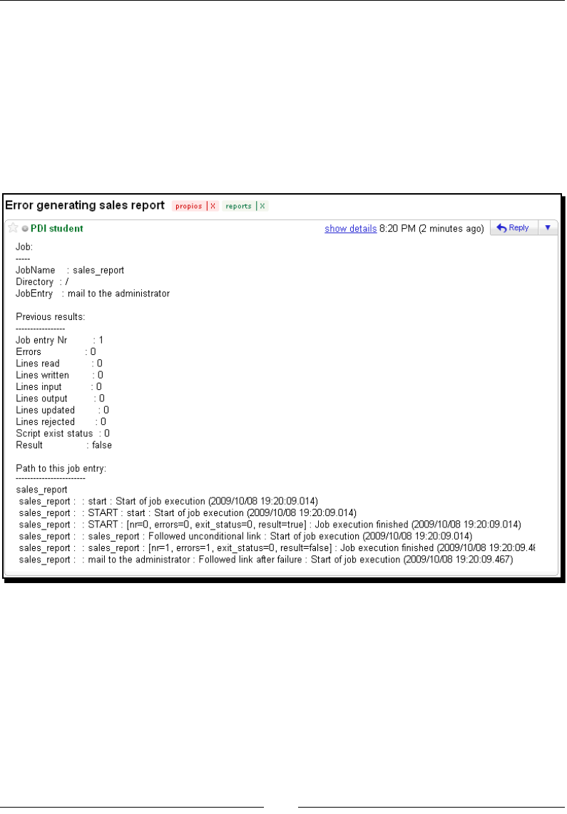
Chapter 10
[ 323 ]
40. Simulate being an intruder and do something that makes your transformaon
fail. You could, for example, stop MySQL or add some strange characters in the
SQL statement.
41. Run the job again.
42. Check the administrator e-mail—the mail you put as desnaon in the second Mail
job entry.
43. The following is the e-mail you received this me:
What just happened?
You generated an Excel le with a crosstab report of sales on a parcular day. If the le is
generated successfully, an e-mail is sent with the Excel le aached. If some error occurs,
an e-mail reporng the problem is sent to the administrator.

Creang Basic Task Flows
[ 324 ]
If you skipped Chapter 8 and sll know nothing about databases with PDI, don't
miss this exercise. Instead of the proposed sales report, create a transformaon
that generates any Excel le. The contents of the sheet is not the key here. Just
make sure you leave the Add lenames to result opon checked in the Excel
output conguraon window. Then proceed as explained.
In this example you used Gmail accounts for sending e-mails from a PDI job. You
can use any mail server as long as you have access to the informaon required in
the Server tab.
Changing the ow of execution on the basis of conditions
The execuon of any job entry either succeeds or fails.
In parcular, the job entries under the category Condions just evaluates something and
success or failure depends upon the result of the evaluaon.
For example, the job entry File Exists succeeds if the le you put in its window exists.
Otherwise, it fails.
Whichever the job entry, you can use the result of its execuon to decide which of the
entries following it execute and which don't.
In the tutorial, you included a transformaon job entry. If the transformaon runs without
problem, this entry succeeds. Then the execuon follows the green hop to the rst Mail
job entry.
If, while running the transformaon, some error occurs, the transformaon entry fails. Then
the execuon follows the red path toward the e-mail to the administrator.
So, when you create a job, you not only arrange the entries and hops according to the
expected order of execuon, you also specify under which condion each job entry runs.
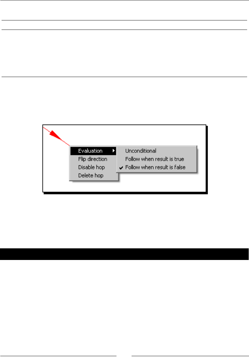
Chapter 10
[ 325 ]
You can dene the condions in the hops. The following table lists the possibilies:
Color of the hop What the color represents The interpretaon
Black Uncondional execuon The desnaon entry executes no maer the
result of the previous entry.
Green Execuon upon success The desnaon entry executes only if the
previous job entry is successful.
Red Execuon upon failure The desnaon entry executes only if the
previous job entry failed.
At any hop, you can dene the condion under which the desnaon job entry will execute.
By default, the rst hop that leaves an entry is created green, whereas the second hop is
created red. You can change the color, that is, the behavior of the hop. Just right-click on the
hop, select Evaluaon, and then the condion.
One excepon is the hop or hops that leave the START step. You cannot edit them. The
desnaon job entries execute uncondionally, that is, always.
Another excepon is the special entry Dummy that does nothing, not even allowing you to
decide if the job entries aer it run or not. They always run.
Have a go hero – rening the sales report
Here we will modify the job that sends the e-mail containing the sales report.
1. Modify the transformaon so that the le is generated in the temporary folder
${java.io.tmpdir}. If there is no sale for today, don't generate the le. You do
this by checking the Do not create le at start opon in the Excel output step.
2. Send the e-mail only if there were sales, that is, only if the le exists.
3. Aer sending the e-mail with the report aached, delete the le.
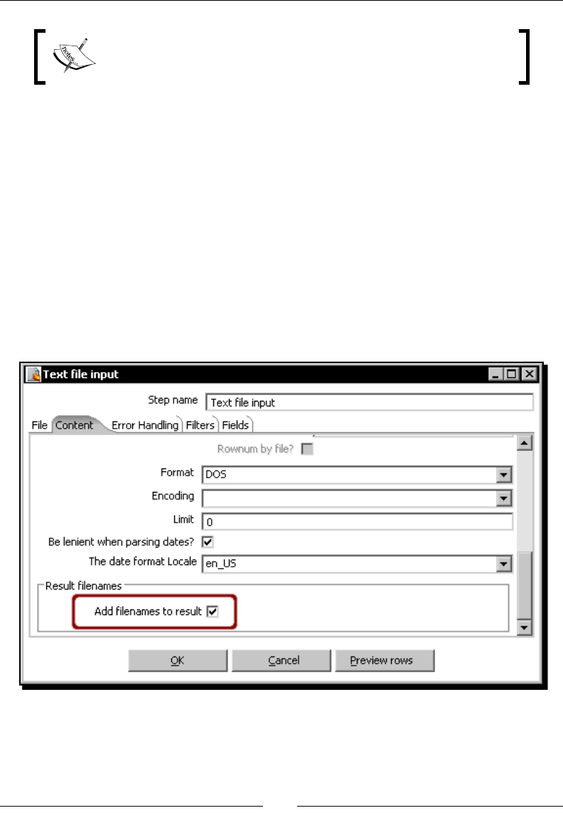
Creang Basic Task Flows
[ 326 ]
Use these new job entries: File Exists from the Condions category and
Delete le from the File management category.
Creating and using a le results list
In the tutorial you congured two Mail job entries. In the mail that follows the green hop,
you aached the Excel le generated by the transformaon. However, you didn't explicitly
specify the name of the le to aach. How could PDI realize that you wanted to aach
that le? it could because of the Add lenames to result checkbox in the Excel output
conguraon window. By checking that opon, you added the name of the Excel le to a
special list named File result.
When PDI hits an e-mail entry where Aach le(s) to message? is checked, it aaches to the
e-mail all les in the File result list.
Most of the transformaon steps that read or write les have this checkbox, and it is checked
by default. The following sample belongs to a Text le input step:
Each me you use one of these steps you are adding names of les to this list, unless you
uncheck the checkbox.
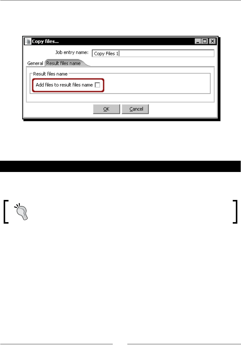
Chapter 10
[ 327 ]
There are also several job entries in the File management and the File transfer categories
that add one or more les to the File result list. Consider the following Copy Files…
entry screen:
As with the Mail entry, there are some other entries that use the File result list. One example
is Copy or Move result lenames. This entry copies or moves the les whose names are in
this special list named File result.
Have a go hero – sharing your work
Suppose you want to share your PDI work with a friend. Send to him/her some of your ktr
les by mail.
Use the Add lenames to result job entry located in the File management
category to build the File result list. Then send the e-mail with the les aached.
Summary
In this chapter, you learned the basics about PDI jobs—what a job is, what you can do with a
job, and how jobs are dierent from transformaons. In parcular, you learned to use a job
for running one or more transformaons.
You also saw how to use named parameters in jobs, and how to supply parameters and
arguments to transformaons when they are run from jobs.
In the next chapter, you will learn to create jobs that are a lile more elaborave than the
jobs you created here, which will give you more power to implement all types of processes.

11
Creating Advanced
Transformations and Jobs
Iterang over a list of items (les, people, codes, and so on), implemenng
a process ow, and developing a reusable procedure are very common
requirements in real world projects. Implemenng these kind of needs in PDI
is not intuive, but it’s not complicate either. It’s just a maer of learning the
right techniques that we will see in this chapter. Among other things, you will
learn to implement process ows, nest jobs, and iterate the execuon of jobs
and transformaons.
Enhancing your processes with the use of variables
For the tutorials in this chapter, you will take as your starng point a Time for acon tutorial
you did in Chapter 2 that involves updang a le with news about examinaons. You are
responsible for collecng the results of an annual examinaon where wring, reading,
speaking, and listening skills are evaluated. The professors grade the examinaons of their
students in the scale 0-100 for each skill, and generate text les with the informaon. Then
they send the les to you for integrang the results in a global list.
In the inial chapters, you were learning the basics of PDI. You were worried about how to
do simple stu such as reading a le or doing simple calculaons. In this chapter, you will go
beyond that and take care of the details such as making a decision if the lename expected
as a command line is not provided or if it doesn't exist.
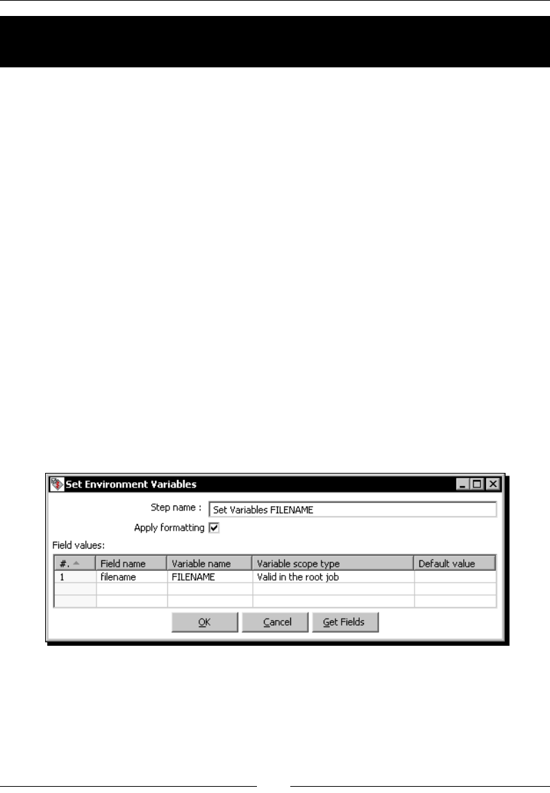
Creang Advanced Transformaons and Jobs
[ 330 ]
Time for action – updating a le with news about examinations
by setting a variable with the name of the le
The transformaon in the Time for acon from Chapter 2 that we just talked about reads a
le provided by a professor, simply by taking the name of the le from the command line,
and appends the le to the global one. Let's enhance that work.
1. Copy the examinaon les you used in Chapter 2 to the input les and folder
dened in your kettle.properties le. If you don't have them, download them
from the Packt website.
2. Open Spoon and create a new transformaon.
3. Use a Get System Info step to get the rst command-line argument. Name the eld
as filename.
4. Add a Filter rows step and create a hop from the Get System Info step to this step.
5. From the Flow category drag an Abort step to the canvas, and from the Job category
of steps drag a Set Variables step.
6. From the Filter rows step, create two hops—one to the Abort step and the other
to the Set Variables step. Double-click the Abort step. As Abort message, put File
name is mandatory.
7. Double-click the Set Variables step and click on Get Fields. The window will be lled
as shown here:
8. Click on OK.
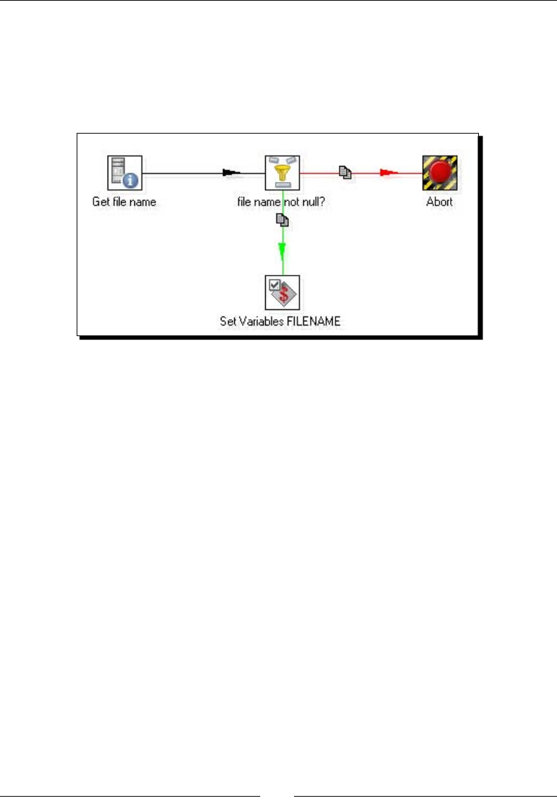
Chapter 11
[ 331 ]
9. Double-click the Filter rows step. Add the following lter: filename IS NOT
NULL. In the drop-down list to the right of Send 'true' data to step, select the Set
Variables step, whereas in the drop-down list to the right of Send 'false' data to
step, select the Abort step.
10. The nal transformaon looks like this:
11. Save the transformaon in the transformations folder under the name
getting_filename.ktr.
12. Open the transformaon named examinations.ktr that was created in Chapter
2 or download it from the Packt website. Save it in the transformations folder
under the name examinations_2.ktr.
13. Delete the Get System Info step.
14. Double-click the Text le input step.
15. In the Accept lenames from previous steps frame, uncheck the Accept lenames
from previous step opon.
16. Under File/Directory in the Selected les grid, type ${FILENAME}. Save the
transformaon.
17. Create a new job.
18. From the General category, drag a START entry and a Transformaon entry to the
canvas and link them.
19. Save the job as examinations.kjb.
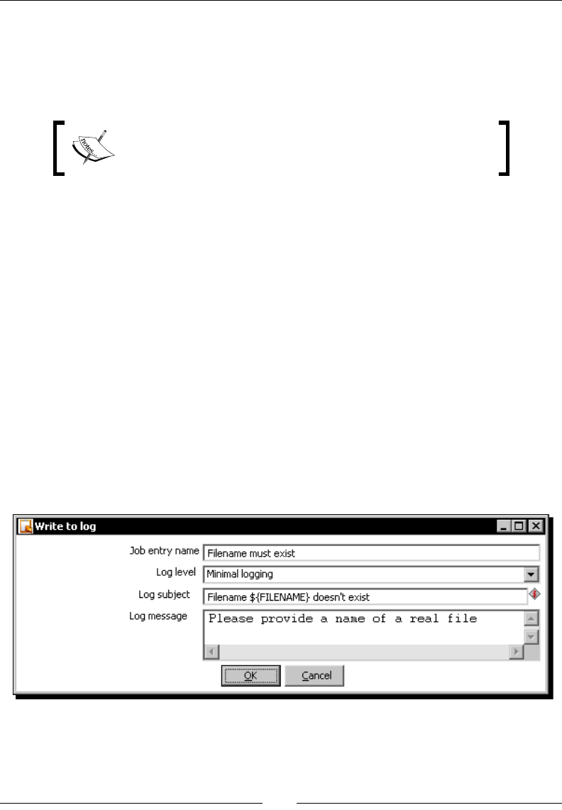
Creang Advanced Transformaons and Jobs
[ 332 ]
20. Double-click the Transformaon entry. As Transformaon lename, put the name
of the rst transformaon that you created: ${Internal.Job.Filename.
Directory}/transformations/getting_filename.ktr.
21. Click on OK.
Remember that you can avoid typing that long variable name by
clicking Ctrl+Space and selecng the variable from the list.
22. From the Condions category, drag a File Exists entry to the canvas and create a hop
from the Transformaon entry to this new one.
23. Double-click the File Exists entry.
24. Write ${FILENAME} in the File name textbox and click on OK.
25. Add a new Transformaon entry and create a hop from the File Exists entry to
this one.
26. Double-click the entry and, as Transformaon lename, put the name of the
second transformaon you created:${Internal.Job.Filename.Directory}/
transformations/examinations_2.ktr.
27. Add a Write To Log entry, and create a hop from the File Exists entry to this. The hop
should be red, to indicate when execuon fails. If not, right-click the hop and change
the evaluaon condion to Follow when result is false.
28. Double-click the entry and ll all the textboxes as shown:
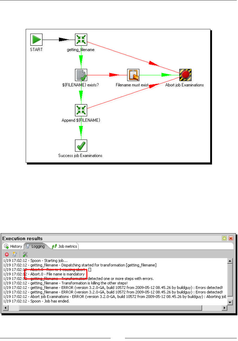
Chapter 11
[ 333 ]
29. Add two entries—an abort and a success. Create hops to these new entries as
shown next:
30. Save the job.
31. Press F9 to run the job.
32. Set the logging level to Minimal logging and click on Launch.
33. The job fails. The following is what you should see in the Logging tab in the
Execuon results window:
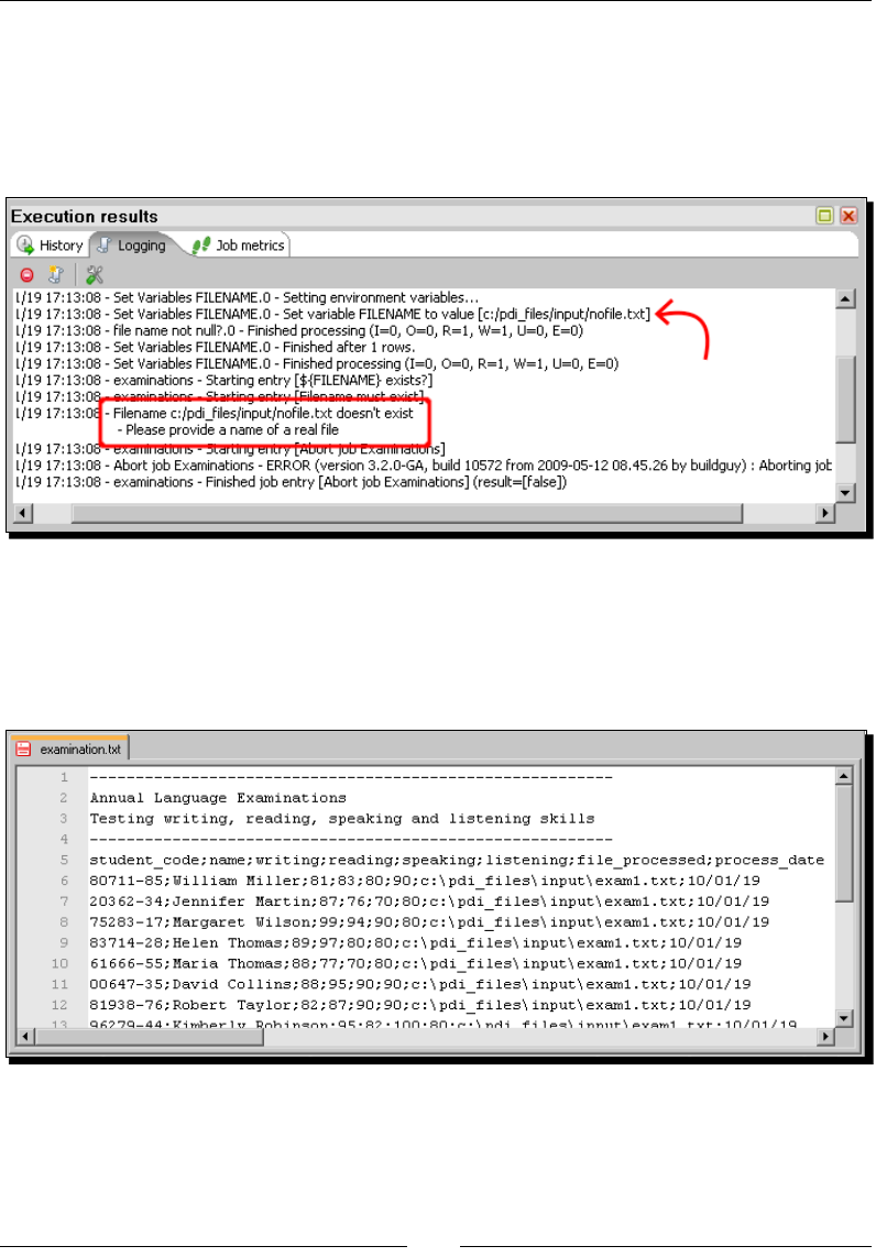
Creang Advanced Transformaons and Jobs
[ 334 ]
34. Press F9 again. This me set Basic logging as the logging level.
35. In the arguments grid, write the name of a cous le—for example,
c:/pdi_files/input/nofile.txt.
36. Click on Launch. This is what you see now in the Logging tab window:
37. Press F9 for the third me. Now provide a real examinaon lename such as
c:/pdi_files/input/exam1.txt.
38. Click on Launch. This me you see no errors. The examinaon le is appended to
the global le:
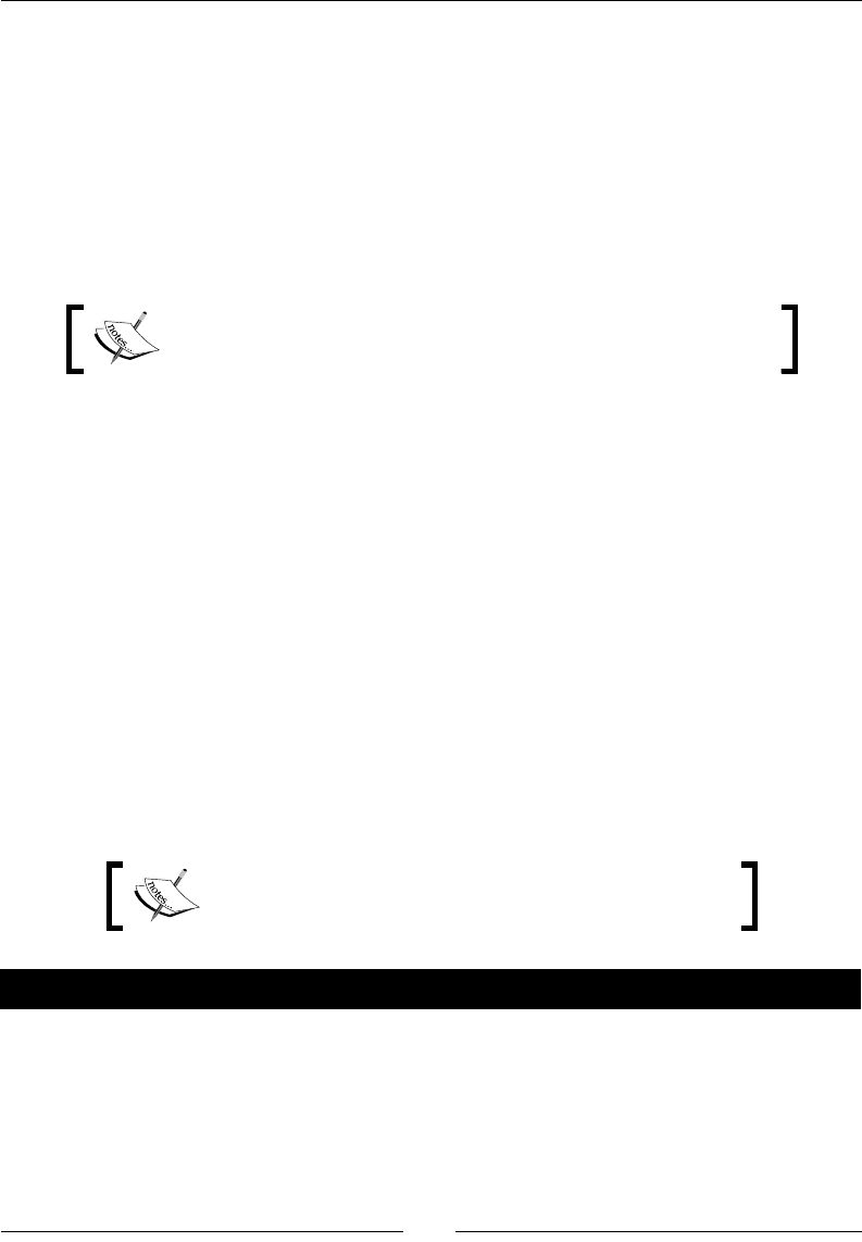
Chapter 11
[ 335 ]
What just happened?
You enhanced the transformaon you created in Chapter 3 for appending an examinaon le
to a global examinaon le. This me you embedded the transformaon in a job. The rst
transformaon checks that the argument is not null. In that case, it sets a variable with the
name provided. The main job veries that the le exists. If everything is all right, then the
second transformaon performs the main task—it appends the given le to the global le.
Note that you changed the logging levels just according to what you needed to see—the
highlighted lines in the earlier explanaon.
You may choose any logging level you want depending on the details
of informaon you want to see.
Setting variables inside a transformation
So far, you had dened variables only in the kettle.properties le or inside Spoon while
you were designing a transformaon. In this last exercise, you learned to dene your own
variables at run me. You set a variable with the name of the le provided as a command-line
argument. You used that variable in the main job to check if the le existed. Then you used the
variable again in the main transformaon. There you used it as the name of the le to read.
This example showed you the how to set a variable with the value of a command-line
argument. This is not always the case. The value you set in a variable can be originated in
dierent ways—it can be a value coming from a table in a database, a value dened with a
Generate rows step, a value calculated with a Formula or a Calculator step, and so on.
The variables you dene with a Set variables step can be used in the same way and the same
places where you use any Kele variable. Just take precauons to avoid using these variables
in the same transformaon where you have set them.
The variables dened in a transformaon are not available
for using unl you leave that transformaon.
Have a go hero – enhancing the examination tutorial even more
Modify the job in the tutorial to avoid processing the same le twice. If the le is
successfully appended to the global le, rename the original le by changing the
extension to processed—for example, aer processing the exam1.txt le rename
it to exam1.processed.
Creang Advanced Transformaons and Jobs
[ 336 ]
Aer verifying if the le exists, also check whether the .processed version exists. If it
exists, put a proper message in the log and abort. If someone accidently tries to process
a le that is already processed, it will be ignored.
Besides the variable with the lename, create a variable with the name
for the processed le. To build this name, simply manipulate the given
name with some PDI steps.
Have a go hero – enhancing the jigsaw database update process
In the Time for acon – inserng new products or updang existent ones secon in Chapter
8, you read a le with a list of products belonging to the manufacturer Classic DeLuxe.
The list was expected as a named parameter. Enhance that process. Create a job that rst
validates the existence of the provided le. If the le doesn't exist, put the proper error
message in the log. If it exists, process the list. Then move the processed le to a folder
named processed.
You don't need to create a transformaon to set a variable with the
name of the le. As it is expected as a named parameter, it is already
available as a variable.
Have a go hero – executing the proper jigsaw database update process
In the hero exercise in Chapter 8 that involves populang the products table, you created
dierent transformaons for updang the products—one for each manufacturer. Now you
will put all that work together.
Create a job that accepts two arguments—the name of the le to process and the code of
the manufacturer to which the le belongs.
Create a transformaon that validates that the code provided belongs to an existent
manufacturer. If the code exists, set a variable named TRANSFORMATION_FILE with the
name of the transformaon that knows how to process the le for that manufacturer.
The transformaon must also check that the name provided is not null. If it is not null, set a
variable named FILENAME with the name supplied.
Then, in the job, check that the le exists. If it exists and the manufacturer code is valid, run
the proper transformaon. In order to do so, put ${TRANSFORMATION_FILE} as the name
of the transformaon in the transformaon job entry dialog window. Now test your job.

Chapter 11
[ 337 ]
Enhancing the design of your processes
When your jobs or transformaons begin to grow, you may nd them a lile disorganized or
jumbled up. It's now me to do some rework. Let's see an example of this.
Time for action – generating les with top scores
In this tutorial, you will read the examinaon global le and generate four les—one for each
parcular skill. The les will contain the top 10 scores for each skill. The scores will not be
the original, but converted to a scale with values in the range 0-5.
As you must be already quite condent with PDI, some explanaons in this
secon will not have the full details. On the contrary, the general explanaon
will be focused on the structure of the jobs and transformaons.
1. Create a new transformaon and save it in the transformations folder under the
name top_scores.ktr.
2. Use a Text le input step to read the global examinaon le generated in the
previous tutorial.
3. Aer the Text le input step, add the following steps and link them in the
same order:
A Select values step to remove the unused elds—
file_processed and process_date.
A Split Fields to split the name of the students in two—name and
last name.
A Formula step to convert name and last name to uppercase.
With the same Formula step, change the scale of the scores.
Replace each skill eld writing, reading, speaking, and
listening with the same value divided by 20—for example,
[writing]/20. You have already done this in Chapter 3.
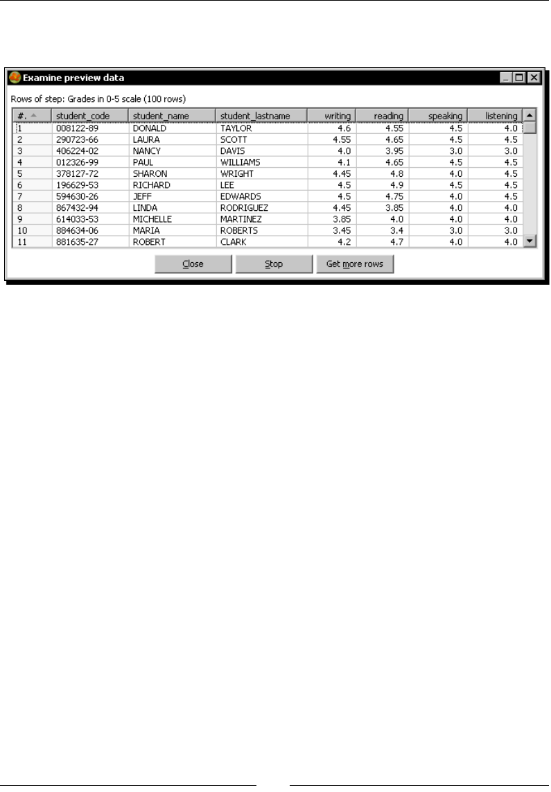
Creang Advanced Transformaons and Jobs
[ 338 ]
4. Do a preview on compleon of the nal step to check that you are doing well. You
should see this:
5. Aer the last Formula step, add and link in this order the following steps:
A Sort rows step to order the rows in descending order by the
writing eld.
A JavaScript step to lter the rst 10 rows. Remember that you
learned to do this in the chapter devoted to JavaScript. You do it by
typing the following piece of code:
trans_Status = CONTINUE_TRANSFORMATION;
if (getProcessCount('r')>10) trans_Status =
SKIP_TRANSFORMATION;
An Add sequence step to add a eld named seq_w. Leave the
defaults so that the eld contains the values 1, 2, 3 …
A Select values step to rename the eld seq_w as position and
the eld writing as score. Specify this change in the Select &
Alter tab, and check the opon Include unspecied elds, ordered.
A Text le output step to generate a le named writing_top10.
txt at the locaon specied by the ${LABSOUTPUT} variable. In the
Fields tab, put the following elds— position, student_code,
student_name, student_lastname, and score.
6. Save the transformaon, as you've added a lot of steps and don't want to lose
your work.
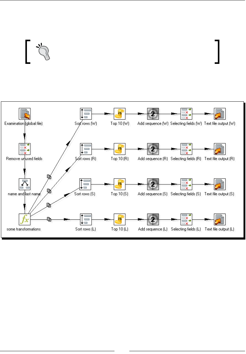
Chapter 11
[ 339 ]
7. Repeat step number 5, but this me sort by the reading eld, rename the sequence
seq_r as position and the eld reading as score, and send the data to the
reading_top10.txt le.
To save me, you can copy all those steps, paste them, and do
the proper adjustments.
8. Repeat the same procedure for the speaking eld and the listening eld.
9. This is how the transformaon looks like:
10. Save the transformaon.
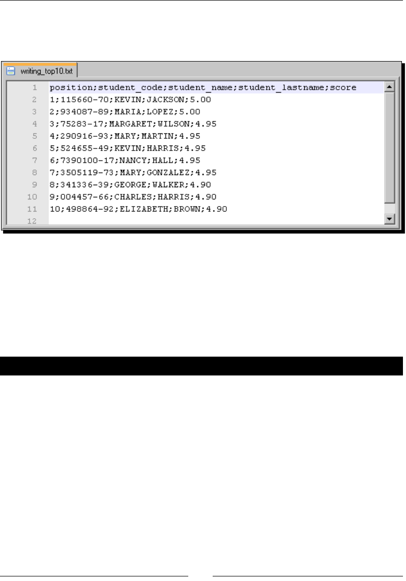
Creang Advanced Transformaons and Jobs
[ 340 ]
11. Run the transformaon. Four les should have been generated. All the les should look
similar. Let's check the writing_top10.txt le (the names and values may vary
depending on the examinaon les that you have appended to the global le):
What just happened?
You read the big le with examinaon results and generated four les with informaon
about the top scores—one le for each skill.
Beyond having used the Add sequences step for the rst me, there was nothing new.
However, there are several improvements you can do to this transformaon. The next
tutorials are meant to teach you some tricks.
Pop quiz – using the Add Sequence step
In the previous tutorial, you used dierent names for the sequences and then you renamed
all of them to position. Which of the following opons gives you the same results you got
in the tutorial?
a. Using position as the name of the sequence in all Add sequence steps
b. Joining the four streams with a single Add sequence step and then spling
the stream back into four streams by using the Distribute method you learned
in Chapter 4
c. Joining the four streams with a single Add sequence step and then spling the
stream back into four streams by using a Switch case step that distributes the
rows properly
d. All of them
e. None of them
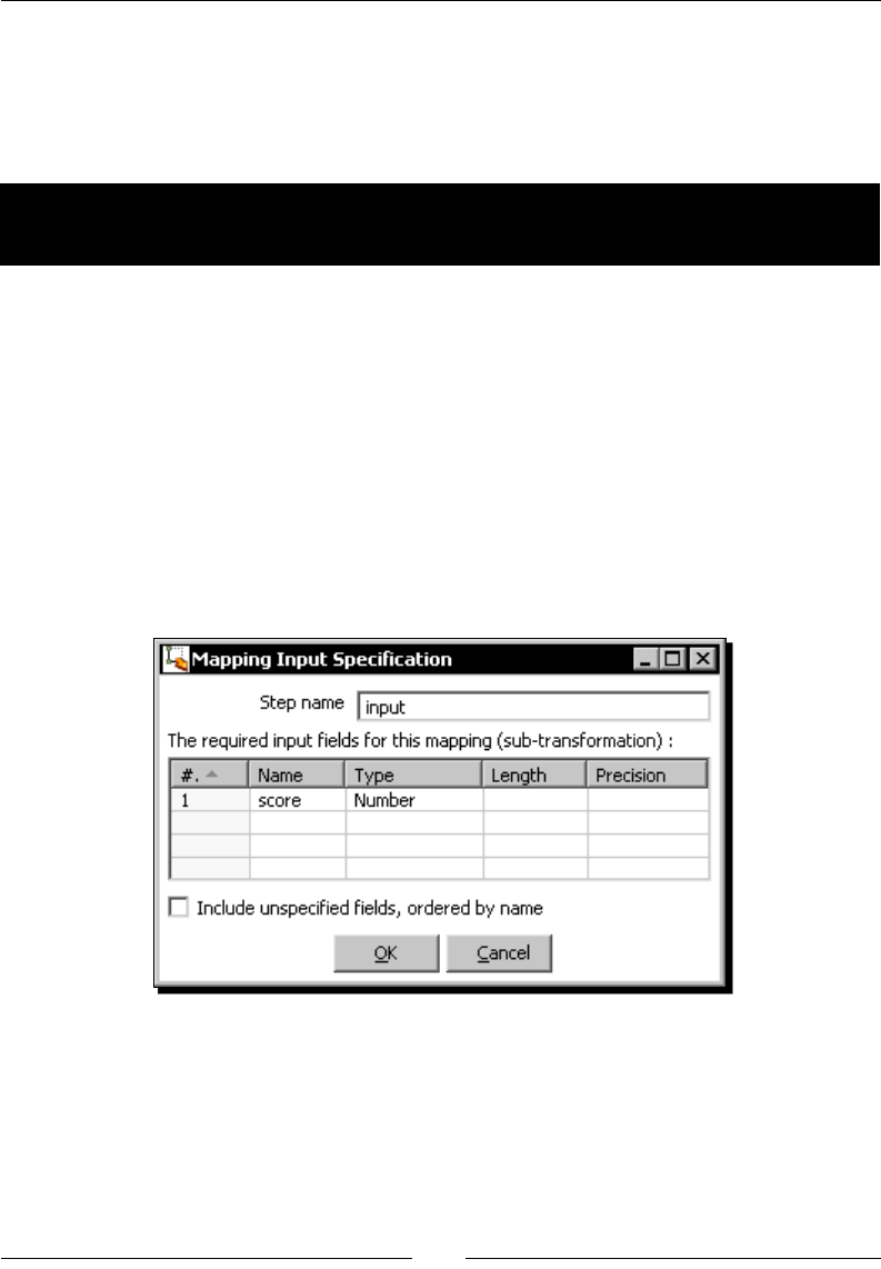
Chapter 11
[ 341 ]
Reusing part of your transformations
As you noced, the sequence of steps used to get the ranks are almost idencal for the four
skills. You could have avoided copying and pasng or doing the same work several mes by
moving those steps to a subtransformaon. Let's do it.
Time for action – calculating the top scores with a
subtransformation
Let's modify the transformaon that calculates the top scores to avoid unnecessary
duplicaon of steps:
1. Under the transformation folder, create a new folder named
subtransformations.
2. Create a new transformaon and save it in that new folder with the name
scores.ktr.
3. Expand the Mapping category of steps. Select a Mapping input specicaon step
and drag it to the work area.
4. Double-click the step and ll it like this:
5. Add a Sort rows step and use it to sort the score eld in descending order.
6. Add a JavaScript step and type the following code to lter the top 10 rows:
trans_Status = CONTINUE_TRANSFORMATION;
if (getProcessCount('r')>10) trans_Status = SKIP_TRANSFORMATION;
7. Add an Add sequence step to add a sequence eld named seq.
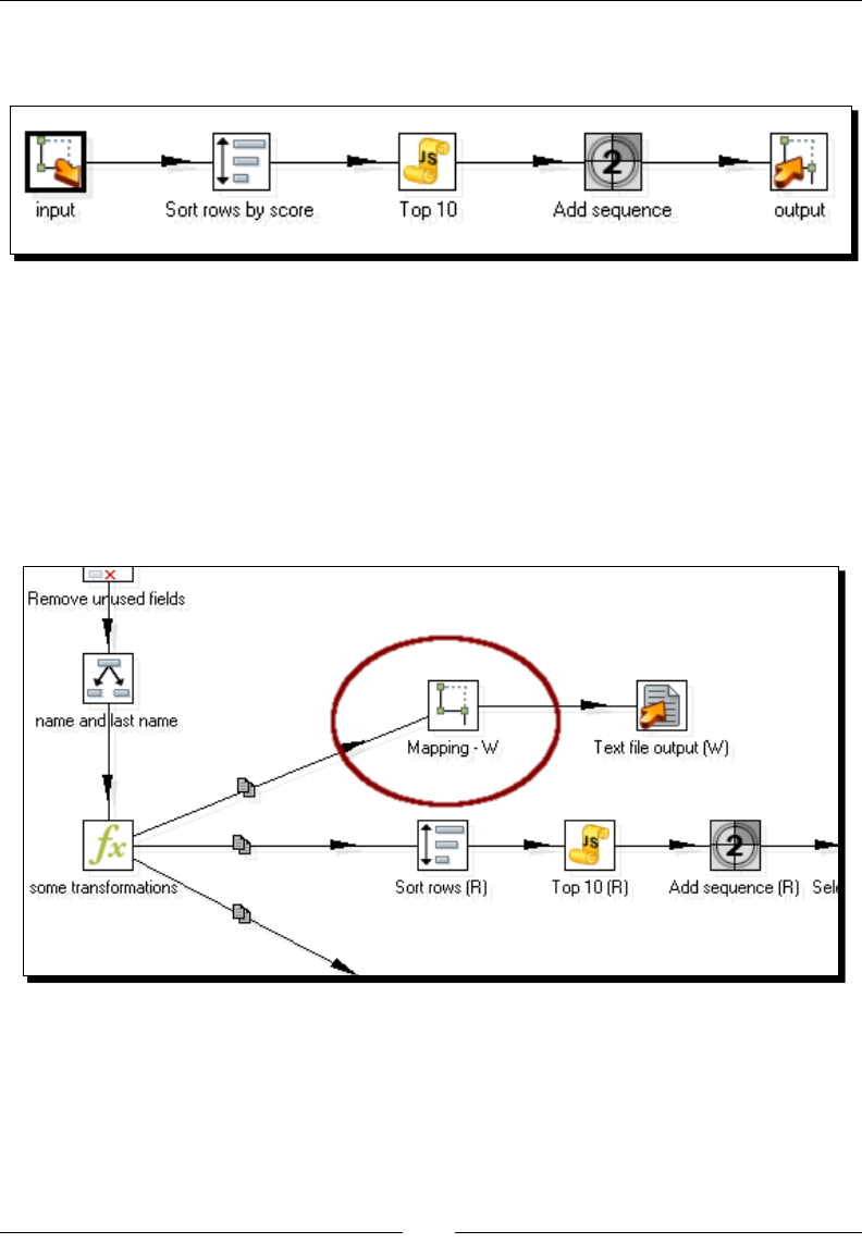
Creang Advanced Transformaons and Jobs
[ 342 ]
8. Finally, add a Mapping output specicaon step. You will nd it in the Mapping
category of steps. Your transformaon looks like this:
9. Save the transformaon.
10. Open the transformaon top_scores.ktr and save it as top_scores_with_
subtransformations.ktr.
11. Modify the wring stream. Delete all steps except the Text le output step—the
Sort rows, JavaScript, Add sequence, and the Select rows steps.
12. Drag a Mapping (sub-transformaon) step to the canvas and put it in the place
where all the deleted steps were. You should have this:
13. Double-click the Mapping step.
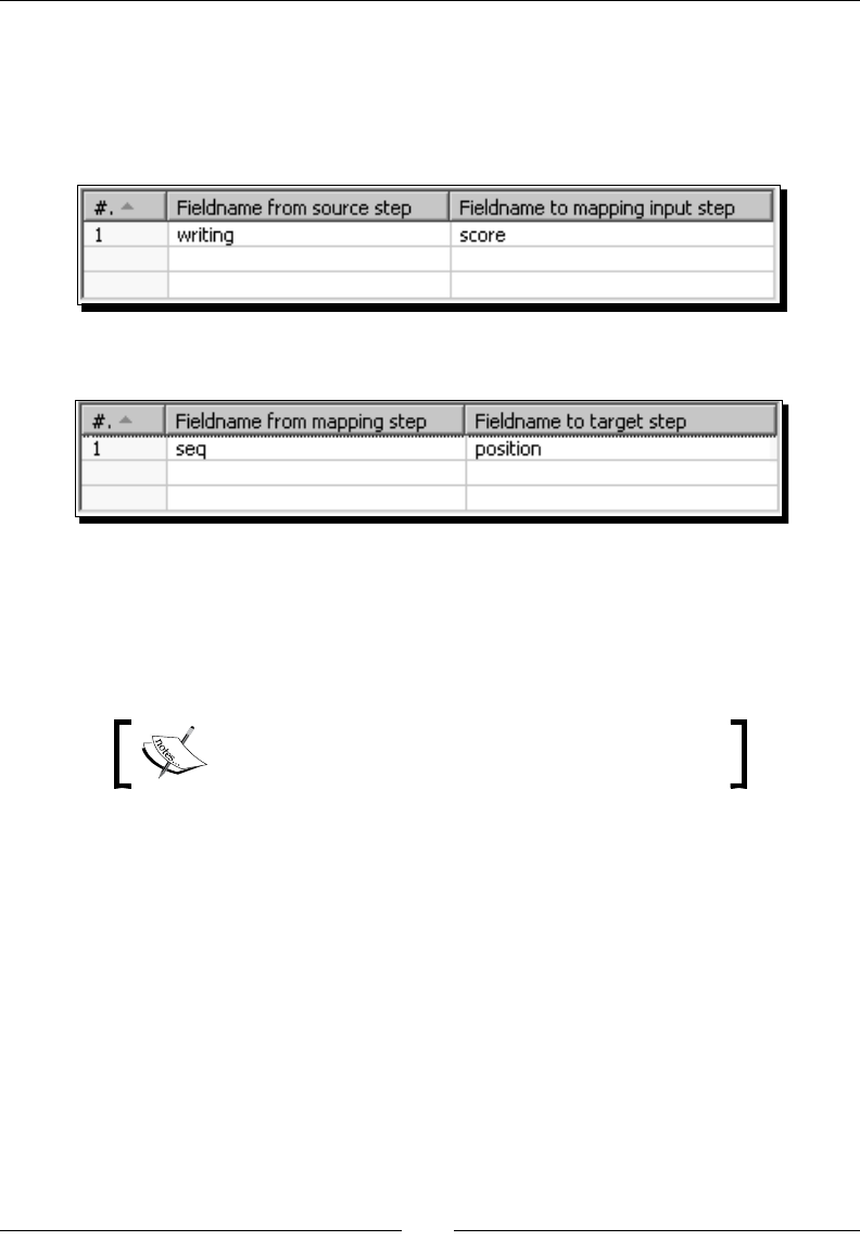
Chapter 11
[ 343 ]
14. In the Mapping transformaon frame, select the opon named Use a le for
the mapping transformaon. In the textbox below it, type ${Internal.
Transformation.Filename.Directory}/subtransformations/scores.
ktr. Select the Input tab, check the Is this the main data path? opon, and ll the
grid as shown:
15. Select the Output tab and ll the grid as shown:
16. Click on OK.
17. Repeat the steps 11 to 16 for the other streams—reading, speaking, and listening.
The only dierence is what you put in the Input tab of the Mapping steps—instead
of writing, you should put reading, speaking, and listening.
Note that you added four Mapping (subtransformaon)
steps, but you only need one subtransformaon le.

Creang Advanced Transformaons and Jobs
[ 344 ]
18. The nal transformaon looks as follows:
19. Save the transformaon.
20. Press F9 to run the transformaon.
21. Select Minimal logging and click on Launch. The Logging window looks like
the following:
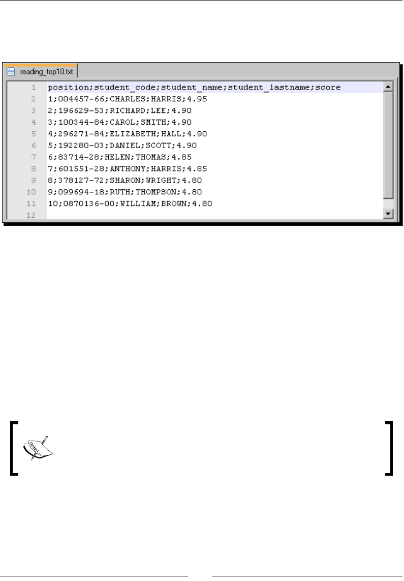
Chapter 11
[ 345 ]
22. The output les should have been generated and should look exactly the same as
before. This me let's check the reading_top10.txt le (the names and values
may vary depending on the examinaon les that you appended to the global le):
What just happened?
You took the bunch of steps that calculate the top scores and moved it to a
subtransformaon. Then, in the main transformaon, you simply called the
subtransformaon four mes, each me using a dierent eld.
It's worth saying that the Text le output step could also have been moved to the
subtransformaon. However, instead of simplifying the work, it would have complicated it.
This is because the names of the les are dierent in each case and, in order to build that
name, it would have been necessary to add some extra logic.
Creating and using subtransformations
Subtransformaons are, as the named suggests, transformaons inside transformaons.
The PDI proper name for a subtransformaon is mapping. However, as the
word mapping is also used with other meanings in PDI, we will use the old,
more intuive name subtransformaon.
In the tutorial, you created a subtransformaon to isolate a task that you needed
to apply four mes. This is a common reason for creang a subtransformaon—to
isolate a funconality that is likely to be needed more than once. Then you called the
subtransformaons by using a single step.

Creang Advanced Transformaons and Jobs
[ 346 ]
Let's see how subtransformaons work. A subtransformaon is like a regular transformaon,
but it has input and output steps, connecng it to the transformaons that use it.
The Mapping input specicaon step denes the entry point to the subtransformaon.
You specify here just the elds needed by the subtransformaon. The Mapping output
specicaon step simply denes where the ow ends.
The presence of Mapping input specicaon and Mapping output
specicaon steps is the only fact that makes a subtransformaon
dierent from a regular transformaon.
In the sample subtransformaon you created in the tutorial, you dened a single eld named
score. You sorted the rows by that eld, ltered the top 10 rows, and added a sequence to
idenfy the rank—a number from 1 to 10.
You call or execute a subtransformaon by using a Mapping (sub-transformaon) step. In
order to execute the subtransformaon successfully, you have to establish a relaonship
between your elds and the elds dened in the subtransformaon.
Let's rst see how to dene the relaonship between your data and the input specicaon.
For the sample subtransformaon, you have to dene which of your elds is to be used as
the input eld score dened in the input specicaon. You can do it in an Input tab in the
Mapping step dialog window. In the rst Mapping step, you told the subtransformaon to
use the eld writing as its score eld.
If you look at the output elds coming out of the Mapping step, you will no longer see the
writing eld but a eld named score. It is the same eld writing that was renamed as
score. If you don't want your elds to be renamed, simply check the Ask these values to
be renamed back on output? opon found in the Input tab. That will cause the eld to be
renamed back to its original name—writing in this example.
Let's now see how to dene the relaonship between your data and the output specicaon.
If the subtransformaon creates new elds, you may want to add them to your main
dataset. To add to your dataset, a eld created in the subtransformaon, you use an Output
tab of the Mapping step dialog window. In the tutorial, you were interested in adding the
sequence. So, you congured the Output tab, telling the subtransformaon to retrieve the
eld named seq in the subtransformaon but renamed as position. This causes a new
eld named position to be added to your stream.
If you want the subtransformaon to simply transform the incoming stream without adding
new elds, or if you are not interested in the elds added in the subtransformaon, you
don't have to create an Output tab.
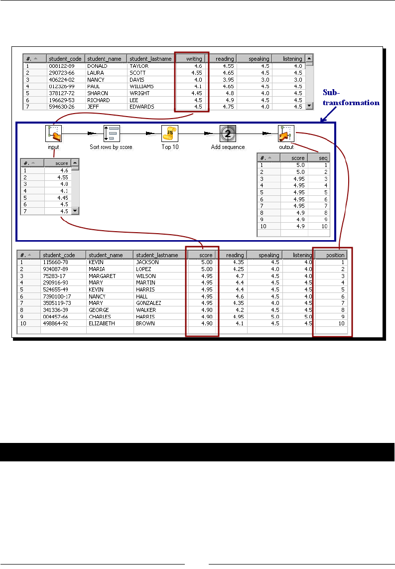
Chapter 11
[ 347 ]
The following screenshot summarizes what was explained just now. The upper and lower grids
show the datasets before and aer the streams have own through the subtransformaon.
The subtransformaon in the tutorial allowed you to reuse a bunch of steps that were
present in several places, avoiding doing the same task several mes. Another common
situaon where you may use subtransformaons is the one where you have a transformaon
with too many steps. If you can idenfy a subset of steps that accomplish a specic purpose,
you may move those steps to a subtransformaon. Doing so, your transformaon will
become cleaner and easier to understand.
Have a go hero – rening the subtransformation
Modify the subtransformaon in the following way:
Add a new eld named below_first. The eld should have the dierence between the
score in the current row and the maximum score. For example, if the maximum score is 5
and the current score is 4.85, the value for the eld should be 0.15.
Modify the main transformaon by adding the new eld to all output les.

Creang Advanced Transformaons and Jobs
[ 348 ]
Have a go hero – counting words more precisely (second version)
Combine the following Hero exercises from Chapter 3:
Counng words, discarding those that are commonly used
Counng words more precisely
Create a subtransformaon that receives a String value and cleans it. Remove extra signs that
may appear as part of the string such as . , ) or ". Then convert the string to lower case.
Also create a ag that tells whether the string is a valid word. Remember that the word is
valid if its length is at least 3 and if it is not in a given list of common words.
Retrieve the modied word and the ag.
Modify the main transformaon by using the subtransformaon. Aer the
subtransformaon step, lter the words by looking at the ag.
Creating a job as a process ow
With the implementaon of a subtransformaon, you simplify much of the transformaon.
But you sll have some reworking to do. In the main transformaon, you basically do two
things. First you read the source data from a le and prepare it for further processing. And
then, aer the preparaon of the data, you generate the les with the top scores. To have a
clearer vision of these two tasks, you can split the transformaon in two, creang a job as a
process ow. Let's see how to do that.
Time for action – splitting the generation of top scores by
copying and getting rows
Now you will split your transformaon into two smaller transformaon so that each meets a
specic task. Here are the instrucons.
1. Open the transformaon in the previous tutorial. Select all steps related to
the preparaon of data, that is, all steps from the Text le input step upto the
Formula step.
2. Copy the steps and paste them in a new transformaon.
3. Expand the Job category of steps.
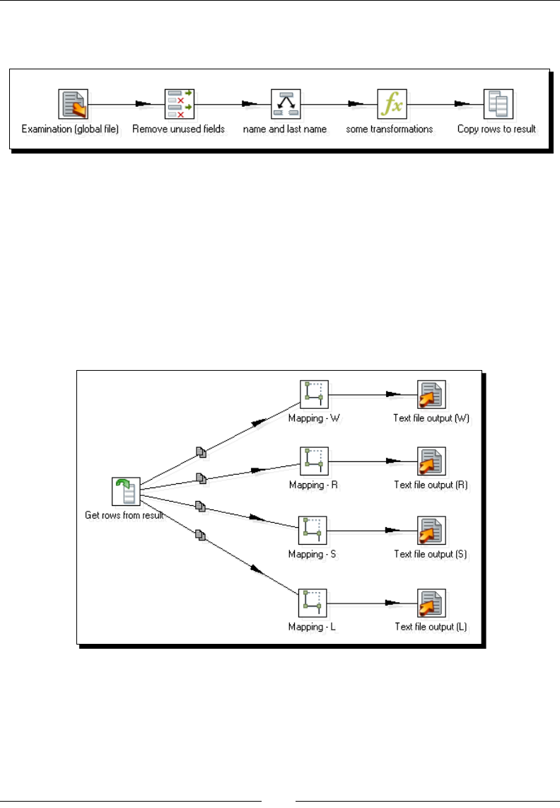
Chapter 11
[ 349 ]
4. Select a Copy rows to result step, drag it to the canvas, and create a hop from the
last step to this new one. Your transformaon looks like this:
5. Save the transformaon in the transformations folder with the name
top_scores_flow_preparing.ktr.
6. Go back to the original transformaon and select the rest of the steps, that is, the
Mapping and the Text le output steps.
7. Copy the steps and paste them in a new transformaon.
8. From the Job category of steps select a Get rows from result step, drag it to
the canvas, and create a hop from this step to each of the Mapping steps. Your
transformaon looks like this:
9. Save the transformaon in the transformations folder with the name top_
scores_flow_processing.ktr.
10. In the top_scores_flow_preparing transformaon , right-click the step Copy
rows to result and select Show output elds.

Creang Advanced Transformaons and Jobs
[ 350 ]
11. The grid with the output dataset shows up.
12. Select all rows. Press Ctrl+C to copy the rows.
13. In the top_scores_flow_processing transformaon, double-click the step Get
rows from result.
14. Press Ctrl+V to paste the values. You have the following result:
15. Save the transformaon.
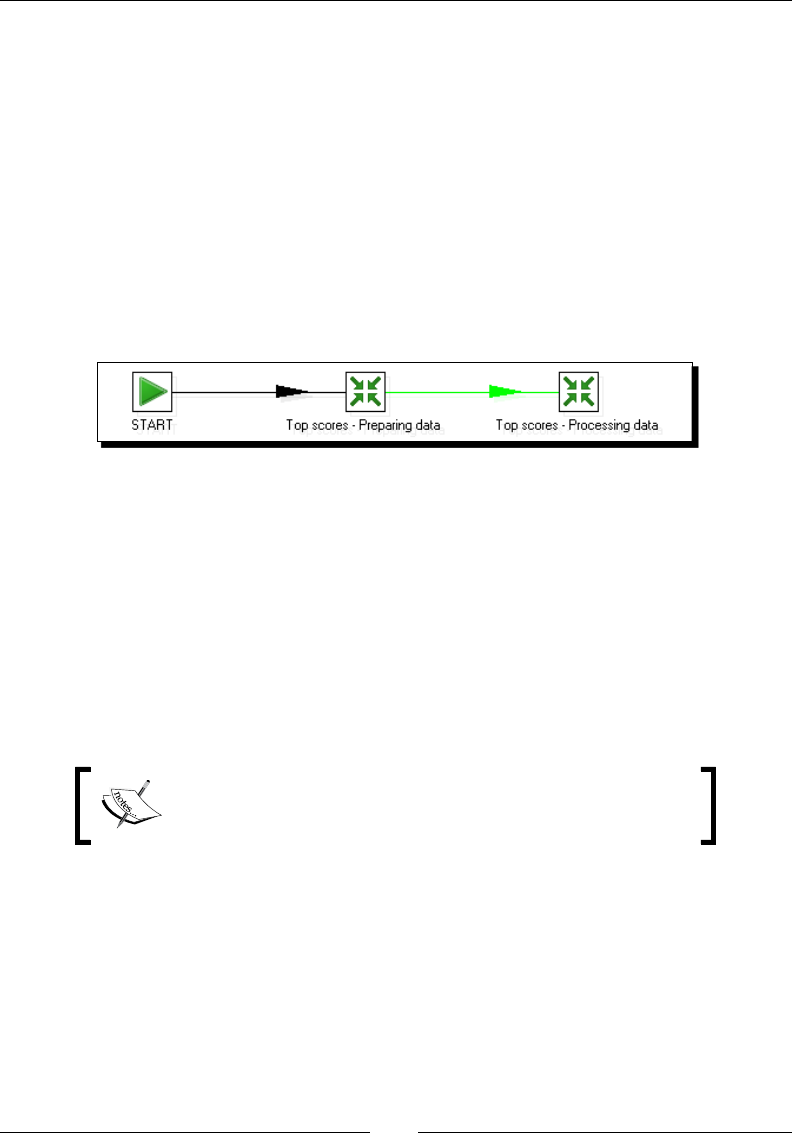
Chapter 11
[ 351 ]
16. Create a new Job.
17. Add a START and two transformaon entries to the canvas and link them one aer
the other.
18. Double-click the rst transformaon. Put ${Internal.Job.Filename.
Directory}/transformations/top_scores_flow_preparing.ktr as the
name of the transformaon.
19. Double-click the second transformaon. Put ${Internal.Job.Filename.
Directory}/transformations/top_scores_flow_processing.ktr as
the name of the transformaon.
20. Your job looks like the following:
21. Save the job. Press F9 to open the Job properes window and click on Launch.
Again, the four les should have been generated, with the very same informaon.
What just happened?
You split the main transformaon in two—one for the preparaon of data and the other for
the generaon of the les. Then you embedded the transformaons into a job that executed
them one aer the other. By using the Copy rows to result step, you sent the ow of data
outside the transformaon, and using Get rows from result step, you picked that data to
connue with the ow. The nal result was the same as before the change.
Noce that you split the last version of the transformaon—the
one with the subtransformaons inside. You could have split the
original. The result would have been exactly the same.
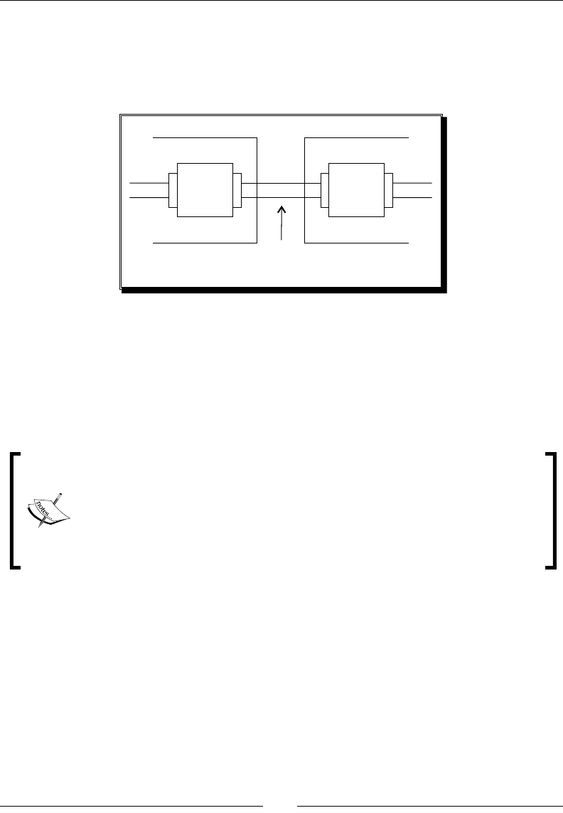
Creang Advanced Transformaons and Jobs
[ 352 ]
Transferring data between transformations by using the copy /get rows
mechanism
The copy/get rows mechanism allows you to transfer data between two transformaons,
creang a process ow. The following drawing shows you how it works:
Copy
rows
step
Transformation A
Data being
transferred
Get
rows
step
Transformation B
The Copy rows to result step transfers your rows of data to the outside of the
transformaon. You can then pick that data by using a Get rows from result step. In the
preceding image, Transformaon A copies the rows and, Transformaon B, which executes
right aer Transformaon A, gets the rows. If you create a single transformaon with all
steps from Transformaon A followed by all steps from Transformaon B, you would get
the same result.
The copy of the dataset is made in memory. It's useful when you have
small datasets. For bigger datasets, you should prefer saving the data in a
temporary le or database table in the rst transformaon, and then create
the dataset from the le or table in the second transformaon.
The Serialize to le /De-serialize from le steps are very useful for this, as the
data and the metadata are saved together.
Chapter 11
[ 353 ]
There is no limit to the number of transformaons that can be chained using this
mechanism. Look at the following image:
Transformation A
Get
Rows
Get
Rows
Copy
rows
Copy
rows .......... ..........
Transformation B Transformation N
As you can see, you may have a transformaon that copies the rows, followed by another
that gets the rows and copies again, followed by a third transformaon that gets the rows,
and so on.
Have a go hero – modifying the ow
Modify the last exercise in the following way:
Include just the students who had an average score above 70.
Note that you have to modify just the transformaon that prepares
the informaon, without caring about what the second process
does with that data.
Generate just the top ve scores for every skill.
Note that you have to modify just the transformaon (or the
subtransformaon) that processes the informaon, without
caring about how the list of students was built.
Create each le in a dierent transformaon. The transformaons execute one aer
the other.

Creang Advanced Transformaons and Jobs
[ 354 ]
This exercise requires that you modify the ow. Each
transformaon gets the rows from the previous transformaon,
then generates a le, and copies the rows to the result to be
used for the next transformaon.
Nesting jobs
Suppose that every me you append a le with examinaon results, you want to generate
updated les with the top 10 scores. You can do it manually, running one job aer the other,
or you can nest jobs.
Time for action – generating the les with top scores by
nesting jobs
Let's modify the job that updates the global examinaon le, so at the end it generates
updated top scores les:
1. Open the examinations job you created in the rst tutorial of this chapter.
2. Aer the last transformaon job entry, add a job entry as Job. You will nd it under
the General category of entries.
3. Double-click the Job job entry.
4. Type ${Internal.Job.Filename.Directory}/top_scores_flow.kjb
as Job lename.
5. Click on OK.
6. Save the job.
7. Pick an examinaon that you have not yet appended to the global le—for example,
exam5.txt.
8. Press F9.
9. In the Arguments grid, type the full path of the chosen le: c:/pdi_files/input/
exam5.txt.
10. Click on Launch.
Download from Wow! eBook <www.wowebook.com>
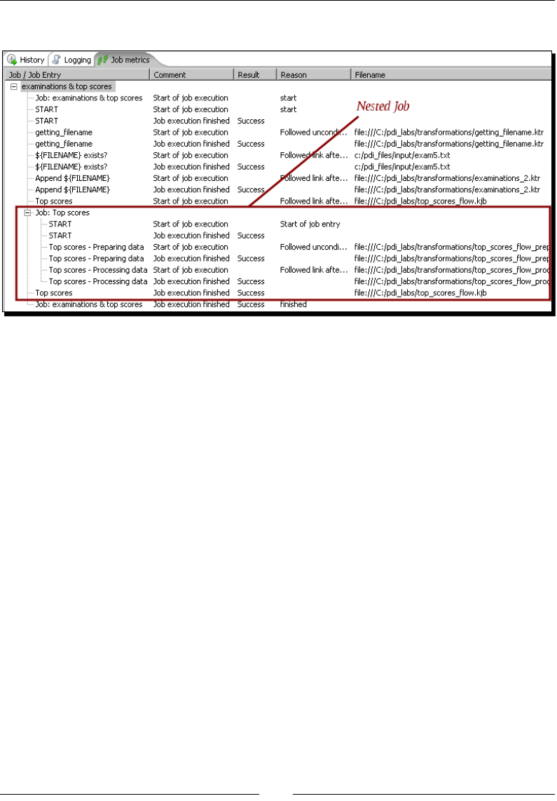
Chapter 11
[ 355 ]
11. In the Job metrics tab of the Execuon results window, you will see the following:
12. Also the chosen le should have been added to the global le, and updated les with
top scores should have been generated.
What just happened?
You modied the job that updates the global examinaon le by including the generaon of
the les with top scores as part of the process. You did it by using a Job job entry whose task
is to run a job inside a job.
In the Job metrics, you could see a hierarchy showing the details of the nested job as a
sub-tree of that hierarchy.
Running a job inside another job with a job entry
The job entry, Job, allows you to run a job inside a job. Just like any job entry, this entry may
end successfully or fail. Upon that result, the main job decides which of the entries that
follows it will execute. None of the entries following the job entry starts unl the nested job
ends its execuon. There is no limit to the levels of nesng. You may call a job, which calls
a job, which again calls a job, and so on. Usually you will not need more than two or
three levels.
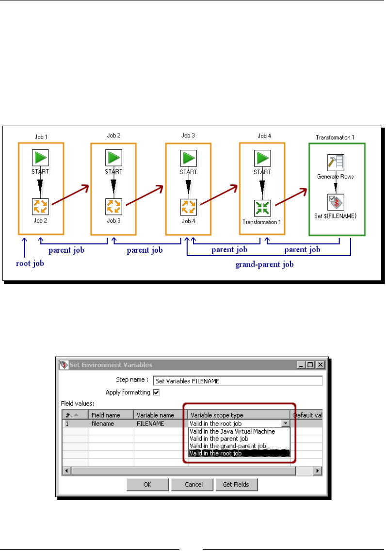
Creang Advanced Transformaons and Jobs
[ 356 ]
As with a transformaon job entry, you must specify the locaon and name of the job le.
If the job (or any transformaon inside the nested job) uses arguments or has dened
named parameters, you have the possibility of providing xed values just as you do in a
Transformaon job entry—by lling the Arguments and Parameters tabs.
Understanding the scope of variables
By nesng jobs, you implicitly create a relaonship between the jobs. Look at the
following diagram:
Here you can see how a job, and even a transformaon, may have parents and grandparents.
The main job is called root job. This hierarchy is useful to understand the scope of variables.
When you dene a variable, you have the opon to set the scope, that is, dene the places
where the variable is visible.

Chapter 11
[ 357 ]
The following table explains which jobs and transformaons can access the variable
depending on the variable's scope.
Variable scope type Visibility of the variable
Valid in the parent job Can be seen by the job that called the transformaon and any
transformaon called by this job.
Valid in the grand-parent job Can be seen by the job that called the transformaon, the job that
called that job, and any transformaon called by any of these jobs.
Valid in the root job Can be seen by all jobs in the chain starng with the main job, and
any transformaon called by any of these jobs.
Valid in the Java Virtual
Machine
Seen by all the jobs and transformaons run from the same
Java Virtual Machine. For example, suppose that you dene a
variable with scope in the Java Virtual Machine. If you run the
transformaon from Spoon, then the variable will be available in all
jobs and transformaons you run from Spoon as long as you don't
exit Spoon.
Pop quiz – deciding the scope of variables
In the rst tutorial you created a transformaon that set a variable with the name of a le.
For the scope, you le the default value: Valid in the root job. Which of the following scope
types could you have chosen geng the same results (you may select more than one):
a. Valid in the parent job
b. Valid in the grand-parent job
c. Valid in the Java Virtual Machine
In general, if you have doubts about which scope type to use, you can use Valid
in the root job and you will be good. Simply ensure that you are not using the
same name of variable for dierent purposes.
Iterating jobs and transformations
It may happen that you develop a job or a transformaon to be executed several mes, once
for each dierent row of your data. Consider that you have to send a custom e-mail to a list
of customers. You would build a job that, for a given customer, get the relevant data such as
name or e-mail account and send the e-mail. You would then run the job manually several
mes, once for each customer. Instead of doing that, PDI allows you to execute the job
automacally once for each customer in your list.
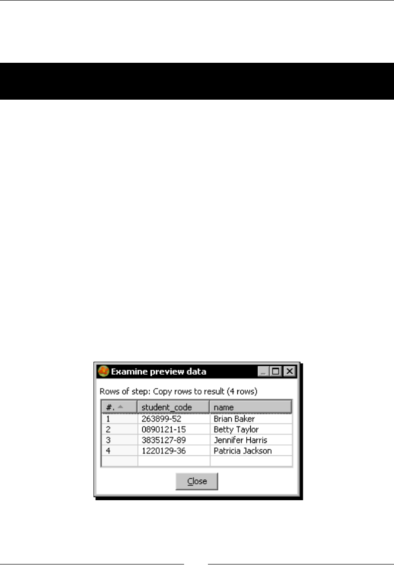
Creang Advanced Transformaons and Jobs
[ 358 ]
The same applies to transformaons. If you have to execute the same transformaon several
mes, once for each row of a set of data, you can do it by iterang the execuon. The next
Time for acon tutorial shows you how to do this.
Time for action – generating custom les by executing a
transformation for every input row
Suppose that 60 is the threshold below which a student must retake the examinaon. Let's
nd out the list of students with a score below 60, that is, those who didn't succeed in the
wring examinaon. Then, let's create one le per student telling him/her about this.
First of all, let's create a transformaon that generates the list of students who will take
the examinaon:
1. Create a new transformaon.
2. Drag a Text le input, a Filter rows, and a Select values step to the canvas and link
them in that order.
3. Use the Text le input step to read the global examinaon le.
4. Use the Filter rows step to keep only those students with a wring score below 60.
5. With the Select values step, keep just the student_code and name values.
6. Aer this last step, add a Copy rows to result step.
7. Do a preview on this last step. You will see the following (the exact names and
values depend on the number of les you have appended to the global le):
8. Save the transformaon in the transformations folder with the name
students_list.ktr.
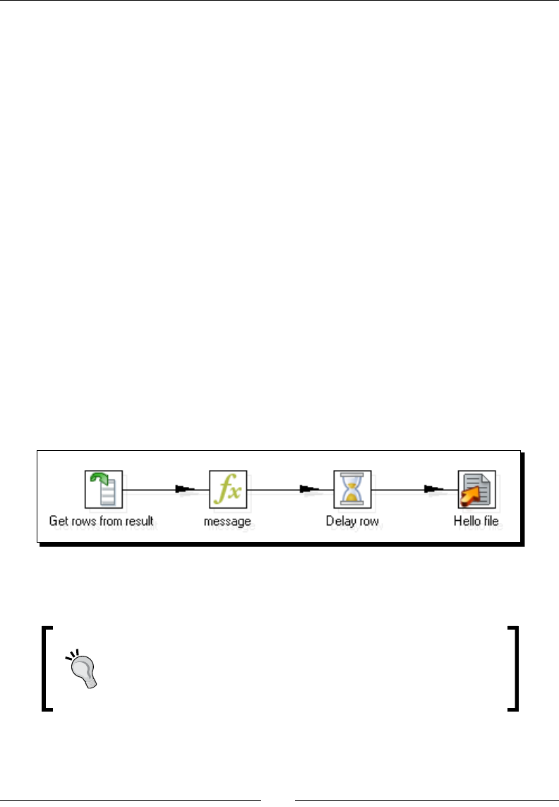
Chapter 11
[ 359 ]
Now let's create a transformaon that generates a single le. This transformaon will be
executed for each student in the list shown in the preceding screenshot:
1. Create a new transformaon.
2. Drag a Get rows from result step to the canvas.
3. Double-click the Get rows from result step and use it to dene two String
elds—a eld named student_code and another eld named name.
4. Add a Formula step and create a hop from the Get rows from result step to this
new step.
5. Use the Formula step to create a new String eld named text. As value, type:
"You'll have to take the examinaon again, " & [name] & ".".
6. Aer the Formula step, add a Delay row step. You will nd it under the Ulity
category of steps.
7. Finally, add a Text le output step, and double-click the step to congure it.
8. As lename type ${LABSOUTPUT}/hello. Check the opon Include me
in lename?.
9. In the content tab, uncheck Header. As Field, select the eld text.
10. This is how your nal transformaon looks:
11. Save the transformaon in the transformations folder under the name
hello_each.ktr.
You can't test this transformaon alone. If you want to test it, just
replace temporarily the Copy rows from result step with a Generate
rows step, generate a single row with xed values for the elds, and
run the transformaon.
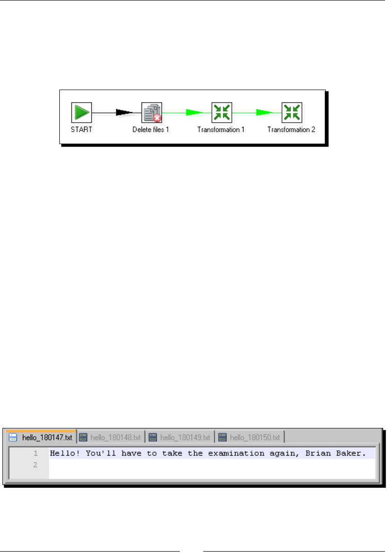
Creang Advanced Transformaons and Jobs
[ 360 ]
Let's create a job that puts everything together:
1. Create a job.
2. Drag a START, a Delete les, and two transformaon entries to the canvas, and link
them one aer the other as shown:
3. Save the job.
4. Double-click the Delete les step. Fill the Files/Folders: grid with a single
row—under File/Folder type ${LABSOUTPUT} and under Wilcard (RegExp) type
hello.*\.txt. This regular expression includes all .txt les whose name start
with the string "hello" in the ${LABSOUTPUT} folder.
5. Double-click the rst transformaon entry. As Transformaon lename, put
${Internal.Job.Filename.Directory}/transformations/student_
list.ktr and click on OK.
6. Double-click the second transformaon entry. As Transformaon lename,
put ${Internal.Job.Filename.Directory}/transformations/
hello_each.ktr.
7. Check the opon Execute for every input row? and click on OK.
8. Save the job and press F9 to run it.
9. When the execuon nishes, explore the folder pointed by your ${LABSOUTPUT}
variable. You should see one le for each student in the list. The les are named
hello_<hhmmddss>.txt where <hhmmddss> is the me in your system at the
moment that the le was generated. The generated les look like the following:

Chapter 11
[ 361 ]
What just happened?
You built a list of students who had to retake the wring examinaon and, for each student,
you generated a le with a custom message.
First, you created a transformaon that built the list of the students and copied the rows
outside the transformaon by using the Copy rows to result step.
Then you created another transformaon that gets a row from the result and generates a
le with a custom hello message.
Finally, you created the main job. First of all, the job deletes all les just in case you run
the job more than once. Then it calls the rst transformaon and then executes the
transformaon that generates the le once for every copied row, that is, once for every
student. Each me the transformaon gets the rows from the result, it gets a single row with
informaon about a single student and generates a le with the message for that student.
Before proceeding with the details about execung each row mechanism, let's briey
explain the new step used here—the Delay row step that is used to deliberately slow down
a transformaon. For each incoming row, the step waits for the amount of me indicated in
its seng window which, by default, is 1 second. Aer that me, the row is given to the
next step.
In this tutorial, the Delay row step is used to ensure that each me the transformaon
executes, the name of the le is dierent. As part of the name for the le, you put the me
of your system including hours, minutes, and seconds. By waing for a second, you can be
sure that in every execuon of the transformaon the name of the le will be dierent from
the name of the previous le.
Executing for each row
The execute for every input row? opon you have in the transformaon entry seng
window allows you to run the transformaon once for every row copied in a previous
transformaon by using the Copy rows to result step. PDI executes the transformaon as
many mes as the number of copied rows, one aer the other. Each me the transformaon
executes and gets the rows from the result, it actually gets a dierent row.
Note that in the transformaon you don't limit the number of incoming
rows. You simply assume that you are receiving a single row. If you forget to
set the execute for every input row? opon in the job, the transformaon
will run but you will get unexpected results.
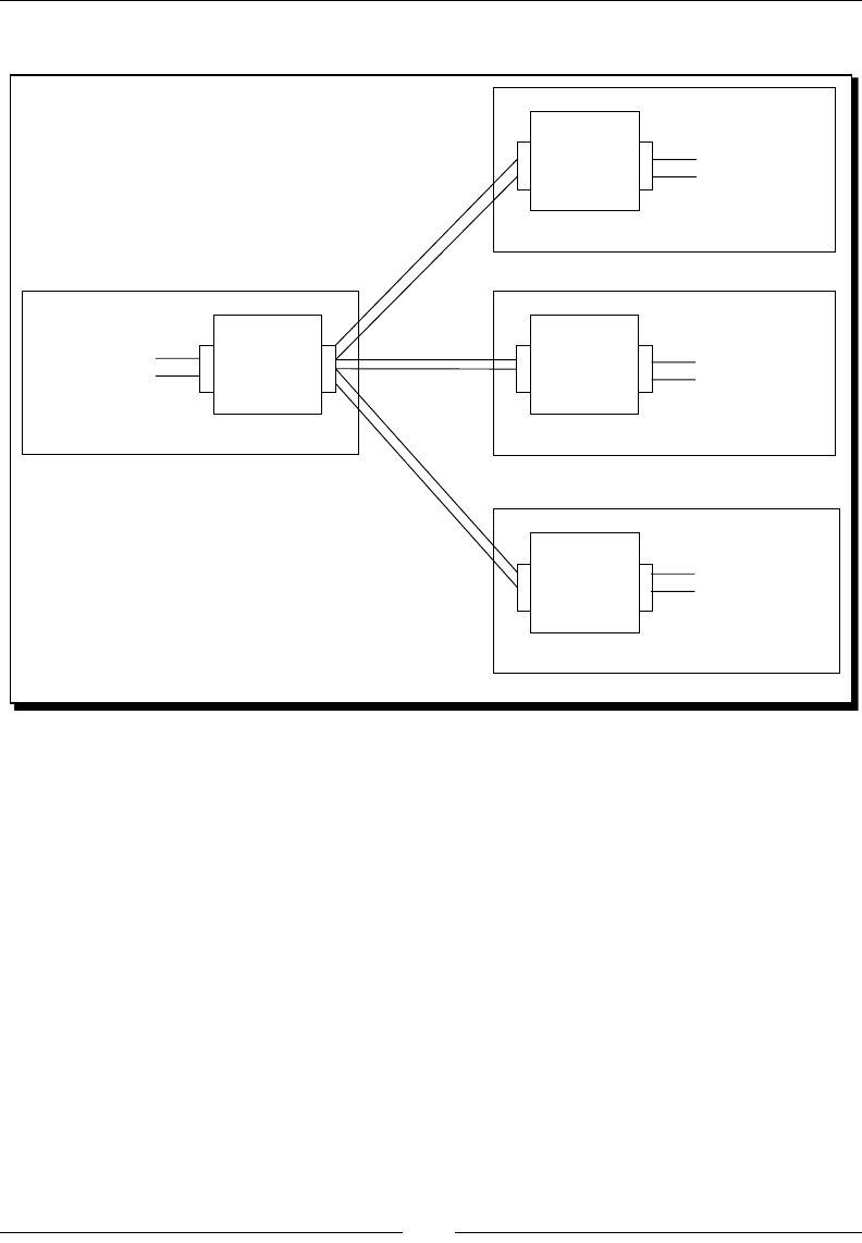
Creang Advanced Transformaons and Jobs
[ 362 ]
This drawing shows you the mechanism for a dataset with three rows:
Copy
rows
step
Transformation A
1st row
Get rows
step
Get rows
step
Get rows
step
Transformation B
Transformation B
Transformation B
......
......
......
......
2nd row
3rd row
The transformaon A in the example copies three rows. Then the transformaon B is
executed three mes—rst for the rst copied row, then for the second, and nally for
the third row.
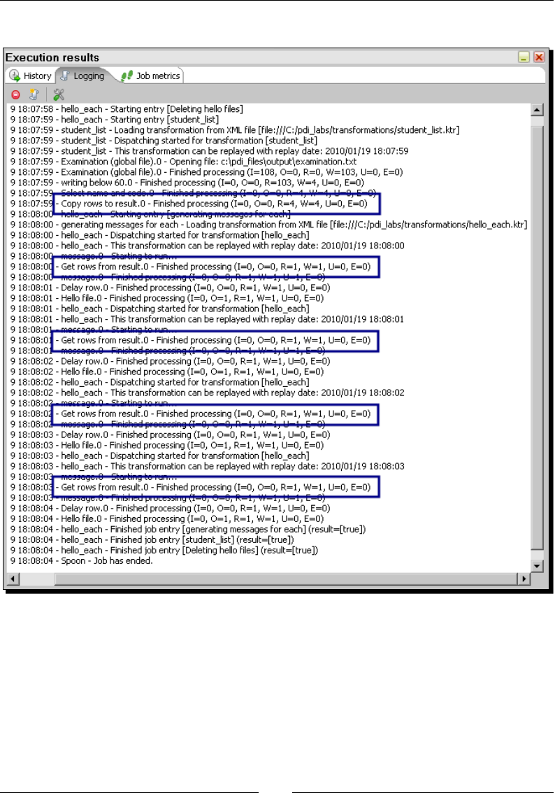
Chapter 11
[ 363 ]
If you look at the log in the tutorial, you can see it working:
The transformaon that builds the list of students copies four rows to the results. Then the
main job executes the second transformaon four mes—once for each of those students.
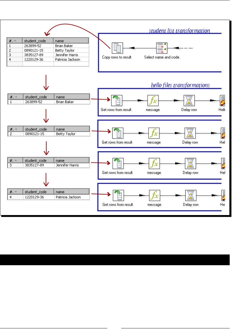
Creang Advanced Transformaons and Jobs
[ 364 ]
The following sketch shows it clearly:
This mechanism of execung for every input row applies also to jobs. To execute a single
job several mes, once for every copied row, you have to check the execute for every input
row? opon that you have in the job entry sengs window.
Have a go hero – processing several les at once
Modify the rst tutorial about Updang a le with news about examinaons. But this me
accept a folder as parameter. Then process all the text les in that folder, ordered by date of
the le. For each processed le, put a line in the log telling the name of the processed le.
You can use the following hint. Create a rst transformaon that, instead of validang the
parameter as a le, validates it as a folder. In order to do that, use the File exists step inside
the Lookup category of steps.

Chapter 11
[ 365 ]
If the folder exists, use a Get File Names step. That step allows you to retrieve the list of
lenames in a given folder, including the aributes for those les. To dene which les to
get, use the opons in the box Filenames from eld. Sort the list by le date and copy the
names to the results.
In the second transformaon, executed for every input row, get a row from the result, then
use a Text le input step accepng the name from the previous step, and proceed as usual.
As you may nd it dicult to use steps you never used before, you
may download a working version for the rst transformaon. You'll
nd it among the material for this chapter.
Have a go hero – building lists of products to buy
This exercise is related to the JS database.
Create a transformaon to nd out the manufacturers for the products that have been sold
best in the current month. Take the rst three manufacturers in the list.
Create another transformaon that, for every manufacturer in that list, builds a le with a list
of products out of stock.
Hint
The rst transformaon must copy the rows to the result. The second transformaon must
execute for every input row. Start the transformaon with a Get rows from result step, then
a Table Input step that receives as parameter a manufacturer's code. The SQL to use could
be something like:
SELECT *
FROM products
WHERE code_man LIKE '?' AND pro_stock<pro_stock_min
Have a go hero – e-mail students to let them know how they did
Suppose some students have asked you to send them an e-mail to tell them how they did in
the examinaon. Get the list of students from a le you'll nd inside the resources, nd out
their scores, and send them an e-mail with that informaon.
Hint
Create a transformaon that builds the list of students that have asked you to send them the
examinaon results, along with their e-mail and scores, and copies the rows to the result.

Creang Advanced Transformaons and Jobs
[ 366 ]
Create a job that does the following: Call a transformaon that gets a row from a result with
the name, e-mail, and scores for a single student. Use that informaon to create variables
needed to send an e-mail, for example Subject. Aer calling that transformaon, use a Mail
entry to send the e-mail by using the dened variables.
Create a main job. Execute the transformaon that builds the list followed by the job
described above, execung it for every input row.
To test the job that sends e-mails, you may temporarily replace the Get rows
from result step with a Generate rows with xed values step.
To test the main job, replace the e-mail accounts in the le with accounts you
have access to.
Summary
In this chapter you learned techniques to combine jobs and transformaons in
dierent ways.
First, you learned to dene your own variables at run me. You dened variables in one
transformaon and then used them in other jobs and/or transformaons. You also learned
to dene dierent scopes for those variables.
Aer that, you learned to isolate part of a transformaon as a subtransformaon. You also
learned to implement process ows by copying and geng rows, and how to nest jobs. By
using all these PDI capabilies, your work will look cleaner and will be more organized.
Finally, you learned to iterate the execuon of jobs and transformaons.
Let's say that this was a really producve chapter. By now, you should be equipped with
enough knowledge to use PDI for developing most of your requirements.
You're now ready for the next chapter, where you will develop the nal project that will allow
you to review a lile of everything you've learned throughout the book.

12
Developing and Implementing a
Simple Datamart
In this chapter you will develop a simple but complete process of loading a
datamart while reviewing all concepts you learned throughout the book.
The chapter will cover the following:
Introducon to a sales datamart based on the Jigsaw puzzles database
Loading the dimensions of the sales datamart
Loading the fact table for the sales datamart
Automang what has been done
Exploring the sales datamart
In Chapter 9, you were introduced to star schemas. In short, a star schema consists of
a central table known as the fact table, surrounded by dimension tables. While the fact
has indicators of your business such as sales in dollars, the dimensions have descripve
informaon for the aributes of your business such as me, customers, and products.
A star that addresses a specic department's needs or that is built for use by a parcular
group of users is called a datamart. You can have datamarts focused on customer
relaonship management, inventory, human resources management, budget,
and more. In this chapter, you will load a datamart focused on sales.
Somemes the term datamart is confused with datawarehouse. However, datamarts and
datawarehouses are not the same.
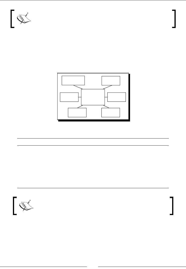
Developing and Implemenng a Simple Datamart
[ 368 ]
The main dierence between datamarts and datawarehouses is that
datawarehouses address the needs of the whole organizaon, whereas
a datamarts addresses the needs of a parcular department.
Datawarehouses contain informaon from mulple subject areas, allowing you to have a
global vision of your business. Therefore, they are oriented to the company's sta such as
execuves or managers.
The following star represents your sales datamart—a central fact named SALES, surrounded
by six dimensions:
Product Type Time
Payment
Method
Buy
Method
Manufac
turer
SALES Region
The following is a brief descripon for the dimensions in your SALES star:
Dimension Descripon
Time The date on which the sales occurred
Regions The geographical area where the products were sold
Manufacturers The name of the manufacturers that build the products sold
Payment method Cash, Check, and so on
Buy method Internet, by telephone, and so on
Product type Puzzle, glue, frame, and so on
In real models you may nd two types of dimensions related with
me—a dimension holding calendar day aributes and a separate
dimension with aributes such as hours, minutes, and seconds.
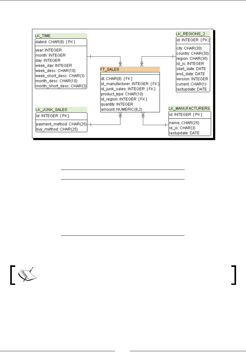
Chapter 12
[ 369 ]
Let's now look at the DER for the database that represents this model. The fact table is
represented by a table named ft_sales.
The following table shows you the correspondence between the dimensions in the model
and the tables in the database:
Dimension Table
Manufacturers lk_manufacturer
Time lk_time
Regions lk_regions_2
Payment method lk_junk_sales
Buy method lk_junk_sales
Product type none
As you can see, there is no one-to-one relaonship between the dimensions in the model
and the tables in the database.
A one-to-one relaonship between a dimension and a database table is not
required, but may coincidentally exist.
The rst three dimensions have their corresponding tables.
The payment and buy method dimensions share a junk dimension. A junk dimension is an
abstract dimension that groups unrelated low-cardinality ags, indicators, and aributes. Each
of those items could technically be a dimension on its own, but grouping them into a junk
dimension has the advantage of keeping your database model simple and it also saves space.

Developing and Implemenng a Simple Datamart
[ 370 ]
The last dimension, product type, doesn't have a separate table. It is so simple that it isn't
worth creang a dimension table. Instead, its values are stored in a dedicated eld in the
fact table. This kind of dimension is called degenerate dimension.
Deciding the level of granularity
The level of detail in your star model is called grain. The granularity is directly related to the
types of quesons you expect your model to answer. Let's see some examples.
The product-related informaon your model has is the manufacturer and the kind of product
(puzzle, glue, and so on). Thus, it allows you to ask quesons such as:
Beyond puzzles, what type of product is the best sold?
Do you sell more products manufactured by Ravensburger than products
manufactured by Educa Jigsaws?
What if you want to know the names of the top ten products sold? You simply can't, as that
level of detail is not stored in the model. For answering this type of queson, you need a
lower level of granularity. You could have that by adding a product dimension where each
record represents a parcular product.
Now let's see the me dimension. Each record in that dimension represents a parcular
calendar day. This allows you to answer quesons such as: how many products did you sell
every day in the last four months?
If you were not interested in daily, but in monthly informaon, you could have designed a
model with a higher level of granularity by creang a me dimension with just one record
per month.
Understanding the level of granularity of your model is a key to the process of loading the
fact table, as you will see when you load the sales fact table.
Loading the dimensions
As you saw, the sales star model consists of a fact surrounded by the dimension tables. In
order to load the star, rst you have to load the dimensions. You already learned how to
load dimension tables. Here you will load the dimensions for the sales star.
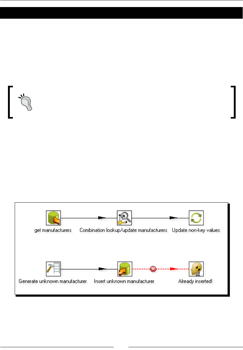
Chapter 12
[ 371 ]
Time for action – loading dimensions for the sales datamart
In this tutorial, you will load each dimension for the sales datamart and enclose them into a
single job. Before starng, check the following things:
Check that the database engine is up and that both the js and the js_dw databases
are accessible from PDI.
If your me dimension table, lk_time, has data, truncate the table. You may do it
by using the Truncate table [lk_me] opon in the database explorer.
You may reuse the js_dw database in which you have been loading data in
previous chapters. There is no problem with that. However, creang a whole
new database is preferred so that you can see how the enre process works.
The explanaon will be focused on the general process. For details of creang a
transformaon that loads a parcular type of dimension, please refer to Chapter 9. You
can also download the full material for this chapter where the transformaons and jobs
are ready to browse and try.
1. Create a new transformaon and use it to load the manufacturer dimension.
This is a Type I SCD dimension. The data for the dimension comes from the
manufacturers table in the js database. The dimension table in js_dw is
lk_manufacturer. Use the following screenshot as a guide:
2. Save the transformaon the lk_transformations.
3. Create a new transformaon and use it to load the regions dimension.
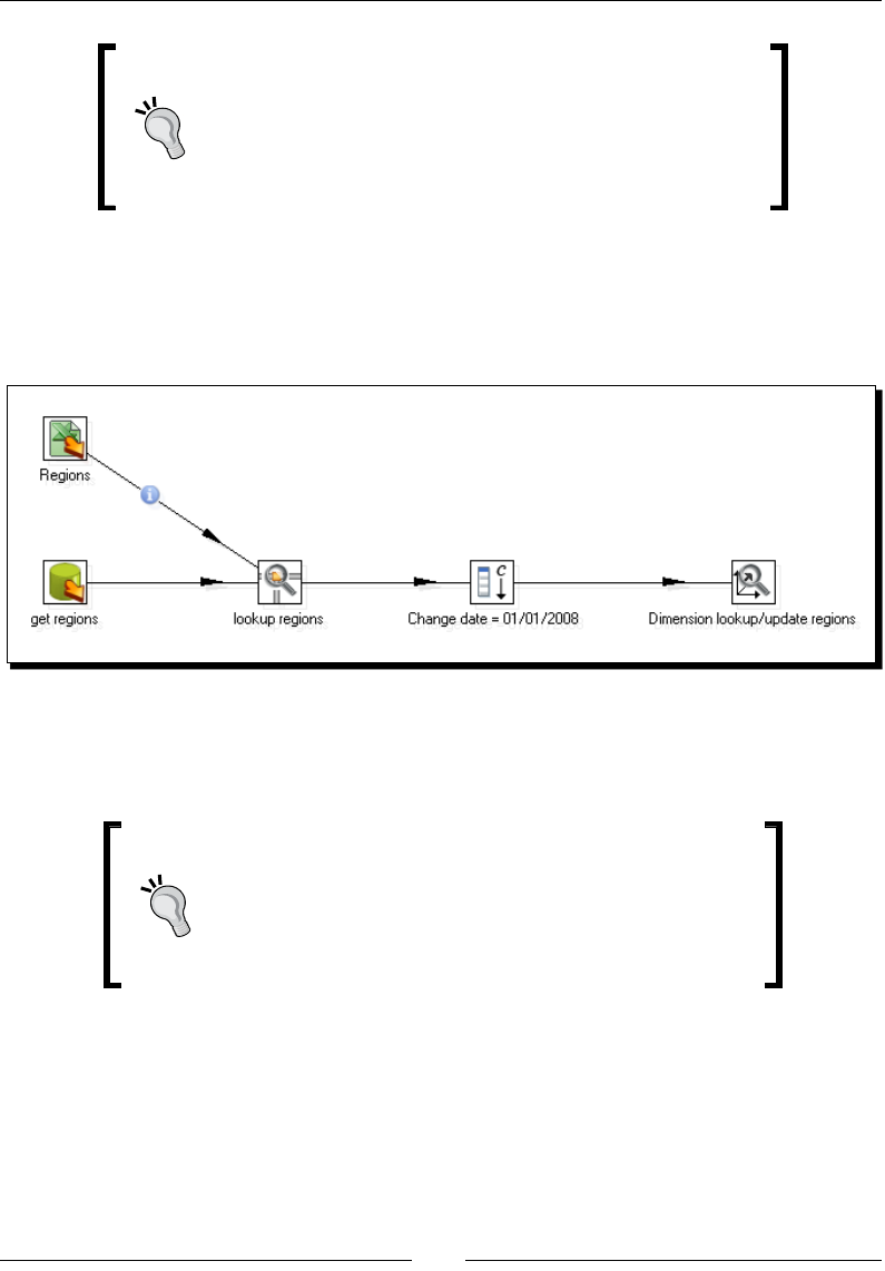
Developing and Implemenng a Simple Datamart
[ 372 ]
You already loaded this dimension in the Time for acon
– loading a region dimension with a Combinaon lookup/
update step secon in Chapter 9. The load of the region eld
was part of a Hero exercise in that chapter. If you did it, you
may skip this step.
4. The region dimension is a Type II SCD dimension. The data for the dimension comes
from the city and country tables. The informaon about regions is in Excel les
that you can download from the Packt web site. The dimension table in js_dw is
lk_regions_2. Use the following screenshot as a guide:
5. Save the transformaon in the lk_transformations folder.
6. Create a new transformaon and use it to load the me dimension.
You already created the dataset for the me dimension
in the Time for acon –creang the me dimension
dataset secon in Chapter 6. Then in Chapter 8 the loading
of the data into a table was part of a Hero exercise. If you
have done it, you may skip this step.
The dimension table in js_dw is lk_time.
7. Save the transformaon in the lk_transformations folder.
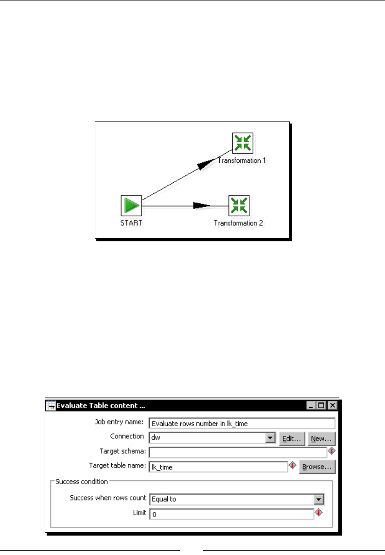
Chapter 12
[ 373 ]
Now you will create a job to put it all together:
8. Create a new job and save it in the same folder where you created the
lk_transformations folder.
9. Drag a START entry and two Transformaon job entries to the canvas.
10. Create a hop from the START entry to each of the transformaon entries. You have
the following:
11. Use one of the transformaon entries to execute the transformaon that loads the
manufacturer dimension.
12. Use the other transformaon entry to execute the transformaon that loads the
region dimension.
13. Add an Evaluate rows number in a table entry to the canvas. You'll nd it under the
Condions category.
14. Create a hop from the START entry towards this new entry.
15. Double-click the new entry and ll it like shown:
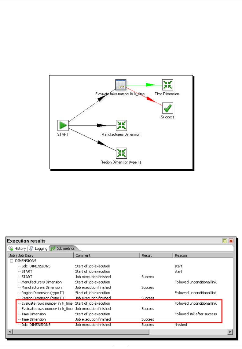
Developing and Implemenng a Simple Datamart
[ 374 ]
16. Aer this entry, add another transformaon entry and use it to execute the
transformaon that loads the me dimension.
17. Finally, from the General category add a Success entry.
18. Create a hop from the Evaluate… step to this entry. The hop should be red, meaning
that this step executes when the evaluaon fails.
19. Your nal job looks like this:
20. Save the job.
21. Run the job. The manufacturer and regions dimensions should be loaded. You can
verify it by exploring the tables from the PDI explorer or in MySQL query browser.
22. In the logging window, you'll see that the evaluaon succeeded and so the me
dimension is also loaded:
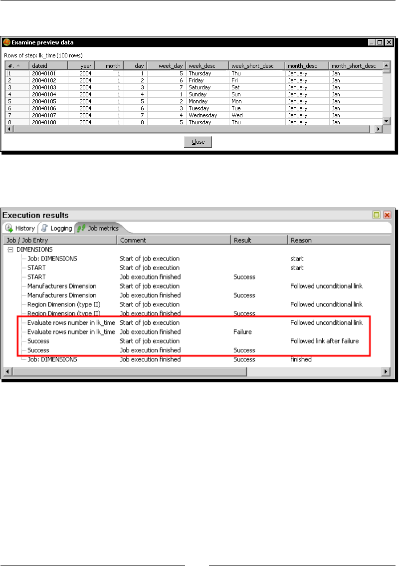
Chapter 12
[ 375 ]
23. You can check it by exploring the table.
24. Run the transformaon again. This me the evaluaon fails and the transformaon
that loads the me dimension is not executed this me.
What just happened?
You created the transformaons to load the dimensions you need for your sales star.
As already explained in Chapter 10, the job entries connected to the START entry run one
aer the other, not in parallel as the arrangement in the work area might suggest.
As for the me dimension, once it is loaded, you don't need to load it again. Therefore, you
put an evaluaon entry to check if the table had already been loaded. The rst me you
run the job, there were no records, so the me dimension was loaded. The second me,
the me dimension had already been loaded. This me the evaluaon failed, avoiding the
execuon of the transformaon that loaded the me dimension.
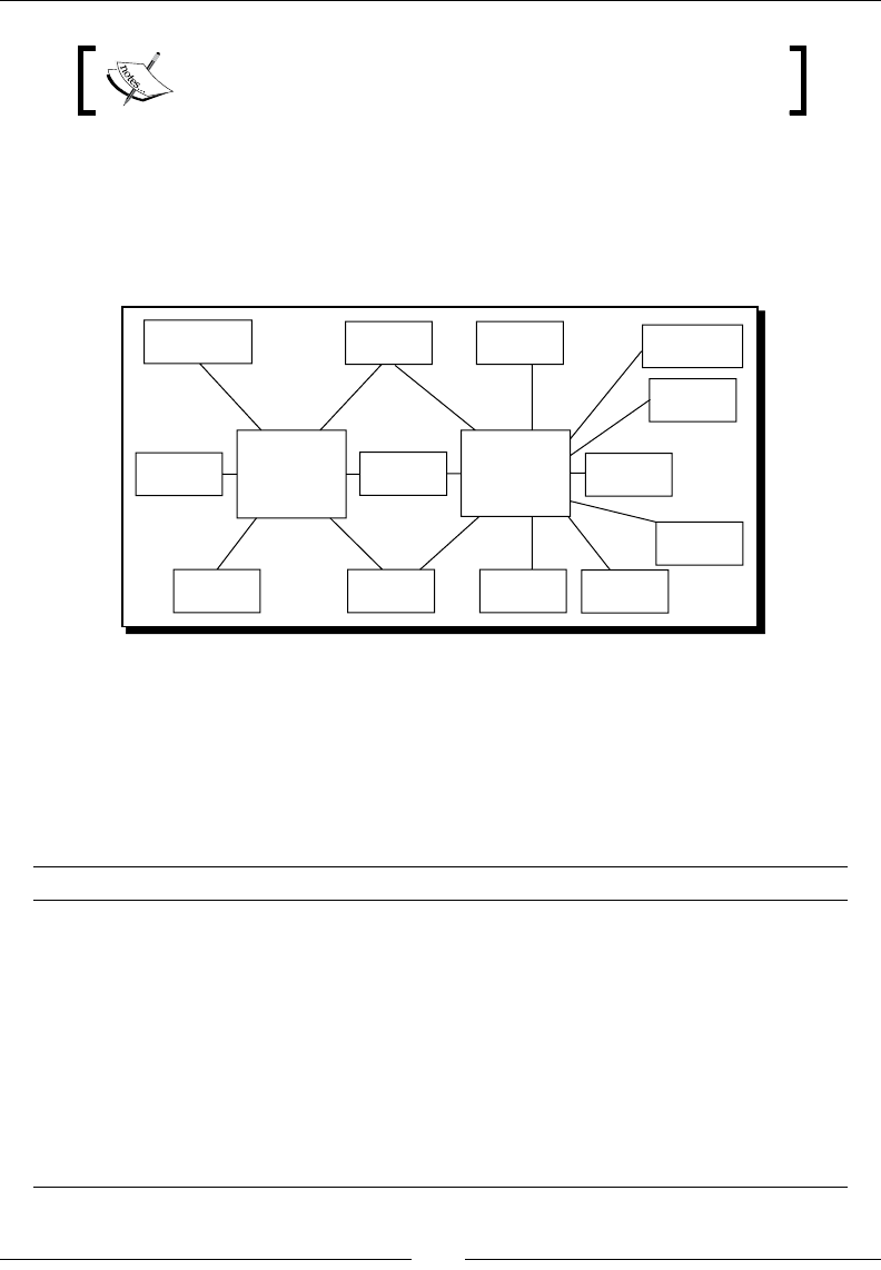
Developing and Implemenng a Simple Datamart
[ 376 ]
Note that you put in a Success entry to avoid the job failing aer
the failed evaluaon.
Extending the sales datamart model
You may, and you usually, have more than one fact table sharing some of the dimensions.
Look at the following diagram:
Product Type Time
Payment
Method
Buy
Method
Manufac
turer
SALES Region PUZZLES
SALES
Theme Glows in the
Dark
3D Puzzle
Wooden
Puzzle
Packaging
Pieces
Panoramic
Puzzle
It shows two stars sharing three dimensions: Regions, Manufacturers, and Time. The star model
to the le is the sales star model you already know. The star model to the right doesn't have
data for accessories, but does have more detail for puzzles such as the number of pieces they
have or the category or theme they belong to. When you have more than one fact table sharing
dimensions as here, you have what is called a constellaon.
The following table summarizes the dimensions added to the datamart:
Dimension Descripon
Pieces Number of pieces of the puzzle, grouped in the following ranges: 0-25,
26-100, and so on
Theme Classicaon of the puzzle in any of the following categories: Fantasy,
Castles, Landscapes, and so on
Glows in the dark Yes/No
3D puzzle Yes/No
Wooden puzzle Yes/No
Panoramic puzzle Yes/No
Packaging Number of puzzles packed together: 1, 2, 3, 4
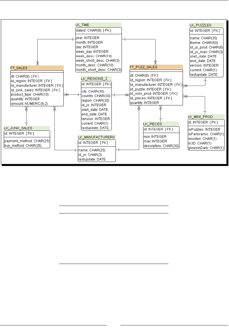
Chapter 12
[ 377 ]
The following is the updated ERD for the database that represents the model:
The new fact table is represented by a table named ft_puzz_sales.
The following table shows you the correspondence between the dimensions added to the
model and the tables in the database.
Dimension Table
Pieces lk_pieces
Theme lk_puzzles
Glows in the dark lk_mini_prod
3D puzzle lk_mini_prod
Wooden puzzle lk_mini_prod
Panoramic lk_mini_prod
Packaging lk_mini_prod
The following Hero exercise allows you to pracce what you learned in the tutorial, but this
me applied to the puzzle star model.

Developing and Implemenng a Simple Datamart
[ 378 ]
Have a go hero – loading the dimensions for the puzzles star model
In this exercise you will load some of the dimensions that were added to the model.
Create a transformaon that loads the lk_pieces dimension. You may create any
range you like. The following table may help you in the creaon:
min max description
0 25 Under 25
26 100 26-100
101 1000 101-1000
1001 2000 1001-2000
2000 99999 >2000
Create another transformaon that loads the lk_puzzles dimensions. This is a
Type II SCD, and you have already loaded it in Chapter 9. If you have the transformaon
that does it, half of your work is done.
Finally, modify the job in the tutorial by adding the execuon of these new
transformaons. Note that the lk_pieces dimension has to be loaded just once.
Loading a fact table with aggregated data
Now that you have data in your dimensions, you are ready to load the sales fact table. In this
secon, you will learn how to do it.
Time for action – loading the sales fact table by looking up
dimensions
Let's load the sales fact table, ft_sales, with sales informaon for a given range of dates.
Before doing this exercise, be sure that you have already loaded the dimensions. You did it in
the previous tutorial.
Also check that the database engine is up and that both the js and the js_dw databases are
accessible from PDI. If everything is in order, you are ready to start:
1. Create a new transformaon.
2. Drag a Table input step to the canvas.
3. Double-click the step. Select js as Connecon—the connecon to the
operaonal database.

Chapter 12
[ 379 ]
4. In the SQL frame type the following query:
SELECT i.inv_date
,d.man_code
,cu.city_id
,pr.pro_type product_type
,b.buy_desc
,p.pay_desc
,sum(d.cant_prod) quantity
,sum(d.price) amount
FROM invoices i
,invoices_detail d
,customers cu
,buy_methods b
,payment_methods p
,products pr
WHERE i.invoice_number = d.invoice_number
AND i.cus_id = cu.cus_id
AND i.buy_code = b.buy_code
AND i.pay_code = p.pay_code
AND d.pro_code = pr.pro_code
AND d.man_code = pr.man_code
AND i.inv_date BETWEEN cast('${DATE_FROM}' as date)
AND cast('${DATE_TO}' as date)
GROUP BY i.inv_date
,d.man_code
,cu.city_id
,pr.pro_type
,b.buy_desc
,p.pay_desc
5. Check the Replace variables in script? opon and click OK.
Let's retrieve the surrogate key for the manufacturer:
6. From the Lookup category, drag a Database lookup step to the canvas.
7. Create a hop from the Table input step to this new step.
8. Double-click the Database lookup step.
9. Select dw as Connecon—the connecon to the datamart database.
10. Click on Browse...and select the lk_manufacturers table.
11. Fill the upper grid with the following condion: id_js = man_code.
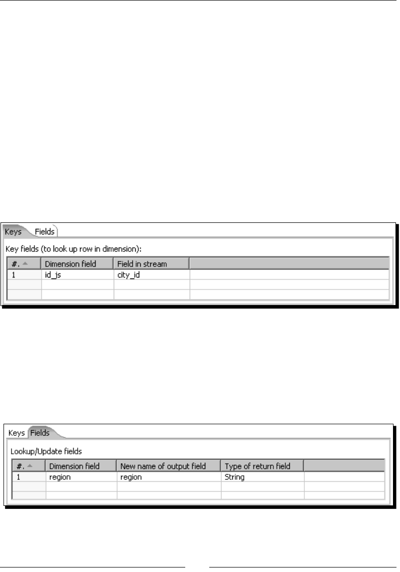
Developing and Implemenng a Simple Datamart
[ 380 ]
12. Fill the lower grid—under Field type id, as New name type id_manufacturer, as
Default type 0, and as Type select Integer.
13. Click on OK.
Now you will get the surrogate key for the region:
14. From the Data Warehouse category drag a Dimension lookup/update step to
the canvas.
15. Create a hop from the Database lookup step to this new step.
16. Double-click the Dimension lookup/update step.
17. As Connecon select dw.
18. Browse and select the lk_regions_2 table.
19. Fill the Keys grid as shown next:
20. Select id as Technical key eld. In the new name textbox, type id_region.
21. As Stream Dateeld select inv_date.
22. As Date range star eld and Table daterange end select start_date and end_date
respecvely.
23. Select the Fields tab and ll it like here:
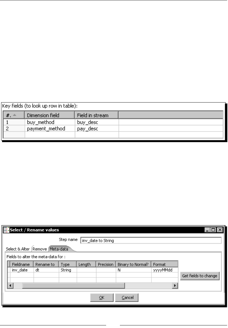
Chapter 12
[ 381 ]
Now it's me to generate the surrogate key for the junk dimension:
24. From the Data Warehouse category drag a Combinaon lookup/update step to the
canvas.
25. Create a hop from the Dimension lookup/update step to this new step.
26. Double-click the Combinaon lookup/update step.
27. Select dw as Connecon.
28. Browse and select the lk_junk_sales table.
29. Fill the grid as shown:
30. As Technical key eld type id. In the Creaon of technical key frame, leave the default
value Use table maximum + 1.
31. Click OK.
32. Add a Select values step and use it to rename the eld id to id_junk_sales.
Finally, let's do some adjustments and send the data to the fact table:
33. Add another Select values step to change the metadata of the inv_date eld
as shown:
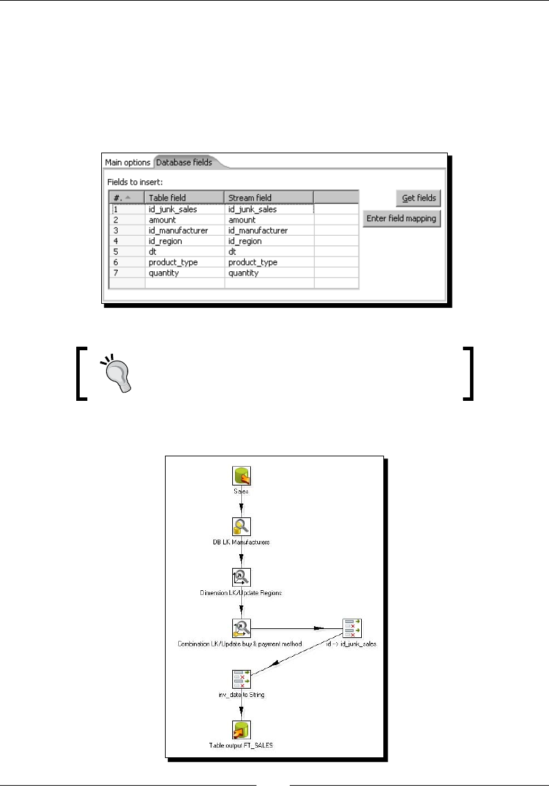
Developing and Implemenng a Simple Datamart
[ 382 ]
34. Add a Table output step and double-click it.
35. Select dw as Connecon.
36. Browse and select the ft_sales table.
37. Check the Specify database elds opon, select the Database elds grid, and ll it as
shown:
Remember that you can avoid typing by using the
Get elds buon.
38. Click on OK. The following is your nal transformaon. Press Ctrl+S to save it.
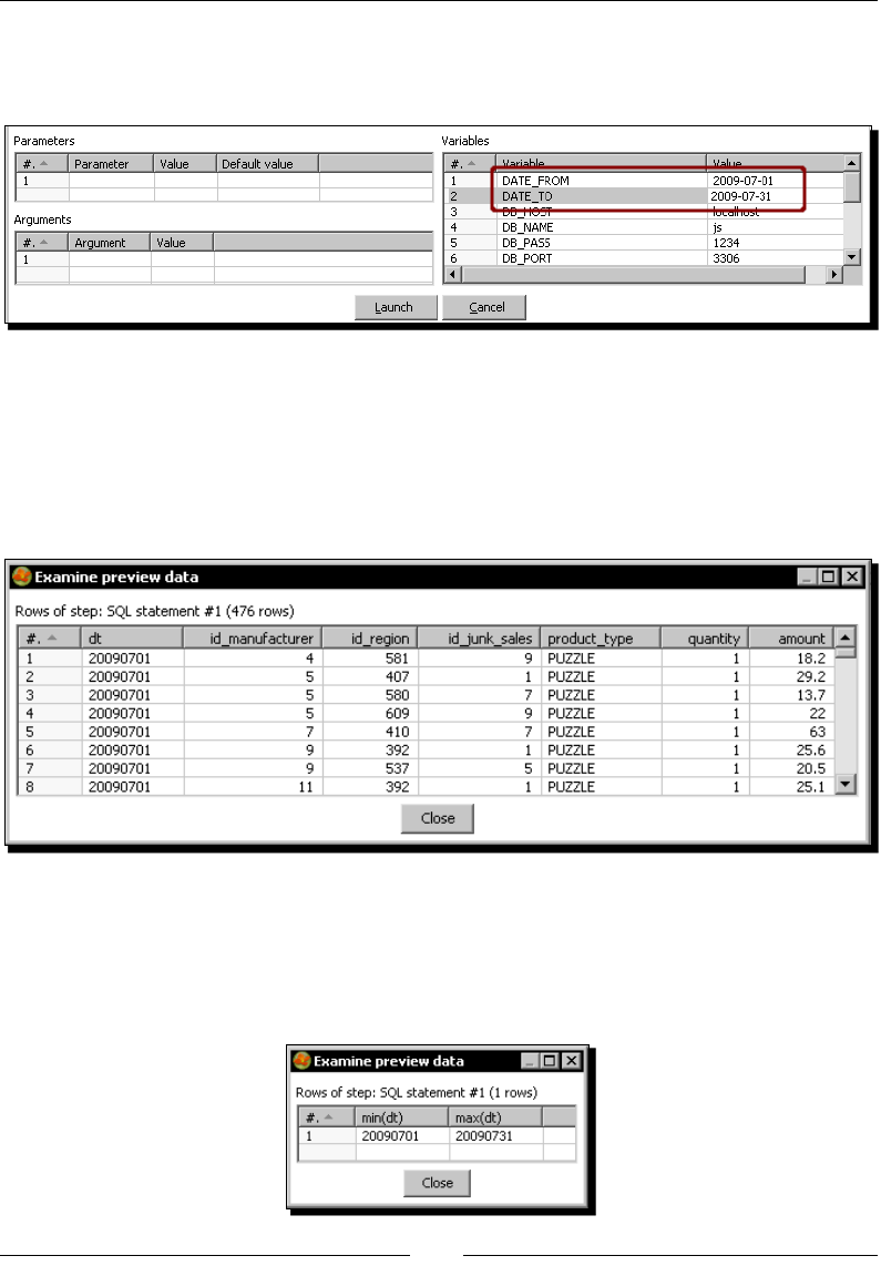
Chapter 12
[ 383 ]
39. Press F9 to run it.
40. In the sengs window, provide some values for the date range.
41. Click on Launch.
42. The fact table should have been loaded. To check it, open the database explorer and run
the following query:
SELECT * FROM ft_sales
You will get the following:
43. To verify that only the sales between the provided dates were processed, run the
following query:
SELECT MIN(dt), MAX(dt) FROM ft_sales
44. You will get the following:

Developing and Implemenng a Simple Datamart
[ 384 ]
What just happened?
You loaded the sales fact table with the sales in a given range of dates.
First of all you got the informaon from the source database. You did it by typing an SQL
query in a Table input step. You already know how a Table input step works.
As said, a fact table has foreign keys to the primary key of the dimension tables. The query
you wrote gave you business keys. So, aer geng the data from the source, you translated
the business keys into surrogate keys. You did it in dierent ways depending on the kind of
each related dimension.
Finally, you inserted the obtained data into the fact table ft_sales.
Getting the information from the source with SQL queries
You already know how to use a Table input step to get informaon from any database.
However, the query in the tutorial may have looked strange or long compared with the
queries you wrote in previous chapters. There is nothing mysterious in that query: It's simply
a maer of knowing what to put in it. Let's explain it in detail.
The rst thing you have to do in order to load the fact table is to look at the grain.
As menoned at the beginning of the chapter, the grain, or level of detail, of the fact is
implicitly expressed in terms of the dimension.
Looking at the model, you can see the following dimensions, along with their level of detail:
Dimension Level of detail (most atomic data)
Manufacturers manufacturer
Regions city
Time day
Product Type product type
Payment method payment method
Buy method buy method
Does this have anything to do with loading the fact? Well, the answer is yes. This is
because the numbers you have to put as measures in the numeric elds must be aggregated
accordingly to the dimensions. These are the measurements—quantity represenng the
number of products sold and Sales represenng the amounts.
So, in order to feed the table, what you need to take from the source is the sum of
quantity and the sum of sales for every combinaon of manufacturer, day, city,
product type, payment method, and buy method.

Chapter 12
[ 385 ]
In SQL terms you do it with a query such as the one you wrote in the Table input step. The
query is not as complicated as it may seem at rst. Let's dissect the query, beginning with
the FROM clause.
FROM invoices i
,invoices_detail d
,customers cu
,buy_methods b
,payment_methods p
,products pr
These are the tables to take the informaon from. The word following the name of the
table is an alias for the table—for example, pr for the table products. The alias is used
to disnguish elds that have the same name but are in dierent tables.
The database engine takes all the records for all the listed tables, side by side, and creates
all the possible combinaon of records where each new record has all the elds for all
the tables.
WHERE i.invoice_number = d.invoice_number
AND i.cus_id = cu.cus_id
AND i.buy_code = b.buy_code
AND i.pay_code = p.pay_code
AND d.pro_code = pr.pro_code
AND d.man_code = pr.man_code
These condions represent the join between tables. A join limits the number of
records you have when combining tables as explained above. For example, consider
the following condion:
i.cus_id = cu.cus_id
This condion implies that out of all the records, the engine keeps only those where
the customer ID in the table invoices is the same as that of the customer ID in the
table customers.
AND i.inv_date BETWEEN cast('${DATE_FROM}' as date)
AND cast('${DATE_TO}' as date)
This query simply lters the sales in the given range. The cast funcon converts a string
to a date.

Developing and Implemenng a Simple Datamart
[ 386 ]
Dierent engines have dierent ways to cast or convert elds from one data type
to another. If you are using an engine dierent from MySQL, you may have to
check your database documentaon and x this part of the query.
GROUP BY i.inv_date
,d.man_code
,cu.city_id
,pr.pro_type
,b.buy_desc
,p.pay_desc
By using the GROUP BY clause, you ask the SQL engine that for each dierent combinaon of
the listed elds, it should return just one record.
Finally, look at the elds following the SELECT clause:
SELECT i.inv_date
,d.man_code
,cu.city_id
,pr.pro_type product_type
,b.buy_desc
,p.pay_desc
,sum(d.cant_prod) quantity
,sum(d.price) amount
These elds are the business keys you need—date of sale, manufacturer, city, and so
on—one for each dimension in the sales model. Note the word product_type aer
the pro_type eld. This is an alias for the eld. Using an alia,s the eld is renamed in
the output.
As you can see, with the excepon of the highlighted elds, the elds you put aer the
SELECT clause are exactly the same as you put in the GROUP BY clause. When you have a
GROUP BY clause in your sentence, aer the SELECT clause you can put only those elds
that are listed in the GROUP BY clause or aggregated funcons such as the following:
,sum(d.cant_prod) quantity
,sum(d.price) amount
sum() is an aggregate funcon that gives you the sum of the column you put into brackets.
Therefore, these last two elds are the sum of the cant_prod eld and the sum of the
price eld for all the grouped records. These two elds give you the measures for your
fact table.
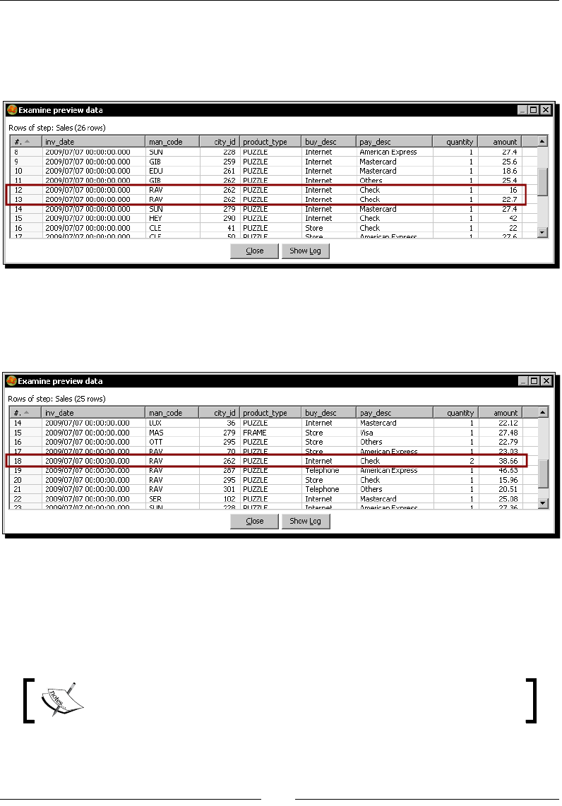
Chapter 12
[ 387 ]
To conrm that the GROUP BY works as explained, let's explore one example. Remove from
the query, the sum() funcons, leaving just the elds, along with the GROUP BY clause.
Do a preview seng 2009-07-07 both as start_date and end_date. You will see
the following:
As you can see, in the same day, in the same city, you sold two products of the same type, made
for the same manufacturer, by using the same payment and buy method. In the fact table you will
not save two records, but will save a single record. Restore the original query and do a preview.
You will see the following:
Here you can see that the GROUP BY clause has grouped those two records into a single one. For
quantity and amount it summed the individual values.
Note that the GROUP BY clause, along with the aggregate funcons, does the same as you
could have done by using a Sort rows step to sort by the listed elds, followed by a Group by
step to get the sum of the numeric elds.
Wherever the database can do the operaons, for performance reasons it's
recommended that you allow the database engine do it.
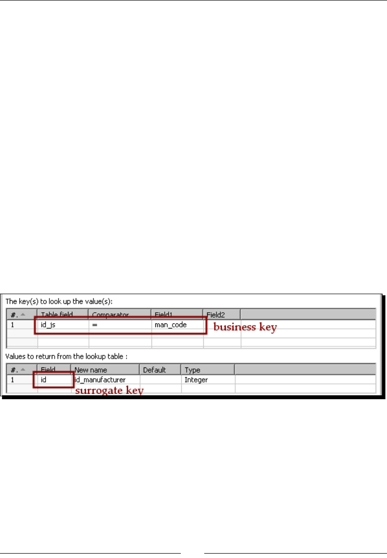
Developing and Implemenng a Simple Datamart
[ 388 ]
Translating the business keys into surrogate keys
You already have the transaconal data for the fact table. But that data contains business
keys. Look at the elds denion for your fact table:
dt CHAR(8) NOT NULL,
id_manufacturer INT(10) NOT NULL,
id_region INT(4) NOT NULL,
id_junk_sales INT(10) NOT NULL,
product_type CHAR(10) NOT NULL,
quantity INT(6) DEFAULT 0 NOT NULL,
amount NUMERIC(8,2) DEFAULT 0 NOT NULL
id_manufacturer, id_region, and id_junk_sales are foreign keys to surrogate keys.
So, before inserng the data into the fact, for each business key you have to nd the proper
surrogate key. Depending on the kind of dimensions referenced by the IDs in the fact table,
you get those IDs in a dierent way. Let's see in the following secon, how you do it in
each case.
Obtaining the surrogate key for a Type I SCD
For geng the surrogate key in the case of a Type I SCD such as the Manufacturer one, you
used a Database lookup step. You are already familiar with this step, so understanding how
to use it is easy.
In the rst grid you provided the business keys. The key to look up in the incoming stream is
man_code, whereas the key to look up in the dimension table is stored in the eld id_js.
With the Database lookup step you returned the eld named id, which is the eld that
stores the surrogate key. You renamed it to id_manufacturer, as this is the name you
need for the fact table.
If the key is not found, you use 0 as default, that is, the record in the dimension reserved for
unknown values.
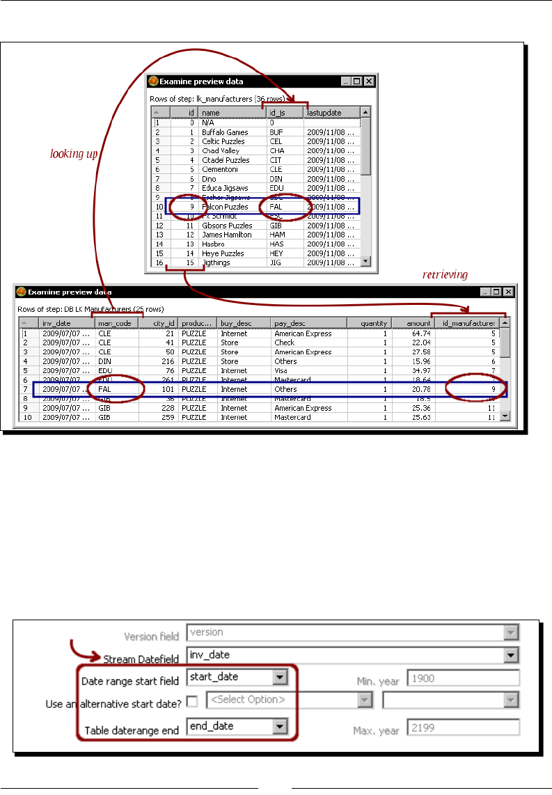
Chapter 12
[ 389 ]
The following screenshot shows you how it works:
Obtaining the surrogate key for a Type II SCD
In the case of a Type II SCD such as the Region dimension, you used the same step that was
used to load the table dimension—a Dimension L/U step. The dierence is that here you
unchecked the Update the dimension? opon. By doing that, the step behaves just as a
database lookup—you provide the keys to lookup and the step returns the elds you put
both in the Fields tab and in the Technical key eld opon. The dierence with this step is
that here you have to provide me informaon. By using that me informaon, PDI nds
and returns, from the Type II SCD, the proper record in me:
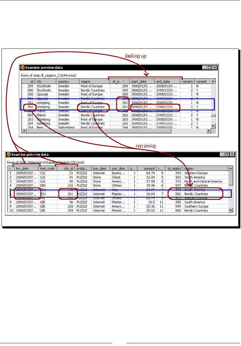
Developing and Implemenng a Simple Datamart
[ 390 ]
Here you give PDI the names for the columns that store the data ranges—start_date
and end_date. You also give it the name of the eld stream to use in order to compare
the dates—in this case inv_date, that is, the date of the sale.
Look at the following screenshot to understand how the lookup works:
The step has to get the surrogate key for the city with ID 261. There are two records
for that city. The key is in nding the proper record, the record valid on 07/07/2009.
So, PDI compares the date provided against the start_date and end_date elds
and returns the surrogate key 582, for which the city is classied as belonging to the
Nordic Countries region.
If no record is found for the given keys on the given date, the step retrieves the ID 0, which is
used for the unknown data.
Chapter 12
[ 391 ]
Obtaining the surrogate key for the Junk dimension
The payment and buy methods are stored in a junk dimension. A junk dimension can be
loaded by using a Combinaon L/U step. You learned how to use this step in the Time for
acon named Loading a region dimension with a Combinaon lookup/update step in
Chapter 9. As all the elds in a junk dimension are part of the primary key, you don't
need an extra Update step to load it.
In the tutorial, you loaded the dimension at the same me you loaded the fact. You know
from Chapter 9 that when you use a Combinaon L/U step, the step returns you the
generated key. So, the use of the step here for loading and geng the key at the same
me ts perfectly.
If the dimension had been loaded previously, instead of a Combinaon
L/U step you could have used a Database lookup step by pung the key
elds in the upper grid and the key in the lower grid of the Database lookup
conguraon window.
Obtaining the surrogate key for the Time dimension
You already obtained the surrogate keys for Type I and Type II SCDs and for the Junk
dimension. Finally, there is a Time dimension. As for the key, you use the date in string format;
the method for geng the surrogate key is simply changing the metadata from date to string
by using the proper format. Once again, if you had used a regular surrogate key instead of the
date, for geng the surrogate key you would have to use a Database lookup step.
The following table summarizes the dierent possibilies:
Dimension type Method for geng the surrogate key Sample
dimension
Type I SCD Database lookup step. Manufacturer
Type II SCD Dimension L/U step. Regions
Junk and Mini Combinaon L/U step if you load the dimension at the same
me as you load the fact (as in the tutorial).
Database lookup step if the dimension is already loaded.
Sales Junk
dimension
Degenerate As you don't have a table nor key to translate, you just store the
data as a eld in the fact. You don't have to worry about geng
surrogate keys.
Product Type
Time Change the metadata to the proper format if you use date as the
key (as in the tutorial).
Dimension L/U step if you use a normal surrogate key.
Time

Developing and Implemenng a Simple Datamart
[ 392 ]
Pop quiz – modifying a star model and loading the star with PDI
Suppose you want to do some modicaons to your star model. What are the changes you'll
have to make in each case:
1. Instead of using a region dimension that keeps history of the changes (Type II SCD),
you want to use a classic region dimension (Type I).
a. As table for the region dimension:
i. You reuse the table lk_regions_2.
ii. You use a dierent table.
iii. Any of the above.
b. As eld with the foreign key in the fact table:
i. You reuse the id_region eld.
ii. You create a new eld.
c. For geng the surrogate key:
i. You keep using the Dimension lookup/update step.
ii. You replace the Dimension lookup/update step by another step.
iii. It depends on the how your dimension table looks.
2. You want to change the grain for the Time dimension; you are interested in
monthly informaon.
a. As table for the me dimension:
i. You reuse the table lk_time.
ii. You use a dierent table.
iii. Any of the above.
b. As eld with the foreign key in the fact table:
i. You reuse the dt eld.
ii. You create a new eld.
c. For geng the surrogate key:
i. You keep using the Select values step and changing the metadata.
ii. You use another method.

Chapter 12
[ 393 ]
3. You decided to create a new table for the product type dimension. The table will
have the following columns: id, product_type_description, and product_
type. As data you would have, for example: 1, puzzle, puzzle for the product
type puzzle, or 2, glue, accessory for the product type glue.
a. As eld with the foreign key in the fact table:
i. You reuse the product_type eld.
ii. You create a new eld.
b. For geng the surrogate key:
i. You use a Combinaon lookup/update step
ii. You use a Dimension lookup/update step
iii. You use a Database lookup/update step
Have a go hero – loading a puzzles fact table
In the previous Hero exercise you were asked to load the dimensions for the puzzle star
model. Now you will load the fact table.
To load the fact table you'll need to build a query taking data from the source. Try to gure
out what the query looks like. Then you may try wring the query by yourself, or you may
cheat; this query will serve you as a starng point:
SELECT
i.inv_date
,d.man_code
,cu.city_id
,pr.pro_theme
,pr.pro_pieces
,pr.pro_packaging
,pr.pro_shape
,pr.pro_style
,SUM(d.cant_prod) quantity
FROM invoices i
,invoices_detail d
,customers cu
,products pr
WHERE i.invoice_number = d.invoice_number
AND i.cus_id = cu.cus_id
AND d.pro_code = pr.pro_code
AND d.man_code = pr.man_code
AND pr.pro_type like 'PUZZLE'
AND i.inv_date BETWEEN cast('${DATE_FROM}' as date)
AND cast('${DATE_TO}' as date)

Developing and Implemenng a Simple Datamart
[ 394 ]
GROUP BY i.inv_date
,d.man_code
,cu.city_id
,pr.pro_theme
,pr.pro_pieces
,pr.pro_packaging
,pr.pro_shape
,pr.pro_style
Aer that, look for the surrogate keys for dimensions of Type I and II.
Here you have a mini-dimension. You may load it at the same me you load the fact as you
did in the tutorial with the Junk dimension. Also, make sure that you properly modify the
metadata for the me eld.
Insert the data into the fact, and check whether the data was loaded as expected.
Getting facts and dimensions together
Loading the star involves both loading the dimensions and loading the fact. You already loaded
the dimensions and the fact separately. In the following two tutorials, you will put it all together:
Time for action – loading the fact table using a range of dates
obtained from the command line
Now you will get the range of dates from the command line and load the fact table using
that range:
1. Create a new transformaon.
2. With a Get system info step, get the rst two arguments from the command line and
name them date_from and date_to.
3. By using a couple of steps, check that the arguments are not null, have the proper
format (yyyy-mm-dd), and are valid dates.
4. If something is wrong with the arguments, abort.
5. If the arguments are valid, use a Set variables step to set two variables named
DATE_FROM and DATE_TO.
6. Save the transformaon in the same folder you saved the transformaon that loads the
fact table.
7. Test the transformaon by providing valid and invalid arguments to see that it works
as expected.
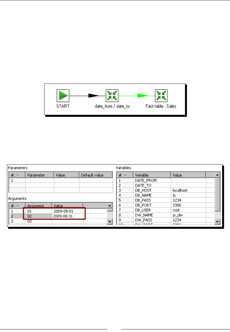
Chapter 12
[ 395 ]
8. Create a job and save it in the same folder you saved the job that loads the dimensions.
9. Drag to the canvas a START and two transformaon job entries, and link them one aer
the other.
10. Use the rst transformaon entry to execute the transformaon you just created.
11. Use the second transformaon entry to execute the transformaon that loads the
fact table.
12. This is how your job should look like:
13. Save the job.
14. Press F9 to run the job.
15. Fill the job sengs window as follows:
16. Click on Launch.

Developing and Implemenng a Simple Datamart
[ 396 ]
17. When the execuon nishes, explore the database to check that the data for the given
dates was loaded in the fact table. You will see this:
What just happened?
You built a main job that loads the sales fact table. First, it reads from the command line the
range of dates to be used for loading the fact and validates it. If they are not valid, the process
aborts. If they are valid, the fact table is loaded for the dates in that range.
Time for action – loading the sales star
You already created a job for loading the dimensions and another job for loading the fact.
In this tutorial, you will put them together in a single main job:
1. Create a new job in the same folder in which you saved those jobs. Name this job
load_dm_sales.kjb.
2. Drag to the canvas a START and two job entries, and link them one aer the other.
3. Use the rst job entry to execute the job that loads the dimensions.
4. Use the second Job entry to execute the job you just created for loading the fact table.
5. Save the job. This is how it looks:

Chapter 12
[ 397 ]
6. Press F9 to run the job.
7. As arguments, provide a new range of dates: 2009-09-01, 2009-09-30. Then
press Launch.
8. The dimensions will be loaded rst, followed by the loading of the fact table.
9. The Job metrics tab in the Execuon results window shows you the whole
process running:

Developing and Implemenng a Simple Datamart
[ 398 ]
10. Exploring the database, you'll see once again the data updated:
What just happened?
You built a main job that loads the sales datamart. First, it loads the dimensions. Aer that, it
loads the fact table by ltering sales in a range of dates coming from the command line.
Have a go hero – enhancing the loading process of the sales fact table
Facts tables are rarely updated. Usually you just insert new data. However, aer loading a
fact, you may detect that there were errors in the source. Or it could also happen that some
data arrives late to the system. In order to take into account those situaons, you should
have the possibility to reprocess data already processed. To avoid duplicates in the fact table,
do the following modicaon to the loading process:
Aer geng the start and end date and before loading the fact table, delete the records that
may have been inserted in a previous execuon for the given range of dates.
Have a go hero – loading the puzzles sales star
Modify the main job so that it also loads the puzzle fact table.
Make sure that the job that loads the dimensions includes all the dimensions needed for both
fact tables. Also, pay aenon that you don't read and validate the arguments twice.
Have a go hero – loading the facts once a month
Modify the whole soluon so the loading of the fact tables is made once a month. Don't modify
the model! You sll want to have daily informaon in the fact tables; what you want to do is
simply replace the daily updang process with a monthly process. Ask for a single parameter as
yyyymm and validate it. Replace the old parameters START_DATE and END_DATE with this new
one, wherever you use them.
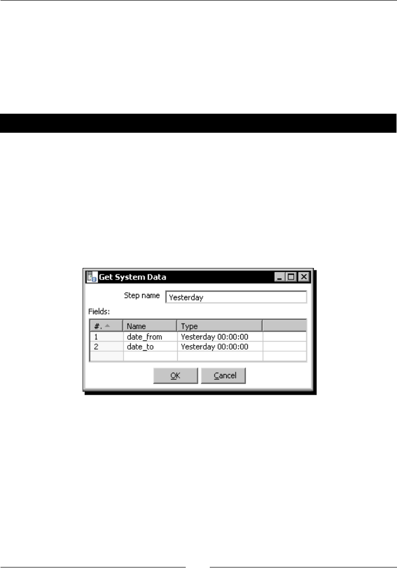
Chapter 12
[ 399 ]
Getting rid of administrative tasks
The soluon you built during the chapter loads both dimensions and fact in a star model for
a given range of dates. Now suppose that you want to keep your datamart always updated.
Would you sit every day in front of your computer, and run the same job over and over
again? You probably would, but you know that it wouldn't be a good idea. There are beer
ways to do this. Let's see how you can get rid of that task.
Time for action – automating the loading of the sales datamart
Suppose that every day you want to update your sales datamart by adding the informaon
about the sales for the day before. Let's do some modicaons to the jobs and
transformaons you did so that the job can run automacally.
In order to test the changes, you'll have to change the date for your system. Set the current
date as 2009-10-02.
1. Create a new transformaon.
2. Drag to the canvas a Get system data step and ll it like here:
3. With a Select values step, change the metadata of both elds: As type put String
and as format, yyyy-MM-dd.
4. Add a Set variables step and use the two elds to create two variables named
START_DATE and END_DATE.
5. Save the transformaon in the same folder you saved the transformaon that loads
the fact.
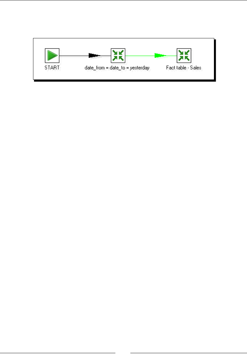
Developing and Implemenng a Simple Datamart
[ 400 ]
6. Modify the job that loads the fact so that instead of execung, the transformaon
that takes the range of dates from the command line executes this one. The job
looks like this:
7. Save it.
Now let's create the scripts for execung the job from the command line:
1. Create a folder named log in the folder of your choice.
2. Open a terminal window.
3. Create a new le with your favorite text editor.
4. If your system is not Windows, go to step 7.
5. Under Windows systems, type the following:
for /f "tokens=1-3 delims=/- " %%a in ('date /t') do set
XDate=%%c%%b%%a
for /f "tokens=1-2 delims=: " %%a in ('time /t') do set
XTime=%%a.%%b
set path_etl=C:\pdi_labs
set path_log=C:\logs
c:\
cd ..
cd pdi-ce
kitchen.bat /file:%path_etl%\load_dm_sales.kjb /level:Detailed >>
%path_log%\sales_"%Xdate% %XTime%".log
6. Save the le as dm_sales.bat in a folder of your choice. Skip the following
two steps.

Chapter 12
[ 401 ]
7. Under Linux, Unix, and similar systems, type the following:
UNXETL=/pdi_labs
UNXLOG=/logs
cd /pdi-ce
kitchen.sh /file:$UNXETL/load_dm_sales.kjb /level:Detailed >>
$UNXLOG/sales_'date +%y%m%d-%H%M'.log
8. Save the le as dm_sales.sh in a folder of your choice.
Irrespecve of your system, please replace the names of the
folders in the highlighted lines with the names of your own
folders, that is path_etl (the folder where your main job is),
path_log (the folder you just created), and pdi-ce (the
folder where PDI is installed).
Now let's test what you've done:
1. Execute the batch you created:
Under windows, type: dm_sales.bat
Under Unix-like systems, type: sh dm_sales.sh
2. When the prompt in the command window is available, it means that the batch
ended. Check the log folder. You'll nd a new le with the extension log, named
sales followed by the date and hour, for example:sales_0210Fri 06.46.log.
3. Edit the log. You'll see the full log for the execuon of the job. Within the lines, you'll
see these:
INFO 02-10 17:46:39,015 - Set Variables DATE_FROM and DATE_TO.0
- Set variable DATE_FROM to value [2009-10-01]
INFO 02-10 17:46:39,015 - Set Variables DATE_FROM and DATE_TO.0
- Set variable DATE_TO to value [2009-10-01]
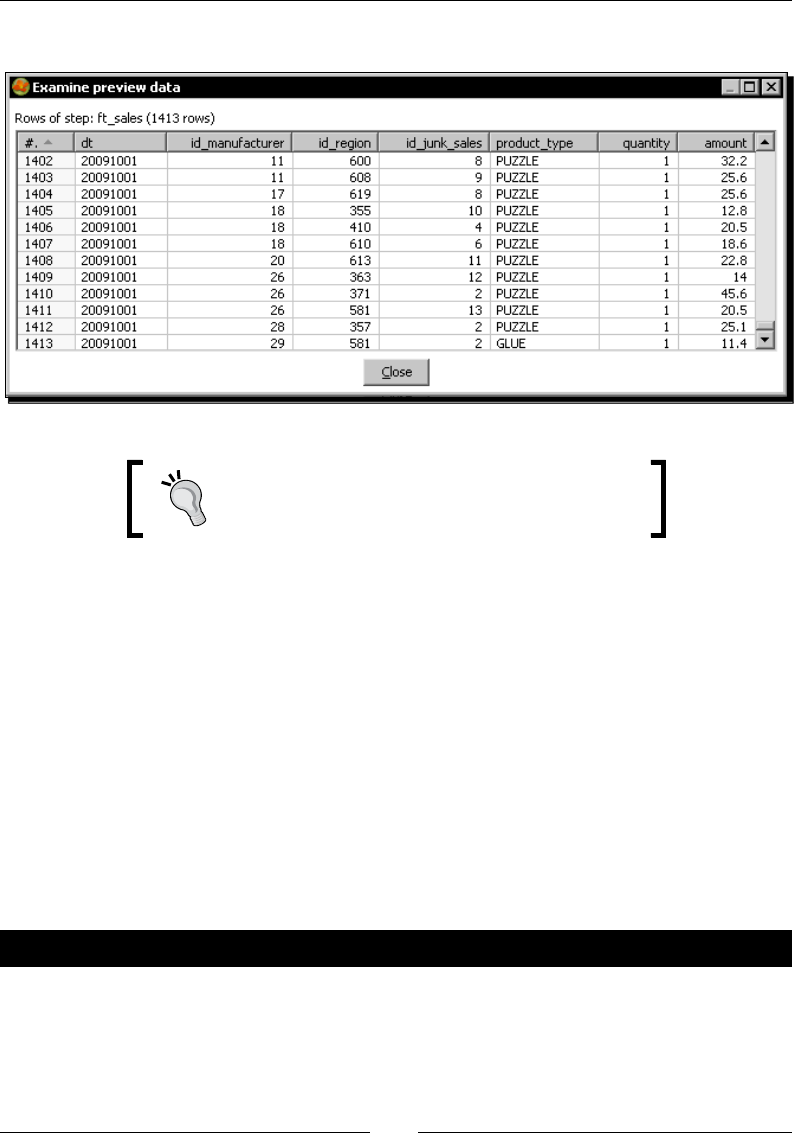
Developing and Implemenng a Simple Datamart
[ 402 ]
4. Also check the fact table. The fact should have data for the sales made yesterday:
Don't forget to restore the date in your system!
What just happened?
You modied the job that loads the sales datamart so that it always loads the sales from a
day before. You also created a script that embedded the execuon of the Kitchen command
and sent the result to a log. The name of the log is dierent for every day; this allows you
keep a history of logs.
To understand exactly the full Kitchen command line you put into the scripts, please refer to
Appendix B, Pan and Kitchen: Launching Transformaons and Jobs from the Command Line.
Doing all this, you don't have to worry about providing dates for the process, nor running
Spoon, nor remembering the syntax of the Kitchen command. Not only that, if you use a
system ulity such as a cron in Unix or the scheduler in Windows to schedule this script to
run every day aer midnight, you are done. You got rid of all the administrave tasks!
Have a go hero – Creating a back up of your work automatically
Choose a folder where you use to save your work (it could be for example the pdi_labs folder)
Create a job that zips your work under the name backup_yyyymmdd.zip where yyyymmdd
represents the system date. Test the job.

Chapter 12
[ 403 ]
Then create a .bat or .sh le that executes your job sending the log to a le. Test the script.
Finally, schedule the script to be executed weekly.
Have a go hero – enhancing the automate process by sending an e-mail if
an error occurs
Modify the main job so if something goes wrong, it sends you an e-mail reporng the problem.
Doing so, you don't have to worry about checking the daily log to see if everything went ne.
Unless there is a problem with the e-mail server, you'll be noed whenever some error occurs.
Summary
In this chapter you created a set of jobs and transformaons that loads a sales datamart.
Specically, you learned how to load a fact table and to embed that process into a bigger
one—the process that loads a full datamart.
You also learned to automate PDI processes, which is useful to get rid of tedious and
repeve manual tasks. In parcular, you automated the loading of your sales datamart.
Beyond that, you must have found this chapter useful for reviewing all you learned since
the rst chapter. If you can't wait for more, read the next chapter. There you will nd useful
informaon for going further.

13
Taking it Further
The lessons learned in previous chapters gave you the basis of PDI. If you liked
working with PDI and intend to use it in your own projects, there is much more
ranging from applying best pracces to using PDI integrated with the Pentaho
BI Suite.
This chapter points you the right direcon for taking it further. The chapter begins by giving
you some advice to take into account in your daily work with PDI. Aer that it introduces you
some advanced PDI concepts for you to know to what extent you can use the tool beyond
the basics.
PDI best practices
If you intend to work seriously with PDI, knowing how to accomplish dierent tasks is not
enough. Here are some guidelines that will help you go in the right direcon.
Outline your ideas on paper before creang a transformaon or a job:
Don't drop steps randomly on the canvas trying to get things working. You could end
up with a transformaon or job that is dicult to understand and even useless.
Document your work:
Write at least a simple descripon in the transformaons and jobs seng windows.
Replace the default names of steps and job entries with meaningful ones. Use notes
to clarify the purpose of the transformaons and jobs. Doing this, your work will be
quite self documented.

Taking it Further
[ 406 ]
Make your jobs and transformaons clear to understand:
Arrange the elements in the canvas so that it doesn't look like a puzzle to solve.
Memorize the shortcuts for arrangement and alignment, and use them regularly.
You'll nd a full list in Appendix D, Spoon shortcuts.
Organize PDI elements in folders:
Don't save all the transformaons and jobs in the same folder. Organize them
according to their purpose.
Make your work exible and reusable:
Make use of arguments, variables, and named parameters. If you idenfy tasks that
are going to be used in several situaons, create subtransformaons.
Make your work portable (ready for deployment):
This involves making sure even if you move your work to another machine or
another folder, or the paths to source or desnaon les change, or the connecon
properes to the databases change, everything should work either with minimal
changes or without changes. In order to make ensure that, don't use xed names
but variables. If you know the values for the variables beforehand, dene the
variables in the kettle.properties le. For the name of the transformaons and
jobs, use relave paths—use the ${Internal.Job.Filename.Directory} and
${Internal.Transformation.Filename.Directory} variables.
Avoid overloading your transformaons:
A transformaon should do a precise task. If it doesn't, think of spling it in two
or more, or create subtransformaons. Doing this will make your transformaon
clearer and also reusable in the case of subtransformaons.
Handle errors:
Try to gure out the kind of errors that may happen and trap them by validang and
handling errors, and taking appropriate acons such as xing data, taking alternave
paths, sending friendly message to the log les, and so on.
Do everything you can to opmize the PDI performance:
You can nd a full checklist at http://wiki.pentaho.com/display/COM/PDI+
Performance+tuning+check-list. As of version 3.1.0, PDI introduced a tool for
tracking the performance of individual steps in a transformaon. You can nd more
informaon at http://wiki.pentaho.com/display/EAI/Step+performance
+monitoring.
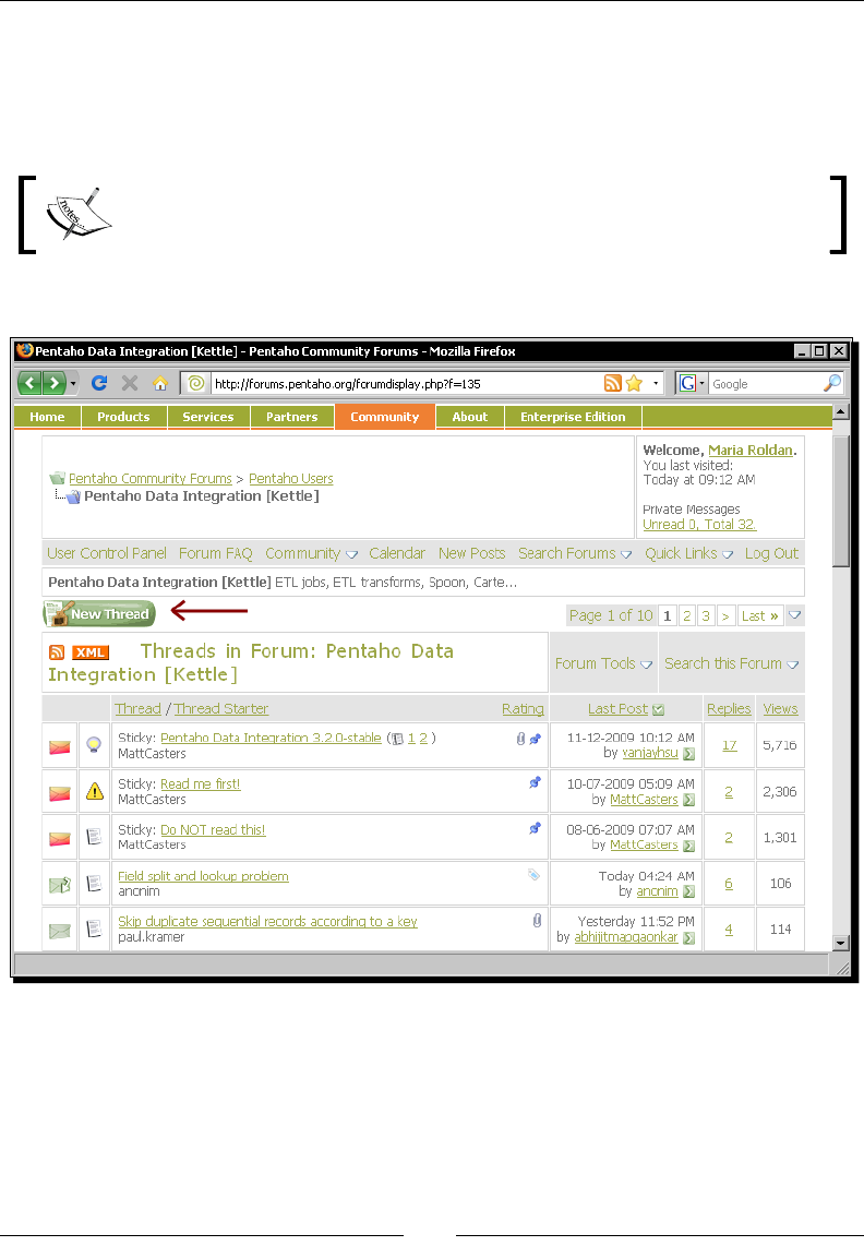
Chapter 13
[ 407 ]
Keep track of jobs and transformaons history:
You can use a versioning system such as subversion. Doing so, you could recover
older versions of your jobs and transformaons or examine the history of how they
changed. For more on subversion, visit http://subversion.tigris.org/.
Bookmark the forum page and visit it frequently. The PDI forum is available
at http://forums.pentaho.org/forumdisplay.php?f=135.
The following is the main PDI forum page:
If you get stuck with something, search for a soluon in the forum. If you don't nd what you're
looking for, create a new thread, expose your doubts or scenario clearly, and you'll get a prompt
answer, as the Pentaho community, and parcularly the PDI one, is quite acve.

Taking it Further
[ 408 ]
Getting the most out of PDI
Throughout the book you learned, step by step, how to use PDI for accomplishing several
kinds of tasks— reading from dierent kinds of sources, wring back to them, transforming
data in several ways, loading data into databases, and even loading a full data mart. You
already have the knowledge and the experience to do anything you want or you need with
PDI from now on. However, PDI oers you some more features that may be useful for you as
well. The following secons will introduce them and will guide you so that you know where
to look for in case they want to put them into pracce.
Extending Kettle with plugins
As you could see while learning Kele, there is a large set of steps and job entries to choose
from when designing jobs and transformaons. The number rises above 200 between steps
and entries! If you sll feel like you need more, there are more opons—plugins.
Kele plugins are basically steps or job entries that you install separately. The available
plugins are listed at http://wiki.pentaho.org/display/EAI/List+of+Available+
Pentaho+Data+Integration+Plugins.
Most of the listed plugins can be downloaded and used for free. Some are so popular or
useful that they end up becoming standard steps of PDI—for example, the Formula step that
you used several mes throughout the book.
There are other plugins that come as a trial version and you have to pay to use them.
It's also possible for you to develop your own plugins. The only prerequisite is knowing how
to develop code in Java. If you are interested in the subject, you can get more informaon at
http://wiki.pentaho.com/display/EAI/Writing+your+own+Pentaho+Data+Int
egration+Plug-In.
It's no coincidence that the author of those pages is Jens Bleuel. Jens used the
plugin architecture back in 2004, in order to connect Kele with SAP, when he was
working at Prorao. The plugin support was incorporated in Kele 2.0 and the
PRORATIO - SAP Connector, today available as a commercial plugin, was one of
the rst developed Kele plugins.
You should know that 3.x plugins no longer work on Kele 4.0.
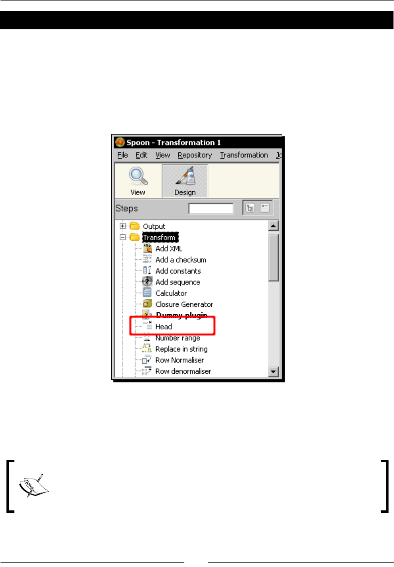
Chapter 13
[ 409 ]
Have a go hero – listing the top 10 students by using the Head plugin step
Browse the plugin page and look for a plugin named Head. As described in the page, this
plugin is a step that keeps the rst x rows of the stream. Download the plugin and install it.
The installaon process is really straighorward. You have to copy a couple of *.jar les to
the libext directory inside the PDI installaon folder, add the environment variable for the
PDI to nd the libraries, and restart Spoon. The downloaded le includes a documentaon
with full instrucons. Once installed, the Head will appear as a new step within the
Transformaon category of steps as shown here:
Create a transformaon that reads the examinaon le that was used in the Time for Acon
– reviewing examinaon by using the Calculator step secon in Chapter 3 and some other
chapters as well. Generate an output le with the top 10 students by average score in
descending order. In order to keep the top 10, use the Head plugin.
Before knowing of the existence of this plugin, you used to do this kind of
ltering by using the JavaScript step. Another way to do it is by using an Add
sequence step followed by a Filter rows step. Note that none of these methods
use an ad hoc step.
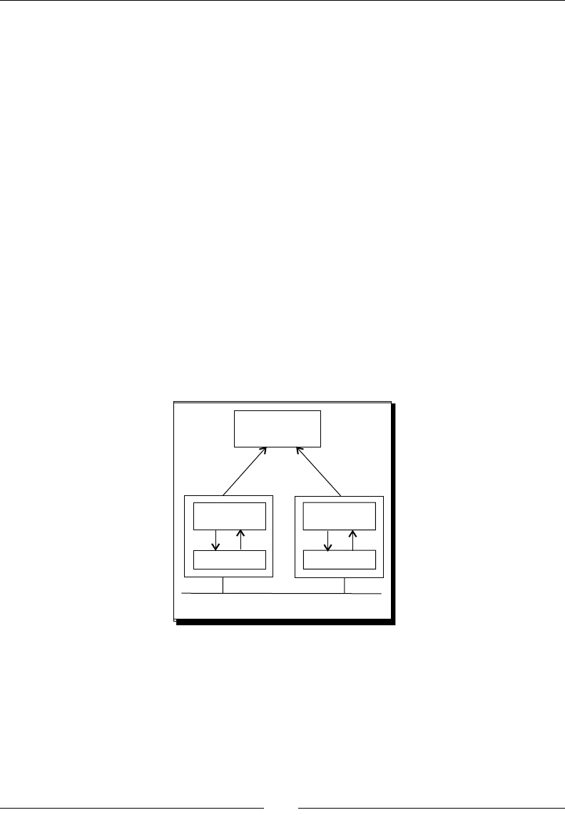
Taking it Further
[ 410 ]
Overcoming real world risks with some remote execution
In order to learn to use Kele, you used very simple and small sets of data. It's worth saying
that all you learned can be also applied for processing huge les and databases with millions
of records. However, that's not for free! When you deal with such datasets, there are many
risks—your transformaons slow down, you may run out of memory, and so on.
The rst step in trying to overcome those problems is to do some remote execuon. Suppose
you have to process a huge le located at a remote machine and that the only thing you
have to do with that le is to get some stascs such as the maximum, minimum, and
average value for a parcular piece of data in the le. If you do it in the classic way, the data
in the le would travel along the network for being processed by Kele in your machine,
loading the network unnecessarily.
PDI oers you the possibility to execute the tasks remotely. The remote execuon capability
allows you to run the transformaon in the machine where the data resides. Doing so, the
only data that would travel through the network will be the calculated data.
This kind of remote execuon is done by Carte, a simple server that you can install in
a remote machine and that does nothing but run jobs and transformaons on demand.
Therefore, it is called a slave server. You can start, monitor, and stop the execuon of
jobs and transformaons remotely as depicted here:
Transformations
and Jobs
Starts
Monitors
Stops
SPOON CARTE
Executes
Kettle Engine Kettle Engine
Network
You don't need to download addional soware because Carte is distributed as part of the
Kele soware. For documentaon on carte, follow this link: http://wiki.pentaho.
com/display/EAI/Carte+User+Documentation.
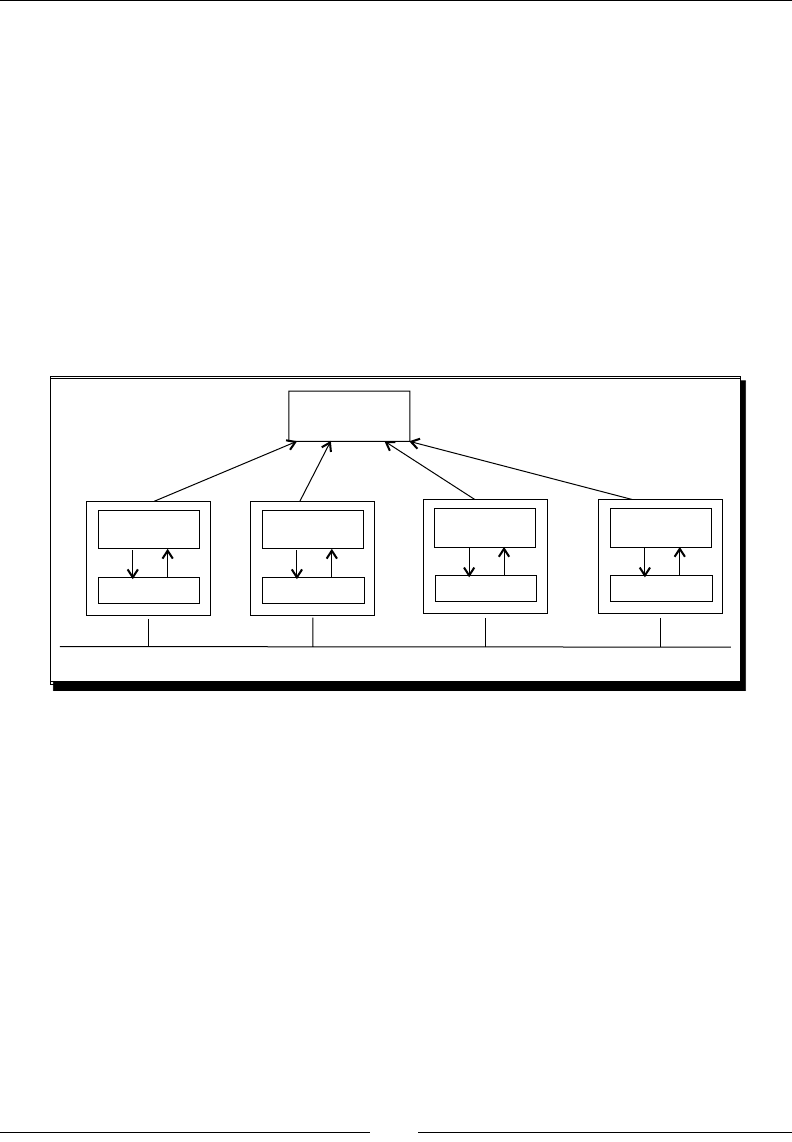
Chapter 13
[ 411 ]
Scaling out to overcome bigger risks
As menoned above, PDI can handle huge volumes of data. However, the bigger the volume
or complexity of your tasks, the bigger the risks. The soluon not only lies in execung
remotely, but in order to enhance your performance and avoid undesirable situaons, you'd
beer increase your power. You basically have two opons—you can either scale up or
scale out. Scaling up involves buying a beer processor, more memory, or disks with more
capacity. Scaling out means to provide more processing power by distribung the work over
mulple machines.
With PDI you can scale out by execung jobs and transformaons in a cluster. A cluster is a
group of Carte instances or slave servers that collecvely execute a job or a transformaon.
One of those servers is designed as the master and takes care of controlling the execuon
across the cluster. Each server executes only a poron of the whole task.
Transformations
and Jobs
Network
CARTE
Kettle Engine
CARTE
Kettle Engine
CARTE
Kettle Engine
CARTE
Kettle Engine
Executes
Executes Executes Executes
MASTER Slave server1 Slave server2 Slave serverN
The list of servers that would make up a cluster may be known in advance, or you can have
dynamic clusters—clusters where the slave servers are known only at run me. This feature
allows you to hire resources—for example, server machines provided as a service over the
Internet, and run your jobs and transformaons processes over those servers in a dynamic
cluster. This kind of Internet service is quite new and is known as cloud-compung, Amazon
EC2 being one of the most popular.
If you are interested in the subject, there is an interesng paper named Pentaho Data
Integraon: Scaling Out Large Data Volume Processing in the Cloud or on Premise,
presented by the Pentaho partner Bayon Technologies. You can download it from
http://www.bayontechnologies.com.
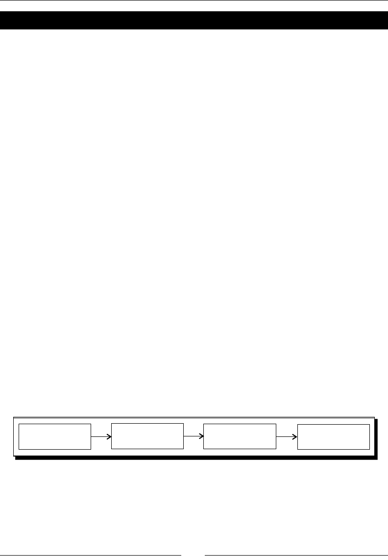
Taking it Further
[ 412 ]
Pop quiz – remote execution and clustering
For each of the following, decide if the sentence is true or false:
a. Carte is a graphical tool for designing jobs and transformaons that are going to be
run remotely.
b. In order to run a transformaon remotely you have to dene a cluster.
c. When you have very complex transformaons or huge datasets you have to execute
in a cluster because PDI doesn’t support that load in a single machine.
d. To run a transformaon in a cluster you have to know the list of servers in advance.
e. If you want to run jobs or transformaons remotely or in a cluster you need the PDI
Enterprise Edion.
Integrating PDI and the Pentaho BI suite
In this book you learned to use PDI standalone, but as menoned in the rst chapter, it is
possible to use it integrated with the rest of the suite. There are a couple of opons for
doing so.
PDI as a process action
In Chapter 1 you were introduced to the Pentaho plaorm. Everything in the Pentaho
plaorm is made by acon sequences. An acon sequence is, as its name suggests, a
sequence of atomic acons that together accomplish small business processes.
Look at the following sample with regard to the Puzzle business:
Consider that you regularly receive updated price lists (one for each manufacturer) and you
drop the les in a given folder. When you decide to hike the prices, you process one of those
les and get a web-based report with the updated prices. You can implement that process
with an acon sequence.
Get list of files
to process Prompt for the file Update prices Run web-based
report
There are four atomic acons in this sequence. You already know how to do the rst and
third acons (building the list of available price lists and updang the prices) with PDI. You
can create transformaons or jobs that perform these tasks and then use them as acons
in an acon sequence. The following is a sample screenshot of Design Studio, the acon
sequence editor:
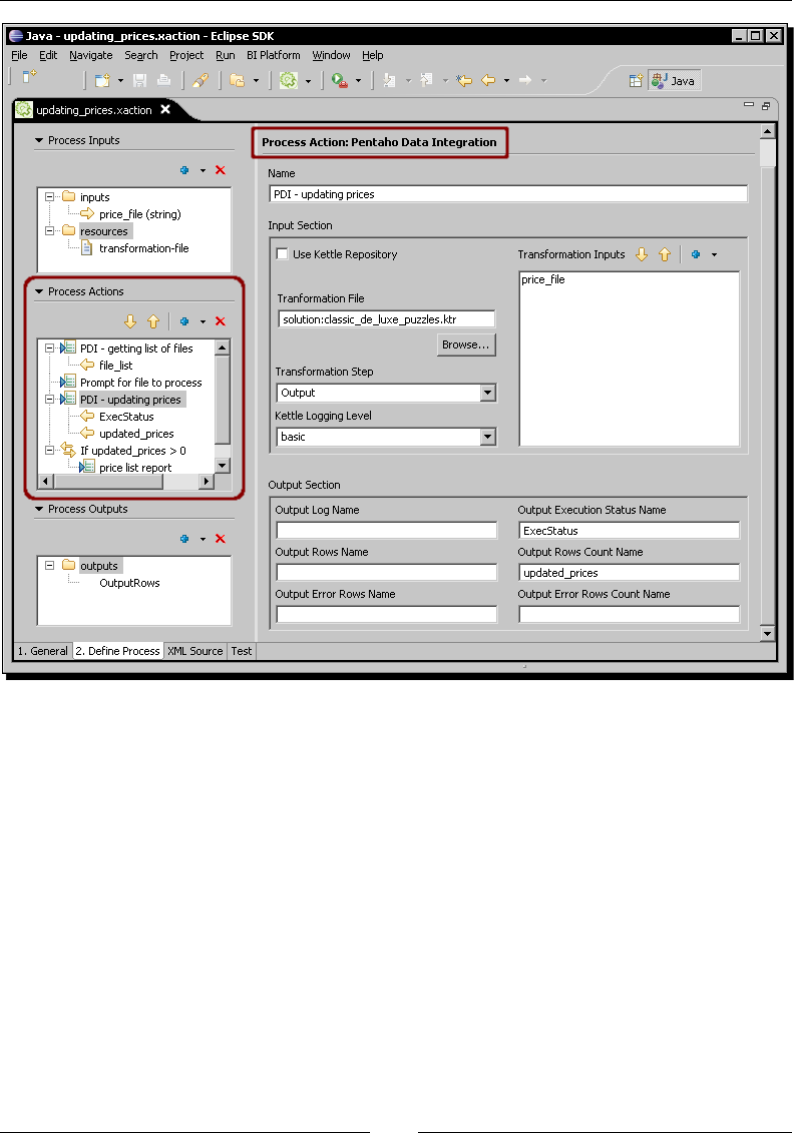
Chapter 13
[ 413 ]
The screenshot shows how the acon sequence editor looks like while eding the explained
acon sequence. In the tree at the le side, you can see the list of acons, while the right
secon allows you to congure each acon. The acon being edited in the screenshot is the
PDI transformaon that updates the prices.
PDI as a datasource
You already created several transformaons that, aer doing some data manipulaon,
generated plain les or Excel sheets. What if, instead of these types of output les, you
wanted the same data displayed as a more aracve, colorful, and interacve web-based
report? You can't do it with PDI alone. With the newest Pentaho report engine you can take
the data that came out of a transformaon and use it as the data source for your report.
Having the data, the reporng tool allows you to generate any kind of output.

Taking it Further
[ 414 ]
If you want to learn more about Pentaho reporng, you can start by vising the wiki at
http://wiki.pentaho.com/display/Reporting/Pentaho+Reporting+Communi
ty+Documentation. Or you can buy the book Pentaho Reporng 3.5 for Java Developers
(ISBN: 3193), authored by Will Gorman, published by Packt Publishing. Despite its name, it
is not just a book for developers; it's a great book for those who are unfamiliar with the tool
and who want to learn how to create reports with it.
Data coming out of a transformaon can also be used as a source data for a CDF dashboard.
A dashboard is an applicaon that shows you visual indicators such as charts, trac lights, or
dials. A CDF dashboard is a dashboard created with a toolkit, known as Community Dashboard
Framework, which is developed by members of the Pentaho community. The CDF dashboards,
recently incorporated as part of the Pentaho suite, accept many types of data sources, PDI
transformaons being one of them. The only restricon (at least for now) is that they only
accept transformaons stored in a repository (see Chapter 1 and Appendix A for details). For
more about CDF here is a link to the wiki page: http://wiki.pentaho.com/display/
COM/Community+Dashboard+Framework.
More about the Pentaho suite
The opons menoned earlier for using PDI integrated with other components of the suite
are a good starng point to begin working with the Pentaho BI suite. By pung into pracce
those examples, you can gradually get familiarized with the suite.
There is much more to learn once you get started. Look at the following sample screen:

Chapter 13
[ 415 ]
This represents a muldimensional view of your sales data mart. Here you can see cross-tab
informaon for puzzle sales in August and September for three specic manufacturers across
dierent regions, countries, and cies. It looks really useful for exploring your sales numbers,
doesn't it? Well, this is just an example of what you can do with Pentaho beyond using PDI
reporng and dashboard tools menoned earlier.
For more about the suite, you can visit the wiki page hp://wiki.pentaho.com/ or the
Pentaho site (www.pentaho.com). If, instead of browsing here and there, you prefer to
read it all in a single place, there is also a new book that brings you a good introducon to
the whole suite. The book is tled Pentaho Soluons (Wiley publishing), authored by Roland
Bouman and Jos van Dongen—two seasoned Pentaho community members.
PDI Enterprise Edition and Kettle Developer Support
Pentaho oers an Enterprise Edion of the Pentaho BI Suite and also for PDI. The PDI
Enterprise Edion adds an Enterprise Console for performance monitoring, remote
administraon, and alerng. There are also a growing number of extra plugins for
enterprise customers. In addion to the PDI extensions, customers get services and support,
indemnicaon, soware maintenance (x versions, e.g. 3.2.2), and a knowledge base with
addional technical resources.
Since the end of 2009, Pentaho also oers Kele Developer Support for the Community
Edion. With this, you can get direct assistance from the product experts for the design,
development, and tesng phases of the ETL lifecycle. This opon is perfect for geng
started, removing roadblocks, and troubleshoong ETL processes.
For further informaon, check the Pentaho site (www.pentaho.com).

Taking it Further
[ 416 ]
Summary
This chapter provided you with a list of best pracces to apply while working with PDI. If
you follow the given advice, your work will not only be useful, but also exible, reusable,
documented, and neatly presented.
You were introduced to PDI plugins, a mechanism that allows you to customize the tool.
A quick review about remote execuon and clustering was given for those interested in
developing PDI in large environments.
Finally, an introducon was given showing you how PDI can be used not only as a standalone
tool but can also be integrated with the Pentaho BI suite.
Some links and references were provided for those of you who, aer reading the book and
parcularly this chapter, are anxious to learn more.
I hope you enjoyed reading the book and learning PDI, and will start using PDI to solve all
your data requirements.

A
Working with Repositories
Spoon allows you to store your transformaons and jobs under two
dierent conguraons—le based and repository based. In contrast to the
le-based conguraon that keeps the transformaons and jobs in XML format
such as *.ktr and *.kjb les in the local le system, the repository-based
conguraon keeps the same informaon in tables in a relaonal database.
While working with the le-based system is simple and praccal, the repository-based
system can be convenient in some situaons. The following is a list of some of the disncve
repository features:
Repositories implement security. In order to work with a repository, you need
credenals. You can create users and proles with dierent permissions on the
repository; however, keep in mind that the kind of permissions you may apply is
limited.
Repositories are prepared for basic team development. The elements you create
(transformaons, jobs, database connecons, and so on) are shared by all repository
users as soon as you create them.
If you want to use PDI as the input source in dashboards made with the CDF (refer to
Chapter 13 for details), the only way you have is by working with repositories.
PDI 4, in its Enterprise version, will include a lot of new repository features such as
version control.

Working with Repositories
[ 418 ]
Before you decide on working with a repository, you have to be aware of the le-based
system benets that you may lose out on. Here are some examples:
When working with the repository-based system, you need access to the repository
database. If, for some reason, you cannot access the database (due to a network
problem or any other issue), you will not be able to work. You don't have this
restricon when working with les—you need only the soware and the
.ktr/.kjb les.
When working with repositories, it is dicult to keep track of the changes. On
the other hand, when you work with the le system, it's easier to know which
jobs or transformaons are modied. If you use Subversion, you even have
version control.
Suppose you want to search and replace some text in all jobs and transformaons.
If you are working with repositories, you would have to do it for each table in the
repository database. When working with the le-based system, this task is quite
simple—you could create an Eclipse project, load the root directory of your jobs
and transformaons, and do the task by using the Eclipse ulies.
This appendix explains how to create a repository and how to work with it. You can give
repositories a try and decide for yourself which method, repository-based or le-based, suits
you best.
Creating a repository
If you want to work with the repository-based conguraon, you have to create a repository
in advance.
Time for action – creating a PDI repository
To create a repository, follow these steps:
1. Open MySQL Command Line Client.
2. In the command window, type the following:
CREATE DATABASE PDI_REPO;
3. Open Spoon.
4. If the repository dialog appears, skip to step 6.
5. Open the repository dialog from the Repository | Connect to repository menu.
6. Click on New to create a new repository. The repository informaon dialog shows
up. Click on New to create a new database connecon.
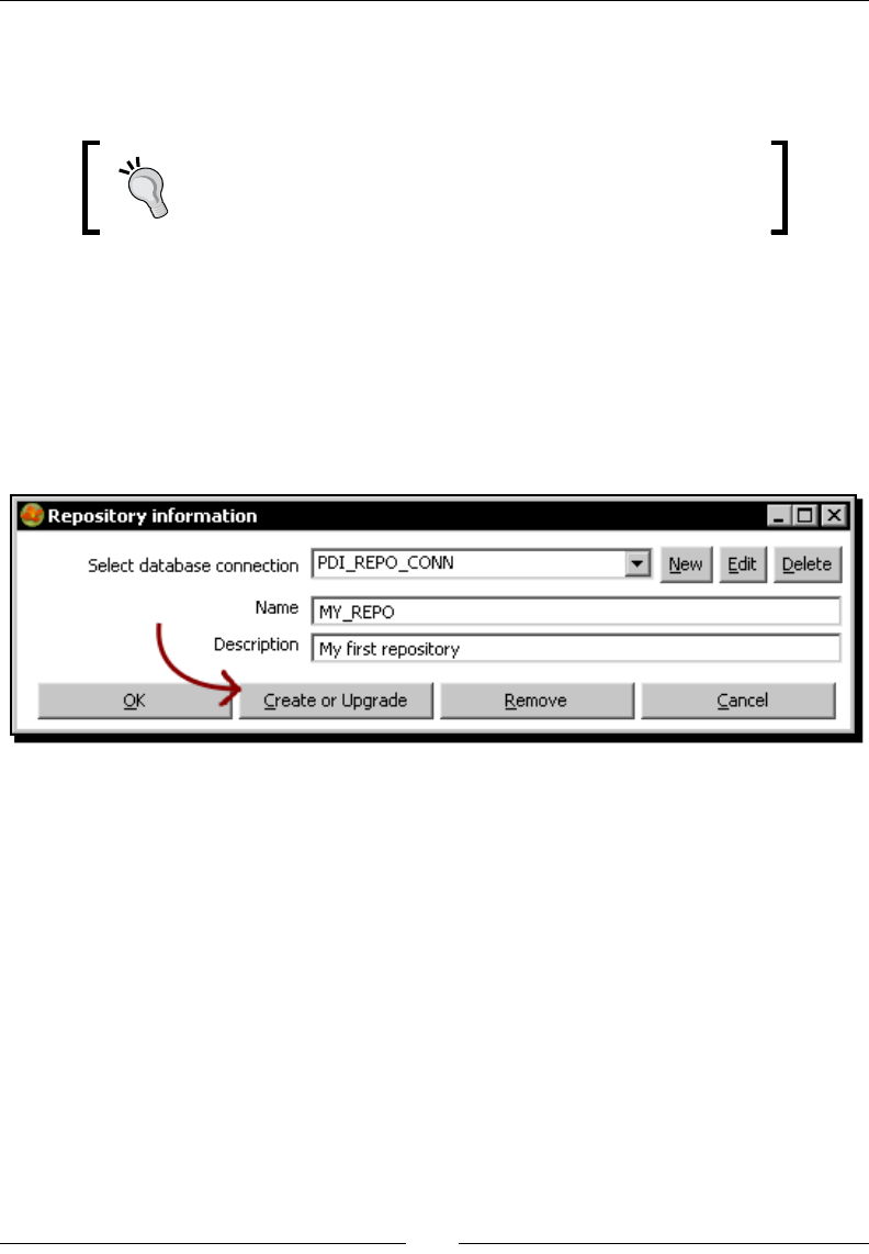
Appendix A
[ 419 ]
7. The database connecon window appears. Dene a connecon to the database
you have just created and give a name to the connecon— PDI_REPO_CONN
in this case.
If you want to refer to the steps on creang the database
connecon, check out Time for acon – creang a connecon to
the Steel Wheels database secon in Chapter 8.
8. Test the connecon to see that it is properly congured.
9. Click OK to close the database connecon window. The Select database connecon
box will show the created connecon.
10. Give the name MY_REPO to the repository. As descripon, type My rst repository.
11. Click on Create or Upgrade.
12. PDI will ask you if you are sure you want to create the repository on the specied
database connecon. Answer Yes if you are sure of the sengs you entered.
13. A dialog appears asking if you want to do a dry run to evaluate the generated SQL
before execuon.
14. Answer No unless you want to preview the SQL that will create the reposProgress
progress window appears showing you the progress while the repository is
being created.
15. Finally, you see a window with the message Kele created the repository on the
specied connecon. Close the dialog window.
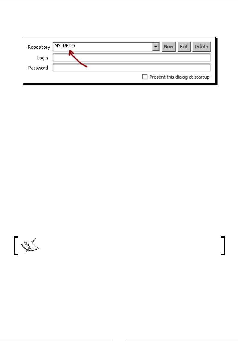
Working with Repositories
[ 420 ]
16. Click on OK to close the repository informaon window. You will be back in the
repository dialog, this me with a new repository available in the repository
drop-down list.
17. If you want to start working with the created repository, please refer to the Working
with the repository storage system secon. If not, click on No Repository. This will
close the window.
What just happened?
In MySQL you created a new database named PDI_REPO. Then you used that database to
create a PDI repository.
Creating repositories to store your transformations and jobs
A Kele repository is a database that provides you with a storage system for your
transformaons and jobs. The repository is the alternave to the *.ktr and *.kjb
le-based system.
In order to create a new repository, a database must have been created previously. In the
tutorial, the repository was created in a MySQL RDBMS. However, you can create your
repositories in any relaonal database.
The PDI repository database should be used exclusively for its purpose!
Note that if the repository has already been created from another machine or by another
user, that is, another prole in the operang system, you don't have to create the repository
again. In that case, just dene the connecon to the repository but don't create it again. In
other words, follow all the instrucons but don't click the Create or Upgrade buon.
Once you have created a repository, its name, descripon, and connecon informaon are
stored in a le named repositories.xml, which is located in the PDI home directory.
The repository database is populated with a bunch of tables with familiar names such as
transformation, job, steps, and steps_type.
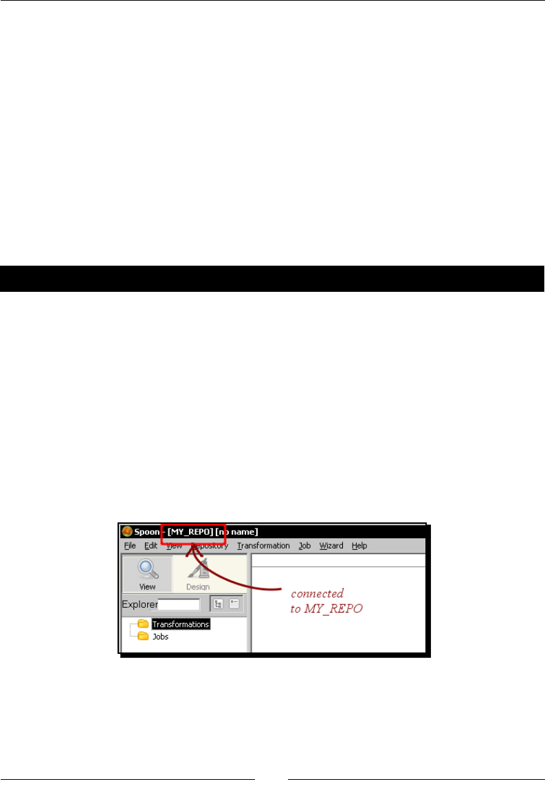
Appendix A
[ 421 ]
Note that you may have more than one repository—dierent repositories for dierent
projects, dierent repositories for dierent versions of a project, a repository just for tesng
new PDI features, and another for serious development, and so on. Therefore, it is important
that you give the repositories meaningful names and descripons so that you don't get
confused if you have more than one.
Working with the repository storage system
In order to work with a repository, you must have created at least one. If you haven't, please
refer to the secon Creang a repository.
If you already have a repository and you want to work with it, the rst thing you have to do is
to log into it. The next tutorial helps you do this.
Time for action – logging into a repository
To log into an existent repository, follow these instrucons:
1. Launch Spoon.
2. If the repository dialog window doesn't show up, select Repository | Connect to
repository from the main menu. The repository dialog window appears.
3. In the drop-down list, select the repository you want to log into.
4. Type your username and password. If you have never created any users, use the
default username and password—admin and admin. Click on OK.
5. You will now be logged into the repository. You will see the name of the repository
in the upper-le corner of Spoon:
What just happened?
You opened Spoon and logged into a repository. In order to do that, you provided the name
of the repository and proper credenals. Once you did it, you were ready to start working
with the repository.
Working with Repositories
[ 422 ]
Logging into a repository by using credentials
If you want to work with the repository storage system, you have to log into the repository
before you begin your work. In order to do that, you have to choose the repository and
provide a repository username and password.
The repository dialog that allows you to log into the repository can be opened from the
main Spoon menu. If you intend to log into the repository oen, you'd beer select Edit |
Opons... and check the general opon Show repository dialog at startup?. This will cause
the repository dialog to always show up when you launch Spoon.
It is possible to log into the repository automacally. Let's assume you have a repository
named MY_REPO and you use the default user. Add the following lines to the
kettle.properties le:
KETTLE_REPOSITORY=MY_REPO
KETTLE_USER=admin
KETTLE_PASSWORD=admin
The next me you launch Spoon, you will be logged into the repository automacally.
For details about the kettle.properties le, refer to the secon on
Kele variables in Chapter 2.
Because the log informaon is exposed, auto login is not recommended.
Dening repository user accounts
To log into a repository, you need a user account. Every repository user has a prole
that dictates the permissions that the user has on the repository. There are three
predened proles:
Prole Permissions
Read-only Cannot create nor modify any element in the repository
User Can create, modify, and delete any object in the repository excepng
users and proles
Administrator Has full permissions, including creang new users and proles

Appendix A
[ 423 ]
There are also two predened users:
admin: A user with Administrator prole. This is the user you used to log into the
repository for the rst me. It has full permissions on the repository.
guest: A user with Read-only prole.
If you have Administrator prole, you can create, modify, rename, or delete users and
proles from the Repository explorer. For details, please refer to the secon Examining and
modifying the contents of a repository with the Repository explorer, later in this chapter. Any
user may change his/her own user informaon both from the Repository explorer and from
the Repository | Edit current user menu opon.
Creating transformations and jobs in repository folders
In a repository, the jobs and transformaons are organized in folders. A folder in a repository
fullls the same purpose as a folder in your drive—it allows you to keep your work organized.
Once you create a folder, you can save both transformaons and jobs in it.
While connected to a repository you design, preview, and run jobs and transformaons
just as you do with les. However, there are some dierences when it comes to opening,
creang, or saving your work. So, let's summarize how you do those tasks when logged
into a repository:
Task Procedure
Open a transformaon / job Select File | Open. The Repository explorer shows up. Navigate the
repository unl you nd the transformaon or job you want to open.
Double-click it.
Create a folder Select Repository | Explore repository, expand the transformaon
or job tree, locate the parent folder, right-click and create the folder.
Alternavely, double-click the parent folder.
Create a transformaon Select File | New | Transformaon or press Ctrl+N.
Create a Job Select File | New | Job or press Ctrl+Alt+N.
Save a transformaon Press Ctrl+T. Give a name to the transformaon. In the Directory
textbox, select the folder where the transformaon is going to be saved.
Press Ctrl+S. The transformaon will now be saved in the selected
directory under the given name.
Save a job Press Ctrl+J. Give a name to the job. In the Directory textbox, select the
folder where the job is going to be saved. Press Ctrl+S. The job will be
saved in the selected directory under the given name.

Working with Repositories
[ 424 ]
Creating database connections, partitions, servers, and clusters
Besides users, proles, jobs, and transformaons, there are some addional PDI elements
that you can dene:
Element Descripon
Database connecons Connecon denions to relaonal databases. These are covered in
Chapter 8.
Paron schemas Paroning is a mechanism by which you send individual rows
to dierent copies of the same step—for example, based on a
eld value.
This is an advanced topic not covered in this book.
Slave servers Slave servers are installed in remote machines to execute jobs and
transformaons remotely. They are introduced in Chapter 13.
Clusters Clusters are groups of slave servers that collecvely execute a job or
a transformaon. They are also introduced in Chapter 13.
All these elements can also be created, modied, and deleted from the Repository explorer.
Once you create any of these elements, it is automacally shared by all repository users.
Backing up and restoring a repository
A PDI repository is a database. As such, you may regularly backup it with the ulies
provided by the RDBMS. However, PDI oers you a method for creang a backup in
an XML le.
You create a backup from the Repository explorer. Right-click the name of the repository and
select Export all objects to an XML le. You will be asked for the name and locaon of the
XML le that will contain the backup data. In order to back up a single folder, instead of right-
clicking the repository name, right-click the name of the folder.
You can restore a backup made in an XML le also from the Repository explorer. Right-click
the name of the repository and select Import all objects from an XML le. You will be asked
for the name and locaon of the XML le that contains the backup.
Examining and modifying the contents of a repository
with the Repository explorer
The Repository explorer shows you a tree view of the repository to which you are
connected. From the main Spoon menu, select Repository | Explore Repository and you
get to the explorer window. The following screenshot shows you a sample Repository
explorer screen:
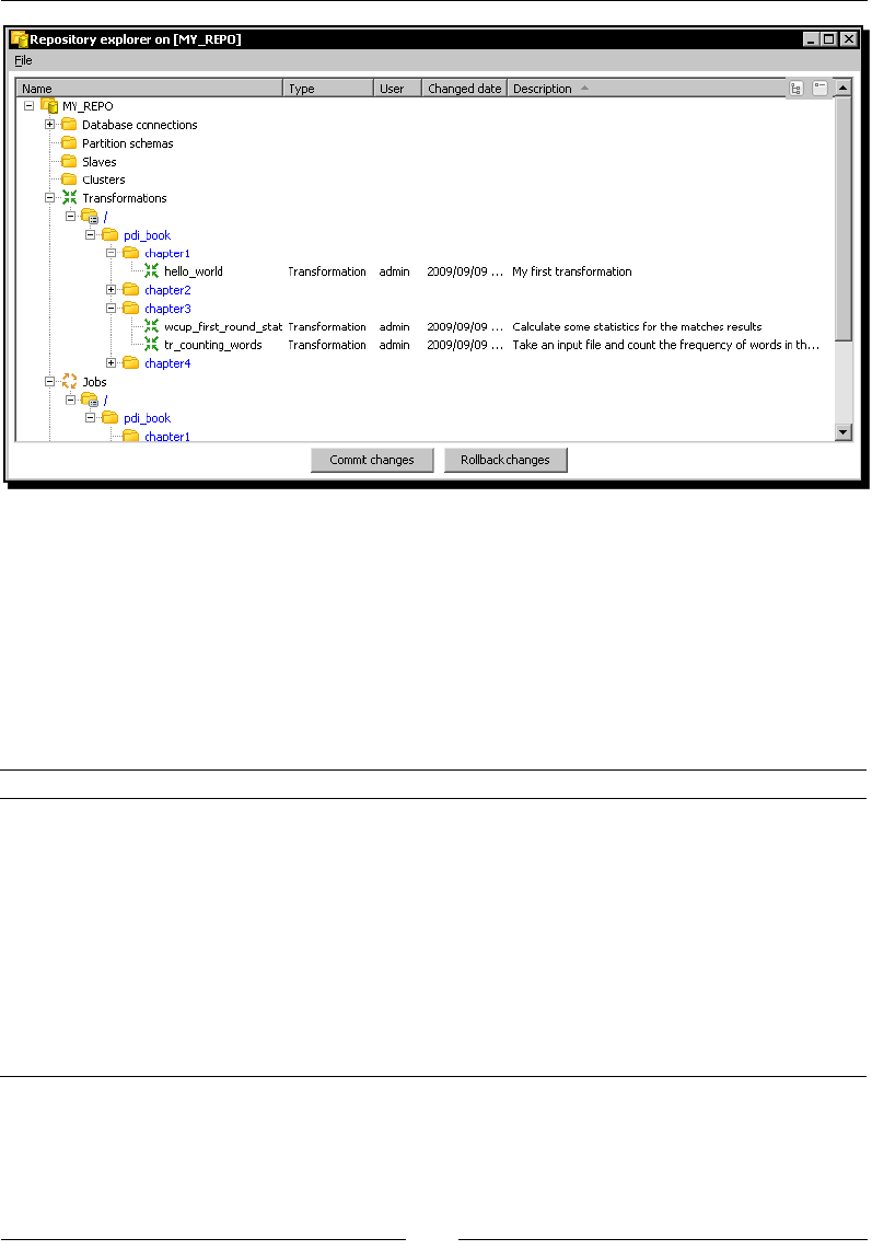
Appendix A
[ 425 ]
In the tree you can see: Database connecons, Paron schemas, Slave servers (slaves in
the tree), Clusters, Transformaons, Jobs, Users, and Proles.
You can sort the dierent elements by name, user, changed data, or descripon by just
clicking on the appropriate column header: Name, User, Changed date, or Descripon. The
sort is made within each folder.
The Repository explorer not only shows you these elements, but also allows you to create,
modify, rename, and delete them. The following table summarizes the available acons:
Acon Procedure Example
Create a new element
(any but
transformaons and
jobs)
Double-click the name of the
element at the top of the list.
Alternavely, right-click any
element in its category and
select the New opon.
In order to create a new user,
double-click the word Users at the
top of the users list, or right-click any
user and select New User.
Open an element for
eding
Right-click it and select the Open
opon. Alternavely, double-
click it.
In order to edit a job, double-click it,
or right-click and select Open job.
Delete an element Right-click it and select the
Delete opon.
In order to delete a user, right-click it
and select Delete user.
Working with Repositories
[ 426 ]
When you explore the repository, you don't see jobs and transformaons
mixed. Consequently, the whole folder tree appears twice—once under
Transformaons and then under Jobs.
In order to conrm your work, click on Commit changes. If you make a mistake, click on
Rollback changes.
Migrating from a le-based system to a repository-based
system and vice-versa
No maer which storage system you are using, le based or repository based, you may want
to move your work to the other system. The following tables summarize the procedure for
doing that:
Migrang from le-based conguraon to repository-based conguraon:
PDI element Procedure for migrang from le to repository
Transformaons or jobs From File | Import from an XML le, browse to locate the .ktr/.kjb le
to import and open it. Once the le has been imported, you can save it into
the repository as usual.
Database connecons,
paron schemas,
slaves, and clusters
When imporng from XML, a job or transformaon that uses the database
connecon, the connecon is imported as well. The same applies to
parons, slave servers, and clusters.
Migrang from le-based conguraon to repository-based conguraon:
PDI element Procedure for migrang from repository to le
Single transformaon
or job
Open the job or transformaon, select File | Export to an XML le, browse
to the folder where you want to save the job or transformaon, and save
it. Once it has been exported, it will be available to work with under the le
storage method or to import from another repository.
All transformaons
saved in a folder
In the Repository explorer, right-click the name of the folder and select
Export transformaons. You will be asked to select the directory where the
folder along with all its subfolders and transformaons will be exported to.
If you right-click the name of the repository or the root folder in the
transformaon tree, you may export all the transformaons.
Appendix A
[ 427 ]
PDI element Procedure for migrang from repository to le
All jobs saved in a folder In the Repository explorer, right-click the name of the folder and select
Export Jobs. You will be asked to select the directory where the folder
along with all its subfolders and jobs will be exported to.
If you right-click the name of the repository or the root folder in the job
tree, you may export all the jobs.
Database connecons,
paron schemas,
slaves and clusters
When exporng to XML a job or transformaon that uses the database
connecon, the connecon is exported as well (it's saved as part of the
KTR/KJB le). The same applies to parons, slave servers, and clusters.
You have to be logged into the repository in order to perform any of the
explained operaons.
If you share a database connecon, a paron schema, a slave server, or a cluster, it will
be available for using both from a le and from any repository, as the shared elements are
always saved in the shared.xml le in the Kele home directory.
Summary
This appendix covered the basics concepts for working with repositories. Besides the topics
covered here, working with repositories is prey much the same as working with les.
Although the tutorials in this book were explained assuming that you work with les, all of
them can be implemented under a repository-based conguraon with minimal changes. For
example, instead of saving a transformaon in c:\pdi_labs\hello.ktr, you could save it
in a folder named pdi_labs with the name hello. Besides these ny details, you shouldn't
have any trouble in developing and tesng the exercises.

B
Pan and Kitchen: Launching
Transformations and Jobs from the
Command Line
All the transformaons and jobs you design in Spoon end up being used as part of batch
processes—for example, processes that run every night in a scheduled fashion. When it
comes to running them in that way, you need Pan and Kitchen.
Pan is a command line program that lets you launch the transformaons designed in
Spoon, both from .ktr les and from a repository.
The counterpart to Pan is Kitchen that allows you to run jobs both from .kjb les
and from a repository.
This appendix shows you dierent opons you have to run these commands.
Running transformations and jobs stored in les
In order to run a transformaon or job stored as a .ktr / .kjb le, follow these steps:
1. Open a terminal window.
2. Go to the Kele installaon directory.
3. Run the proper command according to the following table:
Running a ... Windows Unix-like system
transformaon pan.bat /file:<ktr file
name>
pan.sh /file:<ktr file name>
job kitchen.bat /file:<kjb
file name>
kitchen.sh /file:<kjb file
name>
Download from Wow! eBook <www.wowebook.com>
Pan and Kitchen: Launching Transformaons and Jobs from the Command Line
[ 430 ]
When specifying the .ktr/.kjb lename, you must include the full path. If the name
contains spaces, surround it with double quotes.
Here are some examples:
Suppose that you work with Windows and that your Kele installaon directory is
c:\pdi-ce. In order to execute a transformaon stored in the le c:\pdi_labs\
hello.ktr, you have to type the following commands:
C:
cd \pdi-ce
pan.bat /file:"c:\pdi_labs\hello.ktr"
Suppose that you work with a Unix-like system and that your Kele installaon
directory is /home/yourself/pdi-ce. In order to execute a job stored in the le
/home/pdi_labs/hellojob.kjb, you have to type the following commands:
cd /home/yourself/pdi-ce
kitchen.sh /file:"/home/yourself/pdi-ce/hellojob.kjb"
If you have a repository with auto login (refer Appendix A), as
part of the command, add /norep. This will avoid that PDI
login to the repository.
Running transformations and jobs from a repository
In order to run a transformaon or job stored in a repository follow these steps:
1. Open a terminal window.
2. Go to the Kele installaon directory.
3. Run the proper command according to the following table:
Running a ... Windows Unix-like system
transformaon pan.bat /rep:<value>
/user:<user>
/pass:<value>
/trans:<value>
/dir:<value>
pan.sh /rep:<value>
/user:<user>
/pass:<value>
/trans:<value>
/dir:<value>
job kitchen.bat /rep:<value>
/user:<user>
/pass:<value>
/job:<value>
/dir:<value>
kitchen.sh /rep:<value>
/user:<user>
/pass:<value>
/job:<value>
/dir:<value>
Appendix B
[ 431 ]
In this preceding table:
• rep is the name of the repository to log into
• user and pass are the credenals to log into the repository
• trans and job are the names of the transformaon or job to run
• dir is the name of the directory where the transformaon or job is located
The parameters are shown on dierent lines for you to clearly idenfy all the opons.
When you type the command, you have to write all the parameters on
the same line.
Suppose that you work on Windows, you have a repository named MY_REPO, and you log
into the repository with user PDI_USER and password 1234. To run a transformaon named
Hello located in a directory named MY_WORK in that repository, type the following:
pan.bat /rep:"MY_REPO" /user:"PDI_USER" /pass:"1234" /trans:"Hello" /
dir:"/MY_WORK/"
If you dened auto-login, you don't need to provide the repository
informaon— the rep, user, and pass command line parameters—
as part of the command.
Specifying command line options
In the examples provided in this appendix, all opons are specied by using the /option:
value syntax—for example, /trans:"Hello".
Instead of /, you can also use -. Between the name of the opon and the value, you can also
use =. This means the opons /trans:"Hello" and -trans="Hello" are equivalents.
You may use any combinaon of /,-, :, and =.
In Windows, the use of - and = may cause problems; it's
recommended that you use the /option:value syntax.
If there are spaces in the values, you can use quotes ('') or double quotes ("") to keep the
values together. If there are no spaces, the quotes are oponal.
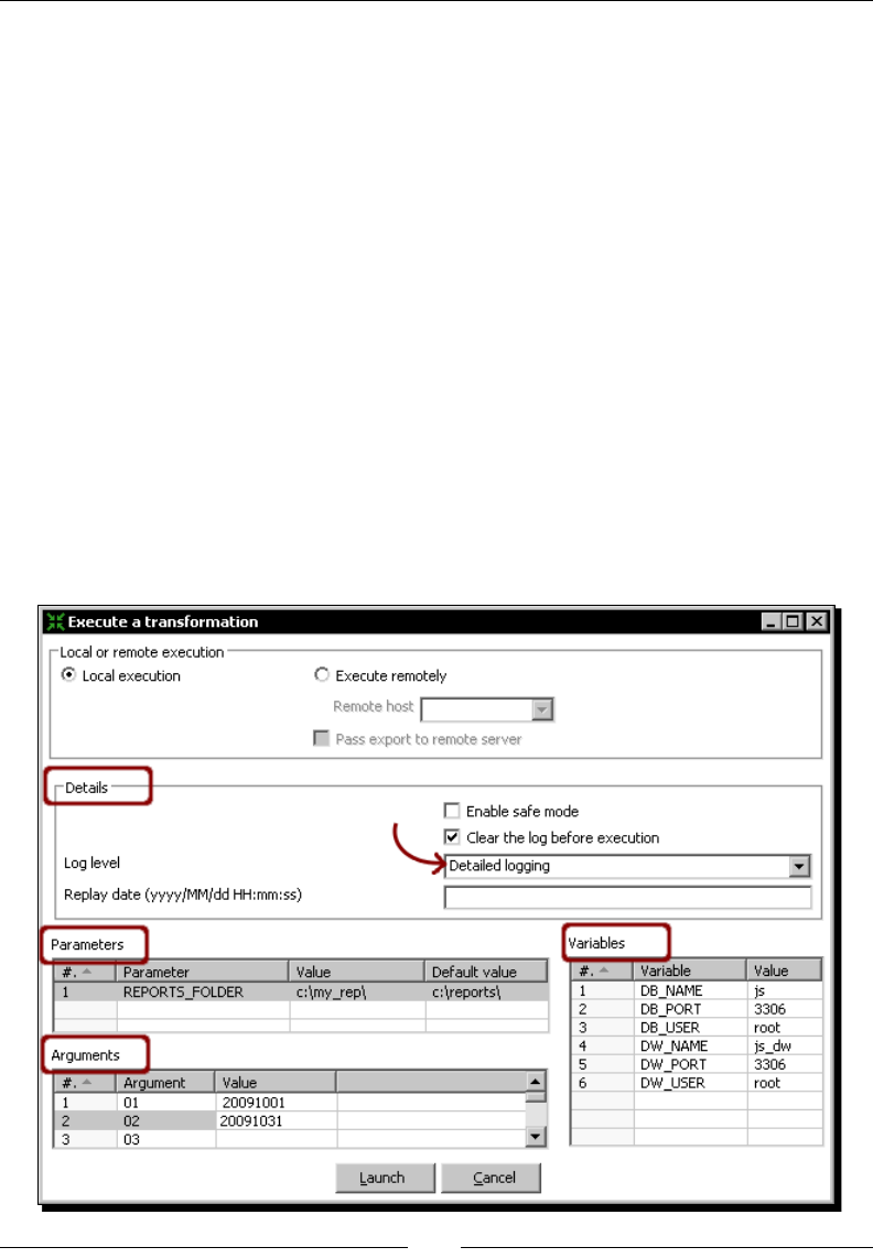
Pan and Kitchen: Launching Transformaons and Jobs from the Command Line
[ 432 ]
Checking the exit code
Both Pan and Kitchen return an error code based on how the execuon went. To check the
exit code of Pan or Kitchen under Windows, type the following command:
echo %ERRORLEVEL%
To check the exit code of Pan or Kitchen under Unix-like systems, type the
following command:
echo $?
If you get a zero, it means that there are no errors, whereas a value greater than zero
implies failure. To understand the meaning of the error, please refer to the Pan / Kitchen
documentaon; URL references are provided at the end of the appendix.
Providing options when running Pan and Kitchen
When you execute a transformaon or a job with Spoon, you have the opon to provide
addional informaon such as named parameters. The following Spoon dialog window
shows you an example of that:

Appendix B
[ 433 ]
When you execute the transformaon or job with Pan or Kitchen respecvely, you provide
this same informaon as opons in the command line. This is how you do it compared
side-by-side with Spoon:
Log details
Spoon Pan/Kitchen opon Example
You specify the log level in
the drop-down list inside
the Details box.
When the transformaon or
job runs, the log is shown
in the Execuon Results
window.
/level:<logging level>
where the logging level can be
one of the following:
Error, Nothing, Minimal,
Basic, Detailed, Debug, or
Rowlevel.
/level:Detailed
The log appears in the terminal
window, but you can use the
command language of your
operang system to redirect
it to a le.
Named parameters
Spoon Pan/Kitchen opon Example
You specify the named
parameters in the
Parameters box. The
window shows you the
name of the dened named
parameters for you to ll
the values or keep the
default values.
/param:
<parameter name>=
<parameter value>
/param:
"REPORTS_FOLDER=
c:\my_rep\"
Arguments
Spoon PAN/Kitchen opon Example
You specify the command
line arguments in the
Arguments grid. Each line
corresponds to a dierent
argument.
You type them in order as part of
the command.
20091001 20091031
Variables
Spoon Pan/Kitchen
The grid named Variables shows the
variables used in the transformaon/job
as well as their current values. At the
me of the execuon, you can type
dierent values.
You cannot set variables either in the Pan or in the
Kitchen command. The variables have to exist. You may
dene them in the kettle.properties le. To
get the details of this le, refer to the Kele Variables
secon in Chapter 2.

Pan and Kitchen: Launching Transformaons and Jobs from the Command Line
[ 434 ]
Suppose that the sample transformaon shown in the screenshot is located at
c:\pdi_labs\sales_report.ktr. Then the following Pan command
pan.bat /file:"c:\pdi_labs\sales_report.ktr" 20091001 20091031 /level:De-
tailed > c:\pdi_labs\logs\sales_report.log
executes the transformaon with the same opons shown in the screenshot. The command
redirects the log to the le c:\pdi_labs\logs\sales_report.log.
Besides these, both Pan and Kitchen have addional opons. For a full list and more
examples, visit the Pan and Kitchen documentaon at http://wiki.pentaho.com/
display/EAI/Pan+User+Documentation and http://wiki.pentaho.com/
display/EAI/Kitchen+User+Documentation.

C
Quick Reference:
Steps and Job Entries
This appendix summarizes the purpose of the steps and job entries used in the tutorials
throughout the book. For each of them, you can see the name of the Time for acon secon
where it was introduced and also a reference to the chapters where you can nd more
examples that use it.
How to use this reference
Suppose you are inside Spoon, eding a Transformaon. If the transformaon
uses a step that you don't know and you want to understand what it does or
how to use it, double-click the step and take note of the tle of the sengs
window; that tle is the name of the step. Then search for that name in the
transformaon steps reference table. The steps are listed in alphabecal order
so that you can nd them quickly. The last column will take you to the place in
the book where the step is explained.
The same applies to jobs. If you see in a job an unknown entry, double-click the
entry and take note of the tle of the sengs window; that tle is the name of
the entry. Then search for that name in the job entries reference table. The job
entries are also listed in alphabecal order.
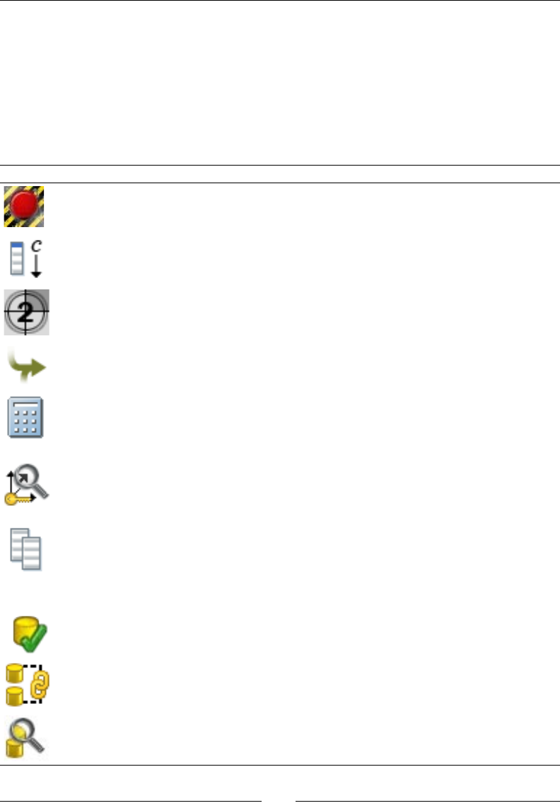
Quick Reference: Steps and Job Entries
[ 436 ]
Transformation steps
The following table includes all the transformaon steps used in the book. For a full list
of steps and their descripons, select Help | Show step plug-in informaon in Spoon's
main menu.
You can also visit http://wiki.pentaho.com/display/EAI/Pentaho+Data+Integra
tion+v3.2.+Steps for a full step reference along with some examples.
Icon Name Purpose Time for acon
Abort Aborts a transformation Aborting when there are too
many errors (Chapter 7); also in
Chapters 11 and 12
Add constants Adds one or more constant
elds to the stream
Gathering progress and
merging all together (Chapter
4); also in Chapters 7, 8, and 9
Add sequence Gets the next value from a
sequence
Assigning tasks by Distributing
(Chapter 4); also in Chapters 6
and 11
Append
streams
Appends two streams in
an ordered way
Giving priority to Bouchard
by using Append Stream
(Chapter 4)
Calculator Creates new elds by
performing simple
calculations
Reviewing examination by
using the Calculator step
(Chapter 3); also in
Chapters 6 and 8
Combination
lookup/update
Updates a junk dimension.
Alternatively, it can be
used to update
Type I SCD.
Loading a region dimension
with a Combination lookup/
update step (Chapter 9); also in
Chapter 12
Copy rows to
result
Write rows to the
executing job. The
information will then be
passed to the next entry in
the job.
Splitting the generation of top
scores by copying and getting
rows (Chapter 11)
Data Validator Validates elds based on a
set of rules
Checking lms le with the
Data Validator (Chapter 7)
Database join Executes a database query
using stream values as
parameters
Using a Database join step
to create a list of suggested
products to buy (Chapter 9)
Database
lookup
Looks up values in a
database table
Using a Database lookup step to
create a list of products to buy
(Chapter 9), also in Chapter 12
Appendix C
[ 437 ]
Icon Name Purpose Time for acon
Delay row For each incoming row,
waits a given time before
giving the row to the
next step
Generating custom les by
executing a transformation for
every input row (Chapter 11)
Delete Delete data in a database
table
Deleting data about
discontinued items (Chapter 8)
Dimension
lookup/update
Updates or looks up a
Type II SCD. Alternatively,
it can be used to update
Type I SCD or hybrid
dimensions.
Keeping a history of product
changes with the Dimension
lookup/update step
(Chapter 9), also in Chapter 12
Dummy (do
nothing)
This step type doesn't do
anything! However it is
used often.
Creating a hello world
transformation (Chapter 1),
also in Chapters 2, 3, 7, and 9
Excel Input Reads data from a
Microsoft Excel (.xls) le
Browsing PDI new features by
copying a dataset (Chapter 4);
also in Chapter 8
Excel Output Writes data to a Microsoft
Excel (.xls) le
Getting data from an XML
le with information about
countries (Chapter 2); also in
Chapters 4 and10
Filter rows Splits the stream in two
upon a given condition.
Alternatively, it is used to
let pass just the rows that
meet the condition.
Counting frequent words by
ltering (Chapter 3); also in
Chapters 4, 6, 7, 9, 11, and 12
Fixed le input Reads data from a xed
width le
Calculating Scores with
JavaScript (Chapter 5)
Formula Creates new elds by
using formulas. It uses
Pentaho's libformula.
Reviewing examination by
using the Formula step
(Chapter 3); also in
Chapters 10 and 11
Generate Rows Generates a number of
equal rows
Creating a hello world
transformation (Chapter 1);
also in Chapters 6, 9, and 10
Get data from
XML
Gets data from XML les Getting data from an XML
le with information about
countries(Chapter 2); also in
chapters 3 and 9
Quick Reference: Steps and Job Entries
[ 438 ]
Icon Name Purpose Time for acon
Get rows from
result
Reads rows from a
previous entry in a job
Splitting the generation of top
scores by copying and getting
rows (Chapter 11)
Get System
Info
Gets information from the
system like system date,
arguments, etc.
Updating a le with news about
examination (Chapter 2) also in
Chapters 7, 8, 10, 11, and12
Get Variables Takes the values of
environment or Kettle
variables and adds them as
elds in the stream
Creating the time dimension
dataset(Chapter 6)
Group by Builds aggregates in a
group by fashion. This
works only on a sorted
input. If the input is
not sorted, only double
consecutive rows are
handled correctly
Calculating World Cup statistics
by grouping data (Chapter 3);
also in Chapters 4, 7, and 9
If eld value is
null
If a eld is null, it changes
its value to a constant. It
can be applied to all elds
of a same data type, or to
particular elds
Enhancing a lms le by
converting rows to columns
(Chapter 6)
Insert / Update Updates or inserts rows in
a database table
Inserting new products or
updating existent ones
(Chapter 8)
Mapping (sub-
transformation)
Runs a subtransformation Calculating the top scores with a
subtransformation (Chapter 11)
Mapping input
specication
Species the input
interface of a
sub-transformation
Calculating the top scores with a
subtransformation (Chapter 11)
Mapping
output
specication
Species the output
interface of a
sub-transformation
Calculating the top scores with a
subtransformation (Chapter 11)
Modied Java
Script Value
Allows you to code
Javascript to modify or
create new elds. It's also
possible to code Java
Calculating Scores with
JavaScript(Chapter 5); also in
Chapters 6, 7, and 11
Number range Creates ranges based on a
numeric eld
Capturing errors while
calculating the age of a lm
(Chapter 7); also in Chapter 8
Appendix C
[ 439 ]
Icon Name Purpose Time for acon
Regex
Evaluation
Evaluates a eld with a
regular expression
Validating Genres with a Regex
Evaluation step (Chapter 7); also
in Chapter 12
Row
denormaliser
Denormalises rows by
looking up key-value pairs
Enhancing a lms le by
converting rows to columns
(Chapter 6)
Row
Normaliser
Normalises data
de-normalised
Enhancing the matches le
by normalizing the dataset
(Chapter 6)
Select values Selects, reorders, or
removes elds. Also
allows you to change the
metadata of elds
Reading all your les at a
time using a single Text le
input step (Chapter 2); also in
Chapters 3, 4, 6, 7, 8, 9, 11,
and 12
Set Variables Sets Kettle variables based
on a single input row
Updating a le with news
about examinations by setting
a variable with the name of the
le (Chapter 11); also in
Chapter 12
Sort rows Sorts rows based upon
eld values, ascending or
descending
Reviewing examinations by
using the Calculator step
(Chapter 3); also in Chapters 4,
6, 7, 8, 9, and 11
Split eld to
rows
Splits a single string eld
and creates a new row for
each split term
Counting frequent words by
ltering (Chapter 3)
Split Fields Splits a single eld into
more than one
Calculating World Cup statistics
by grouping data (Chapter 3);
also in Chapters 6 and 11
Stream lookup Looks up values coming
from another stream in the
transformation
Finding out which language
people speak (Chapter 3); also
in Chapter 6
Switch / Case Switches a row to a certain
target step based on the
value of a eld
Assigning tasks by ltering
priorities with the Switch/ Case
step (Chapter 4)
Table input Reads data from a database
table
Getting data about shipped
orders (Chapter 8); also in
Chapters 9, 10, and 12
Table output Writes data to a database
table
Loading a table with a list of
manufacturers (Chapter 8), also
in Chapters 9 and 12
Quick Reference: Steps and Job Entries
[ 440 ]
Icon Name Purpose Time for acon
Text le input Reads data from a text le Reading all your les at a
time using a single Text le
input step (Chapter 2); also in
Chapters 3, 5, 6, 7, 8, and 11
Text le output Writes data to a text le Sending the results of matches
to a plain le (Chapter 2); also in
Chapters 3, 7, 9, 10, and 11
Update Updates data in a database
table
Loading a region dimension
with a Combination lookup/
update step (Chapter 9)
Value Mapper Maps values of a certain
eld from one value to
another
Browsing PDI new features by
copying a dataset (Chapter 4)
Job entries
The following table includes all the job entries used in the book. For a full list of job
entries and their descripons, select Help | Show job entries plug-in informaon in
Spoon's main menu.
You can also visit http://wiki.pentaho.com/display/EAI/Pentaho+Data+Integra
tion+v3.2.+Job+Entries for more informaon.
There you'll nd a full job entries reference and some examples as well.
Icon Name Purpose Time for acon
Abort job Aborts the job Updating a le with news
about examinations by setting
a variable with the name of the
le (Chapter 11)
Create a folder Creates a folder Creating a simple Hello world
job (Chapter 10)
Delete le Deletes a le Generating custom les by
executing a transformation for
every input row (Chapter 11)
Evaluate rows
number in a
table
Evaluates the content of a
table
Loading the dimensions for the
sales datamart (Chapter 12)
Appendix C
[ 441 ]
Icon Name Purpose Time for acon
File Exists Checks if a le exists Updating a le with news
about examinations by setting
a variable with the name of the
le (Chapter 11)
Job Executes a job Generating the les with top
scores by nesting jobs (Chapter
11); also in Chapter 12
Mail Sends an e-mail Sending a sales report and
warning the administrator
if something were wrong
(Chapter 10)
Special entries Start job entry; mandatory
at the beginning of a job
Creating a simple Hello
world job (Chapter 10); also in
Chapters 11 and 12
Success Forces the success of a job
execution
Updating a le with news
about examinations by setting
a variable with the name of the
le (Chapter 11); also in
Chapter 12
Transformation Executes a transformation Creating a simple Hello
world job (Chapter 10); also in
Chapters 11 and 12
Note that this appendix is just a quick reference. It's not meant at all for learning
to use PDI. In order to learn from scratch, you should read the book starng from
the rst chapter.

D
Spoon Shortcuts
The following tables summarize the main Spoon shortcuts. Have this appendix handy; it will
save a lot of me while working with Spoon.
If you are a Mac user, please be aware that a mixture of Windows and Mac keys
is used. Thus, the shortcut keys are not always what you expect. For example, in
some cases you copy with Ctrl+C, while in others you do it with Command+C.
General shortcuts
The following table lists general Spoon shortcuts:
Acon Shortcut
New job Ctrl+Alt+N
New transformaon Ctrl+N
Open a job/transformaon Ctrl+O
Save a job/transformaon Ctrl+S
Close a job/transformaon Ctrl+F4
Run a job/transformaon F9
Preview a transformaon F10
Debug a transformaon Shi+F10
Verify a transformaon F11
Job sengs Ctrl+J
Transformaon sengs Ctrl+T
Search metadata Ctrl+F
Set environment variables Ctrl+Alt+J
Show environment variables Ctrl+L
Show arguments Ctrl+Alt+U

Spoon Shortcuts
[ 444 ]
Designing transformations and jobs
The following are the shortcuts that help the design of transformaons and jobs:
Acon Shortcut
New step/job entry Drag the step/job entry icon to the work
area and drop it there
Edit step/job entry Double-click
Edit step descripon Double-click the middle mouse buon
New hop Click a step and drag toward the second
step while holding down the middle
mouse buon or while pressing Shi and
holding down the le mouse buon
Edit a hop Double-click in transformaons,
right-click in jobs
Split a hop Drag a step over the hop unl it
gets wider
Select some steps/job entries Ctrl+click
Select all steps Ctrl+A
Clear selecon Esc
Copy selected steps/job entries to clipboard Ctrl+C
Paste from clipboard to work area Ctrl+V
Delete selected steps/job entries Del
Align selected steps/job entries to top Ctrl+Up
Align selected steps/job entries to boom Ctrl+Down
Align selected steps/job entries to le Ctrl+Le
Align selected steps/job entries to right Ctrl+Right
Distribute selected steps/job entries horizontally Alt+Right
Distribute selected steps/job entries vercally Alt+Up
Zoom in Page up
Zoom out Page down
Zoom 100% Home
Snap to grid Alt+Home
Undo Ctrl+Z
Redo Ctrl+Y
Show output stream (only available in transformaons) Posion the mouse cursor over the step;
then press Space bar

Appendix D
[ 445 ]
Grids
Acon Shortcut
Move a row up Ctrl+Up
Move a row down Ctrl+Down
Resize all columns to see the full values (header included) F3
Resize all columns to see the full values (header excluded) F4
Select all rows Ctrl+A
Clear selecon Esc
Copy selected lines to clipboard Ctrl+C
Paste from clipboard to grid Ctrl+V
Cut selected lines Ctrl+X
Delete selected lines Del
Keep only selected lines Ctrl+K
Undo Ctrl+Z
Redo Ctrl+Y
Repositories
Acon Shortcut
Connect to repository Ctrl+R
Disconnect repository Ctr+D
Explore repository Ctrl+E
Edit current user Ctrl+U
E
Introducing PDI 4 Features
While wring this book, version 4.0 of PDI was sll under development. Kele 4.0 was
mainly created to provide a new API for the future—the API that is cleaned up, exible, more
pluggable, and so on. Beside those architectural changes, Kele 4.0 also includes some new
funconal features. This appendix will quickly introduce you to those features.
Agile BI
Pentaho Agile Business Intelligence (Agile BI) is a new, iterave design approach to BI
development. Agile BI provides an integrated soluon that enables you, as an ETL designer,
to work iteravely, modeling the data, visualizing it, and nally providing the data to users
for self-service reporng and analysis. Agile BI is delivered as a plugin to Pentaho Data
Integraon. You can learn more about Agile BI at http://wiki.pentaho.com/display/
AGILEBI/Documentation.
Visual improvements for designing transformations and
jobs
The new version of the product includes mainly Enterprise or advanced features. There are,
however, a couple of noveles in the Community Edion that will catch your aenon as
soon as you start using the new version of the soware. In this secon you will learn about
those noveles.
Experiencing the mouse-over assistance
The mouse-over assistance is the rst new feature you will noce. It assists you while eding
jobs and transformaons. Let's see it working.
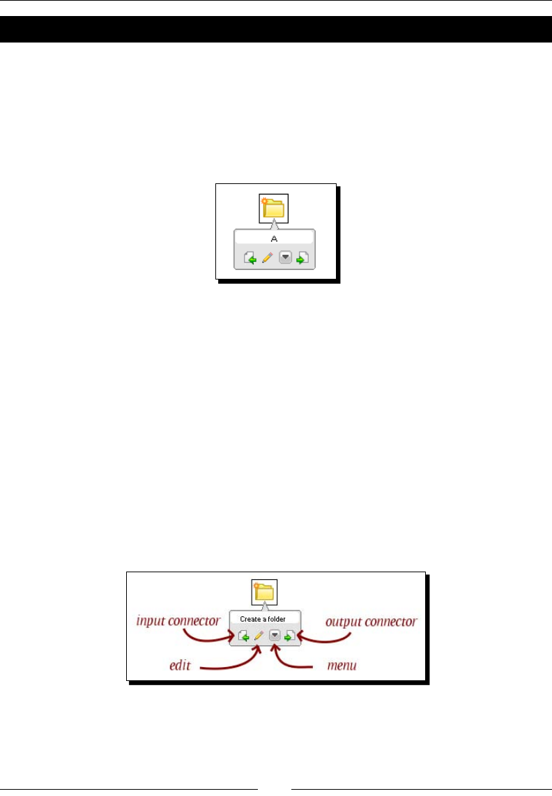
Introducing PDI 4 Features
[ 448 ]
Time for action – creating a hop with the mouse-over assistance
You already know several ways to create a hop between two job entries or two steps. Now
you will learn a new way:
1. Create a job and drag two job entries to the canvas. Name the entries A and B.
2. Posion the mouse cursor over the entry named A and wait unl a ny toolbar
shows up below the entry icon as shown:
3. Click on the output connector (the last icon in the toolbar), and drag toward the
entry named B. A grayed hop is displayed.
4. When the mouse cursor is over the B entry, release the mouse buon. A hop is
created from the A entry to the B entry.
What just happened?
You created a hop between two job entries by using the mouse-over assistance—a feature
incorporated in PDI 4.
Using the mouse-over assistance toolbar
When you posion the mouse cursor over a step in a transformaon or a job entry in a job, a
ny toolbar shows up to assist you. The following diagram depicts its opons:
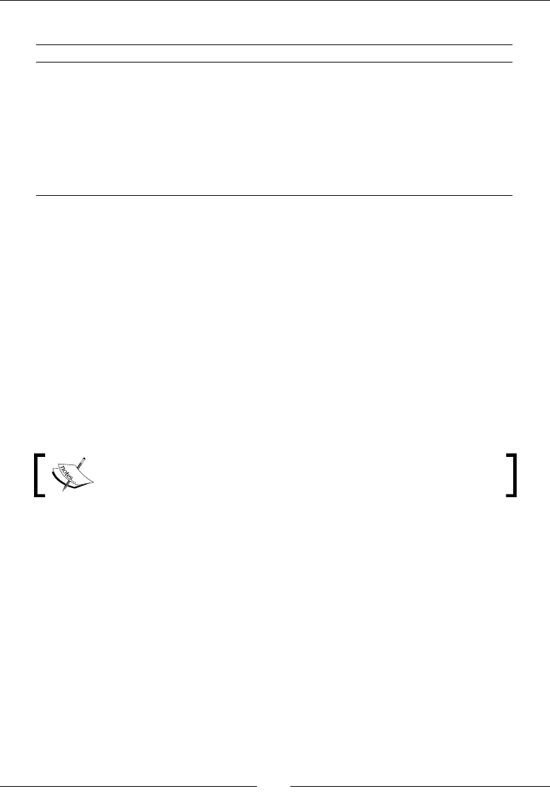
Appendix E
[ 449 ]
The following table explains each buon in this toolbar:
Buon Descripon
Edit Equivalent to double-clicking the job entry/step to edit it.
Menu Equivalent to right-clicking the job entry/step to bring up the
contextual menu.
Input
connector
Assistant for creang hops leaving from this job entry/step. If the job
entry/step doesn't accept any input (that is, START entry job or Generate
Rows step), the input connector is disabled.
Output
connector
Assistant for creang hops directed toward this job entry/step. It's used as
shown in the tutorial, but the direcon of the created hop is the opposite.
In the tutorial, you created a simple hop between two job entries. You can create hops
between steps in the same way. In this case, depending on the kind of source step, you might
be prompted for the kind of hop to create. For example, when leaving a Filter rows step, you
will be asked if the desnaon step is where you'll send the "true" data, or where you will
send the "false" data, or if this is the main output of the step.
Experiencing the sniff-testing feature
The sni-tesng feature allows you to see the rows that are coming into or out of a step
in real me. While a transformaon is running, right-click a step, select Sni test during
execuon | Sni test output rows. A window appears showing you the output data as it
is being processed. In the same way, you can select Sni test during execuon | Sni test
input rows to see the incoming rows.
Note that the sni-tesng feature slows down the transformaon and
its use is recommended just for debugging purposes.
Experiencing the job drill-down feature
In Chapters 10 and 11, you learned how to nest jobs and transformaons. You even learned
how to create subtransformaons. Whichever the case, when you ran the main job or
transformaon, there was a single log tab showing the log for the main and all nested jobs
and transformaons.
In PDI 4.0, when a job entry is running, you can drill-down into that. Drilling down means
opening that entry and seeing what's going on inside that job or transformaon. In a
separate window, you'll see both the step metrics and the log. If there are more nested
transformaons or jobs, you can connue drilling down. You can go even further into a
running subtransformaon. In any of these jobs or transformaons, you may sni test
as well, as described above.

Introducing PDI 4 Features
[ 450 ]
Drilling down is useful, for example, to understand why your jobs or transformaons don't
behave as expected or to nd out where a performance problem is.
You can see the job drill-down and sni-tesng in acon in two videos made by Ma Casters,
Kele chief leader and author of these features at: http://www.ibridge.be/?p=179.
Experiencing even more visual changes
Besides the features that we have just seen, there are some other UI improvements
worth menoning:
Enhanced notes editor: Now you can apply dierent fonts and colors to the notes
you create in Spoon.
Color-coded logs: Now it is easier to read a log, as dierent colors allow you to
quickly idenfy dierent kinds of log messages.
Revamped Repository explorer: The Repository explorer has been completely
redesigned, making this a major UI improvement in Kele 4.0.
Enterprise features
As said, most of the funconal features included in Kele 4.0 apply only to the Enterprise
version of the product. Among those features, the following are the most remarkable:
Job and transformaon versioning and locking
Robust security and administraon capabilies
Ability to schedule jobs and transformaons from Spoon
Enhanced logging architecture for real-me monitoring and debugging of
transformaons
Summary
This appendix introduced you to the main features included in Kele 4.0. All the explanaons
and exercises in this book have been developed, explained, and tested in the latest stable
version 3.2. However, as the new version of the product includes mainly Enterprise or
advanced features, working with Kele 4.0 Community Edion is not so dierent from
working with Kele 3.2. You can try all the examples and exercises in the book in
Kele 4.0 if you want to. You shouldn't have any dicules.
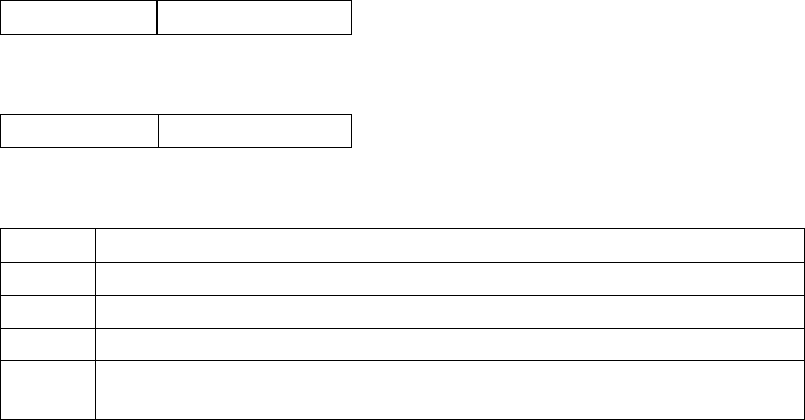
F
Pop Quiz Answers
Chapter 1
PDI data sources
15
PDI prerequisites
1 1 and 3
PDI basics
1False (Spoon is the only graphical tool)
2True
3False (Spoon doesn't generate code, but interprets Transformaon and Jobs)
4 False (The grid size is intended to line up steps in the screen)
5 False (As an example the transformaon in this chapter created the rows of data
from scratch; it didn't use external data)
Pop Quiz Answers
[ 452 ]
Chapter 2
formatting data
1(a) and (b). The eld is already a Number, so you may dene the output
eld as a Number, taking care of the format you apply. If you dene
the output eld as a String and you don't set a format, Kele will send
the eld to the output as 1.0, 2.0, 3.0, etc., which clearly is not
the same as your code. Just to conrm this, create a single le and a
transformaon to see the results for yourself.
Chapter 3
concatenating strings
1(a) and (c). The calculator allows you to use the + operator both for
adding numbers and for concatenang text. The Formula step makes a
dierence: To add numbers you use
+; to concatenate text you have to use & instead.
Chapter 4
data movement (copying and distributing)
1 (b). In the second transformaon the rows are copied, so all the
unassigned rows reach the dummy step. In the rst transformaon the
rows are distributed, so to the lter step arrives half of the rows. When
you do the preview, you see only the unassigned tasks for this half; you
don't see the unassigned tasks that went to the other stream.
splitting a stream
1(c). Both (a) and (b) solve the situaon.

Appendix F
[ 453 ]
Chapter 5
nding the seven errors
11. The type of log a doesn't exist. Look at the sample provided for the
funcon to see the valid opons.
2. The variable uSkill is not dened. Its denion is required if you want
to add it to the list of new elds.
3. setValue() cause an error without compability mode. To change the
value of the Country eld, a new variable should be used instead.
4. A variable named average is calculated but wAverage is used as the
new eld.
5. It is not trans_status; it is trans_Status.
6. No data type was specied for the totalScore eld.
7. The sentence writeToLog(‘Ready to calculate averages...')
will be wrien for every row. To write it at the beginning, you have to put it
in a Start script, not in the main.
Chapter 6
using Kettle variables inside transformations
1(a). You don't need a Get Variables step in this case. As name of the le you simply type
hello_${user.name} or hello_%%user.name%%.
In (b) and (c) you need to add the variables ${user.name} and ${user.
language} respecvely as elds of your dataset. You do it with a Get
Variables step.
Chapter 7
PDI error handling
1 (c). With PDI you cannot avoid unexpected errors; you can capture them avoiding the
crash of the transformaon. Aer that, discarding or treang the bad rows is up to you.
Pop Quiz Answers
[ 454 ]
Chapter 8
dening database connections
1(c)
database datatypes versus PDI datatypes
1(b)
Insert/Update step versus Table Output/Update steps
1(a) If an incoming row belongs to a product that doesn't exist in the products table,
both the Insert/Update step and the Table output step will insert the record.
If an incoming row belongs to a product that already exist in the products table,
the Insert/Update step updates it. In this alternave version, the Table output will
fail (there cannot be two products with the same value for the primary key) but the
failing row goes to the Update step that updates the record.
If an incoming row contains invalid data (for example, a price with a non numeric
value), neither of the Insert/Update step, the Table output step, and the Update
step would insert or update the table with this product.
ltering the rst 10 rows
1(c). To limit the number of rows in MySQL you use the clause LIMIT. (a) and (b) are
dialects: (a) is valid in HSQLDB. (b) is valid in Oracle. If you put any of this opons in
a Table Input for querying the js database, the transformaon would fail
Chapter 9
loading slowly changing dimensions
1(a). The decision for the kind of dimension is not related to data you have.
You just have to know your business, so the last opon is out. You don't
need to keep history for the name of the lm. If the name changes it is because it was
misspelled, or because you want to change the name to upper case, or something like
that. It doesn't have sense to keep the old value. So you create
a Type I SCD.
2(c). You can use any of these steps for loading a Type I SCD. In the tutorial for loading
a type I SCD you used a Combinaon L/U, but you could have used the other too, as
explained above.

Appendix F
[ 455 ]
loading type III slowly changing dimensions
1(b). With a Database lookup to get the current value stored in the dimension. If there is
no data in the dimension table, the lookup fails and returns null; that is not a problem.
Aer that, you compare the found data with the new one and set the proper values for
the dimension columns. Then you load the dimension either with a Combinaon L/U or
with a Dimension lookup, just as you do for a regular Type I SCD.
Chapter 10
dening PDI jobs
1(b)
2All the given opons are True. Simply explore the Job entries tree and you'll nd the
answers.
Chapter 11
using the Add sequence step
1(e) None of the proposed soluon gives you the same results you obtained in the
tutorial. The Add sequence step gives you the next value in a sequence which
can be a database sequence or transformaon counter. In the tutorial you used a
transformaon counter. In the opons (b) and (c), instead of four sequences from 1
to 10, a single sequence from 1 to 40 would have been generated. No maer which
method you use for generang the sequence, if you use the same name of sequence in
more than one Add sequence step, the sequence is the same and is shared by all those
steps. Therefore, the opon (a) also would have generated a single sequence from 1 to
40 shared by the four streams.
Besides these details about the generaon of sequences, the (b) opon introduces an
extra inconvenience. By distribung rows, you cannot be sure that the rows will go to
the proper stream. PDI would have distributed them in its own fashion.
deciding the scope of variables
1All the opons are valid. In the tutorial you had just a transformaon and its parent
job, that is also the root job. So (a) is valid. The grand-parent job scope includes the
parent job so opon (b) is valid too. Opon (c) includes all the other opons, so it is a
valid opon too.

Pop Quiz Answers
[ 456 ]
Chapter 12
modifying a star model and loading the star with PDI
1 a iii As menoned in Chapter 9, despite being
designed for building Type II SCDs, the
Dimension L/U step can be used for building
Type I SCDs as well. So, you have two opons:
Reuse the table (modifying the transformaon
that loads it) and get the surrogate key with
a Dimension L/U step, or use another table
without all elds specic to Type II dimensions
and, for geng the surrogate key, use a DB
Lookup step.
In any case, you may reuse the id_region
eld, as it is a integer and serves in any
situaon.
b i
c iii
2 a ii The dimension table has to have one record by
month. Therefore a dierent table is needed.
For the key you could use a string with the
format yyyymm. If you don't want to change
the fact table, you may reuse the dt eld
leaving blank the last two characters, but it
would be more appropriate to have a string
eld with just 6 posions. For geng the
surrogate key you use a Select values step
changing the metadata but this me you put as
format the new mask yyyymm.
b ii
c i
3 a ii The product_type eld is a string; it's not
the proper eld for referencing a surrogate key
from a fact table, so you have to dene a new
eld for that purpose. For geng the right key
you use a Database lookup step.
b iii
Chapter 13
remote execution and clustering
1 None of the sentences are true.
Index
Symbols
${<variable>} notaon 193
%%<variable>%% notaon 193
*.kjb format 417
*.ktr format 417
.kjb le jobs 429, 430
.ktr le transformaons
running 429, 430
/opon:value syntax 431
A
acon sequence 412
administrave tasks
geng rid of 399
sales datamart loading, automang 399-402
work backup, creang automacally 402
Agile BI 447
B
basic calculaon
calculator step, using 74
data, sorng 81
Dummy step 81
examinaon review, calculator step used 74,
78, 80
eld modicaon, PDI used 82
elds, modifying 82
Select values step, using 81
basic modicaon
Group by step 94
business keys to surrogate keys, sales fact table
junk dimension surrogate key, obtaining 391
me dimension surrogate key, obtaining 391
translang 388-391
TypeII SCD surrogate key, obtaining 389, 390
Type I SCD surrogate key, obtaining 388, 389
C
calculator step used, basic calculaon
about 74
average, taking 74-77
eding 78
examinaon, reviewing 80, 81
nal preview 80
preview 78
Select Values step 79
Sort rows Step 78
Carte 410
CDF 414
change history, maintaining
Dimension lookup/update step, using 286-288
steps 286
transformaon, tesng 288, 289
cloud-compung 411
cluster 411, 424
coding
disadvantages 166
command line argument
named parameters, dierenang between
317, 318
passing, to transformaon 315, 316
use, analyzing 318
Community Dashboard Framework. See CDF
Community Edion 415
complex lookups, data
customers list, rebuilding 275
database to stream data, joining 272-274
performing 270
suggested products list, creang 270, 272

[ 458 ]
columns 218
connecng, with RDBMS 222, 223
constellaon 376
custom me dimension dataset
creang 187-191
generang, Kele variables used 186
Get Variables step 191-193
D
dashboard
screenshot 414
data
normalizing 180, 181
normalizing, Row Normalizer step used 182,
184
reading, from les 35
data, database
complex lookups, doing 270
looking up 266
simple lookups, doing 266
data, reading
football match results, reading 36-40
from les 35
grids 46
input les 41
input les, properes 41, 42
mulple les, reading at once 42, 43
mulple les reading, single Text le input step
used 43, 44
reading les, troubleshoong 45, 46
regular expressions 44
data, sending to database
data, inserng 246-251
data, updang 246-251
Insert/Update step, using 251-253
inserng, table output step used 245
table list, loading 239-244
data, XML les
Get Data From XML input step, conguring 69
node, selecng 69
obtaining 68
path expression, examples 69
XPath, using 68
database connecons 424
database connecons See also connecng, with
RDBMS
database explorer, using 228
database operaons 261
database querying
data, working with 229-231
data obtaining, table input step used 231, 232
SELECT statement, using 232, 233
data cleaning. See data cleansing
data cleansing
about 213, 214
example 214
PDI step, using 214
data eliminaon, from database
Delete step using 259, 260
steps 256-258
data manipulaon
basic calculaon 73
ltering 97
Data Manipulaon Language. See DML
datamart
about 275, 367
datawarehouse, dierence 368
sales datamart 368
data scrubbing. See data cleansing
dataset
custom me dimension dataset, generang 186
data, normalizing 180
modifying, Row Normalizer step used 182, 184
rows, converng to columns 169
data to les, transferring
about 47
eld 50
eld, deleng 52
eld, selecng 52
eld metadata, changing 52
match results, sending 47, 49
output les 49
row 50
rowset 50
streams 51
data transformaon 141
data type, system informaon
date eld 58, 59
date formats, using 62
number 99.55, formang 62
numeric elds 59, 60
transformaon, execung 60, 61

[ 459 ]
data validaon
example 208
lms, checking 209, 210
need for 208
simple validaon rules, dening 211-213
datawarehouse
about 275
datamart, dierence 368
DDL
about 226
example 226
degenerate dimension 370
Design Studio
screenshot 413
dimensional modeling
about 275, 276
datamart 275
datawarehouse 275
dimension tables 275
fact table 275
junk dimension 369
mini dimension 285
SCD 282
star schema 275
dimensions, sales datamart
about 186
loading 371-376
Dimension tables 275
dimension tables, with data
about 275
change history, maintaining 286
dimension data, describing 281, 282
loading 276
loading, combinaon lookup/update step used
276-281
DML
about 226
example 226, 227
dynamic clusters 411
E
E4X 148
Eclipse 418
Enterprise Console 415
Enterprise features 450
enty relaonship diagram. See ERD
ERD 264
errors, capturing
Abort step, using 203
about 195
captured errors, xing 203, 204
error handling funconality, using 200, 201
lm age, calculang 196-199
PDI error handling funconality, acvies 205
rows, treang 205, 206
transformaon, aborng 201-203
ETL 7
exit code
checking, under Unix-based systems 432
checking, under Windows 432
EXtensible Markup Language. See XML
Extracng, Transforming and Loading. See ETL
F
facts 275
fact table
about 275
loading, date ranges used 394-396
eld 50
eld modicaon, basic modicaon
add constants eld 82
calculator step 83
examples 89-92
Formula step 84-87
number range eld 82
replace in string eld 82
split elds 82
student, lisng 88
User Dened Java Expression 83
Value Mapper 82
le
data, reading from 35
le result list, creang 326
le result list, using 326
output les, wring 52
updang 53-56
le-based system
migrang, to repository-based system 426
le result 326
ltering
frequent words, counng 97-102
rows 104, 105
rows, lter rows used 103

[ 460 ]
spoken language, idenfying 105-109
Stream lookup step 109
word count, discarding commonly used 105
lter rows step
using, for ltering row 103
rst transformaon, Spoon
hello world transformaon, creang 20-24
interface, exploring 26
Kele engine, direcng 25
previewing 27, 28
previewing, results in Execuon Results window
28
running 27, 28
structure, viewing 26
ow-control oriented 305
foreign keys (FK) 218
formula step 165
G
grain 370
grid shortcuts
Ctrl+A 445
Ctrl+C 445
Ctrl+Down 445
Ctrl+K 445
Ctrl+Up 445
Ctrl+V 445
Ctrl+X 445
Ctrl+Y 445
Ctrl+Z 445
Del 445
Esc 445
F3 445
F4 445
Group by step, basic modicaon
about 94
elds, reviewing 95
preview 96
tasks 96
H
hash table algorithm 111
hop
about 25, 305
creang 298-300
hop color 325
HSQLDB 222
Hybrid SCD 293
HyperSQL DataBase. See HSQLDB
I
id_junk_sales key 388
id_manufacturer key 388
id_region key 388
installing
MySQL 29
MySQL, on Ubuntu 32-34
MySQL, on Windows 29-31
PDI 14, 15
J
JavaScript
advantages 166
JavaScript code, inserng
about 148
average calculaons, tesng 152, 153
Clone() funcon 165
code, tesng 151
compability switch, turning on 151
elds, adding 150, 151
elds, modifying 150, 151
getProcessCount() funcon 161
Input elds branch 149
LoadScriptFormTab() funcon 159
new average calculaons, tesng 153
script, tesng 153
Transform Funcons 149
JavaScript step
about 154
End Script 159
JavaScript code, inserng 148
Java code, using 161
Main script 159
named parameters, using 158
scores, calculang 142-147
simple tasks, doing 142
Start Script 159
transformaon predened constants, using
159-161, 453
transformaons, modifying 154-157
using, in PDI 147
Download from Wow! eBook <www.wowebook.com>

[ 461 ]
jigsaw puzzle database
buy_methods table 265
cies table 265
countries table 265
customers table 265
exploring 264, 265
invoices table 265
manufactures table 265
payment_methods table 265
populang 261-264
products table 265
job
designing, shortcuts 444
exible version, creang 309-311
hello world le, customizing 309-311
hello world job, creang 298-304
named parameters, using 312
processes, execung 305
running, from repository 430, 431
transformaon job entry, using 307, 308
job, creang as process ow
data ow, modifying 353
data transfer, copy/get rows mechanism used
352, 353
transformaon, spling 348-351
job, running from repository
command line opons, specifying 431
steps 430, 431
job, running from terminal window
steps 313
job entry
abort job 440
about 305
create a folder 440
delete le 440
evaluate rows number in a table 440
File Exists 441
Job 441
mail 441
special entries 441
success 441
transformaon 441
job entry, execung
execuon ow, modifying 324, 325
launching, in parallel 308
sales report, sending 318-323
job iteraon
about 357
custom les, execung 358-361
every input row, execung 361-366
jobs, nesng
les, generang 354, 355
job, running inside another job 355
join 385
junk dimension 369
K
KDE Extracon, Transportaon, Transformaon
and loading Environment. See Kele
Kele 9
kele.properes le 62, 63, 264
Kele 4.0, features
Agile BI 447
Enterprise features 450
visual improvements 447
Kele Developer Support 415
Kele repository 420
Kele variables, XML les
about 70
exploring 71
Get Variable step 193
scope types 357
using 70
variables, geng 192
work documentaon 71
Key Performance Indicators. See KPIs
Kitchen
about 429
arguments 433
documentaon 434
log details 433
named parameters 433
running, opons 432
sales datamart loading, automang 399-402
variables 433
KPIs 8
L
LoadScriptFromTab() funcon 159

[ 462 ]
M
mapping 345
master 411
mini-dimension
loading 285
Modied JavaScript Values step. See JavaScript
step
mouse-over assistance
toolbar, using 448, 449
working 448
MySQL
installing 29
installing, on Ubuntu 32-34
installing, on Windows 29-31
MySQL, installing
onUbuntu 32-34
on Windows 29-32
N
named parameters
command line argument, dierenang
between 317, 318
passing, to transformaon 315, 316
use, analysing 318
using 158
O
OLTP 275
On-Line Transacon Processing. See OLTP
output les
output steps 50
P
Pan
about 429
arguments 433
documentaon 434
examinaon transformaon, execung from
terminal window 60, 61
log details 433
named parameters 433
running, opons 432
variables 433
paron schemas 424
PDI
about 7
and Pentaho BI Suite 7
best pracces 405
cloud-compung 411
cluster 411
dynamic clusters 411
features 408-411
integrang, with Pentaho BI suite 412
graphic designer, launching 15-18
installing 14, 15
job 297
Kele 9
Kele plug-ins 408, 409
master 411
PDI 2.3 10
PDI 2.4 10
PDI 2.5 10
PDI 3.0 10
PDI 3.1 10
PDI 3.2 10
PDI 4.0 10
real world risk, overcoming 410
scaling out 411
scaling up 411
Spoon 15
using, in real world scenarios 11
PDI, using in real world scenarios
data, cleansing 12
data, exporng 13
data, integrang 12
datamart, loading 11, 12
datawarehouse, loading 11, 12
informaon, migraon 13
integrang, Pentaho BI used 13
PDI best pracces 405-407
PDI elements
clusters 424
database connecons 424
paral schemas 424
slave servers 424
PDI Enterprise Edion 415
PDI features
browsing 114
browsing, dataset copied 114-119
PDI graphic designer. See Spoon

[ 463 ]
PDI integraon, with Pentaho BI suite
about 412
as datasource 413
as process acon 412, 413
Pentaho suite 414, 415
PDI opons, stream merge
Bouchard’s rows 137, 138
choosing 134, 135
tasks, merging 138
tasks, sorng 138
union, creang 134
PDI, steps
about 184
lms le, normalizing 185, 186
normalize benets, verifying 185
scores, calculang 186
Pentaho Agile Business Intelligence. See Agile BI
Pentaho BI Suite
analysis engine 7
and PDI 7
dashboards 8
data integraon 8
data mining 8
Pentaho BI Plaorm 8
reporng engine 8
Pentaho BI suite integraon, with PDI
about 412-415
as datasource 413
as process acon 412, 413
Pentaho Data Integraon. See PDI
plug-in
Kele plug-in 408, 409
primary key (PK) 218
process execuon, PDI job
about 305
hop 305
job design, comparing with job transformaon
306
job entry 305
job running, Spoon used 306
puzzles fact table
loading 393
R
RDBMS 222
records 218
regular expressions 44
relaonal database 218
Relaonal Database Management System. See
RDBMS
repository
backing up 424
creang 418-420
details, storing 420
features 417
le-based system benets 418
jobs in folders, creang 42
Kele repository 420
logging into 421
logging into, credenals used 422
restoring 424
storage system, working with 421
tasks 423
transformaon in folders, creang 423
user accounts, using 422, 423
shortcuts 445
repository-based system
migrang, to le-based system 426, 427
repository explorer
element, creang 425
element, deleng 425
element, opening 425
using, for content examinaon 424, 425
using, for content modicaon 424, 425
repository shortcuts
Ctr+D 445
Ctrl+E 445
Ctrl+R 445
Ctrl+U 445
Rhino engine 147
root-job 365
row 50
Row denormalizer
about 173
data, aggregang 176-179
working 173
rows, converng to columns
about 169
data, aggregang 176-179
lms le, enhancing 170-172
Row denormalizer step, using 173-176
total scores, calculang 177-179
rows, Stream split
copying 119, 120

[ 464 ]
distribung 120
tasks, assigning 121-124
rowset 51
S
sales datamart
degenerate dimension 370
dimensions 368
dimensions, loading 370
exploring 369
granularity level, determining 370
junk dimension 369
model 376
sales datamart model
about 376, 377
added dimensions 376
added dimensions, loading 378
sales fact table
business keys to surrogate keys, translang 388
informaon obtaining, SQL queries used
384-387
loading 378
scaling out 411
scaling up 411
SCD
about 282
Type II SCD 289
Type I SCD 282
SELECT statement
aggregate funcon 386
Kele variables, advantages 238
Kele variables, using 236, 237
Kele variables, using in queries 238
parameters, adding 235, 236
parameters, using 234, 235
using 232, 233
simple lookups, data
buyers product list, creang 266, 267
database values, looking up 268, 269
performing 266
slave server 410, 424
Slowly Changing Dimensions. See SCD
sni-tesng feature 449
sorng data 74
split eld to rows step 165
Spoon
about 18
les method 19
rst transformaon, creang 20
jobs, storing 19
launching 16, 17, 18
method, choosing 20
opons window preference, seng 18
repository method 19
shortcuts 443
starng 15
transformaon, storing 19
Spoon Interface
Design view 26, 306
exploring 26
View perspecve 26, 307
transformaon structure 26
Spoon shortcuts
Ctrl+Alt+J 443
Ctrl+Alt+N 443
Ctrl+Alt+U 443
Ctrl+F 443
Ctrl+F4 443
Ctrl+J 443
Ctrl+L 443
Ctrl+N 443
Ctrl+O 443
Ctrl+S 443
Ctrl+T 443
F10 443
F11 443
F9 443
of job design 444
of transformaon design 444
Shi+F10 443
SQL
about 225
cast funcon 385
DDL 226
DML 226
star schema 275
Steel Wheels database
about 217, 218
congured database exploring, database
explorer used 228
connecng, with RDBMS 222, 223
connecng to 219

[ 465 ]
connecon, creang 219-221
sample database, exploring 224, 225
SQL 225
tables 218
stream, merging
about 131
PDI opons 134, 135
progress, gathering 132-134
Stream lookup step, ltering
using 109, 110
word counng, precisely 111
streams
merging 131
spling 113
spling, based on condion 126
Stream split
PDI features, browsing 113
rows, copying 119, 120
rows, distribung 120-124
Stream split, based on condion
PDI, steps 128
task, assigning 128
tasks assignment, Filter rows step used 126,
127
tasks assignment, Switch/Case step used 129,
130
Structured Query Language. See SQL
subtransformaon, transformaon design
about 345
redening 347
using 345
working 346, 347
scores, calculang 341-345
Subversion 418
surrogate key 281
system informaon
data type 58
examinaon news le, updang 53-56
Get System Info step 57
T
table 218
me dimension 186
transformaon
command line arguments, using 314-317
designing, shortcuts 444
running, from repository 430, 431
steps 436
named parameters, using 314-317
transformaon, designing
color-coded logs 450
enhanced notes editor 450
job drill-down feature 449
mouse-over assistance 447, 448
mouse-over assistance toolbar, using 448
revamped repository explorer 450
sni-tesng feature 449
transformaon, enhancing
variables, seng 335, 336
variables, using 330-335
transformaon, running from repository
command line opons, specifying 431
steps 430, 431
transformaon design, enhancing
example 337-340
job, creang as process ow 348
jobs, nesng 354
transformaon iteraon. See job iteraon
transformaon steps
abort 436
add constants 436
add sequence 436
analyc query step 165
append streams 436
calculator 436
combinaon lookup/update 436
copy rows to result 436
database join 436
database lookup 436
data Validator 436
delay row 437
delete 437
dimension lookup/update 437
dummy 437
excel input 437
excel output 437
lter rows 437
xed le input 437
formula 437
generate rows 437
get data from XML 437
get rows from result 438
Get System Info 438

[ 466 ]
Get Variables 438
Group by 438
If eld value is null 438
Insert / Update 438
mapping (sub-transformaon) 438
mapping input specicaon 438
mapping output specicaon 438
Merge Rows (di) 136
Modied Java Script Value 438
Number range 438
Regex Evaluaon 439
Replace in String 82
Row denormaliser 439
RowFlaener 184
Row Normaliser 439
select values 439
Set Variables 439
Sorted Merge 136
Sort rows 439
Split Fields 439
Split eld to rows 439
stream lookup 439
Switch / Case 439
table input 439
table output 439
text le input 440
text le output 440
update 440
Unique rows 184, 214
Univariate Stascs 184
User Dened Java Expression 83
Value Mapper 440
trap detector 135
Type II SCD
about 289-291
loading, Dimension lookup/update step used
291-294
using, to maintain enre history 289-291, 294
Type I SCD
loading, with combinaon lookup/update step
282-284
manufactures dimension, loading 284, 285
regions, adding 284
U
Ubuntu
MySQL, installing 32-34
unexpected errors, avoiding
data, cleansing 213
data, validang 206-210
genres eld, validang 206, 207
unstructured les
contest les, modifying 165
modifying 164
previous rows, viewing 164
reading 162, 163
user accounts, repository
administrator 422
dening 422, 423
predened user, admin 423
predened user, guest 423
read-only 422
user 422
V
variables. See Kele variables, XML les
W
Windows
MySQL, installing 29-31
X
XML
about 67
PDI transformaons les 68
XML les
about 62
basic country informaon, building 62-66
data, obtaining 68
Kele variables 70

Thank you for buying
Pentaho 3.2 Data Integration:
Beginner's Guide
Packt Open Source Project Royalties
When we sell a book written on an Open Source project, we pay a royalty directly to that
project. Therefore by purchasing Pentaho 3.2 Data Integration: Beginner's Guide, Packt will
have given some of the money received to the Pentaho Data Integration project.
In the long term, we see ourselves and you—customers and readers of our books—as part of
the Open Source ecosystem, providing sustainable revenue for the projects we publish on.
Our aim at Packt is to establish publishing royalties as an essential part of the service and
support a business model that sustains Open Source.
If you're working with an Open Source project that you would like us to publish on, and
subsequently pay royalties to, please get in touch with us.
Writing for Packt
We welcome all inquiries from people who are interested in authoring. Book proposals
should be sent to author@packtpub.com. If your book idea is still at an early stage and you
would like to discuss it rst before writing a formal book proposal, contact us; one of our
commissioning editors will get in touch with you.
We're not just looking for published authors; if you have strong technical skills but no writing
experience, our experienced editors can help you develop a writing career, or simply get some
additional reward for your expertise.
About Packt Publishing
Packt, pronounced 'packed', published its rst book "Mastering phpMyAdmin for Effective
MySQL Management" in April 2004 and subsequently continued to specialize in publishing
highly focused books on specic technologies and solutions.
Our books and publications share the experiences of your fellow IT professionals in adapting
and customizing today's systems, applications, and frameworks. Our solution-based books
give you the knowledge and power to customize the software and technologies you're using
to get the job done. Packt books are more specic and less general than the IT books you have
seen in the past. Our unique business model allows us to bring you more focused information,
giving you more of what you need to know, and less of what you don't.
Packt is a modern, yet unique publishing company, which focuses on producing quality,
cutting-edge books for communities of developers, administrators, and newbies alike. For
more information, please visit our website: www.PacktPub.com.

Pentaho Reporting 3.5 for
Java Developers
ISBN: 978-1-847193-19-3 Paperback: 384 pages
Create advanced reports, including cross tabs,
sub-reports, and charts that connect to practically any
data source using open source Pentaho Reporting
1. # Create great-looking enterprise reports in
PDF, Excel, and HTML with Pentaho's Open
Source Reporting Suite, and integrate report
generation into your existing Java application
with minimal hassle
2. Use data source options to develop advanced
graphs, graphics, cross tabs, and sub-reports
3. Dive deeply into the Pentaho Reporting
Engine's XML and Java APIs to create
dynamic reports
Practical Data Analysis and
Reporting with BIRT
ISBN: 978-1-847191-09-0 Paperback: 312 pages
Use the open-source Eclipse-based Business
Intelligence and Reporting Tools system to design
and create reports quickly
1. Get started with BIRT Report Designer
2. Develop the skills to get the most from it
3. Transform raw data into visual and
interactive content
4. Design, manage, format, and deploy high-
quality reports
Please check www.PacktPub.com for information on our titles
Oracle Warehouse Builder 11g:
Getting Started
ISBN: 978-1-847195-74-6 Paperback: 368 pages
Extract, Transform, and Load data to build a
dynamic, operational data warehouse
1. Build a working data warehouse from scratch
with Oracle Warehouse Builder
2. Cover techniques in Extracting, Transforming,
and Loading data into your data warehouse
3. Learn about the design of a data warehouse
by using a multi-dimensional design with an
underlying relational star schema.
Creating your MySQL Database:
Practical Design Tips and
Techniques
ISBN: 978-1-904811-30-5 Paperback: 108 pages
A short guide for everyone on how to structure
your data and set-up your MySQL database tables
efciently and easily
1. How best to collect, name, group, and structure
your data
2. Design your data with future growth in mind
3. Practical examples from initial ideas to nal
designs
4. The quickest way to learn how to design good
data structures for MySQL
Please check www.PacktPub.com for information on our titles
