Phonon Relaxation Manual

User Manual: Pdf

Open the PDF directly: View PDF .
Page Count: 34

First-principles calculation of phonon-induced electron-hole

relaxation dynamics for ﬁnite systems within linear response

theory: Manual and Example

Jonathan Trinastic - jptrinastic@gmail.com

Department of Physics and Quantum Theory Project,

University of Florida, Gainesville, Florida, 32611, USA

(Dated: June 21, 2016)

CONTENTS

I. Overview 3

II. Theory 3

A. Reduced density matrix and Redﬁeld equations 3

B. Nonadiabatic system-reservoir coupling 4

C. Electronic nonadiabatic coupling within LR-TDDFT 5

D. Franck-Condon-weighted density of states 7

E. Phonon-induced relaxation dynamics 7

F. Further References 8

III. Example Calculation: Porphyrin 8

A. Electronic excitations with linear response theory 9

B. Electronic nonadiabatic coupling 12

1. Ab initio molecular dynamics 12

2. DFT and LR-TDDFT calculations 17

3. Kohn-Sham orbital overlap calculations 18

4. LR-TDDFT electronic coupling 20

C. Franck-Condon-weighted density of states 23

1. Phonons 24

2. Excited state geometry relaxation 25

3. Huang-Rhys factors 26

4. Franck-Condon-weighted density of states 29

D. Phonon-induced relaxation dynamics 31

References 34

I. OVERVIEW

This manual reviews the theory and computational methods to calculate phonon-induced

relaxation dynamics of electron-hole pairs in ﬁnite systems within linear response the-

ory. The method employs linear-response, time-dependent density functional theory (LR-

TDDFT) to calculate excited states and the reduced density matrix formalism (RDM) to

investigate the nonequilibrium relaxation dynamics of an initially excited electron-hole pair.

Systems with hundreds of atoms can be explored using the steps described below.

Required software includes a C++ compiler, Fortran compiler, Matlab, Gaussian09, and

VASP (optional for use in generating molecular dynamics trajectories). Input for the latter

two DFT programs is only described brieﬂy, and details about their use can be found at

their respective websites.

The manual is organized as follows. Section II provides a brief introduction into the

underlying theory, which is described in more detail in several references included in Section

II F. Section III then provides a step-by-step example of how to use the code, applying

the method to study phonon-induced relaxation of an excitation in the Soret state of the

porphyrin molecule, which has been previously studied experimentally.

II. THEORY

A detailed overview of the theory and computational steps can be found in published

work1. Only primary equations and descriptions of major variables will be described here -

please see references given for more details.

A. Reduced density matrix and Redﬁeld equations

Within the RDM formalism,2dynamics of a system of interest are determined due to

its interaction with a reservoir that contains many more degrees of freedom and cannot be

described in detail. If a density matrix is constructed of the combined system and reservoir,

then the reduced density matrix (σαβ ) can be made by taking the trace of the density matrix

with respect to the reservoir coordinates. The reduced density matrix then only depends

on the system degrees of freedom. For the model described within, electronic ground and

excited states described by LR-TDDFT are the collective system interacting with a phonon

reservoir that causes downward energy relaxation from an initial excited state.

If we construct the RDM with the electronic eigenstates of the system, then the Redﬁeld

equations describe both population transfer (diagonal elements) and coherence dephasing

(oﬀdiagonal) between eigenstates αand β:

1) Population relaxation:

dσI

αα(t)

dt =−X

Rαα,µµσI

µµ(t) (1)

Rαα,µµ =δαµ X

kακ −kµα (2)

2) Coherence dephasing:

dσI

αβ(t)

dt =−Rαβ,αβσI

αβ(t) (3)

Rαβ,αβ =X

2(kαµ +kβµ) + γ0,(4)

Here, Rαβ,µν is the Redﬁeld relaxation tensor, kαβ is the relaxation rate due to the system-

reservoir interaction, and γ0is a dephasing constant determined from experiment or other

computational methods. Thus, determining energy relaxation rates of excited states requires

the calculation of kαβ, which has been shown to be:2,3

kαβ =2π

~DX

j|hφiΨα|V|φjΨβi|2δ(~ωαβ −~ωij)E,(5)

where Vis the system-reservoir interaction to be deﬁned below, Ψαis an electronic excited or

ground state, φiis a nuclear state, ωαβ and ωij are electronic transition energies and phonon

energies, respectively, and D...E=Pifi=e−βEi/(Pie−βEi), the thermal average over

initial conditions. The sum over ﬁnal reservoir states preserves conservation of energy. The

principle of detailed balance ensures proper behavior as time goes to inﬁnity and provides the

following relationship between forward and backward transition rates kαβ =e~ωαβ /kBTkβα.

B. Nonadiabatic system-reservoir coupling

To model electron-phonon interactions, we follow previous literature that treats the nu-

clear kinetic energy operator as a perturbation to the adiabatically determined electronic

excited states: hφiΨα|V|φjΨβi=Vαβ,ij =hφiΨα|Pk−~2

2Mk∇2

k|φjΨβi, where Mkis the nu-

clear mass and kruns over the Knuclear degrees of freedom, |φii=|φ1

ii|φ2

ii...|φK

ii.2If we

only include terms to ﬁrst order in the nuclear gradient operator, previous work has shown

that the system-reservoir coupling can be rewritten to good approximation as4

Vαβ,ij ≈X

k−i~

MkhΨα|∇k|ΨβihˆpiY

khφk

i|φk

ji,(6)

where hˆpiis the expectation value of the momentum operator and obeys classical equa-

tions of motion according to Ehrenfest’s theorem. If we plug this expression for Vαβ into

Equation 5, then we express the relaxation rates as

kαβ =2π

~D|Vαβ|2EF(ωαβ),(7)

where Vαβ =Pk−i~

MkhΨα|∇k|Ψβihˆpiis the nonadiabatic electronic coupling and F(ωαβ) =

Pi,j fiQk|hφk

i|φk

ji|2δ(~ωαβ −~ωij) is the Franck-Condon-weighted density of states (FC-

DOS). Vαβ describes the coupling of states αand βdue to atomic motion and F(ωαβ)

describes the density of phonon states available to couple to the transition.

Equation 7 is the primary equation we will refer to during the example description in

Section III. The calculation requires three major quantities: 1) the ground and excited

electronic states used to construct the reduced density matrix, which we calculate within

LR-TDDFT; 2) the nonadiabatic electronic coupling (Vαβ), which we calculate using ab

initio molecular dynamics; and 3) the Franck-Condon-weighted density of states, which we

calculate within the harmonic approximation using the minimum-energy conﬁguration of

each excited state and the ground state normal modes.

C. Electronic nonadiabatic coupling within LR-TDDFT

We follow theory developed by Tavernelli et al.5,6 to calculate Vαβ within LR-TDDFT.

The theory is exact for ﬁrst-order nonadiabatic coupling between ground and excted states

and is a good approximation for coupling between excited states (exact within the Tamm-

Dancoﬀ approximation). Tavernelli showed that the nonadiabatic electronic coupling can

be expressed as follows, replacing the nuclear gradient operator with a time derivative and

using ﬁnite diﬀerences in the last expression:

Vαβ =−i~hΨα|∂

∂t|Ψβi≈− i~

2∆t[hΨα(t)|Ψβ(t+ ∆t)i−hΨα(t+ ∆t)|Ψβ(t)i],(8)

where ∆tis the time step. The next step is to deﬁne the wave function used to solve

Equation 8. Within the Casida ansatz,7an excited state within LR-TDDFT can be written

|Ψαi=X

(Xma

α+Yma

α)ˆa†

aˆam|Ψ0i=X

(Xma

α+Yma

α)|Ψm−>ai,(9)

where mand aindex occupied and unoccupied Kohn-Sham orbitals, respectively, ˆa†

aand

ˆamare creation and annihilation operators, Xma

αand Yma

αare the normalized coeﬃcients

corresponding to an excitation from the mth to ath orbital and de-excitation from the

ath to mth orbital, respectively, |Ψ0iis the ground state Slater determinant, and |Ψm−>ai

is a singly excited Slater determinant. Plugging this wave function deﬁnition into Equa-

tion 8, the wave function overlaps can be expressed by singly excited Slater determi-

nant overlaps: hΨα(t)|Ψβ(t+ ∆t)i=Pma Pnb(Xma

α(t) + Yma

α(t))(Xnb

β(t+ ∆t) + Ynb

β(t+

∆t))hΨm−>a(t)|Ψn−>b(t+ ∆t)i. These Slater determinant overlaps can be further decom-

posed into single-particle Kohn-Sham orbital overlaps using Slater-Condon rules:

hΨα(t)|Ψβ(t+ ∆t)i=X

mab

(Xma

α(t) + Yma

α(t))†(Xmb

β(t+ ∆t) + Ymb

β(t+ ∆t))vab

−X

amn

(Xma

α(t) + Yma

α(t))†(Xna

β(t+ ∆t) + Yna

β(t+ ∆t))vmn,

(10)

where vab =hψa|ψbi, and a,bare unoccupied and m,nare occupied Kohn-Sham orbitals,

respectively.

Thus, Equation 10 lays out all the required variables to calculate Vαβ. To do so, we

perform an ab initio molecular dynamics simulation at 300K (or any relevant temperature)

to generate a set of conﬁgurations - the time step of the simulation is ∆t. Changes in

the LR-TDDFT wave functions between time steps represent coupling of the electronic

structure to phonon modes in the system. Thus, calculating Vαβ at adjacent time steps

and averaging across them will provide the thermally averaged, nonadiabatic electronic

coupling we require. This requires knowledge of the LR-TDDFT coeﬃcients and Kohn-

sham orbital wave functions at each step, which come from a self-consistent calculation for

each conﬁguration at each of the two time steps, and are entered into Equation 10. Results

from this equation enter into Equation 8 to ﬁnd Vαβ for a given pair of adjacent time steps.

The thermally averaged electronic nonadiabatic coupling that enters into Equation (7) is

then calculated by averaging the value of Vαβ across all time steps of the AIMD trajectory

consisting of Ntime steps: D|Vαβ|2E=1

NPN

i=1 |Vαβ|2.

D. Franck-Condon-weighted density of states

The ﬁnal term required to calculate relaxation rates is F(ωαβ), describing the density of

phonon states that couple to a given α−βtransition. Assuming a quantum harmonic oscil-

lator phonon bath and that the ground state normal modes are an accurate approximation

for all excited state modes, F(ωαβ) describes the density of phonon states coupled to a given

nonadiabatic transition:2

F(ωαβ) = 1

2π~Z∞

−∞

dteiωαβ teG(t),(11)

where G(t) = PkSk

αβ[(e−iωkt−1)(n(ωk) + 1) + (eiωkt−1)n(ωk)]. Sk

αβ is the Huang-Rhys

factor, a dimensionless quantity representing the coupling strength of the kth normal mode

to the transition, and n(ωk) is the Bose-Einstein distribution for a phonon with energy ~ωk

at a given temperature. The function F(ω) peaks at energies corresponding to modes with

nonzero Sαβ.

To calculate Sk

αβ, we relax the atomic positions for all excited states and project the

change in atomic conﬁguration between two states αand βonto the normal modes of the

system. The Huang-Rhys factor is then calculated as

αβ = (µkωkd2

kαβ )/~,(12)

where µkis the modal reduced mass and dkαβ is the conﬁgurational diﬀerence between

excitations αand βprojected onto the kth mode eigenvector. These values of Sk

αβ enter

Equation 11 along with phonon modes (ωk) calculated within the harmonic approximation.

E. Phonon-induced relaxation dynamics

Once we have determined the LR-TDDFT excited sates, Vαβ, and F(ωαβ), we can examine

phonon-induced relaxation dynamics. We consider a system bathed in light with frequency

ωat t < 0. After the light is switched oﬀ at t= 0, a nonequilibrium carrier distribution

will relax due to interactions with phonons as described by Equations (1) and (7). The

population change in σαβ is then deﬁned as ∆η(E, t) = Pασαα(t)δ(Eα−E)−ηeq, where

Eαis the energy of the αth excitation and ηeq is the equilibrium population.

F. Further References

Reduced density matrix and Redﬁeld equations:

May, V and Kuhn, O. Charge and energy transfer dynamics in molecular systems. John

Wiley and Sons, 2008.

Nonadiabatic system-reservoir coupling:

Prezhdo, O and Rossky, P. Evaluation of quantum transition rates from quantum-classical

moleculary dynamics simulations. J. Chem. Phys., 107(15), 5863-5878, 1997.

Electronic nonadiabatic coupling within LR-TDDFT:

Tavernelli, I et al. Nonadiabatic coupling vectors for excited states within time-dependent

density functional theory in the Tamm-Dancoﬀ approximation and beyond. J. Chem. Phys.,

133(19), 194104, 2010.

Franck-Condon-weighted density of states:

May, V and Kuhn, O. Charge and energy transfer dynamics in molecular systems. John

Wiley and Sons, 2008.

III. EXAMPLE CALCULATION: PORPHYRIN

Phonon-induced relaxation has been well studied in the porphyrin molecule, which

demonstrates a strong absorption peak known as the Soret band between 350-400 nm

depending the solvent (see Figure 1).8Several experimental studies8–10 have measured re-

laxation times from the Soret band to lower states ranging from 50-200 fs. The availablility

of experimental data combined with the small size of the molecule makes this a nice system

to demonstrate the steps for the present method with minimal computational resources.

All calculations and post-processing codes are developed to work with Gaussian09, version

D.01, except for the ab initio molecular dynamics simulations, which can be done using either

Gaussian09 or VASP. This manual will focus on describing the codes speciﬁc to calculating

relaxation rates; see the Gaussian09 and VASP websites for detailed information about

input. All ﬁles for submitting jobs are tailored to NERSC’s Edison system - changes will

need to be made as appropriate for the particular high-performance computing server being

used.

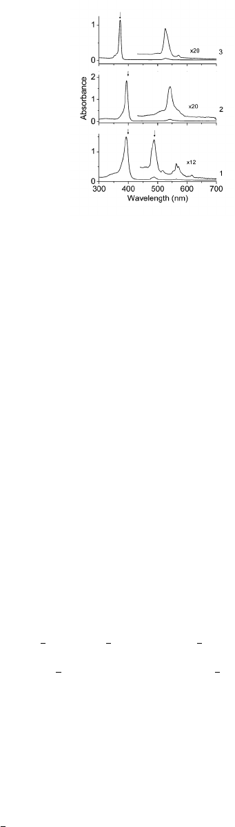
FIG. 1. Porphyrin absorption spectrum8as a function of wavelength in the following solvents: 1)

benzene/cyclohexane 1:10, 2) benzene/cyclohexane 1:10 added with CF3COOH, and 3) concen-

trated HClO4. The Soret band is the large peak between 350-400 nm and the lowest excited state

occurs between 500-600 nm.

A. Electronic excitations with linear response theory

The ﬁrst step requires the calculation of excited states within LR-TDDFT and conﬁr-

mation that the results generally match experimental absorption spectra. This is a crucial

check because a general match with experimental data is a good indication that the excited

state wave functions are well described with the basis set and functional being used. If this

is not the case, then the electronic nonadiabatic couplings (Vαβ) may be inaccurate and

subsequent relaxation rates will not be correct.

•After untarring Phonon Induced Relaxation LRTDDFT.tar attached with this man-

ual, move into Porphyrin Example/Electronic Excitations.

•Within this folder, porphyrin.xyz provides the atomic coordinates for porphyrin in

XYZ format. Look at the molecule using any visualization software (e.g., VESTA) to

understand its general structure as shown in Figure 2.

•Next, open porph lrtddft.com, which is the input ﬁle for Gaussian09 that will cal-

culate the ﬁrst six excitations (TD command). It is assumed that the geometry has

already been optimized to the minimum-energy conﬁguration. Several lines are of

particular importance:

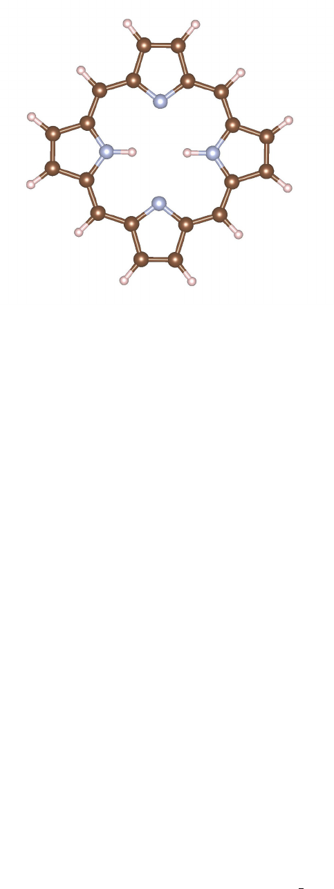
FIG. 2. Atomic structure of porphyrin. Brown spheres are carbon atoms, small pink spheres are

hydrogen atoms, and gray spheres are nitrogen atoms.

–IOP(9/40=2) forces Gaussian to output the LR-TDDFT coeﬃcients that are

greater than 0.01 for each excitation, where IOP(9/40=X) corresponds to print-

ing coeﬃcients greater than 10−X. This value should be at least 2 in order to

accurately calculate Vαβ.

–b3lyp/6-31g* denotes the functional and Gaussian basis set used in the calcu-

lation. Both the B3LYP functional and 6-31g* basis set reproduce excitations in

porphyrin well, but this should be tested for each new system.

–NOSYMMETRY prevents Gaussian from rotating the molecule during any calculation.

This command should be included in all calculations as both Vαβ and

F(ωαβ) require comparisons between conﬁgurations with the same orientation.

–SCRF initiates the Polarizable Continuum Model to represent the benzene solvent

used in most experiments studying porphyrin, which is important to capture the

correct excitation energies.

–TD performs the LR-TDDFT calculation, where the included subcommands in-

struct the program to calculate 6 singlet states.

•After submitting and completing the calculation, porph lrtddft.out will contain

information about the excited state energies and LR-TDDFT coeﬃcients. Within the

TABLE I. Excitation energies and oscillator strengths for ﬁrst six excited states in porphyrin.

Excited State Energy (eV) Energy (nm) Oscillator Strength (f)

1 2.28 544 0.0003

2 2.44 509 0.0000

3 3.22 385 0.8905

4 3.33 372 1.2500

5 3.42 362 0.0000

6 3.62 342 0.0000

ﬁle, look for the keyword Excited State to ﬁnd energies listed for the ﬁrst six states

as listed in Table I. The Soret band corresponds to excited states 3 and 4, which show

strong absorption between 350-400 nm as seen in experiment. This example will look

at phonon-induced relaxation rates of an electron-hole pair initially excited to these

states.

•Below each excited state, a list of Kohn-Sham electron-hole transitions are listed

that make up each LR-TDDFT excitation along with their LR-TDDFT coeﬃcient

or weight. For example, under Excited State 1, ’64 -> 83 -0.01058’ indicates

that the transition from the 64th to 83rd KS orbital has a coeﬃcient of -0.01058*√2

(Gaussian normalizes the coeﬃcients such that their sum of squares is 1 only if you

multiply them by √2).

Having conﬁrmed that the choice of functional and basis set provides an accurate descrip-

tion of excited states, the next step will be the calculation of the electronic nonadiabatic

coupling (Vαβ) between these six states using AIMD and post-processing codes. The energies

of the excitations will also be required as input for calculating F(ωαβ) in Section III C.

B. Electronic nonadiabatic coupling

1. Ab initio molecular dynamics

Calculating Vαβ ﬁrst requires an AIMD trajectory that provides the input conﬁgurations

for subsequent LR-TDDFT and post-processing calculations. This can be done in two ways:

1) using Gaussian09 and the same functional used to calculate electronic structure or 2)

using VASP and a more computationally eﬃcient functional. The former is technically

more accurate and consistent, however non-hybrid, GGA functionals often provide accurate

strutural information and describe phonon modes well. This makes them advantageous for

calculating AIMD trajectories that can be computationally burdensome for large systems.

Each option is outlined below:

GAUSSIAN AIMD

Performing molecular dynamics in Gaussian09 requires two sequential steps: 1) an initial

density matrix propagation method (ADMP) in which the system is connected to a velocity-

rescaling thermostat and nuclear velocities are obtained after reaching thermal equilibration,

and 2) a second NVE run using Born-Oppenheimer dynamics (BOMD) with the ADMP

velocities included as input. The conﬁgurations from the BOMD trajectory are then used

to calculate Vαβ.

•Navigate to Porphyrin Example/Electronic NAC/AIMD/Gaussian09. In this folder,

porph admp.com contains all the input commands required to run the initial ADMP

dynamics to obtain nuclear velocities:

–The input conﬁguration should be the optimized geometry of the system.

–ADMP turns on the density matrix propagation method.

∗Maxpoints is the maximum number of time steps in the simulation.

∗Stepsize indicates the time step size Nin units of N∗0.0001 femtoseconds

(fs). Thus, 2500 is a 0.25 fs time step - a small enough time step must be used

to ﬁnd good temperature and energy behavior during the NVE run. Thus,

the run will last 4000*0.25 = 1000 fs - increase Maxpoints if the system

requires longer time to reach equilibrium.

∗NKE indicates the initial nuclear kinetic energy in units of microHartree. The

relevant formula is NKE = (Natoms −1)(3/2)kT , where Natoms is the

number of atoms, k= 3.1668 microHartree/K, and Tis temperature in

Kelvin. Thus, a 38-atom system (porphyrin) at 300K corresponds to NKE =

52727.

–The IOps are described in the input ﬁle and provide controls over the velocity

rescaling.

•Submit the job in this directory to perform the AIMD calculation, which will take at

least several hours to complete.

•After the AIMD calculation complete, open the porph admp.out ﬁle. This will contain

information, such as energetics and nuclear velocities, about each time step of the

trajectory (search for the Summary information keyword). Move to the last time

step and copy the geometry and nuclear velocities into the input ﬁle for the BOMD

NVE run (example found in the BOMD folder).

•In the BOMD folder, open porph bomd.com to understand the input for the ﬁnal NVE

run:

–BOMD initiates the BOMD NVE AIMD trajectory. Change Maxpoints to a smaller

value, but large enough to have suﬃcient conﬁgurations to converge Vαβ (at least

150 fs).

∗Readmvwel tells the program to read in the nuclear velocities that will be

included below.

∗Sample=Microcanonical will perform the dynamics using the NVE ensem-

ble.

∗Units=Bohr tells the program to look for coordinates and nuclear velocities

in units of bohr (make sure you do this!).

–Below the 0 1, copy in the conﬁguration from the last ADMP time step in units

of bohr. Below the 0, copy in the nuclear velocities matrix from the ADMP

output ﬁle. There are already numbers in these regions to show formatting, but

these do not correspond to positions and velocities in equilibrium.

–Submit the job. Once ﬁnished, plot the temperature and energy as a function

of time step to make sure the system was thermally equilibrated. If the energy

is not roughly constant compared to the potential energy, or the temperature

oscillations are too alrge, try running the ADMP calculation for a longer time to

achieve equilibration, then rerun the BOMD calculation.

•After obtaining the BOMD trajectory, the last step is to extract each conﬁguration

from the porph bomd.out output ﬁle into separate ﬁles that will be used as input for

the next step. To do this, copy porph bomd.out into the Porphyrin Example/Electronic NAC/NAC

folder. In addition, from Codes/Electronic NAC/Config Generator, copy Config

Generator 3Atoms G09.f90 to the same folder.

•Rename the BOMD output ﬁle as MD G09 and look at the input cfg gen ﬁle to un-

derstand its contents (the code discusses its details). Compile and run this code with

MD G09 and input cfg gen in the same directory, and a posX ﬁle should be created

for each timestep of the trajectory. Each ﬁle should list atom labels and correspond-

ing coordinates in the Gaussian09 input format (an example can be found in the

sample output folder). These ﬁles will be used as input for performing DFT and

LR-TDDFT calculations at each step in the next section.

VASP AIMD

Generating the AIMD trajectory using VASP requires three steps: 1) optimizing the

geometry in VASP using the new, more computationally eﬃcient functional; 2) annealing

the structure to room temperature and reaching equilibrium within the NVT ensemble; and

3) obtaining a ﬁnal NVE trajectory that will be used as input for calculating Vαβ in the

next section. This manual assumes that the new geometry optimization has already been

performed and begins with the annealing steps using the NVT ensemble. Note that this

method uses velocity rescaling, but VASP also has a thermostat that may be more accurate

and can be used in a similar manner.

•Move to Porphyrin Example/Electronic NAC/AIMD/VASP. Several ﬁles should be

found that will be used to obtain the AIMD trajectory:

–POTCAR contains the pseudopotential for each atom in the system. For this ex-

ample, the PBE-GGA pseudopotential is uised.

–KPOINTS only includes Gamma point since the porphyrin molecule is a ﬁnite

system.

–POSCAR initial is the molecule in the minimum-energy conﬁguration using the

PBE functional. Make sure the system is optimized using the PBE functional -

don’t just use the same geometry from the Gaussian09 calculation!

–INCAR ﬁles contain the necessary control inputs to tell VASP what type of molec-

ular dynamics simulations to perform, using a 0.25 fs time step for 1200 time

steps.

•Copy POSCAR initial to POSCAR, which VASP looks for as the input conﬁguration ﬁle,

and copy INCAR 0 300 NVT to INCAR. This ﬁrst simulation will anneal the structure

from 0K to 300K using velocity rescaling. Submit the job.

•Once the job has completed, check the vasp.out ﬁle to make sure the system has

heated up to roughly 300K as expected. If so, then copy the CONTCAR ﬁle, which

contains the coordinates and nuclear velocities from the end of the run, as the new

INCAR ﬁle. Copy INCAR 300 300 NVT as INCAR - this run will now equilibrate the

system at 300K for another 1200 time steps. Submit the job.

•Once that job is done, again check the vasp.out ﬁle and conﬁrm that the system is

staying roughly around 300K - if not, run another simulation within the NVT ensemble

until equilibrium is reached.

•Finally, again copy CONTCAR to POSCAR ﬁle and copy INCAR NVE as INCAR. Submit this

job, which will run an NVE ensemble with initial coordinates and nuclear velocities

supplied from the end of the NVT simulation.

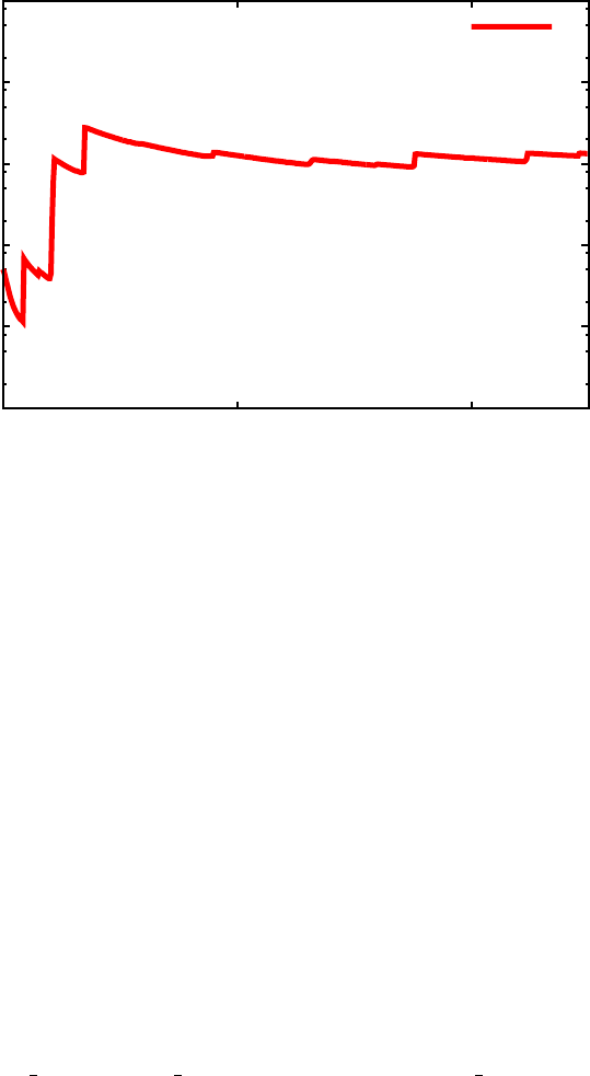
•Once this job is complete, plot the temperature stored in vasp.out as well as the

total energy and potential energy as a function of time (see example in Figure 3).

Make sure temperature is oscillating reasonably (about 15-20% above and below the

average) and that the total energy is conserved relative to the potential energy. If any

of these are not true, rerun the NVT ensemble for a longer period of time to get closer

to equilibrium, and then rerun the NVE simulation. In the sample output folder,

example OUTCAR and vasp.out ﬁles can be found from the ﬁnal NVE simulation. The

-265

-264

-263

-262

-261

-260

0 50 100 150 200 250

Energy (eV))

Time (fs)

Total Energy

Potential Energy

FIG. 3. Total energy and potenteial energy as a function of time over the course of AIMD trajectory

using VASP.

temperature oscillates slightly more than desired, but the results work well enough for

this manual.

•With the NVE trajectroy in hand, copy the OUTCAR ﬁle to Porphyrin Example/Electronic NAC/NAC,

where it will be used to generate the input conﬁgurations for the next section. Also,

from Codes/Electronic NAC/Config Generator, copy Config Generator 3Atoms VASP.f90

to the same folder.

•Look at the input cfg gen ﬁle to understand its contents (the code discusses more

details). Compile and run the code with OUTCAR and input cfg gen in the same

directory, and a posX ﬁle should be created for the X time steps of the trajectory.

Each ﬁle should list atom labels and corresponding coordinates in the Gaussian09

input format (an example can be found in the sample output folder). These ﬁles will

be used as input for performing DFT and LR-TDDFT calculations at each step in the

next section.

2. DFT and LR-TDDFT calculations

Using the posX ﬁles obtained in the previous section, DFT and LR-TDDFT calculations

will be completed to obtain Kohn-Sham orbitals and LR-TDDFT coeﬃcients at each time

step. These orbitals and coeﬃcients will be used as input into a post-processing code that

calculates Vαβ according to Equation 10.

•Copy the contents of Codes/Electronic NAC/DFT TDDFT Calc to the NAC folder where

the posX ﬁles were created. These ﬁles include several short bash scripts and header

and footer ﬁles that will be used to create a folder and input ﬁles for each time step.

•Open cycle dft script to understand its contents. This will be the ﬁrst script to

run, as it will create a folder for each time step X, labeled scfX, in which the DFT

and LR-TDDFT calculations are performed. Inside each folder, a Gaussian09 input

ﬁle (gauss dft.com) used to perform a standard DFT calculation will be created by

combining the head dft,posX, and foot ﬁles. The foot ﬁle lists the name of the

.wfx ﬁle that will contain the orbital information for computing overlaps later in the

section. Check the head dft ﬁle to make sure all entries make sense - all commands

should be identical to those used for the linear response calculation in Section III A,

except for two important changes:

–The TD command has been removed since only a ground state calculation is being

performed.

–IOP(99/18=100) has been added, which instructs Gaussian09 to calculate 100

empty orbitals. This number must be large enough to include all empty Kohn-

Sham orbitals necessary to describe electron-hole transitions constituting each of

the LR-TDDFT excited states as computed in Section III A. Look through all the

excited states from the linear response calculation and make sure that enough

empty orbitals are included, otherwise future steps will not work correctly. One

hundred orbitals should be suﬃcient for porphyrin, but this must be tested on a

case by case basis.

•Run the cycle dft script from the command line in the NAC folder, which will create

10 scf folders with a diﬀerent conﬁguration and Gaussian09 input ﬁle in each. It will

also submit the job in each folder.

•While the DFT calculations are running, the next step will be to submit jobs to cal-

culate the LR-TDDFT excitations for each time step. These calculations will provide

the LR-TDDFT coeﬃcients required to solve Equation 10.

•Open cycle lrtddft script. This bash script is very similar to cycle dft script,

however now a tddft subfolder will be created and head lrtddft will be combined

with posX to create a Gaussian09 input ﬁle to calculate LR-TDDFT excitations for

each conﬁguration. Again, the head lrtddft should contain identical commands as

those used in the earlier linear response calculations. POP=None has been included to

remove some orbital population analysis and save computational time.

•Submit cycle lrtddft script and 10 jobs should be submitted, one in each scfX/tddft

folder.

It is important to note that more than 10 conﬁgurations will be necessary to converge

Vαβ, however this small number will be enough to understand the basic steps. Convergence

with respect to number of time steps must be checked rigorously for each system studied.

Roughly 500-600 steps should be necessary in the porphyrin case.

3. Kohn-Sham orbital overlap calculations

Now that Kohn-Sham orbitals have been found for every time step, the overlaps (vab) can

be calculated that appear in Equation 10.

•Copy the contents of Codes/Electronic NAC/KS Orbital Overlap to the NAC folder

where all the scfX folders have been created. These ﬁles consist of a parallelized

or serialized version of the code to calculate Kohn-Sham overlaps between two wave

functions (ks ovlap gauss mpi.cpp and ks ovlap serial.cpp), the input ﬁle to run

this code (input ovlap), and a bash script to run this overlap code in each scfX folder

(cycle ovlap).

•This manual assumes the use of the parallelized code, but the same instructions follow

for the serial version. Compile ks ovlap gauss mpi.cpp using a C++ compiler and

rename the executable ovlap code. This code requires three inputs:

–input ovlap should have two lines: the ﬁrst line gives the minimum and max-

imum Kohn-Sham band index that will be included in the overlap matrix. So,

40 120 means that overlaps between Kohn-Sham orbitals indexed from 40 to 120

in the SCF calculations will be calculated. Again, make sure this encompasses

all the electron-hole transitions making up each LR-TDDFT excitation of the

system of interest. The second line is the time step from the molecular dynam-

ics trajectory. This is included because the code calculates the single-particle

coupling between Kohn-Sham states, even though the current method applies to

LR-TDDFT state coupling.

–The two wave functions used to calculate the overlap must be in the same folder

and named wfx1 and wfx2.

•Check that input ovlap includes the correct quantities (it should for the porphyrin

example - the 40-120 band range should be plenty). Next, open cycle ovlap and

understand its contents. Running this script from the command line will copy the

compiled code and input ﬁle into each scfX folder, then copy the current time step’s

wave function ﬁle as wfx1 and the adjacent time step’s wave function ﬁle as wfx2 into

the same directory. For this reason, the bash script should only cycle up to N−1

folders, where Nis the total number of time steps, since the adjacent wave function

ﬁle that is required will not exist for the ﬁnal time step.

•Make sure that the job ﬁle is suited for your server, and then run cycle ovlap from

the command line. Nine jobs should now be submitted, one for each of the ﬁrst nine

time steps, and each should only take a few minutes. The default number of processors

to be used is four, but this can be changed.

The ks ovlap gauss mpi.cpp ﬁle contains information about the diﬀerent outputs (all

written out with a output preﬁx), but the primary output required for the next step is

output ovlap. This ﬁle will contain the overlap matrix (vab) for the included bands as

denoted in the input ovlap ﬁle. Diagonal elements should be close to but less than one, as

the nuclear motion creates nonzero oﬀdiagonal overlaps. This ﬁle will be used as input for

the next step that calculates Vαβ between adjacent time steps.

4. LR-TDDFT electronic coupling

Now that Kohn-Sham orbital overlaps and LR-TDDFT excitation coeﬃcients have been

calculated for each time step, every quantity in Equation 10 is known and Vαβ can be found.

This step will use a post-processing code to calculate Vαβ using the output ovlap and

gauss lrtddft.out ﬁles created in the previous sections.

•Copy the contents of Codes/Electronic NAC/LRTDDFT Coupling into the NAC folder,

the directory that should contain all the scf folders. These ﬁles consist of a post-

processing code (lrtddft elec coupling.cpp) to calculate Vαβ between adjacent time

steps and the input ﬁle for the code to run properly (input nac).

•First, open lrtddft elec coupling.cpp and take time to understand the contents of

the code. The code provides a description of each input and output. This code will

take as input:

–the output ovlap ﬁle calculated in the previous section containing the vab matrix.

–input nac, which must list ﬁfteen parameters for the code to run correctly:

∗dft dir name: preﬁx of all folders containing DFT and overlap calculations

from previous steps.

∗td dir name: name of folder within dft dir name folders that contain Gaus-

sian LR-TDDFT calculation.

∗overlap file name: Name of output ﬁle within dft dir name folder for each

time step containing the K-S overlap matrix.

∗tddft file name: name of output ﬁle in td dir name directory containing

LR-TDDFT output information.

∗nsteps: total number of MD time steps for which DFT, overlap, and LR-

TDDFT calculations have been completed (number distinct dft dir name

directories you have).

∗gaus homo: HOMO orbital index

∗gaus emin: lowest orbital index, must match lowest index in output ovlap

ﬁle.

∗gaus emax: highest orbital index, must match highest index in output ovlap

ﬁle.

∗num exc: number of LR-TDDFT excited states in input exc gaussian ﬁles.

All ﬁles must have the same number of excitations and all must be included

in coupling calculation.

∗time step: time step of MD trajectory in femtoseconds.

∗dft ordering: (’yes’ or ’no’) will enforce same ordering of K-S states

across all time-steps by calculating K-S overlaps and switching the order of

states in the overlap matrix to ensure the largest value is along the diagonal.

This ensures that the same K-S states are being used to calculate the coupling

even if their ordering changes throughout the MD trajectory.

∗td ordering: (’yes’ or ’no’) will enforce same ordering of LR-TDDFT

states across all time-steps by calculating LR-TDDFT excitation overlaps

and switching the order of states based on this overlap matrix such that the

largest values are along the diagonal. This ensures that the same LR-TDDFT

states are being used to calculate the coupling even if their ordering changes

throughout the MD trajectory.

∗same sign: (’yes’ or ’no’) program will enforce the sign of all LR-TDDFT

coeﬃcients to not change between time steps. This is used in rare cases when

all LR-TDDFT coeﬃcients ﬂip signs between adjacent time steps, which leads

to unphysically large coupling values.

∗use thresh: (’yes’ or ’no’) program will output all LR-TDDFT excita-

tion coeﬃcients that change by more than the thresh value provided below.

This can be helpful in determining whether nearly degenerate states are ﬂip-

ping positions between time steps, which leads to unphysically large coupling

values.

∗thresh: value of the threshold change in LR-TDDFT excitation coeﬃcients

between time steps above which it is reported in the output threshold ﬁle.

•Compile lrtddft elec coupling.cpp using a C++ compiler and run the code. In

this case, we will only calculate the nonadiabatic coupling matrix using 10 time steps.

More will be necessary in general to converge the matrix elements.

•As the code runs, it will calculate the thermally averaged, squared nonadiabatic cou-

pling matrix by going into each dft dir name directory, using the DFT, LR-TDDFT,

and overlap matrix information to calculate the coupling between adjacent time steps,

and output information in a coupling folder created within dft dir name. It will

do this for every dft dir name, and then calculate the thermally averaged nonadia-

batic coupling matrix by averaging the square of each matrix output in each coupling

folder.

•During the calculation, make sure that the correct number of Excited States are

printed to the screen for each step - in this case, six should be listed twice in a row,

one for each time step. This indicates that the code has correctly read in all excitations

to be included in the coupling matrix.

•Once the calculations have ﬁnished, the most important output will be final NAC matrix total,

which contains the squared, averaged nonadiabatic coupling matrix (Vαβ ) to be used

as input in the ﬁnal step. There is also a NAC timeseries total ﬁle, which plots

in rows the cumulative average of the nonadiabatic coupling value for each matrix

element to check for convergence with respect to time steps.

•Next, move into a coupling folder to understand the various outputs speciﬁc to one

time step:

–output elec details and output hole details: For each excitation combina-

tion, these ﬁles list the electron and hole components (ﬁrst and second terms in

Equation10, respectively) contributing to Vαβ. These ﬁles are helpful to under-

stand which Kohn-Sham orbitals are the dominant contributors to the coupling

values.

–output exc gs details: provides the same information as the other comp ﬁles

but applies to matrix elements between the ground and excited states.

–output NAC GS X: ﬁles contain the ﬁnal Vαβ matrix including the ground state for

X=total,X=elec, and X=hole. By default in the cycling script, output nac GS total

is copied to the lrtddft coupling folder to be used to calculate the thermal

average.

–output NAC X: include same matrix as output nac GS X but does not include the

ground state. Use this matrix if only concerned about excited state dynamics

and not nonradiative recombination to ground state.

–output X flip: If dft ordering or td ordering are turned on, these output

ﬁles will list which states have been ﬂipped at this time step (X = KS or TD).

–output TD overlap: If td ordering are turned on, will output the LR-TDDFT

excitation overlap matrix before and after ordering of states.

–output coeff exc1/2 and output coeff de exc 1/2 contain matrices of all LR-

TDDFT excitation coeﬃcients for the ﬁrst (1) or second (2) time step.

–output threshold lists each excitation combination that includes a change in

LR-TDDFT excitation coeﬃcients greater than the thresh value given as input.

As mentioned above, the squared thermal average of Vαβ is in output NAC matrix total, as

this matrix has been calculated using both terms in Equation 10. output NAC matrix elec

or output NAC matrix hole contain the coupling matrix calculated only using the electronic

or hole component.

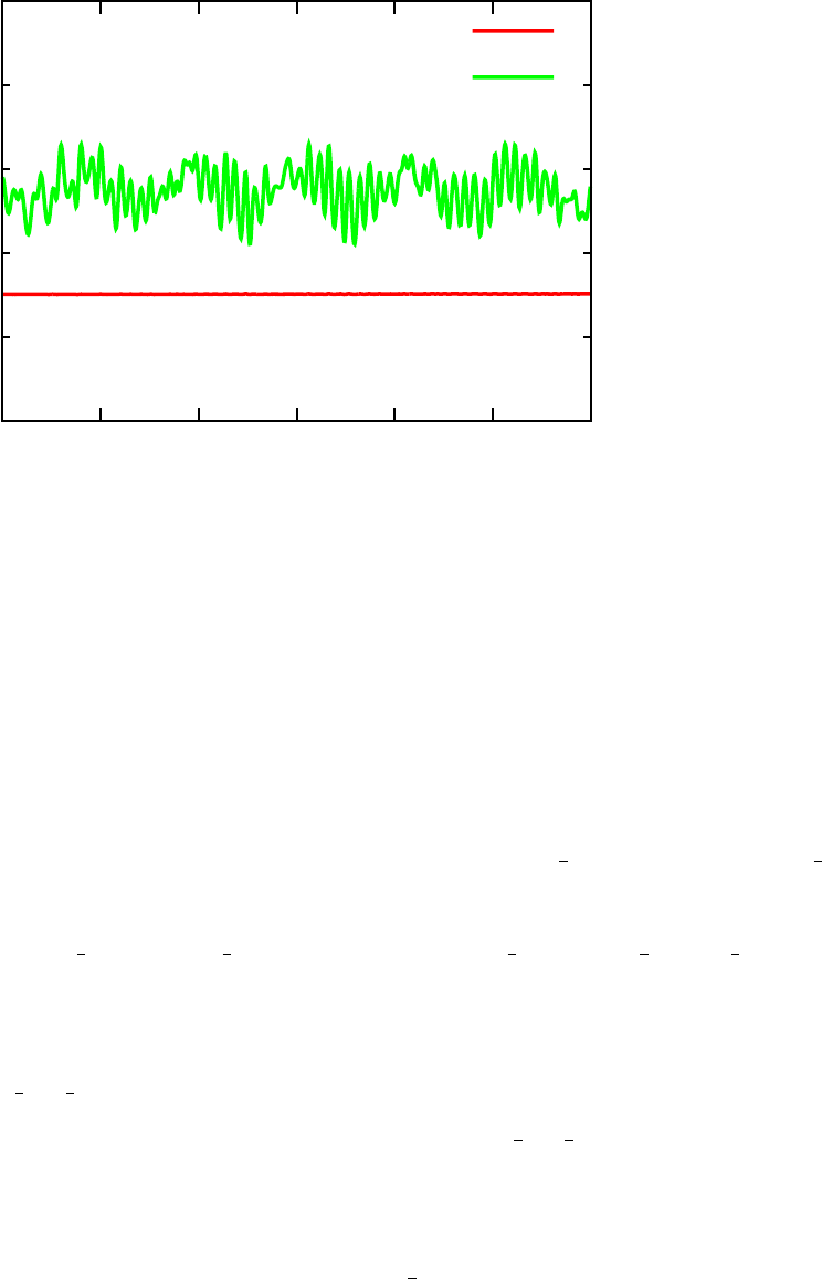
With only nine time steps included, Vαβ in the primary output ﬁle will not be converged.

After running the same steps above for 400 or more time steps, plot the row corresponding

to the coupling between the 2nd and 3rd excited states from final NAC matrix total to

check convergence. Something similar to Figure 4 should be found, with V32 ≈35 meV and

convergence reached after about 100 fs, or 400 time steps.

Congratulations - the output matrix in output NAC matrix total in this step will en-

ter directly into the phonon-induced relaxation dynamics calculated in Section III D! Now

only the Franck-Condon-weighted density of states are required before we can determine

relaxation rates!

C. Franck-Condon-weighted density of states

The second major component of the relaxation rates is F(ωαβ ), the Franck-Condon-

weighted density of states (FC-DOS, Section II D). To calculate this, three major steps are

required: 1) phonon calculation within the harmonic approximation; 2) Huang-Rhys factors

determined using the phonon modes and minimum-energy geometric conﬁgurations for each

10-6

10-5

10-4

10-3

10-2

10-1

0 50 100

|Vαβ|2 (eV2)

Time (fs)

|V32|2

FIG. 4. Cumulative average of squared electronic nonadiabatic coupling between 2nd and 3rd

excited state (V32) in porphyrin as a function of time.

excited state; and 3) the calculation of F(ωαβ ) using the Fourier transform as shown in

Equation 11. Each step is outlined in detail below, again using porphyrin as an example.

1. Phonons

First, phonon modes will be calculated within the harmonic approximation using Gaus-

sian09. This output, along with the excited state conﬁgurations, will be the input to calculate

Huang-Rhys factors for each mode between each excitation.

•Move to Porphyrin Example/FC DOS/Phonons. The porph phonons.com ﬁle acts as

input for a Gaussian calculation that will calculate all harmonic modes of the system.

Open the ﬁle to make sure all commands make sense - the addition of FREQ tells

Gaussian to calculate phonon modes of the system. Note that the atomic positions

have changed from the linear response calculations - this was just due to a symmetric

rotation done during their initial optimization. As long as NOSYMMETRY is included in

all calculations within this section, then this conﬁguration is adequate.

•Submit the calculation using the job script, which should only take ten minutes or so

on two dozen or more processors. Once the job is ﬁnished, the porph phonons.out

ﬁle will include all frequencies of the system (search for the word Frequencies in the

ﬁle).

•If any of the frequencies are negative (beyond a few tens of cm−1, which could be

within the margin of error for the calculation), then this indicates that the geometric

conﬁguration is not located at a stable minimum. Try nudging the atoms slightly

along the directions of the negative mode and rerun an optimization to try to push the

system to a stable ground state. Rerun the frequency calculation until all frequencies

are positive.

•This output ﬁle will serve as one of the inputs to calculate Huang-Rhys factors. The

second input will be the relaxed, excited state conﬁgurations.

2. Excited state geometry relaxation

In this step, six diﬀerent calculations will be performed, a geometry relaxation for each

of the six LR-TDDFT excitations included in this example calculation.

•Move to Porphyrin Example/FC DOS/Excited States. In this folder, six folders la-

beled s1 to s6 exist. An optimization of the excited state conﬁguration will be run

in each folder. At the end, output of each ﬁnal conﬁguration will be concatenated

together to serve as one input ﬁle for the Huang-Rhys factor calculations.

•Move into s1. Open the porph s1.com input ﬁle to understand its contents. All input

will be similar to the linear-response calculation except for two major diﬀerences:

–Root=1 has been included within the TD command - this tells Gaussian which

excited state to use for geometry optimization (since each excitation will have a

diﬀerent charge density that will aﬀect the nuclear conﬁguration). This should

be 1 for the ﬁrst excited state, 2 for the second excited state, and so on.

–OPT has been included in tandem with the TD command - this tells Gaussian to

perform a geometry optimization using the excited state charge density deter-

mined from the LR-TDDFT calculation.

•Run this calculation to optimize the ﬁrst excited state. These calculations can take

several hours to complete, so while waiting for it to ﬁnish, copy the input ﬁle and job

ﬁle into the other ﬁve folders, change the Root=X command to the relevant excited

state, and run the optimization calculations for these as well.

•Note: Make sure NOSYMMETRY is included in all calculations! If not, the molecule could

rotate during optimization, leading to unphysically large displacements in atoms and

nonsensical Huang-Rhys factors!

•Once all jobs have ﬁnished, check each output ﬁle (porph sX.out) to make sure the

geometry has relaxed to a minimum-energy conﬁguration meeting the force criteria

set within Gaussian09. If any do not meet relaxation criteria, resubmit the job using

the same chk ﬁle and included GEOM=Check as an input command. This will instruct

Gaussian to read the last relaxed conﬁguration from the chk ﬁle and continue opti-

mization.

3. Huang-Rhys factors

With phonon modes and eigenvectors as well as all ground and excited state conﬁgura-

tions, the next step will calculate the Huang-Rhys factors (Sk

αβ, Equation 12) between all

combinations of ground and excited states.

•Copy the contents of Codes/FC DOS/Huang Rhys Factors into Porphyrin Example/FC DOS/

Huang Rhys Factors. These ﬁles include the code that calculates Sk

αβ (Huang Rhys Factors.cpp),

and two input ﬁles (energy pop and input fcf):

–energy pop lists the minimum and maximum indices of all states included

(ground state starts as 1). The rest of the rows then include three columns:

1) state index; 2) state energy (in eV); and 3) occupancy (2 for occupied, 0 for

unoccupied). Fill in this ﬁle using results from the linear response calculation.

–input fcf provides input to calculate Sk

αβ, mainly atom number and mass to

calculate the reduced mass:

∗natoms indicates the total number of atoms.

∗n types indicates the total number of atom types.

∗The ﬁrst two lines must contain natoms and n types (one on each line).

There should then be a subsequent input line for each atom type. For each

line, input the atomic symbol, atomic number, mass, and number of this

atom type, in this order (see example input ﬁle for porphyrin example).

•In addition, three more input ﬁles must be created from the Gaussian calculations in

the previous two steps:

–First, copy the output ﬁle from the phonon calculation from porph phonons.out

to this directory and rename it gauss out freq.

–Second, extract all phonon energies from the phonon output ﬁle and list them in

a separate ﬁle called modes cm in ascending order (the same order listed in the

Gaussian output so they coincide with the correct eigenvectors). Use grep or awk

to do this quickly.

–Third, concatenate the ﬁnal atomic conﬁgurations from each output ﬁle of the

ground state calculation (taken from the phonon calculation) and each of the

excited state geometry relaxation calculations. Do this by deleting all lines from

each output ﬁle except for the ﬁnal conﬁguration, keeping the top four lines of

the header that include the dashed lines and thet text Center Number, Atomic

Number, Atomic Type, and Coordinates (Angstroms). See an example in

the sample output folder to better understand which part of the output to keep.

Once each of these conﬁgurations have been concatenated, in order of ascending

states, into one ﬁle, copy it to the Huang Rhys Factors folder and rename it

gauss out coord.

•Compile and run the code with the above input ﬁles in the same directory. This will

project atomic displacements between excited states onto mode eigenvectors and ﬁnd

reduced masses in order to calculate Sk

αβ as in Equation 12. The following output ﬁles

will be created:

–output HRF matrix contains the Sk

αβ matrix that will be used as input in the

next section to calculate F(ωαβ).

–output deltaR provides the conﬁgurational diﬀerence between each ground and

excited state conﬁguration, both in sum and for each atom.

10-2

10-1

100

0 1000 2000 3000

Sαβ (unitless)

Frequency (cm-1)

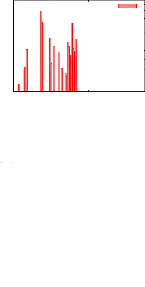
FIG. 5. Huang-Rhys factors (Sk

αβ) as a function of phonon mode energy coupling the 2nd and 3rd

excited staters in porphyrin.

–output HRF info contains a list of phonon mode index, energy, absolute displace-

ment along this mode, Sk

αβ, and reorganization energy for each state combination.

This can be helpful for plotting Huang-Rhys factors and ﬁnding dominant modes

coupled to a given transition. For example, Figure 5 plots the Huang-Rhys fac-

tors Sk

23 (corresponding to Bands 3 and 4 in the output, since the ground state

is indexed as 1).

–output dos unweighted provides a phonon density of states with 25 meV smear-

ing.

–output phonon lists phonon mode energies and reduced masses.

The key output ﬁle here is output HR matlab, as it contains all Sk

αβ elements necessary

to construct G(t) in Equation 11 and calculate F(ωαβ) for each possible transition. This

will be done in the next section, after which the phonon-induced relaxation rates can be

calculated.

4. Franck-Condon-weighted density of states

The output HR matlab,modes cm, and energy pop ﬁles will be used as input to calculate

the matrix elements of F(ωαβ ) elements for each transition using a Matlab code (see Section

II D).

•Copy output HR matlab,modes cm, and energy pop from Porphyrin Example/FC DOS/

Huang Rhys Factors to Porphyrin Example/FC DOS/FC DOS Calc.

•Copy the Matlab code in Codes/FC DOS/FC DOS Calc to the same folder. The code,

FC DOS Calculation.m, will perform three major functions: 1) construct G(t) in Equa-

tion 11 using Sk

αβ and phonon modes ωkprovided as input from output HR matlab

and modes cm; 2) perform the inverse Fourier transform to construct the F(ω) function

for each transition; and 3) ﬁt a cubic spline to each F(ω) and pick out the value of the

function at the corresponding transition energy ωαβ,F(ωαβ). A matrix of the same

size as Vαβ will be created with the values of F(ωαβ ) to be used as input in the ﬁnal

section to calculate phonon-induced relaxation dynamics.

•Open the ﬁle to understand the input section (and rest of code if desired):

–e min and e max indicate the ﬁrst and last excited state indices. Remove the row

containing these values in energy pop.

–energy pop loads in the system’s energy levels from ﬁle.

–HR factors loads in the system’s Huang-Rhys factors from the ﬁle created in the

previous section.

–modes cm loads in the system’s phonon modes from the ﬁle created for the previ-

ous section. These modes are then converted to units of eV and angular frequency.

–IMPORTANT: The Fourier transform in this code should result in a lineshape whose

real part is always positive. In Matlab, this only occurs if enough timesteps and

a short enough unit time step is used to exactly capture the period of all normal

mode frequencies. Unfortunately, this can be prohibitively costly if using the

modes with their default ﬂoating point representation. Thus, the code converts

the modes to units of inverse femtosecond, and then rounds to three signiﬁcant

digits by default. This usually works well for the default 10,000 timesteps in the

code, however a user can test and change these parameters. Just make sure to

always check that the real part of the Fourier transform is positive!

– IMPORTANT:num ts indicates the number of time steps used to construct

G(t), and f s indicates the sampling frequency used for the Fourier transform

to calculate F(ωαβ). Again, make sure these choice of values gives only positive

values for the real part of the Fourier transform performed later in the code.

Values of 10,000 and 10 Hz (default) should suﬃce for most cases.

–Outputs: 1) x axis ev provides the x-axis in units of eV for plotting F(ω) for

each transition; 2) x axis cm provides the same in units of cm−1; 3) lineshapes

plots F(ω) in columns corresponding to each transition in the same order they

appear in output disp norm from the Huang-Rhys factor calculations. Use either

of the previous axis ﬁles to plot against; and 4)

–temp smearing provides the temperature used in calculating the Bose-Einstein

distribution.

–l smearing and g smearing provide broadening parameters in eV for optional

Lorentzian and Gaussian smearing, respectively. Traditionally, the spectrum

should be broadened at least using Lorentzian lineshapes to account for dephasing

times. Gaussian smearing can also be used to account for thermal eﬀects.

–fcf weighted dos values.txt contains the F(ωαβ ) matrix used as input for the

next section.

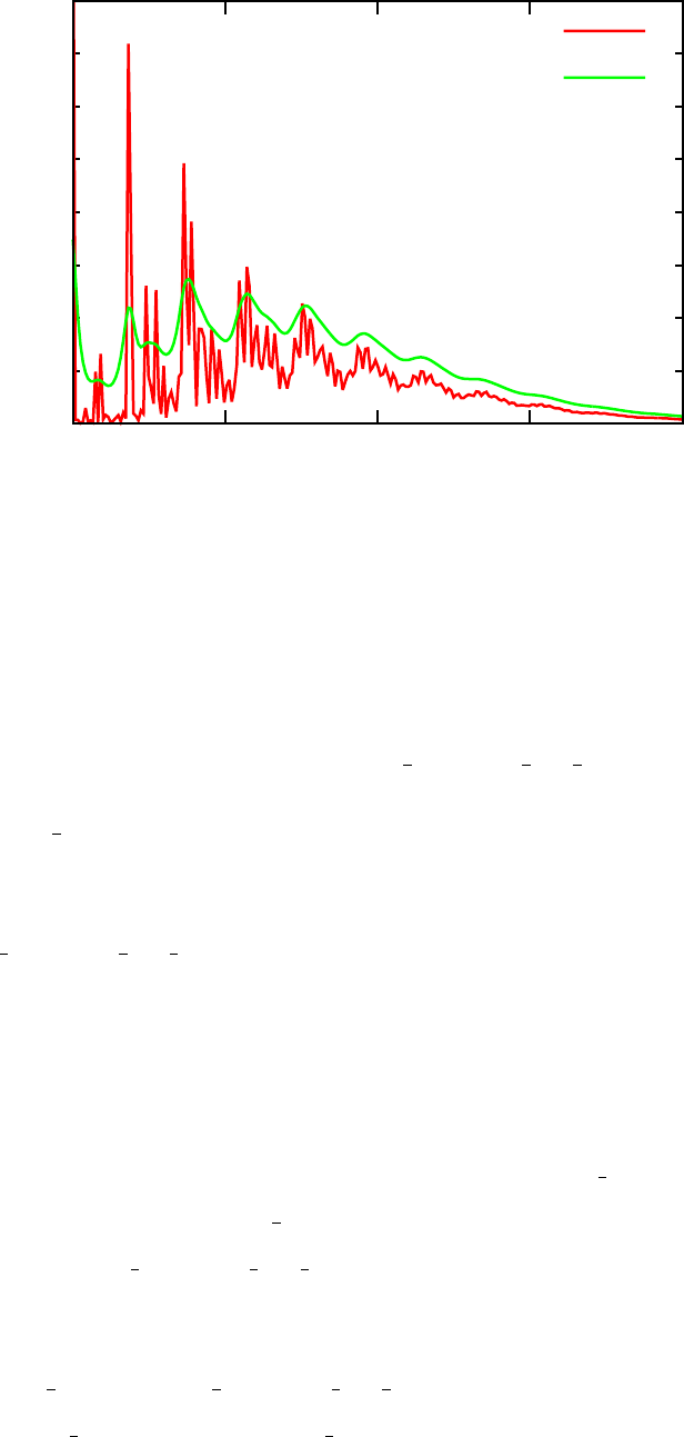
•After understanding the input and code, run the Matlab code using num ts=10000

and f s=10. The 12th column of the lineshapes output contains F(ω) for the S3-S2

transition. Rerun the code after turning on Lorentzian smearing (smearing l = 1).

Plot F(ω) with and without smearing using the x axis ev ﬁle as the x-axis input.

Compare results to those shown in Figure 6. Applying smearing makes the end result

more realistic when considering homogeneous broadening from electronic dephasing.

•Note that the transition energy for the S3-S2transition is about 0.78 eV - the code

then uses the cubic spline ﬁtting to evaluate F(ω) at this energy value, which ends up

0 0.25 0.5 0.75 1

F(ω)

Energy (eV)

No smearing

25 meV Lorentzian

FIG. 6. The F(ω) function for the S3-S2transition with and without 25 meV Lorentzian smearing.

F(ωαβ) is evaluated at the transition energy, which is around 0.78 eV.

being F(ω32)≈2.5 (remember, S0is the ground state, so F(ω32) corresponds to the

4th row and 3rd column of the matrix in fcf weighted dos values).

•Try testing ts int in the same way - increasing this variable will decrease the maxi-

mum energy for which F(ω) is calculated.

Save the fcf weighted dos values.txt output ﬁle from the Lorentzian smearing calcu-

lation. This will be used as input in the ﬁnal section to calculate relaxation rates.

D. Phonon-induced relaxation dynamics

The ﬁnal step will gather excitation energy information (energy pop, the nonadiabatic

electronic coupling matrix (Vαβ,final mat), and the Franck-Condon-weighted density of

states matrix (F(ωαβ,fcf weighted dos values) in the same directory and run a ﬁnal

Matlab code to calculate phonon-induced relaxation rates over time.

•Copy energy pop and fcf weighted dos values from the FC-DOS calculations

into Porphyrin Example/Relaxation Dynamics. Also, copy the ﬁnal output ma-

trix contaning Vαβ from Section ?? into the same directory (here it is referred

to as final mat). Finally, copy Phonon Induced Dynamics LRTDDFT RDM.m from

Codes/Relaxation Dynamics into this directory as well.

•This ﬁnal code solves the Redﬁeld equations given in Equation 1 using relaxation rates

deﬁned in 7. For each transition, kαβ is calculated using the Vαβ and F(ωαβ) matrix

elements, and the resulting phonon-induced relaxation rates are determined. If this

Matlab code is run with visualization enabled, then the output will be a graph of

the an excited population’s energy as a function of time as described in Section II E.

The population of a given state can then be ﬁt to an exponential decay to determine

excited state lifetimes.

•Open the code to understand the input:

–energy pop loads in the ground and excited state energies.

–Vab2 loads in the thermally averaged, squared nonadiabatic electronic coupling

matrix (Vαβ).

–field loads in the Franck-Condon-weighted density of states matrix (F(ωαβ)).

–forME calculates the relaxation rates (kαβ) and converts them to units of ps−1.

–Omin and Omax are the minimum and maximum state index (ground state is 1).

–inib indicates the initial excitation - phonon-induced relaxation dynamics will

inititiate witht the entire excitation in this state.

–time indicates the time (x-axis) grid along which to calculate energies of the

excited state as a function of time. Over time, electron-phonon interactions will

reduce the energy of the initially excited state until it reaches the ground state.

Each of the possible choices for time provides a diﬀerent range, from 200 ps up to

100 ns. The choice of range depends on the system being studied. Here, choose

the ﬁrst range that goes up to 200 ps.

–Egrid provides the energy range to visualize state dynamics - make sure this

range encompasses all excited state energies included in energy pop.

•Since the Soret band corresponds to excited states 3 and 4, this correponds to states

4 and 5 in energy pop. We will begin with a photoexcited electron in the higher of

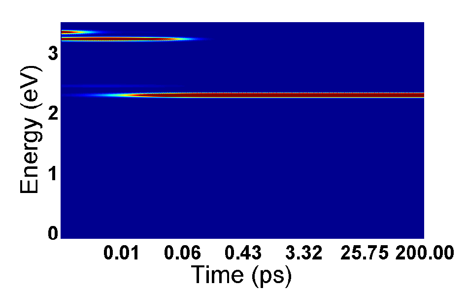
FIG. 7. Excited state energy as a function of time for porphyrin molecule with initial excitation

to Soret band (3.33 eV).

the two states, so set inib=5.

•Make sure the names of all input ﬁles match what the Matlab code will look for,

and then run the code. If visualization is enabled, the output should look like Figure

7, where darker red colors indicate more population at that energy at a given time.

This graph just visualizes the PPe output ﬁle, which can be visualized using any other

software as well.

From these results, one can see that an initial excitation to the top Soret band (3.33 eV),

leads to fast relaxation to the lower Soret band (3.22 eV) in under 10 fs. From there, it

takes about 30 fs to relax to the lowest excited state at 2.28 eV. This 30 fs Soret lifetime

agrees extremely well with experimental results that predict the relaxation rate to be under

50 fs8, supporting the accuracy of the present method. The excitation stays in this state for

over 200 ps - if the time range were extended, nonradiative relaxation to the ground state

would be seen in around 10 ns.

Congratulations! This example illustrates all the major tools included in this method

- although porphyrin only contains 38 atoms, this method can be applied to systems with

hundreds of atoms and is still computationally feasible.

Good luck and please provide feedback about the method and manual at jptrinas-

tic@gmail.com.

1J. Trinastic, I.-H. Chu, and H.-P. Cheng, J Phys Chem C , under review (2015).

2V. May and O. K¨uhn, Charge and energy transfer dynamics in molecular systems (John Wiley

& Sons, 2008).

3M. Khalil, N. Demirdven, and A. Tokmakoﬀ, J. Chem. Phys. 121, 362 (2004).

4O. V. Prezhdo and P. J. Rossky, J. Chem. Phys. 107, 5863 (1997).

5I. Tavernelli, B. F. E. Curchod, A. Laktionov, and U. Rothlisberger, J. Chem. Phys. 133,

194104 (2010).

6I. Tavernelli, E. Tapavicza, and U. Rothlisberger, J. Chem. Phys. 130, 124107 (2009).

7M. E. Casida, Journal of Molecular Structure: THEOCHEM 914, 3 (2009).

8A. Marcelli, P. Foggi, L. Moroni, C. Gellini, and P. R. Salvi, The Journal of Physical Chemistry

A112, 1864 (2008).

9K. Y. Yeon, D. Jeong, and S. K. Kim, Chemical Communications 46, 5572 (2010).

10 Y. He, Y. Xiong, Q. Zhu, and F. Kong, Acta Physico-Chimica Sinica 15, 636 (1999).

Phonon Relaxation Manual

Navigation menu

Versions of this User Manual:

Views

Navigation