Programmers Guide

User Manual: Pdf

Open the PDF directly: View PDF .
Page Count: 92

Estimators
Importing Data
Introduction
Tensors
Graphs and Sessions
Saving and Restoring
Using GPUs
Embeddings
Debugging TensorFlow Programs
TensorBoard: Visualizing Learning
- Serializing the data
- Launching TensorBoard
TensorBoard: Graph Visualization

Estimators

This document introduces Estimators--a high-level TensorFlow API that greatly simpliﬁes machine learning programming.

Estimators encapsulate the following actions:

training

evaluation

prediction

export for serving

You may either use the pre-made Estimators we provide or write your own custom Estimators. All Estimators--whether pre-

made or custom--are classes based on the tf.estimator.Estimator class.

Note: TensorFlow also includes a deprecated Estimator class at tf.contrib.learn.Estimator, which you should not use.

Advantages of Estimators

Estimators provide the following beneﬁts:

You can run Estimators-based models on a local host or on a distributed multi-server environment without changing your

model. Furthermore, you can run Estimators-based models on CPUs, GPUs, or TPUs without recoding your model.

Estimators simplify sharing implementations between model developers.

You can develop a state of the art model with high-level intuitive code, In short, it is generally much easier to create models

with Estimators than with the low-level TensorFlow APIs.

Estimators are themselves built on tf.layers, which simpliﬁes customization.

Estimators build the graph for you. In other words, you don't have to build the graph.

Estimators provide a safe distributed training loop that controls how and when to:

build the graph

initialize variables

start queues

handle exceptions

create checkpoint ﬁles and recover from failures

save summaries for TensorBoard

When writing an application with Estimators, you must separate the data input pipeline from the model. This separation

simpliﬁes experiments with different data sets.

Pre-made Estimators

Pre-made Estimators enable you to work at a much higher conceptual level than the base TensorFlow APIs. You no longer have

to worry about creating the computational graph or sessions since Estimators handle all the "plumbing" for you. That is, pre-

made Estimators create and manage Graph and Session objects for you. Furthermore, pre-made Estimators let you

experiment with different model architectures by making only minimal code changes. DNNClassifier, for example, is a pre-

made Estimator class that trains classiﬁcation models through dense, feed-forward neural networks.

Structure of a pre-made Estimators program

A TensorFlow program relying on a pre-made Estimator typically consists of the following four steps:

1. Write one or more dataset importing functions. For example, you might create one function to import the training set and

another function to import the test set. Each dataset importing function must return two objects:

a dictionary in which the keys are feature names and the values are Tensors (or SparseTensors) containing the

corresponding feature data

a Tensor containing one or more labels

For example, the following code illustrates the basic skeleton for an input function:

(See Importing Data for full details.)

2. Deﬁne the feature columns. Each tf.feature_column identiﬁes a feature name, its type, and any input pre-processing.

For example, the following snippet creates three feature columns that hold integer or ﬂoating-point data. The ﬁrst two

feature columns simply identify the feature's name and type. The third feature column also speciﬁes a lambda the program

will invoke to scale the raw data:

3. Instantiate the relevant pre-made Estimator. For example, here's a sample instantiation of a pre-made Estimator named

LinearClassifier:

4. Call a training, evaluation, or inference method. For example, all Estimators provide a train method, which trains a

model.

Beneﬁts of pre-made Estimators

Pre-made Estimators encode best practices, providing the following beneﬁts:

Best practices for determining where different parts of the computational graph should run, implementing strategies on a

single machine or on a cluster.

Best practices for event (summary) writing and universally useful summaries.

If you don't use pre-made Estimators, you must implement the preceding features yourself.

Custom Estimators

def input_fn(dataset):

... # manipulate dataset, extracting feature names and the label

return feature_dict, label

# Define three numeric feature columns.

population = tf.feature_column.numeric_column('population')

crime_rate = tf.feature_column.numeric_column('crime_rate')

median_education = tf.feature_column.numeric_column('median_education',

normalizer_fn='lambda x: x - global_education_mean')

# Instantiate an estimator, passing the feature columns.

estimator = tf.estimator.Estimator.LinearClassifier(

feature_columns=[population, crime_rate, median_education],

)

# my_training_set is the function created in Step 1

estimator.train(input_fn=my_training_set, steps=2000)

The heart of every Estimator--whether pre-made or custom--is its model function, which is a method that builds graphs for

training, evaluation, and prediction. When you are using a pre-made Estimator, someone else has already implemented the

model function. When relying on a custom Estimator, you must write the model function yourself. A companion document

explains how to write the model function.

Recommended workﬂow

We recommend the following workﬂow:

1. Assuming a suitable pre-made Estimator exists, use it to build your ﬁrst model and use its results to establish a baseline.

2. Build and test your overall pipeline, including the integrity and reliability of your data with this pre-made Estimator.

3. If suitable alternative pre-made Estimators are available, run experiments to determine which pre-made Estimator produces

the best results.

4. Possibly, further improve your model by building your own custom Estimator.

Creating Estimators from Keras models

You can convert existing Keras models to Estimators. Doing so enables your Keras model to access Estimator's strengths, such

as distributed training. Call tf.keras.estimator.model_to_estimator as in the following sample:

Note that the names of feature columns and labels of a keras estimator come from the corresponding compiled keras model.

For example, the input key names for train_input_fn above can be obtained from keras_inception_v3.input_names, and

similarly, the predicted output names can be obtained fromkeras_inception_v3.output_names.

For more details, please refer to the documentation for tf.keras.estimator.model_to_estimator.

Importing Data

# Instantiate a Keras inception v3 model.

keras_inception_v3 = tf.keras.applications.inception_v3.InceptionV3(weights=None)

# Compile model with the optimizer, loss, and metrics you'd like to train with.

keras_inception_v3.compile(optimizer=tf.keras.optimizers.SGD(lr=0.0001, momentum=0.9),

loss='categorical_crossentropy',

metric='accuracy')

# Create an Estimator from the compiled Keras model. Note the initial model

# state of the keras model is preserved in the created Estimator.

est_inception_v3 = tf.keras.estimator.model_to_estimator(keras_model=keras_inception_v3)

# Treat the derived Estimator as you would with any other Estimator.

# First, recover the input name(s) of Keras model, so we can use them as the

# feature column name(s) of the Estimator input function:

keras_inception_v3.input_names # print out: ['input_1']

# Once we have the input name(s), we can create the input function, for example,

# for input(s) in the format of numpy ndarray:

train_input_fn = tf.estimator.inputs.numpy_input_fn(

x={"input_1": train_data},

y=train_labels,

num_epochs=1,

shuffle=False)

# To train, we call Estimator's train function:

est_inception_v3.train(input_fn=train_input_fn, steps=2000)

The tf.data API enables you to build complex input pipelines from simple, reusable pieces. For example, the pipeline for an

image model might aggregate data from ﬁles in a distributed ﬁle system, apply random perturbations to each image, and

merge randomly selected images into a batch for training. The pipeline for a text model might involve extracting symbols from

raw text data, converting them to embedding identiﬁers with a lookup table, and batching together sequences of different

lengths. The tf.data API makes it easy to deal with large amounts of data, different data formats, and complicated

transformations.

The tf.data API introduces two new abstractions to TensorFlow:

A tf.data.Dataset represents a sequence of elements, in which each element contains one or more Tensor objects. For

example, in an image pipeline, an element might be a single training example, with a pair of tensors representing the image

data and a label. There are two distinct ways to create a dataset:

Creating a source (e.g. Dataset.from_tensor_slices()) constructs a dataset from one or more tf.Tensor objects.

Applying a transformation (e.g. Dataset.batch()) constructs a dataset from one or more tf.data.Dataset objects.

A tf.data.Iterator provides the main way to extract elements from a dataset. The operation returned by

Iterator.get_next() yields the next element of a Dataset when executed, and typically acts as the interface between

input pipeline code and your model. The simplest iterator is a "one-shot iterator", which is associated with a particular

Dataset and iterates through it once. For more sophisticated uses, theIterator.initializer operation enables you to

reinitialize and parameterize an iterator with different datasets, so that you can, for example, iterate over training and

validation data multiple times in the same program.

Basic mechanics

This section of the guide describes the fundamentals of creating different kinds of Dataset and Iteratorobjects, and how to

extract data from them.

To start an input pipeline, you must deﬁne a source. For example, to construct a Dataset from some tensors in memory, you

can use tf.data.Dataset.from_tensors() or tf.data.Dataset.from_tensor_slices(). Alternatively, if your input data

are on disk in the recommended TFRecord format, you can construct atf.data.TFRecordDataset.

Once you have a Dataset object, you can transform it into a new Dataset by chaining method calls on the tf.data.Dataset

object. For example, you can apply per-element transformations such as Dataset.map()(to apply a function to each element),

and multi-element transformations such as Dataset.batch(). See the documentation for tf.data.Dataset for a complete

list of transformations.

The most common way to consume values from a Dataset is to make an iterator object that provides access to one element of

the dataset at a time (for example, by calling Dataset.make_one_shot_iterator()). Atf.data.Iterator provides two

operations: Iterator.initializer, which enables you to (re)initialize the iterator's state; and Iterator.get_next(), which

returns tf.Tensor objects that correspond to the symbolic next element. Depending on your use case, you might choose a

different type of iterator, and the options are outlined below.

Dataset structure

A dataset comprises elements that each have the same structure. An element contains one or more tf.Tensor objects, called

components. Each component has a tf.DType representing the type of elements in the tensor, and a tf.TensorShape

representing the (possibly partially speciﬁed) static shape of each element. The Dataset.output_types and

Dataset.output_shapes properties allow you to inspect the inferred types and shapes of each component of a dataset

element. The nested structure of these properties map to the structure of an element, which may be a single tensor, a tuple of

tensors, or a nested tuple of tensors. For example:

It is often convenient to give names to each component of an element, for example if they represent different features of a

training example. In addition to tuples, you can use collections.namedtuple or a dictionary mapping strings to tensors to

represent a single element of a Dataset.

The Dataset transformations support datasets of any structure. When using the Dataset.map(), Dataset.flat_map(), and

Dataset.filter() transformations, which apply a function to each element, the element structure determines the arguments

of the function:

Creating an iterator

Once you have built a Dataset to represent your input data, the next step is to create an Iterator to access elements from that

dataset. The tf.data API currently supports the following iterators, in increasing level of sophistication:

one-shot,

initializable,

reinitializable, and

feedable.

A one-shot iterator is the simplest form of iterator, which only supports iterating once through a dataset, with no need for

explicit initialization. One-shot iterators handle almost all of the cases that the existing queue-based input pipelines support,

but they do not support parameterization. Using the example of Dataset.range():

dataset1 = tf.data.Dataset.from_tensor_slices(tf.random_uniform([4, 10]))

print(dataset1.output_types) # ==> "tf.float32"

print(dataset1.output_shapes) # ==> "(10,)"

dataset2 = tf.data.Dataset.from_tensor_slices(

(tf.random_uniform([4]),

tf.random_uniform([4, 100], maxval=100, dtype=tf.int32)))

print(dataset2.output_types) # ==> "(tf.float32, tf.int32)"

print(dataset2.output_shapes) # ==> "((), (100,))"

dataset3 = tf.data.Dataset.zip((dataset1, dataset2))

print(dataset3.output_types) # ==> (tf.float32, (tf.float32, tf.int32))

print(dataset3.output_shapes) # ==> "(10, ((), (100,)))"

dataset = tf.data.Dataset.from_tensor_slices(

{"a": tf.random_uniform([4]),

"b": tf.random_uniform([4, 100], maxval=100, dtype=tf.int32)})

print(dataset.output_types) # ==> "{'a': tf.float32, 'b': tf.int32}"

print(dataset.output_shapes) # ==> "{'a': (), 'b': (100,)}"

dataset1 = dataset1.map(lambda x: ...)

dataset2 = dataset2.flat_map(lambda x, y: ...)

# Note: Argument destructuring is not available in Python 3.

dataset3 = dataset3.filter(lambda x, (y, z): ...)

Note: Currently, one-shot iterators are the only type that is easily usable with an Estimator.

An initializable iterator requires you to run an explicit iterator.initializer operation before using it. In exchange for this

inconvenience, it enables you to parameterize the deﬁnition of the dataset, using one or more tf.placeholder() tensors that

can be fed when you initialize the iterator. Continuing the Dataset.range()example:

A reinitializable iterator can be initialized from multiple different Dataset objects. For example, you might have a training

input pipeline that uses random perturbations to the input images to improve generalization, and a validation input pipeline

that evaluates predictions on unmodiﬁed data. These pipelines will typically use different Dataset objects that have the same

structure (i.e. the same types and compatible shapes for each component).

dataset = tf.data.Dataset.range(100)

iterator = dataset.make_one_shot_iterator()

next_element = iterator.get_next()

for i in range(100):

value = sess.run(next_element)

assert i == value

max_value = tf.placeholder(tf.int64, shape=[])

dataset = tf.data.Dataset.range(max_value)

iterator = dataset.make_initializable_iterator()

next_element = iterator.get_next()

# Initialize an iterator over a dataset with 10 elements.

sess.run(iterator.initializer, feed_dict={max_value: 10})

for i in range(10):

value = sess.run(next_element)

assert i == value

# Initialize the same iterator over a dataset with 100 elements.

sess.run(iterator.initializer, feed_dict={max_value: 100})

for i in range(100):

value = sess.run(next_element)

assert i == value

A feedable iterator can be used together with tf.placeholder to select what Iterator to use in each call to

tf.Session.run, via the familiar feed_dict mechanism. It offers the same functionality as a reinitializable iterator, but it

does not require you to initialize the iterator from the start of a dataset when you switch between iterators. For example, using

the same training and validation example from above, you can usetf.data.Iterator.from_string_handle to deﬁne a

feedable iterator that allows you to switch between the two datasets:

# Define training and validation datasets with the same structure.

training_dataset = tf.data.Dataset.range(100).map(

lambda x: x + tf.random_uniform([], -10, 10, tf.int64))

validation_dataset = tf.data.Dataset.range(50)

# A reinitializable iterator is defined by its structure. We could use the

# `output_types` and `output_shapes` properties of either `training_dataset`

# or `validation_dataset` here, because they are compatible.

iterator = tf.data.Iterator.from_structure(training_dataset.output_types,

training_dataset.output_shapes)

next_element = iterator.get_next()

training_init_op = iterator.make_initializer(training_dataset)

validation_init_op = iterator.make_initializer(validation_dataset)

# Run 20 epochs in which the training dataset is traversed, followed by the

# validation dataset.

for _ in range(20):

# Initialize an iterator over the training dataset.

sess.run(training_init_op)

for _ in range(100):

sess.run(next_element)

# Initialize an iterator over the validation dataset.

sess.run(validation_init_op)

for _ in range(50):

sess.run(next_element)

Consuming values from an iterator

The Iterator.get_next() method returns one or more tf.Tensor objects that correspond to the symbolic next element of

an iterator. Each time these tensors are evaluated, they take the value of the next element in the underlying dataset. (Note that,

like other stateful objects in TensorFlow, calling Iterator.get_next() does not immediately advance the iterator. Instead

you must use the returned tf.Tensor objects in a TensorFlow expression, and pass the result of that expression to

tf.Session.run() to get the next elements and advance the iterator.)

If the iterator reaches the end of the dataset, executing the Iterator.get_next() operation will raise a

tf.errors.OutOfRangeError. After this point the iterator will be in an unusable state, and you must initialize it again if you

want to use it further.

# Define training and validation datasets with the same structure.

training_dataset = tf.data.Dataset.range(100).map(

lambda x: x + tf.random_uniform([], -10, 10, tf.int64)).repeat()

validation_dataset = tf.data.Dataset.range(50)

# A feedable iterator is defined by a handle placeholder and its structure. We

# could use the `output_types` and `output_shapes` properties of either

# `training_dataset` or `validation_dataset` here, because they have

# identical structure.

handle = tf.placeholder(tf.string, shape=[])

iterator = tf.data.Iterator.from_string_handle(

handle, training_dataset.output_types, training_dataset.output_shapes)

next_element = iterator.get_next()

# You can use feedable iterators with a variety of different kinds of iterator

# (such as one-shot and initializable iterators).

training_iterator = training_dataset.make_one_shot_iterator()

validation_iterator = validation_dataset.make_initializable_iterator()

# The `Iterator.string_handle()` method returns a tensor that can be evaluated

# and used to feed the `handle` placeholder.

training_handle = sess.run(training_iterator.string_handle())

validation_handle = sess.run(validation_iterator.string_handle())

# Loop forever, alternating between training and validation.

while True:

# Run 200 steps using the training dataset. Note that the training dataset is

# infinite, and we resume from where we left off in the previous `while` loop

# iteration.

for _ in range(200):

sess.run(next_element, feed_dict={handle: training_handle})

# Run one pass over the validation dataset.

sess.run(validation_iterator.initializer)

for _ in range(50):

sess.run(next_element, feed_dict={handle: validation_handle})

A common pattern is to wrap the "training loop" in a try-except block:

If each element of the dataset has a nested structure, the return value of Iterator.get_next() will be one or more

tf.Tensor objects in the same nested structure:

Note that evaluating any of next1, next2, or next3 will advance the iterator for all components. A typical consumer of an

iterator will include all components in a single expression.

Reading input data

Consuming NumPy arrays

If all of your input data ﬁt in memory, the simplest way to create a Dataset from them is to convert them to tf.Tensor objects

and use Dataset.from_tensor_slices().

dataset = tf.data.Dataset.range(5)

iterator = dataset.make_initializable_iterator()

next_element = iterator.get_next()

# Typically `result` will be the output of a model, or an optimizer's

# training operation.

result = tf.add(next_element, next_element)

sess.run(iterator.initializer)

print(sess.run(result)) # ==> "0"

print(sess.run(result)) # ==> "2"

print(sess.run(result)) # ==> "4"

print(sess.run(result)) # ==> "6"

print(sess.run(result)) # ==> "8"

try:

sess.run(result)

except tf.errors.OutOfRangeError:

print("End of dataset") # ==> "End of dataset"

sess.run(iterator.initializer)

while True:

try:

sess.run(result)

except tf.errors.OutOfRangeError:

break

dataset1 = tf.data.Dataset.from_tensor_slices(tf.random_uniform([4, 10]))

dataset2 = tf.data.Dataset.from_tensor_slices((tf.random_uniform([4]), tf.random_uniform([4,

100])))

dataset3 = tf.data.Dataset.zip((dataset1, dataset2))

iterator = dataset3.make_initializable_iterator()

sess.run(iterator.initializer)

next1, (next2, next3) = iterator.get_next()

Note that the above code snippet will embed the features and labels arrays in your TensorFlow graph as tf.constant()

operations. This works well for a small dataset, but wastes memory---because the contents of the array will be copied multiple

times---and can run into the 2GB limit for the tf.GraphDef protocol buffer.

As an alternative, you can deﬁne the Dataset in terms of tf.placeholder() tensors, and feed the NumPy arrays when you

initialize an Iterator over the dataset.

Consuming TFRecord data

The tf.data API supports a variety of ﬁle formats so that you can process large datasets that do not ﬁt in memory. For

example, the TFRecord ﬁle format is a simple record-oriented binary format that many TensorFlow applications use for

training data. The tf.data.TFRecordDataset class enables you to stream over the contents of one or more TFRecord ﬁles as

part of an input pipeline.

The filenames argument to the TFRecordDataset initializer can either be a string, a list of strings, or a tf.Tensor of strings.

Therefore if you have two sets of ﬁles for training and validation purposes, you can use atf.placeholder(tf.string) to

represent the ﬁlenames, and initialize an iterator from the appropriate ﬁlenames:

# Load the training data into two NumPy arrays, for example using `np.load()`.

with np.load("/var/data/training_data.npy") as data:

features = data["features"]

labels = data["labels"]

# Assume that each row of `features` corresponds to the same row as `labels`.

assert features.shape[0] == labels.shape[0]

dataset = tf.data.Dataset.from_tensor_slices((features, labels))

# Load the training data into two NumPy arrays, for example using `np.load()`.

with np.load("/var/data/training_data.npy") as data:

features = data["features"]

labels = data["labels"]

# Assume that each row of `features` corresponds to the same row as `labels`.

assert features.shape[0] == labels.shape[0]

features_placeholder = tf.placeholder(features.dtype, features.shape)

labels_placeholder = tf.placeholder(labels.dtype, labels.shape)

dataset = tf.data.Dataset.from_tensor_slices((features_placeholder, labels_placeholder))

# [Other transformations on `dataset`...]

dataset = ...

iterator = dataset.make_initializable_iterator()

sess.run(iterator.initializer, feed_dict={features_placeholder: features,

labels_placeholder: labels})

# Creates a dataset that reads all of the examples from two files.

filenames = ["/var/data/file1.tfrecord", "/var/data/file2.tfrecord"]

dataset = tf.data.TFRecordDataset(filenames)

Consuming text data

Many datasets are distributed as one or more text ﬁles. The tf.data.TextLineDataset provides an easy way to extract lines

from one or more text ﬁles. Given one or more ﬁlenames, a TextLineDataset will produce one string-valued element per line

of those ﬁles. Like a TFRecordDataset, TextLineDataset accepts filenamesas a tf.Tensor, so you can parameterize it by

passing a tf.placeholder(tf.string).

By default, a TextLineDataset yields every line of each ﬁle, which may not be desirable, for example if the ﬁle starts with a

header line, or contains comments. These lines can be removed using the Dataset.skip() andDataset.filter()

transformations. To apply these transformations to each ﬁle separately, we use Dataset.flat_map() to create a nested

Dataset for each ﬁle.

Preprocessing data with Dataset.map()

filenames = tf.placeholder(tf.string, shape=[None])

dataset = tf.data.TFRecordDataset(filenames)

dataset = dataset.map(...) # Parse the record into tensors.

dataset = dataset.repeat() # Repeat the input indefinitely.

dataset = dataset.batch(32)

iterator = dataset.make_initializable_iterator()

# You can feed the initializer with the appropriate filenames for the current

# phase of execution, e.g. training vs. validation.

# Initialize `iterator` with training data.

training_filenames = ["/var/data/file1.tfrecord", "/var/data/file2.tfrecord"]

sess.run(iterator.initializer, feed_dict={filenames: training_filenames})

# Initialize `iterator` with validation data.

validation_filenames = ["/var/data/validation1.tfrecord", ...]

sess.run(iterator.initializer, feed_dict={filenames: validation_filenames})

filenames = ["/var/data/file1.txt", "/var/data/file2.txt"]

dataset = tf.data.TextLineDataset(filenames)

filenames = ["/var/data/file1.txt", "/var/data/file2.txt"]

dataset = tf.data.Dataset.from_tensor_slices(filenames)

# Use `Dataset.flat_map()` to transform each file as a separate nested dataset,

# and then concatenate their contents sequentially into a single "flat" dataset.

# * Skip the first line (header row).

# * Filter out lines beginning with "#" (comments).

dataset = dataset.flat_map(

lambda filename: (

tf.data.TextLineDataset(filename)

.skip(1)

.filter(lambda line: tf.not_equal(tf.substr(line, 0, 1), "#"))))

The Dataset.map(f) transformation produces a new dataset by applying a given function f to each element of the input

dataset. It is based on the map() function that is commonly applied to lists (and other structures) in functional programming

languages. The function f takes the tf.Tensor objects that represent a single element in the input, and returns the tf.Tensor

objects that will represent a single element in the new dataset. Its implementation uses standard TensorFlow operations to

transform one element into another.

This section covers common examples of how to use Dataset.map().

Parsing tf.Example protocol buffer messages

Many input pipelines extract tf.train.Example protocol buffer messages from a TFRecord-format ﬁle (written, for example,

using tf.python_io.TFRecordWriter). Each tf.train.Example record contains one or more "features", and the input

pipeline typically converts these features into tensors.

Decoding image data and resizing it

When training a neural network on real-world image data, it is often necessary to convert images of different sizes to a

common size, so that they may be batched into a ﬁxed size.

# Transforms a scalar string `example_proto` into a pair of a scalar string and

# a scalar integer, representing an image and its label, respectively.

def _parse_function(example_proto):

features = {"image": tf.FixedLenFeature((), tf.string, default_value=""),

"label": tf.FixedLenFeature((), tf.int32, default_value=0)}

parsed_features = tf.parse_single_example(example_proto, features)

return parsed_features["image"], parsed_features["label"]

# Creates a dataset that reads all of the examples from two files, and extracts

# the image and label features.

filenames = ["/var/data/file1.tfrecord", "/var/data/file2.tfrecord"]

dataset = tf.data.TFRecordDataset(filenames)

dataset = dataset.map(_parse_function)

# Reads an image from a file, decodes it into a dense tensor, and resizes it

# to a fixed shape.

def _parse_function(filename, label):

image_string = tf.read_file(filename)

image_decoded = tf.image.decode_image(image_string)

image_resized = tf.image.resize_images(image_decoded, [28, 28])

return image_resized, label

# A vector of filenames.

filenames = tf.constant(["/var/data/image1.jpg", "/var/data/image2.jpg", ...])

# `labels[i]` is the label for the image in `filenames[i].

labels = tf.constant([0, 37, ...])

dataset = tf.data.Dataset.from_tensor_slices((filenames, labels))

dataset = dataset.map(_parse_function)

Applying arbitrary Python logic with tf.py_func()

For performance reasons, we encourage you to use TensorFlow operations for preprocessing your data whenever possible.

However, it is sometimes useful to call upon external Python libraries when parsing your input data. To do so, invoke, the

tf.py_func() operation in a Dataset.map() transformation.

Batching dataset elements

Simple batching

The simplest form of batching stacks n consecutive elements of a dataset into a single element. The Dataset.batch()

transformation does exactly this, with the same constraints as the tf.stack() operator, applied to each component of the

elements: i.e. for each component i, all elements must have a tensor of the exact same shape.

Batching tensors with padding

import cv2

# Use a custom OpenCV function to read the image, instead of the standard

# TensorFlow `tf.read_file()` operation.

def _read_py_function(filename, label):

image_decoded = cv2.imread(image_string, cv2.IMREAD_GRAYSCALE)

return image_decoded, label

# Use standard TensorFlow operations to resize the image to a fixed shape.

def _resize_function(image_decoded, label):

image_decoded.set_shape([None, None, None])

image_resized = tf.image.resize_images(image_decoded, [28, 28])

return image_resized, label

filenames = ["/var/data/image1.jpg", "/var/data/image2.jpg", ...]

labels = [0, 37, 29, 1, ...]

dataset = tf.data.Dataset.from_tensor_slices((filenames, labels))

dataset = dataset.map(

lambda filename, label: tuple(tf.py_func(

_read_py_function, [filename, label], [tf.uint8, label.dtype])))

dataset = dataset.map(_resize_function)

inc_dataset = tf.data.Dataset.range(100)

dec_dataset = tf.data.Dataset.range(0, -100, -1)

dataset = tf.data.Dataset.zip((inc_dataset, dec_dataset))

batched_dataset = dataset.batch(4)

iterator = batched_dataset.make_one_shot_iterator()

next_element = iterator.get_next()

print(sess.run(next_element)) # ==> ([0, 1, 2, 3], [ 0, -1, -2, -3])

print(sess.run(next_element)) # ==> ([4, 5, 6, 7], [-4, -5, -6, -7])

print(sess.run(next_element)) # ==> ([8, 9, 10, 11], [-8, -9, -10, -11])

The above recipe works for tensors that all have the same size. However, many models (e.g. sequence models) work with input

data that can have varying size (e.g. sequences of different lengths). To handle this case, theDataset.padded_batch()

transformation enables you to batch tensors of different shape by specifying one or more dimensions in which they may be

padded.

The Dataset.padded_batch() transformation allows you to set different padding for each dimension of each component,

and it may be variable-length (signiﬁed by None in the example above) or constant-length. It is also possible to override the

padding value, which defaults to 0.

Training workﬂows

Processing multiple epochs

The tf.data API offers two main ways to process multiple epochs of the same data.

The simplest way to iterate over a dataset in multiple epochs is to use the Dataset.repeat() transformation. For example, to

create a dataset that repeats its input for 10 epochs:

Applying the Dataset.repeat() transformation with no arguments will repeat the input indeﬁnitely. The

Dataset.repeat() transformation concatenates its arguments without signaling the end of one epoch and the beginning of

the next epoch.

If you want to receive a signal at the end of each epoch, you can write a training loop that catches the

tf.errors.OutOfRangeError at the end of a dataset. At that point you might collect some statistics (e.g. the validation error)

for the epoch.

dataset = tf.data.Dataset.range(100)

dataset = dataset.map(lambda x: tf.fill([tf.cast(x, tf.int32)], x))

dataset = dataset.padded_batch(4, padded_shapes=[None])

iterator = dataset.make_one_shot_iterator()

next_element = iterator.get_next()

print(sess.run(next_element)) # ==> [[0, 0, 0], [1, 0, 0], [2, 2, 0], [3, 3, 3]]

print(sess.run(next_element)) # ==> [[4, 4, 4, 4, 0, 0, 0],

# [5, 5, 5, 5, 5, 0, 0],

# [6, 6, 6, 6, 6, 6, 0],

# [7, 7, 7, 7, 7, 7, 7]]

filenames = ["/var/data/file1.tfrecord", "/var/data/file2.tfrecord"]

dataset = tf.data.TFRecordDataset(filenames)

dataset = dataset.map(...)

dataset = dataset.repeat(10)

dataset = dataset.batch(32)

Randomly shufﬂing input data

The Dataset.shuffle() transformation randomly shufﬂes the input dataset using a similar algorithm to

tf.RandomShuffleQueue: it maintains a ﬁxed-size buffer and chooses the next element uniformly at random from that buffer.

Using high-level APIs

The tf.train.MonitoredTrainingSession API simpliﬁes many aspects of running TensorFlow in a distributed setting.

MonitoredTrainingSession uses the tf.errors.OutOfRangeError to signal that training has completed, so to use it with

the tf.data API, we recommend usingDataset.make_one_shot_iterator(). For example:

filenames = ["/var/data/file1.tfrecord", "/var/data/file2.tfrecord"]

dataset = tf.data.TFRecordDataset(filenames)

dataset = dataset.map(...)

dataset = dataset.batch(32)

iterator = dataset.make_initializable_iterator()

next_element = iterator.get_next()

# Compute for 100 epochs.

for _ in range(100):

sess.run(iterator.initializer)

while True:

try:

sess.run(next_element)

except tf.errors.OutOfRangeError:

break

# [Perform end-of-epoch calculations here.]

filenames = ["/var/data/file1.tfrecord", "/var/data/file2.tfrecord"]

dataset = tf.data.TFRecordDataset(filenames)

dataset = dataset.map(...)

dataset = dataset.shuffle(buffer_size=10000)

dataset = dataset.batch(32)

dataset = dataset.repeat()

To use a Dataset in the input_fn of a tf.estimator.Estimator, we also recommend using

Dataset.make_one_shot_iterator(). For example:

filenames = ["/var/data/file1.tfrecord", "/var/data/file2.tfrecord"]

dataset = tf.data.TFRecordDataset(filenames)

dataset = dataset.map(...)

dataset = dataset.shuffle(buffer_size=10000)

dataset = dataset.batch(32)

dataset = dataset.repeat(num_epochs)

iterator = dataset.make_one_shot_iterator()

next_example, next_label = iterator.get_next()

loss = model_function(next_example, next_label)

training_op = tf.train.AdagradOptimizer(...).minimize(loss)

with tf.train.MonitoredTrainingSession(...) as sess:

while not sess.should_stop():

sess.run(training_op)

def dataset_input_fn():

filenames = ["/var/data/file1.tfrecord", "/var/data/file2.tfrecord"]

dataset = tf.data.TFRecordDataset(filenames)

# Use `tf.parse_single_example()` to extract data from a `tf.Example`

# protocol buffer, and perform any additional per-record preprocessing.

def parser(record):

keys_to_features = {

"image_data": tf.FixedLenFeature((), tf.string, default_value=""),

"date_time": tf.FixedLenFeature((), tf.int64, default_value=""),

"label": tf.FixedLenFeature((), tf.int64,

default_value=tf.zeros([], dtype=tf.int64)),

}

parsed = tf.parse_single_example(record, keys_to_features)

# Perform additional preprocessing on the parsed data.

image = tf.image.decode_jpeg(parsed["image_data"])

image = tf.reshape(image, [299, 299, 1])

label = tf.cast(parsed["label"], tf.int32)

return {"image_data": image, "date_time": parsed["date_time"]}, label

# Use `Dataset.map()` to build a pair of a feature dictionary and a label

# tensor for each example.

dataset = dataset.map(parser)

dataset = dataset.shuffle(buffer_size=10000)

dataset = dataset.batch(32)

dataset = dataset.repeat(num_epochs)

iterator = dataset.make_one_shot_iterator()

# `features` is a dictionary in which each value is a batch of values for

# that feature; `labels` is a batch of labels.

features, labels = iterator.get_next()

return features, labels

Introduction

This guide gets you started programming in the low-level TensorFlow APIs (TensorFlow Core), showing you how to:

Manage your own TensorFlow program (a tf.Graph) and TensorFlow runtime (a tf.Session), instead of relying on

Estimators to manage them.

Run TensorFlow operations, using a tf.Session.

Use high level components (datasets, layers, and feature_columns) in this low level environment.

Build your own training loop, instead of using the one provided by Estimators.

We recommend using the higher level APIs to build models when possible. Knowing TensorFlow Core is valuable for the

following reasons:

Experimentation and debugging are both more straight forward when you can use low level TensorFlow operations directly.

It gives you a mental model of how things work internally when using the higher level APIs.

Setup

Before using this guide, install TensorFlow.

To get the most out of this guide, you should know the following:

How to program in Python.

At least a little bit about arrays.

Ideally, something about machine learning.

Feel free to launch python and follow along with this walkthrough. Run the following lines to set up your Python

environment:

from __future__ import absolute_import

from __future__ import division

from __future__ import print_function

import numpy as np

import tensorflow as tf

Tensor Values

The central unit of data in TensorFlow is the tensor. A tensor consists of a set of primitive values shaped into an array of any

number of dimensions. A tensor's rank is its number of dimensions, while its shape is a tuple of integers specifying the array's

length along each dimension. Here are some examples of tensor values:

3. # a rank 0 tensor; a scalar with shape [],

[1., 2., 3.] # a rank 1 tensor; a vector with shape [3]

[[1., 2., 3.], [4., 5., 6.]] # a rank 2 tensor; a matrix with shape [2, 3]

[[[1., 2., 3.]], [[7., 8., 9.]]] # a rank 3 tensor with shape [2, 1, 3]

TensorFlow uses numpy arrays to represent tensor values.

TensorFlow Core Walkthrough

You might think of TensorFlow Core programs as consisting of two discrete sections:

1. Building the computational graph (a tf.Graph).

2. Running the computational graph (using a tf.Session).

Graph

A computational graph is a series of TensorFlow operations arranged into a graph. The graph is composed of two types of

objects.

Operations (or "ops"): The nodes of the graph. Operations describe calculations that consume and produce tensors.

Tensors: The edges in the graph. These represent the values that will ﬂow through the graph. Most TensorFlow functions

return tf.Tensors.

Important: tf.Tensors do not have values, they are just handles to elements in the computation graph.

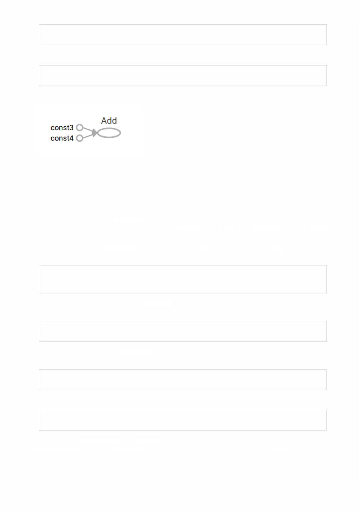
Let's build a simple computational graph. The most basic operation is a constant. The Python function that builds the operation

takes a tensor value as input. The resulting operation takes no inputs. When run, it outputs the value that was passed to the

constructor. We can create two ﬂoating point constants a and b as follows:

a = tf.constant(3.0, dtype=tf.float32)

b = tf.constant(4.0) # also tf.float32 implicitly

total = a + b

print(a)

print(b)

print(total)

The print statements produce:

Tensor("Const:0", shape=(), dtype=float32)

Tensor("Const_1:0", shape=(), dtype=float32)

Tensor("add:0", shape=(), dtype=float32)

Notice that printing the tensors does not output the values 3.0, 4.0, and 7.0 as you might expect. The above statements only

build the computation graph. These tf.Tensor objects just represent the results of the operations that will be run.

Each operation in a graph is given a unique name. This name is independent of the names the objects are assigned to in

Python. Tensors are named after the operation that produces them followed by an output index, as in "add:0" above.

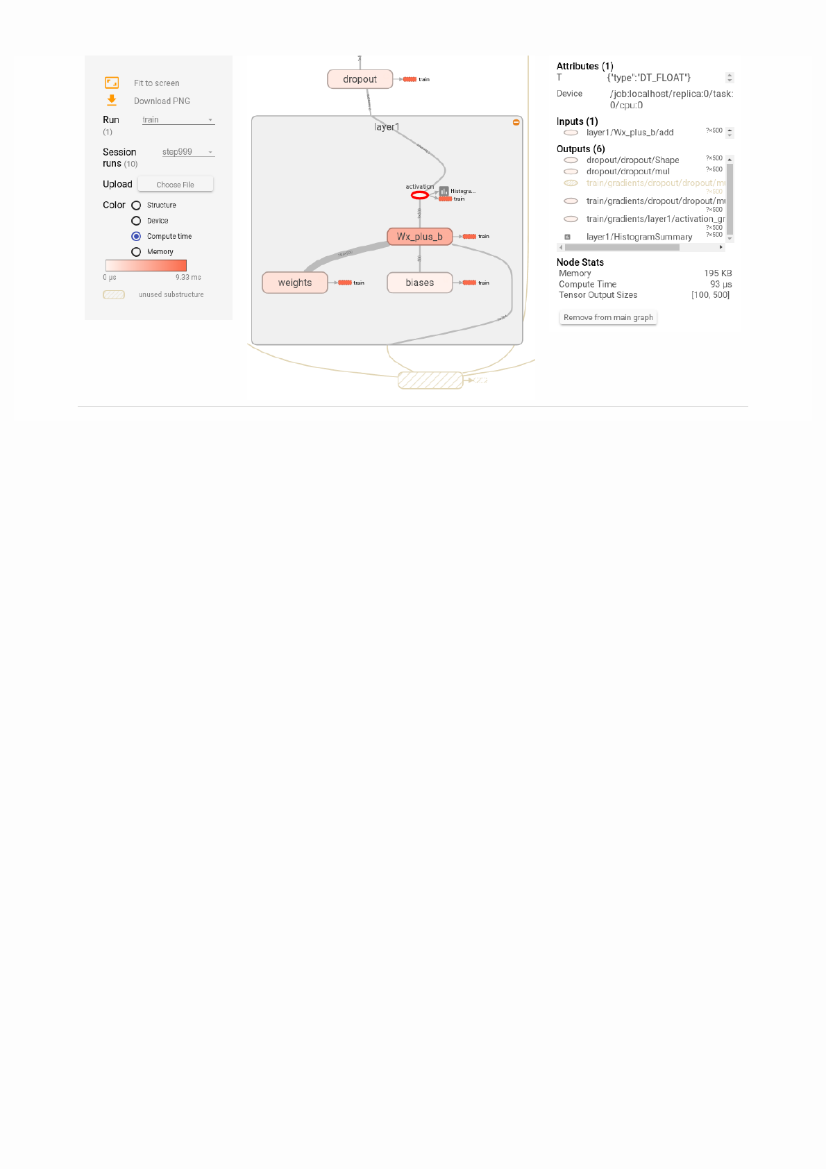
TensorBoard

TensorFlow provides a utility called TensorBoard. One of TensorBoard's many capabilities is visualizing a computation graph.

You can easily do this with a few simple commands.

First you save the computation graph to a TensorBoard summary ﬁle as follows:

writer = tf.summary.FileWriter('.')

writer.add_graph(tf.get_default_graph())

This will produce an event ﬁle in the current directory with a name in the following format:

events.out.tfevents.{timestamp}.{hostname}

Now, in a new terminal, launch TensorBoard with the following shell command:

tensorboard --logdir .

Then open TensorBoard's graphs page in your browser, and you should see a graph similar to the following:

For more about TensorBoard's graph visualization tools see TensorBoard: Graph Visualization.

Session

To evaluate tensors, instantiate a tf.Session object, informally known as a session. A session encapsulates the state of the

TensorFlow runtime, and runs TensorFlow operations. If a tf.Graph is like a .py ﬁle, a tf.Session is like the python

executable.

The following code creates a tf.Session object and then invokes its run method to evaluate the totaltensor we created

above:

sess = tf.Session()

print(sess.run(total))

When you request the output of a node with Session.run TensorFlow backtracks through the graph and runs all the nodes

that provide input to the requested output node. So this prints the expected value of 7.0:

7.0

You can pass multiple tensors to tf.Session.run. The run method transparently handles any combination of tuples or

dictionaries, as in the following example:

print(sess.run({'ab':(a, b), 'total':total}))

which returns the results in a structure of the same layout:

{'total': 7.0, 'ab': (3.0, 4.0)}

During a call to tf.Session.run any tf.Tensor only has a single value. For example, the following code calls

tf.random_uniform to produce a tf.Tensor that generates a random 3-element vector (with values in [0,1)):

vec = tf.random_uniform(shape=(3,))

out1 = vec + 1

out2 = vec + 2

print(sess.run(vec))

print(sess.run((out1, out2)))

The result shows a different random value on each call to run, but a consistent value during a single run(out1 and out2

receive the same random input):

[ 0.52917576 0.64076328 0.68353939]

[ 0.66192627 0.89126778 0.06254101]

(

array([ 1.88408756, 1.87149239, 1.84057522], dtype=float32),

array([ 2.88408756, 2.87149239, 2.84057522], dtype=float32)

)

Some TensorFlow functions return tf.Operations instead of tf.Tensors. The result of calling run on an Operation is None.

You run an operation to cause a side-effect, not to retrieve a value. Examples of this include the initialization, and training ops

demonstrated later.

Feeding

As it stands, this graph is not especially interesting because it always produces a constant result. A graph can be parameterized

to accept external inputs, known as placeholders. A placeholder is a promise to provide a value later, like a function argument.

x = tf.placeholder(tf.float32)

y = tf.placeholder(tf.float32)

z = x + y

The preceding three lines are a bit like a function in which we deﬁne two input parameters (x and y) and then an operation on

them. We can evaluate this graph with multiple inputs by using the feed_dict argument of the run method to feed concrete

values to the placeholders:

print(sess.run(z, feed_dict={x: 3, y: 4.5}))

print(sess.run(z, feed_dict={x: [1, 3], y: [2, 4]}))

This results in the following output:

7.5

[ 3. 7.]

Also note that the feed_dict argument can be used to overwrite any tensor in the graph. The only difference between

placeholders and other tf.Tensors is that placeholders throw an error if no value is fed to them.

Datasets

Placeholders work for simple experiments, but Datasets are the preferred method of streaming data into a model.

To  get  a  runnable  tf.Tensor  from  a  Dataset  you  must  ﬁrst  convert  it  to  a  tf.data.Iterator,  and  then  call  the  Iterator's
get_next method.
The simplest way to create an Iterator is with the make_one_shot_iterator method. For example, in the following code the
next_item tensor will return a row from the my_data array on each run call:
my_data = [
    [0, 1,],
    [2, 3,],
    [4, 5,],
    [6, 7,],
]
slices = tf.data.Dataset.from_tensor_slices(my_data)
next_item = slices.make_one_shot_iterator().get_next()
Reaching the end of the data stream causes Dataset to throw an OutOfRangeError. For example, the following code reads the
next_item until there is no more data to read:
while True:
  try:
    print(sess.run(next_item))
  except tf.errors.OutOfRangeError:
    break
For more details on Datasets and Iterators see: Importing Data.
Layers   
A trainable model must modify the values in the graph to get new outputs with the same input. Layers are the preferred way
to add trainable parameters to a graph.
Layers  package  together  both  the  variables  and  the  operations  that  act  on  them,  .  For  example  a  densely-connected  layer
performs a weighted sum across all inputs for each output and applies an optional activation function. The connection weights
and biases are managed by the layer object.
Creating Layers   
The following code creates a Dense layer that takes a batch of input vectors, and produces a single output value for each. To
apply a layer to an input, call the layer as if it were a function. For example:
x = tf.placeholder(tf.float32, shape=[None, 3])
linear_model = tf.layers.Dense(units=1)
y = linear_model(x)
The layer inspects its input to determine sizes for its internal variables. So here we must set the shape of the xplaceholder so
that the layer can build a weight matrix of the correct size.
Now that we have deﬁned the calculation of the output, y, there is one more detail we need to take care of before we run the
calculation.

Initializing Layers

The layer contains variables that must be initialized before they can be used. While it is possible to initialize variables

individually, you can easily initialize all the variables in a TensorFlow graph as follows:

init = tf.global_variables_initializer()

sess.run(init)

Important: Calling tf.global_variables_initializer only creates and returns a handle to a TensorFlow operation. That

op will initialize all the global variables when we run it with tf.Session.run.

Also note that this global_variables_initializer only initializes variables that existed in the graph when the initializer

was created. So the initializer should be one of the last things added during graph construction.

Executing Layers

Now that the layer is initialized, we can evaluate the linear_model's output tensor as we would any other tensor. For

example, the following code:

print(sess.run(y, {x: [[1, 2, 3],[4, 5, 6]]}))

will generate a two-element output vector such as the following:

[[-3.41378999]

[-9.14999008]]

Layer Function shortcuts

For each layer class (like tf.layers.Dense) TensorFlow also supplies a shortcut function (like tf.layers.dense). The only

difference is that the shortcut function versions create and run the layer in a single call. For example, the following code is

equivalent to the earlier version:

x = tf.placeholder(tf.float32, shape=[None, 3])

y = tf.layers.dense(x, units=1)

init = tf.global_variables_initializer()

sess.run(init)

print(sess.run(y, {x: [[1, 2, 3], [4, 5, 6]]}))

While convenient, this approach allows no access to the tf.layers.Layer object. This makes introspection and debugging

more difﬁcult, and layer reuse impossible.

Feature columns

The easiest way to experiment with feature columns is using the tf.feature_column.input_layer function. This function

only accepts dense columns as inputs, so to view the result of a categorical column you must wrap it in an

tf.feature_column.indicator_column. For example:

features = {

'sales' : [[5], [10], [8], [9]],

'department': ['sports', 'sports', 'gardening', 'gardening']}

department_column = tf.feature_column.categorical_column_with_vocabulary_list(

'department', ['sports', 'gardening'])

department_column = tf.feature_column.indicator_column(department_column)

columns = [

tf.feature_column.numeric_column('sales'),

department_column

]

inputs = tf.feature_column.input_layer(features, columns)

Running the inputs tensor will parse the features into a batch of vectors.

Feature columns can have internal state, like layers, so they often need to be initialized. Categorical columns use lookup tables

internally and these require a separate initialization op, tf.tables_initializer.

var_init = tf.global_variables_initializer()

table_init = tf.tables_initializer()

sess = tf.Session()

sess.run((var_init, table_init))

Once the internal state has been initialized you can run inputs like any other tf.Tensor:

print(sess.run(inputs))

This shows how the feature columns have packed the input vectors, with the one-hot "department" as the ﬁrst two indices and

"sales" as the third.

[[ 1. 0. 5.]

[ 1. 0. 10.]

[ 0. 1. 8.]

[ 0. 1. 9.]]

Training

Now that you're familiar with the basics of core TensorFlow, let's train a small regression model manually.

Deﬁne the data

First let's deﬁne some inputs, x, and the expected output for each input, y_true:

x = tf.constant([[1], [2], [3], [4]], dtype=tf.float32)

y_true = tf.constant([[0], [-1], [-2], [-3]], dtype=tf.float32)

Deﬁne the model

Next, build a simple linear model, with 1 output:

linear_model = tf.layers.Dense(units=1)

y_pred = linear_model(x)

You can evaluate the predictions as follows:

sess = tf.Session()

init = tf.global_variables_initializer()

sess.run(init)

print(sess.run(y_pred))

The model hasn't yet been trained, so the four "predicted" values aren't very good. Here's what we got; your own output will

almost certainly differ:

[[ 0.02631879]

[ 0.05263758]

[ 0.07895637]

[ 0.10527515]]

loss

To optimize a model, you ﬁrst need to deﬁne the loss. We'll use the mean square error, a standard loss for regression problems.

While you could do this manually with lower level math operations, the tf.losses module provides a set of common loss

functions. You can use it to calculate the mean square error as follows:

loss = tf.losses.mean_squared_error(labels=y_true, predictions=y_pred)

print(sess.run(loss))

This will produce a loss value, something like:

2.23962

Training

TensorFlow provides optimizers implementing standard optimization algorithms. These are implemented as sub-classes of

tf.train.Optimizer. They incrementally change each variable in order to minimizethe loss. The simplest optimization

algorithm is gradient descent, implemented by tf.train.GradientDescentOptimizer. It modiﬁes each variable according

to the magnitude of the derivative of loss with respect to that variable. For example:

optimizer = tf.train.GradientDescentOptimizer(0.01)

train = optimizer.minimize(loss)

This code builds all the graph components necessary for the optimization, and returns a training operation. When run, the

training op will update variables in the graph. You might run it as follows:

for i in range(100):

_, loss_value = sess.run((train, loss))

print(loss_value)

Since train is an op, not a tensor, it doesn't return a value when run. To see the progression of the loss during training, we run

the loss tensor at the same time, producing output like the following:

1.35659

1.00412

0.759167

0.588829

0.470264

0.387626

0.329918

0.289511

0.261112

0.241046

...

Complete program

x = tf.constant([[1], [2], [3], [4]], dtype=tf.float32)

y_true = tf.constant([[0], [-1], [-2], [-3]], dtype=tf.float32)

linear_model = tf.layers.Dense(units=1)

y_pred = linear_model(x)

loss = tf.losses.mean_squared_error(labels=y_true, predictions=y_pred)

optimizer = tf.train.GradientDescentOptimizer(0.01)

train = optimizer.minimize(loss)

init = tf.global_variables_initializer()

sess = tf.Session()

sess.run(init)

for i in range(100):

_, loss_value = sess.run((train, loss))

print(loss_value)

print(sess.run(y_pred))

Rank Math entity

0 Scalar (magnitude only)

Next steps

To learn more about building models with TensorFlow consider the following:

Custom Estimators, to learn how to build customized models with TensorFlow. Your knowledge of TensorFlow Core will

help you understand and debug your own models.

If you want to learn more about the inner workings of TensorFlow consider the following documents, which go into more

depth on many of the topics discussed here:

Graphs and Sessions

Tensors

Variables

Tensors

TensorFlow, as the name indicates, is a framework to deﬁne and run computations involving tensors. A tensoris a

generalization of vectors and matrices to potentially higher dimensions. Internally, TensorFlow represents tensors as n-

dimensional arrays of base datatypes.

When writing a TensorFlow program, the main object you manipulate and pass around is the tf.Tensor. A tf.Tensor object

represents a partially deﬁned computation that will eventually produce a value. TensorFlow programs work by ﬁrst building a

graph of tf.Tensor objects, detailing how each tensor is computed based on the other available tensors and then by running

parts of this graph to achieve the desired results.

A tf.Tensor has the following properties:

a data type (float32, int32, or string, for example)

a shape

Each element in the Tensor has the same data type, and the data type is always known. The shape (that is, the number of

dimensions it has and the size of each dimension) might be only partially known. Most operations produce tensors of fully-

known shapes if the shapes of their inputs are also fully known, but in some cases it's only possible to ﬁnd the shape of a

tensor at graph execution time.

Some types of tensors are special, and these will be covered in other units of the Programmer's guide. The main ones are:

tf.Variable

tf.constant

tf.placeholder

tf.SparseTensor

With the exception of tf.Variable, the value of a tensor is immutable, which means that in the context of a single execution

tensors only have a single value. However, evaluating the same tensor twice can return different values; for example that

tensor can be the result of reading data from disk, or generating a random number.

Rank

The rank of a tf.Tensor object is its number of dimensions. Synonyms for rank include order or degree or n-dimension. Note

that rank in TensorFlow is not the same as matrix rank in mathematics. As the following table shows, each rank in TensorFlow

corresponds to a different mathematical entity:

1 Vector (magnitude and direction)

2 Matrix (table of numbers)

3 3-Tensor (cube of numbers)

n n-Tensor (you get the idea)

Rank 0

The following snippet demonstrates creating a few rank 0 variables:

mammal = tf.Variable("Elephant", tf.string)

ignition = tf.Variable(451, tf.int16)

floating = tf.Variable(3.14159265359, tf.float64)

its_complicated = tf.Variable(12.3 - 4.85j, tf.complex64)

Note: A string is treated as a single item in TensorFlow, not as a sequence of characters. It is possible to have scalar strings,

vectors of strings, etc.

Rank 1

To create a rank 1 tf.Tensor object, you can pass a list of items as the initial value. For example:

mystr = tf.Variable(["Hello"], tf.string)

cool_numbers = tf.Variable([3.14159, 2.71828], tf.float32)

first_primes = tf.Variable([2, 3, 5, 7, 11], tf.int32)

its_very_complicated = tf.Variable([12.3 - 4.85j, 7.5 - 6.23j], tf.complex64)

Higher ranks

A rank 2 tf.Tensor object consists of at least one row and at least one column:

mymat = tf.Variable([[7],[11]], tf.int16)

myxor = tf.Variable([[False, True],[True, False]], tf.bool)

linear_squares = tf.Variable([[4], [9], [16], [25]], tf.int32)

squarish_squares = tf.Variable([ [4, 9], [16, 25] ], tf.int32)

rank_of_squares = tf.rank(squarish_squares)

mymatC = tf.Variable([[7],[11]], tf.int32)

Higher-rank Tensors, similarly, consist of an n-dimensional array. For example, during image processing, many tensors of rank

4 are used, with dimensions corresponding to example-in-batch, image width, image height, and color channel.

my_image = tf.zeros([10, 299, 299, 3]) # batch x height x width x color

Rank Shape Dimension number Example

0 [] 0-D A 0-D tensor. A scalar.

1 [D0] 1-D A 1-D tensor with shape [5].

2 [D0, D1] 2-D A 2-D tensor with shape [3, 4].

Getting a tf.Tensor object's rank

To determine the rank of a tf.Tensor object, call the tf.rank method. For example, the following method programmatically

determines the rank of the tf.Tensor deﬁned in the previous section:

r = tf.rank(my_image)

# After the graph runs, r will hold the value 4.

Referring to tf.Tensor slices

Since a tf.Tensor is an n-dimensional array of cells, to access a single cell in a tf.Tensor you need to specify n indices.

For a rank 0 tensor (a scalar), no indices are necessary, since it is already a single number.

For a rank 1 tensor (a vector), passing a single index allows you to access a number:

my_scalar = my_vector[2]

Note that the index passed inside the [] can itself be a scalar tf.Tensor, if you want to dynamically choose an element from

the vector.

For tensors of rank 2 or higher, the situation is more interesting. For a tf.Tensor of rank 2, passing two numbers returns a

scalar, as expected:

my_scalar = my_matrix[1, 2]

Passing a single number, however, returns a subvector of a matrix, as follows:

my_row_vector = my_matrix[2]

my_column_vector = my_matrix[:, 3]

The : notation is python slicing syntax for "leave this dimension alone". This is useful in higher-rank Tensors, as it allows you

to access its subvectors, submatrices, and even other subtensors.

Shape

The shape of a tensor is the number of elements in each dimension. TensorFlow automatically infers shapes during graph

construction. These inferred shapes might have known or unknown rank. If the rank is known, the sizes of each dimension

might be known or unknown.

The TensorFlow documentation uses three notational conventions to describe tensor dimensionality: rank, shape, and

dimension number. The following table shows how these relate to one another:

3 [D0, D1, D2] 3-D A 3-D tensor with shape [1, 4, 3].

n [D0, D1, ... Dn-1] n-D A tensor with shape [D0, D1, ... Dn-1].

Shapes can be represented via Python lists / tuples of ints, or with the tf.TensorShape.

Getting a tf.Tensor object's shape

There are two ways of accessing the shape of a tf.Tensor. While building the graph, it is often useful to ask what is already

known about a tensor's shape. This can be done by reading the shape property of a tf.Tensor object. This method returns a

TensorShape object, which is a convenient way of representing partially-speciﬁed shapes (since, when building the graph, not

all shapes will be fully known).

It is also possible to get a tf.Tensor that will represent the fully-deﬁned shape of another tf.Tensor at runtime. This is done

by calling the tf.shape operation. This way, you can build a graph that manipulates the shapes of tensors by building other

tensors that depend on the dynamic shape of the input tf.Tensor.

For example, here is how to make a vector of zeros with the same size as the number of columns in a given matrix:

zeros = tf.zeros(my_matrix.shape[1])

Changing the shape of a tf.Tensor

The number of elements of a tensor is the product of the sizes of all its shapes. The number of elements of a scalar is always 1.

Since there are often many different shapes that have the same number of elements, it's often convenient to be able to change

the shape of a tf.Tensor, keeping its elements ﬁxed. This can be done with tf.reshape.

The following examples demonstrate how to reshape tensors:

rank_three_tensor = tf.ones([3, 4, 5])

matrix = tf.reshape(rank_three_tensor, [6, 10]) # Reshape existing content into

# a 6x10 matrix

matrixB = tf.reshape(matrix, [3, -1]) # Reshape existing content into a 3x20

# matrix. -1 tells reshape to calculate

# the size of this dimension.

matrixAlt = tf.reshape(matrixB, [4, 3, -1]) # Reshape existing content into a

#4x3x5 tensor

# Note that the number of elements of the reshaped Tensors has to match the

# original number of elements. Therefore, the following example generates an

# error because no possible value for the last dimension will match the number

# of elements.

yet_another = tf.reshape(matrixAlt, [13, 2, -1]) # ERROR!

Data types

In addition to dimensionality, Tensors have a data type. Refer to the tf.DataType page in the programmer's guide for a full

list of the data types.

It is not possible to have a tf.Tensor with more than one data type. It is possible, however, to serialize arbitrary data

structures as strings and store those in tf.Tensors.

It is possible to cast tf.Tensors from one datatype to another using tf.cast:

# Cast a constant integer tensor into floating point.

float_tensor = tf.cast(tf.constant([1, 2, 3]), dtype=tf.float32)

To inspect a tf.Tensor's data type use the Tensor.dtype property.

When creating a tf.Tensor from a python object you may optionally specify the datatype. If you don't, TensorFlow chooses a

datatype that can represent your data. TensorFlow converts Python integers to tf.int32 and python ﬂoating point numbers to

tf.float32. Otherwise TensorFlow uses the same rules numpy uses when converting to arrays.

Evaluating Tensors

Once the computation graph has been built, you can run the computation that produces a particular tf.Tensorand fetch the

value assigned to it. This is often useful for debugging as well as being required for much of TensorFlow to work.

The simplest way to evaluate a Tensor is using the Tensor.eval method. For example:

constant = tf.constant([1, 2, 3])

tensor = constant * constant

print tensor.eval()

The eval method only works when a default tf.Session is active (see Graphs and Sessions for more information).

Tensor.eval returns a numpy array with the same contents as the tensor.

Sometimes it is not possible to evaluate a tf.Tensor with no context because its value might depend on dynamic information

that is not available. For example, tensors that depend on placeholders can't be evaluated without providing a value for the

placeholder.

p = tf.placeholder(tf.float32)

t = p + 1.0

t.eval() # This will fail, since the placeholder did not get a value.

t.eval(feed_dict={p:2.0}) # This will succeed because we're feeding a value

# to the placeholder.

Note that it is possible to feed any tf.Tensor, not just placeholders.

Other model constructs might make evaluating a tf.Tensor complicated. TensorFlow can't directly evaluate tf.Tensors

deﬁned inside functions or inside control ﬂow constructs. If a tf.Tensor depends on a value from a queue, evaluating the

tf.Tensor will only work once something has been enqueued; otherwise, evaluating it will hang. When working with queues,

remember to call tf.train.start_queue_runners before evaluating any tf.Tensors.

Printing Tensors

For debugging purposes you might want to print the value of a tf.Tensor. While tfdbg provides advanced debugging

support, TensorFlow also has an operation to directly print the value of a tf.Tensor.

Note that you rarely want to use the following pattern when printing a tf.Tensor:

t = <<some tensorflow operation>>

print t # This will print the symbolic tensor when the graph is being built.

# This tensor does not have a value in this context.

This code prints the tf.Tensor object (which represents deferred computation) and not its value. Instead, TensorFlow

provides the tf.Print operation, which returns its ﬁrst tensor argument unchanged while printing the set of tf.Tensors it is

passed as the second argument.

To correctly use tf.Print its return value must be used. See the example below

t = <<some tensorflow operation>>

tf.Print(t, [t]) # This does nothing

t = tf.Print(t, [t]) # Here we are using the value returned by tf.Print

result = t + 1 # Now when result is evaluated the value of `t` will be printed.

When you evaluate result you will evaluate everything result depends upon. Since result depends upon t, and

evaluating t has the side effect of printing its input (the old value of t), t gets printed.Variables

A TensorFlow variable is the best way to represent shared, persistent state manipulated by your program.

Variables are manipulated via the tf.Variable class. A tf.Variable represents a tensor whose value can be changed by

running ops on it. Unlike tf.Tensor objects, a tf.Variable exists outside the context of a single session.run call.

Internally, a tf.Variable stores a persistent tensor. Speciﬁc ops allow you to read and modify the values of this tensor. These

modiﬁcations are visible across multiple tf.Sessions, so multiple workers can see the same values for a tf.Variable.

Creating a Variable

The best way to create a variable is to call the tf.get_variable function. This function requires you to specify the Variable's

name. This name will be used by other replicas to access the same variable, as well as to name this variable's value when

checkpointing and exporting models. tf.get_variable also allows you to reuse a previously created variable of the same

name, making it easy to deﬁne models which reuse layers.

To create a variable with tf.get_variable, simply provide the name and shape

my_variable = tf.get_variable("my_variable", [1, 2, 3])

This creates a variable named "my_variable" which is a three-dimensional tensor with shape [1, 2, 3]. This variable will, by

default, have the dtype tf.float32 and its initial value will be randomized viatf.glorot_uniform_initializer.

You may optionally specify the dtype and initializer to tf.get_variable. For example:

my_int_variable = tf.get_variable("my_int_variable", [1, 2, 3], dtype=tf.int32,

initializer=tf.zeros_initializer)

TensorFlow provides many convenient initializers. Alternatively, you may initialize a tf.Variable to have the value of a

tf.Tensor. For example:

other_variable = tf.get_variable("other_variable", dtype=tf.int32,

initializer=tf.constant([23, 42]))

Note that when the initializer is a tf.Tensor you should not specify the variable's shape, as the shape of the initializer tensor

will be used.

Variable collections

Because disconnected parts of a TensorFlow program might want to create variables, it is sometimes useful to have a single

way to access all of them. For this reason TensorFlow provides collections, which are named lists of tensors or other objects,

such as tf.Variable instances.

By default every tf.Variable gets placed in the following two collections: * tf.GraphKeys.GLOBAL_VARIABLES --- variables

that can be shared across multiple devices, * tf.GraphKeys.TRAINABLE_VARIABLES--- variables for which TensorFlow will

calculate gradients.

If you don't want a variable to be trainable, add it to the tf.GraphKeys.LOCAL_VARIABLES collection instead. For example,

the following snippet demonstrates how to add a variable named my_local to this collection:

my_local = tf.get_variable("my_local", shape=(),

collections=[tf.GraphKeys.LOCAL_VARIABLES])

Alternatively, you can specify trainable=False as an argument to tf.get_variable:

my_non_trainable = tf.get_variable("my_non_trainable",

shape=(),

trainable=False)

You can also use your own collections. Any string is a valid collection name, and there is no need to explicitly create a

collection. To add a variable (or any other object) to a collection after creating the variable, calltf.add_to_collection. For

example, the following code adds an existing variable named my_local to a collection named my_collection_name:

tf.add_to_collection("my_collection_name", my_local)

And to retrieve a list of all the variables (or other objects) you've placed in a collection you can use:

tf.get_collection("my_collection_name")

Device placement

Just like any other TensorFlow operation, you can place variables on particular devices. For example, the following snippet

creates a variable named v and places it on the second GPU device:

with tf.device("/device:GPU:1"):

v = tf.get_variable("v", [1])

It is particularly important for variables to be in the correct device in distributed settings. Accidentally putting variables on

workers instead of parameter servers, for example, can severely slow down training or, in the worst case, let each worker

blithely forge ahead with its own independent copy of each variable. For this reason we provide

tf.train.replica_device_setter, which can automatically place variables in parameter servers. For example:

cluster_spec = {

"ps": ["ps0:2222", "ps1:2222"],

"worker": ["worker0:2222", "worker1:2222", "worker2:2222"]}

with tf.device(tf.train.replica_device_setter(cluster=cluster_spec)):

v = tf.get_variable("v", shape=[20, 20]) # this variable is placed

# in the parameter server

# by the replica_device_setter

Initializing variables

Before you can use a variable, it must be initialized. If you are programming in the low-level TensorFlow API (that is, you are

explicitly creating your own graphs and sessions), you must explicitly initialize the variables. Most high-level frameworks such

as tf.contrib.slim, tf.estimator.Estimator and Keras automatically initialize variables for you before training a model.

Explicit initialization is otherwise useful because it allows you not to rerun potentially expensive initializers when reloading a

model from a checkpoint as well as allowing determinism when randomly-initialized variables are shared in a distributed

setting.

To initialize all trainable variables in one go, before training starts, calltf.global_variables_initializer(). This function

returns a single operation responsible for initializing all variables in the tf.GraphKeys.GLOBAL_VARIABLES collection.

Running this operation initializes all variables. For example:

session.run(tf.global_variables_initializer())

# Now all variables are initialized.

If you do need to initialize variables yourself, you can run the variable's initializer operation. For example:

session.run(my_variable.initializer)

You can also ask which variables have still not been initialized. For example, the following code prints the names of all

variables which have not yet been initialized:

print(session.run(tf.report_uninitialized_variables()))

Note that by default tf.global_variables_initializer does not specify the order in which variables are initialized.

Therefore, if the initial value of a variable depends on another variable's value, it's likely that you'll get an error. Any time you

use the value of a variable in a context in which not all variables are initialized (say, if you use a variable's value while

initializing another variable), it is best to use variable.initialized_value()instead of variable:

v = tf.get_variable("v", shape=(), initializer=tf.zeros_initializer())

w = tf.get_variable("w", initializer=v.initialized_value() + 1)

Using variables

To use the value of a tf.Variable in a TensorFlow graph, simply treat it like a normal tf.Tensor:

v = tf.get_variable("v", shape=(), initializer=tf.zeros_initializer())

w = v + 1 # w is a tf.Tensor which is computed based on the value of v.

# Any time a variable is used in an expression it gets automatically

# converted to a tf.Tensor representing its value.

To assign a value to a variable, use the methods assign, assign_add, and friends in the tf.Variable class. For example, here

is how you can call these methods:

v = tf.get_variable("v", shape=(), initializer=tf.zeros_initializer())

assignment = v.assign_add(1)

tf.global_variables_initializer().run()

sess.run(assignment) # or assignment.op.run()

Most TensorFlow optimizers have specialized ops that efﬁciently update the values of variables according to some gradient

descent-like algorithm. See tf.train.Optimizer for an explanation of how to use optimizers.

Because variables are mutable it's sometimes useful to know what version of a variable's value is being used at any point in

time. To force a re-read of the value of a variable after something has happened, you can usetf.Variable.read_value. For

example:

v = tf.get_variable("v", shape=(), initializer=tf.zeros_initializer())

assignment = v.assign_add(1)

with tf.control_dependencies([assignment]):

w = v.read_value() # w is guaranteed to reflect v's value after the

# assign_add operation.

Sharing variables

TensorFlow supports two ways of sharing variables:

Explicitly passing tf.Variable objects around.

Implicitly wrapping tf.Variable objects within tf.variable_scope objects.

While code which explicitly passes variables around is very clear, it is sometimes convenient to write TensorFlow functions

that implicitly use variables in their implementations. Most of the functional layers fromtf.layer use this approach, as well as

all tf.metrics, and a few other library utilities.

Variable scopes allow you to control variable reuse when calling functions which implicitly create and use variables. They also

allow you to name your variables in a hierarchical and understandable way.

For example, let's say we write a function to create a convolutional / relu layer:

def conv_relu(input, kernel_shape, bias_shape):

# Create variable named "weights".

weights = tf.get_variable("weights", kernel_shape,

initializer=tf.random_normal_initializer())

# Create variable named "biases".

biases = tf.get_variable("biases", bias_shape,

initializer=tf.constant_initializer(0.0))

conv = tf.nn.conv2d(input, weights,

strides=[1, 1, 1, 1], padding='SAME')

return tf.nn.relu(conv + biases)

This function uses short names weights and biases, which is good for clarity. In a real model, however, we want many such

convolutional layers, and calling this function repeatedly would not work:

input1 = tf.random_normal([1,10,10,32])

input2 = tf.random_normal([1,20,20,32])

x = conv_relu(input1, kernel_shape=[5, 5, 32, 32], bias_shape=[32])

x = conv_relu(x, kernel_shape=[5, 5, 32, 32], bias_shape = [32]) # This fails.

Since the desired behavior is unclear (create new variables or reuse the existing ones?) TensorFlow will fail. Calling conv_relu

in different scopes, however, clariﬁes that we want to create new variables:

def my_image_filter(input_images):

with tf.variable_scope("conv1"):

# Variables created here will be named "conv1/weights", "conv1/biases".

relu1 = conv_relu(input_images, [5, 5, 32, 32], [32])

with tf.variable_scope("conv2"):

# Variables created here will be named "conv2/weights", "conv2/biases".

return conv_relu(relu1, [5, 5, 32, 32], [32])

If you do want the variables to be shared, you have two options. First, you can create a scope with the same name using

reuse=True:

with tf.variable_scope("model"):

output1 = my_image_filter(input1)

with tf.variable_scope("model", reuse=True):

output2 = my_image_filter(input2)

You can also call scope.reuse_variables() to trigger a reuse:

with tf.variable_scope("model") as scope:

output1 = my_image_filter(input1)

scope.reuse_variables()

output2 = my_image_filter(input2)

Since depending on exact string names of scopes can feel dangerous, it's also possible to initialize a variable scope based on

another one:

Graphs and Sessions

TensorFlow uses a dataﬂow graph to represent your computation in terms of the dependencies between individual operations.

This leads to a low-level programming model in which you ﬁrst deﬁne the dataﬂow graph, then create a TensorFlow session to

run parts of the graph across a set of local and remote devices.

with tf.variable_scope("model") as scope:

output1 = my_image_filter(input1)

with tf.variable_scope(scope, reuse=True):

output2 = my_image_filter(input2)

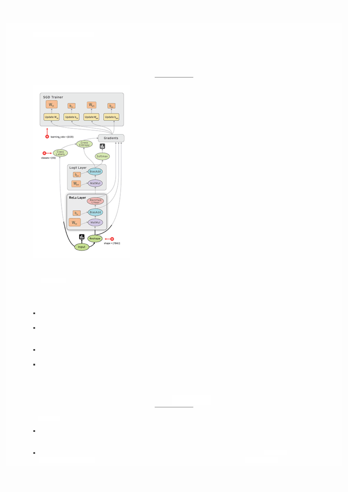
This  guide  will  be  most  useful  if  you  intend  to  use  the  low-level  programming  model  directly.  Higher-level  APIs  such  as
tf.estimator.Estimator and Keras hide the details of graphs and sessions from the end user, but this guide may also be
useful if you want to understand how these APIs are implemented.
Why dataﬂow graphs?   
Dataﬂow  is  a  common  programming  model  for  parallel  computing.  In  a  dataﬂow  graph,  the  nodes  represent  units  of
computation, and the edges represent the data consumed or produced by a computation. For example, in a TensorFlow graph,
the tf.matmul operation would correspond to a single node with two incoming edges (the matrices to be multiplied) and one
outgoing edge (the result of the multiplication).
Dataﬂow has several advantages that TensorFlow leverages when executing your programs:
Parallelism. By using explicit edges to represent dependencies between operations, it is easy for the system to identify 
operations that can execute in parallel.
Distributed execution. By using explicit edges to represent the values that ﬂow between operations, it is possible for 
TensorFlow to partition your program across multiple devices (CPUs, GPUs, and TPUs) attached to different machines. 
TensorFlow inserts the necessary communication and coordination between devices.
Compilation. TensorFlow's XLA compiler can use the information in your dataﬂow graph to generate faster code, for 
example, by fusing together adjacent operations.
Portability. The dataﬂow graph is a language-independent representation of the code in your model. You can build a 
dataﬂow graph in Python, store it in a SavedModel, and restore it in a C++ program for low-latency inference.
What is a tf.Graph?  
A tf.Graph contains two relevant kinds of information:
Graph structure. The nodes and edges of the graph, indicating how individual operations are composed together, but not 
prescribing how they should be used. The graph structure is like assembly code: inspecting it can convey some useful 
information, but it does not contain all of the useful context that source code conveys.
Graph collections. TensorFlow provides a general mechanism for storing collections of metadata in a tf.Graph. The 
tf.add_to_collection function enables you to associate a list of objects with a key (where tf.GraphKeys deﬁnes some of 

the standard keys), and tf.get_collection enables you to look up all objects associated with a key. Many parts of the 
TensorFlow library use this facility: for example, when you create a tf.Variable, it is added by default to collections 
representing "global variables" and "trainable variables". When you later come to create a tf.train.Saver or 
tf.train.Optimizer, the variables in these collections are used as the default arguments.
Building a tf.Graph   
Most  TensorFlow  programs  start  with  a  dataﬂow  graph  construction  phase.  In  this  phase,  you  invoke  TensorFlow  API
functions  that  construct  new  tf.Operation  (node)  and  tf.Tensor  (edge)  objects  and  add  them  to  a  tf.Graph  instance.
TensorFlow provides a default graph that is an implicit argument to all API functions in the same context. For example:
Calling tf.constant(42.0) creates a single tf.Operation that produces the value 42.0, adds it to the default graph, and 
returns a tf.Tensor that represents the value of the constant.
Calling tf.matmul(x, y) creates a single tf.Operation that multiplies the values of tf.Tensorobjects x and y, adds it to 
the default graph, and returns a tf.Tensor that represents the result of the multiplication.
Executing v = tf.Variable(0) adds to the graph a tf.Operation that will store a writeable tensor value that persists 
between tf.Session.run calls. The tf.Variable object wraps this operation, and can be used like a tensor, which will 
read the current value of the stored value. The tf.Variable object also has methods such as assign and assign_add that 
create tf.Operation objects that, when executed, update the stored value. (See Variables for more information about 
variables.)
Calling tf.train.Optimizer.minimize will add operations and tensors to the default graph that calculate gradients, and 
return a tf.Operation that, when run, will apply those gradients to a set of variables.
Most  programs  rely solely  on  the  default  graph.  However,  see  Dealing  with  multiple  graphs  for  more  advanced  use  cases.
High-level APIs such as the tf.estimator.Estimator API manage the default graph on your behalf, and--for example--may
create different graphs for training and evaluation.
Note: Calling  most functions  in the TensorFlow API  merely adds operations  and tensors to  the default  graph,  but does  not
perform  the  actual  computation.  Instead,  you  compose  these  functions  until  you  have  a  tf.Tensor  or  tf.Operation  that
represents  the  overall  computation--such  as  performing  one  step  of  gradient  descent--and  then  pass  that  object  to  a
tf.Session to perform the computation. See the section "Executing a graph in a tf.Session" for more details.
Naming operations   
A tf.Graph object deﬁnes a namespace for the tf.Operation objects it contains. TensorFlow automatically chooses a unique
name for each operation in your graph, but giving operations descriptive names can make your program easier to read and
debug. The TensorFlow API provides two ways to override the name of an operation:
Each API function that creates a new tf.Operation or returns a new tf.Tensor accepts an optional name argument. For 
example, tf.constant(42.0, name="answer") creates a new tf.Operationnamed "answer" and returns a tf.Tensor 
named "answer:0". If the default graph already contained an operation named "answer", the TensorFlow would append 
"_1", "_2", and so on to the name, in order to make it unique.
The tf.name_scope function makes it possible to add a name scope preﬁx to all operations created in a particular context. 
The current name scope preﬁx is a "/"-delimited list of the names of all active tf.name_scope context managers. If a name 
scope has already been used in the current context, TensorFlow appens "_1", "_2", and so on. For example:

c_0 = tf.constant(0, name="c") # => operation named "c"

# Already-used names will be "uniquified".

c_1 = tf.constant(2, name="c") # => operation named "c_1"

# Name scopes add a prefix to all operations created in the same context.

with tf.name_scope("outer"):

c_2 = tf.constant(2, name="c") # => operation named "outer/c"

# Name scopes nest like paths in a hierarchical file system.

with tf.name_scope("inner"):

c_3 = tf.constant(3, name="c") # => operation named "outer/inner/c"

# Exiting a name scope context will return to the previous prefix.

c_4 = tf.constant(4, name="c") # => operation named "outer/c_1"

# Already-used name scopes will be "uniquified".

with tf.name_scope("inner"):

c_5 = tf.constant(5, name="c") # => operation named "outer/inner_1/c"

The graph visualizer uses name scopes to group operations and reduce the visual complexity of a graph. See Visualizing your

graph for more information.

Note that tf.Tensor objects are implicitly named after the tf.Operation that produces the tensor as output. A tensor name

has the form "<OP_NAME>:<i>" where:

"<OP_NAME>" is the name of the operation that produces it.

"<i>" is an integer representing the index of that tensor among the operation's outputs.

Placing operations on different devices

If you want your TensorFlow program to use multiple different devices, the tf.device function provides a convenient way to

request that all operations created in a particular context are placed on the same device (or type of device).

A device speciﬁcation has the following form:

/job:<JOB_NAME>/task:<TASK_INDEX>/device:<DEVICE_TYPE>:<DEVICE_INDEX>

where:

<JOB_NAME> is an alpha-numeric string that does not start with a number.

<DEVICE_TYPE> is a registered device type (such as GPU or CPU).

<TASK_INDEX> is a non-negative integer representing the index of the task in the job named <JOB_NAME>. See

tf.train.ClusterSpec for an explanation of jobs and tasks.

<DEVICE_INDEX> is a non-negative integer representing the index of the device, for example, to distinguish between

different GPU devices used in the same process.

You do not need to specify every part of a device speciﬁcation. For example, if you are running in a single-machine

conﬁguration with a single GPU, you might use tf.device to pin some operations to the CPU and GPU:

# Operations created outside either context will run on the "best possible"
# device. For example, if you have a GPU and a CPU available, and the operation
# has a GPU implementation, TensorFlow will choose the GPU.
weights = tf.random_normal(...)
with tf.device("/device:CPU:0"):
  # Operations created in this context will be pinned to the CPU.
  img = tf.decode_jpeg(tf.read_file("img.jpg"))
with tf.device("/device:GPU:0"):
  # Operations created in this context will be pinned to the GPU.
  result = tf.matmul(weights, img)
If  you  are  deploying  TensorFlow  in  a  @{$deploy/distributed$typical  distributed  conﬁguration},  you  might  specify  the  job
name and task ID to place variables on a task in the parameter server job ("/job:ps"), and the other operations on task in the
worker job ("/job:worker"):
with tf.device("/job:ps/task:0"):
  weights_1 = tf.Variable(tf.truncated_normal([784, 100]))
  biases_1 = tf.Variable(tf.zeroes([100]))
with tf.device("/job:ps/task:1"):
  weights_2 = tf.Variable(tf.truncated_normal([100, 10]))
  biases_2 = tf.Variable(tf.zeroes([10]))
with tf.device("/job:worker"):
  layer_1 = tf.matmul(train_batch, weights_1) + biases_1
  layer_2 = tf.matmul(train_batch, weights_2) + biases_2
tf.device gives you a lot of ﬂexibility to choose placements for individual operations or broad regions of a TensorFlow graph.
In many cases,  there are simple heuristics that work well. For example, thetf.train.replica_device_setter API can be
used  with  tf.device  to  place  operations  for  data-parallel  distributed  training.  For  example,  the  following  code  fragment
shows  how  tf.train.replica_device_setter  applies  different  placement  policies  to  tf.Variable  objects  and  other
operations:
with tf.device(tf.train.replica_device_setter(ps_tasks=3)):
  # tf.Variable objects are, by default, placed on tasks in "/job:ps" in a
  # round-robin fashion.
  w_0 = tf.Variable(...)  # placed on "/job:ps/task:0"
  b_0 = tf.Variable(...)  # placed on "/job:ps/task:1"
  w_1 = tf.Variable(...)  # placed on "/job:ps/task:2"
  b_1 = tf.Variable(...)  # placed on "/job:ps/task:0"
  input_data = tf.placeholder(tf.float32)     # placed on "/job:worker"
  layer_0 = tf.matmul(input_data, w_0) + b_0  # placed on "/job:worker"
  layer_1 = tf.matmul(layer_0, w_1) + b_1     # placed on "/job:worker"
Tensor-like objects   
Many  TensorFlow  operations  take  one  or  more  tf.Tensor  objects  as  arguments.  For  example,  tf.matmultakes  two
tf.Tensor objects, and tf.add_n takes a list of n tf.Tensor objects. For convenience, these functions will accept a tensor-
like  object  in  place  of  a  tf.Tensor,  and  implicitly  convert  it  to  a  tf.Tensorusing  the  tf.convert_to_tensor  method.
Tensor-like objects include elements of the following types:
tf.Tensor

tf.Variable
numpy.ndarray
list (and lists of tensor-like objects)
Scalar Python types: bool, float, int, str
You can register additional tensor-like types using tf.register_tensor_conversion_function.
Note: By  default,  TensorFlow  will  create a  new  tf.Tensor  each  time  you  use the  same  tensor-like object.  If  the tensor-like
object is large (e.g. a numpy.ndarray containing a set of training examples) and you use it multiple times, you may run out of
memory. To avoid this, manually call tf.convert_to_tensor on the tensor-like object once and use the returned tf.Tensor
instead.
Executing a graph in a tf.Session   
TensorFlow  uses  the  tf.Session  class  to  represent a  connection  between  the  client  program---typically a  Python  program,
although a  similar  interface  is  available  in other languages---and  the  C++  runtime.  A  tf.Session  object  provides access  to
devices in the local machine, and remote devices using the distributed TensorFlow runtime. It also caches information about
your tf.Graph so that you can efﬁciently run the same computation multiple times.
Creating a tf.Session   
If you are using the low-level TensorFlow API, you can create a tf.Session for the current default graph as follows:
# Create a default in-process session.
with tf.Session() as sess:
  # ...
# Create a remote session.
with tf.Session("grpc://example.org:2222"):
  # ...
Since  a  tf.Session  owns  physical  resources  (such  as  GPUs  and  network  connections),  it  is  typically  used  as  a  context
manager (in a with block) that automatically closes the session when you exit the block. It is also possible to create a session
without  using  a  with  block,  but  you  should  explicitly  call  tf.Session.closewhen  you  are  ﬁnished  with  it  to  free  the
resources.
Note:  Higher-level  APIs  such  as  tf.train.MonitoredTrainingSession  or  tf.estimator.Estimator  will  create  and
manage  a  tf.Session  for  you.  These  APIs  accept  optional  target  and  config  arguments  (either  directly,  or  as  part  of  a
tf.estimator.RunConfig object), with the same meaning as described below.
tf.Session.**init** accepts three optional arguments:
target. If this argument is left empty (the default), the session will only use devices in the local machine. However, you may 
also specify a grpc:// URL to specify the address of a TensorFlow server, which gives the session access to all devices on 
machines that this server controls. See tf.train.Server for details of how to create a TensorFlow server. For example, in 
the common between-graph replicationconﬁguration, the tf.Session connects to a tf.train.Server in the same process 
as the client. The distributed TensorFlow deployment guide describes other common scenarios.
graph. By default, a new tf.Session will be bound to---and only able to run operations in---the current default graph. If 
you are using multiple graphs in your program (see Programming with multiple graphs for more details), you can specify 
an explicit tf.Graph when you construct the session.
conﬁg. This argument allows you to specify a tf.ConfigProto that controls the behavior of the session. For example, some 
of the conﬁguration options include:
allow_soft_placement. Set this to True to enable a "soft" device placement algorithm, which ignores tf.device 
annotations that attempt to place CPU-only operations on a GPU device, and places them on the CPU instead.
cluster_def. When using distributed TensorFlow, this option allows you to specify what machines to use in the 

computation, and provide a mapping between job names, task indices, and network addresses. See 
tf.train.ClusterSpec.as_cluster_def for details.
graph_options.optimizer_options. Provides control over the optimizations that TensorFlow performs on your graph 
before executing it.
gpu_options.allow_growth. Set this to True to change the GPU memory allocator so that it gradually increases the 
amount of memory allocated, rather than allocating most of the memory at startup.
Using tf.Session.run to execute operations   
The tf.Session.run method is the main mechanism for running a tf.Operation or evaluating a tf.Tensor. You can pass
one or more tf.Operation or  tf.Tensor objects  to tf.Session.run, and TensorFlow  will execute  the operations that  are
needed to compute the result.
tf.Session.run requires you to specify a list of fetches, which determine the return values, and may be a tf.Operation, a
tf.Tensor, or a tensor-like type such as tf.Variable. These fetches determine what subgraph of the overall tf.Graph must
be executed to produce the result: this is the subgraph that contains all operations named in the fetch list, plus all operations
whose outputs are used to compute the value of the fetches. For example, the following code fragment shows how different
arguments to tf.Session.run cause different subgraphs to be executed:
x = tf.constant([[37.0, -23.0], [1.0, 4.0]])
w = tf.Variable(tf.random_uniform([2, 2]))
y = tf.matmul(x, w)
output = tf.nn.softmax(y)
init_op = w.initializer
with tf.Session() as sess:
  # Run the initializer on `w`.
  sess.run(init_op)
  # Evaluate `output`. `sess.run(output)` will return a NumPy array containing
  # the result of the computation.
  print(sess.run(output))
  # Evaluate `y` and `output`. Note that `y` will only be computed once, and its
  # result used both to return `y_val` and as an input to the `tf.nn.softmax()`
  # op. Both `y_val` and `output_val` will be NumPy arrays.
  y_val, output_val = sess.run([y, output])
tf.Session.run  also  optionally  takes  a  dictionary  of  feeds,  which  is  a  mapping  from  tf.Tensor  objects  (typically
tf.placeholder tensors) to values (typically Python scalars, lists, or NumPy arrays) that will be substituted for those tensors
in the execution. For example:

# Define a placeholder that expects a vector of three floating-point values,

# and a computation that depends on it.

x = tf.placeholder(tf.float32, shape=[3])

y = tf.square(x)

with tf.Session() as sess:

# Feeding a value changes the result that is returned when you evaluate `y`.

print(sess.run(y, {x: [1.0, 2.0, 3.0]})) # => "[1.0, 4.0, 9.0]"

print(sess.run(y, {x: [0.0, 0.0, 5.0]})) # => "[0.0, 0.0, 25.0]"

# Raises `tf.errors.InvalidArgumentError`, because you must feed a value for

# a `tf.placeholder()` when evaluating a tensor that depends on it.

sess.run(y)

# Raises `ValueError`, because the shape of `37.0` does not match the shape

# of placeholder `x`.

sess.run(y, {x: 37.0})

tf.Session.run also accepts an optional options argument that enables you to specify options about the call, and an

optional run_metadata argument that enables you to collect metadata about the execution. For example, you can use these

options together to collect tracing information about the execution:

y = tf.matmul([[37.0, -23.0], [1.0, 4.0]], tf.random_uniform([2, 2]))

with tf.Session() as sess:

# Define options for the `sess.run()` call.

options = tf.RunOptions()

options.output_partition_graphs = True

options.trace_level = tf.RunOptions.FULL_TRACE

# Define a container for the returned metadata.

metadata = tf.RunMetadata()

sess.run(y, options=options, run_metadata=metadata)

# Print the subgraphs that executed on each device.

print(metadata.partition_graphs)

# Print the timings of each operation that executed.

print(metadata.step_stats)

Visualizing your graph

TensorFlow includes tools that can help you to understand the code in a graph. The graph visualizer is a component of

TensorBoard that renders the structure of your graph visually in a browser. The easiest way to create a visualization is to pass a

tf.Graph when creating the tf.summary.FileWriter:

# Build your graph.

x = tf.constant([[37.0, -23.0], [1.0, 4.0]])

w = tf.Variable(tf.random_uniform([2, 2]))

y = tf.matmul(x, w)

# ...

loss = ...

train_op = tf.train.AdagradOptimizer(0.01).minimize(loss)

with tf.Session() as sess:

# `sess.graph` provides access to the graph used in a `tf.Session`.

writer = tf.summary.FileWriter("/tmp/log/...", sess.graph)

# Perform your computation...

for i in range(1000):

sess.run(train_op)

# ...

writer.close()

Note: If you are using a tf.estimator.Estimator, the graph (and any summaries) will be logged automatically to the

model_dir that you speciﬁed when creating the estimator.

You can then open the log in tensorboard, navigate to the "Graph" tab, and see a high-level visualization of your graph's

structure. Note that a typical TensorFlow graph---especially training graphs with automatically computed gradients---has too

many nodes to visualize at once. The graph visualizer makes use of name scopes to group related operations into "super"

nodes. You can click on the orange "+" button on any of these super nodes to expand the subgraph inside.

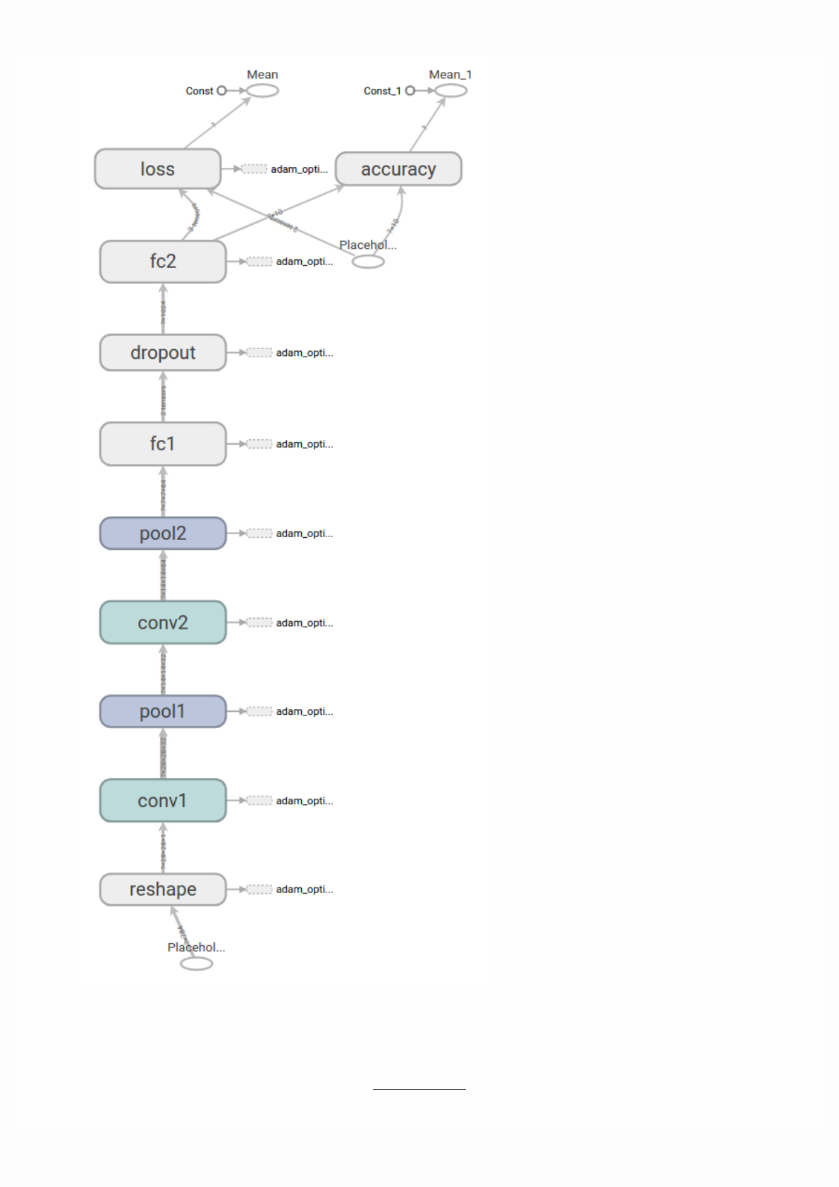
For more information about visualizing your TensorFlow application with TensorBoard, see the TensorBoard tutorial.

Programming with multiple graphs

Note:  When  training  a  model,  a  common  way  of  organizing your  code  is  to  use  one  graph  for  training  your  model,  and  a
separate  graph  for  evaluating  or  performing  inference  with  a  trained  model.  In  many  cases,  the  inference  graph  will  be
different from  the  training  graph:  for  example,  techniques  like  dropout  and  batch  normalization  use  different operations  in
each case. Furthermore, by default utilities like tf.train.Saver use the names of tf.Variable objects (which have names
based on an underlying tf.Operation) to identify each variable in a saved checkpoint. When programming this way, you can
either use completely separate Python processes to build and execute the graphs, or you can use multiple graphs in the same
process. This section describes how to use multiple graphs in the same process.
As noted above, TensorFlow provides a "default graph" that is implicitly passed to all API functions in the same context. For
many  applications,  a  single  graph  is  sufﬁcient.  However,  TensorFlow  also  provides  methods  for  manipulating  the  default
graph, which can be useful in more advanced used cases. For example:
A tf.Graph deﬁnes the namespace for tf.Operation objects: each operation in a single graph must have a unique name. 
TensorFlow will "uniquify" the names of operations by appending "_1", "_2", and so on to their names if the requested 
name is already taken. Using multiple explicitly created graphs gives you more control over what name is given to each 
operation.
The default graph stores information about every tf.Operation and tf.Tensor that was ever added to it. If your program 
creates a large number of unconnected subgraphs, it may be more efﬁcient to use a different tf.Graph to build each 
subgraph, so that unrelated state can be garbage collected.
You can install a different tf.Graph as the default graph, using the tf.Graph.as_default context manager:
g_1 = tf.Graph()
with g_1.as_default():
  # Operations created in this scope will be added to `g_1`.
  c = tf.constant("Node in g_1")
  # Sessions created in this scope will run operations from `g_1`.
  sess_1 = tf.Session()
g_2 = tf.Graph()
with g_2.as_default():
  # Operations created in this scope will be added to `g_2`.
  d = tf.constant("Node in g_2")
# Alternatively, you can pass a graph when constructing a `tf.Session`:
# `sess_2` will run operations from `g_2`.
sess_2 = tf.Session(graph=g_2)
assert c.graph is g_1
assert sess_1.graph is g_1
assert d.graph is g_2
assert sess_2.graph is g_2
To inspect the current default graph, call tf.get_default_graph, which returns a tf.Graph object:
 
Saving and Restoring   
This document explains how to save and restore variables and models.
# Print all of the operations in the default graph.
g = tf.get_default_graph()
print(g.get_operations())

Saving and restoring variables

A TensorFlow variable provides the best way to represent shared, persistent state manipulated by your program. (See Variables

for details.) This section explains how to save and restore variables. Note that Estimators automatically saves and restores

variables (in the model_dir).

The tf.train.Saver class provides methods for saving and restoring models. The tf.train.Saverconstructor adds save

and restore ops to the graph for all, or a speciﬁed list, of the variables in the graph. The Saver object provides methods to run

these ops, specifying paths for the checkpoint ﬁles to write to or read from.

The saver will restore all variables already deﬁned in your model. If you're loading a model without knowing how to build its

graph (for example, if you're writing a generic program to load models), then read the Overview of saving and restoring

models section later in this document.

TensorFlow saves variables in binary checkpoint ﬁles that, roughly speaking, map variable names to tensor values.

Saving variables

Create a Saver with tf.train.Saver() to manage all variables in the model. For example, the following snippet

demonstrates how to call the tf.train.Saver.save method to save variables to checkpoint ﬁles:

# Create some variables.

v1 = tf.get_variable("v1", shape=[3], initializer = tf.zeros_initializer)

v2 = tf.get_variable("v2", shape=[5], initializer = tf.zeros_initializer)

inc_v1 = v1.assign(v1+1)

dec_v2 = v2.assign(v2-1)

# Add an op to initialize the variables.

init_op = tf.global_variables_initializer()

# Add ops to save and restore all the variables.

saver = tf.train.Saver()

# Later, launch the model, initialize the variables, do some work, and save the

# variables to disk.

with tf.Session() as sess:

sess.run(init_op)

# Do some work with the model.

inc_v1.op.run()

dec_v2.op.run()

# Save the variables to disk.

save_path = saver.save(sess, "/tmp/model.ckpt")

print("Model saved in path: %s" % save_path)

Restoring variables

The tf.train.Saver object not only saves variables to checkpoint ﬁles, it also restores variables. Note that when you restore

variables you do not have to initialize them beforehand. For example, the following snippet demonstrates how to call the

tf.train.Saver.restore method to restore variables from the checkpoint ﬁles:

tf.reset_default_graph()

# Create some variables.

v1 = tf.get_variable("v1", shape=[3])

v2 = tf.get_variable("v2", shape=[5])

# Add ops to save and restore all the variables.

saver = tf.train.Saver()

# Later, launch the model, use the saver to restore variables from disk, and

# do some work with the model.

with tf.Session() as sess:

# Restore variables from disk.

saver.restore(sess, "/tmp/model.ckpt")

print("Model restored.")

# Check the values of the variables

print("v1 : %s" % v1.eval())

print("v2 : %s" % v2.eval())

Notes:

There is not a physical ﬁle called "/tmp/model.ckpt". It is the preﬁx of ﬁlenames created for the checkpoint. Users only

interact with the preﬁx instead of physical checkpoint ﬁles.

Choosing which variables to save and restore

If you do not pass any arguments to tf.train.Saver(), the saver handles all variables in the graph. Each variable is saved

under the name that was passed when the variable was created.

It is sometimes useful to explicitly specify names for variables in the checkpoint ﬁles. For example, you may have trained a

model with a variable named "weights" whose value you want to restore into a variable named"params".

It is also sometimes useful to only save or restore a subset of the variables used by a model. For example, you may have trained

a neural net with ﬁve layers, and you now want to train a new model with six layers that reuses the existing weights of the ﬁve

trained layers. You can use the saver to restore the weights of just the ﬁrst ﬁve layers.

You can easily specify the names and variables to save or load by passing to the tf.train.Saver()constructor either of the

following:

A list of variables (which will be stored under their own names).

A Python dictionary in which keys are the names to use and the values are the variables to manage.

Continuing from the save/restore examples shown earlier:

tf.reset_default_graph()

# Create some variables.

v1 = tf.get_variable("v1", [3], initializer = tf.zeros_initializer)

v2 = tf.get_variable("v2", [5], initializer = tf.zeros_initializer)

# Add ops to save and restore only `v2` using the name "v2"

saver = tf.train.Saver({"v2": v2})

# Use the saver object normally after that.

with tf.Session() as sess:

# Initialize v1 since the saver will not.

v1.initializer.run()

saver.restore(sess, "/tmp/model.ckpt")

print("v1 : %s" % v1.eval())

print("v2 : %s" % v2.eval())

Notes:

You can create as many Saver objects as you want if you need to save and restore different subsets of the model variables.

The same variable can be listed in multiple saver objects; its value is only changed when the Saver.restore() method is

run.

If you only restore a subset of the model variables at the start of a session, you have to run an initialize op for the other

variables. See tf.variables_initializer for more information.

To inspect the variables in a checkpoint, you can use the inspect_checkpoint library, particularly the

print_tensors_in_checkpoint_file function.

By default, Saver uses the value of the tf.Variable.name property for each variable. However, when you create a Saver

object, you may optionally choose names for the variables in the checkpoint ﬁles.

Inspect variables in a checkpoint

We can quickly inspect variables in a checkpoint with the inspect_checkpoint library.

Continuing from the save/restore examples shown earlier:

# import the inspect_checkpoint library

from tensorflow.python.tools import inspect_checkpoint as chkp

# print all tensors in checkpoint file

chkp.print_tensors_in_checkpoint_file("/tmp/model.ckpt", tensor_name='', all_tensors=True)

# tensor_name: v1

# [ 1. 1. 1.]

# tensor_name: v2

# [-1. -1. -1. -1. -1.]

# print only tensor v1 in checkpoint file

chkp.print_tensors_in_checkpoint_file("/tmp/model.ckpt", tensor_name='v1', all_tensors=False)

# tensor_name: v1

# [ 1. 1. 1.]

# print only tensor v2 in checkpoint file

chkp.print_tensors_in_checkpoint_file("/tmp/model.ckpt", tensor_name='v2', all_tensors=False)

# tensor_name: v2

# [-1. -1. -1. -1. -1.]

Overview of saving and restoring models

When you want to save and load variables, the graph, and the graph's metadata--basically, when you want to save or restore

your model--we recommend using SavedModel. SavedModel is a language-neutral, recoverable, hermetic serialization format.

SavedModel enables higher-level systems and tools to produce, consume, and transform TensorFlow models. TensorFlow

provides several mechanisms for interacting with SavedModel, including tf.saved_model APIs, Estimator APIs and a CLI.

APIs to build and load a SavedModel

This section focuses on the APIs for building and loading a SavedModel, particularly when using lower-level TensorFlow APIs.

Building a SavedModel

We provide a Python implementation of the SavedModel builder. The SavedModelBuilder class provides functionality to

save multiple MetaGraphDefs. A MetaGraph is a dataﬂow graph, plus its associated variables, assets, and signatures. A

MetaGraphDef is the protocol buffer representation of a MetaGraph. A signature is the set of inputs to and outputs from a

graph.

If assets need to be saved and written or copied to disk, they can be provided when the ﬁrst MetaGraphDef is added. If

multiple MetaGraphDefs are associated with an asset of the same name, only the ﬁrst version is retained.

Each MetaGraphDef added to the SavedModel must be annotated with user-speciﬁed tags. The tags provide a means to

identify the speciﬁc MetaGraphDef to load and restore, along with the shared set of variables and assets. These tags typically

annotate a MetaGraphDef with its functionality (for example, serving or training), and optionally with hardware-speciﬁc

aspects (for example, GPU).

For example, the following code suggests a typical way to use SavedModelBuilder to build a SavedModel:

export_dir = ...

...

builder = tf.saved_model.builder.SavedModelBuilder(export_dir)

with tf.Session(graph=tf.Graph()) as sess:

...

builder.add_meta_graph_and_variables(sess,

[tag_constants.TRAINING],

signature_def_map=foo_signatures,

assets_collection=foo_assets)

...

# Add a second MetaGraphDef for inference.

with tf.Session(graph=tf.Graph()) as sess:

...

builder.add_meta_graph([tag_constants.SERVING])

...

builder.save()

Loading a SavedModel in Python

The Python version of the SavedModel loader provides load and restore capability for a SavedModel. The loadoperation

requires the following information:

The session in which to restore the graph deﬁnition and variables.

The tags used to identify the MetaGraphDef to load.

The location (directory) of the SavedModel.

Upon a load, the subset of variables, assets, and signatures supplied as part of the speciﬁc MetaGraphDef will be restored into

the supplied session.

export_dir = ...

...

with tf.Session(graph=tf.Graph()) as sess:

tf.saved_model.loader.load(sess, [tag_constants.TRAINING], export_dir)

...

Loading a Savedmodel in C++

The C++ version of the SavedModel loader provides an API to load a SavedModel from a path, while

allowingSessionOptions and RunOptions. You have to specify the tags associated with the graph to be loaded. The loaded

version of SavedModel is referred to as SavedModelBundle and contains the MetaGraphDef and the session within which it is

loaded.

const string export_dir = ...

SavedModelBundle bundle;

...

LoadSavedModel(session_options, run_options, export_dir, {kSavedModelTagTrain},

&bundle);

Standard constants   
SavedModel offers the ﬂexibility to build and load TensorFlow graphs for a variety of use-cases. For the most common use-
cases,  SavedModel's  APIs  provide  a  set  of  constants  in  Python  and  C++  that  are  easy  to  reuse  and  share  across  tools
consistently.
Standard MetaGraphDef tags   
You  may use  sets  of tags to  uniquely  identify a  MetaGraphDef  saved in a  SavedModel.  A  subset  of commonly  used  tags is
speciﬁed in:
Python
C++
Standard SignatureDef constants   
A SignatureDef is a protocol buffer that deﬁnes the signature of a computation supported by a graph. Commonly used input
keys, output keys, and method names are deﬁned in:
Python
C++
Using SavedModel with Estimators   
After training an Estimator model, you may want to create a service from that model that takes requests and returns a result.
You can run such a service locally on your machine or deploy it scalably in the cloud.
To prepare a trained Estimator for serving, you must export it in the standard SavedModel format. This section explains how
to:
Specify the output nodes and the corresponding APIs that can be served (Classify, Regress, or Predict).
Export your model to the SavedModel format.
Serve the model from a local server and request predictions.
Preparing serving inputs   
During  training,  an  input_fn()  ingests  data  and  prepares  it  for  use  by  the  model.  At  serving  time,  similarly,
aserving_input_receiver_fn() accepts inference requests and prepares them for the model. This function has the following
purposes:
To add placeholders to the graph that the serving system will feed with inference requests.
To add any additional ops needed to convert data from the input format into the feature Tensors expected by the model.
The  function  returns  a  tf.estimator.export.ServingInputReceiver  object,  which  packages  the  placeholders  and  the
resulting feature Tensors together.
A  typical  pattern  is  that  inference  requests  arrive  in  the  form  of  serialized  tf.Examples,  so  the
serving_input_receiver_fn() creates a single string placeholder to receive them. The serving_input_receiver_fn() is
then also responsible for parsing the tf.Examples by adding a tf.parse_example op to the graph.
When writing such a serving_input_receiver_fn(), you must pass a parsing speciﬁcation to tf.parse_example to tell the
parser what feature names to expect and how to map them to Tensors. A parsing speciﬁcation takes the form of a dict from
feature names to tf.FixedLenFeature, tf.VarLenFeature, and tf.SparseFeature. Note this parsing speciﬁcation should
not include any label or weight columns, since those will not be available at serving time—in contrast to a parsing speciﬁcation

used in the input_fn() at training time.

In combination, then:

feature_spec = {'foo': tf.FixedLenFeature(...),

'bar': tf.VarLenFeature(...)}

def serving_input_receiver_fn():

"""An input receiver that expects a serialized tf.Example."""

serialized_tf_example = tf.placeholder(dtype=tf.string,

shape=[default_batch_size],

name='input_example_tensor')

receiver_tensors = {'examples': serialized_tf_example}

features = tf.parse_example(serialized_tf_example, feature_spec)

return tf.estimator.export.ServingInputReceiver(features, receiver_tensors)

The tf.estimator.export.build_parsing_serving_input_receiver_fn utility function provides that input receiver for

the common case.

Note: when training a model to be served using the Predict API with a local server, the parsing step is not needed because

the model will receive raw feature data.

Even if you require no parsing or other input processing—that is, if the serving system will feed feature Tensors directly—you

must still provide a serving_input_receiver_fn() that creates placeholders for the featureTensors and passes them

through. The tf.estimator.export.build_raw_serving_input_receiver_fnutility provides for this.

If these utilities do not meet your needs, you are free to write your own serving_input_receiver_fn(). One case where this

may be needed is if your training input_fn() incorporates some preprocessing logic that must be recapitulated at serving

time. To reduce the risk of training-serving skew, we recommend encapsulating such processing in a function which is then

called from both input_fn() and serving_input_receiver_fn().

Note that the serving_input_receiver_fn() also determines the input portion of the signature. That is, when writing a

serving_input_receiver_fn(), you must tell the parser what signatures to expect and how to map them to your model's

expected inputs. By contrast, the output portion of the signature is determined by the model.

Performing the export

To export your trained Estimator, call tf.estimator.Estimator.export_savedmodel with the export base path and the

serving_input_receiver_fn.

estimator.export_savedmodel(export_dir_base, serving_input_receiver_fn)

This method builds a new graph by ﬁrst calling the serving_input_receiver_fn() to obtain feature Tensors, and then

calling this Estimator's model_fn() to generate the model graph based on those features. It starts a fresh Session, and, by

default, restores the most recent checkpoint into it. (A different checkpoint may be passed, if needed.) Finally it creates a time-

stamped export directory below the givenexport_dir_base (i.e., export_dir_base/<timestamp>), and writes a

SavedModel into it containing a single MetaGraphDef saved from this Session.

Note: It is your responsibility to garbage-collect old exports. Otherwise, successive exports will accumulate under

export_dir_base.

Specifying the outputs of a custom model

When writing a custom model_fn, you must populate  the export_outputs element of the tf.estimator.EstimatorSpec
return value. This is a dict of {name: output} describing the output signatures to be exported and used during serving.
In the usual case of making a single prediction, this dict contains one element, and the name is immaterial. In a multi-headed
model, each head is represented by an  entry in this dict. In this case the name is a string of your  choice that can  be used to
request a speciﬁc head at serving time.
Each  output  value  must  be  an  ExportOutput  object  such  astf.estimator.export.ClassificationOutput,
tf.estimator.export.RegressionOutput, ortf.estimator.export.PredictOutput.
These  output  types  map  straightforwardly  to  the  TensorFlow  Serving  APIs,  and  so  determine  which  request  types  will  be
honored.
Note: In the multi-headed case, a SignatureDef will be generated for each element of the export_outputs dict returned from
the  model_fn,  named  using  the  same  keys.  These  SignatureDefs  differ  only  in  their  outputs,  as  provided  by  the
corresponding  ExportOutput  entry.  The  inputs  are  always  those  provided  by  the  serving_input_receiver_fn.  An
inference  request  may  specify  the  head  by  name.  One  head  must  be  named  using
signature_constants.DEFAULT_SERVING_SIGNATURE_DEF_KEY  indicating  which  SignatureDef  will  be  served  when  an
inference request does not specify one.
Serving the exported model locally   
For local deployment, you can serve your model using TensorFlow Serving, an open-source project that loads a SavedModel
and exposes it as a gRPC service.
First, install TensorFlow Serving.
Then build and  run the local model server, substituting  $export_dir_base with the path to  the SavedModel you exported
above:
bazel build //tensorflow_serving/model_servers:tensorflow_model_server
bazel-bin/tensorflow_serving/model_servers/tensorflow_model_server --port=9000 --
model_base_path=$export_dir_base
Now you have a server listening for inference requests via gRPC on port 9000!
Requesting predictions from a local server   
The server  responds to  gRPC requests according to the  PredictionService gRPC  API  service deﬁnition.  (The  nested protocol
buffers are deﬁned in various neighboring ﬁles).
From the API service deﬁnition, the gRPC framework generates client libraries in various languages providing remote access to
the API. In a project using the Bazel build tool, these libraries are built automatically and provided via dependencies like these
(using Python for example):
  deps = [
    "//tensorflow_serving/apis:classification_proto_py_pb2",
    "//tensorflow_serving/apis:regression_proto_py_pb2",
    "//tensorflow_serving/apis:predict_proto_py_pb2",
    "//tensorflow_serving/apis:prediction_service_proto_py_pb2"
  ]
Python client code can then import the libraries thus:

from tensorflow_serving.apis import classification_pb2

from tensorflow_serving.apis import regression_pb2

from tensorflow_serving.apis import predict_pb2

from tensorflow_serving.apis import prediction_service_pb2

Note: prediction_service_pb2 deﬁnes the service as a whole and so is always required. However a typical client will

need only one of classification_pb2, regression_pb2, and predict_pb2, depending on the type of requests being

made.

Sending a gRPC request is then accomplished by assembling a protocol buffer containing the request data and passing it to the

service stub. Note how the request protocol buffer is created empty and then populated via thegenerated protocol buffer API.

from grpc.beta import implementations

channel = implementations.insecure_channel(host, int(port))

stub = prediction_service_pb2.beta_create_PredictionService_stub(channel)

request = classification_pb2.ClassificationRequest()

example = request.input.example_list.examples.add()

example.features.feature['x'].float_list.value.extend(image[0].astype(float))

result = stub.Classify(request, 10.0) # 10 secs timeout

The returned result in this example is a ClassificationResponse protocol buffer.

This is a skeletal example; please see the Tensorﬂow Serving documentation and examples for more details.

Note: ClassificationRequest and RegressionRequest contain a tensorflow.serving.Input protocol buffer, which

in turn contains a list of tensorflow.Example protocol buffers. PredictRequest, by contrast, contains a mapping from

feature names to values encoded via TensorProto. Correspondingly: When using the Classify and Regress APIs,

TensorFlow Serving feeds serialized tf.Examples to the graph, so yourserving_input_receiver_fn() should include

a tf.parse_example() Op. When using the generic PredictAPI, however, TensorFlow Serving feeds raw feature data to

the graph, so a pass through serving_input_receiver_fn() should be used.

CLI to inspect and execute SavedModel

You can use the SavedModel Command Line Interface (CLI) to inspect and execute a SavedModel. For example, you can use

the CLI to inspect the model's SignatureDefs. The CLI enables you to quickly conﬁrm that the input Tensor dtype and shape

match the model. Moreover, if you want to test your model, you can use the CLI to do a sanity check by passing in sample

inputs in various formats (for example, Python expressions) and then fetching the output.

Installing the SavedModel CLI

Broadly speaking, you can install TensorFlow in either of the following two ways:

By installing a pre-built TensorFlow binary.

By building TensorFlow from source code.

If you installed TensorFlow through a pre-built TensorFlow binary, then the SavedModel CLI is already installed on your

system at pathname bin\saved_model_cli.

If you built TensorFlow from source code, you must run the following additional command to build saved_model_cli:

$ bazel build tensorflow/python/tools:saved_model_cli

Overview of commands

The SavedModel CLI supports the following two commands on a MetaGraphDef in a SavedModel:

show, which shows a computation on a MetaGraphDef in a SavedModel.

run, which runs a computation on a MetaGraphDef.

show command

A SavedModel contains one or more MetaGraphDefs, identiﬁed by their tag-sets. To serve a model, you might wonder what

kind of SignatureDefs are in each model, and what are their inputs and outputs. The showcommand let you examine the

contents of the SavedModel in hierarchical order. Here's the syntax:

usage: saved_model_cli show [-h] --dir DIR [--all]

[--tag_set TAG_SET] [--signature_def SIGNATURE_DEF_KEY]

For example, the following command shows all available MetaGraphDef tag-sets in the SavedModel:

$ saved_model_cli show --dir /tmp/saved_model_dir

The given SavedModel contains the following tag-sets:

serve

serve, gpu

The following command shows all available SignatureDef keys in a MetaGraphDef:

$ saved_model_cli show --dir /tmp/saved_model_dir --tag_set serve

The given SavedModel `MetaGraphDef` contains `SignatureDefs` with the

following keys:

SignatureDef key: "classify_x2_to_y3"

SignatureDef key: "classify_x_to_y"

SignatureDef key: "regress_x2_to_y3"

SignatureDef key: "regress_x_to_y"

SignatureDef key: "regress_x_to_y2"

SignatureDef key: "serving_default"

If a MetaGraphDef has multiple tags in the tag-set, you must specify all tags, each tag separated by a comma. For example:

$ saved_model_cli show --dir /tmp/saved_model_dir --tag_set serve,gpu

To show all inputs and outputs TensorInfo for a speciﬁc SignatureDef, pass in the SignatureDef key to signature_def

option. This is very useful when you want to know the tensor key value, dtype and shape of the input tensors for executing the

computation graph later. For example:

$ saved_model_cli show --dir \

/tmp/saved_model_dir --tag_set serve --signature_def serving_default

The given SavedModel SignatureDef contains the following input(s):

inputs['x'] tensor_info:

dtype: DT_FLOAT

shape: (-1, 1)

The given SavedModel SignatureDef contains the following output(s):

outputs['y'] tensor_info:

dtype: DT_FLOAT

shape: (-1, 1)

Method name is: tensorflow/serving/predict

To show all available information in the SavedModel, use the --all option. For example:

$ saved_model_cli show --dir /tmp/saved_model_dir --all

MetaGraphDef with tag-set: 'serve' contains the following SignatureDefs:

signature_def['classify_x2_to_y3']:

The given SavedModel SignatureDef contains the following input(s):

inputs['inputs'] tensor_info:

dtype: DT_FLOAT

shape: (-1, 1)

The given SavedModel SignatureDef contains the following output(s):

outputs['scores'] tensor_info:

dtype: DT_FLOAT

shape: (-1, 1)

Method name is: tensorflow/serving/classify

...

signature_def['serving_default']:

The given SavedModel SignatureDef contains the following input(s):

inputs['x'] tensor_info:

dtype: DT_FLOAT

shape: (-1, 1)

The given SavedModel SignatureDef contains the following output(s):

outputs['y'] tensor_info:

dtype: DT_FLOAT

shape: (-1, 1)

Method name is: tensorflow/serving/predict

run command

Invoke the run command to run a graph computation, passing inputs and then displaying (and optionally saving) the outputs.

Here's the syntax:

usage: saved_model_cli run [-h] --dir DIR --tag_set TAG_SET --signature_def

SIGNATURE_DEF_KEY [--inputs INPUTS]

[--input_exprs INPUT_EXPRS] [--outdir OUTDIR]

[--overwrite] [--tf_debug]

The run command provides the following two ways to pass inputs to the model:

--inputs option enables you to pass numpy ndarray in ﬁles.

--input_exprs option enables you to pass Python expressions.

--inputs

To pass input data in ﬁles, specify the --inputs option, which takes the following general format:

--inputs <INPUTS>

where INPUTS is either of the following formats:

<input_key>=<filename>

<input_key>=<filename>[<variable_name>]

You may pass multiple INPUTS. If you do pass multiple inputs, use a semicolon to separate each of the INPUTS.

saved_model_cli uses numpy.load to load the ﬁlename. The ﬁlename may be in any of the following formats:

.npy

.npz

pickle format

A .npy ﬁle always contains a numpy ndarray. Therefore, when loading from a .npy ﬁle, the content will be directly assigned to

the speciﬁed input tensor. If you specify a variable_name with that .npy ﬁle, thevariable_name will be ignored and a warning will

be issued.

When loading from a .npz (zip) ﬁle, you may optionally specify a variable_name to identify the variable within the zip ﬁle to

load for the input tensor key. If you don't specify a variable_name, the SavedModel CLI will check that only one ﬁle is included

in the zip ﬁle and load it for the speciﬁed input tensor key.

When loading from a pickle ﬁle, if no variable_name is speciﬁed in the square brackets, whatever that is inside the pickle ﬁle

will be passed to the speciﬁed input tensor key. Otherwise, the SavedModel CLI will assume a dictionary is stored in the pickle

ﬁle and the value corresponding to the variable_name will be used.

--inputs_exprs

To pass inputs through Python expressions, specify the --input_exprs option. This can be useful for when you don't have

data ﬁles lying around, but still want to sanity check the model with some simple inputs that match the dtype and shape of the

model's SignatureDefs. For example:

`input_key=[[1], [2], [3]]`

In addition to Python expressions, you may also pass numpy functions. For example:

input_key=np.ones((32, 32, 3))

(Note that the numpy module is already available to you as np.)

Save Output

By default, the SavedModel CLI writes output to stdout. If a directory is passed to --outdir option, the outputs will be saved

as npy ﬁles named after output tensor keys under the given directory.

Use --overwrite to overwrite existing output ﬁles.

TensorFlow Debugger (tfdbg) Integration

If --tf_debug option is set, the SavedModel CLI will use the TensorFlow Debugger (tfdbg) to watch the intermediate Tensors

and runtime graphs or subgraphs while running the SavedModel.

Full examples of run

Given:

Your model simply adds x1 and x2 to get output y.

All tensors in the model have shape (-1, 1).

You have two npy ﬁles:

/tmp/my_data1.npy, which contains a numpy ndarray [[1], [2], [3]].

/tmp/my_data2.npy, which contains another numpy ndarray [[0.5], [0.5], [0.5]].

To run these two npy ﬁles through the model to get output y, issue the following command:

$ saved_model_cli run --dir /tmp/saved_model_dir --tag_set serve \

--signature_def x1_x2_to_y --inputs x1=/tmp/my_data1.npy;x2=/tmp/my_data2.npy \

--outdir /tmp/out

Result for output key y:

[[ 1.5]

[ 2.5]

[ 3.5]]

Let's change the preceding example slightly. This time, instead of two .npy ﬁles, you now have an .npz ﬁle and a pickle ﬁle.

Furthermore, you want to overwrite any existing output ﬁle. Here's the command:

$ saved_model_cli run --dir /tmp/saved_model_dir --tag_set serve \

--signature_def x1_x2_to_y \

--inputs x1=/tmp/my_data1.npz[x];x2=/tmp/my_data2.pkl --outdir /tmp/out \

--overwrite

Result for output key y:

[[ 1.5]

[ 2.5]

[ 3.5]]

You may specify python expression instead of an input ﬁle. For example, the following command replaces input x2 with a

Python expression:

$ saved_model_cli run --dir /tmp/saved_model_dir --tag_set serve \

--signature_def x1_x2_to_y --inputs x1=/tmp/my_data1.npz[x] \

--input_exprs 'x2=np.ones((3,1))'

Result for output key y:

[[ 2]

[ 3]

[ 4]]

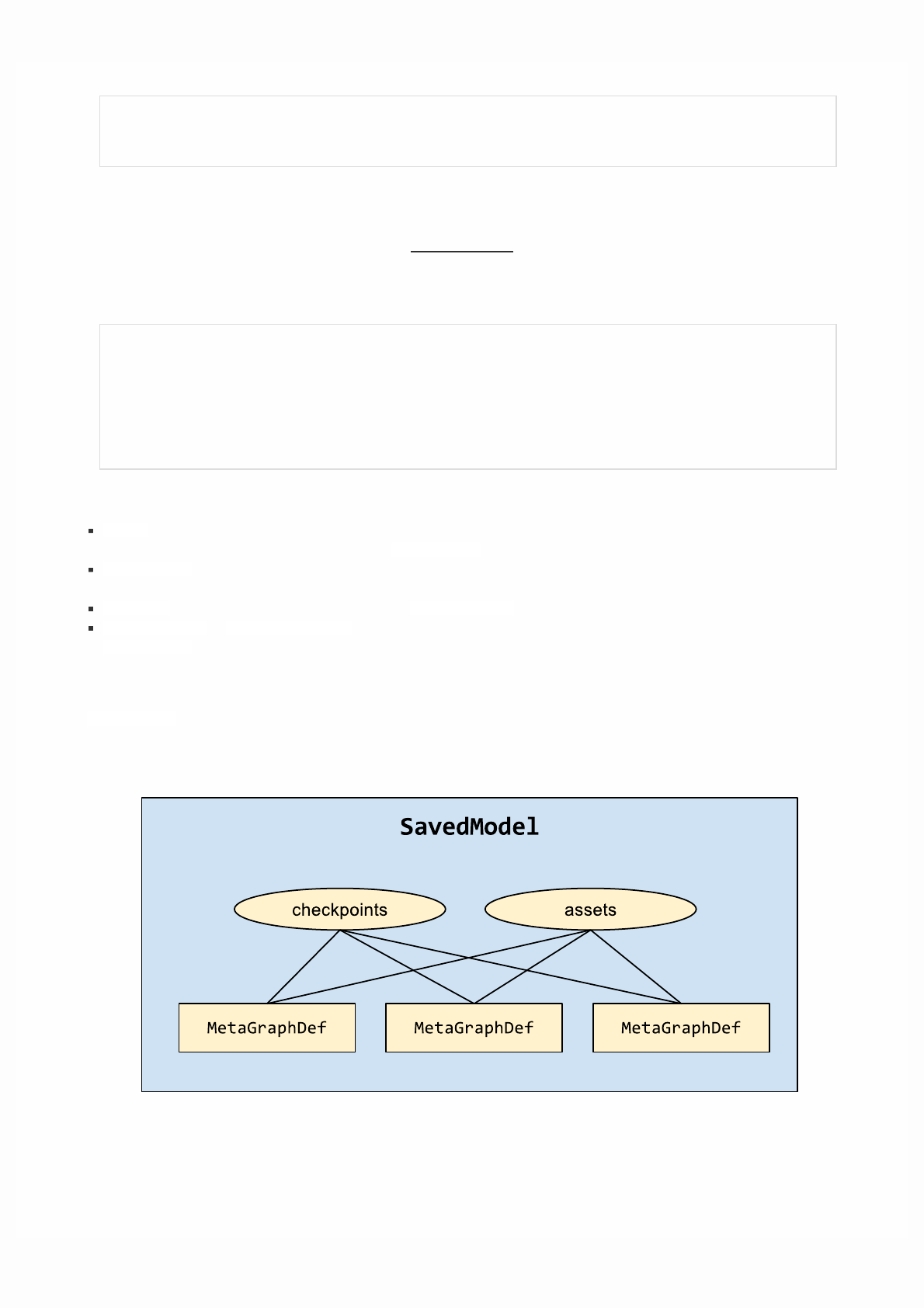
To run the model with the TensorFlow Debugger on, issue the following command:

$ saved_model_cli run --dir /tmp/saved_model_dir --tag_set serve \

--signature_def serving_default --inputs x=/tmp/data.npz[x] --tf_debug

Structure of a SavedModel directory

When you save a model in SavedModel format, TensorFlow creates a SavedModel directory consisting of the following

subdirectories and ﬁles:

assets/

assets.extra/

variables/

variables.data-?????-of-?????

variables.index

saved_model.pb|saved_model.pbtxt

where:

assets is a subfolder containing auxiliary (external) ﬁles, such as vocabularies. Assets are copied to the SavedModel

location and can be read when loading a speciﬁc MetaGraphDef.

assets.extra is a subfolder where higher-level libraries and users can add their own assets that co-exist with the model,

but are not loaded by the graph. This subfolder is not managed by the SavedModel libraries.

variables is a subfolder that includes output from tf.train.Saver.

saved_model.pb or saved_model.pbtxt is the SavedModel protocol buffer. It includes the graph deﬁnitions as

MetaGraphDef protocol buffers.

A single SavedModel can represent multiple graphs. In this case, all the graphs in the SavedModel share a singleset of

checkpoints (variables) and assets. For example, the following diagram shows one SavedModel containing three

MetaGraphDefs, all three of which share the same set of checkpoints and assets:

Each graph is associated with a speciﬁc set of tags, which enables identiﬁcation during a load or restore operation.

Using GPUs

Supported devices

On a typical system, there are multiple computing devices. In TensorFlow, the supported device types are CPUand GPU. They

are represented as strings. For example:

"/cpu:0": The CPU of your machine.

"/device:GPU:0": The GPU of your machine, if you have one.

"/device:GPU:1": The second GPU of your machine, etc.

If a TensorFlow operation has both CPU and GPU implementations, the GPU devices will be given priority when the operation

is assigned to a device. For example, matmul has both CPU and GPU kernels. On a system with devices cpu:0 and gpu:0,

gpu:0 will be selected to run matmul.

Logging Device placement

To ﬁnd out which devices your operations and tensors are assigned to, create the session with log_device_placement

conﬁguration option set to True.

# Creates a graph.

a = tf.constant([1.0, 2.0, 3.0, 4.0, 5.0, 6.0], shape=[2, 3], name='a')

b = tf.constant([1.0, 2.0, 3.0, 4.0, 5.0, 6.0], shape=[3, 2], name='b')

c = tf.matmul(a, b)

# Creates a session with log_device_placement set to True.

sess = tf.Session(config=tf.ConfigProto(log_device_placement=True))

# Runs the op.

print(sess.run(c))

You should see the following output:

Device mapping:

/job:localhost/replica:0/task:0/device:GPU:0 -> device: 0, name: Tesla K40c, pci bus

id: 0000:05:00.0

b: /job:localhost/replica:0/task:0/device:GPU:0

a: /job:localhost/replica:0/task:0/device:GPU:0

MatMul: /job:localhost/replica:0/task:0/device:GPU:0

[[ 22. 28.]

[ 49. 64.]]

Manual device placement

If you would like a particular operation to run on a device of your choice instead of what's automatically selected for you, you

can use with tf.device to create a device context such that all the operations within that context will have the same device

assignment.

# Creates a graph.

with tf.device('/cpu:0'):

a = tf.constant([1.0, 2.0, 3.0, 4.0, 5.0, 6.0], shape=[2, 3], name='a')

b = tf.constant([1.0, 2.0, 3.0, 4.0, 5.0, 6.0], shape=[3, 2], name='b')

c = tf.matmul(a, b)

# Creates a session with log_device_placement set to True.

sess = tf.Session(config=tf.ConfigProto(log_device_placement=True))

# Runs the op.

print(sess.run(c))

You will see that now a and b are assigned to cpu:0. Since a device was not explicitly speciﬁed for the MatMul operation, the

TensorFlow runtime will choose one based on the operation and available devices (gpu:0 in this example) and automatically

copy tensors between devices if required.

Device mapping:

/job:localhost/replica:0/task:0/device:GPU:0 -> device: 0, name: Tesla K40c, pci bus

id: 0000:05:00.0

b: /job:localhost/replica:0/task:0/cpu:0

a: /job:localhost/replica:0/task:0/cpu:0

MatMul: /job:localhost/replica:0/task:0/device:GPU:0

[[ 22. 28.]

[ 49. 64.]]

Allowing GPU memory growth

By default, TensorFlow maps nearly all of the GPU memory of all GPUs (subject to CUDA_VISIBLE_DEVICES) visible to the

process. This is done to more efﬁciently use the relatively precious GPU memory resources on the devices by reducing memory

fragmentation.

In some cases it is desirable for the process to only allocate a subset of the available memory, or to only grow the memory

usage as is needed by the process. TensorFlow provides two Conﬁg options on the Session to control this.

The ﬁrst is the allow_growth option, which attempts to allocate only as much GPU memory based on runtime allocations: it

starts out allocating very little memory, and as Sessions get run and more GPU memory is needed, we extend the GPU memory

region needed by the TensorFlow process. Note that we do not release memory, since that can lead to even worse memory

fragmentation. To turn this option on, set the option in the ConﬁgProto by:

config = tf.ConfigProto()

config.gpu_options.allow_growth = True

session = tf.Session(config=config, ...)

The second method is the per_process_gpu_memory_fraction option, which determines the fraction of the overall amount

of memory that each visible GPU should be allocated. For example, you can tell TensorFlow to only allocate 40% of the total

memory of each GPU by:

config = tf.ConfigProto()

config.gpu_options.per_process_gpu_memory_fraction = 0.4

session = tf.Session(config=config, ...)

This is useful if you want to truly bound the amount of GPU memory available to the TensorFlow process.

Using a single GPU on a multi-GPU system

If you have more than one GPU in your system, the GPU with the lowest ID will be selected by default. If you would like to

run on a different GPU, you will need to specify the preference explicitly:

# Creates a graph.

with tf.device('/device:GPU:2'):

a = tf.constant([1.0, 2.0, 3.0, 4.0, 5.0, 6.0], shape=[2, 3], name='a')

b = tf.constant([1.0, 2.0, 3.0, 4.0, 5.0, 6.0], shape=[3, 2], name='b')

c = tf.matmul(a, b)

# Creates a session with log_device_placement set to True.

sess = tf.Session(config=tf.ConfigProto(log_device_placement=True))

# Runs the op.

print(sess.run(c))

If the device you have speciﬁed does not exist, you will get InvalidArgumentError:

InvalidArgumentError: Invalid argument: Cannot assign a device to node 'b':

Could not satisfy explicit device specification '/device:GPU:2'

[[Node: b = Const[dtype=DT_FLOAT, value=Tensor<type: float shape: [3,2]

values: 1 2 3...>, _device="/device:GPU:2"]()]]

If you would like TensorFlow to automatically choose an existing and supported device to run the operations in case the

speciﬁed one doesn't exist, you can set allow_soft_placement to True in the conﬁguration option when creating the session.

# Creates a graph.

with tf.device('/device:GPU:2'):

a = tf.constant([1.0, 2.0, 3.0, 4.0, 5.0, 6.0], shape=[2, 3], name='a')

b = tf.constant([1.0, 2.0, 3.0, 4.0, 5.0, 6.0], shape=[3, 2], name='b')

c = tf.matmul(a, b)

# Creates a session with allow_soft_placement and log_device_placement set

# to True.

sess = tf.Session(config=tf.ConfigProto(

allow_soft_placement=True, log_device_placement=True))

# Runs the op.

print(sess.run(c))

Using multiple GPUs

If you would like to run TensorFlow on multiple GPUs, you can construct your model in a multi-tower fashion where each

tower is assigned to a different GPU. For example:

# Creates a graph.

c = []

for d in ['/device:GPU:2', '/device:GPU:3']:

with tf.device(d):

a = tf.constant([1.0, 2.0, 3.0, 4.0, 5.0, 6.0], shape=[2, 3])

b = tf.constant([1.0, 2.0, 3.0, 4.0, 5.0, 6.0], shape=[3, 2])

c.append(tf.matmul(a, b))

with tf.device('/cpu:0'):

sum = tf.add_n(c)

# Creates a session with log_device_placement set to True.

sess = tf.Session(config=tf.ConfigProto(log_device_placement=True))

# Runs the op.

print(sess.run(sum))

You will see the following output.

Device mapping:

/job:localhost/replica:0/task:0/device:GPU:0 -> device: 0, name: Tesla K20m, pci bus

id: 0000:02:00.0

/job:localhost/replica:0/task:0/device:GPU:1 -> device: 1, name: Tesla K20m, pci bus

id: 0000:03:00.0

/job:localhost/replica:0/task:0/device:GPU:2 -> device: 2, name: Tesla K20m, pci bus

id: 0000:83:00.0

/job:localhost/replica:0/task:0/device:GPU:3 -> device: 3, name: Tesla K20m, pci bus

id: 0000:84:00.0

Const_3: /job:localhost/replica:0/task:0/device:GPU:3

Const_2: /job:localhost/replica:0/task:0/device:GPU:3

MatMul_1: /job:localhost/replica:0/task:0/device:GPU:3

Const_1: /job:localhost/replica:0/task:0/device:GPU:2

Const: /job:localhost/replica:0/task:0/device:GPU:2

MatMul: /job:localhost/replica:0/task:0/device:GPU:2

AddN: /job:localhost/replica:0/task:0/cpu:0

[[ 44. 56.]

[ 98. 128.]]

The cifar10 tutorial is a good example demonstrating how to do training with multiple GPUs.

Embeddings

This document introduces the concept of embeddings, gives a simple example of how to train an embedding in TensorFlow,

and explains how to view embeddings with the TensorBoard Embedding Projector (live example). The ﬁrst two parts target

newcomers to machine learning or TensorFlow, and the Embedding Projector how-to is for users at all levels.

An embedding is a mapping from discrete objects, such as words, to vectors of real numbers. For example, a 300-dimensional

embedding for English words could include:

blue: (0.01359, 0.00075997, 0.24608, ..., -0.2524, 1.0048, 0.06259)

blues: (0.01396, 0.11887, -0.48963, ..., 0.033483, -0.10007, 0.1158)

orange: (-0.24776, -0.12359, 0.20986, ..., 0.079717, 0.23865, -0.014213)

oranges: (-0.35609, 0.21854, 0.080944, ..., -0.35413, 0.38511, -0.070976)

The individual dimensions in these vectors typically have no inherent meaning. Instead, it's the overall patterns of location and

distance between vectors that machine learning takes advantage of.

Embeddings are important for input to machine learning. Classiﬁers, and neural networks more generally, work on vectors of

real numbers. They train best on dense vectors, where all values contribute to deﬁne an object. However, many important

inputs to machine learning, such as words of text, do not have a natural vector representation. Embedding functions are the

standard and effective way to transform such discrete input objects into useful continuous vectors.

Embeddings are also valuable as outputs of machine learning. Because embeddings map objects to vectors, applications can

use similarity in vector space (for instance, Euclidean distance or the angle between vectors) as a robust and ﬂexible measure of

object similarity. One common use is to ﬁnd nearest neighbors. Using the same word embeddings as above, for instance, here

are the three nearest neighbors for each word and the corresponding angles:

blue: (red, 47.6°), (yellow, 51.9°), (purple, 52.4°)

blues: (jazz, 53.3°), (folk, 59.1°), (bluegrass, 60.6°)

orange: (yellow, 53.5°), (colored, 58.0°), (bright, 59.9°)

oranges: (apples, 45.3°), (lemons, 48.3°), (mangoes, 50.4°)

This would tell an application that apples and oranges are in some way more similar (45.3° apart) than lemons and oranges

(48.3° apart).

Embeddings in TensorFlow

To create word embeddings in TensorFlow, we ﬁrst split the text into words and then assign an integer to every word in the

vocabulary. Let us assume that this has already been done, and that word_ids is a vector of these integers. For example, the

sentence “I have a cat.” could be split into [“I”, “have”, “a”, “cat”, “.”] and then the corresponding word_ids tensor

would have shape [5] and consist of 5 integers. To map these word ids to vectors, we need to create the embedding variable

and use the tf.nn.embedding_lookup function as follows:

word_embeddings = tf.get_variable(“word_embeddings”,

[vocabulary_size, embedding_size])

embedded_word_ids = tf.nn.embedding_lookup(word_embeddings, word_ids)

After this, the tensor embedded_word_ids will have shape [5, embedding_size] in our example and contain the

embeddings (dense vectors) for each of the 5 words. At the end of training, word_embeddings will contain the embeddings for

all words in the vocabulary.

Embeddings can be trained in many network types, and with various loss functions and data sets. For example, one could use

a recurrent neural network to predict the next word from the previous one given a large corpus of sentences, or one could train

two networks to do multi-lingual translation. These methods are described in the Vector Representations of Words tutorial.

Visualizing Embeddings

TensorBoard includes the Embedding Projector, a tool that lets you interactively visualize embeddings. This tool can read

embeddings from your model and render them in two or three dimensions.

The Embedding Projector has three panels:

Data panel on the top left, where you can choose the run, the embedding variable and data columns to color and label points

by.

Projections panel on the bottom left, where you can choose the type of projection.

Inspector panel on the right side, where you can search for particular points and see a list of nearest neighbors.

Projections

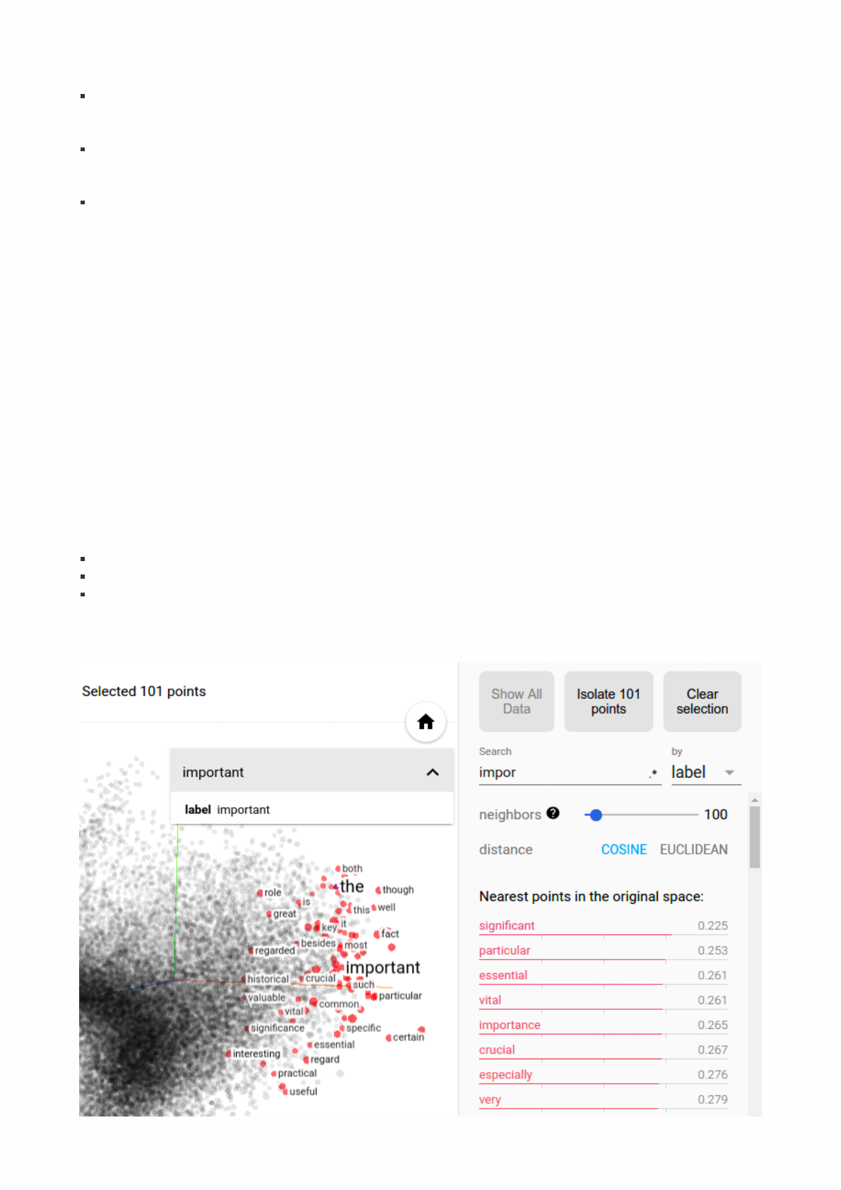
The Embedding Projector provides three ways to reduce the dimensionality of a data set.

t-SNE: a nonlinear nondeterministic algorithm (T-distributed stochastic neighbor embedding) that tries to preserve local

neighborhoods in the data, often at the expense of distorting global structure. You can choose whether to compute two- or

three-dimensional projections.

PCA: a linear deterministic algorithm (principal component analysis) that tries to capture as much of the data variability in

as few dimensions as possible. PCA tends to highlight large-scale structure in the data, but can distort local neighborhoods.

The Embedding Projector computes the top 10 principal components, from which you can choose two or three to view.

Custom: a linear projection onto horizontal and vertical axes that you specify using labels in the data. You deﬁne the

horizontal axis, for instance, by giving text patterns for "Left" and "Right". The Embedding Projector ﬁnds all points whose

label matches the "Left" pattern and computes the centroid of that set; similarly for "Right". The line passing through these

two centroids deﬁnes the horizontal axis. The vertical axis is likewise computed from the centroids for points matching the

"Up" and "Down" text patterns.

Further useful articles are How to Use t-SNE Effectively and Principal Component Analysis Explained Visually.

Exploration

You can explore visually by zooming, rotating, and panning using natural click-and-drag gestures. Hovering your mouse over

a point will show any metadata for that point. You can also inspect nearest-neighbor subsets. Clicking on a point causes the

right pane to list the nearest neighbors, along with distances to the current point. The nearest-neighbor points are also

highlighted in the projection.

It is sometimes useful to restrict the view to a subset of points and perform projections only on those points. To do so, you can

select points in multiple ways:

After clicking on a point, its nearest neighbors are also selected.

After a search, the points matching the query are selected.

Enabling selection, clicking on a point and dragging deﬁnes a selection sphere.

Then click the "Isolate nnn points" button at the top of the Inspector pane on the right hand side. The following image shows

101 points selected and ready for the user to click "Isolate 101 points":

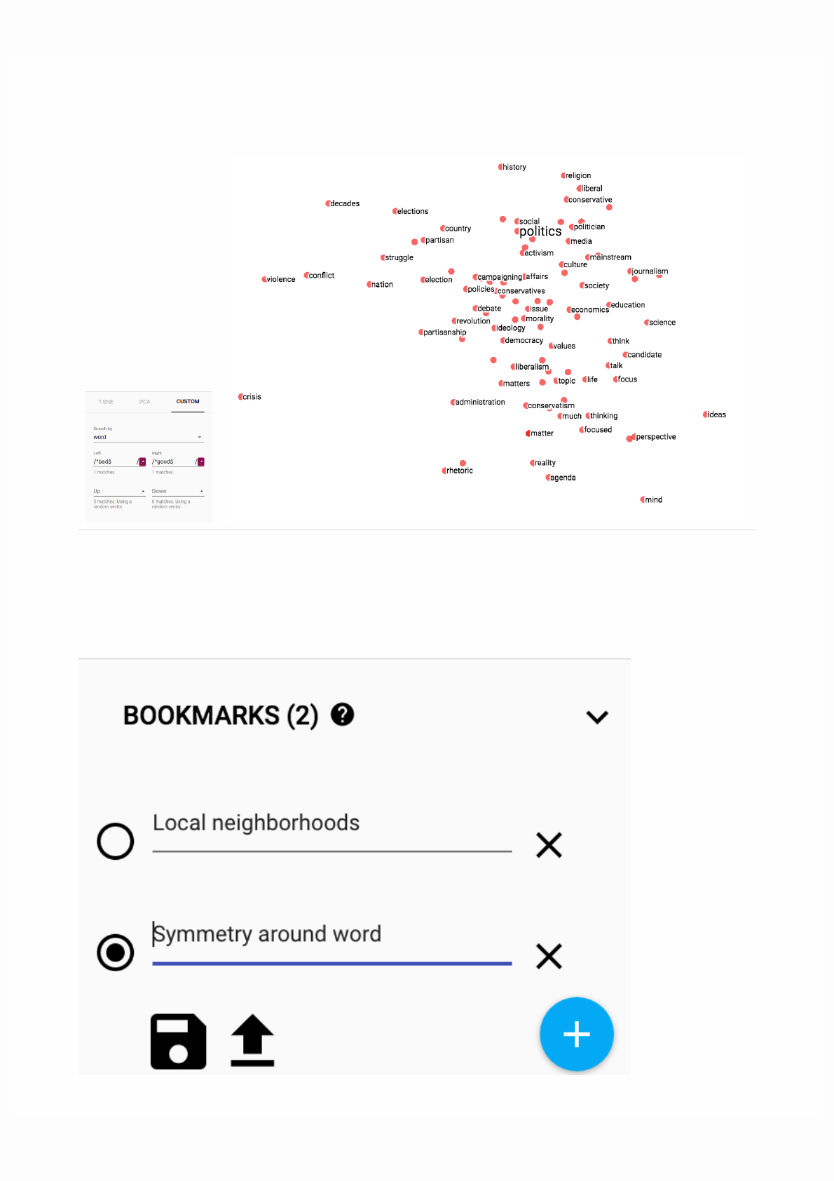
Custom projection

controls.

Custom projection of neighbors of "politics" onto "best" - "worst" vector.

Selection of the nearest neighbors of “important” in a word embedding dataset.

Advanced tip: ﬁltering with custom projection can be powerful. Below, we ﬁltered the 100 nearest neighbors of “politics” and

projected them onto the “worst” - “best” vector as an x axis. The y axis is random. As a result, one ﬁnds on the right side

“ideas”, “science”, “perspective”, “journalism” but on the left “crisis”, “violence” and “conﬂict”.

To share your ﬁndings, you can use the bookmark panel in the bottom right corner and save the current state (including

computed coordinates of any projection) as a small ﬁle. The Projector can then be pointed to a set of one or more of these ﬁles,

producing the panel below. Other users can then walk through a sequence of bookmarks.

0 1 2

3 4 5

6 7

Metadata

If you are working with an embedding, you'll probably want to attach labels/images to the data points. You can do this by

generating a metadata ﬁle containing the labels for each point and clicking "Load data" in the data panel of the Embedding

Projector.

The metadata can be either labels or images, which are stored in a separate ﬁle. For labels, the format should be a TSV ﬁle (tab

characters shown in red) whose ﬁrst line contains column headers (shown in bold) and subsequent lines contain the metadata

values. For example:

**Word\tFrequency**Airplane\t345Car\t241...

The order of lines in the metadata ﬁle is assumed to match the order of vectors in the embedding variable, except for the

header. Consequently, the (i+1)-th line in the metadata ﬁle corresponds to the i-th row of the embedding variable. If the TSV

metadata ﬁle has only a single column, then we don’t expect a header row, and assume each row is the label of the embedding.

We include this exception because it matches the commonly-used "vocab ﬁle" format.

To use images as metadata, you must produce a single sprite image, consisting of small thumbnails, one for each vector in the

embedding. The sprite should store thumbnails in row-ﬁrst order: the ﬁrst data point placed in the top left and the last data

point in the bottom right, though the last row doesn't have to be ﬁlled, as shown below.

Follow this link to see a fun example of thumbnail images in the Embedding Projector.

Mini-FAQ

Is "embedding" an action or a thing? Both. People talk about embedding words in a vector space (action) and about producing

word embeddings (things). Common to both is the notion of embedding as a mapping from discrete objects to vectors.

Creating or applying that mapping is an action, but the mapping itself is a thing.

Are embeddings high-dimensional or low-dimensional? It depends. A 300-dimensional vector space of words and phrases,

for instance, is often called low-dimensional (and dense) when compared to the millions of words and phrases it can contain.

But mathematically it is high-dimensional, displaying many properties that are dramatically different from what our human

intuition has learned about 2- and 3-dimensional spaces.

Is an embedding the same as an embedding layer? No. An embedding layer is a part of neural network, but an embedding is a

more general concept.

Debugging TensorFlow Programs

TensorFlow debugger (tfdbg) is a specialized debugger for TensorFlow. It lets you view the internal structure and states of

running TensorFlow graphs during training and inference, which is difﬁcult to debug with general-purpose debuggers such as

Python's pdb due to TensorFlow's computation-graph paradigm.

NOTE: TensorFlow debugger uses a curses-based text user interface. On Mac OS X, the ncurses library is required and

can be installed with brew install homebrew/dupes/ncurses. On Windows, curses isn't as well supported, so a

readline-based interface can be used with tfdbg by installing pyreadline with pip. If you use Anaconda3, you can install

it with a command such as "C:\Program Files\Anaconda3\Scripts\pip.exe" install pyreadline. Unofﬁcial

Windows curses packages can be downloaded here, then subsequently installed using pip install

<your_version>.whl, however curses on Windows may not work as reliably as curses on Linux or Mac.

This tutorial demonstrates how to use the tfdbg command-line interface (CLI) to debug the appearance of nans and infs, a

frequently-encountered type of bug in TensorFlow model development. The following example is for users who use the low-

level Session API of TensorFlow. A later section of this document describes how to use tfdbg with a higher-level API, namely

tf-learn Estimators and Experiments. To observesuch an issue, run the following command without the debugger (the source

code can be found here):

python -m tensorflow.python.debug.examples.debug_mnist

This code trains a simple neural network for MNIST digit image recognition. Notice that the accuracy increases slightly after

the ﬁrst training step, but then gets stuck at a low (near-chance) level:

Accuracy at step 0: 0.1113

Accuracy at step 1: 0.3183

Accuracy at step 2: 0.098

Accuracy at step 3: 0.098

Accuracy at step 4: 0.098

Wondering what might have gone wrong, you suspect that certain nodes in the training graph generated bad numeric values

such as infs and nans, because this is a common cause of this type of training failure. Let's use tfdbg to debug this issue and

pinpoint the exact graph node where this numeric problem ﬁrst surfaced.

Wrapping TensorFlow Sessions with tfdbg

To add support for tfdbg in our example, all that is needed is to add the following lines of code and wrap the Session object

with a debugger wrapper. This code is already added in debug_mnist.py, so you can activate tfdbg CLI with the --debug ﬂag

at the command line.

# Let your BUILD target depend on "//tensorflow/python/debug:debug_py"

# (You don't need to worry about the BUILD dependency if you are using a pip

# install of open-source TensorFlow.)

from tensorflow.python import debug as tf_debug

sess = tf_debug.LocalCLIDebugWrapperSession(sess)

This wrapper has the same interface as Session, so enabling debugging requires no other changes to the code. The wrapper

provides additional features, including:

Bringing up a CLI before and after Session.run() calls, to let you control the execution and inspect the graph's internal

state.

Allowing you to register special filters for tensor values, to facilitate the diagnosis of issues.

In this example, we have already registered a tensor ﬁlter called tfdbg.has_inf_or_nan, which simply determines if there are

any nan or inf values in any intermediate tensors (tensors that are neither inputs or outputs of the Session.run() call, but

are in the path leading from the inputs to the outputs). This ﬁlter is for nans and infs is a common enough use case that we

ship it with the debug_data module.

Note: You can also write your own custom ﬁlters. See the API documentation of DebugDumpDir.find() for additional

information.

Debugging Model Training with tfdbg

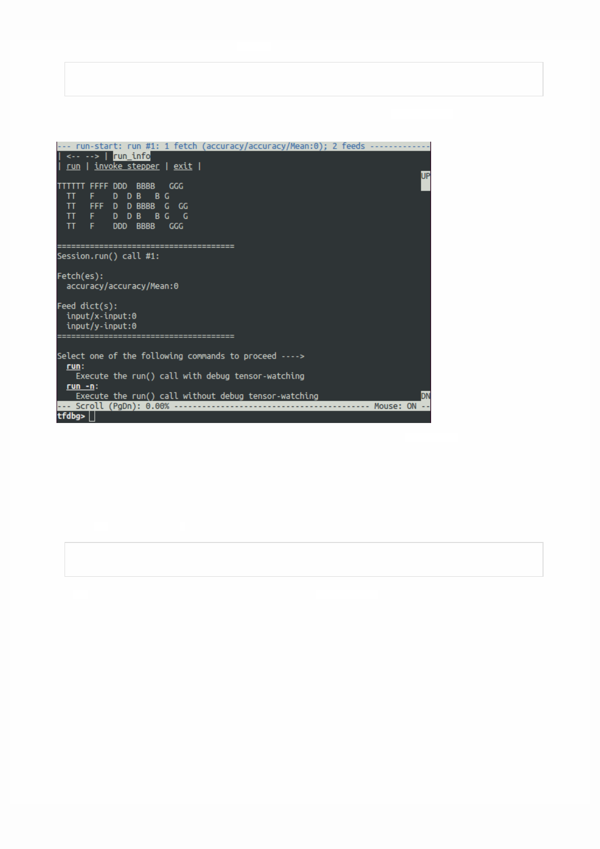
Let's try training the model again, but with the --debug ﬂag added this time:

python -m tensorflow.python.debug.examples.debug_mnist --debug

The debug wrapper session will prompt you when it is about to execute the ﬁrst Session.run() call, with information

regarding the fetched tensor and feed dictionaries displayed on the screen.

This is what we refer to as the run-start CLI. It lists the feeds and fetches to the current Session.run call, before executing

anything.

If the screen size is too small to display the content of the message in its entirety, you can resize it.

Use the PageUp / PageDown / Home / End keys to navigate the screen output. On most keyboards lacking those keys Fn +

Up / Fn + Down / Fn + Right / Fn + Left will work.

Enter the run command (or just r) at the command prompt:

tfdbg> run

The run command causes tfdbg to execute until the end of the next Session.run() call, which calculates the model's accuracy

using a test data set. tfdbg augments the runtime Graph to dump all intermediate tensors. After the run ends, tfdbg displays all

the dumped tensors values in the run-end CLI. For example:

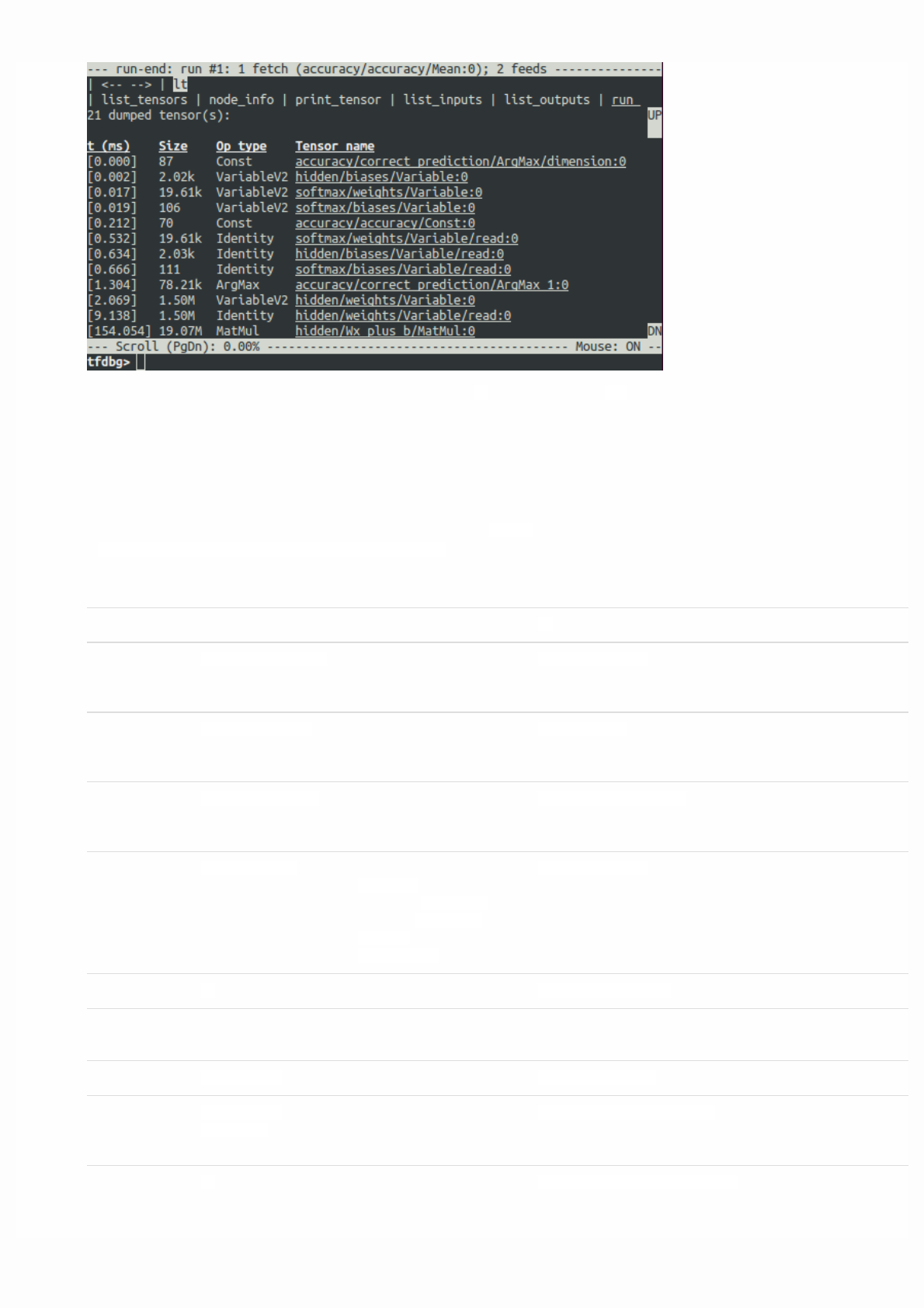
Command Syntax or Option Explanation Example

lt List dumped tensors. lt

-n <name_pattern> List dumped tensors with

names matching given

regular-expression pattern.

lt -n Softmax.*

-t <op_pattern> List dumped tensors with

op types matching given

regular-expression pattern.

lt -t MatMul

-f <filter_name> List only the tensors that

pass a registered tensor

ﬁlter.

lt -f has_inf_or_nan

-s <sort_key> Sort the output by given

sort_key, whose possible

values are timestamp

(default), dump_size,

op_type and

tensor_name.

lt -s dump_size

-r Sort in reverse order. lt -r -s dump_size

pt Print value of a dumped

tensor.

pt <tensor> Print tensor value. pt hidden/Relu:0

pt <tensor>

[slicing]

Print a subarray of tensor,

using numpy-style array

slicing.

pt hidden/Relu:0[0:50,:]

-a Print the entirety of a large

tensor, without using

ellipses. (May take a long

pt -a hidden/Relu:0[0:50,:]

This list of tensors can also be obtained by running the command lt after you executed run.

tfdbg CLI Frequently-Used Commands

Try the following commands at the tfdbg> prompt (referencing the code

attensorflow/python/debug/examples/debug_mnist.py):

time for large tensors.)

-r <range> Highlight elements falling

into speciﬁed numerical

range. Multiple ranges can

be used in conjunction.

pt hidden/Relu:0 -a -r [[-inf,-1],[1,inf]]

-n <number> Print dump corresponding

to speciﬁed 0-based dump

number. Required for

tensors with multiple

dumps.

pt -n 0 hidden/Relu:0

-s Include a summary of the

numeric values of the

tensor (applicable only to

non-empty tensors with

Boolean and numeric types

such as int* and float*.)

pt -s hidden/Relu:0[0:50,:]

@[coordinates] Navigate to speciﬁed

element in pt output.

@[10,0] or @10,0

/regex less-style search for given

regular expression.

/inf

/Scroll to the next line with

matches to the searched

regex (if any).

pf Print a value in the

feed_dict to Session.run.

<feed_tensor_name>

Print the value of the feed.

Also note that the pf

command has the -a, -r

and -sﬂags (not listed

below), which have the

same syntax and semantics

as the identically-named

ﬂags of pt.

pf input_xs:0

eval Evaluate arbitrary Python

and numpy expression.

eval <expression> Evaluate a Python /

numpy expression, with

numpy available as np and

debug tensor names

enclosed in backticks.

eval

"np.matmul((output/Identity:0/Softmax:0).T,Softmax:0)"

-a Print a large-sized

evaluation result in its

entirety, i.e., without using

ellipses.

eval -a 'np.sum(Softmax:0, axis=1)'

ni Display node information.

-a Include node attributes in

the output.

ni -a hidden/Relu

-d List the debug dumps

available from the node.

ni -d hidden/Relu

-t Display the Python stack

trace of the node's creation.

ni -t hidden/Relu

li List inputs to node

-r List the inputs to node,

recursively (the input tree.)

li -r hidden/Relu:0

-d <max_depth> Limit recursion depth

under the -r mode.

li -r -d 3 hidden/Relu:0

-c Include control inputs. li -c -r hidden/Relu:0

-t Show op types of input

nodes.

li -t -r hidden/Relu:0

lo List output recipients of

node

-r List the output recipients of

node, recursively (the

output tree.)

lo -r hidden/Relu:0

-d <max_depth> Limit recursion depth

under the -r mode.

lo -r -d 3 hidden/Relu:0

-c Include recipients via

control edges.

lo -c -r hidden/Relu:0

-t Show op types of recipient

nodes.

lo -t -r hidden/Relu:0

ls List Python source ﬁles

involved in node creation.

-p <path_pattern> Limit output to source ﬁles

matching given regular-

expression path pattern.

ls -p .*debug_mnist.*

-n Limit output to node

names matching given

regular-expression pattern.

ls -n Softmax.*

ps Print Python source ﬁle.

ps <file_path> Print given Python source

ﬁle source.py, with the

lines annotated with the

nodes created at each of

them (if any).

ps /path/to/source.py

-t Perform annotation with

respect to Tensors, instead

of the default, nodes.

ps -t /path/to/source.py

-b <line_number> Annotate source.py

beginning at given line.

ps -b 30 /path/to/source.py

-m <max_elements> Limit the number of

elements in the annotation

for each line.

ps -m 100 /path/to/source.py

run Proceed to the next

Session.run()

run

-n Execute through the next

Session.runwithout

debugging, and drop to

CLI right before the run

after that.

run -n

-t <T> Execute Session.run T -

1 times without

debugging, followed by a

run with debugging. Then

drop to CLI right after the

debugged run.

run -t 10

-f <filter_name> Continue executing

Session.run until any

intermediate tensor

triggers the speciﬁed

Tensor ﬁlter (causes the

ﬁlter to return True).

run -f has_inf_or_nan

--node_name_filter

Execute the next

Session.run, watching

only nodes with names

matching the given

regular-expression pattern.

run --node_name_filter Softmax.*

--op_type_filter

Execute the next

Session.run, watching

only nodes with op types

matching the given

regular-expression pattern.

run --op_type_filter Variable.*

tensor_dtype_filter

Execute the next

Session.run, dumping

only Tensors with data

types (dtypes) matching

the given regular-

expression pattern.

run --tensor_dtype_filter int.*

-p Execute the next

Session.run call in

proﬁling mode.

run -p

ri Display information about

the run the current run,

including fetches and

feeds.

conﬁg Set or show persistent

TFDBG UI conﬁguration.

set Set the value of a conﬁg

item:

{graph_recursion_depth,

mouse_mode}.

config set graph_recursion_depth 3

show Show current persistent UI

conﬁguration.

config show

help Print general help

information

help

help <command> Print help for given

command.

help lt

Note that each time you enter a command, a new screen output will appear. This is somewhat analogous to web pages in a

browser. You can navigate between these screens by clicking the <-- and --> text arrows near the top-left corner of the CLI.

Other Features of the tfdbg CLI

In addition to the commands listed above, the tfdbg CLI provides the following addditional features:

To navigate through previous tfdbg commands, type in a few characters followed by the Up or Down arrow keys. tfdbg will

show you the history of commands that started with those characters.

To navigate through the history of screen outputs, do either of the following:

Use the prev and next commands.

Click underlined <-- and --> links near the top left corner of the screen.

Tab completion of commands and some command arguments.

To redirect the screen output to a ﬁle instead of the screen, end the command with bash-style redirection. For example, the

following command redirects the output of the pt command to the /tmp/xent_value_slices.txt ﬁle:

tfdbg> pt cross_entropy/Log:0[:, 0:10] > /tmp/xent_value_slices.txt

Finding nans and infs

In this ﬁrst Session.run() call, there happen to be no problematic numerical values. You can move on to the next run by

using the command run or its shorthand r.

TIP: If you enter run or r repeatedly, you will be able to move through the Session.run() calls in a sequential manner.

You can also use the -t ﬂag to move ahead a number of Session.run() calls at a time, for example:

tfdbg> run -t 10

Instead of entering run repeatedly and manually searching for nans and infs in the run-end UI after every Session.run()

call (for example, by using the pt command shown in the table above) , you can use the following command to let the

debugger repeatedly execute Session.run() calls without stopping at the run-start or run-end prompt, until the ﬁrst nan or

inf value shows up in the graph. This is analogous to conditional breakpoints in some procedural-language debuggers:

tfdbg> run -f has_inf_or_nan

NOTE: The preceding command works properly because a tensor ﬁlter called has_inf_or_nan has been registered for

you when the wrapped session is created. This ﬁlter detects nans and infs (as explained previously). If you have

registered any other ﬁlters, you can use "run -f" to have tfdbg run until any tensor triggers that ﬁlter (cause the ﬁlter to

return True).

def my_filter_callable(datum, tensor):

# A filter that detects zero-valued scalars.

return len(tensor.shape) == 0 and tensor == 0.0

sess.add_tensor_filter('my_filter', my_filter_callable)

Then at the tfdbg run-start prompt run until your ﬁlter is triggered:

tfdbg> run -f my_filter

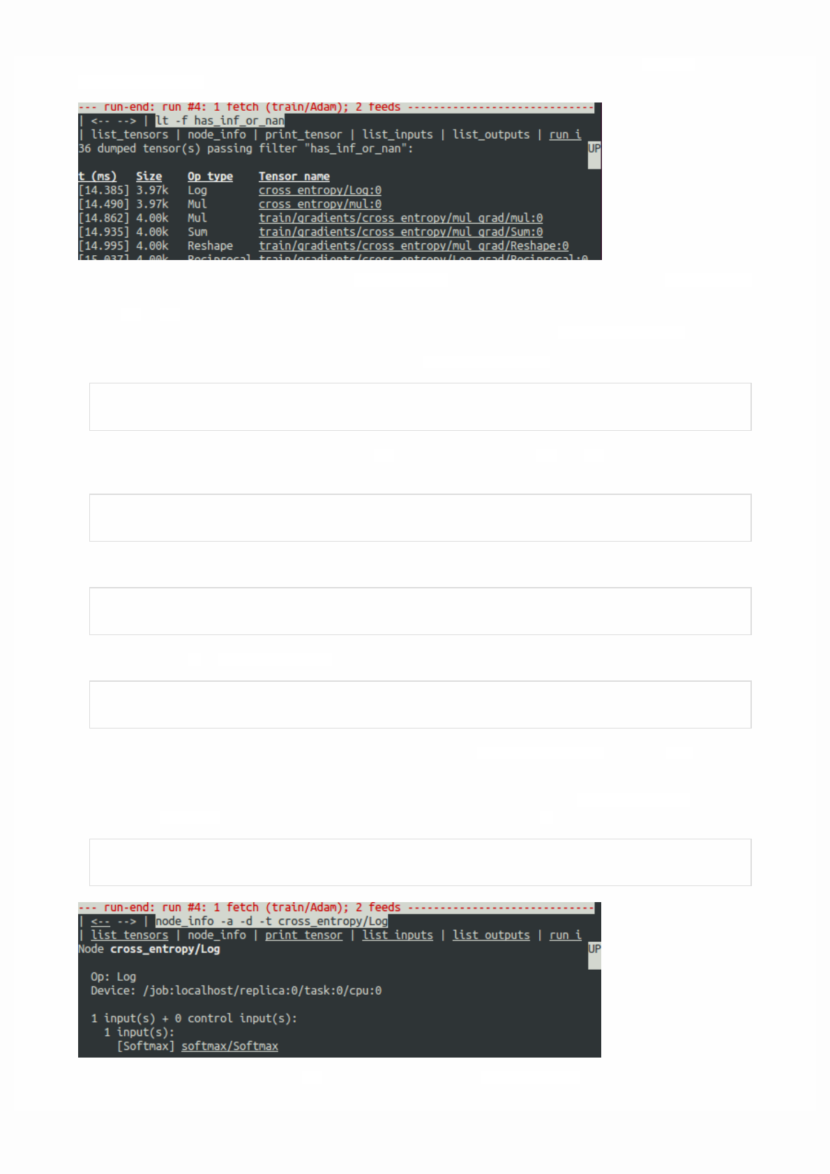
See this API document for more information on the expected signature and return value of the predicateCallable used with

add_tensor_filter().

As the screen display indicates on the ﬁrst line, the has_inf_or_nan ﬁlter is ﬁrst triggered during the fourth Session.run()

call: an Adam optimizer forward-backward training pass on the graph. In this run, 36 (out of the total 95) intermediate tensors

contain nan or inf values. These tensors are listed in chronological order, with their timestamps displayed on the left. At the

top of the list, you can see the ﬁrst tensor in which the bad numerical values ﬁrst surfaced: cross_entropy/Log:0.

To view the value of the tensor, click the underlined tensor name cross_entropy/Log:0 or enter the equivalent command:

tfdbg> pt cross_entropy/Log:0

Scroll down a little and you will notice some scattered inf values. If the instances of inf and nan are difﬁcult to spot by eye,

you can use the following command to perform a regex search and highlight the output:

tfdbg> /inf

Or, alternatively:

tfdbg> /(inf|nan)

You can also use the -s or --numeric_summary command to get a quick summary of the types of numeric values in the tensor:

tfdbg> pt -s cross_entropy/Log:0

From the summary, you can see that several of the 1000 elements of the cross_entropy/Log:0 tensor are -infs (negative

inﬁnities).

Why did these inﬁnities appear? To further debug, display more information about the node cross_entropy/Log by clicking

the underlined node_info menu item on the top or entering the equivalent node_info (ni) command:

tfdbg> ni cross_entropy/Log

You can see that this node has the op type Log and that its input is the node softmax/Softmax. Run the following command to

take a closer look at the input tensor:

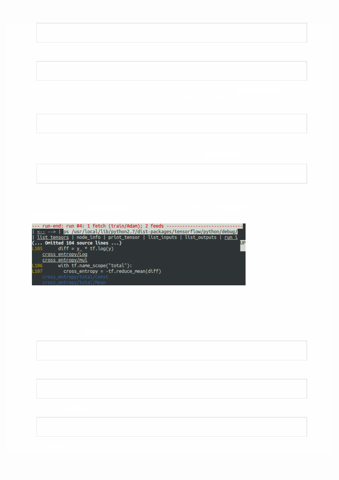
tfdbg> pt softmax/Softmax:0

Examine the values in the input tensor, searching for zeros:

tfdbg> /0\.000

Indeed, there are zeros. Now it is clear that the origin of the bad numerical values is the node cross_entropy/Log taking logs

of zeros. To ﬁnd out the culprit line in the Python source code, use the -tﬂag of the ni command to show the traceback of the

node's construction:

tfdbg> ni -t cross_entropy/Log

If you click "node_info" at the top of the screen, tfdbg automatically shows the traceback of the node's construction.

From the traceback, you can see that the op is constructed at the following line: debug_mnist.py:

diff = y_ * tf.log(y)

tfdbg has a feature that makes it easy to trace Tensors and ops back to lines in Python source ﬁles. It can annotate lines of a

Python ﬁle with the ops or Tensors created by them. To use this feature, simply click the underlined line numbers in the stack

trace output of the ni -t <op_name> commands, or use the ps (or print_source) command such as: ps

/path/to/source.py. For example, the following screenshot shows the output of a ps command.

Fixing the problem

To ﬁx the problem, edit debug_mnist.py, changing the original line:

diff = -(y_ * tf.log(y))

to the built-in, numerically-stable implementation of softmax cross-entropy:

diff = tf.losses.sparse_softmax_cross_entropy(labels=y_, logits=logits)

Rerun with the --debug ﬂag as follows:

python -m tensorflow.python.debug.examples.debug_mnist --debug

At the tfdbg> prompt, enter the following command:

run -f has_inf_or_nan`

Conﬁrm that no tensors are ﬂagged as containing nan or inf values, and accuracy now continues to rise rather than getting

stuck. Success!

Debugging tf-learn Estimators and Experiments

This section explains how to debug TensorFlow programs that use the Estimator and Experiment APIs. Part of the

convenience provided by these APIs is that they manage Sessions internally. This makes the

LocalCLIDebugWrapperSession described in the preceding sections inapplicable. Fortunately, you can still debug them by

using special hooks provided by tfdbg.

Debugging tf.contrib.learn Estimators

Currently, tfdbg can debug the fit() evaluate() methods of tf-learn Estimators. To debug Estimator.fit(), create a

LocalCLIDebugHook and supply it in the monitors argument. For example:

# First, let your BUILD target depend on "//tensorflow/python/debug:debug_py"

# (You don't need to worry about the BUILD dependency if you are using a pip

# install of open-source TensorFlow.)

from tensorflow.python import debug as tf_debug

# Create a LocalCLIDebugHook and use it as a monitor when calling fit().

hooks = [tf_debug.LocalCLIDebugHook()]

classifier.fit(x=training_set.data,

y=training_set.target,

steps=1000,

monitors=hooks)

To debug Estimator.evaluate(), assign hooks to the hooks parameter, as in the following example:

accuracy_score = classifier.evaluate(x=test_set.data,

y=test_set.target,

hooks=hooks)["accuracy"]

debug_tﬂearn_iris.py, based on {$tﬂearn$tf-learn's iris tutorial}, contains a full example of how to use the tfdbg with

Estimators. To run this example, do:

python -m tensorflow.python.debug.examples.debug_tflearn_iris --debug

Debugging tf.contrib.learn Experiments

Experiment is a construct in tf.contrib.learn at a higher level than Estimator. It provides a single interface for training

and evaluating a model. To debug the train() and evaluate() calls to an Experimentobject, you can use the keyword

arguments train_monitors and eval_hooks, respectively, when calling its constructor. For example:

# First, let your BUILD target depend on "//tensorflow/python/debug:debug_py"

# (You don't need to worry about the BUILD dependency if you are using a pip

# install of open-source TensorFlow.)

from tensorflow.python import debug as tf_debug

hooks = [tf_debug.LocalCLIDebugHook()]

ex = experiment.Experiment(classifier,

train_input_fn=iris_input_fn,

eval_input_fn=iris_input_fn,

train_steps=FLAGS.train_steps,

eval_delay_secs=0,

eval_steps=1,

train_monitors=hooks,

eval_hooks=hooks)

ex.train()

accuracy_score = ex.evaluate()["accuracy"]

To build and run the debug_tflearn_iris example in the Experiment mode, do:

python -m tensorflow.python.debug.examples.debug_tflearn_iris \

--use_experiment --debug

The LocalCLIDebugHook also allows you to conﬁgure a watch_fn that can be used to ﬂexibly specify what Tensors to watch

on different Session.run() calls, as a function of the fetches and feed_dict and other states. See this API doc for more

details.

Debugging Keras Models with TFDBG

To use TFDBG with Keras, let the Keras backend use a TFDBG-wrapped Session object. For example, to use the CLI wrapper:

import tensorflow as tf

from keras import backend as keras_backend

from tensorflow.python import debug as tf_debug

keras_backend.set_session(tf_debug.LocalCLIDebugWrapperSession(tf.Session()))

# Define your keras model, called "model".

model.fit(...) # This will break into the TFDBG CLI.

Debugging tf-slim with TFDBG

TFDBG supports debugging of training and evaluation with tf-slim. As detailed below, training and evaluation require slightly

different debugging workﬂows.

Debugging training in tf-slim

To debug the training process, provide LocalCLIDebugWrapperSession to the session_wrapper argument of

slim.learning.train(). For example:

import tensorflow as tf

from tensorflow.python import debug as tf_debug

# ... Code that creates the graph and the train_op ...

tf.contrib.slim.learning.train(

train_op,

logdir,

number_of_steps=10,

session_wrapper=tf_debug.LocalCLIDebugWrapperSession)

Debugging evaluation in tf-slim

To debug the evaluation process, provide LocalCLIDebugHook to the hooks argument of

slim.evaluation.evaluate_once(). For example:

import tensorflow as tf

from tensorflow.python import debug as tf_debug

# ... Code that creates the graph and the eval and final ops ...

tf.contrib.slim.evaluation.evaluate_once(

'',

checkpoint_path,

logdir,

eval_op=my_eval_op,

final_op=my_value_op,

hooks=[tf_debug.LocalCLIDebugHook()])

Ofﬂine Debugging of Remotely-Running Sessions

Often, your model is running on a remote machine or a process that you don't have terminal access to. To perform model

debugging in such cases, you can use the offline_analyzer binary of tfdbg (described below). It operates on dumped data

directories. This can be done to both the lower-level Session API and the higher-level Estimator and Experiment APIs.

Debugging Remote tf.Sessions

If you interact directly with the tf.Session API in python, you can conﬁgure the RunOptions proto that you call your

Session.run() method with, by using the method tfdbg.watch_graph. This will cause the intermediate tensors and

runtime graphs to be dumped to a shared storage location of your choice when the Session.run() call occurs (at the cost of

slower performance). For example:

from tensorflow.python import debug as tf_debug

# ... Code where your session and graph are set up...

run_options = tf.RunOptions()

tf_debug.watch_graph(

run_options,

session.graph,

debug_urls=["file:///shared/storage/location/tfdbg_dumps_1"])

# Be sure to specify different directories for different run() calls.

session.run(fetches, feed_dict=feeds, options=run_options)

Later, in an environment that you have terminal access to (for example, a local computer that can access the shared storage

location speciﬁed in the code above), you can load and inspect the data in the dump directory on the shared storage by using

the offline_analyzer binary of tfdbg. For example:

python -m tensorflow.python.debug.cli.offline_analyzer \

--dump_dir=/shared/storage/location/tfdbg_dumps_1

The Session wrapper DumpingDebugWrapperSession offers an easier and more ﬂexible way to generate ﬁle-system dumps

that can be analyzed ofﬂine. To use it, simply wrap your session in a tf_debug.DumpingDebugWrapperSession. For example:

# Let your BUILD target depend on "//tensorflow/python/debug:debug_py

# (You don't need to worry about the BUILD dependency if you are using a pip

# install of open-source TensorFlow.)

from tensorflow.python import debug as tf_debug

sess = tf_debug.DumpingDebugWrapperSession(

sess, "/shared/storage/location/tfdbg_dumps_1/", watch_fn=my_watch_fn)

The watch_fn argument accepts a Callable that allows you to conﬁgure what tensors to watch on different Session.run()

calls, as a function of the fetches and feed_dict to the run() call and other states.

C++ and other languages

If your model code is written in C++ or other languages, you can also modify the debug_options ﬁeld of RunOptions to

generate debug dumps that can be inspected ofﬂine. See the proto deﬁnition for more details.

Debugging Remotely-Running tf-learn Estimators and Experiments

If your remote TensorFlow server runs Estimators, you can use the non-interactive DumpingDebugHook. For example:

# Let your BUILD target depend on "//tensorflow/python/debug:debug_py

# (You don't need to worry about the BUILD dependency if you are using a pip

# install of open-source TensorFlow.)

from tensorflow.python import debug as tf_debug

hooks = [tf_debug.DumpingDebugHook("/shared/storage/location/tfdbg_dumps_1")]

Then this hook can be used in the same way as the LocalCLIDebugHook examples described earlier in this document. As the

training and/or evalution of Estimator or Experiment happens, tfdbg creates directories having the following name

pattern:/shared/storage/location/tfdbg_dumps_1/run_<epoch_timestamp_microsec>_<uuid>. Each directory

corresponds to a Session.run() call that underlies the fit() or evaluate() call. You can load these directories and inspect

them in a command-line interface in an ofﬂine manner using the offline_analyzeroffered by tfdbg. For example:

python -m tensorflow.python.debug.cli.offline_analyzer \

--dump_dir="/shared/storage/location/tfdbg_dumps_1/run_<epoch_timestamp_microsec>_<uuid>"

Frequently Asked Questions

Q: Do the timestamps on the left side of the lt output reﬂect actual performance in a non-debugging session?

A: No. The debugger inserts additional special-purpose debug nodes to the graph to record the values of intermediate tensors.

These nodes slow down the graph execution. If you are interested in proﬁling your model, check out

1. The proﬁling mode of tfdbg: tfdbg> run -p.

2. tfprof and other proﬁling tools for TensorFlow.

Q: How do I link tfdbg against my Session in Bazel? Why do I see an error such as "ImportError: cannot import name debug"?

A: In your BUILD rule, declare dependencies: "//tensorflow:tensorflow_py" and

"//tensorflow/python/debug:debug_py". The ﬁrst is the dependency that you include to use TensorFlow even without

debugger support; the second enables the debugger. Then, In your Python ﬁle, add:

from tensorflow.python import debug as tf_debug

# Then wrap your TensorFlow Session with the local-CLI wrapper.

sess = tf_debug.LocalCLIDebugWrapperSession(sess)

Q: Does tfdbg help debug runtime errors such as shape mismatches?

A: Yes. tfdbg intercepts errors generated by ops during runtime and presents the errors with some debug instructions to the

user in the CLI. See examples:

# Debugging shape mismatch during matrix multiplication.

python -m tensorflow.python.debug.examples.debug_errors \

--error shape_mismatch --debug

# Debugging uninitialized variable.

python -m tensorflow.python.debug.examples.debug_errors \

--error uninitialized_variable --debug

Q: How can I let my tfdbg-wrapped Sessions or Hooks run the debug mode only from the main thread?

A: This is a common use case, in which the Session object is used from multiple threads concurrently. Typically, the child

threads take care of background tasks such as running enqueue operations. Often, you want to debug only the main thread (or

less frequently, only one of the child threads). You can use thethread_name_filter keyword argument of

LocalCLIDebugWrapperSession to achieve this type of thread-selective debugging. For example, to debug from the main

thread only, construct a wrapped Session as follows:

sess = tf_debug.LocalCLIDebugWrapperSession(sess, thread_name_filter="MainThread$")

The above example relies on the fact that main threads in Python have the default name MainThread.

Q: The model I am debugging is very large. The data dumped by tfdbg ﬁlls up the free space of my disk. What can I do?

A: You might encounter this problem in any of the following situations:

models with many intermediate tensors

very large intermediate tensors

many tf.while_loop iterations

There are three possible workarounds or solutions:

The constructors of LocalCLIDebugWrapperSession and LocalCLIDebugHook provide a keyword argument, dump_root,

to specify the path to which tfdbg dumps the debug data. You can use it to let tfdbg dump the debug data on a disk with

larger free space. For example:

``` python # For LocalCLIDebugWrapperSession sess =

tf_debug.LocalCLIDebugWrapperSession(dump_root="/with/lots/of/space")

# For LocalCLIDebugHook hooks = [tf_debug.LocalCLIDebugHook(dump_root="/with/lots/of/space")] `` Make sure

that the directory pointed to by dump_root is empty or nonexistent. tfdbg cleans up the dump

directories before exiting. * Reduce the batch size used during the runs. * Use the filtering options

of tfdbg'srun` command to watch only speciﬁc nodes in the graph. For example:

tfdbg> run --node_name_filter .*hidden.* tfdbg> run --op_type_filter Variable.* tfdbg> run --

tensor_dtype_filter int.*

The ﬁrst command above watches only nodes whose name match the regular-expression pattern .*hidden.*. The second

command watches only operations whose name match the pattern Variable.*. The third one watches only the tensors whose

dtype match the pattern int.* (e.g., int32).

Q: Why can't I select text in the tfdbg CLI?

A: This is because the tfdbg CLI enables mouse events in the terminal by default. This mouse-mask mode overrides default

terminal interactions, including text selection. You can re-enable text selection by using the command mouse off or m off.

Q: Why does the tfdbg CLI show no dumped tensors when I debug code like the following?

a = tf.ones([10], name="a")

b = tf.add(a, a, name="b")

sess = tf.Session()

sess = tf_debug.LocalCLIDebugWrapperSession(sess)

sess.run(b)

A: The reason why you see no data dumped is because every node in the executed TensorFlow graph is constant-folded by the

TensorFlow runtime. In this exapmle, a is a constant tensor; therefore, the fetched tensor b is effectively also a constant tensor.

TensorFlow's graph optimization folds the graph that contains aand b into a single node to speed up future runs of the graph,

which is why tfdbg does not generate any intermediate tensor dumps. However, if a were a tf.Variable, as in the following

example:

import numpy as np

a = tf.Variable(np.ones[10], name="a")

b = tf.add(a, a, name="b")

sess = tf.Session()

sess.run(tf.global_variables_initializer())

sess = tf_debug.LocalCLIDebugWrapperSession(sess)

sess.run(b)

the constant-folding would not occur and tfdbg should show the intermediate tensor dumps.

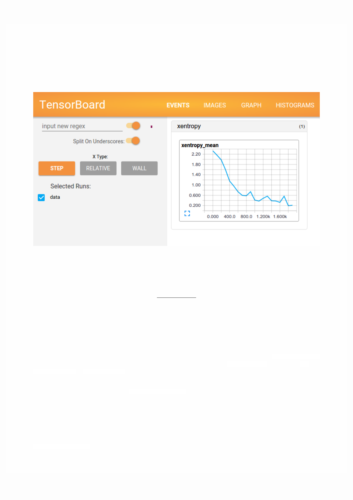
TensorBoard: Visualizing Learning

The computations you'll use TensorFlow for - like training a massive deep neural network - can be complex and confusing. To

make it easier to understand, debug, and optimize TensorFlow programs, we've included a suite of visualization tools called

TensorBoard. You can use TensorBoard to visualize your TensorFlow graph, plot quantitative metrics about the execution of

your graph, and show additional data like images that pass through it. When TensorBoard is fully conﬁgured, it looks like this:

This tutorial is intended to get you started with simple TensorBoard usage. There are other resources available as well! The

TensorBoard's GitHub has a lot more information on TensorBoard usage, including tips & tricks, and debugging information.

Serializing the data

TensorBoard operates by reading TensorFlow events ﬁles, which contain summary data that you can generate when running

TensorFlow. Here's the general lifecycle for summary data within TensorBoard.

First, create the TensorFlow graph that you'd like to collect summary data from, and decide which nodes you would like to

annotate with summary operations.

For example, suppose you are training a convolutional neural network for recognizing MNIST digits. You'd like to record how

the learning rate varies over time, and how the objective function is changing. Collect these by attaching tf.summary.scalar

ops to the nodes that output the learning rate and loss respectively. Then, give each scalar_summary a meaningful tag, like

'learning rate' or 'loss function'.

Perhaps you'd also like to visualize the distributions of activations coming off a particular layer, or the distribution of gradients

or weights. Collect this data by attaching tf.summary.histogram ops to the gradient outputs and to the variable that holds

your weights, respectively.

For details on all of the summary operations available, check out the docs on summary operations.

Operations in TensorFlow don't do anything until you run them, or an op that depends on their output. And the summary

nodes that we've just created are peripheral to your graph: none of the ops you are currently running depend on them. So, to

generate summaries, we need to run all of these summary nodes. Managing them by hand would be tedious, so use

tf.summary.merge_all to combine them into a single op that generates all the summary data.

Then, you can just run the merged summary op, which will generate a serialized Summary protobuf object with all of your

summary data at a given step. Finally, to write this summary data to disk, pass the summary protobuf to a

tf.summary.FileWriter.

The FileWriter takes a logdir in its constructor - this logdir is quite important, it's the directory where all of the events will be

written out. Also, the FileWriter can optionally take a Graph in its constructor. If it receives a Graph object, then TensorBoard

will visualize your graph along with tensor shape information. This will give you a much better sense of what ﬂows through

the graph: see Tensor shape information.

Now that you've modiﬁed your graph and have a FileWriter, you're ready to start running your network! If you want, you

could run the merged summary op every single step, and record a ton of training data. That's likely to be more data than you

need, though. Instead, consider running the merged summary op every n steps.

The code example below is a modiﬁcation of the simple MNIST tutorial, in which we have added some summary ops, and run

them every ten steps. If you run this and then launch tensorboard --logdir=/tmp/tensorflow/mnist, you'll be able to

visualize statistics, such as how the weights or accuracy varied during training. The code below is an excerpt; full source is

here.

def variable_summaries(var):

"""Attach a lot of summaries to a Tensor (for TensorBoard visualization)."""

with tf.name_scope('summaries'):

mean = tf.reduce_mean(var)

tf.summary.scalar('mean', mean)

with tf.name_scope('stddev'):

stddev = tf.sqrt(tf.reduce_mean(tf.square(var - mean)))

tf.summary.scalar('stddev', stddev)

tf.summary.scalar('max', tf.reduce_max(var))

tf.summary.scalar('min', tf.reduce_min(var))

tf.summary.histogram('histogram', var)

def nn_layer(input_tensor, input_dim, output_dim, layer_name, act=tf.nn.relu):

"""Reusable code for making a simple neural net layer.

It does a matrix multiply, bias add, and then uses relu to nonlinearize.

It also sets up name scoping so that the resultant graph is easy to read,

and adds a number of summary ops.

"""

# Adding a name scope ensures logical grouping of the layers in the graph.

with tf.name_scope(layer_name):

# This Variable will hold the state of the weights for the layer

with tf.name_scope('weights'):

weights = weight_variable([input_dim, output_dim])

variable_summaries(weights)

with tf.name_scope('biases'):

biases = bias_variable([output_dim])

variable_summaries(biases)

with tf.name_scope('Wx_plus_b'):

preactivate = tf.matmul(input_tensor, weights) + biases

tf.summary.histogram('pre_activations', preactivate)

activations = act(preactivate, name='activation')

tf.summary.histogram('activations', activations)

return activations

hidden1 = nn_layer(x, 784, 500, 'layer1')

with tf.name_scope('dropout'):

keep_prob = tf.placeholder(tf.float32)

tf.summary.scalar('dropout_keep_probability', keep_prob)

dropped = tf.nn.dropout(hidden1, keep_prob)

# Do not apply softmax activation yet, see below.

y = nn_layer(dropped, 500, 10, 'layer2', act=tf.identity)

with tf.name_scope('cross_entropy'):

# The raw formulation of cross-entropy,

# tf.reduce_mean(-tf.reduce_sum(y_ * tf.log(tf.softmax(y)),

# reduction_indices=[1]))

# can be numerically unstable.

# So here we use tf.losses.sparse_softmax_cross_entropy on the

# raw logit outputs of the nn_layer above.

with tf.name_scope('total'):

cross_entropy = tf.losses.sparse_softmax_cross_entropy(labels=y_, logits=y)

tf.summary.scalar('cross_entropy', cross_entropy)

with tf.name_scope('train'):

train_step = tf.train.AdamOptimizer(FLAGS.learning_rate).minimize(

cross_entropy)

with tf.name_scope('accuracy'):

with tf.name_scope('correct_prediction'):

correct_prediction = tf.equal(tf.argmax(y, 1), tf.argmax(y_, 1))

with tf.name_scope('accuracy'):

accuracy = tf.reduce_mean(tf.cast(correct_prediction, tf.float32))

tf.summary.scalar('accuracy', accuracy)

# Merge all the summaries and write them out to /tmp/mnist_logs (by default)

merged = tf.summary.merge_all()

train_writer = tf.summary.FileWriter(FLAGS.summaries_dir + '/train',

sess.graph)

test_writer = tf.summary.FileWriter(FLAGS.summaries_dir + '/test')

tf.global_variables_initializer().run()

After we've initialized the FileWriters, we have to add summaries to the FileWriters as we train and test the model.

# Train the model, and also write summaries.

# Every 10th step, measure test-set accuracy, and write test summaries

# All other steps, run train_step on training data, & add training summaries

def feed_dict(train):

"""Make a TensorFlow feed_dict: maps data onto Tensor placeholders."""

if train or FLAGS.fake_data:

xs, ys = mnist.train.next_batch(100, fake_data=FLAGS.fake_data)

k = FLAGS.dropout

else:

xs, ys = mnist.test.images, mnist.test.labels

k = 1.0

return {x: xs, y_: ys, keep_prob: k}

for i in range(FLAGS.max_steps):

if i % 10 == 0: # Record summaries and test-set accuracy

summary, acc = sess.run([merged, accuracy], feed_dict=feed_dict(False))

test_writer.add_summary(summary, i)

print('Accuracy at step %s: %s' % (i, acc))

else: # Record train set summaries, and train

summary, _ = sess.run([merged, train_step], feed_dict=feed_dict(True))

train_writer.add_summary(summary, i)

You're now all set to visualize this data using TensorBoard.

Launching TensorBoard

To run TensorBoard, use the following command (alternatively python -m tensorboard.main)

tensorboard --logdir=path/to/log-directory

where logdir points to the directory where the FileWriter serialized its data. If this logdir directory contains subdirectories

which contain serialized data from separate runs, then TensorBoard will visualize the data from all of those runs. Once

TensorBoard is running, navigate your web browser to localhost:6006 to view the TensorBoard.

When looking at TensorBoard, you will see the navigation tabs in the top right corner. Each tab represents a set of serialized

data that can be visualized.

For in depth information on how to use the graph tab to visualize your graph, see TensorBoard: Graph Visualization.

For more usage information on TensorBoard in general, see the TensorBoard's GitHub.

TensorBoard: Graph Visualization

TensorFlow computation graphs are powerful but complicated. The graph visualization can help you understand and debug

them. Here's an example of the visualization at work.

Visualization of a TensorFlow graph.

To see your own graph, run TensorBoard pointing it to the log directory of the job, click on the graph tab on the top pane and

select the appropriate run using the menu at the upper left corner. For in depth information on how to run TensorBoard and

make sure you are logging all the necessary information, see TensorBoard: Visualizing Learning.

Name scoping and nodes

Typical TensorFlow graphs can have many thousands of nodes--far too many to see easily all at once, or even to lay out using

standard graph tools. To simplify, variable names can be scoped and the visualization uses this information to deﬁne a

hierarchy on the nodes in the graph. By default, only the top of this hierarchy is shown. Here is an example that deﬁnes three

operations under the hidden name scope using tf.name_scope:

import tensorflow as tf

with tf.name_scope('hidden') as scope:

a = tf.constant(5, name='alpha')

W = tf.Variable(tf.random_uniform([1, 2], -1.0, 1.0), name='weights')

b = tf.Variable(tf.zeros([1]), name='biases')

This results in the following three op names:

hidden/alpha

hidden/weights

hidden/biases

By default, the visualization will collapse all three into a node labeled hidden. The extra detail isn't lost. You can double-click,

or click on the orange + sign in the top right to expand the node, and then you'll see three subnodes for alpha, weights and

biases.

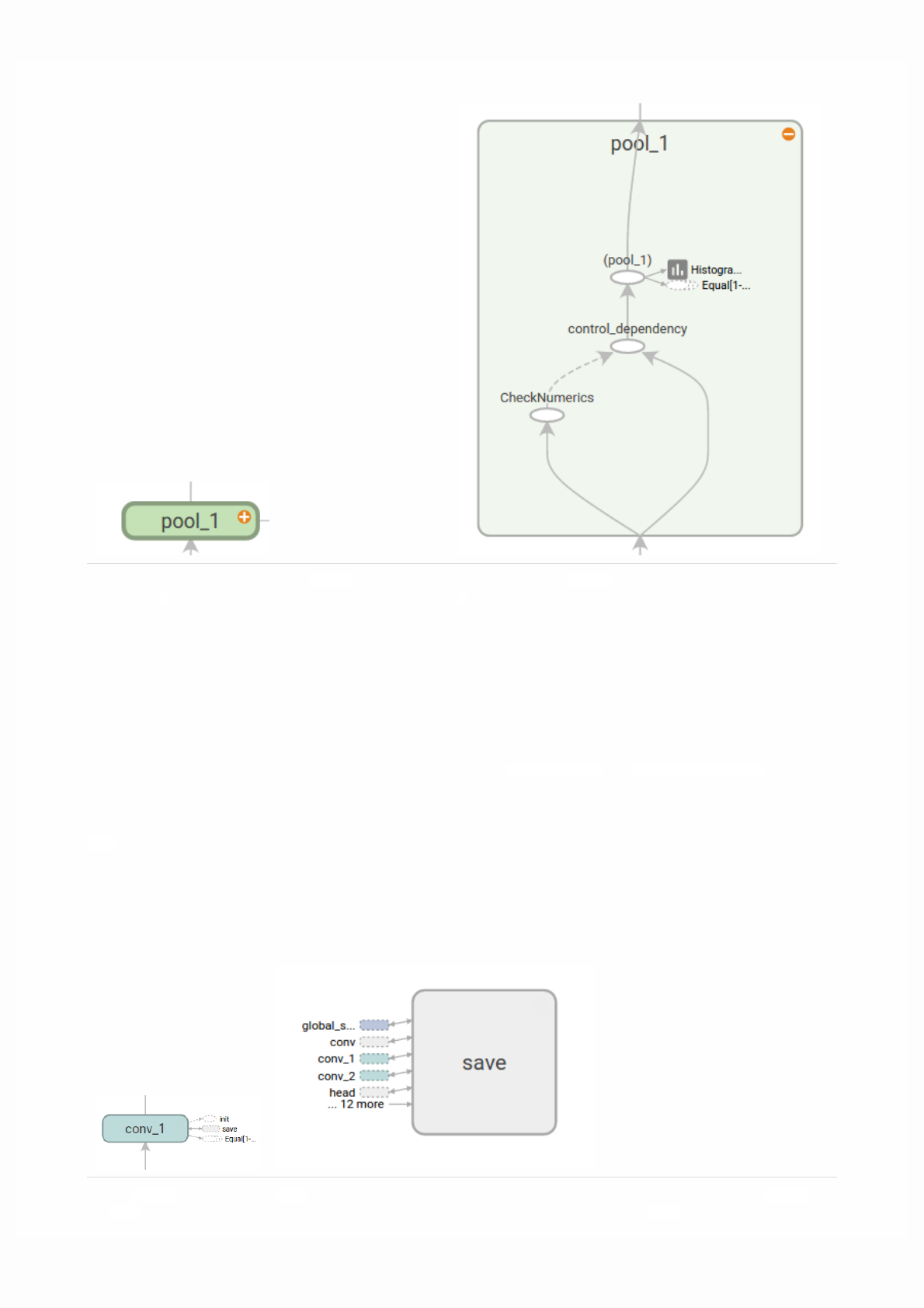
Initial view of top-level name scope pool_1. Clicking on

the orange + button on the top right or double-clicking on

the node itself will expand it.

Expanded view of pool_1 name scope. Clicking on the orange

- button on the top right or double-clicking on the node itself

will collapse the name scope.

Node conv_1 is connected

to save. Note the little

save has a high degree, and will appear as an auxiliary node. The connection with conv_1 is

shown as a node icon on its left. To further reduce clutter, since save has a lot of connections,

Here's a real-life example of a more complicated node in its initial and expanded states.

Grouping nodes by name scopes is critical to making a legible graph. If you're building a model, name scopes give you control

over the resulting visualization. The better your name scopes, the better your visualization.

The ﬁgure above illustrates a second aspect of the visualization. TensorFlow graphs have two kinds of connections: data

dependencies and control dependencies. Data dependencies show the ﬂow of tensors between two ops and are shown as solid

arrows, while control dependencies use dotted lines. In the expanded view (right side of the ﬁgure above) all the connections

are data dependencies with the exception of the dotted line connecting CheckNumerics and control_dependency.

There's a second trick to simplifying the layout. Most TensorFlow graphs have a few nodes with many connections to other

nodes. For example, many nodes might have a control dependency on an initialization step. Drawing all edges between the

init node and its dependencies would create a very cluttered view.

To reduce clutter, the visualization separates out all high-degree nodes to an auxiliary area on the right and doesn't draw lines

to represent their edges. Instead of lines, we draw small node icons to indicate the connections. Separating out the auxiliary

nodes typically doesn't remove critical information since these nodes are usually related to bookkeeping functions. See

Interaction for how to move nodes between the main graph and the auxiliary area.

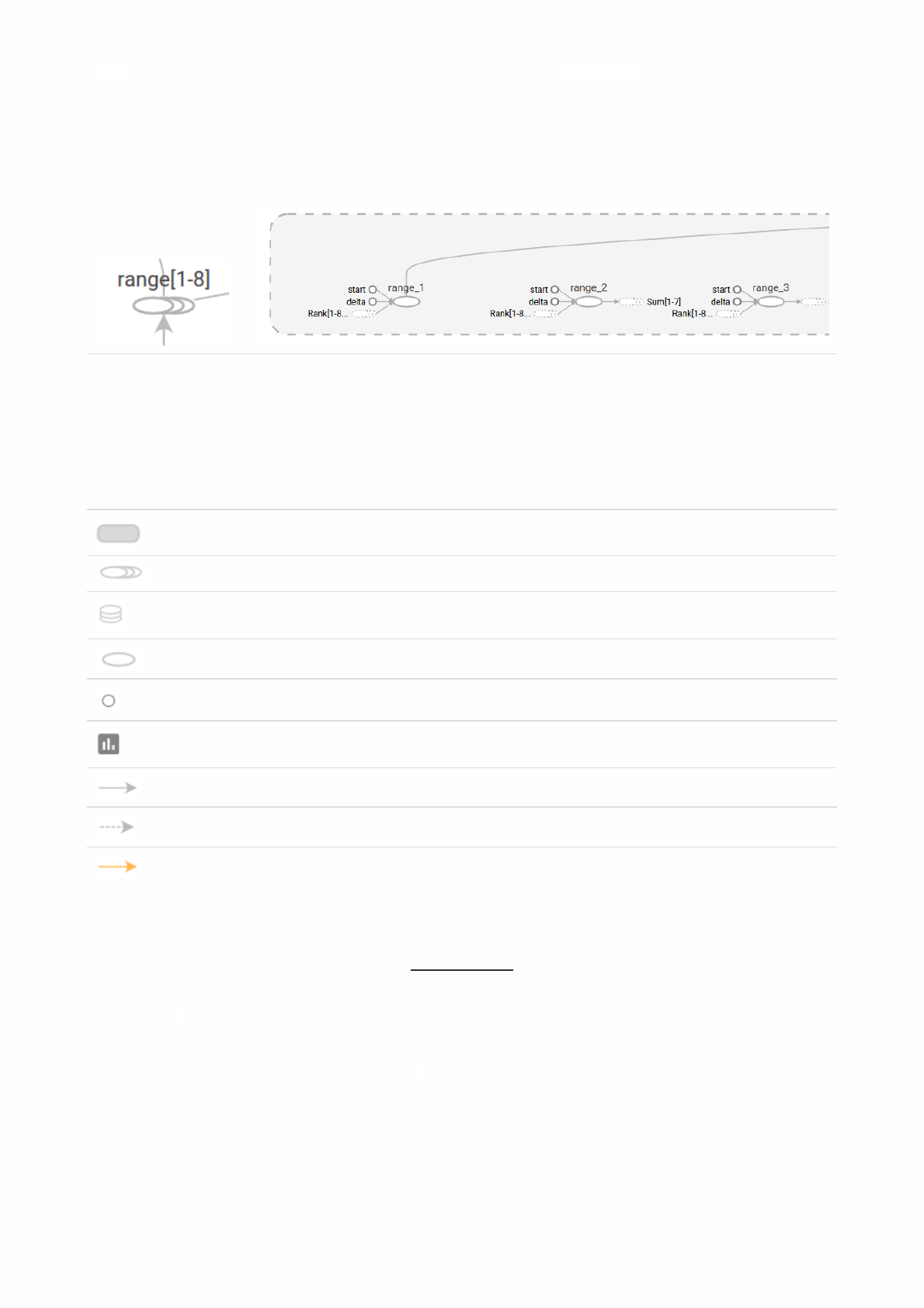
savenode icon on its right. we show the ﬁrst 5 and abbreviate the others as ... 12 more.

A collapsed view of a

node sequence.

A small piece of the expanded view, after double-click.

Symbol Meaning

High-level node representing a name scope. Double-click to expand a high-level node.

Sequence of numbered nodes that are not connected to each other.

Sequence of numbered nodes that are connected to each other.

An individual operation node.

A constant.

A summary node.

Edge showing the data ﬂow between operations.

Edge showing the control dependency between operations.

A reference edge showing that the outgoing operation node can mutate the incoming tensor.

One last structural simpliﬁcation is series collapsing. Sequential motifs--that is, nodes whose names differ by a number at the

end and have isomorphic structures--are collapsed into a single stack of nodes, as shown below. For networks with long

sequences, this greatly simpliﬁes the view. As with hierarchical nodes, double-clicking expands the series. See Interaction for

how to disable/enable series collapsing for a speciﬁc set of nodes.

Finally, as one last aid to legibility, the visualization uses special icons for constants and summary nodes. To summarize, here's

a table of node symbols:

Interaction

Navigate the graph by panning and zooming. Click and drag to pan, and use a scroll gesture to zoom. Double-click on a node,

or click on its + button, to expand a name scope that represents a group of operations. To easily keep track of the current

viewpoint when zooming and panning, there is a minimap in the bottom right corner.

To close an open node, double-click it again or click its - button. You can also click once to select a node. It will turn a darker

color, and details about it and the nodes it connects to will appear in the info card at upper right corner of the visualization.

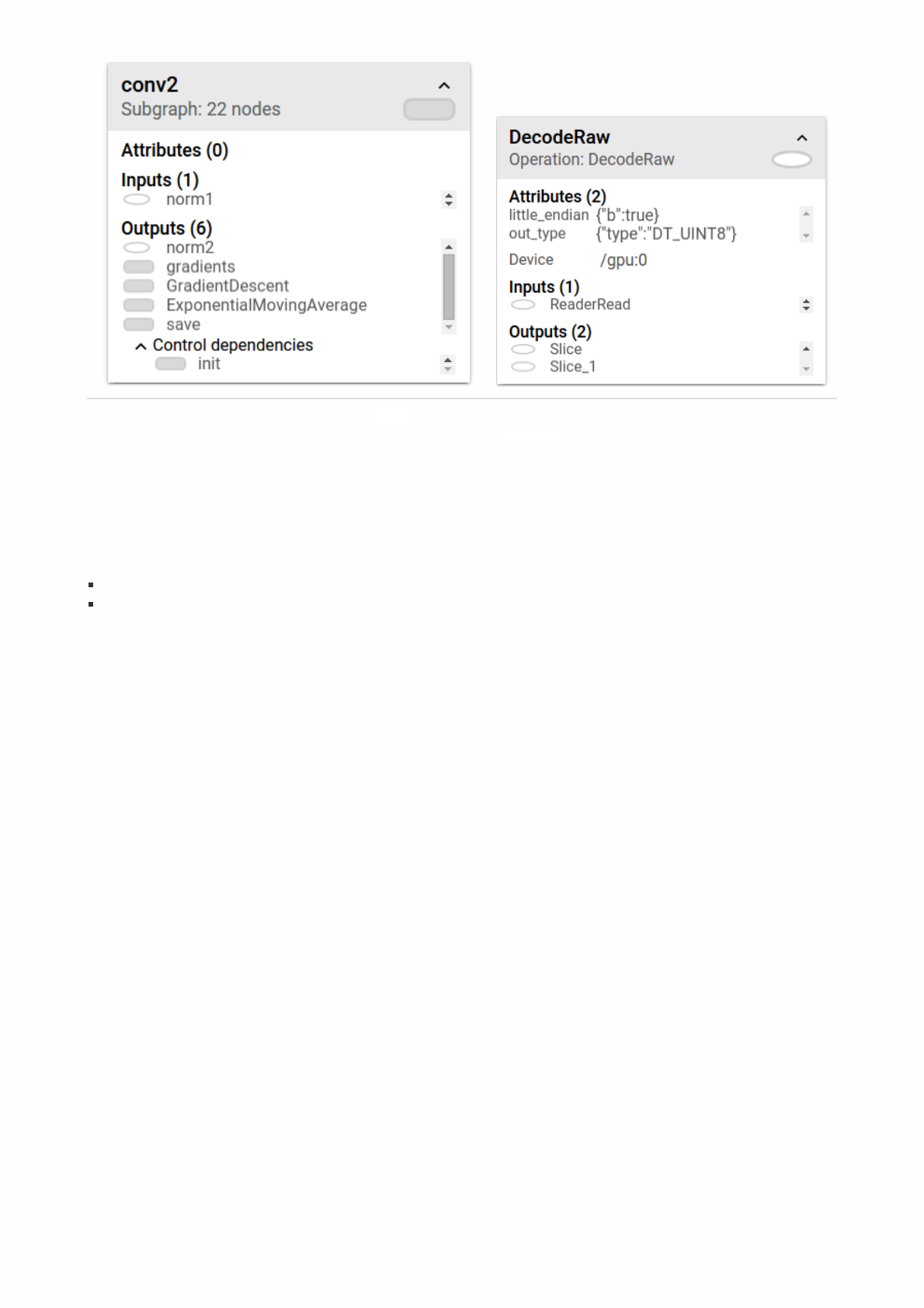
Info card showing detailed information for the conv2 name

scope. The inputs and outputs are combined from the inputs and

outputs of the operation nodes inside the name scope. For name

scopes no attributes are shown.

Info card showing detailed information for the

DecodeRawoperation node. In addition to inputs and

outputs, the card shows the device and the attributes

associated with the current operation.

TensorBoard provides several ways to change the visual layout of the graph. This doesn't change the graph's computational

semantics, but it can bring some clarity to the network's structure. By right clicking on a node or pressing buttons on the

bottom of that node's info card, you can make the following changes to its layout:

Nodes can be moved between the main graph and the auxiliary area.

A series of nodes can be ungrouped so that the nodes in the series do not appear grouped together. Ungrouped series can

likewise be regrouped.

Selection can also be helpful in understanding high-degree nodes. Select any high-degree node, and the corresponding node

icons for its other connections will be selected as well. This makes it easy, for example, to see which nodes are being saved--and

which aren't.

Clicking on a node name in the info card will select it. If necessary, the viewpoint will automatically pan so that the node is

visible.

Finally, you can choose two color schemes for your graph, using the color menu above the legend. The default Structure View

shows structure: when two high-level nodes have the same structure, they appear in the same color of the rainbow. Uniquely

structured nodes are gray. There's a second view, which shows what device the different operations run on. Name scopes are

colored proportionally to the fraction of devices for the operations inside them.

The images below give an illustration for a piece of a real-life graph.

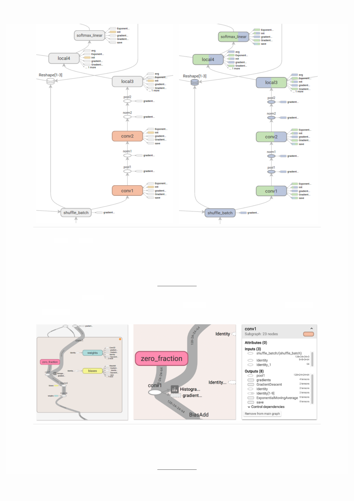
Structure view: The gray nodes have unique structure. The

orange conv1 and conv2 nodes have the same structure,

and analogously for nodes with other colors.

Device view: Name scopes are colored proportionally to the

fraction of devices of the operation nodes inside them. Here,

purple means GPU and the green is CPU.

CIFAR-10 model with tensor shape information.

Tensor shape information

When the serialized GraphDef includes tensor shapes, the graph visualizer labels edges with tensor dimensions, and edge

thickness reﬂects total tensor size. To include tensor shapes in the GraphDef pass the actual graph object (as in sess.graph) to

the FileWriter when serializing the graph. The images below show the CIFAR-10 model with tensor shape information:

Runtime statistics

Often it is useful to collect runtime metadata for a run, such as total memory usage, total compute time, and tensor shapes for

nodes. The code example below is a snippet from the train and test section of a modiﬁcation of the simple MNIST tutorial, in

which we have recorded summaries and runtime statistics. See the Summaries Tutorial for details on how to record summaries.

Full source is here.

# Train the model, and also write summaries.

# Every 10th step, measure test-set accuracy, and write test summaries

# All other steps, run train_step on training data, & add training summaries

def feed_dict(train):

"""Make a TensorFlow feed_dict: maps data onto Tensor placeholders."""

if train or FLAGS.fake_data:

xs, ys = mnist.train.next_batch(100, fake_data=FLAGS.fake_data)

k = FLAGS.dropout

else:

xs, ys = mnist.test.images, mnist.test.labels

k = 1.0

return {x: xs, y_: ys, keep_prob: k}

for i in range(FLAGS.max_steps):

if i % 10 == 0: # Record summaries and test-set accuracy

summary, acc = sess.run([merged, accuracy], feed_dict=feed_dict(False))

test_writer.add_summary(summary, i)

print('Accuracy at step %s: %s' % (i, acc))

else: # Record train set summaries, and train

if i % 100 == 99: # Record execution stats

run_options = tf.RunOptions(trace_level=tf.RunOptions.FULL_TRACE)

run_metadata = tf.RunMetadata()

summary, _ = sess.run([merged, train_step],

feed_dict=feed_dict(True),

options=run_options,

run_metadata=run_metadata)

train_writer.add_run_metadata(run_metadata, 'step%d' % i)

train_writer.add_summary(summary, i)

print('Adding run metadata for', i)

else: # Record a summary

summary, _ = sess.run([merged, train_step], feed_dict=feed_dict(True))

train_writer.add_summary(summary, i)

This code will emit runtime statistics for every 100th step starting at step99.

When you launch tensorboard and go to the Graph tab, you will now see options under "Session runs" which correspond to the

steps where run metadata was added. Selecting one of these runs will show you the snapshot of the network at that step,

fading out unused nodes. In the controls on the left hand side, you will be able to color the nodes by total memory or total

compute time. Additionally, clicking on a node will display the exact total memory, compute time, and tensor output sizes.

Programmers Guide

Navigation menu

Versions of this User Manual:

Views

Navigation