Python Multimedia:Beginner's Guide Multimedia Beginner's (2010)
User Manual: Pdf
Open the PDF directly: View PDF ![]() .
.
Page Count: 292 [warning: Documents this large are best viewed by clicking the View PDF Link!]
- Cover
- Copyright
- Credits
- About the Author
- About the Reviewers
- Table of Contents
- Preface
- Chapter 1: Python and Multimedia
- Chapter 2: Working with Images
- Installation prerequisites
- Reading and writing images
- Time for action – image file converter
- Time for action – creating a new image containing some text
- Time for action – reading images from archives
- Basic image manipulations
- Time for action – resizing
- Time for action – rotating
- Time for action – flipping
- Time for action – capture screenshots at intervals
- Time for action – cropping an image
- Time for action – pasting: mirror the smiley face!
- Project: Thumbnail Maker
- Time for action – play with Thumbnail Maker application
- Time for action – generating the UI code
- Time for action – connecting the widgets
- Time for action – developing image processing code
- Summary
- Chapter 3: Enhancing Images
- Installation and download prerequisites
- Adjusting brightness and contrast
- Time for action—adjusting brightness and contrast
- Tweaking colors
- Time for action – swap colors within an image!
- Time for action – change the color of a flower
- Blending
- Time for action – blending two images
- Creating transparent images
- Time for action – create transparency
- Making composites with image mask
- Time for action – making composites with image mask
- Project: Watermark Maker Tool
- Time for action – Watermark Maker Tool
- Applying image filters
- Time for action – smoothing an image
- Time for action – detecting and enhancing edges
- Time for action – embossing
- Adding a border
- Time for action – enclosing a picture in a photoframe
- Summary
- Chapter 4: Fun with Animations
- Installation prerequisites
- A primer on Pyglet
- Animations with Pyglet
- Time for action – viewing an existing animation
- Time for action – animation using a sequence of images
- Time for action – bouncing ball animation
- Time for action – a simple bowling animation
- Time for action – raindrops animation
- Project: drive on a rainy day!
- Time for action – drive on a rainy day!
- Summary
- Chapter 5: Working with Audios
- Installation prerequisites
- A primer on GStreamer
- Playing music
- Time for action – playing an audio: method 1
- Time for action – playing an audio: method 2
- Converting audio file format
- Time for action – audio file format converter
- Extracting part of an audio
- Time for action – MP3 cutter!
- Recording
- Time for action – recording
- Summary
- Chapter 6: Audio Controls and Effects
- Controlling playback
- Time for action – pause and resume a playing audio stream
- Time for action – MP3 cutter from basic principles
- Adjusting volume
- Time for action – adjusting volume
- Audio effects
- Time for action – fading effects
- Time for action – adding echo effect
- Project: combining audio clips
- Time for action – creating custom audio by combining clips
- Audio mixing
- Time for action – mixing audio tracks
- Visualizing an audio track
- Time for action – audio visualizer
- Summary
- Chapter 7: Working with Videos
- Installation prerequisites
- Playing a video
- Time for action – video player!
- Video format conversion
- Time for action – video format converter
- Video manipulations and effects
- Time for action – resize a video
- Time for action – crop a video
- Adding text and time on a video stream
- Time for action – overlay text on a video track
- Separating audio and video tracks
- Time for action – audio and video tracks
- Mixing audio and video tracks
- Time for action – audio/video track mixer
- Saving video frames as images
- Time for action – saving video frames as images
- Summary
- Chapter 8: GUI-based Media Players Using QT Phonon
- Installation prerequisites
- Introduction to QT Phonon
- Project: GUI-based music player
- Time for action – generating the UI code
- Time for action – connecting the widgets
- Time for action – developing the audio player code
- Project: GUI-based video player
- Time for action – generating the UI code
- Time for action – developing the video player code
- Summary
- Index

Python Multimedia
Beginner's Guide
Learn how to develop mulmedia applicaons using Python
with this praccal step-by-step guide
Ninad Sathaye
BIRMINGHAM - MUMBAI
x
x

Python Multimedia
Beginner's Guide
Copyright © 2010 Packt Publishing
All rights reserved. No part of this book may be reproduced, stored in a retrieval system,
or transmied in any form or by any means, without the prior wrien permission of the
publisher, except in the case of brief quotaons embedded in crical arcles or reviews.
Every eort has been made in the preparaon of this book to ensure the accuracy of the
informaon presented. However, the informaon contained in this book is sold without
warranty, either express or implied. Neither the author, nor Packt Publishing, and its dealers
and distributors will be held liable for any damages caused or alleged to be caused directly or
indirectly by this book.
Packt Publishing has endeavored to provide trademark informaon about all of the
companies and products menoned in this book by the appropriate use of capitals.
However, Packt Publishing cannot guarantee the accuracy of this informaon.
First published: August 2010
Producon Reference: 1060810
Published by Packt Publishing Ltd.
32 Lincoln Road
Olton
Birmingham, B27 6PA, UK.
ISBN 978-1-849510-16-5
www.packtpub.com
Cover Image by Ed Maclean (edmaclean@gmail.com)
x
x

Credits
Author
Ninad Sathaye
Reviewers
Maurice HT Ling
Daniel Waterworth
Sivan Greenberg
Acquision Editor
Steven Wilding
Development Editor
Eleanor Duy
Technical Editor
Charumathi Sankaran
Indexers
Hemangini Bari
Tejal Daruwale
Editorial Team Leader
Aanchal Kumar
Project Team Leader
Priya Mukherji
Project Coordinator
Prasad Rai
Proofreader
Lynda Sliwoski
Graphics
Geetanjali Sawant
Producon Coordinators
Shantanu Zagade
Aparna Bhagat
Cover Work
Aparna Bhagat
x
x

About the Author
Ninad Sathaye (ninad.consult@gmail.com) has more than six years of experience in
soware design and development. He is currently working at IBM, India. Prior to working for
IBM, he was a Systems Programmer at Nanorex Inc. based in Michigan, U.S.A. At Nanorex,
he was involved in the development of an open source, interacve 3D CAD soware, wrien
in Python and C. This is where he developed passion for the Python programming language.
Besides programming, his favorite hobbies are reading and traveling.
Ninad holds a Master of Science degree in Mechanical Engineering from Kansas State
University, U.S.A.
I would like to thank everyone at Packt Publishing, especially, Eleanor Duy,
Steven Wilding, Charu Sankaran, and Prasad Rai for their co-operaon.
This book wouldn't have been possible without your help. I also want to
thank all the technical reviewers of the book for their valuable suggesons.
I wish to express my sincere thanks and appreciaon to Rahul Nayak, my
colleague, who provided many professional quality photographs for this
book. I owe a special thanks to Mark Sims and Bruce Smith, my former
colleagues, for introducing me to the amusing world of Python. Finally,
this book wouldn't have been possible without the encouragement and
support of my whole family. I owe my loving thanks to my wife, Ara, for
providing valuable feedback. She also happens to be the photographer of
several of the pictures used throughout this book.
x
x

About the Reviewers
Maurice HT Ling completed his Ph.D. in Bioinformacs and B.Sc (Hons) in Molecular and
Cell Biology, where he worked on microarray analysis and text mining for protein-protein
interacons. He is currently an Honorary Fellow at The University of Melbourne and
a Lecturer at Singapore Polytechnic where he lectures on microbiology and
computaonal biology.
Maurice holds several Chief Editorships including The Python Papers, iConcept Journal
of Computaonal and Mathemacal Biology, and Methods and Cases in Computaonal,
Mathemacal, and Stascal Biology. In his free me, Maurice likes to train in the gym,
read, and enjoy a good cup of coee. He is also a Senior Fellow of the Internaonal Fitness
Associaon, U.S.A.
Daniel Waterworth is a Python fanac who can oen be found behind his keyboard. He is
always beavering away on a new project having learned to program from a young age. He is a
keen blogger and his ideas can be found at http://active-thought.com.
Sivan Greenberg is a Forum Nokia Champion, with almost ten years of mul-disciplinary
IT experience and a sharp eye for quality. He started with open source technologies and
the Debian project back in 2002. Joining Ubuntu development two years later, Sivan also
contributed to various other open source projects, such as Plone and Nokia's Maemo.
He has experience with quality assurance, applicaon and web development, UNIX system
administraon (including some rather exoc IBM plaorms), and GUI programming and
documentaon. He's been using Python for all of his development needs for the last ve
years. He is currently involved with Nokia's MeeGo project and works with CouchDB and
Python in his day job for a living.
I thank my unique and amazing family, specically my Dad Eric for igning
the spark of curiosity from day zero.
x
x

x
x

To my daughter, Anvita
x
x

x
x

Table of Contents
Preface 1
Chapter 1: Python and Mulmedia 7
Mulmedia 8
Mulmedia processing 8
Image processing 8
Audio and video processing 10
Compression 10
Mixing 11
Eding 11
Animaons 11
Built-in mulmedia support 12
winsound 12
audioop 12
wave 13
External mulmedia libraries and frameworks 13
Python Imaging Library 13
PyMedia 13
GStreamer 13
Pyglet 14
PyGame 14
Sprite 14
Display 14
Surface 14
Draw 14
Event 15
Image 15
Music 15
Time for acon – a simple applicaon using PyGame 15
QT Phonon 18
Other mulmedia libraries 19
x
x

Table of Contents
[ ii ]
Snack Sound Toolkit 19
PyAudiere 20
Summary 20
Chapter 2: Working with Images 21
Installaon prerequisites 21
Python 21
Windows plaorm 22
Other plaorms 22
Python Imaging Library (PIL) 22
Windows plaorm 22
Other plaorms 22
PyQt4 23
Windows plaorm 23
Other plaorms 24
Summary of installaon prerequisites 24
Reading and wring images 25
Time for acon – image le converter 25
Creang an image from scratch 28
Time for acon – creang a new image containing some text 28
Reading images from archive 29
Time for acon – reading images from archives 29
Basic image manipulaons 30
Resizing 30
Time for acon – resizing 30
Rotang 33
Time for acon – rotang 34
Flipping 35
Time for acon – ipping 35
Capturing screenshots 36
Time for acon – capture screenshots at intervals 36
Cropping 39
Time for acon – cropping an image 39
Pasng 40
Time for acon – pasng: mirror the smiley face! 40
Project: Thumbnail Maker 42
Time for acon – play with Thumbnail Maker applicaon 43
Generang the UI code 45
Time for acon – generang the UI code 45
Connecng the widgets 47
Time for acon – connecng the widgets 48
Developing the image processing code 49
x
x

Table of Contents
[ iii ]
Time for acon – developing image processing code 49
Summary 53
Chapter 3: Enhancing Images 55
Installaon and download prerequisites 56
Adjusng brightness and contrast 56
Time for acon – adjusng brightness and contrast 56
Tweaking colors 59
Time for acon – swap colors within an image! 59
Changing individual image band 61
Time for acon – change the color of a ower 61
Gray scale images 63
Cook up negaves 64
Blending 65
Time for acon – blending two images 65
Creang transparent images 68
Time for acon – create transparency 68
Making composites with image mask 70
Time for acon – making composites with image mask 71
Project: Watermark Maker Tool 72
Time for acon – Watermark Maker Tool 73
Applying image lters 81
Smoothing 82
Time for acon – smoothing an image 82
Sharpening 84
Blurring 84
Edge detecon and enhancements 85
Time for acon – detecng and enhancing edges 85
Embossing 87
Time for acon – embossing 87
Adding a border 88
Time for acon – enclosing a picture in a photoframe 89
Summary 90
Chapter 4: Fun with Animaons 91
Installaon prerequisites 92
Pyglet 92
Windows plaorm 92
Other plaorms 92
Summary of installaon prerequisites 93
Tesng the installaon 93
A primer on Pyglet 94
x
x

Table of Contents
[ iv ]
Important components 94
Window 94
Image 95
Sprite 95
Animaon 95
AnimaonFrame 95
Clock 95
Displaying an image 96
Mouse and keyboard controls 97
Adding sound eects 97
Animaons with Pyglet 97
Viewing an exisng animaon 97
Time for acon – viewing an exisng animaon 98
Animaon using a sequence of images 100
Time for acon – animaon using a sequence of images 100
Single image animaon 102
Time for acon – bouncing ball animaon 102
Project: a simple bowling animaon 108
Time for acon – a simple bowling animaon 108
Animaons using dierent image regions 113
Time for acon – raindrops animaon 114
Project: drive on a rainy day! 117
Time for acon – drive on a rainy day! 118
Summary 122
Chapter 5: Working with Audios 123
Installaon prerequisites 123
GStreamer 124
Windows plaorm 124
Other plaorms 125
PyGobject 125
Windows plaorm 125
Other plaorms 125
Summary of installaon prerequisites 126
Tesng the installaon 127
A primer on GStreamer 127
gst-inspect and gst-launch 128
Elements and pipeline 128
Plugins 129
Bins 129
Pads 130
Dynamic pads 130
Ghost pads 131
Caps 131
x
x

Table of Contents
[ v ]
Bus 131
Playbin/Playbin2 131
Playing music 132
Time for acon – playing an audio: method 1 133
Building a pipeline from elements 137
Time for acon – playing an audio: method 2 138
Playing an audio from a website 141
Converng audio le format 142
Time for acon – audio le format converter 142
Extracng part of an audio 150
The Gnonlin plugin 151
Time for acon – MP3 cuer! 152
Recording 156
Time for acon – recording 157
Summary 160
Chapter 6: Audio Controls and Eects 161
Controlling playback 161
Play 162
Pause/resume 162
Time for acon – pause and resume a playing audio stream 162
Stop 165
Fast-forward/rewind 166
Project: extract audio using playback controls 166
Time for acon – MP3 cuer from basic principles 167
Adjusng volume 173
Time for acon – adjusng volume 173
Audio eects 175
Fading eects 175
Time for acon – fading eects 176
Echo echo echo... 179
Time for acon – adding echo eect 179
Panning/panorama 182
Project: combining audio clips 183
Media 'meline' explained 184
Time for acon – creang custom audio by combining clips 185
Audio mixing 194
Time for acon – mixing audio tracks 194
Visualizing an audio track 196
Time for acon – audio visualizer 196
Summary 199
x
x

Table of Contents
[ vi ]
Chapter 7: Working with Videos 201
Installaon prerequisites 202
Playing a video 203
Time for acon – video player! 203
Playing video using 'playbin' 208
Video format conversion 209
Time for acon – video format converter 209
Video manipulaons and eects 215
Resizing 215
Time for acon – resize a video 216
Cropping 217
Time for acon – crop a video 218
Adjusng brightness and contrast 219
Creang a gray scale video 220
Adding text and me on a video stream 220
Time for acon – overlay text on a video track 220
Separang audio and video tracks 223
Time for acon – audio and video tracks 223
Mixing audio and video tracks 226
Time for acon – audio/video track mixer 226
Saving video frames as images 230
Time for acon – saving video frames as images 230
Summary 235
Chapter 8: GUI-based Media Players Using QT Phonon 237
Installaon prerequisites 238
PyQt4 238
Summary of installaon prerequisites 238
Introducon to QT Phonon 238
Main components 239
Media graph 239
Media object 239
Sink 239
Path 239
Eects 239
Backends 239
Modules 240
MediaNode 240
MediaSource 240
MediaObject 240
Path 240
AudioOutput 241
Eect 241
VideoPlayer 241
x
x

Table of Contents
[ vii ]
SeekSlider 241
volumeSlider 241
Project: GUI-based music player 241
GUI elements in the music player 242
Generang the UI code 243
Time for acon – generang the UI code 243
Connecng the widgets 247
Time for acon – connecng the widgets 247
Developing the audio player code 249
Time for acon – developing the audio player code 250
Project: GUI-based video player 257
Generang the UI code 258
Time for acon – generang the UI code 258
Connecng the widgets 260
Developing the video player code 261
Time for acon – developing the video player code 261
Summary 264
Index 265
x
x

x
x

Preface
Mulmedia applicaons are used in a broad spectrum of elds. Wring applicaons that
work with images, videos, and other sensory eects is great. Not every applicaon gets
to make full use of audio/visual eects, but a certain amount of mulmedia makes any
applicaon very appealing.
This book is all about mulmedia processing using Python. This step by step guide gives
you a hands-on experience with developing excing mulmedia applicaons. You will build
applicaons for processing images, creang 2D animaons and processing audio and video.
There are numerous mulmedia libraries for which Python bindings are available. These
libraries enable working with dierent kinds of media, such as images, audio, video, games,
and so on. This book introduces the reader to some of these (open source) libraries through
several implausibly excing projects. Popular mulmedia frameworks and libraries, such
as GStreamer, Pyglet, QT Phonon, and Python Imaging library are used to develop various
mulmedia applicaons.
What this book covers
Chapter 1, Python and Mulmedia teaches you a few things about popular mulmedia
frameworks for mulmedia processing using Python and shows you how to develop a
simple interacve applicaon using PyGame.
Chapter 2, Working with Images explains basic image conversion and manipulaon
techniques using the Python Imaging Library. With the help of several examples and code
snippets, we will perform some basic manipulaons on the image, such as pasng an image
on to another, resizing, rotang/ipping, cropping, and so on. We will write tools to capture
a screenshot and convert image les between dierent formats. The chapter ends with
an excing project where we develop an image processing applicaon with a graphical
user interface.
x
x

Preface
[ 2 ]
Chapter 3, Enhancing Images describes how to add special eects to an image using Python
Imaging Library. You will learn techniques to enhance digital images using image lters, for
example, reducing 'noise' from a picture, smoothing and sharpening images, embossing, and
so on. The chapter will cover topics such as selecvely changing the colors within an image.
We will develop some exing ulies for blending images together, adding transparency
eects, and creang watermarks.
Chapter 4, Fun with Animaons introduces you to the fundamentals of developing animaons
using Python and Pyglet mulmedia applicaon development frameworks. We will work
on some excing projects such as animang a fun car out for a ride in a thunderstorm, a
'bowling animaon' with keyboard controls, and so on.
Chapter 5, Working with Audios teaches you how to get to grips with the primer on
GStreamer mulmedia framework and use this API for audio and video processing. In this
chapter, we will develop some simple audio processing tools for 'everyday use'. We will
develop tools such as a command-line audio player, a le format converter, an MP3 cuer
and audio recorder.
Chapter 6, Audio Controls and Eects describes how to develop tools for adding audio eects,
mixing audio tracks, creang custom music tracks, visualizing an audio track, and so on.
Chapter 7, Working with Videos explains the fundamentals of video processing. This
chapter will cover topics such as converng video between dierent video formats, mixing
or separang audio and video tracks, saving one or more video frames as sll images,
performing basic video manipulaons such as cropping, resizing, adjusng brightness,
and so on.
Chapter 8, GUI-based Media Players using QT Phonon takes you through the fundamental
components of the QT Phonon framework. We will use QT Phonon to develop audio and
video players using a graphical user interface.
Who this book is for
Python developers who want to dip their toes into working with images, animaons, and
audio and video processing using Python.
Conventions
In this book, you will nd several headings appearing frequently.
To give clear instrucons of how to complete a procedure or task, we use:
x
x

Preface
[ 3 ]
Time for action – heading
1. Acon 1
2. Acon 2
3. Acon 3
Instrucons oen need some extra explanaon so that they make sense, so they are
followed with:
What just happened?
This heading explains the working of tasks or instrucons that you have just completed.
You will also nd some other learning aids in the book, including:
Pop quiz – heading
These are short mulple choice quesons intended to help you test your own understanding.
Have a go hero – heading
These set praccal challenges and give you ideas for experimenng with what you
have learned.
You will also nd a number of styles of text that disnguish between dierent kinds of
informaon. Here are some examples of these styles, and an explanaon of their meaning.
Code words in text are shown as follows: "The diconary self.addedEffects keeps track
of all the audio."
A block of code is set as follows:
1 def __init__(self):
2 self.constructPipeline()
3 self.is_playing = False
4 self.connectSignals()
When we wish to draw your aenon to a parcular part of a code block, the relevant lines
or items are set in bold:
1 def constructPipeline(self):
2 self.pipeline = gst.Pipeline()
3 self.filesrc = gst.element_factory_make(
4 "gnlfilesource")
x
x
Preface
[ 4 ]
Any command-line input or output is wrien as follows:
>>>import pygst
New terms and important words are shown in bold. Words that you see on the screen, in
menus or dialog boxes for example, appear in the text like this: "You will need to tweak the
Eects menu UI and make some other changes in the code to keep track of the added eects."
Warnings or important notes appear in a box like this.
Tips and tricks appear like this.
Reader feedback
Feedback from our readers is always welcome. Let us know what you think about this
book—what you liked or may have disliked. Reader feedback is important for us to
develop tles that you really get the most out of.
To send us general feedback, simply send an e-mail to feedback@packtpub.com, and
menon the book tle via the subject of your message.
If there is a book that you need and would like to see us publish, please send us a note in the
SUGGEST A TITLE form on www.packtpub.com or e-mail suggest@packtpub.com.
If there is a topic that you have experse in and you are interested in either wring or
contribung to a book, see our author guide on www.packtpub.com/authors.
Customer support
Now that you are the proud owner of a Packt book, we have a number of things to help you
to get the most from your purchase.
Downloading the example code for this book
You can download the example code les for all Packt books you have purchased
from your account at http://www.PacktPub.com. If you purchased this
book elsewhere, you can visit http://www.PacktPub.com/support and
register to have the les e-mailed directly to you.
x
x

Preface
[ 5 ]
Errata
Although we have taken every care to ensure the accuracy of our content, mistakes do happen.
If you nd a mistake in one of our books—maybe a mistake in the text or the code—we
would be grateful if you would report this to us. By doing so, you can save other readers from
frustraon and help us improve subsequent versions of this book. If you nd any errata, please
report them by vising http://www.packtpub.com/support, selecng your book, clicking
on the errata submission form link, and entering the details of your errata. Once your errata
are veried, your submission will be accepted and the errata will be uploaded on our website,
or added to any list of exisng errata, under the Errata secon of that tle. Any exisng errata
can be viewed by selecng your tle from http://www.packtpub.com/support.
Piracy
Piracy of copyright material on the Internet is an ongoing problem across all media. At Packt,
we take the protecon of our copyright and licenses very seriously. If you come across any
illegal copies of our works, in any form, on the Internet, please provide us with the locaon
address or website name immediately so that we can pursue a remedy.
Please contact us at copyright@packtpub.com with a link to the suspected pirated material.
We appreciate your help in protecng our authors, and our ability to bring you
valuable content.
Questions
You can contact us at questions@packtpub.com if you are having a problem with any
aspect of the book, and we will do our best to address it.
x
x

x
x

1
Python and Multimedia
Since its concepon in 1989, Python has gained increasing popularity as a
general purpose programming language. It is a high-level, object-oriented
language with a comprehensive standard library. The language features
such as automac memory management and easy readability have aracted
the aenon of a wide range of developer communies. Typically, one can
develop complex applicaons in Python very quickly compared to some other
languages. It is used in several open source as well as commercial scienc
modeling and visualizaon soware packages. It has already gained popularity
in industries such as animaon and game development studios, where the focus
is on mulmedia applicaon development. This book is all about mulmedia
processing using Python.
In this introductory chapter, we shall:
Learn about mulmedia and mulmedia processing
Discuss a few popular mulmedia frameworks for mulmedia processing
using Python
Develop a simple interacve applicaon using PyGame
So let's get on with it.
x
x

Python and Mulmedia
[ 8 ]
Multimedia
We use mulmedia applicaons in our everyday lives. It is mulmedia that we deal
with while watching a movie or listening to a song or playing a video game. Mulmedia
applicaons are used in a broad spectrum of elds. Mulmedia has a crucial role to play
in the adversing and entertainment industry. One of the most common usages is to add
audio and video eects to a movie. Educaonal soware packages such as a ight or a drive
simulator use mulmedia to teach various topics in an interacve way.
So what really is mulmedia? In general, any applicaon that makes use of dierent sources
of digital media is termed as a digital mulmedia. A video, for instance, is a combinaon
of dierent sources or contents. The contents can be an audio track, a video track, and a
subtle track. When such video is played, all these media sources are presented together
to accomplish the desired eect.
A mulchannel audio can have a background music track and a lyrics track. It may even
include various audio eects. An animaon can be created by using a bunch of digital images
that are displayed quickly one aer the other. These are dierent examples of mulmedia.
In the case of computer or video games, another dimension is added to the applicaon,
the user interacon. It is oen termed as an interacve type of mulmedia. Here, the users
determine the way the mulmedia contents are presented. With the help of devices such as
keyboard, mouse, trackball, joysck, and so on, the users can interacvely control the game.
Multimedia processing
We discussed some of the applicaon domains where mulmedia is extensively used.
The focus of this book will be on mulmedia processing, using which various mulmedia
applicaons will be developed.
Image processing
Aer taking a snap with a digital camera, we oen tweak the original digital image for
various reasons. One of the most common reasons is to remove blemishes from the image,
such as removing 'red-eye' or increasing the brightness level if the picture was taken in
insucient light, and so on. Another reason for doing so is to add special eects that
give a pleasing appearance to the image. For example, making a family picture black and
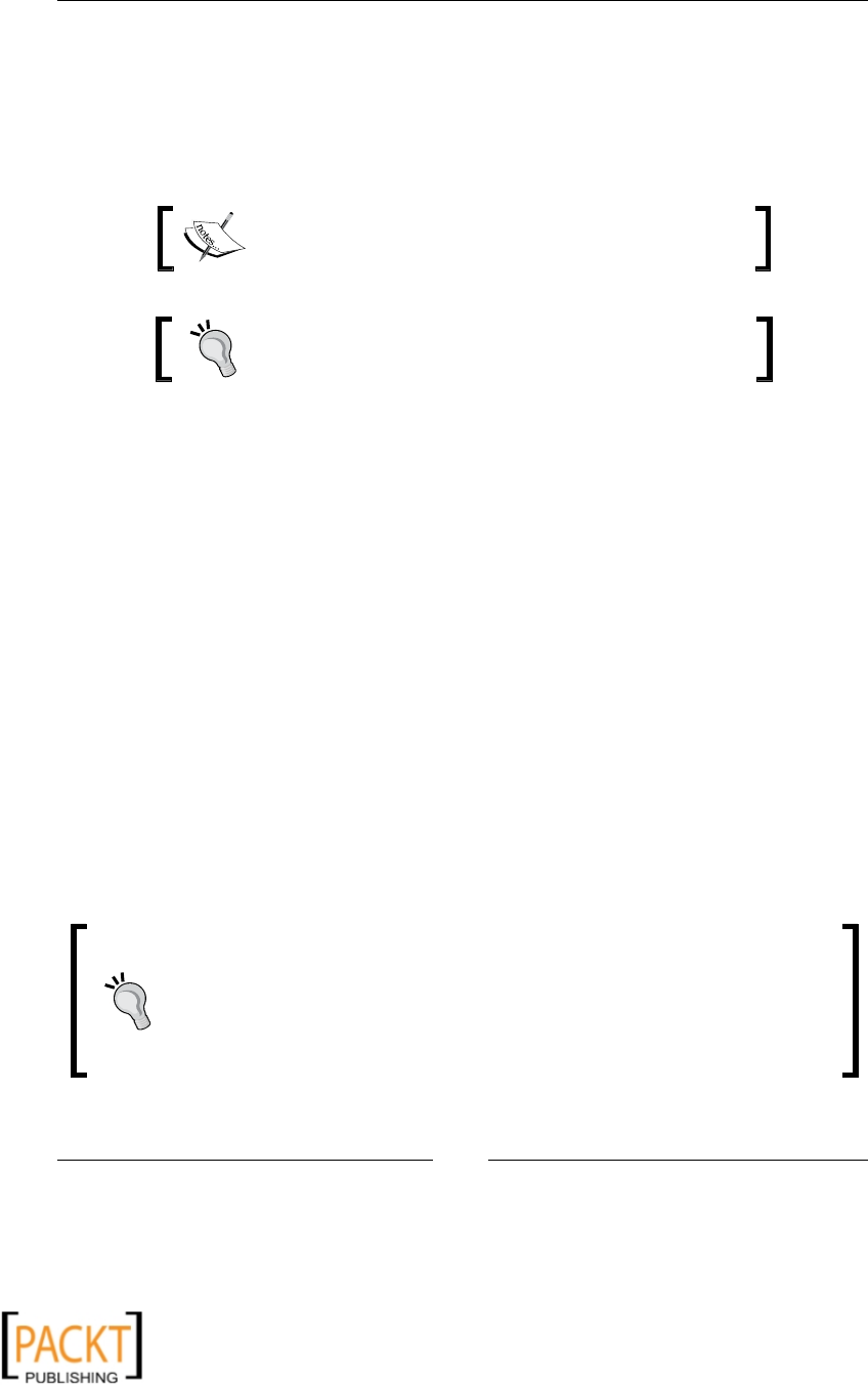
white and digitally adding a frame around the picture gives it a nostalgic eect. The next
illustraon shows an image before and aer the enhancement. Somemes, the original
image is modied just to make you understand important informaon presented by the
image. Suppose the picture represents a complicated assembly of components. One can add
special eects to the image so that only edges in the picture are shown as highlighted. This
x
x
Chapter 1
[ 9 ]
informaon can then be used to detect, for instance, interference between the components.
Thus, we digitally process the image further unl we get the desired output image.
An example where a border is added around an image to change its appearance is as follows:
Digital image processing can be viewed as an applicaon of various algorithms/lters on
the image data. One of the examples is an image smoothing lter. Image smoothing means
reducing the noise from the image. The random changes in brightness and color levels within
the image data are typically referred to as image noise. The smoothing algorithms modify
the input image data so that this noise is reduced in the resultant image.
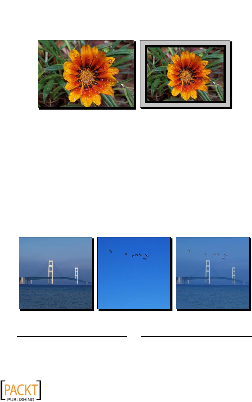
Another commonly performed image processing operaon is blending. As the name
suggests, blending means mixing two compable images to create a new image. Typically,
the data of the two input images is interpolated using a constant value of alpha to produce
a nal image. The next illustraon shows the two input images and the resultant image
aer blending. In the coming chapters we will learn several of such digital image
processing techniques.
The pictures of the bridge and the ying birds are taken at dierent locaons. Using image
processing techniques these two images can be blended together so that they appear as a
single picture:
x
x
Python and Mulmedia
[ 10 ]
Audio and video processing
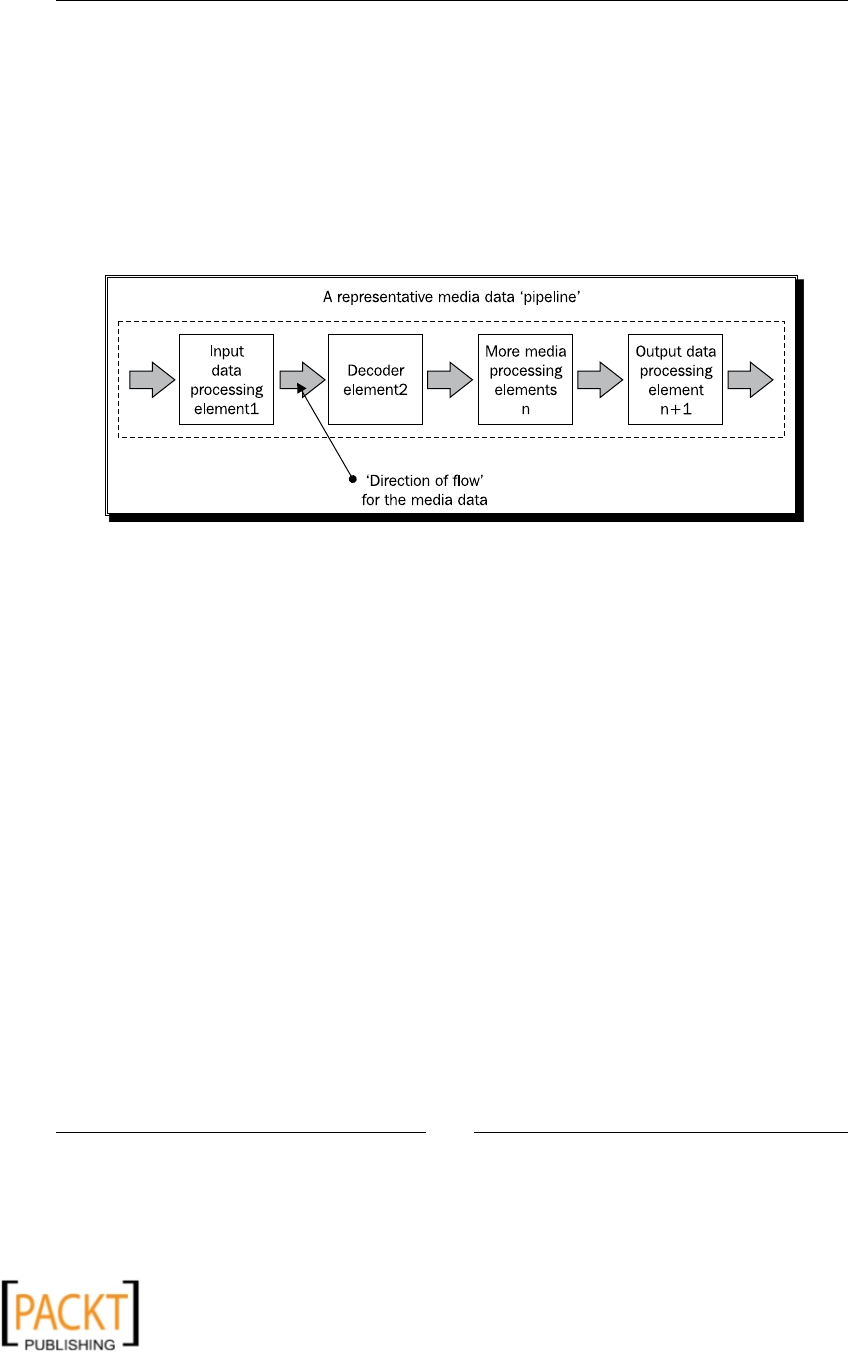
When you are listening to music on your computer, your music player is doing several things
in the background. It processes the digital media data so that it can be transformed into a
playable format that an output media device, such as an audio speaker, requires. The media
data ows through a number of interconnected media handling components, before it
reaches a media output device or a media le to which it is wrien. This is shown in the
next illustraon.
The following image shows a media data processing pipeline:
Audio and video processing encompasses a number of things. Some of them are briey
discussed in this secon. In this book, we will learn various audio-video processing
techniques using Python bindings of the GStreamer mulmedia framework.
Compression
If you record footage on your camcorder and then transfer it to your computer, it will
take up a lot of space. In order to save those moments on a VCD or a DVD, you almost
always have to compress the audio-video data so that it occupies less space. There are two
types of audio and video compression; lossy and lossless. The lossy compression is very
common. Here, some data is assumed unnecessary and is not retained in the compressed
media. For example, in a lossy video compression, even if some of the original data is lost,
it has much less impact on the overall quality of the video. On the other hand, in lossless
compression, the data of a compressed audio or video perfectly matches the original data.
The compression rao, however, is very low. As we go along, we will write audio-video data
conversion ulies to compress the media data.
x
x
Chapter 1
[ 11 ]
Mixing
Mixing is a way to create composite media using more than one media source. In case of
audio mixing, the audio data from dierent sources is combined into one or more audio
channels. For example, it can be used to add audio eect, in order to synchronize separate
music and lyrics tracks. In the coming chapters, we will learn more about the media mixing
techniques used with Python.
Editing
Media mixing can be viewed as a type of media eding. Media eding can be broadly divided
into linear eding and non-linear eding. In linear eding, the programmer doesn't control
the way media is presented. Whereas in non-linear eding, eding is done interacvely. This
book will cover the basics of media eding. For example, we will learn how to create a new
audio track by combining porons of dierent audio les.
Animations
An animaon can be viewed as an opcal illusion of moon created by displaying a
sequence of image frames one aer the other. Each of these image frames is slightly
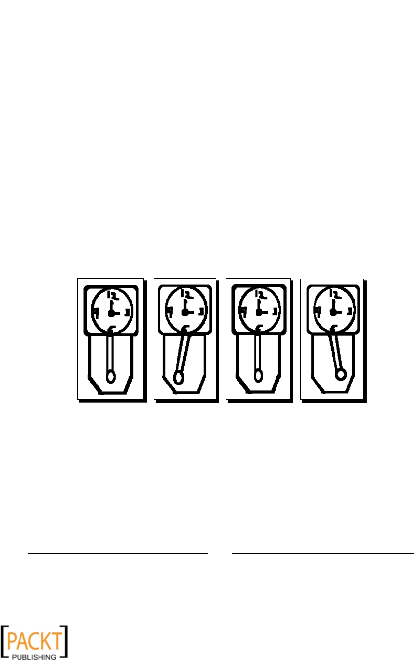
dierent from the previously displayed one. The next illustraon shows animaon
frames of a 'grandfather's clock':
As you can see, there are four image frames in a clock animaon. These frames are
quickly displayed one aer the other to achieve the desired animaon eect. Each of
these images will be shown for 0.25 seconds. Therefore, it simulates the pendulum
oscillaon of one second.
x
x

Python and Mulmedia
[ 12 ]
Cartoon animaon is a classic example of animaon. Since its debut in the early tweneth
century, animaon has become a prominent entertainment industry. Our focus in this
book will be on 2D cartoon animaons built using Python. In Chapter 4, we will learn some
techniques to build such animaons. Creang a cartoon character and bringing it to 'life' is
a laborious job. Unl the late 70s, most of the animaons and eects were created without
the use of computers. In today's age, much of the image creaon work is produced digitally.
The state-of-the-art technology makes this process much faster. For example, one can apply
image transformaons to display or move a poron of an image, thereby avoiding the need
to create the whole cartoon image for the next frame.
Built-in multimedia support
Python has a few built-in mulmedia modules for applicaon development. We will skim
through some of these modules.
winsound
The winsound module is available on the Windows plaorm. It provides an interface which
can be used to implement fundamental audio-playing elements in the applicaon. A sound
can be played by calling PlaySound(sound, flags). Here, the argument sound is used
to specify the path of an audio le. If this parameter is specied as None, the presently
streaming audio (if any) is stopped. The second argument species whether the le to be
played is a sound le or a system sound. The following code snippet shows how to play a
wave formaed audio le using winsound module.
from winsound import PlaySound, SND_FILENAME
PlaySound("C:/AudioFiles/my_music.wav", SND_FILENAME )
This plays the sound le specied by the rst argument to the funcon PlaySound. The
second argument, SND_FILENAME, says that the rst argument is an audio le. If the ag
is set as SND_ALIAS, it means the value for the rst argument is a system sound from
the registry.
audioop
This module is used for manipulang the raw audio data. One can perform several useful
operaons on sound fragments. For example, it can nd the minimum and maximum values
of all the samples within a sound fragment.
x
x

Chapter 1
[ 13 ]
wave
The wave module provides an interface to read and write audio les with WAV le format.
The following line of code opens a wav le.
import wave
fil = wave.open('horn.wav', 'r')
The rst argument of method open is the locaon where the path to the wave le is
specied. The second argument 'r' returns a Wave_read object. This is the mode in which
the audio le is opened, 'r' or 'rb' for read-only mode and 'w' or 'wb' for write-only mode.
External multimedia libraries and frameworks
There are several open source mulmedia frameworks available for mulmedia applicaon
development. The Python bindings for most of these are readily available. We will discuss
a few of the most popular mulmedia frameworks here. In the chapters that follow, we will
make use of many of these libraries to create some useful mulmedia applicaons.
Python Imaging Library
Python Imaging Library provides image processing funconality in Python. It supports several
image formats. Later in this book, a number of image processing techniques using PIL will
be discussed thoroughly. We will learn things such as image format conversion and various
image manipulaon and enhancement techniques using the Python Imaging Library.
PyMedia
PyMedia is a popular open source media library that supports audio/video manipulaon of
a wide range of mulmedia formats.
GStreamer
This framework enables mulmedia manipulaon. It is a framework on top of which one
can develop mulmedia applicaons. The rich set of libraries it provides makes it easier
to develop applicaons with complex audio/video processing capabilies. GStreamer is
wrien in C programming language and provides bindings for some other programming
languages including Python. Several open source projects use GStreamer framework to
develop their own mulmedia applicaon. Comprehensive documentaon is available on
the GStreamer project website. GStreamer Applicaon Development Manual is a very good
starng point. This framework will be extensively used later in this group to develop audio
and video applicaons.
x
x

Python and Mulmedia
[ 14 ]
Pyglet
Interested in animaons and gaming applicaons? Pyglet is here to help. Pyglet provides
an API for developing mulmedia applicaons using Python. It is an OpenGL-based library
that works on mulple plaorms. It is one of the popular mulmedia frameworks for
development of games and other graphically intense applicaons. It supports mulple
monitor conguraon typically needed for gaming applicaon development. Later in this
book, we will be extensively using this Pyglet framework for creang animaons.
PyGame
PyGame (www.pygame.org) is another very popular open source framework that provides
an API for gaming applicaon development needs. It provides a rich set of graphics and
sound libraries. We won't be using PyGame in this book. But since it is a prominent
mulmedia framework, we will briey discuss some of its most important modules and
work out a simple example. The PyGame website provides ample resources on use of this
framework for animaon and game programming.
Sprite
The Sprite module contains several classes; out of these, Sprite and Group are the
most important. Sprite is the super class of all the visible game objects. A Group object
is a container for several instances of Sprite.
Display
As the name suggests, the Display module has funconality dealing with the display. It is
used to create a Surface instance for displaying the Pygame window. Some of the important
methods of this module include flip and update. The former is called to make sure that
everything drawn is properly displayed on the screen. Whereas the laer is used if you
just want to update a poron of the screen.
Surface
This module is used to display an image. The instance of Surface represents an image. The
following line of code creates such an instance.
surf = pygame.display.set_mode((800,600))
The API method, display.set_mode, is used to create this instance. The width and height
of the window are specied as arguments to this method.
Draw
With the Draw module, one can render several basic shapes within the Surface. Examples
include circles, rectangles, lines, and so on.
x
x

Chapter 1
[ 15 ]
Event
This is another important module of PyGame. An event is said to occur when, for instance,
the user clicks a mouse buon or presses a key and so on. The event informaon is used to
instruct the program to execute in a certain way.
Image
The Image module is used to process images with dierent le formats. The loaded image is
represented by a surface.
Music
Pygame.mixer.music provides convenient methods for controlling playback such as play,
reverse, stop, and so on.
The following is a simple program that highlights some of the fundamental concepts
of animaon and game programming. It shows how to display objects in an applicaon
window and then interacvely modify their posions. We will use PyGame to accomplish
this task. Later in this book, we will use a dierent mulmedia framework, Pyglet, for
creang animaons.
Time for action – a simple application using PyGame
This example will make use of the modules we just discussed. For this applicaon to
work, you will need to install PyGame. The binary and source distribuon of PyGame is
available on Pygame's website.
1. Create a new Python source le and write the following code in it.
1 import pygame
2 import sys
3
4 pygame.init()
5 bgcolor = (200, 200, 100)
6 surf = pygame.display.set_mode((400,400))
7
8 circle_color = (0, 255, 255)
9 x, y = 200, 300
10 circle_rad = 50
11
12 pygame.display.set_caption("My Pygame Window")
13
14 while True:
15 for event in pygame.event.get():
x
x

Python and Mulmedia
[ 16 ]
16 if event.type == pygame.QUIT:
17 sys.exit()
18 elif event.type == pygame.KEYDOWN:
19 if event.key == pygame.K_UP:
20 y -= 10
21 elif event.key == pygame.K_DOWN:
22 y += 10
23 elif event.key == pygame.K_RIGHT:
24 x += 10
25 elif event.key == pygame.K_LEFT:
26 x -= 10
27
28 circle_pos = (x, y)
29
30 surf.fill(bgcolor)
31 pygame.draw.circle(surf, circle_color ,
32 circle_pos , circle_rad)
33 pygame.display.flip()
2. The rst line imports the pygame package. On line 4, the modules within this
pygame package are inialized. An instance of class Surface is created using
display.set_mode method. This is the main PyGame window inside which the
images will be drawn. To ensure that this window is constantly displayed on the
screen, we need to add a while loop that will run forever, unl the window is
closed by the user. In this simple applicaon everything we need is placed inside the
while loop. The background color of the PyGame window represented by object
surf is set on line 30.
3. A circular shape is drawn in the PyGame surface by the code on line 31. The
arguments to draw.circle are (Surface, color, position, radius) . This
creates a circle at the posion specied by the argument circle_pos. The instance
of class Surface is sent as the rst argument to this method.
4. The code block 16-26 captures certain events. An event occurs when, for instance,
a mouse buon or a key is pressed. In this example, we instruct the program to
do certain things when the arrow keys are pressed. When the RIGHT arrow key is
pressed, the circle is drawn with the x coordinate oset by 10 pixels to the previous
posion. As a result, the circle appears to be moving towards right whenever you
press the RIGHT arrow key. When the PyGame window is closed, the pygame.QUIT
event occurs. Here, we simply exit the applicaon by calling sys.exit() as done
on line 17.
x
x
Chapter 1
[ 17 ]
5. Finally, we need to ensure that everything drawn on the Surface is visible. This is
accomplished by the code on line 31. If you disable this line, incompletely drawn
images may appear on the screen.
6. Execute the program from a terminal window. It will show a new graphics window
containing a circular shape. If you press the arrow keys on the keyboard, the circle
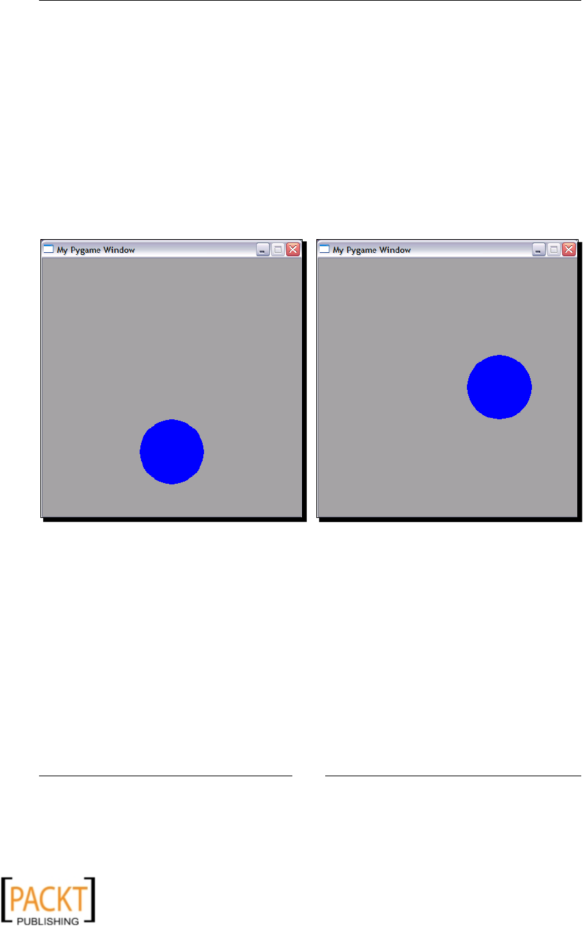
will move in the direcon indicated by the arrow key. The next illustraon shows the
screenshot of the original circle posion (le) and when it is moved using the UP
and RIGHT arrow keys.
A simple PyGame applicaon with a circle drawn within the Surface (window).
The image on the right side is a screenshot taken aer maneuvering the posion
of the circle with the help of arrow keys:
What just happened?
We used PyGame to create a simple user interacve applicaon. The purpose of this
example was to introduce some of the basic concepts behind animaon and game
programming. It was just a preview of what is coming next! Later in this book we
will use Pyglet framework to create some interesng 2D animaons.
x
x

Python and Mulmedia
[ 18 ]
QT Phonon
When one thinks of a media player, it is almost always associated with a graphical user
interface. Of course one can work with command-line mulmedia players. But a media
player with a GUI is a clear winner as it provides an easy to use, intuive user interface to
stream a media and control its playback. The next screenshot shows the user interface of an
audio player developed using QT Phonon.
An Audio Player applicaon developed with QT Phonon:
QT is an open source GUI framework. 'Phonon' is a mulmedia package within QT that
supports audio and video playback. Note that, Phonon is meant for simple media player
funconality. For complex audio/video player funconality, you should use mulmedia
frameworks like GStreamer. Phonon depends on a plaorm-specic backend for media
processing. For example, on Windows plaorm the backend framework is DirectShow.
The supported funconality may vary depending on the plaorm.
To develop a media processing applicaon, a media graph is created in Phonon. This media
graph contains various interlinked media nodes. Each media node does a poron of media
processing. For example, an eects node will add an audio eect, such as echo to the media.
Another node will be responsible for outpung the media from an audio or video device
and so on. In chapter 8, we will develop audio and video player applicaons using Phonon
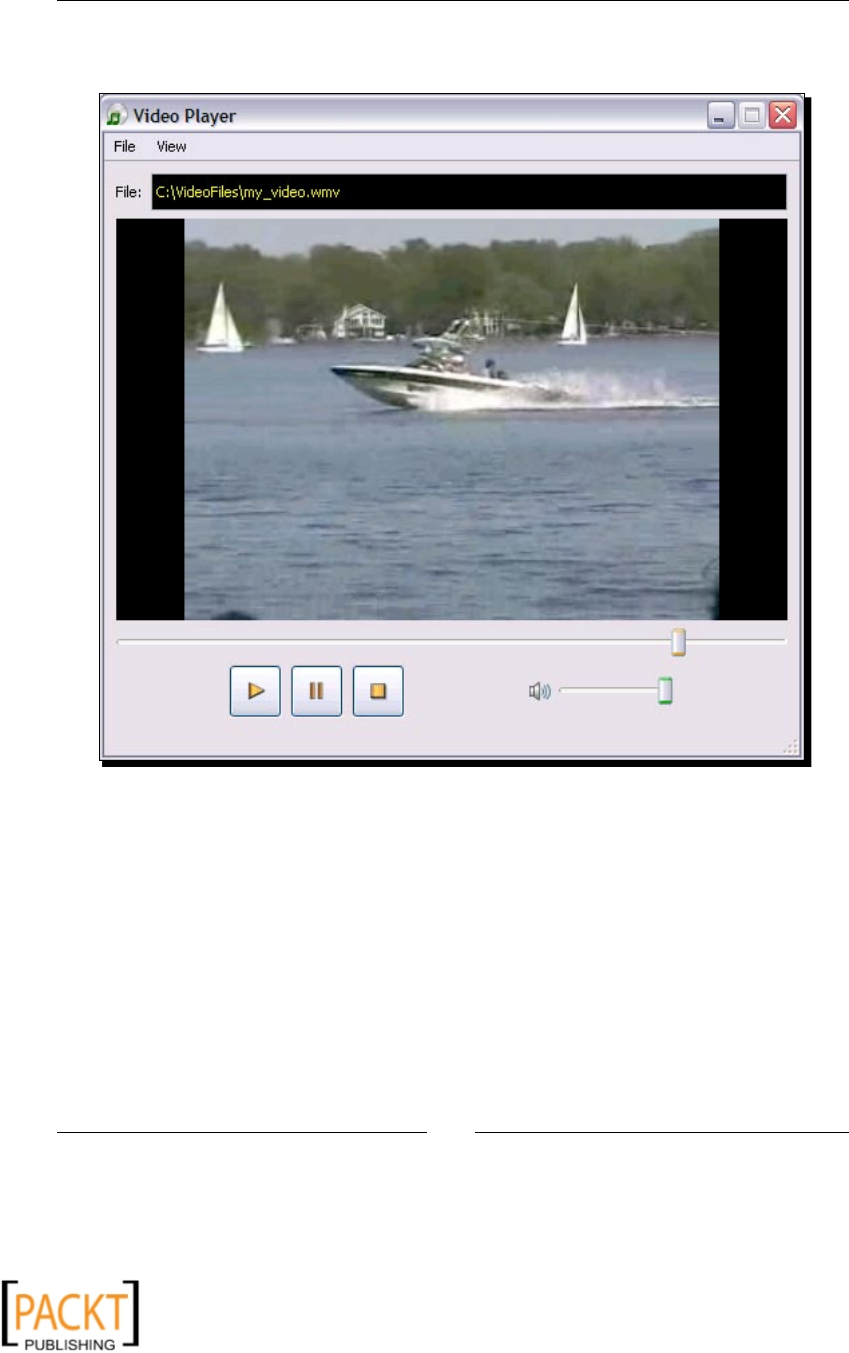
framework. The next illustraon shows a video player streaming a video. It is developed
using QT Phonon. We will be developing this applicaon in Chapter 8.
x
x
Chapter 1
[ 19 ]
Using various built-in modules of QT Phonon, it is very easy to create GUI-based audio
and video players. This example shows a video player in acon:
Other multimedia libraries
Python bindings for several other mulmedia libraries are available on various plaorms.
Some of the popular libraries are menoned below.
Snack Sound Toolkit
Snack is an audio toolkit that is used to create cross-plaorm audio applicaons.
It includes audio analysis and input-output funconality and it has support for
audio visualizaon as well. The ocial website for Snack Sound Toolkit is
http://www.speech.kth.se/snack/.
x
x

Python and Mulmedia
[ 20 ]
PyAudiere
PyAudiere (http://pyaudiere.org/) is an open source audio library. It provides an API
to easily implement the audio funconality in various applicaons. It is based on Audiere
Sound Library.
Summary
This chapter served as an introducon to mulmedia processing using Python.
Specically, in this chapter we covered:
An overview of mulmedia processing. It introduced us to digital image, audio, and
video processing.
We learned about a number of freely available mulmedia frameworks that can be
used for mulmedia processing.
Now that we know what mulmedia libraries and frameworks are out there, we're ready to
explore these to develop excing mulmedia applicaons!
x
x

2
Working with Images
In this chapter, we will learn basic image conversion and manipulaon
techniques using the Python Imaging Library. The chapter ends with an excing
project where we create an image processing applicaon.
In this chapter, we shall:
Learn various image I/O operaons for reading and wring images using the Python
Imaging Library (PIL)
With the help of several examples and code snippets, perform some basic
manipulaons on the image, such as resizing, rotang/ ipping, cropping,
pasng, and so on.
Write an image-processing applicaon by making use of PIL
Use the QT library as a frontend (GUI) for this applicaon
So let's get on with it!
Installation prerequisites
Before we jump in to the main chapter, it is necessary to install the following packages.
Python
In this book we will use Python Version 2.6, or to be more specic, Version 2.6.4.
It can be downloaded from the following locaon:
http://python.org/download/releases/
x
x

Working with Images
[ 22 ]
Windows platform
For Windows, just download and install the plaorm-specic binary distribuon of
Python 2.6.4.
Other platforms
For other plaorms, such as Linux, Python is probably already installed on your machine.
If the installed version is not 2.6, build and install it from the source distribuon. If you are
using a package manager on a Linux system, search for Python 2.6. It is likely that you will
nd the Python distribuon there. Then, for instance, Ubuntu users can install Python from
the command prompt as:
$sudo apt-get python2.6
Note that for this, you must have administrave permission on the machine on which you
are installing Python.
Python Imaging Library (PIL)
We will learn image-processing techniques by making extensive use of the Python Imaging
Library (PIL) throughout this chapter. As menoned in Chapter 1, PIL is an open source
library. You can download it from http://www.pythonware.com/products/pil/.
Install the PIL Version 1.1.6 or later.
Windows platform
For Windows users, installaon is straighorward—use the binary distribuon PIL 1.1.6 for
Python 2.6.
Other platforms
For other plaorms, install PIL 1.1.6 from the source. Carefully review the README le in
the source distribuon for the plaorm-specic instrucons. Libraries listed in the following
table are required to be installed before installing PIL from the source. For some plaorms
like Linux, the libraries provided in the OS should work ne. However, if those do not work,
install a pre-built "libraryName-devel" version of the library. For example, for JPEG support,
the name will contain "jpeg-devel-", and something similar for the others. This is generally
applicable to rpm-based distribuons. For Linux avors like Ubuntu, you can use the
following command in a shell window.
$sudo apt-get install python-imaging.
x
x

Chapter 2
[ 23 ]
However, you should make sure that this installs Version 1.1.6 or later. Check PIL
documentaon for further plaorm-specic instrucons. For Mac OSX, see if you can use
fink to install these libraries. See http://www.finkproject.org/ for more details.
You can also check the website http://pythonmac.org or Darwin ports website
http://darwinports.com/ to see if a binary package installer is available. If such
a pre-built version is not available for any library, install it from the source.
The PIL prerequisites for installing PIL from source are listed in the following table:
Library URL Version Installaon opons
(a) or (b)
libjpeg
(JPEG support)
http://www.ijg.
org/files
7 or 6a or
6b
(a) Pre-built version. For example:
jpeg-devel-7
Check if you can do:
sudo apt-install libjpeg
(works on some avors of Linux)
(b) Source tarball. For example:
jpegsrc.v7.tar.gz
zib
(PNG support)
http://www.gzip.
org/zlib/
1.2.3 or
later
(a) Pre-built version. For example:
zlib-devel-1.2.3..
(b) Install from the source.
freetype2
(OpenType /TrueType
support)
http://www.
freetype.org
2.1.3 or
later
(a) Pre-built version. For example:
freetype2-devel-2.1.3..
(b) Install from the source.
PyQt4
This package provides Python bindings for Qt libraries. We will use PyQt4 to generate GUI for
the image-processing applicaon that we will develop later in this chapter. The GPL version is
available at: http://www.riverbankcomputing.co.uk/software/pyqt/download.
Windows platform
Download and install the binary distribuon pertaining to Python 2.6. For example, the
executable le's name could be 'PyQt-Py2.6-gpl-4.6.2-2.exe'. Other than Python, it includes
everything needed for GUI development using PyQt.
x
x

Working with Images
[ 24 ]
Other platforms
Before building PyQt, you must install SIP Python binding generator. For further details,
refer to the SIP homepage: http://www.riverbankcomputing.com/software/sip/.
Aer installing SIP, download and install PyQt 4.6.2 or later, from the source tarball. For
Linux/Unix source, the lename will start with PyQt-x11-gpl-.. and for Mac OS X,
PyQt-mac-gpl-... Linux users should also check if PyQt4 distribuon is already
available through the package manager.
Summary of installation prerequisites
Package Download locaon Version Windows
plaorm
Linux/Unix/OS X plaorms
Python http://python.org/
download/releases/
2.6.4
(or any
2.6.x)
Install using
binary
distribuon
(a) Install from binary; Also
install addional developer
packages (For example, with
python-devel in the
package name in the rpm
systems) OR
(b) Build and install from the
source tarball.
(c) MAC users can also check
websites such as http://
darwinports.com/ or
http://pythonmac.org/.
PIL www.pythonware.com/
products/pil/
1.1.6 or
later
Install PIL 1.1.6
(binary) for
Python 2.6
(a) Install prerequisites if
needed. Refer to Table #1 and
the README le in PIL source
distribuon.
(b) Install PIL from source.
(c) MAC users can also check
websites like http://
darwinports.com/ or
http://pythonmac.org/.
PyQt4 http://www.
riverbankcomputing.
co.uk/software/
pyqt/download
4.6.2 or
later
Install using
binary
pertaining to
Python 2.6
(a) First install SIP 4.9 or later.
(b) Then install PyQt4.
x
x

Chapter 2
[ 25 ]
Reading and writing images
To manipulate an exisng image, we must open it rst for eding and we also require the
ability to save the image in a suitable le format aer making changes. The Image module in
PIL provides methods to read and write images in the specied image le format. It supports
a wide range of le formats.
To open an image, use Image.open method. Start the Python interpreter and write the
following code. You should specify an appropriate path on your system as an argument to
the Image.open method.
>>>import Image
>>>inputImage = Image.open("C:\\PythonTest\\image1.jpg")
This will open an image le by the name image1.jpg. If the le can't be opened, an
IOError will be raised, otherwise, it returns an instance of class Image.
For saving image, use the save method of the Image class. Make sure you replace the
following string with an appropriate /path/to/your/image/file.
>>>inputImage.save("C:\\PythonTest\\outputImage.jpg")
You can view the image just saved, using the show method of Image class.
>>>outputImage = Image.open("C:\\PythonTest\\outputImage.jpg")
>>>outputImage.show()
Here, it is essenally the same image as the input image, because we did not make any
changes to the output image.
Time for action – image le converter
With this basic informaon, let's build a simple image le converter. This ulity will
batch-process image les and save them in a user-specied le format.
To get started, download the le ImageFileConverter.py from the Packt website,
www.packtpub.com. This le can be run from the command line as:
python ImageConverter.py [arguments]
Here, [arguments] are:
--input_dir: The directory path where the image les are located.
--input_format: The format of the image les to be converted. For example, jpg.
x
x
Working with Images
[ 26 ]
--output_dir: The locaon where you want to save the converted images.
--output_format: The output image format. For example, jpg, png, bmp,
and so on.
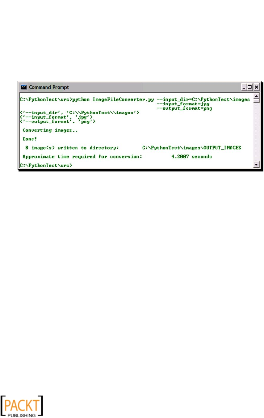
The following screenshot shows the image conversion ulity in acon on Windows XP, that
is, running image converter from the command line.
Here, it will batch-process all the .jpg images within C:\PythonTest\images and save
them in png format in the directory C:\PythonTest\images\OUTPUT_IMAGES.
The le denes class ImageConverter . We will discuss the most important methods in
this class.
def processArgs: This method processes all the command-line arguments
listed earlier. It makes use of Python's built-in module getopts to process these
arguments. Readers are advised to review the code in the le ImageConverter.py
in the code bundle of this book for further details on how these arguments
are processed.
def convertImage: This is the workhorse method of the image-conversion ulity.
1 def convertImage(self):
2 pattern = "*." + self.inputFormat
3 filetype = os.path.join(self.inputDir, pattern)
4 fileList = glob.glob(filetype)
5 inputFileList = filter(imageFileExists, fileList)
6
7 if not len(inputFileList):
8 print "\n No image files with extension %s located \
9 in dir %s"%(self.outputFormat, self.inputDir)
10 return
11 else:
x
x

Chapter 2
[ 27 ]
12 # Record time before beginning image conversion
13 starttime = time.clock()
14 print "\n Converting images.."
15
16 # Save image into specified file format.
17 for imagePath in inputFileList:
18 inputImage = Image.open(imagePath)
19 dir, fil = os.path.split(imagePath)
20 fil, ext = os.path.splitext(fil)
21 outPath = os.path.join(self.outputDir,
22 fil + "." + self.outputFormat)
23 inputImage.save(outPath)
24
25 endtime = time.clock()
26 print "\n Done!"
27 print "\n %d image(s) written to directory:\
28 %s" %(len(inputFileList), self.outputDir)
29 print "\n Approximate time required for conversion: \
30 %.4f seconds" % (endtime – starttime)
Now let's review the preceding code.
1. Our rst task is to get a list of all the image les to be saved in a dierent format.
This is achieved by using glob module in Python. Line 4 in the code snippet nds all
the le path names that match the paern specied by the local variable fileType.
On line 5, we check whether the image le in fileList exists. This operaon can
be eciently performed over the whole list using the built-in filter funconality
in Python.
2. The code block between lines 7 to 14 ensures that one or more images exist. If so, it
will record the me before beginning the image conversion.
3. The next code block (lines 17-23) carries out the image le conversion. On line 18,
we use Image.open to open the image le. Line 18 creates an Image object.
Then the appropriate output path is derived and nally the output image is saved
using the save method of the Image module.
What just happened?
In this simple example, we learned how to open and save image les in a specied image
format. We accomplished this by wring an image le converter that batch-processes a
specied image le. We used PIL's Image.open and Image.save funconality along with
Python's built-in modules such as glob and filter.
Now we will discuss other key aspects related to the image reading and wring.
x
x

Working with Images
[ 28 ]
Creating an image from scratch
So far we have seen how to open an exisng image. What if we want to create our own
image? As an example, it you want to create fancy text as an image, the funconality that we
are going to discuss now comes in handy. Later in this book, we will learn how to use such
an image containing some text to embed into another image. The basic syntax for creang a
new image is:
foo = Image.new(mode, size, color)
Where, new is the built-in method of class Image. Image.new takes three arguments,
namely, mode, size, and color. The mode argument is a string that gives informaon about
the number and names of image bands. Following are the most common values for mode
argument: L (gray scale) and RGB (true color). The size is a tuple specifying dimensions
of the image in pixels, whereas, color is an oponal argument. It can be assigned an RGB
value (a 3-tuple) if it's a mul-band image. If it is not specied, the image is lled with
black color.
Time for action – creating a new image containing some text
As already stated, it is oen useful to generate an image containing only some text or a
common shape. Such an image can then be pasted onto another image at a desired angle
and locaon. We will now create an image with text that reads, "Not really a fancy text!"
1. Write the following code in a Python source le:
1 import Image
2 import ImageDraw
3 txt = "Not really a fancy text!"
4 size = (150, 50)
5 color = (0, 100, 0)
6 img = Image.new('RGB', size, color)
7 imgDrawer = ImageDraw.Draw(img)
8 imgDrawer.text((5, 20), txt)
9 img.show()
2. Let's analyze the code line by line. The rst two lines import the necessary modules
from PIL. The variable txt is the text we want to include in the image. On line 7,
the new image is created using Image.new. Here we specify the mode and size
arguments. The oponal color argument is specied as a tuple with RGB values
pertaining to the "dark green" color.
x
x

Chapter 2
[ 29 ]
3. The ImageDraw module in PIL provides graphics support for an Image object.
The funcon ImageDraw.Draw takes an image object as an argument to create a
Draw instance. In output code, it is called imgDrawer, as used on line 7. This Draw
instance enables drawing various things in the given image.
4. On line 8, we call the text method of the Draw instance and supply posion
(a tuple) and the text (stored in the string txt) as arguments.
5. Finally, the image can be viewed using img.show() call. You can oponally
save the image using Image.save method. The following screenshot shows
the resultant image.
What just happened?
We just learned how to create an image from scratch. An empty image was created using the
Image.new method. Then, we used the ImageDraw module in PIL to add text to this image.
Reading images from archive
If the image is part of an archived container, for example, a TAR archive, we can use the
TarIO module in PIL to open it and then call Image.open to pass this TarIO instance
as an argument.
Time for action – reading images from archives
Suppose there is an archive le images.tar containing image le image1.jpg. The
following code snippet shows how to read image1.jpg from the tarball.
>>>import TarIO
>>>import Images
>>>fil = TarIO.TarIO("images.tar", "images/image1.jpg")
>>>img = Image.open(fil)
>>>img.show()
What just happened?
We learned how to read an image located in an archived container.
x
x

Working with Images
[ 30 ]
Have a go hero – add new features to the image le converter
Modify the image conversion code so that it supports the following new funconality, which:
1. Takes a ZIP le containing images as input
2. Creates a TAR archive of the converted images
Basic image manipulations
Now that we know how to open and save images, let's learn some basic techniques to
manipulate images. PIL supports a variety of geometric manipulaon operaons, such as
resizing an image, rotang it by an angle, ipping it top to boom or le to right, and so on.
It also facilitates operaons such as cropping, cung and pasng pieces of images, and
so on.
Resizing
Changing the dimensions of an image is one of the most frequently used image manipulaon
operaons. The image resizing is accomplished using Image.resize in PIL. The following
line of code explains how it is achieved.
foo = img.resize(size, filter)
Here, img is an image (an instance of class Image) and the result of resizing operaon is
stored in foo (another instance of class Image). The size argument is a tuple (width,
height). Note that the size is specied in pixels. Thus, resizing the image means modifying
the number of pixels in the image. This is also known as image re-sampling. The Image.
resize method also takes filter as an oponal argument. A filter is an interpolaon
algorithm used while re-sampling the given image. It handles deleon or addion of pixels
during re-sampling, when the resize operaon is intended to make image smaller or larger in
size respecvely. There are four lters available. The resize lters in the increasing order
of quality are NEAREST, BILINEAR, BICUBIC, and ANTIALIAS. The default lter opon
is NEAREST.
Time for action – resizing
Let's now resize images by modifying their pixel dimensions and applying various lters
for re-sampling.
1. Download the le ImageResizeExample.bmp from the Packt website. We will
use this as the reference le to create scaled images. The original dimensions of
ImageResizeExample.bmp are 200 x 212 pixels.
x
x

Chapter 2
[ 31 ]
2. Write the following code in a le or in Python interpreter. Replace the inPath and
outPath strings with the appropriate image path on your machine.
1 import Image
2 inPath = "C:\\images\\ImageResizeExample.jpg"
3 img = Image.open(inPath)
4 width , height = (160, 160)
5 size = (width, height)
6 foo = img.resize(size)
7 foo.show()
8 outPath = "C:\\images\\foo.jpg"
9 foo.save(outPath)
3. The image specied by the inPath will be resized and saved as the image
specied by the outPath. Line 6 in the code snippet does the resizing job and
nally we save the new image on line 9. You can see how the resized image looks
by calling foo.show().
4. Let's now specify the filter argument. In the following code, on line 14, the
filterOpt argument is specied in the resize method. The valid filter opons
are specied as values in the diconary filterDict. The keys of filterDict
are used as the lenames of the output images. The four images thus obtained are
compared in the next illustraon. You can clearly noce the dierence between the
ANTIALIAS image and the others (parcularly, look at the ower petals in these
images). When the processing me is not an issue, choose the ANTIALIAS lter
opon as it gives the best quality image.
1 import Image
2 inPath = "C:\\images\\ImageResizeExample.jpg"
3 img = Image.open(inPath)
4 width , height = (160, 160)
5 size = (width, height)
6 filterDict = {'NEAREST':Image.NEAREST,
7 'BILINEAR':Image.BILINEAR,
8 'BICUBIC':Image.BICUBIC,
9 'ANTIALIAS':Image.ANTIALIAS }
10
11 for k in filterDict.keys():
12 outPath= "C:\\images\\" + k + ".jpg"
13 filterOpt = filterDict[k]
14 foo = img.resize(size, filterOpt)
15 foo.save(outPath)
x
x
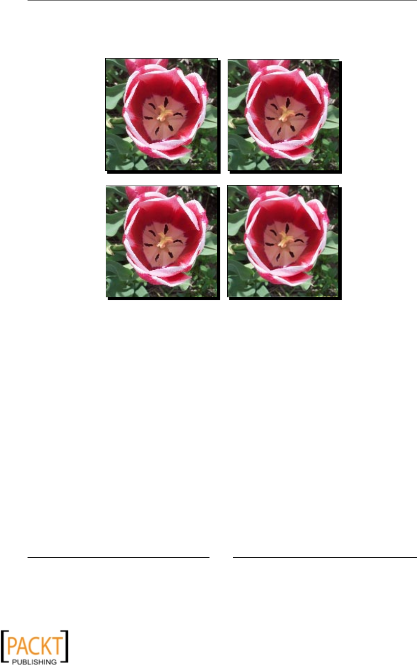
Working with Images
[ 32 ]
The resized images with dierent lter opons appear as follows. Clockwise
from le, Image.NEAREST, Image.BILENEAR, Image.BICUBIC, and
Image.ANTIALIAS:
5. The resize funconality illustrated here, however, doesn't preserve the aspect
rao of the resulng image. The image will appear distorted if one dimension is
stretched more or stretched less in comparison with the other dimension. PIL's
Image module provides another built-in method to x this. It will override the
larger of the two dimensions, such that the aspect rao of the image is maintained.
import Image
inPath = "C:\\images\\ResizeImageExample.jpg"
img = Image.open(inPath)
width , height = (100, 50)
size = (width, height)
outPath = "C:\\images\\foo.jpg"
img.thumbnail(size, Image.ANTIALIAS)
img.save(outPath)
x
x
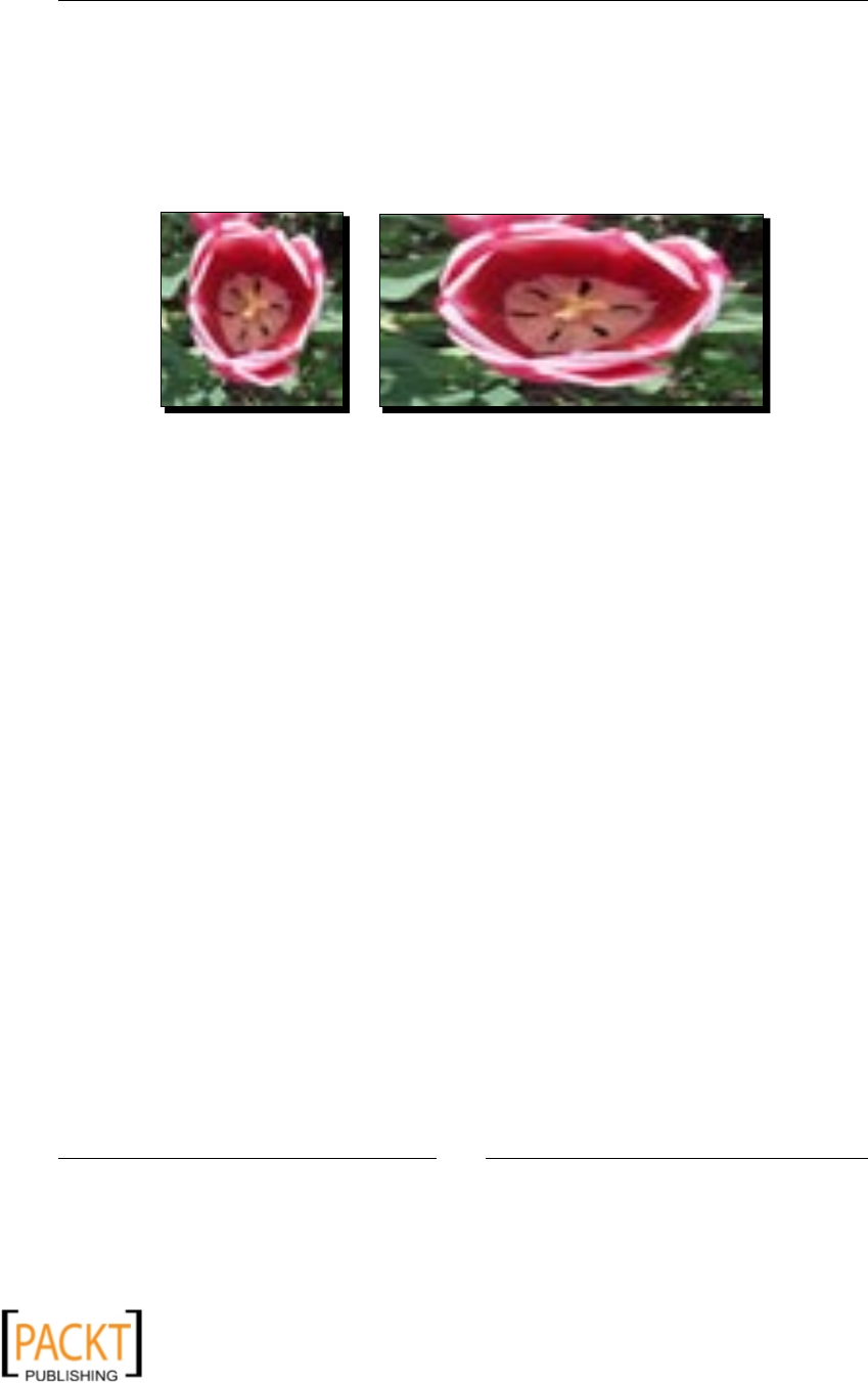
Chapter 2
[ 33 ]
6. This code will override the maximum pixel dimension value (width in this case)
specied by the programmer and replace it with a value that maintains the aspect
rao of the image. In this case, we have an image with pixel dimensions (47, 50).
The resultant images are compared in the following illustraon.
It shows the comparison of output images for methods Image.thumbnail
and Image.resize.
What just happened?
We just learned how image resizing is done using PIL's Image module, by wring a few lines
of code. We also learned dierent types of lters used in image resizing (re-sampling). And
nally, we also saw how to resize an image while sll keeping the aspect rao intact (that is,
without distoron), using the Image.thumbnail method.
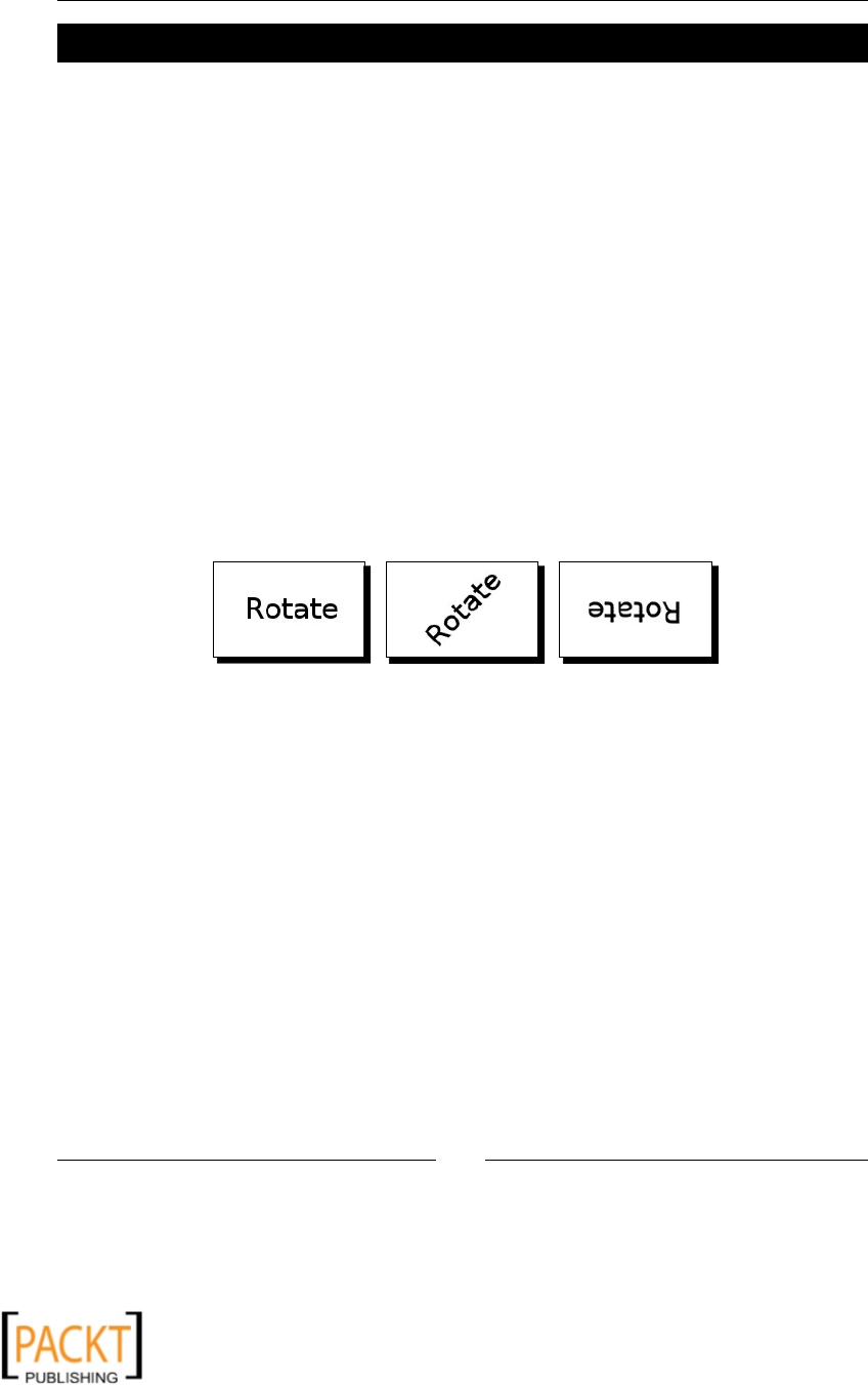
Rotating
Like image resizing, rotang an image about its center is another commonly performed
transformaon. For example, in a composite image, one may need to rotate the text by
certain degrees before embedding it in another image. For such needs, there are methods
such as rotate and transpose available in PIL's Image module. The basic syntax to
rotate an image using Image.rotate is as follows:
foo = img.rotate(angle, filter)
Where, the angle is provided in degrees and filter, the oponal argument, is the
image-re-sampling lter. The valid filter value can be NEAREST, BILINEAR, or BICUBIC.
You can rotate the image using Image.transpose only for 90-, 180-, and 270-degree
rotaon angles.
x
x
Working with Images
[ 34 ]
Time for action – rotating
1. Download the le Rotate.png from the Packt website. Alternavely, you can use
any supported image le of your choice.
2. Write the following code in Python interpreter or in a Python le. As always, specify
the appropriate path strings for inPath and outPath variables.
1 import Image
2 inPath = "C:\\images\\Rotate.png"
3 img = Image.open(inPath)
4 deg = 45
5 filterOpt = Image.BICUBIC
6 outPath = "C:\\images\\Rotate_out.png"
7 foo = img.rotate(deg, filterOpt)
8 foo.save(outPath)
3. Upon running this code, the output image, rotated by 45 degrees, is saved to the
outPath. The lter opon Image.BICUBIC ensures highest quality. The next
illustraon shows the original and the images rotated by 45 and 180 degrees
respecvely—the original and rotated images.
4. There is another way to accomplish rotaon for certain angles by using the
Image.transpose funconality. The following code achieves a 270-degree
rotaon. Other valid opons for rotaon are Image.ROTATE_90 and
Image.ROTATE_180.
import Image
inPath = "C:\\images\\Rotate.png"
img = Image.open(inPath)
outPath = "C:\\images\\Rotate_out.png"
foo = img.transpose(Image.ROTATE_270)
foo.save(outPath)
x
x
Chapter 2
[ 35 ]
What just happened?
In the previous secon, we used Image.rotate to accomplish rotang an image by the
desired angle. The image lter Image.BICUBIC was used to obtain beer quality output
image aer rotaon. We also saw how Image.transpose can be used for rotang the
image by certain angles.
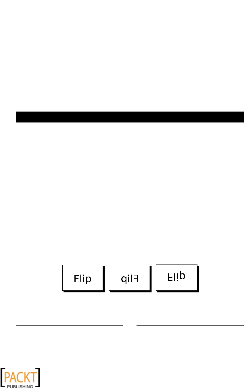
Flipping
There are mulple ways in PIL to ip an image horizontally or vercally. One way to achieve
this is using the Image.transpose method. Another opon is to use the funconality from
the ImageOps module . This module makes the image-processing job even easier with some
ready-made methods. However, note that the PIL documentaon for Version 1.1.6 states
that ImageOps is sll an experimental module.
Time for action – ipping
Imagine that you are building a symmetric image using a bunch of basic shapes. To create
such an image, an operaon that can ip (or mirror) the image would come in handy. So let's
see how image ipping can be accomplished.
1. Write the following code in a Python source le.
1 import Image
2 inPath = "C:\\images\\Flip.png"
3 img = Image.open(inPath)
4 outPath = "C:\\images\\Flip_out.png"
5 foo = img.transpose(Image.FLIP_LEFT_RIGHT)
6 foo.save(outPath)
2. In this code, the image is ipped horizontally by calling the transpose method.
To ip the image vercally, replace line 5 in the code with the following:
foo = img.transpose(Image.FLIP_TOP_BOTTOM)
3. The following illustraon shows the output of the preceding code when the image is
ipped horizontally and vercally.
x
x

Working with Images
[ 36 ]
4. The same eect can be achieved using the ImageOps module. To ip the
image horizontally, use ImageOps.mirror, and to ip the image vercally,
use ImageOps.flip.
import ImageOps
# Flip image horizontally
foo1 = ImageOps.mirror(img)
# Flip image vertically
foo2 = ImageOps.flip(img)
What just happened?
With the help of example, we learned how to ip an image horizontally or vercally using
Image.transpose and also by using methods in class ImageOps. This operaon will be
applied later in this book for further image processing such as preparing composite images.
Capturing screenshots
How do you capture the desktop screen or a part of it using Python? There is ImageGrab
module in PIL. This simple line of code will capture the whole screen.
img = ImageGrab.grab()
Where, img is an instance of class Image.
However, note that in PIL Version 1.1.6, the ImageGrab module supports screen grabbing
only for Windows plaorm.
Time for action – capture screenshots at intervals
Imagine that you are developing an applicaon, where, aer certain me interval, the
program needs to automacally capture the whole screen or a part of the screen. Let's
develop code that achieves this.
1. Write the following code in a Python source le. When the code is executed, it will
capture part of the screen aer every two seconds. The code will run for about
three seconds.
1 import ImageGrab
2 import time
3 startTime = time.clock()
4 print "\n The start time is %s sec" % startTime
5 # Define the four corners of the bounding box.
6 # (in pixels)
7 left = 150
x
x
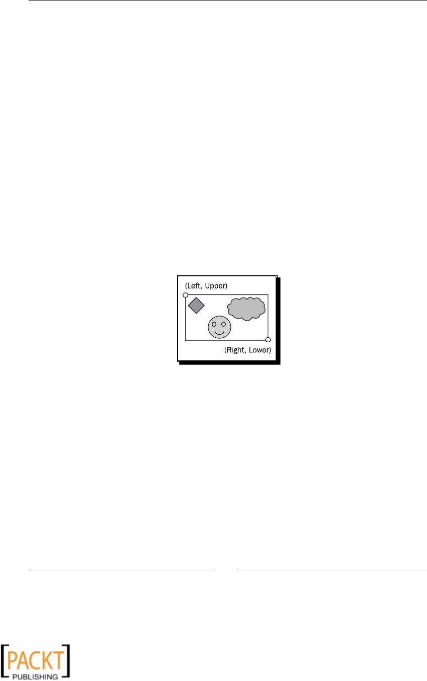
Chapter 2
[ 37 ]
8 upper = 200
9 right = 900
10 lower = 700
11 bbox = (left, upper, right, lower)
12
13 while time.clock() < 3:
14 print " \n Capturing screen at time %.4f sec" \
15 %time.clock()
16 screenShot = ImageGrab.grab(bbox)
17 name = str("%.2f"%time.clock())+ "sec.png"
18 screenShot.save("C:\\images\\output\\" + name)
19 time.sleep(2)
2. We will now review the important aspects of this code. First, import the necessary
modules. The time.clock() keeps track of the me spent. On line 11, a bounding
box is dened. It is a 4-tuple that denes the boundaries of a rectangular region.
The elements in this tuple are specied in pixels. In PIL, the origin (0, 0) is dened
in the top-le corner of an image. The next illustraon is a representaon of a
bounding box for image cropping; see how le, upper and right, lower are specied
as the ends of a diagonal of rectangle.
Example of a bounding box used for image cropping.
3. The while loop runs ll the time.clock() reaches three seconds. Inside the loop,
the part of the screen bounded within bbox is captured (see line 16) and then the
image is saved on line 18. The image name corresponds to the me at which
it is taken.
4. The time.sleep(2) call suspends the execuon of the applicaon for two
seconds. This ensures that it grabs the screen every two seconds. The loop
repeats unl the given me is reached.
x
x
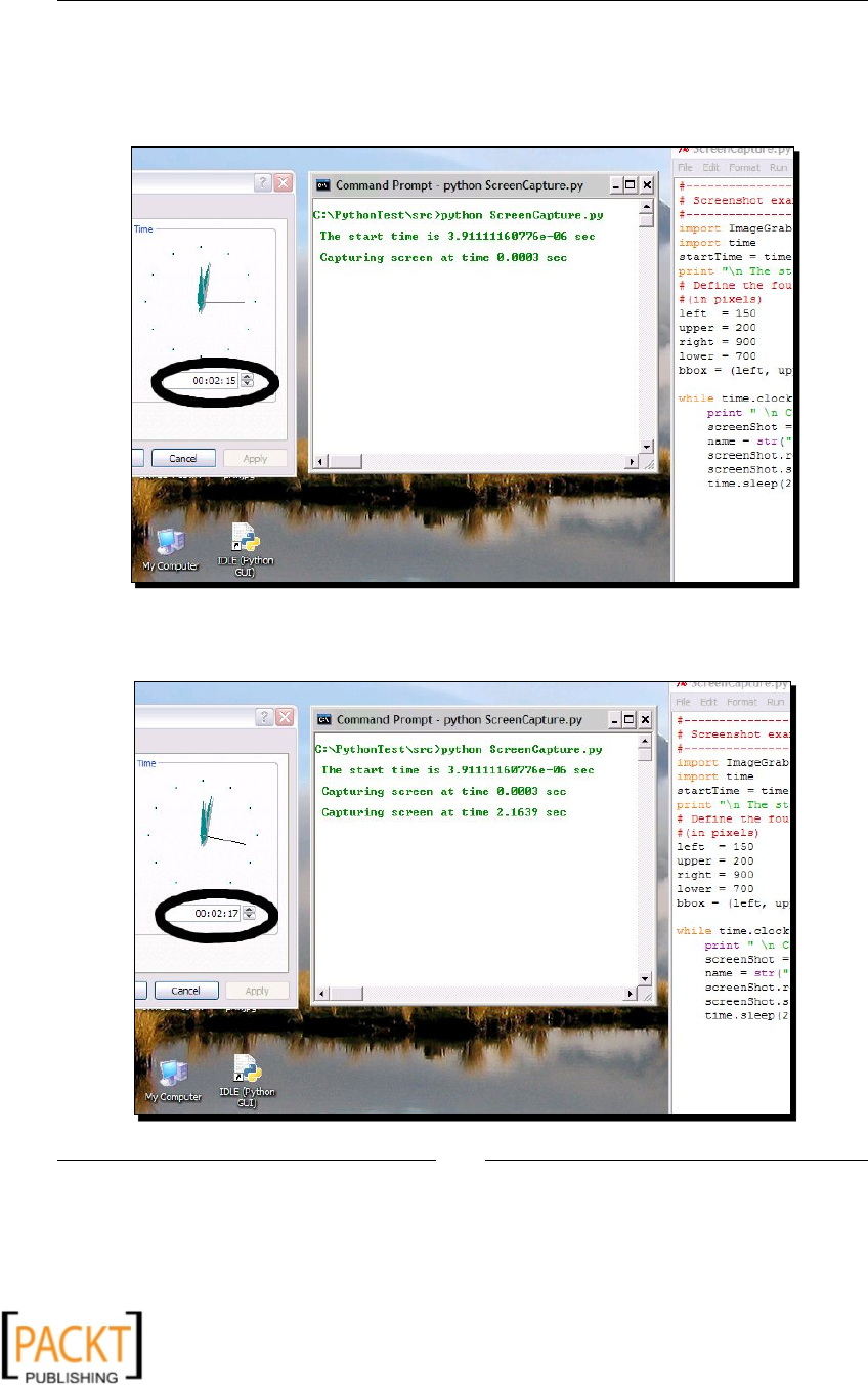
Working with Images
[ 38 ]
5. In this example, it will capture two screenshots, one when it enters the loop for the
rst me and the next aer a two-second me interval. In the following illustraon,
the two images grabbed by the code are shown. Noce the me and console prints
in these images.
The preceding screenshot is taken at me 00:02:15 as shown dialog. The next screenshot is
taken aer 2 seconds, at wall clock me, 00:02:17.
x
x

Chapter 2
[ 39 ]
What just happened?
In the preceding example, we wrote a simple applicaon that captures the screen at regular
me intervals. This helped us to learn how to grab a screen region using ImageGrab.
Cropping
In previous secon, we learned how to grab a part of the screen with ImageGrab. Cropping
is a very similar operaon performed on an image. It allows you to modify a region within
an image.
Time for action – cropping an image
This simple code snippet crops an image and applies some changes on the cropped poron.
1. Download the le Crop.png from Packt website. The size of this image is 400 x
400 pixels. You can also use your own image le.
2. Write the following code in a Python source le. Modify the path of the image le to
an appropriate path.
import Image
img = Image.open("C:\\images\\Crop.png")
left = 0
upper = 0
right = 180
lower = 215
bbox = (left, upper, right, lower)
img = img.crop(bbox)
img.show()
3. This will crop a region of the image bounded by bbox. The specicaon of the
bounding box is idencal to what we have seen in the Capturing screenshots
secon. The output of this example is shown in the following illustraon.
Original image (le) and its cropped region (right).
x
x

Working with Images
[ 40 ]
What just happened?
In the previous secon, we used Image.crop funconality to crop a region within an image
and save the resultant image. In the next secon, we will apply this while pasng a region of
an image onto another.
Pasting
Pasng a copied or cut image onto another one is a commonly performed operaon while
processing images. Following is the simplest syntax to paste one image on another.
img = img.paste(image, box)
Here image is an instance of class Image and box is a rectangular bounding box that
denes the region of img, where the image will be pasted. The box argument can be a
4-tupleError: Reference source not found or a 2-tuple. If a 4-tuple box
is specied, the size of the image to be pasted must be same as the size of the region.
Otherwise, PIL will throw an error with a message ValueError: images do not match.
The 2-tuple on the other hand, provides pixel coordinates of the upper-le corner of the
region to be pasted.
Now look at the following line of code. It is a copy operaon on an image.
img2 = img.copy(image)
The copy operaon can be viewed as pasng the whole image onto a new image. This
operaon is useful when, for instance, you want to keep the original image unaltered
and make alteraons to the copy of the image.
Time for action – pasting: mirror the smiley face!
Consider the example in earlier secon where we cropped a region of an image. The cropped
region contained a smiley face. Let's modify the original image so that it has a 'reecon' of
the smiley face.
1. If not already, download the le Crop.png from the Packt website.
2. Write this code by replacing the le path with appropriate le path on your system.
1 import Image
2 img = Image.open("C:\\images\\Crop.png")
3 # Define the elements of a 4-tuple that represents
4 # a bounding box ( region to be cropped)
5 left = 0
6 upper = 25
7 right = 180
x
x
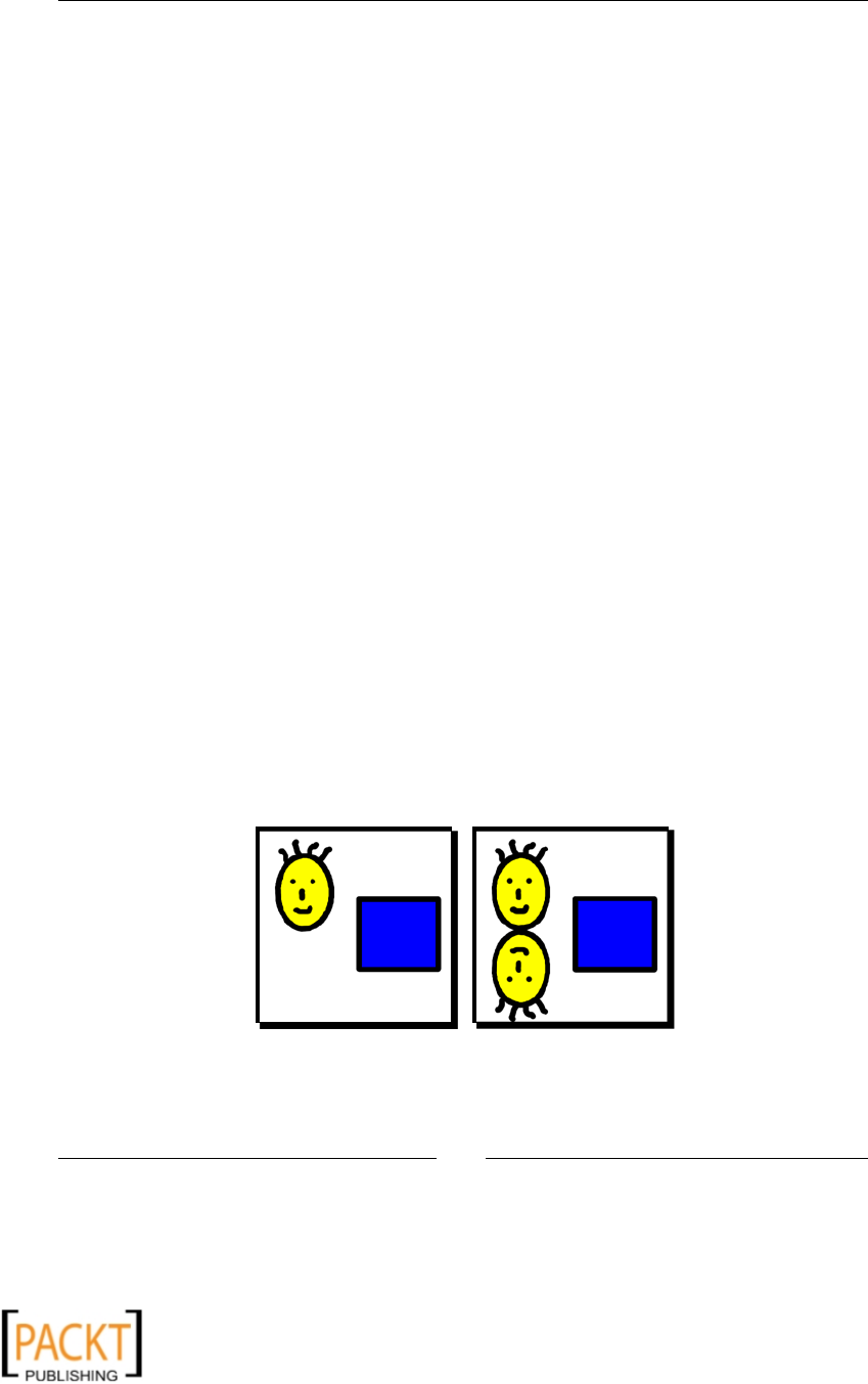
Chapter 2
[ 41 ]
8 lower = 210
9 bbox = (left, upper, right, lower)
10 # Crop the smiley face from the image
11 smiley = img.crop(bbox_1)
12 # Flip the image horizontally
13 smiley = smiley.transpose(Image.FLIP_TOP_BOTTOM)
14 # Define the box as a 2-tuple.
15 bbox_2 = (0, 210)
16 # Finally paste the 'smiley' on to the image.
17 img.paste(smiley, bbox_2)
18 img.save("C:\\images\\Pasted.png")
19 img.show()
3. First we open an image and crop it to extract a region containing the smiley
face. This was already done in secon Error: Reference source not
found'Cropping'. The only minor dierence you will noce is the value of the tuple
element upper. It is intenonally kept as 25 pixels from the top to make sure that the
crop image has a size that can t in the blank poron below the original smiley face.
4. The cropped image is then ipped horizontally with code on line 13.
5. Now we dene a box, bbox_2, for pasng the cropped smiley face back on to the
original image. Where should it be pasted? We intend to make a 'reecon' of the
original smiley face. So the coordinate of the top-right corner of the pasted image
should be greater than or equal to the boom y coordinate of the cropped region,
indicated by 'lower' variable (see line 8) . The bounding box is dened on line 15,
as a 2-tuple represenng the upper-le coordinates of the smiley.
6. Finally, on line 17, the paste operaon is performed to paste the smiley on the
original image. The resulng image is then saved with a dierent name.
7. The original image and the output image aer the paste operaon is shown in the
next illustraon.
The illustraon shows the comparison of original and resulng images aer the
paste operaon.
x
x

Working with Images
[ 42 ]
What just happened?
Using a combinaon of Image.crop and Image.paste, we accomplished cropping a
region, making some modicaons, and then pasng the region back on the image.
Project: Thumbnail Maker
Let's take up a project now. We will apply some of the operaons we learned in this chapter
to create a simple Thumbnail Maker ulity. This applicaon will accept an image as an input
and will create a resized image of that image. Although we are calling it a thumbnail maker, it
is a mul-purpose ulity that implements some basic image-processing funconality.
Before proceeding further, make sure that you have installed all the packages discussed at
the beginning of this chapter. The screenshot of the Thumbnail Maker dialog is show in the
following illustraon.
The Thumbnail Maker GUI has two components:
1. The le panel is a 'control area', where you can specify certain image parameters
along with opons for input and output paths.
2. A graphics area on the right-hand side where you can view the generated image.
x
x
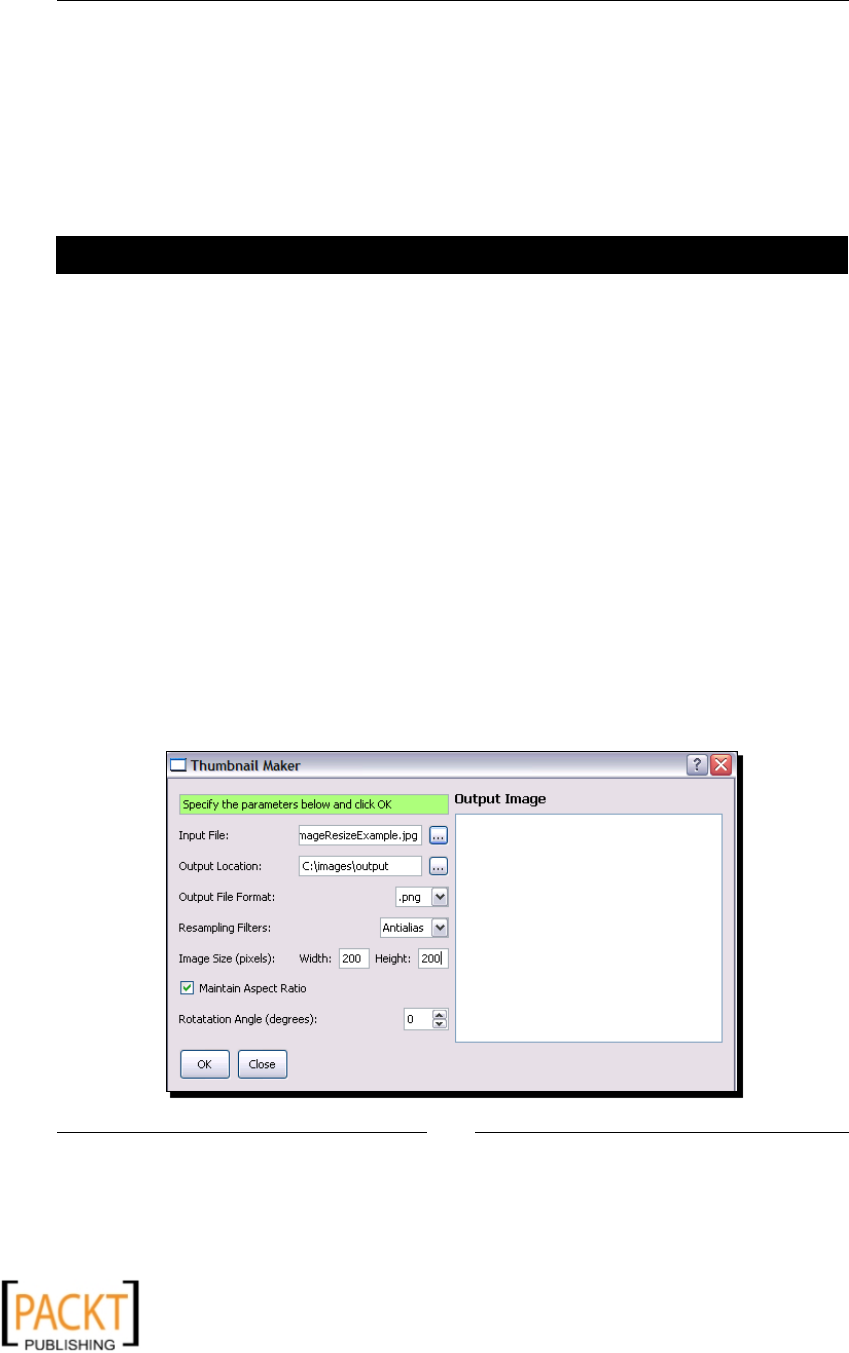
Chapter 2
[ 43 ]
In short, this is how it works:
1. The applicaon takes an image le as an input.
2. It accepts user input for image parameters such as dimensions in pixel, lter for re-
sampling and rotaon angle in degrees.
3. When the user clicks the OK buon in the dialog, the image is processed and saved
at a locaon indicated by the user in the specied output image format.
Time for action – play with Thumbnail Maker application
First, we will run the Thumbnail Maker applicaon as an end user. This warm-up exercise
intends to give us a good understanding of how the applicaon works. This, in turn, will help
us develop/learn the involved code quickly. So get ready for acon!
1. Download the les ThumbnailMaker.py, ThumbnailMakeDialog.py,
and Ui_ThumbnailMakerDialog.py from Packt website. Place these les
in some directory.
2. From the command prompt, change to this directory locaon and type the
following command:
python ThumbnailMakerDialog.py
The Thumbnail Maker dialog that pops up was shown in the earlier screenshot.
Next, we will specify the input-output paths and various image parameters. You can
open any image le of your choice. Here, the ower image shown in some previous
secons will be used as an input image. To specify an input image, click on the small
buon with three dots …. It will open a le dialog. The following illustraon shows
the dialog with all the parameters specied.
x
x

Working with Images
[ 44 ]
3. If Maintain Aspect Rao checkbox is checked, internally it will scale the image
dimension so that the aspect rao of the output image remains the same. When
the OK buon is clicked, the resultant image is saved at the locaon specied by the
Output Locaon eld and the saved image is displayed in the right-hand panel of
the dialog. The following screenshot shows the dialog aer clicking OK buon.
4. You can now try modifying dierent parameters such as output image format or
rotaon angle and save the resulng image.
5. See what happens when the Maintain Aspect Rao checkbox is unchecked. The
aspect rao of the resulng image will not be preserved and the image may appear
distorted if the width and height dimensions are not properly specied.
6. Experiment with dierent re-sampling lters; you can noce the dierence between
the quality of the resultant image and the earlier image.
7. There are certain limitaons to this basic ulity. It is required to specify reasonable
values for all the parameters elds in the dialog. The program will print an error if
any of the parameters is not specied.
What just happened?
We got ourselves familiar with the user interface of the thumbnail maker dialog and saw
how it works for processing an image with dierent dimensions and quality. This knowledge
will make it easier to understand the Thumbnail Maker code.
x
x
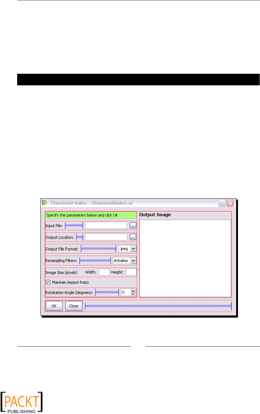
Chapter 2
[ 45 ]
Generating the UI code
The Thumbnail Maker GUI is wrien using PyQt4 (Python bindings for Qt4 GUI framework).
Detailed discussion on how the GUI is generated and how the GUI elements are connected
to the main funcons is beyond the scope of this book. However, we will cover certain main
aspects of this GUI to get you going. The GUI-related code in this applicaon can simply
be used 'as-is' and if this is something that interests you, go ahead and experiment with it
further! In this secon, we will briey discuss how the UI code is generated using PyQt4.
Time for action – generating the UI code
PyQt4 comes with an applicaon called QT Designer. It is a GUI designer for QT-based
applicaons and provides a quick way to develop a graphical user interface containing some
basic widgets. With this, let's see how the Thumbnail Maker dialog looks in QT Designer and
then run a command to generate Python source code from the .ui le.
1. Download the thumbnailMaker.ui le from the Packt website.
2. Start the QT Designer applicaon that comes with PyQt4 installaon.
3. Open the le thumbnailMaker.ui in QT Designer. Noce the red-colored borders
around the UI elements in the dialog. These borders indicate a 'layout' in which
the widgets are arranged. Without a layout in place, the UI elements may appear
distorted when you run the applicaon and, for instance, resize the dialog. Three
types of QLayouts are used, namely Horizontal, Vertical, and Grid layout.
x
x

Working with Images
[ 46 ]
4. You can add new UI elements, such as a QCheckbox or a QLabel, by dragging
and dropping it from the 'Widget Box' of QT Designer. It is located in the le
panel by default.
5. Click on the eld next to the label "Input le". In the right-hand panel of QT
Designer, there is a Property Editor that displays the properes of the selected
widget (in this case it's a QLineEdit). This is shown in the following illustraon.
The Property Editor allows us to assign values to various aributes such as the
objectName, width, and height of the widget, and so on.
Qt Designer shows the details of the selected widget in Property Editor.
6. QT designer saves the le with extension .ui. To convert this into Python source
code, PyQt4 provides a conversion ulity called pyuic4. On Windows XP, for
standard Python installaon, it is present at the following locaon—C:\Python26\
Lib\site-packages\PyQt4\pyuic4.bat. Add this path to your environment
variable. Alternavely specify the whole path each me you want to convert ui
le to Python source le. The conversion ulity can be run from the command
prompt as:
pyuic4 thumbnailMaker.ui -o Ui_ThumbnailMakerDialog.py
7. This script will generate Ui_ThumbnailMakerDialog.py with all the GUI
elements dened. You can further review this le to understand how the UI
elements are dened.
What just happened?
We learned how to autogenerate the Python source code dening UI elements of Thumbnail
Maker Dialog from a Qt designer le.
x
x
Chapter 2
[ 47 ]
Have a go hero – tweak UI of Thumbnail Maker dialog
Modify the thumbnailMaker.ui le in QT Designer and implement the following list of
things in the Thumbnail Maker dialog.
1. Change the color of all the line edits in the le panel to pale yellow.
2. Tweak the default le extension displayed in the Output le Format combobox such
that the rst opon is .png instead of .jpeg
Double click on this combobox to edit it.
3. Add new opon .tiff to the output format combobox.
4. Align the OK and Cancel buons to the right corner.
You will need to break layouts, move the
spacer around, and recreate the layouts.
5. Set the range of rotaon angle 0 to 360 degrees instead of the
current -180 to +180 degrees.
Aer this, create Ui_ThumbnailMakerDialog.py by running the pyuic4 script and then
run the Thumbnail Maker applicaon.
Connecting the widgets
In the earlier secon, the Python source code represenng UI was automacally generated
using the pyuic4 script. This, however, only has the widgets dened and placed in a nice
layout. We need to teach these widgets what they should do when a certain event occurs.
To do this, QT's slots and signals will be used. A signal is emied when a parcular GUI event
occurs. For example, when the user clicks on the OK buon, internally, a clicked() signal
is emied. A slot is a funcon that is called when a parcular signal is emied. Thus, in
this example, it will call a specied method, whenever the OK buon is clicked. See PyQt4
documentaon for a complete list of available signals for various widgets.
x
x

Working with Images
[ 48 ]
Time for action – connecting the widgets
You will noce several dierent widgets in the dialog. For example, the eld which accepts
the input image path or the output directory path is a QLineEdit. The widget where
image format is specied is a QCombobox. On similar lines, the OK and Cancel buons are
QPushButton. As an exercise, you can open up the thumbnailMaker.ui le and click
on each element to see the associated QT class from the Property Editor.
With this, let's learn how the widgets are connected.
1. Open the le ThumbnailMakerDialog.py. The _connect method of class
ThumbnailMakerDialog is copied. The method is called in the constructor
of this class.
def _connect(self):
"""
Connect slots with signals.
"""
self.connect(self._dialog.inputFileDialogButton,
SIGNAL("clicked()"), self._openFileDialog)
self.connect(self._dialog.outputLocationDialogButton,
SIGNAL("clicked()"), self._outputLocationPath)
self.connect(self._dialog.okPushButton,
SIGNAL("clicked()"), self._processImage)
self.connect(self._dialog.closePushButton,
SIGNAL("clicked()"), self.close)
self.connect(self._dialog.aspectRatioCheckBox,
SIGNAL('stateChanged(int)'),
self._aspectRatioOptionChanged)
2. self._dialog is an instance of class Ui_ThumbnailMakerDialog. self.
connect is the inherited method of Qt class QDialog. Here, it takes the following
arguments (QObject, signal, callable), where QObject is any widget type
(all inherit QObject), signal is the QT SIGNAL that tells us about what event
occurred and callable is any method handling this event.
3. For example, consider the highlighted lines of the code snippet. They connect
the OK buon to a method that handles image processing. The rst argument
, self._dialog.okPushButton refers to the buon widget dened in class
Ui_ThumbnailMakerDialog. Referring to QPushButton documentaon, you
will nd there is a "clicked()" signal that it can emit. The second argument
SIGNAL("clicked()") tells Qt that we want to know when that buon is clicked
by the user. The third argument is the method self._processImage that gets
called when this signal is emied.
x
x

Chapter 2
[ 49 ]
4. Similarly, you can review the other connecons in this method. Each of these
connects a widget to a method of the class ThumbnailMakerDialog.
What just happened?
We reviewed ThumbnailMakerDialog._connect() method to understand how the UI
elements are connected to various internal methods. The previous two secons helped us
learn some preliminary concepts of GUI programming using QT.
Developing the image processing code
The previous secons were intended to get ourselves familiar with the applicaon as an end
user and to understand some basic aspects of the GUI elements in the applicaon. With all
necessary pieces together, let's focus our aenon on the class that does all the main image
processing in the applicaon.
The class ThumbnailMaker handles the pure image processing code. It denes various
methods to achieve this. For example, the class methods such as _rotateImage,
_makeThumbnail, and _resizeImage manipulate the given image to accomplish
rotaon, thumbnail generaon, and resizing respecvely. This class accepts input from
ThumbnailMakerDialog. Thus, no QT related UI code is required here. If you want to
use some other GUI framework to process input, you can do that easily. Just make sure to
implement the public API methods dened in class ThumbnailMakerDialog, as those are
used by the ThumbnailMaker class.
Time for action – developing image processing code
Thus, with ThumbnailMakerDialog at your disposal, you can develop your own
code in scratch, in class ThumbnailMaker. Just make sure to implement the method
processImage as this is the only method called by ThumbnailMakerDialog.
Let's develop some important methods of class ThumbnailMaker.
1. Write the constructor for class ThumbnailMaker. It takes dialog as an argument.
In the constructor, we only inialize self._dialog, which is an instance of class
ThumbnailMakerDialog. Here is the code.
def __init__(self, dialog):
"""
Constructor for class ThumbnailMaker.
"""
# This dialog can be an instance of
# ThumbnailMakerDialog class. Alternatively, if
# you have some other way to process input,
x
x

Working with Images
[ 50 ]
# it will be that class. Just make sure to implement
# the public API methods defined in
# ThumbnailMakerDialog class!
self._dialog = dialog
2. Next, write the processImage method in class ThumbnailMaker. The code is
as follows:
Note: You can download the le ThumbnailMaker.py
from Packt website. The code wrien is from this le. The only
dierence is that some code comments are removed here.
1 def processImage(self):
2 filePath = self._dialog.getInputImagePath()
3 imageFile = Image.open(filePath)
4
5 if self._dialog.maintainAspectRatio:
6 resizedImage = self._makeThumbnail(imageFile)
7 else:
8 resizedImage = self._resizeImage(imageFile)
9
10 rotatedImage = self._rotateImage(resizedImage)
11
12 fullPath = self._dialog.getOutImagePath()
13
14 # Finally save the image.
15 rotatedImage.save(fullPath)
3. On line 2, it gets the full path of the input image le. Note that it relies on
self._dialog to provide this informaon.
4. Then the image le is opened the usual way. On line 4, it checks a ag that decides
whether or not to process the image by maintaining the aspect rao. Accordingly,
_makeThumbnail or _resizeImage methods are called.
5. On line 10, it rotates the image resized earlier, using the _rotateImage method.
6. Finally, on line 15, the processed image is saved at a path obtained from the
getOutImagePath method of class ThumbnailMakerDialog.
x
x

Chapter 2
[ 51 ]
7. We will now write the _makeThumbnail method.
1 def _makeThumbnail(self, imageFile):
2 foo = imageFile.copy()
3 size = self._dialog.getSize()
4 imageFilter = self._getImageFilter()
5 foo.thumbnail(size, imageFilter)
6 return foo
8. First a copy of the original image is made. We will manipulate this copy and the
method will return it for further processing.
9. Then the necessary parameters such as the image dimension and lter
for re-sampling are obtained from self._dialog and _getImageFilter
respecvely.
10. Finally the thumbnail is created on line 5 and then method returns this
image instance.
11. We have already discussed how to resize and rotate image. The related code is
straighorward to write and the readers are suggested to write it as an exercise.
You will need to review the code from le ThumbnailMakerDialog.py
for geng appropriate parameters. Write remaining rounes namely,
_resizeImage, _rotateImage and _getImageFilter.
12. Once all methods are in place, run the code from the command line as:
python Thumbnailmaker.py
13. It should show our applicaon dialog. Play around with it to make sure
everything works!
What just happened?
In the previous secon, we completed an excing project. Several things learned in this
chapter, such as image I/O, resizing, and so on, were applied in the project. We developed a
GUI applicaon where some basic image manipulaon features, such as creang thumbnails,
were implemented. This project also helped us gain some insight into various aspects of GUI
programming using QT.
x
x

Working with Images
[ 52 ]
Have a go hero – enhance the ThumbnailMaker application
Want to do something more with the Thumbnail Maker. Here you go! As you will add more
features to this applicaon, the rst thing you would need to do is to change its name—at
least from the capon of the dialog that pops up! Edit the thumbnailMaker.ui le in
QT designer, change the name to something like "Image Processor", and recreate the
corresponding .py le. Next, add the following features to this applicaon.
If you don't want to deal with any UI code, that is ne too! You
can write a class similar to ThumbnailMakerDialog. Do
the input argument processing in your own way. All that class
ThumbnailMaker requires is implementaon of certain public
methods in this new class, to get various input parameters.
1. Accept output lename from the user. Currently, it gives the same name as the
input le.
Edit the .ui le. You would need to break the layouts before adding a QLineEdit
and its QLabel and then recreate the layouts.
2. If there is a previously created output image le in the output directory, clicking OK
would simply overwrite that le. Add a checkbox reading, "Overwrite exisng le
(if any)". If the checkbox in deselected, it should pop up a warning dialog and exit.
For the laer part, there is a commented out code block in
ThumbnailMakerDialog._processImage. Just enable the code.
3. Add a feature that can add specied text in the lower-le corner of the
output image.
4. Create an image with this text, and use the combinaon of crop and paste to
achieve desired results. For user input, you will need to add a new QLineEdit
for accepng text input and then connect signals with a callable method in
ThumbnailMakerDialog._connect.
x
x

Chapter 2
[ 53 ]
Summary
We learned a lot in this chapter about basic image manipulaon.
Specically, we covered image input-output operaons that enable reading and wring of
images, and creaon of images from scratch.
With the help of numerous examples and code snippets, we learned several image
manipulaon operaons. Some of them are:
How to resize an image with or without maintaining aspect rao
Rotang or ipping an image
Cropping an image, manipulang it using techniques learned earlier in the chapter,
and then pasng it on the original image
Creang an image with a text
We developed a small applicaon that captures a region of your screen at regular
me intervals
We created an interesng project implemenng some image processing
funconality learned in this chapter
With this basic image manipulaon knowledge, we are ready to learn how to add some cool
eects to an image. In the next chapter, we will see how to enhance an image.
x
x

x
x

3
Enhancing Images
In the previous chapter, we learned a lot about day-to-day image processing.
We accomplished the learning objecve of performing basic image
manipulaon by working on several examples and small projects. In this
chapter, we will move a step further by learning how to add special eects to
an image. The special eects added to the image serve several purposes. These
not only give a pleasing appearance to the image but may also help you to
understand important informaon presented by the image.
In this chapter, we shall:
Learn how to adjust brightness and contrast levels of an image
Add code to selecvely modify the color of an image and create gray scale images
and negaves
Use PIL funconality to combine two images together and add transparency eects
to the image
Apply various image-enhancement lters to an image to achieve eects such as
smoothing, sharpening, embossing, and so on
Undertake a project to develop a tool to add a watermark or text or a date stamp
to an image
So let's get on with it.
x
x

Enhancing Images
[ 56 ]
Installation and download prerequisites
The installaon prerequisites for this chapter are same as the ones in Chapter 2, Working
with Images. Please refer to that chapter for further details.
It is important to download all the images required for this chapter from the Packt website
at http://www.packtpub.com/. We will be using these images throughout this chapter
in the image processing code. Addionally, please download the PDF le, Chapter 3
Supplementary Material.pdf from Packt website. This is very important if you are
reading a hard copy of this book which is printed in black and white. In the upcoming
secons such as "Tweaking Colors", we compare the images before and aer processing. In
the black and white edion, you won't be able to see the dierence between the compared
images. For example, the eects such as changed image color, modied contrast, and so on,
won't be noceable. The PDF le contains all these image comparisons. So please keep this
le handy while working on the examples in this chapter!
Adjusting brightness and contrast
One oen needs to tweak the brightness and contrast level of an image. For example, you
may have a photograph that was taken with a basic camera, when there was insucient
light. How would you correct that digitally? The brightness adjustment helps make the image
brighter or darker whereas the contrast adjustments emphasize dierences between the
color and brightness level within the image data. The image can be made lighter or darker
using the ImageEnhance module in PIL. The same module provides a class that can
auto-contrast an image.
Time for action – adjusting brightness and contrast
Let's learn how to modify the image brightness and contrast. First, we will write code to adjust
brightness. The ImageEnhance module makes our job easier by providing Brightness class.
1. Download image 0165_3_12_Before_BRIGHTENING.png and rename it to
Before_BRIGHTENING.png.
2. Use the following code:
1 import Image
2 import ImageEnhance
3
4 brightness = 3.0
5 peak = Image.open( "C:\\images\\Before_BRIGHTENING.png ")
6 enhancer = ImageEnhance.Brightness(peak)
7 bright = enhancer.enhance(brightness)
8 bright.save( "C:\\images\\BRIGHTENED.png ")
9 bright.show()
x
x
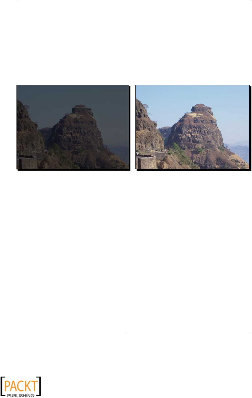
Chapter 3
[ 57 ]
3. On line 6 in the code snippet, we created an instance of the class Brightness. It
takes Image instance as an argument.
4. Line 7 creates a new image bright by using the specied brightness value.
A value between 0.0 and less than 1.0 gives a darker image, whereas a value
greater than 1.0 makes it brighter. A value of 1.0 keeps the brightness of the
image unchanged.
5. The original and resultant image are shown in the next illustraon.
Comparison of images before and aer brightening.
6. Let's move on and adjust the contrast of the brightened image. We will append the
following lines of code to the code snippet that brightened the image.
10 contrast = 1.3
11 enhancer = ImageEnhance.Contrast(bright)
12 con = enhancer.enhance(contrast)
13 con.save( "C:\\images\\CONTRAST.png ")
14 con.show()
7. Thus, similar to what we did to brighten the image, the image contrast was tweaked
by using the ImageEnhance.Contrast class. A contrast value of 0.0 creates a
black image. A value of 1.0 keeps the current contrast.
8. The resultant image is compared with the original in the following illustraon.
x
x
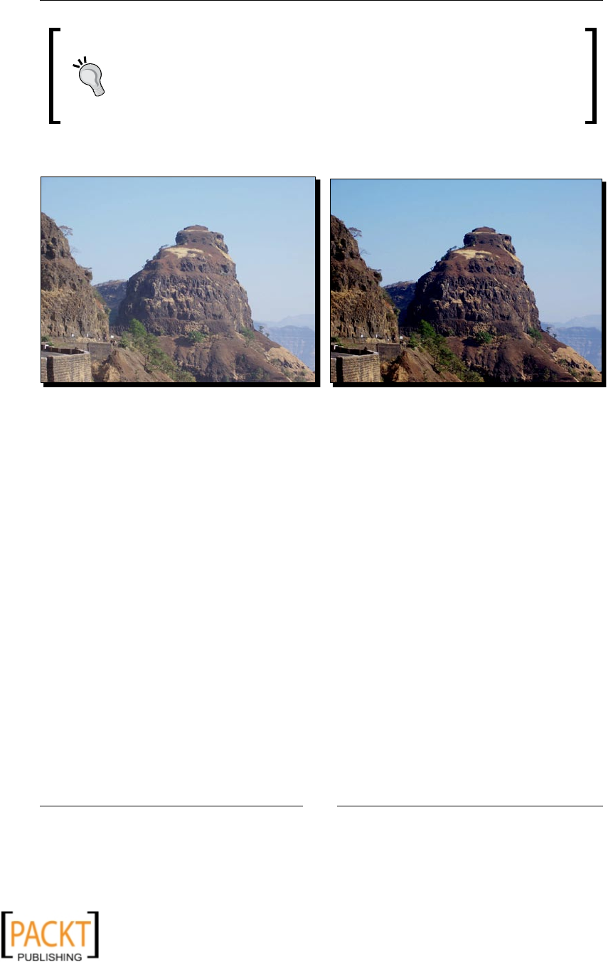
Enhancing Images
[ 58 ]
NOTE: As menoned in the Installaon and Download Prerequisites
secon, the images compared in the following illustraon will appear idencal
if you are reading a hard copy of this book. Please download and refer to the
supplementary PDF le Chapter 3 Supplementary Material.pdf. Here,
the color images are provided, which will help you see the dierence.
The original image with the image displaying the increasing contrast.
9. In the preceding code snippet, we were required to specify a contrast value. If you
prefer PIL for deciding an appropriate contrast level, there is a way to do this. The
ImageOps.autocontrast funconality sets an appropriate contrast level. This
funcon normalizes the image contrast. Let's use this funconality now.
10. Use the following code:
import ImageOps
bright = Image.open( "C:\\images\\BRIGHTENED.png ")
con = ImageOps.autocontrast(bright, cutoff = 0)
con.show()
11. The highlighted line in the code is where contrast is automacally set. The
autocontrast funcon computes histogram of the input image. The cutoff
argument represents the percentage of lightest and darkest pixels to be trimmed
from this histogram. The image is then remapped.
What just happened?
Using the classes and funconality in ImageEnhance module, we learned how to
increase or decrease the brightness and the contrast of the image. We also wrote code
to auto-contrast an image using funconality provided in the ImageOps module. The
things we learned here will be useful in the upcoming secons in this chapter.
x
x

Chapter 3
[ 59 ]
Tweaking colors
Another useful operaon performed on the image is adjusng the colors within an image.
The image may contain one or more bands, containing image data. The image mode
contains informaon about the depth and type of the image pixel data. The most common
modes we will use in this chapter are RGB (true color, 3x8 bit pixel data), RGBA (true color
with transparency mask, 4x8 bit) and L (black and white, 8 bit).
In PIL, you can easily get the informaon about the bands data within an image. To get the
name and number of bands, the getbands() method of the class Image can be used. Here,
img is an instance of class Image.
>>> img.getbands()
('R', 'G', 'B', 'A')
Time for action – swap colors within an image!
To understand some basic concepts, let's write code that just swaps the image band data.
1. Download the image 0165_3_15_COLOR_TWEAK.png and rename it as
COLOR_TWEAK.png.
2. Type the following code:
1 import Image
2
3 img = Image.open( "C:\\images\\COLOR_TWEAK.png ")
4 img = img.convert('RGBA')
5 r, g, b, alpha = img.split()
6 img = Image.merge( "RGBA ", (g, r, b, alpha))
7 img.show()
3. Let's analyze this code now. On line 2, the Image instance is created as usual. Then,
we change the mode of the image to RGBA.
Here we should check if the image already has that mode or if this
conversion is possible. You can add that check as an exercise!
4. Next, the call to Image.split() creates separate instances of Image class,
each containing a single band data. Thus, we have four Image instances—r, g, b,
and alpha corresponding to red, green, and blue bands, and the alpha
channel respecvely.
x
x
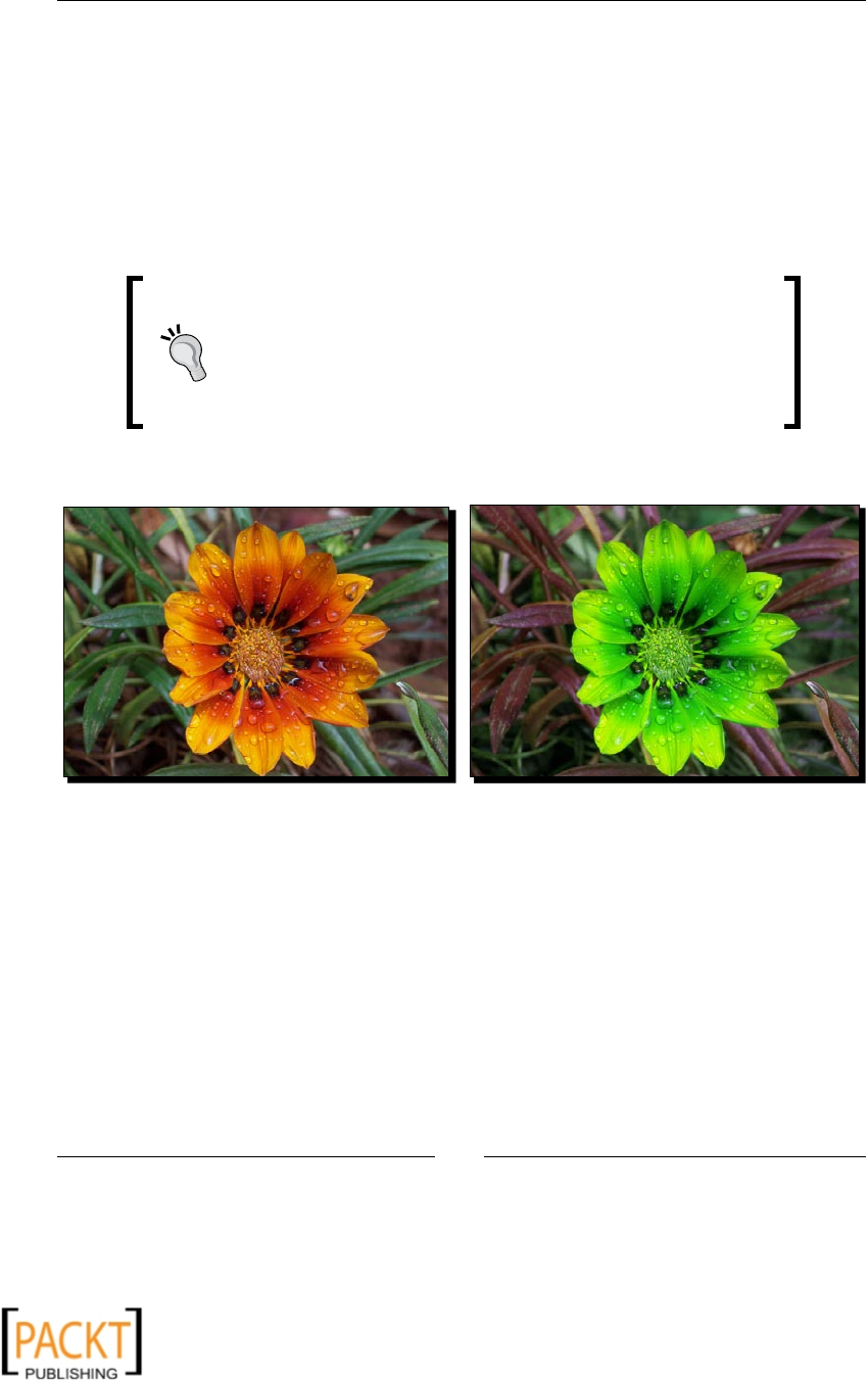
Enhancing Images
[ 60 ]
5. The code in line 6 does the main image processing. The rst argument that
Image.merge takes mode as the rst argument whereas the second argument is a
tuple of image instances containing band informaon. It is required to have same
size for all the bands. As you can noce, we have swapped the order of band data
in Image instances r and g while specifying the second argument.
6. The original and resultant image thus obtained are compared in the next illustraon.
The color of the ower now has a shade of green and the grass behind the ower is
rendered with a shade of red.
As menoned in the Installaon and Download Prerequisites
secon, the images compared in the following illustraon will
appear idencal if you are reading a hard copy of this book. Please
download and refer to the supplementary PDF le Chapter 3
Supplementary Material.pdf. Here, the color images are
provided that will help you see the dierence.
Original (le) and the color swapped image (right).
What just happened?
We accomplished creang an image with its band data swapped. We learned how to use
PIL's Image.split() and Image.merge() to achieve this. However, this operaon was
performed on the whole image. In the next secon, we will learn how to apply color changes
to a specic color region.
x
x

Chapter 3
[ 61 ]
Changing individual image band
In the previous secon, we saw how to change the data represented by the whole band. As
a result of this band swapping, the color of the ower was changed to a shade of green and
the grass color was rendered as a shade of red. What if we just want to change the color
of the ower and keep the color of the grass unchanged? To do this, we will make use of
Image.point funconality along with Image.paste operaon discussed in depth in the
previous chapter.
However, note that we need to be careful in specifying the color region that needs to be
changed. It may also depend on the image. Somemes, it will select some other regions
matching the specied color range, which we don't want.
Time for action – change the color of a ower
We will make use of the same ower image used in the previous secon. As menoned
earlier, our task is to change the color of the ower while keeping the grass color unchanged.
1. Add this code in a Python source le.
1 import Image
2
3 img = Image.open( "C:\\images\\COLOR_TWEAK.png ")
4 img = img.convert('RGBA')
5 r, g, b, alpha = img.split()
6 selection = r.point(lambda i: i > 120 and 150)
7 selection.save( "C:\\images\\COLOR_BAND_MASK.png ")
8 r.paste(g, None, selection)
9 img = Image.merge( "RGBA ", (r, g, b, alpha))
10 img.save( "C:\\images\\COLOR_CHANGE_BAND.png ")
11 img.show()
2. Lines 1 to 5 remain the same as seen earlier. On line 5, we split the original image,
creang four Image instances, each holding a single band data.
3. A new Image instance 'selecon' is created on line 6. This is an important operaon
that holds the key to selecvely modify color! So let's see what this line of code
does. If you observe the original image, the ower region (well, most of it) is
rendered with a shade of red color. So, we have called the point(function)
method on Image instance r. The point method takes a single funcon and an
argument maps the image through this funcon. It returns a new Image instance.
x
x

Enhancing Images
[ 62 ]
4. What does this lambda funcon on line 6 do? Internally, PIL's point funcon does
something of this sort:
lst = map(function, range(256)) * no_of_bands
In this example, function is nothing but the lambda funcon. The no_of_bands
for the image is 1. Thus, line 6 is used to select a region where the red value is
greater than 120. The lst is a list which, in this case has the rst 120 values as
False whereas the remaining values as 150. The value of 150 plays a role in
determining the nal color when we perform the paste operaon.
5. The image mask thus created aer the applicaon of point operaon is shown
in the following illustraon. The white region in this image represents the region
captured by the point operaon that we just performed. Only the white region
will undergo change when we perform paste operaon next.
6. On line 8, we perform a paste operaon discussed in the last chapter. Here, the
image g is pasted onto image r using mask selection. As a result, the band data
of image r is modied.
7. Finally, a new Image instance is created using the merge operaon, by making
use of the individual r, g, b, and alpha image instances containing the new
band informaon.
8. The original and nal processed images are compared in the next illustraon.
The new ower color looks as cool as the original color, doesn't it?
x
x

Chapter 3
[ 63 ]
As menoned in the Installaon and download prerequisites secon, the
images compared in the following illustraon will appear idencal if you
are reading a hard copy of this book. Please download and refer to the
supplementary PDF le Chapter 3 Supplementary Material.pdf.
The color images are provided that will help you see the dierence.
What just happened?
We worked out an example that modied a selecve color region. Individual image band
data was processed to accomplish this task. With the help of point, paste, and merge
operaons in PIL's Image module, we accomplished changing the color of the ower in
the provided image.
Gray scale images
If you want to give a nostalgic eect to an image, one of the many things that you can do
is to convert it to gray scale. There is more than one way to create a gray scale image in
PIL. When the mode is specied as L, the resultant image is gray scale. The basic syntax
to convert color images to black and white is:
img = img.convert('L')
Alternavely, we can use funconality provided in the ImageOps module.
img = ImageOps.grayscale(img)
If you are creang the image from scratch, the syntax is:
img = Image.new('L', size)
x
x
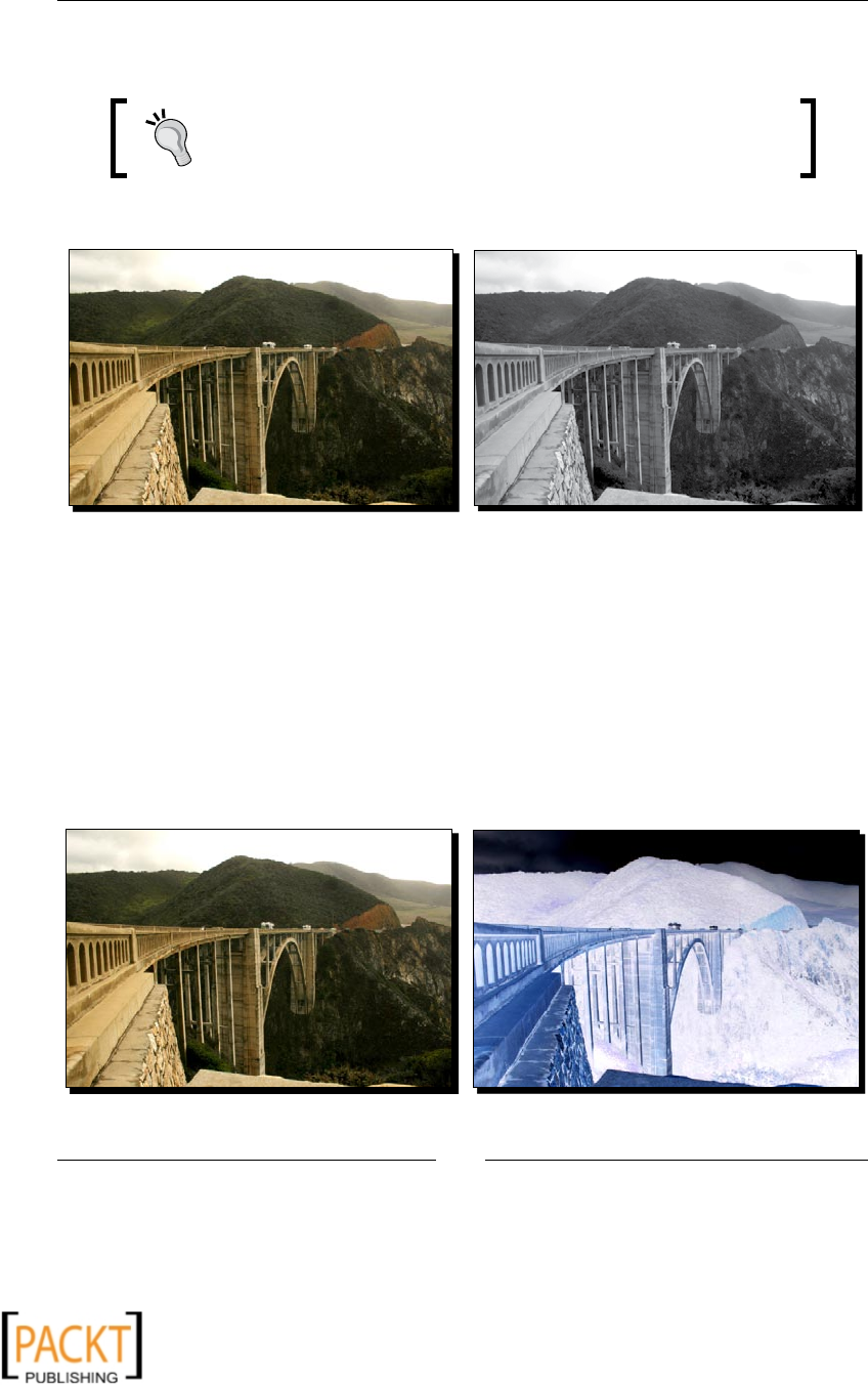
Enhancing Images
[ 64 ]
The following illustraon shows the original and the converted gray scale images created
using one of these techniques.
Please download and refer to the supplementary PDF le Chapter 3
Supplementary Material.pdf. The color images are provided
that will help you see the dierence between the following images.
Original and gray scale images of a bridge:
Cook up negatives
Creang a negave of an image is straighorward. We just need to invert each color pixel.
Therefore, if you have a color x at a pixel, the negave image will have (255 – x) at that pixel.
The ImageOps module makes it very simple. The following line of code creates a negave of
an image.
img = ImageOps.invert(img)
Here is the result of this operaon:
Original image (le) and its negave (right).
x
x

Chapter 3
[ 65 ]
Blending
Have you ever wished to see yourself in a family photo, taken at a me when you were not
around? Or what if you just want to see yourself at the top of Mount Everest at least in a
picture? Well, it is possible to do this digitally, using the funconality provided in PIL such
as blending, composite image processing, and so on.
In this secon, we will learn how to blend images together. As the name suggests, blending
means mixing two compable images to create a new image. The blend funconality in PIL
creates a new image using two input images of the same size and mode. Internally, the two
input images are interpolated using a constant value of alpha.
In the PIL documentaon, it is formulated as:
blended_image = in_image1 * (1.0 - alpha) + in_image2 * alpha
Looking at this formula, it is clear that alpha = 1.0 will make the blended image the same
as 'n_image2 whereas alpha = 0.0 returns in_image1 as the blended image.
Time for action – blending two images
Somemes, the combined eect of two images mixed together makes a big impact
compared to viewing the same images dierently. Now it's me to give way to your
imaginaon by blending two pictures together. In this example, our resultant image shows
birds ying over the Mackinac bridge in Michigan. However, where did they come from? The
birds were not there in the original image of the bridge.
1. Download the following les from Packt website: 0165_3_28_BRIDGE2.png
and 0165_3_29_BIRDS2.png. Rename these les as BRIDGE2.png and
BIRDS2.png respecvely.
2. Add the following code in a Python source le.
1 import Image
2
3 img1 = Image.open( "C:\\images\\BRIDGE2.png ")
4 img1 = img1.convert('RGBA')
5
6 img2 = Image.open( "C:\\images\\BIRDS2.png ")
7 img2 = img2.convert('RGBA')
8
9 img = Image.blend(img1, img2, 0.3)
10 img.show()
11 img.save( "C:\\images\\BLEND.png")
x
x
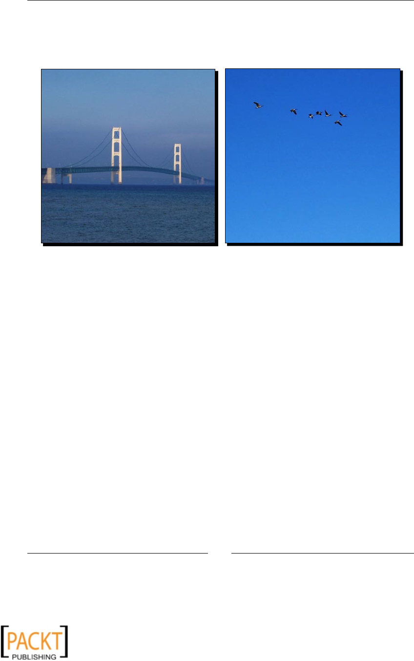
Enhancing Images
[ 66 ]
3. The next illustraon shows the two images before blending, represented by img1
and img2 in the code.
Individual images of a bridge and ying birds, before blending.
4. The lines 3 to 7 open the two input images to be blended. Noce that we have
converted both the images RGBA. It need not be necessarily RGBA mode. We can
specify the modes such as 'RGB' or 'L'. However, it is required to have both the
images with same size and mode.
5. The images are blended on line 9 using the Image.blend method in PIL. The rst
two arguments in the blend method are two Image objects represenng the two
images to be blended. The third argument denes the transparency factor alpha. In
this example, the image of the bridge is the main image we want to focus on. Thus,
the factor alpha is dened such that more transparency is applied to the image of
the ying birds while creang the nal image. The alpha factor can have a value
between 0.0 to 1.0. Note that, while rendering the output image, the second
image, img2, is mulplied by this alpha value whereas the rst image is
mulplied by 1 - alpha. This can be represented by the following equaon.
blended_img = img1 * (1 – alpha) + img2* alpha
Thus, if we select an alpha factor of, for instance, 0.8, it means that the birds will
appear more opaque compared to the bridge. Try changing the alpha factor to see
how it changes the resultant image. The resultant image with alpha = 0.3 is:
x
x
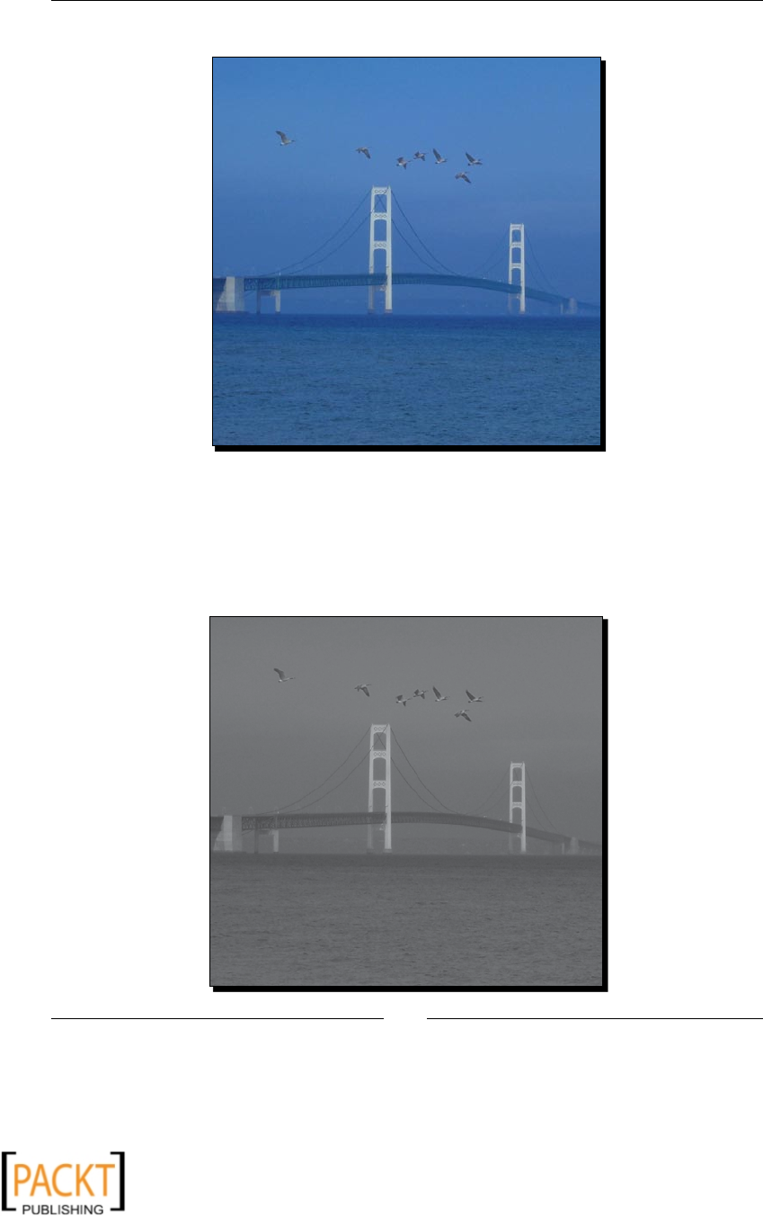
Chapter 3
[ 67 ]
Blended image showing birds ying over a bridge.
6. The picture appears a bit dull due to the transparency eect applied while creang
the image. If you convert the input images to mode L, the resultant image will
look beer—however, it will be rendered as gray scale. This is shown in the
next illustraon.
Blended gray scale image when both the input images have mode L.
x
x

Enhancing Images
[ 68 ]
What just happened?
Blending is an important image enhancement feature. With the help of examples, we
accomplished creang blended images. We learned using the Image.blend method and
applied the transparency factor alpha to achieve this task. The technique learned in this
chapter will be very useful throughout this chapter. In the next secon, we will apply the
blending technique to create a transparent image.
Creating transparent images
In the previous secon, we learned how to blend two images together. In this secon, we
will go one step further and see how the same blend funconality can be used to create a
transparent image! The images with mode RGBA dene an alpha band. The transparency
of the image can be changed by tweaking this band data. Image.putalpha() method
allows dening new data for the alpha band of an image. We will see how to perform
point operaon to achieve the same eect.
Time for action – create transparency
Let's write a few lines of code that add the transparency eects to an input image.
1. We will use one of the images used in Chapter 2. Download 0165_3_25_SMILEY.
png and rename it to SMILEY.png.
2. Use the following code:
1 import Image
2
3 def addTransparency(img, factor = 0.7 ):
4 img = img.convert('RGBA')
5 img_blender = Image.new('RGBA', img.size, (0,0,0,0))
6 img = Image.blend(img_blender, img, factor)
7 return img
8
9 img = Image.open( "C:\\images\\SMILEY.png ")
10
11 img = addTransparency(img, factor =0.7)
3. In this example, the addTransparency() funcon takes the img instance as input
and returns a new image instance with the desired level of transparency.
x
x

Chapter 3
[ 69 ]
4. Now let's see how this funcon works. On line 4, we rst convert the image mode to
RGBA. As discussed in an earlier secon, you can add a condional here to see if the
image is already in the RGBA mode.
5. Next, we create a new Image class instance, image_blender, using the Image.
new method. It has the same size and mode as the input image. The third argument
represents the color. Here, we specify the transparency as 0.
6. On line 6, two images, img (input image) and img_blender, are blended together
by applying a constant alpha value. The funcon then returns this modied
Image instance.
7. The original image and the one with the transparency eect are compared. The
images are the screenshots of the images opened in the GIMP editor. This is done
so that you clearly understand the eect of transparency. The checkered paern
in these images represents the canvas. Noce how the canvas appears in the
transparent image.
8. There is another simple way to add transparency to an image, using the Image.
point funconality! Enter the following code in a Python source le and execute it.
1 import Image
2 img = Image.open( "C:\\images\\SMILEY.png ")
3 r, g, b, alpha = img.split()
4 alpha = alpha.point(lambda i: i>0 and 178)
5 img.putalpha(alpha)
6 img.save( "C:\\images\\Transparent_SMILEY.png ")
9. In this new code, we split the original image into four new image instance, each
having one of the image band data (r, g, b, or alpha). Note that we are assuming
here that the mode of the image is RGBA. If it is not, you need to convert this image
to RGBA! As an exercise, you can add that check in the code.
10. Next, on line 4, the Image.point method is called. The lambda funcon operates
on the alpha band data. It sets the value as 178. This is roughly equal to the alpha
factor of 0.7 that we set earlier. It is computed here as int(255*0.7) ). In the
Changing individual image band secon, where we learned modifying colors
within images, the point operaon was thoroughly discussed.
x
x

Enhancing Images
[ 70 ]
11. On line 5, we put back the new alpha band data in img. The resultant images using
blend and point funconality are shown in the next illustraon.
Image before and aer adding transparency.
What just happened?
We accomplished adding transparency eect to an image. This is a very useful image
enhancement that we need from me to me. We learned how to create a transparent image
using two dierent techniques, namely, using Image.blend funconality and Image.point
operaon. The knowledge gained in this secon will be applied later in this chapter.
Making composites with image mask
So far, we have already seen how to blend two images together. It was done using the
Image.blend operaon where the two input images were blended by using a constant
alpha transparency factor. In this secon, we will learn another technique to combine two
images together. Here, instead of a constant alpha factor, an image instance that denes
the transparency mask is used as the third argument. Another dierence is that the input
images need not have the same mode. For instance, the rst image can be with mode L
and the second with mode RGBA. The syntax to create composite images is:
outImage = Image.composite(img1, img2, mask)
Here, the arguments to the composite method are Image instances. The mask is specied as
alpha. The mode for mask image instance can be 1, L, or RGBA.
x
x

Chapter 3
[ 71 ]
Time for action – making composites with image mask
We will mix the same two images blended in another secon. Just to try out something
dierent, in the composite image, we will focus on the ying birds instead of the bridge.
1. We will use the same set of input images as used in the Blending secon.
1 import Image
2
3 img1 = Image.open( "C:\\images\\BRIDGE2.png ")
4 img1 = img1.convert('RGBA')
5
6 img2 = Image.open( "C:\\images\\BIRDS2.png ")
7 img2 = img2.convert('RGBA')
8
9 r, g, b, alpha = img2.split()
10 alpha = alpha.point(lambda i: i>0 and 204)
11
12 img = Image.composite(img2, img1, alpha)
13 img.show()
2. The code unl line 7 is idencal to the one illustrated in the blending example. Note
that the two input images need not have the same mode. On line 10, the Image.
point method is called. The lambda funcon operates on the alpha band data.
The code on lines 9 and 10 is similar to that illustrated in the secon Creang
Transparent Images. Please refer to that secon for further details. The only
dierence is that the pixel value is set as 204. This modies the band data in the
image instance alpha. This value of 204 is roughly equivalent to the alpha factor
of 0.7 if the image were to be blended. What this implies is the bridge will have a
fading eect and the ying birds will appear prominently in the composite image.
3. One thing you will noce here is we are not pung the modied alpha band data
back in img2. Instead, on line 12, the composite image is created using the mask
as alpha.
x
x

Enhancing Images
[ 72 ]
4. The resultant composite image is shown in the next illustraon—with emphasis on
the image of the ying birds.
What just happened?
We learned how to create an image combining two images, using an alpha mask. This was
accomplished by using Image.composite funconality.
Project: Watermark Maker Tool
We have now learned enough image enhancement techniques to take up a simple project
applying these techniques. Let's create a simple command line ulity, a "Watermark Maker
Tool". Although we call it a "Watermark Maker ", it actually provides some more useful
features. Using this ulity, you can add the date stamp to the image (the date on which
the image was enhanced using this tool). It also enables embedding custom text within
an image. The tool can be run on the command line using the following syntax:
python WaterMarkMaker.py [options]
x
x

Chapter 3
[ 73 ]
Where, the [options] are as follows:
--image1: The le path of the main image that provides canvas.
--waterMark: The le path of the watermark image (if any).
--mark_pos: The coordinates of top-le corner of the watermark image to be
embedded. The values should be specied in double quotes, like 100, 50.
--text: The text that should appear in the output image.
--text_pos: The coordinates of top-le corner of the TEXT to be embedded.
The values should be specied in double quotes, like 100, 50.
--transparency: The transparency factor for the watermark (if any)
--dateStamp: Flag (True or False) that determines whether to insert date
stamp in the image. If True, the date stamp at the me this image was processed
will be inserted.
The following is an example that shows how to run this tool with all the opons specied.
python WaterMarkMaker.py --image1= "C:\foo.png "
--watermark= "C:\watermark.png "
--mark_pos= "200, 200 "
--text= "My Text "
–-text_pos= "10, 10 "
--transparency=0.4
--dateStamp=True
This creates an output image le WATERMARK.png, with a watermark and text at the
specied anchor point within the image.
Time for action – Watermark Maker Tool
Think about all the methods we would need to accomplish this. The rst thing that comes to
mind is a funcon that will process the command-line arguments menoned earlier. Next,
we need to write code that can add a watermark image to the main image. Let's call this
addWaterMark(). On similar lines, we will need methods that add text and date stamp
to the image. We will call this addText() and addDateStamp() respecvely. With this
informaon, we will develop code to make this work. In this project, we will encapsulate
this funconality in a class, but it is not necessary. We do so to make this tool extensible
for future use.
1. Download the le WaterMarkMaker.py. This has the code required in this
project. Just keep it for further use. Some of the methods will not be discussed in
this secon. If you encounter dicules while developing those methods, you can
always go back and refer to this le.
x
x

Enhancing Images
[ 74 ]
2. Open a new Python source le and declare the following class and its methods. Just
create empty methods for now. We will expand these in as we proceed along.
import Image, ImageDraw, ImageFont
import os, sys
import getopt
from datetime import date
class WaterMarkMaker:
def __init__(self):
pass
def addText(self):
pass
def addDateStamp(self):
pass
def _addTextWorker(self, txt, dateStamp = False):
pass
def addWaterMark(self):
pass
def addTransparency(self, img):
pass
def createImageObjects(self):
pass
def _getMarkPosition(self, canvasImage, markImage):
return
def processArgs(self):
pass
def printUsage(self):
pass
3. Next, we will write code in the constructor of this class.
def __init__(self):
# Image paths
self.waterMarkPath = ''
self.mainImgPath = ''
# Text to be embedded
self.text = ''
# Transparency Factor
self.t_factor = 0.5
# Anchor point for embedded text
self.text_pos = (0, 0)
# Anchor point for watermark.
self.mark_pos = None
# Date stamp
self.dateStamp = False
# Image objects
self.waterMark = None
self.mainImage = None
x
x

Chapter 3
[ 75 ]
self.processArgs()
self.createImageObjects()
self.addText()
self.addWaterMark()
if self.dateStamp:
self.addDateStamp()
self.mainImage.save( "C:\\images\\WATERMARK.png ")
self.mainImage.show()
4. The code is self-explanatory. First, all the necessary aributes are inialized and
then the relevant methods are called to create the image with watermark and/or
the embedded text. Let's write the methods in the order in which they are called
in the constructor.
5. The processArgs() method processes the command-line arguments. You
can write this method as an exercise. Alternavely, you can use code in the
WaterMarkMaker.py le from the Packt website. The process arguments method
should take the assignments as shown in the following table. In the reference les,
getopt module is used to process these arguments. Alternavely, you can use
OptionParser in the optparse module of Python.
Argument Value Argument Value
image1 self.mainImgPath text_pos self.text_pos
waterMark self.waterMarkPath transparency self.t_factor
mark_pos self.mark_pos dateStamp self.dateStamp
text self.text
6. The printUsage() method just prints how to run this tool. You can easily write
that method.
7. Let's review the addText()and _addTextWorker() methods now. Note that
some of the code comments are removed from the code samples for clarity. You
can refer to the code in WaterMarkMaker.py for detailed comments.
def addText(self):
if not self.text:
return
if self.mainImage is None:
print "\n Main Image not defined.Returning. "
return
txt = self.text
self._addTextWorker(txt)
The addText() method simply calls _addTextWorker() by providing the
self.text argument received from the command line.
x
x

Enhancing Images
[ 76 ]
8. The _addTextWorker() does the main processing that embeds the text within the
image. This method is used in the following code:
1 def _addTextWorker(self, txt, dateStamp = False):
2 size = self.mainImage.size
3 color = (0, 0, 0)
4 textFont = ImageFont.truetype( "arial.ttf ", 50)
5
6 # Create an ImageDraw instance to draw the text.
7 imgDrawer = ImageDraw.Draw(self.mainImage)
8 textSize = imgDrawer.textsize(txt, textFont)
9
10 if dateStamp:
11 pos_x = min(10, size[0])
12 pos_y = size[1] - textSize[0]
13 pos = (pos_x, pos_y)
14 else:
15 # We need to add text. Use self.text_pos
16 pos = self.text_pos
17 #finally add the text
18 imgDrawer.text(pos, txt, font=textFont)
19
20 if ( textSize[0] > size[0]
21 or textSize[1] > size[1] ):
22 print ( "\n Warning, the specified text "
23 "going out of bounds. " )
In Chapter 2, we created a new image containing a text string. It read "Not really
a fancy text ". Do you remember? Here, we have wrien similar code with some
improvements. The funcon ImageDraw.Draw takes the self.mainImage
(an Image instance) as an argument to create a Draw instance, imgDrawer.
On line 18, the text is embedded onto the given posion using a given font. The
text() method of Draw instance takes three arguments, namely, position,
text, and the font. In the previous chapter, we already made use of the rst two
arguments. The third argument font is an instance of class ImageFont in PIL.
On line 4, we create this instance specifying a font type (arial.ttf) and the font
size (=50). The given text string is now added on to the main image!
x
x

Chapter 3
[ 77 ]
9. The next method we will discuss is addDateStamp(). It calls the same
_addTextWorker() in the end. However, the placement of this date stamp is
xed at the boom le corner of the image and of course we create our date string
by using Python's datetime module. The code is illustrated below along with the
import statement declared earlier.
from datetime import date
def addDateStamp(self):
today = date.today()
time_tpl = today.timetuple()
year, month, day = map(str, time_tpl)
datestamp = "%s/%s/%s "%(year,month, day)
self._addTextWorker(datestamp, dateStamp = True)
The rst line of the code in this method creates a date instance today with today's
date provided as a 3-tuple. Something like this: datetime.date(2010, 1, 20).
Next, we call the timetuple method of date instance. The rst three values in this
tuple are year, month, and day respecvely.
The rest of the code is just the processing of the date stamp as a text string and then
calling the main worker method just discussed.
10. Now we will review the code in the addWaterMark() method. A watermark is
typically a semi-transparent image that appears in the main image. There are two
dierent approaches to accomplish creang a watermark. The following code
considers both these approaches.
1 def addWaterMark(self):
2 # There are more than one way to achieve creating a
3 # watermark. The following flag,if True, will use
4 # Image.composite to create the watermark instead of a
5 # simple Image.paste
6 using_composite = False
7
8 if self.waterMark is None:
9 return
10 # Add Transparency
11 self.waterMark = self.addTransparency(self.waterMark)
12 # Get the anchor point
13 pos_x, pos_y = self._getMarkPosition(self.mainImage,
14 self.waterMark)
15 # Create the watermark
16 if not using_composite:
17 # Paste the image using the transparent
18 # watermark image as the mask.
x
x

Enhancing Images
[ 78 ]
19 self.mainImage.paste(self.waterMark,
20 (pos_x, pos_y),
21 self.waterMark)
22 else:
23 # Alternate method to create water mark.
24 # using Image.composite create a new canvas
25 canvas = Image.new('RGBA',
26 self.mainImage.size,
27 (0,0,0,0))
28 # Paste the watermark on the canvas
29 canvas.paste(self.waterMark, (pos_x, pos_y))
30 # Create a composite image
31 self.mainImage = Image.composite(canvas,
32 self.mainImage,
33 canvas)
11. To add a watermark, rst we make the image transparent. This is accomplished by
calling the addTransparency() method. This method also changes the mode
of the image to RGBA. This method is shown here. It is almost idencal to the one
we developed in an earlier secon where an image was made transparent using
blending funconality of PIL.
def addTransparency(self, img):
img = img.convert('RGBA')
img_blender = Image.new('RGBA',
img.size,
(0,0,0,0))
img = Image.blend(img_blender,
img,
self.t_factor)
return img
Next, on line 13, we determine the anchor point on the main image, where the top-
le corner of the watermark will appear. By default, we will match the boom-le
corner of the watermark with the main image. You can review the code for method
_getMarkPosition() in the le WaterMarkMaker.py to see how this is done.
Moving forward, the code block between lines 16-21 creates the watermark using
the paste funconality. This is one way to create the image with a watermark. The
arguments provided in the Image.paste funcon are image to be pasted,
anchor point, and mask. The mask is selected as the watermark image itself so as
to consider the transparency. Otherwise, the watermark image will appear opaque.
The resultant image with and without image mask specicaon is compared in the
following illustraon.
x
x
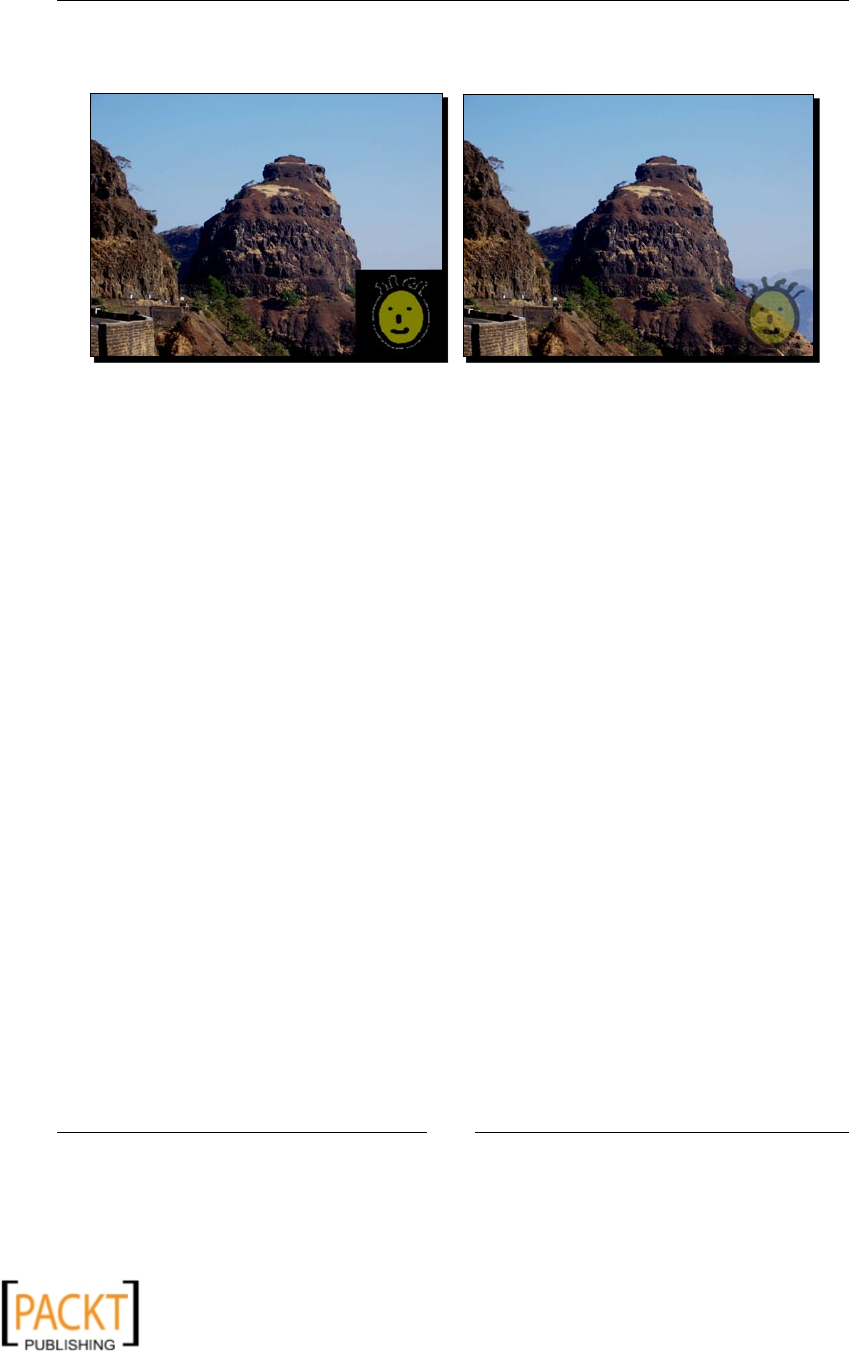
Chapter 3
[ 79 ]
Resultant images using Image.paste operaon created with and
without mask.
Next, in the else condion block (lines 22 to 33), we use Image.composite
funconality in PIL to embed the watermark. The dimensions of the example
watermark image used here are 200x200 pixels, whereas the dimensions of the
main image are 800x600 pixels. To use the composite() method, we need to
make these images of the same size, and yet, make sure to paste the watermark at
the specied posion. How to achieve this? The rst thing to do is to create a canvas
image to hold the watermark. The canvas image is of the same size as that of the
main image. The code block 25-29 creates the canvas and pastes the watermark at
an appropriate locaon.
Finally, on line 31, the composite image is created using the canvas image instance
as the alpha mask.
12. Now lets run this tool! You can use your own image les for main image or the
watermark. Alternavely, you can use the image 0165_3_34_KokanPeak_for_
WATERMARK.png as the main image and 0165_3_38_SMILEY_small.png as the
watermark image. The command-line arguments for this run are:
python WaterMarkMaker.py
--image1= "C:\images\KokanPeak_for_WATERMARK.png "
--text= "Peak "
--text_pos= "10, 10 "
--waterMark= "C:\\images\\SMILEY_small.png "
--dateStamp=True
x
x
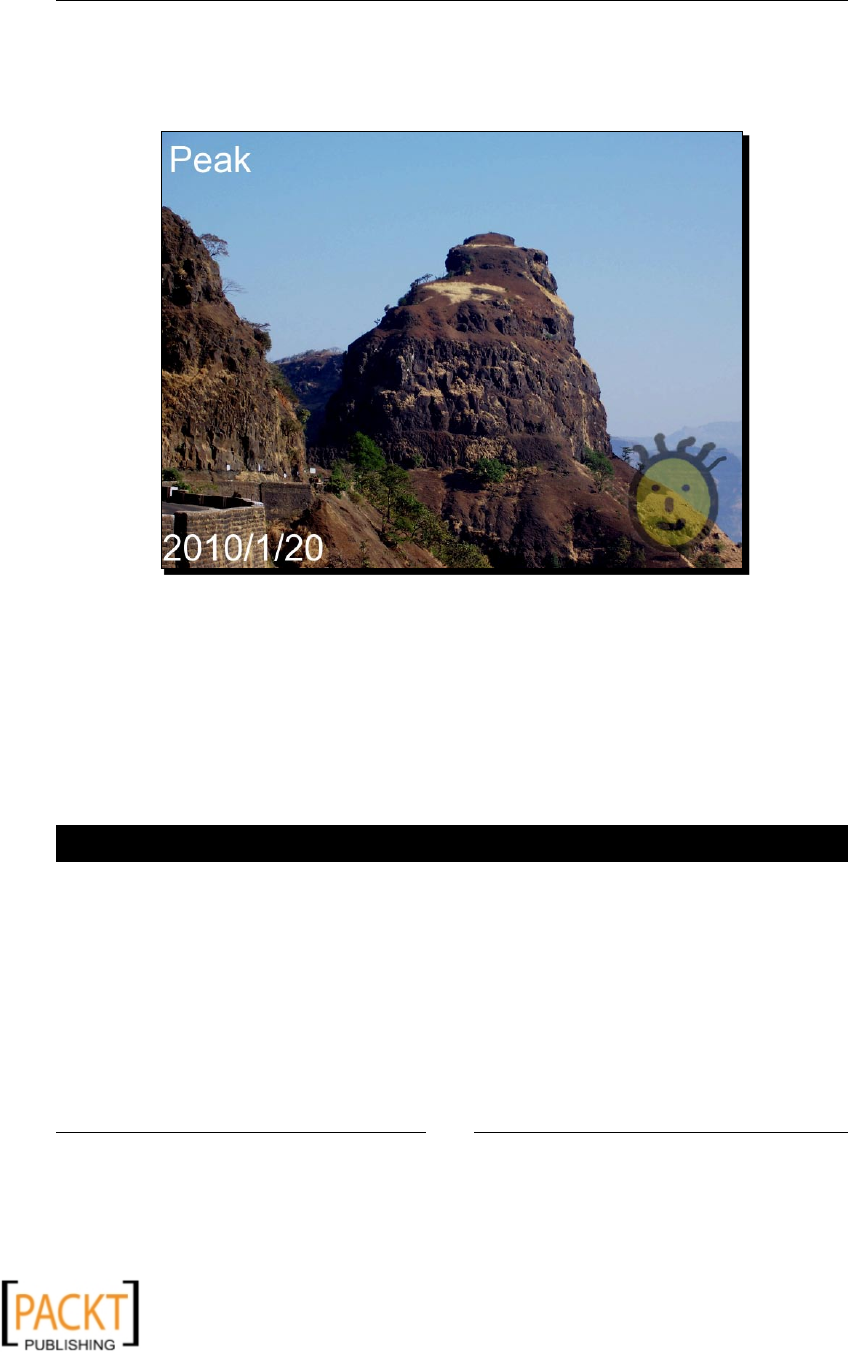
Enhancing Images
[ 80 ]
13. The resultant image with text, date stamp, and the watermark is shown in the
next illustraon.
Final processed image with text, date stamp, and a watermark.
What just happened?
We created a very useful ulity that can add a watermark and/or a text string and/or a date
stamp to an input image. We used several of the image processing techniques learned in this
as well as in an earlier chapter on image processing. Especially, image enhancement features
such as blending, creang composite images, and adding transparency were applied to
accomplish this task. Addionally we made use of common funconality such as pasng
an image, drawing text onto the image, and so on.
Have a go hero – do more with Watermark Maker Tool
Our Watermark Maker tool needs an upgrade. Extend this applicaon so that it supports
following the features:
1. The text or the date stamp color is currently hardcoded. Add a new command-line
argument so that a text color can be specied as an oponal argument.
2. Add some standard default opons for specifying anchor posion for text, date
stamp, and the watermark image. These opons can be TOP_RIGHT, TOP_LEFT,
BOTTOM_RIGHT, and BOTTOM_LEFT.
x
x

Chapter 3
[ 81 ]
3. The command-line opons list is too long. Add code so that all arguments can be
read from a text le.
4. Add support so that it can batch-process images to create desired eect.
Applying image lters
In the previous chapter, filter argument was used while performing the image resize
operaon. This filter determined the quality of the output image. However, there were
only four filter opons available and the scope was limited to a resize operaon. In this
secon, some addional image enhancement lters will be introduced. These are predened
lters and can be directly used on any input image. Following is a basic syntax used for
applying a lter.
img = Image.open('foo.jpg')
filtered_image = img.filter(FILTER)
Here, we created a new image filtered_image by ltering imageby ltering image img . The FILTER
argument can be one of the predened lters in the ImageFilter module of PIL for
ltering the image data. PIL oers several predened image enhancement lters. These can
be broadly classied into the following categories. With the help of examples, we will learn
some of these in the coming secons.
Blurring and sharpening: BLUR, SHARPEN, SMOOTH, SMOOTH_MORE
Edge detecon and enhancement: EDGE_ENHANCE, EDGE_ENHANCE_MORE,
FIND_EDGES, CONTOUR
Distoron/special eects: EMBOSS
The le ImageFilter.py in the PIL source code denes the-menoned lter classes. You
can create your own custom lter by tweaking various arguments in these lter classes.
filterargs = size, scale, offset, kernel
Where, kernel is the convoluon kernel. Here, the 'convoluon' is a mathemacal
operaon, on the image matrix by the 'kernel' matrix to produce a resultant matrix.
The size of matrix is specied by the size argument. It is specied in the form (width, height).
This can either be (3, 3) or (5, 5) size in the current PIL version. The result of each pixel is
divided by scale argument. This is an oponal argument. The offset value, if specied,
has its value is added to the result aer dividing it by the scale argument.
In some of the image enhancement lter examples, we will create our own custom lter.
x
x

Enhancing Images
[ 82 ]
Smoothing
Smoothing an image means reducing the noise within the image data. For this, certain
mathemacal approximaon is applied on the image data to recognize the important
paerns within the image. The ImageFilter module denes class SMOOTH for smoothing
an image. PIL species the following default lter arguments for the image-smoothing lter.
filterargs = (3, 3),
13,
0,
(1, 1, 1,
1, 5, 1,
1, 1, 1)
Time for action – smoothing an image
Let's work out an example where a smoothing lter will be applied to an image.
1. Download the image le 0165_3_Before_SMOOTHING.png from the Packt
website and save it as Before_SMOOTHING.png.
2. This is a low-resoluon image scanned from a developed photograph. As you can
see, there is a lot of salt-and-pepper noise in the image. We will apply smoothing
lter to reduce some of this noise in the image data.
3. Add the following code in a Python le.
import ImageFilter
import Image
img = Image.open( "C:\\images\\Before_SMOOTH.png ")
img = img.filter(ImageFilter.SMOOTH)
img.save( "C:\\images\\ch3\\After_SMOOTH.png")
img.show()
x
x

Chapter 3
[ 83 ]
4. The highlighted line in the code is where the smoothing lter is applied to the
image. The results are shown in the next illustraon.
Picture before and aer smoothing:
5. To reduce the noise further down, you can use ImageFilter.SMOOTH_MORE
or try reapplying the ImageFilter.SMOOTH mulple mes unl you get the
desired eect.
import ImageFilter
import Image
img = Image.open( "C:\\images\\0165_3_2_Before_SMOOTH.png ")
i = 0
while i < 5:
img = img.filter(ImageFilter.SMOOTH)
i += 1
img.save( "C:\\images\\0165_3_3_After_SMOOTH_5X.png")
img.show()
x
x

Enhancing Images
[ 84 ]
As you can observe in the illustraon, the noise is further reduced but the
image appears a lile bit hazy. Thus, one has to determine an appropriate
level of smoothness.
Comparison of the resultant image with single and mulple smoothing lters.
What just happened?
We learned how to reduce high-level noise from the image data using the smoothing lter in
the ImageFilter module.
Sharpening
In the earlier secon, we learned image-smoothing techniques. If you want to view
the ner details within an image, a sharpening lter can be applied over the image.
Like image-smoothing lters, PIL provides predened lters for sharpening called
ImageFilter.SHARPEN. The basic syntax to sharpen an image is as follows:
img = img.filter(ImageFilter.SHARPEN)
You can try this lter on the image that was smoothed mulple mes in the earlier secon.
Blurring
In general, blurring makes an image lose its focus. In PIL, the predened lter for this is
ImageFilter.BLUR. This is typically useful if you want to fade out the background to
highlight some object in the foreground. The syntax is similar to the one used for other lters.
img = img.filter(ImageFilter.BLUR)
x
x
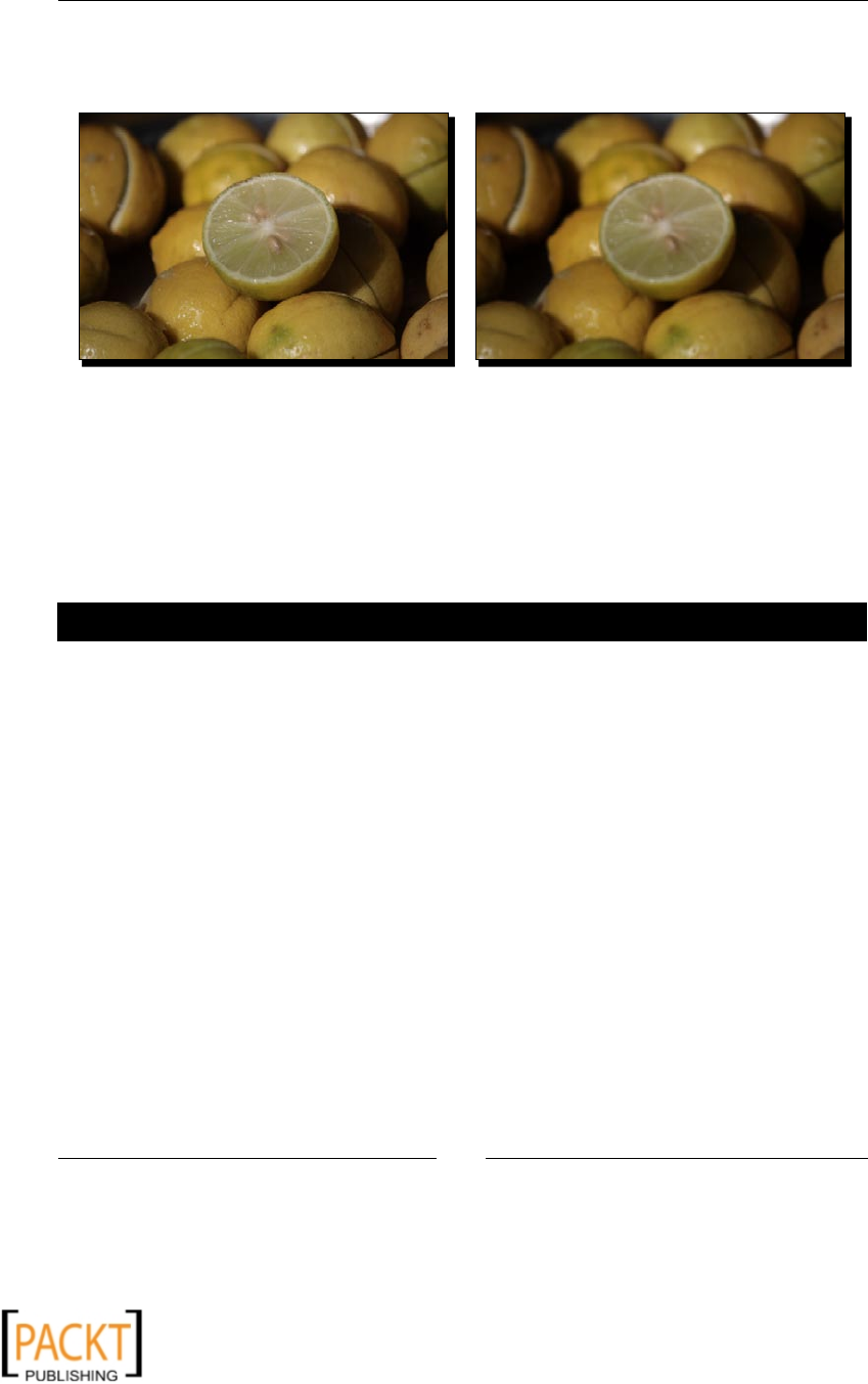
Chapter 3
[ 85 ]
The following illustraon shows the eect of this lter.
Image before and aer applicaon of blurring lter:
Edge detection and enhancements
In this secon, we will learn some general edge detecon and enhancement lters. The
edge enhance lter improves the edge contrast. It increases the contrast of the region very
close to the edge. This makes the edge stand out. The edge detecon algorithm looks for
disconnuies within the pixel data of the image. For example, it looks for sharp change in
the brightness to idenfy an edge.
Time for action – detecting and enhancing edges
Let's see how the edge detecon and enhancement lters modify the data of a picture. The
photograph that we will use is a close-up of a leaf. The original photo is shown in the next
illustraon. Applying an edge detecon lter on this image creates a cool eect where only
edges are highlighted and the remaining poron of the image is rendered as black.
1. Download the image 0165_3_6_Before_EDGE_ENHANCE.png from the Packt
website and save it as Before_EDGE_ENHANCE.png.
2. Add the following code in a Python le.
1 import Image
2 import ImageFilter
3 import os
4 paths = [ "C:\images\Before_EDGE_ENHANCE.png ",
5 "C:\images\After_EDGE_ENHANCE.png ",
6 "C:\images\EDGE_DETECTION_1.png ",
7 "C:\images\EDGE_DETECTION_2.png "
8 ]
9 paths = map(os.path.normpath, paths)
10
x
x
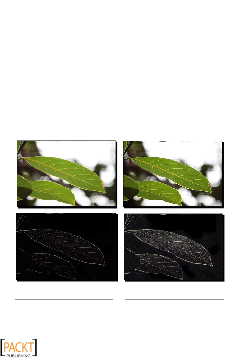
Enhancing Images
[ 86 ]
11 ( imgPath ,outImgPath1,
12 outImgPath2, outImgPath3) = paths
13 img = Image.open(imgPath)
14 img1 = img.filter(ImageFilter.FIND_EDGES)
15 img1.save(outImgPath1)
16
17 img2 = img.filter(ImageFilter.EDGE_ENHANCE)
18 img2.save(outImgPath2)
19
20 img3 = img2.filter(ImageFilter.FIND_EDGES)
21 img3.save(outImgPath3)
3. Line 14 modies the image data using the FIND_EDGES lter and then the resulng
image is saved.
4. Next, we modify the original image data, so that more veins within the leaf become
visible. This is accomplished by the applicaon of ENHANCE_EDGES lter (line 17).
5. On line 20, the FIND_EDGES lter is applied on the edge-enhanced image. The
resultant images are compared in the next illustraon.
a) First row: Images before and aer applicaon of edge enhancement lter b)
Second row: The edges detected by ImageFilter.FIND_EDGES lter.
x
x

Chapter 3
[ 87 ]
What just happened?
We created an image with enhanced edges by applying the EDGE_ENHANCE lter in the
ImageFilter module. We also learned how to detect edges within the image using the
edge detecon lter. In the next secon, we will apply a special form of the edge lter that
highlights or darkens the detected edges within an image. It is called an embossing lter.
Embossing
In image processing, embossing is a process that gives an image a 3-D appearance. The edges
within the image appear raised above the image surface. This opcal illusion is accomplished
by highlighng or darkening edges within the image. The following illustraon shows original
and embossed images. Noce how the edges along the characters in the embossed image
are either highlighted or darkened to give the desired eect.
The ImageFiltermodule provides a predened lter, ImageFilter.EMBOSS, to achieve
the embossing eect for an image. The convoluon kernel of this lter is of a (3, 3) size and
the default lter arguments are:
filterargs = (3, 3), 1, 128, (
-1, 0, 0,
0, 1, 0,
0, 0, 0
)
Time for action – embossing
1. Download the image 0165_3_4_Bird_EMBOSS.png from the Packt website and
save it as Bird_EMBOSS.png.
2. Add the following code in a Python le:
1 import os, sys
2 import Image
3 import ImageFilter
4 imgPath = "C:\images\Bird_EMBOSS.png "
5 outImgPath = "C:\images\Bird_EMBOSSED.png "
6 imgPath = os.path.normpath(imgPath)
x
x
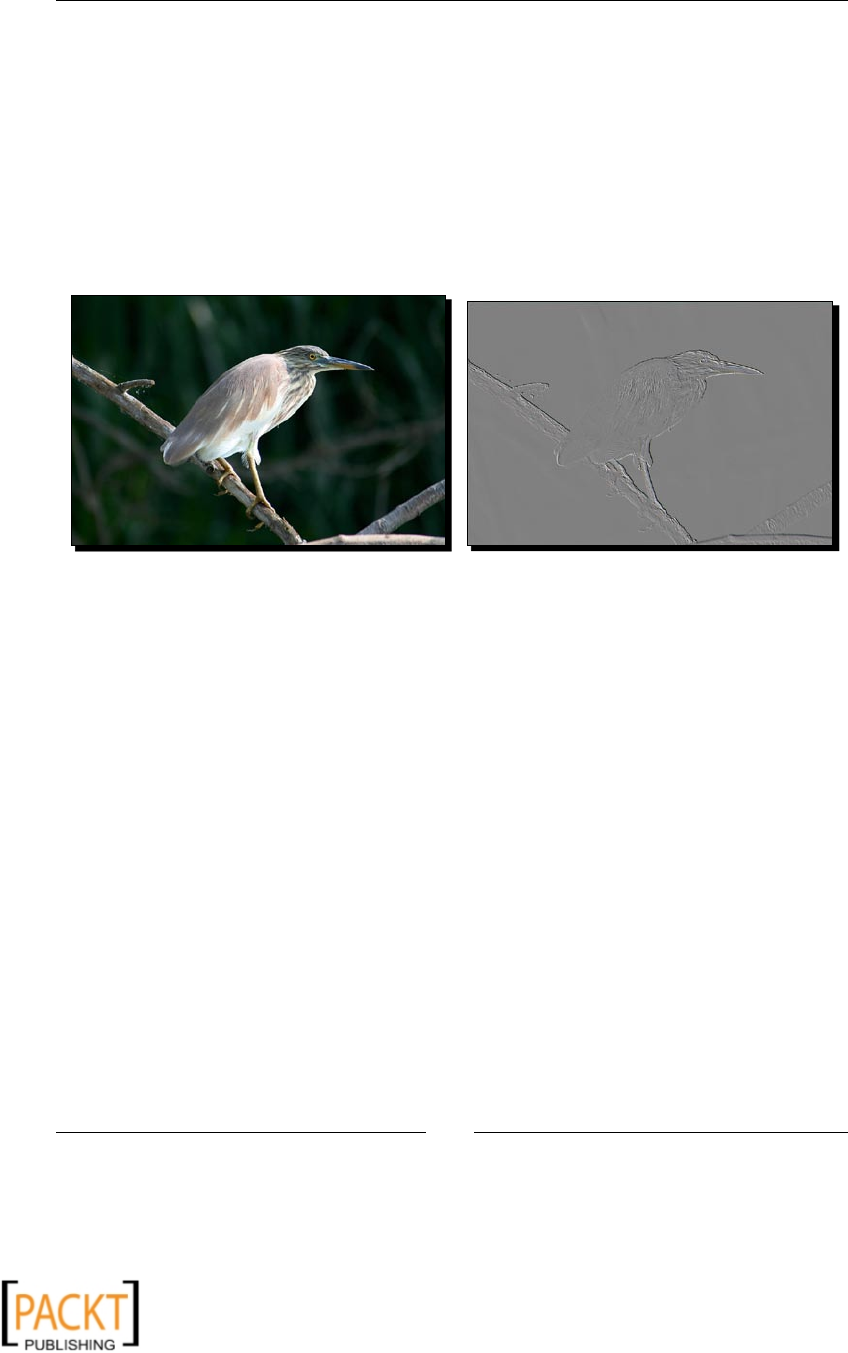
Enhancing Images
[ 88 ]
6 outImgPath = os.path.normpath(outImgPath)
7 bird = Image.open(imgPath)
8 bird = bird.filter(ImageFilter.EMBOSS)
9 bird.save(outImgPath)
10 bird.show()
3. On line 9, the embossing lter ImageFilter.EMBOSS is applied to the
image object bird. The resultant embossed image of the bird is shown
in the next illustraon.
Original and embossed images of a bird using ImageFilter.EMBOSS.
What just happened?
We applied an embossing lter on an image and created an embossed image. As seen in
previous secon, the lter modied the brightness of various edges to make them appear
highlighted or darkened. This created an opcal illusion where the image appeared raised
above the surface.
Adding a border
How would you prefer viewing a family photo? As a bare picture or enclosed in a nice photo
frame? In ImageOps module, PIL provides a preliminary funconality to add a plain border
around the image. Here is the syntax to achieve this:
img = ImageOps.expand(img, border, fill)
x
x

Chapter 3
[ 89 ]
This code creates a border around the image. Internally, PIL just creates an image that has
dimesions such that:
new_width = ( right_border_thickness + image_width +
left_border_thickness )
new_height = ( top_border_thickness + image_height +
bottom_border_thickness )
Then, the original image is pasted onto this new image to create the border eect. The
border argument in the preceding code suggests border thickness in pixels. It is uniform
in this example and is set to 20 pixels for le, right, top, and boom borders. The fill
argument species the border color. It can be a number in the range 0 to 255 indicang the
pixel color, where 0 is for 'black' and 255 for 'white' border. Alternavely, you can specify a
string represenng a color, such as 'red' for red color, and so on.
Time for action – enclosing a picture in a photoframe
Let's develop code that adds a frame around a picture.
1. Download the image 0165_3_15_COLOR_TWEAK.png and rename it to
FLOWER.png.
2. Add the following code in a Python source le. Make sure to modify the code
to specify in the input and output paths appropriately.
1 import Image, ImageOps
2 img = Image.open( "C:\\images\\FLOWER.png ")
3 img = ImageOps.expand(img, border=20, fill='black')
4 img = ImageOps.expand(img, border=40, fill='silver')
5 img = ImageOps.expand(img, border=2, fill='black')
6 img.save( "C:\\images\\PHOTOFRAME.png ")
7 img.show()
3. In this code snippet, three stacked borders are created. The innermost border layer
is rendered with black color. This is intenonally chosen darker.
4. Next, there is a middle layer of border, rendered with a lighter color (silver color in
this case). This is done by the code on line 4. It is thicker than the innermost border.
5. The outermost border is created by code on line 5. It is a very thin layer rendered
as black.
6. Together, these three layers of borders create an opcal illusion of a photo frame, by
making the border appear raised above the original image.
x
x
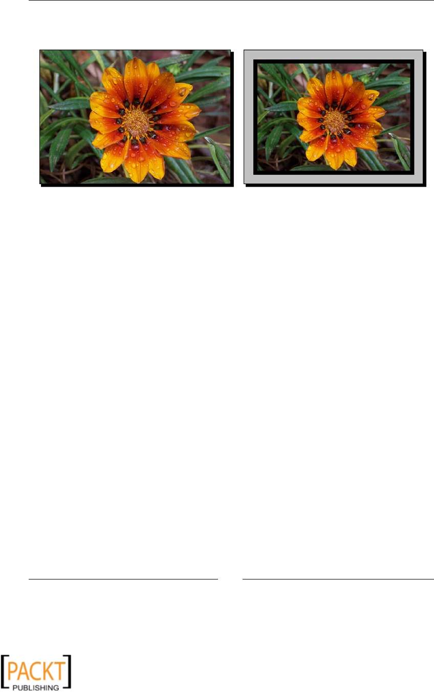
Enhancing Images
[ 90 ]
7. The following image shows the result of adding this border to the specied input
image—it shows the image before and aer enclosing in a 'photo frame'.
What just happened?
We learned how to create a simple border around an image. By calling ImageOps.expand
mulple mes, we created a mul-layered border having each layer of variable thickness and
color. With this, we accomplished creang an opcal illusion where the picture appears to be
enclosed within a simple photo frame.
Summary
This chapter taught us several important image enhancement techniques, specically:
With the help of ample examples, we learned how to adjust the color, brightness,
and contrast of an image.
We learned how to blend images together create composites using image mask and
how to add transparency.
We applied blending, pasng, and other techniques learned to develop an
interesng tool. We implemented features in this tool that enabled inserng
a watermark, text, or date stamp to an image.
A number of image enhancement lters were discussed. Using code snippets we
learned how to reduce high-level noise from image, enhance edges, add sharpening
or blurring eects, emboss an image, and so on.
We learned miscellaneous other useful image enhancements such as creang
negaves and adding border eects to the image.
x
x

4
Fun with Animations
Cartoons have always fascinated the young and old alike. An animaonanimaon
is where the imaginary creatures become alive and take us to a totally
dierent world.
Animaon is a sequence of frames displayed quickly one aer the other. This
creates an opcal illusion where the objects, for instance, appear to be movingillusion where the objects, for instance, appear to be moving
around. This chapter will introduce you to the fundamentals of developing
animaons using Python and Pyglet mulmedia applicaon development
frameworks. Pyglet is designed to do 3D operaons, but we will use it for
developing very simple 2D animaons in this book..
In this chapter, we shall:
Learn the basics of Pyglet framework. This will be used to develop code to create or
play animaons.
Learn how to play an exisng animaon le and create animaons using a sequence
of images.
Work on project 'Bowling animaon', where animaons can be controlled using
inputs from the keyboard.
Develop code to create an animaon using dierent regions of a single image.
Work on an excing project that animates a car moving in a thunderstorm. This
project will cover many important things covered throughout this chapter.
So let's get on with it.
x
x

Fun with Animaons
[ 92 ]
Installation prerequisites
We will cover the prerequisites for the installaon of Pyglet in this secon.
Pyglet
Pyglet provides an API for mulmedia applicaon development using Python. It is an
OpenGL-based library, which works on mulple plaorms. It is primarily used for developing
gaming applicaons and other graphically-rich applicaons. Pyglet can be downloaded from
http://www.pyglet.org/download.html. Install Pyglet version 1.1.4 or later. The
Pyglet installaon is prey straighorward.
Windows platform
For Windows users, the Pyglet installaon is straighorward—use the binary distribuon
Pyglet 1.1.4.msi or later.
You should have Python 2.6 installed. For Python 2.4, there are some more
dependencies. We won't discuss them in this book, because we are using
Python 2.6 to build mulmedia applicaons.
If you install Pyglet from the source, see the instrucons under the next sub-secon,
Other plaorms.
Other platforms
The Pyglet website provides a binary distribuon le for Mac OS X. Download and install
pyglet-1.1.4.dmg or later.
On Linux, install Pyglet 1.1.4 or later if it is available in the package repository of your
operang system. Otherwise, it can be installed from source tarball as follows:
Download and extract the tarballextract the tarball the tarball pyglet-1.1.4.tar.gz or a later version.
Make sure that python is a recognizable command in shell. Otherwise, set therecognizable command in shell. Otherwise, set the command in shell. Otherwise, set the
PYTHONPATH environment variable to the correct Python executable path.
In a shell window, change to the menoned extracted directory and then run then a shell window, change to the menoned extracted directory and then run the
following command:
python setup.py install
Review the succeeding installaon instrucons using the README/install instrucon
les in the Pyglet source tarball.
x
x

Chapter 4
[ 93 ]
If you have the package setuptools (http://pypi.python.org/
pypi/setuptools) installed, the Pyglet installaon should be very easy.installed, the Pyglet installaon should be very easy., the Pyglet installaon should be very easy.
However, for this, you will need a runme egg of Pyglet. But the egg le for
Pyglet is not available at http://pypi.python.org. If you get hold of a
Pyglet egg le, it can be installed by running the following command on Linux or
Mac OS X. You will need administrator access to install the package:
$sudo easy_install -U pyglet
Summary of installation prerequisites
The following table illustrates installaon prerequisites depending on the version
and plaorm.
Package Download locaon Version Windows
plaorm
Linux/Unix/OS X plaorms
Python http://python.
org/download/
releases/
2.6.4 (or any
2.6.x)
Install using
binary
distribuon
Install from binary;
also install addional
developer packages
(For example, with
python-devel in
the package name in
a rpm-based Linux
distribuon).
Build and install from
the source tarball.
Pyglet http://www.
pyglet.org/
download.html
1.1.4 or later Install using
binary
distribuon
(the .msi le)
Mac: Install using disk
image le (.dmg le).
Linux: Build and install
using the source
tarball.
Testing the installation
Before proceeding further, ensure that Pyglet is installed properly. To test this, just start
Python from the command line and type the following:
>>>import pyglet
If this import is successful, we are all set to go!
x
x

Fun with Animaons
[ 94 ]
A primer on Pyglet
Pyglet provides an API for mulmedia applicaon development using Python. It is an
OpenGL-based library that works on mulple plaorms. It is primarily used for developing
gaming and other graphically-rich applicaons. We will cover some important aspects of
Pyglet framework.
Important components
We will briey discuss some of the important modules and packages of Pyglet that we will
use. Note that this is just a ny chunk of the Pyglet framework. Please review the Pyglet
documentaon to know more about its capabilies, as this is beyond the scope of this book.
Window
The pyglet.window.Window module provides the user interface. It is used to create a
window with an OpenGL context. The Window class has API methods to handle various
events such as mouse and keyboard events. The window can be viewed in normal or full
screen mode. Here is a simple example of creang a Window instance. You can dene a size
by specifying width and height arguments in the constructor.
win = pyglet.window.Window()
The background color for the image can be set using OpenGL call glClearColor, as follows:
pyglet.gl.glClearColor(1, 1, 1, 1)
This sets a white background color. The rst three arguments are the red, green, and blue
color values. Whereas, the last value represents the alpha. The following code will set up a
gray background color.
pyglet.gl.glClearColor(0.5, 0.5, 0.5, 1)
The following illustraon shows a screenshot of an empty window with a gray
background color.
x
x

Chapter 4
[ 95 ]
Image
The pyglet.image module enables the drawing of images on the screen. The following
code snippet shows a way to create an image and display it at a specied posion within the
Pyglet window.
img = pyglet.image.load('my_image.bmp')
x, y, z = 0, 0, 0
img.blit(x, y, z)
A later secon will cover some important operaons supported by the
pyglet.image module.
Sprite
This is another important module. It is used to display an image or an animaon frame
within a Pyglet window discussed earlier. It is an image instance that allows us to posion
an image anywhere within the Pyglet window. A sprite can also be rotated and scaled. It is
possible to create mulple sprites of the same image and place them at dierent locaons
and with dierent orientaons inside the window.
Animation
Animation module is a part of pyglet.image package. As the name indicates, pyglet.
image.Animation is used to create an animaon from one or more image frames. There
are dierent ways to create an animaon. For example, it can be created from a sequence
of images or using AnimationFrame objects. We will study these techniques later in the
chapter. An animaon sprite can be created and displayed within the Pyglet window.
AnimationFrame
This creates a single frame of an animaon from a given image. An animaon can be created
from such AnimationFrame objects. The following line of code shows an example.
animation = pyglet.image.Animation(anim_frames)
anim_frames is a list containing instances of AnimationFrame.
Clock
Among many other things, this module is used for scheduling funcons to be called at a
specied me. For example, the following code calls a method moveObjects ten mes
every second.
pyglet.clock.schedule_interval(moveObjects, 1.0/10)
x
x

Fun with Animaons
[ 96 ]
Displaying an image
In the Image sub-secon, we learned how to load an image using image.blit. However,
image bling is a less ecient way of drawing images. There is a beer and preferred
way to display the image by creang an instance of Sprite. Mulple Sprite objects
can be created for drawing the same image. For example, the same image might need
to be displayed at various locaons within the window. Each of these images should be
represented by separate Sprite instances. The following simple program just loads an
image and displays the Sprite instance represenng this image on the screen.
1 import pyglet
2
3 car_img= pyglet.image.load('images/car.png')
4 carSprite = pyglet.sprite.Sprite(car_img)
5 window = pyglet.window.Window()
6 pyglet.gl.glClearColor(1, 1, 1, 1)
7
8 @window.event
9 def on_draw():
10 window.clear()
11 carSprite.draw()
12
13 pyglet.app.run()
On line 3, the image is opened using pyglet.image.load call. A Sprite instance
corresponding to this image is created on line 4. The code on line 6 sets white background
for the window. The on_draw is an API method that is called when the window needs to be
redrawn. Here, the image sprite is drawn on the screen. The next illustraon shows a loaded
image within a Pyglet window.
In various examples in this chapter and others, the le path strings are
hardcoded. We have used forward slashes for the le path. Although this works
on Windows plaorm, the convenon is to use backward slashes. For example,
images/car.png is represented as images\car.png. Addionally,
you can also specify a complete path to the le by using the os.path.
join method in Python. Regardless of what slashes you use, the os.path.
normpath will make sure it modies the slashes to t to the ones used
for the plaorm. The use of os.path.normpath is illustrated in the
following snippet:
import os
original_path = 'C:/images/car.png"
new_path = os.path.normpath(original_path)
x
x

Chapter 4
[ 97 ]
The preceding image illustrates Pyglet window showing a sll image.
Mouse and keyboard controls
The Window module of Pyglet implements some API methods that enable user input to a
playing animaon. The API methods such as on_mouse_press and on_key_press are
used to capture mouse and keyboard events during the animaon. These methods can be
overridden to perform a specic operaon.
Adding sound effects
The media module of Pyglet supports audio and video playback. The following code loads a
media le and plays it during the animaon.
1 background_sound = pyglet.media.load(
2 'C:/AudioFiles/background.mp3',
3 streaming=False)
4 background_sound.play()
The second oponal argument provided on line 3 decodes the media le completely in the
memory at the me the media is loaded. This is important if the media needs to be played
several mes during the animaon. The API method play() starts streaming the specied
media le.
Animations with Pyglet
The Pyglet framework provides a number of modules required to develop animaons. Many
of these were discussed briey in earlier secons. Lets now learn techniques to create 2D
animaons using Pyglet.
Viewing an existing animation
If you already have an animaon in, for example, .gif le format, it can be loaded and
displayed directly with Pyglet. The API method to use here is pyglet.image.load_
animation.
x
x

Fun with Animaons
[ 98 ]
Time for action – viewing an existing animation
This is going to be a short exercise. The goal of this secon is to develop a primary
understanding on use of Pyglet for viewing animaons. So let's get on with it.
1. Download the le SimpleAnimation.py from the Packt website. Also download
the le SimpleAnimation.gif and place it in a sub-directory images. The code is
illustrated as follows:
1 import pyglet
2
3 animation = pyglet.image.load_animation(
4 "images/SimpleAnimation.gif")
5
6 # Create a sprite object as an instance of this animation.
7 animSprite = pyglet.sprite.Sprite(animation)
8
9 # The main pyglet window with OpenGL context
10 w = animSprite.width
11 h = animSprite.height
12 win = pyglet.window.Window(width=w, height=h)
13
14 # r,g b, color values and transparency for the background
15 r, g, b, alpha = 0.5, 0.5, 0.8, 0.5
16
17 # OpenGL method for setting the background.
18 pyglet.gl.glClearColor(r, g, b, alpha)
19
20 # Draw the sprite in the API method on_draw of
21 # pyglet.Window
22 @win.event
23 def on_draw():
24 win.clear()
25 animSprite.draw()
26
27 pyglet.app.run()
The code is self-explanatory. On line 3, the API method image.load_
animation creates an instance of class image.Animation using the
specied animaon le. For this animaon, a Sprite object is created on
line 7. The Pyglet window created on line 12 will be used to display the
animaon. The size of this window is specied by the height and width of
the animSprite. The background color for the window is set using OpenGL
call glClearColor.
x
x
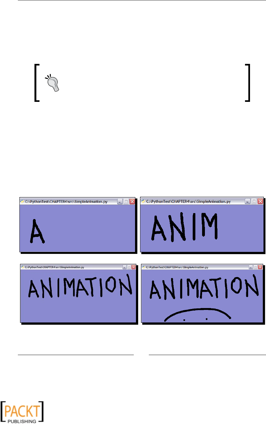
Chapter 4
[ 99 ]
2. Next, we need to draw this animaon sprite into the Pyglet window. The pyglet.
window denes API method on_draw which gets called when an event occurs. The
call to the draw() method of animaon Sprite is made on line 25 to render the
animaon on screen. The code on line 22 is important. The decorator, @win.
event allows us to modify the on_draw API method of pyglet.window.Window
when an event occurs. Finally code on line 27 runs this applicaon.
You can create your own animaon le like SimpleAnimation.
gif using freely available image eding soware packages like GIMP.
This animaon le was created using GIMP 2.6.7, by drawing each
of the characters on a separate layer and then blending all the layers
using Filters | Animaon | Blend.
3. Put the le SimpleAnimation.py along with the animaon le
SimpleAnimation.gif in the same directory and then run the program
as follows:
$python SimpleAnimation.py
This will show the animaon in a Pyglet window. You can use a dierent
animaon le instead of SimpleAnimation.gif. Just modify the related
code in this le or add code to accept any GIF le as a command-line
argument for this program. The next illustraon shows some of the
frames from this animaon at dierent me intervals.
The preceding image is a screen capture of a running animaon at dierent me intervals.
x
x
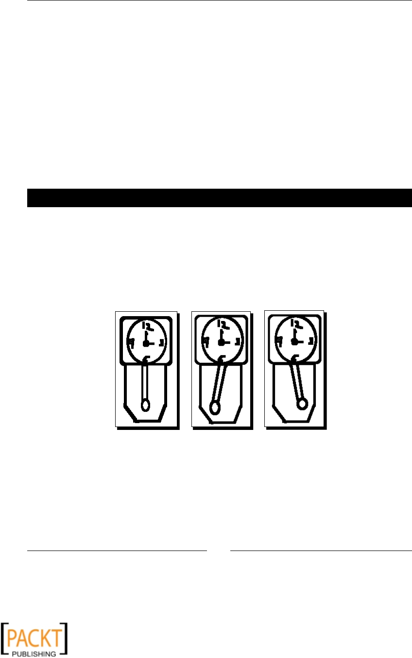
Fun with Animaons
[ 100 ]
What just happened?
We worked out an example where an already created animaon le was loaded and viewed
using Pyglet. This short exercise taught us some preliminary things about viewing animaons
using Pyglet. For example, we learned how to create a Pyglet window and load an animaon
using pyglet.Sprite object. These fundamentals will be used throughout this chapter.
Animation using a sequence of images
The API method Animation.from_image_sequence enables creaon of an animaon
using a bunch of sequenal images. Each of the images is displayed as a frame in the
animaon, one aer the other. The me for which each frame is displayed can be specied
as an argument while creang the animaon object. It can also be set aer the animaon
instance is created.
Time for action – animation using a sequence of images
Let's develop a tool that can create an animaon and display it on the screen. This tool will
create and display the animaon using the given image les. Each of the image les will
be displayed as a frame in the animaon for a specied amount of me. This is going to
be a fun lile animaon that shows a grandfather clock with a pendulum. We will animate
the pendulum oscillaons with other things, including making the dial remaining sll. This
animaon has only three image frames; two of them show the pendulum at opposite
extremes. These images are sequenced as shown in the next illustraon.
x
x

Chapter 4
[ 101 ]
Clock image frames to be animated appear in the preceding image.
1. Download the le ImageSequenceAnimation.py from the Packt website.
2. The code in this le is presented below.
1 import pyglet
2
3 image_frames = ('images/clock1.png',
4 'images/clock2.png',
5 'images/clock3.png')
6
7 # Create the list of pyglet images
8 images = map(lambda img: pyglet.image.load(img),
9 image_frames)
10
11 # Each of the image frames will be displayed for 0.33
12 # seconds
13 # 0.33 seconds chosen so that the 'pendulam in the clock
14 # animation completes one oscillation in ~ 1 second !
15
16 animation = pyglet.image.Animation.from_image_sequence(
17 images, 0.33)
18 # Create a sprite instance.
19 animSprite = pyglet.sprite.Sprite(animation)
20
21 # The main pyglet window with OpenGL context
22 w = animSprite.width
23 h = animSprite.height
24 win = pyglet.window.Window(width=w, height=h)
25
26 # Set window background color to white.
27 pyglet.gl.glClearColor(1, 1, 1, 1)
28
29 # The @win.event is a decorator that helps modify the API
30 # methods such as
31 # on_draw called when draw event occurs.
32 @win.event
33 def on_draw():
34 win.clear()
35 animSprite.draw()
36
37 pyglet.app.run()
x
x

Fun with Animaons
[ 102 ]
The tuple, image_frames contains the paths for the images. The map
funcon call on line 8 creates pyglet.image objects corresponding to
each of the image paths and stores the resultant images in a list. On
line 16, the animation is created using the API method Animation.
from_image_sequence. This method takes the list of image objects
as an argument. The other oponal argument is the me in seconds for
which each of the frames will be shown. We set this me as 0.33 seconds
per image so that the total me for a complete animaon loop is nearly 1
second. Thus, in the animaon, one complete oscillaon of the pendulum
will be complete in about one second. We already discussed the rest of the
code in an earlier secon.
3. Place the image les in a sub-directory images within the directory in which
le ImageSequenceAnimation.py is placed. Then run the program using:
$python ImageSequenceAnimation.py
You will see a clock with an oscillang pendulum in the window. The
animaon will connue in a loop and closing the window will end it.
What just happened?
By rapidly displaying sll images, we just created something like a 'ipbook' cartoon! We
developed a simple ulity that takes a sequence of images as an input and creates an
animaon using Pyglet. To accomplish this task, we used Animation.from_image_
sequence to create the animaon and re-used most of the framework from the
Viewing an exisng animaon secon.
Single image animation
Imagine that you are creang a cartoon movie where you want to animate the moon of
an arrow or a bullet hing a target. In such cases, typically it is just a single image. The
desired animaon eect is accomplished by performing appropriate translaon or
rotaon of the image.
Time for action – bouncing ball animation
Lets create a simple animaon of a 'bouncing ball'. We will use a single image le,
ball.png, which can be downloaded from the Packt website. The dimensions of this
image in pixels are 200x200, created on a transparent background. The following screenshot
shows this image opened in GIMP image editor. The three dots on the ball idenfy its side.
We will see why this is needed. Imagine this as a ball used in a bowling game.
x
x

Chapter 4
[ 103 ]
The image of a ball opened in GIMP appears as shown in the preceding image. The ball size
in pixels is 200x200.
1. Download the les SingleImageAnimation.py and ball.png from the Packt
website. Place the ball.png le in a sub-directory 'images' within the directory in
which SingleImageAnimation.py is saved.
2. The following code snippet shows the overall structure of the code.
1 import pyglet
2 import time
3
4 class SingleImageAnimation(pyglet.window.Window):
5 def __init__(self, width=600, height=600):
6 pass
7 def createDrawableObjects(self):
8 pass
9 def adjustWindowSize(self):
10 pass
11 def moveObjects(self, t):
12 pass
13 def on_draw(self):
14 pass
15 win = SingleImageAnimation()
16 # Set window background color to gray.
17 pyglet.gl.glClearColor(0.5, 0.5, 0.5, 1)
18
19 pyglet.clock.schedule_interval(win.moveObjects, 1.0/20)
20
21 pyglet.app.run()
x
x

Fun with Animaons
[ 104 ]
Although it is not required, we will encapsulate event handling and other
funconality within a class SingleImageAnimation. The program
to be developed is short, but in general, it is a good coding pracce. It
will also be good for any future extension to the code. An instance of
SingleImageAnimation is created on line 14. This class is inherited from
pyglet.window.Window. It encapsulates the funconality we need here.
The API method on_draw is overridden by the class. on_draw is called
when the window needs to be redrawn. Note that we no longer need a
decorator statement such as @win.event above the on_draw method
because the window API method is simply overridden by this inherited class.
3. The constructor of the class SingleImageAnimation is as follows:
1 def __init__(self, width=None, height=None):
2 pyglet.window.Window.__init__(self,
3 width=width,
4 height=height,
5 resizable = True)
6 self.drawableObjects = []
7 self.rising = False
8 self.ballSprite = None
9 self.createDrawableObjects()
10 self.adjustWindowSize()
As menoned earlier, the class SingleImageAnimation inherits pyglet.
window.Window. However, its constructor doesn't take all the arguments
supported by its super class. This is because we don't need to change
most of the default argument values. If you want to extend this applicaon
further and need these arguments, you can do so by adding them as
__init__ arguments. The constructor inializes some instance variables
and then calls methods to create the animaon sprite and resize the
window respecvely.
4. The method createDrawableObjects creates a sprite instance using the
ball.png image.
1 def createDrawableObjects(self):
2 """
3 Create sprite objects that will be drawn within the
4 window.
5 """
6 ball_img= pyglet.image.load('images/ball.png')
7 ball_img.anchor_x = ball_img.width / 2
8 ball_img.anchor_y = ball_img.height / 2
9
x
x
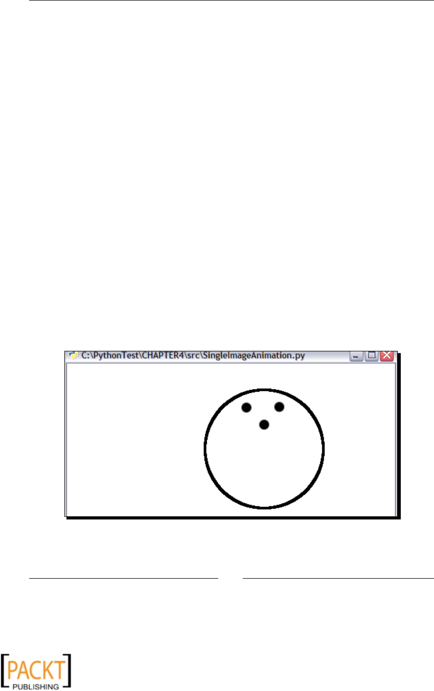
Chapter 4
[ 105 ]
10 self.ballSprite = pyglet.sprite.Sprite(ball_img)
11 self.ballSprite.position = (
12 self.ballSprite.width + 100,
13 self.ballSprite.height*2 - 50)
14 self.drawableObjects.append(self.ballSprite)
The anchor_x and anchor_y properes of the image instance are set
such that the image has an anchor exactly at its center. This will be useful
while rotang the image later. On line 10, the sprite instance self.
ballSprite is created. Later, we will be seng the width and height of
the Pyglet window as twice of the sprite width and thrice of the sprite
height. The posion of the image within the window is set on line 11. The
inial posion is chosen as shown in the next screenshot. In this case, there
is only one Sprite instance. However, to make the program more general,
a list of drawable objects called self.drawableObjects is maintained.
5. To connue the discussion from the previous step, we will now review the
on_draw method.
def on_draw(self):
self.clear()
for d in self.drawableObjects:
d.draw()
As menoned previously, the on_draw funcon is an API method of class
pyglet.window.Window that is called when a window needs to be
redrawn. This method is overridden here. The self.clear() call clears
the previously drawn contents within the window. Then, all the Sprite
objects in the list self.drawableObjects are drawn in the for loop.
The preceding image illustrates the inial ball posion in the animaon.
x
x

Fun with Animaons
[ 106 ]
6. The method adjustWindowSize sets the width and height parameters of the
Pyglet window. The code is self-explanatory:
def adjustWindowSize(self):
w = self.ballSprite.width * 3
h = self.ballSprite.height * 3
self.width = w
self.height = h
7. So far, we have set up everything for the animaon to play. Now comes the fun part.
We will change the posion of the sprite represenng the image to achieve the
animaon eect. During the animaon, the image will also be rotated, to give it
the natural feel of a bouncing ball.
1 def moveObjects(self, t):
2 if self.ballSprite.y - 100 < 0:
3 self.rising = True
4 elif self.ballSprite.y > self.ballSprite.height*2 - 50:
5 self.rising = False
6
7 if not self.rising:
8 self.ballSprite.y -= 5
9 self.ballSprite.rotation -= 6
10 else:
11 self.ballSprite.y += 5
12 self.ballSprite.rotation += 5
This method is scheduled to be called 20 mes per second using the
following code in the program.
pyglet.clock.schedule_interval(win.moveObjects, 1.0/20)
To start with, the ball is placed near the top. The animaon should be such
that it gradually falls down, hits the boom, and bounces back. Aer this,
it connues its upward journey to hit a boundary somewhere near the top
and again it begins its downward journey. The code block from lines 2 to 5
checks the current y posion of self.ballSprite. If it has hit the upward
limit, the ag self.rising is set to False. Likewise, when the lower limit
is hit, the ag is set to True. The ag is then used by the next code snippet
to increment or decrement the y posion of self.ballSprite.
8. The highlighted lines of code rotate the Sprite instance. The current rotaon angle
is incremented or decremented by the given value. This is the reason why we set the
image anchors, anchor_x and anchor_y at the center of the image. The Sprite
object honors these image anchors. If the anchors are not set this way, the ball will
be seen wobbling in the resultant animaon.
x
x
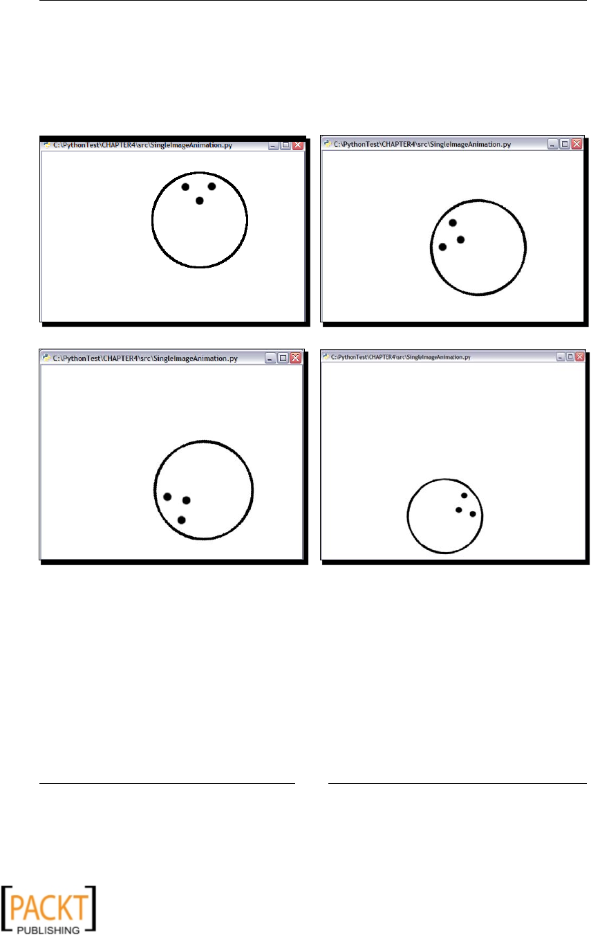
Chapter 4
[ 107 ]
9. Once all the pieces are in place, run the program from the command line as:
$python SingleImageAnimation.py
This will pop up a window that will play the bouncing ball animaon. The
next illustraon shows some intermediate frames from the animaon while
the ball is falling down.
What just happened?
We learned how to create an animaon using just a single image. The image of a ball was
represented by a sprite instance. This sprite was then translated and rotated on the screen to
accomplish a bouncing ball animaon. The whole funconality, including the event handling,
was encapsulated in the class SingleImageAnimation.
x
x
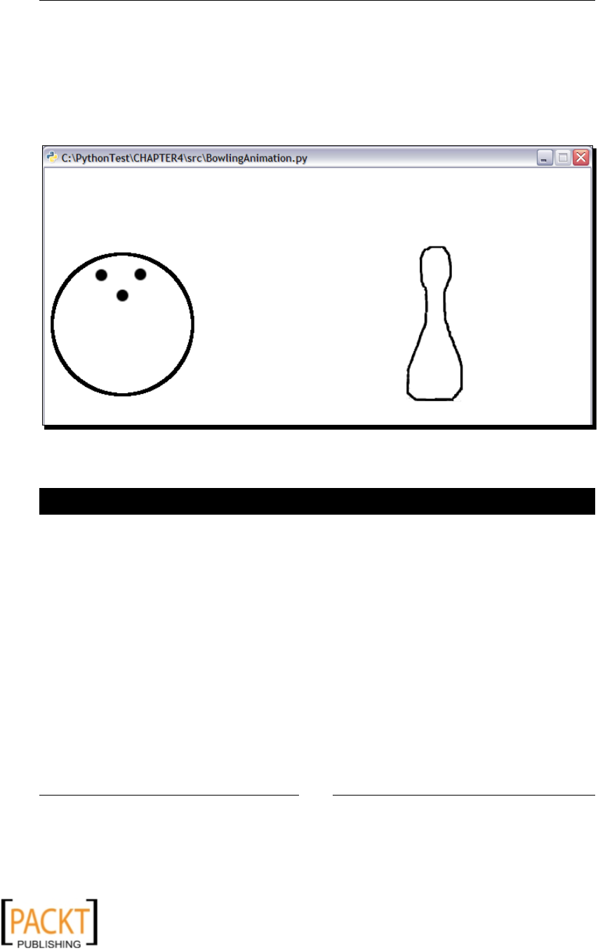
Fun with Animaons
[ 108 ]
Project: a simple bowling animation
It's me for a small project. We will re-use most of the code we used in the Single Image
Animaon secon and some more stu to create an animaon where a rolling ball hits a
pin in a bowling game. Although this chapter covers animaon, this project will give you a
preliminary understanding on how to turn an animaon into a game. This is not a real game
as such, but it will involve some user interacons to control the animaon.
The starng posion in the bowling animaon, showing ball and pin images.
Time for action – a simple bowling animation
Let's develop the code for this applicaon. As menoned earlier, a big chunk of the code
comes from the Single Image Animaon secon. So we will only discuss the new and
modied methods needed to create a bowling animaon.
1. Download the Python source le BowlingAnimation.py from the Packt
website. The overall class design is the same as the one developed in the Single
Image Animaon secon. We will only discuss the new and modied methods.
You can review the rest of the code from this le.
2. Also, download the image les used in this project. These les are ball.png and
pin.png. Place these les in a sub-directory images. The images directory should
be placed in the directory in which the above Python source le is located.
x
x

Chapter 4
[ 109 ]
3. The __init__ method of the class is idencal to that of class
SingleImageAnimation. The only change here is that it inializes the
following ags:
self.paused = False
self.pinHorizontal = False
The ag self.pinHorizontal is used later to check if the pin is knocked
out by the ball. Whereas, self.paused is used to pause or resume the
animaon depending on its value.
4. The createDrawable object method is modied to create a sprite instance for
the pin image. Also, the posion of the ball and pin sprites are adjusted for our
animaon needs. The code is presented as follows:
1 def createDrawableObjects(self):
2 ball_img= pyglet.image.load('images/ball.png')
3 ball_img.anchor_x = ball_img.width / 2
4 ball_img.anchor_y = ball_img.height / 2
5
6 pin_img = pyglet.image.load('images/pin.png')
7 pin_img.anchor_x = pin_img.width / 2
8 pin_img.anchor_y = pin_img.height / 2
9
10 self.ballSprite = pyglet.sprite.Sprite(ball_img)
11 self.ballSprite.position = (0 + 100,
12 self.ballSprite.height)
13
14 self.pinSprite = pyglet.sprite.Sprite(pin_img)
15 self.pinSprite.position = (
16 (self.ballSprite.width*2 + 100,
17 self.ballSprite.height) )
18
19 # Add these sprites to the list of drawables
20 self.drawableObjects.append(self.ballSprite)
21 self.drawableObjects.append(self.pinSprite)
The code block 6-8 creates an image instance for the pin image and then
sets the image anchor at its center. The Sprite instances represenng ball
and pin images are created on lines 10 and 14 respecvely. Their posions
are set such that the inial posions appear as shown in the earlier
illustraon. Finally these sprites are added to the list of drawable
objects that are drawn in on_draw method.
x
x

Fun with Animaons
[ 110 ]
5. Next, let's review the moveObjects method. As before, this method is called every
0.05 seconds.
1 def moveObjects(self, t):
2 if self.pinHorizontal:
3 self.ballSprite.x = 100
4 self.pinSprite.x -= 100
5
6 if self.ballSprite.x < self.ballSprite.width*2:
7 if self.ballSprite.x == 100:
8 time.sleep(1)
9 self.pinSprite.rotation = 0
10 self.pinHorizontal = False
11
12 self.ballSprite.x += 5
13 self.ballSprite.rotation += 5
14
15 if self.ballSprite.x >= self.ballSprite.width*2:
16 self.pinSprite.rotation = 90
17 self.pinSprite.x += 100
18 self.pinHorizontal = True
The if block, from lines 6 to 13, is called for when the x posion of the ball
sprite is between 100 pixels to twice the width of the self.ballSprite.
On line 12, the x posion of self.ballSprite is incremented by 5 pixels.
Also, the sprite is rotated by 5 degrees. The combinaon of these two
transforms creates an eect where we see the ball rolling horizontally, from
le to right, inside the Pyglet window. As seen earlier, the center of the
pin is located at x = self.ballSprite.width*2 + 100 and y = self.
ballSprite.height.
x
x

Chapter 4
[ 111 ]
The if block from lines 15 to 18 is where the ball appears to have hit
the pin. That is, the x coordinate of ball sprite center is about 100 pixels
away from the center of the pin. The 100-pixel value is chosen to account
for the ball radius. Therefore, once the ball hits the pin, the pin image is
rotated by 90 degrees (line 16). This creates a visual eect where the pin
appears to be knocked down by the ball. The x coordinate of the pin is
incremented by 100 pixels so that, aer the pin rotaon, the ball and pin
images don't overlap. You can do some more improvement here. Shi the
y posion of the pin sprite further down, so that the pin appears lying on
the ground. In this if block, we also set the ag self.pinHorizontal
to True. When the moveObjects method is called the next me, the rst
thing that is checked is whether the pin is vercal or horizontal. If the pin is
horizontal, the original posions of the ball and pin are restored by the code
on lines 2 to 4. This is a preparaon for the next animaon loop. On line
9, the pin is rotated back to 0 degree, whereas on line 10, the ag self.
pinHorizontal is reset to False.
6. With the code we developed so far, and with the remaining code from class
SingleImageAnimation, if you run the program, it will show the bowling
animaon. Now let's add some controls to this animaon. A ag, self.paused,
was inialized in the constructor. It will be used here. Just like on_draw, on_key_
press is another API method of pyglet.window.Window. It is overridden here to
implement pause and resume controls.
1 def on_key_press(self, key, modifiers):
2 if key == pyglet.window.key.P and not self.paused:
3 pyglet.clock.unschedule(self.moveObjects)
4 self.paused = True
5 elif key == pyglet.window.key.R and self.paused:
6 pyglet.clock.schedule_interval(
7 self.moveObjects, 1.0/20)
8 self.paused = False
The key argument is one of the keyboard keys pressed by the user. The if
block from lines 2 to 4 pauses the animaon when P key is pressed. The
method self.moveObjects is scheduled to be called every 0.05 seconds.
The scheduled callback to this method is canceled using the pyglet.
clock.unschedule method. To resume the animaon, the schedule_
interval method is called on line 6. The self.paused ag ensures that
the mulple keypresses won't have any undesirable eect on the animaon.
For example, if you press the R key mulple mes, the code will just ignore
the keypress events that follow.
x
x
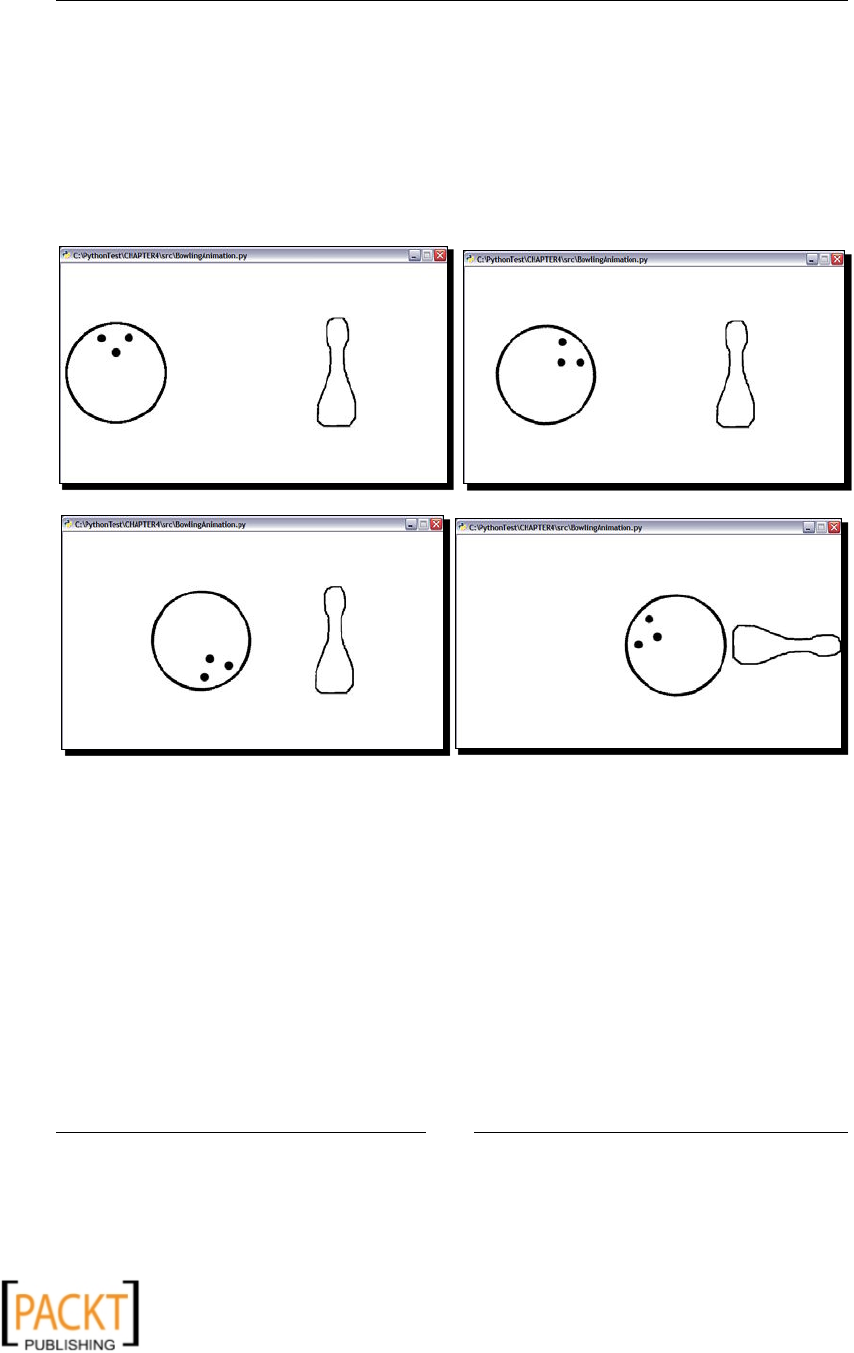
Fun with Animaons
[ 112 ]
7. Refer to the le BowlingAnimation.py to review or develop the rest of the code
and then run the program from the command line as:
$python BowlingAnimation.py
This will pop up a window in which the animaon will be played. Press
the P key on the keyboard to pause the animaon. To resume a paused
animaon, press the R key. The next illustraon shows a few intermediate
frames in this animaon.
The intermediate frames in the bowling animaon appear as shown in the preceding image.
What just happened?
We completed a simple but excing project where an animaon of a bowl hing a pin was
developed. This was accomplished by moving and rotang the image sprites on the screen.
Several methods from the SingleImageAnimation class were re-used. Addionally, we
learned how to control the animaon by overriding the on_key_press API method.
x
x
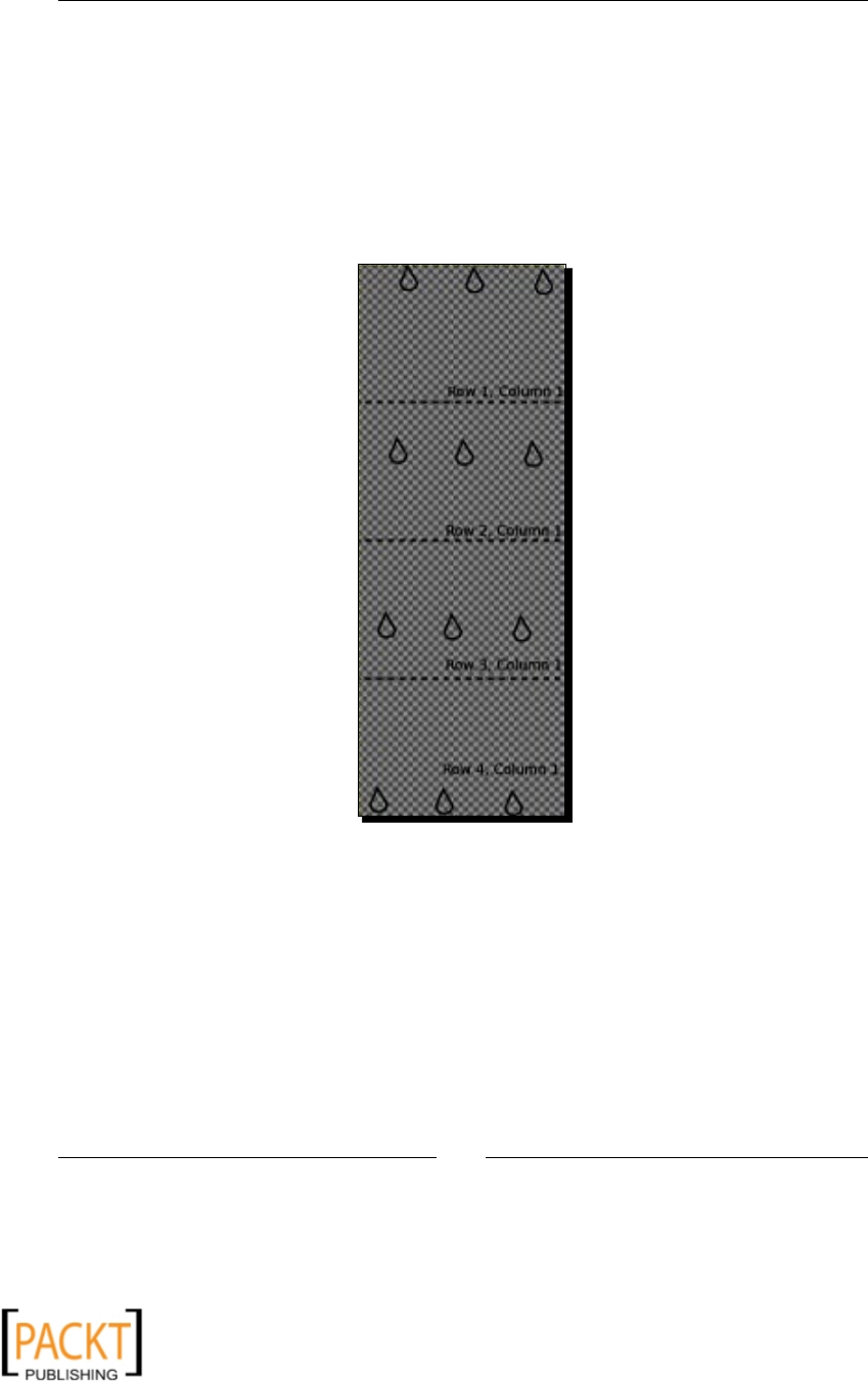
Chapter 4
[ 113 ]
Animations using different image regions
It is possible to create an animaon using dierent regions of a single image. Each of these
regions can be treated as a separate animaon frame. In order to achieve the desired
animaon eect, it is important to properly create the image with regions. In the following
example, the animaon will be created using such regions. We will also be using the default
posion parameters for each of the regions within that image. Thus, our main task in this
secon is simply to use these regions in their original form and create animaon frames out
of them. We will rst see how the image looks. The following illustraon shows this image.
A single image le with an imaginary 'grid' on top of it appears in the previous image.
The horizontal doed lines overlaying this image indicate how an imaginary image grid
divides the image into dierent regions. Here we have four rows and just a single column.
Thus, during the animaon, each of these image regions will be shown as a single animaon
frame. Noce how the droplet images are drawn. In the rst row, the four droplets are drawn
at the top. Then in the next row, these images are slightly oset to the south-west direcon
compared to the droplets in the rst row. This oset is increased further in the third and
fourth rows.
x
x

Fun with Animaons
[ 114 ]
Time for action – raindrops animation
Let's create an animaon of falling raindrops by using dierent regions of a single image.
1. Download the Python source le RainDropsAnimation.py and the image le
droplet.png from the Packt website. As done before, place the image le in a
sub-directory images. The images directory should be placed in the directory in
which the Python source le is located.
2. The __init__ method of the class RainDropsAnimation is presented.
1 def __init__(self, width=None, height=None):
2 pyglet.window.Window.__init__(self,
3 width=width,
4 height=height)
5 self.drawableObjects = []
6 self.createDrawableObjects()
The code is self-explanatory. The class RainDropsAnimation inherits pyglet.
window.Window. The constructor of the class calls the method that creates the
Sprite instance for displaying the animaon on the screen.
3. Let's review the createDrawableObjects method.
1 def createDrawableObjects(self):
2 num_rows = 4
3 num_columns = 1
4 droplet = 'images/droplet.png'
5 animation = self.setup_animation(droplet,
6 num_rows,
7 num_columns)
8
9 self.dropletSprite = pyglet.sprite.Sprite(animation)
10 self.dropletSprite.position = (0,0)
11
12 # Add these sprites to the list of drawables
13 self.drawableObjects.append(self.dropletSprite)
The pyglet.image.Animation instance is created on line 5, by calling
setup_animation method. On line 9, the Sprite instance is created for
this animation object.
x
x

Chapter 4
[ 115 ]
4. The setup_animation method is the main worker method that uses regions
within the image le to create individual animaon frames.
1 def setup_animation(self, img, num_rows, num_columns):
2 base_image = pyglet.image.load(img)
3 animation_grid = pyglet.image.ImageGrid(base_image,
4 num_rows,
5 num_columns)
6 image_frames = []
7
8 for i in range(num_rows*num_columns, 0, -1):
9 frame = animation_grid[i-1]
10 animation_frame = (
11 pyglet.image.AnimationFrame(frame,
12 0.2))
13 image_frames.append(animation_frame)
14
15 animation = pyglet.image.Animation(image_frames)
16 return animation
First, the instance of image is created on line 2. The ImageGrid is an
imaginary grid placed over the droplet image. Each 'cell' or the 'image
region' within this image grid can be viewed as a separate image frame in an
animaon. The ImageGrid instance is constructed by providing the image
object and the number of rows and columns as arguments. The number of
rows in this case is 4 and there is only a single column. Thus, there will be
four such image frames in the animaon corresponding to each of these
rows in the ImageGrid. The AnimationFrame object is created on line 10.
The code on line 8 increments the value of i from maximum to minimum
region or cell of the imaginary grid. Line 9 gets the specic image region and
this is then used to create the pyglet.image.AnimationFrame instance,
as we did on line 10. The second argument is the me for which each frame
will be displayed on the screen. Here, we are displaying each frame for 0.2
seconds. All such animaon frame forms are stored in a list image_frames
and then the pyglet.image.Animation instance is created using this list.
x
x
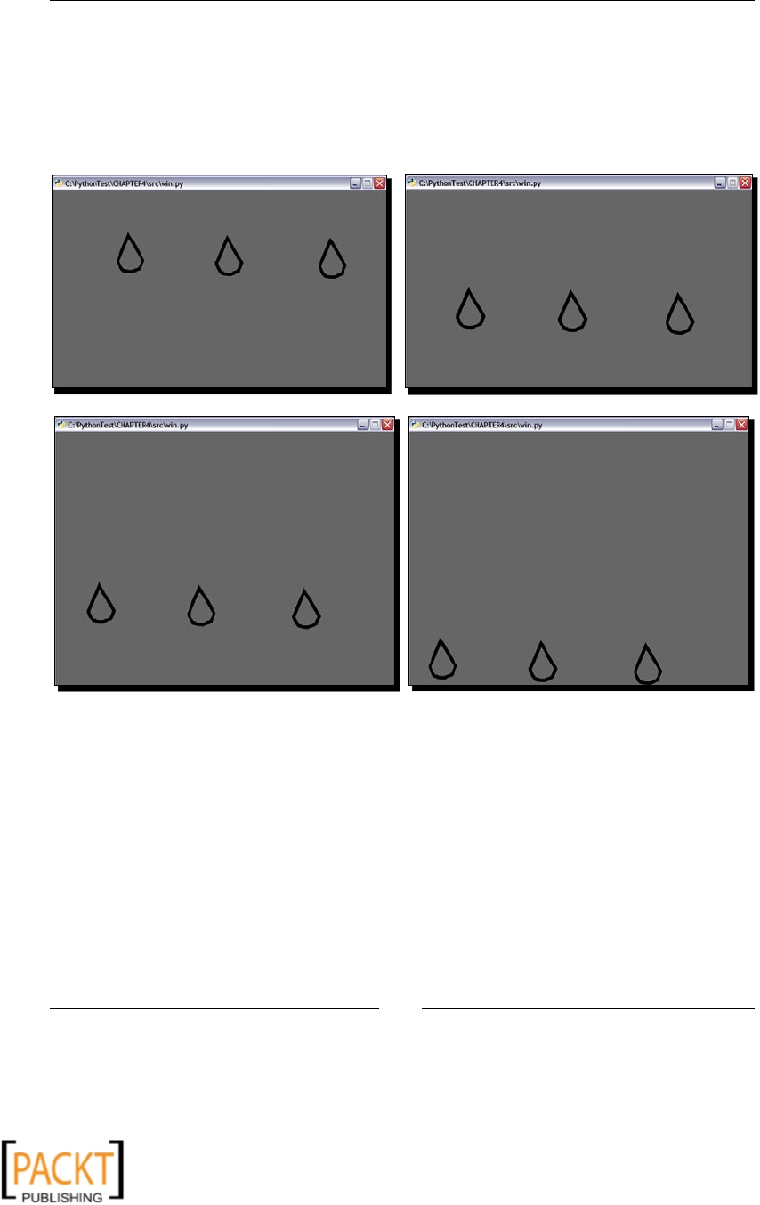
Fun with Animaons
[ 116 ]
5. Refer to the le RainDropsAnimation.py to review the rest of the code and then
run the program from the command line as:
$python RainDropsAnimation.py
This animaon displays four image regions of a single image, one aer
another. The next illustraon shows these four images.
The four image frames that display dierent regions of a single image appear in the previous
illustraon. These four image frames are repeated in the animaon loop.
What just happened?
We created an animaon using dierent regions of a single image. Each of these regions was
treated as a separate animaon frame. The creaon of an image used in this animaon was
briey discussed. Among many other things, we learned how to create and use Pyglet classes
such as ImageGrid and AnimationFrame.
x
x
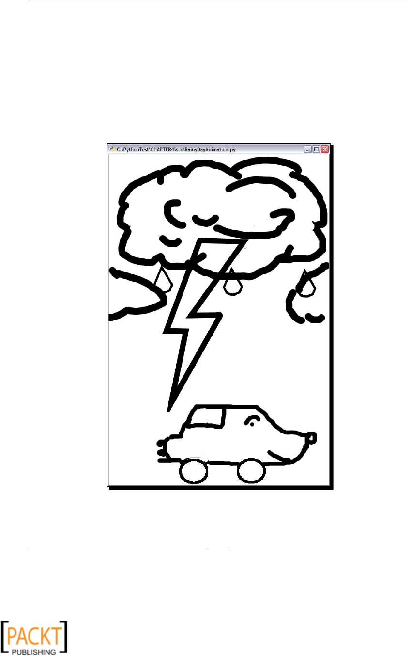
Chapter 4
[ 117 ]
Project: drive on a rainy day!
This project is essenally a summary of what we have learned so far in this chapter.
Addionally, it will cover a few other things such as adding sound eects to an animaon,
showing or hiding certain image sprites while the animaon is being played, and so on. In
this animaon, there will be a staonary cloud image. We will re-use the code from the
raindrops animaon secon to animate falling rain. There will be an image sprite to
animate lightning eect. Finally, a car cartoon will be shown passing by from le to right
in this heavy rain. The following snapshot is an animaon frame that captures all these
component images.
Component images of animaon drive on a rainy day illustrated in the preceding image.
x
x

Fun with Animaons
[ 118 ]
Time for action – drive on a rainy day!
It's me to write the code for this animaon.
1. Download the Python source le RainyDayAnimation.py. We will discuss some
of the important methods from this le. You can go through the rest of the code
from this le.
2. Download the image les, droplet.png, cloud.png, car.png, and
lightening.png from the Packt website. Place these image les in a sub-directory
called images. The images directory should be placed in the directory where the
Python source le is located.
3. The constructor of the class is wrien as follows:
1 def __init__(self, width=None, height=None):
2 pyglet.window.Window.__init__(self,
3 width=width,
4 height=height,
5 resizable=True)
6 self.drawableObjects = []
7 self.paused = False
8
9
10 self.createDrawableObjects()
11 self.adjustWindowSize()
12 # Make sure to replace the following media path to
13 # with an appropriate path on your computer.
14 self.horn_sound = (
15 pyglet.media.load('C:/AudioFiles/horn.wav',
16 streaming=False) )
The code is same as the one developed in the raindrops animaon. The
media le horn.wav is decoded on line 14. The ag streaming is set
to False so that the media can be played mulple mes during the
animaon. Make sure you specify an appropriate audio le path on
your computer on line 15.
x
x

Chapter 4
[ 119 ]
4. Let's review the createDrawableObjects method:
1 def createDrawableObjects(self):
2
3 num_rows = 4
4 num_columns = 1
5 droplet = 'images/droplet.png'
6 animation = self.setup_animation(droplet,
7 num_rows,
8 num_columns)
9
10 self.dropletSprite = pyglet.sprite.Sprite(animation)
11 self.dropletSprite.position = (0,200)
12
13 cloud = pyglet.image.load('images/cloud.png')
14 self.cloudSprite = pyglet.sprite.Sprite(cloud)
15 self.cloudSprite.y = 100
16
17 lightening = pyglet.image.load('images/lightening.png')
18 self.lSprite = pyglet.sprite.Sprite(lightening)
19 self.lSprite.y = 200
20
21 car = pyglet.image.load('images/car.png')
22 self.carSprite = pyglet.sprite.Sprite(car, -500, 0)
23
24 # Add these sprites to the list of drawables
25 self.drawableObjects.append(self.cloudSprite)
26 self.drawableObjects.append(self.lSprite)
27 self.drawableObjects.append(self.dropletSprite)
28 self.drawableObjects.append(self.carSprite)
The code block from lines 3 to 10 is idencal to the one developed in
the raindrops animaon. The self.dropletSprite image is placed
at an appropriate posion. Next, we just create sprites to load images of
clouds, lightning, and car in the Pyglet window. These sprites are placed
at appropriate locaons within the window. For example, the starng
posion of the car is o the screen. It is anchored at x = -500 and y = 0.
The code block from lines 24 to 28 adds all the Sprite instances to self.
drawableObjects . The draw() method of each one of these instances is
called in on_draw method.
x
x

Fun with Animaons
[ 120 ]
5. To achieve the desired animaon eect, we have to move around various sprites
during the animaon. This is done by scheduling a few methods to be called at
specied me intervals. These methods update the coordinates of the sprite or
toggle its visibility when the Pyglet window is redrawn. The code is illustrated
as follows:
# Schedule the method RainyDayAnimation.moveObjects to be
# called every 0.05 seconds.
pyglet.clock.schedule_interval(win.moveObjects, 1.0/20)
# Show the lightening every 1 second
pyglet.clock.schedule_interval(win.show_lightening, 1.0)
We have already seen an example of the moveObjects method
in earlier secons. In this project, we schedule another method,
RainyDayAnimation.show_lightening, to be called every
second. This method created an animaon eect where lightning
strikes every second at dierent posions.
6. We will now review the method show_lightening.
1 def show_lightening(self, t):
2 if self.lSprite.visible:
3 self.lSprite.visible = False
4 else:
5 if(self.lSprite.x == 100):
6 self.lSprite.x += 200
7 else:
8 self.lSprite.x = 100
9
10 self.lSprite.visible = True
self.lSprite is the sprite represenng the lightning image. Our target
is to create an animaon eect where the lightning ashes for a moment
and then disappears. This can be accomplished by toggling the Sprite.
visible property. When this property is set to False, the lightning is
not shown. When it is set to True, the else block 4-10 is executed. The
posion of self.lSprite is changed so that the lightning appears at
dierent locaons the next me this method is called.
x
x
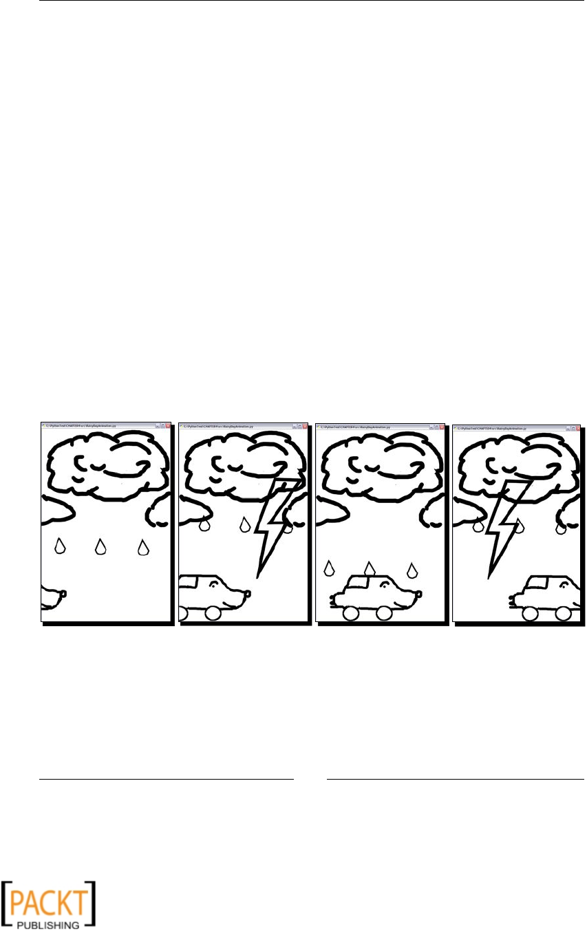
Chapter 4
[ 121 ]
7. The moveObjects method is scheduled to be called every 0.05 seconds.
1 def moveObjects(self, t):
2 if self.carSprite.x <= self.cloudSprite.width:
3 self.carSprite.x += 10
4 else:
5 self.carSprite.x = -500
6 self.horn_sound.play()
Every me it is called, it moves the posion of the Sprite represenng
the car by 10 pixels in the posive direcon of x axis. However, if the x
coordinate of the self.carSprite exceeds its width, the car is reset to its
original posion. Also, at the starng posion of the car, the horn sound
is played.
8. Review the rest of the code from le RainyDayAnimation.py. Make sure to
replace the audio le path for self.horn_sound with an appropriate le path
on your computer. Once everything is all set, run the program from the command
line as:
$python RainyDayAnimation.py
This will pop up a window that will play the animaon in which a fun
car cruises along in a thunderstorm. The next illustraon shows some
intermediate frames from the animaon.
Intermediate frames from an animaon where a car drives along on a rainy
day appear in the preceding image.
x
x

Fun with Animaons
[ 122 ]
What just happened?
The animaon developed in this project used four dierent images. We learned how to add
sound eects and change the visibility of the image sprites during the animaon. Some of
the images were translated or made intermiently visible to achieve the desired animaon
eect. Dierent regions of a single image were used to animate raindrops. Overall, this fun
project covered most of the things we learned throughout this book.
Have a go hero – add more effects
1. Addional sound eects—whenever lightning strikes in the animaon, play a
thunderstorm sound.
2. In the code presented earlier, the lightning image posion is toggled between
two xed locaons. Use random module in Python to get a random coordinate
between 0 to self.cloudSprite.width and use that as the x coordinate of
self.lSprite.
3. Add keyboard controls to change the speed of the car, the frequency of lightning,
and so on.
Summary
We learned a lot in this chapter about creang 2D animaons in Python using Pyglet.
Specically, we:
Learned some fundamental components of the Pyglet framework for
creang animaons. Modules such as Window, Image, Animation, Sprite,
AnimationFrame, ImageGrid, and so on were discussed.
Wrote code to create an animaon using a sequence of images or to play a
pre-created animaon.
Learned things such as modifying the posion of the Pyglet sprite, adding keyboard
and mouse controls and adding sound eects to the animaon.
Worked on a cartoon animaon project 'Drive on a Rainy Day'. Here we applied
several of the techniques learned throughout the chapter.
x
x

5
Working with Audios
Decades ago, silent movies lit up the screen—but later, it was audio eect that
brought life into them. We deal with digital audio processing quite frequently—
when just playing a CD track, recording your own voice or converng songs into
a dierent audio format. There are many libraries or mulmedia frameworks
available for audio processing. This chapter teaches some common digital
audio processing techniques using Python bindings of a popular mulmedia
framework called GStreamer.
In this chapter, we shall:
Learn basic concepts behind GStreamer mulmedia framework
Use GStreamer API for audio processing
Develop some simple audio processing tools for 'everyday use'. We will develop
tools that will batch convert audio le formats, record an audio, and play audio les
So let's get on with it!
Installation prerequisites
Since we are going to use an external mulmedia framework, it is necessary to install thenecessary to install the
packages menoned in this secon.
x
x

Working with Audios
[ 124 ]
GStreamer
GStreamer is a popular open source mulmedia framework that supports audio/video
manipulaon of a wide range of mulmedia formats. It is wrien in the C programming
language and provides bindings for other programming languages including Python.
Several open source projects use GStreamer framework to develop their own mulmedia
applicaon. Throughout this chapter, we will make use of the GStreamer framework
for audio handling. In order to get this working with Python, we need to install both
GStreamer and the Python bindings for GStreamer.
Windows platform
The binary distribuon of GStreamer is not provided on the project website
http://www.gstreamer.net/. Installing it from the source may require
considerable eort on the part of Windows users. Fortunately, GStreamer WinBuilds
project provides pre-compiled binary distribuons. Here is the URL to the project website:
http://www.gstreamer-winbuild.ylatuya.es
The binary distribuon for GStreamer as well as its Python bindings (Python 2.6) are
available in the Download area of the website:
http://www.gstreamer-winbuild.ylatuya.es/doku.php?id=download
You need to install two packages. First, the GStreamer and then the Python bindingsou need to install two packages. First, the GStreamer and then the Python bindings
to the GStreamer. Download and install the GPL distribuon of GStreamer available on
the GStreamer WinBuilds project website. The name of the GStreamer executable is
GStreamerWinBuild-0.10.5.1.exe. The version should be 0.10.5 or higher. By default,
this installaon will create a folder C:\gstreamer on your machine. The bin directory
within this folder contains runme libraries needed while using GStreamer.
Next, install the Python bindings for GStreamer. The binary distribuon is available on the
same website. Use the executable Pygst-0.10.15.1-Python2.6.exe pertaining topertaining to
Python 2.6. The version should be 0.10.15 or higher.
GStreamer WinBuilds appears to be an independent project. It is based on
the OSSBuild developing suite. Visit http://code.google.com/p/
ossbuild/ for more informaon. It could happen that the GStreamer binary
built with Python 2.6 is no longer available on the menoned website at the
me you are reading this book. Therefore, it is advised that you should contact
the developer community of OSSBuild. Perhaps they might help you out!
x
x

Chapter 5
[ 125 ]
Alternavely, you can build GStreamer from source on the Windows plaorm, using a
Linux-like environment for Windows, such as Cygwin (http://www.cygwin.com/). Under
this environment, you can rst install dependent soware packages such as Python 2.6, gcc
compiler, and others. Download the gst-python-0.10.17.2.tar.gz package from the
GStreamer website http://www.gstreamer.net/. Then extract this package and install it
from sources using the Cygwin environment. The INSTALL le within this package will have
installaon instrucons.
Other platforms
Many of the Linux distribuons provide GStreamer package. You can search for the
appropriate gst-python distribuon (for Python 2.6) in the package repository. If such a
package is not available, install gst-python from the source as discussed in the earlier the
Windows plaorm secon.
If you are a Mac OS X user, visit http://py26-gst-python.darwinports.com/. It
has detailed instrucons on how to download and install the package Py26-gst-python
version 0.10.17 (or higher).
Mac OS X 10.5.x (Leopard) comes with the Python 2.5 distribuon. If
you are using packages using this default version of Python, GStreamer
Python bindings using Python 2.5 are available on the darwinports
website: http://gst-python.darwinports.com/
PyGobject
There is a free mulplaorm soware ulity library called 'GLib'. It provides data
structures such as hash maps, linked lists, and so on. It also supports the creaon of
threads. The 'object system' of GLib is called GObject. Here, we need to install the
Python bindings for GObject. The Python bindings are available on the PyGTK website
at: http://www.pygtk.org/downloads.html.
Windows platform
The binary installer is available on the PyGTK website. The complete URL is:
http://ftp.acc.umu.se/pub/GNOME/binaries/win32/pygobject/2.20/..
Download and install version 2.20 for Python 2.6.
Other platforms
For Linux, the source tarball is available on the PyGTK website. There could even be binary
distribuon in the package repository of your Linux operang system. The direct link to the
Version 2.21 of PyGObject (source tarball) is:
http://ftp.gnome.org/pub/GNOME/sources/pygobject/2.21/.
x
x

Working with Audios
[ 126 ]
If you are a Mac user and you have Python 2.6 installed, a distribuon of PyGObject is
available at http://py26-gobject.darwinports.com/. Install version 2.14 or later.
Summary of installation prerequisites
The following table summarizes the packages needed for this chapter.
Package Download
locaon
Version Windows plaorm Linux/Unix/OS X plaorms
GStreamer http://
www.
gstreamer.
net/
0.10.5 or
later
Install using binary
distribuon available on
the Gstreamer WinBuild
website:
http://www.
gstreamer-
winbuild.
ylatuya.es/doku.
php?id=download
Use
GStreamerWinBuild-
0.10.5.1.exe (or later
version if available).
Linux: Use GStreamer
distribuon in package
repository.
Mac OS X: Download
and install by following
instrucons on the website:
http://gstreamer.
darwinports.com/.
Python
Bindings for
GStreamer
http://
www.
gstreamer.
net/
0.10.15 or
later for
Python 2.6
Use binary provided by
GStreamer WinBuild
project. See. See http://
www.gstreamer-
winbuild.ylatuya.
es for details pertaining to
Python 2.6.
Linux: Use gst-python
distribuon in the package
repository.
Mac OS X: Use this package
(if you are using Python2.6):
http://py26-gst-
python.darwinports.
com/.
Linux/Mac: Build and install
from the source tarball.
Python
bindings
for GObject
"PyGObject"
Source
distribuon:
http://
www.pygtk.
org/
downloads.
html
2.14 or
later for
Python 2.6
Use binary package from
pygobject-
2.20.0.win32-
py2.6.exe
Linux: Install from source if
pygobject is not available in
the package repository.
Mac: Use this package
on darwinports (if you
are using Python2.6)
See http://
py26-gobject.
darwinports.com/
for details.
x
x

Chapter 5
[ 127 ]
Testing the installation
Ensure that the GStreamer and its Python bindings are properly installed. It is simple to test
this. Just start Python from the command line and type the following:
>>>import pygst
If there is no error, it means the Python bindings are installed properly.
Next, type the following:
>>>pygst.require("0.10")
>>>import gst
If this import is successful, we are all set to use GStreamer for processing audios and videos!
If import gst fails, it will probably complain that it is unable to work some required DLL/
shared object. In this case, check your environment variables and make sure that the PATH
variable has the correct path to the gstreamer/bin directory. The following lines of code
in a Python interpreter show the typical locaon of the pygst and gst modules on the
Windows plaorm.
>>> import pygst
>>> pygst
<module 'pygst' from 'C:\Python26\lib\site-packages\pygst.pyc'>
>>> pygst.require('0.10')
>>> import gst
>>> gst
<module 'gst' from 'C:\Python26\lib\site-packages\gst-0.10\gst\__init__
.pyc'>
Next, test if PyGObject is successfully installed. Start the Python interpreter and try
imporng the gobject module.
>>import gobject
If this works, we are all set to proceed!
A primer on GStreamer
In this chapter, we will be using GStreamer mulmedia framework extensively. Before
we move on to the topics that teach us various audio processing techniques, a primer
on GStreamer is necessary.
x
x

Working with Audios
[ 128 ]
So what is GStreamer? It is a framework on top of which one can develop mulmedia
applicaons. The rich set of libraries it provides makes it easier to develop applicaons with
complex audio/video processing capabilies. Fundamental components of GStreamer are
briey explained in the coming sub-secons.
Comprehensive documentaon is available on the GStreamer project website.
GStreamer Applicaon Development Manual is a very good starng point. In this
secon, we will briey cover some of the important aspects of GStreamer. For
further reading, you are recommended to visit the GStreamer project website:
http://www.gstreamer.net/documentation/
gst-inspect and gst-launch
We will start by learning the two important GStreamer commands. GStreamer can
be run from the command line, by calling gst-launch-0.10.exe (on Windows) or
gst-launch-0.10 (on other plaorms). The following command shows a typical execuon
of GStreamer on Linux. We will see what a pipeline means in the next sub-secon.
$gst-launch-0.10 pipeline_description
GStreamer has a plugin architecture. It supports a huge number of plugins. To see more
details about any plugin in your GStreamer installaon, use the command gst-inspect-
0.10 (gst-inspect-0.10.exe on Windows). We will use this command quite oen. Use
of this command is illustrated here.
$gst-inspect-0.10 decodebin
Here, decodebin is a plugin. Upon execuon of the preceding command, it prints detailed
informaon about the plugin decodebin.
Elements and pipeline
In GStreamer, the data ows in a pipeline. Various elements are connected together forming
a pipeline, such that the output of the previous element is the input to the next one.
A pipeline can be logically represented as follows:
Element1 ! Element2 ! Element3 ! Element4 ! Element5
Here, Element1 through to Element5 are the element objects chained together by
the symbol !. Each of the elements performs a specic task. One of the element objects
performs the task of reading input data such as an audio or a video. Another element
decodes the le read by the rst element, whereas another element performs the job of
converng this data into some other format and saving the output. As stated earlier, linking
these element objects in a proper manner creates a pipeline.
x
x

Chapter 5
[ 129 ]
The concept of a pipeline is similar to the one used in Unix. Following is a Unix example of a
pipeline. Here, the vercal separator | denes the pipe.
$ls -la | more
Here, the ls -la lists all the les in a directory. However, somemes, this list is too long to
be displayed in the shell window. So, adding | more allows a user to navigate the data.
Now let's see a realisc example of running GStreamer from the command prompt.
$ gst-launch-0.10 -v filesrc location=path/to/file.ogg ! decodebin !
audioconvert ! fakesink
For a Windows user, the gst command name would be gst-launch-0.10.exe. The
pipeline is constructed by specifying dierent elements. The !symbol links the adjacent
elements, thereby forming the whole pipeline for the data to ow. For Python bindings of
GStreamer, the abstract base class for pipeline elements is gst.Element, whereas gst.
Pipeline class can be used to created pipeline instance. In a pipeline, the data is sent to a
separate thread where it is processed unl it reaches the end or a terminaon signal is sent.
Plugins
GStreamer is a plugin-based framework. There are several plugins available. A plugin
is used to encapsulate the funconality of one or more GStreamer elements. Thus we
can have a plugin where mulple elements work together to create the desired output.
The plugin itself can then be used as an abstract element in the GStreamer pipeline. An
example is decodebin. We will learn about it in the upcoming secons. A comprehensive
list of available plugins is available at the GStreamer website http://gstreamer.
freedesktop.org. In this book, we will be using several of them to develop audio/
video processing applicaons. For example, a plugin Playbin will be used for audio
playback. In almost all applicaons to be developed, decodebin plugin will be used. For
audio processing, the funconality provided by plugins such as gnonlin, audioecho,
monoscope, interleave, and so on will be used.
Bins
In GStreamer, a bin is a container that manages the element objects added to it. A bin
instance can be created using gst.Bin class. It is inherited from gst.Element and can act
as an abstract element represenng a bunch of elements within it. A GStreamer plugin
decodebin is a good example represenng a bin. The decodebin contains decoder elements.
It auto-plugs the decoder to create the decoding pipeline.
x
x
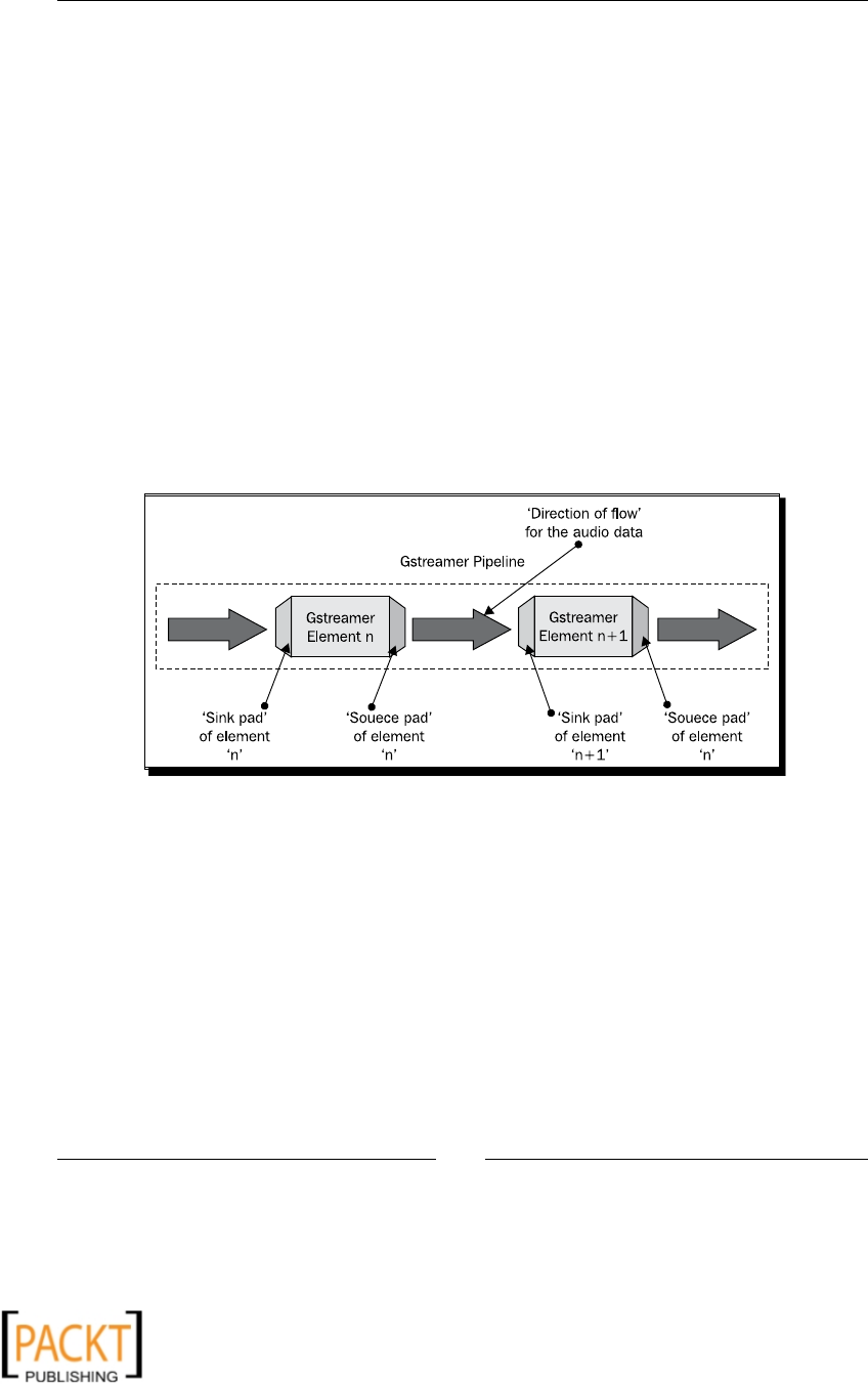
Working with Audios
[ 130 ]
Pads
Each element has some sort of connecon points to handle data input and output.
GStreamer refers to them as pads. Thus an element object can have one or more
"receiver pads" termed as sink pads that accept data from the previous element in the
pipeline. Similarly, there are 'source pads' that take the data out of the element as an
input to the next element (if any) in the pipeline. The following is a very simple example
that shows how source and sink pads are specied.
>gst-launch-0.10.exe fakesrc num-bufferes=1 ! fakesink
The fakesrc is the rst element in the pipeline. Therefore, it only has a source pad. It
transmits the data to the next linkedelement, that is fakesink which only has a sink pad
to accept elements. Note that, in this case, since these are fakesrc and fakesink, just
empty buers are exchanged. A pad is dened by the class gst.Pad. A pad can be aached
to an element object using the gst.Element.add_pad() method.
The following is a diagrammac representaon of a GStreamer element with a pad. It
illustrates two GStreamer elements within a pipeline, having a single source and sink pad.
Now that we know how the pads operate, let's discuss some of special types of pads. In
the example, we assumed that the pads for the element are always 'out there'. However,
there are some situaons where the element doesn't have the pads available all the me.
Such elements request the pads they need at runme. Such a pad is called a dynamic pad.
Another type of pad is called ghost pad. These types are discussed in this secon.
Dynamic pads
Some objects such as decodebin do not have pads dened when they are created. Such
elements determine the type of pad to be used at the runme. For example, depending on
the media le input being processed, the decodebin will create a pad. This is oen referred
to as dynamic pad or somemes the available pad as it is not always available in elements
such as decodebin.
x
x

Chapter 5
[ 131 ]
Ghost pads
As stated in the Bins secon a bin object can act as an abstract element. How is it
achieved? For that, the bin uses 'ghost pads' or 'pseudo link pads'. The ghost pads of
a bin are used to connect an appropriate element inside it. A ghost pad can be created
using gst.GhostPad class.
Caps
The element objects send and receive the data by using the pads. The type of media data
that the element objects will handle is determined by the caps (a short form for capabilies).
It is a structure that describes the media formats supported by the element. The caps are
dened by the class gst.Caps.
Bus
A bus refers to the object that delivers the message generated by GStreamer. A message is
a gst.Message object that informs the applicaon about an event within the pipeline. A
message is put on the bus using the gst.Bus.gst_bus_post() method. The following
code shows an example usage of the bus.
1 bus = pipeline.get_bus()
2 bus.add_signal_watch()
3 bus.connect("message", message_handler)
The rst line in the code creates a gst.Bus instance. Here the pipeline is an instance of
gst.PipeLine. On the next line, we add a signal watch so that the bus gives out all the
messages posted on that bus. Line 3 connects the signal with a Python method. In this
example, the message is the signal string and the method it calls is message_handler.
Playbin/Playbin2
Playbin is a GStreamer plugin that provides a high-level audio/video player. It can
handle a number of things such as automac detecon of the input media le format,
auto-determinaon of decoders, audio visualizaon and volume control, and so on.
The following line of code creates a playbin element.
playbin = gst.element_factory_make("playbin")
It denes a property called uri. The URI (Uniform Resource Idener) should be an
absolute path to a le on your computer or on the Web. According to the GStreamer
documentaon, Playbin2 is just the latest unstable version but once stable, it will
replace the Playbin.
x
x
Working with Audios
[ 132 ]
A Playbin2 instance can be created the same way as a Playbin instance.
gst-inspect-0.10 playbin2
With this basic understanding, let us learn about various audio processing techniques using
GStreamer and Python.
Playing music
Given an audio le, one the rst things you will do is to play that audio le, isn't it? In
GStreamer, what basic elements do we need to play an audio? The essenal elements
are listed as follows.
The rst thing we need is to open an audio le for reading
Next, we need a decoder to transform the encoded informaon
Then, there needs to be an element to convert the audio format so that it is in a
'playable' format required by an audio device such as speakers
Finally, an element that will enable the actual playback of the audio le
How will you play an audio le using the command-line version of GStreamer? One way to
execute it using command line is as follows:
$gstlaunch-0.10 filesrc location=/path/to/audio.mp3 ! decodebin !
audioconvert ! autoaudiosink
The autoaudiosink automacally detects the correct audio device on your
computer to play the audio. This was tested on a machine with Windows XP
and it worked ne. If there is any error playing an audio, check if the audio
device on your computer is working properly. You can also try using element
sdlaudiosink that outputs to the sound card via SDLAUDIO . If this doesn't
work, and you want to install a plugin for audiosink—here is a paral list of
GStreamer plugins:
http://www.gstreamer.net/data/doc/gstreamer/head/gst-
plugins-good-plugins/html/
Mac OS X users can try installing osxaudiosink if the default
autoaudiosink doesn't work.
The audio le should start playing with this command unless there are any missing plugins.
x
x

Chapter 5
[ 133 ]
Time for action – playing an audio: method 1
There are a number of ways to play an audio using Python and GStreamer. Let's start with a
simple one. In this secon, we will use a command string, similar to what you would specify
using the command-line version of GStreamer. This string will be used to construct a
gst.Pipeline instance in a Python program.
So, here we go!
1. Start by creang an AudioPlayer class in a Python source le. Just dene the
empty methods illustrated in the following code snippet. We will expand those in
the later steps.
1 import thread
2 import gobject
3 import pygst
4 pygst.require("0.10")
5 import gst
6
7 class AudioPlayer:
8 def __init__(self):
9 pass
10 def constructPipeline(self):
11 pass
12 def connectSignals(self):
13 pass
14 def play(self):
15 pass
16 def message_handler(self):
17 pass
18
19 # Now run the program
20 player = AudioPlayer()
21 thread.start_new_thread(player.play, ())
22 gobject.threads_init()
23 evt_loop = gobject.MainLoop()
24 evt_loop.run()
Lines 1 to 5 in the code import the necessary modules. As discussed in the
Installaon prerequisites secon, the package pygst is imported rst.
Then we call pygst.require to enable the import of gst module.
x
x

Working with Audios
[ 134 ]
2. Now focus on the code block between lines 19 to 24. It is the main execuon code.
It enables running the program unl the music is played. We will use this or similar
code throughout this book to run our audio applicaon.
On line 21, the thread module is used to create a new thread for playing
the audio. The method AudioPlayer.play is sent on this thread. The
second argument of thread.start_new_thread is the list of arguments
to be passed to the method play. In this example, we do not support any
command-line arguments. Therefore, an empty tuple is passed. Python
adds its own thread management funconality on top of the operang
system threads. When such a thread makes calls to external funcons (such
as C funcons), it puts the 'Global Interpreter Lock' on other threads unl,
for instance, the C funcon returns a value.
The gobject.threads_init() is an inializaon funcon for facilitang
the use of Python threading within the gobject modules. It can enable or
disable threading while calling the C funcons. We call this before running
the main event loop. The main event loop for execung this program is
created using gobject on line 23 and this loop is started by the call
evt_loop.run().
3. Next, ll the AudioPlayer class methods with the code. First, write the constructor
of the class.
1 def __init__(self):
2 self.constructPipeline()
3 self.is_playing = False
4 self.connectSignals()
The pipeline is constructed by the method call on line 2. The ag self.is_
playing is inialized to False. It will be used to determine whether the
audio being played has reached the end of the stream. On line 4, a method
self.connectSignals is called, to capture the messages posted on a
bus. We will discuss both these methods next.
4. The main driver for playing the sound is the following gst command:
"filesrc location=C:/AudioFiles/my_music.mp3 "\
"! decodebin ! audioconvert ! autoaudiosink"
The preceding string has four elements separated by the symbol !. These
elements represent the components we briey discussed earlier.
5. The rst element filesrc location=C:/AudioFiles/my_music.mp3 denes
the source element that loads the audio le from a given locaon. In this string, just
replace the audio le path represented by location with an appropriate le path
on your computer. You can also specify a le on a disk drive.
x
x

Chapter 5
[ 135 ]
If the lename contains namespaces, make sure you specify the path within
quotes. For example, if the lename is my sound.mp3, specify it as follows:
filesrc location =\"C:/AudioFiles/my sound.mp3\"
6. The next element loads the le. This element is connected to a decodebin. As
discussed earlier, the decodebin is a plugin to GStreamer and it inherits gst.Bin.
Based on the input audio format, it determines the right type of decoder element
to use.
The third element is audioconvert. It translates the decoded audio data
into a format playable by the audio device.
The nal element, autoaudiosink, is a plugin; it automacally detects the
audio sink for the audio output.
We have sucient informaon now to create an instance of gst.
Pipeline. Write the following method.
1 def constructPipeline(self):
2 myPipelineString = \
3 "filesrc location=C:/AudioFiles/my_music.mp3 "\
4 "! decodebin ! audioconvert ! autoaudiosink"
5 self.player = gst.parse_launch(myPipelineString)
An instance of gst.Pipeline is created on line 5, using the
gst.parse_launch method.
7. Now write the following method of class AudioPlayer.
1 def connectSignals(self):
2 # In this case, we only capture the messages
3 # put on the bus.
4 bus = self.player.get_bus()
5 bus.add_signal_watch()
6 bus.connect("message", self.message_handler)
On line 4, an instance of gst.Bus is created. In the introductory secon
on GStreamer, we already learned what the code between lines 4 to 6
does. This bus has the job of delivering the messages posted on it from the
streaming threads. The add_signal_watch call makes the bus emit the
message signal for each message posted. This signal is used by the method
message_handler to take appropriate acon.
x
x

Working with Audios
[ 136 ]
Write the following method:
1 def play(self):
2 self.is_playing = True
3 self.player.set_state(gst.STATE_PLAYING)
4 while self.is_playing:
5 time.sleep(1)
6 evt_loop.quit()
On line 2, we set the state of the gst pipeline to gst.STATE_PLAYING to
start the audio streaming. The ag self.is_playing controls the while
loop on line 4. This loop ensures that the main event loop is not terminated
before the end of the audio stream is reached. Within the loop the call to
time.sleep just buys some me for the audio streaming to nish. The
value of ag is changed in the method message_handler that watches for
the messages from the bus. On line 6, the main event loop is terminated.
This gets called when the end of stream message is emied or when some
error occurs while playing the audio.
8. Next, develop method AudioPlayer.message_handler. This method sets the
appropriate ag to terminate the main loop and is also responsible for changing the
playing state of the pipeline.
1 def message_handler(self, bus, message):
2 # Capture the messages on the bus and
3 # set the appropriate flag.
4 msgType = message.type
5 if msgType == gst.MESSAGE_ERROR:
6 self.player.set_state(gst.STATE_NULL)
7 self.is_playing = False
8 print "\n Unable to play audio. Error: ", \
9 message.parse_error()
10 elif msgType == gst.MESSAGE_EOS:
11 self.player.set_state(gst.STATE_NULL)
12 self.is_playing = False
In this method, we only check two things: whether the message on the bus
says the streaming audio has reached its end (gst.MESSAGE_EOS ) or if
any error occurred while playing the audio stream (gst.MESSAGE_ERROR ).
For both these messages, the state of the gst pipeline is changed from
gst.STATE_PLAYING to gst.STATE_NULL. The self.is_playing ag
is updated to instruct the program to terminate the main event loop.
x
x

Chapter 5
[ 137 ]
We have dened all the necessary code to play the audio. Save the le as
PlayingAudio.py and run the applicaon from the command line
as follows:
$python PlayingAudio.py
This will begin playback of the input audio le. Once it is done playing, the
program will be terminated. You can press Ctrl + C on Windows or Linux to
interrupt the playing of the audio le. It will terminate the program.
What just happened?
We developed a very simple audio player, which can play an input audio le. The code we
wrote covered some of the most important components of GStreamer. These components
will be useful throughout this chapter. The core component of the program was a GStreamer
pipeline that had instrucons to play the given audio le. Addionally, we learned how to
create a thread and then start a gobject event loop to ensure that the audio le is played
unl the end.
Have a go hero – play audios from a playlist
The simple audio player we developed can only play a single audio le, whose path is
hardcoded in the constructed GStreamer pipeline. Modify this program so it can play audios
in a "playlist". In this case, play list should dene full paths of the audio les you would like
to play, one aer the other. For example, you can specify the le paths as arguments to this
applicaon or load the paths dened in a text le or load all audio les from a directory.
Hint: In a later secon, we will develop an audio le converter ulity. See if you can use
some of that code here.
Building a pipeline from elements
In the last secon, a gst.Pipeline was automacally constructed for us by the gst.parse_
launch method. All it required was an appropriate command string, similar to the one
specied while running the command-line version of GStreamer. The creaon and linking
of elements was handled internally by this method. In this secon, we will see how to
construct a pipeline by adding and linking individual element objects. 'GStreamer Pipeline'
construcon is a fundamental technique that we will use throughout this chapter and also in
other chapters related to audio and video processing.
x
x

Working with Audios
[ 138 ]
Time for action – playing an audio: method 2
We have already developed code for playing an audio. Let's now tweak the method
AudioPlayer.constructPipeline to build the gst.Pipeline using dierent
element objects.
1. Rewrite the constructPipeline method as follows. You can also download the
le PlayingAudio.py from the Packt website for reference. This le has all the
code we discussed in this and previous secons.
1 def constructPipeline(self):
2 self.player = gst.Pipeline()
3 self.filesrc = gst.element_factory_make("filesrc")
4 self.filesrc.set_property("location",
5 "C:/AudioFiles/my_music.mp3")
6
7 self.decodebin = gst.element_factory_make("decodebin",
8 "decodebin")
9 # Connect decodebin signal with a method.
10 # You can move this call to self.connectSignals)
11 self.decodebin.connect("pad_added",
12 self.decodebin_pad_added)
13
14 self.audioconvert = \
15 gst.element_factory_make("audioconvert",
16 "audioconvert")
17
18 self.audiosink = \
19 gst.element_factory_make("autoaudiosink",
20 "a_a_sink")
21
22 # Construct the pipeline
23 self.player.add(self.filesrc, self.decodebin,
24 self.audioconvert, self.audiosink)
25 # Link elements in the pipeline.
26 gst.element_link_many(self.filesrc, self.decodebin)
27 gst.element_link_many(self.audioconvert,self.audiosink)
2. We begin by creang an instance of class gst.Pipeline.
x
x

Chapter 5
[ 139 ]
3. Next, on line 2, we create the element for loading the audio le. Any new gst
element can be created using the API method, gst.element_factory_make.
The method takes the element name (string) as an argument. For example, on
line 3, this argument is specied as "filesrc" in order to create an instance of
element GstFileSrc. Each element will have a set of properes. The path of the
input audio le is stored in a property location of self.filesrc element. This
property is set on line 4. Replace the le path string with an appropriate audio
le path.
You can get a list of all properes by running the 'gst-inspect-
0.10 ' command from a console window. See the introductory
secon on GSreamer for more details.
4. The second oponal argument serves as a custom name for the created object. For
example, on line 20, the name for the autoaudiosink object is specied as a_a_
sink. Like this, we create all the essenal elements necessary to build the pipeline.
5. On line 23 in the code, all the elements are put in the pipeline by calling the gst.
Pipeline.add method.
6. The method gst.element_link_many establishes connecon between two or
more elements for the audio data to ow between them. The elements are linked
together by the code on lines 26 and 27. However, noce that we haven't linked
together the elements self.decodebin and self.audioconvert. Why? That's
up next.
7. We cannot link the decodebin element with the audioconvert element at the
me the pipeline is created. This is because decodebin uses dynamic pads. These
pads are not available for connecon with the audioconvert element when the
pipeline is created. Depending upon the input data , it will create a pad. Thus, we
need to watch out for a signal that is emied when the decodebin adds a pad!
How do we do that? It is done by the code on line 11 in the code snippet above.
The "pad-added" signal is connected with a method, decodebin_pad_added.
Whenever decodebin adds a dynamic pad, this method will get called.
x
x

Working with Audios
[ 140 ]
8. Thus, all we need to do is to manually establish a connecon between decodebin
and audioconvert elements in the method decodebin_pad_added. Write the
following method.
1 def decodebin_pad_added(self, decodebin, pad ):
2 caps = pad.get_caps()
3 compatible_pad = \
4 self.audioconvert.get_compatible_pad(pad, caps)
5
6 pad.link(compatible_pad)
The method takes the element (in this case it is self.decodebin ) and
pad as arguments. The pad is the new pad for the decodebin element. We
need to link this pad with the appropriate one on self.audioconvert.
9. On line 2 in this code snippet, we nd out what type of media data the pad handles.
Once the capabilies (caps) are known, we pass this informaon to the method
get_compatible_pad of object self.audioconvert. This method returns a
compable pad which is then linked with pad on line 6.
10. The rest of the code is idencal with the one illustrated in the earlier secon. You
can run this program the same way described earlier.
What just happened?
We learned some very crucial components of GStreamer framework. With the simple audio
player as an example, we created a GStreamer pipeline 'from scratch' by creang various
element objects and linking them together. We also learned how to connect two elements by
'manually' linking their pads and why that was required for the element self.decodebin.
Pop Quiz – element linking
In the earlier example, most of the elements in the pipeline linked using gst.element_
link_many in method AudioPlayer.constructPipeline. However, we did not link the
elements self.decodebin and self.audioconvert at the me when the pipeline was
constructed. Why? Choose the correct answer from the following.
1. We were just trying out a dierent technique of manually linking these
elements together.
2. Decodebin uses a dynamic pad that is created at the runme. This pad is not
available when the pipeline is created.
3. We don't need to link these elements in the pipeline. The media data will just nd
its way somehow.
4. What are you talking about? It is impossible to connect decodebin and
audioconvert elements no maer what you try.
x
x

Chapter 5
[ 141 ]
Playing an audio from a website
If there is an audio somewhere on a website that you would like to play, we can prey much
use the same AudioPlayer class developed earlier. In this secon, we will illustrate the use of
gst.Playbin2 to play an audio by specifying a URL. The code snippet below shows the revised
AudioPlayer.constructPipeline method. The name of this method should be changed as it is
playbin object that it creates.
1 def constructPipeline(self):
2 file_url = "http://path/to/audiofile.wav"
3 buf_size = 1024000
4 self.player = gst.element_factory_make("playbin2")
5 self.player.set_property("uri", file_url)
6 self.player.set_property("buffer-size", buf_size)
7 self.is_playing = False
8 self.connectSignals()
On line 4, the gst.Playbin2 element is created using gst.element_factory_make method.
The argument to this method is a string that describes the element to be created. In this case
it is "playbin2" . You can also dene a custom name for this object by supplying an oponal
second argument to this method. Next, on line 5 and 6, we assign values to the properes uri
and buer-size. Set the uri property to an appropriate URL , the full path to the audio le you
would like to play.
Note: When you execute this program, Python applicaon tries to access the
Internet. The an-virus installed on your computer may block the program
execuon. In this case, you will need to allow this program to access the
Internet. Also, you need to be careful of hackers. If you get the fil_url
from an untrusted source, perform a safety check such as assert not
re.match("file://", file_url).
Have a go hero – use 'playbin' to play local audios
In the last few secons, we learned dierent ways to play an audio le using Python and
GStreamer. In the previous secon, you must have noced another simple way to achieve
this, using a playbin or playbin2 object to play an audio. In the previous secon, we learned
how to play an audio le from a URL. Modify this code so that this program can now play
audio les located in a drive on your computer. Hint: You will need to use the correct "uri"
path. Convert the le path using Python's module urllib.pathname2url and then
append it to the string: "file://".
x
x

Working with Audios
[ 142 ]
Converting audio le format
Suppose you have a big collecon of songs in wav le format that you would like to load on
a cell phone. But you nd out that the cell phone memory card doesn't have enough space
to hold all these. What will you do? You will probably try to reduce the size of the song les
right? Converng the les into mp3 format will reduce the size. Of course you can do it using
some media player. Let's learn how to perform this conversion operaon using Python and
GStreamer. Later we will develop a simple command-line ulity that can be used to perform
a batch conversion for all the les you need.
1. Like in the earlier examples, let's rst list the important building blocks we need to
accomplish le conversion. The rst three elements remain the same.
2. As before, the rst thing we need is to load an audio le for reading.
3. Next, we need a decoder to transform the encoded informaon.
4. Then, there needs to be an element to convert the raw audio buers into an
appropriate format.
5. An encoder is needed that takes the raw audio data and encodes it to an
appropriate le format to be wrien.
6. An element where the encoded data will be streamed to is needed. In this case it is
our output audio le.
Okay, what's next? Before jumping into the code, rst check if you can achieve what you
want using the command-line version of GStreamer.
$gstlaunch-0.10.exe filesrc location=/path/to/input.wav ! decodebin !
audioconvert ! lame ! Filesink location=/path/to/output.mp3
Specify the correct input and output le paths and run this command to convert a wave le
to an mp3. If it works, we are all set to proceed. Otherwise check for missing plugins.
You should refer to the GStreamer API documentaon to know more about the properes of
various elements illustrated above. Trust me, the gst-inspect-0.10 (or gst-inspect-
0.10.exe for Windows users) command is a very handy tool that will help you understand
the components of a GStreamer plugin. The instrucons on running this tool are already
discussed earlier in this chapter.
Time for action – audio le format converter
Let's write a simple audio le converter. This ulity will batch process input audio les and
save them in a user-specied le format. To get started, download the le AudioConverter.py
from the Packt website. This le can be run from the command line as:
python AudioConverter.py [options]
x
x

Chapter 5
[ 143 ]
Where, the [options] are as follows:
--input_dir : The directory from which to read the input audio le(s) to
be converted.
--input_format: The audio format of the input les. The format should be in a
supported list of formats. The supported formats are "mp3", "ogg", and "wav". If no
format is specied, it will use the default format as ".wav".
--output_dir : The output directory where the converted les will be saved.
If no output directory is specied, it will create a folder OUTPUT_AUDIOS within
the input directory.
--output_format: The audio format of the output le. Supported output formats
are "wav" and "mp3".
Let's write this code now.
1. Start by imporng necessary modules.
import os, sys, time
import thread
import getopt, glob
import gobject
import pygst
pygst.require("0.10")
import gst
2. Now declare the following class and the ulity funcon. As you will noce, several
of the methods have the same names as before. The underlying funconality of
these methods will be similar to what we already discussed. In this secon we
will review only the most important methods in this class. You can refer to le
AudioConverter.py for other methods or develop those on your own.
def audioFileExists(fil):
return os.path.isfile(fil)
class AudioConverter:
def __init__(self):
pass
def constructPipeline(self):
pass
def connectSignals(self):
pass
def decodebin_pad_added(self, decodebin, pad):
pass
def processArgs(self):
pass
x
x

Working with Audios
[ 144 ]
def convert(self):
pass
def convert_single_audio(self, inPath, outPath):
pass
def message_handler(self, bus, message):
pass
def printUsage(self):
pass
def printFinalStatus(self, inputFileList,
starttime, endtime):
pass
# Run the converter
converter = AudioConverter()
thread.start_new_thread(converter.convert, ())
gobject.threads_init()
evt_loop = gobject.MainLoop()
evt_loop.run()
3. Look at the last few lines of code above. This is exactly the same code we used in the
Playing Music secon. The only dierence is the name of the class and its method
that is put on the thread in the call thread.start_new_thread. At the beginning,
the funcon audioFileExists() is declared. It will be used to check if the
specied path is a valid le path.
4. Now write the constructor of the class. Here we do inializaon of various variables.
def __init__(self):
# Initialize various attrs
self.inputDir = os.getcwd()
self.inputFormat = "wav"
self.outputDir = ""
self.outputFormat = ""
self.error_message = ""
self.encoders = {"mp3":"lame",
"wav": "wavenc"}
self.supportedOutputFormats = self.encoders.keys()
self.supportedInputFormats = ("ogg", "mp3", "wav")
self.pipeline = None
self.is_playing = False
self.processArgs()
self.constructPipeline()
self.connectSignals()
x
x

Chapter 5
[ 145 ]
5. The self.supportedOutputFormats is a tuple that stores the supported output
formats. self.supportedInputFormats is a list obtained from the keys of self.
encoders and stores the supported input formats. These objects are used in self.
processArguments to do necessary checks. The diconary self.encoders
provides the correct type of encoder string to be used to create an encoder
element object for the GStreamer pipeline. As the name suggests, the call to self.
constructPipeline() builds a gst.Pipeline instance and various signals are
connected using self.connectSignals().
6. Next, prepare a GStreamer pipeline.
def constructPipeline(self):
self.pipeline = gst.Pipeline("pipeline")
self.filesrc = gst.element_factory_make("filesrc")
self.decodebin = gst.element_factory_make("decodebin")
self.audioconvert = gst.element_factory_make(
"audioconvert")
self.filesink = gst.element_factory_make("filesink")
encoder_str = self.encoders[self.outputFormat]
self.encoder= gst.element_factory_make(encoder_str)
self.pipeline.add( self.filesrc, self.decodebin,
self.audioconvert, self.encoder,
self.filesink)
gst.element_link_many(self.filesrc, self.decodebin)
gst.element_link_many(self.audioconvert, self.encoder,
self.filesink)
7. This code is similar to the one we developed in the Playing Music sub-secon.
However there are some noceable dierences. In the Audio Player example, we
used the autoaudiosink plugin as the last element. In the Audio Converter, we
have replaced it with elements self.encoder and self.filesink. The former
encodes the audio data coming out of the self.audioconvert. The encoder will
be linked to the sink element. In this case, it is a filesink. The self.filesink is
where the audio data is wrien to a le given by the location property.
x
x

Working with Audios
[ 146 ]
8. The encoder string, encoder_str determines the type of encoder element to
create. For example, if the output format is specied as "mp3" the corresponding
encoder to use is "lame" mp3 encoder. You can run the gst-inspect-0.10 command
to know more about the lame mp3 encoder. The following command can be run
from shell on Linux.
$gst-inspect-0.10 lame
9. The elements are added to the pipeline and then linked together. As before, the
self.decodebin and self.audioconvert are not linked in this method as
the decodebin plugin uses dynamic pads. The pad_added signal from the
self.decodebin is connected in the self.connectSignals() method.
10. Another noceable change is that we have not set the location property for
both, self.filesrc and self.filesink. These properes will be set at the
runme. The input and output le locaons keep on changing as the tool is a batch
processing ulity.
11. Let's write the main method that controls the conversion process.
1 def convert(self):
2 pattern = "*." + self.inputFormat
3 filetype = os.path.join(self.inputDir, pattern)
4 fileList = glob.glob(filetype)
5 inputFileList = filter(audioFileExists, fileList)
6
7 if not inputFileList:
8 print "\n No audio files with extension %s "\
9 "located in dir %s"%(
10 self.outputFormat, self.inputDir)
11 return
12 else:
13 # Record time before beginning audio conversion
14 starttime = time.clock()
15 print "\n Converting Audio files.."
16
17 # Save the audio into specified file format.
18 # Do it in a for loop If the audio by that name already
19 # exists, do not overwrite it
20 for inPath in inputFileList:
21 dir, fil = os.path.split(inPath)
22 fil, ext = os.path.splitext(fil)
23 outPath = os.path.join(
24 self.outputDir,
x
x

Chapter 5
[ 147 ]
25 fil + "." + self.outputFormat)
26
27
28 print "\n Input File: %s%s, Conversion STARTED..."\
29 % (fil, ext)
30 self.convert_single_audio(inPath, outPath)
31 if self.error_message:
32 print "\n Input File: %s%s, ERROR OCCURED" \
33 % (fil, ext)
34 print self.error_message
35 else:
36 print "\nInput File: %s%s,Conversion COMPLETE"\
37 % (fil, ext)
38
39 endtime = time.clock()
40
41 self.printFinalStatus(inputFileList, starttime,
42 endtime)
43 evt_loop.quit()
12. The code between lines 2 to 26 is similar to the one developed in the Image File
conversion ulity in this book. Refer to the Reading and Wring Images secon of
Chapter 2 to know what that code does. All the input audio les are collected in the
list inputFileList by the code between lines 2 to 6 . Then, we loop over each of
these les. First, the output le path is derived based on user inputs and then the
input le path.
13. The highlighted line of code is the workhorse method, AudioConverter.
convert_single_audio, that actually does the job of converng the input audio.
We will discuss that method next. On line 43, the main event loop is terminated. The
rest of the code in method convert is self-explanatory.
14. The code in method convert_single_audio is illustrated below.
1 def convert_single_audio(self, inPath, outPath):
2 inPth = repr(inPath)
3 outPth = repr(outPath)
4
5 # Set the location property for file source and sink
6 self.filesrc.set_property("location", inPth[1:-1])
7 self.filesink.set_property("location", outPth[1:-1])
8
9 self.is_playing = True
x
x

Working with Audios
[ 148 ]
10 self.pipeline.set_state(gst.STATE_PLAYING)
11 while self.is_playing:
12 time.sleep(1)
15. As menoned in the last step, convert_single_audio method is called within a
for loop in the self.convert() . The for loop iterates over a list containing input
audio le paths. The input and output le paths are given as arguments to this
method. The code between lines 8-12 looks more or less similar to AudioPlayer.
play() method illustrated in the Play audio secon. The only dierence is the
main event loop is not terminated in this method. Earlier we did not set the locaon
property for the le source and sink. These properes are set on lines 6 and 7
respecvely.
16. Now what's up with the code on lines 2 and 3? The call repr(inPath) returns a
printable representaon of the string inPath. The inPath is obtained from the
'for loop'. The os.path.normpath doesn't work on this string. In Windows, if
you directly use inPath, GStreamer will throw an error while processing such a
path string. One way to handle this is to use repr(string) , which will return the
whole string including the quotes . For example: if inPath be "C:/AudioFiles/
my_music.mp3" , then repr(inPath) will return "'C:\\\\AudioFiles\\\\
my_music.mp3'". Noce that it has two single quotes. We need to get rid of the
extra single quotes at the beginning and end by slicing the string as inPth[1:-1].
There could be some other beer ways. You can come up with one and then just use
that code as a path string!
17. Let's quickly skim through a few more methods. Write these down:
def connectSignals(self):
# Connect the signals.
# Catch the messages on the bus
bus = self.pipeline.get_bus()
bus.add_signal_watch()
bus.connect("message", self.message_handler)
# Connect the decodebin "pad_added" signal.
self.decodebin.connect("pad_added",
self.decodebin_pad_added)
def decodebin_pad_added(self, decodebin, pad):
caps = pad.get_caps()
compatible_pad=\
self.audioconvert.get_compatible_pad(pad, caps)
pad.link(compatible_pad)
x
x
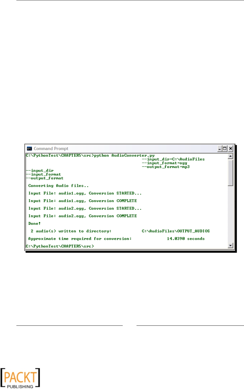
Chapter 5
[ 149 ]
18. The connectSignal method is idencal to the one discussed in the Playing music
secon, except that we are also connecng the decodebin signal with a method
decodebin_pad_added. Add a print statement to decodebin_pad_added to
check when it gets called. It will help you understand how the dynamic pad works!
The program starts by processing the rst audio le. The method convert_
single_audio gets called. Here, we set the necessary le paths. Aer that, it
begins playing the audio le. At this me, the pad_added signal is generated.
Thus based on the input le data, decodebin will create the pad.
19. The rest of the methods such as processArgs, printUsage, and
message_handler are self-explanatory. You can review these methods
from the le AudioConverter.py.
20. The audio converter should be ready for acon now! Make sure that all methods are
properly dened and then run the code by specifying appropriate input arguments.
The following screenshot shows a sample run of audio conversion ulity on
Windows XP. Here, it will batch process all audio les in directory C:\AudioFiles
with extension .ogg and convert them into mp3 le format . The resultant mp3 les
will be created in directory C:\AudioFiles\OUTPUT_AUDIOS.
What just happened?
A basic audio conversion ulity was developed in the previous secon. This ulity can
batch-convert audio les with ogg or mp3 or wav format into user-specied output format
(where supported formats are wav and mp3). We learned how to specify encoder and
lesink elements and link them in the GStreamer pipeline. To accomplish this task, we
also applied knowledge gained in earlier secons such as creaon of GStreamer pipeline,
capturing bus messages, running the main event loop, and so on.
x
x

Working with Audios
[ 150 ]
Have a go hero – do more with audio converter
The audio converter we wrote is fairly simple. It deserves an upgrade.
Extend this applicaon to support more audio output formats such as ogg, flac, and
so on. The following pipeline illustrated one way of converng an input audio le into ogg
le format.
filesrc location=input.mp3 ! decodebin ! audioconvert ! vorbisenc !
oggmux ! filesink location=output.ogg
Noce that we have an audio muxer, oggmux, that needs to be linked with encoder
vorbisenc. Similarly, to create an MP4 audio le, it will need { faac ! mp4mux} as encoder
and audio muxer. One of the simplest things to do is to dene proper elements (such as
encoder and muxer) and instead of construcng a pipeline from individual elements, use
the gst.parse_launch method we studied earlier and let it automacally create and link
elements using the command string. You can create a pipeline instance each me the audio
conversion is called for. But in this case you would also need to connect signals each me
the pipeline is created. Another beer and simpler way is to link the audio muxer in the
AudioConverter.constructPipeline method. You just need to check if it is needed
based on the type of plugin you are using for encoding. In this case the code will be:
gst.element_link_many(self.audioconvert, self.encoder,
self.audiomuxer, self.filesink)
The audio converter illustrated in this example takes input les of only a single audio le
format. This can easily be extended to accept input audio les in all supported le formats
(except for the type specied by the --output_format opon). The decodebin should
take care of decoding the given input data. Extend Audio Converter to support this feature.
You will need to modify the code in the AudioConverter.convert() method where the
input le list is determined.
Extracting part of an audio
Suppose you have recorded a live concert of your favorite musician or a singer. You have
saved all this into a single le with MP3 format but you would like to break this le into small
pieces. There is more than one way to achieve this using Python and GStreamer. We will use
the simplest and perhaps the most ecient way of cung a small piece from an audio track.
It makes use of an excellent GStreamer plugin, called Gnonlin.
x
x

Chapter 5
[ 151 ]
The Gnonlin plugin
The mulmedia eding can be classied as linear or non-linear. Non-linear mulmedia
eding enables control over the media progress in an interacve way. For example, it allows
you to control the order in which the sources should be executed. At the same me it allows
modicaons to the posion in a media track. While doing all this, note that the original
source (such as an audio le) remains unchanged. Thus the eding is non-destrucve. The
Gnonlin or (G-Non-Linear) provides essenal elements for non-linear eding of a mulmedia.
It has ve major elements, namely, gnlfilesource, gnlurisource, gnlcomposition,
gnloperation, and gnlsource. To know more about their properes, run gst-inspect-0.10
command on each of these elements.
Here, we will only focus on the element gnllesource and a few of its properes. This is really
a GStreamer bin element. Like decodebin, it determines which pads to use at the runme.
As the name suggests, it deals with the input media le. All you need to specify is the input
media source it needs to handle. The media le format can be any of the supported media
formats. The gnllesource denes a number of properes. To extract a chunk of an audio, we
just need to consider three of them:
media-start: The posion in the input media le, which will become the start
posion of the extracted media. This is specied in nanoseconds.
media-duration: Total duraon of the extracted media le (beginning from
media-start). This is specied in nanoseconds as well.
uri: The full path of the input media le. For example, if it is a le on your local
hard drive, the uri will be something like file:///C:/AudioFiles/my_music.
mp3. If the le is located on a website, then the uri will something of this sort:
http://path/to/file.mp3.
The gnllesource internally does operaons like loading and decoding the le, seeking the
track to the specied posion, and so on. This makes our job easier. We just need to create
basic elements that will process the informaon furnished by gnllesource, to create an
output audio le. Now that we know the basics of gnllesource, let's try to come up with a
GStreamer pipeline that will cut a poron of an input audio le.
First the gnlfilesource element that does the crucial job of loading, decoding the
le, seeking the correct start posion, and nally presenng us with an audio data
that represents the poron of track to be extracted.
An audioconvert element that will convert this data into an appropriate
audio format.
An encoder that encodes this data further into the nal audio format we want.
A sink where the output data is dumped. This species the output audio le.
x
x

Working with Audios
[ 152 ]
Try running the following from the command prompt by replacing the uri and locaon paths
with appropriate le paths on your computer.
$gst-launch-0.10.exe gnlfilesource uri=file:///C:/my_music.mp3
media-start=0 media-duration=15000000000 !
audioconvert !
lame !
filesink location=C:/my_chunk.mp3
This should create an extracted audio le of duraon 15 seconds, starng at the inial
posion on the original le. Note that the media-start and media-duraon properes take
the input in nanoseconds. This is really the essence of what we will do next.
Time for action – MP3 cutter!
In this secon we will develop a ulity that will cut out a poron of an MP3 formaed audio
and save it as a separate le.
1. Keep the le AudioCutter.py handy. You can download it from the Packt website.
Here we will only discuss important methods. The methods not discussed here are
similar to the ones from earlier examples. Review the le AudioCutter.py which
has all the necessary source code to run this applicaon.
2. Start the usual way. Do the necessary imports and write the following skeleton code.
import os, sys, time
import thread
import gobject
import pygst
pygst.require("0.10")
import gst
class AudioCutter:
def __init__(self):
pass
def constructPipeline(self):
pass
def gnonlin_pad_added(self, gnonlin_elem, pad):
pass
def connectSignals(self):
pass
def run(self):
pass
x
x

Chapter 5
[ 153 ]
def printFinalStatus(self):
pass
def message_handler(self, bus, message):
pass
#Run the program
audioCutter = AudioCutter()
thread.start_new_thread(audioCutter.run, ())
gobject.threads_init()
evt_loop = gobject.MainLoop()
evt_loop.run()
The overall code layout looks familiar doesn't it? The code is very similar
to the code we developed earlier in this chapter. The key here is the
appropriate choice of the le source element and linking it with the rest
of the pipeline! The last few lines of code create a thread with method
AudioCutter.run and run the main event loop as seen before.
3. Now ll in the constructor of the class. We will keep it simple this me. The things
we need will be hardcoded within the constructor of the class AudioCutter. It
is very easy to implement a processArgs() method as done on many occasions
before. Replace the input and output le locaons in the code snippet with a proper
audio le path on your computer.
def __init__(self):
self.is_playing = False
# Flag used for printing purpose only.
self.error_msg = ''
self.media_start_time = 100
self.media_duration = 30
self.inFileLocation = "C:\AudioFiles\my_music.mp3"
self.outFileLocation = "C:\AudioFiles\my_music_chunk.mp3"
self.constructPipeline()
self.connectSignals()
4. the self.media_start_time is the new starng posion of the mp3 le in
seconds. This is the new start posion for the extracted output audio. The self.
duration variable stores the total duraon extracted track. Thus, if you have an
audio le with a total duraon of 5 minutes, the extracted audio will have a starng
posion corresponding to 1 min, 40 seconds on the original track. The total duraon
of this output le will be 30 seconds, that is, the end me will correspond to 2
minutes, 10 seconds on the original track. The last two lines of this method
build a pipeline and connect signals with class methods.
x
x

Working with Audios
[ 154 ]
5. Next, build the GStreamer pipeline.
1 def constructPipeline(self):
2 self.pipeline = gst.Pipeline()
3 self.filesrc = gst.element_factory_make(
4 "gnlfilesource")
5
6 # Set properties of filesrc element
7 # Note: the gnlfilesource signal will be connected
8 # in self.connectSignals()
9 self.filesrc.set_property("uri",
10 "file:///" + self.inFileLocation)
11 self.filesrc.set_property("media-start",
12 self.media_start_time*gst.SECOND)
13 self.filesrc.set_property("media-duration",
14 self.media_duration*gst.SECOND)
15
16 self.audioconvert = \
17 gst.element_factory_make("audioconvert")
18
19 self.encoder = \
20 gst.element_factory_make("lame", "mp3_encoder")
21
22 self.filesink = \
23 gst.element_factory_make("filesink")
24
25 self.filesink.set_property("location",
26 self.outFileLocation)
27
28 #Add elements to the pipeline
29 self.pipeline.add(self.filesrc, self.audioconvert,
30 self.encoder, self.filesink)
31 # Link elements
32 gst.element_link_many(self.audioconvert,self.encoder,
33 self.filesink)
The highlighted line of code (line 3) creates the gnlfilesource. We call
this as self.filesrc. As discussed earlier, this is responsible for loading
and decoding audio data and presenng only the required poron of
audio data that we need. It enables a higher level of abstracon in the
main pipeline.
x
x

Chapter 5
[ 155 ]
6. The code between lines 9 to 13 sets three properes of gnlfilesource, uri,
media-start and media-duration . The media-start and media-duration
are specied in nanoseconds. Therefore, we mulply the parameter value (which is
in seconds) by gst.SECOND which takes care of the units.
7. The rest of the code looks very much similar to the Audio Converter example. In this
case, we only support saving the le in mp3 audio format. The encoder element
is dened on line 19. self.filesink determines where the output le will be
saved. Elements are added to the pipeline by self.pipeline.add call and are linked
together on line 32. Note that the gnlfilesource element, self.filesrc, is
not linked with self.audioconvert while construcng the pipeline. Like the
decodebin, the gnlfilesource implements dynamic pads. Thus, the pad is not
available when the pipeline is constructed. It is created at the runme depending
on the specied input audio format. The "pad_added" signal of gnlfilesource is
connected with a method self.gnonlin_pad_added.
8. Now write the connectSignals and gnonlin_pad_added methods.
def connectSignals(self):
# capture the messages put on the bus.
bus = self.pipeline.get_bus()
bus.add_signal_watch()
bus.connect("message", self.message_handler)
# gnlsource plugin uses dynamic pads.
# Capture the pad_added signal.
self.filesrc.connect("pad-added",self.gnonlin_pad_added)
def gnonlin_pad_added(self, gnonlin_elem, pad):
pad.get_caps()
compatible_pad = \
self.audioconvert.get_compatible_pad(pad, caps)
pad.link(compatible_pad)
The highlighted line of code in method connectSignals connects the
pad_added signal of gnlfilesource with a method gnonlin_pad_
added. The gnonlin_pad_added method is idencal to the decodebin_
pad_added method of class AudioConverter developed earlier.
Whenever gnlfilesource creates a pad at the runme, this method gets
called and here, we manually link the pads of gnlfilesource with the
compable pad on self.audioconvert.
x
x

Working with Audios
[ 156 ]
9. The rest of the code is very much similar to the code developed in the Playing
an audio secon. For example, AudioCutter.run method is equivalent to
AudioPlayer.play and so on. You can review the code for remaining
methods from the le AudioCutter.py.
10. Once everything is in place, run the program from the command line as:
$python AudioCutter.py
11. This should create a new MP3 le which is just a specic poron of the original
audio le.
What just happened?
We accomplished creaon of a ulity that can cut a piece out of an MP3 audio le (yet keep
the original le unchanged). This audio piece was saved as a separate MP3 le. We learned
about a very useful plugin, called Gnonlin, intended for non-linear mulmedia eding. A few
fundamental properes of gnllesource element in this plugin to extract an audio le.
Have a go hero – extend MP3 cutter
Modify this program so that the parameters such as media_start_time
can be passed as an argument to the program. You will need a method like
processArguments(). You can use either getopt or OptionParser
module to parse the arguments.
Add support for other le formats. For example, extend this code so that it can
extract a piece from a wav formaed audio and save it as an MP3 audio le. The
input part will be handled by gnlfilesource. Depending upon the type of output
le format, you will need a specic encoder and possibly an audio muxer element.
Then add and link these elements in the main GStreamer pipeline.
Recording
Aer learning how to cut out a piece from our favorite music tracks, the next excing thing
we will have is a 'home grown' audio recorder. Then use it the way you like to record music,
mimicry or just a simple speech!
Remember what pipeline we used to play an audio? The elements in the pipeline
to play an audio were filesrc ! decodebin ! audioconvert ! autoaudiosink .
The autoaudiosink did the job of automacally detecng the output audio device on
your computer.
x
x

Chapter 5
[ 157 ]
For recording purposes, the audio source is going to be from the microphone connected to
your computer. Thus, there won't be any filesrc element. We will instead replace with
a GStreamer plugin that automacally detects the input audio device. On similar lines, you
probably want to save the recording to a le. So, the autoaudiosink element gets replaced
with a filesink element.
autoaudiosrc is an element we can possibly use for detecng input audio source. However,
while tesng this program on Windows XP, the autoaudiosrc was unable to detect the
audio source for unknown reasons. So, we will use the Directshow audio capture source
plugin called dshowaudiosrc, to accomplish the recording task. Run the gst-inspect-
0.10 dshowaudiosrc command to make sure it is installed and to learn various properes
of this element. Pung this plugin in the pipeline worked ne on Windows XP. The
dshowaudiosrc is linked to the audioconvert.
With this informaon, let's give it a try using the command-line version of GStreamer. Make
sure you have a microphone connected or built into your computer. For a change, we will
save the output le in ogg format.
gst-launch-0.10.exe dshowaudiosrc num-buffers=1000 !
audioconvert ! audioresample !
vorbisenc ! oggmux !
filesink location=C:/my_voice.ogg
The audioresample re-samples the raw audio data with dierent sample rates. Then the
encoder element encodes it. The mulplexer or mux, if present, takes the encoded data and
puts it into a single channel. The recorded audio le is wrien to the locaon specied by
the lesink element.
Time for action – recording
Okay, me to write some code that does audio recording for us.
1. Download the le RecordingAudio.py and review the code. You will noce
that the only important task is to set up a proper pipeline for audio recording.
Content-wise, the other code is very much similar to what we learned earlier in
the chapter. It will have some minor dierences such as method names and print
statements. In this secon we will discuss only the important methods in the
class AudioRecorder.
2. Write the constructor.
def __init__(self):
self.is_playing = False
self.num_buffers = -1
self.error_message = ""
x
x

Working with Audios
[ 158 ]
self.processArgs()
self.constructPipeline()
self.connectSignals()
3. This is similar to the AudioPlayer.__init__() except that we have added a
call to processArgs() and inialized the error reporng variable self.error_
message and the variable that indicates the total duraon of the recording.
4. Build the GStreamer pipeline by wring constructPipeline method.
1 def constructPipeline(self):
2 # Create the pipeline instance
3 self.recorder = gst.Pipeline()
4
5 # Define pipeline elements
6 self.audiosrc = \
7 gst.element_factory_make("dshowaudiosrc")
8
9 self.audiosrc.set_property("num-buffers",
10 self.num_buffers)
11
12 self.audioconvert = \
13 gst.element_factory_make("audioconvert")
14
15 self.audioresample = \
16 gst.element_factory_make("audioresample")
17
18 self.encoder = \
19 gst.element_factory_make("lame")
20
21 self.filesink = \
22 gst.element_factory_make("filesink")
23
24 self.filesink.set_property("location",
25 self.outFileLocation)
26
27 # Add elements to the pipeline
28 self.recorder.add(self.audiosrc, self.audioconvert,
29 self.audioresample,
30 self.encoder, self.filesink)
31
32 # Link elements in the pipeline.
33 gst.element_link_many(self.audiosrc,self.audioconvert,
34 self.audioresample,
35 self.encoder,self.filesink)
x
x

Chapter 5
[ 159 ]
5. We use the dshowaudiosrc (Directshow audiosrc) plugin as an audio source
element. It nds out the input audio source which will be, for instance, the audio
input from a microphone.
6. On line 9, we set the number of buers property to the one specied by self.
num_buffers. This has a default value as -1 , indicang that there is no limit on
the number of buers. If you specify this value as 500 for instance, it will output 500
buers (5 second duraon) before sending a End of Stream message to end the run
of the program.
7. On line 15, an instance of element 'audioresample' is created. This element is
takes the raw audio buer from the self.audioconvert and re-samples it to
dierent sample rates. The encoder element then encodes the audio data into
a suitable format and the recorder le is wrien to the locaon specied by
self.filesink.
8. The code between lines 28 to 35 adds various elements to the pipeline and links
them together.
9. Review the code in le RecordingAudio.py to add rest of the code. Then run the
program to record your voice or anything that you want to record that makes an
audible sound! Following are sample command-line arguments. This program will
record an audio for 5 seconds.
$python RecordingAudio.py –-num_buffers=500
-–out_file=C:/my_voice.mp3
What just happened?
We learned how to record an audio using Python and GStreamer. We developed a simple
audio recording ulity to accomplish this task. The GStreamer plugin, dshowaudiosrc,
captured the audio input for us. We created the main GStreamer Pipeline by adding this
and other elements and used it for the Audio Recorder program.
x
x

Working with Audios
[ 160 ]
Summary
This chapter gave us deeper insight into the fundamentals of audio processing using Python
and the GStreamer mulmedia framework. We used several important components of
GStreamer to develop some frequently needed audio processing ulies. The main
learning points of the chapter can be summarized as follows:
GStreamer installaon: We learned how to install GStreamer and the dependent
packages on various plaorms. This set up a stage for learning audio processing
techniques and will also be useful for the next chapters on audio/video processing.
A primer on GStreamer: A quick primer on GStreamer helped us understand
important elements required for media processing.
Use of GStreamer API to develop audio tools: We learned how to use GStremer API
for general audio processing. This helped us develop tools such as an Audio player, a
le format converter, an MP3 cuer, and audio recorder.
Now that we've learned about basic audio processing using GStreamer, we're ready to add
some 'spice' to the audio. In the next chapter we will learn techniques that will help us add
special eects to an audio.
x
x

6
Audio Controls and Effects
In the previous chapter, the focus was on learning fundamentals of audio
processing. It introduced us to the GStreamer mulmedia framework. We
applied this knowledge to develop some frequently needed audio processing
tools. In this chapter, we will go one step further by developing tools for adding
audio eects, mixing audio tracks, creang custom music tracks, and so on.
In this chapter, we shall:
Learn how to control a streaming audio.
Spice up the audio by adding eects such as fading, echo, and panorama.
Work on a project where a custom music track will be created by combining
dierent audio clips.
Add visualizaon eect to a streaming audio.
Mix two audio streams into a single track. For example, mix an audio containing only
a vocal track with an audio containing only background music track.
So let's get on with it.
Controlling playback
In an audio player, various opons such as Play, Pause, Stop, and so on, provide a way to
control the streaming audio. Such playback controls also nd use in other audio processing
techniques. We have already used some of the playback controls in Chapter 5, Working with
Audios. In this chapter, we will study some more controlling opons.
x
x

Audio Controls and Eects
[ 162 ]
Play
In the previous chapter, we developed a preliminary command-line audio player using
GStreamer. The audio streaming can be started by instrucng the GStreamer pipeline to
begin the ow of audio data. This was achieved by the following code:
self.pipeline.set_state(gst.STATE_PLAYING)
With the above instrucon, the audio will be streamed unl the end of the stream is
reached. Refer to the code in the Playing Audio secon of Chapter 5, Working with Audios to
see what the surrounding code looks like. If you develop a user interface for a simple audio
player, the "Play" buon can be connected to a method that will set the state of pipeline to
gst.STATE_PLAYING.
Pause/resume
The streaming audio can be paused temporarily by seng the GStreamer pipeline state to
gst.STATE_PAUSED. Pausing music in an audio player is another commonly performed
operaon. But this also nds use while doing some special audio processing.
Time for action – pause and resume a playing audio stream
We will now review a very simple example demonstrang various playback control
techniques. The same example will be used in the next few secons. This exercise will be an
ideal preparaon while working on the project 'Extract Audio Using Playback Controls'. So
let's get started!
1. Download the le PlaybackControlExamples.py from the Packt website. This
le has all the necessary code that illustrates various playback controls. The overall
class and its methods are illustrated below for reference. See the source le to know
more about each of these methods.
class AudioPlayer:
def __init__(self):
pass
def constructPipeline(self):
pass
def connectSignals(self):
pass
def decodebin_pad_added(self, decodebin, pad ):
pass
def play(self):
pass
def runExamples(self):
pass
x
x

Chapter 6
[ 163 ]
def runPauseExample(self):
pass
def runStopExample(self):
pass
def runSeekExample(self):
pass
def okToRunExamples(self):
pass
def message_handler(self, bus, message):
pass
The overall code layout is very similar to the code developed in the Playing audio
secon of Chapter 5, Working with Audios. Thus, we will just review some of the
newly added methods relevant to this secon.
2. Here is the code for self.play method.
1 def play(self):
2 self.is_playing = True
3 self.player.set_state(gst.STATE_PLAYING)
4 self.position = None
5 while self.is_playing:
6 time.sleep(0.5)
7 try:
9 self.position = (
10 self.player.query_position(gst.FORMAT_TIME,
11 None) [0] )
16 except gst.QueryError:
17 # The pipeline has probably reached
18 # the end of the audio, (and thus has 'reset'
itself.
19 # So, it may be unable to query the current
position.
20 # In this case, do nothing except to reset
21 # self.position to None.
22 self.position = None
23
24 if not self.position is None:
25 #Convert the duration into seconds.
26 self.position = self.position/gst.SECOND
27 print "\n Current playing time: ",
28 self.position
29
30 self.runExamples()
31 evt_loop.quit()
x
x

Audio Controls and Eects
[ 164 ]
Inside the while loop, on line 9, the current posion of the streaming audio is
queried using the query_position call. This is an API method of GStreamer
Pipeline object. When the pipeline approaches the end of the stream, it may throw
an error while querying the current posion. Therefore, we catch the excepon
gst.QueryError, in the try-except block. The time.sleep call is important
before entering the try-except block. It ensures that the posion is queried
every 0.5 seconds. If you remove this call, the next code will be executed for each
incremental ny step. From a performance standpoint this is unnecessary. The
current posion thus obtained is expressed in nanoseconds, Thus, if the me is say
0.1 seconds, it is obtained as 100 000 000 nanoseconds. To convert it into seconds, it
is divided by a GStreamer constant gst.SECOND. On line 30, the main method that
runs various audio control examples is called.
3. Let's see the code in self.runExamples method now.
1 def runExamples(self):
2
3 if not self.okToRunExamples():
4 return
5
6 # The example will be roughly be run when the streaming
7 # crosses 5 second mark.
8 if self.position >= 5 and self.position < 8:
9 if self.pause_example:
10 self.runPauseExample()
11 elif self.stop_example:
12 self.runStopExample()
13 elif self.seek_example:
14 self.runSeekExample()
15 # this flag ensures that an example is run
16 # only once.
17 self.ranExample = True
The method self.okToRunExamples does some preliminary error checking and
ensures that the total streaming duraon is greater than 20 seconds. This method
will not be discussed here. When the current track posion reaches 5 seconds, one
of the examples is run. Which example to run is determined by the corresponding
boolean ag. For instance, if self.pause_example ag is set to True, it will run
the code that will 'pause' the audio stream. Likewise for the other examples. These
three ags are inialized to False in the __init__ method.
x
x

Chapter 6
[ 165 ]
4. The last method we will review is self.runPauseExample.
1 def runPauseExample(self):
2 print ("\n Pause example: Playback will be paused"
3 " for 5 seconds and will then be resumed...")
4 self.player.set_state(gst.STATE_PAUSED)
5 time.sleep(5)
6 print "\n .. OK now resuming the playback"
7 self.player.set_state(gst.STATE_PLAYING)
The streaming audio is paused by the call on line 4. The time.sleep call will keep
the audio paused for 5 seconds and then the audio playback is resumed by the call
on line 7.
5. Make sure to set the ag self.pause_example to True in the __init__ method
and specify the proper audio le path for the variable for self.inFileLocation.
Then run this example from the command prompt as:
$python PlaybackControlExamples.py
The audio will be played for the rst 5 seconds. It will be then paused for another 5
seconds and nally the playback will be resumed.
What just happened?
With the help of a simple example, we learned how to pause a streaming audio. We also saw
how the current posion of the streaming audio is queried. This knowledge will be used in a
project later in this chapter.
Stop
Seng the state of the GStreamer pipeline to gst.STATE_NULL stops the audio streaming.
Recall the message_handler method explained in the Playing Audio secon of the previous
chapter. We made use of this state when the end of stream message was put on the bus. In
the le PlaybackControlExamples.py, the following code stops the streaming of
the audio.
def runStopExample(self):
print ("\n STOP example: Playback will be STOPPED"
" and then the application will be terminated.")
self.player.set_state(gst.STATE_NULL)
self.is_playing = False
In this le, set the ag self.stop_example to True and then run the program from the
command line to see this illustraon.
x
x

Audio Controls and Eects
[ 166 ]
Fast-forward/rewind
Fast-forwarding or rewinding a track simply means that the current posion on the audio
track being played is shied to some other posion. This is also called seeking a posion
on a track. The pipeline element of GStreamer denes an API method, seek_simple,
that facilitates jumping to a specied posion on the track in a streaming audio. In the le
PlabackControlExamples.py, this is illustrated by the following method.
def runSeekExample(self):
print ("\n SEEK example: Now jumping to position at 15 seconds"
"the audio will continue to stream after this")
self.player.seek_simple(gst.FORMAT_TIME,
gst.SEEK_FLAG_FLUSH,
15*gst.SECOND)
self.player.set_state(gst.STATE_PAUSED)
print "\n starting playback in 2 seconds.."
time.sleep(2)
self.player.set_state(gst.STATE_PLAYING)
When this method is called, the current audio posion is shied to a posion corresponding
to 15 seconds duraon on the audio track. The highlighted lines of code are the key. The
seek_simple method takes three arguments. The rst argument, gst.FORMAT_TIME,
represents the me on the track. The second argument,gst.SEEK_GLAG_FLUSH, is a 'seek
ag'. It tells the pipeline to clear the currently playing audio data. In other words it instructs
to ush the pipeline. This makes the seek operaon faster according to the documentaon.
There are several other seek ags. Refer to the GStreamer documentaon to know more
about these ags. The third argument species the me on the track that will be the new
'current posion' of the streaming audio. This me I specied in nanoseconds and so, it is
mulplied by a constant gst.SECOND. Note that pipeline should be in playing state, before
calling seek_simple method.
Project: extract audio using playback controls
In the last chapter, we learned how to use gnonlin plugin to extract a piece of audio.
Gnonlin made our job very easy. In this project, we will see another way of extracng the
audio les, by applying basic audio processing techniques using GStreamer. We will use some
of the audio playback controls just learned. This project will serve as a refresher on various
fundamental components of GStreamer API.
x
x

Chapter 6
[ 167 ]
Time for action – MP3 cutter from basic principles
Let's create an MP3 cuer from 'basic principles'. That is we won't be using gnonlin to
do this. In this project, we will apply knowledge about seeking a track playing, pausing the
pipeline along with the basic audio processing operaons.
This ulity can be run from the command line as:
$python AudioCutter_Method2.py [options]
Where, the [options] are as follows:
--input_file: The input audio le in MP3 format from which a piece of audio
needs to be cut.
--output_file: The output le path where the extracted audio will be saved. This
needs to be in MP3 format.
--start_time: The posion in seconds on the original track. This will be the
starng posion of the audio to be extracted.
--end_time: The posion in seconds on the original track. This will be the end
posion of the extracted audio.
--verbose_mode: Prints useful informaon such as current posion of the track (in
seconds) while extracng the audio. By default, this ag is set too False.
1. Download the le AudioCutter_Method2.py from the Packt website. We will
discuss only the most important methods here. You can refer to the source code in
this le for developing the rest of the code.
2. We will start as usual, by dening a class with empty methods.
import os, sys, time
import thread
import gobject
from optparse import OptionParser
import pygst
pygst.require("0.10")
import gst
class AudioCutter:
def __init__(self):
pass
def constructPipeline(self):
pass
def decodebin_pad_added(self, decodebin, pad):
x
x

Audio Controls and Eects
[ 168 ]
pass
def connectSignals(self):
pass
def run(self):
pass
def extractAudio(self):
pass
def processArgs(self):
pass
def printUsage(self):
pass
def printFinalStatus(self):
pass
def message_handler(self, bus, message):
pass
audioCutter = AudioCutter()
thread.start_new_thread(audioCutter.run, ())
gobject.threads_init()
evt_loop = gobject.MainLoop()
evt_loop.run()
3. As you can see, the overall structure and the method names are very much
consistent with the MP3 cuer example in earlier chapters. Instead of method
gnonlin_pad_added we have decodebin_pad_added which indicates we are
going to capture the pad_added signal for the decodebin. Also, there are new
methods run and extractAudio. We will discuss these in detail.
4. Now let's review the constructor of the class.
1 def __init__(self):
2 self.start_time = None
3 self.end_time = None
4 self.is_playing = False
5 self.seek_done = False
6 self.position = 0
7 self.duration = None
8 #Flag used for printing purpose only.
9 self.error_msg = ''
10 self.verbose_mode = False
11
12 self.processArgs()
13 self.constructPipeline()
14 self.connectSignals()
x
x

Chapter 6
[ 169 ]
5. The __init__ method calls methods to process user input and then constructs the
GStreamer pipeline by calling the constructPipeline() method. This is similar
to what we have seen in several examples earlier.
6. Think about this. To extract an audio, what elements do you need? We need all the
elements used in audio conversion ulity developed in last chapter. Note that in this
example we are saving the output in the same audio format as the input. Let's try to
construct an inial pipeline.
1 def constructPipeline(self):
2 self.pipeline = gst.Pipeline()
3 self.fakesink = gst.element_factory_make("fakesink")
4 filesrc = gst.element_factory_make("filesrc")
5 filesrc.set_property("location", self.inFileLocation)
6
7 autoaudiosink = gst.element_factory_make(
8 "autoaudiosink")
9
10 self.decodebin = gst.element_factory_make("decodebin")
11
12 self.audioconvert = gst.element_factory_make(
13 "audioconvert")
14
15 self.encoder = gst.element_factory_make("lame",
16 "mp3_encoder")
17
18 self.filesink = gst.element_factory_make("filesink")
19 self.filesink.set_property("location",
20 self.outFileLocation)
21
22 self.pipeline.add(filesrc, self.decodebin,
23 self.audioconvert,
24 self.encoder, self.fakesink)
25
26 gst.element_link_many(filesrc, self.decodebin)
27 gst.element_link_many(self.audioconvert,
28 self.encoder, self.fakesink)
7. We are already familiar with most of the elements included in this pipeline. The
pipeline looks idencal to the one in audio conversion ulity except for the sink
element. Noce that the filesink element is created on line 18. But it is not
added to the pipeline! Instead we have added a fakesink element. Can you guess
why? This is an extracon ulity. We just need to save a poron of an input audio
le. The start posion of the extracted poron may not be the start posion of the
original track. Thus, at this me, we will not add the filesink to the pipeline.
x
x
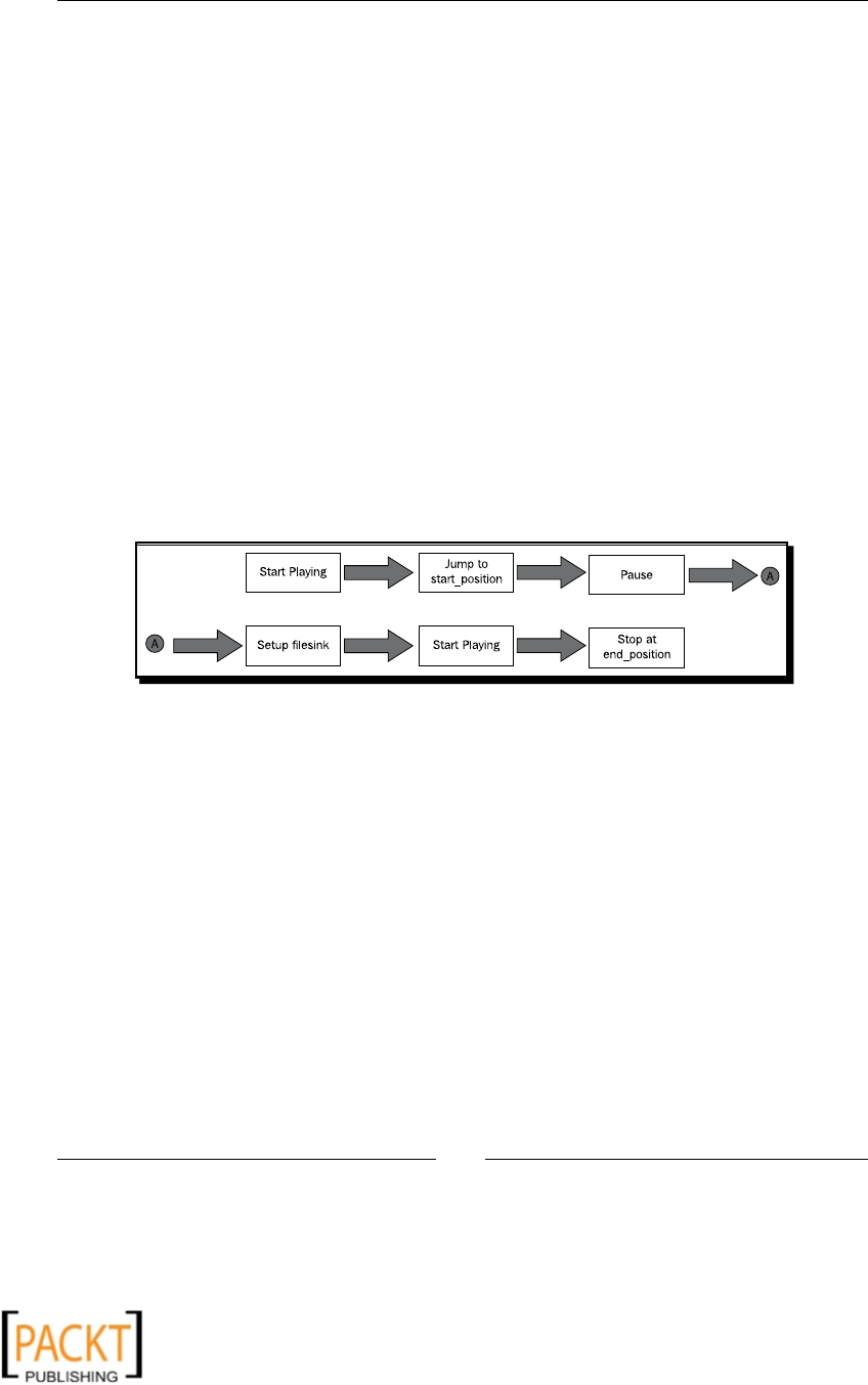
Audio Controls and Eects
[ 170 ]
8. Next write the AudioCutter.run method.
1 def run(self):
2 self.is_playing = True
3 print "\n Converting audio. Please be patient.."
4 self.pipeline.set_state(gst.STATE_PLAYING)
5 time.sleep(1)
6 while self.is_playing:
7 self.extractAudio()
8 self.printFinalStatus()
9 evt_loop.quit()
9. On line 4, we apply one of the playback control commands to instruct the pipeline
to 'begin'. The state of the input audio is set to STATE_PLAYING. As seen earlier,
the ag self.is_playing is changed in the message_handler method. In the
while loop, the workhorse method self.extractAudio() is called. The rest of
the code is self-explanatory.
10. Now we will review the method that does the job of cung the piece of input audio.
Let us rst see the important things considered in extractAudio() method. Then
it will be very easy to understand the code. This following illustraon lists these
important things.
Important steps considered in AudioCutter.extractAudio() method appear in
the preceding image.
11. To extract a piece of audio from the input, the ow of data through the pipeline
needs to be 'started'. Then, we need to jump to a posion in the input audio that
corresponds to the start posion of the audio le to be extracted. Once the start
posion is idened, the GStreamer pipeline needs to be tweaked so that there
is a filesink element. The filesink will specify the output audio le. Aer
seng the pipeline, we need to begin the ow of data. When the user-specied end
posion is reached, the program execuon should stop. Now let's write the code.
1 def extractAudio(self):
2 if not self.seek_done:
3 time.sleep(0.1)
4 self.duration = \
5 self.pipeline.query_duration(gst.FORMAT_TIME,
6 None) [0]
7 self.duration = self.duration/gst.SECOND
x
x

Chapter 6
[ 171 ]
8
9 if self.start_time > self.duration:
10 print "\n start time specified" \
11 " is more than the total audio duration"\
12 " resetting the start time to 0 sec"
13 self.start_time = 0.0
14
15 self.pipeline.seek_simple(gst.FORMAT_TIME,
16 gst.SEEK_FLAG_FLUSH,
17 self.start_time*gst.SECOND)
18
19 self.pipeline.set_state(gst.STATE_PAUSED)
20 self.seek_done = True
21 self.pipeline.remove(self.fakesink)
22
23 self.pipeline.add(self.filesink)
24 gst.element_link_many(self.encoder, self.filesink)
25 self.pipeline.set_state(gst.STATE_PLAYING)
26
27 time.sleep(0.1)
28 try:
29 self.position = self.pipeline.query_position(
30 gst.FORMAT_TIME, None)[0]
31 self.position = self.position/gst.SECOND
32 except gst.QueryError:
33 # The pipeline has probably reached
34 # the end of the audio, (and thus has 'reset' itself)
35 if self.duration is None:
36 self.error_msg = "\n Error cutting the audio
37 file.Unable to determine the audio duration."
38 self.pipeline.set_state(gst.STATE_NULL)
39 self.is_playing = False
40 if ( self.position <= self.duration and
41 self.position > (self.duration - 10) ):
42 # Position close to the end of file.
43 # Do nothing to avoid a possible traceback.
44 #The audio cutting should work
45 pass
46 else:
47 self.error_msg =" Error cutting the audio file"
48 self.pipeline.set_state(gst.STATE_NULL)
49 self.is_playing = False
50
51 if not self.end_time is None:
52 if self.position >= self.end_time:
53 self.pipeline.set_state(gst.STATE_NULL)
54 self.is_playing = False
55
56 if self.verbose_mode:
57 print "\n Current play time: =", self.position
x
x

Audio Controls and Eects
[ 172 ]
12. The code block between lines 3 to 25 is executed only once, when the program
enters this method for the rst me. The ag self.seek_done ensures it is
executed only once. This is an important piece of code that does the steps 2 to 5
represented by rectangular blocks in the above illustraon. Let's review this code in
detail now.
13. On line 3, we ask the program to wait for 0.1 seconds by time.sleep call. This is
necessary for the next line of code that queries the total duraon of the playback.
The API method query duraon returns the total duraon of the playback. The
argument gst.FORMAT_TIME ensures that the return value is in me format
(nanoseconds). To get it in seconds, we divide it by gst.SECOND.
14. Next, on lines 15-17, we jump to the posion on the input audio track pertaining to
the user-supplied argument self.start_time. Note that the me argument in
the method seek_simple needs to be in nanoseconds. So it is mulplied by
gst.SECOND.
15. On line 19, the gst.STATE_PAUSED call pauses the ow of data in the pipeline. The
fakesink element is removed from the pipeline with self.pipline.remove
call. This also unlinks it from the pipeline. Then the self.filesink element is
added and linked in the pipeline on lines 23 and 24. With this, we are all set to start
playing the audio le again. Here onwards, the audio data will be saved to the audio
le indicated by the filesink element.
16. On line 27, the current posion being played is queried. Note that this is done in
a try-except block to avoid any possible error while querying the posion when
the audio is very near to the end of the le. When self.position reaches the
specied self.end_time, the data ow through the pipeline is stopped by the
gst.STATE_NULL call.
17. Write other methods such as decodebin_pad_added, connectSignals. The
source code can be found in the le AudioCutter_Method2.py.
18. We are now all set to run the program. Run it from the command line by specifying
the appropriate arguments menoned at the beginning of this secon.
What just happened?
By applying fundamental audio processing techniques, we developed an MP3 cuer ulity.
This is just another way of extracng audio. We accomplished this task by making use of
various playback controls learned in earlier secons.
x
x

Chapter 6
[ 173 ]
Adjusting volume
One of the most common audio operaons we perform is to adjust the volume level of a
playing audio. Suppose you have a collecon of your favourite songs on your computer. You
have been adding songs to this collecon from various sources over the years and have created
a 'playlist' so that you can listen to them one aer the other. But some of the songs start much
louder than the others. Of course you can adjust the volume every me such songs start playing
but that's not what you would like to do is it?? You want to x this, but how? Let's learn how!
The volume element in GStreamer can be used to control the volume of the streaming
audio. It is classied as a type of audio lter. Run gst-inspect-0.10 command on
volume to know more details about its properes.
How will you adjust volume using the command-line version of GStreamer? Here is the
command on Windows XP that accomplishes this. You should use forward slashes as the
backward slashes are not parsed properly by the 'location' property.
$gstlaunch-0.10 filesrc location=/path/to/audio.mp3 ! decodebin !
Audioconvert ! volume volume=0.8 ! autoaudiosink
This pipeline is very similar to the audio playing example. All we did was to add a volume
element aer audioconvert.
Time for action – adjusting volume
Now let's develop a Python example of modifying volume of an audio le. We will write a
ulity that can take an input audio le and write the output le with increased or decreased
level of the default volume. The ulity will support wring audio les with MP3 format. If
you need some other formats, you can extend this applicaon. Refer to the Audio Converter
project we did in the previous chapter.revious chapter.
1. Download the lee le AudioEffects.py from Packt website. It has the source code
for this example as well as for the Fading eect.
2. Write the constructor of the class AudioEffects.
1 def __init__(self):
2 self.is_playing = False
3 # Flag used for printing purpose only.
4 self.error_msg = ''
5 self.fade_example = False
6 self.inFileLocation = "C:/AudioFiles/audio1.mp3"
7 self.outFileLocation = (
8 "C:/AudioFiles/audio1_out.mp3" )
9
10 self.constructPipeline()
11 self.connectSignals()
x
x

Audio Controls and Eects
[ 174 ]
3. The ag self.fade_example should be set to False in this example. You can
ignore it for now. It will be used in the Fading eects secon. Specify appropriate
input and output audio le paths on lines 6 and 8.
4. We will review the self.constructPipeline() method next.
1 def constructPipeline(self):
2 self.pipeline = gst.Pipeline()
3
4 self.filesrc = gst.element_factory_make("filesrc")
5 self.filesrc.set_property("location",
6 self.inFileLocation)
7
8 self.decodebin = gst.element_factory_make("decodebin")
9 self.audioconvert = gst.element_factory_make(
10 "audioconvert")
11 self.encoder = gst.element_factory_make("lame")
12
13 self.filesink = gst.element_factory_make("filesink")
14 self.filesink.set_property("location",
15 self.outFileLocation)
16
17 self.volume = gst.element_factory_make("volume")
18 self.volumeLevel = 2.0
19
20 if self.fade_example:
21 self.setupVolumeControl()
22 else:
23 self.volume.set_property("volume",
24 self.volumeLevel)
25
26
27 self.pipeline.add(self.filesrc,
28 self.decodebin,
29 self.audioconvert,
30 self.volume,
31 self.encoder,
32 self.filesink)
33
34 gst.element_link_many( self.filesrc, self.decodebin)
35 gst.element_link_many(self.audioconvert,
36 self.volume,
37 self.encoder,
38 self.filesink)
x
x

Chapter 6
[ 175 ]
5. Various GStreamer elements are created the usual way. On line 17, the volume
element is created.
6. The volume element has a "volume" property. This determines the level of volume
in the streaming audio. By default, this has a value of 1.0 which indicates 100% of
the current default volume of the audio. A value of 0.0 indicates no volume. A value
greater than 1.0 will make the audio louder than the original level. Let's set this level
as 2.0, which means the resultant volume will be louder than the original. The rest
of the code in this method adds and links elements in the GStreamer pipeline.
7. Review the rest of the code from the le menoned earlier. It is self- explanatory.
8. Run the program on the command prompt as:
$python AudioEffects.py
9. Play the resultant audio and compare its default sound level with the original audio.
What just happened?
With a very simple illustraon, we learned how to change the default sound level of an audio
le. What if you want to have varying sound levels at certain points in the audio? We will
discuss that very soon, in the Fading eects secon.
Audio effects
One adds spices for improved taste to food, similarly, to enhance the music or any sound we
add audio eects. There is a wide range of audio eect plugins available in GStreamer. We
will discuss some of the commonly used audio eects in the coming secons.
Fading effects
Fading is a gradual increase or decrease in the volume level of an audio. Fading-out means
gradually decreasing the volume of the audio le as it approaches the end. Typically, at
the end, the volume level is set as 0. On similar lines, fade-in eect gradually increases
the volume level from the beginning of an audio. In this chapter, we will learn how to add
fade-out eect to an audio. Once we learn that, it is trivial to implement fade-in eects.
x
x

Audio Controls and Eects
[ 176 ]
Time for action – fading effects
Let's add fade-out eect to an input audio. We will use the same source le as used in the
Adjusng volume secon.
1. If you haven't already, download the le AudioEffects.py that has the source
code for this example.
2. In the __init__ method of this class, you will need to do one small change. Set
the ag self.fade_example to True so that it now runs the code that adds fade-
out eect.
3. We already reviewed the self.constructPipeline() method in Adjusng
volume secon. It calls the method self.setupVolumeControl().
1 def setupVolumeControl(self):
2 self.volumeControl = gst.Controller(self.volume,
3 "volume")
4 self.volumeControl.set("volume", 0.0*gst.SECOND,
5 self.volumeLevel)
6 self.volumeControl.set_interpolation_mode("volume",
7 gst.INTERPOLATE_LINEAR)
4. The GStreamer Controller object is created on line 2. It is a light-weight object
that provides a way to control various properes of GStreamer objects. In this case,
it will be used to adjust the 'volume' property of self.volume. The set method
of the Controller takes three arguments, namely, the property that needs to be
controlled ("volume"), the me on the audio track at which it needs to be changed,
and the new value of that property (self.volumeLevel). Here, the volume level at
the beginning of the audio is set self.volumeLevel. Next, the interpolaon mode
is set for the volume property being adjusted by the Controller object. Here, we
ask the self.volumeControl to linearly change the volume from its earlier value
to the new value as the audio track progresses. For example, if the sound level at the
beginning is set as 1.0 and at 30 seconds it is set as 0.5, the volume levels between
0 to 30 seconds on the track will be linearly interpolated. In this case it will linearly
decrease from level 1.0 at 0 seconds to level 0.5 at 30 seconds.
The GStreamer documentaon suggests that Controller.
set_interpolation_mode is deprecated (but is sll
backward compable in the version 0.10.5 which is used in this
book). See a 'TODO' comment in le AudioEffects.py.
x
x

Chapter 6
[ 177 ]
5. In order to add a fade-out eect towards the end, rst we need to get the total
duraon of the audio being played. We can query the duraon only aer the audio
has been set for playing (example, when it is in gst.STATE_PLAYING mode). This is
done in self.play() method.
def play(self):
self.is_playing = True
self.pipeline.set_state(gst.STATE_PLAYING)
if self.fade_example:
self.addFadingEffect()
while self.is_playing:
time.sleep(1)
self.printFinalStatus()
evt_loop.quit()
6. Once the pipeline's state is set to gst.STATE_PLAYING, the
self.addFadingEffects() method will be called as shown by
the highlighted line of code.
7. We will review this method now.
1 def addFadingEffect(self):
2 # Fist make sure that we can add the fading effect!
3 if not self.is_playing:
4 print ("\n Error: unable to add fade effect"
5 "addFadingEffect() called erroniously")
6 return
7
8 time.sleep(0.1)
9 try:
10 duration = (
11 self.pipeline.query_duration(gst.FORMAT_TIME,
12 None) [0] )
13 #Convert the duration into seconds.
14 duration = duration/gst.SECOND
15 except gst.QueryError:
16 # The pipeline has probably reached
17 # the end of the audio, (and thus has 'reset' itself)
18 print ("\n Error: unable to determine duration."
19 "Fading effect not added." )
20 return
21
22 if duration < 4:
x
x

Audio Controls and Eects
[ 178 ]
23 print ("ERROR: unable to add fading effect."
24 "\n duration too short.")
25 return
26
27 fade_start = duration - 4
28 fade_volume = self.volumeLevel
29 fade_end = duration
30
31 self.volumeControl.set("volume",
32 fade_start * gst.SECOND,
33 fade_volume)
34
35 self.volumeControl.set("volume",
36 fade_end * gst.SECOND,
37 fade_volume*0.01)
8. First we ensure that duraon of the audio being played can be computed without
any errors. This is done by the code block 2-24. Next, the fade_start me is
dened. At this control point the fade-out eect will begin. The fade-out will start 4
seconds before the end of the audio. The volume will linearly decrease from
fade_start me to fade_end me. The fade_volume is the reference volume
level when the fade-out begins. On lines 30 and 34 we actually set these fade ming
and volume parameters for self.volumeController , the Controller object
that adjusts the volume. The gradual decrease in the volume level is achieved by the
gst.INTERPOLATE_LINEAR, discussed in an earlier step.
9. Develop or review the remaining code using the reference le AudioEffects.
py. Make sure to specify appropriate input and output audio paths for variables
self.inFileLocation and self.outFileLocation respecvely. Then run the
program from the command line as:
$python AudioEffects.py
10. This should create the output audio le, with a fade-out eect that begins 4 seconds
before the end of the le.
What just happened?
We learned how to add a fading eect to an audio le using GStreamer mulmedia
framework. We used the same GStreamer pipeline as the one used in the Adjusng
volume secon, but this me, the volume level was controlled using the Controller
object in GStreamer. The technique we just learned will come handy while working on
project 'Combining Audio Clips ' later in this chapter.
x
x

Chapter 6
[ 179 ]
Have a go hero – add fade-in effect
This is going to be straighorward. We added a fade-out eect earlier. Now extend this
ulity by adding a fade-in eect to the input audio. Use a total fade duraon of 4 seconds.
The fade_start me in this case will be 0 seconds. Try the interpolaon mode as
gst.INTERPOLATE_CUBIC.
Echo echo echo...
Echo is a reecon of a sound heard a short me period aer the original sound. In audio
processing, to achieve this eect the input audio signal is recorded and then played back
aer the specied 'delay me' with a specied intensity. An echo eect can be added using
the audioecho plugin in GStreamer. The audio echo plugin should be available by default in
your GStreamer installaon. Check this by running the following command:
$gst-inspect-0.10 audioecho
If it is not available, you will need to install it separately. Refer to the GStreamer website for
installaon instrucons.
Time for action – adding echo effect
Let's write code to add an echo eect to an input audio. The code is very similar to the one
in the AudioEffects.py le discussed in earlier secon. Just to simplify the maer, we
will use the code in le EchoEffect.py le for easier understanding. Later, you can easily
integrate this with the code in AudioEffects.py.
1. Download the le EchoEffect.py that has the source code to add audio
echo eect. The le contains class AudioEffects whose constructor has the
following code.
def __init__(self):
self.is_playing = False
# Flag used for printing purpose only.
self.error_msg = ''
#the flag that determines whether to use
# a gst Controller object to adjust the
# intensity of echo while playing the audio.
self.use_echo_controller = False
self.inFileLocation = "C:/AudioFiles/audio1.mp3"
self.outFileLocation = "C:/AudioFiles/audio1_out.mp3"
self.constructPipeline()
self.connectSignals()
x
x

Audio Controls and Eects
[ 180 ]
It is similar to the __init__ method discussed in the Fading Eects secon. One
dierence here is the ag self.use_echo_controller. If it is set to True, the
GStreamer Controller object will be used to adjust certain echo properes
while the audio is being streamed. We will rst see how a simple echo eect can
be implemented and then discuss the echo control details. Specify the appropriate
values for audio le path variables self.inFileLocation and self.
outFileLocation.
2. Let's build the GStreamer pipeline.
1 def constructPipeline(self):
2 self.pipeline = gst.Pipeline()
3
4 self.filesrc = gst.element_factory_make("filesrc")
5 self.filesrc.set_property("location",
6 self.inFileLocation)
7
8 self.decodebin = gst.element_factory_make("decodebin")
9
10 self.audioconvert = gst.element_factory_make(
11 "audioconvert")
12 self.audioconvert2 = gst.element_factory_make(
13 "audioconvert")
14
15 self.encoder = gst.element_factory_make("lame")
16
17 self.filesink = gst.element_factory_make("filesink")
18 self.filesink.set_property("location",
19 self.outFileLocation)
20
21 self.echo = gst.element_factory_make("audioecho")
22 self.echo.set_property("delay", 1*gst.SECOND)
23 self.echo.set_property("feedback", 0.3)
24
25 if self.use_echo_controller:
26 self.setupEchoControl()
27 else:
28 self.echo.set_property("intensity", 0.5)
29
30 self.pipeline.add(self.filesrc,self.decodebin,
31 self.audioconvert,
32 self.echo,
33 self.audioconvert2,
34 self.encoder,
35 self.filesink)
36
37 gst.element_link_many( self.filesrc, self.decodebin)
x
x

Chapter 6
[ 181 ]
38 gst.element_link_many(self.audioconvert,
39 self.echo,
40 self.audioconvert2,
44 self.encoder,
45 self.filesink)
The audioecho element is created on line 21. The property delay species the
duraon aer which the echo sound will be played. We specify it as 1 second, and
you can increase or decrease this value further. The echo feedback value is set as
0.3. On line 28, the intensity property is set to 0.5. It can be set in a range 0.0 to 1.0
and determines the sound intensity of the echo. Thus, if you set it to 0.0, the echo
won't be heard.
3. Noce that there are two audioconvert elements. The rst audioconvert
converts the decoded audio stream into a playable format input to the self.echo
element. Similarly on the other end of the echo element, we need audioconvert
element to process the audio format aer the echo eect has been added. This
audio is then encoded in MP3 format and saved to the locaon specied by
self.filesink.
4. Run the program from the command line as:
$python EchoEffect.py
If you play the output le, the echo sound will be audible throughout the
playback duraon.
5. Now we will add a feature that will allow us to add echo eect only for a certain
duraon of the audio track. In the __init__ method, set the ag self.use_
echo_controller to True.
6. We will now review the method self.setupEchoControl() which is called in
self.constructPipeline().
def setupEchoControl(self):
self.echoControl = gst.Controller(self.echo, "intensity")
self.echoControl.set("intensity", 0*gst.SECOND, 0.5)
self.echoControl.set("intensity", 4*gst.SECOND, 0.0)
7. Seng up gst.Controller object is very similar to the one developed in the
Fading eects secon. Here, we ask the Controller object, self.echoControl,
to control the property 'intensity' of the audioecho element, self.echo. At
the beginning of the playback (0 seconds), we set the echo intensity as 0.5. We add
another control point at 4 seconds during the playback and set the intensity level
as 0.0. What this eecvely means is that we don't want to hear any echo aer the
rst 4 seconds of the audio playback! .
x
x

Audio Controls and Eects
[ 182 ]
8. Run the program again from the command line as:
$python EchoEffect.py
Note that the only change done here is the value of ag self.use_echo_
controller is set to True. Play the output le; the echo sound will be audible
only for the rst 4 seconds during the playback.
What just happened?
We learned how to add echo to an audio clip. To accomplish this, the audioecho element
was added and linked in the GStreamer pipeline. We also learned how to selecvely add
echo eect to the audio using GStreamer Controller object.
Have a go hero – add Reverberation Effect
Suppose you are in a theater. When an actor at the center stage talks, the sound waves are
reected from the surfaces of the theater before reaching your ears. Thus what you hear is
a bunch of these reected sounds. This is known as reverberaon eect. According to the
audioecho plugin documentaon, if you set the delay property to a value of less than
0.2 seconds in audioecho element, it produces a reverberaon eect. Try seng dierent
values for delay, less than 0.2 seconds and see how it aects the output audio. Note, this
argument is taken as an integer. Therefore, specify this value in nanoseconds. For example
specify 0.05 seconds as 50000000 instead of 0.05*gst.SECOND. This is illustrated below.
self.echo.set_property("delay", 50000000)
Panning/panorama
The stereo panorama eect can be added to a sound by using audiopanorama plugin (part
of audiofx plugin). This plugin should be available by default in your GStreamer installaon.
Use gst-inspect-0.10 to verify it is there and also to know more about its properes.
Download the le PanoramaEffect.py from the Packt website. This le is more or less
idencal to AudioEffects.py or EchoEffect.py. The following is a code snippet from
the self.contructPipeline method in le PanoramaEffect.py
1 # Stereo panorama effect
2 self.panorama = gst.element_factory_make("audiopanorama")
3 self.panorama.set_property("panorama", 1.0)
4
5
6 self.pipeline.add(self.filesrc,
7 self.decodebin,
8 self.audioconvert,
9 self.panorama,
x
x

Chapter 6
[ 183 ]
10 self.encoder,
11 self.filesink)
12
13
14 gst.element_link_many( self.filesrc, self.decodebin)
15 gst.element_link_many(self.audioconvert,
16 self.panorama,
17 self.encoder,
18 self.filesink)
We have discussed the following many mes. Let's go over the code once again as a
refresher… just in case you missed it earlier. The code block 6-11 adds all the elements to
the GStreamer pipeline. Noce that we call gst.element_link_many twice. Do you recall
why? The rst call on line 14 makes a connecon between self.filesrc and self.
decodebin. There is one important point to note when we make a second call to gst.
element_link_many. Noce that we have not linked self.decodebin with self.
audioconvert. This is because self.decodebin implements dynamic pads. So we
connect it at the runme, using the callback method, decodebin_pad_added.
You can review the rest of the code from this le. The audiopanorama element is created
on line 2 in the code snippet. The panorama property can have a value in the range -1.0 to
1.0. If you have stereo speakers connects, the sound will enrely come from the le speaker
if a value of -1.0 is specied. Likewise, a value of 1.0 will make the sound come from right
speaker only. In the above code snippet, we instruct the program to exclusively use the right
speaker for audio streaming. The audio will be streamed from both speakers if the value is
in-between these two limits. Each speaker's contribuon will be determined by actual value.
Have a go hero – control panorama effect and more...
'Move' the sound around! Add a GStreamer Controller object to adjust the panorama
property of the self.panorama element. This is similar to what we did in EchoEffect.
py. Add some control points in the audio stream as done earlier, and specify dierent values
for the panorama property.
Integrate this feature with the code in AudioEffects.py discussed earlier in this chapter.
Project: combining audio clips
It is me for a project! In this project, we will create a single audio le, which has custom
audio clips appended one aer the other. Here, we will apply several of the things learned
in earlier secon, and also in the previous chapter on audio processing.
x
x

Audio Controls and Eects
[ 184 ]
Creang a new audio le, which is a combinaon of several audio tracks of your choice
involves the following steps:
First thing we need are the audio les that need to be included. Depending upon
our requirement, we may need only a small poron of an audio track. So we will
develop a general applicaon considering this possibility. This is illustrated in the
me-line illustrated earlier.
Next, we need to make sure that these audio pieces are played in a specied order.
There should be a 'blank' or a 'silent' audio in-between the two audio pieces.
Next, we will also implement audio fade-out eect for each of the pieces in the
track. This will ensure that the audio doesn't end abruptly.
Media 'timeline' explained
Before we begin this project, it is important to understand the concept of a meline. A
meline can be viewed as the overall representaon of a path where you can control the
me for which an individual audio clip is played.
In this project, since we are saving the resultant audio, it is the same as the total playback
me of the resultant audio. In this meline, we can specify 'when' an audio needs to be
played and how long it needs to be played. This is beer explained with the illustraon
below. Consider a meline with a total duraon of 250 seconds. This is represented by the
central thick line with circles at the end. Suppose there are three audio clips, namely, Media
#1, Media #2 and Media #3 as indicated in the illustraon. We wish to include a poron of
each of these audio clips in the main meline (the audio le to be saved). In the main media
meline, the audio between 0 seconds to 80 second represents a poron from Media #1. It
corresponds to the audio between 30 seconds to 110 seconds in Media #1. Likewise, audio
between 90 to 200 seconds on main media meline represents a chunk from Media #2 and
so on. Thus, we can tweak the priority and posion of the individual audio clips on the main
media meline to create the desired audio output.
Main media meline is represented with mulple media tracks in the preceding image.
x
x

Chapter 6
[ 185 ]
Time for action – creating custom audio by combining clips
Let's develop an applicaon where we will combine mulple audio clips into a
single audio le.
1. Download the le CombiningAudio.py. This le contains all the code necessary
to run this applicaon. As done earlier, we will discuss only the most important
methods in this class.
2. Write the following code.
1 import os, sys, time
2 import thread
3 import gobject
4 from optparse import OptionParser
5
6 import pygst
7 pygst.require("0.10")
8 import gst
9
10 class AudioMerger:
11 def __init__(self):
12 pass
13 def constructPipeline(self):
14 pass
15 def addFadingEffect(self):
16 pass
17 def setupFadeBin(self):
18 pass
19 def addGnlFileSources(self):
20 pass
21 def gnonlin_pad_added(self, gnonlin_elem, pad):
22 pass
23 def run(self):
24 pass
25 def connectSignals(self):
26 pass
27 def printUsage(self):
28 pass
29 def printFinalStatus(self):
30 pass
31 def message_handler(self, bus, message):
32 pass
33 #Run the program
34 audioMerger = AudioMerger()
35 thread.start_new_thread(audioMerger.run, ())
36 gobject.threads_init()
37 evt_loop = gobject.MainLoop()
38 evt_loop.run()
x
x

Audio Controls and Eects
[ 186 ]
The overall structure of the code is idencal to several other examples in this
book. We will expand some of the class methods such as addFadingEffect,
setupFadeBin in the next steps.
3. Now, let's review the constructPipeline method.
1 def constructPipeline(self):
2 self.pipeline = gst.Pipeline()
3 self.composition = (
4 gst.element_factory_make("gnlcomposition") )
5
6 # Add audio tracks to the gnl Composition
7 self.addGnlFileSources()
8
9 self.encoder = gst.element_factory_make("lame",
10 "mp3_encoder")
11 self.filesink = gst.element_factory_make("filesink")
12 self.filesink.set_property("location",
13 self.outFileLocation)
14
15 # Fade out the individual audio pieces
16 # when that audio piece is approaching end
17 self.addFadingEffect()
18
19 self.pipeline.add(self.composition,
20 self.fadeBin,
21 self.encoder,
22 self.filesink)
23
24 gst.element_link_many(self.fadeBin,
25 self.encoder,
26 self.filesink)
We used funconality such as gnlcomposition, gnlcontroller, and so on while
implemenng audio fading eects in an earlier secon. These modules will be used
in this project as well. On line 7, all the audio clips we wish to include are added
to the meline or gnlcomposition. We will review this method later. Note that
the gnlcomposition uses dynamic pads. The pad-added signal is connected in
self.connectSignals. On line 17, a fading eect is set up for the audio clips.
This ensures smooth terminaon of individual audio clips in the meline. Finally,
the code block between lines 19 to 26 constructs the pipeline and links various
GStreamer elements in the pipeline. Let's review other important methods in this
class one by one.
x
x

Chapter 6
[ 187 ]
4. The method self.addGnlFileSources does mulple things. It adds the audio
clips to the main meline in a desired order. This method also ensures that there
is some 'breathing space' or a blank audio of a short duraon in between any two
audio clips. Write the following method.
1 def addGnlFileSources(self):
2 #Parameters for gnlfilesources
3 start_time_1 = 0
4 duration_1 = 20
5 media_start_time_1 = 20
6 media_duration_1 = 20
7 inFileLocation_1 = "C:/AudioFiles/audio1.mp3"
8
9 start_time_2 = duration_1 + 3
10 duration_2 = 30
11 media_start_time_2 = 20
12 media_duration_2 = 30
13 inFileLocation_2 ="C:/AudioFiles/audio2.mp3"
14
15 #Parameters for blank audio between 2 tracks
16 blank_start_time = 0
17 blank_duration = start_time_2 + duration_2 + 3
18
19 # These timings will be used for adding fade effects
20 # See method self.addFadingEffect()
21 self.fade_start_1 = duration_1 - 3
22 self.fade_start_2 = start_time_2 + duration_2 - 3
23 self.fade_end_1 = start_time_1 + duration_1
24 self.fade_end_2 = start_time_2 + duration_2
25
26 filesrc1 = gst.element_factory_make("gnlfilesource")
27 filesrc1.set_property("uri",
28 "file:///" + inFileLocation_1)
29 filesrc1.set_property("start", start_time_1*gst.SECOND)
30 filesrc1.set_property("duration",
31 duration_1 * gst.SECOND )
32 filesrc1.set_property("media-start",
33 media_start_time_1*gst.SECOND)
34 filesrc1.set_property("media-duration",
35 media_duration_1*gst.SECOND)
36 filesrc1.set_property("priority", 1)
37
38 # Setup a gnl source that will act like a blank audio
39 # source.
x
x

Audio Controls and Eects
[ 188 ]
40 gnlBlankAudio= gst.element_factory_make("gnlsource")
41 gnlBlankAudio.set_property("priority", 4294967295)
42 gnlBlankAudio.set_property("start",blank_start_time)
43 gnlBlankAudio.set_property("duration",
44 blank_duration * gst.SECOND)
45
46 blankAudio = gst.element_factory_make("audiotestsrc")
47 blankAudio.set_property("wave", 4)
48 gnlBlankAudio.add(blankAudio)
49
50 filesrc2 = gst.element_factory_make("gnlfilesource")
51 filesrc2.set_property("uri",
52 "file:///" + inFileLocation_2)
53 filesrc2.set_property("start",
54 start_time_2 * gst.SECOND)
55 filesrc2.set_property("duration",
56 duration_2 * gst.SECOND )
57 filesrc2.set_property("media-start",
58 media_start_time_2*gst.SECOND)
59 filesrc2.set_property("media-duration",
60 media_duration_2*gst.SECOND)
61 filesrc2.set_property("priority", 2)
63
63 self.composition.add(gnlBlankAudio)
64 self.composition.add(filesrc1)
65 self.composition.add(filesrc2)
First we declare various parameters needed to put the audio clips in the main
meline. Here, the audio clips are mostly the gnlfilesource elements whereas
the meline is the total length of the output audio track. This parameter seng is
done by the code between lines 3 to 13. In this example, we are combining only two
audio clips. Replace the audio le paths on lines 7 and 13 with the appropriate le
paths on your machine.
Important note for Windows users: Make sure to specify the le path
with forward slashes '/' as shown on line 13 of the code snippet. If
the path is specied as, for instance, C:\AudioFiles\audio2.
mp3, the '\a' is treated dierently by GStreamer! A workaround could
be to normalize the path or to always use forward slashes while
specifying the path. In this case C:/AudioFiles/audio2.mp3.
x
x

Chapter 6
[ 189 ]
The rst media le will be placed for 20 seconds on the main meline. The total
duraon of the audio is specied by the parameter media_duration_1. The
parameter media_start_1 species the actual me of the rst audio le which will
be the start_time_1 on the main meline. The basic concept behind meline is
explained earlier in this secon. Try tweaking a few parameters to get a good grasp
of how the meline works. For the second audio, noce how the start_time_2 is
specied. It is equal to duration_1 + 3. A me of 3 seconds is added so that there
is a 'sound of silence' between two tracks. You can change this to a silent duraon of
your choice.
5. Next, the parameters necessary for the blank audio are dened. In general, the
gnlcomposition will 'play' the blank audio when nothing else is being played (this
is with the assumpon that a proper priority is set). We dene the total duraon
of this silent track suciently long enough, longer than the combined duraon
of all the audio clips, so that this track is 'available to play' when the me comes.
Note that gnlcomposition won't play the silent track for its complete duraon!
It is just so that we have a long enough track that can be played at various points.
In this project, we are only using two audio les. So, it is not really necessary to set
blank duraon parameter as greater than or equal to the total meline duraon.
It is okay if we just have it for 3 seconds. But imagine that you have more than 2
audio clips. The silent audio will be played between tracks 1 and 2 but then it won't
be available for tracks between 2 and 3! If we were to have 3 audio tracks, then the
blank audio duraon can be set as illustrated in the following code snippet and by
adding another gnlfilesource to the self.composition. You can also test the
resultant audio le by specifying blank_duration = 3. In that case, there won't be
a silent track between audio clips 2 and 3!
start_time_3 = start_time_2 + duration_2 + 3
duration_3 = 30
media_start_time_3 = 0
media_duration_3 = 30
inFileLocation_3 ="C:\AudioFiles\audio3.mp3"
# Parameters for blank audio between 2 tracks
blank_start_time = 0
blank_duration = start_time_3 + duration_3 + 3
6. The code between lines 19 to 24 sets up some instance variables needed to add
fade-out eect to the individual audio clips in the gnlcomposition. These will be
used in the self.addFadingEffect method.
x
x

Audio Controls and Eects
[ 190 ]
7. The code blocks 26-36 and 50-61 dene the gnlfilesource elements to be added
to the self.composition along with their properes. We have already learned
about gnlfilesource, so these code blocks should be self-explanatory. However,
see the code on lines 36 ad 61? Here we set the priority of the audio clips in the
main meline. It is important step. If you don't dene the priority, by default, each
gnlsource will have highest priority indicated by value '0'. This is a lile bit tricky.
It is best explained by tweaking certain values and actually playing the output audio!
Let's keep it simple for now. See the next 'Have a go Hero' secon that asks you to
experiment a few things related to the priority.
8. Let's review the code block 40-44. Here, a gnlsource (and not gnlfilesource) is
created on line 40. We call it gnlBlankAudio. Line 41 is very important. It tells the
program to consider this element last. That is, gnlBlankAudio is set with the least
possible priority among the elements added to the gnlcomposition. This ensures
that the blank piece of audio is played only between the tracks and not as an audio
clip of its own. Whenever the start point of the next audio in the gnlcomposition
approaches, it will push the gnlBlankAudio to a backseat and start playing this
new audio clip instead. This is because the other audio clips are set at a higher
priority than the gnlBlankAudio. You might be wondering what the value
4294967295 for priority signies. If you run gst-inspect-0.10 command on
gnlsource you will noce that the priority has a range from 0 to4294967295.
Thus the least possible priority level is 4294967295. In this example, we can get
away with the priority level of 3 because we have specied the blank_duration
parameter appropriately. But, suppose you don't know beforehand what blank_
duration should be and you set it to a large number. In this case, if you have set
the priority of gnlBlankAudio as 3, at the end of the output audio it will play the
remaining poron of the gnlBlankAudio. Thus, the total track duraon will be
unnecessarily increased. Instead, if you use priority as 4294967295, it won't play
the surplus poron of the blank audio. If you have mulple of audio tracks and if
their number is not known to begin with, the least priority level we are using is the
safest value for the blank audio clip. As menoned earlier, the following priority for
gnlBlankAudio should work as well.
gnlBlankAudio.set_property("priority", 3)
x
x

Chapter 6
[ 191 ]
9. On line 46, an audiotestsrc element is created. This plugin should be available
in your installaon of GStreamer. This plugin can be used to generate several
elementary audio signals such as a sine waveform, a silent wave form, and so
on. Run gst-inspect-0.10 on audiotestsrc to see what types of audio
signals it can generate. The type of audio signal we need can be specied by
the 'wave' property of audiotestsrc . The value of 4 for wave property
corresponds to a silence waveform. A value of 3 generates triangle wave forms
and so on. On line 48, the audiotestsrc element is added to the gnlsource
element (gnlBlankAudio). This simply means that when we start playing the
gnlcomposition, the silent audio pertaining gnlsource element is generated
using audiotestsrc element within it.
10. Finally, the code between lines 63-65 adds the gnlfilesource and gnlsource
elements to the self.composition.
11. Now we will quickly review the method self.addFadingEffect().
1 def addFadingEffect(self):
2 self.setupFadeBin()
3
4 #Volume control element
5 self.volumeControl = gst.Controller(self.volume,
6 "volume")
7 self.volumeControl.set_interpolation_mode("volume",
8 gst.INTERPOLATE_LINEAR)
9
10 fade_time = 20
11 fade_volume = 0.5
12 fade_end_time = 30
13
14 reset_time = self.fade_end_1 + 1
15
16 self.volumeControl.set("volume",
17 self.fade_start_1 * gst.SECOND,
18 1.0)
19 self.volumeControl.set("volume",
20 self.fade_end_1 * gst.SECOND,
21 fade_volume*0.2)
22 self.volumeControl.set("volume",
23 reset_time * gst.SECOND,
24 1.0)
25 self.volumeControl.set("volume",
26 self.fade_start_2 * gst.SECOND,
27 1.0)
28 self.volumeControl.set("volume",
29 self.fade_end_2 * gst.SECOND,
30 fade_volume*0.2)
x
x

Audio Controls and Eects
[ 192 ]
12. In Fading eects secon, we added fade-out eect to an audio le. In that secon
individual elements such as audio convert and volume were added and linked in the
main pipeline. Here, we will follow a dierent way, so as to learn a few more things
in GStreamer. We will create a GStreamer bin element to add the fade-out eect
to the audio clips. You can choose to do it the old way, but creang a bin provides
a certain level of abstracon. The bin element is created by the highlighted line of
code. We will review that method next. The rest of the code in this method is very
similar to the one developed earlier. The self.volumeControl is a GStreamer
Controller element. We specify volume at appropriate me intervals in the
meline to implement fade-out eect for the individual audio clips. It is important to
adjust the level of volume back to the original one aer each fade_end me. This
ensures that the next clip starts with an appropriate level of volume. This is achieved
by code between lines 22-24.
13. Now let's see how to construct a GStreamer bin element for the fading eect.
1 def setupFadeBin(self):
2 self.audioconvert = gst.element_factory_make(
3 "audioconvert")
4 self.volume = gst.element_factory_make("volume")
5 self.audioconvert2 = gst.element_factory_make(
6 "audioconvert")
7
8 self.fadeBin = gst.element_factory_make("bin",
9 "fadeBin")
10 self.fadeBin.add(self.audioconvert,
11 self.volume,
12 self.audioconvert2)
13
14 gst.element_link_many(self.audioconvert,
15 self.volume,
16 self.audioconvert2)
17
18 # Create Ghost pads for fadeBin
19 sinkPad = self.audioconvert.get_pad("sink")
20 self.fadeBinSink = gst.GhostPad("sink", sinkPad)
21 self.fadeBinSrc = (
22 gst.GhostPad("src", self.audioconvert2.get_pad("src")) )
23
24 self.fadeBin.add_pad(self.fadeBinSink)
25 self.fadeBin.add_pad(self.fadeBinSrc)
x
x

Chapter 6
[ 193 ]
14. On lines 2-6, we dene the elements necessary to change volume of an audio in
a GStreamer pipeline. This is nothing new. On line 8, we create self.fadeBin, a
GStreamer bin element. A bin is a container that manages the element objects
added to it. The essenal elements are added to this bin on line 10. The elements
are then linked the same way we link elements in a GStreamer pipeline. The bin
itself is prey much set up. But there is one more important thing. We need to
ensure that this bin can be linked with other elements in a GStreamer pipeline.
For that we need to create ghost pads.
15. Recall what a ghost pad is from the last chapter. A bin element is an 'abstract
element'. It doesn't have pads of its own. But in order to work like an element, it
needs pads to connect to the other elements within the pipeline. So the bin uses
a pad of an element within it as if it was its own pad. This is called a ghost pad.
Thus the ghost pads are used to connect an appropriate element inside a bin.
It enables using a bin object as an abstract element in a GStreamer pipeline. We
create two ghost pads. One as src pad and one as sink pad. It is done by the
code on lines 19-22. Note that we use sink pad of self.audioconvert as the
sink ghost pad of the bin and src pad of self.audioconvert2 as src ghost
pad. Which pad to use as src or sink is decided by how we link elements within the
bin. Looking at the code between lines 14 to 17 will make it clear. Finally, the ghost
pads are added to the self.fadeBin on lines 24 and 25.
16. The method self.gnonlin_pad_added() gets called whenever the pad-added
signal is emied for self.composition. Noce that compatible_pad in this
method is obtained from self.fadeBin.
def gnonlin_pad_added(self, gnonlin_elem, pad):
caps = pad.get_caps()
compatible_pad = \
self.fadeBin.get_compatible_pad(pad, caps)
pad.link(compatible_pad)
17. Develop the rest of the methods by reviewing the code in le CombiningAudio.
py. Be sure to specify appropriate input and output audio le locaons. Once all the
pieces are in place, run the program as:
python CombiningAudio.py
This should create the output audio le containing audio clips combined together!
x
x

Audio Controls and Eects
[ 194 ]
What just happened?
In this project we developed a cool applicaon that can combine two or more audio clips
into a single audio le. To accomplish this, we used many audio processing techniques
learned in earlier secons and the previous chapter on audio processing. We made use of
various elements from gnonlin plugin such as gnlcomposition, gnlfilesource, and
gnlsource . We learned how to create and link a GStreamer bin container to represent
the fade-out eect as an abstract element in the pipeline. Among other things, we learned
how to insert a blank audio in-between audio clips.
Have a go hero – change various properties of 'gnllesource'
In the earlier Time for acon secon, we set priority property for the two gnlfilesource
elements added to the gnlcomposition. Tweak the start and the priority properes
of the two gnlfilesource elements to see what happens to the output audio. For
example, swap the priority of two gnlfilesource elements and change the start_time_
2 to duration_1, and see what happens. Noce how it aects the playback of the rst
audio clip!
Audio mixing
Imagine that you have some instrumental music les in your collecon. You have a hidden
desire to become a playback singer and you wish to sing these songs with the background
music. What will you do? Well, the simplest thing to do is to put on headphones and play any
instrumental music. Then sing along and record your vocal. OK, what's next? You need to mix
the instrumental music and your own vocal together to get what you want!
Let's see how to mix two audio tracks together. The interleave is a GStreamer plugin that
facilitates mixing of two audio tracks. It merges mulple mono channel input audios into
a single audio stream in a non-conguous fashion. This plugin should be available in your
default GStreamer installaon.
Time for action – mixing audio tracks
Let's write a ulity that can mix two audio streams together.
1. Download the le AudioMixer.py which contains the source code for this ulity.
2. Now we will review the constructPipeline method. The API method
gst.parse_launch() explained in the previous chapter will be used here.
1 def constructPipeline(self):
2 audio1_str = (" filesrc location=%s ! "
3 "decodebin ! audioconvert ! "
x
x

Chapter 6
[ 195 ]
4 % (self.inFileLocation_1) )
5
6 audio2_str = ( " filesrc location=%s "
7 "! decodebin ! audioconvert ! "
8 %(self.inFileLocation_2) )
9
10 interleave_str = ( "interleave name=mix ! "
11 " audioconvert ! lame ! "
12 " filesink location=%s"%self.outFileLocation )
13
14 queue_str = " ! queue ! mix."
15
16 myPipelineString = (
17 interleave_str + audio1_str + queue_str +
18 audio2_str + queue_str )
19
20 self.pipeline = gst.parse_launch(myPipelineString)
3. The audio1_str and audio2_str are the porons of the main pipeline strings.
Each of these contain filesrc , decodebin, and audioconvert elements. The
filesrc provides the locaon of respecve input audio les. By now, we very well
know what this poron of a GStreamer pipeline does.
4. On lines 10-12, the interleave_str denes another poron of the main pipeline
string. The data output from the interleave element needs to be converted into
a format expected by the encoder element. The encoder is then connected to the
filesink element where the output audio will be stored.
5. As menoned earlier, the interleave merges mulple audio channels into a
single audio stream. In this case, the interleave element reads in data from two
dierent audio streams via queue elements.
The sink pad of the queue element is linked with the audioconvert element.
The queue element is a buer to which the audio data from the audioconvert
is wrien. Then this data is further read by the interleave element. This
linkage within the GStreamer pipeline can be represented by the following string
"audioconvert ! queue ! mix.". Note that the dot '.' aer 'mix' is
important. It is a part of the syntax when gst.parse_launch is used.
6. To summarize, the data streamed from the porons of the pipeline,
audio1_str and audio2_str, will be ulmately read by the interleave
via 'queue' elements and then it will follow the rest of the pipeline represented
by interleave_str.
On line 20, the pipeline string is fed to gst.parse_launch to create a GStreamer
pipeline instance.
x
x

Audio Controls and Eects
[ 196 ]
7. Review the rest of the code from the source le AudioMixer.py. Change the
input and output audio le path strings represented by self.inFileLocation_1,
self.inFileLocation_2, and self.outFileLocation. Then run the code as:
$python AudioMixer.py
This should create the interleaved audio output. If you play this audio le, you will
hear both the audio clips playing at once. Try selecng only a single audio channel,
such as "Le" channel or "Right" channel. In this case, you will noce that each of
these audio clips is sent stored on a separate channel. For example, if you play only
the le channel, only one of these audio clips will be heard, so would be the case for
the other channel.
What just happened?
Using interleave element, we merged two audio tracks to create an interleaved audio.
This can be used as an audio mixing ulity. We learned how to use queue element as an
audio data buer which is then read by the interleave element.
Visualizing an audio track
Most of the popular audio players provide a feature to 'visualize' the audio being played. This
visualizaon eect is typically generated on the y and is synchronized with the audio signal.
Typically, the visualizer responds to changes in audio frequency and volume level among
other properes. These changes are then shown by use of animated graphics. GStreamer
provides certain plugins to visualize a track. The 'monoscope' visualizaon plugin is generally
available in the default GStreamer installaon. It displays a highly stabilized waveform of the
streaming audio. Make sure that the GStreamer installaon has the monoscope plugin by
running the gst-inspect-0.10 command. There are several other popular plugins such
as goom and libvisual. But these are not available by default in the GStreamer binary
installed on Windows XP. You can install these plugins and try using these to add
visualizaon eects.
Time for action – audio visualizer
The visualizaon eect can be added to the streaming audio using dierent techniques. We
will use the simplest approach of all to develop a Music Visualizer ulity.
Here, we will be using the playbin plugin of GStreamer. Recall that the playbin was rst
used in the Playing an audio from a Website secon of the Working with Audios chapter. This
plugin provides a higher level audio /video player and it should be available in the default
GStreamer installaon.
x
x

Chapter 6
[ 197 ]
1. Download the le MusicVisualizer.py from the Packt website. This is a small
program. The class methods are represented below. Look at the code from this le
for more details.
class AudioPlayer:
def __init__(self):
pass
def connectSignals(self):
pass
def play(self):
pass
def message_handler(self, bus, message):
pass
Most of the code is idencal to the one illustrated in the Playing audio from a
website secon of the previous chapter. The only dierence here is the constructor
of the class where various properes of the playbin element are dened.
Now let's review the constructor of the class AudioPlayer.
1 def __init__(self):
2 self.is_playing = False
3 inFileLocation = "C:/AudioFiles/audio1.mp3"
4
5 #Create a playbin element
6 self.player = gst.element_factory_make("playbin")
7
8 # Create the audio visualization element.
9 self.monoscope = gst.element_factory_make("monoscope")
10 self.player.set_property("uri",
11 "file:///" + inFileLocation)
12 self.player.set_property("vis-plugin", self.monoscope)
13 self.connectSignals()
2. Modify the inFileLocation on line 3 to match an audio le path on your
computer. On line 6 and 8, the playbin and monoscope elements are created.
The laer is a plugin that enables audio visualizaon. On line 12, we set the
value for property vis-plugin as the monoscope element created earlier.
The vis-plugin stands for 'visualizaon plugin' that the playbin element
should use to visualize the music.
3. That's all! You can review the rest of the code from the le MusicVisualizer.py.
Now run the program from the command line as:
$python MusicVisualizer.py
x
x
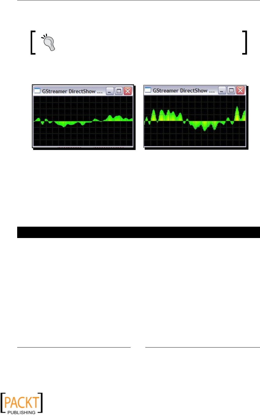
Audio Controls and Eects
[ 198 ]
This should start playing the input audio le and at the same me, it should also pop
up a small window where you can 'visualize' the streaming audio.
Note: The overall performance of this applicaon may depend on the
number of processes running at the me this program is run. It may also
depend on the specicaons of your computer such as processor speed.
Here, the stable audio waveform will be shown as the music plays. The following
shows a snapshot of this visualizaon window at two dierent meframes.
Snapshots at some random meframes using Music Visualizer using 'monoscope' are
depicted here.
What just happened?
We used the GStreamer plugins playbin and monoscope to develop an audio visualizaon
ulity for a streaming audio. The monoscope element provided a way to visualize highly
stable audio waveforms.
Have a go hero – use other visualization plugins
To illustrate visualizaon eects for an audio, the monoscope plugin was used. If you have
some other visualizaon plugins available in the GStreamer installaon, use those to create
dierent visualizaon eects. The following are some of the plugins that can be used for
this purpose: goom, goom2k1, libvisual, and synaesthesia. The audio visualizaon
accomplished by synaesthesia plugin is shown in the next illustraon.
x
x
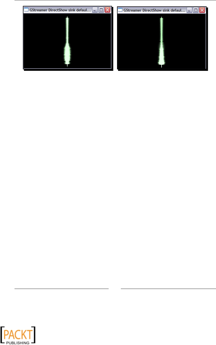
Chapter 6
[ 199 ]
Music Visualizer using 'synaesthesia': Snapshots at some random meframes is
depicted here.
Summary
We learned a lot in this chapter about various audio enhancement and control techniques.
The GStreamer mulmedia framework was used to accomplish this. We specically covered:
Audio controls: How to control the streaming of an audio data. With the help of
coding illustraons, we learned about playback controls such as play, pause, seek,
and stop. These controls were then used in a project where a poron of an audio
was extracted.
Adding eects: Enhancing the audio by adding audio eects such as fade-in,
echo/reverberaon, and so on.
Non-linear audio eding: How to combine two or more audio streams into a single
track. This was done in one of the projects we undertook.
Audio mixing technique to merge mulple mono channel audio streams into a single
interleaved audio.
Addionally, we also learned techniques such as visualizing an audio. This concludes our
discussion on audio processing in Python using GStreamer framework.
In the next chapter, we will learn how to process videos using Python.
x
x

x
x

7
Working with Videos
Photographs capture the moment, but it is the video that helps us relive
that moment! Video has become a major part of our lives. We preserve our
memories by capturing the family vacaon on a camcorder. When it comes to
digitally preserving those recorded memories, the digital video processing plays
an important role. In the previous chapter, to learn various audio processing
techniques, the GStreamer mulmedia framework was used. We will connue
to use GStreamer for learning the fundamentals of video processing.
In this chapter, we shall:
Develop a simple command-line video player
Perform basic video manipulaons such as cropping, resizing, and tweaking the
parameters such as brightness, contrast, and saturaon levels of a streaming video
Add text string on top of a video stream
Learn how to convert video between dierent video formats
Write a ulity that separates audio and video tracks from an input video le
Mix audio and video tracks to create a single video le
Save one or more video frames as sll images
So let's get on with it.
x
x

Working with Videos
[ 202 ]
Installation prerequisites
We will use Python bindings of GStreamer mulmedia framework to process video data.
See the installaon instrucons in Chapter 5, Working with Audios to install GStreamer
and other dependencies.
For video processing, we will be using several GStreamer plugins not introduced earlier.
Make sure that these plugins are available in your GStreamer installaon by running the
gst-inspect-0.10 command from the console (gst-inspect-0.10.exe for Windows
XP users). Otherwise, you will need to install these plugins or use an alternave if available.
Following is a list of addional plugins we will use in this chapter:
autoconvert: Determines an appropriate converter based on the capabilies. It
will be used extensively used throughout this chapter.
autovideosink: Automacally selects a video sink to display a streaming video.
ffmpegcolorspace: Transforms the color space into a color space format that can
be displayed by the video sink.
capsfilter: It's the capabilies lter—used to restrict the type of media data
passing down stream, discussed extensively in this chapter.
textoverlay: Overlays a text string on the streaming video. Used in the Adding
text and me on a video stream secon.
timeoverlay: Adds a mestamp on top of the video buer.
clockoverlay: Puts current clock me on the streaming video.
videobalance: Used to adjust brightness, contrast, and saturaon of the images.
It is used in the Video manipulaons and eects secon.
videobox: Crops the video frames by specied number of pixels—used in the
Cropping secon.
ffmux_mp4: Provides muxer element for MP4 video muxing.
ffenc_mpeg4: Encodes data into MPEG4 format.
ffenc_png: Encodes data in PNG format—used in the Saving video frames as
images secon.
x
x
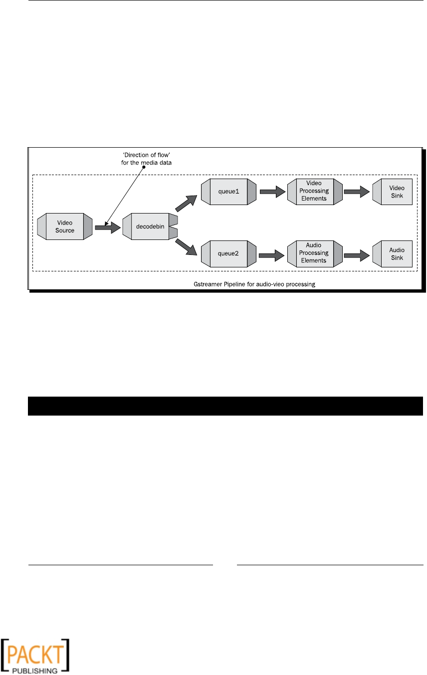
Chapter 7
[ 203 ]
Playing a video
Earlier, we saw how to play an audio. Like audio, there are dierent ways in which a video
can be streamed. The simplest of these methods is to use the playbin plugin. Another
method is to go by the basics, where we create a convenonal pipeline and create and
link the required pipeline elements. If we only want to play the 'video' track of a video le,
then the laer technique is very similar to the one illustrated for audio playback. However,
almost always, one would like to hear the audio track for the video being streamed. There
is addional work involved to accomplish this. The following diagram is a representave
GStreamer pipeline that shows how the data ows in case of a video playback.
In this illustraon, the decodebin uses an appropriate decoder to decode the media data
from the source element. Depending on the type of data (audio or video), it is then further
streamed to the audio or video processing elements through the queue elements. The two
queue elements, queue1 and queue2, act as media data buer for audio and video data
respecvely. When the queue elements are added and linked in the pipeline, the thread
creaon within the pipeline is handled internally by the GStreamer.
Time for action – video player!
Let's write a simple video player ulity. Here we will not use the playbin plugin. The use of
playbin will be illustrated in a later sub-secon. We will develop this ulity by construcng
a GStreamer pipeline. The key here is to use the queue as a data buer. The audio and video
data needs to be directed so that this 'ows' through audio or video processing secons of
the pipeline respecvely.
1. Download the le PlayingVidio.py from the Packt website. The le has the
source code for this video player ulity.
x
x

Working with Videos
[ 204 ]
2. The following code gives an overview of the Video player class and its methods.
import time
import thread
import gobject
import pygst
pygst.require("0.10")
import gst
import os
class VideoPlayer:
def __init__(self):
pass
def constructPipeline(self):
pass
def connectSignals(self):
pass
def decodebin_pad_added(self, decodebin, pad):
pass
def play(self):
pass
def message_handler(self, bus, message):
pass
# Run the program
player = VideoPlayer()
thread.start_new_thread(player.play, ())
gobject.threads_init()
evt_loop = gobject.MainLoop()
evt_loop.run()
As you can see, the overall structure of the code and the main program execuon
code remains the same as in the audio processing examples. The thread module is
used to create a new thread for playing the video. The method VideoPlayer.play
is sent on this thread. The gobject.threads_init() is an inializaon funcon
for facilitang the use of Python threading within the gobject modules. The main
event loop for execung this program is created using gobject and this loop is
started by the call evt_loop.run().
Instead of using thread module you can make use of threading
module as well. The code to use it will be something like:
1. import threading
2. threading.Thread(target=player.play).start()
x
x

Chapter 7
[ 205 ]
You will need to replace the line thread.start_new_thread(player.
play, ()) in earlier code snippet with line 2 illustrated in the code snippet
within this note. Try it yourself!
3. Now let's discuss a few of the important methods, starng with
self.contructPipeline:
1 def constructPipeline(self):
2 # Create the pipeline instance
3 self.player = gst.Pipeline()
4
5 # Define pipeline elements
6 self.filesrc = gst.element_factory_make("filesrc")
7 self.filesrc.set_property("location",
8 self.inFileLocation)
9 self.decodebin = gst.element_factory_make("decodebin")
10
11 # audioconvert for audio processing pipeline
12 self.audioconvert = gst.element_factory_make(
13 "audioconvert")
14 # Autoconvert element for video processing
15 self.autoconvert = gst.element_factory_make(
16 "autoconvert")
17 self.audiosink = gst.element_factory_make(
18 "autoaudiosink")
19
20 self.videosink = gst.element_factory_make(
21 "autovideosink")
22
23 # As a precaution add videio capability filter
24 # in the video processing pipeline.
25 videocap = gst.Caps("video/x-raw-yuv")
26 self.filter = gst.element_factory_make("capsfilter")
27 self.filter.set_property("caps", videocap)
28 # Converts the video from one colorspace to another
29 self.colorSpace = gst.element_factory_make(
30 "ffmpegcolorspace")
31
32 self.videoQueue = gst.element_factory_make("queue")
33 self.audioQueue = gst.element_factory_make("queue")
34
35 # Add elements to the pipeline
36 self.player.add(self.filesrc,
37 self.decodebin,
38 self.autoconvert,
x
x

Working with Videos
[ 206 ]
39 self.audioconvert,
40 self.videoQueue,
41 self.audioQueue,
42 self.filter,
43 self.colorSpace,
44 self.audiosink,
45 self.videosink)
46
47 # Link elements in the pipeline.
48 gst.element_link_many(self.filesrc, self.decodebin)
49
50 gst.element_link_many(self.videoQueue, self.autoconvert,
51 self.filter, self.colorSpace,
52 self.videosink)
53
54 gst.element_link_many(self.audioQueue,self.audioconvert,
55 self.audiosink)
4. In various audio processing applicaons, we have used several of the elements
dened in this method. First, the pipeline object, self.player, is created. The
self.filesrc element species the input video le. This element is connected
to a decodebin.
5. On line 15, autoconvert element is created. It is a GStreamer bin that
automacally selects a converter based on the capabilies (caps). It translates
the decoded data coming out of the decodebin in a format playable by the
video device. Note that before reaching the video sink, this data travels through
a capsfilter and ffmpegcolorspace converter. The capsfilter element is
dened on line 26. It is a lter that restricts the allowed capabilies, that is, the type
of media data that will pass through it. In this case, the videoCap object dened on
line 25 instructs the lter to only allow video-xraw-yuv capabilies .
6. The ffmpegcolorspace is a plugin that has the ability to convert video frames to
a dierent color space format. At this me, it is necessary to explain what a color
space is. A variety of colors can be created by use of basic colors. Such colors form,
what we call, a color space. A common example is an rgb color space where a range
of colors can be created using a combinaon of red, green, and blue colors. The
color space conversion is a representaon of a video frame or an image from one
color space into the other. The conversion is done in such a way that the converted
video frame or image is a closer representaon of the original one.
x
x

Chapter 7
[ 207 ]
The video can be streamed even without using the combinaon of
capsfilter and the ffmpegcolorspace. However, the video
may appear distorted. So it is recommended to use capsfilter and
ffmpegcolorspace converter. Try linking the autoconvert element
directly to the autovideosink to see if it makes any dierence.
7. Noce that we have created two sinks, one for audio output and the other for
the video. The two queue elements are created on lines 32 and 33. As menoned
earlier, these act as media data buers and are used to send the data to audio and
video processing porons of the GStreamer pipeline. The code block 35-45 adds all
the required elements to the pipeline.
8. Next, the various elements in the pipeline are linked. As we already know, the
decodebin is a plugin that determines the right type of decoder to use. This
element uses dynamic pads. While developing audio processing ulies, we
connected the pad-added signal from decodebin to a method decodebin_pad_
added. We will do the same thing here; however, the contents of this method will
be dierent. We will discuss that later.
9. On lines 50-52, the video processing poron of the pipeline is linked. The
self.videoQueue receives the video data from the decodebin. It is linked
to an autoconvert element discussed earlier. The capsfilter allows only
video-xraw-yuv data to stream further. The capsfilter is linked to a
ffmpegcolorspace element, which converts the data into a dierent color
space. Finally, the data is streamed to the videosink, which, in this case, is an
autovideosink element. This enables the 'viewing' of the input video. The audio
processing poron of the pipeline is very similar to the one used in earlier chapter.
10. Now we will review the decodebin_pad_added method.
1 def decodebin_pad_added(self, decodebin, pad):
2 compatible_pad = None
3 caps = pad.get_caps()
4 name = caps[0].get_name()
5 print "\n cap name is =%s"%name
6 if name[:5] == 'video':
7 compatible_pad = (
8 self.videoQueue.get_compatible_pad(pad, caps) )
9 elif name[:5] == 'audio':
10 compatible_pad = (
11 self.audioQueue.get_compatible_pad(pad, caps) )
12
13 if compatible_pad:
14 pad.link(compatible_pad)
x
x

Working with Videos
[ 208 ]
11. This method captures the pad-added signal, emied when the decodebin creates
a dynamic pad. In an earlier chapter, we simply linked the decodebin pad with a
compable pad on the autoaudioconvert element. We could do this because the
caps or the type media data being streamed was always the audio data. However,
here the media data can either represent an audio or video data. Thus, when a
dynamic pad is created on the decodebin, we must check what caps this pad
has. The name of the get_name method of caps object returns the type of media
data handled. For example, the name can be of the form video/x-raw-rgb when
it is a video data or audio/x-raw-int for audio data. We just check the rst ve
characters to see if it is video or audio media type. This is done by the code block
4-11 in the code snippet. The decodebin pad with video media type is linked with
the compable pad on self.videoQueue element. Similarly, the pad with audio
caps is linked with the one on self.audioQueue.
12. Review the rest of the code from the PlayingVideo.py. Make sure you specify an
appropriate video le path for the variable self.inFileLocation and then run
this program from the command prompt as:
$python PlayingVideo.py
This should open a GUI window where the video will be streamed. The
audio output will be synchronized with the playing video.
What just happened?
We created a command-line video player ulity. We learned how to create a GStreamer
pipeline that can play synchronized audio and video streams. It explained how the queue
element can be used to process the audio and video data in a pipeline. In this example, the
use of GStreamer plugins such as capsfilter and ffmpegcolorspace was illustrated.
The knowledge gained in this secon will be applied in the upcoming secons in this chapter.
Have a go hero – add playback controls
In Chapter 6, Audio Controls and Eects we learned dierent techniques to control the
playback of an audio. Develop command-line ulies that will allow you to pause the video
or directly jump to a specied posion on the video track.
Playing video using 'playbin'
The goal of the previous secon was to introduce you to the fundamental method of
processing input video streams. We will use that method one way or another in the
future discussions. If just video playback is all that you want, then the simplest way to
accomplish this is by means of playbin plugin. The video can be played just by replacing
the VideoPlayer.constructPipeline method in le PlayingVideo.py with the
x
x

Chapter 7
[ 209 ]
following code. Here, self.player is a playbin element. The uri property of playbin is
set as the input video le path.
def constructPipeline(self):
self.player = gst.element_factory_make("playbin")
self.player.set_property("uri",
"file:///" + self.inFileLocation)
Video format conversion
Saving the video in a dierent le format is one of the frequently performed tasks—for
example, the task of converng a recorded footage on to your camcorder to a format
playable on a DVD player. So let's list out the elements we need in a pipeline to carry
out the video format conversion.
A filesrc element to stream the video le and a decodebin to decode the
encoded input media data.
Next, the audio processing elements of the pipeline, such as audioconvert,
an encoder to encode the raw audio data into an appropriate audio format
to be wrien.
The video processing elements of the pipeline, such as a video encoder element to
encode the video data.
A mulplexer or a muxer that takes the encoded audio and video data streams and
puts them into a single channel.
There needs to be an element that, depending on the media type, can send the
media data to an appropriate processing unit. This is accomplished by queue
elements that act as data buers. Depending on whether it is an audio or video
data, it is streamed to the audio or video processing elements. The queue is also
needed to stream the encoded data from audio pipeline to the mulplexer.
Finally, a filesink element to save the converted video le (containing both audio
and video tracks).
Time for action – video format converter
We will create a video conversion ulity that will convert an input video le into a
format specied by the user. The le you need to download from the Packt website is
VideoConverter.py. This le can be run from the command line as:
python VideoConverter.py [options]
x
x

Working with Videos
[ 210 ]
Where, the opons are as follows:
--input_path: The full path of the video le we wish to convert. The video format
of the input les. The format should be in a supported list of formats. The supported
input formats are MP4, OGG, AVI, and MOV.
--output_path: The full path of the output video le. If not specied, it will create
a folder OUTPUT_VIDEOS within the input directory and save the le there with
same name.
--output_format: The audio format of the output le. The supported output
formats are OGG and MP4.
As we will be using a decodebin element for decoding the
input media data; there is actually a wider range of input formats
this ulity can handle. Modify the code in VideoPlayer.
processArguments or add more formats to diconary
VideoPlayer.supportedInputFormats.
1. If not done already, download the le VideoConverter.py from the
Packt website.
2. The overall structure of the code is:
import os, sys, time
import thread
import getopt, glob
import gobject
import pygst
pygst.require("0.10")
import gst
class VideoConverter:
def __init__(self):
pass
def constructPipeline(self):
pass
def connectSignals(self):
pass
def decodebin_pad_added(self, decodebin, pad):
pass
def processArgs(self):
pass
def printUsage(self):
pass
def printFinalStatus(self, starttime, endtime):
pass
x
x

Chapter 7
[ 211 ]
def convert(self):
pass
def message_handler(self, bus, message):
pass
# Run the converter
converter = VideoConverter()
thread.start_new_thread(converter.convert, ())
gobject.threads_init()
evt_loop = gobject.MainLoop()
evt_loop.run()
A new thread is created by calling thread.start_new_thread,
to run the applicaon. The method VideoConverter.convert
is sent on this thread. It is similar to the VideoPlayer.play
method discussed earlier. Let's review some key methods of the
class VideoConverter.
3. The __init__ method contains the inializaon code. It also calls methods
to process command-line arguments and then build the pipeline. The code is
illustrated as follows:
1 def __init__(self):
2 # Initialize various attrs
3 self.inFileLocation = ""
4 self.outFileLocation = ""
5 self.inputFormat = "ogg"
6 self.outputFormat = ""
7 self.error_message = ""
8 # Create dictionary objects for
9 # Audio / Video encoders for supported
10 # file format
11 self.audioEncoders = {"mp4":"lame",
12 "ogg": "vorbisenc"}
13
14 self.videoEncoders={"mp4":"ffenc_mpeg4",
15 "ogg": "theoraenc"}
16
17 self.muxers = {"mp4":"ffmux_mp4",
18 "ogg":"oggmux" }
19
20 self.supportedOutputFormats = self.audioEncoders.keys()
21
22 self.supportedInputFormats = ("ogg", "mp4",
23 "avi", "mov")
x
x

Working with Videos
[ 212 ]
24
25 self.pipeline = None
26 self.is_playing = False
27
28 self.processArgs()
29 self.constructPipeline()
30 self.connectSignals()
To process the video le, we need audio and video encoders. This ulity will support
the conversion to only MP4 and OGG le formats. This can be easily extended to
include more formats by adding appropriate encoders and muxer plugins. The values
of the self.audioEncoders and self.videoEncoders diconary objects specify
the encoders to use for the streaming audio and video data respecvely. Therefore,
to store the video data in MP4 format, we use the ffenc_mp4 encoder. The encoders
illustrated in the code snippet should be a part of the GStreamer installaon on your
computer. If not, visit the GStreamer website to nd out how to install these plugins.
The values of diconary self.muxers represent the mulplexer to use in a specic
output format.
4. The constructPipeline method does the main conversion job. It builds the
required pipeline, which is then set to playing state in the convert method.
1 def constructPipeline(self):
2 self.pipeline = gst.Pipeline("pipeline")
3
4 self.filesrc = gst.element_factory_make("filesrc")
5 self.filesrc.set_property("location",
6 self.inFileLocation)
7
8 self.filesink = gst.element_factory_make("filesink")
9 self.filesink.set_property("location",
10 self.outFileLocation)
11
12 self.decodebin = gst.element_factory_make("decodebin")
13 self.audioconvert = gst.element_factory_make(
14 "audioconvert")
15
16 audio_encoder = self.audioEncoders[self.outputFormat]
17 muxer_str = self.muxers[self.outputFormat]
18 video_encoder = self.videoEncoders[self.outputFormat]
19
20 self.audio_encoder= gst.element_factory_make(
21 audio_encoder)
22 self.muxer = gst.element_factory_make(muxer_str)
23 self.video_encoder = gst.element_factory_make(
24 video_encoder)
x
x

Chapter 7
[ 213 ]
25
26 self.videoQueue = gst.element_factory_make("queue")
27 self.audioQueue = gst.element_factory_make("queue")
28 self.queue3 = gst.element_factory_make("queue")
29
30 self.pipeline.add( self.filesrc,
31 self.decodebin,
32 self.video_encoder,
33 self.muxer,
34 self.videoQueue,
35 self.audioQueue,
36 self.queue3,
37 self.audioconvert,
38 self.audio_encoder,
39 self.filesink)
40
41 gst.element_link_many(self.filesrc, self.decodebin)
42
43 gst.element_link_many(self.videoQueue,
44 self.video_encoder, self.muxer, self.filesink)
45
46 gst.element_link_many(self.audioQueue,self.audioconvert,
47 self.audio_encoder, self.queue3,
48 self.muxer)
In an earlier secon, we covered several of the elements used in the previous pipe-
line. The code on lines 43 to 48 establishes linkage for the audio and video process-
ing elements. On line 44, the mulplexer, self.muxer is linked with the video
encoder element. It puts the separate parts of the stream—in this case, the video
and audio data, into a single le. The data output from audio encoder, self.au-
dio_encoder, is streamed to the muxer via a queue element, self.queue3. The
muxed data coming out of self.muxer is then streamed to the self.filesink.
5. Let's quickly review the VideoConverter.convert method.
1 def convert(self):
2 # Record time before beginning Video conversion
3 starttime = time.clock()
4
5 print "\n Converting Video file.."
6 print "\n Input File: %s, Conversion STARTED..." %
7 self.inFileLocation
8
9 self.is_playing = True
10 self.pipeline.set_state(gst.STATE_PLAYING)
11 while self.is_playing:
12 time.sleep(1)
x
x
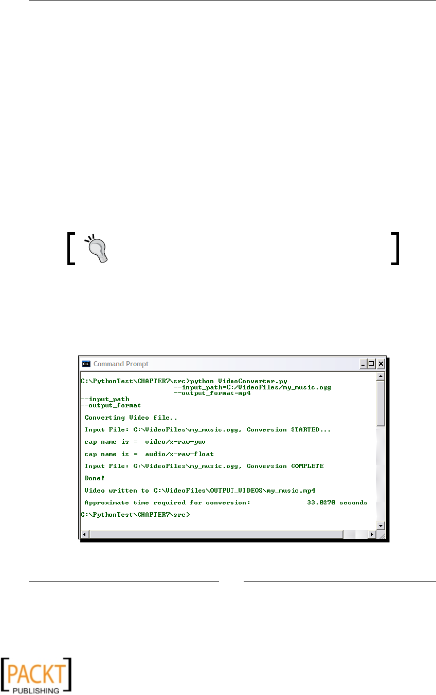
Working with Videos
[ 214 ]
13
14 if self.error_message:
15 print "\n Input File: %s, ERROR OCCURED." %
16 self.inFileLocation
17 print self.error_message
18 else:
19 print "\n Input File: %s, Conversion COMPLETE " %
20 self.inFileLocation
21
22 endtime = time.clock()
23 self.printFinalStatus(starttime, endtime)
24 evt_loop.quit()
On line 10, the GStreamer pipeline built earlier is set to playing. When the
conversion is complete, it will generate the End Of Stream (EOS) message. The
self.is_playing ag is modied in the method self.message_handler. The
while loop on line 11 is executed unl the EOS message is posted on the bus or
some error occurs. Finally, on line 24, the main execuon loop is terminated.
On line 3, we make a call to time.clock(). This actually gives
the CPU me spent on the process.
6. The other methods such as VideoConverter.decodebin_pad_added are
idencal to the one developed in the Playing a video secon. Review the remaining
methods from the le VideoConverter.py and then run this ulity by specifying
appropriate command-line arguments. The following screenshot shows sample
output messages when the program is run from the console window.
This is a sample run of the video conversion ulity from the console.
x
x

Chapter 7
[ 215 ]
What just happened?
We created another useful ulity that can convert video les from one format to the other.
We learned how to encode the audio and video data into a desired output format and then
use a mulplexer to put these two data streams into a single le.
Have a go hero – batch-convert the video les
The video converter developed in previous secons can convert a single video le at a me.
Can you make it a batch-processing ulity? Refer to the code for the audio conversion ulity
developed in the Working with Audios chapter. The overall structure will be very similar.
However, there could be challenges in converng mulple video les because of the use of
queue elements. For example, when it is done converng the rst le, the data in the queue
may not be ushed when we start conversion of the other le. One crude way to address this
would be to reconstruct the whole pipeline and connect signals for each audio le. However,
there will be a more ecient way to do this. Think about it!
Video manipulations and effects
Suppose you have a video le that needs to be saved with an adjusted default brightness
level. Alternavely, you may want to save another video with a dierent aspect rao. In this
secon, we will learn some of the basic and most frequently performed operaons on a
video. We will develop code using Python and GStreamer for tasks such as resizing a video
or adjusng its contrast level.
Resizing
The data that can ow through an element is described by the capabilies (caps) of a pad on
that element. If a decodebin element is decoding video data, the capabilies of its dynamic
pad will be described as, for instance, video/x-raw-yuv. Resizing a video with GStreamer
mulmedia framework can be accomplished by using a capsfilter element, that has
width and height parameters specied. As discussed earlier, the capsfilter element
limits the media data type that can be transferred between two elements. For example, a
cap object described by the string, video/x-raw-yuv, width=800, height=600 will set
the width of the video to 800 pixels and the height to 600 pixels.
x
x

Working with Videos
[ 216 ]
Time for action – resize a video
We will now see how to resize a streaming video using the width and height parameters
described by a GStreamer cap object.
1. Download the le VideoManipulations.py from the Packt website. The overall
class design is idencal to the one studied in the Playing a video secon.
2. The methods self.constructAudioPipeline() and self.
constructVideoPipeline(), respecvely, dene and link elements related to
audio and video porons of the main pipeline object self.player. As we have
already discussed most of the audio/video processing elements in earlier secons,
we will only review the constructVideoPipeline method here.
1 def constructVideoPipeline(self):
2 # Autoconvert element for video processing
3 self.autoconvert = gst.element_factory_make(
4 "autoconvert")
5 self.videosink = gst.element_factory_make(
6 "autovideosink")
7
8 # Set the capsfilter
9 if self.video_width and self.video_height:
10 videocap = gst.Caps(
11 "video/x-raw-yuv," "width=%d, height=%d"%
12 (self.video_width,self.video_height))
13 else:
14 videocap = gst.Caps("video/x-raw-yuv")
15
16 self.capsFilter = gst.element_factory_make(
17 "capsfilter")
18 self.capsFilter.set_property("caps", videocap)
19
20 # Converts the video from one colorspace to another
21 self.colorSpace = gst.element_factory_make(
22 "ffmpegcolorspace")
23
24 self.videoQueue = gst.element_factory_make("queue")
25
26 self.player.add(self.videoQueue,
27 self.autoconvert,
28 self.capsFilter,
29 self.colorSpace,
30 self.videosink)
31
x
x

Chapter 7
[ 217 ]
32 gst.element_link_many(self.videoQueue,
33 self.autoconvert,
34 self.capsFilter,
35 self.colorSpace,
36 self.videosink)
The capsfilter element is dened on line 16. It is a lter that restricts the type
of media data that will pass through it. The videocap is a GStreamer cap object
created on line 10. This cap species the width and height parameters of the
streaming video. It is set as a property of the capsfilter, self.capsFilter. It
instructs the lter to only stream video-xraw-yuv data with width and height
specied by the videocap object.
In the source le, you will see an addional element self.videobox
linked in the pipeline. It is omied in the above code snippet. We will see
what this element is used for in the next secon.
3. The rest of the code is straighorward. We already covered similar methods
in earlier discussions. Develop the rest of the code by reviewing the le
VideoManipulations.py. Make sure to specify an appropriate video le
path for the variable self.inFileLocation .Then run this program from
the command prompt as:
$python VideoManipulations.py
This should open a GUI window where the video will be streamed. The default
size of this window will be controlled by the parameters self.video_width
and self.video_height specied in the code.
What just happened?
The command-line video player developed earlier was extended in the example we just
developed. We used capsfilter plugin to specify the width and height parameters
of the streaming video and thus resize the video.
Cropping
Suppose you have a video that has a large 'guer space' at the boom or some unwanted
poron on a side that you would like to trim o. The videobox GStreamer plugin facilitates
cropping the video from le, right, top, or boom.
x
x

Working with Videos
[ 218 ]
Time for action – crop a video
Let's add another video manipulaon feature to the command-line video player
developed earlier.
1. The le we need here is the one used in the earlier secon,
VideoManipulations.py.
2. Once again, we will focus our aenon on the constructVideoPipeline method
of the class VideoPlayer. The following code snippet is from this method. The rest
of the code in this method is idencal to the one reviewed in the earlier secon.
1 self.videobox = gst.element_factory_make("videobox")
2 self.videobox.set_property("bottom", self.crop_bottom )
3 self.videobox.set_property("top", self.crop_top )
4 self.videobox.set_property("left", self.crop_left )
5 self.videobox.set_property("right", self.crop_right )
6
7 self.player.add(self.videoQueue,
8 self.autoconvert,
9 self.videobox,
10 self.capsFilter,
11 self.colorSpace,
12 self.videosink)
13
14 gst.element_link_many(self.videoQueue,
15 self.autoconvert,
16 self.videobox,
17 self.capsFilter,
18 self.colorSpace,
19 self.videosink)
3. The code is self-explanatory. The videobox element is created on line 1. The
properes of videobox that crop the streaming video are set on lines 2-5.
It receives the media data from the autoconvert element. The source pad
of videobox is connected to the sink of either capsfilter or directly the
ffmpegcolorspace element.
4. Develop the rest of the code by reviewing the le VideoManipulations.
py. Make sure to specify an appropriate video le path for the variable self.
inFileLocation. Then run this program from the command prompt as:
$python VideoManipulations.py
This should open a GUI window where the video will be streamed. The video will be
cropped from le, right, boom, and top sides by the parameters self.crop_left,
self.crop_right, self.crop_bottom, and self.crop_top respecvely.
x
x

Chapter 7
[ 219 ]
What just happened?
We extended the video player applicaon further to add a GStreamer element that can crop
the video frames from sides. The videobox plugin was used to accomplish this task.
Have a go hero – add borders to a video
1. In the previous secon, we used videobox element to trim the video from sides.
The same plugin can be used to add a border around the video. If you set negave
values for videobox properes, such as, boom, top, le and right, instead of
cropping the video, it will add black border around the video. Set negave values
of parameters such as self.crop_left to see this eect.
2. The video cropping can be accomplished by using videocrop plugin. It is similar
to the videobox plugin, but it doesn't support adding a border to the video frames.
Modify the code and use this plugin to crop the video.
Adjusting brightness and contrast
We saw how to adjust the brightness and contrast level in Chapter 3, Enhancing Images.
If you have a homemade video recorded in poor lighng condions, you would probably
adjust its brightness level. The contrast-level highlights the dierence between the color and
brightness level of each video frame. The videobalance plugin can be used to adjust the
brightness, contrast, hue, and saturaon. The next code snippet creates this element and
sets the brightness and contrast properes. The brightness property can accept values in the
range -1 to 1, the default (original) brightness level is 0. The contrast can have values in the
range 0 to 2 with the default value as 1.
self.videobalance = gst.element_factory_make("videobalance")
self.videobalance.set_property("brightness", 0.5)
self.videobalance.set_property("contrast", 0.5)
The videobalance is then linked in the GStreamer pipeline as:
gst.element_link_many(self.videoQueue,
self.autoconvert,
self.videobalance,
self.capsFilter,
self.colorSpace,
self.videosink)
Review the rest of the code from le VideoEffects.py.
x
x

Working with Videos
[ 220 ]
Creating a gray scale video
The video can be rendered as gray scale by adjusng the saturaon property of the
videobalance plugin. The saturaon can have a value in the range 0 to 2. The default
value is 1. Seng this value to 0.0 converts the images to gray scale. The code is illustrated
as follows:
self.videobalance.set_property("saturation", 0.0)
You can refer to the le VideoEffects.py, which illustrates how to use the videobalance
plugin to adjust saturaon and other parameters discussed in earlier secons.
Adding text and time on a video stream
Ability to add a text string or a subtles track to a video is yet another desirable feature one
needs when processing videos. The GStreamer plugin textoverlay enables overlaying
informave text string, such as the name of the le, on top of a video stream. The other
useful plugins such as timeoverlay and clockoverlay provide a way to put the video
buer mestamp and the CPU clock me on top of the streaming video.
Time for action – overlay text on a video track
Let's see how to add a text string on a video track. We will write a simple ulity, which
essenally has the same code structure as the one we developed in the Playing a video
secon. This tool will also add the buer mestamp and the current CPU clock me
on the top of the video. For this secon, it is important that you have textoverlay,
timeoverlay, and clockoverlay plugins available in your GStreamer installaon.
Otherwise, you need to install these plugins or use some other plugins, such as
cairotextoverlay, if available.
1. Download the le VideoTextOverlay.py from the Packt website.
2. The constructVideoPipeline method of the class VideoPlayer is illustrated
in the following code snippet:
1 def constructVideoPipeline(self):
2 # Autoconvert element for video processing
3 self.autoconvert = gst.element_factory_make(
4 "autoconvert")
5 self.videosink = gst.element_factory_make(
6 "autovideosink")
7
8 # Set the capsfilter
9 videocap = gst.Caps("video/x-raw-yuv")
x
x

Chapter 7
[ 221 ]
10 self.capsFilter = gst.element_factory_make(
11 "capsfilter")
12 self.capsFilter.set_property("caps", videocap)
13
14 # Converts the video from one colorspace to another
15 self.colorSpace = gst.element_factory_make(
16 "ffmpegcolorspace")
17
18 self.videoQueue = gst.element_factory_make("queue")
19
20 self.textOverlay = gst.element_factory_make(
21 "textoverlay")
22 self.textOverlay.set_property("text", "hello")
23 self.textOverlay.set_property("shaded-background",
24 True)
25
26 self.timeOverlay = gst.element_factory_make(
27 "timeoverlay")
28 self.timeOverlay.set_property("valign", "top")
29 self.timeOverlay.set_property("shaded-background",
30 True)
31
32 self.clockOverlay = gst.element_factory_make(
33 "clockoverlay")
34 self.clockOverlay.set_property("valign", "bottom")
35 self.clockOverlay.set_property("halign", "right")
36 self.clockOverlay.set_property("shaded-background",
37 True)
38
39 self.player.add(self.videoQueue,
40 self.autoconvert,
41 self.textOverlay,
42 self.timeOverlay,
43 self.clockOverlay,
44 self.capsFilter,
45 self.colorSpace,
46 self.videosink)
47
48 gst.element_link_many(self.videoQueue,
49 self.autoconvert,
50 self.capsFilter,
51 self.textOverlay,
52 self.timeOverlay,
53 self.clockOverlay,
54 self.colorSpace,
55 self.videosink)
x
x
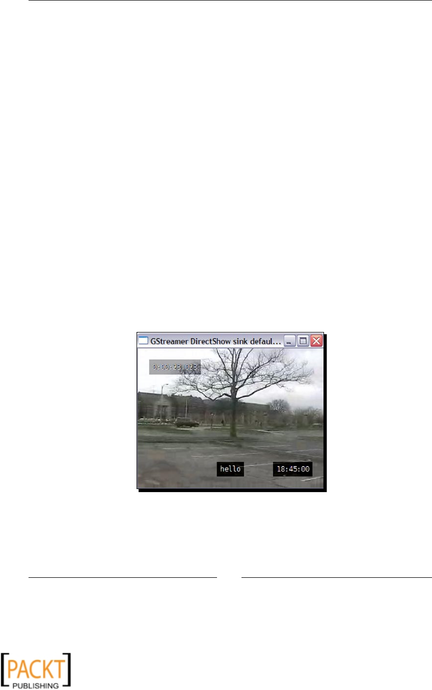
Working with Videos
[ 222 ]
As you can see, the elements for overlaying text, me, or clock can be simply
added and linked in a GStreamer pipeline like other elements. Let's discuss various
properes of these elements now. On lines 20-23, the textoverlay element is
dened. The text property sets the text string that appears on the streaming video.
To ensure that the text string is clearly visible in the video, we add a background
contrast to this text. This is done on line 23 by seng the shaded-background
property to True. The other properes of this plugin help x the text posion on
the video. Run gst-inspect-0.10 on textoverlay plugin to see what these
properes are.
3. Next, on lines 25-36, the me and clock overlay elements are dened. The
properes are similar to the ones available in textoverlay plugin. The clock me
will appear on the boom-le corner of the streaming video. This is accomplished
by seng the valign and halign properes. These three elements are then
linked in the GStreamer pipeline. The internal order in which they are linked
doesn't maer.
4. Develop the rest of the code by reviewing the le VideoTextOverlay.py.
Make sure you specify an appropriate video le path for the variable self.
inFileLocation. Then run this program from the command prompt as:
$python VideoTextOverlay.py
This should open a GUI window where the video will be streamed. The video will
show a text string "hello" along with the running me and the clock me. This is
illustrated by the following snapshot of a video frame.
The screenshot depicts a video frame showing text, me, and clock overlay.
x
x

Chapter 7
[ 223 ]
What just happened?
We learned how to use elements such as textoverlay, timeoverlay, and
clockoverlay in a GStreamer pipeline to add text string, mestamp, and clock
respecvely, on top of a video buer. The textoverlay element can be used further
to add a subtle track to the video le.
Have a go hero – add subtitles to a video track!
Extend the code we just developed to add a subtles track to the video le. To add a subtle
track, you will need the subparse plugin. Note that this plugin is not available by default
in the windows installaon of GStreamer using the GStreamer-WinBuilds binary. Thus,
Windows users may need to install this plugin separately. Review the subparse plugin
reference to see how to accomplish this task. The following code snippet shows how to
create the subparse element.
self.subtitlesrc = gst.element_factory_make("filesrc")
self.subtitlesrc.set_property("location",
"/path/to/subtitles/file")
self.subparse = gst.element_factory_make("subparse")
Separating audio and video tracks
There are mes when you would like to separate an audio and a video track. Imagine that
you have a collecon of your favorite video songs. You are going on a long drive and the old
CD player in your car can only play audio les in a specic le format. Let's write a ulity that
can separate out the audio from a video le!
Time for action – audio and video tracks
We will develop code that takes a video le as an input and then creates two output les,
one with only the audio track of the original le and the other with the video poron.
1. Download the le SeparatingAudio.py from the Packt website. The structure
of the class AudioSeparator is similar to the one seen in the Playing a Video
secon. We will review two methods of this class, constructPipeline and
decodebin_pad_added.
2. Let's start with the code in the constructPipeline method.
1 def constructPipeline(self):
2 # Create the pipeline instance
3 self.player = gst.Pipeline()
4
x
x

Working with Videos
[ 224 ]
5 # Define pipeline elements
6 self.filesrc = gst.element_factory_make("filesrc")
7
8 self.filesrc.set_property("location",
9 self.inFileLocation)
10
11 self.decodebin = gst.element_factory_make("decodebin")
12
13 self.autoconvert = gst.element_factory_make(
14 "autoconvert")
15
16 self.audioconvert = gst.element_factory_make(
17 "audioconvert")
18
19 self.audio_encoder = gst.element_factory_make("lame")
20
21 self.audiosink = gst.element_factory_make("filesink")
22 self.audiosink.set_property("location",
23 self.audioOutLocation)
24
25 self.video_encoder = gst.element_factory_make("
26 ffenc_mpeg4")
27 self.muxer = gst.element_factory_make("ffmux_mp4")
28
29 self.videosink = gst.element_factory_make("filesink")
30 self.videosink.set_property("location",
31 self.videoOutLocation)
32
33 self.videoQueue = gst.element_factory_make("queue")
34 self.audioQueue = gst.element_factory_make("queue")
35 # Add elements to the pipeline
36 self.player.add(self.filesrc,
37 self.decodebin,
38 self.videoQueue,
39 self.autoconvert,
40 self.video_encoder,
41 self.muxer,
42 self.videosink,
43 self.audioQueue,
44 self.audioconvert,
45 self.audio_encoder,
46 self.audiosink)
47
49 # Link elements in the pipeline.
x
x

Chapter 7
[ 225 ]
50 gst.element_link_many(self.filesrc, self.decodebin)
51
52 gst.element_link_many(self. videoQueue,
53 self.autoconvert,
54 self.video_encoder,
55 self.muxer,
56 self.videosink)
57
58 gst.element_link_many(self.audioQueue,
59 self.audioconvert,
60 self.audio_encoder,
61 self.audiosink)
We have already used all the necessary elements in various examples. The key here
is to link them properly. The self.audiosink and self.videoSink elements are
filesink elements that dene audio and video output le locaons respecvely.
Note that, in this example, we will save the output audio in MP3 format and video
in MP4 format. Thus, the lame encoder is used for the audio le whereas we use
encoder ffenc_mpeg4 and mulplexer ffmux_mp4 for the video output. Note that
we have not used ffmpegcolorspace element. It just helps to get an appropriate
color space format for the video sink (in this case, the output video le). In this case,
it is not needed. You can always link it in the pipeline if the output le doesn't ap-
propriately display the video frames. The media data decoded by self.decodebin
needs to be streamed to the audio and video porons of the pipeline, using the
queue elements as data buers.
3. The decodebin creates dynamic pads to decode the input audio and video data.
The decodebin_pad_added method needs to check the capabilies (caps) on the
dynamic pad of the decodebin.
1 def decodebin_pad_added(self, decodebin, pad):
2 compatible_pad = None
3 caps = pad.get_caps()
4 name = caps[0].get_name()
5 print "\n cap name is = ", name
6 if name[:5] == 'video':
7 compatible_pad = (
8 self.videoQueue.get_compatible_pad(pad, caps) )
9 elif name[:5] == 'audio':
10 compatible_pad = (
11 self. audioQueue.get_compatible_pad(pad,caps) )
12
13 if compatible_pad:
14 pad.link(compatible_pad)
x
x

Working with Videos
[ 226 ]
4. This check is done by the code block 6-12. If capabilies indicate it's an audio
data, the decodebin pad is linked to the compable pad on self.audioQueue.
Similarly, a link between to self.videoQueue and self.decodebin is created
when caps indicate it is the video data.
5. You can work through the remaining code in the le SeparatingAudio.
py. Replace the paths represented by self.inFileLocation, self.
audioOutLocation, and self.videoOutLocation with appropriate paths on
your computer and then run this ulity as:
$python SeparatingAudio.py
This should create two output les—a le in MP3 format that contains only the
audio track from the input le and a le in MP4 format containing the video track.
What just happened?
We build a GStreamer pipeline that separates audio and video tracks from an input video
le. Several of the GStreamer elements that we learned about in a number of examples
earlier were used to develop this ulity. We also learned how to use the capabilies (caps)
on the dynamic pads of decodebin to make proper linkage between the decodebin and
the queue elements.
Mixing audio and video tracks
Suppose you have recorded your friend's wedding on your camcorder. For some specic
moments, you would like to mute all other sounds and replace those with background music.
To accomplish this, rst you need to save the video track without the audio as a separate le.
We just learned that technique. Then you need to combine this video track with audio track
containing the background music you wish to play. Let's now learn how to mix audio and
video tracks into a single video le.
Time for action – audio/video track mixer
We will develop a program that generates a video output le, by mixing an audio and a video
track. Think about what change we will need to incorporate when compared to the audio/
video track separaon ulity developed earlier. In that applicaon, two filesink elements
were required as two output les were created. Here, we need the opposite. We require two
filesrc elements containing the audio and video data and a single filesink element
that will contain both the audio and the video track.
1. Download the le AudioVideoMixing.py from the Packt website. We will review
some of the important methods of class AudioVideoMixer.
x
x

Chapter 7
[ 227 ]
2. The constructPipeline method, as usual, builds the GStreamer pipeline with all
necessary elements.
1 def constructPipeline(self):
2 self.pipeline = gst.Pipeline("pipeline")
3
4 self.audiosrc = gst.element_factory_make("filesrc")
5 self.audiosrc.set_property("location",
6 self.audioInLocation)
7
8 self.videosrc = gst.element_factory_make("filesrc")
9 self.videosrc.set_property("location",
10 self.videoInLocation)
11
12 self.filesink = gst.element_factory_make("filesink")
13 self.filesink.set_property("location",
14 self.outFileLocation)
15
16 self.audio_decodebin = gst.element_factory_make(
17 "decodebin")
18 self.video_decodebin= gst.element_factory_make(
19 "decodebin")
20
21 self.audioconvert = gst.element_factory_make(
22 "audioconvert")
23 self.audio_encoder= gst.element_factory_make("lame")
24
25 self.video_encoder = (
26 gst.element_factory_make("ffenc_mpeg4") )
27 self.muxer = gst.element_factory_make("ffmux_mp4")
28 self.queue = gst.element_factory_make("queue")
29
30
31 videocap = gst.Caps("video/x-raw-yuv")
32 self.capsFilter = gst.element_factory_make(
33 "capsfilter")
34 self.capsFilter.set_property("caps", videocap)
35 # Converts the video from one colorspace to another
36 self.colorSpace = gst.element_factory_make(
37 "ffmpegcolorspace")
38
39 self.pipeline.add( self.videosrc,
40 self. video_decodebin,
41 self.capsFilter,
x
x

Working with Videos
[ 228 ]
42 self.colorSpace,
43 self.video_encoder,
44 self.muxer,
45 self.filesink)
46
47 self.pipeline.add(self.audiosrc,
48 self.audio_decodebin,
49 self.audioconvert,
50 self.audio_encoder,
51 self.queue)
52
53 # Link audio elements
54 gst.element_link_many(self.audiosrc,
55 self.audio_decodebin)
56 gst.element_link_many( self.audioconvert,
57 self.audio_encoder,
58 self.queue, self.muxer)
59 #Link video elements
60 gst.element_link_many(self.videosrc,
61 self.video_decodebin)
62 gst.element_link_many(self.capsFilter,
63 self.colorSpace,
64 self.video_encoder,
65 self.muxer,
66 self.filesink)
3. The audio and video le sources are dened by the elements self.audiosrc and
self.videosrc respecvely. These are connected to two separate decodebins
(see lines 54 and 59). The pad-added signals of self.audio_decodebin and
self.video_decodebin are connected in the connectSignals method.
The audio and video data then travels through a chain of audio and video
processing elements respecvely. The data is encoded by their respecve encoders.
The encoded data streams are combined so that the output video le contains
both audio and video tracks. This job is done by the mulplexer, self.muxer. It is
linked with the video encoder element. The audio data is streamed to the muxer
through a queue element (line 57). The data is 'muxed' and fed to the filesink
element, self.filesink. Note that the ffmpegcolorspace element and the
capsfilter, self.capsfiter is not really required. In this case, the output
video should have proper display format. You can try running this applicaon by
removing those two elements to see if it makes any dierence.
x
x

Chapter 7
[ 229 ]
4. In the decodebin_pad_added method, we will check a few extra things before
linking the dynamic pads.
1 def decodebin_pad_added(self, decodebin, pad):
2 compatible_pad = None
3 caps = pad.get_caps()
4 name = caps[0].get_name()
5 print "\n cap name is =%s"%name
6 if ( name[:5] == 'video' and
7 (decodebin is self.video_decodebin) ):
8 compatible_pad = (
9 self.capsFilter.get_compatible_pad(pad, caps) )
10 elif ( name[:5] == 'audio' and
11 (decodebin is self.audio_decodebin) ):
12 compatible_pad = (
13 self.audioconvert.get_compatible_pad(pad, caps) )
14
15 if compatible_pad:
16 pad.link(compatible_pad)
It could happen that each of the input les contains audio as well as video data. For
example, both self.audiosrc and self.videosrc represent dierent video
les with both audio and video data. The le self.audiosrc is linked to self.
audio_decodebin. Thus, we should make sure that when the self.audio_de-
codebin generates a pad-added signal, the dynamic pad is linked only when its
caps have audio data. On similar lines, the pad on self.video_decodebin is
linked only when caps represent video data. This is ensured by the code block 6 – 13.
5. Develop the rest of the code by reviewing le AudioVideoMixer.py. Replace the
paths represented by, self.audioInLocation, self.videoInLocation, and
self.outFileLocation with appropriate paths on your computer and then run
this ulity as:
$python AudioVideoMixer.py
This should create an output video le in MP4 format that contains the audio and
video tracks from the specied input les!
What just happened?
We developed a tool that mixes input audio and video tracks and stores them into a single
output le. To accomplish this task we used most of the audio/video processing elements
that were used in video conversion ulity. We learned how to link the dynamic pads on
decodebin based on the streaming data represented by its 'caps'. The mulplexer plugin
ffmux_mp4 element was used to put the audio and video data together.
x
x

Working with Videos
[ 230 ]
Saving video frames as images
Imagine that you have a wildlife video and it has recorded a very special moment. You would
like to save this image. Let's learn how this can be achieved using the GStreamer framework.
Time for action – saving video frames as images
This le can be run from the command line as:
python ImagesFromVideo.py [options]
Here the [options] are:
--input_file: The full path to input video le from which one or more frames
need to be captured and saved as images.
--start_time: The posion in seconds on the video track. This will be the starng
posion from which one or more video frames will be captured as sll image(s). The
rst snapshot will always be at start_time.
--duration: The duraon (in seconds) of the video track starng from the
start_time. 'N' number of frames will be captured starng from the start_time.
--num_of_captures: Total number of frames that need to be captured from
start_time (including it) up to, end_time= start_time + duration
(but not including the sll image at end_time).
1. If not already done, download the le ImagesFromVideo.py from the Packt
website. Following is an outline of the code for saving video frames.
import os, sys, time
import thread
import gobject
import pygst
pygst.require("0.10")
import gst
from optparse import OptionParser
class ImageCapture:
def __init__(self):
pass
def connectSignals(self):
pass
def constructPipeline(self):
pass
def gnonlin_pad_added(self, gnonlin_elem, pad):
pass
x
x

Chapter 7
[ 231 ]
def captureImage(self):
pass
def capture_single_image(self, media_start_time):
pass
def message_handler(self, bus, message):
pass
def printUsage(self):
pass
def printFinalStatus(self, starttime, endtime):
pass
# Run the program
imgCapture = ImageCapture()
thread.start_new_thread(imgCapture.captureImage, ())
gobject.threads_init()
evt_loop = gobject.MainLoop()
evt_loop.run()
The program execuon starts by calling the captureImage method. The
gnlfilesource element discussed in audio processing chapters will be used
here to seek a parcular frame on the streaming video. The capture_single_im-
age does the main job of saving a single frame as an image. We will discuss some of
these methods next.
2. Let's start with the constructPipeline method which denes and links various
elements needed to capture the video frames.
1 def constructPipeline(self):
2 self.pipeline = gst.Pipeline()
3 self.gnlfilesrc = (
4 gst.element_factory_make("gnlfilesource") )
5
6 self.gnlfilesrc.set_property("uri",
7 "file:///" + self.inFileLocation)
8 self.colorSpace = gst.element_factory_make(
9 "ffmpegcolorspace")
10
11 self.encoder= gst.element_factory_make("ffenc_png")
12
13 self.filesink = gst.element_factory_make("filesink")
14
15 self.pipeline.add(self.gnlfilesrc,
16 self.colorSpace,
17 self.encoder,
18 self.filesink)
x
x

Working with Videos
[ 232 ]
19
20 gst.element_link_many(self.colorSpace,
21 self.encoder,
22 self.filesink)
We already know how to create and connect the gnlfilesource element (called
self.gnlfilesrc). In the examples we have seen so far, the encoder element
used in a GStreamer pipeline encoded the streaming media data either in an audio
or a video format. On line 11, we dene a new encoder element that enables saving
a parcular frame in the streaming video as an image. In this example, we use the
encoder ffenc_png to save the video frame as an image le with PNG le format.
This plugin should be available by default in your GStreamer installaon. If not,
you will need to install it. There are similar plugins available to save the image in
dierent le formats. For example, use jpegenc plugin to save it as a JPEG image
and so on.
The self.gnlfilesrc uses dynamic pad, which is connected to an appropriate
pad on ffmpegcolorspace discussed earlier. The self.colorspace element
converts the color space and this video data is then encoded by the ffenc_png
element. The self.filesink denes the locaon to save a parcular video
frame as an image.
3. The captureImage is the main controlling method. The overall structure is very
similar to the audio conversion ulity developer in Chapter 5, Working with Audios.
This method runs the top-level controlling loop to capture the frames specied as
an argument to the program.
1 def captureImage(self):
2 # Record start time
3 starttime = time.clock()
4
5 # Note: all times are in nano-seconds
6 media_end = self.media_start_time + self.media_duration
7 start = self.media_start_time
8 while start < media_end:
9 self.capture_single_image(start)
10 start += self.deltaTime
11
12 endtime = time.clock()
13 self.printFinalStatus(starttime, endtime)
14 evt_loop.quit()
x
x

Chapter 7
[ 233 ]
The method capture_single_image does the main job of saving each of these
frames. The self.media_start_time denes the posion on the streaming
video from which this ulity should start saving the video frames as images. This is
specied as a command-line argument to this ulity. The media_end variable
denes the posion on the video track at which the program should 'stop' capturing
the sll images (the video frames). The self.media_start_time is when the rst
video frame will be saved as an image. This is the inial value assigned to the local
variable start, which is then incremented in the loop.
The while loop (lines 8-10) calls the capture_single_image method for each
of the video frames we wish to save as an image. The self.deltaTime variable
denes the incremental me steps for capturing video frames. Its value is
determined in the constructor as follows:
self.deltaTime = int(self.media_duration /
self.numberOfCaptures)
Here, self.numberOfCaptures is specied as an argument. If this argument is
not specied, it will save only a single frame as an image. It is used to increment the
variable start.
4. Now, let's see what ImageCapture.capture_single_image does. As the name
suggests, its job is to save a single image corresponding to the video frame at
media_start_time in the streaming video.
1 def capture_single_image(self, media_start_time):
2 # Set media_duration as int as
3 # gnlfilesrc takes it as integer argument
4 media_duration = int(0.01*gst.SECOND)
5
6 self.gnlfilesrc.set_property("media-start",
7 media_start_time)
8 self.gnlfilesrc.set_property("media-duration",
9 media_duration)
10
11 # time stamp in seconds, added to the name of the
12 # image to be saved.
13 time_stamp = float(media_start_time)/gst.SECOND
14 outFile = os.path.join(self.outputDirPath,
15 "still_%.4f.png"%time_stamp )
16 print "\n outfile = ", outFile
17 self.filesink.set_property("location", outFile)
18 self.is_playing = True
19 self.pipeline.set_state(gst.STATE_PLAYING)
20 while self.is_playing:
21 time.sleep(1)
x
x
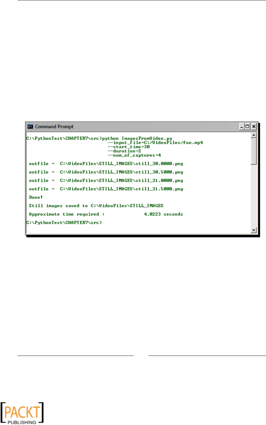
Working with Videos
[ 234 ]
The media_duration is set to a very small value (0.01 seconds), just enough to
play the video frame at media_start_time. The media_start_time and me-
dia_duration used to set the properes of the gnlfilesource represented by
self.gnlfilesrc. On line 14, the locaon of the output image le is specied.
Note that the lename is appended with a mestamp that represents the me on
the meline of the streaming video, at which this snapshot was taken. Aer seng
up the necessary parameter, the pipeline is 'started' on line 20 and will be played
unl the EOS message is posted on the bus, that is, when it nishes wring the
output PNG le.
Review the remaining methods from the le ImagesFromVideo.py and then
run this ulity by specifying appropriate command-line arguments. The following
screenshot shows sample output messages when the program is run from the
console window.
What just happened?
We developed a very useful applicaon that can save specied frames in a streaming video
as image les. To accomplish this, we re-used several of the GStreamer elements/plugins
studied earlier. For example, elements such as gnlfilesource, ffmpegcolorspace,
and so on were used to construct the GStreamer pipeline. Addionally, we used an image
encoder to save the video data in an image format.
x
x

Chapter 7
[ 235 ]
Summary
We learned fundamentals of GStreamer API in previous chapters on audio processing.
In this chapter we moved one step further to develop some useful video processing
ulies using Python and GStreamer. To accomplish this task, we learned about several
new GStreamer plugins required for processing videos.
Specically, we covered:
Pipeline that handles audio and video: We learned how to build a GStreamer
pipeline that can handle both audio and video tracks from the input video le.
This was used to 'play' a video le and it was also the basic pipeline used in
several video-processing tools developed in this chapter.
Separang audio/video: With the help of example, we learned how to save an
audio/video track of a video le into two dierent les.
Mixing audio/video: We wrote a program that can mix an audio and video stream
into a single video le.
Video eects: How to adjust the properes such as brightness, contrast, and
saturaon for a streaming video.
Text overlay: We developed a ulity that can add text, mestamp, and clock strings
on the streaming video.
Sll images from video: We learned how to save a video frame of a streaming video
as an image.
This concludes our discussion on video processing using Python and GStreamer. For the
audio as well as video processing, we mostly developed various command-line tools. It
gave us a good understanding of the use of the underlying components of a mulmedia
framework. There was no user interface component involved in our discussion. The default
GUI appeared only while playing a video.
The focus of the next chapter will be on GUI-based audio and video applicaons.
x
x

x
x

8
GUI-based Media Players Using
QT Phonon
The earlier chapters had focused on developing audio and video processing
tools. The involvement of Graphical User Interface (GUI) was intenonally kept
aside so that we could learn 'pure' mulmedia-processing techniques using the
GStreamer framework. However, to just 'play' an audio or a video, we would
always prefer a media player with a user interface that provides an easy way
to control the playback, adjust the volume, and so on.
In this chapter, we shall:
Develop a GUI for audio and video players using QT
Learn fundamental components of the Phonon framework, such as MediaObject,
MediaSource, AudioOutput, and so on to build a media graph
Learn how to use QT Phonon framework to create media players with graphical
user interface
So let's get on with it.
x
x

GUI-based Media Players Using QT Phonon
[ 238 ]
Installation prerequisites
We will cover the prerequisites for the installaon of QT Python in this secon.
PyQt4
This package provides Python bindings for QT libraries. We will use PyQt4 to generate GUI
for the image processing applicaon to be developed later in this chapter. The GPL version
is available at:
http://www.riverbankcomputing.co.uk/software/pyqt/download
Note that you should install PyQt4 binary for Python version 2.6. The PyQt4 for Python version
2.5 or earlier may not support the Phonon module. Check the PyQt4 documentaon to know
more. The installaon instrucons for PyQt4 were already discussed in Chapter 2, Working
with Images. Refer to that chapter for further details. The following table summarizes the
installaon prerequisites.
Summary of installation prerequisites
Package Download locaon Version Windows
plaorm
Linux/Unix/OS X plaorms
Python http://python.org/
download/releases/
2.6.4
(or any
2.6.x)
Install using
binary
distribuon
Install from binary. Also
install addional developer
packages (for example, with
python-devel in the package
name for rpm-based linux
distribuons).
Build and install from the
source tarball.
PyQt4 http://www.
riverbankcomputing.
co.uk/software/
pyqt/download
4.6.2 or
later
Install using
binary
pertaining to
Python2.6
First install SIP 4.9 or later.
Then install PyQt4.
Introduction to QT Phonon
In earlier chapters on audio and video processing, we extensively used GStreamer
mulmedia framework. Phonon is a mulmedia framework used by QT to provide
audio/video playback. With the GStreamer API knowledge under our belt, it should be
very easy to grasp the fundamental concepts behind the Phonon mulmedia framework.
x
x

Chapter 8
[ 239 ]
Main components
Let's briey discuss some of the fundamental components and concepts behind the
Phonon architecture.
Media graph
This is analogous to a GStreamer pipeline. The media graph species various nodes
(analogous to GStreamer elements) for processing the media stream. For example, the sink
node gives the media data as output. To begin streaming the media data within the Graph,
we call the play()method of the MediaObject module.
Media object
This object is used for the media playback. It is analogous to the poron of a GStreamer
pipeline that handles the input media data. The instance of MediaObject class is used for
this purpose. It provides methods to control the playback, such as playing, pausing, and
stopping the streaming media.
Sink
Just like in GStreamer, Phonon has a media Sink. For example, an audio sink is used to
output the audio through an audio output device.
Path
The Path object is used to connect nodes within a media graph in Phonon. For example,
a MediaObject node is linked to an AudioOutput node to stream an audio.
Effects
To manipulate the streaming media, we need to insert Effects nodes within the Graph,
between the source (MediaObject) and the Sink nodes. These nodes are also called
processors. The Effect class of the Phonon framework facilitates adding various eects
to the streaming media.
Backends
It is a backend that does the heavy liing, which is, processing a media stream in Phonon.
On Windows plaorm the backend framework is DirectShow. If you are using Linux, the
backend framework for Phonon is GStreamer and, it is QuickTime in case you use Mac OS X.
The supported funconality (for example, the media formats supported) may vary depending
on the plaorm.
x
x

GUI-based Media Players Using QT Phonon
[ 240 ]
The namespace, Phonon.BackendCapabilities, includes funcons that provide
informaon about what the Phonon backend is capable of doing. For example, the funcon
BackendCapabilities.availableMimeTypes() returns a list of all the mime types that
the backend is capable of decoding. Addionally, it provides informaon about the available
audio output devices and available eects.
Modules
Qt Phonon includes several modules that help to quickly develop applicaons for audio and
video playback. We will briey discuss a few of the important modules.
MediaNode
This is the superclass for all the nodes within a Phonon media graph. Therefore, it is
inherited by modules such as MediaObject, Effect, and AudioOutput, which
will be discussed next.
MediaSource
As the name indicates, this is used to the input the media source. The MediaObject uses
the media data it provides. The following line of code shows how this is accomplished.
self.mediaObj.setCurrentSource(self.mediaSource)
The API method, setCurrentSouce of class MediaObject, is used to specify the
MediaSource object from which to obtain the media data.
MediaObject
As menoned earlier, the MediaObject module denes an API to manage the playback. The
methods such as play(), pause(), and stop() provide playback controls.
Path
The Path class links the nodes within a graph. It can be created using an API method,
Phonon.createPath. The following code snippet shows an example usage:
self.audioPath = Phonon.createPath(self.mediaObj, self.audioSink)
Here, self.audioPath is an instance of Path class. It links the instance of class
MediaObject with self.audioSink, which is an instance of class AudioOutPut.
More nodes can be added to the graph by using Path.insertEffect.
x
x

Chapter 8
[ 241 ]
AudioOutput
The instance of this class provides an audio output node in the Phonon media graph. The
output device is typically the sound card. AudioOutput is connected to the MediaObject
(and Effect instances) using the Path object we just discussed. The property
AudioOutput.outputDevice() contains informaon about the output device.
Effect
The instance of class Effect can be inserted as a node into the media graph. The
Path.insertEffect can bring about this eect whereas Path.removeEffect facilitates
removal of that node from the graph. This object modies the streaming media data. For
example, an echo eect will add an echo to the audio. Use BackendCapabilities.
availableAudioEffects to nd out which eects are supported by the Phonon backend.
VideoPlayer
This class provides an important funconality. It has several built-in features that eliminate
the need of explicitly creang nodes such as MediaObject. We will discuss this in detail
while developing the video player applicaon.
SeekSlider
SeekSlider is a GUI widget. This class provides a slider to seek a specic posion in the
streaming media. It handles all the necessary updates and signal connecons internally.
All it needs is the media object instance.
volumeSlider
This class provides a widget for controlling the volume. It makes a programmer's job easy by
internally connecng signals. The following line of code sets the audio output device for a
volume slider.
volumeSlider.setAudioOutput(self.audioSink)
Here, the volumeSlider will control the volume for the audio output device of
self.audioSink.
Project: GUI-based music player
Let's get straight to the business. We will develop a simple GUI-based music player using QT
Phonon. The goal of this project is to learn how to put together important components of
the Phonon framework discussed earlier. It will help us get familiar with the overall Phonon
framework. In the second project, we will learn an even simpler way to accomplish the
same task.
x
x

GUI-based Media Players Using QT Phonon
[ 242 ]
The applicaon to be developed here will play an opened audio le. It will have GUI widgets
to control the playback and add various eects to the streaming audio. The screenshot of the
music player applicaon is shown in the following illustraon of its graphical user interface:
GUI elements in the music player
The illustrated music player applicaon uses the following QT widgets.
QMainWindow: This class provides the main applicaon window. In this window,
other elements such as buons and menus are added in a layout.
QToolButton: The play, pause, and stop buons are created using the
QToolButton class. The appearance of these QToolButtons can be
tweaked using a number of properes; for example, calling QToolButtoon.
setAutoRaise(True): Removes the raised buon eect. On mouse hover, the
buon will be highlighted and appear raised above the surface.
VolumeSlider: As discussed earlier, the volume slider widget is used for
controlling the volume of the output audio device.
SeekSlider: Used to seek a posion within the streaming media. While the music
is being played, its posion is automacally updated. You can drag the slider using
mouse to jump to a dierent posion on the track.
QLineEdit: This widget is used to display the full path of the media le currently
being played.
QMenubar: This is the menu bar above the QLineEdit. Here, we add dierent
menus such as File and Eects.
QAction: Various audio eect opons are added to the Eects menu as
QAction instances.
x
x

Chapter 8
[ 243 ]
Some of these QT elements just discussed are pointed out in the following illustraon of a
music player applicaon displaying various QT widgets used:
Generating the UI code
The required GUI is built using the QT Designer applicaon. This should be included in the
binary installer of PyQT4. QT Designer provides a quick way to design and develop the user
interface code. It supports a number of commonly used QT widgets. One can interacvely
add these widgets to a layout. This tool is also very useful to enhance the aesthec appeal of
the applicaon. For example, the widget colors and other properes can easily be changed
using various features available in QT Designer.
Time for action – generating the UI code
The UI le necessary for this applicaon is already created for you. The purpose of this
secon is not to show you how to generate the UI from scratch. It will just illustrate some
of the important aspects of developing GUI using QT Designer for this applicaon. You can
then experiment with it further to add new widgets to the music player applicaon. We used
QT Designer while developing the 'Thumbnail Maker' applicaon in Chapter 2, Working with
Images. We will cover some of those things here as well.
1. Download the le Ui_AudioPlayerDialog.ui from the Packt website.
2. Start the QT Designer applicaon that comes with the PyQt4 installaon.
3. Open this le in QT Designer. Click on each widget element within this audio player
dialog. The QT class associated with the selected widget will be displayed in the
Property Editor panel of the QT Designer.
x
x

GUI-based Media Players Using QT Phonon
[ 244 ]
4. Noce the red-colored borders around various UI widgets within the dialog. These
borders indicate a 'layout' in which the widgets are arranged. The layouts are
created using the QLayout class and its various subclasses. It is a crical component
of the user interface design using QT. Without a layout in place, the UI elements may
appear distorted when you run the applicaon and, for instance, resize the dialog.
The following illustraon shows how the dialog appears when opened in QT
Designer—the music player dialog (.ui le) in QT Designer.
Closely observe the borders around the widgets that indicate the presence
of a layout. You will noce that there are mulple borders. This implies that
we have placed the widgets in mulple layouts. For example, the buons
Play, Pause, and Stop are arranged in a horizontal layout, QHBoxLayout.
These are further arranged in another horizontal layout with the
volumeSlider element. Refer to QT4 and QT Designer
documentaon to know how to arrange widgets in a layout.
5. If you click on the Type Here placeholder in the menu bar, it becomes editable. With
this, you can add a new menu to the menu bar. Similarly, you can add menu items to
the File and Eects menus by opening those menus and clicking on Type Here menu
item. The File menu has two menu items: Open and Exit. Note that the Eects menu
is empty. We will add menu items to this menu later. In the following few steps, we
will make minor changes to this dialog just to get a feel of QT Designer.
6. We will now add a widget that can display digits. This widget can be used to update
the playme informaon of the streaming media. The le panel shows a bunch of
widgets that can be mouse dragged and dropped inside the Audio Player dialog
window. This is illustrated by the following screenshot:
x
x

Chapter 8
[ 245 ]
You can see the Display widget panel of QT Designer and the LCD number
widget inserted into the dialog.
The inserted LCD number widget is shown selected in the screenshot on
the right-hand side. It is inserted in a layout that arranges QToolButtons
and the volumeSlider widgets in a horizontal fashion. Also, noce that
the inserted LCD number widget has a default size. This size needs to
be adjusted so that other widgets get their share of the space. Various
parameters can be adjusted using the property editor panel within QT
Designer for this widget. Here, we adjust the maximum size values as
illustrated in the following screenshot.
The Property Editor for LCD number widget—the screenshot on the right-
hand side shows the edited size parameters.
x
x

GUI-based Media Players Using QT Phonon
[ 246 ]
Once the maximum width and height parameters are adjusted, the LCD
number widget ts in nicely within the horizontal layout. The resultant
dialog is shown in the next illustraon.
That's it! You can keep this LCD number widget in the dialog for now. Aer
compleon of this project, you can use it to add a feature that displays the
me informaon for the streaming media. Note that LCD Number widget is
not the only opon to display the play me. You can even use a QTextLabel
and update the label string with the me.
7. As menoned in the chapter, Chapter 2, Working with Images, the QT Designer
saves the user interface le with an extension .ui. To convert this into Python
source code, PyQt4 provides a conversion ulity called pyuic4. On Windows XP,
for standard Python installaon, the path for this ulity is C:\Python26\Lib\
site-packages\PyQt4\pyuic4.bat. Add the path to the environment variable.
Alternavely, specify the whole path each me you want to convert .ui le to
Python source le. The conversion ulity can be run from the command prompt as:
pyuic4 UI_AudioPlayerDialog.ui -o Ui_AudioPlayerDialog.py
This script will create a Python source le, Ui_AudioPlayerDialog.py
from the input .ui le. You can further review this le to understand how
the UI code is set up. We will use this le 'as-is' for the further discussion.
It is not a good idea to modify the autogenerated Python source le, Ui_
AudioPlayerDialog.py; if you make any changes to the corresponding
.ui le of the QT Designer and run the pyuic4 script again, it will overwrite
the previous Python source le, Ui_AudioPlayerDialog.py, provided we
use the same lename. Instead, you can use the autogenerated le as a base
class and create a subclass to add custom UI elements programmacally.
x
x

Chapter 8
[ 247 ]
What just happened?
This secon gave us a working knowledge of tweaking a user interface using QT Designer.
Just to get the feel of user interface eding, we added a LCD number widget to the Audio
Player dialog. We learned how to autogenerate the Python source code from a .ui le
created with the help of QT Designer.
Connecting the widgets
The command-line ulity pyuic4 (pyuic4.bat for Windows users) enabled conversion of
the user interface created by the QT-Designer into a Python source le. However, various
widgets in this UI need to respond to the user acons. For example, when the Play buon
is clicked, it must start streaming the media le. Thus, we need to add necessary code
that will instruct these widgets what they should do when a certain event occurs. This is
accomplished using the slots and signals. A signal is emied when a parcular GUI event
occurs. For example, when a user clicks on the Pause buon, a "clicked()" signal is
emied. A slot is a method that is called for this signal. This is very similar to the how
we connected pad-added signal by a decodebin element to a method decodebin_pad_
added in earlier chapter. Refer to the PyQt4/ QT4 documentaon that has a comprehensive
list of available signals for various widgets.
Time for action – connecting the widgets
Let's learn how to make widgets respond to a parcular user acon, such as a buon click.
1. Download the le AudioPlayerDialog.py from the Packt website. It denes the
class AudioPlayerDialog.
2. We will now review the method that connects class methods to the emied signals.
These signals are generated whenever a parcular 'event' occurs.
1 def _connect(self):
2 """
3 Connect slots with signals.
4 """
5 self.connect(self._dialog.fileOpenAction,
6 SIGNAL("triggered()"),
7 self._openFileDialog)
8
9 self.connect(self._dialog.fileExitAction,
10 SIGNAL("triggered()"),
11 self.close)
12
x
x

GUI-based Media Players Using QT Phonon
[ 248 ]
13 self.connect(self._dialog.menuAudioEffects,
14 SIGNAL("triggered(QAction*)"),
15 self._changeAudioEffects)
16
17 self.connect(self._dialog.playToolButton,
18 SIGNAL("clicked()"),
19 self._playMedia)
20
21 self.connect(self._dialog.stopToolButton,
22 SIGNAL("clicked()"),
23 self._stopMedia)
24
25 self.connect(self._dialog.pauseToolButton,
26 SIGNAL("clicked()"),
27 self._pauseMedia)
Here, the self._dialog is an instance of class Ui_AudioPlayerDialog.
Note that, the self.connect is an inherited method of the QT class
QMainWindow. It takes the following arguments (QObject, SIGNAL,
callable). The QObject is any widget type; SIGNAL is generated when
a specic event occurs. The callable is a method that handles this event.
The AudioPlayer._connect method connects all the necessary signals
with class methods.
3. The File menu in the Audio Player dialog contains two QActions, namely,
fileOpenAction and fileExitAction. When File->Open is selected, a signal
"triggered" is generated for the QAction. We need to watch out for this signal
and then call a method that will do the job of opening a le. This signal is connected
by the code between lines 5-7. Thus, when "triggered()" signal is emied, for
fileopenAction, a method AudioPlayer._openFileDialog is called that has
necessary code to open an audio le.
4. Let's review the code on line 9-12. This code connects all the QActions within a
QMenu to a method of class AudioPlayer. The rst argument, self._dialog.
menuAudioEffects, is the Eects menu in the menu bar. This is a QMenu. The
second argument SIGNAL("triggered(QAction*)") tells QT that we want to
capture the triggered signal for any of the QActions within the Eects menu. This
is best explained with an example. Imagine that the audio Eects menu has menu
items (QActions) such as Echo and Distoron. When a user selects Eects | Echo
or Eects | Distoron, the triggered(QAction*) signal is emied. The argument
QAction* is just a pointer to that QAction. The third argument is the receiver
method, self._changeAudioEffects that is called when this signal is emied.
x
x

Chapter 8
[ 249 ]
The clicked() signal emied when a QToolButton, such as, Play, Pause,
or Stop is clicked. This signal is connected to appropriate methods of class
AudioPlayer by the code block 13-23.
5. Noce that we didn't connect the SeekSlider and VolumeSlider. The signals for
these widgets are connected internally. All you need to do is set MediaObject and
AudioOutput for these widgets respecvely. We will learn how that's done in the
next secon.
What just happened?
We reviewed AudioPlayerDialog._connect() method to learn how various widgets
within the Audio Player dialog are connected to internal methods. This helped us learn some
preliminary concepts of GUI programming using QT.
Developing the audio player code
The discussion so far has been focused on the graphical user interface. We learned how
to use QT Designer to create user interface and then generate a Python source le
represenng this UI. We also reviewed the code that connects the frontend of our
applicaon with the backend (the class methods). Now, it is me to review the workhorse
audio processing code responsible for playing the audio, controlling the playback, and
operaons like adding audio eects.
x
x

GUI-based Media Players Using QT Phonon
[ 250 ]
Time for action – developing the audio player code
The source le, AudioPlayerDialog.py, used in the earlier secon will be used here
as well. The class AudioPlayerDialog inherits QMainWindow.
1. If you have not done so already, download the Python source le
AudioPlayerDialog.py.
2. Let's start with the constructor of the class, AudioPlayerDialog.
1 def __init__(self):
2 QMainWindow.__init__(self)
3 self.mediaSource = None
4 self.audioPath = ''
5 self.addedEffects = {}
6 self.effectsDict = {}
7
8 # Initialize some other variables.
9 self._filePath = ''
10 self._dirPath = ''
11 self._dialog = None
12 # Create media object , audio sink and path
13 self.mediaObj = phonon.Phonon.MediaObject(self)
14 self.audioSink = Phonon.AudioOutput(
15 Phonon.MusicCategory,
16 self)
17 self.audioPath = Phonon.createPath(self.mediaObj,
18 self.audioSink)
19
20 # Create self._dialog instance and call
21 # necessary methods to create a user interface
22 self._createUI()
23
24 # Connect slots with signals.
25 self._connect()
26
27 # Show the Audio player.
28 self.show()
The code block from lines 2 to 6 inializes some instance variables to be
used later. The dictionary object self.effectsDict will be used
to store informaon about the available audio eects. Whereas, self.
addedEffects is used to check if an audio eect is already added to the
streaming media.
x
x

Chapter 8
[ 251 ]
On line 13, the instance of Phonon.MediaObject is created. It will be
used for controlling the playback of a MediaSource.
An audio output node in the Phonon media graph is created by the code on
lines 14-16. We will call it as self.audioSink, the terminology used in
earlier chapter. The rst argument for AudioOutput is used to specify the
category. It is an object of class Phonon.Category. Since this is a music
player applicaon, we dene the category as Phonon.MusicCategory.
Review QT documentaon to know more about the categories. The second
argument is used as a parent for this audio sink.
The Phonon.Path class links the nodes within a media graph. This object is
created using an API method, Phonon.createPath. On line 17, the Path
self.audioPath links the media object self.mediaObject with the
audio output self.audioSink.
The call to the _createUI method handles the dening of the user
interface. We already learned how the frontend communicates with the
backend using the connecons set up in the _connect method.
Finally, on line 28, the API method QMainWindow.show()displays the
audio player.
3. The method _createUI delegates most of the GUI creaon to the class
UI_AudioPlayerDialog. The method also has the code that further
modies the GUI.
1 def _createUI(self):
2 # Define the instance to access the the UI elements
3 defined in class Ui_AudioPlayerDialog.
4 self._dialog = Ui_AudioPlayerDialog()
5 self._dialog.setupUi(self)
6 self._dialog.retranslateUi(self)
7 playIcon= QIcon("play.png")
8 pauseIcon= QIcon("pause.png")
9 stopIcon= QIcon("stop.png")
10 musicIcon= QIcon("music.png")
11
12 self._dialog.playToolButton.setIcon(playIcon)
13 self._dialog.pauseToolButton.setIcon(pauseIcon)
14 self._dialog.stopToolButton.setIcon(stopIcon)
15 self.setWindowIcon(musicIcon)
16 self._setupEffectsMenu()
17 self._dialog.seekSlider.setMediaObject(self.mediaObj)
18 self._dialog.volumeSlider.setAudioOutput(
19 self.audioSink)
x
x

GUI-based Media Players Using QT Phonon
[ 252 ]
The instance of class UI_AudioPlayerDialog is created on line 4.
setupUI and retranslateUI are the automacally generated methods.
These are generated when the QT Designer le with the UI is converted into
a Python source le. The AudioPlayerDialog instance is passed as an
argument to these two methods.
The code block 7 to 14 sets up the icons for the three QToolButton
instances. The setIcon API method takes QIcon instance as an argument.
The music player icon in the capon (on top-le corner of the dialog)
is created by the code on line 15. As menoned earlier, the Phonon.
SeekSlider signals are internally connected. We only need to tell which
MediaObject it will handle. This is done on line 17. Similarly, on line 18,
the setAudioOutput method of volumeSlider sets up the self.
audiosink as the audio output for this volumeSlider. While seng up
the UI design, we did not add any menu items to the Eects menu. This is
done now, by calling the _setupEffectsMenu method on line 16.
4. Let's review the method _setupEffectsMenu. It adds various available audio
eects in the Phonon framework as menu items to the Eects menu.
1 def _setupEffectsMenu(self):
2 availableEffects = (
3 Phonon.BackendCapabilities.availableAudioEffects())
4 for e in availableEffects:
5 effectName = e.name()
6 self.effectsDict[effectName] = e
7 action = QAction(effectName,
8 self._dialog.menuAudioEffects)
9 action.setCheckable(True)
10 self._dialog.menuAudioEffects.addAction(action)
The namespace, Phonon.BackendCapabilities includes funcons
that provide informaon about the capability of the Phonon backend.
BackendCapabilities.availableAudioeffects() returns
a list of all audio eects supported by Phonon on a given plaorm.
The list, availableEffects, contains objects of the class Phonon.
EffectDescription. self.effectsDict stores the name of the
eect and the EffectDescription object as key-value pairs. This
dictionary will be used later. The Eects menu, menuAudioEffects,
is populated with the QAction instances corresponding to each of the
available audio eects. QAction is created on line 6. The setCheckable
property of QAction toggles the checked state of the acon on mouse click.
The following screenshot shows the Eects menu items on Windows XP.
x
x

Chapter 8
[ 253 ]
5. The method _openFileDialog is called when File | Open is clicked from the
music player.
1 def _openFileDialog(self):
2
3 self._filePath = ''
4
5 self._filePath = (
6 str(QFileDialog.getOpenFileName(
7 self,
8 "Open Audio File",
9 "",
10 "MP3 file (*.mp3);;wav(*.wav);;All Files
11 (*.*);;")) )
12 if self._filePath:
13 self._filePath = os.path.normpath(self._filePath)
14 self._dialog.fileLineEdit.setText(self._filePath)
15 self._loadNewMedia()
This pops up a QFileDialog with the le type lters as specied on
line 10. To know about the supported media formats, you can use the
Phonon.BackEndCapabilities as illustrated by the following line
of code.
types = Phonon.BackendCapabilities.availableMimeTypes()
Where, types is a list of available mime types.
The path of the le specied by the user is then stored in the variable
self._filePath. This path is displayed in the fileLineEdit eld of the
dialog. On line 15, the method _loadNewMedia is called. We will review
that next.
x
x

GUI-based Media Players Using QT Phonon
[ 254 ]
6. The method _loadNewMedia sets up the media source for the MediaObject.
1 def _loadNewMedia(self):
2 # This is required so that the player can play another
3 # file, if loaded while first one is still playing.
4 if self.mediaSource:
5 self._stopMedia()
6 del self.mediaSource
7 self.mediaSource = phonon.Phonon.MediaSource(
8 self._filePath)
9 self.mediaObj.setCurrentSource(self.mediaSource)
The if block on line 4 ensures that the current streaming audio (if any)
is stopped by the media object before seng the new media source to a
playing state. Although it is not necessary, the memory occupied by the
MediaSource object is cleared up by the code on line 6. Line 8 creates a new
instance of class MediaSource. The API method, setCurrentSouce of the
class MediaObject is used to specify the MediaSource that provides the
media data. With this, our media player is all set to stream the audio le.
7. When you click on the Play buon in the music player, the
AudioPlayerDialog._playMedia method is called.
1 def _playMedia(self):
2 if not self._okToPlayPauseStop():
3 return
4
5 if self.mediaObj is None:
6 print "Error playing Audio"
7 return
8
9 self.mediaObj.play()
First the program carries out some primary checks to ensure that the media
is playable and then calls the play() method of Phonon.MediaObject,
which begins streaming the audio. The methods _pauseMedia and
_stopMedia of class AudioPlayerDialog contain similar code.
We just learned how to set up the media graph, stream the media,
and control its playback. Now let's see how to add audio eects to this
streaming media. If any of the items in the Eects menu are clicked, the
AudioPlayerDialog._changeAudioEffects method is called:
1 def _changeAudioEffects(self, action):
2 effectName = action.text()
3
4 if action.isChecked():
5 effectDescription = self.effectsDict[effectName]
6 effect = Phonon.Effect(effectDescription)
x
x

Chapter 8
[ 255 ]
7 self.addedEffects[effectName] = effect
8 self.audioPath.insertEffect(effect)
9 else:
10 effect = self.addedEffects[effectName]
11 self.audioPath.removeEffect(effect)
12 del self.addedEffects[effectName]
The if and else blocks in the preceding code snippet add and remove
eects nodes from the media graph respecvely. The if block is
executed when an acon in the Eects menu is checked. When an
already checked acon is toggled, the program executes the else block.
In the if block, an instance of Phonon.Effect is created on line 6.
This takes an EffectDescription object as an argument. As seen in
the _setupEffectsMenu method, self.effectsDict stores the
EffectDescription objects as the dictionary values. On line 8, this
eect is inserted as a node in the media graph. The self.audioPath links
all the nodes within the media graph.
The dictionary, self.addedEffects keeps track of all the audio
eects inserted within the media graph. The else block removes an already
added eect.
On line 11, an added eect is removed by calling the removeEffect API
method of Phonon.Path. The corresponding key-value pair of self.
addedEffects is also deleted on line 12. This also ensures that there is no
memory leak.
QT Phonon allows adding the same audio eect mulple mes. For
example, you can create mulple 'Chorus' eect nodes within the
media graph using Path.insertEffect. Each of the added
eects will have its own contribuon. However, in our applicaon,
we support adding an eect only once. You can extend this to
support adding the same eect mulple mes. For this, you will
need to tweak the Eects menu UI and make some other changes
in the code to keep track of the added eects.
8. The applicaon will not terminate properly if you close the GUI window while an
audio le is being played. To safely terminate the applicaon without any memory
leaks, AudioPlayerDialog overrides the QMainWindow.closeEvent. Before
closing the window, we do the necessary cleanup to avoid memory leaks. The code
is illustrated below.
1 def closeEvent(self, evt):
2 print "\n in close event"
3 if self.mediaObj:
4 self.mediaObj.stop()
5
x
x

GUI-based Media Players Using QT Phonon
[ 256 ]
6 self.mediaObj = None
7 self._clearEffectsObjects()
8 QMainWindow.closeEvent(self, evt)
The streaming media, if any, is rst stopped. The call to
_clearEffectsObject deletes all the Phonon.Effect and
Phonon.EffectDescription objects (if present). The method
_clearEffectsObject is self-explanatory.
9. The following code creates an instance of QApplication and executes
this program.
1 app = QApplication(sys.argv)
2 musicPlayer = AudioPlayerDialog()
3 app.exec_()
10. Review the rest of the code from the le AudioPlayerDialog.py and then run
the music player as:
$python AudioPlayerDialog.py
This should display the music player GUI window. Use File | Open to specify
a music le and then click on the Play buon to enjoy the music!
What just happened?
We just created our own music player! We developed a frontend for this music player using
QT Phonon mulmedia framework. Use of various modules in QT Phonon was thoroughly
discussed. We learned how to set up audio controls and eects in a media graph by using
modules such as MediaObject, AudioOutput, Path, and so on. We also gained some
higher-level understanding of GUI programming aspects using QT.
Have a go hero – add more features to the audio player
In the Generang the UI code secon, we added a widget to the music player GUI window.
This is an LCD number widget that can display the frame numbers. Connect this widget to
the Audio Player backend, so that it can display the current media me. The next illustraon
shows this LCD number widget in acon for a streaming audio le.
Extend this music player applicaon so that it can play all the songs from a directory
or CD one aer the other. There are a number of ways to create a user interface to
display the les. For example, you can try using widgets such as QDirectoryView ,
QTreeView, or QTableWidget.
x
x
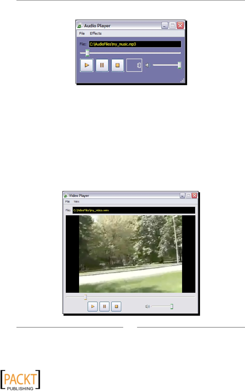
Chapter 8
[ 257 ]
Music player displaying the frame number (me) in the LCD number widget:
Project: GUI-based video player
In the rst project, we learned the fundamentals of the QT Phonon framework. In this
project, we will extend that knowledge further by developing a video player. The Audio
player was developed by building a media graph. Various nodes such as MediaObject,
AudioOutput, and Effects were linked together by creang a Phonon.Path. If the goal is
just to develop a simple audio or video player, the job is even simpler. Phonon has a module
VideoPlayer that provides an abstract way to play an audio or a video without the need
to explicitly create MediaObject, AudioOutput, and some other objects. All it needs
is a MediaSource. It is also possible to create a custom media graph by adding various
audio-eect nodes. We will see how to do it later. For now, let's write a simple video player
applicaon using QT Phonon. The following illustraon shows the video player in acon.
x
x
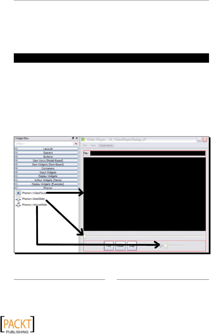
GUI-based Media Players Using QT Phonon
[ 258 ]
Generating the UI code
QT Designer is an excellent resource for generang user interface interacvely. As we have
seen, most of the user interface for this project is built using QT Designer. In addion, some
important points about the user interface design using QT were covered. This secon will
just walk you through the user interface generaon for this applicaon using QT Designer
and pyuic4.
Time for action – generating the UI code
The .ui le is already created. In the following discussion, we will simply use this le and
go through some of the GUI elements needed for this applicaon.
1. Download the le Ui_VideoPlayerDialog.ui from the Packt website.
2. Open this le in QT Designer. Click on each widget element. The QT class associated
with the selected widget will be displayed in the Property Editor panel on the
right-hand side. Most of the widgets used here are same as the ones used in the
earlier project. The only widget that is dierent is the Phonon.VideoPlayer. The
following illustraon shows how the dialog appears when opened in QT Designer.
It also points out various Phonon widgets used in the dialog.
The video player widget in QT Designer appears as shown in the
preceding screenshot.
x
x
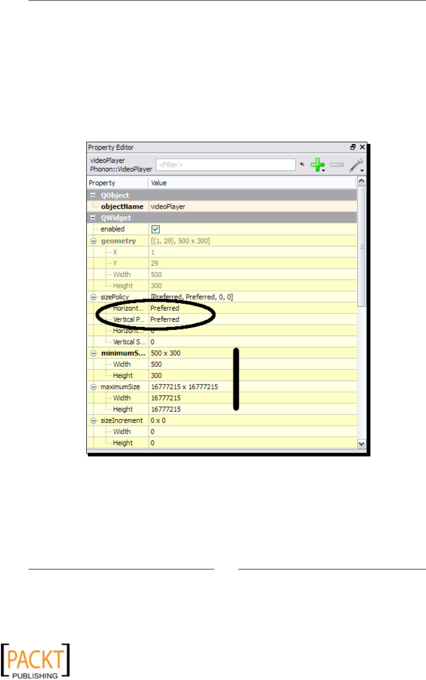
Chapter 8
[ 259 ]
3. Click on the VideoPlayer widget shown in the preceding illustraon. The Property
Editor will display its properes. Pay aenon to how the size of this widget is
dened. This Video Player will support an opon to view the video in 'Full Screen'
mode. Therefore, the maximum size parameters for the VideoPlayer widget are
set to high values as shown in the next screenshot. In fact, we are using the QT
default values for the maximum size property. The only property modied is the
minimum size of the widget. This minimum size will be the default size of the video
player widget.
The Property editor for Video Player widget:
4. The rest of the widgets are the same as the one used in an earlier project. You
can add the LCD Number widget or a simple text label that displays the current
me for the streaming media. Refer to the last project for instrucons on adding
such widgets.
x
x

GUI-based Media Players Using QT Phonon
[ 260 ]
5. Next, convert the .ui le into .py using the pyuic4 conversion ulity. The
conversion ulity can be run from the command prompt as:
pyuic4 UI_VideoPlayerDialog.ui -o Ui_VideoPlayerDialog.py
This script will create a Python source le, Ui_VideoPlayerDialog.py,
from the input .ui le. We will use this le 'as-is' for the further discussion.
What just happened?
The previous discussion served as a refresher on use of QT Designer to generate most of the
user interface elements needed for this project. The pyuic4 conversion ulity was used
to convert the .ui le to a Python source le.
Connecting the widgets
Most of the widgets used in the previous project are re-used here. Therefore, this is going
to be a short discussion. In this project, we have not included an Eects menu. Thus, the
VideoPlayerDialog._connect method has minor changes. This method is illustrated
as follows:
def _connect(self):
self.connect(self._dialog.fileOpenAction,
SIGNAL("triggered()"),
self._openFileDialog)
self.connect(self._dialog.fileExitAction,
SIGNAL("triggered()"),
self.close)
self.connect(self._dialog.fullScreenAction,
SIGNAL("toggled(bool)"),
self._toggleFullScreen)
self.connect(self._dialog.playToolButton,
SIGNAL("clicked()"),
self._playMedia)
self.connect(self._dialog.stopToolButton,
SIGNAL("clicked()"),
self._stopMedia)
self.connect(self._dialog.pauseToolButton,
SIGNAL("clicked()"),
self._pauseMedia)
x
x

Chapter 8
[ 261 ]
The highlighted lines of code are a new widget connecon. The rest of the connecons are
the same as the ones discussed in the previous project. When View | Full Screen is selected,
the toggled(bool) signal of fullScreenAction is emied. When this happens the slot
method self._toggleFullScreen is called. The next secon will have more details about
this method.
Developing the video player code
The generated frontend is connected to the backend for processing the media. In this
secon, we will review the video player backend that actually streams the media and
controls the playback and volume. Our job is easier here. Most of the good work we did in
the earlier project will be re-used here. There will be some minor modicaons because we
will be using Phonon.VideoPlayer for video processing instead of explicitly creang the
objects such as MediaObject.
Time for action – developing the video player code
Let's develop the rest of the video player backend. We will re-use several methods from the
AudioPlayerDialog class with a few minor changes. Only the important methods will be
covered in this secon.
1. Download the le VideoPlayerDialog.py from the Packt website.
2. The constructor of the class is shown below.
1 def __init__(self):
2 QMainWindow.__init__(self)
3 self.mediaSource = None
4 self.audioPath = ''
5
6 # Initialize some other variables.
7 self._filePath = ''
8 self._dialog = None
9
10 # Create self._dialog instance and call
11 # necessary methods to create a user interface
12 self._createUI()
13
14 self.mediaObj = self._dialog.videoPlayer.mediaObject()
15 self.audioSink = self._dialog.videoPlayer.audioOutput()
16
17 self._dialog.seekSlider.setMediaObject(self.mediaObj)
18 self._dialog.volumeSlider.setAudioOutput(
19 self.audioSink)
20
x
x

GUI-based Media Players Using QT Phonon
[ 262 ]
21 # Connect slots with signals.
22 self._connect()
23
24 # Show the Audio player.
25 self.show()
The self._dialog creates an instance of class Phonon.VideoPlayer.
Once a media source is specied, self._dialog.videoPlayer is able
to stream the media. Thus, for the media streaming itself, we don't need to
create the nodes MediaObject and AudioOutput explicitly; the Phonon.
VideoPlayer internally builds the media graph. However, MediaObject
and AudioOutput are required for seekSlider and volumeControl
widgets respecvely. On lines 14 and 15, these objects are obtained from
self._dialog.videoPlayer.
3. The _createUI method is almost idencal to the corresponding method in
AudioPlayerDialog, except that it doesn't have the Eects menu-related code.
4. Following that, the method to review is _playMedia:
1 def _playMedia(self):
2 if not self._okToPlayPauseStop():
3 return
4 self._dialog.videoPlayer.play(self.mediaSource)
The code is self-explanatory. The self.mediaSource is set in
VideoPlayerDialog._loadNewMedia. This MediaSource instance
is passed as an argument to the API method VideoPlayer.play. The
videoPlayer then builds the media graph internally and plays the given
media le.
5. This simple video player supports an opon to view the streaming video in
full screen mode. QMainWindow class provides an easy way to change the
view between full screen and normal viewing mode. This is done by the
method _toggleFullScreen.
def _toggleFullScreen(self, val):
"""
Change between normal and full screen mode.
"""
# Note: The program starts in Normal viewing mode
# by default.
if val:
self.showFullScreen()
else:
self.showNormal()
x
x
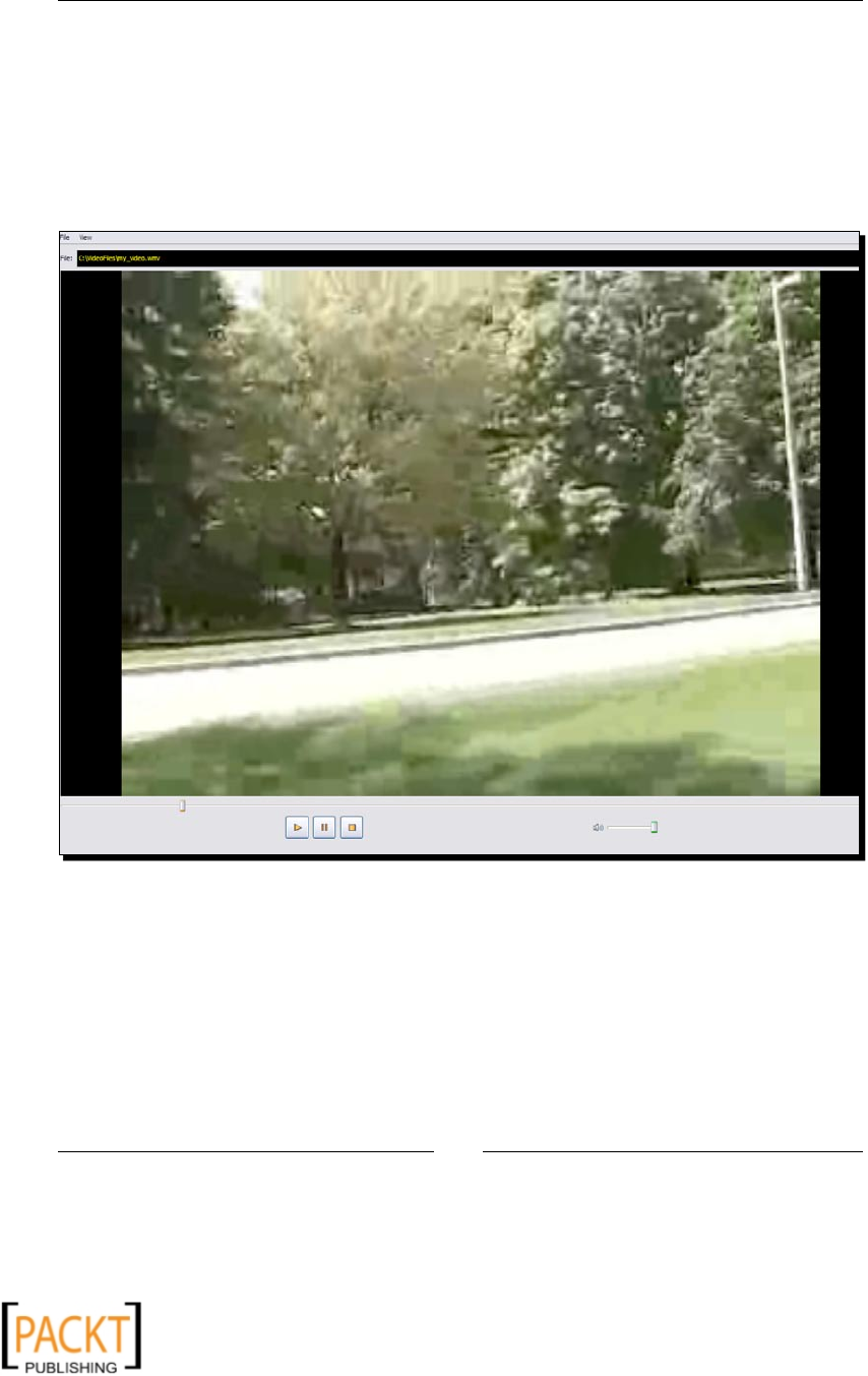
Chapter 8
[ 263 ]
The method, self.showFullScreen() is inherited from class
QMainWindow. If the QAction in the View menu (View | Full Screen) is
checked, the video player window is set to full screen. QMainWindow.
showNormal() changes the video player back to the normal viewing mode.
The following screenshot shows the video player in the full screen mode.
Noce that the window capon bar is hidden in the full screen mode.
Video player in full screen mode is illustrated as shown in the next image:
6. Review the rest of the code from le VideoPlayerDialog.py. Keep this le in the
same directory as Ui_VideoPlayerDialog.py and then run the program from
the command line as:
$python VideoPlayerDialog.py
7. The video player GUI window will appear. Open any supported audio or video le
and click on the Play buon to begin the playback.
x
x

GUI-based Media Players Using QT Phonon
[ 264 ]
What just happened?
We wrote our own video player. This video player is capable of playing video as well as audio
les of supported formats. The module Phonon.VideoPlayer that enables media playback
and control was used here. We also learned how to toggle view between full screen and
normal viewing mode using the API methods of class QMainWindow.
Have a go hero – do more with the video player
1. Here is a simple enhancement. The full screen mode shows widgets such as playback
control buons, seek, and volume sliders. Hide these widgets when the View | Full
Screen acon is checked. Also, add a keyboard shortcut to toggle between normal
and full screen view mode.
2. Add audio eects to the video player GUI. We already learned how to add audio
eects to the media graph in the rst project. You can re-use that code here.
However, you will need an appropriate Phonon.Path object to which the effects
node needs to be added. In the last project, we used Phonon.createPath—we
can't create a new path as it is created internally by the VideoPlayer. Instead, the
path can be obtained using API method MediaObject.outputPaths(). This
method returns a list containing output (audio and video) paths. The line of
code is shown as an example.
self.audioPath = self.mediaObj.outputPaths()[0]
However, be careful with the memory leaks. If you add audio eects, and
then exit the applicaon, the program may freeze. This could be because
the eect nodes are not deleted from the original audio path. Alternavely,
you can build the video player from basic principles. That is, don't use
Phonon.VideoPlayer. Instead, build a custom media graph just like
how we did for the audio player project. In this case, you will need to use
modules such as Phonon.VideoWidget.
Summary
This chapter taught us several things about GUI mulmedia applicaon development using
QT. We worked on two excing projects where audio and video players using QT Phonon
framework were developed. To accomplish these tasks, we:
Used QT Designer to generate the UI source code
Handled the QT generated events by connecng slots (class methods) with signals
Used Phonon framework to set up media graphs for streaming of audio and video
x
x

Index
Symbols
--end_me opon 167
--input_le opon 167
--start_me opon 167
--verbose_mode opon 167
-output_le opon 167
__init__ method 164
_addTextWorker() method 75
_connect method 48
_createUI method 251
_makeThumbnail method 50
_resizeImage method 50
_rotateImage method 50
A
addDateStamp() method 73, 77
addText() method 73, 75
addTransparency() funcon 68
addTransparency() method 78
addWaterMark() method 73
anchor_x property 105
anchor_y property 105
animaon
about 91
bouncing ball animaon 102-107
creang, dierent image regions used 113
creang, sequenal images used 100, 102
creang, single animaon used 102-107
developing, with Pyglet 97
drive on a rainy day project 117-122
raindrop animaon, creang 114, 116
simple bowling animaon project 108-112
viewing, Pyglet used 98, 99
Animaon.from_image_sequence method
100-102
AnimaonFrame module 95
Animaon module 95
animaons 11, 12
audio
part, extracng 150
playing, from playlist 137
playing, from website 141
playing, GStreamer used 132-136
audio-video track
mixing 226
seperang 223-225
audio-video track mixer
developing 226-229
audio and video processing
about 10
compression 10
eding 11
mixing 11
audio clips
combining 183-189
audioconvert element 151
AudioConverter.convert() method 150
AudioCuer.extractAudio() method 170
audioecho plugin 182
audio eects
about 175
echo eect 179-182
fade-out eect, adding 175-178
panorama eect 182
audioFileExists() funcon 144
audio le format
converng 142
x
x

[ 266 ]
audio le format converter
about 142
features 143-150
audioop module 12
AudioOutput module, QT Phonon 241
audiopanorama plugin 183
AudioPlayer._connect method 248
AudioPlayer._openFileDialog method 248
AudioPlayer.play() method 134, 148
AudioPlayer class 133
AudioPlayerDialog._connect() method 249
audio recording 156-159
audiotestsrc element 191
audio tracks
extracng, playback controls used 166-172
mixing 194, 195
pausing 162-165
resuming 162-165
visualizing 196-198
volume, adjusng 173-175
audio visualizer
audio tracks, visualizing 196-198
autoaudiosink element 132, 156
autoaudiosink plugin 145
autoaudiosrc element 157
autocontrast funcon 58
autoconvert element 206, 218
autoconvert plugin 202
autovideosink plugin 202
B
backends, QT Phonon 239
batch-processing ulity 215
bin element 192, 193
bins, GStreamer 129
blending 9
blending, image enhancement
about 65, 68
two images, blending 65-67
blurring 84
border
adding 88
brightness and contrast, image enhancement
adjusng 56-58
brightness and contrast level
adjusng 219
built-in mulmedia modules
audioop 12
wave 13
winsound 12
bus, GStreamer 131
C
caps, GStreamer 131
capslter element 206
capslter plugin 202
captureImage method 231
Clock module 95
clockoverlay plugin 220
color space 206
colors tweaking, image enhancement
about 59
colors, swaping within image 59, 60
ower color, changing 61, 62
gray scale images 63
individual image band, changing 61
negave, creang 64
components, QT Phonon
eects 239
media graph 239
media object 239
path 239
sink 239
composite() method 79
composites
making, with image mask 70-72
compression, audio and video processing
about 10
lossless compression 10
lossy compression 10
connectSignals method 155
constructPipeline() method 169
constructPipeline method 208, 212
constructVideoPipeline method 216
convert_single_audio method 148
convert method 212
createDrawableObjects method 104
cropping, image manipulaons 39
x
x

[ 267 ]
cropping, video manipulaons
about 217
borders, adding 219
video, cropping 218, 219
Cygwin 125
D
darwinports 125
decodebin_pad_added method 207
decodebin plugin 128
def convertImage method 26
def processArgs method 26
digital mulmedia 8
Display module, PyAudiere 14
Draw module, PyAudiere 14
drive on a rainy day project 117-122
dshowaudiosrc plugin 157
dynamic pad 130
E
echo eect
about 179
adding 179-182
EDGE_ENHANCE lter 87
edge detecon and enhancement lters 85
edges, image
detecng 85, 86
enhancing 85, 86
eding, audio and video compression 11
Eect module, QT Phonon 241
eects, QT Phonon components 239
Eects node 239
egg le 93
element linking 140
embossing 87
event module, PyAudiere 15
F
fade-out eect
adding 175-178
fakesrc element 130
fast-forward control 166
enc_mpeg4 plugin 202
enc_png plugin 202
mpegcolorspace converter 206
mpegcolorspace plugin 202
mux_mp4 plugin 202
lesink element 209
lesrc element 134, 157
ipping, image manipulaons 35
for loop 105
freetype2
about 23
URL 23
G
get_name method 208
getbands() method 59
getOutImagePath method 50
ghost pad 131, 193
glClearColor call 98
gnlcomposion element 151, 186, 189, 194
gnlcontroller element 186
gnllesource element 151, 188, 189, 194, 231
properes 151
gnloperaon element 151
gnlsource element 151
gnlurisource element 151
gnonlin_pad_added method 155
Gnonlin plugin
about 151, 166
elements 151
features 151
gnlcomposion element 151
gnllesource element 151
gnloperaon element 151
gnlsource element 151
gnlurisource element 151
GObject 125
gobject modules 204
goom2k1 visualizaon plugin 198
goom visualizaon plugin 196-198
grayscale video
creang 220
gst-inspect-0.10 command 173, 196
gst-inspect command, GStreamer 128
gst-launch command, GStreamer 128
gst.Bin class 129
gst.Bus.gst_bus_post() method 131
x
x

[ 268 ]
gst.Element.add_pad() method 130
gst.FORMAT_TIME argument 166
gst.parse_launch() method 194, 195
gst.QueryError excepon 164
gst.SECOND argument 166
gst.SEEK_GLAG_FLUSH argument 166
gst.STATE_NULL state 165
gst.STATE_PAUSED state 162
gst.STATE_PLAYING state 162
GStreamer
about 13, 124
audio, playing 133, 134
bins 129
bus 131
caps 131
elements 128
essenal elements, for audio play 132
gst-inspect command 128
gst-launch command 128
music, playing 132
on, other plaorm 125
on, Windows plaorm 124
other plaorm 125
pads 130
pipeline 128
playbin/playbin2 131
plug-ins 129
GStreamer installaon
tesng 127
GStreamer Pipeline
creang 137, 139
GStreamer plugins
autoconvert 202
autovideosink 202
capslter 202
clockoverlay 202
enc_mpeg4 202
enc_png 202
mpegcolorspace 202
mux_mp4 202
textoverlay 202
meoverlay 202
videobalance 202
videobox 202
GStreamer WinBuilds 124
GUI-based music player project
audio player code, developing 249-256
developing, QT Phonon used 241, 242
elements, used 242, 243
features, adding to audio player 256
UI code, generang 243-246
widgets, connecng 247-249
GUI-based video player project
developing 257
features, adding to video player 264
UI code, generang 258, 259
video player code, developing 261-263
widgets, connecng 260, 261
I
image
blurring 84
border, adding 88
displaying, Pyglet used 96
edge detecon and enhancements 85
embossing 87, 88
sharpening 84
smoothing 82-84
image.Animaon class 98
Image.blend method 66
image.blit 96
Image.composite funcon 79
image.load_animaon method 98
Image.merge() method 60
Image.new method 69
Image.paste funcon 78
Image.point method 69
Image.putalpha() method 68
Image.resize method 30
Image.save method 27
Image.split() method 60
Image.thumbnail method 33
Image.transpose method 35
image bling 96
ImageEnhance.Contrast class 57
image enhancement techniques
about 55
blending 65
border, adding 88
brightness and contrast, adjusng 56-58
x
x

[ 269 ]
colors, swaping within image 59, 60
colors, tweaking 59
composites, making with image mask 70
image lters, applying 81
installaon prerequisites 56
transparent images, creang 68
Watermark Maker Tool project 72
ImageEnhance module 56
image le converter
building 27
features, adding 30
ImageFilter.BLUR lter 84
ImageFilter.EMBOSS lter 87
ImageFilter.SHARPEN lter 84
ImageFilter module 82
image lters
applying 81
ImageGrid 115
image manipulaons
about 30
cropping 39
ipping 35
pasng 40, 41
resizing 30-33
rotang 33, 34
screenshots, capturing 38
Image module 95
image module, PyAudiere 15
image noise 9
ImageOps module 58
image processing
about 8
image smoothing lter example 9
image re-sampling 30
images
creang, from scratch 28
reading, from archive 29
image smoothing 9
imgDrawer method 29
installaon, Pyglet
prerequisites 92, 93
tesng 93
installaon prerequisites
PyQt4 23
Python 21
Python Imaging Library (PIL) 22
installaon prerequisites, QT Python
about 238
PyQt4 238
interleave plugin 194-196
K
keyboard controls, Pyglet 97
L
libjpeg
about 23
URL 23
libvisual visualizaon plugin 196-198
linkedelement 130
Linux
Pyglet, installing 92
lossless compression 10
lossy compression 10
M
Mac OS X
Pyglet, installing 92
map funcon 102
media graph, QT Phonon components 239
media module 97
MediaNode module, QT Phonon 240
media object, QT Phonon components 239
MediaObject module, QT Phonon 240
MediaSource module, QT Phonon 240
message_handler method 131, 165
mixing, audio and video compression 11
modules, Pyglet
Animaon 95
AnimaonFrame 95
Clock 95
Image 95
media 97
Sprite 95
Window 94
modules, QT Phonon
about 240
AudioOutput 241
Eect 241
x
x

[ 270 ]
MediaNode 240
MediaObject 240
MediaSource 240
Path 240
SeekSlider 241
VideoPlayer 241
volumeSlider 241
monoscope visualizaon plugin 196-198
MP3 cuer
about 152
creang 167-172
extending 156
mulmedia
about 8
digital mulmedia 8
mulmedia frameworks
GStreamer 13
PIL 13
PyGame 14
Pyglet 14
PyMedia 13
QT Phonon 18
mulmedia libraries
PyAudiere 20
Snack Sound Toolkit 19
mulmedia processing
about 8
animaons 11, 12
audio and video processing 10
image processing 8, 9
music module, PyAudiere 15
muxer 209
N
new image containing some text
creang 28
O
on_draw method 96, 99, 104
on_key_press method 97, 111
on_mouse_press method 97
os.path.join method 96
os.path.normpath method 96
P
pads, GStreamer
about 130
dynamic pads 130
ghost pads 131
sink pads 130
panning eect. See panorama eect
panorama eect
about 182
controlling 183
panorama property 183
pasng, image manipulaons 40, 41
path, QT Phonon components 239
Path module, QT Phonon 240
pause control 162-165
Phonon 238
picture
enclosing, in photoframe 89
pipeline, GStreamer
about 128, 129
building, from elements 137
pipeline element 166
pixels 30
play() method 97, 239, 254
playback controls
about 161
adding 208
audio, extracng 166-172
fast-forward 166
pause 162-165
play 162
resume 162-165
rewind 166
stop 165
playbin, GStreamer 131
playbin2, GStreamer 132
playbin plugin 196-198
play control 162
plug-ins, GStreamer
about 129
audioecho 129
autoconvert 202
autovideosink 202
capslter 202
x
x

[ 271 ]
clockoverlay 202
decodebin plugin 129
enc_mpeg4 202
enc_png 202
mpegcolorspace 202
mux_mp4 202
gnonlin 129
interleave 129
monoscope 129
textoverlay 202
meoverlay 202
videobalance 202
videobox 202
point funcon 62
printUsage() method 75
priority property 194
processArgs() method 75, 153
processImage method 50
processors 239
properes, gnllesource element
media-duraon 151
media-start 151
uri 151
PyAudiere 20
PyGame
about 14
Display module 14
Draw module 14
Event module 15
Image module 15
Music module 15
simple applicaon 15, 16
Sprite module 14
Surface module 14
URL 14
Pyglet
about 14, 91, 92
animaons, developing 97
benets 94
exisng animaon, viewing 98, 99
image, displaying 96
installing, on Linux 92
installing, on Mac OS X 92
installing, on Windows 92
installing, prerequisites 92, 93
keyboard controls 97
mouse controls 97
sound eects, adding 97
URL 92
Pyglet modules
Animaon 95
AnimaonFrame 95
Clock 95
Image 95
media 97
Sprite 95
Window 94
pyglet.image.load_animaon method 97
pyglet.image package 95
PyGObject
about 125
on other plaorm 125
on Windows plaorm 125
PyGTK website 125
PyMedia 13
PyQt4
about 23, 238
other plaorms 24
Windows plaorm 23
Python
about 21
download link 21
other plaorms 22
Windows plaorm 22
Python Imaging Library (PIL)
about 13
other plaorms 22
Windows plaorm 22
Q
QAcon, QT widgets 242
QLayout class 244
QLayouts
grid layout 45
horizontal 45
vercal 45
QLineEdit, QT widgets 242
QMainWindow, QT widgets 242
QMenubar, QT widgets 242
x
x

[ 272 ]
QToolBuon, QT widgets 242
QT Phonon
about 18, 238
backends 239
components 239
modules 240
QT Phonon modules
about 240
AudioOutput 241
Eect 241
MediaNode 240
MediaObject 240
MediaSource 240
Path 240
SeekSlider 241
VideoPlayer 241
volumeSlider 241
QT Python
installaon prerequisites 238
QT widgets
QAcon 242
QLineEdit 242
QMainWindow 242
QMenubar 242
QToolBuon 242
SeekSlider 242
VolumeSlider 242
query_posion call 164
R
raindrop animaon
creang 114-116
resizing, image manipulaons 30-33
resizing, video manipulaons
about 215
streaming video, resizing 216, 217
resume control 162-165
reverberaon eect
adding 182
rewind control 166
rotang, image manipulaons 33, 35
S
screenshots
capturing 38
seek_simple method 166
SeekSlider, QT widgets 242
SeekSlider module, QT Phonon 241
self.clear() call 105
self.connectSignals() method 146
self.lesrc element 206
self.player object 206
self.play method 163
sharpening 84
simple applicaon, PyAudiere 15, 16
simple bowling animaon project 108-112
SingleImageAnimaon class 104
sink, QT Phonon components 239
sink node 239
sink pads 130
slot method 261
smoothing 82
Snack Sound Toolkit 19
Sprite module 95
Sprite module, PyAudiere 14
Sprite objects 96
start property 194
stop control 165
subparse plugin 223
Surface module, PyAudiere 14
synaesthesia visualizaon plugin 198, 199
T
textoverlay plugin 202, 220
ThumbnailMakerDialog._connect() method 49
Thumbnail Maker project
enhancing 52
image processing code, developing 49-51
running 44
UI code, generang 45, 46
ui le, tweaking 47
widgets, connecng 47, 48
meline 184
meoverlay plugin 202, 220
transparent images
creang 68, 69
tuple 134
U
UI code, Thumbmail Maker project
generang 45, 46
x
x

[ 273 ]
V
video
playing 203
playing, playbin used 208
videobalance plugin 202, 219
videobox element 218
videobox plugin 202, 219
video conversion ulity
creang 209-214
video le
audio track, seperang 223-225
video track, seperang 223-225
video le format
coverng 209
video frames
saving, as images 230-234
video manipulaons and eects
about 215
brightness and contrast level, adjusng 219
cropping 217, 218
grayscale video, creang 220
resizing 215
VideoPlayer.play method 204
VideoPlayerDialog._connect method 260
VideoPlayer module, QT Phonon 241
video player ulity
wring 203-208
video stream
text and me, adding 220
video track
subtles, adding 223
text string, adding 220, 222
volume element 173
volume property 175
VolumeSlider, QT widgets 242
volumeSlider module, QT Phonon 241
W
watermark 77
Watermark Maker Tool project
creang 72-79
features 80
wave module 13
Window module 94
Windows
Pyglet, installing 92
winsound module 12
Z
zib
about 23
URL 23
x
x

Thank you for buying
Python Multimedia Beginner's Guide
About Packt Publishing
Packt, pronounced 'packed', published its rst book "Mastering phpMyAdmin for Eecve MySQL
Management" in April 2004 and subsequently connued to specialize in publishing highly focused
books on specic technologies and soluons.
Our books and publicaons share the experiences of your fellow IT professionals in adapng and
customizing today's systems, applicaons, and frameworks. Our soluon based books give you the
knowledge and power to customize the soware and technologies you're using to get the job done.
Packt books are more specic and less general than the IT books you have seen in the past. Our unique
business model allows us to bring you more focused informaon, giving you more of what you need to
know, and less of what you don't.
Packt is a modern, yet unique publishing company, which focuses on producing quality, cung-edge
books for communies of developers, administrators, and newbies alike. For more informaon, please
visit our website: www.packtpub.com.
About Packt Open Source
In 2010, Packt launched two new brands, Packt Open Source and Packt Enterprise, in order to connue
its focus on specializaon. This book is part of the Packt Open Source brand, home to books published
on soware built around Open Source licences, and oering informaon to anybody from advanced
developers to budding web designers. The Open Source brand also runs Packt's Open Source Royalty
Scheme, by which Packt gives a royalty to each Open Source project about whose soware a book
is sold.
Writing for Packt
We welcome all inquiries from people who are interested in authoring. Book proposals should be sent
to author@packtpub.com. If your book idea is sll at an early stage and you would like to discuss it
rst before wring a formal book proposal, contact us; one of our commissioning editors will get in
touch with you.
We're not just looking for published authors; if you have strong technical skills but no wring
experience, our experienced editors can help you develop a wring career, or simply get some
addional reward for your experse.
x
x
Matplotlib for Python Developers
ISBN: 978-1-847197-90-0 Paperback: 308 pages
Build remarkable publicaon-quality plots the
easy way
1. Create high quality 2D plots by using Matplotlib
producvely
2. Incremental introducon to Matplotlib, from the
ground up to advanced levels
3. Embed Matplotlib in GTK+, Qt, and wxWidgets
applicaons as well as web sites to ulize them in
Python applicaons
4. Deploy Matplotlib in web applicaons and expose it
on the Web using popular web frameworks such as
Pylons and Django
Expert Python Programming
ISBN: 978-1-847194-94-7 Paperback: 372 pages
Best pracces for designing, coding, and distribung your
Python soware
1. Learn Python development best pracces from
an expert, with detailed coverage of naming and
coding convenon
2. Apply object-oriented principles, design paerns,
and advanced syntax tricks
3. Manage your code with distributed
version control
4. Prole and opmize your code
Please check www.PacktPub.com for informaon on our tles
x
x
