Quick Fatigue Tool User Guide
User Manual: Pdf
Open the PDF directly: View PDF ![]() .
.
Page Count: 266 [warning: Documents this large are best viewed by clicking the View PDF Link!]
- User Guide
- Version Information
- Acknowledgements
- 1. Introduction
- 2. Getting started
- 3. Defining fatigue loadings
- 4. Analysis techniques
- 5. Materials
- 6. Analysis algorithms
- 6.1 Background
- 6.2 Stress-based Brown-Miller
- 6.3 Normal Stress
- 6.4 Findley’s Method
- 6.5 Stress Invariant Parameter
- 6.6 BS 7608 Fatigue of Welded Steel Joints
- 6.6.1 Overview
- 6.6.2 Derivation of the ,𝑺-𝒓.−𝑵 curve
- 6.6.3 Analysis of axially loaded bolts
- 6.6.4 Effect of the characteristic length
- 6.6.5 Effect of stress relief
- 6.6.6 Effect of small cycles
- 6.6.7 Effect of large cycles
- 6.6.8 Effect of exposure to sea water
- 6.6.9 Failure mode
- 6.6.10 Specifying the ,𝑺-𝒓.−𝑵 curve as a BS 7608 weld class
- 6.6.11 Specifying the ,𝑺-𝒓.−𝑵 curve as user data
- 6.6.12 Compatibility with other features
- 6.6.13 Configuring the analysis parameters
- 6.7 NASALIFE
- 6.8 Uniaxial Stress-Life
- 6.9 Uniaxial Strain-Life
- 6.10 User-defined algorithms
- 7. Mean stress corrections
- 8. Safety factor analysis
- 9. Job and environment files
- 10. Output
- 10.1 Background
- 10.2 Output variables
- 10.3 Viewing output
- 10.4 The ODB Interface
- 10.4.1 Overview
- 10.4.2 Accessing the ODB interface via the Export Tool
- 10.4.3 Enabling the ODB interface via the environment file
- 10.4.4 Configuring the ODB interface
- 10.4.5 Mismatching ODB files
- 10.4.6 Large ODB files
- 10.4.7 Exporting field data to multiple Abaqus ODB part instances
- 10.4.8 Minimum requirement for output
- 11. FEA Modelling techniques
- 12. Supplementary analysis procedures
- 12.1 Background
- 12.2 Yield criteria
- 12.3 Composite failure criteria
- 12.3.1 Overview
- 12.3.2 Conventions for fibre-reinforced composites
- 12.3.3 Conventions for closed cell PVC foam
- 12.3.4 Material properties
- 12.3.5 Model definition
- 12.3.6 Loading definition
- 12.3.7 Maximum stress theory
- 12.3.8 Tsai-Hill theory
- 12.3.9 Tsai-Wu theory for fibre-reinforced composites
- 12.3.10 Tsai-Wu theory for closed cell PVC foam
- 12.3.11 Azzi-Tsai-Hill theory
- 12.3.12 Maximum strain failure theory
- 12.3.13 Hashin’s damage initiation criteria
- 12.3.14 LaRC05 damage initiation criteria
- 12.3.15 Output
- 12.3.16 Example Usage
- 13. Tutorial A: Analysis of a welded plate with Abaqus
- 14. Tutorial B: Complex loading of an exhaust manifold
- Appendix I. Fatigue analysis techniques
- Appendix II. Materials data generation
- Appendix III. Gauge fatigue toolbox
- References

1
QUICK FATIGUE TOOL FOR MATLAB®
Multiaxial Fatigue Analysis Code for Finite Element Models
User Guide
© Louis Vallance 2018
2
3
Version Information
Documentation revision: 60 [17/01/2018]
Concurrent code release: 6.11-10
Acknowledgements
Quick Fatigue Tool is a free, independent multiaxial fatigue analysis project. The author would like to
acknowledge the following people for making this work possible:
Dr.-Ing. Anders Winkler, SPE
Senior Technical Specialist
SIMULIA Nordics
Sweden
Technical Advice and collaboration
Fatigue materials data
Giovanni Morais Teixeira
Durability Technology Senior Manager
SIMULIA UK
United Kingdom
Technical advice and collaboration
Eli Billauer
Freelance Electrical Engineer
Isreal
Providing the code for the peak-valley
detection algorithm
Adam Nieslony
Professor of Mechanical Engineering
Opole University of Technology
Poland
Providing the code for the alternative
peak-picking method
Joni Keski-Rahkonen
Senior R&D Engineer
Rolls-Royce Oy Ab
Finland
Providing assistance with the critical
plane code
Bruno Luong
Providing the code for Cardan’s formula
which computes Eigenvalues for
multidimensional tensor arrays
4
Contents
1. Introduction .................................................................................................................................... 7
1.1 Overview ................................................................................................................................. 7
1.2 The stress-life methodology ................................................................................................... 8
1.3 The strain-life methodology .................................................................................................... 8
1.4 Why fatigue from FEA? ........................................................................................................... 9
1.5 Overview of syntax ................................................................................................................ 12
1.6 Required toolboxes ............................................................................................................... 13
1.7 Limitations............................................................................................................................. 14
1.8 Additional notes .................................................................................................................... 16
2. Getting started .............................................................................................................................. 17
2.1 Preparing the application ...................................................................................................... 17
2.2 How the application handles variables ................................................................................. 17
2.3 File structure ......................................................................................................................... 18
2.4 Configuring and running an analysis ..................................................................................... 19
2.5 The analysis method ............................................................................................................. 28
3. Defining fatigue loadings .............................................................................................................. 29
3.1 Loading methods ................................................................................................................... 29
3.2 Creating a stress dataset file ................................................................................................. 35
3.3 Creating a load history .......................................................................................................... 39
3.4 Load modulation ................................................................................................................... 42
3.5 High frequency loadings ....................................................................................................... 43
3.6 The dataset processor ........................................................................................................... 47
4. Analysis techniques ....................................................................................................................... 50
4.1 Background ........................................................................................................................... 50
4.2 Treatment of nonlinearity ..................................................................................................... 50
4.3 Surface finish and notch sensitivity ...................................................................................... 52
4.4 In-plane residual stress ......................................................................................................... 65
4.5 Analysis speed control .......................................................................................................... 66
4.6 Analysis groups ..................................................................................................................... 78
4.7 S-N knock-down factors ........................................................................................................ 87
4.8 Analysis continuation techniques ......................................................................................... 92
4.9 Virtual strain gauges ............................................................................................................. 97
5
5. Materials ..................................................................................................................................... 101
5.1 Background ......................................................................................................................... 101
5.2 Material databases ............................................................................................................. 102
5.3 Using material data for analysis .......................................................................................... 103
5.4 Creating materials using the Material Manager ................................................................. 104
5.5 Creating materials from a text file ...................................................................................... 105
5.6 General material properties ............................................................................................... 109
5.7 Fatigue material properties ................................................................................................ 110
5.8 Composite material properties ........................................................................................... 114
5.9 Estimation techniques ........................................................................................................ 118
6. Analysis algorithms ..................................................................................................................... 120
6.1 Background ......................................................................................................................... 120
6.2 Stress-based Brown-Miller .................................................................................................. 121
6.3 Normal Stress ...................................................................................................................... 125
6.4 Findley’s Method ................................................................................................................ 127
6.5 Stress Invariant Parameter ................................................................................................. 134
6.6 BS 7608 Fatigue of Welded Steel Joints .............................................................................. 138
6.7 NASALIFE ............................................................................................................................. 145
6.8 Uniaxial Stress-Life .............................................................................................................. 151
6.9 Uniaxial Strain-Life .............................................................................................................. 152
6.10 User-defined algorithms ..................................................................................................... 153
7. Mean stress corrections .............................................................................................................. 157
7.1 Background ......................................................................................................................... 157
7.2 Goodman ............................................................................................................................ 159
7.3 Soderberg ............................................................................................................................ 162
7.4 Gerber ................................................................................................................................. 163
7.5 Morrow ............................................................................................................................... 164
7.6 Smith-Watson-Topper......................................................................................................... 165
7.7 Walker ................................................................................................................................. 166
7.8 R-ratio S-N curves................................................................................................................ 169
7.9 User-defined mean stress corrections ................................................................................ 171
8. Safety factor analysis .................................................................................................................. 174
8.1 Background ......................................................................................................................... 174
8.2 Fatigue Reserve Factor ........................................................................................................ 174
6
8.3 Factor of Strength ............................................................................................................... 184
9. Job and environment files ........................................................................................................... 193
10. Output ..................................................................................................................................... 194
10.1 Background ......................................................................................................................... 194
10.2 Output variables.................................................................................................................. 196
10.3 Viewing output .................................................................................................................... 204
10.4 The ODB Interface ............................................................................................................... 206
11. FEA Modelling techniques ...................................................................................................... 220
11.1 Background ......................................................................................................................... 220
11.2 Preparing an FE model for fatigue analysis ......................................................................... 220
12. Supplementary analysis procedures ....................................................................................... 225
12.1 Background ......................................................................................................................... 225
12.2 Yield criteria ........................................................................................................................ 225
12.3 Composite failure criteria ................................................................................................... 227
13. Tutorial A: Analysis of a welded plate with Abaqus ................................................................ 242
13.1 Background ......................................................................................................................... 242
13.2 Preparing the RPT file ......................................................................................................... 243
13.3 Running the analysis ........................................................................................................... 243
13.4 Post processing the results ................................................................................................. 244
14. Tutorial B: Complex loading of an exhaust manifold .............................................................. 247
14.1 Background ......................................................................................................................... 247
14.2 Preparation ......................................................................................................................... 249
14.3 Defining the material .......................................................................................................... 250
14.4 Running the first analysis .................................................................................................... 251
14.5 Viewing the results with Abaqus/Viewer ............................................................................ 253
14.6 Running the second analysis ............................................................................................... 254
14.7 Post processing the results ................................................................................................. 256
Appendix I. Fatigue analysis techniques ........................................................................................ 260
Appendix II. Materials data generation .......................................................................................... 261
Appendix III. Gauge fatigue toolbox ............................................................................................. 262
References .......................................................................................................................................... 263
7
1. Introduction
1.1 Overview
Quick Fatigue Tool for MATLAB is an experimental fatigue analysis code. The application includes:
A general stress-life and strain-life fatigue analysis framework, configured via a text-based
interface;
Material Manager, a material database and MATLAB application which allows the user to
create and store materials for fatigue analysis (Section 5);
Multiaxial Gauge Fatigue, a strain-life code and MATLAB application which allows the user to
perform fatigue analysis from measured strain gauge histories
(document Quick Fatigue Tool Appendices: A3);
Export Tool, an ODB interface which allows the user to export fatigue results to an
Output Database (.odb) file for visualization in SIMULIA Abaqus/Viewer (Section 10.4); and
Supplementary analysis tools for static failure assessment (Section 12).
Quick Fatigue Tool runs entirely within the MATLAB environment, making it a highly customizable
code which is free from external dependencies.
The general analysis framework allows the user to analyse elastic stresses from Finite Element Analysis
(FEA) results. One of the main advantages of calculating fatigue lives from FEA is that it eliminates the
requirement to manually compute stress concentration and notch sensitivity factors. The program is
optimised for reading field output from Abaqus field report (.rpt) files. However, field output can be
specified in any ASCII format provided the data structure in Section 3 is observed.
A Quick Fatigue Tool analysis requires the following inputs from the user:
1. A material definition
2. A loading definition consisting of:
a. Stress datasets
b. Load histories
The above input is specified by means of a job file. This is an .m script or text file containing a list of
options which completely define the analysis. Analyses are performed by running the job file. Basic
fatigue result output is written to the command window, and extensive output is written to a set of
individual data files.
8
1.2 The stress-life methodology
The stress-life methodology is used for calculating fatigue damage where the expected lives are long
and the stresses are elastic. The method is also well-suited to infinite life design where a pass/fail
criterion based on the fatigue limit is sufficient. The stress-life approach ignores local plasticity and
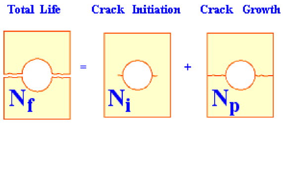
provides a “total life” estimate of fatigue life [1] [2] [3]. This is illustrated by Figure 1.1. If the analyst
wishes to gain insights into the life up to crack initiation (), or wishes to find the number of cycles
required to cause crack growth (), strain and fracture mechanics-based methods should be
explored instead [4].
1.3 The strain-life methodology
The strain-life methodology is used for calculating fatigue damage where the cycles are dominated by
local plasticity. Although the majority of engineering structures are designed such that the operational
stresses do not exceed the elastic limit, unavoidable design features such as notches can result in local
plastic strains.
The strain-life methodology correlates the local plastic deformation in the vicinity of a stress
concentration to the far-field elastic stresses and strains using the constitutive response determined
from displacement-controlled fatigue tests on simple (smooth) laboratory specimens.
Fatigue analysis using the strain-life methodology is capable of accurate predictions of crack initiation
down to a few hundred cycles. Depending on the strain-life data, failure is usually assumed as a surface
crack with a length of approximately .
Figure 1.1: Illustration of the stress-life method where the total life, Nf, is
the sum of the life to crack initiation, Ni, and life to final crack propagation,
Np.
9
1.4 Why fatigue from FEA?
Modern design workflows demand a complex and multidisciplinary mind set from the analyst [5]. The
combination of complex geometry and service loading can make the determination of the most
important stresses an insurmountable task in the absence of powerful computer software.
The finite element method is a popular tool which allows the analyst to determine the stresses acting
on a component with a high degree of accuracy. However, selection of the correct stress is often still
not obvious. Take Figure 1.2 as an example.
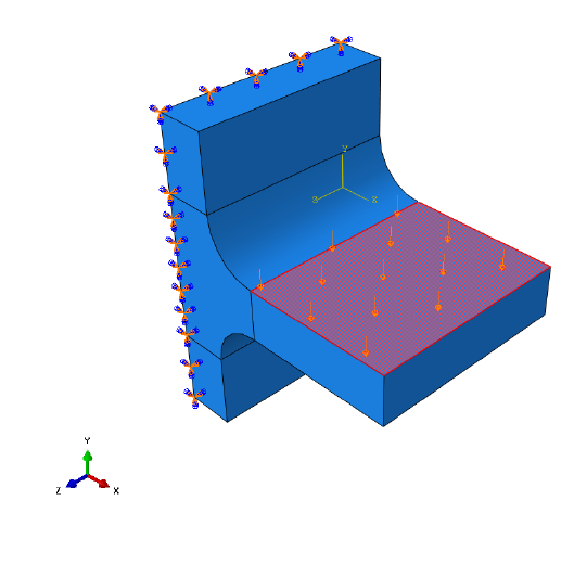
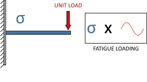
A simple fillet joint is loaded in bending by a unidirectional pressure force. The load is applied to
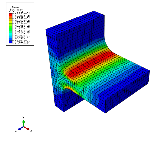
and then removed, resulting in a single pulsating loading event. Figure 1.3 shows the result of
the finite element analysis. The simplest way to relate the stress to fatigue life is by the Wöhler stress-
life curve [6]:
[1.1]
The damage parameter, , is related to the fatigue life in repeats, by the material constants
and . Considering the results from Figure 1.3, it is not obvious which stress should be chosen to take
the place of the parameter . There are several approaches for the evaluation of the fatigue life.
Figure 1.2: Uniaxial load applied to a fillet joint
10
A common approach is to take the node with the maximum principal stress and substitute this value
into the stress-life equation. Alternatively, the model can be viewed in terms of effective stress (for
example, von Mises), and using this parameter for the fatigue calculation. Both of these approaches
have serious drawbacks in that they do not correctly account for the presence of multiaxiality and
non-proportionality which commonly arises in fatigue loadings. Fatigue results obtained using these
techniques can be in significant error and even miss the location of fatigue crack initiation.
The best practise is to employ multiaxial algorithms which correctly identify the stresses on the most
damaging planes. Even unidirectional loads, such as those in the above example, can result in
multiaxial stress fields. Therefore, multiaxial analysis algorithms are always recommended over
uniaxial and effective stress methods.
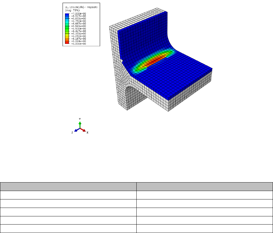
The fillet joint is analysed using Quick Fatigue Tool with several fatigue criteria, the results of which
are summarised in Figure 1.4 and the tabulated data. Algorithms with “(CP)” indicate that they are
multiaxial (critical plane) methods.
The Uniaxial Stress-Life method underestimates the fatigue life, whereas the von Mises stress
overestimates. By considering the maximum principal stress, the uniaxial method assumes that fatigue
failure will occur on a plane perpendicular to the material surface where the shear stress is zero. In
reality, most metals experience crack initiation on shear planes where there is no normal stress. For
this reason, both the uniaxial and normal stress methods produce highly conservative life predictions.
The Stress-based Brown-Miller and Findley’s Method produce the most accurate results, since they
consider the action of both the normal and shear stress acting on several planes.
Figure 1.3: FEA stresses on the fillet joint due to bending load
11
Analysis algorithm
Fatigue life (repeats)
Uniaxial Stress-Life
462,000
Stress Invariant Parameter (von Mises)
1,570,000
Normal Stress (CP)
263,000
Stress-based Brown-Miller (CP)
800,000
Findley’s Method (CP)
1,040,000
By combining results from FEA with a multiaxial analysis technique, the most accurate life prediction
can be obtained. Due to the fact that multiple planes have to be searched in order to take into account
multiaxial stress states, the multiaxial algorithms are very time-consuming compared to the uniaxial
and effective stress methods. Confining the analysis to the location of maximum stress is not
guaranteed to be successful since the location of crack initiation is not guaranteed to coincide with
the location of maximum stress.
Figure 1.4: Fatigue analysis results showing (logarithmic) life using the
Stress-based Brown-Miller multiaxial algorithm

12
1.5 Overview of syntax
1.5.1 Overview
The Quick Fatigue Tool analysis job is created by a combination of job file options and environment
variables. Job file options represent the fundamental aspects of the fatigue analysis, such as material
definition, loading and fatigue analysis algorithm. Job file options are analysis-specific. Environment
variables are used to control the general behavior of Quick Fatigue Tool, such as load gating, critical
plane search precision and results format. Environment variables apply globally to all analyses, but
may be configured for specific analyses.
Detailed information on job file options and environment variables can be found in the document
Quick Fatigue Tool User Settings Reference Guide.
1.5.2 Job file options
All of the available job file options can be found in Project\job\template_job.m. These are standard
MATLAB variables which are passed into the main analysis function when the job file is run.
Job file options can be defined as character arrays or cells, as numeric arrays, or simply left empty,
depending on how the variable is defined.
1.5.3 Environment variables
All of the available environment variables can be found in Application_Files\default\environment.m.
These are MATLAB %APPDATA% variables which are read into the program application data at the
beginning of the analysis.
Environment variables can be defined as character arrays or cells, as numeric arrays, or simply left
empty, depending on how the variable is defined.
Environment variables are set using the setappdata() method. The first argument is the name of the
environment variable and the second argument is the value of the variable.
1.5.4 Units
Material data must be defined in the SI (mm) system of units (, , , ). Stress datasets
can use any system of units, and are automatically converted into before the analysis.
1.5.5 Documentation conventions
The following conventions are used to signify job file options and environment variables throughout
the Quick Fatigue Tool documentation:
job file options defined in MATLAB are presented in BOLDFACE;
job file options defined in text files are preceded by an asterisk ( * );
environment variables are presented in magenta;
file names and string parameters are presented in 'magenta' or 'magenta';
command line parameters are presented in magenta;
default parameters are underlined ( );
Items enclosed in bold square brackets ([ ]) are optional;
items appearing in a list separated by bars ( | ) are mutually exclusive; and
one value must be selected from a list of values enclosed by bold curly brackets ({ }).

13
1.6 Required toolboxes
Quick Fatigue Tool does not require any MATLAB toolboxes to function properly. However, certain
toolboxes are used to enhance the functionality of the code if Quick Fatigue Tool detects that they are
installed. Below is a summary of these toolboxes and the additional functionality they provide.
Toolbox
Functionality
Image Processing Toolbox
Strain gauge preview dialogue box for
Gauge Fatigue Toolbox apps. See Appendix III of
Quick Fatigue Tool Appendices for more
information
Symbolic Math Toolbox
Iterative solver for the following features:
Derivation of the normal stress
sensitivity constant () using the
General Formula option in the
Material Manager app
Derivation of the reference strains from
user-defined strain gauge orientations
using the Multiaxial Gauge Fatigue and
Rosette Analysis apps
Derivation of the initial fibre
misalignment angle () for the LaRC05
composite damage initiation criteria
Statistics Toolbox
RHIST and RC output variables
Signal Processing Toolbox
High frequency loadings with HF_DATASET and
HF_HISTORY
14
1.7 Limitations
1.7.1 Fatigue from FEA
FEA tools
Quick Fatigue Tool has been optimised to use stress data from an Abaqus output database (.odb) file
using the built-in field output report tool in Abaqus/CAE. Stress dataset files generated from other
third party FEA processors must adhere to the rules and conventions detailed in Section 3.2.
Datasets
Quick Fatigue Tool assumes that the FEA stress datasets are elastic for both stress and strain-based
fatigue analyses. In the latter case, the stresses are automatically corrected for the effect of plasticity.
Elements
Special-purpose elements and connector elements are not supported. Structural elements such as
beams, pipes and wires may be used, although they have not been thoroughly tested. Using any of
these elements may cause the analysis to produce error messages or crash.
Stress tensors read from FE models must use a Cartesian coordinate system.
If the model contains plane stress elements from an Abaqus .odb file, only the valid tensor
components are printed to the dataset (.rpt) file. In such cases, the user must set the option
PLANE_STRESS=1.0 in the job file. This ensures that Quick Fatigue Tool is able to correctly identify
plane stress elements.
When exporting stress datasets from Abaqus, Quick Fatigue Tool will fail to process the data if the
element stresses are written to more than two locations on the element. For example, Abaqus usually
writes stresses to two section points for shell elements (top and bottom faces). If the user requested
field output at more than two section points, or the element is defined from a composite section,
Quick Fatigue Tool will not be able to interpret the stress dataset file.
If the user wishes to analyse the surface of a composite structure, the best practise is to define a skin
on the surface of the structure and export the stresses from the skin elements only.
Part instances
Quick Fatigue Tool supports stress datasets which span multiple Abaqus part instances provided that
the element-node numbers are unique between instances. If the stress dataset contains duplicate
element-node numbers, Quick Fatigue Tool is unable to distinguish between individual part instances
and results may be reported at incorrect locations.
If the model is defined as assemblies of part instances and the fatigue analysis spans more than one
instance, the user can ensure unique element-node numbering as follows:
1. Enter the Mesh Module in Abaqus/CAE and select Part as the object
2. From the main menu, select Mesh → Global Numbering Control…
3. Specify a start label for the elements and nodes of the current part instance, such that they
do not clash with other part instances which will be included for fatigue analysis
15
It is strongly recommended that the user works with flat input files. This generates an output database
containing a single part instance, which guarantees unique element-node numbering:
1. (any module in Abaqus/CAE): From the main menu select Model → Edit Attributes → Model
name
2. Select Do not use parts and assemblies in input files
1.7.2 Loading
Quick Fatigue Tool does not directly support multiple block loading. A workaround involves splitting
the load spectrum into several jobs using the CONTINUE_FROM option, which allows
Quick Fatigue Tool to automatically overlay the fatigue damage onto the previous results to give the
total damage due to all blocks. Analysis continuation is discussed in Section 4.8.
1.7.3 Materials
It is assumed that stress relaxation does not occur during the loading and that the material is cyclically
stable. This expedites the fatigue calculation by allowing analysis of each node without considering
the effects of neighbouring nodes, but precludes the effect of global plasticity being accurately taken
into account. However, for the majority of cases this should not be an issue since the stress-life
method is elastic, and the strain-life method is intended for components experiencing relatively small
amounts of local plasticity.
Quick Fatigue Tool is applicable to metals and some engineering plastics where the stresses and
temperatures are sufficiently low that viscoelastic effects are negligible.
Treatment of local notch plasticity requires the use of strain-based fatigue methods. Treatment of
crack propagation requires the use of crack growth methods such as VCCT, CTOD and Paris Law LCF.
Analysis of viscoelastic, hyperelastic, anisotropic and quasi-brittle materials is not supported.
Materials whose fatigue behavior cannot reasonably be modelled by linear elastic stresses and stress-
life curves are not supported.
1.7.4 Performance
The MATLAB programming language is very convenient in terms of the ease and speed of development
it offers. However, in runtime the code is slow in comparison to other languages. Therefore, stress
datasets from even a modest finite element model can result in cumbersome analyses. The user is
advised to consult Section 10: Modelling considerations for assistance on how to minimise analysis
time without compromising on the accuracy of the solution.

16
1.7.5 GUI appearance
It is recommended that you set your monitor DPI scaling to and the resolution to x.
On Windows 7, the DPI settings are found at Control Panel\Appearance and Personalization\Display.
On Windows 10 the settings are at the same location, but you must select set a custom scaling level
under the “Change size of items” section.
If the above settings are not used, Material Manager, Export Tool and the Gauge Fatigue Toolbox apps
may display incorrectly.
An alternative to using the Material Manager app is to import material data from a text file. For
instructions on creating material text files, consult Section 5.6 “Creating a material from a text file”.
1.7.6 Validation
Quick Fatigue Tool has not been validated against any official standard. The author does not take any
responsibility for the accuracy or reliability of the code. Fatigue analysis results should be treated as
supplementary and further investigation is strongly recommended.
1.8 Additional notes
a) It is recommended that you consult the file README.txt in the Documentation directory
before proceeding to the next section of the guide
b) Modifying the file structure (e.g. renaming folders) may prevent the program from working.
c) The change log for the latest version can be found here
d) Quick Fatigue Tool is free for distribution without license, provided that the author
information is retained in each source file
To report a bug or to request an enhancement, please contact the author:
Louis VALLANCE
louisvallance@hotmail.co.uk
17
2. Getting started
2.1 Preparing the application
Preparing Quick Fatigue Tool requires minimal intervention from the user, although it is important to
follow a few simple steps before running an analysis:
Make sure the working directory is set to the root of the Quick Fatigue Tool directory, e.g.
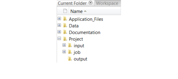
\..\Quick Fatigue Tool\6.x-yy. The directory structure is shown in Figure 2.1. All folders and sub folders
should be added to the MATLAB search path using the function addpath(), or by selecting the folders
Application_Files and Project, right-clicking and selecting Add to Path → Selected Folders and
Subfolders.
If the MATLAB working directory is not configured exactly as described above (e.g. the user enters the
job directory before running a job file), the application will not run.
Before running a fatigue analysis, it is recommended that you first run the job tutorial_intro. This is
because the initial run of a MATLAB function requires some additional computational overhead which
slows down the first analysis.
2.2 How the application handles variables
Quick Fatigue Tool does not store variables in the base workspace, nor does it modify or delete existing
workspace variables. During analysis, variables are stored either in the function workspaces or as
application-defined data using the setappdata() and getappdata() methods.
The application data is utilised for convenience, since variables can easily be accessed throughout the
code without having to pass variables between many functions. In order to prevent unwarranted data
loss, Quick Fatigue Tool does not modify existing application data by default. However, this means
that variables from previous analyses will remain in the application data and could cause unexpected
behavior in subsequent analyses, such as incorrect fatigue results and spurious crashes.
Figure 2.1: Quick Fatigue Tool file structure

18
In order to eliminate the possibility of such conflicts, the user is strongly advised to restart MATLAB
between each analysis so that the application data is cleared. If the user does not wish to restart
MATLAB for each analysis and is not concerned about Quick Fatigue Tool modifying the application
data, the following environment variable may be set with a value of 3.0:
Environment file usage:
Variable
Value
cleanAppData
{1.0 | 2.0 | 3.0 | 4.0}
This ensures that the application data is completely cleared before and after each analysis. This has
the same effect of restarting MATLAB.
The environment file and all of the available user settings are discussed in the document
Quick Fatigue Tool User Settings Reference Guide.
2.3 File structure
Quick Fatigue Tool separates various components of the code into folders. Below is a brief description
of what each folder contains:
Application_Files
Source code and application-specific settings.
There is usually no need to modify the contents
of this directory
Data
User-specific data (models, surface finish curves,
material data, etc.)
Documentation
README file and User Guide
input
Required location for stress datasets and load
histories
job
Job files defining each analysis
output
Fatigue results directory. If this folder does not
exist, it will automatically be created during the
analysis
19
2.4 Configuring and running an analysis
2.4.1 Configuring a standard analysis
Standard analyses are configured and submitted from an .m file.
In this example, a simple fatigue analysis is configured by combining a stress dataset with a load
history. The files can be found in the Data\tutorials\intro_tutorial folder.
1. Define a stress dataset: Open the file stress_uni.dat. A simple stress definition consists of six
components defining the Cauchy stress tensor. The components are defined in the following
order:
Column 1
Column 2
Column 3
Column 4
Column 5
Column 6
The file stress_uni.dat contains a stress tensor at a single material point in a state of uniaxial tension
().
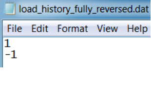
2. Define a load history: Open the file history_fully_reversed.dat. A simple load history consists of
two loading points. Below is a list of common load definitions:
Load type
Definition
Fully-reversed (push-pull)
[1, -1]
Pure tension
[0, 1]
Pure compression
[0, -1]
The file history_fully_reversed.dat defines the fully-reversed loading event:
().
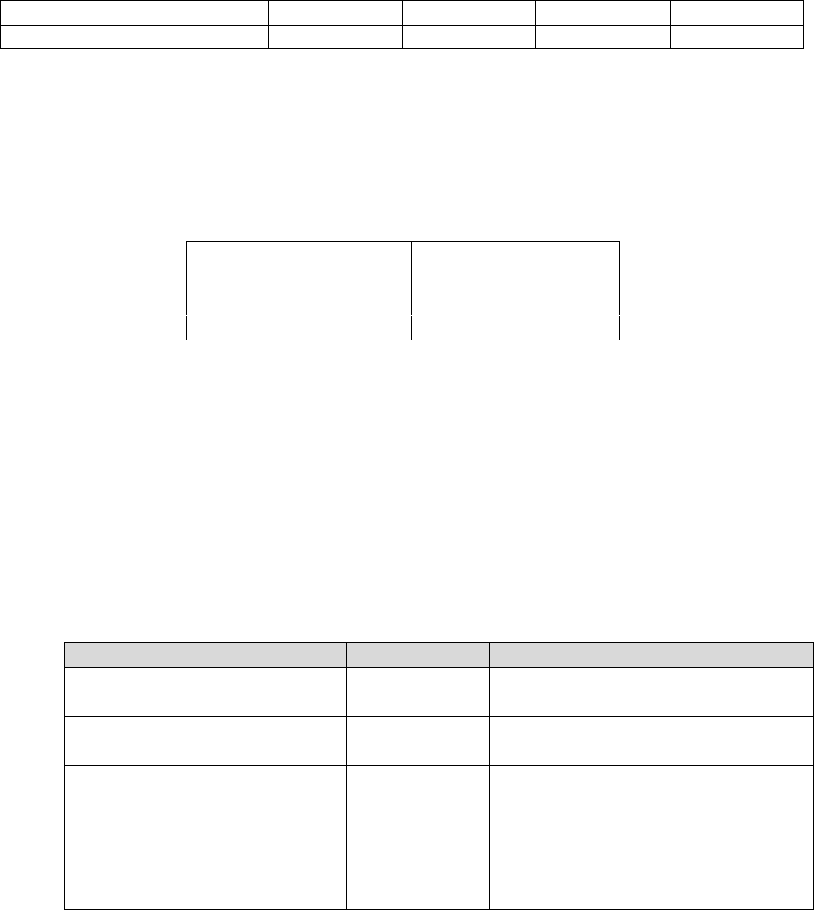
3. Study the job file: Open the job file tutorial_intro.m. The file contains a set of options specifying
all the information necessary for fatigue analysis. Options can be strings or numeric depending on
the meaning of the option. Not all options require a user setting. Below is a summary of each
option in the job file. The user need not worry about the number of definitions; all of the job file
options are explained in the document Quick Fatigue Tool User Settings Reference Guide and in
the tutorials later in this guide.
Option
Meaning
Additional notes
JOB_NAME
The name of
the job
JOB_DESCRIPTION
A description
of the job
The job name and description are
printed to the log file for reference
CONTINUE_FROM
Superimpose
results onto a
previous job
This feature is useful for block loading,
or specifying the analysis algorithm
based on model regions

20
DATA_CHECK
Runs the job
up to the
beginning of
the analysis
Useful for checking the message file
for initial notes and warnings, without
having to run the full fatigue analysis
MATERIAL
Material used
for analysis
'SAE-950C.mat' references a file
containing the material properties.
Materials are stored in
Data\material\local. Materials are
defined using the Material Manager
app. Usage of the app is discussed in
Section 5
USE_SN
Stress-life data
1.0; A flag indicating that S-N data
should be used if available
SN_SCALE
Stress-life data
scale factor
1.0; A linear scale factor applied to
each S-N data point
SN_KNOCK_DOWN
S-N knock-
down factors
Knock-down factors are not used in
this analysis. Knock-down factors are
discussed in Section 4.8
DATASET
Stress data
'stress_uni.dat' references the stress
dataset file. Stress datasets should be
saved in Project\input
HISTORY
Load history
'history_fully_reversed.dat'
references the load history file. Load
histories should be saved in
Project\input
UNITS
Stress units
3.0; A flag with the definition of MPa
CONV
Conversion
factor for
stress units
LOAD_EQ
Load
equivalency
The default loading equivalence is 1
repeat. If the loading represents
another dimension, the fatigue results
can be expressed in a more
appropriate unit (e.g. 1000 hours)
SCALE
Stress scale
0.8285; A linear scale factor applied
to the entire loading
OFFSET
Offset value
for stress
history
Loading offsets are discussed in
Section 3.4
REPEATS
Number of
repetitions of
the loading
HF_DATASET
Dataset(s) for
high frequency
loads
HF_HISTORY
Load history
for high
frequency
loads

21
HF_TIME
Time
compression
for high
frequency
loads
HF_SCALE
Scale factor for
high frequency
loads
High frequency loads are discussed in
Section 3.5
PLANE_STRESS
Element type
(3D stress or
planar)
0.0; A flag indicating that a 3D
element type should be assumed. The
distinction that Quick Fatigue Tool
makes about element types is
discussed in Sections 3.2.4 and 3.6.1
OUTPUT_DATABASE
Model output
database
(.odb) file from
an Abaqus FE
analysis
EXPLICIT_FEA
FEA procedure
type
PART_INSTANCE
FEA part
instance name
STEP_NAME
FEA step name
RESULT_POSITION
FEA result
position
Associating a job with an Abaqus .odb
file is discussed in Sections 4.6 and
9.5. This job is not associated with an
.odb file
ALGORITHM
Analysis
algorithm
0.0; A flag indicating that the default
analysis algorithm should be used
(Stress-based Brown-Miller). Analysis
algorithms are discussed in Section 6
MS_CORRECTION
Mean stress
correction
2.0; A flag indicating that the
Goodman mean stress correction will
be used. Mean stress corrections are
discussed in Section 7
ITEMS
List of items
for analysis
'ALL' indicates that all items in the
model (1) should be analysed.
Selecting analysis items is discussed in
Section 4.5.3
DESIGN_LIFE
The target life
of the system
'CAEL' indicates that the target life
should be set to the material’s
constant amplitude endurance limit
KT_DEF
Surface finish
definition
KT_CURVE
Surface finish
type
This analysis assumes a surface finish
factor of 1. Surface finish definition is
discussed in Section 4.3

22
NOTCH_CONSTANT
Notch
sensitivity
constant
NOTCH_RADIUS
Notch root
radius
GAUGE_LOCATION
Virtual strain
gauge
definition
GAUGE_ORIENTATION
Virtual strain
gauge
orientation
RESIDUAL
Residual stress
0.0; A residual stress value which is
added to the fatigue cycle during the
damage calculation. Residual stress is
discussed in Section 4.4
FACTOR_OF_STRENGTH
Factor of
strength
calculation
0.0; A flag indicating that a factor of
strength calculation will not be
performed. Factor of strength is
discussed in Section 8.3
FATIGUE_RESERVE_FACTOR
2.0; A flag indicating that the
Goodman B envelope will be used for
Fatigue Reserve Factor calculations.
The Fatigue Reserve Factor is
discussed in Section 8.2
HOTSPOT
Hotspot
calculation
0.0; A flag indicating that a hotspot
calculation will not be performed.
Factor of strength is discussed in
Section 4.5.3
OUTPUT_FIELD
Request for
field output
1.0; A flag indicating that field output
will not be written
OUTPUT_HISTORY
Request for
history output
0.0; A flag indicating that history
output will not be written
OUTPUT_FIGURE
Request for
MATLAB
figures
0.0; A flag indicating that MATLAB
figures will not be written. Analysis
output is discussed in Section 10
WELD_CLASS
Weld
classification
for BS 7608
analysis
YIELD_STRENGTH
Yield strength
for BS 7608
analyses
UTS
Ultimate
tensile
strength for BS
7608 analyses
DEVIATIONS_BELOW_MEAN
Degree of
uncertainty for
BS7608
analyses
23
FAILURE_MODE
Failure mode
for BS 7608
analyses
CHARACTERISTIC_LENGTH
Characteristic
dimension for
BS 7608
analyses
SEA_WATER
Environmental
effects factor
for BS 7608
analyses
This analysis does not require a weld
definition. The BS 7608 algorithm is
discussed in Section 6.6
4. Select the material and analysis type: This analysis uses SAE-950C Manten steel as the material.
The materials available for analysis are located in the Data\material folder. Stress units are in MPa.
The analysis algorithm is the default algorithm (Stress-based Brown-Miller), the Goodman mean
stress correction is used, as well as user-defined stress-life data points.
5. Run the job: To execute the analysis, right-click on tutorial_intro.m and click run.
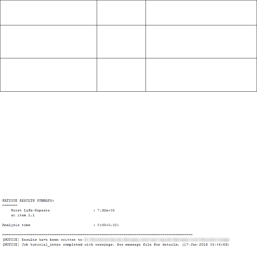
6. A summary of the analysis progress is written to the command window. When the analysis is
complete, the command window should look like that of Figure 2.1.2.
7. The fatigue results summary reports a life of 732 thousand cycles to failure at location 1.1. This is
the default location when a stress dataset is provided without position labels.
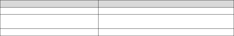
8. In the Project\output directory, a folder with the name of the job is created which contains all of
the requested output. In this analysis, extensive output was not requested, so only the following
three basic files are written:
Figure 2.1.2: Fatigue results summary

24
File
Contents
<job_name>.log
Input summary
Analysis groups
Critical plane summary
Factor of Strength diagnostics
Fatigue results summary
<job_name >.msg
Pre and post analysis messages
o Analysis-specific notes offering
useful information to the user
o Analysis-specific warnings
explaining potential issues
with the analysis
<job_name >.sta
An item-by-item summary of the
analysis progress
9. Open the log and status files and examine their contents. According to the command window
summary, the analysis completed with warnings. Examine the contents of the message file:
a. Extensive output was not requested by the user
b. The damage at design life (10 million cycles by default) is over unity, corresponding to
failure
c. There is a warning that Quick Fatigue Tool encountered an ambiguity whilst determining
the element (stress tensor) type for analysis. A 3D stress tensor was assumed as the input
stress dataset. Since this assumption is correct, the warning can be ignored
10. To run another analysis, it is recommended that you first restart MATLAB to ensure that all the
application data from the previous analysis is cleared.

25
2.4.2 Configuring a data check analysis
A data check runs the job file through the analysis pre-processor, without performing the fatigue
analysis.
Job file usage:
Option
Value
DATA_CHECK
{0.0 | 1.0}
Data checks are useful for ensuring that the analysis definitions are valid, allowing the user to correct
errors which may otherwise only become apparent after a long analysis run. The data check feature
checks the following for consistency:
ODB interface settings
Results directory initialization
Analysis continuation settings
Material definitions and S-N interpolation
Algorithm and mean stress correction settings
Dataset and history definitions
Principal stress histories
Custom mean stress, FRF and surface finish data
Surface detection
Yield criteria analysis
Composite criteria analysis
Nodal elimination
Load proportionality
Virtual strain gauge definition
Duplicate analysis item IDs
Pertinent information regarding the data check run can be found in the message file in
Project\output\<jobName>.
If the user requested field output from the job file, the worst tensor and principal stress per node for
the whole model are written to the files datacheck_tensor.dat and datacheck_principal.dat,
respectively.
26
2.4.3 Configuring an analysis from a text file
Quick Fatigue Tool includes a text file processor, which allows the user to submit a job from an ASCII
text file containing only the options which are required to define the analysis. This results in job files
which are less cumbersome than the standard .m file which must contain every option regardless of
whether or not it is required.
To define a job from a text file, options are specified as keywords.
Job file usage:
Option
Value
*<keyword> =
<value>
Keywords are exactly the same as job file options, but they always begin with an asterisk (). For
example, the job file option DATASET is declared in the text file as *DATASET. Entries which do not
begin with an asterisk, or are not proceeded with an equal sign () followed by a value, are ignored
by the input file processor.
Job file options containing underscores are specified in the text file with spaces. For example, the
option JOB_NAME is specified in the text file as *JOB NAME.
The following should be noted when defining jobs from a text file:
it is not necessary to end the definition with a semi-colon;
it is not necessary to enclose strings with apostrophes;
white spaces are ignored; and
mathematical expressions are not supported.
The user must adhere to the following syntax when defining cells in the text file.
Cell type
Text input
Strings
{<>, <>,…, <>}
Numeric arrays
{[, ,…, ], [, ,…, ],…, [, ,…,
]}
Mixture of strings and numeric arrays
{<>, [, ,…, ]}
Any combination of strings and numerical inputs are supported, provided each element is separated
by a comma.
27
Jobs defined as text files are submitted from the command line.
Command line usage:
>> job <jobFile>
>> job <jobFile> 'option'
The parameter option has two mutually-inclusive values:
interactive – prints an echo of the message (.msg) file to the MATLAB command window.
datacheck – submits the analysis job as a data check analysis.
Any file extension is accepted provided the contents is ASCII text. Job files with the extension .inp can
be specified without appending .inp on the command line. For all other file types, the extension must
be specified. Apostrophes are not required when specifying the input file name.
Example usage
An example of a text-based job file is given by the file tutorial_intro.inp in the
Data\tutorials\intro_tutorial folder. Open the file and study its contents.
There is a text header at the beginning of the file, which is distinguished from the rest of the contents
by double asterisks (**) at the beginning of each line. These lines are ignored by Quick Fatigue Tool.
The first keyword is *USER MATERIAL, which is used to define material data. Guidance on creating
material data in a text file is found in Section 5.5.4 “Specifying material properties in a job file”.
Subsequent keywords specify analysis definitions for a uniaxial stress-life analysis. To submit the file
for analysis, execute the following command:
Command line usage:
>> job tutorial_intro
The material data is first read into the material database. If the material already exists in the
Data\material\local directory, the user is prompted to overwrite the existing material data. The
analysis keywords are then processed and the job is submitted for analysis.
Results of the fatigue analysis are written to Project\output\tutorial_intro.

28
2.5 The analysis method
1. A loading definition is created by combining elastic stress datasets with load histories to produce
a scaled history of stresses for each item in the model
2. If a high frequency loading is provided, it is interpolated and superimposed onto the original load
history
3. If requested, the load histories are pre-gated before the analysis which aims to remove small
cycles from the loading
4. The principal stress history is calculated for each analysis item
5. The load history at each point in the model is assessed for proportionality. The critical plane step
size may automatically be increased if the load is considered to be proportional
6. If requested, nodal elimination is performed which removes analysis items whose maximum stress
range is less than the fatigue limit of the material
7. User stress-life data is interpolated to find the endurance curve for a fully-reversed cycle
8. Stresses are resolved onto planes in a spherical coordinate space to find the plane on which the
most damaging stresses occur
1
9. Stresses on this plane are counted using the rainflow cycle counting method
2
. If requested, the
stress tensors on this plane are gated prior to cycle counting
10. If requested, the stress cycles are corrected for material non-linearity
11. The stress cycles are corrected for the effect of mean stress
12. A damage calculation is performed for each cycle using Miner’s Rule of linear damage
accumulation [7]. The endurance limit may be reduced to 25% of its original value if the cycle
stress amplitudes are damaging
13. Steps 8-12 are repeated for each analysis item
14. If requested, the item with the worst life is analysed once more to calculate extensive output
15. If requested, Factor of Strength (FOS) iterations are performed. The damage is recalculated for
each analysis item to obtain the linear loading scale factor which, if applied to the original loading,
would result in the user-defined design life
1
Only if the fatigue analysis algorithm is multiaxial
2
Only if the load history contains more than two data points
29
3. Defining fatigue loadings
3.1 Loading methods
3.1.1 Overview
The loading definition forms the basis of the analysis, and describes the stress history at each point in
the model. Loadings usually consist of stress datasets (user-defined or from FEA) and load histories.
The stress datasets contain the static stress state at each location in the model. This can be at a node,
integration point, centroid or otherwise. The load history defines the variation of the stresses through
time. However, Quick Fatigue Tool does not distinguish elapsed time between loading points and
hence the load history is treated as being rate-independent.
Quick Fatigue Tool offers five methods for creating loading definitions:
1. Uniaxial history
2. Simple loading
3. Multiple load history (scale and combine) loading
4. Dataset sequences
5. Complex (block sequence) loading
3.1.2 Syntax
Stress datasets are specified as ASCII text files:
'dataset-file-name.*' | {'dataset-file-name-1.*', 'dataset-file-name-2.*',…, 'dataset-file-name-.*'}
Load histories are specified as ASCII text files, or directly as one or more vectors:
'load-history-file-name.*' | {'history-file-name-1.*', 'history-file-name-2.*',…, 'history-file-name-.*'}
[, ,…, ] | {, ,…, }
30
3.1.3 Uniaxial history
A single load history is supplied without a stress dataset.
Job file usage:
Option
Value
DATASET
' '
HISTORY
{'history-file-name.*' | [, ,…, ] }
The load history is analysed without respect to a particular model, and is only valid for uniaxial states
of stress. Uniaxial histories can only be used with the Uniaxial Stress-Life and Uniaxial Strain-Life
algorithms.
Job file usage:
Option
Value
ALGORITHM
{3.0 | 'UNIAXIAL STRAIN'}
ALGORITHM
{10.0 | 'UNIAXIAL STRESS'}
3.1.4 Simple Loading
A simple loading consists of a single stress dataset multiplied by a load history.
Job file usage:
Option
Value
DATASET
'dataset-file-name.*'
HISTORY
{'history-file-name.*' | [, ,…, ] }
An example of a simple fatigue loading is given by Figure 3.1.
Figure 3.1: Demonstration of a simple loading. The stresses, , due
to a unit load are multiplied by a load history
31
Constant amplitude loading
The load history is defined as a minimum and maximum value, an example of which is given below.
Job file usage:
Option
Value
HISTORY
[, ]
The definition can be a single cycle, or repetitions of the same cycle.
Job file usage:
Option
Value
REPEATS
Single load history
The load history is defined as a time history of the loading, scaled with the stress dataset. The dataset
can be defined in two ways:
1. FEA stress from unit load, scaled by a time history of load values
2. FEA stress from maximum load, scaled by a time history of load scale factors
Both methods are valid provided that the FEA is linear and elastic.
32
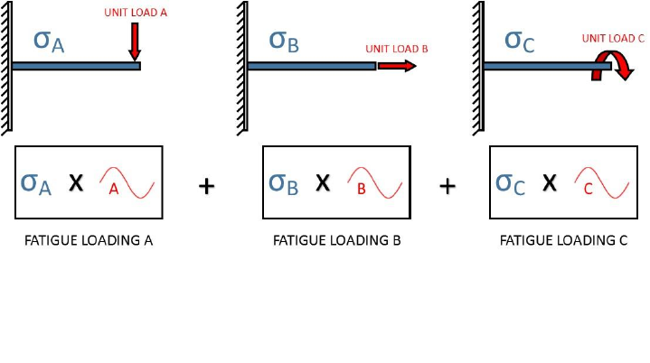
3.1.5 Multiple load history (scale and combine) loading
A multiple load history consists of several stress datasets multiplied by the same number of histories.
At each analysis item, the stress tensor from each dataset is scaled with its respective load history and
combined into a single stress history. The number of stress datasets and load histories must be the
same, although the number of history points in each load history need not be the same.
Job file usage:
Option
Value
DATASET
{'dataset-file-name-1.*', 'dataset-file-name-2.*',…,
'dataset-file-name-.*'}
HISTORY
{'history-file-name-1.*', 'history-file-name-2.*',…,
'history-file-name-.*'}
An example of a scale and combine loading is given by Figure 3.2.
Scale and combine loading is only physically meaningful for elastic stresses. Each channel can be scaled
by its respective load history since the load is directly proportional to the elastic FEA stress. The scale
and combine method assumes that each loading channel is occurring simultaneously.
The load history may be defined by any combination of load history files and vectors.
Job file usage:
Option
Value
HISTORY
{'history-file-name.*', [, ,…, ]}
Figure 3.2: Demonstration of a multiple load history (scale and combine). The stresses,
,
and due to unit loads , and are multiplied by their respective load histories and
summed to produce the resultant fatigue loading
33
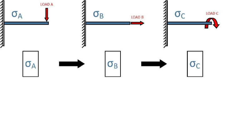
3.1.6 Dataset sequences
A dataset sequence loading consists of several stress datasets.
Job file usage:
Option
Value
DATASET
{'dataset-file-name-1.*', 'dataset-file-name-2.*',…,
'dataset-file-name-.*'}
HISTORY
[ ]
An example of a dataset sequence loading is given by Figure 3.3.
Since the fatigue loading is completely described by the variation of stresses between each dataset,
specification of load histories is not required.
Figure 3.3: Demonstration of a stress dataset sequence loading. The fatigue loading is formed
by the sequence of stress solutions , and , due to the applied loads , and ,
respectively
34
3.1.7 Complex (block sequence) loading
Complex loadings consist of multiple loading blocks, each representing a stage of the component’s
duty. Block sequences are useful in proving ground tests where the component is subjected to a
sequence of distinct loading events, and it is desirable to compute the individual damage contributions
from each event.
Currently, sequences of loading blocks cannot be defined in a single job. However, Quick Fatigue Tool
allows the user to run multiple jobs in series, wherein each job is treated as a separate loading block.
Job file usage:
Option
Value
JOB_NAME
'current-job-name'
CONTINUE_FROM
'previous-job-name'
When a job is run as a continuation of a previous job, Quick Fatigue Tool calculates the individual
damage contribution of the current job, then superimposes the result onto the previous job to give
the cumulative damage of the block sequence.
Analysis continuation is discussed further in Section 4.8.
35
3.2 Creating a stress dataset file
3.2.1 Dataset structure
Stress datasets are text files containing a list of stress tensors. The simplest way to create a stress
dataset file is to specify the tensor components as follows:
Line 1:
, , , , ,
Line 2:
, , , , ,
.
.
.
.
.
.
Line
, , , , ,
Each line defines the stress tensor at each location in the model.
3.2.2 Creating a dataset from Abaqus/Viewer
Stress datasets may be generated from finite element analysis (FEA). To create a stress dataset file
from Abaqus/Viewer, complete the following steps:
1. In the Visualization module, from the main menu, select Result → Options…
2. Under “Averaging”, uncheck “Average element output at nodes”.
3. From the main menu, select Report → Field Output…
4. Under “Step/Frame”, select the step and the frame in the analysis from which the stresses will
be written.
5. In the “Variable” tab, under “Output Variables”, select the position of the output (Integration
Point, Centroid, Element Nodal or Unique Nodal).
6. Expand the variable “S: Stress components” and select all the available Cauchy tensor
variables (S11, S22, S33, S12, S13 and S23); if plane stress elements are used, select (S11, S22,
S33 and S12) and set PLANE_STRESS=1.0 in the job file; if one-dimensional elements are used,
select (S11)
7. If the model contains results at multiple section points or plies, select Settings… from the
section point method and specify the section point or ply of interest
8. In the “Setup” tab, set the file path (e.g. \6.x-xx\Project\input\<filename>.rpt)
9. Under “Data”, uncheck “Column totals” and “Column min/max”. Make sure “Field output” is
checked.
10. Click OK
36
3.2.3 Creating datasets from other FEA packages
If the user wishes to create a stress dataset from an FEA package other than Abaqus, the following
standard data format must be observed for 3D stress elements:
MAIN POSITION ID
(OPTIONAL)
SUB POSITION ID
(OPTIONAL)
S11
S22
S33
S12
S13
S23
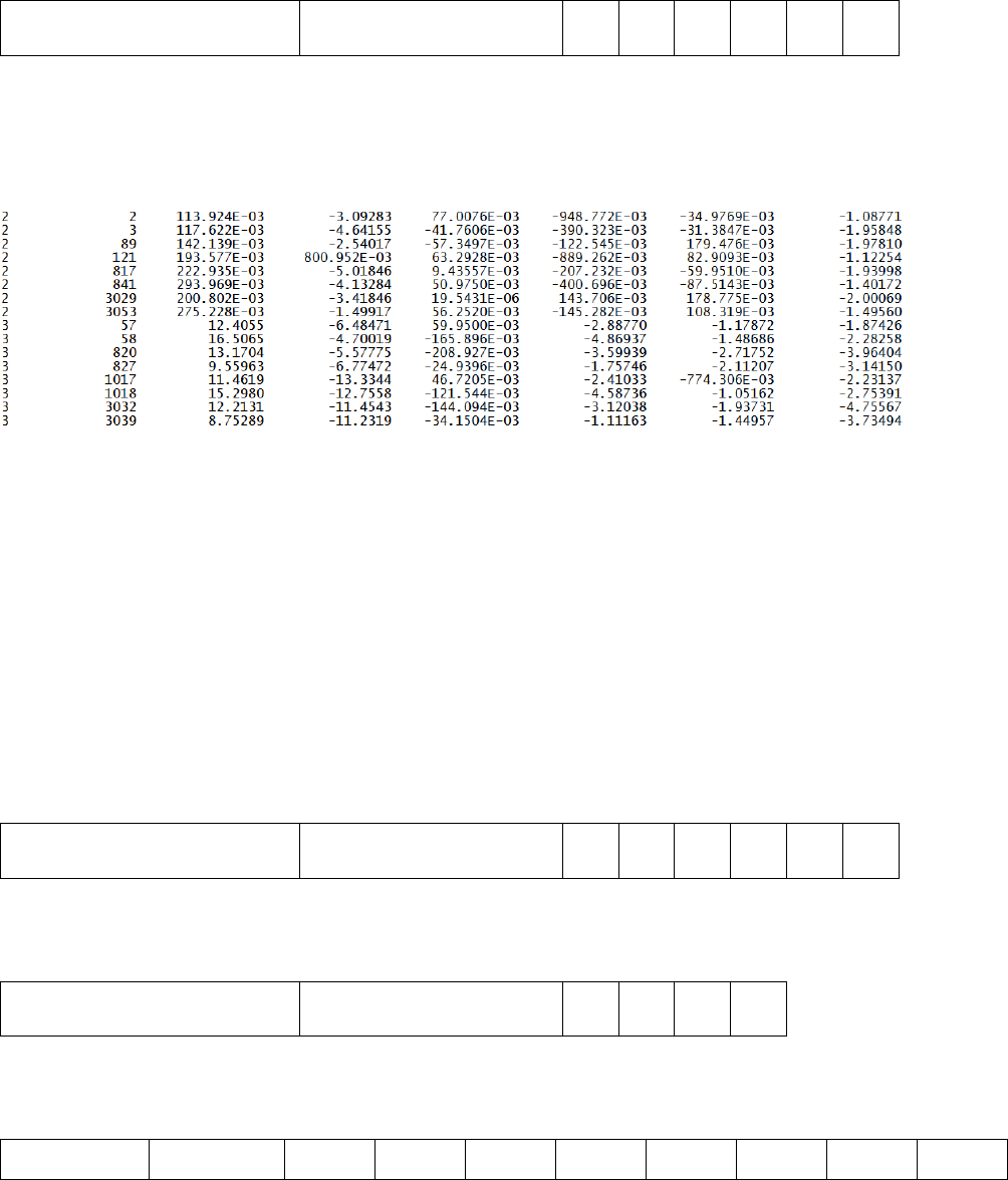
For example, a particular stress dataset may look like the following:
The position labels can be arbitrary, but usually represent the location on the finite element model
(e.g. element.node). Quick Fatigue Tool will quote the position of the shortest fatigue life. Position
labels are not compulsory: The stress dataset can be specified with tensor information only.
Furthermore, it is not compulsory to include both main and sub IDs. For example, if the stress data is
unique nodal (nodal averaged), there is only one position ID which is the node number.
3.2.4 Creating datasets with different element types
Quick Fatigue Tool automatically recognises stress datasets from Abaqus containing multiple element
types. Such files are split into regions, each of which defines the stress tensors for a specific element
type. If the stress dataset file is user-defined, the following conventions must be observed:
3D stress elements:
MAIN POSITION ID
(OPTIONAL)
SUB POSITION ID
(OPTIONAL)
S11
S22
S33
S12
S13
S23
Plane stress elements without shell face information:
MAIN POSITION ID
(OPTIONAL)
SUB POSITION ID
(OPTIONAL)
S11
S22
S33
S12
Plane stress elements with shell face information:
MAIN POSITION ID
(OPTIONAL)
SUB POSITION ID
(OPTIONAL)
S11
(+ve face)
S11
(-ve face)
S22
(+ve face)
S22
(-ve face)
S33
(+ve face)
S33
(-ve face)
S12
(+ve face)
S12
(-ve face)
37
One-dimensional elements:
MAIN POSITION ID
(OPTIONAL)
SUB POSITION ID
(OPTIONAL)
S11
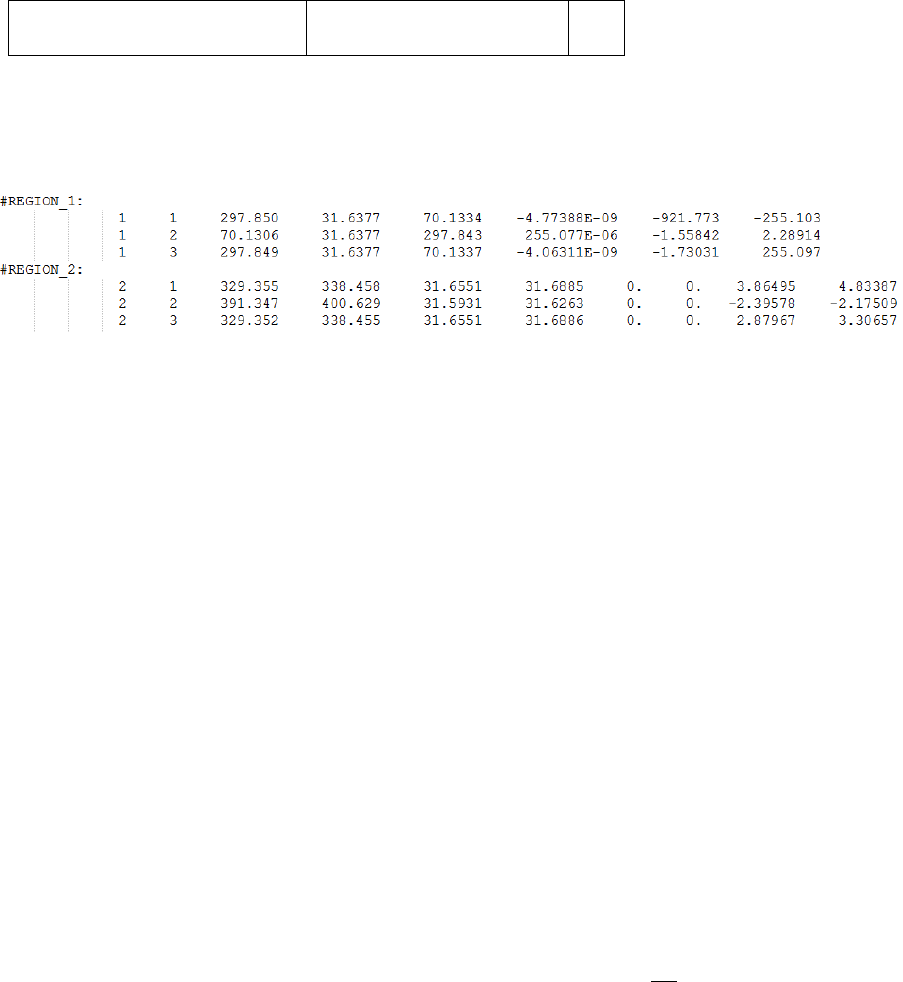
Below is an example of a user-defined stress dataset file containing two elements.
Each element region must be declared by a text header in order to be recognised, and the header
must start with a non-numeric character. In the above example, REGION_1 defines a 3D element and
REGION_2 defines a 2D element with results at both shell faces. Both elements are defined with
element-nodal (nodal un-averaged) position labels. All the datasets in the loading must be defined
with the same position labels otherwise the analysis will not run. To check whether or not the dataset
definition was processed correctly, Quick Fatigue Tool prints the number of detected regions to the
message file. This can be found in Project\output\<jobName>\<jobName>.msg.
Quick Fatigue Tool will automatically detect the element type based on the number of columns in the
dataset file. For example, if there are five columns, this will be interpreted as plane stress (four
columns define the tensor) with one column defining the element position (either unique nodal or
centroidal). If the dataset file contains six columns, this could either be interpreted as 3D stress (all six
columns define the stress tensor) with no position labels, or plane stress (four columns define the
tensor) with two columns defining the element position (either element-nodal or integration point).
This ambiguity is resolved with the use of the following job file option:
Job file usage:
Option
Value
PLANE_STRESS
{0.0 | 1.0}
If the value of PLANE_STRESS is set equal to 1.0, Quick Fatigue Tool will assume that the element
definition is plane stress if it encounters a data region with six data columns.
A complete description of how dataset files are interpreted is provided in Section 3.6.

38
3.2.5 Specifying stress dataset units
Since fatigue analysis uses the SI (mm) system of units, stress datasets are assumed to have units of
Megapascals () by default. If the datasets use a different system of units, these must be specified
in the job file so that Quick Fatigue Tool can convert them into the SI (mm) system.
Job file usage:
Option
Value
UNITS
{'Pa' | 'kPa' | 'MPa' | 'psi' | 'ksi' | 'Msi'}
If the stress dataset units are not listed, they can be user-defined.
Job file usage:
Option
Value
UNITS
0.0
CONV
The parameter is a constant which converts the stress dataset units into Pascals ().
[3.1]
The stress data is converted into the SI (mm) system using Equation 3.2.
[3.2]
39
3.3 Creating a load history
Load histories can be defined in three ways:
1. From a text file
2. As a direct definition
3. As a workspace variable
Create a load history from a text file
If the load history is defined from a text file, it must contain a single or vector of loading
points, as follows:
← First loading point
.
.
← Last loading point
For example, a fully-reversed load history would look like that of Figure 3.4.
Job file usage:
Option
Value
HISTORY
'history-file-name.*'
Load history files must be stored in the Project\input folder in order for Quick Fatigue Tool to locate
the data.
Figure 3.4: Fully-reversed load history
40
Create a load history as a direct definition
Load histories can be specified in the job file as a vector of scale factors.
Job file usage:
Option
Value
HISTORY
[, ,…, ]
Alternatively, the load history can be defined as a function.
Job file usage:
Option
Value
HISTORY
where is a stress amplitude scale factor.
Create a load history as a workspace variable
If the load history is defined as a workspace variable, it must be a or numerical array.
Job file usage:
Option
Value
HISTORY
{, ,…, }
In addition, the variables declared in HISTORY must also be specified as inputs to the function
declaration and the function call.
Job file usage:
function [ ] = <jobName>(, ,…, )
The job is then submitted by executing the job file from the command line.
Command line usage:
>> <jobName>(, ,…, )
41
For scale and combine loadings, it is possible to define a load history using a combination of text files,
direct definitions and workspace variables.
Job file usage:
Option
Value
HISTORY
{'history-file-name.*', [, ], }
Treatment of multiple load histories
The load histories do not have to be the same length. Before the analysis, all the load histories will be
modified to have the same length by appending zeroes to the shorter histories. However, in order to
maximise the reliability and performance of the cycle counting algorithm, it is strongly recommended
that the loadings have a similar length.
Note that multiple load histories are not supported for uniaxial analysis.
42
3.4 Load modulation
The fatigue loading can be scaled and offset using the SCALE and OFFSET job file options, respectively.
The scaled and offset fatigue load, , is given by Equation 3.3.
[3.3]
Defining load scale factors
Load scale factors are defined as follows:
Job file usage:
Option
Value
SCALE
[, ,…, ]
If the analysis is a scale and combine loading, is the number of dataset-history pairs; each load scale
factor is multiplied by its respective dataset-history pair. If the analysis is a dataset sequence, is the
number of datasets; each load scale factor is multiplied by its respective dataset in the sequence.
If the user specifies the Uniaxial Stress-Life algorithm, a single scale factor may be specified. Load
history scales can be used with any loading methods.
Defining load offset values
Load offset values are defined as follows:
Job file usage:
Option
Value
OFFSET
[, ,…, ]
where is the number of dataset-history pairs; each load offset value is summed with its respective
dataset-history pair.
Since load offset values are applied to the load history points only, they may not be used with dataset
sequence loadings. Load offsets may be used with all other loading methods.
43
3.5 High frequency loadings
3.5.1 Overview
The scale and combine method outlined in Section 3.1 does not distinguish between elapsed time and
can produce physically incorrect load histories if two load signals with very different period are
analysed together. The solution is to superimpose the higher frequency load data onto the lower
frequency data.
3.5.2 Defining high frequency loadings
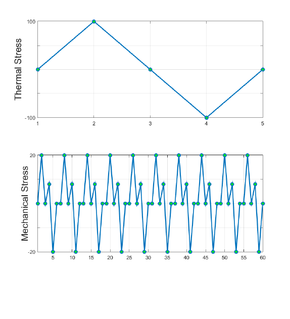
Take the example of a piston which experiences combined thermal and mechanical stresses shown
in Figure 3.5.
For a scale and combine loading, the two signals are defined by the load histories in Figure 3.5.
Normalized thermal load
[0, 1, 0, -1, 0]
Normalized mechanical load
[0,1,0,0.4,-1,0,0,1,0,0.4,-1,0,0,1,0,0.4,-
1,0,0,1,0,0.4,-1,0,0,1,0,0.4,-1,0,0,1,0,0.4,-
1,0,0,1,0,0.4,-1,0,0,1,0,0.4,-1,0,0,1,0,0.4,-
1,0,0,1,0,0.4,-1,0]
Figure 3.5: Thermal and mechanical load signals occurring over the same
period
44
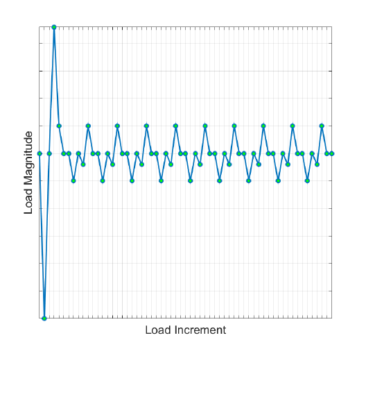
A problem arises if the two loads occur over the same time interval. Since the mechanical load has
many more time points than the thermal load, Quick Fatigue Tool will append most of the mechanical
load onto the end of the load history. Using a standard scale and combine, the resulting load history
would be that of Figure 3.6.
This loading definition is physically incorrect because it does not allow for the fact that the two loads
occur simultaneously over the same period. The solution is to define the mechanical load as a high
frequency dataset. The modified load histories are as follows:
Normalized thermal load
[0, 1, 0, -1, 0]
Normalized mechanical load
[0, 1, 0, 0.4, -1, 0]
In this case, the high frequency data is specified as a single repeat of the mechanical load.
Job file usage:
Option
Value
HF_DATASET
'mechanical-dataset-file-name.*'
HF_HISTORY
'mechanical-history-file-name.*'
HF_TIME
{100.0, 10.0}
Figure 3.6: Result of using the scale and combine technique for the
thermal-mechanical load
45
High frequency loading and load histories are specified in the same manner as standard datasets and
load histories. In order for Quick Fatigue Tool to correctly superimpose the high frequency dataset(s),
it must know the period for both loadings. In this example, the period of the low frequency data is 100
seconds and the period of a single repeat of the high frequency data is 10 seconds. This means that
the high frequency dataset will be superimposed 100/10 = 10 times into the low frequency data.
The resulting load history is shown in Figure 3.7.
Quick Fatigue Tool interpolates the thermal load so that it contains the correct number of data points
for the mechanical load to be superimposed, without resulting in trailing data. In using this technique,
the mechanical data is correctly represented as occurring over the same period as the thermal data.
The same loading methods apply as those outlined in Section 3.1.
3.5.3 Example usage
An example input file containing a high frequency loading definition can be found in
Data\tutorials\intro_tutorial\tutorial_high_frequency.inp.
The job is submitted by executing the following command:
>> job tutorial_high_frequency
Results are written to Project\output\ tutorial_high_frequency.
Figure 3.7: Result of using high frequency loading for the thermal-
mechanical load
46
3.5.4 Additional guidance
The user should take into account the following points when using high frequency loading:
high frequency loading requires the Signal Processing Toolbox to work;
high frequency loading should be used if two or more load histories occur over the same time
interval, where one or more of the load histories is a repetitive load at a much higher
frequency;
the number of analysis items in the high frequency loading must be the same as the number
of items in all other stress datasets. If specific items are listed in the job file, those same items
will be used in the high frequency loading;
if the original datasets contain stresses at shell faces, the high frequency data must also
contain shell face data;
the main load history should contain at least three data points, otherwise the high frequency
loading may not be interpolated properly. If the original load history contains only two data
points, a zero value will be appended to the end of the history;
when defining the high frequency load history, only a single cycle needs to be defined, along
with the period for that cycle. If the entire load history is provided, the resulting load history
will be incorrect;
if load history pre-gating is enabled, the original datasets may be modified prior to the high
frequency loading being added. This may result in an unexpected load history;
if the high frequency data is not in the form of a peak-valley sequence (the loading contains
intermediate data between turning points), this data will not be considered by the selected
gating criterion;
the units of the high and low frequency data must be the same; and
using high frequency loading can increase the analysis time dramatically.
47
3.6 The dataset processor
3.6.1 Determining the dataset type
Quick Fatigue Tool determines the type of dataset based on the number of columns in the dataset file.
The following table describes how datasets are processed.
Number of columns in dataset
Assumption
1
Element type: One-dimensional stress
Position: Unknown
2
Element type: One-dimensional stress
Position: Unique nodal or centroidal
3
Element type: One-dimensional stress
Position: Element-nodal or integration point
4
Element type: Plane stress
Position: Unknown
5
Element type: Plane stress
Position: Unique nodal or centroidal
6
IF PLANE_STRESS = 0.0 in the job file:
Element type: 3D stress
Position: Unknown
ELSEIF PLANE_STRESS = 1.0 in the job file:
Element type: Plane stress
Position: Element-nodal or integration point
7
Element type: 3D stress
Position: Unique nodal or centroidal
8
Element type: 3D stress
Position: Element-nodal or integration point
9
Element type: Plane stress with shell face data
Position: Unique nodal or centroidal
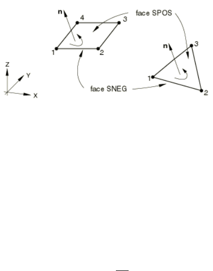
48
10
Element type: Plane stress with shell face data
Position: Element-nodal or integration point
> 10
Not applicable. Quick Fatigue Tool will exit with
an error.
3.6.2 Plane stress elements
If the stress datasets originate from an FE model consisting of plane stress elements, the .rpt file can
contain results on both faces, as shown by Figure 3.8.
Quick Fatigue Tool can read the stresses from either the positive or negative face. The default face is
defined as a variable in the environment file.
Environment file usage:
Variable
Value
shellLocation
{1.0 | 2.0}
1. Negative (SNEG) element face
2. Positive (SPOS) element face
Figure 3.8: Positive normals for three-dimensional
conventional shell elements
49
3.6.3 Multiple element groups
If the stress dataset file was written from an Abaqus output database, it is possible for the data to be
separated into multiple regions. This can happen if there are multiple part instances in the model, or
if the model contains a mixture of element types. In such cases, Quick Fatigue Tool will automatically
process each region and concatenate the stress tensors after all the datasets have been read.
Common examples of when the dataset can contain multiple regions are the analysis of surfaces with
in-plane residual stress and/or surface finish. The recommended practice is to create a skin on the
surface of the FE model and apply the residual stress and surface finish definitions on the skin
elements using the GROUP option in the job file (see Sections 4.3 and 4.4 for more detailed
information). Because of the combination of plane stress elements forming the skin of the component
and the underlying 3D elements, Abaqus (and possibly other FEA packages) may assign duplicate node
numbers between the skin and the solid bulk.
Although the fatigue calculation is not affected by the presence of duplicate node numbers,
Quick Fatigue Tool may report the results at incorrect locations. Problems may also arise when writing
results back to an Abaqus .odb file because Quick Fatigue Tool is unable to resolve the correct location
of the node on the finite element mesh. Thus, the visualization in Abaqus/Viewer could be incorrect.
The workaround in such cases is to use stresses at the element nodes. This ensures that each node in
the model has a unique identifier even in the presence of multiple element regions.
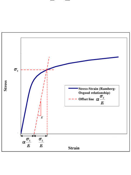
50
4. Analysis techniques
4.1 Background
Quick Fatigue Tool provides a selection of analysis techniques. These techniques provide useful tools
for performing your analysis more efficiently and effectively.
The techniques described in this section are specified in the job and environment files. For detailed
guidance on the usage of job file options and environment variables, consult the document
Quick Fatigue Tool User Settings Reference Guide.
4.2 Treatment of nonlinearity
4.2.1 Overview
Quick Fatigue Tool always assumes that the dataset stresses are linear elastic.
When a stress-based fatigue analysis algorithm is specified, the stresses are not corrected for the
effect of plasticity. This is because the stress-life methodology has been devised for linear elastic
material data.
When a strain-based fatigue analysis algorithm is specified, the stresses are corrected for the effect of
plasticity using the Ramberg-Osgood nonlinear elastic strain-hardening relationship. This function
approximates the local nonlinear stress from elastic stresses [8] [9].
Elastic stresses are converted to nonlinear elastic stresses using Equation 4.1.
[4.1]
Figure 4.1: Generic representation of the stress-strain
curve using the Ramberg-Osgood equation
51
The material constants and are the cyclic strain hardening coefficient and exponent, respectively.
The difference in the monotonic response between the elastic Hookean and the Ramberg-Osgood
model is shown in Figure 4.1. For the offset line, the parameter is defined as
, where
is the yield strength.
4.2.2 Limitations of the nonlinear model
In order to convert between linear and nonlinear quantities, Quick Fatigue Tool uses Neuber’s Rule,
which stipulates that the accumulated strain energy is the same at a notch as it would be in an elastic
stress field far away.
The correction therefore is only valid for local notch plasticity. For smooth specimens, care must be
taken. If the stress at the notch is below the yield strength, stress redistribution occurs, resulting in a
larger plastic zone. Neuber’s Rule does not work as well in these cases because it assumes that the
peak stress is localised and that the plastic zone is surrounded by a comparatively large elastic zone,
forcing the plastic zone to behave similarly to the nearby elastic stress field.
The Stress-Life methodology is based on the elastic stress at a point on the component which is not
affected significantly by local stress concentrations. Traditionally, the elastic stress is used with an
S-N curve which has been corrected with a notch factor to account for the presence of the stress
concentration. As such, the Stress-Life methodology is not intended to be used with true stress
quantities. This causes problems when performing fatigue estimates from elastic FEA, because the
stresses at the notch are typically over-estimated. This can result in highly conservative life predictions
compared to Strain-Life methods. For cases where the stress concentration is judged to be significant,
the following is recommended in lieu of the plasticity correction:
1. Limit the fatigue analysis to the elastic stress a small distance away from the notch and apply
a correction factor using the KT_DEF, KT_CURVE, NOTCH_CONSTANT and NOTCH_RADIUS
job file options. Notch factors for specific geometries are readily available in the literature
2. Use the Strain-Life methodology
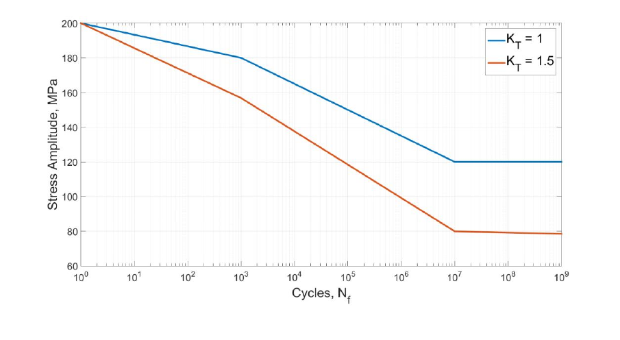
52
4.3 Surface finish and notch sensitivity
4.3.1 Surface finish
Surface roughness has a strong influence on the component’s resistance to crack initiation [10]. While
FEA is able to account for stress concentrations which arise from geometric complexity, the effect of
surface finish cannot be modelled directly. Instead, a surface stress concentration factor, , may be
used to scale the endurance curve so that it corresponds more accurately to the surface strength of
the material.
The result of applying a stress concentration factor to the endurance curve is shown in Figure 4.2.
Quick Fatigue tool allows the surface finish to be defined in three ways:
1. As a surface stress concentration factor ( value)
2. From a list of surface finish types ( curve)
3. As a surface roughness value ( value)
Define the surface finish as a value
Job file usage:
Option
Value
KT_DEF
KT_CURVE
[ ]
where is a value for the surface stress concentration factor, .
Figure 4.2: Reference endurance curve for
and after applying a stress concentration factor of
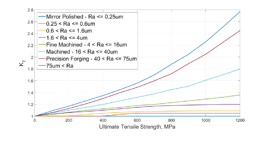
53
Define the surface finish as an curve
To specify the surface finish from a list of surface finish types, a surface finish .kt file from the Data\kt
directory must be specified. The surface finish definition files contain pre-defined curves for various
surface finishes, as a function of the material’s ultimate tensile strength.
Job file usage:
Option
Value
KT_DEF
'surface-finish-file-name.kt'
KT_CURVE
where 'surface-finish-file-name.kt' is the name of the .kt file containing a list of surface finish definitions,
and is the curve number.
The file ‘default.kt’ is plotted in Figure 4.3 as an example. Based on the chosen curve and the ultimate
tensile strength of the material, Quick Fatigue Tool linearly interpolates to find the corresponding
value of . If the material’s ultimate tensile strength exceeds the range specified by the curve, the
last value of is used.
Figure 4.3:
curves for various surface finishes, from the file ‘default.kt’

54
The following .kt files and the available curves are shown below:
‘default.kt’
Surface Finish
1
Mirror Polished – Ra <= 0.25um
2
0.25 < Ra <= 0.6um
3
0.6 < Ra <= 1.6um
4
1.6 < Ra <= 4um
5
Fine Machined – 4 < Ra <= 16um
6
Machined – 16 < Ra <= 40um
7
Precision Forging – 40 < Ra <= 75um
8
75um < Ra
‘juvinall-1967.kt’
Surface finish
1
Mirror Polished
2
Fine-ground or commercially polished
3
Machined
4
Hot-rolled
5
As forged
6
Corroded in tap water
7
Corroded in salt water
‘rcjohnson-1973.kt’
Surface finish
1
AA = 1uins
2
AA = 2uins
3
AA = 4uins
4
AA = 8uins
5
AA = 16uins
6
AA = 32uins
7
AA = 83uins
8
AA = 125uins
9
AA = 250uins
10
AA = 500uins
11
AA = 1000uins
12
AA = 2000uins
55
It is possible to specify the surface finish from a user-defined .kt file. The following file format must be
obeyed:
First column: Range of UTS values over which is defined
Second column: values for the first curve
Third column: values for the second curve
Nth column: values for the (N-1)th curve
Define the surface finish as an value
To specify the surface finish as a surface roughness () value, a surface roughness .ktx file from the
Data\kt directory must be specified. The surface roughness files contain curves over a range of
roughness values, as a function of the material’s ultimate tensile strength.
Job file usage:
Option
Value
KT_DEF
'surface-roughness-file-name.ktx'
KT_CURVE
where <filename> is the name of the .ktx file containing the curves and is the surface roughness,
.
The ‘Niemann-Winter-Rolled-Steel.ktx’ file is plotted in Figure 4.4 as an example. Quick fatigue tool
linearly interpolates to find the curve which corresponds to the user-specified value. If the
surface roughness value exceeds the maximum surface roughness defined in the data, the last set of
values are used.
Based on the ultimate tensile strength of the material, Quick Fatigue Tool linearly interpolates once
more to find the corresponding value of . If the material’s ultimate tensile strength exceeds the
range specified by the curve, the last value of is used.
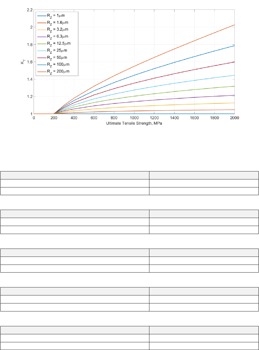
56
The following .ktx files and surface roughness ranges are shown below:
‘Niemann-Winter-Cast-Iron-Lamellar-Graphite.ktx’
UTS Range
0 – 2000Mpa
Range
1 – 200um
‘Niemann-Winter-Cast-Iron-Nodular-Graphite.ktx’
UTS Range
0 – 2000Mpa
Range
1 – 200um
‘Niemann-Winter-Cast-Steel.ktx’
UTS Range
0 – 2000Mpa
Range
1 – 200um
‘Niemann-Winter-Malleable-Cast-Iron.ktx’
UTS Range
0 – 2000Mpa
Range
1 – 200um
‘Niemann-Winter-Rolled-Steel.ktx’
UTS Range
0 – 2000Mpa
Range
1 – 200um
Figure 4.4:
curves for various surface roughness values, from the file ‘Niemann-Winter-Rolled-Steel.ktx’

57
It is possible to specify the surface finish from a user-defined .ktx file. The following file format must
be obeyed:
First row: Range of values over which values are defined
Second row: First UTS value, followed by corresponding values for each value
Third row: Second UTS value, followed by corresponding values for each value
Nth row: UTS value, followed by corresponding values for each value
4.3.2 Effect of notch sensitivity
If the component contains a notch, the stress-life curve may require modification to account for the
notch sensitivity of the material, since the stresses which contribute to fatigue of a notched
component are not on the notch root surface, but a small distance into the subsurface. As such, for
notch-insensitive materials, the stress concentration factor in fatigue is different to the elastic stress
concentration factor, . This is termed the fatigue notch factor, .
The value of can be approximated in several ways, and is set in the environment file.
Environment file usage:
Variable
Value
notchFactorEstimation
{1.0 | 2.0 | 3.0 | 4.0 | 5.0 | 6.0}
1. Peterson (default)
2. Peterson B
3. Neuber
4. Harris
5. Heywood
6. Notch sensitivity
Peterson (default)
Quick Fatigue Tool is optimized to use stresses from finite element analysis. Therefore, the effect of
is implicit in the stress solution. By default, the reduction in fatigue strength due to elastic stress
concentration is calculated using results obtained by Peterson. Equation 4.4 is used to scale the value
of as a function of endurance [11].
[4.4]
The endurance curve is scaled by at each value of N. The Peterson relationship is visualized
by Figure 4.5, for values of .
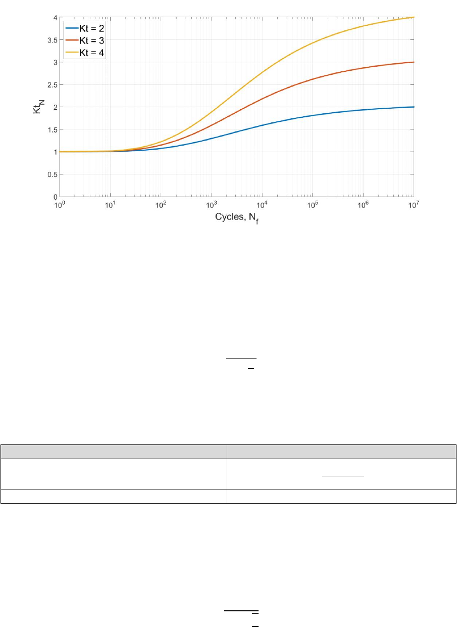
58
Peterson B
Peterson observed that, in general, good approximations for loading can be obtained using
Equation 4.5 [12].
[4.5]
where is a characteristic length and is the notch root radius. The value of can be determined
empirically as a function of the ultimate tensile strength, :
Material
Steel
Aluminium Alloy
Neuber
For parallel side grooves, Neuber developed the following approximate formula for the notch factor
for loading [13]:
[4.6]
where is a characteristic length.
Figure 4.5:
as a function of endurance, for
.
59
Harris
Harris proposed the relationship in Equation 4.7 [14].
[4.7]
where is a characteristic length. Suggested values of are shown in the table below
Material
Steel
Aluminium Alloy
Heywood
Heywood proposed the relationship in Equation 4.8 [15].
[4.8]
where is a characteristic length. The value of varies depending on the notch type. Typical values
proposed for steel are shown in the table below. The values assume that the notch root radius is
measured in inches.
Notch Type
Hole
Shoulder
Groove
Notch sensitivity
The fatigue notch factor can be defined in terms of the notch sensitivity, .
[4.9]
Typical values of for steels and aluminium alloys are shown in Figures 4.6-7 for bending and torsion,
respectively [16].
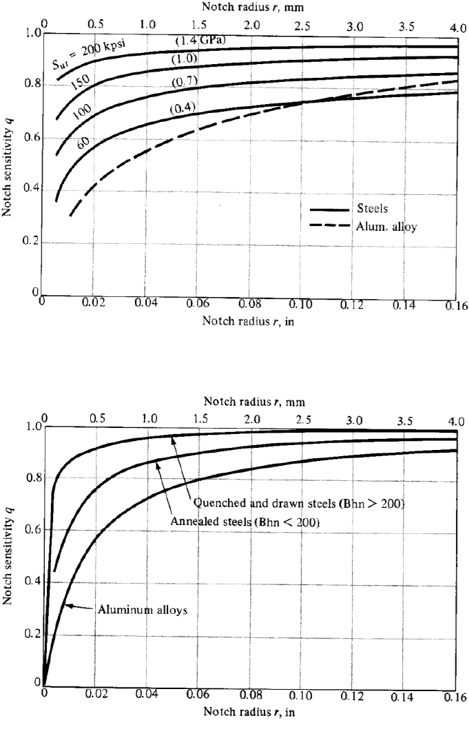
60
Figure 4.6: Notch sensitivity factors for steels and aluminium alloys (bending)
Figure 4.7: Notch sensitivity factors for steels and aluminium alloys (torsion)
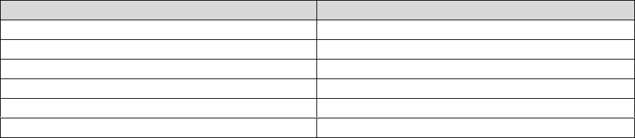
61
Defining notch parameters
The notch characteristic length and the notch root radius are defined in the job file.
Job file usage:
Option
Value
NOTCH_CONSTANT
NOTCH_RADIUS
The notch constant is defined according to the table below.
Notch factor estimation method
Notch constant
Peterson (default)
Peterson B
Neuber
Harris
Heywood
Notch sensitivity
The notch root radius defines the parameter in Equations 4.5-4.8.
Specifying notch factors for FEA stresses
Since Quick Fatigue Tool assumes that the FEA stresses account for the effects of geometry, the default
meaning of is that of a supplementary factor which describes surface finish effects which cannot
easily be modelled in finite elements. To that end, the user must be careful when considering the
inclusion of the fatigue notch factor if the stresses originate from FEA.
If the S-N data is produced from smooth (un-notched) specimens then the nominal stress is equal to
the local stress, as there is no stress gradient effect. In this case, the fatigue notch factor is not required
since the FE solution provides the local stress at the notch surface. However, if the S-N data originated
from a notched test, then the FEA stresses at the notch will produce excessively conservative fatigue
life predictions. In such cases, the user must follow the procedure outlined by their chosen stress-life
guideline in order to estimate the pseudo nominal stress a certain distance away from the notch tip,
and use this stress on the notched S-N curve instead.
62
The fatigue notch factor is estimated from the value of .
Job file usage:
Option
Value
KT_DEF
where is not the surface finish factor, but the elastic stress concentration factor. By defining the
notch sensitivity constant and the notch root radius, the corresponding notch sensitivity is estimated.
The stresses (or the S-N curve) will be scaled in the same way as is done with a standard surface finish
definition (Figure 4.2).
4.3.3 Modelling guidance
Specifying on a material surface
Unless analysis groups are defined, the surface finish definition is applied to every analysis item in the
model. This behavior is incorrect if the model contains subsurface nodes. If subsurface nodes are being
analysed, the recommended practice is to define a skin on the finite element model and apply the
surface finish definition to the skin using a separate analysis group.
Job file usage:
Option
Value
GROUP
{'skin-group-file-name.*', 'DEFAULT'}
The procedure for creating analysis groups is described in Section 4.7. The surface finish is then
defined in the job file.
Job file usage:
Option
Value
KT_DEF
{'surface-finish/roughness-file-name.kt/ktx', [ ]}
KT_CURVE
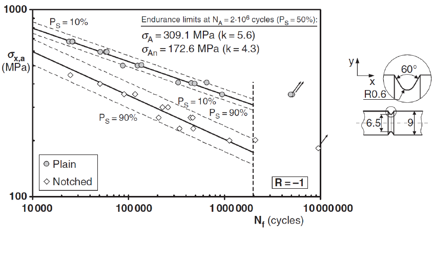
63
Specifying directly
If the fatigue test data was measured for a smooth specimen but the component contains a notch, the
user can specify the fatigue notch factor directly if it is already known. By assuming that the material
is fully notch-sensitive (), then . This means that the surface finish factor can be used as
the notch sensitivity factor.
Environment file usage:
Variable
Value
notchFactorEstimation
6.0
Job file usage:
Option
Value
KT_DEF
KT_CURVE
[ ]
NOTCH_CONSTANT
1.0
Figure 4.8: Fatigue results generated by testing plain and V-notched cylindrical specimens of S690 steel under
rotating bending [17]
64
Take Figure 4.8 as an example. This data was obtained by Susmel [17], and shows the S-N curves for a
notched and a smooth specimen. Using the data at the endurance limit (two million cycles), the value
of is estimated to be
at probability of survival. For a load ratio of ,
a cycle with a stress amplitude of will produce the same life on a smooth specimen as a
cycle with a stress amplitude of on the notched specimen.
This can be verified in Quick Fatigue Tool by defining the smooth specimen material data with the
following S-N data points:
The two definitions below should result in a fatigue life of two million cycles. The Uniaxial Stress-Life
algorithm is used for both definitions. For the second definition, the notch sensitivity is used as the
fatigue notch factor estimation method.
Definition A
Job file usage:
Option
Value
HISTORY
[309.1, -309.1]
KT_DEF
1.0
NOTCH_CONSTANT
[ ]
Definition A
Job file usage:
Option
Value
HISTORY
[172.6, -172.6]
KT_DEF
1.791
NOTCH_CONSTANT
1.0
65
4.4 In-plane residual stress
4.4.1 Overview
Many engineering components exhibit surface residual stresses due to their manufacturing process.
Compressive residual stresses are often introduced by design. However, tensile residual stresses can
accelerate fatigue damage accumulation.
An in-plane residual stress component can be specified directly in the job file.
Job file usage:
Option
Value
RESIDUAL
The stress is assumed to act uniformly in all directions and is added to the mean stress of each cycle.
Unless analysis groups are defined, the residual stress definition is applied to every analysis item in
the model. This behavior is incorrect if the model contains subsurface nodes. If subsurface nodes are
being analysed, the recommended practice is to define a skin on the finite element model and apply
the residual stress to the skin using a separate analysis group.
Job file usage:
Option
Value
GROUP
{'skin-group-file-name.*', 'DEFAULT'}
The procedure for creating analysis groups is described in Section 4.7. The residual stress is then
defined in the job file.
Job file usage:
Option
Value
RESIDUAL
[, 0.0]
Since the residual stress is applied directly to the fatigue cycle and assumes the orientation of the
critical plane, the quantity cannot be visualized with field output. For example, the variable SMAX does
not include the effect of residual stress. Furthermore, the residual stress is not considered by nodal
elimination.
4.4.2 Limitations
Definition of residual stress is not compatible with the BS 7608 algorithm. If residual stress is defined
with Findley’s Method, the stress is added to the cycle during the damage calculation instead of the
mean stress.
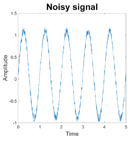
66
4.5 Analysis speed control
4.5.1 Pre-processing time histories
Load histories often contain data which does not contribute to fatigue and can have a spurious effect
on the fatigue calculation. Take the signal in Figure 4.9 as an example.
Analysing signals which contain small cycles puts additional computational load on the cycle counting
algorithm and can impact the analysis time significantly, without improving the estimate of the fatigue
damage. Quick Fatigue Tool offers three procedures for removing redundant cycles.
1. Pre-gate load histories
2. Gate tensors
3. Noise reduction
Quick Fatigue Tool assumes that there is no correlation between the phase of the load histories and
the damage parameter on the critical plane. Therefore, the default behavior is to gate the stress
tensors as this is the most reliable method.
Figure 4.9: Noisy test signal
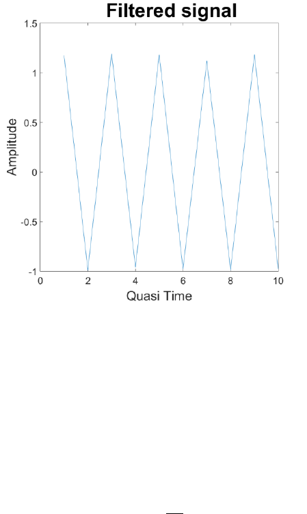
67
Pre-gate load histories
When load history pre-gating is enabled, the load history from each channel is converted into a
separate peak-valley sequence before being combined with the other channels.
Environment file usage:
Variable
Value
gateHistories
{0.0 | 1.0 | 2.0}
historyGate
[, ,…, ]
where is the number of loading channels. The gating values are defined as the percentage of the
maximum component in the load history.
Figure 4.10 shows the result of gating the noisy signal with a gating criterion. The pros and cons
of load history gating are listed below.
Pros:
load history gating is performed once for each loading channel before the start of the analysis,
so it is very fast; and
for simple loadings, load history gating has a similar accuracy to tensor gating.
Cons:
fatigue results may be in error if the loading consists of multiple histories. The method is
applied separately to each history so there is no guarantee that the phase relationship
between the loading channels is maintained.
Figure 4.10: Filtered signal

68
When using pre-gated load histories with multiple load channels, the user should compare the change
in life values between the gated and the original signal. If the difference is significant, load history pre-
gating should be disabled.
When load history pre-gating is enabled and Quick Fatigue Tool detects a constant amplitude loading
condition, then only the first cycle is analysed. This avoids invoking the rainflow cycle counting
algorithm unnecessarily. The number of repeats is automatically adjusted to account for the additional
cycles, according to Equation 4.10.
[4.10]
The total number of repeats, , is the product of the number of repeats defined by the REPEATS job
file option, , and the number of repeats in the load history, .
History point is considered to be constant amplitude with respect to the point provided that
the two points lie within the user-defined tolerance specified by the historyGate environment variable.
If multiple gating values are specified, then the first value will be used.
Gate tensors
When tensor gating is enabled, the original load history is used to determine the principal stress
history and the damage parameter on the critical plane. The damage parameter is then converted into
a peak-valley sequence prior to cycle counting.
Environment file usage:
Variable
Value
gateTensors
{0.0 | 1.0 | 2.0}
tensorGate
[, ,…, ]
where is the number of loading channels. The gating values are defined as the percentage of the
maximum component in the stress tensor which defines the damage parameter.
The pros and cons of tensor gating are listed below.
Pros:
The most accurate method of gating. Since the damage parameter accounts for the
combination of the fatigue loading, the phase relationship between the loading channels is
always maintained
Cons:
The damage parameter is gated per plane, per node, thus tensor gating is much slower than
pre-gated load histories

69
If it is necessary to remove intermediate data (points which lie between peaks and valleys), but
additional gating is not required, the gate value can be set to zero. Quick Fatigue Tool will use a zero
derivative method and all peak-valley pairs will be retained.
Environment file usage:
Variable
Value
tensorGate
0.0
historyGate
0.0
Quick Fatigue Tool includes an alternative peak-valley analysis algorithm, written by Adam Nielsony.
This may be used in cases where the gating criterion is not known. The recommended practice is to
use a gating method.
Environment file usage:
Variable
Value
gateHistories
2.0
gateTensors
2.0
Noise reduction
It is possible to apply noise reduction to the load histories prior to analysis. Quick Fatigue Tool uses a
low-pass filter which removes spikes in the data.
Environment file usage:
Variable
Value
noiseReduction
{0.0 | 1.0}
numberOfWindows
where is the number of averaging segments used to filter the signal.
Care should be taken when using the low-pass filter, since the stress amplitude is always reduced. This
may result in excessively optimistic fatigue life results. Noise reduction should not be used as an
alternative to gating, and its use is not recommended in general unless the load signal is highly affected
by measurement noise.

70
4.5.2 Determining load proportionality
If the direction of the principal stress does not change during the loading, then the stresses are
proportional and critical plane searching is not necessarily required.
Quick Fatigue Tool automatically checks the model for proportional loading before the start of the
analysis and skips critical plane searching at these regions for certain algorithms.
Environment file usage:
Variable
Value
checkLoadProportionality
{0.0 | 1.0}
The principal stress history of the loading is calculated at each location in the model, along with the
orientation of the first principal stress. If the largest change of the angle of the first principal stress
does not exceed the specified tolerance, the loading is assumed to be proportional.
Environment file usage:
Variable
Value
proportionalityTolerance
The purpose of defining a tolerance is to account for solution noise which may cause the direction of
the principal stresses to “wobble”, even if the loading is theoretically proportional.
Load proportionality checking is compatible with the following fatigue analysis algorithms:
Stress-based Brown-Miller
Normal Stress
BS 7608

71
4.5.3 Specifying the analysis region
It is possible to restrict the analysis to a specific region of the model. For very large models, it may be
economical to perform the analysis only at the locations where fatigue failure is likely to occur.
Alternatively, if the location of fatigue failure has already been determined by a previous analysis, an
additional analysis may be performed at this location with additional output and/or more rigorous
critical plane searching.
There are five ways to specify the analysis region:
1. Whole model
2. ODB element surface
3. Maximum principal stress range
4. Hotspot
5. User-defined
Option
Value
ITEMS
{'ALL' | 'SURFACE' | 'MAXPS' | 'file-name.*' | [,…, ]}
Whole model
When ITEMS='ALL', the whole model is used as the analysis region. If the DATASET option is not used
for analysis, the ITEMS option is ignored.
ODB element surface
When ITEMS='SURFACE', the analysis region is restricted to items on the element free surface of the
model Abaqus .odb file. An element is considered to be on the surface if it has at least one node on
the surface. This option is useful in the majority of cases, where fatigue cracks initiate on the
component surface. If subsurface cracks are likely to initiate, ITEMS='ALL' should be used instead.
Surface detection requires both the .odb file and part instance name to be specified.
Job file usage:
Option
Value
OUTPUT_DATABASE
' model-odb-file-name.odb '
PART_INSTANCE
'part-instance-name'
The specified part instances should match those defined in the stress dataset files. If the user specifies
part instances which do not exist in the dataset, the surface detection will not take effect. The element
surface is read according to the user-specified result position.
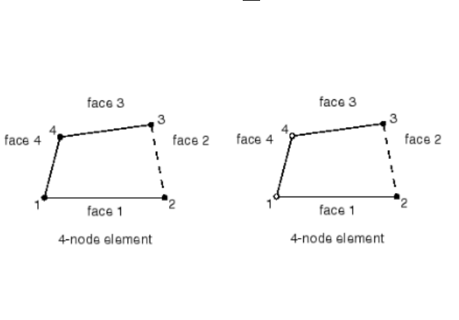
72
Job file usage:
Option
Value
RESULT_POSITION
{'ELEMENT NODAL' | 'UNIQUE NODAL' | 'CENTROID'}
The user should ensure that the specified result position matches the position of the stress datasets.
Surface detection is not supported for integration point results.
If there is no .odb file specified, the whole model is used as the analysis region. ODB element surface
detection is not supported for uniaxial analysis methods.
If the model output database contains shell elements, Quick Fatigue Tool treats the element surface
as the entire shell. Alternatively, the user can specify to treat the element surface as free shell faces.
Environment file usage:
Variable
Value
shellFaces
{0.0 | 1.0}
The difference between these two surface definitions is shown in Figure 4.11.
The surface detection algorithm supports most Abaqus elements with displacement degrees of
freedom. A list of compatible elements is found in Appendix IV “List of supported elements for surface
detection” of the document Quick Fatigue Tool Appendices.
If the stress dataset contains element-nodal or centroidal stress data, Quick Fatigue Tool only searches
the elements in the .odb file which are defined in the dataset. If the dataset contains unique nodal
stress data, the entire part instance is always included by the surface detection algorithm. This
behavior is controlled by the searchRegion environment variable. Values of 0 and 1 indicate that
elements from the stress dataset(s) or the entire part instance will be included by the surface
detection algorithm, respectively.
Figure 4.11: 4-node shell elements whose free faces are shown by dashed faces. Surface
nodes are indicated by solid black circles. (L) Treat shell surface as whole shell. (R) Treat
shell surface as free shell faces.

73
Environment file usage:
Variable
Value
searchRegion
{0.0 | 1.0}
When the search region is limited to dataset elements, Quick Fatigue Tool treats the dataset as the
entire model. This is the preferred method because it is much faster in cases where the part instance
contains a very large number of elements compared to the stress dataset. However, element
boundaries which exist in the dataset may, in reality, be attached to elements in the .odb file which
do not constitute a free surface. Therefore, when searchRegion=0.0, the surface detection algorithm
may overestimate the number of elements on the surface.
If more than one part instance is specified with PART_INSTANCE, then all elements in each part
instance are always included by the surface detection algorithm.
Whenever Quick Fatigue Tool reads the surface of an .odb file, the surface items for the current model
and specified part instances are written to the surface definition file
'Data\surfaces\<model-ID>_surface.dat'. At the start of each job, if ITEMS='SURFACE', the surface
definition file is used to extract the model surface instead of the .odb file; this is much more time-
efficient when running the same job in multiple configurations. This behavior is set with the following
environment variable:
Environment file usage:
Variable
Value
surfaceMode
{0.0 | 1.0}
Maximum principal stress range
When ITEMS='MAXPS', the analysis region is restricted to the item with the largest principal stress
range. This allows the user to quickly identify an analysis item that is likely to reside in one of the
damage hotspots in the model.
This setting can be useful for very large models where even a simple fatigue analysis (such as Stress
Invariant Parameter) could take a long time to complete. Using the 'MAXPS' option allows the user to
select a more rigorous analysis algorithm on a single analysis item without first having to run a whole
model analysis. This option is not intended to replace a complete analysis, however; the location of
maximum stress range does not necessarily coincide with the location of maximum fatigue damage.
Therefore, the 'MAXPS' option should be used with great care if the loading is non-proportional.
Even if the job contains non-default group definitions, Quick Fatigue Tool will still search the whole
model as defined by the DATASET option. If the item with the largest principal stress range exists
outside any of the groups, the analysis will be aborted. This is because the code cannot determine
valid properties for an item which does not have any material or analysis data associated with it.
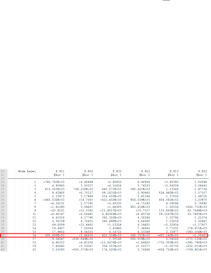
74
Items listed in a text file
When ITEMS='file-name.*', the analysis region is restricted to items defined in a text file. This file may
be user-defined, or it may be created automatically with the HOTSPOT job file option:
Job file usage:
Option
Value
HOTSPOT
{0.0 | 1.0}
Quick Fatigue Tool will save a list of items whose lives fall below the design life (specified by the
DESIGN_LIFE job file option) to 'hotspots.dat' in the folder Project\output\<jobName>\Data Files.
Additionally, any of the following files generated by Quick Fatigue Tool may be specified:
'<model-ID>_surface.dat', 'warn_lcf_items.dat', 'warn_overflow_items.dat' or
'warn_yielding_items.dat'.
User-defined item ID list
When ITEMS=[,…, ], the analysis region is restricted to the item IDs to . The item numbers
correspond to rows in the stress dataset file.
Additional guidance
Consider the FEA definition in Figure 4.12. If ITEMS=16, the analysis will only consider the 16th item in
the definition. Note that if the definition file contains a header, the value of ITEMS will not correspond
to the line number in the file.
After each analysis, Quick Fatigue Tool writes to the message file the ID(s) of the item(s) in the stress
dataset(s) with the worst life. This value can be used in conjunction with the ITEMS option to re-run
the analysis at the worst location in the model.
Figure 4.12: Example FEA definition file

75
4.5.4 Nodal elimination
Introduction
The analysis time can be reduced by ignoring analysis items whose maximum stress is unlikely to cause
damage. When the nodal elimination algorithm is enabled, Quick Fatigue Tool checks the maximum
principal stress range at each item before beginning the analysis. If the stress is below a certain
percentage of the conditional stress, , then the item is not included for analysis. The value of
is calculated as a function of the target life, .
Nodal elimination is enabled from the environment file.
Environment file usage:
Variable
Value
nodalElimination
{0.0 | 1.0 | 2.0}
If nodalElimination=0.0, nodal elimination is disabled.
If nodalElimination=1.0, is taken as the material’s constant amplitude endurance limit () by
default. The value of is the stress amplitude which will result in a life of cycles.
The value of may be specified directly if a user-defined endurance limit is specified in the
environment file.
Environment file usage:
Variable
Value
enduranceLimitSource
3.0;
userEnduranceLimit
;
If nodalElimination=2.0, is taken as the life defined by the option DESIGN_LIFE in the job file. By
default, DESIGN_LIFE='CAEL', in which case is taken from the value of defined in the
material.
For example, if an analysis is run with the Stress-based Brown-Miller algorithm and
nodalElimination=1.0, the conditional stress is obtained from Equation 4.11:
[4.11]
where is the conditional stress at which the life is equal to the constant amplitude endurance
limit, . The analysis item is then removed if the following inequality is satisfied:
[4.12]
76
where is the maximum difference between the first and third principal stresses in the
loading and is the elimination threshold scale factor.
Scaling the conditional stress with
If the fatigue loading contains only one cycle, then the conditional stress can be determined directly
from the fatigue limit. However, if the loading contains multiple cycles then it is possible for finite life
even if the majority of the cycles are below the fatigue limit. Consequently, it is necessary to use a
reduced value of the conditional stress such that the nodal elimination algorithm is effective for
complex loads.
The elimination threshold scale factor is set in the environment file.
Environment file usage:
Variable
Value
thresholdScalingFactor
The default value of is 0.8 (80%).

77
4.5.5 Principal stress calculation
Quick Fatigue Tool can use the built-in function eig() to determine the principal stress history for the
fatigue loading. Since this function only accepts two-dimensional data, the calculation can be very
time-consuming. This is because the principal stresses are calculated separately for each point in the
load history.
For very large models, the three-dimensional Eigensolver written by Bruno Luong is recommended.
This method calculates the principal stresses for the entire load history in a single calculation for each
analysis item, resulting in a much faster calculation.
Environment file usage:
Variable
Value
eigensolver
{1.0 | 2.0}
Luong’s method is used by default. Small numerical round-off errors in the calculation may cause
Quick Fatigue Tool to report a very small mean stress in the results, even if the loading has no mean
stress; this does not affect the fatigue life result.

78
4.6 Analysis groups
4.6.1 Overview
Analysis groups are used to define regions in the model having distinct properties. Analysis groups can
have their own definitions for the following job file options:
Property
Job file option
Material properties
MATERIAL
S-N data scale factor
SN_SCALE
S-N knock-down curves
SN_KNOCK_DOWN
Fatigue Reserve Factor envelope definition
FATIGUE_RESERVE_FACTOR
Surface finish definition
KT_DEF
Surface finish curve
KT_CURVE
Residual stress
RESIDUAL
Notch sensitivity constant
NOTCH_CONSTANT
Notch root radius
NOTCH_RADIUS
Analysis groups can have their own definitions for the following environment variables:
Property
Environment variable
Goodman envelope definition
modifiedGoodman
Goodman mean stress limit
goodmanMeanStressLimit
User-defined Walker parameter
userWalkerGamma
User-defined fatigue limit
userFatigueLimit
User FRF tensile mean stress normalization
parameter
frfNormParamMeanT
User FRF compressive mean stress
normalization parameter
frfNormParamMeanC
User FRF stress amplitude normalization
parameter
frfNormParamAmp
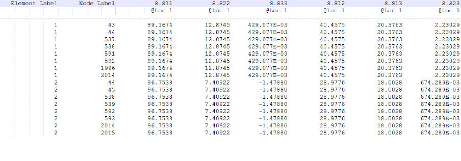
79
Analysis groups can be defined in two ways:
1. An item ID list
2. An FEA subset
An item ID list is a list of indexes corresponding to the row numbers in the stress dataset(s) as they are
defined in the file. An FEA subset is a list of position IDs referencing the location of the elements,
nodes, centroids or integration points in the model.
Analysis groups are declared in the job file.
Job file usage:
Option
Value
GROUP
{'group-file-name-1.*',…, 'group-file-name-.*'}
Groups are defined as ASCII text files.
4.6.2 Defining analysis groups as an item ID list
Consider the stress dataset file in Figure 4.13.
The dataset consists of two quadratic elements (eight-node hexahedrons). The dataset can be split
between two analysis groups, each defining one of the elements in the dataset. This can be achieved
by creating an item ID list defining each element. For example, the ID list for the first element is the
integer series from 1 to 8, while the second element is defined as the integer series from 9 to 16.
These are simply the row numbers corresponding to the nodes of the two elements. Example text file
contents for each group are given below.
Figure 4.13: Example stress dataset
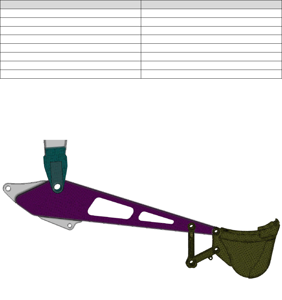
80
‘element 1.txt’
‘element 2.txt’
1
9
2
10
3
11
4
12
5
13
6
14
7
15
8
16
4.6.3 Defining analysis groups as an FEA subset
Item ID lists are a direct and relatively simple way of defining analysis groups for small models.
However, consider the model of an excavator arm shown by Figure 4.14.
In this instance, creating groups for regions A, B and C with an item ID list would be a very cumbersome
task. Instead, FEA subsets can be used which define the groups by their element labels. In Abaqus, this
is easily achieved by creating a display group of the region of interest, then exporting the element
labels as an .rpt file. The process of generating such a file is exactly the same as for generating FEA
stress datasets, and is discussed in detail in Section 3.2.
Figure 4.14: Finite element model of an excavator arm with two regions of interest
Region A
Region B
Region C
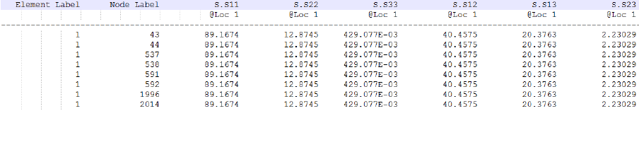
81
For example, consider again the dataset in Figure 4.13. An FEA subset may then resemble that shown
in Figure 4.15.
The group is literally a subset of the element labels from the original dataset. When using FEA subsets,
the following guidance should be observed:
1. The results position between the FEA subset and the original dataset must agree, i.e. if the
original dataset uses element-nodal position labels, then so should the FEA subset
2. Including field data with the FEA subset is not compulsory. However, since Abaqus requires at
least one field to be exported, FEA subsets written by Abaqus/Viewer will always contain at
least one column of field data
It is quite possible that a group defined as an FEA subset will reference more than one element with
the same position label. In order for the group definition to be correct, Quick Fatigue Tool must
somehow match the ID to the correct location in the FE model. In the event that duplicate IDs are
found in a group, field data in the group definition can be used to check the stress tensor of the
duplicate IDs against the tensors in the original stress dataset. Therefore, it is recommended that FEA
subsets retain the same field information as the original datasets.
Quick Fatigue Tool automatically attempts to resolve duplicate IDs based on the availability of the field
data; no additional intervention is required by the user. However, if the loading is defined as either a
multiple scale and combine or as a dataset sequence (the DATASET job file option was specified with
more than one argument), then the field data from the group file must agree with the last dataset in
the loading.
4.6.4 Arranging groups in the job file
Both item ID lists and FEA subsets can be used together for an analysis, and the groups do not have to
be mutually exclusive. Quick Fatigue Tool will process each group as they are encountered in the
GROUP job file option and will exclude the items so that they will not be read a second time if they
appear in subsequent groups. Therefore, the order in which groups are defined will affect which group
the items are assigned to if any of the definitions are inclusive of each other. The hierarchical nature
of the group reading process is illustrated by Figure 4.16.
Figure 4.15: FEA subset of the dataset in Figure 4.9

82
Group 1 is a subset of Group 2, which in turn is a subset of Group 3. Consider the case where the
groups are defined in the job file.
Job file usage:
Option
Value
GROUP
{'group-1.*', 'group-2.*', 'group-3.*'}
Quick Fatigue Tool will first read Group 1. All items from Group 1 will be read into the group definition,
and excluded from re-definition in later groups. Hence, Group 2 will include all of its items except
those already belonging to Group 1. The same logic will apply to Group 3, which will have all items
from Group 2 and Group 1 excluded from its definition.
The groups defined in the excavator model from Figure 4.10 could be defined in the job file.
Job file usage:
Option
Value
GROUP
{'region-A.*', 'region-B.*'}
Quick Fatigue Tool will analyse all of Region A and Region B. None of the items from Region C will be
analysed. In this case, the order does not matter since the groups are mutually exclusive.
If all three regions are to be analysed, but only Region C requires individual properties, the following
group definition may be used.
Job file usage:
Option
Value
GROUP
{'region-C.*', 'DEFAULT'}
Group 3
Group 2
Group 1
Figure 4.16: Group hierarchy

83
In this instance, Quick Fatigue Tool will analyse Region C with individual properties for that group,
followed by all other items in the model. In general, use of the 'DEFAULT' parameter instructs the
program to analyse all remaining items in the model (all other items in the original dataset which do
not belong to any preceding groups). The 'DEFAULT' parameter may only be used as the last argument
in the GROUP job file option.
The 'DEFAULT' parameter is used by its self to analyse the whole model, with no group definitions.
Job file usage:
Option
Value
GROUP
{'DEFAULT'}
Quick Fatigue Tool determines whether a group definition is an item ID list or an FEA subset based on
the contents of the file, and depending on the user setting in the environment file.
Environment file usage:
Variable
Value
groupDefinition
{0.0 | 1.0}
Using this default value, the application will assume that the group definition is an item ID list if there
is only one column of data in the file, and an FEA subset if there is more than one column. By setting
groupDefinition to a value of 1.0, an FEA subset will always be assumed.

84
4.6.5 Assigning properties to groups
Group properties (job file options and environment variables) are specified by assigning multiple
definitions according to the number of groups in the analysis.
Usually, the number of property definitions should match the number of groups in the analysis. If the
analysis contains groups where , and the user assigns a single definition to a property,
Quick Fatigue Tool automatically propagates that definition to all of the analysis groups. Otherwise,
the number of property definitions must exactly match the number of group definitions.
Most properties require valid definitions for number of analysis groups.
Job file usage:
Option
Value
MATERIAL
{'material-file-1.mat',…, 'material-file-.mat'}
This requirement applies to the following job file options and environment variables:
Job file option
Environment variable
MATERIAL
frfNormParamMeanT
SN_SCALE
frfNormParamMeanC
NOTCH_CONSTANT
frfNormParamAmp
FATIGUE_RESERVE_FACTOR
userWalkerGamma
RESIDUAL
userEnduranceLimit
midifiedGoodman
goodmanMeanStressLimit
S-N knock-down factors may not be required for every analysis group.
Job file usage:
Option
Value
SN_KNOCK_DOWN
{'knock-down-file-1.kd', [ ], 'knock-down-file-.kd'}
In this example, knock-down factors have been specified in groups and , and none is define for
Group . In cases where some groups do not require a definition, this must be indicated by an empty
assignment (), otherwise the group definition will be processed incorrectly.
A combination of surface finish definition files and values can be specified over several groups.
Job file usage:
Option
Value
KT_DEF
{'surface-finish-file-1.kt', , 'surface-finish-file-.kt'}
85
In such cases, the KT_CURVE option needs only to be specified according to the number of surface
finish files defined by KT_DEF.
Job file usage:
Option
Value
KT_CURVE
[, ]
In this example, the curve numbers and correspond to the surface finish files
'surface-finish-file-1.kt' and 'surface-finish-file-.kt', respectively; a curve number for the value is not
required since the surface finish is defined directly.
A list of all properties eligible for group definitions, along with typical syntax is provided in the table
below.
Job file option/Environment variable
Example definition
MATERIAL
{'material-file-1.mat',…, 'material-file-.mat'}
SN_SCALE
[,…, ]
SN_KNOCK_DOWN
{'knock-down-file-1.kd', 'knock-down-file-.kd'}
FATIGUE_RESERVE_FACTOR
{,…, 'msc-file-name-.msc'}
KT_DEF
{, 'surface-finish.file-2.kd', 'surface-finish.file-3.kd'}
KT_CURVE
[,…, ]
RESIDUAL
[,…, ]
NOTCH_CONSTANT
[,…, ]
NOTCH_RADIUS
[,…, ]
frfNormParamMeanT
{, '<param2>',…, }
frfNormParamMeanC
{, '<param2>',…, '<paramn>'}
frfNormParamAmp
{'<param1>', '<param2>',…, }
userWalkerGamma
[,…, ]
userEnduranceLimit
[,…, ]
midifiedGoodman
[,…, ]
goodmanMeanStressLimit
{, '<param2>',…, }
86
The following caveats should be noted for the use of analysis groups:
materials must be defined as a cell;
values for SN_SCALE are only required if USE_SN = 1.0;
a combination of surface finish .kt/.ktx files and/or surface finish values can be used within
the same KT_DEF statement;
the number of values in KT_CURVE need only reflect the number of .kt/.ktx files defined in
KT_DEF;
the number of values in frfNormParamMeanT, frfNormParamMeanC and frfNormParamAmp
need only reflect the number of custom FRF envelope definitions in
FATIGUE_RESERVE_FACTOR;
the number of values in goodmanMeanStressLimit need only reflect the number of zero-
valued entries in modifiedGoodman (the Goodman limit stress can only be defined for the
standard Goodman envelope);
if the 'DEFAULT' parameter is used as the last argument in a group definition, the default
group is included in the total number of groups;
if the default analysis algorithm or mean stress correction is specified, the algorithm and
mean stress correction used for analysis is chosen from the last argument of MATERIAL; and
if the DESIGN_LIFE option is set to the material’s constant amplitude endurance limit
('CAEL'), the endurance value is chosen from the last argument of MATERIAL.
4.6.6 Limitations
Analysis groups in Quick Fatigue Tool currently do not support multiple definitions of the following:
mean stress corrections/analysis algorithms; and
BS 7608 material properties.
If a different algorithm or mean stress correction is required for each analysis group, the workaround
is to split the analysis into multiple jobs and superimpose the fatigue results onto a single field output
file using the option CONTINUE_FROM. This technique is discussed in Section 4.8.

87
4.7 S-N knock-down factors
4.7.1 Overview
A set of S-N scale factors can be applied to the material S-N data in the form of knock-down factors,
which scale the stress data points for each specified life value. Knock-down factors are defined in a
separate .kd file and specified in the job file.
Job file usage:
Option
Value
SN_KNOCK_DOWN
{'knock-down-file-name.kd'}
USE_SN
1.0
4.7.2 Defining a knock-down curve file
The knock-down curve file is defined as follows:
First column: Life values at which knock-down factors are to be applied
Second column: Knock-down factors corresponding to each life value
An example .kd file is given by Figure 4.17.
The knock-down factors are applied to the S-N data before the analysis to produce the modified
endurance curve. The life values in the .kd file are treated as sample points and as such, they do not
have to match the position of the S-N data points. Quick Fatigue Tool will automatically interpolate
and extrapolate the S-N data before scaling each data point. An example of this process is shown by
the following table. Note that bracketed values in bold have been interpolated or scaled.
Figure 4.17: Example .kd file containing life
values in the first column and knock-down
factors in the second column
88
Original S-N curve
Knock-down curve
Scaled S-N curve
(800)
(10)
1.1
10
(880)
(10)
(1725)
(50)
1
50
(1725)
(50)
(1400)
(100)
1
100
(1400)
(100)
700
1000
0.8
1000
(560)
(1000)
350
10000
(0.75)
(10000)
(263)
(10000)
(313)
(100000)
0.7
100000
(219)
(100000)
(313)
(100001)
0.5
100001
(157)
(100001)
(280)
(1000000)
0.5
1000000
(140)
(1000000)
250
10000000
(0.4)
(10000000)
(100)
(10000000)
-
-
0.3
100000000
-
-
Knock-down data specified below the minimum life of the original S-N data is extrapolated. However,
Quick Fatigue Tool assumes that the last data point in the original S-N data represents the material’s
endurance limit and thus knock-down data provided beyond this point is not extrapolated.
The original S-N, knock-down and modified S-N curves are illustrated by Figures 4.18-20. If the material
contains S-N curves for multiple R-ratios, each curve is scaled by the knock-down curve before the
beginning of the analysis.
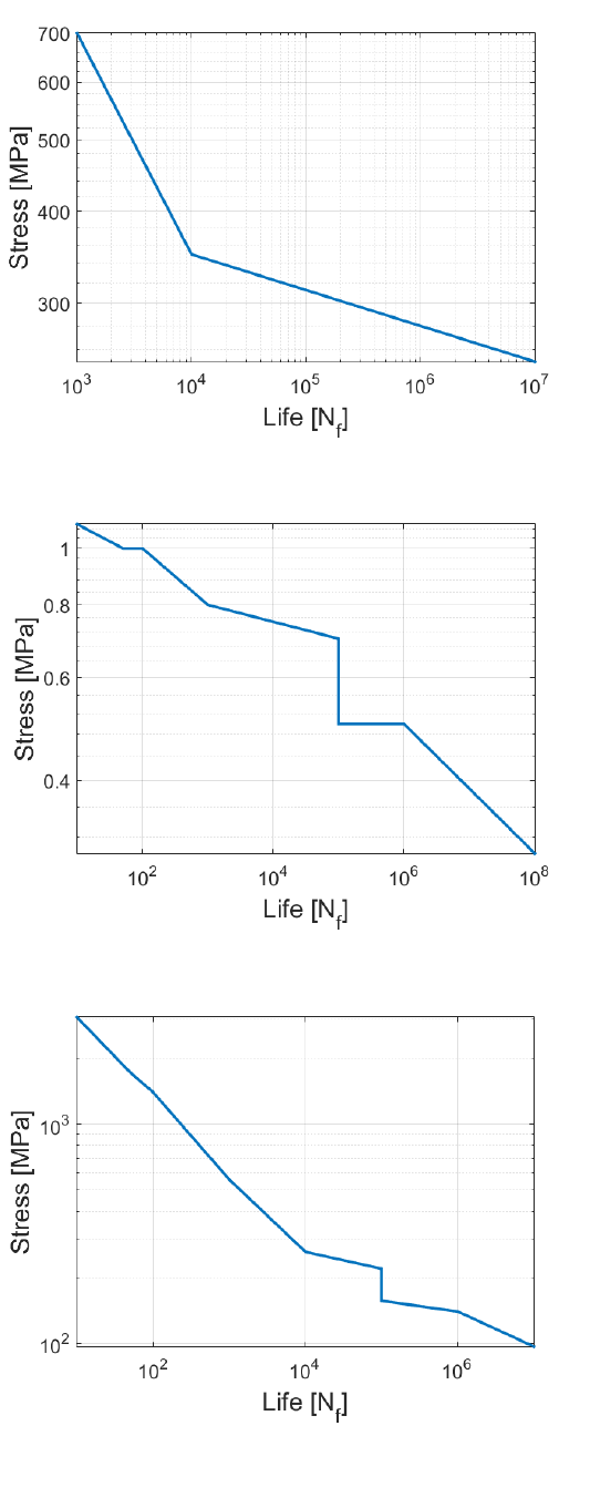
89
Figure 4.18-20: Original S-N curve (top), knock-down factors (middle)
and modified S-N curve (bottom)
90
4.7.3 Example applications
Knock-down curves can be used in addition to the surface finish definition in order to account for
additional manufacturing effects. Imperfections of the manufacturing process can lead to defects,
which reduce the endurance of the material.
Knock-down curves may be used with cast metals where inclusions result in a local loss of fatigue
performance. Another application is in the injection moulding of plastic components. During this
process multiple flow regions can meet, causing a weld line at the interface of the two melts. During
cooling of the newly formed part, voids may develop wherein large thermal gradients exist. Both of
these phenomena can be accounted for via the use of S-N knock-down factors.
One possible approach to using knock-down factors would be to identify the nodes on the FE model
which represent the manufacturing defect, and export a dataset file containing the node numbers and
field data, the process of which is described in Section 3.2. This dataset can then be used to define a
group in the job file with an individual knock-down curve applied. Such a configuration could be
achieved by using the following options.
Job file usage:
Option
Value
MATERIAL
{'knock_down.mat', 'default.mat'}
USE_SN
1.0
SN_KNOCK_DOWN
{'knock_down_curve.kd', [ ]}
GROUP
{'defect_group.rpt', 'DEFAULT'}

91
4.7.4 Exporting knock-down curves
The knock-down curves can be exported to MATLAB figures from the environment file.
Environment file usage:
Variable
Value
figure_KDSN
{0.0 | 1.0}
S-N knock-down curves are exported for groups which have knock-down factors specified. MATLAB
figures must be requested in the job file.
Job file usage:
Option
Value
OUTPUT_FIGURE
1.0
If the material contains S-N curves for multiple R-ratios, only the curve for is exported. If an
curve is not defined then it is automatically interpolated.
92
4.8 Analysis continuation techniques
4.8.1 Overview
Quick Fatigue Tool provides the capability to perform an analysis as a continuation of a previous job.
Field output from the current job is written onto the field output from a previous job. An analysis
which uses the continuation feature:
can be used to model block loading, where each job defines a distinct loading event;
can be used to assign different analysis algorithms to multiple regions in a model; and
allows the user to specify completely new definitions for any job file option for each job.
When used in conjunction with the ODB interface, analysis continuation:
can be used to superimpose field data onto the same mesh;
can be used to append field data onto a mesh at locations different to those which were
analysed in the previous job; and
a combination of the above.
A job which uses analysis continuation runs in the usual way. At the end of the analysis, field data is
superimposed onto the field output file from a specified job. The rules for combining field data depend
on the variable type, and are listed in the table below.
Variables
Rule
D
L; LL; DDL
FOS; SFA; FRFR; FFH; FRFV
FRFW
Derived from the values of and
SMAX; SMXP; SMXU; TRF; WCM; WCA; WCDP;
YIELD
WCATAN
Derived from the values of and
The subscripts and correspond to the first and second jobs, respectively. The superscript
corresponds to the superimposed field variable.
93
4.8.2 Referencing the previous job
The previous analysis is specified in the job file of the current analysis.
Job file usage:
Option
Value
CONTINUE_FROM
'previous-job-name'
The name of the previous job is the name given by the option JOB_NAME in the previous job file. Field
output must be requested for the first job. Field output is written automatically for the second job,
provided that a valid definition of CONTINUE_FROM is specified.
Job file usage:
Option
Value
OUTPUT_FIELD
1.0
4.8.3 Example applications
Multiple analysis algorithms
Analysis continuation can be used to circumvent the limitation of analysis groups, which does not
support multiple definitions for the analysis algorithm or mean stress correction. Analysis continuation
allows the user to define the algorithm and mean stress correction for multiple regions in the model,
and analyse each region as a separate job. Field data is superimposed onto the previous field data file
in a chained fashion by specifying the name of the previous job for each analysis. Finally, the
cumulative results of all analyses may be written to an .odb file using the ODB interface, which is
discussed in Section 10.4.
Multiple block loading
The definition of multiple loading blocks is not directly supported by Quick Fatigue Tool. However,
analysis continuation can be used to separate the load spectrum across several job files, where each
analysis represents a particular loading block, or event, in the component’s operational duty.
Consider the loading profile for a given component:
Block #
Descriptor
1
Applied load in 1-direction; fully-reversed [1, -1] load history; 3 repeats
2
Applied load in 2-direction; pulsating [0, 1] load history; 10 repeats
3
Applied load in 1-direction; mixed [1, -1, 2, -1] load history; 1 repeat
Each block is defined as a separate job file, along with their own definitions for the DATASET, HISTORY
and REPEATS job file options.
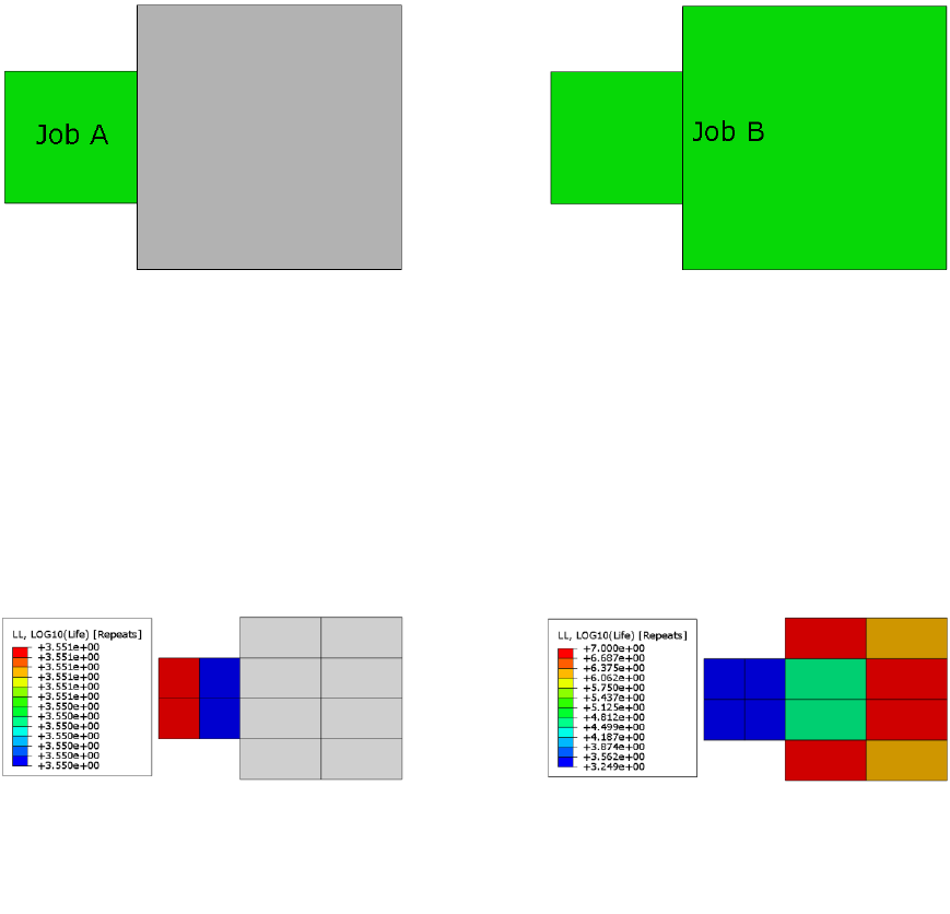
94
4.8.4 Additional guidance
Mismatching models
When superimposing results onto a previous analysis, Quick Fatigue Tool searches for matching item
IDs between the two field output files. Field data at items which match with the previous file are
superimposed to create the field data for the combined result. Items which do not match with the
previous job are appended onto the end of the field output file. This is advantageous, since the loading
in each block does not have to be applied to the same region between analyses; the definition of
DATASET does not have to be consistent.
Such a scenario is illustrated by Figure 4.21.
After running Job A, fatigue results are written to the left-hand portion of the model. After running
Job B with CONTINUE_FROM='Job A', fatigue results common to the analysis region from Job A are
superimposed onto the previous data. Fatigue results corresponding to the right-hand portion of the
model are appended to the field data without superimposition. This is illustrated by Figure 4.22. Note
how the results at the left-hand side have changed to account for the second loading block from
Job B.
Figure 4.21: FE model split into two analysis regions (green). The first loading block is applied to the smaller region,
while the second loading block is applied to the whole model.
Figure 4.22: Fatigue results for the model depicted in Figure 4.21. Common nodes are superimposed; new nodes are
appended as additional field data

95
Changing the analysis algorithm
It is possible to use a different fatigue analysis algorithm from the previous job. This is especially
advantageous if the analysis items in the second job differ completely to those in the first job. For
example, a model containing welded features may be analysed with BS7608 near the weld seams, and
a different stress-life algorithm at other non-welded locations.
If the analysis items in both models are the same (i.e. damage values are superimposed onto previous
results), the user should not move from stress-life to strain-life. Since the stress and strain histories
calculated by the strain-life methodology are a function of all previously calculated inelastic strains,
the correct damage parameter cannot be obtained if the preceding fatigue history is elastic.
Updating the material state
When a strain-based algorithm is selected for fatigue analysis, Quick Fatigue Tool automatically saves
the final material state. If analysis continuation is used with another strain-based procedure, the load
history of the second job is automatically adjusted to ensure that material hysteresis is preserved.
This feature is enabled from the environment file.
Environment file usage:
Variable
Value
importMaterialState
{0.0 | 1.0}
96
4.8.5 Limitations
Analysis continuation is subject to the following limitations:
the load equivalency (LOAD_EQ) must be the same for all jobs;
the design life (DESIGN_LIFE) must be the same for all jobs;
the results position must be the same for all jobs;
the number of cycles quoted in the log file only applies to the most recent analysis;
the field output file must be located in the default directory according to the job name.
Renaming of files or folders will prevent Quick Fatigue Tool from locating the necessary files;
the analysis will crash if the previous field output file is opened by an external process during
the fatigue analysis;
load transitions are not supported. The cycle counting algorithm will treat each block as a
separate event, therefore the effect of large cycles in previous blocks will not be taken into
effect in subsequent blocks. If the yield calculation is active over multiple blocks, the effect of
hardening is not imported to the next job, rather, the stress-strain state will be reset to zero
at the beginning of each block;
the values of L and LL are capped at the constant amplitude endurance limit of the material
corresponding to the second analysis;
virtual strain gauge definitions are not carried forward to subsequent analyses;
combining stress-based and strain-based algorithms is not permitted;
if ODB element/node sets are written to the .odb file after each analysis, the set names must
be unique between jobs, otherwise the ODB interface will exit with an error;
while the ODB interface can handle collapsed elements, results from these elements cannot
be superimposed onto previous field data, since Quick Fatigue Tool is unable to resolve the
ambiguity caused by duplicate position labels; and
analysis continuation is not supported for composite criteria analysis.
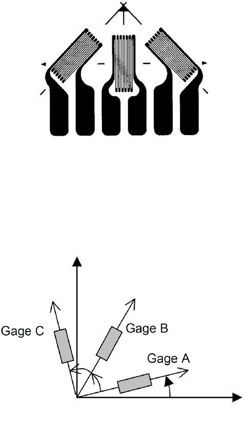
97
4.9 Virtual strain gauges
4.9.1 Overview
Virtual strain gauges are used to assess the behavior of calculated load histories compared to
measured strain data, as a means to validate the input stresses. In FEA, strain gauges can be difficult
to model and usually require the definition of axial connector elements positioned at strategic
locations on the mesh surface which correspond to the laboratory test. Quick Fatigue Tool offers the
specification of a virtual strain gauge, which is a location on the model (integration point, node, etc.)
at which the strain history is measured in a particular direction.
4.9.2 Gauge definition
The virtual strain gauge has a rectangular rosette format, an example of which is shown in Figure 4.23.
The gauge is represented in Cartesian space in Figure 4.24, with the rosette arms , and orientated
according to the angles , and , counter clockwise from the positive x-direction.
Figure 4.23: Typical layout of a rectangular rosette gauge
α
β
γ
x
y
Figure 4.24: Rosette gauge orientation relative to Cartesian axes

98
4.9.3 Technical background
The calculation of the strain histories is based on the linear elastic stresses defined in the stress data
set file. If the material contains values of the cyclic strain hardening coefficient and exponent ( and
, respectively) then the elastic stresses are first converted to elasto-plastic strain histories. These
histories are then resolved onto the directions of the gauge arms according to Equations 4.13-15.
[4.13]
[4.14]
[4.15]
The plasticity correction uses the same algorithm as the Multiaxial Gauge Fatigue app and is described
in the document Quick Fatigue Tool Appendices: A3.2.4.
If cyclic data is not provided, then the strains are calculated from the stresses elastically, according to
Equations 4.16-18.
[4.16]
[4.17]
[4.18]
4.9.4 Specifying the position of the strain gauge
Virtual strain gauges are defined by specifying the position IDs identifying the location of the gauges
to on the model.
Job file usage:
Option
Value
GAUGE_LOCATION
{'<mainID>.<subID>1',…, '<mainID>.<subID>n'}
For uniaxial analyses, the gauge location is simply '1.1'. The user may specify multiple strain gauges by
listing the position IDs as separate strings.
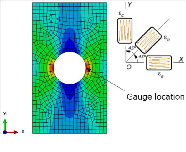
99
4.9.5 Specifying the orientation of the strain gauge
The strain gauge orientation is defined by providing the values of , and for gauges to ,
according to Figure 4.23.
Job file usage:
Option
Value
GAUGE_ORIENTATION
{,…, }
Alternatively, the user may use the flags 'RECTANGULAR' or 'DELTA' to indicate that the gauge has a
rectangular [] or delta [] layout, respectively.
Job file usage:
Option
Value
GAUGE_ORIENTATION
{'RECTANGULAR' | 'DELTA'}
4.9.6 Example usage
Consider the model in Figure 4.25. A gauge is to be defined at element , node . The gauge is
aligned with the global x-axis, giving an orientation of , and . The virtual gauge
is defined in the job file.
Figure 4.25: Virtual gauge location on FE model
100
Job file usage:
Option
Value
GAUGE_LOCATION
{'657.7'}
GAUGE_ORIENTATION
{[0.0, 45.0, 45.0]}
Additional gauges can be added by appending position IDs and orientations as necessary.
Results for each gauge are written to a text file and stored in Project\output\<jobName>\Data Files.
4.9.7 Modelling guidance
Virtual strain gauges are intended for components in a state of plane strain. The gauge will only detect
the two-dimensional state of strain relative to the global x-y plane. The user is therefore advised to
specify the gauges on plane stress elements to facilitate the definition. If the model contains solid
elements, a skin should be applied over the surface (a layer of shell elements), and the gauges defined
on these elements.
The position IDs used to define the gauges should be consistent with the element position used to
generate the stress data set file. For example, if the stresses were exported at integration points or
element nodes, both the main and sub IDs are required. For centroidal and unique nodal data, the
item is defined by the main ID; the sub ID always has a value of .
Output from virtual strain gauges can be used as input to the Multiaxial Gauge Fatigue application
(Quick Fatigue Tool Appendices: A3.2). The user must ensure that the orientations specified by
GAUGE_ORIENTATION match those defined in the application.
If the user wishes only to extract virtual strain gauge histories, the fatigue analysis can be omitted by
setting DATA_CHECK=1 in the job file. Alternatively, the Virtual Strain Gauge application
(Quick Fatigue Tool Appendices: A3.4) can be used to generate strain gauge histories from a strain
tensor definition; both methods use the same underlying analysis technique discussed in this section.
4.9.8 Limitations
Virtual strain gauges convert the linear elastic stresses to elasto-plastic strains using a simple
multilinear hardening rule. The correction is applied separately to each strain component and as such,
results will be inaccurate where a large amount of plasticity is present in the material. The virtual
strain gauge should be used as a rough estimate of the local nonlinear strain history only; in cases
where a more thorough treatment is required, the user is advised to define the gauge directly on the
finite element model.
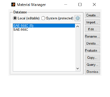
101
5. Materials
5.1 Background
5.1.1 Overview
This section describes how to define and use material properties for analysis in Quick Fatigue Tool. In
general, this involves:
creating material properties interactively with the Material Manager application, or from a
text file; and
specifying the material in the job file.
Material data is stored as a MATLAB binary (.mat) file and is located by default in the directory
Data\material\local.
5.1.2 Accessing the Material Manager
The Material Manager application is used to create and edit material data. It can be accessed either
from the command line or by installing the Material Manager GUI application.
To install the Material Manager, double-click the file Material Manager.mlappinstall in the
Application_Files\toolbox directory. The app will appear in the apps bar in MATLAB.
Figure 5.1 shows the Material Manager GUI.
The Material Manager GUI is launched by doing one of the following:
select the Material Manager launch icon from the APPS ribbon; or
execute the command material.manage from the MATLAB command line.
Figure 5.1: Material Manager GUI

102
5.2 Material databases
5.2.1 Overview
Material Manager separates material data into two databases:
Local
Local copies of materials are stored here
Materials in this database can be
modified
Materials in this database can be used
for analysis
System
Database containing materials included
with the Quick Fatigue Tool application
Materials in this database cannot be
modified
Materials in this database must be
fetched in order to be used for analysis
If the full path to the material .mat file is specified in the job file, Quick Fatigue Tool will search for the
material in this location only. If the material is given without a path, Quick Fatigue Tool will search for
the material in the following order:
1. Local material database
2. Default local database path (<quick-fatigue-tool-root>\Data\material\local)
3. MATLAB search path (first encounter)
The local material database is the work directory used by the Material Manager application for storing
material data.
5.2.2 Specifying the local material database
When Material Manager is started for the first time, the user is prompted to specify the directory for
the local material database. If the default location (<quick-fatigue-tool-root>\Data\material\local) is
available, this is selected automatically. Once the directory is selected, Quick Fatigue Tool saves the
location into the %APPDATA% and writes a text file in that directory as a marker, so that
Quick Fatigue Tool can recall the local database after restarting MATLAB.
The local material database can be changed at any time by selecting the button from the main
Material Manager GUI, or by specifying the database on the command line.
Material Manager usage:
Database region of the MaterialManager dialogue: Select . In the
dialogue box that appears, select the default location with the check
box, or specify a user-defined path in the edit region of the GUI.
Command line usage:
>> material.database('<database-path>')
103
5.3 Using material data for analysis
5.3.1 Specifying the material in the job file
The analysis material is specified in the job file by providing the .mat file containing the material data.
Job file usage (M-file):
Option
Value
MATERIAL
'material-file-name.mat'
where 'material-file-name.mat' is a material in the local database.
Job file usage (text file):
Option
Value
*MATERIAL =
'material-file-name.mat'
Detailed guidance on specifying job file options in a text file is provided in Section 2.4.3.
5.3.2 Fetching materials from the system database
To use a material from the system database, the material is fetched from the file mat.mat in
Data\material\system and a copy is stored in the local database.
Material Manager usage:
Database region of the MaterialManager dialogue: Select System
(protected). Select a material from the list of system materials.
Select Fetch…. Verify the name of the material. Select OK.
Command line usage:
>> material.fetch()
>> <database number>
>> <material number>
The fetched material appears in the Local database list in the Material Manager GUI. A list of materials
in the local database is shown using the following command:
Command line usage:
>> material.list()
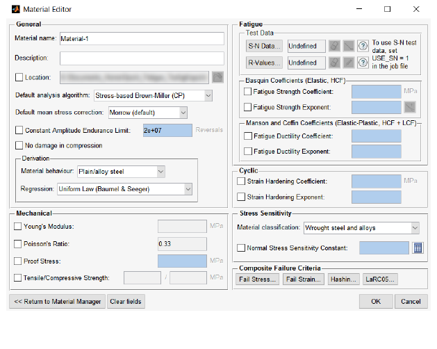
104
5.4 Creating materials using the Material Manager
5.4.1 Overview
Material properties are defined by launching the material property editor.
Material Manager usage:
To create a new material, from the MaterialManager dialogue select
Create…. To modify an existing material, select Edit….
Command line usage:
>> material.create
>> material.edit('material-name')
The material property editor is shown in Figure 5.2.
Property values are specified by first checking the property to indicate that it is user-defined. When a
property is unchecked, its input field turns blue, meaning that the property is not defined by the user
and will be derived automatically if applicable.
5.4.2 Units
Properties with units of stress must be specified in Megapascals. The constant amplitude endurance
limit is given in repeats (); this is the number of cycles, , multiplied by two.
Figure 5.2: Material property editor for a user-defined material
105
5.5 Creating materials from a text file
5.5.1 Overview
Material data defined in a text file can be used for
importing materials into the local database using Material Manager; and
defining material data directly in the job file for text-based job submission.
Material properties are declared using keywords in combination with parameters and data lines (if
applicable).
5.5.2 Material keyword syntax
Materials defined from text files must adhere to strict syntax rules which allow Quick Fatigue Tool to
recognize the data. Each material definition must begin with the following keyword:
Text file usage:
Keyword
Parameter(s)
*USER MATERIAL
name
This keyword declares the material definition and assigns a material name using the name parameter.
An example usage of this keyword is given below:
*USER MATERIAL, manten steel
There are no data lines associated with this keyword; only the keyword itself and the material name
are required.
Some keywords require a data line to complete their definition:
Text file usage:
Keyword
Parameter(s)
Data line(s)
*CAEL
(none)
This keyword defines the constant amplitude endurance limit. There is no associated parameter. The
first (and only) data line defines the constant amplitude endurance limit value, , and an optional
flag, , indicating whether this value is active in the material definition. Several material
parameters have an associated flag; a value of is equivalent to the action of checking the
respective property box in the Material Manager GUI.
106
An example usage of this keyword is given below:
*CAEL
2e7, 1.0
Some keywords have optional data lines:
Text file usage:
Keyword
Parameter(s)
Data line(s)
*MECHANICAL
(none)
First line:
Second line:
This keyword defines the mechanical constants for the material. The data line entries and
specify the Young’s Modulus, Poisson’s ratio, the ultimate tensile strength and the yield strength,
respectively.
In this case, only the first data line is compulsory. The second data line may be used to specify whether
the properties are active in the definition. It is not necessary to define all the properties on the first
data line, and consequently the user is only required to specify the flags corresponding to the
defined properties.
An example usage of this keyword where all properties are defined is given below:
*MECHANICAL
200e3, 0.3, 400, 325
In this case, all four mechanical properties have been specified. The flag has a default value of
for any defined properties, so all of the properties are active in the material.
An example usage of this keyword where only some properties are defined is given below:
*MECHANICAL
200e3, , 400, ,
1.0, , 0.0, ,
In this case, only the Young’s Modulus and the ultimate tensile strength are defined. The flags
are specified such that the Young’s Modulus is active and the ultimate tensile strength is inactive.
If a parameter is left undefined, this must be indicated by an empty assignment (two consecutive
commas), otherwise the definition may be processed incorrectly.
The user indicates the end of a material definition by specifying *END MATERIAL as the last keyword
in the definition. This instructs Quick Fatigue Tool to stop processing the material text file.
107
5.5.3 Importing materials from a text file
Materials are imported into the local database by using the Import function in Material Manager. The
material text file is read through a text file processor and the definitions are saved as a MATLAB binary
(.mat) file in Data\material\local.
Material data is imported into the local database using the Material Manager GUI or via the command
line.
Material Manager usage:
From the MaterialManager dialogue select Import…. Change the file
selection filter to Normal text file (*.txt). Select the text file
containing material data and select Open.
Command line usage:
>> material.import('material-file-name.* ')
5.5.4 Specifying material properties in a job file
Material data may be defined as part of a text-based job file. Job submission from text files is discussed
in Section 2.4.3. The material definition may be placed anywhere in the job file provided that it begins
and ends with the keywords *USER MATERIAL and *END MATERIAL, respectively. Failing to do so may
result in an error.
An example job file containing material data is given below:
*JOB NAME = holePlate
*MATERIAL = steel
*DATASET = stressData.dat
*HISTORY = [1, -1]
beginning of material definitions:
*USER MATERIAL, steel
*MECHANICAL
200e3, , 400, ,
*FATIGUE, constants
930, -0.095, , ,
1, 1, , ,
*END MATERIAL
*USER MATERIAL, aluminium
*MECHANICAL
79e3, , 110, ,
*FATIGUE, test data
10000, 62.7, 51.6
1e6, 38.3, 32.7
*R RATIOS
-1, 0
*END MATERIAL
additional options to define the fatigue analysis:
*OUTPUT FIELD = 1
*FATIGUE RESERVE FACTOR = 1
108
Note that the job file contains two material definitions; although only one of the materials is
referenced by the MATERIAL job file option, both materials are copied to the local material database
as .mat files.
5.5.5 Material keyword reference
A complete list of material keywords and their associated syntax can be found in the document Quick
Fatigue Tool User Settings Reference Guide.
If the user hovers their mouse over a property in the material property editor dialogue box
(Figure 5.2), the associated text file keyword is revealed as a tooltip string.
109
5.6 General material properties
5.6.1 Overview
General material properties are non-physical attributes of the material. It is not compulsory to define
general properties and Quick Fatigue Tool will use default properties if none is specified by the user.
5.6.2 Default analysis settings
The default analysis algorithm and mean stress correction is specified in the material. If the default
algorithm is selected in the job file, Quick Fatigue Tool always tried to apply the default algorithm
defined in the material.
Material Manager usage:
General region of the Material Editor dialogue: Select an option
from the Default analysis algorithm and Default mean stress
correction drop-down boxes.
Text file usage:
Keyword
Parameter(s)
Data line(s)
*DEFAULT ALGORITHM
{UNIAXIAL STRESS | UNIAXIAL STRAIN | SBBM |
NORMAL | FINDLEY | INVARIANT | NASALIFE}
(NONE)
*DEFAULT MSC
{MORROW | GOODMAN | SODERBERG |
WALKE | SWT | GERBER | RATIO | NONE}
(NONE)
Algorithms in the Material Manger GUI which include the letters (CP) utilize critical plane searching.
The BS 7608 algorithm cannot currently be specified as a default analysis algorithm.
5.6.3 Treatment of fully-compressive cycles
The effect of compressive stresses can be ignored during the analysis.
Material Manager usage:
General region of the Material Editor dialogue: Check the option
No damage in compression.
Text file usage:
Keyword
Parameter(s)
Data line(s)
*NO COMPRESSION
(NONE)
(NONE)
This setting has the following effects:
fatigue damage is not calculated for fully-compressive cycles (maximum stress in cycle 0);
the Fatigue Reserve Factor is reset to the maximum value for fully-compressive cycles; and
compressive stresses are reset to zero for the yield and composite criteria assessments.

110
5.7 Fatigue material properties
5.7.1 Overview
Fatigue material properties can be defined for stress-based and strain-based fatigue analysis. Stress-
based properties define the Wöhler curve, which the user provides either with the Basquin fatigue
constants, or fatigue test data in the form of a stress-life (S-N) curve. Strain-based properties define
the strain-life curve, which the user provides with the Manson and Coffin fatigue constants.
For stress-based analysis, the user can specify whether to use the Basquin fatigue constants or fatigue
test data.
Job file usage:
Option
Value
USE_SN
{0.0 |1.0}
Quick Fatigue Tool checks the value of USE_SN before the analysis. If the value is set to 1.0, fatigue
test data will be used if it is available; otherwise fatigue coefficients will be used instead. If neither is
available, Quick Fatigue Tool will attempt to derive the fatigue coefficients from the mechanical
properties. If the required mechanical properties are unavailable, the analysis will be aborted due to
insufficient material data.
5.7.2 Fatigue constants
Fatigue constants are specified using the material property editor or from a text file.
Material Manager usage:
Basquin/Manson and Coffin Coefficients region of the Material
Editor dialogue: Check the property and fill out the edit box.
Text file usage:
Keyword
Parameter(s)
Data line(s)
*FATIGUE
CONSTANTS
First line: , , ,
An alternative value of the fatigue strength exponent can be specified beyond a certain life to create
a “knee” on the Wöhler curve.
Material Manager usage:
Basquin Coefficients region of the Material Editor dialogue: Open
the Insert Knee dialogue by selecting the button and fill out the
edit box.
Text file usage:
Keyword
Parameter(s)
Data line(s)
*KNEE
(NONE)
First (and only) line: ,
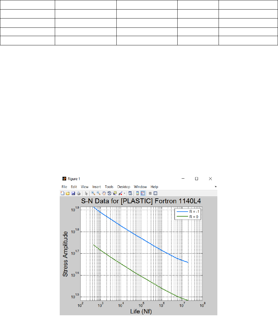
111
5.7.3 Fatigue test data
The S-N curve can be defined as test data, and is read into the property editor via a text file. The data
can be tab, space or comma separated, and has the following format:
…
.
.
.
.
.
.
.
.
The first data column is always cycles, and the number of cycles must be increasing down the column.
Each subsequent data column is the stress amplitude for each measured load ratio ( to ). The
stress datasets should be ordered so that the load ratios are monotonically increasing. The S-N data
can also be specified as the transpose of the above (row-wise).
If S-N data is provided for one load ratio, the stress amplitude will be assumed to represent a fully-
reversed cycle, irrespective of the R-ratio provided.
S-N data can be plotted using the plot button. An example of S-N data for multiple R-ratios is given in
Figure 5.3.
S-N data stress values must be specified in .
Figure 5.3: S-N data for Fortron 1140L4

112
User S-N data is specified using the material property editor or from a text file.
Material Manager usage:
Test Data region of the Material Editor dialogue: Select S-N Data.
Navigate to the S-N data file and select Open.
Text file usage:
Keyword
Parameter(s)
Data line(s)
*FATIGUE
TEST DATA
First line: , , ,…,
Second line: , , ,…,
th line: , , ,…,
If the S-N data is defined over multiple R-ratios, these must be specified separately.
Material Manager usage:
Test Data region of the Material Editor dialogue: Select R-Values.
Enter the list of R-values in order of lowest to highest. Select OK.
Text file usage:
Keyword
Parameter(s)
Data line(s)
*R RATIOS
(none)
First (and only) line: , ,…,
5.7.4 Defining the fatigue limit for fatigue test data
If the stress cycle is below the fatigue limit, Quick Fatigue Tool may assume zero damage. The fatigue
limit is usually calculated from the value of the Constant Amplitude Endurance Limit (defined in
Material Manager). However, it is possible to use the fatigue limit directly from the S-N data. When
USE_SN=1 in the job file Quick Fatigue Tool determines the fatigue and endurance limits based on the
following logic:
CAEL
(Material
Manager
usage)
CAEL
(text file
usage)
Fatigue limit definition
Endurance limit definition
*CAEL
n
1.0
USE_SN={1|0}: Derived from using
the definition of the fatigueLimitSource
environment variable (unless fatigue
limit is user-defined)
USE_SN={1|0}:
*CAEL
2e+07
0.0
USE_SN=1: The S-value corresponding
to the last N-value on the user S-N
curve
USE_SN=0: Derived from
reversals using the definition of the
fatigueLimitSource environment
variable (unless fatigue limit is user-
defined)
USE_SN=1: The N-value
corresponding to the last
S-value on the user S-N
curve
USE_SN=0:
reversals
113
If the fatigue limit is derived from the S-N data and multiple S-N curves are defined, Quick Fatigue Tool
uses the curve (interpolated if necessary).
The behavior described above only applies to stress-based fatigue analysis.
Not all materials exhibit an endurance limit. Therefore, Quick Fatigue Tool only enforces the limit in
certain conditions. Settings related to the endurance limit are described in the document
Quick Fatigue Tool Appendices: A1.
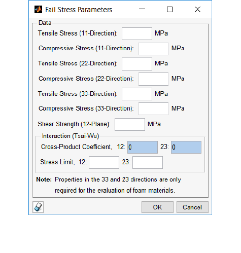
114
5.8 Composite material properties
5.8.1 Overview
Quick Fatigue Tool can perform failure and damage initiation analyses for fibre-reinforced composite
materials. The user must provide the necessary material data for the analysis to evaluate the
composite for the desired criterion. Properties are provided for the longitudinal (fibre) and transverse
strength of the composite.
When composite material properties are supplied and the composite failure criteria assessment is
specified, Quick Fatigue Tool does not perform a subsequent fatigue analysis. Therefore, fatigue
properties are not required in conjunction with composite properties.
Refer to Section 12.3 for a detailed overview of each criterion.
5.8.2 Defining properties for stress-based failure criteria
Stress-based properties are required for the following criteria:
maximum stress theory;
Tsai-Hill theory;
Tsai-Wu theory; and
Azzi-Tsai-Hill theory.
These properties are defined using the Fail Stress dialogue in the Material Manager app (Figure 5.4),
or in a text file.
Figure 5.4: Fail Stress dialogue
115
Material Manager usage:
Composite Failure Criteria region of the Material Editor dialogue:
Select Fail Stress. Enter properties into the Fail Stress dialogue.
Text file usage:
Keyword
Parameter(s)
Data line(s)
*COMPOSITE
STRESS
First (and only) line: , , ,
, , , , , ,
,
Properties can be entered in the three anisotropic directions (11, 22 and 33). The properties , ,
and (directions 33 and 23) are only required for the evaluation of closed cell polyvinyl
chloride (PVC) foam in states of plane strain. For the evaluation of fibre-reinforced composites in
states of plane stress, only the properties in directions 11, 22 and 12 are required.
Values of and are only required for the Tsai-Wu theory. If a value of is not specified, the
value of is used instead. The default value of is zero, indicating an uncoupled relationship
between the direct and shear stresses.
5.8.3 Defining properties for the maximum strain failure theory
Strain-based properties are required for the maximum strain failure theory.
These properties are defined using the Fail Strain dialogue in the Material Manager app (Figure 5.5),
or in a text file.
Material Manager usage:
Composite Failure Criteria region of the Material Editor dialogue:
Select Fail Strain. Enter properties into the Fail Strain dialogue.
Text file usage:
Keyword
Parameter(s)
Data line(s)
*COMPOSITE
STRAIN
First (and only) line: , ,
, , , , ,
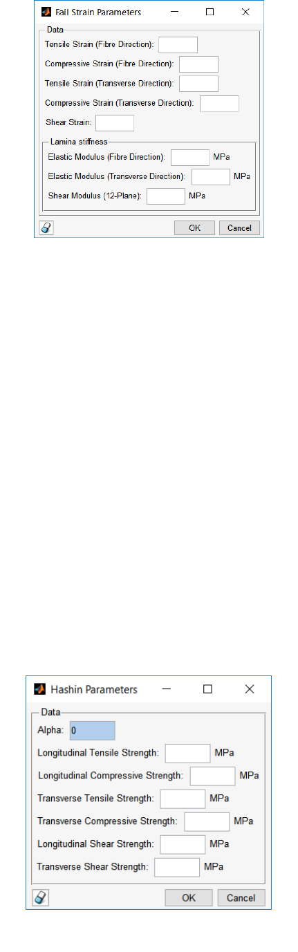
116
5.8.4 Defining properties for Hashin’s damage initiation criteria
Properties for Hashin’s theory are defined using the Hashin Damage dialogue in the Material Manager
app (Figure 5.6), or in a text file.
Material Manager usage:
Composite Failure Criteria region of the Material Editor dialogue:
Select Hashin Damage. Enter properties into the Hashin Damage
dialogue.
Text file usage:
Keyword
Parameter(s)
Data line(s)
*COMPOSITE
HASHIN
First (and only) line: , , ,
, , ,
The default value of is zero, indicating an uncoupled relationship between the direct and shear
stresses.
Figure 5.5: Fail Strain dialogue
Figure 5.6: Hashin Damage dialogue
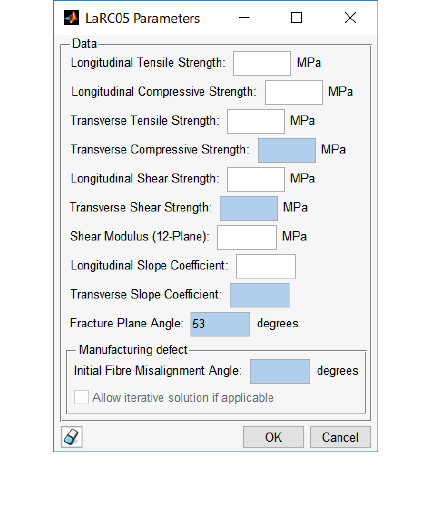
117
5.8.5 Defining properties for the LaRC05 damage initiation criteria
Properties for the LaRC05 damage initiation criteria are defined using the LaRC05 Damage dialogue in
the Material Manager app (Figure 5.7), or in a text file.
Material Manager usage:
Composite Failure Criteria region of the Material Editor dialogue:
Select LaRC05 Damage. Enter properties into the LaRC05 Damage
dialogue.
Text file usage:
Keyword
Parameter(s)
Data line(s)
*COMPOSITE
LARC05
First (and only) line: , , ,
, , , , , , ,
Figure 5.7: LaRC05 dialogue

118
5.9 Estimation techniques
5.9.1 Approximating material data
Fatigue material properties are difficult to find and often only partial data is available. The user can
allow Quick Fatigue Tool to approximate material properties using a specified regression algorithm.
In Material Manager, material properties which allow for approximation are distinguished by light blue
input fields. If a property is approximated, the method selected in the Regression drop-down menu
will be used.
Material Manager usage:
Derivation region of the Material Editor dialogue: Select the
regression method from the Regression drop-down box.
Text file usage:
Keyword
Parameter(s)
Data line(s)
*REGRESSION
{UNIFORM | UNIVERSAL | MODIFIED | 9050 | NONE}
(none)
For detailed information on each regression method, consult the document
Quick Fatigue Tool Appendices: A2.
A material property has one of four statuses: Undefined, user-defined, approximated or default. The
material estimation logic is described in the table below.
The property is unspecified
The property cannot be approximated
The property is undefined
The property is specified indirectly
The property cannot be approximated
Quick Fatigue Tool will use the default value
The property is unspecified
Quick Fatigue Tool will attempt to approximate the property
If the property cannot be approximated, it will be undefined
The property is specified indirectly
Quick Fatigue Tool will attempt to approximate the property first
If the property cannot be approximated, the user-defined value will be used
The property is specified directly
Quick Fatigue Tool will not attempt to approximate the property
The property is user-defined
119
5.9.2 Disabling material data approximation
The user may specify that fatigue material data is not approximated.
Material Manager usage:
Derivation region of the Material Editor dialogue: Select None from
the Regression drop-down box.
Text file usage:
Keyword
Parameter(s)
Data line(s)
*REGRESSION
NONE
(none)
5.9.3 Defining material behavior
The material behavior is specified in order to instruct Quick Fatigue Tool how to derive certain
properties. Specifying the material behavior:
controls the default regression method in Material Manager;
controls the derivation method of the Walker -parameter when standard values are used
(walkerGammaSource=2.0); and
controls the default enforcement of the endurance limit (ndEndurance=0.0).
Material Manager usage:
Derivation region of the Material Editor dialogue: Select the
behavior from the Material behavior drop-down box.
Text file usage:
Keyword
Parameter(s)
Data line(s)
*BEHAVIOR
{STEEL | ALUMINIUM | OTHER}
(none)
5.9.4 Defining material classification
The material classification is specified in order to instruct Quick Fatigue Tool how to derive the
fatigue shear strength coefficient, for Findley’s Method.
Material Manager usage:
Stress Sensitivity region of the Material Editor dialogue: Select the
classification from the Material classification drop-down box.
Text file usage:
Keyword
Parameter(s)
Data line(s)
*CLASS
{WROUGHT STEEL | DUCTILE IRON| MALLEABLE IRON|
WROUGHT IRON | CAST IRON | ALUMINIUM | OTHER}
(none)
120
6. Analysis algorithms
6.1 Background
The choice of fatigue analysis algorithm is very important for obtaining a good correlation between
the applied stresses and the fatigue life. This section explains the algorithms available in
Quick Fatigue Tool and recommendations for how they could be applied.
Below is a summary of the available algorithms and their applications.
Algorithm
Application
Job file option
Uniaxial Strain-Life
Uniaxial strains only
ALGORITHM={3.0 | 'uniaxial strain'}
Stress-based
Brown-Miller
General
Ductile metals
ALGORITHM={4.0 | 'sbbm'}
Normal Stress
General
Brittle metals
Engineering plastics
ALGORITHM={5.0 | 'normal'}
Findley’s Method
Compliance -
Marine/Automotive
Ductile and brittle metals,
crankshafts
ALGORITHM={6.0 | 'findley'}
Stress Invariant
Parameter
General, compliance
ALGORITHM={7.0 | 'invariant'}
BS 7608
Compliance - Offshore
Welded steel joints
Axially loaded bolts
ALGORITHM={8.0 | 'weld'}
NASALIFE
Compliance – Aerospace
Aero engine components
ALGORITHM={9.0 | 'nasalife'}
Uniaxial Stress-Life
Uniaxial stresses only
ALGORITHM={10.0 | 'uniaxial stress'}
User-defined
N/A
ALGORITHM={11.0 | 'user'}
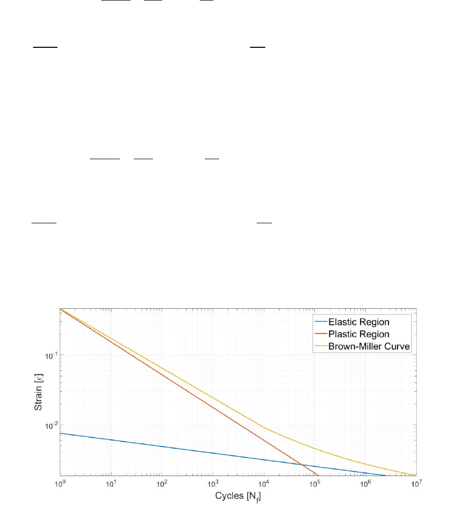
121
6.2 Stress-based Brown-Miller
6.2.1 Overview
The Brown-Miller algorithm postulates that the fatigue damage is dominated by the combination of
shear and normal strain [18] [19] [20]:
[6.2.1]
where
is the maximum shear strain amplitude,
is the normal strain amplitude, is the
tensile fatigue strength coefficient, is Young’s Modulus, is Basquin’s exponent, is the fatigue
ductility coefficient, is the fatigue ductility exponent and is the life in repeats (cycles).
The Stress-based Brown-Miller is the same algorithm, but the damage parameter is stress-based. Thus,
Equation 6.2.1 becomes:
[6.2.2]
where
is the maximum shear stress amplitude and
is the normal stress amplitude. The right-
hand side of Equation 6.2.2 is multiplied by Young’s Modulus to retain homogeneity.
The Brown-Miller strain-life curve is shown in Figure 6.1.1:
For lives greater than one million cycles, the Brown-Miller curve closely resembles its elastic
constituent. Therefore, for HCF applications it is usually sufficient to assume that plasticity effects are
sufficiently small so that the plastic portion of the equation can be neglected. This is the default
behavior in Quick Fatigue Tool; however, the plastic portion of the equation can be activated with the
Figure 6.1.1: Brown-Miller strain-life curve, with separate elastic and plastic regions shown.

122
environment variable plasticSN. This invokes one-dimensional interpolation and can cause the analysis
time to increase significantly.
The Stress-based Brown-Miller algorithm gives the best results for ductile metals. Using the algorithm
for brittle materials can result in non-conservative fatigue life predictions.
The following material properties are required to perform an analysis with the Stress-based Brown-
Miller algorithm:
Property
Symbol
Importance
Tensile fatigue strength
coefficient
REQUIRED
Tensile fatigue strength
exponent
REQUIRED
Young’s Modulus
REQUIRED
Fatigue ductility coefficient
OPTIONAL
Fatigue ductility exponent
OPTIONAL
6.2.2 Using stress-life data
Due to the nature of the Stress-based Brown-Miller equation, results obtained from stress-life data
can differ significantly compared to the use of material coefficients. When using stress-life data with
USE_SN=1.0 in the job file, Quick Fatigue Tool uses the damage parameter to interpolate the
endurance curve. Since the endurance curve typically arises from stress-based testing and the Stress-
based Brown-Miller equation take sit form from its strain-life counterpart, the corresponding life
values are not guaranteed to be the same.
6.2.3 Cycle counting
The Stress-based Brown-Miller algorithm uses the normal and shear stress amplitude to define the
total damage parameter. This poses an additional challenge for the cycle counting process, because
the formulation in Equation 6.2.2 suggests that the damage parameter is the sum of the cycle counted
normal and shear stress. However, if these two quantities are cycle counted before being summed,
there is no guarantee that the counted histories will still have the same length, and matrix addition
may not be immediately possible.
The alternative is to combine the normal and the shear stress beforehand, and cycle count the single
combined parameter. This circumvents the issue of matrix addition, but may lead to incorrect fatigue
results. For example, consider the normal and shear histories [100, 50] and [20, 50], respectively. Their
individual amplitudes are 25 and 15, respectively, meaning that the sum of their amplitudes is 40. If
the parameters are combined first to give the history [120, 100], the resulting amplitude is 10.
Therefore, cycle counting the combined history may lead to a totally different value of fatigue damage.
123
The user can control the order of operations to suit their needs.
Environment file usage:
Variable
Value
rainflowAlgorithm
;
The value of dictates the following:
1. Combine the normal and shear parameters, then count the resulting history (default)
2. Count the normal and shear parameters separately, then combine the resulting histories
The second method is considered by the author to be the most physically correct approach, although
it is significantly more time-consuming. Before the cycle counted normal and shear stress histories are
combined, Quick Fatigue Tool checks the length of each history and resamples the shorter parameter
in order to allow matrix addition. If significant resampling is required, the combined stress parameter
may no longer be accurate. In such cases, the user should compare the fatigue life results for both
cycle counting methods.
Testing reveals that for the majority of simple load cases, there is little or no difference in the fatigue
result between the two methods. For loads where there is a significant phase difference between the
normal and shear stresses, the user should compare the fatigue life results for both cycle counting
methods and elect the method which offers the favourable accuracy-to-time ratio. The default setting
is the first approach.

124
6.2.4 Proportional loading
If Quick Fatigue Tool detects that the fatigue loading is proportional, the Stress-based Brown-Miller
algorithm is run without critical plane searching, since the direction of the principal stresses does not
change. In such cases, Quick Fatigue Tool assumes by default that the damage parameter is the
maximum combination of normal and shear stress by stress transformation.
Environment file usage:
Variable
Value
sbbmParameter
{1.0 | 2.0};
1. Maximum normal stress
2. Maximum combined (normal + shear) stress
The maximum combined stress, , is calculated from the principal stress according to
Equations 6.2.1-2:
[6.2.1]
[6.2.2]
where are the maximum and minimum principal stresses, respectively, is the hydrostatic stress
and is the fracture transformation angle.
The solution of is the value of which produces the numerically largest value of in the range
:
[6.2.3]
Load proportionality is discussed further in Section 4.5.2.
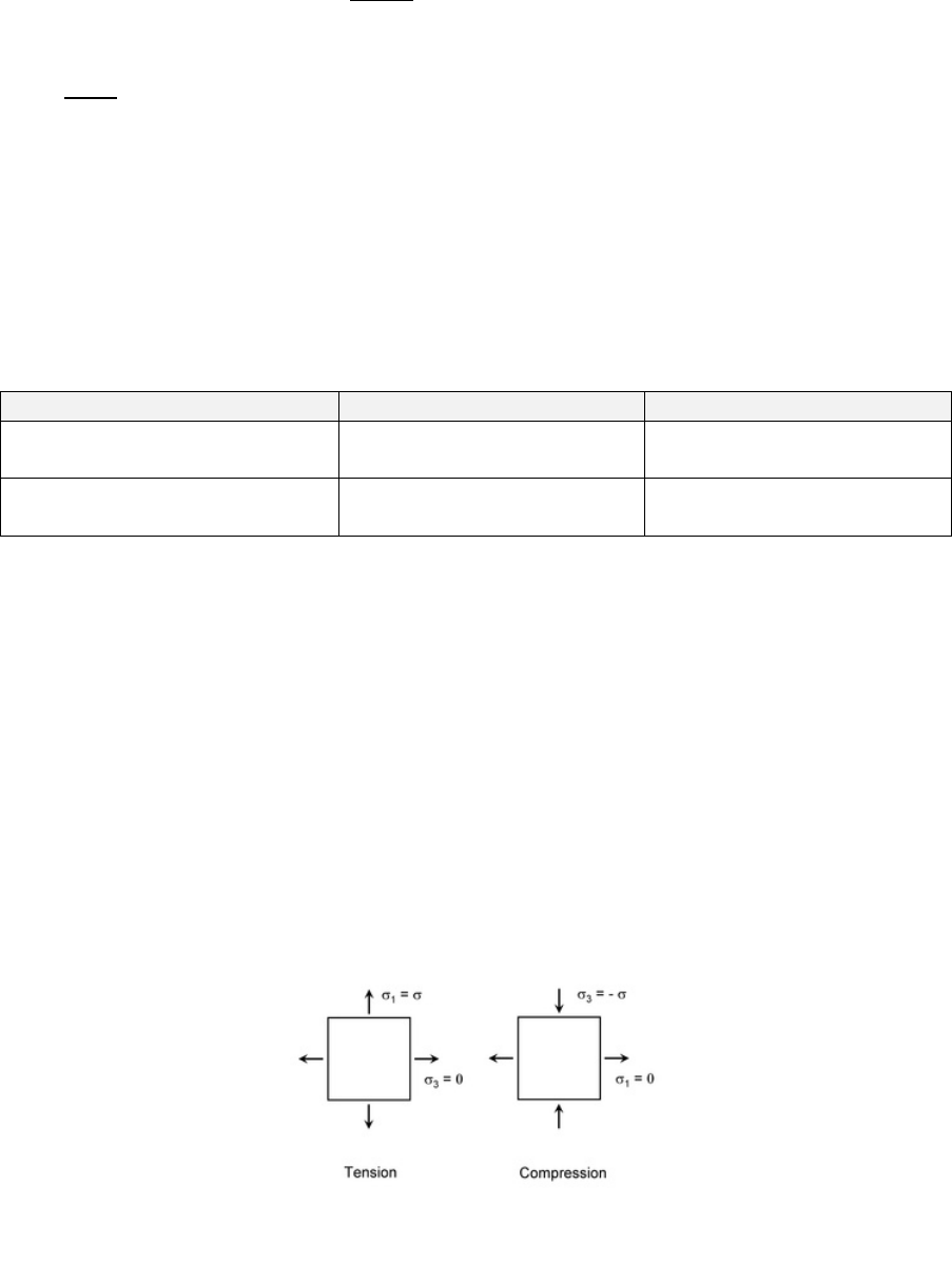
125
6.3 Normal Stress
6.3.1 Overview
The Normal Stress algorithm uses the normal stress amplitude as the damage parameter in the stress-
life equation:
[6.3.1]
where
is the maximum normal stress amplitude on the critical plane and the other symbols have
their usual meaning. The algorithm predicts that the fatigue strength in torsion and tension is the
same. In reality, the allowable normal stress in torsion is approximately 60% of the allowable axial
stress. Therefore, the Normal Stress algorithm only provides accurate fatigue life estimates for brittle
materials whose crack initiation is dominated by normal stresses. The algorithm is highly non-
conservative for ductile metals where the fatigue life is dominated by shear stresses [21].
The following material properties are required to perform an analysis with the Normal Stress
algorithm:
Property
Symbol
Importance
Tensile fatigue strength
coefficient
REQUIRED
Tensile fatigue strength
exponent
REQUIRED
6.3.2 Critical plane searching
The principal stress is often used as an effective stress parameter; since it is an invariant quantity, it is
tempting to bypass critical plane searching. However, even for simple loadings, relying on the value of
the maximum principal stress can yield unexpected results. Take the simple stress tensor given by
Equation 6.3.2:
[6.3.2]
The resulting principal stress state when the above tensor is subjected to a fully-reversed loading
event, , is given by Figure 6.3.1.
Figure 6.3.1: Principal stress state due to fully-
reversed load
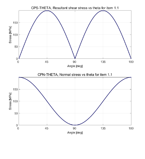
126
Since the principal stresses are ordered such that , a simple tension-compression event
causes the principal direction to rotate by 90 degrees. This problem is avoided if the normal tensile
stresses are calculated over a series of planes using critical plane searching [22]. The critical plane is
defined as the plane which experiences the largest combination of normal stress range and mean
stress.
The Normal Stress algorithm posits that a component subjected to a uniaxial stress cycle, ,
will fail on a plane where the shear stress is zero. The normal and shear stress on the critical plane
using the Normal Stress algorithm are illustrated in Figure 6.3.2.
The critical plane occurs when theta is zero, which corresponds to one of the principal planes.
Figure 6.3.2: Normal and resultant shear stress on the critical plane for
uniaxial tension

127
6.4 Findley’s Method
6.4.1 Overview
Findley’s Method proposes that crack initiation is due to the combined effect of the average normal
stress and the alternating shear stress on the critical plane [23] [24] [25]:
[6.4.1]
where
is the maximum shear stress amplitude on the critical plane, is the normal stress, is a
material constant describing the sensitivity of the material to normal stresses and is a function of
the torsional fatigue strength coefficient.
Findley’s Method was originally presented in the form of a safety factor; however, by introducing the
stress-life curve defined by and , the algorithm is also well-suited to finite, HCF life prediction.
The value of is determined experimentally from the tensile and torsional fatigue limit, and
determines the influence of the normal stress on the calculated fatigue damage. Consider the example
where a specimen under torsional loading experiences a very large mean normal stress. Even if the
normal stress amplitude is small (close to static), the predicted fatigue damage from Findley’s Method
can be very conservative. The normal stress sensitivity constant acts to attenuate the effect of on
the loading and can be considered a form of mean stress correction.
Another advantage of Findley’s Method is that it is well-suited to both brittle and ductile metals. The
tensile and torsional fatigue limit can be used to “tune” a value of which accurately characterises
the material response.
Work by Kallmeyer et al. has shown that the Findley critical plane method provides the best
representation for smooth bar data, which gives the method significance in applications involving
shafts under shear loads [26] [27].
The following material properties are required to perform an analysis with the Findley algorithm:
Property
Symbol
Importance
Tensile fatigue strength
coefficient
REQUIRED
Tensile fatigue strength
exponent
REQUIRED
Normal stress sensitivity
constant
REQUIRED3
Modified fatigue shear strength
coefficient
REQUIRED4
Poisson’s Ratio
OPTIONAL
Tensile Fatigue Strength Limit
OPTIONAL
Torsional Fatigue Strength Limit
OPTIONAL
Ultimate Tensile Strength
OPTIONAL
3
If no value is specified, a default value is used.
4
This parameter is computed automatically.
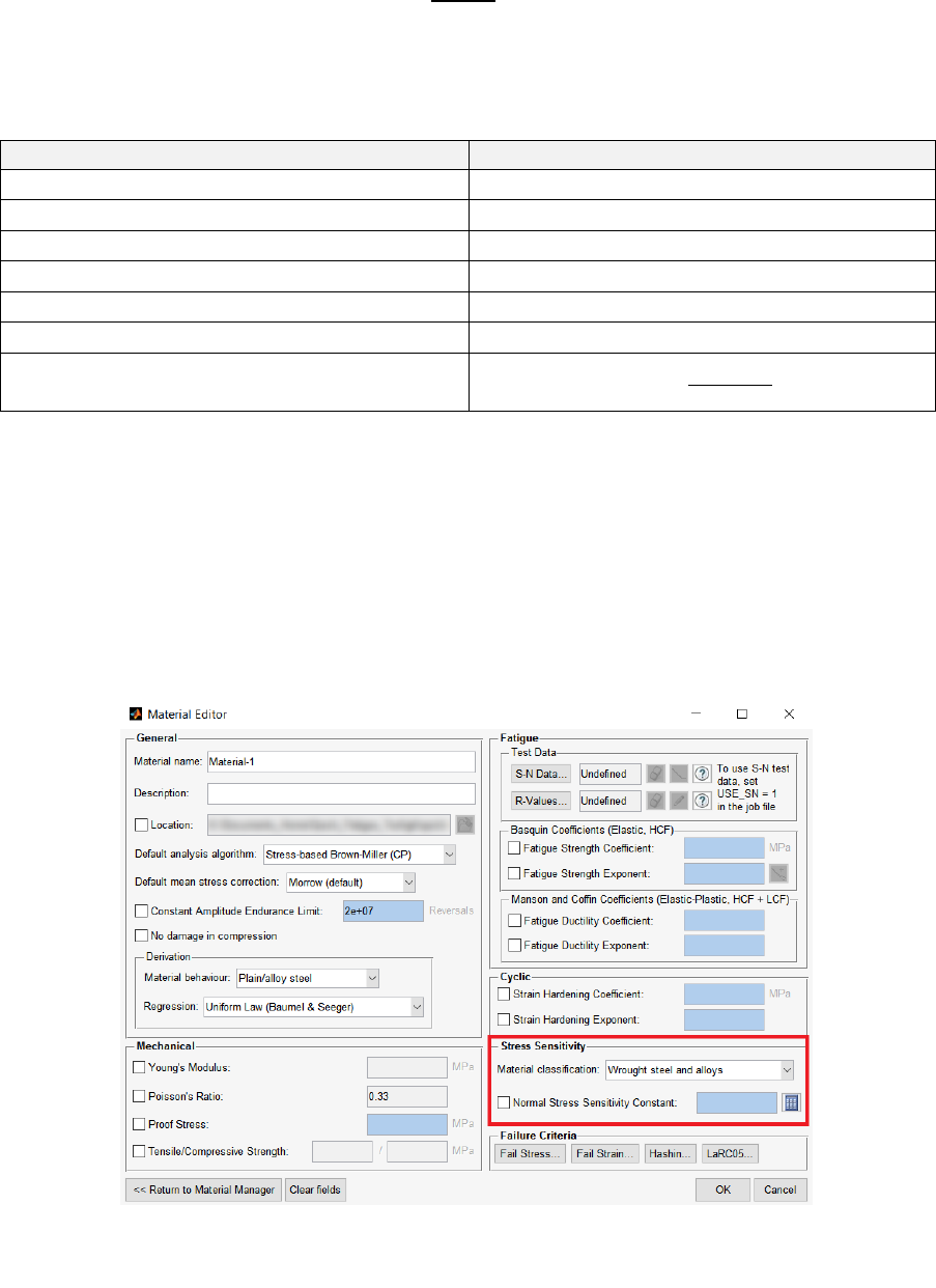
128
6.4.2 Determining the value of
The modified fatigue shear strength coefficient is calculated from the standard equation:
[6.4.2]
where is the fatigue shear strength coefficient. is obtained from the following table:
Material classification
Fatigue Shear Strength Coefficient
Wrought steel and alloys
Ductile iron
Malleable iron – pearlitic structure
Wrought iron
Cast iron
Aluminium/copper and alloys
Other
Guidance on defining material classification can be found in Section 5.9.
6.4.3 Determining the value of
The normal stress sensitivity constant is determined by comparing the fatigue limit of a material under
tension and torsion fatigue tests. The value of is specified in the Stress Sensitivity region of the
material editor (Figure 6.4.1).
Figure 6.4.1: Definition of the normal stress sensitivity constant in the material editor
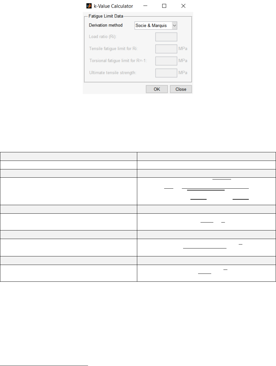
129
The value can either be specified directly by checking the box next to the input box, or a value may be
calculated based on the fatigue limit. This is done by clicking on the calculator button. The resulting
dialogue box is shown in Figure 6.4.2.
The value of is calculated according to the table below. Note that if the input field is left blank, the
Socie & Marquis value of 0.2857 will be assumed [28]. For ductile materials has a solution in the
range of [29].
Derivation Method
Solution
Socie & Marquis
General formula5
Dang van
Sines
Crossland
Where is the tensile fatigue limit for a load ratio , is the fully-reversed tensile fatigue limit and
is fully-reversed torsional fatigue limit. Since the derivation models attempt to approximate
based on the fatigue limit, they are not guaranteed to find a solution. In such cases, the Socie &
Marquis value may be used.
Note that defining as zero makes Findley’s Method a maximum shear stress criterion.
5
Requires the Symbolic Math Toolbox
Figure 6.4.2: Calculator tool to estimate the value of

130
6.4.4 Critical plane searching
Findley’s Method uses critical plane searching to determine the value of
. The stress
tensor on the critical plane is split into one normal and two shear components:
[6.4.3]
The variable is described in the document Quick Fatigue Tool Appendices: A1. The normal and shear
stress history is illustrated for a plane of an arbitrary orientation by Figure 6.4.3.
On these planes, the direction is always perpendicular to the plane on which the shear stresses
act. The quantity is the resultant shear stress history, which scribes the path . The value of the
maximum normal stress is simply the maximum value of the normal stress history, . Determining
the value of the maximum shear stress is less trivial.
Several methods have been proposed for determining the maximum shear stress. These include, but
are not limited to, the longest chord [30], the longest projection [31], the minimum circumscribed
circle [32], the minimum circumscribed ellipse [33] [34] and the maximum variance [35] [36] of the
path . It has been noted by Susmel [25] that the longest chord method is not only simple but also
very effective when applied in conjunction with the critical plane concept. Quick Fatigue Tool uses the
longest chord method to determine the maximum shear stress history on the critical plane. This is
given by Equation 6.4.4.
[6.4.4]
Figure 6.4.3: Normal and shear stress relative to plane
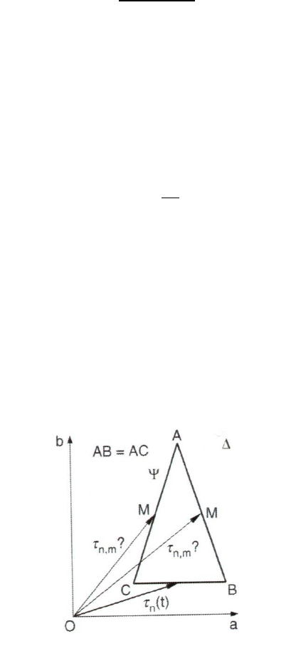
131
where and are two instants of the cyclic load history having period equal to . The maximum
chord method requires every shear pair along to be compared. Therefore, for large histories the
analysis may be slowed down significantly. In cases where the calculation time of the maximum shear
stress is unreasonable, the maximum resultant shear stress may be used instead:
[6.4.5]
This option is specified by in the environment file
Environment file usage:
Variable
Value
cpShearStress
{1.0 | 2.0}
The maximum chord method suffers from a theoretical set-back. Figure 6.4.4 illustrates how the mean
value of the shear stress cannot be defined with certainty when two or more reference chords having
the same length can be defined. However, Susmel states that from a practical point of view, this
ambiguity should not affect the accuracy in estimating high-cycle fatigue since the torsional mean
stress can be neglected provided that the maximum shear stress in the loading does not exceed the
material torsional yield strength.
The maximum chord method is only applied to the calculation of the maximum shear stress history on
the critical plane (output variable CS). For the critical plane analysis, the cycle counted shear quantity
is the resultant shear stress given by Equation 6.4.5.
Figure 6.4.4: Limitation of the longest chord method
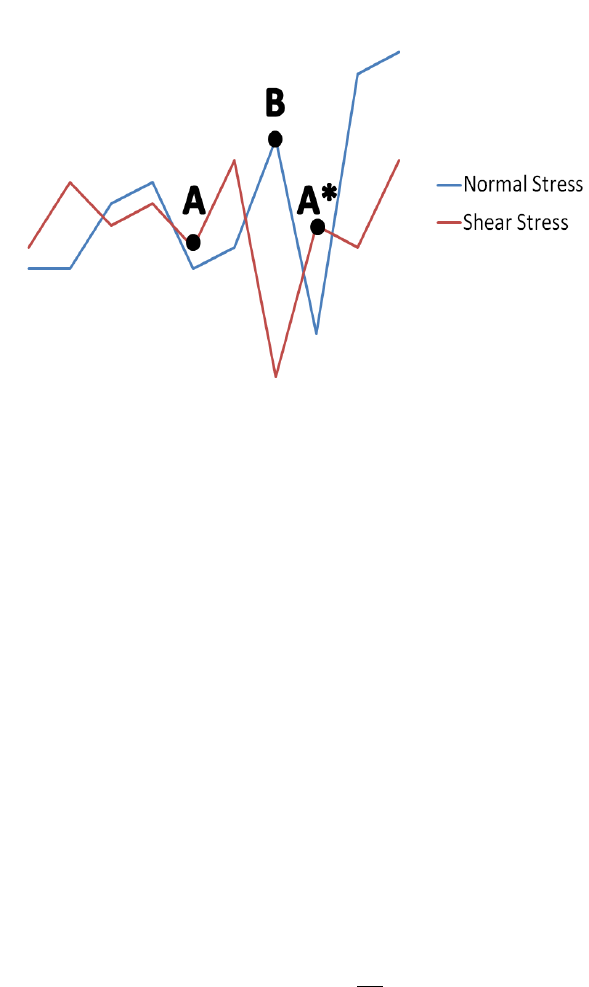
132
The maximum shear stress history on each plane is cycle counted using the Rainflow method described
in the document Quick Fatigue Tool Appendices: A1. It is not obvious how the maximum normal stress
should be combined with the shear stress cycles. This issue is illustrated by Figure 6.4.5.
By default, Quick Fatigue Tool uses the maximum normal stress which occurs in the interval of each
shear cycle. This behavior can be changed to use the average normal stress in each shear cycle interval
or the maximum normal stress over the entire loading. The latter is the most conservative approach.
Treatment of the normal stress is specified in the environment file.
Environment file usage:
Variable
Value
findleyNormalStress
{1.0 | 2.0 | 3.0}
Figure 6.4.5: A shear stress cycle with start and end points A and A*,
respectively. By default, the normal stress associated with the shear cycle A-
A* is the maximum normal stress occurring over the period of the shear cycle
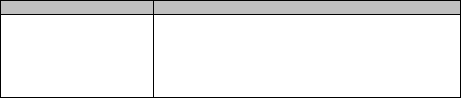
133
6.4.5 Output
The variables WCM and SFA have a slightly different meaning when using Findley’s Method:
Variable
Usual meaning
Findley’s Method
Mean value of the damage
parameter on the critical plane
(algorithm-dependent)
Mean value of the resultant
shear stress on the critical
plane
Ratio between the material
fatigue limit and the maximum
stress in the loading
Ratio between the material
fatigue limit and the Findley
parameter
6.4.6 Limitations
The critical plane search algorithm used by Findley’s Method is found to be very sensitive to the search
increment when compared to other algorithms which use critical plane searching. Therefore, Findley’s
Method is not compatible with load proportionality checking. The step size will always be the value
defined in the environment file.
Literature sources reference the shear stress in conjunction with Rainflow cycle counting. However, it
is not clear which shear stress quantity should be cycle counted. Currently, Quick Fatigue Tool uses
the resultant shear stress history as the cycle counting parameter. This has the drawback that the
resultant shear stress is always positive. In order to circumvent this problem, a scheme similar to that
used by the Stress Invariant Parameter algorithm is used, whereby the shear stress history is multiplied
by a factor based on a pre-determined sign convention (Section 6.5.3).
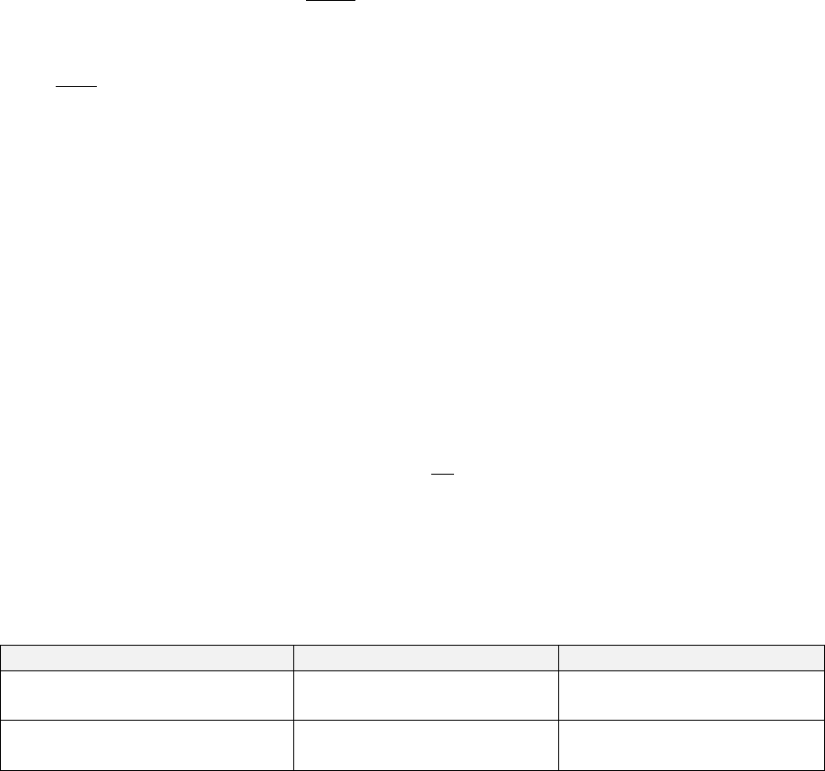
134
6.5 Stress Invariant Parameter
6.5.1 Overview
The Stress Invariant Parameter analysis algorithm uses a Cauchy stress invariant term as the damage
parameter in the stress-life relationship:
[6.5.1]
where
is the effective stress amplitude. The user can specify one of the following stress invariant
parameters as the effective stress amplitude:
0. Program controlled
1. von Mises
2. Principal
3. Hydrostatic
4. Tresca
The parameter is specified in the environment file.
Environment file usage:
Variable
Value
stressInvariantParameter
{0.0 | 1.0 | 2.0 | 3.0 | 4.0}
The value of stressInvariantParameter takes its meaning from the list above.
The following material properties are required to perform an analysis with the Stress Invariant
Parameter algorithm:
Property
Symbol
Importance
Tensile fatigue strength
coefficient
REQUIRED
Tensile fatigue strength
exponent
REQUIRED
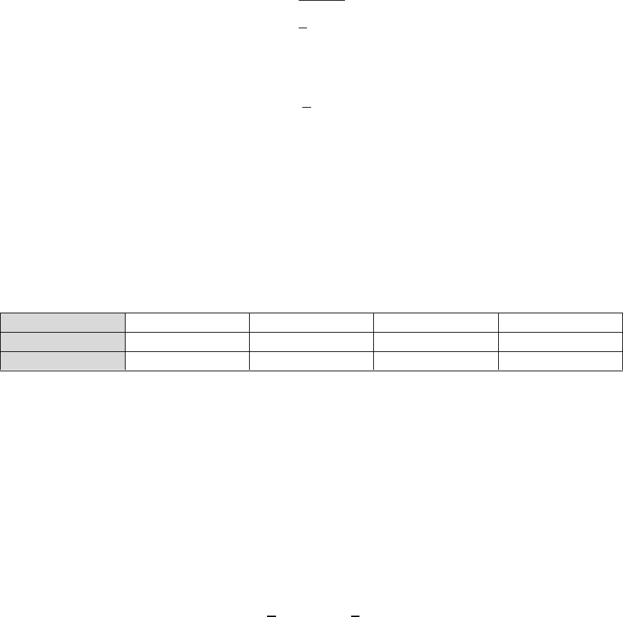
135
6.5.2 Effective stress parameters
von Mises
The von Mises stress is based on the second invariant stress, and provides an estimate of the onset of
yielding. The von Mises stress is given by Equation 6.5.2:
[6.5.2]
where are the components of the stress deviator tensor :
[6.5.3]
Principal
The principal stress parameter defines the load history as the largest (positive or negative) principal
stress at each point in the loading. For example, if the absolute value of the minimum principal stress
is larger than the value of the maximum principal stress at a given loading point, then the minimum
principal stress is used for that point. The following load history illustrates the use of the principal
stress as the invariant parameter.
S1
349
294
174
441
S3
-294
-349
-147
-523
Load history
349
-349
174
-523
The principal stress is valid for uniaxial test data. Loadings which exhibit a high degree of biaxiality do
not correlate well to the principal stress, since failure is not guaranteed to occur at the locations of
maximum stress. For loadings which exhibit a high degree of non-proportionality, the direction of the
principal stress will change throughout the history; in such cases, the Normal Stress algorithm is
recommended instead.
Hydrostatic
The hydrostatic stress defines the load history in terms of the equivalent pressure stress.
[6.5.4]
The hydrostatic stress is an isotropic parameter given by the average of the direct pressure forces
acting on a body. Deformation states dominated by expansion correlate well with a hydrostatic
criterion. The hydrostatic stress parameter is less conservative than the principal stress parameter.
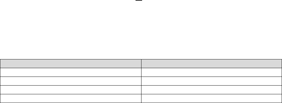
136
Tresca
The Tresca stress is defined as the maximum difference between the first and third principal stress.
[6.5.5]
The Tresca stress is the maximal shear stress and is used as a yield criterion for ductile metals. As a
fatigue criterion, the Tresca stress assumes that crack initiation is driven by states of pure shear. This
can provide reasonable estimates for shear-dominated loads with a high degree of proportionality. In
all other cases, a balanced shear-normal biaxial criterion such as the Stress-based Brown-Miller
algorithm or Findley’s method is recommended instead.
Program controlled
Quick Fatigue Tool can attempt to choose a suitable stress invariant parameter. The applicability of a
given stress invariant parameter depends on the biaxiality ratio, :
[6.5.6]
Stress invariants are applicable to uniaxial () and equibiaxial () loads, as well as
proportional biaxial loads () [37]. The table below shows the applicable range of the
biaxiality ratio for each stress invariant parameter.
Invariant
Range of
von Mises
and
Principal
Hydrostatic
Tresca
The stress invariant parameter is chosen on the basis of the applicable range of . If no suitable
parameter can be found, the principal stress is used by default.
The range of over the loading is printed in the message file at the item with the largest principal
stress, for each analysis group.

137
6.5.3 Specifying a sign convention
The von Mises and Tresca stresses are always positive, meaning that damage in compression is
neglected. A material element in a state of pure hydrostatic compression appears to experience zero
effective stress, even if the volumetric deformation is large enough to cause fatigue damage. The
solution is to correct the stresses by using a criterion which determines the correct sign of the effective
stress parameter. Quick Fatigue Tool corrects the stresses based either on the sign of the hydrostatic
stress or the largest principal stress. The sign convention is set from the environment file.
Environment file usage:
Variable
Value
signConvention
{1.0 | 2.0 | 3.0}
6.5.4 Additional guidance
The stress invariant parameters do not correlate well to multiaxial stress states. Although the
algorithm can be used to quickly locate the region of expected maximum stress, the location of
maximum damage can often be elsewhere due to the fact that the in-plane principal directions can
change during the loading. Thus, the Stress Invariant Parameter analysis algorithm is included for
completeness only; none of the invariants are recommended as a damage parameter except for the
simplest cases.
The user should check the validity of the selected stress invariant parameter before the analysis. This
can be done by setting DATA_CHECK=1 in the job file and inspecting the message file for feedback
regarding the selected parameter. The following points should be observed:
for , the Tresca stress is very conservative; the von Mises stress is conservative;
the principal stress is acceptable;
for , the Tresca, von Mises and principal stresses are all acceptable;
for , the Tresca stress is acceptable; the von Mises stress is non-conservative; and
for , both the Tresca and von Mises stresses are acceptable.
Critical plane searching is not required, and rough estimates of life can be obtained very quickly.
However, the Stress Invariant Parameter algorithm is not considered to be a valid durability
assessment criterion for general fatigue analysis problems [6].
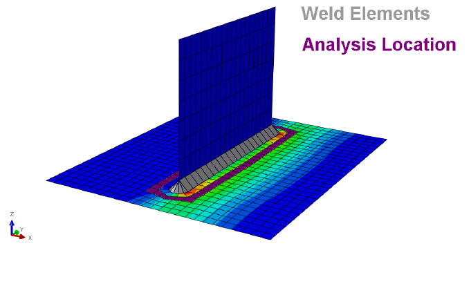
138
6.6 BS 7608 Fatigue of Welded Steel Joints
6.6.1 Overview
Quick Fatigue Tool includes an implementation of the British Standard BS 7608:1993 code of practice
for fatigue design and assessment of steel structures [38]. The standard is applicable to the following:
a) Parent material remote from joints
b) Welded joints (in air or sea water) in such material
c) Bolted or riveted joints in such material
d) Shear connectors between concrete slabs and steel girders acting compositely in flexure
The standard offers a family of curves based on weld geometry criteria, spanning ten weld
classifications. The damage parameter is the stress range acting on the critical plane. The code
stipulates that the stress range is whichever of the two in-plane principal stresses lie within +/- 45
degrees of an axis perpendicular to the weld toe. However, Quick Fatigue Tool performs a full critical
plane search in a spherical coordinate space. The user may choose between the normal and the shear
stress as the damage parameter.
The standard is based on the assumption that the exact stresses at the weld toe cannot be determined
analytically. The provided curves account for the effect of the stress concentration, thus the
analyst need only compute the stresses as if the weld feature did not exist. If the stress solution is
obtained from finite element analysis and the weld detail is modelled, the calculated stress range may
be greatly overestimated and could result in highly conservative fatigue life predictions. Therefore, in
such cases the analyst should choose the stress a short distance away from the weld toe, an example
of which is given in Figure 6.6.1.
Figure 6.6.1: Example analysis location for BS 7608
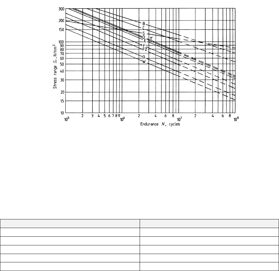
139
6.6.2 Derivation of the curve
The curve is defined explicitly as Equation 6.6.1
[6.6.1]
where is the stress range, is the Paris Law exponent related to the energy release rate of a crack,
is the number of cycles to failure and is a constant relating to the weld classification. The resulting
curves are shown in Figure 6.6.2. The curves are material-independent and as such, no material
needs to be specified in the job file.
The weld classification constant, , is related to the probability of failure by the number of standard
deviations from the mean curve. The number of deviations, , can be specified in the job file.
For example, a value of means that there is a probability that the component will fail before
the predicted life. Some values of and their corresponding probabilities of failure are given below.
Probability of failure (%)
50
0.0
69
0.5
84
1.0
97.7
2.0
99.86
3.0
A value of corresponds to the mean-line curve, while a value of corresponds to
the standard design curve.
Figure 6.6.2:
curve family for BS 7608
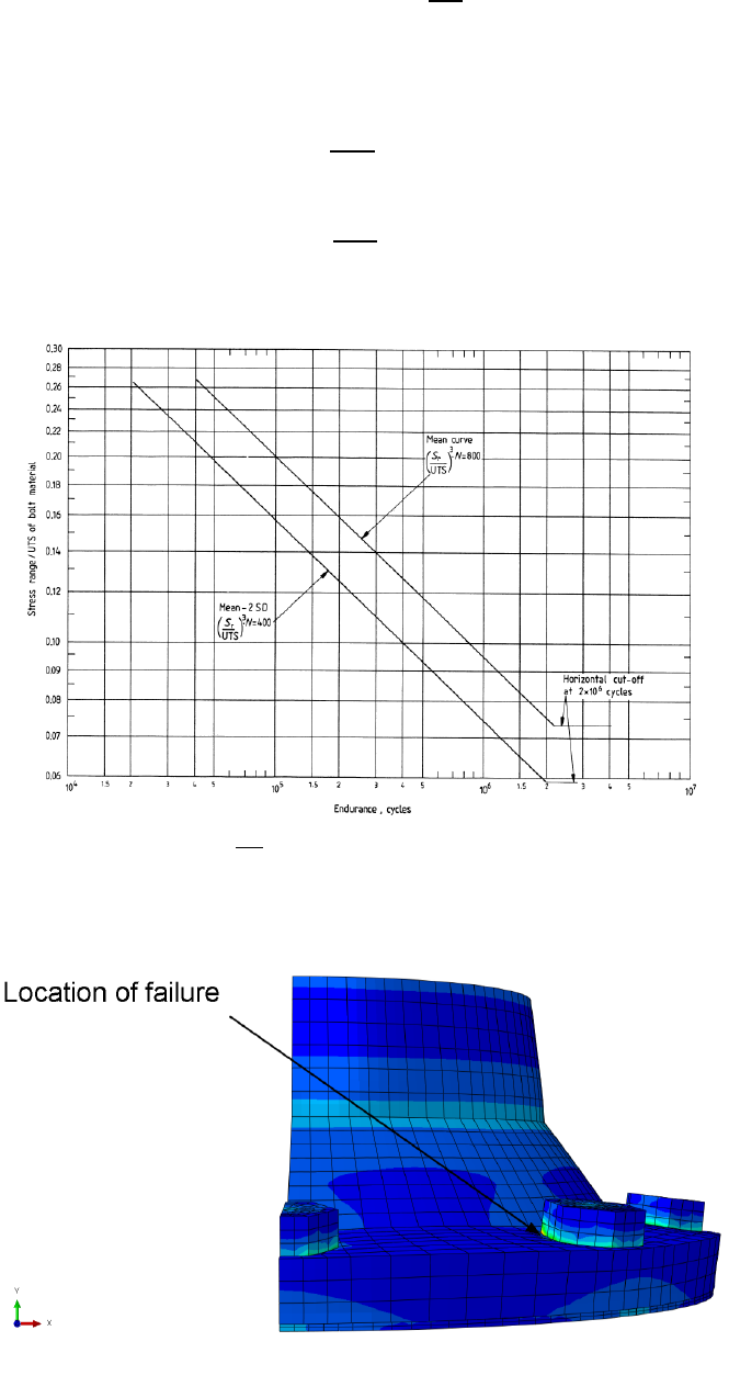
140
6.6.3 Analysis of axially loaded bolts
In addition to welded joints, BS 7608 also offers a set of
curves for axially loaded bolts with
cut, ground or rolled threads up to 25mm in diameter. These curves belong to class X. The curves are
defined by Equations 6.6.2-3 and illustrated by Figure 6.6.3.
[6.6.2]
[6.6.3]
Figure 6.6.4: Example of a bolt failure in FEA
Figure 6.6.3:
curve family for axially loaded bolts

141
The
curves in this classification are only defined for the mean line or two standard deviations
from the mean. The ultimate tensile strength of the bolt feature must be provided. The
curves
are valid only for values of the ultimate tensile strength up to 785MPa.
If the bolt is modelled in FEA such as the one shown in Figure 6.6.4, the effective stress should be
taken a small distance away from the stress concentration at the location of crack initiation otherwise
the fatigue analysis will produce conservative results.
Job file usage:
Option
Value
WELD_CLASS
'X'
6.6.4 Effect of the characteristic length
For welded joints, the characteristic length is the plate thickness. For class X (axially loaded bolts), the
bolt diameter is used instead.
The fatigue life of welded joints and bolts reduces with increasing characteristic length. If a value for
the weld length is specified in the job file, the curve may be scaled according to Equation
6.6.4
[6.6.4]
where is the fatigue strength of a weld (or bolt) of thickness (or diameter) and is the fatigue
strength of the weld without considering the effect of thickness (or diameter). The characteristic
length is given in units of . The curves are already valid for the lengths given by the table
below. Thus, the correction is only performed if the specified length lies outside the pre-defined range.
Classification
Range of characteristic length
Nodal joints (Class T)
only
Non-nodal joints (Classes B to G)
Up to
Bolts (Class X)
Up to diameter
All other weld classes
only
6.6.5 Effect of stress relief
BS 7608 assumes that the stress range is the sum of the tensile and 60% of the compressive
component of the cycle. For example, if a cycle has a range of -100 to 50, the effective range will be
calculated as .
6.6.6 Effect of small cycles
BS 7608 stipulates that earlier fatigue failure could be predicted if it is assumed that that all stress
ranges below the fatigue limit are non-damaging. Thus, the Paris Law exponent is changed from to
for cycles below the fatigue limit, at which the calculated life is 1e7 cycles.

142
6.6.7 Effect of large cycles
BS 7608 stipulates that the curves may be extrapolated no further than twice the material’s
yield strength. Cycles exceeding this value will result in non-fatigue failure.
6.6.8 Effect of exposure to sea water
Unprotected welds situated in sea water accumulate fatigue damage faster than the same weld in
fresh air. If the effect of sea water is specified in the job file, the correction for small cycles is ignored
and the fatigue strength of the weld is reduced by a factor of two.
6.6.9 Failure mode
According to BS 7608, the damage parameter is taken as the principal stress acting on the critical
plane. However, the implementation in Quick Fatigue Tool allows the user to choose between a pure
normal, pure shear and combined normal-shear stress criterion, depending on how the crack is
expected to propagate.
Job file usage:
Option
Value
FAILURE_MODE
{'NORMAL' | 'SHEAR' | 'COMBINED'}
The damage parameter quoted in the field output corresponds to either the normal, shear or
combined (normal + shear) stress on the critical plane, according to the definition of the above option.
6.6.10 Specifying the curve as a BS 7608 weld class
The curve can be defined by one of the ten standard BS 7608 weld classes. Choice of weld class
requires knowledge of the weld features and access to Section 2. Classification of details from
document BS 7608:1993.
Job file usage:
Option
Value
WELD_CLASS
{'B' | 'C' | 'D' | 'E' | 'F' | 'F2' | 'G' | 'W' | 'S' | 'T'}
6.6.11 Specifying the curve as user data
The can be defined as tabulated data.
Job file usage:
Option
Value
WELD_CLASS
'user-weld-curve-file-name.sn'
The format of the user data file should meet the requirements explained in Section 5.4. The
values in the data file must be provided in terms of the stress range. values are assumed to be
143
provided at a load ratio of ; values defined over multiple load ratios are not accepted. The
fatigue limit is taken as the last value in the data.
By default, Quick Fatigue Tool processes the user in a column-wise fashion:
.
.
However, both column-wise and row-wise data may be provided by indicating this in the job
file.
Job file usage:
Option
Value
WELD_CLASS
{'user-weld-curve-file-name.sn', ['ROW' | 'COL']}
6.6.12 Compatibility with other features
The BS 7608 method is not compatible with the following analysis features:
Mean stress correction
Nodal elimination
Plasticity correction
S-N data (USE_SN)
S-N Scale factors (SN_SCALE)
S-N knockdown curves (SN_KNOCK_DOWN)
Fatigue notch factors
The following output variables are not available:
FOS, SFA, FRFH, FRFV, FRFR, FRFW

144
6.6.13 Configuring the analysis parameters
Material properties are not required to perform analyses with BS 7608. However, the user can
configure algorithm-specific settings from the job file in the “Algorithm Specific Settings” section. The
available options are shown below. For a description of each option, consult the document
Quick Fatigue Tool User Settings Reference Guide.
Option
Meaning
Importance
WELD_CLASS
curve for analysis
REQUIRED
YIELD_STRENGTH
Used to set extrapolation
limit
OPTIONAL
UTS
Used to define
curve
REQUIRED6
DEVIATIONS_BELOW_MEAN
Standard deviations below
mean curve
REQUIRED
FAILURE_MODE
Failure criterion
(normal or shear)
OPTIONAL
CHARACTERISTIC_LENGTH
Plate thickness or
bolt diameter
OPTIONAL
SEA_WATER
Fatigue strength correction
for sea water exposure
OPTIONAL
6
For Class X welds only.

145
6.7 NASALIFE
6.7.1 Overview
NASALIFE is a fatigue life prediction software developed by General Electric Aircraft Engines and the
NASA Enabling Propulsion Materials program, to assess the durability of ceramic matrix composites
(CMCs) subject to varying thermo-mechanical loads. The methodology is required by some regulatory
bodies in the aviation sector for the validation of aero engine components [39].
6.7.2 Methodology
The NASALIFE method has been partially implemented in Quick Fatigue Tool as a stress-based, HCF
fatigue analysis algorithm. The analysis procedure is as follows:
1. Explore all possible stress pair (cycle) combinations in the load history
2. For each cycle, calculate the effective mean stress and stress amplitude based on the effective
stress parameter
3. Using the Walker mean stress correction, find the cycle pair with the largest damage. This is
the most damaging major cycle (MDMC)
4. For the MDMC, find the principal directions and orientation of the octahedral shear plane
5. Align the stress tensor history with the octahedral plane of the MDMC and convert the stress
tensor history into the octahedral shear stress history
6. Rainflow cycle count the shear stress history and record the position index of each cycle in
the stress history
7. Convert the effective stress history into a matrix of cycles based on the indexes from step 6
8. Repeat steps 2 and 3 to calculate the damage of each cycle
The stress tensor history is organized into all possible pairs using the combination formula given by
Equation 6.7.1:
[6.7.1]
where is the number of stress tensor pair combinations from a loading consisting of history
points.
Each cycle is calculated from an effective stress parameter. This parameter is explained in more detail
in Section 6.7.3. For the case of the Manson McKnight parameter, the equivalent mean stress and
stress amplitude are calculated by Equations 6.7.2-3, respectively.
[6.7.2]
[6.7.3]
Where is the first stress invariant (hydrostatic stress).
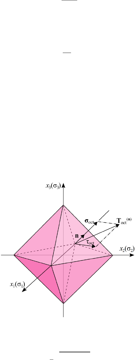
146
Each stress cycle is corrected for the effect of mean stress using the Walker mean stress correction in
Equation 6.7.4:
[6.7.4]
where is the effective stress amplitude due to cycle , the load ratio and the Walker parameter
. The method of calculating is discussed in Section 7.7. The -ratio is calculated as Equation 6.7.5:
[6.7.5]
If the -ratio is less than or greater than , the Walker mean stress correction is modified to
Equation 6.7.6:
[6.7.6]
The mean stress correction is limited to positive mean stress only; negative mean stress will not
increase the fatigue life of the component.
The MDMC is resolved onto octahedral planes, shown by Figure 6.7.1. The octahedral shear stress,
, is given by Equation 6.7.7.
[6.7.7]
Figure 6.7.1: Octahedral planes showing the unit normal and
shear directions

147
where is the second stress invariant, and is related to the von Mises stress, , by Equation 6.7.8.
[6.7.8]
After identifying the octahedral shear plane, the original stress history is transformed to the
principal directions of the MDMC using the rotation matrix and tensor transform given by
Equations 6.7.9-10, respectively:
[6.7.9]
where are the principal and are the normal stresses of the MDMC tensor.
[6.7.10]
Where and are the rotated and un-rotated stress tensors for each point in the load history,
respectively.
The transformed load history is resolved into its octahedral shear component and then cycle counted.
The indices of the octahedral shear cycles are then used with the original tensor history to locate stress
cycles from the effective stress. The damage per cycle is calculated using Equation 6.7.11:
[6.7.11]

148
6.7.3 The effective stress parameter
The NASALIFE algorithm uses one of five effective stress parameters for the calculation of the cycle
combinations. The effective stress parameter is set in the environment file.
Environment file usage:
Variable
Value
nasalifeParameter
{1.0 | 2.0 | 3.0 | 4.0 | 5.0}
1. Manson-McKnight
When nasalifeParameter=1.0, the Manson-McKnight parameter is selected. The effective mean stress
and stress amplitude are based on the concept of a signed von Mises stress, given by
Equations 6.7.12-13. The sign is taken from the hydrostatic stress of the current cycle.
[6.7.12]
[6.7.13]
For situations where the loading is shear-dominated, the sign of the mean stress can be unreliable.
Therefore, if the signs of the maximum and the minimum principal stresses differ, a modified version
of the Manson-McKnight method is used instead, given by Equation 6.7.14:
2. Sines
When nasalifeParameter=2.0, the Sines parameter is selected. The Sines method determines the
effective mean stress as the hydrostatic stress [40]. The effective stress amplitude is then modified by
the mean stress. These are given by Equations 6.7.15-16:
[6.7.15]
[6.7.16]
The constant is intended to have a value of for uniaxial loads and for multiaxial loads.
However, the loading is assumed to be multiaxial and a value of is always used.
The -ratio is assumed to be infinite, hence the Walker mean stress correction takes the modified
form of Equation 6.7.6.
[6.7.14]

149
3. Smith-Watson-Topper
When nasalifeParameter=3.0, the Smith-Watson-Topper parameter is selected. The Smith-Watson-
Topper method assumes that the effective mean stress is zero, therefore for loadings with a load ratio
of , use of this parameter will produce highly non-conservative results. The effective stress
amplitude is a function of the maximum and the minimum value of the first principal stress of the
current cycle [41]. These are given by Equations 6.7.17-18:
[6.7.17]
[6.7.18]
4. R-Ratio Sines
When nasalifeParameter=4.0, the R-Ratio Sines parameter is selected. The R-Ratio Sines Method uses
the hydrostatic stress as the effective mean stress, but keeps the original definition of the effective
stress amplitude. These are given by Equations 6.7.19-20:
[6.7.19]
[6.7.20]
5. Effective Method
When nasalifeParameter=5.0, the Effective Method parameter is selected. The Effective Method
defines the effective mean stress as twice the distortion energy minus the effective stress amplitude.
The effective stress amplitude takes the same from as that from the Manson McKnight method. These
are given by Equations 6.7.21-22:
[6.7.21]
[6.7.22]

150
6.7.4 Defining a NASALIFE analysis
NASALIFE analyses require the following material parameters:
Property
Symbol
Importance
Tensile fatigue strength
coefficient
REQUIRED
Tensile fatigue strength
exponent
REQUIRED
Ultimate tensile strength
OPTIONAL
Walker gamma parameter
REQUIRED7
6.7.5 Guidance for load history gating
The NASALIFE algorithm locates the MDMC by considering every stress tensor combination in the load
history. If tensor gating is enabled then the original, un-gated load history is used, and the resulting
analysis time can become very large. If the load history contains many data points, it may be expedient
to pre-gate the load histories.
Environment file usage:
Variable
Value
gateTensors
0.0
gateHistories
1.0
Care should be taken when pre-gating multiple load histories, as the phase relationship between the
loading channels may be lost and the accuracy of the fatigue result may be adversely affected.
7
This parameter can be user-defined or computed automatically. Consult Section 7.7 for detailed information
about the Walker gamma parameter.
151
6.8 Uniaxial Stress-Life
6.8.1 Overview
Uniaxial Stress-Life is the most basic fatigue analysis technique. The method is ideal for simple loading
conditions where fatigue damage is caused primarily by stresses in a single direction. The algorithm is
especially useful for measured stress data from plane stress specimens. Since the algorithm does not
require critical plane searching, it is computationally much less expensive than the biaxial methods
such as the Stress-based Brown-Miller fatigue algorithm.
The Uniaxial Stress-Life algorithm is defined by Equation 6.8.1:
[6.8.1]
where
is the uniaxial stress amplitude.
6.8.2 Defining a uniaxial stress-life analysis
The Uniaxial Stress-Life algorithm only requires a single stress history. Stress datasets are not
recognised by the program.
Job file usage:
Option
Value
DATASET
[ ]
HISTORY
'history-file-name.*'
The following material properties are required to perform an analysis with the Uniaxial Stress-Life
algorithm:
Property
Symbol
Importance
Fatigue strength coefficient
REQUIRED
Fatigue strength exponent
REQUIRED

152
6.9 Uniaxial Strain-Life
6.9.1 Overview
Uniaxial Strain-Life is a method for analysing simple unidirectional strain histories. The uniaxial elastic
stress history is converted into an inelastic strain history using the Ramberg-Osgood nonlinear elastic
strain-hardening model. The same model is used to convert the elastic principal stress histories into
inelastic principal strain histories.
The Uniaxial Strain-Life algorithm is defined by Equation 6.9.1:
[6.9.1]
where
is the uniaxial strain amplitude.
6.9.2 Defining a uniaxial strain-life analysis
The Uniaxial Strain-Life algorithm only requires a single elastic stress history. Stress datasets are not
recognised by the program.
Job file usage:
Option
Value
DATASET
[ ]
HISTORY
'history-file-name.*'
The following material properties are required to perform an analysis with the Uniaxial Strain-Life
algorithm:
Property
Symbol
Importance
Fatigue strength coefficient
REQUIRED
Fatigue strength exponent
REQUIRED
Fatigue ductility coefficient
REQUIRED
Fatigue ductility exponent
REQUIRED
Young’s Modulus
REQUIRED
Cyclic strain-hardening coefficient
REQUIRED
Cyclic strain-hardening exponent
REQUIRED

153
6.10 User-defined algorithms
6.10.1 Overview
The Quick Fatigue Tool framework allows the user to create their own fatigue analysis algorithm.
Information is passed into the class algorithm_user, which is used to evaluate the fatigue damage at
each analysis item.
The user algorithm class file algorithm_user.m is located in Application_Files\code\main. The file
contains a single function called main. This is the function which Quick Fatigue Tool calls iteratively for
each analysis item.
The class algorithm_user can be expanded so that the function main calls other functions within
algorithm_user.
6.10.2 Variables passed in for information
Quick Fatigue Tool passes the following arguments into algorithm_user.main:
Argument
Description
Notes
S11
Stress tensor history in the
normal Cartesian 1-direction.
S22
Stress tensor history in the
normal Cartesian 1-direction.
S33
Stress tensor history in the
normal Cartesian 1-direction.
S12
Stress tensor history in the
shear Cartesian 12-direction.
S23
Stress tensor history in the
shear Cartesian 23-direction.
S13
Stress tensor history in the
shear Cartesian 13-direction.
N
Current analysis item number.
N = 1 unless the stress dataset
contains more than one
analysis item.
MSC
Identifier defining the selected
mean stress correction.
Consult Section 7.1 for a table
relating the value of MSC to the
mean stress correction.

154
6.10.3 Variables to be defined
The user must define the following output arguments:
Argument
Description
Format
Example usage (per analysis item)
DPARAMI
Maximum damage
parameter at the current
analysis item.
numeric
array.
DPARAMI() = ;
X is the maximum damage
parameter.
AMPI
Stress amplitude of each
cycle for the loading at the
current analysis item.
cell array.
AMPI{} = [, ,…, ];
to are the amplitudes over
the load history.
PAIRI
Cycle pairs for the loading
at the current analysis
item.
cell array.
PAIRI{} = [, ;…;
, ];
and are the minimum
and maximum cycle values for
each pair in the loading.
DAMI
Total damage for the
loading at the current
analysis tem.
numeric
array.
DAMI() = ;
is the total damage over the
load history.
is the number of analysis items; is the number of cycle in the load history; is the current analysis
item.
6.10.4 Material properties
Material properties are accessed using the getappdata() method:
property = getappdata(0, 'identifier');
A complete list of material properties and their identifiers is given below:
Property
Identifier
Property
Identifier
Young’s modulus
E
Default analysis algorithm
defaultAlgorithm
Poisson’s ratio
poisson
Default mean stress correction
defaultMSC
Ultimate tensile strength
uts
Constant amplitude
endurance limit
cael
Proof stress
twops
S-N data points: S-values
(interpolated at R=-1)
s_values_reduced
S-N data points: S-values
s_values
S-N data points: Number of
curves
nSNDatasets
S-N data points: N-values
n_values
Fatigue strength exponent at
knee-point
b2
S-N data points: R-values
r_values
Life at knee-point
b2Nf
Fatigue strength coefficient
Sf
Fatigue limit
fatigueLimit
Fatigue strength exponent
b
Residual stress
residualStress
Fatigue ductility coefficient
Ef
Surface finish
kt
Fatigue Ductility exponent
c
Notch sensitivity constant
notchRootRadius
155
Cyclic strain hardening
coefficient
kp
Notch root radius
notchSensitivityConstant
Cyclic strain hardening
exponent
np
Normal stress sensitivity
constant
k
If analysis groups are used, material properties will depend on which group the current analysis item
belongs to.
6.10.5 Utility functions
User-defined algorithms can call to other Quick Fatigue Tool functions to facilitate the analysis.
Rainflow cycle counting
A stress history can be cycle counted using the following function:
M-file usage:
rfData = analysis.rainflow(history);
The variable rfData is a matrix where is the number of counted cycles. The first two columns
are the cycle points. The last two columns are the indexes in the stress history corresponding to the
cycle.
The amplitude of each cycle is extracted using the following function:
M-file usage:
pairs = rfData(:, 1.0:2.0);
amplitudes = analysis.getAmps(pairs);
Mean stress correction
The variables pairs and amplitudes, as defined above, can be corrected for the effect of mean stress.
M-file usage:
[mscAmplitudes, ~, ~] = analysis.masc(amplitudes, pairs, MSC);
The variable MSC is the identifier which is passed into algorithm_user.main.
156
6.10.6 Additional stress histories
Before the analysis, Quick Fatigue Tool calculates the principal stress and von Mises stress history.
These can be accessed at the current analysis item using getappdata():
History variable
Definition
First principal stress
getappdata(0, 'S1');
Second principal stress
getappdata(0, 'S2');
Third principal stress
getappdata(0, 'S3');
Von Mises stress
getappdata(0, 'VM');
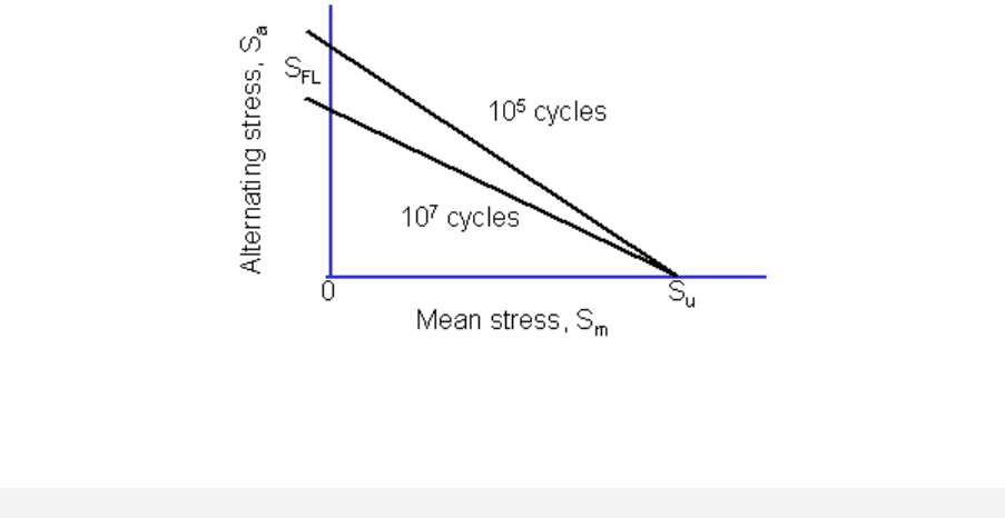
157
7. Mean stress corrections
7.1 Background
Tensile mean stresses tend to reduce the fatigue life of components, so a mean stress correction is
necessary in order to obtain accurate life predictions.
Mean stress corrections are usually represented by Haigh diagrams, which gives the allowable stress
amplitude as a function of the mean stress (Figure 7.1). Each line on the Haigh diagram represents the
allowable combinations of stress amplitude and mean stress for a given fatigue life.
Quick Fatigue Tool offers several mean stress corrections, depending on the selected algorithm:
Algorithm
Available Mean Stress Corrections
Stress-based Brown Miller
Morrow
Goodman
Gerber
Soderberg
R-Ratio S-N Curves
User-defined
Normal Stress
Morrow
Goodman
Gerber
Walker
R-Ratio S-N Curves
Smith-Watson Topper
User-defined
Findley’s Method
None (built-in)
Figure 7.1: Haigh diagram showing contours of constant life.
Image courtesy of eFatigue.

158
Stress Invariant Parameter
Goodman
Gerber
Walker
R-Ratio S-N Curves
User-defined
BS 7608
None (built-in)
Uniaxial Stress-Life
Goodman
Gerber
Walker
Soderberg
R-Ratio S-N Curves
User-defined
Uniaxial Strain-Life
Morrow
Smith-Watson-Topper
Walker
NASALIFE
Walker (built-in)
The mean stress correction is specified from the job file. If the default mean stress correction is
specified Quick Fatigue Tool will use the correction defined in the material .mat file.
Mean stress correction
Job file option
Default
{MS_CORRECTION=0.0 | 'DEFAULT'}
Morrow
{MS_CORRECTIO 1.0 | 'MORROW'}
Goodman
{MS_CORRECTION=2.0 | 'GOODMAN'}
Soderberg
{MS_CORRECTION=3.0 | 'SODERBERG'}
Walker
{MS_CORRECTION=4.0 | 'WALKER'}
Smith-Watson-Topper
{MS_CORRECTION=5.0 | 'SWT'}
Gerber
{MS_CORRECTION=6.0 | 'GERBER'}
R-ratio S-N curves
{MS_CORRECTION=7.0 | 'RATIO'}
None
{MS_CORRECTION=8.0 | 'NONE'}
User-defined
{MS_CORRECTION='filename.msc'}

159
7.2 Goodman
The Goodman mean stress correction assumes that, for mirror polished specimens, the relationship
between the allowable stress amplitude and tensile mean stress is linear [42]:
[7.1]
Equation 7.1 can be plotted on a Haigh diagram to give Figure 7.2.
For each cycle in the loading, Quick Fatigue Tool evaluates the mean stress and finds the equivalent
stress amplitude as if the cycle had zero mean stress. This is achieved by re-arranging Equation 7.1
into Equation 7.2:
[7.2]
It should be noted that, when using the Goodman mean stress correction, Quick Fatigue Tool assumes
that the equivalent stress amplitude has zero mean stress. Therefore, if custom S-N data is being used
which was measured at an R-ratio other than -1 then the Goodman correction will not produce a
reliable solution.
Figure 7.2: Haigh diagram representation of Goodman relationship for different reference lives. The curves meet the
material’s ultimate tensile strength.
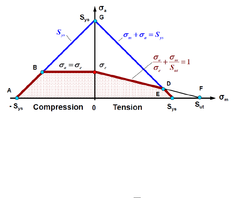
160
Modified Goodman envelopes
The standard implementation of the Goodman mean stress correction is non-conservative for large
values of mean stress and assumes no change in the allowable stress amplitude for negative mean
stress. A modified version of the Goodman correction combines the standard slope with the Buch line,
shown in Figure 7.3.
The modified Goodman envelope is enabled from the environment file.
Environment file usage:
Variable
Value
modifiedGoodman
{0.0 | 1.0}
The modified Goodman envelope requires a value of the proof stress. If the proof stress is undefined,
the standard Goodman envelope is used instead.
Care must be taken when using the Goodman mean stress correction. Since the stress amplitude is
zero along the horizontal axis, there is no fatigue in this regime. The assumption that the limiting
fatigue strength is equal to the static tensile strength is therefore incorrect, since static and fatigue
failure are driven by physically distinct mechanisms. The Goodman correction can often over predict
fatigue lives by a factor of three to four. In cases where the Goodman correction fails to produce
acceptable results, the Walker correction is recommended as an alternative.
Figure 7.3: Modified Goodman line (red), defined by the intersection of the standard line (black) with the
Buch line (blue); copyright © Professor Grzegorz Glinka [58]; reproduced with permission.
161
Setting the Goodman limit stress
By default, the intercept between the Goodman envelope and the horizontal (mean stress) axis is
the material ultimate tensile strength. This intercept value can be changed by the user from the
environment file.
Environment file usage:
Variable
Value
goodmanMeanStressLimit
The value of can be set as follows:
'UTS'
Material UTS
'PROOF'
Material 0.2% proof stress
'S-N'
S-N intercept (at 1 repeat)
User-defined value
When the modified Goodman envelope is enabled, the Goodman limit stress is taken as the yield
strength and cannot be modified by the user.

162
7.3 Soderberg
The Soderberg mean stress correction is similar to Goodman, but uses the proof stress as the
maximum allowable mean stress [43]:
[7.3]
It should be noted that, when using the Soderberg mean stress correction, Quick Fatigue Tool assumes
that the equivalent stress amplitude has zero mean stress. Therefore, if custom S-N data is being used
which was measured at an R-ratio other than -1, then the Soderberg correction will not produce a
reliable solution.
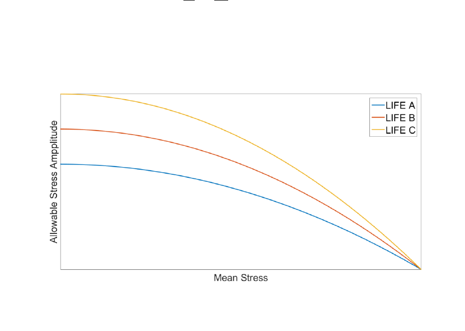
163
7.4 Gerber
The Gerber mean stress correction is a non-linear version of Goodman:
[7.4]
The Haigh diagram representation is shown in Figure 7.4:
The Gerber correction is more conservative than Goodman; however, for compressive mean stresses,
the Gerber correction increases the fatigue life, whereas the Goodman correction has no effect in
compression.
Figure 7.4: Haigh diagram representation of Gerber relationship for different reference lives. The curves meet the
material’s ultimate tensile strength.

164
7.5 Morrow
7.5.1 Strain-life
The Morrow mean stress correction modifies the elastic component of the strain-life curve [44]. This
reflects the observation that the mean stress has the most noticeable effect in the HCF regime. The
correction is expressed in its original form as Equation 7.5:
[7.5]
Although the Morrow mean stress correction gives reasonable results, it does not reflect the
material’s true behavior. The correction postulates that the ratio between the elastic and plastic strain
components varies with mean stress. In fact, the hysteresis behavior of metals is a function of strain
only.
7.5.2 Stress-life
Stress-life algorithms which use the Morrow mean stress correction only have their fatigue strength
term modified:
[7.6]

165
7.6 Smith-Watson-Topper
7.6.1 Strain-life
The Smith-Watson-Topper (SWT) relationship [41] is obtained by multiplying the damage parameter
by the maximum stress in the load cycle, and the right-hand side by the tensile fatigue strength
coefficient:
[7.7]
The SWT correction gives acceptable results for a wide range of materials and load types, and is less
conservative than the Morrow correction for compressive mean stress.
7.6.2 Stress-life
The stress-life implementation of the SWT mean stress correction is applied to the stress cycle, rather
than the stress-life equation. This is achieved using the Walker mean stress correction with .

166
7.7 Walker
7.7.1 Overview
The Walker mean stress correction is similar to the Smith-Watson-Topper correction, with the addition
of the material parameter . The Walker equation corrects the stress amplitude term in the stress-life
equation:
[7.8]
where
is the equivalent stress amplitude at zero mean stress,
is the stress amplitude of the
cycle and is the load ratio of the cycle.
7.7.2 Walker -parameter
The Walker -parameter can be calculated in three ways:
1. Walker regression fit
2. Standard values for steel and aluminium
3. User-defined
Variable
Value
walkerGammaSource
{1.0 | 2.0 | 3.0}
When either the Walker regression fit or standard values are specified, the value of is selected based
on the material behavior. Guidance on defining material behavior can be found in Section 5.9.
from Walker regression fit
When walkerGammaSource=1.0, the value of is approximated using the regression fit in Figure 7.5.
The value of correlates well with steels [45]. However, there exists no such correlation between the
Walker parameter and aluminium, as shown by Figure 7.6. It is therefore recommended that the
Walker regression fit is not used with non-steels.
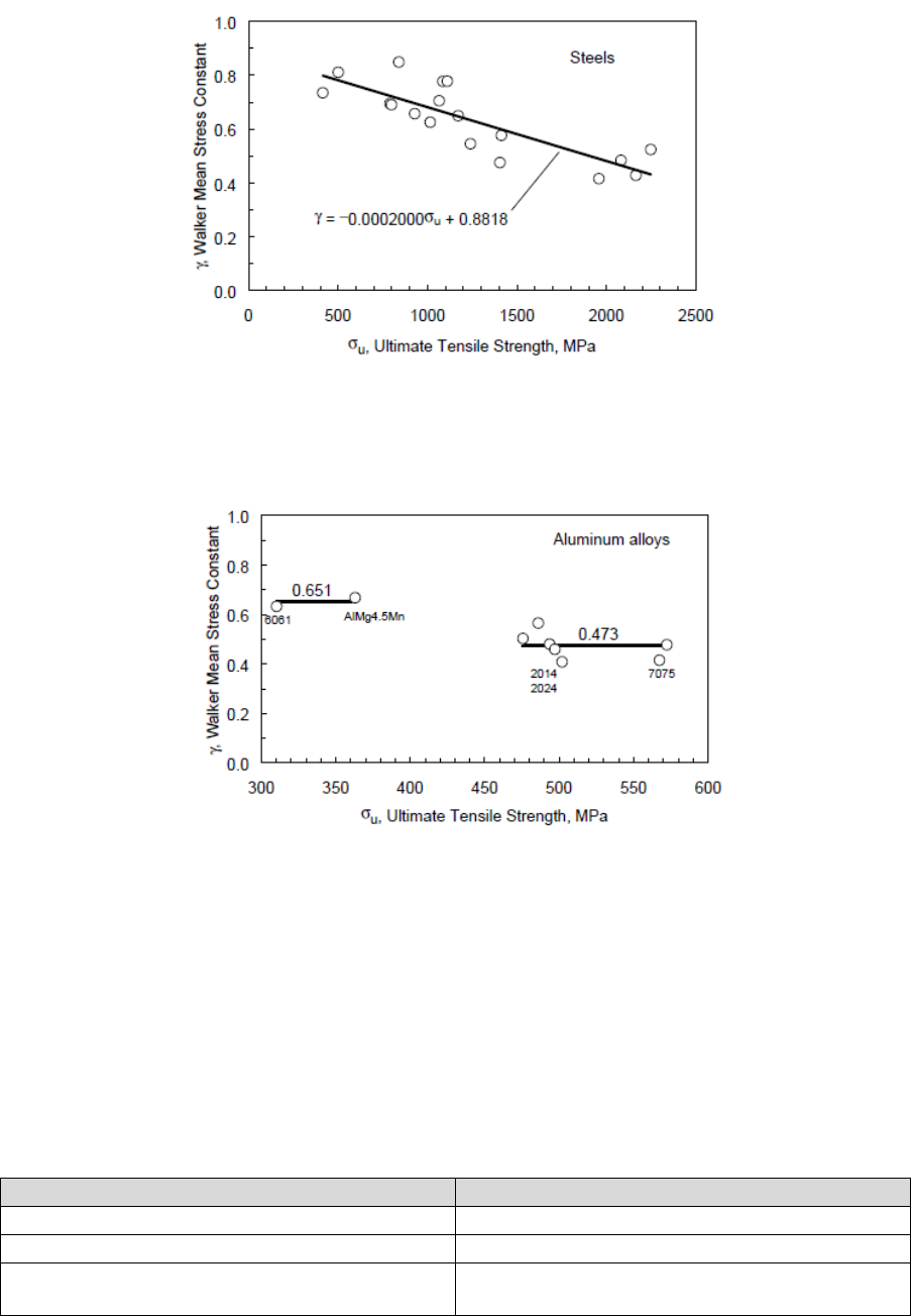
167
from standard values
When walkerGammaSource=2.0, the value of is found from standard values. Work by Dowling [46]
has shown that the value of can be approximated for most steel and aluminium specimens. If the
material is neither steel nor aluminium, is calculated as a function of the load ratio, .
The value of is calculated according to the following table:
Material behavior
-Solution
Steel
Aluminium
Other
Figure 7.5: Approximation of based on the ultimate tensile strength of
steel
Figure 7.6: Approximation of based on the ultimate tensile strength
of aluminium

168
Material Manager usage:
Derivation region of the Material Editor dialogue: Select the
behavior from the Material behavior drop-down menu.
Text file usage:
Specifying the material behavior from a material text file is not
currently supported.
from user input
When walkerGammaSource=3.0, the value of is specified by user input from the environment file.
Environment file usage:
Variable
Value
userWalkerGamma
7.7.3 Strain-life
The strain-life implementation of the Walker mean stress correction has been described by Dowling
[47] and Ince [48], and is given in the form of Equation 7.9:
[7.9]
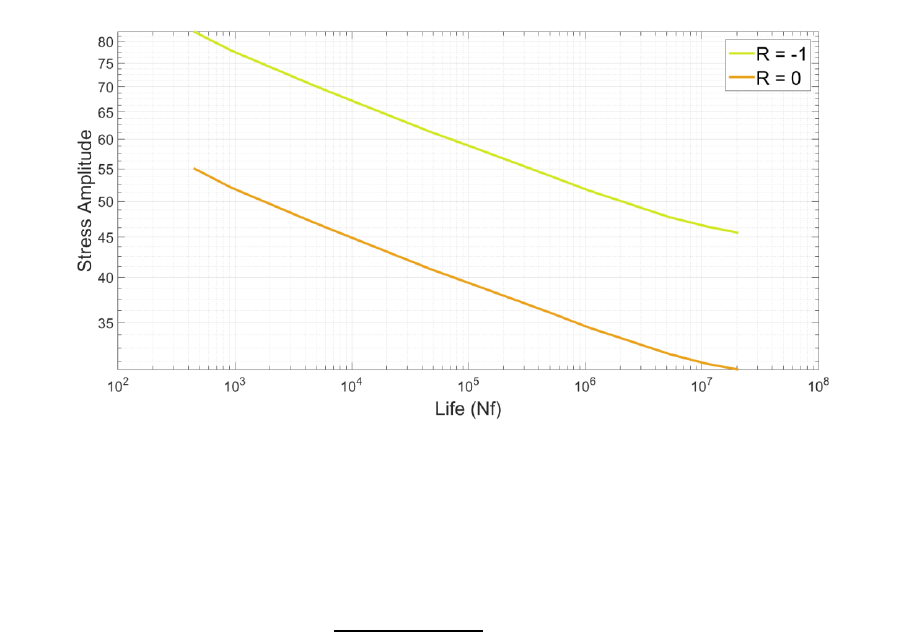
169
7.8 R-ratio S-N curves
The loading can be corrected for the effect of mean stress using experimental stress-life data, where
the endurance curve for the material has been measured at more than one load ratio. An example of
a multi R-ratio S-N curve from the Material Manager is shown in Figure 7.7. Creating S-N data with
multiple load ratios is explained in Section 5.4.
If R-ratio S-N curves are selected, Quick Fatigue Tool interpolates between the two curves that
envelope the load ratio of the current cycle. The standard interpolation formula is used:
[7.10]
where is the stress-life curve at the calculated load ratio . and are the upper and
lower load ratios corresponding to the curves and , respectively, which envelope the required
curve.
If the required S-N curve lies outside the range of S-N data (i.e. the required curve is not bound by a
curve to either side), then the stress-life data is extrapolated. In such cases, accuracy is not
guaranteed, and a warning will be written to the message file.
R-ratio S-N curves may only be used for . Fully-compressive cycles () will use the S-N curve
at . S-N curves may not be defined for infinite-valued R-ratios.
Figure 7.7: Example S-N data from the Material Manager, for a load ratio of -1 and 0

170
Treatment of the fatigue limit
When the R-ratio S-N Curves mean stress correction is used, the fatigue limit depends on the load
ratio of the current cycle. Therefore, the fatigue limit is re-calculated for each cycle based on the
interpolated S-N curve; the values of the environment variables fatigueLimitSource and
userFatigueLimit are ignored.
Under certain conditions, Quick Fatigue Tool reduces the fatigue limit such that previously non-
damaging cycles may become damaging. Modification of the fatigue limit is enabled with the
environment variable modifyEnduranceLimit, and is discussed in detail in the document
Quick Fatigue Tool Appendices: A1.5. If modification of the fatigue limit is enabled then the
instantaneous fatigue limit, , is based on the interpolated S-N curve for the current cycle.
Subsequent cycles are compared either to the reduced fatigue limit, , or (whichever is smaller).
If the subsequent cycles are non-damaging, will recover towards . Hence, the rate of recovery
may change depending on the load ratio of the current cycle.
It is not clear how best to treat this “bouncing” endurance limit in combination with multiple R-ratio
S-N curves; the above outlined methodology is a suggestion only. In case the user has doubt as to the
applicability of the modified endurance limit, it can be enabled or disabled from the environment file.
Environment file usage:
Variable
Value
modifyEnduranceLimit
{0.0 | 1.0}
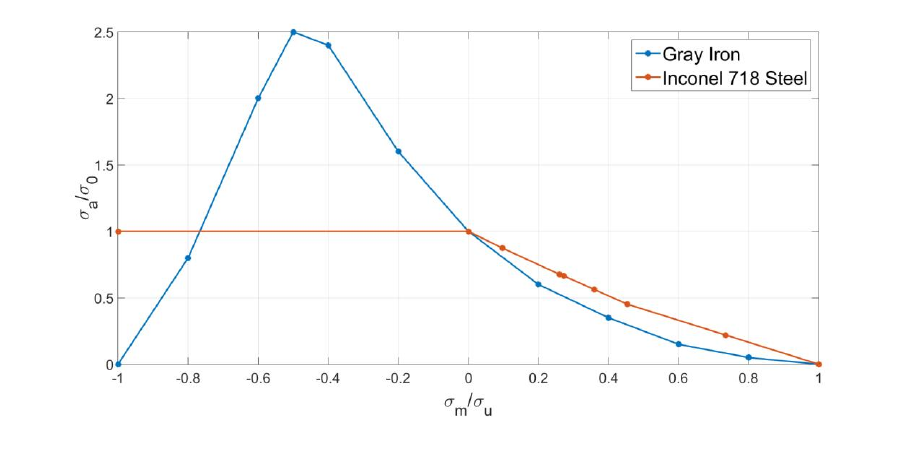
171
7.9 User-defined mean stress corrections
User-defined mean stress corrections can be provided for an analysis. The data should describe the
allowable stress amplitude at the material’s endurance limit as a function of the mean stress. The
result is a Haigh envelope which Quick Fatigue Tool uses to calculate a mean stress correction factor.
User-defined mean stress corrections are specified in the job file as a mean stress correction (.msc)
file.
Material Manager usage:
User-defined mean stress corrections are not supported in
Material Manager.
Job file usage:
Option
Value
MS_CORRECTION
'msc-file-name.msc'
where 'msc-file-name.msc' is a file containing normalized mean stress and allowable stress amplitude
data defining the Haigh envelope. The file must be saved in Data\msc.
Quick Fatigue Tool includes .msc files for Gray Iron and Inconel 718 Steel. These are shown in
Figure 7.8.
Figure 7.8: Allowable stress amplitude as a function of mean stress for Gray Iron and Inconel 718 Steel
172
According to the Haigh data, Inconel 718 has an allowable stress amplitude in compression which
remains constant, hence compressive cycles are not corrected for the mean stress.
Gray Iron has increased strength in compression at up to 50% of its compressive strength, hence
compressive cycles within this region are corrected in a sense that reduces the resulting fatigue
damage. Beyond 50% of the compressive strength, the fatigue strength reduces to zero, at which point
crushing is expected.
In tension, both materials have decreasing fatigue strength until the mean stress equals the ultimate
tensile strength, at which point static failure is expected.
The mean stress correction factor is calculated by comparing the allowable stress amplitude at zero
mean stress to the allowable stress amplitude corresponding to the mean stress of the cycle. Consider
the following user-defined mean stress data:
Now consider a stress cycle which has a mean stress of and stress amplitude of . If
the material’s UTS is , then the normalized mean stress is
. Quick Fatigue Tool
determines the corresponding allowable stress amplitude by assuming that intermediate stress
amplitude data follows a linear relationship and hence fits the equation of a straight line
(). The normalized stress amplitude corresponding to the mean stress of the cycle is then
. The mean stress correction factor is therefore
. The
equivalent stress amplitude at zero mean stress is . In general, the mean
stress correction factor is given by Equation 7.11:
[7.11]
where
is the local gradient of the Haigh data, is the cycle mean stress and and are the
allowable mean stress and stress amplitude at point , respectively. The equivalent stress amplitude
at zero mean stress is given by Equation 7.12:
[7.12]
User-defined mean stress correction data is usually obtained from existing Haigh diagrams for the
given material. The mean stress and stress amplitude are typically normalized by the ultimate tensile
strength and the tensile fatigue limit, respectively. For cycles with negative mean stress,
Quick Fatigue Tool will normalize those cycles by the compressive strength. If the compressive
strength is not defined, the tensile strength will be used for all cycles.
173
The following file format must be obeyed for user-defined mean stress data:
First column: Normalized mean stress values
Second column: Normalized stress amplitude values
The values of the normalized mean stress must be decreasing.
If the mean stress of the cycle is less than the minimum, or greater than the maximum value of mean
stress defined in the .msc file, Quick Fatigue Tool will calculate the mean stress correction factor
directly from the first or last stress amplitude value in the data, respectively.
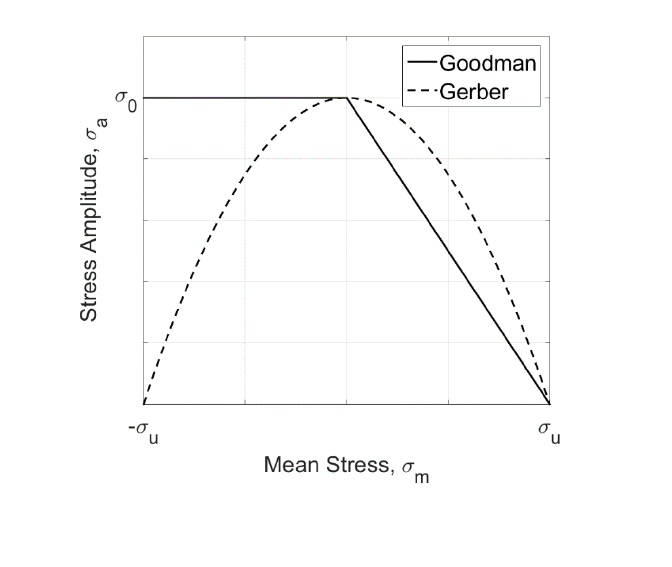
174
8. Safety factor analysis
8.1 Background
Some designs require that the fatigue performance of a component is expressed as a safety factor,
rather than a number of cycles. The finite life calculation is substituted for a pass/fail criterion, such
that a value greater than unity indicates that safety has been achieved by a certain margin; values less
than unity indicate that design and/or load modification is required. Quick Fatigue Tool offers two
design factor calculations:
1. Fatigue Reserve Factor (FRF)
2. Factor of Strength (FOS)
The two parameters are similar in their objectives. However, their methodologies have some
fundamental differences which should be considered before the analysis.
8.2 Fatigue Reserve Factor
8.2.1 Overview
The FRF is a linear scale factor which considers the worst stress cycle in the loading and compares the
mean stress and stress amplitude to a given target life. There are three types of calculation:
1. Horizontal
2. Vertical
3. Radial
Figure 8.1 shows the Goodman and Gerber life envelopes which can be used for the FRF calculation.
The FRF is calculated for the worst cycle in the loading.
Figure 8.1: Goodman and Gerber envelopes for FRF calculation
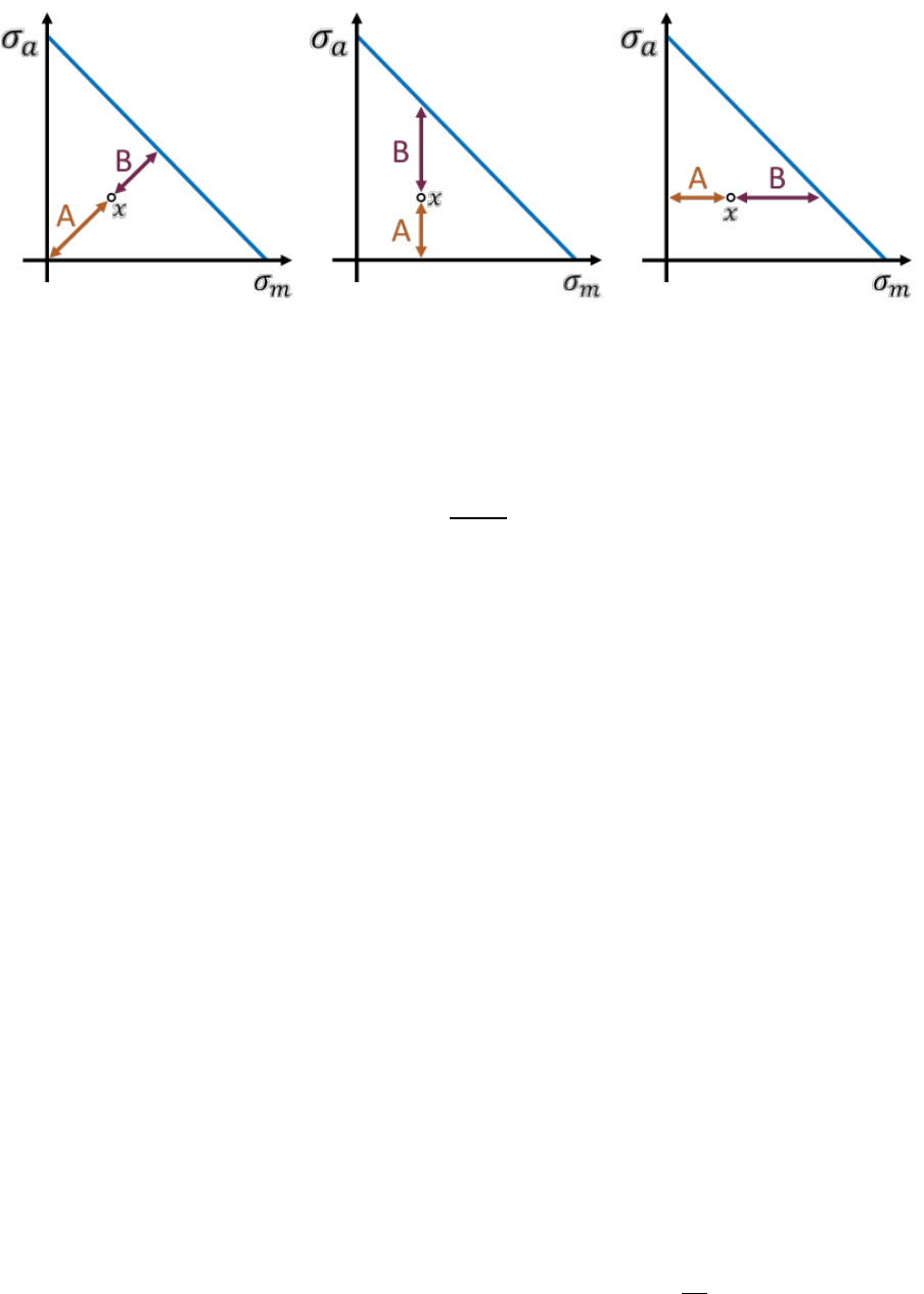
175
An arbitrary cycle, , is plotted on a Haigh diagram in Figure 8.2. The value of the FRF in the radial,
vertical and horizontal direction is given by Equation 8.1. The terms and correspond to the
mean stress and stress amplitude, respectively.
[8.1]
The pros and cons of the FRF calculation are as follows:
Pros:
the calculation is fast; and
results are accurate for simple, constant amplitude loading.
Cons:
the choice of design envelope is usually subjective;
results are inaccurate for variable amplitude loading;
since the FRF is not calculated from the complete loading, it cannot be used to reliably scale
the stresses; and
the number of loading repeats set by REPEATS in the job file will not affect the FRF calculation.
8.2.2 Included envelopes
Quick Fatigue Tool includes the Goodman, Goodman B and Gerber design envelopes. The Goodman B
envelope is used by default and is selected from the job file. Values of 1, 2 and 3 correspond to the
Goodman, Goodman B and Gerber envelopes, respectively.
Job file usage:
Option
Value
FATIGUE_RESERVE_FACTOR
{1.0 | 2.0 | 3.0}
Figure 8.2: Radial, vertical and horizontal fatigue reserve factor relative to an arbitrary cycle, , on a Haigh diagram. The
blue line represents an arbitrary design envelope

176
Goodman
The Goodman envelope is defined by Equation 8.2:
[8.2]
The mean stress and stress amplitude is given by and , respectively. The envelope is limited by
the ultimate tensile strength and the endurance limit, and , respectively.
By rearranging Equation 8.2, the values of the Goodman fatigue reserve factors in the horizontal,
vertical and radial directions are given by Equations 8.3-8.5, respectively:
[8.3]
[8.4]
[8.5]
The terms and are given by Equations 8.6-8.7:
[8.6]
[8.7]
where and is the mean stress and stress amplitude of the cycle, respectively. The terms and
are given by Equations 8.8-8.9:
[8.8]
[8.9]
The above equations apply to the standard Goodman envelope. By default, Quick Fatigue Tool uses a
modified version of this envelope called Goodman B, which is the intersection between the standard
Goodman and Buch envelopes. The Goodman B envelope is illustrated in Figure 7.3. If the proof stress
is not defined in the material, the standard Goodman envelope is automatically used by default.

177
Gerber
The Gerber envelope is the quadratic equivalent of the Goodman envelope, and is defined by Equation
8.10:
[8.10]
By rearranging Equation 8.10, the values of the Gerber fatigue reserve factors in the horizontal,
vertical and radial directions are given by Equations 8.11-8.13, respectively:
[8.11]
[8.12]
[8.13]
The terms and are given by Equations 8.14-8.15:
[8.14]
[8.15]
The terms and are given by Equations 8.16-8.17:
[8.16]
[8.17]
Fatigue reserve factors calculated from the Goodman envelope are slightly more conservative than
those calculated from the Gerber envelope.
178
8.2.3 Specifying the target life
The FRF target life can either be the infinite life envelope defined by the material’s endurance limit,
or a user-defined design life. The target life mode is configured in the environment file.
Environment file usage:
Variable
Value
frfTarget
A value of corresponds to the user-defined design life set by DESIGN_LIFE in the job file, while
a value of corresponds to the material’s endurance limit.
8.2.4 Specifying the FRF limits
By default, Quick Fatigue Tool limits the FRF values so that the minimum and maximum reported
values are capped at and , respectively. These values can be changed in the environment file.
Environment file usage:
Variable
Value
frfMaxValue
frfMinValue
If the user specifies the option No damage in compression (*NO COMPRESSION) in the material
definition and the cycle is purely compressive, then a value of is always assumed for that cycle.
8.2.5 Enabling FRF output
The FRF algorithm requires field output to be requested from the job file.
Job file usage:
Option
Value
OUTPUT_FIELD
1.0
Although the radial FRF is defined for any combination of stress amplitude and mean stress, the
horizontal and vertical FRFs are only defined within certain regimes. For example, with respect to the
Goodman B envelope the horizontal FRF is only defined for stress amplitudes below the fatigue limit,
whereas the vertical FRF is only defined for mean stresses less than the proof stress. If the FRF cannot
be evaluated, a value of is reported to the field output file.
179
8.2.6 User-defined FRF envelopes
The FRF can be calculated with user-defined data. This is a file containing a material life envelope as
Haigh diagram () data. FRF data files are created in the same way as user-defined mean stress
correction (.msc) files. Quick Fatigue Tool uses the .msc file for both user mean stress correction and
FRF calculations. For guidance on creating custom FRF data, see Section 7.9.
Job file usage:
Option
Value
FATIGUE_RESERVE_FACTOR
'msc-file-name.msc'
Quick Fatigue Tool interpolates the user-defined data to find the point on the envelope which forms
the intersecting line with the stress cycle coordinate (radial, horizontal and vertical).
Environment file usage:
Variable
Value
frfInterpOrder
{'NEAREST' | 'LINEAR' | 'SPLINE | 'PCHIP'}
The user can choose between the following interpolation methods:
MODE
DESCRIPTION
'NEAREST'
Nearest neighbour method
'LINEAR'
Linear ()
'SPLINE'
Cubic, piecewise polynomial
'PCHIP'
Cubic, shape-preserving
The linear method is shown in Figure 8.3. A comparison between the spline and pchip methods are
shown in Figures 8.4-5.
The linear method is appropriate in most cases, and especially when few data points are available. The
spline method is globally very smooth, while pchip only considers local curvature between data points.
Although the pchip method results in coarser interpolation, its behavior is preferable over the spline
method in cases where the data contains sudden changes in gradient, as shown by Figure 8.5.
The Nearest neighbour method is not recommended as it can produce highly inaccurate results.
180
Modelling compressive behavior for user-defined FRF data
Metals tend to show greater fatigue strength when loaded in compression, compared with tension.
This behavior is often represented by a plateau on the FRF curve as shown by Figure 8.1, in the case
of the Goodman envelope. Care should be taken when defining these plateaus with user-defined FRF
data, since this can result in undesirable behavior from the interpolation algorithm in MATLAB.
For an endurance envelope with a compressive plateau, the FRF data may be defined as below:
Mean stress
Stress amplitude
1
0
0
1
-1
1
-1
0
Since the mean stress values must be monotonically decreasing, the definition above will result in an
error. The problem is resolved by modifying the mean stress values by a very small amount, as shown
below.
Mean stress
Stress amplitude
1
0
0
1
-0.9999
1
-1
0
Quick Fatigue Tool automatically adjusts the stress amplitude values to ensure the correct behavior
of the interpolation algorithm.
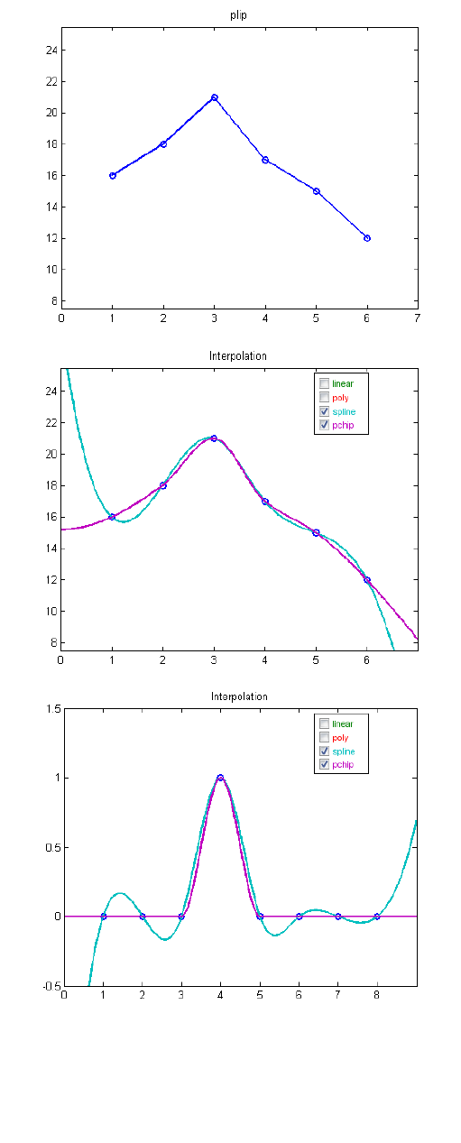
181
Figures 8.3-5: From top to bottom: Linear; spline vs PCHIP for
smooth data; spline vs PCHIP for discontinuous data.
Image credit: Cleve Moler, “Splines and Pchips”, July 16 2012, The
Mathworks.

182
Specifying normalization parameters for user-defined FRF data
Quick Fatigue Tool normalizes the mean stress and stress amplitude of each fatigue cycle to the limits
of the design envelope before performing an FRF calculation with user-defined FRF data. By default,
the design envelope limits are those defined by the Goodman FRF: Tensile and compressive mean
stresses are normalized by the ultimate tensile and ultimate compressive strength, respectively, while
the stress amplitude is normalized by the fatigue limit stress. These default values can be changed
with the following environment variables.
Environment file usage:
Variable
Value
frfNormParamMeanT
{'UTS' | 'UCS' | 'PROOF' | }
frfNormParamMeanC
{'UTS' | 'UCS' | 'PROOF' | }
frfNormParamAmp
{'LIMIT' | }
The parameters 'UTS', 'UCS', 'PROOF' and 'LIMIT' correspond to the ultimate tensile strength, ultimate
compressive strength, 0.2% proof stress and fatigue limit stress, respectively. The normalization
parameter can be specified directly with a numerical value, .
Visualizing user FRF envelopes
The user-defined FRF envelope can be plotted for a chosen analysis item with its respective radial,
horizontal and vertical projections. This MATLAB figure is enabled from the environment file, and
requires MATLAB figure output to be enabled for the analysis.
Environment file usage:
Variable
Value
frfDiagnostics
The item number corresponds to the analysis item as defined by its position in the data set file. An
example diagnostic output is shown in Figure 8.6 for the uniaxial cycle [, ], with the
envelope ‘Gray Iron.msc’.
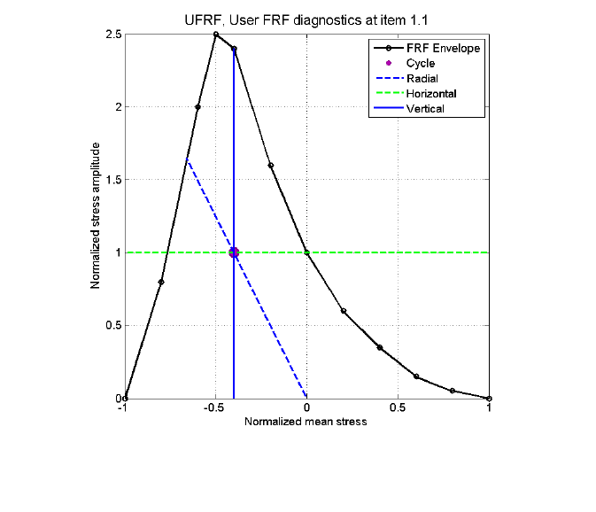
183
Precautions for user FRF envelopes
The user should ensure that the user-defined FRF data is defined in such a way that valid FRF
calculations are possible. If Quick Fatigue Tool is unable to calculate the FRF based on the user data, a
value of will be assigned. If the data is considered unusable, the analysis will exit with an error.
User FRF data is checked against the following conditions before the start of the analysis:
there must be exactly two columns of data;
there must be at least two FRF data pairs;
mean stress values must be decreasing down the column;
stress amplitude values must be positive;
the radial from the origin, through the cycle, must not be able to cross the FRF envelope more
than once; and
duplicate stress amplitude values on a given side of the amplitude axis are not permitted (the
same amplitude value can be specified as long as it is on the other side of the amplitude axis).
The following observations apply to user-defined FRF data:
mean stress values should not be over unity;
adjacent stress amplitude values are automatically adjusted to prevent zero gradients;
the FRF envelope should be closed at both ends (zero amplitude at mean stress limits); and
horizontal FRF values will default to if there is more than one possible solution.
8.2.7 Treatment of residual stresses
If a residual stress is defined with RESIDUAL, the FRF calculation is modified such that the origin of the
Haigh diagram is shifted from () to ().
Figure 8.6: An example FRF diagnostics with ‘Gray Iron.msc’. Mean stress and stress
amplitude values are normalized by and , respectively.
184
8.3 Factor of Strength
8.3.1 Overview
The FOS is a linear scale factor which, when applied to the fatigue loading, results in the specified
design life. Although traditionally the FRF was preferred over the FOS due to it being relatively
inexpensive, modern computers are able to perform FOS calculations in a reasonable amount of time
and as such the FOS is generally preferred over the FRF.
The FOS takes into account the nonlinear relationship between the damage parameter and the fatigue
life by iterating to recalculate the life until a stop condition is met.
Quick Fatigue Tool performs the following procedure when calculating the FOS:
1. Assume an initial FOS of
2. Compare the calculated fatigue life with the target life:
a. If the calculated life is less than the target life, decrease the FOS by a fixed increment
b. If the calculated life is greater than the target life, increase the FOS by a fixed
increment
3. Apply the current FOS to the original loading and re-calculate the life
4. Repeat steps 2 and 3 until one of the following stop conditions is met:
a. The maximum number of iterations has been reached
b. The specified tolerance has been achieved
c. The target life lies between the last two computed values of fatigue life
d. The current FOS is less than or equal to the minimum specified FOS
e. The current FOS is greater than or equal to the maximum specified FOS
The FOS is far more computationally expensive than the FRF because it repeats the damage calculation
at every analysis item. Furthermore, for the multiaxial algorithms such as the Stress-based Brown-
Miller, a new critical plane analysis must be performed each time. This is because changes in the mean
stress caused by re-scaling of the load history can affect the orientation of the critical plane.
For simple, constant amplitude loading, the FOS does not provide additional accuracy over the FRF. In
such cases, the FRF should be used instead.

185
8.3.2 Enabling the FOS calculation
The FOS calculation is enabled by setting the relevant option in the job file:
Job file usage:
Option
Value
FACTOR_OF_STRENGTH
{0.0 | 1.0}
The FOS algorithm requires field output to be requested from the job file:
Job file usage:
Option
Value
OUTPUT_FIELD
1.0
The FOS target life can either be the infinite life envelope defined by the material’s endurance limit,
or a user-defined design life. The target life mode is configured in the environment file.
Environment file usage:
Variable
Value
fosTarget
{1.0 | 2.0}
A value of corresponds to the user-defined design life set by the DESIGN_LIFE option in the job file,
while a value of corresponds to the material’s endurance limit.
8.3.3 Setting FOS band definitions
By default, Quick Fatigue Tool limits the FOS values so that the minimum and maximum reported
values are capped between and , respectively. These values can be changed in the environment
file.
Environment file usage:
Variable
Value
fosMaxValue
fosMinValue
186
During each iteration, the FOS is increased or decreased by a fixed increment. The value of the
increment depends on whether the current FOS lies within the fine band set by the user. The default
minimum and maximum fine band sizes are and , respectively.
Environment file usage:
Variable
Value
fosMaxFine
fosMinFine
The FOS band values must be decreasing:
Furthermore,
FOS values within this band are incremented with a smaller value. This fine value must be smaller than
or equal to the coarse value. The increment size for the fine and coarse bands are set by the user in
the environment file.
Environment file usage:
Variable
Value
fosCoarseIncrement
0.1
fosFineIncrement
0.01
The default stop conditions can also be modified from the environment file.
Environment file usage:
Variable
Value
fosMaxCoarseIterations
8.0
fosMaxFineIterations
12.0
fosTolerance
5.0

187
The pros and cons of the FOS calculation are as follows:
Pros:
subjective choice of design envelope is not required;
results are accurate for both simple and complex, variable amplitude loading; and
since the whole damage calculation is repeated, the FOS takes into account changes in the
critical plane orientation, mean stress, surface finish definition, plasticity correction etc.
Cons:
the calculation is computationally expensive; and
since the calculation accounts for the global load state, the FOS is only valid when used to
scale the stress at every point in the model. For example, models containing bolts where the
preload level is fixed may yield overly conservative FOS values.
8.3.4 Additional guidance on FOS parameters
Quick Fatigue Tool estimates the solution to the FOS by linearly scaling the original loading by
successive estimates of the FOS. If the target life is very far away from the calculated life, or if the
target life is very small, the FOS calculation can become unreliable. This is due to the finite allowable
increments in the first case and the severe nonlinearity of the S-N curve at low lives in the second
case. In fact, there is no single configuration of the FOS parameters which is guaranteed to achieve a
reliable solution for all target lives.
The user is strongly encouraged to review the accuracy of the FOS calculation, which is printed to the
log file (Project\output\<jobName>\<jobName>.log). Detailed information about the calculation can
be obtained by limiting the analysis to the worst item using the ITEMS option in the job file, and
requesting FOS diagnostics.
Environment file usage:
Variable
Value
fosDiagnostics
{0.0 | 1.0}
This creates a MATLAB figure showing the successive FOS and life values over each iteration, which
allows the user to easily check whether the scaled loading results in a fatigue life sufficiently close to
the target value. The iteration history is printed to the log file, and the FOS accuracy for each analysis
item is written to the file Project\output\<job>\Data Files\fos_accuracy.log. If automatic export is
enabled, the FOS accuracy per analysis item is written to the .odb file as an additional results field.
MATLAB figures must be enabled from the job file in order to generate the FOS diagnostic figure.
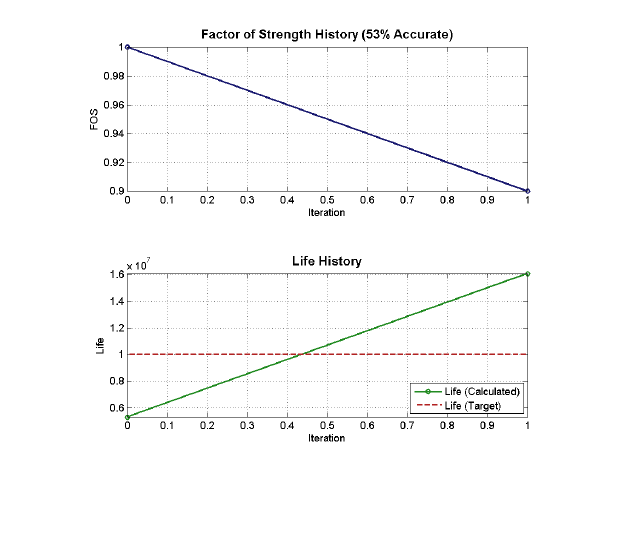
188
An example FOS diagnostic output is shown by Figure 8.7 for the job tutotial_intro. In this case only
one iteration was performed because the value of the FOS crossed the target life. The value of the FOS
is reported as because the original value of life is closer to the design target than the initial FOS
calculation would produce. This represents an accuracy of . It is clear that the default FOS
configuration for this analysis failed to achieve an acceptable value.
The coarse and fine increments are reduced to allow Quick Fatigue Tool to perform more iterations
before the target life is crossed.
Environment file usage:
Variable
Value
fosCoarseIncrement
0.01
fosFineIncrement
0.001
Furthermore, the maximum number of iterations is increased.
Environment file usage:
Variable
Value
fosMaxCoarseIterations
16.0
fosMaxFineIterations
24.0
Figure 8.7: Example FOS diagnostics for tutorial_intro with a target life of 1E7
repeats. The course and fine increments are 0.1 and 0.01, respectively.

189
The FOS diagnostic for this run is shown in Figure 8.8. The calculated FOS is and scaling the loading
by this value results in a life of repeats. This solution is within of the target life.
Therefore, the value is considered to be acceptable.
If the target life is below one million cycles, linearly scaling the loading by even very small amounts
can have a dramatic effect on the fatigue life. This can cause numerical difficulties when
Quick Fatigue Tool attempts to find a solution for the FOS. An example of “chattering” is shown in
Figure 8.9, where the FOS never converges on the target life. This can be prevented by enabling a
bracketing condition which ends the FOS calculation if the current calculated life crosses the target
life.
Environment file usage:
Variable
Value
fosBreakAfterBracket
{0.0 | 1.0}
If the FOS algorithm detects a chattering condition, bracketing is automatically enabled to prevent
additional iterations. Quick Fatigue Tool will automatically accept the best solution based on the
tolerance.
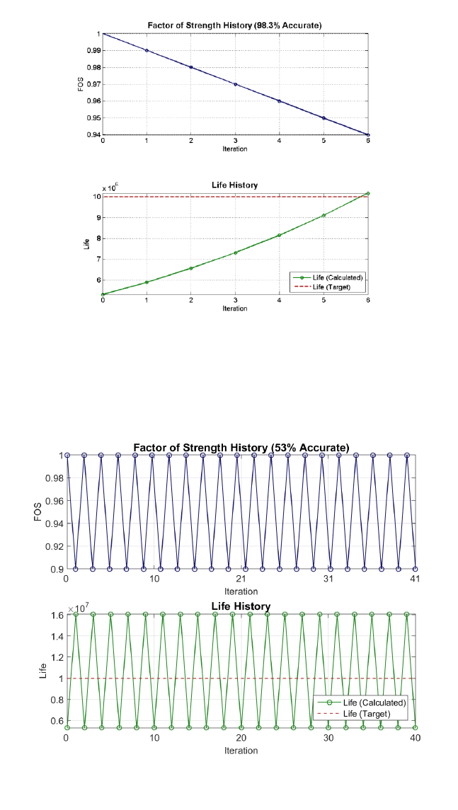
190
Figure 8.8: Example FOS diagnostics for tutorial_intro with a target life of 1E7
repeats. The course and fine increments are 0.01 and 0.001, respectively.
Figure 8.9: An example of FOS “chattering” where the algorithm is unable to
converge on the target life.

191
8.3.5 FOS augmentation
Selection of the correct incrementation settings is often unobvious and can lead to a time-consuming
process of trial and error. Even with well-tuned settings, the default incrementation scheme is linear,
and it is easy to unnecessarily spend many iterations. FOS augmentation is a scheme which attempts
to accelerate FOS convergence by modifying the user-defined incrementation parameters if the
current iteration is judged to cause unsatisfactory convergence behavior. Thus, FOS augmentation
aims to alleviate the manual aspect of the FOS algorithm by applying a certain level of automation to
the incrementation scheme.
Since the effect of estimating the FOS depends on a number of factors, such as loading, critical plane
analysis, material properties (and so on), even the augmented FOS scheme is required to make guesses
as to the appropriate incrementation.
The augmented FOS scheme is enabled in the environment file.
Environment file usage:
Variable
Value
fosAugment
{0.0 | 1.0}
When augmentation is enabled, Quick Fatigue Tool compares , the difference in fatigue life between
the two most recent iterations, with , the difference between the previously calculated fatigue life
and the target life. If the ratio between and is less than a threshold value, , the next FOS
increment is increased by a factor .
The threshold value and augmentation factor is set in the environment file.
Environment file usage:
Variable
Value
fosAugmentThreshold
fosAugmentFactor
The default values of the augmentation threshold and factor are and , respectively.
Figures 8.10-11 illustrate the improvement in convergence behavior when FOS augmentation is
enabled with the default settings using tutorial_intro.m as an example (note that the load factor and
algorithm have been modified to improve the illustration).
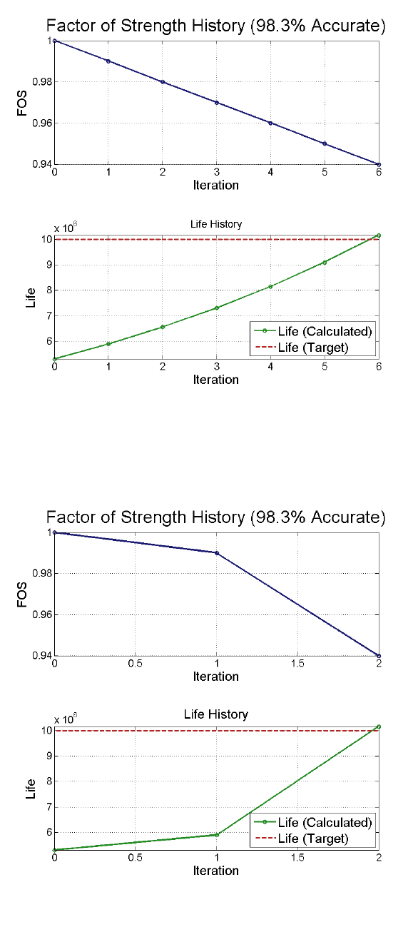
192
Figure 8.10: FOS diagnostics with augmentation disabled
Figure 8.11: FOS diagnostics with augmentation enabled
193
9. Job and environment files
This section has been released in the document Quick Fatigue Tool User Settings Reference Guide.

194
10. Output
10.1 Background
Quick Fatigue Tool reports extensive analysis output in addition to the fatigue life and safety factors
at the worst analysis item.
There are four categories of output:
1. Worst item log file summary
2. Field variables
3. History variables (worst analysis item)
4. History variables (all analysis items)
The worst item is defined as the item with the largest fatigue damage. In cases where more than one
item has the largest damage, the item with the largest principal stress over the set of worst items is
taken.
Field and history data is written to a set of text files. Pre-selected history variables can be plotted
automatically and saved in the results directory as MATLAB figures. If FEA stresses were analysed from
an Abaqus model, field data can be written to an output database (.odb) file and viewed on the finite
element mesh with Abaqus/Viewer. This functionality is discussed in Section 10.4.
Field and history data is requested in the job file.
Job file usage:
Option
Value
OUTPUT_FIELD
{0.0 | 1.0}
OUTPUT_HISTORY
{0.0 | 1.0}
Pre-selected MATLAB figures are also requested from the job file.
Job file usage:
Option
Value
OUTPUT_FIGURE
{0.0 | 1.0}
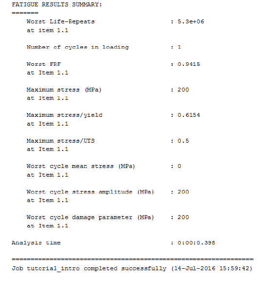
195
When an analysis runs to completion, a compact summary of a selection of variables is displayed in
the command window and written to the log file, an example of which is shown in Figure 10.1. If
extensive output is requested in the job file, the fields and histories are written to separate output
files.
Figure 10.1: Example fatigue results summary from the log file
196
10.2 Output variables
10.2.1 Fatigue analysis field variable identifiers
L
Fatigue life (linear scale) at each item in the model. The
units depend on the string value set by LOAD_EQ in the
job file.
LL
The value of L. Note that values of LL are capped
at the material’s endurance limit. For example, if the
endurance limit is 2E+07 reversals, then the maximum
reported value of LL will be 7.0.
D
Fatigue damage at each item in the model.
DDL
Fatigue damage at design life. Calculated by multiplying
the damage, D, by the user-specified design life.
FOS
Factor of strength at design life. A linear scale which,
when multiplied by the loading, results in the design life.
This field has a value of -1.0 if the FOS calculation was
not requested.
The FOS calculation is enabled by setting
FACTOR_OF_STRENGTH=1.0 in the job file.
SFA
Endurance safety factor. The ratio between the material
fatigue limit and the maximum stress/strain amplitude,
WCA, at each item in the model. The endurance limit is
discussed in the document Quick Fatigue Tool
Appendices: A1.
For strain-life analysis, the fatigue limit is converted to
elastic strain.
FRFH
Horizontal fatigue reserve factor.
For user-defined FRF data, a value of -1.0 is returned if
the calculation was unsuccessful.

197
FRFV
Vertical fatigue reserve factor.
For user-defined FRF data, a value of -1.0 is returned if
the calculation was unsuccessful.
FRFR
Radial fatigue reserve factor.
For user-defined FRF data, a value of -1.0 is returned if
the calculation was unsuccessful.
FRFW
Fatigue reserve factor (worst of above three).
SMAX
Largest stress in loading. If the absolute value of the third
principal stress is greater than the absolute value of the
first principal stress, the maximum stress will be the
third principal.
The calculation of the maximum stress does not include
the effect of residual stress.
SMXP
SMAX divided by the 0.2% proof stress.
SMXU
SMAX divided by the material’s ultimate tensile
strength.
TRF
Stress triaxiality factor (ratio between hydrostatic and
von Mises stress):
where is the Cauchy stress tensor, is the first stress
invariant and is the second deviatoric stress invariant.
WCM
Worst cycle mean stress/strain. Note that the mean
stress/strain is taken as the mean value of the worst
cycle at each item in the model defined by the damage
parameter. Therefore, the value of WCM depends on
the selected fatigue analysis algorithm.
198
WCA
Worst cycle stress/strain amplitude. The stress/strain
amplitude is the cycle counted quantity according the
selected analysis algorithm:
Uniaxial Stress/Strain-Life: Uniaxial stress/strain
/ (defined directly as the stress history).
Stress-based Brown-Miller: Sum of the shear and
normal stress on the critical plane.
Normal Stress: Normal stress on the critical plane.
Findley’s Method: Shear stress on the critical plane
(note that the normal stress is not included in the
definition of the stress amplitude).
Stress Invariant Parameter: von Mises equivalent stress.
BS 7608: Normal, shear or (normal + shear) stress on the
critical plane, depending on the value of FAILURE_MODE
in the job file
NASALIFE: Effective stress, defined by the environment
variable nasalifeParameter. The effective stress variables
are described in Section 6.8.3.
WCATAN
Worst cycle arctangent between WCM and WCA.
WCDP
Worst cycle damage parameter. The damage parameter
is the stress used in the fatigue damage calculation and
is usually the stress/strain amplitude.
The damage parameter includes the effect of the mean
stress correction (except in the case of the Morrow and
R-ratio S-N curves corrections, since these are applied
indirectly). Therefore, if mean stress correction is
applied to the loading, the values of WCDP and WCA will
differ.
If no mean stress correction is applied, or if the mean
stress in the loading is zero, the value of WCDP and WCA
is the same. The exception is with the use of Findley’s
Method with , since the amplitude parameter is
different from the damage parameter.
199
10.2.2 Static analysis field variable identifiers
YIELD
Items in the model which are yielding.
This field has a value of 1.0 if the items have yielded
according to the selected criterion, 0.0 if the item has
not yielded, -2.0 if the yield criterion could not be
evaluated or -1.0 if the yield calculation was not
requested.
TSE
If the variable YIELD has a value of 1.0 anywhere in the
model, the total strain energy per unit volume is written
to ‘warn_yielding_items.dat’.
PSE
If the variable YIELD has a value of 1.0 anywhere in the
model, the plastic strain energy per unit volume is
written to ‘warn_yielding_items.dat’.
MSTRS
Maximum stress theory failure measure.
MSTRN
Maximum strain theory failure measure.
TSAIH
Tsai-Hill theory failure measure.
TSAIW
Tsai-Wu theory failure measure.
TSAIWTT
Tsai-Wu theory failure measure for closed cell PVC foam.
AZZIT
Azzi-Tsai-Hill theory failure measure.
HSNFTCRT
Hashin’s fibre tensile damage initiation criterion.
HSNFCCRT
Hashin’s fibre compression damage initiation criterion.
HSNMTCRT
Hashin’s matrix tensile damage initiation criterion.
HSNMCCRT
Hashin’s matrix compression damage initiation criterion.
200
LARPFCRT
LaRC05 polymer failure measure.
LARMFCRT
LaRC05 matrix failure measure.
LARKFCRT
LaRC05 fibre kink failure measure.
LARSFCRT
LaRC05 fibre split failure measure.
LARTFCRT
LaRC05 fibre tensile failure measure.
201
10.2.3 Fatigue analysis history variable identifiers
History output represents the load-varying quantities for the most damaged analysis item in the
model. The following histories are written, with their respective identifiers:
ST
Stress tensor at worst item, on the critical plane, for the
loading.
HD
Haigh diagram for the worst cycle on the critical plane.
VM
von Mises stress for the loading.
PS1
Maximum (first) principal stress for the loading.
PS2
Middle (second) principal stress for the loading.
PS3
Minimum (third) principal stress for the loading.
CN
Maximum normal stress history for the loading. For
Uniaxial Stress-Life or von Mises analyses, the normal
stress is the hydrostatic stress. For multiaxial analyses, it
is the maximum normal stress history on the critical
plane.
CS
Maximum shear stress history for the loading. For
Uniaxial Stress-Life or von Mises analyses, the shear
stress is the Tresca stress. For multiaxial analyses, it is
the maximum shear stress history on the critical plane,
determined either by the maximum chord method or
the maximum resultant shear stress. This is specified by
the environment variable cpShearStress.
DP
Damage vs. plane angle.
DPP
Damage parameter vs. plane angle.
LP
Life vs. plane angle.
DAC
Damage accumulation at worst analysis item. Only
available if more there is more than one cycle in the
loading.
RHIST
Rainflow histogram of cycle counted stresses.
RC
Stress range distribution.
SIG
Uniaxial load history (before and after gating if
applicable).
202
10.2.4 Whole model variable identifiers
Whole model histories are load histories at every item in the model:
ANHD
Worst cycle Haigh diagram for each item in the model.

203
10.2.5 MATLAB figure variable identifiers
Certain history data can also be plotted to a series of figures. The default figure type is the MATLAB
.fig file. This default may be changed in the environment file.
Environment file usage:
Variable
Value
figureFormat
'<format>'
Any valid file format is accepted, e.g. 'png', 'jpeg', 'jpg' etc.
ANHD + HD
Worst cycle Haigh diagram for all items and the critical
plane.
KDSN
S-N curves for materials using knock-down factors.
CN + CS
Normal and shear stress history on the critical plane at
the worst item.
DP
Damage vs. angle at the worst item.
DPP
Damage parameter vs. angle at the worst item.
LP
Life vs. angle at the worst item.
CPS
Normal stress and resultant shear stress vs. plane angle
at the worst item.
P(S/E)
Principal stresses and/or strains at the worst item.
VM
von Mises stress at the worst item.
DAC
Cumulative damage at the worst item.
RHIST8
Rainflow cycle histogram at the worst item.
RC
Stress range distribution at the worst item.
SIG(S/E)
Uniaxial stress and/or strain load history (before and
after gating, if applicable).
LH
Tensor load histories at the worst item.
FOS
Factor of strength diagnostics.
8
Requires the Statistics Toolbox
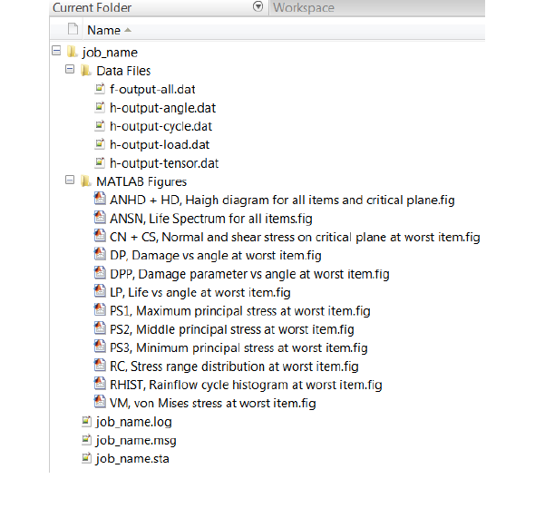
204
10.3 Viewing output
10.3.1 Output location
Field and history output for a particular analysis is stored under Project\output\<jobName>\Data Files.
The output directory has the file structure shown in Figure 10.2.
The name of the output directory shares the name of the job with which the output is associated. If a
job is submitted with the same name as an existing output directory, Quick Fatigue Tool will overwrite
the previous results files. Therefore, care should be taken when choosing the job name in the job file.
Output is stored as human-readable ASCII text, and can be viewed in MATLAB or with any text editor.
10.3.2 Changing the output format
By default, floating-point values are converted to text using fixed-point notation ('%f'). This can be
changed using the following environment variables.
Environment file usage:
Variable
Value
fieldFormatString
'<format>'
historyFormatString
'<format>'
For example, '.2f' represents two digits after the decimal mark, '12f' represents twelve characters in
the output and '.0f' represents integer output. The user is not required to specify the '%' format
identifier. More information on formatting text can be found in the official MATLAB documentation.
Figure 10.2: Output directory structure
205
10.3.3 Limitations of critical plane output
If the user specifies OUTPUT_FIGURE=1.0 and the analysis utilises critical plane searching,
Quick Fatigue Tool exports MATLAB figures of pertinent analysis quantities (including the damage
parameter of the chosen algorithm) on the analysed planes. The critical plane is denoted by a red
marker on each curve.
The following precautions should be taken into account when viewing critical plane plots:
the plots are written for the worst analysis item only
if critical plane smoothing is specified with cpSample>0.0 then the location of the indicated
critical plane may not appear on the curve, and the plotted values may not match those
printed to the 'h-output-angle.dat' history file; and
if the worst cycle mean stress at the worst analysis item is non-zero then the indicated critical
plane may not coincide with the plane of maximum damage parameter.
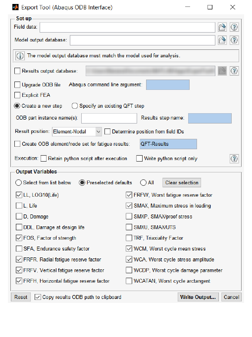
206
10.4 The ODB Interface
10.4.1 Overview
Quick Fatigue Tool includes an interface which is capable of writing fatigue results to an Abaqus output
database (.odb) file. This allows the user to visualize selected field output variables in Abaqus/Viewer.
There are two methods for accessing the ODB interface:
1. Via the job and environment files (text-based)
2. Via the Export Tool application (UI-based)
The first method allows the user to configure the interface to automatically write fatigue results to
the .odb file immediately after the analysis, whereas the second method allows the user to write
results to an .odb file based on a selected field data file, after the analysis has already been performed.
Both methods represent the same functionality; the differences lie in how and when the interface is
accessed.
The ODB interface requires that Abaqus is installed on the host machine. If an installation cannot be
found, the interface will exit with an error.
Figure 10.3: Export Tool interface

207
10.4.2 Accessing the ODB interface via the Export Tool
The Export Tool is a MATLAB GUI application which gives the user interactive access to functions of
the ODB interface.
The Export Tool is launched either by running the file ExportTool.m in the
Application_Files\code\odb_interface directory, or by installing and running the tool as a MATLAB app.
The app installer can be found in Application_Files\toolbox. The Export Tool interface is shown in
Figure 10.3.
10.4.3 Enabling the ODB interface via the environment file
As long as the ODB interface is enabled, Quick Fatigue Tool will automatically export field results to an
output database file if it finds a valid definition in the job file.
Environment file usage:
Variable
Value
autoExport_ODB
{0.0 | 1.0}
10.4.4 Configuring the ODB interface
Specifying the field data to export
The ODB interface copies results data from the field output file in the output directory. This is typically
located in \Project\output\<jobName>\Data Files\f-output-all.dat. The field output file must be
specified by the user in advance.
Export Tool usage:
Set-up region: Select the field data file either by entering the
absolute path in the file window, or by selecting the file via the file
browser using the button.
Job/environment file
usage:
The field data file is created during the job and automatically located
after the analysis. The user is not required to specify the field data
file.

208
Specifying the model ODB file
The ODB interface must be able to locate the original (model) .odb file so that it can make a copy of
the file and append the result step.
Export Tool usage:
Set-up region: Select the model output database file either by
entering the absolute path in the file window, or by selecting the file
via the file browser using the button.
Job file usage:
Option
Value
OUTPUT_DATABASE
'model-odb-file-name.odb'
The user must always specify the absolute path of the .odb file.
Specifying the results ODB file
Quick Fatigue Tool automatically chooses the location of the results .odb file. By default, the file is
stored in the Project\output\<jobName>\Data Files directory. This behavior may be overridden with
the Export Tool.
Export Tool usage:
Set-up region: Check the option Results output database. Select the
results output database location either by entering the absolute
path in the directory window, or by selecting the location via the file
browser using the button.
Job/environment file
usage:
The results .odb file location cannot be modified by the user. It will
always be stored under Project\output\<jobName>\Data Files.
Specifying the FE procedure
Due to rules defined within the Abaqus modelling framework, general static procedures are not
permitted directly after an Abaqus/Explicit procedure. By default, the ODB interface will attempt to
append a static step to the model .odb file for fatigue results. Therefore, if the previous FEA step
originated from an Abaqus/Explicit analysis, the user must indicate this directly.
Export Tool usage:
Set-up region: Check the option Explicit FEA.
Job file usage:
Option
Value
EXPLICIT_FEA
{0.0 | 1.0}

209
Specifying the Abaqus API version
The user can specify which version of the Abaqus API will be used to create the results .odb file. This
is done by specifying the Abaqus command line argument. The command line argument is the name
of the batch file corresponding to the Abaqus version. These files are typically located in
<Abaqus_installation_directory>\Commands.
Export Tool usage:
Set-up region: Fill out the Abaqus command line argument edit box.
Environment file usage:
Variable
Value
autoExport_abqCmd
'abaqus-command'
By default, the command 'abaqus' is used. Assuming a standard Abaqus installation exists on the host
machine, this argument points to the most recently installed Abaqus version.
If the installed Abaqus version is more recent than the model .odb file, the upgrade utility can be used
to upgrade the file to a more recent version. The command line syntax for this is as follows:
>> <abaqus_command> upgrade –job <jobName> -odb <oldOdbFileName>
This functionality can be accessed via the ODB interface.
Export Tool usage:
Set-up region: Check the option Upgrade ODB file.
Environment file usage:
Variable
Value
autoExport_upgradeODB
{0.0 | 1.0}
If the user specified to upgrade the .odb file, the ODB interface chooses the Abaqus version specified
by 'abaqus-command'.
Specifying the part instance
Quick Fatigue Tool can usually only recognise stress datasets originating from a single part instance,
since Abaqus may assign duplicate element-node numbers for each instance. Therefore, the part
instance name must be specified to resolve potential ambiguity. Part instance names are inherited
from the part itself. For example, if the part was named BOLT, then the part instance will be named
BOLT-n. To check the name of the part instance, from Abaqus/Viewer, query an element on a region
of the model from where stress data was exported. In the message window, the element type and
corresponding part instance name is shown.
210
Export Tool usage:
Set-up region: Fill out the ODB part instance name(s) edit box.
Job file usage:
Option
Value
PART_INSTANCE
'part-instance-name'
If the Abaqus job was run from a flat input file, there is only a single part instance in the output
database called PART-1-1. If a flat input file was used, this name should be specified.
If the field data spans multiple part instances, these can be specified together.
Export Tool usage:
Set-up region: Fill out the ODB part instance name(s) edit box.
Separate part instance names with double quotes (“”).
Job file usage:
Option
Value
PART_INSTANCE
{'part-instance-1',… , 'part-instance-'}
Specifying the step name
The ODB interface can either append a new step to the results .odb file, or it can write fatigue results
to an existing step that was created by the interface on a previous occasion.
Export Tool usage:
Set-up region: Choose either Create a new step or Specify an
existing QFT step from the radio button selector. If a new step is
being created, the name can be specified; otherwise a default name
will be used. If an existing step is specified, the name of the step
must be given.
The step name is specified by filling out the Results step name edit
box.
Job file usage:
Option
Value
STEP_NAME
'step-name'
Environment file usage:
Variable
Value
autoExport_stepType
211
The value of dictates the following:
1. A new step is created
2. Results are exported to an existing QFT step
If a new step is chosen, the step name is optional. If no name is specified, Quick Fatigue Tool will
choose a name automatically based on a combination of the job name and the part instance.
If an existing step is chosen, the name of the step must be specified. The following limitations apply:
the step must have been written by the ODB interface on a previous occasion;
the same field output variables must be written as when the step was created
Specifying the element result position
The result position is required because the ODB interface must tell the Abaqus API where on the
element to write the fatigue results.
Export Tool usage:
Set-up region: Select the position from the Result position drop-
down menu.
Job file usage:
Option
Value
RESULT_POSITION
{'ELEMENT NODAL' | 'UNIQUE NODAL' | 'INTEGRATION POINT' | 'CENTROID'}
If the result position is unknown, the ODB interface can “guess” the most suitable position based on
the format of the field data.
Export Tool usage:
Set-up region: Check the option Determine position from field IDs
Environment file usage:
Variable
Value
autoExport_autoPosition
The value of dictates the following:
0. The position is not determined automatically
1. The ODB interface will attempt to select the mist suitable results position
It is possible for the code to determine the incorrect position, so the user should ensure that the
selected result position matches the selection made when exporting the RPT file.
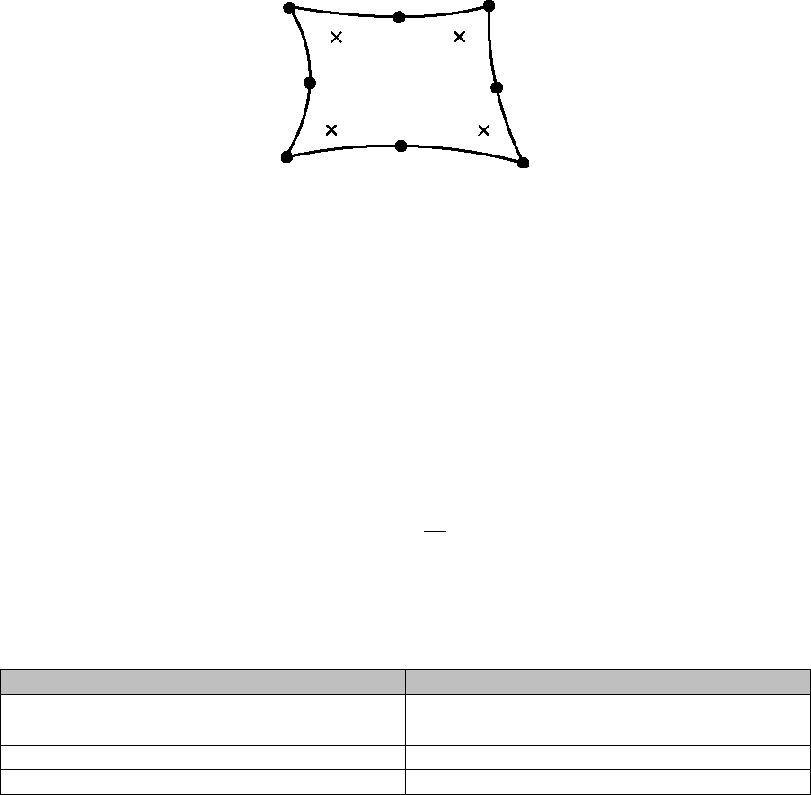
212
Figure 10.4 is an example of a plane stress element. If the result position is unique or element-nodal,
data is written to the outer points of the element. Integration point data is written to the Gauss points
in the element subsurface. Centroidal data is written to the geometric centre of each element.
Creating an element/node set
The ODB interface can create an element or node set in the results ODB file to facilitate easier results
visualization in Abaqus/Viewer.
Export Tool usage:
Set-up region: Check the option Create ODB element/node set for
fatigue results and fill out the edit box.
Environment file usage:
Variable
Value
autoExport_createODBSet
{0.0 | 1.0}
autoExport_ODBSetName
'ODB-set-name'
The format of the ODB set is as follows:
Result position
ODB set type
Element-nodal
Node and element
Unique nodal
Node
Integration point
Element
Centroidal
Element
If an ODB set is written to the same ODB file by a subsequent analysis, the API will return the following
error:
OdbError: Duplicate set or surface name QFT_PART-1-1_QFT
ODB sets can only be written to the output database if the selected field data file exactly matches
the element-nodes for the selected part instance. ODB sets will not be written if more than one part
instance name is specified.
Figure 10.4: S8R Shell element with
four integration points and nine
nodes
213
Specifying how the python script is handled
The Export Tool works by writing a Python script containing all the instructions necessary to create a
copy of the model ODB with an additional step containing the fatigue analysis result data. The script
is submitted to the Python interpreter within the Abaqus/CAE framework, which then creates the
output database. The process schematic is shown in Figure 10.5. The Python script used for the export
operation may be retained, or the user can specify that only the python script should be written and
it should not be submitted to the Abaqus API. In this case a results .odb file will not be created.
Export Tool usage:
Set-up region: Check the option Retain python script after
execution or Write python script only. The options are mutually
exclusive.
Environment file usage:
Variable
Value
autoExport_executionMode
The value of dictates the following:
1. Export results and discard the python script
2. Export results and retain the python script
3. Write the python script only. No results are exported
Specifying the field output variables
The user can choose which field output variables to export to the output database file.
Export Tool usage:
Output Variables region: Choose either Select from list below,
Preselected defaults or All from the radio button selector.
If Select from the list below is selected, check the field output
variables you wish to export to the output database file
Environment file usage:
Variable
Value
autoExport_selectionMode
autoExport_fieldName
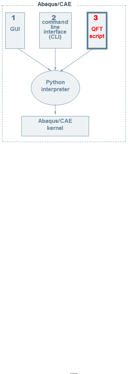
214
The value of dictates the following:
1. Select the field output variables manually
2. Use preselected defaults
3. Export all field output variables
The value of dictates the following:
0. Do not export the field output variables
1. Export the field output variable
Exporting yield criterion variables to the output database
If the user enabled the yield criterion, the yield flag and associated strain energies can be exported to
the results output database file.
Export Tool usage:
The YIELD variable is not supported in Export Tool.
Environment file usage:
Variable
Value
autoExport_YIELD
{0.0 | 1.0}
Figure 10.5: Interface between Quick Fatigue Tool and
Abaqus/CAE
215
10.4.5 Mismatching ODB files
While it is important that the source model matches the results data, Quick Fatigue Tool will attempt
to match field data to corresponding elements and nodes in the model ODB, even if the finite element
mesh is different. If the user selects the “Unique Nodal” or “Centroidal” options,
Quick Fatigue Tool will write field data directly to the ODB based on the position labels provided in the
field output file. If the user selects the “Element-Nodal” or “Integration Point” options,
Quick Fatigue Tool will request the nodal connectivity matrix from the Abaqus API. This is required
due to the fact that the order of the element-node or element-integration point data in the field
output file will not necessarily match the order required in the ODB.
If the ODB interface finds nodes in the ODB file which cannot be found in the field data, that node and
all others belonging to the same element will be ignored. If the Export Tool finds elements in the ODB
which cannot be found in the field data, that element and all of its nodes or integration points will be
ignored. As such, it is not necessary to export stress datasets from every element in the part instance
when generating the RPT file(s), since the ODB interface will automatically ignore regions of the part
instance which weren’t included in the fatigue analysis.
10.4.6 Large ODB files
For very large ODB files, it is unnecessary (and often impractical) to copy all of the FEA data to the
results ODB. In cases where copying the ODB would could consume a significant amount of time, the
user is advised to create a data check ODB. These files contain the mesh from the FE model, but no FE
results data. Hence, data check ODBs are more efficient as a container for fatigue analysis results.
Abaqus/CAE usage:
Expand the jobs container from the model tree. Right-clock on the
job and select Data Check.
Command line usage:
abaqus job=<jobName> datacheck
10.4.7 Exporting field data to multiple Abaqus ODB part instances
Since Quick Fatigue Tool only uses the element-node numbers written to the field report file, it does
not distinguish between individual part instances. Although it is possible to write field data to multiple
part instances, the user must ensure that element-node numbers are not reused between instances,
otherwise results will not be written to the output database correctly. There are four approaches for
writing field data to multiple part instances:
1. Write multiple steps to the same .odb file, each step containing results at one part instance
2. Append field output from subsequent part instances to a previously created results step
3. Run the FEA from a flat input file
4. Manually set node numbering in Abaqus/CAE to enforce unique element-node numbers
Example: Write multiple steps to the same .odb file
If the user only has access to the .odb file and is unable to modify the attributes of the original model,
field data may be written to multiple part instances by running a separate fatigue analysis job for each
instance. Upon completion of each job, field data is written back to the previous result .odb file as a
new step.
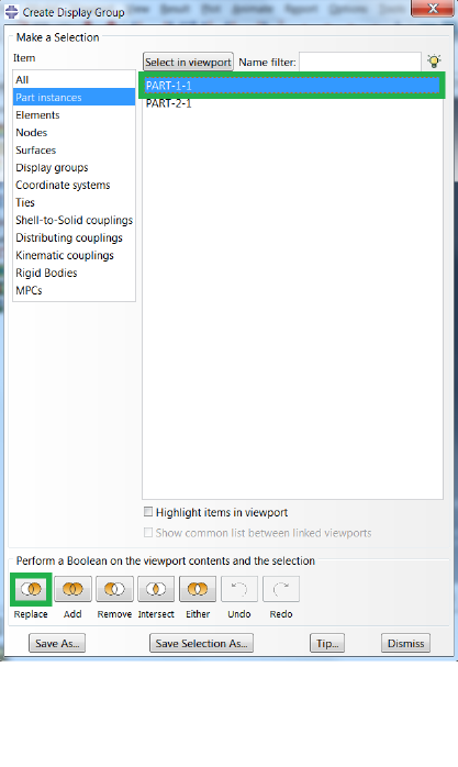
216
Individual part instances are selected in Abaqus/Viewer using the Create Display Group tool. In order
to create the necessary stress dataset file, only the required part instance should be displayed in the
viewport. This is achieved by selecting the required part instance and selecting Replace, as shown in
Figure 10.6.
The stress dataset file is then created by following the steps outlined in Section 3.2, corresponding to
the first part instance of interest. For the first job, the Abaqus ODB options are configured from the
job file.
Job file usage:
Option
Value
DATASET
'dataset-A.rpt'
OUTPUT_DATABASE
'<absolutePath>\model-ODB.odb'
PART_INSTANCE
'part-instance-name-A'
STEP_NAME
'step-name-A'
A second job is run for the dataset corresponding to the second part instance of interest. The model
output database is specified as the results output database from the previous analysis and the name
of the second part instance is specified.
Figure 10.6: Create display group tool showing how to
replace the viewport contents with the required part
instance
217
Job file usage:
Option
Value
DATASET
'dataset-B.rpt'
OUTPUT_DATABASE
'<absolutePath>\results-ODB.odb'
PART_INSTANCE
'part-instance-name-B'
STEP_NAME
'step-name-B'
This will append a new step to the existing results output database containing field data for the second
part instance. The STEP_NAME option adds an additional string to the name of the results step and is
not compulsory. However, adding a step name for each analysis minimizes the risk of
Quick Fatigue Tool attempting to create two steps with the same name in a single .odb file, which
would result in an error.
The advantage of writing field output to individual steps is that the field output variable selection can
differ between part instances. However, the drawback of this method is that it is not possible to view
a field over all part instances simultaneously; rather, the user must switch between steps in order to
view results at different regions in the model.
Example: Append field output from subsequent part instances to a previously created results step
An alternative to the previous method is to append results from subsequent analyse to a results ODB
step created from a previous analysis. Output is written to the first part instance.
Job file usage:
Option
Value
DATASET
'dataset-A.rpt'
OUTPUT_DATABASE
'<absolutePath>\model-ODB.odb'
PART_INSTANCE
'part-instance-name-A'
STEP_NAME
'step-name-A'
218
The analysis is then repeated for the second part instance.
Job file usage:
Option
Value
DATASET
'dataset-B.rpt'
OUTPUT_DATABASE
'<absolutePath>\results-ODB.odb'
PART_INSTANCE
'<partName_B>'
STEP_NAME
'<stepName>'
In this case, the path to the output database is defined as the path to the results output database from
the first analysis. The step names must match between the two models. By default,
Quick Fatigue Tool creates a new step for the results data. Therefore, in order to instruct the program
to append results to the previous step, the following environment variable must be set from the
environment file.
Environment file usage:
Variable
Value
autoExport_stepType
2.0
The following caveats must be observed when appending output to an existing step:
The previous step must have been written by Quick Fatigue Tool
The fields must exactly match those written in the original step, otherwise the Python API will
exit with errors
The advantage of appending results data to a previous step is that fields can be visualized over all part
instances simultaneously, without having to switch between steps. The results position of the
elements does not have to be the same between part instances, although exporting data at different
positions will result in duplicate field variables being written to the ODB frame. Results which are
appended may also overwrite results which were written during previous analyses.
Example: Run the FEA from a flat input file
The alternative solution is to avoid writing individual part instances and assemblies to the input file.
This is achieved by selecting Do not use parts and assemblies in input files in the Edit Model
Attributes dialogue in Abaqus/CAE.
After the analysis, Quick Fatigue Tool will write to the message file the number of regions found in the
.rpt file.

219
10.4.8 Minimum requirement for output
The Abaqus API imposes minimum requirements for the amount of field data which must be written
to a given result frame. These requirements are detailed in the table below:
Result position
Requirement
Element-nodal
All the nodes defining a single element
Unique Nodal
At least two nodes
Integration Point
All the integration points defining a single
element
Centroid
At least two centroids
Failure to adhere to above requirements will cause the ODB interface to exit with the following error
message:
Element-nodal/Integration Point
Error: No matching position labels were found
from the model output database
Unique Nodal/Centroid
ODBgetSeqSeqDoubleFromArray() num dims (1)
!= 2
220
11. FEA Modelling techniques
11.1 Background
This section applies to users who wish to use stress datasets from a finite element analysis. Detailed
guidance and illustrations focus on SIMULIA Abaqus, but the concepts can be applied to any FEA
package.
11.2 Preparing an FE model for fatigue analysis
Consider the model in Figure 11.1. We wish to determine the fatigue life of the shaft when subject to
a fully-reversed bending load. The first consideration is whether it is viable to analyse the whole
model. The shaft is made from 56,720 elements and 60,867 nodes. Analyses with Quick Fatigue Tool
can be cumbersome for models containing more than a few thousand nodes, so it would be
unadvisable to analyse every element. At this stage, the user should ask the following questions:
a) Is analysing the whole FE model reasonable considering the size of the mesh?
If the answer to a) is no, then ask the following question:
b) Are the stresses concentrated at a particular location? i.e. are there regions in the model
where the stresses are clearly non-damaging?
If the answer to b) is yes, then reduce the number of elements for analysis
In the example of the shaft model, the bending load has resulted in a stress concentration at one of
the fillet radii, so it is only necessary to analyse this region.
Using the Display Group Manager, the elements at the notch containing the stress concentration are
isolated, shown by Figure 11.2. The model could be cut once more in the x-z plane to exploit the
symmetry of the result. However, for this example the full notch geometry will be considered.
Quick Fatigue Tool defines “failure” as the complete propagation of a crack across a material surface
defined by critical plane analysis. In most cases, these cracks initiate on the component surface,
therefore subsurface elements may be excluded in cases where the stress gradient is sufficiently large.
Subsurface elements are excluded from the analysis by creating a new display group and choosing to
select elements “by angle”, shown in Figure 11.3. The final element set for the analysis is shown in
Figure 11.4.
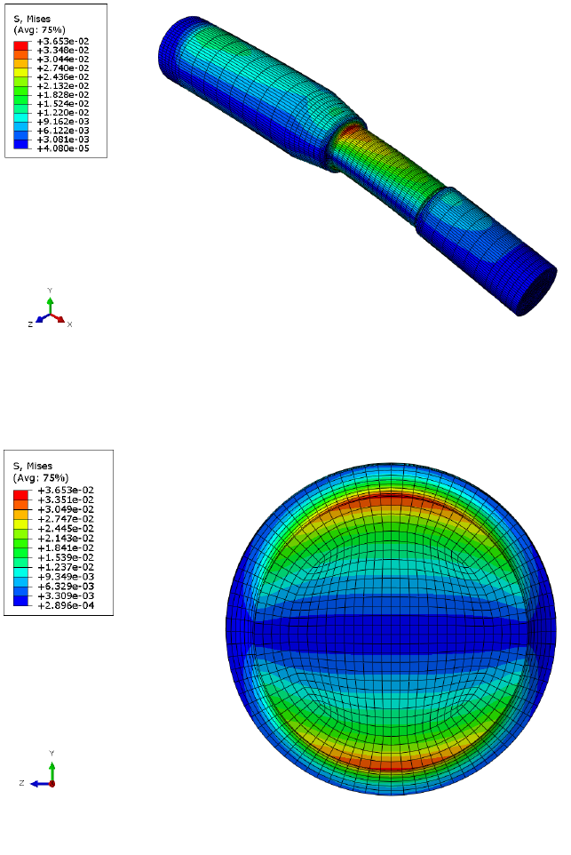
221
Before exporting the stress tensors for analysis, it is recommended that result averaging is turned off
so that the stresses written to the .rpt file are a closer representation of the calculated gauss point
values. From the main menu bar, go to Result → Options… and make sure that “Average element
output at nodes” is unchecked (Figure 11.5).
Figure 11.1: SAE shaft model in bending
Figure 11.2: Isolating the stress concentration
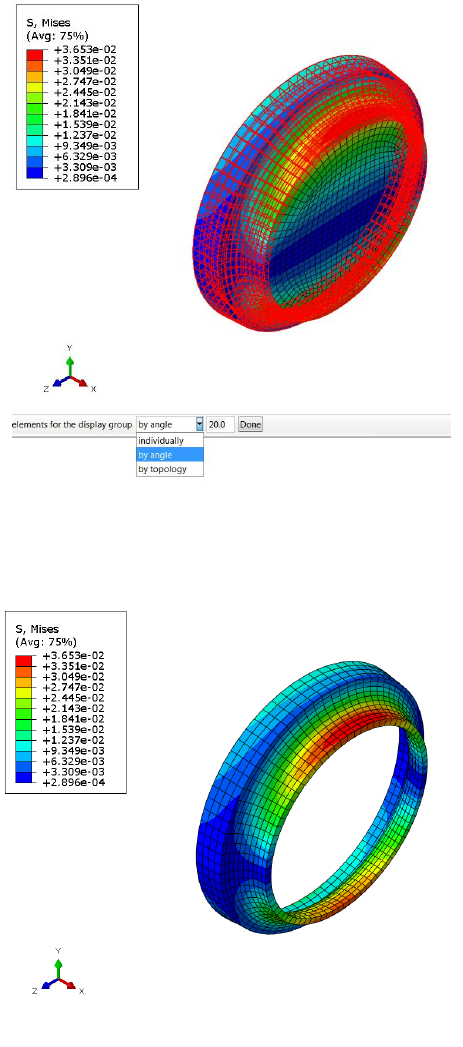
222
11.3: Picking surface elements by angle
Figure 11.4: Final element analysis group
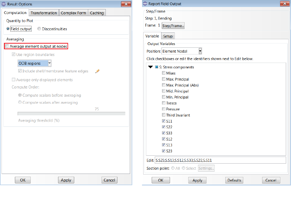
223
The stresses are then exported by going to Report -> Field Output… and choosing the stress
components, as shown in Figure 11.6. The user has the option to select the position for the field
output. The choices of positions compatible with Quick Fatigue Tool are described below.
Figure 11.5: Result options dialogue in Abaqus/CAE
Figure 11.6: Selecting stresses for the .rpt file

224
Position
Description
Integration Point
“True” stress solution
Size of output depends on the
integration order
Produces accurate results for brittle
materials where crack initiation is in the
element sub-surface
Not recommended for ductile metals
Centroid
Single, averaged value at the geometric
centre of each element
Size of output depends only on the size
of the mesh. Generates the least
amount of output
Good for quick fatigue estimates
Offers the worst solution accuracy
Element Nodal
Un-averaged result for each node of
each element (nodes belonging to N
elements have N solutions)
Size of output depends on the element
geometric order
Produces accurate results for ductile
materials where crack initiation is on
the element free surface
Not recommended for brittle metals
Unique Nodal
Single, averaged value at each node
Size of output depends on the element
geometric order
Recommended for ductile metals
Offers slightly shorter analysis time
than Element Nodal at the expense of
some solution accuracy
If the stresses are written using the Unique Nodal position, the number of nodes written for analysis
for the example shaft model is 2,240. Since this is approximately 27 times less nodes than originally
present, the expected analysis should also be approximately 27 times faster.

225
12. Supplementary analysis procedures
12.1 Background
Quick Fatigue Tool includes a set of validation procedures to assess the static strength of components
undergoing either static or varying stress histories:
yield criteria for homogeneous components; and
failure and damage initiation criteria for composite components.
The yield criteria assessment can be run alongside a standard fatigue analysis, or it may be run
separately using the data check option:
Job file usage:
Option
Value
DATA_CHECK
1.0
Quick Fatigue Tool does not support composite materials for fatigue analysis. Therefore, fatigue
analysis is not performed after the composite assessment.
12.2 Yield criteria
12.2.1 Overview
The yield criteria analysis determines whether plastic strains are likely to develop based on the
specified loading. The yield criteria analysis is enabled from the job file.
Job file usage:
Option
Value
YIELD_CRITERIA
{0.0 | 1.0 | 2.0}
12.2.2 Beltrami-Haigh isotropic total strain energy theory
Yield is defined by one of the following strain energy criteria:
The stored energy associated with elastic deformation at the point of yield is independent of the
specific stress tensor. Thus yield occurs when the strain energy per unit volume is greater than the
strain energy at the elastic limit in simple tension [49]. For the three-dimensional stress state this is
given by Equation 4.19:
[4.19]
Job file usage:
Option
Value
YIELD_CRITERIA
1.0
226
12.2.3 Shear strain energy theory
Failure occurs when the shear strain energy in the actual case exceeds the shear strain energy in a
simple tension test. For the three-dimensional stress state this is given by Equation 4.20:
[4.20]
Job file usage:
Option
Value
YIELD_CRITERIA
2.0
12.2.4 Material properties
In addition to the yield stress, the yield calculation requires the cyclic stress-strain material properties
and and the Young’s Modulus . The stresses are corrected for plasticity using the
Ramberg-Osgood multilinear cyclic hardening model.
The algorithm accounts for the effect of hysteresis and material memory. Therefore, the
instantaneous elastic-plastic stress is a function of all previous stress states in the history. Stress
hardening due to small amounts of ratcheting may result in delayed yielding as the yield surface is
shifted along the σ-axis.
Treatment of compressive stresses
If the user specifies the option No damage in compression (*NO COMPRESSION) in the material
definition, then compressive values in the stress history are reset to zero.
12.2.5 Output
The yield calculation outputs the field YIELD. This is a flag indicating the result of the calculation, and
has the following meaning:
Value
Meaning
The item has not yielded
The item has yielded according to the specified criterion
A yield criterion was not specified
The specified yield criterion could not be evaluated
The value of YIELD can be written to an Abaqus output database (.odb) file by specifying the model
database in the job file (consult Section 10.4 for instructions on associating a job file with an output
database).
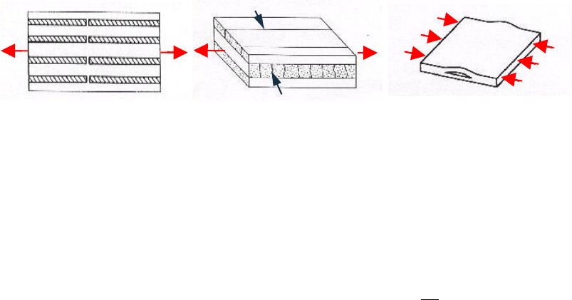
227
12.3 Composite failure criteria
12.3.1 Overview
Composite failure criteria can be used to assess the strength of fibre-reinforced composite laminate
components subject to biaxial loading. The criteria have also been extended to the analysis of closed
cell PVC foam.
A composite can fail in two basic failure modes:
1. Failure of individual plies in tension, compression, or shear (fibre and matrix)
2. Delamination between plies
These composite failure modes are illustrated by Figure 12.1. Quick Fatigue Tool is able to assess the
first mode of failure.
The composite criteria analysis is enabled from the job file.
Job file usage:
Option
Value
COMPOSITE_CRITERIA
{0.0 | 1.0}
12.3.2 Conventions for fibre-reinforced composites
The procedure assumes that the loading represents an orthotropic state of stress; out-of-plane
stresses are ignored. The ply directions are given by Equation 12.1.
[12.1]
Quick Fatigue Tool requires stress components , and for the fibre, transverse and shear
directions, respectively.
12.3.3 Conventions for closed cell PVC foam
For closed-cell PVC foam, the stress components and represent the in-plane directions, while
the stress components and represent the through-thickness of the foam.
Figure 12.1: (L-R) Fibre, matrix and delamination failure

228
12.3.4 Material properties
Stress-based failure criteria
For stress-based failure criteria, the following material properties are required:
Symbol
Definition
Tensile stress (11-direction)
Compressive stress (11-direction)
Tensile stress (22-direction)
Compressive stress (22-direction)
Tensile stress (33-direction)
Compressive stress (33-direction)
Shear strength (12- plane)
Cross-product coefficient (12-plane)
Cross-product coefficient (23-plane)
Stress limit (12-plane)
Stress limit (23-plane)
Maximum strain failure theory
For the maximum strain failure theory, the following material properties are required:
Symbol
Definition
Tensile strain (fibre direction)
Compressive strain (fibre direction)
Tensile strain (transverse direction)
Compressive strain (transverse direction)
Shear strain
Modulus of elasticity (fibre direction)
Modulus of elasticity (transverse direction)
Shear modulus (12-plane)
Hashin’s damage initiation theory
For Hashin’s damage initiation theory, the following material properties are required:
Symbol
Definition
Shear influence parameter
Longitudinal tensile strength
Longitudinal compressive strength
Transverse tensile strength
Transverse compressive strength
Longitudinal shear strength
Transverse shear strength

229
LaRC05 damage initiation theory
For the LaRC05 damage initiation theory, the following material properties are required:
Symbol
Definition
Longitudinal tensile strength
Longitudinal compressive strength
Transverse tensile strength
Transverse compressive strength
Longitudinal shear strength
Transverse shear strength
Shear modulus (12-plane)
Longitudinal slope coefficient
Transverse slope coefficient
Fracture plane angle for pure compression
Initial fibre misalignment angle
Defining material data
Detailed guidance on creating composite material data can be found in Section 5.8. A folder containing
several example materials using composite properties from Pinho et al. [50] can be found in
Data\material\composites.
Treatment of compressive stresses
If the user specifies the option No damage in compression (*NO COMPRESSION) in the material
definition, then compressive values in the stress history are reset to zero. This setting is not
recommended for composite criteria analysis.
12.3.5 Model definition
Stress datasets are created in the same fashion as a standard fatigue analysis. Instructions on creating
stress datasets are found in Section 3.2.
If the stress datasets originate from an Abaqus output database (.odb) file, then it is important to
ensure that stresses are reported only at the location of interest. By default, Abaqus will write stresses
for all available section points. However, Quick Fatigue Tool can only read stresses from a single
location.

230
To create a stress dataset (.rpt) file from Abaqus/Viewer for composite analysis, the following steps
are recommended:
1. Make sure that the regions of the model you wish you export are displayed in the active
viewport
2. From the main menu in Abaqus/Viewer, select Report → Field Output…
3. From the Output Variables region of the Report Field Output dialogue, select Select as the
section point, then select Settings….
4. From the Field Report Section Point Settings dialogue that appears, select either Categories
or Plies as the selection method. For composite structures, selecting results by ply is usually
more convenient
5. From the Categories/Plies region, select the location/section point, or the ply/result location
of interest, then select OK.
Stress datasets are not required if the composite failure analysis is defined with uniaxial histories.
12.3.6 Loading definition
The loading definition is created in the same fashion as a standard fatigue analysis. All of the available
loading methods in Quick Fatigue Tool are described in Section 3. The load history can have a length
of one.
The composite failure assessment is intended for static problems where only the maximum stress is
of interest, thus the load history is usually expected to be a single point. If the user defines a load
history with more than one point, the criteria are evaluated separately for each point in the history.
The quoted value for each criteria is the maximum value computed over the entire load history for
each analysis item. Cycle counting is not employed for composite failure assessment.
Composite failure criteria are only compatible with linear elastic stress datasets.
12.3.7 Maximum stress theory
The maximum stress theory predicts composite failure by comparing each stress component to its
respective strength, according to Equation 12.2.
[12.2]
The value of the tensile (fibre) strength, , and transverse strength, , is determined according to
Equations 12.3-4.
[12.3]
[12.4]
This theory does not account for the interaction between the stress components in different
directions. Therefore, its accuracy is limited.
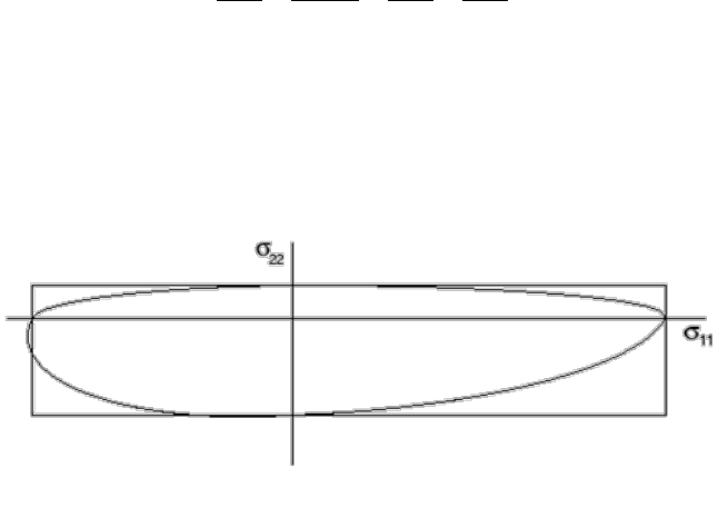
231
12.3.8 Tsai-Hill theory
Tsai proposed a composite failure criterion as an extension of Hill’s anisotropic plasticity model [51].
This simple model defines the failure criterion as a function of the three stress components according
to Equation 12.5.
[12.5]
The value of the tensile (fibre) strength, , and transverse strength, , is determined according to
Equations 12.3-4.
The Tsai-Hill theory is a piecewise-continuous failure surface, shown by Figure 12.2.
Figure 12.2: Tsai-Hill piecewise-continuous failure surface
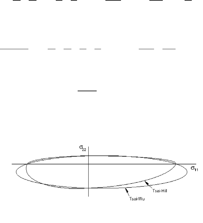
232
12.3.9 Tsai-Wu theory for fibre-reinforced composites
The Tsai-Wu composite failure criterion is a smooth form of the Tsai-Hill criterion [52]. The direct and
shear stress is coupled by the Tsai-Wu by the parameter , which is a function of either the cross-
product coefficient, or the stress limit, .
The criterion is defined according to Equation 12.6.
[12.6]
The Tsai-Wu coefficients are defined according to Equation 12.7.
[12.7]
If the stress limit, , is defined, the coupling parameter, , is given by Equation 12.8.
[12.8]
If the stress limit is not defined, the coupling parameter is defined by Equation 12.9.
[12.9]
The default value of is zero. If , the Tsai-Wu failure surface is given by Figure 12.3.
Figure 12.3: Tsai-Wu piecewise-continuous failure surface (
)

233
12.3.10 Tsai-Wu theory for closed cell PVC foam
The Tsai-Wu failure criterion has been applied to closed cell PVC foam under plain strain conditions,
according to Equation 12.10.
[12.10]
The Tsai-Wu coefficients are defined according to Equation 12.11.
[12.11]
If the stress limit, , is defined, the coupling parameter, , is given by Equation 12.12.
[12.12]
If the stress limit is not defined, the coupling parameter is defined by Equation 12.13.
[12.13]
The default value of is zero.
The foam is assumed to be in a state of plane strain, such that .
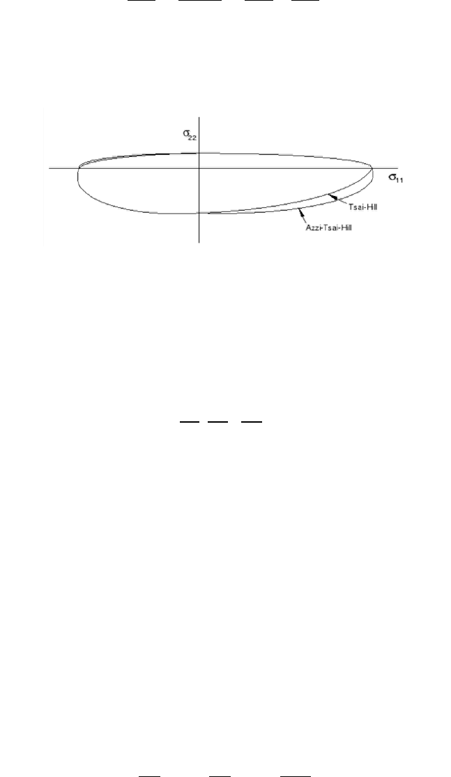
234
12.3.11 Azzi-Tsai-Hill theory
The Azzi-Tsai-Hill composite failure criterion is the same as the Tsai-Hill theory, except that the
absolute value of the cross-product term is used, according to Equation 12.14.
[12.14]
The Azzi-Tsai-Hill failure surface is given by Figure 12.4.
12.3.12 Maximum strain failure theory
The maximum failure strain theory predicts composite failure by comparing each strain component to
its respective strain limit, according to Equation 12.15.
[12.15]
The value of the tensile (fibre) strain, , and transverse strain, , is determined according to
Equations 12.16-17.
[12.16]
[12.17]
Experimental data suggests that the maximum failure strain theory is not as accurate as the maximum
stress theory.
The maximum failure strain theory assumes that the stresses in the composite are linear elastic until
. The elastic stress is converted into elastic strain using the shear modulus, , according to
Equation 12.18.
[12.18]
Figure 12.4: Azzi-Tsai-Hill piecewise-continuous failure surface

235
12.3.13 Hashin’s damage initiation criteria
The damage initiation criteria for fibre-reinforced composites is calculated using Hashin’s theory [53].
The model considers the following modes of failure:
I. Fibre tension ()
II. Fibre compression ()
III. Matrix tension ()
IV. Matrix compression ()
The criteria for each mode are calculated according to Equations 12.19-22.
[12.19]
[12.20]
[12.21]
[12.22]
The effective stress tensor,
, is given by Equation 12.23.
[12.23]

236
12.3.14 LaRC05 damage initiation criteria
An alternative failure criterion has been proposed by Pinho et al. [50] [54], wherein the damage in the
composite is based on a pressure-dependent, three-dimensional constitutive law. The model
considers the following modes of failure:
I. Polymer ()
II. Matrix ()
III. Fibre kinking/splitting ()
IV. Fibre tensile ()
The model has been used to make predictions of the test cases presented from the second World-
Wide Failure Exercise [55].
Polymer failure
The polymer failure criterion is calculated according to Equation 12.24.
[12.24]
The hydrostatic stress is given by Equation 12.25.
[12.25]
The parameter, , is given by Equation 12.26.
[12.26]
The maximum, middle and minimum principal stresses are given by , and , respectively.
Matrix failure
The matrix failure criterion is calculated according to Equation 12.27.
[12.27]
The stresses , and are the traction components on each trial fracture plane, and are calculated
according to Equations 12.28-30.
[12.28]
[12.29]
[12.30]

237
Fibre kinking/splitting failure
The fibre kinking and splitting failure criteria are calculated according to Equation 12.31.
[12.31]
The stresses on the kink band plane are given by Equations 12.32-35.
[12.32]
[12.33]
[12.34]
[12.35]
The stresses on the fibre misalignment frame are given by Equations 12.36-38.
[12.36]
[12.37]
[12.38]
The misalignment angle, , is the sum of the initial misalignment angle, , and the shear strain, ,
and is given by Equation 12.39.
[12.39]
Fibre tensile failure
The tensile failure criterion is calculated according to Equation 12.40.
[12.40]

238
Derived properties
If the value of is not specified, it is derived from Equation 12.41.
[12.41]
If the value of is not specified, it is derived from Equation 12.42.
[12.42]
The parameter represents the fracture plane angle for pure transverse compression. Several
sources report that is typical for glass and carbon composites [50] [56] [57]. A default
value of 53 degrees is assumed.
If the value of is not specified then it can be derived iteratively from Equations 12.43-44, otherwise
a value of 0 degrees is assumed.
[12.43]
[12.44]
This calculation is enabled by checking the option Allow iterative solution if applicable
9
in the LaRC05
Parameters dialogue box (Figure 5.7). This option may be time-consuming if the assessment is run for
more than 100 analysis items.
Critical plane searching
The values of and which maximise the functions and are found by performing critical
plane analyses for , respectively.
Quick Fatigue Tool searches 19 planes by default. This can be changed with following environment
variable.
Environment file usage:
Variable
Value
stepSize
9
Requires the Symbolic Math Toolbox

239
12.3.15 Output
Output failure indices
The failure measures, , are evaluated based on the available material data. Except for Hashin’s
theory and LaRC05, values of are quoted in terms of the failure index , so that for the given stress
state :
[12.45]
That is,
is the scaling factor by which all of the stress components must be simultaneously
multiplied to hit the failure surface. The term
can be used with the SCALE job file option in order
to make for the specified failure criterion.
The calculation of depends on the failure criterion, and is summarised according to the following
table:
Failure criterion
Failure index,
Maximum stress theory
Maximum strain theory
Tsai-Hill theory
Tsai-Wu theory for fibre-reinforced composites
Tsai-Wu theory for closed cell PVC foam
Azzi-Tsai-Hill theory
For the Tsai-Wu theory for fibre-reinforced composites:
[12.46]
[12.47]
For the Tsai-Wu theory for closed cell PVC foam:
[12.48]
[12.49]
[12.50]
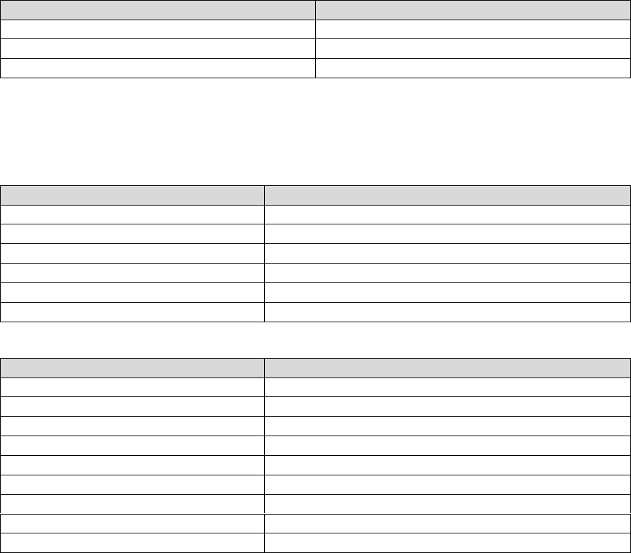
240
For Hashin’s theory and LaRC05, is not evaluated; output for these criteria is given directly as the
value of .
The values of and should be interpreted according to the following table:
Range of values of /
Meaning
Composite is safe, or damage has not initiated
Composite has failed, or damage has initiated
Criterion could not be evaluated
Composite failure criteria analysis field variable identifiers
The criterion variable names take their meaning from the following tables:
Failure index,
Meaning
MSTRS
Maximum stress theory failure measure
MSTRN
Maximum strain theory failure measure
TSAIH
Tsai-Hill theory failure measure
TSAIW
Tsai-Wu theory failure measure
TSAIWTT
Tsai-Wu theory failure measure for closed cell PVC foam
AZZIT
Azzi-Tsai-Hill theory failure measure
Failure measure,
Meaning
HSNFTCRT
Hashin’s fibre tensile damage initiation criterion
HSNFCCRT
Hashin’s fibre compressive damage initiation criterion
HSNMTCRT
Hashin’s matrix tensile damage initiation criterion
HSNMCCRT
Hashin’s matrix compressive damage initiation criterion
LARPFCRT
LaRC05 polymer failure measure
LARMFCRT
LaRC05 matrix failure measure
LARKFCRT
LaRC05 fibre kinking failure measure
LARSFCRT
LaRC05 fibre splitting failure measure
LARTFCRT
LaRC05 fibre tensile failure measure
241
Output files
If there are sufficient material properties to evaluate at least one criterion, the results for each analysis
item are written to Project\output\<job-name>\Data Files\composite-criteria.dat.
In addition to tabulated results, a summary of the analysis is written to the message file; the user is
notified if any individual criterion has a value equal-to or greater-than one. If every criterion evaluates
to less than one, this outcome is also written to the message file.
If the user specified an Abaqus output database (.odb) file, then Quick Fatigue Tool will automatically
write the results to a copy of this file.
Environment file usage:
Variable
Value
autoExportODB
Job file usage:
Option
Value
OUTPUT_DATABASE
'model-odb-file-name.odb'
The ODB interface is discussed in Section 10.4.
12.3.16 Example Usage
Composite failure assessments are run as jobs in much the same way as standard fatigue analyses.
Example input files can be found in Data\tutorials\composite_tutorial. Damage in the fibre and the
matrix are each considered as separate jobs, given by the text files composite_load_fibre.inp and
composite_load_matrix.inp, respectively. The composite assessment is specified using the
*COMPOSITE CRITERIA keyword.
The job is submitted by executing the following command:
>> composite_tutorial
Results are written to Project\output\composite_tutorial\Data Files\composite-criteria.dat.
Since the composite failure criteria assessment is always run as a data check analysis, the user is not
required to specify ALGORITHM or MS_CORRECTION in the job file.
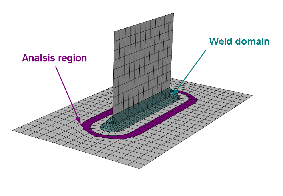
242
13. Tutorial A: Analysis of a welded plate with Abaqus
13.1 Background
This tutorial outlines the procedure for analysing a welded structure using an Abaqus output database
file with Quick Fatigue Tool. The analysis is based upon the continuum shell model of a welded T-joint
in bending, shown in Figure 13.1.
The model will be analysed using the British Standard BS 7608 method for the analysis region indicated
by the magenta elements in Figure 13.1. The methodology corrects the Stress-Life curve to account
for the presence of a stress concentration at the weld toe; therefore, the stresses used for analysis
should be a small distance away from the weld line, in order to avoid excessively conservative results.
For more information about the BS 7608 method, refer to Section 6.6.
The stress datasets are first extracted from the output database and written to an RPT file. A fatigue
analysis is then performed with Quick Fatigue Tool and the results are written back to the ODB using
the Export Tool.
Figure 13.1: Weld plate model

243
13.2 Preparing the RPT file
If you do not have Abaqus installed, you can skip this step; the file weldPlate.m has already been added
to the Data\datasets folder. You must copy this file into the Project\input folder before continuing.
To generate an RPT file for the analysis region, open the Create Display Group dialogue box. From the
Item region, select Elements. Select the element group PLATE-1_ANALYSE and select Replace from the
list of Boolean operations.
The exported stress tensors should not have any averaging applied to them. From the main menu,
select Result → Options…. From the Averaging region, deselect “Average element output at nodes”
and select OK. From the main menu, select Report → Field Output… From the Variable tab, select
Element-Nodal as the result position and select all four stress tensor components S11, S22, S33 and
S12. From the Setup tab, specify the absolute path to the Quick Fatigue Tool input folder Project\input
and name the file weldPlate.rpt. Deselect Column totals and Column min/max from the data region
and select OK.
13.3 Running the analysis
From the Project\input folder, open the job file named tutorial_A.m and review the contents. Ensure
that the DATASET option points to the correct file. A summary of the other pertinent options are listed
below.
Option
Details
PLANE_STRESS=1.0
The elements are plane stress
ALGORITHM=8.0
The algorithm is set to BS 7608
OUTPUT_FIELD=1.0
Field output is required to write results to the
ODB
WELD_CLASS='F2'
Weld classification. For guidelines on choosing
the weld class, consult the document BS 7608
YIELD_STRENGTH=325
UTS=400
Mechanical properties of the weld plate
material (MPa)
DEVIATIONS_BELOW_MEAN=2.0
Confidence interval (95% probability of failure)
FAILURE_MODE='NORMAL'
Failure criterion
CHARACTERISTIC_LENGTH=1.0
Plate thickness (mm)
SEA_WATER=0.0
Atmospheric condition (fresh air)
Run the analysis by right-clicking the job file and selecting Run. The analysis may take a few minutes
depending the computer’s hardware specification. The result summary is displayed in the command
window (Figure 13.2).
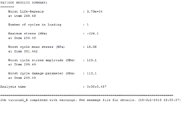
244
The predicted life is 37,300 repeats at element 299, node 49. Open the message file (located in
Project\output\tutorial_A) to view information about the analysis. Take note of which element face
Quick Fatigue Tool analysed. By default, the negative shell face is used for analysis.
13.4 Post processing the results
This step can only be completed if the user has access to Abaqus/Viewer.
The field data for the entire analysis region can be written back to the Abaqus output database. Start
the Export Tool either by clicking on the App icon, or by running the file ExportTool.m in
Application_Files\code\python. Configure the dialogue so that it appears as shown in Figure 13.3.
For the Field Data input, select the file f-output-all.dat from Project\output\Tutorial_A\Data Files.
For the Model output database input, select weldPlate_614.odb from Data\abaqus.
Check Results output database and select Project\output\Tutorial_A as the result directory.
Accept the default field output and select Write Output.... The progress of the export is displayed in
the command window.
The contents of the export log file are shown in Figure 13.4. Since the fatigue analysis only considered
a subset of elements, 615 of the 655 total elements in the ODB were ignored.
The fatigue results ODB path is copied to the clipboard. Open Abaqus/CAE and press Ctrl+O. In the
Open Database dialogue, paste the ODB path into the file box and press Enter. The fatigue results are
shown in Figure 13.5.
Figure 13.2: Fatigue results summary
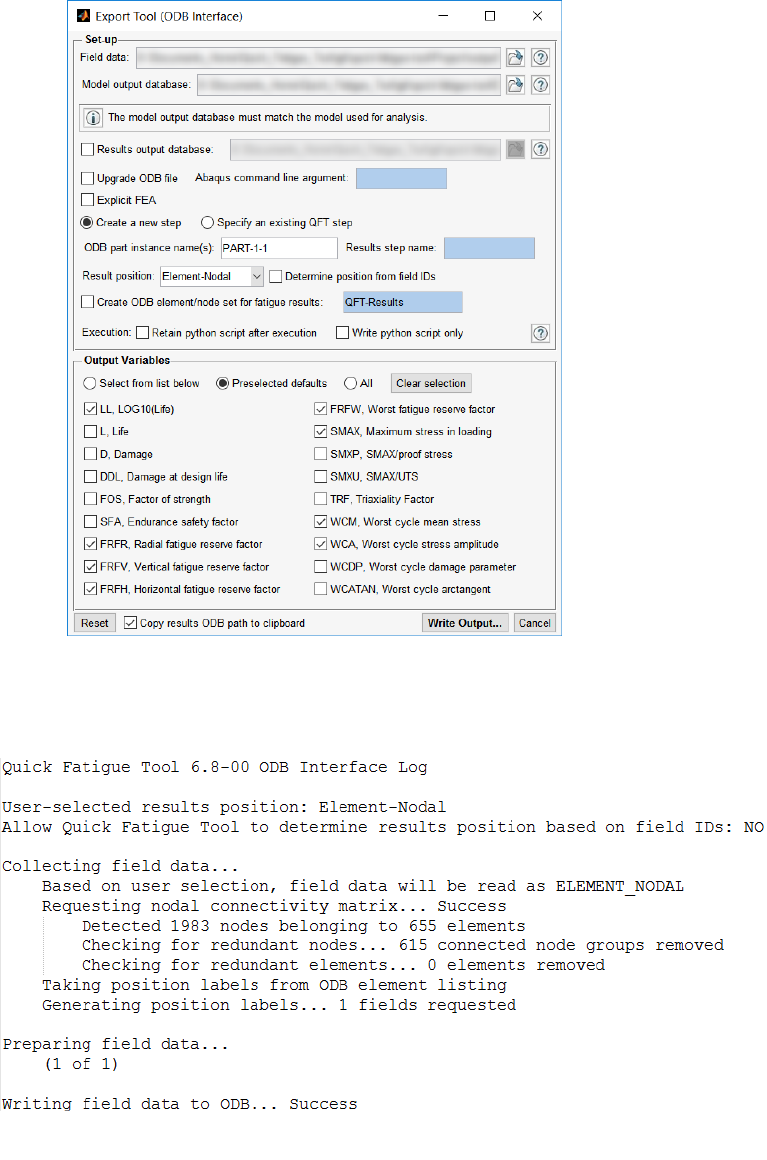
245
Figure 12.3: Export Tool setup
Figure 12.4: ODB export log file
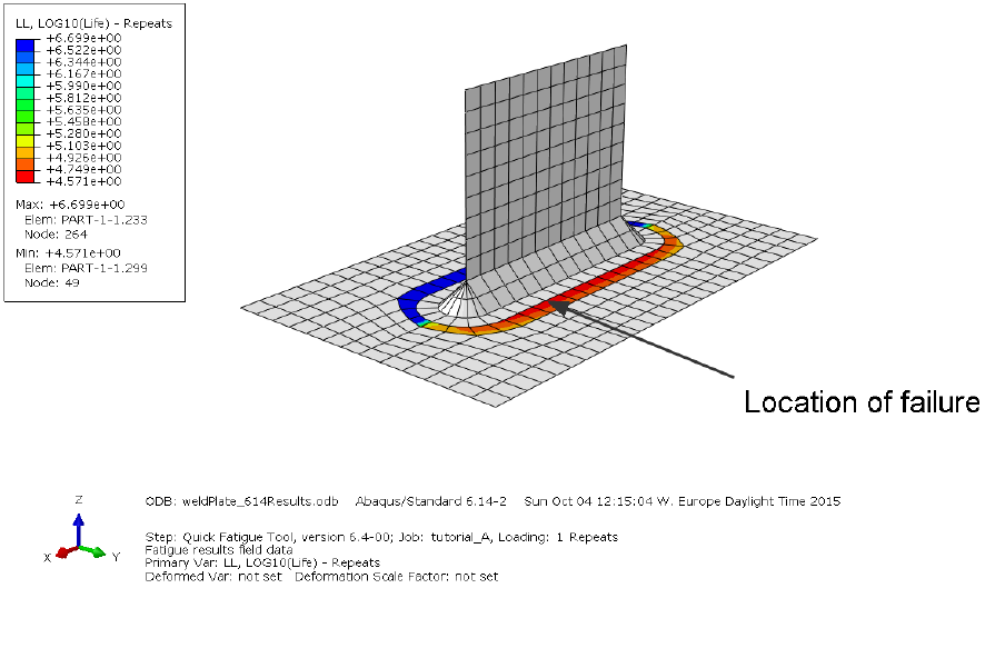
246
Figure 12.5: Fatigue results ODB
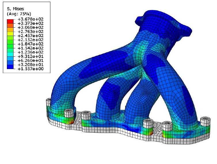
247
14. Tutorial B: Complex loading of an exhaust manifold
14.1 Background
This tutorial outlines the procedure for analysing an exhaust manifold using an Abaqus output
database file with Quick Fatigue Tool. The manifold model used is that shown in Figure 14.1.
The analysis consists of three loading steps. First, a pre-tension is applied to the bolts. The manifold is
then subjected to a transient thermal load. The load is then removed and the model is allowed to
return to ambient temperature. The stresses are obtained at each load step and analysed as a stress
dataset sequence. The peak stress history is shown in Figure 14.2. In addition to the thermal loading,
the mechanical load history shown in Figure 14.3 is superimposed onto the thermal stress as a high
frequency stress dataset. The mechanical load is defined in Quick Fatigue Tool as a simple loading of
the stress data from the pre-tension step with a user-defined load history.
This tutorial demonstrates the use of several features in Quick Fatigue Tool. However, the model data
itself is arbitrary. Sections of the tutorial use Abaqus/Viewer for results post-processing. If the user
does not have access to Abaqus/Viewer, these sections may be skipped.
Figure 14.1: Exhaust manifold model
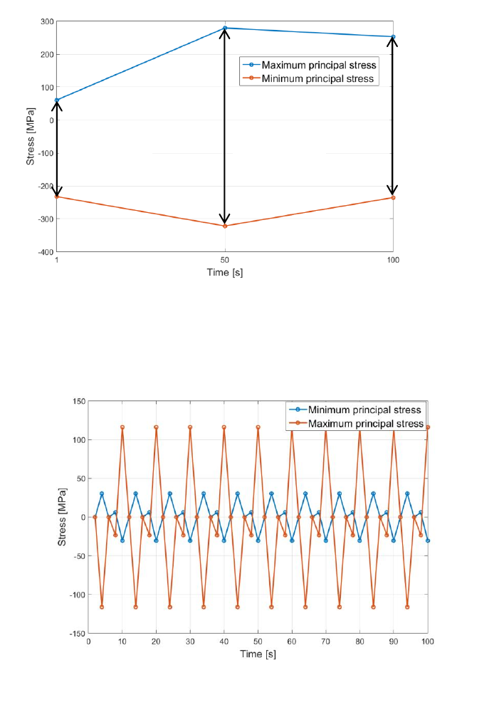
248
Figure 14.2: Peak thermal stress
Pretension
Apply heat
Cool down
Figure 14.3: Peak mechanical load
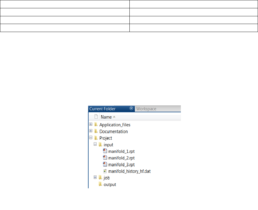
249
14.2 Preparation
Analysing finite element models with complex load histories with Quick Fatigue Tool can sometimes
be time-consuming; therefore, the analysis will be split into two procedures. First, the whole model
will be analysed with a simplified loading configuration to find the location of maximum damage.
Afterwards, a second analysis will be performed on the node which experiences maximum damage
with the complete loading definition.
Before running the analysis, verify that the following files exist in the Project\input directory:
‘manifold_1.rpt’
Stress data for step 1 (pretension)
‘manifold_2.rpt’
Stress data for step 2 (thermal load)
‘manifold_3.rpt’
Stress data for step 3 (cool-down)
‘manifold_history_hf.dat’
Normalized history data for the mechanical load
Copy the datasets and history file from Data\datasets and Data\histories, respectively, into the
Project\input folder. The input folder should appear as in Figure 14.4.
The datasets may be created in Abaqus/CAE following the procedure outlined in Section 3.2, using
unique nodal as the result position.
In order to customise the analysis, setting in the environment file can be changed. However, future
analyses should not be affected by this change, so a separate environment file will be stored locally,
which corresponds to the analysis in Tutorial B. To create a local environment file, copy the file
environment.m from Application_Files\default and paste it into Project\job. Rename the file to
tutorial_B_env.m. If the file is named differently, it will be ignored during analysis. File names are case-
sensitive. The job folder should appear as in Figure 14.5.
Figure 14.4: Required input files for
Tutorial B
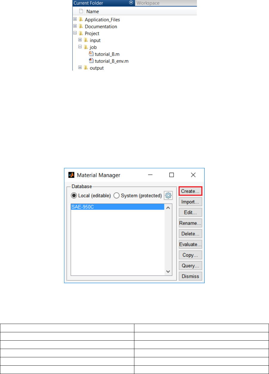
250
14.3 Defining the material
The analysis job file tutorial_B.m references a material called material_tutorial_B.mat. This material
needs to be created using the material manager. To launch the material manager, run the file
materialManager.m from Application_Files\code\material_manager or run the material manager app
from the app menu. The main dialogue is shown in Figure 14.6.
Click Create… to create a new material. The material editor is shown in Figure 14.7. Enter the
parameters as shown by the green boxes. The material properties are as follows:
Material name
material_tutorial_B
Young’s Modulus
200GPa
Fatigue Strength Coefficient
1050MPa
Fatigue Strength Exponent
-0.085
Strain Hardening Coefficient
1200MPa
Strain Hardening Exponent
0.19
Press OK to save the material to the workspace. The newly created material should now appear in the
list of workspace materials in the Material Manager main dialogue box. Exit the Material Manager by
clicking Dismiss.
Figure 14.5: Required job files for Tutorial B
Figure 14.6: Material Manager dialogue
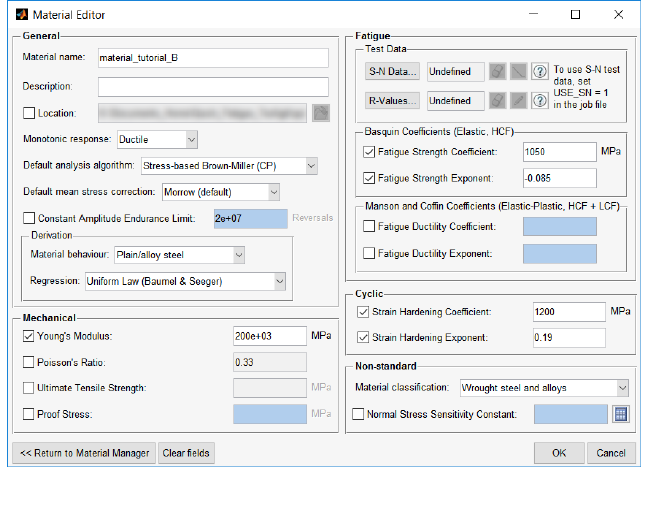
251
14.4 Running the first analysis
The first analysis is run to identify the location of maximum damage. The loading is restricted to the
thermal stress and the critical plane step size is increased to reduce the analysis time.
Close the environment file and open tutorial_B.m from the job folder and review the settings:
The thermal load is defined by DATASET as a sequence of stress datasets representing each
loading step from the finite element analysis
The high frequency mechanical loading defined by HF_DATASET and HF_HISTORY is
commented out for this analysis
The default algorithm and mean stress correction are set by ALGORITHM and
MS_CORRECTION, respectively
ITEMS is used to indicate that all items in the model will be analysed
A residual stress of 10MPa is specified using RESIDUAL
Field output is requested using OUTPUT_FIELD
For a complete description of analysis options, consult the document
Quick Fatigue Tool User Settings Reference Guide.
Figure 14.7: Material editor dialogue
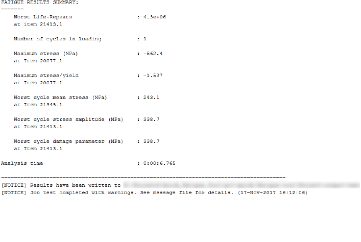
252
To run the analysis, right-click on tutorial_B.m and select Run, or press F5 while the file is open in the
editor. Analysis progress is displayed in the command window. Figure 14.8 shows the result of the
analysis.
The stress data from Abaqus was extracted at the nodes and averaged, therefore the worst life is
quoted at the unique nodal position. Since the mechanical stresses were not included for analysis the
life result is unimportant. However, the analysis result indicates that failure will occur at node 21413
on the finite element model.
Figure 14.8: Fatigue analysis results indicating node 21413 as the location of
failure
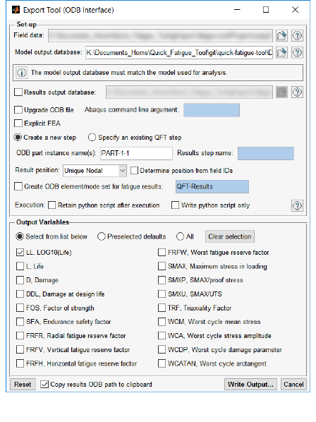
253
14.5 Viewing the results with Abaqus/Viewer
This step may be skipped if the user does not have Abaqus 6.14 or later installed on their machine.
To view the life data on the manifold model, launch the Export Tool by running the file exportTool.m
from Application_Files\code\python, or by running the app from the app bar. Configure the dialogue
box so that it appears as in Figure 14.9.
1. Select the field data file f-output-all.dat from Project\output\tutorial_BData Files
2. Select the model output database manifold_614.odb from Data\abaqus
3. Specify the part instance name PART-1-1
4. Uncheck Determine position from field IDs and select Unique Nodal as the result position
5. Click Clear selection to deselect all fields, then select LL, LOG10(Life)
6. Click Write Output… to write the life data to an Abaqus ODB file
For a detailed explanation of the Export Tool, consult Section 10.4.
To view the ODB file in Abaqus/Viewer, start Abaqus and open the ODB in the usual way. The full path
to the results ODB file has been copied to the clipboard, so pressing Ctrl+V can be used. Isolate the
location of failure by selecting Create Display Group. Select Elements as the item and Element Sets as
the method of creating the display group. Select PART-1-1.FL2 and click Replace. The location of failure
is shown in Figure 14.10.
Figure 14.9: Export Tool settings for the results ODB
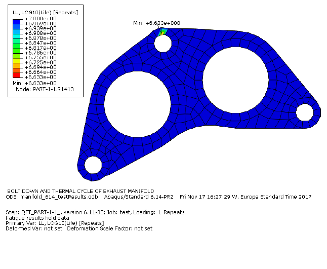
254
14.6 Running the second analysis
The previous analysis determined that the manifold will fail at node 21426. By inspecting the message
file, Quick Fatigue Tool tells us that this node corresponds to item number 10505 in the dataset. A
second analysis will be performed on this item only. From the job file, specify this item as follows:
ITEMS=10505;
The mechanical load must now be considered. Define the high frequency data as follows:
HF_DATASET='manifold_1.rpt'
HF_HISTORY='manifold_history_hf.dat'
Commented versions of these entries are already provided below the previous definitions.
Request histories and MATLAB figures in addition to fields:
OUTPUT_FIELD=1.0
OUTPUT_HISTORY=1.0
OUTPUT_FIGURE=1.0
Figure 14.10: Location of failure shown in Abaqus/Viewer
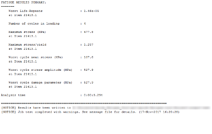
255
MATLAB should be restarted before running the analysis, to ensure that all data from the previous
analysis is cleared. After running the analysis, a summary of the fatigue results are displayed in the
command window, as in Figure 14.11.
The analysis indicates a life of 146,000 repeats of the loading until failure.
Figure 14.11: Fatigue analysis results from the second analysis
256
14.7 Post processing the results
The results of the analysis are stored in Project\output\tutorial_B.
Field and history data is written to a set of tabulated data files
Certain results data is automatically plotted to a set of MATLAB figures
An overview of the analysis is written to tutorial_B.log
Warnings and messages are written to tutorial_B.msg
Open the message file to view possible issues with the analysis:
MESSAGES:
=======
***NOTE: The proof stress for material material_tutorial_B.mat (group 1)
was not specified
-> A derived value of 368.4MPa will be used
***WARNING: In at least one group, the UTS is undefined. The following
fields are unavailable:
-> FRFR, FRFH, FRFV, FRFW, SMXU
***NOTE: Worst damage at design life (1e+07) is 68.6
***WARNING: 1 items have lives less than 1e+06 Repeats
The proof stress was derived based on the cyclic material properties using the 0.2% strain
offset rule
Certain variables are not available because the ultimate tensile strength was not defined
The manifold will not survive the default design life of 10 million loading repeats
The stress-life methodology is not well-suited to low-cycle fatigue problems (lives below 1
million repeats)
A summary of the cycle counting process can be viewed either as a Haigh diagram or a rainflow
histogram. The rainflow histogram is shown by Figure 14.12. This indicates that the damage is
primarily caused by one cycle in the loading where the stress range is significantly higher than every
other location in the history.
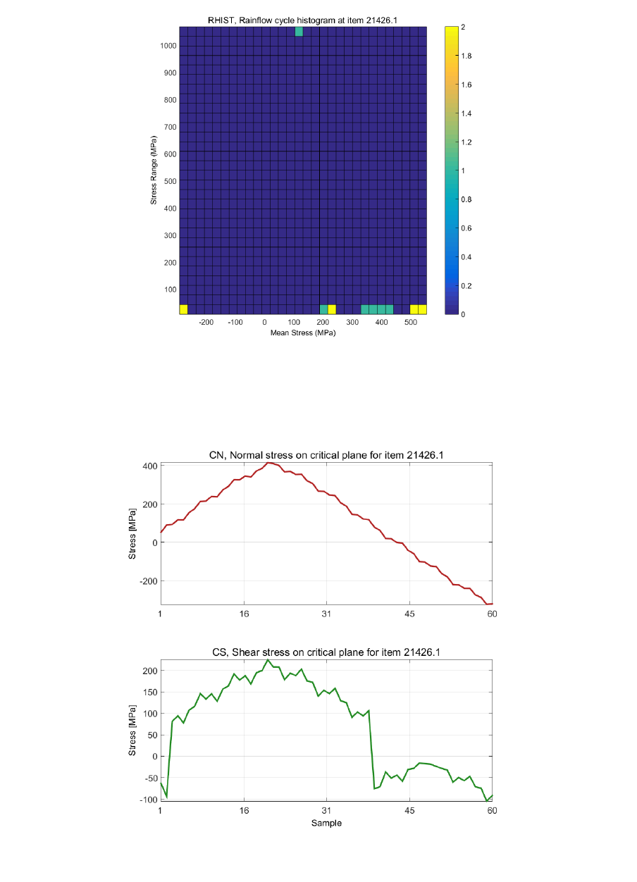
257
Figure 14.12: Rainflow histogram of cycles
Figure 14.13: Normal and shear stress on the critical plane

258
The normal and shear stress on the critical plane is shown by Figure 14.13. It is clear from the data
that the mechanical stress was superimposed onto the thermal stress correctly.
The results of the critical plane analysis are shown by Figures 14.15-16. Planes of maximum shear
stress occur at 45 degrees, which is expected since ductile metals in pure tension fail along planes at
45 degrees to the free surface. According to the log file, the critical plane occurs where theta is 110
degrees (Figure 14.14). This represents the angle at which the combination of shear and normal stress
is maximised.
By inspecting Figure 14.16, it is clear that the damage parameter is maximised when theta equals 110
degrees. In fact, the damage profile is symmetrical about 90 degrees. This is the point at which the
shear stress is zero.
Figure 14.14: Sample log file output
indicating the orientation of the critical plane
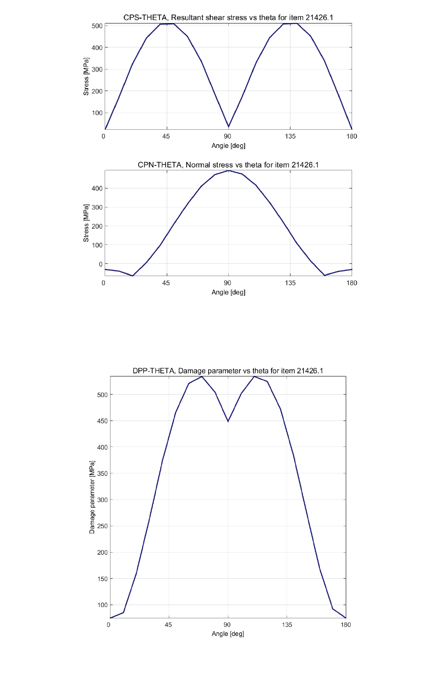
259
Figure 14.15: Critical plane analysis results
Figure 14.16: Damage parameter on the critical plane
260
Appendix I. Fatigue analysis techniques
This section has been released in the document Quick Fatigue Tool Appendices.
261
Appendix II. Materials data generation
This section has been released in the document Quick Fatigue Tool Appendices.
262
Appendix III. Gauge fatigue toolbox
This section has been released in the document Quick Fatigue Tool Appendices.
263
References
[1]
J. A. Bannantine, J. J. Comer and J. L. Handrock, Fundamentals of Metal Fatigue Analysis,
Prentice Hall, 1989.
[2]
R. I. Stephens, A. Fataemi, R. R. Stephend and H. O. Fuchs, Metal Fatigue in Engineering, Jon
Wiley & Sons, 2001.
[3]
D. N. W. M. Bishop and D. F. Sherratt, Finite Element Based Fatigue Calculations, Glashow: The
International Association for the Engineering Analysis Community (NAFEMS), 2000, p. 18.
[4]
D. Taylor, The theory of critical distances: a new perspective in fracture mechanics, 1st ed.,
Elsevier, 2007, pp. 11, 164-165.
[5]
L. Vallance, A. Winkler and A. Belles Meseguer, “An Engineering Approach to Advanced Fatigue
of Welded Joints,” Graz, 2015.
[6]
J. Draper, Modern Metal Fatigue Analysis, East Sussex: EMAS Publishing, 2008.
[7]
M. A. Miner, “Cumulative Damage in Fatigue,” Journal of Applied Mechanics Vol 12, Trans ASME
Vol 67, vol. 12, pp. A159-A164, 1945.
[8]
W. Ramberg and W. R. Osgood, “Description of Stress-Strain Curves by Three Parameters,”
National Advising Committee for Aeronautics, no. Technical Note no. 902, 1947.
[9]
N. E. Dowling, Mechanical Behavior of Materials, 4th ed., Pearson, 2013, pp. 644-648.
[10]
L. Pook, “Metal Fatigue: What It Is, Why It Matters: Prelimenary Entry No. 1525,” Solid
Mechanical and its Applications, vol. 145, p. 25, 9 March 2007.
[11]
R. E. Peterson, “Analytical Approach to Stress Concentration Effect in Fatigue of Aircraft
Structures,” WADS Symposium, 1959.
[12]
R. E. Peterson, Notch Sensitivity, McGraw-Hill Book Co., In., 1959, p. Metal Fatigue Chapter 13.
[13]
P. Kuhn and H. F. Hardrath, “An Engineering Method for Estimating Notch-Size Effect in Fatigue
Tests on Steel,” National Advisory Committee for Aeronautics, p. Technical Note 2805, October
1952.
[14]
H. J. Harris, New York: Pregamon Press, 1961.
[15]
R. B. Heywood, Design by photoelasticity, London: Chapman and Hall Ltd., 1952, p. 348.
[16]
J. E. Shigley and C. R. Mischke, Mechanical Engineering Design, 5th ed., New York: McGraw-Hill,
Inc., 1989, pp. Fig. 5-16 and Fig. 5-17.
264
[17]
L. Susmel, “La progettazione a fatica in presenza di stati complessi di sollecitazione (PhD
thesis),” Padova, 2001.
[18]
M. W. Brown and K. J. Miller, “A Theory Of Fatigue Under Multiaxial Strain Conditions,” Proc
Inst Mech Eng, vol. 187, pp. 745-755, 1973.
[19]
K. J. Miller, “Fatigue Under Complex Stress,” Metal Science, pp. 482-488, August-September
1977.
[20]
M. W. Brown and K. J. Miller, “A Theory for Fatigue Failure under Multiaxial Stress-Strain
Conditions,” Proceedings of the Institution of Mechanical Engineering, vol. 187, no. 1, pp. 745-
755, June 1973.
[21]
C. Lipson and R. C. Juvenal, Handbook of Stress And Strength - Design And Material Application,
MacMillan, 1963.
[22]
A. Carpinteri and A. Spagnoli, “Multiaxial high-cycle fatigue criterion for hard metals,”
International Journal of Fatigue, vol. 23, no. 2, pp. 135-145, 2001.
[23]
W. N. Findley, “A Theory for the Effect of Mean Stress on Fatigue of Metals Under Combined
Torsion and Axial Loading or Bending,” Journal of Engineering and Industry, vol. 81, pp. 301-
306, 1959.
[24]
W. N. Findley, B. Hanley and J. J. Coleman, “Theory for Combined Bending and Torsion Fatigue
with Data for SAE 4349 Steel,” Proceedings for the International Conference on Fatigue of
Metals, September 1956.
[25]
L. Susmel, Multiaxial Notch Fatigue, Oxford: Woodhear Publishing, 2009, p. 101.
[26]
A. R. Kallmeyer, “Mutiaxial Fatigue Life Prediction Methods for Notched Bars of Ti-6AL-4V,”
Fargo, Urbana.
[27]
A. Winkler, S. Holt and L. Vallance, “Concerning the Synergy of Stress and Strain-based Methods
in Modern Metal Fatigue Analysis,” in AVL AST User Conference, Graz, 2013.
[28]
D. Socie and G. Marquis, Multiaxial Fatigue, SAE International, 1999.
[29]
G. Marquis and D. Socie, “Long-life torsion fatigue with normal mean stress,” Fatigue & Fracture
of Engineering Materials & Structures, vol. 23, no. 4, 2000.
[30]
J. Lemaitre and J. L. Chaboche, Mechanics of Solid Materials, Cambridge: Cambridge University
Press, 1990.
[31]
V. Grubisic and A. Simbürger, “Fatigue under combined out of phase multiaxial stresses,”
Processdings of International Conference on Fatigue Testing and Design, pp. 27.1-27.8, 1976.
265
[32]
I. V. Papadopoulos, “Critical plane approaches in high-cycle fatigue: on the definition of the
amplitude and mean value of the shear stress acting on the critical plane,” Fatigue and Fracture
of Engineering Materials and Structures, vol. 21, pp. 269-285, 1997.
[33]
B. Li, J. L. T. Santos and M. de Freitas, “A computerized procedure for long-life fatigue
assessment under multiaxial loading,” Fatigue and Fracture of Engineering Materials and
Structures, vol. 24, pp. 165-177, 2001.
[34]
N. Zouain and E. N. Mamiya, “Using enclosing ellipsoids in multiaxial fatigue strength criteria,”
European Journal of Mechanics and Solids, vol. 25, pp. 51-71, 2006.
[35]
K. Bel Knani, D. Benasciutti, A. Signorini and R. Tovo, “Fatigue damage assessment of a car body-
in-white using a frequency-domain approach,” Internationa Journal of Materials and Product
Technology, vol. 30, pp. 172-198, 2007.
[36]
T. Lagoda, E. Macha and A. Dragon, “Influence of correlations between stresses on calculated
fatigue life of machine elements,” International Journal of Fatigue, vol. 18, pp. 547-555, 1996.
[37]
P. Heyes, “Multiaxial Fatigue,” 1 May 2012. [Online]. Available:
http://www.ncode.com/fileadmin/mediapool/nCode/downloads/events/Multiaxial_Fatigue_
UGM_May_2012_Heyes__Compatibility_Mode_.pdf. [Accessed 21 November 2016].
[38]
British Standard, “Code of practice for Fatigue design and assessment of steel structures,”
British Standard, 1993.
[39]
J. Z. Gyekenyesi, P. L. N. Murthy and S. K. Mital, “NASALIFE - Component Fatigue and Creep Life
Prediciton Program,” NASA Center for Aerospace Information; National Technical Information
Service, Cleveland, Ohio 44135, 2014.
[40]
G. Sines and G. Ohgi, “Fatigue Criteria Under Combined Stresses and Strains,” Journal of
Engineering Materials and Technology, vol. 103, pp. 82-90, 1981.
[41]
K. N. Smith, P. Watson and T. H. Topper, “A Stress-Strain Function for the Fatigue of Metals,”
Journal of Materials, vol. 5, no. 4, pp. 767-778, December 1970.
[42]
J. Goodman, Mechanics Applied to Engineering, London: Longmans Green, 1899.
[43]
C. R. Soderberg, “Factors of Safety and Working Stress,” Trans. ASME, 1939.
[44]
J. Morrow, Fatigue Design Handbook, Society of Automotive Engineers, 1968, pp. 21-29.
[45]
K. Walker, “The Effect of Stress Ratio during Crack Propagation and Fatigue for 2024-T3 and
7075-T6 Aluminum,” American Society of Testing and Materials, no. STP 462, pp. 1-14, 1970.
[46]
N. E. Dowling, “Mean Stress Effects in Stress-Life and Strain-Life Fatigue,” 2004.
266
[47]
N. E. Dowling, “Mean Stress Effects in Stress-Life and Strain-Life Fatigue,” SAE Technical Paper,
no. No. 2004-01-2227, 2004.
[48]
A. Ince and G. Glinka, “A modification of Morrow and Smith-Watson-Topper mean stress
correction models,” Fatigue & Fracture of ENgineering Materials & Structures, vol. 34, no. 11,
pp. 854-867, 17 February 2011.
[49]
K. Golos and F. Ellyin, “A Total Strain Energy Density Theory for Cumulative Fatigue Damage,”
J. Pressure Vessel Technol, vol. 110, no. 1, pp. 36-41, 1st Feb 1988.
[50]
S. Pinho, P. Camanho and L. Lannucci, “Failure Models and Criteria for FRP Under In-Plane or
Three-Dimensional Stress States Including Shear Non-Linearity,” NASA, 2005.
[51]
W. C. Cui, M. R. Wisnom and M. Jones, “A comparison of failure criteria to predict delamination
of unidirectional glass/epoxy specimens waisted through the thickness,” Composites, vol. 23,
no. 3, pp. 158-166, May 1992.
[52]
S. W. Tsai and E. M. Wu, “A general theory of strength for anisotropic materials,” Journal of
Composite Materials, vol. 5, pp. 58-80, 1971.
[53]
Z. Hashin and A. Rotem, “A Fatigue Failure Criterion For Fiber Reinforced Materials,” Isreal
Institute of Technology, Haifa, 1973.
[54]
S. Pinho, G. Vyas and P. Robinson, “Material and structural response of polymer-matrix fibre-
reinforced composites: Part B,” Journal of Composite Materials, vol. 47, no. 6-7, pp. 679-696,
26 March 2013.
[55]
P. D. Soden, A. S. Kaddour and M. J. Hinton, “Recommendations for designers and researchers
resulting from the world-wide failure exercise,” Composites Science and Technology, vol. 64,
no. 3-4, pp. 589-604, March 2004.
[56]
S. T. Pinho, L. Iannucci and P. Robinson, “Physically-based failure models and criteria for
laminated fibre-reinforced composites with emphasis on fibre kinking: Part I: Development,”
Composites A: Applied Science and Manufacturing, vol. 37, no. 1, pp. 63-73, 2006.
[57]
A. Puck and H. Schuermann, “Failure analysis of FRP laminates by means of physically based
phenomenological models.,” Composites Science and Technology, vol. 62, no. 12-13, pp. 12-13,
2002.
[58]
G. Glinka, “Fatigue and Fracture of Materials and Structures (A practical approach),” August
2014. [Online]. [Accessed 2015].
