RGFGRID User Manual RGFGRID_User_Manual
User Manual: Pdf RGFGRID_User_Manual
Open the PDF directly: View PDF ![]() .
.
Page Count: 142 [warning: Documents this large are best viewed by clicking the View PDF Link!]
- List of Figures
- List of Tables
- 1 Guide to this manual
- 2 Introduction to RGFGRID
- 3 Getting started
- 4 General operation
- 5 Menu options
- 5.1 File menu
- 5.2 Edit menu
- 5.3 Operations menu
- 5.3.1 Domain
- 5.3.2 Create
- 5.3.3 Delete
- 5.3.4 Convert grid
- 5.3.5 Change splines into grid
- 5.3.6 Grow grid from boundaries
- 5.3.7 Grow grid from splines
- 5.3.8 Grow grid from polygons
- 5.3.9 Create rectangular or circular grid
- 5.3.10 Regular Grid Coarseness
- 5.3.11 Undo Grid Operation
- 5.3.12 Irregular Grid Coarseness
- 5.3.13 Orthogonalise grid
- 5.3.14 Flip Lines
- 5.3.15 Grid
- 5.3.16 Samples
- 5.3.17 Attach Grids at DD Boundaries
- 5.3.18 Compile DD Boundaries
- 5.4 View menu
- 5.4.1 Spherical Coordinates
- 5.4.2 3D View
- 5.4.3 Show Legend
- 5.4.4 Show Grids
- 5.4.5 Show Grid defined by Circumcentres
- 5.4.6 Grid Administration
- 5.4.7 Grid Property
- 5.4.8 Grid Property Style
- 5.4.9 Regular Grid Administration
- 5.4.10 Previous Regular Grid
- 5.4.11 Show Grid Boundaries
- 5.4.12 Actual and maximum data dimensions
- 5.4.13 Land Boundaries
- 5.4.14 Samples
- 5.4.15 Splines
- 5.5 Coordinate System menu
- 5.6 Settings menu
- 5.7 Help menu
- 6 Tutorial
- References
- A Files of RGFGRID

Delft3D flexible Mesh suite
1D/2D/3D Modelling suite for integral water solutions
User Manual
RGFGRID
DRAFT
DRAFT
DRAFT
RGFGRID
Generation and manipulation of structured and un-
structured grids, suitable for Delft3D-FLOW, Delft3D-
WAVE or D-Flow Flexible Mesh
User Manual
Released for:
Delft3D FM Suite 2018
D-HYDRO Suite 2018
Version: 5.00
SVN Revision: 54962
April 18, 2018
DRAFT
RGFGRID, User Manual
Published and printed by:
Deltares
Boussinesqweg 1
2629 HV Delft
P.O. 177
2600 MH Delft
The Netherlands
telephone: +31 88 335 82 73
fax: +31 88 335 85 82
e-mail: info@deltares.nl
www: https://www.deltares.nl
For sales contact:
telephone: +31 88 335 81 88
fax: +31 88 335 81 11
e-mail: software@deltares.nl
www: https://www.deltares.nl/software
For support contact:
telephone: +31 88 335 81 00
fax: +31 88 335 81 11
e-mail: software.support@deltares.nl
www: https://www.deltares.nl/software
Copyright © 2018 Deltares
All rights reserved. No part of this document may be reproduced in any form by print, photo
print, photo copy, microfilm or any other means, without written permission from the publisher:
Deltares.

DRAFT
Contents
Contents
List of Figures vii
List of Tables xi
1 Guide to this manual 1
1.1 Introduction .................................. 1
1.2 Name and specifications of the program . . . . . . . . . . . . . . . . . . . 1
1.3 Manual version and revisions ......................... 2
1.4 Typographical conventions .......................... 2
1.5 Changes with respect to previous versions .................. 3
2 Introduction to RGFGRID 5
2.1 Introduction .................................. 5
2.2 Coordinate systems .............................. 5
2.3 Program considerations ............................ 5
3 Getting started 7
3.1 Overview of Delft3D .............................. 7
3.2 Starting Delft3D ................................ 7
3.3 Getting into RGFGRID ............................ 8
3.4 Exploring some menu options ......................... 10
3.5 Exiting RGFGRID ............................... 13
4 General operation 15
4.1 General program operation instruction . . . . . . . . . . . . . . . . . . . . 15
4.1.1 Toolbars ............................... 15
4.1.1.1 Main toolbar . . . . . . . . . . . . . . . . . . . . . . . . 15
4.1.1.2 RGFGRID toolbar . . . . . . . . . . . . . . . . . . . . . 16
4.2 Key stroke functions ............................. 17
5 Menu options 19
5.1 File menu ................................... 19
5.1.1 New project .............................. 19
5.1.2 Open project ............................. 20
5.1.3 Save project ............................. 20
5.1.4 Save project as . . . . . . . . . . . . . . . . . . . . . . . . . . . . 20
5.1.5 Attribute files ............................. 20
5.1.6 Import ................................ 23
5.1.7 Export ................................ 24
5.1.8 Open Colour map ........................... 26
5.1.9 Open Settings . . . . . . . . . . . . . . . . . . . . . . . . . . . . 26
5.1.10 Save Settings ............................. 26
5.1.11 Exit .................................. 26
5.2 Edit menu ................................... 26
5.2.1 Select Domain . . . . . . . . . . . . . . . . . . . . . . . . . . . . 27
5.2.2 Multi Select .............................. 27
5.2.3 Regular Grid ............................. 27
5.2.3.1 Menu Options ....................... 28
5.2.3.2 Point . . . . . . . . . . . . . . . . . . . . . . . . . . . . 28
5.2.3.3 Line . . . . . . . . . . . . . . . . . . . . . . . . . . . . 29
5.2.3.4 Block . . . . . . . . . . . . . . . . . . . . . . . . . . . . 31
5.2.3.5 Valid action keys are . . . . . . . . . . . . . . . . . . . . 32
5.2.4 Irregular grid ............................. 33
Deltares iii

DRAFT
RGFGRID, User Manual
5.2.4.1 Menu Options ....................... 33
5.2.4.2 Node . . . . . . . . . . . . . . . . . . . . . . . . . . . . 34
5.2.4.3 Edge . . . . . . . . . . . . . . . . . . . . . . . . . . . . 34
5.2.4.4 Valid action keys are . . . . . . . . . . . . . . . . . . . . 36
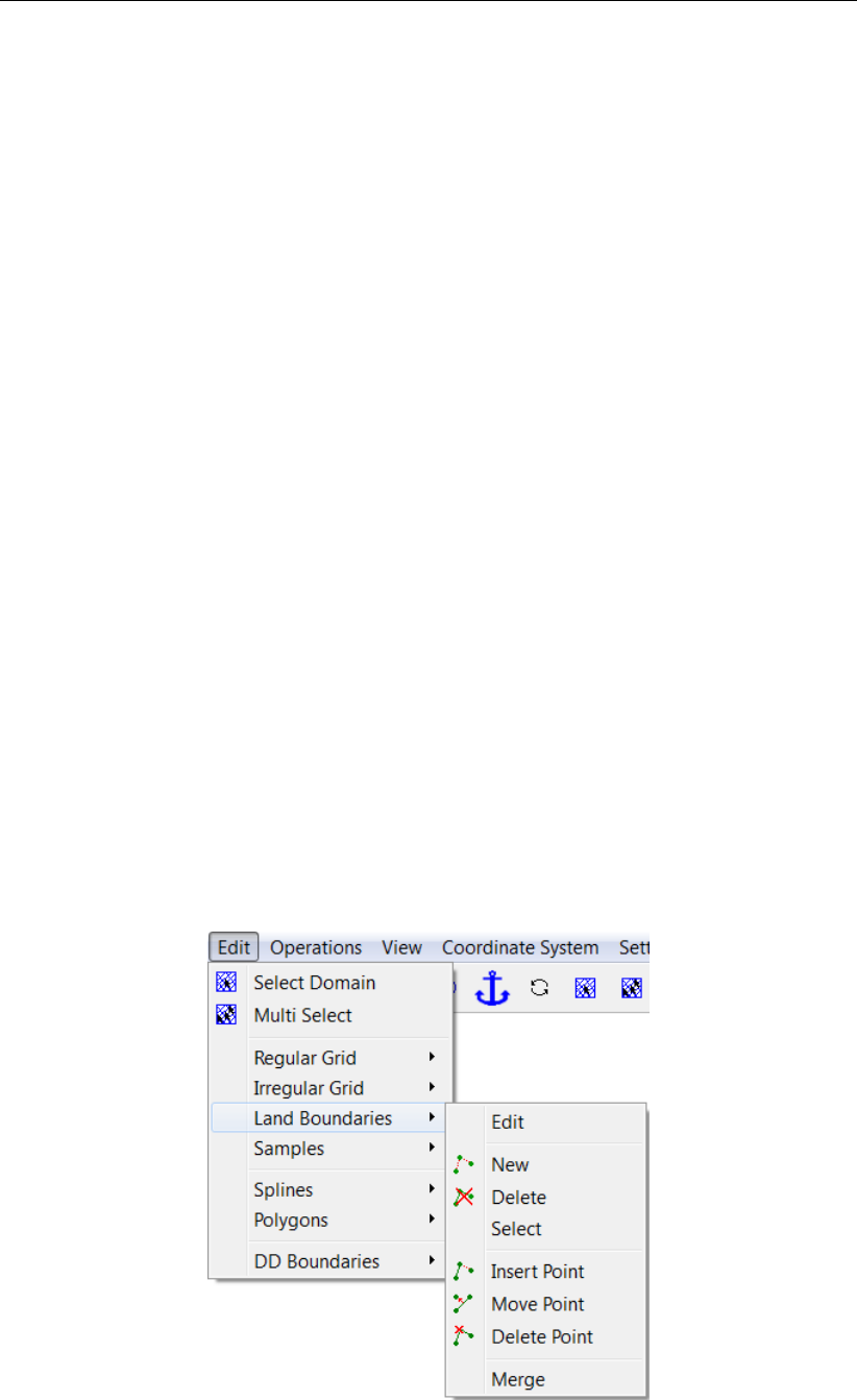
5.2.5 Land Boundaries ........................... 36
5.2.5.1 Menu options . . . . . . . . . . . . . . . . . . . . . . . . 37
5.2.5.2 Valid action keys are . . . . . . . . . . . . . . . . . . . . 38
5.2.6 Samples ............................... 38
5.2.6.1 Menu Options ....................... 38
5.2.6.2 Valid action keys are . . . . . . . . . . . . . . . . . . . . 39
5.2.7 Splines ................................ 39
5.2.7.1 Menu options . . . . . . . . . . . . . . . . . . . . . . . . 39
5.2.7.2 Valid action keys are . . . . . . . . . . . . . . . . . . . . 41
5.2.8 Polygons ............................... 41
5.2.8.1 Menu Options ....................... 42
5.2.8.2 Valid action keys are . . . . . . . . . . . . . . . . . . . . 45
5.2.9 DD Boundaries . . . . . . . . . . . . . . . . . . . . . . . . . . . . 46
5.3 Operations menu ............................... 49
5.3.1 Domain ................................ 50
5.3.2 Create ................................ 51
5.3.3 Delete ................................ 52
5.3.4 Convert grid ............................. 53
5.3.5 Change splines into grid . . . . . . . . . . . . . . . . . . . . . . . 54
5.3.6 Grow grid from boundaries . . . . . . . . . . . . . . . . . . . . . . 55
5.3.7 Grow grid from splines . . . . . . . . . . . . . . . . . . . . . . . . 55
5.3.8 Grow grid from polygons . . . . . . . . . . . . . . . . . . . . . . . 56
5.3.9 Create rectangular or circular grid . . . . . . . . . . . . . . . . . . . 56
5.3.10 Regular Grid Coarseness . . . . . . . . . . . . . . . . . . . . . . . 58
5.3.11 Undo Grid Operation ......................... 59
5.3.12 Irregular Grid Coarseness . . . . . . . . . . . . . . . . . . . . . . 59
5.3.13 Orthogonalise grid . . . . . . . . . . . . . . . . . . . . . . . . . . 61
5.3.14 Flip Lines ............................... 61
5.3.15 Grid ................................. 61
5.3.16 Samples ............................... 63
5.3.17 Attach Grids at DD Boundaries . . . . . . . . . . . . . . . . . . . . 63
5.3.18 Compile DD Boundaries . . . . . . . . . . . . . . . . . . . . . . . 66
5.4 View menu .................................. 66
5.4.1 Spherical Coordinates . . . . . . . . . . . . . . . . . . . . . . . . 67
5.4.2 3D View ............................... 68
5.4.3 Show Legend ............................. 68
5.4.4 Show Grids .............................. 68
5.4.5 Show Grid defined by Circumcentres . . . . . . . . . . . . . . . . . 68
5.4.6 Grid Administration . . . . . . . . . . . . . . . . . . . . . . . . . . 68
5.4.7 Grid Property ............................. 69
5.4.8 Grid Property Style . . . . . . . . . . . . . . . . . . . . . . . . . . 71
5.4.9 Regular Grid Administration . . . . . . . . . . . . . . . . . . . . . . 71
5.4.10 Previous Regular Grid . . . . . . . . . . . . . . . . . . . . . . . . 72
5.4.11 Show Grid Boundaries . . . . . . . . . . . . . . . . . . . . . . . . 73
5.4.12 Actual and maximum data dimensions . . . . . . . . . . . . . . . . 73
5.4.13 Land Boundaries ........................... 73
5.4.14 Samples ............................... 73
5.4.15 Splines ................................ 73
5.5 Coordinate System menu ........................... 74
5.5.1 Cartesian coordinates . . . . . . . . . . . . . . . . . . . . . . . . 74
iv Deltares

DRAFT
Contents
5.5.2 Spherical coordinates ......................... 74
5.5.3 Translation and rotation of Cartesian coordinates . . . . . . . . . . . 75
5.5.4 From Cartesian into Spherical coordinates . . . . . . . . . . . . . . 75
5.5.5 From Spherical into Cartesian coordinates . . . . . . . . . . . . . . 76
5.6 Settings menu ................................ 76
5.6.1 General ................................ 77
5.6.2 Set extent .............................. 79
5.6.3 Orthogonalisation regular . . . . . . . . . . . . . . . . . . . . . . . 79
5.6.4 Orthogonalisation irregular . . . . . . . . . . . . . . . . . . . . . . 81
5.6.5 CellsAndFaces2 ........................... 83
5.6.6 Grow grid from splines . . . . . . . . . . . . . . . . . . . . . . . . 83
5.6.7 Change colour map . . . . . . . . . . . . . . . . . . . . . . . . . . 84
5.6.8 Legend ................................ 84
5.6.9 Colours ................................ 85
5.6.10 Sizes ................................. 85
5.6.11 Order caches ............................. 85
5.6.12 Change Centre of Projection . . . . . . . . . . . . . . . . . . . . . 87
5.7 Help menu .................................. 88
5.7.1 User manual ............................. 88
5.7.2 About ................................. 88
6 Tutorial 91
6.1 Harbour .................................... 91
6.1.1 Coordinate system . . . . . . . . . . . . . . . . . . . . . . . . . . 91
6.1.2 Open a land boundary . . . . . . . . . . . . . . . . . . . . . . . . 91
6.1.3 Zoom in and out ........................... 91
6.1.4 Define splines . . . . . . . . . . . . . . . . . . . . . . . . . . . . 92
6.1.5 Generate grid from splines . . . . . . . . . . . . . . . . . . . . . . 92
6.1.6 Refine grid .............................. 94
6.1.7 Fit grid boundary to land boundary . . . . . . . . . . . . . . . . . . 94
6.1.8 Check grid orthogonality . . . . . . . . . . . . . . . . . . . . . . . 95
6.1.9 Orthogonalise grid . . . . . . . . . . . . . . . . . . . . . . . . . . 95
6.1.10 Check other grid properties . . . . . . . . . . . . . . . . . . . . . . 97
6.1.11 Completion .............................. 97
6.2 Grid design samples ............................. 99
6.3 Paste two grids ................................100
6.4 Regular grids, irregular grids and their mutual coupling . . . . . . . . . . . . 100
6.4.1 A new method to generate curvilinear grids . . . . . . . . . . . . . . 100
6.4.2 Irregular grids . . . . . . . . . . . . . . . . . . . . . . . . . . . . . 102
6.4.3 The coupling of regular and irregular grids . . . . . . . . . . . . . . 103
6.4.4 Relation to existing regular grid generation . . . . . . . . . . . . . . 105
6.5 Multi-domain grids and domain decomposition boundaries . . . . . . . . . . 105
6.6 RGFGRID in the ArcMap environment . . . . . . . . . . . . . . . . . . . . 108
References 111
A Files of RGFGRID 113
A.1 Delft3D project file ..............................113
A.2 Land boundary file ..............................115
A.3 Sample file ..................................116
A.4 Spline file . . . . . . . . . . . . . . . . . . . . . . . . . . . . . . . . . . . 116
A.5 Polygon file ..................................117
A.6 Orthogonal curvilinear grid file . . . . . . . . . . . . . . . . . . . . . . . . 118
A.7 Grid enclosure file ..............................120
Deltares v


DRAFT
List of Figures
List of Figures
3.1 Title window of Delft3D ............................ 7
3.2 Main window Delft3D-MENU ......................... 8
3.3 Selection window for Grid and Bathymetry .................. 8
3.4 Select working directory window ...................... 9
3.5 Select working directory window to set the working directory to <rgfgrid/habour>9
3.6 A part of the current working directory is shown in the title bar due to its length 9
3.7 Main window of the RGFGRID . . . . . . . . . . . . . . . . . . . . . . . . 10
3.8 Operational information displayed in the statusbar . . . . . . . . . . . . . . . 10
3.9 Coordinate System menu, Cartesian Coordinates selected . . . . . . . . . . 10
3.10 Menu item File →Attribute Files →Open Land Boundary . . . . . . . . . . 11
3.11 File open window Open Land Boundary . . . . . . . . . . . . . . . . . . . 11
3.12 Example of a spline grid ........................... 12
3.13 Menu option Operations →Delete →Splines . . . . . . . . . . . . . . . . 12
3.14 Spline grid from tutorial file <harbour.spl>. . . . . . . . . . . . . . . . . . 13
3.15 Result of operation OPerations →Change Splines into Grid . . . . . . . . . 13
3.16 Window Save Grid to save grid file . . . . . . . . . . . . . . . . . . . . . . 14
4.1 Main toolbar ................................. 15
4.2 Menu item placed into extra toolbar . . . . . . . . . . . . . . . . . . . . . . 16
4.3 RGFGRID specific toolbar . . . . . . . . . . . . . . . . . . . . . . . . . . 16
4.4 Location of anchor +and distance between anchor and cursor at the right . . 17
5.1 RGFGRID menu options ........................... 19
5.2 Options on the File menu ........................... 19
5.3 Options on the File→Attribute Files menu . . . . . . . . . . . . . . . . . . . 21
5.4 File →Import menu options . . . . . . . . . . . . . . . . . . . . . . . . . . 23
5.5 File →Export sub-menu options ....................... 25
5.6 Options on the Edit menu ........................... 26
5.7 Options on the Edit →Regular Grid menu . . . . . . . . . . . . . . . . . . 28
5.8 Options on the Edit →Irregular Grid menu . . . . . . . . . . . . . . . . . . 33
5.9 Options on the Edit →Land Boundaries menu . . . . . . . . . . . . . . . . 36
5.10 Options on the Edit →Samples menu . . . . . . . . . . . . . . . . . . . . . 38
5.11 Options on the Edit →Splines menu . . . . . . . . . . . . . . . . . . . . . 39
5.12 Options on the Edit →Polygons menu . . . . . . . . . . . . . . . . . . . . 42
5.13 Polygon between grid boundaries. . . . . . . . . . . . . . . . . . . . . . . 44
5.14 Filling a gap in an unstructered grid using the option Polygon between Grid
Boundaries................................... 45
5.15 Filled a gap in an unstructered grid . . . . . . . . . . . . . . . . . . . . . . 45
5.16 Example of a 1-to-3 refinement along a DD boundary . . . . . . . . . . . . . 46
5.17 Two examples of not allowed domain decompositions, although both DD-boundaries
(A and B) satisfy the refinement condition; the red line and blue lines do not
cover each other ............................... 47
5.18 Options on the Edit →DD Boundaries menu . . . . . . . . . . . . . . . . . 48
5.19 DD Boundary in a single domain . . . . . . . . . . . . . . . . . . . . . . . 49
5.20 Options on the Operations menu . . . . . . . . . . . . . . . . . . . . . . . 50
5.21 Options on the Operations menu . . . . . . . . . . . . . . . . . . . . . . . 50
5.22 Options on the Operations →Create menu . . . . . . . . . . . . . . . . . . 51
5.23 Options on the Operations →Delete menu . . . . . . . . . . . . . . . . . . 52
5.24 Options on the Operations →Convert Grid menu . . . . . . . . . . . . . . . 53
5.25 Different representation of splines . . . . . . . . . . . . . . . . . . . . . . . 54
5.26 Grow curvilinear grid from an irregular grid’s boundary. . . . . . . . . . . . . 55
5.27 Create grid from splines with option Grow Grid from Spline . . . . . . . . . . 56
Deltares vii

DRAFT
RGFGRID, User Manual
5.28 Create grid from selected polygon . . . . . . . . . . . . . . . . . . . . . . . 56
5.29 Parameters for Rectangular or Circular Grid form. . . . . . . . . . . . . . 57
5.30 Rectangular grid, created with Maximum Size / Delta X = “5” and Maximum
Size / Delta Y = “5” .............................. 58
5.31 Options on the Operations →Regular Grid Coarseness menu . . . . . . . . . 58
5.32 Options on the Operations →Irregular Grid Coarseness menu . . . . . . . . 59
5.33 Example of Casulli refinement of an irregular squared grid . . . . . . . . . . 60
5.34 Example of Casulli refinement of an irregular triangular grid . . . . . . . . . . 60
5.35 The circumcentres of cell Iand II coincide at Mand should be merged. . . 62
5.36 Operations →Attach Grids at DD Boundaries . . . . . . . . . . . . . . . . 64
5.37 Operations →Attach Grids at DD Boundaries→Regular grids . . . . . . . . . 65
5.38 Operations →Attach Grids at DD Boundaries . . . . . . . . . . . . . . . . . 65
5.39 Save DD-Boundaries window . . . . . . . . . . . . . . . . . . . . . . . . 66
5.40 Options on the View menu . . . . . . . . . . . . . . . . . . . . . . . . . . 67
5.41 Options on the View →Spherical Coordinates menu . . . . . . . . . . . . . 67
5.42 Options on the View →Grid Administration menu . . . . . . . . . . . . . . . 68
5.43 View →Grid Property options ......................... 69
5.44 View →Grid Property Style options . . . . . . . . . . . . . . . . . . . . . . 71
5.45 View →Regular Grid Administration options ................. 72
5.46 View →Previuos Regular Grid options . . . . . . . . . . . . . . . . . . . . 72
5.47 Operations menu, Actual and Maximum data dimensions . . . . . . . . . . . 73
5.48 Menu option Coordinate System ....................... 74
5.49 Menu option Coordinate System.. . . . . . . . . . . . . . . . . . . . . . . 74
5.50 Parameters for translation and rotation form for transformation to Cartesian
coordinates .................................. 75
5.51 Parameters for Coordinate transformation form for transformation to spher-
ical coordinates ................................ 76
5.52 Parameters for Coordinate transformation form for transformation to Carte-
sian coordinates ............................... 76
5.53 Options on Settings menu . . . . . . . . . . . . . . . . . . . . . . . . . . 77
5.54 Options on Settings window ......................... 77
5.55 Set horizontal extent window . . . . . . . . . . . . . . . . . . . . . . . . 79
5.56 Options on Orthogonalisation Parameters window . . . . . . . . . . . . . 79
5.57 Options on Orthogonalisation Parameters (irregular) window . . . . . . . . 81
5.58 Options on Grow Grid from Splines: Parameters window . . . . . . . . . . 83
5.59 Options on Colour Map for Parameter window . . . . . . . . . . . . . . . . 84
5.60 Options on Settings →Legend menu ..................... 84
5.62 Options on Settings →Sizes menu . . . . . . . . . . . . . . . . . . . . . . 85
5.61 Options on Settings →Colours menu . . . . . . . . . . . . . . . . . . . . . 86
5.63 Options on Order Caches window . . . . . . . . . . . . . . . . . . . . . . 87
5.64 Options on Help menu . . . . . . . . . . . . . . . . . . . . . . . . . . . . 88
5.66 About box ................................... 88
5.65 Front page of the manual ........................... 89
6.1 Land boundary outline of <harbour.ldb>. . . . . . . . . . . . . . . . . . . 91
6.2 Display of splines and land boundary in the ‘harbour’ tutorial . . . . . . . . . 92
6.3 Spline grid changed into result grid with a refinement of 3 . . . . . . . . . . . 93
6.4 Splines not displayed anymore . . . . . . . . . . . . . . . . . . . . . . . . 93
6.5 Grid after another refinement of 3 by 3 . . . . . . . . . . . . . . . . . . . . 94
6.6 Indicating outer grid line and influence area to be moved to land boundary . . 95
6.7 Grid after Line to Land Boundary action . . . . . . . . . . . . . . . . . . . . 95
6.8 Grid properties; orthogonality ......................... 96
6.9 Grid properties; orthogonality. After 1 orthogonalisation action. . . . . . . . . 96
6.10 Indicating corners for Block Orthogonalise . . . . . . . . . . . . . . . . . . 97
viii Deltares

DRAFT
List of Figures
6.11 Grid orthogonality after one block orthogonalisation operation . . . . . . . . . 97
6.12 Final result after refining, obsolete grid cells removed . . . . . . . . . . . . . 98
6.13 Grid and samples for the grid design based upon bathymetry . . . . . . . . . 99
6.14 Result grid after orthogonalisation using samples . . . . . . . . . . . . . . . 99
6.15 Splines drawn ................................101
6.16 Settings for the ’Grow grid from Spline’ procedure. . . . . . . . . . . . . . . 101
6.17 Generated curvilinear mesh after the new ’Grow Grid from Splines’ procedure. 102
6.18 Generated irregular grid within a polygon. . . . . . . . . . . . . . . . . . . . 103
6.19 Coupling of the two grids (regular and irregular, in blue) through manually in-
serting connecting grid lines (in red lines) between the two grids. . . . . . . . 104
6.20 A regular grid is suitable for the sluice area. Connections with the existing grid
should further be established as well as additional orthogonalisation iterations. 105
6.21 Example of grid refinement in the horizontal direction . . . . . . . . . . . . . 106
6.22 Let interface grid points coincide . . . . . . . . . . . . . . . . . . . . . . . 106
6.23 Defining DD-Boundaries . . . . . . . . . . . . . . . . . . . . . . . . . . . 107
6.24 The Save DD-Boundaries dialog . . . . . . . . . . . . . . . . . . . . . . . 108
6.25 ARC-GIS data frame properties form . . . . . . . . . . . . . . . . . . . . . 109
6.26 Options on the Operations menu . . . . . . . . . . . . . . . . . . . . . . . 110
A.1 Example of computational grid enclosures . . . . . . . . . . . . . . . . . . 121
Deltares ix

DRAFT
RGFGRID, User Manual
x Deltares


DRAFT
RGFGRID, User Manual
xii Deltares

DRAFT
1 Guide to this manual
1.1 Introduction
This User Manual concerns the grid generation module, RGFGRID, of the Delft3D software
suite. To make this manual more accessible we will briefly describe the contents of each
chapter and appendix.
If this is your first time to start working with RGFGRID module we suggest you to read and
practice the getting started of Chapter 3 and the tutorial of Chapter 6. These chapters explain
the user interface options and guide you through the generation of your first grid.
Chapter 2:Introduction to RGFGRID, provides specifications of RGFGRID and the areas
of applications.
Chapter 3:Getting started, explains the use of the overall menu program, which gives
access to all Delft3D modules and to the pre- and post-processing tools. Last but not least
you will get a first introduction into the RGFGRID Graphical User Interface, used to define a
grid which can be used in a hydrodynamic or wave simulation.
Chapter 4:General operation, provides practical information on the general operation of the
RGFGRID module.
Chapter 5:Menu options, provides a description of all menu and toolbar options.
Chapter 6:Tutorial, emphasis at giving you some first hands-on experience in using the
RGFGRID module to define the input of a simple problem and in executing a water quality
simulation.
References, provides a list of publications and related material on the RGFGRID module.
Appendix A:Files of RGFGRID, gives a description of the files that can be used in RGFGRID
as input or output. Generally, these files are generated by RGFGRID or other modules of the
Delft3D suite and you need not to be concerned about their internal details. However, in
certain cases it can be useful to know these details, for instance to generate them by means
of other utility programs.
1.2 Name and specifications of the program
Title RGFGRID
Description RGFGRID is a program for generation and manipulation of structured
curvilinear grids for Delft3D-FLOW and Delft3D-WAVE and unstruc-
tured grids for D-Flow Flexible Mesh. The coordinate system may be
Cartesian or spherical. Delft3D-FLOW is a simulation program for hy-
drodynamic flows and transports in 2 and 3 dimensions on curvilinear
grids (Delft3D-FLOW UM,2013) and D-Flow Flexible Mesh is it for un-
structured grids (D-Flow FM UM,2015). The wave model in Delft3D-
WAVE is SWAN; see SWAN UM (2000).
Special facilities Sketch of coarse grid using splines
Smooth refinement module
Orthogonalisation module
Various grid manipulation options
Grid design by bathymetry or polygon control
Deltares 1 of 128
DRAFT
RGFGRID, User Manual
Cartesian or spherical coordinates
Dynamic memory allocation
Multiple grids supported
1.3 Manual version and revisions
This manual applies to RGFGRID, version 5.00.
RGFGRID is shipped with
Delft3D 4 Suite
Delft3D Flexible Mesh Suite
D-HYDRO Suite
1.4 Typographical conventions
Throughout this manual, the following conventions help you to distinguish between different
elements of text to help you learn about RGFGRID.
Example Description
Module
Project
Title of a window or a sub-window are in given in bold.
Sub-windows are displayed in the Module window and
cannot be moved.
Windows can be moved independently from the Mod-
ule window, such as the Visualisation Area window.
Save Item from a menu, title of a push button or the name of
a user interface input field.
Upon selecting this item (click or in some cases double
click with the left mouse button on it) a related action
will be executed; in most cases it will result in displaying
some other (sub-)window.
In case of an input field you are supposed to enter input
data of the required format and in the required domain.
<\tutorial\wave\swan-curvi>
<siu.mdw>
Directory names, filenames, and path names are ex-
pressed between angle brackets, <>. For the Linux
and UNIX environment a forward slash (/) is used in-
stead of the backward slash (\) for PCs.
“27 08 1999” Data to be typed by you into the input fields are dis-
played between double quotes.
Selections of menu items, option boxes etc. are de-
scribed as such: for instance ‘select Save and go to
the next window’.
delft3d-menu Commands to be typed by you are given in the font
Courier New, 10 points.
In this User manual, user actions are indicated with this
arrow.
2 of 128 Deltares
DRAFT
Guide to this manual
Example Description
[m s−1] [−] Units are given between square brackets when used
next to the formulae. Leaving them out might result in
misinterpretation.
1.5 Changes with respect to previous versions
Version Description
5.00.00 Generation of unstructured grids for D-Flow Flexible Mesh
4.00.00 Complete new version of RGFGRID
Deltares 3 of 128

DRAFT
RGFGRID, User Manual
4 of 128 Deltares

DRAFT
2 Introduction to RGFGRID
2.1 Introduction
The purpose of the RGFGRID program is to create, modify and visualise orthogonal, curvilin-
ear grids for the Delft3D-FLOW module.
Curvilinear grids are applied in finite difference models to provide a high grid resolution in the
area of interest and a low resolution elsewhere, thus saving computational effort.
Grid lines may be curved along land boundaries and channels, so that the notorious ’stair
case’ boundaries, that may induce artificial diffusion, can be avoided.
Curvilinear grids should be smooth in order to minimise errors in the finite difference approxi-
mations. Finally, curvilinear grids for Delft3D-FLOW have to be orthogonal, which saves some
computationally expensive transformation terms. Extra effort in the model set-up phase, re-
sults in faster and more accurate computations.
2.2 Coordinate systems
The grid system used in RGFGRID can be either Cartesian (in metres) or spherical (in decimal
degrees). Cartesian coordinates can be displayed on a screen directly, just using a scale
factor. Spherical coordinates can be displayed on screen as plane coordinates or as projected
coordinates. Plane coordinates on screen give distortion in the polar direction. Depending on
the type of projection, projected coordinates have no distortion in distance and angles. For
this reason a stereographic projection is used in RGFGRID.
Starting from scratch, you have to select a coordinate system. The coordinates of all objects
(land boundary, splines, grid, samples, etc.) are then in the selected coordinate system.
When opening a grid, RGFGRID will read the coordinate system of the imported grid. The
coordinates of other objects (land boundary, splines, polygons, samples and text files) are not
checked; this is the responsibility of the user.
2.3 Program considerations
RGFGRID is designed to create grids with minimum effort, fulfilling the requirements of smooth-
ness and orthogonality. The program allows for an iterative grid generation process, starting
with a rough sketch of the grid by splines. Then, the splines are transformed into a grid, which
can be smoothly refined by the program. Whenever necessary, you can orthogonalise the grid
in order to fulfil the Delft3D-FLOW requirement of orthogonality.
Various grid manipulation options are provided in order to put the grid lines in the right position
with the right resolution. For instance, a grid line can be ’snapped’ to a land boundary. The
surrounding grid smoothly follows. More detail is brought into the grid after every refinement
step.
Existing grids may be modified or extended using this program. Grids can be locally refined by
insertion of grid lines. The resulting local ’jump’ in grid sizes can be smoothed by a so-called
’line smoothing’.
Bathymetry data can be displayed on the screen, so that internal gullies can be taken into
account while drawing the design grid. Existing model grids can be opened and displayed on
the screen, while creating new grids to be pasted later to the original. Before each modification
or edit action, the grid is saved to the so-called ’previous grid’. Pressing Esc after an edit
Deltares 5 of 128

DRAFT
RGFGRID, User Manual
action, copies the previous grid back to the grid. If desired, the previous grid can be shown
together with the active grid.
Grid properties such as smoothness, resolution, orthogonality etc, can be visualised to check
the grid quality. Graphical output can easily be created in various formats.
6 of 128 Deltares
DRAFT
3 Getting started
3.1 Overview of Delft3D
The Delft3D program suite is composed of a set of modules (components) each of which
covers a certain range of aspects of a research or engineering problem. Each module can be
executed independently or in combination with one or more other modules.
Delft3D is provided with a menu shell through which you can access the various modules. In
this chapter we will guide you through some of the input screens to get the look-and-feel of
the program. In the Tutorial, Chapter 6, you will learn to define a simple scenario.
3.2 Starting Delft3D
To start Delft3D:
On an MS Windows platform: select Delft3D in the Programs menu.
On Linux machines: type delft3d-menu on the command line.
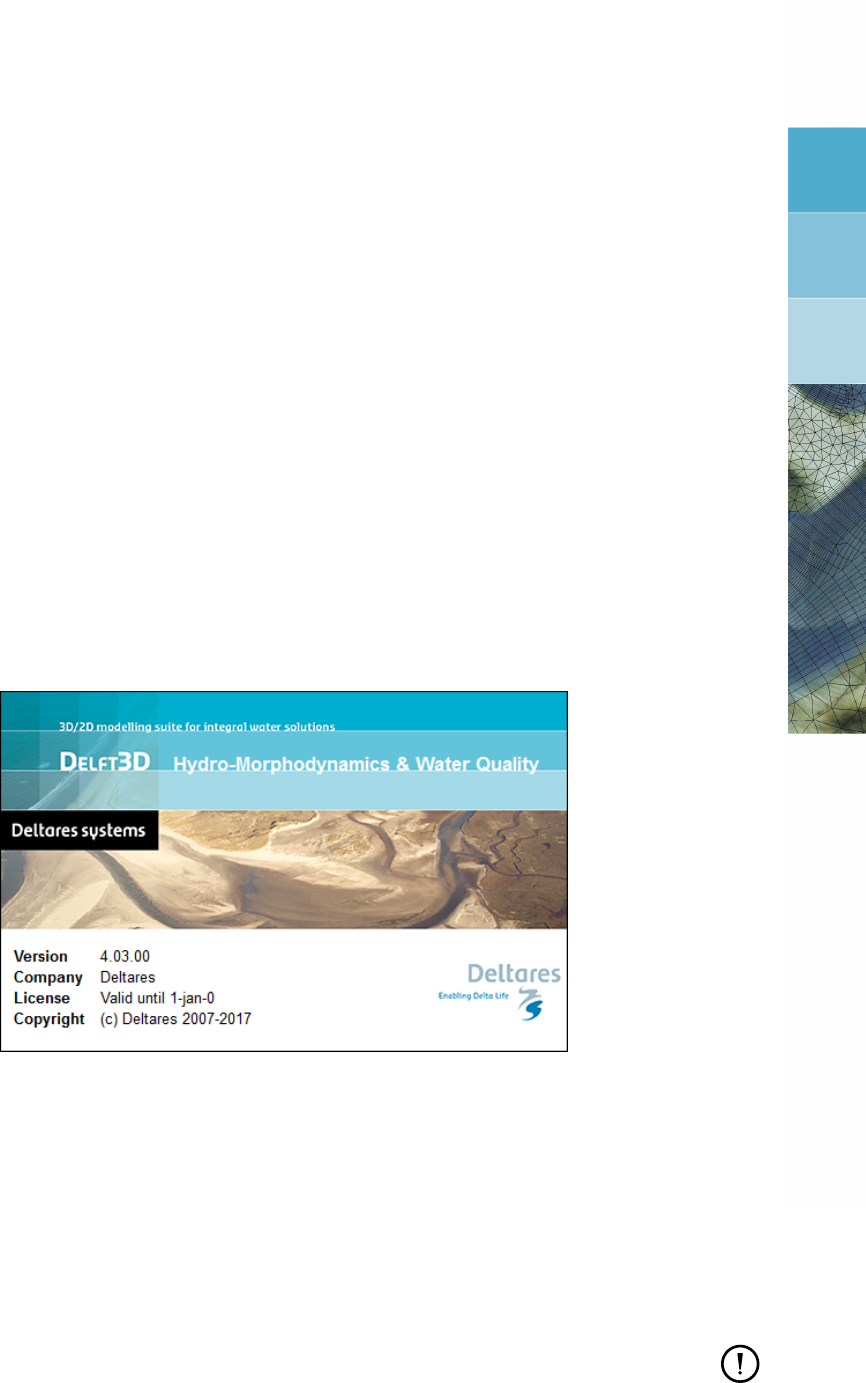
Next the title window of Delft3D is displayed, Figure 3.1.
Figure 3.1: Title window of Delft3D
After a short while the main window of the Delft3D-MENU appears, Figure 3.2.
Several menu options are shown. For now, only concentrate on exiting Delft3D-MENU, hence:
Click on the Exit push button.
The window will be closed and you are back in the Windows Desktop screen for PCs or on
the command line for Linux workstations.
Remark:
In this and the following chapters several windows are shown to illustrate the presen-
tation of Delft3D-MENU and RGFGRID. These windows are grabbed from the PC-
platform. For Linux workstation the content of the windows is the same, but the colours
may be different.
Deltares 7 of 128
DRAFT
RGFGRID, User Manual
Figure 3.2: Main window Delft3D-MENU
3.3 Getting into RGFGRID
To continue start the menu program again as indicated in Section 3.2.
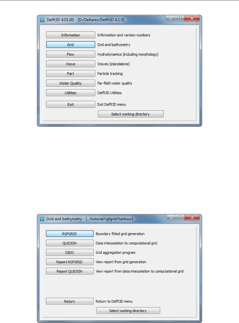
Click the Grid button, see Figure 3.2
Next the selection window for Grid and bathymetry is displayed for preparing a curvilinear
grid, interpolate data on that grid and aggregate the hydrodynamic cells, see Figure 3.3.
Figure 3.3: Selection window for Grid and Bathymetry
Note that in the title bar the current directory is displayed, in our case <D:\Deltares\Delft3D
4.01.00\tutorial>.
Before continuing with any of the selections of this Grid and bathymetry window, you select
the directory in which you are going to prepare scenarios and execute computations:
Click the Select working directory button.
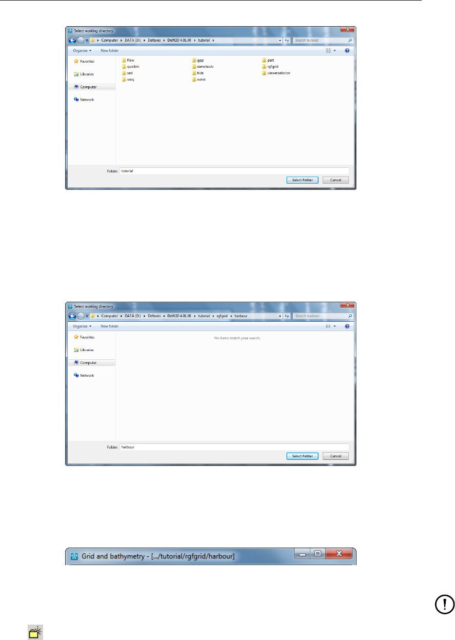
Next the Select working directory window is displayed, see Figure 3.4 (your current directory
may differ, depending on the location of your Delft3D installation).
8 of 128 Deltares
DRAFT
Getting started
Figure 3.4: Select working directory window
Browse to and open the <tutorial>sub-directory of your Delft3D Home-directory.
Open the <rgfgrid>directory.
Open the <harbour>directory.
Close the Select working directory window by clicking button Choose, see Figure 3.5.
Figure 3.5: Select working directory window to set the working directory to
<rgfgrid/habour>
Next the Grid and bathymetry window is re-displayed, but now the changed current working
directory is displayed in the title bar, see Figure 3.6.
Figure 3.6: A part of the current working directory is shown in the title bar due to its length
Remark:
In case you want to start a new project for which no directory exists yet, you can select
in the Select working directory window to create a new folder.
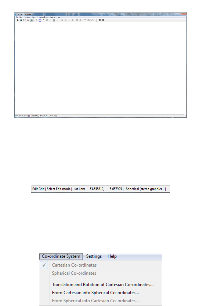
Click on RGFGRDID in the Grid and bathymetry window, see Figure 3.3.
RGFGRID is loaded and the primary input screen is opened, Figure 3.7.
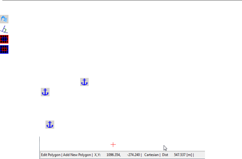
In the lower-left corner of the status bar RGFGRID gives additional operational information,
see Figure 3.8, such as:
Deltares 9 of 128
DRAFT
RGFGRID, User Manual
Figure 3.7: Main window of the RGFGRID
User selections.
Operational instructions (for instance Toggle anchor mode).
xand ycoordinates of the current cursor position.
Coordinate system: Cartesian or Spherical.
Distance (in metre) to a user-defined anchor point (only displayed when the anchor is
activated).
Figure 3.8: Operational information displayed in the statusbar
3.4 Exploring some menu options
First, set the coordinate system to the system you want to work in. Since we are going to work
in the Cartesian coordinate system:
On the Coordinate System menu click Cartesian Coordinates, see Figure 3.9
Figure 3.9: Coordinate System menu, Cartesian Coordinates selected
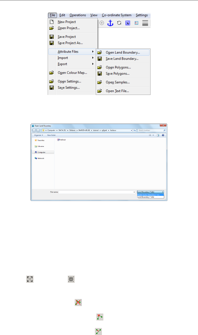
To open a land boundary:
Upon selecting File →Attribute Files →Open Land Boundary, you can open a collection
of land boundaries, see Figure 3.10. Land boundaries (or land-water marking) are in files
with default mask <∗.ldb>.
10 of 128 Deltares
DRAFT
Getting started
Figure 3.10: Menu item File →Attribute Files →Open Land Boundary
Next the Open Land Boundary window is displayed, see Figure 3.11.
Figure 3.11: File open window Open Land Boundary
In the current directory one land boundary file is present.
Select <harbour.ldb>and click Open to open the land boundary file.
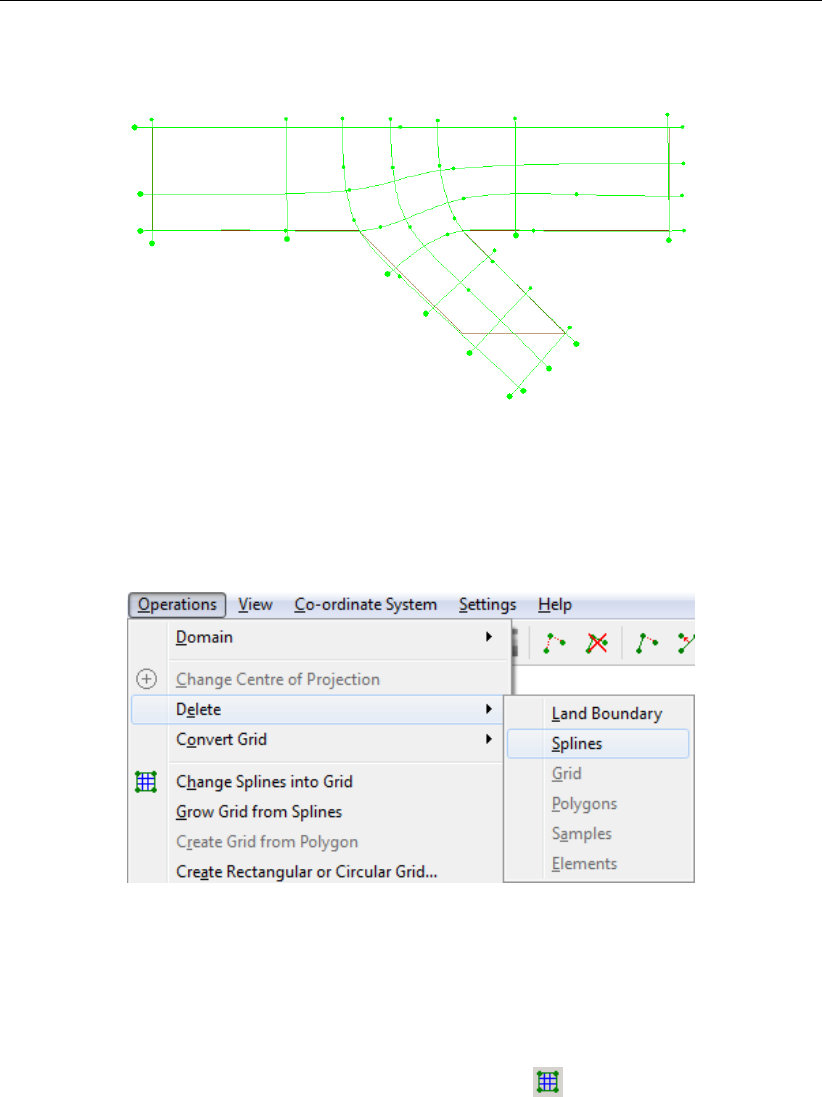
On the Edit menu point to Spline and click New.
To draw a spline, click with the left-mouse to define spline-points. To finish the current
spline click with the right-mouse. Click left to start with the next spline. The result may
look like as in Figure 3.12
Practise with zooming in or out. To zoom in or out, either:
Click on to zoom in and zoom out on the toolbar.
Press the +and -key while keeping the CTRL-key pressed.
Use the mouse scroll wheel.
To delete an entire spline, click on the toolbar and click one of the supporting points of
the spline to be deleted and then press the right mouse button to perform the delete.
To delete a single point of a spline, click and click a spline point to delete this single
point.
To move a single point of a spline, click or press R, click the point and click again at
the new location.
Deltares 11 of 128
DRAFT
RGFGRID, User Manual
Figure 3.12: Example of a spline grid
Now we delete this spline grid:
On the Operations menu, point to Delete and click Splines, see Figure 3.13
Figure 3.13: Menu option Operations →Delete →Splines
We will continue with an existing splines file
On the File menu, point to Import and click Splines.
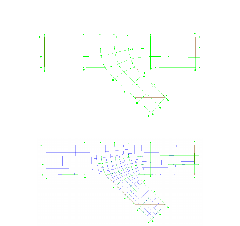
Select <harbour2.spl>. After selection the file is loaded and displayed, see Figure 3.14.
On the Operations →Change Splines into Grid, or click on the toolbar.
This operations transforms the spline grid into a grid and at the same time refines it 3 times in
both directions, see Figure 3.15. The refinement factors can be set in the General Parame-
ters form menu item Settings →General.
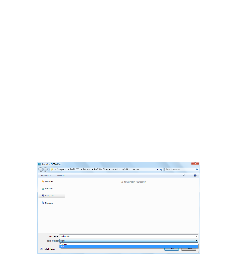
To save the grid
On the File menu, point to Export and click Grid
The Save As window opens, see Figure 3.16.
Type <harbour>and click Save to save your grid
12 of 128 Deltares
DRAFT
Getting started
Figure 3.14: Spline grid from tutorial file <harbour.spl>
Figure 3.15: Result of operation OPerations →Change Splines into Grid
You will be back in the main window of RGFGRID.
3.5 Exiting RGFGRID
To exit the RGFGRID
Click Exit on the File menu.
You will be back in the Grid and bathymetry window, see Figure 3.3
Click Return to return to the main window of Delft3D-MENU, see Figure 3.2
Click Exit.
The window is closed and the control is returned to the desk top or the command line.
In this Getting Started session you have learned to access the RGFGRID and to open and
and to generate and save a grid file.
We encourage new users next to run the tutorial described in Chapter 6.
Deltares 13 of 128
DRAFT
RGFGRID, User Manual
Figure 3.16: Window Save Grid to save grid file
14 of 128 Deltares
DRAFT
4 General operation
4.1 General program operation instruction
Help
Upon selecting Help →User Manual, the RGFGRID User Manual in PDF-format will be
opened. Use the bookmarks in the contents to locate the subject you are interested in.
File menu
The file-menu is the standard Open and Save As window. The file mask depends on the type
of data that you want to open or save. You can change the directory by navigating through the
folders.
It is possible to specify whether to Stay on the Start-up Directory or not, in the Settings
General form.
General cursor and keyboard functions
The left mouse button activates or confirms desired actions. The Esc key cancels the last
edit action. The right mouse button may also confirm actions, or may put the program back
into its original mode.
4.1.1 Toolbars
The main window contains a men bar and two icon bars. The two icon bars are separated in
a main toolbar belonging to the overall handling and a toolbar belonging to specific handling
of the program RGFGRID.
4.1.1.1 Main toolbar
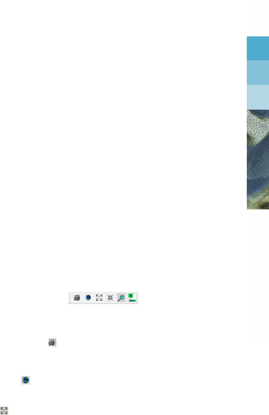
The main toolbar is shown in Figure 4.1.
Figure 4.1: Main toolbar
Print screen
Press Ctrl-P or click on the toolbar to obtain the print window for a hardcopy of the
current screen. This file is called <rgfgrid_date_time.pdf>
Zoom to extent
Click the icon to zoom to the full extent of the project area.
Zoom in
Click on the toolbar to zoom in.
Deltares 15 of 128
DRAFT
RGFGRID, User Manual
Zoom out
Click on the toolbar to zoom out.
Zoom box
To define a zoom box, click on the toolbar and drag a box. If you define a zoom box from
right to left and from bottom to top then it will zoom out instead of zoom in.
Menu item to toolbar
When using the icon , the next chosen menu item will be placed in a separate toolbar.
As example, click the icon , and select from the menu File →Import →Grid (RGFGRID). . . .
An extra toolbar will appear with the chosen menu option, see Figure 4.2.
Figure 4.2: Menu item placed into extra toolbar
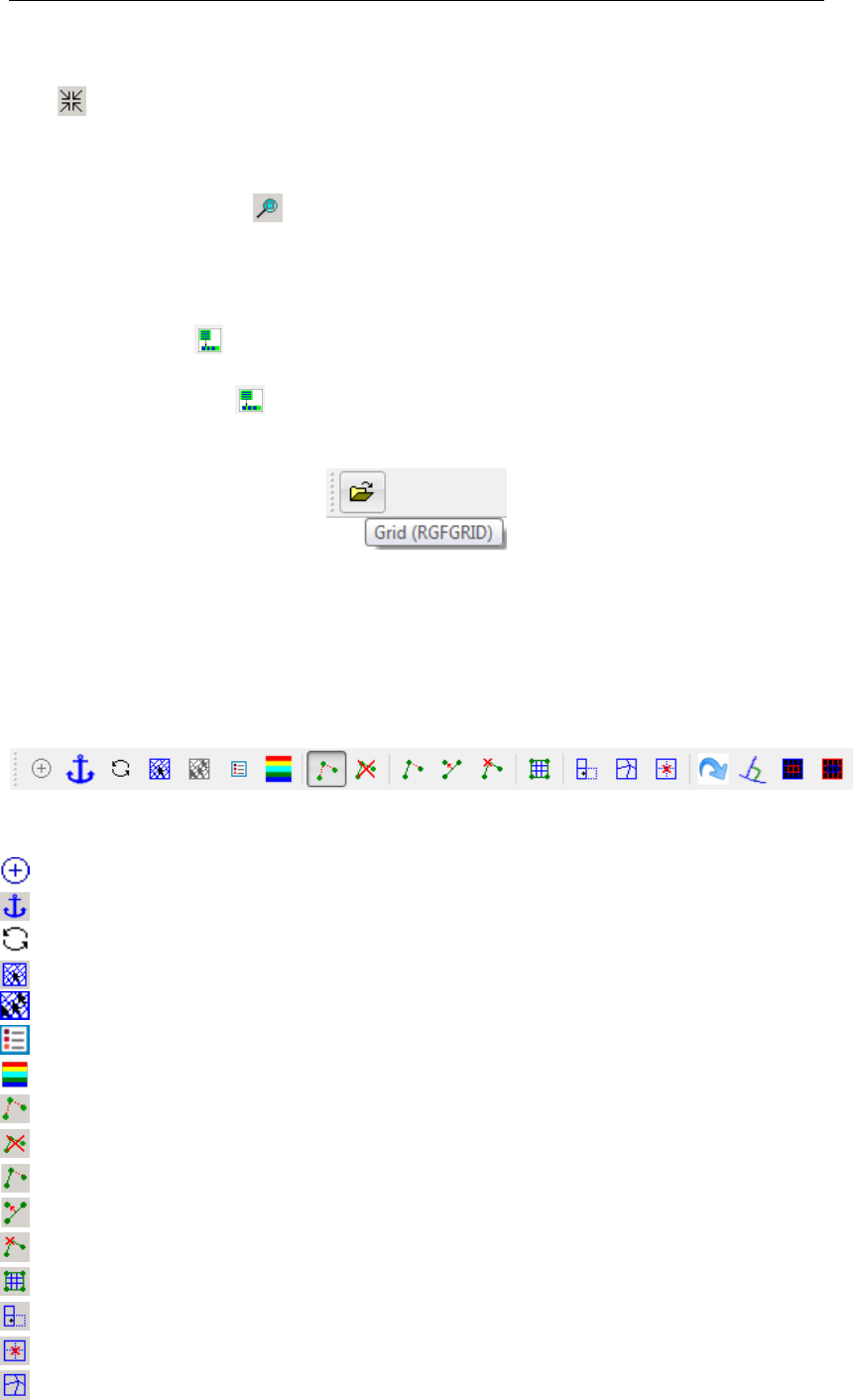
4.1.1.2 RGFGRID toolbar
The program specific toolbar, see Figure 4.3, consists of icons which can also be reached via
menu options.
Figure 4.3: RGFGRID specific toolbar
Recompute the stereographic projection.
See section 4.2 key-stroke A.
Refresh the internal administration of the program.
Select a domain.
Activate or deacivate the multi selecting tool.
Show or hide the legend.
Show or hide the grid properties.
Start editting a new polygon, land boundary or spline.
Delete the slected polygon, land boundary or spline.
Insert a point into a polygon, land boundary or spline.
Move a point of a polygon, land boundary or spline.
Delete a point of a polygon, land boundary or spline.
Attach the selected spline to the grid (regular grid only).
Mirror a grid cell at the boundary of a regular grid.
Delete a grid point/node.
Move a grid point.
16 of 128 Deltares
DRAFT
General operation
Repeat the previous action.
Orthogonalise the grid.
Deletergular grid outside the indicated points.
Delete regular grid inside the the indicated points.
4.2 Key stroke functions
Key A= Anchor, or on toolbar
When clicking on the toolbar and next pressing the Akey on the keyboard, a so-called
anchor will appear, which acts as zero-distance point. The distance (in metre) of the present
cursor position to this point is displayed in the status bar at the right of the coordinate system
indicator, see Figure 4.4. Moving the cursor around and pressing Aagain will relocate the
anchor. Clicking again will de-activate the anchor.
Figure 4.4: Location of anchor +and distance between anchor and cursor at the right
Key D= Delete
In the Edit →Polygon options, pressing Dallows you to delete individual points (polygon,
depth or sample).
Key E= Erase polygon
In Edit →Polygon, keeping Epressed allows you to delete the indicated polygon.
Key I= Insert
In Edit →Polygons, pressing Istarts the vertex insert action depending on the first click
on the screen. If the first click is in between two vertices of the polygon then a point will be
inserted in the closest edge.
Key Ctrl-P = Print screen
Pressing Ctrl-P will open the print window. The current screen will be printed to your printer
or to a file.
Key R= Replace
In Edit →Polygon, pressing Rallows you to replace (move) individual points.
Key Mouse wheel
Use the mouse wheel to zoom in and zoom out. Other ways are:
Key Ctrl + = Zoom in
Keep the Ctrl-key pressed and use the +key to zoom in more.
Key Ctrl - = Zoom out
Keep the Ctrl-key pressed and use the -key to zoom in more.
Key Ctrl move cursor = move focus of screen
Keep the Ctrl-key pressed and move the cursor around. The current screen will move
accordingly.
Deltares 17 of 128

DRAFT
RGFGRID, User Manual
Key Ctrl arrow keys = move focus of screen left, right, up or down
Keep the Ctrl-key pressed and use the arrow keys to move the focus of the screen accord-
ingly.
Key Esc = Undo
In various edit modes the latest action will be undone pressing Esc.
18 of 128 Deltares
DRAFT
5 Menu options
The menu bar contains the following items, see Figure 5.1, each item is discussed in a sepa-
rate section.
Figure 5.1: RGFGRID menu options
5.1 File menu
Before opening an attribute file (land boundaries, samples, splines or polygons) be sure you
have set the coordinate system on the Coordinate System menu, see Section 5.5.
When opening files, RGFGRID will not check the coordinate system in the file against the
current coordinate system in RGFGRID, except when opening a grid.
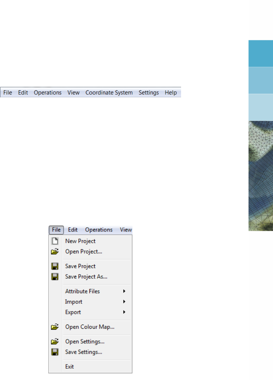
On the File menu, see Figure 5.2, options are available to open a project (collection of grids
and ddb-file), attribute files required for the definition of a grid (i.e. land boundary and samples)
and to import grid related files (grids, splines and DD boundaries). The results at each stage
of the grid definition process can be saved. The option to quit RGFGRID is located here also.
Figure 5.2: Options on the File menu
The start-up directory to open and save files can be configured in the General Parameters
form on the menu Settings →General. As default the file menu starts at the last directory
selected.
For the formats of the files you are referred to Appendix A.
5.1.1 New project
Upon selecting File →New Project, all objects (land boundaries, polygons, splines, grids,
samples, etc.) will be deleted; i.e. you start from scratch.
Deltares 19 of 128
DRAFT
RGFGRID, User Manual
5.1.2 Open project
Upon selecting File →Open Project, the Open Project window appears in which you can
browse to an existing project (<∗.d3d>file).
Remark:
A project saved by QUICKIN or D-Waq DIDO can be read by RGFGRID.
5.1.3 Save project
Upon selecting File →Save Project, the current project (grid filenames and, if applicable, DD
boundaries filename) will be saved under the same name. If the project name is not known
yet, the Save Project window appears.
Remark:
When you started with an existing project, or when you saved the project before, saving
the project will not save changes you have made to the grid(s). Either use Save Project
As or save individual grids.
5.1.4 Save project as
Upon selecting File →Save Project As, the current project can be saved under a different
name.
5.1.5 Attribute files
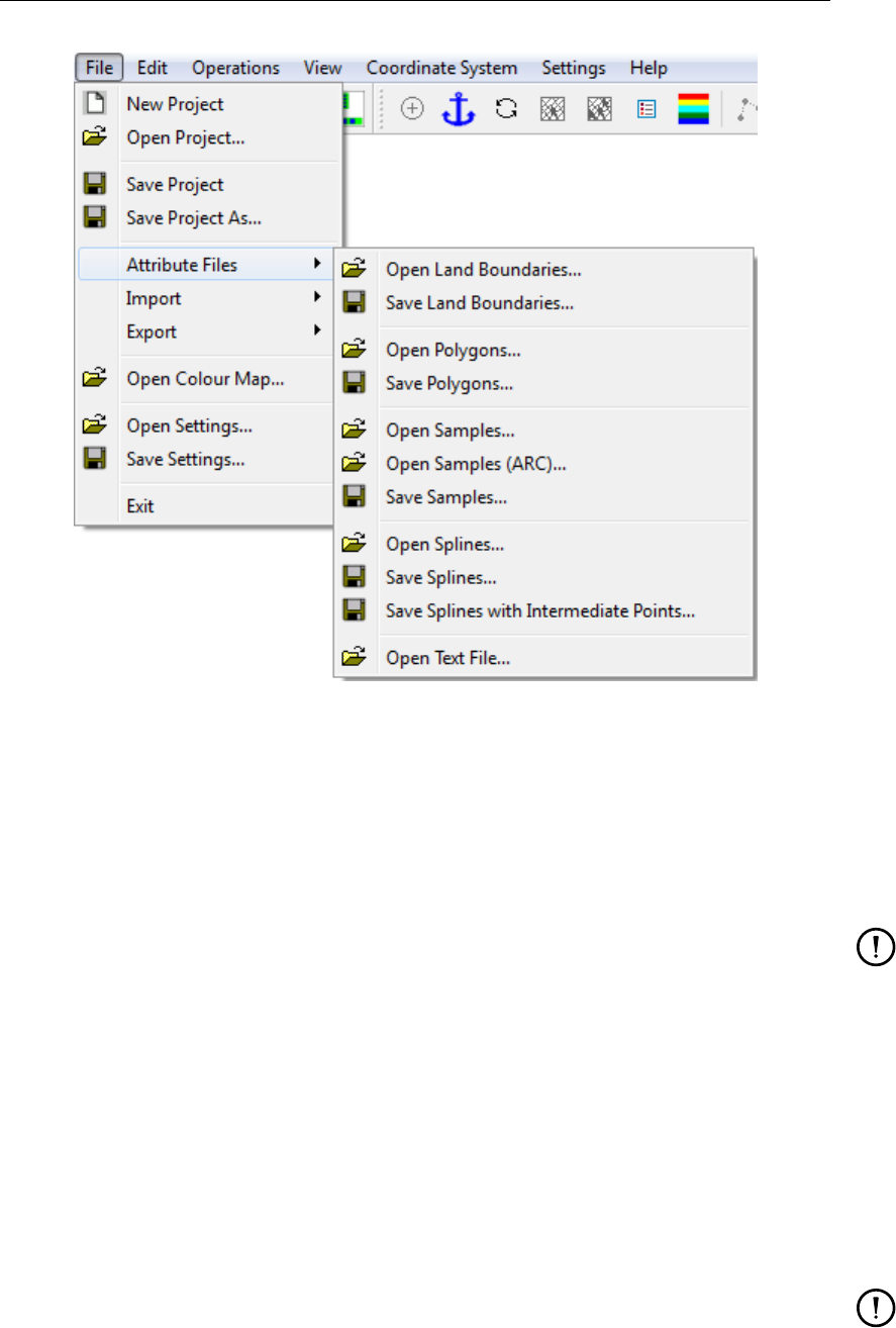
On the File →Attribute Files sub-menu, see Figure 5.3, options are available to open and
save objects that are indirectly related to the grids, so grid independent.
20 of 128 Deltares
DRAFT
Menu options
Figure 5.3: Options on the File→Attribute Files menu
Open land boundaries
Upon selecting File →Attribute Files →Open Land Boundaries..., you can open a collection
of land boundaries. Land boundaries (or land-water marking) are in files with default mask
<∗.ldb>. For a real application the land boundary is a guidance to define a grid for the model
area.
Remark:
If you open another land boundary file, it will be visualised together with the existing
land boundary.
Save land boundaries
Land boundaries are saved in a file with default mask <∗.ldb>.
Open polygons
Upon selecting File →Attribute Files →Open Polygons... you can open a collection of poly-
gons in a file with mask (<∗.pol>). Polygons are per definition closed. If the polygon is not
closed in the file it will still be shown as closed.
Remark:
If you open another polygons file, they will be visualised together with existing polygons.
Deltares 21 of 128

DRAFT
RGFGRID, User Manual
Save polygons
When saving polygons, each polygon will be saved as a closed polyline. A polygon file has
as default mask <∗.pol>.
Open samples
The bathymetry can be used as a guideline to determine the orientation and resolution of the
required grid. This can be done visually, but also the grid design can take into account the
samples. See Settings →Orthogonalisation, item Design Method, see Section 5.6.3.
The samples in a file with mask <∗.xyz>, may be a set of disordered x,y,zvalues given in
a sequential list of free-formatted x,y,zvalues.
Remark:
If you open another samples file, the samples will be visualised together with existing
samples.
Open Samples (ARC)
A set of samples located on a regular grid — without holes — is called structured. These can
be read from an ArcInfo raster file using this menu option. During the reading process, the
user is prompted for row and column refinement factors. hose factors determine the blocksize
of the resampling operation, which averages a block of samples and loads it as a single
sample.
Save samples
Samples are saved in a file with default mask <∗.xyz>. This save function can be used to
convert the samples loaded with the option File →Attribute Files →Open Samples (ARC). . .
to a file with default mask <∗.xyz>.
Note: Samples can not be editted by RGFGRID.
Open splines
The initial sketch of the grid is done by drawing splines. Splines are in files with default mask
<∗.spl>.
Remark:
If you open another splines file, the new splines will replace existing splines.
Save splines
Splines are saved in a file with default mask <∗.spl>. Only those points which are visualised
with a dot are stored in the file.
Save splines with intermediate points
The splines including the intermediate points between the points visualised with a dot, can be
saved in a file with default file mask <∗.spt>.
22 of 128 Deltares
DRAFT
Menu options
Open text file
Texts can be displayed in the graphics area if their position (x, y), the text and colour are
defined. See an example in Appendix A.8.
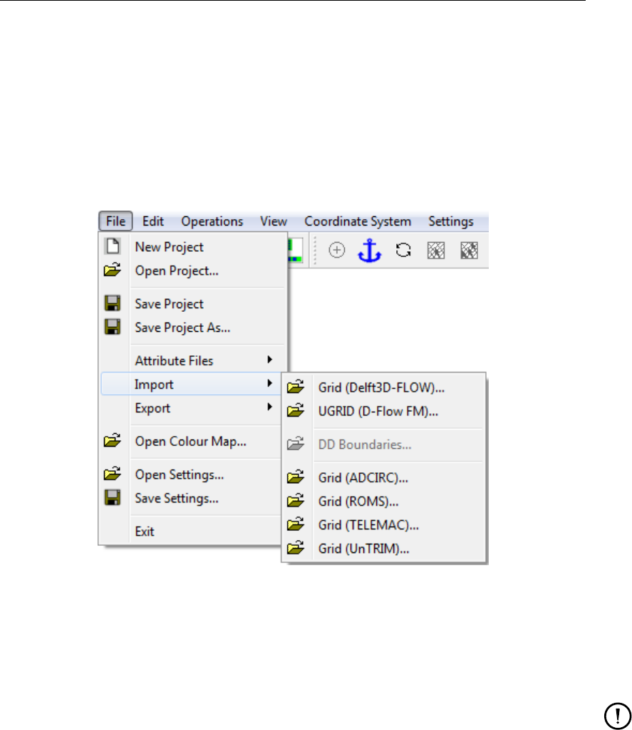
5.1.6 Import
On the Import sub-menu, see Figure 5.4, options are available to import objects that are
directly related to the grids.
Figure 5.4: File →Import menu options
Grid (RGFGRID)
Upon selecting File →Import →Grid (RGFGRID). . . , you can open a collection of grids. The
grid file has a default mask <∗.grd>or <∗_rgf.nc>.
Remarks:
The coordinate system in RGFGRID is set accordingly to the system specified in the
grid file.
If the coordinate system is spherical then the coordinates are shown in stereographic
projection.
If no coordinate system is specified, Cartesian is presumed.
UGRID (D-Flow FM)
Upon selecting File →Import →UGRID (D-Flow FM). . . , you can open a collection of grids.
The grid file has a default mask <∗_net.nc>.
Deltares 23 of 128

DRAFT
RGFGRID, User Manual
DD boundaries
In case of a domain decomposition application you will have multiple grids. How the grids are
linked to each other is contained in the domain decomposition boundary file (ddb-file). The
ddb-file will be made if you select Operations →Compile DD Boundaries, see Section 5.3.18.
Grid (ADCIRC)
Upon selecting File →Import →Grid (ADCIRC). . . , you can open a collection of irregular grids
in the NetCDF format. The grid file has a default mask <∗_adcirc.nc>. See ADCIRC.
Grid (ROMS)
Upon selecting File →Import →Grid (ROMS). . . , you can open a collection of regular grids
in the NetCDF format off the Regional Ocean Modeling System. The grid file has a default
mask <∗_roms.nc>. See ROMS.
Grid (TELEMAC)
Upon selecting File →Import →Grid (TELEMAC) . . . , you can open a collection of grids
suitable for TELEMAC (triangle grid). The grid is in a file with default mask <∗.geo>or
<∗.slf>. The open boundary files with required mask <∗.cli>, are together read with the
grid if the basename of the file is the same. See TELEMAC.
Remark:
The open boundary file can not be read separately after the grid is read.
Grid (UnTRIM)
Upon selecting File →Import →Grid (UnTRIM). . . , you can open a collection of irregular grids
in the NetCDF format. The grid file has a default mask <∗_untrim.nc>. See UnTRIM (V.
Casulli)
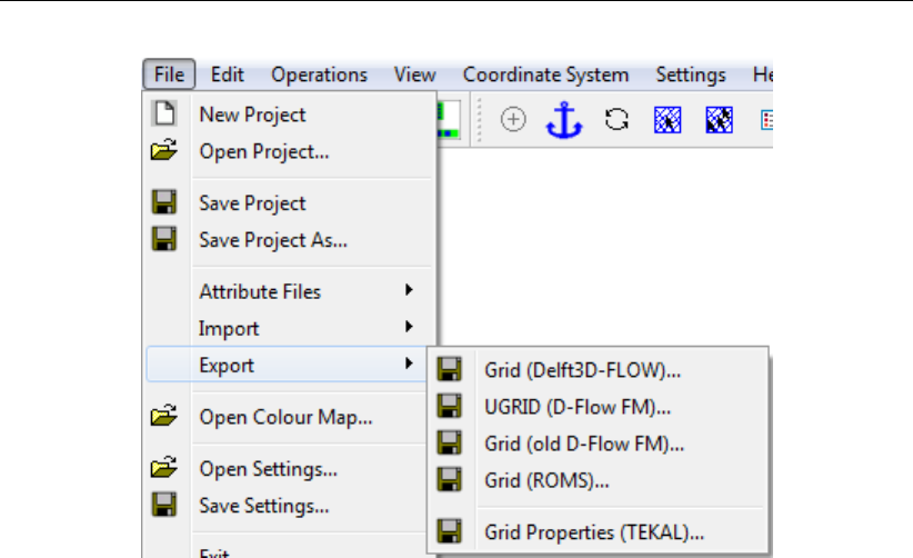
5.1.7 Export
On the File →Export sub-menu, see Figure 5.5, options are available to export objects that
are directly related to the grids.
24 of 128 Deltares
DRAFT
Menu options
Figure 5.5: File →Export sub-menu options
Grid (RGFGRID)
The grid is saved in a file with mask <∗.grd>or <∗_rgf.nc>. Along with the <∗.grd>file, a
second file is saved with mask <∗.enc>, containing the so-called grid enclosure, that outlines
all active computational grid cells in Delft3D-FLOW.
UGRID (D-Flow FM)
The grid is saved in the NetCDF file format with the UGRID naming conventions, suitable for
D-Flow FM. The default mask <∗_net.nc>is used.
Grid (D-Flow FM)
The grid is saved in the NetCDF file format suitable for D-Flow FM, the default mask <∗_net.nc>
is used.
Grid (ROMS)
The grid is saved in the NetCDF file format suitable for the Regional Ocean Modeling System,
the default mask <∗_roms.nc>is used.
Grid properties (TEKAL)
The grid properties can be saved in a so-called TEKAL format, so that the properties can
be visualised with Delft3D-QUICKPLOT or GPP, see QUICKPLOT UM (2013) and GPP UM
(2013). The data is saved in a file with mask <∗.tek>, and contains the x,ycoordinates, the
orthogonality, the resolution, the smoothness, the curvatures, the grid sizes and the aspect
ratios in columns.
Deltares 25 of 128
DRAFT
RGFGRID, User Manual
5.1.8 Open Colour map
You can choose from a number of pre-defined colour schemes (in file with masks <∗.clr>or
<∗.clrmap>). These colour schemes have the same format as used for Delft3D-QUICKPLOT,
see Appendix A.10 for the file format.
Restriction:
Only the colour space RGB is supported
Remark:
If the file <rgfgrid.clrmap>exists on the start-up directory then this file will be read, if
the file does not exist on the start-up directory it will try to read the file on the installation
directory <$D3D_HOME/$ARCH/plugins/default>.
5.1.9 Open Settings
If you have saved your RGFGRID settings in a previous session, you can open these settings
again, see Appendix A.11 for the file format.
Remark:
If the file <rgfgrid.ini>exists on the start-up directory then this file will be read, if the file
does not exist on the start-up directory it try to read the file on the installation directory
<$D3D_HOME/$ARCH/plugins/default>.
5.1.10 Save Settings
If you have made changes in one of the forms on the Settings menu, you can save these
settings to be used later on again.
5.1.11 Exit
Exit from the RGFGRID program.
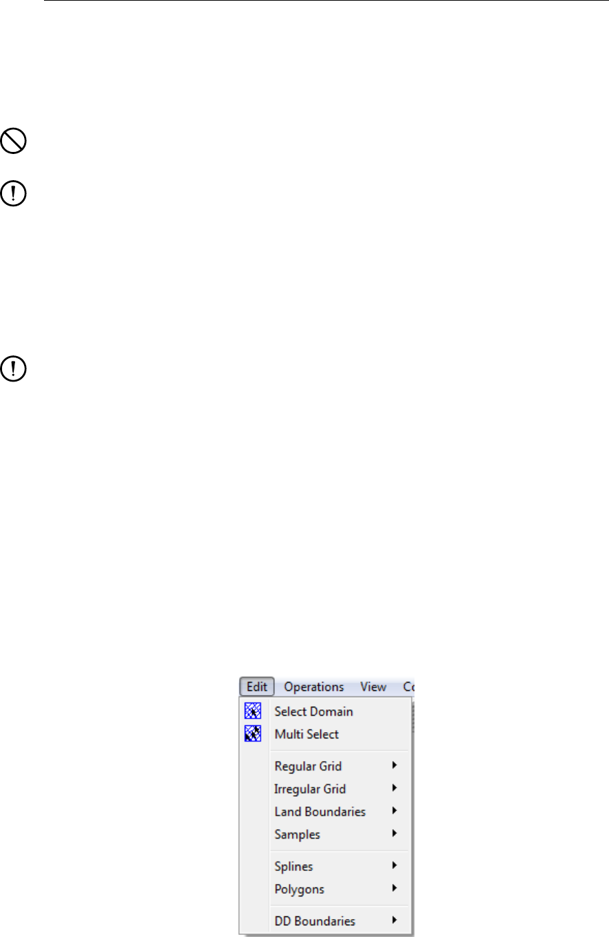
5.2 Edit menu
On the Edit menu, see Figure 5.6, several edit modes can be selected.
Figure 5.6: Options on the Edit menu
26 of 128 Deltares
DRAFT
Menu options
An edit mode is an operation mode which needs at least a mouse click, i.e. a set of operation
instructions which is valid for a certain data set, and which may go with some specific display
method. The following objects may be modified:
Regular grid
Irregular grid
Land boundaries
Samples
Splines
Polygons
DD boundaries
Esc = Undo
In most edit modes, Esc will undo the latest action.
5.2.1 Select Domain
If your project consists of multiple grids (so-called domain decomposition application) you
can switch between the domains (grids) by clicking Edit →Select Domain, or click on the
toolbar. Next, click on the grid you want to become the active grid.
5.2.2 Multi Select
When selecting option Edit →Multi Select you are able to select more than one polyline of the
land boundary, polygon or grid. For example, to merge several irregular grids use this option
to select which domains need to be merged.
5.2.3 Regular Grid
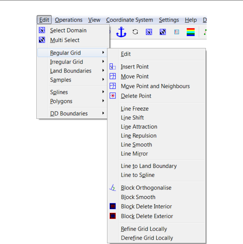
On the Edit menu, point to Regular Grid you can edit the grid, see Figure 5.7
Deltares 27 of 128
DRAFT
RGFGRID, User Manual
Figure 5.7: Options on the Edit →Regular Grid menu
5.2.3.1 Menu Options
The key stroke to reach the menu item Edit →Regular Grid →Edit is: CTRL+ALT+G
Edit
Upon selecting Edit →Regular Grid →Edit, you can start editing a grid. When there is no grid
the edit mode is set to New, which means start editing a new irregular grid. Otherwise you
have to select first a grid (from the menu Edit →Grid →Select or press the key s). After you
have selected the grid you can use key-strokes, icons in the toolbar or menu items to switch
the edit mode.
5.2.3.2 Point
On the Edit menu, point to Grid and click on one of the options to operate on individual grid
points. To insert, delete or move grid points you can either use the menu options, the icons
on the toolbar, or the keyboard to switch between these operations.
After selecting one of the options: insert, move or delete point the program is in point edit
mode
28 of 128 Deltares
DRAFT
Menu options
Insert Point
Press the I-key, use the toolbar icon or click the menu item Edit →Regular Grid →Insert
Point to bring the program into insert mode.
If the program is in insert mode, (message ’Select Grid Cell’ at the lower left side of the
screen), click the left mouse inside a grid cell to create a new grid cell at the border of the grid.
The indicated grid cell will be ’mirrored’ to the grid cell side closest to the clicking point.
Move Point
Press the R-key (Replace), use the toolbar icon or click the menu item Edit →Regular
Grid →Move Point to bring the program into replace mode.
The message at the lower left of the screen now reads ’Get a point’. Click left to indicate a
grid point; the message will read ’Put a point’. Move the cursor to the desired position and
click left again.
Move Point and Neighbours
Modifications will be made by shifting the centre point of a field of points. The field transforma-
tion is based upon the relative shift of the centre point. For all cells in the vicinity of the centre,
that shift is transformed to their local grid cell orientation and will be decreased in magnitude
in proportion to the physical distance to the centre cell. In that way a quasi-orthogonal trans-
formation is induced. The area of influence is always one sixth of the area that is currently
displayed on the screen. (So, if you want to decrease or increase the area of influence, zoom
in or zoom out).
Delete Point
Press the D-key, use the toolbar icon or click the menu item Edit →Regular Grid →Delete
Point to bring the program into delete mode.
If the program is in delete mode, delete grid points by just clicking them.
5.2.3.3 Line
The operations line freeze, line shift, line attraction, line repulsion and line smooth operate in
line mode, see Figure 5.7.
They all use the same procedure to indicate a line and an influence area.
You first indicate a line by marking its end points, using the left mouse; next you indicate the
influence area by marking one or two grid-points at one or both side of the line, respectively.
Pressing Esc enables the replacement of the last added point; pressing Esc+Esc cancels
all the selected block points, after you may redo the selection procedure. You click the right
mouse for the final selection of line and area. After the indication you perform the operation
(e.g. line shifting, attraction or repulsion). The result can still be reversed (by pressing several
times the Esc key).
Deltares 29 of 128

DRAFT
RGFGRID, User Manual
Line Freeze
Frozen lines are grid lines that are kept fixed in the orthogonalisation process. That is, the
end points are kept fixed and the points in between can only move in the direction along the
grid line. Frozen lines can be edited by clicking 2 points that lie on the same grid line. You
can unfreeze grid lines by first pressing the Dkey and click with the left mouse on one of the
endpoints. You can also use I(insert) mode to define lines to freeze.
Line Shift
This option provides the possibility to fit the grid’s edges to a land boundary. First you indicate
a line and indicate the influence area. Then, you can shift the line by shifting some or all of
the individual points of that line. The end points can also be shifted. After clicking the right
mouse to indicate that the line has been put into the correct new position, the points on the line
between the end-points will be shifted by linear interpolation between all repositioned points.
Then, a field transformation will be performed in the influence area, with centre points that are
now consecutive points on the shifted centre line. If you are not satisfied with the transformed
result, press several times the Esc key. You will then be put back into Edit →Line →Shift
mode. You can carry on shifting lines by simply repeating the same sequence of actions.
Line Attraction
Here, you have again to ‘Indicate a line’, by marking its end points, and to ‘Indicate an influence
area’ (see Edit →Regular Grid →Line Shift). The grid will be attracted to the indicated line,
making use of the line transformation described above, in the field indicated by the influence
area.
In Settings →General the parameter Attraction/Repulsion Parameter can be changed, see
Figure 5.54.
Line Repulsion
The reverse of Edit →Regular Grid →Line Attraction.
In Settings →General the parameter Attraction/Repulsion Parameter can be changed, see
Figure 5.54.
Line Smooth
You have to ‘Indicate a line’, by marking its end points, and to ‘Indicate an influence area’
(see Edit →Regular Grid →Line Shift). Within this area, the grid will be smoothed into the
direction indicated by the line.
The smoothing process can be configured, see Section 5.6.1, parameters Number Smoothing
Iterations and Smoothing Parameter.
Line Mirror
Indicate a grid line at the edge of the grid by marking its end points. Click right to execute the
mirror process; grid cells will be created. After this the operation can be repeated by using
the key CTRL+M
30 of 128 Deltares

DRAFT
Menu options
Line to Land Boundary
The edge of the grid can be fitted to a land boundary by hand, using the Edit →Regular Grid
→Line Shift option, or automatically, using the present option, Edit →Regular Grid →Line
to Land Boundary. The automatic option may not always deliver exactly what you want. This
can be caused by irregular shapes in the land boundary. However, we do not want to be
compelled to analyse and polish up the land boundary a priori, in the digitising phase.
Therefore, both the automated and hand option are included in the program. Just indicate the
first and last point of the line that you want to fit to the land boundary. Then click the right
mouse. Next, all intermediate points will be translated to their nearest land boundary. Then,
a line shift will be performed, equal to the one mentioned above, shifting the indicated line
and the surrounding grid. Press Esc three times if the result is unsatisfactory. The original
grid will then be restored. The algorithm which decides to which land boundary line segment
the grid line should be attracted, first looks for the closest land boundary point. An error may
occur here, if the closest land boundary line segment is very long, and land boundary points of
other segments are more close to the indicated grid line. In that case open the land boundary
as a polygon and add (insert) some points to the long land boundary segment, so that points
on this segment are closest to the indicated grid line.
Line to spline
Similar as line to land boundary. If you do not need the spline grid anymore, first delete the
splines and then draw just 1 spline to which you want to attach the grid.
5.2.3.4 Block
Block delete, block cut, block orthogonalise and block smooth all operate in block mode, see
Figure 5.7. An influence area (block) is indicated by clicking two, three or four points.
Block orthogonalise
Click two, three, or four points to indicate the corners of the grid block. A minimal block is
selected which just contains the selected points. Press Esc if you want to replace the latest
indicated point, press Esc+Esc to redo the selection of the block. Clicking right results in
the orthogonalisation of the grid inside the selected block. Press Esc+Esc+Esc if you want
to cancel the latest action, or click Undo on the Operations menu.
You can specify parameters that control the orthogonalisation in Settings →Orthogonalisation,
see Figure 5.56.
Block smooth
Click two, three, or four points to indicate the corners of the grid block. A minimal block is
selected which just contains the selected points. Press Esc if you want to replace the latest
indicated point, press Esc+Esc to redo the selection of the block. Clicking the right mouse
results in the smoothing of the grid inside the selected block. Press Esc+Esc+Esc if you
want to cancel the latest action.
The smoothing process can be configured, see Settings →General, parameters Number
Smoothing Iterations and Smoothing Parameter, see Figure 5.54.
Deltares 31 of 128

DRAFT
RGFGRID, User Manual
Block delete interior
Click two points to indicate the corners of the grid block that you want to delete. A minimal
block is selected which just contains the selected points. Clicking right results in the annihi-
lation of the block area. Press Esc if you want to replace the latest indicated point, press
Esc+Esc to redo the selection of the block. Press Esc+Esc+Esc if you want to cancel the
latest action, or select Undo on the Operations menu.
Block delete exterior
Click two points to indicate the corners of the grid block. A minimal block is selected which
just contains the selected points. Clicking right results in the annihilation of the grid in the area
outside the selected block. Press Esc if you want to replace the latest indicated point, press
Esc+Esc to redo the selection of the block. Press Esc+Esc+Esc if you want to cancel the
latest action, or click Undo on the Operations menu.
5.2.3.5 Valid action keys are
The key stroke to reach the menu item Edit →Regular Grid →Edit is: CTRL+ALT+G
In Edit →Regular Grid mode the following keys can be used:
Key c: Delete (clear) edge (irregular grid)
Pressing callows you to delete an individual edge in the irregular grid.
Key d: Delete grid point
Pressing dallows you to delete individual grid points.
Key i: Insert grid point
Pressing iallows you to mirror a singel grid cell (regular grids) or grid points (irregular
grids).
Key m: Merge grid points (irregular grids)
Pressing mwill merge two grid points. Select both points to be merged.
Key CTRL+m: Mirror grid cells (regular grids)
Pressing CTRL+m will mirror the grid cells after using the menu option Edit →Grid →Line
Mirror. This key-stroke can be used several times after each other.
Key r: Replace grid point
Pressing rallows you to replace (move) individual grid points.
Key s: Split edge (irregular grid)
Pressing sallows you to split a indivual edge.
Key SHIFT+s: Split row or column (irregular grid)
Pressing SHIFT+s allows you a row or column of edges, only applicable on quadrilateral
grid cells.
Key BACKSPACE: Remove grids
Pressing BACKSPACE willl delete all grids, or if a selection polygon is defined the part of
the grid in the polygons.
Refine grid locally
This option operates on part of the grid and the direction depends on the grid line indicated
by you.
First you specify (on the Settings →General menu) the number of times that the grid has to
be refined in the M- or N-direction (see Section 5.3.10). Then you indicate 2 points on a grid
line between which the refinement has to be performed.
32 of 128 Deltares
DRAFT
Menu options
Derefine grid locally
This option operates on part of the grid and the direction depends on the grid line indicated
by you. This operation is the opposite of Refine Grid Locally. First you specify (menu Settings
→General), the number of times that the grid has to be de-refined in the M or N direction (see
Section 5.3.10). Then you indicate on a grid line 2 points between which the de-refinement
has to be performed. Next, smooth the jump in grid sizes.
5.2.4 Irregular grid
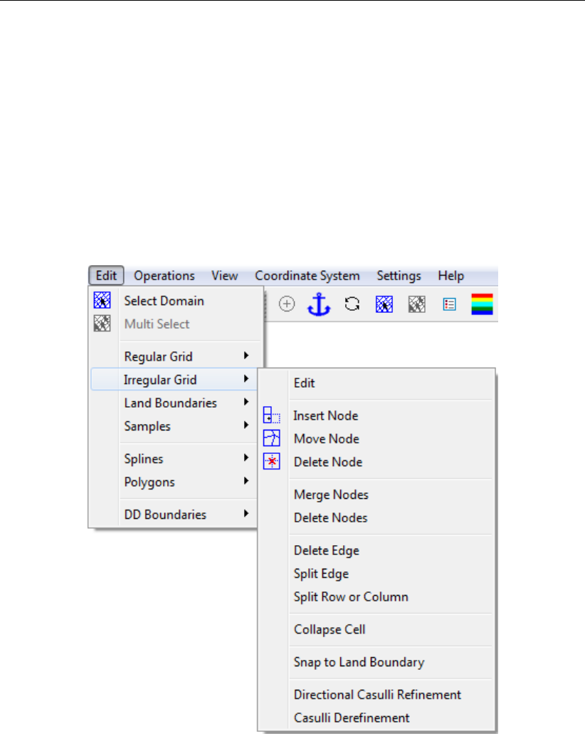
On the Edit menu, click on Irregular Grid to see the edit options for the currently selected
irregular grid, see Figure 5.8
Figure 5.8: Options on the Edit →Irregular Grid menu
5.2.4.1 Menu Options
The key stroke to reach the menu item Edit →Irregular Grid →Edit is: CTRL+ALT+G
Edit
Upon selecting Edit →Irregular Grid →Edit, you can start editing a grid. When there is no
grid the edit mode is set to New, which means start editing a new irregular grid. Otherwise
you have to select a grid first (from the menu Edit →Select Domain or press the key s). After
you have selected the grid you can use key-strokes, icons in the toolbar or menu items to
switch the edit mode.
Deltares 33 of 128
DRAFT
RGFGRID, User Manual
5.2.4.2 Node
On the Edit menu, point to Irregular Grid and click on one of the options to operate on indi-
vidual grid points. To insert, delete or move grid points you can either use the menu options,
the icons on the toolbar, or the keyboard to switch between these operations.
After selecting one of the options: insert, move or delete point the program is in point edit
mode
Insert Node
Press the I-key, use the toolbar icon or click the menu item Edit →Irregular Grid →Insert
Node to bring the progrma into insert mode.
If the program is in insert mode, (message ’Select Grid Cell’ at the lower left side of the
screen), click the left mouse inside a grid cell to create a new grid cell at the border of the grid.
The indicated grid cell will be ’mirrored’ to the grid cell side closest to the clicking point.
Move Node
Press the R-key (Replace), use the toolbar icon or click the menu item Edit →Irregular
Grid →→Move Node to bring the program into replace mode.
The message at the lower left of the screen now reads ’Get a point’. Click left to indicate a
grid point; the message will read ’Put a point’. Move the cursor to the desired position and
click left again.
Delete Node
Press the D-key, use the toolbar icon or click the menu item Edit →Irregular Grid →Delete
Node to bring the program into delete mode.
If the program is in delete mode, delete grid points by just clicking them.
Merge Nodes
Upon selecting Edit →Irregular Grid →Merge Nodes two nodes can be merged. Select a
node by the left mouse button and than select a node to which the first selected node is
merged to.
Delete Nodes
This option deletes all vertices which have a z-value larger than a user-defined value, in case
all directly connected vertices also meet this criterion. A pop-up window is show to obtain the
value from the user.
5.2.4.3 Edge
Delete Edge
This option enables the user to delete individual edges by clicking on them.
34 of 128 Deltares

DRAFT
Menu options
Split Edge
This option enabled the user to locally refine the grid by clicking on an edge. A new node
is inserted there and it is connected by automatically generated edges. It is intended to be
used on rectangular elements. Clicking on opposing edges grows the local refinement like a
straight line, capped by triangles.
Split Row or Column
This option performs the Split Line operation on a column or row of rectangular elements,
producing the same result as when Split Line was performed repeatedly by hand. It is possible
to restrict the extent of this operation by creating a polygon, selecting the polygon and then
applying Split Row or Column on a contained edge.
Collapse Cell
This option switches to a mode in which any subsequent left mouse button click inside a cell
leads to that cell being removed from the irregular grid by merging its vertices into a single
vertex. When in Edit Grid Mode, collapse cell can be activated by pressing the K-key.
Snap to Land Boundary
The edge of an irregular grid can be fitted to a land boundary by using the Edit →Irregular
Grid →Snap to Land Boundary option. Then, the irregular grid is shifted towards the land
boundary, so that the alignment with the land boundary is optimized. Noted that the whole
irregular grid is shifted towards the bouncary, while in case of structured grids subsections
have to be selected, see also Edit →Regular Grid →Line to Land Boundary option.
Directional Casulli Refinement
Upon selecting Edit →Irregular Grid →Directional Casulli Refinement, you can refine an
irregular grid in one coordinate direction. To this purpose, the irregular grid should have a
structured shape. Otherwise, RGFGRID can not recognize the direction of refinement. This
refinement yields a combination of quadrilaterals and triangles for the refined area.
We remark that the above-described algorithm are based on the ideas of Prof. V. Casulli,
which have been used in the JANET grid generation program for UnTRIM (Consult GmbH,
2015).
Casulli Derefinement
Upon selecting Edit →Irregular Grid →Casulli Derefinement, you can derefine an irregular
grid. To that purpose, a start location has to be selected. This is done by clicking on the left
mouse. Then, the grid derefinement starts at this location. Noted that this is slightly different
from the key Operations →Irregular Grid Coarseness →Derefine Casulli, for which the user
cannot specify a start location.
We remark that the above-described algorithm are based on the ideas of Prof. V. Casulli,
which have been used in the JANET grid generation program for UnTRIM (Consult GmbH,
2015).
Deltares 35 of 128
DRAFT
RGFGRID, User Manual
5.2.4.4 Valid action keys are
The key stroke to reach the menu item Edit →Irregular Grid →Edit is: CTRL+ALT+G
In Edit →Irregular Grid mode the following keys can be used:
Key c: Delete (clear) edge (irregular grid)
Pressing callows you to delete an individual edge in the irregular grid.
Key d: Delete grid point
Pressing dallows you to delete individual grid points.
Key i: Insert grid point
Pressing iallows you to mirror a singel grid cell (regular grids) or grid points (irregular
grids).
Key m: Merge grid points (irregular grids)
Pressing mwill merge two grid points. Select both points to be merged.
Key CTRL+m: Mirror grid cells (regular grids)
Pressing CTRL+m will mirror the grid cells after using the menu option Edit →Grid →Line
Mirror. This key-stroke can be used several times after each other.
Key r: Replace grid point
Pressing rallows you to replace (move) individual grid points.
Key s: Split edge (irregular grid)
Pressing sallows you to split a indivual edge.
Key SHIFT+s: Split row or column (irregular grid)
Pressing SHIFT+s allows you a row or column of edges, only applicable on quadrilateral
grid cells.
Key BACKSPACE: Remove grids
Pressing BACKSPACE willl delete all grids, or if a selection polygon is defined the part of
the grid in the polygons.
5.2.5 Land Boundaries
The land boundary is used to visualise the land-water interface. To edit (define or modify) a
land boundary, for possible edit actions see Figure 5.9.
Figure 5.9: Options on the Edit →Land Boundaries menu
36 of 128 Deltares
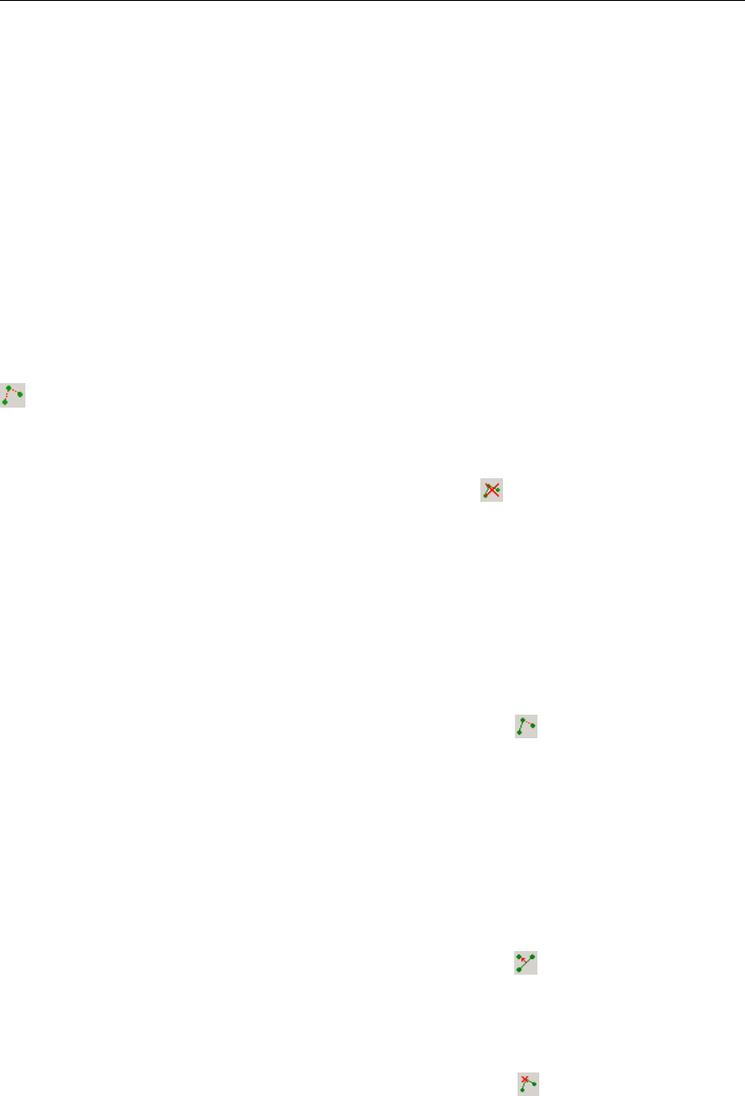
DRAFT
Menu options
5.2.5.1 Menu options
The key stroke to reach the menu item Edit →Land Boundary →Edit is: CTRL+ALT+L
Edit
Upon selecting Edit →Land Boundary →Edit, you can start editting a polyline that defines an
Land Boundary. When there is no polyline the edit mode is set to New, otherwise you have
to select first a polyline (from the menu Edit →Land Boundary →Select or press the key s).
After you have selected the polyline you can use key-strokes, icons in the toolbar or menu
items to switch the edit mode.
New
Upon selecting Edit →Land Boundary →New, you can start to define a new polyline, click on
, or use the key-stroke nto start a new polyline.
Delete
Upon selecting Edit →Land Boundary →Delete, click on , or use the key-stroke e, to
delete (erase) the selected polyline.
Select
Upon selecting Edit →Land Boundary →Select, or use the key-stroke s, you can select a
polyline by clicking on one of its edges or vertices. After that the polyline will be highlighted
Insert point
Upon selecting Edit →Land Boundary →Insert Point, click on , or use the key-stroke i,
you can insert a point into the selected polyline.
In Edit →Land Boundary, pressing Istarts the vertex insert action depending on the first click
on the screen. If the first click is in between two vertices of the land boundary then a point will
be inserted in the closest edge. The message at the left of the statusbar now reads ’Insert a
point’, click the left mouse to insert individual points.
Move point
Upon selecting Edit →Land Boundary →Move Point, click on , or use the key-stroke r,
you can move (replace) a point on the selected polyline.
Delete point
Upon selecting Edit →Land Boundary →Delete Point, click on , or use the key-stroke d,
you can delete a point on the selected polyline by indicating it.
Merge
Two land boundaries can be merged into one by first selecting an end point of the first land
boundary and then an end point of the second land boundary.
Deltares 37 of 128
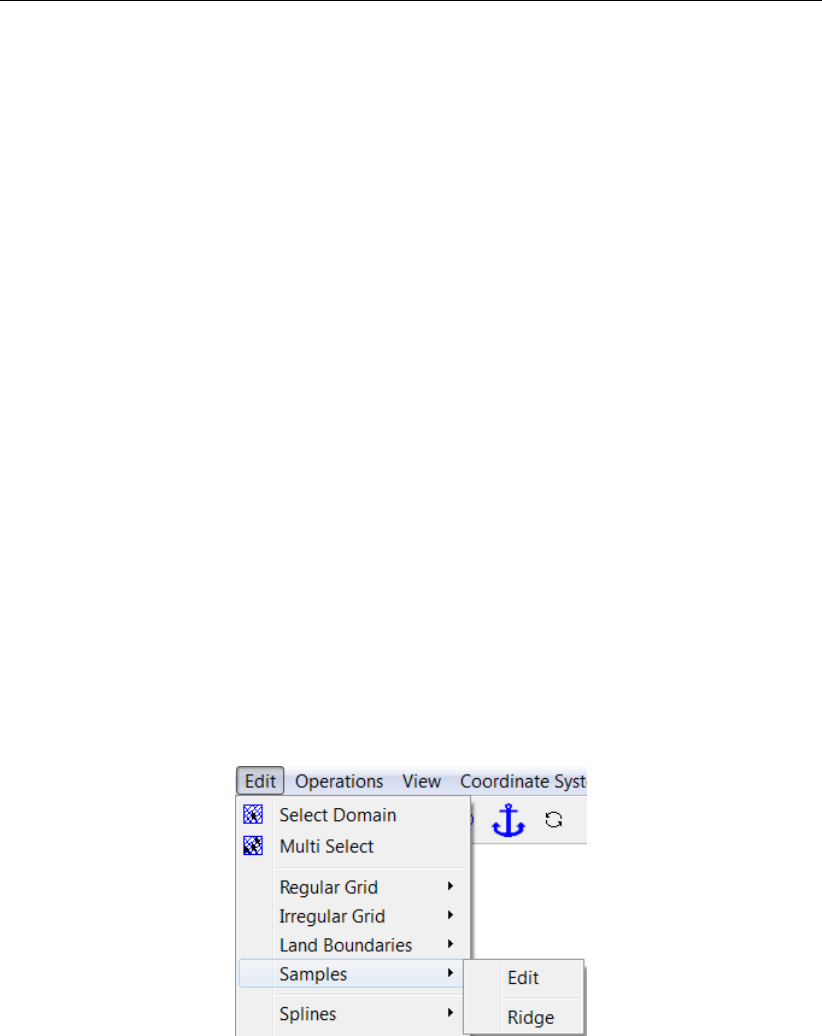
DRAFT
RGFGRID, User Manual
5.2.5.2 Valid action keys are
The key stroke to reach the menu item Edit →Land Boundary →Edit is: CTRL+ALT+L
In Edit →Land Boundary mode the following keys can be used (mode is indicated in the
statusbar):
Key a: Add point after
Add a point after the last point of a selected land boundary (after)
Key b: Add point before
Add a point before the first point of a selected land boundary (before)
Key d: Delete single point
delete single point in selected land boundary
Key i: Insert single point
In Edit →Land Boundary, pressing Istarts the vertex insert action depending on the first
click on the screen. If the first click is in between two vertices of the land boundary then
a point will be inserted in the closest edge. The message at the left of the statusbar now
reads ’Insert a point’, click the left mouse to insert individual points.
Key r: Move (replace) single point
Replace single point in the selected land boundary
Key s: Select land boundary
Select a land boundary
Key x: Delete land boundary
Delete a complete land boundary
5.2.6 Samples
On the Edit menu, point to Samples, see Figure 5.10
Figure 5.10: Options on the Edit →Samples menu
5.2.6.1 Menu Options
Edit
Samples can be inserted (with a specified depth value), replaced or deleted in the same way
as the points of a polygon. The value of the marked sample is displayed in the status bar at
the bottom of the screen together with the xand ycoordinates and/or the distance from the
anchor.
38 of 128 Deltares
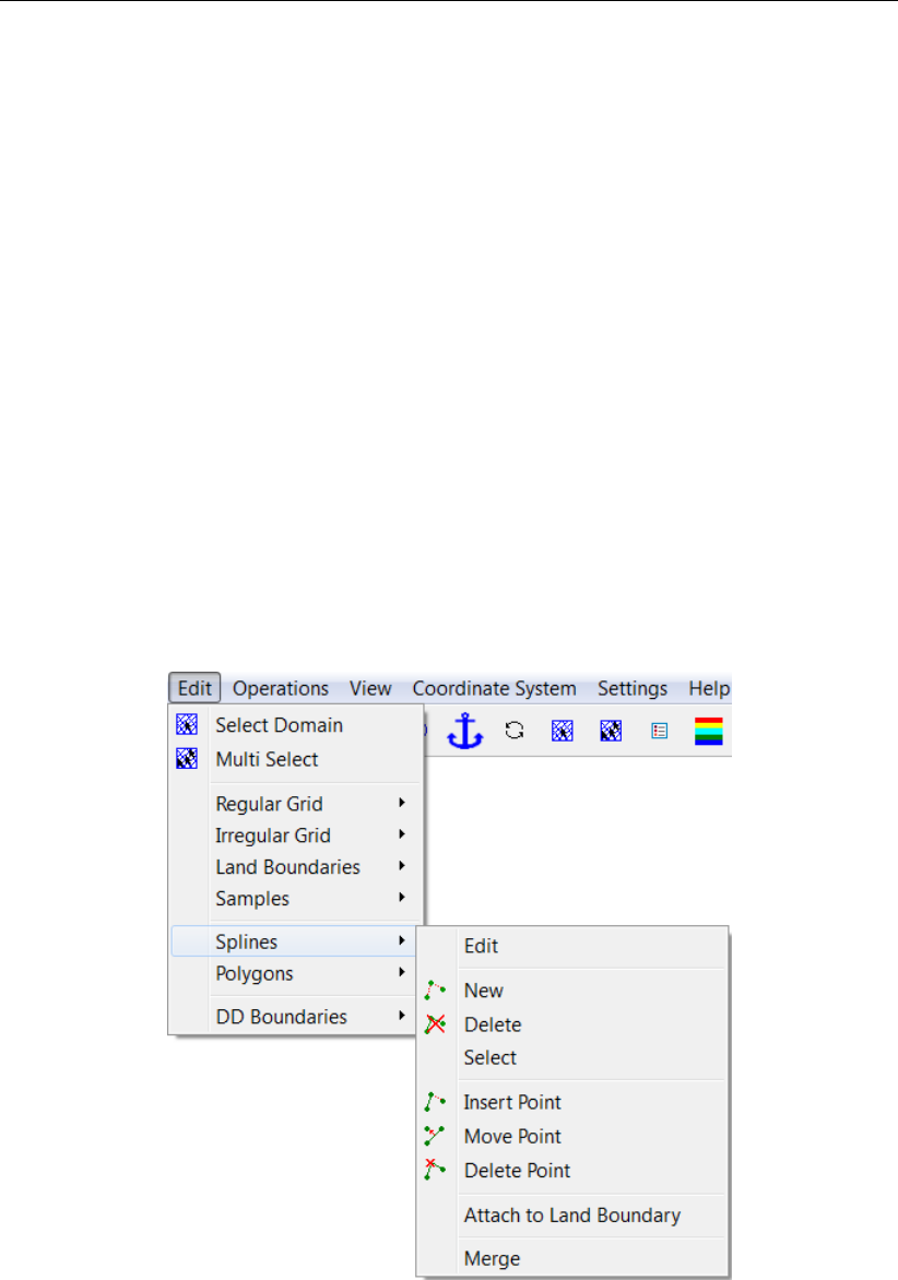
DRAFT
Menu options
Ridge
A structured sample set can contain ridges, for instance representing dikes. By clicking on a
ridge it is copied to a land boundary.
5.2.6.2 Valid action keys are
In Edit →Samples mode the following keys can be used (mode is indicated in the statusbar):
Key +,-:
The value of the marked sample can then be modified by pressing the +(increase) or -
(decrease) key.
Key c: Change
Sample value can be modified.
Key d: Delete
Delete sample point.
Key i: Insert
Insert new sample point.
5.2.7 Splines
On the Edit menu, point to Splines, see Figure 5.12
Figure 5.11: Options on the Edit →Splines menu
5.2.7.1 Menu options
The key stroke to reach the menu item Edit →Splines →Edit is: CTRL+ALT+S
Deltares 39 of 128

DRAFT
RGFGRID, User Manual
Edit
Upon selecting Edit →Splines →Edit, you can start editting a spline (handled as a polyline).
When there is no spline the edit mode is set to New, otherwise you have to select first a spline
(from the menu Edit →Spline →Select or press the key s). After you have selected the spline
you can use key-strokes, icons in the toolbar or menu items to switch the edit mode.
New
Up on selecting Edit →Splines →New you can start defining a new spline. Click the left
mouse button at different positions to create a spline. To start a new spline, click the right
mouse button and click the left mouse button again to create the next spline.
Delete
Up on selecting Edit →Splines →Delete you can delete a spline . Click with the left mouse
button on a spline point, than that spline will be deleted.
Select
Upon selecting Edit →Splines →Select, or use the key-stroke s, you can select a spline by
clicking on one of its vertices. All of the spline’s vertices will be highlighted to indicate the
spline is selected. By clicking on a vertex of a selected spline, it is deselected and therefore
no longer highlighted.
Insert Point
Upon selecting Edit →Splines →Insert Point, you can insert a point. But first you have to
select the spline in which you want to insert a point.
Move Point
Upon selecting Edit →Splines →Move Point, you can move a point on a spline. But first you
have to select the spline in which you want to insert a point.
Delete Point
Upon selecting Edit →Splines →Delete Point, you can delete a point of a spline. But first you
have to select the spline in which you want to insert a point.
Attach to Land Boundary
One can snap (part of) a spline to the nearest land boundary by selecting Edit →Splines
→Attach to Land Boundary. Click on two different vertices of a spline to select the part of that
spline which must be snapped. To perform the attach operation, click the right mouse button.
In addition to the original spline, a different coloured spline is drawn to show the result. A
message window offers the choice between improving the snap or accepting the result.
Merge
Two splines can be merged into one by first selecting an end point of the first spline and then
an end point of the second spline.
40 of 128 Deltares

DRAFT
Menu options
5.2.7.2 Valid action keys are
The key stroke to reach the menu item Edit →Splines →Edit is: CTRL+ALT+S
In Edit →Splines mode the following keys can be used (mode is indicated in the statusbar):
Key a: Add point after
Add a point after the last point of a selected spline (after)
Key b: Add point before
Add a point before the first point of a selected spline (before)
Key d: Delete single point
delete single point in selected spline
Key i: Insert single point
Insert single point in the selected spline
Key n: New spline
Pressing nallows you to start drawing a new spline.
Key r: Move (replace) single point
Replace single point in the select spline
Key s: Select spline
Select a spline
Key x: Delete spline
Delete a complete spline
5.2.8 Polygons
The polygon is used to limit the area of influence of operations and or edit actions. All grid
points and samples that are inside the polygon are active in the subsequent interpolation or
manipulation steps. The polygon is self closing.
Deltares 41 of 128
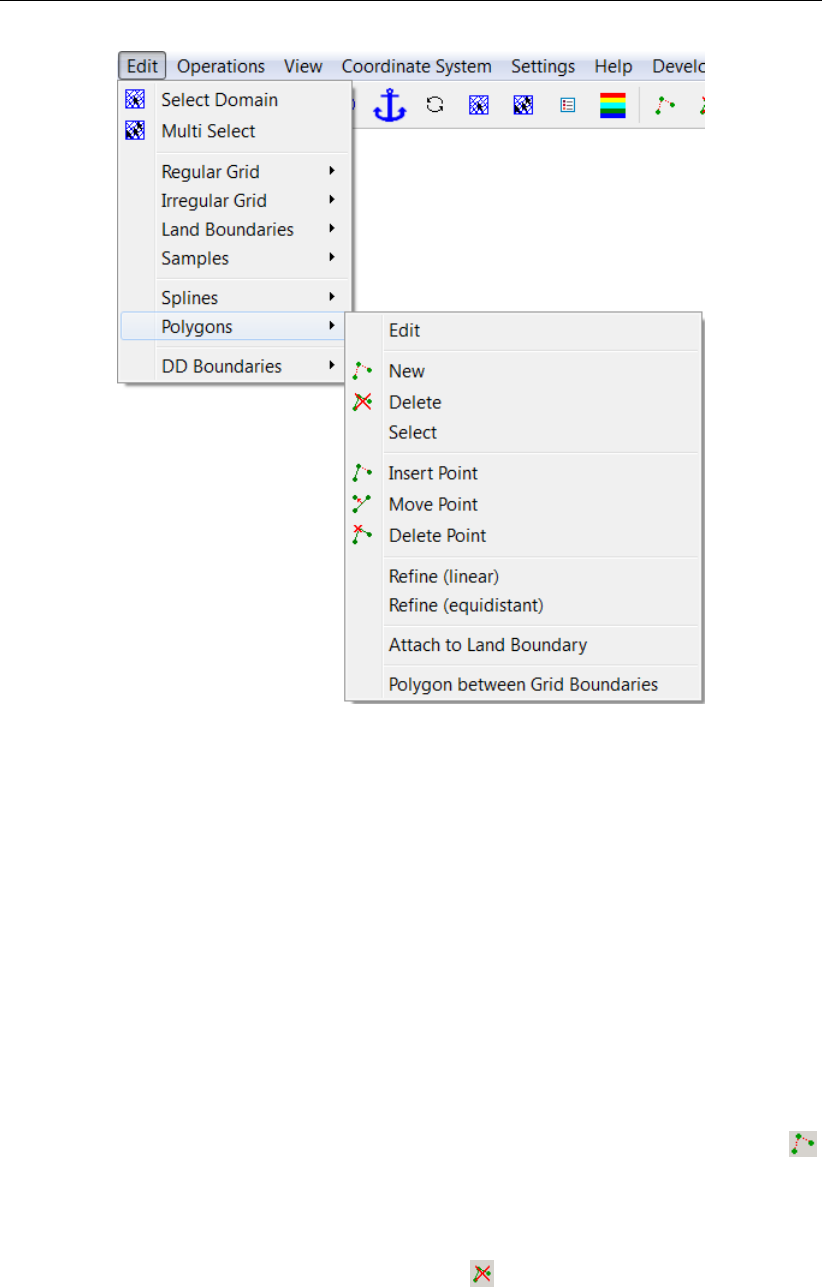
DRAFT
RGFGRID, User Manual
Figure 5.12: Options on the Edit →Polygons menu
5.2.8.1 Menu Options
The key stroke to reach the menu item Edit →Polygons →Edit is: CTRL+ALT+P
Edit
Upon selecting Edit →Polygons →Edit, you can start editting a polygon that defines an area
of interest. When there is no polygon the edit mode is set to New, otherwise you have to
select first a polygon (from the menu Edit →Polygons →Select or press the key s). After
you have selected the polygon you can use key-strokes, icons in the toolbar or menu items to
switch the edit mode.
New
Upon selecting Edit →Polygons →New, you can start to define a new polygon, click on ,
or use the key-stroke nto start a new polygon.
Delete
Upon selecting Edit →Polygons →Delete, click on , or use the key-stroke e, to delete
(erase) the selected polygon.
42 of 128 Deltares
DRAFT
Menu options
Select
Upon selecting Edit →Polygons →Select, or use the key-stroke s, you can select a polygon
by clicking on one of its edges or vertices. AFter that the polygon will be highlighted
Insert point
Upon selecting Edit →Polygons →Insert Point, click on , or use the key-stroke i, you can
insert a point into the selected polygon. In Edit →Polygon, pressing Istarts the vertex insert
action depending on the first click on the screen. If the first click is in between two vertices of
the polygon then a point will be inserted in the closest edge. The message at the left of the
statusbar now reads ’Insert a point’, click the left mouse to insert individual points.
Move point
Upon selecting Edit →Polygons →Move Point, click on , or use the key-stroke r, you can
move (replace) a point on the selected polygon.
Delete point
Upon selecting Edit →Polygons →Delete Point, click on , or use the key-stroke d, you can
delete a point on the selected polygon by indicating it.
Refine (linear)
The option Edit →Polygons →Refine (linear) enables one to refine (part of) a polygon. This
is done by first selecting a polygon and then selecting two vertices of that polygon. Upon
selecting the second vertex, the intermediate segments will be refined.
The selected polygon segments are determined as follows:
Upon selecting a polygon, its vertices and their numbers are shown. If the first selected vertex
A has a lower number then the second selected vertex B, the segments connecting A to A+1
through B-1 to B are selected. Otherwise the inverse is selected.
The algorithm for the refinement is as follows:
The distances between the first selected vertex and its neighbour, and between the last se-
lected vertex and its neighbour are determined. The intermediate segments will be refined
using linear interpolation of these two distances, such that a gradual change in segment
length is obtained along the selected part of the polygon. The existing intermediate vertices
are replaced by new ones.
Refine (equidistant)
The option Edit →Polygons →Refine (equidistant) enables one to refine (part of) a polygon.
This is done by first selecting a polygon and then selecting two vertices of that polygon. Upon
selecting the second vertex, a pop-up window will request the desired segment length, after
which the intermediate segments will be refined.
The selected polygon segments are determined as follows:
Upon selecting a polygon, its vertices and their numbers are shown. If the first selected vertex
A has a lower number then the second selected vertex B, the segments connecting A to A+1
through B-1 to B are selected. Otherwise the inverse is selected.
Deltares 43 of 128
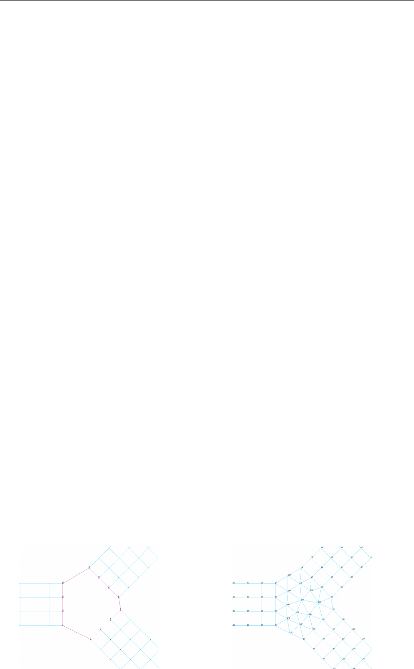
DRAFT
RGFGRID, User Manual
Attach to Land Boundary
Through the Edit →Polygons →Attach to Land Boundary option, a subset of a polygon’s
vertices can be selected and snapped to the nearest land boundary. In case no polygon is
currently selected, the user is asked to select one by clicking near a polygon vertex. With a
polygon selected, the first vertex can be selected by clicking near it. Clicking the same vertex
for a second time deselects it. By selecting a second vertex, a subset of vertex points is
snapped to the nearest land boundary. The subset consists of vertices [n,m] if m >n or all
but [m+1,n-1] if m <n.
Polygon between Grid Boundaries
The aim of this option is to define a polygon in which an irregular grid can be generated, this
irregular grid can subsequently be merged with the existing irregular grids.
In the Edit →Polygons →Polygon between Grid Boundaries mode a polygon can be defined
by selecting two or more sections of computational boundaries. The polygon will consist
of vertices which are generated from the boundary grid node coordinates of the selected
sections. Afterwards this polygon can be handled with the normal polygon edit options to
adjust the shape and refinement of the polygon. Be sure that you do not move the vertices
which are located at the grid boundaries. Because an extra grid will be generated select
first the option Operations →Domain →New before generating the intermediate grid with the
option Operations →Grow Grid from Polygons.
The procedure is as follows:
Select the grids, use Edit →Multi Select, for which an in-between grid is needed. These grids
will be highlighted. Choose Edit →Polygons →Polygon between Grid Boundaries and select
two points on the boundary of the first grid. All boundary points in between these two points
are selected, using a shortest node-path algorithm. Select two points on the boundary of the
second grid. All boundary points in between these two points are selected, using a shortest
node-path algorithm. More boundary sections can be selected as desired. Press the right
mouse button to complete this edit action and obtain a polygon as shown in Figure 5.13a.
The resulting polygon can be edited to obtain the appropriate shape and refinement. If you are
satisfied then you can generate the irregular grid by selecting, Operations →Domain →New
and than Operations →Grow Grid from Polygons from the menu bar. Now the in-between
grid is generated, remove the polygon by choosing Operations →Delete →Polygons from
the menu-bar. To merge the grids, first choose Edit →Multi Select from the menu bar and
then select the grids (including the just generated) which you want to merge, and then select
Operations →Grid →Merge Grids (an axample result is given in Figure 5.13b).
(a) Grid boundary polygon (b) Result grid
Figure 5.13: Polygon between grid boundaries.
44 of 128 Deltares
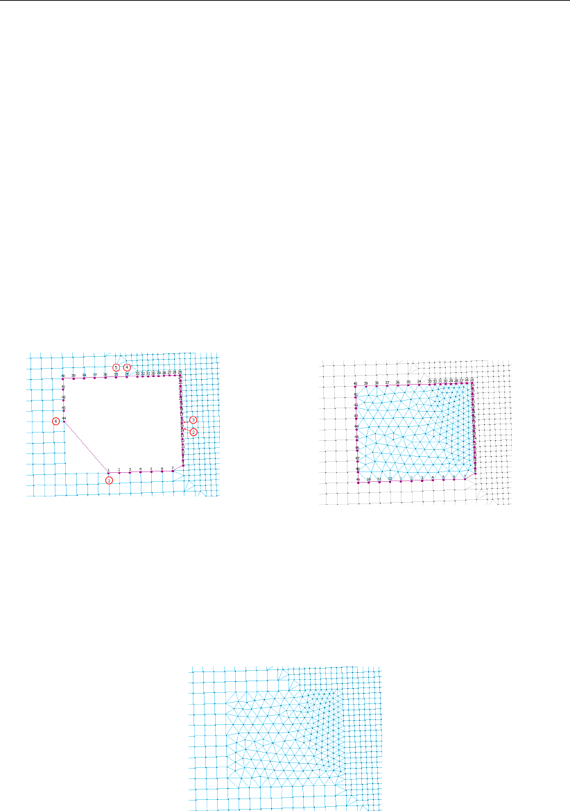
DRAFT
Menu options
If you accidentally moved one vertex of the polygon which should lie on the grid boundary (and
it was not merged) then you can merge these nodes by using the option Operations →Grid
→Merge Points.
Example, filling a gap in a unstructured grid
In this example we will explain the option Polygon between Grid Boundaries to fill a gap in a
single unstructured grid. Because the distance between two succesively clicked points on the
boundary of the gap is based on the shortest cell distance you whave to devide the boundary
in several sections, in this example 4. Choose the option Edit →Polygons →Polygon between
Grid Boundaries from the menu bar and start clicking the boundary of the gap, indicate with
a circled 1 (see Figure 5.14a). Then click the end of the first section (circled 2 and vertex 14
of the polygon). For the second section, start at circled 3 which is on one cell distance from
the end point of the first section, which will be vertex 15 of the polygon. Go on with defining
sections, circles 4, 5 and so on. So for this example you need to define 4 sections. After
pressing the right mouse button and generating the grid by selecting Operations →Grow Grid
from Polygons, something like Figure 5.14b will appear.
(a) Unstructured grid with gap, numbers indi-
cate click order (b) Gapp filled with unstructured grid
Figure 5.14: Filling a gap in an unstructered grid using the option Polygon between Grid
Boundaries.
Now the standard procedure to merge unstructured grids can be used, do not forget to delete
the polygon. See Figure 5.15 for the final result of this example.
Figure 5.15: Filled a gap in an unstructered grid
5.2.8.2 Valid action keys are
The key stroke to reach the menu item Edit →Polygons →Edit is: CTRL+ALT+P
In Edit →Polygons mode the following keys can be used:
Key d: Delete
Pressing dallows you to delete individual polygon points.
Deltares 45 of 128
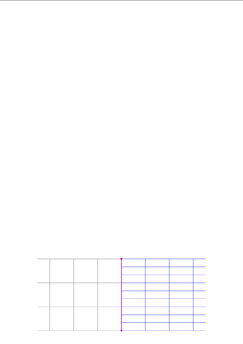
DRAFT
RGFGRID, User Manual
Key e: Erase polygon
Entire polygon sections are deleted. Press key eand then click with the left mouse button
on a point of the polygon which need to be deleted. Finish the operation by pressing the
right mouse button.
Key i: Insert
In Edit →Polygons, pressing Istarts the vertex insert action depending on the first click
on the screen. If the first click is in between two vertices of the polygon then a point will be
inserted in the closest edge. The message at the left of the statusbar now reads ’Insert a
point’, click the left mouse to insert individual points.
Key n: New polygon
Pressing nallows you to start drawing a new polygon.
Key r: Replace
Pressing rallows you to replace (move) individual polygon points. The message at the
left of the statusbar now reads ’Replace: Get a Vertex’. If you have got it by clicking the
left mouse, the message will read ’Replace: Put a Vertex’, and you can do so by clicking
the left mouse at the new desired position.
5.2.9 DD Boundaries
This option is only relevant to users of the Delft3D domain-decomposition system, or if you
want to keep some parts of the boundary fixed in the orthogonalisation.
At the interface between two grids of a multi-domain model (DD Boundaries) the grids should
satisfy the following rules:
At sub-domain interfaces the grids should be nicely connected (no overlap and “no holes”
between sub-domains).
In case of horizontal grid refinement, grid lines in the coarse domain should be continued
in the fine sub-domain, see Figure 5.16. Thus, there should be a 1-to-N refinement, with
N an integer number.
Figure 5.16: Example of a 1-to-3 refinement along a DD boundary
Each grid line should cover or be covered by another grid line. The domain decomposition
of Figure 5.17 does not fulfil this requirement. Although the DD-boudaries A and B have
a correct refinement factor.
46 of 128 Deltares
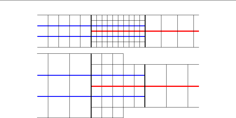
DRAFT
Menu options
AB
A
B
Figure 5.17: Two examples of not allowed domain decompositions, although both DD-
boundaries (A and B) satisfy the refinement condition; the red line and blue
lines do not cover each other
Grids must be of the same type (thus, all in spherical coordinates, or all in Cartesian
coordinates).
The grid orientation should be the same (increasing M- and N-numbering in the same
direction).
No coupling of columns to rows or vice versa.
Sub-domain interfaces should be straight lines (no stair-case interfaces).
DD boundaries can be edited by clicking boundary points that lie on the same grid line, see
Figure 5.18. You can delete boundary points by first pressing the Dkey and click with the left
mouse. R(replace) mode and I(insert) mode are also available. The specified boundaries
are saved together with the grid in a file with mask <∗.ddb>. This file is created when
selecting Operations →Compile DD Boundaries. See Appendix A.9 for the format of this file.
DD boundaries are also used in the orthogonalisation process. Because DD boundaries can
only be located on boundary points, their administration can be used to fix boundary points in
the orthogonalisation process.
Deltares 47 of 128
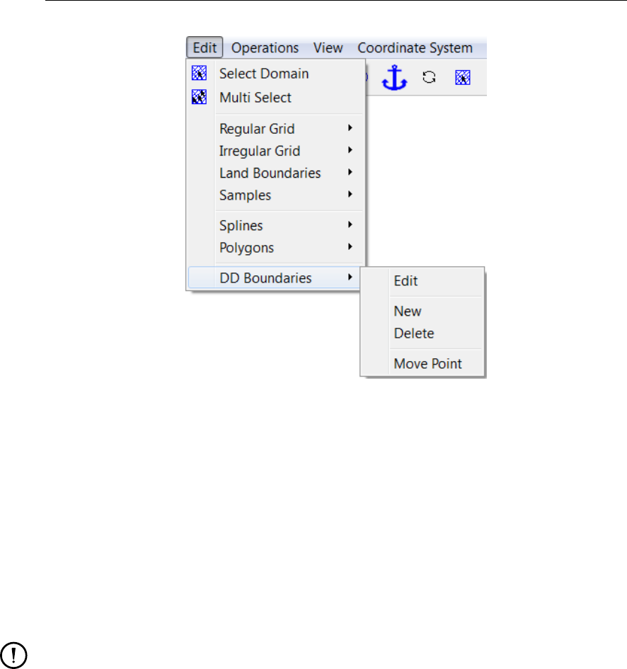
DRAFT
RGFGRID, User Manual
Figure 5.18: Options on the Edit →DD Boundaries menu
New
Start defining a new DD boundary.
Delete
Delete a single point of a DD boundary.
Move point
Replace a single point of a DD boundary.
Remark:
DD Boundaries can also be defined in a single domain, see Figure 5.19.
48 of 128 Deltares
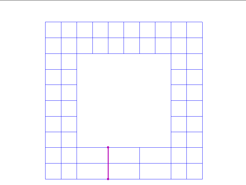
DRAFT
Menu options
Figure 5.19: DD Boundary in a single domain
5.3 Operations menu
On the Operations menu, see Figure 5.20, you may choose to generate a grid from a set
of splines and to perform various operations on the grid (create, de/refine, orthogonalise,
compile dd, etc.). Refinement and orthogonalisation parameters must be changed on the
Settings menu. Operations at individual grid points can be selected on the Edit menu.
Deltares 49 of 128
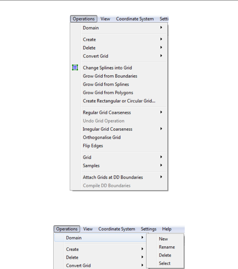
DRAFT
RGFGRID, User Manual
Figure 5.20: Options on the Operations menu
5.3.1 Domain
Figure 5.21: Options on the Operations menu
New
When selecting Operations →Domain →New, a new domain is created. In addition, it en-
ables the new domain mode, which means that every subsequent grid generation action will
add a new domain to your model. By default, the add points to irregular grid operation is
active. This means that if one starts clicking points on the canvas, a new irregular grid will be
made and added to the current domain.
Rename
When selecting Operations →Domain →Rename you can change the name of the domain.
This is mostly needed to change the default name of the domain.
Delete
When selecting Operations →Domain →Delete you can delete a domain from the list of
domains.
50 of 128 Deltares
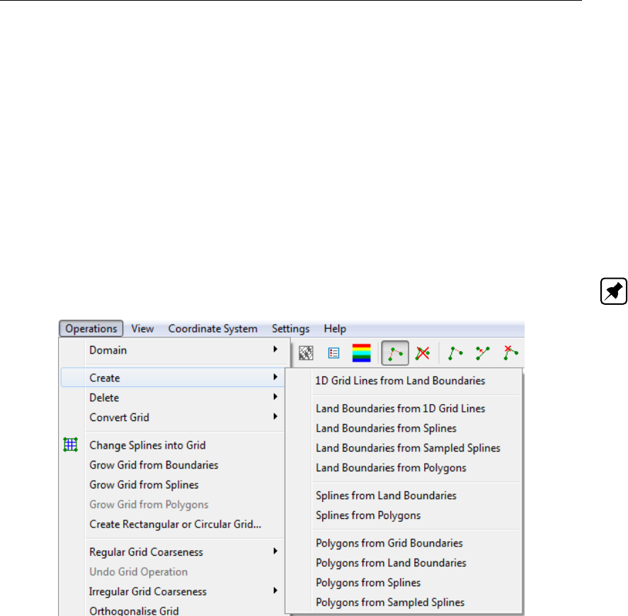
DRAFT
Menu options
Select
When selecting Operations →Domain →Select you can set a domain as active by selecting
from the list of domains.
5.3.2 Create
The Operations →Create →... options, see Figure 5.22, operate on parts of features (land
boundaries, splines, polygons or grid boundaries). These parts consist of collections of ver-
tices, which are determined in two steps:
each user-selected feature is a part, if no features are selected, then all features are parts
if there are polygons, vertices outside the user-selected polygons are discarded
Note: Creation of 1D edges does not support this selection mechanism.
Figure 5.22: Options on the Operations →Create menu
1D Grid Lines from Land Boundaries
This operation copies land boundaries and converts each to a network of 1D edges. Either
the currently selected irregular grid is extended, or a new irregular grid is constructed.
Land Boundaries from 1D Grid Lines
This operation copies all networks of 1D edges and converts those to land boundaries.
Land Boundaries from Splines
This operation copies splines and converts those to land boundaries.
Land Boundaries from Sampled splines
This operation copies sampled splines and converts those to land boundaries.
Deltares 51 of 128
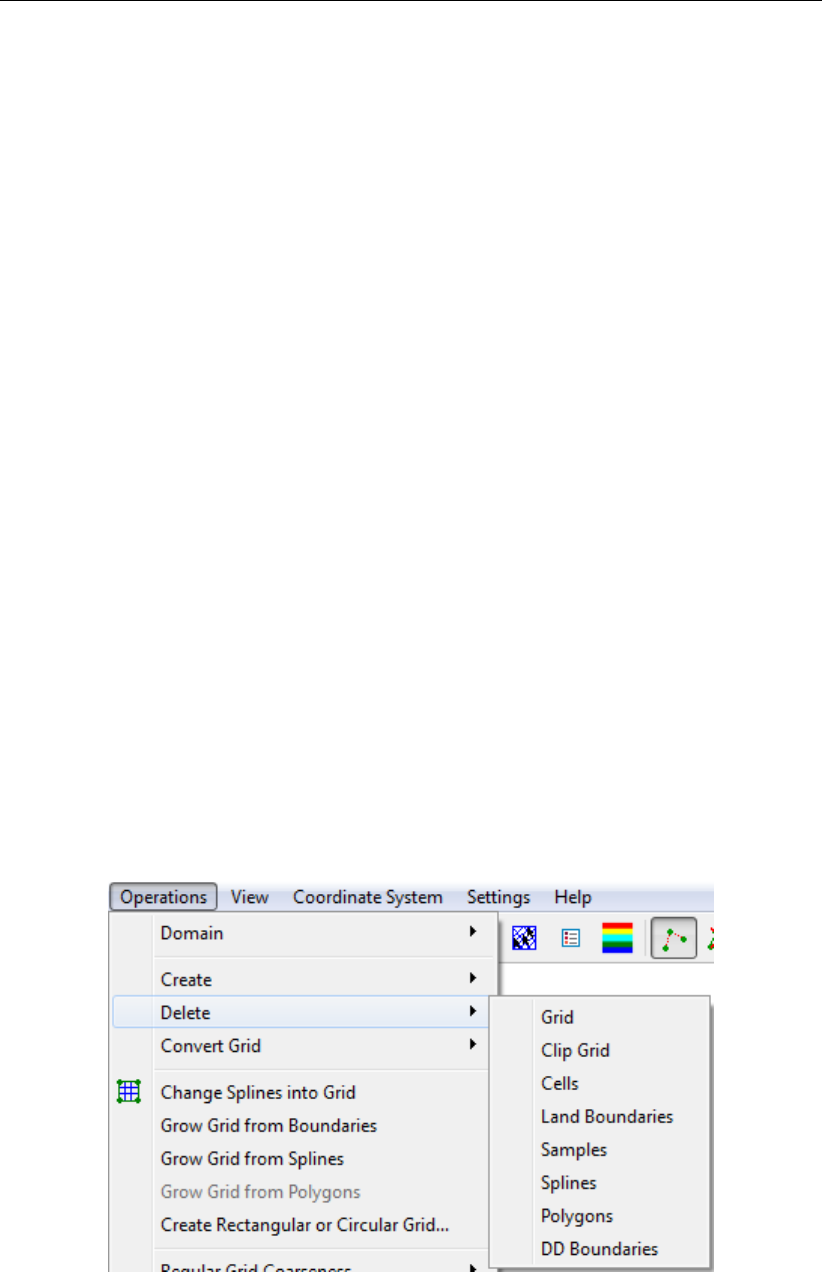
DRAFT
RGFGRID, User Manual
Land Boundaries from Polygons
This operation copies polygons and converts those to land boundaries.
Splines from Land Boundaries
This operation copies land boundaries and converts those to splines.
Splines from Polygons
This operation copies polygons and converts those to splines.
Polygons from Grid Boundaries
This operation copies grid boundaries and converts those to polygons.
Polygons from Land Boundaries
This operation copies land boundaries and converts those to polygons.
Polygons from Splines
This operation copies splines and converts those to polygons.
Polygons from Sampled splines
This operation copies sampled splines and converts those to polygons.
5.3.3 Delete
On the Operations →Delete menu, see Figure 5.24, you may choose to delete grids, land
boundaries, samples, splines, polygons or DD boundaries.
Figure 5.23: Options on the Operations →Delete menu
52 of 128 Deltares
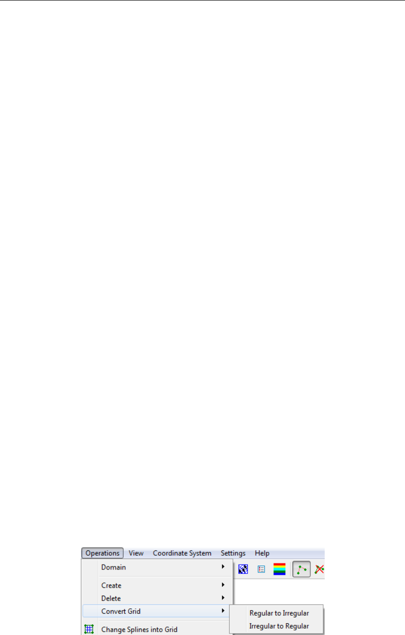
DRAFT
Menu options
Grid
The grid elements (partly) inside any polygon will be deleted. If no polygon is defined, you are
asked if you want to delete all grid points.
Clip Grid
The irregular grid elements completely inside any selected polygon are deleted and those
partly inside are clipped.
Cells
The irregular grid elements whose centre of mass are within any selected polygon are deleted.
Land Boundaries
Delete either the active land boundary or all land boundaries. In case polygons are present,
this selection is refined to the land boundary vertices inside a selected polygon or inside any
polygon.
Samples
Delete all samples or only those inside any selected polygon.
Splines
Delete either the active spline or all splines. In case polygons are present, this selection is
refined to the spline vertices inside a selected polygon or inside any polygon.
Polygons
Delete the selected polygons or all polygons.
DD Boundaries
Delete all domain decomposition boundaries.
5.3.4 Convert grid
Upon selecting Operations →Covert Grid you are able to convert a regular to irregular grid or
the other way around.
Figure 5.24: Options on the Operations →Convert Grid menu
Deltares 53 of 128
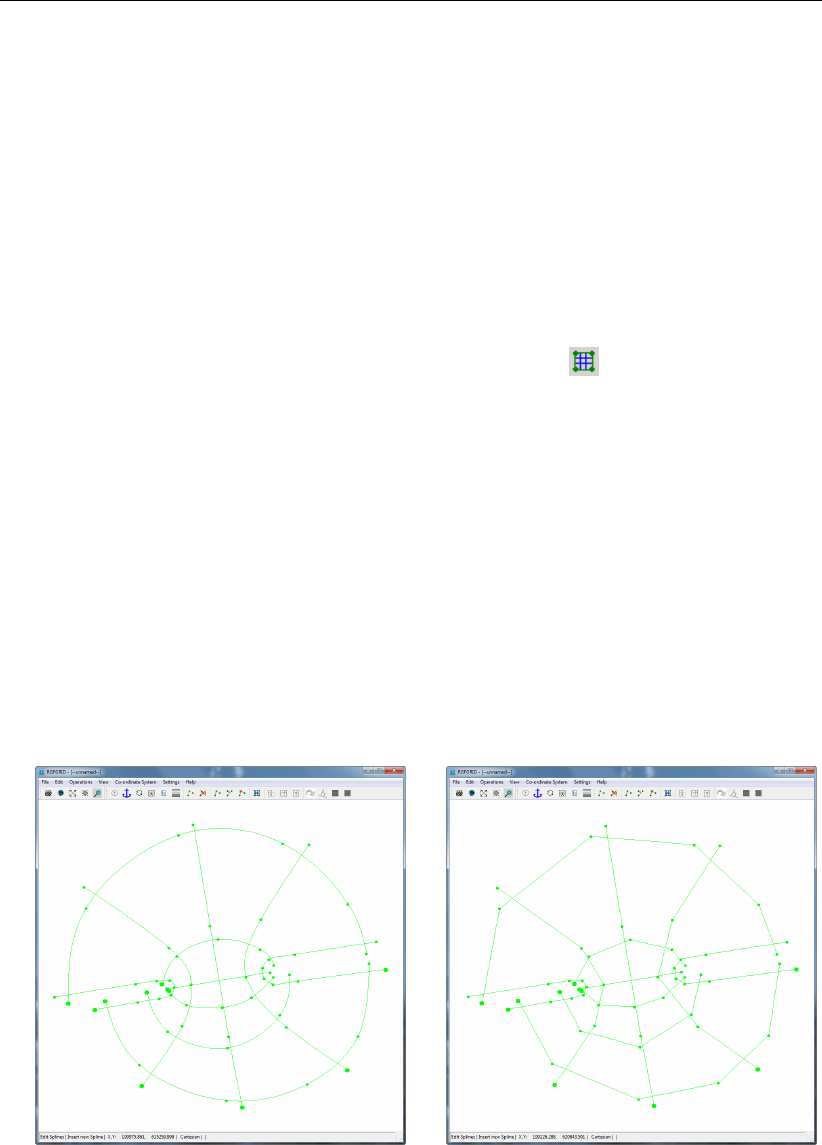
DRAFT
RGFGRID, User Manual
Regular to Irregular
Convert the selected regular grid to an irregular grid.
Irregular to regular
Convert the selected irregular grid to a regular grid. Some times you need to select Operations
→Grid →Rotate Grid Administration several times to get the orientation of the grid indices in
the right order.
5.3.5 Change splines into grid
This operation can also be activated from the toolbar by clicking .
The splines are ordered and directly refined into a regular grid. The refinement factors can
be specified by selecting Settings →General and specifying the M-Refinement Factor and
N-Refinement Factor,Figure 5.54). Spline intersection points can only be identified if the
straight lines between the control points of two splines intersect. To check this visually, you
can display the splines as straight lines, Figure 5.25, this can be set in the Settings →General
form, parameter Line or Spline Representation. The correct ordering is only possible if a
consistent result-grid is feasible.
At present, the spline-grid must satisfy the following restrictions:
The set of splines need to be topological equivalent with a rectangle.
Splines may not intersect twice or intersect themselves
Splines with the same orientation may not intersect
(a) Curved representation (b) Linear representation
Figure 5.25: Different representation of splines
The smoothness of the result-grid can be influenced by specifying the parameter Equidistant
or Smooth Interpolation in Settings →General, see Figure 5.54.
54 of 128 Deltares
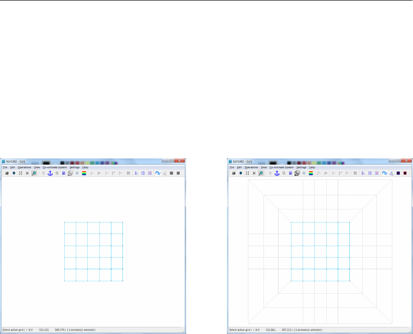
DRAFT
Menu options
5.3.6 Grow grid from boundaries
The Operations →Grow Grid from Boundaries option constructs a new curvilinear grid (see
Figure 5.26). It starts at the boundary of the currently active irregular grid, copying the bound-
ary as the start of the curvilinear grid. Additional layers are grown with certain widths. The
number of layers is determined by the N-Refinement Factor from the General Parameters
menu. The width is given by the Uniform Gridsize from the General Parameters menu, or
— when it is set to 0.0 — determined by the irregular grid’s geometry. For convenience,
the General Parameters menu is automatically opened when operations →Grow Grid from
Boundaries is clicked.
(a) Currently active irregular grid. (b) New inactive curvilinear grid around active
irregular grid.
Figure 5.26: Grow curvilinear grid from an irregular grid’s boundary.
5.3.7 Grow grid from splines
When selecting operations →Grow Grid from Spline a regular grid will be generated from a
centre spline. This option is especially suitable to generate a grid for river simulations. The
user is required to provide a centre spline - consisting of at least three points - from which the
grid is grown perpendicularly.
Note that the grid can be grown from multiple centre splines simultaneously. Per centre spline,
the extent of the grid and the heights of the grid layers can be controlled by supplementary
splines and setting parameters (see menu option Settings →Grow Grid from Splines. . . ). See
Figure 5.58.
For instance it is possible to grow a uniform part around a centre spline, with an exponentially
growing part outside that. This requires a spline along each side of the centre spline and two
cross splines. A cross spline consists of two points and crosses the other three splines.
Deltares 55 of 128
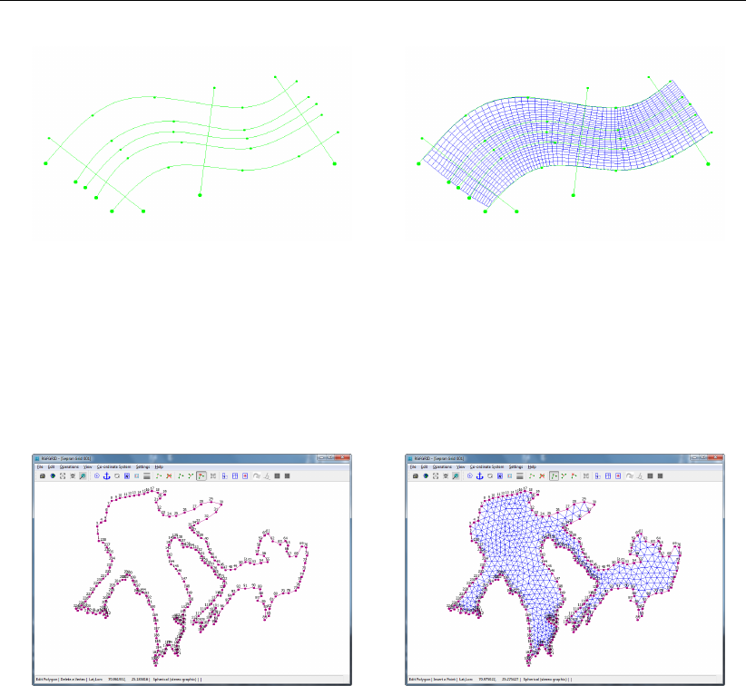
DRAFT
RGFGRID, User Manual
(a) Splines (b) Generated grid from splines
Figure 5.27: Create grid from splines with option Grow Grid from Spline
5.3.8 Grow grid from polygons
When selecting operations →Grow grid from polygons an irregular grid will be generated
inside the selected polygon(s) (see Figure 5.28).
(a) Selected polygon (b) Generated grid from polygon
Figure 5.28: Create grid from selected polygon
5.3.9 Create rectangular or circular grid
Specify the grid spacing, grid origin and the number of grid cells in both directions to quickly
create a rectangular grid. Grid sizes may be increased in size towards the boundaries by
specifying the ration of the maximum grid-size at the boundaries relative to the size of the
uniform fraction. The uniform fraction is the number of grid cells with uniform spacing vs. the
total number of grid cells in a direction. A circular grid is created if the radius of curvature
is non-zero. In that case, the grid origin is interpreted as its centre point. The parameters
involved are, see Figure 5.29.
56 of 128 Deltares
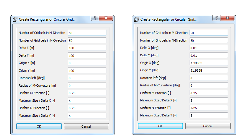
DRAFT
Menu options
(a) Cartesian grid (b) Spherical grid
Figure 5.29: Parameters for Rectangular or Circular Grid form.
The default settings are:
Number of Grid Cells in M-Direction default: 50
Number of Grid Cells in N-Direction default: 50
Delta X [m] or [deg] default: 100.0 or 0.01
Grid cell size M-direction [m] or [deg]
Delta Y [m] or [deg] default: 100.0 or 0.01
Grid cell size N-direction [m] or [deg]
Origin X [m] or [deg] default: 0.0 or 4.3803
Origin Y [m] or [deg] default: 100.0 or 51.9858
Rotation left [deg] default: 0.0
Radius of M-Curvature [m] default: 0.0
Uniform M-Fraction [-] default: 0.25
Fraction of grid cells which contains the default grid size (ex. 0.25*50 = 13+1 grid cells
with width size of 100 [m]))
Maximum Size / Delta X [-] default: 5.0
Uniform N-Fraction [-] default: 0.25
Fraction of grid cells which contains the default grid size (ex. 0.25*50 = 13+1 grid cells
with width size of 100 [m]))
Maximum Size / Delta Y [-] default: 5.0
Deltares 57 of 128
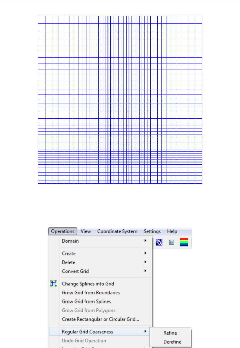
DRAFT
RGFGRID, User Manual
Figure 5.30: Rectangular grid, created with Maximum Size / Delta X = “5” and Maximum
Size / Delta Y = “5”
5.3.10 Regular Grid Coarseness
Figure 5.31: Options on the Operations →Regular Grid Coarseness menu
58 of 128 Deltares
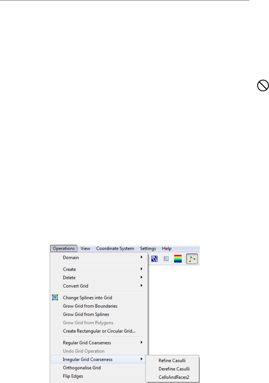
DRAFT
Menu options
Refine
This option operates on the whole grid and in both directions.
In Settings →General you first specify the number of times you want to refine the grid. The
parameters for the M and N direction are M-Refinement Factor and N-Refinement Factor,
respectively. You can identify the M and N direction by selecting View →Grid →Lines and M,
N Indices.
Restriction:
The number of refinement must be an integer number.
Derefine
This option operates on the whole grid and in both directions.
The opposite of Refine Grid. One limitation of the refinement procedure is that it can only
refine by an integer number. The combination of refine and de-refine allows you to reach a
rational number as refinement factor. e.g. You wish a refinement factor of 1.5; first refine by a
factor of 3, next de-refine by a factor of 2. Next, go to Edit →Line →Smooth to decrease the
jump in grid-sizes.
5.3.11 Undo Grid Operation
Some of the grid manipulation operations can be undone, after they have been performed
and before another operation is performed. The following operations can be undone: Refine
Casulli, Derefine Casulli, CellsAndFaces2, Orthogonalise Grid and Flip Lines.
5.3.12 Irregular Grid Coarseness
Figure 5.32: Options on the Operations →Irregular Grid Coarseness menu
Deltares 59 of 128
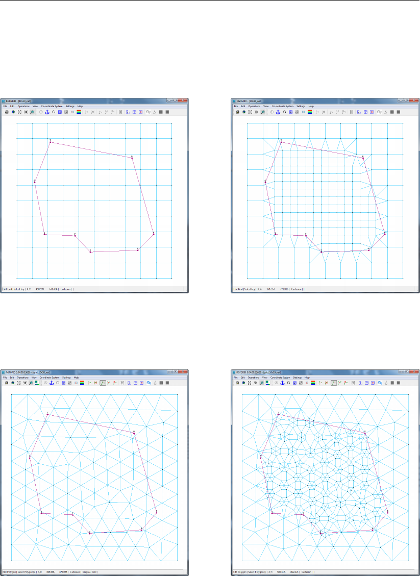
DRAFT
RGFGRID, User Manual
Refine Casulli
Only applicable for whole irregular meshes. Two examples are given, one for square grid cells
(Figure 5.33) and one for triangular grid cells, which results in a unstructured grid formed by
trinagles and rectangles (Figure 5.34).
(a) Original square grid (∆x= 100 m), with
polygon
(b) After Casulli refinement within polygon
(most grid cells have ∆x= 50 m)
Figure 5.33: Example of Casulli refinement of an irregular squared grid
(a) Original square grid (∆xalong boundary
is 100 m), with polygon
(b) After Casulli refinement within polygon, tri-
angles and squares
Figure 5.34: Example of Casulli refinement of an irregular triangular grid
Derefine Casulli
This option operates on the whole irregular grid and derefines the grid. It is the opposite of
Refine Casulli.
60 of 128 Deltares

DRAFT
Menu options
CellsAndFaces2
This is another approach for refinement of an irregular grid compared to the Casulli approach.
In the latter approach nodes are converted into cells and the intermediate area between the
new cells is filled with irregular grid cells as well. The option CellAndFaces2 subdivides cell
on the basis of its area. A triangle is subdivided into four new triangles, which each cell one-
fourth of its original area. Similarly, a quadrilateral is subdivided into four new quadrilaterals,
which each cell one-fourth of its original area.
5.3.13 Orthogonalise grid
This option operates on the whole grid or on a part of the grid. To operate on a part of the
grid:
For regular grids use Edit →Block →Orthogonalise. The grid will be orthogonalised in ac-
cordance with the local grid cell resolution, i.e. the overall shape will be conserved, but in-
dividual points may be shifted to get better orthogonality. You can specify parameters that
control the orthogonalisation in Settings →Orthogonalisation (regular), see Figure 5.56.
For irregular grids you have to specify one or more polygons. The orthogonalisation will
be performed only for the selected polygons. You can specify parameters that control the
orthogonalisation in Settings →Orthogonalisation (irregular), see Figure 5.57.
Keystrokes
Key SPACEBAR
Cycle between:
1 Add drawing the edges.
2 Prevent drawing the red dots and edges.
3 Draw the red dots on the nodes.
Key ESC
Stops the orthogonalisation process
5.3.14 Flip Lines
Minimise the number of edges connected to a node. The optimal number of edges to a node
is six.
Nodes that are connected to more than, say, six other nodes, are typically enclosed by cells
of highly non-uniform shape and wildly varying sizes. This motivates to improve the mesh
connectivity by selecting Operation →Flip Lines.
5.3.15 Grid
Set Edge Type to 1D
The edge type of all edges of all active irregular grids is set to 1D. The operation is limited to
the inside of all selected polygons, in case those are present. An edge is considered inside a
selection polygon when at least one of its vertices is inside.
Deltares 61 of 128
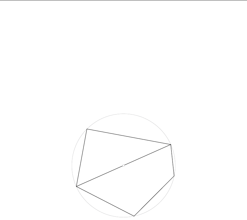
DRAFT
RGFGRID, User Manual
Set Edge Type to 2D
The edge type of all edges of all active irregular grids is set to 2D. The operation is limited to
the inside of all selected polygons, in case those are present. An edge is considered inside a
selection polygon when at least one of its vertices is inside.
Merge Circumcenters
An irregular grid can be used to calculate water flow. This involves a pressure gradient be-
tween the circumcenters of neighbouring cells. That procedure is numerically unreliable when
the distance between said circumcenters becomes too small. The option Merge Circumcen-
ters merges such neighbouring cells, also called remove small flow links.
M
I
II
Figure 5.35: The circumcentres of cell Iand II coincide at Mand should be merged.
Merge nodes
This operation merges pairs of nodes which are within the distance specified by Settings
→General... item Merge Nodes Distance.
Merge grids
To merge several grids you have to indicated which grids need to be merged, to select the grids
use the multi selection tool (Edit →Allow Multi Select). After selecting some grids this option
will merge the indicated irregular grids. Nodes from different grids with the same location will
be merged.
Paste two grids
The second (inactive) grid is pasted to the active grid. The M,N-orientations of both grids
do not have to match. The grid points on the junction line(s) should be relatively close to each
other, i.e. less than one quarter of a grid cell apart. On the junction line, the grid points are a
weighted average of the active grid and the inactive grid. The weighting factor can be changed
in the menu option Settings →General, see Figure 5.54.
A value of 0.0 will freeze the active grid; the inactive grid will move to the active grid.
62 of 128 Deltares

DRAFT
Menu options
Rotate grid administration
The M,Norientation of the grid is rotated over 90 degrees (counter clock-wise). Maybe you
need to adjust the grid administration because the grid administration over a DD-boundary
should have the same grid orientation.
5.3.16 Samples
Sample Ridges
This operation identifies ridges in a structured sample set. All samples which do not belong
to the ridges are deleted.
Generate Samples from Cells
Creates a sample for each element in the selected irregular grid. Selection polygons can be
used to make this operation only use elements inside those polygons. A sample is created
at the circumcentre or mass centre each element, using the element’s surface as the sample
value. In order to visualise the created samples, select Edit →Samples.
5.3.17 Attach Grids at DD Boundaries
There is a small difference between attaching regular and irregular grids. For regular grids
you are able to move the DD-boundary points of one regular grid to the DD-boundary of the
other regular grid, so the boundary is exactly on the same place. After that operation you have
to perform the operation Menu →Operations →Compile DD Boundaries. For irregular grids
the DD-boundaries should have the same location before the merge operation can be applied
by Operations →Attach Grids at DD Boundaries →Irregular grids.
For the menu layout see Figure 5.38.
Deltares 63 of 128
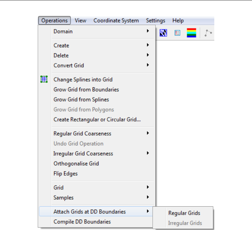
DRAFT
RGFGRID, User Manual
Figure 5.36: Operations →Attach Grids at DD Boundaries
Regular Grids
This option is only relevant if you want to use the multi-domain option of Delft3D-FLOW. First
you have to indicate the domain decomposition boundaries in the mode Edit →DD Bound-
aries.
One of the restrictions of domain decomposition is that the domain boundary between two
domains have to coincide, so there is no overlap or gap between the domains on the DD-
boundary. This option attach the grid at the DD-boundary to each other, for all DD-boundaries
of the current active grid. This is achieved by moving the grid points on the DD-bounday of
the active grid, to the corresponding inactive grid, see Figure 5.37.
64 of 128 Deltares
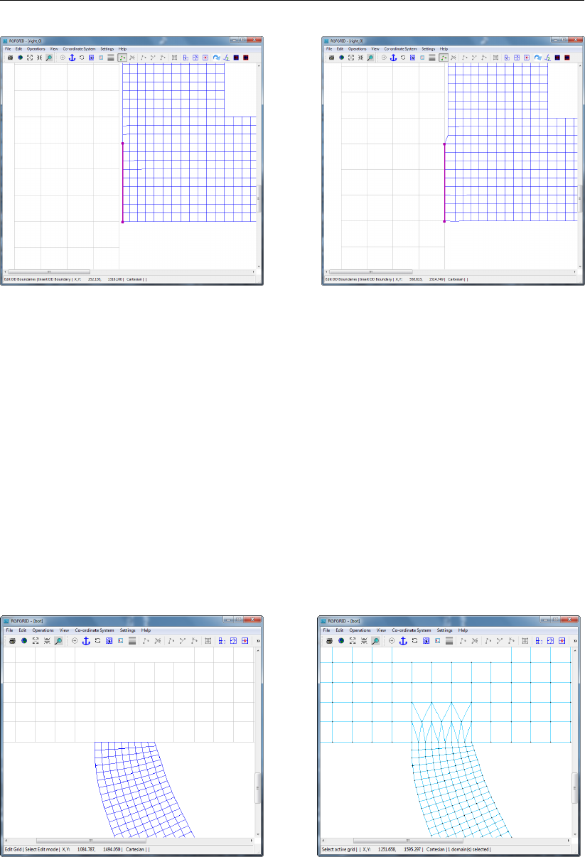
DRAFT
Menu options
(a) Before attach operation (b) After attach operation
Figure 5.37: Operations →Attach Grids at DD Boundaries→Regular grids
Irregular Grids
This option is most relevant if you have a multi-domain simulation model suitable for Delft3D-
FLOW and you want to use D-Flow FM.
Load the regular grids which need to be merged to one irregular grid at domain decomposition
boundaries (ex. Figure 5.38a).
Convert the regular grids to irregular by choosing menu option Operations →Convert Grid
→Regular to Irregular.
To perform the merge of the irregular grids choose menu option Operations →Attach Grids at
DD Boundaries →Irregular grids (ex. Figure 5.38b).
(a) Before attach operation (b) After attach operation
Figure 5.38: Operations →Attach Grids at DD Boundaries
Deltares 65 of 128
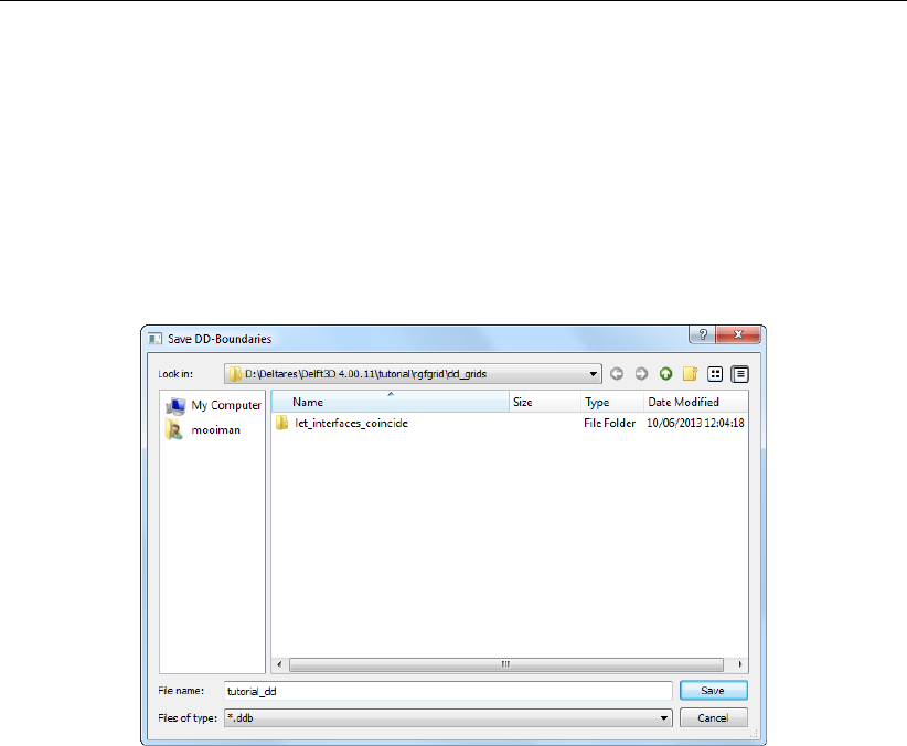
DRAFT
RGFGRID, User Manual
5.3.18 Compile DD Boundaries
This option is only relevant if you want to use the multi-domain option of Delft3D-FLOW.
First you have to indicate the domain decomposition (DD-)boundaries in the mode Edit →DD
Boundaries.
When you have defined the DD Boundaries, the grids needed in your multi-domain application,
are coupled here. Upon clicking Operations →Compile DD Boundaries a window opens, in
which you can select where the DD-boundary will be saved, see Figure 5.39.
Figure 5.39: Save DD-Boundaries window
The DD administration is written to a file with default mask <∗.ddb>, see Appendix A.9 for
its format.
5.4 View menu
On the View menu (see Figure 5.40) options are presented how to display a spherical grid,
whether or not to show the boundary and legend, to inspect the grid in 3 dimensions, how to
display the objects, and to view grid properties. Display characteristics (for the legend, colours
and sizes) may be changed in the Settings menu.
66 of 128 Deltares
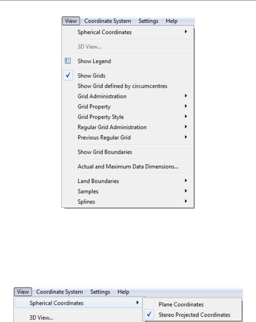
DRAFT
Menu options
Figure 5.40: Options on the View menu
5.4.1 Spherical Coordinates
Default: A spherical grid is shown in stereographic projected coordinates.
In the spherical coordinate system you can view the objects stereographic projected, see
Figure 5.42.
Figure 5.41: Options on the View →Spherical Coordinates menu
Plane coordinates
The coordinates are displayed just as they are and there is no well known projection used.
Stereographic projected coordinates
To display the coordinates a stereographic projection is used. The centre point of the stereo-
graphic projection is default the centre of the window. When zooming or scrolling the centre
point is not recalculated, for recalculation the centre point you have to press menu option
Operations →Change Centre of Projection.
Deltares 67 of 128
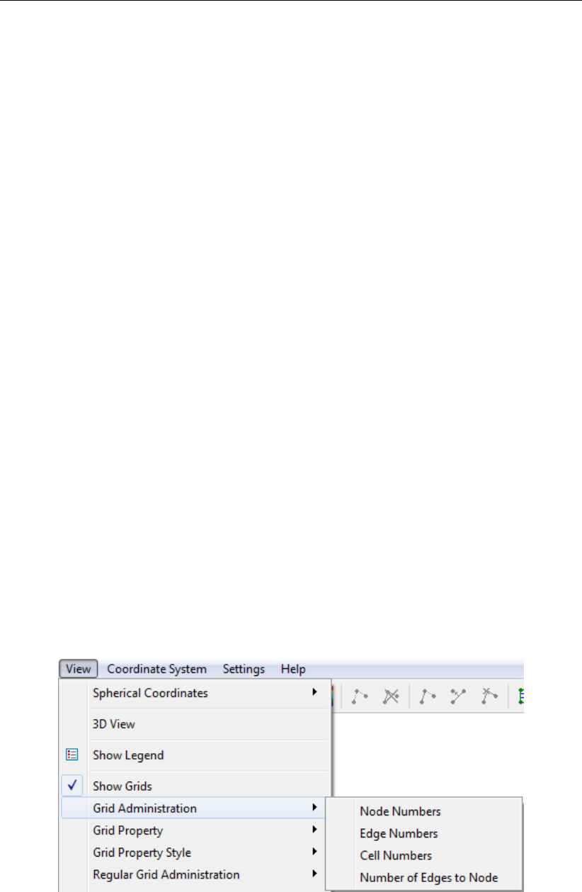
DRAFT
RGFGRID, User Manual
5.4.2 3D View
In the Delft3D-3DView window a fully 3-dimensional view of the data is shown.
c: Switch rendering mode
h: Toggle help
i: Inverse depth
r: Reste view
s: Toggle samples
x: Increase depth
z: Decrease depth
left mouse: Rotate in xy-plane
CTRL+left mouse: move origin xy-plane
middle-mouse: zoom
right mouse: rotate z-axis
5.4.3 Show Legend
Default: Show the (colour) legend.
Show or hide the colour legend on the screen.
5.4.4 Show Grids
Show or hide the grids.
5.4.5 Show Grid defined by Circumcentres
Show or hide the grid defined by the circumcentres.
5.4.6 Grid Administration
Upon selecting View →Grid Administration you show or hide several numberings of the grid.
Figure 5.42: Options on the View →Grid Administration menu
Node numbers
Show or hide the node number for regular grids it has the format (m, n)and for irregular grids
it is a single integer.
68 of 128 Deltares
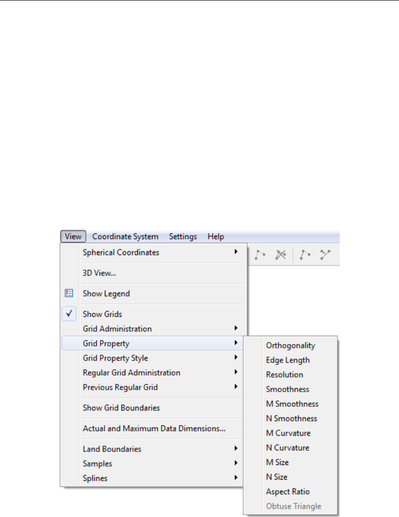
DRAFT
Menu options
Edge numbers
Show or hide the edge number.
Cell numbers
Show or hide the cell number.for regular grids it has the format (m, n)and for irregular grids
it is a single integer.
Number of edges to node
Show or hide the number of edges that are connected to a node.
5.4.7 Grid Property
Specify the desired grid property to be shown, see Figure 5.43.
Figure 5.43: View →Grid Property options
Orthogonality
Regular grids:
Cell centred cosine value. Keep this value low in the inner model area, e.g. 0.02-0.04. The
error in the direction of the pressure gradient in Delft3D-FLOW is proportional to the deviation
of the cosine value from zero. Near closed boundaries, larger values can be tolerated than in
the inner model area.
Irregular grids:
Cosine value of the angle between an edge and the line between the circumcentres of the
enclosing elements of that edge. Keep this value low, e.g. <0.001.
Deltares 69 of 128

DRAFT
RGFGRID, User Manual
Line length
Show the edge length.
Resolution
Square root of grid element area ([m]).
Smoothness
Irregular grids only. Plotting irregular grid smoothness.
M-Smoothness
Regular grids only. Ratio between adjacent grid element lengths in M-direction, value ≥1.
Preferably less than 1.2 in the area of interest.
N-Smoothness
Regular grids only. Ratio between adjacent grid element lengths in N-direction, value ≥1.
Preferably less than 1.2 in the area of interest.
M-Curvature
Regular grids only. Reciprocal value of radius of curvature, times 1000 ([1/m]).
N-Curvature
Regular grids only. Reciprocal value of radius of curvature, times 1000 ([1/m]).
M-Size
Regular grids only. Grid cell size in M-direction ([m]).
N-Size
Regular grids only. Grid cell size in N-direction ([m]).
Aspect-Ratio
Regular grids only. Ratio of M-size/N-size, value ≥1. Must be in the range [1,2] unless the
flow is predominantly along one of the grid lines.
Obtuse Triangle
Irregular cartesian grids only. Show the obtuse triangles in an irregular grid, they will be
indicated by a dot.
70 of 128 Deltares
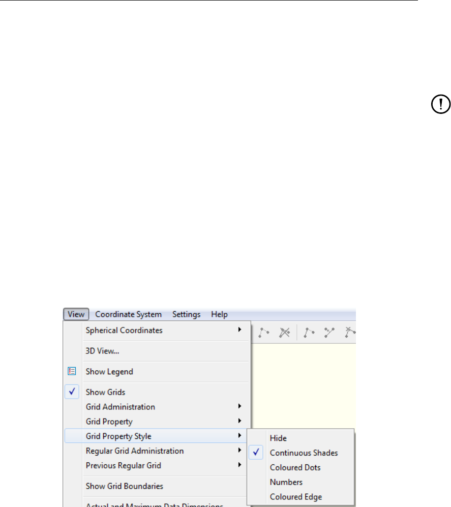
DRAFT
Menu options
Circumcentre too close
Irregular grids only. The distane between the two circumcentres of two adjacent cells should
be not too close. If the distance is too small it will be indicated by a dot. The threshold value
can be specifeid in the window General Settings.
Remark:
For a spherical grid the resolution, curvature and grid size are also given in the metric
system.
5.4.8 Grid Property Style
Default: Show the grid property as continuous shading.
Specify how to display the desired grid property:
Hide
Continuous Shades
Coloured Dots
Numbers
Coloured Edge
Figure 5.44: View →Grid Property Style options
5.4.9 Regular Grid Administration
Default: Hide the regular grid administration.
This option allows you to visualise the grid topology in the ’computational’ space (as opposed
to the physical space). It helps you decide which grid extensions are allowable so that overlap
is avoided. The each domain grid should always have a mono-block structure.
Select the required option:
Hide
Lines
Lines and M, N Indices
Deltares 71 of 128
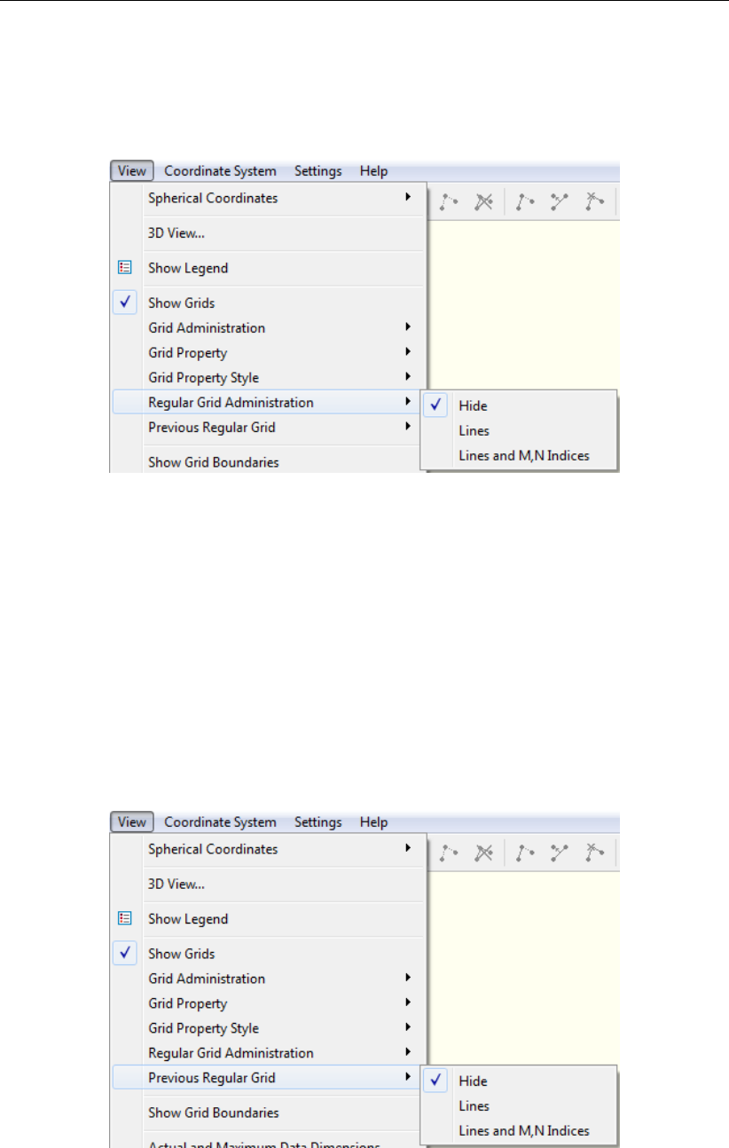
DRAFT
RGFGRID, User Manual
The latter option is provided so that you can check and control the grid administrative lower
left corner, i.e. the location of the (1,1) point. It gives the least confusion if this point is, the
more the less, located at the lower left corner of the screen. The ’computational’ grid is plotted
north of the ’physical’ grid.
Figure 5.45: View →Regular Grid Administration options
5.4.10 Previous Regular Grid
Default: Hide the previous regular grid as lines.
Sometimes, when editing the regular grid, it may be convenient to display the grid both in its
present and previous state on the screen at the same time. The usual display options are
available:
Hide
Lines
Lines and M, N Indices
Figure 5.46: View →Previuos Regular Grid options
72 of 128 Deltares
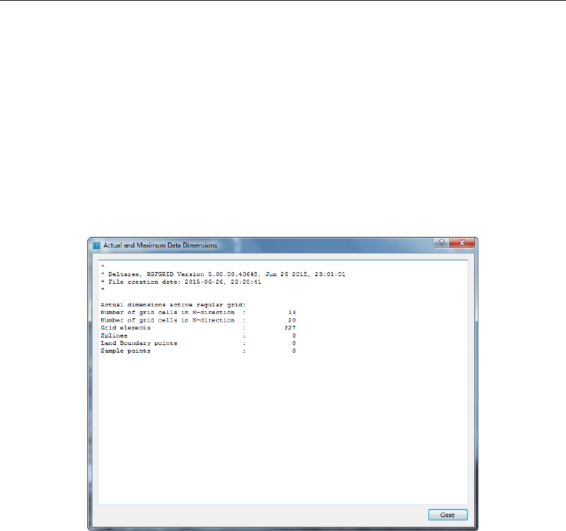
DRAFT
Menu options
5.4.11 Show Grid Boundaries
Default: Hide the boundary.
Show or hide the boundaries, open, domain decomposition as well as computational bound-
aries.
5.4.12 Actual and maximum data dimensions
The actual and maximum dimensions of various data objects are presented in ‘history’, see
Figure 5.47
Figure 5.47: Operations menu, Actual and Maximum data dimensions
5.4.13 Land Boundaries
Default: Show the land boundary as lines.
The following display options are available for displaying the land boundary:
Hide
Lines
Filled
5.4.14 Samples
Default: Show samples as coloured dots.
Specify how to display the samples:
Hide
Coloured Dots
Coloured Numbers
Mono Coloured Numbers
5.4.15 Splines
Default: Show the splines as lines with dots.
Deltares 73 of 128
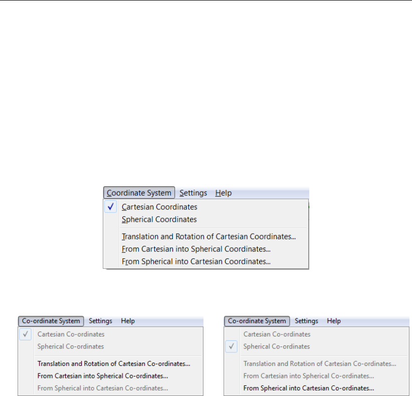
DRAFT
RGFGRID, User Manual
The following display options are available:
Hide
Lines with Dots
Lines with Dots and M, N Indices
5.5 Coordinate System menu
On the Coordinate System menu you can set the desired coordinate system (see Figure 5.48)
to Cartesian or spherical coordinates, see Figure 5.49. Furthermore, you can translate or
rotate the objects in a Cartesian coordinate system and you can transform Cartesian coordi-
nates to spherical coordinates and vice versa.
Figure 5.48: Menu option Coordinate System
(a) Cartesian coordinates selected (b) Spherical coordinates selected
Figure 5.49: Menu option Coordinate System.
5.5.1 Cartesian coordinates
In this case the coordinates are easting and northing in metres.
5.5.2 Spherical coordinates
In this case the coordinates are longitude and latitude, in decimal degrees.
74 of 128 Deltares
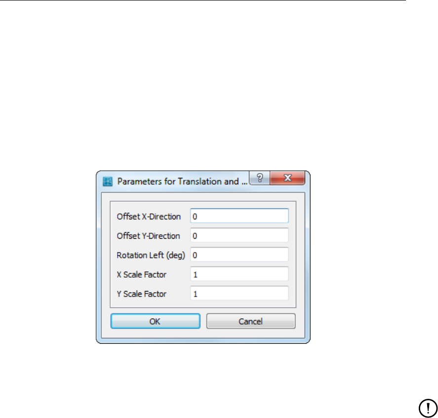
DRAFT
Menu options
5.5.3 Translation and rotation of Cartesian coordinates
This option may be applied if you are changing to a new Cartesian coordinate system which
has a different position of the origin or another orientation. The parameters involved are, see
Figure 5.50:
Offset X direction [m] default 0.0
Offset Y direction [m] default 0.0
Rotation left [degrees] default 0.0
X Scale factor default 1.0
Y Scale factor default 1.0
Figure 5.50: Parameters for translation and rotation form for transformation to Carte-
sian coordinates
Remark:
A translation and rotation operates only on samples, polygon the active grid.
5.5.4 From Cartesian into Spherical coordinates
A form will appear with the parameters for the coordinate conversion, see Figure 5.51. The
first parameter indicates the current coordinate system:
1 UTM,
2 Amersfoort / RD new (EPSG:28992) or
3 RD (Parijs) (EPSG:2489).
Putting the cursor on top of this field will show the help text. If the current system is UTM you
have to specify the zone number. The option Swap to Spherical will mark the coordinates
as cartesian without performing a transformation on the coordinates. The user is responsible
to assure that coordinates are in a valid range for spherical coordinates, i.e. longitude λ∈
[−180,180] and altitude φ∈[−90,90].
Deltares 75 of 128
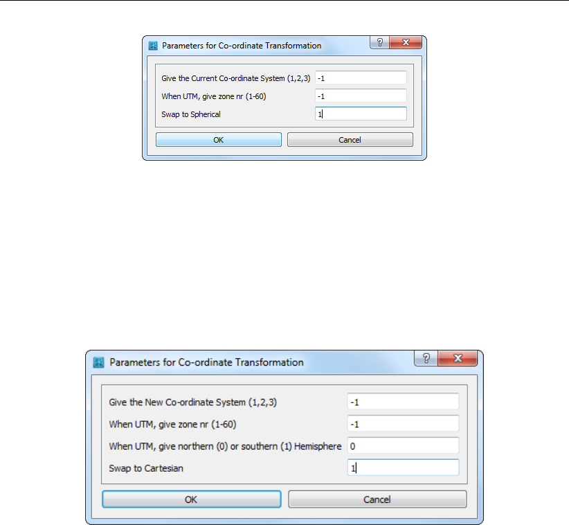
DRAFT
RGFGRID, User Manual
Figure 5.51: Parameters for Coordinate transformation form for transformation to
spherical coordinates
5.5.5 From Spherical into Cartesian coordinates
Figure 5.52 shows the parameters involved for the conversion from spherical to Cartesian
coordinates. If the target system is UTM you have to specify the zone number and the hemi-
sphere. The option Swap to Cartesian will mark the coordinates as spherical without perform-
ing a transformation on the coordinates.
Figure 5.52: Parameters for Coordinate transformation form for transformation to
Cartesian coordinates
5.6 Settings menu
The following options can be accessed through the Settings menu, see Figure 5.53
76 of 128 Deltares
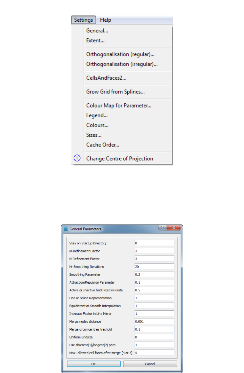
DRAFT
Menu options
Figure 5.53: Options on Settings menu
5.6.1 General
The following parameters influence the behaviour of the operations above. They are set via
the following parameter list, see Figure 5.54
Figure 5.54: Options on Settings window
Stay on Startup Directory default: 0 (Off)
When navigating through the directories in the file menu, you can specify whether to keep
the latest visited directory (0), or always go back to the start-up directory (1).
M-refinement factor default: 3
Deltares 77 of 128

DRAFT
RGFGRID, User Manual
A value of 2 gives twice as many grid cells in m-direction. An odd value assure that the
cell centre and the mid of a cell edge are available in the coarse as well as in the refined
grid.
N-refinement factor default: 3
A value of 2 gives twice as many grid cells in n-direction. An odd value assure that the
cell centre and the mid of a cell edge are available in the coarse as well as in the refined
grid.
Nr Smoothing Iterations default: 20
The smoothing in edit mode is controlled by this parameter.
Smoothing Parameter default: 0.2
The smoothing in edit mode is also controlled by this parameter. A value of 0.0 results in
no smoothing, a value of 1.0 in maximum smoothing.
Attraction/Repulsion Parameter default: 0.1
Attraction/repulsion in edit mode is controlled by this parameter. The value is the fractional
change in size of the first grid cell adjacent to the indicated line. Increase this value for
more attraction or repulsion.
Active or Inactive Grid Fixed in Paste default: 0.5
When pasting an active grid to an inactive grid, the grid points on the grid junction line are
a weighted average between both grids. If you want to keep these points in the position of
the active grid, set this parameter to 0.0. To keep the position of the inactive grid, choose
1.0; a value in between averages.
Line or Spline Representation (0 or 1) default: 1 (Spline)
Splines, or grid boundaries in the orthogonalisation process, can also be represented as
straight lines if this parameter is put to a zero value.
Equidistant or Smooth Interpolation (0 or 1) default: 1 (Smooth)
When interpolating the splines into a grid, equidistant interpolation can be specified using
a value of 0.
Increase Factor in Line Mirror (1.0 - 10.0) default: 1.0
When adding grid cells using the Edit →Line →Mirror option, this parameter defines the
size of the new grid cells.
Merge nodes distance default: 0.001
Maximum distance between nodes which must be merged.
Merge circumcentres treshold default: 0.1
Circumcentres who are too close to each other, determined by this threshold, should
be removed. These circumcentres can be visualised by the menu-option: View →Grid
property →Circumcentres too close.
Uniform Grid size default: 0.0
Use shortest(1)/Longest(2) path default: 0.001
Select shortest or longest path between two points on a computational boundary.
Max. allowed cell faces after merge (4 or 5) default: 5
Maximum allowed cell faces after merge circumcentres (4 or 5).
78 of 128 Deltares
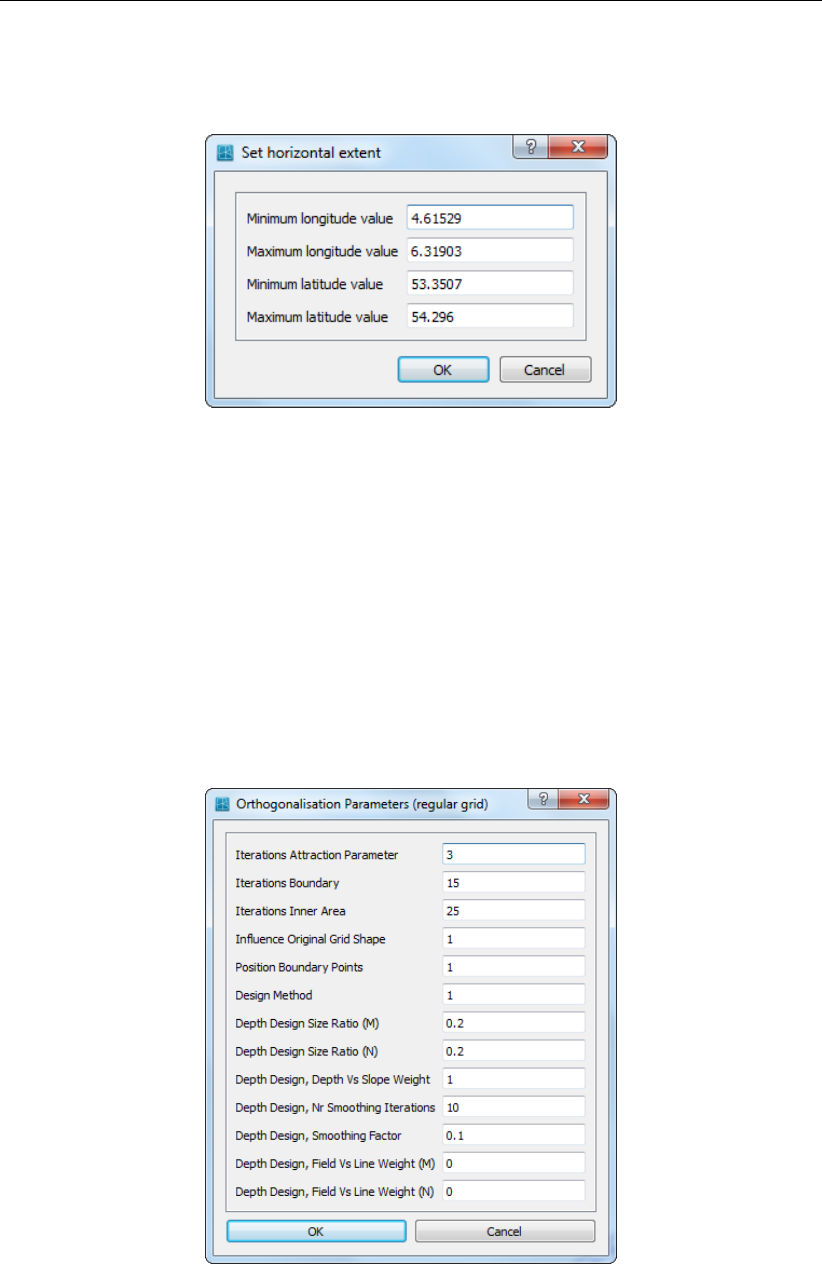
DRAFT
Menu options
5.6.2 Set extent
Set the horizontal extent of the canvas
Figure 5.55: Set horizontal extent window
Minimum visible x-value
Maximum visible x-value
Minimum visible y-value
Maximum visible y-value
The used extent is dependent on the current window size, keeping the x/y ratio to 1.
5.6.3 Orthogonalisation regular
With the Orthogonalisation Parameters form, see Figure 5.56, the orthogonalisation pro-
cess can be controlled:
Figure 5.56: Options on Orthogonalisation Parameters window
Iterations Attraction Parameter default: 3
The shape of the resulting grid is based on the so-called attraction parameter, i.e. the local
aspect ratio of the original grid. One complete orthogonalisation cycle consists of three
loops. The outer loop is the attraction parameter loop, in which this parameter field is
Deltares 79 of 128

DRAFT
RGFGRID, User Manual
established. Only few of these loops are usually performed. Next, several boundary loops
are performed, in each of which the inner area is solved several times. Increasing the
number of attraction parameter iterations improves orthogonality, but it increases deviation
from the originally designed shape.
Iterations Boundary default: 15
In one boundary loop, all boundary points are updated once, and all inner area points
are updated as many times as specified by the next parameter. We advise values in the
following range: [5 – 20].
Iterations Inner Area default: 25
The number of inner area iterations in the orthogonalisation is advised in the range: [10 -
50].
Influence Original Grid Shape default: 1.0
This parameter specifies the influence of the specified grid shape in the inner area during
the orthogonalisation procedure. The grid shape in the inner area can be specified in three
ways, see ‘Design Method’ below. With a value of 1 the specified shape is maintained as
closely as possible. With a value of 0, the shape mostly depends on the shape of the
boundaries and the internal corner points. Any value between 0 and 1 can be chosen.
Position Boundary Points default: 1.0
This parameter specifies the freedom of movement of boundary points. These points
move along splines spanned by the outer points of the grid. A value of 1 gives full freedom
of movement, whereas a value of 0 keeps boundary points completely fixed. Any value
between 0 and 1 may be chosen.
Design Method, 1, 2, or 3 default: 1
This parameter specifies in what way the attraction parameter (local aspect ratio) field is
created. The three methods are:
1 This method is based upon the aspect ratios of the original design grid (default).
2 This method uses a polygon, the polygon can be applied to control grid spacing.
3 With this method the grid resolution is controlled based upon features in a bathymetry
that can be opened by means of the samples. This method is therefore called ‘Depth
design’.
In these methods, the attraction parameter field is based upon grid spacing functions both
in the M- and N-Direction. Their local ratio forms the desired attraction parameter field.
Both the M- and N-grid spacing functions can be controlled by a number of parameters,
that are explained below. The same parameters also apply to method 2, that can be
seen as a special case of method 3, in which the bathymetry is specified by specifying
a constant ‘depth’ inside the polygon, different from the also constant ‘depth’ outside the
polygon.
Depth Design Size Ratio (M) default: 0.2
Both for the M- and the N-direction, the size ratio between the smallest and largest grid
size in that direction can be specified. If a value of 1 is specified, a uniform distribution
results. Choosing a small value will result in large grid size variation. If a value of 0 is
specified, this is seen as a special case and the original grid shape is applied as the
desired grid spacing function.
Depth Design Size Ratio (N) default: 0.2
See Depth Design Size Ratio (M) above.
Depth Design, Depth vs Slope Weight default: 1
Both the depth and the slope can be applied as grid spacing control functions. To obtain a
high resolution in deep areas only, specify a Small/large Size Ratio below 1, e.g. 0.1, and
specify a Depth vs. Slope Weight parameter of 1. To obtain small cells at steep slopes
only, specify a value of 0. Any value in between 0 and 1 can be applied. In the future, the
slope variation is foreseen as a controlling parameter as well.
Depth Design, Number of Smoothing Iterations default: 10
To obtain smoother transitions between sloping and non-sloping areas, the grid spacing
80 of 128 Deltares
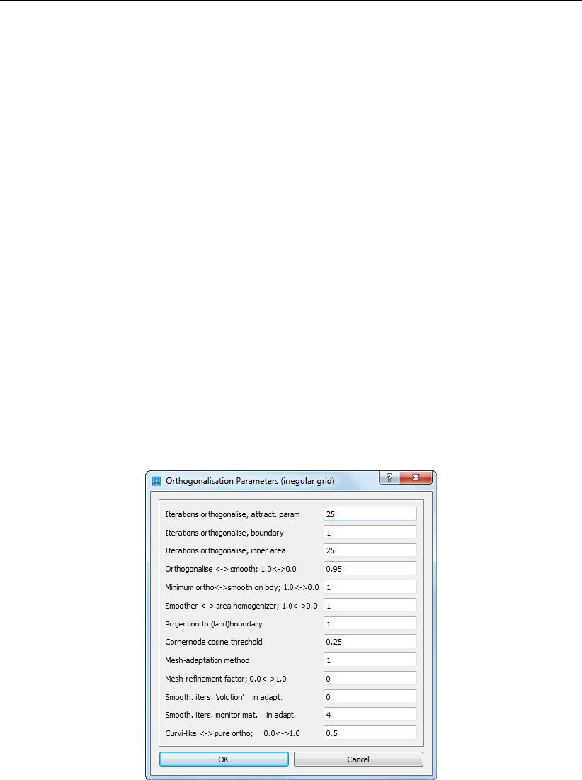
DRAFT
Menu options
functions can be smoothed. The smoothing parameters apply both to the (M) and (N)
direction. Also, the smoothing may be applied to ‘spread’ the grid spacing information
towards grid cells that initially may lie outside the area that needs to get a high resolution.
In each attraction parameter iteration, see above, the grid point spacing function is evalu-
ated, and applied in the following orthogonalisation loop, which results in shifting the grid
points to their final position. Once getting closer to their final position, the smoothing may
be decreased, so that the bathymetry features become more apparent in the grid. This
process may be automated in future.
Depth Design, Smoothing Factor default: 0.1
Smoothing weight of point itself to neighbours.
Depth Design, Field vs. Line Weight (M) default: 0
The Small/Large Size Ratio parameter can either be specified to apply to the whole grid,
or to every grid line. i.e. should the specified Size Ratio in the given direction be applied
to the whole grid or to every grid line? If a value of 1 is chosen, this ratio will only occur
at the maximum value of entire spacing function. If a value of 0 is chosen, this size ration
will occur at every grid line.
Depth Design, Field vs. Line Weight (N) default: 0
See Depth Design, Field vs. Line Weight (N) above.
5.6.4 Orthogonalisation irregular
With the Orthogonalisation Parameters (irregular) form, see Figure 5.57, the orthogonali-
sation process of irregular grids can be controlled:
Figure 5.57: Options on Orthogonalisation Parameters (irregular) window
Iterations orthogonalise, attraction parameters: Default: 25
The number of iterations in which the attraction parameters are computed for the grid.
The attraction parameter is the fractional change in size of the first grid cell adjacent to the
indicated line.
Iterations orthogonalise, boundary: Default: 1
This parameter can be used to prescribe the number of iterations in which the grid is
moved along the boundaries to improve the orthogonality of the grid.
Iterations orthogonalise, inner area: Default: 25
This parameter can be used to prescribe the number of iterations in which the grid is
moved along in the interior of the domain to improve the orthogonality of the grid. T
Deltares 81 of 128
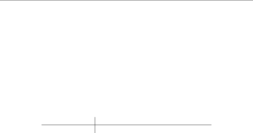
DRAFT
RGFGRID, User Manual
he total number of iterations is the product of the three iteration values (attract. param,
boundary and inner area).
Orthogonalise ↔smooth; 1.0 ↔0.0 Default: 0.95
The balance between mesh-smoothing (0.0) and mesh-orthogonalization (1.0). One has
to keep in mind that mesh smoothing (ortho. param. →0) will compromise mesh orthog-
onality. Sole orthogonalization (ortho. parameter=1) on the other hand, can cause highly
distorted, non-smooth meshes, especially for meshes consisting of quadrilaterals. It is
advised to choose a low orthogonalization parameter and repeat the process while grad-
ually increasing the orthogonalization parameter at every repetition The orthogonality is
defined by the angle between the line connecting water level points and the line connect-
ing two grid cell corners. The smoothness is defined as the ratio between the areas of two
adjacent grid cells.
stage 1 2 3 4 5 6
ortho. parameter 0.5 0.8 0.9 0.99 0.999 0.9999
Table 5.1: Multi-stage orthogonalization strategy
Minimum ortho ↔smooth on boundary; 1.0 ↔0.0 Default: 1
This parameter can be used to prescribe the number of iterations in which the grid is
moved along in the interior of the domain to improve the orthogonality of the grid. The total
number of iterations is the product of the three iteration values (attract. param, boundary
and inner area).
Circum- or masscentre; 1.0 ↔0.0: Default: 1
Define whether the orthogonality is measured based on the circumcenter of the triangle
or on the mass center of a triangle.
Smoother ↔area homogenizer; 1.0 ↔0.0: Default: 1
Projection to (land)boundary: Default: 1
0 means no projection of the grid to the land boundary while orthogonalising the grid. 1
means projection of the grid boundaries to the original grid boundaries as before orthogo-
nalising the grid. 2 means projection of the grid boundaries to the nearest land boundary.
3 means projection of the grid boundaries as well as parts of interior part of the grid to the
nearest land boundaries.
Corner node cosine threshold: Default: 0.25
Determines whether a node is a corner on the basis of the cosine of the boundary edge
angle. If a node is a corner, then the node is not moved during orthogonalisation.
Mesh adaption method: Default: 1
Selection of a mesh-adaptation method. 0 means a Winslow type monitor function, 1 an
arc-length monitor function and 2 a harmonic map monitor function. See Huang (2001,
sect 3.3).
Mesh refinement factor; 0.0 ↔1.0: Default: 0
Concentation of the mesh in a refined region (parameter in the mesh-adaptation method).
See Huang (2001).
Smooth. iters. ’solution’ in adapt.: Default: 0
Number of smoothing iterations of solution u in mesh-adaptation method. See Huang
(2001, sec. 3.3).
Smooth. iters. ’monitor mat.: Default: 4
Number of smoothing iterations of monitor matrix G in mesh-adaptation method. See
Huang (2001, sec. 3.3).
Curvi-like ↔pure ortho; 0.0 ↔0.5: Default: 0
Chooses between pure orthogonalisation versus curvi-grid-like orthogonalisation in quads.
82 of 128 Deltares
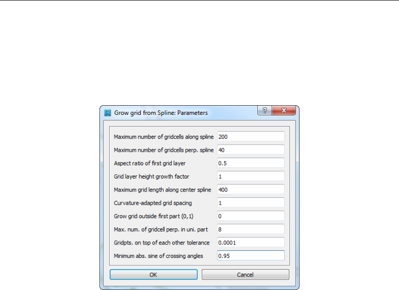
DRAFT
Menu options
5.6.5 CellsAndFaces2
TODO(??): TODOUnder construction; as long as samples are not available in RGFGRID, this sec-
tion has no meaning
5.6.6 Grow grid from splines
Figure 5.58: Options on Grow Grid from Splines: Parameters window
Maximum number of grid cells along spline: Default: 50
Upper bound of the number of grid cells along the centre spline. The actual number of
grid cells is determined by the cell and spline lengths, but will not exceed this number. In
practice one has to set this number sufficiently large.
Maximum number of grid cells perp. spline: Default: 40
Upper bound of the number of grid layers that will be grown from the centre spline. The
actual number of grid layer is determined by the grid height (specified by the splines) the
height of the first grid layer and the grid layer growth factor, see below, but it will not exceed
this number. In practice one has to set this number sufficiently large.
Aspect ratio of first grid layer: Default: 0.1
The ratio of the grid cell height and length at the centre spline. If a centre spline is provided
solely, the aspect ratio of the grid on either side of the centre spline is determined by this
variable.
Grid layer height growth factor: Default: 1.1
The fractional increase of grid layer heights in the exponentially growing part of the grid.
Maximum grid length along centre spline: Default: 500
The maximum grid cell length. Note that the length decreases where the spline curvature
increases
Curvature-adapted grid spacing: Default: 1
Disable (0) or enable (1) curvature-adapted grid spacing in length direction.
Grow grid outside first part (0,1): Default: 1
create the exponentially growing grid supplementary to the uniform part (1) or not (0).
This parameter has no effect if no uniform part is present, i.e. no bounding splines are
provided. In that case the exponentially growing grid is the sole grid created.
Maximum number of grid cell perpendicular to the center spline in the uniform part: De-
fault: 5
The number of grid cells will not exceed this number. If necessary, the cells will be en-
larged, and the aspect ratio is disregarded.
Gridpoints on top of each other tolerance: Default: 0.0001
A tolerance on merged grid lines; for expert users only.
Deltares 83 of 128
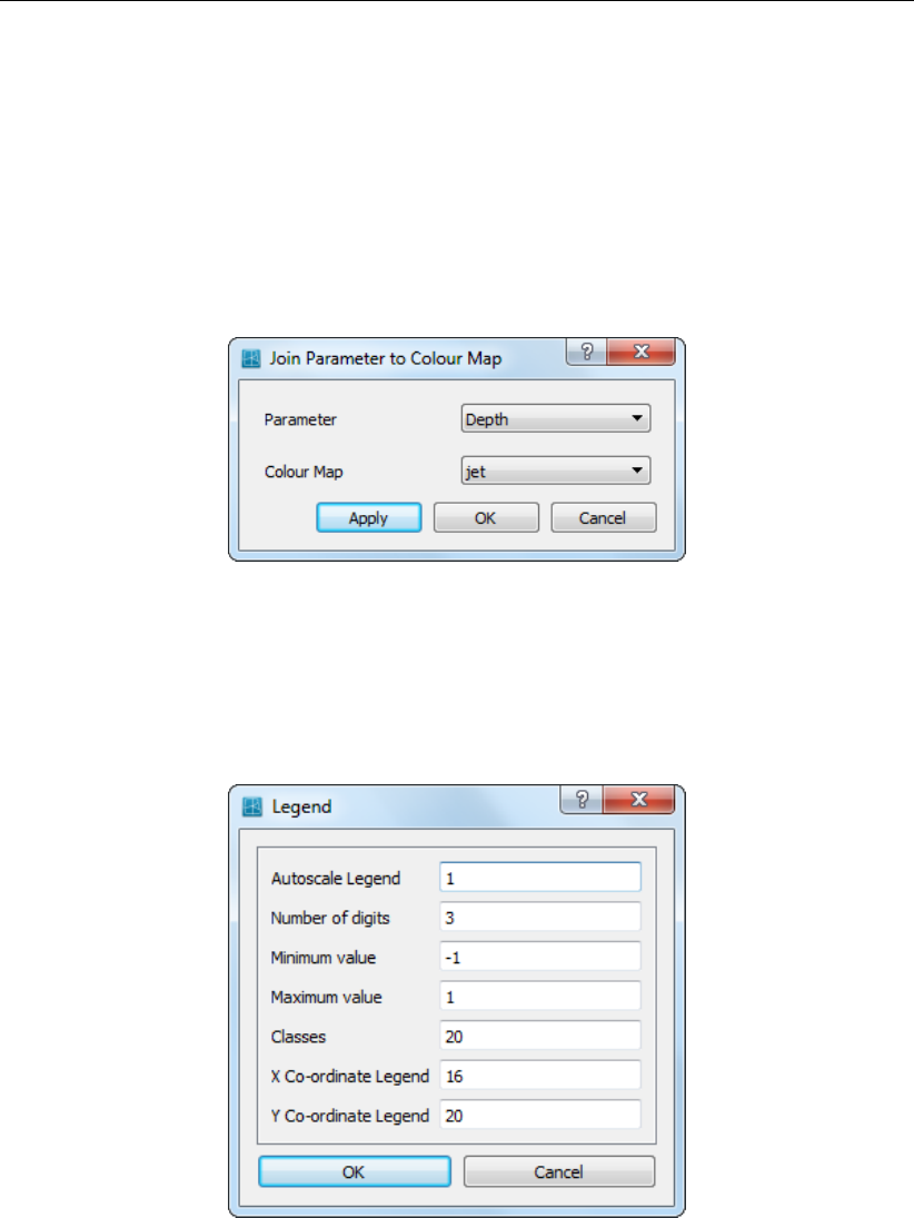
DRAFT
RGFGRID, User Manual
Minimum absolute sine of crossing angles: Default: 0.95
Minimum value of |sin α|where αis the angle between the edge and the line connecting
the circumcentres of the adjacent cells to that edge.
5.6.7 Change colour map
When clicking on the Settings →Change Colour Map menu, a form opens in which you can
select the relation between a parameter (i.e. Depth) and the loaded colour maps; see Fig-
ure 5.59
Figure 5.59: Options on Colour Map for Parameter window
5.6.8 Legend
When clicking on the Settings →Legend menu, a form opens in which you can define how
the iso-colour figures should be displayed; see Figure 5.60
Figure 5.60: Options on Settings →Legend menu
Autoscale Legend default: On
Specify whether the program should determine the iso-colour values automatically, or to
do it yourself. If you leave it to the program, it will determine the minimum and maximum
depth value within the viewing area and display the number of iso-colours specified above.
Zooming in will always result in display of the same number of iso-colours. If you want to
specify the iso-colour values yourself, you have to specify one of the three parameters
below. When zooming in, the iso-colour values will remain fixed.
Minimum Value default: Off
Specifying this value turns autoscale off.
84 of 128 Deltares
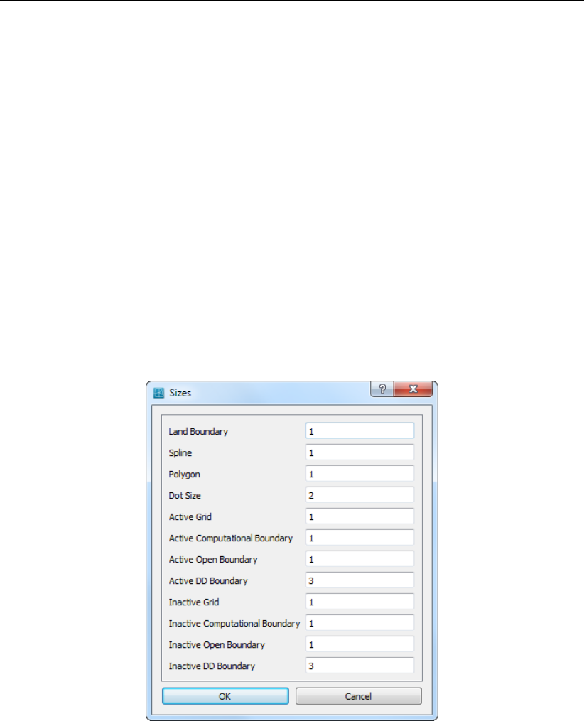
DRAFT
Menu options
Maximum Value default: Off
Specifying this value turns autoscale off.
Classes default: 20
The number of classes can be specified
X Coordinate Legend default: 16
xCoordinate of lower left corner of legend in pixels
Y Coordinate Legend default: 20
yCoordinate of lower left corner of legend in pixels
5.6.9 Colours
When clicking on the Settings →Colours menu, a form opens in which you can define the
colours for background, land boundary, polygons, etc.; see Figure 5.61
5.6.10 Sizes
When clicking on the Settings →Sizes menu, a form opens in which you can define the
linewidth and dotsize in pixels. See Figure 5.62
Figure 5.62: Options on Settings →Sizes menu
5.6.11 Order caches
The parameters set in the Order caches window, see Figure 5.63, influence the drawing order
of the several items. The drawing order of the caches is: 5,4,3,2,1,0. Cache 5is drawn
first and cache 0is drawn last. So the items which will drawn in cache 0are drawn on top. If
there is no need to draw a cache it will not be done, this improves the drawing performance
by avoiding unnecessary drawings. Therefore, if an item is changed in cache 3only caches
3,2,1and 0are drawn.
Deltares 85 of 128
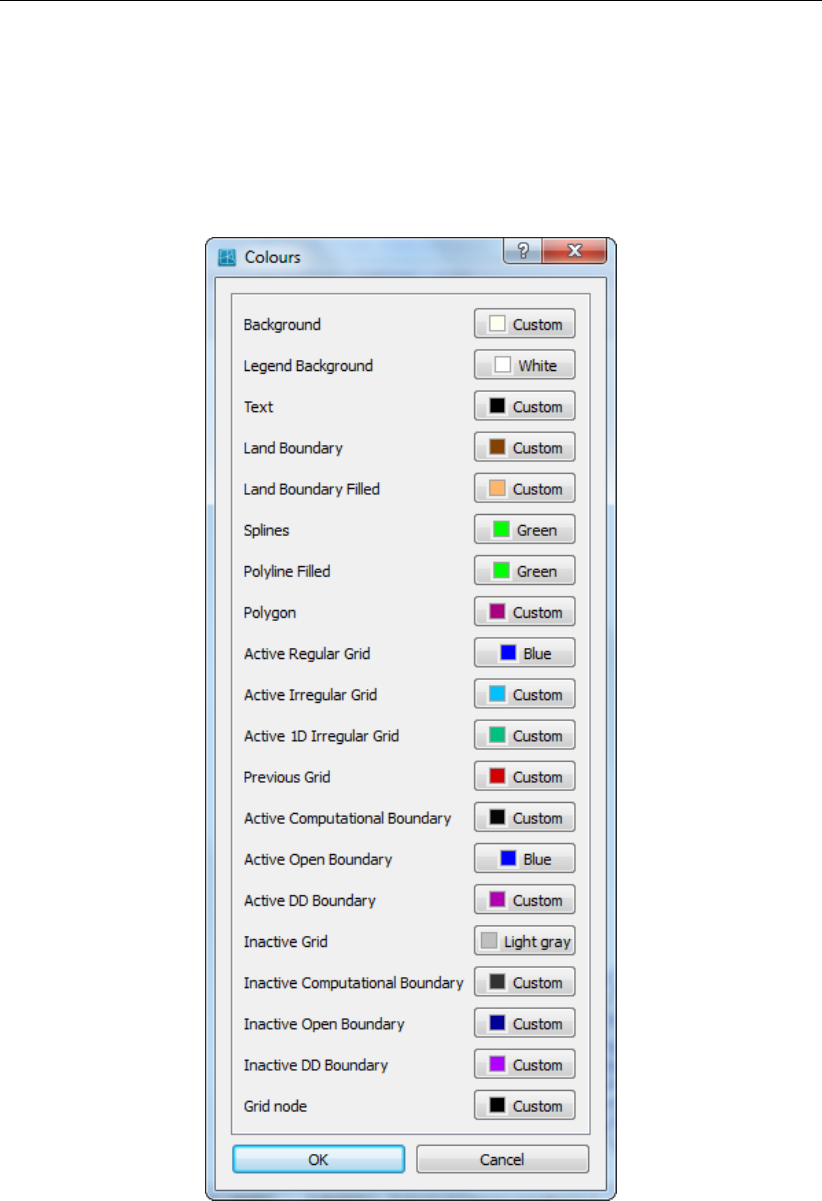
DRAFT
RGFGRID, User Manual
Figure 5.61: Options on Settings →Colours menu
86 of 128 Deltares
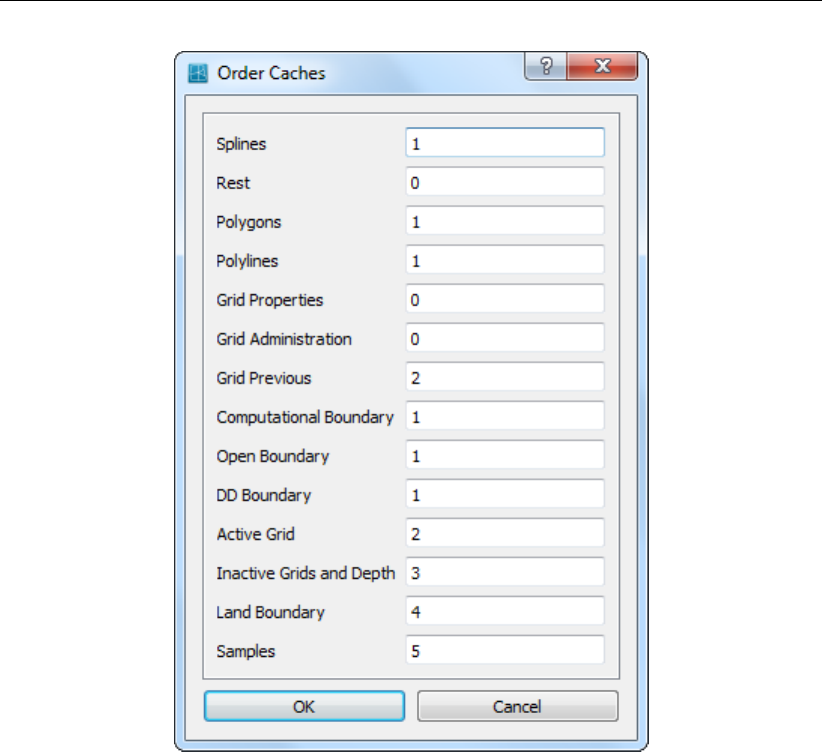
DRAFT
Menu options
Figure 5.63: Options on Order Caches window
Splines default: 0
Rest default: 0
Polygons default: 0
Grid Properties default: 0
Grid Administration default: 0
Grid Previous default: 2
Computational Boundary default: 1
Open Boundary default: 1
DD Boundary default: 1
Active Grid default: 2
Inactive Grids and Depth default: 3
Land Boundary default: 4
Samples default: 5
5.6.12 Change Centre of Projection
For spherical coordinates RGFGRID can use two different projections, plane projection and
stereographic projection. For stereographic projection a special function is implemented to
centre the computer screen to the centre of projection and the sphere. This function can be
invoked by clicking the menu item Operations →Change Centre of Projection see Figure 5.20.
When using this command the centre of the projection is set to the centre of the screen. This
action requires recalculation of the projection and a new screen refresh. The centre of the
projection does not change when using zoom in, zoom out or pan, so there is no performance
drawback and a smooth screen-refresh is obtained.
Deltares 87 of 128
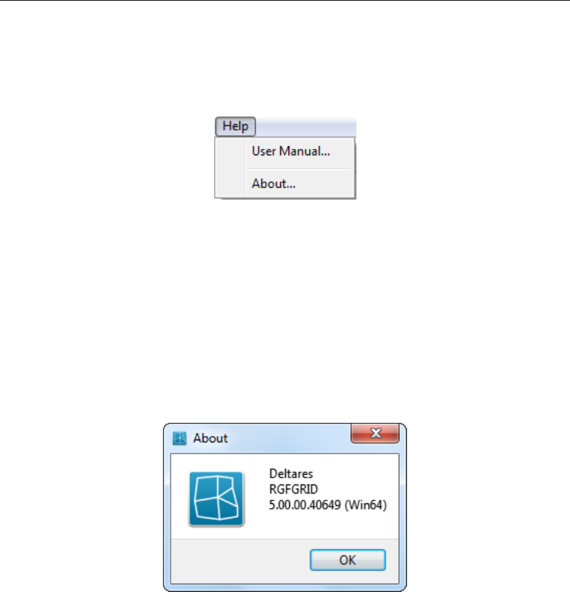
DRAFT
RGFGRID, User Manual
5.7 Help menu
On the Help menu, you may choose to read the user manual or the version number of RGF-
GRID; see Figure 5.64
Figure 5.64: Options on Help menu
5.7.1 User manual
When clicking on the Help →User Manual the user manual of RGFGRID will be displayed
(file <RGFGRID _User_manual.pdf>), see Figure 5.65.
5.7.2 About
When clicking on the Help →About a window will display the current version number of RGF-
GRID.
Figure 5.66: About box
88 of 128 Deltares
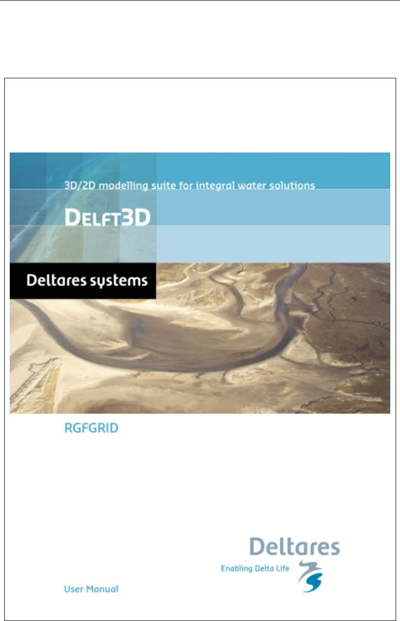
DRAFT
Menu options
Figure 5.65: Front page of the manual
Deltares 89 of 128

DRAFT
RGFGRID, User Manual
90 of 128 Deltares
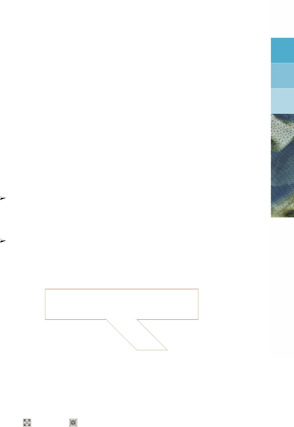
DRAFT
6 Tutorial
6.1 Harbour
Start RGFGRID as explained in section 3.3 and select the tutorial directory of RGFGRID
(<My Documents\Deltares\Delft3D 4.03.02\tutorial\rgfgrid\harbour>). If you are using an-
other Delft3D version, then the directory name will be different. This tutorial uses the land
boundary and spline files which are available in that directory.
6.1.1 Coordinate system
Before opening a land boundary and generating a grid, you have to indicate in which co-
ordinate system you are going to work. The default is Cartesian coordinates. To change
the coordiate system use the Coordinate System menu and select your preferred coordinate
system.
6.1.2 Open a land boundary
Open a file which defines the land boundary.
On the File menu, point to Attribute Files and click Open Land Boundaries.
If you have not started RGFGRID with the current directory being
<My Documents\Deltares\Delft3D 4.03.02\tutorial\rgfgrid\harbour>
then browse to this directory.
Highlight and Open file <harbour.ldb>.
After opening the boundary outline as shown in Figure 6.1 is now visible on your screen.
Figure 6.1: Land boundary outline of <harbour.ldb>
6.1.3 Zoom in and out
To zoom in or out several facilities are available:
click to zoom in or to zoom out
press the +or -key of the numeric pad while keeping the Ctrl-key pressed. When using
the +of the keyboard press also the Shift-key.
use the mouse scroll wheel.
Deltares 91 of 128
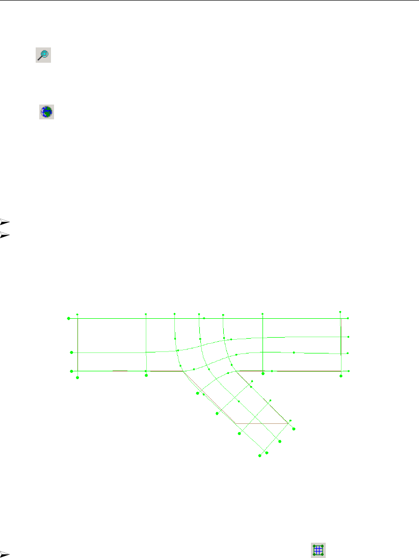
DRAFT
RGFGRID, User Manual
To zoom in on a specific area:
use and drag a box around the area.
To zoom out to the full extent:
click to zoom to full extent
To pane the grid: keep the Ctrl-key pressed and move around with the cursor.
6.1.4 Define splines
Open a file with definition of splines.
On the File menu, point to Attribute Files and click Open Splines.
Open spline file <harbour.spl>.
After opening the file with spline definitions, your screen looks like Figure 6.2.
Figure 6.2: Display of splines and land boundary in the ‘harbour’ tutorial
6.1.5 Generate grid from splines
Generating a grid after opening splines.
On the Operations menu, click Change Splines into Grid, or click on the toolbar.
From the splines a regular grid is generated, see Figure 6.3.
92 of 128 Deltares
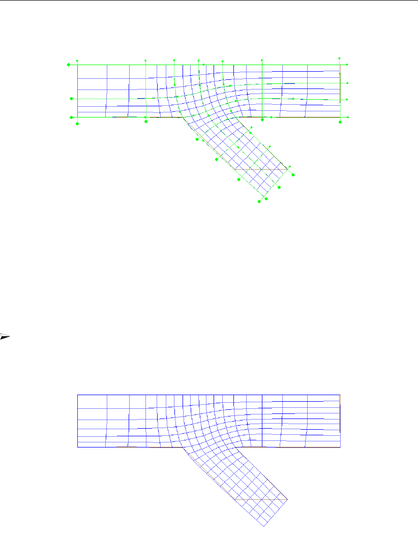
DRAFT
Tutorial
Figure 6.3: Spline grid changed into result grid with a refinement of 3
The refinement factors can be specified in Settings →General. The default is 3 in both direc-
tions.
Because the splines are not used anymore for grid generation, hide the splines. So just the
relevant data is shown.
On the View menu, point to Splines, and click Hide, see Figure 6.4.
Figure 6.4: Splines not displayed anymore
Deltares 93 of 128
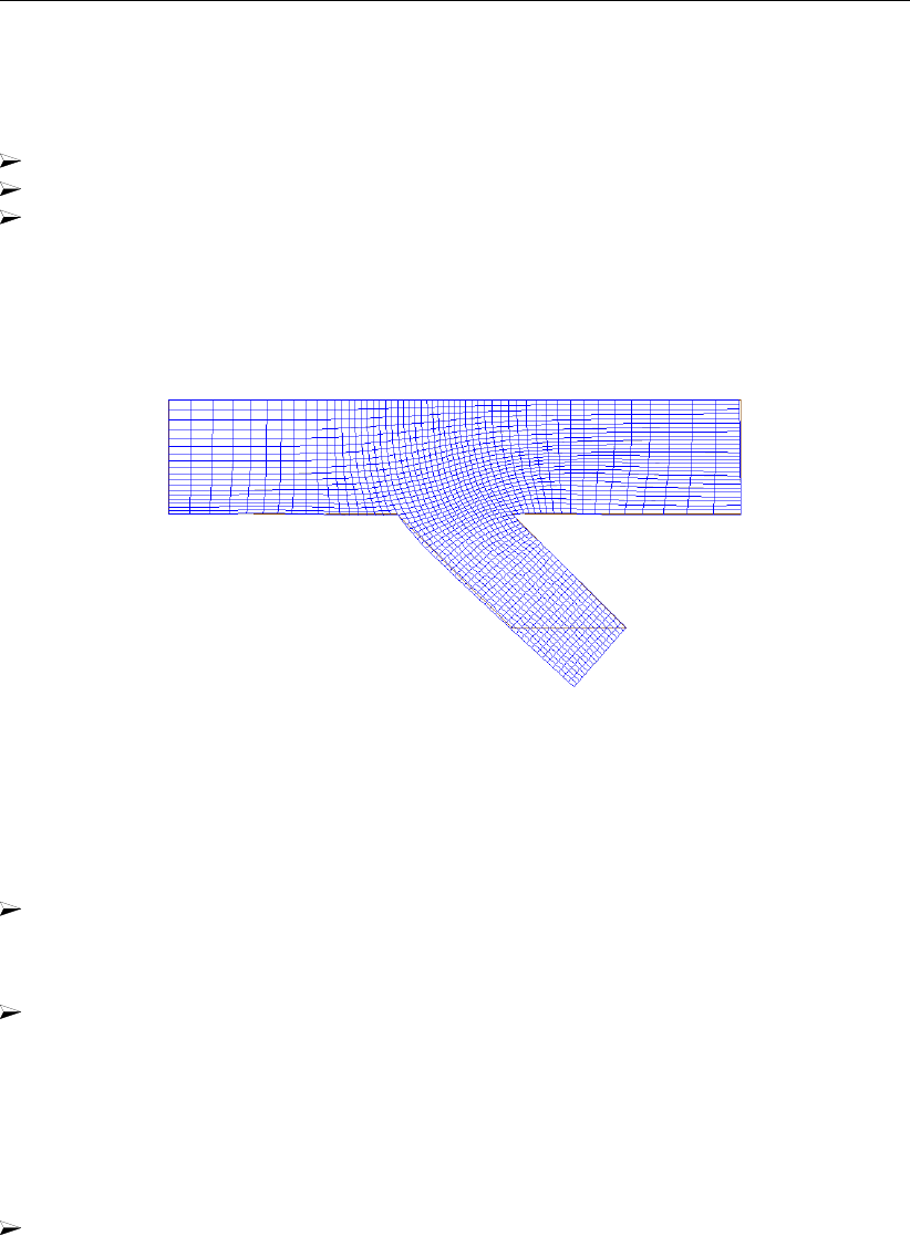
DRAFT
RGFGRID, User Manual
6.1.6 Refine grid
Refine a grid.
On the Settings menu, click General. . . .
Specify M and N refinement factors of “3” by “3”.
On the Operations menu, click Regular Grid Coarseness →Refine.
The result of the refinement should look like in Figure 6.5.
Figure 6.5: Grid after another refinement of 3 by 3
6.1.7 Fit grid boundary to land boundary
The grid boundaries can be fitted to the land boundary (see also Line to Land Boundary).
On the Edit menu, point to Regular Grid and click Line to Land Boundary.
You are now in “Edit Grid in Line mode” as reported in the statusbar.
Click the two end points of the grid line segment that you want to attach to the land bound-
ary.
The concerning segment of the grid line will be highlighted. To expand the area of influence of
the attachment transformation click one point on the grid side of the indicated line and perform
the transformation, see Figure 6.6. When no influence area is indicated just the grid boundary
segment is shifted to the land boundary.
Click for instance a point halfway in between fixed boundaries.
94 of 128 Deltares
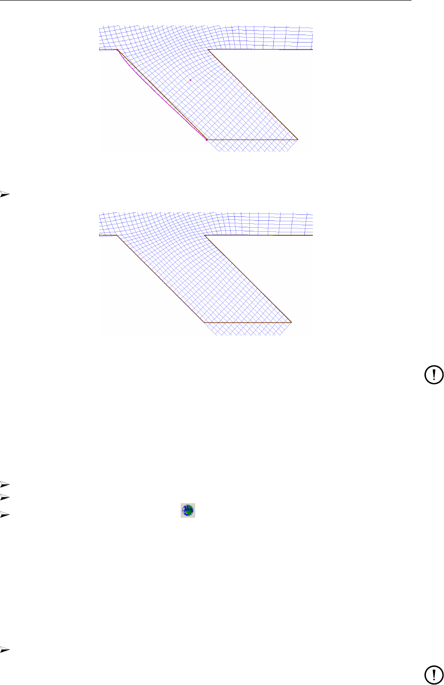
DRAFT
Tutorial
Figure 6.6: Indicating outer grid line and influence area to be moved to land boundary
Click right to execute the Line to Land Boundary action, the result will look like Figure 6.7.
Figure 6.7: Grid after Line to Land Boundary action
Remark:
The previous grid can be shown using one of the options in View →Previous Grid.
This steps can be repeated until all necessary grid boundaries are fitted to the land boundary.
6.1.8 Check grid orthogonality
To inspect the quality of the grid, for instance the orthogonality:
On the View menu, point to Grid Property, and click Orthogonality.
And View →Grid Property Style→Continuous Shades.
Press the icon to zoom to full extent, .
This will show a plot (see Figure 6.8) of the cosine values of grid corners. The cosine values
should be close to zero. The error in the computed direction of the pressure term in Delft3D-
FLOW is proportional to these values. In offshore areas the orthogonality should be less than
0.02. Near closed boundaries, higher values are sometimes acceptable.
6.1.9 Orthogonalise grid
Now we will improve the orthogonality:
On the Operations menu, click Orthogonalise Grid to improve the grid orthogonality.
Remarks:
Default the legend uses fix-scaling. With respect to Figure 6.8, the value used in Fig-
ure 6.9 are the same.
Deltares 95 of 128
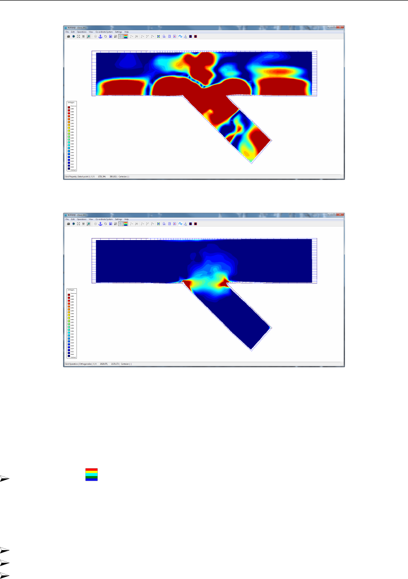
DRAFT
RGFGRID, User Manual
Figure 6.8: Grid properties; orthogonality
Figure 6.9: Grid properties; orthogonality. After 1 orthogonalisation action.
To set the auto-scaling off, click on Settings →Legend, and change the appropriate
parameter to 0.
To hide the grid properties.
Press the icon on the toolbar to disable/enable the property view or select from the
View menu, point to Grid Property and select a property or click on Hide.
In practice, making the grid orthogonal, you will work in parts of the model grid rather than on
the whole grid. To make the grid orthogonal locally:
Select on the Edit menu, point to Regular Grid and click Block Orthogonalise.
Click 2, 3, or 4 opposite block corners, see Figure 6.10.
Click right to activate the orthogonalisation process.
96 of 128 Deltares
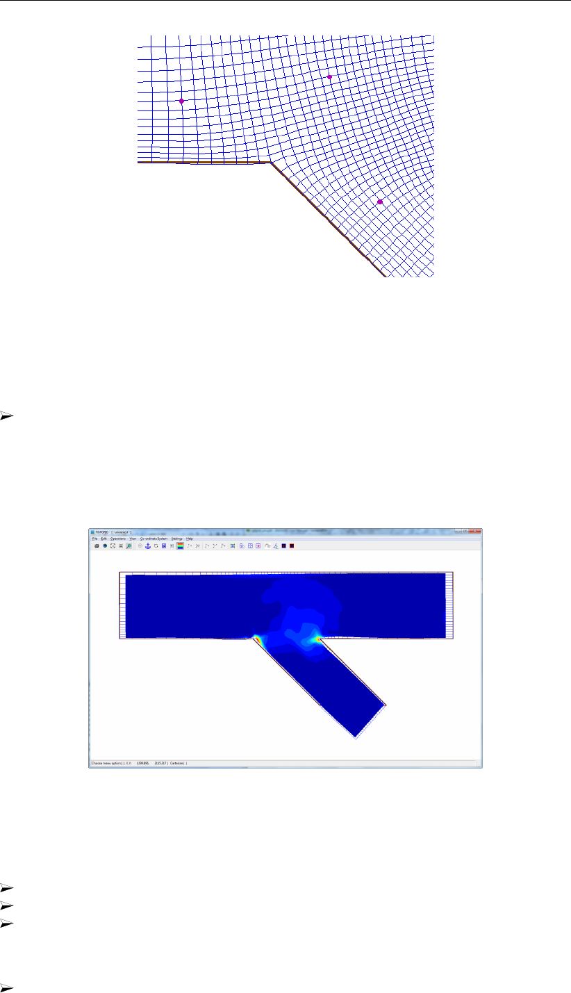
DRAFT
Tutorial
Figure 6.10: Indicating corners for Block Orthogonalise
6.1.10 Check other grid properties
First set the legend scaling to automatic by selecting Settings →Legend. . . from the menubar
and set Autoscale Legend to “1”.
On the View menu, point to Grid Property and click Orthogonality again to check the
result of the previous action, see Figure 6.11.
Other grid properties such as grid smoothness and resolution can also be displayed. The grid
should be smooth to minimise truncation errors in the finite difference scheme. Adjacent grid
cell sizes should vary less than 20 percent, although locally exceptions may be acceptable.
Figure 6.11: Grid orthogonality after one block orthogonalisation operation
6.1.11 Completion
To delete grid cells outside the land boundary:
On the Edit menu, point to Regular Grid and click Block Delete Interior.
Indicate a block to be deleted by clicking on opposite corners.
Click right to activate the delete action.
You can also delete individual grid points:
On the Edit menu, point to Regular Grid and click Delete Point.
Deltares 97 of 128
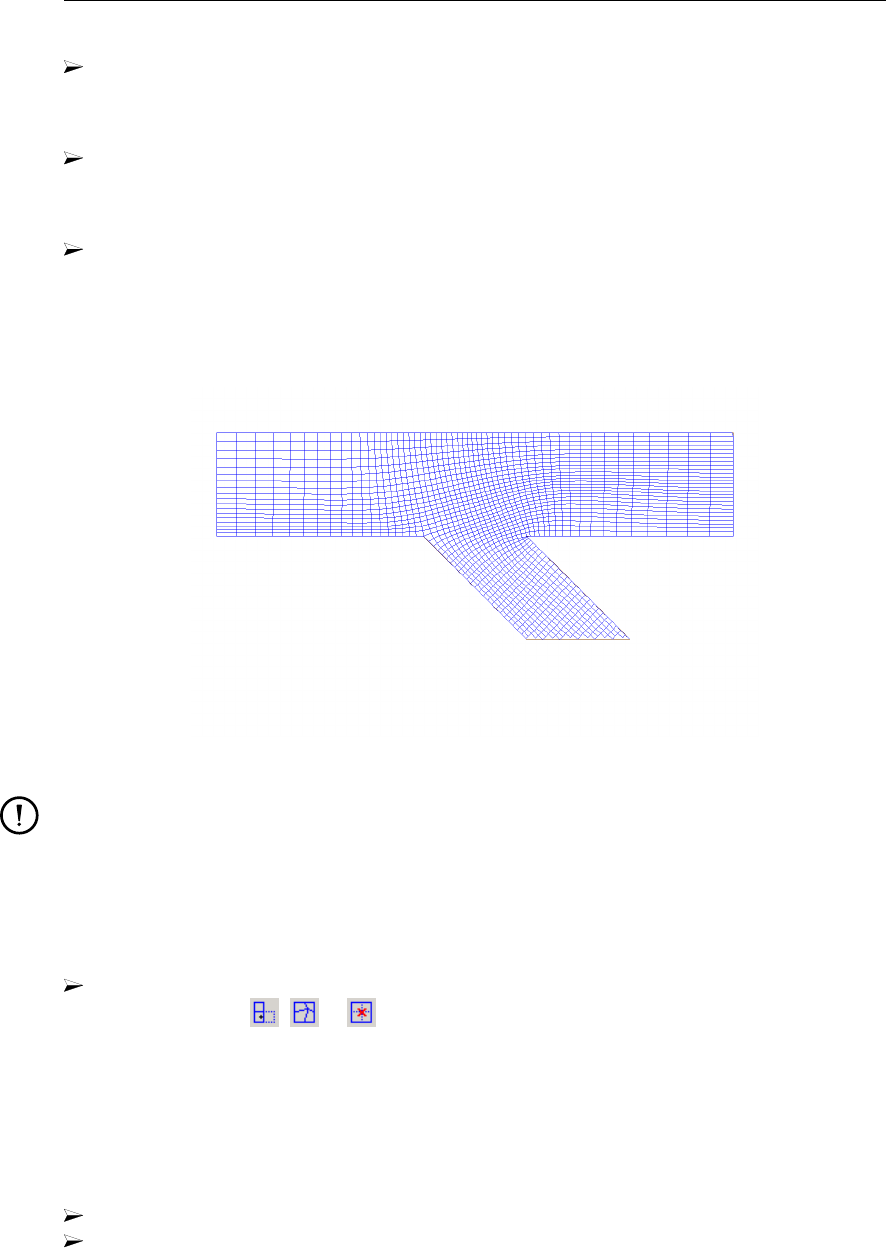
DRAFT
RGFGRID, User Manual
Press the d-key on your keyboard and click points you want to delete.
In the Point Mode you can also move (replace) grid points.
First press the r-key, next click on a grid point, move it somewhere else, and click again.
Also in the Point Mode, you can add individual grid cells.
First press the i-key and then click in a border cell near the concerning edge.
Do not delete grid cells outside the land boundary in earlier refinement steps, if this introduces
staircase boundaries (as in the present example at the end of the harbour). The final grid may
look like Figure 6.12.
Figure 6.12: Final result after refining, obsolete grid cells removed
Remarks:
Each corner point on the grid will remain fixed in the orthogonalisation procedure.
Only internal points and points along boundaries can be shifted to improve the grid
orthogonality.
To shift individual grid cells:
On the Edit menu, select Regular Grid and click Insert Point,Move Point or Delete Point
or click the icons , or on the toolbar.
You can also switch between the move, insert and delete actions by pressing the I,Ror D
key. Once a mode is selected, use the left mouse to let the actions take effect. Press Esc to
undo edit actions. In the ‘spline edit mode’-mode of the program, the same keys can be used.
To save the grid and to exit the RGFGRID program you have to do:
On the File menu, click Export →Grid (Delft3D-FLOW) and specify a filename
On the File menu, click Exit.
98 of 128 Deltares
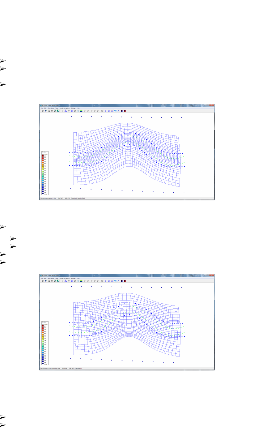
DRAFT
Tutorial
6.2 Grid design samples
In this example we will demonstrate how to design a grid in which the shape is based on
the bathymetry. This tutorial exercise refers to the <grid_design_samples>directory of the
RGFGRID tutorial.
Start RGFGRID and browse to the tutorial directory <grid_design_samples>.
Open the grid file <river.grd>. Select from the menubar File →Import →Grid (Delft3D-
FLOW). . .
Open the samples file <river.xyz>. Select from the menubar File →Attribute Files →Open
Samples. . . , for the result see Figure 6.13.
Figure 6.13: Grid and samples for the grid design based upon bathymetry
On the Settings menu, click Orthogonalisation (regular). . . :
Set the Design Method to “3”.
Depth Design, Depth vs.Slope Weight to “0.2”
Click OK.
On the Operations menu, click Orthogonalise Grid, the result is shown in Figure 6.14.
Figure 6.14: Result grid after orthogonalisation using samples
To save the grid and to exit the RGFGRID program you have to do:
Click on File →Export →Grid (Delft3D-FLOW) and specify a filename.
Click on File →Exit.
Deltares 99 of 128

DRAFT
RGFGRID, User Manual
6.3 Paste two grids
This tutorial exercise refers to the <paste_passive_grid_to_grid>directory of the RGFGRID
tutorial. A reason to paste two grids can be to extend an existing grid with another grid.
In order to paste two grids you have to do the following:
Start RGFGRID and browse to the tutorial directory <Paste_Passive_Grid_to_Grid>.
Import the grid files <fti_02_north.grd>and <fti_02_south.grd>via File →Import →Grid
(Delft3D-FLOW).
In order to paste the two grids click on Operations →Grid →Paste two Grids.
Restrictions:
Perpendicular to the intersection line the grid lines of both grids should be similar. Thus,
refinements at the intersection are not allowed.
The grid points to paste should already be close to each other.
This option only works if two grids are loaded in RGFGRID. After pasting two grids
another grid can be loaded to paste.
6.4 Regular grids, irregular grids and their mutual coupling
This tutorial exercise refers to the <fm_scheldt>directory of the RGFGRID tutorial.
The present exercise deals with four aspects of new functionalities related to the extension
from curvilinear grids with unstructured, triangular grids:
1 to ’grow’ a curvilinear grid (a ’regular’ grid) from a geometric base line,
2 to generate unstructured, triangular grids: ’irregular’ grids,
3 the coupling between regular and irregular grids,
4 the relation to existing regular grid generation options.
6.4.1 A new method to generate curvilinear grids
RGFGRID provides an improved method to generate curvilinear meshes directly from splines.
In this method, a mesh is gradually developed from a base line of the channel towards the
boundaries. This method requires less actions by the user and provides better orthogonality.
This approach can be illustrated as follows:
Load the land boundary file <scheldtharbour.ldb>.
Draw two cross-splines, intending to mark the inflow and outflow cross-section of the river
part, through Edit →Spline →New.
Draw two additional splines, intended to loosely follow the riverbanks, in longitudinal di-
rection.
Draw an additional splines along the river axis in longitudinal direction.
100 of 128 Deltares
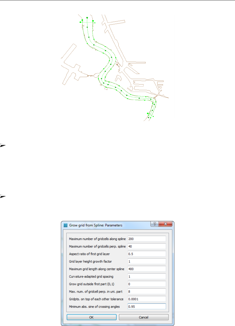
DRAFT
Tutorial
Figure 6.15: Splines drawn
Select one of the longitudinal splines and select the option Edit →Spline →Attach to Land
Boundary. Select now a first and last point on the selected spline. Click right mouse
button to snap. The spline is now snapped to the land boundary. A message box will
appear, press Yes to do extra snapping iterations or No to stop the snapping algorithm.
Repeat this action until you are satisfied with the result. For the second longitudinal spline,
the actions can be repeated. The result of these actions is provided in the directory as
<scheldt01.spl>.
Before generating curvilinear grid you can set input parameters, choose Settings →Grow
Grid from Splines. Now you are able to set several settings of the operator. The upper
seven entries should be adapted into the values shown in Figure 6.16.
Figure 6.16: Settings for the ’Grow grid from Spline’ procedure.
A brief explanation:
The option Grid layer height growth factor enables the user to demand for a non-
equidistant mesh in cross-sectional direction. The value represents the width-ratio of
two adjacent cells. Using the option Grow grid outside first part (0/1), one can extend
a mesh outside the longitudinal splines, for instance to capture winter bed regions of
a river.
By using the parameters Maximum grid length along centre spline, the user can give
an indication of the length of the cells in longitudinal direction. Based on the value
Deltares 101 of 128
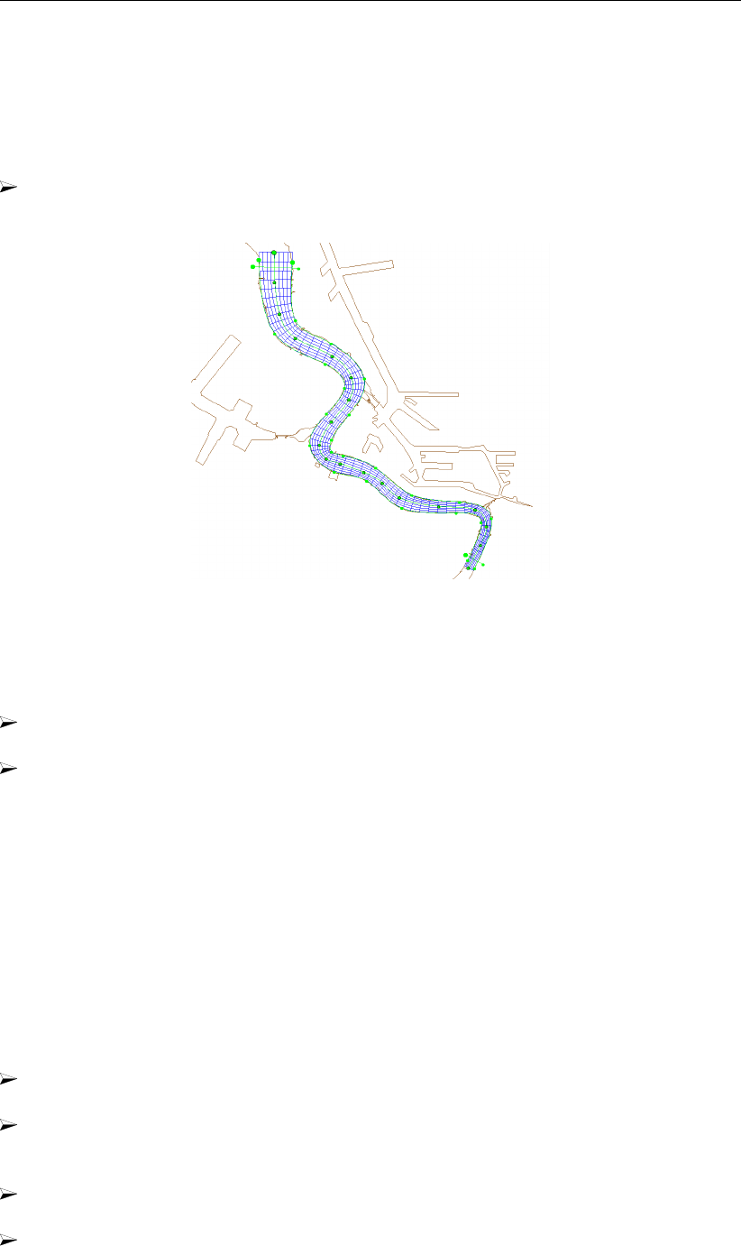
DRAFT
RGFGRID, User Manual
of the parameter Aspect ratio of first grid layer, the algorithm establishes a suitable
mesh, under the restrictions of the prevailing maximum numbers of grid cells (first two
entries).
Using the parameter Max. num. of grid cells perpin uni. part, the user can give an
indication of the number of cells across the width between the longitudinal splines.
After entering the values of Figure 6.16, choose Operations →Grow Grid from Splines.
This will deliver the mesh as shown in Figure 6.17.
Figure 6.17: Generated curvilinear mesh after the new ’Grow Grid from Splines’ proce-
dure.
To be able to further extend the grid with an unstructured part you have to convert the grid.
Choose Operations →Convert grid →Regular to irregular. Strictly, the grid is now not
structured curvilinear anymore, but unstructured.
Choose View →Grid Property Style →Coloured edge and then View →Grid Property
→Orthogonality. Now, the orthogonality of the mesh is shown. The result for the grid is
also provided in the directory as <scheldtcurvi_1_net.nc>.
6.4.2 Irregular grids
From the previous section, a curvilinear mesh is available for the Scheldt river (file
<scheldtcurvi_1_net.nc>). The river is separated from the harbour, west of the river, by a
sluice. The small area between the sluice and the Scheldt will benefit from an unstructured
mesh options of RGFGRID because of its irregular geometry. This irregular geometry is
meshed in this section first and afterwards connected to the existing Scheldt river mesh.
The approach is as follows:
Click on Edit →Polygons →New. The intention is to mark the area of interest (i.e. the
area that should be captured by the grid) through a polygon.
Start drawing a polygon at a distance of the order of a grid cell away from the curvilinear
mesh. Let the second point be at a relatively small distance from the first one. This
distance is later used as an indication of the size of the triangular grid cells to be placed.
Mark the elementary locations of the area (land boundary) and place the final point again
at a distance of the order of a grid cell away from the river mesh.
Next, we choose Edit →Polygons →Refine (linear) and click on two points at the righthand-
side, located close to each other, and click on the right mouse button. Now, the poly-
102 of 128 Deltares
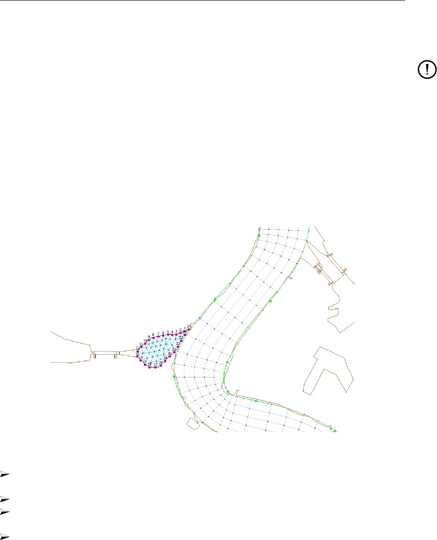
DRAFT
Tutorial
gon is divided into a finer set of line elements. This refined polygon is also available as
<scheldtpolygon.pol>.
Remarks:
Sometimes the GUI does not allow to switch to another option. For example, when
one wants to switch from Edit →Regular Grid →Edit to Edit →Polygons. As a
remedy, one can click several times on the right mouse button.
The distance between the points of the polygon is derived from the distance of the
two polyline segments at both sides of the selected segment. The length of the poly-
line segments varies linearly from the segment length at the one side of the selected
segment towards the segment length at the other side of the selected segment.
You can play around to see how this works. If needed, you can add extra points by
choosing Edit →Polygons →Insert point.
Choose Edit →Polygons →Move point if a point move would make sense.
You can snap the refined polygon to the land boundary through Edit →Polygons
→Polygon to Land Boundary. The result is shown in Figure 6.18.
Figure 6.18: Generated irregular grid within a polygon.
Choose Operations →Domain →New to indicate that the new grid to be generated grid
should be created next to the already existing one (and not replace it).
Choose Operations →Grow Grid from Polygons. The result is shown in Figure 6.18.
Improve the orthogonality through Operations →Orthogonalise grid. With the default set-
tings also the smoothness is improved.
To further orthogonalise the grid by manipulating the settings, choose Settings →Orthogonalisation
(irregular), and then choosing Operations →Orthogonalise grid once again. The result for
the grid is also provided in the directory as <scheldttriangle_net.nc>.
6.4.3 The coupling of regular and irregular grids
In the previous section we have ended up with two separate grids (file <scheldtcurvi_1_net.nc>
and file <scheldttriangle_net.nc>). Obviously, these two grids should properly be integrated
into one single grid. Before we can couple the two grids, we should first make sure that the
typical gridsize is of the same order of magnitude for both grids at the location where the
connection is to be laid. Hence, basically two operations are to be done:
Split the grid cells in the Scheldt river grid over the full width. Hence, the gridcell size in
the river will match the grid cell size of the unstructured grid.
Deltares 103 of 128
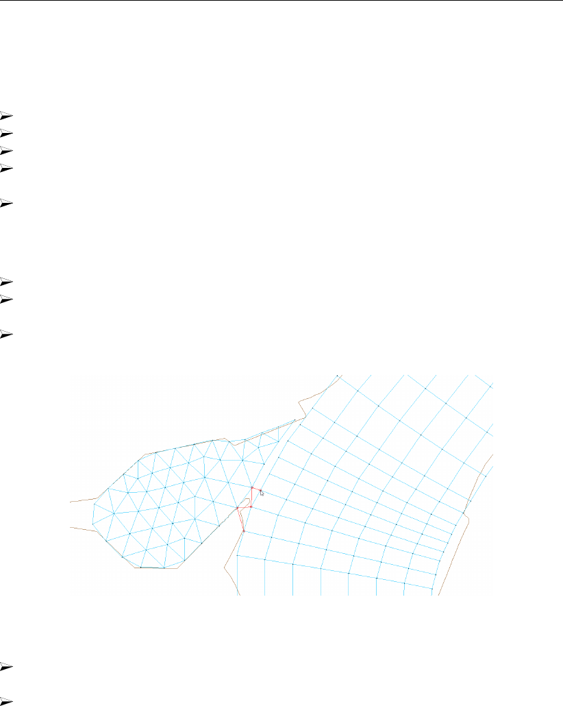
DRAFT
RGFGRID, User Manual
Merge the two grids by putting connections in between.
The splitting can be established as follows:
Delete the polygon, choose Operations →Delete →Polygons
Select the river grid through Edit →Select domain and clicking the river grid.
Choose Edit →Irregular Grid →Split row or column.
Select the grid lines that should be split. Start at the left boundary, and apply multiple line
split operations towards the other side of the Scheldt river.
Try to achieve the picture shown in Figure 6.19 as regards the typical grid size in the
curved area. The result is provided in the directory as <scheldtcurvi_2_net.nc>).
The merging part of the coupling schedule can be done as follows:
Choose Edit →Multi Select. By now, you enable the option to select multiple grids.
Click on the triangular part of the grid. As soon as you have clicked on it, both meshes are
highlighted blue.
Merge the two separate grids through Operations →Grid →Merge Grids. Now, the grids
have been merged. The result of this merging operation is provided as <scheldtmerge_net.nc>.
Figure 6.19: Coupling of the two grids (regular and irregular, in blue) through manually
inserting connecting grid lines (in red lines) between the two grids.
As soon as the grids have been merged, new connections can be laid. Hence, choose
Edit →Irregular Grid →Insert node.
Insert new gridlines in a zigzag-like style: see the red grid lines in Figure 6.19. Now, you
will benefit from the (more or less) equal resolution in the river region as in the unstructured
region. The integrated grid is available as <scheldtcoupling_net.nc>.
104 of 128 Deltares
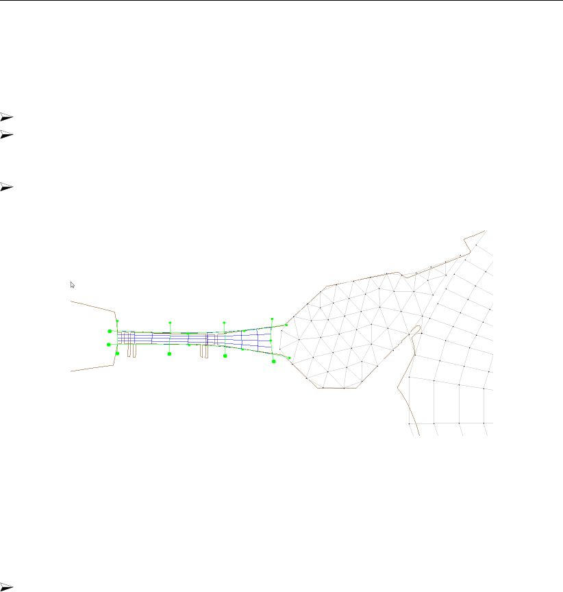
DRAFT
Tutorial
6.4.4 Relation to existing regular grid generation
The sluice area can the best be captured by a regular grid because of its rectangular shape.
Therefore, you should:
At first draw some splines in this area (see for instance Figure 6.20).
Then you can establish a 3×4grid in each block separated by splines, by setting these
values in menu bar item Settings →General. . . and the edit fields M-refinement Factor
and N-refinement Factor.
Finally choose Operations →Change Splines into Grid. The splines for the sluice area
are available as <scheldtsluice.spl>.
Figure 6.20: A regular grid is suitable for the sluice area. Connections with the existing
grid should further be established as well as additional orthogonalisation
iterations.
The docks of the harbour are rectangularly shaped as well. Hence, regular grids are preferred.
You can also try to establish an irregular grid in this area. Therefore:
Draw a polygon, refine this polygon and choose Operations →Grow Grid from Polygons.
Notice that the grid configuration as shown in Figure 6.20 needs proper connections between
the sluice area and the already existing grid. Moreover, further orthogonalisation iterations
before it can actually be used in computations. An example of further elaboration of the area
is provided as <scheldtfinal_net.nc>.
6.5 Multi-domain grids and domain decomposition boundaries
This tutorial exercise refers to the <dd_grids>directory of the RGFGRID tutorial.
The grids for a multi-domain model must satisfy the following rules:
At subdomain interfaces the grids should be nicely connected (no overlap and “no holes”
between sub-domains), see Section 5.3.17.
In case of horizontal, grid lines in the coarse domain should be continued in the fine sub-
domain, see Figure 5.16. Thus, there should be a 1-to-N refinement, with N an integer
number.
In case of horizontal refinement it is advised to have an equidistant refinement.
Grids must be of the same type (thus, all in Spherical coordinates, or all in Cartesian
coordinates).
The grid orientation should be the same (increasing M- or N-numbering in both sub-
domains at the DD-boundary).
Deltares 105 of 128
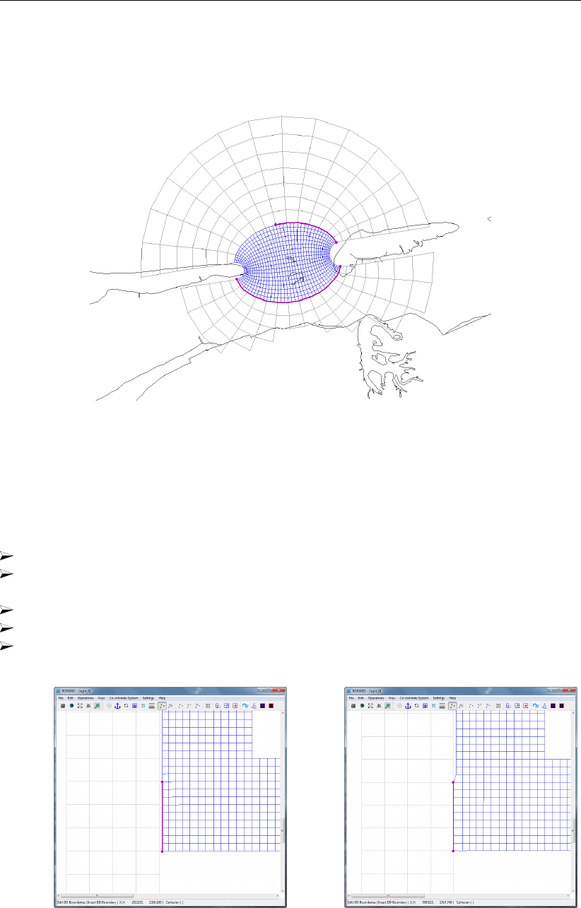
DRAFT
RGFGRID, User Manual
No coupling of columns to rows or vice versa.
Sub-domain interfaces should be straight lines (no stair-case interfaces).
Figure 6.21: Example of grid refinement in the horizontal direction
RGFGRID has an option to let sub-domain interfaces coincide, see section 5.3.17. The best
moment to use this option is before refining one of the sub-domains, i.e. as long as the refine-
ment is 1-1.
To demonstrate this functionality
Go to directory <let_interfaces_coincide>, within the <dd_grids>directory.
Open the grids <left_n.grd>and <right_0.grd>, zoom in on the interface between both
grids.
On the Edit menu, point to DD Boundaries →New.
Click with the mouse the end points of the DD-Boundary on the interface of the active grid.
Click Operations →Attach Grids at DD Boundaries →Regular Grids then the whole DD-
Boundary will be shifted to the interface points of the inactive grid, see Figure 6.22.
(a) Before attach operation (b) After attach operation
Figure 6.22: Let interface grid points coincide
Now we have the interfaces coincide we are going to define the interfaces between the various
sub-domain models.
106 of 128 Deltares
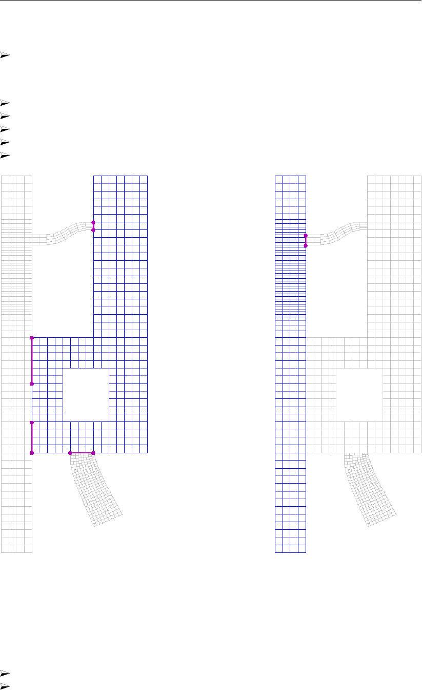
DRAFT
Tutorial
Close and start RGFGRID in the <dd_grids>directory and load all grids into RGFGRID.
Open the grids <bot.grd>,<left.grd>,<right.grd>and <top.grd>.
To define the DD-boundaries you select one domain as active domain, Figure 6.23:
Make the <right.grd>the active domain
On the Edit menu, point to DD Boundaries and click New.
Specify the four DD-Boundaries as shown in Figure 6.23
Make the <left.grd>the active domain
Specify the last DD-Boundaries as shown in Figure 6.23
(a) DD-Boundaries at the right do-
main
(b) DD-Boundaries at the right do-
main
Figure 6.23: Defining DD-Boundaries
Now we have defined the DD-boundaries between the various domains. To gather all these
information into 1 file:
On the Operations menu, click Compile DD Boundaries.
The Save DD-Boundaries dialog opens, see Figure 6.24.
Deltares 107 of 128
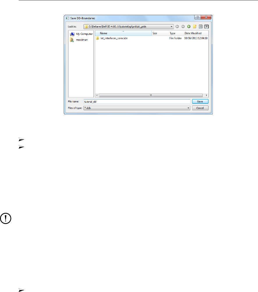
DRAFT
RGFGRID, User Manual
Figure 6.24: The Save DD-Boundaries dialog
After pressing OK a message appears about the number of DD-Boundaries.
Press OK.
The final administration will be written to a file named <tutorial_dd.ddb>. For the tutorial it
looks like:
left.grd 5 61 5 65 top.grd 1 1 1 5
bot.grd 1 28 10 28 right.grd 6 1 9 1
left.grd 5 14 5 18 right.grd 1 1 1 5
left.grd 5 25 5 29 right.grd 1 12 1 16
top.grd 9 1 9 5 right.grd 9 30 9 31
Remarks:
Before defining DD-boundaries check the orientation of each sub-domain grid.
The orientation and order of interfaces (DD-boundaries) is free.
It is irrelevant in which grid you define an interface, but define it once.
If the interfacing boundaries coincide, be aware that when you orthogonalise a sub-
domain grid, the grid points along these interfaces may move. To keep these points at
the same place, you just re-define the DD-boundaries.
To exit the RGFGRID
Click Exit on the File menu.
6.6 RGFGRID in the ArcMap environment
In this case you should be familiar with using coordinate systems in ArcMap.
ArcMap layers (e.g. shape files, SDE layers) most times have also information about the
coordinate system (spatial reference). If not available, ArcMap marks this as unknown. On
the other hand, if it is known to you, spatial reference can be added to these layers by the
program ArcCatalog.
If the layers in ArcMap have a projected coordinate system or probably an unknown coordinate
system, then you can use Cartesian in RGFGRID. It is your responsibility the coordinates have
the unit metres. You can see the used (projected) coordinate system of the layers and of the
data frame via the properties of the data frame. For RGFGRID the coordinate system of the
data frame is leading. As you know, ArcMap has possibilities to set the coordinate system of
the data frame, while layers have different coordinate systems.
108 of 128 Deltares
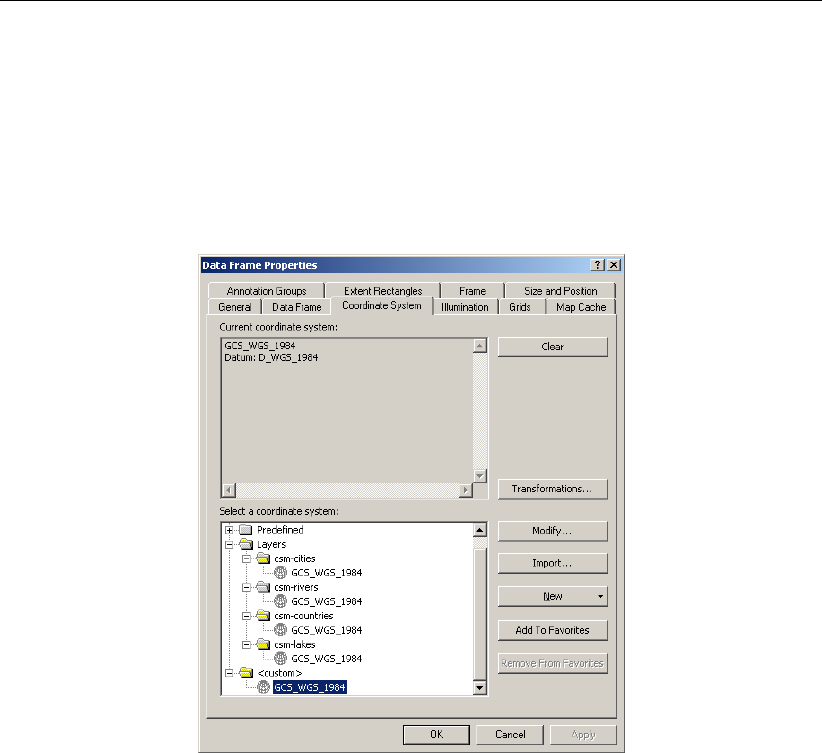
DRAFT
Tutorial
If you want to use spherical coordinates in RGFGRID while using ArcMap, the coordinate
system of the data frame must be WGS84 (in ArcMap it has the name CGS_WGS_1984).
This will be the case when all layers have this coordinate system.
If you are familiar with ArcMap you can have one or more layers with different coordinate
systems and select (import) the WGS84 system for the data frame. Figure 6.25 shows the
properties window of de data frame, <custom>give the coordinate system of the data frame.
Figure 6.25: ARC-GIS data frame properties form
You start loading layers or an <∗.mxd >file in ArcMap. The coordinate system of the data
frame must be as described above. You will see that ArcMap displays the values of longitude
and latitude as plane coordinates in degrees.
Then you can start using the commands and functions of RGFGRID. The program has a menu
item to change into projected coordinates. When using this command, the layers in ArcMap
are displayed as projected and also the grid, polygons, samples of the program.
When using the menu item View →Spherical Coordinates →Plane Coordinates, both the
layers in ArcMap and the objects of Dleft3D-RGFGRID are displayed as plane coordinates.
Centring the screen in stereographic mode
In the standalone version of RGFGRID, the visualisation using the stereographic projection
method always uses the centre of the screen as the point where the screen touches the
sphere. This is more difficult to realise when working within the GIS environment because
screen handling now is governed by the GIS system. Therefore a special function has been
implemented to perform this task of centring the computer screen. This function can be in-
voked by clicking the menu item Operations →Change Centre of Projection, see Figure 6.26.
When using this command the centre of the projection is set to the centre of the screen. This
action needs recalculation of the projection and a new screen refresh. By using this command
you are aware of changing the screen. When using zoom in, zoom out, pan, the centre of the
projection does not change. So there is more performance and a smooth screen-refresh in
this case.
Deltares 109 of 128
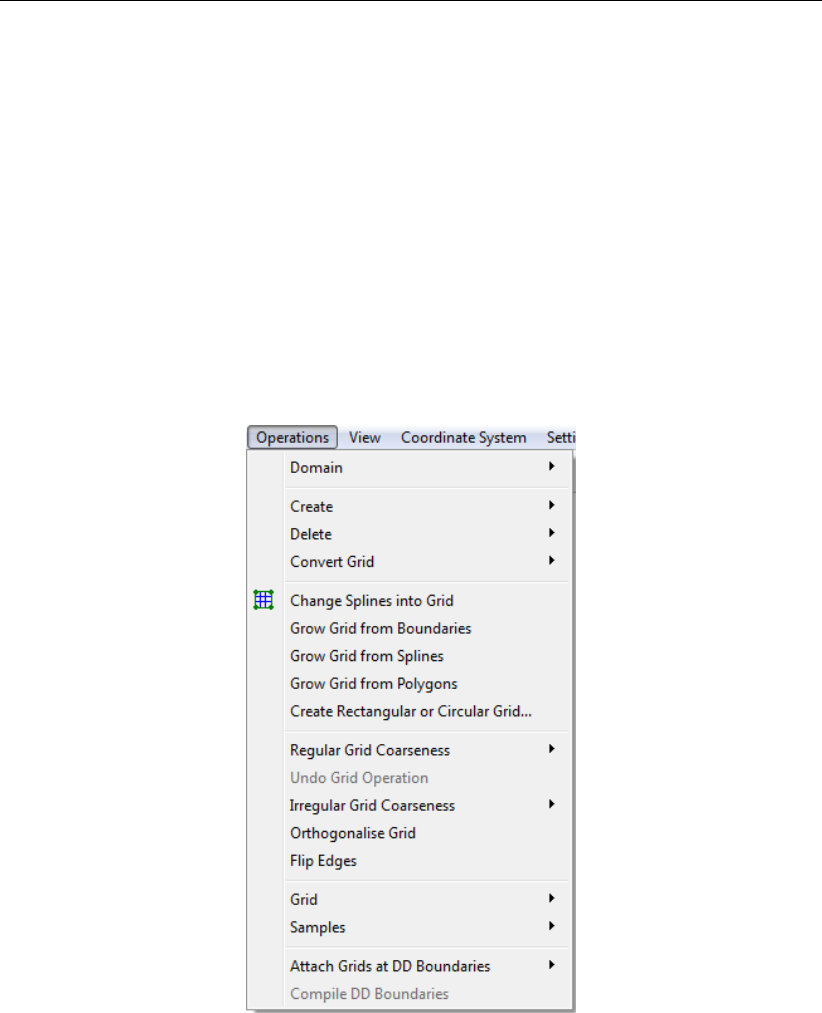
DRAFT
RGFGRID, User Manual
Figure 6.26: Options on the Operations menu
110 of 128 Deltares

DRAFT
References
UnTRIM (V. Casulli). “Tidal, Residual, Inter-tidal Mud-flat (TRIM).”
ADCIRC.
D-Flow FM UM, 2015. D-Flow FM Hydro- and Morphodynamics User Manual. Deltares,
1.1.124 ed.
Delft3D-FLOW UM, 2013. Delft3D-FLOW User Manual. Deltares, 3.14 ed.
GmbH, S. consult, 2015. Preprocessor JANET. Grid generation for UNTRIM, 1.0 (19.5.2005)
ed.
GPP UM, 2013. Delft3D-GPP User Manual. Deltares, 2.14 ed.
Huang, W., 2001. “Practical Aspects of Formulation and Solution of Moving Mesh Partial
Differential Equations.” Journal of Computational Physics 171: 753–775.
QUICKPLOT UM, 2013. Delft3D-QUICKPLOT User Manual. Deltares, 2.14 ed.
ROMS. “Regional Ocean Modeling System.”
SWAN UM, 2000. SWAN Cycle III version 40.11 User Manual (not the short version). Delft
University of Technology, Delft, The Netherlands, 0.00 ed.
TELEMAC.
Deltares 111 of 128

DRAFT
RGFGRID, User Manual
112 of 128 Deltares
DRAFT
A Files of RGFGRID
In the following sections we describe the attribute files used in RGFGRID.
For each file which can be handled by RGFGRID we give the following information:
File contents.
Filetype (free formatted, fix formatted or unformatted).
Filename and extension.
Generated by (i.e. how to generate the file).
Restrictions on the file contents.
Example(s).
Remarks:
The access mode of all attribute files is sequential.
In the examples the file content is printed in font Courier and comment (not included in
the file) between curly brackets font, unless explicitly stated differently.
A.1 Delft3D project file
File contents Domain input for a model.
Filetype ASCII
File format Free formatted.
Filename <name.d3d>
Generated RGFGRID, QUICKIN, D-Waq DIDO, or manually offline
Record description:
A header block containing general information and then for each domain a detailed descrip-
tion.
Keyword Description
FileInformation
FileCreatedBy Version string of the program who generated this file the first time
FileCreationDate Creation date and time
FileVersion Version number of <∗.d3d>file
Geometry
LandBoundaryName Name of the file with the land boundaries
LandBoundaryFormat Format of the land boundary file, possible values are: TEKAL,
NETCDF or SHAPEFILE. The NetCDF file is according the ’World
Vector Shoreline’ format
DDBound
FileDDBound Name of the file with the domain decomposition boundaries
Deltares 113 of 128
DRAFT
RGFGRID, User Manual
For each grid
Keyword Description
Grid
Type Format of the grid file, possible values are: RGF, RGF_NETCDF,
DFLOW_FM, TELEMAC
FileName Name of grid file with the geographical co-ordinates
FlowDepth Name of the file containing the depth values at the cell corners of
the grid
Aggregation Name of the aggregation file
Restriction:
The maximum record length in the file is 132.
Example:
The model friesian_tidal_inlet contains three different subdomains (f01, f02, f03) and the
project file has the name <friesian_tidal_inlet.d3d.>
[FileInformation]
FileGeneratedBy = Deltares, Delft3D-DIDO Version 4.04.00.11836M, Jun 21 2010, 12:09:34
FileCreationDate = 2010-06-21, 13:35:22
FileVersion = 0.03
[DDBound]
FileDDBound = f34-123.ddb
[Grid]
Type = RGF
FileName = f01.grd
Aggregation = f34_dd-f01.dwq
Monitoring Areas = f34_dd-f01.dmo
[Grid]
Type = RGF
FileName = f02.grd
Aggregation = f34_dd-f02.dwq
Monitoring Areas = f34_dd-f02.dmo
[Grid]
Type = RGF
FileName = f03.grd
Aggregation = f34_dd-f03.dwq
Monitoring Areas = f34_dd-f03.dmo
114 of 128 Deltares
DRAFT
Files of RGFGRID
A.2 Land boundary file
File contents The co-ordinates of one or more polylines. Each polyline (piecewise
linear) is written in a single block of data.
Filetype ASCII
File format Free formatted
Filename <name.ldb>
Generated RGFGRID, QUICKIN, etc
Record description:
Record Record description
Preceding description records, starting with an asterisk (∗), and will
be ignored.
1 A non blank character string, starting in column one
2 Two integers representing the numbers of rows and number of
columns for this block of data
Two reals representing the x, y or λ, φ-co-ordinate
Example:
*
*Polyline L007
*
L007
6 2
132400.0 549045.0
132345.0 549030.0
132165.0 549285.0
131940.0 549550.0
131820.0 549670.0
131585.0 549520.0
*
*Polyline L008
*
L008
4 2
131595.0 549685.0
131750.0 549865.0
131595.0 550025.0
131415.0 550175.0
*
*Polyline L009
*
L009
6 2
131595.0 549655.0
148975.0 564595.0
150000.0 564935.0
152105.0 565500.0
153150.0 566375.0
154565.0 567735.0
Remark:
In case this file is read as a polygon file then the polylines are closed by RGFGRID to
Deltares 115 of 128

DRAFT
RGFGRID, User Manual
get a polygon.
A.3 Sample file
File contents The location and value of samples.
Filetype ASCII
File format Free formatted
Filename <name.xyz>
Generated Manually or Offline with QUICKIN or Delta Shell and data from digi-
tised charts or GIS-database.
Record description:
Filetype Record description
Free formatted Location and sample value per row
Two reals representing the x, y or λ, φ-coordinate and one real rep-
resenting the sample value
Example:
Sample file with 12 sample values with their location (free formatted file).
213813.2 603732.1 -4.053000
214686.0 607226.1 -4.522000
214891.7 610751.2 -5.000000
210330.8 601424.1 -2.169000
211798.0 604444.8 -2.499000
212460.0 607475.7 -2.760000
212436.9 610362.5 -2.865000
185535.4 606607.9 1.360000
186353.0 603789.4 1.122000
187959.2 601197.6 0.9050000
190193.0 599101.5 0.7050000
208578.7 602513.7 -0.7990000
A.4 Spline file
File contents The co-ordinates of one or more polygons. Each polygon is written
in a single block of data
Filetype ASCII
File format Free formatted
Filename <name.spl>
Generated Delft3D-RGFRID
Record description:
116 of 128 Deltares

DRAFT
Files of RGFGRID
Record Record description
Preceding description records, starting with an asterisk (∗), and will
be ignored.
1 Character string of at least 1 character.
2 Two integers representing the numbers of rows and number of
columns for this block of data
Two reals representing the x, y or λ, φ-coordinate
Example:
*
*Deltares, \DRGFGRID\ Version 4.16.01.4887, Oct 18 2008, 13:26:48
*File creation date: 2008-10-19, 13:33:05
*
*Coordinate System = Cartesian
*
S001
6 2
-1.1520000E+02 9.9630000E+02
1.2911200E+03 9.9878100E+02
2.2075800E+03 1.0299500E+03
3.0180600E+03 1.3105000E+03
4.1090800E+03 1.3479100E+03
5.1315300E+03 1.3354400E+03
S002
2 2
3.4607000E+03 -6.0347500E+02
4.0405100E+03 5.7377700E+01
A.5 Polygon file
File contents The co-ordinates of one or more polygons. Each polygon is written
in a single block of data
Filetype ASCII
File format Free formatted
Filename <name.pol>
Generated RGFGRID, QUICKIN, D-Waq DIDO, etc
Record description:
The file may contain one or more polygons. For every polygon the file should contain a line
indicating the name of the polygon, followed by a line indicating the number of points making
up the polygon and the number of coordinates, i.e. 2, finally followed by the coordinate data.
Deltares 117 of 128
DRAFT
RGFGRID, User Manual
Record Record description
Preceding description records, starting with an asterisk (∗), and will
be ignored.
1 A non blank character string, starting in column one
2 Two integers representing the numbers of rows and number of
columns for this block of data
Two reals representing the x, y or λ, φ-coordinate
Restriction:
The first record and the last record in the block should be the same
Example:
*
*Deltares, Delft3D-DIDO Version 3.39.01.4423:4459, Sep 25 2008, 20:10:54
*2008-09-25, 22:11:08
*
Observation Area 001
5 2
1.8768018E+05 6.1708738E+05
1.8996981E+05 6.1001035E+05
1.9746314E+05 6.1266423E+05
1.9480925E+05 6.1838830E+05
1.8768018E+05 6.1708738E+05
Observation Area 002
5 2
2.0011703E+05 6.1818015E+05
1.9819166E+05 6.1063479E+05
2.0568498E+05 6.0870942E+05
2.0797461E+05 6.1599460E+05
2.0011703E+05 6.1818015E+05
Observation Area 003
5 2
1.9340425E+05 6.1396516E+05
2.0183425E+05 6.1365294E+05
1.9944054E+05 6.0558720E+05
1.9522555E+05 6.0595146E+05
1.9340425E+05 6.1396516E+05
A.6 Orthogonal curvilinear grid file
File contents The co-ordinates of the orthogonal curvilinear grid at the depth points.
Filetype ASCII
File format Free formatted
Filename <name.grd>
Generated RGFGRID
118 of 128 Deltares

DRAFT
Files of RGFGRID
Record description:
Record Record description
Preceding description records, starting with an asterisk (∗), will be
ignored.
1 Record with Co-ordinate System = Cartesian or value
Spherical
2 Record with
Missing Value = -9.99999000000000024E+02.
If this record is not given 0.0will be assumed as missing value.
3 The number of grid points in m- and n-direction (2 integers).
4 Three real values (not used).
5 to K+5 A label and record number, the x-component of the world co-
ordinates of all points in m-direction, starting with row 1 to row
nmax, with as many continuation records as required by mmax
and the number of co-ordinates per record. The label and record
number are suppressed on the continuation lines. This set of records
is repeated for each row until n=nmax.
K+5 to 2K+4 A similar set of records for the y-component of the world co-
ordinates.
K is the number of records to specify for all grid points a set of x- and y-co-ordinates.
Restrictions:
The grid must be orthogonal.
Input items in a record are separated by one or more blanks.
Example:
*
*Deltares, Delft3D-RGFGRID Version 4.16.01.4531, Sep 30 2008, 23:32:27
*File creation date: 2008-10-01, 23:19:22
*
Coordinate System = Cartesian
9 7
000
Eta= 1 0.00000000000000000E+00 1.00000000000000000E+02 2.000000...
5.00000000000000000E+02 6.00000000000000000E+02 7.000000...
Eta= 2 0.00000000000000000E+00 1.00000000000000000E+02 2.000000...
5.00000000000000000E+02 6.00000000000000000E+02 7.000000...
Eta= 3 0.00000000000000000E+00 1.00000000000000000E+02 2.000000...
5.00000000000000000E+02 6.00000000000000000E+02 7.000000...
Eta= 4 0.00000000000000000E+00 1.00000000000000000E+02 2.000000...
5.00000000000000000E+02 6.00000000000000000E+02 7.000000...
Eta= 5 0.00000000000000000E+00 1.00000000000000000E+02 2.000000...
5.00000000000000000E+02 6.00000000000000000E+02 7.000000...
Eta= 6 0.00000000000000000E+00 1.00000000000000000E+02 2.000000...
5.00000000000000000E+02 6.00000000000000000E+02 7.000000...
Eta= 7 0.00000000000000000E+00 1.00000000000000000E+02 2.000000...
5.00000000000000000E+02 6.00000000000000000E+02 7.000000...
Deltares 119 of 128

DRAFT
RGFGRID , User Manual
Eta= 1 1.00000000000000000E+02 1.00000000000000000E+02 1.000000...
1.00000000000000000E+02 1.00000000000000000E+02 1.000000...
Eta= 2 2.00000000000000000E+02 2.00000000000000000E+02 2.000000...
2.00000000000000000E+02 2.00000000000000000E+02 2.000000...
Eta= 3 3.00000000000000000E+02 3.00000000000000000E+02 3.000000...
3.00000000000000000E+02 3.00000000000000000E+02 3.000000...
Eta= 4 4.00000000000000000E+02 4.00000000000000000E+02 4.000000...
4.00000000000000000E+02 4.00000000000000000E+02 4.000000...
Eta= 5 5.00000000000000000E+02 5.00000000000000000E+02 5.000000...
5.00000000000000000E+02 5.00000000000000000E+02 5.000000...
Eta= 6 6.00000000000000000E+02 6.00000000000000000E+02 6.000000...
6.00000000000000000E+02 6.00000000000000000E+02 6.000000...
Eta= 7 7.00000000000000000E+02 7.00000000000000000E+02 7.000000...
7.00000000000000000E+02 7.00000000000000000E+02 7.000000...
A.7 Grid enclosure file
File contents The indices of the external computational grid enclosure(s) and op-
tionally one or more internal computational grid enclosures that out-
lines the active computational points in a Delft3D-FLOW computa-
tion. The file is strongly related to the curvilinear grid file.
Filetype ASCII
File format Free formatted
Filename <name.enc>
Generated RGFGRID
Record description:
Record Record description
All One pair of M and N indices representing the grid co-ordinates
where a line segment of the computational grid enclosure (polygon)
changes direction.
Restrictions:
A polygon must be closed. The first point of the polygon is repeated as last point.
A line segment may not intersect or touch any other line segment.
The angle formed by consecutive line segments (measured counter clock-wise) can
have a value of: 45, 90, 135, 225, 270 or 315 degrees, but not 0, 180 and 360 degrees.
In a row or column there should be at least two active computational grid cells.
Input items in a record are separated by one or more blanks.
Example:
Model area with (one) external and one internal polygon, see Figure A.1.
1 1 begin external polygon
6 1
8 3
9 3
9 1
16 1
19 4
19 6
17 8
4 8
1 5
1 1 end external polygon
120 of 128 Deltares
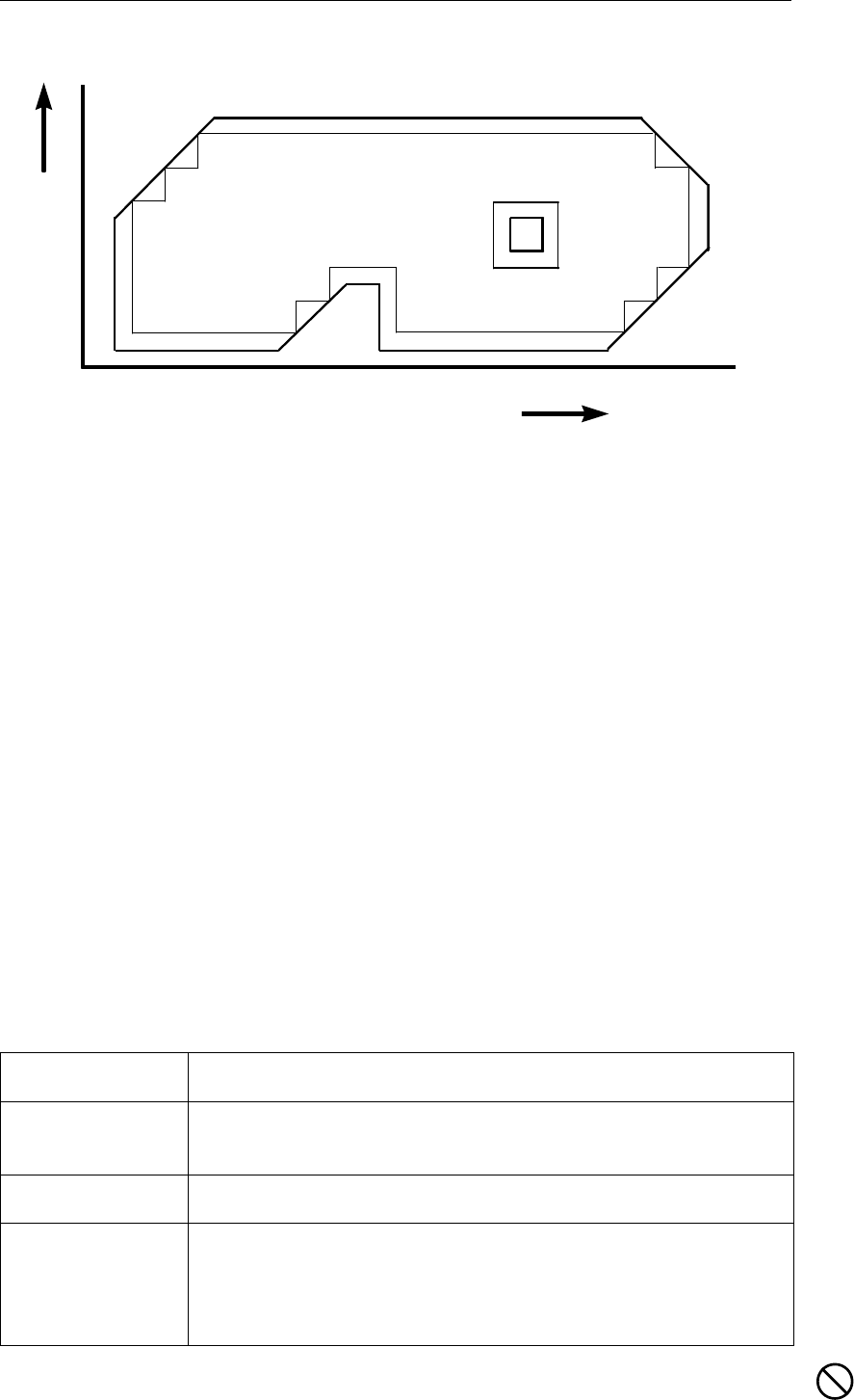
DRAFT
Files of RGFGRID
-+ +
++
-
-
-
-
-
-
-
-+
+
+ +
++
--
- -
-
-
-
-
-
-
-
-+ +
++
-
-
-
-
-
-
-
-+
+
+ +
++
--
- -
-
-
-
-
-
-
-
-+ +
++
-
-
-
-
-
-
-
-+
+
+ +
++
--
- -
-
-
-
-
-
-
-
-+ +
++
-
-
-
-
-+
+
+ +
++
--
- -
-
-
-
-
-
-
-
-+
+
+ +
++
--
- -
-
-
-
-
-
-
-
-+
+
+ +
++
--
- -
-
-
-
-
-
-
-
-+
+
+ +
++
--
- -
-
-
-
-
-
-
-
+
+
-
-
- -
+
+
-
-
- -
-+
+
+ +
++
--
- -
-
-
-
-
-
-
-
-+
+
+ +
++
--
- -
-
-
-
-
-
-
-
-+
+
+ +
++
--
- -
-
-
-
-
-
-
-
-+
+
+ +
++
--
- -
-
-
-
-
-
-
-
+
+
-
-
- -
+
+
-
-
- -
-
-
-
-+
+
+ +
++
--
- -
-
-
-
-
-
-
-
-+
+
+ +
++
--
- -
-
-
-
-
-
-
-
-+
+
+ +
++
--
- -
-
-
-
-
-
-
-
-+
+
+ +
++
--
- -
-
-
-
-
-
-
-
-+
+
+ +
++
--
- -
-
-
-
-
-
-
-
+
+
-
-
- -
+
+
-
-
- -
-+
+
+ +
++
--
- -
-
-
-
-
-
-
-
-+
+
+ +
++
--
- -
-
-
-
-
-
-
-
-+
+
+ +
++
--
- -
-
-
-
-
-
-
-
-+
+
+ +
++
--
- -
-
-
-
-
-
-
-
+
+
-
-
- -
+
+
-
-
- -
12 3 4 5 6 7 8 9 10 11 12 13 14 15 16 17 18 19
1
2
3
4
5
6
7
8
M - direction
N - direction
Legend:
+water level point
|v-velocity point
−u-velocity point
Full thick line grid enclosure and (for the external polygon only) loca-
tion of water level open boundaries.
Full thin line location for velocity or discharge open boundaries.
Figure A.1: Example of computational grid enclosures
13 4 begin internal polygon
14 4
14 5
13 5
13 4 end internal polygon
A.8 Annotation file
File contents File with xand yco-ordinates, string and rgb-colour.
Filetype ASCII
File format Free formatted.
Filename <name.txt>
Generated manually offline
Record description:
Record Record Description
1 Records starting with a ∗are comment lines
Character string to define the datablock (nonblank)
2 Number of rows
3–N real, real, string, integer:
geographical co-ordinates (2 reals),
text between quotes which need to be plotted (string) and
rgb-colour (integer; = 256 ∗256 ∗r+ 256 ∗g+b)
Deltares 121 of 128
DRAFT
RGFGRID, User Manual
Restriction:
The maximum record length in the file is 132.
Example:
*
BL01
8 4
10.0 10.0 ’string-01’ 6553625
10.0 20.0 ’string-02’ 9830425
20.0 10.0 ’string-03’ 13120000
20.0 20.0 ’string-04’ 16724480
30.0 10.0 ’string-05’ 38425
30.0 20.0 ’string-06’ 65305
40.0 10.0 ’string-07’ 255
40.0 20.0 ’string-08’ 0
A.9 DD Boundary file
File contents Domain decomposition boundaries connecting two grids for the pre-
scribed indices.
Filetype ASCII
File format Fix formatted.
Filename <name.ddb>
Generated RGFGRID, or manually offline
Record description:
Record Record Description
N Name of the first grid, followed by four integers indicating the gridline
on which the boundary lies, followed by the name of the second grid
and four integers indicating the gridline on which the boundary lies.
Restrictions:
No space allowed in grid filename.
The maximum record length in the file is 132.
Example:
In the following example 4 sub-domains exist. Domain d01_ns is coupled to oa1_ns, ob1_ns
and oc1_ns. Furthermore oa1_ns is coupled to ob1_ns, and ob1_ns to oc1_ns.
d01_ns.grd 5 16 5 1 oa1_ns.grd 28 35 28 20
d01_ns.grd 245 1 5 1 ob1_ns.grd 17 21 1 21
d01_ns.grd 245 52 245 1 oc1_ns.grd 1 44 1 27
ob1_ns.grd 1 4 1 21 oa1_ns.grd 28 3 28 20
ob1_ns.grd 17 4 17 21 oc1_ns.grd 1 10 1 27
A.10 Colour scheme file
File contents The colour scheme
Filetype ASCII
File format Free formatted
Filename <name.clr>or <name.clrmap>
Generated manually
122 of 128 Deltares

DRAFT
Files of RGFGRID
Record description:
Record Record description
1 COLORMAP
2 NAME=name
3 SPACE=RGB, RGB is the only allowed space for this program
4 – N one real and three integers.
The first column represent the relative distribution of the defined colours in column 2–4 (rep-
resenting the RGB values).
Example:
COLORMAP
NAME=copper
SPACE=RGB
0.0000 0 0 0
0.8000 255 159 101
1.0000 255 199 127
A.11 Settings file
File contents Settings of the program
Filetype ASCII
File format Fix formatted
Filename <name.ini>
Generated By the program
Record description:
Deltares 123 of 128
DRAFT
RGFGRID , User Manual
Record Record description
FileInformation
FileCreatedBy RGFGRID version number
FileCreationDate creation date and time
FileVersion version number of <∗.ini>file
RGFParameter
name integer value
TextSettings
name value (integer or real)
RGFsettings
name value (integer or real)
DepthDesign
name value (integer or real)
Colours
name RGB value (3 integers)
line width
dots sizes
Example:
[FileInformation]
FileGeneratedBy = Deltares, Delft3D-RGFGRID Version 4.20.00.11763:11790M, Jun 16 2010, 14:21:46
FileCreationDate = 2010-06-16, 14:23:25
FileVersion = 0.02
[RGFParameter]
AutoscaleLegend = 1
XCoorLegend = 16
YCoorLegend = 20
[TextSettings]
Line1 =
Line2 =
Line3 =
Fontsize = 3.00000000000000000E+00
Xposition = 0.00000000000000000E+00
Yposition = 0.00000000000000000E+00
FontsizeTimeDate = 3.00000000000000000E+00
XposTimeDate = 0.00000000000000000E+00
YposTimeDate = 3.00000000000000000E+00
[RGFSettings]
MGridCells = 50
NGridCells = 50
DeltaX = 1.00000000000000000E+02
DeltaY = 1.00000000000000000E+02
OriginX = 0.00000000000000000E+00
124 of 128 Deltares

DRAFT
Files of RGFGRID
OriginY = 1.00000000000000000E+02
RotationLeft = 0.00000000000000000E+00
RadiusCurvatureM = 0.00000000000000000E+00
MFraction = 1.00000000000000000E+00
MaximumSizeUniformMSize = 1.00000000000000000E+00
NFraction = 1.00000000000000000E+00
MaximumSizeUniformNSize = 1.00000000000000000E+00
SphereMGridCells = 50
SphereNGridCells = 50
SphereDeltaX = 1.00000000000000002E-02
SphereDeltaY = 1.00000000000000002E-02
SphereOriginX = 4.38082999999999956E+00
SphereOriginY = 5.19858300000000000E+01
SphereRotationLeft = 0.00000000000000000E+00
SphereRadiusCurvatureM = 0.00000000000000000E+00
SphereMFraction = 1.00000000000000000E+00
SphereMaximumSizeUniformMSize = 1.00000000000000000E+00
SphereNFraction = 1.00000000000000000E+00
SphereMaximumSizeUniformNSize = 1.00000000000000000E+00
StayOnStartupDirectory = 0
MRefinementFactor = 3
NRefinementFactor = 3
NrSmoothingIterations = 20
SmoothingParameter = 2.00000000000000011E-01
AttractionRepulsionParameter = 1.00000000000000006E-01
ActiveInactivePaste = 5.00000000000000000E-01
LineOrSplineRepresentation = 1.00000000000000000E+00
EquidistantSmoothInterpolation = 1.00000000000000000E+00
IncreaseFactorLineMirror = 1.00000000000000000E+00
IterationsAttractionParameter = 3
IterationsBoundary = 15
IterationsInnerArea = 25
InfluenceOriginalGridShape = 1.00000000000000000E+00
PositionBoundaryPoints = 1.00000000000000000E+00
DesignMethod = 1
[DepthDesign]
DepthDesignSizeRatioM = 2.00000000000000011E-01
DepthDesignSizeRatioN = 2.00000000000000011E-01
DepthDesignDepthVsSlope = 1.00000000000000000E+00
DepthDesignNrSmoothingIterations = 10
DepthDesignSmoothingFactor = 1.00000000000000006E-01
DepthDesignFieldVsLineWeightM = 0.00000000000000000E+00
DepthDesignFieldVsLineWeightN = 0.00000000000000000E+00
[Colours]
ColourBackground = 255 255 200
LegendColourBackground = 255 255 255
lineColourText = 000 255 255
lineColourLandBoundary = 132 066 000
fillColourLandBoundary = 255 182 108
lineColourSplines = 000 255 000
lineColourPolyline = 000 255 000
fillColourPolyline = 000 255 000
lineColourPolygon = 170 000 127
lineColourActiveGrid = 000 000 255
lineColourPreviousGrid = 211 000 000
lineColourActiveCmpBnd = 005 005 005
lineColourActiveOpenBnd = 000 000 255
lineColourActiveDDBnd = 176 000 176
lineColourGrid = 192 192 192
lineColourCmpBnd = 050 050 050
lineColourOpenBnd = 000 000 150
lineColourDDBnd = 176 000 255
[Width]
lineWidthLandBoundary = 1
lineWidthPolyline = 1
lineWidthPolygon = 1
Deltares 125 of 128

DRAFT
RGFGRID, User Manual
DotSizeSamples = 2
lineWidthActiveGrid = 1
lineWidthActiveCmpBnd = 1
lineWidthActiveOpenBnd = 1
lineWidthActiveDDBnd = 3
lineWidthGrid = 1
lineWidthCmpBnd = 1
lineWidthOpenBnd = 1
lineWidthDDBnd = 3
[Caches]
splines = 0
rest = 0
polygons = 0
polylines = 0
gridprop = 0
gridadm = 0
gridprev = 2
cmpbound = 1
openbound = 1
ddbound = 1
actgrid = 2
inactgrid = 3
landboundary = 4
samples = 5
126 of 128 Deltares
DRAFT

PO Box 177
2600 MH Del
Boussinesqweg 1
2629 VH Del
The Netehrlands
+31 (0)88 335 81 88
sales@deltaressystems.nl
www.deltaressystems.nl
DRAFT
