SACGUI User Guide

User Manual: Pdf

Open the PDF directly: View PDF .
Page Count: 2

SACGUI 1.1 User Guide

By: Jiang Yiran Email: yiranj@pku.edu.cn

1. Introduction:

So far, many MATLAB code have been written to process earthquake waveform data,

like filtering, decimating and so on. Visual interface is important for some processes, for

example phase picking. We are trying to provide users with a program which has a visual

interface. Considering many of the users have used SAC before, we are imitating it in some

operations.

As we know, both the visual mode and command mode have its own advantages, we

want to combine their advantages. It means you can do part of the works by commands

lines. It will be convenient for batch processing. To achieve all operations are compatible

with the visualization and command line mode is very difficult. We just make the most

important operations compatible with both ones.

It may be difficult to handle all the things by ourselves. It’s lucky that we can get many

written codes from the website to do part of the work. We sincerely thank these writers.

With their works, we can focus on more important things. It is why we choose MATLAB to

build our program in.

If you’re interested in our work, welcome to join us. You can contact to us via Email.

2. Installation

First unpack SACGUI.zip and open the unpacked folder in your MATLAB. You should

then add the folder and its subfolder into the MATLAB’s path. The temp_sacfile folder

contains some sac files as samples.

Now your can simply run main.m to start.

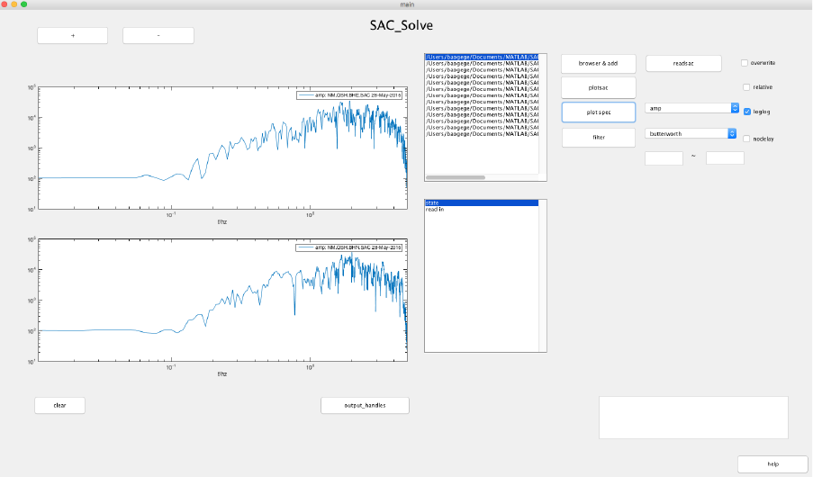
3. Visual Mode

There is a visualization interface. You can press the buttons to do some operations. We

will show you how to use this buttons.

(1) browse and add: by pressing the ‘browser & add ‘button, you can select multiple files at

once, or add new files after the selected files. The files you select will show in the sacfile

list box.

(2) readsac: after selecting files, you can press the ‘readsac’ button to read them into

memory. If this operation have been done, the program will add a ‘read in’ line in the

‘state’ box. If there is no file selected, the line will be ‘no file in list’.

(3) plotsac: press the ‘plotsac’ button to plot the waveform data in the axes. If ‘relative’

checkbox is selected, the waveform data is plotted with reference to the kztime.

(4) zoom in: press ‘x’ on keyboard, then select(left-click) two points in axes;

press ‘o’ to zoom out back.

(5) plot next and previous waveform: press ‘n’ or ‘b’ on keyboard.

(6) pick phase: press ‘p’, ’s’, or ‘f’ on the keyboard and then select(left-click) one point in

axes.

(7) ‘+’ and ‘-‘: press the ‘+ ’ or ‘-‘ button to change the number of axes. You can also press ‘+’

or ‘-‘ on the keyboard.

(8) clear boxes or axes: select one box or axes, then press ‘c’ on the keyboard to reset it.

(9) plot spectrum: press ‘plot spec’ to plot the spectrum

you can choose to plot the amplitude, phase, real part or image part of

the spectrum.

you can also choose whether to use the loglog axes.

(10) filter: press ‘filter’ to do data filtering.

there are two filter. The Bessel is a low pass filter. Only the right

frequency will work if you choose Bessel.

and you should input the frequencies by yourself.

we have a no delay filter way for you.

(11) save files: press ‘w’ on the keyboard to save the changed sac files.

if ‘overwrite’ check is on, the saved files will directly overwrite the source

files, otherwise the file in accordance with the ‘original file name _ temp’ in the form of

preservation in the working directory.

(12) quit: press ‘q’ on the keyboard to quit.

4. Command Line Mode

to be continued