SAS/STAT 9.2 User's Guide: Introduction To Clustering Procedures (Book Excerpt) SAS Users Guide
User Manual: Pdf
Open the PDF directly: View PDF ![]() .
.
Page Count: 48

SAS/STAT®9.2 User’s Guide
Introduction to Clustering
Procedures
(Book Excerpt)
SAS®Documentation
This document is an individual chapter from SAS/STAT®9.2 User’s Guide.
The correct bibliographic citation for the complete manual is as follows: SAS Institute Inc. 2008. SAS/STAT®9.2
User’s Guide. Cary, NC: SAS Institute Inc.
Copyright © 2008, SAS Institute Inc., Cary, NC, USA
All rights reserved. Produced in the United States of America.
For a Web download or e-book: Your use of this publication shall be governed by the terms established by the vendor
at the time you acquire this publication.
U.S. Government Restricted Rights Notice: Use, duplication, or disclosure of this software and related documentation
by the U.S. government is subject to the Agreement with SAS Institute and the restrictions set forth in FAR 52.227-19,
Commercial Computer Software-Restricted Rights (June 1987).
SAS Institute Inc., SAS Campus Drive, Cary, North Carolina 27513.
1st electronic book, March 2008
2nd electronic book, February 2009
SAS®Publishing provides a complete selection of books and electronic products to help customers use SAS software to
its fullest potential. For more information about our e-books, e-learning products, CDs, and hard-copy books, visit the
SAS Publishing Web site at support.sas.com/publishing or call 1-800-727-3228.
SAS®and all other SAS Institute Inc. product or service names are registered trademarks or trademarks of SAS Institute
Inc. in the USA and other countries. ® indicates USA registration.
Other brand and product names are registered trademarks or trademarks of their respective companies.

Chapter 11
Introduction to Clustering Procedures
Contents
Overview: Clustering Procedures ........................... 209
Clustering Variables ................................. 211
Clustering Observations ............................... 212
Methods for Clustering Observations ......................... 213
Well-Separated Clusters ............................ 213
Poorly Separated Clusters ........................... 215
Multinormal Clusters of Unequal Size and Dispersion ............ 223
Elongated Multinormal Clusters ........................ 233
Nonconvex Clusters .............................. 240
The Number of Clusters ............................... 243
References ...................................... 246
Overview: Clustering Procedures
You can use SAS clustering procedures to cluster the observations or the variables in a SAS data
set. Both hierarchical and disjoint clusters can be obtained. Only numeric variables can be analyzed
directly by the procedures, although the DISTANCE procedure can compute a distance matrix that
uses character or numeric variables.
The purpose of cluster analysis is to place objects into groups, or clusters, suggested by the data,
not defined a priori, such that objects in a given cluster tend to be similar to each other in some
sense, and objects in different clusters tend to be dissimilar. You can also use cluster analysis to
summarize data rather than to find “natural” or “real” clusters; this use of clustering is sometimes
called dissection (Everitt 1980).
Any generalization about cluster analysis must be vague because a vast number of clustering meth-
ods have been developed in several different fields, with different definitions of clusters and similar-
ity among objects. The variety of clustering techniques is reflected by the variety of terms used for
cluster analysis: botryology, classification, clumping, competitive learning, morphometrics, nosog-
raphy, nosology, numerical taxonomy, partitioning, Q-analysis, systematics, taximetrics, taxonorics,
typology, unsupervised pattern recognition, vector quantization, and winner-take-all learning. Good
(1977) has also suggested aciniformics and agminatics.
210 FChapter 11: Introduction to Clustering Procedures
Several types of clusters are possible:
Disjoint clusters place each object in one and only one cluster.
Hierarchical clusters are organized so that one cluster can be entirely contained within another
cluster, but no other kind of overlap between clusters is allowed.
Overlapping clusters can be constrained to limit the number of objects that belong simultane-
ously to two clusters, or they can be unconstrained, allowing any degree of overlap in cluster
membership.
Fuzzy clusters are defined by a probability or grade of membership of each object in each
cluster. Fuzzy clusters can be disjoint, hierarchical, or overlapping.
The data representations of objects to be clustered also take many forms. The most common are as
follows:
a square distance or similarity matrix, in which both rows and columns correspond to the
objects to be clustered. A correlation matrix is an example of a similarity matrix.
a coordinate matrix, in which the rows are observations and the columns are variables, as in
the usual SAS multivariate data set. The observations, the variables, or both can be clustered.
The SAS procedures for clustering are oriented toward disjoint or hierarchical clusters from coor-
dinate data, distance data, or a correlation or covariance matrix. The following procedures are used
for clustering:
CLUSTER performs hierarchical clustering of observations by using eleven agglomerative
methods applied to coordinate data or distance data.
FASTCLUS finds disjoint clusters of observations by using a k-means method applied to
coordinate data. PROC FASTCLUS is especially suitable for large data sets.
MODECLUS finds disjoint clusters of observations with coordinate or distance data by using
nonparametric density estimation. It can also perform approximate nonparamet-
ric significance tests for the number of clusters.
VARCLUS performs both hierarchical and disjoint clustering of variables by using oblique
multiple-group component analysis.
TREE draws tree diagrams, also called dendrograms or phenograms, by using output
from the CLUSTER or VARCLUS procedure. PROC TREE can also create a
data set indicating cluster membership at any specified level of the cluster tree.
The following procedures are useful for processing data prior to the actual cluster analysis:
ACECLUS attempts to estimate the pooled within-cluster covariance matrix from coordi-
nate data without knowledge of the number or the membership of the clusters
(Art, Gnanadesikan, and Kettenring 1982). PROC ACECLUS outputs a data set
containing canonical variable scores to be used in the cluster analysis proper.

Clustering Variables F211
DISTANCE computes various measures of distance, dissimilarity, or similarity between the
observations (rows) of a SAS data set. PROC DISTANCE also provides various
nonparametric and parametric methods for standardizing variables. Different
variables can be standardized with different methods.
PRINCOMP performs a principal component analysis and outputs principal component
scores.
STDIZE standardizes variables by using any of a variety of location and scale measures,
including mean and standard deviation, minimum and range, median and ab-
solute deviation from the median, various M-estimators and A-estimators, and
some scale estimators designed specifically for cluster analysis.
Massart and Kaufman (1983) is the best elementary introduction to cluster analysis. Other im-
portant texts are Anderberg (1973), Sneath and Sokal (1973), Duran and Odell (1974), Hartigan
(1975), Titterington, Smith, and Makov (1985), McLachlan and Basford (1988), and Kaufmann
and Rousseeuw (1990). Hartigan (1975) and Spath (1980) give numerous FORTRAN programs for
clustering. Any prospective user of cluster analysis should study the Monte Carlo results of Milligan
(1980), Milligan and Cooper (1985), and Cooper and Milligan (1988). Important references on the
statistical aspects of clustering include MacQueen (1967), Wolfe (1970), Scott and Symons (1971),
Hartigan (1977, 1978, 1981, 1985), Symons (1981), Everitt (1981), Sarle (1983), Bock (1985), and
Thode, Mendell, and Finch (1988). Bayesian methods have important advantages over maximum
likelihood; see Binder (1978, 1981), Banfield and Raftery (1993), and Bensmail et al. (1997). For
fuzzy clustering, see Bezdek (1981) and Bezdek and Pal (1992). The signal-processing perspective
is provided by Gersho and Gray (1992). See Blashfield and Aldenderfer (1978) for a discussion of
the fragmented state of the literature on cluster analysis.
Clustering Variables
Factor rotation is often used to cluster variables, but the resulting clusters are fuzzy. It is preferable
to use PROC VARCLUS if you want hard (nonfuzzy), disjoint clusters. Factor rotation is better if
you want to be able to find overlapping clusters. It is often a good idea to try both PROC VARCLUS
and PROC FACTOR with an oblique rotation, compare the amount of variance explained by each,
and see how fuzzy the factor loadings are and whether there seem to be overlapping clusters.
You can use PROC VARCLUS to harden a fuzzy factor rotation; use PROC FACTOR to create an
output data set containing scoring coefficients and initialize PROC VARCLUS with this data set as
follows:
proc factor rotate=promax score outstat=fact;
run;
proc varclus initial=input proportion=0;
run;
You can use any rotation method instead of the PROMAX method. The SCORE and OUTSTAT=
options are necessary in the PROC FACTOR statement. PROC VARCLUS reads the correlation

212 FChapter 11: Introduction to Clustering Procedures
matrix from the data set created by PROC FACTOR. The INITIAL=INPUT option tells PROC
VARCLUS to read initial scoring coefficients from the data set. The option PROPORTION=0
keeps PROC VARCLUS from splitting any of the clusters.
Clustering Observations
PROC CLUSTER is easier to use than PROC FASTCLUS because one run produces results from
one cluster up to as many as you like. You must run PROC FASTCLUS once for each number of
clusters.
The time required by PROC FASTCLUS is roughly proportional to the number of observations,
whereas the time required by PROC CLUSTER with most methods varies with the square or cube
of the number of observations. Therefore, you can use PROC FASTCLUS with much larger data
sets than PROC CLUSTER.
If you want to hierarchically cluster a data set that is too large to use with PROC CLUSTER directly,
you can have PROC FASTCLUS produce, for example, 50 clusters, and let PROC CLUSTER
analyze these 50 clusters instead of the entire data set. The MEAN= data set produced by PROC
FASTCLUS contains two special variables:
The variable _FREQ_ gives the number of observations in the cluster.
The variable _RMSSTD_ gives the root mean square across variables of the cluster standard
deviations.
These variables are automatically used by PROC CLUSTER to give the correct results when clus-
tering clusters. For example, you could specify Ward’s minimum variance method (Ward 1963):
proc fastclus maxclusters=50 mean=temp;
var x y z;
run;
proc cluster method=ward outtree=tree;
var x y z;
run;
Or you could specify Wong’s hybrid method (Wong 1982):
proc fastclus maxclusters=50 mean=temp;
var x y z;
run;
proc cluster method=density hybrid outtree=tree;
var x y z;
run;
More detailed examples are given in Chapter 29, “The CLUSTER Procedure.”

Characteristics of Methods for Clustering Observations F213
Characteristics of Methods for Clustering Observations
Many simulation studies comparing various methods of cluster analysis have been performed. In
these studies, artificial data sets containing known clusters are produced using pseudo-random-
number generators. The data sets are analyzed by a variety of clustering methods, and the degree
to which each clustering method recovers the known cluster structure is evaluated. See Milligan
(1981) for a review of such studies. In most of these studies, the clustering method with the best
overall performance has been either average linkage or Ward’s minimum variance method. The
method with the poorest overall performance has almost invariably been single linkage. However,
in many respects, the results of simulation studies are inconsistent and confusing.
When you attempt to evaluate clustering methods, it is essential to realize that most methods are bi-
ased toward finding clusters possessing certain characteristics related to size (number of members),
shape, or dispersion. Methods based on the least squares criterion (Sarle 1982), such as k-means
and Ward’s minimum variance method, tend to find clusters with roughly the same number of ob-
servations in each cluster. Average linkage is somewhat biased toward finding clusters of equal
variance. Many clustering methods tend to produce compact, roughly hyperspherical clusters and
are incapable of detecting clusters with highly elongated or irregular shapes. The methods with the
least bias are those based on nonparametric density estimation such as single linkage and density
linkage.
Most simulation studies have generated compact (often multivariate normal) clusters of roughly
equal size or dispersion. Such studies naturally favor average linkage and Ward’s method over
most other hierarchical methods, especially single linkage. It would be easy, however, to design a
study that uses elongated or irregular clusters in which single linkage would perform much better
than average linkage or Ward’s method (see some of the following examples). Even studies that
compare clustering methods that use “realistic” data might unfairly favor particular methods. For
example, in all the data sets used by Mezzich and Solomon (1980), the clusters established by field
experts are of equal size. When interpreting simulation or other comparative studies, you must,
therefore, decide whether the artificially generated clusters in the study resemble the clusters you
suspect might exist in your data in terms of size, shape, and dispersion. If, like many people doing
exploratory cluster analysis, you have no idea what kinds of clusters to expect, you should include
at least one of the relatively unbiased methods, such as density linkage, in your analysis.
The rest of this section consists of a series of examples that illustrate the performance of various
clustering methods under various conditions. The first, and simplest, example shows a case of well-
separated clusters. The other examples show cases of poorly separated clusters, clusters of unequal
size, parallel elongated clusters, and nonconvex clusters.
Well-Separated Clusters
If the population clusters are sufficiently well separated, almost any clustering method performs
well, as demonstrated in the following example, which uses single linkage. In this and subsequent
examples, the output from the clustering procedures is not shown, but cluster membership is dis-
214 FChapter 11: Introduction to Clustering Procedures
played in scatter plots. The SAS autocall macro MODSTYLE is specified to change the default
marker symbols for the plot. For more information about autocall libraries, see SAS Macro Lan-
guage: Reference. The following SAS statements produce Figure 11.1:
data compact;
keep x y;
n=50; scale=1;
mx=0; my=0; link generate;
mx=8; my=0; link generate;
mx=4; my=8; link generate;
stop;
generate:
do i=1 to n;
x=rannor(1)*scale+mx;
y=rannor(1)*scale+my;
output;
end;
return;
run;
proc cluster data=compact outtree=tree
method=single noprint;
run;
proc tree noprint out=out n=3;
copy x y;
run;
%modstyle(name=ClusterStyle,parent=Statistical,type=CLM,
markers=Circle Triangle Square circlefilled);
ods listing style=ClusterStyle;
proc sgplot;
scatter y=y x=x / group=cluster;
title ’Single Linkage Cluster Analysis’;
title2 ’of Data Containing Well-Separated, Compact Clusters’;
run;

Poorly Separated Clusters F215
Figure 11.1 Data Containing Well-Separated, Compact Clusters: PROC CLUSTER with
METHOD=SINGLE and PROC SGPLOT
Poorly Separated Clusters
To see how various clustering methods differ, you must examine a more difficult problem than that
of the previous example.
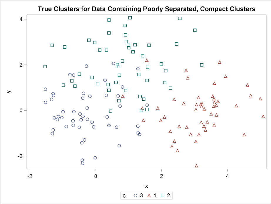
The following data set is similar to the first except that the three clusters are much closer together.
This example demonstrates the use of PROC FASTCLUS and five hierarchical methods available in
PROC CLUSTER. To help you compare methods, this example plots true, generated clusters. Also
included is a bubble plot of the density estimates obtained in conjunction with two-stage density
linkage in PROC CLUSTER. The following SAS statements produce Figure 11.2:
216 FChapter 11: Introduction to Clustering Procedures
data closer;
keep x y c;
n=50; scale=1;
mx=0; my=0; c=3; link generate;
mx=3; my=0; c=1; link generate;
mx=1; my=2; c=2; link generate;
stop;
generate:
do i=1 to n;
x=rannor(9)*scale+mx;
y=rannor(9)*scale+my;
output;
end;
return;
run;
title ’True Clusters for Data Containing Poorly Separated, Compact Clusters’;
proc sgplot;
scatter y=y x=x / group=c ;
run;
Figure 11.2 Data Containing Poorly Separated, Compact Clusters: Plot of True Clusters
Poorly Separated Clusters F217
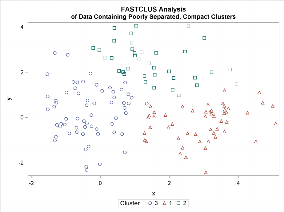
The following statements use the FASTCLUS procedure to find three clusters and then use the
SGPLOT procedure to plot the clusters. The following statements produce Figure 11.3:
proc fastclus data=closer out=out maxc=3 noprint;
var x y;
title ’FASTCLUS Analysis’;
title2 ’of Data Containing Poorly Separated, Compact Clusters’;
run;
proc sgplot;
scatter y=y x=x / group=cluster;
run;
Figure 11.3 Data Containing Poorly Separated, Compact Clusters: PROC FASTCLUS
218 FChapter 11: Introduction to Clustering Procedures
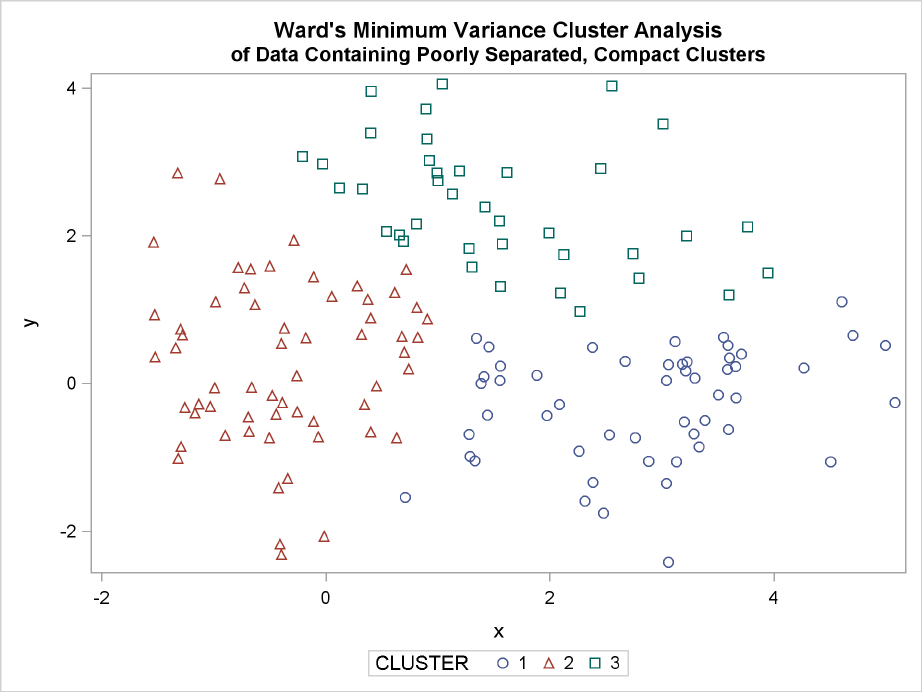
The following SAS statements produce Figure 11.4:
proc cluster data=closer outtree=tree method=ward noprint;
var x y;
run;
proc tree noprint out=out n=3;
copy x y;
title ’Ward’’s Minimum Variance Cluster Analysis’;
title2 ’of Data Containing Poorly Separated, Compact Clusters’;
run;
proc sgplot;
scatter y=y x=x / group=cluster;
run;
Figure 11.4 Data Containing Poorly Separated, Compact Clusters: PROC CLUSTER with
METHOD=WARD
Poorly Separated Clusters F219
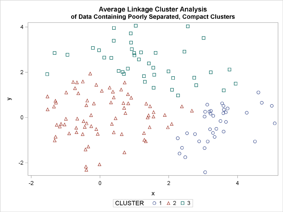
The following SAS statements produce Figure 11.5:
proc cluster data=closer outtree=tree method=average noprint;
var x y;
run;
proc tree noprint out=out n=3 dock=5;
copy x y;
title ’Average Linkage Cluster Analysis’;
title2 ’of Data Containing Poorly Separated, Compact Clusters’;
run;
proc sgplot;
scatter y=y x=x / group=cluster;
run;
Figure 11.5 Data Containing Poorly Separated, Compact Clusters: PROC CLUSTER with
METHOD=AVERAGE
220 FChapter 11: Introduction to Clustering Procedures
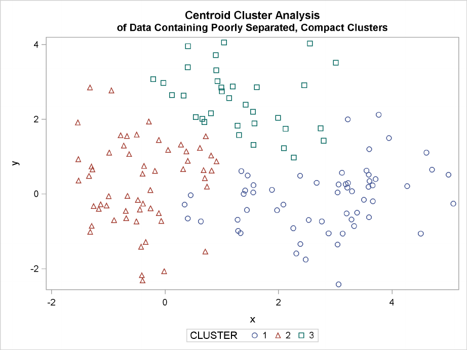
The following SAS statements produce Figure 11.6:
proc cluster data=closer outtree=tree
method=centroid noprint;
var x y;
run;
proc tree noprint out=out n=3 dock=5;
copy x y;
title ’Centroid Cluster Analysis’;
title2 ’of Data Containing Poorly Separated, Compact Clusters’;
run;
proc sgplot;
scatter y=y x=x / group=cluster;
run;
Figure 11.6 Data Containing Poorly Separated, Compact Clusters: PROC CLUSTER with
METHOD=CENTROID
The following SAS statements produce Figure 11.7 and Figure 11.8:
proc cluster data=closer outtree=tree
method=twostage k=10 noprint;
var x y;
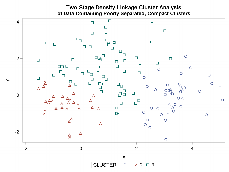
Poorly Separated Clusters F221
run;
proc tree noprint out=out n=3;
copy x y _dens_;
title ’Two-Stage Density Linkage Cluster Analysis’;
title2 ’of Data Containing Poorly Separated, Compact Clusters’;
run;
proc sgplot;
scatter y=y x=x / group=cluster;
run;
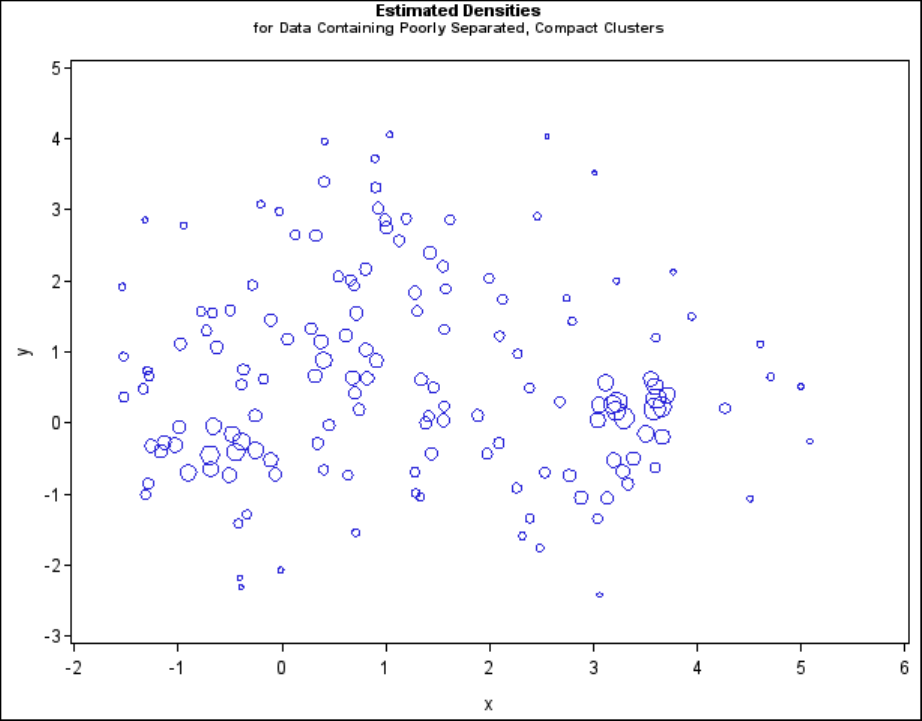
axis1 minor=none label=(angle=90 rotate=0);
axis2 minor=none;
proc gplot;
bubble y*x=_dens_/frame vaxis=axis1 haxis=axis2 bsize=10;
title h=1.2 ’Estimated Densities’;
title2 h=1 ’for Data Containing Poorly Separated, Compact Clusters’;
run;
Figure 11.7 Data Containing Poorly Separated, Compact Clusters: PROC CLUSTER with
METHOD=TWOSTAGE
222 FChapter 11: Introduction to Clustering Procedures
Figure 11.8 Data Containing Poorly Separated, Compact Clusters: PROC CLUSTER with
METHOD=TWOSTAGE
In two-stage density linkage, each cluster is a region surrounding a local maximum of the estimated
probability density function. If you think of the estimated density function as a landscape with
mountains and valleys, each mountain is a cluster, and the boundaries between clusters are placed
near the bottoms of the valleys.
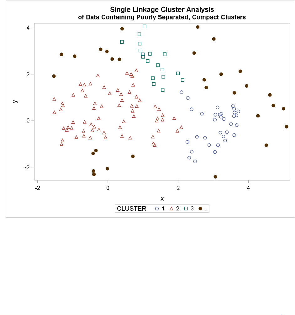
The following SAS statements produce Figure 11.9:
proc cluster data=closer outtree=tree
method=single noprint;
var x y;
run;
proc tree data=tree noprint out=out n=3 dock=5;
copy x y;
title ’Single Linkage Cluster Analysis’;
title2 ’of Data Containing Poorly Separated, Compact Clusters’;
run;
proc sgplot;
scatter y=y x=x / group=cluster;
run;
Multinormal Clusters of Unequal Size and Dispersion F223
Figure 11.9 Data Containing Poorly Separated, Compact Clusters: PROC CLUSTER with
METHOD=SINGLE
The two least squares methods, PROC FASTCLUS and Ward’s, yield the most uniform cluster sizes
and the best recovery of the true clusters. This result is expected since these two methods are biased
toward recovering compact clusters of equal size. With average linkage, the lower-left cluster is
too large; with the centroid method, the lower-right cluster is too large; and with two-stage density
linkage, the top cluster is too large. The single linkage analysis resembles average linkage except
for the large number of outliers resulting from the DOCK= option in the PROC TREE statement;
the outliers are plotted as filled circles (missing values).
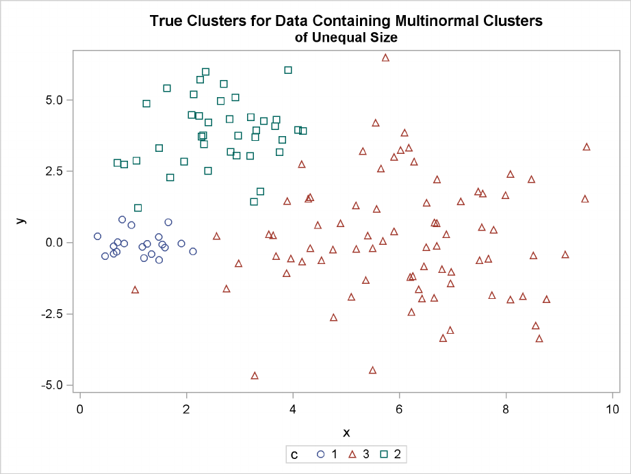
Multinormal Clusters of Unequal Size and Dispersion
In this example, there are three multinormal clusters that differ in size and dispersion. PROC FAST-
CLUS and five of the hierarchical methods available in PROC CLUSTER are used. To help you
compare methods, the true, generated clusters are plotted.
224 FChapter 11: Introduction to Clustering Procedures
The following SAS statements produce Figure 11.10:
data unequal;
keep x y c;
mx=1; my=0; n=20; scale=.5; c=1; link generate;
mx=6; my=0; n=80; scale=2.; c=3; link generate;
mx=3; my=4; n=40; scale=1.; c=2; link generate;
stop;
generate:
do i=1 to n;
x=rannor(1)*scale+mx;
y=rannor(1)*scale+my;
output;
end;
return;
title ’True Clusters for Data Containing Multinormal Clusters’;
title2 ’of Unequal Size’;
proc sgplot;
scatter y=y x=x / group=c;
run;
Figure 11.10 Data Containing Generated Clusters of Unequal Size
Multinormal Clusters of Unequal Size and Dispersion F225
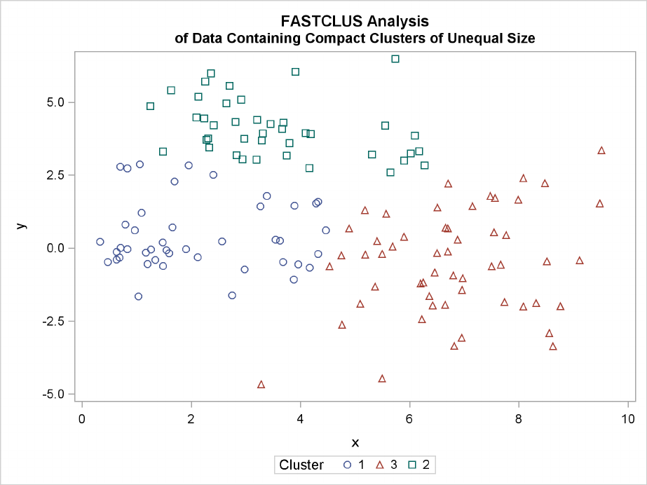
The following statements use the FASTCLUS procedure to find three clusters and then use the
SGPLOT procedure to plot the clusters. The following statements produce Figure 11.11:
proc fastclus data=unequal out=out maxc=3 noprint;
var x y;
title ’FASTCLUS Analysis’;
title2 ’of Data Containing Compact Clusters of Unequal Size’;
run;
proc sgplot;
scatter y=y x=x / group=cluster;
run;
Figure 11.11 Data Containing Compact Clusters of Unequal Size: PROC FASTCLUS
226 FChapter 11: Introduction to Clustering Procedures
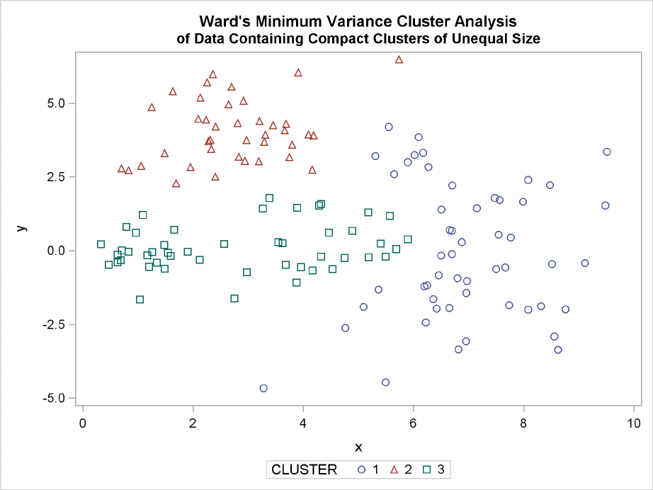
The following SAS statements produce Figure 11.12:
proc cluster data=unequal outtree=tree
method=ward noprint;
var x y;
run;
proc tree noprint out=out n=3;
copy x y;
title ’Ward’’s Minimum Variance Cluster Analysis’;
title2 ’of Data Containing Compact Clusters of Unequal Size’;
run;
proc sgplot;
scatter y=y x=x / group=cluster;
run;
Figure 11.12 Data Containing Compact Clusters of Unequal Size: PROC CLUSTER with
METHOD=WARD

Multinormal Clusters of Unequal Size and Dispersion F227
The following SAS statements produce Figure 11.13:
proc cluster data=unequal outtree=tree method=average
noprint;
var x y;
run;
proc tree noprint out=out n=3 dock=5;
copy x y;
title ’Average Linkage Cluster Analysis’;
title2 ’of Data Containing Compact Clusters of Unequal Size’;
run;
proc sgplot;
scatter y=y x=x / group=cluster;
run;
Figure 11.13 Data Containing Compact Clusters of Unequal Size: PROC CLUSTER with
METHOD=AVERAGE
228 FChapter 11: Introduction to Clustering Procedures
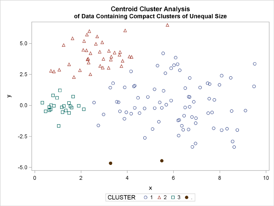
The following SAS statements produce Figure 11.14:
proc cluster data=unequal outtree=tree
method=centroid noprint;
var x y;
run;
proc tree noprint out=out n=3 dock=5;
copy x y;
title ’Centroid Cluster Analysis’;
title2 ’of Data Containing Compact Clusters of Unequal Size’;
run;
proc sgplot;
scatter y=y x=x / group=cluster;
run;
Figure 11.14 Data Containing Compact Clusters of Unequal Size: PROC CLUSTER with
METHOD=CENTROID
Multinormal Clusters of Unequal Size and Dispersion F229
The following SAS statements produce Figure 11.15 and Figure 11.16:
proc cluster data=unequal outtree=tree method=twostage
k=10 noprint;
var x y;
run;
proc tree noprint out=out n=3;
copy x y _dens_;
title ’Two-Stage Density Linkage Cluster Analysis’;
title2 ’of Data Containing Compact Clusters of Unequal Size’;
run;
proc sgplot;
scatter y=y x=x / group=cluster;
run;
axis1 minor=none label=(angle=90 rotate=0);
axis2 minor=none;
proc gplot;
bubble y*x=_dens_/frame vaxis=axis1 haxis=axis2 bsize=10;
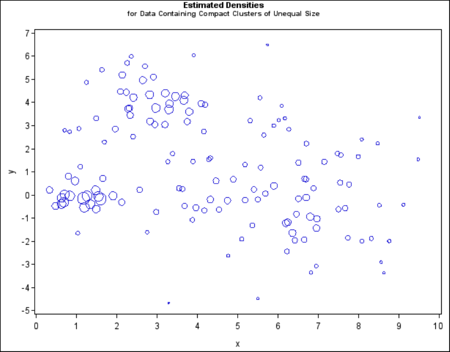
title h=1.2 ’Estimated Densities’;
title2 h=1 ’for Data Containing Compact Clusters of Unequal Size’;
run;
230 FChapter 11: Introduction to Clustering Procedures
Figure 11.15 Data Containing Compact Clusters of Unequal Size: PROC CLUSTER with
METHOD=TWOSTAGE
Multinormal Clusters of Unequal Size and Dispersion F231
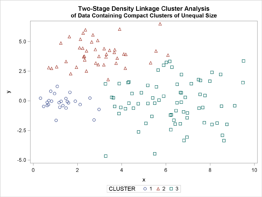
Figure 11.16 Data Containing Compact Clusters of Unequal Size: PROC CLUSTER with
METHOD=TWOSTAGE
232 FChapter 11: Introduction to Clustering Procedures
The following SAS statements produce Figure 11.17:
proc cluster data=unequal outtree=tree
method=single noprint;
var x y;
run;
proc tree data=tree noprint out=out n=3 dock=5;
copy x y;
title ’Single Linkage Cluster Analysis’;
title2 ’of Data Containing Compact Clusters of Unequal Size’;
run;
proc sgplot;
scatter y=y x=x / group=cluster;
run;
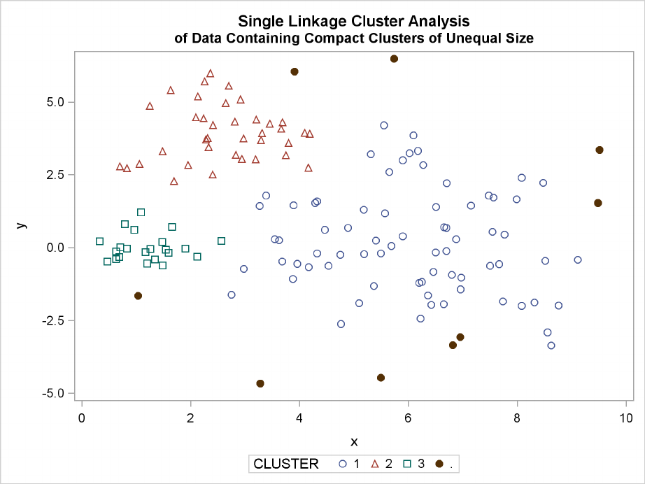
Figure 11.17 Data Containing Compact Clusters of Unequal Size: PROC CLUSTER with
METHOD=SINGLE
In the PROC FASTCLUS analysis, the smallest cluster, in the bottom-left portion of the plot, has
stolen members from the other two clusters, and the upper-left cluster has also acquired some obser-
vations that rightfully belong to the larger, lower-right cluster. With Ward’s method, the upper-left

Elongated Multinormal Clusters F233
cluster is separated correctly, but the lower-left cluster has taken a large bite out of the lower-right
cluster. For both of these methods, the clustering errors are in accord with the biases of the methods
to produce clusters of equal size. In the average linkage analysis, both the upper-left and lower-
left clusters have encroached on the lower-right cluster, thereby making the variances more nearly
equal than in the true clusters. The centroid method, which lacks the size and dispersion biases of
the previous methods, obtains an essentially correct partition.
Two-stage density linkage does almost as well, even though the compact shapes of these clusters
favor the traditional methods. Single linkage also produces excellent results.
Elongated Multinormal Clusters
In this example, the data are sampled from two highly elongated multinormal distributions with
equal covariance matrices. The following SAS statements produce Figure 11.18:
data elongate;
keep x y;
ma=8; mb=0; link generate;
ma=6; mb=8; link generate;
stop;
generate:
do i=1 to 50;
a=rannor(7)*6+ma;
b=rannor(7)+mb;
x=a-b;
y=a+b;
output;
end;
return;
proc fastclus data=elongate out=out maxc=2 noprint;
run;
%modstyle(name=ClusterStyle2,parent=Statistical,type=CLM,
markers=Circle Triangle circlefilled);
ods listing style=ClusterStyle;
proc sgplot;
scatter y=y x=x / group=cluster;
title ’FASTCLUS Analysis’;
title2 ’of Data Containing Parallel Elongated Clusters’;
run;
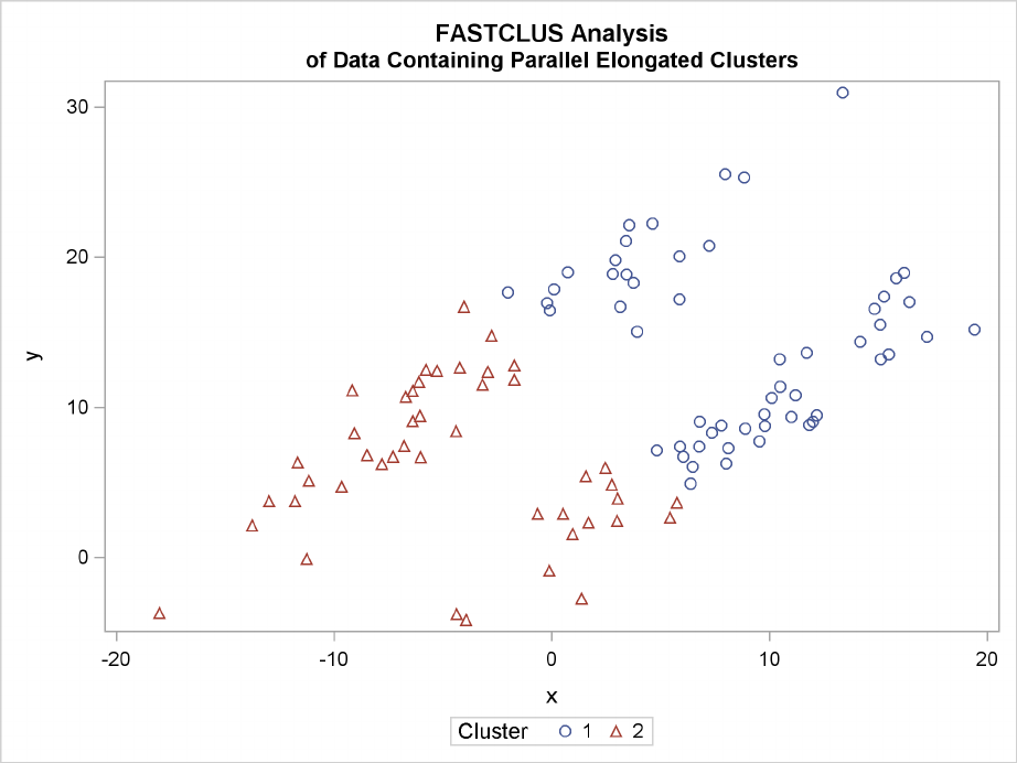
Notice that PROC FASTCLUS found two clusters, as requested by the MAXC= option. However,
it attempted to form spherical clusters, which are obviously inappropriate for these data.
234 FChapter 11: Introduction to Clustering Procedures
Figure 11.18 Data Containing Parallel Elongated Clusters: PROC FASTCLUS
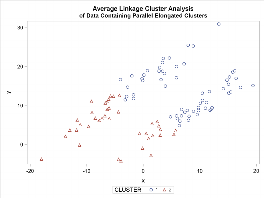
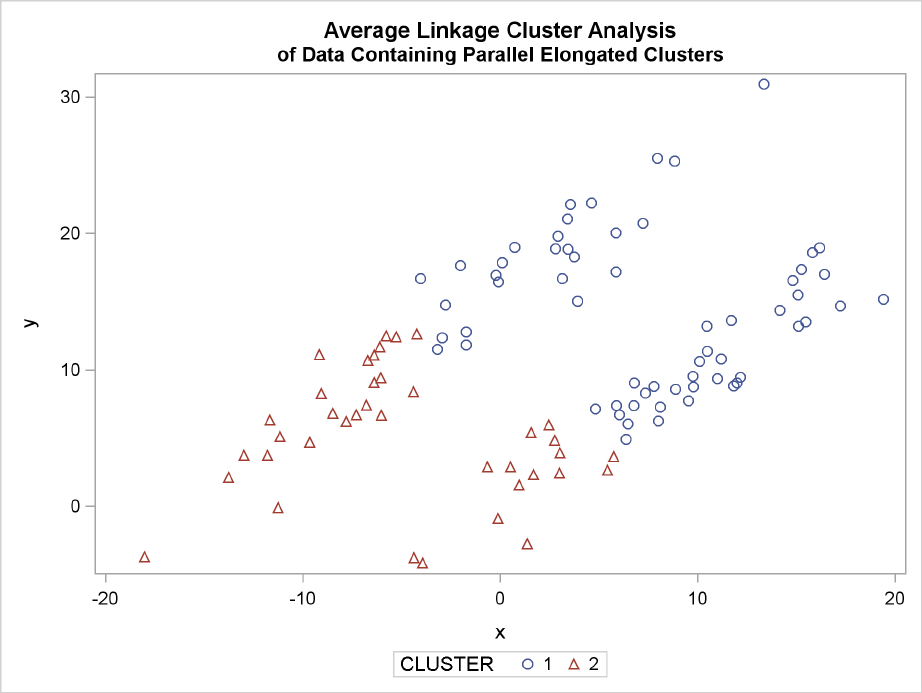
The following SAS statements produce Figure 11.19:
proc cluster data=elongate outtree=tree
method=average noprint;
run;
proc tree noprint out=out n=2 dock=5;
copy x y;
run;
proc sgplot;
scatter y=y x=x / group=cluster;
title ’Average Linkage Cluster Analysis’;
title2 ’of Data Containing Parallel Elongated Clusters’;
run;
Elongated Multinormal Clusters F235
Figure 11.19 Data Containing Parallel Elongated Clusters: PROC CLUSTER with
METHOD=AVERAGE
The following SAS statements produce Figure 11.20:
proc cluster data=elongate outtree=tree
method=twostage k=10 noprint;
run;
proc tree noprint out=out n=2;
copy x y;
run;
proc sgplot;
scatter y=y x=x / group=cluster;
title ’Two-Stage Density Linkage Cluster Analysis’;
title2 ’of Data Containing Parallel Elongated Clusters’;
run;
236 FChapter 11: Introduction to Clustering Procedures
Figure 11.20 Data Containing Parallel Elongated Clusters: PROC CLUSTER with
METHOD=TWOSTAGE
PROC FASTCLUS and average linkage fail miserably. Ward’s method and the centroid method (not
shown) produce almost the same results. Two-stage density linkage, however, recovers the correct
clusters. Single linkage (not shown) finds the same clusters as two-stage density linkage except for
some outliers.
In this example, the population clusters have equal covariance matrices. If the within-cluster co-
variances are known, the data can be transformed to make the clusters spherical so that any of the
clustering methods can find the correct clusters. But when you are doing a cluster analysis, you
do not know what the true clusters are, so you cannot calculate the within-cluster covariance ma-
trix. Nevertheless, it is sometimes possible to estimate the within-cluster covariance matrix without
knowing the cluster membership or even the number of clusters, using an approach invented by Art,
Gnanadesikan, and Kettenring (1982). A method for obtaining such an estimate is available in the
ACECLUS procedure.
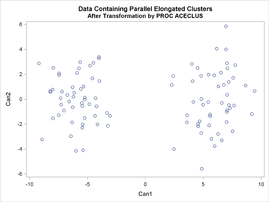
In the following analysis, PROC ACECLUS transforms the variables X and Y into the canonical
variables CAN1 and CAN2. The latter are plotted and then used in a cluster analysis by Ward’s
method. The clusters are then plotted with the original variables X and Y.

Elongated Multinormal Clusters F237
The following SAS statements produce Figure 11.21 and Figure 11.22:
proc aceclus data=elongate out=ace p=.1;
var x y;
title ’ACECLUS Analysis’;
title2 ’of Data Containing Parallel Elongated Clusters’;
run;
proc sgplot;
scatter y=can2 x=can1;
title ’Data Containing Parallel Elongated Clusters’;
title2 ’After Transformation by PROC ACECLUS’;
run;
Figure 11.21 Data Containing Parallel Elongated Clusters: PROC ACECLUS
ACECLUS Analysis
of Data Containing Parallel Elongated Clusters
The ACECLUS Procedure
Approximate Covariance Estimation for Cluster Analysis
Observations 100 Proportion 0.1000
Variables 2 Converge 0.00100
Means and Standard Deviations
Standard
Variable Mean Deviation
x 2.6406 8.3494
y 10.6488 6.8420
COV: Total Sample Covariances
x y
x 69.71314819 24.24268934
y 24.24268934 46.81324861
Initial Within-Cluster Covariance Estimate = Full Covariance Matrix
Threshold = 0.328478

238 FChapter 11: Introduction to Clustering Procedures
Figure 11.21 continued
Iteration History
Pairs
RMS Distance Within Convergence
Iteration Distance Cutoff Cutoff Measure
------------------------------------------------------------
1 2.000 0.657 672.0 0.673685
2 9.382 3.082 716.0 0.006963
3 9.339 3.068 760.0 0.008362
4 9.437 3.100 824.0 0.009656
5 9.359 3.074 889.0 0.010269
6 9.267 3.044 955.0 0.011276
7 9.208 3.025 999.0 0.009230
8 9.230 3.032 1052.0 0.011394
9 9.226 3.030 1091.0 0.007924
10 9.173 3.013 1121.0 0.007993
WARNING: Iteration limit exceeded.
ACE: Approximate Covariance Estimate Within Clusters
x y
x 9.299329632 8.215362614
y 8.215362614 8.937753936
Eigenvalues of Inv(ACE)*(COV-ACE)
Eigenvalue Difference Proportion Cumulative
1 36.7091 33.1672 0.9120 0.9120
2 3.5420 0.0880 1.0000
Eigenvectors (Raw Canonical Coefficients)
Can1 Can2
x -.748392 0.109547
y 0.736349 0.230272
Standardized Canonical Coefficients
Can1 Can2
x -6.24866 0.91466
y 5.03812 1.57553
Elongated Multinormal Clusters F239
Figure 11.22 Data Containing Parallel Elongated Clusters after Transformation by PROC
ACECLUS
The following SAS statements produce Figure 11.23:
proc cluster data=ace outtree=tree method=ward noprint;
var can1 can2;
copy x y;
run;
proc tree noprint out=out n=2;
copy x y;
run;
proc sgplot;
scatter y=y x=x / group=cluster;
title ’Ward’’s Minimum Variance Cluster Analysis’;
title2 ’of Data Containing Parallel Elongated Clusters’;
title3 ’After Transformation by PROC ACECLUS’;
run;

240 FChapter 11: Introduction to Clustering Procedures
Figure 11.23 Transformed Data Containing Parallel Elongated Clusters: PROC CLUSTER with
METHOD=WARD
Nonconvex Clusters
If the population clusters have very different covariance matrices, using PROC ACECLUS is of
no avail. Although methods exist for estimating multinormal clusters with unequal covariance ma-
trices (Wolfe 1970; Symons 1981; Everitt and Hand 1981; Titterington, Smith, and Makov 1985;
McLachlan and Basford 1988), these methods tend to have serious problems with initialization and
might converge to degenerate solutions. For unequal covariance matrices or radically nonnormal
distributions, the best approach to cluster analysis is through nonparametric density estimation, as in
density linkage. The next example illustrates population clusters with nonconvex density contours.
The following SAS statements produce Figure 11.24:
data noncon;
keep x y;
do i=1 to 100;
a=i*.0628319;
x=cos(a)+(i>50)+rannor(7)*.1;
y=sin(a)+(i>50)*.3+rannor(7)*.1;
output;
end;
Nonconvex Clusters F241
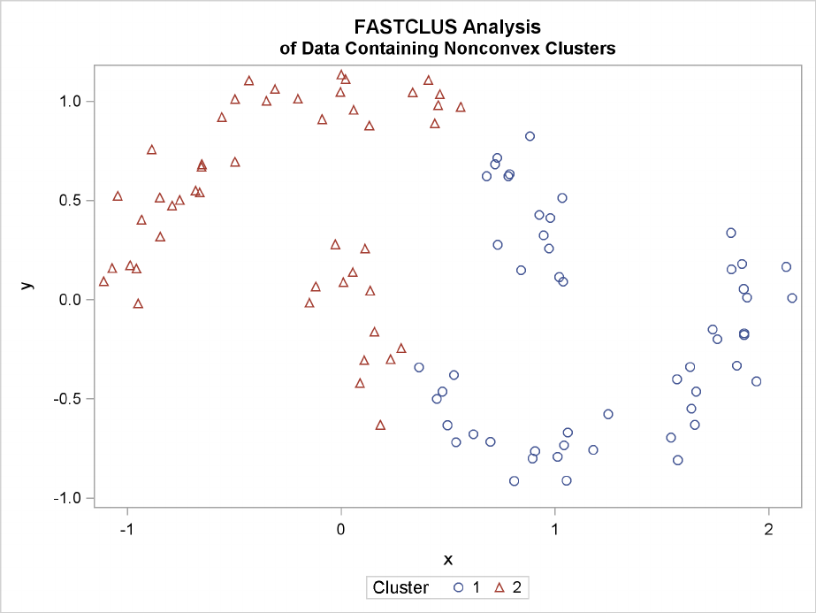
proc fastclus data=noncon out=out maxc=2 noprint;
run;
proc sgplot;
scatter y=y x=x / group=cluster;
title ’FASTCLUS Analysis’;
title2 ’of Data Containing Nonconvex Clusters’;
run;
Figure 11.24 Data Containing Nonconvex Clusters: PROC FASTCLUS
The following SAS statements produce Figure 11.25:
proc cluster data=noncon outtree=tree
method=centroid noprint;
run;
proc tree noprint out=out n=2 dock=5;
copy x y;
run;
proc sgplot;
scatter y=y x=x / group=cluster;
title ’Centroid Cluster Analysis’;
title2 ’of Data Containing Nonconvex Clusters’;
run;
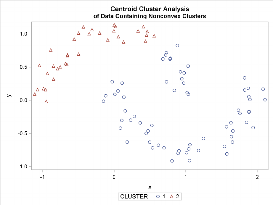
242 FChapter 11: Introduction to Clustering Procedures
Figure 11.25 Data Containing Nonconvex Clusters: PROC CLUSTER with
METHOD=CENTROID
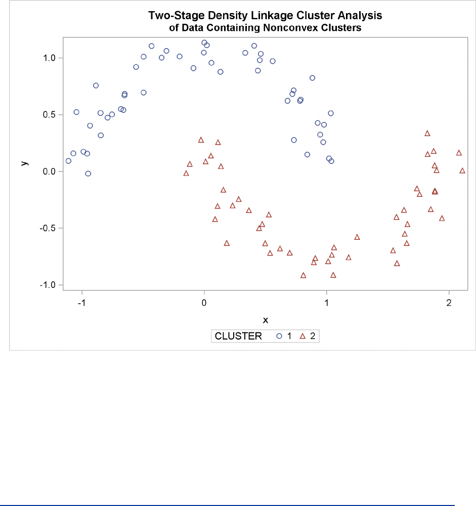
The following SAS statements produce Figure 11.26:
proc cluster data=noncon outtree=tree
method=twostage k=10 noprint;
run;
proc tree noprint out=out n=2;
copy x y;
run;
proc sgplot;
scatter y=y x=x / group=cluster;
title ’Two-Stage Density Linkage Cluster Analysis’;
title2 ’of Data Containing Nonconvex Clusters’;
run;
The Number of Clusters F243
Figure 11.26 Data Containing Nonconvex Clusters: PROC CLUSTER with
METHOD=TWOSTAGE
Ward’s method and average linkage (not shown) do better than PROC FASTCLUS but not as well as
the centroid method. Two-stage density linkage recovers the correct clusters, as does single linkage
(not shown).
The preceding examples are intended merely to illustrate some of the properties of clustering meth-
ods in common use. If you intend to perform a cluster analysis, you should consult more systematic
and rigorous studies of the properties of clustering methods, such as Milligan (1980).
The Number of Clusters
There are no completely satisfactory methods that can be used for determining the number of pop-
ulation clusters for any type of cluster analysis (Everitt 1979; Hartigan, J. A. 1985; Bock 1985).
If your purpose in clustering is dissection—that is, to summarize the data without trying to uncover
real clusters—it might suffice to look at R square for each variable and pooled over all variables.
Plots of R square against the number of clusters are useful.
244 FChapter 11: Introduction to Clustering Procedures
It is always a good idea to look at your data graphically. If you have only two or three variables,
use PROC SGPLOT to make scatter plots identifying the clusters. With more variables, use PROC
CANDISC to compute canonical variables for plotting.
Ordinary significance tests, such as analysis of variance Ftests, are not valid for testing differences
between clusters. Since clustering methods attempt to maximize the separation between clusters,
the assumptions of the usual significance tests, parametric or nonparametric, are drastically violated.
For example, if you take a sample of 100 observations from a single univariate normal distribution,
have PROC FASTCLUS divide it into two clusters, and run a ttest between the clusters, you usually
obtain a p-value of less than 0.0001. For the same reason, methods that purport to test for clusters
against the null hypothesis that objects are assigned randomly to clusters (such as McClain and Rao
1975; Klastorin 1983) are useless.
Most valid tests for clusters either have intractable sampling distributions or involve null hypotheses
for which rejection is uninformative. For clustering methods based on distance matrices, a popular
null hypothesis is that all permutations of the values in the distance matrix are equally likely (Ling
1973; Hubert 1974). Using this null hypothesis, you can do a permutation test or a rank test. The
trouble with the permutation hypothesis is that, with any real data, the null hypothesis is implausible
even if the data do not contain clusters. Rejecting the null hypothesis does not provide any useful
information (Hubert and Baker 1977).
Another common null hypothesis is that the data are a random sample from a multivariate nor-
mal distribution (Wolfe 1970, 1978; Duda and Hart 1973; Lee 1979). The multivariate normal
null hypothesis arises naturally in normal mixture models (Titterington, Smith, and Makov 1985;
McLachlan and Basford 1988). Unfortunately, the likelihood ratio test statistic does not have the
usual asymptotic 2distribution because the regularity conditions do not hold. Approximations to
the asymptotic distribution of the likelihood ratio have been suggested (Wolfe 1978), but the ade-
quacy of these approximations is debatable (Everitt 1981; Thode, Mendell, and Finch 1988). For
small samples, bootstrapping seems preferable (McLachlan and Basford 1988). Bayesian inference
provides a promising alternative to likelihood ratio tests for the number of mixture components for
both normal mixtures and other types of distributions (Binder 1978, 1981; Banfield and Raftery
1993; Bensmail et al. 1997).
The multivariate normal null hypothesis is better than the permutation null hypothesis, but it is not
satisfactory because there is typically a high probability of rejection if the data are sampled from a
distribution with lower kurtosis than a normal distribution, such as a uniform distribution. The tables
in Englemann and Hartigan (1969), for example, generally lead to rejection of the null hypothesis
when the data are sampled from a uniform distribution. Hawkins, Muller, and ten Krooden (1982,
pp. 337–340) discuss a highly conservative Bonferroni method for the use of hypothesis testing. The
conservativeness of this approach might compensate to some extent for the liberalness exhibited by
tests based on normal distributions when the population is uniform.
Perhaps a better null hypothesis is that the data are sampled from a uniform distribution (Hartigan
1978; Arnold 1979; Sarle 1983). The uniform null hypothesis leads to conservative error rates when
the data are sampled from a strongly unimodal distribution such as the normal. However, in two or
more dimensions and depending on the test statistic, the results can be very sensitive to the shape of
the region of support of the uniform distribution. Sarle (1983) suggests using a hyperbox with sides
proportional in length to the singular values of the centered coordinate matrix.
The Number of Clusters F245
Given that the uniform distribution provides an appropriate null hypothesis, there are still serious
difficulties in obtaining sampling distributions. Some asymptotic results are available (Hartigan
1978, 1985; Pollard 1981; Bock 1985) for the within-cluster sum of squares, the criterion that
PROC FASTCLUS and Ward’s minimum variance method attempt to optimize. No distributional
theory for finite sample sizes has yet appeared. Currently, the only practical way to obtain sampling
distributions for realistic sample sizes is by computer simulation.
Arnold (1979) used simulation to derive tables of the distribution of a criterion based on the deter-
minant of the within-cluster sum of squares matrix jWj. Both normal and uniform null distributions
were used. Having obtained clusters with either PROC FASTCLUS or PROC CLUSTER, you can
compute Arnold’s criterion with the ANOVA or CANDISC procedure. Arnold’s tables provide a
conservative test because PROC FASTCLUS and PROC CLUSTER attempt to minimize the trace
of Wrather than the determinant. Marriott (1971, 1975) also provides useful information about jWj
as a criterion for the number of clusters.
Sarle (1983) used extensive simulations to develop the cubic clustering criterion (CCC), which can
be used for crude hypothesis testing and estimating the number of population clusters. The CCC is
based on the assumption that a uniform distribution on a hyperrectangle will be divided into clusters
shaped roughly like hypercubes. In large samples that can be divided into the appropriate number
of hypercubes, this assumption gives very accurate results. In other cases the approximation is
generally conservative. For details about the interpretation of the CCC, consult Sarle (1983).
Milligan and Cooper (1985) and Cooper and Milligan (1988) compared 30 methods of estimating
the number of population clusters by using four hierarchical clustering methods. The three criteria
that performed best in these simulation studies with a high degree of error in the data were a pseudo
Fstatistic developed by Calinski and Harabasz (1974), a statistic referred to as Je.2/=Je.1/ by
Duda and Hart (1973) that can be transformed into a pseudo t2statistic, and the cubic clustering
criterion. The pseudo Fstatistic and the CCC are displayed by PROC FASTCLUS; these two statis-
tics and the pseudo t2statistic, which can be applied only to hierarchical methods, are displayed
by PROC CLUSTER. It might be advisable to look for consensus among the three statistics—that
is, local peaks of the CCC and pseudo Fstatistic combined with a small value of the pseudo t2
statistic and a larger pseudo t2for the next cluster fusion. It must be emphasized that these criteria
are appropriate only for compact or slightly elongated clusters, preferably clusters that are roughly
multivariate normal.
Recent research has tended to deemphasize mixture models in favor of nonparametric models in
which clusters correspond to modes in the probability density function. Hartigan and Hartigan
(1985) and P. M. Hartigan (1985) developed a test of unimodality versus bimodality in the univariate
case.
Nonparametric tests for the number of clusters can also be based on nonparametric density esti-
mates. This approach requires much weaker assumptions than mixture models, namely, that the
observations are sampled independently and that the distribution can be estimated nonparametri-
cally. Silverman (1986) describes a bootstrap test for the number of modes using a Gaussian kernel
density estimate, but problems have been reported with this method under the uniform null distri-
bution. Further developments in nonparametric methods are given by Mueller and Sawitzki (1991),
Minnotte (1992), and Polonik (1993). All of these methods suffer from heavy computational re-
quirements.

246 FChapter 11: Introduction to Clustering Procedures
One useful descriptive approach to the number-of-clusters problem is provided by Wong and
Schaack (1982), based on a kth-nearest-neighbor density estimate. The kth-nearest-neighbor clus-
tering method developed by Wong and Lane (1983) is applied with varying values of k. Each value
of kyields an estimate of the number of modal clusters. If the estimated number of modal clusters
is constant for a wide range of kvalues, there is strong evidence of at least that many modes in the
population. A plot of the estimated number of modes against kcan be highly informative. Attempts
to derive a formal hypothesis test from this diagnostic plot have met with difficulties, but a simula-
tion approach similar to Silverman’s (1986) does seem to work (Girman 1994). The simulation, of
course, requires considerable computer time.
Sarle and Kuo (1993) document a less expensive approximate nonparametric test for the number
of clusters that has been implemented in the MODECLUS procedure. This test sacrifices statistical
efficiency for computational efficiency. The method for conducting significance tests is described
in the chapter on the MODECLUS procedure. This method has the following useful features:
No distributional assumptions are required.
The choice of smoothing parameter is not critical since you can try any number of different
values.
The data can be coordinates or distances.
Time and space requirements for the significance tests are no worse than those for obtaining
the clusters.
The power is high enough to be useful for practical purposes.
The method for computing the p-values is based on a series of plausible approximations. There
are as yet no rigorous proofs that the method is infallible. Neither are there any asymptotic results.
However, simulations for sample sizes ranging from 20 to 2000 indicate that the p-values are almost
always conservative. The only case discovered so far in which the p-values are liberal is a uniform
distribution in one dimension for which the simulated error rates exceed the nominal significance
level only slightly for a limited range of sample sizes.
References
Anderberg, M. R. (1973), Cluster Analysis for Applications, New York: Academic Press.
Arnold, S. J. (1979), “A Test for Clusters,” Journal of Marketing Research, 16, 545–551.
Art, D., Gnanadesikan, R., and Kettenring, R. (1982), “Data-based Metrics for Cluster Analysis,”
Utilitas Mathematica, 21A, 75–99.
Banfield, J. D. and Raftery, A.E. (1993), “Model-Based Gaussian and Non-Gaussian Clustering,”
Biometrics, 49, 803–821.
Bensmail, H., Celeux, G., Raftery, A. E., and Robert, C. P. (1997), “Inference in Model-Based
Cluster Analysis,” Statistics and Computing, 7, 1–10.
References F247
Bezdek, J. C. (1981), Pattern Recognition with Fuzzy Objective Function Algorithms, New York:
Plenum Press.
Bezdek, J. C. and Pal, S. K. (Editor) (1992), Fuzzy Models for Pattern Recognition, IEEE Press,
New York.
Binder, D. A. (1978), “Bayesian Cluster Analysis,” Biometrika, 65, 31–38.
Binder, D. A. (1981), “Approximations to Bayesian Clustering Rules,” Biometrika, 68, 275–285.
Blashfield, R. K. and Aldenderfer, M. S. (1978), “The Literature on Cluster Analysis,” Multivariate
Behavioral Research, 13, 271–295.
Bock, H. H. (1985), “On Some Significance Tests in Cluster Analysis,” Journal of Classification, 2,
77–108.
Calinski, T. and Harabasz, J. (1974), “A Dendrite Method for Cluster Analysis,” Communications
in Statistics, 3, 1–27.
Cooper, M. C. and Milligan, G. W. (1988), “The Effect of Error on Determining the Number of
Clusters,” Proceedings of the International Workshop on Data Analysis, Decision Support and Ex-
pert Knowledge Representation in Marketing and Related Areas of Research, 319–328.
Duda, R. O. and Hart, P. E. (1973), Pattern Classification and Scene Analysis, New York: John
Wiley & Sons.
Duran, B. S. and Odell, P. L. (1974), Cluster Analysis, New York: Springer-Verlag.
Englemann, L. and Hartigan, J. A. (1969), “Percentage Points of a Test for Clusters,” Journal of the
American Statistical Association, 64, 1647–1648.
Everitt, B. S. (1979), “Unresolved Problems in Cluster Analysis,” Biometrics, 35, 169–181.
Everitt, B. S. (1980), Cluster Analysis, Second Edition, London: Heineman Educational Books.
Everitt, B. S. (1981), “A Monte Carlo Investigation of the Likelihood Ratio Test for the Number of
Components in a Mixture of Normal Distributions,” Multivariate Behavioral Research, 16, 171–80.
Everitt, B. S. and Hand, D. J. (1981), Finite Mixture Distributions, New York: Chapman & Hall.
Gersho, A. and Gray, R. M. (1992), Vector Quantization and Signal Compression, Kluwer Aca-
demic Publishers.
Girman, C. J. (1994), “Cluster Analysis and Classification Tree Methodology as an Aid to Improve
Understanding of Benign Prostatic Hyperplasia,” Ph.D. diss., Department of Biostatistics, Univer-
sity of North Carolina.
Good, I. J. (1977), “The Botryology of Botryology,” in Classification and Clustering, ed. J. Van
Ryzin, New York: Academic Press.
Harman, H. H. (1976), Modern Factor Analysis, Third Edition, Chicago: University of Chicago
Press.
248 FChapter 11: Introduction to Clustering Procedures
Hartigan, J. A. (1975), Clustering Algorithms, New York: John Wiley & Sons.
Hartigan, J. A. (1977), “Distribution Problems in Clustering,” in Classification and Clustering, ed.
J. Van Ryzin, New York: Academic Press.
Hartigan, J. A. (1978), “Asymptotic Distributions for Clustering Criteria,” Annals of Statistics, 6,
117–131.
Hartigan, J. A. (1981), “Consistency of Single Linkage for High-Density Clusters,” Journal of the
American Statistical Association, 76, 388–394.
Hartigan, J. A. (1985), “Statistical Theory in Clustering,” Journal of Classification, 2, 63–76.
Hartigan, J. A. and Hartigan, P. M. (1985), “The Dip Test of Unimodality,” Annals of Statistics, 13,
70–84.
Hartigan, P. M. (1985), “Computation of the Dip Statistic to Test for Unimodality,” Applied Statis-
tics, 34, 320–325.
Hawkins, D. M., Muller, M. W., and ten Krooden, J. A. (1982), “Cluster Analysis,” in Topics in
Applied Multivariate Analysis, ed. D. M. Hawkins, Cambridge: Cambridge University Press.
Hubert, L. (1974), “Approximate Evaluation Techniques for the Single-Link and Complete-Link
Hierarchical Clustering Procedures,” Journal of the American Statistical Association, 69, 698–704.
Hubert, L. J. and Baker, F. B. (1977), “An Empirical Comparison of Baseline Models for Goodness-
of-Fit in r-Diameter Hierarchical Clustering,” in Classification and Clustering, ed. J. Van Ryzin,
New York: Academic Press.
Kaufman, L. and Rousseeuw, P. J. (1990), Finding Groups in Data, New York: John Wiley & Sons.
Klastorin, T. D. (1983), “Assessing Cluster Analysis Results,” Journal of Marketing Research, 20,
92–98.
Lee, K. L. (1979), “Multivariate Tests for Clusters,” Journal of the American Statistical Association,
74, 708–714.
Ling, R. F. (1973), “A Probability Theory of Cluster Analysis,” Journal of the American Statistical
Association, 68, 159–169.
MacQueen, J. B. (1967), “Some Methods for Classification and Analysis of Multivariate Observa-
tions,” Proceedings of the Fifth Berkeley Symposium on Mathematical Statistics and Probability, 1,
281–297.
Marriott, F. H. C. (1971), “Practical Problems in a Method of Cluster Analysis,” Biometrics, 27,
501–514.
Marriott, F. H. C. (1975), “Separating Mixtures of Normal Distributions,” Biometrics, 31, 767–769.
Massart, D. L. and Kaufman, L. (1983), The Interpretation of Analytical Chemical Data by the Use
of Cluster Analysis, New York: John Wiley & Sons.
References F249
McClain, J. O. and Rao, V. R. (1975), “CLUSTISZ: A Program to Test for the Quality of Clustering
of a Set of Objects,” Journal of Marketing Research, 12, 456–460.
McLachlan, G. J. and Basford, K. E. (1988), Mixture Models, New York: Marcel Dekker.
Mezzich, J. E. and Solomon, H. (1980), Taxonomy and Behavioral Science, New York: Academic
Press.
Milligan, G. W. (1980), “An Examination of the Effect of Six Types of Error Perturbation on Fifteen
Clustering Algorithms,” Psychometrika, 45, 325–342.
Milligan, G. W. (1981), “A Review of Monte Carlo Tests of Cluster Analysis,” Multivariate Behav-
ioral Research, 16, 379–407.
Milligan, G. W. and Cooper, M. C. (1985), “An Examination of Procedures for Determining the
Number of Clusters in a Data Set,” Psychometrika, 50, 159–179.
Minnotte, M. C. (1992), “A Test of Mode Existence with Applications to Multimodality,” Ph.D.
diss., Rice University, Department of Statistics.
Mueller, D. W. and Sawitzki, G. (1991), “Excess Mass Estimates and Tests for Multimodality,”
JASA 86, 738–746.
Pollard, D. (1981), “Strong Consistency of k-Means Clustering,” Annals of Statistics, 9, 135–140.
Polonik, W. (1993), “Measuring Mass Concentrations and Estimating Density Contour Clusters—
An Excess Mass Approach,” Technical Report, Beitraege zur Statistik Nr. 7, University of Heidel-
berg.
Sarle, W. S. (1982), “Cluster Analysis by Least Squares,” Proceedings of the Seventh Annual SAS
Users Group International Conference, 651–653.
Sarle, W. S. (1983), Cubic Clustering Criterion, SAS Technical Report A-108, Cary, NC: SAS
Institute Inc.
Sarle, W. S. and Kuo, An-Hsiang (1993), The MODECLUS Procedure, SAS Technical Report P-
256, Cary, NC: SAS Institute Inc.
Scott, A. J. and Symons, M. J. (1971), “Clustering Methods Based on Likelihood Ratio Criteria,”
Biometrics, 27, 387–397.
Silverman, B. W. (1986), Density Estimation, New York: Chapman & Hall.
Sneath, P. H. A. and Sokal, R. R. (1973), Numerical Taxonomy, San Francisco: W. H. Freeman.
Spath, H. (1980), Cluster Analysis Algorithms, Chichester, England: Ellis Horwood.
Symons, M. J. (1981), “Clustering Criteria and Multivariate Normal Mixtures,” Biometrics, 37,
35–43.
Thode, H. C., Jr., Mendell, N. R., and Finch, S. J. (1988), “Simulated Percentage Points for the
Null Distribution of the Likelihood Ratio Test for a Mixture of Two Normals,” Biometrics, 44,
250 FChapter 11: Introduction to Clustering Procedures
1195–1201.
Titterington, D. M., Smith, A. F. M., and Makov, U. E. (1985), Statistical Analysis of Finite Mixture
Distributions, New York: John Wiley & Sons.
Ward, J. H. (1963), “Hierarchical Grouping to Optimize an Objective Function,” Journal of the
American Statistical Association, 58, 236–244.
Wolfe, J. H. (1970), “Pattern Clustering by Multivariate Mixture Analysis,” Multivariate Behavioral
Research, 5, 329–350.
Wolfe, J. H. (1978), “Comparative Cluster Analysis of Patterns of Vocational Interest,” Multivariate
Behavioral Research, 13, 33–44.
Wong, M. A. (1982), “A Hybrid Clustering Method for Identifying High-Density Clusters,” Journal
of the American Statistical Association, 77, 841–847.
Wong, M. A. and Lane, T. (1983), “A kth Nearest Neighbor Clustering Procedure,” Journal of the
Royal Statistical Society, Series B, 45, 362–368.
Wong, M. A. and Schaack, C. (1982), “Using the kth Nearest Neighbor Clustering Procedure to
Determine the Number of Subpopulations,” American Statistical Association 1982 Proceedings of
the Statistical Computing Section, 40–48.

Your Turn
We welcome your feedback.
If you have comments about this book, please send them to
yourturn@sas.com. Include the full title and page numbers (if
applicable).
If you have comments about the software, please send them to
suggest@sas.com.

SAS® Publishing Delivers!
Whether you are new to the work force or an experienced professional, you need to distinguish yourself in this rapidly
changing and competitive job market. SAS® Publishing provides you with a wide range of resources to help you set
yourself apart. Visit us online at support.sas.com/bookstore.
SAS® Press
Need to learn the basics? Struggling with a programming problem? You’ll find the expert answers that you
need in example-rich books from SAS Press. Written by experienced SAS professionals from around the
world, SAS Press books deliver real-world insights on a broad range of topics for all skill levels.
support.sas.com/saspress
SAS® Documentation
To successfully implement applications using SAS software, companies in every industry and on every
continent all turn to the one source for accurate, timely, and reliable information: SAS documentation.
We currently produce the following types of reference documentation to improve your work experience:
• Onlinehelpthatisbuiltintothesoftware.
• Tutorialsthatareintegratedintotheproduct.
• ReferencedocumentationdeliveredinHTMLandPDF– free on the Web.
• Hard-copybooks. support.sas.com/publishing
SAS® Publishing News
Subscribe to SAS Publishing News to receive up-to-date information about all new SAS titles, author
podcasts, and new Web site features via e-mail. Complete instructions on how to subscribe, as well as
access to past issues, are available at our Web site. support.sas.com/spn
SAS and all other SAS Institute Inc. product or service names are registered trademarks or trademarks of SAS Institute Inc. in the USA and other countries. ® indicates USA registration.
Otherbrandandproductnamesaretrademarksoftheirrespectivecompanies.©2009SASInstituteInc.Allrightsreserved.518177_1US.0109
