SAS/STAT 9.2 User's Guide: The FASTCLUS Procedure (Book Excerpt) SAS Users Guide
User Manual: Pdf
Open the PDF directly: View PDF ![]() .
.
Page Count: 64

SAS/STAT®9.2 User’s Guide
The FASTCLUS Procedure
(Book Excerpt)
SAS®Documentation
This document is an individual chapter from SAS/STAT®9.2 User’s Guide.
The correct bibliographic citation for the complete manual is as follows: SAS Institute Inc. 2008. SAS/STAT®9.2
User’s Guide. Cary, NC: SAS Institute Inc.
Copyright © 2008, SAS Institute Inc., Cary, NC, USA
All rights reserved. Produced in the United States of America.
For a Web download or e-book: Your use of this publication shall be governed by the terms established by the vendor
at the time you acquire this publication.
U.S. Government Restricted Rights Notice: Use, duplication, or disclosure of this software and related documentation
by the U.S. government is subject to the Agreement with SAS Institute and the restrictions set forth in FAR 52.227-19,
Commercial Computer Software-Restricted Rights (June 1987).
SAS Institute Inc., SAS Campus Drive, Cary, North Carolina 27513.
1st electronic book, March 2008
2nd electronic book, February 2009
SAS®Publishing provides a complete selection of books and electronic products to help customers use SAS software to
its fullest potential. For more information about our e-books, e-learning products, CDs, and hard-copy books, visit the
SAS Publishing Web site at support.sas.com/publishing or call 1-800-727-3228.
SAS®and all other SAS Institute Inc. product or service names are registered trademarks or trademarks of SAS Institute
Inc. in the USA and other countries. ® indicates USA registration.
Other brand and product names are registered trademarks or trademarks of their respective companies.

Chapter 34
The FASTCLUS Procedure
Contents
Overview: FASTCLUS Procedure .......................... 1621
Background .................................. 1622
Getting Started: FASTCLUS Procedure ....................... 1624
Syntax: FASTCLUS Procedure ............................ 1632
PROC FASTCLUS Statement ......................... 1632
BY Statement ................................. 1640
FREQ Statement ................................ 1640
ID Statement .................................. 1641
VAR Statement ................................. 1641
WEIGHT Statement .............................. 1641
Details: FASTCLUS Procedure ........................... 1642
Updates in the FASTCLUS Procedure ..................... 1642
Missing Values ................................. 1642
Output Data Sets ................................ 1643
Computational Resources ........................... 1647
Using PROC FASTCLUS ........................... 1647
Displayed Output ................................ 1649
ODS Table Names ............................... 1652
Examples: FASTCLUS Procedure .......................... 1653
Example 34.1: Fisher’s Iris Data ....................... 1653
Example 34.2: Outliers ............................ 1662
References ...................................... 1673
Overview: FASTCLUS Procedure
The FASTCLUS procedure performs a disjoint cluster analysis on the basis of distances computed
from one or more quantitative variables. The observations are divided into clusters such that every
observation belongs to one and only one cluster; the clusters do not form a tree structure as they do
in the CLUSTER procedure. If you want separate analysis for different numbers of clusters, you
can run PROC FASTCLUS once for each analysis. Alternatively, to do hierarchical clustering on
a large data set, use PROC FASTCLUS to find initial clusters, and then use those initial clusters as
input to PROC CLUSTER.

1622 FChapter 34: The FASTCLUS Procedure
By default, the FASTCLUS procedure uses Euclidean distances, so the cluster centers are based
on least squares estimation. This kind of clustering method is often called a k-means model, since
the cluster centers are the means of the observations assigned to each cluster when the algorithm is
run to complete convergence. Each iteration reduces the least squares criterion until convergence is
achieved.
Often there is no need to run the FASTCLUS procedure to convergence. PROC FASTCLUS is
designed to find good clusters (but not necessarily the best possible clusters) with only two or three
passes through the data set. The initialization method of PROC FASTCLUS guarantees that, if
there exist clusters such that all distances between observations in the same cluster are less than all
distances between observations in different clusters, and if you tell PROC FASTCLUS the correct
number of clusters to find, it can always find such a clustering without iterating. Even with clusters
that are not as well separated, PROC FASTCLUS usually finds initial seeds that are sufficiently
good that few iterations are required. Hence, by default, PROC FASTCLUS performs only one
iteration.
The initialization method used by the FASTCLUS procedure makes it sensitive to outliers. PROC
FASTCLUS can be an effective procedure for detecting outliers because outliers often appear as
clusters with only one member.
The FASTCLUS procedure can use an Lp(least pth powers) clustering criterion (Spath 1985,
pp. 62–63) instead of the least squares (L2) criterion used in k-means clustering methods. The
LEAST=poption specifies the power pto be used. Using the LEAST= option increases execution
time since more iterations are usually required, and the default iteration limit is increased when
you specify LEAST=p. Values of pless than 2 reduce the effect of outliers on the cluster centers
compared with least squares methods; values of pgreater than 2 increase the effect of outliers.
The FASTCLUS procedure is intended for use with large data sets, with 100 or more observations.
With small data sets, the results can be highly sensitive to the order of the observations in the data
set.
PROC FASTCLUS uses algorithms that place a larger influence on variables with larger variance,
so it might be necessary to standardize the variables before performing the cluster analysis. See the
“Using PROC FASTCLUS” section for standardization details.
PROC FASTCLUS produces brief summaries of the clusters it finds. For more extensive examina-
tion of the clusters, you can request an output data set containing a cluster membership variable.
Background
The FASTCLUS procedure combines an effective method for finding initial clusters with a standard
iterative algorithm for minimizing the sum of squared distances from the cluster means. The result
is an efficient procedure for disjoint clustering of large data sets. PROC FASTCLUS was directly
inspired by Hartigan’s (1975) leader algorithm and MacQueen’s (1967) k-means algorithm. PROC
FASTCLUS uses a method that Anderberg (1973) calls nearest centroid sorting. A set of points
called cluster seeds is selected as a first guess of the means of the clusters. Each observation is
assigned to the nearest seed to form temporary clusters. The seeds are then replaced by the means
Background F1623
of the temporary clusters, and the process is repeated until no further changes occur in the clusters.
Similar techniques are described in most references on clustering (Anderberg 1973; Hartigan 1975;
Everitt 1980; Spath 1980).
The FASTCLUS procedure differs from other nearest centroid sorting methods in the way the initial
cluster seeds are selected. The importance of initial seed selection is demonstrated by Milligan
(1980).
The clustering is done on the basis of Euclidean distances computed from one or more numeric
variables. If there are missing values, PROC FASTCLUS computes an adjusted distance by using
the nonmissing values. Observations that are very close to each other are usually assigned to the
same cluster, while observations that are far apart are in different clusters.
The FASTCLUS procedure operates in four steps:
1. Observations called cluster seeds are selected.
2. If you specify the DRIFT option, temporary clusters are formed by assigning each observation
to the cluster with the nearest seed. Each time an observation is assigned, the cluster seed is
updated as the current mean of the cluster. This method is sometimes called incremental,
on-line, or adaptive training.
3. If the maximum number of iterations is greater than zero, clusters are formed by assigning
each observation to the nearest seed. After all observations are assigned, the cluster seeds are
replaced by either the cluster means or other location estimates (cluster centers) appropriate
to the LEAST=poption. This step can be repeated until the changes in the cluster seeds
become small or zero (MAXITER=n1).
4. Final clusters are formed by assigning each observation to the nearest seed.
If PROC FASTCLUS runs to complete convergence, the final cluster seeds will equal the cluster
means or cluster centers. If PROC FASTCLUS terminates before complete convergence, which
often happens with the default settings, the final cluster seeds might not equal the cluster means or
cluster centers. If you want complete convergence, specify CONVERGE=0 and a large value for
the MAXITER= option.
The initial cluster seeds must be observations with no missing values. You can specify the maximum
number of seeds (and, hence, clusters) by using the MAXCLUSTERS= option. You can also specify
a minimum distance by which the seeds must be separated by using the RADIUS= option.
PROC FASTCLUS always selects the first complete (no missing values) observation as the first
seed. The next complete observation that is separated from the first seed by at least the distance
specified in the RADIUS= option becomes the second seed. Later observations are selected as new
seeds if they are separated from all previous seeds by at least the radius, as long as the maximum
number of seeds is not exceeded.
If an observation is complete but fails to qualify as a new seed, PROC FASTCLUS considers using
it to replace one of the old seeds. Two tests are made to see if the observation can qualify as a new
seed.
First, an old seed is replaced if the distance between the observation and the closest seed is greater
than the minimum distance between seeds. The seed that is replaced is selected from the two

1624 FChapter 34: The FASTCLUS Procedure
seeds that are closest to each other. The seed that is replaced is the one of these two with the
shortest distance to the closest of the remaining seeds when the other seed is replaced by the current
observation.
If the observation fails the first test for seed replacement, a second test is made. The observation
replaces the nearest seed if the smallest distance from the observation to all seeds other than the
nearest one is greater than the shortest distance from the nearest seed to all other seeds. If the
observation fails this test, PROC FASTCLUS goes on to the next observation.
You can specify the REPLACE= option to limit seed replacement. You can omit the second test
for seed replacement (REPLACE=PART), causing PROC FASTCLUS to run faster, but the seeds
selected might not be as widely separated as those obtained by the default method. You can also
suppress seed replacement entirely by specifying REPLACE=NONE. In this case, PROC FAST-
CLUS runs much faster, but you must choose a good value for the RADIUS= option in order to
get good clusters. This method is similar to Hartigan’s (1975, pp. 74–78) leader algorithm and the
simple cluster seeking algorithm described by Tou and Gonzalez (1974, pp. 90–92).
Getting Started: FASTCLUS Procedure
The following example demonstrates how to use the FASTCLUS procedure to compute disjoint
clusters of observations in a SAS data set.
The data in this example are measurements taken on 159 freshwater fish caught from the same lake
(Laengelmavesi) near Tampere in Finland. This data set is available from the Data Archive of the
Journal of Statistics Education. The complete data set is displayed in Chapter 82, “The STEPDISC
Procedure.”
The species (bream, parkki, pike, perch, roach, smelt, and whitefish), weight, three different length
measurements (measured from the nose of the fish to the beginning of its tail, the notch of its tail,
and the end of its tail), height, and width of each fish are tallied. The height and width are recorded
as percentages of the third length variable.
Suppose that you want to group empirically the fish measurements into clusters and that you want to
associate the clusters with the species. You can use the FASTCLUS procedure to perform a cluster
analysis.
The following DATA step creates the SAS data set Fish:
proc format;
value specfmt
1=’Bream’
2=’Roach’
3=’Whitefish’
4=’Parkki’
5=’Perch’
6=’Pike’
7=’Smelt’;
run;
Getting Started: FASTCLUS Procedure F1625
data fish (drop=HtPct WidthPct);
title ’Fish Measurement Data’;
input Species Weight Length1 Length2 Length3 HtPct WidthPct @@;
*** transform variables;
if Weight <= 0 or Weight =. then delete;
Weight3=Weight**(1/3);
Height=HtPct*Length3/(Weight3*100);
Width=WidthPct*Length3/(Weight3*100);
Length1=Length1/Weight3;
Length2=Length2/Weight3;
Length3=Length3/Weight3;
logLengthRatio=log(Length3/Length1);
format Species specfmt.;
symbol = put(Species, specfmt2.);
datalines;
1 242.0 23.2 25.4 30.0 38.4 13.4 1 290.0 24.0 26.3 31.2 40.0 13.8
1 340.0 23.9 26.5 31.1 39.8 15.1 1 363.0 26.3 29.0 33.5 38.0 13.3
1 430.0 26.5 29.0 34.0 36.6 15.1 1 450.0 26.8 29.7 34.7 39.2 14.2
1 500.0 26.8 29.7 34.5 41.1 15.3 1 390.0 27.6 30.0 35.0 36.2 13.4
1 450.0 27.6 30.0 35.1 39.9 13.8 1 500.0 28.5 30.7 36.2 39.3 13.7
1 475.0 28.4 31.0 36.2 39.4 14.1 1 500.0 28.7 31.0 36.2 39.7 13.3
1 500.0 29.1 31.5 36.4 37.8 12.0 1 . 29.5 32.0 37.3 37.3 13.6
1 600.0 29.4 32.0 37.2 40.2 13.9 1 600.0 29.4 32.0 37.2 41.5 15.0
... more lines ...
7 9.8 11.4 12.0 13.2 16.7 8.7 7 12.2 11.5 12.2 13.4 15.6 10.4
7 13.4 11.7 12.4 13.5 18.0 9.4 7 12.2 12.1 13.0 13.8 16.5 9.1
7 19.7 13.2 14.3 15.2 18.9 13.6 7 19.9 13.8 15.0 16.2 18.1 11.6
;
The double trailing at sign (@@) in the INPUT statement specifies that observations are input from
each line until all values are read. The variables are rescaled in order to adjust for dimensionality.
Because the new variables Weight3–logLengthRatio depend on the variable Weight, observations with
missing values for Weight are not added to the data set. Consequently, there are 157 observations in
the SAS data set Fish.
In the Fish data set, the variables are not measured in the same units and cannot be assumed to have
equal variance. Therefore, it is necessary to standardize the variables before performing the cluster
analysis.
The following statements standardize the variables and perform a cluster analysis on the standard-
ized data:
proc standard data=Fish out=Stand mean=0 std=1;
var Length1 logLengthRatio Height Width Weight3;
proc fastclus data=Stand out=Clust
maxclusters=7 maxiter=100 ;
var Length1 logLengthRatio Height Width Weight3;
run;

1626 FChapter 34: The FASTCLUS Procedure
The STANDARD procedure is first used to standardize all the analytical variables to a mean of 0 and
standard deviation of 1. The procedure creates the output data set Stand to contain the transformed
variables.
The FASTCLUS procedure then uses the data set Stand as input and creates the data set Clust.
This output data set contains the original variables and two new variables, Cluster and Distance.
The variable Cluster contains the cluster number to which each observation has been assigned. The
variable Distance gives the distance from the observation to its cluster seed.
It is usually desirable to try several values of the MAXCLUSTERS= option. A reasonable beginning
for this example is to use MAXCLUSTERS=7, since there are seven species of fish represented in
the data set Fish.
The VAR statement specifies the variables used in the cluster analysis.
The results from this analysis are displayed in the following figures.
Figure 34.1 Initial Seeds Used in the FASTCLUS Procedure
Fish Measurement Data
The FASTCLUS Procedure
Replace=FULL Radius=0 Maxclusters=7 Maxiter=100 Converge=0.02
Initial Seeds
logLength
Cluster Length1 Ratio Height Width Weight3
-----------------------------------------------------------------------------
1 1.388338414 -0.979577858 -1.594561848 -2.254050655 2.103447062
2 -1.117178039 -0.877218192 -0.336166276 2.528114070 1.170706464
3 2.393997461 -0.662642015 -0.930738701 -2.073879107 -1.839325419
4 -0.495085516 -0.964041012 -0.265106856 -0.028245072 1.536846394
5 -0.728772773 0.540096664 1.130501398 -1.207930053 -1.107018207
6 -0.506924177 0.748211648 1.762482687 0.211507596 1.368987826
7 1.573996573 -0.796593995 -0.824217424 1.561715851 -1.607942726
Criterion Based on Final Seeds = 0.3979
Figure 34.1 displays the table of initial seeds used for each variable and cluster. The first line in the
figure displays the option settings for REPLACE, RADIUS, MAXCLUSTERS, and MAXITER.
These options, with the exception of MAXCLUSTERS and MAXITER, are set at their respective
default values (REPLACE=FULL, RADIUS=0). Both the MAXCLUSTERS= and MAXITER=
options are set in the PROC FASTCLUS statement.
Next, PROC FASTCLUS produces a table of summary statistics for the clusters. Figure 34.2 dis-
plays the number of observations in the cluster (frequency) and the root mean squared standard
deviation. The next two columns display the largest Euclidean distance from the cluster seed to any
observation within the cluster and the number of the nearest cluster.
The last column of the table displays the distance between the centroid of the nearest cluster and
the centroid of the current cluster. A centroid is the point having coordinates that are the means of
all the observations in the cluster.

Getting Started: FASTCLUS Procedure F1627
Figure 34.2 Cluster Summary Table from the FASTCLUS Procedure
Cluster Summary
Maximum Distance
RMS Std from Seed Radius Nearest
Cluster Frequency Deviation to Observation Exceeded Cluster
-----------------------------------------------------------------------------
1 17 0.5064 1.7781 4
2 19 0.3696 1.5007 4
3 13 0.3803 1.7135 1
4 13 0.4161 1.3976 7
5 11 0.2466 0.6966 6
6 34 0.3563 1.5443 5
7 50 0.4447 2.3915 4
Cluster Summary
Distance Between
Cluster Cluster Centroids
-----------------------------
1 2.5106
2 1.5510
3 2.6704
4 1.4266
5 1.7301
6 1.7301
7 1.4266
Figure 34.3 displays the table of statistics for the variables. The table lists for each variable the
total standard deviation, the pooled within-cluster standard deviation and the R-square value for
predicting the variable from the cluster. The ratio of between-cluster variance to within-cluster
variance (R2to 1R2) appears in the last column.
Figure 34.3 Statistics for Variables Used in the FASTCLUS Procedure
Statistics for Variables
Variable Total STD Within STD R-Square RSQ/(1-RSQ)
------------------------------------------------------------------------
Length1 1.00000 0.31428 0.905030 9.529606
logLengthRatio 1.00000 0.39276 0.851676 5.741989
Height 1.00000 0.20917 0.957929 22.769295
Width 1.00000 0.55558 0.703200 2.369270
Weight3 1.00000 0.47251 0.785323 3.658162
OVER-ALL 1.00000 0.40712 0.840631 5.274764
Pseudo F Statistic = 131.87
Approximate Expected Over-All R-Squared = 0.57420

1628 FChapter 34: The FASTCLUS Procedure
The pseudo Fstatistic, approximate expected overall R square, and cubic clustering criterion (CCC)
are listed at the bottom of the figure. You can compare values of these statistics by running PROC
FASTCLUS with different values for the MAXCLUSTERS= option. The R square and CCC values
are not valid for correlated variables.
Values of the cubic clustering criterion greater than 2 or 3 indicate good clusters. Values between
0 and 2 indicate potential clusters, but they should be taken with caution; large negative values can
indicate outliers.
PROC FASTCLUS next produces the within-cluster means and standard deviations of the variables,
displayed in Figure 34.4.
Figure 34.4 Cluster Means and Standard Deviations from the FASTCLUS Procedure
Cluster Means
logLength
Cluster Length1 Ratio Height Width Weight3
-----------------------------------------------------------------------------
1 1.747808245 -0.868605685 -1.327226832 -1.128760946 0.806373599
2 -0.405231510 -0.979113021 -0.281064162 1.463094486 1.060450065
3 2.006796315 -0.652725165 -1.053213440 -1.224020795 -1.826752838
4 -0.136820952 -1.039312574 -0.446429482 0.162596336 0.278560318
5 -0.850130601 0.550190242 1.245156076 -0.836585750 -0.567022647
6 -0.843912827 1.522291347 1.511408739 -0.380323563 0.763114370
7 -0.165570970 -0.048881276 -0.353723615 0.546442064 -0.668780782
Cluster Standard Deviations
logLength
Cluster Length1 Ratio Height Width Weight3
-----------------------------------------------------------------------------
1 0.3418476428 0.3544065543 0.1666302451 0.6172880027 0.7944227150
2 0.3129902863 0.3592350778 0.1369052680 0.5467406493 0.3720119097
3 0.2962504486 0.1740941675 0.1736086707 0.7528475622 0.0905232968
4 0.3254364840 0.2836681149 0.1884592934 0.4543390702 0.6612055341
5 0.1781837609 0.0745984121 0.2056932592 0.2784540794 0.3832002850
6 0.2273744242 0.3385584051 0.2046010964 0.5143496067 0.4025849044
7 0.3734733622 0.5275768119 0.2551130680 0.5721303628 0.4223181710
It is useful to study further the clusters calculated by the FASTCLUS procedure. One method is
to look at a frequency tabulation of the clusters with other classification variables. The following
statements invoke the FREQ procedure to crosstabulate the empirical clusters with the variable
Species:
proc freq data=Clust;
tables Species*Cluster;
run;

Getting Started: FASTCLUS Procedure F1629
Figure 34.5 displays the marked division between clusters.
Figure 34.5 Frequency Table of Cluster versus Species
Fish Measurement Data
The FREQ Procedure
Table of Species by CLUSTER
Species CLUSTER(Cluster)
Frequency |
Percent |
Row Pct |
Col Pct | 1| 2| 3| 4| Total
----------+--------+--------+--------+--------+
Bream | 0 | 0 | 0 | 0 | 34
| 0.00 | 0.00 | 0.00 | 0.00 | 21.66
| 0.00 | 0.00 | 0.00 | 0.00 |
| 0.00 | 0.00 | 0.00 | 0.00 |
----------+--------+--------+--------+--------+
Roach | 0 | 0 | 0 | 0 | 19
| 0.00 | 0.00 | 0.00 | 0.00 | 12.10
| 0.00 | 0.00 | 0.00 | 0.00 |
| 0.00 | 0.00 | 0.00 | 0.00 |
----------+--------+--------+--------+--------+
Whitefish | 0 | 2 | 0 | 1 | 6
| 0.00 | 1.27 | 0.00 | 0.64 | 3.82
| 0.00 | 33.33 | 0.00 | 16.67 |
| 0.00 | 10.53 | 0.00 | 7.69 |
----------+--------+--------+--------+--------+
Parkki | 0 | 0 | 0 | 0 | 11
| 0.00 | 0.00 | 0.00 | 0.00 | 7.01
| 0.00 | 0.00 | 0.00 | 0.00 |
| 0.00 | 0.00 | 0.00 | 0.00 |
----------+--------+--------+--------+--------+
Perch | 0 | 17 | 0 | 12 | 56
| 0.00 | 10.83 | 0.00 | 7.64 | 35.67
| 0.00 | 30.36 | 0.00 | 21.43 |
| 0.00 | 89.47 | 0.00 | 92.31 |
----------+--------+--------+--------+--------+
Pike | 17 | 0 | 0 | 0 | 17
| 10.83 | 0.00 | 0.00 | 0.00 | 10.83
| 100.00 | 0.00 | 0.00 | 0.00 |
| 100.00 | 0.00 | 0.00 | 0.00 |
----------+--------+--------+--------+--------+
Smelt | 0 | 0 | 13 | 0 | 14
| 0.00 | 0.00 | 8.28 | 0.00 | 8.92
| 0.00 | 0.00 | 92.86 | 0.00 |
| 0.00 | 0.00 | 100.00 | 0.00 |
----------+--------+--------+--------+--------+
Total 17 19 13 13 157
10.83 12.10 8.28 8.28 100.00
(Continued)

1630 FChapter 34: The FASTCLUS Procedure
Figure 34.5 continued
Fish Measurement Data
The FREQ Procedure
Table of Species by CLUSTER
Species CLUSTER(Cluster)
Frequency |
Percent |
Row Pct |
Col Pct | 5| 6| 7| Total
----------+--------+--------+--------+
Bream | 0 | 34 | 0 | 34
| 0.00 | 21.66 | 0.00 | 21.66
| 0.00 | 100.00 | 0.00 |
| 0.00 | 100.00 | 0.00 |
----------+--------+--------+--------+
Roach | 0 | 0 | 19 | 19
| 0.00 | 0.00 | 12.10 | 12.10
| 0.00 | 0.00 | 100.00 |
| 0.00 | 0.00 | 38.00 |
----------+--------+--------+--------+
Whitefish | 0 | 0 | 3 | 6
| 0.00 | 0.00 | 1.91 | 3.82
| 0.00 | 0.00 | 50.00 |
| 0.00 | 0.00 | 6.00 |
----------+--------+--------+--------+
Parkki | 11 | 0 | 0 | 11
| 7.01 | 0.00 | 0.00 | 7.01
| 100.00 | 0.00 | 0.00 |
| 100.00 | 0.00 | 0.00 |
----------+--------+--------+--------+
Perch | 0 | 0 | 27 | 56
| 0.00 | 0.00 | 17.20 | 35.67
| 0.00 | 0.00 | 48.21 |
| 0.00 | 0.00 | 54.00 |
----------+--------+--------+--------+
Pike | 0 | 0 | 0 | 17
| 0.00 | 0.00 | 0.00 | 10.83
| 0.00 | 0.00 | 0.00 |
| 0.00 | 0.00 | 0.00 |
----------+--------+--------+--------+
Smelt | 0 | 0 | 1 | 14
| 0.00 | 0.00 | 0.64 | 8.92
| 0.00 | 0.00 | 7.14 |
| 0.00 | 0.00 | 2.00 |
----------+--------+--------+--------+
Total 11 34 50 157
7.01 21.66 31.85 100.00
Getting Started: FASTCLUS Procedure F1631
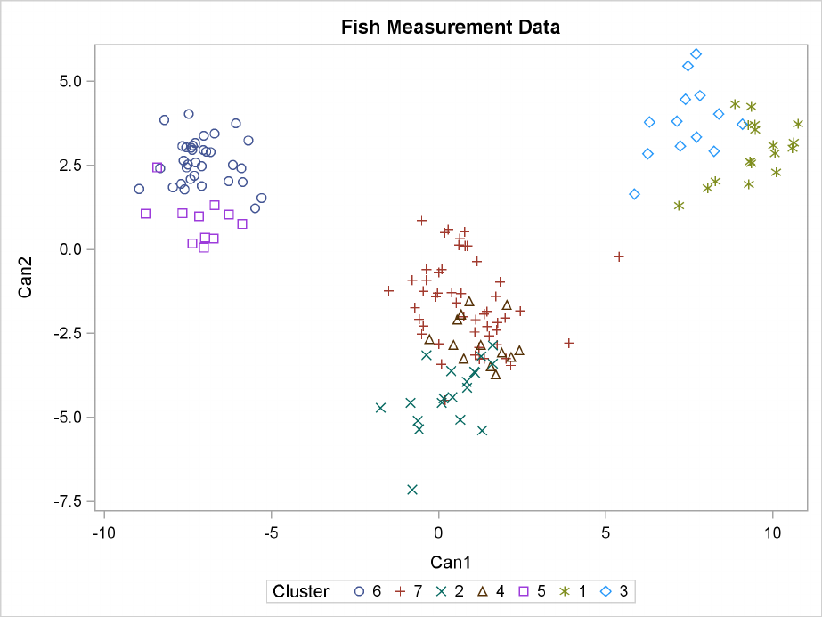
For cases in which you have three or more clusters, you can use the CANDISC and SGPLOT proce-
dures to obtain a graphical check on the distribution of the clusters. In the following statements, the
CANDISC and SGPLOT procedures are used to compute canonical variables and plot the clusters:
proc candisc data=Clust out=Can noprint;
class Cluster;
var Length1 logLengthRatio Height Width Weight3;
proc sgplot data=Can;
scatter y=Can2 x=Can1 / group=Cluster ;
run;
First, the CANDISC procedure is invoked to perform a canonical discriminant analysis by using the
data set Clust and creating the output SAS data set Can. The NOPRINT option suppresses display
of the output. The CLASS statement specifies the variable Cluster to define groups for the analysis.
The VAR statement specifies the variables used in the analysis.
Next, the SGPLOT procedure plots the two canonical variables from PROC CANDISC, Can1 and
Can2. The PLOT statement specifies the variable Cluster as the identification variable. The resulting
plot (Figure 34.6) illustrates the spatial separation of the clusters calculated in the FASTCLUS
procedure.
Figure 34.6 Plot of Canonical Variables and Cluster Value

1632 FChapter 34: The FASTCLUS Procedure
Syntax: FASTCLUS Procedure
The following statements are available in the FASTCLUS procedure:
PROC FASTCLUS <DATA=SAS-data-set >
<MAXCLUSTERS=n>
<RADIUS=t>;
VAR variables ;
ID variables ;
FREQ variable ;
WEIGHT variable ;
BY variables ;
Usually you need only the VAR statement in addition to the PROC FASTCLUS statement. The
BY, FREQ, ID, VAR, and WEIGHT statements are described in alphabetical order after the PROC
FASTCLUS statement.
PROC FASTCLUS Statement
PROC FASTCLUS MAXCLUSTERS= n| RADIUS=t<options >;
You must specify the MAXCLUSTERS= option or RADIUS= option or both in the PROC FAST-
CLUS statement.
MAXCLUSTERS=n
MAXC=n
specifies the maximum number of clusters permitted. If you omit the MAXCLUSTERS=
option, a value of 100 is assumed.
RADIUS=t
R=t
establishes the minimum distance criterion for selecting new seeds. No observation is con-
sidered as a new seed unless its minimum distance to previous seeds exceeds the value given
by the RADIUS= option. The default value is 0. If you specify the REPLACE=RANDOM
option, the RADIUS= option is ignored.

PROC FASTCLUS Statement F1633
You can specify the following options in the PROC FASTCLUS statement. Table 34.1 summarizes
the options.
Table 34.1 PROC FASTCLUS Statement Options
Option Description
Specify input and output data sets
DATA= specifies input data set
INSTAT= specifies input SAS data set previously created by
the OUTSTAT= option
SEED= specifies input SAS data set for selecting initial
cluster seeds
VARDEF= specifies divisor for variances
Output Data Processing
CLUSTER= specifies name for cluster membership variable in
OUTSEED= and OUT= data sets
CLUSTERLABEL= specifies label for cluster membership variable in
OUTSEED= and OUT= data sets
OUT= specifies output SAS data set containing original
data and cluster assignments
OUTITER specifies writing to OUTSEED= data set on every
iteration
OUTSEED= or MEAN= specifies output SAS data set containing cluster
centers
OUTSTAT= specifies output SAS data set containing statistics
Initial Clusters
DRIFT permits cluster to seeds to drift during initializa-
tion
MAXCLUSTERS= specifies maximum number of clusters
RADIUS= specifies minimum distance for selecting new
seeds
RANDOM= specifies seed to initializes pseudo-random num-
ber generator
REPLACE= specifies seed replacement method
Clustering Methods
CONVERGE= specifies convergence criterion
DELETE= deletes cluster seeds with few observations
LEAST= optimizes an Lpcriterion, where 1p 1
MAXITER= specifies maximum number of iterations
STRICT prevents an observation from being assigned to a
cluster if its distance to the nearest cluster seed is
large

1634 FChapter 34: The FASTCLUS Procedure
Table 34.1 continued
Option Description
Arcane Algorithmic Options
BINS= specifies number of bins used for computing me-
dians for LEAST=1
HC= specifies criterion for updating the homotopy pa-
rameter
HP= specifies initial value of the homotopy parameter
IRLS uses an iteratively reweighted least squares
method instead of the modified Ekblom-Newton
method for 1<p<2
Missing Values
IMPUTE imputes missing values after final cluster assign-
ment
NOMISS excludes observations with missing values
Control Displayed Output
DISTANCE displays distances between cluster centers
LIST displays cluster assignments for all observations
NOPRINT suppresses displayed output
SHORT suppresses display of large matrices
SUMMARY suppresses display of all results except for the
cluster summary
The following list provides details on these options. The list is in alphabetical order.
BINS=n
specifies the number of bins used in the bin-sort algorithm for computing medians for
LEAST=1. By default, PROC FASTCLUS uses from 10 to 100 bins, depending on the
amount of memory available. Larger values use more memory and make each iteration some-
what slower, but they can reduce the number of iterations. Smaller values have the opposite
effect. The minimum value of nis 5.
CLUSTER=name
specifies a name for the variable in the OUTSEED= and OUT= data sets that indicates cluster
membership. The default name for this variable is CLUSTER.
CLUSTERLABEL=name
specifies a label for the variable CLUSTER in the OUTSEED= and OUT= data sets. By
default this variable has no label.
CONVERGE=c
CONV=c
specifies the convergence criterion. Any nonnegative value is permitted. The default value is
0.0001 for all values of pif LEAST=pis explicitly specified; otherwise, the default value is
0.02. Iterations stop when the maximum relative change in the cluster seeds is less than or
PROC FASTCLUS Statement F1635
equal to the convergence criterion and additional conditions on the homotopy parameter, if
any, are satisfied (see the HP= option). The relative change in a cluster seed is the distance
between the old seed and the new seed divided by a scaling factor. If you do not specify the
LEAST= option, the scaling factor is the minimum distance between the initial seeds. If you
specify the LEAST= option, the scaling factor is an L1scale estimate and is recomputed on
each iteration. Specify the CONVERGE= option only if you specify a MAXITER= value
greater than 1.
DATA=SAS-data-set
specifies the input data set containing observations to be clustered. If you omit the DATA=
option, the most recently created SAS data set is used. The data must be coordinates, not
distances, similarities, or correlations.
DELETE=n
deletes cluster seeds to which nor fewer observations are assigned. Deletion occurs after
processing for the DRIFT option is completed and after each iteration specified by the MAX-
ITER= option. Cluster seeds are not deleted after the final assignment of observations to
clusters, so in rare cases a final cluster might not have more than nmembers. The DELETE=
option is ineffective if you specify MAXITER=0 and do not specify the DRIFT option. By
default, no cluster seeds are deleted.
DISTANCE | DIST
computes distances between the cluster means.
DRIFT
executes the second of the four steps described in the section “Background” on page 1622.
After initial seed selection, each observation is assigned to the cluster with the nearest seed.
After an observation is processed, the seed of the cluster to which it is assigned is recalculated
as the mean of the observations currently assigned to the cluster. Thus, the cluster seeds drift
about rather than remaining fixed for the duration of the pass.
HC=c
HP=p1<p2>
pertains to the homotopy parameter for LEAST=p, where 1 < p < 2. You should specify
these options only if you encounter convergence problems when you use the default values.
For 1<p<2, PROC FASTCLUS tries to optimize a perturbed variant of the Lpclustering
criterion (Gonin and Money 1989, pp. 5–6). When the homotopy parameter is 0, the opti-
mization criterion is equivalent to the clustering criterion. For a large homotopy parameter,
the optimization criterion approaches the least squares criterion and is therefore easy to opti-
mize. Beginning with a large homotopy parameter, PROC FASTCLUS gradually decreases
it by a factor in the range [0.01,0.5] over the course of the iterations. When both the homo-
topy parameter and the convergence measure are sufficiently small, the optimization process
is declared to have converged.
If the initial homotopy parameter is too large or if it is decreased too slowly, the optimization
can require many iterations. If the initial homotopy parameter is too small or if it is decreased
too quickly, convergence to a local optimum is likely. The following list gives details on
setting the homotopy parameter.
1636 FChapter 34: The FASTCLUS Procedure
HC=cspecifies the criterion for updating the homotopy parameter. The homotopy
parameter is updated when the maximum relative change in the cluster seeds
is less than or equal to c. The default is the minimum of 0.01 and 100 times
the value of the CONVERGE= option.
HP=p1specifies p1as the initial value of the homotopy parameter. The default is 0.05
if the modified Ekblom-Newton method is used; otherwise, it is 0.25.
HP=p1p2also specifies p2as the minimum value for the homotopy parameter, which
must be reached for convergence. The default is the minimum of p1and 0.01
times the value of the CONVERGE= option.
IMPUTE
requests imputation of missing values after the final assignment of observations to clusters. If
an observation that is assigned (or would have been assigned) to a cluster has a missing value
for variables used in the cluster analysis, the missing value is replaced by the corresponding
value in the cluster seed to which the observation is assigned (or would have been assigned).
If the observation cannot be assigned to a cluster, missing value replacement depends on
whether or not the NOMISS option is specified. If NOMISS is not specified, missing values
are replaced by the mean of all observations in the DATA= data set having a value for that
variable. If NOMISS is specified, missing values are replace by the mean of only observations
used in the analysis. (A weighted mean is used if a variable is specified in the WEIGHT
statement.) For information about cluster assignment see the section “OUT= Data Set” on
page 1643. If you specify the IMPUTE option, the imputed values are not used in computing
cluster statistics.
If you also request an OUT= data set, it contains the imputed values.
INSTAT=SAS-data-set
reads a SAS data set previously created with the FASTCLUS procedure by using the OUT-
STAT= option. If you specify the INSTAT= option, no clustering iterations are performed and
no output is displayed. Only cluster assignment and imputation are performed as an OUT=
data set is created.
IRLS
causes PROC FASTCLUS to use an iteratively reweighted least squares method instead of
the modified Ekblom-Newton method. If you specify the IRLS option, you must also specify
LEAST=p, where 1<p<2. Use the IRLS option only if you encounter convergence
problems with the default method.
LEAST=p| MAX
L=p| MAX
causes PROC FASTCLUS to optimize an Lpcriterion, where 1p 1 (Spath 1985,
pp. 62–63). Infinity is indicated by LEAST=MAX. The value of this clustering criterion is
displayed in the iteration history.
If you do not specify the LEAST= option, PROC FASTCLUS uses the least squares (L2)
criterion. However, the default number of iterations is only 1 if you omit the LEAST= option,
so the optimization of the criterion is generally not completed. If you specify the LEAST=
option, the maximum number of iterations is increased to permit the optimization process a
chance to converge. See the MAXITER= option for details.

PROC FASTCLUS Statement F1637
Specifying the LEAST= option also changes the default convergence criterion from 0.02 to
0.0001. See the CONVERGE= option for details.
When LEAST=2, PROC FASTCLUS tries to minimize the root mean squared difference
between the data and the corresponding cluster means.
When LEAST=1, PROC FASTCLUS tries to minimize the mean absolute difference between
the data and the corresponding cluster medians.
When LEAST=MAX, PROC FASTCLUS tries to minimize the maximum absolute difference
between the data and the corresponding cluster midranges.
For general values of p, PROC FASTCLUS tries to minimize the pth root of the mean of the
pth powers of the absolute differences between the data and the corresponding cluster seeds.
The divisor in the clustering criterion is either the number of nonmissing data used in the
analysis or, if there is a WEIGHT statement, the sum of the weights corresponding to all
the nonmissing data used in the analysis (that is, an observation with nnonmissing data
contributes ntimes the observation weight to the divisor). The divisor is not adjusted for
degrees of freedom.
The method for updating cluster seeds during iteration depends on the LEAST= option, as
follows (Gonin and Money 1989).
LEAST=pAlgorithm for Computing Cluster Seeds
pD1bin sort for median
1<p<2 modified Merle-Spath if you specify IRLS;
otherwise modified Ekblom-Newton
pD2arithmetic mean
2 < p < 1Newton
pD 1 midrange
During the final pass, a modified Merle-Spath step is taken to compute the cluster centers for
1p < 2 or 2 < p < 1.
If you specify the LEAST=poption with a value other than 2, PROC FASTCLUS computes
pooled scale estimates analogous to the root mean squared standard deviation but based on
pth power deviations instead of squared deviations.
LEAST=pScale Estimate
pD1mean absolute deviation
1 < p < 1root mean pth-power absolute deviation
pD 1 maximum absolute deviation
The divisors for computing the mean absolute deviation or the root mean pth-power absolute
deviation are adjusted for degrees of freedom just like the divisors for computing standard
deviations. This adjustment can be suppressed by the VARDEF= option.
LIST
lists all observations, giving the value of the ID variable (if any), the number of the cluster
to which the observation is assigned, and the distance between the observation and the final
cluster seed.

1638 FChapter 34: The FASTCLUS Procedure
MAXITER=n
specifies the maximum number of iterations for recomputing cluster seeds. When the value of
the MAXITER= option is greater than zero, PROC FASTCLUS executes the third of the four
steps described in the section “Background” on page 1622. In each iteration, each observation
is assigned to the nearest seed, and the seeds are recomputed as the means of the clusters.
The default value of the MAXITER= option depends on the LEAST=poption.
LEAST=pMAXITER=
not specified 1
pD120
1 < p < 1:5 50
1:5 p < 2 20
pD210
2<p 1 20
MEAN=SAS-data-set
creates an output data set to contain the cluster means and other statistics for each cluster. If
you want to create a permanent SAS data set, you must specify a two-level name. See “SAS
Data Files” in SAS Language Reference: Concepts for more information about permanent
data sets.
NOMISS
excludes observations with missing values from the analysis. However, if you also specify
the IMPUTE option, observations with missing values are included in the final cluster assign-
ments.
NOPRINT
suppresses the display of all output. Note that this option temporarily disables the Output
Delivery System (ODS). For more information, see Chapter 20, “Using the Output Delivery
System.”
OUT=SAS-data-set
creates an output data set to contain all the original data, plus the new variables CLUSTER and
DISTANCE. See “SAS Data Files” in SAS Language Reference: Concepts for more informa-
tion about permanent data sets.
OUTITER
outputs information from the iteration history to the OUTSEED= data set, including the clus-
ter seeds at each iteration.
OUTSEED=SAS-data-set
OUTS=SAS-data-set
is another name for the MEAN= data set, provided because the data set can contain location
estimates other than means. The MEAN= option is still accepted.
OUTSTAT=SAS-data-set
creates an output data set to contain various statistics, especially those not included in the
OUTSEED= data set. Unlike the OUTSEED= data set, the OUTSTAT= data set is not suitable
for use as a SEED= data set in a subsequent PROC FASTCLUS step.

PROC FASTCLUS Statement F1639
RANDOM=n
specifies a positive integer as a starting value for the pseudo-random number generator for
use with REPLACE=RANDOM. If you do not specify the RANDOM= option, the time of
day is used to initialize the pseudo-random number sequence.
REPLACE=FULL | PART | NONE | RANDOM
specifies how seed replacement is performed, as follows:
FULL requests default seed replacement as described in the section
“Background” on page 1622.
PART requests seed replacement only when the distance between the observation
and the closest seed is greater than the minimum distance between seeds.
NONE suppresses seed replacement.
RANDOM selects a simple pseudo-random sample of complete observations as initial
cluster seeds.
SEED=SAS-data-set
specifies an input data set from which initial cluster seeds are to be selected. If you do not
specify the SEED= option, initial seeds are selected from the DATA= data set. The SEED=
data set must contain the same variables that are used in the data analysis.
SHORT
suppresses the display of the initial cluster seeds, cluster means, and standard deviations.
STRICT
STRICT=s
prevents an observation from being assigned to a cluster if its distance to the nearest cluster
seed exceeds the value of the STRICT= option. If you specify the STRICT option without a
numeric value, you must also specify the RADIUS= option, and its value is used instead. In
the OUT= data set, observations that are not assigned due to the STRICT= option are given
a negative cluster number, the absolute value of which indicates the cluster with the nearest
seed.
SUMMARY
suppresses the display of the initial cluster seeds, statistics for variables, cluster means, and
standard deviations.
VARDEF=DF | N | WDF | WEIGHT | WGT
specifies the divisor to be used in the calculation of variances and covariances. The default
value is VARDEF=DF. The possible values of the VARDEF= option and associated divisors
are as follows.
Value Description Divisor
DF error degrees of freedom nc
N number of observations n
WDF sum of weights DF .Piwi/c
WEIGHT | WGT sum of weights Piwi
In the preceding definitions, crepresents the number of clusters.

1640 FChapter 34: The FASTCLUS Procedure
BY Statement
BY variables ;
You can specify a BY statement with PROC FASTCLUS to obtain separate analysis on observations
in groups defined by the BY variables. When a BY statement appears, the procedure expects the
input data set to be sorted in order of the BY variables.
If your input data set is not sorted in ascending order, use one of the following alternatives:
Sort the data by using the SORT procedure with a similar BY statement.
Specify the BY statement option NOTSORTED or DESCENDING in the BY statement for
the FASTCLUS procedure. The NOTSORTED option does not mean that the data are un-
sorted but rather that the data are arranged in groups (according to values of the BY variables)
and that these groups are not necessarily in alphabetical or increasing numeric order.
Create an index on the BY variables by using the DATASETS procedure.
If you specify the SEED= option and the SEED= data set does not contain any of the BY variables,
then the entire SEED= data set is used to obtain initial cluster seeds for each BY group in the
DATA= data set.
If the SEED= data set contains some but not all of the BY variables, or if some BY variables do
not have the same type or length in the SEED= data set as in the DATA= data set, then PROC
FASTCLUS displays an error message and stops.
If all the BY variables appear in the SEED= data set with the same type and length as in the DATA=
data set, then each BY group in the SEED= data set is used to obtain initial cluster seeds for the
corresponding BY group in the DATA= data set. All BY groups in the DATA= data set must also
appear in the SEED= data set. The BY groups in the SEED= data set must be in the same order as
in the DATA= data set. If you specify the NOTSORTED option in the BY statement, both data sets
must contain exactly the same BY groups in the same order. If you do not specify NOTSORTED,
some BY groups can appear in the SEED= data set but not in the DATA= data set; such BY groups
are not used in the analysis.
For more information about the BY statement, see SAS Language Reference: Concepts. For more
information about the DATASETS procedure, see the Base SAS Procedures Guide.
FREQ Statement
FREQ variable ;
If a variable in the data set represents the frequency of occurrence for the other values in the obser-
vation, include the variable’s name in a FREQ statement. The procedure then treats the data set as
if each observation appears ntimes, where nis the value of the FREQ variable for the observation.

ID Statement F1641
If the value of the FREQ variable is missing or less than or equal to zero, the observation is not
used in the analysis. The exact values of the FREQ variable are used in computations: frequency
values are not truncated to integers. The total number of observations is considered to be equal to
the sum of the FREQ variable when the procedure determines degrees of freedom for significance
probabilities.
The WEIGHT and FREQ statements have a similar effect, except in determining the number of
observations for significance tests.
ID Statement
ID variable ;
The ID variable, which can be character or numeric, identifies observations on the output when you
specify the LIST option.
VAR Statement
VAR variables ;
The VAR statement lists the numeric variables to be used in the cluster analysis. If you omit the
VAR statement, all numeric variables not listed in other statements are used.
WEIGHT Statement
WEIGHT variable ;
The values of the WEIGHT variable are used to compute weighted cluster means. The WEIGHT
and FREQ statements have a similar effect, except the WEIGHT statement does not alter the degrees
of freedom or the number of observations. The WEIGHT variable can take nonintegral values. An
observation is used in the analysis only if the value of the WEIGHT variable is greater than zero.

1642 FChapter 34: The FASTCLUS Procedure
Details: FASTCLUS Procedure
Updates in the FASTCLUS Procedure
Some FASTCLUS procedure options and statements have changed from previous versions. The
differences are as follows:
Values of the FREQ variable are no longer truncated to integers. Noninteger variables speci-
fied in the FREQ statement produce results different from those in previous releases.
The IMPUTE option produces different cluster standard deviations and related statistics.
When you specify the IMPUTE option, imputed values are no longer used in computing clus-
ter statistics. This change causes the cluster standard deviations and other statistics computed
from the standard deviations to be different from those in previous releases.
The INSTAT= option reads a SAS data set previously created with the FASTCLUS proce-
dure by using the OUTSTAT= option. If you specify the INSTAT= option, no clustering
iterations are performed and no output is produced. Only cluster assignment and imputation
are performed as an OUT= data set is created.
The OUTSTAT= data set contains additional information used for imputation.
_TYPE_=SEED corresponds to values that are cluster seeds. Observations previously desig-
nated _TYPE_=’SCALE’ are now _TYPE_=’DISPERSION’.
Missing Values
Observations with all missing values are excluded from the analysis. If you specify the NOMISS
option, observations with any missing values are excluded. Observations with missing values cannot
be cluster seeds.
The distance between an observation with missing values and a cluster seed is obtained by comput-
ing the squared distance based on the nonmissing values, multiplying by the ratio of the number of
variables, n, to the number of variables having nonmissing values, m, and taking the square root:
rn
mX.xisi/2
where
nDnumber of variables
mDnumber of variables with nonmissing values
xiDvalue of the ith variable for the observation
siDvalue of the ith variable for the seed

Output Data Sets F1643
If you specify the LEAST=poption with a power pother than 2(the default), the distance is
computed using
n
mX.xisi/p1
p
The summation is taken over variables with nonmissing values.
The IMPUTE option fills in missing values in the OUT= output data set.
Output Data Sets
OUT= Data Set
The OUT= data set contains the following:
the original variables
a new variable indicating the cluster assignment status of each observation. The value will
be less than the permitted number of clusters (see the MAXCLUSTERS= option) if the pro-
cedure detects fewer clusters than the maximum. A positive value indicates the cluster to
which the observation was assigned. A negative value indicates that the observation was not
assigned to a cluster (see the STRICT option), and the absolute value indicates the cluster
to which the observation would have been assigned. If the value is missing, the observation
cannot be assigned to any cluster. You can specify the variable name with the CLUSTER=
option. The default name is CLUSTER.
a new variable, DISTANCE, giving the distance from the observation to its cluster seed
If you specify the IMPUTE option, the OUT= data set also contains a new variable, _IMPUTE_,
giving the number of imputed values in each observation.
OUTSEED= Data Set
The OUTSEED= data set contains one observation for each cluster. The variables are as follows:
the BY variables, if any
a new variable giving the cluster number. You can specify the variable name with the CLUS-
TER= option. The default name is CLUSTER.
either the FREQ variable or a new variable called _FREQ_ giving the number of observations
in the cluster
the WEIGHT variable, if any
1644 FChapter 34: The FASTCLUS Procedure
a new variable, _RMSSTD_, giving the root mean squared standard deviation for the cluster.
See Chapter 29, “The CLUSTER Procedure,” for details.
a new variable, _RADIUS_, giving the maximum distance between any observation in the
cluster and the cluster seed
a new variable, _GAP_, containing the distance between the current cluster mean and the
nearest other cluster mean. The value is the centroid distance given in the output.
a new variable, _NEAR_, specifying the cluster number of the nearest cluster
the VAR variables giving the cluster means
If you specify the LEAST=poption with a value other than 2, the _RMSSTD_ variable is replaced by
the _SCALE_ variable, which contains the pooled scale estimate analogous to the root mean squared
standard deviation but based on pth-power deviations instead of squared deviations:
LEAST=1 mean absolute deviation
LEAST=proot mean p-th-power absolute deviation
LEAST=MAX maximum absolute deviation
If you specify the OUTITER option, there is one set of observations in the OUTSEED= data set for
each pass through the data set (that is, one set for initial seeds, one for each iteration, and one for
the final clusters). Also, several additional variables appear:
_ITER_ is the iteration number. For the initial seeds, the value is 0. For the final clus-
ter means or centers, the _ITER_ variable is one greater than the last iteration
reported in the iteration history.
_CRIT_ is the clustering criterion as described under the LEAST= option.
_CHANGE_ is the maximum over clusters of the relative change in the cluster seed from the
previous iteration. The relative change in a cluster seed is the distance between
the old seed and the new seed divided by a scaling factor. If you do not specify
the LEAST= option, the scaling factor is the minimum distance between the
initial seeds. If you specify the LEAST= option, the scaling factor is an L1scale
estimate and is recomputed on each iteration.
_HOMPAR_ is the value of the homotopy parameter. This variable appears only for
LEAST=pwith 1<p<2.
_BINSIZ_ is the maximum bin size used for estimating medians. This variable appears only
for LEAST=1.
If you specify the OUTITER option, the variables _SCALE_ or _RMSSTD_,_RADIUS_,_NEAR_, and
_GAP_ have missing values except for the last pass.
You can use the OUTSEED= data set as a SEED= input data set for a subsequent analysis.

Output Data Sets F1645
OUTSTAT= Data Set
The variables in the OUTSTAT= data set are as follows:
BY variables, if any
a new character variable, _TYPE_, specifying the type of statistic given by other variables (see
Table 34.2 and Table 34.3)
a new numeric variable giving the cluster number. You can specify the variable name with
the CLUSTER= option. The default name is CLUSTER.
a new numeric variable, OVER_ALL, containing statistics that apply over all of the VAR vari-
ables
the VAR variables giving statistics for particular variables
The values of _TYPE_ for all LEAST= options are given in Table 34.2.
Table 34.2 _TYPE_
_TYPE_ Contents of VAR Variables Contents of OVER_ALL
INITIAL Initial seeds Missing
CRITERION Missing Optimization criterion (see the
LEAST= option); this value is
displayed just before the “Cluster
Summary” table.
CENTER Cluster centers (see the LEAST= op-
tion)
Missing
SEED Cluster seeds: additional information
used for imputation
DISPERSION Dispersion estimates for each cluster
(see the LEAST= option); these val-
ues are displayed in a separate row
with title depending on the LEAST=
option
Dispersion estimates pooled over
variables (see the LEAST= op-
tion); these values are displayed
in the “Cluster Summary” ta-
ble with label depending on the
LEAST= option.
FREQ Frequency of each cluster omitting
observations with missing values for
the VAR variable; these values are not
displayed
Frequency of each cluster based
on all observations with any non-
missing value; these values are
displayed in the “Cluster Sum-
mary” table.

1646 FChapter 34: The FASTCLUS Procedure
Table 34.2 continued
_TYPE_ Contents of VAR variables Contents of OVER_ALL
WEIGHT Sum of weights for each cluster omit-
ting observations with missing values
for the VAR variable; these values are
not displayed
Sum of weights for each clus-
ter based on all observations with
any nonmissing value; these val-
ues are displayed in the “Cluster
Summary” table.
Observations with _TYPE_=’WEIGHT’ are included only if you specify the WEIGHT statement.
The _TYPE_ values included only for least squares clustering are given Table 34.3. Least squares
clustering is obtained by omitting the LEAST= option or by specifying LEAST=2.
Table 34.3 _TYPE_
_TYPE_ Contents of VAR Variables Contents of OVER_ALL
MEAN Mean for the total sample; this is not
displayed
Missing
STD Standard deviation for the total sam-
ple; labeled “Total STD” in the output
Standard deviation pooled over
all the VAR variables; labeled
“Total STD” in the output
WITHIN_STD Pooled within-cluster standard
deviation
Within cluster standard deviation
pooled over clusters and all the
VAR variables
RSQ R square for predicting the vari-
able from the clusters; labeled “R-
Squared” in the output
R square pooled over all the VAR
variables; labeled “R-Squared”
in the output
RSQ_RATIO R2
1R2; labeled “RSQ/(1-RSQ)” in the
output
R2
1R2; labeled “RSQ/(1-RSQ)”
in the output
PSEUDO_F Missing Pseudo Fstatistic
ESRQ Missing Approximate expected value of
R square under the null hypoth-
esis of a single uniform cluster
CCC Missing Cubic clustering criterion

Computational Resources F1647
Computational Resources
Let
nDnumber of observations
vDnumber of variables
cDnumber of clusters
pDnumber of passes over the data set
Memory
The memory required is approximately 4.19v C12cv C10c C2max.c C1; v// bytes.
If you request the DISTANCE option, an additional 4c.c C1/ bytes of space is needed.
Time
The overall time required by PROC FASTCLUS is roughly proportional to nvcp if cis small with
respect to n.
Initial seed selection requires one pass over the data set. If the observations are in random order, the
time required is roughly proportional to
nvc Cvc2
unless you specify REPLACE=NONE. In that case, a complete pass might not be necessary, and
the time is roughly proportional to mvc, where cmn.
The DRIFT option, each iteration, and the final assignment of cluster seeds each require one pass,
with time for each pass roughly proportional to nvc.
For greatest efficiency, you should list the variables in the VAR statement in order of decreasing
variance.
Using PROC FASTCLUS
Before using PROC FASTCLUS, decide whether your variables should be standardized in some
way, since variables with large variances tend to have more effect on the resulting clusters than
those with small variances. If all variables are measured in the same units, standardization might
not be necessary. Otherwise, some form of standardization is strongly recommended. The STAN-
DARD procedure can standardize all variables to mean zero and variance one. The FACTOR or
1648 FChapter 34: The FASTCLUS Procedure
PRINCOMP procedure can compute standardized principal component scores. The ACECLUS
procedure can transform the variables according to an estimated within-cluster covariance matrix.
Nonlinear transformations of the variables can change the number of population clusters and should
therefore be approached with caution. For most applications, the variables should be transformed
so that equal differences are of equal practical importance. An interval scale of measurement is
required. Ordinal or ranked data are generally not appropriate.
PROC FASTCLUS produces relatively little output. In most cases you should create an output data
set and use another procedure such as PRINT, PLOT, CHART, MEANS, DISCRIM, or CANDISC
to study the clusters. It is usually desirable to try several values of the MAXCLUSTERS= option.
Macros are useful for running PROC FASTCLUS repeatedly with other procedures.
A simple application of PROC FASTCLUS with two variables to examine the 2- and 3-cluster
solutions can proceed as follows:
proc standard mean=0 std=1 out=stan;
var v1 v2;
run;
proc fastclus data=stan out=clust maxclusters=2;
var v1 v2;
run;
proc plot;
plot v2*v1=cluster;
run;
proc fastclus data=stan out=clust maxclusters=3;
var v1 v2;
run;
proc plot;
plot v2*v1=cluster;
run;
If you have more than two variables, you can use the CANDISC procedure to compute canonical
variables for plotting the clusters. For example:
proc standard mean=0 std=1 out=stan;
var v1-v10;
run;
proc fastclus data=stan out=clust maxclusters=3;
var v1-v10;
run;
proc candisc out=can;
var v1-v10;
class cluster;
run;

Displayed Output F1649
proc plot;
plot can2*can1=cluster;
run;
If the data set is not too large, it might also be helpful to use the following to list the clusters:
proc sort;
by cluster distance;
run;
proc print;
by cluster;
run;
By examining the values of DISTANCE, you can determine if any observations are unusually far
from their cluster seeds.
It is often advisable, especially if the data set is large or contains outliers, to make a preliminary
PROC FASTCLUS run with a large number of clusters, perhaps 20 to 100. Use MAXITER=0 and
OUTSEED=SAS-data-set. You can save time on subsequent runs if you select cluster seeds from
this output data set by using the SEED= option.
You should check the preliminary clusters for outliers, which often appear as clusters with only one
member. Use a DATA step to delete outliers from the data set created by the OUTSEED= option
before using it as a SEED= data set in later runs. If there are severe outliers, you should specify the
STRICT option in the subsequent PROC FASTCLUS runs to prevent the outliers from distorting
the clusters.
You can use the OUTSEED= data set with the PLOT procedure to plot _GAP_ by _FREQ_. An
overlay of _RADIUS_ by _FREQ_ provides a baseline against which to compare the values of _GAP_.
Outliers appear in the upper-left area of the plot, with large _GAP_ values and small _FREQ_ values.
Good clusters appear in the upper-right area, with large values of both _GAP_ and _FREQ_. Good
potential cluster seeds appear in the lower right, as well as in the upper-right, since large _FREQ_
values indicate high-density regions. Small _FREQ_ values in the left part of the plot indicate poor
cluster seeds because the points are in low-density regions. It often helps to remove all clusters with
small frequencies even though the clusters might not be remote enough to be considered outliers.
Removing points in low-density regions improves cluster separation and provides visually sharper
cluster outlines in scatter plots.
Displayed Output
Unless the SHORT or SUMMARY option is specified, PROC FASTCLUS displays the following:
Initial Seeds, cluster seeds selected after one pass through the data
Change in Cluster Seeds for each iteration, if you specify MAXITER=n>1

1650 FChapter 34: The FASTCLUS Procedure
If you specify the LEAST=poption, with .1 < p < 2/, and you omit the IRLS option, an additional
column is displayed in the Iteration History table. This column contains a character to identify the
method used in each iteration. PROC FASTCLUS chooses the most efficient method to cluster
the data at each iterative step, given the condition of the data. Thus, the method chosen is data
dependent. The possible values are described as follows:
Value Method
N Newton’s Method
I or L iteratively weighted least squares (IRLS)
1 IRLS step, halved once
2 IRLS step, halved twice
3 IRLS step, halved three times
PROC FASTCLUS displays a Cluster Summary, giving the following for each cluster:
Cluster number
Frequency, the number of observations in the cluster
Weight, the sum of the weights of the observations in the cluster, if you specify the WEIGHT
statement
RMS Std Deviation, the root mean squared across variables of the cluster standard deviations,
which is equal to the root mean square distance between observations in the cluster
Maximum Distance from Seed to Observation, the maximum distance from the cluster seed
to any observation in the cluster
Nearest Cluster, the number of the cluster with mean closest to the mean of the current cluster
Centroid Distance, the distance between the centroids (means) of the current cluster and the
nearest other cluster
A table of statistics for each variable is displayed unless you specify the SUMMARY option. The
table contains the following:
Total STD, the total standard deviation
Within STD, the pooled within-cluster standard deviation
R-Squared, the R square for predicting the variable from the cluster
RSQ/(1 - RSQ), the ratio of between-cluster variance to within-cluster variance .R2=.1R2//
OVER-ALL, all of the previous quantities pooled across variables
PROC FASTCLUS also displays the following:

Displayed Output F1651
Pseudo FStatistic,
R2
c1
1R2
nc
where R square is the observed overall R square, cis the number of clusters, and nis the
number of observations. The pseudo Fstatistic was suggested by Calinski and Harabasz
(1974). See Milligan and Cooper (1985) and Cooper and Milligan (1988) regarding the use of
the pseudo Fstatistic in estimating the number of clusters. See Example 29.2 in Chapter 29,
“The CLUSTER Procedure,” for a comparison of pseudo Fstatistics.
Observed Overall R-Squared, if you specify the SUMMARY option
Approximate Expected Overall R-Squared, the approximate expected value of the overall R
square under the uniform null hypothesis assuming that the variables are uncorrelated. The
value is missing if the number of clusters is greater than one-fifth the number of observations.
Cubic Clustering Criterion, computed under the assumption that the variables are uncorre-
lated. The value is missing if the number of clusters is greater than one-fifth the number of
observations.
If you are interested in the approximate expected R square or the cubic clustering criterion but
your variables are correlated, you should cluster principal component scores from the PRIN-
COMP procedure. Both of these statistics are described by Sarle (1983). The performance
of the cubic clustering criterion in estimating the number of clusters is examined by Milligan
and Cooper (1985) and Cooper and Milligan (1988).
Distances Between Cluster Means, if you specify the DISTANCE option
Unless you specify the SHORT or SUMMARY option, PROC FASTCLUS displays the following:
Cluster Means for each variable
Cluster Standard Deviations for each variable

1652 FChapter 34: The FASTCLUS Procedure
ODS Table Names
PROC FASTCLUS assigns a name to each table it creates. You can use these names to reference
the table when using the Output Delivery System (ODS) to select tables and create output data sets.
These names are listed in Table 34.4. For more information on ODS, see Chapter 20, “Using the
Output Delivery System.”
Table 34.4 ODS Tables Produced by PROC FASTCLUS
ODS Table Name Description Statement Option
ApproxExpOverAllRSq Approximate expected overall R-
squared, single number
PROC default
CCC CCC, Cubic Clustering Crite-
rion, single number
PROC default
ClusterList Cluster listing, obs, id, and dis-
tances
PROC LIST
ClusterSum Cluster summary, cluster num-
ber, distances
PROC PRINTALL
ClusterCenters Cluster centers PROC default
ClusterDispersion Cluster dispersion PROC default
ConvergenceStatus Convergence status PROC PRINTALL
Criterion Criterion based on final seeds,
single number
PROC default
DistBetweenClust Distance between clusters PROC default
InitialSeeds Initial seeds PROC default
IterHistory Iteration history, various statis-
tics for each iteration
PROC PRINTALL
MinDist Minimum distance between ini-
tial seeds, single number
PROC PRINTALL
NumberOfBins Number of bins PROC default
ObsOverAllRSquare Observed overall R-squared, sin-
gle number
PROC SUMMARY
PrelScaleEst Preliminary L(1) scale estimate,
single number
PROC PRINTALL
PseudoFStat Pseudo Fstatistic, single num-
ber
PROC default
SimpleStatistics Simple statistics for input vari-
ables
PROC default
VariableStat Statistics for variables within
clusters
PROC default

Examples: FASTCLUS Procedure F1653
Examples: FASTCLUS Procedure
Example 34.1: Fisher’s Iris Data
The iris data published by Fisher (1936) have been widely used for examples in discriminant anal-
ysis and cluster analysis. The sepal length, sepal width, petal length, and petal width are measured
in millimeters on 50 iris specimens from each of three species, Iris setosa, I. versicolor, and I.
virginica. Mezzich and Solomon (1980) discuss a variety of cluster analysis of the iris data.
In this example, the FASTCLUS procedure is used to find two and then three clusters. In the
following code, an output data set is created, and PROC FREQ is invoked to compare the clusters
with the species classification. See Output 34.1.1 and Output 34.1.2 for these results.
For three clusters, you can use the CANDISC procedure to compute canonical variables for plotting
the clusters. See Output 34.1.3 and Output 34.1.4 for the results.
proc format;
value specname
1=’Setosa ’
2=’Versicolor’
3=’Virginica ’;
run;
data iris;
title ’Fisher (1936) Iris Data’;
input SepalLength SepalWidth PetalLength PetalWidth Species @@;
format Species specname.;
label SepalLength=’Sepal Length in mm.’
SepalWidth =’Sepal Width in mm.’
PetalLength=’Petal Length in mm.’
PetalWidth =’Petal Width in mm.’;
symbol = put(species, specname10.);
datalines;
503314021642856223652846152673156243
632851153463414031693151233622245152
593248182463610021613046142602751162
653052203562539112653055183582751193
683259233513317051572845132623454233
... more lines ...
552340132663044142682848142543417021
513715041523515021582851243673050172
63 33 60 25 3 53 37 15 02 1
;
proc fastclus data=iris maxc=2 maxiter=10 out=clus;
var SepalLength SepalWidth PetalLength PetalWidth;
run;

1654 FChapter 34: The FASTCLUS Procedure
proc freq;
tables cluster*species;
run;
proc fastclus data=iris maxc=3 maxiter=10 out=clus;
var SepalLength SepalWidth PetalLength PetalWidth;
run;
proc freq;
tables cluster*Species;
run;
proc candisc anova out=can;
class cluster;
var SepalLength SepalWidth PetalLength PetalWidth;
title2 ’Canonical Discriminant Analysis of Iris Clusters’;
run;
proc sgplot data=Can;
scatter y=Can2 x=Can1 /group=Cluster ;
title2 ’Plot of Canonical Variables Identified by Cluster’;
run;
Output 34.1.1 Fisher’s Iris Data: PROC FASTCLUS with MAXC=2 andPROC FREQ
Fisher (1936) Iris Data
The FASTCLUS Procedure
Replace=FULL Radius=0 Maxclusters=2 Maxiter=10 Converge=0.02
Initial Seeds
Cluster SepalLength SepalWidth PetalLength PetalWidth
-------------------------------------------------------------------------------
1 43.00000000 30.00000000 11.00000000 1.00000000
2 77.00000000 26.00000000 69.00000000 23.00000000
Minimum Distance Between Initial Seeds = 70.85196
Iteration History
Relative Change
in Cluster Seeds
Iteration Criterion 1 2
----------------------------------------------
1 11.0638 0.1904 0.3163
2 5.3780 0.0596 0.0264
3 5.0718 0.0174 0.00766
Convergence criterion is satisfied.
Criterion Based on Final Seeds = 5.0417

Example 34.1: Fisher’s Iris Data F1655
Output 34.1.1 continued
Cluster Summary
Maximum Distance
RMS Std from Seed Radius Nearest
Cluster Frequency Deviation to Observation Exceeded Cluster
-----------------------------------------------------------------------------
1 53 3.7050 21.1621 2
2 97 5.6779 24.6430 1
Cluster Summary
Distance Between
Cluster Cluster Centroids
-----------------------------
1 39.2879
2 39.2879
Statistics for Variables
Variable Total STD Within STD R-Square RSQ/(1-RSQ)
---------------------------------------------------------------------
SepalLength 8.28066 5.49313 0.562896 1.287784
SepalWidth 4.35866 3.70393 0.282710 0.394137
PetalLength 17.65298 6.80331 0.852470 5.778291
PetalWidth 7.62238 3.57200 0.781868 3.584390
OVER-ALL 10.69224 5.07291 0.776410 3.472463
Pseudo F Statistic = 513.92
Approximate Expected Over-All R-Squared = 0.51539
Cubic Clustering Criterion = 14.806
WARNING: The two values above are invalid for correlated variables.
Cluster Means
Cluster SepalLength SepalWidth PetalLength PetalWidth
-------------------------------------------------------------------------------
1 50.05660377 33.69811321 15.60377358 2.90566038
2 63.01030928 28.86597938 49.58762887 16.95876289
Cluster Standard Deviations
Cluster SepalLength SepalWidth PetalLength PetalWidth
-------------------------------------------------------------------------------
1 3.427350930 4.396611045 4.404279486 2.105525249
2 6.336887455 3.267991438 7.800577673 4.155612484

1656 FChapter 34: The FASTCLUS Procedure
Output 34.1.1 continued
Fisher (1936) Iris Data
The FREQ Procedure
Table of CLUSTER by Species
CLUSTER(Cluster) Species
Frequency|
Percent |
Row Pct |
Col Pct |Setosa |Versicol|Virginic| Total
| |or |a |
---------+--------+--------+--------+
1 | 50 | 3 | 0 | 53
| 33.33 | 2.00 | 0.00 | 35.33
| 94.34 | 5.66 | 0.00 |
| 100.00 | 6.00 | 0.00 |
---------+--------+--------+--------+
2 | 0 | 47 | 50 | 97
| 0.00 | 31.33 | 33.33 | 64.67
| 0.00 | 48.45 | 51.55 |
| 0.00 | 94.00 | 100.00 |
---------+--------+--------+--------+
Total 50 50 50 150
33.33 33.33 33.33 100.00
Output 34.1.2 Fisher’s Iris Data: PROC FASTCLUS with MAXC=3 and PROC FREQ
Fisher (1936) Iris Data
The FASTCLUS Procedure
Replace=FULL Radius=0 Maxclusters=3 Maxiter=10 Converge=0.02
Initial Seeds
Cluster SepalLength SepalWidth PetalLength PetalWidth
-------------------------------------------------------------------------------
1 58.00000000 40.00000000 12.00000000 2.00000000
2 77.00000000 38.00000000 67.00000000 22.00000000
3 49.00000000 25.00000000 45.00000000 17.00000000
Minimum Distance Between Initial Seeds = 38.23611
Iteration History
Relative Change in Cluster Seeds
Iteration Criterion 1 2 3
----------------------------------------------------------
1 6.7591 0.2652 0.3205 0.2985
2 3.7097 0 0.0459 0.0317
3 3.6427 0 0.0182 0.0124

Example 34.1: Fisher’s Iris Data F1657
Output 34.1.2 continued
Convergence criterion is satisfied.
Criterion Based on Final Seeds = 3.6289
Cluster Summary
Maximum Distance
RMS Std from Seed Radius Nearest
Cluster Frequency Deviation to Observation Exceeded Cluster
-----------------------------------------------------------------------------
1 50 2.7803 12.4803 3
2 38 4.0168 14.9736 3
3 62 4.0398 16.9272 2
Cluster Summary
Distance Between
Cluster Cluster Centroids
-----------------------------
1 33.5693
2 17.9718
3 17.9718
Statistics for Variables
Variable Total STD Within STD R-Square RSQ/(1-RSQ)
---------------------------------------------------------------------
SepalLength 8.28066 4.39488 0.722096 2.598359
SepalWidth 4.35866 3.24816 0.452102 0.825156
PetalLength 17.65298 4.21431 0.943773 16.784895
PetalWidth 7.62238 2.45244 0.897872 8.791618
OVER-ALL 10.69224 3.66198 0.884275 7.641194
Pseudo F Statistic = 561.63
Approximate Expected Over-All R-Squared = 0.62728
Cubic Clustering Criterion = 25.021
WARNING: The two values above are invalid for correlated variables.
Cluster Means
Cluster SepalLength SepalWidth PetalLength PetalWidth
-------------------------------------------------------------------------------
1 50.06000000 34.28000000 14.62000000 2.46000000
2 68.50000000 30.73684211 57.42105263 20.71052632
3 59.01612903 27.48387097 43.93548387 14.33870968

1658 FChapter 34: The FASTCLUS Procedure
Output 34.1.2 continued
Cluster Standard Deviations
Cluster SepalLength SepalWidth PetalLength PetalWidth
-------------------------------------------------------------------------------
1 3.524896872 3.790643691 1.736639965 1.053855894
2 4.941550255 2.900924461 4.885895746 2.798724562
3 4.664100551 2.962840548 5.088949673 2.974997167
Fisher (1936) Iris Data
The FREQ Procedure
Table of CLUSTER by Species
CLUSTER(Cluster) Species
Frequency|
Percent |
Row Pct |
Col Pct |Setosa |Versicol|Virginic| Total
| |or |a |
---------+--------+--------+--------+
1 | 50 | 0 | 0 | 50
| 33.33 | 0.00 | 0.00 | 33.33
| 100.00 | 0.00 | 0.00 |
| 100.00 | 0.00 | 0.00 |
---------+--------+--------+--------+
2 | 0 | 2 | 36 | 38
| 0.00 | 1.33 | 24.00 | 25.33
| 0.00 | 5.26 | 94.74 |
| 0.00 | 4.00 | 72.00 |
---------+--------+--------+--------+
3 | 0 | 48 | 14 | 62
| 0.00 | 32.00 | 9.33 | 41.33
| 0.00 | 77.42 | 22.58 |
| 0.00 | 96.00 | 28.00 |
---------+--------+--------+--------+
Total 50 50 50 150
33.33 33.33 33.33 100.00
Output 34.1.3 Fisher’s Iris Data using PROC CANDISC
Fisher (1936) Iris Data
Canonical Discriminant Analysis of Iris Clusters
The CANDISC Procedure
Total Sample Size 150 DF Total 149
Variables 4 DF Within Classes 147
Classes 3 DF Between Classes 2
Number of Observations Read 150
Number of Observations Used 150

Example 34.1: Fisher’s Iris Data F1659
Output 34.1.3 continued
Class Level Information
Variable
CLUSTER Name Frequency Weight Proportion
1 _1 50 50.0000 0.333333
2 _2 38 38.0000 0.253333
3 _3 62 62.0000 0.413333
Fisher (1936) Iris Data
Canonical Discriminant Analysis of Iris Clusters
The CANDISC Procedure
Univariate Test Statistics
F Statistics, Num DF=2, Den DF=147
Total Pooled Between
Standard Standard Standard R-Square
Variable Label Deviation Deviation Deviation R-Square / (1-RSq) F Value Pr > F
Sepal Sepal 8.2807 4.3949 8.5893 0.7221 2.5984 190.98 <.0001
Length Length
in mm.
Sepal Sepal 4.3587 3.2482 3.5774 0.4521 0.8252 60.65 <.0001
Width Width
in mm.
Petal Petal 17.6530 4.2143 20.9336 0.9438 16.7849 1233.69 <.0001
Length Length
in mm.
Petal Petal 7.6224 2.4524 8.8164 0.8979 8.7916 646.18 <.0001
Width Width
in mm.
Average R-Square
Unweighted 0.7539604
Weighted by Variance 0.8842753
Multivariate Statistics and F Approximations
S=2 M=0.5 N=71
Statistic Value F Value Num DF Den DF Pr > F
Wilks’ Lambda 0.03222337 164.55 8 288 <.0001
Pillai’s Trace 1.25669612 61.29 8 290 <.0001
Hotelling-Lawley Trace 21.06722883 377.66 8 203.4 <.0001
Roy’s Greatest Root 20.63266809 747.93 4 145 <.0001
NOTE: F Statistic for Roy’s Greatest Root is an upper bound.
NOTE: F Statistic for Wilks’ Lambda is exact.

1660 FChapter 34: The FASTCLUS Procedure
Output 34.1.3 continued
Fisher (1936) Iris Data
Canonical Discriminant Analysis of Iris Clusters
The CANDISC Procedure
Adjusted Approximate Squared
Canonical Canonical Standard Canonical
Correlation Correlation Error Correlation
1 0.976613 0.976123 0.003787 0.953774
2 0.550384 0.543354 0.057107 0.302923
Eigenvalues of Inv(E)*H
= CanRsq/(1-CanRsq)
Eigenvalue Difference Proportion Cumulative
1 20.6327 20.1981 0.9794 0.9794
2 0.4346 0.0206 1.0000
Test of H0: The canonical correlations in the
current row and all that follow are zero
Likelihood Approximate
Ratio F Value Num DF Den DF Pr > F
1 0.03222337 164.55 8 288 <.0001
2 0.69707749 21.00 3 145 <.0001
Fisher (1936) Iris Data
Canonical Discriminant Analysis of Iris Clusters
The CANDISC Procedure
Total Canonical Structure
Variable Label Can1 Can2
SepalLength Sepal Length in mm. 0.831965 0.452137
SepalWidth Sepal Width in mm. -0.515082 0.810630
PetalLength Petal Length in mm. 0.993520 0.087514
PetalWidth Petal Width in mm. 0.966325 0.154745
Between Canonical Structure
Variable Label Can1 Can2
SepalLength Sepal Length in mm. 0.956160 0.292846
SepalWidth Sepal Width in mm. -0.748136 0.663545
PetalLength Petal Length in mm. 0.998770 0.049580
PetalWidth Petal Width in mm. 0.995952 0.089883

Example 34.1: Fisher’s Iris Data F1661
Output 34.1.3 continued
Pooled Within Canonical Structure
Variable Label Can1 Can2
SepalLength Sepal Length in mm. 0.339314 0.716082
SepalWidth Sepal Width in mm. -0.149614 0.914351
PetalLength Petal Length in mm. 0.900839 0.308136
PetalWidth Petal Width in mm. 0.650123 0.404282
Fisher (1936) Iris Data
Canonical Discriminant Analysis of Iris Clusters
The CANDISC Procedure
Total-Sample Standardized Canonical Coefficients
Variable Label Can1 Can2
SepalLength Sepal Length in mm. 0.047747341 1.021487262
SepalWidth Sepal Width in mm. -0.577569244 0.864455153
PetalLength Petal Length in mm. 3.341309573 -1.283043758
PetalWidth Petal Width in mm. 0.996451144 0.900476563
Pooled Within-Class Standardized Canonical Coefficients
Variable Label Can1 Can2
SepalLength Sepal Length in mm. 0.0253414487 0.5421446856
SepalWidth Sepal Width in mm. -.4304161258 0.6442092294
PetalLength Petal Length in mm. 0.7976741592 -.3063023132
PetalWidth Petal Width in mm. 0.3205998034 0.2897207865
Raw Canonical Coefficients
Variable Label Can1 Can2
SepalLength Sepal Length in mm. 0.0057661265 0.1233581748
SepalWidth Sepal Width in mm. -.1325106494 0.1983303556
PetalLength Petal Length in mm. 0.1892773419 -.0726814163
PetalWidth Petal Width in mm. 0.1307270927 0.1181359305
Class Means on Canonical Variables
CLUSTER Can1 Can2
1 -6.131527227 0.244761516
2 4.931414018 0.861972277
3 1.922300462 -0.725693908
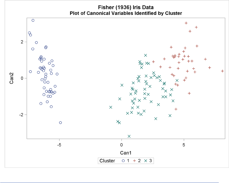
1662 FChapter 34: The FASTCLUS Procedure
Output 34.1.4 Plot of Fisher’s Iris Data using PROC CANDISC
Example 34.2: Outliers
This example involves data artificially generated to contain two clusters and several severe outliers.
A preliminary analysis specifies 20 clusters and outputs an OUTSEED= data set to be used for
a diagnostic plot. The exact number of initial clusters is not important; similar results could be
obtained with 10 or 50 initial clusters. Examination of the plot suggests that clusters with more
than five (again, the exact number is not important) observations can yield good seeds for the main
analysis. A DATA step deletes clusters with five or fewer observations, and the remaining cluster
means provide seeds for the next PROC FASTCLUS analysis.
Two clusters are requested; the LEAST= option specifies the mean absolute deviation criterion
(LEAST=1). Values of the LEAST= option less than 2 reduce the effect of outliers on cluster
centers.
The next analysis also requests two clusters; the STRICT= option is specified to prevent outliers
from distorting the results. The STRICT= value is chosen to be close to the _GAP_ and _RADIUS_
values of the larger clusters in the diagnostic plot; the exact value is not critical.
A final PROC FASTCLUS run assigns the outliers to clusters.

Example 34.2: Outliers F1663
The following SAS statements implement these steps, and the results are displayed in Output 34.2.3
through Output 34.2.8. First, an artificial data set is created with two clusters and some outliers.
Then PROC FASTCLUS is run with many clusters to produce an OUTSEED= data set. A diagnostic
plot using the variables _GAP_ and _RADIUS_ is then produced using the SGSCATTER procedure.
The results from these steps are shown in Output 34.2.1 and Output 34.2.2.
data x;
title ’Using PROC FASTCLUS to Analyze Data with Outliers’;
drop n;
do n=1 to 100;
x=rannor(12345)+2;
y=rannor(12345);
output;
end;
do n=1 to 100;
x=rannor(12345)-2;
y=rannor(12345);
output;
end;
do n=1 to 10;
x=10*rannor(12345);
y=10*rannor(12345);
output;
end;
run;
title2 ’Preliminary PROC FASTCLUS Analysis with 20 Clusters’;
proc fastclus data=x outseed=mean1 maxc=20 maxiter=0 summary;
var x y;
run;
proc sgscatter data=mean1 ;
compare y=(_gap_ _radius_) x=_freq_ ;
run;
Output 34.2.1 Preliminary Analysis of Data with Outliers Using PROC FASTCLUS
Using PROC FASTCLUS to Analyze Data with Outliers
Preliminary PROC FASTCLUS Analysis with 20 Clusters
The FASTCLUS Procedure
Replace=FULL Radius=0 Maxclusters=20 Maxiter=0
Criterion Based on Final Seeds = 0.6873

1664 FChapter 34: The FASTCLUS Procedure
Output 34.2.1 continued
Cluster Summary
Maximum Distance
RMS Std from Seed Radius Nearest
Cluster Frequency Deviation to Observation Exceeded Cluster
-----------------------------------------------------------------------------
1 8 0.4753 1.1924 19
2 1 . 0 6
3 44 0.6252 1.6774 5
4 1 . 0 20
5 38 0.5603 1.4528 3
6 2 0.0542 0.1085 2
7 1 . 0 14
8 2 0.6480 1.2961 1
9 1 . 0 7
10 1 . 0 18
11 1 . 0 16
12 20 0.5911 1.6291 16
13 5 0.6682 1.4244 3
14 1 . 0 7
15 5 0.4074 1.2678 3
16 22 0.4168 1.5139 19
17 8 0.4031 1.4794 5
18 1 . 0 10
19 45 0.6475 1.6285 16
20 3 0.5719 1.3642 15
Cluster Summary
Distance Between
Cluster Cluster Centroids
-----------------------------
1 1.7205
2 6.2847
3 1.4386
4 5.2130
5 1.4386
6 6.2847
7 2.5094
8 1.8450
9 9.4534
10 4.2514
11 4.7582
12 1.5601
13 1.9553
14 2.5094
15 1.7609
16 1.4936
17 1.5564
18 4.2514
19 1.4936
20 1.8999
Pseudo F Statistic = 207.58
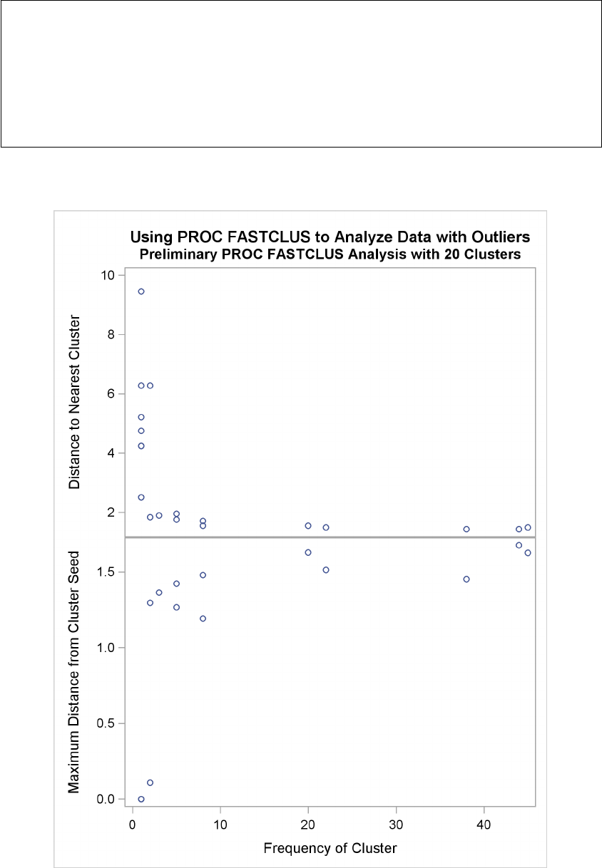
Example 34.2: Outliers F1665
Output 34.2.1 continued
Observed Over-All R-Squared = 0.95404
Approximate Expected Over-All R-Squared = 0.96103
Cubic Clustering Criterion = -2.503
WARNING: The two values above are invalid for correlated variables.
Output 34.2.2 Preliminary Analysis of Data with Outliers: Plot Using and PROC SGSCATGTER

1666 FChapter 34: The FASTCLUS Procedure
In the following SAS statements, a DATA step is used to remove low frequency clusters, then
the FASTCLUS procedure is run again, selecting seeds from the high frequency clusters in the
previous analysis using LEAST=1 clustering criterion. The results are shown in Output 34.2.3 and
Output 34.2.4.
data seed;
set mean1;
if _freq_>5;
run;
title2 ’PROC FASTCLUS Analysis Using LEAST= Clustering Criterion’;
title3 ’Values < 2 Reduce Effect of Outliers on Cluster Centers’;
proc fastclus data=x seed=seed maxc=2 least=1 out=out;
var x y;
run;
proc sgplot data=out;
scatter y=y x=x /group=cluster;
run;
Output 34.2.3 Analysis of Data with Outliers Using the LEAST= Option
Using PROC FASTCLUS to Analyze Data with Outliers
PROC FASTCLUS Analysis Using LEAST= Clustering Criterion
Values < 2 Reduce Effect of Outliers on Cluster Centers
The FASTCLUS Procedure
Replace=FULL Radius=0 Maxclusters=2 Maxiter=20 Converge=0.0001 Least=1
Initial Seeds
Cluster x y
-------------------------------------------
1 2.794174248 -0.065970836
2 -2.027300384 -2.051208579
Minimum Distance Between Initial Seeds = 6.806712
Preliminary L(1) Scale Estimate = 2.796579
Number of Bins = 100
Iteration History
Relative Change
Maximum in Cluster Seeds
Iteration Criterion Bin Size 1 2
----------------------------------------------------------
1 1.3983 0.2263 0.4091 0.6696
2 1.0776 0.0226 0.00511 0.0452
3 1.0771 0.00226 0.00229 0.00234
4 1.0771 0.000396 0.000253 0.000144
5 1.0771 0.000396 0 0

Example 34.2: Outliers F1667
Output 34.2.3 continued
Convergence criterion is satisfied.
Criterion Based on Final Seeds = 1.0771
Cluster Summary
Mean Maximum Distance
Absolute from Seed Radius Nearest
Cluster Frequency Deviation to Observation Exceeded Cluster
-----------------------------------------------------------------------------
1 102 1.1278 24.1622 2
2 108 1.0494 14.8292 1
Cluster Summary
Distance Between
Cluster Cluster Medians
----------------------------
1 4.2585
2 4.2585
Cluster Medians
Cluster x y
-------------------------------------------
1 1.923023887 0.222482918
2 -1.826721743 -0.286253041
Mean Absolute Deviations from Final Seeds
Cluster x y
-------------------------------------------
1 1.113465261 1.142120480
2 0.890331835 1.208370913
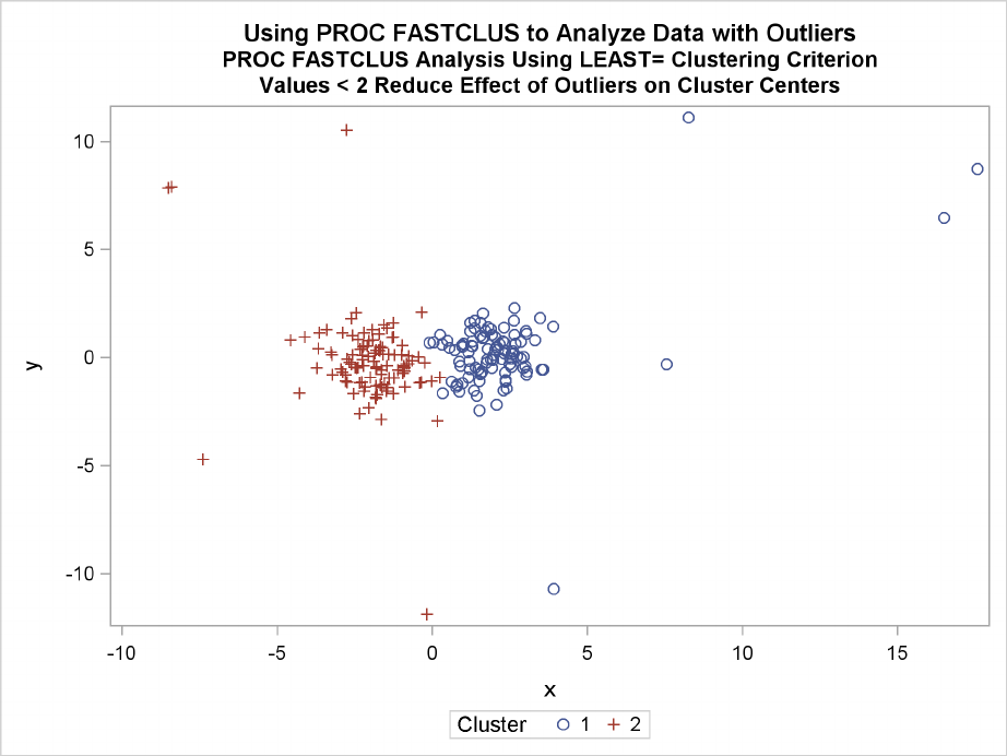
1668 FChapter 34: The FASTCLUS Procedure
Output 34.2.4 Analysis Plot of Data with Outliers
The FASTCLUS procedure is run again, selecting seeds from high frequency clusters in the pre-
vious analysis. STRICT= prevents outliers from distorting the results. The results are shown in
Output 34.2.5 and Output 34.2.6.
title2 ’PROC FASTCLUS Analysis Using STRICT= to Omit Outliers’;
proc fastclus data=x seed=seed
maxc=2 strict=3.0 out=out outseed=mean2;
var x y;
run;
proc sgplot data=out;
scatter y=y x=x /group=cluster ;
run;

Example 34.2: Outliers F1669
Output 34.2.5 Cluster Analysis with Outliers Omitted: PROC FASTCLUS SGPLOT
Using PROC FASTCLUS to Analyze Data with Outliers
PROC FASTCLUS Analysis Using STRICT= to Omit Outliers
The FASTCLUS Procedure
Replace=FULL Radius=0 Strict=3 Maxclusters=2 Maxiter=1
Initial Seeds
Cluster x y
-------------------------------------------
1 2.794174248 -0.065970836
2 -2.027300384 -2.051208579
Criterion Based on Final Seeds = 0.9515
Cluster Summary
Maximum Distance
RMS Std from Seed Radius Nearest
Cluster Frequency Deviation to Observation Exceeded Cluster
-----------------------------------------------------------------------------
1 99 0.9501 2.9589 2
2 99 0.9290 2.8011 1
Cluster Summary
Distance Between
Cluster Cluster Centroids
-----------------------------
1 3.7666
2 3.7666
12 Observation(s) were not assigned to a cluster
because the minimum distance to a cluster seed exceeded the STRICT= value.
Statistics for Variables
Variable Total STD Within STD R-Square RSQ/(1-RSQ)
------------------------------------------------------------------
x 2.06854 0.87098 0.823609 4.669219
y 1.02113 1.00352 0.039093 0.040683
OVER-ALL 1.63119 0.93959 0.669891 2.029303
Pseudo F Statistic = 397.74
Approximate Expected Over-All R-Squared = 0.60615
Cubic Clustering Criterion = 3.197
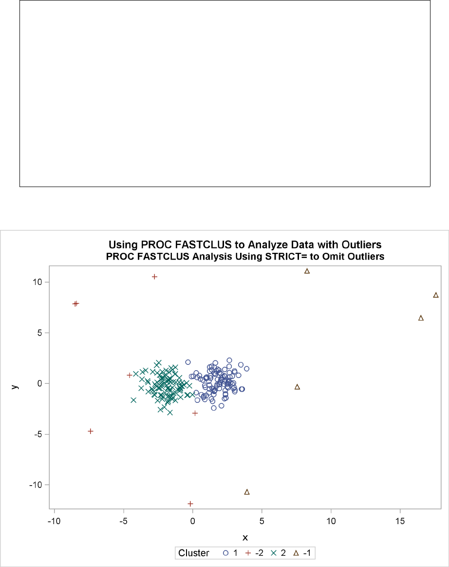
1670 FChapter 34: The FASTCLUS Procedure
Output 34.2.5 continued
WARNING: The two values above are invalid for correlated variables.
Cluster Means
Cluster x y
-------------------------------------------
1 1.825111432 0.141211701
2 -1.919910712 -0.261558725
Cluster Standard Deviations
Cluster x y
-------------------------------------------
1 0.889549271 1.006965219
2 0.852000588 1.000062579
Output 34.2.6 Cluster Analysis with Outliers Omitted: Plot Using PROC SGPLOT
Finally, the FASTCLUS procedure is run one more time with zero iterations to assign outliers and
tails to clusters. The results are show in Output 34.2.7 and Output 34.2.8.

Example 34.2: Outliers F1671
title2 ’Final PROC FASTCLUS Analysis Assigning Outliers to ’
’Clusters’;
proc fastclus data=x seed=mean2 maxc=2 maxiter=0 out=out;
var x y;
run;
proc sgplot data=out;
scatter y=y x=x /group=cluster ;
run;
Output 34.2.7 Cluster Analysis with Outliers Omitted: PROC FASTCLUS
Using PROC FASTCLUS to Analyze Data with Outliers
Final PROC FASTCLUS Analysis Assigning Outliers to Clusters
The FASTCLUS Procedure
Replace=FULL Radius=0 Maxclusters=2 Maxiter=0
Initial Seeds
Cluster x y
-------------------------------------------
1 1.825111432 0.141211701
2 -1.919910712 -0.261558725
Criterion Based on Final Seeds = 2.0594
Cluster Summary
Maximum Distance
RMS Std from Seed Radius Nearest
Cluster Frequency Deviation to Observation Exceeded Cluster
-----------------------------------------------------------------------------
1 103 2.2569 17.9426 2
2 107 1.8371 11.7362 1
Cluster Summary
Distance Between
Cluster Cluster Centroids
-----------------------------
1 4.3753
2 4.3753
Statistics for Variables
Variable Total STD Within STD R-Square RSQ/(1-RSQ)
------------------------------------------------------------------
x 2.92721 1.95529 0.555950 1.252000
y 2.15248 2.14754 0.009347 0.009435
OVER-ALL 2.56922 2.05367 0.364119 0.572621
Pseudo F Statistic = 119.11
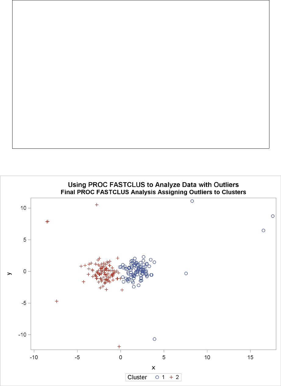
1672 FChapter 34: The FASTCLUS Procedure
Output 34.2.7 continued
Approximate Expected Over-All R-Squared = 0.49090
Cubic Clustering Criterion = -5.338
WARNING: The two values above are invalid for correlated variables.
Cluster Means
Cluster x y
-------------------------------------------
1 2.280017469 0.263940765
2 -2.075547895 -0.151348765
Cluster Standard Deviations
Cluster x y
-------------------------------------------
1 2.412264861 2.089922815
2 1.379355878 2.201567557
Output 34.2.8 Cluster Analysis with Outliers Omitted: Plot Using PROC SGPLOT

References F1673
References
Anderberg, M. R. (1973), Cluster Analysis for Applications, New York: Academic Press.
Bock, H. H. (1985), “On Some Significance Tests in Cluster Analysis,” Journal of Classification, 2,
77–108.
Calinski, T. and Harabasz, J. (1974), “A Dendrite Method for Cluster Analysis,” Communications
in Statistics, 3, 1–27.
Cooper, M. C. and Milligan, G. W. (1988), “The Effect of Error on Determining the Number of
Clusters,” Proceedings of the International Workshop on Data Analysis, Decision Support, and
Expert Knowledge Representation in Marketing and Related Areas of Research, 319–328.
Everitt, B. S. (1980), Cluster Analysis, Second Edition, London: Heineman Educational Books.
Fisher, R. A. (1936), “The Use of Multiple Measurements in Taxonomic Problems,” Annals of
Eugenics, 7, 179–188.
Gonin, R. and Money, A. H. (1989), Nonlinear Lp-Norm Estimation, New York: Marcel Dekker.
Hartigan, J. A. (1975), Clustering Algorithms, New York: John Wiley & Sons.
Hartigan, J. A. (1985), “Statistical Theory in Clustering,” Journal of Classification, 2, 63–76.
Journal of Statistics Education, “Fish Catch Data Set,” http://www.amstat.org/
publications/jse/jse_data_archive.html.
MacQueen, J. B. (1967), “Some Methods for Classification and Analysis of Multivariate Observa-
tions,” Proceedings of the Fifth Berkeley Symposium on Mathematical Statistics and Probability, 1,
281–297.
McLachlan, G. J. and Basford, K. E. (1988), Mixture Models, New York: Marcel Dekker.
Mezzich, J. E. and Solomon, H. (1980), Taxonomy and Behavioral Science, New York: Academic
Press.
Milligan, G. W. (1980), “An Examination of the Effect of Six Types of Error Perturbation on Fifteen
Clustering Algorithms,” Psychometrika, 45, 325–342.
Milligan, G. W. and Cooper, M. C. (1985), “An Examination of Procedures for Determining the
Number of Clusters in a Data Set,” Psychometrika, 50, 159–179.
Pollard, D. (1981), “Strong Consistency of k-Means Clustering,” Annals of Statistics, 9, 135–140.
Sarle, W. S. (1983), “The Cubic Clustering Criterion,” SAS Technical Report A-108, Cary, NC:
SAS Institute Inc.
Spath, H. (1980), Cluster Analysis Algorithms, Chichester, Eng.: Ellis Horwood.
1674 FChapter 34: The FASTCLUS Procedure
Spath, H. (1985), Cluster Dissection and Analysis, Chichester, Eng.: Ellis Horwood.
Titterington, D. M., Smith, A. F. M., and Makov, U. E. (1985), Statistical Analysis of Finite Mixture
Distributions, New York: John Wiley & Sons.
Tou, J. T. and Gonzalez, R. C. (1974), Pattern Recognition Principles, Reading, MA: Addison-
Wesley.
Subject Index
analyzing data in groups
FASTCLUS procedure, 1640
bin-sort algorithm, 1634
cluster
centers, 1623,1637
deletion, 1635
final, 1623
initial, 1622,1623
mean, 1637
median, 1634,1637
midrange, 1637
minimum distance separating, 1623
seeds, 1622
cluster analysis
disjoint, 1621
large data sets, 1621
robust, 1622,1637
clustering criterion
FASTCLUS procedure, 1622,1636,1637
clustering methods
FASTCLUS procedure, 1622,1624
computational problems
convergence (FASTCLUS), 1635
computational resources
FASTCLUS procedure, 1647
disjoint clustering, 1621,1622,1624
distance
between clusters (FASTCLUS), 1642
data (FASTCLUS), 1622
Euclidean (FASTCLUS), 1623
Ekblom-Newton algorithm
FASTCLUS procedure, 1637
Euclidean distances, 1623
FASTCLUS procedure
algorithm for updating cluster seeds, 1637
bin-sort algorithm, 1634
cluster deletion, 1635
clustering criterion, 1622,1636,1637
clustering methods, 1622,1624
compared to other procedures, 1647
computational problems, convergence, 1635
computational resources, 1647
controlling iterations, 1638
convergence criterion, 1634
distance, 1622,1623,1642
DRIFT option, 1623
Ekblom-Newton algorithm, 1637
homotopy parameter, 1635
imputation of missing values, 1636
incompatibilities, 1642
iteratively reweighted least squares, 1636
Lpclustering, 1622,1636
MEAN= data sets, 1638
memory requirements, 1647
Merle-Spath algorithm, 1637
missing values, 1623,1636,1638,1642
Newton algorithm, 1637
OUT= data sets, 1643
outliers, 1622
output data sets, 1638,1643
output table names, 1652
OUTSTAT= data set, 1638,1645
random number generator, 1639
scale estimates, 1635,1637,1642,1644
seed replacement, 1623,1639
weighted cluster means, 1639
homotopy parameter
FASTCLUS procedure, 1635
imputation of missing values
FASTCLUS procedure, 1636
initial seeds
FASTCLUS procedure, 1622,1623,1639
k-means clustering, 1622
leader algorithm, 1622
Lpclustering
FASTCLUS procedure, 1622
Lpclustering
FASTCLUS procedure, 1636
MEAN= data sets
FASTCLUS procedure, 1638
median
cluster, 1634,1637
memory requirements
FASTCLUS procedure, 1647
Merle-Spath algorithm
FASTCLUS procedure, 1637
missing values
FASTCLUS procedure, 1623,1636,1638,
1642
nearest centroid sorting, 1622,1623
Newton algorithm
FASTCLUS procedure, 1637
OUT= data sets
FASTCLUS procedure, 1643
outliers
FASTCLUS procedure, 1622
output data sets
FASTCLUS procedure, 1638,1643
output table names
FASTCLUS procedure, 1652
robust
cluster analysis, 1622,1637
scale estimates
FASTCLUS procedure, 1635,1637,1642,
1644
simple cluster-seeking algorithm, 1624
Syntax Index
BINS= option
PROC FASTCLUS statement, 1634
CLUSTER= option
PROC FASTCLUS statement, 1634
CLUSTERLABEL= option
PROC FASTCLUS statement, 1634
CONVERGE= option
PROC FASTCLUS statement, 1634
DATA= option
PROC FASTCLUS statement, 1635
DELETE= option
PROC FASTCLUS statement, 1635
DISTANCE option
PROC FASTCLUS statement, 1635
DRIFT option
PROC FASTCLUS statement, 1635
FASTCLUS procedure
MAXCLUSTERS= option, 1623
RADIUS= option, 1623
syntax, 1632
FASTCLUS procedure, BY statement, 1640
FASTCLUS procedure, FREQ statement, 1640
FASTCLUS procedure, ID statement, 1641
FASTCLUS procedure, PROC FASTCLUS
statement, 1632
BINS= option, 1634
CLUSTER= option, 1634
CLUSTERLABEL= option, 1634
CONVERGE= option, 1634
DATA= option, 1635
DELETE= option, 1635
DISTANCE option, 1635
DRIFT option, 1635
HC= option, 1635
HP= option, 1635
IMPUTE option, 1636
INSTAT= option, 1636
IRLS option, 1636
L= option, 1636
LEAST= option, 1636
LIST option, 1637
MAXCLUSTERS= option, 1632
MAXITER= option, 1638
MEAN= option, 1638
NOMISS option, 1638
NOPRINT option, 1638
OUT= option, 1638
OUTITER option, 1638
OUTS= option, 1638
OUTSEED= option, 1638
OUTSTAT= option, 1638
RADIUS= option, 1632
RANDOM= option, 1639
REPLACE= option, 1639
SEED= option, 1639
SHORT option, 1639
STRICT= option, 1639
SUMMARY option, 1639
VARDEF= option, 1639
FASTCLUS procedure, VAR statement, 1641
FASTCLUS procedure, WEIGHT statement,
1641
HC= option
PROC FASTCLUS statement, 1635
HP= option
PROC FASTCLUS statement, 1635
IMPUTE option
PROC FASTCLUS statement, 1636
INSTAT= option
PROC FASTCLUS statement, 1636
IRLS option
PROC FASTCLUS statement, 1636
L= option
PROC FASTCLUS statement, 1636
LEAST= option
PROC FASTCLUS statement, 1636
LIST option
PROC FASTCLUS statement, 1637
MAXCLUSTERS= option
PROC FASTCLUS statement, 1632
MAXITER= option
PROC FASTCLUS statement, 1638
MEAN= option
PROC FASTCLUS statement, 1638
NOMISS option
PROC FASTCLUS statement, 1638
NOPRINT option
PROC FASTCLUS statement, 1638
OUT= option
PROC FASTCLUS statement, 1638
OUTITER option
PROC FASTCLUS statement, 1638
OUTS= option
PROC FASTCLUS statement, 1638
OUTSEED= option
PROC FASTCLUS statement, 1638
OUTSTAT= option
PROC FASTCLUS statement, 1638
PROC FASTCLUS statement, see FASTCLUS
procedure
RADIUS= option
PROC FASTCLUS statement, 1632
RANDOM= option
PROC FASTCLUS statement, 1639
REPLACE= option
PROC FASTCLUS statement, 1639
SEED= option
PROC FASTCLUS statement, 1639
SHORT option
PROC FASTCLUS statement, 1639
STRICT= option
PROC FASTCLUS statement, 1639
SUMMARY option
PROC FASTCLUS statement, 1639
VARDEF= option
PROC FASTCLUS statement, 1639

Your Turn
We welcome your feedback.
If you have comments about this book, please send them to
yourturn@sas.com. Include the full title and page numbers (if
applicable).
If you have comments about the software, please send them to
suggest@sas.com.

SAS® Publishing Delivers!
Whether you are new to the work force or an experienced professional, you need to distinguish yourself in this rapidly
changing and competitive job market. SAS® Publishing provides you with a wide range of resources to help you set
yourself apart. Visit us online at support.sas.com/bookstore.
SAS® Press
Need to learn the basics? Struggling with a programming problem? You’ll find the expert answers that you
need in example-rich books from SAS Press. Written by experienced SAS professionals from around the
world, SAS Press books deliver real-world insights on a broad range of topics for all skill levels.
support.sas.com/saspress
SAS® Documentation
To successfully implement applications using SAS software, companies in every industry and on every
continent all turn to the one source for accurate, timely, and reliable information: SAS documentation.
We currently produce the following types of reference documentation to improve your work experience:
• Onlinehelpthatisbuiltintothesoftware.
• Tutorialsthatareintegratedintotheproduct.
• ReferencedocumentationdeliveredinHTMLandPDF– free on the Web.
• Hard-copybooks. support.sas.com/publishing
SAS® Publishing News
Subscribe to SAS Publishing News to receive up-to-date information about all new SAS titles, author
podcasts, and new Web site features via e-mail. Complete instructions on how to subscribe, as well as
access to past issues, are available at our Web site. support.sas.com/spn
SAS and all other SAS Institute Inc. product or service names are registered trademarks or trademarks of SAS Institute Inc. in the USA and other countries. ® indicates USA registration.
Otherbrandandproductnamesaretrademarksoftheirrespectivecompanies.©2009SASInstituteInc.Allrightsreserved.518177_1US.0109
