SOBEK User Manual SOBEK_User_Manual
User Manual: Pdf SOBEK_User_Manual
Open the PDF directly: View PDF ![]() .
.
Page Count: 932 [warning: Documents this large are best viewed by clicking the View PDF Link!]
- List of Figures
- List of Tables
- List of Symbols
- 1 Introduction
- 2 Getting started
- 3 Installation manual
- 4 Tutorials
- 4.1 Tutorial Hydrodynamics in open water (SOBEK-Rural 1DFLOW module)
- 4.1.1 Task block: Import Network
- 4.1.2 Task block: Settings
- 4.1.3 Task block: Meteorological Data
- 4.1.4 Task block: Schematisation
- 4.1.5 Saving the network and the model
- 4.1.6 Task block: Simulation
- 4.1.7 Task block: Results in Maps
- 4.1.8 Task block: Results in Tables
- 4.1.9 Task block: Results in Charts
- 4.1.10 Interpolation over a Connection Node
- 4.1.11 Saving the network and the model
- 4.2 Tutorial Hydrodynamics in sewers (SOBEK-Urban 1DFLOW + RR modules)
- 4.2.1 Task block: Import Network
- 4.2.2 Task block: Settings
- 4.2.3 Task block: Meteorological Data
- 4.2.4 Task block: Schematisation
- 4.2.5 Task block: Simulation
- 4.2.6 Task block: Results in Maps
- 4.2.7 Task block: Results in Tables
- 4.2.8 Task block: Results in Charts
- 4.2.9 Case Analysis Tool
- 4.2.10 Series simulation based on independent rainfall events
- 4.2.11 Task block: Schematisation extending your schematisation
- 4.3 Tutorial Hydrodynamics - 1D2D floodings (SOBEK-Rural 1DFLOW + Overland Flow modules)
- 4.4 Tutorial Hydrology in polders (SOBEK-Rural RR module)
- 4.4.1 Introduction
- 4.4.2 Getting started
- 4.4.3 Case management
- 4.4.4 Task block: Import Network
- 4.4.5 Task block: Settings
- 4.4.6 Task block: Meteorological Data
- 4.4.7 Task block: Schematisation
- 4.4.8 Task block: Simulation
- 4.4.9 Task block: Results in Maps
- 4.4.10 Task block: Results in Tables
- 4.4.11 Task block: Results in Charts
- 4.4.12 Extending your model
- 4.4.13 Epilogue
- 4.1 Tutorial Hydrodynamics in open water (SOBEK-Rural 1DFLOW module)
- 5 Graphical User Interface
- 5.1 Case management
- 5.2 SOBEK GIS interface (NETTER)
- 5.3 Node description (hydrodynamics)
- 5.3.1 Flow - Bridge node
- 5.3.2 Flow - Calculation point
- 5.3.3 Flow - Compound Structure
- 5.3.4 Different types of Flow - Connection nodes
- 5.3.5 Flow - Cross Section
- 5.3.6 Flow - Culvert node
- 5.3.7 Flow - Database structure
- 5.3.8 Flow - Extra Resistance
- 5.3.9 Flow - Boundary
- 5.3.10 Flow - General Structure
- 5.3.11 Flow - Lateral Flow
- 5.3.12 Flow - Flow manhole
- 5.3.13 Flow - Measurement station
- 5.3.14 Flow - Orifice node
- 5.3.15 Flow - Pump station node
- 5.3.16 Flow - River Advanced Weir
- 5.3.17 Flow - River Pump
- 5.3.18 Flow - River Weir
- 5.3.19 Flow - Universal Weir
- 5.3.20 Flow - Weir
- 5.3.21 Flow - 2D-Boundary
- 5.3.22 Flow - 2D-Breaking Dam
- 5.3.23 Flow - 2D-Grid
- 5.3.24 Flow - 2D-History
- 5.3.25 Flow - 2D initial water level point
- 5.4 Node description (Rainfall-Runoff)
- 5.4.1 RR - Boundary
- 5.4.2 RR - Flow-RR Connection on Channel node
- 5.4.3 RR - Flow-RR Connection on Flow Connection node
- 5.4.4 RR - Greenhouse area
- 5.4.5 RR - Industry
- 5.4.6 RR - Open water
- 5.4.7 RR - Orifice node
- 5.4.8 RR - Paved node
- 5.4.9 RR - Pump Station
- 5.4.10 RR - QH relation node
- 5.4.11 RR - Sacramento node
- 5.4.12 RR - Unpaved node
- 5.4.13 D-NAM Input Screens
- 5.4.14 RR - Wastewater Treatment Plant
- 5.4.15 RR - Weir
- 5.5 Branch description
- 5.5.1 Branch - Channel
- 5.5.2 Branch - Flow 1D Dam Break branch and the Once Hydraulic Trigger
- 5.5.2.1 Application examples of the Flow 1D Dam Break Branch
- 5.5.2.2 Method of modelling bbranching and Bbranch growth options/formulae
- 5.5.2.3 Specifying the point-in-time that bbranching should start in a Flow 1D Dam Break Branch
- 5.5.2.4 Input screens of the Flow 1D Dam Break Branch
- 5.5.2.5 Output available at a Flow 1D Dam Break Branch
- 5.5.3 Branch - Flow pipe
- 5.5.4 Flap Gates available for specific type of Pipes
- 5.5.5 Branch - 1D-2D Internal Boundary Condition
- 5.5.6 Branch - 2D Line discharge measurement
- 5.5.7 Branch - 2D-Line boundary
- 5.6 Cross Section types
- 5.6.1 Overview of available cross-sectional profiles
- 5.6.2 Flow - Cross Section node (Arch type)
- 5.6.3 Flow - Cross Section node (Asymmetrical trapezium type)
- 5.6.4 Flow - Cross Section node (Closed Lumped Y-Z type)
- 5.6.5 Flow - Cross Section node (Closed Tabulated type)
- 5.6.6 Flow - Cross Section node (Cunette type)
- 5.6.7 Flow - Cross Section node (Egg-shape type)
- 5.6.8 Flow - Cross Section node (Elliptical type)
- 5.6.9 Flow - Cross Section node (Open Lumped Y-Z type)
- 5.6.10 Flow - Cross Section node (Open Tabulated type)
- 5.6.11 Flow - Cross Section node (Open vertically segmented Y-Z type)
- 5.6.12 Flow - Cross Section node (Rectangle type)
- 5.6.13 Flow - Cross Section node (River Profile type) (beta functionality)
- 5.6.14 Flow - Cross Section node (Round type)
- 5.6.15 Flow - Cross Section node (Steel Cunette type)
- 5.6.16 Flow - Cross Section node (Trapezium type)
- 5.7 SOBEK-Urban 1DFLOW (Sewer Flow)
- 5.8 River Flow controllers and triggers
- 5.9 SOBEK-Rural/Urban/River Overland Flow (2D)
- 5.10 SOBEK-Rural RR (Rainfall-Runoff)
- 5.11 SOBEK-Urban RR (Rainfall-Runoff)
- 5.12 SOBEK-Rural/Urban/River RTC (Real Time Control)
- 5.12.1 Why a separate RTC (Real-time Control) module
- 5.12.2 Condition
- 5.12.3 Data locations in RTC
- 5.12.4 Data measurement location
- 5.12.5 Decision Parameters in RTC
- 5.12.6 Decision rules in RTC - General
- 5.12.7 External Data - His File in RTC
- 5.12.8 Example of a MATLAB M-file
- 5.12.9 Features Real-time Control
- 5.12.10 Flow Measures in RTC
- 5.12.11 Flow structure parameters in RTC and Matlab
- 5.12.12 Measures – general
- 5.12.13 Precipitation Data in RTC
- 5.12.14 Rainfall-Runoff measure
- 5.12.15 Real-time Control concepts or elements
- 5.12.16 RR Data in RTC
- 5.12.17 RTC Communication-General
- 5.12.18 RTC definitions and options in Settings
- 5.12.19 RTC does not overrule Flow Triggers
- 5.12.20 RTC - Matlab Coupling
- 5.12.21 RTC - TCN (Telecontrolnet) coupling
- 5.12.22 RTC Output options in Settings
- 5.12.23 RTC Time settings (Time-step) in Settings
- 5.12.24 RTC Wind/Rain/Matlab/Reservoir Control options in Settings
- 5.12.25 Setpoints in RTC
- 5.12.26 Type of Measures available in Real-time Control
- 5.12.27 Wind Data in RTC
- 5.12.28 1D Flow Data in RTC
- 5.12.29 2D Flow Data in RTC
- 5.13 SOBEK Tools
- 5.14 1D Hydraulic friction concepts
- 6 Conceptual description
- 6.1 Hydrodynamics D-Flow1D
- 6.1.1 Model equations
- 6.1.2 Hydrodynamic definitions
- 6.1.3 Inertia
- 6.1.4 Convection
- 6.1.5 Convection (1D)
- 6.1.6 Water level gradient
- 6.1.7 Wind friction
- 6.1.8 Initial conditions
- 6.1.9 Boundary
- 6.1.10 Discharge
- 6.1.11 Lateral discharges
- 6.1.12 Bed friction
- 6.1.13 Froude number
- 6.1.14 Boussinesq
- 6.1.15 Accuracy
- 6.1.16 Structures
- 6.1.16.1 Advanced weir
- 6.1.16.2 Bridge
- 6.1.16.3 Compound structure
- 6.1.16.4 Culvert
- 6.1.16.5 Database structure
- 6.1.16.6 General structure
- 6.1.16.7 Inverted siphon
- 6.1.16.8 Orifice
- 6.1.16.9 Pump station and Internal Pump station
- 6.1.16.10 External Pump station
- 6.1.16.11 River Pump
- 6.1.16.12 River Weir
- 6.1.16.13 Siphon
- 6.1.16.14 Universal Weir
- 6.1.16.15 Vertical obstacle friction
- 6.1.16.16 Weir
- 6.1.17 Staggered grid
- 6.1.18 Construction of the numerical bathymetry on basis of user-defined cross-sections
- 6.1.19 Method of interpolating between user-defined cross-sections
- 6.1.19.1 Method of Interpolating between Round cross-sections and between Egg-shape cross-sections
- 6.1.19.2 Method of Interpolating between Open Vertical Segmented Y-Z profiles and between Asymmetrical Trapezium profiles
- 6.1.19.3 Method of Interpolating between Cross-sections not being a Round, Egg-shape, Open Vertical Segmented Y-Z profile or Asymmetrical Trapezium profile
- 6.1.20 Methods for computing conveyance
- 6.1.21 Delft-scheme
- 6.1.22 Drying/flooding
- 6.1.23 Free board
- 6.1.24 Ground layer
- 6.1.25 Measurement station
- 6.1.26 Network
- 6.1.27 Robustness
- 6.1.28 Simulation output parameters at branch segments
- 6.1.29 Time step reductions during the simulation
- 6.1.30 Slope
- 6.1.31 Stationary computation
- 6.1.32 Summer dike
- 6.1.33 Super-critical flow
- 6.1.34 Surface level
- 6.2 Transport equation
- 6.3 Hydrodynamics Overland 2DFLOW
- 6.4 Triggers and Controllers
- 6.5 Hydrology (Rainfall Runoff modules)
- 6.5.1 SOBEK-Rural RR (Rainfall Runoff) concept
- 6.5.1.1 Alpha reaction factor
- 6.5.1.2 Capillary rise
- 6.5.1.3 Crop factors agricultural crops
- 6.5.1.4 Crop factors open water
- 6.5.1.5 De Zeeuw-Hellinga drainage formula
- 6.5.1.6 DrainageDeltaH option
- 6.5.1.7 Dry Weather Flow (DWF)
- 6.5.1.8 Equal filling controller
- 6.5.1.9 Ernst drainage formula
- 6.5.1.10 Evaporation (when using capsim)
- 6.5.1.11 Evapo(transpi)ration
- 6.5.1.12 Fixed level difference controller
- 6.5.1.13 Fixed upstream level controller
- 6.5.1.14 Hydrologic Cycle
- 6.5.1.15 Improved separated sewer
- 6.5.1.16 Infiltration
- 6.5.1.17 Infiltration from open water
- 6.5.1.18 Krayenhoff van de Leur drainage formula
- 6.5.1.19 Minimum filling percentage for greenhouse storage basin
- 6.5.1.20 Minimum level difference controller
- 6.5.1.21 Mixed sewer
- 6.5.1.22 Open water node
- 6.5.1.23 Paved area node
- 6.5.1.24 Paved node surface runoff
- 6.5.1.25 Percolation
- 6.5.1.26 QH-relation
- 6.5.1.27 Root zone
- 6.5.1.28 RR controllers
- 6.5.1.29 RR routing link
- 6.5.1.30 RR - Orifice
- 6.5.1.31 RR - Weir
- 6.5.1.32 Separated sewer
- 6.5.1.33 Silo capacity/Pump capacity
- 6.5.1.34 Soil surface level
- 6.5.1.35 Storage coefficient
- 6.5.1.36 Surface runoff
- 6.5.1.37 Target level controller
- 6.5.1.38 Time step output
- 6.5.1.39 Unpaved area node
- 6.5.1.40 Unpaved surface flow link
- 6.5.2 Sacramento Rainfall-Runoff model
- 6.5.2.1 Sacramento, the Segment module: implemented in SOBEK
- 6.5.2.2 Upper zone storage
- 6.5.2.3 Lower zone storage
- 6.5.2.4 Percolation from upper to lower zones
- 6.5.2.5 Distribution of percolated water from upper zone
- 6.5.2.6 Groundwater flow
- 6.5.2.7 Actual evapotranspiration
- 6.5.2.8 Impervious and temporary impervious areas
- 6.5.2.9 Routing of surface runoff
- 6.5.2.10 Sacramento - Estimation of segment parameters
- 6.5.2.11 Segment parameter estimation for gauged catchments.
- 6.5.3 Description of the D-NAM rainfall-runoff model
- 6.5.3.1 External forces acting on a D-NAM model
- 6.5.3.2 D-NAM storages and their water-storage capacity
- 6.5.3.3 D-NAM external and internal fluxes
- 6.5.3.4 Computing water depths in the surface flow storage
- 6.5.3.5 Computing water depths in the lower zone storage and overland flow storage
- 6.5.3.6 Evaporation from the surface storage
- 6.5.3.7 Interflow out of the surface storage
- 6.5.3.8 Infiltrated water into the soil
- 6.5.3.9 Overland flow out of the surface storage
- 6.5.3.10 Infiltration into the lower zone storage and percolation into the groundwater storage
- 6.5.3.11 Transpiration from the root zone layer
- 6.5.3.12 Capillary rise
- 6.5.3.13 Fast and slow base flow component
- 6.5.3.14 External (ground)water flowing into the lower zone storage and groundwater storage
- 6.5.3.15 Abstraction by the groundwater pump
- 6.5.3.16 Supply by the groundwater pump
- 6.5.3.17 D-NAM output time-series
- 6.5.3.18 Comparing the D-NAM model and the NAM model
- 6.5.4 SOBEK-Urban RR (Rainfall Runoff) concept
- 6.5.1 SOBEK-Rural RR (Rainfall Runoff) concept
- 6.1 Hydrodynamics D-Flow1D
- References
- A Dimension of Steel Cunnete Cross-sections
- B River Flow controller options
- C Deprecated functionality
- D SOBEK input file formats
- D.1 SOBEK Input file formats: the Model Database 4.00
- D.2 Structure of the Model Database: subdivision into layers
- D.3 1DFLOW and Overland Flow(2D)
- D.4 2D Grid layer
- D.5 Condition layer
- D.5.1 flb-file (condition layer)
- D.5.2 fll-file (condition layer)
- D.5.3 mob-file (condition layer)
- D.5.4 mol-file (condition layer)
- D.5.5 mon-file (condition layer)
- D.5.6 net-file (condition layer)
- D.5.7 sab-file (condition layer)
- D.5.8 sal-file (condition layer)
- D.5.9 wqb-file (condition layer)
- D.5.10 wql-file (condition layer)
- D.6 Cross Section layer
- D.6.1 dat-file (cross section layer)
- D.6.2 def-file (cross section layer)
- D.6.3 Tabulated cross section
- D.6.4 Trapezium cross section
- D.6.5 Open circle cross section
- D.6.6 Sedredge cross section
- D.6.7 Closed circle cross section: (only SOBEK Urban/Rural)
- D.6.8 Egg shaped cross section: (only SOBEK Urban/Rural)
- D.6.9 y-z table cross section: (only SOBEK Urban/Rural)
- D.6.10 Asymmetrical trapeziodal cross section: (only SOBEK Urban/Rural)
- D.6.11 net-file (cross section layer)
- D.7 Dispersion layer
- D.8 Friction layer
- D.9 Grid layer
- D.10 Groundwater layer
- D.11 Initial Conditions layer
- D.12 Measured Data layer
- D.13 Meteo layer
- D.14 Run Time Data layer
- D.14.1 flh-file (SOBEK River) (run time data layer)
- D.14.2 flm-file (run time data layer)
- D.14.3 fln-file (run time data layer)
- D.14.4 flt-file (run time data layer)
- D.14.5 lim-file (grid layer)
- D.14.6 moh-file (run time data layer)
- D.14.7 mom-file (run time data layer)
- D.14.8 pwq-file (run time data layer)
- D.14.9 mon-file (run time data layer)
- D.14.10 sah-file (run time data layer)
- D.14.11 sam-file (run time data layer)
- D.14.12 san-file (run time data layer)
- D.14.13 seh-file (run time data layer)
- D.14.14 sem-file (run time data layer)
- D.14.15 sen-file (run time data layer)
- D.14.16 wqh-file (run time data layer)
- D.14.17 wqm-file (run time data layer)
- D.14.18 wqn-file (run time data layer)
- D.14.19 wqt-file (run time data layer)
- D.15 Structure layer
- D.15.1 cmp-file (structure layer)
- D.15.2 cms-file (structure layer)
- D.15.3 con-file (structure layer)
- D.15.4 dat-file (structure layer)
- D.15.5 dbs-file (structure layer in SOBEK RE)
- D.15.6 def-file (structure layer)
- D.15.7 net-file (structure layer)
- D.15.8 sal-file (structure layer)
- D.15.9 trg-file (structure layer)
- D.15.10 Valve.tab (structure layer)
- D.16 Substance layer
- D.17 Topography layer
- D.18 Transport formula layer
- D.19 RR (Rainfall Runoff)
- D.19.1 Boundary layer
- D.19.2 Control layer
- D.19.3 General layer
- D.19.4 Greenhouse layer
- D.19.5 Industry layer
- D.19.6 NWRW layer
- D.19.7 Open water layer
- D.19.8 Paved area layer
- D.19.9 Runoff layer
- D.19.10 NAM rainfall runoff model
- D.19.11 Walrus rainfall runoff model
- D.19.12 Structure layer
- D.19.13 Topography layer
- D.19.14 RR-Routing link layer
- D.19.15 Unpaved area layer
- D.19.16 WWTP layer
- D.20 RTC (Real Time Control)
- E Error Messages
- F The SOBEK OpenMI interface
SOBEK
1D/2D modelling suite for integral water solutions
User Manual
Hydrodynamics, Rainfall Runo and Real Time Control
DRAFT
DRAFT
DRAFT
SOBEK
Hydrodynamics, Rainfall Runoff and
Real Time Control
User Manual
Version: 1.00
SVN Revision: 55373
April 18, 2018
DRAFT
SOBEK, User Manual
Published and printed by:
Deltares
Boussinesqweg 1
2629 HV Delft
P.O. 177
2600 MH Delft
The Netherlands
telephone: +31 88 335 82 73
fax: +31 88 335 85 82
e-mail: info@deltares.nl
www: https://www.deltares.nl
For sales contact:
telephone: +31 88 335 81 88
fax: +31 88 335 81 11
e-mail: software@deltares.nl
www: https://www.deltares.nl/software
For support contact:
telephone: +31 88 335 81 00
fax: +31 88 335 81 11
e-mail: software.support@deltares.nl
www: https://www.deltares.nl/software
Copyright © 2018 Deltares
All rights reserved. No part of this document may be reproduced in any form by print, photo
print, photo copy, microfilm or any other means, without written permission from the publisher:
Deltares.

DRAFT
Contents
Contents
List of Figures xv
List of Tables xxvii
List of Symbols xxix
1 Introduction 1
1.1 About SOBEK ................................ 1
1.2 Product Info .................................. 1
1.3 Introduction to SOBEK-Rural ......................... 3
1.4 Introduction to SOBEK-Urban ......................... 4
1.5 Introduction to SOBEK-River ......................... 5
1.6 Support .................................... 5
1.7 About Deltares ................................ 6
1.8 Notation ................................... 7
2 Getting started 9
2.1 Starting SOBEK ............................... 9
2.2 Free trial options ............................... 9
3 Installation manual 11
3.1 Introduction .................................. 11
3.1.1 System requirements ......................... 11
3.2 Deltares License Manager . . . . . . . . . . . . . . . . . . . . . . . . . . 12
3.3 Installing SOBEK ............................... 12
3.3.1 Installing the SOBEK using the command line . . . . . . . . . . . . 22
3.4 Starting SOBEK ............................... 23
4 Tutorials 25
4.1 Tutorial Hydrodynamics in open water (SOBEK-Rural 1DFLOW module) . . . 25
4.1.1 Task block: Import Network ..................... 27
4.1.2 Task block: Settings ......................... 28
4.1.3 Task block: Meteorological Data . . . . . . . . . . . . . . . . . . . 30
4.1.4 Task block: Schematisation ..................... 31
4.1.5 Saving the network and the model . . . . . . . . . . . . . . . . . . 41
4.1.6 Task block: Simulation . . . . . . . . . . . . . . . . . . . . . . . . 41
4.1.7 Task block: Results in Maps ..................... 41
4.1.8 Task block: Results in Tables . . . . . . . . . . . . . . . . . . . . 44
4.1.9 Task block: Results in Charts . . . . . . . . . . . . . . . . . . . . 45
4.1.10 Interpolation over a Connection Node . . . . . . . . . . . . . . . . . 45
4.1.11 Saving the network and the model . . . . . . . . . . . . . . . . . . 51
4.2 Tutorial Hydrodynamics in sewers (SOBEK-Urban 1DFLOW + RR modules) . 51
4.2.1 Task block: Import Network ..................... 54
4.2.2 Task block: Settings ......................... 55
4.2.3 Task block: Meteorological Data . . . . . . . . . . . . . . . . . . . 58
4.2.4 Task block: Schematisation ..................... 59
4.2.5 Task block: Simulation . . . . . . . . . . . . . . . . . . . . . . . . 67
4.2.6 Task block: Results in Maps ..................... 67
4.2.7 Task block: Results in Tables . . . . . . . . . . . . . . . . . . . . 70
4.2.8 Task block: Results in Charts . . . . . . . . . . . . . . . . . . . . 71
4.2.9 Case Analysis Tool . . . . . . . . . . . . . . . . . . . . . . . . . . 74
4.2.10 Series simulation based on independent rainfall events . . . . . . . . 75
4.2.11 Task block: Schematisation extending your schematisation . . . . . 77
Deltares iii

DRAFT
SOBEK, User Manual
4.3 Tutorial Hydrodynamics - 1D2D floodings (SOBEK-Rural 1DFLOW + Overland
Flow modules) ................................ 81
4.3.1 Starting with a 2D grid . . . . . . . . . . . . . . . . . . . . . . . . 83
4.3.2 Flooding from the lake . . . . . . . . . . . . . . . . . . . . . . . . 88
4.3.3 Flooding from the lake with a 2D dam break . . . . . . . . . . . . . 93
4.3.4 Flooding from a 1D channel . . . . . . . . . . . . . . . . . . . . . . 95
4.4 Tutorial Hydrology in polders (SOBEK-Rural RR module) . . . . . . . . . . . 104
4.4.1 Introduction ..............................104
4.4.2 Getting started . . . . . . . . . . . . . . . . . . . . . . . . . . . . 105
4.4.3 Case management . . . . . . . . . . . . . . . . . . . . . . . . . . 105
4.4.4 Task block: Import Network . . . . . . . . . . . . . . . . . . . . . 107
4.4.5 Task block: Settings . . . . . . . . . . . . . . . . . . . . . . . . . 108
4.4.6 Task block: Meteorological Data . . . . . . . . . . . . . . . . . . . 111
4.4.7 Task block: Schematisation . . . . . . . . . . . . . . . . . . . . . 112
4.4.8 Task block: Simulation . . . . . . . . . . . . . . . . . . . . . . . . 120
4.4.9 Task block: Results in Maps . . . . . . . . . . . . . . . . . . . . . 120
4.4.10 Task block: Results in Tables . . . . . . . . . . . . . . . . . . . . 121
4.4.11 Task block: Results in Charts . . . . . . . . . . . . . . . . . . . . 121
4.4.12 Extending your model . . . . . . . . . . . . . . . . . . . . . . . . . 122
4.4.13 Epilogue . . . . . . . . . . . . . . . . . . . . . . . . . . . . . . . 125
5 Graphical User Interface 127
5.1 Case management ..............................127
5.1.1 Task block: Import Network . . . . . . . . . . . . . . . . . . . . . 127
5.1.1.1 Procedure for importing a Duflow model . . . . . . . . . . 127
5.1.1.2 Procedure for importing a Mike11 model . . . . . . . . . . 128
5.1.1.3 Import SVK19 files . . . . . . . . . . . . . . . . . . . . . 130
5.1.2 Task block: Settings . . . . . . . . . . . . . . . . . . . . . . . . . 133
5.1.2.1 Rural . . . . . . . . . . . . . . . . . . . . . . . . . . . . 133
5.1.2.2 River/Urban/Rural . . . . . . . . . . . . . . . . . . . . . 146
5.1.2.3 Water Quality . . . . . . . . . . . . . . . . . . . . . . . . 157
5.1.3 Task block: Metereological Data . . . . . . . . . . . . . . . . . . . 158
5.1.4 Task block: Schematisation . . . . . . . . . . . . . . . . . . . . . 171
5.1.5 Task block: Simulation . . . . . . . . . . . . . . . . . . . . . . . . 174
5.1.6 Task block: Results in Maps . . . . . . . . . . . . . . . . . . . . . 174
5.1.6.1 River/Urban/Rural . . . . . . . . . . . . . . . . . . . . . 174
5.1.6.2 Netter . . . . . . . . . . . . . . . . . . . . . . . . . . . 177
5.1.6.3 Incremental and GIS output files . . . . . . . . . . . . . . 178
5.1.7 Task block: Results in Charts . . . . . . . . . . . . . . . . . . . . 183
5.1.8 Task block: Results in Tables . . . . . . . . . . . . . . . . . . . . 183
5.2 SOBEK GIS interface (NETTER) . . . . . . . . . . . . . . . . . . . . . . . 183
5.2.1 Adjusting the scale settings . . . . . . . . . . . . . . . . . . . . . . 183
5.2.2 Curving a branch . . . . . . . . . . . . . . . . . . . . . . . . . . . 185
5.2.3 Background map layers . . . . . . . . . . . . . . . . . . . . . . . . 186
5.2.4 Customising NETTER Settings . . . . . . . . . . . . . . . . . . . . 188
5.2.5 Exporting results to a database . . . . . . . . . . . . . . . . . . . . 188
5.2.6 Model data editor . . . . . . . . . . . . . . . . . . . . . . . . . . . 189
5.2.7 Shortcuts to various menu options . . . . . . . . . . . . . . . . . . 195
5.2.8 The Active Legend . . . . . . . . . . . . . . . . . . . . . . . . . . 196
5.2.9 Create a list with user defined output . . . . . . . . . . . . . . . . . 197
5.3 Node description (hydrodynamics) . . . . . . . . . . . . . . . . . . . . . . 198
5.3.1 Flow - Bridge node . . . . . . . . . . . . . . . . . . . . . . . . . . 198
5.3.2 Flow - Calculation point . . . . . . . . . . . . . . . . . . . . . . . . 203
5.3.2.1 Flow - Calculation point (basic) . . . . . . . . . . . . . . . 203
iv Deltares

DRAFT
Contents
5.3.2.2 Flow - Fixed Calculation point . . . . . . . . . . . . . . . 207
5.3.3 Flow - Compound Structure . . . . . . . . . . . . . . . . . . . . . . 208
5.3.4 Different types of Flow - Connection nodes . . . . . . . . . . . . . . 210
5.3.4.1 Flow - Connection node . . . . . . . . . . . . . . . . . . 211
5.3.4.2 Flow - Connection node with Lateral Flow . . . . . . . . . 212
5.3.4.3 Flow - Connection node with Storage and Lateral Flow . . . 212
5.3.5 Flow - Cross Section . . . . . . . . . . . . . . . . . . . . . . . . . 214
5.3.6 Flow - Culvert node . . . . . . . . . . . . . . . . . . . . . . . . . . 221
5.3.7 Flow - Database structure . . . . . . . . . . . . . . . . . . . . . . 226
5.3.8 Flow - Extra Resistance . . . . . . . . . . . . . . . . . . . . . . . . 229
5.3.9 Flow - Boundary . . . . . . . . . . . . . . . . . . . . . . . . . . . 231
5.3.10 Flow - General Structure . . . . . . . . . . . . . . . . . . . . . . . 234
5.3.11 Flow - Lateral Flow . . . . . . . . . . . . . . . . . . . . . . . . . . 238
5.3.12 Flow - Flow manhole . . . . . . . . . . . . . . . . . . . . . . . . . 242
5.3.12.1 Flow - Flow manhole (basic) . . . . . . . . . . . . . . . . 242
5.3.12.2 Flow - Flow manhole with level measurement . . . . . . . . 244
5.3.12.3 Flow - Flow manhole with runoff . . . . . . . . . . . . . . 245
5.3.13 Flow - Measurement station . . . . . . . . . . . . . . . . . . . . . 245
5.3.14 Flow - Orifice node . . . . . . . . . . . . . . . . . . . . . . . . . . 246
5.3.15 Flow - Pump station node . . . . . . . . . . . . . . . . . . . . . . . 248
5.3.16 Flow - River Advanced Weir . . . . . . . . . . . . . . . . . . . . . 253
5.3.17 Flow - River Pump . . . . . . . . . . . . . . . . . . . . . . . . . . 256
5.3.18 Flow - River Weir . . . . . . . . . . . . . . . . . . . . . . . . . . . 258
5.3.19 Flow - Universal Weir . . . . . . . . . . . . . . . . . . . . . . . . . 261
5.3.20 Flow - Weir ..............................263
5.3.21 Flow - 2D-Boundary . . . . . . . . . . . . . . . . . . . . . . . . . 265
5.3.22 Flow - 2D-Breaking Dam . . . . . . . . . . . . . . . . . . . . . . . 270
5.3.23 Flow - 2D-Grid . . . . . . . . . . . . . . . . . . . . . . . . . . . . 274
5.3.24 Flow - 2D-History . . . . . . . . . . . . . . . . . . . . . . . . . . . 282
5.3.25 Flow - 2D initial water level point . . . . . . . . . . . . . . . . . . . 283
5.4 Node description (Rainfall-Runoff) . . . . . . . . . . . . . . . . . . . . . . 284
5.4.1 RR - Boundary . . . . . . . . . . . . . . . . . . . . . . . . . . . . 284
5.4.2 RR - Flow-RR Connection on Channel node . . . . . . . . . . . . . 287
5.4.3 RR - Flow-RR Connection on Flow Connection node . . . . . . . . . 290
5.4.4 RR - Greenhouse area . . . . . . . . . . . . . . . . . . . . . . . . 294
5.4.5 RR - Industry . . . . . . . . . . . . . . . . . . . . . . . . . . . . . 299
5.4.6 RR - Open water . . . . . . . . . . . . . . . . . . . . . . . . . . . 301
5.4.7 RR - Orifice node . . . . . . . . . . . . . . . . . . . . . . . . . . . 307
5.4.8 RR - Paved node . . . . . . . . . . . . . . . . . . . . . . . . . . . 310
5.4.9 RR - Pump Station . . . . . . . . . . . . . . . . . . . . . . . . . . 318
5.4.10 RR - QH relation node . . . . . . . . . . . . . . . . . . . . . . . . 321
5.4.11 RR - Sacramento node . . . . . . . . . . . . . . . . . . . . . . . . 323
5.4.12 RR - Unpaved node . . . . . . . . . . . . . . . . . . . . . . . . . . 331
5.4.13 D-NAM Input Screens . . . . . . . . . . . . . . . . . . . . . . . . 340
5.4.14 RR - Wastewater Treatment Plant . . . . . . . . . . . . . . . . . . . 344
5.4.15 RR - Weir . . . . . . . . . . . . . . . . . . . . . . . . . . . . . . . 346
5.5 Branch description ..............................354
5.5.1 Branch - Channel . . . . . . . . . . . . . . . . . . . . . . . . . . . 354
5.5.2 Branch - Flow 1D Dam Break branch and the Once Hydraulic Trigger . 355
5.5.2.1 Application examples of the Flow 1D Dam Break Branch . . 355
5.5.2.2 Method of modelling bbranching and Bbranch growth op-
tions/formulae . . . . . . . . . . . . . . . . . . . . . . . 357
5.5.2.3 Specifying the point-in-time that bbranching should start in
a Flow 1D Dam Break Branch . . . . . . . . . . . . . . . 359
Deltares v

DRAFT
SOBEK, User Manual
5.5.2.4 Input screens of the Flow 1D Dam Break Branch . . . . . . 360
5.5.2.5 Output available at a Flow 1D Dam Break Branch . . . . . . 365
5.5.3 Branch - Flow pipe . . . . . . . . . . . . . . . . . . . . . . . . . . 366
5.5.4 Flap Gates available for specific type of Pipes . . . . . . . . . . . . . 366
5.5.5 Branch - 1D-2D Internal Boundary Condition . . . . . . . . . . . . . 367
5.5.6 Branch - 2D Line discharge measurement . . . . . . . . . . . . . . 370
5.5.7 Branch - 2D-Line boundary . . . . . . . . . . . . . . . . . . . . . . 372
5.6 Cross Section types ..............................373
5.6.1 Overview of available cross-sectional profiles . . . . . . . . . . . . . 373
5.6.2 Flow - Cross Section node (Arch type) . . . . . . . . . . . . . . . . 376
5.6.3 Flow - Cross Section node (Asymmetrical trapezium type) . . . . . . 377
5.6.4 Flow - Cross Section node (Closed Lumped Y-Z type) . . . . . . . . . 378
5.6.5 Flow - Cross Section node (Closed Tabulated type) . . . . . . . . . . 379
5.6.6 Flow - Cross Section node (Cunette type) . . . . . . . . . . . . . . . 380
5.6.7 Flow - Cross Section node (Egg-shape type) . . . . . . . . . . . . . 381
5.6.8 Flow - Cross Section node (Elliptical type) . . . . . . . . . . . . . . 381
5.6.9 Flow - Cross Section node (Open Lumped Y-Z type) . . . . . . . . . 381
5.6.10 Flow - Cross Section node (Open Tabulated type) . . . . . . . . . . . 383
5.6.11 Flow - Cross Section node (Open vertically segmented Y-Z type) . . . 384
5.6.12 Flow - Cross Section node (Rectangle type) . . . . . . . . . . . . . 386
5.6.13 Flow - Cross Section node (River Profile type) (beta functionality) . . . 386
5.6.14 Flow - Cross Section node (Round type) . . . . . . . . . . . . . . . 392
5.6.15 Flow - Cross Section node (Steel Cunette type) . . . . . . . . . . . . 394
5.6.16 Flow - Cross Section node (Trapezium type) . . . . . . . . . . . . . 399
5.7 SOBEK-Urban 1DFLOW (Sewer Flow) . . . . . . . . . . . . . . . . . . . . 402
5.7.1 Features SOBEK-Urban 1DFLOW . . . . . . . . . . . . . . . . . . 402
5.7.2 Flow - Pipe with Infiltration . . . . . . . . . . . . . . . . . . . . . . 403
5.7.2.1 Input screens of the Flow - Pipe with Infiltration . . . . . . . 403
5.7.2.2 Additional Output available for Flow - Pipe with Infiltration . . 407
5.7.3 Storage graph . . . . . . . . . . . . . . . . . . . . . . . . . . . . 408
5.7.4 Coupling with other modules . . . . . . . . . . . . . . . . . . . . . 410
5.7.5 Connecting the Rainfall-Runoff module to the 1DFLOW module . . . . 412
5.8 River Flow controllers and triggers . . . . . . . . . . . . . . . . . . . . . . 413
5.9 SOBEK-Rural/Urban/River Overland Flow (2D) . . . . . . . . . . . . . . . . 415
5.9.1 Introduction ..............................415
5.9.2 Viewing 2D Grid Info . . . . . . . . . . . . . . . . . . . . . . . . . 416
5.9.3 Coupling with other modules . . . . . . . . . . . . . . . . . . . . . 418
5.10 SOBEK-Rural RR (Rainfall-Runoff) . . . . . . . . . . . . . . . . . . . . . . 422
5.10.1 Features SOBEK-Rural Rainfall-Runoff . . . . . . . . . . . . . . . . 422
5.10.2 Connecting the Rainfall-Runoff module to the 1DFLOW module . . . . 423
5.10.3 Selecting a subset period of a rainfall event . . . . . . . . . . . . . . 423
5.11 SOBEK-Urban RR (Rainfall-Runoff) . . . . . . . . . . . . . . . . . . . . . . 424
5.11.1 Features SOBEK-Urban RR (Rainfall-Runoff) module . . . . . . . . . 424
5.11.2 The SOBEK-Urban RR (Rainfall-Runoff) concept . . . . . . . . . . . 425
5.11.3 SOBEK-Urban RR (Rainfall-Runoff) input screens . . . . . . . . . . 426
5.12 SOBEK-Rural/Urban/River RTC (Real Time Control) . . . . . . . . . . . . . 430
5.12.1 Why a separate RTC (Real-time Control) module . . . . . . . . . . . 430
5.12.2 Condition . . . . . . . . . . . . . . . . . . . . . . . . . . . . . . . 431
5.12.3 Data locations in RTC . . . . . . . . . . . . . . . . . . . . . . . . 431
5.12.4 Data measurement location . . . . . . . . . . . . . . . . . . . . . . 431
5.12.5 Decision Parameters in RTC . . . . . . . . . . . . . . . . . . . . . 433
5.12.6 Decision rules in RTC - General . . . . . . . . . . . . . . . . . . . 437
5.12.7 External Data - His File in RTC . . . . . . . . . . . . . . . . . . . . 437
5.12.8 Example of a MATLAB M-file . . . . . . . . . . . . . . . . . . . . . 438
vi Deltares

DRAFT
Contents
5.12.9 Features Real-time Control . . . . . . . . . . . . . . . . . . . . . . 440
5.12.10 Flow Measures in RTC . . . . . . . . . . . . . . . . . . . . . . . . 440
5.12.11 Flow structure parameters in RTC and Matlab . . . . . . . . . . . . 443
5.12.12 Measures – general . . . . . . . . . . . . . . . . . . . . . . . . . 446
5.12.13 Precipitation Data in RTC . . . . . . . . . . . . . . . . . . . . . . . 447
5.12.14 Rainfall-Runoff measure . . . . . . . . . . . . . . . . . . . . . . . 447
5.12.15 Real-time Control concepts or elements . . . . . . . . . . . . . . . 449
5.12.16 RR Data in RTC . . . . . . . . . . . . . . . . . . . . . . . . . . . 449
5.12.17 RTC Communication-General . . . . . . . . . . . . . . . . . . . . . 449
5.12.18 RTC definitions and options in Settings . . . . . . . . . . . . . . . . 450
5.12.19 RTC does not overrule Flow Triggers . . . . . . . . . . . . . . . . . 451
5.12.20 RTC - Matlab Coupling . . . . . . . . . . . . . . . . . . . . . . . . 451
5.12.21 RTC - TCN (Telecontrolnet) coupling . . . . . . . . . . . . . . . . . 453
5.12.22 RTC Output options in Settings . . . . . . . . . . . . . . . . . . . . 459
5.12.23 RTC Time settings (Time-step) in Settings . . . . . . . . . . . . . . 459
5.12.24 RTC Wind/Rain/Matlab/Reservoir Control options in Settings . . . . . 460
5.12.25 Setpoints in RTC . . . . . . . . . . . . . . . . . . . . . . . . . . . 462
5.12.26 Type of Measures available in Real-time Control . . . . . . . . . . . 462
5.12.27 Wind Data in RTC . . . . . . . . . . . . . . . . . . . . . . . . . . 462
5.12.28 1D Flow Data in RTC . . . . . . . . . . . . . . . . . . . . . . . . . 462
5.12.29 2D Flow Data in RTC . . . . . . . . . . . . . . . . . . . . . . . . . 464
5.13 SOBEK Tools . . . . . . . . . . . . . . . . . . . . . . . . . . . . . . . . . 465
5.13.1 Calibration data editor . . . . . . . . . . . . . . . . . . . . . . . . 465
5.13.2 Online Visualisation (SOBEK-1D2D) . . . . . . . . . . . . . . . . . 466
5.13.3 ReaHis (Convert HIS files to ASCII) . . . . . . . . . . . . . . . . . . 471
5.13.4 Time tables in SOBEK . . . . . . . . . . . . . . . . . . . . . . . . 472
5.14 1D Hydraulic friction concepts . . . . . . . . . . . . . . . . . . . . . . . . . 474
5.14.1 Global (or Model-wide) friction concept . . . . . . . . . . . . . . . . 474
5.14.2 Local (or Branch-wise) friction concept . . . . . . . . . . . . . . . . 475
5.14.3 Cross-section friction concept . . . . . . . . . . . . . . . . . . . . . 475
5.14.4 Culvert friction concept . . . . . . . . . . . . . . . . . . . . . . . . 475
6 Conceptual description 477
6.1 Hydrodynamics D-Flow 1D . . . . . . . . . . . . . . . . . . . . . . . . . . 477
6.1.1 Model equations . . . . . . . . . . . . . . . . . . . . . . . . . . . 477
6.1.1.1 Continuity equation (1D) . . . . . . . . . . . . . . . . . . 477
6.1.1.2 Momentum equation (1D) . . . . . . . . . . . . . . . . . 478
6.1.2 Hydrodynamic definitions . . . . . . . . . . . . . . . . . . . . . . . 478
6.1.2.1 Model datum/reference level . . . . . . . . . . . . . . . . 478
6.1.2.2 Bed level . . . . . . . . . . . . . . . . . . . . . . . . . . 479
6.1.2.3 Water depth . . . . . . . . . . . . . . . . . . . . . . . . 479
6.1.2.4 Water level . . . . . . . . . . . . . . . . . . . . . . . . . 480
6.1.2.5 Flow area . . . . . . . . . . . . . . . . . . . . . . . . . 480
6.1.2.6 Storage area . . . . . . . . . . . . . . . . . . . . . . . . 480
6.1.2.7 Wetted area . . . . . . . . . . . . . . . . . . . . . . . . 481
6.1.2.8 Wetted perimeter . . . . . . . . . . . . . . . . . . . . . . 481
6.1.2.9 Flow velocity . . . . . . . . . . . . . . . . . . . . . . . . 481
6.1.2.10 Velocity . . . . . . . . . . . . . . . . . . . . . . . . . . . 482
6.1.2.11 Hydraulic radius . . . . . . . . . . . . . . . . . . . . . . 482
6.1.3 Inertia ................................483
6.1.4 Convection ..............................483
6.1.5 Convection (1D) . . . . . . . . . . . . . . . . . . . . . . . . . . . 483
6.1.6 Water level gradient . . . . . . . . . . . . . . . . . . . . . . . . . . 483
6.1.7 Wind friction . . . . . . . . . . . . . . . . . . . . . . . . . . . . . 483
Deltares vii

DRAFT
SOBEK, User Manual
6.1.8 Initial conditions . . . . . . . . . . . . . . . . . . . . . . . . . . . 484
6.1.9 Boundary . . . . . . . . . . . . . . . . . . . . . . . . . . . . . . . 485
6.1.10 Discharge ..............................485
6.1.11 Lateral discharges . . . . . . . . . . . . . . . . . . . . . . . . . . 485
6.1.11.1 Incorporating Lateral discharges in the Continuity Equation . 486
6.1.11.2 Options for Assigning Lateral Discharges to ζ-calculation
point(s) . . . . . . . . . . . . . . . . . . . . . . . . . . . 487
6.1.11.3 Examples of Lateral Discharges . . . . . . . . . . . . . . 488
6.1.11.4 Area Based Point Lateral Flow . . . . . . . . . . . . . . . 488
6.1.11.5 Pipe with infiltration (having a lateral diffusive discharge op-
tion) . . . . . . . . . . . . . . . . . . . . . . . . . . . . 488
6.1.12 Bed friction ..............................491
6.1.12.1 Bos-Bijkerk . . . . . . . . . . . . . . . . . . . . . . . . . 492
6.1.12.2 Chézy . . . . . . . . . . . . . . . . . . . . . . . . . . . 492
6.1.12.3 Manning . . . . . . . . . . . . . . . . . . . . . . . . . . 493
6.1.12.4 Nikuradse . . . . . . . . . . . . . . . . . . . . . . . . . 493
6.1.12.5 Strickler . . . . . . . . . . . . . . . . . . . . . . . . . . 493
6.1.12.6 White-Colebrook . . . . . . . . . . . . . . . . . . . . . . 494
6.1.13 Froude number . . . . . . . . . . . . . . . . . . . . . . . . . . . . 494
6.1.14 Boussinesq ..............................495
6.1.15 Accuracy . . . . . . . . . . . . . . . . . . . . . . . . . . . . . . . 496
6.1.16 Structures ..............................497
6.1.16.1 Advanced weir . . . . . . . . . . . . . . . . . . . . . . . 498
6.1.16.2 Bridge . . . . . . . . . . . . . . . . . . . . . . . . . . . 500
6.1.16.3 Compound structure . . . . . . . . . . . . . . . . . . . . 502
6.1.16.4 Culvert . . . . . . . . . . . . . . . . . . . . . . . . . . . 502
6.1.16.5 Database structure . . . . . . . . . . . . . . . . . . . . . 506
6.1.16.6 General structure . . . . . . . . . . . . . . . . . . . . . . 506
6.1.16.7 Inverted siphon . . . . . . . . . . . . . . . . . . . . . . . 511
6.1.16.8 Orifice . . . . . . . . . . . . . . . . . . . . . . . . . . . 515
6.1.16.9 Pump station and Internal Pump station . . . . . . . . . . 516
6.1.16.10 External Pump station . . . . . . . . . . . . . . . . . . . 521
6.1.16.11 River Pump . . . . . . . . . . . . . . . . . . . . . . . . 526
6.1.16.12 River Weir . . . . . . . . . . . . . . . . . . . . . . . . . 531
6.1.16.13 Siphon . . . . . . . . . . . . . . . . . . . . . . . . . . . 533
6.1.16.14 Universal Weir . . . . . . . . . . . . . . . . . . . . . . . 536
6.1.16.15 Vertical obstacle friction . . . . . . . . . . . . . . . . . . 539
6.1.16.16 Weir . . . . . . . . . . . . . . . . . . . . . . . . . . . . 540
6.1.17 Staggered grid . . . . . . . . . . . . . . . . . . . . . . . . . . . . 541
6.1.18 Construction of the numerical bathymetry on basis of user-defined
cross-sections . . . . . . . . . . . . . . . . . . . . . . . . . . . . 542
6.1.18.1 The Y-Z type of profiles . . . . . . . . . . . . . . . . . . . 542
6.1.18.2 All cross-section types except for the Y-Z type of profiles . . 543
6.1.19 Method of interpolating between user-defined cross-sections . . . . . 543
6.1.19.1 Method of Interpolating between Round cross-sections and
between Egg-shape cross-sections . . . . . . . . . . . . . 544
6.1.19.2 Method of Interpolating between Open Vertical Segmented
Y-Z profiles and between Asymmetrical Trapezium profiles . 544
6.1.19.3 Method of Interpolating between Cross-sections not being
a Round, Egg-shape, Open Vertical Segmented Y-Z profile
or Asymmetrical Trapezium profile . . . . . . . . . . . . . 544
6.1.20 Methods for computing conveyance . . . . . . . . . . . . . . . . . . 545
6.1.20.1 Lumped conveyance approach . . . . . . . . . . . . . . . 545
6.1.20.2 Vertically segmented conveyance approach . . . . . . . . 546
viii Deltares

DRAFT
Contents
6.1.21 Delft-scheme . . . . . . . . . . . . . . . . . . . . . . . . . . . . . 551
6.1.22 Drying/flooding . . . . . . . . . . . . . . . . . . . . . . . . . . . . 552
6.1.23 Free board ..............................552
6.1.24 Ground layer . . . . . . . . . . . . . . . . . . . . . . . . . . . . . 553
6.1.25 Measurement station . . . . . . . . . . . . . . . . . . . . . . . . . 553
6.1.26 Network . . . . . . . . . . . . . . . . . . . . . . . . . . . . . . . 554
6.1.26.1 Branch . . . . . . . . . . . . . . . . . . . . . . . . . . . 554
6.1.26.2 Branch length . . . . . . . . . . . . . . . . . . . . . . . 555
6.1.26.3 Branch segment . . . . . . . . . . . . . . . . . . . . . . 556
6.1.26.4 Connection node . . . . . . . . . . . . . . . . . . . . . . 556
6.1.27 Robustness ..............................557
6.1.28 Simulation output parameters at branch segments . . . . . . . . . . 558
6.1.29 Time step reductions during the simulation . . . . . . . . . . . . . . 558
6.1.30 Slope . . . . . . . . . . . . . . . . . . . . . . . . . . . . . . . . . 560
6.1.31 Stationary computation . . . . . . . . . . . . . . . . . . . . . . . . 560
6.1.32 Summer dike . . . . . . . . . . . . . . . . . . . . . . . . . . . . . 560
6.1.33 Super-critical flow . . . . . . . . . . . . . . . . . . . . . . . . . . . 564
6.1.34 Surface level . . . . . . . . . . . . . . . . . . . . . . . . . . . . . 564
6.2 Transport equation ..............................565
6.2.1 Temperature: heat flux model . . . . . . . . . . . . . . . . . . . . . 565
6.2.1.1 General . . . . . . . . . . . . . . . . . . . . . . . . . . 565
6.2.1.2 Heat balance . . . . . . . . . . . . . . . . . . . . . . . . 566
6.2.1.3 Excess temperature model . . . . . . . . . . . . . . . . . 567
6.2.1.4 Composite temperature model . . . . . . . . . . . . . . . 567
6.2.1.5 Solar radiation . . . . . . . . . . . . . . . . . . . . . . . 568
6.2.1.6 Effective back radiation . . . . . . . . . . . . . . . . . . . 570
6.2.1.7 Evaporative heat flux . . . . . . . . . . . . . . . . . . . . 570
6.2.1.8 Convective heat flux . . . . . . . . . . . . . . . . . . . . 573
6.2.1.9 Input parameters for composite model . . . . . . . . . . . 574
6.2.2 Salinity dispersion . . . . . . . . . . . . . . . . . . . . . . . . . . 575
6.2.3 Sediment transport capacity . . . . . . . . . . . . . . . . . . . . . 576
6.3 Hydrodynamics Overland 2DFLOW . . . . . . . . . . . . . . . . . . . . . . 578
6.3.1 Continuity equation (2D) . . . . . . . . . . . . . . . . . . . . . . . 578
6.3.2 Momentum equations (2D) . . . . . . . . . . . . . . . . . . . . . . 578
6.3.3 Branch growth formulae available at a "Flow 1D Dam Break Branch" . 579
6.3.3.1 Verheij-vdKnaap(2002) bbranch growth formula . . . . . . 579
6.3.3.2 vdKnaap(2000) bbranch growth formula . . . . . . . . . . 581
6.3.4 1D-2D connection . . . . . . . . . . . . . . . . . . . . . . . . . . 583
6.3.5 2D-2D connection . . . . . . . . . . . . . . . . . . . . . . . . . . 585
6.4 Triggers and Controllers . . . . . . . . . . . . . . . . . . . . . . . . . . . . 586
6.4.1 Controller . . . . . . . . . . . . . . . . . . . . . . . . . . . . . . . 586
6.4.1.1 Combinations of controllers . . . . . . . . . . . . . . . . . 588
6.4.1.2 Hydraulic controller . . . . . . . . . . . . . . . . . . . . . 588
6.4.1.3 Interval controller . . . . . . . . . . . . . . . . . . . . . . 589
6.4.1.4 PID controller . . . . . . . . . . . . . . . . . . . . . . . 591
6.4.1.5 Relative time controller . . . . . . . . . . . . . . . . . . 592
6.4.1.6 Relative from value (time) controller . . . . . . . . . . . . 593
6.4.1.7 Time controller . . . . . . . . . . . . . . . . . . . . . . . 593
6.4.2 Triggers . . . . . . . . . . . . . . . . . . . . . . . . . . . . . . . 594
6.4.2.1 Combinations of triggers . . . . . . . . . . . . . . . . . . 594
6.4.2.2 Time trigger . . . . . . . . . . . . . . . . . . . . . . . . 595
6.4.2.3 Hydraulic trigger . . . . . . . . . . . . . . . . . . . . . . 595
6.4.2.4 Time & Hydraulic triggers . . . . . . . . . . . . . . . . . . 596
6.5 Hydrology (Rainfall Runoff modules) . . . . . . . . . . . . . . . . . . . . . 596
Deltares ix

DRAFT
SOBEK, User Manual
6.5.1 SOBEK-Rural RR (Rainfall Runoff) concept . . . . . . . . . . . . . . 596
6.5.1.1 Alpha reaction factor . . . . . . . . . . . . . . . . . . . . 597
6.5.1.2 Capillary rise . . . . . . . . . . . . . . . . . . . . . . . . 598
6.5.1.3 Crop factors agricultural crops . . . . . . . . . . . . . . . 600
6.5.1.4 Crop factors open water . . . . . . . . . . . . . . . . . . 600
6.5.1.5 De Zeeuw-Hellinga drainage formula . . . . . . . . . . . . 601
6.5.1.6 DrainageDeltaH option . . . . . . . . . . . . . . . . . 603
6.5.1.7 Dry Weather Flow (DWF) . . . . . . . . . . . . . . . . . . 604
6.5.1.8 Equal filling controller . . . . . . . . . . . . . . . . . . . . 604
6.5.1.9 Ernst drainage formula . . . . . . . . . . . . . . . . . . . 605
6.5.1.10 Evaporation (when using capsim) . . . . . . . . . . . . . . 606
6.5.1.11 Evapo(transpi)ration . . . . . . . . . . . . . . . . . . . . 607
6.5.1.12 Fixed level difference controller . . . . . . . . . . . . . . . 609
6.5.1.13 Fixed upstream level controller . . . . . . . . . . . . . . . 610
6.5.1.14 Hydrologic Cycle . . . . . . . . . . . . . . . . . . . . . . 610
6.5.1.15 Improved separated sewer . . . . . . . . . . . . . . . . . 611
6.5.1.16 Infiltration . . . . . . . . . . . . . . . . . . . . . . . . . 611
6.5.1.17 Infiltration from open water . . . . . . . . . . . . . . . . . 611
6.5.1.18 Krayenhoff van de Leur drainage formula . . . . . . . . . . 612
6.5.1.19 Minimum filling percentage for greenhouse storage basin . . 613
6.5.1.20 Minimum level difference controller . . . . . . . . . . . . . 613
6.5.1.21 Mixed sewer . . . . . . . . . . . . . . . . . . . . . . . . 614
6.5.1.22 Open water node . . . . . . . . . . . . . . . . . . . . . . 614
6.5.1.23 Paved area node . . . . . . . . . . . . . . . . . . . . . . 615
6.5.1.24 Paved node surface runoff . . . . . . . . . . . . . . . . . 616
6.5.1.25 Percolation . . . . . . . . . . . . . . . . . . . . . . . . . 618
6.5.1.26 QH-relation . . . . . . . . . . . . . . . . . . . . . . . . . 619
6.5.1.27 Root zone . . . . . . . . . . . . . . . . . . . . . . . . . 619
6.5.1.28 RR controllers . . . . . . . . . . . . . . . . . . . . . . . 620
6.5.1.29 RR routing link . . . . . . . . . . . . . . . . . . . . . . . 620
6.5.1.30 RR - Orifice . . . . . . . . . . . . . . . . . . . . . . . . 623
6.5.1.31 RR - Weir . . . . . . . . . . . . . . . . . . . . . . . . . 625
6.5.1.32 Separated sewer . . . . . . . . . . . . . . . . . . . . . . 627
6.5.1.33 Silo capacity/Pump capacity . . . . . . . . . . . . . . . . 628
6.5.1.34 Soil surface level . . . . . . . . . . . . . . . . . . . . . . 628
6.5.1.35 Storage coefficient . . . . . . . . . . . . . . . . . . . . . 632
6.5.1.36 Surface runoff . . . . . . . . . . . . . . . . . . . . . . . 639
6.5.1.37 Target level controller . . . . . . . . . . . . . . . . . . . . 639
6.5.1.38 Time step output . . . . . . . . . . . . . . . . . . . . . . 641
6.5.1.39 Unpaved area node . . . . . . . . . . . . . . . . . . . . 642
6.5.1.40 Unpaved surface flow link . . . . . . . . . . . . . . . . . 643
6.5.2 Sacramento Rainfall-Runoff model . . . . . . . . . . . . . . . . . . 643
6.5.2.1 Sacramento, the Segment module: implemented in SOBEK 643
6.5.2.2 Upper zone storage . . . . . . . . . . . . . . . . . . . . 645
6.5.2.3 Lower zone storage . . . . . . . . . . . . . . . . . . . . 646
6.5.2.4 Percolation from upper to lower zones . . . . . . . . . . . 646
6.5.2.5 Distribution of percolated water from upper zone . . . . . . 647
6.5.2.6 Groundwater flow . . . . . . . . . . . . . . . . . . . . . 647
6.5.2.7 Actual evapotranspiration . . . . . . . . . . . . . . . . . . 649
6.5.2.8 Impervious and temporary impervious areas . . . . . . . . 649
6.5.2.9 Routing of surface runoff . . . . . . . . . . . . . . . . . . 649
6.5.2.10 Sacramento - Estimation of segment parameters . . . . . . 650
6.5.2.11 Segment parameter estimation for gauged catchments. . . . 652
6.5.3 Description of the D-NAM rainfall-runoff model . . . . . . . . . . . . 664
x Deltares

DRAFT
Contents
6.5.3.1 External forces acting on a D-NAM model . . . . . . . . . 664
6.5.3.2 D-NAM storages and their water-storage capacity . . . . . 664
6.5.3.3 D-NAM external and internal fluxes . . . . . . . . . . . . . 665
6.5.3.4 Computing water depths in the surface flow storage . . . . 666
6.5.3.5 Computing water depths in the lower zone storage and over-
land flow storage . . . . . . . . . . . . . . . . . . . . . . 666
6.5.3.6 Evaporation from the surface storage . . . . . . . . . . . . 667
6.5.3.7 Interflow out of the surface storage . . . . . . . . . . . . . 668
6.5.3.8 Infiltrated water into the soil . . . . . . . . . . . . . . . . 668
6.5.3.9 Overland flow out of the surface storage . . . . . . . . . . 669
6.5.3.10 Infiltration into the lower zone storage and percolation into
the groundwater storage . . . . . . . . . . . . . . . . . . 669
6.5.3.11 Transpiration from the root zone layer . . . . . . . . . . . . 671
6.5.3.12 Capillary rise . . . . . . . . . . . . . . . . . . . . . . . . 672
6.5.3.13 Fast and slow base flow component . . . . . . . . . . . . 672
6.5.3.14 External (ground)water flowing into the lower zone storage
and groundwater storage . . . . . . . . . . . . . . . . . . 674
6.5.3.15 Abstraction by the groundwater pump . . . . . . . . . . . 676
6.5.3.16 Supply by the groundwater pump . . . . . . . . . . . . . . 677
6.5.3.17 D-NAM output time-series . . . . . . . . . . . . . . . . . 678
6.5.3.18 Comparing the D-NAM model and the NAM model . . . . . 679
6.5.4 SOBEK-Urban RR (Rainfall Runoff) concept . . . . . . . . . . . . . 680
6.5.4.1 Real Time Control (RTC module) . . . . . . . . . . . . . . 683
References 689
A Dimension of Steel Cunnete Cross-sections 693
B River Flow controller options 703
B.1 Time controller ................................704
B.2 Relative time controller . . . . . . . . . . . . . . . . . . . . . . . . . . . . 705
B.3 Relative from value (time) controller . . . . . . . . . . . . . . . . . . . . . . 706
B.4 Hydraulic controller ..............................708
B.5 Interval controller . . . . . . . . . . . . . . . . . . . . . . . . . . . . . . . 709
B.6 PID controller . . . . . . . . . . . . . . . . . . . . . . . . . . . . . . . . . 711
C Deprecated functionality 715
C.1 Linkage node . . . . . . . . . . . . . . . . . . . . . . . . . . . . . . . . . 715
C.1.1 Flow - Linkage node (deprecated) . . . . . . . . . . . . . . . . . . 715
C.1.2 How to replace linkage nodes with connection nodes . . . . . . . . . 719
C.2 Rainfall Runoff Friction . . . . . . . . . . . . . . . . . . . . . . . . . . . . 722
C.2.1 Flow - RR-Friction (deprecated) . . . . . . . . . . . . . . . . . . . . 722
C.2.2 RR Friction node (deprecated) . . . . . . . . . . . . . . . . . . . . 725
D SOBEK input file formats 727
D.1 SOBEK Input file formats: the Model Database 4.00 . . . . . . . . . . . . . 727
D.1.1 Philosophy behind the Model Database . . . . . . . . . . . . . . . . 727
D.2 Structure of the Model Database: subdivision into layers . . . . . . . . . . . 727
D.3 1DFLOW and Overland Flow(2D) . . . . . . . . . . . . . . . . . . . . . . . 729
D.3.1 General principles of the model database . . . . . . . . . . . . . . . 729
D.3.2 Global definitions file . . . . . . . . . . . . . . . . . . . . . . . . . 731
D.4 2D Grid layer . . . . . . . . . . . . . . . . . . . . . . . . . . . . . . . . . 732
D.4.1 net-file (2D Grid layer) . . . . . . . . . . . . . . . . . . . . . . . . 732
D.5 Condition layer ................................735
D.5.1 flb-file (condition layer) . . . . . . . . . . . . . . . . . . . . . . . . 735
Deltares xi

DRAFT
SOBEK, User Manual
D.5.2 fll-file (condition layer) . . . . . . . . . . . . . . . . . . . . . . . . 738
D.5.3 mob-file (condition layer) . . . . . . . . . . . . . . . . . . . . . . . 741
D.5.4 mol-file (condition layer) . . . . . . . . . . . . . . . . . . . . . . . 741
D.5.5 mon-file (condition layer) . . . . . . . . . . . . . . . . . . . . . . . 742
D.5.6 net-file (condition layer) . . . . . . . . . . . . . . . . . . . . . . . . 743
D.5.7 sab-file (condition layer) . . . . . . . . . . . . . . . . . . . . . . . 745
D.5.8 sal-file (condition layer) . . . . . . . . . . . . . . . . . . . . . . . . 745
D.5.9 wqb-file (condition layer) . . . . . . . . . . . . . . . . . . . . . . . 746
D.5.10 wql-file (condition layer) . . . . . . . . . . . . . . . . . . . . . . . . 746
D.6 Cross Section layer ..............................747
D.6.1 dat-file (cross section layer) . . . . . . . . . . . . . . . . . . . . . . 747
D.6.2 def-file (cross section layer) . . . . . . . . . . . . . . . . . . . . . . 748
D.6.3 Tabulated cross section . . . . . . . . . . . . . . . . . . . . . . . . 748
D.6.4 Trapezium cross section . . . . . . . . . . . . . . . . . . . . . . . 750
D.6.5 Open circle cross section . . . . . . . . . . . . . . . . . . . . . . . 750
D.6.6 Sedredge cross section . . . . . . . . . . . . . . . . . . . . . . . . 750
D.6.7 Closed circle cross section: (only SOBEK Urban/Rural) . . . . . . . . 751
D.6.8 Egg shaped cross section: (only SOBEK Urban/Rural) . . . . . . . . 751
D.6.9 y-z table cross section: (only SOBEK Urban/Rural) . . . . . . . . . . 751
D.6.10 Asymmetrical trapeziodal cross section: (only SOBEK Urban/Rural) . 752
D.6.11 net-file (cross section layer) . . . . . . . . . . . . . . . . . . . . . . 753
D.7 Dispersion layer ................................754
D.7.1 brm-file (dispersion layer) . . . . . . . . . . . . . . . . . . . . . . . 754
D.7.2 gld-file (dispersion layer) . . . . . . . . . . . . . . . . . . . . . . . 755
D.7.3 fwt-file (dispersion layer) . . . . . . . . . . . . . . . . . . . . . . . 756
D.7.4 lod-file (dispersion layer) . . . . . . . . . . . . . . . . . . . . . . . 756
D.7.5 mou-file (dispersion layer) . . . . . . . . . . . . . . . . . . . . . . 757
D.8 Friction layer . . . . . . . . . . . . . . . . . . . . . . . . . . . . . . . . . 757
D.8.1 bed-file (friction layer) . . . . . . . . . . . . . . . . . . . . . . . . . 757
D.8.2 exr-file (friction layer) . . . . . . . . . . . . . . . . . . . . . . . . . 762
D.8.3 glf-file (friction layer) . . . . . . . . . . . . . . . . . . . . . . . . . 762
D.8.4 wnd-file (friction layer) . . . . . . . . . . . . . . . . . . . . . . . . 763
D.9 Grid layer . . . . . . . . . . . . . . . . . . . . . . . . . . . . . . . . . . . 763
D.9.1 net-file (grid layer) . . . . . . . . . . . . . . . . . . . . . . . . . . 764
D.9.2 seg-file (grid layer) . . . . . . . . . . . . . . . . . . . . . . . . . . 764
D.10 Groundwater layer ..............................764
D.10.1 gwm-file (groundwater layer) . . . . . . . . . . . . . . . . . . . . . 765
D.10.2 gwn-file (runtime-data layer) . . . . . . . . . . . . . . . . . . . . . 765
D.11 Initial Conditions layer . . . . . . . . . . . . . . . . . . . . . . . . . . . . . 765
D.11.1 ifl-file (initial conditions layer) . . . . . . . . . . . . . . . . . . . . . 766
D.11.2 igl-file (initial conditions layer) . . . . . . . . . . . . . . . . . . . . . 767
D.11.3 imo-file (initial conditions layer) . . . . . . . . . . . . . . . . . . . . 767
D.11.4 isa-file (initial conditions layer) . . . . . . . . . . . . . . . . . . . . 768
D.11.5 iwq-file (initial conditions layer) . . . . . . . . . . . . . . . . . . . . 768
D.12 Measured Data layer . . . . . . . . . . . . . . . . . . . . . . . . . . . . . 769
D.12.1 net-file (measured data layer) . . . . . . . . . . . . . . . . . . . . . 769
D.13 Meteo layer ..................................769
D.13.1 air-file (meteo layer) . . . . . . . . . . . . . . . . . . . . . . . . . 770
D.13.2 sun-file (meteo layer) . . . . . . . . . . . . . . . . . . . . . . . . . 770
D.13.3 wat-file (meteo layer) . . . . . . . . . . . . . . . . . . . . . . . . . 771
D.13.4 wnd-file (meteo layer) . . . . . . . . . . . . . . . . . . . . . . . . . 771
D.14 Run Time Data layer . . . . . . . . . . . . . . . . . . . . . . . . . . . . . 772
D.14.1 flh-file (SOBEK River) (run time data layer) . . . . . . . . . . . . . . 772
D.14.2 flm-file (run time data layer) . . . . . . . . . . . . . . . . . . . . . . 773
xii Deltares

DRAFT
Contents
D.14.3 fln-file (run time data layer) . . . . . . . . . . . . . . . . . . . . . . 773
D.14.4 flt-file (run time data layer) . . . . . . . . . . . . . . . . . . . . . . 774
D.14.5 lim-file (grid layer) . . . . . . . . . . . . . . . . . . . . . . . . . . . 775
D.14.6 moh-file (run time data layer) . . . . . . . . . . . . . . . . . . . . . 775
D.14.7 mom-file (run time data layer) . . . . . . . . . . . . . . . . . . . . . 775
D.14.8 pwq-file (run time data layer) . . . . . . . . . . . . . . . . . . . . . 776
D.14.9 mon-file (run time data layer) . . . . . . . . . . . . . . . . . . . . . 776
D.14.10 sah-file (run time data layer) . . . . . . . . . . . . . . . . . . . . . 776
D.14.11 sam-file (run time data layer) . . . . . . . . . . . . . . . . . . . . . 776
D.14.12 san-file (run time data layer) . . . . . . . . . . . . . . . . . . . . . 777
D.14.13 seh-file (run time data layer) . . . . . . . . . . . . . . . . . . . . . 777
D.14.14 sem-file (run time data layer) . . . . . . . . . . . . . . . . . . . . . 777
D.14.15 sen-file (run time data layer) . . . . . . . . . . . . . . . . . . . . . 778
D.14.16 wqh-file (run time data layer) . . . . . . . . . . . . . . . . . . . . . 778
D.14.17 wqm-file (run time data layer) . . . . . . . . . . . . . . . . . . . . . 778
D.14.18 wqn-file (run time data layer) . . . . . . . . . . . . . . . . . . . . . 778
D.14.19 wqt-file (run time data layer) . . . . . . . . . . . . . . . . . . . . . 779
D.15 Structure layer ................................779
D.15.1 cmp-file (structure layer) . . . . . . . . . . . . . . . . . . . . . . . 779
D.15.2 cms-file (structure layer) . . . . . . . . . . . . . . . . . . . . . . . 780
D.15.3 con-file (structure layer) . . . . . . . . . . . . . . . . . . . . . . . . 780
D.15.4 dat-file (structure layer) . . . . . . . . . . . . . . . . . . . . . . . . 787
D.15.5 dbs-file (structure layer in SOBEK RE) . . . . . . . . . . . . . . . . 788
D.15.6 def-file (structure layer) . . . . . . . . . . . . . . . . . . . . . . . . 789
D.15.7 net-file (structure layer) . . . . . . . . . . . . . . . . . . . . . . . . 797
D.15.8 sal-file (structure layer) . . . . . . . . . . . . . . . . . . . . . . . . 798
D.15.9 trg-file (structure layer) . . . . . . . . . . . . . . . . . . . . . . . . 798
D.15.10 Valve.tab (structure layer) . . . . . . . . . . . . . . . . . . . . . . . 800
D.16 Substance layer ................................800
D.16.1 sub-file (substance layer) . . . . . . . . . . . . . . . . . . . . . . . 800
D.16.2 Tables ................................801
D.16.3 Tables in network layer . . . . . . . . . . . . . . . . . . . . . . . . 802
D.17 Topography layer . . . . . . . . . . . . . . . . . . . . . . . . . . . . . . . 803
D.17.1 cpt-file (topography layer) . . . . . . . . . . . . . . . . . . . . . . . 803
D.17.2 dat-file (topography layer) . . . . . . . . . . . . . . . . . . . . . . . 803
D.17.3 net-file (topography layer) . . . . . . . . . . . . . . . . . . . . . . . 804
D.17.4 nfl-file (topography layer) . . . . . . . . . . . . . . . . . . . . . . . 805
D.17.5 nsa-file (topography layer) . . . . . . . . . . . . . . . . . . . . . . 805
D.17.6 nsm-file (topography layer) . . . . . . . . . . . . . . . . . . . . . . 806
D.18 Transport formula layer . . . . . . . . . . . . . . . . . . . . . . . . . . . . 806
D.18.1 dat-file (transport formula layer) . . . . . . . . . . . . . . . . . . . . 806
D.19 RR (Rainfall Runoff) . . . . . . . . . . . . . . . . . . . . . . . . . . . . . 807
D.19.1 Boundary layer . . . . . . . . . . . . . . . . . . . . . . . . . . . . 809
D.19.2 Control layer . . . . . . . . . . . . . . . . . . . . . . . . . . . . . 810
D.19.3 General layer . . . . . . . . . . . . . . . . . . . . . . . . . . . . . 813
D.19.4 Greenhouse layer . . . . . . . . . . . . . . . . . . . . . . . . . . . 832
D.19.5 Industry layer . . . . . . . . . . . . . . . . . . . . . . . . . . . . . 833
D.19.6 NWRW layer . . . . . . . . . . . . . . . . . . . . . . . . . . . . . 834
D.19.7 Open water layer . . . . . . . . . . . . . . . . . . . . . . . . . . . 837
D.19.8 Paved area layer . . . . . . . . . . . . . . . . . . . . . . . . . . . 839
D.19.9 Runoff layer . . . . . . . . . . . . . . . . . . . . . . . . . . . . . 842
D.19.10 NAM rainfall runoff model . . . . . . . . . . . . . . . . . . . . . . . 844
D.19.11 Walrus rainfall runoff model . . . . . . . . . . . . . . . . . . . . . . 847
D.19.12 Structure layer . . . . . . . . . . . . . . . . . . . . . . . . . . . . 851
Deltares xiii

DRAFT
SOBEK, User Manual
D.19.13 Topography layer . . . . . . . . . . . . . . . . . . . . . . . . . . . 858
D.19.14 RR-Routing link layer . . . . . . . . . . . . . . . . . . . . . . . . . 860
D.19.15 Unpaved area layer . . . . . . . . . . . . . . . . . . . . . . . . . . 861
D.19.16 WWTP layer . . . . . . . . . . . . . . . . . . . . . . . . . . . . . 865
D.20 RTC (Real Time Control) . . . . . . . . . . . . . . . . . . . . . . . . . . . 866
D.20.1 Data Locations layer . . . . . . . . . . . . . . . . . . . . . . . . . 870
D.20.2 Decision layer . . . . . . . . . . . . . . . . . . . . . . . . . . . . 873
D.20.3 Measures layer . . . . . . . . . . . . . . . . . . . . . . . . . . . . 886
E Error Messages 891
E.1 Error Messages on Startup . . . . . . . . . . . . . . . . . . . . . . . . . . 891
E.2 General error messages or unexpected results . . . . . . . . . . . . . . . . 891
E.3 Error Messages Model data editor . . . . . . . . . . . . . . . . . . . . . . 891
E.4 Error Messages SOBEK-Rural / Urban 1DFLOW . . . . . . . . . . . . . . . 891
E.5 Error Messages SOBEK-Rural / Urban RR (Rainfall-Runoff) . . . . . . . . . . 895
F The SOBEK OpenMI interface 897
F.1 Introduction ..................................897
F.2 Installation ..................................897
F.3 The omi file .................................897
xiv Deltares

DRAFT
List of Figures
List of Figures
3.1 SOBEK welcome window . . . . . . . . . . . . . . . . . . . . . . . . . . 13
3.2 Select installation window, Deltares Software License Manager selected . . . 13
3.3 Select installation window, SOBEK selected . . . . . . . . . . . . . . . . . 14
3.4 Previous Installation(s) Detected, Install New Version selected . . . . . . . 15
3.5 SOBEK installation, select Product Line . . . . . . . . . . . . . . . . . . . . 16
3.6 Enter SOBEK installation directory . . . . . . . . . . . . . . . . . . . . . . 17
3.7 Select destination drive(s) ........................... 18
3.8 Select destination drive(s) ........................... 18
3.9 Miscellaneous Options . . . . . . . . . . . . . . . . . . . . . . . . . . . . 19
3.10 Check installation properties ......................... 20
3.11 Installation progress bar ........................... 21
3.12 Finish installation window ........................... 21
4.1 The case manager window. . . . . . . . . . . . . . . . . . . . . . . . . . . 26
4.2 The import network window. ......................... 27
4.3 The settings window. ............................. 28
4.4 The case manager after completing the ’settings’ and ’import network’ tasks. . 30
4.5 The meteorological data window. . . . . . . . . . . . . . . . . . . . . . . . 31
4.6 The schematisation to be created in this tutorial. . . . . . . . . . . . . . . . 32
4.7 Click this section of a toolbar to drag it to your screen! . . . . . . . . . . . . . 33
4.8 Node functions toolbar . . . . . . . . . . . . . . . . . . . . . . . . . . . . 34
4.9 Create a network similar to this one . . . . . . . . . . . . . . . . . . . . . . 35
4.10 An example of a side view animation. . . . . . . . . . . . . . . . . . . . . . 43
4.11 The results in tables window. ......................... 44
4.12 The torrent branch. .............................. 45
4.13 The entire network after adding the torrent branch . . . . . . . . . . . . . . . 47
4.14 The filled in Data Edit screen for the ’Torrent_connection’ node . . . . . . . . 49
4.15 The case manager screen. . . . . . . . . . . . . . . . . . . . . . . . . . . 52
4.16 The import network window. ......................... 54
4.17 The settings window. ............................. 55
4.18 The case manager after completing the ’settings’ and ’import network’ tasks. . 57
4.19 The meteorological data window. . . . . . . . . . . . . . . . . . . . . . . . 58
4.20 The schematisation to be extended in this tutorial. . . . . . . . . . . . . . . . 60
4.21 Open sloped area ............................... 62
4.22 Node functions toolbar . . . . . . . . . . . . . . . . . . . . . . . . . . . . 63
4.23 Reach segment names visualised on the map . . . . . . . . . . . . . . . . . 64
4.24 Side view ................................... 65
4.25 Storage graph ................................ 66
4.26 User Defined Output functions . . . . . . . . . . . . . . . . . . . . . . . . 68
4.27 Time water on street, maximum . . . . . . . . . . . . . . . . . . . . . . . . 69
4.28 The results in tables window. ......................... 71
4.29 The results in charts window. ......................... 71
4.30 The ODS_VIEW window. ........................... 72
4.31 An example of a graph created in the ’Results in Maps’ task block. . . . . . . 73
4.32 Maximum difference between two cases . . . . . . . . . . . . . . . . . . . 75
4.33 Window Structure Statistics.. . . . . . . . . . . . . . . . . . . . . . . . . 76
4.34 Structure Statistics graph for external weir 00-8002, event 6 . . . . . . . . . 77
4.35 Extended schematisation Urban. . . . . . . . . . . . . . . . . . . . . . . . 79
4.36 Activating the ’1DFLOW (Rural)’ and ’Overland Flow (2D)’ modules . . . . . . 82
4.37 Drag the toolbar containing Overland Flow node types to your screen . . . . . 84
4.38 Drag the toolbar containing the 2D-grid edit actions to your screen . . . . . . 84
4.39 Impression of the model within its GIS environment. . . . . . . . . . . . . . . 85
Deltares xv

DRAFT
SOBEK, User Manual
4.40 The 1D network of the tutorial case. . . . . . . . . . . . . . . . . . . . . . . 86
4.41 Flooding from the lake. . . . . . . . . . . . . . . . . . . . . . . . . . . . . 89
4.42 Adding history stations. . . . . . . . . . . . . . . . . . . . . . . . . . . . . 90
4.43 1D + 2D map output for a certain time step and time series graph . . . . . . . 92
4.44 2D map output for a certain time step and graph showing the water depth . . . 92
4.45 Cells after changing depth from 0 m to 8 m. . . . . . . . . . . . . . . . . . . 94
4.46 Add a 2D dam break node. . . . . . . . . . . . . . . . . . . . . . . . . . . 94
4.47 Growth of the breach depth (m) in time. . . . . . . . . . . . . . . . . . . . . 95
4.48 The tutorial 2D grid extended with a 1D channel. . . . . . . . . . . . . . . . 97
4.49 Filling in the 1D Q-boundary table. . . . . . . . . . . . . . . . . . . . . . . 100
4.50 The dummy branch used to control the flooding of the Amstellandboezem into
the 2D grid. ..................................101
5.1 Rotate or shift coordinates during Duflow import. . . . . . . . . . . . . . . . 128
5.2 Rotate and shift coordinates during MIKE11 import. . . . . . . . . . . . . . . 129
5.3 The Import Network window. . . . . . . . . . . . . . . . . . . . . . . . . . 130
5.4 Select SUF-HYD file. . . . . . . . . . . . . . . . . . . . . . . . . . . . . . 131
5.5 Shift coordinates during SVK19 import. . . . . . . . . . . . . . . . . . . . . 131
5.6 Importing an optional Mouse runoff file. . . . . . . . . . . . . . . . . . . . . 132
5.7 Opening a Mouse runoff file. . . . . . . . . . . . . . . . . . . . . . . . . . 132
5.8 Converting Mouse HGF-runoff catchment types. . . . . . . . . . . . . . . . 133
5.9 Prefixing SVK19 id’s with a district id. . . . . . . . . . . . . . . . . . . . . . 133
5.10 The Settings window with only the Channel Flow module activated. . . . . . . 134
5.11 Flowdiagram of running the Rainfall-Runoff module and Channel Flow module
sequentially. . . . . . . . . . . . . . . . . . . . . . . . . . . . . . . . . . 134
5.12 Flowdiagram of running the Rainfall-Runoff module and Channel Flow module
simultaneously. ................................135
5.13 Selecting a simulation mode. . . . . . . . . . . . . . . . . . . . . . . . . . 135
5.14 The Time settings tab of the Channel flow module. . . . . . . . . . . . . . . 136
5.15 The Simulation settings tab of the Channel flow module. . . . . . . . . . . . 137
5.16 The Advanced settings tab of the Channel flow module. . . . . . . . . . . . . 139
5.17 The Initial data tab of the Channel flow module. . . . . . . . . . . . . . . . . 140
5.18 The Nodes tab in the Channel flow Output options. . . . . . . . . . . . . . . 141
5.19 The Branches tab in the Channel flow Output options. . . . . . . . . . . . . . 142
5.20 The Structures tab in the Channel flow/Urban flow Output options. . . . . . . 143
5.21 The Numerical Parameters tab of the Channel flow module. . . . . . . . . . . 144
5.22 The Settings task block. . . . . . . . . . . . . . . . . . . . . . . . . . . . . 147
5.23 The Simulation Settings window for the Overland Flow settings task block. . . 148
5.24 The Advanced Settings window for the Overland Flow settings task block. . . . 149
5.25 Example of a 1D2D schematisation. . . . . . . . . . . . . . . . . . . . . . 150
5.26 Assume no dikes. . . . . . . . . . . . . . . . . . . . . . . . . . . . . . . . 151
5.27 Assume Highest/Lowest Level of Embankments. . . . . . . . . . . . . . . . 151
5.28 The initial data tab from the Overland Flow SETTINGS task block. . . . . . . 152
5.29 GIS Output tab in the Overland Flow settings task block. . . . . . . . . . . . 153
5.30 The incremental output tab for the Overland Flow settings task block. . . . . . 155
5.31 The Meteorological Data task block. . . . . . . . . . . . . . . . . . . . . . . 159
5.32 The Meteorological Data window. . . . . . . . . . . . . . . . . . . . . . . . 160
5.33 Rainfall and corresponding sewer inflow for a flat closed paved area . . . . . . 161
5.34 Rainfall and corresponding sewer inflow for three types of closed paved area . 162
5.35 The precipitation window . . . . . . . . . . . . . . . . . . . . . . . . . . . 163
5.36 Define meteo stations. . . . . . . . . . . . . . . . . . . . . . . . . . . . . 164
5.37 Defining the name, start/end date and timestep of a new event. . . . . . . . . 164
5.38 Editing event data. ..............................165
5.39 Task block settings, output options. . . . . . . . . . . . . . . . . . . . . . . 167
xvi Deltares

DRAFT
List of Figures
5.40 Results in charts, Flows at branch segments. . . . . . . . . . . . . . . . . . 168
5.41 Entering Edit Network mode. . . . . . . . . . . . . . . . . . . . . . . . . . 171
5.42 Entering Model Data mode. . . . . . . . . . . . . . . . . . . . . . . . . . . 172
5.43 Example of a 2D Path under a particular user defined line of 2D cells. . . . . . 174
5.44 Example of a SideView. . . . . . . . . . . . . . . . . . . . . . . . . . . . . 174
5.45 Setup Animation of a SideView. . . . . . . . . . . . . . . . . . . . . . . . . 175
5.46 The SideView Window. . . . . . . . . . . . . . . . . . . . . . . . . . . . . 176
5.47 The active legend . . . . . . . . . . . . . . . . . . . . . . . . . . . . . . . 177
5.48 A waterlevel color range in the Active Legend of NETTER. . . . . . . . . . . 183
5.49 Changing the Active Legend color range and scale. . . . . . . . . . . . . . . 184
5.50 A straight river flowing from A to B. . . . . . . . . . . . . . . . . . . . . . . 185
5.51 A harmonica-shaped river from point A to B. . . . . . . . . . . . . . . . . . 185
5.52 A meandernig river from point A to B. . . . . . . . . . . . . . . . . . . . . . 186
5.53 The default map of The Netherlands in SOBEK. . . . . . . . . . . . . . . . . 186
5.54 The Default Map Settings window. . . . . . . . . . . . . . . . . . . . . . . 187
5.55 The global Netter options window. . . . . . . . . . . . . . . . . . . . . . . . 188
5.56 Adding a definition in the SOBEK Export Tool. . . . . . . . . . . . . . . . . 189
5.57 Starting the single data editor from the Model Data menu. . . . . . . . . . . . 190
5.58 The multiple data editor. . . . . . . . . . . . . . . . . . . . . . . . . . . . 191
5.59 Changing a whole column in the multiple data editor. . . . . . . . . . . . . . 191
5.60 Importing data in the multiple data editor. . . . . . . . . . . . . . . . . . . . 192
5.61 Enter the network editing mode. . . . . . . . . . . . . . . . . . . . . . . . . 193
5.62 Mouse-over a node to show its label. . . . . . . . . . . . . . . . . . . . . . 194
5.63 Output functions window . . . . . . . . . . . . . . . . . . . . . . . . . . 197
5.64 Adding definitions in the Output functions window. . . . . . . . . . . . . . . 198
5.65 User defined output in the Active Legend. . . . . . . . . . . . . . . . . . . . 198
5.66 The Bridge tab of a bridge. . . . . . . . . . . . . . . . . . . . . . . . . . . 199
5.67 The Cross section tab of a bridge. . . . . . . . . . . . . . . . . . . . . . . . 201
5.68 The Friction tab of a bridge. . . . . . . . . . . . . . . . . . . . . . . . . . . 202
5.69 Setting a calculation grid on all branches. . . . . . . . . . . . . . . . . . . . 204
5.70 The Branch tab of the Calculation points window. . . . . . . . . . . . . . . . 205
5.71 The 2D Grid tab of the Calculation points window. . . . . . . . . . . . . . . . 206
5.72 An example of a schematisation that contains calculation points. . . . . . . . 207
5.73 Branches connected to Flow connection nodes . . . . . . . . . . . . . . . . 210
5.74 Interpolating data over Branch 1 and 2 at a Flow - Connection Node . . . . . 211
5.75 The Bottom level tab of a Flow - Connection node with Storage and Lateral Flow.213
5.76 The Lateral flow tab of a Flow - Connection node with Storage and Lateral Flow.214
5.77 The Location tab of a Flow - Cross Section node type. . . . . . . . . . . . . 215
5.78 The Cross section tab of a Flow - Cross Section node of the Y-Z Profile type. . 216
5.79 Y-Z and Asymmetrical Trapezium friction input screen. . . . . . . . . . . . . 217
5.80 River profile friction input screen. . . . . . . . . . . . . . . . . . . . . . . . 218
5.81 Friction input screen for the remaining profile types. . . . . . . . . . . . . . . 219
5.82 Example of a valid network configuration containing a cross section. . . . . . 220
5.83 The Culvert tab of a Flow - Culvert node.. . . . . . . . . . . . . . . . . . . 222
5.84 The Cross section tab of a Flow - Culvert node.. . . . . . . . . . . . . . . . 223
5.85 The Friction tab of a Flow - Culvert node.. . . . . . . . . . . . . . . . . . . 224
5.86 The Controller tab of a Flow - Culvert node.. . . . . . . . . . . . . . . . . . 225
5.87 The Database Structure tab of a Flow - Database structure node.. . . . . . . 227
5.88 The Definitions tab of a Flow - Database structure node.. . . . . . . . . . . 228
5.89 The Structure Database window of a Flow - Database structure node.. . . . . 229
5.90 The Extra Resistance tab of a Flow - Extra Resistance node.. . . . . . . . . 230
5.91 Input Table for Extra Resistance coefficients of a Flow - Extra Resistance node.231
5.92 The Boundary condition tab of a Flow - Boundary node.. . . . . . . . . . . . 232
5.93 Examples of valid configurations with Flow - Boundary nodes . . . . . . . . . 234
Deltares xvii

DRAFT
SOBEK, User Manual
5.94 Data Edit window, General Structure tab . . . . . . . . . . . . . . . . . . . 235
5.95 Data Edit window, Definitions tab . . . . . . . . . . . . . . . . . . . . . . . 236
5.96 Cross-sectional view on general structure; definitions of vertical distances . . . 237
5.97 Top view on general structure; definitions of width distances . . . . . . . . . . 237
5.98 Data Edit window, Lateral flow tab . . . . . . . . . . . . . . . . . . . . . . 239
5.99 Change Table window . . . . . . . . . . . . . . . . . . . . . . . . . . . . 240
5.100 Data Edit window, Lateral flow tab . . . . . . . . . . . . . . . . . . . . . . 241
5.101 Example of network with a Lateral Flow node . . . . . . . . . . . . . . . . . 242
5.102 Data Edit window, Storage tab . . . . . . . . . . . . . . . . . . . . . . . . 243
5.103 The difference between Flow-manholes of the type "closed", "reservoir" and
"loss" .....................................244
5.104 Placement of a Flow Measurement Station node . . . . . . . . . . . . . . . 245
5.105 Data Edit window, Orifice tab . . . . . . . . . . . . . . . . . . . . . . . . . 246
5.106 Data Edit window, Controller tab . . . . . . . . . . . . . . . . . . . . . . . 247
5.107 Example of a valid network configuration containing a pump station. . . . . . 249
5.108 Example of a Flow - Pump Station . . . . . . . . . . . . . . . . . . . . . . 250
5.109 Data Edit window, Pump tab . . . . . . . . . . . . . . . . . . . . . . . . . 251
5.110 Data Edit window, Capacity Reduction Table tab . . . . . . . . . . . . . . . 252
5.111 Data Edit window, Capacity Reduction Table tab . . . . . . . . . . . . . . . 253
5.112 Data Edit window, Advanced Weir tab . . . . . . . . . . . . . . . . . . . . 254
5.113 Data Edit window, Definitions tab . . . . . . . . . . . . . . . . . . . . . . . 255
5.114 Data Edit window, River Pump tab . . . . . . . . . . . . . . . . . . . . . . 257
5.115 Data Edit window, Definition tab . . . . . . . . . . . . . . . . . . . . . . . 258
5.116 Data Edit window, River Weir tab . . . . . . . . . . . . . . . . . . . . . . . 259
5.117 Data Edit window, Definitions tab . . . . . . . . . . . . . . . . . . . . . . . 260
5.118 Data Edit window, Universal Weir tab . . . . . . . . . . . . . . . . . . . . . 262
5.119 Data Edit window, Cross section tab . . . . . . . . . . . . . . . . . . . . . 263
5.120 Data Edit window, Weir tab ..........................264
5.121 Data Edit window, Controller tab . . . . . . . . . . . . . . . . . . . . . . . 265
5.122 Possible configuration of a 2D boundary node. Note: the white (transparent)
cells contain no-data values . . . . . . . . . . . . . . . . . . . . . . . . . . 266
5.123 2D-boundary edit window - boundary condition tab . . . . . . . . . . . . . . 267
5.124 Change table window . . . . . . . . . . . . . . . . . . . . . . . . . . . . . 268
5.125 Data Edit window, Boundary condition tab . . . . . . . . . . . . . . . . . . 269
5.126 Example of 2D- Breaking Dams located on 2D grid cells . . . . . . . . . . . 270
5.127 Example of selecting the controller option for a 2D Breaking - Dam . . . . . . 271
5.128 Example of a Decrease in Height Time Table available at a 2D Breaking – Dam 272
5.129 Example defining a controller for a 2D Breaking – Dam . . . . . . . . . . . . 273
5.130 Edit network menu, Import 2D-Grid... menu . . . . . . . . . . . . . . . . . . 274
5.131 Grid properties ................................276
5.132 Node settings . . . . . . . . . . . . . . . . . . . . . . . . . . . . . . . . . 277
5.133 2D Grid Order Window . . . . . . . . . . . . . . . . . . . . . . . . . . . . 278
5.134 Grid data window - 2D Grid location tab . . . . . . . . . . . . . . . . . . . 279
5.135 Grid data window - Grid Cell Bottom Depth tab . . . . . . . . . . . . . . . . 280
5.136 Grid data window - Friction tab . . . . . . . . . . . . . . . . . . . . . . . . 281
5.137 Grid data window - Grid Cell Friction tab . . . . . . . . . . . . . . . . . . . 282
5.138 Data Edit for Boundary Area window - Boundary tab . . . . . . . . . . . . 285
5.139 An example of RR boundary nodes connected to other nodes . . . . . . . . . 286
5.140 Data Edit for Boundary Area window - Boundary tab . . . . . . . . . . . . 288
5.141 Settings window . . . . . . . . . . . . . . . . . . . . . . . . . . . . . . . 289
5.142 Move node icon ................................290
5.143 An example of a valid network . . . . . . . . . . . . . . . . . . . . . . . . 290
5.144 Data Edit for Boundary Area window - Boundary tab . . . . . . . . . . . . 291
5.145 Settings window . . . . . . . . . . . . . . . . . . . . . . . . . . . . . . . 292
xviii Deltares

DRAFT
List of Figures
5.146 Data Edit for Node window - Storage tab . . . . . . . . . . . . . . . . . . . 293
5.147 An example of a valid schematisation containing a Flow - RR connection on
Flow connection node . . . . . . . . . . . . . . . . . . . . . . . . . . . . . 294
5.148 Volume balance in the greenhouse areas . . . . . . . . . . . . . . . . . . . 295
5.149 Data Edit for Greenhouse,Area tab . . . . . . . . . . . . . . . . . . . . . 296
5.150 Data Edit for Greenhouse,Storage tab . . . . . . . . . . . . . . . . . . . 297
5.151 Data Edit for Greenhouse,Silo tab . . . . . . . . . . . . . . . . . . . . . 298
5.152 Data Edit for Industry,Industry tab . . . . . . . . . . . . . . . . . . . . . 300
5.153 Data Edit for Open Water,Surface tab . . . . . . . . . . . . . . . . . . . . 302
5.154 Data Edit for Open Water,Management tab . . . . . . . . . . . . . . . . . 303
5.155 Data Edit for Open Water,Seepage tab . . . . . . . . . . . . . . . . . . . 304
5.156 Data Edit for Open Water,Rainfall station tab . . . . . . . . . . . . . . . . 305
5.157 Example of RR Open Water node connections. . . . . . . . . . . . . . . . . 306
5.158 Data Edit for Gate/Orifice,Options tab . . . . . . . . . . . . . . . . . . . . 307
5.159 Data Edit for Open Water,Orifice tab . . . . . . . . . . . . . . . . . . . . 308
5.160 Data Edit for Open Water,Controller tab . . . . . . . . . . . . . . . . . . . 309
5.161 An example of a network where RR Orifices are used . . . . . . . . . . . . . 310
5.162 The storage on the street and the sewer storage can be considered as two
reservoirs . . . . . . . . . . . . . . . . . . . . . . . . . . . . . . . . . . . 311
5.163 Data Edit for Paved Area window, the Area tab . . . . . . . . . . . . . . . 312
5.164 Data Edit for Paved Area window, the Management tab . . . . . . . . . . . 313
5.165 Sewer type: Mixed system . . . . . . . . . . . . . . . . . . . . . . . . . . 313
5.166 Sewer type: Separate system . . . . . . . . . . . . . . . . . . . . . . . . . 314
5.167 Sewer type: Improved separate system . . . . . . . . . . . . . . . . . . . . 314
5.168 Data Edit for Paved Area window, the Dry Weather Flow tab . . . . . . . . . 315
5.169 Data Edit for Paved Area window, the Rainfall Station tab . . . . . . . . . . 316
5.170 Data Edit for Paved Area window, the Storage tab . . . . . . . . . . . . . . 317
5.171 Select RR-Paved node connection . . . . . . . . . . . . . . . . . . . . . . 318
5.172 Connecting an RR Paved node to an RR open water for the sewer overflows
and surface runoff and an RR boundary for the sewerage discharge. . . . . . 318
5.173 Connecting an RR Paved node to an RR open water for the sewer overflows
and surface runoff and an RR Waste Water Treatment Plant for the sewerage
discharge . . . . . . . . . . . . . . . . . . . . . . . . . . . . . . . . . . . 318
5.174 Data Edit for Pump, the Options tab . . . . . . . . . . . . . . . . . . . . . 319
5.175 Data Edit for Pump, the Pump tab . . . . . . . . . . . . . . . . . . . . . . 320
5.176 Data Edit for Q-H relation window, Q-h relation tab . . . . . . . . . . . . . 322
5.177 The rainfall-runoff processes that are included in the Sacramento concept. . . 323
5.178 Flowchart of the processes that are covered by the Sacramento concept. . . . 324
5.179 Catchment divided into a number of segments . . . . . . . . . . . . . . . . 325
5.180 Data Edit for Sacramento node window, Area tab . . . . . . . . . . . . . . 326
5.181 Data Edit for Sacramento node window, Unit Hydrograph tab . . . . . . . . 328
5.182 Data Edit for Sacramento node window, Capacities tab . . . . . . . . . . . 329
5.183 Showing the RR-Link connection type . . . . . . . . . . . . . . . . . . . . . 330
5.184 Connecting an RR Sacramento node to an RR Open Water node . . . . . . . 330
5.185 Two ways to connect an RR Sacramento node to a channel . . . . . . . . . . 331
5.186 Representation of the rainfall-runoff process in unpaved areas . . . . . . . . 332
5.187 Data for UnPaved Area window, Area tab . . . . . . . . . . . . . . . . . . 333
5.188 Data for UnPaved Area window, Soil tab . . . . . . . . . . . . . . . . . . . 334
5.189 Data for UnPaved Area window, Storage tab . . . . . . . . . . . . . . . . . 335
5.190 Data for UnPaved Area window, Infiltration tab . . . . . . . . . . . . . . . . 336
5.191 Data for UnPaved Area window, Drainage tab . . . . . . . . . . . . . . . . 337
5.192 Data for UnPaved Area window, Seepage tab . . . . . . . . . . . . . . . . 338
5.193 RR-link connection type . . . . . . . . . . . . . . . . . . . . . . . . . . . . 339
Deltares xix

DRAFT
SOBEK, User Manual
5.194 Connecting an RR Unpaved node to an RR Open Water node. Notice the
defined link directions. . . . . . . . . . . . . . . . . . . . . . . . . . . . . 339
5.195 Two ways to connect an RR Unpaved node to a channel (only available if you
have a license for the flow module). . . . . . . . . . . . . . . . . . . . . . . 339
5.196 The D-NAM Tab of the D-NAM ModelEdt Form . . . . . . . . . . . . . . . . 340
5.197 The Meteo Stations Tab of the D-NAM ModelEdt Form . . . . . . . . . . . . 340
5.198 The Soil Tab of the D-NAM ModelEdt Form . . . . . . . . . . . . . . . . . . 341
5.199 The Soil2 Tab of the D-NAM ModelEdt Form . . . . . . . . . . . . . . . . . 341
5.200 The Initial Tab of the D-NAM ModelEdt Form . . . . . . . . . . . . . . . . . 342
5.201 The Runoff Tab of the D-NAM ModelEdt Form . . . . . . . . . . . . . . . . 343
5.202 The Base Flow Tab of the D-NAM ModelEdt Form . . . . . . . . . . . . . . . 343
5.203 The GW Pump Tab of the D-NAM ModelEdt Form . . . . . . . . . . . . . . . 344
5.204 Data for WWTP window, WWTP tab . . . . . . . . . . . . . . . . . . . . . 345
5.205 Typical example of a schematisation that contains a WWTP node . . . . . . . 346
5.206 Example of a broad crested weir. Photo: Dutch waterboard "Peel and Maas-
vallei" .....................................347
5.207 Data for Weir window, Options tab . . . . . . . . . . . . . . . . . . . . . . 348
5.208 Data for a normal RR-Weir window, Weir tab . . . . . . . . . . . . . . . . 349
5.209 Example of a broad crested weir . . . . . . . . . . . . . . . . . . . . . . . 349
5.210 Example of a V-notch weir . . . . . . . . . . . . . . . . . . . . . . . . . . 350
5.211 Example of a multiple-stage weir . . . . . . . . . . . . . . . . . . . . . . . 351
5.212 Data Edit for Weir window, Weir tab . . . . . . . . . . . . . . . . . . . . . 352
5.213 Data Edit for RR - Weir window, controller tab . . . . . . . . . . . . . . . . 353
5.214 Example of a network with RR Weirs . . . . . . . . . . . . . . . . . . . . . 354
5.215 Visualising the defined direction of a branch. . . . . . . . . . . . . . . . . . 355
5.216 Bbranching of a dike in a 2D model using a "Flow 1D Dam Break Branch" . . . 356
5.217 Bbranching of a river levee using a "Flow 1D Dam Break Branch" . . . . . . . 357
5.218 Bbranching of a 1D river dam using a "Flow 1D Dam Break Branch" . . . . . . 357
5.219 Development of a bbranch in a "Flow 1D Dam Break Branch" . . . . . . . . . 358
5.220 "Flow 1D Dam Break Branch"; Location Tab . . . . . . . . . . . . . . . . . . 361
5.221 "Flow 1D Dam Break Branch"; the Verheij-vdKnaap(2002) Dam Break Tab . . 362
5.222 "Flow 1D Dam Break Branch"; the vdKnaap(2000) Dam Break Tab . . . . . . 362
5.223 "Flow 1D Dam Break Branch"; Option 1", Controller Tab for the Verheij-vdKnaap(2002)
formula with an "Once Hydraulic Trigger" . . . . . . . . . . . . . . . . . . . 363
5.224 "Flow 1D Dam Break Branch"; Option 4, Controller Tab for the vdKnaap(2000)
formula and without an "Once Hydraulic Trigger" . . . . . . . . . . . . . . . 364
5.225 The Triggers Tab of the "Flow 1D Dam Break Branch" . . . . . . . . . . . . . 365
5.226 "Flow 1D Dam Break Branch"; Trigger Table of the "Once Hydraulic Trigger" . . 365
5.227 The Flap Gate input screen, that is available for specific type of pipes . . . . . 367
5.228 Placing a 1D-2D internal boundary in a model . . . . . . . . . . . . . . . . . 368
5.229 Data Edit,Boundary condition tab . . . . . . . . . . . . . . . . . . . . . . 369
5.230 Definition of the sign of the effective 2D Discharge passing a 2D Line discharge
measurement . . . . . . . . . . . . . . . . . . . . . . . . . . . . . . . . . 371
5.231 View Data window ..............................372
5.232 Possible configuration of a 2D Line boundary . . . . . . . . . . . . . . . . . 373
5.233 Data Edit,Cross section tab . . . . . . . . . . . . . . . . . . . . . . . . . 376
5.234 Asymmetrical trapezium cross section . . . . . . . . . . . . . . . . . . . . 377
5.235 Example of a closed Lumped Y-Z profile defined in ModelEdt . . . . . . . . . 378
5.236 User defined closed Lumped Y-Z profile . . . . . . . . . . . . . . . . . . . . 379
5.237 SOBEK adapted closed Lumped Y-Z profile . . . . . . . . . . . . . . . . . . 379
5.238 Symmetrical tabulated closed lumped Y-Z profile . . . . . . . . . . . . . . . 379
5.239 The Cross section tab of a cunette profile . . . . . . . . . . . . . . . . . . . 380
5.240 The corresponding tabulated profile data of the cunette profile in Figure 5.239 . 381
5.241 Example of an Open Lumped Y-Z profile defined in ModelEdt . . . . . . . . . 382
xx Deltares

DRAFT
List of Figures
5.242 User defined open Lumped Y-Z profile . . . . . . . . . . . . . . . . . . . . 383
5.243 SOBEK adapted open Lumped Y-Z profile . . . . . . . . . . . . . . . . . . . 383
5.244 Symmetrical tabulated open lumped Y-Z profile . . . . . . . . . . . . . . . . 383
5.245 Example of an Open Vertically Segmented Y-Z profile defined in ModelEdt . . 384
5.246 Data Edit,Friction tab, Open vertically segmented YZ profile . . . . . . . . . 385
5.247 Example of a ’river profile’ type cross section . . . . . . . . . . . . . . . . . 386
5.248 Table where a cross section’s dimensions are defined. . . . . . . . . . . . . 387
5.249 Activating the ’summer dike’ option . . . . . . . . . . . . . . . . . . . . . . 388
5.250 The advanced settings tab for the SOBEK-River settings. . . . . . . . . . . . 389
5.251 Defining subsections for unique friction values on different sections . . . . . . 390
5.252 Window for friction settings of the main profile section. . . . . . . . . . . . . 390
5.253 Entering friction values as a function of water levels and location . . . . . . . 391
5.254 Locations for which the friction values are known, added to the table. . . . . . 392
5.255 Data Edit,Cross section tab, Round type . . . . . . . . . . . . . . . . . . . 393
5.256 Steel Cunette type Cross section input screen. . . . . . . . . . . . . . . . . 394
5.257 Editing an existing Steel Cunette profile. . . . . . . . . . . . . . . . . . . . 395
5.258 Construction of a Steel Cunette Cross-section, type 3 . . . . . . . . . . . . . 397
5.259 Construction of a Steel Cunette Cross-section, type 4 . . . . . . . . . . . . . 398
5.260 Data Edit,Cross section tab, Trapezium . . . . . . . . . . . . . . . . . . . 399
5.261 Calculation points,General tab . . . . . . . . . . . . . . . . . . . . . . . 401
5.262 Calculation points,Branch tab . . . . . . . . . . . . . . . . . . . . . . . . 401
5.263 Pipe with Infiltration, a drainage pipe located in a trench . . . . . . . . . . . . 403
5.264 The Location Tab of the Pipe with Infiltration . . . . . . . . . . . . . . . . . . 404
5.265 The Cross Section Tab of the Pipe with Infiltration . . . . . . . . . . . . . . . 404
5.266 The Friction Tab of the Pipe with Infiltration . . . . . . . . . . . . . . . . . . 405
5.267 The Trench Profile Tab of the Pipe with Infiltration . . . . . . . . . . . . . . . 406
5.268 The Trench Data Tab of the Pipe with Infiltration . . . . . . . . . . . . . . . . 407
5.269 The "Settings for 1DFLOW module Form" available in the Settings Taskblock . 408
5.270 To start the storage graph . . . . . . . . . . . . . . . . . . . . . . . . . . . 408
5.271 Definition of storage graph options . . . . . . . . . . . . . . . . . . . . . . 409
5.272 Storage graph result . . . . . . . . . . . . . . . . . . . . . . . . . . . . . 410
5.273 Coupling a manhole ot the type loss with a 2D grid cell . . . . . . . . . . . . 411
5.274 Coupling a manhole ot the type reservoir with a 2D grid cell . . . . . . . . . . 412
5.275 Data Edit,Controllers tab . . . . . . . . . . . . . . . . . . . . . . . . . . . 413
5.276 Data Edit,Triggers tab . . . . . . . . . . . . . . . . . . . . . . . . . . . . 414
5.277 Data Edit,Controllers tab . . . . . . . . . . . . . . . . . . . . . . . . . . . 415
5.278 Example of a 2D Path under a particular user defined line . . . . . . . . . . . 418
5.279 Available node types for the Overland Flow & Channel Flow modules . . . . . 419
5.280 Example of a 1D dummy branch . . . . . . . . . . . . . . . . . . . . . . . 420
5.281 Coupling a manhole ot the type loss with a 2D grid cell . . . . . . . . . . . . 421
5.282 Coupling a manhole ot the type reservoir with a 2D grid cell . . . . . . . . . . 422
5.283 Definition of simulation period for Rainfall-Runoff model. . . . . . . . . . . . 423
5.284 Interactions of Rainfall-Runoff module with Flow module. . . . . . . . . . . . 424
5.285 Illustration of rainfall-runoff process . . . . . . . . . . . . . . . . . . . . . . 425
5.286 Data Edit for Sewerage Inflow,Surface tab . . . . . . . . . . . . . . . . . 426
5.287 Data Edit for Sewerage Inflow,DWF tab . . . . . . . . . . . . . . . . . . 427
5.288 Data Edit for Sewerage Inflow,Rainfall station tab . . . . . . . . . . . . . . 427
5.289 Data Edit for Sewerage Inflow,Runoff tab . . . . . . . . . . . . . . . . . . 428
5.290 Data Edit for Sewerage Inflow,Storage tab . . . . . . . . . . . . . . . . . 428
5.291 Data Edit for Sewerage Inflow,Infiltration tab . . . . . . . . . . . . . . . . 429
5.292 Concept of Urban runoff model . . . . . . . . . . . . . . . . . . . . . . . 430
5.293 RTC Flow data locations input screen . . . . . . . . . . . . . . . . . . . . . 432
5.294 Example of RTC input screen for Function (decision) parameters . . . . . . . 434
5.295 Definition of RTC Flow Measures . . . . . . . . . . . . . . . . . . . . . . . 441
Deltares xxi

DRAFT
SOBEK, User Manual
5.296 SOBEK RTC Editor window, the tab Measure →RR Measure . . . . . . . . 448
5.297 Definition of RR measure . . . . . . . . . . . . . . . . . . . . . . . . . . . 448
5.298 Settings input screen for SOBEK-Rural 1DFLOW-RTC run . . . . . . . . . . 450
5.299 RTC settings for the RTC - TCN coupling . . . . . . . . . . . . . . . . . . . 454
5.300 Defining a RTC decision parameter, which data is transferred towards TCN . . 455
5.301 Example of a <name.csv>file written by RTC to transfer data to TCN . . . . 455
5.302 Defining a 1D flow controller to be overruled by TCN . . . . . . . . . . . . . 456
5.303 Example of a <name.csv>file written by TCN to transfer data to RTC . . . . 456
5.304 Example of a RTC-TCN definition (SOBEKTCN.ini) file . . . . . . . . . . . . 457
5.305 Example of a RTC-TCN log file (sobektcn.log) . . . . . . . . . . . . . . . . . 458
5.306 Example of a <name.bat>file used to start the RTC-TCN coupling . . . . . . 459
5.307 RTC Output Options in Settings . . . . . . . . . . . . . . . . . . . . . . . . 459
5.308 Settings for RTC module, the Time Settings tab . . . . . . . . . . . . . . 460
5.309 RTC Control options . . . . . . . . . . . . . . . . . . . . . . . . . . . . . 461
5.310 RTC Flow Data input screen . . . . . . . . . . . . . . . . . . . . . . . . . 463
5.311 RTC 2D Flow Data input screen . . . . . . . . . . . . . . . . . . . . . . . . 464
5.312 Hisfile editor . . . . . . . . . . . . . . . . . . . . . . . . . . . . . . . . . 465
5.313 ODS view . . . . . . . . . . . . . . . . . . . . . . . . . . . . . . . . . . . 466
5.314 ODS View, parameter list . . . . . . . . . . . . . . . . . . . . . . . . . . . 466
5.315 Examples of the Online Visualisation. . . . . . . . . . . . . . . . . . . . . . 467
5.316 Enabling the Online Visualisation in the SOBEK Options window. . . . . . . . 468
5.317 The Online Visualisation. . . . . . . . . . . . . . . . . . . . . . . . . . . . 469
5.318 Explanation of cross-section for Onlie Visualisation . . . . . . . . . . . . . . 470
5.319 Online Visualisation 2D velocity vectors. . . . . . . . . . . . . . . . . . . . 471
5.320 A generic table. ................................472
5.321 This picture shows which part of your table will be continuously repeated if the
periodicity timespan that you choose is shorter than the available data in your
table. .....................................473
5.322 In this graph you can see how SOBEK handles periodicities that exceed the
time span in your table. . . . . . . . . . . . . . . . . . . . . . . . . . . . . 474
6.1 Definition of model datum/reference level . . . . . . . . . . . . . . . . . . . 478
6.2 Definition of bed level . . . . . . . . . . . . . . . . . . . . . . . . . . . . . 479
6.3 Definition of water depth h=ζ−zb. . . . . . . . . . . . . . . . . . . . . 479
6.4 Definition of water level . . . . . . . . . . . . . . . . . . . . . . . . . . . . 480
6.5 Definiton of flow area (AF) and storage area (AS). . . . . . . . . . . . . . 480
6.6 Wetted perimeter . . . . . . . . . . . . . . . . . . . . . . . . . . . . . . . 481
6.7 Wetted perimeter for the main channel . . . . . . . . . . . . . . . . . . . . 481
6.8 Computation of hydraulic radius . . . . . . . . . . . . . . . . . . . . . . . . 482
6.9 Wetted perimeter for the main channel (Subdivision in main channel and flood-
plains only in SOBEK-River) . . . . . . . . . . . . . . . . . . . . . . . . . 482
6.10 Wind direction ................................484
6.11 Diffuse lateral discharge . . . . . . . . . . . . . . . . . . . . . . . . . . . 486
6.12 Lateral discharges, point and line source . . . . . . . . . . . . . . . . . . . 486
6.13 Pipe with Infiltration, a drainage pipe located in a trench . . . . . . . . . . . . 489
6.14 Pipe with infiltration: definition of variables . . . . . . . . . . . . . . . . . . 490
6.15 Definition of energy and water level . . . . . . . . . . . . . . . . . . . . . . 498
6.16 Pillar bridge ..................................500
6.17 A suspension bridge with abutments . . . . . . . . . . . . . . . . . . . . . 501
6.18 Fixed bed bridge . . . . . . . . . . . . . . . . . . . . . . . . . . . . . . . 502
6.19 Soil bed bridge ................................502
6.20 Side view of a culvert . . . . . . . . . . . . . . . . . . . . . . . . . . . . . 503
6.21 Good modelling practice, Culvert, Inverted Siphon and Siphon . . . . . . . . 505
6.22 General structure, side view . . . . . . . . . . . . . . . . . . . . . . . . . . 507
xxii Deltares

DRAFT
List of Figures
6.23 General structure, top view . . . . . . . . . . . . . . . . . . . . . . . . . . 507
6.24 Drowned gate flow ..............................508
6.25 Drowned weir-flow ..............................509
6.26 Side view of an inverted siphon . . . . . . . . . . . . . . . . . . . . . . . . 512
6.27 Good modelling practice, Culvert, Inverted Siphon and Siphon . . . . . . . . 514
6.28 Orifice ....................................515
6.29 Pump station with positive pump direction and two pump stages . . . . . . . 517
6.30 Pump station with negative pump direction and two pump stages . . . . . . . 517
6.31 External pump station with pump direction IN and two pump stages . . . . . . 522
6.32 External pump station with pump direction OUT and two pump stages . . . . 522
6.33 River pump with Upward control and start-level above stop-level . . . . . . . 527
6.34 River pump with Upward control and stop-level above start-level . . . . . . . 528
6.35 River pump with Downward control and start-level above stop-level . . . . . . 528
6.36 River pump with Downward control and stop-level above start-level . . . . . . 529
6.37 Free and drowned weir flow . . . . . . . . . . . . . . . . . . . . . . . . . . 531
6.38 Drowned flow reduction curves . . . . . . . . . . . . . . . . . . . . . . . . 533
6.39 Siphon ....................................533
6.40 Good modelling practice, Culvert, Inverted Siphon and Siphon . . . . . . . . 536
6.41 Crest level (Y-Z) profile of a Universal weir, divided into three rectangular weir
sections (2, 4 and 6) and four triangular weir sections (1, 3, 5 and 7) . . . . . 537
6.42 Weir .....................................540
6.43 Staggered grid, ζ- and u-calculation points at different locations . . . . . . . 542
6.44 Construction of numerical bathymetry for Y-Z profiles . . . . . . . . . . . . . 543
6.45 Construction of numerical bathymetry other than Y-Z profiles . . . . . . . . . 543
6.46 Concept of the lumped conveyance approach . . . . . . . . . . . . . . . . . 545
6.47 Example of constructed vertical segments in a Y-Z profile . . . . . . . . . . . 546
6.48 Definition sketch of a vertical segment, considered in computing conveyance
for a Y-Z profile and an Asymmetrical Trapezium cross-section . . . . . . . . 548
6.49 Free board ..................................552
6.50 Ground layer in circular cross section . . . . . . . . . . . . . . . . . . . . . 553
6.51 Network . . . . . . . . . . . . . . . . . . . . . . . . . . . . . . . . . . . 554
6.52 Branch length in model network . . . . . . . . . . . . . . . . . . . . . . . . 555
6.53 Branch segment . . . . . . . . . . . . . . . . . . . . . . . . . . . . . . . 556
6.54 Connection nodes ..............................557
6.55 Summer dike option, available in a river profile . . . . . . . . . . . . . . . . 561
6.56 Flow area behind the summer dike as function of local water levels. . . . . . . 562
6.57 Total area behind the summer dike as function of local water levels. . . . . . . 564
6.58 Overview of the heat exchange mechanisms at the surface . . . . . . . . . . 565
6.59 Co-ordinate system position Sun
δ: declination; θ: latitude; ωt: angular speed . . . . . . . . . . . . . . . . . 568
6.60 Dam break Bbranch vdKnaap(200), timestep subdivision . . . . . . . . . . . 582
6.61 Bbranch width computation according vdKnaap(2000) . . . . . . . . . . . . 583
6.62 Connections between 1D and 2D . . . . . . . . . . . . . . . . . . . . . . . 584
6.63 Connections made between different grids . . . . . . . . . . . . . . . . . . 586
6.64 Example of hydraulic controller . . . . . . . . . . . . . . . . . . . . . . . . 589
6.65 Example of interval controller . . . . . . . . . . . . . . . . . . . . . . . . . 591
6.66 Example of time controller . . . . . . . . . . . . . . . . . . . . . . . . . . 593
6.67 Drainage levels ................................597
6.68 Surface run-off ................................598
6.69 Parallell drainage systems (default: DrainageDeltaH=-1) . . . . . . . . . 603
6.70 Stacked drainage systems (DrainageDeltaH=0) . . . . . . . . . . . . . 604
6.71 Principles of Ernst method . . . . . . . . . . . . . . . . . . . . . . . . . . 605
6.72 Reduction coefficient for root water uptake, αE, as a function of soil water
pressure head h(Feddes et al., 1978). . . . . . . . . . . . . . . . . . . . . 606
Deltares xxiii

DRAFT
SOBEK, User Manual
6.73 Infiltration from open water . . . . . . . . . . . . . . . . . . . . . . . . . . 612
6.74 Drainage according to Krayenhoff van de Leur . . . . . . . . . . . . . . . . 612
6.75 Representation of the rainfall-runoff process of an open-water area . . . . . . 615
6.76 Impact of delay coefficient on runoff pattern . . . . . . . . . . . . . . . . . . 616
6.77 Discharge from Paved to Open Water without delay . . . . . . . . . . . . . . 617
6.78 Discharge from Paved to Open Water using QH-relation . . . . . . . . . . . . 618
6.79 QH-relation ..................................619
6.80 Example input data ..............................622
6.81 Possible usage in a network . . . . . . . . . . . . . . . . . . . . . . . . . . 623
6.82 Orifice ....................................623
6.83 Weir .....................................625
6.84 Two-stage weir ................................626
6.85 Two-stage weir, crest bottom width at crestlevel 1 . . . . . . . . . . . . . . . 626
6.86 V-notch broad-crested weir . . . . . . . . . . . . . . . . . . . . . . . . . . 627
6.87 Change table . . . . . . . . . . . . . . . . . . . . . . . . . . . . . . . . . 629
6.88 Inundation ..................................630
6.89 Example of definition of reaction factor layers when the surface level is not
constant (in this case the number of sub-areas defined in the table is equal to 6)631
6.90 Rootzone sub areas . . . . . . . . . . . . . . . . . . . . . . . . . . . . . 632
6.91 Output reductions in Settings . . . . . . . . . . . . . . . . . . . . . . . . . 641
6.92 Time step computation . . . . . . . . . . . . . . . . . . . . . . . . . . . . 641
6.93 Time step output = 12 ∗time step computation . . . . . . . . . . . . . . . . 642
6.94 Conceptualisation of the rainfall-runoff process in a segment. . . . . . . . . . 644
6.95 Schematisation of the rainfall-runoff process in a segment . . . . . . . . . . . 645
6.96 Actual percolation demand representation . . . . . . . . . . . . . . . . . . . 647
6.97 Principle of computation of lower zone recession coefficient . . . . . . . . . . 648
6.98 Principles of the Clark method for simulating surface runoff and interflow. . . . 650
6.99 Calculation of PCTIM . . . . . . . . . . . . . . . . . . . . . . . . . . . . . 653
6.100 UZK as function of number of days with significant interflow . . . . . . . . . . 655
6.101 Selection of period for LZTWM estimation . . . . . . . . . . . . . . . . . . . 657
6.102 Schematic cross-section through basin aquifer . . . . . . . . . . . . . . . . 662
6.103 Cases of multiple exponential decay of recession curve . . . . . . . . . . . . 663
6.104 Maximum water depths in lower zone storage and groundwater storage . . . . 665
6.105 Schematic representation of fluxes in the D-NAM rainfall runoff model . . . . . 666
6.106 Water depths, thresholds and fluxes related to the surface storage . . . . . . 666
6.107 Fluxes related to the lower zone storage and groundwater storage . . . . . . 667
6.108 Distributing infiltrated water over the lower zone storage and the groundwater
storage ....................................670
6.109 Computing Fast base flow and Slow base flow . . . . . . . . . . . . . . . . 672
6.110 Determining the inflow of external (ground)water inflow . . . . . . . . . . . . 675
6.111 Reservoir . . . . . . . . . . . . . . . . . . . . . . . . . . . . . . . . . . . 684
C.1 River confluences with linkage nodes . . . . . . . . . . . . . . . . . . . . . 715
C.2 River confluences for linkage nodes showing interpolation over linkage node
for main channel . . . . . . . . . . . . . . . . . . . . . . . . . . . . . . . 716
C.3 Check mark Allow Edit for selected objects . . . . . . . . . . . . . . . . . . 717
C.4 Select Flow - Linkage node . . . . . . . . . . . . . . . . . . . . . . . . . . 717
C.5 Select branch to join . . . . . . . . . . . . . . . . . . . . . . . . . . . . . 718
C.6 Select action <Join branches>. . . . . . . . . . . . . . . . . . . . . . . . 718
C.7 Join branches by the selectd path window . . . . . . . . . . . . . . . . . 719
C.8 Existing node is replaced by Linkage Node . . . . . . . . . . . . . . . . . . 719
C.9 A schematisation with a Flow - Linkage Node. . . . . . . . . . . . . . . . . . 720
C.10 Example schematisation after the linkage node has been replaced by a con-
nection node. . . . . . . . . . . . . . . . . . . . . . . . . . . . . . . . . . 721
xxiv Deltares

DRAFT
List of Figures
C.11 The filled in Data Edit screen for the example connection node. . . . . . . . . 722
C.12 Data for friction, the friction tab . . . . . . . . . . . . . . . . . . . . . . . 723
C.13 Connecting two RR open water nodes through an RR friction node . . . . . . 724
C.14 Connecting an RR Open Water node to a Channel via an RR Friction node. . . 725
C.15 Explanation of symbols for calculating the wetted area . . . . . . . . . . . . 726
Deltares xxv

DRAFT
SOBEK, User Manual
xxvi Deltares

DRAFT
List of Tables
List of Tables
5.1 Standard precipitation events . . . . . . . . . . . . . . . . . . . . . . . . . 161
5.2 Special <*.asc>output files . . . . . . . . . . . . . . . . . . . . . . . . . 179
5.3 Overview of Cross-section types that may lay on the same branch . . . . . . 373
5.3 Overview of Cross-section types that may lay on the same branch . . . . . . 374
5.4 Properties of available cross-section types . . . . . . . . . . . . . . . . . . 374
5.4 Properties of available cross-section types . . . . . . . . . . . . . . . . . . 375
5.5 Cross Section - Y-Z table . . . . . . . . . . . . . . . . . . . . . . . . . . . 384
5.6 Examples of Steel Cunette Cross-sections . . . . . . . . . . . . . . . . . . 398
5.7 Mathematical manipulations available for a set of data series . . . . . . . . . 435
5.8 Data Type=Date/Time (yyyy-mm-dd; hh:mm:ss) . . . . . . . . . . . . . . . . 436
5.9 Output (or set-point) of RTC Flow Measure as function of overruled Controller
type ......................................441
5.10 Data per structure type for RTC Matlab communication . . . . . . . . . . . . 443
5.10 Data per structure type for RTC Matlab communication . . . . . . . . . . . . 444
5.10 Data per structure type for RTC Matlab communication . . . . . . . . . . . . 445
5.10 Data per structure type for RTC Matlab communication . . . . . . . . . . . . 446
5.11 Table: Strings in a Matlab m-file for obtaining values of data series that are
available at data locations defined in the RTC module . . . . . . . . . . . . . 452
5.12 Table: Strings in a Matlab m-file for transferring computed setpoints for a par-
ticular Flow or RR controller towards the RTC module. . . . . . . . . . . . . 453
6.1 Example of switch-on-levels and switch-off-levels at the suction-side and the
delivery-side of a pump station . . . . . . . . . . . . . . . . . . . . . . . . 520
6.2 Example of switch-on-levels and switch-off-levels at the suction-side and the
delivery-side of an external pump station . . . . . . . . . . . . . . . . . . . 525
6.3 Flow-Pump station covers the options of a River pump with respect to the
pump direction ................................531
6.4 Crest shape and coefficients for simple weir structure (default values) . . . . . 532
6.6 ........................................580
6.10 Average storage coefficients depending on soil type and dranaige basis. . . . 633
6.11 Percolation exponent REXP for different soil types . . . . . . . . . . . . . . 656
6.12 Overview of D-NAM output time-series . . . . . . . . . . . . . . . . . . . . 678
6.12 Overview of D-NAM output time-series . . . . . . . . . . . . . . . . . . . . 679
6.13 Default parameters of Delay of Runoff (Rational Method) . . . . . . . . . . . 680
6.13 Default parameters of Delay of Runoff (Rational Method) . . . . . . . . . . . 681
6.14 Default parameters Horton equation . . . . . . . . . . . . . . . . . . . . . 681
6.14 Default parameters Horton equation . . . . . . . . . . . . . . . . . . . . . 682
A.1 Steel cunette cross-section . . . . . . . . . . . . . . . . . . . . . . . . . . 693
D.1 Soil types and related Walrus parameter values. . . . . . . . . . . . . . . . 849
Deltares xxvii

DRAFT
SOBEK, User Manual
xxviii Deltares

DRAFT
List of Symbols
List of Symbols
Symbol Unit Description
AFm2Cross sectional flow area
ARm2Rainfall runoff area
ASm2Cross sectional storage area
ATm2Cross sectional total area (i.e. AF+AS)
Azm2Surface area
C m1/2/s Chézy coefficient
Cd- Drag coefficient
Cwind - The wind friction coefficient.
fd- Global design factor for overall extreme high or low load (rain-
fall)
g m/s2Acceleration due to gravity (≈9.81)
h m Total water depth
h0m average water depth in a branch
iRmm/s Intensity of rainfall
ismm/s Intensity of seepage
O m Wetted perimeter
Q m3/s Discharge
qlat m2/s Lateral discharge per unit length
R m Hydraulic radius
t s Time
wfmCross sectional width at water level
x m Cartesian coordinate along channel
y m Cartesian coordinate across channel
zbmBed level, positive up
φwind deg Angle between the wind direction and the local channel direc-
tion
ρwkg/m3Water density
ρair kg/m3Density of air
τwind N/m2Wind shear stress
Deltares xxix

DRAFT
SOBEK, User Manual
xxx Deltares

DRAFT
1 Introduction
1.1 About SOBEK
SOBEK is named after the ancient Egyptian crocodile river god. Crocodiles were believed to
have predictive powers, as they would lay their eggs just above the level of the upcoming Nile
flood.
SOBEK is an integrated software package for river, urban or rural management. Seven pro-
gram modules work together to give a comprehensive overview of waterway systems keeping
you in control. Its integrated framework also means that SOBEK can link river, canal and
sewer systems for a total water management solution. This program is very easy to configure
and quick to learn. It guides you in obtaining correct model descriptions. The graphically ori-
ented interface makes it more user friendly than similar types of software. SOBEK is designed
to interface with your existing software. It can download information from a variety of standard
data formats and GIS systems. SOBEK is based on high performance computer technology.
That means it can handle water networks of any size - big or small. And because of the ro-
bustness of the numerical core, your computer will not crash no matter how complicated the
simulation.
1.2 Product Info
SOBEK, your answer to changing conditions
Water systems are influenced by many different factors. Heavier than expected, rainfall, high
winds and pollution loads can have an impact on the water system. SOBEK ’s unique inte-
grated format means that you can check the effectiveness of measures taken to keep your
system running at peak efficiency. The manual or automatic operation of pumps, sluice gates,
weirs, storage tanks and other structures can all be incorporated into your model, giving you
a realistic picture of how your system behaves in extreme scenarios. Results are displayed
as maps, graphs, tables and animations helping you to analyse and communicate your ideas.
Product lines
SOBEK has three basic product lines covering any fresh water management situation in River,
Urban and Rural systems alike. Each product line consists of different modules to simulate
particular aspects of the water system. These modules can be operated separately or in
combination. The data transfer between the modules is fully automatic and modules can be
run in sequence or simultaneously to facilitate the physical interaction.
Deltares 1 of 900
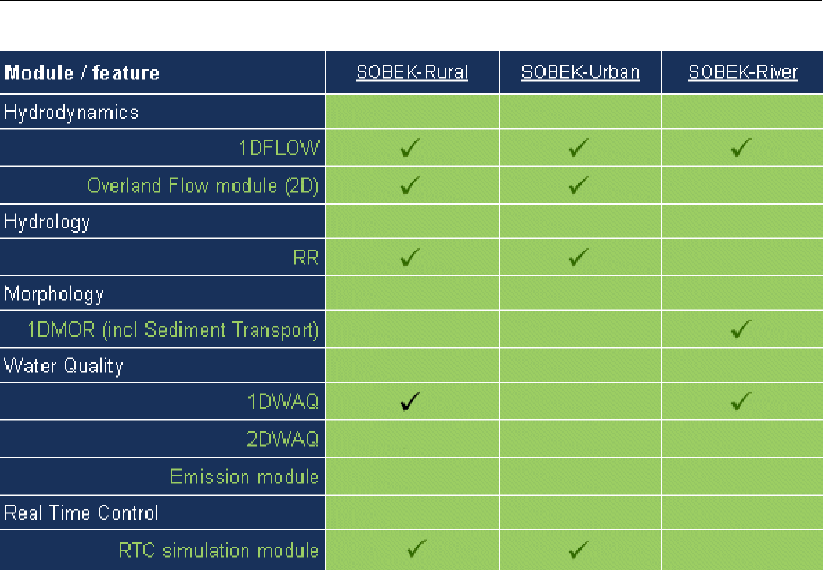
DRAFT
SOBEK, User Manual
All product lines use the same interface components. The interfaces of the urban and rural
product lines are fully integrated. So, when you know how to work with one module, you know
how to work with them all. The user interface is used to prepare your schematisation, control
your input data, check for possible schematisation errors, and helps you to analyse both input
data and all computed parameters.
Open interface
SOBEK has been developed by Deltares in partnership with the National Dutch Institute of In-
land Water Management and Wastewater Treatment (RIZA), and the major Dutch consulting
companies. SOBEK is the concrete result of our experience with governments, city authori-
ties, water boards, private consulting companies and research institutes. Because so many
people have helped to develop SOBEK, we’ve made the program as open as possible.
SOBEK is designed to interface with your existing software. It has a transparent ASCII
database and can download information from a variety of standard data formats and GIS
systems, so there’s no need for extra typing. The program is very easy to configure and
quick to learn. It checks extensively for data input and schematisation errors. The GIS ori-
ented interface makes it more user-friendly than most other programs, especially for larger
networks. The computer screen automatically adjusts itself to your needs and expertise so
you can organise your water system information and tasks.
Application areas
2 of 900 Deltares
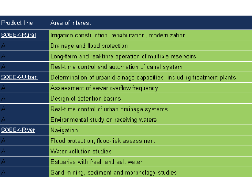
DRAFT
Introduction
The integrated approach makes SOBEK a valuable instrument for flood forecasting, naviga-
tion, optimising drainage systems, controlling irrigation systems, reservoir operation, sewer
overflow design, groundwater level control, river morphology regulation, and water quality
control. The integrated approach also means that SOBEK can combine river systems, urban
systems and rural systems for a total water management solution.
Size and complexity doesn’t matter
SOBEK is based on high-performance computer technology. That means it can handle water
networks of any size (big or small) and complexity.
It automatically configures itself to the type of water system you’re modelling. All numerical
computations have self-selecting time steps and are extremely robust.
1.3 Introduction to SOBEK-Rural
SOBEK-Rural gives regional water managers a high-quality tool for modelling irrigation sys-
tems, drainage systems, natural streams in lowlands and hilly areas. Applications are typically
related to optimizing agricultural production flood control, irrigation, canal automation, reser-
voir operation, and water quality control. SOBEK-Rural can also answer questions about in-
creased pollution loads in response to growing urbanisation. SOBEK-Rural offers the support
you need for effective planning, design and operation of new and existing water systems.
The software calculates (easily, accurately and fast) the flow in simple or complex channel
networks, consisting of thousands of branches, cross sections and structures. You can define
all types of boundary conditions, as well as define lateral inflow and outflow using time series
or standard formulae. For more detail, the rainfall run-off process of urban areas and vari-
ous types of unpaved areas can be modelled, taking into account land use, the unsaturated
zone, groundwater, capillary rise and the interaction with water levels in open channels. For
water quality and environmental problems the Water Quality module offers almost unlimited
possibilities.
Deltares 3 of 900
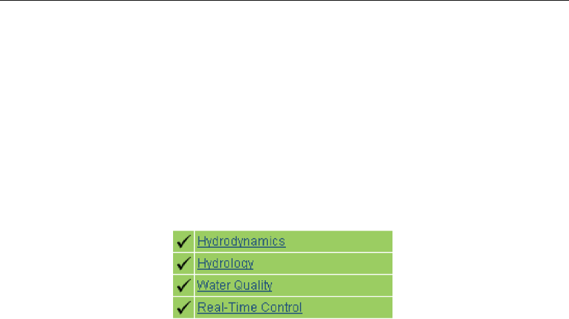
DRAFT
SOBEK, User Manual
The graphic display superimposes your network over a (GIS or aerial photo) map of the area
so you can see the canals, reservoirs, weirs, pumping stations, treatment plants, urban and
rural areas at a glance. Animation options show the direction of flow through the network and
by varying the thickness and colours of selected network elements, all input and computed
parameters can be visualised. By clicking on the map you can draw your network and adjust
any detail to suit your needs. The network can also be viewed from the side. Side view allows
you to print the design and watch the water profiles and real-time operation of structures in
detail.
SOBEK-Rural incorporates four modules:
1.4 Introduction to SOBEK-Urban
SOBEK-Urban offers a comprehensive modelling tool for simple or extensive urban drainage
systems consisting of sewers and open channels. SOBEK-Urban allows you to design new
urban areas or analyse and improve existing ones. You can use it to find out what measures
will prevent drainage congestion, street flooding and water pollution from sewer overflows.
The return period of street flooding and sewer overflows can be analysed using long time
series of rainfall data or storm events.
The models help you to find out how the performance of the urban drainage system can be
improved by a better operation of the pumps gates and weirs. The impact of treatment plants
and sewer overflows on the receiving water can be analysed by combining everything into one
model. It’s the ideal tool for the design, management and renovation of urban sewer systems.
SOBEK-Urban models the rainfall run-off process for various types of paved and unpaved
areas. It doesn’t matter whether the urban drainage system consists of open channels and
sewer pipes, storage tanks and reservoirs. Even street flow can be modelled with SOBEK-
Urban.
The application handles all kinds of cross sections, control structures and any network config-
uration (branched and looped). The size and complexity of the system doesn’t matter either.
The computation is extremely fast, also for large networks (e.g. 25 000 sewer pipes and man-
holes in one model). On top of that, SOBEK-Urban offers virtually any real-time control option
for pumps, weirs and gates in the urban system.
The graphic display superimposes your network over a (GIS or aerial photo) map of the area
so you can see sewer pipes, manholes, canals weirs and pumping stations at a glance. By
clicking on the map you can draw your network and adjust any detail to suit your needs.
Animation options show the direction of flow and by varying the thickness and colours of
network elements all input and computed parameters can be visualised. The network can
also be viewed from the side and allows you to print the design and watch the filling and
drying process in detail.
The software conforms to strict Dutch guidelines for sewerage calculations.
SOBEK-Urban consists of three modules:
4 of 900 Deltares

DRAFT
Introduction
1.5 Introduction to SOBEK-River
SOBEK-River is the product line designed for simple and complex river systems and estuar-
ies. It simulates the water flows, the water quality and morphological changes in river sys-
tems, estuaries and other types of alluvial channel networks. The networks can be branched
or looped. SOBEK-River is able to work with complex cross-sectional profiles consisting of
various sub-sections.
The Windows-based interface makes it easy to use and have the Windows look and feel that
you’re used to. Direct on-screen display of the river network gives you an overall view of your
system.
SOBEK-River works with one or more of the following modules:
1.6 Support
General information
If you have a question about SOBEK for which you cannot find the answer in the manual, you
can contact SOBEK Support at Deltares.
You should have the following information ready:
the version number of SOBEK (visible in the upper-left corner of the window after the
program is started);
the type of hardware you are using;
the operating system you are using;
the exact wording of any message that appeared on your screen (write it down or take a
screenshot);
a description of what happened and what you were doing when the problem occurred;
a description of how you tried to solve the problem;
whether you are able to reproduce the problem by repeating what you did when the prob-
lem occurred.
It may also be necessary to send the project data to SOBEK Support. The best way to do
this is to close SOBEK, zip the relevant project folder (*.lit) and send it using an e-mail. If the
project is too large to be included as an attachment in an e-mail, SOBEK Support can provide
the credentials to an ftp account where the data can be uploaded.
Security software
FlexNet
Our software uses license managing software by Flexera Software. If you want to know more
about the security software, see the following link: http://www.flexerasoftware.com/products/flexnet-
publisher.htm
Deltares 5 of 900

DRAFT
SOBEK, User Manual
In case you have additional questions about the security software, Flexera Software support
can be found here: http://support.flexerasoftware.com/
It may be useful to seek out Flexera support if you are using various software packages using
different security systems.
The dongle manufacturers
If you want to know more about new and old dongle manufactures, see the link below. In this
document you can find links to drivers and other tools. It is also a comprehensive manual.
Note: You do not need to install any drivers linked to in this document, the program setup
will install the correct dongle drivers automatically as part of the Deltares License Manager
Installation. These links are provided for troubleshooting purposes only:
http://www.flexerasoftware.com/webdocuments/PDF/faq_FLEXid_dongles.pdf
A direct link to the drivers for the dongles used in our software:
http://www.aladdin.com/support/hasp/enduser.aspx
1.7 About Deltares
In 2008, four renowned Dutch organisations decided to pool their knowledge and expertise.
WL |Delft Hydraulics, GeoDelft, TNO’s Subsurface and Groundwater unit and parts of Rijk-
swaterstaat (the Dutch Directorate-General for Public Works and Water Management) joined
together to set up Deltares, an independent institute for the development, dissemination and
application of knowledge concerning water, soil and subsurface. The result is an organisation
superbly well-equipped to address complex, integrated issues relating to water, soil, subsur-
face management and spatial planning in deltas, coastal areas and river basins.
Clients
Our national and international clients include government authorities, policy makers and ad-
ministrators responsible for the short- and long-term governance of bodies of water and re-
lated infrastructures. Our clients are also in the private sector: for example, among multilat-
eral agencies, consulting engineers, contractors, and in industry. They all have one thing in
common: the need for solid, practical advice. They come to us because they know that we
understand their concerns and are prepared to approach their questions from independent,
fresh perspectives.
What we can do for you
Deltares brings together a long-standing reputation for excellence in hydrology, hydraulics,
morphology, water quality and ecology. Construction and design matters related to offshore,
coasts, harbours, estuaries, rivers and canals, and industry — also our forte — are ap-
proached in a manner tuned to the specific requirements of the client. In addition, we op-
erate at the policy level by delivering decision support and carrying out environmental impact
6 of 900 Deltares

DRAFT
Introduction
assessments in the above mentioned working areas.
We have a full range of experimental facilities and computer programs, most of which have
been developed and validated by our experts in residence. On the basis of a sound under-
standing of the processes involved, all water systems can be simulated by us, numerically,
experimentally, or through a combination of the two. At Deltares, transfer of technology and
know-how is an inherent part of our approach. This is done through a variety of training
courses and seminars, and on the job.
More demanding
Demands of increased production and economic growth are frequently coming in direct — and
public — conflict with environmental concerns. Balancing the needs of one with those of the
other, not only for today, but also for the future, is often expressed in the phrase "sustainable
development".
No simple matter, it makes our clients’ jobs more demanding. In turn, they demand more of us,
not only for construction — and design — related issues, but also for far-branching policy and
management concerns. They expect and get from us optimal performance: a multidisciplinary,
scientifically rigorous approach linked to cost-conscious good business sense.
1.8 Notation
In this manual the following conventions in type style are used:
Type style Used for
Button Buttons ( on the screen or on the keyboard) that perform the indicated
action or give access to a corresponding window. The text can be lo-
cated on the button itself or next to the button.
Window Name of a window, shown in the name bar. Also used for subwindows,
indicating a group of buttons and/or data fields.
Deltares 7 of 900

DRAFT
SOBEK, User Manual
8 of 900 Deltares

DRAFT
2 Getting started
2.1 Starting SOBEK
To get a good insight of the capabilities of SOBEK please use the tutorials provided with this
SOBEK release.
The following tutorials are available:
section 4.1,Tutorial Hydrodynamics in open water (SOBEK-Rural 1DFLOW module)
section 4.2,Tutorial Hydrodynamics in sewers (SOBEK-Urban 1DFLOW + RR modules)
section 4.3,Tutorial Hydrodynamics - 1D2D floodings (SOBEK-Rural 1DFLOW + Overland
Flow modules)
section 4.4,Tutorial Hydrology in polders (SOBEK-Rural RR module)
The SOBEK-Rural 1DWAQ tutorial can be found in the D-Water Quality User Manual (D-
WAQ UM,2013)
The following manuals provide information regarding this SOBEK release:
This manual (The Hydrodynamics, Rainfall Runoff and Real Time Control User Manual),
The D-Water Quality User Manual (D-WAQ UM,2013),
The D-Water Quality Processes Library Description
The D-Water Quality Processes Tables (D-WAQ PLT,2013).
2.2 Free trial options
If you do not have a license file, SOBEK can still be used in Free Trial Copy mode. In this
mode the following schematization restrictions apply:
SOBEK-Rural 1DFLOW (100 node limit)
SOBEK-Rural Overland Flow (2D) module - 2DFLOW (1000 active 2D cell limit)
SOBEK-Rural RR (5 node limit)
SOBEK-Urban 1DFLOW (100 node limit)
SOBEK-Urban RR (100 node limit).
The Water Quality module cannot be used in Free Trial Copy mode.
While in Free Trial Copy mode, the user has the full functionality of the Task blocks: Import,
Meteo,Results in Maps,Results in Charts and Results in Tables at her/his disposal.
The following Tutorials can be followed in Free Trial Copy mode:
4.1,Tutorial Hydrodynamics in open water (SOBEK-Rural 1DFLOW module)
4.2,Tutorial Hydrodynamics in sewers (SOBEK-Urban 1DFLOW + RR modules)
4.3,Tutorial Hydrodynamics - 1D2D floodings (SOBEK-Rural 1DFLOW + Overland Flow
modules)
4.4,Tutorial Hydrology in polders (SOBEK-Rural RR module)
Deltares 9 of 900

DRAFT
SOBEK, User Manual
10 of 900 Deltares

DRAFT
3 Installation manual
3.1 Introduction
Deltares has developed a unique, fully integrated modelling framework for a multi-disciplinary
approach and 1D-2D computations for river systems and estuaries, irrigation and drainage
systems and wastewater and storm water systems. It can carry out simulations of flows,
rainfall-runoff, sediment transports, water quality, morphological developments and ecology.
It has been designed for experts and non-experts alike. The framework is composed of sev-
eral modules, grouped around a mutual interface, while being capable of interacting with one
another.
3.1.1 System requirements
Operating Systems:
Windows Server 2008
Windows 7
Windows 8.1
Windows 10
Administrative privileges are required in order to install and use the software.
Minimum hardware specifications:
1,5 GHz Intel Core processor or equivalent
2 GB of RAM
2 GB free hard disk space
a graphics adapter with 128 MB video memory and screen resolution of 800x600
Preferred hardware specifications:
3 GHz Intel Core processor or equivalent
6 GB of RAM, 64-bit Windows Operating System
20 GB free hard disk space
a graphics adapter with 256MB video memory and a screen resolution of 1024x768
SOBEK is a 32-bit application. On 32-bit Windows operating systems, SOBEK can use a
maximum of 2GB RAM (address space). On 64-bit Windows operating systems, SOBEK can
use a maximum of 4GB RAM.
Regional Settings format in Windows: SOBEK should be installed on machines using a dot
(.) as decimal separator symbol and a comma (,) as digit grouping symbol. For example as
English format.
Deltares 11 of 900

DRAFT
SOBEK, User Manual
3.2 Deltares License Manager
For information about the Deltares License Manager, including installation manual and Fre-
quently Asked Questions, please visit:
https://publicwiki.deltares.nl/display/LMADMIN/Deltares+License+
Management
In order to use SOBEK, the license manager must be installed.
3.3 Installing SOBEK
This document describes the steps that should be taken to install SOBEK on your personal
computer.
The installation consists of two parts:
The installation of the Deltares Software License Manager
The installation of the SOBEK software package
The licensing of your software is managed by the Deltares Software License Manager (DS_Flex),
which is based on the FlexNet Publisher licensing system. It provides a user friendly environ-
ment in which a range of license constructions can be arranged, varying from single user
licenses to multiple user network licenses.
Note that your license file may not be suitable for all mentioned license constructions.
Log on to the PC. You need to log on as administrator (or a similar account with similar
user privileges).
Start the program setup (named SETUPSOBEK.EXE or similar), from the installation CD
or the location where you downloaded it to.
Now you are lead through the setup procedure by a graphic user interface:
The first dialog is the SOBEK Welcome screen:
12 of 900 Deltares
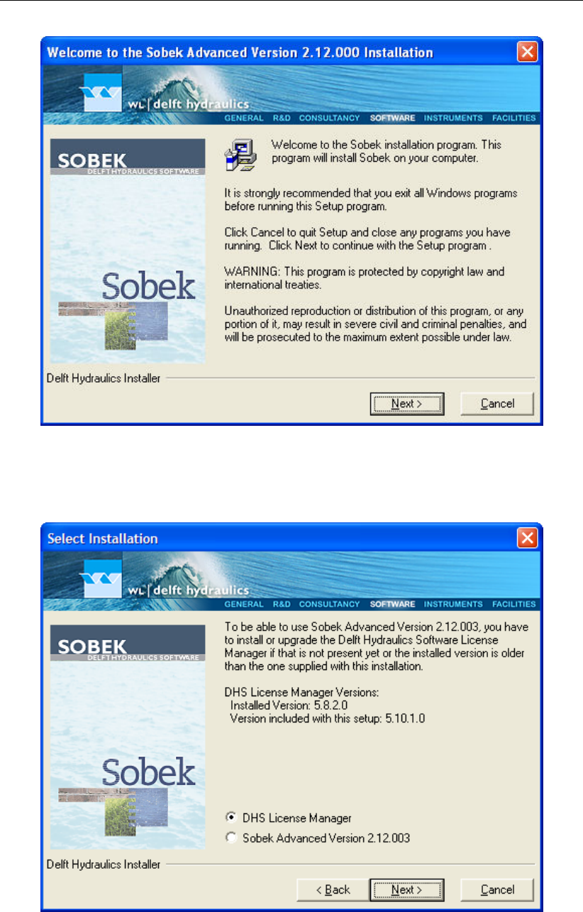
DRAFT
Installation manual
Figure 3.1: SOBEK welcome window
Click the Next button to go to the next dialog.
Figure 3.2: Select installation window, Deltares Software License Manager selected
This dialog gives the opportunity to choose to install the license manager or to install SOBEK.
Deltares 13 of 900

DRAFT
SOBEK, User Manual
In this example the version of the Deltares Software License Manager is newer than the
already installed one. It is highly recommended to use always the most recent version of the
Deltares Software License Manager. If the license manager has not been installed yet, the
installed version will be displayed as ’None’.
Note:
The Deltares Software License Manager must always be installed in order to use SOBEK.
Even when trying out the Free Trial functionality of the software. Failure to install the li-
cense manager will result in a SOBEK Startup error. (Run-time error ’53’. File not found:
wlauth40.dll)
Click the Next button to install the Deltares Software License Manager.
The actual installation of the Deltares Software License Manager is described in a separate
paragraph. After it has been installed, the following situation will be displayed:
Figure 3.3: Select installation window, SOBEK selected
Select the SOBEK option if not selected yet.
Click the Next button to install SOBEK.
If there are already one or more SOBEK versions installed, the following dialog will appear:
14 of 900 Deltares
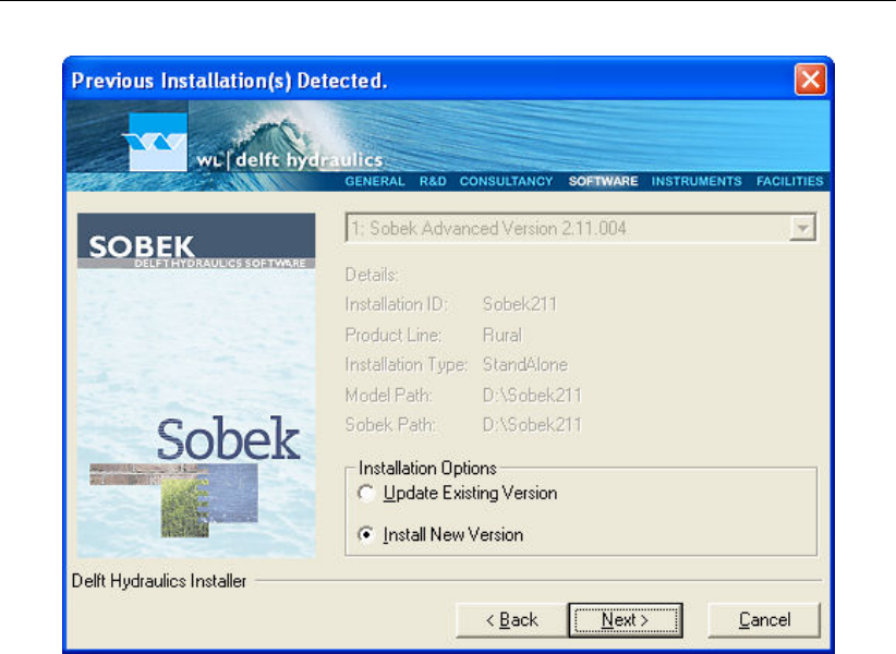
DRAFT
Installation manual
Figure 3.4: Previous Installation(s) Detected, Install New Version selected
Here you can select the Update option and select a SOBEK version which you want to update.
In that case all the options of that installation will be taken from the selected installation, like
Installation ID, Product Line, Installation Type and the directories where the files are stored.
Ensure that in case of network installations the installation path is accessible and writable.
When you select to update an existing version, after clicking the Next button the Miscellaneous
Options dialog will appear. This dialog will be explained later.
When the Install New Version option is selected, clicking the Next button will activate the
following dialog:
Deltares 15 of 900
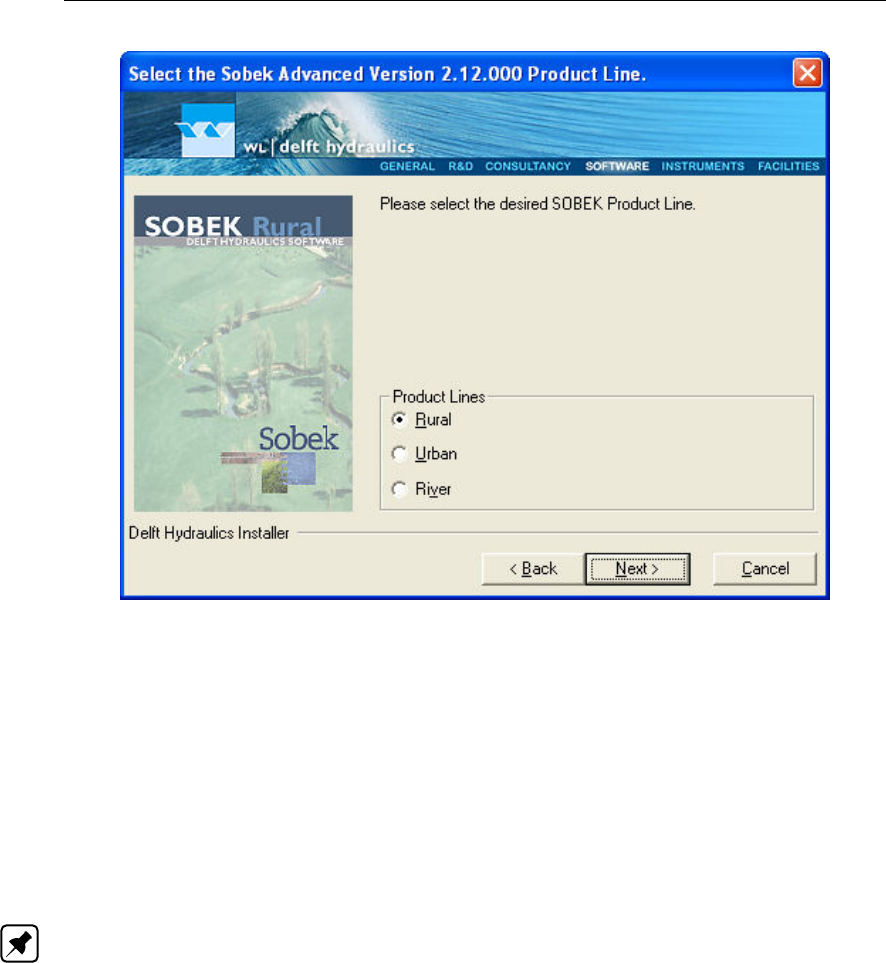
DRAFT
SOBEK, User Manual
Figure 3.5: SOBEK installation, select Product Line
In this dialog the desired SOBEK Product Line can be selected. You can choose between
Rural, Urban and River.
Choosing one of these options will have the following consequences:
Typical Rural, Urban or River default numerical parameters will be selected for new projects.
Numerical parameters can always be changed later in the Settings menu.
A different background image for the SOBEK startup screen will be used.
Note:
Choosing between Rural, Urban and River has no consequences as to which modules you
can use. Which modules you can use is determined entirely by your license file.
Click the Next button to go forward to the Installation ID dialog.
16 of 900 Deltares
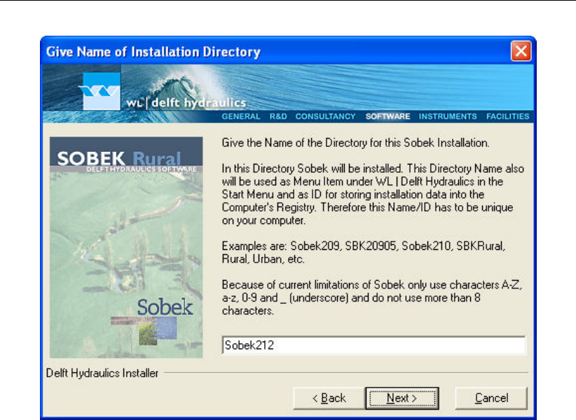
DRAFT
Installation manual
Figure 3.6: Enter SOBEK installation directory
Here you must specify the name of the directory where SOBEK will be installed. This directory
name also will be used as entry in the Windows Start Menu under Delft Hydraulics and as
ID for storing installation data into the computer’s registry. You can install multiple versions of
SOBEK on the same computer, but you have to use a unique folder name for each installation.
The Installation ID is limited to 8 characters and may only contain A–Z, a–z, 0–9 and ’_’
(underscore).
Click the Next button to go to the Drive Selection dialog.
In the dialog below you must select the drive where the SOBEK system will be installed. The
actual directory will be <Drive:\Install_ID>
Deltares 17 of 900

DRAFT
SOBEK, User Manual
Figure 3.7: Select destination drive(s)
In some case it is desired or even required to separate the programs and the model data. In
that case you can mark the checkbox and then select separate drives for the programs and the
model data. In the example below (using the Installation ID from the earlier example dialog)
the programs will be stored in <C:\Sobek214>and the model data in <D:\Sobek214>.
Figure 3.8: Select destination drive(s)
18 of 900 Deltares
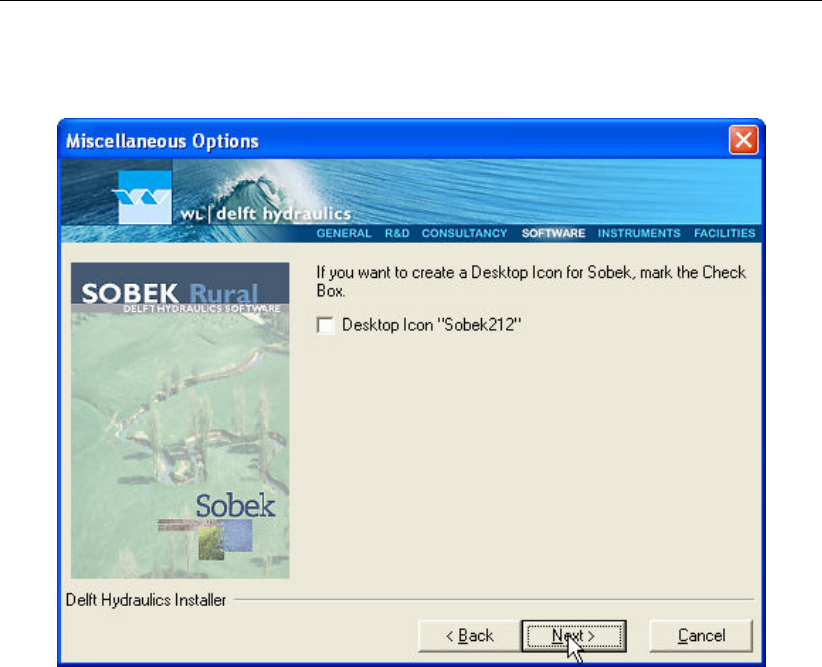
DRAFT
Installation manual
Click the Next button to got to the Miscellaneous Options dialog.
Figure 3.9: Miscellaneous Options
At this moment you can specify that you want to create a Desktop Icon to be able to start
SOBEK fast. To distinguish the several SOBEK installations, the Installation ID is added to
the Icon name. If you want to create the Desktop Icon, mark the checkbox ’Desktop Icon
"Sobek..."’.
Click the Next button to go to the last pre-install dialog.
Deltares 19 of 900
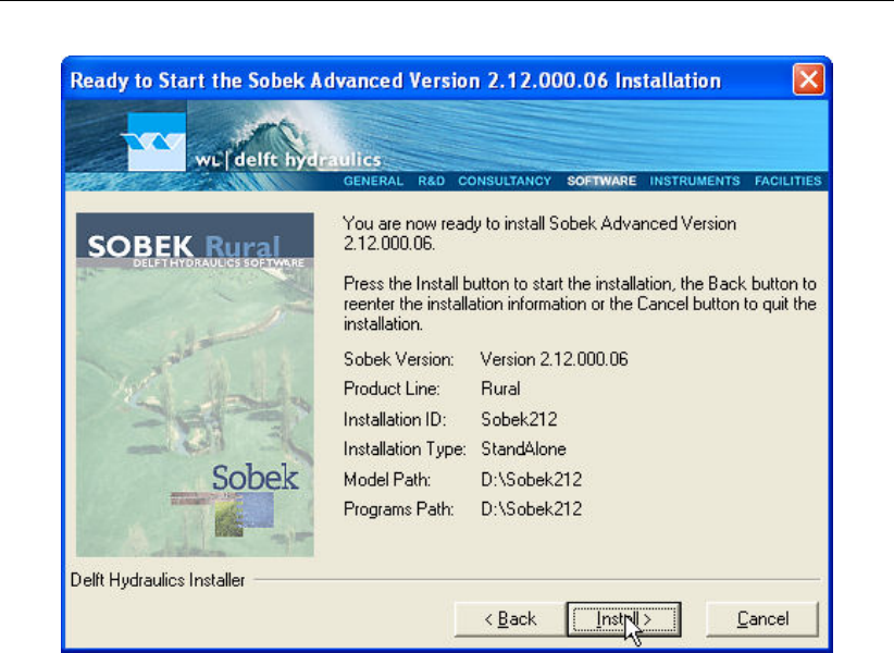
DRAFT
SOBEK, User Manual
Figure 3.10: Check installation properties
The dialog above gives an outline of the options that you selected in the previous steps of the
installation. If you find anything incorrect, you can go back by clicking the Back button and
re-enter the installation information or quit the installation by clicking the Cancel button.
If everything looks OK, you can start the installation by clicking the Install button. The instal-
lation will start now and take some time. The duration depends on the type of installation that
you selected and the capacities of your computer. A few minutes is a normal time span.
During the installation the progress can be seen in the window as shown below:
20 of 900 Deltares
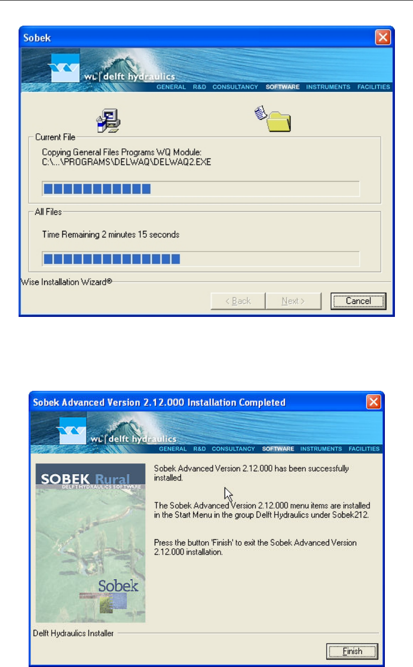
DRAFT
Installation manual
Figure 3.11: Installation progress bar
After the installation process has been finished successfully, the following dialog will pop up:
Figure 3.12: Finish installation window
Click the <Finish>button to leave the installation program.
Deltares 21 of 900

DRAFT
SOBEK, User Manual
You will be asked for a reboot to conclude the installation. It is recommended to do so.
General information
If you have a question about SOBEK for which you cannot find the answer in the on-line
manual, you can contact SOBEK Support at Deltares.
You should have the following information ready:
the version number of SOBEK (visible in the upper-left corner of the window after the
program is started);
the type of hardware you are using;
the operating system you are using;
the exact wording of any message that appeared on your screen (write it down or take a
screenshot);
a description of what happened and what you were doing when the problem occurred;
a description of how you tried to solve the problem;
whether you are able to reproduce the problem by repeating what you did when the prob-
lem occurred.
It may also be necessary to send the project data to SOBEK Support. The best way to do this
is to close SOBEK, zip the relevant project folder <*.lit>and send it using an e-mail. If the
project is too large to be included as an attachment in an e-mail, SOBEK Support can provide
the credentials to an ftp account where the data can be uploaded.
3.3.1 Installing the SOBEK using the command line
Below, the various options for installing SOBEK using the command line are detailed. These
options are intended for advanced users only. Most of the input validations performed in the
user interface version of the SOBEK setup are not performed when using a command line
installation.
/SILENT Run silent/unattended.
/DESKTOP If present, a desktop icon will be created.
/DRIVE=D Specifies the drive to install SOBEK on.
/SBTYP=Rural Specifies the SOBEK product line. Default: Rural.
Can be Rural, Urban or River.
/SBID=SOBEK215 Installation ID and Directory name. E.g. for SOBEK 2.15, use SOBEK215.
Because SBID is used as directory name it has to be specified ac-
cording to the rules for any directory name. Additionally, this ID is
limited to a maximum of 8 characters.
For example:
SetupSOBEK_2.15.001.exe /SILENT /DESKTOP /DRIVE=D /SBTYP=Rural /SBID=SOBEK215
If the switches are specified as above: SOBEK 2.15 Rural will be installed in <D:\SOBEK215>
and a desktop icon will be created.
22 of 900 Deltares

DRAFT
Installation manual
3.4 Starting SOBEK
The installation procedure creates a menu item for SOBEK on the ‘Programs’ menu under the
Windows Start button. To start SOBEK you must do the following:
Click on the Windows Start button;
Select the ‘Programs’ menu;
Select the ‘Delft Hydraulics’ menu;
Select the SOBEK menu item;
Click on the SOBEK icon.
Deltares 23 of 900

DRAFT
SOBEK, User Manual
24 of 900 Deltares
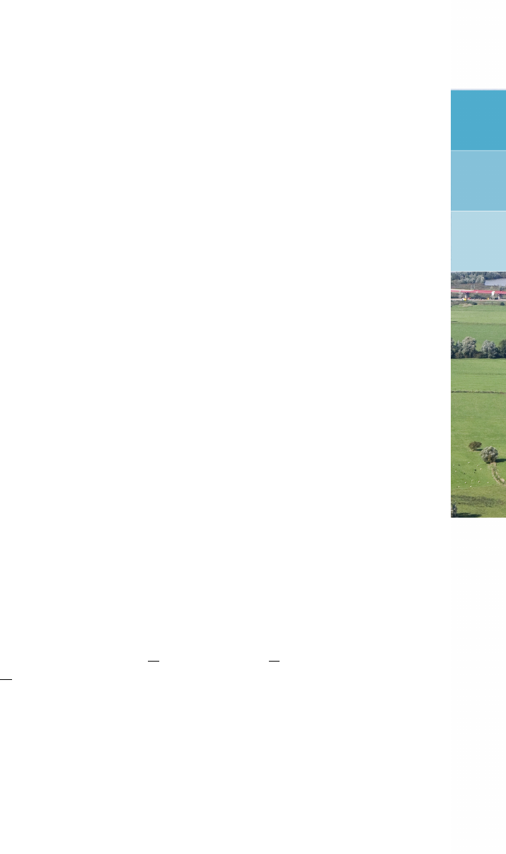
DRAFT
4 Tutorials
4.1 Tutorial Hydrodynamics in open water (SOBEK-Rural 1DFLOW module)
General
In this tutorial the basic principles of working with the 1DFLOW module of SOBEK-Rural are
explained step by step and you will be guided to set-up a simple network and to extend this
network with new elements. This tutorial will only show a limited number of the large amount
of options. It will teach the basic principles of working with the 1DFLOW module of SOBEK-
Rural and give you enough experience to continue on your own. Some experience in working
with the Microsoft R
Windows R
operating system is required.
The tutorial contains:
1 setting up a simple network;
2 editing boundary conditions;
3 editing profiles.
The tutorial does not explain all options in all windows that appear. Once you get the hang-
and-feel of the modelling system, you may wish to browse through the options not dealt with
in the tutorial.
Getting started
Click the Windows Start button.
Select the ’All Programs’ or ’All Apps’ menu.
Select the ’Delft Hydraulics’ menu.
Select the ’SOBEK’ menu item (SOBEK215).
Click the ’SOBEK’ icon.
In the SOBEK main window: select the menu item ’Options’ - ’SOBEK Options’.
Select the tab ’Background Map’.
Select the file <Tutorial1.map>.
Press OK button to save and close SOBEK Options.
Click the New Project button.
Type the name ’T_CHANN’.
The program converts all the characters into upper case. If a project with the same name
already exists, the user has to enter a different name here.
Click the OK button.
You have added a new project with the name ’T_CHANN’. You are now asked: do you want
to work with this project?
Click the Yes button.
Case management
The screen of the so-called case manager appears. This tool automatically keeps track of
cases and the related files. For instance: you might want to save different scenario’s within a
project as cases with different names. This is organized through the case manager.
Deltares 25 of 900

DRAFT
SOBEK, User Manual
Figure 4.1: The case manager window.
On the screen a number of blocks will appear:
1 Import Network;
2 Settings;
3 Meteorological Data;
4 Schematisation;
5 Simulation;
6 Results in Maps;
7 Results in Charts;
8 Results in Tables.
Each block represents a specific task. A task can be a model, a set of linked models, the
selection of a scenario or strategy, or a (graphical) presentation tool. The arrows between the
blocks represent the relations between the tasks. When an arrow is pointing from block "A" to
block "B", the task of block B can only be executed after the task of block A is finished.
The Case Manager has the following tasks:
1 Administration of cases (which data is related to which cases);
2 Checking whether the model calculations for the cases are performed in the predefined
order;
3 Logging the actions of the Case Manager (including view and print);
4 Providing access to the computational framework through a user interface, so the user
can:
manipulate a case (read, save, delete, etc.);
view and check the status of all tasks;
view the relation between the various tasks.
choose and run predefined tasks (modules);
26 of 900 Deltares
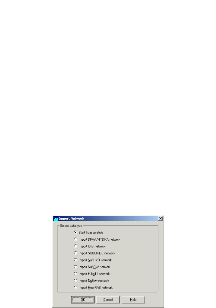
DRAFT
Tutorials
When the Case Manager screen appears first after you have added a project all task blocks
are grey. To activate the task blocks you have to open the default case of this new project:
Select the menu option ’Case’ - ’Open’.
Select ’Default’ from the list.
Click OK button.
Another method is to double-click one of the grey task blocks and select ’Default’.
Once you have opened the default case the task blocks are no longer grey, but one of the
following colors:
1 yellow: the task can be executed;
2 green: the task has been executed at least once and can be executed again;
3 red: the task cannot be executed until the preceding task has been executed.
When the task is being executed the task block is purple. You can execute a task by double-
clicking on the task block. When you select a yellow or green task block, the color will change
to purple and then change to green again when the task is finished.
Now, we will discuss each task block.
4.1.1 Task block: Import Network
The color of this task block is yellow, which means that this task block is still waiting to be
executed.
Execute the task block ’Import Network’ by double-clicking it. The block then turns purple
and the Import network window will pop up:
Figure 4.2: The import network window.
In this task block the origin of the schematisation must be defined. Schematisations, used in
SOBEK, can be either imported from a database or set-up from scratch. If a schematisation is
already available in the standard exchange format it can easily be imported from the database
to SOBEK. Links with data formats can be custom made on request. For that reason some
radio buttons might be turned grey.
Deltares 27 of 900
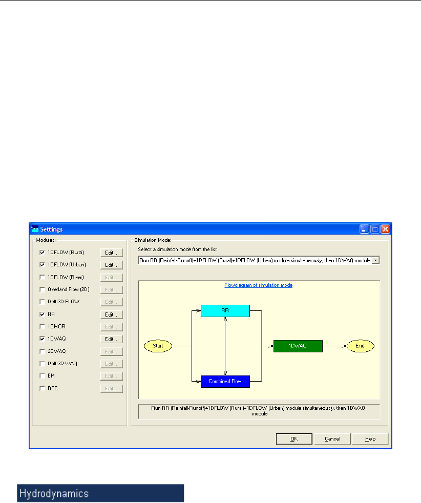
DRAFT
SOBEK, User Manual
Let’s set up a schematisation from scratch.
Select the radio button Start from scratch.
Press OK button.
Notice that you’re back in the Case Manager now and that the task block ’Import Network’ has
turned green.
4.1.2 Task block: Settings
The ’Settings’ task block is used to select the SOBEK modules that you want to use for your
project. Also computational parameters such as calculation time steps, simulation period and
initial water levels can be set in the ’Settings’ task block. Depending on the set of modules
that you purchased, some of them may be disabled (grey), and some may be enabled.
Figure 4.3: The settings window.
SOBEK-Rural 1DFLOW
The SOBEK-Rural 1DFLOW module is a sophisticated module that can be used for the
simulation of one-dimensional flow in irrigation and drainage systems. It is a tool that can
be used to simulate and solve problems in regional water management, such as irrigation
construction, drainage, automation of canal systems, dredging and flood protection. This
module can be used stand-alone or in combination with other modules, for example the
SOBEK-Rural RR module (Rainfall-Runoff).
SOBEK-Urban 1DFLOW
The SOBEK-Urban 1DFLOW module is a sophisticated module for the simulation of one-
dimensional flow in wastewater and storm water systems. It is a tool that can be used to
simulate and solve problems in urban drainage systems such as determination of urban
drainage capacities including treatment plants, assessment of sewer overflow frequency
and design of detention basins. The SOBEK-Urban 1DFLOW module can also be used
in combination with the SOBEK-Rural 1DFLOW module, the SOBEK-Urban RR (Rainfall-
Runoff) module and other modules. One of the competitive advantages is the combination
with the SOBEK-Rural 1DFLOW module for environmental study on receiving waters.
SOBEK-River 1DFLOW
28 of 900 Deltares
DRAFT
Tutorials
The SOBEK-River 1DFLOW module is a sophisticated module that can be used for the
simulation of one-dimensional water flow in river systems and estuaries. It is a tool that
can be used to simulate and solve problems in river water management such as flood
protection, flood-risk assessment, real-time forecasting, dam break analysis, navigation
and dredging. This module can be used stand-alone or in combination with other modules.
The RR (Rainfall-Runoff) module is a module that can be used for the simulation of
rainfall-runoff processes. This module is a part of a large family of modules which can
be linked. The list of modules includes (amongst others) SOBEK-Rural 1DFLOW module,
SOBEK-Urban 1DFLOW module and RTC (Real Time Control) module. The RR mod-
ule is frequently used in combination with the SOBEK-Rural 1DFLOW and SOBEK-Urban
1DFLOW modules. It is then possible to either to perform calculations for both modules
simultaneously or sequentially.
The RTC (Real Time Control) module is a module that can be used for the simulation
of complex real time control of hydraulic systems. It can be applied to rainfall-runoff, hy-
draulics and water quality computations. In that case the rainfall-runoff and water quality
computations are run simultaneously with the hydrodynamics computations, thus incorpo-
rating full interaction between all processes.
The above mentioned modules can also be used in combination with modules for simu-
lating water quality processes (1DWAQ module, 2DWAQ module and/or EM (EMission)
module).
Thus, several combinations of modules are possible. Depending on the problems to be solved
you can set the desired combination. The modules can easily be selected via the task block
’Settings’.
Double-click the ’Settings’ task block. Its colour changes and the settings window appears.
Unselect all the selected modules if any.
Select the ’1DFLOW (Rural)’ module.
Press the Edit... button of ’1DFLOW (Rural)’.
You have to define a number of settings.
Select the tab ’Time settings’.
Set the ’time step in computation’ to 10 minutes (type “10” in the ’min’ edit box and “0” in
the others).
Select the radio button Simulation period defined as below.
Enter the year of the start time of the simulation: “2006”.
Enter also the ’Month’, ’Day’, ’Hour’, ’Min’ and ’Sec’ data of the start time of the simulation:
“1”, “1”, “1”, “0”, “0”.
Enter the end time of the simulation: “2006”, “1”, “1”, “10”, “0”, “0” in the respective edit
boxes.
Select the tab ’Output options’.
Enter the output step: “30” minutes in the respective edit box.
Note that the simulation period data and the time step can also be changed by clicking the
arrows left of the edit boxes.
Select the tab ’Initial data’.
Select the radio button define local values in <Edit Network>.
Deltares 29 of 900
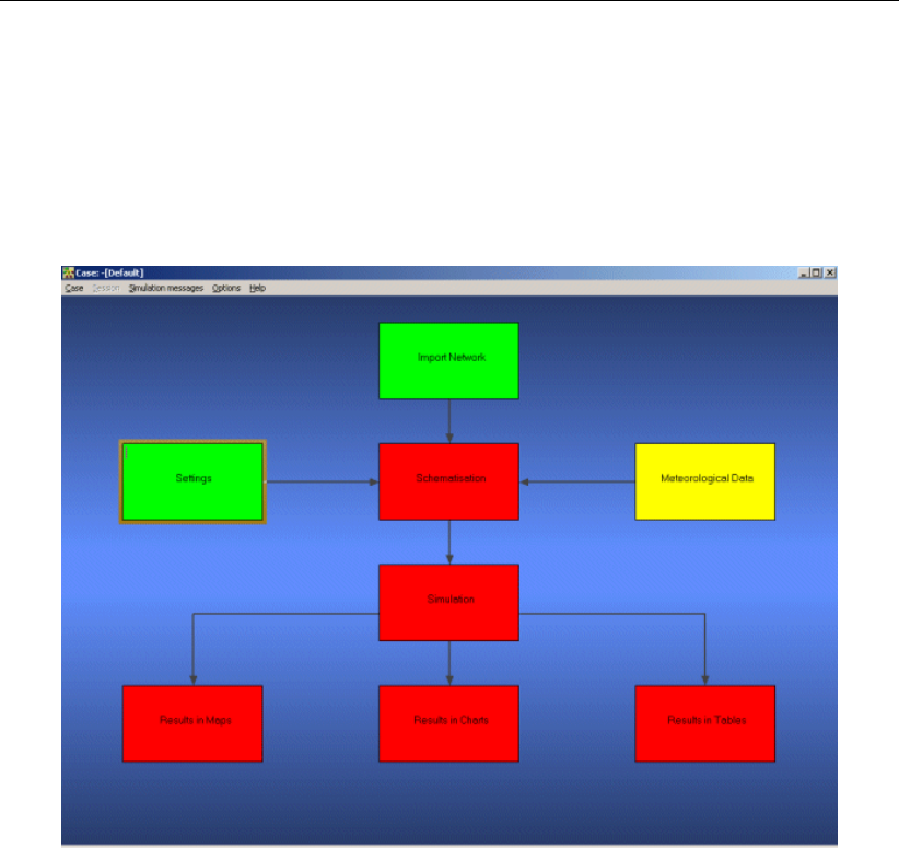
DRAFT
SOBEK, User Manual
Press the OK button to return to the Settings window.
Finally press the OK button, to save your settings and return to the Case Manager.
You should now see the following screen, which indicates that both the ’Settings’ task and the
’Import Network’ task have been completed and that the Meteorological data task should still
be performed:
Figure 4.4: The case manager after completing the ’settings’ and ’import network’ tasks.
4.1.3 Task block: Meteorological Data
SOBEK Rural simulations require meteorological input data, i.e. precipitation data, evapora-
tion data and wind data. The Meteorological data task block provides precipitation and evap-
oration data to the RR (Rainfall-Runoff) module and wind data to the 1DFLOW and Overland
Flow (2D) modules. For simplified rainfall-runoff processes precipitation data can optionally
be provided to the 1DFLOW and Overland Flow (2D) modules.
As this tutorial deals with hydrodynamics, the ’Meteorological data’ task block is of minor
importance. We will not include wind effects nor rainfall on the channel.
Double-click the ’Meteorological Data’ task block of the Case Manager.
The following screen will appear:
30 of 900 Deltares

DRAFT
Tutorials
Figure 4.5: The meteorological data window.
In the dialog that pops up you can see how precipitation, evaporation and wind data are
defined.
Click OK to leave the Meteorological data window.
Now you have finished defining the meteorological data. Notice that this task block has turned
green too!
4.1.4 Task block: Schematisation
A schematisation can easily be set up with the help of the network editor. You will set up a
simple schematisation.
Double-click the ’Schematisation’ task block of the Case Manager.
You can choose to edit a new or an existing model by clicking the upper Edit Model button.
Click Edit model.
When the option Edit Model of the ’Schematisation’ is selected, the network editor starts.
The network editor is called NETTER and is a component of the Delft Hydraulics Decision
Support System (Delft-DSS) tools. NETTER offers the possibility to set-up the schematisation
on top of a background GIS map. NETTER also offers advanced analysis tools to show model
results linked to the schematisation and provide the user with full printing facilities to make high
quality prints.
Within NETTER you can do the following:
1 Interactively and graphically prepare a schematisation;
2 Generate schematisations upon GIS map Layers;
3 Carry out schematisation operations: search for a certain node, show node numbers and
names, show link numbers, etc.;
4 Carry out map operations: zooming in, zooming out, (de)activating map layers, colouring
of map layers, adding title information on the map, etc.;
Deltares 31 of 900
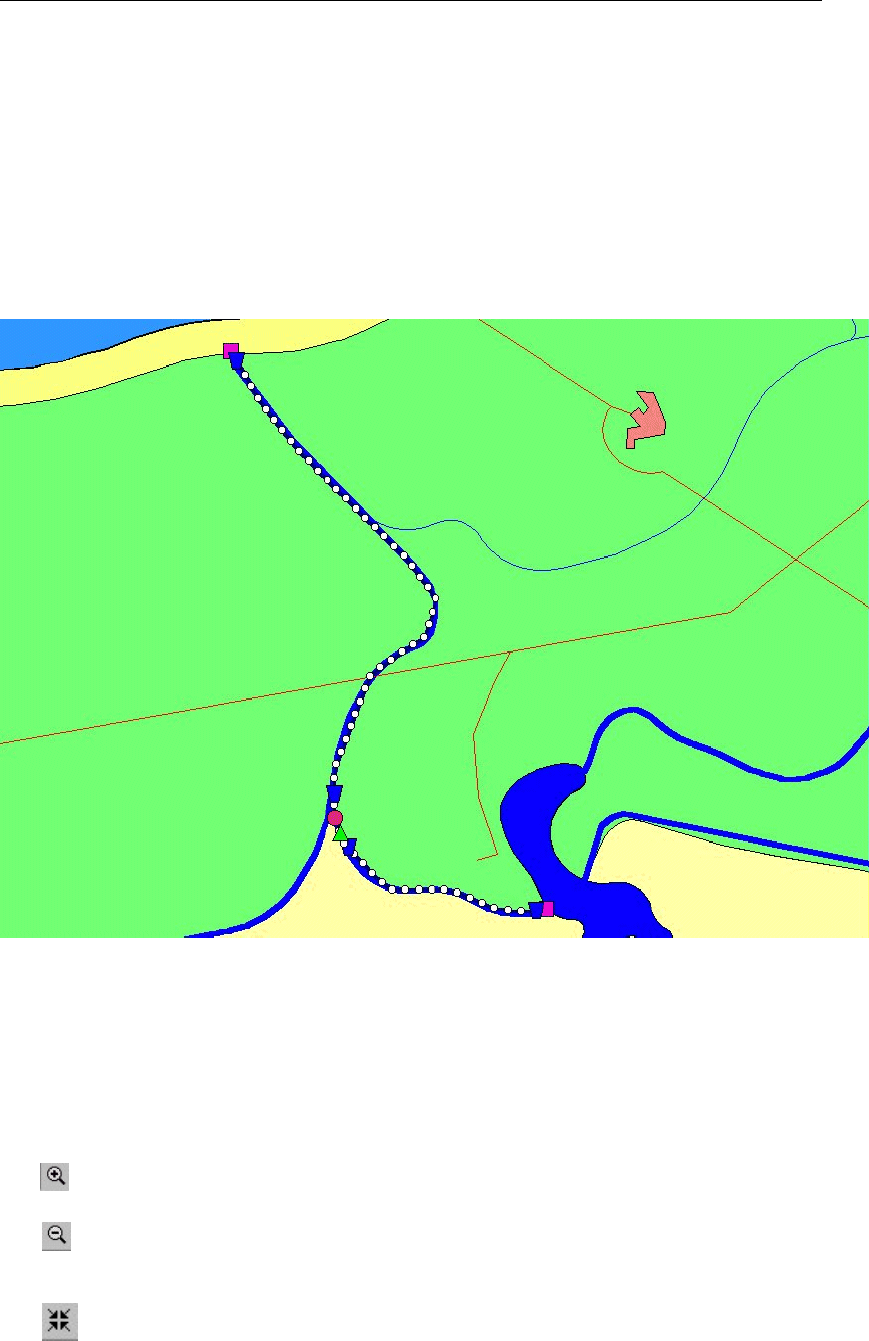
DRAFT
SOBEK, User Manual
5 View results of simulation models for schematisations created in NETTER;
6 Print maps or schematisations.
Generally speaking, NETTER has two edit modes. The first mode is the mode to set-up the
schematisation, e.g. by adding new nodes. The second edit mode is the mode for editing
the attribute data. In this mode you provide the attributes of the schematisation objects. For
example, a pump station must have a pump capacity and switch on/off levels.
In this exercise you will work on a simple schematisation.
Figure 4.6: The schematisation to be created in this tutorial.
In order to focus on a small part of the map, you can use the zoom functionalities.
The View menu contains commands to zoom in, zoom out, centre the window, move the
window and show all schematisation or map layers.
The button allows you to zoom in on any part of the "active main window".
The button allows you to zoom out by shrinking the displayed part of the "active main
window".
The button allows you to centre a schematisation or map GIS object. When choosing
this command and then clicking on an object NETTER, redraws the map centring the chosen
object to the NETTER window.
32 of 900 Deltares
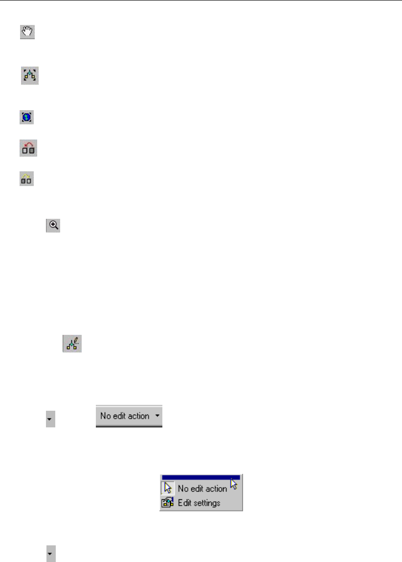
DRAFT
Tutorials
The button allows you to shift the view by clicking the mouse anywhere in the NETTER
window and dragging the view to another position.
The button redraws the view while fitting all schematisation objects into the NETTER
window.
The button redraws the view while fitting all GIS map layers into the NETTER window.
The button restores the view to the previous zoom state.
The button restores the view to the state before the last ’Show Previous’ command.
You are now asked to zoom in on the area between the lake and the sea.
Select button.
Move the mouse pointer to the main window.
Click and hold down the left mouse button, while dragging the pointer across the main
window. The size of the rectangle determines the magnification.
Release the left mouse button.
Now, you will build a simple schematisation. This schematisation consists of a small open
channel with a weir. We will now build this schematisation.
Select the button, Edit Network, to start the edit network mode.
When you have selected the edit network mode all edit network functions and network objects
for the selected module will be available.
Select from the section and click the ’General’ edit network functions to
unveil the General functions toolbar and move it to anywhere on your screen by clicking
the upper section of the selected toolbar and dragging it:
Figure 4.7: Click this section of a toolbar to drag it to your screen!
Select and the ’Node’ edit network functions to place the Node functions toolbar any-
where on your screen.
Deltares 33 of 900
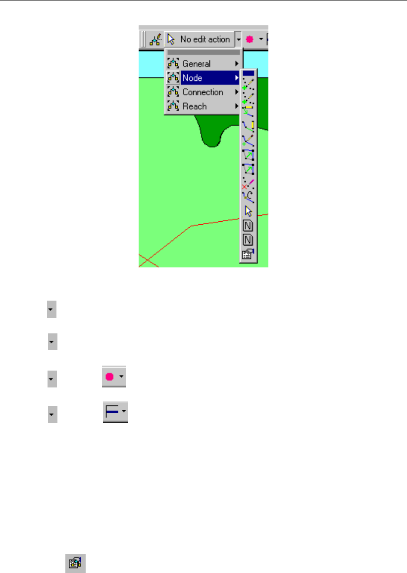
DRAFT
SOBEK, User Manual
Figure 4.8: Node functions toolbar
Select and the ’Connection’ edit network functions to place the Connection functions
toolbar anywhere on your screen.
Select and the ’Reach’ edit network functions to place the Reach functions toolbar
anywhere on your screen.
Select from the section and place the node objects toolbar anywhere on your
screen.
Select from the section to place the reach objects toolbar anywhere on your
screen.
If you desire more information explaining the large amount of objects, you can customize the
toolbars by clicking ’View’ - ’Toolbars’ - ’Customize...’. Caption only, Icon only and Icon and
Caption are the available options. ’Icon only’ means that you for the selected toolbar you will
only see the icons. Choosing Icon and Caption will also place a label explaining each symbol.
It is possible to define the identifiers (or ID’s) of the nodes and branches (links) automatically
or manually.
Select the button in the ’General’ tool bar, Edit settings, to go to the edit network
options.
Select the tab ’Node’.
In the ’ID’ group box, select the radio button Manual.
In the ’Name’ group box, select the radio button Manual.
Select the tab ’Link’.
Set the ’ID’ and ’Name’ to ’automatic’.
Click the OK button.
34 of 900 Deltares
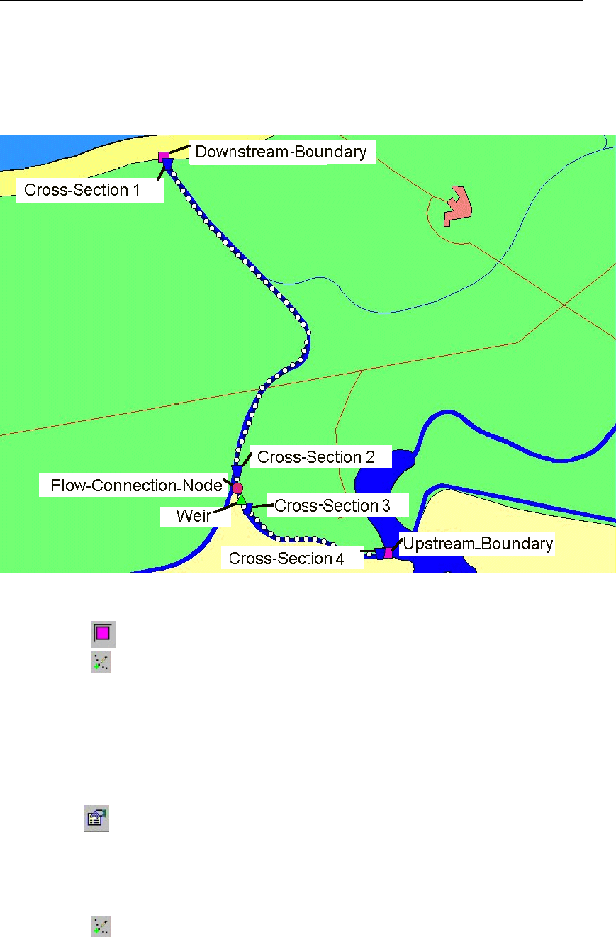
DRAFT
Tutorials
Create a schematisation:
Now you can start drawing your application. You will create a schematisation that is similar
to the one below. The schematisation will involve a river section that connects a lake to the
coast:
Figure 4.9: Create a network similar to this one
Select the node, Flow-Boundary.
Select the button to select the function ’Add node’.
Enter ’Upstream_Boundary’ in both input fields.
Click the OK button.
Locate the mouse at a position where you want to add the Upstream Boundary node and
click the left-mouse button again to actually add the node.
In order to see the identifiers on the map please:
Click the button in the Active Legend or select the menu item ’Options’ - ’Network
Data...’.
Select the tab ’Node’.
Select the radio button Name.
Press the OK button.
Select the button again.
Enter ’Downstream_Boundary’ in both input fields.
Click the OK button.
Add the Downstream Boundary node as before.
Deltares 35 of 900
DRAFT
SOBEK, User Manual
Select the node, Flow-Connection Node.
Select the button again.
Enter ’Flow-Connection_Node’ in both input fields.
Click the OK button.
Click on the left-mouse button to actually add the Flow-Connection node on your screen.
Select the button, Flow-Channel.
Select the button to select the function ’Connect nodes’.
Click with the left mouse button on the upstream boundary node, and drag to the con-
nection node while keeping the button pressed. Release the left mouse button to add the
connection.
Click with the left mouse button on the connection node and drag to the downstream
boundary node while keeping the button pressed. Release the left mouse button.
Now the two boundary nodes and the connection node are connected.
The model will need a calculation grid. We will switch off the automatic generation of names
before generating this grid because we do not want to generate calculation points with names
for this tutorial.
Select the button in the ’General’ tool bar, Edit settings, to show the edit network
options window.
Select the tab ’Node’.
In the ’Name’ data group, select the radio button No Names.
Press the OK button.
Several options are available to generate a grid.
Select the button to select the function ’Calculation grid all reaches’.
Select the ’Split Vector’ option.
Select the node type ’Flow - Calculation Point’ from the drop down list.
Then enter ’100’ in the length edit box to set the calculation grid to a 100 m length.
Click the OK button.
Now we can view the defined direction of the links on which we just generated a calculation
grid. The option ’defined direction’ can be used to see the positive defined direction. This
option is enabled by default, and can also be manually enabled by following these steps:
Select ’Options’ - ’Network Data...’.
Select the tab ’Link’.
In the data group ’Show Direction’, select the radio button Defined.
Click the OK button.
To disable titles on links, if enabled:
Select ’Options’ - ’Network Data...’.
Select the tab ’Link’.
Under ’Show Titles’, Select the radio button None.
36 of 900 Deltares
DRAFT
Tutorials
The vector layer:
To show schematizations with high performance, by default NETTER shows connections be-
tween two Flow - nodes in a straight line. However the length between the nodes may differ
from the distance between the nodes in a straight line. The actual length between Flow -
nodes is stored in the vector layer. You can edit the length in this layer.
Select the button, ’Edit Reach Vectors’, to edit a selected reach vector.
Select either of the two reaches.
Select the button to show the coordinates.
Select the button to add a coordinate.
Click with the left mouse button on the reach to actually add a coordinate on your screen
and while keeping the button down drag the new coordinate to the new location.
Add and drag other coordinates of the selected reach.
De-select the button to stop adding coordinates.
Select the other reach.
Select the button to add a coordinate again.
Click with the left mouse button on the reach to actually add a coordinate on your screen
and while keeping the button down drag the new coordinate to the new location.
Add and drag other coordinates of the selected reach.
De-select the button, ’Edit Reach Vectors’, to stop editing the reach vector.
Add reach objects:
Select the button in the ’General’ tool bar, Edit settings, to go to the edit network
options.
Select the tab ’Node’.
In the group box ’Name’, select the radio button Manual.
Press the OK button.
Select the node, Flow - Cross Section node.
Select the (add node) function.
Enter “Cross-Section1” in both input fields.
Click the OK button.
Click on the left-mouse button to actually add the Flow-Cross Section node on your screen,
near the ’Downstream_Boundary’ node.
Add the other three Flow-Cross Section nodes as shown in the example Figure 4.9.
Select the node, Flow - Weir node.
Select the function.
Enter “Weir” in both input fields.
Click the OK button.
Click on the left-mouse button to actually add the Flow-Weir node on your screen.
A schematisation has been set-up. The next step is to define the attribute data of the schema-
tisation.
Deltares 37 of 900

DRAFT
SOBEK, User Manual
Editing the boundary data:
Now, we will set the attribute data for the boundary nodes. The upstream node will be a
discharge boundary, whereas the downstream node will be a water level boundary.
Select the downstream boundary node (click on the node with the left mouse button).
Click with your right mouse button.
Select ’Model data’ - ’Flow Model’.
Select ’water level (h)’.
Enter a constant value of “0”.
Click the OK button.
Select the upstream boundary node.
Click with your right mouse button.
Select ’Model data’ - ’Flow Model’.
Select ’flow (Q)’.
Enter a constant value of “50”.
Click the OK button.
Editing the cross section data:
For the calculation of the hydraulic conductivity, every reach needs to contain at least one Flow
- Cross Section node. On this node type the bed level and profile can be defined. SOBEK
offers the functionality to make re-usage of profile definitions. On each flow-cross section
node you can either create a new profile definition, or select a profile definition that you had
already created for another node!
Select (by using the left mouse button) the downstream Flow-Cross section node Cross-
Section1.
Click with your right mouse button.
Select ’Model data’ - ’Flow Model’.
Select ’Location’ tab.
Set ’Bed level’ to “-2”.
Set ’Surface level’ to “3”.
Select ’Cross section’ tab.
Select ’Trapezium’ cross section type.
Enter “My profile 1” in ’Cross section: ’ field.
Press the Define dimensions button.
Set ’Slope’ to “1”.
Set ’Bottom width’ to “20”.
Set ’Maximum flow width’ to “26”.
Click the Save dimensions button (You changed the profile definition name, do you want
to add it as a new definition?).
Now we will add friction data. Note that you can choose to submit a global value or a local
value. The global value is used in all reaches for which no local value was defined. The local
values are used for the entire reach on which that cross section is located. If you choose to
submit local values, make sure that the "use local value for this cross section" box is checked
and that the "local values" are shown in the ’Show’ combo box.
Select ’Friction’ tab.
Select ’Use local value(s) for this cross section’.
Select ’Local value(s)’ in the ’Show’ combo box.
Select ’Chézy (C)’ for type friction (Bed).
Enter “35” for constant value.
Select ’Initial Value’ tab.
38 of 900 Deltares

DRAFT
Tutorials
Select ’Use local initial value for this reach’.
Enter “2” for Initial ’water level’, local value.
Enter “0” for ’Initial flow in positive direction’, local value.
Click the OK button.
We will add the data for the remaining Flow-cross section nodes by using the Multiple Data
Editor.
Cross section
node
bed level surface
level
profile defi-
nition
friction initial water
level/depth
Cross-Section2
(second from
downstream)
-1 4 My profile 1 local,
Chézy 35
2m water
level
Cross-Section3
(third from down-
stream)
-1 4 My profile 1 local,
Chézy 35
3m water
depth
Cross-Section4
(fourth from
downstream)
5 9 My profile 1 local,
Chézy 35
3m water
depth
Select the button, ’Select by rectangle’.
Select the whole schematisation by dragging a rectangle around it.
Click right mouse button.
Select ’Model data’ - ’Flow Model’.
Select ’Flow - Cross Section’.
Select ’Cross Section’.
Select the column ’Cross Section’.
Click right mouse button.
Select ’Replace’
Select ’My profile 1’ from the list.
Press OK button.
Enter “-1” as Reference Level [mAD] of Cross-Section2.
Enter “4” as Surface Level [mAD] of Cross-Section2.
Enter “-1” as Reference Level [mAD] of Cross-Section3.
Enter “4” as Surface Level [mAD] of Cross-Section3.
Enter “5” as Reference Level [mAD] of Cross-Section4.
Enter “9” as Surface Level [mAD] of Cross-Section4.
All input data of the Multiple Data Editor can be viewed in Graphs.
Select the column ’Surface Level [mAD].
Click right mouse button.
Select ’Graph’.
Close the graph.
The data may also be shown on the map.
Select the column ’Reference Level [mAD].
Click right mouse button again.
Select ’Show on Map’.
Deltares 39 of 900
DRAFT
SOBEK, User Manual
Click ’Cross Section’ of ’Model data’ in the Active Legend.
Click on the button in the Active Legend or select the menu item ’Options’ - ’Network
Data...’.
Select the tab ’Node’.
Select the radio button Data value.
Press the OK button.
To stop showing Reference levels on the map:
Save the newly added data by choosing ’File’ - ’Save Data’ within the Multiple Data Editor.
Close the Multiple Data Editor by selecting ’File’ - ’Exit’.
Click on the button in the Active Legend or select the menu item ’Options’ - ’Network
Data...’.
Select the tab ’Node’.
Select the radio button Name.
Press the OK button.
Now we will add the friction data.
Select the button, ’Select by rectangle’.
Select the whole schematisation again by dragging a rectangle around it.
Select ’Model data’ - ’Flow Model’ to open the multiple data editor.
Select ’Flow - Cross Section’.
Select ’Friction’.
In the remaining reach: Select Friction Type ’Chézy’.
Enter Value: “35”.
And last but not least we will add the initial values.
Select ’Initial values’.
Press the Yes button (Do you want to save the data?)
To get a good insight which objects you edit in the Multiple Data Editor, SOBEK offers the
functionality to mark these objects.
In the column ’Reach ID’ of the Multiple Data Editor, select the reaches and view on the
map which reach has been marked until the upstream reach has been selected.
Set the ’Discharge m3/s’ for this reach to ’0’.
Select ’Depth’ as the type of the initial level for the upstream reach.
Enter Value: “3”.
Select ’File’ - ’Exit’ of the Multiple Data Editor.
Press the Yes button (Do you want to save the data?).
Editing the weir data:
Select the Flow-Weir node.
Click right mouse button.
Select ’Model data’ - ’Flow Model’.
Enter “20” for the flow-weir’s crest width.
Keep the weir’s crest level at it’s default value of 0.7 m.
Click the OK button.
40 of 900 Deltares

DRAFT
Tutorials
4.1.5 Saving the network and the model
The schematisation has been setup. Now we will save the map settings, the schematisation,
leave the task block ’Schematisation’ and save the case.
Select ’File’ - ’Save’ - ’Map’.
Select button in NETTER.
Select the menu item ’File’-’Exit’, to leave NETTER.
Click the OK button in the schematisation window.
Now only your schematisation has been saved in NETTER. The whole case must be saved
too!
Select the menu item ’Case’-’Save As’.
Enter the name “Case_one” to save the case.
Click the OK button.
4.1.6 Task block: Simulation
The next step in the modelling process is to perform the calculations.
Double-click the task block ’Simulation’.
You will see a window appearing, showing a simulation status bar. After the simulation has
successfully finished, this window will disappear again, and the ’Simulation’ task block in the
case manager will turn green.
4.1.7 Task block: Results in Maps
Results in maps gives you a clear impression of the results in time. The program NETTER is
used in this task block. Since NETTER also is used to set up a schematisation, it will be easy
for you, being an experienced user now, to view the results.
Double-click ’Results in Maps’ task block to analyse the results.
Plotting the water levels
.
Select ’Results at nodes’ in the Active Legend.
Select a node.
Click the right mouse button.
Select ’Show Graph’.
Select another node.
Click the right mouse button.
Select ’Show Graph’.
The Graph Server window will show the data plot of the two selected nodes.
Select ’File’ - ’Exit’ to close the Graph Server.
To get a quick overview of the results data, you can make the nodes change colour and size,
according to their data value.
Deltares 41 of 900
DRAFT
SOBEK, User Manual
Choose ’Options’ - ’Network data’ in the menu bar.
Click the ’All Data’ tab.
Activate the ’width’ checkbox for ’Show node data’.
Click the OK button.
Use the buttons to animate the change of water levels in the model.
Plotting discharges
Notice that water levels are calculated at nodes, whereas discharges are calculated at reach
segments. To plot discharges in a graph you will therefore have to select reach segments:
Select ’Results at reach segments’ in the Active Legend.
Select a reach segment.
Click the right mouse button.
Select ’Show Graph’. Note: if both the ’Show Graph’ option and the button in the
View Data window do not appear, you’ve probably selected a node, in stead of a reach
segment. Zoom in a little to make sure you select a reach segment.
Now analyse your results!
Animating the flows:
The direction of the flows through the model can be animated on the map:
Make sure that you have selected the item ’Results at reach segments’ from the Active
Legend.
Zoom in on a small part of the water system.
Choose ’Options’ - ’Network data’ in the menu bar.
Click on the tab ’Link’.
Select ’All data’ of the ’Show Direction’ topic.
Select the ’Arrow flow’ box.
Click OK button.
Use the buttons from the ’View data’ window to animate the flows.
Note: If you do not see arrows moving trough the network, the arrows might be too small
compared to the reach thickness. You can enlarge them by changing the size of the arrows,
after selecting ’Options’ - ’Network options...’ and pressing the button Links....
User Defined Output
To reduce the number of user actions SOBEK offers the User Defined Output options in NET-
TER.
Select ’Tools’ - ’Output options’.
Select ’Flow module’ from the ’Module’ list.
Select ’water level’ from the ’Output title’ list.
Select ’maximum’ from the ’Function’ list.
Press Add button.
Select ’Flow module’ from the list again.
Select ’water depth’ from the list.
Select ’minimum’ from the list.
Press the OK button.
42 of 900 Deltares

DRAFT
Tutorials
Now with only one user action the maximum water levels can be viewed on the map.
Select ’water depth, minimum’ in the Active Legend under User Defined Output.
The data is also available by selecting ’Results at nodes’ in the Active Legend, in the ’View
Data’ window, selecting ’Waterdepth [m]’ from the list, and in the menu bar, selecting ’Options’
- ’Data Statistics’ - ’Minimum’.
Creating a Side view animation
Select the upstream Flow - Boundary node while holding down the Shift key. Keep
the Shift key pressed. Then click the downstream Flow-Boundary node. Now, you can
release the Shift key.
Click the right mouse button (on the selection) and select ’Side view’.
Press the OK button of the Set up animation.
Click to watch the animation.
The animation will look like this:
Figure 4.10: An example of a side view animation.
In the side view the different network objects can easily be distinguished: the image depicts
the surface level (upper line), bed level (bottom line) and structures (thick vertical line). Various
options are available to plot object labels in the side view.
You can also select objects in Side view and view the input and output data of a selected
object.
Select the Flow - Weir structure in Side view.
Click the right mouse button.
Select ’Show Info’.
Press Close viewer.
Click the right mouse button again.
Select ’Show Graph’.
Multiple select ’Discharge [m3/s]’ - ’Waterlevel up [mAD]’ and ’Waterlevel down [mAD]’.
Press OK button.
Select ’File’ - ’Exit’ of the Graph Server to close the graph.
Deltares 43 of 900
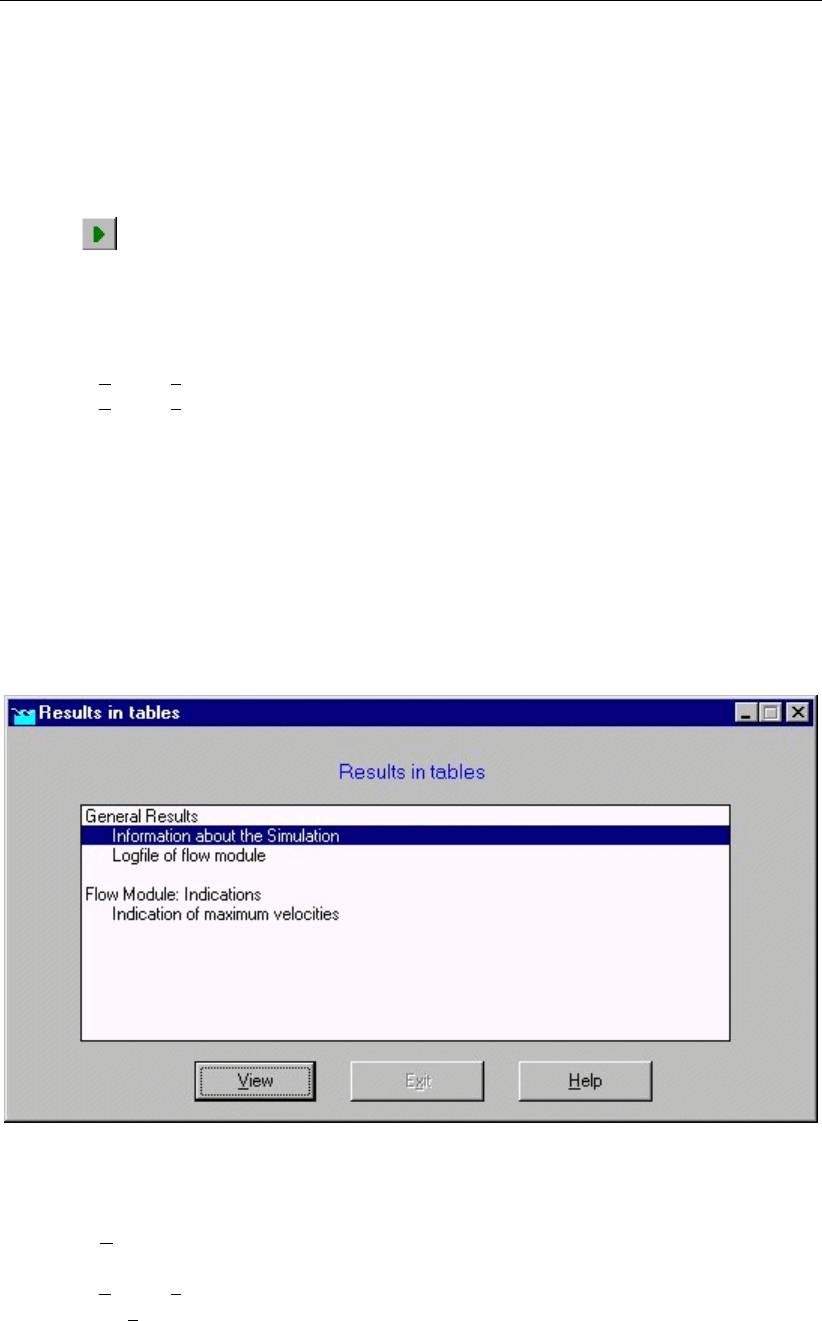
DRAFT
SOBEK, User Manual
You can also load other results to be viewed in Side view.
Select ’View’ - ’User Data’ - ’Load other results..’.
Select ’Results at reach segments’.
Press the OK button.
Select ’Velocity [m/s]’.
Press OK button.
Click to watch the animation.
Note that you may load any other results available for the selected objects. For example water
quality results, if available.
Select ’File’ - ’Exit’ in the side view window [SOBEK Side view].
Select ’File’ - ’Exit’ to close NETTER.
Do not forget to save the case!
Select the menu item ’Case’-’Save’.
4.1.8 Task block: Results in Tables
The ’Results in tables’ task block provides detailed reports about the simulation.
Double-click ’Results in tables’ task block.
Figure 4.11: The results in tables window.
Select ’Information about the Simulation’;
Select ’View’ and view the results. Important information regarding the water balance of
your computation and the total balance error are given in this file (amongst others);
Select ’File’ - ’Exit’ from the ’View’ window;
Click the Exit button in the ’Results in tables’ window.
44 of 900 Deltares
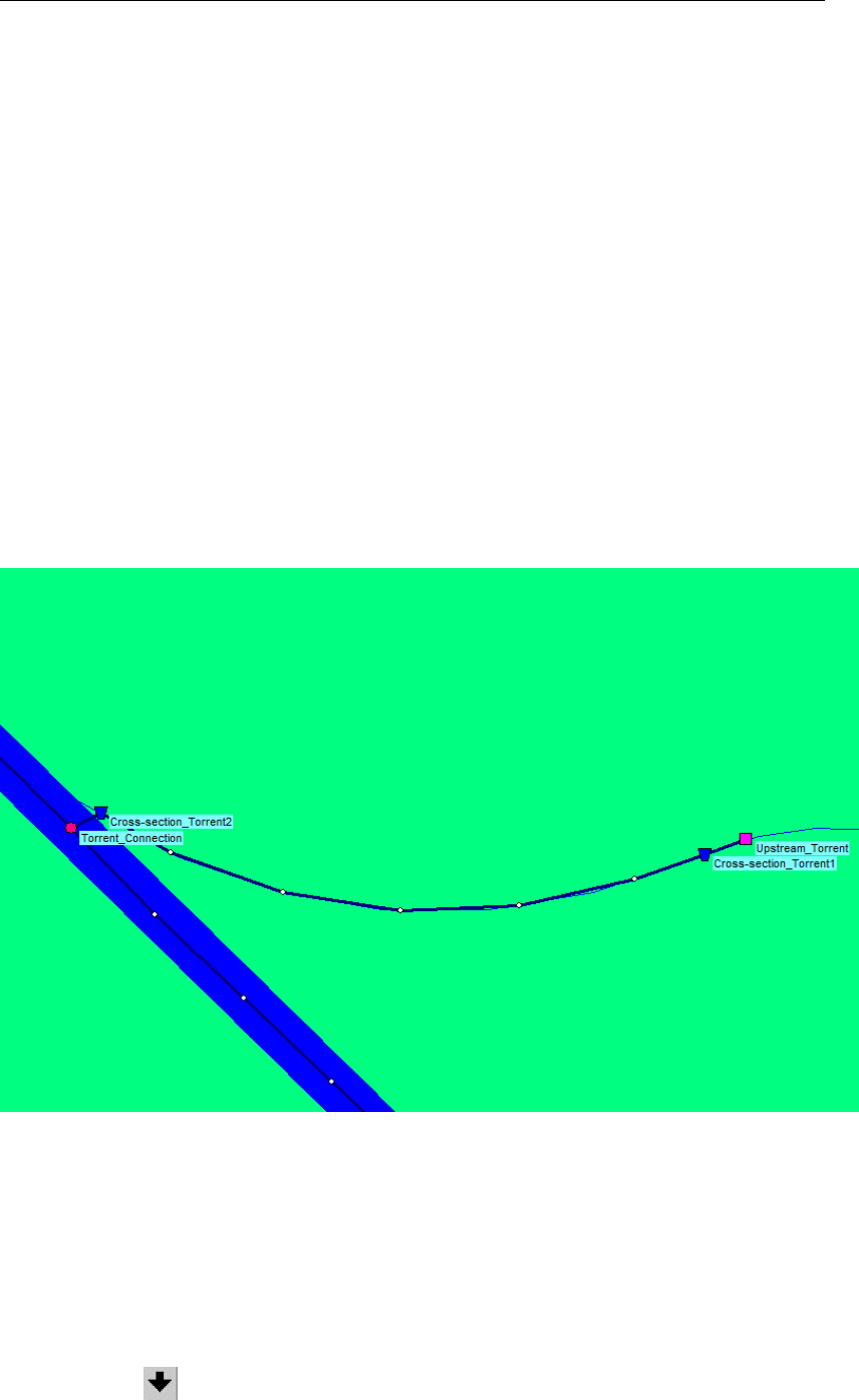
DRAFT
Tutorials
4.1.9 Task block: Results in Charts
In the task block ’Results in Charts’ the user can easily depict result data in one graph.
Double-click on the ’Results in Charts’ task block.
Select ’Water Balance’.
Click the View button.
Select the parameter ’Volume (1 000 m3)’.
Press the All button of Locations.
Press the All button of Timesteps.
Press the Graph button.
Select ’File’ - ’Exit’ to close the ’Graph Server’ window.
Press the Exit button to close ODS_VIEW.
Press the Exit button to close the task block ’Results in Charts’.
4.1.10 Interpolation over a Connection Node
In order make it possible to easily add branches to a main drainage system, Flow - Connection
Nodes offer user-definable interpolation of cross-section bathymetry data. To demonstrate this
functionality we will add a torrent to the existing schematisation.
Figure 4.12: The torrent branch.
Double-click the ’Schematisation’ task block of the Case Manager.
Click the Edit model button.
The Tutorial map folder contains a map layer of the torrent.
Select ’Map’ in the Active Legend.
Select ’Torrent’ from the list of layers.
Click on the button to move the selected layer to the bottom of the list. Now this layer
will be on top.
Deltares 45 of 900
DRAFT
SOBEK, User Manual
Press OK button.
Now we will add the Flow - Connection node with which we connect the torrent to the existing
schematisation. A connection node can only be added to an existing reach by splitting the
reach. We will manually add a h-calculation point and split the reach at its location:
Select the button, Edit Network, to start the edit network mode.
Select the button, Flow - Calculation Point.
Select the button to select the function ’Add node’.
Enter “Torrent_connection” in both input fields.
Click the OK button.
Click on the left-mouse button again to actually add the Torrent_connection node on your
screen. The node should be placed in the intersection between the main river and the
torrent.
Remark:
It is possible that a h-calculation point is already present at the intersection between the
main river and the torrent in your tutorial model. In that case, it is also possible to split
the reach at the automatically generated calculation node. However, it should be noted
that this node will not have a name, and have an automatically generated ID. For the
purpose of this tutorial, it is assumed that the ’Torrent_connection’ node was manually
added as described above.
Now select the button, Flow - Connection node.
Select the button ’Split reach at node’ in the ’Reach’ toolbar.
Use the left-mouse button on the Torrent_connection node to actually add the Flow - Con-
nection node on your screen.
The h-Calculation Point is now changed to a Connection Node, splitting the reach and provid-
ing a location to which we can connect the torrent section of this network.
Select the node, Flow-Boundary, by clicking on it.
Select the button to select the function ’Add node’.
Enter “Upstream_Torrent” in both input fields.
Click the OK button.
Click on the left-mouse button again to actually add the Upstream Torrent node on your
screen.
Zoom in to get a good view on the Torrent_connection node and the Flow - Boundary
node.
46 of 900 Deltares
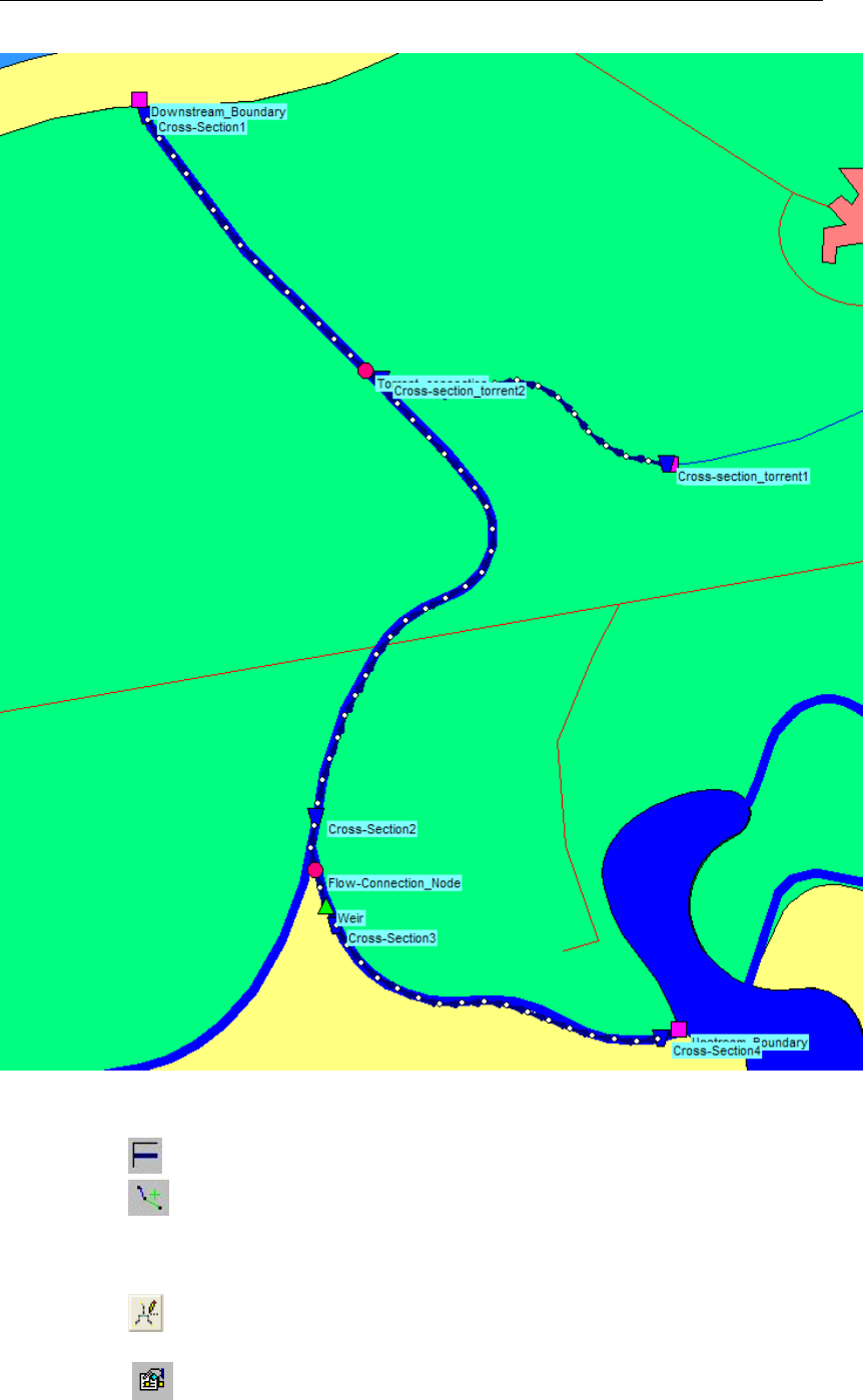
DRAFT
Tutorials
Figure 4.13: The entire network after adding the torrent branch
Select the button, Flow-Channel, by clicking on it.
Select the button to select the function ’Connect nodes’.
Click with the left mouse button on the upstream torrent node, which you have already
added and drag to the Torrent_connection node while keeping the button down. Release
the left mouse button.
Select the button, ’Edit Reach Vectors’.
Edit the vector layer to introduce the correct distances.
Select the button in the ’General’ tool bar, Edit settings, to show the edit network
options window.
Deltares 47 of 900

DRAFT
SOBEK, User Manual
Select the tab ’Node’.
In the ’Name’ data group, select the radio button No Names.
Press the OK button.
Select the button to select the function ’Calculation grid all reaches’.
Click the OK button.
Now we should enable interpolation along the connection node ’Torrent_connection’. When
we split the reach earlier, the upstream and downstream parts of the main river were also split
in two. For this tutorial we want the main river to be treated as a single river, as it was before
we split the reach.
Select the menu item ’Options’ - ’Network Data...’.
Select the tab ’Link’.
Select the radio button Reach.
Press the OK button.
The reach ID’s are now shown in the schematisation. This is useful when enabling interpola-
tion along a connection node.
Select the Torrent_connection by left-mouse clicking it
Click with your right mouse button.
Select ’Model data’ - ’Flow Model’.
Left-mouse click the tab ’Interpolation Over node’.
Enable the option ’Interpolate Cross-section bathymetry (only) over Node’ by left-mouse
clicking it.
For ’First Reach’, select the upstream reach ’2’.
For ’Second Reach’, select the downstream reach ’3’.
Press the OK button.
Interpolation of Cross-section data over the Torrent_connection is now enabled.
48 of 900 Deltares
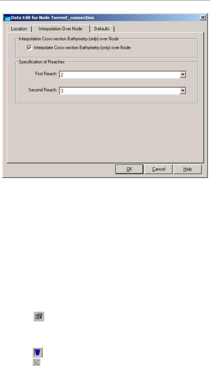
DRAFT
Tutorials
Figure 4.14: The filled in Data Edit screen for the ’Torrent_connection’ node
We will now disable the showing of reach ID’s in NETTER:
Select the menu item ’Options’ - ’Network Data...’.
Select the tab ’Link’.
Under ’Show Titles’, Select the radio button None.
Press the OK button.
SOBEK offers a powerful tool to validate your network.
Select ’Tools’ - ’Validate network by model’ - ’Flow Model’.
The following message appears in the Network Validation window: "A Flow reach must contain
a Profile node".
Select the message in the Network Validation window. Now the torrent reach will be
selected on the map.
Press the Finished button.
Select the button in the ’General’ tool bar, Edit settings, to show the edit network
options window.
Select the tab ’Node’.
In the ’Name’ data group, select the radio button Manual.
Press the OK button.
Select the node, Flow - Cross Section node.
Select the (add node) function.
Deltares 49 of 900
DRAFT
SOBEK, User Manual
Enter “Cross-Section _Torrent1” in both input fields.
Click the OK button.
Click on the left-mouse button to actually add the Flow-Cross Section node on your screen,
near the Upstream torrent boundary.
Select the (add node) function.
Enter “Cross-Section_Torrent2” in both input fields.
Click the OK button.
Click on the left-mouse button to actually add the Flow-Cross Section node on your screen,
near the Torrent_connection node.
Select the button, Select by rectangle, by clicking on it.
Select the part of the schematisation which includes the new Cross Section nodes by
clicking on the map and dragging while keeping the button down.
Release the left mouse button.
Click right mouse button.
Select ’Model data’ - ’Flow Model’.
Select ’Flow - Cross Section’.
Select ’Cross Section’.
Select the column ’Cross Section’.
Click right mouse button.
Select ’Replace’
Select ’My profile 1’ from the list.
Press OK button.
Enter “15” as Reference Level [mAD] of Cross-Section_Torrent1.
Enter “20” as Surface Level [mAD] of Cross-Section_Torrent1.
Enter “0” as Reference Level [mAD] of Cross-Section_Torrent2.
Enter “2” as Surface Level [mAD] of Cross-Section_Torrent2.
Now we will add the friction data.
Select ’Friction’.
Press Yes button.
Select ’Chézy’.
Enter “35”.
And last but not least we will add the initial values.
Select ’Initial values’.
Press Yes button.
Select ’Depth’ as the type of the initial level for the upstream reach. Note that the current
reach will be selected in NETTER.
Enter “0” for ’Discharge’.
Enter “1.25” for "Value".
Select ’File’ - ’Exit’ of the Multiple Data Editor.
Press Yes to save the data.
Select the ’Upstream Torrent’ node on the map.
Click right mouse button.
Select ’Model data’ - ’Flow Model’.
Select the radio button flow (Q).
Enter the value “10”.
Press the OK button.
50 of 900 Deltares

DRAFT
Tutorials
4.1.11 Saving the network and the model
The schematisation has been setup. Now we will save the map settings, the schematisation,
leave the task block ’Schematisation’ and save the case.
Select ’File’ - ’Save’ - ’Map’.
Select button in NETTER.
Select the menu item ’File’-’Exit’, to leave NETTER.
Click the OK button in the schematisation window.
Now only your schematisation has been saved in NETTER. The whole case must be saved
too!
Select the menu item ’Case’-’Save As’
Enter the name “Case_two” to save the case.
Click the OK button.
Please run the simulation and view the results when using interpolation of cross-section bathy-
metry data over a Connection Node. SideView is a good tool for this.
Epilogue
In this tutorial the most important aspects of working with SOBEK have been discussed.
Extended documentation can also be found in the SOBEK Manual. All PDF files containing
documentation can be found in the "Manuals" directory in the Start menu, next to the SOBEK
start icon. Since you have now gained experience it will not be that difficult to find out the
options and possibilities of SOBEK that not have been discussed here. Good luck!
4.2 Tutorial Hydrodynamics in sewers (SOBEK-Urban 1DFLOW + RR modules)
General
In this tutorial the basic principles of working with the SOBEK-Urban 1DFLOW module and RR
(Rainfall-Runoff) module are explained step by step and you will be guided to set-up a simple
network on your own and to extend this network. This tutorial will only show a limited number
of the large number of options. It will teach the basic principles of working with SOBEK-Urban
and give you enough experience to continue on your own. Some experience in working with
the Microsoft R
Windows R
operating system is required.
The tutorial contains:
1 setting up a simple schematisation, using the Dutch Standard Exchange Format (SUF-
HYD);
2 analyzing results;
3 extending the schematisation.
The tutorial does not explain all options in all windows that appear. Once you get the hang-
and-feel of the modelling system, you may wish to browse through the options not dealt with
in the tutorial.
Deltares 51 of 900

DRAFT
SOBEK, User Manual
Getting started
Click on the Windows Start button.
Select the ’All Programs’ or ’All Apps’ menu.
Select the ’Delft Hydraulics’ menu.
Select the ’SOBEK’ menu item (SOBEK215).
Click on the ’SOBEK’ icon.
Select the menu item ’Options’ - ’SOBEK Options’.
Select the tab ’Background Map’.
Select the file <Tutorial1.map>.
Press OK button to save and close SOBEK Options.
Click the ’New Project’ button.
Type the name “T_SEWER”.
The program converts all the characters into upper case. If a project with the same name
already exists, the user has to enter a different name here.
Click the OK button.
You have added a new project with the name ’T_SEWER’. You are now asked: do you want
to work with this project?
Click the Yes button.
Case management
The screen of the so-called "case manager" appears. This tool automatically keeps track of
cases and the related files. For instance: you might want to save different scenario’s within a
project as cases with different names. This is organized trough the case manager.
Figure 4.15: The case manager screen.
52 of 900 Deltares

DRAFT
Tutorials
On the screen a number of blocks are visible:
1 Import Network;
2 Settings;
3 Meteorological Data;
4 Schematisation;
5 Simulation;
6 Results in Maps;
7 Results in Charts;
8 Results in Tables.
Each block represents a specific task. A task can be a model, or a set of linked models, or the
selection of a scenario or strategy, or a (graphical) presentation tool. The arrows between the
blocks represent the relations between the tasks. When an arrow is pointing from block "A" to
block "B", the task of block B can only be executed after the task of block A is finished.
The Case Manager has the following tasks:
1 Administration of cases (which data is related to which cases);
2 Checking whether the model calculations for the cases are performed in the predefined
order;
3 Logging the actions of the Case Manager (including view and print);
4 Providing access to the computational framework through a user interface, so the user
can:
manipulate a case (read, save, delete, etc.);
view and check the status of all tasks;
view the relation between the various tasks.
choose and run predefined tasks (modules);
When the Case Manager screen appears first after you have added a project all task blocks
are grey. To activate the task blocks you have to open the default case of this new project:
Select the menu option ’Case’-’Open’.
Select ’Default’ from the list.
Click OK button.
Another method is to click on one of the grey task blocks and select ’Default’.
Once you have opened the default case the task blocks are no longer grey, but one of the
following colors:
1 yellow: the task can be executed;
2 green: the task has been executed at least once and can be executed again;
3 red: the task cannot be executed until the preceding task has been executed.
When the task is being executed the task block is purple. You can execute a task by double-
clicking on the task block. When you select a yellow or green task block, the color will change
to purple and then change to green.
Now, we will discuss each task block.
Deltares 53 of 900
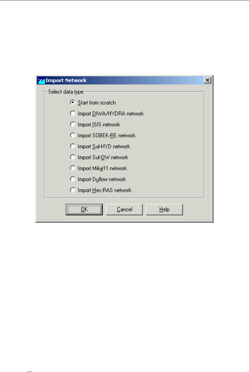
DRAFT
SOBEK, User Manual
4.2.1 Task block: Import Network
The color of this task block is yellow, so this means that this task block must be executed.
Execute the task block ’Import Network’ by double-clicking.
The Import network window will pop up:
Figure 4.16: The import network window.
In this task block the origin of the schematisation must be defined. Schematisations, used in
SOBEK, can be either imported from database or set-up from scratch.
If a schematisation is already available in the standard exchange format it can easily be im-
ported from the database to SOBEK. Links with data formats can be custom made on request.
For that reason some radio buttons might be turned grey.
Let’s import a SUF-HYD network. SUF-HYD is the Dutch standard exchange file format for
data regarding sewer systems.
Select the radio button Import Suf-HYD network by pointing at the corresponding radio
button with the mouse pointer and by clicking the left mouse button.
Press OK button.
Press OK button.
Select the file <Tutorial.hyd>.
Press Open button.
Press Yes button. View the messages in the log file that is shown.
Select ’File’ - ’Exit’ to close the file.
Notice that you’re back in the Case Manager now and that the task block ’Import Network’ has
turned green.
54 of 900 Deltares
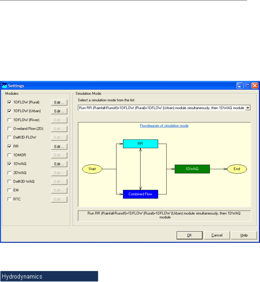
DRAFT
Tutorials
4.2.2 Task block: Settings
The ’Settings’ task block is used to select the SOBEK modules that you want to use for your
project. Also computational parameters such as calculation time steps, simulation period and
initial water levels, can be set in the ’Settings’ task block.
Depending on the set of modules that you purchased, some may be disabled (grey), and
some may be enabled.
Figure 4.17: The settings window.
SOBEK-Rural 1DFLOW
The SOBEK-Rural 1DFLOW module is a sophisticated module that can be used for the simu-
lation of one-dimensional flow in irrigation and drainage systems. It is a tool that can be used
to simulate and solve problems in regional water management, such as irrigation construc-
tion, drainage, automation of canal systems, dredging and flood protection. This module can
be used stand-alone or in combination with other modules, for example the SOBEK-Rural RR
module (Rainfall-Runoff).
Deltares 55 of 900

DRAFT
SOBEK, User Manual
SOBEK-Urban 1DFLOW
The SOBEK-Urban 1DFLOW module is a sophisticated module for the simulation of one-
dimensional flow in waste water and storm water systems. It is a tool that can be used to sim-
ulate and solve problems in urban drainage systems such as determination of urban drainage
capacities including treatment plants, assessment of sewer overflow frequency and design
of detention basins. The SOBEK-Urban 1DFLOW module can also be used in combination
with the SOBEK-Rural 1DFLOW module, the SOBEK-Urban RR (Rainfall-Runoff) module and
other modules. One of the competitive advantages is the combination with the SOBEK-Rural
1DFLOW module for environmental study on receiving waters.
SOBEK-River 1DFLOW
The SOBEK-River 1DFLOW module is a sophisticated module that can be used for the sim-
ulation of one-dimensional water flow in river systems and estuaries. It is a tool that can be
used to simulate and solve problems in river water management such as flood protection,
flood-risk assessment, real-time forecasting, dam break analysis, navigation and dredging.
This module can be used stand-alone or in combination with other modules.
The RR (Rainfall-Runoff) module is a module that can be used for the simulation of rainfall-
runoff processes. This module is a part of a large family of modules which can be linked. The
list of modules includes (amongst others) SOBEK-Rural 1DFLOW module, SOBEK-Urban
1DFLOW module and RTC (Real Time Control) module. The RR module is frequently used
in combination with the SOBEK-Rural 1DFLOW and SOBEK-Urban 1DFLOW modules. It is
then possible to either to perform calculations for both modules simultaneously or sequentially.
The RTC (Real Time Control) module is a module that can be used for the simulation of com-
plex real time control of hydraulic systems. It can be applied to rainfall-runoff, hydraulics and
water quality computations. In that case the rainfall-runoff and water quality computations are
run simultaneously with the hydrodynamics computations, thus incorporating full interaction
between all processes.
The above mentioned modules can also be used in combination with modules for simulating
water quality processes (1DWAQ module, 2DWAQ module and/or EM (EMission) module).
Thus, several combinations of modules are possible. Depending on the problems to be solved
you can set the desired combination. The modules can easily be selected via the task block
’Settings’.
Double-click the ’Settings’ task block.
Unselect all the selected modules if any.
Select the ’1DFLOW (Urban)’ module.
And select the ’RR’ module.
Press the Edit... button of ’1DFLOW (Urban)’.
Enter the time step in computation: “1” minute.
Click on the tab ’Initial data’ with the left mouse button.
Select the radio button initial depth in channels [m].
56 of 900 Deltares
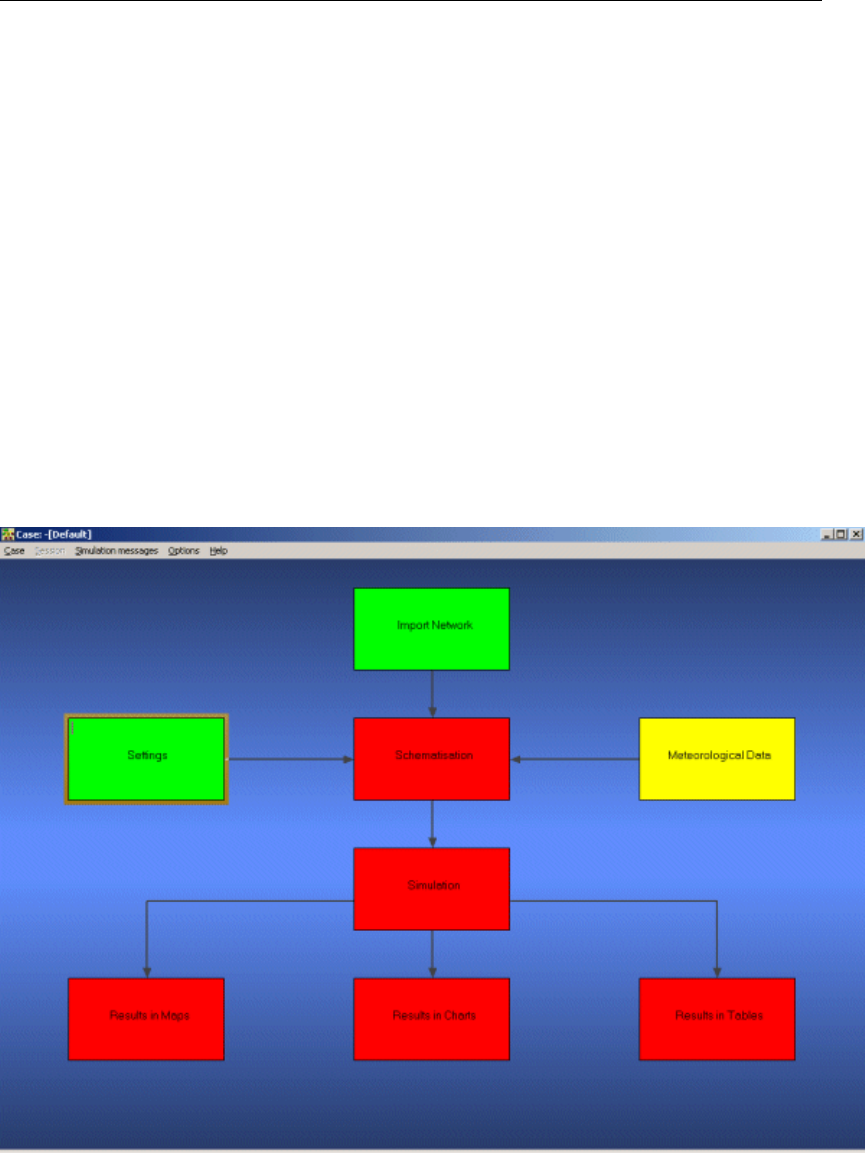
DRAFT
Tutorials
Enter the value “0”.
Select the ’Output options’ tab.
Enter the output time step in computation: “1” minute.
Select the tab ’Branches’ of ’Output parameters’.
Select ’water level gradient’.
Press the OK button to return to the ’Settings’ window.
Press the Edit... button of ’RR’.
Enter the time step in computation: “1” minute.
Select the radio button Simulation period will be derived from meteorological data.
Select the ’Output options’ tab.
Enter the output time step in computation: “1” minute.
Press the OK button to return to the ’Settings’ window.
Finally press the OK button, to save your settings and return to the Case Manager.
You should now see the screen depicted below, indicating that both the ’Settings’ task and the
’Import Network’ task have been completed and that the Meteorological data task should still
be performed.
Figure 4.18: The case manager after completing the ’settings’ and ’import network’ tasks.
Deltares 57 of 900
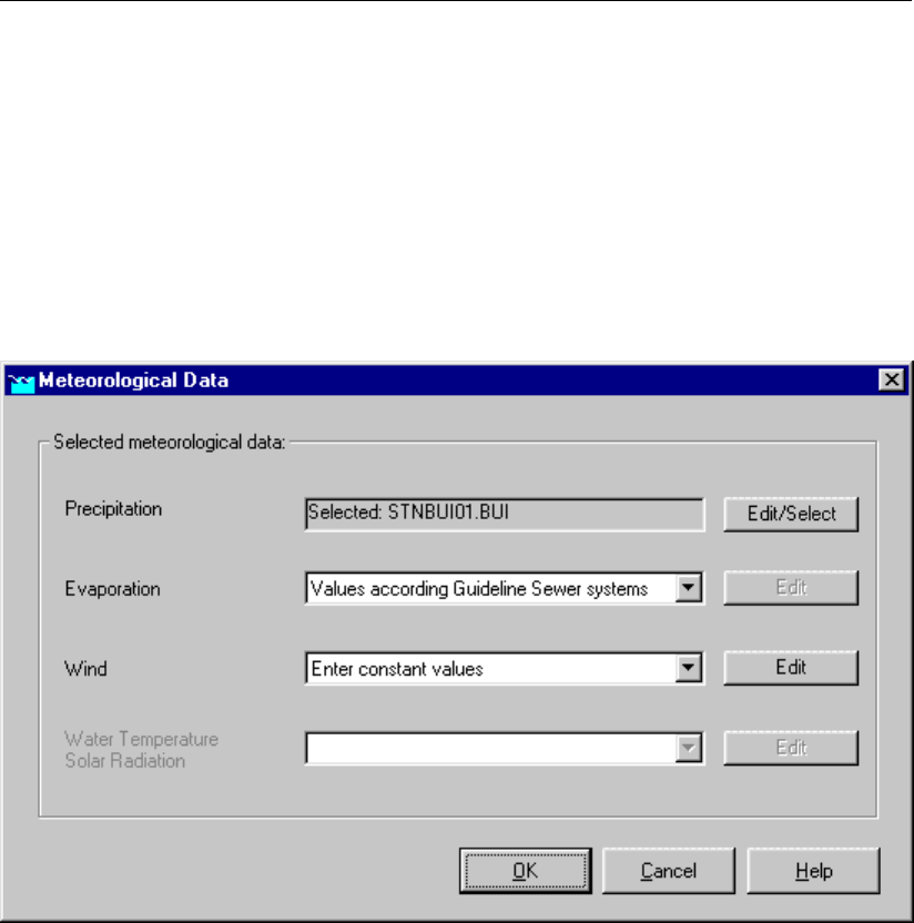
DRAFT
SOBEK, User Manual
4.2.3 Task block: Meteorological Data
SOBEK-Urban simulations require meteorological input data, i.e. precipitation data and evap-
oration data.
The evaporation data are connected with the time series of the precipitation data. The simu-
lation period is determined by the start- and end date of the precipitation data.
Double-click the ’Meteorological Data’ task block of the Case Manager. The following
screen will appear:
Figure 4.19: The meteorological data window.
Now you can select and edit the precipitation data and evaporation data.
Click the Edit/Select button next to the Precipitation box.
Press the Select event... button.
Select the rainfall event named ’STNBUI07.BUI’.
Click the OK button.
Click OK again to leave the ’edit precipitation data’ window.
Select ’Values according Guideline Sewer systems’ for evaporation.
Click the OK button to leave the Meteorological Data window.
Now you have finished defining the meteorological data. Notice that this task block has turned
green too!
58 of 900 Deltares

DRAFT
Tutorials
4.2.4 Task block: Schematisation
A schematisation can easily be set up with the help of the network editor.
Double-click the ’Schematisation’ task block of the Case Manager.
Click Edit model.
When the option Edit Model of the ’Schematisation’ is selected, the network editor starts.
The network editor is called NETTER and is a component of the Delft Hydraulics Decision
Support System (Delft-DSS) tools. NETTER offers the possibility to set-up the schematisation
on top of a background GIS map. NETTER also offers advanced analysis tools to show model
results attached to the schematisation and provide the user with full printing facilities to make
high quality prints.
Within NETTER you can do the following:
1 Interactively and graphically prepare a schematisation;
2 Generate schematisations upon GIS map Layers;
3 Carry out schematisation operations: search for a certain node, show node numbers and
names, show link numbers, etc.;
4 Carry out map operations: zooming in, zooming out, (de)activating map layers, colouring
of map layers, adding title information on the map, etc.;
5 View results of simulation models for schematisations created in NETTER;
6 Print maps or schematisations.
Generally speaking, NETTER has two edit modes. The first mode is the mode to set-up the
schematisation, e.g. by adding new nodes. The second edit mode is the mode for editing the
attribute data. In this mode you give attributes to the schematisation objects. For example, a
pump station must have a pump capacity and switch on/off levels.
In this exercise you will work on a simple schematisation.
Deltares 59 of 900

DRAFT
SOBEK, User Manual
Figure 4.20: The schematisation to be extended in this tutorial.
Several zoom options are available. The View menu contains commands to zoom in, zoom
out, centre the window, move the window and show all schematisation or map layers.
The button allows you to zoom in on any part of the "active main window".
The button allows you to zoom out by shrinking the displayed part of the "active main
window".
The button allows you to center a schematisation or map GIS object. When choosing
this command and then clicking with the left mouse button on an object, NETTER redraws the
map centering the chosen object to the NETTER window.
The button allows you to shift the view by clicking the mouse anywhere in the NETTER
window and dragging the view to another position.
The button redraws the view fitting all schematisation objects into the NETTER window.
The button redraws the view fitting all GIS map layers into the NETTER window.
The button restores the view of the map before the last zoom command was given.
60 of 900 Deltares
DRAFT
Tutorials
The button restores the view of the map before the last ’Show Previous’ command was
given.
In order to focus on a small part of the map you can use the zoom functionalities.
Now you will zoom in to the city.
Select button.
Move the mouse pointer to the main window.
Click and hold the left mouse button, make a rectangle by dragging the pointer across the
main window. The size of this rectangle determines the magnification.
Release the left mouse button.
The schematisation, showing a part of the city’s sewer system, including attribute data, was
directly imported from a SUF-HYD file (standard file format used for sewer network data). We
will view and adjust the schematisation later on. Now we will save the schematisation; leave
the task block ’Schematisation’; save the case and go to the task block ’Simulation’.
Select ’File’ - ’Save’ - ’Map’.
Select the button, to save the network.
To get a good insight of the schematisation it is possible to show all the input data on the map
or in graphs.
Select the button, Select by rectangle, by clicking on it.
Select the whole schematisation by clicking on the map and dragging while keeping the
button down. Release the left mouse button.
Click right mouse button.
Select ’Model data’ - ’Rainfall Runoff Model’.
Select ’Flow - Manhole with Runoff’.
Select ’Sewerage Runoff’.
Select the column ’Open Sloped area [m2]’.
Click the right mouse button.
Select ’Show on Map’.
Select ’Sewerage Runoff’ in the Active Legend.
Click on the button in the Active Legend or select the menu item ’Options’ - ’Network
Data...’.
Select the ’All Data’ tab.
Select ’Width’ of ’Show node data’.
Press the OK button.
The following figure appears:
Deltares 61 of 900
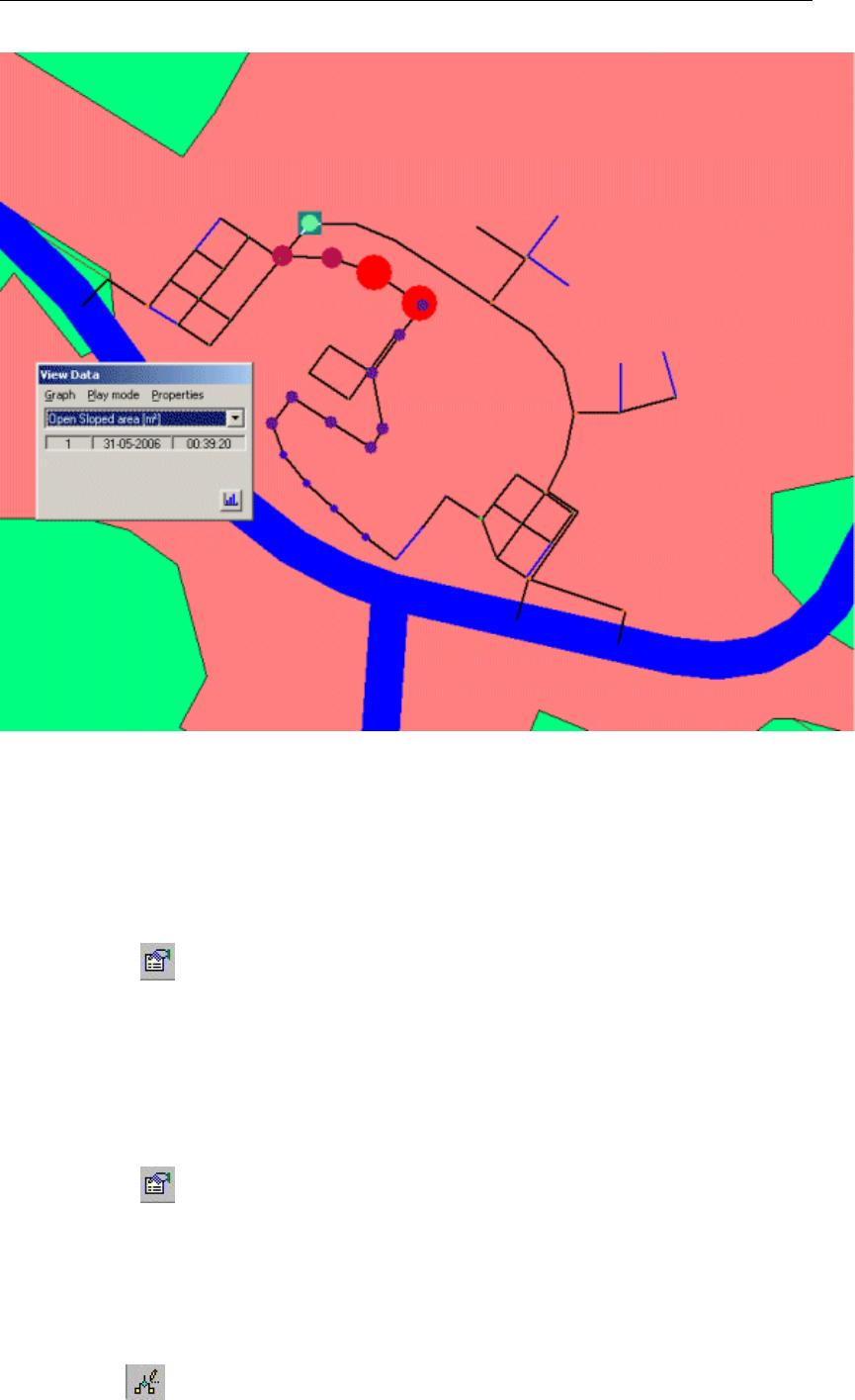
DRAFT
SOBEK, User Manual
Figure 4.21: Open sloped area
In this way all input data available in the Multiple Data Editor can be viewed on the map with
colour and size of the objects according to their data value!
Now we will close the Multiple Data Editor and we will return to the default visualisation mode.
Click on the button in the Active Legend.
Select the ’All Data’ tab.
Unselect ’Width’ of ’Show node data’.
Press the OK button.
Select ’File’ - ’Exit’ in the Multiple Data Editor.
The identifiers of all objects can be viewed on the map, using the following options:
Click on the button in the Active Legend.
Select the ’Link’ tab.
Select ’ID’.
Press the OK button.
Now we are going to provide street names to Flow - Pipes:
Select the button, Edit Network, to switch to the edit network mode.
62 of 900 Deltares

DRAFT
Tutorials
When you have selected the edit network mode all edit network functions and network objects
for the selected module will be available.
Select the button and the ’Node’ edit network functions to place the ’Node functions’
toolbar anywhere on your screen.
Figure 4.22: Node functions toolbar
Select the network editing option ’Properties’.
To search the Flow - Pipe with ID 00-1011-00-1010, press the Ctrl key plus the Fkey.
Click ’ID’ of ’Link’.
Enter “00-1011-00-1010” (without the quotes).
Press the OK button.
Now click on the selected Flow - Pipe on the map using your mouse.
Enter the Name “Market Street”.
Press the OK button.
Press the Ctrl key plus the Fkey.
Enter “00-1010-00-1009”.
Click on the selected Flow - Pipe on the map.
Enter the Name “Market Street” again.
Press the OK button.
Now rename the Flow - Pipes ’00-1009-00-1008’, ’00-1008-00-1007’, ’00-1007-00-1006’
and ’00-1006-00-1005’ to ’Market Square’.
And the Flow - Pipes ’00-1005-00-1004’ and ’00-1004-00-1003’ to ’Cherry Street’.
The Names can be viewed on the map, using the following options:
Click on the button in the Active Legend.
Select the ’Link’ tab.
Select ’Name’.
Press the OK button.
Deltares 63 of 900
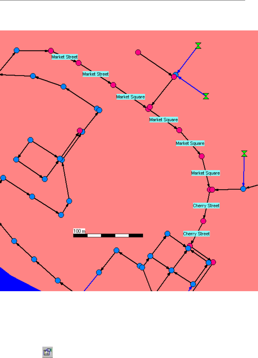
DRAFT
SOBEK, User Manual
Now your model will look as depicted in Figure 4.23.
Figure 4.23: Reach segment names visualised on the map
Another way to get good insight in the schematisation is make a side view. Note that the street
names, used more than once, are displayed only once for the whole street.
Select the network editing option ’No edit action’ to return to using the normal cursor.
Click on the button in the Active Legend.
Select the ’Node’ tab.
Select ’ID’.
Press the OK button.
To search for the objects with the ID 00-10003 and ID 00-8002, press the Ctrl key plus
the Fkey
Click ’ID’ of ’Node’.
Enter “00-10003”
Press the OK button.
Search for the object ’00-8002’ too.
64 of 900 Deltares
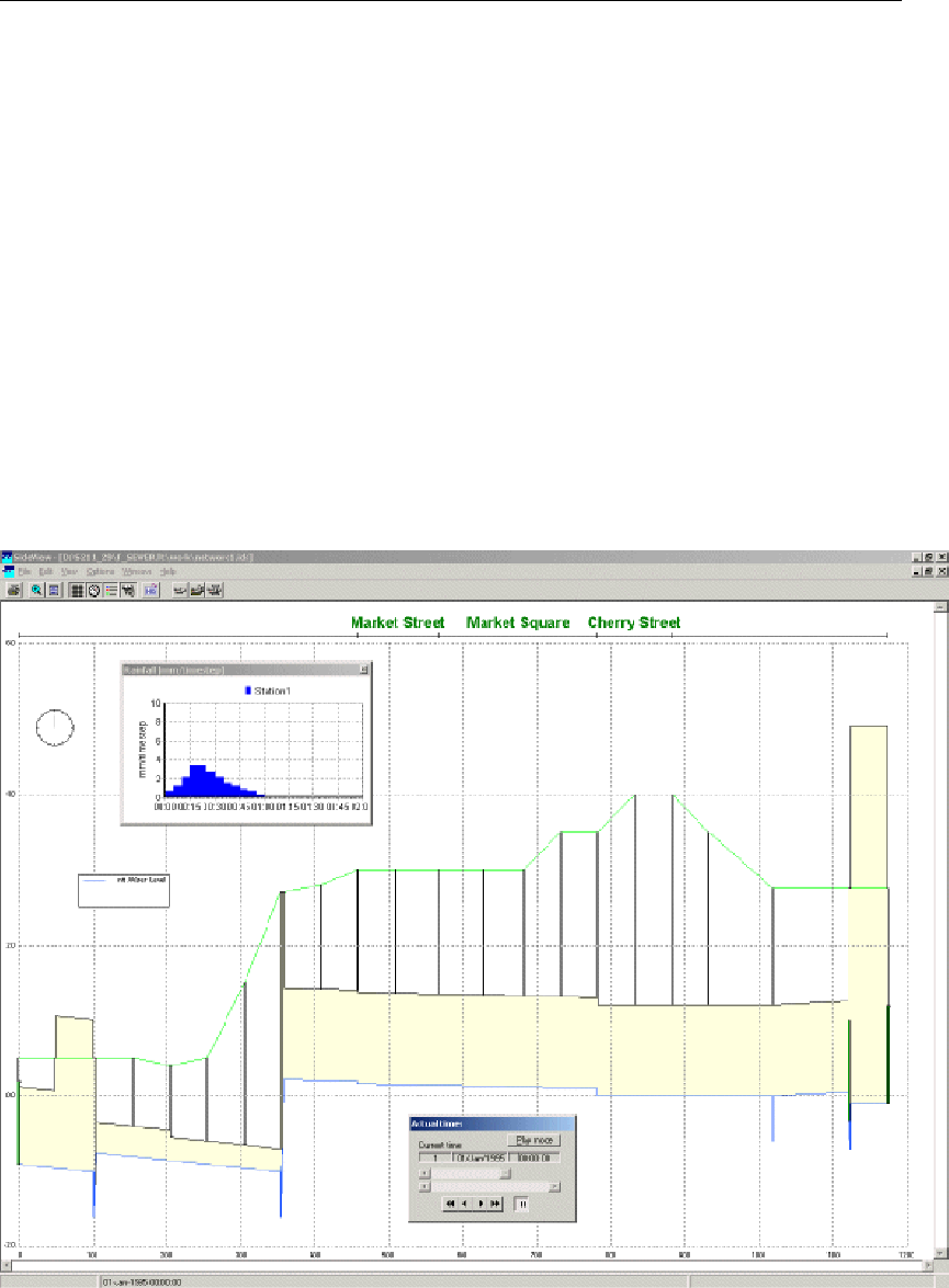
DRAFT
Tutorials
Click simultaneously the Shift key on the keyboard and select the Flow - External Weir
with the ID 00-10003 with the left mouse button. Keep the Shift key pressed. Then click
the Flow - External Weir with the ID 00-8002. Now, you can release the Shift key.
Click the right mouse button (on the selection).
Select ’Side view’.
In the side view the different network objects can easily be distinguished: the image depicts
the surface level (upper line), pipe diameter (middle and bottom line), manholes (vertical lines),
structures (thick vertical line). Various options are available to plot object labels in the side
view.
Select ’Options’ - ’Sideview Settings ..’.
Select the tab ’Branch Settings’.
Select the checkbox ’Show branch labels’.
Select the item ’Branch Name’.
Click the OK button.
Figure 4.24: Side view
You can save this side view path:
Select ’File’ - ’Save’.
Enter the file name “Path1.ids”.
Press the Save button.
Select ’File’ - ’Exit’.
Deltares 65 of 900
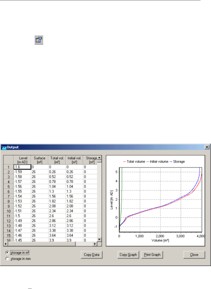
DRAFT
SOBEK, User Manual
We will re-use this path later in this tutorial.
Now we will disable the showing of Link and Node ID’s and names:
Click on the button in the Active Legend.
Select the ’Node’ tab.
Select ’None’.
Select the ’Link’ tab.
Select ’None’.
Press the OK button.
And last but not least you can make a storage graph.
Select ’Tools’ - ’Storage Graph’.
Select ’whole network’.
Select ’use storage in nodes’.
Press the Process button.
The following figure appears.
Figure 4.25: Storage graph
Click the Close button.
Press the Exit button.
To start the simulation you will have to leave NETTER.
Select the menu item ’File’-’Exit’, to leave NETTER.
Click the Yes button to save the name changes.
Click the OK button.
Select the menu item ’Case’-’Save As...’
Enter the name “Case_one” to save the case.
66 of 900 Deltares
DRAFT
Tutorials
Click the OK button.
4.2.5 Task block: Simulation
The next step in the modelling process is to perform the calculations.
Double-click the task block ’Simulation’.
You will see a bar appearing, showing the progression from the simulation. After the simulation
has finished, the Results in Maps, Results in Charts and Results in Tables task blocks will
become yellow.
4.2.6 Task block: Results in Maps
Results in maps gives you a clear impression of the results in time. The program NETTER is
used in this task block. Since NETTER also is used to set up a schematisation, it will be easy
for you, being an experienced user now, to view the results.
Double-click ’Results in Maps’ task block to analyse the results.
Creating a side view animation
Select ’Tools’ - ’Side view’.
Select the file <Path1.ids>.
Press the Open button.
Press the OK button of the Set up Animation.
Click to watch the animation;
If you would like to add other side views in the same SideView application, just select another
path on the map, click the right mouse button, select ’Side view’ and press the OK button.
Select ’File’ - ’Exit’.
User Defined Output
Select ’Tools’ - ’Output options’.
Select ’global SOBEK’ from the list button ’Use definition as defined in: ’.
Press the Add button a few times until the total number of rows is 4.
Fill in the data as shown in Figure 4.26.
Deltares 67 of 900

DRAFT
SOBEK, User Manual
Figure 4.26: User Defined Output functions
Press the OK button.
In ’User Defined Output’ of the Active Legend, select ’Time water-on-street, maximum’.
The following figure appears:
68 of 900 Deltares
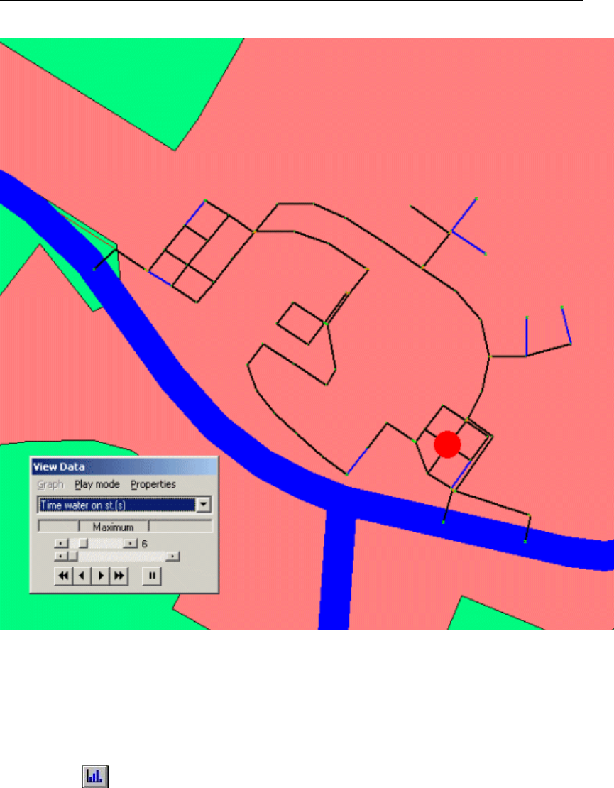
DRAFT
Tutorials
Figure 4.27: Time water on street, maximum
Plotting water levels
Select the item ’Results at nodes’ in the Active Legend.
Select several nodes by using simultaneously the Ctrl key on the keyboard.
In the ’View Data’ window, select the item ’Waterlevel [mAD].
Click the button on the ’View Data’ window.
Select ’File’ - ’Exit’ of the ’Graph Server’ window.
Deltares 69 of 900
DRAFT
SOBEK, User Manual
Plotting discharges
Notice that water levels are calculated at nodes, whereas discharges are calculated at reach
segments. To plot discharges in a graph you will therefore have to select reach segments:
Select ’Results at reach segments’ in the Active Legend.
Select a pipe.
In the ’View Data’ window, select the item ’Discharge [m3/s]’.
Click the button on the ’View Data’ window.
Select ’File’ - ’Exit’ of the ’Graph Server’ window.
Animating the flows
The direction of the flows through the model can be animated on the map:
Make sure that you still have selected the ’Results at reach segments’ in the Active Leg-
end.
Select ’Options’ - ’Network Data...’.
Select the ’Link’ tab.
Under the ’Show Direction’ topic select ’All Data’.
Click the ’arrow flow’ box.
Select the ’All Data’ tab.
Un-select the ’Width’ of ’Show branch data’, if it is still turned on.
Click the OK button.
Use the buttons from the ’View data’ window to animate the flows.
Note: If you do not see arrows moving trough the network, the arrows might be too small
compared to the reach thickness. You can enlarge them by changing the size of the arrows,
after selecting ’Options’ - ’Network options...’ and pressing the button Links....
Select ’File’ - ’Exit’ to leave NETTER.
4.2.7 Task block: Results in Tables
The ’Results in tables’ task block provides detailed reports about the simulation and the input
and the output data.
Double-click the ’Results in Tables’ task block.
70 of 900 Deltares
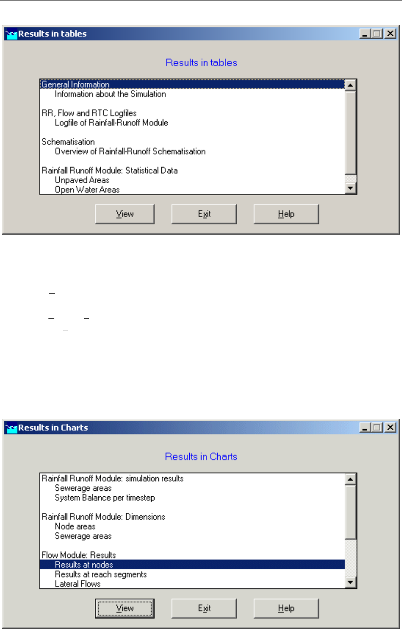
DRAFT
Tutorials
Figure 4.28: The results in tables window.
Select ’Information about the Simulation’.
Select ’View’ and view the results. Important information regarding the water balance of
your computation and the total balance error are given in this file (amongst others).
Select ’File’ - ’Exit’.
Click the Exit button in the ’Results in tables’ window.
4.2.8 Task block: Results in Charts
In the task block ’Results in Charts’ the user can easily depict result data in one graph.
Double-click on the Results in Charts task block.
Figure 4.29: The results in charts window.
Select ’Results at nodes’.
Click the View button.
Deltares 71 of 900
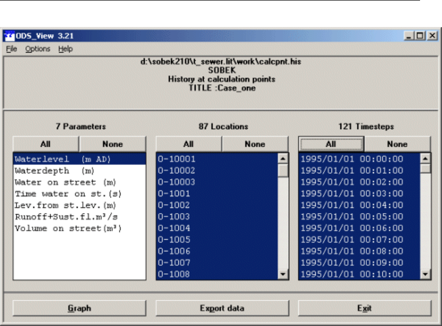
DRAFT
SOBEK, User Manual
Figure 4.30: The ODS_VIEW window.
To plot a graph of your model results, select one or more parameters in the left box, select
one or more locations for which you want to view results, and select the time span that you
want to view results for.
Use the Ctrl or Shift keys to select more than one item within a box.
After creating a graph, feel free to explore the wide range of possibilities for display manage-
ment. Adjust the axes according to your wishes, apply different graph templates, plot one
parameter on the left axis and another parameter on the right one, etc.
72 of 900 Deltares

DRAFT
Tutorials
Figure 4.31: An example of a graph created in the ’Results in Maps’ task block.
One can also choose to export the data to different file formats such as a spreadsheet. To do
so, click the Export data button in the ’Results in Charts’ window.
Select the parameter ’Waterlevel [mAD]’.
Select the location 00-1004, 00-1005 and 00-1006.
Press the All button of Timesteps.
Press the Export data button.
Feel free to export the data in any of the possible formats.
Now, we will exit the ’Results in Charts’ task block:
Select ’File’ - ’Exit’ to close the ’Graph Server’ window.
Press the Exit button to close ODS_VIEW.
Press the Exit button to close the task block ’Results in Charts’.
Select ’Case’ - ’Save’ to save the case.
Deltares 73 of 900
DRAFT
SOBEK, User Manual
4.2.9 Case Analysis Tool
In ’Case_one’ we used the rain event ’STNBUI07.BUI’. The total rainfall in this event is 19.8
mm. To show the impact of a much larger rainfall event we will select the rainfall event
’STNBUI10.BUI. The total rainfall in this event is 35.7 mm.
Double-click the task block ’Meteorological Data’.
Press the Edit/Select button.
Press the Select event... button.
Select ’STNBUI10.BUI’ from the list.
Press the OK button.
Press the OK button.
Press the OK button.
Double-click the task block ’Schematisation’.
Press the OK button.
Double-click the task block ’Simulation’.
Select ’Case’ - ’Save as...’.
Enter the name “Case_two”.
Press the OK button.
Select ’Case’ - ’Exit’.
Select ’Projects’ - ’Case Analysis Tool’.
Select ’T_SEWER’ from the list.
Press the OK button.
Select the tab ’Cases’.
Select ’Case_one’ from the cases list.
Select the item ’FLOW: results of nodes’.
Select ’Case_two’ from the cases list.
Select the item ’FLOW: results of nodes’.
Check ’Case_one’ as the Reference Case.
Select the tab ’Locations’.
Press the button to select all locations.
Select the tab ’Parameters’.
Double click on the item ’Water level [mAD] FLOW: results at nodes’.
Select the tab ’Functions’.
Click ’CaseFunctions’.
Double click ’Difference with base case’.
Press the button .
To easily visualize the maximum difference:
Select ’Options’ - ’Data Statistics’ - ’Maximum’.
Select ’Options’ - Network Data..’ - ’All Data’ and enable the option ’Width’ of ’Show node
data’.
The following figure appears. This figure shows the maximum difference between the two
cases.
74 of 900 Deltares
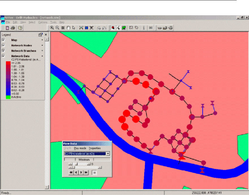
DRAFT
Tutorials
Figure 4.32: Maximum difference between two cases
Now reset the network visualisation to normal:
Select ’Options’ - Network Data..’ - ’All Data’ and disable the option ’Width’ of ’Show node
data’.
Select ’File’ - ’Exit’.
Select ’Application’ - ’Exit’.
Press the button No.
4.2.10 Series simulation based on independent rainfall events
Simulating a long period of time, for example 50 years, may take a lot of time. If you are only
interested in the sewer overflows, the method of independent rainfall events may be of interest
to you since it reduces the computation time and focuses on the events that matter. SOBEK
offers the functionality to run in series mode (multiple independent rainfall events). It offers
also structure statistics functionality, such as Total Volume [m3], Volume / Year [m3], Net Spill
Time [min].
Select ’Projects’ - ’Open Project’.
Select ’T_SEWER’ from the list.
Press the OK button.
Select ’Case’ - ’Open as new’.
Select ’Case_two’.
Enter the name “T_SEWER.RKS”.
Press the OK button.
Double click the ’Meteorological Data’ task block.
Deltares 75 of 900

DRAFT
SOBEK, User Manual
Press the Edit/Select button.
Press the Select series... button.
Select the item ’T_SEWER.RKS’ from the list.
Press the OK button.
Press the OK button.
Press the OK button.
Double click the ’Schematisation’ task block.
Press the OK button.
Double click the ’Simulation’ task block.
Press the Yes button, to select the mean output option.
Double click the ’Results in Maps’ task block.
Select ’Tools’ - ’Structure Statistics’.
Press the Process button.
The following figure appears:
Figure 4.33: Window Structure Statistics.
Select the cell with ID ’00-8002’.
Click the right mouse button.
Select ’Show Graph’.
Scroll to event number 6.
The following figure appears:
76 of 900 Deltares
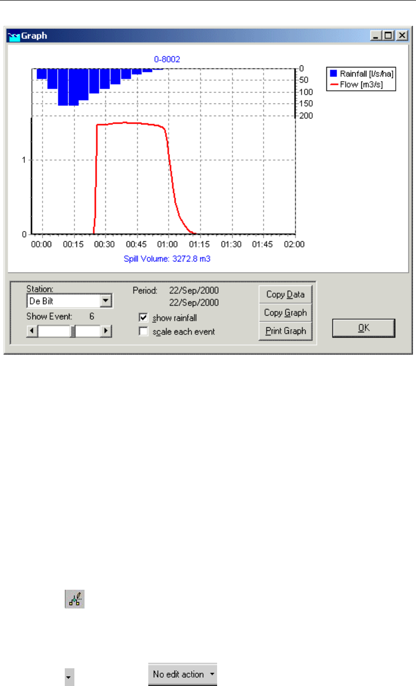
DRAFT
Tutorials
Figure 4.34: Structure Statistics graph for external weir 00-8002, event 6
Press the OK button.
Select ’File’ - ’Exit’.
Press the Exit button.
Select ’File’ - ’Exit’.
Select ’Case’ - ’Save’.
4.2.11 Task block: Schematisation extending your schematisation
Now, you will extend the simple schematisation.
Select ’Case’ - ’Open as new’.
Select ’Case_two’.
Enter the name “Extended case”.
Press the OK button.
Double-click the ’Schematisation’ task block.
Press the Edit model button.
Select the button, Edit Network, to switch to the edit network mode.
When you have selected the edit network mode all edit network functions and network objects
for the selected module will be available.
Select the button from the section and the ’General’ edit network func-
tions to unveil the ’General functions’ toolbar and move it to anywhere on your screen by
clicking the upper part of the selected toolbar and dragging it:
Deltares 77 of 900
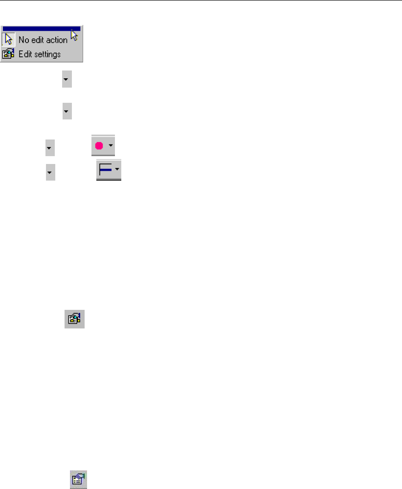
DRAFT
SOBEK, User Manual
Select the button and the ’Connection’ edit network functions to place the ’Connection’
functions toolbar anywhere on your screen.
Select the button and the ’Reach’ edit network functions to place the ’Reach functions’
toolbar anywhere on your screen.
Select from the section and the place the objects toolbar anywhere on your screen.
Select from the section and place the objects toolbar anywhere on your screen.
If you desire more information explaining the large amount of objects, you can customise the
toolbars by clicking ’View’ - ’Toolbars’ - ’Customize...’. Caption only, Icon only and Icon and
Caption are the available options. ’Icon only’ means that, for the selected toolbar, you will only
see the icons, but no label explaining them. Choosing Icon and Caption will also place a label
explaining each symbol.
It is possible to set the identifiers (or ID’s) of the nodes and branches (links) automatically or
manually.
Select the button in the ’General’ tool bar, Edit settings, to go to the edit network
options.
Select the tab ’Node’.
In the group box ’ID’, select the radio button Manual.
In the group box ’Name’, select the radio button Manual.
Select the tab ’Link’.
In the group box ’ID’, select the radio button Manual.
In the group box ’Name’, select the radio button Manual.
Click the OK button.
In order to see the identifiers on the map please:
Click on the button in the Active Legend or select the menu item ’Options’ - ’Network
Data...’.
Select the tab ’Node’.
Select the radio button ID.
Select the tab ’Link’
Select the radio button ID.
Press the OK button.
Select ’Select ’ - ’Search...’ from the menu bar.
Enter “00-7003”.
Press the OK button.
Zoom in towards node ’00-7003’ .
Now we will start drawing the extended schematisation with node ’00-7006’ and link ’00-7006-
00-7003’. When finished with this chapter, your extended schematisation will look as follows:
78 of 900 Deltares
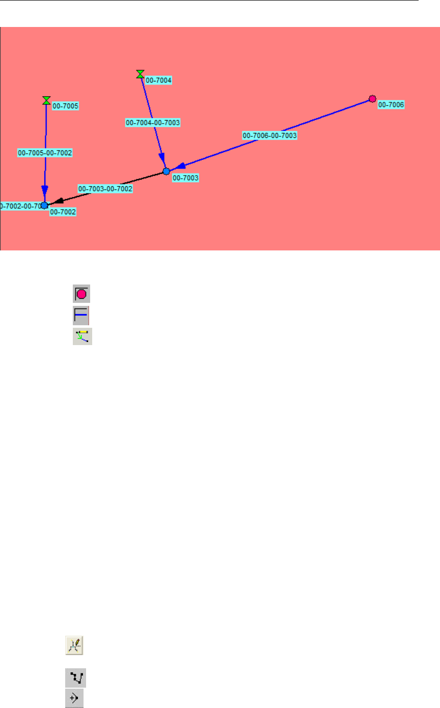
DRAFT
Tutorials
Figure 4.35: Extended schematisation Urban.
Activate the button, Flow-Manhole, by clicking on it.
Activate the button, Flow-Pipe with Runoff, by clicking on it.
Activate the button, ’Add connect’, by clicking on it.
Enter “00-7006” as the ID of the Node definition.
Enter “00-7006” as the Name of the Node definition.
Enter “00-7006-00-7003” as the ID of the Link definition.
Enter “00-7006-00-7003” as the Name of the Link definition.
Press the OK button.
Next, click the desired location on the screen to actually add the node, keep you mouse
button down while dragging to node ’00-7003’ and release the mouse button.
Now the new Flow-Manhole object is connected to the simple schematisation. The option
’defined direction’ can be used to see the positive defined direction. The defined direction can
be viewed by selecting ’Options’-’Network Data...’-’Link’-’Defined’.
The vector layer
To show schematizations with high performance, NETTER shows by default connections be-
tween two Flow - nodes in a straight line. However the length between the nodes may differ
from the distance between the nodes in a straight line. The actual length between Flow -
nodes is stored in the vector layer. You can edit the length in this layer.
For the purpose of this tutorial, either the default straight line or a user-defined vector layer
will suffice. The vector layer can be edited as follows:
Select the button, ’Edit Reach Vectors’, to edit a selected reach vector.
Select the reach.
Select the button to show the coordinates.
Select the button to add a coordinate.
Click with the left mouse button on the reach to actually add a coordinate on your screen
Deltares 79 of 900

DRAFT
SOBEK, User Manual
and while keeping the button down drag the new coordinate to the new location.
Add and drag other coordinates.
Unselect the button, ’Edit Reach Vectors’ to leave the ’vector layer’ mode.
Unselect the button, ’Edit network’, to leave the ’edit network’ mode.
The schematisation has been extended. The next step is to define the attribute data of the
schematisation. Therefore you have to switch to the model attribute data mode.
Editing node (manhole) data
Select the Flow-Manhole ’00-7006’.
Click with your right mouse button.
Select ’Model data’ - ’Flow Model’.
Select the tab ’Storage’.
Enter “1.6” for the Bottom Level.
Enter a constant value of “4” of the storage area at Storage Reservoir.
Select ’Reservoir’ of the Water on street type.
Select the constant value option.
Enter “3.5” of the Street Level.
Enter “500” for the Storage Area at Water on Street.
Press the OK button.
Editing reach (pipe) data
Select the newly added Flow-Pipe with Runoff object.
Click with your right mouse button.
Select ’Model data’ - ’Flow Model’.
Select the tab ’Cross section’.
Select Cross sections type ’Round’.
Select the Cross section ’Round 800 mm’.
Select the tab ’Location’.
Press the Get Levels button.
Click the OK button.
Select the new Flow - Pipe ’00-7006-00-7003’, the Flow - Pipe ’00-7004-00-7003 and the
Flow - Pipe ’00-7005-00-7002’ by clicking simultaneously the "Shift" key on the keyboard
and the objects one by one with the left mouse button. Now, you can release the "Shift"
key.
Click with your right mouse button.
Select ’Model data’ - ’Rainfall-Runoff Model’.
Select the item Flow - Pipe with Runoff’ in the tree.
Select ’Sewerage Runoff’.
Select the column ’Open Sloped area [m2]’.
From edit menu, select ’Edit Column’ - ’Distribute catchment area’
Enter the value “2000”.
Click the OK button.
Select button.
Select ’File’ - ’Exit’.
Select ’Tools’ - ’Validate network by model’ - ’Flow Model’.
Press the OK button.
Select ’Tools’ - ’Validate network by model’ - ’Rainfall Runoff Model’.
Press the OK button.
80 of 900 Deltares

DRAFT
Tutorials
Select button.
Select the menu item ’File’-’Exit’, to leave NETTER.
Press the OK button.
Select ’Case’ - ’Save’.
Please start the simulation and analyze the results.
Epilogue
In this tutorial the most important aspects of working with SOBEK have been discussed.
Extended documentation can also be found in the SOBEK Manual. All PDF files containing
documentation can be found in the "Manuals" directory in the Start menu, next to the SOBEK
start icon. Since you have now gained experience it will not be that difficult to find out the
options and possibilities of SOBEK that not have been discussed here. Good luck!
4.3 Tutorial Hydrodynamics - 1D2D floodings (SOBEK-Rural 1DFLOW + Overland Flow
modules)
General
The Overland Flow (2D) module of SOBEK-Rural is designed to calculate two-dimensional
flooding scenarios. The module is fully integrated with the 1DFLOW module for accurate
flooding simulation. It is especially designed to simulate dam breaks and dike breaks. The
hydrodynamic simulation engine underneath is based upon the complete Saint Venant Equa-
tions. It can simulate steep fronts, wetting and drying processes and sub critical and super-
critical flow.
This tutorial will guide you through a certain number of basic steps of both the Overland Flow
(2D) module and the 1DFLOW module. Some experience in working with the Microsoft R
Windows R
operating system is required.
Good luck!
Setting up a combined 1DFLOW and Overland Flow (2D) system
Click on the Windows Start button.
Select the ’All Programs’ or ’All Apps’ menu.
Select the ’Delft Hydraulics’ menu.
Select the ’SOBEK’ menu item (SOBEK215).
Click on the ’SOBEK’ icon.
Select the menu item ’Options’ - ’SOBEK Options’.
Select the tab ’Background Map’.
Select the file <Tutorial1D2D.map>.
Press OK button to save and close SOBEK Options.
Click the ’New Project’ button.
Type the name “T_1D2D”.
The program converts all the characters into upper case. If a project with the same name
already exists, the user has to enter a different name here.
Click the OK button.
You have added a new project with the name ’T_1D2D’. You are now asked: do you want to
work with this project?
Deltares 81 of 900

DRAFT
SOBEK, User Manual
Click the Yes button.
Select the menu option ’Case’-’Open’.
Select ’Default’ from the list.
Click OK button.
Double click the ’Import Network’ task block.
Select ’Start from scratch’.
Click OK button.
At the ’Settings’ task block, you have to activate the two dimensional ’Overland Flow (2D)’
module. Notice that you cannot choose the Overland Flow (2D) module alone. It will always
work in combination with the ’1DFLOW (Rural)’ module (see figure):
Figure 4.36: Activating the ’1DFLOW (Rural)’ and ’Overland Flow (2D)’ modules
Double click the ’Settings’ task block.
Unselect all the selected modules if any.
Select the ’1DFLOW (Rural)’ module.
And select the ’Overland Flow (2D)’ module.
Edit the 1DFLOW (Rural) settings:
Press the Edit button of the ’1DFLOW (Rural)’ module.
Select the tab ’Time settings’.
Choose ’1 minute’ as the ’Time step in computation’ (Simulation time step).
Select the option ’Simulation period defined as below’ for Simulation period.
Define the ’start of simulation’ as ’2006/01/01; 00:00:00’.
Define the ’end time’ as ’2006/01/01 02:30:00’.
Select the tab ’Simulation settings’.
Choose (of course) the ’unsteady calculation’.
Select the ’Initial data’ tab.
Choose the initial water depth option ’initial depth in channels [m]’.
82 of 900 Deltares
DRAFT
Tutorials
Set 1m as the initial water depth.
Select the ’Output options’ tab.
Define an output time step of ’00:01:00 (hh:mm:ss)’.
Leave the Settings editor for ’1DFLOW (Rural)’ by clicking the OK button.
Edit the Overland Flow settings:
Click the Edit button of the ’Overland Flow(2D)’ module.
Select the ’Simulation settings’ tab.
Choose for the option ’use as height’, because the values in the 2D grid that we will use
are defined as heights with relation to the reference level.
Select the ’GIS Output options’ tab.
Switch off all output parameters.
Select the ’Incremental output’ tab, keep the values as they are.
Select the ’history output’ tab
Choose Time step output equal to 1 time step.
Click the OK button to leave the settings for the ’Overland Flow(2D)’ module window.
Click the OK button to leave the Settings window.
Double click the ’Meteorological Data’ task block. There is no special data input necessary.
Click the OK button.
The following section describes the steps that must be followed to create a schematisation
and provide data to the model.
4.3.1 Starting with a 2D grid
The 2D grid
A predefined 2D grid will be used in this tutorial. This 2D grid file is named <2D_OF Tutorial.asc>
and is available in the <Drive:\SOBEK Install Directory\map\tutorial2Dflooding\>directory.
During this tutorial, we will show you how to add this grid file to your network.
Perform the following actions to open it in your schematisation:
Double click the ’Schematisation’ task block.
Click the Edit model button.
Enter the ’edit network’ mode by clicking the button.
It is possible to define the identifiers (or ID’s) of the nodes and branches (links) automatically
or manually.
Select the button in the ’General’ tool bar, Edit settings, to go to the edit network
options.
Select the tab ’Node’.
In the group box ’ID’, select the radio button Manual.
In the group box ’Name’, select the radio button Manual.
Select the tab ’Link’.
In the group box ’ID’, select the radio button Automatic.
In the group box ’Name’, select the radio button Automatic.
Click the OK button.
Click on the button from the section, click on the ’Overland Flow model’ option
Deltares 83 of 900
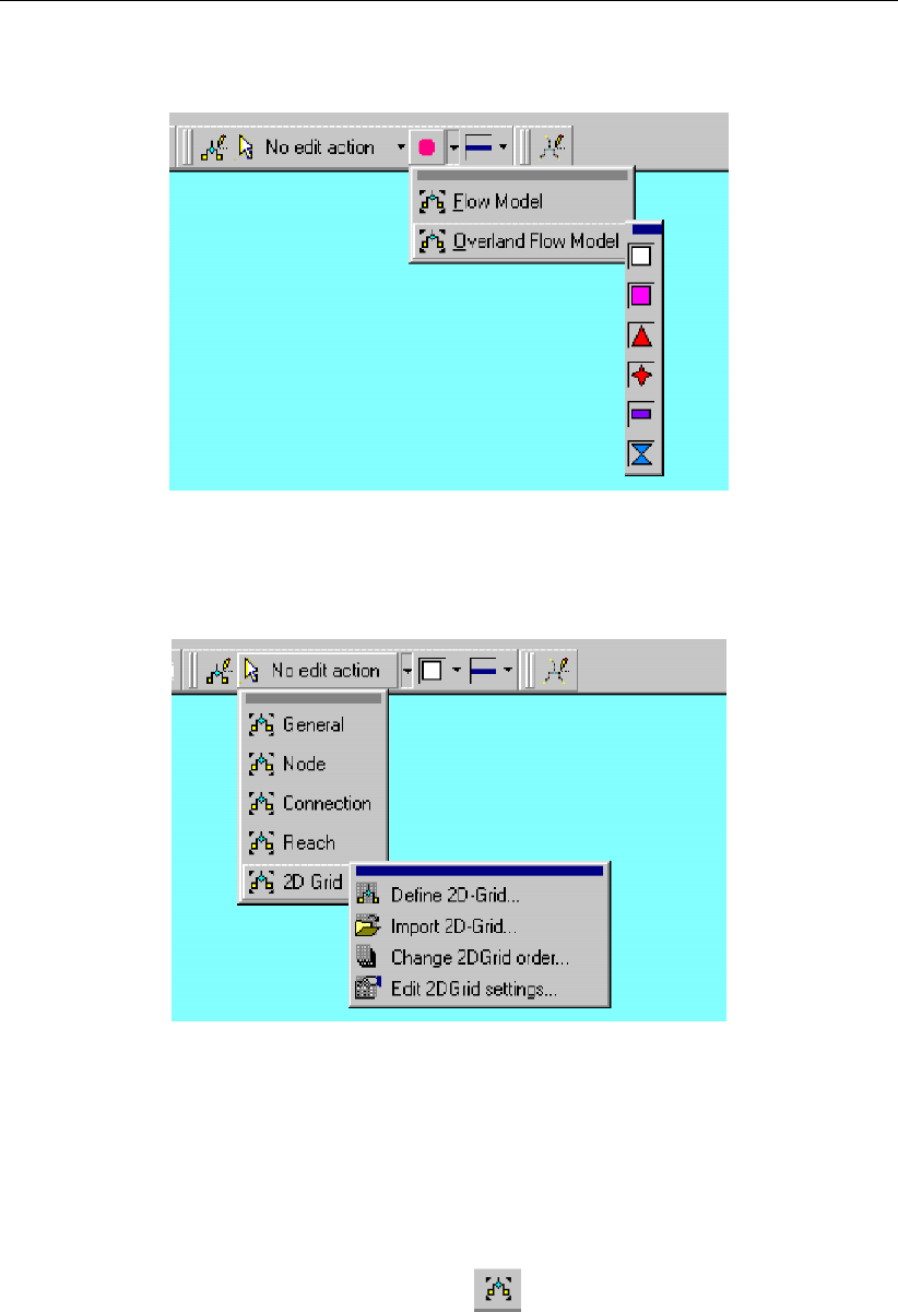
DRAFT
SOBEK, User Manual
and drag the toolbar that shows its node types to your screen.
Figure 4.37: Drag the toolbar containing Overland Flow node types to your screen
Select ’2D Grid tool bar’and drag it to your screen.
Figure 4.38: Drag the toolbar containing the 2D-grid edit actions to your screen
Select ’2D - Grid’ object from the overland flow node types toolbar (white square).
Now select the ’Import 2D-Grid...’ option from the ’Edit 2D Grid’ toolbar.
Enter “2D-Grid” in both input fields.
Click the OK button.
Browse to the <2D_OF Tutorial.ASC>file (<Drive:\SOBEK215\map\tutorial2Dflooding\>).
Open the <2D_OF Tutorial.ASC>file.
Zoom in on the entire network by clicking the button (show full network).
Finally, make the grid cells visible by choosing ’Options’ - ’2D-Grid options...’ - ’General’.
In the window that pops up, select ’Solid’ from the combo-box under the topic named
’Lines’.
Click the OK button.
The grid you imported should now look like this:
84 of 900 Deltares
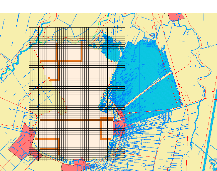
DRAFT
Tutorials
Figure 4.39: Impression of the model within its GIS environment.
The model shows a grid of the ’Groot Mijdrecht’ polder, located alongside the ’Vinkeveense
Plassen’ in the Netherlands.
With the menu option ’Select’ - ’2D grid cell info’ and selecting 2D grid cells you can investigate
the altitude of the 2D grid at several places. The grid has an altitude of 0 m from above datum,
except for some dikes which are 1 or 2 m higher. The dike which splits the polder in two parts
is a railway dike.
Now change the appearance of the grid under ’Options’, followed by ’2D Grid options...’ -
’Model data’.
Click on the classify button.
Enter at minimum “0” and maximum “6”.
Click the OK button.
Click the OK button to close the ’Properties 2D - Grid: ’ window.
In the menu bar, select ’Edit’ - ’Model data’.
In the ’Model Data’ window, select ’2D-Grid’ in the list box.
Press the Edit button.
Select the ’Friction’ tab.
Select the option ’Manning (mn)’ for friction type.
Enter a constant value of “0.02”. Keep the ’Friction value (Vertical Obstacle Friction)’ at 0.
Press the OK button.
Close the ’Model Data’ window.
Deltares 85 of 900

DRAFT
SOBEK, User Manual
Adding a simple network
Now we can start the 1D part: the channel flow network. Our schematisation of a ditch will be
modeled as shown in Figure 4.40.
Figure 4.40: The 1D network of the tutorial case.
Select the button, Flow-Connection Node.
Select the button to select the function ’Add node’.
Enter “North” in both input fields.
Click the OK button.
Click on the left-mouse button again to actually add the Flow-Connection Node on your
screen, in the Northern part.
Select the button, ’Add node’, again.
Enter “South” in both input fields.
Click the OK button.
86 of 900 Deltares
DRAFT
Tutorials
Click on the left-mouse button again to actually add the Flow-Connection Node on your
screen, in the Southern part.
Select the button, Flow-Channel, by clicking on it.
Select the button to select the function ’Connect nodes’.
Click with the left mouse button on the node "North" and drag to the node "South". Release
the mouse button.
The model will need a calculation grid. Before generating this grid we will switch off the
generation of names.
Select the button in the ’General’ tool bar, Edit settings, to go to the edit network
options.
Select the tab ’Node’.
In the group box ’ID’, select the radio button Automatic.
In the group box ’Name’, select the radio button No Names.
Select the tab ’Link’.
In the group box ’ID’, select the radio button Automatic.
In the group box ’Name’, select the radio button Automatic.
Press the OK button.
Select the button to select the function ’Calculation grid all reaches’.
Select the ’Split Vector’ option.
Select the node type ’Flow - Calculation Point’ from the drop down list.
Then enter “150” in the length edit box to set the calculation grid to a 150 m length.
Click the OK button.
Now re-enable the naming of new nodes:
Select the button in the ’General’ tool bar, Edit settings, to go to the edit network
options.
Select the tab ’Node’.
In the group box ’Name’, select the radio button Manual.
Press the OK button.
For a useful way of identifying the important nodes in your network, set the following options:
Click on the button in the Active Legend or select the menu item ’Options’ - ’Network
Data...’.
In the tab ’Node’, select the radio button Name.
Select the tab ’Link’.
Under ’Show Titles’, Select the radio button None.
SOBEK offers a powerful tool to validate your network.
Select ’Tools’ - ’Validate network by model’ - ’Flow Model’.
The following message appears: "A Flow reach must contain a Profile node".
Select the message in the Network Validation window. Now the torrent reach will be
selected on the map.
Deltares 87 of 900

DRAFT
SOBEK, User Manual
Press the Finished button.
Select the node, Flow - Cross Section node.
Select the (add node) function.
Enter “Cross-Section_Ditch1” in both input fields.
Click the OK button.
Click on the left-mouse button to actually add the Flow-Cross Section node on your screen.
Now, set the model data for the cross section:
Select the ’Cross-Section_Ditch1’ node.
Click with your right mouse button.
Select ’Model data’ - ’Flow Model’.
Select the ’Location’ tab.
Enter the value “-1” as the bed level. The ditch has a bed level at -1 meters with respect
to reference level.
Enter the value “0” as the surface level. The ditch has a surface level at 0 m with respect
to reference level.
Select the ’Cross section’ tab.
Select the type ’Trapezium’.
First enter the name “profile” at ’Cross section: ’.
Click the Define dimensions button.
Set the slope at ’1’.
Set the bottom width at ’1 m’.
And set the maximum flow width at ’3 m’.
Press the Save dimensions button.
Press the OK button.
Select ’Friction’ tab.
Select ’Use local value(s) for this cross section’.
Select ’Local value(s)’ in the ’Show’ combo box.
Select ’Chézy (C)’ for type friction (Bed).
Enter “50” for constant value.
Click OK to close.
4.3.2 Flooding from the lake
The next step in this tutorial will be to add a 2D boundary node, called ’Lake’ at the edge of
the grid. This node will schematise the lake, which has a constant water level of 0 m reference
level. For the time being we assume that the water from the lake has free access to the polder
(so no dikes or dike breaks in that area).
88 of 900 Deltares
DRAFT
Tutorials
Figure 4.41: Flooding from the lake.
In 2D - nodes toolbar, select the button, 2D - Boundary Node.
Select the button to select the function ’Add node’.
Enter “Lake” in both input fields.
Click the OK button.
Click on the left-mouse button again to actually add the 2D - Boundary Node on your
screen, at column number 30, and row number 36. The row and column numbers are
shown in the bottom right corner of the NETTER screen, while you move the mouse
pointer over the grid cells. Starting from the right, the first and second number display the
column and row number, and the third number displays the (inverted) height of the grid
cell.
Select the ’Lake’ node.
Click with your right mouse button.
Select ’Model data’ - ’Overland Flow Model’.
Deltares 89 of 900

DRAFT
SOBEK, User Manual
Select the tab ’Boundary condition’.
Select the type ’water level (h)’.
Enter a constant water level of “3.85” m.
Click the OK button.
Next, add some 2D history stations at the (approximate) locations in the polder, as de-
picted below.
Figure 4.42: Adding history stations.
Select the button, 2D - History Node, by clicking on it.
Select the button to select the function ’Add node’.
Enter “History-node1” in both input fields.
Click the OK button.
Click on the left-mouse button again to actually add the 2D - History Node on your screen,
90 of 900 Deltares
DRAFT
Tutorials
at column number 27, and row number 32.
Select the button to select the function ’Add node’.
Enter “History-node2” in both input fields.
Click the OK button.
Click on the left-mouse button again to actually add the 2D - History Node on your screen,
at column number 18, and row number 20.
Add ’History-node3’ at column number 12, and row number 39.
Add ’History-node4’ at column number 5, and row number 39.
Add ’History-node5’ at column number 8, and row number 32.
Add ’History-node6’ at column number 28, and row number 12.
Add ’History-node7’ at column number 21, and row number 11.
Add ’History-node8’ at column number 8, and row number 12.
Add ’History-node9’ at column number 7, and row number 6.
History stations will save the calculated results for each time step for water levels at their
locations. Place these nodes at ’interesting’ places (e.g. behind a breach). These nodes
need no extra data input in Model data.
Select button.
Select the menu item ’File’-’Exit’, to leave NETTER.
Click the OK button to leave the schematisation window.
Select the menu item ’Case’-’Save As’.
Enter the name “Tutorial 1D2D with 2D boundary node” to save the case.
Click the OK button.
Proceed with the simulation by double clicking the block ’Simulation’ in the case window.
Once the simulation is completed you can proceed to view the results in maps and in
charts.
The visualisation of 1D results are explained in the Tutorial Hydrodynamics in open water
(SOBEK-Rural 1DFLOW module) Together with the visualisation of 1D results, the user can
see the 2D results.
Double-click the ’Results in Maps’ task block. The Netter GIS application will re-appear.
Select ’Depths (incremental)’ from the Active legend.
Click the buttons and keep them pressed to animate the flooding of the area!
If one or several 1D-elements are selected, it is possible to observe time history graphs at
those locations for the computed parameters (see figure below). The same can be done for
the 2D - History stations.
The figure shows a 2D map water depth output at a certain time step and a graph showing the
water depth variation at selected 2D cells. The latter one (made by choosing ’Select’- ’2D grid
cell info’, selecting a 2D cell and clicking the button), is based on incremental information
and it shows the moments where the water depth in one cell changes from one class to the
next while flooding proceeds.
Deltares 91 of 900
DRAFT
SOBEK, User Manual
Figure 4.43: Results of the visualization on maps; 1D + 2D map output for a certain time
step and time series graph showing the water level history at two different
2D History stations (which actually are 1D objects)
Figure 4.44: Results of the visualization on maps; 2D map output for a certain time step
and graph showing the water depth variation at selected 2D cells based
on incremental information (this graph shows the moments when the water
depth class changes)
92 of 900 Deltares
DRAFT
Tutorials
Select ’File’ - ’Exit’ to leave the Results in Maps task block.
Select ’Case’ - ’Save’.
4.3.3 Flooding from the lake with a 2D dam break
Select ’Case’ - ’Open as new’.
Select the case ’Tutorial 1D2D with 2D boundary node’.
Enter the name “Tutorial 1D2D, flooding from 2D breach growth node”.
Press the OK button.
Double-click the ’Schematisation’ task block.
Press the Edit model button.
The idea behind this case is to simulate a breach of the dike, followed by a flooding from the
lake.
Choose ’Edit’ - ’Model data’.
Select ’2D - Grid’ from the list box.
Select the node ’2D-Grid’.
Click the Edit button.
Select the tab ’Grid Cell Bottom Level’.
Enter a value of “8” in the following cells:
Column number Row number
31 34
30 34
29 34
28 34
28 35
28 36
Click the OK button.
Enter the file name “2D_DAMBREAK.ASC”.
Save the grid under the directory <T_1D2D.LIT\FIXED>.
Select ’Options’ - ’2D-Grid options’ - ’Model data...’.
Press the Classify... button.
Enter the maximum legend scale into 8 (minimum = “0”, maximum = “8”).
Click the OK button.
Click the OK button.
The result should look like Figure 4.45.
Deltares 93 of 900
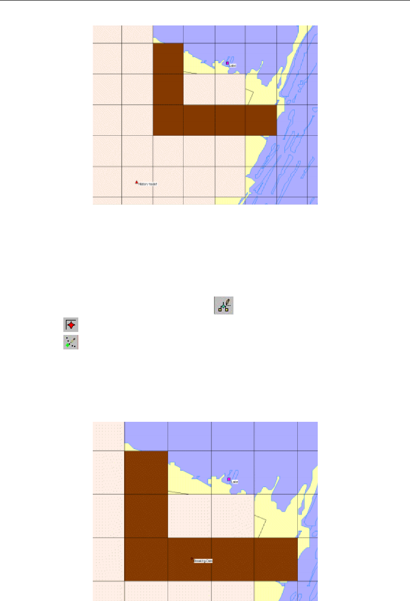
DRAFT
SOBEK, User Manual
Figure 4.45: Cells after changing depth from 0 m to 8 m.
As you can see after saving, the cell beneath the 2D boundary node is raised to 8 m +
reference level. Between the lake and the polder is a sort of a dike now, that will break by a
breach.
Enter the ’edit network’ mode by clicking the button.
Select the button, 2D - Breaking Dam Node, by clicking on it.
Select the button to select the function ’Add node’.
Enter “Breaking_Dam” in both input fields.
Click the OK button.
Click on the left-mouse button again to actually add the 2D - Breaking Dam Node on your
screen, in the cell with column number 29 and row number 34.
Figure 4.46: Add a 2D dam break node.
Select the node ’Breaking_Dam’.
Click with your right mouse button.
Select ’Model data’ - ’Overland Flow Model’.
Select the tab ’2D Breaking Dam’.
Press the Table... button.
Click on Add Row button.
94 of 900 Deltares
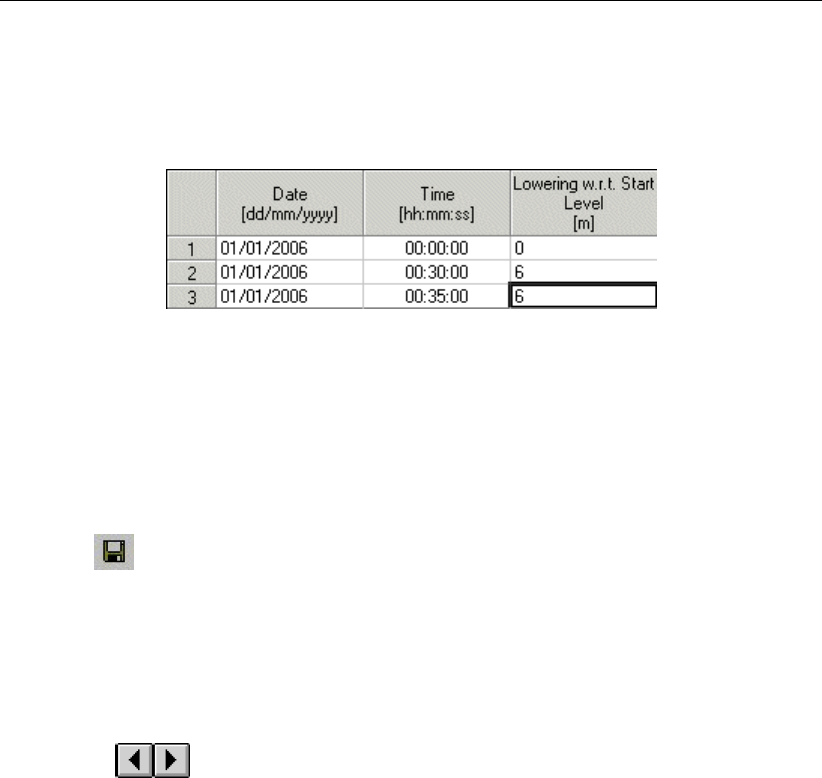
DRAFT
Tutorials
Enter “1”.
Press OK button.
Fill in the table as shown in Figure 4.47.
Figure 4.47: Growth of the breach depth (m) in time.
Press the OK button to leave the ’Edit table window’.
Press the OK button to leave the data edit window.
This data means that the cell will decrease in height from 8 m to 2 m with respect to the
reference level in 30 minutes time.
Select button in NETTER.
Select the menu item ’File’-’Exit’, to leave NETTER.
Press the OK button.
Select ’Case’ - ’Save’.
Double click the ’Simulation’ task block.
Double click the ’Results in Maps’ task block.
Select ’Depths (incremental)’ from the Active legend.
Click the buttons and keep them pressed to animate the flooding of the area.
Select ’File’ - ’Exit’ to leave the Results in Maps task block.
Select ’Case’ - ’Save’.
Select ’Case’ - ’Close’.
4.3.4 Flooding from a 1D channel
In the final case of this tutorial, the flooding will occur from a 1D channel, in stead of from
a 2D boundary like in the first two cases. This type of model is used when enough detailed
information is available about the river/channel network to incorporate a river/channel into the
model (1D2D). So the 1D channel network replaces the 2D - Boundary node.
The flooding itself will occur from one of the surrounding channels of the Dutch ’Amstelland-
boezem’, and will happen due to a planned inundation of the polder, and not because of a
dike break. This kind of inundations may be necessary to prevent dikes from breaking at
some other point in the channel, causing great economic damage and possibly loss of human
lives. The inundation will occur by opening a structure next to the channel.
Select ’Case’ - ’Open as new’.
Select the case ’Tutorial 1D2D with 2D boundary node’.
Enter the name of the new case “Flooding from 1D”.
Press the OK button.
Double click the ’Settings’ task block.
Press the Edit... button of the 1DFLOW (Rural) module.
Select the ’Initial data’ tab.
Select the option ’define local values in Edit network option.
Deltares 95 of 900

DRAFT
SOBEK, User Manual
Press the OK button.
Press the OK button to leave settings.
Double click the ’Schematisation’ task block.
Press the Edit model button.
Enter the ’edit network’ mode by clicking the button.
Select the button , ’Delete node’.
Select the ’Lake’ node.
Press the Yes button.
Zoom out a little bit, until you have a clear view of the channel branch to the North-West
of the polder. Take a look at Figure 4.48 for an example.
Next, you will model a part of a channel branch by defining two 1D boundary nodes and a
channel reach between them, by adding two profile to the channel, and by defining a calcula-
tion grid of 150 meters between every h-calculation point. Finally, you will change the course
of the channel according to the map by using the vector layer mode. The result should look
something like Figure 4.48:
96 of 900 Deltares
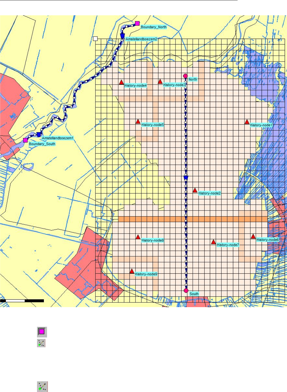
DRAFT
Tutorials
Figure 4.48: The tutorial 2D grid extended with a 1D channel.
Select the node, Flow-Boundary.
Select the button to select the function ’Add node’.
Enter ’Boundary_North’ in both input fields.
Click the OK button.
Click on the left-mouse button again to actually add the ’Boundary_North’ node on your
screen.
Select the button again.
Enter ’Boundary_South’ in both input fields.
Click the OK button.
Deltares 97 of 900

DRAFT
SOBEK, User Manual
Click on the left-mouse button again to actually add the ’Boundary_South’ node on your
screen.
Select the button, Flow-Channel, by clicking on it.
Select the button to select the function ’Connect nodes’.
Click with the left mouse button on the ’Boundary_South’ node and drag to the ’Bound-
ary_North’ node while keeping the button down. Release the left mouse button.
Select the button in the ’General’ tool bar, Edit settings, to go to the edit network
options.
Select the tab ’Node’.
In the group box ’Name’, select the radio button ’No Names’.
Press the OK button.
Select the button, Edit Reach Vectors’, to edit a selected reach vector.
Select the reach.
Select the button to show the coordinates.
Select the button to add a coordinate.
Click with the left mouse button on the reach to actually add a coordinate on your screen
and while keeping the button down drag the new coordinate to the new location.
Add and drag other coordinates of the selected reach.
De-select the button, Edit Reach Vectors’, to stop editing the reach vector.
Select the button to select the function ’Calculation grid all reaches’.
Select the ’Split Vector’ option.
Select the node type ’Flow - Calculation Point’ from the drop down list.
Then enter ’150’ in the length edit box to set the calculation grid to a 150 m length.
Click the OK button.
Add reach objects:
Select the button in the ’General’ tool bar, Edit settings, to go to the edit network
options.
Select the tab ’Node’.
In the group box ’Name’, select the radio button ’Manual’.
Press the OK button.
Select the node, Flow - Cross Section node.
Select the (add node) function.
Enter ’Amstellandboezem1’ in both input fields.
Click the OK button.
Click on the left-mouse button to actually add the Flow-Cross Section node on your screen,
near ’Boundary_South’.
Select the node, Flow - Cross Section node.
Select the (add node) function.
Enter ’Amstellandboezem2’ in both input fields.
Click the OK button.
Click on the left-mouse button to actually add the Flow-Cross Section node on your screen,
near ’Boundary_North’.
98 of 900 Deltares

DRAFT
Tutorials
Select the node ’Amstellandboezem1’.
Click with your right mouse button.
Select ’Model data’ - ’Flow Model’.
Select the ’Location’ tab.
Enter the value 2 as the bed level.
Enter the value 4.5 as the surface level.
Select the ’Cross section’ tab.
First enter the name ’Amstellandboezem’ at ’Cross section: ’.
Click the Define dimensions button.
Set the slope at ’2’.
Set the bottom width at ’10 m’.
And set the maximum width at ’20 m’.
Press the Save dimensions button.
Select ’Friction’ tab.
Select ’Use local value(s) for this cross section’.
Select ’Local value(s)’ in the ’Show’ combo box.
Select ’Chézy (C)’ for type friction (Bed).
Enter ’50’ for constant value.
Select ’Initial Value’ tab.
Select ’Use local initial value for this reach’.
Select initial ’water level’.
Enter the value 3.85 m.
Enter the value 1 m3/s for the initial flow in positive direction.
Click the OK button to close the data edit window.
Select the node ’Amstellandboezem2’.
Click with your right mouse button.
Select ’Model data’ - ’Flow Model’.
Select the ’Location’ tab.
Enter the value 1.9 as the bed level.
Enter the value 4.4 as the surface level.
Select the ’Cross section’ tab.
In the combo box ’Cross section: ’ select: ’Amstellandboezem’.
Select ’Friction’ tab.
Select ’Use local value(s) for this cross section’.
Select ’Local value(s)’ in the ’Show’ combo box.
Select ’Chézy (C)’ for type friction (Bed).
Enter ’50’ for constant value.
Select ’Initial Value’ tab.
Select ’Use local initial value for this reach’.
Select Initial ’water level’.
Enter the value 3.85 m.
Enter the value 1 m3/s for the initial flow in positive direction.
Click the OK button to close the data edit window.
Select the node ’Boundary_South’.
Click with your right mouse button.
Select ’Model data’ - ’Flow Model’.
In tab ’Boundary Condition’, select the option ’flow (Q)’.
Select ’Function of time :’.
Press Table....
Press Add Row.
Enter 5.
Press the OK button.
Deltares 99 of 900
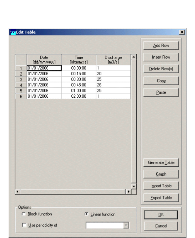
DRAFT
SOBEK, User Manual
Fill in the table as shown in Figure 4.49.
Figure 4.49: Filling in the 1D Q-boundary table.
Press the OK button.
Press the OK button.
Select the node "Boundary_North".
Click with your right mouse button.
Select ’Model data’ - ’Flow Model’.
Select the option ’Q-h relation’.
Press the Table... button.
Press the Add Row.
Enter 4.
Press the OK button.
Fill in the table as shown in the figure below.
100 of 900 Deltares
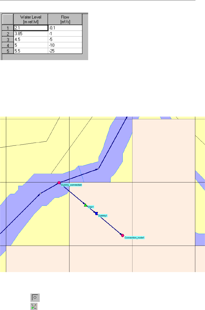
DRAFT
Tutorials
Press the OK button.
Press the OK button.
Now we have defined the channel branch from which the flooding will occur. The next step is
to model the ’dummy branch’ containing the structure that is used to control the flooding. We
will use a Connection Node to connect the dummy branch to the Amstellandboezem at the
location shown in Figure 4.50. We will also add a cross-section and a structure, a weir.
Figure 4.50: The dummy branch used to control the flooding of the Amstellandboezem
into the 2D grid.
Select the button, Flow - Calculation Point.
Select the button to select the function ’Add node’.
Enter ’Dummy_connection’ in both input fields.
Click the OK button.
Click on the left-mouse button again to actually add the Dummy_connection node on your
screen. This node should be placed at the location where we want to connect the dummy
Deltares 101 of 900
DRAFT
SOBEK, User Manual
branch to the existing branch as shown in Figure 4.50).
Select the button, Flow-Connection Node, by clicking on it.
Select the button Split reach at node in the ’Reach’ toolbar.
Use the left-mouse button on the Dummy_connection node to actually add the Flow -
Connection node on your screen.
By following the above steps, we have split the reach at the location of the Dummy_connection
h-calculation node and replaced it with a connection node. Next, we will set the Cross-section
bathymetry to interpolate along the two reaches:
Select the ’Dummy_connection’ node by left-mouse clicking it
Click with your right mouse button.
Select ’Model data’ - ’Flow Model’.
Left-mouse click the tab ’Interpolation Over node’.
Enable the option ’Interpolate Cross-section bathymetry (only) over Node’ by left-mouse
clicking it.
For ’First Reach’, select the upstream reach ’2’.
For ’Second Reach’, select the downstream reach ’3’.
Press the OK button.
Select the button to select the function ’Add node’.
Enter ’Connection_node1’ in both input fields.
Click the OK button.
Click on the left-mouse button again to actually add the Flow-Connection Node on your
screen.
Select the button, Flow-Channel.
Select the button to select the function ’Connect nodes’.
Click with the left mouse button on the node ’Dummy_connection’ and drag to the node
"Connection_node1" while keeping the button down. Release the left mouse button.
Select the node, Flow - Cross Section node.
Select the (add node) function.
Enter ’Dummy1’ in both input fields.
Click the OK button.
Click on the left-mouse button to actually add the Flow-Cross Section node on your screen.
Select the node, Flow - Weir node.
Select the (add node) function.
Enter ’Weir1’ in both input fields.
Click the OK button.
Click on the left-mouse button to actually add the Flow-Weir node on your screen.
Select the Cross section node ’Dummy1’.
Click with your right mouse button.
Select ’Model data’ - ’Flow Model’.
Select the ’Location’ tab.
Enter the value 2 as the bed level.
Enter the value 4 as the surface level.
Select the ’Cross section’ tab.
Select ’Rectangle’ as the cross section type.
First enter the name ’Dummy1’ at ’Cross section: ’.
102 of 900 Deltares

DRAFT
Tutorials
Click the Define dimensions button.
Enter 10 m as width.
Enter 2 m as height.
Press the Save dimensions button.
Press the OK button.
Select ’Friction’ tab.
Select ’Use local value(s) for this cross section’.
Select ’Local value(s)’ in the ’Show’ combo box.
Select ’Chézy (C)’ for type friction (Bed).
Enter ’50’ for constant value.
Select ’Initial Value’ tab.
Select ’Use local initial value for this reach’.
Select Initial ’water level’.
Enter the value 3.85 m.
Enter the value 0 m3s−1 for the initial flow in positive direction.
Click the OK button to close.
Select the Weir node ’Weir1’.
Click with your right mouse button.
Select ’Model data’ - ’Flow Model’.
Enter 2 m as width.
Enter 0.7 m as crest level.
Select the ’Controller’ tab.
Select ’Time’ as type of controller.
Enter ’Weir1’ as name.
Press the Table... button.
Press the Add Row.
Enter 2.
Press the OK button.
Fill in the table as shown in the figure below.
Press the OK button.
Press the OK button.
Your new schematisation is now ready.
Select button in NETTER.
Select the menu item ’File’ - ’Exit’, to leave NETTER.
Press the OK button.
Select ’Case’ - ’Save’.
Double click the ’Simulation’ task block.
Double click the ’Results in Maps’ task block.
Select ’Depths (incremental)’ from the Active legend.
Click the buttons and keep them pressed to animate the flooding of the area.
Deltares 103 of 900
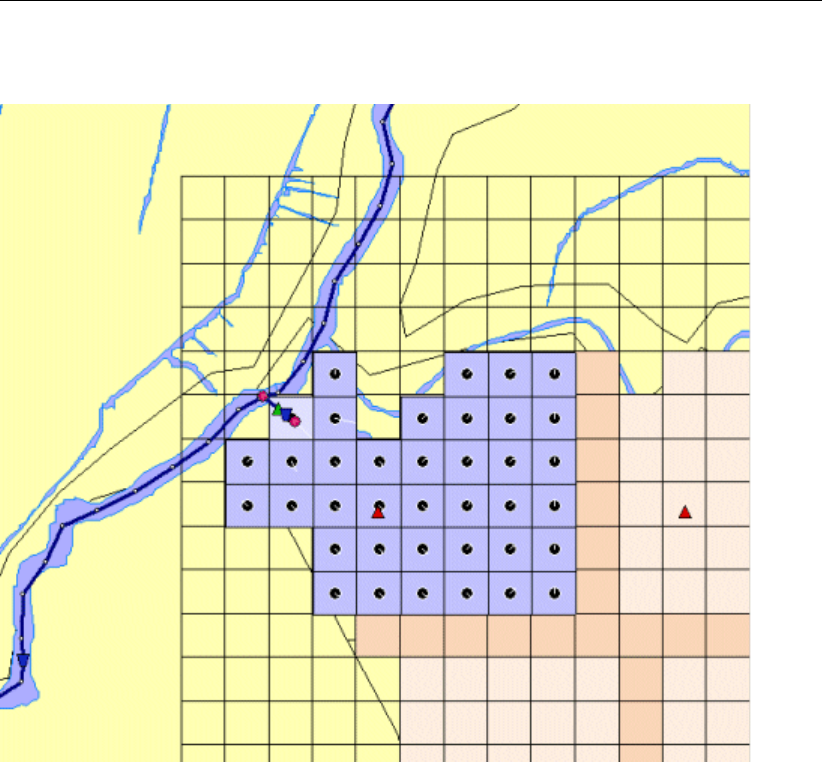
DRAFT
SOBEK, User Manual
The resulting flooding is shown in the figure below:
Select ’File’ - ’Exit’ to leave the Results in Maps task block.
Select ’Case’ - ’Save’.
Select ’Case’ - ’Close’.
Select ’Case’ - ’Exit’.
Select ’Files’ - ’Exit Sobek’.
4.4 Tutorial Hydrology in polders (SOBEK-Rural RR module)
4.4.1 Introduction
In this tutorial the basic principles of working with the Rainfall-Runoff module of SOBEK-Rural
are explained step by step and you will be guided to set-up a simple schematisation. Rainfall-
Runoff offers a wide range of options. This tutorial however only shows a limited number of
them. After finishing the tutorial, one will have enough experience to continue oneself. Some
experience on working with the WINDOWS Operating System is required.
The tutorial contains:
1 setting up a simple model;
2 computing;
3 viewing the results;
4 extending your model.
The tutorial does not explain all options in all windows that will appear. Once you get the
hang-and-feel of the modelling system, you may wish to browse through the options not dealt
104 of 900 Deltares

DRAFT
Tutorials
with in the tutorial by browsing through the menu system.
4.4.2 Getting started
Click on the Windows Start button.
Select the ’Programs’ menu.
Select the ’All Programs’ or ’All Apps’ menu.
Select the ’Delft Hydraulics’ menu.
Select the ’SOBEK’ menu item (SOBEK215).
Click on the ’SOBEK’ icon.
Select the menu item ’Options’ - ’SOBEK Options’.
Select the tab ’Background Map’.
Select the file ’Tutorial1.map’.
Press OK button to save and close SOBEK Options.
Click the New Project button.
Type the name ’T_RR’.
The program converts all the characters into upper case. If a project with the same name
already exists, the user has to enter a different name here.
Click the OK button.
You have added a new project with the name ’T_RR’. You are now asked: do you want to work
with this project?
Click the Yes button.
4.4.3 Case management
The screen of the so-called "Case Manager" appears. This tool automatically keeps track of
cases and the related files. For instance: you might want to save different scenarios within a
project as cases with different names. This is organized through the Case Manager.
Deltares 105 of 900
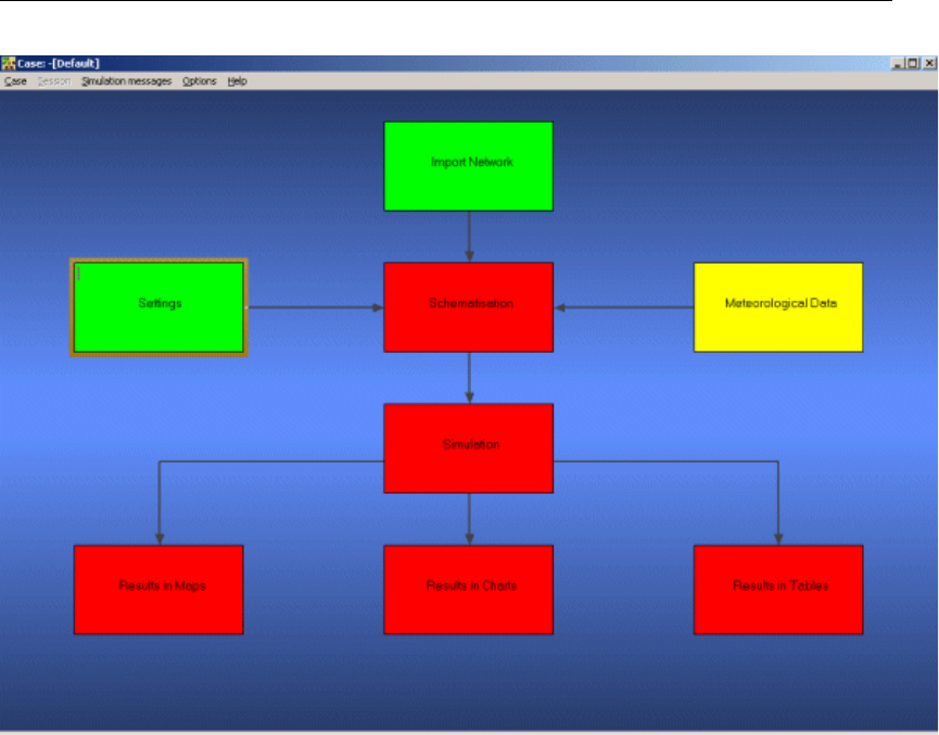
DRAFT
SOBEK, User Manual
The case manager screen.
On the screen a number of blocks are visible:
1 Import Network;
2 Settings;
3 Meteorological Data;
4 Schematisation;
5 Simulation;
6 Results in Maps;
7 Results in Charts;
8 Results in Tables.
Each block represents a specific task. A task can be a model, a set of linked models, the
selection of a scenario or strategy, or a (graphical) presentation tool. The arrows between the
blocks represent the relations between the tasks. When an arrow is pointing from block "A" to
block "B", the task of block B can only be executed after the task of block A is finished.
The Case Manager has the following tasks:
1 Administration of cases (which data is related to which cases);
2 Checking whether the model calculations for the cases are performed in the predefined
order;
3 Logging the actions of the Case Manager (including view and print);
4 Providing access to the computational framework through a user interface, so the user
can:
manipulate a case (read, save, delete, etc.);
view and check the status of all tasks;
106 of 900 Deltares

DRAFT
Tutorials
view the relation between the various tasks.
choose and run predefined tasks (modules);
When the Case Manager screen appears first after you have added a project all task blocks
are grey. To activate the task blocks you have to open the default case of this new project:
Select the menu option ’Case’ - ’Open’.
Select ’Default’ from the list.
Click the OK button.
Another method is to click on one of the grey task blocks and select ’Default’.
Once you have opened the default case the task blocks are no longer grey, but one of the
following colors:
1 yellow: the task can be executed;
2 green: the task has been executed at least once and can be executed again;
3 red: the task cannot be executed until all preceding tasks have been executed.
When the task is being executed the task block is purple. You can execute a task by double-
clicking the task block. When you select a yellow or green task block, the color will change to
purple and then change to green.
Now, we will discuss each task block.
4.4.4 Task block: Import Network
The color of this task block is yellow, which means that this task block must be executed.
Execute the task block ’Import Network’ by double-clicking.
In this task block the origin of the schematisation can be defined. Schematisations, used in
SOBEK, can be either imported from a database or set-up from scratch.
If a schematisation is already available in the standard exchange format it can easily be im-
ported to SOBEK. Links with data formats can be made upon request. For that reason some
radio buttons might be turned grey.
Let’s set up a schematisation from scratch.
Select the radio button ’Start from scratch’.
Press the OK button.
Notice that you’re back in the Case Manager now and that the task block ’Import Network’ has
turned green.
Deltares 107 of 900

DRAFT
SOBEK, User Manual
4.4.5 Task block: Settings
The ’Settings’ task block is used to select the SOBEK modules that you want to use for your
project. Also computational parameters such as calculation time steps, simulation period and
initial water levels, can be set in this task block.
Depending on the set of modules that you purchased, some may be disabled (grey), and
some may be enabled.
SOBEK-Rural 1DFLOW
The SOBEK-Rural 1DFLOW module is a sophisticated module that can be used for the simu-
lation of one-dimensional flow in irrigation and drainage systems. It is a tool that can be used
to simulate and solve problems in regional water management, such as irrigation construc-
tion, drainage, automation of canal systems, dredging and flood protection. This module can
be used stand-alone or in combination with other modules, for example the SOBEK-Rural RR
module (Rainfall-Runoff).
SOBEK-Urban 1DFLOW
The SOBEK-Urban 1DFLOW module is a sophisticated module for the simulation of one-
dimensional flow in wastewater and storm water systems. It is a tool that can be used to sim-
ulate and solve problems in urban drainage systems such as determination of urban drainage
capacities including treatment plants, assessment of sewer overflow frequency and design
of detention basins. The SOBEK-Urban 1DFLOW module can also be used in combination
with the SOBEK-Rural 1DFLOW module, the SOBEK-Urban RR (Rainfall-Runoff) module and
other modules. One of the competitive advantages is the combination with the SOBEK-Rural
1DFLOW module for environmental study on receiving waters.
108 of 900 Deltares

DRAFT
Tutorials
SOBEK-River 1DFLOW
The SOBEK-River 1DFLOW module is a sophisticated module that can be used for the sim-
ulation of one-dimensional water flow in river systems and estuaries. It is a tool that can be
used to simulate and solve problems in river water management such as flood protection,
flood-risk assessment, real-time forecasting, dam break analysis, navigation and dredging.
This module can be used stand-alone or in combination with other modules.
The RR (Rainfall-Runoff) module is a module that can be used for the simulation of rainfall-
runoff processes. This module is a part of a large family of modules which can be linked. The
list of modules includes (amongst others) SOBEK-Rural 1DFLOW module, SOBEK-Urban
1DFLOW module and RTC (Real Time Control) module. The RR module is frequently used
in combination with the SOBEK-Rural 1DFLOW and SOBEK-Urban 1DFLOW modules. It is
then possible to either to perform calculations for both modules simultaneously or sequentially.
The RTC (Real Time Control) module is a module that can be used for the simulation of com-
plex real time control of hydraulic systems. It can be applied to rainfall-runoff, hydraulics and
water quality computations. In that case the rainfall-runoff and water quality computations are
run simultaneously with the hydrodynamics computations, thus incorporating full interaction
between all processes.
The above mentioned modules can also be used in combination with modules for simulating
water quality processes (1DWAQ module, 2DWAQ module and/or EM (EMission) module).
Thus, several combinations of modules are possible. Depending on the problems to be solved
you can set the desired combination. The modules can easily be selected via the task block
’Settings’.
Start editing the settings for the Rainfall-Runoff module:
Double-click the ’Settings’ task block.
The number of active modules depends on which modules you bought. In this tutorial we will
only activate the Rainfall-Runoff module, the other modules are inactive.
Unselect all the selected modules if any.
Select the ’RR’ module.
Press the Edit... button of the ’RR’ module.
You have to define certain settings, such as the
Click the ’Time Settings’ tab.
Set the ’time step in computation’ to 30 minutes (type ’30’ in the ’min’ edit box and ’0’ in
the others).
Select the ’Output Options’ tab (located on the right side of the window).
Define ’output time step’ to 30 minutes.
Deltares 109 of 900
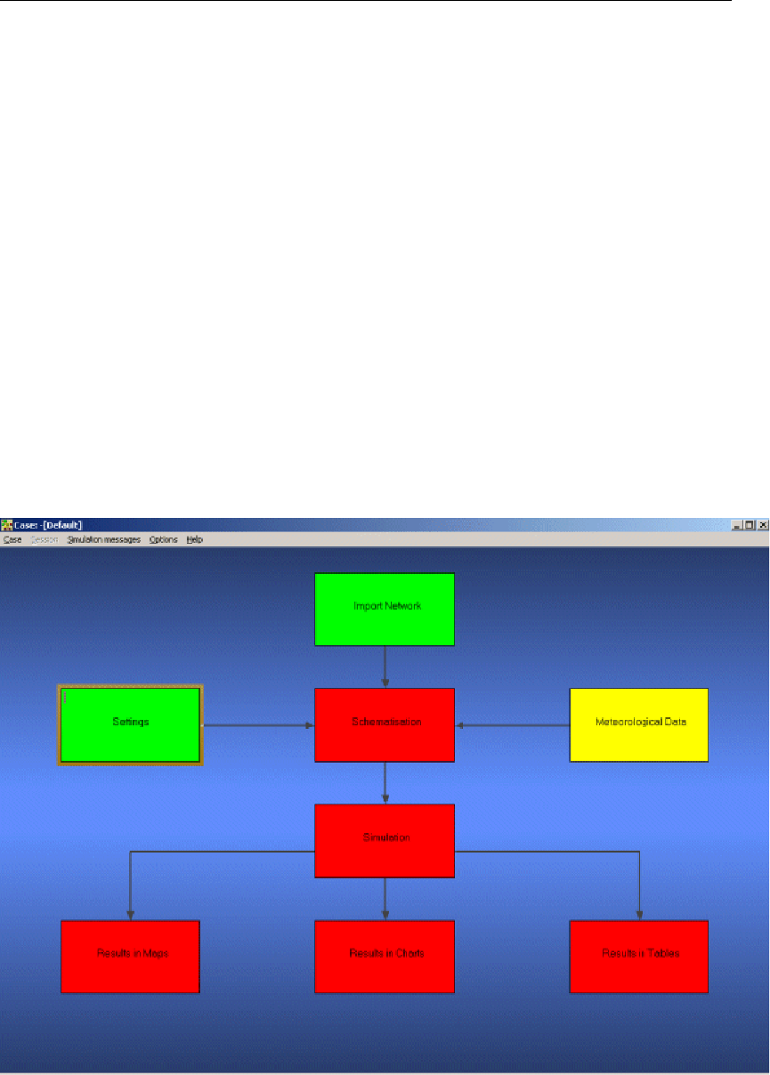
DRAFT
SOBEK, User Manual
Activate the following output options:
Flows at links
Open water node
Structure node
Unpaved node
Press the OK button.
For this guided tour all remaining default values are fine.
Did you notice that you did not have to define the begin and end of the simulation period?
Rainfall-Runoff will automatically derive this from the rainfall data. The rainfall data are incor-
porated in the ’Meteorological Data’ task block. The next section deals with this task block.
Press the OK button to exit this task. Your settings are then saved.
You should now see the following screen, indicating that both the ’Settings’ task and the
’Import Network’ task have been completed and that the Meteorological data task should still
be performed.
110 of 900 Deltares
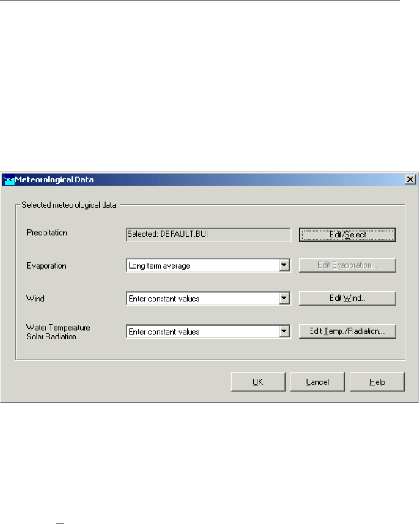
DRAFT
Tutorials
4.4.6 Task block: Meteorological Data
SOBEK-Rural simulations require meteorological input data, i.e. precipitation data and evap-
oration data.
The evaporation data are linked to the time series of the precipitation data. The simulation
period is determined by the start- and end dates of the precipitation data.
Double-click the ’Meteorological Data’ task block of the Case Manager.
The following screen will appear:
Now you can select and edit the precipitation data and evaporation data.
Click the Edit/Select button next to the Precipitation box.
Click the Select event button.
Select the rainfall event named <DEFAULT.BUI>.
Press OK button.
Press OK button again to leave the ’edit precipitation data’ window.
Select ’Long term average’ for evaporation.
Click the OK button to leave the Meteorological Data window.
Now you have finished defining the meteorological data. Notice that this task block has turned
green too!
Deltares 111 of 900

DRAFT
SOBEK, User Manual
4.4.7 Task block: Schematisation
A schematisation can easily be set up with the help of the network editor. You will set up a
simple schematisation.
Double-click the ’Schematisation’ task block of the Case Manager.
You can choose to edit the model by clicking the upper button Edit model.
Click the Edit model button.
When the option Edit model of the ’Schematisation’ is selected, the network editor starts.
The network editor is called NETTER and is a component of the Delft Hydraulics Decision
Support System (Delft-DSS) tools. NETTER offers the possibility to set-up the schematisation
on top of a background GIS map. NETTER also offers advanced analysis tools to show model
results linked to the schematisation and provide the user with full printing facilities to make high
quality prints.
Within NETTER you can do the following:
1 Interactively and graphically prepare a schematisation;
2 Generate schematisations upon GIS map Layers;
3 Carry out schematisation operations: search for a certain node, show node numbers and
names, show link numbers, etc.;
4 Carry out map operations: zooming in, zooming out, (de)activating map layers, colouring
of map layers, adding title information on the map, etc.;
5 View results of simulation models for schematisations created in NETTER;
6 Print maps or schematisations.
Generally speaking, NETTER has two edit modes. The first mode is the mode to set-up the
schematisation. The second edit mode is the mode for editing the attribute data. In this mode
you provide attributes for the schematisation objects. For example, a pump station must have
a pump capacity and switch on/off levels.
In this exercise you will work on a simple schematisation.
112 of 900 Deltares
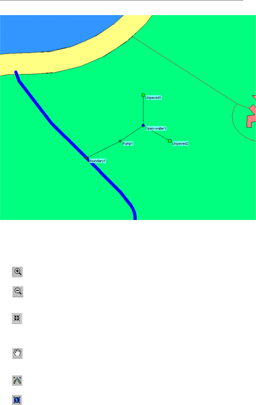
DRAFT
Tutorials
In order to focus on a small part of the map you can use the zoom functionalities.
The View menu contains commands for zoom in, zoom out, centre the window, move the
window and show all schematisation or map layers.
The button allows you to zoom in on any part of the "active main window".
The button allows you to zoom out by shrinking the displayed part of the "active main
window".
The button allows you to centre a schematisation or map GIS object. When choosing this
command and then clicking with the left mouse button on an object NETTER redraws the map
centring the chosen object to the NETTER window.
The button allows you to shift the view by clicking the mouse anywhere in the NETTER
window and dragging the view to another position.
The button redraws the view fitting all schematisation objects in to the NETTER window.
The button redraws the view fitting all GIS map layers in to the NETTER window.
Deltares 113 of 900
DRAFT
SOBEK, User Manual
The button restores the view of the map before the last zoom command was given.
The button restores the view of the map before the last ’Show Previous’ command was
given.
Select button.
Move the mouse pointer to the main window.
Click and hold the left mouse button, make a rectangle by dragging the pointer across the
main window. The size of this rectangle determines the magnification.
Release the left mouse button.
Now, you will build the simple schematisation. This schematisation consists of a small open
channel with a weir.
Select the button, Edit Network, to start the edit network mode.
In the edit network mode, all edit network functions and network objects for the selected
module are available.
Select and the ’General’ edit network functions to place the General functions toolbar
anywhere on your screen.
Select and the ’Node’ edit network functions to place the Node functions toolbar any-
where on your screen.
Select and the ’Connection’ edit network functions to place the Connection functions
toolbar anywhere on your screen.
Select and the node objects to place the ’Rainfall-Runoff Model’ node objects toolbar
anywhere on your screen.
Select and the ’Rainfall-Runoff Model’ link objects to place the reach objects toolbar
anywhere on your screen.
It is possible to define the identifiers (or ID’s) of the nodes and branches (links) automatically
or manually.
114 of 900 Deltares
DRAFT
Tutorials
Select the button in the ’General’ tool bar, Edit settings, to go to the edit network
options.
Select the tab ’Node’.
In the ’ID’ group box, select the radio button Manual.
In the ’Name’ group box, select the radio button Manual.
Select the tab ’Link’.
Set the ’ID’ and ’Name’ to ’automatic’.
Click the OK button.
Now you can start drawing you application.
Select the button, RR-Unpaved node.
Select the button to select the function ’Add node’.
Enter “Unpaved1” in both input fields.
Click the OK button.
Locate the mouse at a position where you want to add the RR-Unpaved node and click
the left-mouse button again to actually add the node.
Select the button, RR-Open Water node.
Select the button.
Enter “Open_water1” in both input fields.
Click the OK button.
Click on the left-mouse button again to actually add the node on your screen.
Select the button, RR-link.
Select the button to select the function ’Connect nodes’.
Click with the left mouse button on the RR-Unpaved node and drag to the RR-Open Water
node while keeping the button down. Release the left mouse button.
In order to see the identifiers on the map please:
Click the button in the Active Legend or select the menu item ’Options’ - ’Network
Data...’.
Select the tab ’Node’.
Select the radio button ’Name’.
Select the tab ’Link’.
Select the radio button ’None’.
Press the OK button.
Select the button, RR-Unpaved node.
Select the button, RR-link.
Select the button to select the function ’Add connect’.
Enter “Unpaved2” in both input fields.
Click the OK button.
Click with the left mouse button on the map where the second RR-Unpaved should be
placed and drag to the RR-Open Water node while keeping the button down. Release the
left mouse button.
Deltares 115 of 900
DRAFT
SOBEK, User Manual
Now the two unpaved area nodes are connected to the open water node.
Downstream of an unpaved area node should be an open water or a boundary node. The
option ’defined direction’ can be used to see the downstream site. The defined direction
can be viewed by selecting ’Options’-’Network Data...’-’Links’-’Defined’. Note that the arrow
is pointed towards the open water node. This means that downstream of the unpaved area
node is the open water node and the unpaved area discharges on the open water node.
Select the button, RR - Pump Station.
Select the button.
Enter “Pump1” in both input fields.
Click the OK button.
Click on the left-mouse button again to add the node on your screen.
Select the button, RR - Boundary node.
Select the button.
Enter “Boundary1” in both input fields.
Click the OK button.
Click on the left-mouse button again to add the node on your screen.
Select the button, RR-link.
Select the button to select the function ’Connect nodes’.
Click with the left mouse button on the RR - Open Water node and drag to the RR - Pump
Station while keeping the button down. Release the left mouse button.
Click with the left mouse button on the RR - Pump Station and drag to the RR - Boundary
node while keeping the button down. Release the left mouse button.
The schematisation has been set-up. The next step is to define the attribute data of the
schematisation.
You will provide the following data step-by-step during this tutorial:
Unpaved area node
1 Area per crop = 280 ha grass;
2 Groundwater area = 400 ha;
3 Surface level = 1 m above reference level (constant value);
4 Soil type = sand_maximum (µ= 0.117 per m);
5 Thickness groundwater layer = 5 m. This information is only relevant for computing of
salt concentration, thus for computing the volume of this node. The option to compute
salt concentrations can be turned on in the "settings task block", but is turned off in this
tutorial;
6 Initial groundwater level = equal to target level open water or level at boundary node;
7 Storage, Maximum on land = 3 mm;
8 Storage, Initial = 0 mm;
9 Infiltration capacity = 10 mm/hr;
10 Computation option for drainage = De Zeeuw - Hellinga
11 Reaction factor Surface runoff = 100 1/day;
12 Reaction factor Horizontal inflow = 0.05 1/day;
13 Reaction factor Drainage 0 - 1 m alpha = 0.4 1/day;
14 Reaction factor Drainage 1 - 2 m alpha = 0.4 1/day;
15 Reaction factor Drainage 2 - 3 m alpha = 0.4 1/day;
116 of 900 Deltares

DRAFT
Tutorials
16 Reaction factor Drainage 3 - infinity alpha = 0.4 1/day;
17 Seepage = 0 mm/day.
Unselect the button, Edit Network, to close the edit network mode.
Select the ’Unpaved1’ node.
Click right mouse button.
Select ’Model data’ - ’Rainfall Runoff Model’.
Select the ’Area’ tab.
In the group box ’Area per crop’, select [ha] as the unit.
Click the Table... button.
Enter “280” for the crop ’grass’.
Click the OK button.
Check the check box ’Use different area for groundwater computations:’.
Enter the value “400”.
In the group box ’Surface level’, select ’constant value’.
Enter the value “1”.
Select the ’Soil’ tab.
Select ’sand_maximum (µ= 0.117 per m)’.
Type ’5’ in the input box ’Thickness groundwater layer’.
Type ’1.5’ in the input box ’Maximum allowed groundwater level:’
In the ’Initial groundwater level’ group box, select ’equal to initial target level open water or
level at boundary node’.
Select the ’Storage’ tab.
Type the name ’storage1’ in the combo box.
Click the Define button.
Select [mm] as the unit.
Enter the value of “3” mm for maximum storage on land.
Enter the value of “0” mm for initial storage.
Then press the Save button.
Then press the OK button (You have added a Storage definition. Accept this as a new
definition?).
Select the ’Infiltration’ tab.
Type the name ’infiltration1’ in the text box.
Click on the Define button.
Select [mm/hr] as the unit.
Enter the value for infiltration capacity of “10” mm/hr.
Click the Save button.
Click the OK button (You have added an Infiltration definition. Accept this as a new defini-
tion?).
Select the ’Drainage’ tab.
Select the radio button ’De Zeeuw-Hellinga’ in the ’Computation option for drainage’ group
box.
In the ’Definition’ group box, enter the name “drainage1”.
Click the Define button.
Enter “100” as the surface runoff reaction factor [1/d].
Enter “0.05” as the horizontal inflow reaction factor.
In the ’Reaction factor [1/d]’ group box, check the top check box. A table appears in which
the reaction factor data can be entered.
To define the top drainage layer from 0 - 1 m below surface, enter “1” in the input box.
Enter “0.4” as the reaction factor for this layer.
Enter the following data:
Deltares 117 of 900
DRAFT
SOBEK, User Manual
Reaction factor Drainage 1 – 2 m 0.4 1/day
Reaction factor Drainage 2 – 3 m 0.4 1/day
Reaction factor Drainage 3 – ∞0.4 1/day
Click the Save button.
Click the OK button (You have added a definition. Accept this as a new definition?).
Select the Seepage tab.
Type the name ’seepage1’.
Click on Define button.
Select the option constant for seepage.
Enter the value “0”.
Click the button Save to save this set of parameters.
Click the OK button (You have added a Seepage definition. Accept this as a new defini-
tion?).
Click the OK button.
For the second RR - Unpaved node data you will use the Multiple Data Editor.
Select the button, Select by rectangle.
Select the two RR - Unpaved nodes by clicking on the map and dragging while keeping
the button down. Release the left mouse button.
Alternatively, select both RR - Unpaved nodes by left-clicking the two nodes while keeping
the Ctrl pressed.
Click right mouse button.
Select ’Model data’ - ’Rainfall Runoff Model’.
Select ’RR-UnPaved’.
Select ’Unpaved area’.
Select the row of ’Unpaved1’.
Select ’Edit’ - ’Copy’.
Select the row of ’Unpaved2’.
Select ’Edit’ - ’Paste’.
Select ’File’ - ’Save Data’.
Select ’File’ - ’Exit’.
Open water
Select the open water node.
Click the right mouse button.
Select ’Model data’ - ’Rainfall-Runoff Model’.
Select the ’Surface’ tab.
Enter the ’Bottom level’ at “-1” m above datum.
This information is only relevant for computing of salt concentration, thus for computing the
volume of this node.
Select ’constant area’.
Choose ’ha’ for area unit.
Enter a surface area of “20” hectares.
Select the ’Management’ tab.
118 of 900 Deltares

DRAFT
Tutorials
Select ’Fixed target level [m above datum]’.
Enter “0” as the fixed target level.
Enter “0” m above datum as the maximum permissible level.
Select the ’Seepage’ tab.
Type the name ’seepage open water1’ in the combo box.
Click the Define button.
Enter a seepage of “0” mm/day.
Then press the Save button.
Click the OK button (You have added a Seepage definition. Accept this as a new defini-
tion?).
Click the OK button.
Pump
Select the RR - Pump Station.
Click right mouse button.
Then select ’Model data’ - ’Rainfall Runoff Model’.
Select the ’Options’ tab.
Select ’Normal’ as the ’Pump type’ (Note that the upstream level is checked only).
Select the ’Pump’ tab.
Choose ’m3/min’ as the capacity unit.
In the group box ’Low capacity’, enter the capacity of “30”.
In the group box ’Low capacity’, click the Table (Day) of ’Switch on/off levels’.
Enter the following values:
Date [dd/mm/yyyy] Time [hh:mm:ss] Switch on level dur-
ing the day - target
level [m]
Switch off level dur-
ing the day - target
level [m]
01/01/2002 00:00:00 0.01 -0.01
31/12/2002 23:59:00 0.01 -0.01
Click the OK button.
If you changed the default values in this table: Click the OK button. (’Enter the table
name’)
In the group box ’High capacity’, enter the additional capacity of “0”.
Click the OK button to leave the ’Data Edit for Pump’ window.
Boundary node
Select the RR - Boundary node.
Click the right mouse button.
Select ’Model data’ - ’Rainfall Runoff Model’.
Select the ’Boundary’ tab.
Select the ’Fixed boundary’ option.
Enter “0.5” m above datum as the fixed boundary level.
Click the OK button.
Select ’File’ - ’Save’ - ’Map’.
Select button.
Deltares 119 of 900
DRAFT
SOBEK, User Manual
Select the menu item ’File’ - ’Exit’, to leave NETTER.
Click the OK button.
Now only your schematisation has been saved in NETTER. The whole case must be saved
as well!
Select the menu item ’Case’ - ’Save As...’.
Enter the name “Case_one”.
Click the OK button.
4.4.8 Task block: Simulation
The next step in the modelling process is to perform the calculations.
Double-click the task block ’Simulation’.
4.4.9 Task block: Results in Maps
Results in maps gives you a clear impression of the results in time. The program NETTER is
used in this task block. Since NETTER also is used to set up a schematisation, it will be easy
for you, being an experienced user now, to view the results.
Double-click ’Results in Maps’ task block to analyse the results.
Select the item ’Open water nodes’ in the Active Legend.
Select the node ’Open_water1’ by clicking it.
Click the button on the ’View Data’ window.
Now analyse your results!
Suppose, you want to analyse the open water level and the groundwater level. Therefore it
should be useful to depict both variables in one graph.
Do not close the graph server.
Select the item ’Unpaved nodes’ in the Active Legend.
In the ’View data’ window, select the item ’Groundw.Level [m]’.
Select the ’Unpaved1’ node.
Click the button in the ’View data’ window.
As you see a graph appears containing two variables!
Select ’File’ - ’Exit’ to close the Graph Server.
Select ’File’ - ’Exit’ to close NETTER.
120 of 900 Deltares
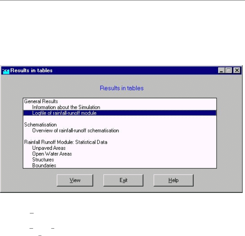
DRAFT
Tutorials
4.4.10 Task block: Results in Tables
The ’Results in tables’ task block provides detailed reports about the simulation and the input
and the output data.
Double-click ’Results in tables’ task block.
Select ’Information about the Simulation’.
Select ’View’ and view the results. Important information regarding the water balance of
your computation and the total balance error are given in this file (amongst others).
Select ’File’ - ’Exit’.
Click the Exit button.
4.4.11 Task block: Results in Charts
In the task block ’Results in Charts’ the user can easily depict result data in one graph.
Double-click on the ’Results in Charts’ task block.
Select ’System Balance per timestep’.
Click the View button.
Select the parameters ’Rainfall’ - ’Storage Unpaved’ - ’Storage OpenWater’ - ’Boundaries
out’ by using the Ctrl key.
Select the location ’Total RR system’.
Press the All button of Timesteps.
Press the Graph button.
Select ’File’ - ’Exit’ to close the ’Graph Server’ window.
Press the Exit button to close ODS_VIEW.
Press the Exit button to close the task block ’Results in Charts’.
Select ’Case’ - ’Save’ to save the case.
Deltares 121 of 900
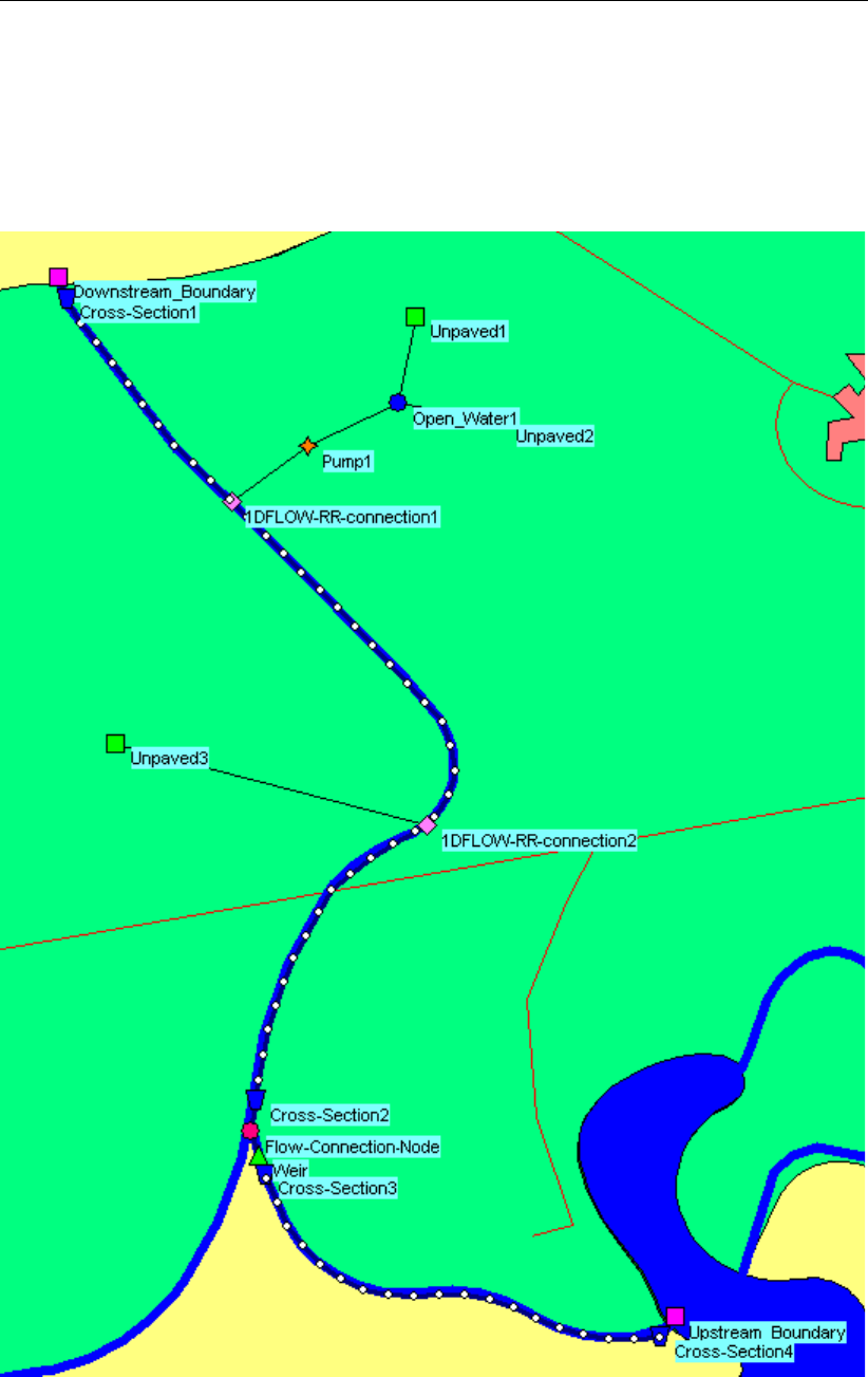
DRAFT
SOBEK, User Manual
4.4.12 Extending your model
In this exercise we are using a combined schematisation of the SOBEK-Rural RR module and
the SOBEK-Rural 1DFLOW module. This part is only possible if you have finished the tutorial
’Hydrodynamics in open water (SOBEK-Rural 1DFLOW module)’ and the end results of the
tutorial are available on the computer you are now using.
The RR model determines the runoff of various types of areas each with their characteristic
influence on the dynamics of the rainfall-runoff process. The different area types can be
described by various types of so-called runoff-nodes. The computed runoff is used as input
122 of 900 Deltares
DRAFT
Tutorials
for a one-dimensional hydrodynamic flow model. The 1DFLOW model computes the water
levels and flows in a network of open canals.
The exchange of data between the two models can be both sequentially and simultaneously.
In the sequential mode the RR model can be considered as a pre-processor for the 1DFLOW
model while in the simultaneous mode real on-line interaction can be taken into account.
Running 1DFLOW and RR simultaneously
Double-click the ’Settings’ task block.
Press the Edit... button of ’RR’.
Select the tab ’Time Settings’.
Enter the time step in computation: “10” minutes.
Select the tab ’Output options’.
Enter the output time step : “10” minutes in the respective edit box.
Click the OK button.
Turn on the checkbox ’1DFLOW (Rural)’.
In the ’Simulation mode:’ group box, select the mode ’Run RR (Rainfall-Runoff) and
1DFLOW (Rural) module simultaneously’.
Press the Edit... button of ’1DFLOW (Rural)’.
Select the tab ’Time Settings’.
Enter the time step in computation: “10” minutes.
Select the radio button ’simulation period will be derived from meteorological data’.
Select the tab ’Simulation settings’.
Select the radio button ’unsteady calculation’.
Select the tab ’Initial data’.
Select the radio button ’define local values in Edit network.
Select the tab ’Output options’.
Enter the output time step : “10” minutes in the respective edit box.
Press the OK button.
Press the OK button to exit the ’Settings’ task and save your settings.
Double-click the ’Schematisation’ task block.
Click the Edit model button.
Select the button, Edit Network, to start the edit network mode.
To give the whole RR schematisation unique identifiers we will add a preposition for all links.
Select the button, Select by rectangle.
Select the whole schematisation by clicking on the map and dragging while keeping the
button down. Release the left mouse button.
Select the button to select the function ’Change IDs’.
Enter the preposition “RR-”.
Uncheck the ’Nodes’ check box.
Check the ’Branches’ check box.
Click the OK button.
Note:
Please note that for larger models than this tutorial, it is recommended to also run the "Clean
Up Utility" on both the models before combining them. This is recommended in order to
prevent the IDs of removed or unused network objects for both models conflicting with each
other, causing further simulations to stop with an error message "Double ID in file ...". Adding
a prefix without cleaning up the models is not enough to guarantee unique IDs. This utility can
Deltares 123 of 900

DRAFT
SOBEK, User Manual
be found in the schematisation menu, button "Cleanup 1D/2D Model Data".
Now we will import the schematisation of the tutorial ’Hydrodynamics in open water’.
Select ’File’ - ’Import Case...’.
Select ’Case_one’ of the project ’T_CHANN’.
Click the OK button.
Click the Yes button (Do you want to combine the new Network with the existing network?).
Now we will connect the two schematisations.
Select the node, Flow - RR Connection on Channel.
Select the button to select the function ’Add node’.
Enter “1DFLOW-RR_connection1” in both input fields.
Click the OK button.
Locate the mouse at a position where you want to add the Flow - RR Connection on
Channel node and click the left-mouse button again to actually add the node.
Select the button to select the function ’Delete node’.
Select the ’Boundary1’ node.
Press the Yes button (Are you sure you want to delete RR - Boundary: RR-Boundary1?).
Select the button, RR-link.
Select the button to select the function ’Connect nodes’.
Click with the left mouse button on the RR - Pump Station and drag to the ’1DFLOW-
RR_connection1’ node while keeping the button down. Release the left mouse button.
Note:
Take care not to accidentally connect the pump station to a calculation point rather than the
1DFLOW - RR Connection node!
Select the node, RR - Unpaved.
Select the button to select the function ’Add node’.
Enter “Unpaved3” in both input fields.
Click the OK button.
Locate the mouse at a position where you want to add the RR - Unpaved node and click
the left-mouse button again to add the node.
Select the node, Flow - RR Connection on Channel.
Select the button to select the function ’Add node’.
Enter “1DFLOW-RR_connection2” in both input fields.
Click the OK button.
Locate the mouse at a position where you want to add the Flow - RR Connection on
Channel node and click the left-mouse button again to actually add the node.
Select the button, RR-link.
Select the button to select the function ’Connect nodes’.
Click with the left mouse button on the ’Unpaved3’ node and drag to the ’1DFLOW - RR
connection2’ node while keeping the button down. Release the left mouse button.
Select ’Tools’ - ’Validate network by model’ - ’Rainfall Runoff Model’.
Click the OK button (No errors detected).
124 of 900 Deltares

DRAFT
Tutorials
Select the button to exit the edit network mode.
Select the ’1DFLOW-RR_connection1’ node.
Click right mouse button.
Select ’Model data’ - ’Rainfall Runoff Model’.
Select the ’Boundary’ tab.
Select the radio button ’Variable boundary’.
Select the radio button ’Online from Flow Module’.
Click the OK button.
Do the same for the ’1DFLOW-RR_connection2’ node.
Select the button, Select by rectangle.
Select the whole schematisation by clicking on the map and dragging while keeping the
button down. Release the left mouse button.
Click right mouse button.
Select ’Model data’ - ’Rainfall Runoff Model’.
Select ’RR-UnPaved’.
Select ’Unpaved area’.
Select the row of ’Unpaved1’.
Select ’Edit’ - ’Copy’.
Select the row of ’Unpaved3’.
Select ’Edit’ - ’Paste’.
Select ’File’ - ’Save Data’.
Select ’File’ - ’Exit’.
Select button.
Select the menu item ’File’ - ’Exit’, to leave NETTER.
Click the OK button.
Select the menu item ’Case’ - ’Save As...’.
Enter the name “Extended”.
Click the OK button.
Double-click the task block ’Simulation’.
Note:
This step cannot be completed while in Free Trial mode. The number of nodes in the schema-
tisation now exceeds the amount of nodes allowed in a free trial computation.
Double-click ’Results in Maps’ task block.
Select the item ’Lateral Flows’ in the Active Legend.
Select the nodes ’1DFLOW-RR_connection1’ and ’1DFLOW-RR_connection2’ by using
the Ctrl key.
Click the button on the ’View Data’ window.
Now analyse your results!
4.4.13 Epilogue
In this tutorial some of the most important aspects of working with SOBEK have been dis-
cussed. Since you have gained experience now it’s not that difficult to find out other options
and possibilities of SOBEK which not have been discussed here. Good luck!
Deltares 125 of 900

DRAFT
SOBEK, User Manual
126 of 900 Deltares

DRAFT
5 Graphical User Interface
5.1 Case management
5.1.1 Task block: Import Network
5.1.1.1 Procedure for importing a Duflow model
Duflow models for the computation of the water levels and flows in water systems can be im-
ported into SOBEK-Rural. As SOBEK makes use of a Geographical Information environment,
its models need coordinates for the nodes. These coordinates are available in models that
are used in Duflow for Windows. For older models the Duflow file <conversion.sid>must be
filled with coordinates for all connection nodes according to the format of Duflow for Windows
(example):
NOD NOD00000 150912 421819 1
NOD NOD00001 153064 419729 2
NOD NOD00002 141070 417258 6
SCH SCH00000 149755 416906 3
ARE ARE00000 149755 416906 3 1
WEI WEI00000 144207 417130 4 5
If a model is stored in the binary format of Duflow, the model must be converted to the original
ASCII-format (.net). This can be done as follows:
Open the model (.dms).
Select Calculation from the menu.
Select Convert network.
Select Write Duflow files. Now the .net and .sid files are saved.
The following Duflow functionalities are imported into SOBEK:
Network topography (Duflow for Windows format)
Profiles (Tabulated profiles containing flow and storage widths)
Bed friction (Chézy and Mannings)
Boundary conditions. (Constant and time table of discharges and water levels)
Structures. (Broad crested weir and round, rectangular and elliptical culverts. Flow factor
µon a culvert is not used in SOBEK. Instead an inlet and outlet loss coefficient must be
selected)
Manually the following functionalities have to be added.
Initial conditions
Simulation time and time step
Pump stations
Inlet and outlet loss coefficient of culverts.
The import procedure is as follows:
Open a project.
Open a new case .
Click the block <Settings>in the Case Manager, Select the module ’Channel Flow’, di-
rectly followed by OK .
Deltares 127 of 900
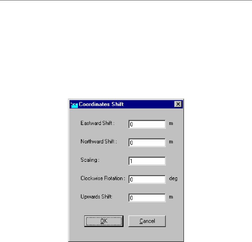
DRAFT
SOBEK, User Manual
Click the block <Meteorological Data>, directly followed by OK .
Click the block <Import Network>.
Select ’Import Duflow network’.
Press OK.
Open a Duflow scenario file at any location (other files of the scenario must be available
in the same location).
After the reading of the file, the user is asked for a shift, rotation or scaling of the coordinates
that are given in the Duflow geometry file <conversion.sid>:
Figure 5.1: Rotate or shift coordinates during Duflow import.
Modify the coordinates shift if required and press OK. After converting the data the network
editor is started and the topology of the network is displayed. If the network is not visible
select ’View’ from the menu followed by ’Show full network’.
The location of the nodes can be moved with ’Edit’, ’Vector Layer’. Also curves in branches
can be constructed by adding vector points (See SOBEK manual for details).
If the topology is satisfactory, the network can be saved with ’File’, ’Save’, ’Network’. In
older versions of the network editor the procedure is: ’File’, ’Save as’, ’Network’, change
the name from network.sob into network.ntw, ’Save’ and replace the existing network.ntw;
Select ’File’, ’Exit’.
The log-file is shown.
Close the log-file.
The import procedure is executed successfully and <Schematisation>can now be started
to finalize the model manually.
5.1.1.2 Procedure for importing a Mike11 model
Mike11 models for the computation of the water levels and flows in water systems can be
imported into SOBEK-Rural. To convert the cross sections, these cross sections should first
be exported in Mike11 as raw data. The file name must be identical to the binary cross section,
except the extension should be changed to .txt.
The following Mike11 functionalities are imported into SOBEK:
128 of 900 Deltares
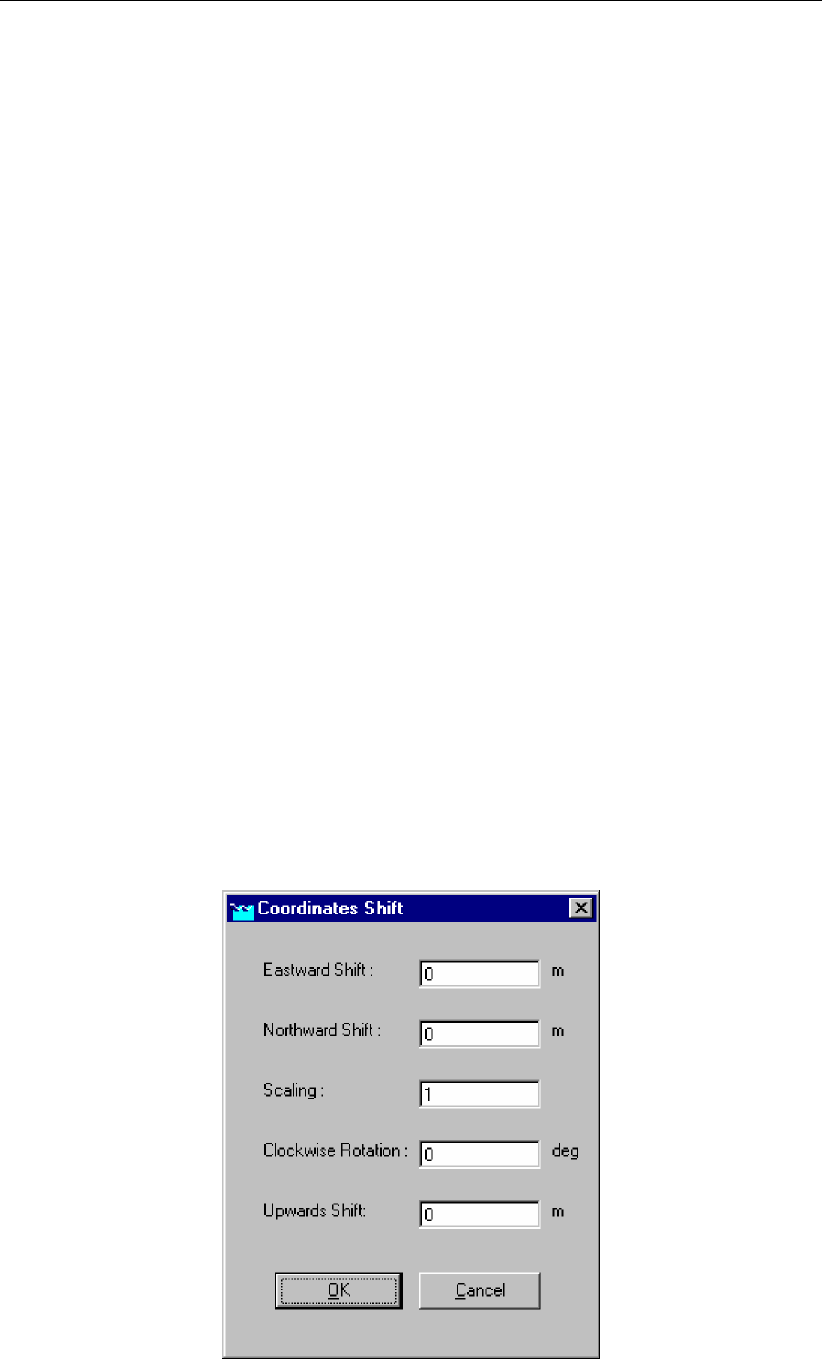
DRAFT
Graphical User Interface
Network topography
Profiles (first exported as raw data)
Locations of boundary conditions and type of boundary condition (water level or flow). The
values of the boundary conditions are stored in a binary format and can therefore not be
read by the conversion program.
Weirs with a fixed width
Weirs with a varying width over the height
Manually the following functionalities have to be added.
Initial conditions
Simulation time and time step
Calculation grid
Boundary condition values
Friction values
The import procedure is as follows:
Open a project.
Open a new case .
Click the block <Settings>in the Case Manager, Select the module ’Channel Flow’, di-
rectly followed by OK .
Click the block <Meteorological Data>, directly followed by OK .
Click the block <Import Network>.
Select ’Import Mike11 network’.
Press OK.
Open a Mike11 simulation file (*.sim) at any location (other files of the scenario must be
available in the same location).
A shift, rotation of the coordinates can be applied with the window that pops up (scaling is not
possible):
Figure 5.2: Rotate and shift coordinates during MIKE11 import.
Deltares 129 of 900
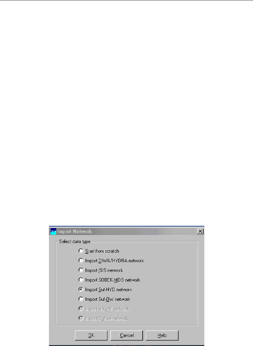
DRAFT
SOBEK, User Manual
Modify the coordinates shift if required and press OK.After converting the data the network
editor is started and the topology of the network is displayed. If the network is not visible
select ’View’ from the menu followed by ’Show full network’
The location of the nodes can be moved with ’Edit’, ’Vector Layer’. Also curves in branches
can be constructed by adding vector points (See SOBEK manual for details). If the topol-
ogy is satisfactory, the network can be saved with ’File’, ’Save’, ’Network’. In older versions
of the network editor the procedure is: ’File’, ’Save as’, ’Network’, change the name from
network.sob into network.ntw, ’Save’ and replace the existing network.ntw;
Select ’File’, ’Exit’.
The log-file is shown.
Close the log-file.
The import procedure is executed successfully and <Schematisation>can now be started to
finalize the model manually.
5.1.1.3 Import SVK19 files
SVK19 is the standard Scandinavian exchange format for sewer systems, comparable with the
SUF-HYD exchange format in the Netherlands. This functionality enables SOBEK to import
Mouse schematisations.
Importing Mouse files is available under the Import menu, Import sewerage networks (SUF-
HYD), and selecting the file type *.txt.
Figure 5.3: The Import Network window.
130 of 900 Deltares
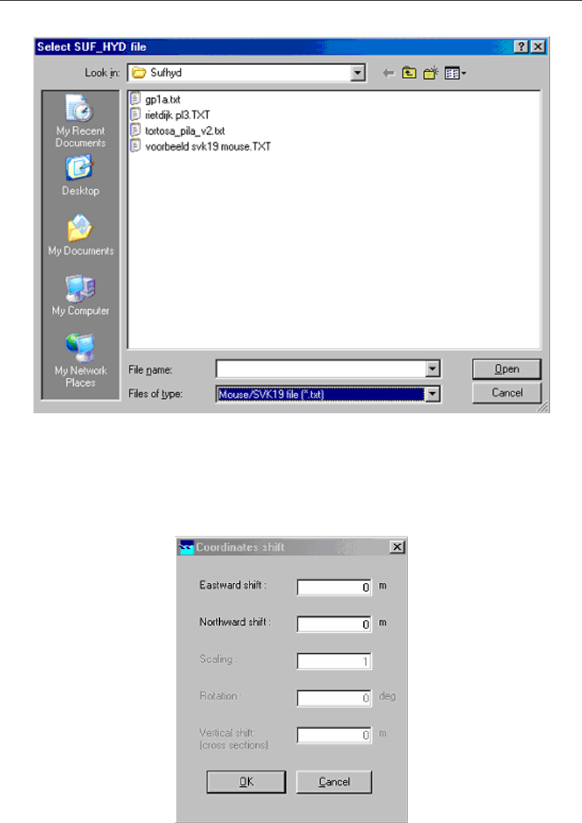
DRAFT
Graphical User Interface
Figure 5.4: Select SUF-HYD file.
It is possible to adjust the coordinates from the imported SVK19 file to your own coordinate
system by a north/east shift, to be specified in the next screen:
Figure 5.5: Shift coordinates during SVK19 import.
When the SVK19 file is imported, it is possible also to import a Mouse runoff file (HGF file).
Deltares 131 of 900

DRAFT
SOBEK, User Manual
Figure 5.6: Importing an optional Mouse runoff file.
Figure 5.7: Opening a Mouse runoff file.
The standard Mouse HGF-runoff catchment types have to be converted to the standard
NWRW types of area (combination of surface type and slope).
132 of 900 Deltares
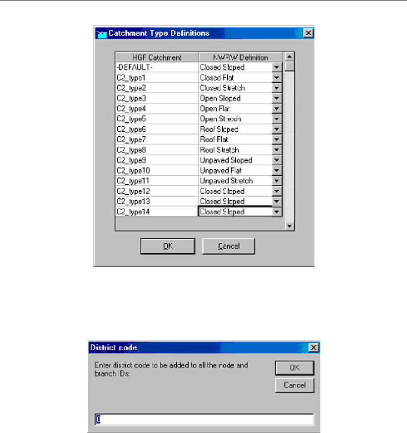
DRAFT
Graphical User Interface
Figure 5.8: Converting Mouse HGF-runoff catchment types.
Finally, the SVK19 id’s can be prefixed with a district id.
Figure 5.9: Prefixing SVK19 id’s with a district id.
5.1.2 Task block: Settings
5.1.2.1 Rural
Settings window for Channel Flow
In the Settings window, you can define general settings for the module of your choice. Here
the section on the Channel Flow module is discussed. The Settings window can be accessed
by double-clicking the "Settings" task block in the Case Management Tool window.
One can define:
The simulation period & the computational time step
Initial data, restart data
Output options: which output, and by which time interval
and more
Deltares 133 of 900
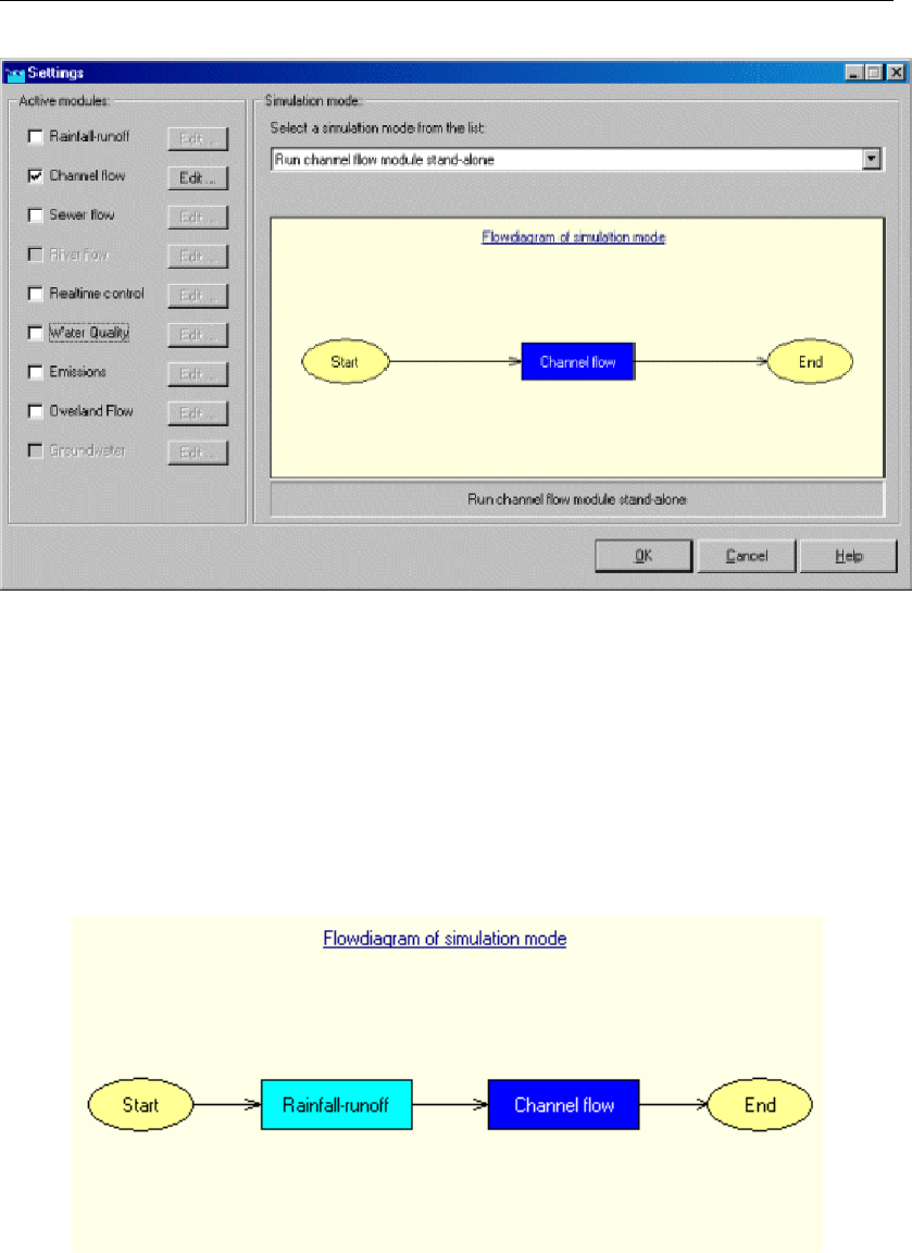
DRAFT
SOBEK, User Manual
Figure 5.10: The Settings window with only the Channel Flow module activated.
Clicking the Edit button, next to the Channel Flow check box, will open the "Settings for Chan-
nel Flow module" window. The options for that module are discussed in the next chapters.
Simulation options
If the Channel Flow module is combined with other modules, the modeller has various sim-
ulation options. For example, one can run the Rainfall-Runoff module and the Channel Flow
module simultaneously or sequentially:
Figure 5.11: Flowdiagram of running the Rainfall-Runoff module and Channel Flow mod-
ule sequentially.
134 of 900 Deltares

DRAFT
Graphical User Interface
Figure 5.12: Flowdiagram of running the Rainfall-Runoff module and Channel Flow mod-
ule simultaneously.
These options can be selected in the "Simulation mode" section:
Figure 5.13: Selecting a simulation mode.
Tab - Time settings
One of the options when opening "Settings" for Channel Flow is "Time settings". These can
be found on the "Time settings" tab. The options are explained below.
Deltares 135 of 900
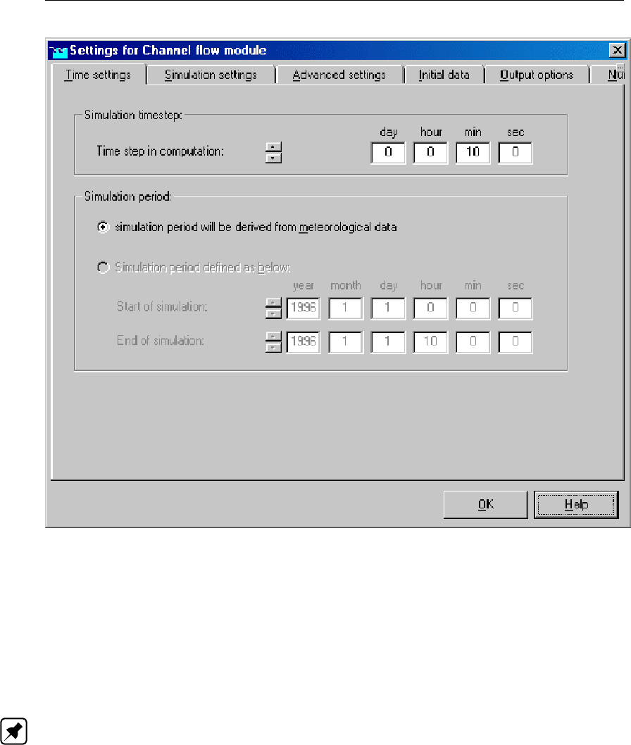
DRAFT
SOBEK, User Manual
Figure 5.14: The Time settings tab of the Channel flow module.
Simulation time step
Here, you can define the computational time step that SOBEK uses in its hydrodynamic com-
putations. Note that the time scale for hydrodynamic processes lies in the order of minutes
to even seconds. For most computations, a time step of 10m should be sufficient, but for
river systems with a very quick respond-time (such as mountain streams), a smaller time step
might be more appropriate.
Note: SOBEK will automatically reduce its computational time step if necessary. Information
about whether this has happened during your simulation can be found in the results "simula-
tion info at branch segments".
Simulation period
The simulation period can be defined in two ways: it can be derived from the precipitation
event that you have defined (Meteorological data task block), or it can be defined manually.
If the Rainfall-Runoff module is active too, only the first option is available. In the Edit section
of the Rainfall-Runoff module, you can then define a simulation period manually or refer to a
precipitation event.
Tab - Simulation settings
One of the options when opening "Settings" for Channel Flow is "Simulation settings". These
can be found on the "simulation settings" tab. The options are explained below.
136 of 900 Deltares
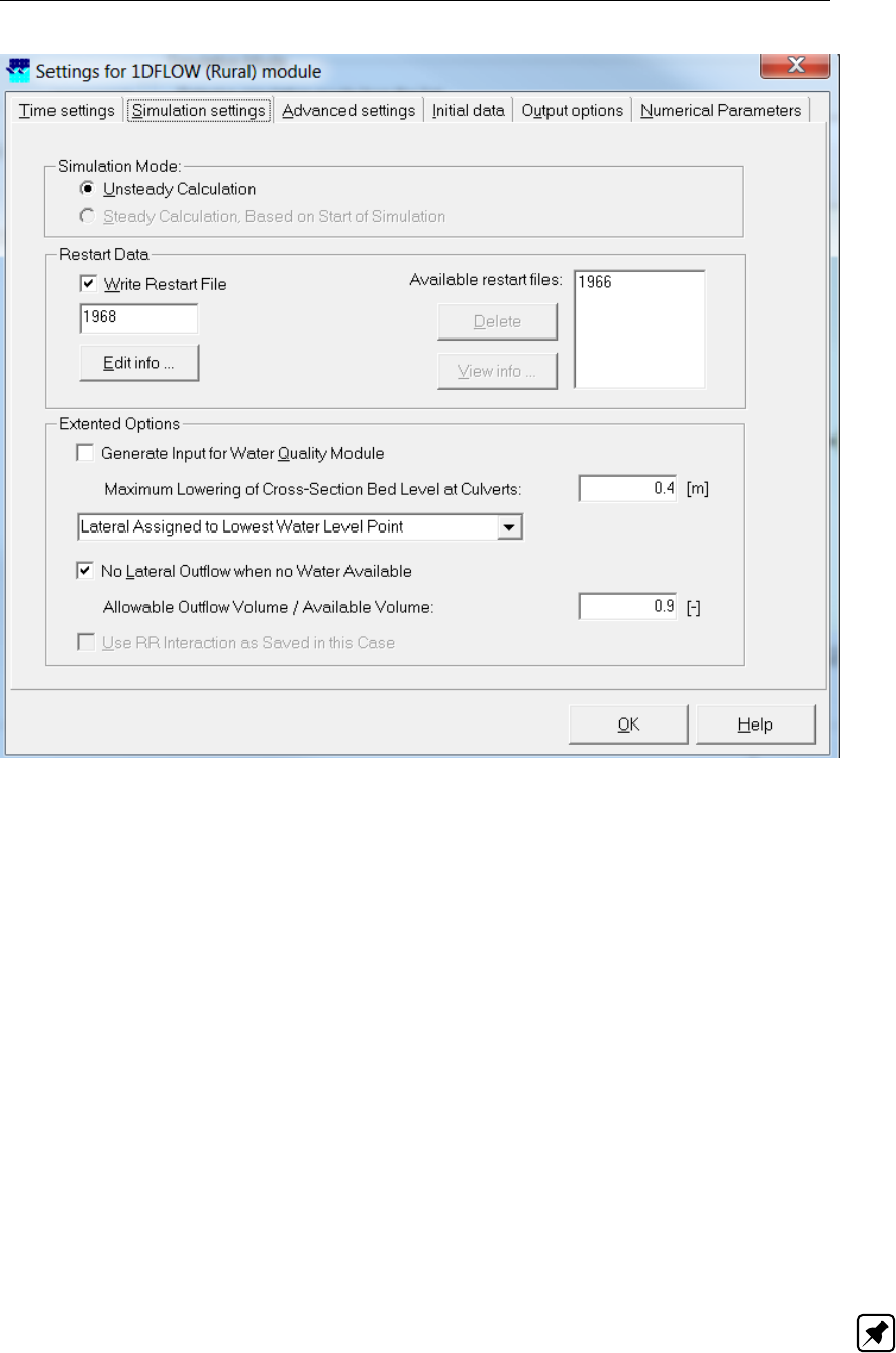
DRAFT
Graphical User Interface
Figure 5.15: The Simulation settings tab of the Channel flow module.
Simulation mode
Unsteady calculation means that the computation will be simulating a certain time span,
where it will not branch a steady state, but where all conditions within the model may
change during time (rainfall, boundary conditions etc.)
Steady calculation means that the simulation will only calculate one situation: the equi-
librium state. All boundary conditions will be fixed values (non-variable in time) and the
model will calculate the situation where an equilibrium is branched.
Restart data
A restart file contains all information of the state of a simulation during its last time step. This
file can optionally be used to define the initial values for a new simulation.
The option "write restart file" allows you to create a restart file from the last time step of the
simulation that you are about to run. You can give this file a name. If you want to use it later
on for the initialisation of another simulation, select it on the "Initial data tab".
Note: Restart files are no longer usable if a network has changed since the restart file was
written. Additionally, it is recommended to create a new restart file when updating a SOBEK
model to a new SOBEK version.
Extended options
Deltares 137 of 900

DRAFT
SOBEK, User Manual
Generate output for water quality module. This option is activated only when the Water
Quality module is active. However, if you run the Channel Flow stand alone, and you con-
sider to run the WQ module in the future, it is wise to activate this option.If not, you would
have to re-calculate the flow computations first to make future water quality computations
with this case.
Maximum Lowering of Cross-section Bed Level at Culvert. If the bed level of a (inter-
polated) cross-section in front of a culvert is lying more than the value defined for "Max-
imum Lowering of Cross-section Bed Level at Culvert" above the ground-layer level (=
invert level + ground-layer thickness), the bed level of the cross-section is lowered to the
ground-layer level. For all (interpolated) cross-sections in front of a culvert, having bed lev-
els lying more than the value defined for "Maximum Lowering of Cross-section Bed Level
at Culvert" above the ground-layer level, no changes are made only a warning is given in
the SOBEK.Log message file. It is advised to avoid that the bed level of a cross-section
in front of a Culvert is above the ground-layer level, since such situation can result in very
small computational time-steps (e.g. long required wall-clock times) or even in a termina-
tion of the simulation (for more information, see section Culvert, Good modelling practice
aspects ). The same as discussed for a Culvert also applies for a Siphon and an Inverted
Siphon.
List box: Lateral Assigned to Lowest (or Nearest) Water Level Point. Using this
list box, the user can specify if lateral flows are to be assigned to the lowest water level
point or that lateral flows are to be assigned to the nearest water level point. For more
information on the difference between assigning to the lowest or to the nearest water level
point, reference is made to section 6.1.11.2
No Lateral Outflow when no Water Available By checking the check-box in front of "No
Lateral Outflow when no Water Available", SOBEK reduces the user-defined lateral inflow
in case insufficient water is available for meeting the user-defined lateral outflow. The
advantage of this option is that SOBEK does not apply (extremely) small time-steps, that
require a lot of computational effort (wall-clock time). Using this option, even a termination
of a simulation might be avoided. The ratio "Allowable Outflow Volume/Available Volume"
can be specified. SOBEK provides as output both the user-defined lateral outflow (Defined
Lateral) and the actual applied lateral outflow (Lateral Actual).
Use RR interaction as saved in this case If you don’t want to have to re-calculate the
Rainfall Runoff computations again for every case where you only change things in the
flow module, it is wise to activate this option. Note: in order to click this option, the Rainfall
Runoff module should be active.
Tab - Advanced settings
One of the options when opening "Settings" for Channel Flow is "Advanced settings". These
can be found on the "Advanced settings" tab. The options are explained below.
138 of 900 Deltares

DRAFT
Graphical User Interface
Figure 5.16: The Advanced settings tab of the Channel flow module.
Design Factor for Area Based Lateral Flow
The "Design Factor for Area Based Lateral Flows" is a multiplication factor (expressed as
percentage) that is applied to only those lateral flows, that are calculated using the so-called
"Area Based" method (see Figure 5.100 and Equation (6.14)).
Tab - Initial data
One of the options when opening "Settings" for Channel Flow is "Initial data". These can be
found on the "Initial data" tab. The options are explained below.
Deltares 139 of 900
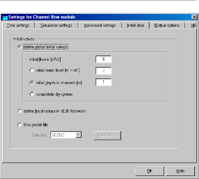
DRAFT
SOBEK, User Manual
Figure 5.17: The Initial data tab of the Channel flow module.
Define global initial values If this option is chosen, the initialisation values that you enter
in this section will be applied to the entire model.
Define local values in <Edit Network>. This option allows you to define initial water
levels and/or depths individually for every branch in the model. For those branches where
you do not enter the initial state, the values from the "Define global initial values" section
apply.
Use restart file Get the initial situation for the model from the results of a previous simu-
lation. In order to do this, there should be a restart file available.You can create a restart
file by defining one on the "Simulation settings" tab and running the simulation. After this
simulation has run, the results of the last time step will be written to the restart file.
Tab - Output options
One of the options when opening "Settings" for Channel Flow is "Output options". These can
be found on the "Output options" tab. The options are explained below.
Time step Output For most simulations, it is not useful to have simulation results for every
computational time step. That would require enormous disk space and would not give
useful extra information. Therefore, an output time step can be defined.You can choose
to have current, average or maximum values written to the result file. For example: if
the computational time step is 10 min, and the output time step is 1 hour, there will be 6
computational results available for 1 result to be written. Thus, you can choose to have
the actual computed value written for every output time step (current), or you can choose
to take the maximum or the average of those 6 results.
Output parameters Here you can define which results should be written to file.
140 of 900 Deltares
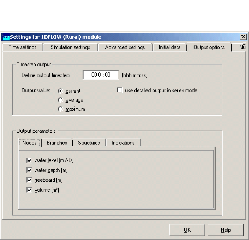
DRAFT
Graphical User Interface
The different Output parameters for Nodes:
Figure 5.18: The Nodes tab in the Channel flow Output options.
It is possible to choose between:
water level [mAD]
water depth [m]
freeboard [m]
volume [m3]
The different Output parameters for Branches:
Deltares 141 of 900
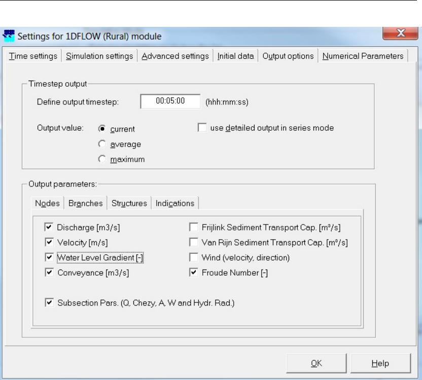
DRAFT
SOBEK, User Manual
Figure 5.19: The Branches tab in the Channel flow Output options.
It is possible to choose between:
Discharge [m3/s]
Velocity [m/s]
Water Level Gradient
Conveyance
(Subsection) Pars. (Q, Chézy, A, W, and Hydr. Rad.)
Frijlink Sediment Transport Cap. [m3/s]
Van Rijn Sediment Transport Cap. [m3/s]
Wind (velocity, direction)
Froude Number [-]
The different Output parameters for Structures:
142 of 900 Deltares
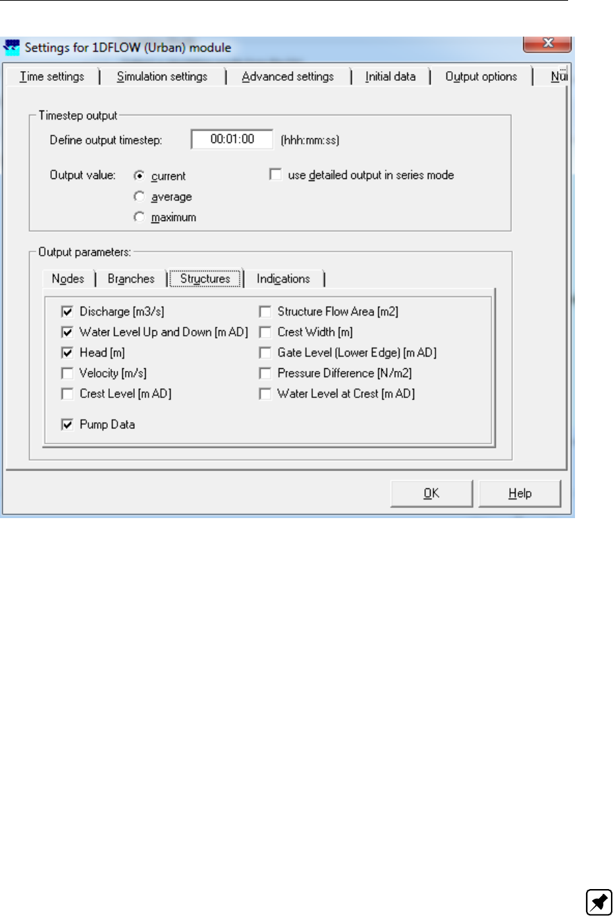
DRAFT
Graphical User Interface
Figure 5.20: The Structures tab in the Channel flow/Urban flow Output options.
It is possible to choose between:
Discharge [m3/s]
waterlevel up and down [mAD]
head [m]
Velocity [m/s]
crest level [mAD]
pump data
structure flow area [m2]
crest width [m]
gate level (lower edge) [mAD]
pressure difference [N/m2]
water level at crest [mAD]
This item is only available for General Structures.
Tab - Numerical Parameters
One of the tabs in settings of Channel Flow is the "Numerical Parameters" tab. The numerical
parameters are explained below. Note: Modifying these advanced numerical parameters
is not supported. Only modify these settings when necessary for specific purposes, and
carefully verify results after making changes.
Deltares 143 of 900

DRAFT
SOBEK, User Manual
Figure 5.21: The Numerical Parameters tab of the Channel flow module.
Default settings
Typical Rural schematisation A default selection of numerical parameters that are most
suitable for hydrodynamics in open water systems, mainly channels and small rivers.
Typical Urban schematisation A default selection of numerical parameters that are most
suitable for hydrodynamics in urban water systems, mainly sewer pipes.
User defined
An option to choose your own numerical settings:
Accuracy factor
minimum time step
epsilon for volume
epsilon for water depth
threshold water depth for flooding of channels
threshold water depth for flooding of land
factor for structure dynamics (Channel Flow & Sewer Flow only)
To the structure equations an inertia term is added. This inertia term acts as a kind of
numerical demping. This is done to avoid numerical oscillations/instabilities in case of
unsteady flow conditions. The numerical parameter "factor for structure dynamics" is a
factor/scalar applied to this inertia term. Default value of 1.0 is suggested for the "fac-
tor for structure dynamics" Note: for steady flow conditions the inertia term equals zero.
144 of 900 Deltares

DRAFT
Graphical User Interface
Hence, the "factor for structure dynamics" is not of influence for the computed steady-state
discharge through a structure.
structure inertia dampening factor (River Flow only)
In settings a default value for the so called structure inertia damping factor can be de-
fined, that is applied for the River weir, the Advanced weir, the General structure and the
Database structure both as single structure or member of a compound structure. In the
schematization Task block, this default value can be overruled for each individual afore
mentioned structure type. In the linearization of the concerning structure equation a term
α∂U/∂t is added, where
αstructure inertia damping factor [−];
Uflow velocity [m/s]; and
tcomputational time [s].
The structure inertia damping factor can be used for avoiding instabilities during compu-
tation.
relaxation factor
theta
minimum length of branch segment
volume based on water level or discharges (0=false; 1=true)
In SOBEK there are two options for computing the volume of a ζ-calculation point (or branch
segment) at a specific point-in-time, viz:
1 Volumes based on water level or discharges (0=false; 1=true)
If the option "Volumes based on water levels" is selected, this means that the volume at
each ζ-calculation point (or each segment) follows from the computed water level and its
corresponding cross-sectional profile.
If the option "Volumes based on discharges" is selected, this means that the volume at each
calculation point (or branch segment) is the summation of its volume in the previous time-step
and the resulting net inflow during the computational time-step.
In Water Quality computations especially use is made of volumes and discharges. By choos-
ing the option "Volumes computed based on discharges" a more coherent set of volumes and
discharges is obtained, than in case the option "Volumes computed based on water levels" is
selected.
Note: The selected way in which volume is computed also yields for 2D hydrodynamic com-
putations.
maximum flow (1D) and velocity (2D) Courant number
maximum degree of nodal points to be eliminated by Gaussian elimination
maximum number of iterations
rho (density of fresh water)
gravity acceleration
minimum surface in node
minimum surface on street
extra resistance for general structure
In settings a default value can be defined for the so called extra resistance coefficient of
the General structure type, both as a single structure and as a member of a compound
structure. In the schematization Task block, this default value can be overruled for each
individual General structure type. The so called extra resistance refers to a bed shear
stress force, that is accounted for in the impuls balance, that is solved in case of drowned
Deltares 145 of 900

DRAFT
SOBEK, User Manual
gate flow or drowned weir flow. The bed shear stress force reads
LgW2ρ2u2
2/C2or λρ2W2u2
2(5.1)
where:
λ= (Lg/C2)extra resistance coefficient;
Llength of hydraulic jump behind the structure [m];
gacceleration due to gravity [m2/s];
CChézy coefficient [m1/2/s];
ρ2 density of water in hydraulic jump [kg/m3];
Udownstream flow velocity [m/s]; and
W2downstream structure width [m].
factor on 1D acceleration term dU/dt (can vary between 0 and 1)
0 means that DU/Dt or ∂U/∂t +U∂U/∂x terms in all 1D hydrodynamic momentum
equations are neglected, hence waves are computed/considered as diffusive waves.
1 means no reduction on DU/Dt or ∂U/∂t +U∂U/∂x terms in all 1D hydrodynamic
momentum equations are neglected, hence waves are computed/considered as dynamic
waves.
In case user defines a factor on 1D acceleration term ∂U/∂t < 0, SOBEK applies factor=
0. In case user defines a factor >1, SOBEK applies factor= 1.
use time step reduction on structure (0= false; 1= true)
In case the user defines a value for "use time step reduction on structure" equal to 1,
at the point-in-time of the wetting of the crest of a structure (i.e. for weirs and orifices
only) a time step reduction will be applied during a time-span equal to two times the user
defined time step. This functionality was implemented for avoiding oscillation in specific
Urban schematisations which having sharp inflow hydrographs, it can be applied in Rural
schematisations as well. Unneccessary use of this option might result in a longer compu-
tational time needed.
5.1.2.2 River/Urban/Rural
General
The settings task block gives the user the following two options (see Figure 5.22):
The combination of SOBEK modules used for the simulation can be selected here, and
For every module selected general settings can be defined.
146 of 900 Deltares
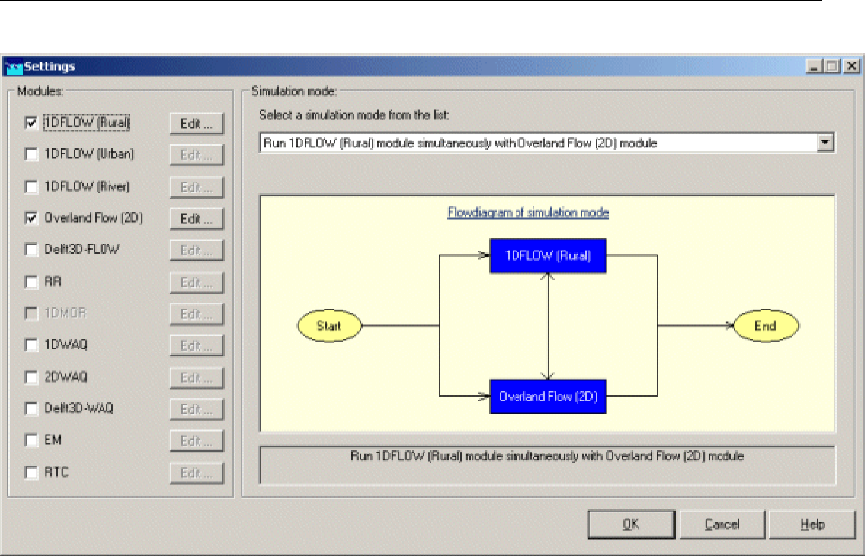
DRAFT
Graphical User Interface
Figure 5.22: The Settings task block.
Simulation settings tab
Deltares 147 of 900
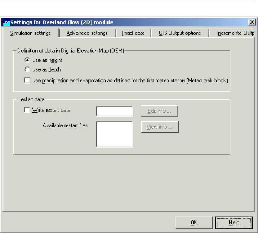
DRAFT
SOBEK, User Manual
Figure 5.23: The Simulation Settings window for the Overland Flow settings task block.
Definition of data in Digital Elevation Map (DEM)
Here, the user can specify how the data within the DEM to be used is oriented: as heights or
as depths.
heights: a higher z-value means a higher level
depths: a higher z-value means a lower level
With the checkbox "Use precipitation and evaporation as defined for the first meteo station"
you can define whether the rain fall and evaporation is to be included on your 2D grid. The
precipitation and evaporation from the first rainfall station defined in the "Meteorological data"
task block is then applied. If the checkbox is switched off, no rainfall or evaporation will con-
sidered on the 2D grid.
Note:
1) Rainfall and evaporation is applied to all active 2D grid cells (i.e. 2D grid cells not having a
missing value). At present only spatially uniform distributed rainfall and evaporation can be de-
fined, meaning that each active 2D grid obtains the same amount of rainfall and evaporation.
The spatially uniform distributed rainfall and evaporation can be a function of time.
2) Rainfall and evaporation can not be directly entered on 1D open channel network. Us-
ing the Rainfall-Runoff module, the outflow of catchment areas as result of nett precipitation
can be provided as inflow on a 1D open channel network. The same applies for a sewer
148 of 900 Deltares
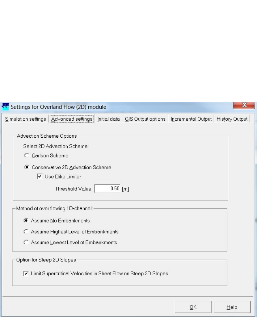
DRAFT
Graphical User Interface
network/system.
Restart data
Restart data allows users to create realistic initial conditions for their calculation. When the
"write restart file" option is checked and the model is run, the results for the last time step
of the calculation are written to a file with the name you entered. For other calculations the
available restart file may then be referred to define the initial conditions.
Advanced Settings tab
Figure 5.24: The Advanced Settings window for the Overland Flow settings task block.
The Conservative 2D Advection scheme allows for a more accurate computation of the prop-
agation speed of flood waves, over initially dry bed or wet bed.
Special care has been taken to ensure that weir flow is computed accurately, even when weirs
are represented by only 1 grid cell that is raised above the field level. Weir discharges are
reproduced accurately both for the sub critical and the supercritical flow regime. These fea-
tures are demonstrated and compared to analytical solutions by test computations in several
geometries.
The Conservative 2D Advection scheme is based upon ‘A staggered conservative scheme for
every Froude number in rapidly varied shallow water flows’ (Stelling and Duinmeijer,2003).
Deltares 149 of 900
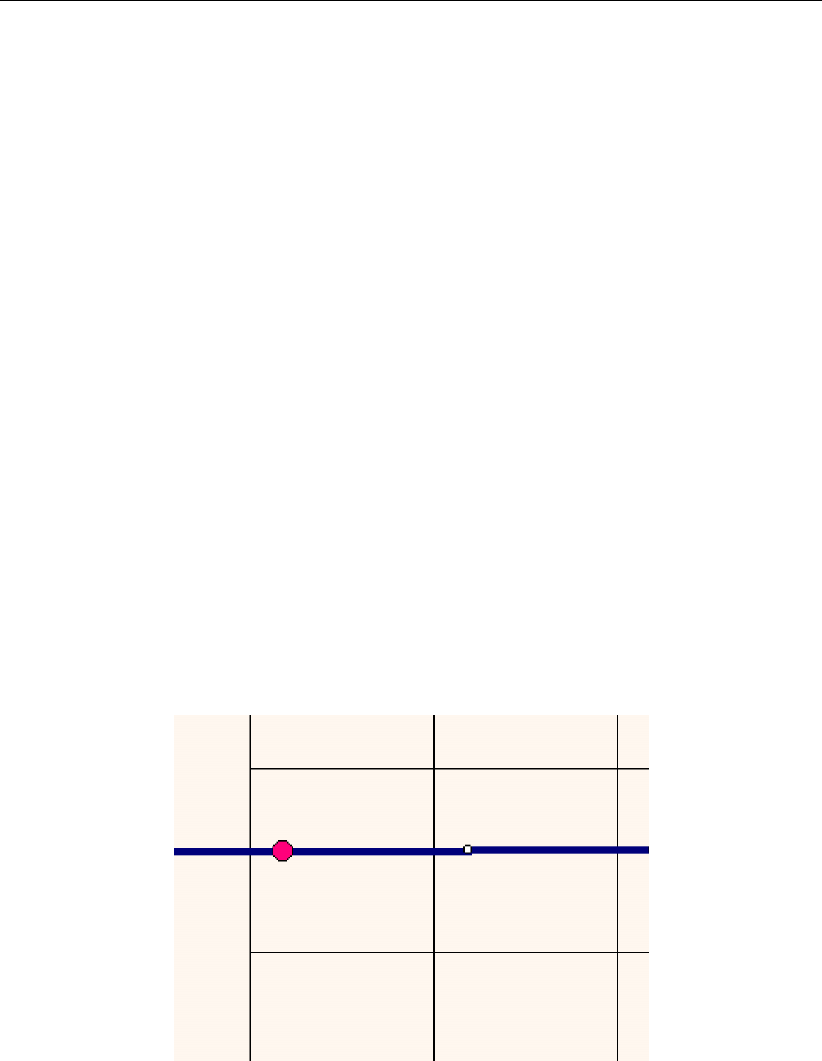
DRAFT
SOBEK, User Manual
In order to invoke the Conservative 2D Advection scheme, one can select in ‘Settings, Over-
land Flow (2D), Advanced settings’, the Conservative 2D Advection scheme. In order to invoke
the special treatment for weir flow, select ‘Use Dike Limiter’. Grid cells will be flagged as ‘dikes’
when the height difference with surrounding grid cells exceeds a user specifiable ‘Dike limiter’
treshold value.
Note that the less accurate Carlson scheme is still available for use. The use of the Conser-
vative 2D Advection scheme is recommended.
Limiting super critical flow velocities on a steep 2D flow: If there are steep slopes within
the topography of a 2D grid, it is possible that sheet-flow with super critical flow velocities
occurs on these steep 2D slopes. In other words that a thin layer of water runs down these
steep slopes with very high flow velocities. These very high flow velocities may result in severe
reductions of the user-defined time-step and hence increase in the required computational
effort. These super critical flow velocities can be limited by checking the option "Limiting
super critical velocities in sheet flow on steep 2D slopes" available on the "Advanced settings
Tab" of the "Overland Flow (2D) module" in "Settings" (see Figure 5.24).
Method of overflowing 1D channel
Here the user can specify a number of general options for the 2D simulation, starting with the
method of overflowing 1D channel. This is a very important option which will greatly influence
the results of the simulation, so it is very important that you set this option wisely.
It concerns the connection of the 1D cross-section with the underlying 2D grid cell, and is
explained in the following example:
Figure 5.25: Example of a 1D2D schematisation.
A 1D channel delimited by dikes passes through a low lying area, say a polder. When the
water level inside the 1D channel overtops the dikes, water will start to flow into the underlying
2D grid elements. The dikes of the 1D channel can be modelled in two different ways, as is
shown in the following two cross-sections of the schematisation depicted in Figure 5.25.
Options 1: Assume No Embankments.
150 of 900 Deltares
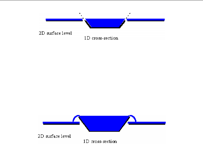
DRAFT
Graphical User Interface
Figure 5.26: Assume no dikes.
Notice: At this moment, the option of method of overflowing 1D-channel refers to all 1D cross
sections.
In this case, water enters the 2D grid as soon as the channel water level branches the terrain
level in the 2D grid, so the part of the dike in the 1D cross-section above this level is neglected.
Option 2: Assume Highest/Lowest Level of Embankments.
Figure 5.27: Assume Highest/Lowest Level of Embankments.
In this case, water enters the 2D grid when the highest level of the 1D profile is overtopped,
and not earlier. So, the dikes form a barrier between the channel and the 2D area. Moreover,
they form a barrier for water flowing towards this 1D cross section over the 2D grid.
The terms highest and highest refers to both sides of the cross section. If Assume Highest
Level of Embankments is chosen, and the left bank’s surface level is higher than the right
bank’s, then the surface level from the left bank is used as the level for overtopping.
If Assume Lowest Level of Embankments is chosen, the surface level from the right bank is
used.
Note: if overtopping takes place, water will always overtop on both sides of the channel, no
matter if one side has a higher surface level. If you want to prevent this from happening, create
an additional elevation in the grid on one side of the channel.
Initial Data Tab
Deltares 151 of 900
DRAFT
SOBEK, User Manual
Figure 5.28: The initial data tab from the Overland Flow SETTINGS task block.
Note: The first option, define global values, cannot be selected at the present.
At this moment, there are either one or two options available here. If you haven’t run a
simulation before with a restart file as output, you won’t be able to select the second option
use restart file, so you will need to use the default option, define local initial values per 2D-grid.
There are a number of things you need to remember when using the restart option:
make sure you select the use restart file option in both the overland flow module AND
the channel flow module !!
The restart file can only be used as input for exactly the same schematisation that was
used in the simulation that generated the restart file.
The restart file itself is saved under the project directory; this means that you will only be
able to use this restart file as input for a (any) case within the same project, but not for a
case in another project.
GIS output options tab
152 of 900 Deltares
DRAFT
Graphical User Interface
.
Figure 5.29: GIS Output tab in the Overland Flow settings task block.
The output for GIS systems, like ARCView, is one of the three types of 2D-specific output
available. In this screen, you can select if you want this output to be generated or not, and
for which time steps. If any (combination) of the available variables is selected here, SOBEK
will automatically create ’.ASC’ output files which can be imported into a GIS based program.
There are some additional rules to remember, which will be explained further on.
The GIS output data is written to a number of different files. The first type consists of output
files in .asc format (see also section 5.1.6.3). SOBEK creates these output files only when
the switch ’create ASCII-output for water depth, water level and velocity’ is switched on! One
of these is generated for every selected output time step and for every selected variable. In
general, it is a good idea to wait with generating this output (if you need it at all, of course) until
you are pretty sure that the simulation is going to give you the results that you need. Suppose
your simulation lasts 24 hours, and you want GIS output for every time step (of, for example,
one minute) and for all five variables, you would get 5x24x60 equals 7 200 output files!
Warning: Right now, SOBEK can handle only a certain maximum number of files in the case
directory. If you decide to switch on the ’ASCII-Output Option’, you might actually branch
this maximum number of files (because of all the .asc files generated), which means that you
might not be able to save your case properly! In that case you will get the message with saving
your case: "too many files in case directory; Check the configuration of the application;
erase unregistered files". In this case you should reconsider you output choices to decrease
the number of output files.
Deltares 153 of 900

DRAFT
SOBEK, User Manual
The second type of output files is the binary ’.map’ file. For every variable chosen, a file is
produced. It contains the values of that variable for every time step and every grid element
of one particular grid. In results in maps, the user can select these .map files and produce
.asc files out of them. So actually, the .map file contains the same information as the .asc files
described earlier, but in a compressed format. Please note that whether MAP files are written
or not, only depends on the Output Parameters chosen in the GIS Output Options tab, and
not on the ASCII-Output option switch!
The last type of GIS output files are ’special’ .asc files. These files contain the following
variables:
maximum water depth (d_max)
time of maximum water depth (t_dmax)
maximum water level (h_max)
time of maximum water level (t_hmax)
maximum velocity (v_max)
time of maximum velocity (t_vmax)
time of wetting (t_wet)
time of wetting per class (steady state’) (t_wet/class)
time of drying (t_dry)
time of drying per class (steady state’) (t_dry/class)
rate of change of water depth (dd/dt)
These files are only produced when the corresponding ’basic’ variable is selected in the GIS
tab, see figure. For example, the maximum depth is generated only when the option ’water
depth’ is checked. The same goes for other variables like the maximum velocities (linked to
’velocity’) or maximum levels (linked to ’water level’). The files giving a time (period) and the
rate of change of water depth are all linked to the ’water depth’ output option.
Incremental Output Tab
154 of 900 Deltares
DRAFT
Graphical User Interface
Figure 5.30: The incremental output tab for the Overland Flow settings task block.
The second type of 2D output is the so-called ’incremental output’. This is output that is
generated specifically for result analysis in SOBEK (’results in maps’) itself, so you should
normally have at least some of these options turned on. Otherwise, you will not be able to
visualize the results in SOBEK.
The incremental file system was developed to reduce the enormous amount of data generated
by the 2D simulations. It works by defining a number of classes for every output variable which
are then used in the output files instead of the actual data value itself. So, for example, if a
water depth in a certain 2d grid cell equals 0.43 m, it would fall in class ’0.4 - 0.5’ (if you
have specified such a class). This is also the result you would get when examining the results
for that particular grid cell in ’results in maps’. So, this output is especially useful for getting
a quick idea as to how the water flows through the 2d grid system; if you are interested in
the exact values for the variables for a certain number of grid cells, there is another option
available to the user, which is the history output, explained in the next paragraph.
The incremental output always has the same time step as the actual calculation time step
chosen in the channel flow module.
Concerning the output parameters, it is important to know that the velocity (u component) and
the velocity (v component) are necessary if you are interested in seeing the velocity vectors
later on, when viewing the results in results in maps.
The number of classes can be selected manually, and influences the detail you will get when
Deltares 155 of 900

DRAFT
SOBEK, User Manual
viewing the results; ten classes of 10 cm difference show much more information than 2
classes of 50 cm difference, but also require more disk space and computation time. The
number of classes will be the same for all variables, so it’s not possible to have 5 classes for
the water depth and 15 for the velocity. But, if you have defined 15 classes (for all variables),
and you need only 5 for one particular variable, you can define the unnecessary classes as
no-data values (-999).
A few rules to remember:
The water depth can be only positive, so it’s no use to define negative classes here
The ’u’ and ’v’ velocity components can be both positive and negative. It is important to
remember to use exactly the same classification for both variables.
This classification needs to be classified symmetrical around zero for correct determina-
tion of the vectors!
History Output Tab
If you are interested in the exact values of all variables on specific locations in the 2D grid, it
is possible to use a special kind of node called a History station. For more information, please
see the 2D-History node chapter.
2D Bathymetry input as heights (or levels)
Functionality:
2D bathymetry input as Heights (or levels) refers to the fact that the user can define bed
elevations of a 2D grid according to a vertical axis, having its positive axis pointing in upwards
direction.
Up to now 2D bathymetry input could only be defined as Depths, meaning that bed elevations
are defined according to a vertical axis, having its positive direction pointing in downwards
direction. All 2D bathymetry input is either defined as Heights or as Depths. Hence it is not
possible to define a particular 2D bathymetry input grid as Height while another is defined as
Depths.
How to define Bathymetry input as Heights (or levels):
Double click the ‘Settings’ task block.
In the ‘Settings’ window, take care that the Overland Flow (2D) check-box is checked and
click on the Edit button next to it
In the ‘Settings for Overland Flow (2D) module’ window under Definition of data in Digital
Elevation Map (DEM), define whether you want bathymetry input defined as Heights (or
levels) or bathymetry input defined as Depths.
Close the ‘Settings for Overland Flow (2D) module’ window by clicking the OK button,
Close the ‘Settings’ task block by clicking in the ‘Settings’ window on the OK button,
Now start to import your 2D bathymetry input grids under the ‘Schematisation’ task block.
156 of 900 Deltares

DRAFT
Graphical User Interface
5.1.2.3 Water Quality
Editing time settings
The simulation period for the Water Quality module can be derived from a selected meteoro-
logical event (if the Rainfall-Runoff module is active) or specified by hand. In the latter case, it
is necessary that the simulation period for the Water Quality module is the same or lies within
the simulation period for the Water Flow module.
The simulation time step may be equal to, smaller than and larger than the time step for the
other modules. However, we advise you to select a time step either equal to the time step of
the Water Flow module, or equal to the time step of the Water Flow module multiplied by a
whole factor (2, 3, 4, etc.) or equal to the time step of the Water Flow module divided by a
whole factor (2, 3, 4, etc.).
Furthermore, the selected numerical method may impose a stability limit on the time step (see
below). Also, the modelling of water quality processes may impose a stability limit on the time
step (see par. 4.2).
Make sure that the "Channel Flow" and "Water Quality" modules are activated in the "Set-
tings" Window.
Click the Edit button of the "Water Quality" module.
Adjust the simulation period and/or the time step in the corresponding edit boxes.
Editing simulation settings
The simulation options include the choice between fraction computations and regular water
quality computations, as well as the selection of initial conditions. Optionally a user-defined
file with boundary conditions can be connected.
Click the "Simulation options" tab form.
Select "Calculate fraction" or "Calculate water quality".
Make sure that the tick box "processes active" is on, if you have selected "Calculate wa-
ter quality" (unless you want to run a water quality simulation without substance-specific
processes).
If you intend to run the current case in batch mode, decide whether or not you want the
previous flow results used in batch mode. If you do, check the associated tick box. (See
also: the ’Simulation’ task).
Select the appropriate option for the initial conditions:
select a file with initial conditions you generated yourself (.RSF file);
select a file with initial conditions generated by earlier SOBEK runs;
start with 100% initial water (fraction computation) or model-wide initial conditions.
To edit the model-wide initial conditions click the Edit button.
If you specify a Water Quality computation and you click the Edit button belonging to the "start
simulation with global initial values" option, the "Initial Values" window appears.
Note: The user-supplied files with initial conditions must have the extension <*.RSF>. They
should be located in the <SOBEK\FIXED\>directory (mentioned in the "Simulation Options"
tab form).
Note: The option to use files with initial conditions computed by earlier SOBEK runs is only
active if such files exist.
Warnings:
If you use hand-made restart files, be sure that the state variables or fractions are in
Deltares 157 of 900

DRAFT
SOBEK, User Manual
agreement with the current selection. The Water Quality module does not check this!
If you use restart files from an earlier run, be sure that you have not changed the state
variables or fractions (or your Water Quality schematisation) since you generated the
file. The Water Quality module does not check this!
5.1.3 Task block: Metereological Data
Time-dependent and spatial constant wind-fields
Functionality:
The user can define time-dependent and spatial constant wind-fields acting on 2D flow. No
distinction can be made between different 2D grids. Wind velocity and wind direction can
vary as function of time. The wind is taken into account in the momentum equations as
an additional shear-stress acting on the water surface (see manual). Please note that once
the user defines wind, this wind will act both on the 1D Channel flow and on the 2D water
movement.
How to define:
For how to define time-dependent and spatial constant wind-fields acting on 2D grids, refer-
ence is made to the explanation given in the user manual concerning 1D Channel flow.
Time-dependent and spatial constant rainfall or evaporation
Functionality:
The user can define time-dependent and spatial constant rainfall or evaporation acting on 2D
flow only (hence not on 1D flow). No distinction can be made between different 2D grids or
different rainfall stations (i.e. only one station can be considered). The rainfall or evaporation
is respectively taken care as an external lateral inflow or outflow in the continuity equations.
How to define:
For how to define time-dependent and spatial constant rainfall or evaporation acting on 2D
grids, reference is made to the explanation given in the user manual under ‘Meteorological
Data’ task block.
Meteorological Data
After opening or creating a SOBEK project and case, you’ll see the Case Manager screen
appear, which consists of a number of task blocks. Each block represents a different part of
the modelling process. In this chapter, the Meteorological Data Task Block is discussed:
158 of 900 Deltares
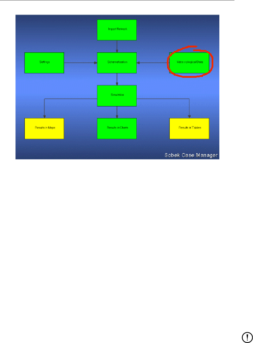
DRAFT
Graphical User Interface
Figure 5.31: The Meteorological Data task block.
Under the Meteorological Data task block, you can define the meteorological circumstances
that apply to your study.
These are:
Precipitation
Evaporation
Wind data
SOBEK contains a default precipitation event (<DEFAULT.BUI>).
************** IMPORTANT *****************************************
The meteorological data is stored in a separate directory <\SOBEK215\Fixed>, which is
accessible for all SOBEK projects. If you make adjustments in a meteorological file that is
also used within another project, these adjustments will also affect the results of that project
(after running its computation again)!
*******************************************************************
Remark:
File names of meteo files are limited to a maximum of 8 characters. Files created
in the user interface will automatically be limited to 8 characters. When renaming or
creating meteo files outside of the user interface, make sure the file name length does
not exceed 8 characters. This 8 character limitation holds true for most SOBEK files,
including .lit directories.
After double-clicking the task block, the following window will appear:
Deltares 159 of 900
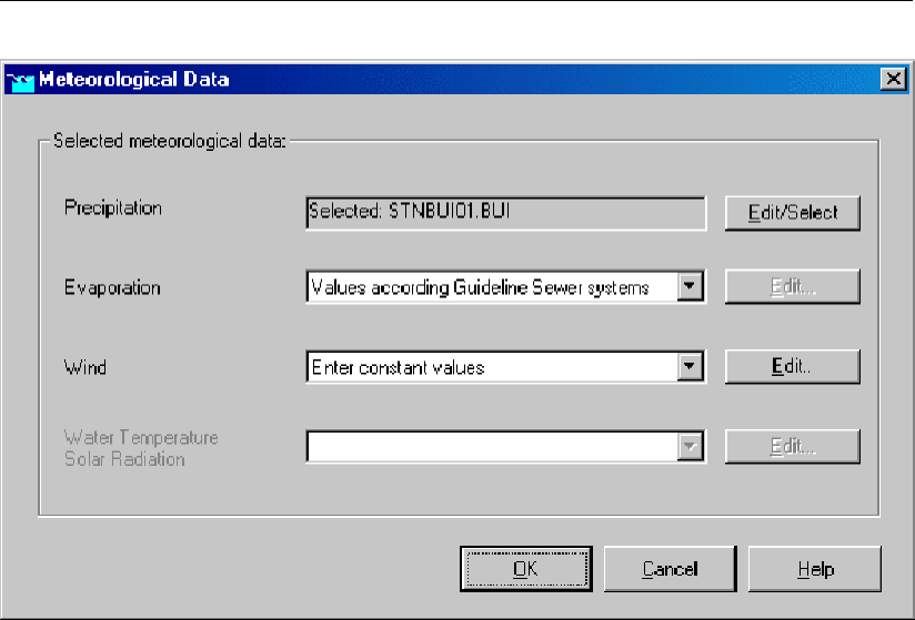
DRAFT
SOBEK, User Manual
Figure 5.32: The Meteorological Data window.
Each of the Meteorological components will be discussed in the chapters hereafter.
Evaporation
During dry periods evaporation plays an important role in the water balance of natural water
systems. Especially for Rainfall-Runoff computations.
SOBEK contains two evaporation series: a long term average series and the time series of
daily values measured between 1951 and 1994 at the De Bilt , the weather station at the Royal
Dutch Meteorological Institute.
Precipitation
A precipitation event is characterised by either consecutive periods with intensive rainfall, or a
longer period with continuous precipitation. A precipitation series contains precipitation events
separated by periods with very little or no rainfall.
Whether a precipitation event can be used as a design event depends on the problem at issue.
For the design of the storage- and pumping capacity, it is mainly the behaviour of the sewer
system during extreme precipitation that is of interest. For the evaluation of target levels of
pumps and weir settings more moderate events are of interest.
SOBEK-RR-SF meets the Dutch guidelines ’sewer systems computations, hydraulic function-
ing’. This implies that both storm events and long time series can be simulated.
The guidelines prescribe ten standard events which must be used to analyse the behaviour of
sewer systems. The ten standard precipitation events are derived from 15 minutes time series
measured at De Bilt, a meteostation of the Royal Dutch Meteorological Institute (KNMI), in the
period 1955-1979. Six different return periods and two different shapes are used to determine
the events. The shape is characterised by the location of the peak. The criteria used for the
selection of the standard events are described in the guidelines. The standard events with
characteristic return period and location of the peak are described in Table 5.1.
160 of 900 Deltares
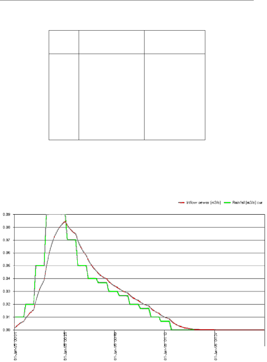
DRAFT
Graphical User Interface
Table 5.1: Standard precipitation events
CODE RETURN PERIOD
(year)
LOCATION OF
PEAK
01 0.25 front
02 0.25 back
03 0.50 front
04 0.50 back
05 1.00 front
06 1.00 back
07 2.00 front
08 2.00 back
09 5.00 front
10 10.00 front
The events in Table 5.1 are available within SOBEK-RR-SF.
Figure 5.33 shows the rainfall of standard event 05 and the inflow into the sewer for a flat
closed paved area of 1 ha. as determined by the RR-module:
Figure 5.33: Rainfall and corresponding sewer inflow for a flat closed paved area
Figure 5.34 shows the rainfall of standard event 05 and the inflow into the sewer for three
closed paved areas (with a slope, flat, flat stretched) of 1 ha each:
Deltares 161 of 900
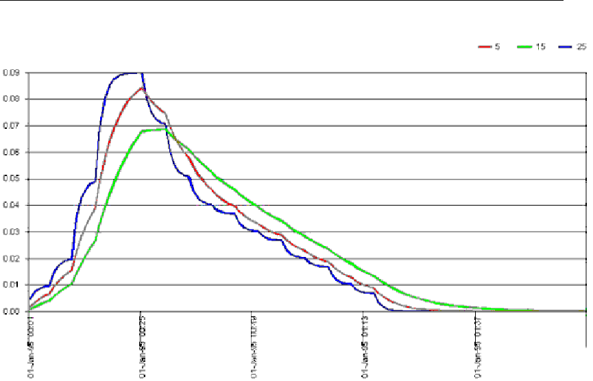
DRAFT
SOBEK, User Manual
Figure 5.34: Rainfall and corresponding sewer inflow for three types of closed paved area
Precipitation options
Under the Meteorological Data task block, you can define rainfall intensities that apply to your
schematisation. In this chapter, the precipitation editor is discussed.
162 of 900 Deltares
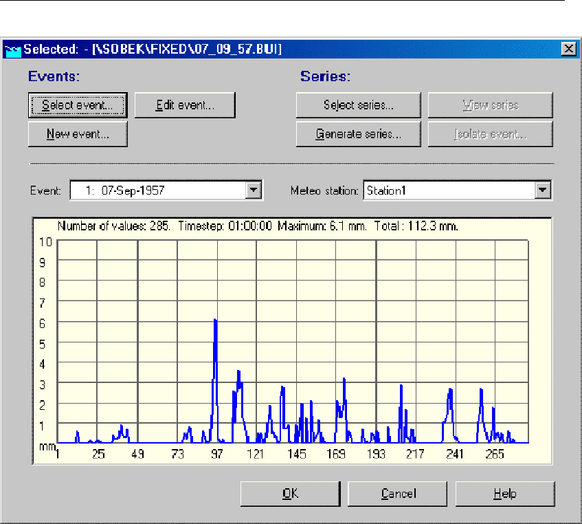
DRAFT
Graphical User Interface
Figure 5.35: The precipitation window
Rainfall Events v.s. Rainfall Series
The basis of the precipitation editor is formed by rainfall events. These are characterised by
either consecutive periods with intensive rainfall, or a longer period with continuous precipita-
tion.
A chain of rainfall events may form a rainfall series. Rainfall series allow you to model a long
time span of precipitation without having to model the dry periods in between.
Rainfall events:
The <Select event>option: This option allows you to select a rainfall event from a list
of available events.
The <Edit event>option: Allows you to edit the currently selected rainfall event. Please
be aware that, if this rainfall event is also used within other projects, editing it may also
affect the results of those projects after you compute them again.
The <New event>option: Allows you to create a new rainfall event. Firstly, you are
asked to enter the number of rainfall stations of which you have data for the event. Then,
you’ll have to enter the names of those rainfall stations. Later, when you create your
model, you can refer to any of these stations.
Deltares 163 of 900
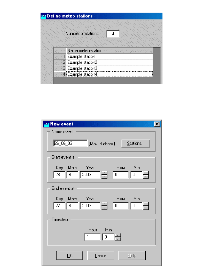
DRAFT
SOBEK, User Manual
Figure 5.36: Define meteo stations.
Next, you are asked to define the name, the starting date, the end date and the timestep
of the event:
Figure 5.37: Defining the name, start/end date and timestep of a new event.
Finally, a window pops up, that contains a spreadsheet-like environment. The user can
copy the available data from a spreadsheet, such as Microsoft Excel, into these fields:
164 of 900 Deltares
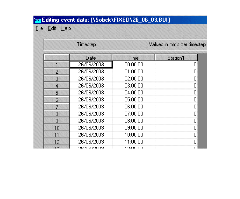
DRAFT
Graphical User Interface
Figure 5.38: Editing event data.
Please note: If you want to copy data from a Spreadsheet program into these fields, make
sure that the field format within the spreadsheet equals that of the fields in SOBEK, thus:
dates: dd/mm/yyyy times: hh:mm:ss Then, save the file that you have just created by
clicking "File" - "Save" from the menu. In the end, don’t forget to actually select the file
that you’ve just created.
Rainfall Series (For the time being only usable for Dutch situations)
As was mentioned above, a rainfall series is a sequence of single rainfall events, which can
be run sequentially within one model run. Notice that for every rainfall event within a series,
the basic initial conditions apply! It is not so that the results of the final time step of event1
provides the initial conditions for event2.
The <Select Series>option: This option allows you to select an existing rainfall se-
ries. Notice that you can view each individual event from that series by choosing it in the
<Event>box on the left side of the screen.
The <Generate Series>option: This option allows you to generate a rainfall series,
based on hourly data between 1951 and 1994 from the Dutch De Bilt rainfall station.
Based on criteria that you define, the individual rainfall events are extracted from that
data. It is not (yet) possible to enter your own long-term rainfall data and generate series
from them.
Wind
In channel systems with long stretches of narrow channels and/or large open water surfaces
strong winds can cause a local increase in water level. In areas where the storage capacity is
small this can cause problems under wet conditions. Water Flow takes the influence of wind
into account.
Specifying multiple wind fields
In SOBEK up to version 2.05, the user interface only supported a global wind field.
Deltares 165 of 900

DRAFT
SOBEK, User Manual
The computational core of SOBEK 2.07 was extended to support the functionality of specifying
multiple wind station data independent of the coupling of SOBEK-branches to wind stations.
The user-interface does not support this functionality.
Model data base
First the changes to the model database are described. The changes pertain to the existing
wind data file, and the introduction of a new wind location data file.
Wind data file
The wind data file of the meteo data layer contains the wind definitions. This can be one of
the following options:
a variable or a constant global wind field;
a wind definition per branch;
using more than one wind.
An example of a global wind field:
GLMT MTEO id ‘1’ ci ‘-1’ wu 1 wv tv 1 TBLE .... tble wd td 1 TBLE .... tble mteo glmt
or
GLMT MTEO id ‘1’ ci ‘-1’ wu 1 wv tv 0 3 wd td 0 270 ... mteo glmt
An example of a wind field per branch:
MTEO id ‘2’ ci ‘1’ wu 1 wv tv 1 TBLE ... tble wd td 1 TBLE .... tble mteo
The exact lay-out of these records has not changed. A more detailed description is available
in the on-line help (Model data base). One can also check with existing wind files (*.WND in
the <\Fixed>subdirectory of the directory where SOBEK is installed)
Using wind stations the user can specify the wind field table per wind station, and specify the
coupling of branches to wind stations separately.
The functionality of a wind field per wind station is made available using the WSTA keyword.
The records are very similar to the existing MTEO or GLMT records. An example:
WSTA id ‘Windstation’ wu 1 wv tv 1 TBLE ... tble wd td 1 TBLE .... tble wsta
with
id wind station id
wu wind used (as in MTEO records)
wv tv wind velocity (as in MTEO records)
wd td wind direction (as in MTEO records)
The appendix contains an example file.
Wind location file
WLOC ci ‘1’ st ‘Windstation1’ wloc
WLOC ci ‘3’ st ‘Windstation1’ wloc with
166 of 900 Deltares
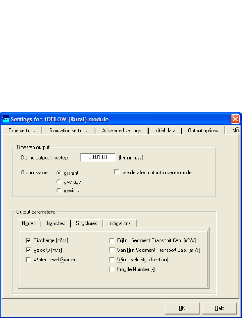
DRAFT
Graphical User Interface
ci carrier id (branch id)
st wind station id; this id should match with a wind station id in the WSTA records
of the wind data file
If a SOBEK-branch is not coupled explicitly to a wind station, the global wind data will be used
by default.
Settings
In Settings, you can specify the desired output. Additional available output is the wind direction
and wind speed per branch. Just select the additional item wind (velocity, direction) in the
’Output options’ tab form with output for ’Branches’.
Figure 5.39: Task block settings, output options.
Meteo
Use Meteo only to select a wind file. A wind data file containing other data than only global
data should never be edited in the user interface using Meteo. It should be done ’behind the
screens’ using a text editor.
Behind the screens
The wind data file and wind location file should be edited using an ASCII text editor.
Deltares 167 of 900
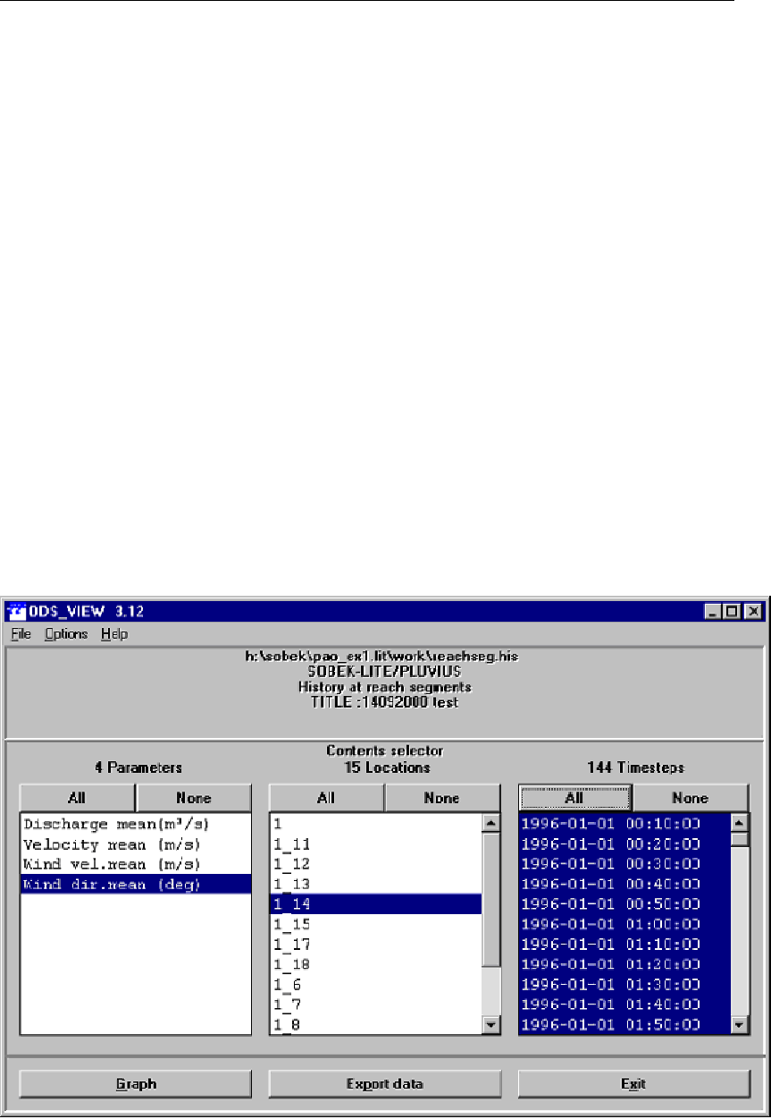
DRAFT
SOBEK, User Manual
The wind file is located in <\SOBEK215\Fixed>. The name of the file is taken from the name
of the rainfall file. Only the extension is different: the wind file has extension .WDC (constant
wind field) of .WND (variable wind field).
The wind location data file Wnd_Loc.Dat can be different for each case. For a fixed set of
wind stations, you can investigate the impacts of allocating SOBEK-branches to wind stations
without needing to change the wind station data.
The wind location file <Wnd_Loc.Dat>should only be edited in the Work directory.
The simplest and safest way to do this is: Open a case, than double-click on the schemati-
sation task-block, and press OK in the next menu. Then you get the question: "Nothing has
been changed. Do you want to continue to the <simulation>task?". Answer Yes.
After that the wind location data file <WND_LOC.DAT>is in the WORK directory, where it
can be edited.
Post-processing
The extra available output per branch (wind velocity and wind direction) can be viewed in the
’Results in charts’ and ’Results in maps’ task block.
In the ’Result in charts’ task block, first select the ’Flows at branch segments’ output and then
select the wind data you want to see from the next screen.
Figure 5.40: Results in charts, Flows at branch segments.
In the ’Result in maps’ task block, you will get the network schematisation on the screen. After
that, open the output data ’Flows at branch segments’, select the appropriate output variable
(default is the first parameter, i.e. discharge mean [m3/s], and click on the desired output
168 of 900 Deltares

DRAFT
Graphical User Interface
location.
Example wind file and wind-location file
Wind Location file (Wnd_Loc.Dat)
WLOC ci ’1’ st ’Test1’ wloc
WLOC ci ’3’ st ’Test1’ wloc
WLOC ci ’5’ st ’Test1’ wloc
WLOC ci ’7’ st ’Test1’ wloc
WLOC ci ’389’ st ’Test2’ wloc
WLOC ci ’388’ st ’Test2’ wloc
WLOC ci ’386’ st ’Test2’ wloc
Note:
The branches with id 1, 3, 5 and 7 will be using the wind data from wind station Test1. The
branches with id 386, 388 and 389 will use the wind data from station Test2. All other branches
in the schematisation will be using the global wind data.
Wind data file (e.g. Sept1994.Wnd)
The example wind file below contains the definition of a global wind field and 2 other wind
fields.
GLMT MTEO nm ’(null)’ ss 0 id ’0’ ci ’-1’ lc 9.9999e+009 wu 1
wv tv 1 0 9.9999e+009 ’Wind Velocity’ PDIN 0 0 ” pdin
CLTT ’Time’ ’Velocity’ cltt CLID ’(null)’ ’(null)’ clid
TBLE
’1994/10/23;00:00:00’ 6.000000 <
’1994/10/23;02:00:00’ 6.000000 <
’1994/10/23;04:00:00’ 5.000000 <
’1994/10/23;06:00:00’ 6.500000 <
’1994/10/23;08:00:00’ 6.000000 <
’1994/10/23;10:00:00’ 7.500000 <
’1994/10/23;11:00:00’ 9.500000 <
’1994/10/23;12:00:00’ 9.500000 <
’1994/10/23;13:00:00’ 8.500000 <
’1994/10/23;16:00:00’ 6.000000 <
tble
wd td 1 0 9.9999e+009 ’Wind Direction’ PDIN 0 0 ” pdin
CLTT ’Time’ ’Direction’ cltt CLID ’(null)’ ’(null)’ clid
TBLE
’1994/10/23;00:00:00’ 170.000000 <
’1994/10/23;01:00:00’ 180.000000 <
’1994/10/23;03:00:00’ 190.000000 <
’1994/10/23;06:00:00’ 190.000000 <
’1994/10/23;07:00:00’ 180.000000 <
’1994/10/23;11:00:00’ 190.000000 <
’1994/10/23;13:00:00’ 200.000000 <
Deltares 169 of 900

DRAFT
SOBEK, User Manual
’1994/10/23;15:00:00’ 190.000000 <
’1994/10/23;16:00:00’ 180.000000 <
tble
su 0 sh ts 0 9.9999e+009 9.9999e+009 tu 0 tp tw 0
9.9999e+009 9.9999e+009 au 0 at ta 0 9.9999e+009 9.9999e+009 mteo
glmt
WSTA id ’Test1’ nm ’Teststation1’ wu 1 wv tv 1 0 9.9999e+009 ’Wind Velocity’ PDIN 0 0 ” pdin
CLTT ’Time’ ’Velocity’ cltt CLID ’(null)’ ’(null)’ clid
TBLE
’1994/10/23;00:00:00’ 16.000000 <
’1994/10/23;02:00:00’ 16.000000 <
’1994/10/23;03:00:00’ 15.500000 <
’1994/10/23;04:00:00’ 15.000000 <
’1994/10/23;06:00:00’ 16.500000 <
’1994/10/23;11:00:00’ 19.500000 <
’1994/10/23;13:00:00’ 18.500000 <
’1994/10/23;14:00:00’ 18.500000 <
’1994/10/23;15:00:00’ 17.500000 <
’1994/10/23;16:00:00’ 16.000000 <
tble
wd td 1 0 9.9999e+009 ’Wind Direction’ PDIN 0 0 ” pdin CLTT ’Time’ ’Direction’ cltt CLID
’(null)’ ’(null)’ clid
TBLE
’1994/10/23;00:00:00’ 279.000000 <
’1994/10/23;01:00:00’ 289.000000 <
’1994/10/23;03:00:00’ 299.000000 <
’1994/10/23;06:00:00’ 299.000000 <
’1994/10/23;07:00:00’ 289.000000 <
’1994/10/23;12:00:00’ 299.000000 <
’1994/10/23;16:00:00’ 289.000000 <
tble
su 0 sh ts 0 9.9999e+009 9.9999e+009 tu 0 tp tw 0
9.9999e+009 9.9999e+009 au 0 at ta 0 9.9999e+009 9.9999e+009
wsta
WSTA id ’Test2’ nm ’Teststation2’ wu 1 wv tv 1 0 9.9999e+009 ’Wind Velocity’ PDIN 0 0 ” pdin
CLTT ’Time’ ’Velocity’ cltt CLID ’(null)’ ’(null)’ clid
TBLE
’1994/10/23;00:00:00’ 26.000000 <
’1994/10/23;06:00:00’ 26.500000 <
’1994/10/23;12:00:00’ 29.500000 <
170 of 900 Deltares
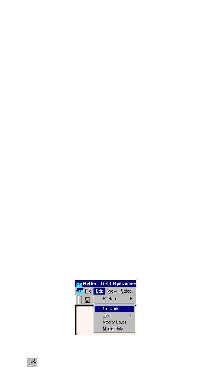
DRAFT
Graphical User Interface
’1994/10/23;16:00:00’ 26.000000 <
tble
wd td 1 0 9.9999e+009 ’Wind Direction’ PDIN 0 0 ” pdin CLTT ’Time’ ’Direction’ cltt CLID
’(null)’ ’(null)’ clid
TBLE
’1994/10/23;00:00:00’ 179.000000 <
’1994/10/23;01:00:00’ 189.000000 <
’1994/10/23;03:00:00’ 199.000000 <
’1994/10/23;07:00:00’ 189.000000 <
’1994/10/23;11:00:00’ 199.000000 <
’1994/10/23;13:00:00’ 209.000000 <
’1994/10/23;15:00:00’ 199.000000 <
’1994/10/23;16:00:00’ 189.000000 <
tble
su 0 sh ts 0 9.9999e+009 9.9999e+009 tu 0 tp tw 0
9.9999e+009 9.9999e+009 au 0 at ta 0 9.9999e+009 9.9999e+009
wsta
5.1.4 Task block: Schematisation
General
Within this task block the actual schematisation is built and verified. As mentioned before, this
manual will only deal with the 2D additions to the 1D channel flow version of SOBEK. Please
refer to the general SOBEK user manuals for more details on the outline of schematisation
task block and the use of the 1D channel flow module in specific.
Just like the 1D schematisation, the 2D schematisation is built in two steps using a number
of building blocks. In the first step, the edit network mode, the grids and the other building
blocks, like initial water level nodes, are being placed on the map. In the second step, the edit
model data mode, the characteristics of all these building blocks are defined. Both steps will
be explained in detail in the following two paragraphs.
Edit Network mode
To start creating a network, you have to switch to the ’Edit Network’ mode. To do so, choose
"Network" from the "Edit" menu:
Figure 5.41: Entering Edit Network mode.
Or click the node.
Deltares 171 of 900
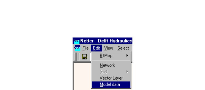
DRAFT
SOBEK, User Manual
Edit Model Data mode
To start editing the parameters for your model objects, choose "Model Data" from the "Edit"
menu.
Figure 5.42: Entering Model Data mode.
The next step in building the schematisation is specifying the parameters for the different 2D
elements defined in the edit network mode. The order in which the 2D elements are handled
is the same as in the previous paragraph.
An object needs to be selected before its data can be defined. After the Model Data option
has been selected from the edit menu, the model data window appears. This window can
be used to browse through all objects and select them for editing. The objects can also be
selected by clicking on them in the main Netter screen.
Viewing 2D Grid Info
Functionality:
Using the 2D Grid Info option, information can be obtained on:
individual 2D grid cells, or
on a path of 2D grid cells.
The user can add the information of various individual 2D grid cells to one and the same
graph. A path of 2D grid cells can cross at any angle over a 2D grid. At present the path of
2D grid cells can not pass over nested grids (i.e. parent grid and child grid) in such way that
only the active parent and child 2D grid cells are being selected.
Further on a distinction is to be made between static values and dynamic values. Static values
refers to the values on the underlying 2D grid (for instance a bed elevation) or underlying
map file (for instance maximum water depths). Dynamic values refers to time-dependent
computation results (for instance incremental water depths).
How to make a 2D path:
Both in the ‘Schematisation’ and ‘Results in Maps’ Task blocks.
In the main menu, click on Select/2D-Grid cell info
Click on the 2D grid cell at which you like to start your 2D path (i.e. starting 2D grid cell).
Note that in the ‘Path2D-Grid Info’ window, the column and row number of the starting 2D
grid cell are given in the two boxes in front of the Path check-box.
Click the Path check-box,
While pressing on the Shift key, place the mouse-pointer on the 2D grid cell at which you
like to end your 2D path (i.e. the end 2D grid cell). Releasing the Shift key will result in the
172 of 900 Deltares

DRAFT
Graphical User Interface
selection of the end 2D grid cell. The column- and row number of the end 2D grid cell are
now filled in the two boxes behind the Path check-box.
Click on the <show>button in the ‘2D-Grid info’ window to visualise the 2D grid cells
contained in your 2D Path.
Remark: In case you have more than 1(one) 2D grid (for instance in case of nested grids), the
2D grid cell of the 2D grid that lies on top will be selected. Using the Next Grid button the grid
cell on the underlying 2D grid will be selected. Note that in this case the Grid ID will change.
How to retrieve 2D Grid Info:
Under the ‘Schematisation’ Task block only information on static values of the 2D grid
cells are available. In case the 2D path option is not used, the static value of the selected
2D grid cell is depicted on the one most last line in the ‘2D-Grid Info’ window (Note that
dynamic values are not available under the ‘Schematisation Task’ block). In case a 2D
path is selected, the static values of the concerning 2D grid cells can be obtained by
clicking the Graph button. Note that in the main menu of this graph the x-axis can be
changed to either value (distances) or labels (column and row number of the 2D grid).
Under the ‘Results in Maps’ Task block, information on both static- and dynamic values of
the 2D grid cells are available. In case the 2D path option is not used, the static- and actual
dynamic value of the selected 2D grid cell is depicted on the last two lines in the ‘2D-Grid
Info’ window. Please note that static values are displayed in grey. Clicking the most left
<Graph>button, provides a graph of dynamic values of each selected 2D grid cell as
function of time. Please note that by clicking on another 2D grid cell and sequentially
clicking on this <Graph>button again, the user can add the dynamic results of various
2D grid cells in one and the same graph. In case a 2D path was selected, clicking on the
most left Graph button results in a graph of the dynamic values of the starting 2D grid cell
of the 2D path. Clicking the most right Graph button provides a graph, showing for all 2D
grid cells lying on the 2D path, its static value as well as its dynamic values for a particular
point-in-time.
Notes:
1) the x-axis of this graph can be plotted as function of value (distance) or labels (column
or row number);
2) dynamic values are only available in case they are selected beforehand (Click in main
menu on File/Open Data/ Depth Incremental (in the ‘Select Item’ window));
3) using the ‘View Data’ window dynamic values can be added to the graph; and
4) using the forward and backward buttons in the ‘View Data’ window, the point-in-time for
which the dynamic values are shown under the most right Graph button can be changed.
Deltares 173 of 900
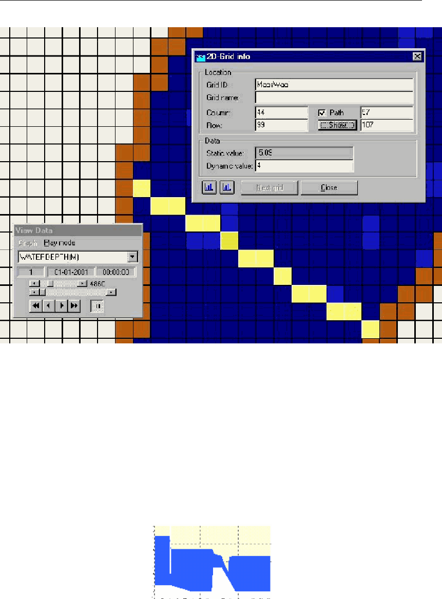
DRAFT
SOBEK, User Manual
Figure 5.43: Example of a 2D Path under a particular user defined line of 2D cells.
5.1.5 Task block: Simulation
5.1.6 Task block: Results in Maps
5.1.6.1 River/Urban/Rural
SideView
In the "Results in Maps" mode, you can create an animation of your hydrodynamic results,
plotted alongside a channel, river or sewer pipe. Note: SideView is only available for the
SOBEK 1D Flow modules: Channel Flow, Sewer Flow and River Flow.
Figure 5.44: Example of a SideView.
This chapter explains:
How to create a SideView
Advanced SideView options
Creating a SideView
174 of 900 Deltares

DRAFT
Graphical User Interface
Go to the "Results in Maps" task block
Click the starting node (left side of the animation) on the map.
Press the Shift key on your keyboard and keep it pressed
Click the end node (right side for the animation) on the map
SideView now automatically selects the shortest connection between both selected points.
Right-click your mouse and select "SideView" from the pop-up menu.
The "Setup Animation" window is then loaded:
Figure 5.45: Setup Animation of a SideView.
Here, you can select the period for which an animation should be shown.
After pressing OK, the "SideView" window is opened:
Deltares 175 of 900
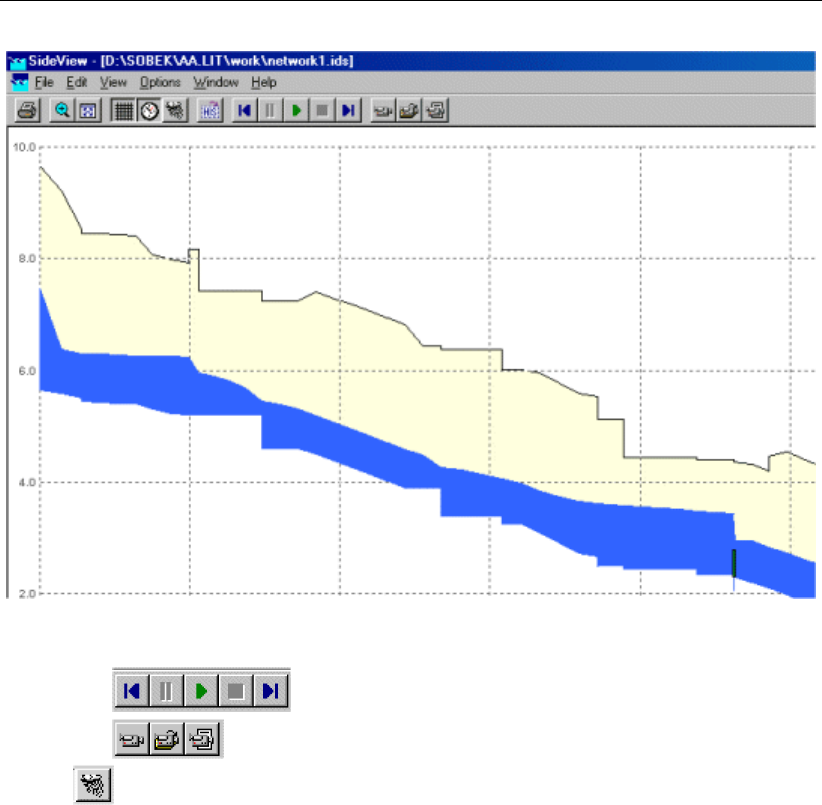
DRAFT
SOBEK, User Manual
Figure 5.46: The SideView Window.
With the buttons, you can start, pause and stop the animation.
With the buttons, you can record the animation and save it as a movie file.
The button toggles whether you will see the rainfall intensities in a graph during the
animation.
Advanced SideView options
If you desire to select another path than the shortest way between the start- and endpoint,
you can sequentially add parts of the desired path by keeping the Shift Button pressed,
thus forcing the path to follow the route that you desire.
Note: if a specific branch cannot be selected with the Shift key, because it is never the
shortest route, you may release the Shift key, and select it (including its surrounding
nodes) with the Ctrl key.
You can save the path for a SideView you have chosen. Choose "File" - "Save" or press
Ctrl-S to store the path and give it a name.
You can add the results form another case to your current SideView. Choose "View" -
"User data" - "Get from case" to add them. These results will become visible as red dots
in your animation.
You can view multiple SideViews in one window by opening previously stored paths in
addition to your current selection. Choose "File" - "Open" to do so.
You can create graphs of the results at nodes, branch segments and structures from
within the SideView window. Click the object in the SideView for which you desire to
create a graph, right-click your mouse and select "show graph".
176 of 900 Deltares
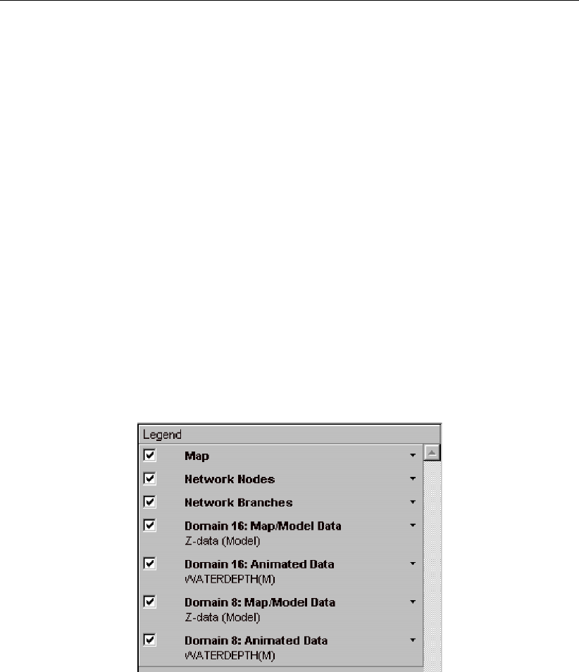
DRAFT
Graphical User Interface
5.1.6.2 Netter
General
The ’results in maps’ task is the most important of the three task blocks when viewing and
analyzing results from a simulation. It is usually the first place to go to if you want a quick
scan of the results, because the Netter environment provides you with many tools to help
you. Once again, the user is expected to have a working knowledge of SOBEK and Netter
before reading this manual. This paragraph focuses on explaining the additions to the Netter
environment concerning the viewing and exporting of 2D data. It starts with explaining the
use of the active legend, which is a great help to quickly understand exactly what results you
are viewing and to turn data layers on and off. After that, some more information will be given
concerning the three output formats: incremental (only for use within Netter) and GIS (for
output to GIS applications). The third output format, History stations (for use in Netter or as
output to for example EXCEL), is not explained any further in this document, as it is a standard
SOBEK output format which is already explained in the regular SOBEK documentation.
Viewing model and output data in NETTER
Active Legend
The active legend is one of the major additions to this new version of SOBEK/Delft-1D2D. It
can be switched on in Netter in both the schematisation task and the results in maps task, by
selecting options →active legend. It is a great help with identifying and selecting output data.
Figure 5.47: The active legend
Once the active legend has been switched on, the model and output data become visible
as groups in the legend window (Figure 5.47). All groups can be turned on or off using the
check-boxes. Selecting a group in the legend window activates a shortcut to the properties/
settings of the group. The triangle-like symbol on the right hand side of the group names turn
the group-legends on and off.
Depending on the schematisation and the type of currently selected output data (under file →
open data), one or more of the following groups become available:
map (model data)
The currently loaded map-layer.
Network nodes (model data).
All nodes, both 1D and 2D, in the schematisation
Network branches (model data).
All branches in the schematisation
Deltares 177 of 900

DRAFT
SOBEK, User Manual
Map/model data for every grid (called ’domain’)
This data layer can contain either model data OR output data:
z-data (model data)
terrain levels with respect to reference level. Positive means downward. The topogra-
phy *.asc files are examples of the z-data.
depths/levels/velocities (output ’map’ data)
output results for a selected time step. It is not possible to ’scroll’ through the simulation
time.
Animated (output) data for every grid.
This layer can contain any one of the following output data:
Depths
Levels
as opposed to the z-data, the levels are always defined as positive in Upward direction!
Velocities
Should always be positive.
Network data.
This layer can contain the results of a selected 1D-output option (i.e. water levels at nodes)
OR the 2D results at history stations.
5.1.6.3 Incremental and GIS output files
Incremental files are generated by SOBEK mainly as a means to visualise animated results
in Netter. However, it is also possible to generate an .ASC output file of the current time step
and for a selected grid via the export option (file →Export →2D Grid data →Animated
data). Remember that the incremental files contain classes instead of actual values, so the
.ASC file generated as output will contain classes as well. In most cases it will be more useful
to create .asc files from either a MAP file or use a GIS .asc file directly.
These files are created mainly for the purpose of exporting output data to a GIS-based system
such as ARCview.
The GIS files are the .asc output files that the user selected in the settings task. A distinction
is made between ’normal’ asc files and ’special’ asc files. One ’Normal’ asc file is generated
automatically for every (in Settings) selected GIS output time step and variable. One ’Special’
asc file is generated for every special variable, but only one for the whole simulation period!
The exception to this rule are the files for the dD/dt variable, which are generated every GIS
output time step. After the simulation has completed and the case has been saved, these
files are written to the <case name>-directory. Remember that these files contain the actual
values and not the classes. Each file represents the actual values for a particular variable and
for a particular time.
The following table summarizes the available special .asc output files:
continued on next page
178 of 900 Deltares

DRAFT
Graphical User Interface
continued from previous page
Parameter Symbol Unit Filename Explanation
Table 5.2: Special <*.asc>output files
Parameter Symbol Unit Filename Explanation
maximum water
depth
d_max m dmNMAXDX.ASC/
dNNMAXDX.ASC
in each cell the maximum
water depth of all calculated
timesteps is written
time of max-
imum water
depth
t_dmax hr dmNTMAXD.ASC/
dNNTMAXD.ASC
in each cell is written af-
ter what period this maxi-
mum water depth has been
branched
maximum water
level
h_max m ref.
level
dmNMAXHX.ASC/
dNNMAXHX.ASC
in each cell the maximum
water level of all calculated
timesteps is written
time of max-
imum water
level
t_hmax hr dmNTMAXH.ASC/
dNNTMAXH.ASC
in each cell is written af-
ter what period this maxi-
mum water level has been
branched
maximum
velocity
c_max m/s dmNMAXCX.ASC/
dNNMAXCX.ASC
in each cell the maximum
velocity (absolute value) of
all calculated timesteps is
written
time of maxi-
mum velocity
t_cmax hr dmNTMAXC.ASC/
dNNTMAXC.ASC
in each cell is written after
what period this maximum
velocity (absolute value) has
been branched
time of wetting t_wet hr dmNTWTXX.ASC/
dNNTWTXX.ASC
in each cell the first timestep
is written at which the cell
starts to become wet. If the
cell doesn’t become wet it
remains ‘-999’
time of wet-
ting per class
(‘steady state’)
t_wet/class hr dmNWTCII.ASC/
dNNWTCII.ASC
for each incremental class in
each cell the first timestep at
which this class is exceeded
is written. If the class is
never exceeded it remains ‘-
999’
continued on next page
Deltares 179 of 900

DRAFT
SOBEK, User Manual
continued from previous page
Parameter Symbol Unit Filename Explanation
time of drying t_dry hr dmNTEMXX.ASC/
dNNTEMXX.ASC
in each cell the last timestep
is written at which the cell
starts to become dry again
after wetting. If the cell
doesn’t become dry after
wetting it remains ‘-999’
time of dry-
ing per
class(‘steady
state’)
t_dry/class hr dmNEMCII.ASC/
dNNEMCII.ASC
for each incremental class in
each cell the last timestep
at which the water depth is
lower than this class is writ-
ten. If the water depth is al-
ways higher than a class, it
remains ‘-999’
rate of change
of water depth
dd/dt m/s dmNRSSSS.ASC/
dNNRSSSS.ASC
in each cell the difference
in water depth is written be-
tween two GIS output files
divided by the GIS output
options timestep Dt
Notice that in the files, where ‘hr’ is the unit, t = 0 is at the start of the simulation.
Example for the ‘rate of change of water depth’: if you run 10 hours of simulation period, and
you choose in ‘GIS output options’ Dt = 02:00:00 hh:mm:ss, then this will result in 5 maps.
Filename structure
Most of the .asc filenames generated have the following structure:
dmNVSSSS.asc/dNNVSSSS.asc
General notations used for ASC and MAP files are :
’dm’ or ’d’ →an abbreviated form of ’domain’ (another name for ’grid’), dm is used when
domain number is between 1 and 9, and d is used for domain numbers between 10 and 99.
’N’ →domain number, from 1-9. This is an internal number, which is not the same as the
domain ID.
’NN’ →If domain number is from 10 onwards till 99, then the name of the .asc file will begin
with ‘dNN’ i.e. for say domain 19 it will be d19VSSSS.ASC
To check which domain number is related to which domain ID, please refer to file <FLSGIS.HLF>
file in your case directory.
’V’ →type of variable:
d depth
180 of 900 Deltares

DRAFT
Graphical User Interface
h level
c current
u velocity in x-direction
v velocity in y-direction
r Dd/Dt
’SSSS’ →represents chosen output time step number (not the time step chosen for the
calculation!). In other words, if the time step selected is 15 minutes, then at start of simulation,
SSSS = 0000, at 15 minutes after the start of simulation , SSSS=0001 and so on.
’XXXX’ or ’XX’ or ’X’ →represents 0 or 1 placed to make the filename 8 character long.
‘II’ →represents the class interval number as given in the Incremental file for a selected
parameter.
Similar to the ASC file a MAP file is also created with the name
dmNVXXXX.map/dNNVXXXX.map
The main differences between the ASC and MAP file are that ,
MAP file is a binary file as opposed to ASC file
MAP file contains actual values for all time step, while one ASC file contains actual values for
a one time step. Hence no matter how many time steps are defined by the user, there will be
only one map file created.
There are a number of other .ASC file created for variables like maximum water depth/ max-
imum water level/ time at which maximum depth occurs/ time at which maximum water level
occurs etc.. These files can be identified from their filenames:
The filenames for such variables are:
Maximum water depth
dmNMAXDX.ASC/dNNMAXDX.ASC
dmNTMAXD.ASC/dNNTMAXD.ASC
The maximum water depth value for the whole simulation run is written in dmNMAXDX.ASC/
dNNMAXDX.ASC while the corresponding timestep when the maximum water depth occurs
is written in dmNTMAXD.ASC/ dNNTMAXD.ASC. These files are generated when the option
of water depth is checked on in Settings.
Rate of change of water depth
dmNRSSSS.ASC/dNNRSSSS.ASC
The rate of change of depth per selected output time step is written in dmNRSSSS.ASC/dNNRSSSS.ASC.
These files are generated when the option of water depth is checked on in Settings. The time
step at which these files are written is same as the selected time step for incremental file and
thus irrespective of what the output time step is for generation of GIS/MAP files in settings.
Maximum velocity
Deltares 181 of 900

DRAFT
SOBEK, User Manual
dmNMAXCX.ASC/dNNMAXCX.ASC
dmNTMAXC.ASC/dNNTMAXC.ASC
The maximum velocity value for the whole simulation run is written in dmNMAXCX.ASC/ dNN-
MAXCX.ASC while the corresponding timestep when the maximum velocity occurs is written
in dmNTMAXC.ASC/ dNNTMAXC.ASC. These files are generated when the option of velocity
is checked on in Settings.
Maximum water level
dmNMAXHX.ASC/dNNMAXHX.ASC
dmNTMAXH.ASC/dNNTMAXH.ASC
The maximum water level value for the whole simulation run is written in dmNMAXHX.ASC/
dNNMAXHX.ASC while the corresponding timestep when the maximum water level occurs is
written in dmNTMAXH.ASC/ dNNTMAXH.ASC. These files are generated when the option of
water level is checked on in Settings.
Time of wetting/drying
dmNTWTXX.ASC/dNNTWTXX.ASC
dmNTEMXX.ASC/dNNTEMXX.ASC
These two files are special output files. The values in the file dmNTWTXX.ASC/ dNNTWTXX.ASC
gives the maximum time span the grid cell remains flooded i.e wetted and dmNTEMXX.ASC/
dNNTEMXX.ASC gives the maximum time span the grid cell remains dry i.e empty. These
files are generated when the option of water depth is checked on in Settings.
Time of wetting/drying per class
dmNWTCII.ASC/dNNWTCII.ASC
dmNEMCII.ASC/dNNEMCII.ASC
These two files are special output files. The values in the file dmNWTCII.ASC/ dNNWTCII.ASC
gives the time step when a water depth in a grid cell is high enough to be in the particular
class. For examples: if there are three classes for depth values i.e. less than 0.1 m, greater
than or equal to 0.1 m but less than 1.0 m, and greater than or equal to 1.0 m. So in total
three files will be generated for each domain i.e dmNWTC01.ASC/ dmNWTC02.ASC/ dm-
NWTC03.ASC. When a grid is just flooded but the water depth is still less then 0.1 m then
the time step at which the grid cell is flooded is written in dmNWTC01.ASC, when the water
depth in grid cell becomes just higher or equal to 0.1 m but less than 1.0 m that time step is
written in dmNWTC02.ASC, and when the water depth becomes just higher or equal to 1.0m
that time step is written in dmNWTC03.ASC.
Similarly the values in the file dmNEMCII.ASC/ dNNEMCII.ASC the time step when a water
depth in a grid cell is receding and is low enough to be the particular class.
These files are generated when the option of water depth is checked on in Settings.
182 of 900 Deltares

DRAFT
Graphical User Interface
5.1.7 Task block: Results in Charts
5.1.8 Task block: Results in Tables
Description of the task
Double-click the "Results in tables" task box. The Results in Tables window appears.
Select the appropriate output file and click the View button.
The available files are:
General Balances Output: cumulative mass balances for the whole model area and the
whole simulation period (the <altoys.mes>file).
Water Balance for Water Quality network: cumulative water balance for the whole model
area and the whole simulation period (the <waterbal.prn>file).
5.2 SOBEK GIS interface (NETTER)
5.2.1 Adjusting the scale settings
When simulation results are opened in NETTER (Task block "Results in Maps"), a scale is
automatically created and plotted in the Active Legend. However, you may want to define
your own scale settings and re-use them for other cases.
Activate the "Results in Maps" task block
Open a set of simulation results of your choice
Open the Color Range window by clicking the name of the results in the Active Legend
For example: water level.
Figure 5.48: A waterlevel color range in the Active Legend of NETTER.
Alternatively, you can choose "Options" - "Data value options" from the Netter menu and then
click Scale.
Deltares 183 of 900

DRAFT
SOBEK, User Manual
Figure 5.49: Changing the Active Legend color range and scale.
Adjust the colours and values until they meet your taste. You can then choose to save
these settings by pressing <Save legend>. Use the Save style check box if you want to
save these settings only for the currently active type of output. Thus:
means: save the current settings only for the currently active results type (i.e. results at
nodes)
means: save the legend settings. Depending whether "save style" is switched on, this
legend will then apply to all output, or only to the currently active results type. The legend
settings (style) are always stored in the <Netter.leg>file. Additional settings are stored
in the <Netter.nls>file.
Optionally, you can choose to save the legend settings to a file. Choose "File" - "Export
style" in order to do so
Important: depending on your SOBEK settings, the customised legends will apply either to
one project only or to all SOBEK projects. See the topic "Saving your custom NETTER
settings" to learn more about that.
184 of 900 Deltares
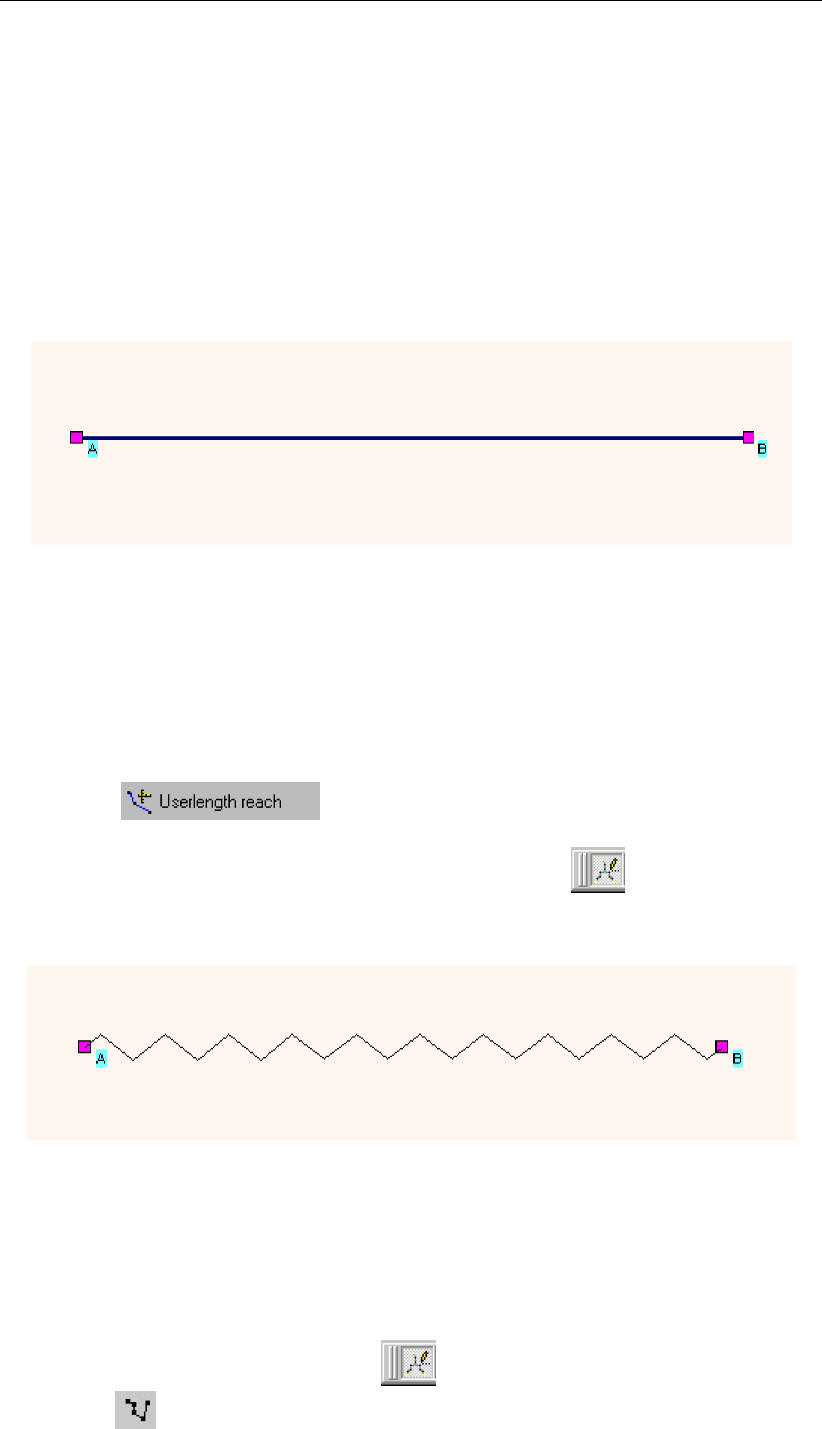
DRAFT
Graphical User Interface
5.2.2 Curving a branch
The length of the thalway (low water bed) from a river or channel may differ from the distance
between two nodes in a straight line. The meanders which cause this can be implemented
by switching to the ’vector layer’ mode, adding coordinates and dragging them to their natural
position on the map. A quicker method is to simply submit a value for the real length. In the
vector layer, the branch will then show as a harmonica, forcing itself to adapt the user defined
length.
Example:
Suppose there is a river flowing from point A to B:
Figure 5.50: A straight river flowing from A to B.
The distance in a straight line between A and B is approximately 1 000 m. However, in reality
the river meanders, thus making the real length of the river 1 300 meters. Now, how to make
SOBEK uses 1 300 meters for the calculation of hydrodynamics?
The simple method to submit the ’real’ river length is to:
Click the button from the "branch" toolbar, click the branch and
enter the value of 1300m.
See effect this action had in the vector layer by clicking the button. Notice that in
the vector layer the branch has been given a harmonica shape, thus forcing it to be 1 300
m:
Figure 5.51: A harmonica-shaped river from point A to B.
Back in the normal mode you will only see these artificial meanders when you add objects
to the branch.
The advanced method to submit the ’real’ river length is to:
Activate the vector layer by clicking the button
Click the (show coordinates) button and select the branch.
Deltares 185 of 900

DRAFT
SOBEK, User Manual
Click the button and add coordinates to the branch by clicking and dragging.
Thus you can make the branch follow the real meandering of the river. The result will look like
this:
Figure 5.52: A meandernig river from point A to B.
Don’t be surprised if the meanders disappear again when you leave the "vector layer" mode:
the coordinates you just added will only show in the normal mode where there is an object
(cross section, calculation point, structure) placed on the branch!
5.2.3 Background map layers
SOBEK offers a library of geographical map layers, such as the map of The Netherlands.
Figure 5.53: The default map of The Netherlands in SOBEK.
These maps can be used as the default background for your schematisations. This chapter
explains explains how to do this.
186 of 900 Deltares
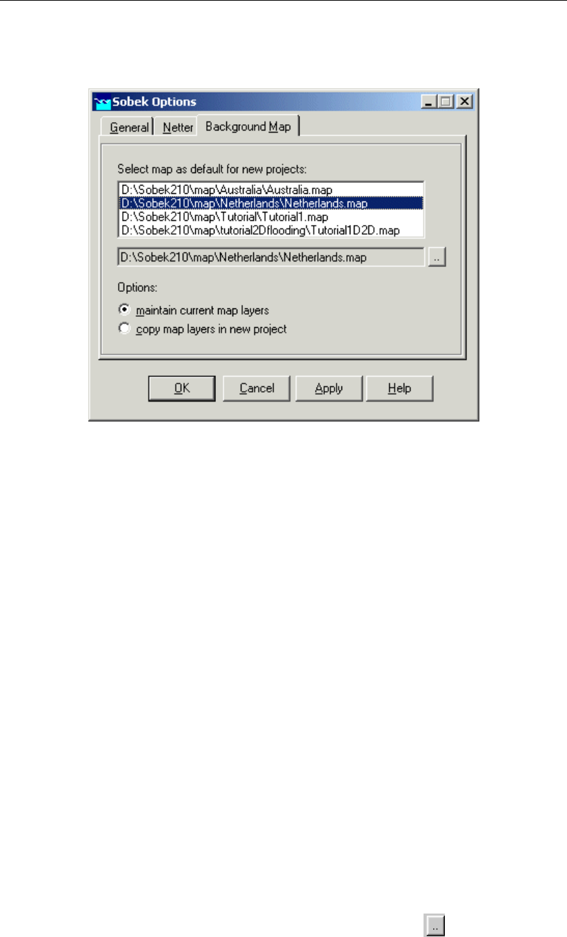
DRAFT
Graphical User Interface
Choose ’Options’ - ’SOBEK options’ from the main menu on the SOBEK startup screen.
The ’Default Map Settings’ window will pop up:
Figure 5.54: The Default Map Settings window.
In this window, you can choose which map should be the default for all your new projects.
Every time you create a new SOBEK project, that map will be used as the default map.
The option ’maintain current map layers’ means that your maps will be stored in the spec-
ified directory only. This will save disk space, since the maps will not be copied to each
new project. However, if you intend to send your project-files to a third-party, it might be
handy if the maps are included in the project directory. In that case, choose the ’copy map
layers in new project’ option.
What if your country is not in the list?
If your country does not appear in the list of available maps, you can create one yourself:
Don’t bother about the default map for the time being, but simply start creating a project,
based on the existing default map.
Learn how to work with projects first by completing a tutorial!
Once you’ve branched the point where the model schematisation is created (SOBEK’s
GIS environment), compose your own map by choosing "Options" - "Map Options" and
importing various GIS map layers that you might have. Note: the distance-units of your
maps should always be meters, as SOBEK interprets them as such! Map layers in lat/lon
co-ordinates, yards, inches or feet are not supported!
All the map-based data (including background maps) that you want to use in SOBEK need
to be in a UTM-type (WGS84) cartesian projection, with XY coordinates in meters (and
not in degrees).
When you’re satisfied with the composition, you can export it. Choose ’File’ - ’Export’ -
’Map’ and give it a proper name.
The next time you start SOBEK, you can go back to the ’Default Map Settings’ option
and select your newly created map as the default one! Click the button to select the
location where you stored the map.
Deltares 187 of 900
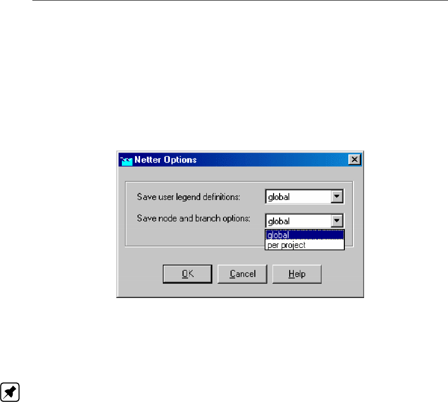
DRAFT
SOBEK, User Manual
5.2.4 Customising NETTER Settings
There are different possibilities to configure NETTER. You can choose to store these configu-
rations on a global level, or to specify them per project:
Start SOBEK
Choose "Options" - "Netter options" from the menu in the SOBEK Startup window. The "Netter
options" window will appear:
Figure 5.55: The global Netter options window.
Here you can choose whether the settings you will define in NETTER (legend and node/branch
settings) should be applied globally (to all projects) or per project.
Note: For the ‘node and branch options’, the results are stored in the file <NtrUser.ini>.
The Netter Legend options are stored in the <Netter.leg>file. When stored as ’global’, they
can be found in <\SOBEK215\Fixed\User>; when stored per project they can be found in the
<\Fixed>directory of the project.
5.2.5 Exporting results to a database
It is possible to automatically gather specific results and prepare them for exporting to a Mi-
crosoft Access (<*.MDB>) database. This is useful for generating standardised reports.
The export definitions can be stored on three different levels:
On a case level - for each case, you will have to create a new definition of the desired
output combination
On a project level - within every case of the project, the standard export settings will remain
the same
On a global SOBEK level
For every case, you can select which of the above level should apply.
Go to the "Results in Maps" task block
Choose ’Tools’ - ’Export Options’. The "SOBEK Export tool" window will appear:
188 of 900 Deltares
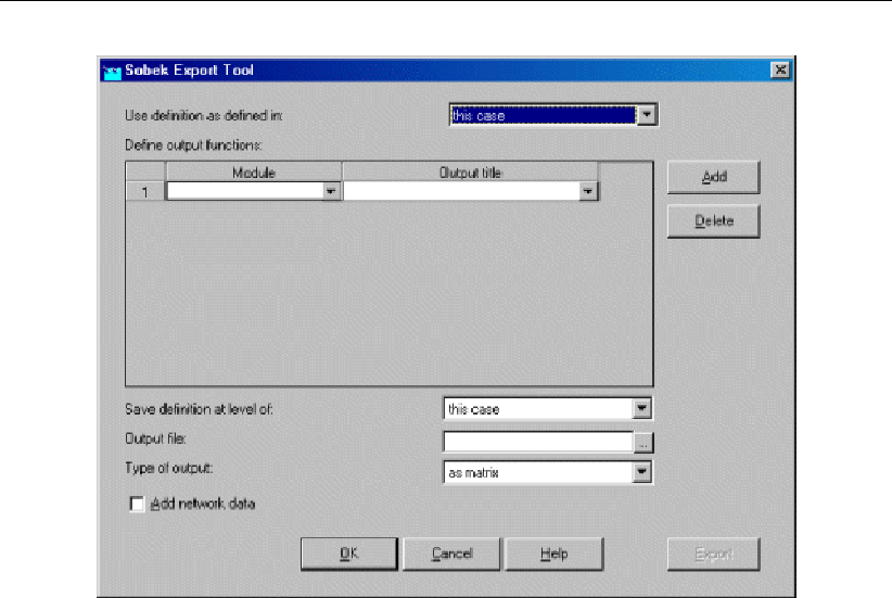
DRAFT
Graphical User Interface
Figure 5.56: Adding a definition in the SOBEK Export Tool.
Define for which level your definition should be saved (case, project, global) in the field
"save definition at level of:"
Define a name for the output file
Select in the fields "Module" and "Output file"
Select the type of output: as a matrix or as a table
Click Export to actually create the MDB file
5.2.6 Model data editor
For many objects in your network, you will have to submit parameter values. For example,
these can be the bed level or shape of a river’s cross section, the friction value of a sewer
pipe, the infiltration capacity of an unpaved area, and so on.
(If you don’t know how to create a network, view the chapter basics of network editing or follow
one of the tutorials provided in this document).
There are two ways to define the parameter values (model data) to the schematisation:
Using the single data editor(editing one object at a time)
Using the multiple data editor(editing multiple objects at a time)
Using the single data editor
To submit parameters to an individual object at a time, the following steps can be followed:
Option 1: accessing the single data editor through the menu
Make sure that you are in the SOBEK model editing environment (’schematisation’ task,
’edit model’)
Switch to the ’Model data’ mode by clicking ’Edit’ - ’Model data’
Deltares 189 of 900

DRAFT
SOBEK, User Manual
The following window will appear:
Figure 5.57: Starting the single data editor from the Model Data menu.
Select from the combo box and list for which object you want to edit the parameters.
Click the Edit button. You’ll see an edit-window appearing for the object that you selected.
Option 2: selecting from the map
Make sure that you are in the SOBEK model editing environment (’schematisation’ task,
’edit model’)
Switch to the ’Model data’ mode by clicking ’Edit’ - ’Model data’
Click on the button in the
toolbar to activate the "select" tool.
Click with the right mouse button on the object for which you want to edit the data.
Choose ’Model data’ from the window that appears.
Notice that an edit-window for the selected object appears.
Using the Multiple Data Editor
To submit parameters to multiple objects at a time, the following steps can be followed:
Choose one of the buttons to drag an area on the map, covering all the objects
you want to edit.
Click with the right mouse button
Choose ’Model data’ from the window that appears.
Notice that the "multiple data editor" is opened. Here you can edit data for several objects
at the same time, in a spreadsheet-like manner.
Some extra options are added to the multiple data editor, allowing quick manipulation of data.
For sewer applications, it is useful to have the option to multiply a unit runoff area per meter
190 of 900 Deltares
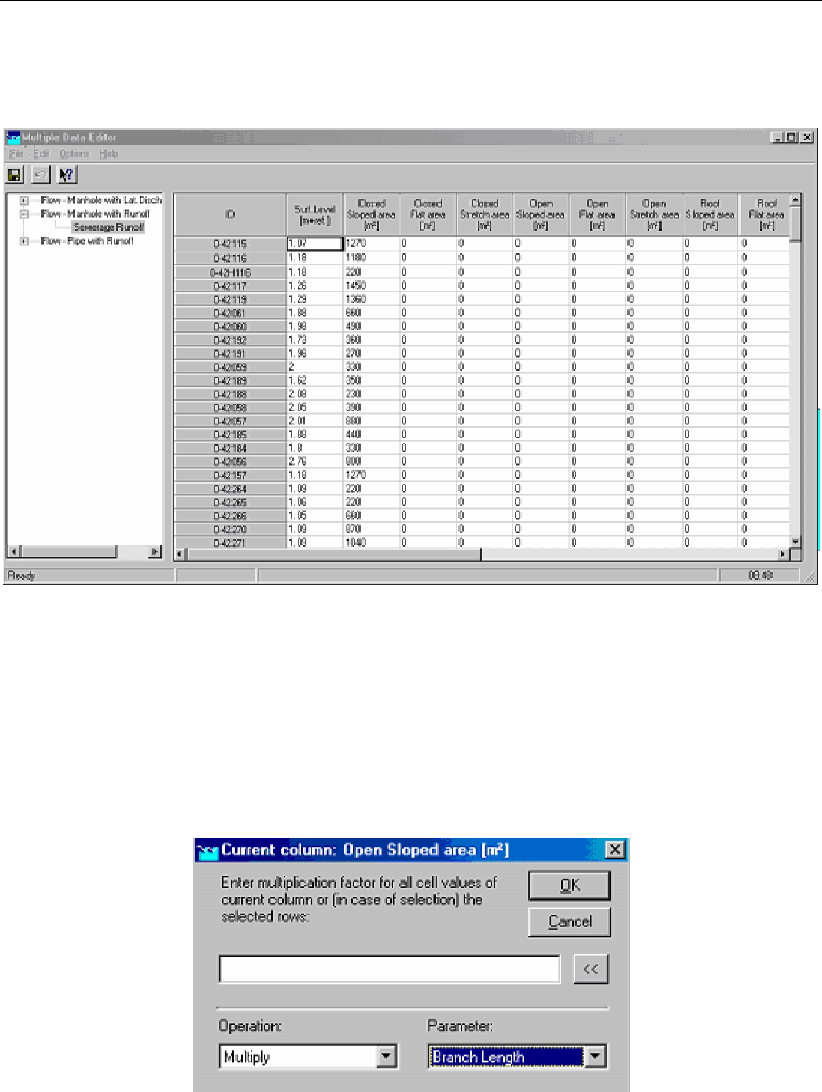
DRAFT
Graphical User Interface
pipe with the actual pipe length. This option is available by using the right mouse button menu
after selecting a column. Also, the option to import data from a database has been added.
Figure 5.58: The multiple data editor.
The following edit options are possible:
Change individually;
Select a whole column, use the right mouse button, several options are available(Add,
Multiply, Replace);
Figure 5.59: Changing a whole column in the multiple data editor.
Select a whole column, use the right mouse button, Import option to import a column from
a DBF file is available. After selecting the DBF file, the coupling of the id’s in the DBF file
to the SOBEK id’s, and the data column to be imported can be indicated in the following
screen. If the DBF contains multiple records for the same id, the data of all records with
the same id can be added together using the switch ’Add all occurences together’.
Deltares 191 of 900
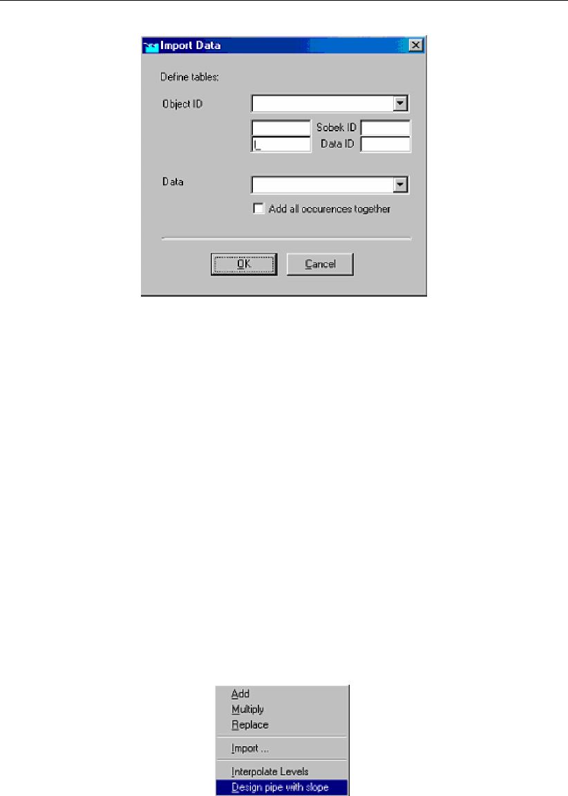
DRAFT
SOBEK, User Manual
Figure 5.60: Importing data in the multiple data editor.
Select a whole column, use the right mouse button, Distribute Catchment option. The
specified catchment will be distributed over the runoff area. If it concerns pipes with runoff,
the distribution will be according to pipe length. If it concerns manhole, the distribution will
be proportionally (all manholes with the same runoff area).
When selecting Flow - pipes, there are also options to interpolate the pipe levels between
the first and the last selected row, or to design the pipes with a fixed slope. In order to
apply this in a meaningful way, the pipe must be in logical sequence and all in the same
direction.
Not every object type is available for editing in the Multiple Data Editor. These objects
should be modified with the Single Data Editor.
Although friction for Y-Z and Asymmetrical Trapezium profiles may appear to be editable
by using the multiple data editor, this is not recommended. The friction concept that is
used in the Multiple Data Editor is the Local (or Branch-wise) friction concept. However,
Y-Z and Asymmetrical profiles make use of the so-called Cross-section friction concept.
This can cause the (Local type) friction value reported in the Multiple Data Editor to differ
from the (Cross-section type) friction value reported in the Single Data Editor for Y-Z and
Asymmetrical Trapezium profiles. See the chapter 1D Hydraulic friction concepts for more
information.
Basics of network editing
One of the first things to do when you start working with SOBEK is to create a network that
represents your water system. Whether it is a river, channel or sewer system, the principles
are the same: it will be a GIS-based network or grid. In this chapter the general concepts
behind editing your hydraulic model schematisation are explained.
1. Start SOBEK’s GIS environment (NETTER)
After you’ve opened or created a case, you’ll see the Case Management Tool (CMT), showing
eight different task-blocks that can be executed. Read more about the CMT in the chapter
192 of 900 Deltares
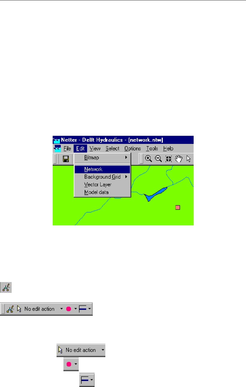
DRAFT
Graphical User Interface
Managing SOBEK projects and cases. If a task-block is yellow or green, it means that this
task is ready to be executed.
Make sure that the ’Schematisation’ task-block is ready to be executed;
Double click it;
Click the Edit model button on the window that appears. Now SOBEK’s GIS-environment
named NETTER is started.
2. Switch to the network editing mode
After entering SOBEK’s GIS environment under the "Schematisation" task block, one can
toggle between three modes:
The data-editing mode
The network-editing mode (discussed in this chapter)
The vector layer mode
Figure 5.61: Enter the network editing mode.
Choose ’Edit’ - ’Network’ to switch to the mode where you can adjust or create a schema-
tisation.
Switch to the network-editing mode by choosing ’Edit’ - ’network’ in the main menu or click the
button. You’ll see the following toolbar appearing:
3. Network editing toolbars
The toolbar shown above consists of three main sections:
an action section
a node type section
a connection type section
The philosophy behind it is as follows: when creating or editing a 1D hydraulic model, you
choose to perform an certain action that applies for a certain node type and/or a certain
connection type. So when performing edit actions, make sure you select the right node type
Deltares 193 of 900
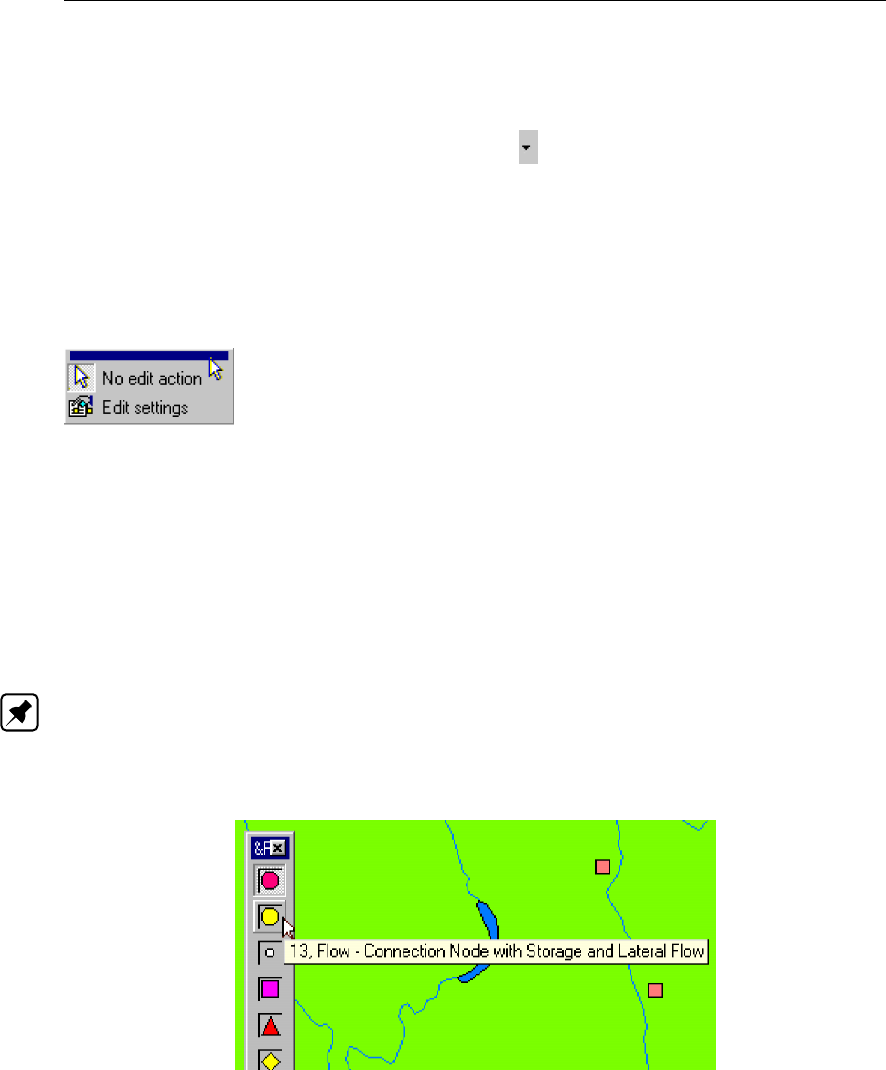
DRAFT
SOBEK, User Manual
(for instance a Flow-cross section) and the right connection type (for instance a Flow-branch
with lateral flow).
Each of the sections can be opened by clicking the button next to it.
Notice that all toolbars underneath can be dragged to your screen by clicking their blue line
on the top!
An example: you can drag the ’General’ toolbar, under the ’action’ section to your screen by
clicking it’s upper part, as shown below.
In a similar way, you can drag the ’node types’ toolbar to your screen. When moving with the
mouse over the different node types in that toolbar, it will then tell you which types they are.
Helpful hints for the user:
Add labels to the node types shown in the toolbar! If you have difficulty recognising the
various node- or branch types in the objects-toolbars, you can have their label shown:
’Choose ’View’ - ’Toolbars’ - ’Customise’ and select ’Icon and caption’ for node types
and/or branch types.
Note: In recent SOBEK versions, labels are enabled by default.
See what type of node is shown in the toolbar After you dragged the toolbar containing
node types to your screen, you can move over it with the mouse. The node type will then
be shown:
Figure 5.62: Mouse-over a node to show its label.
See what node type is shown in the "nodes" toolbar by moving over it (only after the toolbar
has been dragged to your screen)
ID’s of nodes and branches Object ID’s are directly used by the calculation core so users
should be very careful when modifying or manually setting such an ID.
It is recommended to let SOBEK pick the ID. Users should preferably use the name field to
add additional information about network objects. Although it is possible to use spaces in
object ID’s, this is not recommended. If the user wishes to manually set an ID, underscores
’_’ should be used instead of spaces. When using the Water Quality module, ID’s should
contain no more than 19 characters. See the water quality documentation for more details.
To get started creating a model schematisation, you can learn to: Create a branch, Curve a
194 of 900 Deltares

DRAFT
Graphical User Interface
branch, Place objects on a branch, or do one of the tutorials for Channel Flow, Sewer Flow or
Overland Flow
Save unique display settings for a specific type of output
After opening a certain type of results, you may customise the way in which they are plot-
ted, and save these settings for the next time. The procedure is best explained through an
example.
Example:
Say, that every time we open the results at branch segments we want them plotted in such a
way that:
All nodes are invisible
The flow direction will be shown by animated arrows
In order to do so, you will need to do the following
Open the Results at branch segments by clicking on it in the Active Legend
Uncheck the checkbox left from the category "Nodes" in the Active Legend
Click the button , in the right upper corner of the Active Legend to activate the "Set-
tings" menu.
Click the "links" tab and activate the options "all data" and after that: "arrow flow"
Click OK to leave the Settings menu.
Open the "Scale settings" window by clicking the "Network data" in the Active Legend.
Activate the checkbox left from the option ’save style’. With this option, you will save
the output ’style’ that belongs to "results at branch segments".
Click OK to leave the Scale settings window.
You can check it by first clicking the "Results at nodes" (which will restore the default settings
again) and then clicking the "Results at branch segments" again. The results will again be
shown in the way you had previously stored. You can load a series without a saved style/user
legend, the last style in use will then still be used.
5.2.7 Shortcuts to various menu options
You can click the header of each category to customise its settings. The headers provide a
shortcut to the corresponding menu options
Clicking Map will open the Map properties window. This will allow you to arrange, and
adjust the settings for the GIS layers that you use as a background in the schematisation.
Clicking Network Nodes will open the Node Settings window, which will allow you to
adjust the way (size, shape, colour) nodes are plotted in the main window. It also allows
you to select which node types should be visible, and which not.
Clicking Network Branches will open the Link Settings window, which will allow you to
adjust the way (size, colour) branches (branches and links) are plotted in the main window.
It also allows you to select which node types should be visible, and which not.
Clicking Network Data will open the Scale Settings window, which will allow you to cus-
tomise the scale and colours for the data legend.
Deltares 195 of 900

DRAFT
SOBEK, User Manual
5.2.8 The Active Legend
The active legend is an interactive legend, showing all objects and results that are available
within the GIS interface. The Active Legend can be customised entirely to the user’s wishes.
If the Active Legend is not yet visible in NETTER, it can be activated with the menu option
"Options" - "Active Legend".
Features of the Active Legend:
Gives Shortcuts to various menu options, such as the windows: Settings, Map Properties,
Node Settings, Link Settings and Scale settings
Allows you to save the display settings for each different type of output. For example: it
can remember that you want nodes to be invisible when viewing the results at branches.
This feature is explained further in this chapter.
Allows you to create a list with user defined output; shortcuts to simulation results that you
frequently view.
The following categories can be activated:
Simulation results (select the kind of computational re-
sults that should be opened)
Map layers (GIS layers for background plotting)
Network Nodes (shows the used node types in your
schematisation)
Network branches (shows the used branches and links
in your schematisation)
Network data (showing the legend of the results of a
simulation)
General usage of the Active Legend
With the check boxes , each category can be made visible or invisible in the main
window.
196 of 900 Deltares
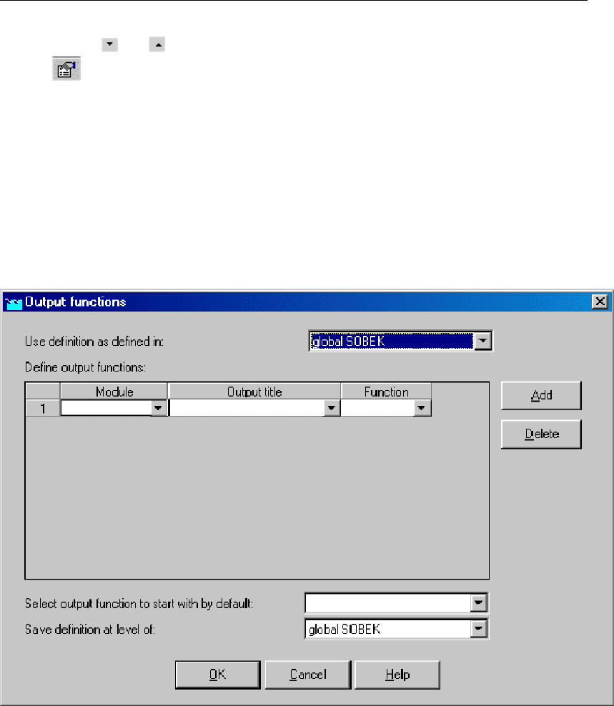
DRAFT
Graphical User Interface
Clicking the and buttons will respectively show and hide each category’s contents.
The button opens the Settings window, which allows you to plot labels next you the
objects of your choice. This button is a shortcut to the menu "Options" - "Network Data"
5.2.9 Create a list with user defined output
If there’s certain output that you often need to watch, you can make it accessible quicker in
the following way:
Open the NETTER menu option "Tools" - "Output options"
The Output functions window will pop up:
Figure 5.63: Output functions window
In this window, you can add the time series that you desire to access quickly every time
after a calculation. Use the fields "module" - "output title" and "function" to define a certain
time series.
Example:
Deltares 197 of 900
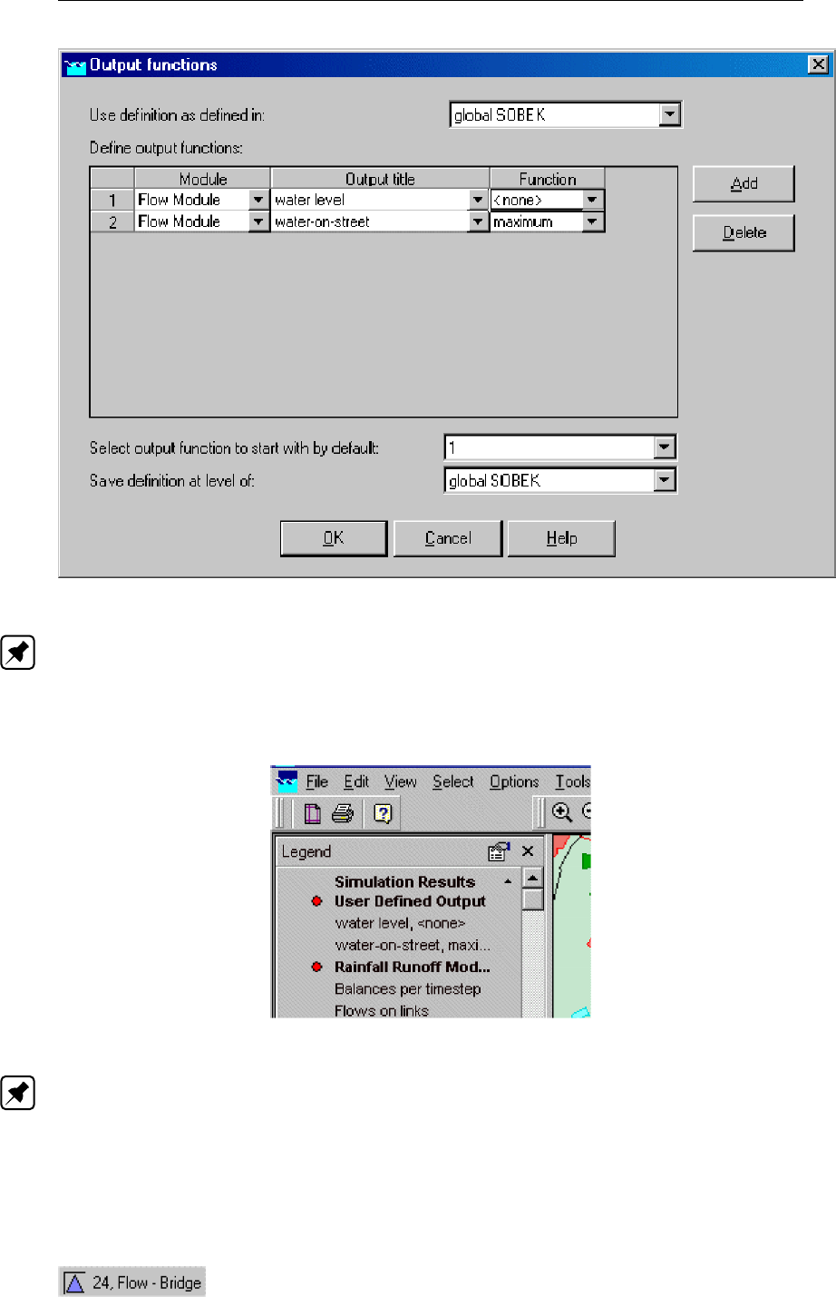
DRAFT
SOBEK, User Manual
Figure 5.64: Adding definitions in the Output functions window.
Note: If you choose <none>in the function field, all values that are available for all time
steps from the time series are taken. The other options speak for themselves.
After clicking OK the series that you’ve selected here, will become available under the
header "user defined output" in the Active Legend:
Figure 5.65: User defined output in the Active Legend.
Note: Also on these customised series, you can save your unique display settings, as
described in the chapter above!
5.3 Node description (hydrodynamics)
5.3.1 Flow - Bridge node
Description
198 of 900 Deltares

DRAFT
Graphical User Interface
In this chapter, the Flow - Bridge node type is described.
For a detailed description of this node’s input parameters: see the "Flow - Bridge node
input screens" section from the Reference Manual;
For a detailed description of this node’s possible network configurations: see the Flow -
Bridge node topology section from the Reference Manual
For a detailed description of this node’s underlying mathematical equations: see the
"Bridge section from the Technical Reference Manual".
With a Flow - Bridge node you can simulate four types of bridges:
Pillar bridge
Abutment bridge
Fixed bed bridge
Soil bed bridge
Input screens
When starting the model data editor for an Flow - Bridge node type, the following tabs will be
available for input:
Bridge:
Figure 5.66: The Bridge tab of a bridge.
A bridge of the type Pillar Bridge requires the following parameters:
Total pillar width (sum of the width of all pillars, perpendicular to the flow direction)
Deltares 199 of 900

DRAFT
SOBEK, User Manual
Shape factor
Possible flow direction
See the Technical Reference manual, ‘Bridge Section’ in order to see how these parameters
are used in the structure’s equations.
A bridge of the type Abutment bridge requires the following parameters:
Bed level
Length
Inlet loss coefficient
Outlet loss coefficient
Possible flow direction
A bridge of the type Fixed Bed Bridge requires the following parameters:
Bed level
Length
Inlet loss coefficient
Outlet loss coefficient
Possible flow direction
A bridge of the type Soil Bed Bridge requires the following parameters:
Bed level
Length
Inlet loss coefficient
Outlet loss coefficient
Possible flow direction
Ground layer depth (note: this parameter is defined on the Cross Section tab)
Below, all of the mentioned parameters will be discussed.
Bed level: Represents the bottom of the construction, in meters w.r.t. reference level.
Length: Represents the length (in the flow direction) of the bridge.
Inlet loss coefficient: Represents the energy loss of water that enters the bridge (through
contraction). See the "Bridge" section from the Technical Reference Manual to see how
this parameter is embedded in the structure’s equations.
Outlet loss coefficient: Represents the energy loss of water that leaves the bridge. See
the "Bridge" section from the Technical Reference Manual to see how this parameter is
embedded in the structure’s equations.
Possible flow direction: This parameter defines in which direction(s) water can flow
through the orifice. The directions are defined with relation to the defined branch direc-
tion. Positive means: in the same direction as the defined branch direction; negative
means: in the opposite direction than the defined branch direction. If you don’t know the
defined direction of the branch, read the Flow - Branch topology section of the Functional
Reference Manual.
Cross Section: (Note: Not available when bridge type "pillar" has been chosen)
200 of 900 Deltares
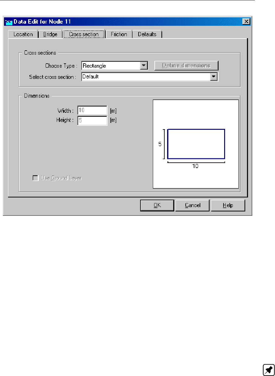
DRAFT
Graphical User Interface
Figure 5.67: The Cross section tab of a bridge.
On this tab the cross sectional shape of the culvert should be defined. This is done by means
of cross section definitions, very similar to the ones you define for the shape of a river bed.
The only real difference is that the number of cross section types is limited to two:
Table-form
Rectangle
For a detailed description of all available cross section types and their input parameter, see
the "Functional Reference Manual" - "Channel Flow module" - "Cross section types" section.
The ground layer option is available only for bridges of the type "Soil layer bridge". For that
type of bridges you can enter a ground layer depth, which represents a layer of sediment that’s
often present in structures. On the "Friction" tab, this layer can be given its own hydraulic
roughness value. Note: the option "use ground layer" should be switched on too!
Friction: (Note: Not available when bridge type "pillar" has been chosen)
Deltares 201 of 900
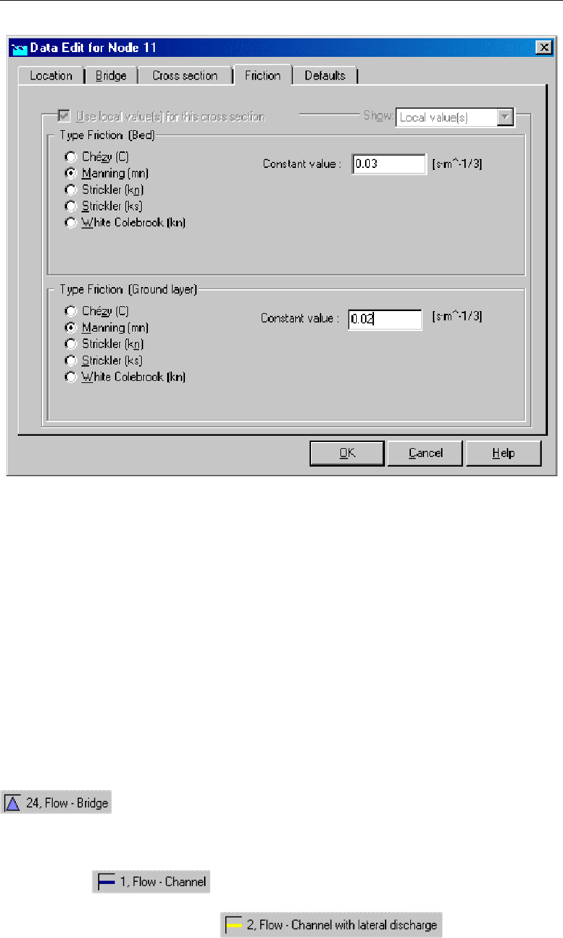
DRAFT
SOBEK, User Manual
Figure 5.68: The Friction tab of a bridge.
On this tab, the friction values for the bridge can be entered:
Type friction bed: This friction value represents the roughness of the bridge’s walls.
Thus, if the bridge is made of concrete, a proper hydraulic roughness value for concrete
should be entered.
Type friction ground layer: (only for bridge type "soil bed bridge")If the bridge type
"soil bed bridge" has been chosen and the "use ground layer option has been activated
on the "cross section" tab, this option becomes active. It represents the roughness value
of the ground layer that lays on the bottom of the bridge.
For more information about the various friction options, see the "Bed Friction" section from the
Technical Reference Manual.
Topology
Nodes of the type Flow - Bridge need to be attached to one of these branch types:
Flow Channel:
Flow Channel with lateral discharge
Add a Flow - Bridge node to your schematisation in the following way:
202 of 900 Deltares
DRAFT
Graphical User Interface
Select the appropriate node type (Flow Bridge)
Use the "add node" button to add it to the schematisation. When clicking, SOBEK
will automatically find the nearest channel to attach it to.
If desired, the node may later-on be moved to other locations on the branch, or even to
another branch by using the "move node" button.
Note: Before adding a bridge to your schematisation, you should have at least one of the
above Channel types present.
5.3.2 Flow - Calculation point
5.3.2.1 Flow - Calculation point (basic)
Description
This chapter describes the nodes of the type Flow Calculation Point, which all together form
the Calculation Grid or Computational Grid. The Flow - Calculation Point node type is one of
the most important nodes for hydrodynamic modelling as their presence determine the spatial
discretisation of the model area.
For the input options you have when creating a calculation grid: see the Flow - Calculation
grid input screens section from the Reference Manual;
For a detailed description of this node’s possible network configurations: see the "Flow -
Calculation point topology" section from the Reference Manual
For a detailed description of this node’s underlying mathematical equations: see the "Cal-
culation point section from the Technical Reference Manual".
The SOBEK Water Flow modules solve the model equations on this grid of ζ-calculation
points. For good model performance it is therefore important that these points are spaced
evenly. Therefore SOBEK has an option to generate the calculation grid automatically. This
can be done after the schematisation has been completed.
Flow - Calculation grid input screens
After you have chosen to create a calculation grid, by using the Set calculation grid branch or
Set calculation grid all branches buttons ( ), the following screen will appear:
Tab: General
Deltares 203 of 900
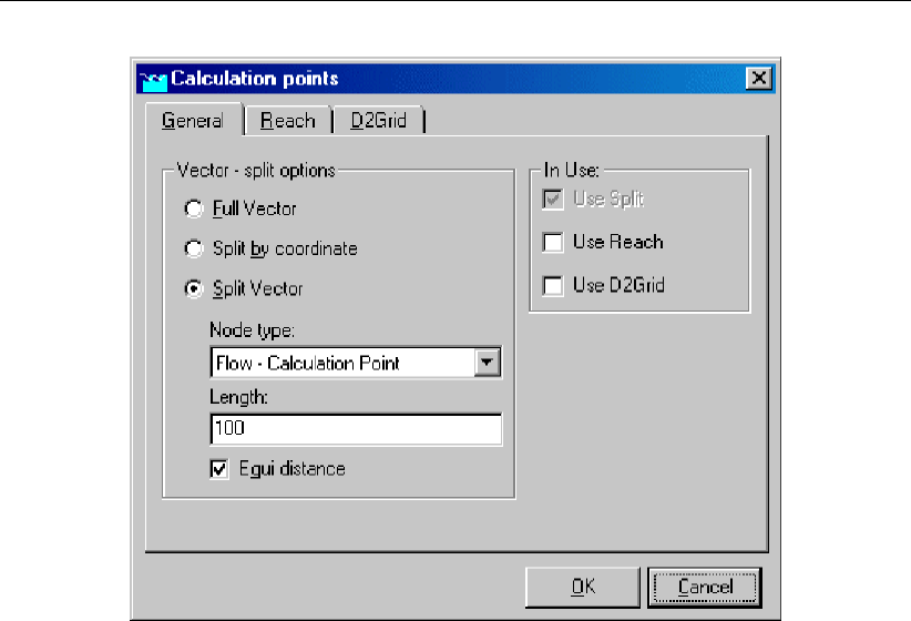
DRAFT
SOBEK, User Manual
Figure 5.69: Setting a calculation grid on all branches.
This tab will probably be the only one you will ever use. Here you can define how the
branch(es) should be divided into computational segments. The following options are avail-
able:
Full Vector: This option means: the branch will not be split up into computational seg-
ments. Therefore no calculation points will be added to the branch. You can also use this
option to remove calculation points from an existing branch.
Split by coordinate: When using this option, the branch will receive a ζ-calculation point
on every vertex. ’Vertex’ is a GIS term for all points on a line, that define its curves. For
example: a branch may run from node A to node B, but it may have some meanders.
These meanders are defined through vertices. These also determine the actual length of
the branch. You can manually remove or add such vertices to your SOBEK branch in the
Edit Vector Layer mode.
Length: This option will split the branch(es) into computational segments of a certain
length. It does so by adding ζ-calculation points.
Equidistance: Gives you a choice of what to do with the remaining lengths while creating
the ζ-calculation grid. Suppose that your branch has a length of 1 020 m. Setting a ζ-
calculation grid with a length of 100 m: Equidistance = off: this will result in ten branch
segments of each 100 m and one of 20 m. Equidistance = on: this will result in ten branch
segments of each 102 m.
In use: With these check boxes you can define whether the other tabs will also be used:
- Branch- 2DGridMore information about those tabs and their options is given below.
Tab Branch
204 of 900 Deltares
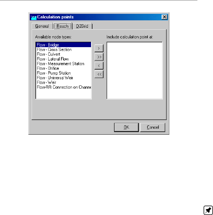
DRAFT
Graphical User Interface
Figure 5.70: The Branch tab of the Calculation points window.
On this tab, you can select what type of objects you want to use as a ζ-calculation point
(besides their original purpose). When a certain node type has been selected, it will keep its
original purpose, but in addition it will work as a ζ-calculation point and will show water levels
in the simulation results. Select the node types with the >and buttons.
Do not forget to activate the "Branch" checkbox on the "General" tab. Otherwise this option
will not be active!
Important Note: If you select a node type that’s usually invisible in the "Results in Maps"
mode (for instance the Flow - Cross Section node type), you’ll have to make it visible first in
order to view the results on these nodes.
Tab 2D Grid:
Deltares 205 of 900
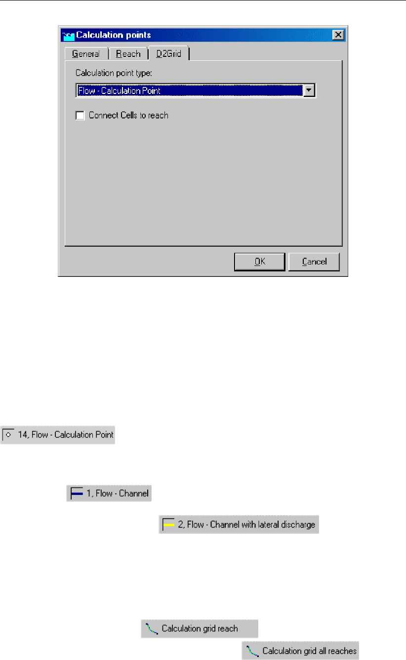
DRAFT
SOBEK, User Manual
Figure 5.71: The 2D Grid tab of the Calculation points window.
This tab is necessary to couple a 1D branch with a 2D grid. When the option "Connect Cells
to branch" is activated, for every 2D grid cell that the 1D branch crosses, a ζ-calculation point
is created and linked with the ζ-calculation point of that particular cell.
Do not forget to activate the "2DGrid" checkbox on the "General" tab. Otherwise this option
will not be active!
Topology
Nodes of the type Flow - Calculation point need to be attached to one of these branch types:
Flow Channel:
Flow Channel with lateral discharge
Unlike structure and cross section nodes, ζ-calculation points are usually not placed in a
schematisation one by one. SOBEK provides an option to automatically generate a grid of
ζ-calculation points for all branches or for one branch at a time:
Switch to the "edit network" mode in NETTER
Open the "Branch" toolbar and choose one of the following options: 1. click the button
<Calculation grid branch>and click on the desired branch.
2. click the button <Calculation grid all branches>
Choose an appropriate grid spacing distance. The best value depends on various things,
but to give you an impression: for most channel systems 50 to 100 meters is a good
value. For slow rivers that show little changes in bed shape and bed level 500 meters is
206 of 900 Deltares
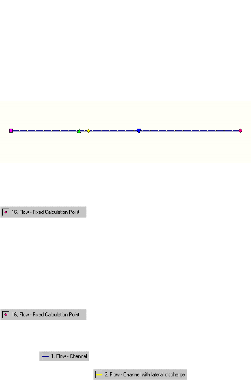
DRAFT
Graphical User Interface
appropriate. See the chapter: Flow - Calculation Grid input screens from the Functional
Reference Manual for a detailed information on the various options.
It is also possible to add calculation points manually. This may be desirable when two struc-
tures are located closely to each other. Between two structures or lateral discharges there
should always be a calculation point.
The image below shows an example of a valid schematisation that contains calculation points.
Notice that between the weir and the lateral discharge node at least one calculation point
should be present.
Figure 5.72: An example of a schematisation that contains calculation points.
5.3.2.2 Flow - Fixed Calculation point
Description
In this chapter, the Flow - Fixed Calculation Point is described.
This type of calculation point is equal to the normal calculation points, except that it will not
be automatically removed when you decide to re-generate a calculation grid. This might, for
example, be a useful feature for locations where you desire to compare measured water levels
with computed water levels.
For a detailed description of this node’s possible network configurations: see the "topol-
ogy" section from the Reference Manual
Topology
Nodes of the type Flow - Fixed Calculation Point need to be attached to one of these branch
types:
Flow Channel:
Flow Channel with lateral discharge
Add a Flow - Fixed Calculation Point node to your schematisation in the following way:
Select the appropriate node type (Flow - Fixed Calculation Point)
Deltares 207 of 900
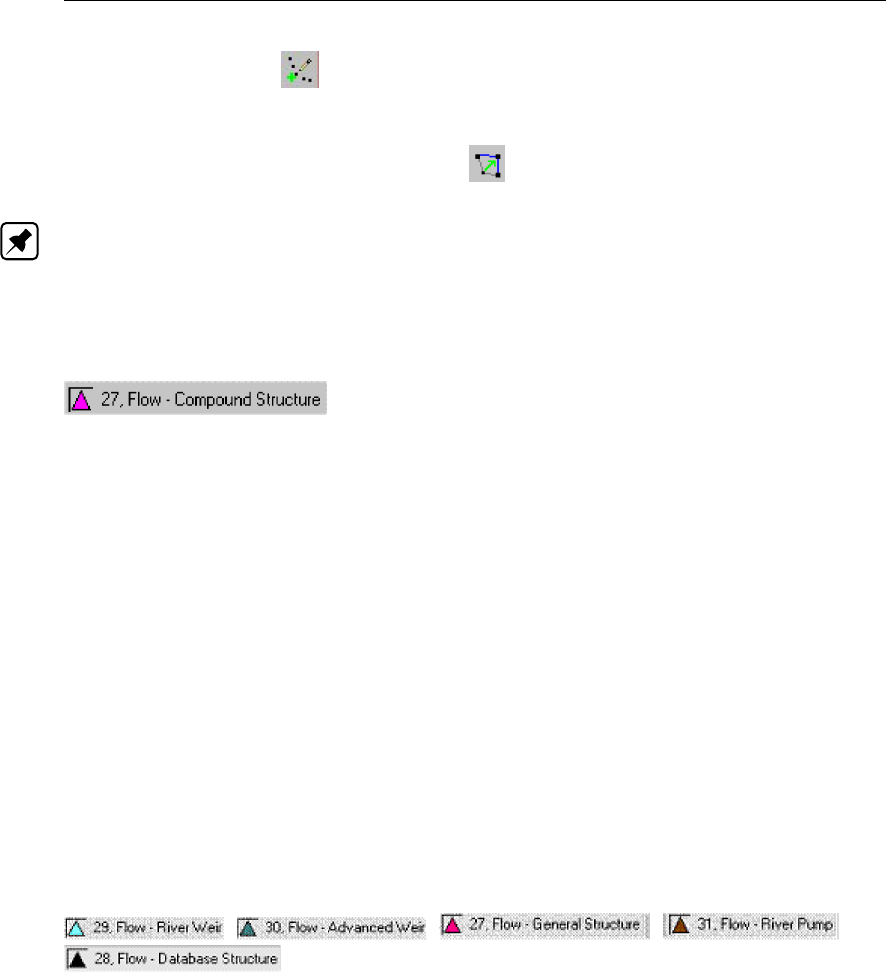
DRAFT
SOBEK, User Manual
Use the "add node" button to add it to the schematisation. When clicking, SOBEK
will automatically find the nearest channel to attach it to.
If desired, the node may later-on be moved to other locations on the branch, or even to
another branch by using the "move node" button.
Note: Before adding a structure to your schematisation, you should have at least one of the
above Channel types present in it.
5.3.3 Flow - Compound Structure
Description
This chapter describes the Flow - Compound Structure node type. A compound structure can
combine two or more different type of structures into one node. It considers these structures
to lay parallel to each-other within the same water course.
For a detailed description of this node’s input parameters: see the "Flow - Compound
Structure node input screens" section from the Technical Reference Manual;
For a detailed description of this node’s possible network configurations: see the "Flow -
Compound Structure node topology" section from the Technical Reference Manual
Structure types that can join in a Compound Structure node as a compound member are:
River Weir (discharge computed on basis of energy-levels)
Advanced weir (discharge computed on basis of energy levels)
General Structure (discharge computed on basis of energy-levels)
River Pump (discharge computed on basis of water levels)
Database Structure (discharge computed on basis of water levels)
Please note that the above structure types are also available as single structures (respectively:
; ; ; ; and
.
Input screens
When starting the model data editor for an Flow - Compound Structure node type, the follow-
ing tabs will be available for input:
Compound Structure Tab:
208 of 900 Deltares
DRAFT
Graphical User Interface
You can use the default value for structure inertia damping factor as defined in Setting, Tab
– numerical parameters, or you can define a value for structure inertia damping factor for
each compound structure member separately. For meaning of structure inertia damping
factor see Numerical parameter.
Under the "Member definitions" section, one can define the structures that become part
of the Compound Structure. Type a name of a new member in the field, and click on the
<Define>button. For explanation on the other sections of this tab, see the Functional
Reference Manual for the coresponding member as single structure.
All other tabs are identical to the tabs as for the coresponding member as single structure.
See that chapter in the Functional Reference Manual for a detailed explanation.
Definitions tab:
The definition tab will look differently, depending on the type of structure you are editing.
Please refer to the chapters named "input screens" in the "Reference Manual’ for the specific
structure types that you can edit there:
River Weir
Advanced weir
General Structure
River Pump
Database Structure
Controllers & Triggers tabs:
see section 5.8.
Topology
Deltares 209 of 900
DRAFT
SOBEK, User Manual
Figure 5.73: Branches connected to Flow connection nodes
Nodes of the type Flow - Compound Structure need to be attached to one of these branch
types:
Flow Channel:
Flow Channel with lateral discharge
Add a Flow - Compound Structure node to your schematisation in the following way:
Select the appropriate node type (Flow - Compound Structure)
Use the "add node" button to add it to the schematisation. When clicking, SOBEK
will automatically find the nearest channel to attach it to.
If desired, the node may later-on be moved to other locations on the branch, or even to
another branch by using the "move node" button.
Note:
1. Before adding a compound structure to your schematisation, you should have at least one
of the above Channel types present in it.
2. SOBEK by default places a computational point 0.5 m upstream and 0.5 m downstream
of the compound structure location. Hence the compound structure is default located on a
branch having a length of 1 m.
5.3.4 Different types of Flow - Connection nodes
The following types of Flow - Connection nodes are available:
Flow - Connection node
Flow - Connection node with Lateral Flow
Flow - Connection node with Storage and Lateral Flow
For each type of connection node yields that one or more branches can be connected to each
other (see Figure 5.73). A connected branch might either a pipe or a Flow - Channel.
210 of 900 Deltares
DRAFT
Graphical User Interface
Figure 5.74: Interpolating data over Branch 1 and 2 at a Flow - Connection Node
5.3.4.1 Flow - Connection node
At a Flow - Connection node it is possible to interpolate data (see definition and restrictions
hereafter) between two adjacent Flow – Channels. For these two Flow - Channels should yield
that one ends at (i.e. the so-called First Branch), while the one starts from (i.e. the so-called
Second Branch) the concerning “Flow - Connection node” (see Figure 5.74).
A left mouse click on a Flow - Connection Node opens the Data Edit for Node Form. In a
scroll box you can define here the branches for which data is to be interpolated over the Flow
- Connection Node.
Definition of data interpolation over a Flow - Connection Node
For the open channel part from cross-section R1_Crs_A to cross-section R2_Crs_B (see
Figure 5.74), interpolating data over the Flow - Connection Node means:
Bathymetrical data:
The bathymetry of the cross-section at the Flow – Connection Node is obtained by linear
interpolation between the nearest cross-section on the “First Branch” (e.g. R1_Crs_A and
the nearest cross-section on “Second Branch” (e.g. R2_Crs_B). In hydraulic calculations,
this interpolated cross-section is respectively placed at the end of the “First Branch” and
at the beginning of the “Second Branch”.
Friction data
Interpolation of friction data for “Y-Z” and “Asymmetrical Trapezium” profiles only.
For Y-Z and Asymmetrical Trapezium profiles yields that friction is defined per cross-
section. Firstly, for each cross-section a conveyance table is constructed on basis
of its defined roughness and cross-sectional profile. For each h- and u-point lying
in between two cross-sections, a tabulated type of cross-sectional profile is obtained
by linear interpolation. For each u-point, conveyance tables are obtained by linear
interpolating between the conveyance tables available at its adjacent cross-sections.
No interpolation of friction data for profiles that are not Y-Z and Asymmetrical Trapez-
Deltares 211 of 900
DRAFT
SOBEK, User Manual
ium profiles. For profiles other than Y-Z and Asymmetrical Trapezium profiles, the
friction applied for the interpolated cross-section located at the “First Branch” and the
“Second Branch” are respectively obtained from the user-defined friction at the “First
Branch” and the “Second Branch”.
Diffusive lateral discharges:
Data with respect to diffusive lateral inflows is not interpolated over a “Flow - Connection
node”.
Restrictions for data interpolation over a Flow - Connection Node:
Table 5.4 in section 5.6.1 provides an overview of the various available different types of cross-
sections. Cross-section types that may lay on the same branch are given in Table 5.3. With
respect to data interpolation over a Flow - Connection Node yields that interpolation is only
allowed between cross-sections that may lay on the same channel branch (see Table 5.3).
5.3.4.2 Flow - Connection node with Lateral Flow
Description
Definition and Restrictions for data interpolation over a Flow - Connection Node with
Lateral Flow:
AFlow - Connection Node with Lateral Flow has the same functionality with respect to inter-
polating cross-sections as a Flow - Connection Node. For more information reference is made
to section 5.3.4.1.
AFlow - Connection Node with Lateral Flow has the same lateral flow functionalities as a
Flow - Connection Node with Storage and Lateral Flow. No storage is, however, availabe at a
Flow - Connection Node with Lateral Flow. For the flow functionalities of a Flow - Connection
Node with Lateral Flow reference is made to section 5.3.4.3.
5.3.4.3 Flow - Connection node with Storage and Lateral Flow
Description
In this chapter, the Flow - Connection node with storage and lateral flow is described.
For a detailed description of this node’s input parameters: see the "Flow - Connection node
with Storage and Lateral Flow node input screens" section from the Reference Manual;
For a detailed description of this node’s possible network configurations: see the "Flow -
Connection node topology" section from the Reference Manual
Definition and Restrictions for data interpolation over a Flow - Connection Node with
Storage and Lateral Flow:
AFlow - Connection Node with Storage and Lateral Flow has the same functionality with
respect to interpolating cross-sections as a Flow - Connection Node. For more information
reference is made to section 5.3.4.1.
This type of node is very similar to the normal Flow - Connection node, apart from the fact
that it has some extra features:
212 of 900 Deltares

DRAFT
Graphical User Interface
It gives the opportunity to add lateral discharge. This option is often used to submit known
discharges from industry or smaller rivers that have not been included in the schematisa-
tion.
It can bear additional storage area. This option is often used to include the area that is
represented by small water courses which have not been included as Flow - Branches in
the schematisation. For non-stationary simulations, the storage capacity of such smaller
watercourses may be of importance.
Location of Lateral Flow:
The location of the lateral inflow or lateral outflow coincides with the location of the Flow -
Connection Node with Storage and Lateral Flow.
Input screens
When starting the model data editor for a Flow - Connection node with Storage and Lateral
Flow type, the following tabs will be available for input:
Bottom Level:
Figure 5.75: The Bottom level tab of a Flow - Connection node with Storage and Lateral
Flow.
On this tab, the storage capacity of the node should be entered.
Bed Level: Represents the level where the additional storage area starts. This may be
higher than the bed level of the channel itself. For example: if the storage on this node
should represent small watercourses that are connected to the main channel, the bed
level of those watercourses should be entered here: not the bed level of the main channel.
Deltares 213 of 900

DRAFT
SOBEK, User Manual
Storage Area: Here, the storage area for this node should be entered. For example: if the
storage capacity of this node should represent a secondary ditch of 200 m long and 2 m
wide that has not been schematised as a branch, the area should be 400 m2.Optionally,
the storage area can be entered as a function of level. Use the option "variable" to do so.
Lateral Flow:
Figure 5.76: The Lateral flow tab of a Flow - Connection node with Storage and Lateral
Flow.
On this tab, the lateral inflow can be entered. It gives three options:
Constant: Use this option if a constant amount of water flows into or out of the model.
(plus = in, minus = out)
5.3.5 Flow - Cross Section
Description
In this chapter, the Flow - Cross Section node is described. This is one of the most important
node types when creating a hydrodynamic model. It defines the dimensions of the channel-
s/rivers that you want to model.
For a detailed description of this node’s input parameters: see the "Flow - Cross Section
node input screens" section from the Reference Manual;
214 of 900 Deltares
DRAFT
Graphical User Interface
For a detailed description of this node’s possible network configurations: see the "Flow -
Cross section node topology" section from the Reference Manual
For a detailed description of this node’s underlying mathematical equations and the ap-
plied interpolation methods, see the "Cross Section" section from the Technical Reference
Manual".
The discharges through a river or channel are greatly determined by the shape of the river
bed. To obtain a proper schematisation, it is therefore important to supply it with a sufficient
amount of cross section data. This is done by adding nodes of the Flow - Cross Section node
type to the schematisation.
From the cross section data, the bed levels and hydraulic radiuses are interpolated towards
the calculation points, for which every time step water levels are calculated.
Input screens
When starting the model data editor for an Flow - Cross Section node type, the following tabs
will be available for input:
Location:
Figure 5.77: The Location tab of a Flow - Cross Section node type.
On this tab, you can define the bed level and surface level for the particular cross section.
Bed level or cross-section level shift: For some cross-sections a bed level, or lowest
point of the cross-section, can be entered. Examples of cross-sections with a bed level
are the Trapezium, Round and Egg-Shape types.For other cross-sections, a cross-section
Deltares 215 of 900
DRAFT
SOBEK, User Manual
level shift can be entered. The defined cross-section level shift is added to all the levels
defined in the cross-section definition. Examples of cross-sections with a cross-section
level shift are the Y-Z, River Profile and Tabulated types.
Surface level: The value you enter here represents the level of the embankments at this
cross section. This value will become visible in the results as follows: — in Sideview as
the green line — in results at nodes it will be used to calculate the freeboard. Note: In
the hydrodynamics calculations the value that you fill in for surface level will not be used.
Cross Section:
Figure 5.78: The Cross section tab of a Flow - Cross Section node of the Y-Z Profile type.
On this tab, you should define the shape of the cross section. Notice you should first type
a name for the cross section shape that you want to define. Then later this shape can be
re-used on other Flow - Cross Section nodes! This prevents double work.
Select Cross Section: If you had already created several cross section definitions for
the chosen type, you can choose one here. If not, you can define a cross section shape
by typing a name in this field and clicking the <Define Dimensions>button.Dependent
on the cross section type you chose, various buttons will become active where you can
define the shape of the cross section. For each type of cross section, a separate chapter
is available in the "Functional Reference Manual" - "Channel Flow module" - "Flow - Cross
section node" section: - Trapezium type- Round type- Egg-shape type- Tabulated type-
Rectangle type- Y-Z profile type- Trapezium type- Asymmetrical trapezium type- Elliptical
type- Arch type- Cunette type- Steel cunette type
216 of 900 Deltares
DRAFT
Graphical User Interface
Friction:
Three different friction input screens are available when using the model data editor.
Figure 5.79: Y-Z and Asymmetrical Trapezium friction input screen.
Deltares 217 of 900
DRAFT
SOBEK, User Manual
Figure 5.80: River profile friction input screen.
218 of 900 Deltares
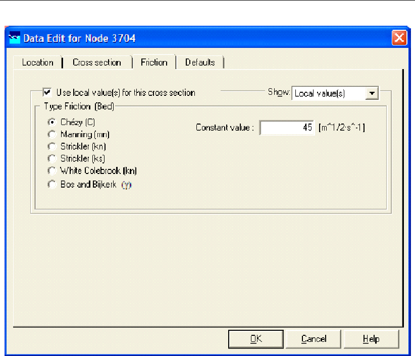
DRAFT
Graphical User Interface
Figure 5.81: Friction input screen for the remaining profile types.
For all cross-sections except Y-Z and Asymmetrical Trapezium profiles, the friction value that
you define will count for the entire branch on which it is located. For every branch, therefore
only the friction value of one of its cross sections needs to be edited.
For the Y-Z and Asymmetrical Trapezium profiles it is possible to define different friction val-
ues per cross-section lying on a branch. For river profiles it is possible to define friction as
f(x),f(h, x)and f(Q, x). More information is available in the chapter 1D hydraulic friction
concepts.
Use local value for this cross section You have the opportunity to choose between a
local friction value or a global friction value for the cross section. Global means that you
have a global (or model-wide)friction value that will apply to all branches for which you did
not define "use local friction values for this cross-section". To edit and apply the global
value, do the following:
switch off the "use local value" checkbox
select in the "Show:" combo box "Global value(s)".
Change the friction value according to your wishes.
Note that if you change the global value, the friction value for all branches that refer to this
value is changed too!To edit and apply the local value, do the following:
switch on the "use local value" checkbox
select in the "Show" combo box "Local value(s)"
Change the friction value according to your wishes.
Type friction: Various friction formulas are available. Choose the one of your wishes.
Deltares 219 of 900
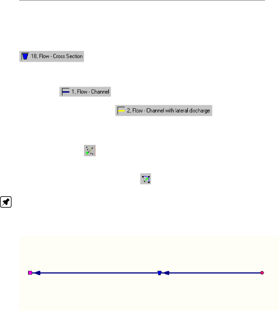
DRAFT
SOBEK, User Manual
More information about the various friction types is available in the "Bed Friction" section
from the Technical Reference Manual.
Topology
Nodes of the type Flow - Cross Section need to be attached to one of these branch types:
Flow Channel:
Flow Channel with lateral discharge
Add a Flow - Cross Section node to your schematisation in the following way:
Select the appropriate node type (Flow Cross Section)
Use the "add node" button to add it to the schematisation. When clicking, SOBEK
will automatically find the nearest channel to attach it to.
If desired, the node may later-on be moved to other locations on the branch, or even to
another branch by using the "move node" button.
Note: Before adding a cross section to your schematisation, you should have at least one of
the above Channel types present in it.
Example of a valid network configuration containing a cross section:
Figure 5.82: Example of a valid network configuration containing a cross section.
220 of 900 Deltares
DRAFT
Graphical User Interface
5.3.6 Flow - Culvert node
Description
In this chapter, the Flow - Culvert node is described.
For a detailed description of this node’s input parameters: see the "Flow - Culvert node
input screens" section from the Reference Manual;
For a detailed description of this node’s possible network configurations: see the "Flow -
Culvert node topology" section from the Reference Manual
For a detailed description of this node’s underlying mathematical equations: see the "Cul-
vert section from the Technical Reference Manual".
Definition of a culvert:
A culvert is a sleeve-shaped structure (with usually a freely moving water level) which con-
nects two water courses with each other (Dutch Hydrological Society,2002).
In SOBEK, a culvert can be modelled by a Flow - Culvert node. For this node, a cross section,
bed levels on both sides, length and some other parameters should be defined.
Note: It is best to use this node type only for rather short culverts (up to several tens of
meters). If you would model a long culvert with this node type, the amount of storage in your
water system would be over-estimated. The reason is that adding a Flow - Culvert node does
not automatically reduce the storage capacity on the branch according to the culvert’s length.
The branch will still assume that its cross sections remain valid over the entire branch; which
is not the case because you just added a long culvert. So in case of a long culvert, where the
storage capacity of the channel/river is an important factor, it is best to simulate it by creating
a branch of its length and applying cross section to it that’s equal to the culvert’s dimensions.
Input screens
When starting the model data editor for an Flow - Culvert node type, the following tabs will be
available for input:
Culvert:
Deltares 221 of 900

DRAFT
SOBEK, User Manual
Figure 5.83: The Culvert tab of a Flow - Culvert node.
On this tab, the general dimensions of the culvert can be defined:
Type: Here you can choose what kind of culvert it will be:- Culvert- Syphon- Inverted
Syphon
Bed level: These parameters define the bed levels of both sides (upstream and down-
stream) of the culvert.Left means: the "upstream" side with relation to the defined branch
direction.Right means: the "downstream" side with relation to the defined branch direction.
Length: This parameter defines the length of the culvert. See the "Culvert" section from
the Technical Reference Manual for more details on the application of this parameter within
the structure equations.
Inlet loss coefficient: This parameter represents the energy loss due to the contraction
of the water when it has to enter the culvert. See the "Culvert" section from the Technical
Reference Manual for more details on the application of this parameter within the structure
equations.
Outlet loss coefficient: This parameter represents the energy loss of water when it
leaves the culvert. See the "Culvert" section from the Technical Reference Manual for
more details on the application of this parameter within the structure equations.
Valve: If the culvert also includes an internal valve, this option should be switched on.
Then also the tab "Controller" will become active. The valve should have an initial opening
height for the first time step of the simulation. For every next time step, the defined con-
troller will operate the valve. In the table for "Loss coefficients", an energy loss factor has
to be defined for various opening heights.
Possible flow direction: This parameter defines in which direction(s) water can flow
through the orifice. The directions are defined with relation to the defined branch direc-
tion. Positive means: in the same direction as the defined branch direction; negative
222 of 900 Deltares

DRAFT
Graphical User Interface
means: in the opposite direction than the defined branch direction. If you don’t know the
defined direction of the branch, read the Flow - Branch topology section of the Functional
Reference Manual.
Cross Section:
Figure 5.84: The Cross section tab of a Flow - Culvert node.
On this tab the cross sectional shape of the culvert should be defined. This is done by means
of cross section definitions, very similar to the ones you define for the shape of a river bed.
The only real difference is that the number of cross section types is limited to eight:
Round
Egg-shape
Table-form
Rectangle
Elliptical
Arch
Cunette
Steel cunette
For a detailed description of all available cross section types and their input parameter, see
the "Functional Reference Manual" - "Channel Flow module" - "Cross section types" section.
Friction:
Deltares 223 of 900
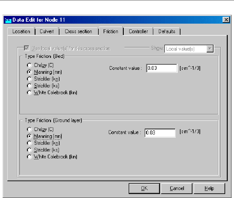
DRAFT
SOBEK, User Manual
Figure 5.85: The Friction tab of a Flow - Culvert node.
On this tab, the friction values for the culvert can be entered:
Type friction (bed):This friction value represents the roughness of the culvert’s walls.
Thus, if the culvert is made of concrete, a proper hydraulic roughness value for concrete
should be entered.
Type friction (ground layer):If the option "use ground layer" had been activated on the
"cross section" tab, this option becomes active. It represents the roughness value of the
ground layer that lays on the bottom of the culvert.
For more information about the various friction options, see the "Bed Friction" section from the
Technical Reference Manual.
Controller:
224 of 900 Deltares
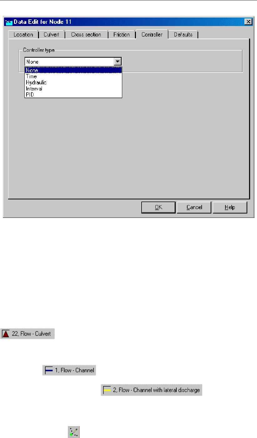
DRAFT
Graphical User Interface
Figure 5.86: The Controller tab of a Flow - Culvert node.
This option is only activated when the "valve" option on the "Culvert" tab has been switched
on. The valve can be operated by a controller. A controller will overrule your general settings
for the valve’s opening height and apply the chosen controlling rules to it. Read more about
them in the Controller section of the Technical Reference Manual.
Note that three of the four available controller options only become available after you have
defined a Flow - Measurement station within the schematisation and saved that schematisa-
tion.
Topology
Nodes of the type Flow - Culvert need to be attached to one of these branch types:
Flow Channel:
Flow Channel with lateral discharge
Add a Flow - Culvert node to your schematisation in the following way:
Select the appropriate node type (Flow Culvert)
Use the "add node" button to add it to the schematisation. When clicking, SOBEK
will automatically find the nearest channel to attach it to.
Deltares 225 of 900
DRAFT
SOBEK, User Manual
If desired, the node may later-on be moved to other locations on the branch, or even to
another branch by using the "move node" button.
Note: Before adding a culvert to your schematisation, you should have at least one of the
above Channel types present.
5.3.7 Flow - Database structure
Description
World-wide various different types of weirs have been constructed in rivers and channels.
Although the most common types of weirs are available in SOBEK, definitely not all type of
weirs (e.g. crump weir) are available in SOBEK. For this reason the Flow-Database structure
was implemented in SOBEK.
Crest levels of a Flow-Database structure cannot vary in height along the weir. The discharge
over any structure can be defined as a relationship between upstream and downstream water
level. The Database structure allows you to define this relationship is in a tabulated form
(e.g. database). For more information on how discharges are computed from a user-defined
database, reference is made to section 6.1.16.5.
Although not advised (see section 6.1.16.5), the crest level of a Database structure can be
varied by a controller. A structure inertia damping factor (see Numerical parameters) can be
defined for each Database structure.
Input screens
When starting the model data editor for a Flow - Database structure node type, the following
tabs will be available for input:
Database structure tab:
226 of 900 Deltares

DRAFT
Graphical User Interface
Figure 5.87: The Database Structure tab of a Flow - Database structure node.
On this tab, you can select a previously defined structure definition. If there is no definition
available yet, go to the "definitions" tab first, to create one.
Also, you can select the controllers that apply to this structure. If there are no controllers
available to be selected yet, go to the "controller" tab first to create them.
You can use the default value for structure inertia damping factor as defined in Setting, Tab –
numerical parameters, or you can define a value for structure inertia damping factor for this
particular Database structure. For meaning of structure inertia damping factor see Numerical
parameters.
Definitions tab:
Deltares 227 of 900

DRAFT
SOBEK, User Manual
Figure 5.88: The Definitions tab of a Flow - Database structure node.
On this tab, you can define the properties of your database structure. Select an existing defi-
nition from the drop-down box or create one by typing an appropriate name in the "definition"
field and then clicking <Define>.
Then you can:
Define the crest level of the structure
Choose whether the discharge is a function of:
- difference between upstream water level & crest level and- difference between down-
stream water level & crest level or
- difference between upstream water level & crest level and- difference between upstream
& downstream water level
Create a table which contains the data for the type of function you chose. Click the Edit
button to open the "Structure database window"
228 of 900 Deltares
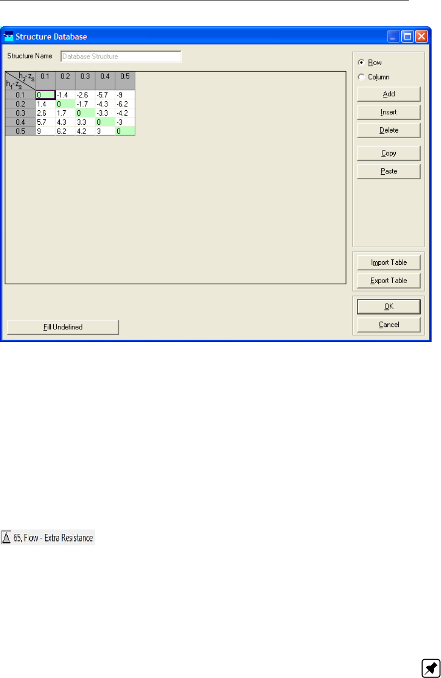
DRAFT
Graphical User Interface
Figure 5.89: The Structure Database window of a Flow - Database structure node.
You can add rows or columns by activating the "Row" or "Column" radio button respectively
and subsequently clicking <Add>. First you will be asked how many rows/columns you want
to add, then you will be asked to enter the row/column titles (values) one by one.Note that the
title (value) of the first row and column should be equal!The table can be checked by clicking
the <Fill Undefined>button. If everything is fine, the OK button will become active.
Controllers & Triggers tabs: see section 5.8.
5.3.8 Flow - Extra Resistance
Description
Placing a Flow - Extra Resistance Node on a branch segment, means that an additional term
(describing the influence of the Extra Resistance) is added to the momentum equation, which
is solved for this specific branch segment (see section 6.1.1.2). More precisely, it means
that an additional water level difference is invoked over this branch segment equal to ξQ|Q|,
where ξis the Extra Resistance coefficient and Qthe discharge flowing through the branch
segment. The additional water level difference is added to the upstream located water level
point.
Note: In case of an Extra Resistance Node an additional term is added to the momentum
equation. For a structure located on a branch segment yields that the momentum equation
is replaced by the structure equation. Hence, an Extra Resistance can not be considered to
be a structure. Nevertheless, in the task blocks "Results in Maps" and "Results in Charts",
Deltares 229 of 900
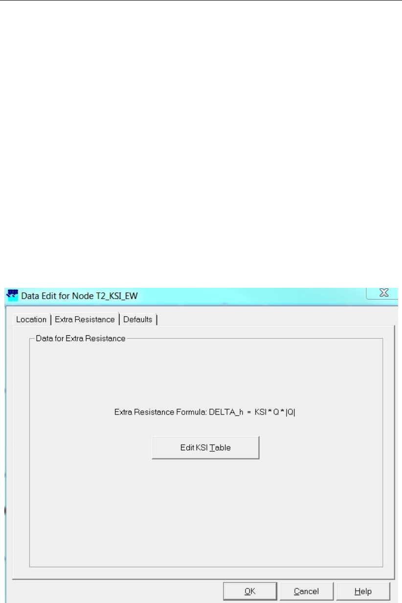
DRAFT
SOBEK, User Manual
the output of an Extra Resistance Node is provided under "Results at Structures and Extra
Resistances"’.
Following restrictions yields for Flow - Extra Resistance Nodes:
Flow - Extra Resistance Nodes are only allowed on a "Flow - Channel" and a "Flow -
Channel with lateral discharge".
Only 1 (one) Flow - Extra Resistance Node is allowed per branch segment
AFlow - Extra Resistance Node may not be located on a "Flow - Calculation point", a
"Flow - Fixed Calculation Point", a "Flow - Connection Node" and a "Flow - Boundary
Node.
AFlow - Extra Resistance Node may not be located on a branch segment adjacing a "Flow
- Boundary Node".
AFlow - Extra Resistance Node may not be located on a branch segment on which a
structure is located".
Input screens
Selecting a Flow - Extra Resistance Node and left mouse click opens the Extra Resistance
input screen (see Figure 5.90). Clicking on the <Edit KSI Table> button opens a table, where
Extra resistance coefficients (ξ) can be defined as function of water level (see Figure 5.91)
Figure 5.90: The Extra Resistance tab of a Flow - Extra Resistance node.
230 of 900 Deltares
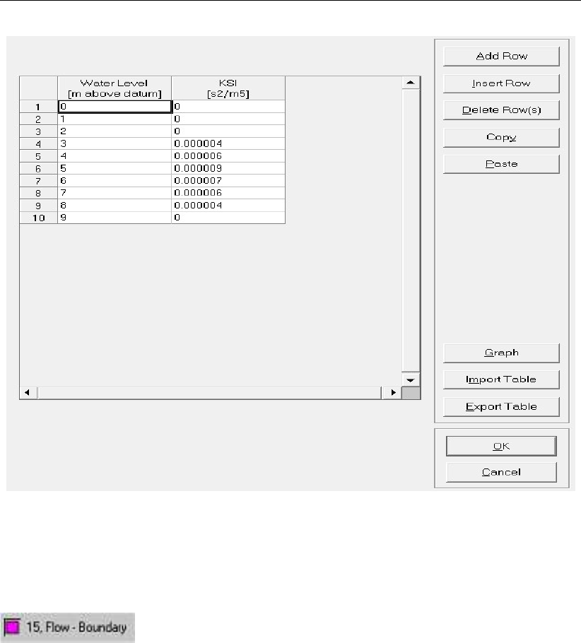
DRAFT
Graphical User Interface
Figure 5.91: Input Table for Extra Resistance coefficients of a Flow - Extra Resistance
node.
5.3.9 Flow - Boundary
Description
In this chapter, the Flow - Boundary node is described.
For a detailed description of this node’s input parameters: see the "Flow - Boundary node
input screens" section from the Reference Manual;
For a detailed description of this node’s possible network configurations: see the "Flow -
Boundary node topology" section from the Reference Manual
For a detailed description of this node’s underlying mathematical equations: see the
"Boundary section from the Technical Reference Manual".
Nodes of this type mark the outer edges of a hydraulic schematisation. In short, these nodes
represent the geographical locations where a model has been cut out of the real world. There-
fore their interaction with the world outside the model should be applied in terms of hydraulic
boundary conditions. The following options are available:
Flow boundary condition: the user submits a constant or alternating discharge that flows
into or out of the model (positive values mean in, negative mean out). Example: the
upstream edge of a river model where the model receives water from the upstream river
branches should be given such a condition;
Water Level boundary condition: the user submits a constant or alternating water level at
Deltares 231 of 900
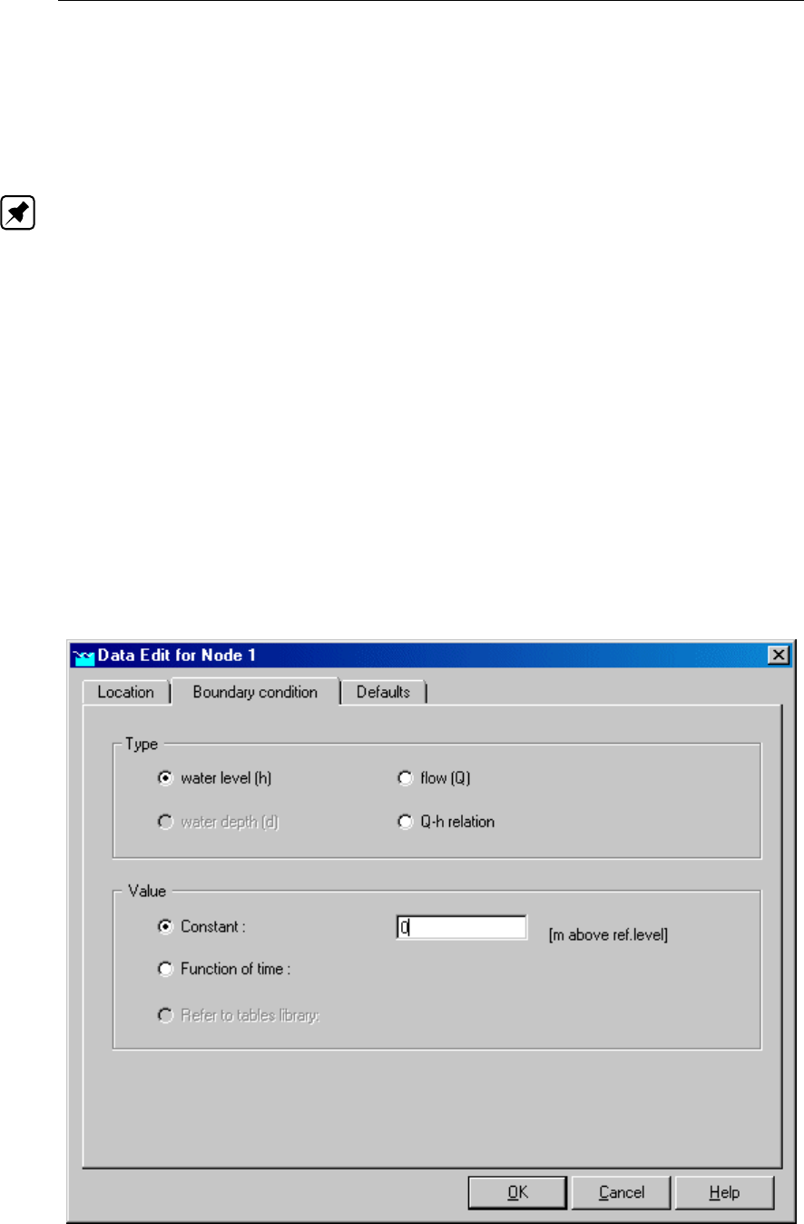
DRAFT
SOBEK, User Manual
the edge of the model’s area. Example: a river’s mouth, where tidal movement forms the
downstream boundary condition for the model;
A Q-H boundary condition: the user submits a relationship between water level and dis-
charge. This type of condition is commonly used on the downstream edge of a river
model.
Note:
1 one should always place his or her boundary nodes at a sufficient distance from the area
that is to be modelled. The flow conditions that you apply to artificial boundary conditions
should never be allowed to influence the hydraulic results in the area of interest!
2 In case more than one branch is connected to a 1D h-boundary node, only a water level
boundary can be defined at this particular boundary condition. Further on the user-defined
water level boundary condition is applied to each and every branch that is connected to
this particular water level boundary.
3 Commonly, nodes of the Flow - Connection node type are also used as boundary nodes
for hydraulic schematisation. This too is allowed, as these nodes are similar to Flow -
Boundary nodes with a Q = 0 boundary condition.
Input screens
When starting the model data editor for a Flow - Boundary node, the following tabs will be
available for input:
The Boundary condition tab:
Figure 5.92: The Boundary condition tab of a Flow - Boundary node.
232 of 900 Deltares

DRAFT
Graphical User Interface
On this tab, the following data can be entered:
A fixed or alternating water level as boundary condition By choosing the type "water
level (h)", the user can apply a fixed or alternating water level as a hydraulic boundary
condition to this node. This type of boundary condition is commonly used on the down-
stream edges of river models that end in a lake or sea. The option "Function of time" can
be used when the water levels at the downstream boundary alter in time (i.e. tidal waves)
More information about the tables for alternating boundary conditions can be found in the
chapter section 5.13.4..
A fixed or alternating discharge as boundary condition By choosing the type "flow
(Q)" the user can apply a fixed or alternating discharge as a hydraulic boundary condition
to this node. This type of boundary condition is commonly used on upstream edges of
river models, as these receive a certain discharge from upstream branches.
Note: although it is also possible to apply a discharge-boundary to a downstream node,
we advice you NOT to do so.
The reason is rather simple: in reality the discharge through a downstream boundary is
affected by the water levels in the area of interest. By enforcing a downstream discharge,
this relationship is discarded, thus leading to fake results. On downstream nodes therefore
we recommend the usage of "water level" or "Q-H" boundary conditions.
More information about the tables for alternating boundary conditions can be found in the
chapter section 5.13.4..
A Q-H relation as boundary condition By choosing the type "Q-H relation", the user
can define how the water levels and discharge at the boundary are related. This type of
boundary condition is commonly used for downstream boundaries in river models, when
the downstream boundary node lies somewhere in the middle of a river.
The Q-H relationship consists of a table that relates water levels and discharges to each-
other. It is not easy to determine a proper Q-H relation for a river. Globally, there are two
ways to determine it: — measure it in the river — estimate it by calculating the hydraulic
radius at various water levels and applying the Chézy formula.
Topology
Nodes of the Flow - Boundary node type serve as the end- or starting point for a Flow - Branch
or a Sewer Pipe. Do not place nodes of this type just as loose objects in the schematisation
or on top of an existing branch. Flow Boundary nodes should always be part of a branch
themselves. A correct working method is:
Switch to the "edit network" mode in NETTER
Select the node type Flow - Boundary
Select the "add node" option
Place the node in the schematisation by clicking
Select the appropriate branch type (Flow Branch or Sewer Pipe)
Select the "connect nodes" option
Connect the boundary node that you just added to another node by clicking and dragging.
Some examples of valid methods to apply Flow-Boundary nodes:
Deltares 233 of 900

DRAFT
SOBEK, User Manual
Figure 5.93: Examples of valid configurations with Flow - Boundary nodes
Note: when you attach more than one Flow - Branch to one Flow - Boundary node, you
can only apply a water level boundary condition to it. The reason for this is that in case of
a discharge condition, it would not be clear how to divide the discharge over the connected
branches.
5.3.10 Flow - General Structure
Description
In this chapter, the Flow - General structure node is described. The general structure com-
bines weir and gate flow in one structure type. It offers you much freedom in defining geom-
etry and dimensions of the structure. Discharges through a general structure are computed
on basis of upstream and downstream energy levels. The crest level, crest width and gate
lower edge level [mAD] can be varied by a controller. A structure inertia damping factor (see
Numerical parameters) can be defined for each General structure.
For a detailed description of this node’s input parameters: see the "input screens" section
from the Reference Manual;
For a detailed description of this node’s possible network configurations: see the "topol-
ogy" section from the Reference Manual
For a detailed description of this node’s underlying mathematical equations: see the "Gen-
eral structure" section in the "Technical Reference Manual.
Input screens
When starting the model data editor for an Flow - General Structure node type, the following
tabs will be available for input:
234 of 900 Deltares
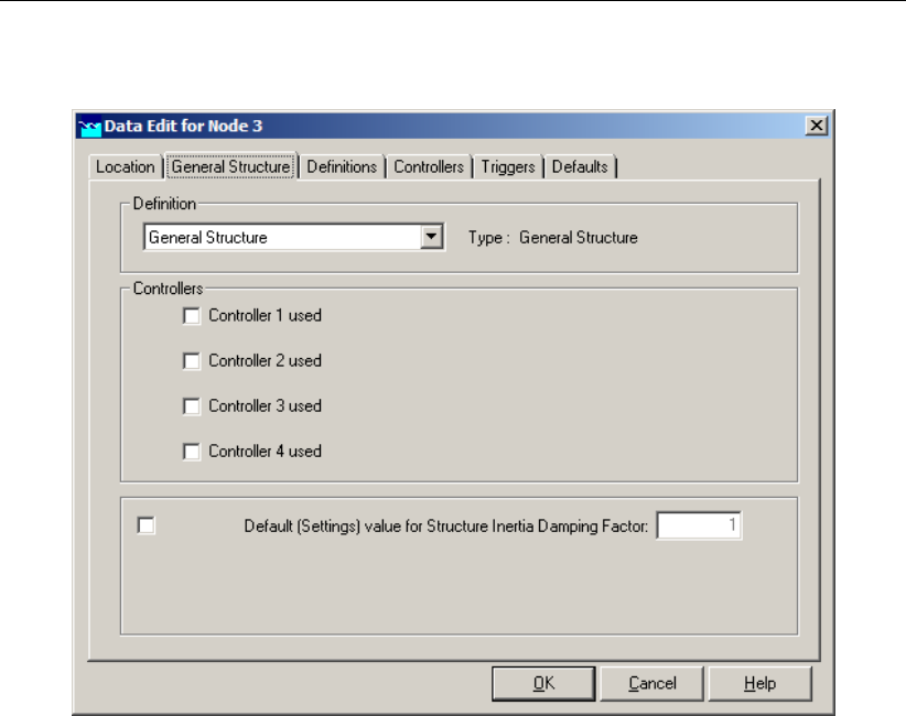
DRAFT
Graphical User Interface
General structure tab:
Figure 5.94: Data Edit window, General Structure tab
On this tab, you can select a previously defined structure definition. If there is no definition
available yet, go to the "definitions" tab first, to create one.
Also, you can select the controllers that apply to this structure. If there are no controllers
available to be selected yet, go to the "controller" tab first to create them.
You can use the defined value for structure inertia damping factor as defined in Setting, Tab
– numerical parameters, or you can define a value for structure inertia damping factor for this
particular General structure. For meaning of structure inertia damping factor see Numerical
parameters.
Definitions tab:
Deltares 235 of 900
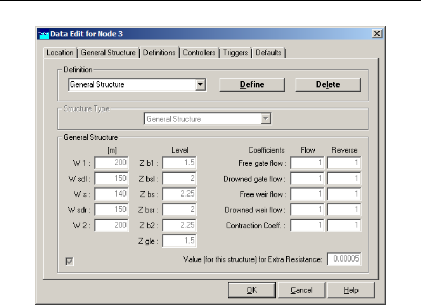
DRAFT
SOBEK, User Manual
Figure 5.95: Data Edit window, Definitions tab
You must enter five dimensions for the flow width along the structure, plus five bed elevations
and the gate lower edge level (Zgle) See for the use and meaning of each dimension see the
Technical Reference Manual, Flow modules, General Structure.
You can use the default value for Extra resistance as defined in Setting, Tab – numerical
parameters, or you can define a value for Extra resistance for this particular General structure.
For meaning of Extra resistance see Numerical parameters.
236 of 900 Deltares

DRAFT
Graphical User Interface
Figure 5.96: Cross-sectional view on general structure; definitions of vertical distances
Figure 5.97: Top view on general structure; definitions of width distances
Depending on the downstream water level free or drowned (submerged) flow can occur for
the weir or for the gate. For each of these conditions you must specify a reduction factor; if
you wish you can also enter values for the condition of reverse flow. The reduction factors
are used in the formulas given in the last part of the description in the Technical Reference
Manual.
Free gate flow cgf
Drowned gate flow cgd
Free weir flow cwf
Drowned weir flow cwd
Zgle Gate lower edge: the lower crest level of the gate.
Deltares 237 of 900

DRAFT
SOBEK, User Manual
The default value for each coefficient is 1.00. Finally you must enter a contraction coefficient
for gate flow.
Controllers & Triggers tabs: see section 5.8.
Topology
Nodes of the type Flow - General Structure need to be attached to one of these branch types:
Flow Channel:
Flow Channel with lateral discharge
Add a Flow - General Structure node to your schematisation in the following way:
Select the appropriate node type (Flow - General Structure)
Use the "add node" button to add it to the schematisation. When clicking, SOBEK will
automatically find the nearest channel to attach it to.
If desired, the node may later-on be moved to other locations on the branch, or even to
another branch by using the "move node" button.
Note:
1 Before adding a general structure to your schematisation, you should have at least one of
the above Channel types present in it.
2 SOBEK by default places a computational point 0.5 m upstream and 0.5 m downstream of
the general structure location. Hence the general structure is default located on a branch
having a length of 1 m.
5.3.11 Flow - Lateral Flow
Description
A "Flow - Lateral Flow Node" can be used to model the lateral inflow (positive values) of water
and/or the lateral outflow (negative values) of water in a branch. For how lateral discharges
are assigned to a particular calculation point, reference is made to section 6.1.11.2.
Input screens
When starting the model data editor for an Flow - Lateral Flow node type, the following tab
will be available for input:
238 of 900 Deltares
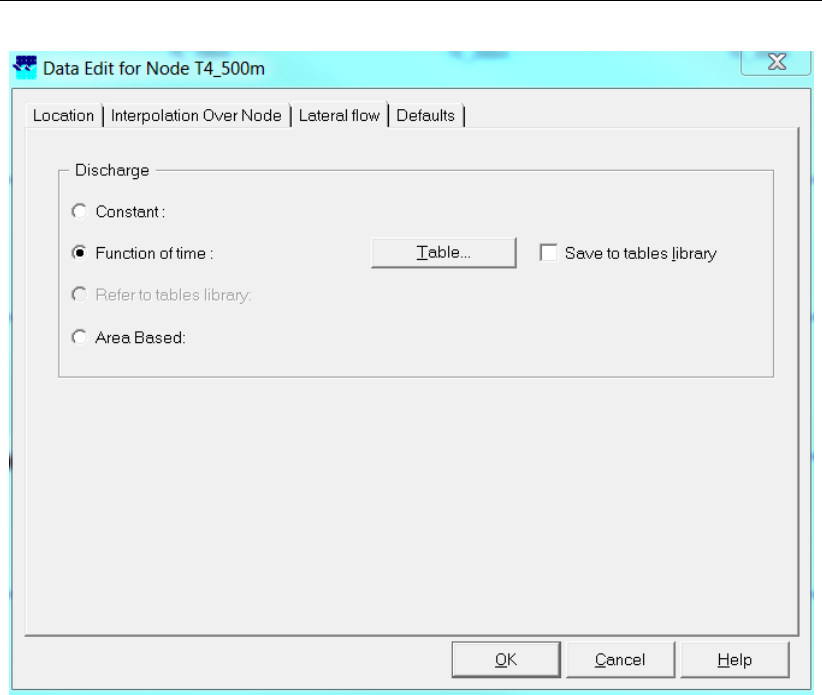
DRAFT
Graphical User Interface
Figure 5.98: Data Edit window, Lateral flow tab
Here, the lateral discharge can be specified.
Constant discharge When choosing this option, a constant lateral discharge is applied.
A positive value means inflow of water, a negative value means outflow of water.
Function of time Here a lateral inflow and or outflow as function of time can be specified.
Clicking the Table button opens a window like the one depicted below:
Deltares 239 of 900

DRAFT
SOBEK, User Manual
Figure 5.99: Change Table window
In this table, the modeller can submit lateral discharges as function of time. More in-
formation about the input options of such tables can be found in the following chapter:
section 5.13.4.
Area based method The Area based method calculates lateral discharges based on the
runoff area, design factor, rainfall, seepage and/or infiltration (see Equation (6.14)). When
choosing the Area based method, the input window looks like this:
240 of 900 Deltares
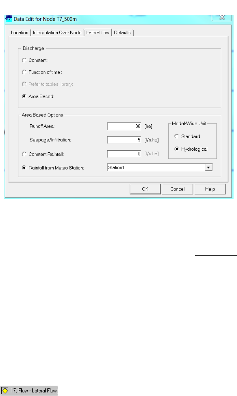
DRAFT
Graphical User Interface
Figure 5.100: Data Edit window, Lateral flow tab
Model-Wide Unit: Either Standard units or Hydrological units can be selected. In case
of Standard units: the runoff area is to be given in [square metres]; while seepage,
infiltration and constant rainfall are to be given in [milimetres/seconds]. In case of
Hydrological units: the runoff area is to be given in [hectares]; while seepage, infiltra-
tion and constant rainfall are to be given in [liters/second/hectares]. Please note that
selecting the option "Rainfall from Meteo Station" means that irrespective of the se-
lected unit (Standard or Hydrological), the unit of the rainfall equals the unit defined
for the concerning Meteo station. Please further note that changing the selected unit
(f.i. from Standard unit into Hydrological unit) at a specific "Flow - Lateral Flow Node",
means that you change the unit for all lateral flows in your entire model schematization
that are computed using the Area based method .
Runoff Area: represents the surface area of the catchment, that is assigned to the
Lateral Flow node. For the unit of runoff area, see item "Model-Wide unit" above.
Seepage/Infiltration: Only constant Seepage (positive value, inflow) or or constant Infil-
tration (negative value, outflow) can be defined. For the unit of seepage and infiltration,
see item "Model-Wide unit" above.
Constant Rainfall: Here you can define a constant rainfall. For the unit of constant
rainfall, see item "Model-Wide unit" above.
Rainfall from Meteo Station: Here you can define that the rainfall (including unit) from
a particular Meteo station, defined in the Meteorological Task Block, is to be used.
Topology
Nodes of the type Flow - Lateral Flow need to be attached to one of these branch types:
Deltares 241 of 900
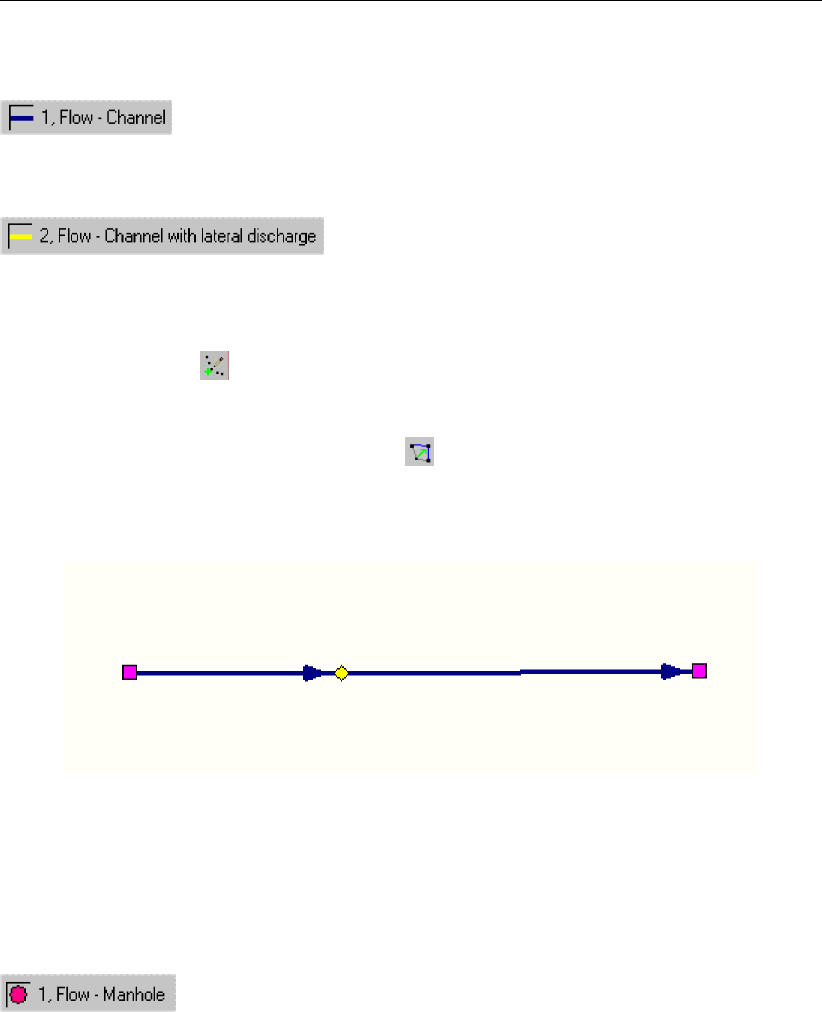
DRAFT
SOBEK, User Manual
Flow Channel:
Flow Channel with lateral discharge
Add a Flow - Lateral Flow node to your schematisation in the following way:
Select the appropriate node type (Flow - Lateral Flow)
Use the add node button to add it to the schematisation. When clicking, SOBEK will
automatically find the nearest channel to attach it to.
If desired, the node may later-on be moved to other locations on the branch, or even to
another branch by using the "move node" button.
Example of how a network could contain a Lateral Flow node:
Figure 5.101: Example of network with a Lateral Flow node
5.3.12 Flow - Flow manhole
5.3.12.1 Flow - Flow manhole (basic)
Flow Manhole description
This chapter describes the Flow - Manhole node. These nodes form a basic modelling ele-
ment for all urban schematisations. Manholes can be interconnected by Flow-Pipes and/or
internal structures. At Flow-Manholes the Water levels are calculated. On Flow-Pipes, dis-
charges are calculated.
For a detailed description of this nodes input parameters, see the "Flow - manhole input
screens" section from the Reference Manual.
Flow Manhole input screens
When starting the model data editor for an Flow - Manhole node type, the following tabs will
be available for input:
Storage tab:
242 of 900 Deltares
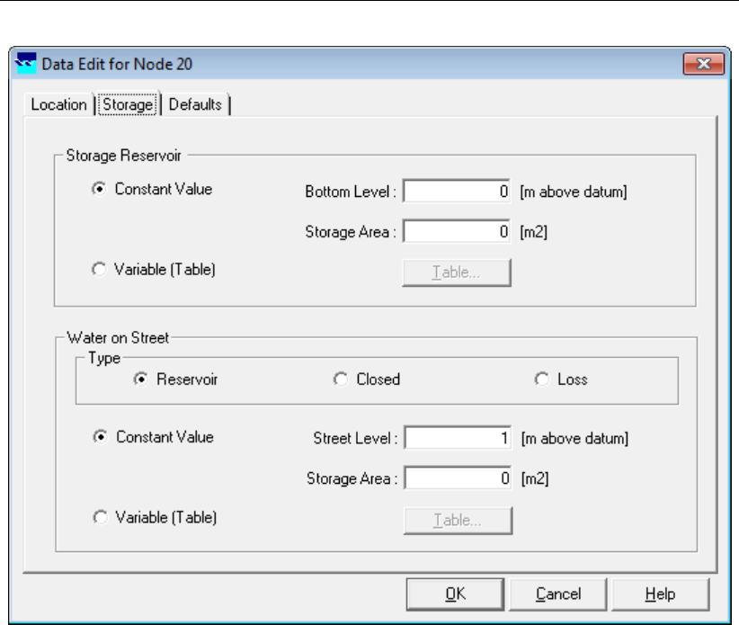
DRAFT
Graphical User Interface
Figure 5.102: Data Edit window, Storage tab
On this tab, the following data can be entered:
The bottom level level and storage area of the manhole.
A manhole is in fact a small reservoir that interconnects two or more sewer pipes. There-
fore, it has a certain storage volume. This volume is defined by the bottom level, the
surface level and the area of the manhole. (Surface level - Bottom level)*surface area =
total storage capacity of the manhole.
On this tab, the modeller can also choose between three manhole types:
Deltares 243 of 900

DRAFT
SOBEK, User Manual
Figure 5.103: The difference between Flow-manholes of the type "closed", "reservoir"
and "loss"
The difference between Flow-manholes of the type "closed", "reservoir" and "loss"
Three manhole types that can be chosen. Note: In case the ’loss’ type is chosen, all water
that exceeds the surface level, will be removed from the model. However, if you connect it
with a 2D grid (Overland Flow module), it will exchange water with the grid.
Reservoir In case the manhole type "Reservoir" is chosen, there will be an open connec-
tion between the manhole and the street surface. This means that, if the water level in the
manhole exceeds the street level, it will inundate the ’storage area’ that can be entered
in the section below.Choosing the type ’reservoir’ is useful if you desire to connect your
sewer model with a 2D grid (Overland Flow module). That will allow interaction between
flow in the pipes (1D) and flow over the land (2D).
Closed Choosing a manholes of the type "Closed" means that you have selected a man-
hole that has a lid at street level, thus there will be no interaction between the water within
the manhole and the street surface.
Loss Manholes of the type "Loss" will have all water that exceeds the entered street level
flow out.Thus, you might want to use this manhole type if you need to connect it to a 2D
grid (Overland Flow module). Water that exceeds the street level will then start flowing
over the 2D grid.
5.3.12.2 Flow - Flow manhole with level measurement
Measurement stations
Measurement stations represent locations where structure controllers get the required hy-
draulic information. Flow-Measurement Pipes are Flow-Pipes with a discharge measurement
station. These branches have a length, a cross section and a resistance. Flow-Manholes with
Level Measurement are Flow-Manholes with a water level measurement station. Before you
can specify a controller you must define a measurement location in the schematisation.
244 of 900 Deltares
DRAFT
Graphical User Interface
5.3.12.3 Flow - Flow manhole with runoff
Flow-manhole with runoff - description
This chapter describes the Flow - Manhole with Runoff.
Basically, these nodes are equal to Flow - Manholes. The only difference is that Flow -
manholes with runoff have an extra option to transfer rainfall into a discharge into the pipes
(rainfall-runoff).
For a detailed description of this node’s input parameters defining its physical dimensions
(Sewer Flow), see the "Flow - manhole input screens" section from the Reference Manual.
For a detailed description of this node’s Rainfall-Runoff input parameters defining the
catchment dimensions, see the "Module - Rainfall runoff section of the Reference Manual"
For a detailed description of this node’s possible network configurations: see the "Flow -
Manhole topology" section from the Reference Manual
5.3.13 Flow - Measurement station
Description
In this chapter, the Flow Measurement station node is described.
Measurement stations represent the locations from where structure controllers get their re-
quired hydraulic information. Before you can specify a controller you must place at least one
measurement station in the schematisation.
For a detailed description of this node’s possible network configurations: see the "Mea-
surement station node topology" section from the Reference Manual
Note that, after placement of a measurement station, your schematisation needs to be saved
before a structure will know that it exists! After saving, you’ll notice that when editing model
data for structures, various controlling options become available under the "controller" tab.
Topology
Nodes of the type ’Measurement Station’ need to be placed on a Flow Branch. Do this by
using the (add node) button.
Figure 5.104: Placement of a Flow Measurement Station node
Note: the measurement station will derive information about the water level from the nearest
ζ-calculation point.
Deltares 245 of 900
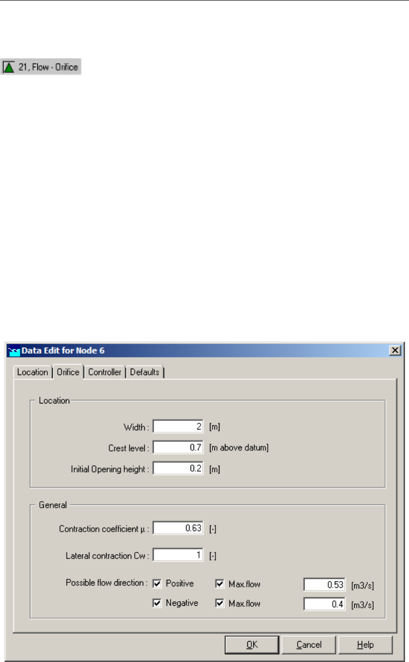
DRAFT
SOBEK, User Manual
5.3.14 Flow - Orifice node
Description
In this chapter, the Flow - Orifice node is described.
With a Flow - Orifice node you can simulate rectangle-shaped gates through which water
within a channel or river is led. Orifices are used to regulate the water flow through or towards
a channel or river. For a detailed description of this node’s underlying mathematical equations:
see section 6.1.16.8.
Some applications are:
In rivers: used to regulate the division of flows over an upstream split-point.
In deltas: to protect the delta against storms on the coast (the orifices close during a
storm).
In smaller channels: to allow water to flow into an area in periods of drought.
Input screens
When starting the model data editor for an Flow - Orifice node type, the following tabs will be
available for input:
Orifice:
Figure 5.105: Data Edit window, Orifice tab
246 of 900 Deltares
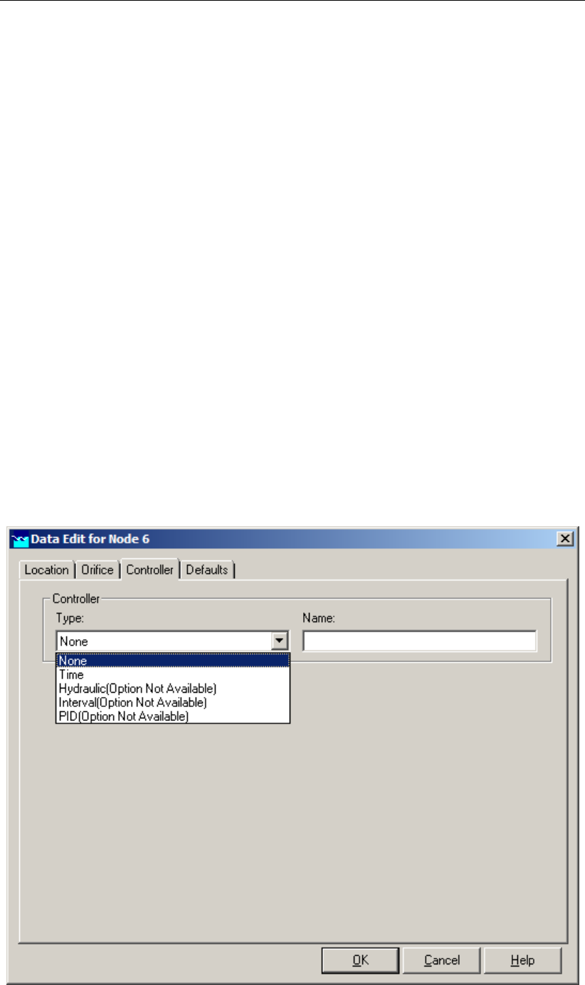
DRAFT
Graphical User Interface
On this tab, you can fill in the general dimensions and parameters for the orifice:
Width: This parameter represents the width of the gate through which the water will flow.
Crest level: This parameter represents the bottom crest level of the gate.
Initial openings height: Here you can enter the vertical dimension of the gate for the
start of the simulation. For orifices it is common to apply a controller, which will define
the gate height during the simulation. If you don’t define a controller, the initial openings
height will remain valid throughout the entire simulation.
Contraction coefficient µ: This parameter represents the energy loss that is caused by
contraction of the flow towards the orifice. This phenomenon generally occurs when the
weir’s crest is less wide than the channel. See the Technical Reference Manual for the
exact mathematical implementation of this parameter.
Lateral Contraction Cw: This parameter represents the energy loss that is caused by
contraction of the flow towards the orifice. This phenomenon generally occurs when the
weir’s crest is less wide than the channel. See the Technical Reference Manual for the
exact mathematical implementation of this parameter.
Possible flow directions: This parameter defines in which direction(s) water can flow
through the orifice. The directions are defined with relation to the defined branch direc-
tion. Positive means: in the same direction as the defined branch direction; negative
means: in the opposite direction than the defined branch direction. If you don’t know the
defined direction of the branch, read the Flow - Branch topology section of the Functional
Reference Manual. In addition to defining the flow directions, you can also define a maxi-
mum flow through the gate for each flow direction. To do so, activate the check boxes next
to the word "Max. flow" and enter a value.
Controller:
Figure 5.106: Data Edit window, Controller tab
Deltares 247 of 900
DRAFT
SOBEK, User Manual
On this tab, you can define a controller for your orifice. A controller will overrule your general
settings for the orifice’s opening height and apply the chosen controlling rules to it. Read
more about them in section 6.4.1.
Note that three of the four available controller options only become available after you have
defined a Flow - Measurement station within the schematisation and saved that schematisa-
tion.
Topology
Nodes of the type Flow - Orifice need to be attached to one of these branch types:
Flow Channel:
Flow Channel with lateral discharge
Add a Flow - Orifice node to your schematisation in the following way:
Select the appropriate node type (Flow Orifice)
Use the "add node" button to add it to the schematisation. When clicking, SOBEK
will automatically find the nearest channel to attach it to.
If desired, the node may later-on be moved to other locations on the branch, or even to
another branch by using the "move node" button.
Note: Before adding an orifice to your schematisation, you should have at least one of the
above Channel types present.
5.3.15 Flow - Pump station node
AFlow - Pump station can be used to remove excess water or to supply water for drought
prevention. In the section Topology it is explained how to place a Flow - Pump station on
a network. The data input screens are described in the section Data input screens. See
section 6.1.16.9 for detailed information on:
Pump discharge direction with respect to the positive x-direction along the branch,
Pump stages,
Controller options at a Pump station,
Capacity reduction table,
Pump station output parameters,
Dead-band triggering algorithm,
Conventions for switch-on and switch-off levels.
Topology
Nodes of the type Flow - Pump Station need to be attached to one of these branch types:
Flow Channel:
248 of 900 Deltares

DRAFT
Graphical User Interface
Flow Channel with lateral discharge
Add a Flow - Pump Station node to your schematisation in the following way:
Select the appropriate node type (Flow Pump Station)
Use the "add node" button to add it to the schematisation. When clicking, SOBEK
will automatically find the nearest channel to attach it to.
If desired, the node may later-on be moved to other locations on the branch, or even to
another branch by using the "move node" button.
Note: Before adding a pump station to your schematisation, you should have at least one of
the above Channel types present in it.
Figure 5.107: Example of a valid network configuration containing a pump station.
Deltares 249 of 900
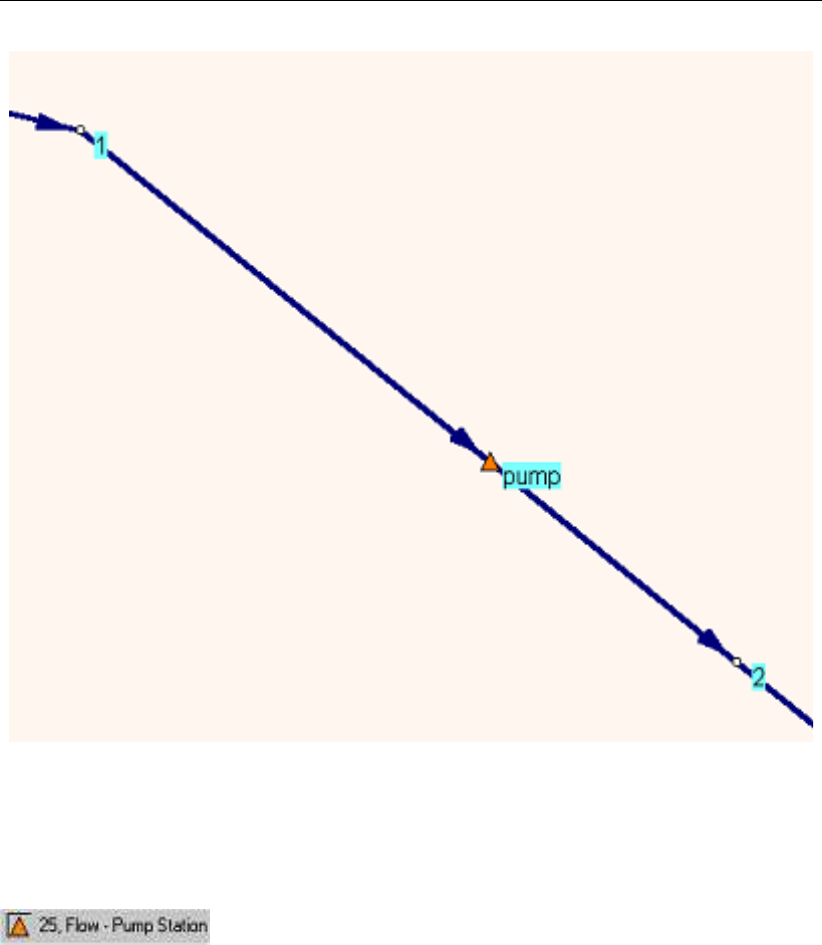
DRAFT
SOBEK, User Manual
Figure 5.108: Example of the application of a Flow - Pump Station. If you would define
a "positive pump direction", here node #1 would be the suction side and
node #2 would be the pressure side.
Data input screens
After starting the model data editor for an Flow - Pump Station node type, the Pump tab (see
Figure 5.109) becomes available. On the Pump tab two separate windows can be opened,
respectively the reduction table window (see Figure 5.110) and the pump data window (see
Figure 5.111) For detailed information on the various pump station input parameters, refer-
ence is made to section 6.1.16.9.
Following pump characteristics can be defined on the Pump tab (see Figure 5.109):
Number of different pump stages
Reduction factors on pump discharge capacity (see also Figure 5.110)
Unit of the specified pump discharge capacity
Location of dead-band triggers (Suction-side only, Delivery-side only, both Suction-side
and Delivery-side)
Pump stage data (see also Figure 5.111)
250 of 900 Deltares
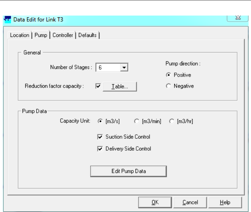
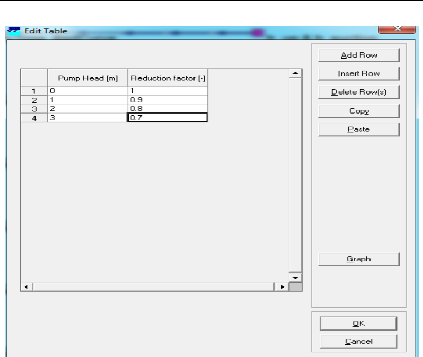
DRAFT
SOBEK, User Manual
Figure 5.110: Data Edit window, Capacity Reduction Table tab
In the Pump data window (see Figure 5.111), for each pump stage following parameters can
be defined:
Pump stage capacity
Switch-on-level at the Suction-side (if applicable)
Switch-on-level at the Delivery-side (if applicable)
Switch-off-level at the Suction-side (if applicable)
Switch-off-level at the Delivery-side (if applicable)
252 of 900 Deltares

DRAFT
Graphical User Interface
Figure 5.111: Data Edit window, Capacity Reduction Table tab
5.3.16 Flow - River Advanced Weir
Description
In this chapter, the Flow - Advanced Weir node is described.
The advanced weir requires entry of values for crest level, (net) sill width and number of piers.
Discharges through an Advanced weir are computed on basis of upstream and downstream
energy-levels. The crest level can be varied by a controller. A structure inertia damping factor
(see Numerical parameters) can be defined for each Advanced weir.
For a detailed description of this node’s input parameters: see the "input screens" section
from the Reference Manual;
For a detailed description of this node’s possible network configurations: see the "topol-
ogy" section from the Reference Manual
For a detailed description of this node’s underlying mathematical equations: see the "Ad-
vanced weir" section in the "Technical Reference Manual".
Input screens
When starting the model data editor for an Flow - Advanced Weir node type, the following
tabs will be available for input:
Advanced weir tab:
Deltares 253 of 900
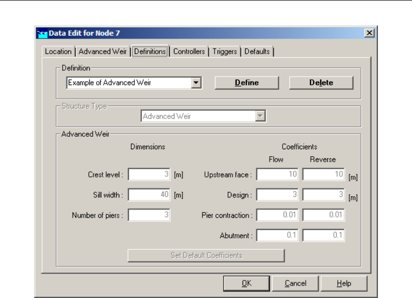
DRAFT
SOBEK, User Manual
Figure 5.112: Data Edit window, Advanced Weir tab
On this tab, you can select a previously defined structure definition. If there is no definition
available yet, go to the "definitions" tab first, to create one.
Also, you can select the controllers that apply to this structure. If there are no controllers
available to be selected yet, go to the "controller" tab first to create them.
You can use the default value for structure inertia damping factor as defined in Setting, Tab –
numerical parameters, or you can define a value for structure inertia damping factor for this
particular Advanced weir. For the mening of structure inertia damping factor see Numerical
parameters.
Definitions tab:
254 of 900 Deltares
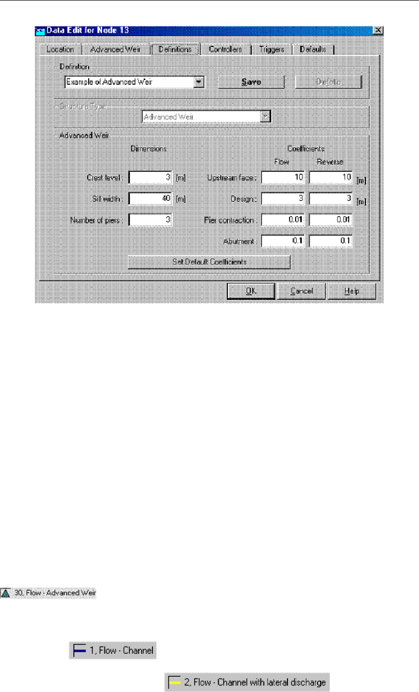
DRAFT
Graphical User Interface
Figure 5.113: Data Edit window, Definitions tab
The advanced weir requires entry of values for crest level, (net) sill width and number of piers.
The crest level can be varied by a controller. For the following parameters you get default
values in the corresponding data fields, which you may adapt to your particular situation.
1Upstream face height The height of the weir relative to the bed level at the upstream
sideA default value of 10 m is available, but you should enter the actual value.
2Design head The head for which the structure was designed. A default value of 3 m is
available, but you should enter the actual value.
3Pier contraction The contraction coefficient represents the net sill-width reduction due to
the presence of piers. It depends on the shape of the piers. Default value is 0.01.
4Abutment contraction The contraction coefficient represents the net total flow width re-
duction due to the presence of abutments. It depends on the shape of the abutments.
Default value is 0.10. If reverse flow may occur you can adapt the values for that condition
as well.
Controllers & Triggers tabs: see section 5.8.
Topology
Nodes of the type Flow - Advanced Weir need to be attached to one of these branch types:
Flow Channel:
Flow Channel with lateral discharge
Add a Flow - Advanced Weir node to your schematisation in the following way:
Deltares 255 of 900
DRAFT
SOBEK, User Manual
Select the appropriate node type (Flow - Advanced Weir)
Use the "add node" button to add it to the schematisation. When clicking, SOBEK will
automatically find the nearest channel to attach it to.
If desired, the node may later-on be moved to other locations on the branch, or even to
another branch by using the "move node" button.
Note:
1. Before adding an Advanced weir to your schematisation, you should have at least one of
the above Channel types present in it.
2. SOBEK by default places a computational point 0.5 m upstream and 0.5 m downstream of
the Advanced weir location. Hence the Advanced weir is default located on a branch having
a length of 1 m.
5.3.17 Flow - River Pump
AFlow - River Pump can be used to remove excess water or to supply water for drought
prevention. Controllers can not be assigned to a River pump. In the section Topology it
is explained how to place a Flow - River Pump on a network. The data input screens are
described in the section Data input screens. See section 6.1.16.11 for detailed information
on:
Pump discharge direction with respect to the positive x-direction along the branch,
Pump stage,
Constant Reduction Factor,
Reduction Factor F(Pump Head),
Pump station output parameters,
Dead-band triggering algorithm,
Comparison of a River Pump and a Pump station.
Topology
Nodes of the type Flow - River Pump need to be attached to one of these branch types:
Flow Channel:
Flow Channel with lateral discharge
Add a Flow - River Pump node to your schematisation in the following way:
Select the appropriate node type (Flow - River Pump)
Use the "add node" button to add it to the schematisation. When clicking, SOBEK will
automatically find the nearest channel to attach it to.
If desired, the node may later-on be moved to other locations on the branch, or even to
another branch by using the "move node" button.
Note:
1 Before adding a river pump to your schematisation, you should have at least one of the
256 of 900 Deltares

DRAFT
Graphical User Interface
above Channel types present in it.
2 SOBEK by default places a computation point 0.5 m upstream and 0.5 m downstream of
the River pump location. Hence the River pump is default located on a branch segment
having a length of 1 m.
Data input screens
After starting the model data editor for an Flow - River Pump node type, the River Pump
tab (see Figure 5.114) becomes available. On the River Pump tab you can select a previ-
ously defined River Pump definition. Various River Pumps definitions can be specified on the
Definition tab (see Figure 5.115).
Figure 5.114: Data Edit window, River Pump tab
On the Definition tab of a River Pump (see Figure 5.115) following parameters can be defined:
Control direction,
Capacity,
Start level,
Stop level,
A Constant Reduction Factor or a Reduction Factor F(Pump Head),
For detailed information on these various River Pump input parameters, reference is made to
section 6.1.16.11.
Deltares 257 of 900
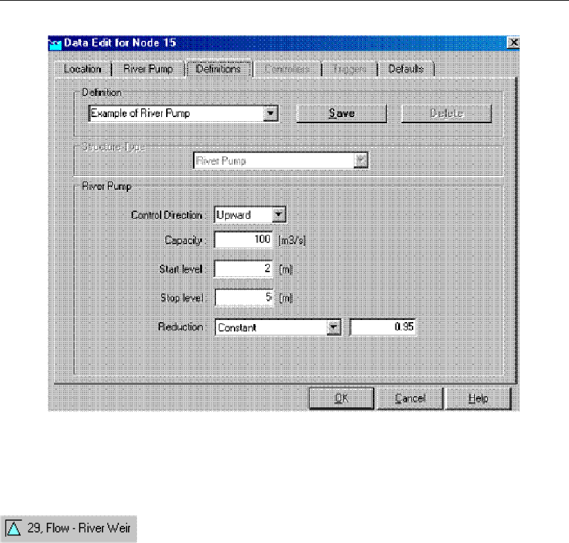
DRAFT
SOBEK, User Manual
Figure 5.115: Data Edit window, Definition tab
5.3.18 Flow - River Weir
Description
Different crest shapes (broad crested, triangular, round or sharp) can be defined for a Flow
- River Weir by selecting a particular "drowned reduction curve" (see Figure 6.38 in sec-
tion 6.1.16.12). Crest levels of a Flow - River Weir cannot vary in height along the weir.
Discharges through a Flow - River Weir are computed on basis of upstream and downstream
energy-level. For the applied mathematical equations, reference is made to section 6.1.16.12.
The crest level and crest width of a river weir can be varied by a controller. A structure inertia
damping factor (see Numerical parameters) can be defined to each River weir.
Input screens
When starting the model date editor for an Flow - River Weir node type, the following tabs will
be available for input:
River weir tab:
258 of 900 Deltares
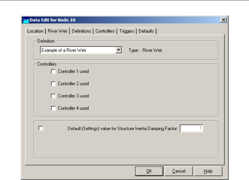
DRAFT
Graphical User Interface
Figure 5.116: Data Edit window, River Weir tab
On this tab, you can select a previously defined structure definition. If there is no definition
available yet, go to the "definitions" tab first, to create one.
Also, you can select the controllers that apply to this structure. If there are no controllers
available to be selected yet, go to the "controller" tab first to create them.
Definitions tab:
Deltares 259 of 900
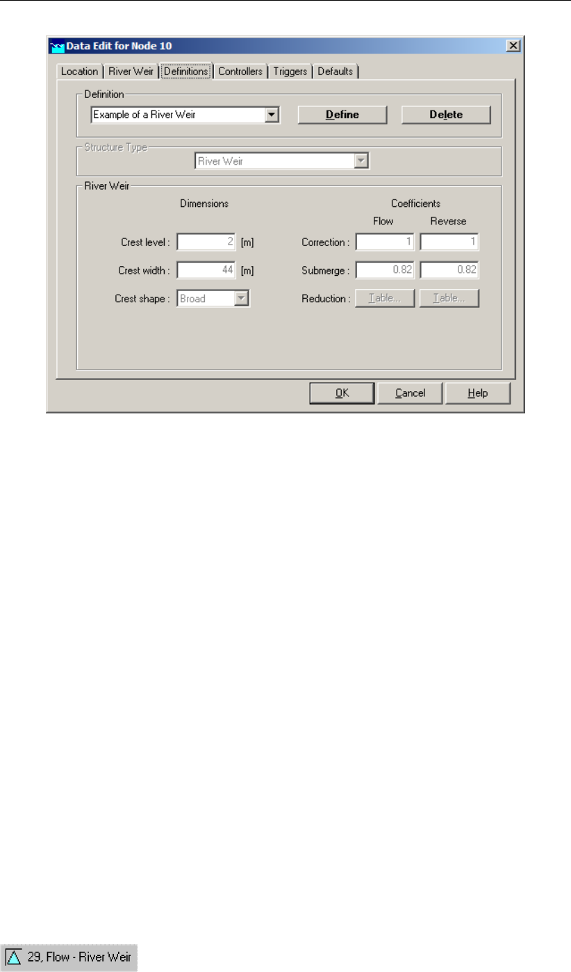
DRAFT
SOBEK, User Manual
Figure 5.117: Data Edit window, Definitions tab
On this tab, you can define the properties of your River Weir structure. Select an existing def-
inition from the drop-down box or create one by typing an appropriate name in the "definition"
field and then clicking <Define>.
Then you can:
Define the crest level of the weir
Define the crest width of the weir
Define the crest’s shape: choose between (broad, triangular, sharp and round)Note that
changing the crest’s shape will change the default flow coefficients.
Define a correction coefficient: For flow in the positive direction of the branch or in the
opposite direction, default correction coefficients cw are proposed by SOBEK for each
crest shape (see also Technical Reference Manual, Flow Modules, River Weir). If you
wish, you can replace them by other values.
Define the submerge flow coefficient. If the tail water level affects the weir flow, drowned
(submerged) flow occurs. Whether this happens is determined by the submergence (or
modular) limit. For each crest shape a default value is presented. If the submergence
factor Sf ((H2-Zs)/(H1-Zs)) is above the submergence limit, the flow is multiplied by a
corresponding drowned reduction factor, which is also a function of the crest shape. The
default values are shown in the Technical Reference Manual, Flow Modules, River Weir. If
you wish to apply other factors you can enter them in a table, accessible through Edit. A
similar table is available for reduction factors applying to the reverse flow condition
Controllers & Triggers tabs: see section 5.8.
Topology
260 of 900 Deltares
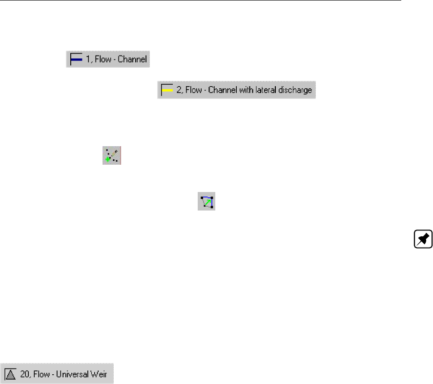
DRAFT
Graphical User Interface
Nodes of the type Flow - River Weir need to be attached to one of these branch types:
Flow Channel:
Flow Channel with lateral discharge
Add a Flow - River Weir node to your schematisation in the following way:
Select the appropriate node type (Flow - River Weir)
Use the "add node" button to add it to the schematisation. When clicking, SOBEK will
automatically find the nearest channel to attach it to.
If desired, the node may later-on be moved to other locations on the branch, or even to
another branch by using the "move node" button.
Note:
1 Before adding a River weir to your schematisation, you should have at least one of the
above Channel types present in it.
2 SOBEK by default places a computational point 0.5 m upstream and 0.5 m downstream
of the River weir location. Hence the River weir is default located on a branch having a
length of 1m.
5.3.19 Flow - Universal Weir
Description
The Flow - Universal Weir is a broad crested weir. Crest levels may vary in height along the
weir. For the assumptions made in the parameterization of the Flow - Universal Weir as well
as for the applied mathematical equations, reference is made to section 6.1.16.14
Input screens
When starting the model data editor for an Flow - Universal Weir node type, the following tabs
will be available for input:
Universal Weir:
Deltares 261 of 900
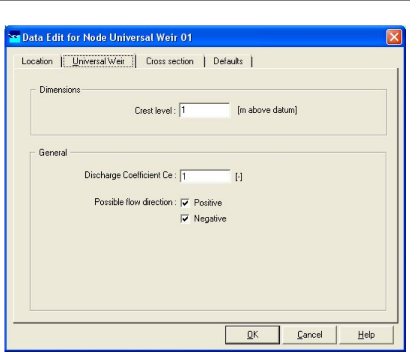
DRAFT
SOBEK, User Manual
Figure 5.118: Data Edit window, Universal Weir tab
On this tab, the general dimensions of the weir can be defined:
Crest Level: This value represents the lowest part of the weir’s crest. On the cross
section tab, later on the exact shape of the crest can be defined.
Discharge coefficient Ce: This parameter represents the discharge coefficient for the
weir, as present in the formula that applies to this type of structure. See the "Univer-
sal Weir" section in the Technical Reference Manual for the exact implementation of this
parameter.
Possible flow direction: This parameter defines in which direction(s) water can flow over
the weir. The directions are defined with relation to the defined branch direction. Positive
means: in the same direction as the defined branch direction; negative means: opposite
of the defined branch direction. If you don’t know the defined direction of the branch, read
more about it in the Flow - Branch topology section of the Functional Reference Manual.
Cross Section:
262 of 900 Deltares
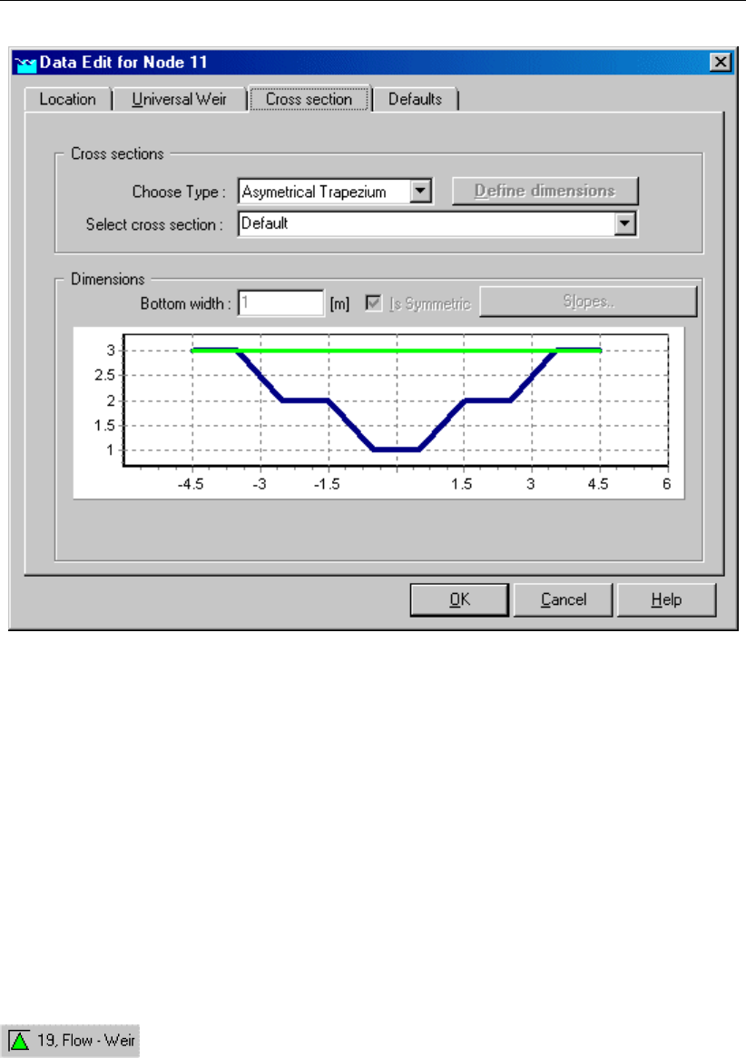
DRAFT
Graphical User Interface
Figure 5.119: Data Edit window, Cross section tab
On this tab, the actual shape of the weir’s crest should be defined. This is done by means of
cross section definitions, very similar to the ones you define for the shape of a river bed.
The only real difference is that the number of cross section types is limited to two:
Y-Z profile
Asymmetrical Trapezium
For a detailed description of both cross section types and their input parameter, see the "Func-
tional Reference Manual" - "Channel Flow module" - "Cross section types" section.
5.3.20 Flow - Weir
Description
The Flow - Weir is a broad crested weir. Crest levels cannot vary in height along the weir. For
the applied mathematical equations, reference is made to section section 6.1.16.16.
Input screens
When starting the model data editor for an Flow - Weir node type, the following tabs will be
available for input:
Weir:
Deltares 263 of 900
DRAFT
SOBEK, User Manual
Figure 5.120: Data Edit window, Weir tab
On this tab, the weir’s general dimensions can be filled in:
Width This parameter represents the width of the crest over which the water will flow.
Crest level This parameter represents the level (with relation to reference level) of the
weir’s crest. Note that the value you fill in here may be overruled by a controller, if you
desire.
Discharge coefficient Ce This parameter represents the discharge coefficient that is
used for calculation of the discharge. See the Technical Reference Manual for the exact
mathematical implementation of this parameter.
Lateral contraction coefficient Cw This parameter represents the energy loss that is
caused by contraction of the flow towards the weir. This phenomenon generally occurs
when the weir’s crest is less wide than the channel. See the Technical Reference Manual
for the exact mathematical implementation of this parameter.
Possible flow direction This parameter defines in which direction(s) water can flow over
the weir. The directions are defined with relation to the defined branch direction. Positive
means: in the same direction as the defined branch direction; negative means: in the
opposite direction than the defined branch direction. If you don’t know the defined direc-
tion of the branch, read the Flow - Branch topology section of the Functional Reference
Manual.
Controller:
264 of 900 Deltares
DRAFT
Graphical User Interface
Figure 5.121: Data Edit window, Controller tab
On this tab, you can define a controller for your weir. A controller will overrule your general
settings for the weir’s crest level and apply the chosen controlling rules to it. Read more about
them in the Controller section of the Technical Reference Manual.
Note that three of the four available controller options only become available after you have
defined a Flow - Measurement station within the schematisation and saved that schematisa-
tion.
5.3.21 Flow - 2D-Boundary
Description
General description:
The 2D - boundary node works more or less the same as its counterpart in the 1D-channel
flow module. The boundary condition is either a water level or a discharge, both of which can
be either constant or varying in time.
Important: the grid cell on which a 2D-Boundary node is placed, should be given the no-data
value! (often -9999) If not, this object will not work.
Deltares 265 of 900
DRAFT
SOBEK, User Manual
How the 2D-boundary node works:
Any 2D grid cell can discharge into any of the four cells directly surrounding it. However, a
2D cell containing a boundary can only discharge into (any) ONE of these cells! By default, it
discharges into the cell directly to the right of it. The flow direction can be controlled by defining
no-data values in the surrounding cells to which the boundary cell should NOT discharge. This
way, if you define 3 no-data values out of 4 surrounding cells, the boundary cell will discharge
into the remaining cell (see example Figure 5.122).
Figure 5.122: Possible configuration of a 2D boundary node. Note: the white (transpar-
ent) cells contain no-data values
In case of a 2D h(t)boundary condition, the water level is directly imposed at the active
grid cell that lies in front of the concerning 2D boundary grid cell. Hence there is no water
movement over the concerning 2D boundary grid cell.
In case of a 2D Q(t)or 2D Q-hboundary, an artificial 1D link is created from the concerning
2D boundary grid cell towards the active 2D grid cell that lies in front of this 2D boundary grid
cell. The hydraulic properties of this artificial 1D link are based on the properties of the active
2D grid cell lying in front of the 2D boundary grid cell. This implies that in case of a 2D Q(t)
or 2D Q-hboundary water movement over the 2D boundary grid cell is taken into account.
Suggestions for the user:
If you decide to use a Discharge boundary condition as part of the 2D schematisation, it is
wise to define an initial water level point in the 2D grid cell into which the cell containing the
boundary condition should flow. The reason for the initial water level point in this case is
purely a numerical one, as sometimes no water will flow at all from the discharge boundary.
The water depth can be very small, for example one centimeter.
The initial water level node will (instantly) fill up all surrounding 2D grid cells with water, until
cells which have a higher terrain level are branched, or if the edge of the grid is branched.
This can be a problem when using a discharge boundary condition on a high point in the grid:
an initial water level used for numerical reasons may fill a large part of the grid! This problem
can be solved by lowering the terrain level of the 2D grid containing the initial water level point
slightly below the level of the surrounding cells.
266 of 900 Deltares
DRAFT
Graphical User Interface
One more rule to remember when using this node is that the 2D grid cell containing the node
should be defined manually as ’no-data value’!. This can be done in ’edit model data’ mode,
under the properties of the 2D grid.
Finally, it is not possible to add this type of node to a grid cell that already contains a 1D-
boundary node.
2D-Boundary nodes are normally used in situations where the dam break is modelled starting
in the 2D schematisation, as opposite to starting in the 1D-schematisation.
Editing 2D-Boundary data
After selecting any 2D-boundary node in the edit model data mode and pressing Edit, the data
edit window for this node type pops up. The first tab ’location’ displays the (non-editable) id
and location of node.
Under tab ’boundary condition’, the user can specify the boundary condition. See Figure 5.123.
There is a choice between a Water level boundary condition or a Flow boundary condition.
Both of these can be given either a constant value or a value changing in time.
Figure 5.123: 2D-boundary edit window - boundary condition tab
A variable water level or flow in time can ben entered by pressing table. . . and filling in the
table, as shown in the example in Figure 5.124:
Deltares 267 of 900
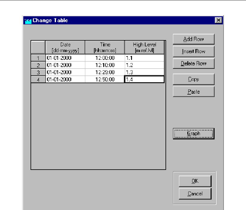
DRAFT
SOBEK, User Manual
Figure 5.124: Change table window
Please note that the water level is defined relative to the reference level (positive above the
reference level), and that it is not possible to enter a water depth as a boundary condition.
Also note that a positive value for the flow means input into the system, while a negative value
means output.
2D Q-h tabulated boundary condition
Functionality:
The 2D Q-h tabulated boundary condition enables the user to apply a Q-h relationship as
the (downstream) boundary condition of a 2D grid. A Q-h relationship is to be defined as
discharges as function of water levels Q=f(h). Presently a 2D Q-h tabulated boundary
condition may not pass over nested grids and should be parallel to either the x-axis or y-axis
of the 2D grid. Further on a 2D Q-h tabulated boundary condition is supposed not to pass
over a 1D channel flow schematisation.
How to define:
Double click the ‘Schematisation’ task block and thereafter click the Edit Model button on
the Schematisation window.
Click the Zoom in button and go to the location where you want to place the 2D Q-h
Tabulated boundary condition.
Click the Edit Network button.
Click the Nodes button, pull-down the menu and click the Overland Flow Model/ 41, 2D -
Corner node.
268 of 900 Deltares
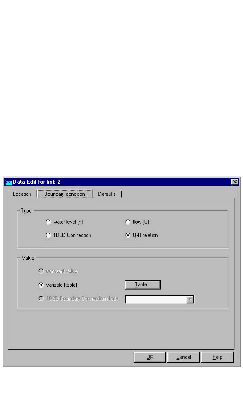
DRAFT
Graphical User Interface
Click the Branch button, pull-down the menu and click the Overland Flow Model/ 16, 2D -
Line Boundary.
Click the Edit action button, pull-down the menu and click on Nodes/Add Nodes. Go to
the location where you want to place the first 2D Corner node of the 2D Q-h Tabulated
Boundary Condition and click with your left mouse button. Place the second 2D Corner
node in the same way.
Click the Edit action button, pull-down the menu and click on Connection/Connect nodes.
Click with the left mouse button on your first 2D Corner node. While pressing down the
left mouse button drag a line to your second 2D Corner node and release your left mouse
button.
Click the <Edit Network>button to end the network editing activities.
Click on the 2D Q-h Tabulated Boundary Condition and thereafter click with your right
mouse button, and click on Model data/ Overland Flow Model. The ‘Data Edit’ window
should appear on your screen.
Click the ‘Q-h relation’ check-box in the ‘Boundary condition’ Tab of the ‘Data Edit’ window.
Click on the <Table>button in the ‘Data Edit’ window to enter your Tabulated Q-h relation
in the ‘Change Table’ window.
Close both the ‘Change Table’ and the ‘Data Edit’ windows by clicking OK.
Click the Save Network button for saving your defined 2D Q-h Tabulated Boundary Con-
dition.
Figure 5.125: Data Edit window, Boundary condition tab
How to retrieve information:
Under the ‘Results in Maps’ Task block
Deltares 269 of 900
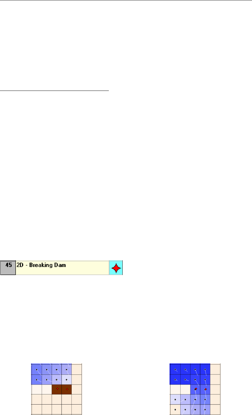
DRAFT
SOBEK, User Manual
Double click the ‘Results in Maps’ task block.
Click in the main menu on File/Open Data/Overland Flow Module Result at history stations
(i.e. in the ‘Select item’ window)
In the ‘View Data’ window select for instance the hydraulic parameters "Water level" and
Abs.Disch [m3/s]’.
Click the 2D Q-h Tabulated Boundary Condition and then click with right mouse and then
on show graph or click on the <graph>button in the ‘View Data’ window.
Under the ‘Results in Charts’ Task block
Double click the ‘Results in Charts’ task block.
Double click on Overland Flow Module/ Results at history stations (in the ‘Results in
Charts’ window).
In the ‘ODS-View’ window select under parameters Water level and Abs Disch [m3/s],
under location select location l_x (where l stands for link and x for the ID of the 2D Q-
h Tabulated boundary condition), under time-steps select the required time-period. Now
click on the Graph button or Export button to respectively view a graph or export to the
data to a particular file.
2D Refined Q boundary condition
Functionality:
In effect the 2D refined Q-boundary condition refers to an improvement of the existing 2D
Q-line boundary condition. In the past imposed discharges were equally distributed over
the number of concerning 2D grid cells. Nowadays imposed discharges are distributed in
accordance with the conveyance capacity of the concerning 2D grid cells.
5.3.22 Flow - 2D-Breaking Dam
Description
Dike bbranches can be modeled either in 1D (see Branch – Flow Dam Break) or in 2D using
a2D Breaking - Dam Node (see Figure below). You have two options for controlling the bed
level of the 2D grid cell that lies underneath a 2D Breaking – Dam:
Using the Decrease in Height Time Table,
Using a controller that can be overruled by RTC or RTC-Matlab. For more information see
Module – SOBEK Real Time Control (RTC).
For information on how to use these control options, see Editing Node 2D Breaking Dam.
Figure 5.126: Example of 2D- Breaking Dams located on 2D grid cells
270 of 900 Deltares
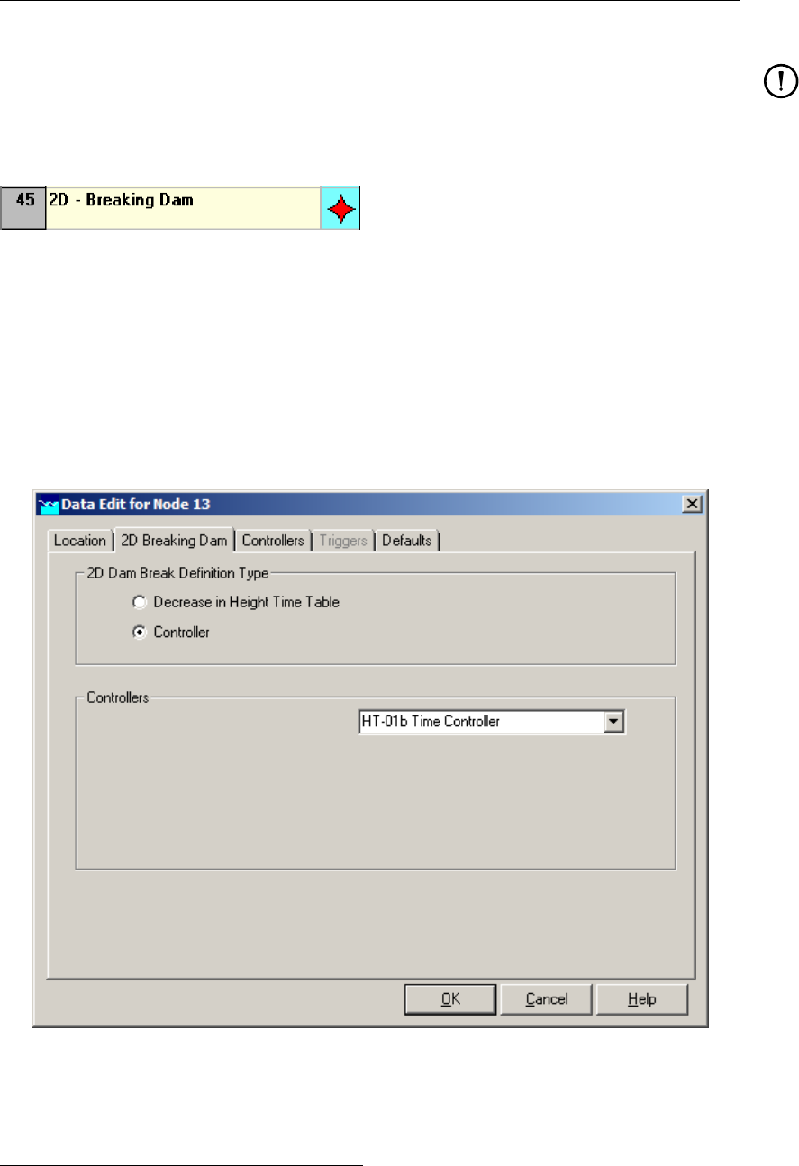
DRAFT
Graphical User Interface
Remark:
A 2D breaking dam node may not lay on an active 2D grid cell that is surrounded by a
boundary condition cell.
Editing 2D-Breaking Dam data
The 2D-Breaking Dam enables you to control the bed level of its underneath lying 2D grid cell.
Following control options are available:
Option 1: The Decrease in Height Time Table,
Option 2: A controller that can be overruled by RTC or RTC-Matlab. For more information
see Module – SOBEK Real Time Control (RTC).
You can select either option 1 or option 2 by checking its corresponding radio bullet (see
Figure 5.127 below).
Figure 5.127: Example of selecting the controller option for a 2D Breaking - Dam
Option 1: The Decrease in Height Time Table
Check the “Decrease in Height Time Table” radio bullet and click on the Table button. You can
now specify the lowering of the 2D grid cell lying beneath your 2D Breaking – Dam as function
of time (see Figure 5.128).
Deltares 271 of 900
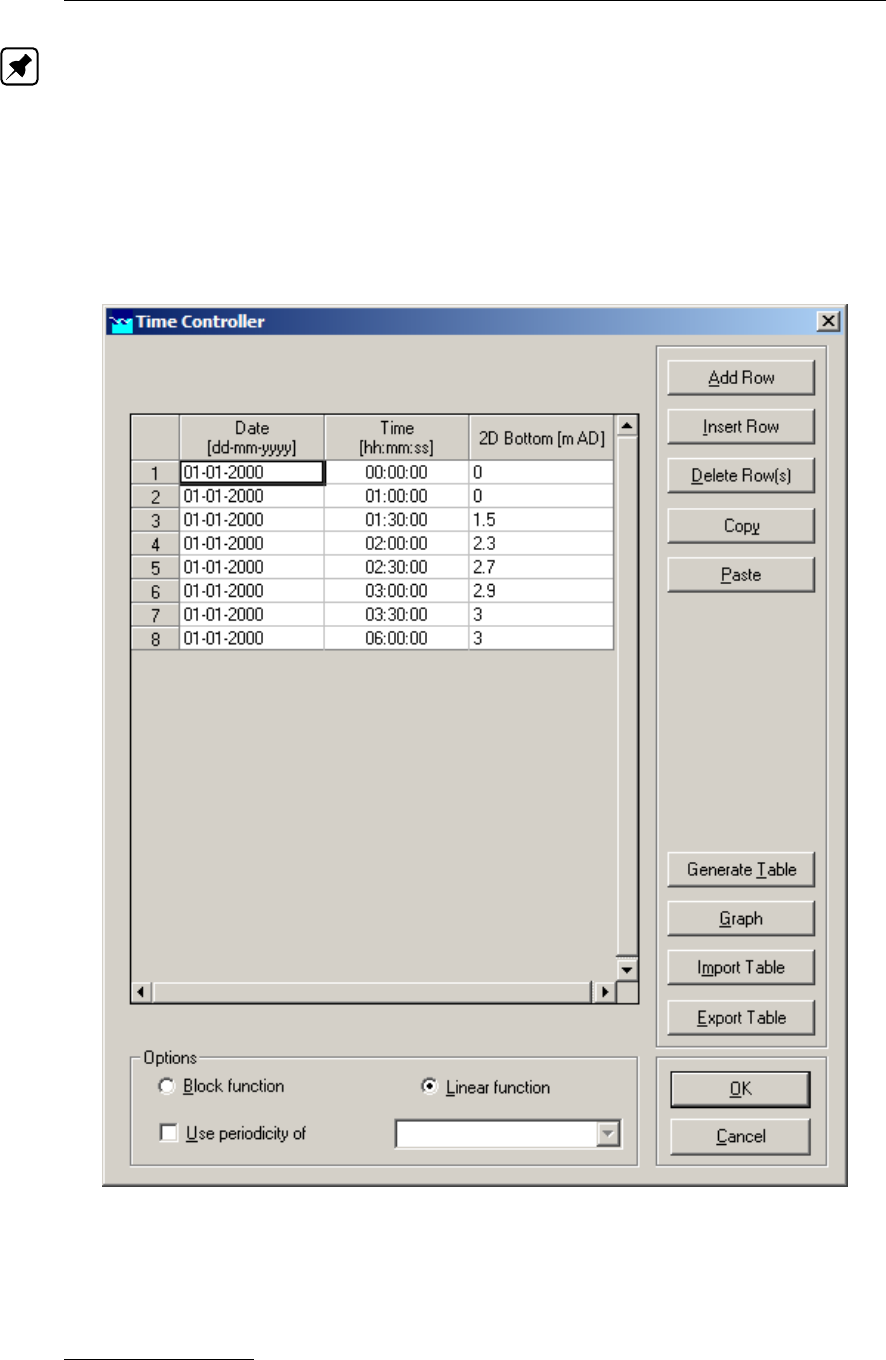
DRAFT
SOBEK, User Manual
Note:
1 You specify the lowering with respect to the start level (or initial bed level) defined in your
2D bed level grid (i.e. <*.asc>file). Positive and negative values respectively mean that
your grid cell will moved downwards or upwards,
2 SOBEK applies linear interpolation in the Decrease in Height Time Table,
3 In case the actual computational time is before the first time or after the last time specified
in your Table, SOBEK will respectively apply the value on the first row or the value on the
last row of your Time Table.
Figure 5.128: Example of a Decrease in Height Time Table available at a 2D Breaking –
Dam
Option 2: A controller
Firstly you have to define a controller. Thereafter you can select this controller as the one
providing set points for the bed level of the 2D grid cell lying beneath your 2D Breaking –
272 of 900 Deltares
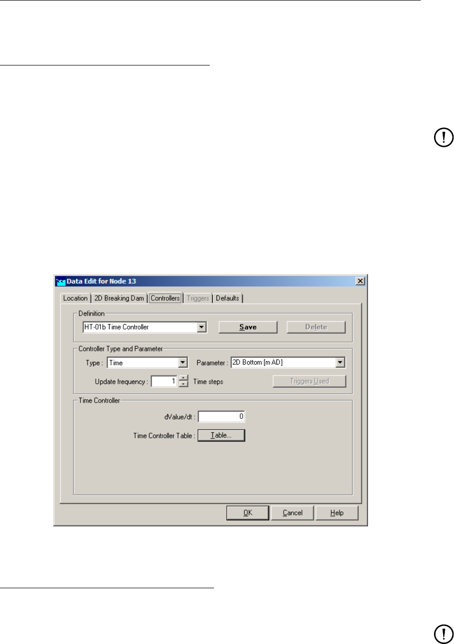
DRAFT
Graphical User Interface
Dam.
Defining a controller for a 2D Breaking – Dam:
Click on the “Controllers” Tab (see Figure 5.129) and type a name in the “Definition” scroll
box. Now click the Define button and specify your controller. Don’t forget to click the Save
button in order to save your controller definition.
Remarks:
Presently only a Time Controller providing bottom(bed) levels as set point for a 2D
Breaking – Dam can be defined,
Update frequency=1, means that the set point of controller is updated after each hydro-
dynamic time step, defined in Settings; Update frequency=10, means that the set point
of the controller is updated every 10 hydrodynamic time steps,
dValue/dt=0.002 m/s, means a maximum speed for the change in bed level (either pos-
itive or negative) of 0.002 m/s. Hence in one minute a maximum bed level change of
0.12 m (=0.002 m/s * 60 s) is allowed,
Click on the Time Controller Table button for specifying your set points.
Figure 5.129: Example defining a controller for a 2D Breaking – Dam
Assigning a controller at a 2D Breaking – Dam:
Click on the 2D Breaking – Dam Tab and check the “Controller” radio button. Now select your
previously defined controller in the “Controllers” scroll box (see Figure 5.129 above).
Remark:
In the “Controller” scroll-box you can only select so-called 2D Flow controllers. Hence
you cannot select a 1D Flow controller or a RR controller.
Deltares 273 of 900
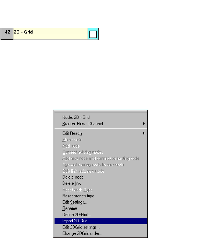
DRAFT
SOBEK, User Manual
5.3.23 Flow - 2D-Grid
2D-Grid node
This is one of the most important building blocks for the modelling of 2D systems, and the
one you would usually start with. It is referred to in the user interface as a ’node’ which at first
sounds confusing, as this node actually represents a whole grid.
A grid can be either imported from a GIS system, or defined within SOBEK as a new grid.
Importing a ’2D grid’ is possible by selecting the ’import 2D grid’ option, an option which
has been added to the standard SOBEK edit network menu (see Figure 5.130). Note that this
option is only available after you have selected the ’2D grid’ node as a building block.
Figure 5.130: Edit network menu, Import 2D-Grid... menu
Edit network menu
After you have selected this option, you need to select the <asc>-file that contains the grid
information you want import. As mentioned before, this <asc>-file is a standard grid defi-
nition file, which can be generated as output by for example ARCView (see appendix for an
example). The file contains the following information about the grid:
the number of columns
the number of rows
x-coordinate of the bottom left corner of the grid
y-coordinate of the bottom left corner of the grid
cell size of the grid elements (same for x and y size)
the no_data value (’missing value’), usually -999 or -9999
For every cell the terrain level.
274 of 900 Deltares

DRAFT
Graphical User Interface
In theory, you can select the file from any given path, for example <c:\gisfiles\grid1.asc>.
However, we strongly recommend using the default directory for these filenames, which is the
<projectname\fixed\>directory. This makes it easier to make a copy of an existing project
and give it to somebody else.
After you have successfully imported the grid, it should appear on the map at the coordinates
specified in the file. You can then visualise the terrain levels of all grid cells by turning on
the active legend (under options) and activate the z-data (model data) from the legend panel.
The active legend will be explained later on.
Most of the time, grids will (need to) be imported from GIS based programs. It is however also
possible to define the 2D grids by hand, by selecting the ’define 2D grid’ option from the edit
network menu (see Figure 5.131). This means that the user will not only have to define the
exact location and size of the grid, but also the terrain level for every grid element. In theory,
one can place the grid at any given location and make it any given size. However, the way the
grids are defined have a major impact on the accuracy of the results, so accurate definition of
2D grids is very important. There are a number of considerations important in this matter:
The number of grids and the number of elements determine the simulation time. The less
elements there are, the shorter the simulation takes.
The smaller the grid elements are, the more accurate the results can be. It is therefore a
good idea to choose a coarse grid in (most) places where accuracy is not required, and a
more fine grid in places where results are critical, for example close to the inlet point/ dam
break point. Another option is to choose the resolution of the grid in the same order as the
resolution of the available terrain level input data.
The grid elements containing a no-data value don’t participate in the calculations; they are
used to specify the barrier around the area of interest, and possibly as no-flow locations
within the area of interest.
Grid properties
For every grid you need to specify a number of properties, some of which need to be specified
immediately, while others can be defined later in the ’model data’ mode.
Figure 5.131 shows the properties that need to be defined.
Deltares 275 of 900
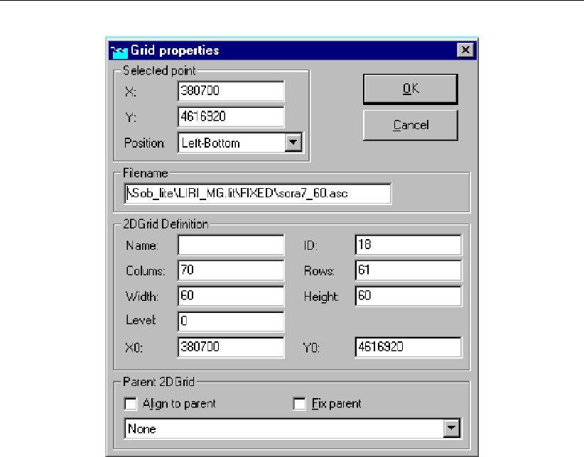
DRAFT
SOBEK, User Manual
Figure 5.131: Grid properties
Selected point information
The ’X’ and ’Y’ coordinates are the coordinates of the map position you selected by pressing
the mouse button just before entering this menu. They represent a (any) corner of the 2D
grid you are about to define. If you are not satisfied with the coordinates, you can alter them
manually here.
The Position represents which of the four corners should appear at the X-Y coordinate you
defined. By default it’s the left-bottom corner.
Filename
The default location for putting the .asc files is the <project directory\fixed\>directory. Make
sure you select a path before saving the grid file.
2D grid definition
Name If you want to, you can specify a unique grid name. This is not absolutely necessary,
as a default name will be defined for you if you don’t specify a name here.
Columns/Rows Every grid is rectangular in shape, the size of which is determined by the
number of rows and columns. The area of interest is inside the rectangular grid, which is
filled up with the no-data values.
Width/Height [m] The width and height of every cell are uniform for the whole grid, so it’s
not possible to specify varying grid size elements throughout one grid. However, different
grids within one schematisation can have different grid sizes.
Level [m] (above OR below reference level, dependent on your definition in SETTINGS)
When using the define 2d grid option, it is only possible to define one uniform terrain level.
276 of 900 Deltares
DRAFT
Graphical User Interface
Later on, in the edit model data mode, there is the possibility to change terrain levels for
single grid elements.
X0/Y0 This is the same coordinate as specified under selected point.
Parent 2D-grid
This option is only relevant when using multiple grids that are either overlapping or nested.
If you select the align to parent option, the child grid will be replaced according to the parent
grid. If you select Fix parent, the position of the parent grid will be changed according to the
position of the child grid. Note that the position of the top left corner of the grid selected will
be changed, and not the number of rows or columns. So, make sure to check both the top
left and bottom right corner of the child grid afterwards to check the alignment. It may be
necessary to adjust the size (columns/ rows) of the child grid manually.
Note: due to an error in the options ’align to parent’ and ’fix parent’, these options should not
be used at the moment!
Edit 2D-grid. . .
This option is available under the edit network menu (see Figure 5.130). Opening the grid
properties window (see Figure 5.131), it gives the user the possibility to change grid proper-
ties, after the grid has been defined. If you decide to resize the grid (number of columns and/
or rows, don’t forget to edit the terrain levels in the <asc>-file accordingly.
Before you can edit the properties of any grid, you will first have to select the node that
represents the grid. And in order to be able to select this type of node, they first have to be
made visible. This can be done by selecting options →network options →nodes. . . select
the 2D grid node and turn on visibility (see Figure 5.132). The 2D-grid nodes should now be
visible in the schematisation.
Figure 5.132: Node settings
Deltares 277 of 900

DRAFT
SOBEK, User Manual
Change 2D-grid order. . .
After selecting this option from the edit network menu, Figure 5.133 appears:
Figure 5.133: 2D Grid Order Window
Here you can change the order of nested grids according to the rules specified in the FAQ on
multiple grids. In short, the child grid (in Figure 5.133 the small green grid, grid 25) should be
’on top of’ the parent grid (the blue grid, grid 18).
This means that in the table on the left, the parent grid should be mentioned BEFORE the
child grid. If the grid order is wrong (clearly visible in the 2D grid order window because the
child grid is hidden behind the parent grid), the simulation will stop. By default, the grid order
is defined by the order in which the grids are defined in the first place. So if you first define
the parent grid, and then the child, the grid order will be correct. If you first define the child,
and the parent, the order needs to be changed using this option.
So, it is very important to always check this option after defining new grids!
Editing 2D-Grid data
After a 2D grid node has been selected for editing, window Figure 5.134 appears:
278 of 900 Deltares
DRAFT
Graphical User Interface
Figure 5.134: Grid data window - 2D Grid location tab
This tab displays general information about the selected grid, which was already defined dur-
ing the edit network mode. If you want to change any of the data specified here, you need to
go back to the edit network mode and use the ’Edit 2D grid settings’ option.
The next tab contains the terrain levels for all 2D grid elements:
Deltares 279 of 900
DRAFT
SOBEK, User Manual
Figure 5.135: Grid data window - Grid Cell Bottom Depth tab
In this window, two aspects are of interest:
The terrain levels in this window can be displayed as either bottom levels (m above ref.lev.)
or bottom depths (m below ref.lev.), whichever one the user prefers. The option selected
here does not influence the simulation in any way, nor the way the results are displayed.
The table contains terrain levels (either depth or height) for all grid-cells. Cell (1,1) repre-
sents the top-left corner of the grid. The user is free to alter any of these values. When
the user presses OK after anything has been changed, the changed .ASC file containing
the terrain levels can be saved under the same name or another. Please verify that the
file is written to the correct directory (preferably <casename\fixed>), and when you enter
a new filename, don’t forget to add the <asc>extension.
The next tab contains the friction values for all grid cells:
280 of 900 Deltares

DRAFT
Graphical User Interface
Figure 5.136: Grid data window - Friction tab
The user can choose between three types of friction formulations, Chézy, Manning or White-
Colebrook. Only one type of friction can be selected per grid. The user can either define one
(uniform) friction value for the whole grid, or select a <asc>-file containing friction values
for all 2D grid elements as a way to model distributed friction. This <asc>-file should have
exactly the same format (including number of columns and rows) as the height definition file.
It is possible, however, to have no-data values in 2D grid cells in the height <asc>-file where
there ARE values in the friction <asc>-file. The other way around is not possible.
Note: that in the user interface, the number on the horizontal axis have been replaced by
letters, ranging from ’A’ to ’XX’.
The next tab, grid cell friction, displays a table with all friction values. This tab is only available
when a distributed friction file has been selected first. It is not possible to modify any of the
values seen here. If the user want to change any of these values, he/she will have to edit the
friction <asc>-file directly (outside SOBEK).
Deltares 281 of 900
DRAFT
SOBEK, User Manual
Figure 5.137: Grid data window - Grid Cell Friction tab
The last tab, defaults, gives the user the possibility to save or load certain grid-related param-
eters as default. For example, if you save the ’friction’ as default (only with uniform friction!),
the next grid you define will have the same friction as the current grid.
5.3.24 Flow - 2D-History
The 2D-history node is a special type of object which can be used to specify (in the Schema-
tisation Taskblock) those 2D grid cells for which output is to be provided. After the simulation
has finished, the output will be available as “Results at history stations” in the Result in Maps
Taskblock.
In case a 2D-History node is located on a 2D grid cell that has a missing value for the bed el-
evation, no output for such 2D-History node will available, meaning that all output parameters
(see below) will have missing values only. The same yields if a 2D-History node is located on
a 2D grid cell of a nested grid that has a missing value, while the underlying parent 2D grid
might have a real value for its bed elevation.
Following output is provided for each 2D-History node:
Bottom, the bed elevation of its underlying 2D grid cell in m.
Waterdepth, the water depth above its underlying 2D grid cell in m.
Waterlevel, the water level in m.
282 of 900 Deltares
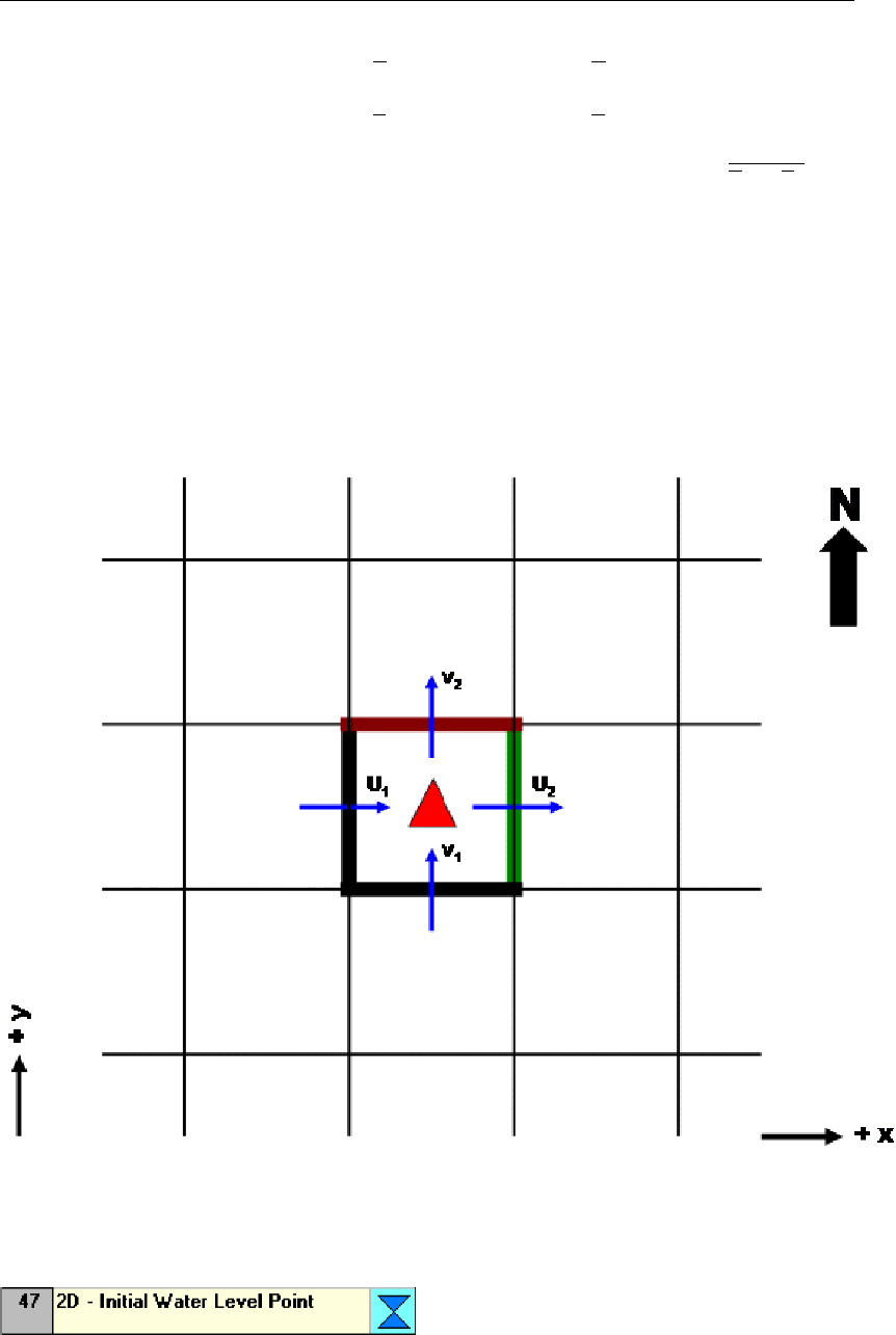
DRAFT
Graphical User Interface
U-Velocity, the average flow velocity (u) in x-direction in m/s (u= (u1+u2)/2; see figure
below).
V-Velocity, the average flow velocity (v) in y-direction in m/s (v= (v1+v2)/2; see figure
below)
Abs Velocity, the resulting none-directional flow velocity (C) in m/s (C=√u2+v2).
Specific U-Discharge, the discharge per meter length (i.e. in m2/s) flowing in x-direction
through the eastern side (green line in figure below) of the underlying 2D grid cell. More
precisely, the specific U-Discharge equals the water depth times the u2-flow velocity at
the eastern side of the underlying 2D grid cell.
Specific V-Discharge, the discharge per meter length (i.e. in m2/s) flowing in y-direction
through the northern side (brown line in figure below) of the underlying 2D grid cell. More
precisely, the specific V-Discharge equals the water depth times the v2-flow velocity at the
northern side of the underlying 2D grid cell.
5.3.25 Flow - 2D initial water level point
Description
This node can be used to create an initial water level in a part of the grid. This is useful in two
cases:
Initially there really is water in part of the 2D system, for example a lake.
A discharge boundary condition is used as part of the 2D schematisation. In this case, it
Deltares 283 of 900
DRAFT
SOBEK, User Manual
is best to define an initial water level point somewhere to make sure that the 2D grid cell
adjacent to the cell containing the boundary condition is not initially dry. So, the reason
for the initial water level point in this case is purely a numerical one, as sometimes no
water will flow at all from the discharge boundary. The water depth can be very small, for
example 1 cm.
The initial water level node will (instantly) fill up all surrounding 2D grid cells with water, until
cells are branched that have a higher terrain level, or the edge of the grid is branched. This
can be a problem when using a discharge boundary condition on a high point in the grid: an
initial water level used for numerical reasons may fill a large part of the grid! This problem
can be solved by lowering the terrain level of the 2D grid containing the initial water level point
slightly below the level of the surrounding cells.
Editing 2D-Initial Water level point data
The only variable that needs to be specified for this node type is the initial water level, relative
to the reference level. Note that a positive value means above the reference level, as opposite
to terrain levels, which are defined as positive in downward direction.
5.4 Node description (Rainfall-Runoff)
5.4.1 RR - Boundary
RR RR - Boundary node
In this chapter, the RR boundary node is described. This node type is used to define boundary
conditions for a Rainfall-Runoff schematisation.
For a detailed description of this node’s input parameters: see the "boundary node input
screens" section from the Reference Manual;
For a detailed description of this node’s possible network configurations: see the "bound-
ary node topology" section from the Reference Manual
What does an RR boundary node do?
RR boundary nodes hold a certain water level, which will form a boundary condition for the
schematisation. This boundary condition is then used to calculate the interaction with the
other RR nodes that are connected to it. For example: if an RR unpaved node is directly
connected to an RR boundary node, on every time step the outflow of the unpaved area
towards that boundary depends on the groundwater level and the boundary value.
Input screens for the RR - Boundary node type
When starting the model data editor for an RR - boundary node, the following tab will be
available for input:
284 of 900 Deltares

DRAFT
Graphical User Interface
Figure 5.138: Data Edit for Boundary Area window - Boundary tab
Here, the water level that applies to the model’s boundary should be entered. There are two
options:
Fixed water level: In this case, the water level on the boundary is constant.
Variable water level (from a table): With this option, the water level on the boundary
node can be given as a function of time.Notice that the option "online from flow mod-
ule" is dimmed. This option is only available for types of nodes that connect the Rainfall
Runoff module with one of the Flow modules (RR on Flow connection node and the RR -
connection on Channel)
Boundary node topology
Nodes of the RR - boundary type can be connected to nearly all of the other RR nodes:
RR - weir node
RR - orifice node
RR - pump station node (either applied as a pump or as an inlet)
RR - QH relation node
RR - friction node This node is considered deprecated functionality.
Use is not recommended.
RR - unpaved node
RR - paved node
Deltares 285 of 900
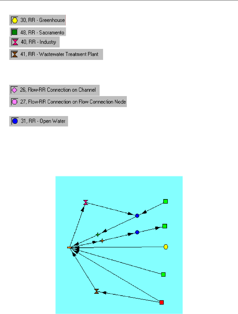
DRAFT
SOBEK, User Manual
RR - greenhouse node
RR - Sacramento node
RR - industry node
RR - wastewater treatment plant node
The only node types that can not be directly connected to an RR boundary node are:
RR Connection on Channel nodes
RR Connection on Flow connection node(These
nodes actually form boundary nodes themselves)
Flow RR Open water node(If such a node would be connected
directly to a boundary, it would immediately get a water level equal to the boundary value.
Thus, that would be of no use at all)
The picture below gives some examples of how RR boundary nodes can be connected to
other node types. Note that these are only some of the possibilities.
Figure 5.139: An example of RR boundary nodes connected to other nodes
In this example you can see the following phenomena:
Upper chain: an industry node that withdraws water from the boundary (demand), and
injects water into an RR open water node
Second chain: an unpaved area that drains towards an Open Water node, which on its
turn is connected to the boundary via a weir.
Third chain: a pumping station that is used as an inlet (see the link directions) to supply
an RR open water node & unpaved area during periods of drought.
Fourth chain: a greenhouse node that drains off towards a boundary node.
Fifth chain: an unpaved area node that drains off directly towards a boundary node.
286 of 900 Deltares
DRAFT
Graphical User Interface
Sixth & Seventh chain: a paved area where the sewer discharge is pumped towards the
boundary via a Waste Water Treatment Plant node, and where the sewer spills directly
towards that boundary.
5.4.2 RR - Flow-RR Connection on Channel node
Description
In this chapter, the Flow - RR Connection on Channel node is described. This is one of two
node types through which an RR schematisation can be linked to a CF schematisation. The
other such node type is the Flow-RR connection on Flow connection node.
The large difference between both nodes is that this node is a derivative of a normal Flow -
Lateral Flow node. This means that this node type should be attached to a branch by simply
using the "add node" button. The other node type is a derivative of a Flow - Connection node,
thus that one should form the start or end of a branch itself.
For a detailed description of this node’s input parameters: see the "Flow - RR Connection
on Channel node input screens" section from the Reference Manual;
For a detailed description of this node’s possible network configurations: see the "Flow -
RR Connection on Channel node topology" section from the Reference Manual
Input screens
When starting the model data editor for an Flow - RR connection on Channel node type, the
following tabs will be available for input:
Boundary:
Deltares 287 of 900
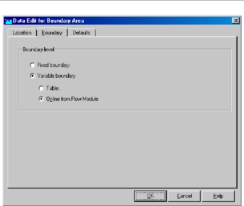
DRAFT
SOBEK, User Manual
Figure 5.140: Data Edit for Boundary Area window - Boundary tab
The parameters that need to be filled in here will form the boundary condition for the Rainfall
- Runoff module. The availability of the options is dependent on your simulation settings:
The "online from flow module" option is only available when you have the RR and CF simula-
tion settings set to "simultaneous". This can be done in the SETTINGS task block:
288 of 900 Deltares
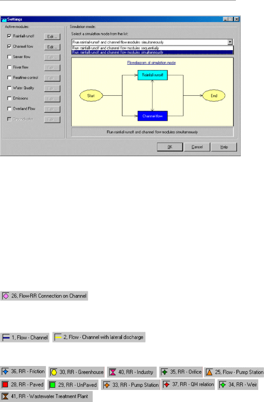
DRAFT
Graphical User Interface
Figure 5.141: Settings window
Fixed boundary: If you choose for a fixed boundary value, the Rainfall-Runoff process will
take place completely independent of the Flow processes. This means that alternating
water levels on the channel will not affect the Rainfall-Runoff process. The RR module
will have a fixed boundary condition to calculate its in- or outflow towards CF.
Variable boundary - table: Also if you choose for a table with varying boundary values,
the Rainfall-Runoff process will take place completely independent of the Channel Flow
processes. This means that alternating water levels on the channel will not affect the
Rainfall-Runoff process. The RR module will have a fixed boundary condition to calculate
its in- or outflow towards CF.
Variable boundary - online from Flow module: This option allows the Rainfall Runoff
module to receive its boundary conditions every time step from the Flow module. This
means that changing water levels in the Flow module will cause the boundary conditions
for the Rainfall- Runoff module to change too, thus influencing its in- or outflow.
Topology
Nodes of the type Flow - RR Connection on Channel need to be attached to one of the
Channel Flow branch types depicted below:
,
On the Rainfall - Runoff side, it should be linked with one of the following RR node types:
, , , ,
, , , ,
Deltares 289 of 900
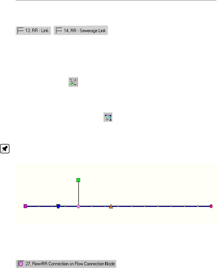
DRAFT
SOBEK, User Manual
The link with RR should be made through one of the following types:
,
Please keep in mind that the RR links should point from the RR nodes towards the Flow -
RR Connection on Channel node.
Add a Flow - RR Connection on Channel node to your schematisation in the following way:
Select the appropriate node type (Flow - RR Connection on Channel)
Use the "add node" button to add it to the schematisation. When clicking, SOBEK
will automatically find the nearest channel to attach it to.
If desired, the node may later-on be moved to other locations on the branch, or even to
another branch by using the "move node"
button.
Figure 5.142: Move node icon
Note: Before adding a Flow - RR Connection on Channel node to your schematisation, you
should have at least one of the above channel types present.
Figure 5.143: An example of a valid network
5.4.3 RR - Flow-RR Connection on Flow Connection node
Description
In this chapter, the Flow - RR Connection on Flow Connection node is described. This is one
of two node types through which an RR schematisation can be linked to a CF schematisation.
The other such node type is the Flow-RR Connection on Channel.
The large difference between both nodes is that this node is a derivative of a normal Flow
- Connection node. This means that this node type should not be attached to an existing
branch, but that itself it should form the start or end of a branch.
The other node (Flow-RR Connection on Channel) is a derivative of a normal Flow - Lateral
Flow node, which means that it can be attached to a branch by simply using the "add node"
button.
290 of 900 Deltares
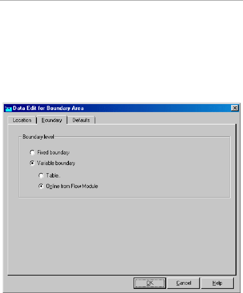
DRAFT
Graphical User Interface
For a detailed description of this node’s input parameters: see the "Flow - RR Connection
on Flow Connection node input screens" section from the Reference Manual;
For a detailed description of this node’s possible network configurations: see the "Flow -
RR Connection on Flow Connection node topology" section from the Reference Manual
Input screens
When starting the model data editor for an Flow - RR connection on Flow connection node
node type, the following tabs will be available for input:
Boundary tab:
Figure 5.144: Data Edit for Boundary Area window - Boundary tab
The parameters that need to be filled in here will form the boundary condition for the Rainfall
- Runoff module. The availability of the options is dependent on your simulation settings:
The "online from flow module" option is only available when you have the RR and CF simula-
tion settings set to "simultaneous". This can be done in the SETTINGS task block:
Deltares 291 of 900
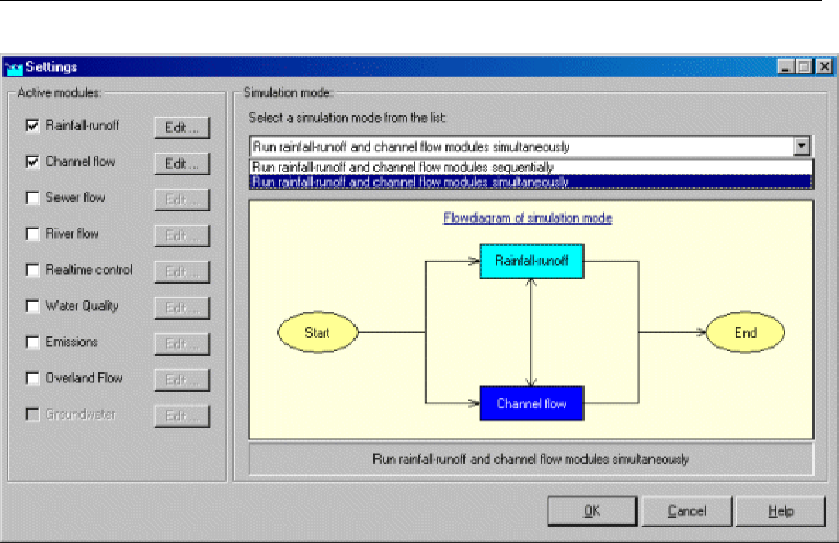
DRAFT
SOBEK, User Manual
Figure 5.145: Settings window
Fixed boundary: If you choose for a fixed boundary value, the Rainfall-Runoff process will
take place completely independent of the Flow processes. This means that alternating
water levels on the channel will not affect the Rainfall-Runoff process. The RR module
will have a fixed boundary condition to calculate its in- or outflow towards CF.
Variable boundary - table: Also if you choose for a table with varying boundary values,
the Rainfall-Runoff process will take place completely independent of the Channel Flow
processes. This means that alternating water levels on the channel will not affect the
Rainfall-Runoff process. The RR module will have a fixed boundary condition to calculate
its in- or outflow towards CF.
Variable boundary - online from Flow module: This option allows the Rainfall Runoff
module to receive its boundary conditions every time step from the Flow module. This
means that changing water levels in the Flow module will cause the boundary conditions
for the Rainfall- Runoff module to change too, thus influencing its in- or outflow.
The Storage tab depicted below is only activated when the Urban 1DFLOW (Sewer flow)
module is activated.
Storage tab:
292 of 900 Deltares
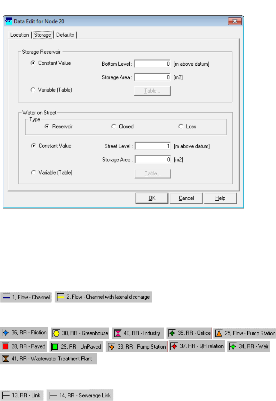
DRAFT
Graphical User Interface
Figure 5.146: Data Edit for Node window - Storage tab
For a more detailed description of the Storage tab, see section 5.3.12.1 paragraph input
screens
Topology
Nodes of the type Flow - RR connection on Flow connection need to form the starting or
end point of one of the Channel Flow branch types depicted below:
,
On the Rainfall - Runoff side, it should be linked with one of the following RR node types:
, , , ,
, , , ,
The link with RR should be made through one of the following types:
,
Please keep in mind that the RR links should point from the RR nodes towards the Flow
- RR connection on Flow connection node. Remember that Flow - RR connection on Flow
Deltares 293 of 900
DRAFT
SOBEK, User Manual
connection nodes should always be part of a branch themselves. A correct working method
is:
Switch to the "edit network" mode in NETTER
Select the node type Flow - RR connection on Flow connection
Select the "add node" option
Place the node in the schematisation by clicking
Select the appropriate branch type (Flow Branch or Sewer Pipe)
Select the "connect nodes" option
Connect the node that you just added to another one by clicking and dragging.
Figure 5.147: An example of a valid schematisation containing a Flow - RR connection
on Flow connection node
5.4.4 RR - Greenhouse area
Greenhouse area
A greenhouse horticulture area can be schematised with a greenhouse node.
For a detailed description of this node’s input parameters: see the "greenhouse node input
screens" section from the Reference Manual;
For a detailed description of this node’s possible network configurations: see the "green-
house node topology" section from the Reference Manual
For a detailed description of this node’s underlying mathematical equations: see the "Tech-
nical Reference" manual.
What does a greenhouse node do?
The rainfall-runoff process on greenhouses is described by volume balances in two storage
reservoirs:
storage on the greenhouses; and
storage in rainwater basins.
Storage-on-greenhouses represents the storage of water on greenhouse glass surface area
(roofs). Rainfall can be stored on the roofs, before it evaporates or flows into the rainwater
storage basins above- or underground.
294 of 900 Deltares
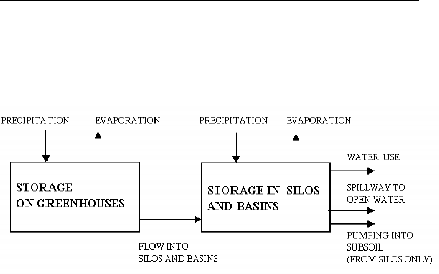
DRAFT
Graphical User Interface
The above-ground basins take in runoff-water from the glass surface as well as from direct
precipitation. The amount of water stored is reduced by evaporation, water use in green-
houses, and possible pumping to the subsoil (under ground storage). When the maximum
storage capacity is exceeded, the excess water flows into the adjacent open water. The figure
below shows the volume balance in the greenhouse areas.
Figure 5.148: Volume balance in the greenhouse areas
Representation of the rainfall-runoff process in greenhouse areas
In SOBEK the rainwater basins have been divided into ten categories, depending on their
volume per hectare of draining glass surface. SOBEK uses the lower limits of the categories.
For example: all basins with a storage between 2500 and 3000 cubic meters per hectares of
glass are considered as basins with a capacity of 2500 cubic meters per hectare of glass.
SOBEK-rr distinguishes itself from most other models with respect to the way greenhouse
areas are treated. They are considered a special area type with provisions for the way horti-
culture makes use of rainwater storage basins. For instance, the initial filling percentage can
be defined. Since the rainwater storage basins are usually not completely filled at the start of
a rainfall period, this possibility often leads to a more realistic description of the flow into open
water.
The (remaining) storage present in the basins at the beginning of the computation is an impor-
tant variable determining whether spilling from the basins will occur or not. Therefore, SOBEK
also provides historical data about the development of the storage in basins. To that end a
separate computation has been carried out for each of the ten basin categories for the period
1951–1994, using the detailed greenhouse model of the Staring Centre-LDO. This accurate
model is based on the water usage by a standard glass culture firm. This model takes into ac-
count aspects such as the management of rainwater basins by the market gardeners, return
flow of water due to the combustion of natural gas etc. All assumptions have been rounded
conservatively, so that the remainder storage in basins are under-estimated.
Greenhouse area input screens
When starting the model data editor for an RR - Greenhouse area node type, the following
tabs will be available for input:
Deltares 295 of 900
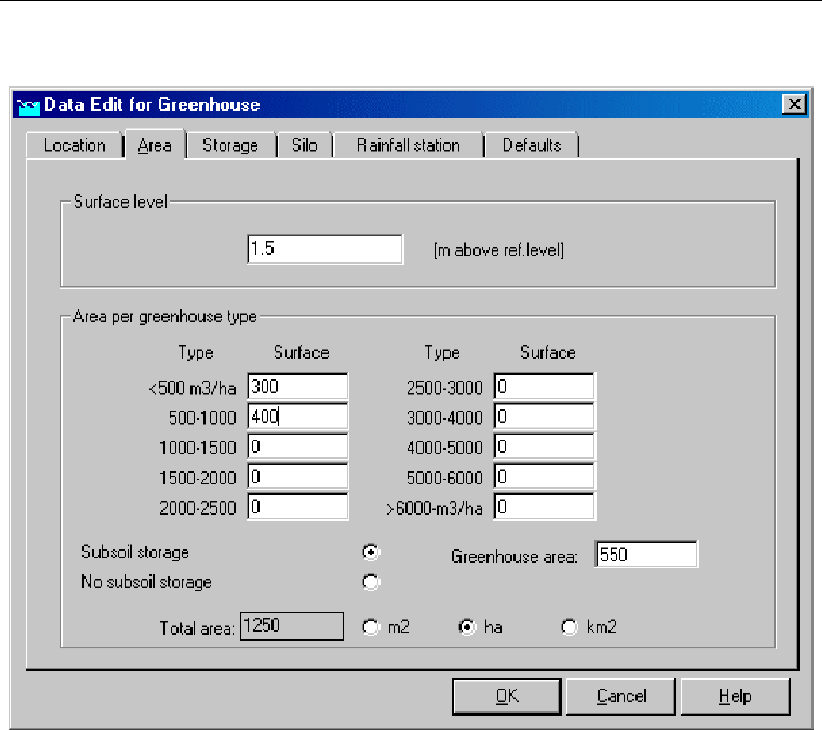
DRAFT
SOBEK, User Manual
Area tab
Figure 5.149: Data Edit for Greenhouse,Area tab
On this tab, all data related to the area of different greenhouse types should be entered:
Surface level: Represents the surface level of the soil.
Area per greenhouse type: As explained in the Functional Reference Manual chapter
"greenhouse area description", the rainwater basins have been divided into ten categories,
depending on their volume per hectare of draining glass surface. On this tab, the surface
area for each of these categories can be entered. Of course, the sum of all areas should
correspond with the total surface of the greenhouses.
Subsoil storage:For some greenhouses, additional water can be stored in subsoil si-
los. Here the greenhouse area that uses such storage method should be entered. After
choosing this option, the tab "Silo" becomes active.
296 of 900 Deltares
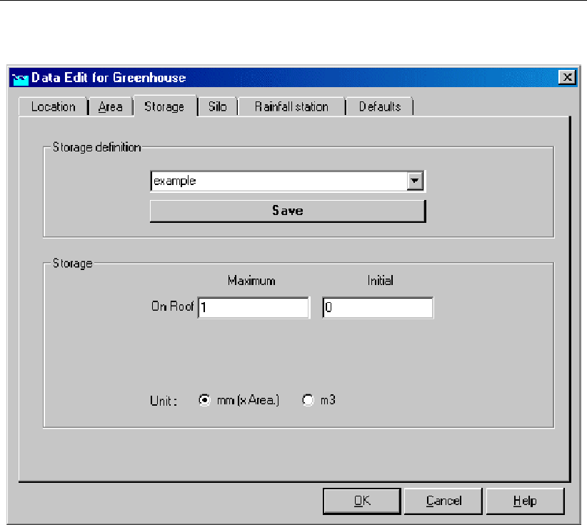
DRAFT
Graphical User Interface
Storage tab
Figure 5.150: Data Edit for Greenhouse,Storage tab
On the storage tab, the maximum and initial amount of water that can be stored on the roof of
the greenhouses is defined. The chosen values can be saved in a separate "storage definition"
so that the same values can easily be applied to other greenhouse nodes.
Enter the data as follows:
first type a name in the "storage definition" field
click the Define button
enter the appropriate values for maximum and initial storage;
click the Save button;
note that you can re-use this storage definition on other greenhouse nodes.
Explanation of the parameters:
Maximum storage: Equals the amount of water that can be stored on the rooftop without
being drained off. Only after the rainfall amount exceeds this amount, water starts draining
off the roofs.
Initial storage: If your simulation starts right after a wet period, it might be the case that
the storage capacity of the roof itself is already partially filled with water. That amount of
water should be entered here.
Deltares 297 of 900

DRAFT
SOBEK, User Manual
Silo Tab
Figure 5.151: Data Edit for Greenhouse,Silo tab
If the "subsoil storage" option on the "Area" tab has been chosen, this tab will become active.
Here the storage and pumping capacity of a subsoil silo can be entered.
Due to rainfall on the greenhouse area that is connected to this silo, the silo is filled with water.
In the meantime, water is being pumped out in order to supply the plants with water. If, due
to heavy rainfall, the silo’s storage capacity is exceeded, the excess amount will "overflow"
towards a connected RR - Open water node or boundary node.
Silo capacity:This parameter represents the storage capacity of the subsoil silo in volume
per unit of greenhouse area. When multiplying this value with the "Greenhouse area" value
on the "Area" tab, the total volume of the silo is obtained.
Pumping capacity:This parameter represents the capacity of the pumps that supply wa-
ter from the silo to the plants within the greenhouse. In the model, this amount of water is
simply defined as an outflowing term.
These values too are entered as a "definition". This allows for re-using that definition on other
greenhouse nodes.
Enter the data as follows:
first type a name in the "silo definition" field
click the Define button
enter the appropriate values for maximum and initial storage
click the Save button;
298 of 900 Deltares
DRAFT
Graphical User Interface
note that you can re-use this silo definition on other greenhouse nodes.
Rainfall station tab:
Here, the rainfall station that applies for this node can be selected. Rainfall stations can be
created in the "Meteorological data" task block.
Greenhouse area node topology
Nodes of the RR - Greenhouse area type may drain off towards one of the following nodes:
RR - open water node
RR - boundary node
Commonly, a greenhouse node is connected with an open water node.
5.4.5 RR - Industry
RR - Industry node general description
In this chapter, the RR - Industry node is described. With an RR - Industry node you can
simulate lateral discharges to and from the water system. This node type is commonly used
to simulate industrial water extraction and -return (e.g. water for process cooling).
But this node type can also be used to simulate lateral discharges (extractions and discharges)
of known amounts.
For a detailed description of this node’s input parameters: see the "RR - Industry node
input screens" section from the Reference Manual;
For a detailed description of this node’s possible network configurations: see the "RR -
Industry node topology" section from the Reference Manual
RR - Industry node input screens
When the model data editor for an RR - Orifice node type is started, the following tabs will
become available for input:
Industry tab:
Deltares 299 of 900

DRAFT
SOBEK, User Manual
Figure 5.152: Data Edit for Industry,Industry tab
On this tab, lateral discharges (discharges and extractions of water) can be defined. Extrac-
tions are defined as "demands" and "discharges" as "injections".
Demands: Here, the amount of water that is extracted from the system should be entered
(as a function of time). Click the <Table>button to open the table where the values should
be entered.Note that demands are always extracted from an "upstream" connected node.
See the chapter on Industrial node topology for more information.
Discharge: In this section, the amount of water that is injected into the system should be
entered (as a function of time). This can be done with two options:
1 "Use return flow factor of the demand". Using this option, the amount of injected water
will be a percentage of the amount that is extracted according to the Demands settings.
Fill the appropriate percentage in into the box next to this parameter name.
2 "Variable discharge (table)". Using this option, the amount of injected water will take
place independently of the demand, but can be defined manually as a function of time.
Click the <Table>button to open the table where the values should be entered.
Note: that discharges are always injected on a "downstream" connected node. See the
chapter on Industrial node topology for more information.
300 of 900 Deltares

DRAFT
Graphical User Interface
RR - Industry node topology
The RR - Industry node requires an upstream node to extract its demands and a downstream
node to inject its discharges. Note that the arrows on the RR links indicate which nodes are
defined as "upstream" and which ones as "downstream".
RR Industry nodes can be connected to the following node types:
RR - Open Water nodes:
RR - boundary nodes:
CF RR on Flow connection nodes:
CF RR on channel connections.
5.4.6 RR - Open water
Open water node descriptions
In this chapter, the open water node is described. It is a commonly used modelling object
within the SOBEK Rural Rainfall-Runoff module.
What does the open water node do?
It can represent the area which is occupied by a number of water courses. Such area may
vary with the prevailing water level, due to existing bank slopes. Usually, the open water node
receives water from connected nodes of the following types:
Unpaved area node
Paved area
Greenhouse area
Industry
Waste Water Treatment Plant
Sacramento
Furthermore it can exchange water with other open water nodes, a Flow model (Channel Flow
or River Flow module) or a model boundary, via structures or a friction node.
Note: in dry periods the above described procedure can be reversed to let water in. In that
case water is deliberately led from a boundary or Flow model towards the open water node,
and finally infiltrated in the unpaved area.
Open water node input screens
When the model data editor for an RR - Open Water node type is started, the following tabs
will become available for input:
Tab Surface:
Deltares 301 of 900
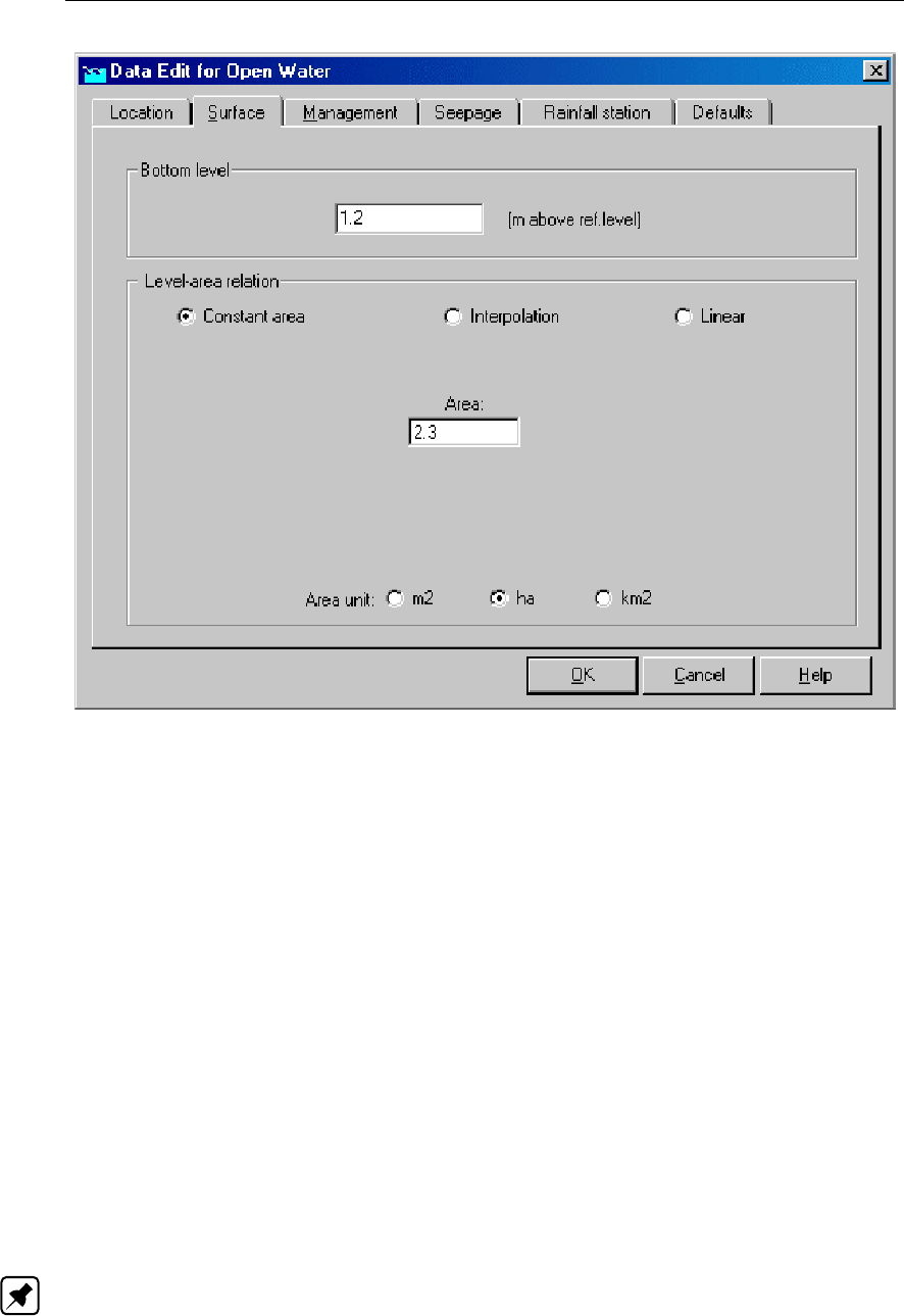
DRAFT
SOBEK, User Manual
Figure 5.153: Data Edit for Open Water,Surface tab
Note that an RR Open Water node represents a series of channels through a certain volume
of water, thus:
The area that is covered by the open water (may be dependent of the water level)
The water depth, which is calculated during every time step.
The following variables have to be specified:
Bed level: Represents the bed level of the channels/ditches that are represented by the
open water node.
Level-Area relation: In this section, the open water area (as seen from above) is entered.
It may be constant (independent of the water level; this is the case if all ditches have ver-
tical walls) or an area that varies with the water level (if the ditches have side slopes).The
options:
1 A constant area.
Independent of the water level.
2 Interpolation from values in a table.
This option lets you fill in six water levels for which the open water area is known.
The area for other water levels is then interpolated from this table. Note: when
using this option, it is wise to include the open water area at the bottom level in the
table. Otherwise the calculation of the area at bottom level will be calculated by linear
extrapolation of the lowest two values from the table. Sometimes this may lead to
negative areas.
3 Linear.
Allows to fill in the area of open water at the target level and the percentage by which
302 of 900 Deltares

DRAFT
Graphical User Interface
it increases with rising water level. You can check the interpolation table which is
generated and used in SOBEK by switching towards the "interpolation" option after
having specified your values for linear interpolation.
Tab Management:
Figure 5.154: Data Edit for Open Water,Management tab
On this tab, the hydrological management characteristics for this open water node need to be
entered:
Target Level: Generally, in second order ditches, a certain target level is being maintained
by weirs or other structures. This kind of target level needs to be filled in here. It can either
be a fixed level or variable in time.
Note: the target level value on itself will not have any effect on the water management.
The actual water levels are determined by the operation of structures (such as weirs) that
are connected to this area. You’ll need a structure to actually maintain the desired target
level. The reason to enter a value for target level here is mainly for the creation of output
files that refer to that value.
Maximum permissible level: This parameter does not have any effect on the calcula-
tions. It is only used to calculate the amount and duration by which a certain level is
exceeded.
Tab Seepage:
Deltares 303 of 900
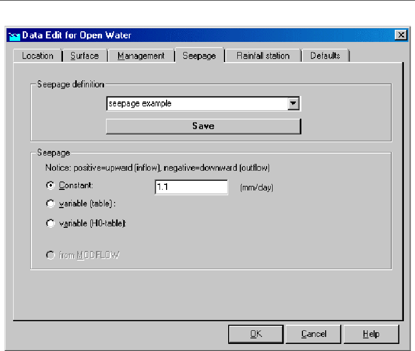
DRAFT
SOBEK, User Manual
Figure 5.155: Data Edit for Open Water,Seepage tab
The Seepage tab refers to the exchange of water between the top layer (all soil that’s higher
than the bottom of the ditches) and the groundwater underneath
First, enter a name for the seepage definition, then click on <Define>and enter the appro-
priate value. A positive value represents inflow, a negative value represents outflow.
The values can either be:
Constant
Variable (in time)
Calculated from a variable H0 value (pressure head in the underlying aquifer) and the
resistance value of a confining layer in between.
Tab Rainfall Station:
304 of 900 Deltares
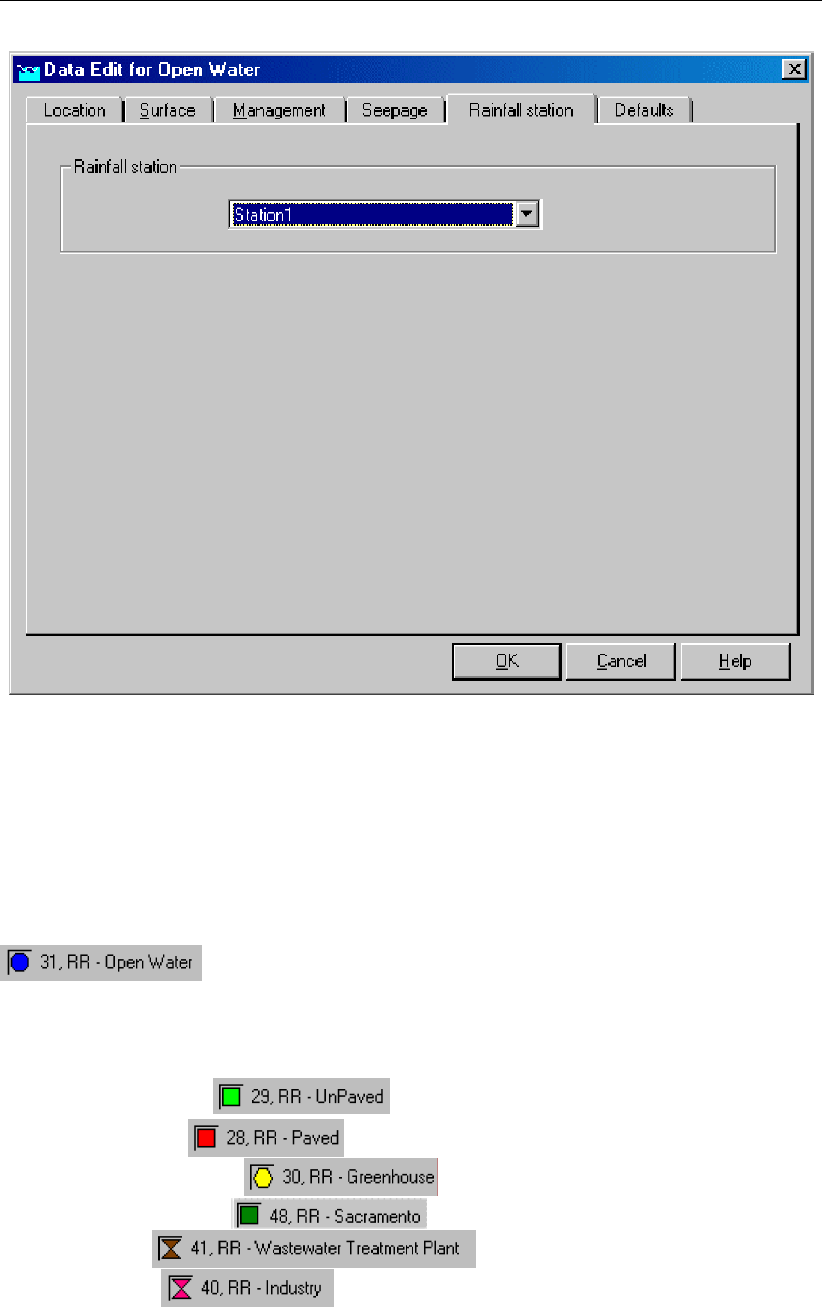
DRAFT
Graphical User Interface
Figure 5.156: Data Edit for Open Water,Rainfall station tab
On this tab you choose the meteorological station that will apply to the Open Water node.
Rainfall and evaporation will apply to the area open water on every time step. Wind data will
have no influence because the Open Water node is a 0-dimentional node type (point objects
without physical outstretches in the horizontal plain).
Open water node topology
An RR open water node can only be connected to other RR objects. On the upstream side, it
may be connected with:
RR Unpaved nodes
RR Paved nodes
RR Greenhouse nodes
RR Sacramento node
WWTP node
Industry node
Notice that the first four node types transfer a rainfall intensity to a certain outflow. When
connecting these nodes to an RR Open Water node, this outflow will therefore flow into the
RR Open Water node.
Deltares 305 of 900
DRAFT
SOBEK, User Manual
On the downstream and upstream side, the RR Open Water node may be connected to RR
structures or a friction node:
RR Weir nodes
RR Orifice nodes
RR Pump station nodes
RR Friction nodes
RR QH relation nodes
Note: on their turn, these structures should be connected to another RR Open Water node
or an RR boundary node.
Optionally, one may connect an additional RR Industry node to an RR
Open Water node in order to withdraw or inject a certain amount of water in time. Typical
schematisations covering RR Open water nodes could look like this:
Figure 5.157: Example of RR Open Water node connections.
In this example an RR Open Water node receives water from an Unpaved area, a Paved area
and a Greenhouse area. The node is connected to a Boundary node via a Weir, thus when
the water level exceeds the crest level of the weir, water is discharged to the boundary node.
Furthermore there is a connection with another Open Water node via a friction node, causing
a slight difference in water level between both Open Water nodes. The downstream Open
Water node is connected to the SOBEK Channel Flow module via a RR Pump Station (which
could have been any RR structure).
306 of 900 Deltares

DRAFT
Graphical User Interface
5.4.7 RR - Orifice node
RR - Orifice node general description
In this chapter, the RR - Orifice node is described. With an RR - Orifice node you can simulate
a structure with a controllable gate height, through which water flows.
For a detailed description of this node’s input parameters: see the "RR - Orifice node input
screens" section from the Reference Manual;
For a detailed description of this node’s possible network configurations: see the "RR -
Orifice node topology" section from the Reference Manual
For a detailed description of this node’s underlying mathematical equations: see the "Ori-
fice section from the Technical Reference Manual".
RR - Orifice node input screens
When the model data editor for an RR - Orifice node type is started, the following tabs will
become available for input:
Options Tab:
Figure 5.158: Data Edit for Gate/Orifice,Options tab
On this tab, you can define how the orifice is to be used:
Orifice type: normalThis option means that water can flow through the orifice in both
directions.
Deltares 307 of 900
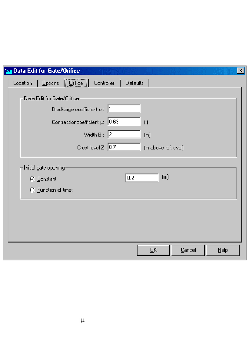
DRAFT
SOBEK, User Manual
Orifice type: inletThis option means that water may only flow through the orifice in posi-
tive direction. The arrows on the links that connect the orifice to other objects indicate the
positive flow direction.
Orifice tab:
Figure 5.159: Data Edit for Open Water,Orifice tab
On this tab, the dimensions of the orifice should be entered:
Discharge coefficient c: See the "Orifice" section of the Technical Reference Manual for
the exact implementation of this parameter in the discharge formula of this structure type.
Contraction coefficient This is a coefficient that represents the energy loss due to
contraction of the water mass that flows through the orifice. See the "Orifice" section
of the Technical Reference Manual for the exact implementation of this parameter in the
discharge formula of this structure type.
Width B: Represents the width of the gate through which the water flows.
Crest level Z: Represents the crest level of the gate, thus the bottom of the gate opening.
Initial gate opening: This parameter represents the orifice’s gate opening. Notice that it
is called "initial" gate opening height. This name has been chosen because the opening
may eventually be overruled by a controller. If there’s no controller active for the orifice, the
gate opening will remain equal to the "initial gate opening" throughout the entire simulation.
Controller Tab:
308 of 900 Deltares
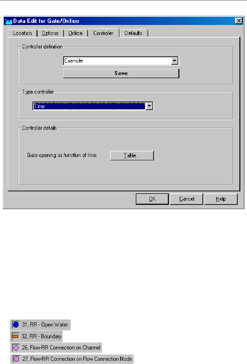
DRAFT
Graphical User Interface
Figure 5.160: Data Edit for Open Water,Controller tab
On the controller tab, the behaviour of the orifice can be controlled (optional). With a controller,
the initial opening heights, as defined on the "Orifice" tab, are overruled.For RR - Orifices, only
a so-called time controller is available. This means that the gate height can be defined as a
function of time.
RR - Orifice node topology
An RR - Orifice should always be connected to at least one RR - Open Water node, as it is
meant to let water flow in or out of an open water section.
RR - Orifices can be connected to nodes of the following types:
(available in the Flow modules only)
(available in the Flow modules only)
Deltares 309 of 900
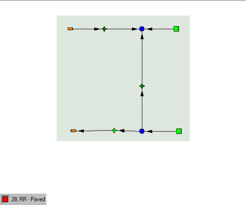
DRAFT
SOBEK, User Manual
Figure 5.161: An example of a network where RR Orifices are used
5.4.8 RR - Paved node
Paved area node; general description
In paved areas water can be stored on the surface (“on-the-street storage”) and in a sewer
system. The first one represents the storage on paved areas like roofs and roads. The second
one represents the water stored in sewer mains of separated or combined sewer systems. The
representation of the rainfall-runoff process in paved areas is shown.
The storage on the street and the sewer storage can be considered to be two reservoirs.
The rainfall-runoff module calculates a water balance of these reservoirs. When precipitation
occurs on the paved area, first the on-the-street storage reservoir is filled. If this reservoir is
full, it starts spilling into the sewer reservoir. The amount of on-the-street storage is reduced
by evaporation.
Water can enter the sewer reservoir in two ways: first by spilling from the on-the-street storage,
and second by return flow from domestic water use (dry weather flow). Depending on the type
of sewer system, the inflow from the surface and the dry weather flow are mixed in one sewer
storage reservoir, or put into separate sewer storage reservoirs.
When the sewer storage reservoir contains water, the sewer pumps are switched on, and
water is pumped from the sewer to the local open water or to a boundary representing a
waste-water treatment plant outside the system. If the sewer is full, it can also spill directly
into the open water. Flows from paved to unpaved areas and vice versa are neglected.
310 of 900 Deltares
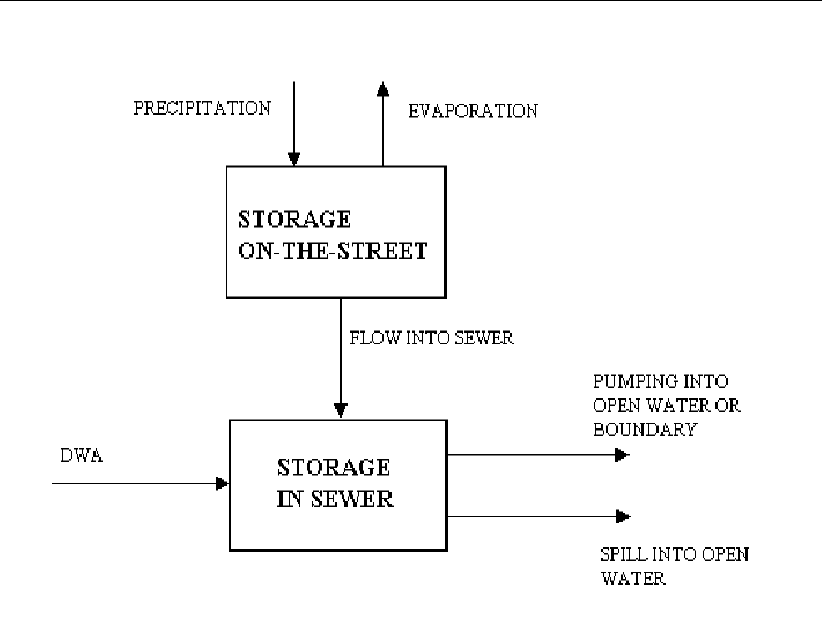
DRAFT
Graphical User Interface
Figure 5.162: The storage on the street and the sewer storage can be considered as two
reservoirs
Representation of the rainfall-runoff process in paved areas.
You can model multiple types of paved area by dividing the total area into sub-areas with
specific characteristics. In this way areas with and without sewers can be modelled. By
definition, there is no infiltration to groundwater in paved areas. When modelling urban areas,
as a rule of thumb about 50 percent of the urban area can be considered as paved area, and
50 percent can be considered as unpaved area (private gardens and public parks).
Paved area input screens
When starting the model data editor for a paved area node type, the following tabs will be
available for input:
The Area tab
Deltares 311 of 900
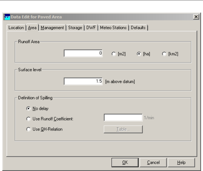
DRAFT
SOBEK, User Manual
Figure 5.163: Data Edit for Paved Area window, the Area tab
On this tab, the following data can be entered:
Runoff Area: The value filled in here will represent the paved area on which rainfall from
the selected rainfall station for this node will fall. When the maximum storage capacity
of the surface (storage tab) is exceeded, the water will immediately start flowing into the
sewer system (management tab).
Surface level: Surface level equals the street level for the paved area node. If the water
level in a connected open water node will exceed this level, the water will inundate the
paved area.
Definition of Spilling:
No delay: All surface runoff branches the outflow point in the same timestep.
Use Runoff Coefficient: A runoff delay coefficient, similar to the RR-Urban runoff
model.
Use QH-Relation (Beta functionality): Limit the discharge Q(mm/s) based on the
water level H(m above datum).
For more information on these options, see section 6.5.1.24.
312 of 900 Deltares
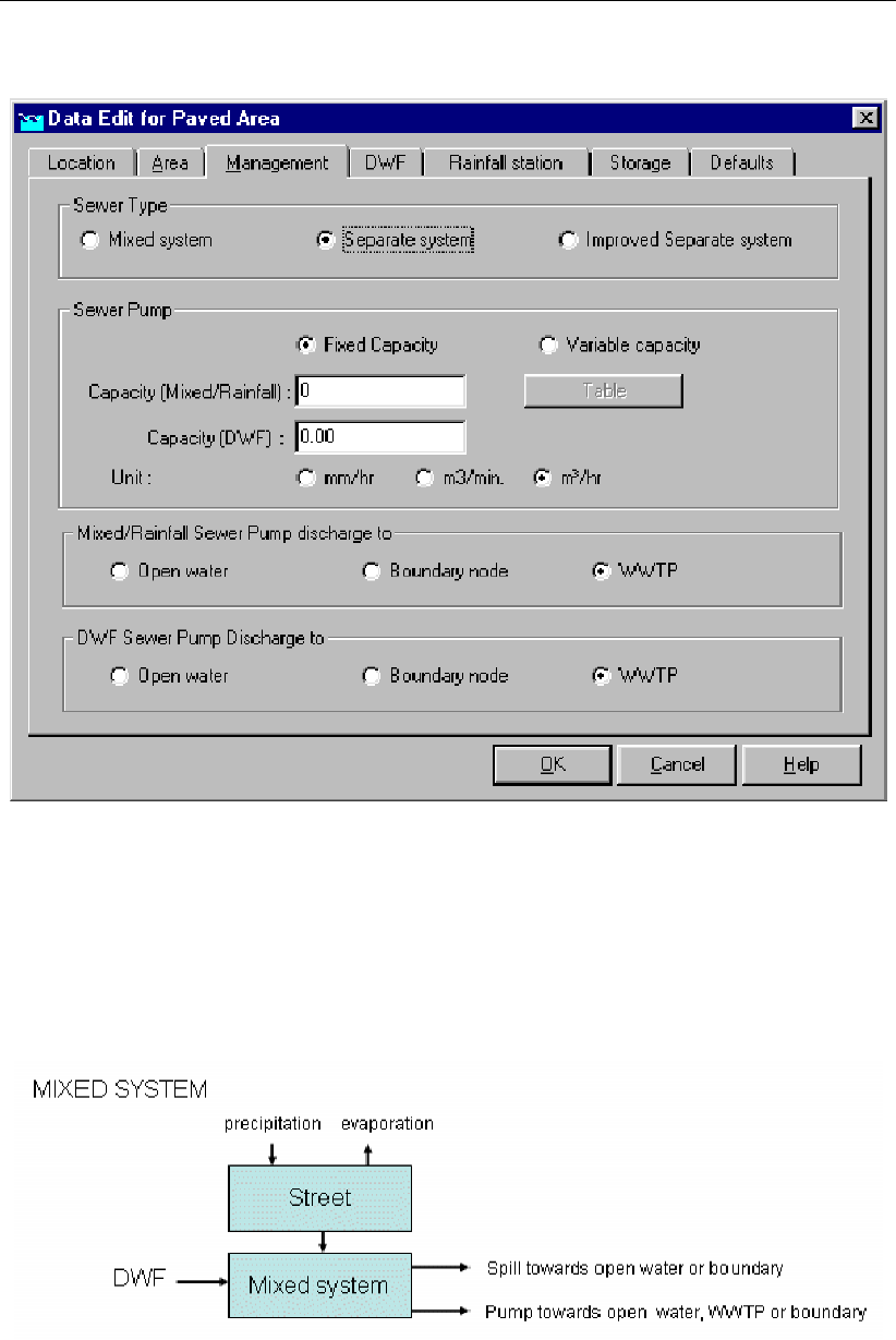
DRAFT
Graphical User Interface
The Management tab
Figure 5.164: Data Edit for Paved Area window, the Management tab
On the Management tab, one can define the operation of the sewer system into which the
intercepted rainfall flows.
Sewer Type: There are three sewer types: Mixed system, Separate system and Improved
separate system. The images below show how they work:
Figure 5.165: Sewer type: Mixed system
Deltares 313 of 900
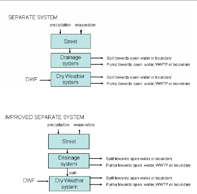
DRAFT
SOBEK, User Manual
Figure 5.166: Sewer type: Separate system
Figure 5.167: Sewer type: Improved separate system
Sewer pump: Here, the pumping capacities for the sewer pump[s] should be specified.
These pump will attempt to keep the systems empty. In case of a separate system, each
subsystem has its own pump.
Pump discharge to: You should also define whereto the sewer pump[s] should trans-
port its/their discharge. This can either be an RR open water node, a boundary node or
a Waste Water Treatment Plant. If you want to have the discharge pumped towards a
Channel Flow connection, select ’boundary’. The Rainfall Runoff module sees RR-Flow
connections as boundaries.
314 of 900 Deltares

DRAFT
Graphical User Interface
The Dry Wether Flow (DWF) tab
Figure 5.168: Data Edit for Paved Area window, the Dry Weather Flow tab
On this tab, you should define the amount of inhabitants and the amount of water they use
daily. Both numbers are then multiplied and simulated as an inflow towards the paved nodes
sewer system.
The Rainfall Station tab
Deltares 315 of 900

DRAFT
SOBEK, User Manual
Figure 5.169: Data Edit for Paved Area window, the Rainfall Station tab
Select here the rainfall station that applies for this node. Rainfall stations can be created in
the "Meteorological data" task block.
The Storage tab
316 of 900 Deltares
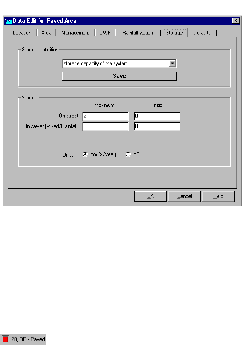
DRAFT
Graphical User Interface
Figure 5.170: Data Edit for Paved Area window, the Storage tab
On the storage tab, the maximum storage capacities of the street level and the sewer system
should be specified.
How does it work:
When the rainfall intensity exceeds the maximum storage on street, the remaining amount will
flow into the sewer system. On its turn, when that discharge exceeds the maximum storage
plus pumping capacity of the sewer, the remaining discharge is spilled (see Management tab).
The initial storage fields can be used when part of the available storage is already filled up at
the start of a simulation.
Paved area node topology
RR - Paved nodes give a choice to create one or two connections.
In case only one connection is used, both the sewer pump discharges and the sewer
overflows (spills) will flow towards the same node.
In case two connections are used, the user may, for example, choose to have the sewer
pump discharges flow towards a boundary node, and the sewer overflows towards an RR
open water node. By default, all sewer overflows (spills) flow towards open water nodes.
RR - Paved nodes can be connected to either one of the following node types:
Deltares 317 of 900
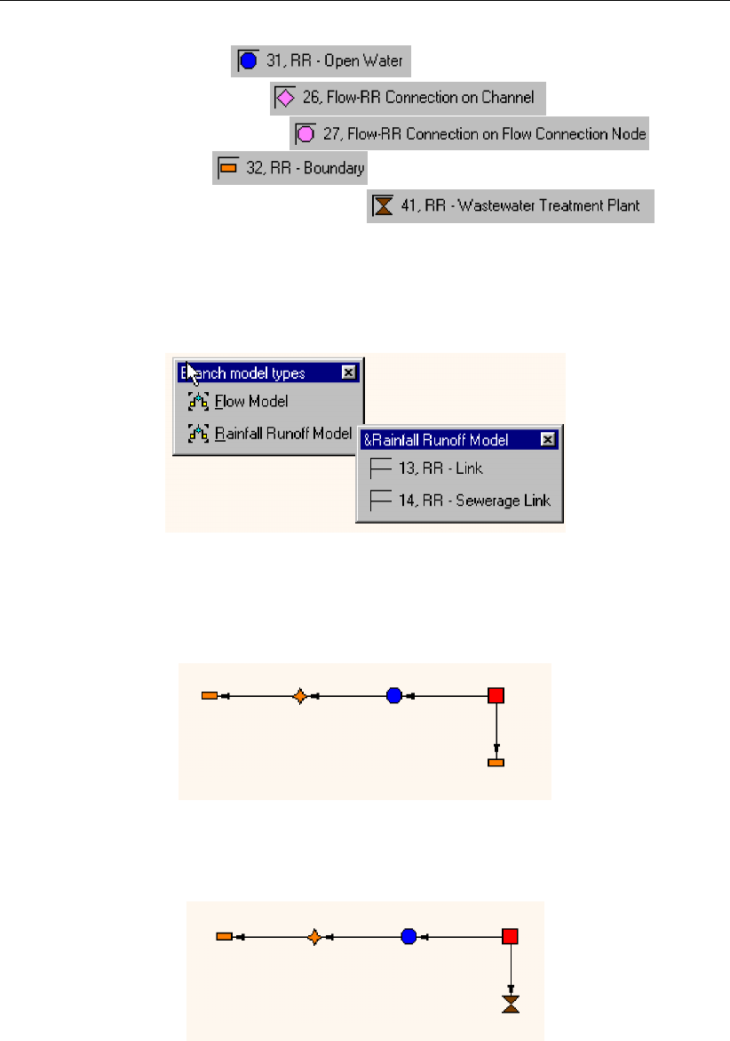
DRAFT
SOBEK, User Manual
An RR Open Water node
An RR on channel connection
An RR on Flow connection node
An RR Boundary node
An RR Waste Water Treatment Plant node
When connecting a paved area node to one of these nodes, make sure you have selected
the RR-link connection type. Notice: the usage of an RR-Sewerage Link is optional. The
difference with a regular RR link is only for presentation purposes.
Figure 5.171: Select RR-Paved node connection
Below, some examples of typical RR Paved connections are given.
Figure 5.172: Connecting an RR Paved node to an RR open water for the sewer overflows
and surface runoff and an RR boundary for the sewerage discharge.
Figure 5.173: Connecting an RR Paved node to an RR open water for the sewer over-
flows and surface runoff and an RR Waste Water Treatment Plant for the
sewerage discharge. Note that the WWTP node on its turn should be con-
nected to another node.
5.4.9 RR - Pump Station
318 of 900 Deltares
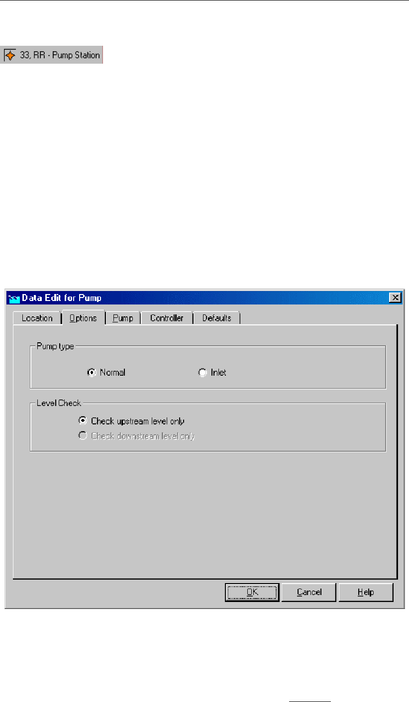
DRAFT
Graphical User Interface
RR - Pump station node general description
In this chapter, the RR - Pump station node is described. With an RR - Pump station node
you can simulate a pump that is activated or deactivated through changing water levels. RR -
Pump stations can either be applied to withdraw excess water or to supply water in periods of
shortage.
For a detailed description of this node’s input parameters: see the "RR - Pump station
node input screens" section from the Reference Manual;
For a detailed description of this node’s possible network configurations: see the "RR -
Pump station node topology" section from the Reference Manual
RR - Pump station node input screens
When the model data editor for an RR - Pump Station node type is started, the following tabs
will become available for input:
Options tab
Figure 5.174: Data Edit for Pump, the Options tab
On the "Pump" tab, one can define how the pump will be used:
Normal: The pump will operate as a normal pump that starts extracting water when the
water level on the upstream side (suction side) exceeds the switch-on level. It will then
Deltares 319 of 900
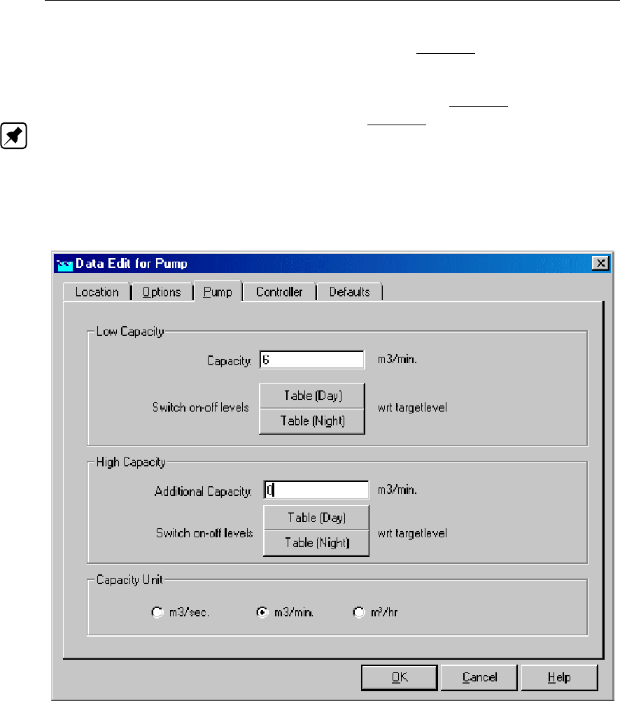
DRAFT
SOBEK, User Manual
continue pumping until the water level drops below the switch-off level. In this case, the
switch-on level will be higher than the switch-off level.
Inlet: The pump will supply water to prevent water shortage in the downstream area
(pressure side) when the water level there drops below the switch-on level. It will then
continue pumping until the water exceeds the switch-off level again. In this case, the
switch-on level will be lower than the switch-off level. Note: look at the direction of the
arrows on the RR-links to find out which side of the pump is defined as the pressure side,
and which one as the suction side. You may need to reverse the directions in order to
make the pump work the way you want it to.
Pump tab:
Figure 5.175: Data Edit for Pump, the Pump tab
On this tab, pump capacities and switch-on and -off levels should be entered. Two pump
capacities can be entered. For each pump capacity, the corresponding switch-on and switch-
off values for day- and nighttime should be entered.
The distinction between day- and night is made because the usage of electricity is cheaper
during nighttime. During nighttime, pumps are usually switched on earlier and switched off
later. The night- and day hours can be specified in the SETTINGS task block for the Rainfall-
Runoff module.
Notice that, when both capacities are active at the same time, both values are summed up in
order to get the total capacity of that moment.
320 of 900 Deltares
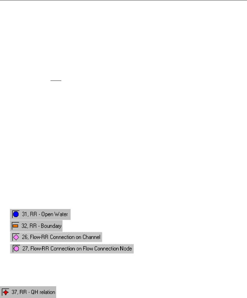
DRAFT
Graphical User Interface
Controller tab:
On this tab, a time controller can be applied. With a time controller the pumping capacity can
be defined as a function of time, and the capacities according to the values on the "Pump" tab
are overruled.
******************* IMPORTANT ***************************************
The controller will only adjust the pump capacity.Not its status of active or inactive. The
status of active or inactive is controlled by the values on the "Pump" tab.
In other words: if the pump would be inactive judging from the settings on the "Pump" tab, it
cannot be re-activated by the controller! Therefore, make sure that, if you want the controller
to be active all the time, your pumping station should also be active according to the settings
on the "Pump" tab. Only then, the controller will be able to adjust the capacity to your desired
values in time.
**********************************************************************
RR - Pump station node topology
An RR - pump station should always be connected to at least one RR - Open Water node, as
it is meant to let water flow in or out of an open water section.
RR - pump station can be connected to nodes of the following types:
(available in the Flow modules only)
(available in the Flow modules only)
5.4.10 RR - QH relation node
RR-QH Relation node general description
In this chapter, the RR-QH Relation node is described. If the relationship between the water
levels in an area and the discharges from that area is known, such knowledge may be applied
to a QH-Relation node.
In fact one can simulate any structure type by using a RR-QH Relation node. In hydraulic
river models (1D flow) QH-relations are commonly used to define downstream boundary con-
ditions.
For a detailed description of this node’s input parameters: see "RR-QH Relation node
input screens";
For a detailed description of this node’s possible network configurations: see "RR-QH
Relation node topology"
For a detailed description of this node’s underlying mathematical equations: see QH-
relation.
RR-QH Relation input screens
Deltares 321 of 900
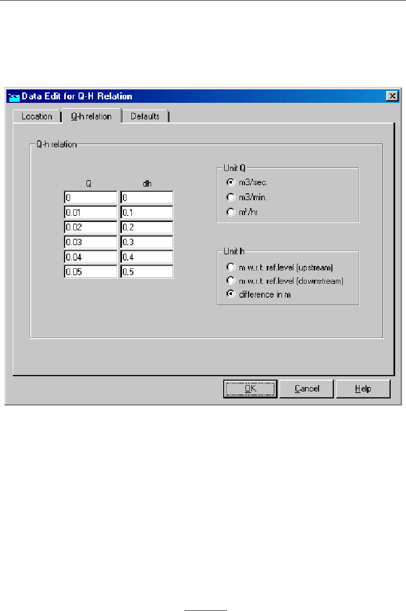
DRAFT
SOBEK, User Manual
When the model data editor for an RR-QH Relation node type is started, the following tabs
will become available for input:
Q-h relation tab:
Figure 5.176: Data Edit for Q-H relation window, Q-h relation tab
In the table, the relationship between water levels in the area and the discharge through the
"structure" should be entered. For six representative water levels (or level differences), a
corresponding discharge should be entered.
There are three options for the RR-QH Relation. The options can be chosen in the Unit-h
section of this tab.
1Discharge related to upstream water level only If this option is chosen, the calculated
discharge will only depend on the upstream water level.
2Discharge related to downstream water level only If this option is chosen, the calcu-
lated discharge will only depend on the downstream water level.
3Discharge related to water level difference If this option is chosen, the calculated dis-
charge will depend on the water level difference between the upstream and downstream
RR nodes.
RR-QH Relation topology
Like any other RR structure type, an RR-QH Relation should always be connected to at least
one RR - Open Water node, as it is meant to let water flow in or out of an open water section.
RR-QH Relations can be connected to nodes of the following types:
322 of 900 Deltares
DRAFT
Graphical User Interface
(available in the Flow modules only)
(available in the Flow modules only)
5.4.11 RR - Sacramento node
Sacramento node general description
In this chapter, the Sacramento node is described. Nodes of this type host the Sacramento
Rainfall-Runoff modelling concept, which has been implemented in the SOBEK RR module.
Figure 5.177: The rainfall-runoff processes that are included in the Sacramento concept.
What is Sacramento?
Sacramento is a concept for rainfall-runoff modelling. It has originally been derived from the
Stanford Watershed model, and designed for the Sacramento river system, United States.
Today, it is one of the most popular rainfall-runoff modelling concepts. It describes the mathe-
matical equation that count for each process within the transformation of rainfall into an outflow
towards a river.
Deltares 323 of 900
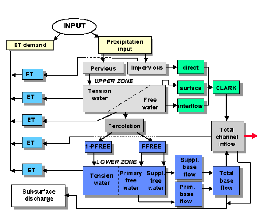
DRAFT
SOBEK, User Manual
Figure 5.178: Flowchart of the processes that are covered by the Sacramento concept.
For a detailed description of this node’s input parameters: see the Sacramento node input
screens section from the Reference Manual;
For a manual on the Sacramento rainfall-runoff model concept: see the Technical Refer-
ence Manual for the Rainfall Runoff module.
For guidelines on Sacramento parameters: see the document on Estimation of Sacra-
mento segment parameters in the Technical Reference Manual for Rainfall Runoff
The application of the Sacramento model in the way it has been integrated in SOBEK is
based on a semi-distributed approach. It implies that a catchment is divided into a number of
segments, which are interconnected by channel branches as shown in the figure below:
324 of 900 Deltares
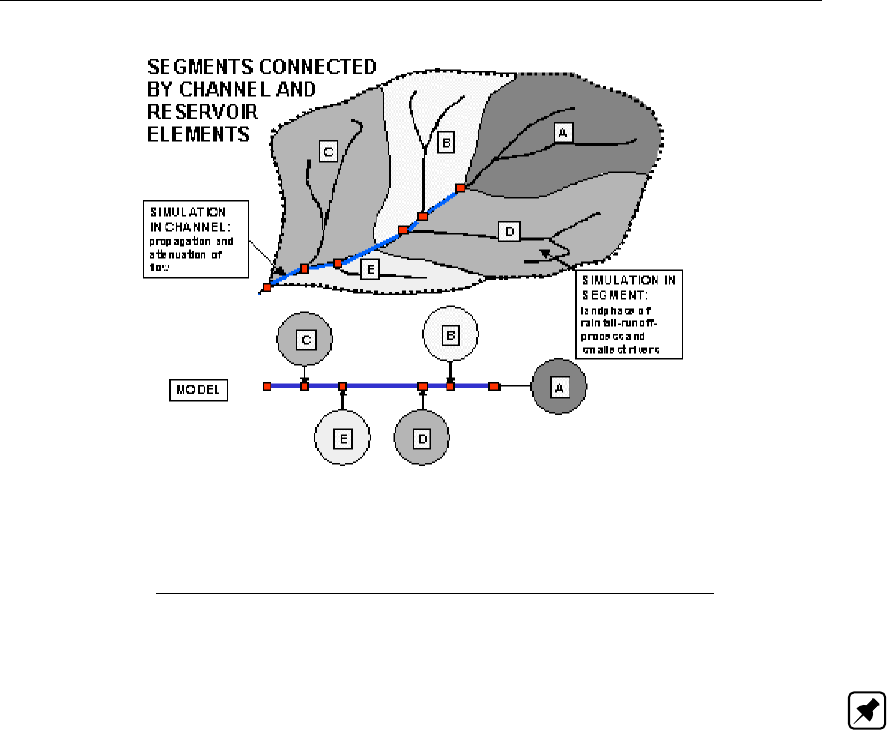
DRAFT
Graphical User Interface
Figure 5.179: Catchment divided into a number of segments
In each segment, rainfall is transformed into runoff towards the main river system. Within each
segment, areal homogeneity of rainfall input and basin characteristics is assumed. The con-
tributions of the segments may be linked to a SOBEK Channel Flow or River Flow schemati-
sation.
Note: to apply hydrodynamics to your schematisation, link the Sacramento nodes to your
SOBEK Flow schematisations by using RR connection on Flow connection nodes, or RR
connection on channel nodes.
Sacramento node input screens
When starting the model data editor for a Sacramento node type, the following tabs will be
available for input:
Area tab:
Deltares 325 of 900
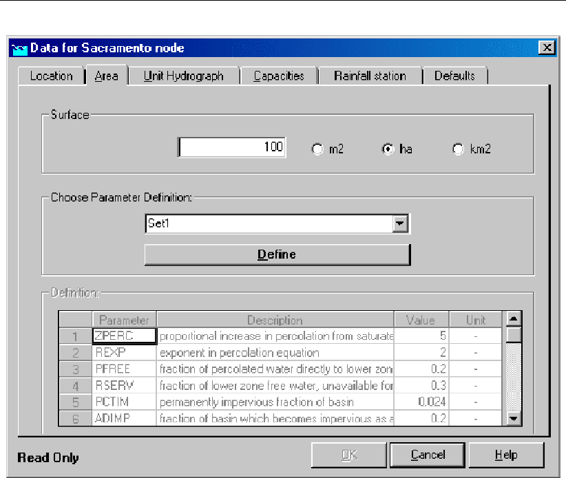
DRAFT
SOBEK, User Manual
Figure 5.180: Data Edit for Sacramento node window, Area tab
Here, the following parameters can be specified:
Surface Enter the total surface , i.e. pervious and impervious area.
Parameter set definition You may want to apply a unique combination of parameter val-
ues for multiple nodes. For that reason, such a combination can be saved as a parameter
set. Enter a name for the set in the drop down box, and click the Define button. Then,
enter the appropriate parameter values. Finally click Save, and the set can be selected for
any Sacramento node by choosing it from the drop down box.
ZPERC The proportional increase in percolation from saturated to dry condition is ex-
pressed by the term ZPERC. The value of ZPERC is best determined through computer
trials. The initial estimate can be derived by sequentially running one or two months con-
taining significant hydrograph response following a dry period. The value of ZPERC should
be initially established so that a reasonable determination of the initial run-off conditions
is possible.
REXP The exponent in the percolation equation which determines the rate at which per-
colation demand changes from the dry condition, (ZPERC + 1) * PBASE, to the wet con-
dition, PBASE. Figure VIII.3.4 illustrates how different values of the exponent affects the
infiltration rate. It is recommended that an initial estimate of this exponent is made from
the same record which is used in determining an initial estimate of ZPERC. The interac-
tion between PBASE, ZPERC and REXP may require a shift of all three terms whenever
it becomes clear that a single term should be changed. Visualising the percolation curve
generated by these three terms helps to ascertain the necessary changes. The observed
range of REXP is usually between 1.0 and 3.0. Generally a value of about 1.8 is an
effective starting condition.
PFREE Fraction of the percolated water which is transmitted directly to the lower zone free
326 of 900 Deltares

DRAFT
Graphical User Interface
water aquifers. Its magnitude cannot generally be determined from hydrograph analysis.
An initial value of 0.20 is suggested. Generally, values will range between 0 and 0.40. The
analysis of early season baseflow allows an effective determination of PFREE.
RSERV Fraction of the lower zone free water which is unavailable for transpiration pur-
poses. Generally this value is between zero and 0.40 with 0.30 being the most common
value. This factor has very low sensitivity.
PCTIM Permanently impervious fraction of the basin contiguous with stream channels. It
can be determined from small storms after a significant period of dry weather. Then the
volume of direct runoff (= observed runoff - baseflow) divided by the volume of rain gives
the percentage impervious fraction of the basin. PCTIM should not be close to 1!
ADIMP Fraction of the basin which becomes impervious as all tension water requirements
are met. It can be estimated from small storms after a very wet period. As before, the
volume of direct runoff divided by the volume of rain gives the total percentage of imper-
vious area. The estimate for ADIMP follows from:ADIMP = Total Percentage Impervious -
PCTIM
SARVA Fraction of the basin covered by streams, lakes, and riparian vegetation, under
normal circumstances. The SARVA area is considered to be the same as or less than
PCTIM. Detailed maps may be referred to in order to estimate the extent of paved areas
which drain directly to the streams so that differences between PCTIM and SARVA can
be approximated. Generally, SARVA appears to range between 40 % and 100 % of the
PCTIM value.
SSOUT The sub-surface outflow along the stream channel which must be provided by
the stream before water is available for surface discharge. This volume expressed in
mm/time interval is generally near zero. It is recommended that the value of zero be
utilised, and SSOUT is applied only if the log Q vs time plot requires a constant addition
in order to achieve a valid recession characteristic. If constant volumes of flow are added
to observed stream flow, the slope of the discharge plot will be altered. That value, which
is required to linearize the primary recession, is the appropriate value of SSOUT. It should
be realised that where SSOUT is required, an effective determination of lower zone free
water storages and discharge rates will require inclusion of the SSOUT value.
PM, PT1, PT2 Time interval increment parameter (PM) and rainfall thresholds (lower rain-
fall threshold PT1 and upper rainfall threshold PT2).The model simulates the rainfall-runoff
process with a time step which is smaller than the time interval of the basic data (usually
one day). The number of increments in the time interval is derived from:N t = 1 + PM *
(UZFWC * F + Peff)where:F = 1 : for Peff <PT1F = (Peff/PT2)0.5 : for PT1 <= Peff <=
PT2F = 1-PT2/Peff : for Peff >PT2 If the input time interval equals an hour, this option is
internally skipped.
Unit Hydrograph tab:
Deltares 327 of 900
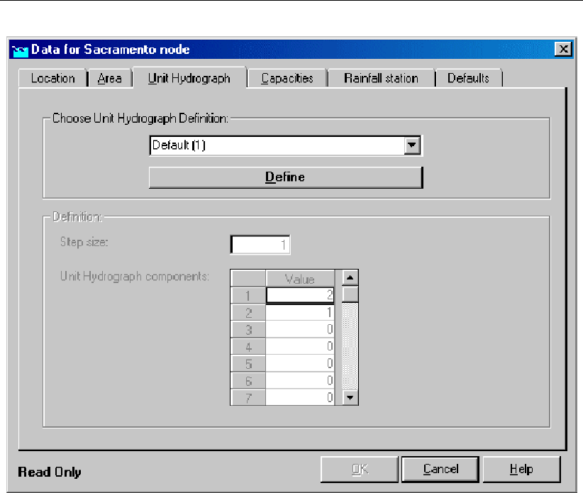
DRAFT
SOBEK, User Manual
Figure 5.181: Data Edit for Sacramento node window, Unit Hydrograph tab
About the Unit Hydrograph:
On this tab, a Unit Hydrograph can be defined. It is used to transform the runoff from impervi-
ous areas (direct runoff), the surface runoff and the interflow into an adapted time distribution
of these flow rates. Before the runoff from the impervious areas (direct runoff), the surface
runoff and the interflow branches the channel, they may be transformed according to a Unit
Hydrograph.
The unit hydrograph (UH) runs for hourly and daily intervals only. Hence, only one hour
UH or one day UH’s can be entered. At maximum 36 (non-zero) UH-ordinates can be
entered, together with a step size. The units with which the UH are to be entered are
not of importance; they should only be mutually consistent. First the given ordinates (with
given step-size) are interpolated down to ordinates at one hour intervals. Then the sum of
the ordinates is computed and all ordinates are subsequently divided by the sum, so the
sum of the adjusted ordinates will always be 1.
To test the behaviour of the UH for surface runoff, a run can be made with all storages
initially filled and with UZK and LZSK e.g. = 10−5. The only reservoir that is depleted then
will be the Lower Zone Primary reservoir = LZPWC * LZPK. Note that LZPK, LZSK and
UZK are to be given as fraction of runoff per day. To get the hourly value the daily value
is internally adjusted as follows:UZK(hr)=(1-(1-UZK(day))1/24), etc. for the other linear
reservoirs.
Example:
1 Given unit hydrograph components : 2. 4. 3. 2. 1. . . . . . . . .
2 Step size = 2
3 Computed unit hydrograph components:
328 of 900 Deltares
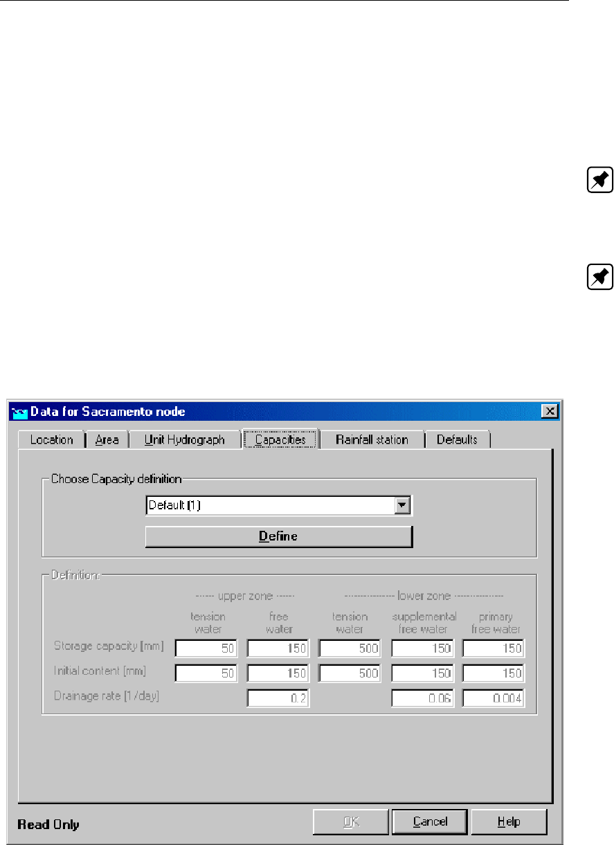
DRAFT
Graphical User Interface
0.042 0.083 0.125 0.167 0.146 0.125 0.104 0.083 0.063 0.042 0.021
4 Given the 5 (non-zero) ordinates at 2 hour intervals a time base of 12 hours is consid-
ered.
The ordinates at two hourly intervals first are converted to ordinates at 1 hour intervals:
1, 2, 3, 4, 3.5, 3, 2.5, 2, 1.5, 1, 0.5. Its sum is 24. Dividing the 1 hour ordinates by 24
results in the above shown computed components.
Note:
In the SOBEK Sacramento node the UH is available to transform the direct runoff + surface
runoff + interflow as described above.
The original Sacramento model concept offers some methods to transform the total inflow
hydrograph (i.e. direct runoff + surface runoff + interflow + 2 baseflow components). These
methods are the Standard Muskingum method or the Clark method. Note: The latter is
not available in the SOBEK Sacramento node.
Instead of using routing methods like Muskingum, one can use SOBEK-Channel flow for
routing the inflow hydrograph from a SOBEK Sacramento node.
The Capacities tab:
Figure 5.182: Data Edit for Sacramento node window, Capacities tab
Here, one can define the storage capacity of the five reservoir types (see the figure in the
chapter Sacramento node general description) These types are: Upper zone, tension water
Upper zone, free water Lower zone, tension water Lower zone, supplemental free watero
Lower zone, primary free water
Deltares 329 of 900
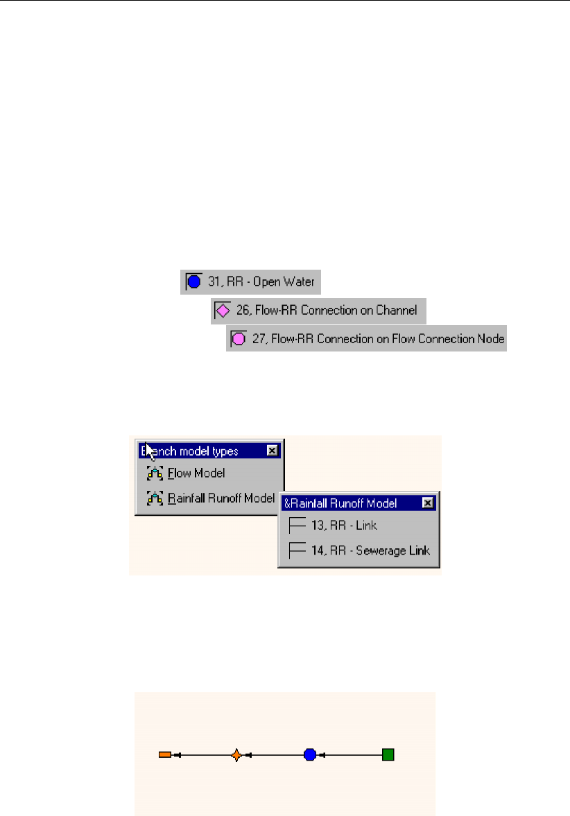
DRAFT
SOBEK, User Manual
Initial Content Initial content of the reservoirs, thus the amount of storage capacity that is
already occupied at the start of a simulation.
Drainage rate Upper zone free watero Lower zone, supplemental free watero Lower zone,
primary free water
Rainfall Station tab:
Select here the rainfall station that applies to this node. Note: rainfall stations and rainfall data
can be specified in the Meteorological Data task block.
Sacramento node topology
Nodes of the Sacramento type can be placed in a network in exactly the same way as RR-
unpaved nodes. They can be connected to either of the following three node types:
An RR Open Water node
An RR on channel connection
An RR on Flow connection node
When connecting a Sacramento area node to one of these nodes, make sure you have se-
lected the RR-link connection type:
Figure 5.183: Showing the RR-Link connection type
The images below show how the Sacramento area node can be connected to the three nodes
mentioned.
Figure 5.184: Connecting an RR Sacramento node to an RR Open Water node. Notice
the defined link directions.
330 of 900 Deltares
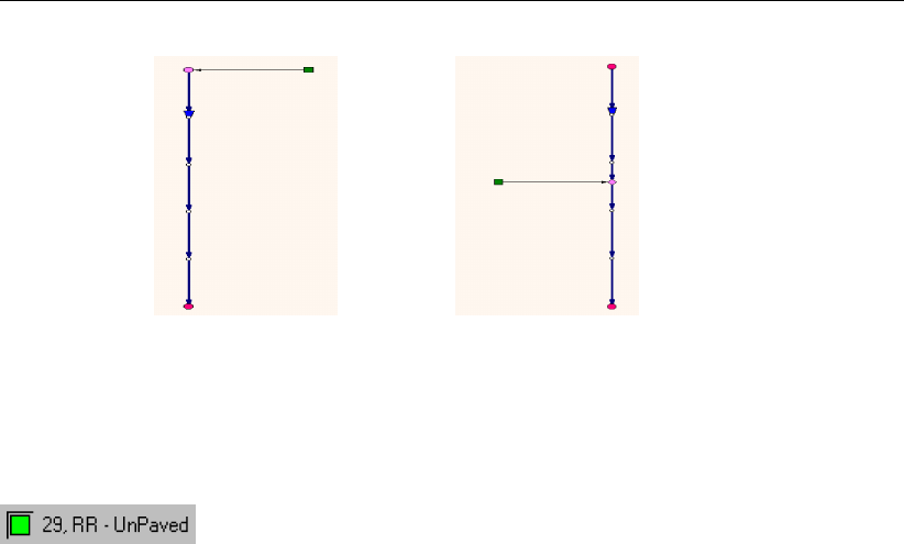
DRAFT
Graphical User Interface
Figure 5.185: Two ways to connect an RR Sacramento node to a channel (only available
if you have a license for the flow module).
5.4.12 RR - Unpaved node
General description of the unpaved area node
In this chapter, the unpaved area node is described. It is by far the most important modelling
object within the SOBEK-Rural Rainfall-Runoff module.
For a detailed description of this node’s input parameters: see the "unpaved area input
screens" section from the Reference Manual;
For a detailed description of this node’s possible network configurations: see the "unpaved
area node topology" section from the Reference Manual
For a detailed description of this node’s underlying mathematical equations: see the "Tech-
nical Reference" manual.
What does the unpaved area node do?
This node type transforms rainfall that falls on a parcel of land into an outflow towards open
water. In order to do so, it catches rainfall, which infiltrates in the soil and/or is stored on
the land. The infiltrated water fills up the groundwater, so that the groundwater level will rise.
Through different soil layers, each covering its own drainage capacity it will then flow out of
the soil towards the connected open water. Also evaporation, infiltration and percolation can
be modelled. If desired, unsaturated zone processes can be included in the calculations.
Because the SOBEK Rainfall-Runoff module is a so-called zero-dimensional model, an un-
paved node can be seen as a container where water flows in (rainfall and seepage), water is
stored (change in groundwater table & unsaturated zone) and water flows out, (evaporation,
runoff, surface runoff and infiltration). The picture below gives an impression of the various
terms which apply to the unpaved area node.
Deltares 331 of 900
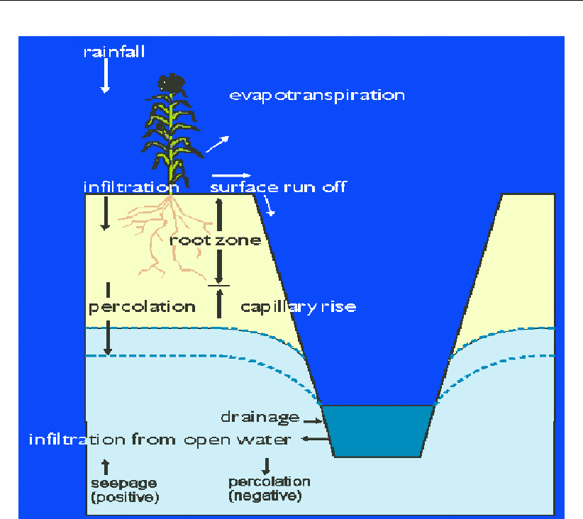
DRAFT
SOBEK, User Manual
Figure 5.186: Representation of the rainfall-runoff process in unpaved areas
In addition, the user can choose whether to use the above described definition of modelling
the transport processes in the unpaved area, or to use a more detailed description. In that
case the unsaturated zone is modelled by means of root zone reservoir.
The unsaturated zone is modelled as vertically oriented 1-D model using the steady-state
approach. The 1-D column model consists of a reservoir representing the root zone and
the subsoil. The equilibrium moisture storage in the root zone is defined as the amount of
moisture corresponding with a steady-state situation with no-flow conditions to or from the
root zone. If the equilibrium moisture storage for the root zone is exceeded, excess water will
percolate to the saturated zone. If the moisture storage is less than the equilibrium moisture
storage, upward flow from the saturated zone is simulated through capillary rise. The height
of the phreatic surface is calculated from the water balance of the subsoil, using a storage
coefficient which is dependent on the depth of the groundwater table.
The root zone reservoir is used for calculations of evapotranspiration. The subsoil reservoir is
used to calculate the saturated storage coefficient.
Evapotranspiration is determined by the crop and the moisture content in the root zone. For
these calculations, recorded values of precipitation and potential evapotranspiration of a ref-
erence crop and woodland must be available. The potential evapotranspiration for other crops
or vegetation types are derived from the values for the reference crop by conversion.
Some important characteristics of the unsaturated zone, i.e. upward flux, storage coefficient
332 of 900 Deltares
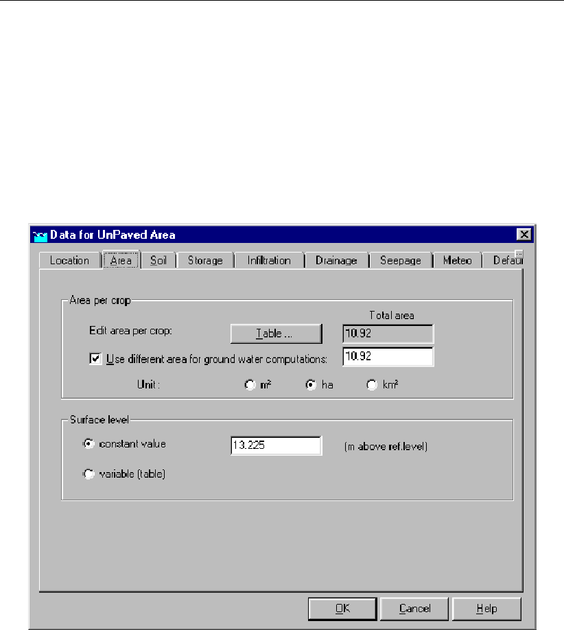
DRAFT
Graphical User Interface
and equilibrium moisture storage of the root zone, are calculated from the soil moisture
retention-, and hydraulic conductivity curves using the CAPSIM model which is based on
the assumption of steady state soil moisture flow (Wesseling,1991). For more than twenty
different soil types, sets of pre-defined tables are provided with SOBEK.
Input screens for the unpaved area node type
When starting the model data editor for an unpaved area node type, the following tabs will be
available for input:
The Area tab
Figure 5.187: Data for UnPaved Area window, Area tab
Here, the following data can be entered:
Area per crop: Every crop type has it’s own evaporation characteristics. Therefore it is
important to define which crops are grown on the area you want to model. The sum of all
crop-areas should be equal to the total area you want to model with this unpaved node.
Use different area for groundwater computations: Sometimes, a part of the area you
want to model might be paved, having it’s own runoff system. Such areas do not contribute
to the rainfall-runoff process for your unpaved area. However, the soil underneath the
paved area will. For such cases this variable can be used. Example: an area of 10 000
m2has 2 000 m2of paved area, which has it’s own runoff system. The rest is unpaved
area where grass is grown. Only 8 000 m2of the area will therefore catch rainfall, actually
contributing to the rainfall-runoff process. However, the rainfall on these 8 000 m2will
apply to the groundwater of a 10 000 m2large area, because there is a soil underneath
the paved area. In this case, we fill in: 8 000 m2for the Area per crop, type grass, 10000
m2for the total area (for groundwater computations).
Surface level: Here, the surface level for the area should be filled in. The surface level is
important for several processes within the calculations:
Deltares 333 of 900
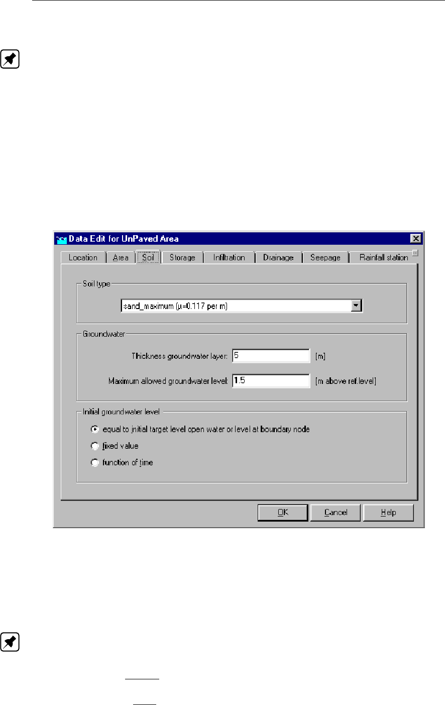
DRAFT
SOBEK, User Manual
1 When the unsaturated zone module "CAPSIM" is not active, the initial groundwater
depth (= surface level - initial groundwater level) will be used to calculate the soil
storage coefficient. Note: CAPSIM can be switched on in the SETTINGS task block
for the RR module.
2 When the groundwater level branches the surface level, excess water will be stored on
land or run off over land
3 When the water level in a connected node exceeds the unpaved area surface level,
the area will be inundated.
The surface level can be entered as ’constant’ or ’variable’. When using the ’variable’ type,
for various levels the percentage of land laying below it can be filled in, thus creating an
S-curve. Important: when using the variable surface level type, the value you previously
filled in for the constant value, will still be used for calculation of the soil storage coefficient!
The Soil tab
Figure 5.188: Data for UnPaved Area window, Soil tab
On the Soil tab, the following variables can be filled in:
Soil type: Choosing a certain soil type, actually implies choosing the soil storage coeffi-
cients that will be used during the calculations. These coefficients determine how quickly
the groundwater table will rise due to recharge.
Note: is important to know whether the unsaturated zone module CAPSIM is active or
inactive. You can activate CAPSIM in the SETTINGS task block for the RR module.
If CAPSIM is inactive:
At the start of each simulation, SOBEK will determine for all unpaved nodes:— the
soil type — the initial groundwater depth (in cm below surface)SOBEK will then search
for an appropriate storage coefficient in the file <\SOBEK\FIXED\3B\BERGCOEF>.
334 of 900 Deltares
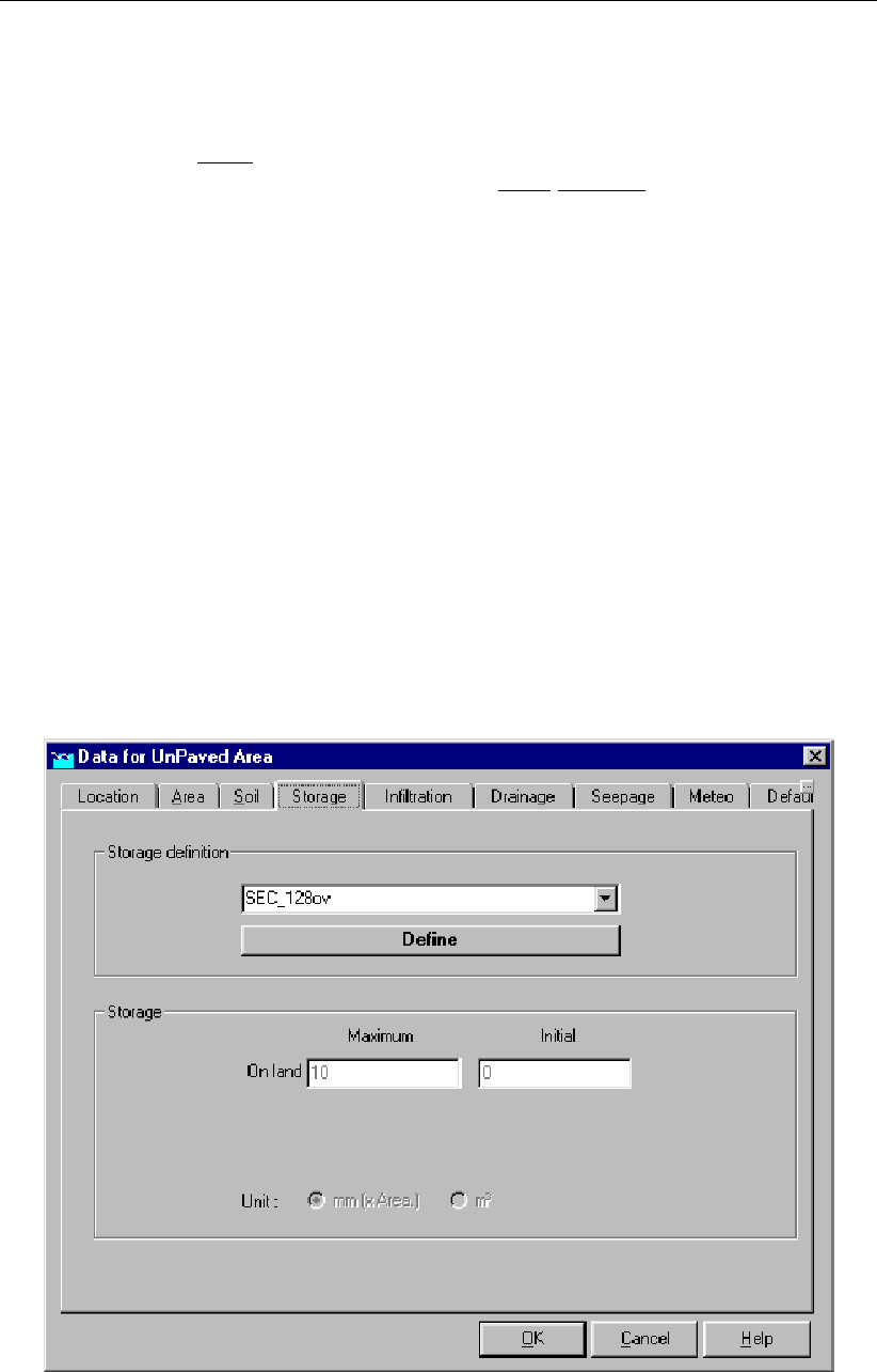
DRAFT
Graphical User Interface
The coefficient it finds there, will then be applied to the corresponding unpaved node
during the entire simulation. The deeper the initial groundwater level lies, the higher
the storage coefficient will be.
If CAPSIM is active:
soil storage coefficient will be calculated on every time step. It will depend on:- soil
type- actual groundwater level
Thickness groundwater layer: This parameter is only of importance when salinity cal-
culations are done. For calculation of salinity, the water volume of each object should
be known. Therefore a groundwater depth should be given (soil volume = surface area *
depth)
Maximum allowed groundwater level: This parameter is not used in the calculation it-
self, but it may be very usable for output. In the post processing phase, one can determine
whether, and for how long the maximum allowed groundwater level has been exceeded.
This is suitable for the calculation of the damage of floodings to crops.
Initial groundwater level: Unless you’re using a restart file for the initialisation of your
simulation, the initial groundwater level is the groundwater level which is applied during
the first time step of the simulation. Furthermore, it is used to determine the soil storage
coefficient (see the points above). Notice that the initial groundwater level is defined in
[meters below surface level]. When choosing the initial groundwater level as a function of
time, you can have a rainfall events in summertime starting with different initial groundwa-
ter levels than rainfall events in wintertime.
The Storage tab
Figure 5.189: Data for UnPaved Area window, Storage tab
On the Storage tab, values for the initial and maximum storage on land can be filled in. These
values can then be saved in a "Storage definition" so that you can re-use them on other nodes.
Deltares 335 of 900

DRAFT
SOBEK, User Manual
The storage on land determines how long it takes before surface runoff will occur. Surface
runoff will start when the rainfall intensity is so high that the sum of the infiltration capacity and
the maximum storage on land is exceeded. To define the storage parameters, type a name of
the storage definition and click Define. Then fill in the values for maximum and initial storage
on land. Finally click Save. On other unpaved area nodes you can select your previously
defined values or create a new set.
The Infiltration Tab
Figure 5.190: Data for UnPaved Area window, Infiltration tab
On the Infiltration tab, one may enter values for the infiltration capacity of the soil. If the
rainfall exceeds the infiltration capacity, water will be stored on land. To define the infiltration
parameters, type a name for the infiltration definition and click <Define>. Then fill in the value
infiltration capacity. Finally click <Save>. On other unpaved area nodes you can then select
your previously defined values or create a new set.
The Drainage tab
336 of 900 Deltares
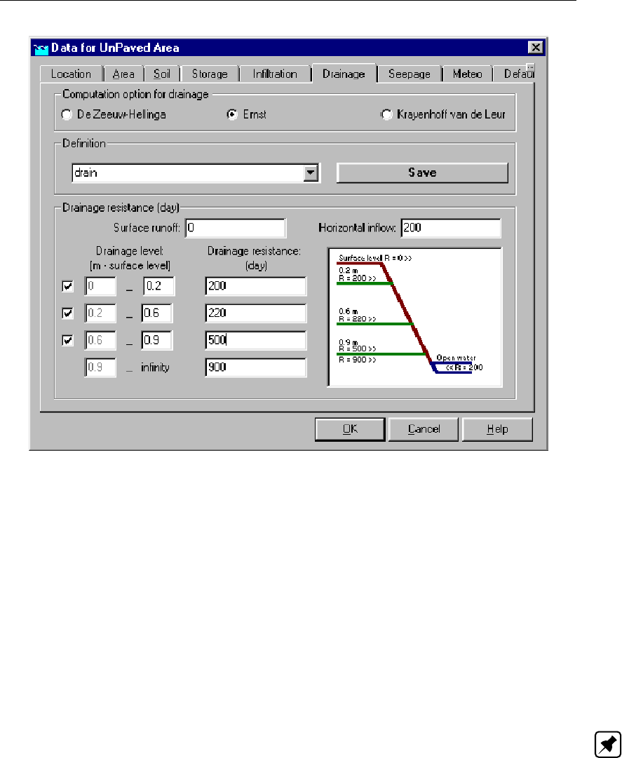
DRAFT
Graphical User Interface
Figure 5.191: Data for UnPaved Area window, Drainage tab
This tab is one of the most important ones. Here the drainage resistance values for different
soil layers are filled in. The groundwater outflow is determined by:
1 groundwater level
2 drainage resistance values
3 soil storage coefficient
4 downstream water level
Computation option for drainage: Three drainage formulas are available:
1 De Zeeuw - Hellinga,
2 Ernst and
3 Krayenhoff van de Leur
Note:
If you are using CAPSIM for calculation of the unsaturated zone, you are advised to use
the ERNST drainage formula.
Definition: The values that you fill in for a certain node, may be re-used on other nodes.
Therefore, they can be stored in a "definition". Define a name for the set of values you en-
ter and save it. On the other nodes you can then refer to this previously defined definition.
The values to be entered: The name of the section where the values should be entered
varies with the chosen computation method.
surface runoff: the drainage resistance (Ernst) or reaction factor (Zeeuw-Hellinga) for
the surface-runoff process (usually a very quick process, so low drainage resistance
or high reaction factor)
horizontal inflow: the values for water flowing backwards from surface water into the
soil.
drainage levels: for different soil layers, different values may apply.
Deltares 337 of 900
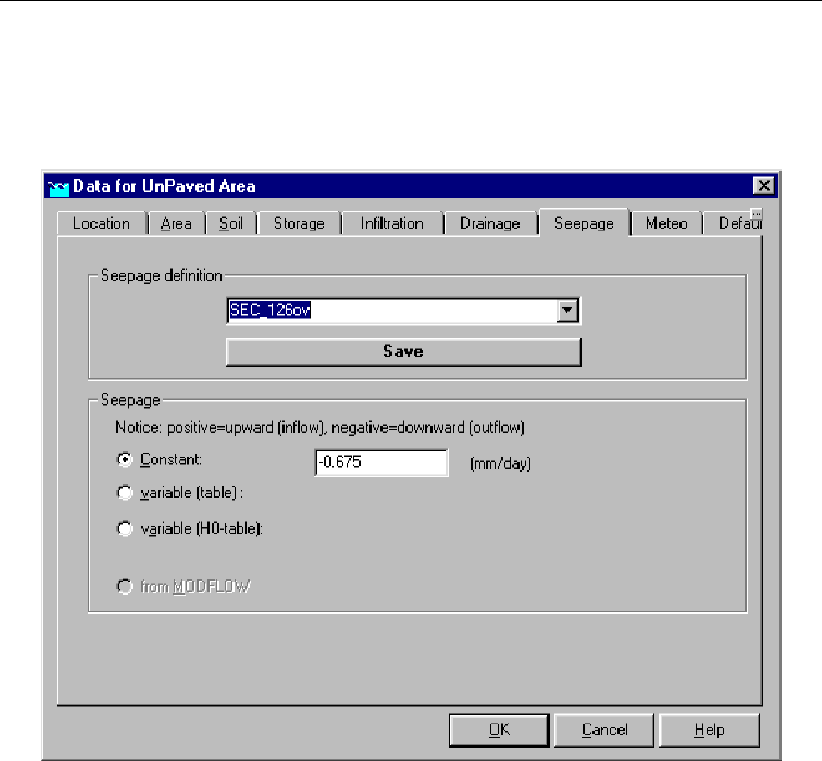
DRAFT
SOBEK, User Manual
All levels are defined as from xmeters below surface level to ymeters below surface level.
The Seepage tab
Figure 5.192: Data for UnPaved Area window, Seepage tab
Besides rainfall and evaporation, also seepage and infiltration are input/output terms for un-
paved area nodes. On the Seepage tab, one can define the flux from or towards deep aquifers.
Various options are available:
Constant: A negative value means that the amount of water will be withdrawn from the
unpaved area node; a positive values means that the amount of water is supplied to the
node.
Variable (table): The seepage and infiltration can be entered as a function of time
Variable (H0-table): The seepage and infiltration is calculated as a function of: - ground-
water table in the unconfined aquifer (as calculated by SOBEK) - groundwater head in the
aquifer below (entered as a constant or function of time) - hydraulic resistance value of the
aquitard between the unconfined and confined aquifer.
Future option: from Modflow: In this future option, SOBEK RR and the groundwater
software Modflow will be able to run simultaneously. Modflow will then supply SOBEK
every time step with values for the groundwater head, so that the seepage/infiltration can
be calculated according to the difference between phreatic and piezometric head.
The Meteo tab
On the Meteo tab, one selects the rainfall station that applies for the unpaved area node.
Rainfall stations and - values can be created in the Meteorological Data Task block.
338 of 900 Deltares

DRAFT
Graphical User Interface
Unpaved area node topology
Nodes of the unpaved area type can be connected to four types of nodes:
An RR Open Water node
An RR on channel connection
An RR on Flow connection node
An RR boundary node
When connecting an unpaved area node to one of these nodes, make sure you have selected
the RR-link connection type:
Figure 5.193: RR-link connection type
The images below show how the Unpaved area node can be connected to the three nodes
mentioned.
Figure 5.194: Connecting an RR Unpaved node to an RR Open Water node. Notice the
defined link directions.
Figure 5.195: Two ways to connect an RR Unpaved node to a channel (only available if
you have a license for the flow module).
Deltares 339 of 900
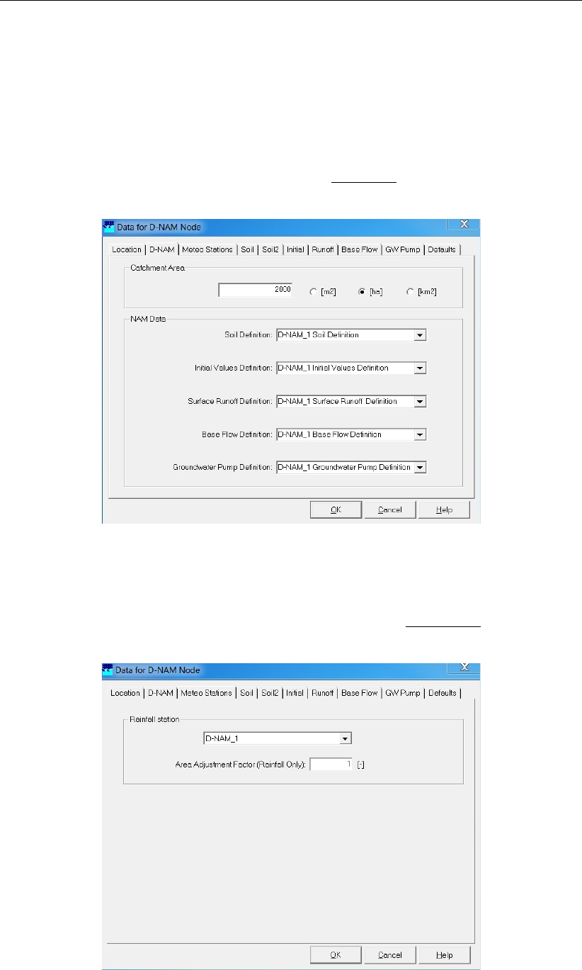
DRAFT
SOBEK, User Manual
5.4.13 D-NAM Input Screens
Hereunder the D-NAM rainfall-runoff model input screens are described. For more information
on the various input parameters, reference is made to section 6.5.3.
The D-NAM Tab (see Figure 5.196): On this tab, the catchment area can be defined. To
be selected on this tab are a Soil definition, an Initial value definition, a Surface runoff
definition, a Base flow definition and a Groundwater pump definition. These definitions
can respectively be specified and deleted on the Soil&Soil2 tab, the Initial tab, the Runoff
tab, the Base flow tab and the GW Pump tab.
Figure 5.196: The D-NAM Tab of the "Data for D-NAM Node" Form
The Meteo Stations Tab (see Figure 5.197): The meteo (rainfall) station of the D-NAM
rainfall-runoff model is specified on this tab. In addition, an area adjustment factor is
defined, being a multiplication factor applied on rainfall only. Please note that rainfall and
evapotranspiration data of meteo stations are defined in the Meteo Task Block.
Figure 5.197: The Meteo Stations Tab of the "Data for D-NAM Node" Form
340 of 900 Deltares
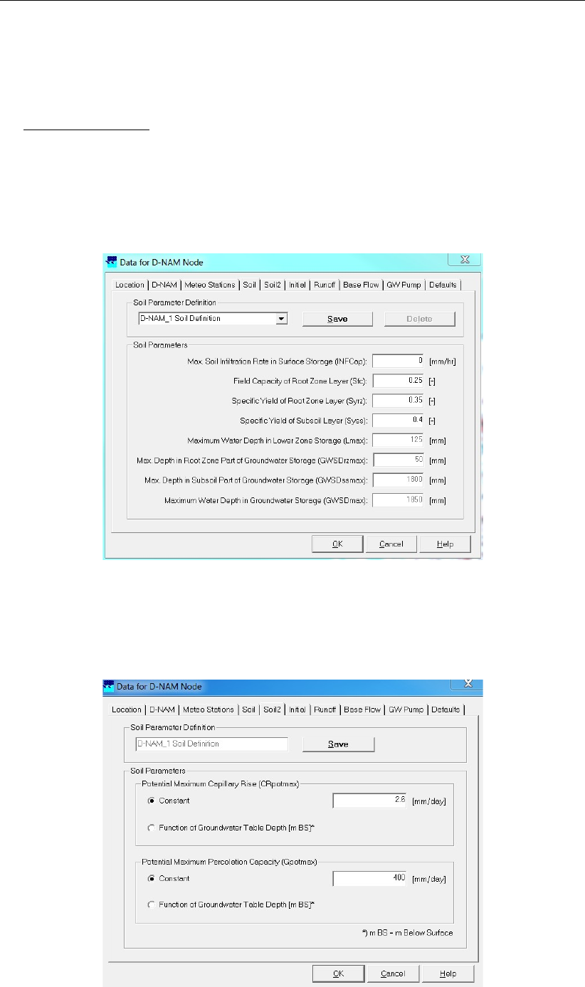
DRAFT
Graphical User Interface
The Soil Tab (see Figure 5.198): On this tab are specified the maximum soil infiltration
rate of water contained in the surface storage [mm/hr], the field capacity of the root zone
layer [-], the specific yield of the root zone layer [-] and the specific yield of the subsoil
layer [-].
For information only are shown the maximum water depth in the lower zone storage [mm],
the maximum water depth in the root zone part of the groundwater storage [mm], the max-
imum water depth in the subsoil part of the groundwater storage [mm] and the maximum
water depth in the groundwater storage [mm]. These maximum water depths are com-
puted using the field capacity and specific yields defined on this tab as well as the values
defined on the intial tab for the surface level, the bed level of the root zone layer and the
bed level of the subsoil layer.
Figure 5.198: The Soil Tab of the "Data for D-NAM Node" Form
The Soil2 Tab (see Figure 5.199): On this tab are defined the potential maximum capil-
lary rise [mm/day] and the potential maximum percolation capacity [mm/day] either as a
constant or as function of the groundwater table depth.
Figure 5.199: The Soil2 Tab of the "Data for D-NAM Node" Form
Deltares 341 of 900
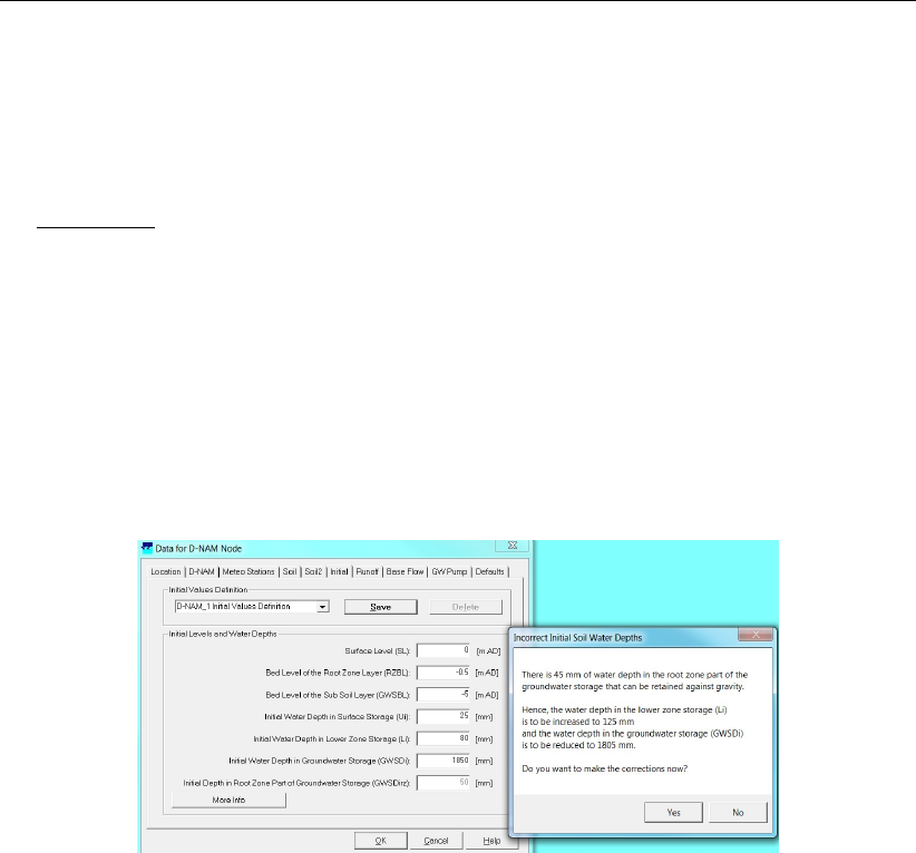
DRAFT
SOBEK, User Manual
The Initial Tab (see Figure 5.200): On this tab are defined the surface level of the catch-
ment area [m above datum], the bed level of the root zone layer [m above datum], the bed
level of the subsoil layer [m above datum], the initial water depth in the surface storage
[mm], the initial water depth in the lower zone storage [mm] and the initial water depth in
the groundwater storage [mm].
Please note that the resulting initial water depth in the root zone part of the groundwater
storage (GW SDi,rz) is computed and shown for information only. If GW SDi,rz >0
while the initial water depth in the lower zone storage (Li) is less than its maximum water
depth (Lmax), means that there is water contained in the root zone part of the ground-
water storage that can be retained against gravity. In such case a form pops up (see
Figure 5.200) informing on the amount of water depth in the root zone part of the ground-
water storage that should be transferred to the lower zone storage. By clicking on the
<OK>button, the initial water depth in the lower zone storage (Li) and the initial water
depth in the groundwater storage (GW SDi) are adapted in such way that the root zone
part of the groundwater storage does not contain any water that can be retained against
gravity.
Figure 5.200: The Initial Tab of the "Data for D-NAM Node" Form
The Runoff Tab (see Figure 5.201): On this tab are defined the catchment length in
drainage direction [m], the surface slope [-], the Manning roughness of the catchment land-
use [s/m1/3], the surface-storage-threshold for overland flow [mm], the interflow reservoir
coefficient [days], the surface-storage-threshold for interflow [mm] and the lower-zone-
storage threshold for interflow [mm].
342 of 900 Deltares
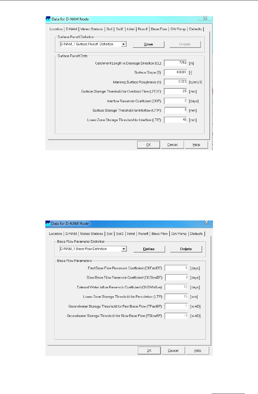
DRAFT
Graphical User Interface
Figure 5.201: The Runoff Tab of the "Data for D-NAM Node" Form
The Base Flow Tab (see Figure 5.202): On this are defined the fast base flow reservoir
coefficient [days], the slow base flow reservoir coeffient [days], the external (ground)water
inflow reservoir coeffient [days], the lower-zone-storage threshold for percolation [mm], the
groundwater-storage threshold for fast base flow [m above datum] and the groundwater-
storage threshold for slow base flow [m above datum].
Figure 5.202: The Base Flow Tab of the "Data for D-NAM Node" Form
The GW Pump Tab (see Figure 5.203): On this tab the discharge of the groundwater
pump [m3/s] is defined either as a constant or as function of time. Please note that
a positive groundwater pump discharge means that water is to be abstracted, while a
negative groundwater pump discharge means that water is to be supplied.
Deltares 343 of 900
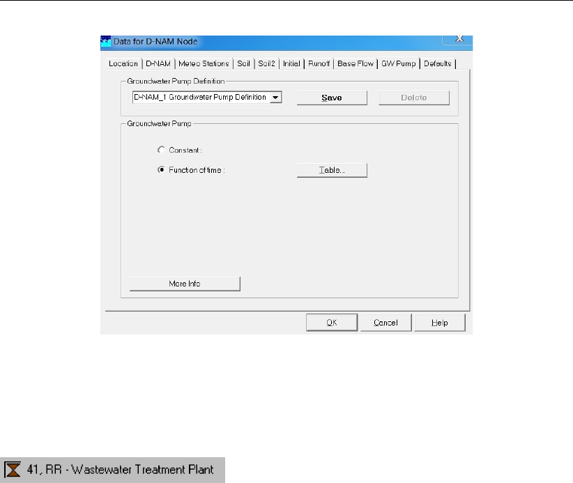
DRAFT
SOBEK, User Manual
Figure 5.203: The GW Pump Tab of the "Data for D-NAM Node" Form
5.4.14 RR - Wastewater Treatment Plant
RR - WWTP node description
A WWTP node can be used when there is measured data available for the discharges from a
waste water treatment plant towards a boundary or an open water node that is connected on
the downstream side.
For a detailed description of this node’s input parameters: see the "RR - WWTP node
input screens" section from the Reference Manual;
For a detailed description of this node’s possible network configurations: see the "RR -
WWTP node topology" section from the Reference Manual
RR - WWTP node input screens
When the model data editor for an RR - Orifice node type is started, the following tabs will
become available for input:
WWTP Tab:
344 of 900 Deltares
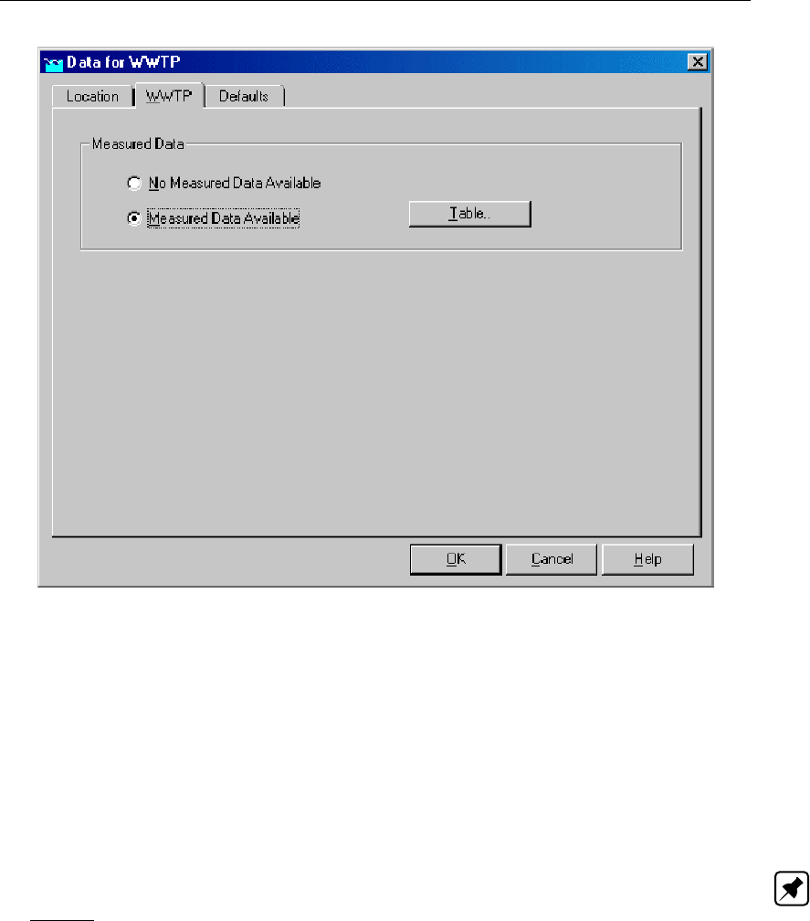
DRAFT
Graphical User Interface
Figure 5.204: Data for WWTP window, WWTP tab
Here, the discharges from the Waste Water Treatment Plant to a boundary or Open Water
node can be entered. There are two options:
No measured data available: With this option, the discharges from the WWTP node
towards a downstream side connected Boundary or Open Water node will be derived
directly from the combined actual flows of all RR - Paved area nodes that are connected
on the upstream side.
Measured data available: If this option is active, discharges from the WWTP node to-
wards a Boundary node or Open Water node can be entered as a function of time.
Note: : the specified WWTP discharges only apply for the flow from the WWTP node
towards a downstream Boundary or Open Water node. Not for the flow from the RR paved
nodes towards the WWTP. For that flow, the summed up sewer pump discharges apply.
The difference between the flow towards and from the WWTP will become visible as a
storage change in the results for the WWTP.
Deltares 345 of 900
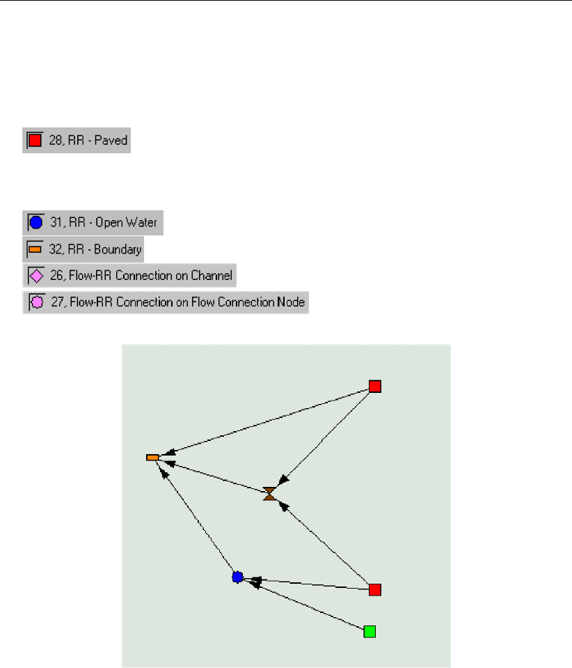
DRAFT
SOBEK, User Manual
RR - WWTP node topology
A WWTP node always forms an interconnection between two nodes:
On the upstream side:
(multiple nodes of this type are allowed)
On the downstream side:
(available in the Flow modules only)
(available in the Flow modules only)
Figure 5.205: Typical example of a schematisation that contains a WWTP node
In this example, the upper paved node will pump its sewer discharge towards the WWTP
node. The sewer overflows from that paved node will flow directly towards a boundary node.
The lower paved node also pumps its sewer discharge towards the WWTP, but sewer over-
flows will take place on an RR Open Water node.
On the WWTP node, the modeller now has the option of applying measured data for the flow
towards the boundary, or to apply the sewer discharges from the connected paved nodes
directly to the WWTP.
5.4.15 RR - Weir
346 of 900 Deltares
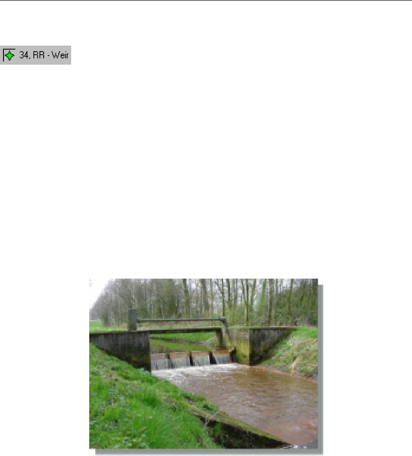
DRAFT
Graphical User Interface
Description of the RR - Weir node type
In this chapter, the RR - Weir node is described. With an RR - Weir node you can simulate
a structure over which water flows. Nodes of this type therefore can represent three types of
weirs: broad crested weirs (rectangular), v-notch weirs or 2-stage weirs.
For a detailed description of this node’s input parameters: see the "RR - Weir node input
screens" section from the Reference Manual;
For a detailed description of this node’s possible network configurations: see the "RR -
Weir node topology" section from the Reference Manual
For a detailed description of this node’s underlying mathematical equations: see the "Weir
section from the Technical Reference Manual".
Definition of a Weir (barrage):
A weir is a fixed or movable structure that aims to control a certain water level on its upstream
side (Dutch Hydrological Society,2002).
Figure 5.206: Example of a broad crested weir. Photo: Dutch waterboard "Peel and
Maasvallei"
RR - Weir node input screens
When the model data editor for an RR - Weir node type is started, the following tabs will
become available for input:
Options Tab:
Deltares 347 of 900
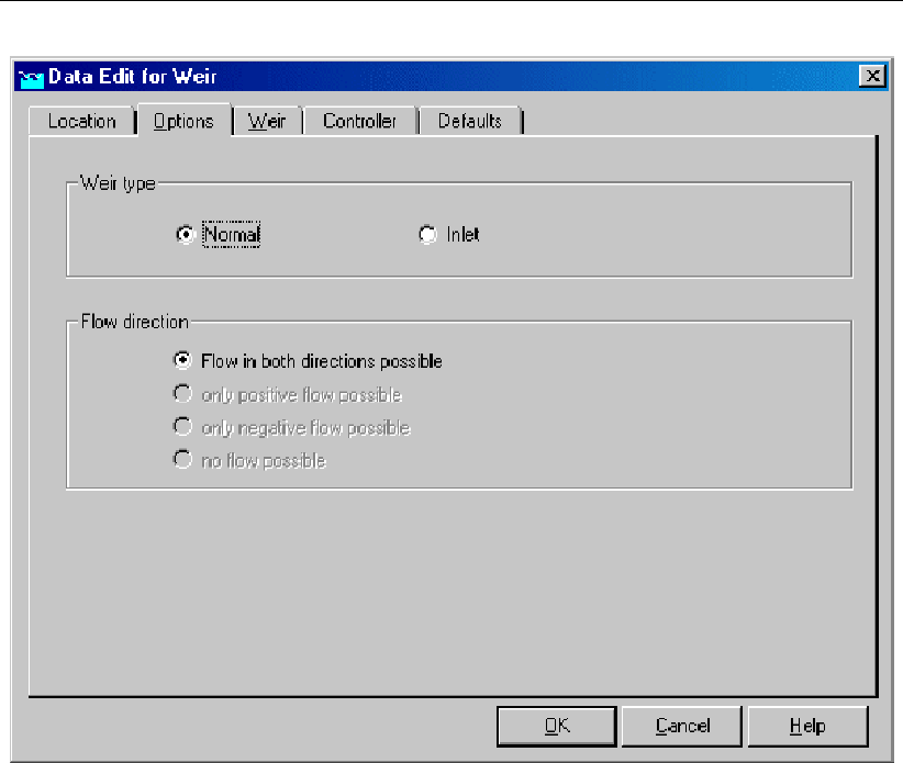
DRAFT
SOBEK, User Manual
Figure 5.207: Data for Weir window, Options tab
On this tab, you can define how the weir is to be used:
Weir type: normal This option means that water is allowed to flow over the weir in both
directions.
Weir type: inlet This option means that water may only flow over the weir in positive
direction. The arrows on the links that connect the weir to other objects indicate the
positive flow direction.
Weir tab (normal type):
348 of 900 Deltares
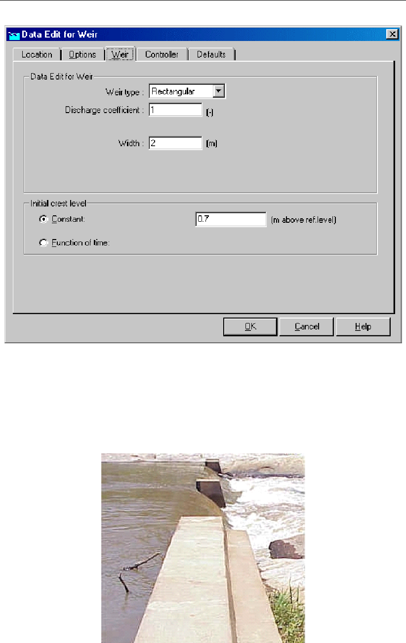
DRAFT
Graphical User Interface
Figure 5.208: Data for a normal RR-Weir window, Weir tab
On the "Weir" tab, the shape and crest level of the weir is defined. In the "Weir type" combo
box can choose between three types of weirs:
Rectangular weir (broad crest):
Figure 5.209: Example of a broad crested weir. Photo: South African Department of
Water Affairs
Deltares 349 of 900
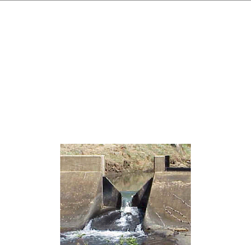
DRAFT
SOBEK, User Manual
This weir type requires the following input parameters:
discharge coefficient: See the "Weir" section of the Technical Reference Manual for the
exact implementation of this parameter in the discharge formula of this structure type.
Width: Represents the width of the weir’s crest. See the "Weir" section of the Technical
Reference Manual for the exact implementation of this parameter in the discharge formula.
Initial Crest level: This parameter represents the weir’s crest level. Notice that it is called
"initial" crest level. This name has been chosen because the crest level may be overruled
in certain cases:
1 by a controller. If there’s no controller active for the weir, the crest level will remain
equal to the "initial crest level" throughout the entire simulation.
2 if the option "adjust weir setting automatically to <= upstream target level" in the "Set-
tings" task block has been activated.
V-notch weir:
Figure 5.210: Example of a V-notch weir. Photo: South African Department of Water
Affairs
If the V-notch type is selected for the weir, there will be some other parameters required than
in case of a rectangular one:
Discharge coefficient: See the "Weir" section of the Technical Reference Manual for the
exact implementation of this parameter in the discharge formula of this structure type.
Slope: Represents the tangent of the weir’s side slopes. Thus a value of 2 results in a
steep V-shape (1 horizontally ->2 vertically)
Initial Crest level: This parameter represents the weir’s crest level. Notice that it is called
"initial" crest level. This name has been chosen because the crest level may be overruled
in case the option "adjust weir setting automatically to <= upstream target level" has been
activated in the "Settings" task block .
2-stage weir:
350 of 900 Deltares
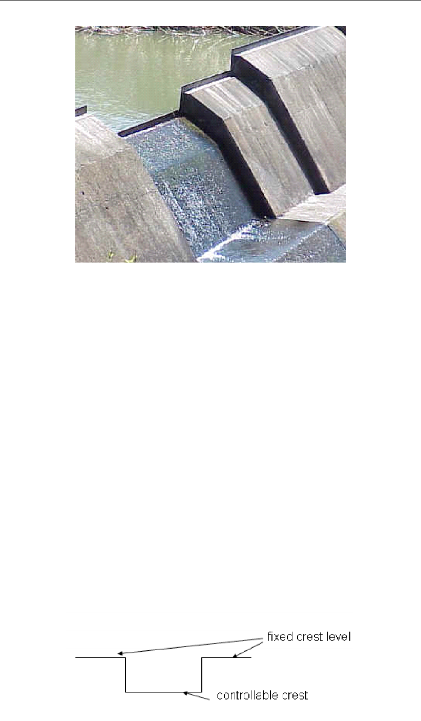
DRAFT
Graphical User Interface
Figure 5.211: Example of a multiple-stage weir. Photo: South African Department of
Water Affairs
Weirs of this type are a variety of the broad crested type. In stead of one crest level they
have two: at the lowest point there is a small crest which is meant to maintain sufficient flow
velocities over the weir in periods of low discharge. A little higher, the crest becomes broad.
This is meant to allow enough water to flow over the weir in cases of high discharges.
The following parameters are required for this weir type:
Discharge coefficient: See the "Weir" section of the Technical Reference Manual for the
exact implementation of this parameter in the discharge formula of this structure type.
Width: Represents the width of the crest at its narrowest point.
Additional width 2nd stage: Represents the amount by which the weir broadens at the
crest level of the 2nd stage.
Crest level 2nd stage: Represents the crest level for the second stage; thus the crest
level for the broad part of the weir. Naturally this value should be higher than the crest
level for the 1st (narrow) stage.
Initial Crest level: This parameter represents the weir’s crest level. Notice that it is called
"initial" crest level. This name has been chosen because the crest level may be overruled
in two cases:
1 by a controller. If there’s no controller active for the weir, the crest level will remain
equal to the "initial crest level" throughout the entire simulation. Note that only the
crest for the first stage can be controlled:
Deltares 351 of 900
DRAFT
SOBEK, User Manual
2 if the option "adjust weir setting automatically to <= upstream target level" in the "Set-
tings" task block has been activated.
Weir tab (Inlet type):
Figure 5.212: Data Edit for Weir window, Weir tab
If the option Inlet is selected in the "Options" tab, the "Weir" tab will allow the user to set two
additional parameters:
Minimum flushing flow: This is the minimum amount of flow when the inlet is active.
Switch on-off levels: The inlet will open according to the switch on-off levels (relative to
the downstream target level).
Controller tab:
352 of 900 Deltares

DRAFT
Graphical User Interface
Figure 5.213: Data Edit for RR - Weir window, controller tab
On the controller tab, the behaviour of the weir can be controlled (optional). With a controller,
the initial crest levels, as defined on the "Weir" tab, are overruled. For more details on the
available controllers and their function, see the Controller section of the RR Technical Refer-
ence Manual.
RR - Weir node topology
An RR - Weir should always be connected to at least one RR - Open Water node, as it is
meant to control the water level on an open water node.
RR - Weirs can be connected to nodes of the following types:
(available in the Flow modules only)
(available in the Flow modules only)
An example of a network where RR Weirs are used is given below:
Deltares 353 of 900
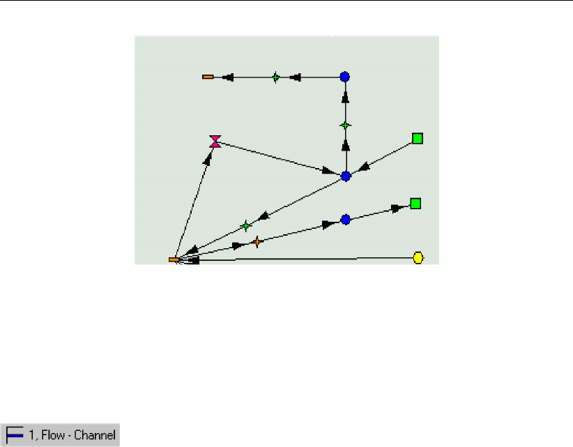
DRAFT
SOBEK, User Manual
Figure 5.214: Example of a network with RR Weirs
5.5 Branch description
5.5.1 Branch - Channel
Description
In this chapter, the Flow - Channel branch is described. This type of object forms the basis for
any River or Channel. With a branch you can define the course of the river or channel that you
want to schematise. A branch is always interconnecting two nodes; these may be boundary
nodes, or connection nodes. On top of the branch, you may later add other objects, such as
weirs, pumping stations etc.
This branch has no input parameters for itself.
For a detailed description of this branch’s possible network configurations: see the "Flow
- Channel branch topology" section from the Reference Manual
This branch type has no underlying mathematical equations for itself. Its length, the
boundary nodes and other objects attached to it determine the flow through branches
of this type.
In SOBEK-Rural Water Flow channels are represented by branches of the type ‘Flow - Chan-
nel’. In contrast to the branches in SOBEK-Rural Rainfall-Runoff, the so-called RR-Links, the
lengths of these branches have a physical meaning. Furthermore, they can have objects at-
tached to the, such as cross sections, ζ-calculation points and structures. The cross section
is defined per branch by a cross section node. Various branches can be connected by con-
nection nodes which can comprise extra storage capacity and lateral inflow. The connection
of the modelled area with the outside world (which can also be a sobek-Rural Rainfall-Runoff
schematisation) is represented by the boundary condition nodes.
Topology
The direction of a branch is defined when you create it:
If you create a branch by starting at node A and drawing the mouse to node B, the branch
direction is from A to B.
If you create a branch by starting at node B and drawing the mouse to node A, the branch
direction is from B to A.
354 of 900 Deltares
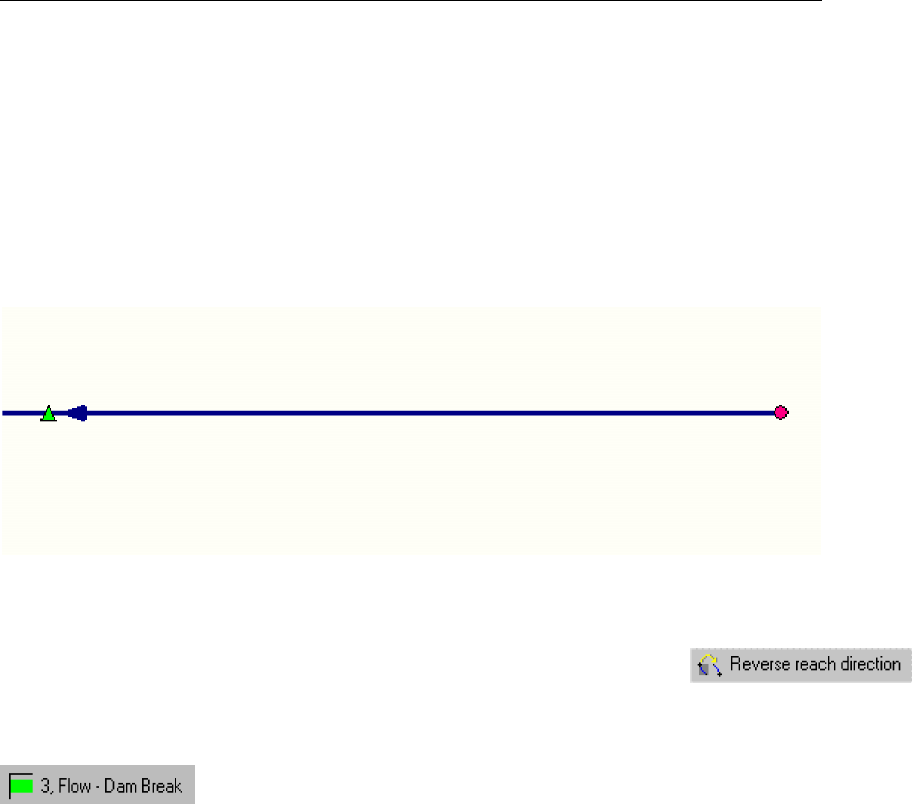
DRAFT
Graphical User Interface
If you don’t know the branch direction, do the following:
Click the Menu "Options" - "Network Data" - "Links"- Select the option "Defined" under the
"show direction" section.
Click OK
You should now see an arrow that indicates the branch direction.
If you still don’t see it, zoom in on the branch.
Figure 5.215: Visualising the defined direction of a branch.
The branch direction can be reversed with the "reverse branch direction" button
5.5.2 Branch - Flow 1D Dam Break branch and the Once Hydraulic Trigger
This section describes the "Flow 1D Dam Break branch", including the "Once Hydraulic Trig-
ger":
Application examples of the "Flow 1D Dam Break branch" are given in section 5.5.2.1.
The method of modelling bbranching and the available bbranch growth options/formulae
are discussed in section 5.5.2.2.
Options for specifying the point-in-time that bbranching should start (e.g. at an absolute
point-in-time or at the point-in-time that a specific hydraulic event occurs) are discussed in
section 5.5.2.3.
The "Flow 1D Dam Break branch" input screens are discussed in section 5.5.2.4.
The output parameters available at a "Flow 1D Dam Break branch" are explained in sec-
tion 5.5.2.5.
For detailed information on the Verheij-vdKnaap(2002) bbranch growth formula and the vd-
Knaap(2000) bbranch growth formula both available at "Flow 1D Dam Break branch", refer-
ence is respectively made to section 6.3.3.1 and section 6.3.3.2.
5.5.2.1 Application examples of the Flow 1D Dam Break Branch
The "Flow 1D Dam Break Branch" can be used to model the hydraulic consequences of a
dam break or dike failure. Possible applications are:
The bbranching of a dike in a 2D model (see Figure 5.216). The dike is represented
by elevated 2D grid cells. The "Flow 1D Dam Break Branch" is located between two
Deltares 355 of 900
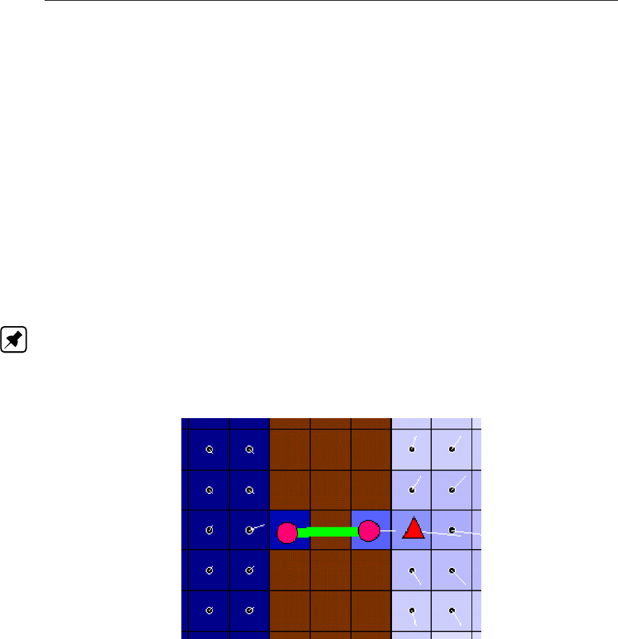
DRAFT
SOBEK, User Manual
Connection Nodes, that are respectively located at the west-side and east-side of the
dike. Due to bbranching, water flows though the "Flow 1D Dam Break Branch" from the
west-side towards the east-side of the dike. Please note that if the water at the east-side
is higher than the elevation of the 2D dike cells, in addition to 1D flow through the "Flow
1D Dam Break Branch" also 2D water will flow over the 2D dike grid cells from west to
east.
The bbranching of a river levee (see Figure 5.217). The river is modelled as 1D flow.
The left and right river levees are represented by elevated 2D grid cells. The "Flow 1D
Dam Break Branch" connects the 1D river with a connection node located on the 2D grid
part, representing the left flood plain of the river. Due to bbranching, river water will flow
through "Flow 1D Dam Break Branch" into the left flood plain.
Bbranching of a 1D river dam (see Figure 5.218). A "Flow 1D Dam Break Branch"
can be incorporated into a 1D river model to represent a river dam. Due to bbranching,
reservoir water stored upstream of the river dam will flow through the "Flow 1D Dam Break
Branch" towards the downstream located river sections.
Note: In the application examples give above, the point-in-time that bbranching should start
can be specified either as an absolute point-in-time or as the point-in-time that a specific
hydraulic event occurs (for instance: the exceedance of water level upstream of the "Flow 1D
Dam Break Branch"). For more information, see section 5.5.2.3).
Figure 5.216: Bbranching of a dike in a 2D model using a "Flow 1D Dam Break Branch"
356 of 900 Deltares
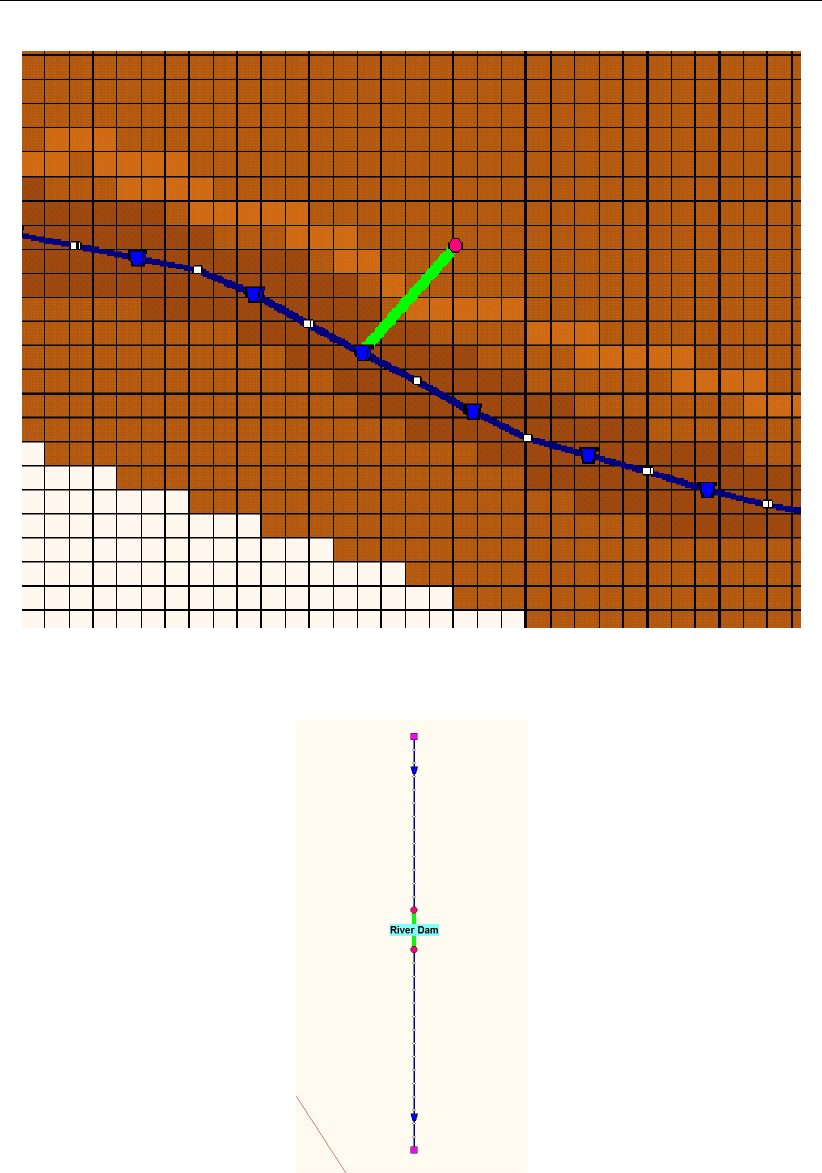
DRAFT
Graphical User Interface
Figure 5.217: Bbranching of a river levee using a "Flow 1D Dam Break Branch"
Figure 5.218: Bbranching of a 1D river dam using a "Flow 1D Dam Break Branch"
5.5.2.2 Method of modelling bbranching and Bbranch growth options/formulae
In this section three topics are discussed:
Method of modelling bbranching.
Bbranch growth options/formulae.
Controller table, defining the development of the bbranch area in time.
Deltares 357 of 900
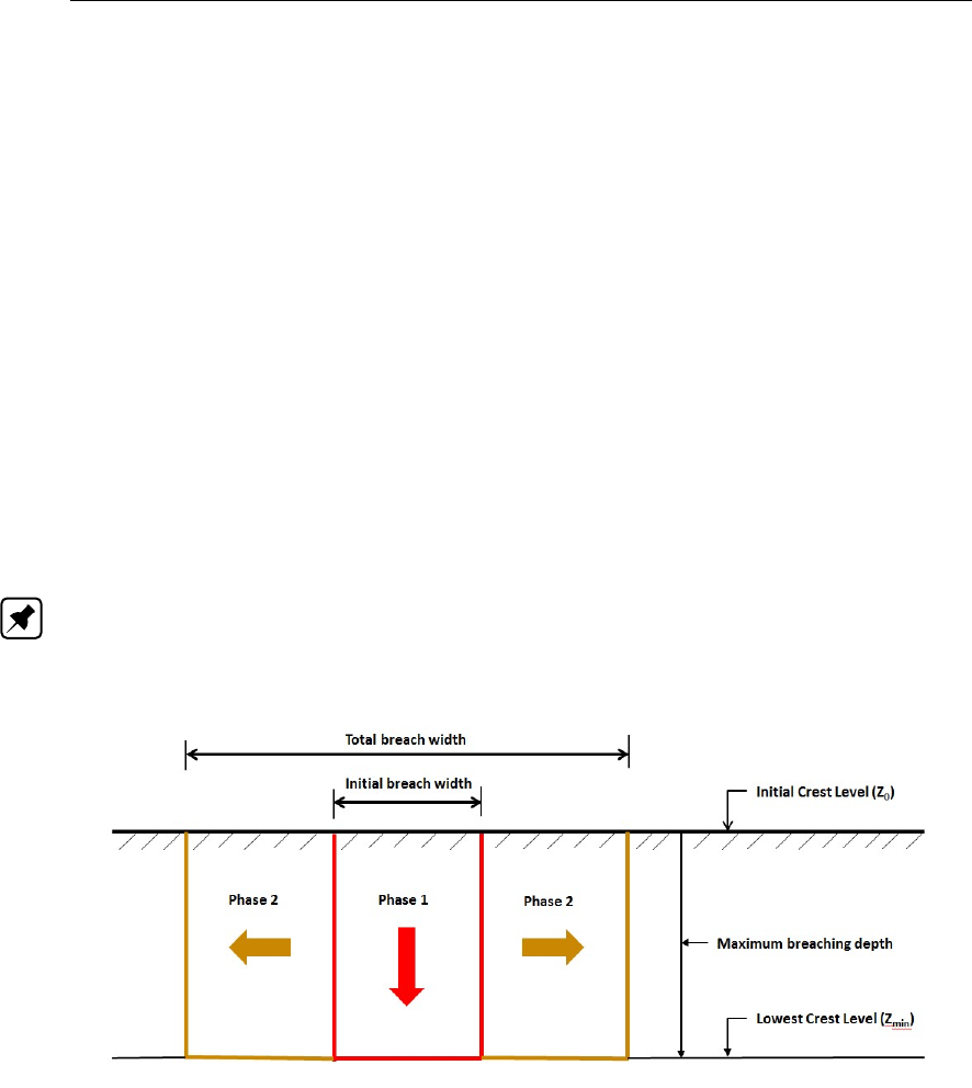
DRAFT
SOBEK, User Manual
Method of modelling bbranching
Bbranching (e.g. development of a bbranch, resulting in a dam break or dike failure) is mod-
elled by lowering the crest level and increasing the crest width of a weir, accommodated in the
"Flow 1D Dam Break Branch". The discharge over this weir is computed in accordance with
the formulae given in section 6.1.16.16, where for the "Flow 1D Dam Break Branch" yields
that the dimensionless lateral contraction coefficient (cw) is set equal to 1.
Two phases are discerned in the development of a bbranch (see Figure 5.219):
Phase 1: At the on-start of the bbranching process, the initial crest level of the weir is
set equal to the user-defined initial crest level (Z0, supposed to coincide with the crown
height of the dike) and the initial crest width of the weir is set equal to the user-defined
initial bbranch width (B0). In phase 1 for a constant crest width equal to B0, the crest level
of the weir is lowered from Z0to the user-defined lowest crest level (Zmin). Please note
that for vdKnaap(2000) yields that Zmin is equal to Z0minus the user-defined maximum
bbranching depth.
Phase 2: After phase 1 is completed, the bbranch only grows in width (e.g. crest width of
the weir increases). Hence, in phase 2 the crest level of the weir remains equal to Zmin.
Note: If the "Flow 1D Dam Break Branch" is connected by means of a Connection node to a
2D grid cell, the elevation of this 2D grid cell will be set equal to the user-defined lowest crest
level (Zmin).
Figure 5.219: Development of a bbranch in a "Flow 1D Dam Break Branch"
Bbranch growth options/formulae
Three bbranch growth options/formula are available at a "Flow 1D Dam Break Branch", viz:
The Verheij-vdKnaap(2002) formula: The bbranch width growth in phase 2 (see Fig-
ure 5.219) depends on the actual flow velocity in the bbranch (e.g. the average flow velocity
over the weir, accommodated in the "Flow 1D Dam Break Branch"). For more information
on the Verheij-vdKnaap(2002) formula, reference is made to section 6.3.3.1.
The vdKnaap(2000) formula. The bbranch width growth in phase 2 (see Figure 5.219)
is independent of the actual flow velocity in the bbranch. For more information on the
vdKnaap(2000) formula, reference is made to section 6.3.3.2).
User defined bbranch development: You can define your own bbranch development in-
dependent of the actual flow velocity in the bbranch by manually editting the controller
table, that is generated by applying the vdKnaap(2000) formula (see section 5.5.2.4).
Hereunder, in paragraph "Controller table, defining the development of the bbranch area
358 of 900 Deltares

DRAFT
Graphical User Interface
in time" it is explained how the controller table defines the development of the bbranch.
Note: For all bbranch growth options/formula yields that the final bbranch width may become
larger than the 2D grid cell size.
Controller table, defining the development of the bbranch area in time
During the bbranching process, SOBEK obtains the crest level and crest width of the weir,
accomodated in the "Flow 1D Dam Break Branch" from a controller table (see Controller Tab
description in section 5.5.2.4), that specifies the bbranch area [m2] as function of (relative)
time.
Verheij-vdKnaap(2002): The controller table describes only phase 1 of the bbranch de-
velopment and comprise of two rows only. First row [start-time of phase 1 (T0); 0])
and second row [end-time of phase 1 (T1); Bbranch area at the end of phase 1 (A1)],
where A1= Initial bbranch width(B0) * (Initial Crest level(Z0) - Lowest Crest Level(Zmin)).
During phase 1 the actual crest level is determined by linear interpolation in the con-
troller table (e.g. crest level equals Z0minus bbranch area divided by B0). Please note
that the bbranch width growth (e.g. crest widths) in phase 2 follows from the Verheij-
vdKnaap(2002) formula (see section 6.3.3.1) taking into account the actual hydraulic con-
ditions in the bbranch.
vdKnaap(2000) and User defined bbranch development: The controller table describes
both phase 1 and phase 2 of the bbranch development and may comprise of several rows.
The first row [start-time of phase 1 (T0); 0] and the last row [end-time of phase 2 (T2);
Bbranch area at the end of phase 2 (A2)]. For intermediate rows yields [0<Time<T2;
0<Bbranch area<A2]. For the bbranch area at the end of phase 1 (A1) yields A1= Initial
bbranch width(B0) * (Initial Crest level(Z0) - Maximum bbranching depth). The end-time
of phase 1 (T1) follows from the controller table (e.g. T1is point-in-time that the bbranch
area equals A1). In the same way as explained for Verheij-vdKnaap(2002), the crest levels
in phase 1 are obtained by linear interpolation in the controller table. Crest levels remain
constant in phase 2 (see Figure 5.219). For the crest width (e.g. bbranch width) in phase
2 yields: crest width = bbranch area / (Z0- maximum bbranching depth). Crest widths in
phase 2 are also obtained by linear interpolation in the controller table.
5.5.2.3 Specifying the point-in-time that bbranching should start in a Flow 1D Dam Break
Branch
There are two options for specifying the point-in-time that bbranching should start in a "Flow
1D Dam Break Branch":
Option 1: Start bbranching at an absolute point-in-time, and
Option 2: Start bbranching if a specific hydraulic event occurs.
Option 1: Start bbranching at an absolute point-in-time
In this case the user specifies the absolute point-in-time (dd-mm-yyyy hh:mm:ss) that the
bbranching process in the "Flow 1D Dam Break Branch" should start. For more information
on how to specify the absolute point-in-time, see section 5.5.2.4
Deltares 359 of 900

DRAFT
SOBEK, User Manual
Option 2: Start bbranching if a specific hydraulic event occurs
In this case the bbranching in a "Flow 1D Dam Break Branch" starts if a specific hydraulic
event occurs somewhere in the hydraulic model schematization. Such event can for instance
be the exceedance of a water level upstream of the "Flow 1D Dam Break Branch".
The bbranching is initiated by a so-called Once Hydraulic Trigger that is assigned to a
Relative-time controller, having a relative-time controller table (first column: time in seconds;
second column: bbranch area). At the on-start of a computation the status of the Once Hy-
draulic Trigger is "Off". If the trigger condition of the Once Hydraulic Trigger becomes "True",
the status of the Once Hydraulic Trigger becomes "On" and remains "On" during the entire
computation, this irrespective of the hydraulic conditions occuring after the status change.
Hence, the status of a Once Hydraulic Trigger can only change once (e.g. from "Off" to "On")
during a computation.
The relative times in the relative-time controller table are made absolute in the time-step (∆t),
executed after the absolute point-in-time (TOn) that the status of the Once Hydraulic Trigger
becomes "On". Meaning that the relative times in seconds are replaced by absolute times
(dd-mm-yyyy hh:mm:ss); where yields: absolute time = TOn +∆t+ relative-time in seconds.
From this moment onwards, the absolute time controller table is used for determining the
bbranching of the "Flow 1D Dam Break Branch". For more information on how to specify an
Once Hydraulic Trigger, reference is made to section 5.5.2.4
The trigger condition of an Once Hydraulic Trigger can be specified using one of the following
hydraulic parameters:
A water level at a 1D measuring station,
A discharge at a 1D measuring station,
A head difference over a 1D structure,
A force difference over a 1D structure,
The crest level (value and direction[lowering or rising]) of 1D structure,
The crest width (value and direction[decreasing or increasing]) of 1D structure, and
The gate lower edge level (value and direction[lowering or rising] of 1D structure.
5.5.2.4 Input screens of the Flow 1D Dam Break Branch
The "Flow 1D Dam Break Branch" comprise of
The Location Tab (see Figure 5.220): On this tab, the ID and Name of the "Flow 1D Dam
Break Branch" are shown.
360 of 900 Deltares

DRAFT
Graphical User Interface
Figure 5.220: "Flow 1D Dam Break Branch"; Location Tab
The Dam Break Tab: By means of a radio bullet, either the input data (see Figure 5.221)
of the Verheij-vdKnaap (2002) bbranch growth formula or the input data (see Figure 5.222)
of the vdKnaap(2000) bbranch growth formula can be defined on the Dam Break tab of
the "Flow 1D Dam Break Branch". For a description of the input parameters, reference is
made to section 6.3.3.1 and section 6.3.3.2.
For defining the vdKnaap(2000) controller table it is necessary to first check the "Use
Generation of Table" check-box, enter the input data and thereafter click on the <Gen-
erate Table> button. After changing vdKnaap(2000) input data, click on the <Generate
Table> button for updating the controller table.
Notice that by checking the "Once Hydraulic Trigger (see section 5.5.2.3)" check-box the
"Start bbranch growth" input fields disappear in both Figure 5.221 and Figure 5.222.
Deltares 361 of 900
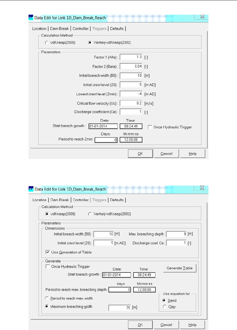
DRAFT
SOBEK, User Manual
Figure 5.221: "Flow 1D Dam Break Branch"; the Verheij-vdKnaap(2002) Dam Break Tab
Figure 5.222: "Flow 1D Dam Break Branch"; the vdKnaap(2000) Dam Break Tab
The Controller Tab: The defined bbranch development of the "Flow 1D Dam Break
Branch" can be inspected on the Controller Tab. There are four options: 1) Verheij-
vdKnaap(2002) formula with "Once Hydraulic Trigger (see section 5.5.2.3)"; 2) Verheij-
vdKnaap(2002) formula without "Once Hydraulic Trigger"; 3) vdKnaap(2000) formula with
"Once Hydraulic Trigger"; and 4) Verheij-vdKnaap(2000) formula without "Once Hydraulic
Trigger".
Option 1 is shown in Figure 5.223. Since the Verhey-vdKnaap(2002) formula is selected,
the controller table contains only two rows, defining the bbranch development of phase 1
362 of 900 Deltares
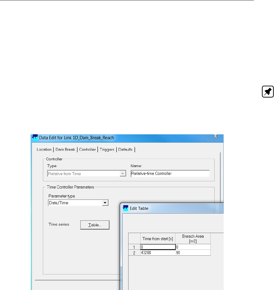
DRAFT
Graphical User Interface
only (see section 5.5.2.2 and paragraph "Controller table, defining the development of the
bbranch area in time"). Using an "Once Hydraulic Trigger" implies a "relative-time con-
troller table (see section 5.5.2.3)" with times in seconds.
Option 4 is shown in Figure 5.224. Since the vdKnaap(2000) formula is selected, the con-
troller table comprises of several rows, defining the bbranch development of phase 1 and
phase 2 (see section 5.5.2.2 and paragraph "Controller table, defining the development
of the bbranch area in time"). Not using an "Once Hydraulic Trigger" implies a controller
table with absolute times (dd-mm-yyyy hh:mm:ss).
Note: The controller table cannot be edited in case the Verheij-vdKnaap(2002) formula
is selected. However, the controller table can be edited if the vdKnaap(2000) formula
is selected, which allows for defining an "User defined bbranch development (see sec-
tion 5.5.2.2)". Please note that clicking on the <Generate Table> button on the Dam Break
Tab (see Figure 5.222) will overwrite your edited controller table.
Figure 5.223: "Flow 1D Dam Break Branch"; Option 1", Controller Tab for the Verheij-
vdKnaap(2002) formula with an "Once Hydraulic Trigger"
Deltares 363 of 900
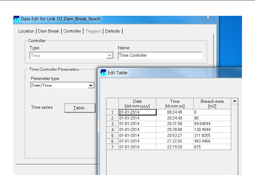
DRAFT
SOBEK, User Manual
Figure 5.224: "Flow 1D Dam Break Branch"; Option 4, Controller Tab for the vd-
Knaap(2000) formula and without an "Once Hydraulic Trigger"
The Triggers Tab: The Triggers Tab is only available if the "Once Hydraulic Trigger" is
selected on the Dam Break Tab. At the Triggers Tab (see Figure 5.225) only a trigger
of the type "Once Hydraulic Trigger" can be selected in the Trigger Type scroll-box. By
typing a Name in the Definition scroll-box a "Once Hydraulic Trigger" can be added and
specified. An existing "Once Hydraulic Trigger" can be selected in the Definition scroll-box,
and thereafter been edited or deleted. Optional hydraulic parameters are the water level
or discharge at a 1D measuring station; the head difference, force difference, crest level,
crest width or gate lower edge level of a 1D structure (see Parameter scroll-box). In the
Measurement Location scroll-box the ID of the 1D measuring station or 1D structure is to
be selected.
The Trigger table (see Figure 5.226) can be obtained by clicking on the <Trigger Table>
button. A trigger table is interpreted as a blocked function. In Figure 5.226 it can be seen
that the trigger condition of the "Once Hydraulic Trigger" becomes "True": a) if from 01-
01-2014 00:00:00 onwards up to 01-01-2014 03:00:00 minus the computational time-step
(∆t), the water level at the measuring station becomes above 1.00 m; b) if from 01-01-
2014 03:00:00 onwards till the end of the computation, the water level at the measuring
station becomes above 1.5 m. Trigger condition is "True" means that the status of the
"Once Hydraulic Trigger" is set to "On", that the relative controller table is made absolute
and the bbranching starts (for more details, see section 5.5.2.3).
364 of 900 Deltares
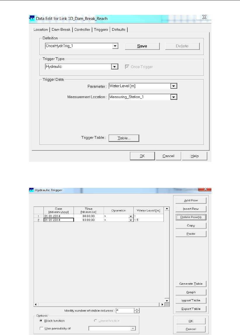
DRAFT
Graphical User Interface
Figure 5.225: The Triggers Tab of the "Flow 1D Dam Break Branch"
Figure 5.226: "Flow 1D Dam Break Branch"; Trigger Table of the "Once Hydraulic Trigger"
5.5.2.5 Output available at a Flow 1D Dam Break Branch
Output parameters available at a Flow 1D Dam Break Branch are in effect structure output
parameters, hence:
Firstly, in the "Settings" Task block, click on the <Edit> button of the "1DFLOW" module.
Thereafter select the "Output options" Tab and click on the "Structure Tab" available in
the "Output parameters" window. Now select your Flow 1D Dam Break Branch output
parameters.
Deltares 365 of 900

DRAFT
SOBEK, User Manual
After a computation, these output parameters can be viewed in the "Results in Maps"
Tasblock (e.g. at a Flow 1D Dam Break branch) as well as in the "Results in Charts" Task
block (e.g. under "Results at Structures and Extra Resistance")
The Flow 1D Dam Break Branch output parameters comprise off:
Discharge, the discharge through the "Flow 1D Dam break branch" (e.g. discharge
through the bbranch) [m3/s].
Water Level Up, water level at the ζ-calculation point having the lowest x-coordinate along
the "Flow 1D Dam break branch" [m].
Water Level Down, water level at the ζ-calculation point having the highest x-coordinate
along the "Flow 1D Dam break branch" [m].
Head, the head (=upstream water level minus downstream water level) of the "Flow 1D
Dam break branch" (e.g. head over the bbranch) [m].
Velocity, the velocity over the weir, accommodated in the "Flow 1D Dam break branch"
(e.g. velocity through the bbranch) [m/s].
Crest Level, crest level of the weir, accommodated in the "Flow 1D Dam break branch".
The crest level represents the bed level of the bbranch (see section 5.5.2.2 and Fig-
ure 5.219) [m].
Structure Flow Area, flow area above the crest level of the weir, accommodated in the
"Flow 1D Dam break branch" [m2].
Crest Width, crest width of the weir, accommodated in the "Flow 1D Dam break branch".
The crest width represents the width of the bbranch (see section 5.5.2.2 and Figure 5.219)
[m].
Note: The bbranch area at a particular point-in-time is equal to the actual crest width times
the difference between the initial crest level and the actual crest level.
5.5.3 Branch - Flow pipe
Pipes
In SOBEK-Urban Water Flow pipes are represented by branches of the type ‘Flow-Pipe’. The
Flow-Pipe with Runoff is considered equal to the Flow-Pipe by the Sewer flow module. These
branches have a length, a cross section and a resistance. The cross section is defined per
branch. Various branches can be connected by various types of Flow-Manholes which can
comprise extra storage capacity and lateral inflow.
5.5.4 Flap Gates available for specific type of Pipes
An example of a flap gate is at a tidal outlet; where water can flow into the sea as long as
water levels in the pipe are above the sea-level; and where by a hinged flap gate, sea-water
is prevented from flowing into the pipe if sea-levels are higher than the water level in the pipe.
A Flap Gate can be accommodated in the following type of pipes only:
Flow - Dry Weather Pipe
Flow - Flow Measurement Pipe
Flow - Pipe
Flow - Pipe with Runoff
Flow - Rain Pipe
On the "Flap Gate" Tab (see Figure 5.227), the user can specify the allowable flow direction(s)
in a pipe. Following options are available:
366 of 900 Deltares

DRAFT
Graphical User Interface
None, Flow in Both Directions, meaning no restriction regarding the flow direction in this
pipe (e.g. no flap gate present).
Only Positive Flow, meaning that only positive flow is allowed in this pipe. Flow is positive
if flowing in pipe-direction (e.g. flowing from the beginning towards the end of the pipe).
Only Negative Flow, meaning that only negative flow is allowed in this pipe. Flow is neg-
ative if flowing in opposite pipe-direction (e.g. flowing from the end towards the beginning
of the pipe).
Note: If a "Pipe with Flap Gate" is located adjacent to a 1D Boundary Node, then only a
"water level (h)" boundary condition is allowed. Hence, in such case no "flow (Q)" or "Q-h
relation" is allowed as boundary condition.
Figure 5.227: The Flap Gate input screen, that is available for specific type of pipes
5.5.5 Branch - 1D-2D Internal Boundary Condition
Description
Functionality:
The 1D-2D internal boundary condition enables the user to connect several 2D grid cells to
the end of a 1D channel (see picture below). The 1D channel outflow is distributed over the
concerning 2D grid cells in accordance with their conveyance capacity. The flow in the 2D grid
cells is transferred to the 1D channel. At a 1D-2D Internal boundary condition only 1(one) 1D
channel can/may be connected to a particular 2D grid.
Note: At present, a 1D-2D internal boundary condition may not pass over nested grids and
should be parallel to either the x-axis or y-axis.
Deltares 367 of 900
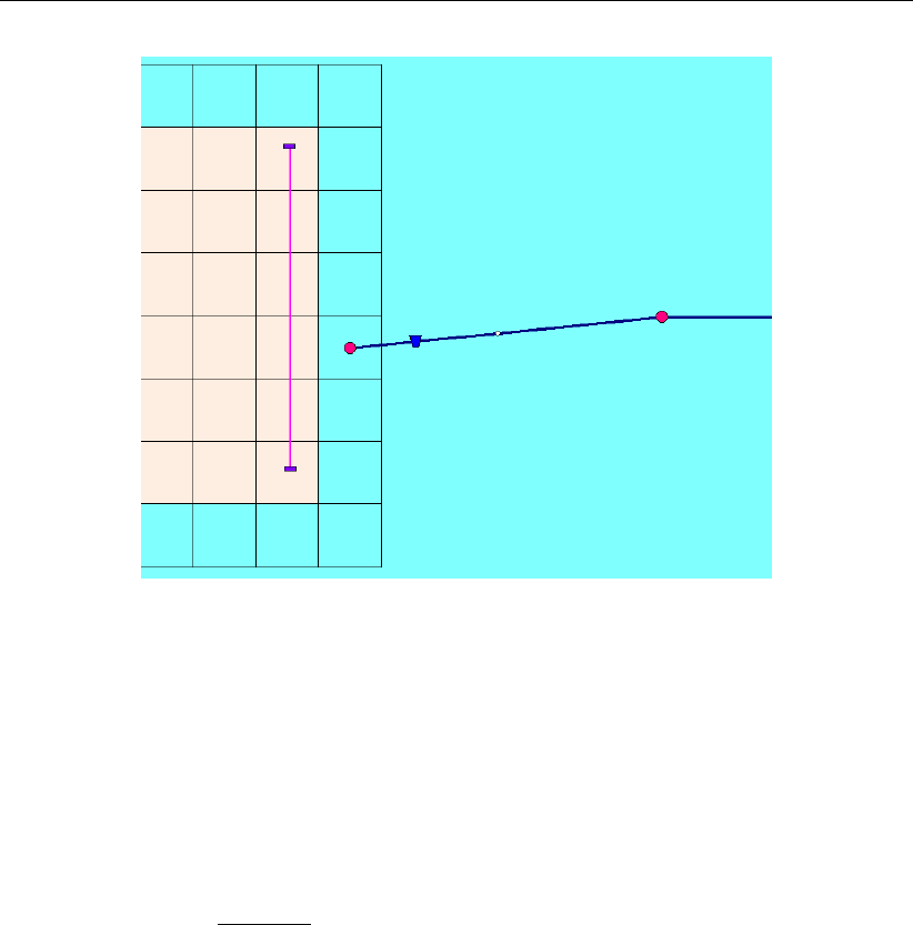
DRAFT
SOBEK, User Manual
Figure 5.228: Placing a 1D-2D internal boundary in a model
How to define:
Doubleclick the ‘Schematisation’ task block and thereafter click the Edit Model button on
the Schematisation window.
Click the Zoom in button and go to the location where you want to place the 1D-2D Internal
boundary condition.
Click the Edit Network button.
Take care that the end node of the 1D Channel, that you like to connect to the 2D grid is a
type 36: Flow - 1D2D Internal Boundary Node.
Click the Nodes button, pull-down the menu and click the Overland Flow Model/ 41, 2D -
Corner node.
Click the Branch button, pull-down the menu and click the Overland Flow Model/ 15, 2D -
Line 1D2D Internal Boundary.
Click the Edit action button, pull-down the menu and click on Nodes/Add Nodes. Go to the
location where you want to place the first 2D Corner node of the 1D-2D Internal boundary
condition and click with your left mouse button. Place the second 2D- Corner node in the
same way. Take care that the two 2D - Corner nodes are located: 1) on either a horizontal
or vertical line; 2) on 2D grid cells not having missing values; and 3) that the 2D grid cells
lying directly in front of the line through the two 2D Corner nodes are active 2D grid cells
(i.e. having no missing value)
Click the Edit action button, pull-down the menu and click on Connection/Connect nodes.
Click with the left mouse button on a 2D Corner node. While pressing down the left mouse
button drag a line to the other 2D Corner node and release your left mouse button.
It is advised to locate the end node of the 1D Channel on a 2D grid cell, that is part of
the 2D grid cells lying under the line connecting the 2D Corner nodes. For moving the
end node of the 1D Channel, click the Edit action button, pull-down the menu and click on
Node/Move Node Click, thereafter click with the left mouse button on the end node and
drag it to its new position.
Click the Edit Network button to end the network editing activities.
Click on the 1D-2D Internal boundary condition and thereafter click with your right mouse
button, and click on Model data/ Overland Flow Model. The ‘Data Edit’ window should
368 of 900 Deltares
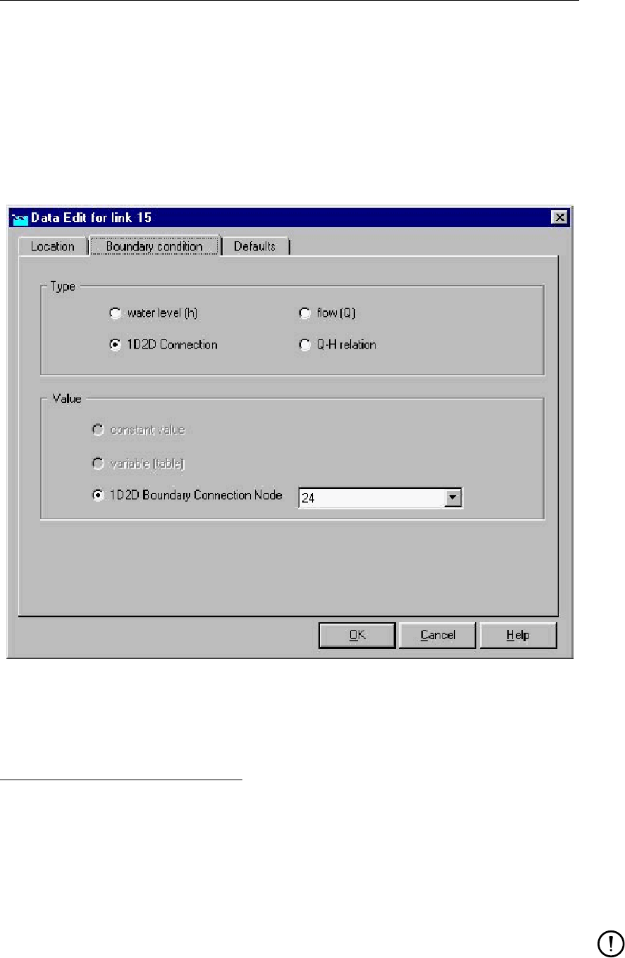
DRAFT
Graphical User Interface
appear on your screen.
Click under Type the 1D2D connection ’ check-box’ in the ‘Boundary condition’ Tab of the
‘Data Edit’ window.
Pull down the list-box left of 1D2D Boundary Connection Node and select the ID of the
end node of the 1D Channel that you wish to connect to the 2D grid (see Figure below).
The ID of a particular node can be obtained by clicking on it, right mouse click, show info.
Click the Save Network button for saving your defined 2D Q-h Tabulated Boundary Con-
dition.
Figure 5.229: Data Edit,Boundary condition tab
How to retrieve information:
Under the ‘Results in Maps’ Task block
Double click the ‘Results in Maps’ task block.
Click in the main menu on File/Open Data/Overland Flow Module Result at history stations
(i.e. in the ‘Select item’ window)
In the View Data window select the hydraulic parameters "Water level" and "Abs. Disch
[m3/s]".
Click the 1D-2D Internal boundary condition and then click with right mouse and then on
show graph or click on the graph button in the ‘View Data’ window.
Remarks:
the shown water level is the same as the one at the 1D2D boundary connection
node, that is connected to this particular 1D-2D Internal boundary condition;
the discharge is given as an absolute discharge, hence only the magnitude but not
the direction of the flow is given,
Deltares 369 of 900

DRAFT
SOBEK, User Manual
the direction of the discharge can either be seen from the concerning 1D Channel
branch or by providing a discharge-measuring-section on the 2D grid near the 1D-
2D Internal boundary condition
Under the ‘Results in Charts’ Task block
Double click the ‘Results in Charts’ task block.
Double click on Overland Flow Module/ Results at history stations (in the ‘Results in
Charts’ window).
In the ‘ODS-View’ window select under parameters Water level and Abs Disch [m3/s],
under locations select the location l_x (where l stands for link and xfor the ID of the 1D-
2D Internal boundary condition), under time-steps select the required time-period. Now
click on the Graph button or Export button to respectively view a graph or export to the
data to a particular file.
5.5.6 Branch - 2D Line discharge measurement
Description
Functionality:
The 2D Line discharge measurement provides the user with information on both the direc-
tion and magnitude of the 2D flow passing through the 2D Line discharge measurement as
function of time. Using 2D Path, the 2D grid cells that are lying under the 2D Line discharge
measurements can be shown. These 2D grid cells are used for determining the actual 2D
flow that is passing the 2D Line discharge measurement. From a 2D Line discharge mea-
surement one can obtain the 2D discharge in U direction (i.e. U-Discharge [m3/s]) and the
2D discharge in V direction (i.e. V-Discharge [m3/s]) passing through the 2D Line discharge
measurement. Discharges in U and V-direction are positive when the flow is respectively
flowing in the positive x- and y-direction of the underlying 2D grid. In addition the 2D Line
discharge measurement provides the user with information on the direction and magnitude of
the effective 2D flow (i.e. Eff.Disch_2D [m3/s]), passing through the 2D Line discharge mea-
surement as function of time. The sign of this effective 2D discharge depends on the direction
in which the user has drawn the 2D Line discharge measurement (see also how to define a
2D Line discharge measurement). In dragging the 2D Line discharge measurement, it is as-
sumed that the user defines an arrow pointing from the starting 2D Corner node towards the
ending 2D Corner node. The positive direction of the effective 2D discharge is the clock-wise
direction seen from the starting 2D Corner node. In case the effective 2D discharge passes
the 2D Line discharge measurement in clock-wise direction or in anti-clock-wise direction, the
effective 2D discharge is respectively given a positive or a negative sign (see figure below).
It is to be mentioned that at present discharge-measurement sections must lay on 1
(one) 2D grid and may not pass over nested grids. It is anticipated that in the very-
near future the functionality of the discharge-measurement-section will be extended,
allowing for a 2D Line discharge measurement to pass several 2D grids (parent and
nested 2D grids) as well as areas having no 2D grid at all. In addition information on
the effective 1D discharges will be available for the user.
370 of 900 Deltares
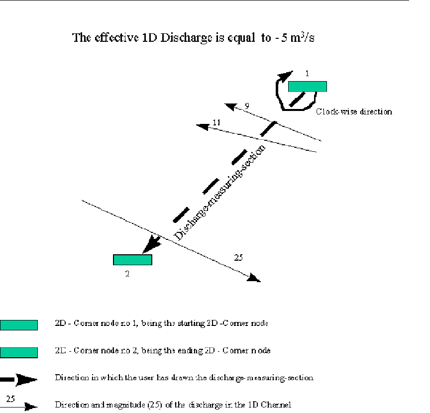
DRAFT
Graphical User Interface
Figure 5.230: Definition of the sign of the effective 2D Discharge passing a 2D Line dis-
charge measurement
How to define a 2D Line discharge measurement:
Double click the ‘Schematisation’ task block and thereafter click the Edit Model button on
the Schematisation window.
Click the Zoom in button and go to the location where you want to place the 2D Line
discharge measurement.
Click the Edit Network button.
Click the Nodes button, pull-down the menu and click the Overland Flow Model/ 41, 2D -
Corner node.
Click the Branch button, pull-down the menu and click the Overland Flow Model/ 16, 2D –
Line Measurement.
Click the Edit action button, pull-down the menu and click on Nodes/Add Nodes. Go to
the locations where you want to place the 2D Corner nodes of the 2D Line discharge
measurement and click with your left mouse button.
Click the Edit action button, pull-down the menu and click on Connection/Connect nodes.
Click with the left mouse button the starting 2D Corner node. While pressing down the
left mouse button drag a line to your ending 2D Corner node and release your left mouse
button.
Click the Edit Network button to end the network editing activities.
Deltares 371 of 900
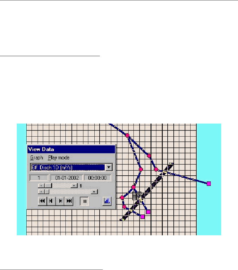
DRAFT
SOBEK, User Manual
Click the Save Network button for saving your defined 2D Line discharge measurement
How to retrieve information on a 2D Line discharge measurement:
Under the Results in Maps Task block
Double click the Results in Maps task block.
Click in the main menu on File/Open Data/Overland Flow Module Result at history stations
(i.e. in the Select item window)
In the View Data window select for instance the hydraulic property "Eff. Discharge 2D
[m3/s]"
Click the 2D Line discharge measurement and then click with right mouse and then on
show graph or click on the graph button in the View Data window.
Figure 5.231: View Data window
Under the ‘Results in Charts’ Task block
Double click the ‘Results in Charts’ task block.
Double click on Overland Flow Module/ Results at history stations (in the ‘Results in
Charts’ window).
Select the hydraulic parameter (for instance Eff. Disch 2D [m3/s]), under locations select
location l_x (where l stands for link and x for the ID of the 2D Line discharge measure-
ment), under time-steps select the required time-period. Now click on the Graph button or
Export button to respectively view a graph or export to the data to a particular file.
5.5.7 Branch - 2D-Line boundary
Description
The 2D-line boundary can be used instead of the 2D-boundary node when there are multiple
grid cells next to each other that have the same boundary condition (i.e. tidal boundary). The
boundary condition specified for the line boundary (in edit model data mode) is used for all
underlying 2D grid cells.
The 2D-line boundary is made up of a construction of two 2D-corner nodes and one 2D-
line boundary. This construction is made by first placing the 2 nodes on the grid, and then
connecting them using the ’2D-line boundary’ branch type and the ’connect existing nodes’
372 of 900 Deltares
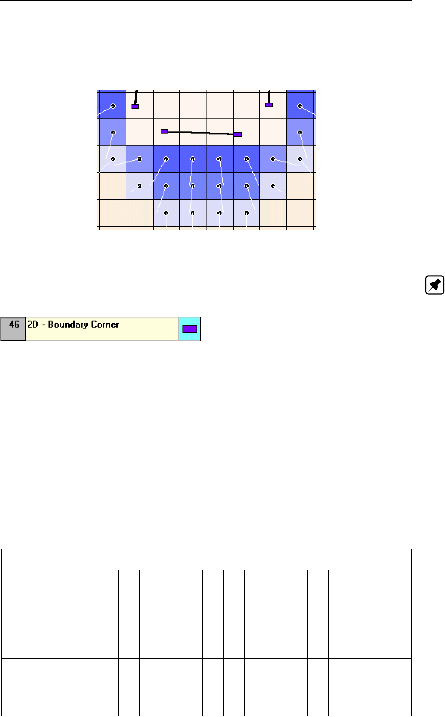
DRAFT
Graphical User Interface
option from the edit network menu. The line boundary can be either horizontal or vertical, but
not anything else. All underlying 2D grid cells should contain no-data values, and from every
boundary cell the water should be allowed to flow to (or from) only one other cell. See the
Figure 5.232 for an example.
Figure 5.232: Possible configuration of a 2D Line boundary
Note: the 2D line boundary should not pass over a nested grid.
Editing 2D Boundary Corner and Line Boundary data
At a 2D-line boundary the user can define a water level or discharge as function of time (i.e.
h(t)or Q(t)) as an external forcing boundary condition. In case of a water level boundary
all 2D grid cells lying under the 2D-line boundary obtain the same water level. In case of a
discharge boundary condition, the inflowing discharge is distributed over the 2D grid cells lying
under the 2D-line boundary in accordance with the conveyance capacity of each individual 2D
grid cell.
5.6 Cross Section types
5.6.1 Overview of available cross-sectional profiles
An overview of the cross-section types that may lay on the same branch is given in Table 5.3.
An overview of the properties of the available cross-section types is given in Table 5.4.
Table 5.3: Overview of Cross-section types that may lay on the same branch
Overview of Cross-section types that may lay on the same SOBEK branch
Arch
Asym. Trapezium
Closed Lumped Y-Z
Closed Tabulated1
Cunnette
Egg-shape
Elliptical
Open Lumped Y-Z
Open Tabulated1
Open Vert.Segm. Y-Z
Rectangle
River Profile
Round
Steel Cunette
Trapezium
Arch X- - X X -X---X- - X-
AsymTrap - X-------X- - - - -
Closed Lumped Y-Z - - X- - - - - - - - - - - -
Closed Tabulated1X- - X X -X---X- - X-
Cunnette X- - X X -X---X- - X-
Deltares 373 of 900

DRAFT
SOBEK, User Manual
Table 5.3: Overview of Cross-section types that may lay on the same branch
Overview of Cross-section types that may lay on the same SOBEK branch
Arch
Asym. Trapezium
Closed Lumped Y-Z
Closed Tabulated1
Cunnette
Egg-shape
Elliptical
Open Lumped Y-Z
Open Tabulated1
Open Vert.Segm. Y-Z
Rectangle
River Profile
Round
Steel Cunette
Trapezium
Egg-shape - - - - - X---------
Elliptical X--X X -X---X- - X-
Open Lumped Y-Z - - - - - - - X- - - - - - -
Open Tabulated1--------X-----X
Open Vert.Segm. Y-Z - X-------X- - - - -
Rectangle X--X X -X---X- - X-
River Profile - - - - - - - - - - - X- - -
Round - - - - - - - - - - - - X- -
Steel Cunette X--X X -X---X- - X-
Trapezium - - - - - - - - X-----X
1A Tabulated profile is closed in case the total width at its highest level is less than 20 mm
Table 5.4: Properties of available cross-section types
Type
Open/Closed
Summer dike
Storage Width
Conveyance method
No. of Friction Sections
Ground layer Thickness
Bed Friction definition
Ground layer Friction def.
Arch Closed no no lumped 1 yes G&L G&L
AsymTrap Open no no V.Segm n no Crs -
Closed Lumped Y-Z Closed no no lumped 1 no Crs -
Closed Tabulated Closed no no lumped 1 yes G&L G&L
Cunnette Closed no no lumped 1 yes G&L G&L
Egg-shape Closed no no lumped
analytic
1 yes G&L G&L
Elliptical Closed no no lumped 1 yes G&L G&L
Open Lumped Y-Z Open no no lumped 1 no Crs -
Open Tabulated Open no yes lumped 1 yes G&L G&L
Open Vert.Segm. Y-Z Open no no V.Segm n no Crs -
Rectangle Closed no no lumped 1 yes G&L G&L
River Profile Open yes yes lumped 3 no G&L
f(x),
f(x, h),
f(x, Q)
-
Round Closed no no lumped
analytic
1 yes G&L G&L
Steel Cunette Closed no no lumped 1 yes G&L G&L
374 of 900 Deltares

DRAFT
Graphical User Interface
Table 5.4: Properties of available cross-section types
Type
Open/Closed
Summer dike
Storage Width
Conveyance method
No. of Friction Sections
Ground layer Thickness
Bed Friction definition
Ground layer Friction def.
Trapezium Open no no lumped 1 yes G&L G&L
Note:
1 Open/Closed:
Closed means that pressurized flow occurs for water depths higher than the inner
cross-sectional height.
A tabulated profile is closed in case the total width at the highest level is less than 20
millimetres. At all levels of a closed Tabulated profile should yield that the total width
equals flow width (hence no storage allowed)
2 Method for computing conveyance (see section 6.1.20):
Lumped means that conveyance is computed using the “lumped conveyance method”
(see section 6.1.20.1)
Lumped analytical means that in computing “the lumped conveyance” use is made of
analytical formulae, giving the wetted area and the wetted perimeter as function of the
actual water depth.
V.Segm. means that conveyance is computed using “the vertically segmented con-
veyance method” (see section 6.1.20.2).
3 Number of Friction sections
For a River profile three different friction sections can be defined (main section, flood-
plain1 and floodplain2)
For a Y-Z and Asym. Trapezium profile yields that a particular friction section may not
be smaller than the width of its underlying vertical segment (W=Yi+1 −Yi)
4 Ground layer Thickness
The surface level of the ground layer equals the lowest level in the cross-sectional
profile plus the ground layer thickness.
The cross-sectional part, located below the surface level of the ground layer is omitted
in the hydraulic computations.
The “ground layer width” is the width of the cross-sectional profile at the surface level
of the ground layer.
For the “ground layer width” a roughness value can be defined that differs from the
roughness value applied to the remaining part of the wetted cross-sectional perimeter.
The roughness of the ground layer width is referred to as Ground layer friction. The
roughness value applied to the remaining part of the wetted cross-sectional perimeter
is referred to as Bed friction.
The same friction formula (Chézy, Manning etc) is applied for bed friction as well as
for ground layer friction.
Deltares 375 of 900
DRAFT
SOBEK, User Manual
5 Bed and Ground layer Friction definitions
G means constant global (or model-wide) friction value.
Lmeans for the entire branch a constant (local) friction value.
f(x),f(x, h)and f(x, Q)means that bed-friction along a branch can be defined as
function of the x-coordinate, as function of the x-coordinate and the actual water level,
or as function of the x-coordinate and the actual discharge.
Crs means that bed friction is to be defined for each and every cross-section.
5.6.2 Flow - Cross Section node (Arch type)
Cross sections of the Arch type are closed profiles using the tabulated lumped conveyance
approach (see section 6.1.20.1).
The input screen looks as follows:
Figure 5.233: Data Edit,Cross section tab
In the right-lower corner of the screen, an impression of the cross section shape that you enter
will be plotted. The dimensions that you filled in will be plotted next to it.
Create a cross section definition:
To start creating a cross section definition, do the following:
choose the cross section of the "Arch" type in the ’Choose Type’ box.
Create a new definition by typing a name for it in the "select cross section" field
Click the button Define Dimensions;
Enter the desired values in the parameter fields "width", "height" and "arc height";
376 of 900 Deltares
DRAFT
Graphical User Interface
Optionally, turn on the "use ground layer option" and enter a value;
Click the button Save Dimensions.
Parameters:
This cross section type requires the following parameters:
Width: represents the width of the arch.
Height: represents the height of the rectangle part of the arch(from the bottom up to the
point where the curved section starts)
Arc Height: represents the height of the curved part.
Use Ground Layer: switch on if a layer of sediment lies in the cross section. An individual
roughness value may be given for the ground layer. See the ’Friction’ tab for this.
Ground layer: enter the thickness of the sediment layer that lies within the cross section.
This thickness will be made visible in the image on the right side through a red line.
5.6.3 Flow - Cross Section node (Asymmetrical trapezium type)
Cross-sections of the Asymmetrical trapezium type (see Figure 5.234) are open profiles using
the vertically segmented conveyance approach (see section 6.1.20.2).
Figure 5.234: Asymmetrical trapezium cross section
The bed level that you define on the Location tab becomes the lowest point of this cross
section.
There is no restriction to the number of side slopes that are chosen left and right. Of course
a trapezium cross section that is symmetrical can be modelled by using the same side slope,
heights and extra width at the left and right side of the cross section.
The maximum flow width is limited by the outer left and outer right point of this profile. These
points are the left and right bank of the profile. The surface level is equal to the highest point
of the cross-sectional profile.
Deltares 377 of 900
DRAFT
SOBEK, User Manual
For the Asymmetrical trapezium profile the vertically segmented conveyance approach is ap-
plied.
5.6.4 Flow - Cross Section node (Closed Lumped Y-Z type)
Cross-sections of the closed Lumped Y-Z type use the tabulated lumped conveyance ap-
proach (see section 6.1.20.1). A ground-layer as well as total widths (i.e. storage) can not be
defined for a closed lumped Y-Z profile. Furthermore, only one roughness value and corre-
sponding roughness formula can be defined, which are applied to the entire wetted perime-
ter. Please note that a Closed Lumped Y-Z profile is obtained by selecting the item ’Closed
Lumped’ in the ’Type of Y-Z profile’ list-box (see Figure 5.235), accomodated on the ’Cross-
section’ Tab (Edit/Model data/ Flow - Cross Section).
Figure 5.235: Example of a closed Lumped Y-Z profile defined in ModelEdt
If the user defines a closed lumped Y-Z profile that is actually not closed (see Figure 5.236),
such lumped Y-Z profile will be closed by adding a (Y,Z) point at the end of the user-defined
Y-Z table. This added (Y,Z) point equals the first user-defined (Y,Z) point (see Figure 5.237).
The computational procedure is as follows. Firstly, it is verified if a valid closed lumped Y-Z
profile is defined and an error message is given if this is not the case. Thereafter, a tabu-
lated closed lumped Y-Z table is constructed (see Figure 5.238). Next, based on the sym-
metrical tabulated closed lumped Y-Z profile depicted in Figure 5.238, for a particular water
level the corresponding flow area and wetted perimeter is determined. Finally, using this
information and the defined roughness, the corresponding conveyance is computed (see sec-
tion 6.1.20.1).
378 of 900 Deltares
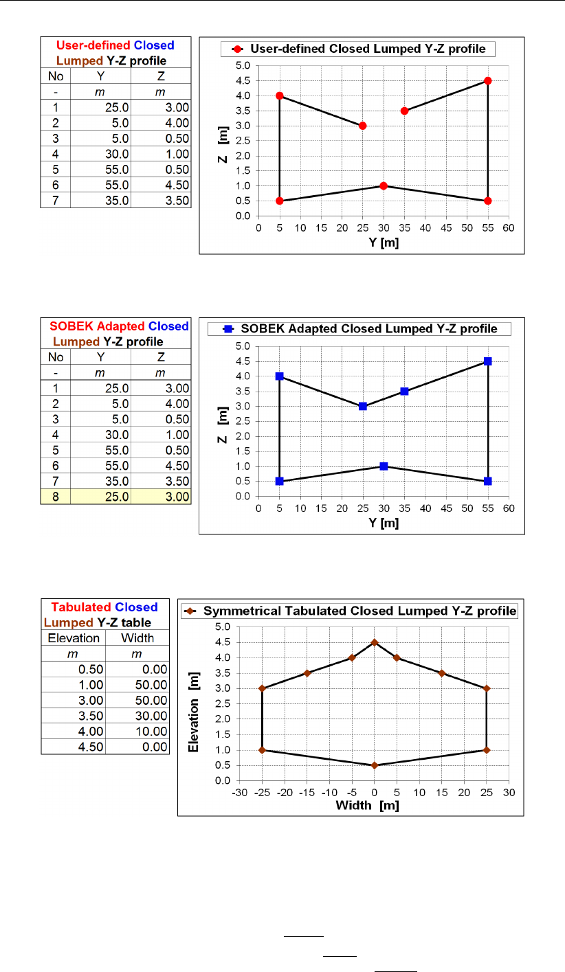
DRAFT
Graphical User Interface
Figure 5.236: User defined closed Lumped Y-Z profile
Figure 5.237: SOBEK adapted closed Lumped Y-Z profile
Figure 5.238: Symmetrical tabulated closed lumped Y-Z profile
5.6.5 Flow - Cross Section node (Closed Tabulated type)
Cross-sections of the tabulated type use the tabulated lumped conveyance approach (see
section 6.1.20.1). A tabulated cross-section is closed if the flow width at the heighest defined
elevation is smaller than 20 millimetres, else it is an Open tabulated cross-section (see sec-
tion 5.6.10). Total widths (i.e. storage) cannot be defined for a Closed tabulated cross-section.
Deltares 379 of 900
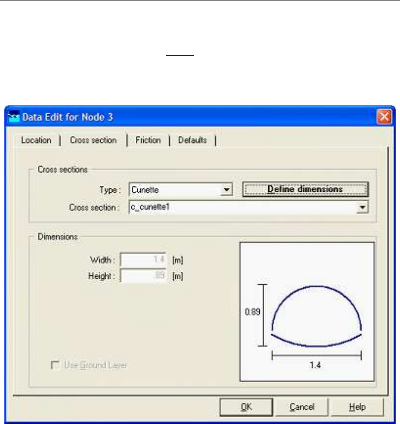
DRAFT
SOBEK, User Manual
5.6.6 Flow - Cross Section node (Cunette type)
Cross sections of the Cunette type are closed profiles using the tabulated lumped conveyance
approach (see section 6.1.20.1).
The input screen looks as follows:
Figure 5.239: The Cross section tab of a cunette profile
The parameter Height is determined based on the user-defined Width. Internally, a cunette
profile is handled as a tabulated profile. When reopening a cunette profile, SOBEK will show
the converted tabulated profile based on the cunette profile as defined by the user. See
Figure 5.240. A tabulated type originating from a cunette profile is prefixed by ’c_’.
380 of 900 Deltares
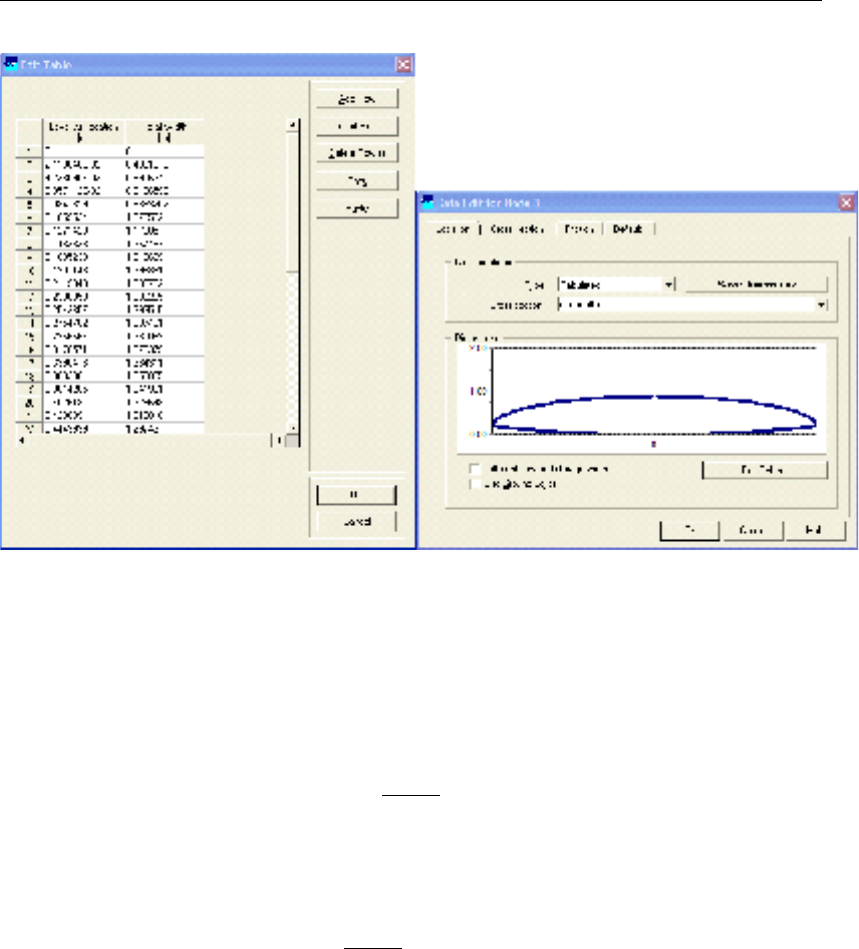
DRAFT
Graphical User Interface
Figure 5.240: The corresponding tabulated profile data of the cunette profile in Fig-
ure 5.239
For more information, see Cross-Section type: Steel Cunette (section 5.6.15).
5.6.7 Flow - Cross Section node (Egg-shape type)
Cross-sections of the Egg-shape type are closed profiles using analytical formulae for com-
puting lumped conveyance as function of water depth. An egg-shaped cross section is defined
by its bed level and width. The height is by definition 3/2 times the width.
5.6.8 Flow - Cross Section node (Elliptical type)
Cross-sections of the Elliptical type are closed profiles using the tabulated lumped conveyance
approach (see section 6.1.20.1). An Elliptical cross section is defined by its maximum width
and maximum height.
5.6.9 Flow - Cross Section node (Open Lumped Y-Z type)
Cross-sections of the open Lumped Y-Z type use the tabulated lumped conveyance approach
(see section 6.1.20.1). A ground-layer as well as total widths (i.e. storage) can not be defined
for an open lumped Y-Z profile. Furthermore, only one roughness value and corresponding
roughness formula can be defined, which are applied to the entire wetted perimeter. Please
note that an Open Lumped Y-Z profile is obtained by selecting the item ’Open Lumped’ in
the ’Type of Y-Z profile’ list-box (see Figure 5.241), accomodated on the ’Cross-section’ Tab
(Edit/Model data/ Flow - Cross Section).
Deltares 381 of 900
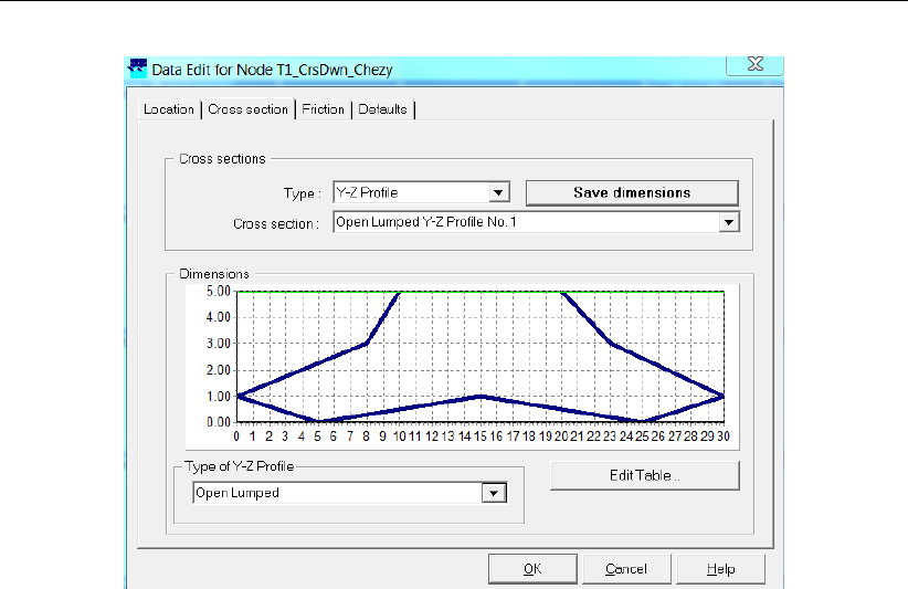
DRAFT
SOBEK, User Manual
Figure 5.241: Example of an Open Lumped Y-Z profile defined in ModelEdt
The algorithm in SOBEK does not allow for open lumped Y-Z profiles, having ’Y-Z line-segments’
that can be wetted from both sides. See for instance the ’Y-Z line-segment’ from (Y,Z) points
(25,3) to (5,4) in Figure 5.242, that is intersected by a water level of 3.5 metres. Hence a
part of this ’Y-Z line-segment is at a water level of 3.5 metres wetted at its left-side as well
as at its right-side. To avoid wetting from both sides. If the Z-value of the first user-defined
(Y,Z) point is below the maximum Z-value (Zmax) in the user defined open lumped Y-Z profile,
a (Y,Z) point is added at the beginning of the user-defined Y-Z table for which yields that its
Y-value equals the Y-value of the first user-defined (Y,Z) point and its Z-value equals Zmax.
The same applies when the Z-value of the last user-defined (Y,Z) point is below Zmax. In
such case a (Y,Z) point is added at the end of the user-defined Y-Z table for which yields that
its Y-value equals the Y-value of the last user-defined (Y,Z) point and its Z-value equals Zmax.
In Figure 5.243 it can be seen that two additional (Y,Z) points are added by SOBEK to the Y-Z
table of the open lumped Y-Z profile, that is depicted in Figure 5.242.
The computational procedure is as follows. Firstly, it is verified if a valid open lumped Y-Z
profile is defined and an error message is given if this is not the case. Thereafter, a tabulated
open lumped Y-Z table is constructed (see Figure 5.244). Next, based on the symmetrical
tabulated open lumped Y-Z profile depicted in Figure 5.244, for a particular water level the
corresponding flow area and wetted perimeter is determined. Finally, using this information
and the defined roughness,the corresponding conveyance is computed (see section 6.1.20.1).
382 of 900 Deltares
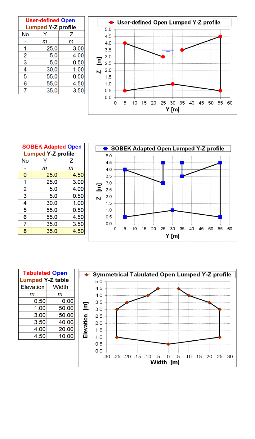
DRAFT
Graphical User Interface
Figure 5.242: User defined open Lumped Y-Z profile
Figure 5.243: SOBEK adapted open Lumped Y-Z profile
Figure 5.244: Symmetrical tabulated open lumped Y-Z profile
5.6.10 Flow - Cross Section node (Open Tabulated type)
Cross-sections of the tabulated type use the tabulated lumped conveyance approach (see
section 6.1.20.1). A tabulated cross-section is open if the flow width at the heighest defined
elevation is greater or equal than 20 millimetres, else it is a closed tabulated cross-section (see
section 5.6.5). Total widths (i.e. storage) can be defined for open tabulated cross-sections.
Deltares 383 of 900
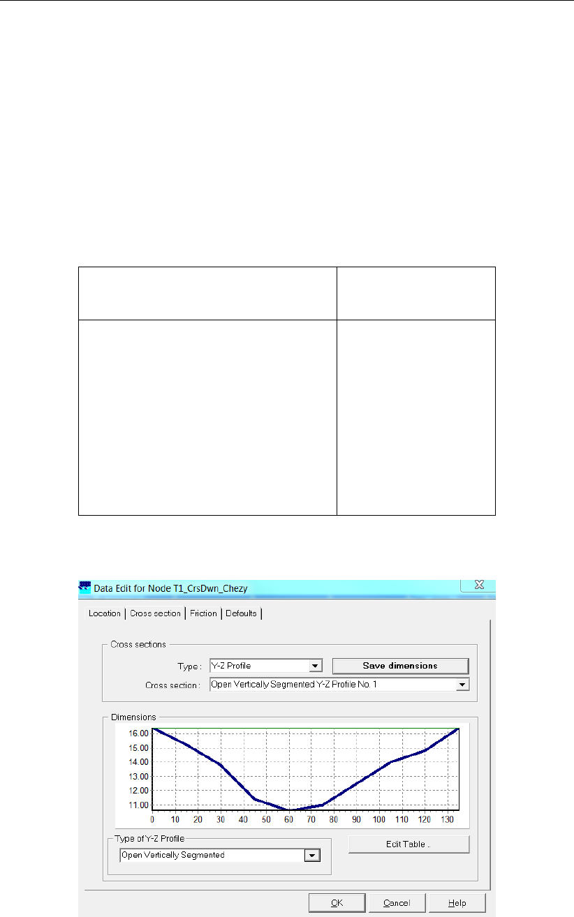
DRAFT
SOBEK, User Manual
5.6.11 Flow - Cross Section node (Open vertically segmented Y-Z type)
Cross-sections of the open vertically segmented Y-Z profile type use the vertically segmented
conveyance approach (see section 6.1.20.2). Please note that an Open vertically segmented
Y-Z profile is obtained by selecting the item ’Open Vertically Segmented’ in the ’Type of Y-Z
profile’ list-box (see Figure 5.245), accomodated on the ’Cross-section’ Tab (Edit/Model data/
Flow - Cross Section).
Open vertically segmented Y-Z profiles are often used when river bed loadings (bathymetry
measurements) are available. The Y-Z table corresponding to Figure 5.245 is given in Ta-
ble 5.5.
Table 5.5: Cross Section - Y-Z table
Y
distance along measuring-section
Z
level of the river bed
0 16.4
15 15.2
30 13.8
45 11.4
60 10.6
75 11.0
90 12.5
105 14.0
120 14.8
135 16.4
Cross section tab:
Figure 5.245: Example of an Open Vertically Segmented Y-Z profile defined in ModelEdt
Create a cross section definition:
384 of 900 Deltares

DRAFT
Graphical User Interface
To start creating a cross section definition, do the following:
1 Choose the cross section of the "Y-Z profile" type in the ’Choose Type’ box;
2 Create a new definition by typing a name for it in the "select cross section" field
3 Select option "Open Vertically Segmented" in the "Type of Y-Z profile" frame
4 Click the button Define Dimensions and subsequently Edit Table;
5 Enter the desired values in the parameter columns Y and Z;
6 Leave the table editor again by clicking OK
7 Click the button Save Dimensions.
Friction tab:
Figure 5.246: Data Edit,Friction tab, Open vertically segmented YZ profile
The conveyance of an open vertically segmented Y-Z profile is computed based on the ver-
tically segmented conveyance approach. You can define subsections along the Y-Z profile,
having different friction values. For instance, the main gully may have a lower friction value
than the area near the embankments. In the above figure, this principle is shown.
You can change the number of subsections by clicking the arrow keys next to the ’Number of
sections’ field. Subsequently, you’ll have to assign the distances from the shore where the
change in friction will occur. Do that in the ’to Y’ fields.
Deltares 385 of 900
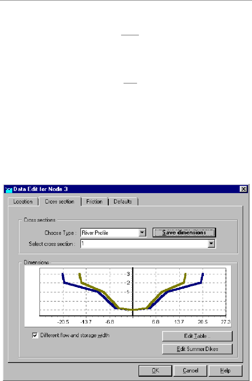
DRAFT
SOBEK, User Manual
5.6.12 Flow - Cross Section node (Rectangle type)
Cross-sections of the Rectangular type are closed profiles using the tabulated lumped con-
veyance approach (see section 6.1.20.1). The rectangular cross-section is defined by its bed
level, its width and its height.
5.6.13 Flow - Cross Section node (River Profile type) (beta functionality)
Cross-sections of the River Profile type are open profiles using the tabulated lumped con-
veyance approach (see section 6.1.20.1).
The "River Profile" cross section type becomes available when selecting the River Flow mod-
ule in the Settings task block. In this chapter the options for this cross section type are dis-
cussed in more detail.
The Cross Section tab
The river profile is a cross section type that can be used to model river sections. It comes
available by selecting the ‘River Profile’ cross section type in the second tab of the properties
of a cross section. Once selected, the user can start to define the properties. Figure 5.247
shows an example of a profile:
Figure 5.247: Example of a ’river profile’ type cross section
The user has the option to differentiate between flow width and storage width. This is a useful
option when part of the cross section, i.e. the sections between groynes, does not participate
in the conveyance of the water, but does contribute to the river’s storage capacity. The picture
386 of 900 Deltares
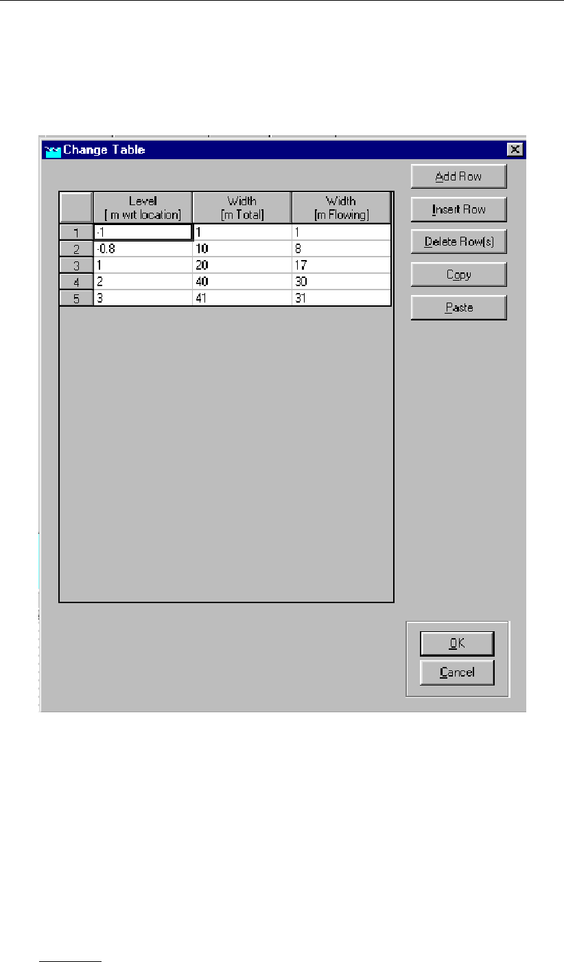
DRAFT
Graphical User Interface
of the cross section will show the flow width as a green line, and the total width with a blue
line.
The level-width table is entered in the table window, which is opened by pressing the edit table
button:
Figure 5.248: Table where a cross section’s dimensions are defined.
The levels in the cross-section should be entered in ascending order. At each next level
both the flow width and the total width (flow width) are to be specified. The entire (total)
cross-section is divided into a flow part and a storage part. As a consequence, the terms
storage width and storage area refer to the storage part of the cross-section and the terms
total width and total area are used when the entire cross-section is meant. In view of the
applied numerical solution method, it is important not to specify widths that change too rapidly
with increasing level. Remark that such rapidly varying widths should also be avoided because
of reasons of accuracy. A maximum relative increase of about a factor of 5 over 1 cm (or a
factor of 50 over 10 cm, etc.) is recommended, i.e.
Wi+1/Wi
zi+1 −zi
=O(5/cm)(5.2)
Deltares 387 of 900
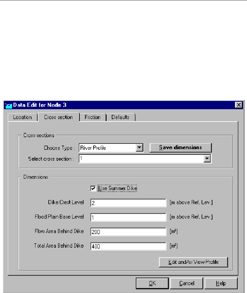
DRAFT
SOBEK, User Manual
with Wiand Wi+1 the cross-sectional widths specified at the two consecutive levels Ziand
Zi+1 (this applies to both flow width and storage width). So for example, when the storage
width at a certain level measures 85 m, the storage width to be specified at a level that is 1
cm (5 cm) higher should not be much larger than 425 m (2 125 m), i.e., the bank slope should
not be smaller than about 0.0025 m/100 m in this particular case.
Both the total width and the flowing width can be entered here as a function of the vertical
level. The total width should always be equal to or larger than the flow width. When you
choose to use a summer dike, you can enter the necessary information by selecting the ‘edit
summer dikes’ option and switching on the ‘use summer dike’ option. See Figure 5.249.
Figure 5.249: Activating the ’summer dike’ option
The transition height for summer dikes should be defined in the ’Advanced Settings’ Tab in the
SOBEK-River section on the SETTINGS task block from the Case Manager. This transition
height will act on all summer dikes defined in the model.
388 of 900 Deltares
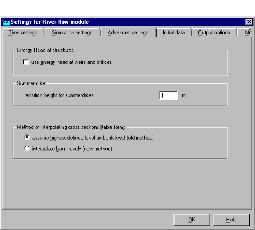
DRAFT
Graphical User Interface
Figure 5.250: The advanced settings tab for the SOBEK-River settings.
When a flood plain is separated from the river by a summer dike, the cross section profile
including the floodplain does not increase monotonously in height. In this case, it is possible
to include summer dikes in the schematisation.
The Friction Tab
The friction type and value can be specified per subsection of the flowing part of the cross
section. There are three different subsections: (i) the main river, (ii) floodplain 1 (fp1) and
(iii) floodplain 2 (fp2). For every section the flow width can be chosen. The width of the three
sections combined is always equal to the total flow width specified in the level-width table.
The following friction types can be applied:
Chézy
Manning
Strickler (kn)
Strickler (ks)
White-Colebrook
Engelund
Deltares 389 of 900
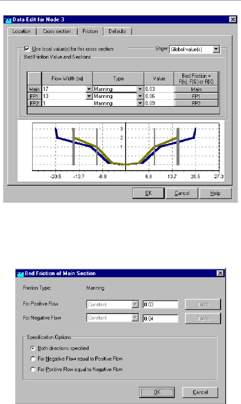
DRAFT
SOBEK, User Manual
Figure 5.251: Defining subsections for unique friction values on different sections
By default, the friction value is the same for river flow in positive direction (defined branch
direction) and in negative direction. The user can choose to change this by pressing the
corresponding button in the ‘bed friction column in Figure 5.251. As a result, the form depicted
in Figure 5.252 pops up.
Figure 5.252: Window for friction settings of the main profile section.
390 of 900 Deltares
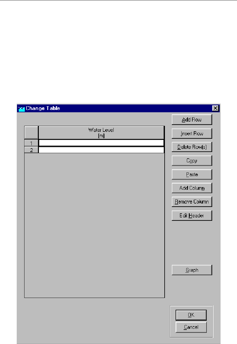
DRAFT
Graphical User Interface
Finally, the Chézy, Nikuradse, Manning or Strickler coefficients may be defined as
a constant;
spatially varying along the river branch (F(X));
a tabulated function of both the water level (h) and the x-axis (F(h)) or both the total
discharge (Q) and the x-axis (F(Q)).
The last two options are only available for local friction definitions (when also local values have
been selected), not for global definitions. All options are available for all three sections of the
flowing part of the river. Figure 5.253 shows the empty table that can be filled in for friction
values dependent on water levels and location.
Figure 5.253: Entering friction values as a function of water levels and location
First of all, the locations for which the friction is a known variable should be filled in. This is
done by adding columns (locations), and giving them the numerical value of the distance along
the branch from the start of the branch to the location itself. In Figure 5.254, two locations
have been added at 1 200 m and 2 400 m from the beginning, respectively. Next, the number
of rows needs to match the number of water levels for which there is data. In the example
Deltares 391 of 900

DRAFT
SOBEK, User Manual
below, two levels have been added to make a total of four levels available. Finally, the friction
values as a function of f(X, h)can be entered.
Figure 5.254: Locations for which the friction values are known, added to the table.
5.6.14 Flow - Cross Section node (Round type)
Cross-sections of the Round type are closed profiles using analytical formulae for computing
lumped conveyance as function of water depth.
The input screen looks as follows:
392 of 900 Deltares

DRAFT
Graphical User Interface
Figure 5.255: Data Edit,Cross section tab, Round type
In the right-lower corner of the screen, an impression of the cross section shape that you enter
will be plotted. The dimensions that you filled in will be plotted next to it.
Create a cross section definition:
To start creating a cross section definition, do the following:
1 choose the cross section of the "Round" type in the ’Choose Type’ box;
2 Create a new definition by typing a name for it in the "select cross section" field
3 Click the button Define Dimension;
4 Enter the desired value in the parameter fields "diameter";
5 Optionally, turn on the "use ground layer option" and enter a value;
6 Click the button Save Dimensions.
Parameters:
This cross section type requires the following parameters:
Diameter: represents the diameter the cross section.
Use Ground Layer: switch this on if a layer of sediment lies in the cross section. An
individual roughness value may be given for the ground layer. See the ’Friction’ tab for
this.
Ground layer: enter the thickness of the sediment layer that lies within the cross section.
This thickness will be made visible in the image on the right side through a red line.
Deltares 393 of 900
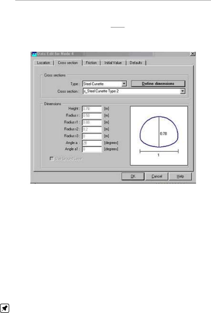
DRAFT
SOBEK, User Manual
5.6.15 Flow - Cross Section node (Steel Cunette type)
Cross sections of the Steel Cunette type are closed profiles using the tabulated lumped con-
veyance approach (see section 6.1.20.1).
The input screen looks as follows:
Figure 5.256: Steel Cunette type Cross section input screen.
In the right-lower corner of the screen, an impression of the cross-section shape that you
enter will be plotted. The dimensions that you filled in will be plotted next to it.
Create a Steel Cunette cross section definition (see Figure 5.256):
To start creating a cross-section definition do the following:
Choose the cross section of the “Steel Cunette” type in the ‘Choose Type’ box;
Create a new definition by typing a name (e.g. Steel Cunette Type 2) for it in the “Cross
section” field
Click the button Define Dimensions;
Enter the desired values in the parameter fields “Height, Radius r, Radius r1, Radius r2,
Radius r3, Angle a, and Angle a1. To define a coherent set of these parameters, see the
section Types of Steel Cunette Cross-section hereafter;
Optionally, turn on the “use ground layer option” and enter a value;
Click the button Save Dimension
Note:
That the prefix “s_” has been added in front of your defined Cross-section name, indicating that
the Steel Cunette Cross-section is stored as Tabulated Cross-section, the entered parameters
are not stored.
Editing a defined Steel Cunette cross-section (see Figure 5.257):
394 of 900 Deltares
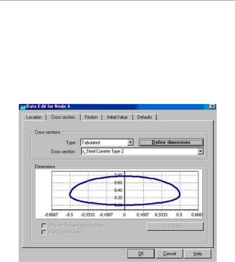
DRAFT
Graphical User Interface
Once a Steel Cunette Cross-section has been saved, its dimensions can be changed in the
following manner:
Choose the cross section of the “Tabulated” type in the ‘Choose Type’ box;
Open the scroll box available in the “Cross section” field and select the “s_Steel Cunette
Type 2” cross-section;
Click the button Define Dimensions.
Optionally, turn on the “use ground layer option” and enter a value;
Optionally, check the option “Different flow and storage width”;
Click the button Edit Table for making changes in the [Level, Total width, Flow width] table,
Click the button Save Dimension for saving your changes
Figure 5.257: Editing an existing Steel Cunette profile.
Types of Steel Cunette Cross-sections:
Steel Cunette Cross-sections are symmetric w.r.t. the vertical axis through the centre of the
profile. A Steel Cunette Cross-section may comprise of either three or four different circle
segments.
Steel Cunette Cross-section comprising of three different circle segments:
A Steel Cunette comprising of three different circle segments is depicted in Figure 5.258. For
obtaining a realistic cross-sectional profile the user-defined values for the parameters: Height,
Angle a, Angle a1, Radius r, Radius r1, Radius r2 and Radius r3 should be mutually consistent
(see Figure 5.258):
Create the first circle segment (i.e. AB) with Radius r by starting at point A (located any-
where on the vertical symmetry axis) with centre point M (located on the vertical symmetry
axis at a distance of Radius r below point A) and rotate over an angle of half the Angle a.
In this way point B is obtained,
Create the second circle segment (i.e. BC) with Radius r2 by starting at point B with centre
point M2 (located at a distance of Radius r2 from point B on the line through points B and
Deltares 395 of 900

DRAFT
SOBEK, User Manual
M) and rotate over a particular angle in order to obtain point C,
Create the third circle segment (i.e. CD) with Radius r1 by starting at point C with centre
point M1 (located at the intersection of the vertical symmetry axis and the line through
points C and M2) and rotate up to the intersection with the vertical symmetry axis and
obtain point D.
Parameter Height is the vertical distance between points D and A. Parameters Angle a, Radius
r, Radius r1 and Radius r2 follow from the three circle segments. Parameters Angle a1 and
Radius r3 are equal to zero.
Remarks:
In case the user-defined Angle a = 120 degrees; Angle a is used to compute the cross-
sectional profile, including its actual height that is used instead of the user-defined
height.
In case Angle a <120 degrees, the user-defined Angle a is ignored and the actual
applied Angle a is computed using the formula below (see Figure 5.258). Using this
computed Angle a, the cross-sectional profile is computed including its actual height,
that is used instead of the user-defined height.
1
2a= arccos l2
M,M1+l2
M,M2−l2
M1,M2/(2lM,M1lM,M2)(5.3)
lM,M1=r1−H+r(5.4)
lM,M2=r−r2(5.5)
lM1,M2=r1−r2(5.6)
Steel Cunette Cross-section comprising of four different circle segments:
A Steel Cunette comprising of four different circle segments is depicted in Figure 5.259. For
obtaining a realistic cross-sectional profile the user-defined values for the parameters: Height,
Angle a, Angle a1, Radius r, Radius r1, Radius r2 and Radius r3 should be mutually consistent
(see Figure 5.259):
Create the first circle segment (i.e. AB) with Radius r by starting at point A (located any-
where on the vertical symmetry axis) with centre point M (located on the vertical symmetry
axis at a distance of Radius r below point A) and rotate over an angle of half the Angle a.
In this way point B is obtained,
Create the second circle segment (i.e. BC) with Radius r3 by starting at point B with centre
point M3 (located at a distance of Radius r3 from point B on the line through points B and
M) and rotate over Angle a1 in order to obtain point C.
Create the third circle segment (i.e. CD) with Radius r2 by starting at point C with centre
point M2 (located at a distance of Radius r2 from point C on the line through points C and
M3) and rotate over a particular angle in order to obtain point D,
Create the fourth circle segment (i.e. DE) with Radius r1 by starting at point D with centre
point M1 (located at the intersection of the vertical symmetry axis and the line through
points D and M2) and rotate up to the intersection with the vertical symmetry axis and
obtain point E.
Parameter Height is the vertical distance between points E and A. Parameters Angle a, Angle
a1, Radius r, Radius r1, Radius r2 and Radius r3 follow from the four circle segments.
396 of 900 Deltares
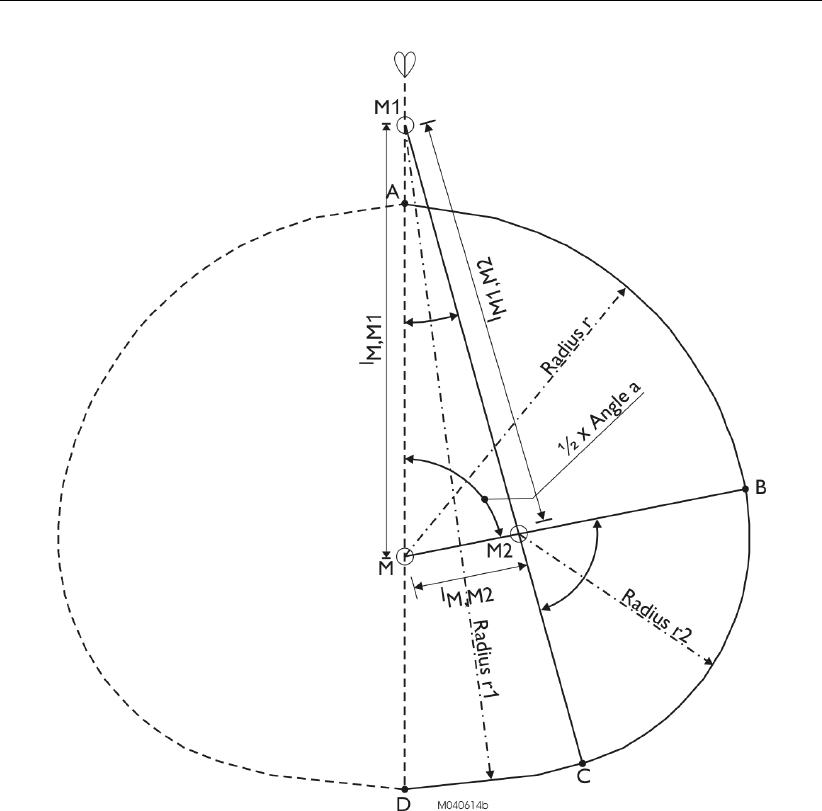

DRAFT
SOBEK, User Manual
Figure 5.259: Construction of a Steel Cunette Cross-section comprising of four circle
Segments (i.e. Type 4, see Table 5.6 for examples of Steel Cunette Cross-
sections)
Examples of Steel Cunette Cross-sections:
In Table 5.6 four examples of Steel Cunette Cross-sections are given. Type 1 to 3 are based
on three circle segments only, while Type 4 is based on four circle segments. For Type 1 the
actual height is smaller than the user-defined height.
Table 5.6: Examples of Steel Cunette Cross-sections
Parameter Type 1
(three circles)
Type 2
(three circles)
Type 3
(three circles)
Type 4
(four circles)
Height [m] 0.55 0.78 1.55 2.01
Radius r [m] 0.35 0.5 0.93 0.84
Radius r1 [m] 0.98 0.8 1.72 1.79
Radius r2 [m] 0.11 0.2 0.63 0.7
Radius r3 [m] 0 0 0 1.69
398 of 900 Deltares

DRAFT
Graphical User Interface
Angle a (deg) 180 28 159 112
Angle a1 (deg) 0 0 0 32
5.6.16 Flow - Cross Section node (Trapezium type)
Cross-sections of the Trapezium type are open profiles using the tabulated lumped con-
veyance approach (see section 6.1.20.1).
The input screen looks as follows:
Figure 5.260: Data Edit,Cross section tab, Trapezium
In the right-lower corner of the screen, an impression of the cross section shape that you enter
will be plotted. The dimensions that you filled in will be plotted next to it.
Create a cross section definition:
To start creating a cross section definition, do the following:
Choose the cross section of the "Trapezium" type in the ’Choose Type’ box.
Create a new definition by typing a name for it in the "select cross section" field.
Click the button Define Dimensions.
Enter the desired values in the parameter fields "Slope", "Bottom Width" and "Maximum
Flow width".
Optionally, turn on the "use ground layer option" and enter a value.
Click the button Save Dimensions.
Deltares 399 of 900
DRAFT
SOBEK, User Manual
Parameters:
This cross section type requires the following parameters:
Slope represents the side slopes of the channel or pipe. Note that this
value represents Horizontal/Vertical. Thus values <0 represent
steep side slopes.
Bottom width Brepresents the with at the bed level of the cross section;
Maximum Flow width the final term that is needed to define the shape of a trapezium,
though not really a physical realistic parameter in case of Cross Sec-
tions. Make sure that you choose a maximum flow width so that the
channel’s shape is correctly described from bed level to surface level.
The surface level that you filled in on the "location" tab is visible here
as a green line. It is best if the top of the trapezium lies higher than
that line.
Use Ground Layer switch on if a layer of sediment lies in the cross section. An individual
roughness value may be given for the ground layer. See the ’Friction’
tab for this.
Ground layer enter the thickness of the sediment layer that lies within the cross
section. This thickness will be made visible in the image on the right
side through a red line.
Connecting the Rainfall-Runoff module to the 1DFLOW module
You can connect a SOBEK Rainfall-Runoff module to a SOBEK Channel Flow or River Flow
schematisation by using either of the following node types:
The Flow-RR Connection on Channel is an object that should be placed on an existing Flow
branch. A Flow-RR Connection on Flow Connection node is an equivalent for a normal Flow
Connection node. That node type should therefore form the start or the end of a branch.
To both node types, an RR schematisation can be connected. The nodes will then form the
boundary for the Rainfall-Runoff schematisation.
Tips ’n Tricks
Calculate water levels on other model objects, such as cross sections or structures
Besides the node type "calculation point" it is also possible to use other model objects for
the calculation of water levels. One can, for instance, use cross sections as if they were
calculation points. For every cross section in the model, the resulting water level will then be
written to the result-files.
Here’s how to include model objects such as cross sections in the calculation grid:
Go to the Edit Network mode of SOBEK;
Open the "Branch" toolbar and click the "Calculation Grid All branches" button
The following screen will then pop up:
400 of 900 Deltares
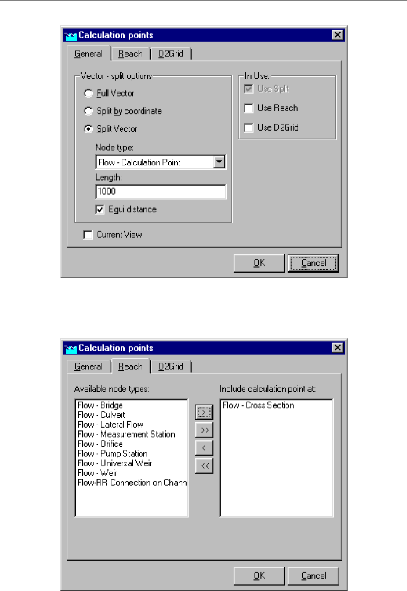
DRAFT
Graphical User Interface
Figure 5.261: Calculation points,General tab
Activate the "Use Branch" option and go to the "Branch" tab:
Figure 5.262: Calculation points,Branch tab
Move the objects that you want to use as calculation points to the right side by using the
buttons in the middle of the screen.
Click OK
After you run the model, output data will also be available on the type of objects you
selected above.
Deltares 401 of 900

DRAFT
SOBEK, User Manual
IMPORTANT NOTE: the type of objects you chose to use as calculation points will probably
NOT be visible in the "Results in Maps" yet. Make them visible by clicking "Options" - "Network
Options" - "Nodes" , selecting the node type, and activating the "visible" checkbox".
5.7 SOBEK-Urban 1DFLOW (Sewer Flow)
5.7.1 Features SOBEK-Urban 1DFLOW
Uses the complete de Saint Venant Equations, thus including backwater and transient flow
phenomena
Models a wide variety of cross sections and manhole shapes (including user-defined ones)
and allows you to build up your own cross section and manhole database
Specially designed to handle large and complex sewer networks on an ordinary PC, where
the computation time is only linear with the size of the network and independent of its
complexity
Has an automatic drying and pressurised procedure and handles real super critical flow
and is always 100% mass conservative
Self-selecting time step so your computer won’t crash and accuracy is guaranteed
All possible boundary conditions can be specified by you or are automatically applied
You can specify virtually any type of hydraulic structure, such as single or multiple stage
pumps, weirs of any shape, rectangular and circular gates, culverts and basins. All struc-
tures handle free, submerged and transient flow conditions
Real-time control options, including PID control, are available for all structures and is ideal
for complex centralised control systems using rainfall predictions
Sediment transport computation shows where sediment might be deposited; interfaces
completely with the SOBEK-Rural product line to provide an integrated model of the urban
water system and its environment
Water flow
The Water Flow module of SOBEK-Urban allows you to analyse the hydrodynamic behaviour
of a sewer network under different hydrological conditions and different management opera-
tion strategies. An example of an application is the analysis of the management of a sewer
network discharging the inflow of runoff under high rainfall conditions. Such an application
focuses on preventing high water levels at specific locations by taking measures such as cre-
ating additional storage, increasing the discharge capacity of the network, or adaptation of the
operation rules.
In SOBEK-Urban Water Flow sewer systems can be modelled by the following branch ele-
ments:
Flow-Pipe ;
Flow-Pipe with Runoff ;
Flow-Pipe with Infiltration ;
Flow-Flow Measurement Pipe ;
Flow-Internal Weir ;
Flow-Internal Orifice ;
Flow-Internal Pump Station ;
In SOBEK-Urban Water Flow sewer systems can be modelled by the following node elements:
Flow-Manhole;
Flow-Manhole with Level Measurement ;
Flow-Manhole with Runoff;
402 of 900 Deltares
DRAFT
Graphical User Interface
Flow-Manhole with Lateral Flow;
Flow-External Weir ;
Flow-External Orifice ;
Flow-External Pump Station ;
With these node and branch types a wide range of networks can be represented. Consult the
Technical Reference for detailed information about the topics mentioned.
5.7.2 Flow - Pipe with Infiltration
A pipe with infiltration refers to a drainage pipe fully located inside a trench (see Figure 5.263).
Although the drainage pipe is porous it still can get pressurized. The trench is filled with
material (for instance gravel) having a certain porosity.
A pipe with infiltration allows for the exchange of water in the pipe towards the trench (positive
sign) and vice versa as well as for the exchange of water in the trench towards the groundwater
(negative sign) and vice versa. Hence, a pipe with infiltration can be seen as a pipe having a
diffusive lateral discharge option (e.g. infiltration of water in the pipe towards the trench and
exfiltration of water in the trench towards the pipe). For more information on the infiltration and
exfiltration process, reference is made to Ellis and Bertrand-Krajewski (2010), Rutsch et al.
(2008) and Karpf et al. (2008). For more information on the computational procedure of a
Pipe with Infiltration reference is made to Section 6.1.11.5.
Pipe flow
Trench
Figure 5.263: Pipe with Infiltration (e.g. a drainage pipe located in a trench); Allowing for
the exchange of water in the pipe towards the trench (positive sign) and
vice versa; Allowing for the exchange of water from the trench towards the
groundwater (negative sign) and vice versa
5.7.2.1 Input screens of the Flow - Pipe with Infiltration
The Pipe with Infiltration input screens comprise of:
The Location Tab (see Figure 5.264): On this tab, the ID and Name of the Pipe with
Infiltration are shown. Furthermore, the invert level at the beginning of the pipe (e.g.
upstream side) and the invert level at the end of the pipe (e.g. downstream side) can be
defined.
Deltares 403 of 900
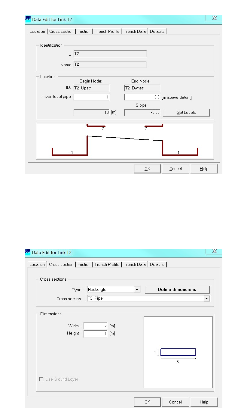
DRAFT
SOBEK, User Manual
Figure 5.264: The Location Tab of the Pipe with Infiltration
The Cross-section Tab (see Figure 5.265): On this tab, the pipe cross-section can be
defined. Notice that in the "Type scroll box" only a Round, Egg-Shape or Rectangle closed
cross-section type can be selected. Provide a name in the window, standing next to
Cross sections, then click on the <Define dimensions> button and enter the cross-section
dimensions. Now click on the <Save dimensions> button to save your cross-sectional
profile.
Figure 5.265: The Cross Section Tab of the Pipe with Infiltration
404 of 900 Deltares
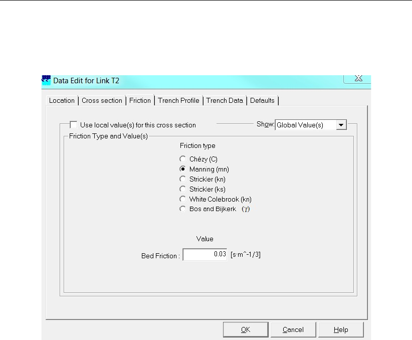
DRAFT
Graphical User Interface
The Friction Tab (see Figure 5.266): On this tab, the friction formula and friction value to
applied for computing the 1D flow through the Pipe part of the Pipe with Infiltration can be
defined.
Figure 5.266: The Friction Tab of the Pipe with Infiltration
The Trench Profile Tab (see Figure 5.267): On this tab, the trench profile can be defined.
In the "Type scroll box" only a Trapezium or a Rectangle trench profile can be selected.
Please notice that both the trapezium and rectangle trench profiles are open profiles.
Hence, the water level in the trench may rise above the highest elevation, defined for such
trench profile. Dimensions of the trench profile can be specified in the same manner as
explained for the Cross-section Tab. In the picture, shown on the Trench profile Tab, it can
be verified if the cross-sectional area of the pipe is fully located inside the trench profile.
If this is not the case, a simulation will be terminated with a message in the SOBEK.log
file.
Deltares 405 of 900

DRAFT
SOBEK, User Manual
Figure 5.267: The Trench Profile Tab of the Pipe with Infiltration
The Trench Data Tab (see Figure 5.267): On this tab in the trench window, the resistance
of the interface between the Pipe and Trench, the porosity of the trench material (notice
that porosity = 1, for trench water level above the top level of the trench or water on
street) and the initial water level in the trench (e.g. user-defined value, equal to initial 1D
water level or equal to groundwater level) can be defined. In the Groundwater window,
the permeability of the ground/soil (e.g. permeable or impermeable), the resistance of the
interface between the Trench and the Groundwater (only possible if the option permeable
is selected) and groundwater levels (only possible if the option permeable is selected)
can be defined. For more information on the background of the various input parameters,
reference is made to Section 6.1.11.5.
406 of 900 Deltares
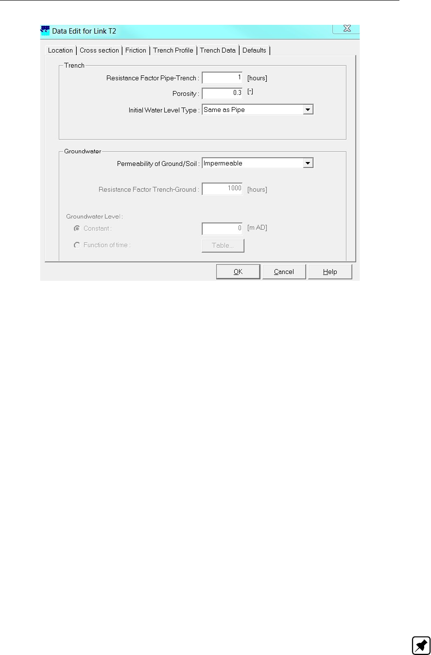
DRAFT
Graphical User Interface
Figure 5.268: The Trench Data Tab of the Pipe with Infiltration
5.7.2.2 Additional Output available for Flow - Pipe with Infiltration
The "Settings for 1DFLOW module" Form (see Figure 5.269) becomes available after clicking
on the 1D Flow <Edit> buttton in the Settings Task block. Additional output parameters for a
Flow - Pipe with Infiltration become available by checking "Results from Infiltration Pipes" in
the output parameter-box, located on the Output options Tab (see Figure 5.269). After a com-
putation, these additional output parameters can be viewed at a Flow - Pipe with Infiltration
in the "Results in Maps" Task block or under "Results at Branch Segments" in the "Results in
Charts" Task block. The additional "Flow - Pipe with Infiltration" output parameters comprise
of:
Groundwater level at trench: The groundwater level boundary condition applied for the
Flow - Pipe with Infiltration. [m above datum]
Groundw. to trench lat. flow: Exchange of water between the external groundwater
reservoir and the trench. Positive if water flows from the groundwater reservoir towards
the trench. Negative if water flows from the trench towards the groundwater reservoir.
[m3/s]
Pipe to trench lat. flow: Exchange of water between the pipe and the trench. Positive
if water flows from the pipe towards the trench. Negative if water flows from the trench
towards the pipe. [m3/s]
Volume in trench: The volume of water stored in the trench [m3].
Water depth in trench: The water depth in the trench of the Flow - Pipe with Infiltration.
[m]
Water level in trench: The water level in the trench of the Flow - Pipe with Infiltration.
[m above datum]
Note: If there is no water in the trench, a water level equal to the bed level of the trench is
provided as output.
Deltares 407 of 900

DRAFT
SOBEK, User Manual
Figure 5.269: The "Settings for 1DFLOW module Form" available in the Settings
Taskblock
5.7.3 Storage graph
Especially for sewer systems it is useful to determine the storage in the pipe system. Therefore
you can use the Storage Graph tool. This tool can be used from the Tools menu in the network
editor.
Figure 5.270: To start the storage graph
Once the program has been started the user has the option to determine the storage for the
whole network, or for a part of the network, that must be selected already.
408 of 900 Deltares
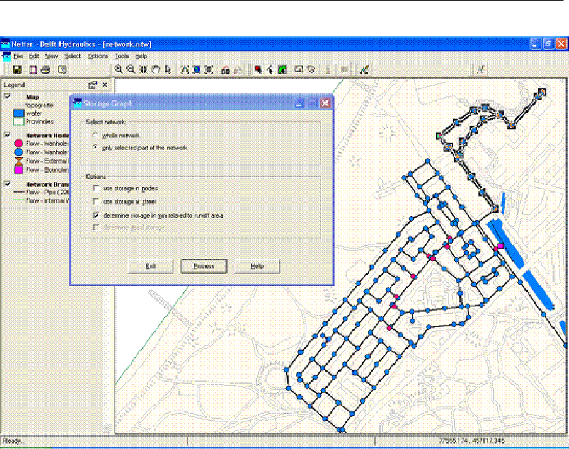
DRAFT
Graphical User Interface
Figure 5.271: Definition of storage graph options
The next options are available (see Figure 5.271:
Use storage in nodes If selected, both the storage in the pipes and the nodes are taken
into account. If not selected, only the storage in the pipes are included.
Use the storage at the street
Determine storage in mm related to the defined runoff area If you select this option, the
storage is not only determined in cubic metres, but also related to the runoff area that is
defined in the selected network.
To perform the calculation of the storage, you have to press the Process button. The calcula-
tion might take a few seconds and finally the graph pops up as shown in Figure 5.272
Deltares 409 of 900
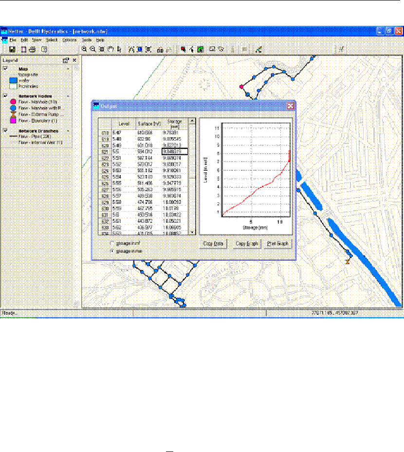
DRAFT
SOBEK, User Manual
Figure 5.272: Storage graph result
The left part of the window contains a table with the surface area [m2] and storage (m3) as
function of the level. The table starts at the lowest part in the network and runs with a step of
1 cm to the highest level.
The right part of the window shows the graph. It is possible to print the graph and to copy
the graph to the clipboard. Next to that also the contents of the table can be copied to the
clipboard by pressing the button Copy Data.
5.7.4 Coupling with other modules
Coupling a Sewer Flow manhole with the Overland Flow module (2D grid)
If you desire to create an interaction between the Sewer Flow module and the Overland Flow
module, you may want to couple a Flow - Manhole with the 2D-grid. You can either choose to
use a manhole of the type "reservoir" or the type "loss".
Manhole of the type "closed":
If a Flow-manhole of the type "closed" is placed on a 2D grid cell, there will be no exchange
of water between the 2D grid and the manhole.
Manhole of the type loss:
If you choose place a Flow-Manhole of the type loss on a 2D grid cell, the street level for that
manhole is overruled by the level of the connected 2D grid cell:
410 of 900 Deltares
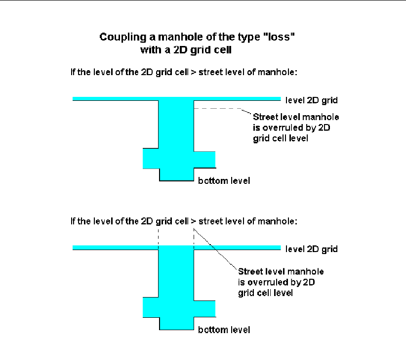
DRAFT
Graphical User Interface
Figure 5.273: Coupling a manhole ot the type loss with a 2D grid cell
Manhole of the type reservoir:
If you choose a Flow-manhole of the type reservoir, and place it on top of a 2D grid cell, two
situations may occur. See the picture below.
Deltares 411 of 900
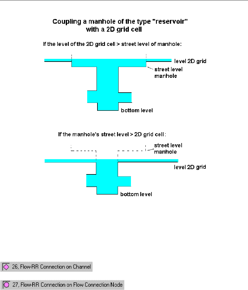
DRAFT
SOBEK, User Manual
Figure 5.274: Coupling a manhole ot the type reservoir with a 2D grid cell
5.7.5 Connecting the Rainfall-Runoff module to the 1DFLOW module
You can connect a SOBEK Rainfall-Runoff module to a SOBEK Channel Flow or River Flow
schematisation by using either of the following node types:
The Flow-RR Connection on Channel is an object that should be placed on an existing Flow
branch. A Flow-RR Connection on Flow Connection node is an equivalent for a normal Flow
Connection node. That node type should therefore form the start or the end of a branch.
To both node types, an RR schematisation can be connected. The nodes will then form the
boundary for the Rainfall-Runoff schematisation.
412 of 900 Deltares
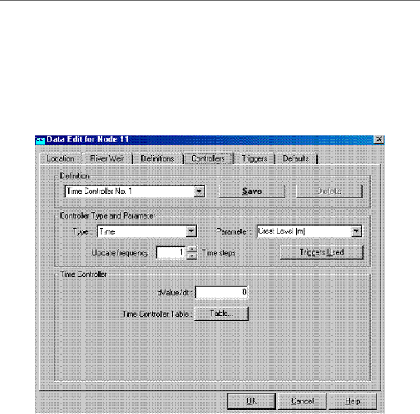
DRAFT
Graphical User Interface
5.8 River Flow controllers and triggers
In this section the so called River Flow controllers and triggers are discussed. These con-
trollers and triggers can be assigned to compound structure members (excluding River Pump),
a Database structure, a General structure, an Advanced weir and a River weir.
The Controllers tab:
Figure 5.275: Data Edit,Controllers tab
Each above mentioned structure can be operated by a combination of controllers (max. 4).
There are six possible controllers that can be applied:
Time Controller
Hydraulic Controller
Interval Controller
PID Controller
Relative from Time controller
Relative from Value controller
A detailed description of the parameters for these controller types is given in the Technical
Reference Manual. For further detailed explanation on controller functionalities, reference is
made to Appendix River Flow controller options.
Defining a controller:A new controller can be defined as follows:
Type an appropriate name for the controller in the "Definition" field.
Click the button <Define>
Choose the appropriate controller type from the "Type" drop-down box.
Enter the parameter values for the chosen controller.
Deltares 413 of 900
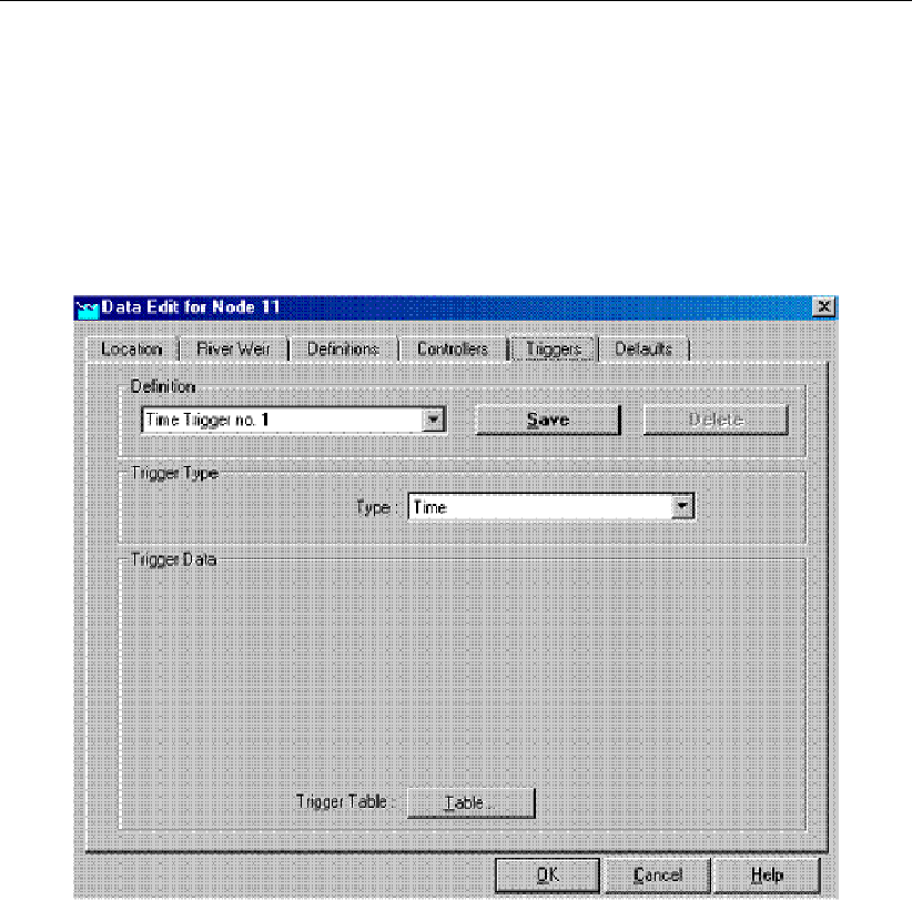
DRAFT
SOBEK, User Manual
If necessary, let the controller be activated and deactivated by a trigger. Do this by ap-
pointing the appropriate trigger on the <Triggers Used>button. Triggers can be defined
on the "Triggers" tab.
Don’t forget to activate the controller. Do this on the tab "Structure"
Triggers:
Figure 5.276: Data Edit,Triggers tab
A certain controller can be activated or deactivated by using a trigger. A trigger can be pro-
grammed so that it is activated under certain circumstances. We distinguish three types of
triggers:
Time triggers: a time table defines when the trigger is active and when it is inactive.
Hydraulic triggers: the trigger is activated or inactivated under specific hydraulic circum-
stances at a measurement location.
Time & Hydraulic triggers: this refers to a combined of a Time trigger and Hydraulic trigger.
Defining a trigger:
Type an appropriate name for the trigger in the "Definition" field.
Click the button <Define>
Choose the appropriate trigger type from the "Trigger Type" drop-down box.
Enter the parameter values for the chosen trigger.
Don’t forget to let your controller know that it should ’listen’ to this trigger. Do this by clicking
the <Triggers Used>button on the "Controllers" tab. For an example see Figure below,
where you can see that Time Trigger no 1 is used to activate and de-activate Time Controller
no 1. Note that clicking on the controller data button in the Figure below, provides information
414 of 900 Deltares
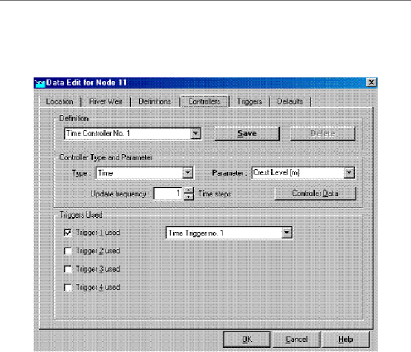
DRAFT
Graphical User Interface
on the controller data of Time Controller no 1. Thereafter clicking one of the ’Trigger used’
buttons (see two figures above) provides information on the triggers used (i.e. figure below is
obtained again).
Figure 5.277: Data Edit,Controllers tab
5.9 SOBEK-Rural/Urban/River Overland Flow (2D)
5.9.1 Introduction
In January 1998, RWS|DWW and WL |Delft Hydraulics branched an agreement to work to-
gether on a project to combine the functions of Delft-FLS and the SOBEK-Rural 1DFLOW
module. The goal was to create a single computer model that could be used to model com-
bined 1D and 2D flow for different scenarios, like for example a dike-bbranch. The agreement
resulted in a number of projects which had as a goal to improve and expand the possibilities
of the program. Many refinements were added, among which the concept of multiple grids.
The resulting functionality is known as ’1D2D functionality. This functionality is available in
case a 1DFLOW module and the Overland Flow (2D) module are selected.
Definitions
This chapter gives an overview of various terms used in this manual to describe the Overland
Flow module.
ArcView
ArcView is a desktop-GIS application, that gives the user the possibility to solve GIS related
problems in a very user-friendly environment.
Delft-FLS
Purely 2D hydrodynamical flood modelling system.
Deltares 415 of 900

DRAFT
SOBEK, User Manual
DEM
Digital Elevation Model. A DEM is a representation of terrain heights in grid format. Also
called DTM (Digital Terrain Model)
GIS:
Geographic Information System. Geographically oriented database used to analyze and
present spatially distributed data.
NETTER:
A GIS- tool from the Delft-Tools family. It is used within SOBEK to view and edit schematisa-
tions, and to visualize results from simulations.
Note: all units used in this manual and in SOBEK are metric (S.I. standard).
5.9.2 Viewing 2D Grid Info
Using the 2D Grid Info option, information can be obtained on:
individual 2D grid cells, or
on a path of 2D grid cells.
The user can add the information of various individual 2D grid cells to one and the same
graph. A path of 2D grid cells can cross at any angle over a 2D grid. At present the path of
2D grid cells can not pass over nested grids (i.e. parent grid and child grid) in such way that
only the active parent and child 2D grid cells are being selected.
Further on a distinction is to be made between static values and dynamic values. Static values
refers to the values on the underlying 2D grid (for instance a bed elevation) or underlying
map file (for instance maximum water depths). Dynamic values refers to time-dependent
computation results (for instance incremental water depths).
How to make a 2D path:
Both in the ‘Schematisation’ and ‘Results in Maps’ Task blocks.
In the main menu, click on Select/2D-Grid cell info
Click on the 2D grid cell at which you like to start your 2D path (i.e. starting 2D grid cell).
Note that in the ‘Path2D-Grid Info’ window, the column and row number of the starting 2D
grid cell are given in the two boxes in front of the Path check-box.
Click the Path check-box,
While pressing on the Shift key, place the mouse-pointer on the 2D grid cell at which you
like to end your 2D path (i.e. the end 2D grid cell). Releasing the Shift key will result in the
selection of the end 2D grid cell. The column- and row number of the end 2D grid cell are
now filled in the two boxes behind the Path check-box.
Click on the <show>button in the ‘2D-Grid info’ window to visualise the 2D grid cells
contained in your 2D Path.
Remark: In case you have more than 1(one) 2D grid (for instance in case of nested grids), the
2D grid cell of the 2D grid that lies on top will be selected. Using the Next Grid button the grid
cell on the underlying 2D grid will be selected. Note that in this case the Grid ID will change.
How to retrieve 2D Grid Info:
Under the ‘Schematisation’ Task block only information on static values of the 2D grid
416 of 900 Deltares

DRAFT
Graphical User Interface
cells are available. In case the 2D path option is not used, the static value of the selected
2D grid cell is depicted on the one most last line in the ‘2D-Grid Info’ window (Note that
dynamic values are not available under the ‘Schematisation Task’ block). In case a 2D
path is selected, the static values of the concerning 2D grid cells can be obtained by
clicking the Graph button. Note that in the main menu of this graph the x-axis can be
changed to either value (distances) or labels (column and row number of the 2D grid).
Under the ‘Results in Maps’ Task block, information on both static- and dynamic values
of the 2D grid cells are available. In case the 2D path option is not used, the static- and
actual dynamic value of the selected 2D grid cell is depicted on the last two lines in the
‘2D-Grid Info’ window. Please note that static values are displayed in grey. Clicking the
most left Graph button, provides a graph of dynamic values of each selected 2D grid cell
as function of time. Please note that by clicking on another 2D grid cell and sequentially
clicking on this Graph button again, the user can add the dynamic results of various 2D
grid cells in one and the same graph. In case a 2D path was selected, clicking on the
most left Graph button results in a graph of the dynamic values of the starting 2D grid cell
of the 2D path. Clicking the most right Graph button provides a graph, showing for all 2D
grid cells lying on the 2D path, its static value as well as its dynamic values for a particular
point-in-time.
Note:
1 the x-axis of this graph can be plotted as function of value (distance) or labels (column
or row number);
2 dynamic values are only available in case they are selected beforehand (Click in main
menu on File→Open Data→Depth Incremental (in the Select Item window));
3 using the ‘View Data’ window dynamic values can be added to the graph; and
4 using the forward and backward buttons in the ‘View Data’ window, the point-in-time
for which the dynamic values are shown under the most right Graph button can be
changed.
Deltares 417 of 900
DRAFT
SOBEK, User Manual
Figure 5.278: Example of a 2D Path under a particular user defined line
5.9.3 Coupling with other modules
General Aspects of a 1D2D model
The figure below depicts the currently available building blocks (called ’nodes’ in SOBEK). For
now, two groups of nodes are available, namely the flow nodes and the 2D nodes. The flow
nodes are the ones used to build 1D schematisations, please refer to the SOBEK Channel-
flow manual. The 2D nodes are the elements that have been added to SOBEK for the mod-
elling of 2D systems. Together they make up the 1D-2D schematisation.
One important 2D building block that is not included in Figure 5.279 is the flow - dam break
branch. This is a branch type, and not a node, which means that it can be found with the
branches.
418 of 900 Deltares
DRAFT
Graphical User Interface
Figure 5.279: Available node types for the Overland Flow & Channel Flow modules
A very important aspect to consider when using this type of schematisation is the interaction
between the 1D and the 2D system. The theory behind this interaction was explained in
chapter 2, and the FAQ-section contains an example of a dike-bbranch modelled in 1D.
When building a 2D schematisation, there are a number of rules that need to be obeyed.
One of the first rules is that every 2D-schematistion needs to contain al least one 1D-branch,
even when the schematisation is purely 2D. In this case, the 1D-branch is referred to as a
’dummy-branch’. Usually, this branch would be placed somewhere outside of the grid, and it’s
properties would be as simple as possible. The figure below shows an example:
Deltares 419 of 900

DRAFT
SOBEK, User Manual
Figure 5.280: Example of a 1D dummy branch
The second rule is that it is not possible to put more than one object in one 2D grid cell. The
only exception to this rule is the 2D- history node, which can be combined with any other type
of 2D node.
One also needs to take care when combining 1D and 2D schematisations. Some combina-
tions of elements will not be possible because of the (automatic) links made between the two
models. As explained in chapter 2, links with the 2D grid are only possible starting from a 1D
connection node or a 1D calculation point, and not from any other type of 1D node, like a 1D
boundary. Because there can be only one 1D node connected to a 2D grid cell, it is a good
idea to have exactly One, no more and no less, 1D calculation point (or connection node)
defined per 2D grid cell.
Finally, the last important fact to remember is that SOBEK internally removes all outside grid
cells from the grid, before starting the simulation! So the grid used for calculation will be 2
columns and 2 rows smaller. Knowing this, it is also not possible to define any 2D nodes in
any of the outer grid cells. If you do so anyway, SOBEK can stop the simulation with an error
message.
Coupling a Sewer Flow manhole with the Overland Flow module (2D grid)
If you desire to create an interaction between the Sewer Flow module and the Overland Flow
module, you may want to couple a Flow - Manhole with the 2D-grid. You can either choose to
use a manhole of the type "reservoir" or the type "loss".
Manhole of the type "closed":
If a Flow-manhole of the type "closed" is placed on a 2D grid cell, there will be no exchange
of water between the 2D grid and the manhole.
Manhole of the type loss:
If you choose place a Flow-Manhole of the type loss on a 2D grid cell, the street level for that
manhole is overruled by the level of the connected 2D grid cell:
420 of 900 Deltares

DRAFT
Graphical User Interface
Figure 5.281: Coupling a manhole ot the type loss with a 2D grid cell
Manhole of the type reservoir:
If you choose a Flow-manhole of the type reservoir, and place it on top of a 2D grid cell, two
situations may occur. See the picture below.
Deltares 421 of 900
DRAFT
SOBEK, User Manual
Figure 5.282: Coupling a manhole ot the type reservoir with a 2D grid cell
5.10 SOBEK-Rural RR (Rainfall-Runoff)
5.10.1 Features SOBEK-Rural Rainfall-Runoff
Models rainfall run-off and other hydrological processes in rural areas and urban areas
Catchment areas can easily be modelled in a lumped or detail manner, with no restriction
to the number of catchment areas
Catchment areas can be modelled in any detail using land elevation curves, soil charac-
teristics, land cultivation, drainage characteristics etc.
Distinguishes between various rainfall run-off processes such as surface run-off, sub-soil
drainage and storage in saturated and unsaturated areas, taking into account crop evap-
oration and capillary rise
Uses separate storm events or long time series of meteorological data for statistical anal-
ysis
You can input your own rainfall patterns or use historical data, and model any number of
rainfall gauges taking into account the spatial variation
Model both flood events and dry spells
Module can be used in combination with the flow module and real-time control module
Can also be used as a stand-alone, using reservoir approach for open water flow
422 of 900 Deltares
DRAFT
Graphical User Interface
5.10.2 Connecting the Rainfall-Runoff module to the 1DFLOW module
You can connect a SOBEK Rainfall-Runoff module to a SOBEK Channel Flow or River Flow
schematisation by using either of the following node types:
The Flow-RR Connection on Channel is an object that should be placed on an existing Flow
branch. A Flow-RR Connection on Flow Connection node is an equivalent for a normal Flow
Connection node. That node type should therefore form the start or the end of a branch.
To both node types, an RR schematisation can be connected. The nodes will then form the
boundary for the Rainfall-Runoff schematisation.
5.10.3 Selecting a subset period of a rainfall event
This page explains how to select a subset period of a rainfall event for running the Flow
module, while running the full period for the rainfall-runoff module.
For combined Rainfall-Runoff and Flow schematisations, it is possible to run the Flow simu-
lations for a subset of the Rainfall-Runoff simulation period. Usually, the simulation period of
the Rainfall-Runoff model is determined by the rainfall file as indicated in the following figure.
Figure 5.283: Definition of simulation period for Rainfall-Runoff model.
The Channel or Sewer Flow module simulation period is specified using a similar screen.
Deltares 423 of 900
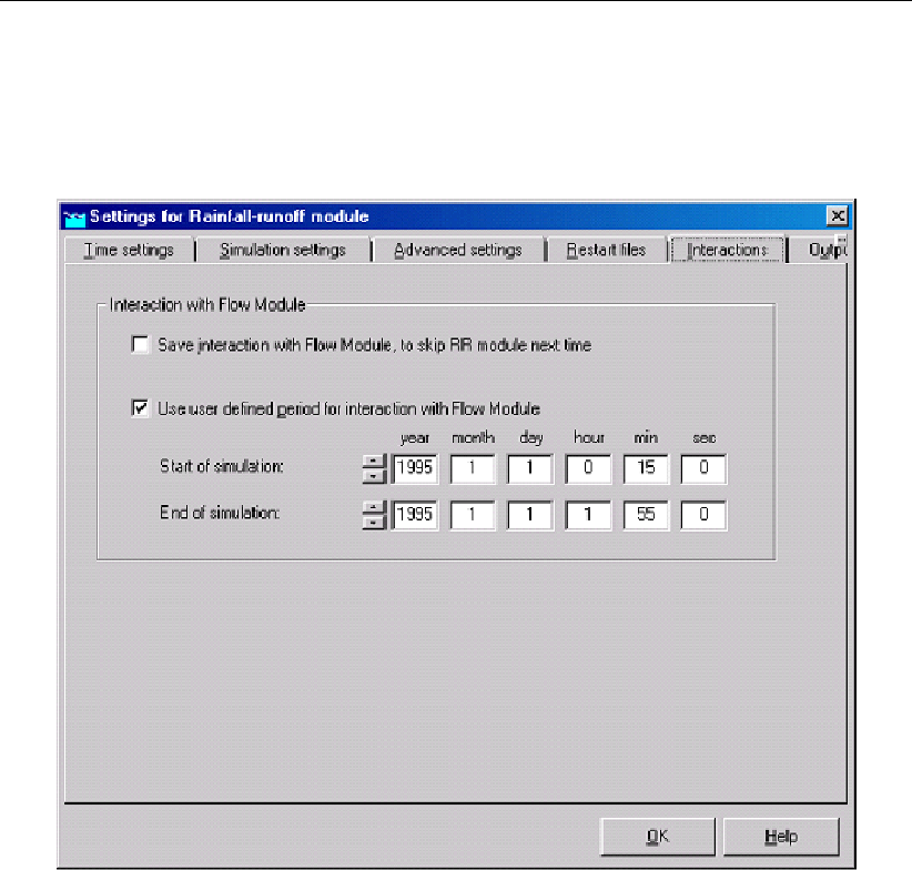
DRAFT
SOBEK, User Manual
As an additional option, when both the RR and CF/SF simulation periods are derived from the
meteorological data, there is the option to specify the interaction period for the RR and CF/SF
modules. This is done in the Settings screens of the Rainfall-Runoff module. Of course, the
interaction period should be a subset of the period covered by the meteorological data.
Figure 5.284: Interactions of Rainfall-Runoff module with Flow module.
In the example shown in the figure, the Rainfall-runoff module will use the full precipitation
event (from 1995-01-01 0 o’clock to 2 o’clock) while the Flow module covers the period from
00:15 to 01:55 o’clock.
5.11 SOBEK-Urban RR (Rainfall-Runoff)
5.11.1 Features SOBEK-Urban RR (Rainfall-Runoff) module
Models dry weather flows and the rainfall run-off processes for various types of paved
areas, such as streets, roofs and parking lots
Extended possibilities for unpaved areas and groundwater using the fully integrated link
with the Rainfall Run-off module of the SOBEK-Rural product line
Urban catchment areas can be easily modelled in a lumped or detailed manner with no
limit to the number of catchments
You can input your own time and spatially varied rainfall pattern or use historical data of
storm events and long time series with or without dry periods
Links two directionally to the hydrological database program HYMOS
Infiltration is specified as a time-dependent process following the HORTON eqation
424 of 900 Deltares
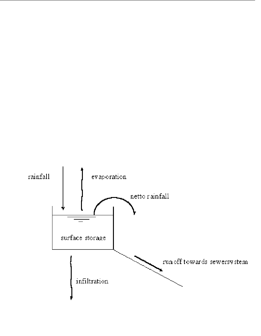
DRAFT
Graphical User Interface
5.11.2 The SOBEK-Urban RR (Rainfall-Runoff) concept
The inflow towards the sewer system consists of runoff from rainfall and dry weather flow. The
Runoff model of Flow-Manhole and Flow-Pipe, also called NWRW model, Nationale Werk-
groep Riolering en Waterkwaliteit (NLingenieurs,1978), describes the dry weather flow and
the transformation in time of rainfall into runoff entering the sewer system. The Runoff model
is based on the guidelines. The processes included are:
moistening and puddle forming;
infiltration;
runoff delay.
It is illustrated that the rainfall-runoff process with netto rainfall is the same as the runoff
towards the sewer system and is equal to the rainfall minus evaporation minus infiltration
minus the change of storage.
Figure 5.285: Illustration of rainfall-runoff process
The rainfall-runoff process
As a result of moistening and puddle forming, part of the rainfall will be stored temporarily on
the surface. This storage is called surface storage. This storage is reduced by evaporation
as well as infiltration. Different types of surfaces can be distinguished, depending on surface
characteristics and slope. The model distinguishes four types of surfaces (closed paved,
open paved, roof, unpaved) and three types of slopes (area with a slope, flat, stretched flat),
thus twelve different area types. The slope of the surface and the infiltration capacity largely
influence the rainfall-runoff process.
The infiltration of rainfall takes place in the open paved areas and unpaved areas. The infiltra-
Deltares 425 of 900
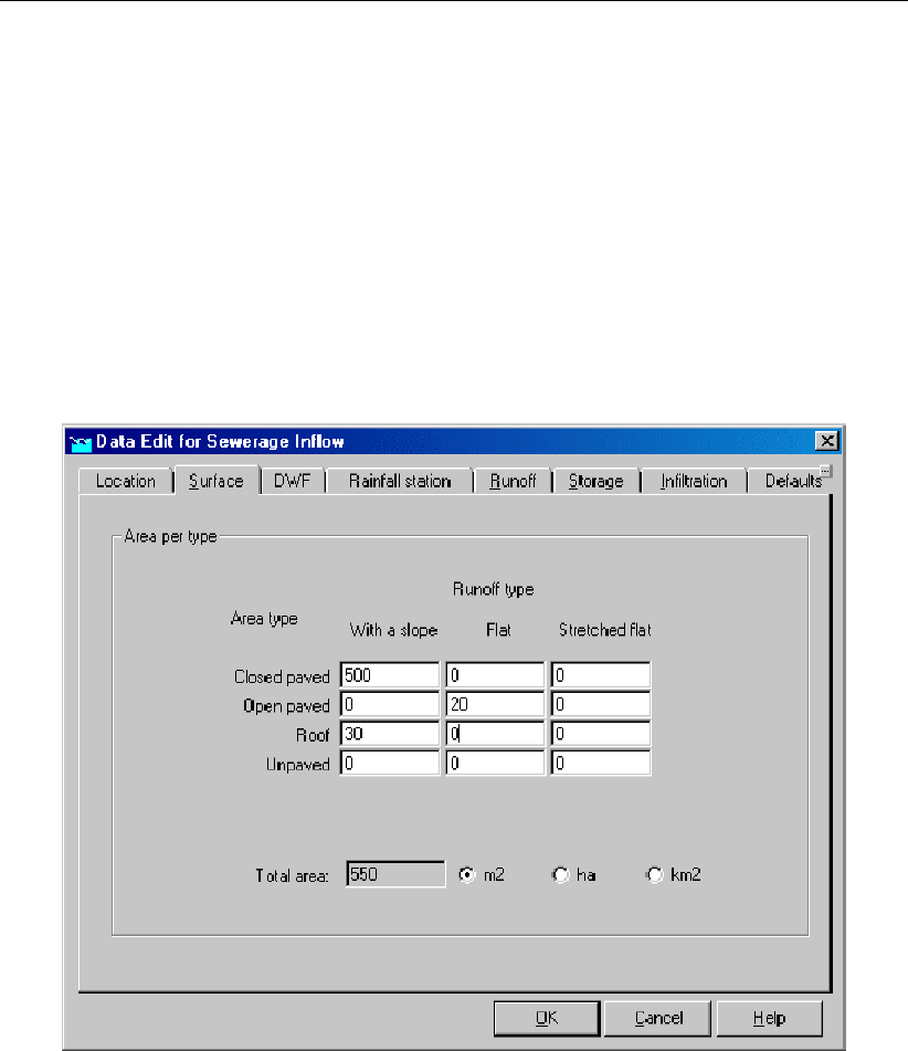
DRAFT
SOBEK, User Manual
tion capacity depends mostly on the type of surface and moisture condition. Other factors may
also play an important role. For example, the infiltration capacity of brick paths depends on the
condition of the openings between the bricks. The infiltration capacity of the unpaved areas
depends on the vegetation, the kind of soil and the percentage of moisture in the subsurface.
The description of the infiltration of the Runoff model is based on the formula of Horton (See
also Technical Reference).
The delay of runoff depends on the average distance to the inflow location in sewer system,
the slope and the geometry of the catchment. The formula which describes the runoff to the
sewer system is the formula of the rational method (See also section 6.5.4).
5.11.3 SOBEK-Urban RR (Rainfall-Runoff) input screens
Figure 5.286: Data Edit for Sewerage Inflow,Surface tab
426 of 900 Deltares
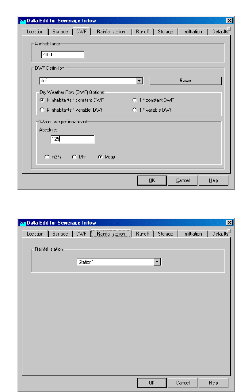
DRAFT
Graphical User Interface
Figure 5.287: Data Edit for Sewerage Inflow,DWF tab
Figure 5.288: Data Edit for Sewerage Inflow,Rainfall station tab
Deltares 427 of 900
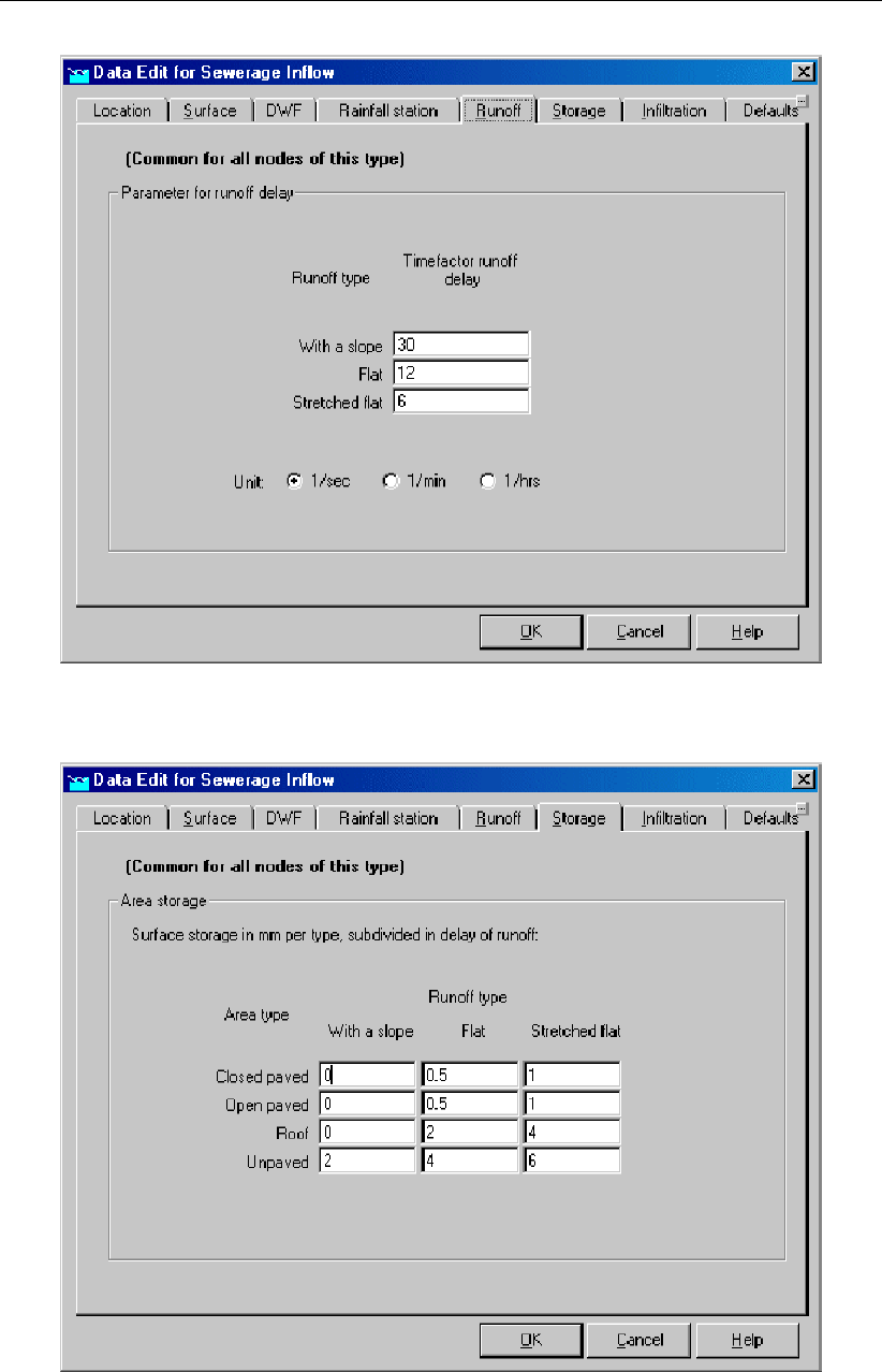
DRAFT
SOBEK, User Manual
Figure 5.289: Data Edit for Sewerage Inflow,Runoff tab
Figure 5.290: Data Edit for Sewerage Inflow,Storage tab
428 of 900 Deltares
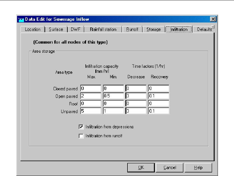
DRAFT
Graphical User Interface
Figure 5.291: Data Edit for Sewerage Inflow,Infiltration tab
For NWRW nodes (Urban rainfall-runoff model), there are two infiltration options available in
the user interface:
Infiltration from depressions;
Infiltration from runoff;
Figure 5.298 illustrates the NWRW modelling concept.
The infiltration from depressions indicates the infiltration from water that is stored in depres-
sions. The surface storage in depressions is typically a few mm. When the surface (depres-
sion) storage exceeds the defined threshold, runoff is computed.
However, the runoff may take some time to branch the outflow point (for urban sewer systems:
the point where the runoff flows into the sewer system). The option ’infiltration from runoff’
can be used to simulate infiltration from the runoff dynamic storage. The same set of Hor-
ton infiltration parameters are used for both infiltration from depressions and infiltration from
runoff.
Default only the infiltration from depressions is switched on. Switching on the infiltration from
runoff will result in some additional infiltration losses and less inflow in the sewer system.
Deltares 429 of 900
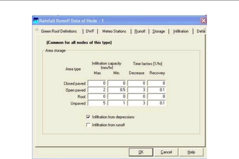
DRAFT
SOBEK, User Manual
Figure 5.292: Concept of Urban runoff model
5.12 SOBEK-Rural/Urban/River RTC (Real Time Control)
5.12.1 Why a separate RTC (Real-time Control) module
Real-time Control is a separate module within SOBEK. One could ask for the reason for this.
In a SOBEK-Urban 1DFLOW, a SOBEK-Rural 1DFLOW, a SOBEK-River 1DFLOW and a RR
schematisation, controllers can be defined for operating the available structures. So real-time
control options are already available within these modules. The reasons for having a separate
Real-time Control (RTC) module are:
the controllers in the SOBEK-Urban 1DFLOW, SOBEK-Rural 1DFLOW and SOBEK-River
1DFLOW modules are local controllers, looking at 1 (one) water level or flow in the hydro-
dynamic schematisation. Using Real-time Control, it is possible to take into account more
than 1 location: you can control the structure looking at any linear combination of values
at different locations;
in Real-time Control, it is possible to define a measure (or RTC controller) for a (previously
defined) controller in the Flow or Rainfall-Runoff schematisation. Such RTC measure can
consist of several different type of decision rules, where each decision rule has its own
priority. If defined active, such RTC measure will overrule its associated active controller
in the Flow or Rainfall-Runoff schematisation. In case the associated controller is not-
active (i.e. not triggered), the setpoint provided by the RTC measure will be neglected
(see for more details RTC does not overrule Flow Triggers).
most important, using Real-time Control it is possible to take into account information from
different SOBEK modules. One can define the operation of a pump in Rainfall-Runoff
based on results of the Flow modules (or hydrodynamic computational results), or define
the operation of a weir or pump in a Flow module based on computed runoff by the rainfall-
runoff module, or based on available rainfall and wind data, or on other data (e.g. water
quality). This gives many more possibilities than just using local controllers in a Flow or
Rainfall-Runoff schematisation.
SOBEK RTC is equiped with a special reservoir module, allowing operation of reservoirs
or ponds with multiple outlets using a set of rule curves.
Further on the Real-time Control (RTC) module can be online coupled with a Matlab com-
430 of 900 Deltares

DRAFT
Graphical User Interface
putation, allowing for any type of controller to be applied.
5.12.2 Condition
A Real-time Control measure usually involves a logical condition. Only if that condition is
satisfied, the measure will be active.
A condition is of the following form:
‘value of decision parameter’ ‘check’ ‘check value’
The check can be ‘<’, ‘=’ or ‘>’.
The check value can either be a constant input value, or the value of another decision param-
eter.
5.12.3 Data locations in RTC
Data locations in Real-time Control (RTC) represent, as the name suggests, those locations
at which data can be defined. Using the data defined at data locations, so-called decision
parameters can be defined. In RTC so-called measures can be defined. A measure consists
of a number of decision rules. These decision rules can be formulated using the defined deci-
sion parameters. In case a measure is defined active, the corresponding decision rules will be
evaluated and will result in a setpoint for the associated Flow or RR controller, that is assigned
to a particular structure[s] located in either the Flow or Rainfall-Runoff schematisation.
In Real-time Control five different types of data locations can be defined:
1DFLOW Data; computed hydrodynamic parameters at specific locations in the SOBEK-
Urban 1DFLOW, SOBEK-Rural 1DFLOW and SOBEK-River 1DFLOW schematisations
2DFLOW Data; computed hydrodynamic parameters at specific locations in the Overland
Flow schematisation
RR Data; computed parameters at specific locations in the Rainfall-Runoff schematisation
Precipitation Data; user-defined rainfall data
Wind Data; user-defined wind data (i.e. wind velocities and wind directions)
External Data - His Files; user-defined External Data (can be data, that is not used or
computed by any SOBEK module)
5.12.4 Data measurement location
The data measurement locations represent, as the name suggests, those locations at which
data is available for Real-time Control. At the moment, 4 types of data measurement locations
are available. These are:
locations in the Water Flow module (Water Flow locations)
locations in the Rainfall-Runoff module (Rainfall-Runoff locations)
rainfall prediction locations
other locations (also called external locations); at the moment these locations are used for
wind predictions and for data from external HIS files.
Deltares 431 of 900
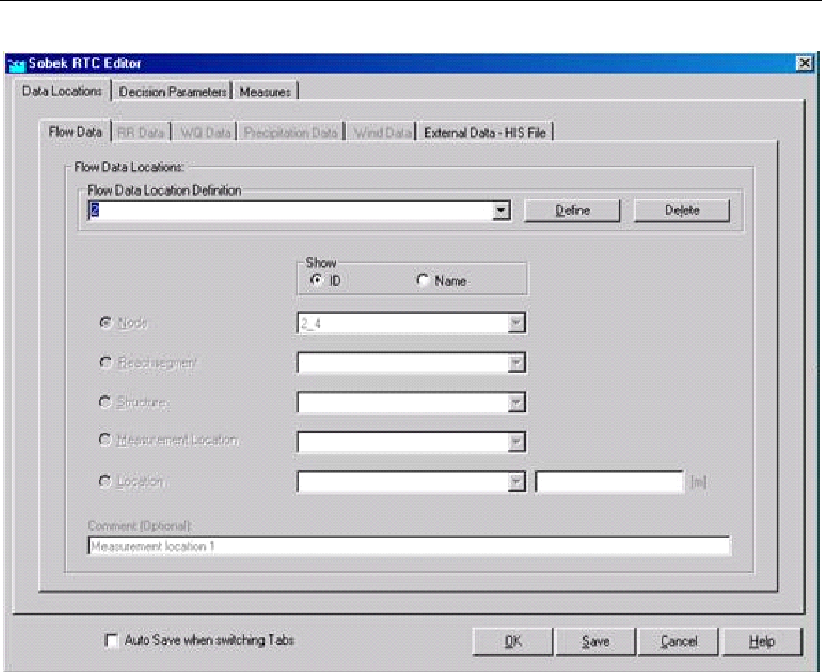
DRAFT
SOBEK, User Manual
Figure 5.293: RTC Flow data locations input screen
The available data (measurements) at Water Flow locations are given in the following list:
water level + RefL [m];
flow [m3/s];
surface area [m2];
water depth [m];
crest level [m];
crest width [m];
gate lower edge [m];
gate opening height [m];
structure flow area [m2];
discharge at the structure [m3/s];
flow velocity at the structure [m/s];
water level up [m];
water level down [m];
head over structure [m];
pressure difference over structure;
pump capacity [m3/s].
Data availability depends on the type of location (a node, a branchsegment, a flow measure-
ment location, or a structure) and type of structure. For instance, for a weir, no pump capacity
is available.
The available data at Rainfall-Runoff locations are:
open water level (m + RefL);
432 of 900 Deltares

DRAFT
Graphical User Interface
groundwater level (m + RefL);
The available data at rainfall prediction locations are:
rainfall prediction at time step t+1 (mm/time step);
rainfall prediction at time step t+2 (mm/time step);
rainfall prediction at time step t+3, etc.
The available data for wind prediction are:
wind direction prediction at time step t+1 (degrees);
wind direction prediction at time step t+2; etc. and
wind velocity prediction at time step t+1 [m/s];
wind velocity prediction at time step t+2, etc.
The available data for external locations related to a SOBEK HIS file are taken from the exter-
nal HIS file and indicated by the user.
5.12.5 Decision Parameters in RTC
In Real-time Control (RTC), decision parameters can be defined on basis of the data available
at earlier defined Data locations. Decision parameters are used in defining measures (or RTC
controllers), that determine how a particular structure is to be operated.
Real-time Control allows to define a wide range of decision parameters. Examples of decision
parameters are:
The water level or discharge at a particular location in a 1DFLOW schematisation,
The waterlevel or abs. velocity at particular location in an Overland Flow schematization,
The outflow discharge from a Rainfall-Runoff schematisation,
The predicted area weighted average rainfall of all rainfall stations,
The predicted wind velocity
In RTC following type of decision parameters are discerned (see Figure below):
Function (decision) parameters,
Time (decision) parameters, and
Reservoir (decision) parameters.
Please note that Interpolation Tables are not decision parameters. Interpolation Tables are
used in defining so-called Interpolation Function decision parameter (see mathematical ma-
nipulations available for function decision parameters hereafter).
Deltares 433 of 900
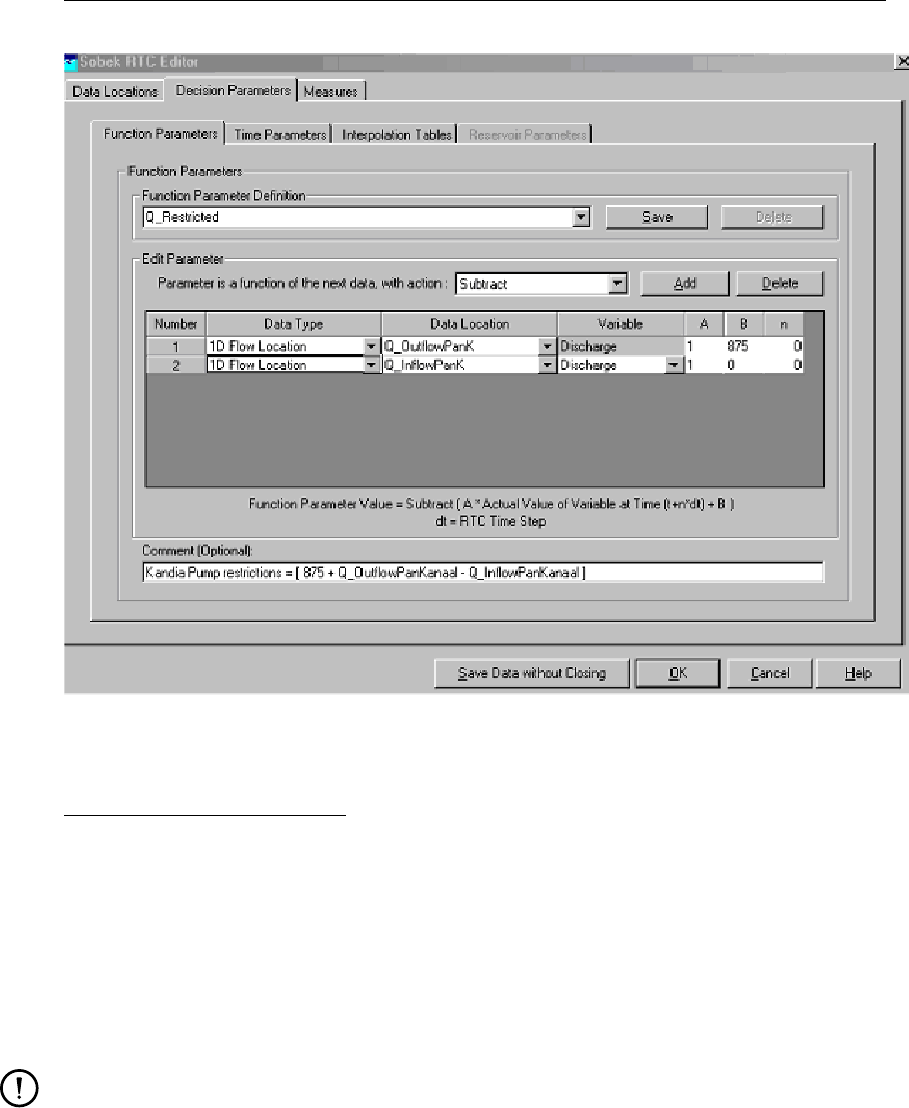
DRAFT
SOBEK, User Manual
Figure 5.294: Example of RTC input screen for Function (decision) parameters
Function (decision) parameters:
The actual time-dependent value of a Function decision parameter can result from a mathe-
matical manipulation:
on the corresponding value of a single data series, or
on the corresponding values of a set of data series.
Mathematical manipulations available for single data series are: None, Sin, Cos, Tan, ArcSin,
ArcCos, ArcTan, Sinh, Cosh, Tanh, Interpolate, Floor, Ceil, Nint, Exp, Log, Log10, Square and
Sqrt.
Remarks:
None means that no mathematical manipulation is carried out on the data series,
Interpolate; for each independent value, a corresponding dependent value (or Interpo-
late Function Decision parameter) is determined by linear interpolation in an Interpo-
lation Table (first column: independent variable in ascending order; second column:
dependent variable). If an independent variable is smaller than the value on the first
row, the dependent variable will be set equal to its value on the first row. If an indepen-
dent variable is larger than the value on the last row, the dependent variable will be set
equal to its value on the last row.
Floor(12.8)=12.0; Ceil(12.2)=13.0;
Nint (Nearest INTeger), Nint(12.1)=12, Nint(12.5)=13, Nint(-12.5)=-13
Mathematical manipulations available for a set of data series are: Add, Subtract, Multiply,
Divide, Max, Min, Average and Power (for more information, see Table 5.7)
434 of 900 Deltares

DRAFT
Graphical User Interface
Table 5.7: Mathematical manipulations available for a set of data series
Mathematical ma-
nipulation
Values (V) of data series Function Decision Parameter value
Add V1, V2, V3, . . . . . . Vn V1 + V2 + V3 . . . + Vn
Subtract V1, V2, V3, . . . . . . Vn V1 - V2 - V3 . . . - Vn
Multiply V1, V2, V3, . . . . . . Vn V1 * V2 * V3 . . . * Vn
Divide V1, V2, V3, . . . . . . Vn V1 / V2 / V3 . . . / Vn
Max V1, V2, V3, . . . . . . Vn Max (V1, V2, V3, . . . , Vn)
Min V1, V2, V3, . . . . . . Vn Min (V1, V2, V3, . . . , Vn)
Average V1, V2, V3, . . . . . . Vn (V1 + V2 + V3 + . . . + Vn) / n
Power V1, V2, V3, . . . . . . Vn (((V1ˆV2)ˆV3)ˆV4) . . . ˆVn)
Note: V1 is the value of the data series defined on the first row and Vn is the value of the
data series defined on the last row (see Figure above).
A data series is defined by its:
1 Data Type, Data location, and Variable Type,
2 Multiplication factor A, Off-set B, and RTC Time shift n.
Ad 1) Data Type, Data location, and Variable Type:
Presently the following data types are supported:
Data Type=1D Flow location: Computed 1D Flow data at “1D Flow Data locations” previ-
ously defined on the “1D Flow Data” Tab (see 1D Flow Data in RTC),
Data Type=2D Flow location: Computed 2D Flow data at “2D Flow Data locations” previ-
ously defined on the “2D Flow Data” Tab (see 2D Flow Data in RTC),
Data Type=External: Available data locations are the “External Data locations” previously
defined on the “External Data – His File” Tab (see External Data – His File in RTC),
Data Type=Decision parameter: Available data locations are the previously defined Func-
tion/Time/Reservoir (decision) parameters,
Data Type=Date/Time: Data source is the RTC computational point-in-time; Available data
locations are: Year, Month, Day, Hour, Minute, Second, Date, Time, Date+Time, Day of
Week and CompTimestep; Variable follows from the actual RTC computational point-in-
time (for more information, see Table below)
Ad 2) Multiplication factor A, Off-set B, and RTC Time shift n:
Each data series can be a linear function of the actual value of a specific variable at a particular
data location. The linear function is defined as: Data series value = A * Variable(t+n*dt)
+ B, where: A = Constant multiplication factor, t = actual RTC computational point-in-time,
n=number of timesteps, dt= time step defined in RTC Settings, and B = Constant off-set
value.
Deltares 435 of 900

DRAFT
SOBEK, User Manual
Resuming:
Say that a Function (decision) parameter should be the 1D water levels, computed at Rotter-
dam at a point-in-time that is 2 RTC time steps earlier than the actual RTC computational time.
This Function (decision) parameter should comprise of only one data series with mathemat-
ical manipulation “None”. This data series is to be defined as: Data type=1D Flow location,
Data location=Rotterdam (defined at the 1D Flow Data Tab), Variable=water level, A=1, B=0
and n=-2.
Table 5.8: Data Type=Date/Time (yyyy-mm-dd; hh:mm:ss)
Data Type Data location Variable
RTC “Date/Time” Year Integer value = “yyyy”
RTC “Date/Time” Month Integer value = “mm”
RTC “Date/Time” Day Integer value = “dd”
RTC “Date/Time” Hour Integer value = “hh”
RTC “Date/Time” Minute Integer value = “mm”
RTC “Date/Time” Second Integer value = “ss”
RTC “Date/Time” Date Integer value = “yyyymmdd”
RTC “Date/Time” Time Integer value = “hhmmss”
RTC “Date/Time” Date+Time Real value = “yyyymmdd.hhmmss”
RTC “Date/Time” Day of week Integer value = day no.
RTC “Date/Time” CompTimestep RTC timestep in seconds
Remarks:
Say that: the RTC time-step=10 seconds; the actual RTC “Date/Time” is Tuesday,
March 29th, 2005 at 12:10:50 (2005-03-29; 12:10:50); A=2; B=-4; and n=96. Than
if:
Data location=Year; resulting value = 2*[2005-03-29; 12:10:50 – 96*10s]-4= 2*yyyy-
4=4006
Data location=Minute; resulting value = 2*[2005-03-29; 12:10:50 – 96*10s]-4= 2*mm-
4= 104
Data location=Date; resulting value = 2*[2005-03-29; 12:10:50 – 96*10s]-4= 2*hhmmss-
4= 230896
Data location=Date+Time; resulting value = 2*[2005-03-29; 12:10:50 – 96*10s]-4=
2*yyyymmdd.hhmmss-4= 40100654.230900
Data location=Day of week; resulting value = 2*[2005-03-29; 12:10:50 – 96*10s]-4=
2*Day_of_week -4= 0
Day_of_week(Sunday)=0; Day_of_week(Monday)=1; and Day_of_week(Saturday)=6
Please note that resulting values follow from a mathematic expression only, and might
become negative integer values or negative real values.
436 of 900 Deltares

DRAFT
Graphical User Interface
Time (decision) parameters:
A Time decision parameter can be a user-defined function of time.
5.12.6 Decision rules in RTC - General
In Real-time Control (RTC), Measures can be defined consisting of a set of so-called Decision
rules. For each decision rule, the user has to define its priority and its decision rule type. A
decision rule might consist of a number of criteria. Each criteria has the following form:
“Value of decision parameter” “Check” “Check value”
Note:
The value of a decision parameter is the value that corresponds to the RTC computational
point-in-time.
The “Check” can be ‘<’, ‘=’ or ‘>’
“Check value” can be a constant or a user-defined decision parameter
In case for a decision rule all its criteria are “True”, than the evaluation of such decision rule is
“True”. Else the evaluation of such decision rule is “False”.
In case the evaluation of more than one decision rule is “True”, than the setpoint for the
Measure will be equal to the set-point of the decision rule having the highest priority (e.g.
lowest integer number)
In case the evaluation of more than 1 (one) decision rule having the highest defined priority
are “True”, than the set-point for the Measure will be equal to the set-point of the decision
rule that is the closest to end of the drop-down list.
In case not one of the defined decision rules is “True”, than the set-point of the Measure
will be kept equal to the set-point determined in the previous RTC time-step.
For more information on the type of decision rules available for RTC Flow Measures, see Flow
Measures in RTC.
5.12.7 External Data - His File in RTC
On the External Data – His File Tab available under the Data locations Tab in Real-time Control
(RTC), data contained in a so-called His file (<name>.his) can be selected. This His file can
be placed at any location/folder at your computer and should be available at the start of the
computation. A His file may contain any kind of data (for instance number of crocodiles lying
on a river bank). In addition a His file can contain different type of data for a large number of
locations.
Deltares 437 of 900

DRAFT
SOBEK, User Manual
5.12.8 Example of a MATLAB M-file
The example program below shows the use of some SOBEK output variables, the conver-
sion of the SOBEKTime string to numerical values and the passing of setpoints computed by
Matlab back to SOBEK.
if (SOBEKFirst == 1)
SOBEKC_Matlab1=1;
Sinitial=1;
end
SOBEKS_Matlab1=Sinitial;
Level_measurementlocation1=SOBEKH_2_4;
Level_measurementlocation2=SOBEKH_6;
Flow_measurementlocation1=SOBEKQ_2_4;
Flow_measurementlocation2=SOBEKQ_4;
Crestlevel=SOBEKCL_17;
Crestwidth=SOBEKCW_17;
DeltaHStructure=SOBEKDH_17;
TimeControllerSetpoint=1.;
temp_time=str2num(SOBEKTime);
Hour=round(floor(temp_time/1000000));
temp=temp_time-Hour*1 000 000;
Minute = round(floor(temp/10000));
if (temp_time <6000000)
TimeControllerSetpoint=1.;
elseif (temp_time <10000000)
TimeControllerSetpoint=0.9;
elseif (temp_time <12000000)
TimeControllerSetpoint=1.;
elseif (temp_time <15000000)
NrMinutes=(Hour-12)*60 + Minute
TimeControllerSetpoint=1. + (NrMinutes)/180 * 0.4;
elseif (temp_time <20000000)
NrMinutes=(Hour-15)*60 + Minute
TimeControllerSetpoint=1.4 - (NrMinutes)/300 * 0.4;
end
if (Flow_measurementlocation1 >1.0)
SOBEKS_Matlab1 = TimeControllerSetpoint;
end
Example m-file
Note:
1 In Matlab, you can on-line check the values of the variables in your program. You can
request which variables are available by using the who command. The value of a variable
can be requested by simply typing the name of the variable and pressing Enter. Note that
Matlab is case-sensitive, so carefully check the variable names used in your m-file and the
SOBEK-ids.
2 Matlab declarations must not be written to the screen, so must always end with a semi-
colon (;), e.g. SOBEKC_0_65=1;
3 When using Matlab 6.1., errors in the Matlab m-file (e.g. an undefined variable is used;
438 of 900 Deltares

DRAFT
Graphical User Interface
since Matlab is case-sensitive this may just be a typing error) , will be heard by regular
beeps whenever the m-file is executed (each time step in the RTC-Matlab coupling). Older
Matlab versions do not give this indication of error!
The M-FILE that is selected in the [Matlab Options] tab, must produce the following variables
for the Flow controllers which are controlled by Matlab:
SOBEKC_<controller>(optional)Indication if Matlab controls the SOBEK controller. For
example with: SOBEKC_0_65 for the controller ’0-65’. This identifier corresponds with the
identifier following keyword id in the inputfile <SBK_MEAS.RTC>. The result has value
1 (=central control by Matlab) or 0 (=local control in the hydrodynamic model).
SOBEKS_<controller>Setpoint for local controller or the controlled parameter of a con-
troller. For example with: SOBEKS_0_65 for identifier ’0-65’. This identifier corresponds
with the identifier following keyword id in the input file <SBK_MEAS.RTC>.
The M-FILE that is selected in the [Matlab Options] tab, must produce the following variables
for the RR structures which are controlled by Matlab:
RRC_<RRstructure>(optional) Indication if Matlab controls the RR structure. For exam-
ple with: RRC_0_65 for the structure ’0-65’. This identifier corresponds with the identifier
following keyword ‘id’ in the inputfile 3B_MEAS.RTC. The result has value 1 (=central con-
trol by Matlab) or 0 (=local control in the rainfall-runoff model).
RRSlowon_<RRstructure>Switch on level low capacity pump for RR structure with id
<RRstructure>as defined in the inputfile <3B_MEAS.RTC>.
RRSlowoff_<RRstructure>Switch off level low capacity pump for RR structure with id
<RRstructure>as defined in the inputfile <3B_MEAS.RTC>.
RRShighon_<RRstructure>Switch on level low capacity pump for RR structure with id
<RRstructure>as defined in the inputfile <3B_MEAS.RTC>.
RRShighoff_<RRstructure>Switch off level low capacity pump for RR structure with id
<RRstructure>as defined in the inputfile <3B_MEAS.RTC>.
Note:
1 The old variables with flow structure parameters: SOBEKP_<Structure>=X are not sup-
ported anymore. The old SOBEKP parameter contained different types of parameters as
function of the type of corresponding structure.
2 The new version of RTC communicates structure parameters in more detail using different
variables mentioned above, e.g. SOBEKCL_<Structure>=X to get the crest level of a
weir, or SOBEKPC_<Structure>=X to get the pump capacity of a SOBEK pump.
Deltares 439 of 900

DRAFT
SOBEK, User Manual
5.12.9 Features Real-time Control
Real-time control often saves money in the construction, operation and management of
the water system infrastructure. The RTC module shows to what extent the existing in-
frastructure can be used in a better way
Allows you to simulate complex real-time control of all structures in the canal network
Allows the system to react optimally to actual water levels, discharges, (forecasted) rainfall,
by controlling gates, weirs, sluices and pumps
The Real-Time Control module can also be linked to Matlab, the industrial standard for
control engineers, and even allows you to define your complete control system in Matlab
Enables you to intervene in events taking place within your water system
Helps you make informed choices about automation and the best water control strategy
All standard irrigation automation concepts can be handled with this module
5.12.10 Flow Measures in RTC
On the Flow Measures Tab in Real-time Control (RTC), you can create a so-called “Flow
Measure (or RTC Flow controller)” for any type of Controller defined in a Flow schematisation.
This is done by clicking on the “Create RTC Controller” check-box. In case the “Create RTC
Controller” check-box is not checked, there exists no Flow Measure for the selected Controller
in the Flow schematisation. In other words, there will be no Flow Measure data what-so-ever
stored in the SOBEK Model Database for the selected Controller in the Flow schematisation
(see Figure below). A Flow-measure can be defined active by clicking on the “Active” check-
box (see Figure below). A Flow Measure, when defined active, will overrule its associated
active (see below) Flow Controller, that can be assigned to a structure located in a Flow
schematisation. In the user-interface a Flow Measure can be linked to a particular Controller
in the Flow schematisaton based on the Controller ID or the Controller Name (see Figure
below). Internally, the Flow Measure identification is based on the Controller ID.
It is explicitly mentioned that RTC does not overrule Triggers, that might be assigned to Flow
controllers. This means that in case a particular Flow controller is not triggered (i.e. not
activated) at a certain point-in-time, this Flow controller will not be overruled by its associated
Flow Measure (or RTC Flow controller). Hence, the setpoint of a not-triggered Flow controller
will be equal to the setpoint of the last point-in-time for which it was triggered. Further on
please note that in case no triggers are defined for a Flow controller, this means that such
Flow controller will be activated during the entire computation.
Note:
1 For SOBEK-Urban 1DFLOW and SOBEK-Rural 1DFLOW structures; the Controller ID is
identical to the structure ID given when the structure is defined. Later on the structure ID
can be changed. However, the controller ID cannot be changed. Controller Names are
user-defined and not related to the Structure Name,
2 For single and compound River structures (i.e. River Weir, Advanced Weir, General Struc-
ture, River Pump and Database Structure only) both Controller ID’s and Names are not
related to structure ID’s and Names, and Controller Names are user-defined. The same
applies for controllers assigned to 2D Breaking – Dams in the Overland Flow module.
Warnings:
Suppose that you defined a Flow Measure for a Flow controller assigned to a particular
structure, and that you later-on delete this structure in the Flow schematisation. The
Real-time Control (RTC) module is not aware that the structure has been deleted and
will determine a setpoint for the Flow Measure and provide this setpoint to the Flow con-
troller. You should be aware that this setpoint will be ignored in the hydrodynamic (Flow)
440 of 900 Deltares
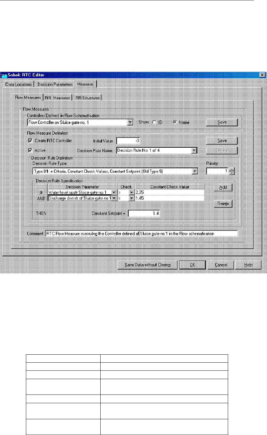
DRAFT
Graphical User Interface
computation. Hence, to make things transparent, it is advised to either delete such Flow
Measure or make it inactive. The same applies for Rainfall-Runoff RR measures.
River Flow controllers may be assigned to various different type of single and compound
River structures. You should be aware that a RTC Flow Measure associated to a River
Flow controller might affect the operation of more that one structure. The same applies
for controllers assigned to 2D Breaking – Dams in the Overland Flow module.
Figure 5.295: Definition of RTC Flow Measures
RTC Flow measures can overrule all six different type of Flow Controllers. The output (or set-
point) of a RTC Flow Measure depends on the type of overruled Flow Controller (see Table
below).
Table 5.9: Output (or set-point) of RTC Flow Measure as function of overruled Controller
type
Flow Controller Type Output of RTC Flow Measure
Time controller set point for controlled structure parameter
Relative-time controller set point for controlled structure parameter
Relative-from-value
(time) controller
set point for controlled structure parameter
Hydraulic controller set point for controlled structure parameter
Interval controller set point for controlled water level or dis-
charge
PID controller set point for controlled water level or dis-
charge
Deltares 441 of 900
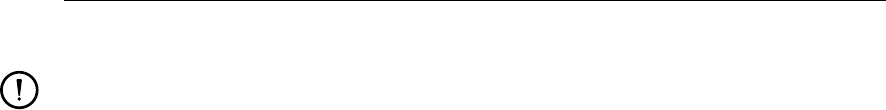
DRAFT
SOBEK, User Manual
Remark:
If the RTC Flow Measure is defined active, it means:
for a Time controller, a Relative-time controller, a Relative-from-value (time) con-
troller, and a hydraulic controller, that the associated Flow controller is not active
anymore, and
for a Interval controller and a PID controller, that only the set point (steer value) is
provided by RTC, but that the controlling mechanisms of these controllers as such
are still active.
For each Flow Measure, the user has to define its initial/default value. This initial/default
value will be provided as setpoint in case:
1 an initial setpoint is not available for whatsoever reason;
2 in case the defined RTC decision rules do not result in the determination of a set-
point. A Flow Measure may be composed of several so-called “Decision rules”.
For each Decision rule, you have to define its priority and its decision rule type. For decision
rules comprising of criteria (see Decision rules in RTC – General):
The evaluation of a decision rule can either be “true” or “false”. In case the evaluation
of more than one decision rule is “true”, the set-point for the RTC Flow Measure will be
equal to the set-point of the decision rule having the highest priority (e.g. lowest integer
number).
In case the evaluation of more than 1 (one) decision rule having the highest defined priority
are “true”, the set-point for the RTC Flow Measure will be equal to the set-point of the
decision rule that is the closest to end of the drop-down list.
In case not one of the defined “Decision rules is “True”, than the set-point of the Flow
Measure will be equal to the set-point determined in the previous RTC time-step.
Eight different type of decision rules are available for RTC Flow Measures:
Type A: Setpoint f(t)from user-defined Interpolation Table (Internal Type 2)The user has
to select a previously defined decision parameter and a so-called Interpolation Table, with
in the first column a value for the selected decision parameter and in the second col-
umn the corresponding set point. During the computation on basis of the actual decision
parameter value, the set point value for the next computation RTC point-in-time will be
determined from the Interpolation Table.
Type B1: n criteria, Constant Check Values, Constant Setpoint (Internal Type 5)The user
can define a number of criteria, that check if previously defined decision parameters are
“<”, “=” or “>” than an user-defined constant check-value. The evaluation of the decision
rule is only “true” in case all defined criteria are “true”, else the evaluation of the decision
rule is “false”. In case the evaluation of the decision rule is “true”, the setpoint will become
equal to the user-defined constant set point. In case the evaluation of the decision rule is
“false”, the set point will be equal to the set-point determined in the previous RTC time-
step.
Type B2: n criteria, Constant Check Values, Set point f(t) (Internal Type 6)Same as Type
B1, with the exception that if all defined criteria are “true”, the setpoint will be equal to the
actual (time) value of a user-defined decision parameter.
Type B3: n criteria, Check Values f(t), Constant Set point (Internal Type 7) Same at Type
B1, with the exception that for check-values previously defined decision parameters can
be applied, meaning that these check-values are a function of the actual computational
time.
Type B4: n criteria, Check Values f(t), Set point f(t) (Internal Type 8)Same at Type B3, with
442 of 900 Deltares

DRAFT
Graphical User Interface
the exception that if all defined criteria are “true”, the setpoint will be equal to the actual
(time) value of a user-defined decision parameter.
Type B5: Unconditional Setpoint f(t) (Internal Type 10)Set points will be the values of the
specified decision parameter.
Type C1: Set point from Matlab simulation (Internal Type 9)The value for the set point will
be retrieved from a Matlab computation. The user has to define a Matlab ID, which will be
linked to ID of the selected Controller in the Flow schematisation. In addition the user has
to define a “Default value”. The RTC set point will be taken equal to this “Default value”
in case during a computation no set-point is provided by Matlab (i.e. SOBEKC_<Matlab
ID>= 0) For further information on the use of Matlab, reference is made to the topics:
RTC Wind/Rain/Matlab/Reservoir Control options in Settings, RTC-Matlab communication
– General, Flow structure parameters in RTC and Matlab and Example of a Matlab m-file.
Type C2: Set point from external TCN measure (Internal Type 12)The value for the set
point will be retrieved from a TCN (TeleControlNet) computation. The user has to define
an ID, which will be linked to ID of the selected Controller in the Flow schematisation.
In addition the user has to define a “Default value”. The RTC set point will be taken
equal to this “Default value” in case during a computation no set-point is provided by
TCN. For further information on the use of TCN, reference is made to the topics: RTC
Wind/Rain/Matlab/Reservoir Control options in Settings (see section 5.12.24).
It is to be mentioned that from the v2.10 SOBEK version onwards, the old decision rule Types
1, 3 and 4 are not anymore available, since they are special cases of respectively Type B1
to B4. When opening a model created in a previous SOBEK version (i.e. <v2.10), the old
decision rule Types 1, 3 and 4 will be automatically be updated to the new B1, B2, B3 and B4
ones. The same applies for the old decision rule Types 2, 5, 6, 7 and 8.
5.12.11 Flow structure parameters in RTC and Matlab
The type of data series, available at (Flow) Structures on the 1D Flow Data Tab and 2D Flow
Data Tab under Data locations in RTC, depend on the type of structure. These data series
can be transferred by RTC to Matlab. In the Table below an overview is given of available
data per structure type, including its Matlab string (see also RTC Matlab Communication –
General, Example of a MATLAB m-file).
Table 5.10: Data per structure type for RTC Matlab communication
Structure type Available Parameters String in Matlab m-file
“Flow - External
Weir”
1. Crest level
2. Structure flow area
3. Discharge structure
4. Structure velocity
5. Water level Up
6. Water level Down
7. Head
8. Pressure difference
1. SOBEKCL_<SOBEK structure ID>=X
2. SOBEKFA_<SOBEK structure ID>=X
3. SOBEKQS_<SOBEK structure ID>=X
4. SOBEKVS_<SOBEK structure ID>=X
5. SOBEKHU_<SOBEK structure ID>=X
6. SOBEKHD_<SOBEK structure ID>=X
7. SOBEKDH_<SOBEK structure ID>=X
8. SOBEKPD_<SOBEK structure ID>=X
Deltares 443 of 900

DRAFT
SOBEK, User Manual
Table 5.10: Data per structure type for RTC Matlab communication
Structure type Available Parameters String in Matlab m-file
“Flow - External
Orifice”
1. Opening height
2. Structure flow area
3. Discharge structure
4. Structure velocity
5. Water level Up
6. Water level Down
7. Head
8. Pressure difference
1. SOBEKGO_<SOBEK structure ID>=X
2. SOBEKFA_<SOBEK structure ID>=X
3. SOBEKQS_<SOBEK structure ID>=X
4. SOBEKVS_<SOBEK structure ID>=X
5. SOBEKHU_<SOBEK structure ID>=X
6. SOBEKHD_<SOBEK structure ID>=X
7. SOBEKDH_<SOBEK structure ID>=X
8. SOBEKPD_<SOBEK structure ID>=X
“Flow - External
Culvert”
1. Gate lower edge level
2. Structure flow area
3. Discharge structure
4. Structure velocity
5. Water level Up
6. Water level Down
7. Head
1. SOBEKGL_<SOBEK structure ID>=X
2. SOBEKFA_<SOBEK structure ID>=X
3. SOBEKQS_<SOBEK structure ID>=X
4. SOBEKVS_<SOBEK structure ID>=X
5. SOBEKHU_<SOBEK structure ID>=X
6. SOBEKHD_<SOBEK structure ID>=X
7. SOBEKDH_<SOBEK structure ID>=X
“Flow - External
Pump station”
1. Pump capacity
2. Pump structure
3. Water level Up
4. Water level Down
5. Head
1. SOBEKPC_<SOBEK structure ID>=X
2. SOBEKQS_<SOBEK structure ID>=X
3. SOBEKHU_<SOBEK structure ID>=X
4. SOBEKHD_<SOBEK structure ID>=X
5. SOBEKDH_<SOBEK structure ID>=X
“Flow - Internal
Weir”
see External Weir see External Weir
“Flow - Internal
Orifice”
see External Orifice see External Orifice
“Flow - Internal
Culvert”
see External Culvert see External Culvert
“Flow - Internal
Pump station”
see External Pump sta-
tion
see External Pump station
“Flow - Weir” see External Weir see External Weir
“Flow - Orifice” see External Orifice see External Orifice
“Flow - Culvert” see External Culvert see External Culvert
“Flow - Pump
station”
see External Pump sta-
tion
see External Pump station
“Flow - Universal
weir”
1. Discharge structure
2. Water level Up
3. Water level Down
4. Head
1. SOBEKQS_<SOBEK structure ID>=X
2. SOBEKHU_<SOBEK structure ID>=X
3. SOBEKHD_<SOBEK structure ID>=X
4. SOBEKDH_<SOBEK structure ID>=X
444 of 900 Deltares

DRAFT
Graphical User Interface
Table 5.10: Data per structure type for RTC Matlab communication
Structure type Available Parameters String in Matlab m-file
“Flow - Bridge” 1. Discharge structure
2. Water level Up
3. Water level Down
4. Head
1. SOBEKQS_<SOBEK structure ID>=X
2. SOBEKHU_<SOBEK structure ID>=X
3. SOBEKHD_<SOBEK structure ID>=X
4. SOBEKDH_<SOBEK structure ID>=X
“Flow - River
weir”
1. Crest level
2. Crest width
3. Structure flow area
4. Discharge structure
5. Structure velocity
6. Water level Up
7. Water level Down
8. Head
9. Pressure difference
1. SOBEKCL_<SOBEK structure ID>=X
2. SOBEKCW_<SOBEK structure ID>=X
3. SOBEKFA_<SOBEK structure ID>=X
4. SOBEKQS_<SOBEK structure ID>=X
5. SOBEKVS_<SOBEK structure ID>=X
6. SOBEKHU_<SOBEK structure ID>=X
7. SOBEKHD_<SOBEK structure ID>=X
8. SOBEKDH_<SOBEK structure ID>=X
9. SOBEKPD_<SOBEK structure ID>=X
“Flow - Advanced
weir”
1. Crest level
2. Discharge structure
3. Water level Up
4. Water level Down
5. Head
6. Pressure difference
1. SOBEKCL_<SOBEK structure ID>=X
2. SOBEKQS_<SOBEK structure ID>=X
3. SOBEKHU_<SOBEK structure ID>=X
4. SOBEKHD_<SOBEK structure ID>=X
5. SOBEKDH_<SOBEK structure ID>=X
6. SOBEKPD_<SOBEK structure ID>=X
“Flow - General
structure”
1. Crest level
2. Crest width
3. Gate lower edge level
4. Structure flow area
5. Discharge structure
6. Structure velocity
7. Water level Up
8. Water level Down
9. Head
10. Pressure difference
1. SOBEKCL_<SOBEK structure ID>=X
2. SOBEKCW_<SOBEK structure ID>=X
3. SOBEKGL_<SOBEK structure ID>=X
4. SOBEKFA_<SOBEK structure ID>=X
5. SOBEKQS_<SOBEK structure ID>=X
6. SOBEKVS_<SOBEK structure ID>=X
7. SOBEKHU_<SOBEK structure ID>=X
8. SOBEKHD_<SOBEK structure ID>=X
9. SOBEKDH_<SOBEK structure ID>=X
10. SOBEKPD_<SOBEK structure
ID>=X
“Flow - Database
structure”
1. Crest level
2. Discharge structure
3. Water level Up
4. Water level Down
5. Head
6. Pressure difference
1. SOBEKCL_<SOBEK structure ID>=X
2. SOBEKQS_<SOBEK structure ID>=X
3. SOBEKHU_<SOBEK structure ID>=X
4. SOBEKHD_<SOBEK structure ID>=X
5. SOBEKDH_<SOBEK structure ID>=X
6. SOBEKPD_<SOBEK structure ID>=X
“Flow - River
pump”
1. Pump capacity
2. Pump structure
3. Water level Up
4. Water level Down
5. Head
1. SOBEKPC_<SOBEK structure ID>=X
2. SOBEKQS_<SOBEK structure ID>=X
3. SOBEKHU_<SOBEK structure ID>=X
4. SOBEKHD_<SOBEK structure ID>=X
5. SOBEKDH_<SOBEK structure ID>=X
Deltares 445 of 900

DRAFT
SOBEK, User Manual
Table 5.10: Data per structure type for RTC Matlab communication
Structure type Available Parameters String in Matlab m-file
Compound “Flow
- River weir”
member
see River weir see River weir
Compound “Flow
- Advanced weir”
member
see Advanced weir see Advanced weir
Compound “Flow
- General struc-
ture” member
see General structure see General structure
Compound “Flow
- Database struc-
ture” member
see Database structure see Database structure
Compound “Flow
- River pump”
member
see River pump see River pump
2D Breaking -
Dam
Water level
Water depth
Bottom(bed) level
U-velocity
V-velocity
Abs. velocity
[=sqrt(U2+V2)]
1. SOBEK1D2DH_<SOBEK ID>=X
2. SOBEK1D2DWD_<SOBEK ID>=X
3. SOBEK1D2DBL_<SOBEK ID>=X
4. SOBEK1D2DU_<SOBEK ID>=X
5. SOBEK1D2DV_<SOBEK ID>=X
6. SOBEK1D2DC_<SOBEK ID>=X
5.12.12 Measures – general
Real-time Control allows to define measures for Water Flow and for the Rainfall-Runoff. A
measure is a decision rule using one or more decision parameters. A measure can be active
or inactive, based on the evaluation of a logical condition. When a measure is active, it can
change the set point of a structure in Water Flow or change the availability of pumps in Rainfall-
Runoff. Several measures can apply to one object (e.g. a structure in the hydrodynamic
module Water Flow).
Measures can be complementary in the sense that one measure defines the set point of
the structure for low flow conditions, one for medium flow conditions, and one for high flow
conditions (in which the conditions are mutually exclusive, and cover all possible situations).
In this case there is always only one active measure.
But also it is possible that several measures are active at the same time. In this case the
measure with the highest priority determines the set point. In case of equal priorities, the
first/last active measure determines the set point.
The Real-Time Control module in fact adjusts the settings of a Flow controller. RTC control
can therefore only be applied on Flow-structures which are using a controller (a time controller,
hydraulic controller, interval controller or PID controller). The interpretation of the RTC results
in the Flow module is depending on the type of controller defined:
446 of 900 Deltares

DRAFT
Graphical User Interface
Type of local controller in Flow module Interpretation of RTC result
Time controller setting of control parameter
Hydraulic controller setting of control parameter
Interval controller set point
PID controller set point
So for a time controller or hydraulic controller you can directly set the weir crest level, gate
opening height or pump capacity using RTC.
For an interval controller or PID controller, you adjust the set point of the controller, i.e. the
the desired water level or discharge at the specified measurement location of the local Flow
controller. The Flow controller will than adjust the control parameter (weir crest level, gate
opening height or pump capacity) according to the local controller rules.
Real-time Control measures for Rainfall-Runoff can only be defined for all structures in Rainfall-
Runoff, but they are typically applied for RR-pump stations. With RTC, you can temporarily
switch off the structure (i.e. set the flow to zero) in Rainfall-Runoff based on conditions out-
side Rainfall-Runoff. Using Matlab, for RR-pumps also the switch-on and -off levels can be
adjusted.
5.12.13 Precipitation Data in RTC
On the Precipitation Data Tab available under the Data locations Tab in Real-time Control
(RTC), you can select the precipitations stations available for use in RTC. It is possible to
select Precipitation data on basis of rainfall data defined for individual rainfall stations.
5.12.14 Rainfall-Runoff measure
Real-time Control measures for Rainfall-Runoff can be defined for all structures in Rainfall-
Runoff. They are typically applied for RR-pump stations. This can be either an inlet or an
outlet pump. With RTC, you can temporarily switch off the structure (i.e. set the flow to zero)
in Rainfall-Runoff based on conditions outside Rainfall-Runoff. Using Matlab, for RR-pumps
also the switch-on and -off levels can be adjusted.
A typical application for a combined Water Flow and Rainfall-Runoff network in wet situations
is the following: in order to prevent too high water levels at the Water Flow network, out-
let pumps in the Rainfall-Runoff schematisation are switched off if the water level at certain
locations in the Water Flow network is exceeding a critical maximum level.
A similar type of rule can be applied for dry situations: in that case the Rainfall-Runoff inlet
pumps are switched off if the water level in the Channel Flow network is below a critical
minimum level.
The measures for RR can be defined in the user-interface using screens like shown below.
Deltares 447 of 900
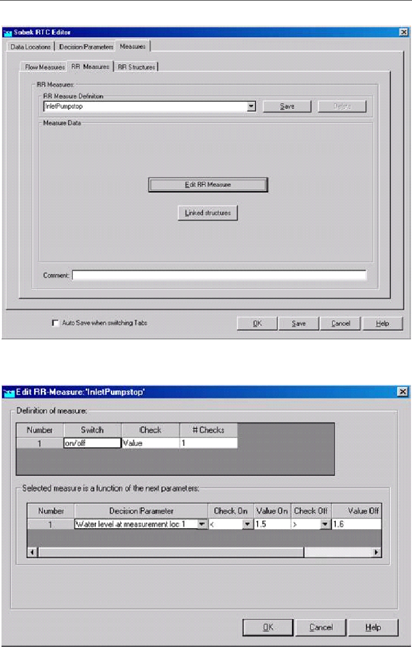
DRAFT
SOBEK, User Manual
Figure 5.296: SOBEK RTC Editor window, the tab Measure →RR Measure
Figure 5.297: Definition of RR measure
448 of 900 Deltares

DRAFT
Graphical User Interface
5.12.15 Real-time Control concepts or elements
There are three important concepts (or elements) in Real-time Control. They are:
Data locations;
Decision parameters; and
Measures;
5.12.16 RR Data in RTC
On the RR Data Tab, available under the Data locations Tab, you can define the Rainfall-
Runoff (RR) locations for which RTC will receive data, computed by the Rainfall-Runoff mod-
ule.
The following type of RR Data are available:
open water level at RR Open water nodes [m AD];
groundwater level at RR unpaved nodes [m AD];
5.12.17 RTC Communication-General
At present the Real-time Control (RTC) module can be used in combination with following
SOBEK modules:
The SOBEK-Urban 1DFLOW module,
The SOBEK-Rural 1DFLOW module,
The SOBEK-River 1DFLOW module,
The SOBEK-Rural RR module, and
The SOBEK-Rural 1DWAQ module (Note: 1DWAQ data can not yet be defined in the RTC
Editor)
In the RTC module use can be made of the user-defined Meteo (rainfall & wind) data as well
as user-defined external data.
Further on the RTC module can be linked to online Matlab computations, allowing for any kind
of control mechanism to be incorporated into SOBEK.
In the above mentioned options (i.e. linkage with other SOBEK modules, the use of other data
sources, and the use of Matlab, the RTC module take cares of the following data exchange:
RTC – SOBEK-Urban 1DFLOW, SOBEK-Rural 1DFLOW and SOBEK-River 1DFLOW mod-
ules:
Exchange of Flow (computational) data towards RTC,
Exchange of computed setpoints from RTC towards Flow controllers
RTC – SOBEK-Rural RR module:
Exchange of Rainfall Runofff (computational) data towards RTC,
Exchange of computed setpoints from RTC towards RR controllers
RTC – other data sources:
Transfer of other (rain, wind, external) Data towards RTC
Deltares 449 of 900
DRAFT
SOBEK, User Manual
RTC – Matlab computation:
Exchange of Flow (computational) data from RTC towards Matlab
Exchange of Rainfall Runofff (computational) data from RTC towards Matlab,
Exchange of other (rain, wind, external) data from RTC towards Matlab
Exchange of by Matlab computed setpoints for RR controllers towards RTC
Exchange of by Matlab computed setpoints for Flow controllers towards RTC
5.12.18 RTC definitions and options in Settings
The SOBEK Real-Time Control (RTC) module can be activated by checking the “Realtime
control” check-box in Settings (see Figure below). The RTC module runs simultaneously
with other SOBEK modules, since RTC may overrule controllers defined in other SOBEK
modules. In addition you might like to use data, computed by other SOBEK modules for
defining decision rules. These decision rules determine the setpoints for the controllers. At
present SOBEK modules that can run simultaneously with the RTC module are:
SOBEK-Rural RR module
SOBEK-Rural 1DFLOW module
SOBEK-Urban 1DFLOW module
SOBEK-River 1DFLOW module
SOBEK Overland Flow module
1DWAQ module (Note: 1DWAQ data can not yet be defined in the RTC Editor)
By pressing the Edit button behind the Realtime control module (see Figure 5.298), following
RTC options can be specified:
RTC Time settings
RTC Wind/Rain/Matlab/Reservoir Control options
RTC Output options
Figure 5.298: Settings input screen for SOBEK-Rural 1DFLOW-RTC run
450 of 900 Deltares

DRAFT
Graphical User Interface
5.12.19 RTC does not overrule Flow Triggers
In Real-time Control (RTC), RTC Measures (or RTC Flow controllers) can be defined. In
case a RTC Measure is defined active, this Measure will provide a setpoint for its associated
controller in either a Flow or Rainfall-Runoff schematisation. In case the associated controller
is active, the setpoint provided by the RTC Measure will be used in either the Flow or Rainfall-
Runoff computation. Hence in such situation the RTC Measure overrules the controller.
RTC does, however, not overrule Triggers defined for River Flow controllers. The evaluation of
these triggers determine whether the controller is active or not active during the computation.
In case the controller is in-active, a setpoint provided by a RTC Measure will be neglected
and the setpoint of the in-active controller will be kept equal to the previously applied setpoint
value.
Note: that in case no triggers are defined for controllers in a model schematisation, this
means that these controllers are always active during a computation.
5.12.20 RTC - Matlab Coupling
You can use RTC together with Matlab for overruling a particular controller defined in your
Flow or Rainfall-Runoff (RR) schematisation (see also: Example of a MATLAB m-file). More
precisely this means that the setpoints of this controller are determined in a Matlab computa-
tion, and that these Matlab setpoints are transferred from Matlab to this Flow or RR controller
by RTC. For determining the setpoints in Matlab, you can make use of the data series avail-
able at the data locations that you defined in the RTC module. Hence the coupling between
RTC and Matlab consists of:
Transfer of data series by RTC to Matlab,
Transfer of computed setpoints by Matlab to RTC
Note:
1Flow controllers that are not actived by their associated triggers, will not be overruled
by an active RTC-Matlab Measure (see section 5.12.19);
Flow controllers having no associated triggers will always be active and hence will
always be overruled by RTC-Matlab.
2 In order to facilitate the coupling between Matlab and RTC, installing Matlab and SOBEK
might not be enough. If RTC informs you that Matlab cannot be found, Matlab will need
to manually registered for coupling through com files. This can be done by typing this
command in your Matlab installation directory:
matlab.exe /regserver
Please use the Windows option ’Run as Administrator’ to run this command.
Ad 1) Transfer of data series by RTC to Matlab:
All data series available at the data locations (see section 5.12.3) that you defined in the RTC
module, can be used in a Matlab computation. Furthermore the RTC computational point-
in-time and the RTC computational time-step can be passed to Matlab. The corresponding
“strings” to be used in a Matlab m-file are given in the Table below. An overview of the type of
data series that are available for each Flow structure is given in section 5.12.11.
Deltares 451 of 900

DRAFT
SOBEK, User Manual
Table 5.11: Table: Strings in a Matlab m-file for obtaining values of data series that are
available at data locations defined in the RTC module
String in Matlab m-file Explanation
SOBEKFirst=X Indication whether this is the first simulation
timestep (X=1) or not (X=0)
SOBEKDate=X Date of simulation step. The date is given as
a string of the form yyyymmdd (e.g. 20041231
is December 31st, 2004)
SOBEKTime=X Time of simulation step. The time is given as
a string of the form HHmmsshh, where HH
are “hours” and hh are “seconds/100”. So
22150000 is a quarter past ten in the evening.
SOBEKCompTimestepSize=X RTC computational time-step (as defined in
Settings) in seconds
SOBEKH_<SOBEK node id>=X water level
SOBEKQ_<SOBEK branchsegment
id>=X
discharge
SOBEKSA_<SOBEK node id>=X surface area
SOBEKWD_<SOBEK node id>=X water depth
SOBEKCL_<SOBEK structure id>=X crest level of structure
SOBEKCW_<SOBEK structure id>=X crest width of structure
SOBEKGL_<SOBEK structure id>=X gate lower edge level (orifice)
SOBEKGO_<SOBEK structure id>=X opening height (orifice)
SOBEKFA_<SOBEK structure id>=X structure flow area
SOBEKQS_<SOBEK structure id>=X discharge structure
SOBEKVS_<SOBEK structure id>=X velocity at structure
SOBEKHU_<SOBEK structure id>=X water level up
SOBEKHD_<SOBEK structure id>=X water level down
SOBEKDH_<SOBEK structure id>=X head over structure
SOBEKPD_<SOBEK structure id>=X pressure difference over structure
SOBEKPC_<SOBEK structure id>=X pump capacity (pump)
SOBEK1D2DH_<location id>=X 2D water level
SOBEK1D2DWD_<location id>=X 2D water depth
SOBEK1D2DBL_<location id >=X 2D bed level
SOBEK1D2DU_<location id >=X 2D U-velocity
SOBEK1D2DV_<location id >=X 2D V-velocity
SOBEK1D2DC_<location id >=X 2D Abs velocity [=√U2+V2]
RRH_<RR id>=X RR water level or groundwater level
RainH_<rain_id>=X precipitation
Ad 2) Transfer of computed setpoints by Matlab to RTC
In a Matlab computation, the setpoints for a Flow or Rainfall-Runoff (RR) controller can be
determined. These Matlab setpoints are transferred by the RTC module to the corresponding
Flow or RR controller. The corresponding “strings” to be used in a Matlab m-file are given in
the Table below. For Flow controllers, the id in the Matlab string is the “Matlab id” defined on
the Flow Measures Tab in RTC (see decision rule Type C in Flow Measures in RTC). For RR
controllers, the id in the Matlab string is the id of the structure in the RR schematisation.
452 of 900 Deltares

DRAFT
Graphical User Interface
Table 5.12: Table: Strings in a Matlab m-file for transferring computed setpoints for a
particular Flow or RR controller towards the RTC module.
String in Matlab m-file Explanation
SOBEKC_<Matlab id>=X optional, controlled by RTC yes(=1)/no(=0)
SOBEKS_<Matlab id>=X setpoint of SOBEK-Flow controller
RRSLowon<RRStructure id>=X RR-pump switch on level, low capacity
RRSLowoff<RRStructure id>=X RR-pump switch off level, low capacity
RRSHighon<RRStructure id>=X RR-pump switch on level, high capacity
RRSHighoff<RRStructure id>=X RR-pump switch off level, high capacity
Note: ID’s in Matlab can only consist of letters, digits and underscores. Matlab ID’s can
not contain dots, plus signs, minus signs, equal or not-equal signs, etc., since these are
interpreted by Matlab. However, SOBEK can handle these signs in ID’s. Therefore, in sending
data to Matlab all these characters are changed into underscores. Hence unique ID’s in
SOBEK might not be unique ID’s in Matlab, in case SOBEK ID’s contain the above mentioned
characters that are interpreted by Matlab. Also Matlab will not accept these signs in the ID’s
for which data has to be sent to SOBEK.
Example: Suppose the water level at SOBEK node with id 0-64 is 0.55 m, and this node is
specified as a data location for RTC. SOBEK-RTC will then pass the following string to Matlab:
SOBEKH_0_64=0.55
Note that the -sign in the SOBEK-id is replaced by the _ sign in the string put to Matlab.
5.12.21 RTC - TCN (Telecontrolnet) coupling
In a SOBEK computation, the real time control (RTC) module can be coupled with the external
Telecontrolnet software, which is developed by InterAct (www.telecontrolnet.nl). This coupling
is, hereafter, shortly referred to as the RTC - TCN coupling.
Using the RTC - TCN coupling, any triggered (or active, see section 5.12.19) controller in a
1D Flow schematisation can be overruled by TCN. Overruling means that the setpoint for an
overruled controller is determined by TCN. Such setpoint is determined by TCN on basis of
values of state parameters (water levels, discharges etc.) in the Flow schematisation, that are
provided by the RTC module.
Note: Overruling does not affect the algorithm applied by a controller in a Flow schematisa-
tion. Say that a PID controller has to main water levels upstream of a weir by adjusting the
crest level of this weir. Overruling this PID controller means that TCN only provides the values
for the water levels to be maintained upstream of this weir. The controller using its PID algo-
rithm, still determines the weir crest levels required for maintaining these (by TCN provided)
water levels upstream of the weir.
Specifying a RTC -TCN coupling comprises of:
1 In the Settings task block, click on <Edit>button next to RTC and open the Contol options
tab (see Figure 5.299). On the Control options tab:
1.1 Check the check-box "Use TCN-Coupling"
1.2 In the box next to "TCN Run Command:", specify the path and name of the TCN run
command (i.e. a <name>.bat batch file, see example in Figure 5.306), which calls
Deltares 453 of 900
DRAFT
SOBEK, User Manual
TCN at the beginning of each RTC computational time step. In a TCN call two or
three command line arguments (%1 to %3) are included:
%1: The RTC event number. A Flow - RTC computation comprises of one
(1) event only with a duration, that follows from the begin-time and end-time of
the simulation as specified in settings. For a rainfall-runoff(RR) - Flow - RTC
computation the number of events is equal to the number of rainfall events (or
storms) defined in the Meteo task block (either in the <name>.bui file or in the
<name>.rks file). The duration of each event is equal to the duration of its
rainfall event.
%2: The RTC time step number within the event. This is an integer, varying from
1 up to the duration of the event divided by the RTC computational time step.
%3: Firstrun. This text string is only given for the first RTC time step within a
particular event.
1.3 In the box next to "SOBEK to TCN:", specify the path of the <name>.csv file in
which the RTC module writes the current values of all specified decision parameters
(for more information, see point 2 hereunder).
1.4 In the box next to "TCN to SOBEK:", specify the path of the <name>.csv file in
which TCN writes the setpoints for the by TCN overruled controllers (for more infor-
mation, see point 3 hereunder) and which setpoints are applied in the current RTC
computational time step.
Figure 5.299: Settings Task block, RTC settings for the RTC - TCN coupling
2 In the RTC editor (see section 5.12.5), define those decision parameters which values are
to be transferred towards TCN in a <name>.csv file (SOBEK to TCN, see Figure 5.299)
at the beginning of each RTC computational time step. Please note that the values of all
454 of 900 Deltares
DRAFT
Graphical User Interface
decision parameters are transferred to TCN.
As an illustration Figure 5.300 shows that decision parameter with id "//11/N1_mwfrtc" is
defined as the water level of the 1D water level point with id "10_292810". In Figure 5.301,
file <Peilen>.csv is shown in which at the beginning of a particular RTC computational
time step, the value of decision parameter with id "//11/N1_mwfrtc" is transferred towards
TCN. The first line in file <Peilen>.csv is a header ("id","description","value") line. Each
next line contains the information of a specific decision parameter. Please note that on
such line the id and the description are between double quotes, so better make sure that
the id and description (defined in the RTC editor) itself does not contain a double quote.
Figure 5.300: RTC editor in the Schematisation Task block. Definition of RTC decision
parameter with id "//11/N1_mwfrtc", which data is transferred towards TCN
in a <name>.csv file (SOBEK to TCN, see Figure 5.299) at the beginning
of each RTC computational time step (see Figure 5.301).
Figure 5.301: Example file <Peilen.csv>in which RTC at the beginning of each RTC
computational time step, transfers the value for decision parameter with id
"//11/N1_mwfrtc" towards TCN.
3 In the RTC editor, define a Flow Measure with decision rule type C2 (including its TCN ID)
for each controller in the 1D flow schematisation that is to be overruled by TCN (see sec-
tion 5.12.10). TCN will provide setpoints for these controllers in a <name>.csv file (TCN
to SOBEK, see Figure 5.299) which are applied by RTC in the current RTC computational
time step. How TCN determines these setpoints is beyond the scope of this manual.
As an illustration Figure 5.302 shows that 1D flow controller with id "1_751010-21_751010"
Deltares 455 of 900

DRAFT
SOBEK, User Manual
is overruled by the setpoint with TCN id "//26/X1_spstrrtc", that is provided by TCN. In Fig-
ure 5.303, file <Streefpeilen>.csv is shown in which TCN writes the setpoint with TCN
id "//26/X1_spstrrtc", that is used to overrule the 1D flow controller with id "1_751010-
21_751010". The first line in file <Streefpeilen>.csv is a header ("id","value") line. Each
next line contains the information of a specific TCN setpoint. Please note that on such line
the TCN id is between double quotes, so better make sure that the TCN id (defined in the
RTC editor) itself does not contain a double quote.
Figure 5.302: RTC editor in the Schematisation Task block. Defining that 1D flow con-
troller with id "1_751010-21_751010" is to be overruled by the TCN set-
point with TCN id "//26/X1_spstrrtc". TCN provides this setpoint in a
<name>.csv file (TCN to SOBEK, see Figure 5.299) at the end of each
RTC computational time step (see Figure 5.303).
Figure 5.303: Example file <Streefpeilen.csv>in which TCN at the end of each
RTC computational time step, transfers the setpoint with TCN id
"//26/X1_spstrrtc", which is used by RTC to overrule 1D flow controller with
id "1_751010-21_751010".
4 Specify the communication protocol between RTC and TCN by means of:
4.1 The <SOBEKTCN>.ini file:
Default the SOBEKTCN.ini file is located in the \SOBEK\Programs\RTC\TCN di-
rectory. The communication program SOBEKTCN.exe as well as the \Certifi sub-
directory are also located in this directory. Please note that if you have several
456 of 900 Deltares
DRAFT
Graphical User Interface
projects using a RTC - TCN coupling, it is advised to copy the SOBEKTCN.exe and
the SOBEKTCN.ini file into a sub-directory under the concerning project directory.
The SOBEKTCN.ini (see Figure 5.304) is to be edited manually:
4.1.1 The data behind keywords, which are left empty (being keywords: tcndo-
main, user, password, client_id and client_secret) are to be filled in with
the values supplied by Interact (company that developed the Telecontrolnet
software).
4.1.2 The file names behind keyword input_file (default: Peilen.csv) and keyword
output_file (default: Streefpeilen.csv) should respectively match with the file
names specified in the box behind "SOBEK to TCN" and the box "TCN to
SOBEK" in RTC settings (see Figure 5.299). Path names are to be omit-
ted. Please note that on the TCN website, file names are case sensitive,
while in SOBEK-RTC they are not case sensitive (since SOBEK runs under
Windows).
4.1.3 Value RTC_SYS for keyword location_code means that TCN knows that it
concerns a RTC - TCN coupling.
4.1.4 Please note that in case the duration of a TCN call lasts longer than the
number of seconds specified with keyword time_out_seconds, the current
RTC calculation is finalized using the setpoints that were provided by TCN
in the previous RTC calculation time step. In such case, following mes-
sage is given in the <RTC>.log file: value for parameter id not found in
ReadCsvFile and set to previous value, where id refers to the TCN ID of an
overruled controller.
4.1.5 An example of a sobektcn.log file or communication file of the RTC - TCN
coupling is given in Figure 5.305
Figure 5.304: Example of the SOBEKTCN.ini file, defining the communication protocol
between RTC and TCN in a RTC - TCN coupling.
Deltares 457 of 900
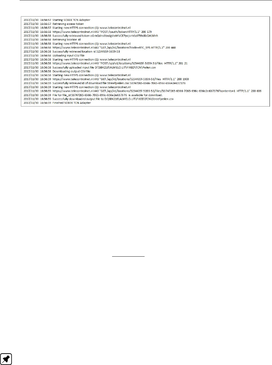
DRAFT
SOBEK, User Manual
Figure 5.305: Example of a sobektcn.log file or communication file of the RTC - TCN
coupling
4.2 The <name>.bat file
As mentioned in point 1.2 above, TCN is called at the beginning of each RTC com-
putational time step using a <name>.bat batch file. Such batch file not only calls
TCN by starting SOBEKTCN.exe, but may as well contain some commands, that
store the communication between SOBEK-RTC and TCN. In addition the batch file
starts SOBEKTCN.exe with the proper command line arguments (%1 to %3, see
point 1.2 above).
In Figure 5.299 TCN is called using batch file <TestTCN>.bat. This batch file is
depicted in Figure 5.306 and does following:
4.2.1 The first line changes the working directory from the CMTWORK directory
to the directory d:\SBK216\ALMELO.lit\FIXED\TCN
4.2.2 The second line start the SobekTCN.exe, which calls TCN (i.e. starts the
RTC - TCN coupling program). The command line argument %3 denotes if
it is the first TCN call within a particular event or not (i.e. textstring is either
"firstrun" or ""). Please note that the SOBEKTCN.exe should be located in
directory d:\SBK216\ALMELO.lit\FIXED\TCN.
4.2.3 Optional. The third line stores all <sobektcn>.log files (see Figure 5.305)
in directory d:\SBK216\ALMELO.lit\FIXED\TCN\test, including the RTC event
number (%1) and the RTC time step number within the event (%2).
4.2.4 Optional. The fourth line stores all <Peilen>.csv files (see Figure 5.301) in
directory d:\SBK216\ALMELO.lit\FIXED\TCN\test, including the RTC event
number (%1) and the RTC time step number within the event (%2).
4.2.5 Optional. The fifth line stores all <Streefpeilen>.csv files (see Figure 5.303)
in directory d:\SBK216\ALMELO.lit\FIXED\TCN\test, including the RTC event
number (%1) and the RTC time step number within the event (%2).
4.2.6 The last row changes the working directory from d:\SBK216\ALMELO.lit\
FIXED\TCN to d:\SBK216\ALMELO.lit\CMTWORK.
Note: The third line, fourth line and fifth line described above and shown in Fig-
ure 5.306) are optional (i.e. not essential) in defining a RTC - TCN coupling. These
optional lines are, however, handy to verify if a RTC - TCN coupling is working to
satisfaction.
458 of 900 Deltares
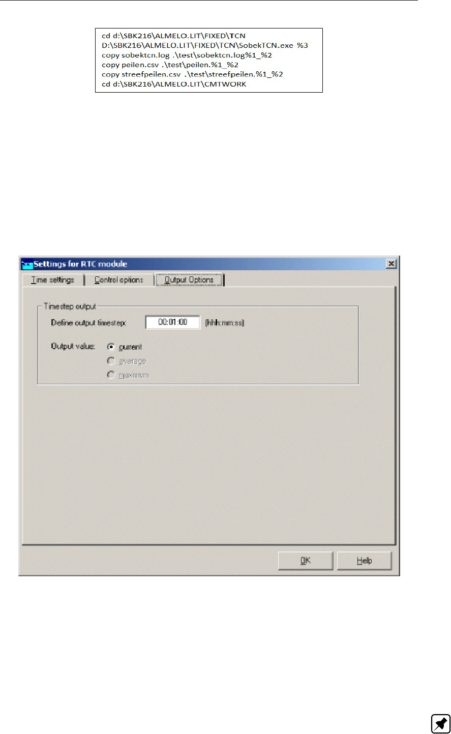
DRAFT
Graphical User Interface
Figure 5.306: Example <TestTCN>.bat, applied to call TCN and to store all communica-
tion files <Peilen>.csv (SOBEK to TCN) and <Streefpeilen>.csv (TCN to
SOBEK) produced in a RTC - TCN coupling.
5.12.22 RTC Output options in Settings
The RTC Output options Tab becomes available by clicking on the Edit button behind the RTC
module in Settings (see Figure 5.307). On this Tab, the user can define the time-step for the
RTC output data, available under the Result in Charts Task block and the Result in Maps
Task block. The RTC output time-step should be a multiple of the defined RTC computational
time-step.
Figure 5.307: RTC Output Options in Settings
5.12.23 RTC Time settings (Time-step) in Settings
The RTC Time settings Tab becomes available by clicking on the Edit button behind the RTC
module in Settings (see Figure below).
The time-step applied in Real-time Control (RTC) is defined in the Settings Task block (see
Figure below).
Note:
Deltares 459 of 900
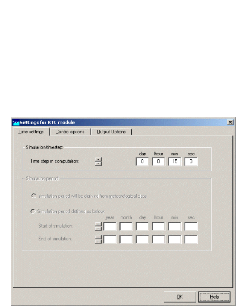
DRAFT
SOBEK, User Manual
The defined RTC time-step is applied for each and every RTC measure, that might be over-
ruling a controller defined in either the SOBEK-Urban 1DFLOW, SOBEK-Rural 1DFLOW,
SOBEK-River 1DFLOW, SOBEK Overland Flow or SOBEK-Rural RR schematisation.
This is also valid when the RTC setpoints are determined by a Matlab computation.
In a combined Flow-RTC computation, the RTC time-step may be larger than the Flow
time-step (i.e. time-step applied in the hydrodynamic computations), this means that the
setpoints of the Flow controllers, that are overruled by a RTC Flow measure (or RTC Flow
controller) are less frequently updated as the set points of Flow controllers that are not
overruled by RTC Flow measures
In a combined RR-RTC computation, the RTC time-step should be equal to the time-step
applied in the RR computation. The same yields for a combined Flow-RR-RTC computa-
tion.
Figure 5.308: Settings for RTC module, the Time Settings tab
5.12.24 RTC Wind/Rain/Matlab/Reservoir Control options in Settings
By clicking on the Edit button behind the RTC module in Settings, the RTC Control options
Tab becomes available (see Figure 5.309). By clicking on the corresponding check-box, the
following RTC options can be activated:
Use rain predictor (rain data to be defined in Meteo Task block),
Use wind predictor (rain data to be defined in Meteo Task block)
Use Matlab
Use reservoir control
460 of 900 Deltares
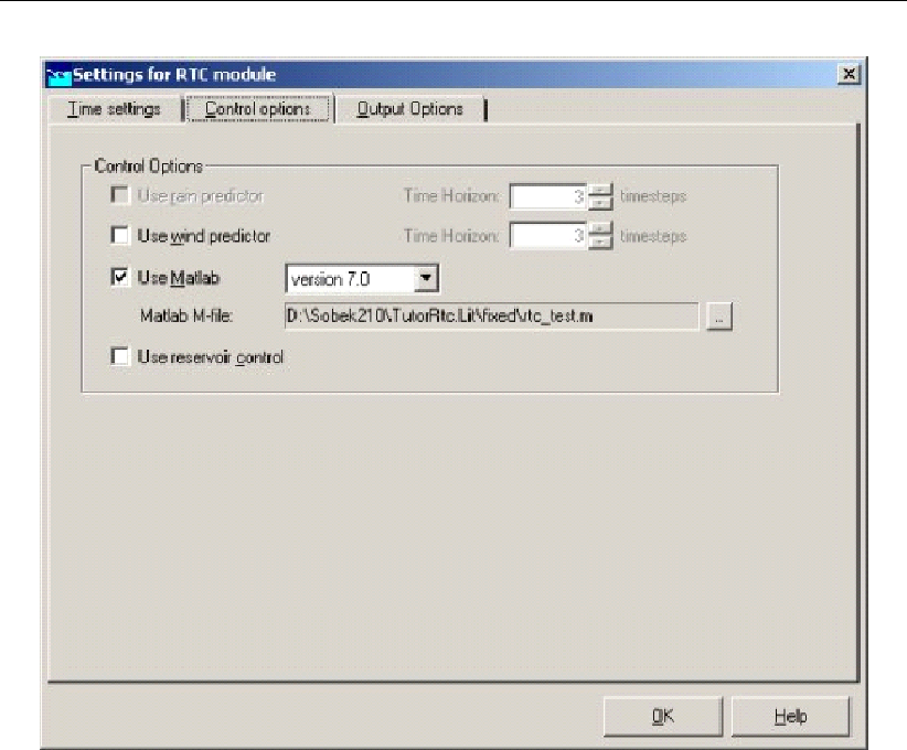
DRAFT
Graphical User Interface
Figure 5.309: RTC Control options
Matlab is a general purpose software package, which allows you to write your own programs
(so-called m-files) using e.g. ‘fuzzy logic’ or other control features which are available in Mat-
lab. SOBEK RTC can make use of your Matlab m-files.
In order to use Matlab, it is required to have an installation of Matlab on your own PC or an
accessible network drive. It is not necessary to specify to SOBEK where Matlab is located. If
Matlab has been properly installed and used on the PC before, SOBEK will be able to com-
municate with it. However, if you specify a version of Matlab which is different from the version
last used on your PC, the SOBEK RTC module will not be able to set up communication with
Matlab properly. In that case you will get a message after starting the first timestep of the
simulation, saying that there was an error starting Matlab.
To define the use of Matlab, go to the tab <Control Options>, switch on the use of Matlab,
and specify which version of Matlab you want to use. SOBEK supports communication with
Matlab versions 5.3, 6.0, 6.1, 6.5 and 7.0.
You also have to specify the location of your Matlab m-file.
Deltares 461 of 900

DRAFT
SOBEK, User Manual
5.12.25 Setpoints in RTC
If defined active a RTC Measure will overrule an active controller, that is defined in a Flow or
a Rainfall-Runoff schematisation. With overruling is meant that the RTC Measure determines
the setpoint for the controller (i.e. the gate-height, crest level, water level to be controlled etc.).
Note:
1 Flow controllers that are not actived by their associated triggers, will not be overruled by
an active RTC Measure;
2 Flow controllers having no associated triggers will always be active and hence will always
be overruled by RTC. For more information, see RTC does not overrule Flow Triggers.
For information on the type of set-points corresponding to each Flow controller, see Flow
Measures in RTC.
5.12.26 Type of Measures available in Real-time Control
In Real-time Control following Type of Measures are available:
Flow Measures,
RR Measures,
Flow Measures (or RTC Flow controllers), when defined active, will overrule their associated
active Flow controller in the SOBEK-Urban 1DFLOW, SOBEK-Rural 1DFLOW or SOBEK-
River 1DFLOW schematisation (see Flow Measures in RTC and RTC does not overrule Flow
Triggers).
RR Measures, when defined active, will overrule their associated controller in the Rainfall
Runoff schematisation. At present RR Measures are to defined on the RR Measure Tab and
the RR Structure Measure Tab.
5.12.27 Wind Data in RTC
On the Wind Data Tab available under the Data locations Tab in Real-time Control (RTC),
you can select wind data (velocity and direction) available for use in RTC. At present only the
complete set of wind data defined in the Meteo Task block can be selected at the Wind data
Tab. Under Decision Parameters in RTC, however, it is possible to make a selection on basis
of individual wind stations defined in the Meteo Task block.
5.12.28 1D Flow Data in RTC
On the 1D Flow Data Tab, available under the Data locations Tab, you can define the 1D Flow
locations for which RTC will receive data, computed by the SOBEK 1DFLOW modules.
462 of 900 Deltares
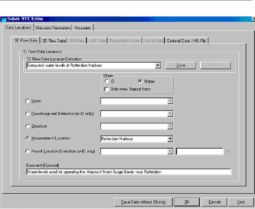
DRAFT
Graphical User Interface
Figure 5.310: RTC Flow Data input screen
For each 1D Flow Data location, the user can define its ID as well as an optional comment
string (see Figure above). Data locations can be selected on basis of their ID or user-defined
Name. Five different type of 1D Flow Data locations are discerned, viz:
Nodes:
Branch segments
Structures
Measurement locations (or stations)
Branch locations
Hint: If the “Show Name” option together with a checked “Only show Named Items” check-
box is used (see Figure above), than only those objects in the drop-down lists are shown for
which the user has defined a Name. In this way you can considerably reduce the length of the
drop-down list (and hence the time needed for finding your object).
The data availability depends on the selected 1D Flow Data type. For instance: at Nodes,
water levels and water depth are available; at Branch segment: velocities and discharges
are available. Below an overview of the available 1D Flow Data (i.e, computed hydrodynamic
parameters) is given
water level [m AD];
flow [m3/s];
surface area [m2];
water depth [m];
crest level [m];
crest width [m];
Deltares 463 of 900
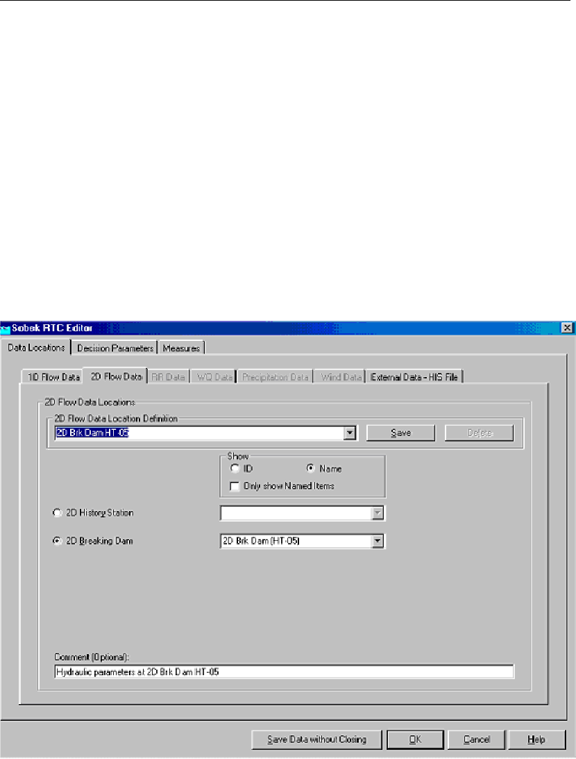
DRAFT
SOBEK, User Manual
gate lower edge [m];
gate opening height [m];
structure flow area [m2];
discharge at the structure [m3/s];
flow velocity at the structure [m/s];
water level up [m];
water level down [m];
head over structure [m];
pressure difference over structure;
pump capacity [m3/s];
5.12.29 2D Flow Data in RTC
On the 2D Flow Data Tab, available under the Data locations Tab, you can define the 2D Flow
locations for which RTC will receive data, computed by the SOBEK Overland Flow module.
Figure 5.311: RTC 2D Flow Data input screen
For each 2D Flow Data location, the user can define its ID as well as an optional comment
string (see Figure 5.311). Data locations can be selected on basis of their ID or user-defined
Name. Two different type of 2D Flow Data locations are discerned, viz:
2D History stations
2D Breaking – Dams
Hint: If the “Show Name” option together with a checked “Only show Named Items” check-
box is used (see Figure above), than only those objects in the drop-down lists are shown for
464 of 900 Deltares
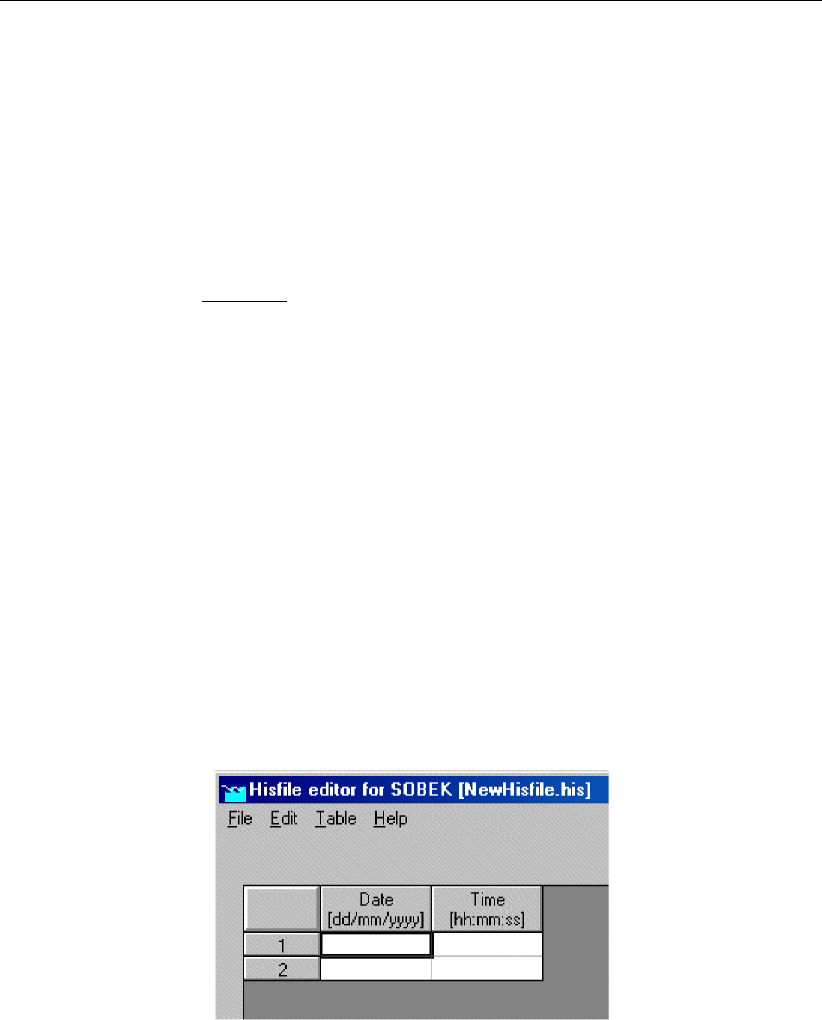
DRAFT
Graphical User Interface
which the user has defined a Name. In this way you can considerably reduce the length of the
drop-down list (and hence the time needed for finding your object).
Following data is available at 2D History stations and 2D Breaking – Dams:
water level [m AD];
water depth [m];
bottom(bed) level [m AD];
U-velocity in [m/s];
V-velocity in [m/s];
Abs. velocity [=√U2+V2] in [m/s].
5.13 SOBEK Tools
5.13.1 Calibration data editor
If you desire to compare measured data with computed data, you can create a "measured
data file" according to the SOBEK Output format (.his files). This file can then be imported
into the "Results in Tables" window or into the "Case Analysis Tool" for comparison with your
simulation results.
Creating a custom HIS file (SOBEK results file)
Go to the SOBEK Startup window
Choose "Utilities" - "Calibration data editor" from the menu. The "Edit History file" window
will appear.
Choose "File" - "new". A spreadsheet-like environment will appear:
Figure 5.312: Hisfile editor
Use the "Table" - "Add/Insert/Delete Row" options to customise the size of your table.
Add measurement locations by choosing "Table" - "Add Location" and entering the name
of the location.Note: you may decide to make this name equal to the ID of a node or
branch segment in your schematisation!
Enter the parameter name by choosing "Edit" - "Description". Choose for example the
parameter name "water levels measured"
You can copy and paste data from Excel into the fields. Important: the "date format"
and "time format" of your cells in Excel must be equal to the format as indicated in the
Hisfile editor: dd/mm/yyyy. You can change this format in Excel by selecting the cells,
right-clicking your mouse, and selecting "format cells".
When your file is ready, choose "File" - "Save as", and type a name for your HIS file.
Using your custom HIS file
Deltares 465 of 900
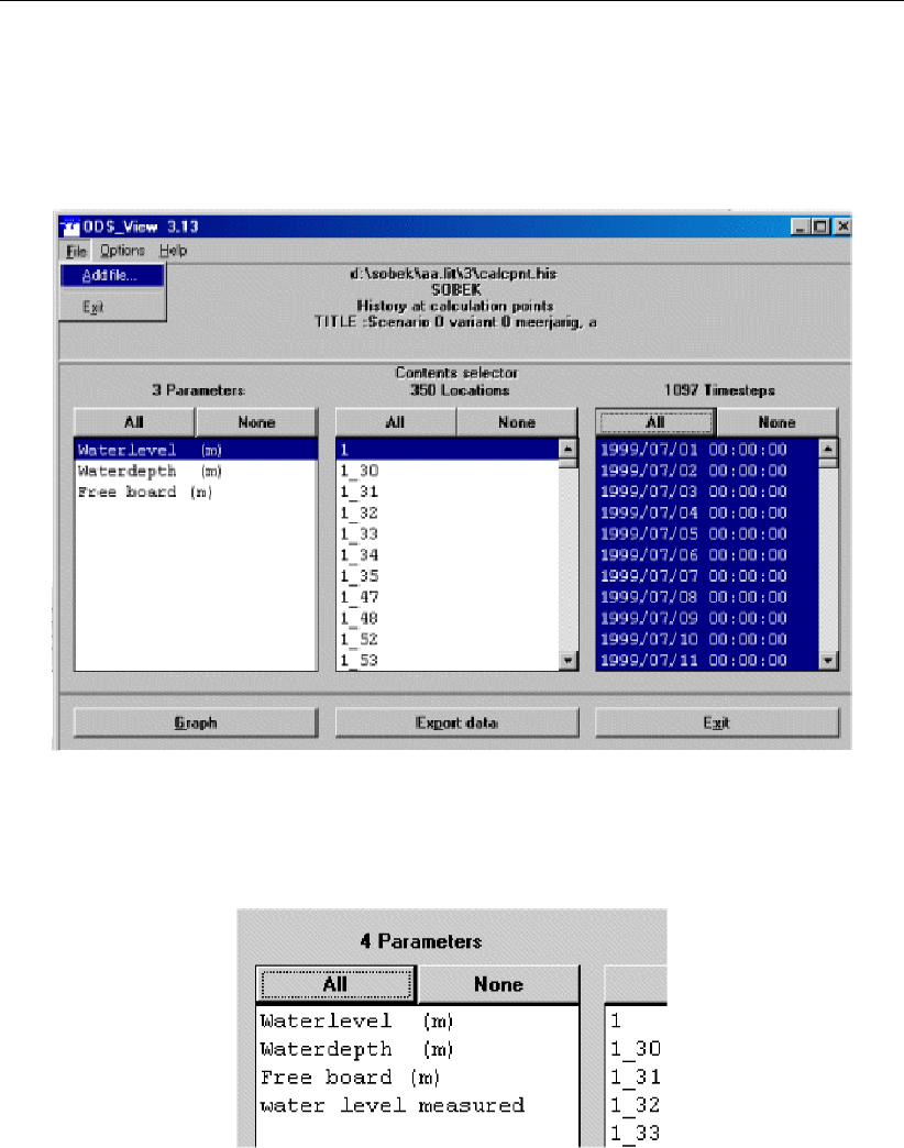
DRAFT
SOBEK, User Manual
You can open this file in the Case Analysis Tool to compare it with your simulation results.
You can also add this file to the "results in charts". In order to do so, open your simulation
results and choose "File" - "add file" from the "Ods_view" window:
Figure 5.313: ODS view
Your measurement results will then appear as an extra parameter, but with the same
location ID in the list of results:
Figure 5.314: ODS View, parameter list
5.13.2 Online Visualisation (SOBEK-1D2D)
Sometimes it may be useful to visualise simulation results during computation on a detailed
level. In Online Visualisation it is possible to click on waterlevel points (nodes) or on velocity
points (links) and show the printed values of selected parameters.
To use Online Visualisation
Online Visualisation is available in SOBEK version 2.12.002 and upwards.
After starting SOBEK, click on the menu item: "Options".
Select the option: "SOBEK Options".
Switch on the option"Online Visualisation" in the "Simulation" tab.
466 of 900 Deltares

DRAFT
Graphical User Interface
Figure 5.315: Examples of the Online Visualisation.
Deltares 467 of 900
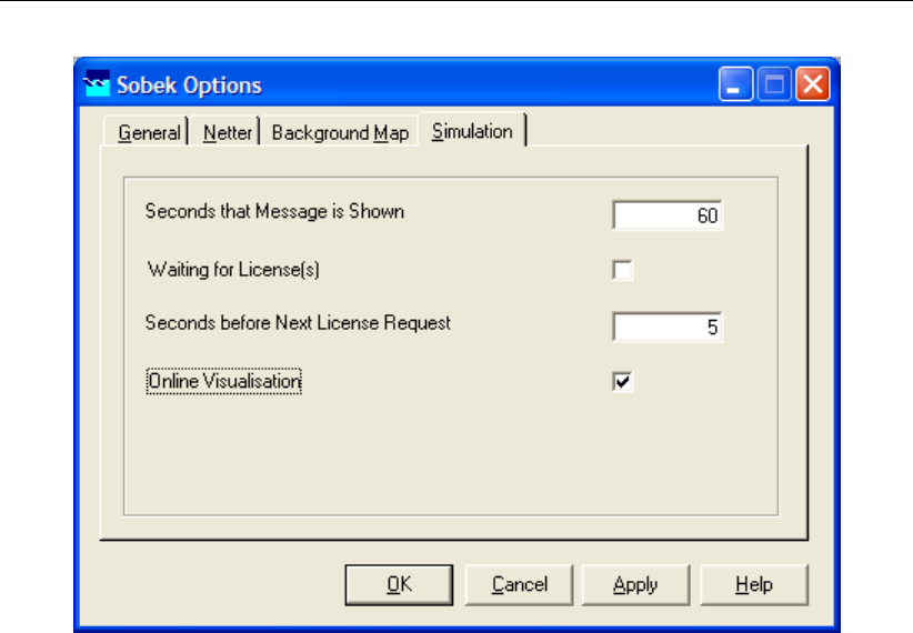
DRAFT
SOBEK, User Manual
Figure 5.316: Enabling the Online Visualisation in the SOBEK Options window.
Continue or interrupt computation
Double click the taskblock ’Simulation’ to start a simulation.
When the Online Visualisation Component appears, left mouse click on your screen.
Click <Tab>to start the simulation, left mouse click to pause the simulation.
Click spacebar if you want to proceed a single timestep.
Interrogate data on nodes and links
Left mouse click either on nodes (square boxes) to display nodes values, or on links, (dots
in 1D). Flow velocity, discharge, cross-sectional area etc will be shown.
When clicking on a link, the items on both connected nodes will also be refreshed.
In the top screen line, one can select a field parameter to be displayed: e.g.
‘Display’ →‘Node values’ →Waterlevel
When a node or link is clicked, this parameter is also printed as the last parameter in
the list, see ‘Userpar’
The left and right isoscales pertain to the requested node- and link-parameter fields.
468 of 900 Deltares
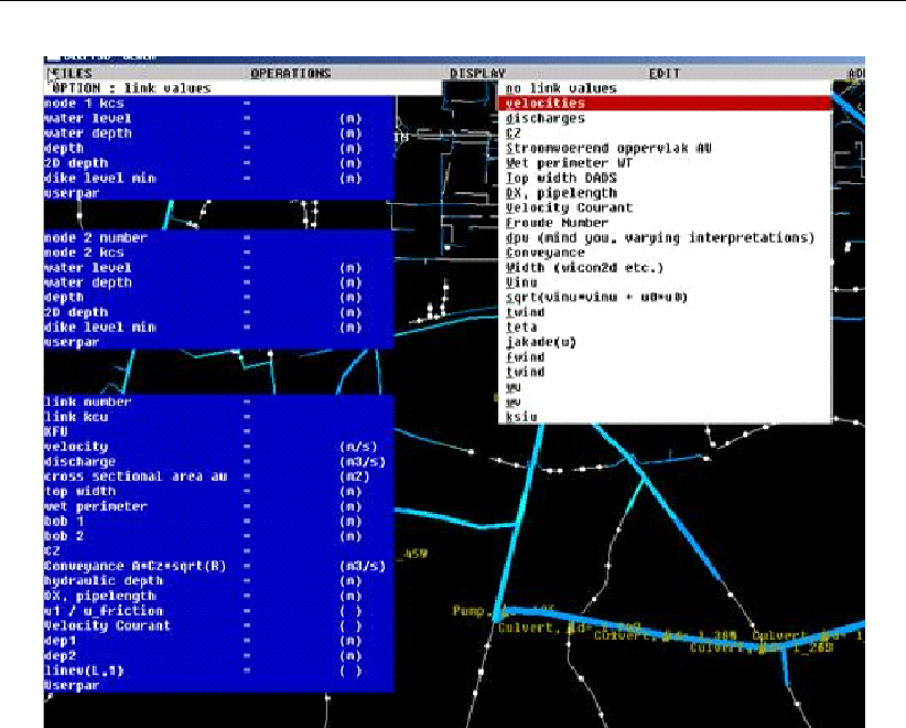
DRAFT
Graphical User Interface
Figure 5.317: The Online Visualisation.
On the left side, from top tot bottom, after clicking on a link, we get the first node, the second
node and the link in between. When more links exist on the same location, click more times.
For the first node:
Node id: Corresponding to Netter id
Node nr: Internal array nr
Kcs code: 1 for 1D point, 100 for 2D point, 101 for 1D2D point
Water level: Level in [m] upward [1]
Water depth: Difference between water level and bottom level [2]
Depth: Negative value of bottom level, depth increases downward [3]
2D depth: Negative value of 2D bottom level [4]
Dike level min: Lowest level for connecting 1D and 2D [5]
Userpar: The value for the parameter specified in ‘Display’ →‘Node values’
Deltares 469 of 900
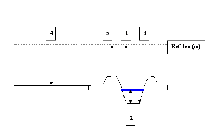
DRAFT
SOBEK, User Manual
Figure 5.318: Explanation of cross-section for Onlie Visualisation
For the second node: same as for left node
For the connecting link:
Link id: Corresponding to Netter id
Link nr.
Link kcu: 1=1D link, 100=2D link
Kfu: 1=wet, 0=dry
Velocity.
Discharge.
Cross sectional area: Flow carrying area
Top width.
Wet perimeter.
Bob 1: Depth (pos down) at left side of pipe or link
Bob 2: Depth (pos down) at right side of pipe or link
Cz: Chézy parameter, if applicable
Conveyance: given if applicable
Hydraulic depth
Dx, pipelength
U1/Ufriction: Velocity vs equilibrium friction velocity
Velocity Courant
Dep1: Depth of manhole or waterlevel point on left side of link
Dep2: Depth of manhole or waterlevel point on right side of link
Linev(L,1) : Internal nr
Userpar : The value for the parameter specified in ‘Display’ →‘Link values’
Display area control
Left mouse click on the schematisation, so that the crosshair cursor appears and the coordi-
nates of the cursor are displayed in the top right corner of the screen.
Click <z>.
470 of 900 Deltares
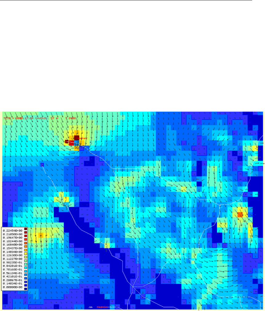
DRAFT
Graphical User Interface
A window will appear that can be moved around. Now you can:
Zoom in, with a left mouse click.
Zoom out, with another <z>.
Pan by moving the zoom window until it touches the screen border.
Restore default viewing area with a right mouse click.
Press <a>to drop an anchor, to show the distance between the cursor and the anchor
position in the upper right corner of the screen.
The size of 2D velocity vectors can be adjusted, Display, Display Parameters, Vectorsize.
Figure 5.319: Online Visualisation 2D velocity vectors.
5.13.3 ReaHis (Convert HIS files to ASCII)
The ReaHis command-line tool can be used to easily convert .HIS files to ASCII format. After
converting to ASCII, the output can be imported in other software packages or used in scripts.
The tool ReaHis.exe can be used after installing SOBEK. It is located in
.\SOBEK215\PROGRAMS\ReaHis\
Usage: ReaHis <InputHis.his> > <Output.txt>
For example: ReaHis flowhis.his >flowhis.txt
Deltares 471 of 900

DRAFT
SOBEK, User Manual
5.13.4 Time tables in SOBEK
Tables for parameters as a function of time
In many situations, one may encounter tables that have to be filled with time-dependent data.
For example lateral inflows at a Flow - Lateral Flow node, or water levels at a Flow - Boundary
node. In this chapter, the structure and the options of such tables is explained.
The general lay-out for the tables window looks like this:
Remark:
The numbers in the table below do not correspond with the graphs later on.
Figure 5.320: A generic table.
Left Column: date Here, the dates for which you want to change certain parameter
values should be entered. It is not necessary to type all values by hand: you can copy
them from a spreadsheet, such as Microsoft Excel. But note that the field format within the
spreadsheet should correspond to the format indicated by SOBEK: dd-mm-yyyy. In Excel,
the field format can be altered by right-clicking a field, choosing "format cell" - "number"
- "custom" - and type the appropriate format: dd-mm-yyyy (or dd-mm-jjjj in the Dutch
472 of 900 Deltares

DRAFT
Graphical User Interface
version)
Middle Column: time Here, the times on which you want to change certain parameter
values should be entered. It is not necessary to type all values by hand: you can copy
them from a spreadsheet, such as Microsoft Excel. But note that the field format within the
spreadsheet should correspond to the format indicated by SOBEK: hh:mm:ss. In Excel,
the field format can be altered by right-clicking a field, choosing "format cell" - "number" -
"custom" - and type the appropriate format: hh:mm:ss (or uu:mm:ss in the Dutch version)
Right Column: parameter value This column represents the parameter that needs to be
changed in time. For example: discharges, water levels, moist content, crest levels etc.
The buttons on the right side of the window <Add Row>adds one or more rows to the
downside of the table <Insert Row>adds a new row just above the one that’s currently
selected <Delete Row(s)>deletes the currently selected row
<Copy>copies the data of the currently selected cells to the clipboard. An alternative to
this button is to press Ctrl+ C.
<Paste>pastes data from the clipboard to the currently selected cells. An alternative to
this button is to press Ctrl + P. Important: make sure that the data that you want to
paste has the correct format (dd-mm-yyyy for date and hh:mm:ss for time)!
Graph plots a graph of the data in the table <Import Table>gives the option to import a
previously stored table <Export Table>gives the option to save the current table. This
table may then be used for other objects too.
Options
Block function: interprets the data from the table as a block function, thus the param-
eter value will be constant during the period between two data entries.
Linear function: for the calculation period between two data entries the values of both
surrounding entries will be linearly interpolated.
Periodicity: - Use periodicity: let the values in the table repeat themselves with a certain
interval (year, month, week, day, 12 hours, hour)
If the periodicity interval you chose is smaller than the time span of your table, SOBEK will
apply the periodicity procedure to the last section of the table that covers the periodicity
interval. The picture below shows how this situation is handled within SOBEK:
Figure 5.321: This picture shows which part of your table will be continuously repeated if
the periodicity timespan that you choose is shorter than the available data
in your table.
Note 2: If the periodicity interval you chose is larger than the time span of your table,
Deltares 473 of 900
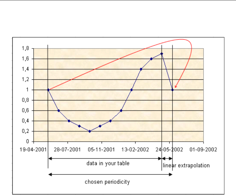
DRAFT
SOBEK, User Manual
SOBEK will linearly interpolate between the data in the last record of the table and the
value from the first record of the table. See the picture below for a better understanding:
Figure 5.322: In this graph you can see how SOBEK handles periodicities that exceed
the time span in your table.
The first value from the table is then assumed to occur at the end of the periodicity too, and
all values between the last value of the table and that value are then interpolated blockwise
or linearly, depending on the chosen interpolation option. The example assumes linear
interpolation has been specified.
5.14 1D Hydraulic friction concepts
The following hydraulic friction concepts can be discerned in 1D flow:
Global (or Model-wide) friction concept
Local (or Branch-wise) friction concept
Cross-section friction concept
Culvert friction concept
5.14.1 Global (or Model-wide) friction concept
Global friction refers to defining (formula & value) for Bed friction (and optional Groundlayer
friction):
Use of Global friction:
If Global friction definition is selected at cross-section X, this means that the Global friction
definition is applied for all cross-sections, that are located on the same branch as cross-
section X.
Restrictions for Global friction:
Not available at “Y-Z” and “Asymetrical Trapezium” cross-sections.
At “River profiles” only Global Bed friction can be defined.
474 of 900 Deltares

DRAFT
Graphical User Interface
Warning for Global friction:
Changing the Global friction at cross-section X, has consequences for all branches using
Global friction.
For “River profiles” two situations are to be discerned:
There are only River profiles in the model: Different global values for positive flow and
negative flow as well as friction formulations can be specified for Main section, Floodplain
1 and Floodplain 2.
There is also another type of cross-section: In case a global value and friction formulation
is defined at a non-River profile (i.e. another type of cross-section), all the information
regarding different global values and friction formulations for positive and negative flow at
Main section, Floodplain 1 and Floodplain 2 is overruled by the global value and friction
formulation defined at the non-River profile.
5.14.2 Local (or Branch-wise) friction concept
Local friction refers to defining (formula & value) for Bed friction (and optional Groundlayer
friction):
Use of Local Friction
If local friction definition is selected at cross-section X, this means that this specific Local
friction definition is applied for all cross-sections, located on the same branch as cross-
section X
Restrictions for Local friction:
Not available at “Y-Z” and “Asymetrical Trapezium” cross-sections.
At “River profiles” only Local Bed friction can be defined.
Exception for Local friction:
Only at River Profiles, Local Bed friction can be defined as function of the branch x_coordinate
(f(x),f(Q, x)and f(h, x))
Warning for Local friction:
Changing local friction at cross-section X, has consequence for all cross-sections, that are
located on the same branch as cross-section X.
5.14.3 Cross-section friction concept
Cross-section friction means that Bed friction (formula & value) can be defined per cross-
section:
Use of Cross-section friction
Only available for “Y-Z” and “Asymetrical Trapezium” cross-sections.
The cross-sectional area can be divided in (vertical) roughness sections for which a
different Bed friction (formulae & value) can be defined.
Restriction for Cross-section friction
Groundlayer friction cannot be defined
5.14.4 Culvert friction concept
Culvert friction means that Bed and optional Groundlayer friction (formula & value) can be
defined for the closed cross-section available at a Culvert:
Use of Culvert friction:
Only available for Culverts, Inverted Siphons and Siphons
Deltares 475 of 900

DRAFT
SOBEK, User Manual
476 of 900 Deltares

DRAFT
6 Conceptual description
6.1 Hydrodynamics D-Flow 1D
6.1.1 Model equations
The water flow is computed by solving the complete De Saint Venant (1871) equations for
unstaedy flow are based upon the the following series of assumptions (Cunge et al.,1980):
The flow is one-dimensional i.e. the velocity can be representated by a uniform flow over
the cross-section and the water level can be assumed to be horizontal across the section.
The streamline curvature is small and the vertical accelerations are negiglible, hence the
pressure is hydrostatic.
The effects of boundary friction and turbulence can be accounted for through resistance
laws analogous to those used for steady flow.
The average channel bed slope is small so that the cosine of the angle it makes with the
horizontal may be replace by unity.
For one dimensional flow (Channel Flow and Sewer Flow modules) the following equations
are solved
continuity equation 1D
momentum equation 1D
For two dimensional flow (Overland Flow module), three equations are solved:
continuity equation 2D
momentum equation 2D for the x-direction
momentum equation 2D for the y-direction
These equations are solved numerically using the Delft-scheme.
Note: on the 2D equations
As opposed to the shallow water equations, the described equations do not incorporate the
turbulent stress terms, accounting for the sub grid transfer of momentum in between grid
cells. These terms have been omitted because they are relatively unimportant for flood flow
computations, in order to save computational effort.
The wall friction terms have been introduced to account for the added resistance that is caused
by vertical obstacles, like houses or trees. The wall friction coefficient is based on the average
number and diameter of the obstacles per unit area and the average obstacle drag coefficient
(Cdcoefficient).
6.1.1.1 Continuity equation (1D)
The 1D continuity equation reads:
∂AT
∂t +∂Q
∂x =qlat (6.1)
where:
ATTotal area (sum of flow area and storage area) [m2]
QDischarge [m3/s]
Deltares 477 of 900

DRAFT
SOBEK, User Manual
qlat Lateral discharge per unit length [m2/s]. Positive value refers to inflow. Nega-
tive value refers to outflow.
6.1.1.2 Momentum equation (1D)
The 1D momentum equation reads:
∂Q
∂t +∂
∂x Q2
AF+gAF
∂ζ
∂x +gQ|Q|
C2RAF−wf
τwind
ρw
+gAF
ξQ|Q|
Lx
= 0 (6.2)
The first term describes the inertia
The second term describes the convection
The third term describes the water level gradient
The fourth term describes the bed friction
The fifth term describes the influence of the wind force
The sixth term describes the influence of extra resistance
where:
AFFlow area [m2]
CChézy value [m1/2/s]
gAcceleration due to gravity [m/s2]
ζWater level [m]
LxLength of branchsegment, accomodating an Extra Resistance Node [m]
QDischarge [m3/s]
RHydraulic radius [m]
tTime [s]
wfWater surface width [m]
xDistance along the channel axis [m]
ρwDensity of fresh water [kg/m3]
τwind Wind shear stress [N/m2] (see section 6.1.7)
ξExtra Resistance coefficient [s2/m5]
6.1.2 Hydrodynamic definitions
6.1.2.1 Model datum/reference level
The Model datum and reference level both refer to a horizontal plane from which elevations
are defined (positive in upward direction). By default the model datum and reference level are
equal to zero.
Reference level/Model datum
Bed level
Water level
ζ
h
zb
Q
Figure 6.1: Definition of model datum/reference level
Note: All levels (quantities with a vertical coordinate) in SOBEK are defined with respect to
the model datum or reference level.
478 of 900 Deltares
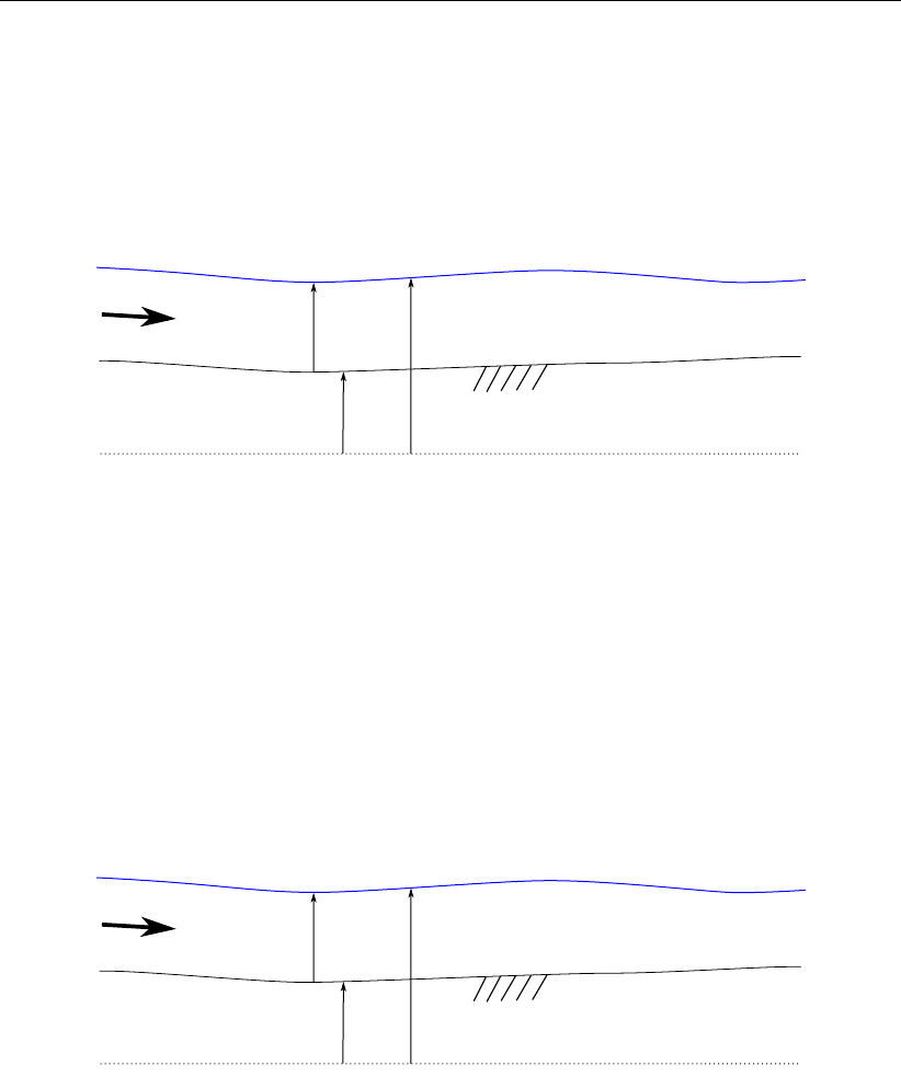
DRAFT
Conceptual description
6.1.2.2 Bed level
The bed level is defined as the lowest point in the cross section. In the definition of the cross
section an example is given of the interpolation and extrapolation of the bed levels over a
branch. The used symbol in the D-Flow1D module is zb.
It is given relative to a reference level, for example Mean Sea Level .
Reference level/Model datum
Bed level
Water level
ζ
h
zb
Q
Figure 6.2: Definition of bed level
If the water level is lower than the bed level, drying occurs.
6.1.2.3 Water depth
In the D-Flow 1D module the water depth is the distance between the water level and the bed
level. The symbol used for the water depth is h.
h=ζ−zb(6.3)
Reference level/Model datum
Bed level
Water level
ζ
h
zb
Q
Figure 6.3: Definition of water depth h=ζ−zb
Deltares 479 of 900
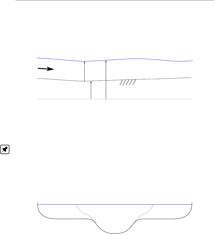
DRAFT
SOBEK, User Manual
6.1.2.4 Water level
The water level (ζ) is the level of the water surface relative to the reference level or Model
datum (= reference level).
In the one-dimensional D-Flow 1D module the water level perpendicular to the flow direction
is assumed to be horizontal.
Reference level/Model datum
Bed level
Water level
ζ
h
zb
Q
Figure 6.4: Definition of water level
The water level together with the discharge form the result of the D-Flow 1D module compu-
tations. Water levels are calculated at the connection nodes and the ζ-calculation points.
Note: In each D-Flow 1D, all levels are relative to the reference level
6.1.2.5 Flow area
The flow area AFof a cross-section is the area through which water is actually flowing.
In a cross-section, distinction can be made between the flow area and the storage area. In
the latter part, water is stored only, see Figure 6.5.
AS= storage area AS= storage area
AF= Flow area
Figure 6.5: Definiton of flow area (AF) and storage area (AS)
The shape of the cross-section, and the distinction between the flow area and storage area
are defined for each cross-section by user input.
6.1.2.6 Storage area
The storage area ASof a cross-section is the area in which only water is stored i.e. the
non-conveying part of the cross-section.
In a cross-section, distinction can be made between the flow area and the storage area, see
Figure 6.5.
The shape of the cross-section, and the distinction between the flow area and storage area is
defined for each cross-section by user input.
480 of 900 Deltares

DRAFT
Conceptual description
The total area ATis defined as the flow area plus the storage area.
6.1.2.7 Wetted area
The wetted area (AF[m2]) is the part of the cross section that is filled with water. See
Figure 6.6
6.1.2.8 Wetted perimeter
The wetted perimeter (O[m]) is the interface between the soil and the flowing water.
See Figure 6.6.
In the case of a main channel and one or two floodplains in the cross-section, a wetted perime-
ter is computed for each section. In that case the water interface between the sections is not
included in the wetted perimeter. See also Figure 6.6 and Figure 6.7
The wetted perimeter is used to compute the hydraulic radius, which is important for the
computation of the bed friction.
Figure 6.6: Wetted perimeter
Figure 6.7: Wetted perimeter for the main channel
6.1.2.9 Flow velocity
The flow velocity (u) is defined as the average flow velocity in the flow section of the cross-
section. It is by default given in [m/s].
The average flow velocity is derived by dividing the discharge [m3/s] by the flow area [m2].
Output of the overall average flow velocity, the flow velocity in the main channel, the flow
Deltares 481 of 900

DRAFT
SOBEK, User Manual
velocity in floodplain 1 and the flow velocity in floodplain 2 is possible.
u=Q
AF
, u0=Q
A0
, u1=Q
A1
, u2=Q
A2
.(6.4)
The indices 0, 1, 2 indicate the main channel, floodplain 1 and floodplain 2 respectively.
6.1.2.10 Velocity
The velocity (u) is defined as the average flow velocity in the wetted area of the cross section.
It is given in [m/s].
u=Q
AF
(6.5)
Note: Discharges and velocities are defined in branch segments, whereas cross sections are
defined in ζ-calculation points. For the computation of the velocities according to the above
formula. The D-Flow 1D module uses the upstream cross section
6.1.2.11 Hydraulic radius
The hydraulic radius is defined as the wetted area of the cross section divided by the wetted
perimeter.
R=AF
O(6.6)
Figure 6.8: Computation of hydraulic radius
Figure 6.9: Wetted perimeter for the main channel (Subdivision in main channel and
floodplains only in SOBEK-River)
482 of 900 Deltares

DRAFT
Conceptual description
6.1.3 Inertia
The flow in one dimension is described by two equations: the momentum equation and the
continuity equation. The first term in the momentum equation is the inertia term:
inertia =∂Q
∂t (6.7)
QDischarge [m3/s]
tTime [s]
6.1.4 Convection
In the D-Flow 1D module an convection term is used to guarantee the conservation of momen-
tum in a branch (between branch segments). The same holds for a connection node when
two branches are connected to this node. It that case the connection nodes could also have
been modelled as a ζ-calculation point. If there are more than two branches connected to a
connection node the convection term is set to zero.
When a branch has subsections, all subsections have an independent solution for the velocity.
The velocity that is used for the conservation of momentum over the branch is the average of
the velocities uiof the subsections in the cross section.
6.1.5 Convection (1D)
The flow in one dimension is described by two equations: the momentum equation and the
continuity equation. One of the terms in the momentum equation is the convection term:
convection =∂
∂x Q2
AF(6.8)
QDischarge [m3/s]
AFFlow area [m2]
xDistance [m]
6.1.6 Water level gradient
The third term in the momentum equation is the water level gradient.
water level gradient =gAF
∂ζ
∂x (6.9)
xDistance [m]
AFFlow area [m2]
gAcceleration due to gravity [m/s2] (≈9.81)
ζWater level [m] (with respect to the reference level)
This force tries to achieve a flat water surface under influence of the gravitational acceleration.
This force together with the bed friction have the greatest effect on the water movements.
6.1.7 Wind friction
The wind friction term in the momentum equation is expressed as:
τwind =−ρair Cwind u2
wind cos(ϕwind −ϕchannel )(6.10)
Deltares 483 of 900
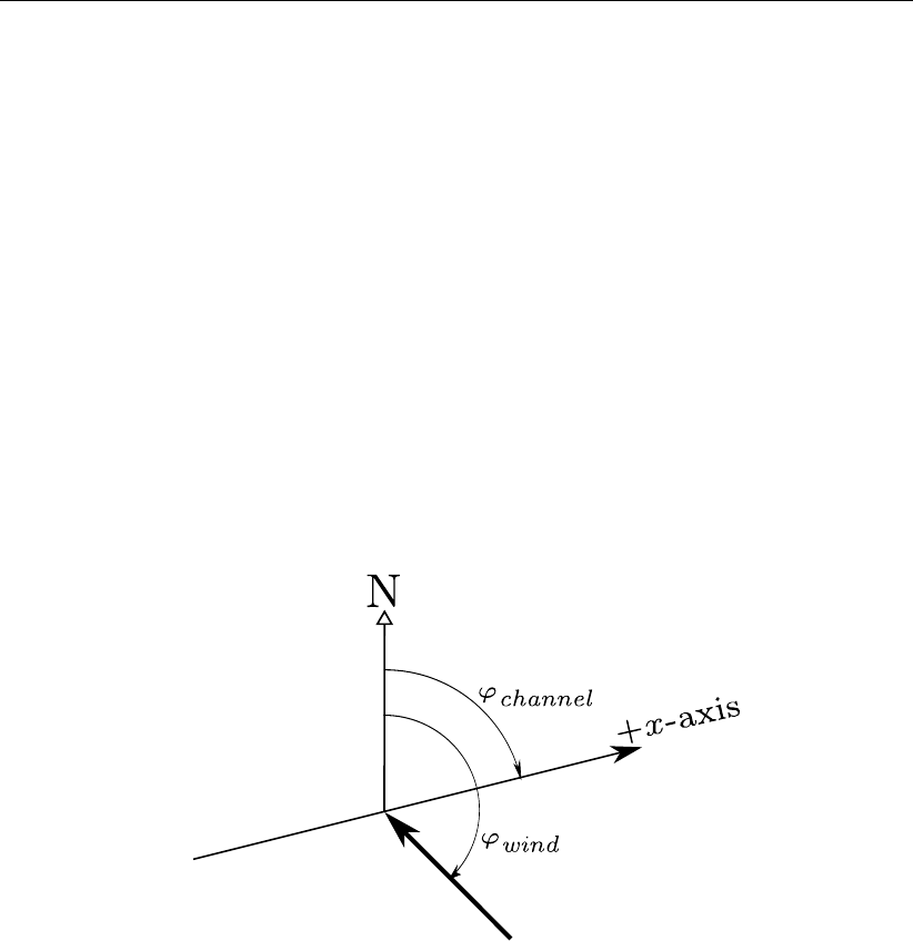
DRAFT
SOBEK, User Manual
τwind Wind shear stress (positive if acting along the positive x-axis of an open chan-
nel) [N/m2]
ρair Density of air, 1.205 kg/m3
Cwind αwind,1+αwind,2uwind , the wind friction coefficient. The used values are:
awind,1= 0.50 ×10⁻³[−] (6.11)
awind,2= 0.06 ×10⁻³[s/m] (6.12)
uwind Wind velocity [m/s]
ϕchannel Clock-wise angle between the positive x-axis of the 1D open channel and the
North (Nautical convention) [degrees]
ϕwind Clock-wise angle between the wind direction and the North (Nautical conven-
tion) [degrees]
The wind direction that is specified in the D-Flow 1D module is the direction from which the
wind is blowing with respect to the north. So, if the wind is blowing from the north, the wind
direction is 0 degrees. Wind from the southeast has a wind direction of 135 degrees.
1D Open Channel
Figure 6.10: Wind direction
When a cross section has a top width smaller than 20 mm (circular, egg-shaped, or nearly
closed tabulated cross section) than the cross section is considered closed. In that case the
wind is neglected in the momentum equation
6.1.8 Initial conditions
The initial conditions are the water levels or depths and the discharges at the beginning of
the simulation. The initial conditions are defined over a branch (water level and depth at
the ζ-calculation points, discharges at the branch segments). Therefore the water level that
initially should be taken at connection nodes is not strictly defined. This happens when, for
example, branch 1 with initial water level 0.5 is connected by a node to branch 2 with initial
water level 0.6. In that case the water level at the connection node is set to the lowest value
of the connected branches (0.5). Because the ζ-calculation point at the end of branch 1,
the connection node and the ζ-calculation point at the beginning of branch 2 have the same
location, the water levels of these three points are set to 0.5.
484 of 900 Deltares

DRAFT
Conceptual description
6.1.9 Boundary
A boundary can be applied at the locations where the model network ends with a boundary
node.
In order to solve the water flow equations (continuity equation and momentum equation),
information about the water flow at the model boundaries must be supplied.
At each boundary node, one condition for the water flow must be specified. The following
options are available:
discharge (constant, tabulated function of time, tabulated function of the water level)
water level (constant, tabulated function of time)
Because in the staggered grid, used by D-Flow 1D module, the discharges are defined for the
branch segments, a discharge boundary is imposed on the first branch segment next to the
boundary. Therefore the ζ-calculation point just before this first branch segment (first one in
a branch) is undefined and will not be taken into consideration during a calculation.
A water level boundary is defined in the first calculation point next to the boundary. This
ζ-calculation point actually has the same coordinates as the boundary node.
Note: In channel flow, usually, the discharge will be specified at boundaries where water is
flowing into the model, and the water level where water is flowing out of the model. In both
sewer and channel systems a dead end (or beginning) of a branch can be a connection node
at the end of a pipe or channel. In contrast to a boundary node, this node has storage.
6.1.10 Discharge
The discharge Qis the amount of water passing a branch segment per unit of time. It is given
in [m3/s].
The discharges at the branch segments together with the water levels at the ζ-calculation
points, form the results of a water flow simulation.
The D-Flow 1D module gives a positive discharge when the water flows in positive direction
with respect to the defined direction of a branch. If the water is flowing from branch end to
branch beginning, the discharge is negative.
6.1.11 Lateral discharges
A distinction is to be made between a Point and Diffusive lateral discharge.
Point lateral discharge: A point lateral discharge (Qlat, [m3/s]) refers to the inflow or
outflow of water at a specific point/location in a model schematization.
Diffusive lateral discharge: A diffusive lateral discharge (qlat, [m2/s]) refers to the inflow
or outflow of water along a specific branchsegment in a model schematization. A branch
segment is the distance (li, [m]) between two ζ-calculation points. A branch may consists
of several branchsegments. The total diffusive lateral discharge at a branch segment
equals qlat ×li. A diffusive lateral discharge is uniform distributed along the axis of a
branch (see Figure 6.11).
Deltares 485 of 900
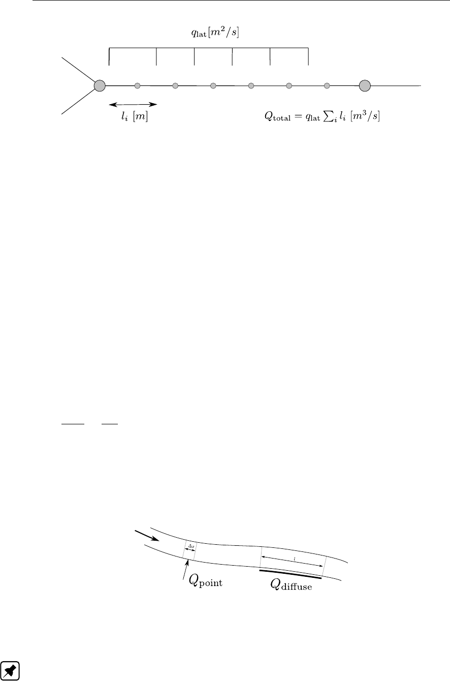
DRAFT
SOBEK, User Manual
Figure 6.11: Diffuse lateral discharge
For both point lateral discharges and diffuse lateral discharges yields that they are assigned to
aζ-calculation point(s). More precisely, their lateral inflow or outflow volume is accounted for
in the local water balance of such ζ-calculation point (e.g. local discretization of the continuity
equation, see section 6.1.11.1).
Two options are available for determining to which adjacent ζ-calculation point a lateral dis-
charges is assigned (see section 6.1.11.2).
An overview of lateral discharges, available in SOBEK, is given in section 6.1.11.3. In general
lateral discharges can be defined as a constant or as a function of time. Exceptions are:
The Area Based Point lateral inflow (see section 6.1.11.4)
The Pipe with Infiltration (see section 6.1.11.5)
6.1.11.1 Incorporating Lateral discharges in the Continuity Equation
Both point lateral discharges and diffusive lateral discharges (see Figure 6.12) are included in
the third term (qlat) of the continuity equation (see Equation (6.13)).
∂AF
∂t +∂Q
∂x =qlat (6.13)
AFFlow area [m2]
tTime [s]
QDischarge [m3/s]
xDistance [m]
qlat Lateral discharge per unit length [m2/s]
Figure 6.12: Lateral discharges:
Point lateral discharge: qlat =Qpoint/∆x; and
Diffuse lateral discharge: qlat =Qdiffuse/l
Note: A large withdrawal of water (negative lateral discharge) can cause problems when
the amount of outflowing water is larger than the storage available in a ζ-calculation point.
As a result negative volumes could be computed in the continuity equation. For that reason
the time step is temporarily reduced when the outflowing water volume is larger than half the
available volume (safety factor) in the ζ-calculation point. The time step is set to a value that
486 of 900 Deltares

DRAFT
Conceptual description
allows a withdrawal of half the available volume in one time step. If the time step resulting
from this action is smaller than 0.01 second, the lateral withdrawal is set to zero.
6.1.11.2 Options for Assigning Lateral Discharges to ζ-calculation point(s)
Two different lateral discharge assignment options are available in Settings (see 1D Flow,
Simulation Settings Tab), that determine to which ζ-calculation (or water level) point(s) a par-
ticular lateral discharge is to be assigned. The two different lateral discharge assignment
options are:
Option 1: Lateral Assigned to Lowest Water Level Point,
Option 2: Lateral Assigned to Nearest Water Level Point.
Hereafter, the consequences of the two different lateral discharge assignment options are
discussed for each type of lateral discharge (see section 6.1.11.3) separately.
Lateral discharge on a Node [m3/s]:
Irrespective of the selected lateral discharge assignment option, a lateral discharge on
a Node is assigned to its concerning Node (e.g. ζ-calculation point, Connection Node or
Manhole).
Point-lateral discharge on a Branch [m3/s]:
A point-lateral discharge on a Branch is either assigned to one or equally distributed over
both of the ζ-calculation points, that are respectively located at the left-side and the right-
side of the point-lateral discharge.
If option 1 (Lateral Assigned to Lowest Water Level Point) is selected, the point-lateral
discharge is assigned to the ζ-calculation point having the lowest bed level. If both
calculation points have the same bed level and the point-lateral discharge is located at
au-velocity point (e.g. centre-point of the two adjacent ζ-calculation points), the point-
lateral discharge is equally distributed over both adjacent calculation points. Else the
point-lateral discharge is assigned to the nearest ζ-calculation point.
If option 2 (Lateral Assigned to Nearest Water Level Point) is selected and the point-
lateral discharge is located at a u-velocity point (e.g. centre-point of the two adjacent ζ-
calculation points), the point-lateral discharge is equally distributed over both adjacent
ζ-calculation points. Else the point-lateral discharge is assigned to the nearest ζ-
calculation point.
Diffusive lateral discharge along a Pipe or Branch [m2/s]:
A diffusive lateral discharge along a Pipe or Branch is either assigned to one or equally
distributed over both of the ζ-calculation points, that are respectively located at the begin-
ning and the end of a pipe or branchsegment, receiving a diffusive lateral discharge.
If option 1 (Lateral Assigned to Lowest Water Level Point) is selected, the diffusive
lateral discharge is assigned to the ζ-calculation point having the lowest bed level.
Else the diffusive lateral discharge is equally distributed over both adjacent calculation
points.
If option 2 (Lateral Assigned to Nearest Water Level Point) is selected, the diffusive
lateral discharge is equally distributed over both adjacent ζ-calculation points.
Deltares 487 of 900

DRAFT
SOBEK, User Manual
6.1.11.3 Examples of Lateral Discharges
Three different types of lateral discharges are discerned:
1 Lateral Discharge on a Node [m3/s]:
Examples of lateral discharges on a Node are:
Point-Lateral Discharge, that is exactly located on a ζ-calculation point,
Connection Node with Storage and Lateral Flow,
Manhole with Lateral Flow,
Manhole with Lateral Disch. and Runoff
Manhole with Runoff
Flow - RR Connection on Flow Connection Node.
2 Point-Lateral Discharge on a Branch [m3/s]:
Examples of a point-lateral discharge on a Branch are:
Flow - Lateral Flow Node
Flow - RR Connection on Channel.
3 Diffusive Lateral Discharge along a Pipe or Branch [m2/s]:
Examples of a diffusive lateral discharge along a Pipe or Branch are:
Flow - Pipe with Runoff,
Flow - Dry Weather Pipe,
Flow - Rain Pipe,
Flow - Pipe with Infiltration
Flow - Channel with Lateral Discharge.
6.1.11.4 Area Based Point Lateral Flow
Area based Point lateral flow is computed as:
Qlat =A(fdR+S)(6.14)
Qlat Lateral discharge [m3/s]
fdDesign factor for area based lateral flow [−].
RRainfall [m/s].
AThe catchment runoff area [m2]
SSeepage (positive, inflow of groundwater) or Infiltration (negative, outflow to
groundwater reservoir) [m/s].
6.1.11.5 Pipe with infiltration (having a lateral diffusive discharge option)
A pipe with infiltration refers to a drainage pipe fully located inside a trench (see Figure 6.13).
Although the drainage pipe is porous it still can get pressurized. The trench is filled with
material (for instance gravel) having a certain porosity.
A pipe with infiltration allows for the exchange of water in the pipe towards the trench (positive
sign) and vice versa as well as for the exchange of water in the trench towards the groundwater
(negative sign) and vice versa. Hence, a pipe with infiltration can be seen as a pipe having a
diffusive lateral discharge option (e.g. infiltration of water in the pipe towards the trench and
exfiltration of water in the trench towards the pipe). For more information on the infiltration and
exfiltration process, reference is made to Ellis and Bertrand-Krajewski (2010), Rutsch et al.
(2008) and Karpf et al. (2008).
488 of 900 Deltares

DRAFT
Conceptual description
Pipe flow
Trench
Figure 6.13: Pipe with Infiltration (e.g. a drainage pipe located in a trench); Allowing for
the exchange of water in the pipe towards the trench (positive sign) and
vice versa; Allowing for the exchange of water from the trench towards the
groundwater (negative sign) and vice versa
For the computational procedure of a pipe with infiltration yields:
The flow (water levels (ζp, see Figure 6.14), discharges and velocities) through a pipe
with infiltration is computed in exactly the same manner as the flow in any pipe (e.g. by
solving the one dimensional depth averaged St. Venant momentum and continuity equa-
tions), where the diffusive lateral flow along a pipe with infiltration is taken into account in
accordance with the selected lateral discharge assignment option (see section 6.1.11.2).
The exchange of water between the pipe and the trench is computed according to the
“Darcy leakage approach (see Rutsch et al. (2008) and Karpf et al. (2008))” in which it is
assumed that the rate of exchange of water between two media is a function of the resis-
tance at the interface, the interface area and the hydraulic head over the interface. More
precisely per meter pipe length (see Figure 6.14), the rate of exchange of water between
the pipe and the trench (e.g. specific discharge qp↔tr, see Equation (6.15)) depends on
the resistance (cp−tr), the wetted perimeter (Pp−tr), the averaged water level in the pipe
(ζp) and the water level in the trench (ζtr).
Per metre pipe length, the maximum volume of water that can be stored in the trench (e.g.
fully saturated trench) equals the cross-sectional area of the trench that is filled with trench
material (Afiled with trench material) times the porosity of the trench material (φtr, [-]). Once the
trench is fully saturated, the water level in the trench (htr, see Figure 6.14) may rise above
the top level of the trench (ztr,top). In such case, per metre of pipe length an additional
volume of water is stored, that is equal to the top width of the trench (Wtr,top) times the
water depth on the trench (=ζtr −ztr,top). The top level of the trench is supposed to
coincide with the local surface level. Therefore in urban terminology, water depth on the
trench is referred to as water on street.
The exchange of water between the groundwater and the trench per metre pipe length
(e.g. specific discharge qgw↔tr) is also computed according to the “Darcy leakage ap-
proach” (see Equation (6.16)).
The groundwater reservoir as such is not modelled. The user-defined groundwater levels
(hgw, see Figure 6.14) are used as boundary conditions only.
Note: The local surface level is supposed to coincide with the top level of the trench. From
a physical point of view, a groundwater level can not rise above the local surface level (see
Figure 6.14). Therefore, at the start of a computation it is verified if user-defined ground
water levels (hgw) are above the top level of the trench (ztr,top). If this is the case (e.g.
if hgw > ztr,top), the computation is terminated with an error message denoting for which
"Pipes with Infiltration" yields that groundwater level(s) are above the top level of the trench.
Note: The thickness of a possible ground-layer in a pipe does affect the flow through a pipe
and is consequently taken into account in determining pipe flow. However, the thickness of a
possible ground-layer is neglected in the resistance factor, applied for the interface between
Deltares 489 of 900
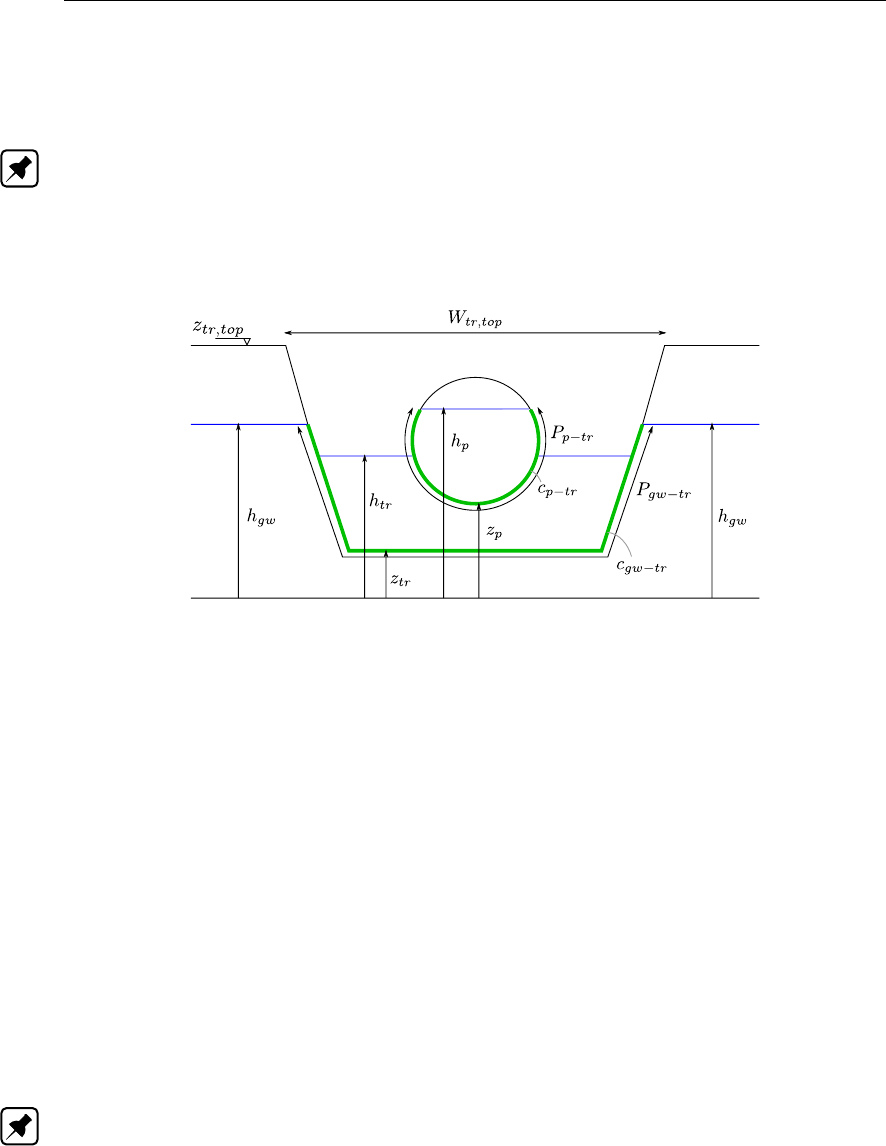
DRAFT
SOBEK, User Manual
pipe and trench. In other words, irrespective of the thickness of a possible ground-layer, the
resistance factor applied for the pipe-trench interface equals the user-defined resistance factor
(cp−tr) (see Equation (6.15)).
Note: Selecting the option "Impermeable" in the "Permeability of Ground/Soil" scroll-box,
available on the "Trench Data" tab (see Section 5.7.2.1), means that the interface between
trench and groundwater is considered to be impermeable (e.g. no exchange of water between
trench and groundwater). More precisely, if impermeable is selected Equation (6.16) is not
considered in the computational procedure.
Figure 6.14: Pipe with infiltration: definition of variables
The specific discharge (qp↔tr) between the pipe and the trench (see Figure 6.14) per metre
pipe length is computed according to the “Darcy leakage approach” as follows:
qp↔tr =
0if ζp≤zpand ζtr ≤zp
Pp−tr(ζp−zp)/cp−tr if ζp> zpand htr ≤zp
Pp−tr(ζp−ζtr)/cp−tr if ζp> zpand htr > zp
(6.15)
cp−tr resistance factor of the interface between pipe and trench [h].
ζ1water level in the pipe (may become pressurized) at the beginning of the pipe
(e.g. pipe-side with lowest x-coordinate) [m above datum].
ζ2water level in the pipe (may become pressurized) at the end of the pipe (e.g.
pipe-side with highest x-coordinate) [m above datum].
ζpaveraged water level in the pipe (e.g. (ζ1+ζ2)/2, may become pressurized)
[m above datum].
ζtr water level in the trench [m above datum].
Pp−tr wetted perimeter (e.g. length of the interface) between pipe and trench [m].
Note: If ζp≤zpand ζtr ≤zp, the wetted perimeter equals zero. Else the
maximum water level (e.g. max(ζp;ζtr)) determines the length of the wetted
perimeter.
qp↔tr specific discharge per metre pipe length between trench and pipe. Positive if
water flows from pipe towards the trench [m2/h].
z1invert level at the beginning of the pipe (e.g. pipe-side with lowest x-coordinate)
[m above datum].
z2invert level at the end of the pipe (e.g. pipe-side with highest x-coordinate) [m
above datum].
zpaveraged pipe invert level (e.g. (z1+z2)/2) [m above datum].
The specific discharge (qgw↔tr) between the pipe and the trench (see Figure 6.14) per metre
490 of 900 Deltares
DRAFT
Conceptual description
pipe length is computed according to the “Darcy leakage approach” as follows:
qgw↔tr =
0if ζtr ≤ztr and hgw ≤ztr
Pgw−tr(ζtr −ztr)/cgw−tr if ζtr > ztr and hgw ≤ztr
Pgw−tr(ζtr −hgw)/cgw−tr if ζtr > ztr and hgw > ztr
(6.16)
cgw−tr resistance factor of the interface between groundwater and trench [h].
hgw groundwater level [m above datum].
ζtr water level in the trench [m above datum].
Pgw−tr wetted perimeter (e.g. length of the interface) between groundwater and trench
[m]. Note: If ζtr ≤ztr and hgw ≤ztr, the wetted perimeter equals zero.
Else the water level (ζpm) determining the length of the wetted perimeter is
computed as ζpm = max(h∗
tr;h∗
gw), where: if ζtr ≥ztr,top then hζ∗
tr =ztr,top
else ζ∗
tr =ζtr; and if hgw ≥ztr,top then h∗
gw =ztr,top else h∗
gw =hgw.
qgw↔tr specific discharge per metre pipe length between groundwater and trench. Pos-
itive if ground water flows into the trench [m2/h].
ztr,top top level of the trench [m above datum]
6.1.12 Bed friction
The bed friction is the friction between the flowing water and the channel bed. As such, it
exerts a force on the flowing water always in the direction opposite the water flow.
In water courses, this force together with the force caused by earth gravity usually determines
the flow conditions: the other forces are far less important.
The fourth term of the momentum equation is the bed-friction term:
bed friction =gQ|Q|
C2RAF
(6.17)
where:
gAcceleration due to gravity [m/s2] (≈9.81)
QDischarge [m3/s]
CChézy coefficient [m1/2/s]
RHydraulic radius [m]
AFWetted area [m2]
Note:
If the specified roughness parameter is equal to zero (Chézy=0, Manning=0, etc.), then the
bed friction term is not taken into account in the momentum equation.
The following roughness definitions can be used:
6.1.12.1,Bos-Bijkerk;
6.1.12.2,Chézy;
6.1.12.3,Manning;
6.1.12.4,Nikuradse;
6.1.12.5,Strickler;
6.1.12.6,White-Colebrook.
Deltares 491 of 900

DRAFT
SOBEK, User Manual
6.1.12.1 Bos-Bijkerk
The bed friction formulation according to de Bos-Bijkerk describes the Manning coefficient as
a function of the water depth and a parameter. This parameter can be used to shape the
function to a certain empirical curve:
km=γh1/3(6.18)
kmManning roughness coefficient [m1/3/s]
hWater depth [m]
γParameter [1/s], normally between 20 and 40
This formula can be rewritten to a formulation for the Chézy coefficient as a function of the
water depth
C=γh1/3R1/6(6.19)
CChézy coefficient [m1/2/s]
RHydraulic radius [m]
For every computational time step the new friction value is calculated according to the Bos-
Bijkerk formula and sequentially applied to the hydrodynamics calculations.
6.1.12.2 Chézy
The D-Flow 1D module uses the Chézy bed friction value in solving the water flow equations.
The following roughness formulations are possible:
Chézy coefficient
Bos-Bijkerk friction shape parameter g, resulting in a Chézy value according to:
C=γh1/3R1/6(6.20)
hWater depth [m]
γParameter [1/s], normally between 20 and 40
CChézy coefficient [m1/2/s]
RHydraulic radius [m]
White-Colebrook, using the Nikuradse roughness coefficient kn, results in a Chézy value
according to:
C= 18 10log 12R
kn(6.21)
Manning coefficient, nm, resulting in a Chézy coefficient according to:
C=R1/6
nm
(6.22)
Strickler, using the Nikuradse knroughness coefficient, results in a Chézy value according
to:
C= 25 R
kn1/6
(6.23)
492 of 900 Deltares

DRAFT
Conceptual description
Strickler, using the Strickler ksroughness coefficient, results in a Chézy value according
to:
C=ksR1/6(6.24)
Engelund-like roughness predictor (for main sections of SOBEK-River profiles only) re-
sulting in a Chézy value according to:
C=C90rθ90
θs
(6.25)
For SOBEK-River, the Chézy, Nikuradse, Manning or Strickler coefficients may be
a constant
spatially varying
a tabulated function of the water level (h) or the total discharge (Q)
Different values or tables are possible for positive as well as negative flow. See also the
chapter 1D hydraulic friction concepts for information on the different friction concepts present
in the user interface.
6.1.12.3 Manning
One of the methods to define the bed roughness is using the Manning coefficient, symbol nm.
In the D-Flow 1D module, the Manning coefficient is used to compute the actual value of the
Chézy coefficient, by:
C=R1/6
nm
(6.26)
CChézy coefficient [m1/2/s]
RHydraulic radius [m]
nmManning coefficient [s/m1/3]
6.1.12.4 Nikuradse
One of the methods to define the bed friction is by entering an equivalent roughness according
to Nikuradse, represented by the symbol kn[m].
Values of knfor open channels with bed forms are in the same order of magnitude as the
height of the bed forms.
Using this option, the actual value of the Chézy coefficient will be computed according to the
White-Colebrook formula.
6.1.12.5 Strickler
One of the methods to define the bed roughness is by using the Strickler formula. The actual
value of the Chézy coefficient is computed using:
C= 25 R
kn1/6
(6.27)
or:
C=ksR1/6(6.28)
Deltares 493 of 900
DRAFT
SOBEK, User Manual
CChézy coefficient [m1/2/s]
RHydraulic radius [m]
ksStrickler roughness coefficient [m1/3/s]
in which knis the Nikuradse equivalent roughness, and ksis the Strickler roughness coeffi-
cient. You may select either ks or kn as input value.
The value of the hydraulic radius Ris taken from the last iteration loop.
It is possible to enter the coefficients varying in space and depending on the local flow direc-
tion.
6.1.12.6 White-Colebrook
One of the methods to define the bed friction is by specifying an equivalent roughness ac-
cording to Nikuradse. Using this option, the value of the Chézy coefficient will be computed
according to the White-Colebrook formula:
C= 18 10log 12R
kn(6.29)
CChézy coefficient
RHydraulic radius
knNikuradse equivalent roughness
Note:
Actually, this formula is a simplification of the complete White-Colebrook formula.
6.1.13 Froude number
The Froude number is defined by u/c, with uthe average flow velocity and cthe wave celerity.
Herein is cas follows:
c=sgAF
Wf
(6.30)
Thus
Froude number =u
pgAF/Wf
(6.31)
uVelocity (u=Q/AF) [m/s]
gAcceleration due to gravity [m/s2] (≈9.81)
AFWetted area [m2]
WfFlow width [m]
Remarks:
When the Froude number is less than 1, the flow is sub-critical, when it is larger than 1,
the flow is super-critical
Transitions from sub-critical to super-critical flow causes an hydraulic jump.
494 of 900 Deltares
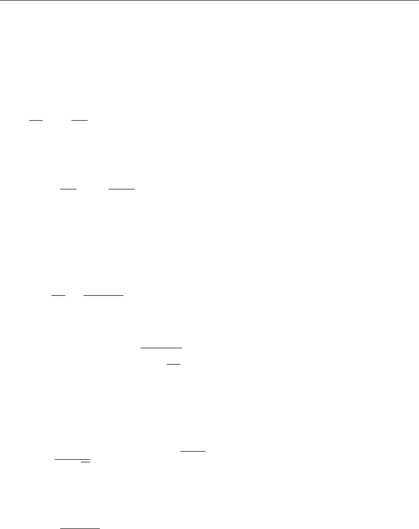
DRAFT
Conceptual description
6.1.14 Boussinesq
The Boussinesq coefficient is a parameter in the momentum equation for the water flow. It
accounts for the non-uniform velocity distribution in a cross-section.
The Boussinesq constant αBis multiplier to the convective term:
∂
∂x αB
Q2
AF(6.32)
The definition of the coefficient αBis:
αB=AF
Q2ZWf
0
q(y)2
h(y)dy (6.33)
The constant of Boussinesq is computed by D-Flow 1D. The computation is based upon the
Engelund approach (Engelund and Hansen,1967). In this approach the water level gradient
and bed-friction term are assumed to be an order of magnitude larger than the other terms in
the momentum equation. The resulting equation is:
gAF
∂h
∂x =gQ2
C2RAF
(6.34)
in which locally a constant water level gradient is assumed. In an arbitrary cross-section the
discharge can be expressed as:
Q=ZWf
0
C(y)h(y)rR(y)∂h
∂x dy (6.35)
in which his the water depth. Furthermore, it is assumed that the water level and water level
slope are the same for main and floodplains. Combining Equation (6.34) and Equation (6.35)
leads to a more accurate estimate of the Chézy coefficient based upon the average of the
local Chézy coefficients.
C=1
AF√RZWf
0
C(y)h(y)pR(y)dy (6.36)
Now Equation (6.33) gives combined with Equation (6.34) and Equation (6.35) the following
expression for the Boussinesq coefficient:
αB=1
AFRC2ZWf
0
C2(y)h(y)R(y)dy (6.37)
Cross-sections in D-Flow 1D may be divided in two or three parts. So the following three
options are available.
option 1:
The cross-section is not divided into sections with different roughness (only a main channel is
present). This gives for the Boussinesq coefficient:
αB= 1 (6.38)
option 2:
The cross-section is divided into two sections with different roughness for the modeling of, for
example, a cross-section with a main channel and a floodplain. During a computation this
gives two possibilities:
Deltares 495 of 900

DRAFT
SOBEK, User Manual
possibility 1:
Actual water flow is in the main channel only:
αB= 1 (6.39)
possibility 2:
Actual water flow is in the main channel and the floodplain:
αB=C2
0Af0R0+C2
1Af1R1
C2RAF
(6.40)
The indices 0 and 1 respectively indicate the main channel and floodplain.
option 3:
The cross-section is divided into three sections with different roughness (main channel, flood-
plain 1 and floodplain 2). During a computation this gives three possibilities:
possibility 1:
Actual water flow is in the main channel only:
αB= 1 (6.41)
possibility 2:
Actual water flow is in the main channel and floodplain 1:
αB=C2
0Af0R0+C2
1Af1R1
C2RAF(ζ)(6.42)
The indices 0 and 1 respectively indicate the main channel and floodplain.
possibility 3:
Water is actually flowing in all sections, main channel, floodplain 1 and floodplain 2:
αB=C2
0Af0R0+C2
1Af1R1+C2
2Af2R2
C2RAF
(6.43)
The indices 0, 1 and 2 respectively indicate the main channel, floodplain 1 and floodplain
2.
6.1.15 Accuracy
Whether you are measuring in a prototype, studying water flow in a scale model or modelling
with a software system, you should always make some considerations about the accuracy of
your activities and of the results of your study.
As for the results of a mathematical model study, the following elements play a role in estab-
lishing the overall accuracy:
The reliability of the available data describing the prototype;
The accuracy of the available data describing the prototype;
The violation of certain assumptions underlying the mathematical modelling concept being
used;
The experience and skill of the modeller(s);
The overall accuracy that is required (perhaps more accurate results could be obtained
but the aim of the study may not require such accuracy or due to a lack of time you may
have to settle for less);
The accuracy of the applied numerical modelling technique.
496 of 900 Deltares

DRAFT
Conceptual description
In general practice the first five items are the most important when you are using a one-
dimensional mathematical model for hydrodynamic flow. The numerical accuracy is in that
case normally of minor importance.
The D-Flow 1D module uses the Delft-scheme to solve the water flow equations. This scheme
is developed with robustness as the most important design aspect. It can deal with phenom-
ena such as drying/flooding, super-critical flow and it guarantees a solution for every time
step.
The accuracy of the solution depends on the grid size; the smaller the grid sizes, the more
accurate the solution is. The time step can be chosen arbitrarily. It is reduced internally
when this is necessary to guarantee stability by means of a time step estimation procedure.
Obviously small grid sizes result in a network with more elements and therefore in a longer
simulation time.
The Delft-scheme is designed to produce a closed water balance.
6.1.16 Structures
In the D-Flow 1D-modules the following structure types are available:
6.1.16.1 Advanced weir
6.1.16.2 Bridge
6.1.16.3 Compound structure
6.1.16.4 Culvert
6.1.16.5 Database structure
6.1.16.6 General structure
6.1.16.7 Inverted siphon
6.1.16.8 Orifice
6.1.16.9 Pump station and Internal Pump station
6.1.16.10 External Pump station
6.1.16.11 River Pump
6.1.16.12 River Weir
6.1.16.13 Siphon
6.1.16.14 Universal Weir
6.1.16.15 Vertical obstacle friction
6.1.16.16 Weir
The flow through structures is computed based on:
Upstream water level or energy level (River weir, Advanced weir and General structure
only)
Downstream water level or energy level (River weir, Advanced weir and General structure
only)
Structure dimensions (some can be controlled: i.e. crest level, opening height, pump ca-
pacity, opening of valve)
A number of user-defined parameters, depending on the structure type (contraction coef-
ficient, reduction factor, etc.).
The discharges and wetted areas that are computed in the structure formulas are imposed
in the branch segment where the structure is located. The formulas use the water levels of
the ζ-calculation points on either side of the branch segment. For the River weir, Advanced
weir, General structure, River pump, Database structure and Compound structure yields that
Deltares 497 of 900
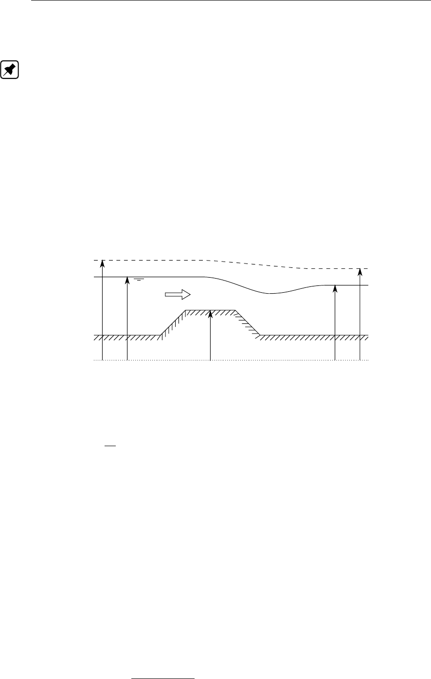
DRAFT
SOBEK, User Manual
SOBEK by default places a computational point 0.5 m upstream and 0.5 m downstream of the
structure location. Hence such structure is located in a branch having a default length of 1 m.
Note:
The dimensions of the structure do not contribute to the storage in the water system.
6.1.16.1 Advanced weir
Please note that the discharge through an Advanced weir is computed on basis of upstream
and downstream energy levels. Further on please note that default a computational point is
located 0.5 m in front and 0.5 m behind an Advanced weir.
Notation
The flow direction can be either positive or negative. A positive flow direction is a flow in
the direction that the branches have been specified, i.e. with increasing x-coordinates. The
upstream side, facing the beginning of the branch is denoted by the subscript 1, whereas the
downstream location facing the end of the branch is denoted with 2. The subscript sis used
for locations at the sill.
Reference level/Model datum
Energy level
H1ζ1
zs
ζ2
H2
Figure 6.15: Definition of energy and water level
and the energy level His defined as:
H=ζ+u2
2g(6.44)
The user must enter the following input parameters for this type of hydraulic structure:
zsLevel of crest
WnTotal net width
NNumber of piers
PLevel of upstream face
H0Design head of the weir
KpPier contraction coefficient
KaAbutment contraction coefficient
The following parameters can be controlled by a hydraulic structure controller:
WsWidth across flow section
zsCrest level of weir
The discharge through the structure is computed with:
Q=C1C2Wp2g(H1−zs)3(6.45)
498 of 900 Deltares

DRAFT
Conceptual description
In which Wis the active width and C1and C2are factors computed in the following way.
Note:
if ζ1< zsthen Q= 0.
W=Wk−2(NKp+Ka)(H1−zs)(6.46)
C1=C0Ck(6.47)
The value of C0is computed depending on the value of the ratio between the upstream face
and the design head:
χ=P
H0
(6.48)
if χ < 2then:
C0= (0.1256χ5−1.0178χ4+ 3χ3−3.94χ2+ 2.28χ+ 1.66) ξ
√2g(6.49)
where ξis a correction factor computed with:
ξ=−0.052χ3+ 0.145χ2−0.096χ+ 1.01 (6.50)
if χ > 2then:
C0=2.1549008
√2g(6.51)
The value of χis computed depending on the value of the ratio between the energy level
minus the sill level and the design head:
χ1=H1−zs
H0
(6.52)
Ck=0.1394χ3
1−0.416χ2
1+ 0.488χ1+ 0.785 χ1<1.6
1.0718224 χ1≥1.6(6.53)
The value of Ctis computed depending on the value of the ratio between the energy level
minus the downstream water level and the energy level minus the sill level:
χ2=H1−h2
H1−zs
(6.54)
Ct=(q(1 −(χ2−0.7)2
0.49 ) + 27(0.7−χ2)4pχ3
2χ2<0.7
1χ2≥0.7(6.55)
Deltares 499 of 900
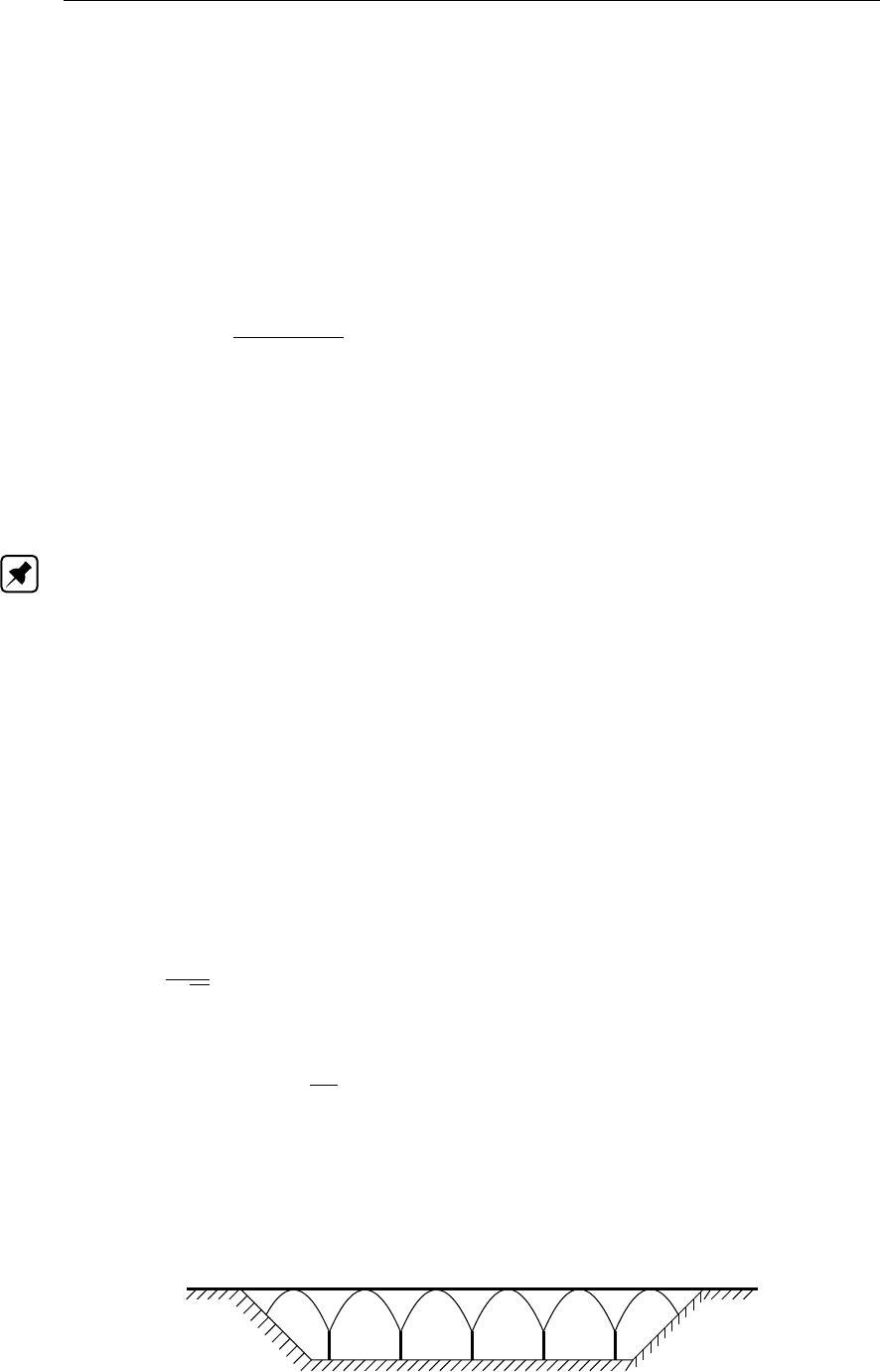
DRAFT
SOBEK, User Manual
6.1.16.2 Bridge
A bridge is one of the structure types that can be included in the SOBEK-Flow-module. The
following types of bridges can be modelled:
Pillar bridge
Abutment bridge
Fixed bed bridge
Soil bed bridge
The general description of the discharge through a bridge is given by:
Q=µAfp2g(ζ1−ζ2)(6.56)
QDischarge through bridge [m3/s]
µDischarge coefficient derived from loss-coefficients [−]
AfWetted area [m2] of flow through bridge at upstream side
gAcceleration due to gravity [m/s2] (≈9.81)
ζ1Upstream water level [m]
ζ2Downstream water level [m]
Note: For numerical reasons (e.g. validity of structure Equation (6.56)) the discharge co-
efficient (µ) is limited to a maximum of 1.0. In other words if the discharge coefficient (µ)
according to Equation (6.57) (Pilar bridge) or Equation (6.59) (Abutment bridge, Fixed bed
bridge or Soil bed bridge) becomes larger than 1.0, the actual applied discharge coefficient in
Equation (6.56) is limited to 1.0. This means that for a given discharge, the water level differ-
ence over such bridge might be larger than anticipated, when considering the defined friction
loss coefficients. In such case it is advised to apply the Extra Resistance Node for mod-
elling this particular bridge. An Extra Resistance Node (see section 5.3.8 and section 6.1.1.2)
adds additional(extra) resistance to the St. Venant momemtum equation. Hence no structure
equation is solved at an Extra Resistance Node.
Pillar bridge
A pillar bridge has one or more pillars that affect the discharge through the bridge with the
following definition for the discharge coefficient (µ)
µ=1
pξy
(6.57)
ξyPillar loss coefficient, defined as
ξy=βαy
Af
(6.58)
βParameter [−] depending on shape of pillar[s] (shape factor). Normally be-
tween 0.22 and 1.56
AfWetted area [m2] of flow through bridge at upstream side
αyArea [m2] of wetted part of pillar [s] perpendicular to the flow direction, consid-
ered at upstream side
Figure 6.16: Pillar bridge
500 of 900 Deltares
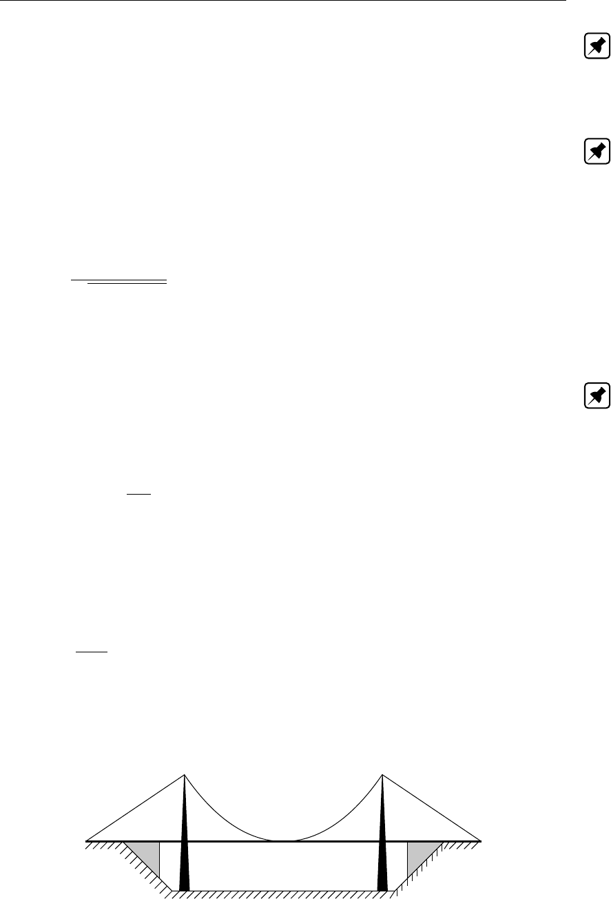
DRAFT
Conceptual description
Note: For numerical reasons the discharge coefficient (µ) is limited to a maximum of 1.0. For
more information, see the note below Equation (6.56).
The plate of the bridge is always so high that it does not effect the flow through the bridge. So
the cross section is considered as open.
Note:
Pillar bridges are not allowed in closed cross-sections.
Abutment bridge
For the abutment bridge the overall loss coefficient is defined as:
µ=1
pξi+ξf+ξo
(6.59)
ξiEntrance loss coefficient (in). Constant
ξfFriction loss coefficient
ξoExit loss coefficient (out).
Note: For numerical reasons the discharge coefficient (µ) is limited to a maximum of 1.0. For
more information, see the note below Equation (6.56).
The ξocoefficient is defined as:
ξo=k1−Af
Af22
(6.60)
kConstant exit loss coefficient
AfWetted area [m2] of flow through bridge at upstream side
Af2Wetted area [m2] of flow in branch at downstream side of bridge
The ξfcoefficient is defined as:
ξf=2gL
C2R(6.61)
gAcceleration due to gravity [m/s2] (≈9.81)
LLength of bridge [m]
CChézy coefficient [m1/2/s]
RHydraulic radius [m]
Figure 6.17: A suspension bridge with abutments
Here, the plate of the bridge can effect the flow through the bridge. The cross section is closed
Deltares 501 of 900
DRAFT
SOBEK, User Manual
Note:
The definition of this bridge is similar to the definition of a culvert.
Fixed bed bridge
This bridge has the same formulation as the abutment bridge except it has a rectangular
profile.
Figure 6.18: Fixed bed bridge
Soil bed bridge
This bridge has the same formulation as the fixed bed bridge including the rectangular profile.
In addition to this it has a ground layer with a different friction formulation. This ground layer
can have a zero thickness.
Figure 6.19: Soil bed bridge
6.1.16.3 Compound structure
A compound structure consists of several hydraulic structures parallel to each other at one
location. These hydraulic structures may be of the same type or of different types. Presently
following structure types can be placed as a member in a compound structure, viz.: General
structure, Database structure, Advanced weir, River weir and River pump.
Please note that a value for structure inertia damping factor can be defined for each individual
member of the compound structure.
Each member of the compound structure has its own triggers and controllers.
6.1.16.4 Culvert
A culvert is one of the structure types that can be included in the SOBEK-Flow-module. A
culvert is an underground structure that normally connects two open channels. The flow
through a culvert is affected by its upstream and downstream invert levels, the size and shape
of its closed cross section, its ground layer thickness, its entrance loss, its friction loss, its
valve loss and its exit loss.
Figure 6.20 shows a side view of a culvert.
502 of 900 Deltares
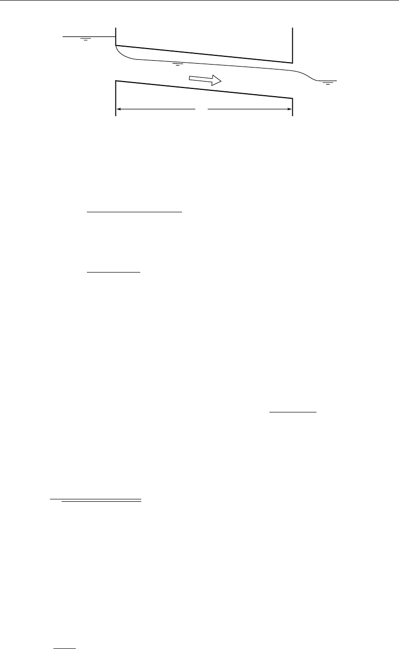
DRAFT
Conceptual description
ζ1
ζ2
zc2
zc1
L
Figure 6.20: Side view of a culvert
Two flow conditions can occur:
Free flow when ζ2< zc2+hc2
Q=µAfcp2g(ζ1−(zc2+hc2)) (6.62)
Submerged flow when ζ2≥zc2+hc2:
Q=µAfcp2g(ζ1−ζ2)(6.63)
QDischarge through culvert [m3/s]
µDischarge coefficient, derived from loss-coefficients [−]
Afc Discharge culvert flow area min(Afc1, Afcgate)[m2]
Afc1: Flow area in the culvert at its upstream side [m2]
Afcgate: Flow area under the culvert gate [m2]
gAcceleration due to gravity [m/s2] (≈9.81)
ζ1Upstream water level [m]
ζ2Downstream water level [m]
zc2Downstream culvert invert level [m]
hc2Critical culvert depth at the downstream side, 3
pQ2/(gT 2
2)[m]
T2Surface width in the culvert at its downstream side [m]
For numerical reasons the discharge coefficient (µ) is limited to a maximum of 1.0. The
discharge coefficient (µ) is computed as follows:
µ=1
pξi+ξf+ξv+ξo
(6.64)
ξiEntrance loss coefficient [−]
ξfFriction loss coefficient [−]
ξvValve loss coefficient [−]
ξoExit loss coefficient [−]
The entrance loss coefficient (ξi) can be defined as a constant value only.
The friction loss coefficient (ξf) is computed as follows:
ξf=2gL
C2
1R(6.65)
LLength of the culvert [m]
C1Chézy coefficient in the culvert at its upstream side [m1/2/s]
Deltares 503 of 900

DRAFT
SOBEK, User Manual
RHydraulic radius [m]
R=Rc1ζ1≥zc1+hgate
Rgate ζ1< zc1+hgate
(6.66)
hgate Gate height opening [m]
Rc1Hydraulic radius in the culvert at its upstream side [m]
Rgate Hydraulic radius based on actual gate height opening [m]
zc1Upstream culvert invert level [m]
The valve loss coefficient (ξv) can be defined as a constant value or as a function of the ratio
of the “Gate height opening” and the “maximum inner culvert height”.
Note:
In case the valve loss coefficient (ξv) is not a constant, in computations the actual valve
loss coefficient (ξv) is derived from the user defined table, while using the ratio of the
“actual gate height opening and the “actual maximum inner culvert height”.
In case the ground layer thickness is greater than zero, both the “actual gate height open-
ing” and the “actual maximum inner culvert height” will differ from the values as defined in
the user interface (see next paragraph)
The exit loss coefficient (ξo) is computed as follows:
Submerged flow (ζ2=zc2+hc2):
ξo=k1−Afc
Afr22
(6.67)
kUser defined constant exit loss coefficient [−]
Afr2Flow area in the branch, adjacent to the downstream culvert side [m2]
Afc Culvert flow area [m2]
Afc =Afcgate h1≥zc1+hgate
Afc1h1< zc1+hgate
(6.68)
hgate Gate height opening [m]
zc1Upstream culvert invert level [m]
Afcgate Flow area under the culvert gate [m2]
Afc1Flow area in the culvert at its upstream side [m2]
Free flow (ζ2< zc2+hc2):
ξo= 0 (6.69)
Culvert cross-sections, bed friction and ground layer
For a culvert all available closed cross-section types can be used. In a culvert, a ground
layer with constant thickness can be defined. Culvert friction and ground layer friction can be
specified, using any of the available bed friction formulations.
Defining a ground layer thickness >0implies that in culvert computations:
Defined invert levels are raised with the ground layer thickness,
504 of 900 Deltares
DRAFT
Conceptual description
Gate height openings are reduced with the ground layer thickness,
Maximum inner height of the culvert is reduced with the ground layer thickness,
Cross-sectional parameters (such as: flow areas, hydraulic radius and so on) are com-
puted based on a cross-sectional profile, that is reduced by the ground layer thickness.
Culvert, Good modelling practice aspects
It is advised to avoid that the bed level of a cross-section in front of a Culvert, Inverted Siphon
or Siphon is above the ground-layer level (= invert level + ground-layer thickness), since such
situation can result in very small computational time-steps (e.g. long required wall-clock times)
or even in a termination of the simulation.
This is explained as follows. Consider the situation depicted in Figure 6.40 were the bed level
in front of a Culvert (Inverted Siphon or Siphon) is 0.60 m above the ground-layer level. This
means that at small upstream water depths, water will be sucked into the culvert (Inverted
Siphon or Siphon), resulting in large flow velocities. For the computational time-step (∆t)
yields that ∆t≤∆x/U, where Uis the local flow velocity and ∆xis distance between two
water level computational points (or ζ-points). At very low discharges even negative water
depths may be computed, leading to a termination of the simulation.
The situation explained above can be avoided by making the bed level in front of the Culvert
(Inverted Siphon or Siphon) equal to the ground-layer level. In other words by defining a
bed level slope from ζ-point ζ2to ζ3as depicted in Figure 6.40. Providing for the parameter
"Maximum Lowering of Cross-section Bed Level at Culvert" a value greater or equal to 0.60 m
means that before the computation starts, the bed level at ζ-point ζ3is set equal to the ground-
layer level. In Figure 5.15 it is shown how to provide a value for parameter "Maximum Lowering
of Cross-section Bed Level at Culvert".
Figure 6.21: Good modelling practice, Culvert, Inverted Siphon and Siphon
Deltares 505 of 900

DRAFT
SOBEK, User Manual
6.1.16.5 Database structure
Please note that default a computational point is located 0.5 m before and 0.5 m behind a
Database structure. In a hydraulic structure the discharge through the structure depends on
upstream and downstream water levels and structure parameters that define the dimension
of the structure etc. In other words the hydraulic behaviour of a structure can be defined in
the structure equation as a relationship between upstream and dowstream water level. In the
database structure however, this relationship is defined in a tabulated form which is stored in
a database. The user has to define this database.
The database consists in fact of a matrix of discharges. At every point of the matrix a dis-
charge (Q) is defined as a function of two corresponding water levels: one facing the begin-
ning of the branch (ζ1) and one facing the end (ζ2), are defined. There are two ways to define
the relation:
a function of both water levels Q=Q(ζ1−zs, ζ2−zs), to be used for structures with
relatively high head differences; zs=crest level w.r.t. datum
a function of the water level and the water level difference Q=Q(ζ1−zs,∆ζ=ζ1−ζ2),
to be used for structures with relatively small water level differences combined with large
water level variations; zs=crest level w.r.t. datum
All discharges in a row correspond to the same water level (ζ1) facing the beginning of the
branch segment. All discharges in a column correspond either to the same water level (ζ2)
facing the end of the branch segment or to the water level difference (∆ζ=ζ1−ζ2). The
water levels that are part of the database are defined with respect to a user defined datum.
During a simulation, discharges at any point in the domain of the matrix will be obtained by
interpolation. In most cases this will be a linear interpolation in two directions. However when
the discharge is requested at a water level that lies within 10 percent of a water level defined
in the matrix, cubic interpolation takes place for that water level.
Warning:
The crest level can be adjusted by a controller. This implies the assumption that the
discharge head relation is independent of the level of the crest. This is not completely
correct. The user should be aware of this.
6.1.16.6 General structure
Please note that default a computational point is located 0.5 m in front and 0.5 m behind
a general structure. In the general structure type in sobek weir and gate flow is combined
in one structure type. In addition, the general structure gives more freedom in defining the
dimensions and the geometry of the hydraulic structure. The geometrical shape is given in
Figure 6.22 and Figure 6.23. See section 5.3.10 for the definition of input parameters. Please
note that the discharge through a General structure is computed on basis of upstream and
downstream energy levels. Please note as well that a structural inertia damping factor can be
defined for each individual General structure.
506 of 900 Deltares
DRAFT
Conceptual description
Figure 6.22: General structure, side view
Figure 6.23: General structure, top view
Flow across the general structure can be of the following types: drowned weir flow, free weir
flow, drowned gate flow, and free gate flow, depending on the dimensions of the structure and
the flow conditions.
When salt intrusion is modelled, the density difference of the water over the structure is incor-
porated in the impulse balance (this is not the case with the other structure types).
In the solution method for the general structure particular attention has been given to the
modelling of the transition between free- and submerged flow.
For this purpose, the water level at the sill (ζs) is computed by applying an impulse balance
instead of taking it equal to the water level further downstream.
As a result the general structure is especially attractive for those who want to simulate the
shifting conditions from free- to submerged gate flow accurately and of course in case of
important density-differences over the structure.
Deltares 507 of 900

DRAFT
SOBEK, User Manual
Computation of downstream water level
In case of drowned gate flow or drowned weir flow the water level at the sill or downstream of
the gate is required. This level is computed by application of the impulse balance.
drowned gate-flow
Figure 6.24: Drowned gate flow
The water depth hscan be described by a second order algebraic equation:
Awh2
s+Bwhs+Cw= 0 (6.70)
with:
Ag= (1 + ρ∗)Wsd
3+W2
6+ (1 −ρ∗)Wsd
4+W2
12 (6.71)
Bg= (1 + ρ∗)(∆S1+ ∆S2−h2)Wsd
3+W2
6+ (2∆S1+h2)Wsd
6+
(∆S1+ 2h2)W2
6+
+ (1 −ρ∗)∆S1
Wsd
3+ (∆S1+h2)Wsd +W2
6+
+4ρ∗c2
gdµ2
gdd2
gW2
s
W2h2
(1 + λ
d2
)−4cgdµgddgWs(6.72)
Cg= (1 + ρ∗)(∆S1+ ∆S2−h2)2∆S1+h2)Wsd
6+ (∆S1+ 2h2)W2
6+
+ (1 −ρ∗)(∆S1)2Wsd
6+ (∆S1+h2)Wsd +W2
12 +
−4ρ∗c2
gdµ2
gdd2
gW2
sHs1
W2h2
(1 + λ
h2
)+4cgdµgddgWsHs1(6.73)
508 of 900 Deltares
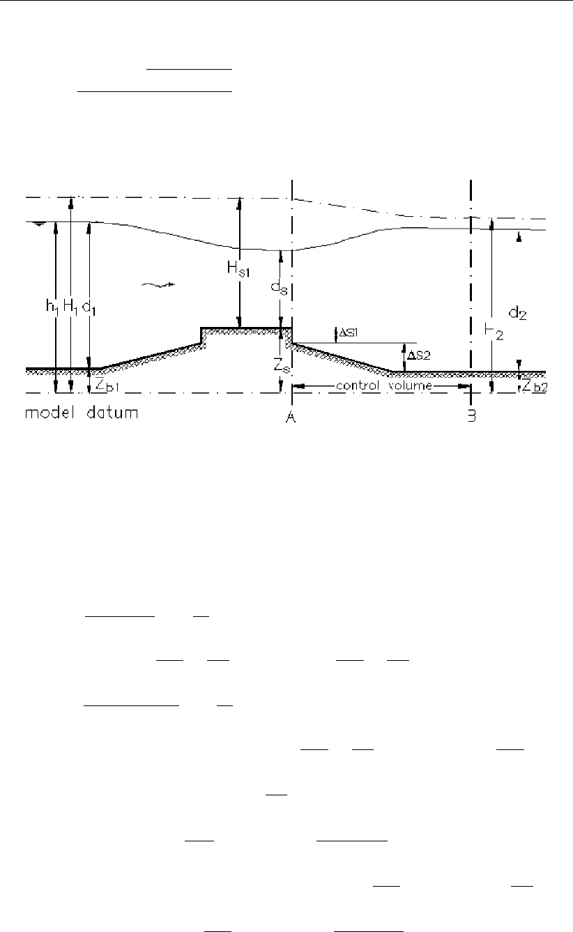
DRAFT
Conceptual description
Equation (6.70) leads to:
hs=−Bg+pB2
g−4AgCg
2Ag
(6.74)
drowned weir-flow
Figure 6.25: Drowned weir-flow
The water depth at the sill hsis described by a third order algebraic equation:
Dwh3
s+Awh2
s+Bwhs+Cw= 0 (6.75)
with:
Dw=4ρ∗c2
wdW2
s
W2h2
(1 + λ
h2
)(6.76)
Aw= (1 + ρ∗)Wsd
3+W2
6+ (1 −ρ∗)Wsd
4+W2
12 +
−4ρ∗c2
wdW2
sHs1
W2h2
(1 + λ
h2
)+4cwdWs(6.77)
Bw= (1 + ρ∗)(∆S1+ ∆S2−h2)Wsd
3+W2
6+ (2∆S1+h2)Wsd
6+
(∆S1+ 2h2)W2
W2
6+
+ (1 −ρ∗)∆S1
Wfd
3+ (∆S1+h2)Wfd +W2
6+ 4CwdWsHs1(6.78)
Cw= (1 + ρ∗)(∆S1+ ∆S2−h2)(2∆S1+h2)Wsd
6+ (∆S1+ 2h2)W2
6+
+ (1 −ρ∗)(∆S1)2Wsd
6+ (∆S1+h2)Wsd +W2
12 (6.79)
A direct method is applied to calculate hsfrom equation Equation (6.75).
Deltares 509 of 900

DRAFT
SOBEK, User Manual
Please note that:
The relative density ρ∗is given by the expression:
ρ∗=ρ2
ρ1
(6.80)
where:
ρ∗relative density [−]
ρ1density of the water at the upstream side of the General structure [kg/m3]
ρ2density of the water at the downstream side of the General structure [kg/m3]
The extra resistance parameter λrelates to the friction force in the impulse balance, that
in case of drowned gate flow or drowned weir flow is solved for the water movement at the
downstream side of the General structure. The extra resistance parameter λis given by the
expression:
λ=gL
C2(6.81)
where:
λExtra resistance parameter [m]
LLength of the expansion zone at the downstream side of the General structure
[m]
gAcceleration due to gravity [m/s2]
CChézy value, representing the friction-roughness at the downstream side of the
General structure [m1/2/s]
Discharge equations
The following discharge equations are applied during the computations.
Free gate flow:
us=µgf cgf q2g(H1−(zs+µgf dg)) (6.82)
Af=Wsdg(6.83)
Q=usAf=µgf cgf Wsdgq2g(H1−(zs+µgf dg)) (6.84)
Drowned gate flow:
us=µgdcgdp2g(H1−(zs+ds)) (6.85)
Af=Wsdg(6.86)
Q=usAf=µgdcgdWsdgp2g(H1−(zs+ds)) (6.87)
(6.88)
Free weir flow:
us=cwf r2
3g(H1−zs)(6.89)
Af=Ws
2
3(H1−zs)(6.90)
Q=usAf=cwf Ws
2
3r2
3g(H1−zs)3/2(6.91)
510 of 900 Deltares
DRAFT
Conceptual description
Drowned weir flow:
us=cwdp2g(H1−(zs+ds)) (6.92)
Af=Wsds(6.93)
Q=usAf=cwdWsdsp2g(H1−(zs+ds)) (6.94)
where:
µgf contraction coefficient for free gate flow
µgd contraction coefficient for drowned gate flow (µgd =µgf )
cgf correction coefficient for free gate flow
cgd correction coefficient for drowned gate flow
cwf correction coefficient for free weir flow
cwd correction coefficient for drowned weir flow
Note:
The contraction coefficient has a maximum value µ= 1.0. In case the user specifies a higher
value, a warning will be generated
Criteria for flow types
First it is assumed that it is weir flow. Then the water level at the sill ζsand the critical depth
hc=2
3(H1−zs)are calculated.
The criteria are:
ζs> hcand dg> ζsdrowned weir flow
ζs< hcand dg> ζsfree weir flow
otherwise gate flow.
In the latter case the water level at the sill ζsis recalculated using the gate flow conditions.
The critical depth hcis now defined as µgf dg.
The criteria are.
ζs> hcdrowned gate flow
ζs< hcfree gate flow
ζsimaginary free gate flow (i.e. downstream water level below crest level)
Note:
In case upstream water level is above gate lower edge level, there can still be drowned weir
flow if ζs> hcand dg> ζsor free weir flow if ζs< hcand dg> ζs.
6.1.16.7 Inverted siphon
An inverted siphon is one of the structure types, that can be included in the D-Flow 1D-module.
An inverted siphon is a structure that normally connects two open channels, that are sepa-
rated by a particular infrastructural work (e.g. dike, railroad). The inverted siphon makes an
underground connection through such infrastructural work. An inverted siphon is assumed to
be fully filled with water at its deepest point. In case this does not yield for your stucture, you
can consider to use a culvert. The flow through an inverted siphon is affected by its upstream
and downstream invert level, the size and shape of its closed cross section, its ground layer
thickness, its entrance loss, friction loss, its valve loss, losses due to its bends (bend loss),
and its exit loss.
Deltares 511 of 900

DRAFT
SOBEK, User Manual
Figure 6.26: Side view of an inverted siphon
Two flow conditions can occur:
1 Free flow when ζ2< zc2+dc2
Q=µAfisp2g(ζ1−(zc2+dc2)(6.95)
2 Submerged flow when ζ2≥zc2+dc2:
Q=µAfisp2g(ζ1−ζ2)(6.96)
QDischarge through inverted siphon [m3/s]
µDischarge coefficient, derived from loss-coefficients [−]
Afis Discharge inverted siphon flow area (= min(Afcrs, Af isgate)) [m2]
Afcrs Cross-sectional area of the inverted siphon. At its deepest point the inverted
siphon is considered to be completely filled with water [m2]
Afisgate Flow area under the inverted siphon gate [m2]
gAcceleration due to gravity [m/s2] (≈9.81)
ζ1Upstream water level [m]
ζ2Downstream water level [m]
zc2Downstream inverted siphon invert level [m]
dc2Critical inverted siphon depth at the downstream side
dc2=3
qQ2/(gT 2
2)[m] (6.97)
T2Surface width in the inverted siphon at its downstream side [m]
For numerical reasons the discharge coefficient (µ) is limited to a maximum of 1.0. The
discharge coefficient (µ) is computed as follows:
µ=1
pξi+ξf+ξv+ξb+ξo
(6.98)
ξiEntrance loss coefficient [−]
ξfFriction loss coefficient [−]
ξvValve loss coefficient [−]
ξbBend loss coefficient [−]
ξoExit loss coefficient [−]
The entrance loss coefficient (ξi) can be defined as a constant value only.
The friction loss coefficient (ξf) is computed as follows:
ξf=2gL
C2R(6.99)
512 of 900 Deltares

DRAFT
Conceptual description
LLength of the inverted siphon [m]
CChézy coefficient for fuly water filled inverted siphon [m1/2/s]
RHydraulic radius [m]
If GHO <MIISH; R=Rgate
If GHO ≥MIISH; R=Rinverted siphon
GHO Gate height opening [m]
MIISH Maximum inner inverted siphon height [m]
Rinverted siphon Hydraulic radius based on a fully water filled inverted siphon [m]
Rgate Hydraulic radius based on actual gate height opening [m]
The valve loss coefficient (ξv) can be defined as a constant value or as a function of the ratio
of the “Gate height opening” and the “maximum inner inverted siphon height”.
Note:
In case the valve loss coefficient (ξv) is not a constant, in computations the actual valve
loss coefficient (ξv) is derived from the user defined table, while using the ratio of the
“actual gate height opening and the “actual maximum inner inverted siphon height”.
In case the ground layer thickness is greater than zero, both the “actual gate height open-
ing” and the “actual maximum inner inverted siphon height” will differ from the values as
defined in the user interface.
The exit loss coefficient (ξo) is computed as follows:
Submerged flow (ζ2=zc2+dc2):
ξo=k1−Afis
Afr22
(6.100)
kUser defined constant exit loss coefficient [−]
Afr2Flow area in the branch, adjacent to the downstream inverted siphon side [m2]
Afis Inverted siphon flow area [m2]
If GHO ≤MIISH; Afis =Afisgate
If GHO >MIISH; Afis =Ainverted siphon
GHO Gate height opening [m]
MIISH Maximum inner inverted siphon height [m]
Afisgate Flow area under the inverted siphon gate [m2]
Ainverted siphon Flow area based on a fully water filled inverted siphon [m2]
Free flow (ζ2< zc2+dc2):
ξo= 0 (6.101)
Inverted siphon cross-sections, bed friction and ground layer:
For an inverted siphon all available closed cross-section types can be used. In an inverted
siphon, a ground layer width constant thickness can be defined. Inverted siphon friction and
ground layer friction can be specified, using any of the available bed friction formulations.
Defining a ground layer thickness >0 implies that in inverted siphon computations:
Defined invert levels are raised with the ground layer thickness,
Gate height openings are reduced with the ground layer thickness,
Maximum inner height of the inverted siphon is reduced with the ground layer thickness,
Deltares 513 of 900
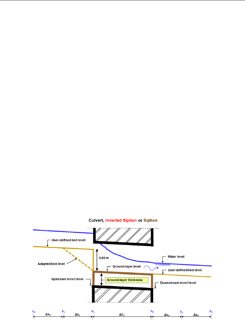
DRAFT
SOBEK, User Manual
Cross-sectional parameters (such as: flow areas, hydraulic radius and so on) are com-
puted based on a cross-sectional profile, that is reduced by the ground layer thickness.
Inverted Siphon, Good modelling practice aspects
It is advised to avoid that the bed level of a cross-section in front of a Culvert, Inverted Siphon
or Siphon is above the ground-layer level (= invert level + ground-layer thickness), since such
situation can result in very small computational time-steps (e.g. long required wall-clock times)
or even in a termination of the simulation.
This is explained as follows. Consider the situation depicted in Figure 6.40 were the bed level
in front of a Culvert (Inverted Siphon or Siphon) is 0.60 m above the ground-layer level. This
means that at small upstream water depths, water will be sucked into the culvert (Inverted
Siphon or Siphon), resulting in large flow velocities. For the computational time-step (∆t)
yields that ∆t≤∆x/U, where Uis the local flow velocity and ∆xis distance between two
water level computational points (or ζ-points). At very low discharges even negative water
depths may be computed, leading to a termination of the simulation.
The situation explained above can be avoided by making the bed level in front of the Culvert
(Inverted Siphon or Siphon) equal to the ground-layer level. In other words by defining a
bed level slope from ζ-point ζ2to ζ3as depicted in Figure 6.40. Providing for the parameter
"Maximum Lowering of Cross-section Bed Level at Culvert" a value greater or equal to 0.60 m
means that before the computation starts, the bed level at ζ-point ζ3is set equal to the ground-
layer level. In Figure 5.15 it is shown how to provide a value for parameter "Maximum Lowering
of Cross-section Bed Level at Culvert".
Figure 6.27: Good modelling practice, Culvert, Inverted Siphon and Siphon
514 of 900 Deltares
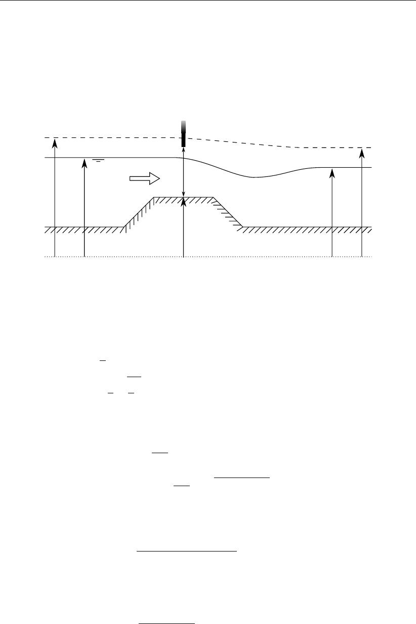
DRAFT
Conceptual description
6.1.16.8 Orifice
The geometrical shape of an orifice is given in Figure 6.28. Four different types of orifice flow
can be discerned, viz: free weir flow, submerged weir flow, free gate flow and submerged gate
flow. No discharge flows through the orifice if its gate is closed, if the upstream water level
equals the downstream water level or if both the upstream water level and the downstream
water level are below the crest level.
Reference level/Model datum
Energy level
H2
ζ1
zs
dg
ζ2
H1
Figure 6.28: Orifice
The following four discharge equations are applied:
1 Free weir flow:
Af=Ws
2
3(ζ1−zs)(6.102)
Q=cwWs
2
3r2
3g(ζ1−zs)3/2(6.103)
2 Submerged weir flow:
Af=Wsζ1−zs−us2
2g(6.104)
Q=cecwWsζ1−zs−us2
2gp2g(ζ1−ζ2)(6.105)
3 Free gate flow:
Af=Wsµ dg(6.106)
Q=cwWsµdgq2g(ζ1−(zs+µ dg)) (6.107)
4 Submerged gate flow:
Af=Wsµ dg(6.108)
Q=cwWsµ dgp2g(ζ1−ζ2)(6.109)
QDischarge across orifice [m3/s]
AFFlow area [m2]
µContraction coefficient [−] Normally 0.63
cwLateral contraction coefficient [−]
ceDischarge coefficient [−]
WsCrest width [m]
Deltares 515 of 900

DRAFT
SOBEK, User Manual
dgOpening height [m] (gate lower edge level minus crest level)
gGravity acceleration [m/s2] (≈9.81)
ζ1Upstream water level [m]
ζ2Downstream water level [m]
zsCrest level [m]
usVelocity over crest [m/s]
The different formulas are applied when the following conditions are met
Free weir flow:
ζ1−zs<3
2dgand ζ1−zs>3/2(ζ2−zs)(6.110)
Submerged weir flow:
ζ1−zs<3
2dgand ζ1−zs≤3
2(ζ2−zs)(6.111)
Free gate flow:
ζ1−zs≥3
2dgand ζ2≤zs+dg(6.112)
Submerged gate flow:
ζ1−zs≥3
2dgand ζ2> zs+dg(6.113)
6.1.16.9 Pump station and Internal Pump station
The functionality of a Pump station and an Internal Pump station is identical. The only differ-
ence comprises the fact that:
Pump station: A Pump station is located on an open channel branch. The pump discharge
is determined using the water levels at the nearest ζ-calculation points, respectively lo-
cated at the upstream-side and downstream-side of the Pump station.
Internal Pump station: An Internal Pump station is accommodated in a pipe. The pump
discharge is determined using the water levels (or hydrostatic pressure heads) at the
upstream side of the pipe and at the downstream side of the pipe.
Here after, both the Pump station and the Internal Pump station are referred to as the Pump
station. Please note that:
When activated, water is always pumped from the suction-side towards the delivery-side,
A Pump station cannot be placed in a compound structure,
A Time Controller, Hydraulic controller, a PID controller or an Interval controller can over-
rule the pump capacity of a Pump station.
Pump station output parameters becomes available by checking the Pump Data check-box
on the 1DFLOW/Output options/Structures Tab in Settings.
Pump direction
Positive pump direction means that the pump discharge is flowing in the positive x-direction
along a branch (see Figure 6.29). Hence, water is pumped in downstream direction to-
wards the pump-side with the highest x-coordinate.
Negative pump direction means that the pump discharge is flowing in the negative x-
direction along a branch (see Figure 6.30). Hence, water is pumped in upstream direction
towards the pump-side with the lowest x-coordinate.
516 of 900 Deltares
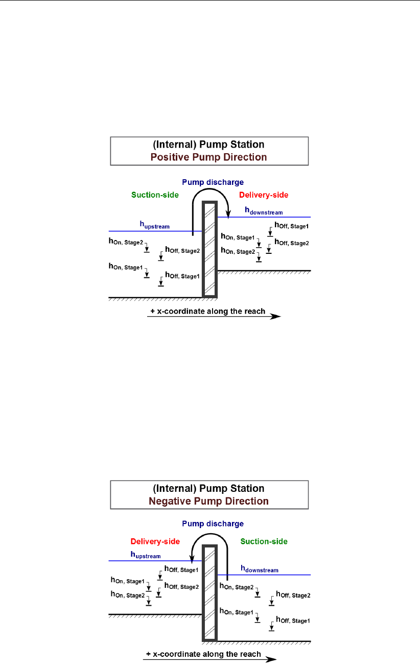
DRAFT
Conceptual description
Figure 6.29: Pump station with positive pump direction and two pump stages
Figure 6.30: Pump station with negative pump direction and two pump stages
Deltares 517 of 900

DRAFT
SOBEK, User Manual
Six possible pump stages
A Pump station comprises of one (1) pump only, which can have up to six different pump
stages (1, 2, 3, 4, 5 or 6). Each pump stage can have a different pump capacity. At each
point-in-time, the pump can be in one (1) particular pump stage only.
The actual pump stage
The actual pump stage is determined using dead-band triggers, defined either at the suction-
side only, at the delivery-side only or both at the suction-side and the delivery-side of the
pump. At the beginning of each time-step for all pump stages, the status [On/Off] of their
dead-band trigger at the suction-side (if defined) and their dead-band trigger at the delivery-
side (if defined) are evaluated. This evaluation is done on basis of actual water levels and the
Switch-on and Switch-off levels, defined for the concerning pump stage. For more details, see
dead-band trigger algorithm. For more information on how to define Switch-on and Switch-off
levels at the suction-side and the delivery-side of the pump, see Conventions for switch-on and
switch-off levels. The actual pump stage, applied in the time-step from t=tto t=t+ ∆t,
is the number of the highest pump stage (1, 2, 3, 4, 5 or 6) that is triggered at t=t, meaning
that all its dead-band triggers have the status [On]. If not any pump stage is triggered, the
pump becomes inactive (pump discharge is zero) and the actual pump stage is set to 0. If the
pump is overruled by a controller, the actual pump stage is set to -1.
Controllers
A Time-controller, a Hydraulic-controller, a PID controller or an Interval controller can be as-
signed to a pump station. A controller is only active in case the pump is triggered in ac-
cordance with the Switch-on and Switch-off levels, defined for stage 1. An active controller
overrules the pump capacity of the triggered pump stage, while the actual pump stage is set
to -1. Please note that capacity reduction factors are applied to the pump capacities set by a
controller. Advice: In using a controller at a pump station, define only one (1) pump stage and
take care that its dead-band trigger is always [On].
Capacity reduction table
A capacity reduction table can be defined, which is applied to all pump stages as well as
to pump capacities, that are set by a controller. In the capacity reduction table a capacity
reduction factor can be given as function of the pump head (e.g. water level at delivery-side
minus water level at suction-side). Pump heads (first column) in a capacity reduction table
should be in increasing order. Capacity reduction factors should be equal or larger than 0.
The pump discharge equals the pump capacity times the capacity reduction factor. If no
capacity reduction table is defined in effect a capacity reduction factor equal to 1 is applied.
Please note that the pump head at t=tis used to determine the capacity reduction factor to
be applied in the time-step from t=tto t=t+ ∆t.
518 of 900 Deltares

DRAFT
Conceptual description
Pump station output parameters
Pump station output parameters can be viewed in Result in Charts (Pump.his file) by checking
the Pump Data check-box on the 1DFLOW/Output options/Structures Tab in Settings. Avail-
able pump station output parameters as function of time are:
Suction-Side level: Water level at the suction-side of the pump.
Delivery-Side level: Water level at the delivery-side of the pump.
Pump Head: The water level at the delivery-side of the pump minus the water level at the
suction-side of the pump.
Actual Pump Stage: Equal to -1 if pump is overruled by a controller; equal to 0 if pump is
inactive; or equal to 1, 2, 3, 4, 5 or 6 depending on the actual pump stage that is triggered
(see Dead-band triggering algorithm).
Pump Capacity: The pump capacity is either defined by its controller; equal to zero if
pump is inactive; or equal to the pump capacity defined for the actual pump stage.
Reduction Factor: The reduction factor follows from the pump head and the capacity re-
duction table.
Pump Discharge: The pump discharge is equal to the pump capacity times the reduction
factor.
Dead-band triggering algoritm
A distinction is to be made between evaluating the status [On/Off] of dead-band triggers de-
fined at the suction-side of the pump and dead-band triggers defined at the delivery-side of
the pump:
Dead-band triggering at the Suction-side of the pump
Parameters used in determining the status [On/Off] of a suction-side dead-band trigger are
hSuction (water level at the suction-side), hOn,Suction (switch-on-level) and hOff,Suction (switch-
off-level), where hOn,Suction > hOff,Suction. Two booleans are used (e.g. SOn,Suction and
SOf f,Suction):
If hSuction > hOn,Suction ⇒SOn,Suction =T rue;Else SOn,Suction =F alse
If hSuction < hOf f,suction ⇒SOf f,Suction =T rue;Else SOf f,Suction =F alse
If at the start of a computation yields that hOf f,Suction ≤hSuction ≤hOn,Suction the dead-
band trigger is set [On]. During a computation the dead-band trigger is set [On] or [Off]
according to the following rules:
If (SOn,Suction =T rue and SOf f,Suction =F alse)⇒T rigger = [On]
If (SOn,Suction =F alse and SOf f,Suction =T rue)⇒T rigger = [Off]
If (SOn,Suction =F alse and SOff,Suction =F alse)⇒T rigger obtains the
status determined in the previous computational time step.
Deltares 519 of 900

DRAFT
SOBEK, User Manual
Dead-band triggering at the Delivery-side of the pump
Parameters used in determining the status [On/Off] of a delivery-side dead-band trigger are
hDelivery (water level at the delivery-side), hOn,Delivery (switch-on-level), hOf f,Delivery (switch-
off-level), where hOff,Delivery > hOn,Delivery. Two booleans are used (e.g. SOn,Delivery and
SOf f,delivery):
If hDelivery < hOn,Delivery ⇒SOn,Delivery =T rue;Else SOn,Delivery =F alse
If hDelivery > hOff,Delivery ⇒SOf f,Delivery =T rue;Else SOf f,Delivery =
F alse
If at the start of a computation yields that hOn,Delivery ≤hDelivery ≤hOff,Delivery the
dead-band trigger is set [On]. During a computation the dead-band trigger is set [On] or [Off]
according to the following rules:
If (SOn,Delivery =T rue and SOf f,Delivery =F alse)⇒T rigger = [On]
If (SOn,Delivery =F alse and SOff,Delivery =T rue)⇒T rigger = [Off]
If (SOn,Delivery =F alse and SOff,Delivery =F alse)⇒T rigger obtains the
status determined in the previous computational time step
Conventions for switch-on and switch-off levels
A distinction is to be made between switch-on-levels and switch-off-levels, defined at the
suction-side and defined at the delivery-side of the pump (see Table 6.1).
Suction-side: The switch-on level should increase with increasing stage number. For each
stage, its switch-off-level should be lower than its switch-on-level. The switch-off-level
should increase with increasing stage number.
Delivery-side: The switch-on-level should decrease with increasing stage number. For
each stage, its switch-off-level should be higher than its switch-on-level. The switch-off-
level should decrease with increasing stage number.
Table 6.1: Example of switch-on-levels and switch-off-levels at the suction-side and the
delivery-side of a pump station
Pump Suction-side Delivery-side
Stage Capacity Switch- Switch- Switch- Switch-
on-level off-level on-level off-level
No m3/s m m m m
1 0.1 0.80 0.10 0.80 1.90
2 0.2 0.90 0.20 0.70 1.80
3 0.3 1.00 0.30 0.60 1.70
4 0.4 1.10 0.40 0.50 1.60
5 0.5 1.20 0.50 0.40 1.50
6 0.6 1.30 0.60 0.30 1.40
520 of 900 Deltares

DRAFT
Conceptual description
6.1.16.10 External Pump station
An External Pump station is to located at the end of an open channel branch or at the end of
a (closed) pipe. The end of an open channel branch can either have the highest x-coordinate
or an x-coordinate equal to zero. The same applies for a pipe. The pump discharge is either
determined using the boundary water level and the water level at the branch-side of the pump
or determined using the boundary water level and the water level (or hydrostatic pressure
head) at the pipe-side of the pump. Please note that:
When activated, water is always pumped from the suction-side towards the delivery-side.
Water can be stored at an External Pump station, for more information see Storage options
at an External Pump station.
The ”External Pump station” cannot be placed in a compound structure,
A Time Controller, Hydraulic controller, a PID controller or an Interval controller can over-
rule the pump capacity of an External Pump station.
External Pump station output parameters becomes available by checking the Pump Data
check-box on the 1DFLOW/Output options/Structures Tab in Settings.
External Pump direction:
Pump direction IN means that (see Figure 6.31):
Water is pumped into the model or flows towards the branch/pipe-side (or upstream-
side) of the pump,
The pump discharge has a negative sign, this is irrespective of the x-direction along
the branch (or pipe).
Pump direction OUT means that (see Figure 6.32):
Water is pumped out off the model or flows towards the boundary-side (or downstream-
side) of the pump ,
The pump discharge has a postive sign, this is irrespective of the x-direction along the
branch (or pipe).
Deltares 521 of 900
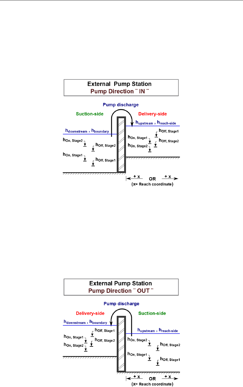
DRAFT
SOBEK, User Manual
Figure 6.31: External pump station with pump direction IN and two pump stages
Figure 6.32: External pump station with pump direction OUT and two pump stages
522 of 900 Deltares

DRAFT
Conceptual description
Six possible External Pump stages
An External Pump station comprises of one (1) pump only, which can have up to six different
pump stages (1, 2, 3, 4, 5 or 6). Each pump stage can have a different pump capacity. At
each point-in-time, the pump can be in one (1) particular pump stage only.
The actual pump stage
The actual pump stage is determined using dead-band triggers, defined either at the suction-
side only, at the delivery-side only or both at the suction-side and the delivery-side of the
pump. At the beginning of each time-step for all pump stages, the status [On/Off] of their
dead-band trigger at the suction-side (if defined) and their dead-band trigger at the delivery-
side (if defined) are evaluated. This evaluation is done on basis of actual water levels and the
Switch-on and Switch-off levels, defined for the concerning pump stage. For more details, see
dead-band trigger algorithm. For more information on how to define Switch-on and Switch-off
levels at the suction-side and the delivery-side of the External Pump station, see Conventions
for switch-on and switch-off levels. The actual pump stage, applied in the time-step from t=t
to t=t+dt, is the number of the highest pump stage (1, 2, 3, 4, 5 or 6) that is triggered at
t=t, meaning that all its dead-band triggers have the status [On]. If not any pump stage is
triggered, the pump becomes inactive (pump discharge is zero) and the actual pump stage is
set to 0. If the pump is overruled by a controller, the actual pump stage is set to -1.
Controllers
A Time-controller, a Hydraulic-controller, a PID controller or an Interval controller can be as-
signed to an External Pump station. A controller is only active in case the pump is triggered in
accordance with the Switch-on and Switch-off levels, defined for stage 1. An active controller
overrules the pump capacity of the triggered pump stage, while the actual pump stage is set
to -1. Please note that capacity reduction factors are applied to the pump capacities set by a
controller. Advice: In using a controller at an External Pump station, define only one (1) pump
stage and take care that its dead-band trigger is always [On].
Capacity reduction table
A capacity reduction table can be defined, which is applied to all pump stages as well as
to pump capacities, that are set by a controller. In the capacity reduction table a capacity
reduction factor can be given as function of the pump head (e.g. water level at delivery-side
minus water level at suction-side). Pump heads (first column) in a capacity reduction table
should be in increasing order. Capacity reduction factors should be equal or larger than 0.
The pump discharge equals the pump capacity times the capacity reduction factor. If no
capacity reduction table is defined in effect a capacity reduction factor equal to 1 is applied.
Please note that the pump head at t=tis used to determine the capacity reduction factor to
be applied in the time-step from t=tto t=t+ ∆t.
Deltares 523 of 900

DRAFT
SOBEK, User Manual
External Pump station output parameters
External Pump station output parameters can be viewed in Result in Charts (Pump.his file)
by checking the Pump Data check-box on the 1DFLOW/Output options/Structures Tab in Set-
tings. Available External pump station output parameters as function of time are:
Suction-Side level: Water level at the suction-side of the pump.
Delivery-Side level: Water level at the delivery-side of the pump.
Pump Head: The water level at the delivery-side of the pump minus the water level at the
suction-side of the pump.
Actual Pump Stage: Equal to -1 if pump is overruled by a controller; equal to 0 if pump is
inactive; or equal to 1, 2, 3, 4, 5 or 6 depending on the actual pump stage that is triggered
(see Dead-band triggering algorithm).
Pump Capacity: The pump capacity is either defined by its controller; equal to zero if
pump is inactive; or equal to the pump capacity defined for the actual pump stage.
Reduction Factor: The reduction factor follows from the pump head and the capacity re-
duction table.
Pump Discharge: The pump discharge is equal to the pump capacity times the reduction
factor.
Dead-band triggering algoritm
A distinction is to be made between evaluating the status [On/Off] of dead-band triggers de-
fined at the suction-side of the External Pump station and dead-band triggers defined at the
delivery-side of the External Pump station:
Dead-band triggering at the Suction-side of the External Pump station:
Parameters used in determining the status [On/Off] of a suction-side dead-band trigger are
hSuction (water level at the suction-side), hOn,Suction (switch-on-level) and hOff,Suction (switch-
off-level), where hOn,Suction > hOff,Suction. Two booleans are used (e.g. SOn,Suction and
SOf f,Suction):
If hSuction > hOn,Suction ⇒SOn,Suction =T rue;Else SOn,Suction =F alse
If hSuction < hOf f,suction ⇒SOff,Suction =T rue;Else SOf f,Suction =F alse
If at the start of a computation yields that hOf f,Suction ≤hSuction ≤hOn,Suction the dead-
band trigger is set [On]. During a computation the dead-band trigger is set [On] or [Off]
according to the following rules:
If (SOn,Suction =T rue and SOff,Suction =F alse)⇒T rigger = [On]
If (SOn,Suction =F alse and SOf f,Suction =T rue)⇒T rigger = [Off]
If (SOn,Suction =F alse and SOff,Suction =F alse)⇒T rigger obtains the
status determined in the previous computational time step.
Dead-band triggering at the Delivery-side of the External Pump station:
Parameters used in determining the status [On/Off] of a delivery-side dead-band trigger are
hDelivery (water level at the delivery-side), hOn,Delivery (switch-on-level), hOf f,Delivery (switch-
off-level), where hOff,Delivery > hOn,Delivery. Two booleans are used (e.g. SOn,Delivery and
SOf f,delivery):
524 of 900 Deltares

DRAFT
Conceptual description
If hDelivery < hOn,Delivery ⇒SOn,Delivery =T rue;Else SOn,Delivery =F alse
If hDelivery > hOff,Delivery ⇒SOf f,Delivery =T rue;Else SOf f,Delivery =
F alse
If at the start of a computation yields that hOn,Delivery ≤hDelivery ≤hOff,Delivery the
dead-band trigger is set [On]. During a computation the dead-band trigger is set [On] or [Off]
according to the following rules:
If (SOn,Delivery =T rue and SOf f,Delivery =F alse)⇒T rigger = [On]
If (SOn,Delivery =F alse and SOff,Delivery =T rue)⇒T rigger = [Off]
If (SOn,Delivery =F alse and SOff,Delivery =F alse)⇒T rigger obtains the
status determined in the previous computational time step
Conventions for switch-on and switch-off levels
A distinction is to be made between switch-on-levels and switch-off-levels, defined at the
suction-side and defined at the delivery-side of the External Pump station (see Table 6.2).
Suction-side: The switch-on level should increase with increasing stage number. For each
stage, its switch-off-level should be lower than its switch-on-level. The switch-off-level
should increase with increasing stage number.
Delivery-side: The switch-on-level should decrease with increasing stage number. For
each stage, its switch-off-level should be higher than its switch-on-level. The switch-off-
level should decrease with increasing stage number.
Table 6.2: Example of switch-on-levels and switch-off-levels at the suction-side and the
delivery-side of an external pump station
Pump Suction-side Delivery-side
Stage Capacity Switch- Switch- Switch- Switch-
on-level off-level on-level off-level
No m3/s m m m m
1 1.1 1.80 1.10 2.80 3.90
2 2.2 1.90 1.20 2.70 3.80
3 3.3 2.00 1.30 2.60 3.70
4 4.4 2.10 1.40 2.50 3.60
5 5.5 2.20 1.50 2.40 3.50
6 6.6 2.30 1.60 2.30 3.40
Deltares 525 of 900

DRAFT
SOBEK, User Manual
Storage options at an External Pump station
Water can be stored at the site, accommodating an external pump station. In SOBEK a
distinction is made between water stored below and above a certain design level, hereafter
referred to as street level.
Below street level: At water levels below street level, water is considered to be stored in a
so-called bottom-storage-reservoir.
Above street level: For water levels above street level, there are three options:
Water is stored in a street-level-reservoir, having a bed level equal to street level and
walls that cannot be overtopped;
Water cannot be stored (e.g. closed pump station), hence water levels inside the pump
station may become pressurized; and
Water leaves the external pump station (e.g. loss of water) by flowing towards low lying
areas, while the water level inside the pump station is considered to remain at street
level.
6.1.16.11 River Pump
The River Pump is to be located on an open channel branch. Please note that:
When activated, water is always pumped from the suction-side towards the delivery-side.
The River – Pump can be placed in a compound structure.
Controllers cannot be assigned to a River - Pump,
Flow - ζ-calculation points are default located 0.5 m in front and 0.5 m behind a River -
Pump.
River pump output parameters becomes available by checking the Pump Data check-box
on the 1DFLOW/Output options/Structures Tab in Settings.
Control direction determines location of trigger-water level (htrig) of a River pump:
The control direction of the River pump defines the location of the so-called trigger-water level
(htrig ):
Upward control direction means that the trigger water level (htrig) is located upward, e.g.
at the pump-side with the lowest x-coordinate along the branch.
Downward control direction means that the trigger water level (htrig) is located downward,
e.g. at the pump-side with the highest x-coordinate along the branch.
Start-level and stop-level determine location of the suction-side and the delivery-side:
The elevation of the start-level (hstart) and the elevation of the stop-level (hstop) define the
location of the suction-side and the delivery-side of a river pump as follows:
If start-level is above stop-level: water is pumped away from the trigger-water level side of
the pump (e.g. trigger-water level side coincides with the suction-side of the pump).
If stop-level is above start-level: water is pumped towards the trigger-water level side of
the pump (e.g. trigger-water level side coincides with the delivery-side of the pump).
526 of 900 Deltares

DRAFT
Conceptual description
Discharge direction of a River pump:
The discharge direction of a river pump with respect to the positive x-direction along the
branch is defined by the control direction and the elevations of the start-level and the stop-
level. Four different situations can be discerned:
Upward control and start-level above stop-level (see Figure 6.33),
Upward control and stop-level above start-level (see Figure 6.34),
Downward control and start-level above stop-level (see Figure 6.35),
Downward control and stop-level below start-level (see Figure 6.36),
Figure 6.33: River pump with Upward control and start-level above stop-level
Deltares 527 of 900
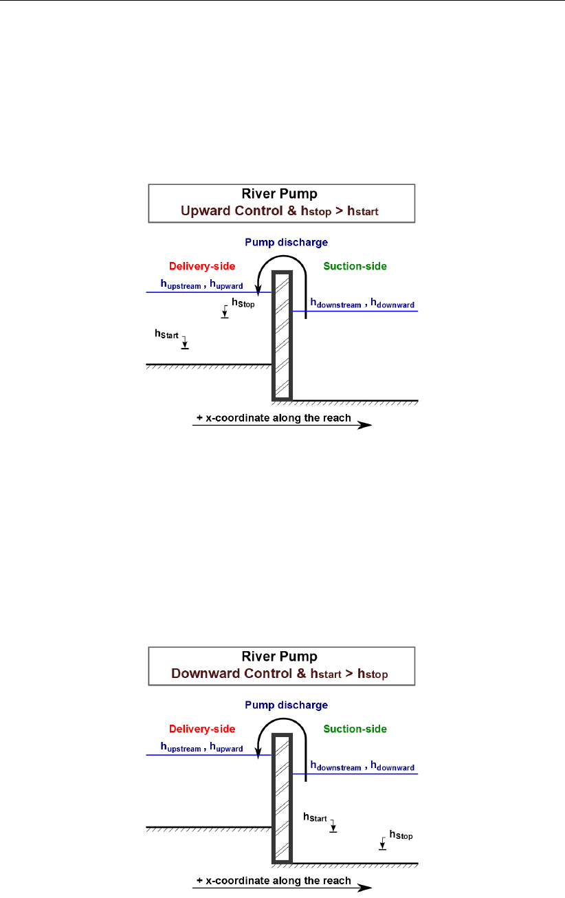
DRAFT
SOBEK, User Manual
Figure 6.34: River pump with Upward control and stop-level above start-level
Figure 6.35: River pump with Downward control and start-level above stop-level
528 of 900 Deltares
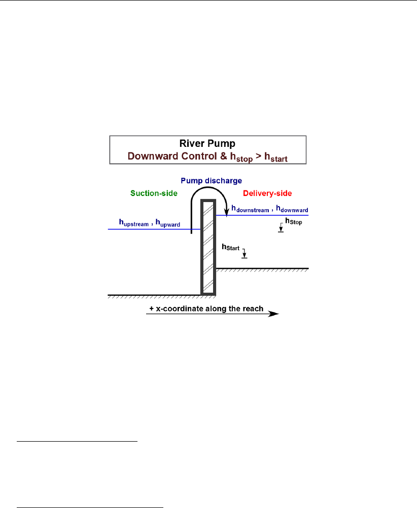
DRAFT
Conceptual description
Figure 6.36: River pump with Downward control and stop-level above start-level
River pump stages
A River pump has only one pump stage, hence only one pump capacity can be defined.
Constant Reduction Factor or Reduction Factor F(Pump Head)
Constant Reduction Factor: WARNING: This means that irrespective of the pump head,
the actual pump capacity always equals the defined pump capacity times the constant
reduction factor. Say you defined a pump capacity of 100 m3/s and constant reduction
factor of 0.7. This means that the pump will have a capacity of 70 (=0.7*100) m3/s for
both positive and negative pump heads.
Reduction Factor F(Pump Head): With this option you define a capacity reduction factor
as function of the pump head (e.g. water level at the delivery-side minus the water level
at the suction-side). The capacity reduction factor may vary between 0 and 1. The first
row in the F(PumpHead )table should read 0,1 (pump head, capacity reduction factor).
For positive pump-heads, the pump discharge equals the pump capacity times the ca-
pacity reduction factor. For negative pump-heads a capacity reduction factor equal to 1
is applied. Please note that the pump head at t=tnis used to determine the capacity
reduction factor to be applied in the time-step from t=tnto t=tn+ ∆t.
Deltares 529 of 900

DRAFT
SOBEK, User Manual
River pump output parameters
River pump output parameters can be viewed in Result in Charts (<Pump.his>file) by check-
ing the Pump Data check-box on the 1DFLOW/Output options/Structures Tab in Settings.
Available River pump output parameters as function of time are:
Suction-Side level: Water level at the suction-side of the pump.
Delivery-Side level: Water level at the delivery-side of the pump.
Pump Head: The water level at the delivery-side of the pump minus the water level at the
suction-side of the pump.
Actual Pump Stage: Equal to 0 if pump is inactive; or equal to 1 if the pump is triggered
(Please note that a river pump has one pump stage only).
Pump Capacity: The pump capacity is either equal to zero if pump is inactive; or equal to
its defined pump capacity.
Reduction Factor: The reduction factor is either a constant or follows from the F(Pump
Head) table
Pump Discharge: The pump discharge is equal to the pump capacity times the reduction
factor.
Dead-band triggering algorithm
A dead-band trigger [On/Off] determines if the River Pump should pump (e.g. actual pump
stage = 1) or not pump (e.g. pump discharge is zero; actual pump stage = 0). The actual status
[On/Off] of the dead-band trigger is determined as follows. Firstly, the value of two Booleans
(Son and Soff ) is determined. In case of triggering at the suction-side of the pump, or in
other words if the start-level (hStart) is above the stop-level (hStop) yields (see Figure 6.33
and Figure 6.35):
If htrig > hStart ⇒Son =T rue;Else Son =F alse
If htrig < hStop ⇒Sof f =T rue;Else Sof f =F alse
In case of triggering at the delivery-side of the pump, or in other words if the stop-level (hStop)
is above the start-level (hStart) yields (see Figure 6.34 and Figure 6.36):
If htrig < hStart ⇒Son =T rue;Else Son =F alse
If htrig > hStop ⇒Sof f =T rue;Else Sof f =F alse
If at the start of a computation yields that hstop ≤htrig ≤hof f , the dead-band trigger is set
[On]. During a computation the dead-band trigger is set [On] or [Off] according to the following
algorithm
If (Son =T rue and Soff =F alse)⇒T rigger = [On]
If (Son =F alse and Soff =T rue)⇒T rigger = [Off]
If (Son =F alse and Soff =F alse)⇒T rigger obtains the status determined
in the previous computational time step
Comparing a River Pump and a Pump station:
From a pump direction point of view the Pump station covers the options available at a
River Pump (see Table 6.3).
Advantage of the River Pump over a Pump station is the fact that it can be placed in a
compound structure
Limitations of the River Pump with respect to the Pump station:
No controllers can be assigned,
Only one (1) pump stage can be defined,
530 of 900 Deltares

DRAFT
Conceptual description
Only one (1) dead-band trigger can be defined at a River Pump, hence it is not possible
to operate the pump on basis of water levels at both its suction-side and its delivery-
side.
Table 6.3: Flow-Pump station covers the options of a River pump with respect to the pump
direction
River pump Pump station
Control Start-level (hstart)Pump Triggering at
Direction Stop-level (hstop)Direction
Upward hstart > hstop Positive Suction-side
Upward hstop > hstart Negative Delivery-side
Downward hstart > hstop Negative Suction-side
Downward hstop > hstart Positive Delivery-side
6.1.16.12 River Weir
Please note that discharges are computed on basis of upstream and downstream energy
levels. Further on please note that default a computational point is located 0.5 m in front
and 0.5 m behind a River weir. A structure inertia damping factor can be defined for each
individual River weir.
Two types of flow conditions can occur in the case of weir flow. These are free (modular) flow
and drowned (submerged) flow. If high tail water conditions do affect the flow, the weir is said
to be drowned. These conditions may then be computed by applying a reduction factor to the
modular function, i.e. to the equation applied if the weir or flume is not drowned (Ackers et al.,
1978;Schmidt,1955;Bos,1989).
Figure 6.37: Free and drowned weir flow
The discharge through the weir is computed with:
Q=cwfWs
2
3r2
3g(H1−zs)3/2(6.114)
in which:
cwcorrection coefficient
Wswidth across flow section
H1upstream energy level
Deltares 531 of 900

DRAFT
SOBEK, User Manual
fsdrowned flow reduction factor
zscrest or sill level of weir
The submergence factor of the weir is defined as:
Sf=H2−zs
H1−zs
(6.115)
in which:
Sfsubmergence factor
H2downstream energy level
If the actual submergence factor exceeds the submergence limit, drowned flow occurs. In all
other cases modular flow occurs and a drowned flow reduction factor equal to 1.0 should be
applied. The submergence limit depends on the crest shape (see Table 6.4).
For a weir the user must specify:
level of crest or crest height
crest width across flow section
crest shape (broad, triangular, round, or sharp)
Depending on the crest shape the following parameters are used (Table 6.4), which can be
adjusted by the user:
correction coefficient (default see Table 6.4)
submergence limit (default see Table 6.4)
drowned flow reduction curve (default see Table 6.4)
Table 6.4: Crest shape and coefficients for simple weir structure (default values)
Crest shape Correction coef. Submergence limit Reduction curve
(Figure 6.38)
broad 1.0 0.82 1
triangular 1.05 0.67 2
round 1.1 0.3 4
sharp 1.2 0.01 5
Notes:
If only one flow direction has been specified, the coefficients for that flow direction are
used as default coefficients for the other flow direction.
The default drowned flow reduction curve depends on the submergence limit.
The drowned flow reduction curve is stored in tabulated format.
532 of 900 Deltares
DRAFT
Conceptual description
Figure 6.38: Drowned flow reduction curves
6.1.16.13 Siphon
A siphon (see Figure 6.39) can only transport water from its upstream defined side to its
downstream defined side. Hence, only positive flow is possible.
A switch-on-level and a switch-off-level at its downstream side determine if the siphon may or
may not discharge water. If the downstream water level drops below the switch-on-level, the
siphon start discharging water. If the downstream water level rises above the switch-off-level,
the siphon stops discharging water. If the downstream water level is in between the switch-on-
level and the switch-off-level (e.g. in between its dead-band), the siphon remains in its present
state of operation. In case the downstream water level is in its dead-band at the onstart of a
computation, the siphon will start discharging water.
Discharge can only flow through a siphon if its upstream cross-sectional area is fully filled with
water, meaning that the upstream water level is above the obvert level (invert level + inner
cross-sectional height) of the siphon. If the upstream cross-sectional area is not fully filled
with water, air will be contained in het upper part of the siphon, this air will prevent the siphon
from discharging water.
ζ1
ζ2
zc1
zc2
L
Figure 6.39: Siphon
Two flow conditions can occur:
Deltares 533 of 900

DRAFT
SOBEK, User Manual
Free flow when ζ2< zc2+dc2
Q=µAfsp2g(ζ1−(zc2+dc2)(6.116)
Submerged flow when ζ2≥zc2+dc2:
Q=µAfsp2g(ζ1−ζ2)(6.117)
QDischarge through siphon [m3/s]
µDischarge coefficient, derived from loss-coefficients [−]
Afs Discharge siphon flow area (= min(Afcrs , Afsgate )) [m2]
Afcrs Cross-sectional area of the siphon. At its highest point the siphon is considered
to be completely filled with water [m2]
Afsgate Flow area under the siphon gate [m2]
gAcceleration due to gravity [m/s2] (≈9.81)
ζ1Upstream water level [m]
ζ2Downstream water level [m]
zc2Downstream siphon invert level [m]
dc2Critical siphon depth at the downstream side
(= 3
qQ2/(gT 2
2)) [m] (6.118)
T2Surface width in the siphon at its downstream side [m]
For numerical reasons the discharge coefficient (µ) is limited to a maximum of 1.0. The
discharge coefficient (µ) is computed as follows:
µ=1
pξi+ξf+ξv+ξb+ξo
(6.119)
ξiEntrance loss coefficient [−]
ξfFriction loss coefficient [−]
ξvValve loss coefficient [−]
ξbBend loss coefficient [−]
ξoExit loss coefficient [−]
The entrance loss coefficient (ξi) can be defined as a constant value only.
The friction loss coefficient (ξf) is computed as follows:
ξf=2gL
C2R(6.120)
LLength of the siphon [m]
CChézy coefficient for fuly water filled siphon [m1/2/s]
RHydraulic radius [m]
If GHO <MIISH; R=Rgate
If GHO ≥MIISH; R=Rsiphon
GHO Gate height opening [m]
MIISH Maximum inner inverted siphon height [m]
Rsiphon Hydraulic radius based on a fully water filled siphon [m]
Rgate Hydraulic radius based on actual gate height opening [m]
534 of 900 Deltares

DRAFT
Conceptual description
The valve loss coefficient (ξv) can be defined as a constant value or as a function of the ratio
of the “Gate height opening” and the “maximum inner siphon height”.
Note:
In case the valve loss coefficient (ξv) is not a constant, in computations the actual valve
loss coefficient (ξv) is derived from the user defined table, while using the ratio of the
“actual gate height opening and the “actual maximum inner siphon height”.
In case the ground layer thickness is greater than zero, both the “actual gate height open-
ing” and the “actual maximum inner siphon height” will differ from the values as defined
in the user interface (see the paragraph "Siphon cross-sections, bed friction and ground
layer" below)
The exit loss coefficient (ξo) is computed as follows:
Submerged flow (ζ2=zc2+dc2):
ξo=k1−Afs
Afr22
(6.121)
kUser defined constant exit loss coefficient [−]
Afr2Flow area in the branch, adjacent to the downstream siphon side [m2]
Afis Siphon flow area [m2]
If GHO ≤MISH; Afs =Afsgate
If GHO >MISH; Afs =Asiphon
GHO Gate height opening [m]
MISH Maximum inner siphon height [m]
Afsgate Flow area under the siphon gate [m2]
Asiphon Flow area based on a fully water filled siphon [m2]
Free flow (ζ2< zc2+dc2):
ξo= 0 (6.122)
Siphon cross-sections, bed friction and ground layer:
For a siphon all available closed cross-section types can be used. In a siphon, a ground
layer with constant thickness can be defined. Siphon friction and ground layer friction can be
specified, using any of the available bed friction formulations.
Defining a ground layer thickness >0 implies that in siphon computations:
Defined invert levels are raised with the ground layer thickness,
Gate height openings are reduced with the ground layer thickness,
Maximum inner height of the siphon is reduced with the ground layer thickness,
Cross-sectional parameters (such as: flow areas, hydraulic radius and so on) are com-
puted based on a cross-sectional profile, that is reduced by the ground layer thickness.
Siphon, Good modelling practice aspects
It is advised to avoid that the bed level of a cross-section in front of a Culvert, Inverted Siphon
or Siphon is above the ground-layer level (= invert level + ground-layer thickness), since such
Deltares 535 of 900
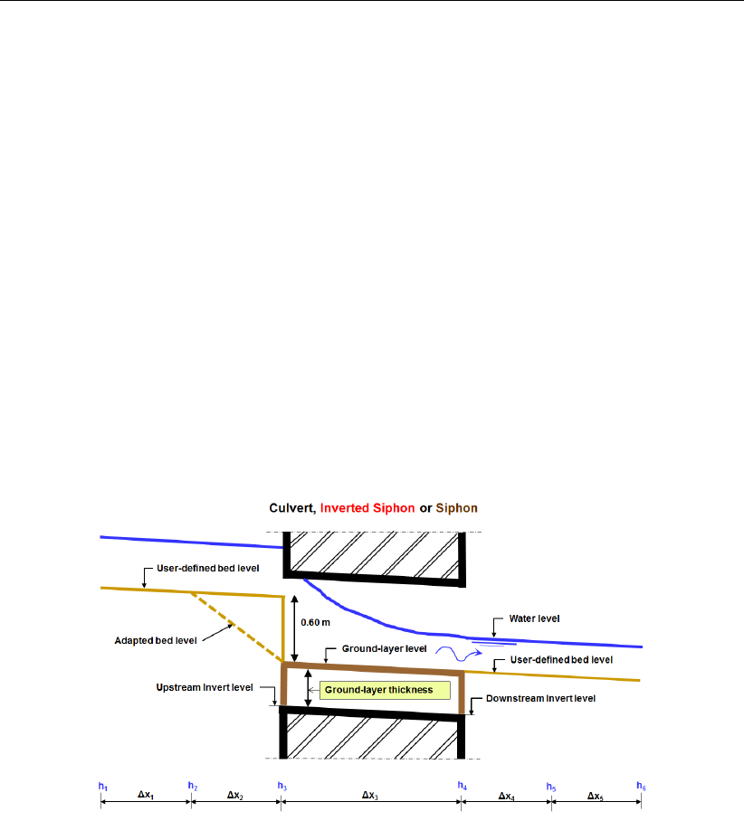
DRAFT
SOBEK, User Manual
situation can result in very small computational time-steps (e.g. long required wall-clock times)
or even in a termination of the simulation.
This is explained as follows. Consider the situation depicted in Figure 6.40 were the bed level
in front of a Culvert (Inverted Siphon or Siphon) is 0.60 m above the ground-layer level. This
means that at small upstream water depths, water will be sucked into the culvert (Inverted
Siphon or Siphon), resulting in large flow velocities. For the computational time-step (∆t)
yields that ∆t≤∆x/U, where Uis the local flow velocity and ∆xis distance between two
water level computational points (or ζ-points). At very low discharges even negative water
depths may be computed, leading to a termination of the simulation.
The situation explained above can be avoided by making the bed level in front of the Culvert
(Inverted Siphon or Siphon) equal to the ground-layer level. In other words by defining a
bed level slope from ζ-point ζ2to ζ3as depicted in Figure 6.40. Providing for the parameter
"Maximum Lowering of Cross-section Bed Level at Culvert" a value greater or equal to 0.60 m
means that before the computation starts, the bed level at ζ-point ζ3is set equal to the ground-
layer level. In Figure 5.15 it is shown how to provide a value for parameter "Maximum Lowering
of Cross-section Bed Level at Culvert".
Figure 6.40: Good modelling practice, Culvert, Inverted Siphon and Siphon
6.1.16.14 Universal Weir
Crest levels of a universal weir (see Figure 6.41) can be defined as a Y-Z profile. The crest
level profile of a universal weir is divided into rectangular weir sections having a horizontal
bed and triangular weir sections having a sloping bed. It is assumed that the discharge
over an universal weir is the summation of the discharges over each individual weir section.
Rectangular weir sections are considered as a broad-crested weir. Triangular weir sections
are considered as (the half of) a broad-crested weir with truncated triangular control section
(Bos,1989).
536 of 900 Deltares

DRAFT
Conceptual description
Figure 6.41: Crest level (Y-Z) profile of a Universal weir, divided into three rectangular
weir sections (2, 4 and 6) and four triangular weir sections (1, 3, 5 and 7)
Parameters depicted in Figure 6.41 are:
AiFlow area of section i[m2]
WiWidth of weir section i[m]
zi,left Elevation at the left side of weir section i[mAD]
zi,right Elevation at the right side of weir section i[mAD]
zCrest Crest level of the Universal weir (output parameter only), equal to the lowest
elevation of its crest level profile [mAD]
ζWater level [mAD]
Following equations yield for a universal weir:
Q=
N
X
i
(uiAi) =
N
X
i
Qi(6.123)
A=
N
X
i
Ai(6.124)
Ustructure =Q/A (6.125)
where:
AFlow area of the universal weir [m2]
AiFlow area of weir section i[m2]
NNumber of weir sections i[−]
QDischarge over the universal weir [m3/s]
QiDischarge over weir section i[m3/s]
uiFlow velocity in weir section i[m/s]
Ustructure Average flow velocity over the universal weir [m/s]
Following equations yield for a rectangular weir section i:
zi,crest =min(zi,left , zi,right)(6.126)
Deltares 537 of 900

DRAFT
SOBEK, User Manual
mlrectangular ,i= 2/3(6.127)
Free rectangular weir flow if ζ2−zi,crest
ζ1−zi,crest ≤mlrectangular ,i
ui=cer2
3gpζ1−zi,crest (6.128)
Ai=2
3Wi(ζ1−zi,crest)(6.129)
Qi=uiAi=ce
2
3r2
3g Wi(ζ1−zi,crest)3/2(6.130)
Submerged rectangular weir flow if ζ2−zi,crest
ζ1−zi,crest > mlrectangular ,i
ui=cep2g(ζ1−ζ2)(6.131)
Ai=Wi(ζ2−zi,crest)(6.132)
Qi=uiAi=ceWi(ζ2−zi,crest)p2g(ζ1−ζ2)(6.133)
Following equations yield for a triangular weir section i:
zi,crest =min(zi,left , zi,right)(6.134)
dzi=|zi,left −zi,right|(6.135)
mltriangular,i=
4
5if (ζ1−zi,crest)) ≤1.25 dzi
2
3+1
6
dzi
(ζ1−zi,crest)if (ζ1−zi,crest)) >1.25 dzi
(6.136)
Free triangular weir flow if ζ2−zi,crest
ζ1−zi,crest ≤mltriangular ,i
ui=ceq2g(1 −mltriangular,i)(ζ1−zi,crest)(6.137)
Ai=
Wi(mltriangular,i(ζ1−zi,crest))2
2dziif ζ1−zi,crest
1/mltriangular,i≤dzi
Wiζ1−zi,crest
1/mltriangular,i−dzi
2if ζ1−zi,crest
1/mltriangular,i> dzi
(6.138)
Qi=uiAi(6.139)
Submerged triangular weir flow if ζ2−zi,crest
ζ1−zi,crest > mltriangular ,i
ui=cep2g(ζ1−ζ2)(6.140)
Ai=
Wi(ζ2−zi,crest)2
2dziif ζ2−zi,crest ≤dzi
Wi(ζ2−zi,crest −dzi
2)if ζ2−zi,crest > dzi
(6.141)
Qi=uiAi(6.142)
538 of 900 Deltares

DRAFT
Conceptual description
where:
AiFlow area of weir section i[m2]
ceDischarge coefficient, applicable to all rectangular weir sections as well as to all
triangular weir sections of a universal weir [−]
dziVertical distance between the elevation at the left side and the right side of a
triangular weir section i[m]
gAcceleration due to gravity [m/s2] (≈9.814)
mlrectangular ,iWater-level-based modular limit of a rectangular weir section i. Its value is
always equal to 2/3 [−]
mltriangular,iWater-level-based modular limit of a triangular weir section i. Its value de-
pends on the actual water depth. [−]
QiDischarge over weir section i[m3/s]
uiVelocity in weir section i[m/s]
WiWidth of weir section i[m]
zi,crest Crest level of weir section i[mAD]
zi,left Elevation at the left side of weir section i[mAD]
zi,right Elevation at the right side of weir section i[mAD]
ζ1Water level at the upstream side of the universal weir [mAD]
ζ2Water level at the downstream side of the universal weir [mAD]
6.1.16.15 Vertical obstacle friction
The vertical obstacle friction terms have been introduced to account for the added resistance
that is caused by vertical obstacles, like houses or trees. The vertical obstacle friction coef-
ficient is based on the number of obstacles, their diameter and drag coefficient. This spatial
coefficient can be prescribed in a ARC-INFO grid file, like the bathymetry.
The vertical obstacle friction coefficient ais specified as the summation of the product of
obstacle width and drag coefficient over the number of obstacles per unit area.
a=1
A
N
X
i=1
DiCdi(6.143)
where:
aVertical obstacle friction coefficient [1/m]
NNumber of obstacles in unit area [−]
AUnit area [m2]
DiDiameter of obstacle i[m]
CdiDrag coefficient of obstacle i[−]
For round pillars, Cd is usually 1.0. In this formulation it is assumed that the obstacle height
will always be larger than the waterdepth. In case the obstacles do become submerged, a
more advanced option is the Depth-Dependent Vegetation Roughness.
Deltares 539 of 900
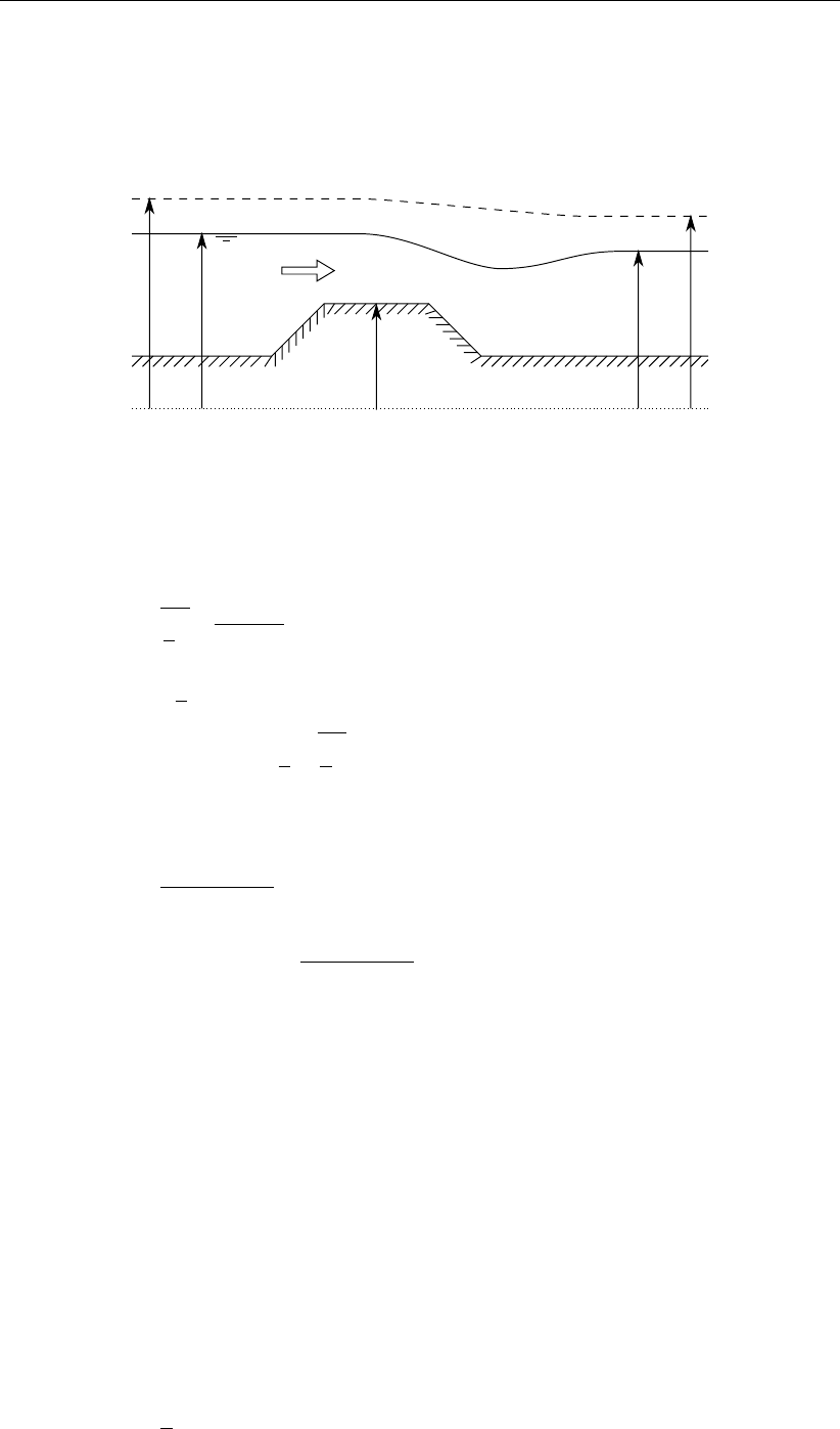
DRAFT
SOBEK, User Manual
6.1.16.16 Weir
Three types of flow conditions can occur in the case of weir flow. These are free (modular)
flow, submerged flow and no flow (water levels below crest level). If high tail water conditions
do affect the flow, the weir is said to be submerged.
Reference level/Model datum
Energy level
H1ζ1
zs
ζ2
H2
Figure 6.42: Weir
The discharge and wetted area through the weir is computed with the following formulas:
Free weir flow:
us=cer2
3gpζ1−zs(6.144)
Af=cwWs
2
3(ζ1−zs)(6.145)
Q=usAf=cecwWs
2
3r2
3g(ζ1−zs)3/2(6.146)
Submerged weir flow:
us=cep2g(ζ1−ζ2)(6.147)
Af=cwWs(ζ2−zs)(6.148)
Q=usAf=cecwWsp2g(ζ1−ζ2)(ζ2−zs)(6.149)
QDischarge across weir [m3/s]
AfWetted area [m2]
ceDischarge coefficient [−]
cwLateral contraction coefficient [−]
WsCrest width [m]
gAcceleration due to gravity [m/s2] (≈9.81)
ζ1Upstream water level [m]
ζ2Downstream water level [m]
zsCrest level [m]
usVelocity over crest [m/s]
The different formulas are applied when the following conditions occur
Free weir flow:
ζ1−zs>3
2(ζ2−zs)(6.150)
540 of 900 Deltares

DRAFT
Conceptual description
Submerged weir flow:
ζ1−zs≤3
2(ζ2−zs)(6.151)
Note:
Broad weirs can cause oscillations, because the discharge calculated with the broad crest
move a lot of water at a time step. This large discharge can lower the upstream water level
significantly resulting in a discharge with a reverse flow direction at the next time step. The
following (rather conservative) rule-of-thumb can be used to avoid oscillations:
As=3
2Ws(6.152)
AsStorage area upstream of the structure [m2]
WsCrest width [m]
6.1.17 Staggered grid; ζ- and u-calculation points at different locations
A SOBEK-Flow-model consists of a network of branches connected to each other at connec-
tion nodes. The SOBEK-Flow-model uses a staggered grid. On a staggered grid the water
level points (e.g. ζ-calculation points) and velocity points (e.g. u-calculation points) are at
different locations (see Figure 6.43). Water levels are computed at the ζ-calculation points,
while velocities are computed half way between the ζ-calculation points, on the so called u-
calculation points. Please note that Connection Nodes and Boundary Nodes are ζ-calculation
points.
In each branch a number of ζ-calculation points can be defined. These ζ-calculation points
represent the spatial numerical grid used in the simulation. The momentum equation is solved
between ζ-calculation points, while the continuity equation is solved between the u-calculation
points.
The location of each ζ-calculation point should be selected on various criteria:
the distance between two neighbouring ζ-calculation points should not be too large (for
accuracy and proper representation of the physical processes)
the distance between two neighbouring ζ-calculation points should not be too small be-
cause of increasing simulation time. The default minimum distance SOBEK uses during a
simulation is 1 meter.
the location of the ζ-calculation points may be non-equidistant.
Deltares 541 of 900
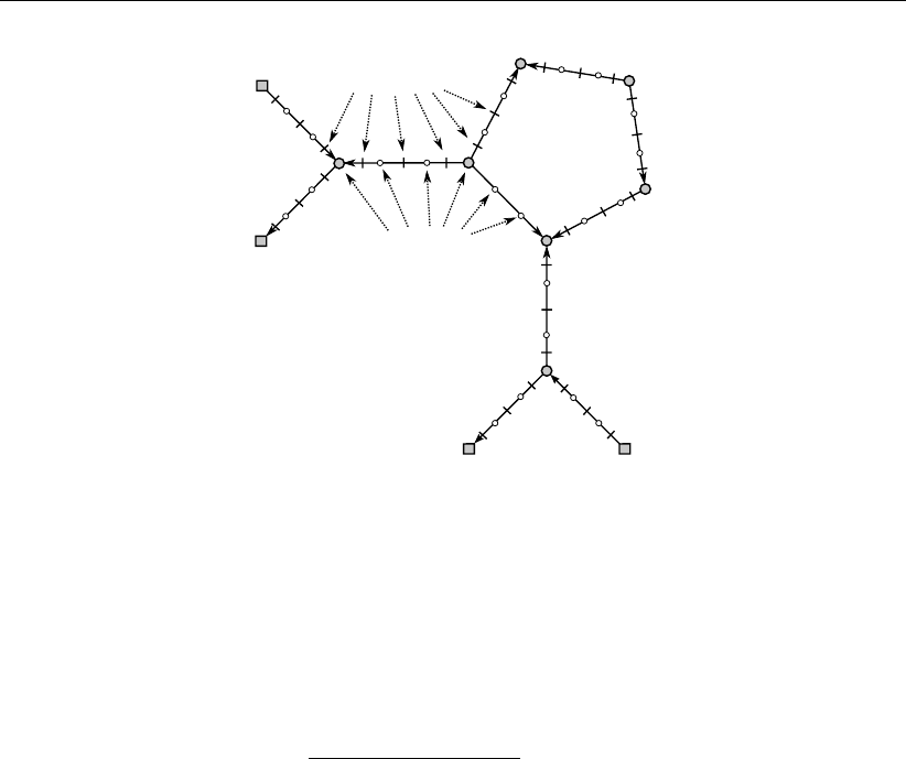
DRAFT
SOBEK, User Manual
ζ-calculation points
u-calculation points
Figure 6.43: Staggered grid, ζ- and u-calculation points at different locations
6.1.18 Construction of the numerical bathymetry on basis of user-defined cross-sections
Cross-sections (e.g. bathymetrical data) may be defined at arbitrary locations in a model,
provided that for each branch at least one cross-section is specified. An overview of the
available type of cross-sections is given in section 5.6.1.
This section explains how the numerical bathymetry of a SOBEK model is constructed on
basis of the user-defined cross-sections. With numerical bathymetry is referred to the bathy-
metrical information, that depending on the cross-section type is available at ζ-calculation
points only or available at both ζ- and u-calcuation points. Water levels and discharges are
computed using this numerical bathymetrical information. For more information on ζ- and
u-calculation points, reference is made to section 6.1.17.
In constructing the numerical bathymetry a distinction is to be made between"’
The Y-Z type of profiles (e.g. Open Vertical Segmented Y-Z profile, Asymmetrical Trapez-
ium profile, Open Lumped Y-Z profile and Closed Lumped Y-Z profile).
All cross-section types except for the Y-Z type of profiles.
6.1.18.1 The Y-Z type of profiles
With the Y-Z type of profiles is referred to the Open Vertical Segmented Y-Z profile, the Asym-
metrical Trapezium profile, the Open Lumped Y-Z profile and the Closed Lumped Y-Z profile
(for more information, see section 5.6.1).
For the Y-Z type of profiles yields that numerical bathymetrical information is made available
at both ζ- and u-calculation points by interpolating (see section 6.1.19) between the user-
defined cross-sectional profiles. The construction of the numerical bathymetrical information
for Y-Z type of profiles is depicted in Figure 6.44.
542 of 900 Deltares
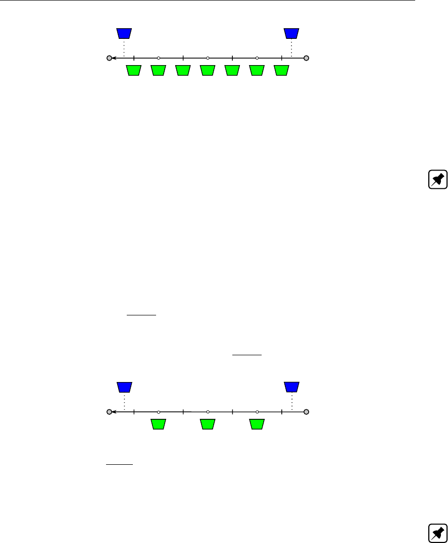
DRAFT
Conceptual description
Figure 6.44: Construction of the numerical bathymetrical information for Y-Z type of pro-
files; Blue coloured objects are the user-defined cross-sections; Green
coloured objects are the interpolated numerical bathymetrical information;
Open circle are ζ-calculation points; Small vertical lines are u-calculation
points
Note: If only one cross-section is specified for a branch, the bathymetrical information of
each ζ-calculation point and each u-calculation point located on this branch will be identical
to this specified cross-section.
6.1.18.2 All cross-section types except for the Y-Z type of profiles
With the Y-Z type of profiles is referred to the Open Vertical Segmented Y-Z profile, the Asym-
metrical Trapezium profile, the Open Lumped Y-Z profile and the Closed Lumped Y-Z profile
(for more information, see Section 5.6.1).
For all cross-section types except for the Y-Z type of profiles yields that numerical bathy-
metrical information is made available at ζ-calculation points only by interpolating (see sec-
tion 6.1.19) between user-defined cross-sectional profiles. The construction of the numerical
bathymetrical information for all cross-section types except the Y-Z type of profiles is depicted
in Figure 6.45.
Figure 6.45: Construction of the numerical bathymetrical information for all cross-section
types except for the Y-Z type of profiles; Blue coloured objects are the user-
defined cross-sections; Green coloured objects are the interpolated numer-
ical bathymetrical information; Open circle are ζ-calculation points; Small
vertical lines are u-calculation points
Note: If only one cross-section is specified for a branch, the numerical bathymetrical infor-
mation for each ζ-calculation point located on this branch will be identical to this specified
cross-section.
6.1.19 Method of interpolating between user-defined cross-sections
This section explains the method of interpolating between user-defined cross-sections. An
overview of the available type of cross-sections is given in section 5.6.1. Following distinction
between cross-sections types is to be made:
Round and Egg-shape (see section 6.1.19.1).
Open Vertical Segmented Y-Z profile and Asymmetrical Trapezium profile (see section 6.1.19.2).
Cross-sections not being a Round, Egg-shape, Open Vertical Segmented Y-Z profile or
Asymmetrical Trapezium profile (see section 6.1.19.3).
Deltares 543 of 900

DRAFT
SOBEK, User Manual
6.1.19.1 Method of Interpolating between Round cross-sections and between Egg-shape
cross-sections
A Round is specified by an invert level, a diameter and the elevation of a ground-layer surface.
Interpolating between two Round cross-sections refers to the linear interpolation along the
branch of invert level, diameter and the elevation of the ground-layer surface.
An Egg-shape is specified by an invert level, a height, a width and the elevation of a ground-
layer surface. Interpolating between two Egg-shape cross-sections refers to the linear inter-
polation along the branch of invert level, height, width and the elevation of the ground-layer
surface.
6.1.19.2 Method of Interpolating between Open Vertical Segmented Y-Z profiles and between
Asymmetrical Trapezium profiles
For both an Open Vertical Segmented Y-Z profile and an Asymmetrical Trapezium profile
yields that first from the user-defined cross-sectional information so-called conveyance ta-
bles are constructed. In a conveyance table the width, area and conveyance as function of
water level are given. Interpolation between two of these type of profile refers to the linear
interpolation along the branch of their respective conveyance tables.
6.1.19.3 Method of Interpolating between Cross-sections not being a Round, Egg-shape, Open
Vertical Segmented Y-Z profile or Asymmetrical Trapezium profile
For all cross-sections not being a Round, Egg-shape, Open Vertical Segmented Y-Z profile or
Asymmetrical Trapezium profile yields that the cross-sectional profile is defined in a Table.
Before interpolation starts it is taken care of that the concerning two cross-sections contain
exactly the same vertical spacing for flow and total widths. In this context vertical spacing
means the level at which a certain width in one of the two cross-sections is defined minus the
bed level (lowest point) of the concerning cross-section. Afterwards, for each vertical spacing
the flow width and total width of an intermediate constructed cross-section is determined by
linear interpolation along the branch. The ground-layer surface of an intermediate constructed
cross-section is determined by linear interpolation along the branch as well.
Note: In case of a River profile, the properties of a summer dike (e.g. Flow area, Total area,
Dike crest level and Flood plain base level) are linear interpolated along the branch. The same
applies for the width of the main section, the width of floodplain 1 and the width of flood plain
2.
Note: The height of a cross-section is the maximum level at which a width is defined minus
the bed level (lowest point) of this cross-section. For open cross-sectional profiles yields that
in case two cross-sections have different heights, the height of the lowest cross-section will be
vertically extended with a width equal to the width defined at its maximum level. This is done
to obtain in the lowest cross-section exactly the same vertical spacing as in the highest cross-
section. Please note that the same procedure is applied for closed cross-sections, with the
exception that the width of the lowest cross-section above its obvert level (maximum defined
level) becomes equal to zero.
544 of 900 Deltares
DRAFT
Conceptual description
6.1.20 Methods for computing conveyance
Conveyance is computed for each u-calculation point (or velocity calculation point). A u-
calculation point is located in the centre point of its two adjacent ζ-calculation points (or water
level calculation points). A distinction is to be made between:
The lumped conveyance approach (see section 6.1.20.1),
Analytical formulae for computing lumped conveyance, and
The vertically segmented conveyance approach (see section 6.1.20.2).
The vertically segmented conveyance approach is used for Y-Z profiles and Asymmetrical
Trapezium cross-sections only. Analytical formulae for computing lumped conveyance are
used for the Egg-shaped cross-section and the Round cross-section. For the remaining cross-
section types, the lumped conveyance approach is used.
6.1.20.1 Lumped conveyance approach
In the lumped conveyance approach, it is assumed that there is an uniform flow velocity (U)
in the cross-sectional profile for a given water level (see Figure 6.46). Hence, it is assumed
that differences in flow velocities across the cross-sectional profile can be neglected. This
assumption generally does not yield for rivers. Therefore, in modelling rivers Y-Z profiles (or
Asymmetrical Trapeziums) are preferred, where conveyance is computed using the vertically
segmented conveyance approach (see section 6.1.20.2).
h
A,Ū
Figure 6.46: Concept of the lumped conveyance approach
First an asymmetrical cross-sectional profile as depicted in Figure 6.46 is transferred into a
symmetrical cross-sectional profile. Thereafter the lumped conveyance is computed as:
K(h) = A(h)C(h)pR(h)(6.153)
where:
K(h)Lumped conveyance at water level h
A(h)Cross-sectional area at water level h
C(h)Chézy friction value at water level h
P(h)Wetted Perimeter at water level h
R(h)Hydraulic radius at water level h(R(h) = A(h)/P (h))
If the water level in an open tabulated rises above the highest level in a cross-sectional profile,
the lumped conveyance is computed taking the flow width at this water level equal to the flow
width, defined at the highest cross-sectional level.
Deltares 545 of 900
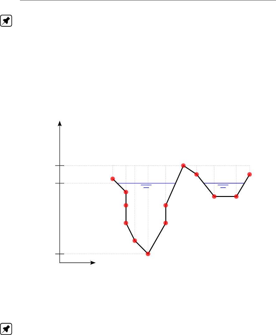
DRAFT
SOBEK, User Manual
Note: Please note that in case of a River profile, the lumped conveyance of its main section,
floodplain 1 and floodplain 2 are computed separately, and thereafter added to obtain the total
lumped conveyance of a river profile at a particular water level.
6.1.20.2 Vertically segmented conveyance approach
The vertically segmented conveyance approach is suited for modelling flow in rivers, since
in this approach it is assumed that flow velocities vary across the cross-sectional profile for a
given water level. In line with this assumption, the cross-section is divided in vertical segments
(see Figure 6.47).
h
Zmin
h
Y
Zmax
Z,
1 2 3 4 5 6 7 8 9
Figure 6.47: Example of constructed vertical segments in a Y-Z profile
13 (yi, zi)points red dots
9 vertical segments
Note: Conveyance table constructed from Zmin to Zmax.
A Y-Z profile is defined by a number (n) of (yi, zi)points. For the total number (nseg) of
vertical segments yields: nseg =n−a−1, where a= number of succeeding (yi, zi)
points for which yi=yi+1. So, please note that vertical walls in a Y-Z profile do not induce
a vertical segment. Moreover, the length of vertical walls is not considered in computing
the conveyance of a Y-Z profile. Omitting vertical walls in computing the conveyance of a Y-Z
profile, means that for a canal having a rectangular profile with a small ratio of width and water
depth only, substantial difference in discharge capacity can occur if such canal is modelled as
a rectangular cross-section (i.e. lumped conveyance approach) or as a rectangle shaped Y-Z
profile (i.e. vertically segmented conveyance approach). The surface level of a Y-Z profile is
equal to its highest (yi, zi)point. In analogy, the same yields for an Asymmetrical Trapezium
cross-section.
The conveyance (Ki) of each vertical segment is computed separately (for formulae, see
546 of 900 Deltares

DRAFT
Conceptual description
conveyance per vertical segment further below). The conveyance of each inclined vertical
segment is determined by solving an integral from yito yi+1. The advantage of using an
integral is that irrespective of the number of user-defined intermediate points, that lie on a
straight line between (y0, z0)to (y1, z1), the same conveyance for the cross-sectional part
from y0to y1is computed. The total conveyance (Ktot) at a particular water level is the
summation of the conveyance of all the vertical segments (Ktot =PKi).
Conveyance tables, applied in the vertically segmented conveyance approach
A conveyance table gives the conveyance, flow width and flow area of a cross-section as func-
tion of water level. Conveyance tables are used for Y-Z profiles and Asymmetrical Trapeziums
only. These conveyance tables are made by a pre-processor before the onstart of a hydrody-
namic calculation. In constructing the conveyance table of each user-defined cross-section,
it is ensured that the difference in conveyance between two succeeding water levels is less
than 1 %. Conveyance tables are used for reducing computational efforts, hence increasing
SOBEK’s computational performance.
Conveyance tables are made from the bed-level up to the highest (yi, zi)point, irrespective of
the actual location of the highest (yi, zi)point within the cross-sectional profile. This implies
that no distinction is made between the left and the right embankment height.
Conveyance tables for computational points located in between two user-defined cross-sections
are obtained by linear interpolating the conveyance tables, constructed at these two user-
defined cross-sections (see also cross-section).
Extrapolation of conveyance tables
Say the water level (h) rises above the highest level (nmax) of a conveyance table. In this
case the conveyance (Kh) at water level (h) is computed as
Kh=a(h−zmin)b,(6.154)
where: zmin is the lowest level in the cross-sectional profile; and a,bare constants derived
from the conveyances at levels nmax and nmax −1.
Lumped hydraulic output for Y-Z profiles and Asymmetical Trapezium
As a courtesy at subsection branch output, lumped hydraulic output (Q,Clumped ,Aflow ,Wflow
and R) are provided for Y-Z profiles and Asymmetrical Trapeziums. The discharge (Q) is
the discharge through the profile, having a flow area (Aflow ) and flow width (Wflow ). The
hydraulic radius (R) is computed on basis of Aflow and Wflow assuming a symmetrical profile
as function of water level. The latter assumption is made, since different Y-Z profiles may
have different shapes, that might have to be interpolated. The lumped Chézy value (Clumped )
is computed as
Clumped =K
Aflow √R,(6.155)
where Kis the conveyance.
Conveyance per vertical segment
A vertical segment is defined by two (y0, z0)and (y1, z1)points for which yields that y0is not
equal to y1(see Figure 6.48).
Deltares 547 of 900
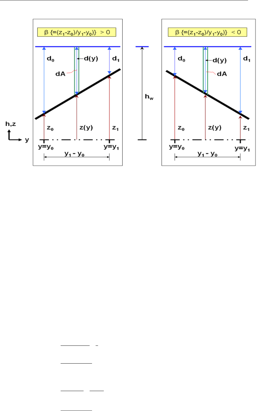
DRAFT
SOBEK, User Manual
Figure 6.48: Definition sketch of a vertical segment, considered in computing conveyance
for a Y-Z profile and an Asymmetrical Trapezium cross-section
Hereunder, the conveyance formulae for a vertical segment are given in case of:
Chézy roughness,
Manning roughness,
Strickler (kn) roughness,
Strickler (ks) roughness,
White-Colebrook (kn) roughness, and
Bos&Bijkerk (γ) roughness.
Chézy roughness conveyance for a vertical segment (see Figure 6.48):
d= max(d0, d1)
if d≤0then
k= 0
else
if d < |z1−z0|then
if |β| ≤ 0.01 then
k1=2C
|β|(1+β2)1/4d
25/2
elseif |β|>0.01 then
k2=2C
5|β|(1+β2)1/4d5/2
elseif d≥ |z1−z0|then
if |β| ≤ 0.01 then
k3=C
(1+β2)1/4d0+d1
23/2(y1−y0)
elseif |β|>0.01 then
k4=2C
5|β|(1+β2)1/4d5/2
0−d5/2
1
endif
endif
548 of 900 Deltares

DRAFT
Conceptual description
endif
Manning roughness conveyance for a vertical segment (see Figure 6.48):
d= max(d0, d1)
if d≤0then
k= 0
else
if d < |z1−z0|then
if |β| ≤ 0.01 then
k1=2
n|β|(1+β2)1/4d
28/3
elseif |β|>0.01 then
k2=3
8n|β|(1+β2)1/4d8/3
elseif d≥ |z1−z0|then
if |β| ≤ 0.01 then
k3=1
n(1+β2)1/4d0+d1
25/3(y1−y0)
elseif |β|>0.01 then
k4=3
8n|β|(1+β2)1/4d8/3
0−d8/3
1
endif
endif
endif
Strickler (kn) roughness conveyance for a vertical segment (see Figure 6.48):
d= max(d0, d1)
if d≤0then
k= 0
else
if d < |z1−z0|then
if |β| ≤ 0.01 then
k1=50k−1/6
n
|β|(1+β2)1/4d
28/3
elseif |β|>0.01 then
k2=75k−1/6
n
8|β|(1+β2)1/4d8/3
elseif d≥ |z1−z0|then
if |β| ≤ 0.01 then
k3=25k−1/6
n
(1+β2)1/4d0+d1
25/3(y1−y0)
elseif |β|>0.01 then
k4=75k−1/6
n
8|β|(1+β2)1/4d8/3
0−d8/3
1
endif
endif
endif
Strickler (ks) roughness conveyance for a vertical segment (see Figure 6.48):
d= max(d0, d1)
if d≤0then
k= 0
Deltares 549 of 900

DRAFT
SOBEK, User Manual
else
if d < |z1−z0|then
if |β| ≤ 0.01 then
k1=2ks
|β|(1+β2)1/4d
28/3
elseif |β|>0.01 then
k2=3ks
8|β|(1+β2)1/4d8/3
elseif d≥ |z1−z0|then
if |β| ≤ 0.01 then
k3=ks
(1+β2)1/4d0+d1
25/3(y1−y0)
elseif |β|>0.01 then
k4=3ks
8|β|(1+β2)1/4d8/3
0−d8/3
1
endif
endif
endif
White-Colebrook (kn) roughness conveyance for a vertical segment (see Figure 6.48):
d= max(d0, d1)
c1= (1 + β2)1/4ln(10)
c2=kn
12
if d≤0then
k= 0
else
if d < |z1−z0|then
if |β| ≤ 0.01 then
if 6d
kn≤1.0005 then
k1=36
|β|(1+β2)1/40.00022 d
25/2
else
k1=36
|β|(1+β2)1/4
10log n6d
knod
25/2
endif
elseif |β|>0.01 then
if d
c2≤1.495 then
k2=36
5|β|c1d5/20.00213
else
k2=36
5|β|c1d5/2ln nd
c2o−2
5
endif
elseif d≥ |z1−z0|then
if |β| ≤ 0.01 then
if 6(d0+d1)
kn≤1.0005 then
k3=18
(1+β2)1/40.00022(y1−y0)d0+d1
23/2
else
k3=18
(1+β2)1/4
10log n6(d0+d1)
kno(y1−y0)d0+d1
23/2
endif
elseif |β|>0.01 then
if d0
c2≤1.495 and d1
c2≤1.495 then
k4=36
5|β|c1d5/2
00.00213 −d5/2
10.00213
550 of 900 Deltares

DRAFT
Conceptual description
elseif d0
c2≤1.495 and d1
c2>1.495 then
k4=36
5|β|c1d5/2
00.00213 −d5/2
1ln nd1
c2o−2
5
elseif d0
c2>1.495 and d1
c2≤1.495 then
k4=36
5|β|c1d5/2
0ln nd0
c2o−2
5−d5/2
10.00213
else
k4=36
5|β|c1d5/2
0ln nd0
c2o−2
5−d5/2
1ln nd1
c2o−2
5
endif
endif
endif
endifendif
Bos&Bijkerk (γ) roughness conveyance for a vertical segment (see Figure 6.48):
d= max(d0, d1)
if d≤0then
k= 0
else
if d < |z1−z0|then
if |β| ≤ 0.01 then
k1=2γ
|β|(1+β2)1/4d
23
elseif |β|>0.01 then
k2=γ
3|β|(1+β2)1/4d3
elseif d≥ |z1−z0|then
if |β| ≤ 0.01 then
k3=γ
(1+β2)1/4d0+d1
22(y1−y0)
elseif |β|>0.01 then
k4=γ
3|β|(1+β2)1/4|d3
0−d3
1|
endif
endif
endif
6.1.21 Delft-scheme
The computation of the water levels and discharges in the SOBEK-flow-network is performed
with the Delft-scheme. This scheme solves the De Saint-Venant equations (continuity and
momentum equation) by means of a staggered grid. In this staggered grid the water levels
are defined at the connection nodes and ζ-calculation points, while the discharges are defined
at the intermediate branches or branch segments.
In general, numerical approximations must satisfy the following requirements:
Robust, i.e. effective or capable of dealing with a wide range of practical problems, without
producing numerical instabilities,
Efficient, i.e. efficient use of computational resources such as processor time,
Accurate, i.e. sufficient accuracy given the modelling purpose.
For the Delft-scheme robustness has been the most important design aspect. By the range
of practical problems to be dealt with the following problems are included:
Drying and flooding
Deltares 551 of 900
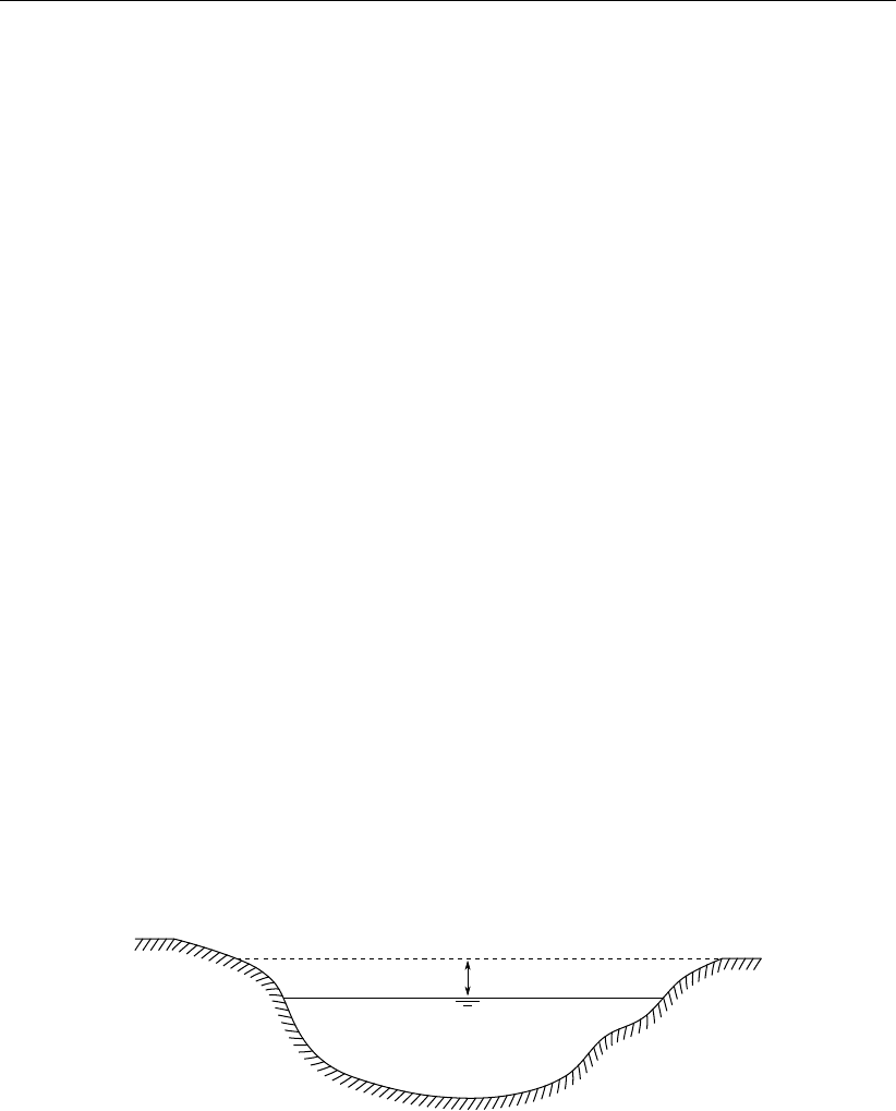
DRAFT
SOBEK, User Manual
Super-critical flow including hydraulic jump.
The used procedure guarantees a solution. In certain flow conditions the time step is reduced
temporarily by a time step estimation procedure to avoid numerical instability.
The Delft-scheme uses a so-called minimum degree algorithm with an iterative simulation
technique. This is highly efficient in case of large networks and long time series.
The Delft-scheme is designed to produce a closed water balance, which makes it very suitable
for water quality computations.
6.1.22 Drying/flooding
When a water level upstream of a branch segment is lower than 5 mm above the bed level of
the ζ-calculation point at this upstream side, the branch segment is assumed to be dry; the
discharge through this branch segment is said to be zero. When a branch segment is dry and
upstream or downstream of the segment the water level rises higher than 10 mm above the
bed level of the ζ-calculation point at that side, the branch segment starts flooding again.
The same deadband is used for the check on drying and flooding of structures. In case of a
weir and orifice, the upstream water level is compared to the crest level. In case of culverts,
siphons and inverted siphons, the water level is compared to the maximum of the bed level
and the bottom of the structure at the upstream side.
6.1.23 Free board
Freeboard is the difference between surface level and water level at some location in the
system. It is defined from surface level to water level, so the freeboard is positive when the
water level is lower than the surface level. When the freeboard is negative, there is a flood at
that location.
Free board
Surface level
Water level
Figure 6.49: Free board
552 of 900 Deltares
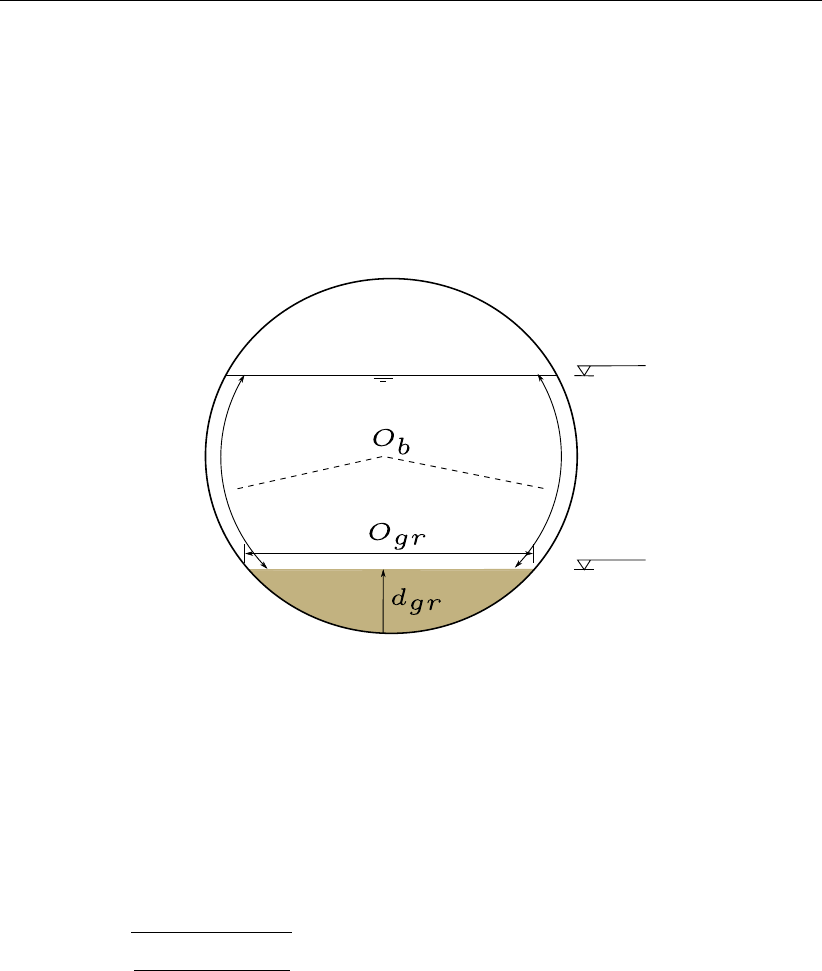
DRAFT
Conceptual description
6.1.24 Ground layer
Except for a Y-Z profile, cross sections can have a fixed horizontal ground layer (or sediment
layer). The ground layer level (top level of the ground layer) equals the bottom level (or invert
level) plus the ground layer thickness. The part of the cross-section located beneath the
ground layer level is omitted in the hydraulic computations. Hence, a ground layer reduces
both the wetted area and the wetted perimeter for a given water level. In Figure 6.50 a circular
cross section is shown with a ground layer with thickness Dgr
Ground layer
Water level
Figure 6.50: Ground layer in circular cross section
For a ground layer a friction value can be specified that differs from the bed friction value. The
ground layer friction value is applied for the cross-sectional width at the ground layer level only.
For the remaining wetted perimeter of the cross-section, the bed friction value is applied. The
same friction formulation (i.e. Chézy, Manning etc.) is to be applied for both the ground layer
and the remaining wetted perimeter (i.e. the bed) of the cross-sectional profile. The combined
friction that is used is computed according to:
ks=sObk2
sb+Ogrk2
sgr
Ob+Ogr
(6.156)
ksCombined Strickler friction value
ksbStrickler bed friction value
ksgr Strickler friction value of the ground layer
ObWetted perimeter of the bed
Ogr Wetted perimeter of the ground layer
6.1.25 Measurement station
In channel flow a measurement station is placed on a branch. From a measurement station
the actual (calculated) value of a water level or a discharge can be retrieved. This value can
then be used in an algorithm of a controller.
The water level that a measurement station retrieves is the water level at the nearest cal-
culation point. The retrieved discharge is the discharge at the branch segment where the
measurement station is located.
Deltares 553 of 900

DRAFT
SOBEK, User Manual
In sewer flow the measurement station can be placed on a connection node or on a branch
Water levels are taken at the nodes, discharges at the branches.
6.1.26 Network
The schematic basis of each model is the network of branches. These branches are con-
nected to each other at connection nodes.
One can say that the network of branches and nodes is the modelled representation of the
real geographic data of the modelled area.
Connection nodes
Branches
ζ-calculation points
Boundary nodes
Figure 6.51: Network
In the Delft-scheme used by the D-Flow 1D module, the network is split up into a staggered
grid. The water levels are defined at the connection nodes and the ζ-calculation points of this
grid, while the discharges are defined at the branch segments.
6.1.26.1 Branch
A branch in a SOBEK-Flow-model is one of the basic elements in the schematisation. A
branch connects two nodes, and has the following attributes:
Begin node
End node
Branch length
554 of 900 Deltares
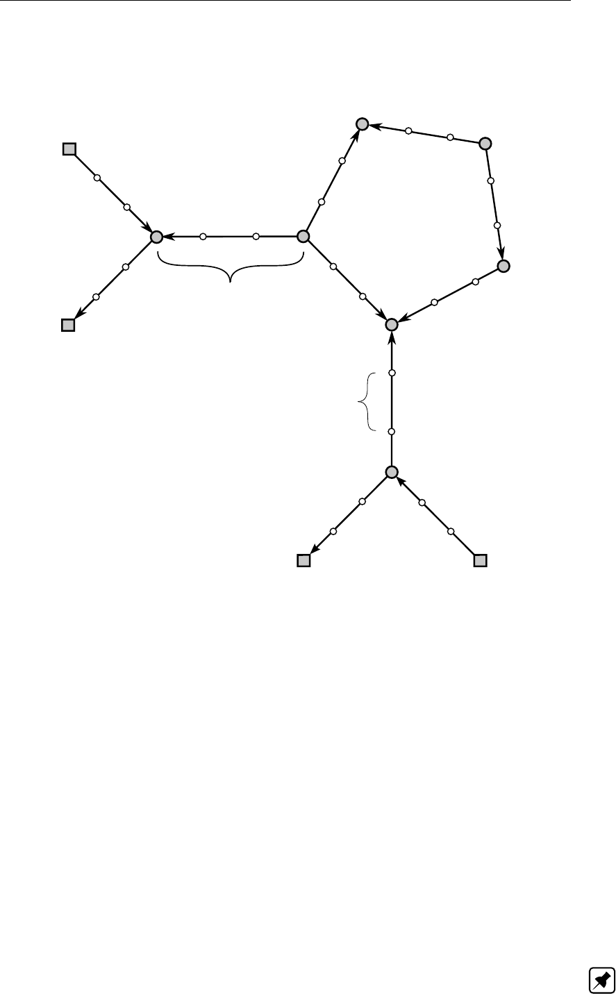
DRAFT
Conceptual description
A geographical orientation (used only in case wind friction effect is included in your model).
The direction of the branch (positive x-direction) is from begin node to end node.
Branch length
Branch segment
Figure 6.52: Branch length in model network
When using channel flow, ζ-calculation points can be specified on a branch. If this is done, the
branch is split up into branch segments. The numerical simulation will be carried out based
on these ζ-calculation points and branch segments in a staggered grid. The discharges are
calculated at the branch or branch segments Water levels are calculated at the connection
nodes and ζ-calculation points.
In case of sewer flow, each branch has a maximum of two ζ-calculation points at the beginning
and end of that branch. The branch can be interpreted as one branch segment
6.1.26.2 Branch length
In sewer systems the length of a branch is the length from the begin connection node to the
end connection node. This length is referred to as the co-ordinate length. In open channel
systems, a branch can be made longer than this minimum co-ordinate length, with the use of
vector points on the branch. This length is referred to as vector length. With this vector length
the actual length of a meandering river or channel can be modelled. If the vector length is
defined on a branch, this length is used in the computation of the water flow equations. If this
length is not defined, the co-ordinate length is used.
Note: The vector length is always equal to or greater than the co-ordinate length
Deltares 555 of 900
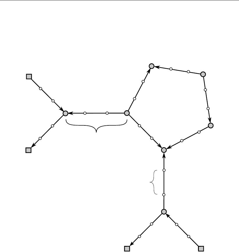
DRAFT
SOBEK, User Manual
6.1.26.3 Branch segment
A SOBEK-Flow-network consists of branches that are connected in connection nodes. These
branches can be divided by ζ-calculation points into segments; the so-called branch seg-
ments. The discharges that result from the water flow equations are defined in these branch
segments
Branch length
Branch segment
Figure 6.53: Branch segment
In sewer networks no ζ-calculation points can be used. So each branch consists of one
branch segment.
6.1.26.4 Connection node
A connection node in a SOBEK-Flow-model is a location where branches can be joined to
other branches. Water levels are defined at the connection nodes and the ζ-calculation points.
556 of 900 Deltares
DRAFT
Conceptual description
Connection nodes
Figure 6.54: Connection nodes
Note: A node located at the bounds of the model can be a connection node (with storage) or
a boundary node (no storage).
6.1.27 Robustness
The Delft-scheme is developed with robustness as its most important design aspect. This
scheme can deal with phenomena such as drying/flooding, supercritical flow and flow transi-
tions (hydraulic jumps) and guarantees a solution for every time step, though the actual com-
putational time step can be reduced internally under certain flow conditions (large discharges
in combination with little storage).
The computational time step reduction is done by a time step estimation procedure before a
new time step or at the end of a time step when negative depths are computed. In the latter
case the step is repeated with a time step reduced by a factor 2 until a correct solution is
achieved.
Deltares 557 of 900

DRAFT
SOBEK, User Manual
6.1.28 Simulation output parameters at branch segments
For more background information on time step reductions, see section Time step reductions
during the simulation. The simulation output parameters available at each branch segment
(see option "Simulation Info at the Branch Segments" in the file <flowanal.his>or in Results
in Charts and Results in Maps) are:
Time step estimation: This refers to the number of times that the time step is reduced,
since the allowable Courant time step of this branch segment is smaller than the user-
defined time step.
No iteration up and No iteration down: Parameters "No iteration up" and "No iteration
down", respectively refer to the number of times that convergence in the Newton iteration
process is not satisfied at the water level point with the lowest x-coordinate ("No iteration
up") and the water level point with highest x-coordinate ("No iteration down") of the branch
segment.
Negative depth up and Negative depth down: Parameters "Negative depth up" and
"Negative depth down", respectively refer to the number of times that a time step re-
duction is needed for avoiding negative depths at the upstream water level point (lowest
x-coordinate) and the downstream water level point (highest x-coordinate) of the branch
segment.
Total: The number of times that the allowable Courant time step is smaller than the user-
defined time step and the number of times that the time step is reduced for either satisfying
the convergence condition or for avoiding negative depths.
6.1.29 Time step reductions during the simulation
The user can define a time step in the Settings Task block. During the computation this user-
defined time step may be reduced for stability reasons (e.g. to prevent the simulation from
crashing). D-Flow1D performs the following checks:
At the start (t=tk) of each computational time-step, the allowable Courant time-step is
determined. This is done as follows:
For each 1D branch segment (i) its 1D Courant time step is computed as:
∆ti=σVoli,tot
Qi,t
1D Courant (6.157)
where:
σthe user-defined value for "maximum flow (1D) and velocity (2D) Courant
number" in Settings
Voli,tot the total volume of water at the upwind (or upstream) water level point
Qi,tkthe discharge at t=tk
Then the 1D branch segment having the smallest 1D Courant time step (e.g. the al-
lowable 1D Courant time step) is determined. The applicable 1D time step at t=tk
is the minimum of the user-defined time step and the allowable 1D Courant time step.
The branch segment with the smallest 1D Courant time step is logged in case its 1D
Courant time step is smaller than the user-defined time step.
The 2D Courant time step for all 2D links in U-direction and for all 2D links in V-direction
are respectively computed as:
∆t=σ∆xm
Um,tk
2D Courant, U-direction (6.158)
and
∆t=σ∆yn
Vn,tk
2D Courant, V-direction (6.159)
558 of 900 Deltares

DRAFT
Conceptual description
where:
σthe user-defined value for "maximum flow (1D) and velocity (2D) Courant
number" in Settings
∆xmthe grid spacing in x-direction
∆ynthe grid spacing in y-direction
Um,tkthe depth-averaged flow velocity in x-direction at t=tk
Vn,tkthe depth-averaged flow velocity in y-direction at t=tk
The allowable 2D Courant time step is the minimum of the 2D Courant time steps
of all 2D U-links and 2D V-links. The applicable 2D time step is the minimum of the
user-defined time step and the allowable 2D Courant time step.
In case of a combined 1D-2D hydraulic computation, the applied time step (∆t) is the
minimum of the applicable 1D time step and the applicable 2D time step.
In each computational time step (from t=tkto tk+1 =tk+ ∆t), it is checked that for
each water level point yields that the lateral inflow volume is not larger than its volume of
water at t=tk. If this condition is not satisfied, the user defined time step is reduced
to such extend that this condition is met. The reduced time step, however, is not made
smaller than the user-defined "minimum time step" in Settings.
Due to various circumstances (discontinuities in model schematization, unrealistic bound-
ary conditions, etc.), the above determined actual time step (∆t) may still be too large for
finding a valid solution at tk+1 =tk+ ∆t. Two conditions are to be fulfilled in finding a
valid solution:
The first condition is that the Newton iteration process converges in terms of water
levels and volumes (both computed at water level points). In other words differences
in water levels and volumes between the last and previous Newton solution are to be
within the user-defined values for "epsilon for water depth" and "epsilon for volume".
In Settings, the user can define the "maximum number of Newton iterations". If the
convergence condition is not satisfied within the maximum number of Newton itera-
tions, the time step is reduced by a factor 2. If this does not satisfy the convergence
condition, the time step is again reduced by a factor 2. The simulation is terminated if a
time step smaller than the user-defined "minimum time step" (see Settings) is needed
for satisfying the convergence condition. All water level points, that after the maximum
number of Newton iterations are conducted, still having a water level convergence
error are logged during a computational time step.
The second condition is that no negative depths (e.g. water level is below bed level)
may occur. Negative depths at a particular water level point may occur if the outflow
during a time step is larger than the volume stored at t=tk. If negative depths occur,
the time step is reduced up to a time step for which yields that the outflow during the
reduced time step is smaller than the volume stored at t=tkand hence no negative
depth occurs. The simulation is terminated if a reduced time step smaller than the
user-defined "minimum time step" (see Settings) is needed to avoid negative depths.
All water level points for which the time step needs to be reduced in order to avoid
negative depths are logged during a computational time step.
Note: If a model run requires a lot of computational effort (e.g. an unexpected long simulation
time is needed), often a large number of time step reductions during simulation is performed.
These time step reductions are needed to find a valid solution and/or to prevent the model
from crashing. Defining a smaller calculation time step in Settings may result in shorter sim-
ulation times. The reason for this, the smaller user-defined time step allows more moderated
intermediate solutions to be found. More moderate solutions reduce the number of circum-
stances in which the model encounters large discontinuities, which require a considerable
Deltares 559 of 900

DRAFT
SOBEK, User Manual
amount of time step reductions before finding a valid solution. The final actual time step can
be much smaller than the user-defined time step. In other words: A smaller user-defined time
step can result in significant less total number of time step reductions leading to a decrease of
total computational time. This is because the total required simulation time is directly related
to the total number of computational time steps.
6.1.30 Slope
In the D-Flow 1D module slope can refer to the slope of the water level or the bed slope. If the
word "slope" is used without further indication, then it pertains to the slope of the water level
in the model. The symbol used is i:
i=∂ζ
∂x (6.160)
where
ζWater level [m]
xDistance [m]
For bed slope, the symbol used is ib:
Bed slope:
ib=∂zb
∂x (6.161)
with zbas the bed level.
6.1.31 Stationary computation
A stationary computation is performed in the D-Flow 1D module by running a non-stationary
simulation until a steady state is branched. During this simulation, all time depending param-
eters, such as lateral and boundary conditions, are set to their initial value and kept constant.
In some cases a steady state cannot be branched, for example, when a pump is switching on
and off. In that case the computation stops after 1 000 simulation steps (not time steps, see
Time step estimation) and the maximum difference of water level compared to the last time
step in the network is given. If this value is low enough (<1 mm for example) the solution can
be considered as steady.
The results of a stationary computation can be used as an initial condition for a non-stationary
simulation.
6.1.32 Summer dike
A flood plain might be separated from a river by means of a small dike, having a crest level
lower than the crest level of the main dike (see Figure 6.55). In the Netherlands large floods
usually occur in winter. The main dike and the small dike are, therefore, respectively referred
to as the “winter dike” and the “summer dike”.
The presence of a summer dike implies that the cross-sectional profile as measured in situ
(see shadowed line in Figure 6.55) does not increase monotonously with rising water levels.
When the water level becomes slightly higher than the crest level of the summer dike, first
the area behind the summer dike is to be filled, before water levels can become any higher.
This implies a local attenuation of the flood wave at water levels just above the crest level of
560 of 900 Deltares
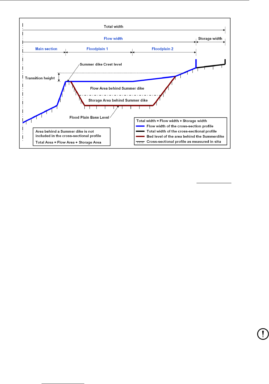
DRAFT
Conceptual description
Figure 6.55: Summer dike option, available in a river profile
the summer dike. This hydraulic phenomenon can be modelled using the summer dike option
available at a river profile.
In defining a summer dike in a river profile a distinction is to be made between:
The cross-sectional profile
The cross-sectional profile comprises of a “flow area” and a “storage area”, which in Fig-
ure 6.55 are respectively located above the blue lines and the black lines. The summation
of flow area and storage area is called the “total area”. Both flow area and total area are
defined by its width as function of elevation. At each elevation in the cross-sectional profile
yields that storage width equals total width minus flow width. Hence, no storage is defined
if total width equals flow width. The flow area of the cross-sectional profile can be divided
in three separate flow sections, respectively called the (i) main section, (ii) floodplain 1
and (iii) floodplain 2 . Each such flow section can have a different roughness value and a
different roughness formulation.
The area behind the summer-dike
In analogy with the cross-sectional profile, the “total area behind a summer dike” is divided
in a “flow area” and a “storage area”. The “Flood Plain Base Level” coincides with the
lowest part of the area behind the summer dike (see Figure 6.55).
Remark:
Both the cross-sectional profile and the area behind the summer dike should be mutu-
ally consistent with the cross-sectional profile as measured in situ (see shadowed line
in Figure 6.55). Hence, both the flow area and the storage area behind the summer
dike should not be included in the cross-sectional profile.
The so-called “transition height” is used for avoiding numerical oscillations. More precisely,
the transition height ensures that the flow area and storage area behind the summer dike
are gradually taken into computation. Transition height for summer dikes is a model-wide
parameter, that is defined in the Settings Taskblock (Edit button next to 1DFLOW (River);
Advanced settings Tab).
Lets consider the following summer dike properties:
Deltares 561 of 900
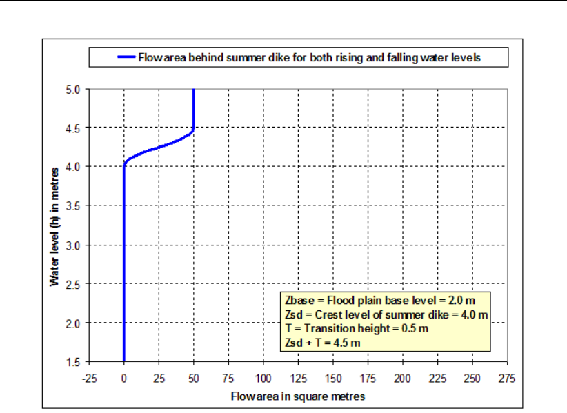
DRAFT
SOBEK, User Manual
Figure 6.56: Flow area behind the summer dike as function of local water levels.
flood plain base level (zbase) of 2 m,
summer dike crest level (zsd) of 4 m,
transition height (T) of 0.5 m,
storage area behind the summer dike of 200 m2,
flow area behind the summer dike (ExtraFlowArea) of 50 m2, and
total area behind the summer dike (ExtraTotalArea) of 250 m2.
In explaining how a summer dike is taken into computation, we make a distinction between:
The actual value of the (extra) flow area behind the summer dike,
The flow velocity applied to the (extra) flow area behind the summer dike, and
The actual value of the (extra) total area behind the summer dike.
The actual (extra) flow area is a unique function of the local water level (h) in the cross-
sectional profile (see Figure 6.56). More precisely:
If ζ < zsd ; Flow area behind the summer dike is zero.
If zsd ≤ζ≤zsd +T; Flow area behind the summer dike varies as a quadratic function
of water level (ζ) between zero and ExtraFlowArea (= 50 m2).
If ζ > zsd +T; Flow area behind the summer dike is equal to ExtraFlowArea.
The flow velocity applied to the (extra) flow area behind the summer dike is the flow velocity in
one of the three available flow sections. Hence, either the flow velocity in the main section, in
floodplain 1 or in floodplain 2. The actual flow velocity applied to the (extra) flow area behind
the summer dike is determined as follows:
1 Default the flow velocity in floodplain 2 is used.
2 However, if the wetted area of floodplain 2 becomes less than 0.4 m2, the flow velocity in
floodplain 1 is used,
562 of 900 Deltares

DRAFT
Conceptual description
3 Furthermore, if the wetted area of floodplain 1 becomes less than 0.4 m2, the flow velocity
of the main section is used.
Remarks:
Please contact Deltares if you like to use a different threshold value (i.e. not 0.4 m2)
for discerning which flow velocity is to be applied to the (extra) flow area behind the
summer dike.
The flow velocity applied to the (extra) flow area behind the summer dike is computed
as follows
Ui=CipRiS i ∈ {main section,floodplain 1,floodplain 2}(6.162)
where:
Uiaverage flow velocity
CiChézy coefficient of the flow section
Ri(Ai+Asd)/Pi: hydraulic radius of the flow section
Aiwetted area of the flow section
Asd extra flow area behind the summer dike
Piwetted perimeter of the flow section
Swater level slope
The discharge including the (extra) flow area behind the summer dike is computed as
follows
Qi=Ui(Ai+Asd)(6.163)
Figure 6.57 depicts the actual (extra) total area behind the summer dike as function of the
local water level (ζ) in the cross-sectional profile. The (extra) total area behind the summer
dike is added to the total area of the cross-sectional profile. There is a hysteresis in the extra
total area for water levels varying from flood plain base level (zbase = 2.0m) to crest level
of summer dike plus transition height (zsd +T= 4.5m). We call line ABC the rising limp
and line CA the falling limp of the hysteresis. The so-called “hysteresis flag” determines which
limp of the hysteris is to be followed. In case the hysteresis flag=1 the rising limp of the
hysteresis is followed, else the falling limp is followed. At the onstart of a computation yields
that the hysteresis flag=1. The actual applied extra total area behind the summer dike is
computed as follows:
1 If ζ < zbase; Hysteresis flag is set to 1. Total area behind the summer dike is zero.
2 If zbase ≤ζ≤zsd +Tand hysteresis flag=1;
For zbase ≤ζ < zsd; Total area behind the summer dike is zero.
For zsd ≤ζ≤zsd +T; Total area behind the summer dike varies as a quadratic
function of water level (ζ) between zero and ExtraTotalArea (= 250 m2)
3 If zbase ≤ζ≤zsd +Tand hysteresis flag=0; Total area behind the summer dike
varies as a quadratic function of water level (ζ) between zero and ExtraTotalArea.
4 If ζ > zsd +T; Hysteresis flag is set to 0. Total area behind the summer dike is equal to
ExtraTotalArea.
Deltares 563 of 900
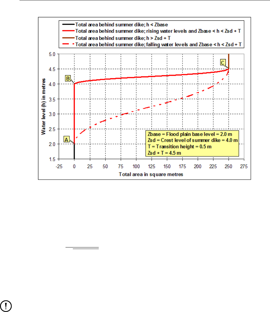
DRAFT
SOBEK, User Manual
Figure 6.57: Total area behind the summer dike as function of local water levels.
6.1.33 Super-critical flow
The D-Flow 1D module can deal with super-critical flow. The flow in a branch or branch
segment is super-critical if the Froude number [−] is higher than 1:
Froude =u
pgAf/Wf
(6.164)
uVelocity [m/s]
gAcceleration due to gravity [m/s2] (≈9.81)
AfWetted area [m2]
WfFlow width [m]
Remarks:
When the Froude number is less than 1, the flow is sub-critical.
Transitions from super-critical to sub-critical flow causes an hydraulic jump.
6.1.34 Surface level
The surface level is the level of the soil surface i.e. the embankment level of the cross section.
When the water level is higher than this level there is a flood. Normally water is stored above
this level on a certain storage area. When the water level drops, this storage is emptying back
into the branch or node.
564 of 900 Deltares
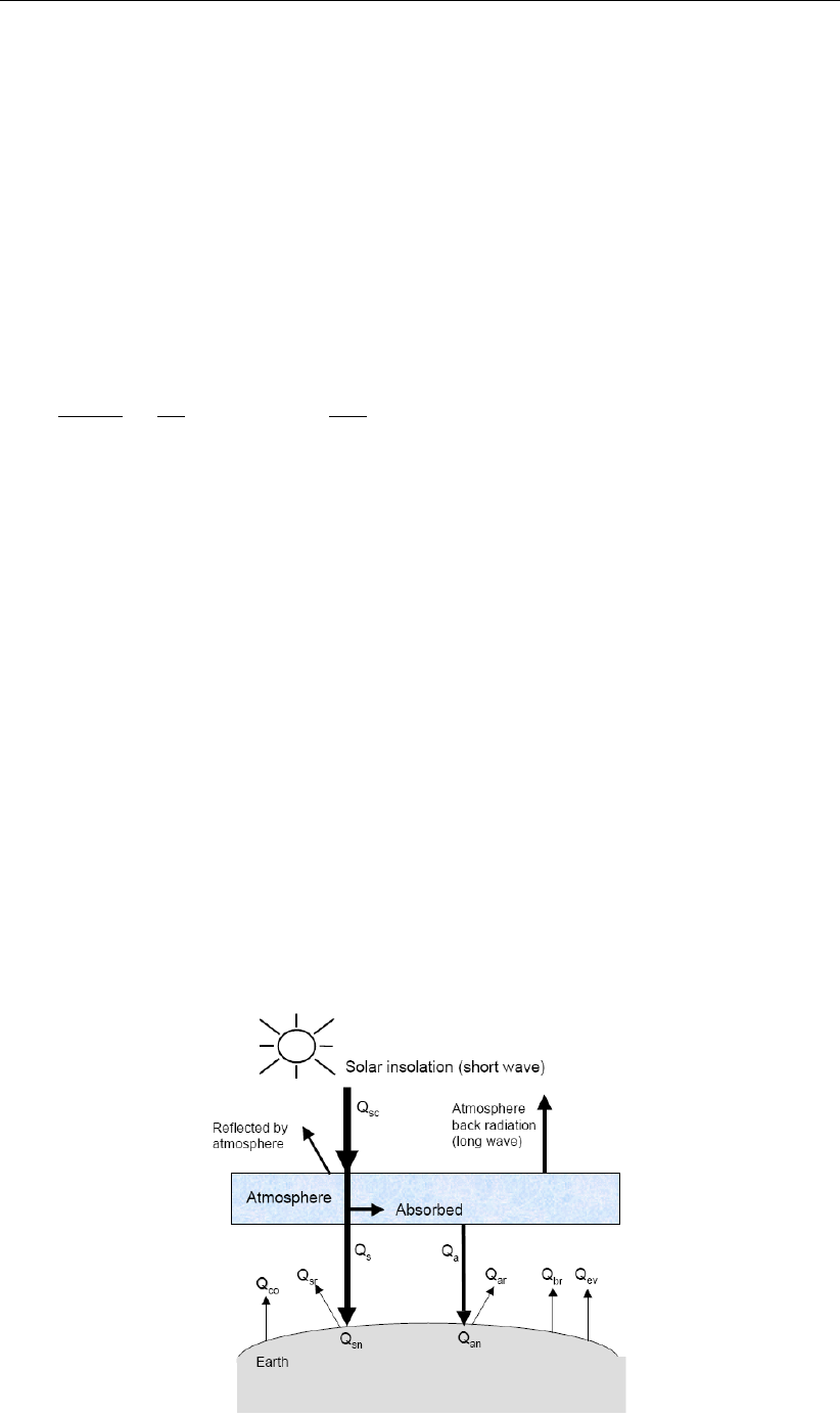
DRAFT
Conceptual description
6.2 Transport equation
The transport of salt, temperature and sediment in estuaries, tidal rivers and alluvial rivers
can be considered as transport of conservative substance in water. These transports are
described by an advection-diffusion equation, which is called the transport equation.
Next to the additional transport equation, density differences have to be accounted for in the
momentum equation of the water flow module. The water flow module is therefore coupled
with the salt intrusion module and temperature by the density and the flow field. The concen-
trations are denoted by C.
The transport equation is described by an advection-diffusion equation including source term
and read:
∂ATC
∂t +∂
∂x QC−AFD∂C
∂x =Ss(6.165)
in which
Cconcentration of salt or chloride, averaged over the total cross-sectional area
[kg/m3]
Ddispersion coefficient [m2/s]
Sssource term [kg/(ms)]
Qdischarge (water) [m3/s]
ATtotal cross-sectional area [m2]
AFflow area [m2]
6.2.1 Temperature: heat flux model
6.2.1.1 General
In D-Flow 1D the heat exchange at the free surface is modelled by taking into account the
separate effects of solar (short wave) and atmospheric (long wave) radiation, and heat loss
due to back radiation, evaporation and convection. In literature there is a great variety of
empirical formulations to calculate these heat fluxes across the sea surface. Most formulations
differ in the dependency of the exchange on the meteorological parameters such as wind
speed, cloudiness and humidity. Some formulations were calibrated for coastal seas others
for lakes.
Figure 6.58: Overview of the heat exchange mechanisms at the surface
Deltares 565 of 900

DRAFT
SOBEK, User Manual
Legend for Figure 6.58:
Qsc radiation (flux) for clear sky condition in [J/m2s]
Qco heat loss due to convection (sensible) in [J/m2s]
Qsr reflected solar radiation in [J/m2s]
Qssolar radiation (short wave radiation) in [J/m2s]
Qsn net incident solar radiation (short wave), =Qs−Qsr
Qaatmospheric radiation (long wave radiation) in [J/m2s]
Qan net incident atmospheric radiation (long wave)
Qar reflected atmospheric radiation in [J/m2s]
Qbr back radiation (long wave radiation) in [J/m2s]
Qev heat loss due to evaporation (latent) in [J/m2s]
In D-Flow 1D the heat exchange at the free surface is modelled by taking into account the
separate effects of solar (short wave) and atmospheric (long wave) radiation, and heat loss
due to background radiation, evaporation and convection. Two heat flux models have been
implemented:
1Excess temperature model
The heat exchange flux at the air-water interface is computed. Only the background tem-
perature is required.
2Composite temperature model
The fraction of the sky covered by clouds is prescribed (in %). The effective back radiation
and the heat losses due to evaporation and convection are computed by the model. Ad-
ditionally, when air and water densities and/or temperatures are such that free convection
occurs, free convection of latent and sensible heat is computed by the model. This model
formulation typically applies for large water bodies.
For the physical background of the heat exchange at the air-water interface and the definitions,
we refer to Octavio et al. (1977) for the excess model and Lane (1989) for the composite
model.
6.2.1.2 Heat balance
The change in temperature Ts(in ◦C) is given by:
∂Ts
∂t =Qtot
ρwcp∆zs
(6.166)
with:
Qtot total heat flux through the air-water surface (in J/(m2s))
ρwspecific density of water (in kg/m3)
cpspecific heat capacity of sea water (= 3930 J/(kg K) )
∆zswater depth
In D-Flow 1D, the heat exchange at the bed is assumed to be zero. This may lead to over-
prediction of the water temperature in shallow areas.
Remarks:
The temperature Tis by default expressed in ◦C. However, in some formulas the abso-
lute temperature ¯
Tin K is used. They are related by:
¯
T=T+ 273.15.(6.167)
In Equation (6.166) the total incoming heat flux is assumed to be absorbed in the water
column. This may result in an unrealistically high surface temperature when the top
566 of 900 Deltares

DRAFT
Conceptual description
layer is thin. This can be prevented by absorbing the incoming radiation as a function
of depth. Currently, this is only implemented in heat flux models 4 and 5.
When using the composite heat flux model, the free convection of latent and sensible
heat is also determined.
6.2.1.3 Excess temperature model
The excess temperature model computes the heat fluxes through the water surface in such a
way that the temperature of the surface layer relaxates to the natural background temperature
specified by you. The heat transfer coefficient mainly depends on the water temperature and
the wind speed.
In the excess temperature model the solar radiation does not play an explicit role, but is part
of the background temperature.
Qtot =−λ(Ts−Ta),(6.168)
with:
λHeat exchange coefficient, is defined by:
λ= 4.48 + 0.049Ts+f(U10)1.12 + 0.018Ts+ 0.00158T2
s(6.169)
Taair temperature
Tswater surface temperature
f(U10)wind function:
f(U10) = (3.5+2.0U10)5.0×10⁶
Sarea 0.05
(6.170)
U10 wind speed
Sarea exposed water surface in m2
6.2.1.4 Composite temperature model
In the Composite temperature model, the heat fluxes through the water surface by incoming
radiation, back radiation, evaporation and convection are computed separately. Evaporation
and convection depend on the air temperature, the water temperature near the free surface,
relative humidity, and wind speed.
The total heat flux through the free surface reads:
Qtot =Qsn +Qan −Qbr −Qev −Qco,(6.171)
with:
Qsn net incident solar radiation (short wave)
Qan net incident atmospheric radiation (long wave)
Qbr back radiation (long wave)
Qev evaporative heat flux (latent heat)
Qco convective heat flux (sensible heat).
Qtot =Qsn −Qeb −Qev −Qco,(6.172)
with:
Deltares 567 of 900
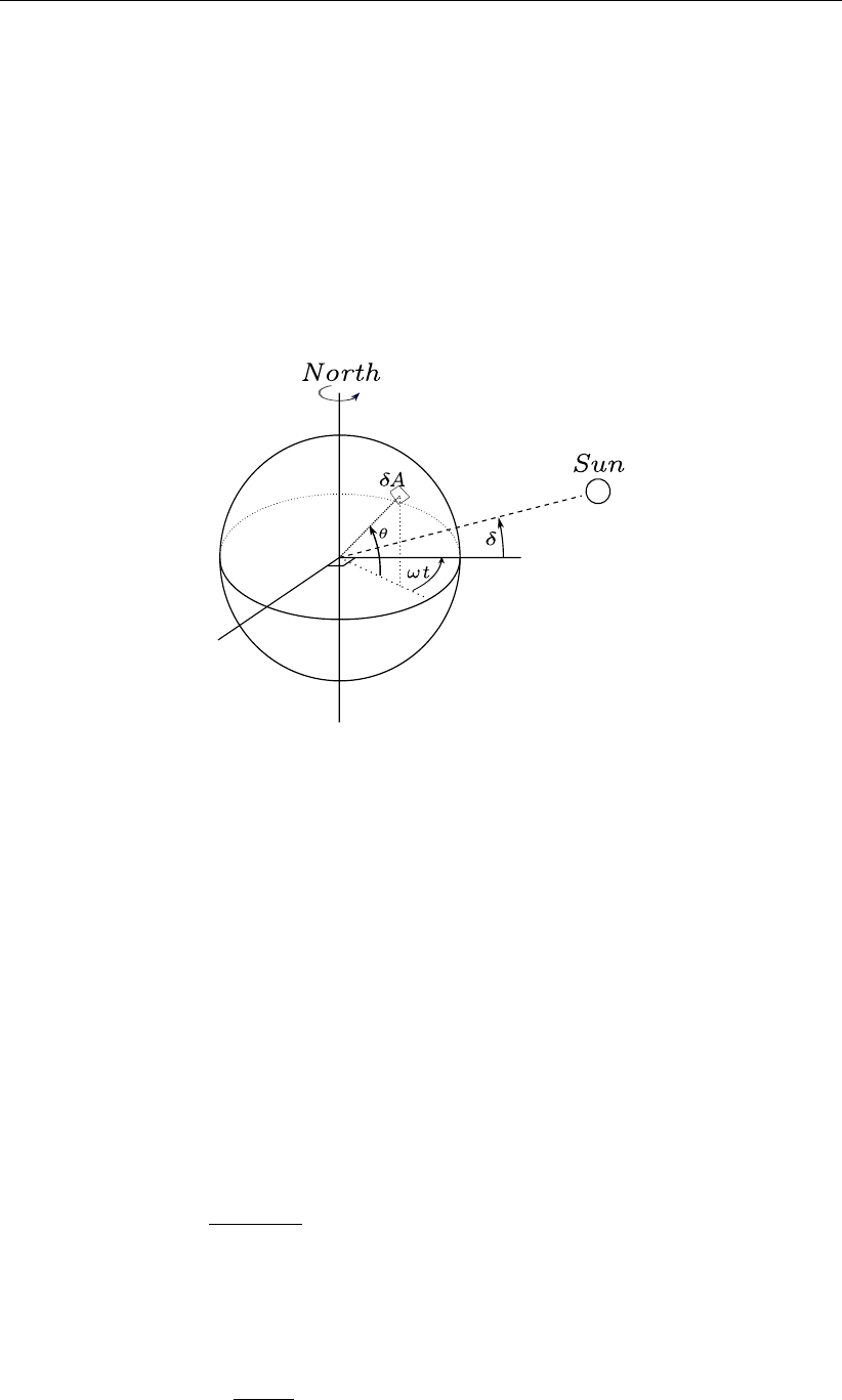
DRAFT
SOBEK, User Manual
Qeb =Qbr −Qan
The subscript nrefers to a net contribution.
6.2.1.5 Solar radiation
The short-wave radiation emitted by the sun that reaches the earth surface under a clear sky
condition is computed by means of an emperical formula
The solar radiation is computed by D-Flow 1D and is dependent on the geographical position
at the earth and the local time.
Figure 6.59: Co-ordinate system position Sun
δ: declination; θ: latitude; ωt: angular speed
Not all of the radiation is absorbed at the water surface. A part is transmitted to deeper water.
Short waves can penetrate over a distance of 3 to 30 meters, depending on the clarity of the
water, while the relatively longer waves are absorbed at the surface. Therefore, it is convenient
to separate the incoming solar insolation into two portions:
1βQsn, the longer wave portion, which is absorbed at the surface and
2(1 −β)Qsn, the remainder part, which is absorbed in deeper water.
The absorption of heat in the water column is an exponential function of the distance Hfrom
the water surface:
(1 −β)Qsn =ZH
0
e−γz dz ⇒(6.173)
Qsn (h) = γe−γh
1−e−γH (1 −β)Qsn,(6.174)
with:
βpart of Qsn absorbed at the water surface which is a function of the wavelength.
The default value of βin Delft3D-FLOW is 0.06.
γextinction coefficient (measured) in m−1, also related to the so-called Secchi-
depth γ=1.7
HSecchi
hdistance to the water surface in meters.
Htotal water depth.
568 of 900 Deltares

DRAFT
Conceptual description
Remark:
The exponential decay function, Equation (6.174) has only been implemented in 3D-
computations. Since D-Flow 1D is a depth averaged model, the distinction between
long and short wave radiation is not relevant.
The incoming energy flux at the water surface depends on the angle (declination) between
the incoming radiation and the Earth’s surface. This declination depends on the geographical
position on the Earth and the local time. The Earth axis is not perpendicular to the line
connecting the Sun with Earth. This tilting (angle δ) varies with the time of the year and it
leads to a seasonal variation of the radiation flux. At June 21, the declination is maximal,
23.5 degrees. Of course, by the rotation of the Earth the solar radiation also varies during the
day. Near twelve o’clock local time, the sun elevation above the horizon is maximal. For an
overview of the angles used to determine the solar elevation angle γ, see Figure 6.59.
The temporal and latitude-dependent solar elevation angle γis estimated by:
sin (γ) = sin (δ) sin πφ
180−cos (δ) cos πφ
180cos (ω1t)(6.175)
with:
δ=23.5π
180 cos(ω0t−2.95)
ω0frequency of the annual variation (= 2π/(365.24 ×24))
ω1frequency of the diurnal variation (= 2π/24)
φlatitude
tnumber of hours since 1st of january
The incoming short-wave solar radiation through a clear sky at ground level Qsc is about 0.76
of the flux incident at the top of the atmosphere (Gill,1982):
Qsc =0.76Ssin(γ),sin(γ)≥0,
0.0,sin(γ)<0.(6.176)
The solar constant S= 1 368 J/(m2s) or W/m2. This is the average energy flux at the mean
radius of the Earth.
A part of the radiation that reaches the water surface is reflected. The fraction reflected or
scattered (surface albedo) is dependent on latitude and season. Cloud cover will reduce the
magnitude of the radiation flux that reaches the sea surface. The cloudiness is expressed by
a cloud cover fraction Fc, the fraction of the sky covered by clouds. The correction factor for
cloud cover is an empirical formula. The absorption of solar radiation is calculated (Gill,1982)
as the product of the net downward flux of short wave-radiation in cloudless conditions and
factors correcting for reflection and cloud cover:
Qsn =Qs−Qsr = (1 −α)Qscf(Fc),(6.177)
with:
Qssolar radiation (short wave radiation) in [J/(m2s)]
Qsr reflected solar radiation in [J/(m2s)]
Qsc see Equation (6.176)
sin (γ)see Equation (6.175)
f(Fc) = 1.0−0.4Fc−0.38F2
c
Deltares 569 of 900

DRAFT
SOBEK, User Manual
αalbedo (reflection) coefficient (= 0.06)
Fcfraction of sky covered by clouds (user-defined input)
Ssolar constant (=1368 J m−2 s−1)
6.2.1.6 Effective back radiation
The total net long wave radiation flux is called the effective back radiation:
Qeb =Qbr −Qan.(6.178)
The atmospheric radiation depends on the vapour pressure ea, the air temperature Taand
the cloud cover Fc. The back radiation depends on the surface temperature Ts.
Qeb =εσ ¯
T4
s(0.39 −0.05√ea)1.0−0.6F2
c,(6.179)
with:
εemissivity factor (0.985 )
σStefan-Boltzmann’s constant = 5.67 ×10⁻⁸in [J/(m2sK4]
¯
Tsthe (absolute) water surface temperature in [K].
eaactural vapour pressure:
ea=rhum100.7859+0.03477Ta
1.0+0.00412Ta(6.180)
Fcfraction of sky covered by clouds (user-defined input)
6.2.1.7 Evaporative heat flux
Evaporation is an exchange process that takes place at the interface between water and air
and depends on the conditions both in the water near the surface and the air above it. The
evaporation depends on meteorological factors (wind-driven convection) and vapour pres-
sures.
The evaporative heat flux Qev is defined by:
Qev =LvE, (6.181)
with Lvthe latent heat of vaporisation in J/kg water:
Lv= 2.5×10⁶−2.3×10³Ts.(6.182)
The evaporation rate Eis defined as the mass of water evaporated per unit area per unit time
[kg/(m2s)]. It is computed by using a form of Dalton’s law of mass transfer:
E=f(U10) (es−ea),(6.183)
where the actual vapour pressure eaand the saturated vapour pressure es, is defined as:
es= 100.7859+0.03477Ts
1.0+0.00412Ts,(6.184)
ea=rhum100.7859+0.03477Ta
1.0+0.00412Ta.(6.185)
Here rhum is the relative humidity in [-].
Remarks:
570 of 900 Deltares

DRAFT
Conceptual description
The relative humidity rhum is specified as a function of time.
The vapour pressures are calculated using air and water surface temperature in ◦C.
When the computed Eis negative, it is replaced by zero, assuming that it is caused by
modelling misfit and not by the actual physical process of water condensation out ot the
air into the water.
The evaporation rate is computed from the difference in relative humidity, rather than from
the difference in vapour pressure. The contribution to the evaporative heat flux is split in a
contribution by forced convection and a contribution by free convection. These are discussed
separately.
Forced convection of latent heat
The latent heat flux due to forced convection reads:
Qev,forced =LVρaf(U10){qs(Ts)−qa(Ta)},(6.186)
with qsand qathe specific humidity of respectively saturated air and remote air (10 m above
water level):
qs(Ts) = 0.62es
Patm −0.38es
,(6.187)
qa(Ta) = 0.62ea
Patm −0.38ea
.(6.188)
The saturated and remote vapour pressures esand eaare given by Eqs. (6.184) and (6.185).
The latent heat Lvis given by equation (6.182)
The wind function in Equation (6.186) is defined as:
f(U10) = ceU10,(6.189)
Free convection of latent heat
Loss of heat due to evaporation occurs not only by forced convection, wind driven, but also
by free convection. Free convection is driven by buoyant forces due to density differences
(by temperature and/or water vapour content) creating unstable conditions in the atmospheric
boundary layer (ABL). Evaporation due to free convection is important in circumstances where
inverse temperature/density gradients are present and wind speeds are almost negligible so
that the amount of forced convection is small. Neglecting free convection in this situation will
lead to underestimating the heat loss. (Ryan et al.,1974) developed a correction to the wind
function, accounting for free convection. The derivation of evaporation by just free convection
is based on the analogy of heat and mass transfer.
The latent heat flux due to free convection reads:
Qev,free =ksLVρa(qs−qa),(6.190)
with the average air density:
ρa=ρa0+ρa10
2,(6.191)
Deltares 571 of 900

DRAFT
SOBEK, User Manual
and with the heat transfer coefficient defined as:
ks=(0if ρa10 −ρa0≤0
cfr.conv ngα2
νair ρa(ρa10 −ρa0)o1/3if ρa10 −ρa0>0(6.192)
where the coefficient of free convection cfr.conv was calibrated to be 0.14, see (Ryan et al.,
1974). The viscosity of air νair is assumed to have the constant value 16.0×10⁻⁶m2/s. The
molecular diffusivity of air αm2/s is defined as
α=νair
σ,(6.193)
with σ= 0.7(for air) the Prandtl number. In Equation (6.190), the saturated air density is
given by:
ρa0=
100Patm−100es
Rdry +100es
Rvap
Ts+ 273.15 ,(6.194)
the remote air density (10 m above the water level):
ρa10 =
100Patm−100ea
Rdry +100ea
Rvap
Tair + 273.15 ,(6.195)
where Rdry is the gas constant for dry air: 287.05 J/(kg K) and Rvap is the gas constant
for water vapour: 461.495 J/(kg K). The specific humidity of respectively saturated air and
remote air (10 m above the water level), qsand qaare given by Eqs. (6.187) and (6.198). The
saturated and remote vapour pressure esand eaare defined in Eqs. (6.184) and (6.185).
Qev evaporative heat flux summarized
The total heat flux due to evaporation then results from adding the forced convection of latent
heat in Equation (6.186) and the free convection of latent heat in Equation (6.190):
Qev =Qev,forced +Qev,free (6.196)
Qev,free =ksLVρa{qs(Ts)−qa(Ta)}(6.197)
Qev,forced =LVρaf(U10){qs(Ts)−qa(Ta)}(6.198)
with:
ksheat transfer coefficient:
ks=(0if ρa10 −ρa0≤0
cfr.conv ngα2
νair ρa(ρa10 −ρa0)o1/3if ρa10 −ρa0>0(6.199)
LVLvthe latent heat of vaporisation
LV= 2.5×10⁶−2.3×10³Ts(6.200)
qs(Ts)The specific humidity of saturated air
qs(Ts) = 0.62es
Patm −0.38es
(6.201)
qa(Ta)The specific humidity of remote air
qa(Ta) = 0.62ea
Patm −0.38ea
(6.202)
572 of 900 Deltares

DRAFT
Conceptual description
f(U10)wind function: ceU10
ρaaverage air density:
ρa=ρa0+ρa10
2(6.203)
ρa0The saturated air density is given by:
ρa0=
100Patm−100es
Rdry +100es
Rvap
Ts+ 273.15 (6.204)
ρa10 remote air density (10 m above the water level):
ρa10 =
100Patm−100ea
Rdry +100ea
Rvap
Ta+ 273.15 (6.205)
essaturated pressure:
es= 100.7859+0.03477Ts
1.0+0.00412Ts(6.206)
earemote vapour pressure:
ea=rhum100.7859+0.03477Ta
1.0+0.00412Ta(6.207)
Rdry gas constant for dry air: 287.05 J/(kg K) is the
Rvap gas constant for water vapour: 461.495 J/(kg K)
Patm Atmospheric pressure
U10 Wind velocity at 10 m
ceDalton number (=0.0015)
rhum relative humidity
Taair temperature
Tswater surface temperature
cfr.conv coefficient of free convection (= 0.14)
ggravity
αmolecular diffusivity (= νair/σ)
νair viscosity of air (=16.0×10⁻⁶m2/s)
σPrandtl number (= 0.7)
6.2.1.8 Convective heat flux
The convective heat flux is split into two parts, just as the evaporative heat flux. The con-
vective heat flux is divided into a contribution by forced convection and a contribution by free
convection.
Qco =Qco,forced +Qco,free (6.208)
Forced convection of sensible heat
The sensible heat flux due to forced convection is computed by:
Qco,forced =ρacpg(U10) (Ts−Ta),(6.209)
with:
ρaair density as specified in input
g(U10)wind speed function is defined following Gill (1982): cHU10
Deltares 573 of 900

DRAFT
SOBEK, User Manual
cHStanton number (= 0.0013)
Taair temperature
Tswater surface temperature
cpa specific heat capacity of air; = 1004.0 J/(kg K)
Free convection of sensible heat
The sensible heat flux due to free convection is computed by:
Qco,free =ksρacpa (Ts−Ta)(6.210)
with:
ksheat transfer coefficient:
ks=(0if ρa10 −ρa0≤0
cfr.conv ngα2
νair ρa(ρa10 −ρa0)o1/3if ρa10 −ρa0>0(6.211)
ρaaverage air density:
ρa=ρa0+ρa10
2(6.212)
ρa0The saturated air density is given by:
ρa0=
100Patm−100es
Rdry +100es
Rvap
Ts+ 273.15 (6.213)
ρa10 remote air density (10 m above the water level):
ρa10 =
100Patm−100ea
Rdry +100ea
Rvap
Ta+ 273.15 (6.214)
cHStanton number (= 0.0013)
Taair temperature
Tswater surface temperature
cpa specific heat capacity of air; = 1004.0 J/(kg K)
6.2.1.9 Input parameters for composite model
The input parameters for the composite model are:
Fcpercentage of sky covered by clouds (time dependent, Meteo data)
Taair temperature in ◦C (time dependent, Meteo data)
rhum percentage of relative humidity (time dependent, Meteo data)
ceDalton number (default value: 0.0013)
cHStanton number (default value: 0.0013)
cpspecific heat capacity of water (default value: 3930 J/(kg K) for sea water)
574 of 900 Deltares

DRAFT
Conceptual description
6.2.2 Salinity dispersion
When one of the boundaries of a river or estuary is in contact with the sea, salt water may enter
the system. Salt intrusion into a river or estuary is determined by the fresh water discharge
on the river side and mixing of the water column by the tides. Mixing occurs due to tidal shear
between streamlines of different velocities, tidal trapping of water in tidal flats or side channels,
residual currents within the cross section (tidal pumping) and turbulent mixing at small scales.
The dominant physical process is the gravitational circulation: it transports salt and thus more
dense water near the bed in landward direction and fresh water near the surface in seaward
direction. Mixing of the water column by the tide reduces the gravitational circulation.
For the one-dimensional D-Flow 1D the three-dimensional mixing processes are parametrized
into a dispersion term. This dispersion term represents the processes that cannot be de-
scribed in a cross section averaged model. The advection term in D-Flow 1D only repre-
sents the transport of salt with the cross sectional averaged flow. In D-Flow 1D a disper-
sion coefficient is used in the advection-diffusion equation SOBEK3_TRM (2013, §1.7). The
advection-diffusion equation is coupled via a state equation, relating salinity and density, to
the momentum equation.
For estuaries several formulations for the dispersion coefficient are available. Thatcher and
Harleman (1972) defined a dispersion formula based on field observations in three estuaries
in the USA and on a tidal flume experiment. Within their formula they made distinction be-
tween shear dispersion which is also present in the fresh water region of an estuary (first part)
and tidal dispersion (second part):
D= 77 u n R5/6+kL2
e
u0
s0,max
N1/4
r
∂s
∂x
(6.215)
in which:
uflow velocity [m s−1],
nManning coefficient [s m−1
3],
Rhydraulic radius [m],
kparameter for tidal dispersion to be defined by the user [-],
Lethe estuary length [m],
u0absolute maximum flood flow velocity [ms−1],
s0,max the maximal salt concentration in the estuary mouth [kg m−3],
Nrestuarine Richardson number [-],
ssalt concentration [kg m−3],
xCoordinate along branch [m].
The estuarine Richardson number (Nr) expresses the balance between the stratifying factors
(fresh water input) and the mixing factors due to the tide. Therewith it is a measure for the
degree of stratification. It is used in all formulations. For low numbers of Nrthe estuary is
well mixed, while for high numbers it is highly stratified. According Fischer et al. (1979) the
transition for Nroccurs between 0.08 and 0.8. The estuarine Richardson number is defined
as:
Nr=∆ρ
ρw
ghQfT
u2
0Pe
(6.216)
in which:
∆ρdensity of sea water minus density of inflowing fresh water [kg/m3]
ρwdensity of inflowing fresh water [kg/m3]
Qffresh water discharge [m3/s]
Deltares 575 of 900

DRAFT
SOBEK, User Manual
Ttidal period [s]
Petidal prism: the water entering the estuary from the sea side during flood [m3]
gacceleration due to gravity [ms−2],
hTotal water depth [m]
Various newer dispersion formulations exist. Kuijper and Van Rijn (2011) modified a formula-
tion for the tidal dispersion term described by Savenije (2012). Based on Ippen and Harleman
(1961) they added a friction parameter to account for vertical mixing related to the ratio of
dissipated energy by means of bed friction and gained potential energy of the fresh river wa-
ter due to an increase in density. Furthermore, they added depth explicitly in the formulation.
They distinguished between convergent (trumpet shaped) and prismatic estuaries (having
straight banks). The formulation for prismatic channels is defined at high water slack (HWS):
DHW S = 6αcu0d0N1/2
r
C
√geφx sHW S
sHW S
0
(6.217)
and for convergent estuaries:
DHW S = 60αcu0
h0
aE0N1/2
r
C
√geφx sHW S
sHW S
0
(6.218)
in which:
φ=δu
2+3(a−b)
2ab +1
2a(6.219)
with:
αccalibration factor with default 1, and 0.7≤αc≤1.3[-],
s0salt concentration in the mouth [kg m−3],
φdamping term for the damping of tidal amplitude [m−1],
xLocation increasing into the estuary [m],
δudamping coefficient [m−1],
across-sectional convergence length [m],
bwidth convergence length [m].
h0average water depth in a branch [m], ,
E0tidal excursion length [m],
CChézy coefficeint [m0.5 s−1],
6.2.3 Sediment transport capacity
The D-Flow 1D module computes the sediment transport capacity according to the following
two formulations.
Frijlink
Tv=D50pgµR|Se|5 exp −0.27D90
µR|Se|(6.220)
µ=
C
18 10log 12R
D90+3ν
√gR|Se|
3/2
(6.221)
SE=
∆h+u2
2g
∆x(6.222)
576 of 900 Deltares

DRAFT
Conceptual description
TvSediment transport capacity per mbed width [m2/s]
µBottom roughness factor (ripple factor)
D50 Grain diameter at which 50 % of the grains is smaller [m]
D90 Grain diameter at which 90 % of the grains is smaller [m]
RHydraulic radius [m]
SeEnergy slope [−]
CChézy coefficient [m1/2/s]
νKinematic viscosity [m2/s]. Normally 1.002 ×10⁻⁶
hWater level [m]
uVelocity [m/s]
gAcceleration due to gravity [m/s2] (≈9.81)
xLength of branch segment [m]
Van Rijn
Tv= 0.053 T2.1
gr
D0.3
gr p(s−1)gD1.5
50 (6.223)
Tgr =u2
∗−u2
∗c
u2
∗c
if u2
∗> u2
∗c(6.224)
Tgr = 0 if u2
∗≤u2
∗c(6.225)
u∗=u√g
C(6.226)
C= 18 10log 12R
3D90 (6.227)
CChézy coefficient related to bed material
uAverage flow velocity [m/s]
u∗cCritical shear stress velocity according to Shields [m/s]
The grain size under water is defined dimensionless by Dgr:
Dgr =D50
3
r(s−1)g
ν2(6.228)
(s−1) Relative density
ss = s/w
rsDensity of sediment [kg/m3]. Normally 2650 kg/m3
rwDensity of water [kg/m3]. Normally 1000 kg/m3
νKinematic viscosity [m2/s]
The critical shear stress velocity according to Shields u∗ccan be found with
u∗c=pθcr(s−1)gD50 (6.229)
θcr =
0.24D−1
gr if Dgr ≤4
0.14D−0.64
gr if 4< Dgr ≤10
0.04D−0.1
gr if 10 < Dgr ≤20
0.013D−0.29
gr if 20 < Dgr ≤150
0.055 if Dgr >150
(6.230)
Note: The sediment transport capacity computed with these formulas is always positive.
To give an indication of the direction of the sediment transport in the network, the result is
multiplied by the sign of the velocity.
Deltares 577 of 900

DRAFT
SOBEK, User Manual
The mentioned formulas are defined in sediment transport capacity per meter bed width. To
arrive at a more comprehensible definition the results are multiplied with a certain character-
istic width. For closed cross sections, the maximum width of the profile is taken. For open
cross sections the wetted perimeter at a certain level (normally 0.30 m) above the bed level is
taken.
Note: The parameters that are used in the formulations, like grain diameters, are constant
over the whole network
6.3 Hydrodynamics Overland 2DFLOW
6.3.1 Continuity equation (2D)
The flow in two dimensions is described by three equations:
1 the continuity equation,
2 the momentum equation for the x-direction and
3 the momentum equation for the y-direction.
The continuity equation reads:
∂ζ
∂t +∂hu
∂x +∂hv
∂y = 0 (6.231)
where:
uvelocity in x-direction [m/s]
vvelocity in y-direction [m/s]
ζwater level above plane of reference [m]
htotal water depth [m]
ddepth below plane of reference [m]
The continuity equation ensures the conservation of fluid.
6.3.2 Momentum equations (2D)
For two dimensional flow, two momentum equations are calculated, together with the continu-
ity equation 2D. The momentum equations read:
∂u
∂t +u∂u
∂x +v∂u
∂y +g∂ζ
∂x +gu|~u|
C2h+au|u|= 0 (6.232)
∂v
∂t +u∂v
∂x +v∂v
∂y +g∂ζ
∂y +gv|~u|
C2h+av|v|= 0 (6.233)
where:
uvelocity in x-direction [m/s]
vvelocity in y-direction [m/s]
|~u|velocity magnitude (=√u2+v2) [m/s]
ζwater level above plane of reference [m]
CChézy coefficient [√m/s]
htotal water depth (=d+ζ) [m]
ddepth below plane of reference [m]
awall friction coefficient [1/m]
578 of 900 Deltares

DRAFT
Conceptual description
They consist of acceleration terms, the horizontal pressure gradient terms, convective terms,
bottom friction terms and wall friction terms. These equations are non-linear and they are
a subset of the well-known shallow water equations, that describe water motion for which
vertical accelerations are small compared to horizontal accelerations (this applies to tidal flow,
river flow, flood flow).
6.3.3 Branch growth formulae available at a "Flow 1D Dam Break Branch"
Two bbranch growth formulae are available at a "Flow 1D Dam Break Branch":
The Verheij-vdKnaap(2002) formula (see section 6.3.3.1), and
The vdKnaap(2000) formula section 6.3.3.2).
6.3.3.1 Verheij-vdKnaap(2002) bbranch growth formula
First the Verheij-vdKnaap(2002) bbranch growth formula is discussed. Thereafter, default
values (as well as a range of values) for the parameters used in the Verheij-vdKnaap(2002)
formula are given.
The Verheij-vdKnaap(2002) formula:
Two phase can be discerned:
Phase 1: during which the bbranch, for a constant initial width(B0), is lowered from its
initial dike level or crest level (zcrest level) to its final bed level or crest level (Zmin).
Phase 2: during which the bbranch only grows in width as long as the flow velocity through
the bbranch is larger than the critical flow velocity for eroding sediment/soil particles (uc).
Phase 1:
For Tstart ≤t≤Tstart +tPhase 1
B(t) = B0(6.234)
z(t) = zcrest level −t−TStart
tPhase 1 (zcrest level −zmin)(6.235)
Phase 2:
For t > Tstart +tPhase 1 (hence B(t)≥B0):
z(t) = zmin (6.236)
B(ti+1) = B(ti)+∆t∂B
∂t ti
(6.237)
∂B
∂t ti(f1f2
ln(10)
(g(hup−max(hdown,zmin)))3/2
u2
c
1
1+ f2g
uc(ti−t0)if |u|> uc
0if |u| ≤ uc
(6.238)
where:
f1factor1: constant factor (input parameter) [−] (default value =1.3)
f2factor 2: constant factor (input parameter) [−] (default value = 0.04)
Deltares 579 of 900

DRAFT
SOBEK, User Manual
B(t)width of the dike-bbranch at point-in-time t[m]
B0Initial width of the dike-bbranch [m]
∂B
∂t tiRate of bbranch width growth in time-step ∆tfrom tito ti+1 [m/h]
gacceleration due to gravity [m/s2]
hup upstream water level at point-in-time t[m]
hdown downstream water level at point-in-time t[m]
tactual computational point-in-time [h]
Tstart +tPhase 1 = the point-in-time when the maximum bbranch-depth (zmin) is branched,
tPhase 1 duration of phase 1, the time period over which the bbranch for a constant initial
width (B0) is lowered from its initial dike level or crest level (zcrest level) to its final
bed level or crest level (zmin) [h].
Note: T0in hours relative to a reference time!
Tstart computational point in time at which the development of the initial bbranch starts
[h]
uaverage flow velocity in the bbranch [m/s]
ucconstant critical flow velocity for eroding sediment/soil particles (input parame-
ter). If u>ucbbranch material is picked up by the flow [m/s]
z(t)elevation of the dike-bbranch at point-in-time t[m]
zcrest level elevation of the crest level of the dike at t=tstart (input parameter) [m]
zmin Elevation of the dike-bbranch at t=t0(input parameter) [m]
Defaults in the Verheij-vdKnaap(2002) formula
To submit proper values a list of default values as well as the range of values given in the table
below can be used.
Parameter Default Range
f1 1.3 0.5 - 5
f2 0.04 0.01 - 1
B0 10 1 - 100 m
T0 0.1 hours 0.1 - 12 hours
Uc0.2 m/s 0.1 - 10 m/s
Zcrest level - -
Zmin - -
Characterising soil strength:
The parameter uc, applied in the Verheij-vdKnaap(2002) formula may be derived from the
table given below.
Table 6.6
Soil type Bodemtype (Dutch) Uc[m/s]τc[Pa]
580 of 900 Deltares

DRAFT
Conceptual description
grass, good gras, goed 7 185
grass, moderate gras, matig 5 92.5
grass, bad gras, slecht 4 62
clay, very good (com-
pacted)
klei, zeer goed 1.0 4
(compact; tongedraineerd = 80 - 100
kPa)
clay, good (firm) klei met 60% zand, 0.8 2.5
(stevig; tongedraineerd = 40 - 80 kPa)
clay, moderate (little
structure)
goede klei met weinig structuur 0.7 2
clay moderate (consider-
able structured)
goede klei, sterk 0.6 1.5
clay, bad (weak) slechte klei 0.4 0.65
(slap; tongedraineerd = 20 - 40 kPa)
sand with 17% silt zand met 17% silt 0.225 0.20
sand with 10% silt zand met 10% silt 0.20 0.15
sand with 0% silt7 zand met 0 % silt 0.16 0.10
In addition, it is possible to calculate ucfrom τcby applying the following formula:
uc= 0.5√τc(6.239)
or
uc=uc,sand(1 + 0.01αPclay +β(0.65 −v)(6.240)
using the defaults, α= 15,β= 1,Uc,sand = 0.2m/s
Further on yields:
v=n/(1 −n)(6.241)
where n= the soils pore fraction (default n= 0.4), and Pclay = percentage of clay.
Literature:
Formula Verheij-vdKnaap (2002):Verheij (2002)
6.3.3.2 vdKnaap(2000) bbranch growth formula
This formula consists of equations: one for sand dikes, and one for clay dikes.
The following information is used in calculating the bbranch area (or time-Area) table:
maximum allowed bbranch width Bmax; 200 m for sand and 75 m for clay
maximum number of steps for the bbranch area (or time-Area) curve when the dam break
grows in width (nmax = 20)
minimum step size for generated a bbranch area (or time-Area) table (smin = 5 s)
minimum increase in bbranch area per time step for a generated bbranch area (or time-
Area) table (dAmin =0.01 m2)
percentage areal increase for 1st step on bbranch area (or t-A) curve to smooth linear part
with logarithmic curve (p = 10 %)
Deltares 581 of 900
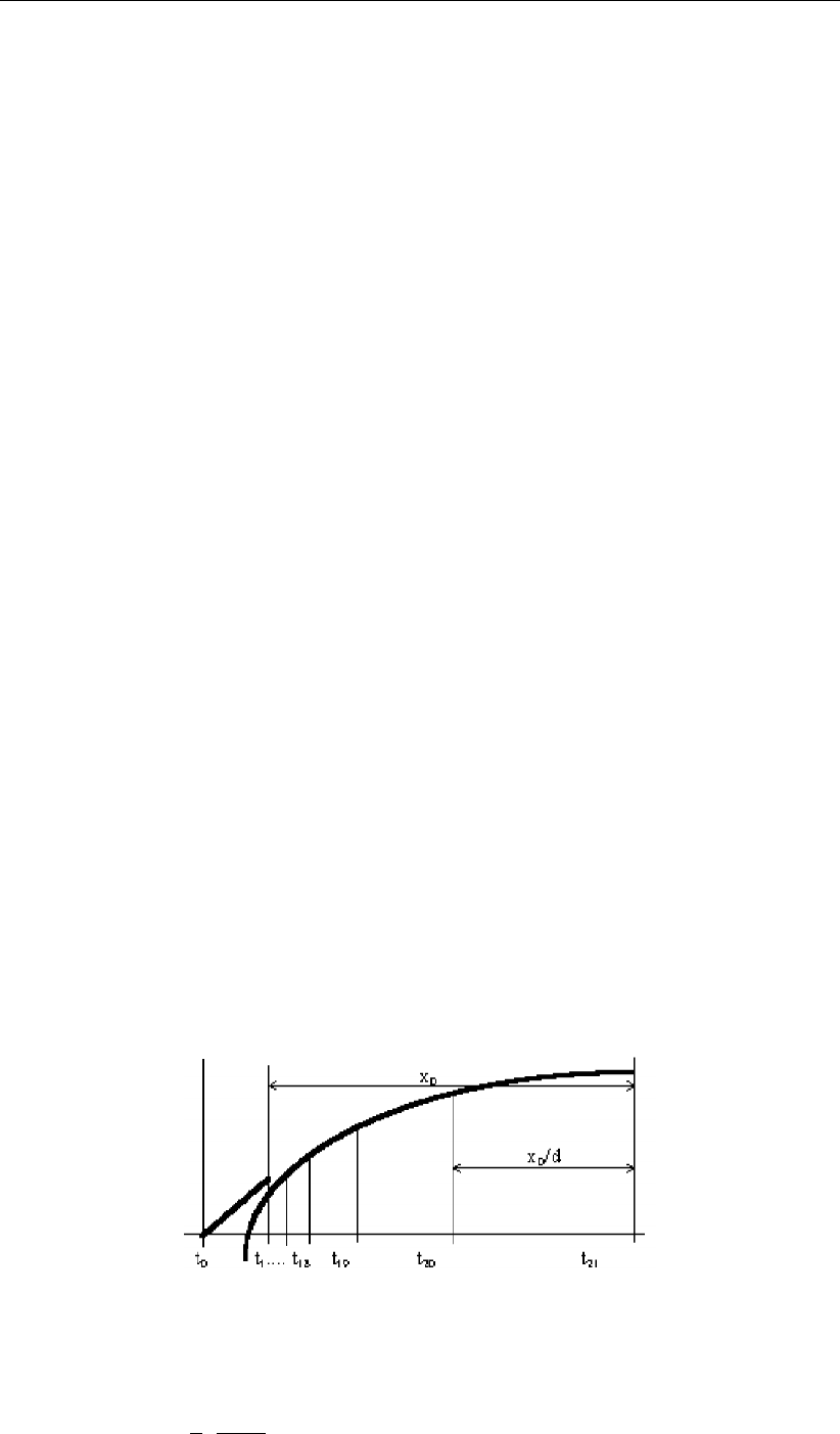
DRAFT
SOBEK, User Manual
Info supplied by the user through the user interface:
initial bbranch width (Bini)
maximum bbranch depth (Dmax)
start of dam break (t0)
time to branch maximum bbranch depth (dt1)
type of dam material (i.e. sand or clay)
either maximum bbranch width (Bmax) or time to branch max. bbranch width (dtmax)
The dam material (i.e. sand or clay) determines the equations that will be used to compute
the time-dependent development of the branch, viz:
for sand: B(t) = 67 10log(t/522) and t(B) = 522 ×10B/67
for clay: B(t) = 20 10log(t/288) and t(B) = 288 ×10B/20
The info supplied by the user is checked on the following conditions:
Bini >0
Dmax >0
Bini +B(sminnmax)≤Bmax
dt1+sminnmax ≤dtmax < t(Bmax)
If all conditions are met, two initial time steps (the linear part) are calculated:
1st time step: A0= 0 m2
2nd time step: t1=t0+dt1and A1=DmaxBini
Then, based on the end condition, the last time step is calculated according to the applicable
equation. The starting point for the equation (t= 0) is supposed to coincide with t1.
NB: The total number of time steps is nmax time steps + 2 initial time steps (i.e. 22).
22nd time step: t21 =t0+dtmax or t21 =t1+t(Bmax)and A21 =DmaxB(t21 −t1)
Now all intermediate time steps (3rd through 21st) can be calculated. Because of the equa-
tions being logarithmic functions, these time steps are not linearly divided over the remaining
interval, but as shown in the figure below, thus producing more values for Bin the region
where the curve is steep.
Figure 6.60: Dam break Bbranch vdKnaap(200), timestep subdivision
When x0=t21 −t1,x1=t20 −t1and dis a divider such that d=x0/(t21 −t20)then:
xn=x0(1 −1
d)1
nmax
and xn≥smin (6.242)
582 of 900 Deltares
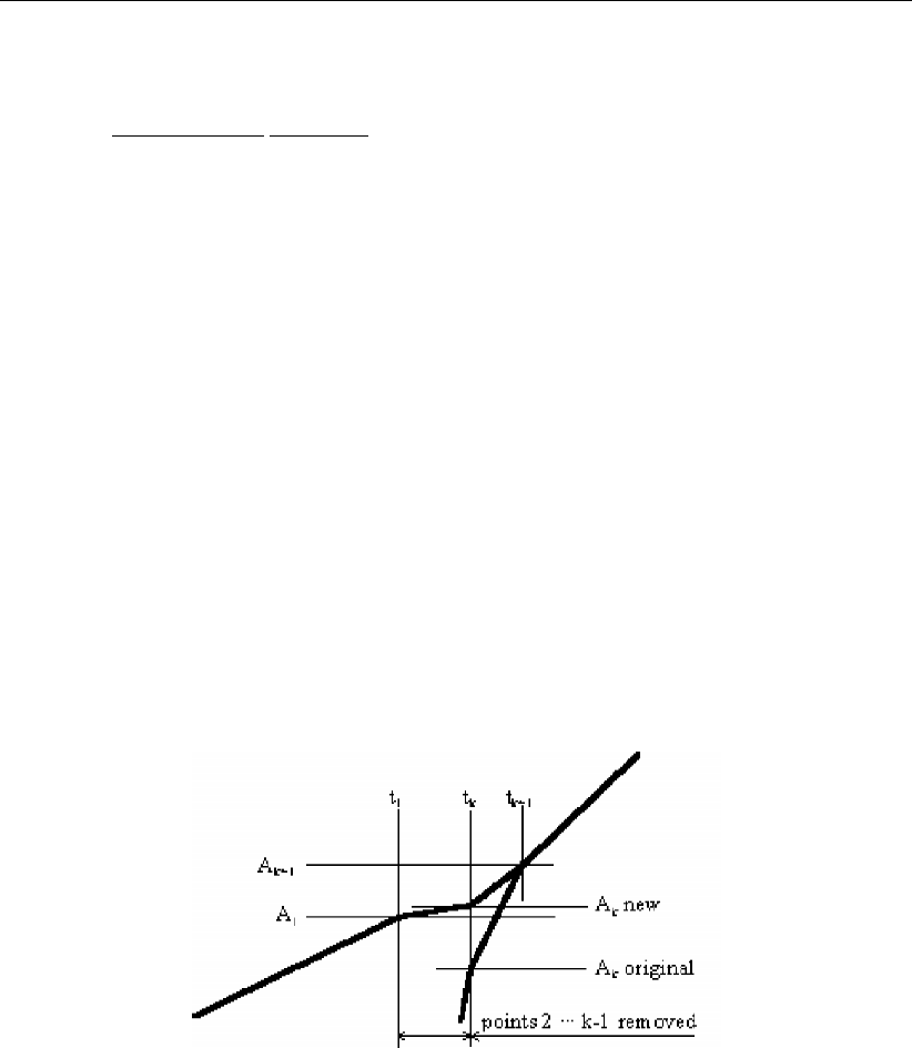
DRAFT
Conceptual description
or
d≥1
(1 −smin/x0)
1
nmax −1(6.243)
Based on this divider dthe time steps t20 through t2can be calculated:
ti=ti+1 + (t1−ti+1)/d (6.244)
Ai=DmaxB(ti−t1)(6.245)
Since the logarithmic functions will evaluate negative values when closing in to t= 0, there
will often be some values (from t2upto tk) calculated for the bbranch width smaller than Bini.
Of course the bbranch width can not decrease, so these values are removed from the table,
except for the last one (tkwith Aksuch that Ak+1 > A1), which is used to smoothen the
linear part with the logarithmic curve.
A percentage pis introduced to determine the bbranch width value for this point according to
the following rule:
Ak=A1+p(Ak+1 −A1)(6.246)
Figure 6.61: Bbranch width computation according vdKnaap(2000)
Literature:
Formulas vdKnaap (2000): Van der Knaap (2000),
6.3.4 1D-2D connection
The 1D network is linked with the 2D grid in the following ways:
The connection between the 1D connection Node and 2D grid cell;
The connection between the 1D ζ-calculation Points and 2D grid cell.
The following rules should be kept in mind, only one connection per grid cell is allowed. In
other words, you cannot have both a connection node and calculation point in one grid cell,
nor more that one connection node or ζ-calculation point per grid cell. It is simpler to as-
sume that 1D and 2D networks are two independent map layers, with the 2D network map
layer overlapping a 1D network. The computational code determines the connection points
Deltares 583 of 900
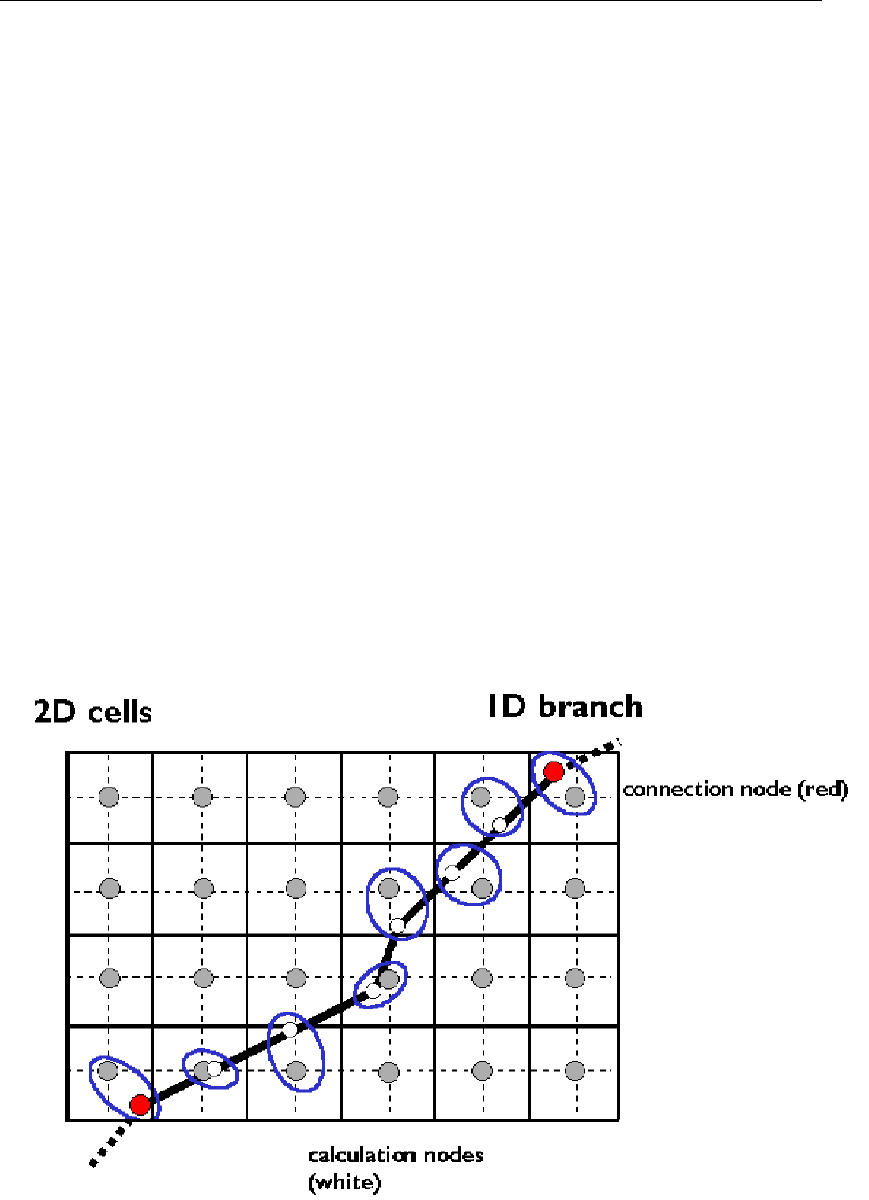
DRAFT
SOBEK, User Manual
between 1D and 2D based on the map coordinates for the centre of 2D grid cell and the 1D
connection node / ζ-calculation node. If they fall within certain criteria, then the connection
is made between them, else not. The criteria, if expressed in mathematical terms, are as
follows:
if (|X1−X2| ≤ ∆x/2) and (|Y1−Y2| ≤ ∆y/2), where:
X1xmap coordinate for 1D point
X2xmap coordinate for 2D grid cell
Y1ymap coordinate for 1D point
Y2ymap coordinate for 2D grid cell
∆xwidth of grid cell in x-direction
∆ywidth of grid cell in y-direction (∆xand ∆yare equal)
then the 1D point is assumed to lie completely within the 2D grid cell.
The connection between the 2D cells and the 1D network is done in the following way (see
figure below):
The center of 1D node is internally moved to match with the center of 2D grid cell, without
changing the length of the connecting 1D branches.
The 2D Grid Cell is counted as part of 1D Node.
The flow in 1D channel below the 2D grid level is treated as 1D flow, while the flow above
the 2D Grid level is treated as 2D flow with the area of 2D grid cell.
Figure 6.62: Connections between 1D and 2D
584 of 900 Deltares

DRAFT
Conceptual description
Modelling 1D2D
Principle is that the top width of the remaining (clarification below) 1D channel should be
smaller than the 2D grid cell size. The way of 1D-2D linking depends on the option you
choose in the Advanced Settings tab:
Assume No Embankments: In this case the elevation of the underlying 2D grid cell
remains the same. The 1D cross-sectional profile above the elevation of the underlying
2D grid cell is omitted (hence excluded from computation).
In case the water level is below 2D grid elevation, the flow is fully 1D only (note that
the width of the 1D channel might be (and preferably: should be) smaller than the 2D
grid cell size).
In case water level is above the 2D grid cell elevation; there is a 1D flow as well as
2D flow. In the 1D cross-sectional profile below the 2D grid cell elevation, 1D flow is
computed in accordance with the underlying 1D profile and 1D hydraulic roughness.
Above the 2D grid cell elevation, there is only 2D flow and this is of course over the full
2D grid cell size, both in x- and y- direction.
Assume Highest Level of Embankments: In this case SOBEK raises the elevation of
the underlying 2D grid cell to the highest embankment level. No part of the 1D cross-
sectional profile is omitted. Thereafter the computation is identical as described under
option 1 (Assume no embankments), with the notation that not the original 2D grid cell
elevation is used but the raised grid cell elevation.
Assume Lowest Level of Embankments: Same as option 2 above, but with notation that
the part of the 1D cross-sectional profile above the lowest embankment level (i.e. minimum
of left and right 1D embankments) is omitted and that the elevation of the underlying 2D
gridcell is raised to the elevation of the lowest embankment level.
In general you can best model your river fully 2D when your 1D profile width >2D grid cell
size.
6.3.5 2D-2D connection
The 2D grid cell connection to another 2D grid cell when one grid is partially or fully overlap-
ping another grid, is done in such a way that the 2D Grid cell of the nested grid is connected
to the 2D grid cell of underlaying grid by a branch. This branch carries the flow to and from
the two connecting grid cells. This branch is given the property of the smallest grid cell and
with a very low friction coefficient so that the hindrance of flow is negligible.
The computational core defines the connection between two 2D grid cells based on the map
coordinates for the center of each grid cells. If they fall within certain criteria, then the con-
nection is made between them else not. The criteria, expressed in mathematical terms, are:
(|X1−X2| ≤ ∆x)and (|Y1−Y2|< Y H . . . 1) (6.247)
(|Y1−Y2| ≤ ∆y)and (|X1−X2|< XH . . . 2) (6.248)
where:
X1xmap coordinate for 2D grid cell in first grid
X2xmap coordinate for 2D grid cell in second grid
Y1ymap coordinate for 2D grid cell in first grid
Y2ymap coordinate for 2D grid cell in second grid
∆x(∆x1/2+∆x2/2)
∆x(∆y1/2+∆y2/2)
XH maximum of ∆x1/2or ∆x2/2
Deltares 585 of 900
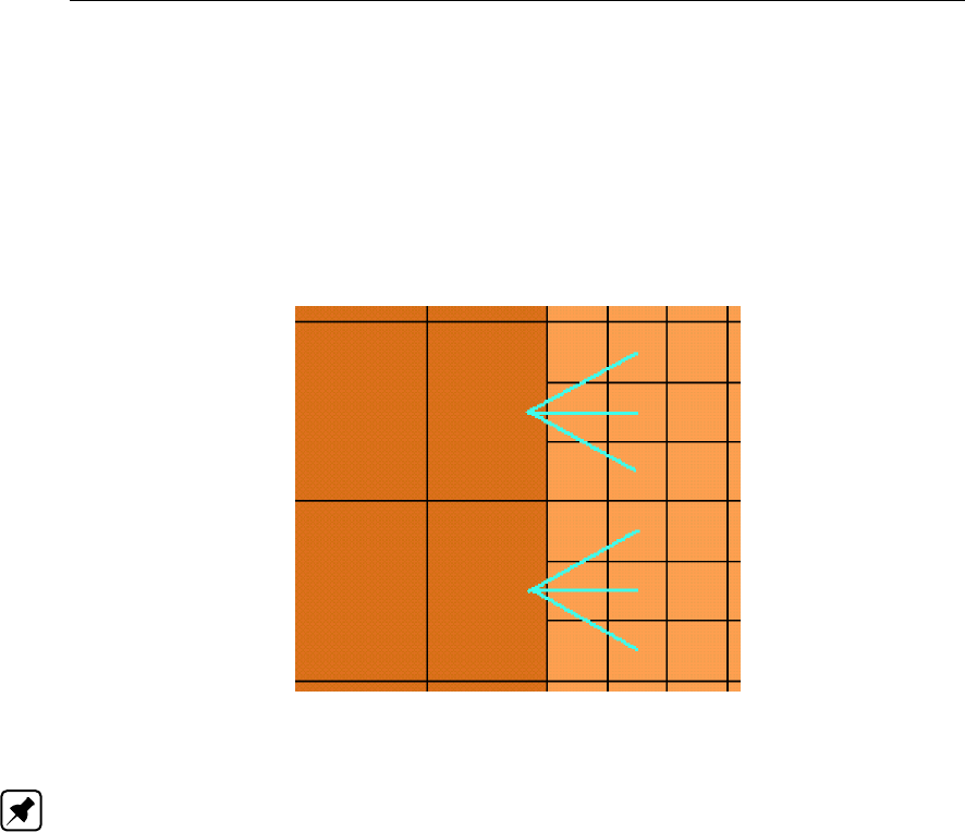
DRAFT
SOBEK, User Manual
Y H maximum of ∆y1/2or ∆y2/2
∆x1width of grid cell in x-direction in first grid
∆y1width of grid cell in y-direction in first grid
∆x2width of grid cell in x-direction in second grid
∆y2width of grid cell in y-direction in second grid
The connection is made, if any of the above two criteria matches. It is possible that there are
more connections made to the same 2D grid cell from different 2D grid cells in another grid.
Figure 6.63: Connections made between different grids
Note: please bear in mind that the outside cells of any grid are removed from the calculation.
So, in the example of Figure 6.63, the connections are made between the large (parent) grid
cell and the second column of grid cells of the child grid!
6.4 Triggers and Controllers
6.4.1 Controller
The SOBEK-Flow-module offers the option to operate hydraulic structures.
The adjustable part of a hydraulic structure (e.g. crest level, crest width, Gate Lower Edge
Level [mAD]) can be adjusted by a controller. In the River Flow and Real Time Control
modules, more than one controller can operate on the same hydraulic structure, however,
a specific control parameter (crest level, etc.) can be steered by only one controller at a
time. Also, one controller can steer the same control parameter of more than one hydraulic
structure, e.g., it is possible to steer the gate lower edge level of a series of structures by only
one controller.
In case no trigger is assigned to a controller, this controller will be active during the entire
computation.
Six controller types have been implemented:
1 Interval controller
2 Hydraulic controller
3 PID controller
4 Time controller
5 Relative time controller
586 of 900 Deltares

DRAFT
Conceptual description
6 Relative from value (time) controller
The parameters that can be controlled are:
Crest level of a weir
Crest level and crest width of River weir
Crest level of Advanced weir
Crest level, crest width and gate lower edge level of General structure
Crest level of Database structure
Opening height of a orifice
Capacity of a pump (Rural Flow module only)
Valve opening of a culvert
Valve opening of a siphon
Valve opening of an inverted siphon
For more details on controllers available for the Advanced weir, Database structure, General
structure and River weir, see also Appendix B (River Flow controller options).
A control frequency should be given. This frequency defines when the controller function
should be updated. This may be every time step (control frequency 1), but also after a number
of time steps (control frequency n).
Procedure for the River Flow module (usage of triggers):
The controller function is activated once for each time step in the computational process (the
controller is not updated during the iteration process of solving the flow equations). Just before
the start of the iteration process the controller is updated in the following way.
For each controller:
if (a trigger is defined for this structure) then
if ’trigger==ON’ then
activate controller function
else
do not activate controller function
endif
else
activate controller function
endif
As you see, a controller can be activated by a trigger, but it can also be activated by a com-
bination of triggers. The computation of the actual control parameter (the carrying out of
controller function) for a structure is as follows:
if controller should be evaluated (depending on the user defined control frequency) then
if ’time controller’ then evaluate time controller
if ’hydraulic controller’ then evaluate hydraulic controller
if ’Interval controller’ then evaluate interval controller
if ’pid controller’ then evaluate pid controller
if ’relative time controller’ then evaluate relative time controller
if ’relative from value controller’ then evaluate relative from value controller
Deltares 587 of 900

DRAFT
SOBEK, User Manual
A control frequency should also be given. This defines when the controller function should be
updated. This may be every time step (control frequency 1), but also after a higher number of
time steps.
The control frequency of an hydraulic controller can also be specified zero. This means that
the control parameter will be updated only the first time after the end of an inactive period. A
trigger should be used to activate the hydraulic controller.
If a time controller, a relative time controller or a relative from value controller is used the
parameter ’dvalue/dt’ must be given a value. This parameter defines the maximum speed of
increase or decrease of the control parameter. It provides some physical damping, to prevent
that instabilities arise due to sudden changes in the structure opening. With for instance a
value of ’dvalue=0.1’, the speed of opening or closing of a gate is 0.1 m/s (e.g., 1 m change
of gate lower edge level in a computational time step of 10s).
6.4.1.1 Combinations of controllers
The crest level, crest width or gate lower edge level of a hydraulic structure can be operated
by more than one controller. SOBEK allows up to four controllers for one structure. A specific
crest level, crest width or gate lower edge level of a hydraulic structure can be operated by
only one controller at a time. In case two or more controllers are given a value for a particular
structure parameter (e.g. crest level), then SOBEK stops the computation. By using triggers
the user should avoid the situation that two or more controllers are simultaneous active for
one and the same structure parameter.
6.4.1.2 Hydraulic controller
The hydraulic controller is a relatively simple controller type which can be used to operate
a structure as a (tabulated) function of a specified hydraulic parameter. In other words: the
crest level, opening height, pump capacity or valve opening is a function of one of the following
parameters:
Water level at a specified measurement station
Discharge at a specified measurement station
And, only for the River Flow module:
head difference over a hydraulic structure(perhaps another structure than the controlled
one!);
flow velocity at a specified measurement station;
flow direction at a specified measurement station;
pressure difference over a structure or compound structure member (perhaps another
structure than the controlled one!).
The computation procedure is straightforward. First, the value of the hydraulic argument at
the previous time step is determined. Next, the control parameter is computed by interpolation
in the controller table. In case of the discharge a user specified time lag with respect to the
current time can be taken into account.
588 of 900 Deltares

DRAFT
Conceptual description
Figure 6.64: Example of hydraulic controller
If the control frequency of an hydraulic controller is specified zero, the control parameter will
be updated only at the start of an active period. A trigger should be used to activate the
hydraulic controller
In case the head difference ∆hover a structure is used as controller, the following formula
will be used:
∆h=h1−h2(6.249)
In case the pressure difference ∆Pover a structure is used as controller, the following formula
will be used:
∆P=1
2g(ρ1(h1−zs)2−ρ2(h2−zs)2)(6.250)
This is in fact the difference between the pressure triangles with respect to the crest level zs
on both sides.
where
h1water level at structure facing beginning of the branch;
h2water level at structure facing end of the branch;
zscrest level of structure;
ρ1water density at structure facing beginning of the branch;
ρ2water density at structure facing end of the branch.
6.4.1.3 Interval controller
The interval controller can be used to operate a structure in such a way that a specified
hydraulic parameter is maintained. The controlled parameter can be the water level at a
specified measurement station in the model, the discharge at a specified measurement station
in the model, or the sum of up to five discharges at specified measurement stations in the
model .
The user defines the following input for the interval controller:
Control parameter (crest level, crest width, gate lower edge level)
Control frequency (see controller).
A selection of the controlled parameter (water level or discharge at the measurement
station).
Deltares 589 of 900

DRAFT
SOBEK, User Manual
Setpoints for the controlled parameter (constant or tabulated function of time).
The so called ”when below deadband” and ”when above deadband” control values.
These “<Deadband” and “>Deadband” values are the extreme values or upper and
lower boundaries allowed for the control parameter (e.g. crest level) (see also River Flow
Controller options). The desired direction is also determined from these values. (upward
or downward of the control parameter (e.g. crest level).
A selection of the deadband type:
fixed deadband: enter a value
deadband as a percentage of the discharge: you must enter percentages and maxi-
mum and minimum deadband values
selection of the controller interval type (or maximum allowable change in value of control
parameter):
fixed interval: you must enter fixed interval value of the controlled parameter
check velocity: enter the controller velocity or speed in m/s (positive values only)
The value of the control parameter νsis computed as follows:
νs=
νs,old +d∆νsif e < −1
2D
νs,old if −1
2D≤e≤1
2D
νs,old −d∆νsif e > 1
2D
(6.251)
where:
DDeadband (in [m] in case of water level, and in [m3/s] in case of discharge)
eDeviation of the controlled variable, e= setpoint - actual measured (computed)
value
dControl direction (1 or -1). We define control values aand b:
Define aas the value of the lower boundary of the control parameter. (User
interface: ”when below deadband”)
Define bas the value of the upper boundary of the control parameter. (User
interface: ”when above deadband”)
The control direction is positive if a>band negative if b > a.
νsMaximum change of control structure parameter, νs=v×dt
v=maximum change of control structure parameter per second
dt =timestep in seconds
So, the rough algorithm is as follows:
if ’interval controller’ present, then
determine value at the previous time step of controlled parameter
compute deviation of the value of the controlled parameter at the previous time step from
the setpoint
compute the value of the control parameter (according to the algorithm described)
check if the control parameter is within its extreme values (if not: set the extreme value).
The extreme values are the allowed value for the control parameter (e.g. crest level) and
are equal to “<Deadband (or when below deadband)” and “>Deadband (or when above
deadband)” values.
590 of 900 Deltares
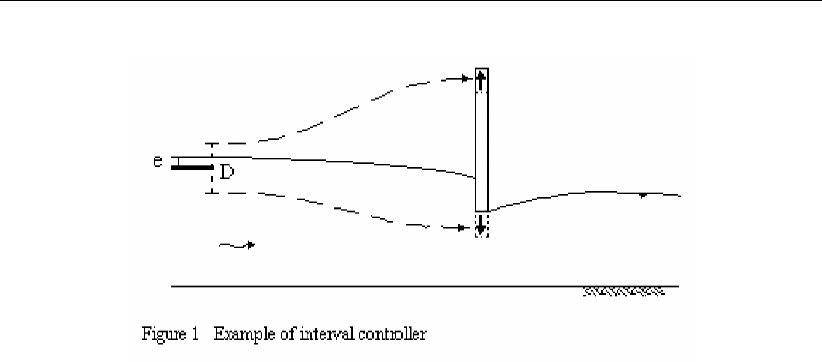
DRAFT
Conceptual description
Figure 6.65: Example of interval controller
The interval controller is not a very advanced type of controller. It is, for instance, sensitive
to instabilities, particularly if the controller velocity, control frequency or deadband are not
selected properly. Also the control history (before the last time step) is not taken into account
to determine the control parameter.
A more advanced controller (the PID controller) is available as well. The PID controller takes
the control history into account, thus enabling a more appropriate behaviour of the control
parameter.
6.4.1.4 PID controller
The PID-controller can be used to operate a structure in such way, that a specified hydraulic
parameter (e.g. water level or discharge) is maintained. The PID-controller consist of a Pro-
portional, Integrating and Differentiating part. The controlled parameter can be the water
level or the discharge at a specified measurement station in the model. The user defines the
following input for the PID controller:
control parameter (crest height, width, gate lower edge level)
control frequency (see controller)
a selection of the controlled parameter (water level or discharge at the measurement sta-
tion). For river flow, also the sum of discharges adding up to five measuring stations.
setpoints for the controlled parameter (constant or tabulated function of time)
initial value of the controlled parameter; note that the initial control value should preferably
be the same as for the structure definition
maximum and minimum value of the control parameter (e.g. control parameter can be
between fixed limits)
maximum change of control structure parameter per second (vmax in m/s)
Proportional gain factor Kp(determines the reaction time of the controller)
Integral gain factor Ki(reduces the standard deviation induced by Kp)
Differential gain factor Kd(provides damping in the controller)
A control (Update) frequency which may be used to filter out high frequency oscillations
in the input signal, but which must be sufficiently small to reproduce the relevant waves in
the controlled variable.
The new value of the control parameter w(t)is computed as follows:
Deltares 591 of 900

DRAFT
SOBEK, User Manual
1 First compute the correction value
u(t) = K0
pe(t) + K0
i
t
X
t=0
e(t) + K0
d(e(t)−e(t−1)) (6.252)
K0
p=k1Kp, K0
i=k2Ki, K0
d=k3Kd(6.253)
2 Perform this correction value to the control parameter w(t)
w(t) = w(t−1) + u(t)(6.254)
In which:
Kp,Ki,KdCoefficient of the PID-controller.
kjj= 1,2,3. Conversion factor between the controll parameter (e.g. discharges
[m3/s]) and the controlled parameter (e.g. water levels [m])
e(t)deviation of the controlled parameter y(t),e(t) = ysp(t)−y(t)
u(t)correction factor on the control parameter, e.g. e(t)≡0⇒u(t)=0⇒w(t)
is unchanged.
Remark:
Equation (6.254) is slightly different from a the PID-controller as reported in Åström and
Hägglund (1995) and as report in RTC-Tools TRM (2012).
The algorithm to compute the control parameter is as follows:
determine value of controlled parameter at previous time level
compute deviation of this value from the setpoint
compute change of deviation from the setpoint (e=e(t)−e(t−1))
compute summation of deviation from the setpoint
compute the value of the control parameter w(t)
check if the computed change of the control parameter ∆w=w(t)−w(t−1) is within
the user-defined limitations
The gain factors Kp,Ki,Kdmust be calibrated for optimal performance of the PID controller.
See section B.6
6.4.1.5 Relative time controller
The relative time controller can be used to specify the controlled parameter as a function
of time, where the time (in seconds) is given relative to the moment that the controller is
activated for the first time by a trigger. When the controller is activated for the first time, the
relative controller table is made absolute (= computational time + relative time), thereafter
the controller starts at the top of the table and continues downward until it is turned off by
the trigger. The controller table will remain absolute during the user-defined so called Start
period. In case the controller is activated after this start period has passed, the controller
table will be made absolute again. Start period = 0, means that the controller table is made
absolute each and every time that the controller is triggered. In case the user defined value
for d(value)/dt is too small to allow for the in the controller Table defined changes in control
parameter, SOBEK will divert from these defined controller parameter values in such way as
to best fit the overall controller table. d(value)/dt = 0, means that there is no restriction in
change in controller parameter over one time step. When it branches the end of the table, the
value of the controlled parameter is kept constant at the last value.
592 of 900 Deltares
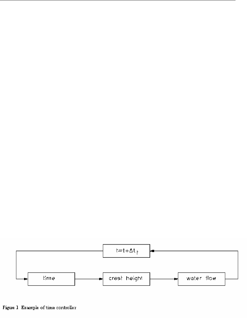
DRAFT
Conceptual description
6.4.1.6 Relative from value (time) controller
The relative time controller can be used to specify the controlled parameter (e.g. crest level)
as a function of time, where the time (in seconds) is given relative. The difference with the
relative time controller is the fact that when activated for the first time (or after start period has
passed, see here after), the controller does not start at the top of the controller table but at
the row that coincides with the actual value of the structure controlled parameter (e.g. crest
level) and continues from there on downwards in the controller table. The advantage of the
relative from value (time) controller is that if used cleverly discontinuities in structure controlled
parameter can be avoided.
The first time that the relative-from-value (time) controller is activated, the controller table
will be made absolute (= computational time + relative time), the controller table will remain
absolute during the so called start period. Hence in case the controller is de-activated and
activated again within the start period, the controller table remains absolute. In case the
controller is activated after the start period has passed, the controller table will be made
absolute for the then yielding computational time again. Start period = 0, means that the
controller table is made absolute each and every time that the controller is triggered. In
case the user defined value for d(value)/dt is too small to allow for the in the controller
table defined changes in controlled parameter (e.g. crest level), SOBEK will divert from these
defined controller parameter values in such way as to best fit the overall controller table. A
value of d(value)/dt = 0, means that there is no restriction in change in controlled parameter
over one computational time step. When it branches the end of the Table, the value of the
controlled parameter is kept constant at the last value.
6.4.1.7 Time controller
The time controller is the most simple and straight forward controller. The control param-
eter (e.g. crest level, opening height, pump capacity, valve opening) is given explicitly as a
(tabulated) function of time.
Figure 6.66: Example of time controller
Deltares 593 of 900

DRAFT
SOBEK, User Manual
6.4.2 Triggers
A hydraulic structure can be adjusted by a controller. Each controller in SOBEK can be acti-
vated or de-activated by a trigger, which can have the value ON or OFF. Also a combination
of triggers can activate a controller, while more than one controller can be activated by one
trigger or trigger combination. In case no trigger is assigned to a controller, this controller will
be active during the entire computation.
Three different trigger types are available:
1 time trigger;
2 hydraulic trigger;
3 Time & Hydraulic trigger (combined trigger).
Moreover, it is possible to perform a logical “and” or logical “or” function on the combination of
time trigger and hydraulic trigger.
Whether a trigger is ON or OFF is determined as follows:
if AND/OR period defined then
determine AND/OR period (AND/OR)
evaluate time trigger (ON/OFF)
evaluate hydraulic trigger (ON/OFF)
trigger = OFF
if (AND and (time trigger = ON and hydraulic trigger = ON)) then
trigger = ON
if (OR and (time trigger = ON or hydraulic trigger = ON)) then
trigger = ON
else if time trigger then
evaluate time trigger (ON/OFF)
else if hydraulic trigger then
evaluate hydraulic trigger (ON/OFF)
6.4.2.1 Combinations of triggers
Up to four triggers can be combined to activate or de-activate a controller. When the user
specifies more than one trigger, he must specify how the triggers work together by specifying
the relationship between the triggers with logical and-or statements. Evaluation of AND-OR
statements are according to the usual logical rules. This means that AND statements are
evaluated before OR statements.
This results in the following:
the combination of triggers ’trig1 and trig2’, ’trig12’, is evaluated as follows:
if (trig1 == ON and trig2 == ON)then
trig12 = ON
else
trig12 = OF F
endif
the combination of triggers ’trig1 or trig2’, ’trig12’, is evaluated as follows:
if (trig1 == ON or trig2 == ON)then
trig12 = ON
else
trig12 = OF F
594 of 900 Deltares

DRAFT
Conceptual description
endif
the combination of triggers ’trig1 and trig2 and trig3’, ’trig123’, is evaluated as follows:
if (trig1 == ON and trig2 == ON and trig3 == ON)then
trig123 = ON
else
trig123 = OF F
endif
the combination of triggers ’trig1 and trig2 or trig3’, ’trig123’, is evaluated as follows:
if ((trig1 == ON and trig2 == ON)or trig3 == ON)then
trig123 = ON
else
trig123 = OF F
endif
the combination of triggers ’trig1 or trig2 and trig3’, ’trig123’, is evaluated as follows:
if ((trig1 == ON or trig2 == ON)and trig3 == ON)then
trig123 = ON
else
trig123 = OF F
endif
6.4.2.2 Time trigger
To determine if a time trigger is ON or OFF, a user-defined time table, is used. In the time
table periods are defined during which the trigger is either ON or OFF.
6.4.2.3 Hydraulic trigger
To determine if a hydraulic trigger is ON or OFF, first the hydraulic parameter will be calculated
or the gate lower edge level will be retrieved. After this
SOBEK checks if the computed value exceeds a user defined threshold value.
Eight hydraulic trigger types are possible:
1 water level at a specified location
2 discharge at a specified location
3 gate lower edge level at a hydraulic structure
4 crest level at a hydraulic structure
5 crest width at a hydraulic structure
6 the water level in retention area
7 head difference at a hydraulic structure
8 force difference per unit width at a hydraulic structure
The head difference at a structure used by a trigger is defined as:
∆h=h1−h2(6.255)
The force difference (∆F) per unit width over a structure is defined as:
∆F=1
2g(ρ1(h1−zs)2−ρ2(h2−zs)2)(6.256)
where
Deltares 595 of 900

DRAFT
SOBEK, User Manual
gacceleration due to gravity;
h1water level at structure, facing beginning of branch;
h2water level at structure, facing end of branch;
zscrest level of structure;
ρ1water density at structure, facing beginning of branch;
ρ2water density at structure, facing end of branch
If gate lower edge level,crest level or crest width is chosen two options are available:
1 the value is checked against the threshold
2 the direction of variation (increase or decrease of the value) can be checked
The following procedure is used:
determine hydraulic trigger type
determine location
determine threshold value and whether it should be triggered on a "higher" value or a
"lower" value
trigger = OFF
if ’hydraulic trigger type = water level’ then
if ’trigger on higher value’
if ’h(location) >value’
trigger = ON
if ’trigger on lower value’
if ’h(location) <value’
trigger = ON
elseif ’trigger type = head difference’ then
head difference = hleft −hright of structure
if ’trigger on higher value’
if ’head difference >value’
trigger = ON
if ’trigger on lower value’
if head difference <value
trigger = ON
endif
6.4.2.4 Time & Hydraulic triggers
The Time & Hydraulic trigger is actually a combination of a Hydraulic trigger with a Time
trigger. This can be applied in “AND” or in “OR” mode.
AND mode means: Time & Hydraulic trigger value is ON if both the Hydraulic trigger and
the Time trigger are ON.
OR mode means: Time & Hydraulic trigger value is ON if either the Time trigger or the
Hydraulic trigger is ON, but also if both Time and Hydraulic triggers are ON.
6.5 Hydrology (Rainfall Runoff modules)
6.5.1 SOBEK-Rural RR (Rainfall Runoff) concept
596 of 900 Deltares

DRAFT
Conceptual description
6.5.1.1 Alpha reaction factor
The reactionfactor αis an important parameter in the De Zeeuw-Hellinga equation which is
used in SOBEK to calculate the different components of the groundwater/subsurface flow:
qt=qt−1e−α∆t+ (I+S)(1 −e−α∆t)(6.257)
qtspecific discharge at time t[m/d]
qt−1specific discharge at time t−1[m/d]
∆ttime step [d]
αreaction factor [1/d]
Iinfiltration [m/d]
Sseepage (percolation) [m/d]
In SOBEK, the De Zeeuw-Hellinga equation is used to calculate the following components of
flow:
groundwater drainage (towards drainpipes or channels);
surface run-off;
infiltration from open water.
For each process, the user must define specific reaction factors.
Reaction factor groundwater drainage
In SOBEK, the ground can be divided into different ground layers, each with it’s own a. The
total specific discharge is calculated by applying the De Zeeuw-Hellinga equation to all layers,
and summing the result (see Figure 6.67)
Figure 6.67: Drainage levels
Usually, the division between the ground layers is placed at the level of the drains, which are
then simulated by giving the above drain level (αd,1to αd,3in the figure) a much higher value
than the a below drain level (αd,4in Figure 6.67).
To obtain indications for the values of the reaction factor one can:
use the values in the Table below (Vademecum,1988):
αDischarge type
100–200 Surface runoff from steep slopes
1–10 Surface runoff from soils with impervious subsoil
0.3–0.7 Drainage discharge from well-drained agricultural soil
0.03–0.07 Discharge from grassland without drainage system
Measure the decrease of discharge in time. This only can be done after a period of
(heavy)rain, and no additional precipitation, and no (or very little) evaporation.
Deltares 597 of 900
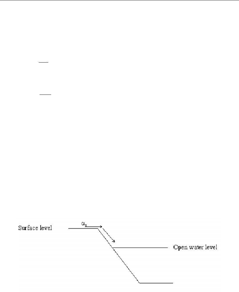
DRAFT
SOBEK, User Manual
Derive the αvalue from
q=αµ∆h(6.258)
and
q=∆h
W(6.259)
and equals
α=1
µW (6.260)
qspecific discharge [m/d]
Dh groundwater level above drainage depth or open water level [m]
αreaction coefficient [1/d]
mstorage coefficient [−]
Wdrainage resistance [d]
Reaction factor surface run-off
When the groundwater level branches the surface level or the precipitation excess exceeds the
infiltration capacity, water is stored on land. When the storage on land is filled in a SOBEK-RR
unpaved node the surface runoff process starts.
Therefore, the user must define a reaction factor αs. The above table gives indications for the
values of this reaction factor.
Figure 6.68: Surface run-off
Reaction factor infiltration from open water
In dry periods the groundwater level can decrease. When the groundwater level is lower than
the open water level, infiltration from the open water occurs. In SOBEK-RR, this process is
described by the modified De Zeeuw-Hellinga equation. Again, the user must define a specific
reaction factor, αi
6.5.1.2 Capillary rise
Capillary rise describes the unsaturated flow in the subsoil from the groundwater to the root
zone. Capillary rise occurs in case of a water deficit in the root zone. Water deficit is defined
as a water content less than equilibrium moisture storage. If the water content in the root
zone exceeds equilibrium the excess water percolates to the groundwater. The excess water
is the potential root zone volume minus the equilibrium moisture content. To assess whether
598 of 900 Deltares

DRAFT
Conceptual description
capillary rise or percolation will occur over a time step, the potential root zone volume is
determined from the net precipitation and the evapotranspiration, based on the soil moisture
storage in the root zone at the previous time step:
V0(t) = V(t−∆t)+(Pn−E)∆t(6.261)
where:
V0(t)potential root zone volume at time t[m]
V(t−∆t)root zone volume after the previous time step [m]
Pnnet precipitation [m/d]
Eevapotranspiration [m/d]
∆ttime step [d]
In case of a water deficit in CAPSIM the capillary rise flux is calculated in 2 steps. First
the potential capillary rise flux is calculated. The potential capillary rise flux depends on the
groundwater level, the soil physical unit and the root zone thickness:
qpot =f(s, dg, dr)(6.262)
with:
qpot Potential capillary rise [mm/d]
sSoil physical unit [-]
dgDepth groundwater level [m]
drRoot zone thickness [m]
The potential capillary rise flux is calculated with the 1-D, steady state simulation model CAP-
SEV (Wesseling,1991), assuming pF = 3 in the root zone. The potential capillary rise fluxes
are tabulated.
Secondly SOBEK-CAPSIM uses the potential capillary rise flux, the actual moisture storage
in the root zone and the equilibrium moisture storage to calculate the actual capillary rise flux,
according to:
qact =(qpot veq−vact
veq−vpF 3vact > vpF 3
qpot vact < vpF 3
(6.263)
where:
qact Actual capillary rise flux [mm/d]
veq Equilibrium soil moisture content [m]
vact Actual soil moisture content [m]
Equilibrium soil moisture content veq
The moisture storage of the root zone at equilibrium condition is calculated with the function:
Veq =f(s, dg, dr)(6.264)
where:
Veq the moisture storage of the root zone at equilibrium condition [m]
ssoil physical unit [-]
drthickness of root zone [m]
dgdepth of the groundwater level [m]
Deltares 599 of 900

DRAFT
SOBEK, User Manual
Soil moisture content at pF = 3,vpF 3
The moisture storage of the root zone at pF = 3 is calculated assuming steady conditions
and a groundwater level of 10 m minus soil surface.
6.5.1.3 Crop factors agricultural crops
The fixed input file with crop names and crop factors as a function of time. 1 year of data is
enough, since it is assumed that the crop factors are constant over the years; the variation is
taken into account in the reference evaporation data and not in the crop factors.
The header of the file contains the number of crops and crop names.
*Number of crops
16
*Names
’1 grass ’
’2 corn ’
’3 potatoes ’
’4 sugarbeet ’
’5 grain ’
’6 miscellaneous ’
’7 non-arable land ’
’8 greenhouse area ’
’9 orchard ’
’10 bulbous plants ’
’11 foliage forest ’
’12 pine forest ’
’13 nature ’
’14 fallow ’
’15 vegetables ’
’16 flowers ’
*Year/Month/Day/Cropfact 1 2 3 4 5 6 7 8 9 10 11 12 13 14 15 16
0000 1 1 0.95 1.00 1.00 1.00 1.00 0.95 1.00 0.00 1.00 0.00 0.90 1.20 0.95 1.00 1.00 0.00
0000 1 2 0.95 1.00 1.00 1.00 1.00 0.95 1.00 0.00 1.00 0.00 0.90 1.20 0.95 1.00 1.00 0.00
0000 1 3 0.95 1.00 1.00 1.00 1.00 0.95 1.00 0.00 1.00 0.00 0.90 1.20 0.95 1.00 1.00 0.00
0000 1 4 0.95 1.00 1.00 1.00 1.00 0.95 1.00 0.00 1.00 0.00 0.90 1.20 0.95 1.00 1.00 0.00
0000 1 5 0.95 1.00 1.00 1.00 1.00 0.95 1.00 0.00 1.00 0.00 0.90 1.20 0.95 1.00 1.00 0.00
0000 1 6 0.95 1.00 1.00 1.00 1.00 0.95 1.00 0.00 1.00 0.00 0.90 1.20 0.95 1.00 1.00 0.00
0000 1 7 0.95 1.00 1.00 1.00 1.00 0.95 1.00 0.00 1.00 0.00 0.90 1.20 0.95 1.00 1.00 0.00
0000 1 8 0.95 1.00 1.00 1.00 1.00 0.95 1.00 0.00 1.00 0.00 0.90 1.20 0.95 1.00 1.00 0.00
0000 1 9 0.95 1.00 1.00 1.00 1.00 0.95 1.00 0.00 1.00 0.00 0.90 1.20 0.95 1.00 1.00 0.00
0000 1 10 0.95 1.00 1.00 1.00 1.00 0.95 1.00 0.00 1.00 0.00 0.90 1.20 0.95 1.00 1.00 0.00
0000 1 11 0.95 1.00 1.00 1.00 1.00 0.95 1.00 0.00 1.00 0.00 0.90 1.20 0.95 1.00 1.00 0.00
0000 1 12 0.95 1.00 1.00 1.00 1.00 0.95 1.00 0.00 1.00 0.00 0.90 1.20 0.95 1.00 1.00 0.00
0000 1 13 0.95 1.00 1.00 1.00 1.00 0.95 1.00 0.00 1.00 0.00 0.90 1.20 0.95 1.00 1.00 0.00
etc.
6.5.1.4 Crop factors open water
The fixed input file with open water evaporation factors is a function of time. 1 year of data is
enough; it is assumed that the evaporation factors are the same for all years.
*Surface water
1
*Names
’0.0 Surface water ’
*Year/Month/Day/Cropfact 1
0000 1 1 0.50
0000 1 2 0.50
0000 1 3 0.50
0000 1 4 0.50
600 of 900 Deltares

DRAFT
Conceptual description
0000 1 5 0.50
0000 1 6 0.50
0000 1 7 0.50
0000 1 8 0.50
0000 1 9 0.50
0000 1 10 0.50
0000 1 11 0.50
0000 1 12 0.50
0000 1 13 0.50
etc.
6.5.1.5 De Zeeuw-Hellinga drainage formula
To simulate the flow of groundwater towards the drainage system (i.e. drain pipes and/or
channels) the modified equation of De Zeeuw-Hellinga is used in the Rainfall-Runoff module.
The theory behind this equation is treated here.
The head loss of groundwater flowing to a drain can be subdivided in head loss caused by:
vertical flow;
horizontal flow;
radial flow nearby the drain/channel;
entrance in the drain/channel.
In the equation of De Zeeuw-Hellinga it is assumed that the head loss is mainly caused by
radial flow and entrance loss. The head loss by horizontal flow and vertical flow is neglected.
This equation is based on a reservoir containing a volume of ground. The reservoir discharges
through a capillary tube. The discharge depends on the difference in pressure head. Thus:
Q=c∆h(6.265)
Qdischarge [m3/d]
cproportional coefficient [m2/d]
∆hdifference in pressure head [m]
and
q=Q
A=c2h=αµh (6.266)
qspecific discharge [m/d]
Qdischarge [m3/d]
Aarea [m2]
c2proportional coefficient [1/d]
hgroundwater level above drainage depth [m]
αreaction coefficient [1/d]
µstorage coefficient
The water balance for time dt is:
(I+S−q)∆t=µ∆h(6.267)
Iinfiltration [m/d]
Sseepage (percolation) [m/d]
ttime [d]
Deltares 601 of 900

DRAFT
SOBEK, User Manual
This equals:
∆t=µ
I+S−αµh∆h(6.268)
and eliminating the integration constant (t= 0,q=q0) they lead to the equation of De
Zeeuw-Hellinga:
qt=q0e−αt + (I+S)(1 −e−αt)(6.269)
qtspecific discharge at time t[m/d]
q0specific discharge at time 0[m/d]
With this equation the groundwater flow to a drain can be calculated for a constant I+S.
When I+Sis not constant, the I+Sseries can be seen as a series of constant I+S,
positive and negative. For each constant I+Sin the series the qtcan be calculated, with
tdepending on the start of the component. Because the De Zeeuw-Hellinga equation is
linear, superposition may be applied. It is easier though to calculate the qtfor several short
successive periods wherein I+Sis constant. This results in the following modified equation:
qt=qt−1e−α∆t+ (I+S)(1 −e−α∆t)(6.270)
qt−1specific discharge at time t−1[m/d]
∆ttime step [d]
For each time step infiltration and seepage must be constant.
The total volume of water flowing to the drain can be calculated by integrating the equation of
De Zeeuw-Hellinga and multiplying it with the area:
Vt=AZ∆t
0
qtdt (6.271)
VtVolume of groundwater flow to drain at time t[m3]
Vtbecomes:
Vt=AZ∆t
0
qtdt (6.272)
=A−1
αq0eαt + (I+S)(t+1
αe−αt)∆t
0
(6.273)
=A−1
αq0eα∆t+ (I+S)(∆t+1
αe−α∆t) + 1
αq0−1
α(I+S)(6.274)
=Aq0−(I+S)
α(1 −e−α∆t)+(I+S)∆t(6.275)
and
q0=αµ∆h0(6.276)
Substituting gives:
Vt=Aαµ∆h−A(I+S)
α(1 −e−α∆t) + A(I+S)∆t(6.277)
602 of 900 Deltares

DRAFT
Conceptual description
The average discharge Qt,average [m3/d] is computed by
Qt,average =Vt
∆t(6.278)
Thus the average discharge in a time step to the drain as is used by the Rainfall-Runoff
module is:
Qt,average =Aαµ∆h−A(I+S)
α∆t(1 −e−α∆t) + A(I+S)(6.279)
This is the so-called modified equation of De Zeeuw-Hellinga. Two important differences from
the ‘normal’ equation of De Zeeuw-Hellinga:
the storage coefficient µis explicit, and
the pressure head ∆his in the Rainfall-Runoff module calculated per time step as the
difference between the groundwater level and the open water level.
6.5.1.6 DrainageDeltaH option
DrainageDeltaH=-1 ! -1=parallell systems (default), 0=stacked system;
Given the definition of the drainage levels, and the Hellinga-de Zeeuw alfa reaction factors α,
or the Ernst drainage resistances γ, there are two options for computing the relevant heads
on which the αfactors or drainage resistances are applied to.
Figure 6.69: Parallell drainage systems (default: DrainageDeltaH=-1)
Deltares 603 of 900
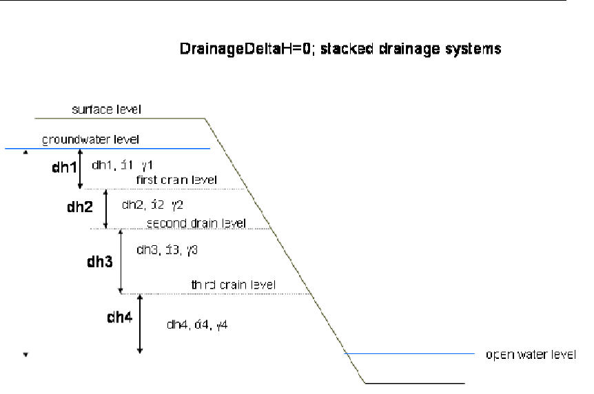
DRAFT
SOBEK, User Manual
Figure 6.70: Stacked drainage systems (DrainageDeltaH=0)
See also: <Delft_3B.Ini>as described in SOBEK input file formats.
6.5.1.7 Dry Weather Flow (DWF)
The DWF or dry weather flow can be taken into account at the RR-paved node. Also the
DWF is part of the formulation in the RR-NWRW node, Nationale Werkgroep Riolering en
Waterkwaliteit (NLingenieurs,1978).
The dry weather flow represents return flow from domestic use, like showers, washing, flush-
ing the toilets, etc.
The dry weather flow can be specified in one of the following ways:
as a constant flow [m3/s] during the whole day
as a variable flow [m3/s] for 24 hours; 1 value for each hour.
as a constant flow [m3/s] per day per person, multiplied with the number of persons
as a variable flow [m3/s] per hour per person, multiplied with the number of persons
For paved area, the dry weather flow is discharged into the DWF sewer in case of a separated
or improved separated system. In case of a mixed system it is discharged into the mixed
sewer system, where it is mixed with sewer inflow due to rainfall.
For a NWRW node the dry weather flow is added to the computed sewer inflow with the
NWRW rainfall-runoff model.
6.5.1.8 Equal filling controller
Given initial, target and maximum allowable upstream and downstream levels, the controller
tries to operate the weir such that the upstream and downstream open water nodes will expe-
rience the same filling percentage.
604 of 900 Deltares
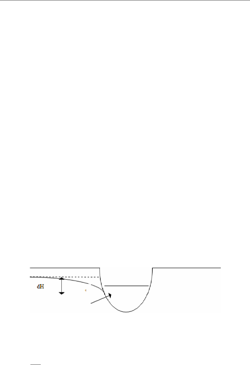
DRAFT
Conceptual description
The filling percentage is defined in terms of water levels as:
(actual level −target level)/(maximum allowable level −target level)×100 %.
(6.280)
This means that the controller will try to achieve similar exceedance patterns of the target
levels, taking into account the maximum allowable levels. In calculating the flow which results
in equal filling percentages, a linear relation between water level and volume is assumed.
For open waters with a constant area this is a valid assumption. However, if the open wa-
ter area increases with increasing level, the procedure will not result in exactly equal filling
percentages.
The calculated flow to branch equal filling percentages is limited by a maximum allowed flow
Qmax. This maximum flow Qmax is determined by:
Qmax =QMaxAtTargetLevel +FillingUpstream ×(QMaxAtMaxLevel −QMaxAtTargetLevel).
(6.281)
The maximum flows QMaxAtTargetLevel and QMaxAtMaxLevel are user defined input data
for the equal filling controller.
Furthermore, the flow Qmax is limited (taking into account other calculated flows from previous
iterations) such that the upstream water level does not fall below target level.
6.5.1.9 Ernst drainage formula
One of the options of modelling the drainage from unpaved area towards open water is the
Ernst formulation (Ernst,1978). Other options available are the De Zeeuw-Hellinga formula-
tion and the Krayenhoff van de Leur formulation.
The following figure illustrates the principles of the Ernst method.
Figure 6.71: Principles of Ernst method
The equation reads:
q=dH
γf (6.282)
where:
qdrainage [m/d]
dH difference between groundwater level and drainage basis [m]
γdrainage resistance [d]
ffactor (0.65 - 0.85 (Ernst,1978)), depending on the shape of the groundwa-
tertable [−]
Deltares 605 of 900

DRAFT
SOBEK, User Manual
The ffactor can not be entered via the User Interface of SOBEK. Instead, the user has to
take this factor into account in the drainage resistance.
6.5.1.10 Evaporation (when using capsim)
The actual evapotranspiration ETact is calculated as:
ETact =αEEr(6.283)
with
αE=fV
Veq (6.284)
where:
αErelative evapotranspiration factor [−]
Vactual soil moisture storage in the root zone [m]
Veq equilibrium soil moisture storage in the root zone [m]
Erpotential evapotranspiration [m]
Figure 6.72: Reduction coefficient for root water uptake, αE, as a function of soil water
pressure head h(Feddes et al.,1978).
Water uptake by roots is zero at soil water pressure h4which is assumed to be the wilting
point, see Figure 6.72. Soil water pressure h3is called the reduction point. In between the
wilting point and the reduction point the potential evapotranspiration rate is linearly reduced.
The location of the reduction point depends on the potential evapotranspiration. If the potential
evapotranspiration is less than or equal to 1 mm/d then the curve Elow is used. If the potential
evapotranspiration is equal to or greater than 5 mm/d then the curve Ehigh is used. In between
SOBEK-CAPSIM linearly interpolates between the reduction curves Elow and Ehigh.
Between soil water pressures h2and h3the evapotranspiration is at maximum (’potential’).
As a result of oxygen deficiency in the root zone, water uptake is hampered for some crops
between soil water pressures h2and h1. SOBEK-CAPSIM does not take this reduction into
account (αE= 1 between soil water pressures h2and h1).
606 of 900 Deltares

DRAFT
Conceptual description
SOBEK-CAPSIM doesn’t compute the soil waterpressure head directly, but uses the relative
root zone storage V/Veq. The relative root zone storages for h4,h3l,h3h,h2and h1are
calculated by CAPSEV and tabulated in SOBEK-CAPSIM. Then Figure 6.72 can be better
explained by:
αE= 0 when 0≤V/Veq < V/Veq(h4)(6.285)
0≤αE≤1when V/Veq(h4)≤V/Veq < V/Veq(h3lor h3h)(6.286)
αE= 1 when V/Veq ≥V/Veq(h3lor h3h)(6.287)
6.5.1.11 Evapo(transpi)ration
Open water
For open water, related to Makkink evapotranspiration, the following ’crop’ factors are used.
These values are based on Hooghart and Lablans (1988).
Decade1) Value Decade Value Decade Value
jan-01 0.50 may-01 1.30 sep-01 1.17
jan-02 0.50 may-02 1.30 sep-02 1.17
jan-03 0.70 may-03 1.30 sep-03 1.17
feb-01 0.80 jun-01 1.31 oct-01 1.00
feb-02 1.00 jun-02 1.31 oct-02 0.90
feb-03 1.00 jun-03 1.31 oct-03 0.80
mar-01 1.20 jul-01 1.29 nov-01 0.80
mar-02 1.30 jul-02 1.27 nov-02 0.70
mar-03 1.30 jul-03 1.24 nov-03 0.60
apr-01 1.30 aug-01 1.21 dec-01 0.50
apr-02 1.30 aug-02 1.19 dec-02 0.50
apr-03 1.30 aug-03 1.18 dec-03 0.50
1) Decades are parts of a month, defined as: first 10 days, second 10 days and rest of the month.
Related input file:
crop factor open water
Unpaved areas
The potential evapotranspiration in unpaved areas depends on the vegetation. The standard
way to determine the potential evapotranspiration is to multiply the reference evaporation (p.e.
Makkink) by a so called crop factor. The crop factor can differ per vegetation, in time and per
location on earth. The default crop factors are orientated towards the Dutch situation for a
limited number of crops, listed in the table below.
crop nr. 1 2 3 4 5 6 7 8 9 10 11 12 13 14 15 16
decade
grass
corn
potatoes
sugarbeet
grain
miscellaneous
non-arable land
greenhouse area
orchard
bulbous plants
foliage forest
pine forest
nature
fallow
vegetables
flowers
jan-01 0.95 1.00 1.00 1.00 1.00 0.95 1.00 0.00 1.00 1.00 0.90 1.20 0.95 1.00 1.00 0.00
jan-02 0.95 1.00 1.00 1.00 1.00 0.95 1.00 0.00 1.00 1.00 0.90 1.20 0.95 1.00 1.00 0.00
Deltares 607 of 900
DRAFT
SOBEK, User Manual
crop nr. 1 2 3 4 5 6 7 8 9 10 11 12 13 14 15 16
decade
grass
corn
potatoes
sugarbeet
grain
miscellaneous
non-arable land
greenhouse area
orchard
bulbous plants
foliage forest
pine forest
nature
fallow
vegetables
flowers
jan-03 0.95 0.71 0.71 0.71 0.71 0.95 0.71 0.00 0.71 0.71 0.90 1.20 0.95 0.71 0.71 0.00
feb-01 0.95 0.63 0.63 0.63 0.63 0.95 0.63 0.00 0.63 0.63 0.90 1.20 0.95 0.63 0.63 0.00
feb-02 0.95 0.50 0.50 0.50 0.50 0.95 0.50 0.00 0.50 0.50 0.90 1.20 0.95 0.50 0.50 0.00
feb-03 0.95 0.40 0.40 0.40 0.40 0.95 0.40 0.00 0.40 0.40 0.90 1.20 0.95 0.40 0.40 0.00
mar-01 0.95 0.33 0.33 0.33 0.33 0.95 0.33 0.00 0.33 0.33 1.00 1.20 0.95 0.33 0.33 0.00
mar-02 0.95 0.23 0.23 0.23 0.23 0.95 0.23 0.00 0.23 0.23 1.00 1.20 0.95 0.23 0.23 0.00
mar-03 0.95 0.23 0.23 0.23 0.23 0.95 0.23 0.00 0.23 0.78 1.00 1.20 0.95 0.23 0.23 0.00
apr-01 1.00 0.23 0.23 0.23 0.65 1.00 0.23 0.00 1.04 0.91 1.05 1.20 1.00 0.23 0.23 0.00
apr-02 1.00 0.23 0.23 0.23 0.78 1.00 0.23 0.00 1.04 0.91 1.05 1.20 1.00 0.23 0.52 0.00
apr-03 1.00 0.23 0.23 0.23 0.91 1.00 0.23 0.00 1.04 0.91 1.05 1.20 1.00 0.23 0.65 0.00
may-01 1.00 0.52 0.15 0.52 1.04 1.00 0.15 0.00 1.43 1.04 1.15 1.20 1.00 0.15 0.78 0.00
may-02 1.00 0.52 0.65 0.52 1.04 1.00 0.15 0.00 1.43 1.04 1.15 1.20 1.00 0.15 0.91 0.00
may-03 1.00 0.52 0.91 0.52 1.04 1.00 0.15 0.00 1.43 1.04 1.15 1.20 1.00 0.15 1.04 0.00
jun-01 1.00 0.79 1.05 0.79 1.18 1.00 0.15 0.00 1.57 1.05 1.20 1.20 1.00 0.15 1.18 0.00
jun-02 1.00 1.05 1.05 1.05 1.18 1.00 0.15 0.00 1.57 1.05 1.20 1.20 1.00 0.15 1.18 0.00
jun-03 1.00 1.18 1.18 1.18 1.18 1.00 0.15 0.00 1.57 0.92 1.20 1.20 1.00 0.15 1.18 0.00
jul-01 1.00 1.29 1.16 1.16 1.03 1.00 0.16 0.00 1.68 0.77 1.25 1.20 1.00 0.16 1.03 0.00
jul-02 1.00 1.27 1.14 1.14 0.89 1.00 0.16 0.00 1.65 0.64 1.25 1.20 1.00 0.16 0.76 0.00
jul-03 1.00 1.24 1.12 1.12 0.74 1.00 0.16 0.00 1.61 0.50 1.25 1.20 1.00 0.16 0.16 0.00
aug-01 1.00 1.21 1.09 1.09 0.61 1.00 0.17 0.00 1.33 0.17 1.10 1.20 1.00 0.17 0.17 0.00
aug-02 1.00 1.19 0.83 1.07 0.17 1.00 0.17 0.00 1.31 0.17 1.10 1.20 1.00 0.17 0.17 0.00
aug-03 0.90 1.18 0.83 1.06 0.25 0.90 0.25 0.00 1.18 0.25 1.10 1.20 0.90 0.25 0.25 0.00
sep-01 0.90 1.17 0.70 1.05 0.26 0.90 0.26 0.00 1.17 0.26 1.05 1.20 0.90 0.26 0.26 0.00
sep-02 0.90 1.17 0.26 1.05 0.26 0.90 0.26 0.00 1.17 0.26 1.05 1.20 0.90 0.26 0.26 0.00
sep-03 0.90 1.17 0.26 1.05 0.26 0.90 0.26 0.00 1.17 0.26 1.05 1.20 0.90 0.26 0.26 0.00
oct-01 0.90 0.40 0.30 0.40 0.30 0.90 0.30 0.00 0.30 0.30 1.00 1.20 0.90 0.30 0.30 0.00
oct-02 0.95 0.45 0.44 0.44 0.44 0.95 0.44 0.00 0.44 0.44 1.00 1.20 0.95 0.44 0.44 0.00
oct-03 0.95 0.50 0.50 0.50 0.50 0.95 0.50 0.00 0.50 0.50 1.00 1.20 0.95 0.50 0.50 0.00
nov-01 0.95 0.50 0.50 0.50 0.50 0.95 0.50 0.00 0.50 0.50 0.95 1.20 0.95 0.50 0.50 0.00
nov-02 0.95 0.71 0.71 0.71 0.71 0.95 0.71 0.00 0.71 0.71 0.95 1.20 0.95 0.71 0.71 0.00
nov-03 0.95 0.83 0.83 0.83 0.83 0.95 0.83 0.00 0.83 0.83 0.95 1.20 0.95 0.83 0.83 0.00
dec-01 0.95 1.00 1.00 1.00 1.00 0.95 1.00 0.00 1.00 1.00 0.90 1.20 0.95 1.00 1.00 0.00
dec-02 0.95 1.00 1.00 1.00 1.00 0.95 1.00 0.00 1.00 1.00 0.90 1.20 0.95 1.00 1.00 0.00
dec-03 0.95 1.00 1.00 1.00 1.00 0.95 1.00 0.00 1.00 1.00 0.90 1.20 0.95 1.00 1.00 0.00
Related input file:
crop factor agricultural crops
Remarks:
The crop factor file is specified for a limited number of crops and suitable for the Dutch
situation or for simular conditions only. In other situations (or other crops) please define
your own crop factors. This can be done by changing the input file <../../fixed/cropfact>.
We recommend saving the default crop factor file first. We also recommend to save the
changed crop factor file at a different location as well, because when installing a new
release of SOBEK the crop factor file will be replaced by a new default crop factor file.
The values in the table above are based on the Makkink evapotranspiration. The
used information comes from the Dutch Cultuurtechnisch Vademecum (3rd edition),
Hooghart, Spieksma et. al, Lysimeter results and PAWN (DEMGEN) documentation.
The growing season of the specified crops is marked yellow. Outside the growing sea-
son the values are the same as the values for fallow (bare soil).
Non-arable land is assumed to be the same as fallow.
Miscellaneous is assumed to be the same as grass.
Nature depends entirely on the kind of nature. Therefore it is assumed to be the same
as grass.
For greenhouse crops (greenhouse and greenhouse-flowers), the values are set to zero.
608 of 900 Deltares

DRAFT
Conceptual description
For proper use, please use the greenhouse node. Other flowers are assumed to be
bulbous plants.
For vegetables peas and beans are assumed.
For both open water as well as unpaved areas a fatal error (the programm stops) will
occur when a crop factor is used with a value lower than 0 or higher than 2.5.
When a crop factor with value 0 is used, a warning will be given in the log file (<SOBEK_3B.log>).
The programm continues.
The actual evapotranspiration can be determined by using the potential evapotranspiration
(default) or by taking into account the reduction for root water uptake as a function of soil
water pressure head (using Capsim).
6.5.1.12 Fixed level difference controller
With the fixed level difference controller one can keep the difference between the upstream
target level and downstream target level. By increasing downstream water level, SOBEK-RR
will increase the crest level. In this way, more storage capacity is created in the upstream
area.
The algorithm is given as follows:
User input:
Upstream target level T Lup
Downstream target level T Ldown
Model input, i.e. parameters computed by SOBEK-RR:
Upstream level Lup
Downstream level Ldown
Crest level = Ldown + (T Lup −T Ldown)
Model input, i.e. parameters computed by SOBEK-RR:
Upstream level Lup
Downstream level Ldown
Crest level = Ldown + (T Lup −T Ldown)
This formulation makes sure the upstream open water will only discharge to the downstream
open water if the level difference exceeds the specified fixed level. The controller does not
guarantee that the level difference is always equal to the specified fixed level. In fact, the level
difference can be lower (if the upstream water level is below the crest level), or higher. In case
the level difference is higher, the crest level is put at the desired fixed level difference, so the
water levels will move towards the desired fixed level difference.
Deltares 609 of 900

DRAFT
SOBEK, User Manual
6.5.1.13 Fixed upstream level controller
This controller tries to maintain the upstream target level as long as the flow over the structure
does not exceed the maximum flow. If the flow equals to the maximum flow, the level may
increase up to the maximum level; at that time the maximum flow may also be exceeded. If
the downstream level exceeds the specified maximum downstream level, a more strict flow
limitation will be used.
The calculated flow by the controller is limited in two ways. Firstly, it is verified that this flow
can be physically realised by lowering the weir to the specified lowest value zmin (either
bottom level, or a higher user defined level). Secondly, there may be a maximum crest level
zmax which limits the operation of the weir. If not specified, the controller operates such
that negative weir flows are not allowed (this is equivalent with specifying zmax very high).
If a zmax is specified, negative flows may occur (if the downstream level is higher than the
upstream level); and also either the downstream level is above the zmax level or the upstream
level is below the target level.
The algorithm is given as follows:
User input:
Maximum flow MF
Maximum level above which the maximum flow may be exceeded ML
Maximum downstream level MD
Minimum crest level related to the reference level zmin. If it is not specified, the lowest
crest level is taken equal to the bottom level of the boundary or the RR-open water; this
keyword provides a way to specify a higher lowest level.
Maximum crest level related to the reference level zmax. If it is not specified, +9999.99 is
used, thus preventing negative flow; this is backward compatible. This keyword provides
a way to specify a lower maximum crest level.
6.5.1.14 Hydrologic Cycle
Water circulates through the hydrosphere through a maze of paths, in a cycle without a be-
ginning or an end. Water evaporates from the oceans, is transported to other parts of the
atmosphere, and precipitates on the land or the oceans. From there, it will eventually branch
the seas via different processes known as infiltration, percolation, and groundwater flow. This
cycle of processes is known as the hydrologic cycle.
Basically, SOBEK Rainfall Runoff focuses on the following transport processes:
precipitation
evapo(transpi)ration
surface runoff
infiltration
(Drainage) outflow
Seepage
Percolation
In SOBEK RR, the user can choose from many different ways to model the flows of water
over and under the ground surface, depending on the area type. The following area types are
available:
paved area
unpaved area
610 of 900 Deltares

DRAFT
Conceptual description
greenhouse area
open water
industrial area
Please refer to the corresponding sections for more information about the way the water trans-
port and storage processes are modelled.
6.5.1.15 Improved separated sewer
The sewer type of a paved area node can be one of the following types:
mixed sewer
separated sewer
improved separated sewer
A separated sewer system has separate sewer systems for rainfall and dry weather flow. The
improved separated system is designed to reduce the sewer overflows of a separated system.
Although overflows from the rainfall sewer system do not contain waste loads originating from
DWF, they do contain waste loads from street surfaces, and thus can have negative impacts
on water quality of the receiving water (the so-called ‘first flush’)
The improved separated sewer system has a connection between the rainfall sewer and the
DWF sewer. This connection is used to store overflows from the rainfall sewer in the DWF
sewer, if storage in the DWF sewer is available and no overflow of the DWF sewer is caused.
If storage in the DWF sewer is not enough to store the overflow of the rainfall sewer system,
the rainfall sewer will still spill into open water (but less than in case of a normal separated
system).
6.5.1.16 Infiltration
Infiltration is the process by which water infiltrates from the surface of the ground into the root
zone (subsoil), and is thus a part of the so-called Hydrologic Cycle. The infiltration capacity is
influenced by many factors, like the condition of the soil surface and its vegetative cover, the
soil properties and the current moisture content of the soil.
In SOBEK-RR, the infiltration capacity of the unpaved areas is considered to have a constant
value in time, and can be entered in either mm/hour or mm/day.
6.5.1.17 Infiltration from open water
In dry periods the groundwater level can decrease. When the groundwater level is lower than
the open water level, infiltration from the open water occurs. The infiltration rate depends on
1 the difference between open water level and groundwater level and 2 the resistance of the
channel
In SOBEK-RR, this process is described by the modified De Zeeuw-Hellinga equation.
Therefore, the user must define a specific reaction factor, α. The difference between the open
water level and groundwater level is computed by SOBEK-RR.
Deltares 611 of 900
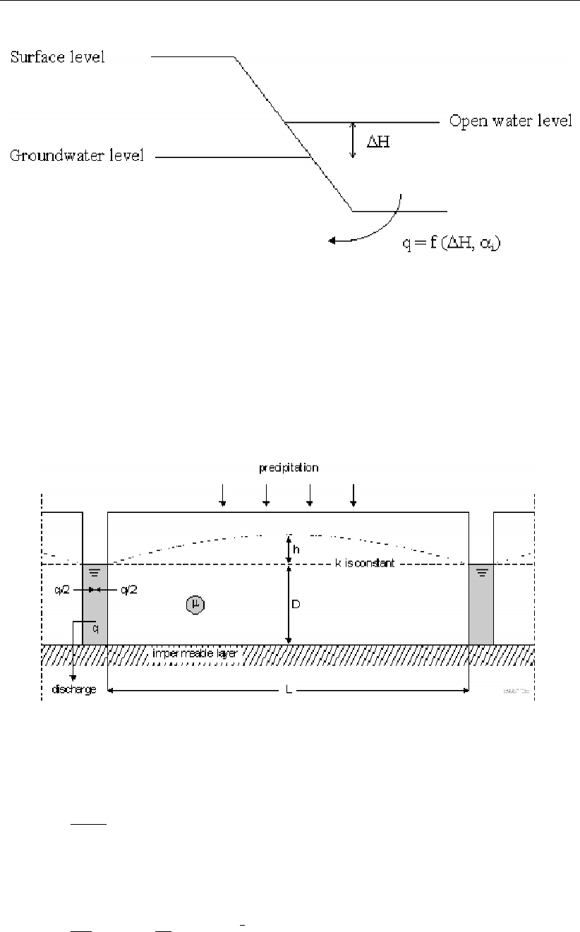
DRAFT
SOBEK, User Manual
Figure 6.73: Infiltration from open water
6.5.1.18 Krayenhoff van de Leur drainage formula
One of the options of modelling the runoff for unpaved area is the Krayenhoff van de Leur
formulation. Another available option is the de Hellinga-de Zeeuw formulation.
The following figure illustrates the principles of the Krayenhoff van de Leur method.
Figure 6.74: Drainage according to Krayenhoff van de Leur
The reservoir coefficient jis either specified directly, or calculated as:
j=µL2
π2kD
(6.288)
The (cumulative) drainage flow qis computed as:
q=8P
π2
n→∞
X
n=1,3,5,...
1
n2(1 −e−n2t
j)(6.289)
612 of 900 Deltares

DRAFT
Conceptual description
and the (cumulative) highest groundwater level between the ditches as computed as:
h=π2P
8µj 1−32
π3
n→∞
X
n=1,3,5,...
1
n3e−n2t
j!(6.290)
where:
jreservoir coefficient [d]
mstorage coefficient (specific yield) [−]
Ldistance between drainage ditches [m]
kDsoil transmissibility (transmissivity) [m2/d]
kDcan be derived from:
ksoil permeability [m/d]
Dthickness of permeable layer [m]
Pprecipitation [m]
q(cumulative) drainage flow [m/d]
hdifference between highest groundwater level and ditch level [m]
ttime [d]
Given the area A[m2], precipitation and drainage flow can be converted to [m3/s]
6.5.1.19 Minimum filling percentage for greenhouse storage basin
When the water level in the greenhouse storage basins becomes equal/lower than this mini-
mum filling percentage, the withdrawal of water out of the basins will be stopped.
Default: 10 %
6.5.1.20 Minimum level difference controller
With the minimum level difference controller one can keep a minimum difference between the
upstream water level and the downstream water level. This controller is closely related to the
fixed level controller. There are two differences:
the fixed level controller determines the level difference from the specified target levels
which can be variable within the year, whereas the minimum level difference controller
uses one constant minimum level difference;
the fixed level controller allows a crest level below the values specified in the crest level
table, whereas the minimum level difference controller does not allow this.
The algorithm of the minimum level difference controller is given as follows:
User input:
Minimum level difference Min_dif
initial crest level
Model input, i.e. parameters computed by SOBEK-RR:
Downstream level Ldown
The minimum level difference controller adjusts the crest level of the weir in the following way:
Deltares 613 of 900

DRAFT
SOBEK, User Manual
Crest level = Max (Crest level according to input table, (Ldown + Min_dif))
6.5.1.21 Mixed sewer
The sewer type of a paved area node can be one of the following types:
mixed sewer
separated sewer
improved separated sewer
A mixed sewer system means that there is only one system for the discharge of both rainfall
water and dry weather flow (return flow from domestic water use, e.g. showers, toilets, etc.)
Spilling from the sewer system after heavy rainfall thus contains a mix of rainfall water and
domestic return flow. Spilling from a mixed sewer system therefore in general has a negative
effect on the water quality of the receiving open water.
6.5.1.22 Open water node
In SOBEK-RR the local surface water is represented by open water nodes. An open water
node can also be considered a storage basin in which the variation of water level follows from
the volume balance equation. In this equation an increase of the storage with higher water
levels (effect from banks) can be taken into account. An open water node is always connected
with a structure to another open water node or to a boundary node representing the boundary
of the water system.
Storage at open water nodes increases through precipitation, seepage from deep groundwa-
ter, flows from adjacent paved area, unpaved area and greenhouse area, and inflow through
structures from other open water nodes or form boundaries. Open water storage decreases
through evaporation, percolation to deep groundwater, flows to unpaved area (if the open
water level is higher than the groundwater level), and flows through structures to other open
water nodes or boundaries.
In order to obtain an accurate computation of the open water level, the level changes and
flow-through-structures, which depend on water levels, are computed iteratively.
614 of 900 Deltares
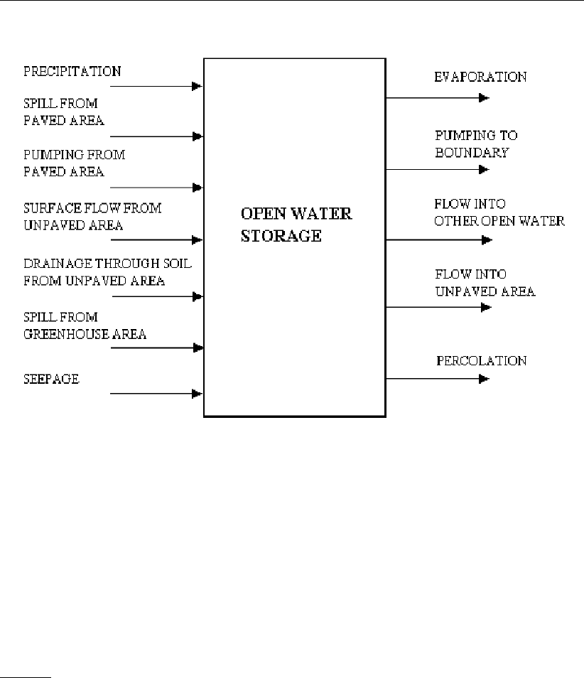
DRAFT
Conceptual description
Figure 6.75: Representation of the rainfall-runoff process of an open-water area
Amount of rainfall on open water node
The amount of rainfall on a open water node depends on the surface area of open water,
which can increase with an increasing water level. SOBEK does take this effect into account.
But the increase of open water surface means that in SOBEK the total area also increases. In
reality, the surface area of the unpaved area decreases. SOBEK does not take this effect into
account.
6.5.1.23 Paved area node
General
The paved area node is used to simulate the rainfall-runoff process on paved or impervious
areas.
A paved area is characterized by:
area [ha]
maximum storage on street [mm]
maximum storage in sewer [mm]
sewer pump capacity [m3/s]
sewer type (mixed, separated, or improved separated system)
DWF (dry weather flow)
Important processes are surface runoff or sewer overflow, occurring when the storage on land
or storage in the sewer exceeds its maximum and rapid runoff occurs.
Deltares 615 of 900
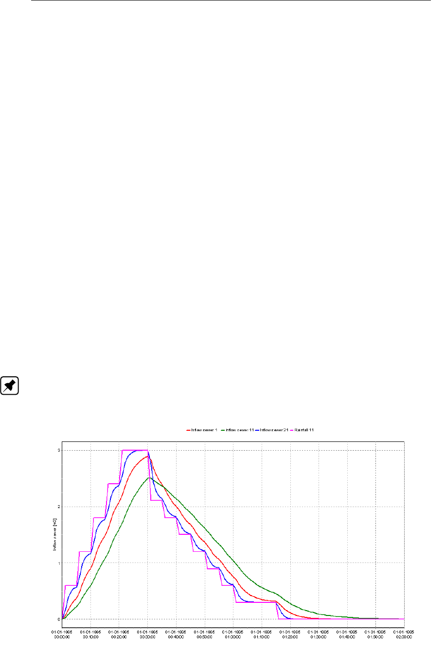
DRAFT
SOBEK, User Manual
6.5.1.24 Paved node surface runoff
When the amount of water on the RR-paved surface exceeds the maximum storage, surface
runoff will occur. The surface runoff can be implemented using either
no delay,
using a runoff delay coefficient, or
using a QH-relation.
The first option, no delay, means all surface runoff branches the outflow point in the same
timestep. Surface runoff can be blocked however if the open water level at the connecting
node exceeds the surface level of the paved node. But when using the ‘no delay’ option the
surface storage will immediately runoff as soon as the water level drops below the paved
surface level. This may lead to very spiky discharges from the paved node to the RR-open
water or RR-Boundary node.
The second option, using a runoff delay coefficient, is similar to the RR-Urban runoff model.
(See also the description of delay of runoff in the RR-Urban documentation, section 6.5.4.
This is formulating the surface runoff using the rational method (q=ch). The runoff delay
coefficient cis specified as a number between zero and one (1/min). A coefficient of one
means all runoff occurs in 1 minute, while a coefficient of 0.1 means only 10 % of the excess
volume will branch the open water in 1 minute.
The impact of the runoff delay coefficient on the runoff pattern is shown in the following graph.
The graph shows the rainfall time-series used, and the runoff using runoff delay coefficients
of 0.1, 0.2 and 0.5. It is assumed that there is no infiltration or sewer, and that the maximum
storage on the street is zero.
Note: The example Figure 6.76 is actually taken from a simulation of the RR-Urban inflow
model, but the behaviour for the RR-Paved node is the same.
Figure 6.76: Impact of delay coefficient on runoff pattern
616 of 900 Deltares
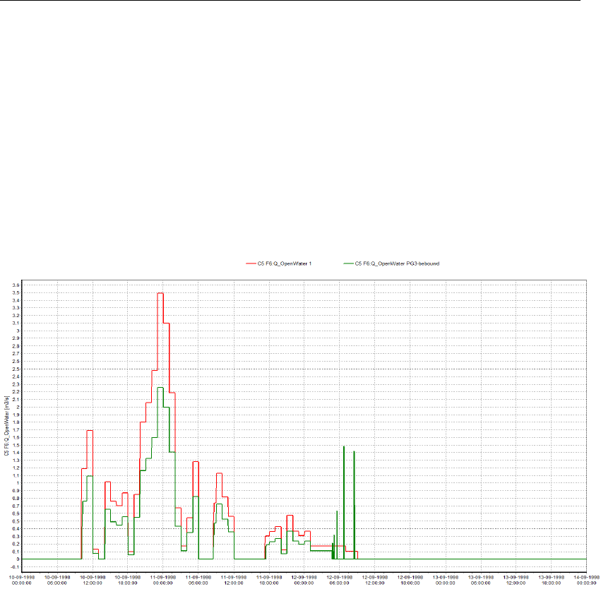
DRAFT
Conceptual description
The third option, using a QH-relation, allows limiting of the Qbased on the water level h.
Based on the interpolation table defined by the user a maximum Qis determined with which
the overflowing discharge is limited.
The used his the water level of the open water node or RR-CF-connection node downstream
of the paved node, where the overflowing discharge of the RR-paved node is discharged to.
See the following two examples:
1Figure 6.77 shows the result of water overflowing from two paved nodes to open water
nodes without delay of discharge from the paved nodes.
2Figure 6.78 shows the discharges after using a QH-relation.
Figure 6.77: Discharge from Paved to Open Water without delay
Deltares 617 of 900
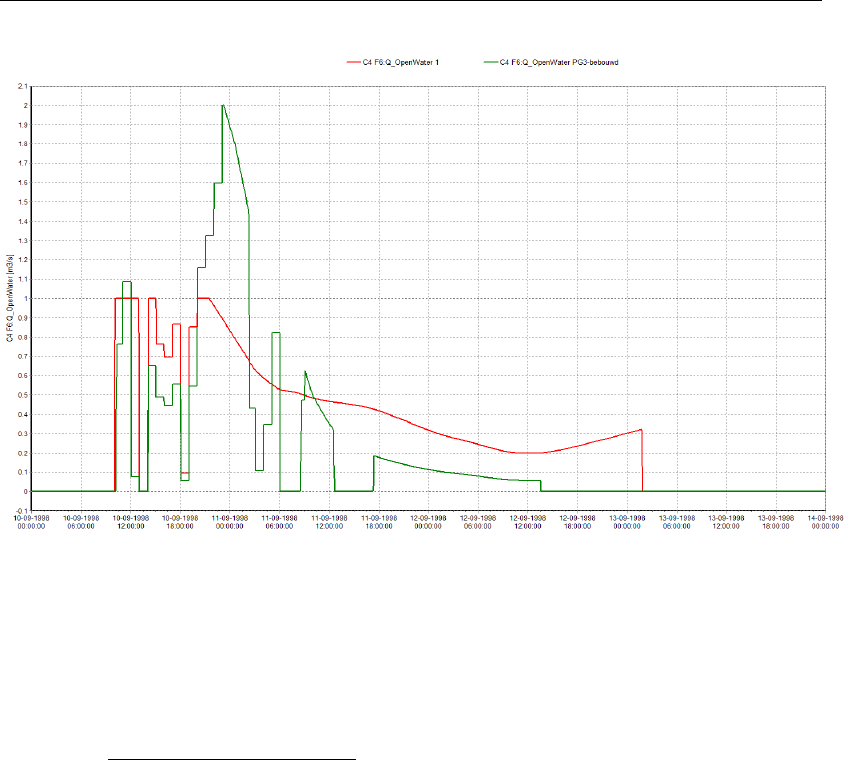
DRAFT
SOBEK, User Manual
Figure 6.78: Discharge from Paved to Open Water using QH-relation
6.5.1.25 Percolation
If the moisture storage in the root zone exceeds the equilibrium content, percolation occurs
from root zone to groundwater:
qp=Veq −(V(t−∆t)+∆V)
∆t(6.291)
qpPercolation [m/d]
VSoil moisture storage in the root zone [m]
Veq Equilibrium moisture storage in the root zone [m]
∆tTime step [d]
If percolation occurs, it is assumed that the percolating water branches the groundwater table
within the current time step of the groundwater.
The equilibrium moisture storage in the root zone is defined as the amount of moisture corre-
sponding with a steady-state simulation with no-flow conditions to or from the root zone.
618 of 900 Deltares
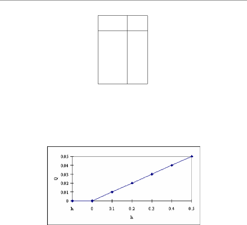
DRAFT
Conceptual description
Q h
0 0
0.01 0.1
0.02 0.2
0.03 0.3
0.04 0.4
0.05 0.5
6.5.1.26 QH-relation
A QH-relation can be used to represent any type of structure. When the user defines the
QH-relation as follows:
then SOBEK-RR computes the discharge Qas a function of the water level h:
Figure 6.79: QH-relation
6.5.1.27 Root zone
The root zone for which the water balance is considered has a thickness which is a function
of the land use type and the soil physical unit:
dr=f(j, s)(6.292)
where:
drroot zone thickness
jland use type (1,. . . ,16)
ssoil physical unit (1,. . . ,21)
The thickness of the root zone is assumed to be constant, regardless of season and year. The
moisture storage of the root zone at equilibrium condition is calculated with the function:
Veq =f(s, dr, dg)(6.293)
where:
Veq the moisture storage of the root zone at equilibrium condition [m]
ssoil physical unit [−]
drthickness of root zone [m]
dgdepth of the groundwater level [m]
Deltares 619 of 900

DRAFT
SOBEK, User Manual
Initial storage in the root zone
The initial storage in the root zone can be defined by one of the three following options:
the equilibrium root zone storage for the given crop-soil combination and specified initial
groundwater level;
the root zone storage at pF= 2;
the root zone storage at pF= 3.
Root zone thickness defining more than one crop
When the user defines more than one crop per unpaved node SOBEK calculated the over-
all root zone by weighted averaging. So, the area of the individual crops is also taken into
account.
For calculating the evaporation SOBEK uses the crop with the largest sub-areal.
6.5.1.28 RR controllers
The SOBEK Rainfall-Runoff module offers the option to operate hydraulic structures such as
weirs and orifices to a certain extent.
The available controllers are:
Time controller
Target level controller
Fixed Level difference controller
Minimum level difference controller
Equal filling controller
See their sections in the Technical Reference Manual for more information on each type of
controller.
6.5.1.29 RR routing link
The standard RR-links are links indicating connections between e.g. an unpaved node and an
open water node. The link flow in that case represents the flow from the unpaved area to the
open water. There is no difference between link inflow and link outflow.
Within SOBEK, the hydrodynamic flow aspects involving time delay between link inflow and
outflows are typically handled using the SOBEK-Channel Flow module. However, in some
cases a simple approach may be necessary. For instance, if only flow measurements at
an upstream location and a downstream location (without additional inflows in between) are
known, but no cross-section information is available. In such situations a simple routing ap-
proach can be used. An example of such a simple approach is the well-known Muskingum
method. This method is available in SOBEK-RR by using the so-called RR-Routing link.
620 of 900 Deltares

DRAFT
Conceptual description
Standard Muskingum method
The standard Muskingum method is using a layered routing approach. The inflow hydrograph
is divided into a number of layers, where each layer has its own routing coefficient.
According to the standard Muskingum method (McCarthy,1938) the outflow Qat time step
i+ 1 is computed using outflow Qat time step iand inflows Iat time step iand i+ 1:
Qi+1 =c1Ii+c2Ii+1 +c3Qi(6.294)
where:
c1=∆T+ 2Kx
2K(1 −x)+∆T(6.295)
c2=∆T−2Kx
2K(1 −x)+∆T(6.296)
c3=2K(1 −x)−∆T
2K(1 −x)+∆T(6.297)
The parameter Kis a proportionality factor with the dimension of time, it is dependent on the
time step you select. Kis the travel time of a flood wave through the branch. The parameter
xis a dimensionless weighting factor with 0≤x≤0.5. In natural streams values of x
ranging from 0 to 0.3 are often found. Great accuracy in determining xmay not be necessary
as the final result is relatively insensitive to the value of x.
It is easily verified that c1+c2+c3= 1 and further that ∆Tand Kshould have the same
time units. The use of the method requires choices on ∆T,Kand x. The routing interval
∆Tis the calculation time step size in SOBEK-RR. The chosen time step size should be
less than K, as otherwise peaks will be missed at the downstream side. It is advised the
SOBEK-RR computation time step size ∆Tto be taken as 1/2to 1/4of K. If, however, a
∆Tis selected which is much smaller than K, then c2becomes negative. This will lead to a
dip in outflows, or even to negative outflows when the inflow starts rising. To avoid negative
coefficients the routing interval should be within the range: 2Kx ≤∆T≤K. For values of
xclose to 0.5 this requirement leaves little freedom in the selection of ∆T. If one is mostly
interested in the higher part of the flood wave the above condition can be relaxed somewhat
by accepting slightly negative values for c2.
The Muskingum routing method allows the routing to be split in multiple layers. This can be
of great value when the river contains a minor bed and a floodplain. In the floodplain the
Muskingum parameters will be completely different from the parameters of the minor bed.
An example of this computation is given below. Suppose that you use 2-layers for routing the
flood wave:
layer 1: x= 0.4K= 3.5Qmax = 100 m3s−1
layer 2: x= 0.1K= 9
SOBEK-RR will then route all discharges up to Q= 100 m3s−1with the parameters of the
first layer, all discharges above Q= 100 m3s−1will be routed with the parameters of the
second layer
(and using Qlayer2=Qi−100[m3/s]).
Deltares 621 of 900
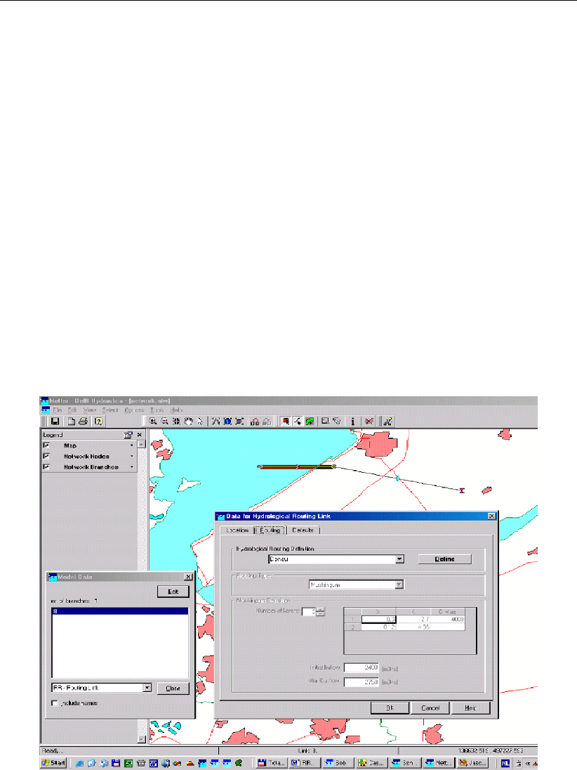
DRAFT
SOBEK, User Manual
RR connection node
Similar to a Flow Connection node, now also a RR-connection node is available. The RR-
Connection node does not require any input data. The basic function of the RR-Connection
node is that of a confluence: adding up all flows from incoming links and supplying that to the
downstream link.
Network validation rules for RR-routing link and RR-connection nodes
The following rules apply to the use of the RR-routing link and RR-connection nodes:
The RR-routing link can be used to connect:
a Sacramento node to an RR-connection node;
an RR-connection node to an RR-connection node;
an RR-connection node to a RR-boundary node;
At RR-connection nodes, multiple upstream links are possible, but only 1 downstream
(routing) link is allowed.
Examples of network layout and ModelEdit user interface:
Figure 6.80: Example input data
622 of 900 Deltares
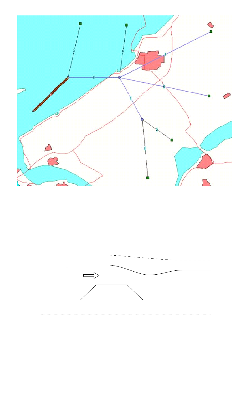
DRAFT
Conceptual description
Figure 6.81: Possible usage in a network
6.5.1.30 RR - Orifice
The orifice is one of the structures available in the SOBEK-RR-module. The geometrical
shape is given in Figure 6.82.
Figure 6.82: Orifice
Flow across the orifice can be of the following types: drowned weir flow, free weir flow,
drowned orifice flow, free orifice flow or no flow (water levels below crest level or orifice closed)
depending on the dimensions of the structure and the flow conditions.
The following discharge equations are applied during the computations:
Free orifice flow:
Q=µcBdq2g(h1−(z+µdg)) (6.298)
Deltares 623 of 900

DRAFT
SOBEK, User Manual
Drowned orifice flow:
Q=µcBdp2g(h1−h2)(6.299)
Free weir flow:
Q=cB 2
3r2
3g(h1−zs)3/2(6.300)
Drowned weir flow:
Q=cB(h1−z)p2g(h1−h2)(6.301)
QDischarge across orifice [m3/s]
µContraction coefficient [−]
cDischarge coefficient [−]
BCrest width [m]
dgOpenings height [m] (openings level - crest level)
gGravity acceleration [m/s2]
h1Upstream water level [m]
h2Downstream water level [m]
zsCrest level [m]
The different formulas are applied when the following conditions occur:
Free orifice flow:
h1−z≥3
2dgand h2≤zs+dg(6.302)
Drowned orifice flow:
h1−z≥3
2dgand h2> zs+dg(6.303)
Free weir flow:
h1−z < 3
2dgand h1−zs>3/2(h2−zs)(6.304)
Drowned weir flow:
h1−z < 3
2dgand h1−zs≤3
2(h2−zs)(6.305)
624 of 900 Deltares
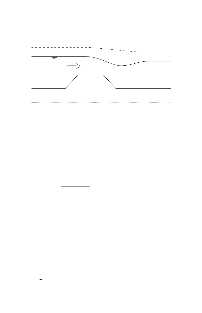
DRAFT
Conceptual description
6.5.1.31 RR - Weir
Three types of flow conditions can occur in the case of weir flow. These are free (modular)
flow, drowned (submerged) flow and no flow (water levels below crest level). If high tail water
conditions do affect the flow, the weir is said to be drowned.
Figure 6.83: Weir
The discharge through the weir is computed with the following formulas:
Free weir flow:
Q=cB 2
3r2
3g(h1−zs)3/2(6.306)
Drowned weir flow:
Q=cB(h1−zs)p2g(h1−h2)(6.307)
QDischarge across weir [m3/s]
cDischarge coefficient [−]
BCrest width [m]
gAcceleration due to gravity [m/s2]
h1Upstream water level [m]
h2Downstream water level [m]
zsCrest level [m]
The different formulas are applied when the following conditions occur:
Free weir flow:
h2−zs<2
3(h1−zs)(6.308)
Drowned weir flow:
h2−zs≥2
3(h1−zs)(6.309)
Two-stage weir:
The flow over a 2-stage weir is determined as the sum of the two weirs:
A rectangular weir with crest level Crestlevel1 and width Width1; and
Deltares 625 of 900
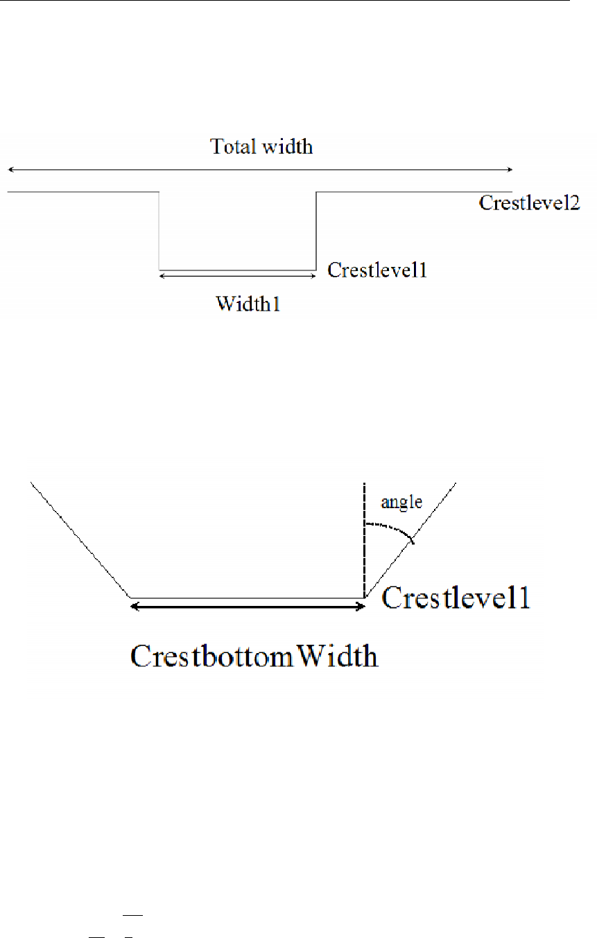
DRAFT
SOBEK, User Manual
A rectangular weir with crest level Crestlevel2 and width Width2.
The Rainfall Runoff module separately determines the flow conditions for both levels (free or
drowned flow, or no flow). The normal Weir formulae are used.
Figure 6.84: Two-stage weir
The crest level of the lower stage of the weir can optionally be adjusted according to the
upstream open water target level (depending on the switch specified in the Settings module).
The crest level of the second stage is not adjusted.
Figure 6.85: Two-stage weir, crest bottom width at crestlevel 1
Output for 2-stage weirs: Both the total flow over the weir and the seperate flows of the two
levels are shown.
V-notch broad-crested weir
Free weir flow:
Q=dc
16
25r2
5gtan(α)H2.5(6.310)
where dcis typically between 0.85 and 1.05.
626 of 900 Deltares
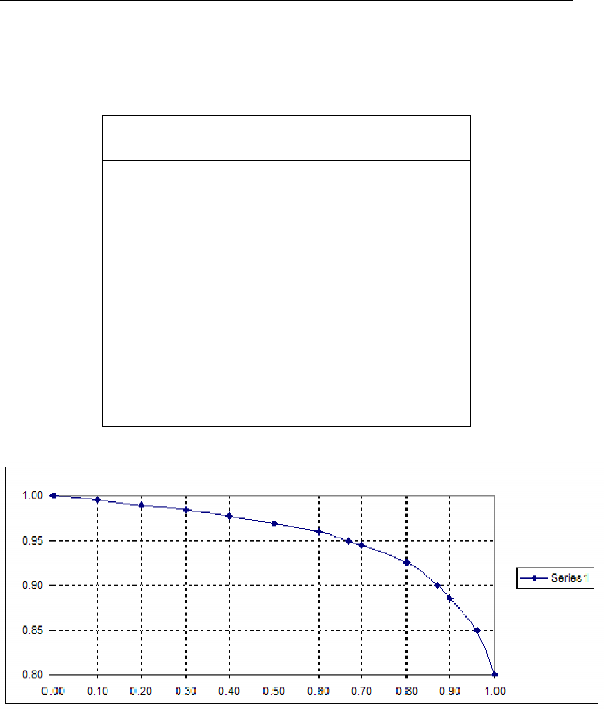
DRAFT
Conceptual description
Drowned weir flow
The drowned flow reduction factor is given as a function of the ratio of the upstream and
downstream waterlevels above the crest level (Bos,1989, Par. 4.3.3).
H2/H1 Reduction
factor
Remark
1 0 H2=H1, no flow
0.995 0.1
0.99 0.2
0.985 0.3
0.978 0.4
0.97 0.5
0.96 0.6
0.95 0.67
0.945 0.7
0.925 0.8
0.9 0.87
0.885 0.9
0.85 0.96
0.8 1.0 free weir flow
Figure 6.86: V-notch broad-crested weir
6.5.1.32 Separated sewer
The sewer type of a paved area node can be one of the following types:
mixed sewer
separated sewer
improved separated sewer
A separated sewer has separate sewer systems for rainfall and dry weather flow. This system
is designed to reduce water quality impacts of sewer overflows on the receiving open water.
In a mixed sewer system spilling contains DWF water (domestic return flows). In a separated
sewer system however, sewer overflows usually only originate from the rainfall sewer system
Deltares 627 of 900

DRAFT
SOBEK, User Manual
and not from the DWF sewer system. Therefore, the sewer overflows do not contain the waste
loads from the domestic return flows.
6.5.1.33 Silo capacity/Pump capacity
Apart from storage in rainfall basins in some greenhouse areas there is also storage of water
in silo’s. These silo’s, usual capacity approximately 200 m3ha−1, function as a temporary
storage before pumping the water into the soil (subsoil storage). The pump capacity for subsoil
storage usually is about 15 m3h−1.
6.5.1.34 Soil surface level
There are two options to define the soil surface level:
Surface level = constant
The user can define any constant surface level he wants, usually the (almost) lowest surface
level in the unpaved area.
Storage on land
groundwater level rise: when the groundwater table branches the lowest surface level,
surface runoff occurs only when the storage on land is filled.
high precipitation rate: when the net precipitation rate exceeds the infiltration rate, water
will be stored on land. Surface runoff occurs only when the storage on land is filled.
Surface level = not constant
When this option was chosen, the user can specify the soil surface level in a more detailed
way.
SOBEK does take into account up to a maximum of 100 sub-areas (default). The user can
define these areas in a table, see Figure 6.87.
628 of 900 Deltares
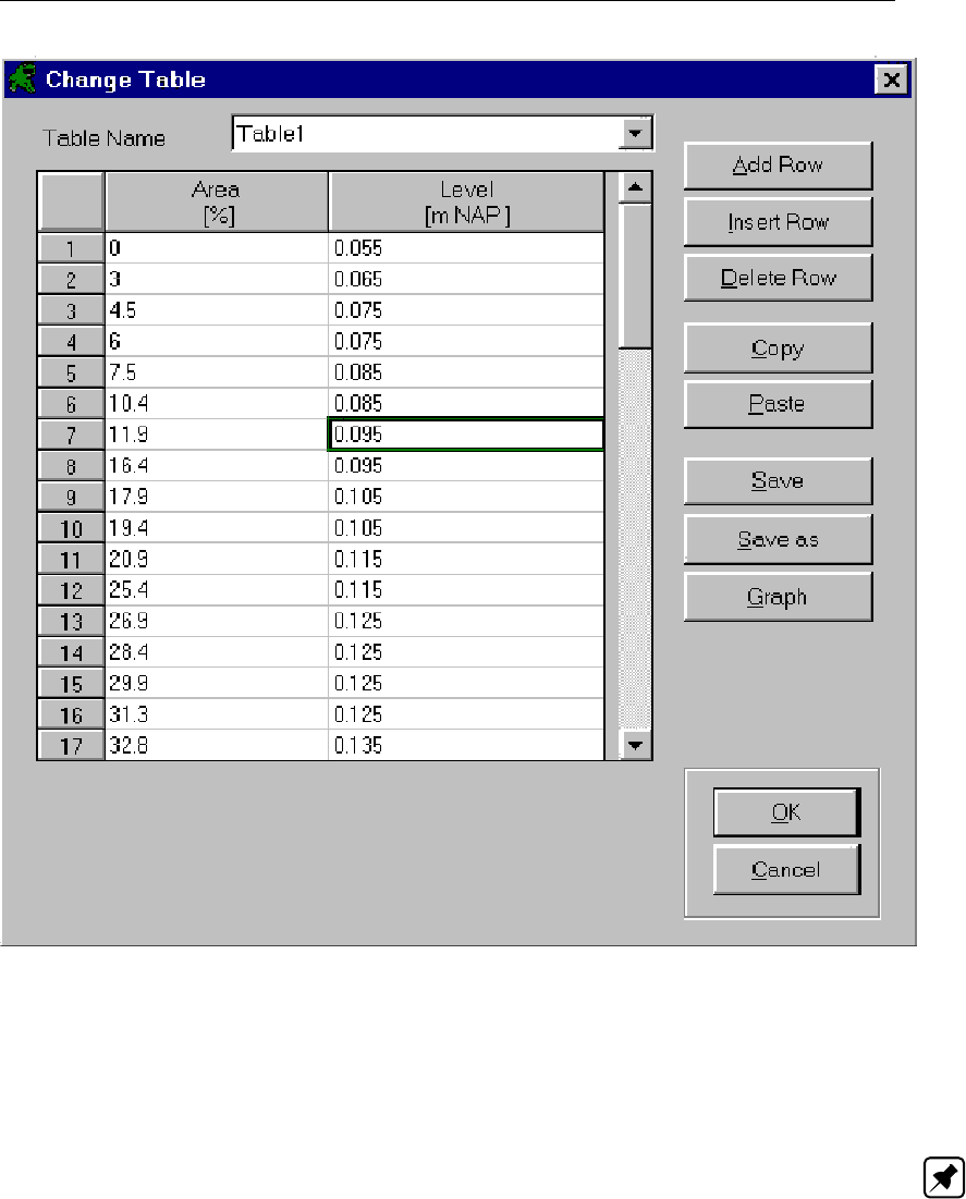
DRAFT
Conceptual description
Figure 6.87: Change table
The user should make sure that 0 and 100 % are present in this table. In between the user
can define as many rows as he wants. Above the 100 % level it is assumed that the area does
not increase.
Note: By showing the graph of the S-curve you can check whether you entered the s-curve
data correctly.
Deltares 629 of 900
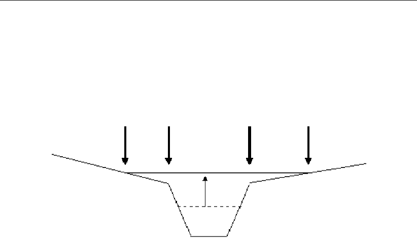
DRAFT
SOBEK, User Manual
Inundation
When the open water level exceeds the lowest surface level, inundation occurs. See Fig-
ure 6.88. SOBEK does take into account the extra volume to store water. SOBEK does not
take into account the precipitation and evaporation on the area of this extra storage volume.
In fact, the precipitation and evaporation on this area was already taken into account with the
surface of the unpaved area.
Figure 6.88: Inundation
Vertical infiltration of water in this extra storage area is not considered as well.
Finally, when the open water level exceeds the lowest surface level it is assumed that the
potential storage on land is equal to zero.
Initial groundwater level
When the surface level is not constant, it is assumed that the initial groundwater level is
defined w.r.t. the lowest surface level. For example, in Figure 6.87 the initial groundwater level
is defined w.r.t. the level of 0.055 m NAP.
Reaction factor α
In SOBEK it is possible to schematise the drainage process by defining four different layers.
For each layer a different reaction factor αis defined. When the surface level is not constant,
the reaction factor layers are defined relative to the surface level according to the table, see
Figure 6.89.
630 of 900 Deltares
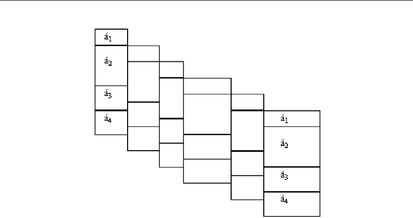
DRAFT
Conceptual description
Figure 6.89: Example of definition of reaction factor layers when the surface level is not
constant (in this case the number of sub-areas defined in the table is equal
to 6)
Actually, the above figure is a bit more complex, because default a 100 sub-areas are consid-
ered. The surface level of each sub-area is determined by interpolation of the surface level
table defined by the user.
Storage on land
Surface level is not constant:
groundwater level rise: when the groundwater table branches the lowest surface level,
immediately surface runoff occurs. Storage on land is not considered.
high precipitation rate: when the net precipitation rate exceeds the infiltration rate, water
will be stored on land. Surface runoff occurs only when the storage on land is filled.
Storage coefficient i
Surface level = not constant AND NOT using CAPSIM for unsaturated zone
The storage coefficient used to calculate the groundwater level fluctuation, is determined as
the average of the initial storage coefficients for each sub-area. The initial storage coefficient
is determined by the soil type and the distance between the soil surface and initial groundwater
level.
When the initial groundwater level exceeds part of the surface level (storage on land) then the
storage coefficients of this part of the surface are excluded from the averaging procedure.
Surface level = not constant AND using CAPSIM for unsaturated zone
CAPSIM needs , among others, the root zone depth and initial groundwater level. If the
surface level is not constant, the root zone depth and initial groundwater level passed to
CAPSIM are defined relative to the surface level (Figure 6.90). The root zone depth is equal
for each sub-area, because the root zone depth only depends on the soil type and the crop.
For each sub-area, separate actual evaporation, percolation and capillary rise, and volume of
water in the unsaturated zone are computed.
Deltares 631 of 900
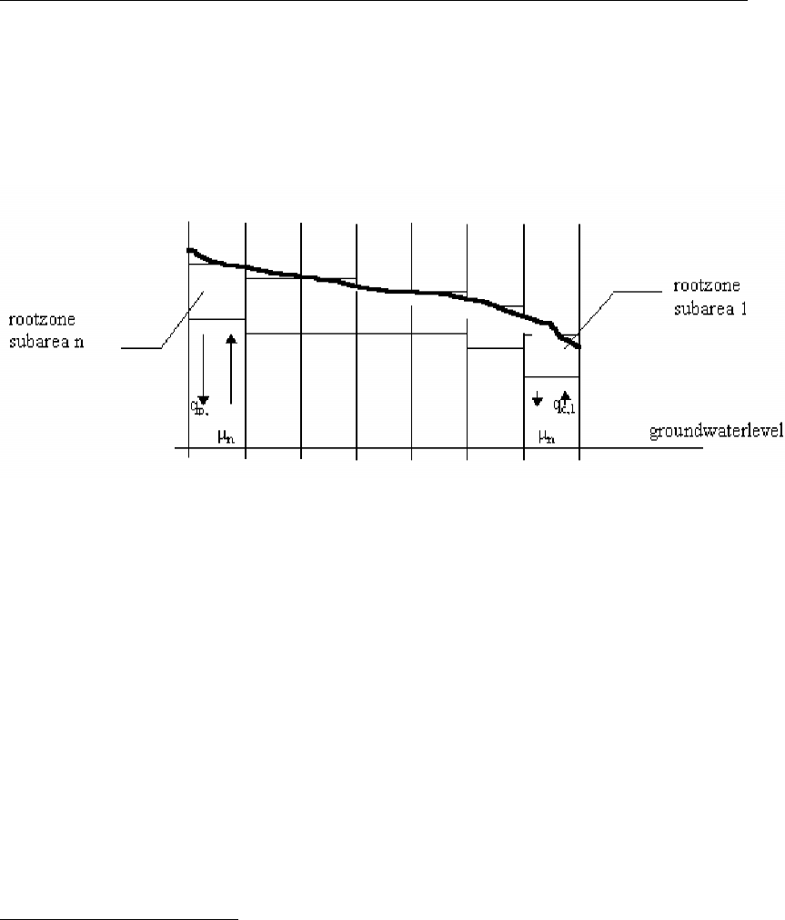
DRAFT
SOBEK, User Manual
The groundwater level is determined using the total percolation/capillary rise flow for all sub-
areas. The storage coefficient used to calculate the groundwater level fluctuation, is deter-
mined as the average of the actual storage coefficients for each sub-area. When the ground-
water level exceeds part of the surface level (storage on land) then the storage coefficients of
this part of the surface are excluded from the averaging procedure.
Figure 6.90: Rootzone sub areas
6.5.1.35 Storage coefficient
The storage coefficient m represents the percentage of soil-volume which is available for
storage of water. Once the storage coefficient is known, the total storage capacity can be
calculated:
V=µd (6.311)
Vstorage capacity [mm]
µstorage coefficient [m/m]
ddepth to groundwater table [mm]
With the storage coefficient, the change of the groundwater level can be calculated.
Option ’Unsaturated zone = none’
Calculating groundwater level
For calculating the groundwater level the average storage coefficient is used during the sim-
ulation period (Table 6.10). This average storage coefficient depends on the drainage basis,
i.e. the distance between the surface level and the initial groundwater level. These coefficients
are provided by the Winand Staring Centre -DLO.
The soil types are:
1 loamy, humous fine sand,
2 peat,
3 heavy clay,
4 humous clay and peat,
5 light loamy sand, medium coarse sand,
6 loamy silt,
7 humous clay and peat with silty top layer,
8 clay and light clay,
9 loamless, medium coarse and coarse sand,
632 of 900 Deltares
DRAFT
Conceptual description
10 silt,
11 very light clay,
12 sand with a silty top layer.
Table 6.10: Average storage coefficients depending on soil type and dranaige basis.
Drainage
basis [m]
Soil type
1 2 3 4 5 6 7 8 9 10 11 12
0.1
0.2
0.3
0.4
0.5
0.6
0.7
0.8
0.9
1.0
1.2
1.5
0.0074
0.0183
0.0302
0.0419
0.0532
0.0664
0.0805
0.0938
0.1061
0.1173
0.1372
0.1614
0.0077
0.0153
0.0226
0.0305
0.0387
0.0467
0.0545
0.0621
0.0702
0.0784
0.0939
0.1158
0.0094
0.0166
0.0226
0.0278
0.0323
0.0363
0.0399
0.0431
0.0461
0.0489
0.0538
0.0600
0.0063
0.0134
0.0206
0.0279
0.0350
0.0420
0.0486
0.0551
0.0613
0.0673
0.0786
0.0941
0.0046
0.0124
0.0220
0.0323
0.0427
0.0528
0.0625
0.0715
0.0801
0.0880
0.1024
0.1208
0.0049
0.0103
0.0158
0.0211
0.0262
0.0310
0.0364
0.0416
0.0466
0.0514
0.0605
0.0729
0.0049
0.0118
0.0181
0.0237
0.0289
0.0339
0.0386
0.0430
0.0472
0.0512
0.0586
0.0685
0.0048
0.0092
0.0132
0.0171
0.0206
0.0240
0.0271
0.0300
0.0328
0.0355
0.0404
0.0470
0.0027
0.0098
0.0162
0.0228
0.0294
0.0359
0.0422
0.0484
0.0542
0.0598
0.0704
0.0845
0.0029
0.0066
0.0105
0.0145
0.0186
0.0226
0.0265
0.0303
0.0341
0.0377
0.0446
0.0541
0.0025
0.0052
0.0079
0.0107
0.0134
0.0160
0.0185
0.0210
0.0235
0.0258
0.0303
0.0366
0.0013
0.0032
0.0052
0.0074
0.0096
0.0120
0.0143
0.0167
0.0191
0.0214
0.0261
0.0329
Calculating drainage flux
For calculating the drainage flux according to De Zeeuw- Hellinga a constant storage coef-
ficient is used. This storage coefficient, which is the same as for calculation the changes in
groundwater level, is the storage coefficient corresponding with the initial groundwater level.
Option ’Unsaturated zone = CAPSIM’
Groundwater level
For calculating the groundwater level a storage coefficient is used depending on the actual
groundwater level during the simulation period.
Drainage flux
The storage coefficient is calculated by averaging all coefficients within in the domain of the
groundwater level and the open water level. Since the groundwater level and the open water
level may change during the simulation period, the average storage coefficient may change.
The coefficients for calculating the groundwater level and the drainage flux are tabulated in in
SOBEK. These storage coefficients depend on the soil type, the root zone thickness end the
groundwater level. Below the storage coefficients are depicted for a root zone thickness of 20
cm. SOBEK also takes into account storage coefficient for root zone thicknesses of 10 cm, 50
cm, 100 cm and 200 cm.
All coefficients are provided by Alterra.
Deltares 633 of 900
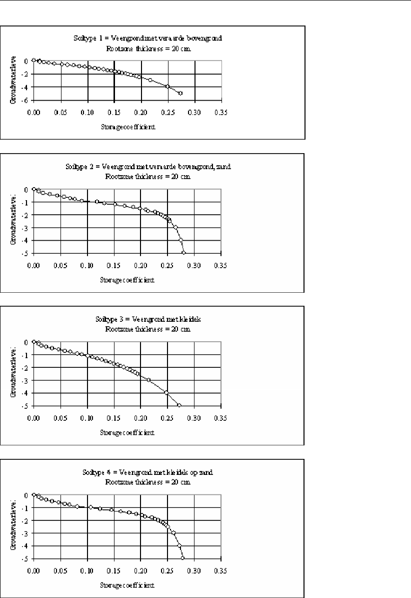
DRAFT
SOBEK, User Manual
634 of 900 Deltares
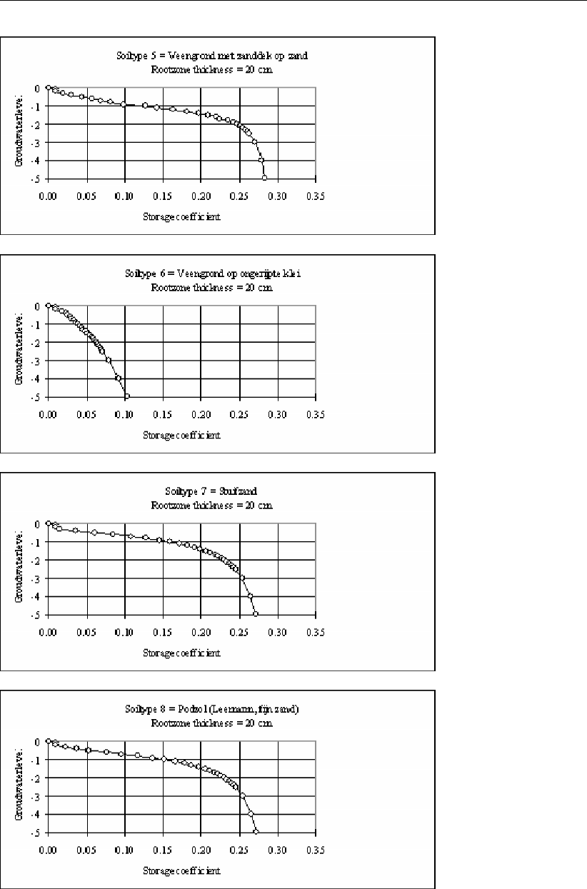
DRAFT
Conceptual description
Deltares 635 of 900
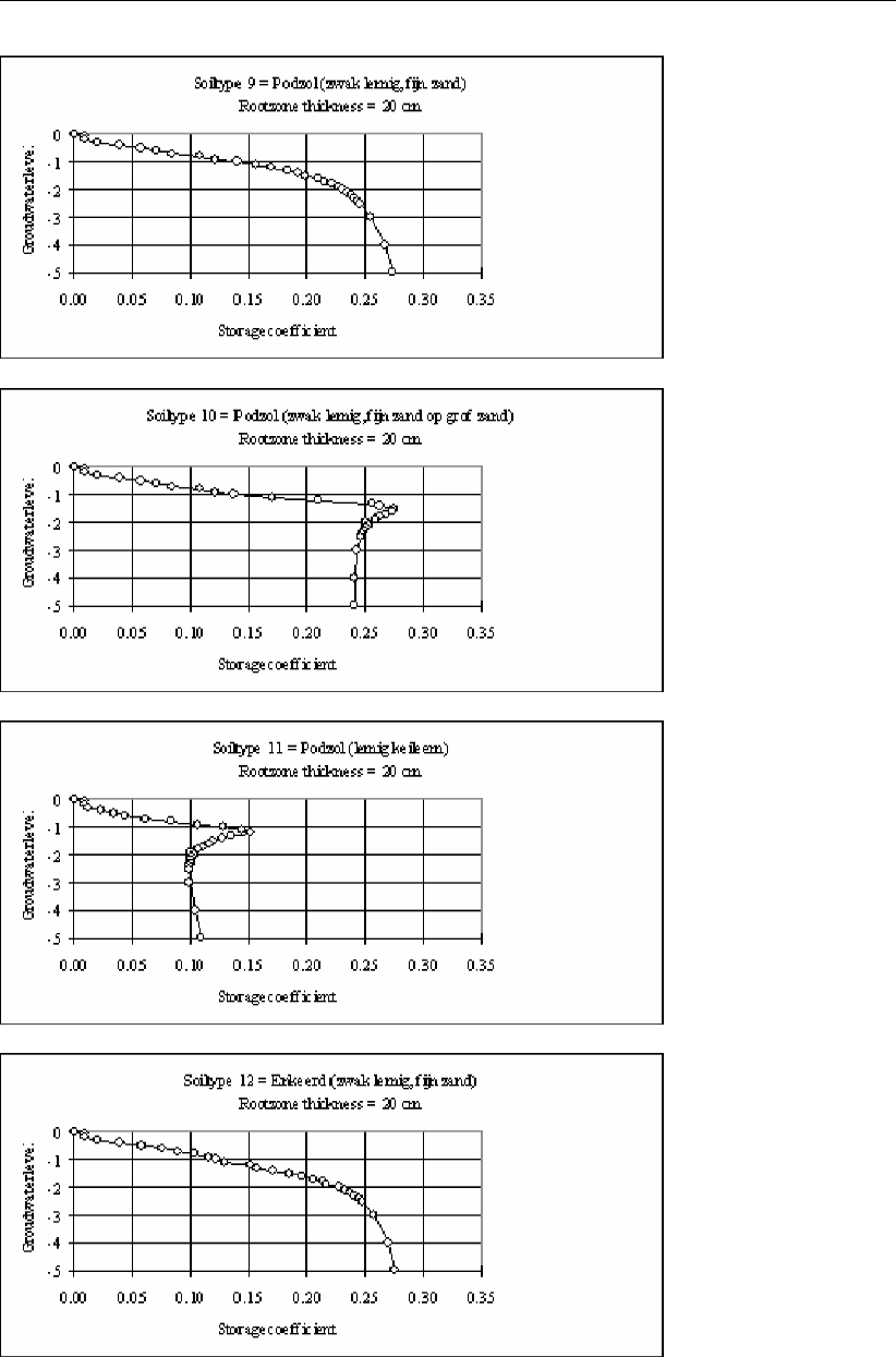
DRAFT
SOBEK, User Manual
636 of 900 Deltares
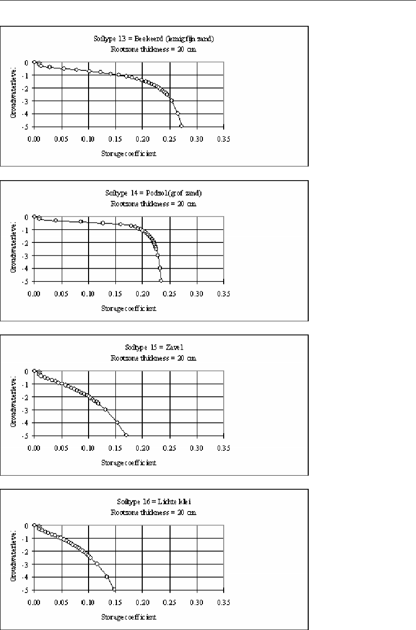
DRAFT
Conceptual description
Deltares 637 of 900
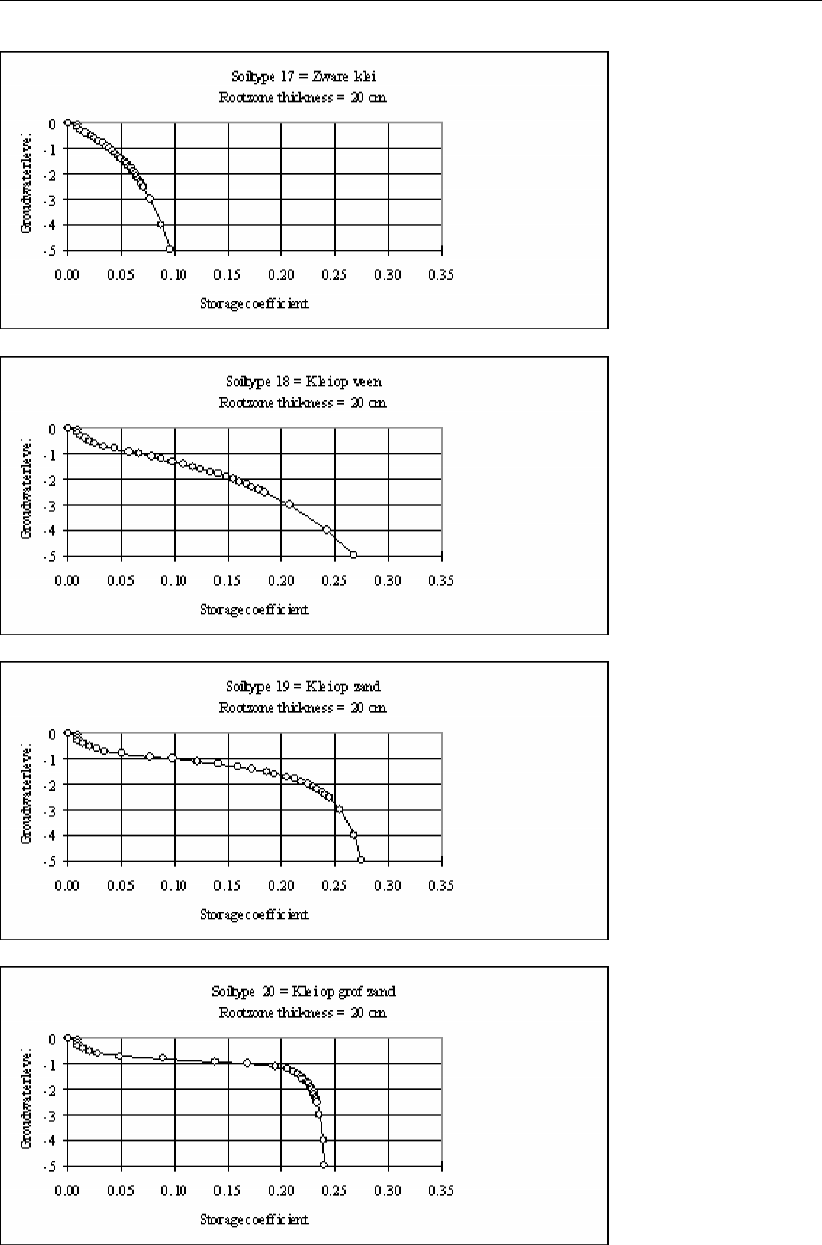
DRAFT
SOBEK, User Manual
638 of 900 Deltares
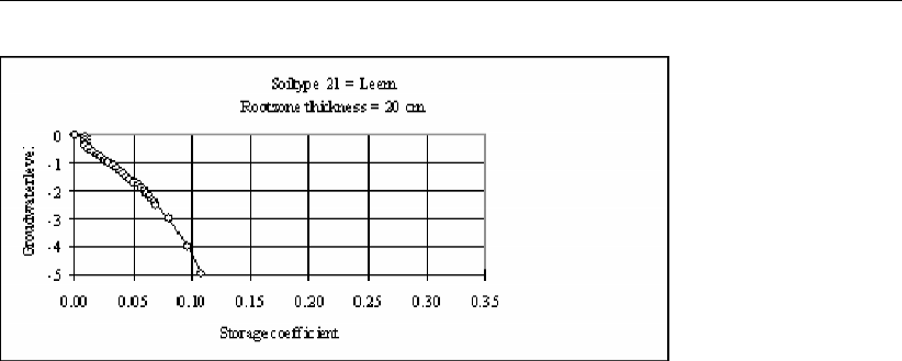
DRAFT
Conceptual description
6.5.1.36 Surface runoff
Surface runoff in paved areas
In paved areas surface runoff occurs when the ‘storage on street’ reservoir is completely filled.
Surface runoff in unpaved areas
In unpaved nodes surface runoff to open water can occur in two cases:
1 when the ‘storage on land’ reservoir is filled by the precipitation (minus evaporation and
infiltration into the soil).
2 when the groundwater level has branched the soil surface level. In this case, the storage
on land has not been taken into account, so surface runoff will immediately take place
when the groundwater level has branched the surface level.
In both cases the runoff process is simulated by means of the de Zeeuw-Hellinga equation.
Therefore, the user must define a specific surface runoff reaction factor.
Notice that when the soil surface is defined as a constant level, the total area defined in the
unpaved node is part of the surface runoff process. Often this causes very large discharges
to the open water.
When the soil surface is defined as a variable level, only the inundated part of the soil surface
is part of the surface runoff process.
6.5.1.37 Target level controller
With the target level controller one can control the upstream target level. The algorithm is
given as follows:
User input:
Maximum flow Qmax
Maximum allowed upstream level MAXLup
Maximum allowed downstream level MAXLdown
Upstream target level TLup
Downstream target level TLdown
Parameters computed by SOBEK-RR:
Upstream level Lup
Downstream level Ldown
Weir flow Q
Deltares 639 of 900

DRAFT
SOBEK, User Manual
A weir with a target level controller tries to maintain the upstream water level at the user
specified target level TLup. Upstream here means upstream with respect to the defined link
direction. When the upstream water level gets above the target level TLup, the crest of the
weir will be lowered in order to let the excess water flow away to the downstream node. The
weir crest can be lowered until the maximum defined discharge Qmax is branched (or the
crest branches is specified minimum level, which is by default the bed level).
The discharge is kept at or below the maximum defined discharge Qmax until the upstream
water level branches the specified maximum allowed upstream level MAXLup. In that case,
the specified maximum discharge Qmax may be exceeded, but only if the downstream water
level is below the specified maximum allowed downstream water level MAXLdown.
In extreme conditions, the downstream level is allowed to exceed the specified maximum
allowed downstream water level MAXLdown, but the upstream water level will not be allowed
to rise above the maximum upstream water level MAXLup.
Note: that the controller only operates in case of upstream excess water; it is not active in
case the upstream water level is below the target level.
The computation is done using the symbols as defined above, and additionally:
TimestepSize computation time step size in seconds
UpLvlEst estimated upstream level, without flow over the weir
DoLvlInit downstream level at beginning of the computation timestep
VolNow upstream volume in m3at level UpLvlEst
VolTarget upstream volume in m3at upstream target level TLup
VolMax upstream volume in m3at maximum allowed level MAXLup
A pseudo code of the computation is: (lines starting with ! are comments)
! Set upstream target end volume
if (DoLvlInit >MAXLdown) then
! downstream water level above maximum allowed downstream level;
! upstream level may rise until maximum allowed upstream level
EndV olume =V olMax
else
! normal situation: target end volume corresponding with upstream target level
EndV olume =V olT arget
endif
! Set provisional flow over the weir to get to the target EndVolume
if (VolNow >EndVolume) then
QOut = min(Qmax, (V olNow −EndV olume)/T imestepSize)
else
QOut = 0
endif
! Set provisional upstream End volume
EndV olume =V olNow −Qout ∗T imestepSize
! Check provisional end volume with maximum allowed upstream level (volume):
! The upstream level may never exceed the maximum allowed upstream water level
if EndV olume > V olM ax then
QOut = max(Qout, (V olNow −V olMax)/T imestepSize)
endif
! Final computed weir flow
Qout = min(Qout, flow with lowest possible crest level)
640 of 900 Deltares
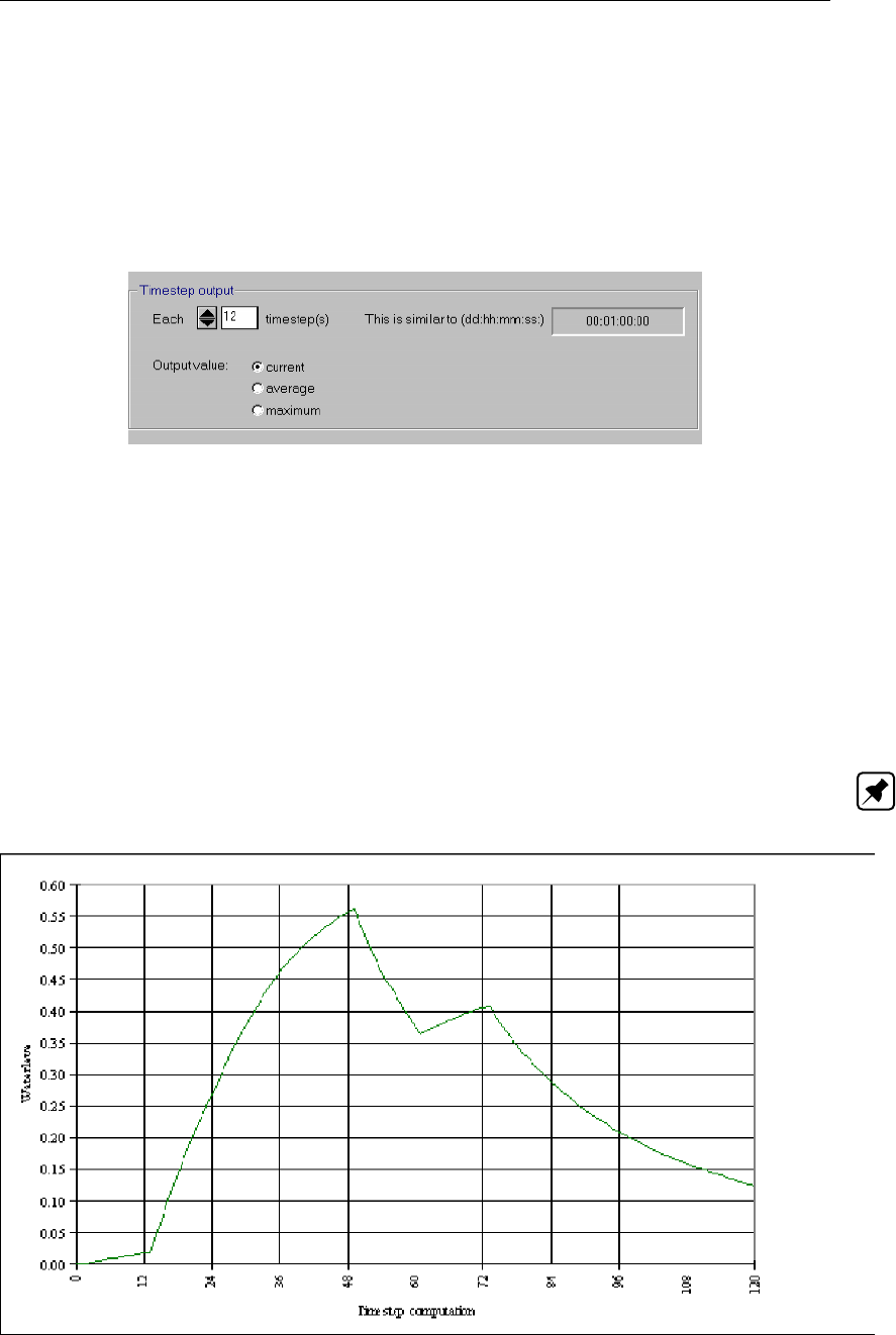
DRAFT
Conceptual description
6.5.1.38 Time step output
By default the time step of the results is equal to the time step of the computation. Especially
when a small time step is chosen, this results in a very large amount of output values. Then
the user can choose an other option in the Settings task in order to reduce the number of
output values.
Output reduction options in Settings:
Figure 6.91: Output reductions in Settings
In this case each 12th computed value is shown in the results graphs. The user can define
any interval he wants.
Other options;
Current: each nth computed value is written to the output file;
Average: the average value of n computed values is written to the output file;
Maximum: the maximum value of n computed values is written to the output file.
Note: the user should realise that the chosen options are of great importance to the shape
of the output graph, see this example:
Figure 6.92: Time step computation
Deltares 641 of 900
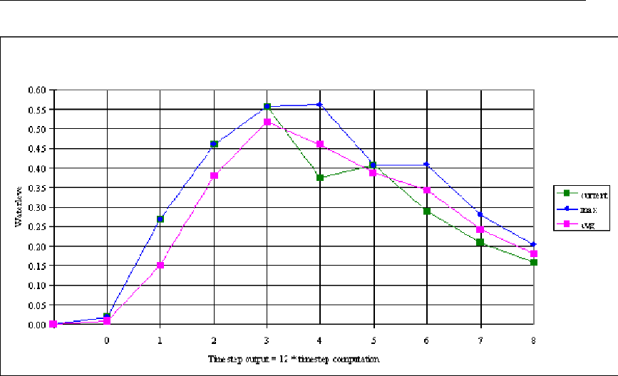
DRAFT
SOBEK, User Manual
Figure 6.93: Time step output = 12 ∗time step computation
When SOBEK is used to compute series of precipitation events, then the maximum realised
level is written to the output file, based on all computed values. The options current, average
and maximum are not relevant anymore.
6.5.1.39 Unpaved area node
General
The unpaved area node is used to simulate the rainfall-runoff process on unpaved areas.
An unpaved area is characterized by:
total unpaved area (sum of crop areas)
groundwater area
area per crop
soil surface level
soil type
storage coefficient
root zone
saturated zone
evaporation
capillary rise/percolation from root zone to groundwater
storage on land
infiltration capacity
drainage resistance value / reaction factor (dependent on the chosen method)
seepage/percolation (constant, variable in time or calculated from a defined groundwater
head in the lower confined aquifer and the resistance value of the confining layer)
surface runoff
The unpaved area is modeled using boxes representing storage on land, storage in the unsat-
urated zone, and the saturated zone. The unsaturated zone is optional. The surface area is
divided into area for different crops. The sum of the crop area is the total unpaved area. This
642 of 900 Deltares

DRAFT
Conceptual description
area is used for the surface storage and unsaturated zone computations. The saturated zone
computations use the groundwater area. This area is by default equal to the total unpaved
area, but can be defined separately by the user.
6.5.1.40 Unpaved surface flow link
The unpaved surface flow link is a branch type in RR which can be used to split the runoff from
a RR-unpaved node into two components: groundwater outflow (drainage) and surface runoff.
If an unpaved node has both a normal RR-link and an unpaved surface flow link connecting
it to the 1DFlow schematisation, the RR link will carry the groundwater drainage, and the
unpaved surface flow link will carry the surface runoff to the 1DFlow schematisation. In case
no unpaved surface flow link is used, the RR link will transport the total flow (groundwater
drainage plus surface runoff) to the 1DFlow schematisation.
This allows the user to specify different outflow locations for groundwater drainage and surface
runoff, and also allows to specify different waste loads or background concentrations for the
groundwater drainage and surface runoff in water quality computations.
The groundwater drainage computations use the open water level taken from the node down-
stream of the RR-link (remember that the driving force of the groundwater drainage is the
head difference between this open water level and the groundwater level) , while the surface
runoff computation uses the open water level taken from the node downstream of the RR-
unpaved surface flow link. The surface runoff is stopped when the open water level exceeds
the RR-unpaved surface level.
6.5.2 Sacramento Rainfall-Runoff model
6.5.2.1 Sacramento, the Segment module: implemented in SOBEK
The segment module simulates the rainfall-runoff process in part of the catchment, where the
attention is on the land-phase of the rainfall-runoff process. It is assumed that the open water
system in the segments contributes little to the shaping of the hydrograph. The conceptuali-
sation of the processes as described in the segment module is presented in Figure 6.94.
Deltares 643 of 900
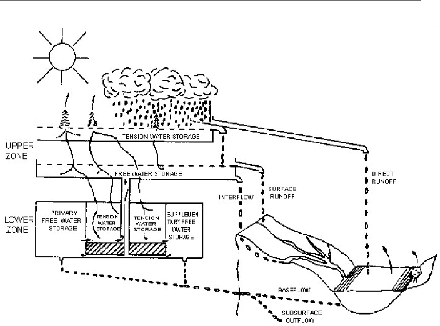
DRAFT
SOBEK, User Manual
Figure 6.94: Conceptualisation of the rainfall-runoff process in a segment.
The segment module is divided into the following components, (see also Figure 6.95):
Impervious area with transfers to direct runoff
Pervious area
Upper zone
◦Tension storage with transfers to evaporation, free water storage
◦Free water storage with transfers to evaporation, percolation,
◦surface runoff and interflow
Lower zone
◦Tension storage with transfers to evaporation. free water storage
◦Free water storage with transfers to base flow
From the impervious areas, precipitation immediately discharges to the channel. However,
impervious areas, which drain to a pervious part before branching the channel, are not con-
sidered impervious. Both zones have a tension and a free water storage element. Tension
water is considered as the water closely bound to soil particles. Generally first the tension
water requirements are fulfilled before water enters the free water storage.
644 of 900 Deltares
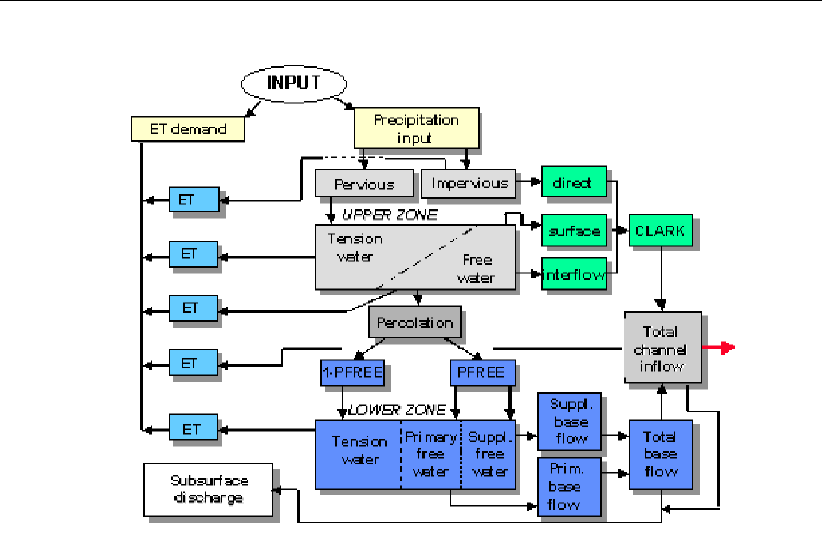
DRAFT
Conceptual description
Figure 6.95: Schematisation of the rainfall-runoff process in a segment
In the following sub-sections the various components will be described in detail
6.5.2.2 Upper zone storage
The upper zone tension storage represents that precipitation volume required under dry con-
ditions:
to meet all interception requirements, and
to provide sufficient moisture to the upper soil so that percolation can begin.
If the maximum storage capacity of the upper-zone tension storage is exceeded, water be-
comes available for the upper zone free water storage, a temporary storage from which water
percolates to the lower zone system and from which water discharges to the channel via the
interflow component. The preferred flow direction from the upper zone is the vertical direction,
i.e. percolation to the lower zone system.
Interflow occurs only when the precipitation rate exceeds the percolation rate. The upper zone
is treated as a linear storage element which is emptied exponentially: discharge = storage
∗storage depletion coefficient. The upper zone free water storage depletion coefficient is
denoted by UZK and the upper zone free water content by UZFWC then the interflow takes
place at a rate:
Qinterflow =UZF W C ∗UZK (6.312)
When the precipitation intensity exceeds the percolation intensity and the maximum interflow
drainage capacity, then the upper zone free water capacity (UZF W M) is completely filled
and the excess precipitation causes surface runoff.
Deltares 645 of 900

DRAFT
SOBEK, User Manual
6.5.2.3 Lower zone storage
The lower zone consists of the
tension water storage, i.e. the depth of water held by the lower zone soil after wetting and
drainage (storage up to field capacity) and
two free water storages: the primary and supplemental storage elements representing
the storages leading to a slow and a fast groundwater flow component, respectively. The
introduction of two free lower zone storages is made for greater flexibility in reproducing
observed recession curves caused by groundwater flow.
6.5.2.4 Percolation from upper to lower zones
The percolation rate from the upper zone to the lower zone depends on the one hand on the
lower zone demand, i.e. requirements determined by the lower zone water content relative to
its capacity and on the other hand on the upper zone free water content relative to its capacity.
The lower zone percolation demand is denoted by P ERCact.dem. The upper zone free wa-
ter content relative to its capacity is UZF W C/UZF W M . Hence, the actual percolation
intensity then reads:
P ERC =P ERCact.dem ×U ZF W C/U ZF W M (6.313)
The lower zone percolation demand has a lower and an upper limit:
the minimum lower zone percolation demand, and
the maximum lower zone percolation demand.
The minimum lower zone percolation demand occurs when all three lower zone storages are
completely filled. Then by continuity the percolation rate equals the groundwater flow rate
from full primary and supplemental reservoirs. Denoting the minimum demand by PBASE
then it follows:
P ERCmin.dem =P BASE =LZF P M ×LZP K +LZF SM ×LZSK
(6.314)
where:
LZF P M lower zone primary free water storage capacity
LZF SM lower zone supplemental free water storage capacity
LZP K drainage factor of primary storage
LZSK drainage factor of supplemental storage
The maximum lower zone percolation demand takes place if the lower zone is completely
dried out i.e. if its content = 0. Then the maximum percolation rate is expressed as a function
of PBASE:
P ERCmax.dem =P BASE(1 + ZP ERC)(6.315)
with: ZP ERC 1usually.
The actual lower zone percolation demand depends on the lower zone content relative to its
capacity. Computationally it means that ZPERC has to be multiplied by a function Gof the
relative lower zone water content such that this function:
equals 1 in case of a completely dry lower zone
equals 0 in case of a completely saturated lower zone
646 of 900 Deltares
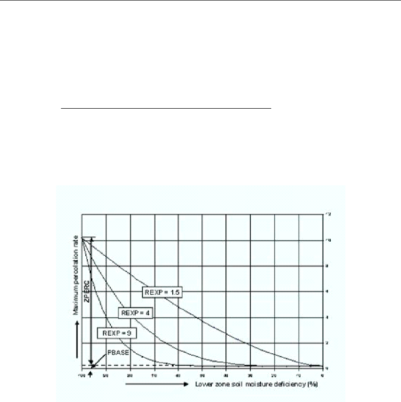
DRAFT
Conceptual description
represents an approximate exponential decay of the percolation rate in case of a continu-
ous recharge.
In the Sacramento model this function has the following form:
G=P(lower zone capacities −lower zone content)
P(lower zone capacities)REXP
(6.316)
and the actual percolation demand is given by (see Figure 6.96):
P ERCact.dem =P BASE(1 + ZP ERC ∗G)(6.317)
Figure 6.96: Actual percolation demand representation
6.5.2.5 Distribution of percolated water from upper zone
The percolated water drains to three reservoirs, one tension and two free water reservoirs.
Based on the preceding comments one would expect that the lower zone tension storage
is filled first before percolation to the lower zone free water storages takes place. However,
variations in soil conditions and in precipitation amounts over the catchment cause deviations
from the average conditions. This implies that percolation to the free water reservoirs and
hence groundwater flow takes place before the tension water reservoir is completely filled.
The model allows for this to let a fraction of the infiltrated water percolate to the two free water
storages. When the tension water reservoir is full, all percolated water drains to the primary
and supplemental free water storage in a ratio corresponding to their relative deficiencies.
6.5.2.6 Groundwater flow
Base flow to the river from groundwater depends on the contents of the two lower zone free
water storages and two drainage constants expressed in fractions of the content per day. If
the actual contents of the primary and supplemental free water zones are denoted by LZFPC
and LZFSC respectively then the total base flow QBASE becomes, in accordance with the
linear reservoir theory:
QBASE =LZF P C ×LZP K +LZF SC ×LZSK (6.318)
Deltares 647 of 900
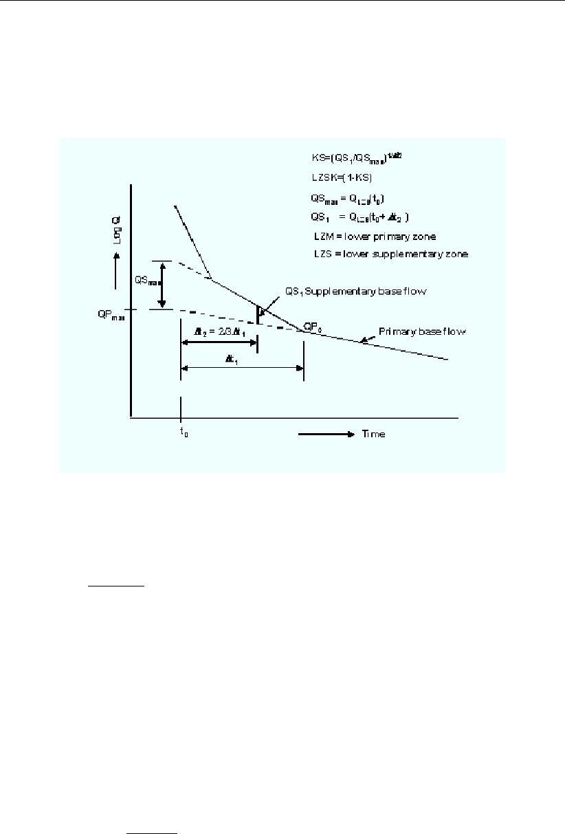
DRAFT
SOBEK, User Manual
The drainage factors LZP K and LZSK can be determined from the recession part of the
hydrograph by plotting that part of the hydrograph on semi-logarithmic paper (Fig. 6).
In the lowest part of the recession curve only the slow base flow component is acting while in
the higher stages both base flow components contribute.
Figure 6.97: Principle of computation of lower zone recession coefficient
The drainage factor LZP K follows from:
K=QPt0+∆t
QPt01/∆t
(6.319)
and
LZP K = 1 −K(6.320)
where:
Krecession coefficient of primary base flow for the time unit used
∆tnumber of time units, generally days
QPt0+∆ta discharge when recession is occurring at the primary base flow rate
QPt0the discharge ttime units later
If QPmax represents the maximum value of the primary base flow, then the maximum water
content of the lower zone becomes:
LZF P M =QPmax
LZP K (6.321)
and similarly the supplemental lower zone free water capacity is determined; at least this
procedure provides first estimates of the lower zone free water capacities (Figure 6.97).
The total base flow contributes completely or in part to the channel flow. A complete contribu-
tion occurs if subsurface discharge (i.e. discharge from the segment, which is not measured
at the outlet) is absent. Otherwise a fraction of the total base flow represents the subsurface
flow.
648 of 900 Deltares

DRAFT
Conceptual description
6.5.2.7 Actual evapotranspiration
Evaporation at a potential rate occurs from that fraction of the basin covered by streams,
lakes and riparian vegetation. Evapotranspiration from the remaining part of the catchment is
determined by the relative water contents of the tension water zones. If ED is the potential
evapotranspiration, then the actual evapotranspiration from the upper zone reads:
E1=ED ×U ZT W C
UZT W M (6.322)
i.e. the actual rate is a linear function of the relative upper zone water content. Where E1<
ED water is subtracted from the lower zone as a function of the lower zone tension water
content relative to the tension water capacity:
E2= (ED −E1)LZT W C
UZT W M +LZT W M (6.323)
If the evapotranspiration should occur at such a rate that the ratio of content to capacity of the
free water reservoirs exceeds the relative tension reservoir content then water is transferred
from free water to tension water such that the relative loadings balance. This correction is
made for the upper and lower zone separately. However, a fraction RSERV of the lower
zone free water storage is unavailable for transpiration purposes.
6.5.2.8 Impervious and temporary impervious areas
Besides runoff from the pervious area, the channel may be filled by rainwater from the imper-
vious area. With respect to the size of the impervious area it is noted that in the Sacramento
model a distinction is made between permanent and temporary impervious areas where
temporary impervious areas are created when all tension water requirements are met, i.e. an
increasing fraction of the catchment assumes impervious characteristics.
6.5.2.9 Routing of surface runoff
Before the runoff from the impervious areas, the overland- and interflow branch the channel,
they may be transformed according to a unit hydrograph leading to an adapted time distribu-
tion of these flow rates.
Use can be made here of the Clark method, which is a combined time-area and storage rout-
ing method. The model requires the construction of a time-area diagram. For this isochrones
are constructed representing points of equal travel time to the segment outlet, see Figure 5.
The areas between successive isochrones is determined and subsequently properly scaled
by the time of concentration Tc. The latter is defined as the time required to have the effect of
rainfall fallen in the most remote part felt at the segment outlet. The time-area diagram can be
thought of as the outflow from the segment if only translation and no deformation takes place
of an instantaneous unit supply of rain over the entire segment. Subsequently, the time area
diagram flow is routed through a linear reservoir, which characterises the effect of storage in
the open drainage system of the segment. This reservoir is represented by the second pa-
rameter: the recession coefficient k. It is noted that the output from the reservoir represents
the instantaneous unit hydrograph (IUH). This has to be transformed into say a 1-hour unit
hydrograph, dependent on the chosen routing interval
Deltares 649 of 900

DRAFT
SOBEK, User Manual
Figure 6.98: Principles of the Clark method for simulating surface runoff and interflow.
The two parameters Tcand kcan be obtained from observed rainfall and discharge hydro-
graphs. The time of concentration is equal to the time interval between cessation of rainfall
and the time the hydrograph has receded to its inflection point. Alternatively it is determined
from physical features of the segment as length and slope. A large number of empirical for-
mulas are available which relate the time of concentration to topographical features of the
basin. It is noted, though, that these formulas have generally only local validity. The best is
to estimate the celerity from the flow velocities in the drainage system taking account of the
following characteristics of celerity:
If the rivulet remains inbank the celerity is about 1.5 to 1.7 times the cross-sectional flow
velocity
If the flow becomes overbank the above celerity has to be multiplied with the ratio of
the drain width and the total width of the flow at the water surface (i.e. inclusive of the
floodplain)
To the time required to travel through the drainage system one has to add the overland flow
time.
The recession coefficient k is determined from the slope of recession part of the surface runoff
hydrograph, similar to the procedure for groundwater.
6.5.2.10 Sacramento - Estimation of segment parameters
650 of 900 Deltares

DRAFT
Conceptual description
Overview of parameters
The following groups of parameters can be distinguished for a particular segment:
Segment
[-] Segment area [km2]
Direct runoff
PCTIM Permanently impervious fraction of segment contiguous with stream chan-
nels
ADIMP Additional impervious fraction when all tension water requirements are met
SARVA Fraction of segment covered by streams, lakes and riparian vegetation
Upper soil moisture zone
UZTWM Capacity of upper tension water zone [mm]
UZFWM Capacity of upper free water zone [mm]
UZK Upper zone lateral drainage rate (fraction of contents per day)
Percolation
ZPERC Proportional increase in percolation from saturated to dry conditions in lower
zone
REXP Exponent in percolation equation, determining the rate at which percolation
demand changes from dry to wet conditions
Lower zone
LZTWM Capacity of lower zone tension water storage [mm]
LZFPM Capacity of lower zone primary free water storage [mm]
LZFSM Capacity of lower zone supplemental free water storage [mm]
LZPK Drainage rate of lower zone primary free water storage (fraction of contents
per day)
LZSK Drainage rate of lower zone supplemental free water storage (fraction of
contents per day)
PFREE Fraction of percolated water, which drains directly to lower zone free water
storages
RSERV Fraction of lower zone free water storages which is unavailable for transpi-
ration purposes
SIDE Ratio of unobserved to observed base flow
SSOUT Fixed rate of discharge lost from the total channel flow [mm/∆t]
Surface runoff
[-] Unit hydrograph ordinates
Internal routing interval
PM Time interval increment parameter
PT1 Lower rainfall threshold
PT2 Upper rainfall threshold
Basically two procedures are available to get first estimates for the majority of the segment
parameters:
from observed rainfall and runoff records: this method is usually applied and works well
provided that the model concepts are applicable and that reliable records are available for
some time covering the majority of the range of flows
from soil characteristics: this method is particularly suitable if no runoff records are avail-
able, i.e. for ungauged catchments.
With respect to gauged catchments the following grouping of parameters according to the
Deltares 651 of 900

DRAFT
SOBEK, User Manual
method of estimation can be made:
Parameters computed and estimated from basin map solely:
segment area and SARVA
Parameters estimated from observed rainfall and runoff records:
readily: LZFPM, LZPK, LZFSM, LZSK, PCTIM
approximately: UZTWM, UZFWM, UZK, LZTWM, SSOUT and PFREE
Parameters estimated from topographic maps and rainfall and runoff records:
unit hydrograph ordinates obtained from Clark method
Parameters to be obtained through trial runs:
ZPERC, REXP, SIDE, ADIMP, RSERV
Internal routing parameters, as per requirement:
PM, PT1, PT2
In the next sub-sections guidelines are given for the determination and estimation of the
segment parameters for gauged catchments.
6.5.2.11 Segment parameter estimation for gauged catchments.
The estimation of the segment parameters is presented according to their order of appearance
in the previous sub-section. The sequence in which the estimation is done in practice is
different from this order, for which reference is made to the end of the sub-section.
Segment
Segment area
To allow a good comparison between the observed and simulated runoff from the basin, the
segment area (km2) should refer to the total segment area draining upstream of the gauging
station. Any difference between total segment area up to the main stream and the area
upstream of the gauging station can be accommodated for in the channel routing part.
Direct runoff
PCTIM
Permanently impervious fraction of the basin contiguous with stream channels. It can be
determined from small storms after a significant period of dry weather. Then the volume of
direct runoff (= observed runoff - base flow) divided by the volume of rain gives the percentage
impervious fraction of the basin. PCTIM should not be close to 1!
An example is given below.
652 of 900 Deltares
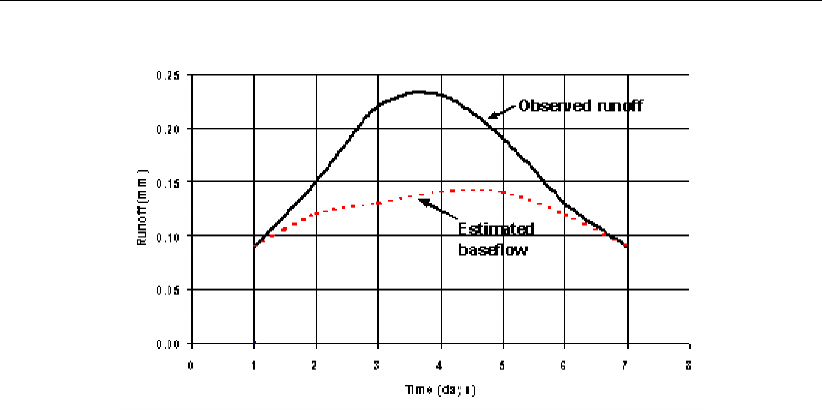
DRAFT
Conceptual description
Figure 6.99: Calculation of PCTIM
ADIMP
Fraction of the basin, which becomes impervious as all tension water requirements are met.
It can be estimated from small storms after a very wet period. As before, the volume of
direct runoff divided by the volume of rain gives the total percentage of impervious area. The
estimate for ADIMP follows from:
ADIMP =Total Percentage Impervious −P CT IM (6.324)
SARVA
Fraction of the basin covered by streams, lakes, and riparian vegetation, under normal circum-
stances. The SARVA area is considered to be the same as or less than PCTIM (see below).
Detailed maps may be referred to in order to estimate the extent of paved areas, which drain
directly to the streams so that differences between PCTIM and SARVA can be approximated.
Generally, SARVA appears to range between 40 % and 100 % of the PCTIM value.
Upper soil moisture zone
UZTWM - the upper tension storage capacity
The depth of water, which must be filled over non-impervious areas before any water becomes
available for free water storage. Since upper zone tension water must be filled before any
stream flow in excess of the impervious response can occur, its capacity can be approximated
from hydrograph analysis. Following a dry period when evapotranspiration has depleted the
upper soil moisture, the capacity of upper zone tension water can be estimated. That volume
of rainfall, which is retained before runoff from the pervious fraction is visible, is identified as
UZTWM. To that rainfall volume the losses to evaporation during the considered period should
be added. All periods of rain following a dry period should be checked for estimation of this
parameter. Generally the capacity of the upper zone tension will vary between 25 and 175
mm, depending on the soil type.
Following the logic of the Curve Number method, where the initial abstraction before rainfall
becomes effective is estimated as 20 % of the potential maximum retention, the UZTWM
Deltares 653 of 900

DRAFT
SOBEK, User Manual
becomes:
UZT W M = 50.8100
CN −1[mm] (6.325)
CN-values range from 30 to about 90 for rural areas and are a function of:
soil type (soil texture and infiltration rate); hydrological soil groups A–D are distinguished
land use, type of land cover, treatment and hydrologic or drainage condition
It is also a function of antecedent moisture condition, for which the condition “dry” should be
taken in view of the meaning of U ZT W M. Based on this assumption UZT W M would
vary between 120 and 6 mm, values which are in the range of those given above, particularly
if one realises that the 20 % of the potential maximum as initial abstraction is an average
value. Reference is made to standard textbooks on hydrology for CN-values
UZFWM - the upper free water storage capacity
Upper zone free water represents that depth of water, which must be filled over the non-
impervious portion of the basin in excess of UZT W M in order to maintain a wetting front
at maximum potential. This volume provides the head function in the percolation equation
and also establishes that volume of water, which is subject to interflow drainage. Generally its
magnitude ranges from 10–100 mm. It is not generally feasible to derive the magnitude of the
upper zone free water from direct observations, and successive computer runs are required
in order to establish a valid depth.
However, if a rough estimate of UZK is available (see below), then a rough value of UZF W M
can be obtained from the hydrograph at the time of the highest interflow, by reducing the flow
value with primary and supplemental base flow.
UZK - the upper zone lateral drainage rate
The upper zone lateral drainage rate is expressed as the ratio of the daily withdrawal to the
available contents. Its range is roughly 0.18 to 1.0, with 0.40 generally serving as an effective
initial estimate. Though basically, this factor is not capable of direct observation and must be
determined by successive computer runs, Peck (1978) suggests the following approximate
procedure. UZK is roughly related to the amount of time that interflow occurs following a
period with major direct and surface runoff. A long period of interflow results in a small value
for UZK. Assuming that interflow is observed during Nconsecutive days and that interflow
becomes insignificant when it is reduced to less than 10 % of its maximum value it follows:
(1 −UZK)N= 0.10 or UZK = 1 −0.11/N (6.326)
Values for UZK as a function of Ncan be read from Figure 6.100.
654 of 900 Deltares
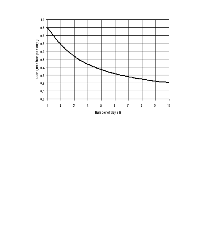
DRAFT
Conceptual description
Figure 6.100: UZK as function of number of days with significant interflow
Percolation
ZPERC
The proportional increase in percolation from saturated to dry condition is expressed by the
term ZPERC. The value of ZPERC is best determined through computer trials. The initial
estimate can be derived by sequentially running one or two months containing significant hy-
drograph response following a dry period. The value of ZPERC should be initially established
so that a reasonable determination of the initial run-off conditions is possible.
Amstrong (1978) provides a procedure to derive ZPERC from the lower zone tension and free
water reservoir capacities and drainage rates, using Equation (6.314) and Equation (6.315).
The maximum percolation takes place when the upper zones are full and the lower zones are
empty. Assuming that the maximum daily percolation will be the maximum contents of the
lower zones, from equation Equation (6.315) it follows for ZPERC:
ZP ERC =LZT W M +LZF P M +LZF SM −P BASE
P BASE (6.327)
If data would be available on maximum percolation rates ZPERC can be estimated using
equation Equation (6.315). Values for ZPERC ranging from 5 to 80 have been used.
REXP
The exponent in the percolation equation which determines the rate at which percolation
demand changes from the dry condition, (ZP ERC + 1)P BASE, to the wet condition,
PBASE.Figure 6.98 illustrates how different values of the exponent affect the infiltration rate.
It is recommended that an initial estimate of this exponent is made from the same record
which is used in determining an initial estimate of ZPERC. The interaction between PBASE,
ZPERC and REXP may require a shift of all three terms whenever it becomes clear that a
single term should be changed. Visualising the percolation curve generated by these three
terms helps to ascertain the necessary changes. The observed range of REXP is usually
between 1.0 and 3.0. Generally a value of about 1.8 is an effective starting condition. Values
for REXP for different soils are given by Amstrong (1978) and are presented in Table 6.11.
Deltares 655 of 900
DRAFT
SOBEK, User Manual
Table 6.11: Percolation exponent REXP for different soil types
Soil classification REXP
Sand 1.0
Sandy loam 1.5
Loam 2.0
Silty loam 3.0
Clay, silt 4.0
Lower zone
LZTWM - lower zone tension water capacity [mm]
This volume is one of the most difficult values to determine effectively. In as much as carryover
moisture in this storage may exist for a period of many years, its total capacity may not be
readily discernible from available records. If a drought condition during the period of record in
the basin or in the area being studied has been sufficient to seriously affect the transpiration
process of deep rooted plants, then the period of record is usually sufficient to determine
the maximum storage value of lower zone tension water. Often, however, field data is not
adequate for this purpose. As a result, unless great care is taken, the depth of lower zone
tension water storage may inadvertently be set near the maximum deficit experienced during
the period of record rather than the actual capacity of the zone. It has been noted that the
plant growth of an area is a relatively effective indicator of the capacity of the lower zone
tension water zone. In heavily forested regions of deep-rooted conifers, this zone may be
approximately 600 mm in magnitude. In areas of deep-rooted perennial grasses this depth
is more likely to be close to 150 mm. Where vegetation is composed primarily of relatively
shallow-rooted trees and grasses, this depth may be as little as 75 mm. It should be realised
that this zone represents that volume of water, which will be tapped by existing plants during
dry periods.
An approximate procedure to estimate LZTWM from a water balance analysis is presented
by Peck (1978). For this a period is selected with direct and/or surface runoff following an
extended dry spell. The selected period is bounded by the times t1and t2. At both times t1
and t2only base flow occurs. The start t1is selected immediately prior to the occurrence of
direct/surface runoff and t2immediately following a period of interflow. The times t1and t2
can best be selected from a semi-log plot of the runoff, see Figure 6.101.
656 of 900 Deltares
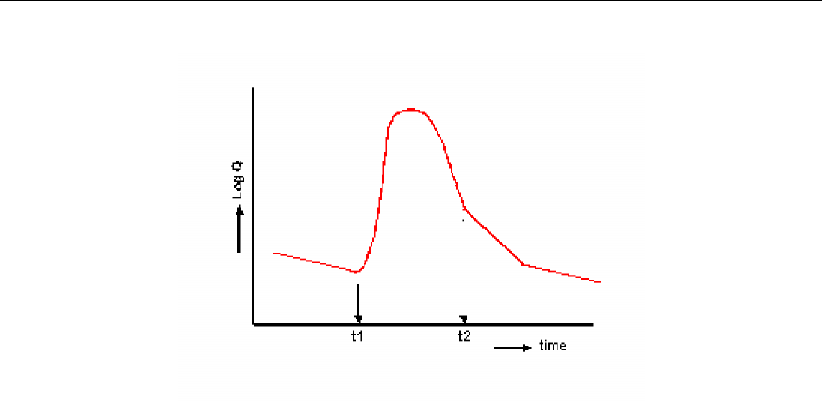
DRAFT
Conceptual description
Figure 6.101: Selection of period for LZTWM estimation
Assuming that UZTW is full and UZFWC is empty at times t1and t2the water balance for the
period t1−t2then reads:
P−R−E−DLZF P C −DLZF SC =DLZT W C (6.328)
where:
Pprecipitation from t1to t2[mm]
Rtotal runoff from t1to t2[mm]
Esegment evaporation [mm]; this amount would small for most wet period and
may be neglected
DLZF P C change in storage in LZ primary free water reservoir from t1to t2[mm]
DLZF SC change in storage in LZ supplemental free water reservoir from t1to t2[mm]
DLZT W C change in the lower zone tension water [mm]
DLZTWC is a lower limit of LZTWM since:
1 The lower zone tension water reservoir may not have been fully empty at t1
2 The lower zone tension water reservoir may not have been completely filled at t2
Hence some 10 to 20 % (or more) may be added to the value obtained through Equa-
tion (6.328). If such ideal cases as assumed above cannot be found, water balances for
periods of 3 to 4 months may be considered.
In Equation (6.328) LZFPC and DLZFSC are computed as follows:
DLZF P C =LZF P C(t2)−LZF P C(t1)where LZF P C(t) = QP (t)/LZP K
(6.329)
DLZF SC =LZF SC(t2)−LZF SC(t1)where LZF SC(t) = QS(t)/LZSK
(6.330)
The primary baseflows QP at times t1and t2are estimated by extrapolation from other
periods. Let the discharges at t1and t2be denoted by Q1and Q2, then the supplemental
baseflows follow from:
QS(t1) = Q1−QP (t1)and QS(t2) = Q2−QP (t2)(6.331)
Deltares 657 of 900

DRAFT
SOBEK, User Manual
LZFPM - lower zone primary free water storage
The maximum capacity of the primary lower zone free water, which is subject to drainage at
the rate expressed by LZP K. The value of the lower zone primary free water maximum can
be approximated from hydrograph analysis. For this the primary base flow, obtained from a
semi-log plot of the lower end of the recession curve, is extended backward to the occurrence
of a peak flow. Assuming that the primary free water reservoir is completely filled then, so
that it outflow is at maximum (QP max), its value is determined from Equation (6.321). The
effectiveness of this computation in determining the maximum capacity is dependent upon
the degree to which the observed hydrograph provides a representation of the maximum
primary base flow. If only a portion of the groundwater discharge is observable in the stream
channel, the estimated capacity based upon surface flows must be increased to include the
non-channel components by applying the term SIDE (See below).
LZFSM - lower zone supplemental free water storage
The maximum capacity of the lower zone supplemental free water reservoir, which is subject
to drainage at the rate expressed by LZSK. A lower limit of the lower zone free water supple-
mental maximum can be approximated from hydrograph analysis. Figure 6.97 illustrates the
computation of the lower zone free water supplemental maximum. Note that first the primary
base flow has to be identified and corrected for, see also Equation (6.331). The effectiveness
of this computation in determining the maximum capacity is dependent upon the degree to
which the observed hydrograph provides a representation of the maximum base flow capa-
bility of the basin. If only a portion of the groundwater discharge is observable in the stream
channel, the estimated capacity based upon surface flows must be increased to include the
non-channel components by applying the term SIDE (See below).
LZPK - lateral drainage of the lower zone primary free water reservoir.
Lateral drainage rate of the lower zone primary free water reservoir expressed as a fraction
of the contents per day. The coefficient is determined from the primary base flow recession
curve. Selecting flow values from this curve at some time interval Dt apart provides with the
help of Equation (6.319) and Equation (6.320) the required estimate, see also Figure 6.97.
LZSK - lateral drainage of the lower zone supplemental free water reservoir
Lateral drainage rate of the lower zone supplemental free water reservoir, expressed as a
fraction of the contents per day. Its computation is outlined in Figure 6.97. The procedure is
similar to that of LZPK, with the exception that the flow values have to be corrected for the
primary base flow.
PFREE
The fraction of the percolated water, which is transmitted directly to the lower zone free water
aquifers. Its magnitude cannot generally be determined from hydrograph analysis. An initial
value of 0.20 is suggested. Values will range between 0 and 0.50. The analysis of early
season base flow allows an effective determination of PFREE. The relative importance of
PFREE can be determined from storms following long dry spells that produce runoff (UZTW
completely filled). If the hydrograph returns to approximately the same base flow as before
then little filling of the lower zone free water reservoirs did take place and hence the PFREE-
value can be rated small, 0 to 0.2. If, on the contrary, the base flow has increased significantly
aPFREE-value as high as 0.5 may be applicable.
RSERV
658 of 900 Deltares

DRAFT
Conceptual description
Fraction of the lower zone free water, which is unavailable for transpiration purposes. Gener-
ally this value is between zero and 0.40 with 0.30 being the most common value. This factor
has very low sensitivity.
SIDE
Represents that portion of base flow, which is not observed in the stream channel. When
the soil is saturated, if percolation takes place at a rate, which is greater than the observable
base flow, the need for additional soil moisture drainage becomes manifest. SIDE is the ratio
of the unobserved to the observed portion of base flow. When the saturated soils do not
drain to the surface channel, SIDE allows the correct definition of PBASE, in order that the
saturated percolation rate may be achieved. In an area where all drainage from base flow
aquifers branches surface channels, SIDE will be zero. Zero or near zero values occur in a
large proportion of basins. However, in areas subject to extreme subsurface drainage losses,
SIDE may be as high as 5.0. It is conceivable that in some areas the value of SIDE may be
even higher.
SSOUT
The sub-surface outflow along the stream channel, which must be provided by the stream
before water is available for surface discharge. This volume expressed in mm/time interval
is generally near zero. It is recommended that the value of zero be utilised, and SSOUT is
applied only if the 10log Qvs. time plot requires a constant addition in order to achieve a valid
recession characteristic. If constant volumes of flow are added to observed stream flow, the
slope of the discharge plot will be altered. That value, which is required to linearize the primary
recession, is the appropriate value of SSOUT. It should be realised that where SSOUT is
required, an effective determination of lower zone free water storages and discharge rates will
require inclusion of the SSOUT value (mm/∆t)
Surface runoff
Unit hydrograph ordinates for the routing of flow from the impervious and pervious surfaces as
well as interflow towards the segment outlet can be obtained through standard unit hydrograph
procedures. It requires the selection of rainfall events (corrected for losses) with their resulting
flood hydrographs (corrected for base flow). Note that for each event the net rainfall amount
should match with the surface runoff and interflow amount. Various procedures are available
to arrive at a unit hydrograph. If the rainfall intensity during the storm varies, multiple linear
regression and discrete convolution techniques may be applied. The regression technique is
readily available in spreadsheet software. The resulting unit hydrographs generally will show
some irregularities and hence requires some smoothing afterwards. Unit hydrographs from
various storms may appropriately be averaged to arrive at a representative unit hydrograph
for the segment.
Another option is to use the Clark method. The principle of the Clark method was dealt with
in Sub-section 2.2.8. First requirement is the derivation of a time-area diagram. If a Digital
Elevation Model (DEM) is available from a catchment with appropriate software automatic
calculation of the time-area diagram is possible. In the absence from a DEM the time-area
diagram is derived from a basin map. By estimating travel times to the basin outlet (from
river and terrain slopes, assumed roughness and flow depth) isochrones can be determined.
The areas between successive isochrones is determined leading to a first estimate of the
time-area diagram. The total time base of the time-area diagram should be the concentration
time Tc, but due to inaccurate assessment of celerities in the basin it may differ from that.
Therefore, the time base of the time-area diagram is scaled by a more appropriate estimate of
Tc. An estimate for Tcmay be obtained as the time lapse between the cessation of rainfall and
Deltares 659 of 900

DRAFT
SOBEK, User Manual
the occurrence of recession on the falling limb of the hydrograph of surface runoff. The time
base of the time-area diagram is scaled by this time lapse. Alternatively, the concentration
time is estimated from an empirical formula applicable to the region. E.g. for a number of
small catchments in the Indus basin the following equation applies:
Tc=1
119
L
√S(6.332)
where:
Tcconcentration time [h]
Llength of river [km]
Sslope of main river
The units of the time-area diagram (km2) are converted into m3/s by multiplication with
0.278/∆t, with ∆tin hours. Subsequently, the time-area diagram is routed through a linear
reservoir, with reservoir coefficient k, estimated from the slope of the recession curve of the
surface water hydrograph. The routing is carried out by the following equation:
Oi+1 =c1Iav +c2Oi(6.333)
Iav =1
2(Ii+1 +Ii)(6.334)
c1=∆t
k+ ∆t/2(6.335)
c2=k−∆t/2
k+ ∆t/2(6.336)
c1+c2= 1 (6.337)
where:
Iav average inflow during ∆t(input is in form of histogram)
Ooutflow from the linear reservoir
The outflow from the reservoir is the Instantaneous Unit Hydrograph (IUH) for the basin, which
has to be transformed by averaging or S-curve technique into the Unit Hydrograph resulting
from a rainfall of duration equal to the routing interval.
Internal routing interval
P M Time interval increment parameter
P t1Lower rainfall threshold
P t2Upper rainfall threshold
In case the time step used in the model is larger than 1 hour, the model simulates the redistri-
bution of water between the various reservoirs with a time step, which is smaller than the time
interval of the basic data. Particularly for the infiltration process this effect could be important.
Also the rainfall will be lumped to that smaller interval. The number of increments in the time
interval is derived from:
N∆t= 1 + P M ∗(UZF W C ∗F+Peff )(6.338)
where:
F= 1 for Peff < P t1(6.339)
F= 1/2Peff /P t2for P t1≤Peff ≤P t2(6.340)
F= 1 −1/2P t2/Peff for Peff > P t2(6.341)
660 of 900 Deltares

DRAFT
Conceptual description
The most important parameter is seen to be PM. Taking a very small value for P M (say
P M = 0.01), then N∆tremains approximately1. If e.g. P M = 0.1then N∆tbecomes
substantially larger than 1. To limit the increase of N∆ta low value for P t1is to be chosen in
combination with a large value of P t2, which will reduce the value of F.
Sequence of parameter estimation
From the presentation above it will be clear that certain parameters should be estimated before
other can be assessed. The following sequence is recommended of which the first three steps
are mandatory:
1 Segment area
2 Lower zone primary free water parameters LZPK and LZFPM
3 Lower zone supplemental free water parameters LZSK and LZFSM
4 Impervious fraction PCTIM
5 Upper zone parameters UZTWM, UZK and UZFWM
6 Lower zone tension capacity LZTWM
7 Percolation parameters ZPERC and REXP
8 Remaining parameters
Linear reservoirs
An essential feature of the Sacramento model is that the free water reservoirs are considered
as linear reservoirs, i.e. there is a linear relation between the reservoir storage Sand the
outflow Q:
S=kQ (6.342)
If the recharge is indicated by I, the continuity equation for the linear reservoir reads:
dS
dt =I−Q(6.343)
Eliminating Sfrom above equations results in a linear first order differential equation in Q:
dQ
dt +1
kQ−1
kI= 0 (6.344)
With Iconstant and at t=t0,Qt=Qt0the solution to Equation (6.344) reads:
Qt=I1−exp −t−t0
k+Qt0exp −t−t0
kfor t≥t0(6.345)
When there is no recharge to the reservoir (I= 0)Equation (6.345) reduces to:
Qt=Qt0exp −t−t0
kfor t≥t0(6.346)
This equation can be compared with Equation (6.319), using the same notation:
Qt=Qt0K(t−t0)(6.347)
Deltares 661 of 900
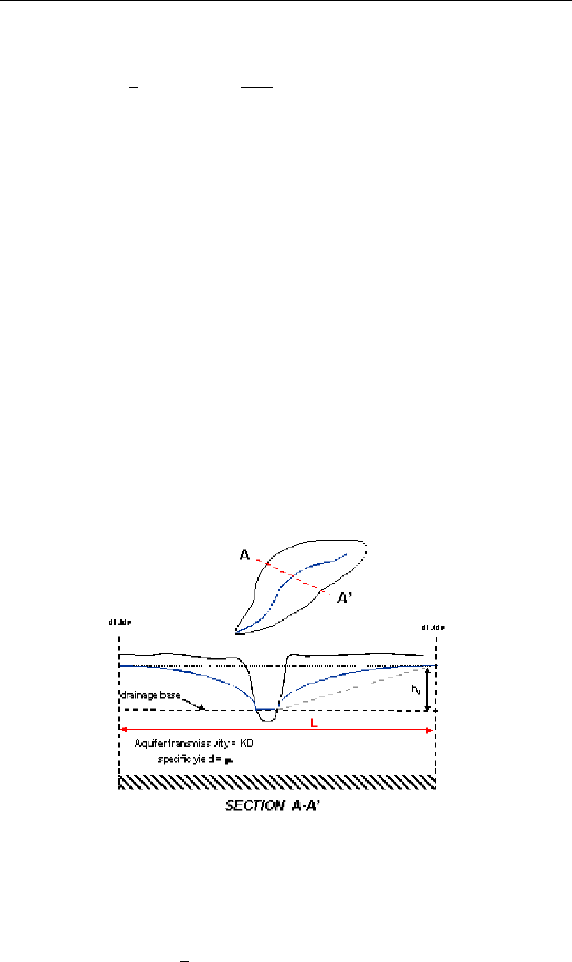
DRAFT
SOBEK, User Manual
Hence:
K= exp −1
kor k=−1
ln K(6.348)
Expressing time in days, then the amount of water released from the reservoir in 1 day
amounts according to equation Equation (6.342):
S0−S1=kQ0−kQ1=kQ01−exp −1
k=S0(1 −K)(6.349)
This is seen to match with e.g. the equations for the lower zone primary free water reservoir,
where:
S0=LZF P C and 1−K=LZP K (6.350)
Equation (6.348) provides a means to express the lower zone free water parameters in terms
of dimensions and physical properties of aquifers. Consider the phreatic aquifer shown in
Figure 6.102, which has the following dimensions and properties:
1 The width of the aquifer perpendicular to the channel is L
2 The water table at the divides is h0above the drainage base
3 The specific aquifer yield is m
4 The aquifer transmissivity is T.
Figure 6.102: Schematic cross-section through basin aquifer
The amount of water stored above the drainage base per unit length of channel available for
drainage is:
S=mc1Lh0with 1
2< c1<1(6.351)
662 of 900 Deltares
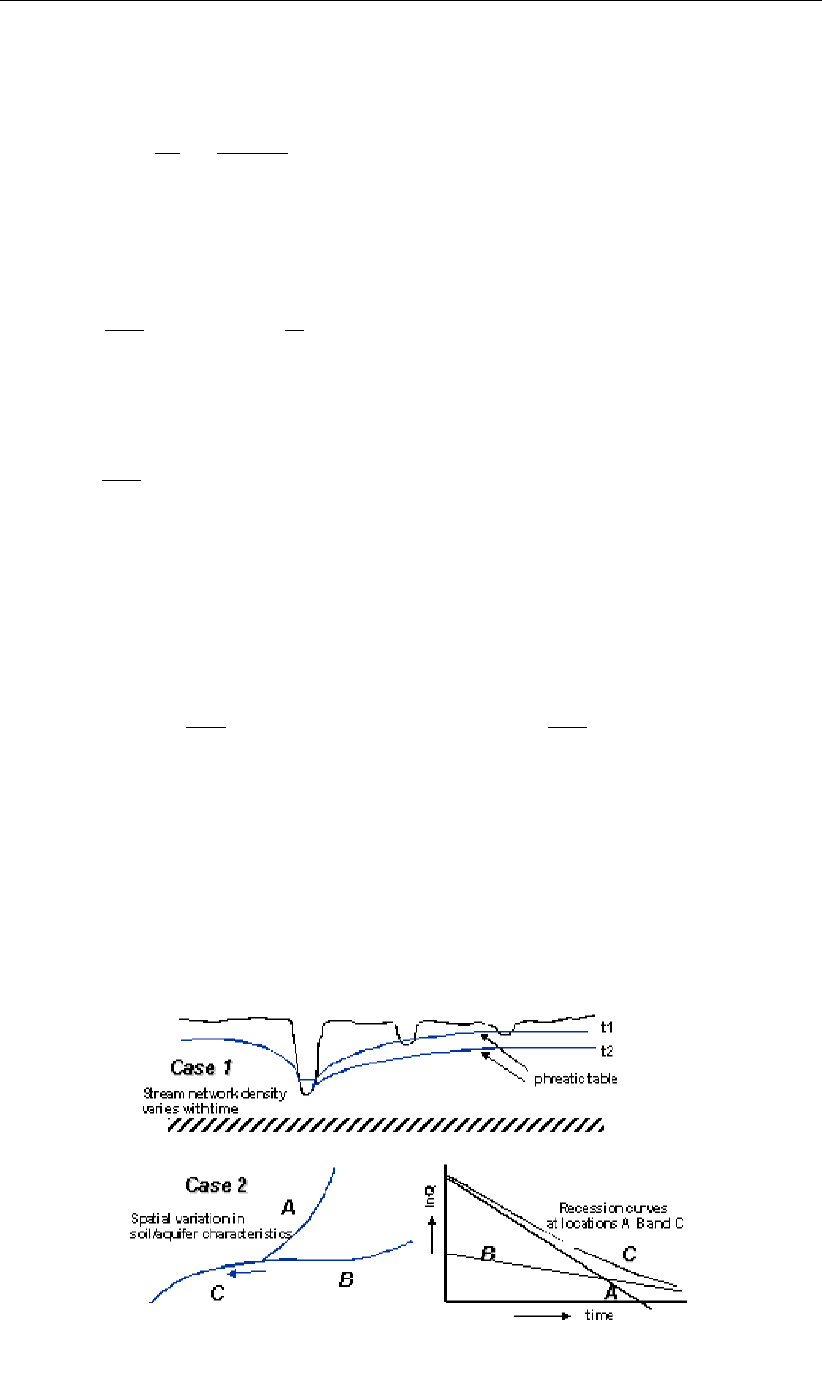
DRAFT
Conceptual description
The discharge to the channel per unit length of channel according to Darcy with the Dupuit
assumption
Q=−2Tdh
dx =2T c2h0
(L/2) with c2>1(6.352)
Combining the above two equations by eliminating h0and bringing it in the form of the linear
storage discharge relation Equation (6.342) :
S=µL2
4cT Qwith c=c2
c1
>1(6.353)
Hence for the reservoir coefficient kin Equation (6.342) it follows:
k=µL2
4cT (6.354)
The reservoir coefficient kis seen to be proportional to the square of the aquifer width and
inversely proportional to T, which is logical as kis a measure for the reside-time of the
percolated water in the groundwater zone. The value of cvaries between 2 and 2.5 dependent
on the shape of the water table. For the parameters Kand LZPK for the lower zone primary
free water storage it then follows:
K= exp −4cT
µL2and LZP K = 1 −exp −4cT
µL2(6.355)
A similar story applies for the lower zone free supplemental reservoir, which can be viewed as
representing the drainage from the shallower based denser network of the smaller channels,
see Figure 6.103. Since its main difference is with the aquifer width L, which is much smaller
than for the deeper based primary channel network, its reservoir coefficient will be smaller
than of the primary free water storage and consequently LZSK LZP K.
Figure 6.103: Cases of multiple exponential decay of recession curve
Deltares 663 of 900

DRAFT
SOBEK, User Manual
Note that similar differences in a basin between fast and slow draining aquifers if different soils
are present leading to different transmissivities.
6.5.3 Description of the D-NAM rainfall-runoff model
The "D-NAM" rainfall-runoff model is developed at Deltares. It concerns an improvement
and expansion of the NAM rainfall-runoff model, developed at the Institute of Hydrodynamics
and Hydraulic Engineering of the Technical University of Denmark (see Nielsen and Hansen
(1973)). NAM is the abbreviaton of the Danish "Nedbør-Afstrømmings-Model" (in Dutch
"Neerslag-Afvoer Model"), meaning rainfall-runoff model.
The D-NAM rainfall-runoff model is a deterministic, lumped and conceptual model, that treats
each catchment as a single unit. Model parameters and variables, therefore, represent aver-
age values for the entire catchment area.
A comparison of the D-NAM model and the NAM model is made in section 6.5.3.18.
6.5.3.1 External forces acting on a D-NAM model
External forces (or boundary conditions) acting on a D-NAM model comprise of:
1 Rainfall (P), defined in the "Meteo" Task block.
2 Potential evapotranspiration (EP ), defined in the "Meteo" Task block.
3 Groundwater pump discharge (GW P ump), defined on the "GWPump" tab of the D-NAM
Node in the "Schematisation" Task block.
4 External water level (h). Either defined at a RR boundary Node (rainfall-runoff modelling
only) or computed by a 1D flow model (combined rainfall-runoff and 1D flow modelling).
6.5.3.2 D-NAM storages and their water-storage capacity
The D-NAM model comprises of three different reservoirs:
1 The surface storage, that is situated on the surface of the catchment area and has an
unlimited water-storage capacity.
2 The lower zone storage, having a limited water-storage capacity only and representing the
field capacity of the root zone layer (sfc [-]). In other words the part of the soil moisture
content that can be retained against gravity.
3 The groundwater storage, having a limited water-storage capacity only and representing
the soil moisture content that can not be retained against gravity.
The lower zone storage and the groundwater storage jointly represent the water-storage-
capacity of the modelled soil layer thickness (see Figure 6.104). The soil beneath the surface
level (SL [m AD]) is divided into a root zone layer with bed level RZBL [m AD] and specific
yield sy,rz [-] and a subsoil layer with bed level GW SBL [m AD] and specific yield sy,ss [-].
For water-storage-capacities yield (see Figure 6.104):
The maximum water depth in the lower zone storage (Lmax [mm]) amounts to sfc(SL −
RZBL).
The maximum water depth in the root zone part of the groundwater storage
(GW SDrz,max [mm]) amounts to (sy,rz −sfc)(SL −RZBL).
The maximum water depth in the subsoil part of the groundwater storage (GW SDss,max
[mm]) amounts to sy,ss(RZBL −GW SBL).
The maximum water depth in the groundwater storage (GW SDmax [mm]) amounts to
GW SDrz,max +GW SDrz,max.
664 of 900 Deltares
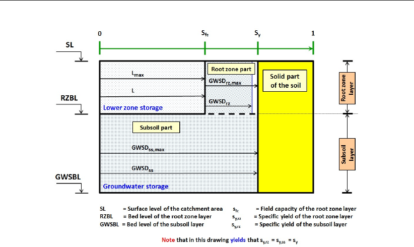
DRAFT
Conceptual description
Figure 6.104: Maximum water depths in lower zone storage and groundwater storage.
The solid part of the soil (coloured yellow) can not contain any groundwater.
6.5.3.3 D-NAM external and internal fluxes
The D-NAM model discerns nine external fluxes (see Figure 6.105):
1 Rainfall into the surface storage (P).
2 Evaporation from the surface storage (E1).
3 Interflow out of the surface storage (IF ).
4 Overland flow out of the surface storage (OF ).
5 Transpiration from the root zone layer (E2); being the summation of the transpiration
from the lower zone storage (E2LZS ) and the transpiration from the root zone part of the
groundwater storage (E2GW S,rz ).
6 Groundwater Pump. Either the abstraction of water contained in the groundwater storage
(GWABS,Act) or the supply of external water (GWSUP,Act); being the summation of the
supply of external water into the lower zone storage (DLGW P ump) and the supply of
external water into the groundwater storage (GWGW P ump).
7 Fast base flow component out of the groundwater storage (F astBF ).
8 Slow base flow component out of the groundwater storage (SlowBF ).
9 Inflow of external (ground)water (GW Inflow); being the summation of the inflow of
external (ground)water into the lower zone storage (DLExt) and the inflow of external
(ground)water into the groundwater storage (GWExt).
The D-NAM model discerns four internal fluxes (see Figure 6.105):
1 Infiltrated water (IN F ) or water in the surface storage that infiltrates into the soil.
2 Infiltration into the lower zone storage (DL).
3 Percolation into the groundwater storage (G).
4 Capillary rise of water (CR), contained in the subsoil part of the groundwater storage.
Deltares 665 of 900
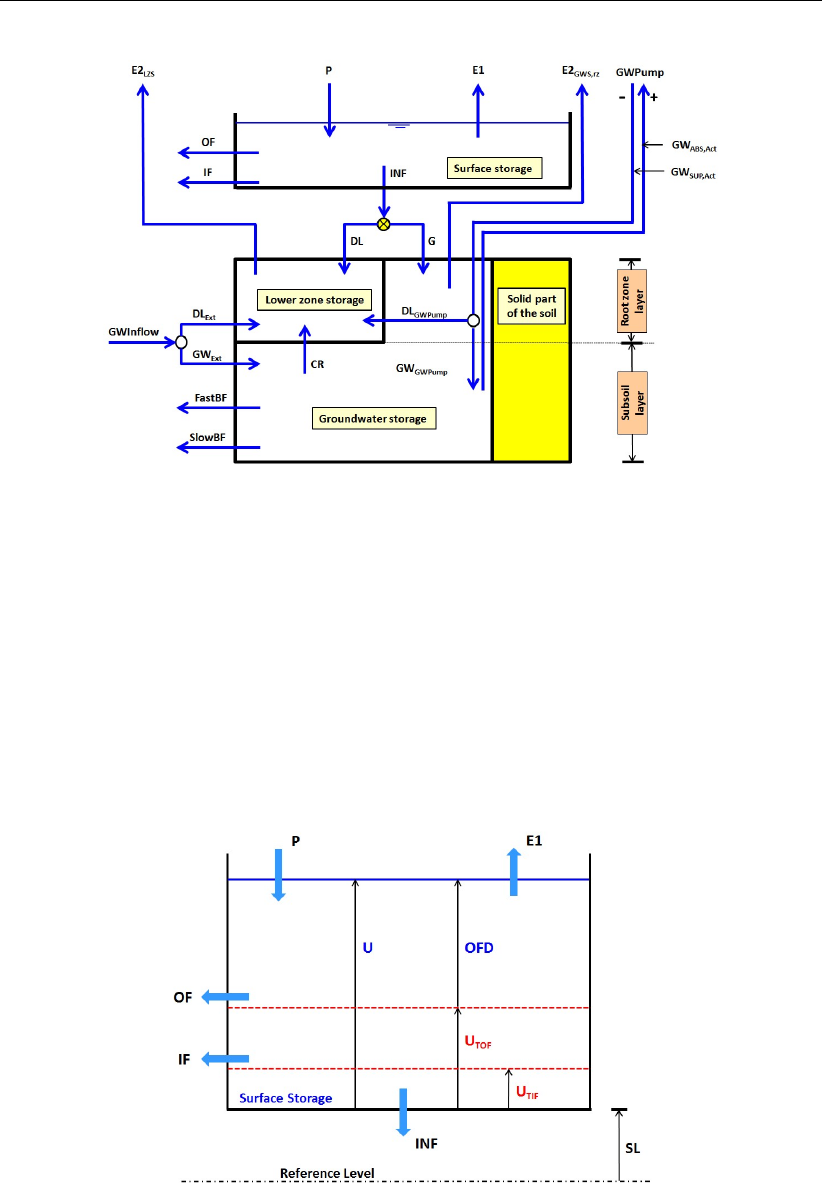
DRAFT
SOBEK, User Manual
Figure 6.105: Schematic representation of fluxes in the D-NAM rainfall runoff model.
6.5.3.4 Computing water depths in the surface flow storage
Water depths in the surface storage (U[mm]) are computed accounting for fluxes in the
following sequence (see Figure 6.106):
1 Rainfall P[mm] is added.
2 Evaporation E1[mm] (see section 6.5.3.6) is subtracted.
3 Interflow IF [mm] (see section 6.5.3.7) is subtracted.
4 Infiltrated water INF [mm] (see section 6.5.3.8) is subtracted.
5 Overland flow OF [mm] (see section 6.5.3.9) is subtracted.
Figure 6.106: Water depths, thresholds and fluxes related to the surface storage
6.5.3.5 Computing water depths in the lower zone storage and overland flow storage
Water depths in the lower zone storage (L[mm]) and the groundwater storage (GW SD
[mm]) are computed accounting for fluxes (see Figure 6.107) in the following sequence:
1 Infiltration DL [mm] (see section 6.5.3.10) is added to the lower zone storage.
2 Percolation G[mm] (see section 6.5.3.10) is added to the groundwater storage.
666 of 900 Deltares
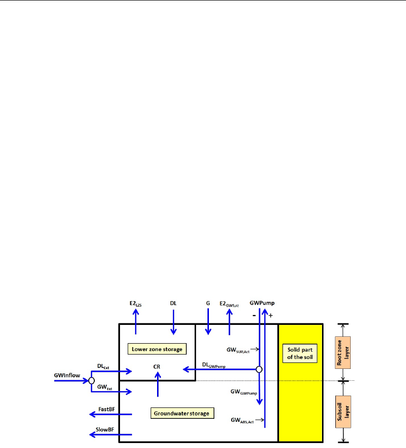
DRAFT
Conceptual description
3 Transpiration E2LZS [mm] (see section 6.5.3.11) is subtracted from the lower zone stor-
age.
4 Transpiration E2GW Srz [mm] (see section 6.5.3.11) is subtracted from the groundwater
storage.
5 Capillary rise CR [mm] (see section 6.5.3.12) is subtracted from the groundwater storage
and added to the lower zone storage.
6 Fast base flow F astBF [mm] (see section 6.5.3.13) is subtracted from the groundwater
storage.
7 Slow base flow SlowBF [mm] (see section 6.5.3.13) is subtracted from the groundwater
storage.
8 External (ground)water DLExt [mm] (see section 6.5.3.14) is added to the lower zone
storage.
9 External (ground)water GWExt [mm] (see section 6.5.3.14) is added to the groundwater
storage.
10 Abstraction by the groundwater pump GWABS,Act [mm] (see section 6.5.3.15) is sub-
tracted from the groundwater storage.
11 Supply by the groundwater pump DLGW P ump [mm] (see section 6.5.3.16) is added to
the lower zone storage.
12 Supply by the groundwater pump GWGW P ump [mm] (see section 6.5.3.16) is added to
the groundwater storage.
Figure 6.107: Fluxes related to the lower zone storage and groundwater storage. The
solid part of the soil (coloured yellow) can not contain any groundwater.
6.5.3.6 Evaporation from the surface storage
For the evaporation (E1[mm]) from the surface storage yields:
E1 = min(EP, U)
where:
EP User-defined potential evapotranspiration (see section 6.5.3.1) [mm].
UWater depth in the surface storage [mm].
Deltares 667 of 900

DRAFT
SOBEK, User Manual
6.5.3.7 Interflow out of the surface storage
For interflow (IF [mm]) out of the surface storage yields:
Lα= (L−LT IF )/(Lmax −LT IF ), where Lα= 0 if L≤LT IF
CKIF∆t= 1/(1 −(1 −1/CKIF )∆t/86400)
IF = (Lα/CKIF∆t)max(0, U −UT IF )
Note: No interflow occurs if U≤UT IF or L≤LT IF
where:
CKIF User-defined reservoir coefficient applied in routing interflow [day].
CKIF∆tReservoir coefficient used in each time-step ∆t[s] for routing interflow [∆t].
LWater depth in lower zone storage [mm].
Lmax Maximum water depth in lower zone storage (see section 6.5.3.2 and Fig-
ure 6.104) [mm].
LT IF User-defined lower-zone-storage threshold for interflow (Figure 6.106) [mm].
UWater depth in the surface storage [mm].
UT IF User-defined surface-storage threshold for interflow (Figure 6.106) [mm].
∆tUser-defined time-step [s].
6.5.3.8 Infiltrated water into the soil
For infiltrated water (INF [mm]) from the surface storage into the soil yields:
INFcap,∆t=IN F Cap (∆t/3600)
DLmax =Lmax −L.
Gmax =min(GW SDmax −GW SD , Gpot,max (∆t/86400) )
INF =min(U , INFcap,∆t, DLmax +Gmax)
Note: Infiltrated water (IN F ) equals zero if INF Cap = 0
where:
DLmax Available water-storage-depth in the lower zone storage [mm].
Gmax Water depth that can potentially be stored in the groundwater storage
[mm].
Gpot,max User-defined maximum rate of percolation into the groundwater stor-
age [mm/day].
GW SD Water depth in the groundwater storage [mm].
GW SDmax Maximum water depth in the groundwater storage (see section 6.5.3.2
and Figure 6.104) [mm].
INF Cap User-defined maximum infiltration rate for water contained in the sur-
face storage [mm/hr].
INF Cap∆tAmount of water contained in the surface storage that infiltrates into
the soil in time-step ∆t[mm/hr].
LWater depth in lower zone storage [mm].
Lmax Maximum water depth in lower zone storage (see section 6.5.3.2 and
Figure 6.104) [mm].
668 of 900 Deltares

DRAFT
Conceptual description
UWater depth in the surface storage [mm].
∆tUser-defined time-step [s].
6.5.3.9 Overland flow out of the surface storage
Overland flow (OF [mm]) is determined using an approximate analytical formula that:
1 Describes overland flow with the Manning roughness formula for open channel flow.
2 Assumes that the catchment area is a rectangular container with drainage length CL [m]
and width B[m], having a slope S[-] towards its overland outflow point.
3 Assumes that overland flow occurs in such way, that at each point-in-time yields that water
depths in the surface storage are constant in space.
This approximate analytical formula is given below:
OF D =max(0 , U −UT OF )
OF =OF D −1000 (OF D/1000)−2/3+ (2 ∆t√S)/(3 n CL)−3/2
Note: No overland flow occurs if U≤UT OF .
where:
OF D Overland flow depth (see Figure 6.106), defined as the water depth in the sur-
face storage above UT OF [mm].
UWater depth in the surface storage [mm].
UT OF Surface-storage threshold for overland flow [mm].
nManning value for the surface roughness of the catchment area [s/m1/3].
∆tUser-defined time-step [s].
6.5.3.10 Infiltration into the lower zone storage and percolation into the groundwater storage
Infiltrated water (INF [mm], see section 6.5.3.8) is distributed as infiltration in the lower zone
storage (DL) [mm] and percolation in the groundwater storage (G) [mm] (see Figure 6.108).
This distribution is done as follows:
Deltares 669 of 900
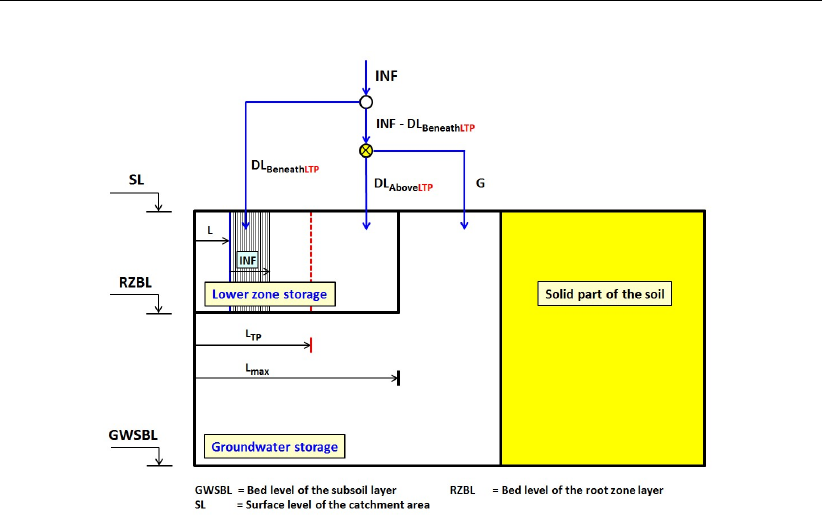
DRAFT
SOBEK, User Manual
Figure 6.108: Distributing infiltrated water (IN F ) over the lower zone storage and the
groundwater storage. The solid part of the soil (coloured yellow) can not
contain any groundwater.
1DLBeneathLT P [mm] is the part of the infiltrated water (IN F ) that is stored in the lower
zone storage beneath the lower-zone-storage threshold for percolation (LT P [mm], see
Figure 6.108).
DLBeneathLT P =max(0 , min(LT P −L , INF )).
where:
LWater depth in the lower zone storage [mm].
LT P Lower-zone-storage threshold for percolation [mm].
The value for LT P determines the degree in which infiltrated water (INF ) is distributed
over the lower zone storage and the groundwater storage as proposed by Nielsen and
Hansen (1973). More precisely:
If LT P =Lmax the distribution proposed by Nielsen and Hansen (1973) is overruled.
Since, first the lower zone storage is completely filled up before infiltrated water can
percolate into the groundwater storage.
If 0≤LT P < Lmax the distribution proposed by Nielsen and Hansen (1973) be-
comes applicable as soon as the lower zone storage is filled up to LT P , meaning
that part of the infiltrated water (INF ) can percolate into the groundwater storage (or
G > 0) before the lower zone storage is at field capacity (or L<Lmax).
2DLNH,AboveLT P [mm] (see Figure 6.108) is the part of the infiltrated water (INF ) that, in
line with the Nielsen and Hansen (1973) distribution, infiltrates into the lower zone storage
above LT P .
DLNH,AboveLT P =min(ADAboveLT P ,(1 −(L/Lmax))(INF −DLBeneathLT P ))
where:
ADAboveLT P Available water-storage-depth in the lower zone storage above
LT P [mm].
670 of 900 Deltares

DRAFT
Conceptual description
Lmax Maximum water depth in the lower zone storage (see section 6.5.3.2
and Figure 6.104) [mm].
3GNH [mm] (see Figure 6.108) is the part of the infiltrated water (INF ) that, in line with
the Nielsen and Hansen (1973) distribution, percolates into the groundwater storage.
GNH =INF −DLBeneathLT P −DLNH,AboveLT P
4 The actual percolation (G[mm]) follows from limiting GNH to the user-defined maximum
percolation rate Gpot,max [mm/day].
G=max(GNH , Gpot,max (∆t/86400))
where:
Gpot,max User-defined maximum rate of percolation into the groundwater storage
[mm/day].
∆tUser-defined time-step [s].
5 For the actual infiltration into the lower zone storage (DL [mm], see Figure 6.108) yields.
DL =INF −G
6.5.3.11 Transpiration from the root zone layer
Transpiration from the root zone layer (E2[mm], see Figure 6.107) respectively comprises of
transpiration from the root zone part of the groundwater storage (E2GW S,rz [mm]) and tran-
spiration from the lower zone storage (E2LZS [mm]). E2GW S,rz and E2LZS are computed
as follows:
GW SDrz =max(0, GW SD −GW SDss,max)
E2 = min(L+GW SDrz ,(EP −E1)(L+GW SDrz )/(Lmax +GW SDrz))
E2GW S,rz =min(E2, GW SDrz).
E2LZS =E2−E2GW S,rz
where:
E1Evaporation from the surface storage (see section 6.5.3.6) [mm].
EP User-defined potential evapotranspiration (see section 6.5.3.1) [mm].
GW SD Water depth in the groundwater storage [mm].
GW SDrz Water depth in the root zone part of the groundwater storage [mm].
GW SDss,max Maximum water depth in the root zone part of the groundwater stor-
age (see section 6.5.3.2 and Figure 6.104) [mm].
LWater depth in the lower zone storage [mm].
Lmax Maximum water depth in the lower zone storage (see section 6.5.3.2
and Figure 6.104) [mm].
Deltares 671 of 900
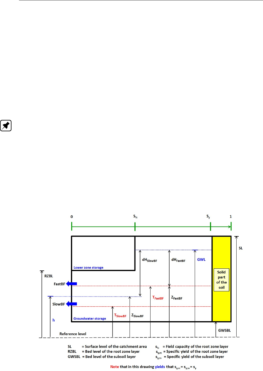
DRAFT
SOBEK, User Manual
6.5.3.12 Capillary rise
For capillary rise (CR [mm], see Figure 6.107) yields:
CR = min(Lmax −L , GW SD , (∆t/86400) CRpot,max )
where:
CRpot,max User-defined maximum capillary rise [mm/day].
GW SD Water depth in the groundwater storage [mm].
LWater depth in the lower zone storage [mm].
Lmax Maximum water depth in the lower zone storage (see section 6.5.3.2 and Fig-
ure 6.104) [mm].
∆tUser-defined time-step [s].
Note: The surface level (SL [m AD]) and the bed level of the groundwater storage (GW SBL
[m AD]) determine the thickness of the soil layer, that is considered in a D-NAM model. So the
bed level of the groundwater storage is to be considered as watertight. Therefore, CRpot,max
is set equal to zero if GW SD = 0, this irrespective of the user-defined value for CRpot,max.
6.5.3.13 Fast and slow base flow component
Base flow occurs only if the external water level (h[m AD]) is below the groundwater level
(GW L [m AD]). Base flow equals zero if h≥GW L (see Figure 6.109). Water contained in
the lower zone storage can not flow out as base flow, since this water can be retained against
gravity.
Figure 6.109: Computing the Fast base flow component and the Slow base flow com-
ponent. The solid part of the soil (coloured yellow) can not contain any
groundwater.
The fast base flow component (F astBF ) and the slow base flow component (SlowBF ) are
672 of 900 Deltares

DRAFT
Conceptual description
computed as follows (see Figure 6.109):
GW SDss =min(GW SD , GW SDss,max)
GW SDrz =max(0 , GW SD −GW SDss,max)
GW L =GW SBL + (GW SDss/1000 sy,ss) + ((GW SDrz +L)/1000 sy,rz)
ZF astBF =max(h, TF astBF )
ZSlowBF =max(h, TSlowBF )
dHF astBF =max(0, GW L −ZF astBF )
dHSlowBF =max(0, GW L −ZSlowBF )
GW SDZF astBF =f(ZF astBF , SL , RZBL , GW SBL , sy,rz , sf c , sy,ss)
GW SDZSlowBF =f(ZSlowBF , SL , RZBL , GW SBL , sy,rz , sf c , sy,ss)
Vpot,F astBF =max(0, GW SD −GW SDZF astBF )
Vpot,SlowBF =max(0, GW SD −GW SDZSlowBF )
CKF astBF∆t= 1/(1 −(1 −1/CKF astBF )∆t/86400)
CKSlowBF∆t= 1/(1 −(1 −1/CKSlowBF )∆t/86400)
F astBFpot =min(Vpot,F astBF ,1000(dHF astBF /CKF astBF∆t) )
SlowBFpot =min(Vpot,SlowBF ,1000(dHSlowBF /CKSlowBF∆t) )
GWOutflowpot =FastBFpot +SlowBFpot
F astBF =F astBFpot if GWOutflow pot ≤Vpot ,FastBF
F astBF =Vpot,F astBF F astBFpot
GWOutflowpot if GWOutflow pot >Vpot ,FastBF
SlowBF =SlowBFpot if F astBF +SlowBFpot ≤Vpot,SlowBF
SlowBF =Vpot,SlowBF −F astBF if F astBF +SlowBFpot > Vpot,SlowBF
where:
CKF astBF User-defined reservoir coefficient applied in routing the fast base
component (CKF astBF > 1) [day].
CKF astBF∆tReservoir coefficient used in each time-step ∆t[s] for routing the
fast base component [∆t].
CKSlowBF User-defined reservoir coefficient applied in routing the slow base
component (CKSlowBF > 1) [day].
CKSlowBF∆tReservoir coefficient used in each time-step ∆t[s] for routing the
slow base component [∆t] .
dHF astBF Hydraulic head (or driving force) of the fast base flow component [m].
dHSlowBF Hydraulic head (or driving force) of the slow base flow component
Deltares 673 of 900

DRAFT
SOBEK, User Manual
[m].
F astBFpot Potential fast base flow component [mm].
SlowBFpot Potential slow base flow component [mm].
GW L Groundwater level [m AD].
GWOutflowpot Potential groundwater outflow (=F astBFpot +SlowBFpot) [mm].
GW SBL Bed level of the groundwater storage [m AD].
GW SD Water depth in the groundwater storage [mm].
GW SDrz Water depth in the root zone part of the groundwater storage [mm].
GW SDss Water depth in the subsoil part of the groundwater storage [mm].
GW SDss,max Maximum water depth in the subsoil part of the groundwater storage
(see section 6.5.3.2 and Figure 6.104) [mm].
GW SDZF astBF Water depth in the groundwater storage if GW L equals ZF astBF
[mm].
GW SDZSlowBF Water depth in the groundwater storage if GW L equals ZSlowBF
[mm].
hExternal water level [m AD].
LWater depth in the lower zone storage [mm].
RZBL Bed level of the root zone layer [m AD].
sfc Field capacity of the soil in the root zone layer [-].
SL Surface level of the catchment area [m AD]
sy,rz Specific yield of the root zone layer (ratio of the volume of water in a
fully saturated root zone layer to its total soil volume) [-].
sy,ss Specific yield of the subsoil layer (ratio of the volume of water in a
fully saturated subsoil layer to its total soil volume) [-].
TF astBF Threshold for the fast base flow component. Only water in the ground-
water storage above TF astBF may flow out as fast base flow [m AD].
TSlowBF Threshold for the slow base flow component. Only water in the
groundwater storage above TSlowBF may flow out as slow base flow
[m AD].
Vpot,F astBF Volume of water in the groundwater storage, that is potentially avail-
able for drainage by the fast base flow component [mm].
Vpot,SlowBF Volume of water in the groundwater storage, that is potentially avail-
able for drainage by the slow base flow component [mm].
ZF astBF Drainage level of the fast base flow component [m AD].
ZSlowBF Drainage level of the slow base flow component [m AD].
∆tUser-defined time-step [s].
6.5.3.14 External (ground)water flowing into the lower zone storage and groundwater storage
Inflow of external (ground)water into the soil (GWInflow [mm]) occurs only if the external
water level (h[m AD]) is above the groundwater level (GW L [m AD]). GWInflow equals
zero if h≤GW L (see Figure 6.110). The sequence of filling the lower zone storage and the
groundwater storage by inflowing external (ground)water is as follows:
Firstly, the subsoil part of the groundwater storage is completely filled-up
Secondly, the lower zone storage is completely filled-up.
Thirdly and finally, the root zone part of the groundwater storage is filed-up.
674 of 900 Deltares

DRAFT
Conceptual description
Figure 6.110: Determining the inflow of external (ground)water (GWInflow). The solid
part of the soil (coloured yellow) can not contain groundwater.
The inflow of external (ground)water (GWInflow [mm]), the part following into the lower zone
storage (DLExt [mm]), and the part flowing into the groundwater storage (GWExt [mm]) are
computed as follows (see Figure 6.110):
GW SDss =min(GW SD , GW SDss,max)
GW SDrz =max(0 , GW SD −GW SDss,max)
GW L =GW SBL + (GW SDss/1000 sy,ss) + ((GW SDrz +L)/1000 sy,rz)
dHGW Inf low =max(0, h −GW L)
Vpot,GW Inf low =f(h , GW L , SL , RZBL , GW SBL , sy,rz , sy,ss)
CKGWInflow∆t =1/(1−(1−1/CKGWInflow)∆t/86400 )
GWInflow =min(1000 (dHGWInflow /CKGWInflow∆t ),Vpot,GWInflow )
DLExt =max(0 , min(Lmax −L , GW SD +GWInflow −GWSDss,max )
GWExt =GW Inflow −DLExt
where:
CKGWInflow User-defined reservoir coefficient, applied for the inflow of external
(ground)water (CKGWInflow >1) [day].
CKGWInflow∆t Reservoir coefficient used in each time-step ∆t[s] for computing the
inflow of external (ground)water [∆t].
dHGWInflow Hydraulic head (or driving force) for the inflow of external (ground)water
[m].
Deltares 675 of 900

DRAFT
SOBEK, User Manual
GW L Groundwater level [m AD].
GW SBL Bed level of the groundwater storage [m AD].
GW SD Water depth in the groundwater storage [mm].
GW SDrz Water depth in the root zone part of the groundwater storage [mm].
GW SDss Water depth in the subsoil part of the groundwater storage [mm].
GW SDss,max Maximum water depth in the subsoil part of the groundwater storage
(see section 6.5.3.2 and Figure 6.104) [mm].
hExternal water level [m AD].
LWater depth in the lower zone storage [mm].
Lmax Maximum water depth in the lower zone storage (see section 6.5.3.2
and Figure 6.104) [mm].
RZBL Bed level of the root zone layer [m AD].
sfc Field capacity of the soil in the root zone layer [-].
SL Surface level of the catchment area [m AD].
sy,rz Specific yield of the root zone layer (ratio of the volume of water in a
fully saturated root zone layer to its total soil volume) [-].
sy,ss Specific yield of the subsoil layer (ratio of the volume of water in a
fully saturated subsoil layer to its total soil volume) [-].
Vpot,GW Inf low Volume of water in both the lower zone storage and the groundwa-
ter storage, that potentially can be filled-up by the inflow of external
(ground)water [mm].
∆tUser-defined time-step [s].
6.5.3.15 Abstraction by the groundwater pump
Abstraction by the groundwater pump (GWABS,Act [mm], see Figure 6.107) occurs only if
the groundwater pump discharge (GW P ump [m3/s]) is greater than zero. Water contained
in the lower zone storage can not be abstracted by the groundwater pump. GWABS,Act is
computed as follows:
GWABS,max =GW SD
GWABS,pot =max(0 ,(1000∆t /CatchmentArea)GWPump)
GWABS,Act =min(GWABS,max , GWABS,pot)
where:
GWABS,max Maximum water depth in the groundwater storage that can be ab-
stracted by the groundwater pump [mm].
GWABS,pot Potential water depth that can be abstracted according to the user-
defined groundwater pump discharge [mm].
GW SD Water depth in the groundwater storage [mm].
∆tUser-defined time-step [s].
676 of 900 Deltares

DRAFT
Conceptual description
6.5.3.16 Supply by the groundwater pump
Supply of water by the groundwater pump (GWSU P,Act [mm]), see Figure 6.107) occurs only
if the groundwater pump discharge (GW P ump [m3/s]) is less than zero. The sequence
of filling the lower zone storage and the groundwater storage by the groundwater pump is as
follows:
Firstly, the subsoil part of the groundwater storage is completely filled-up
Secondly, the lower zone storage is completely filled-up.
Thirdly and finally, the root zone part of the groundwater storage is filed-up.
Supply of water by the groundwater pump (GWSUP,Act) comprises of supply to the lower zone
storage (DLGW P ump [mm]) and supply to the groundwater storage (GWGW P ump [mm]).
DLGW P ump and GWGW P ump are computed as follows:
GWSU P,max = (GW SDmax −GW SD)+(Lmax −L)
GWSU P,pot =max(0 ,−(1000∆t /CatchmentArea)GWPump)
GWSU P,Act =min(GWSUP,max , GWSUP,pot)
ADGW S,ss,GW P ump =max(0, GW SDss,max −GW SD))
DLGW P ump =min(Lmax−L, GWSUP,Act−min(ADGW S,ss,GW P ump , GWSUP,Act))
GWGW P ump =GWSUP,Act −DLGW P ump
where:
ADGW S,ss,GW P ump Water-storage-depth available in the subsoil part of the groundwater
storage for the supply of water by the groundwater pump [mm].
GW SD Water depth in the groundwater storage [mm].
GW SDmax Maximum water depth in the groundwater storage (see section 6.5.3.2
and Figure 6.104) [mm].
GW SDss,max Maximum water depth in the subsoil part of the groundwater storage
(see section 6.5.3.2 and Figure 6.104) [mm].
GWSU P,max Maximum water-storage-depth available for the supply of water by
the groundwater pump. Sum of available water-storage-depth in the
lower zone storage and groundwater storage. [mm].
GWSU P,pot Potential water depth that can be supplied according to the user-
defined groundwater pump discharge [mm].
LWater depth in the lower zone storage [mm].
Lmax Maximum water depth in the lower zone storage (see section 6.5.3.2
and Figure 6.104) [mm].
∆tUser-defined time-step [s].
Deltares 677 of 900

DRAFT
SOBEK, User Manual
6.5.3.17 D-NAM output time-series
Table 6.12 provides an overview of the output time-series available for each D-NAM rainfall-
runoff model. The second column contains for each output time-series the symbols that are
used in equations.
Please note that the "Runoff node" is to be checked on the "Output options" tab in RR Set-
tings in order to obtain the output time-series (see Table 6.12) available under "Runoff Node"
in "Results in Charts" Task block.
Table 6.12: Overview of D-NAM output time-series
Name of Output Time Series Symbols Unit Description
Rainfall P mm Rainfall as defined in the "Meteo Task" block
PotEvap EP mm Evapotranspiration as defined in the "Meteo
Task" block.
ActEvap mm Sum of evaporation from surface storage
(E1) and transpiration from the lower zone
storage (E2).
Runoff mm Equals overland flow (OF ) + interflow (IF )
+ fast base flow component (F astBF ) +
slow base flow component (SlowBF ) - in-
flow of external (ground)water into the soil
(GW Inf low).
Outflow m3/s Equals overland flow (OF ) + interflow (IF )
+ fast base flow component (F astBF ) +
slow base flow component (SlowBF ) - in-
flow of external (ground)water into the soil
(GW Inf low).
D-NAM ExternalWaterLevel h m AD External water level.
D-NAM GWPumpDefinedDischarge GW P ump m3/s Groundwater pump discharge.
D-NAM EvapSurfaceStorage E1mm Evaporation from the surface storage.
D-NAM EvapRootZoneLayer E2mm Transpiration from the root zone layer.
D-NAM EvapRootZonePartGWStorage E2GW S,rz mm Transpiration from the root zone part of the
groundwater storage.
D-NAM EvapLowerZoneStorage E2LZS mm Transpiration from the lower zone storage.
D-NAM OverlandFlow OF mm Overland flow (outflow from surface storage).
D-NAM Interflow IF mm Interflow (outflow from surface storage).
D-NAM FastBaseFlow F astBF mm Fast base flow component (outflow from
groundwater storage).
D-NAM SlowBaseFlow SlowBF mm Slow base flow component (outflow from
groundwater storage).
D-NAM ExternalGWInflow GW Inf low mm Inflow of external (ground)water into the soil.
D-NAM ExternalGWInflowLowerZoneStorage DLExt mm Inflow of external (ground)water into the
lower zone storage.
D-NAM ExternalGWInflowGroundwaterStorage GWExt mm Inflow of external (ground)water into the
groundwater storage.
D-NAM GWPumpAbsGroundwaterStorage GWABS,Act mm Abstraction of water from the groundwater
storage by the groundwater pump.
D-NAM GWPumpSupLowerZoneStorage DLGW P ump mm Supply of water into the lower zone storage
by the groundwater pump.
D-NAM GWPumpSupGroundwaterStorage GWGW P ump mm Supply of water into the groundwater storage
by the groundwater pump.
D-NAM Infiltration INF mm Water contained in the surface storage that
infiltrates into the soil.
D-NAM InfiltrationLowerZoneStorage DL mm Water contained in the surface storage that
infiltrates into the lower zone storage.
D-NAM Percolation G mm Water contained in the surface storage that
percolates into the groundwater storage.
D-NAM CapillaryRise CR mm Capillary rise of water from the subsoil part of
the groundwater storage into the lower zone
storage.
D-NAM DepthSurfaceStorage U mm Water depth in the surface storage.
678 of 900 Deltares

DRAFT
Conceptual description
Table 6.12: Overview of D-NAM output time-series
Name of Output Time Series Symbols Unit Description
D-NAM DepthLowerZoneStorage L mm Water depth in the lower zone storage.
D-NAM DepthGroundwaterStorage GW SD mm Water depth in the groundwater storage.
D-NAM VolumeSurfaceStorage VUm3Volume of water contained in the surface
storage.
D-NAM VolumeLowerZoneStorage VLm3Volume of water contained in the lower zone
storage.
D-NAM VolumeGroundwaterStorage VGW S m3Volume of water contained in the groundwa-
ter storage.
D-NAM GroundWaterLevel GW L mAD Groundwater level (measured in metres
above datum).
D-NAM GroundWaterTableDepth GW T D mBS Groundwater table depth (measured in me-
tres below surface level).
D-NAM AvailableSoilStorage AVsoil m3Volume in the soil that is still available for the
storage of water.
D-NAM BaseFlow BF mm Equals fast base flow component (F astBF )
+ slow base flow component (SlowBF ) - in-
flow of external (ground)water into the soil
(GW Inf low).
D-NAM GWPumpActualDischarge GW P umpAct m3/s Actual groundwater pump discharge. Posi-
tive if water is abstracted. Negative if water is
supplied.
D-NAM GWPumpActual-DefinedDischarge GW P ump m3/s Actual groundwater pump discharge minus
Act−Def ined the user-defined groundwater pump dis-
charge. If positive, the amount of discharge
that could not be supplied. If negative,
the amount of discharge that could not be
abstracted.
6.5.3.18 Comparing the D-NAM model and the NAM model
Concepts of the Nielsen and Hansen (1973) NAM model implemented into the D-NAM model
are:
1 Interflow occurs only if the water depth in the lower zone storage (L) is above the lower-
zone-threshold for interflow (LT IF ). Interflow is a function of the relative moisture content
in the lower zone storage above LT IF . (see factor Lαin section 6.5.3.7).
2 Percolation may occur if the water depth in the lower zone storage is below field capacity
(see section 6.5.3.10).
3 Transpiration from the root zone layer (E2) is a function of the relative moisture content in
the root zone layer (see section 6.5.3.11).
Reasons for developing the D-NAM rainfall-runoff model are:
1 The NAM model stores water on the surface of a catchment area in three different stacked
on each other storages, being the NAM surface storage, the NAM interflow storage and
the NAM overland flow storage. As a result hereof, water contained in the latter two NAM
storages is not available for evaporation and for infiltration into the soil.
In the D-NAM model all water on the surface of a catchment area is contained in one
surface storage only and hence all water on the surface of a D-NAM model is at any point-
in-time available for evaporation, interflow, infiltration into the soil and overland flow (see
Figure 6.106).
2 The NAM surface storage, receiving precipitation has a watertight bed and a maximum
water-storage-capacity. Hence, water contained in the NAM surface storage can not di-
rectly infiltrate into the soil. Only if the water depth in the NAM surface storage, after
accounting for evaporation and inflow into the interflow storage, exceeds its maximum
water-storage-capacity, the surplus of water in the NAM surface storage is divided into
infiltration into the soil and inflow into the overland flow storage. This division of surplus
water in the NAM surface storage is, however, made irrespective of the actual water depth
Deltares 679 of 900

DRAFT
SOBEK, User Manual
in the NAM overland flow storage.
In the D-NAM model the surface storage has an unlimited water-storage-capacity and its
bed is not watertight, allowing water to infiltrate into the soil (INF ). Infiltrated water is
limited by the actual water depth in the surface storage, the available water-storage-depth
in the soil, and the user defined maximum infiltration and percolation capacity (see sec-
tion 6.5.3.8).
Additional functionalities in the D-NAM model with respect to the NAM model are:
1 The D-NAM model makes a distinction between the specific yield of root zone layer and
the specific yield of the subsoil layer (see section 6.5.3.2)
2 The NAM model is suited for free discharging catchment areas only. The D-NAM model
allows for the inflow of external (ground)water (see section 6.5.3.14), that is required in
modelling deltaic areas.
3 The D-NAM model determines overland flow using the Manning formula for open channel
flow (see section 6.5.3.9).
4 The D-NAM model makes a distinction between a fast and a slow base flow component
(see Figure 6.109).
5 The D-NAM model includes a groundwater pump, that can abstract water (see section 6.5.3.15
or supply water (see section 6.5.3.16).
6.5.4 SOBEK-Urban RR (Rainfall Runoff) concept
Delay of Runoff
The delay of runoff (in SOBEK-Urban Rainfall-Runoff) depends on the average distance to the
inflow location in sewer system, the slope and the geometry of the catchment. The formula
which describes the runoff to the sewer system is the formula of the Rational Method:
q=ch (6.356)
where:
qinflow into sewer [mm/min]
crunoff factor [1/min]
hrainfall, dynamic storage on catchment [mm]
The runoff factor, c, is a function of length, roughness and slope. Twelve different area types
are described in the ‘Dutch Guidelines for sewer systems computations, hydraulic functioning’.
The types and default values are presented in Table 6.13.
Table 6.13: Default parameters of Delay of Runoff (Rational Method)
Number Area type Runoff type Runoff factor,
c
Surface storage,
h
1 closed paved with a slope 0.5 0.0
2 closed paved flat 0.2 0.5
3 closed paved stretched flat 0.1 1.0
4 open paved with a slope 0.5 0.0
5 open paved flat 0.2 0.5
6 open paved stretched flat 0.1 1.0
7 roof with a slope 0.5 0.0
8 roof flat 0.2 2.0
9 roof stretched flat 0.1 4.0
680 of 900 Deltares

DRAFT
Conceptual description
Table 6.13: Default parameters of Delay of Runoff (Rational Method)
Number Area type Runoff type Runoff factor,
c
Surface storage,
h
10 unpaved with a slope 0.5 2.0
11 unpaved flat 0.2 4.0
12 unpaved stretched flat 0.1 6.0
An area ‘with a slope’ is an area with a slope more than 4 %. A stretched flat area is an area
with the distance to the nearest inflow point in the sewer larger than 100 meters.
Horton equation
The description of the infiltration in the Urban version of the Rainfall Runoff module (NWRW
model; Nationale Werkgroep Riolering en Waterkwaliteit (NLingenieurs,1978)) is based on
the formula of Horton:
Decreasing infiltration capacity:
ft=fe+ (fb−fe)e−kat
Recovering infiltration capacity:
ft=fe−(fb−fe)e−kht
where:
ftinfiltration capacity at moment of time t [mm/h]
fbmaximum infiltration capacity at t=0 [mm/h]
feminimum infiltration capacity [mm/h]
katime factor decreasing infiltration capacity [1/h]
khtime factor recovering infiltration capacity [1/h]
ttime [h]
The rate of decreasing and recovering infiltration capacity between the maximum value fb and
the minimum value fe depends on the time factors ka and kh. See also the table below. It is
assumed that at the beginning of each rainfall event, the infiltration capacity is at its maximum.
Infiltration capacity is decreasing as long as there is water stored on the surface. If infiltration
capacity branches the minimum value, and there is still water on the surface, it will remain at
the minimum value. Infiltration capacity will increase as soon as the surface is dry and it is
not raining. If infiltration capacity branches the maximum value and there is no water on the
surface, it will remain at the maximum value.
Table 6.14: Default parameters Horton equation
nr Area type Runoff type Infiltration
capacity
maximum, fb
Infiltration
capacity
minimum, fe
Time factor
decreasing,
ka
Time factor
recovering,
kh
1 closed paved with a slope 0.0 0.0 0.0 0.0
2 closed paved flat 0.0 0.0 0.0 0.0
3 closed paved stretched flat 0.0 0.0 0.0 0.0
4 open paved with a slope 2.0 0.5 3.0 0.1
Deltares 681 of 900

DRAFT
SOBEK, User Manual
Table 6.14: Default parameters Horton equation
nr Area type Runoff type Infiltration
capacity
maximum, fb
Infiltration
capacity
minimum, fe
Time factor
decreasing,
ka
Time factor
recovering,
kh
5 open paved flat 2.0 0.5 3.0 0.1
6 open paved stretched flat 2.0 0.5 3.0 0.1
7 roof with a slope 0.0 0.0 0.0 0.0
8 roof flat 0.0 0.0 0.0 0.0
9 roof stretched flat 0.0 0.0 0.0 0.0
10 unpaved with a slope 5.0 1.0 3.0 0.1
11 unpaved flat 5.0 1.0 3.0 0.1
12 unpaved stretched flat 5.0 1.0 3.0 0.1
Choosing the appropriate Rainfall Runoff concept
SOBEK provides three different Rainfall Runoff concepts. Basically all three have the task to
transform rainfall intensities into an outflow discharge towards open water. However, they all
have different environments in which they fit best. In this chapter, you are explained which
Rainfall Runoff concept to use.
The original SOBEK-Rural Rainfall Runoff concept.
This concept has originally been developed by WL |Delft Hydraulics for use in low lying
areas, such as polders. It provides a wide range of modelling objects, such as unpaved
areas, weirs, greenhouses and waste water treatment plants.
The SOBEK-Urban Rainfall Runoff concept (NWRW; NLingenieurs (1978))
This concept is only active for modelling objects of the Sewer Flow module, thus for sewer
pipes and manholes. The rainfall runoff options that are attached to those object types are
always of this concept.
The Sacramento Concept
Throughout the world, Sacramento has become a hugely popular Rainfall Runoff concept
for use in river basins and catchment areas. SOBEK now provides modelling objects that
support this concept. Objects of this type can easily be combined with objects from the
original SOBEK-Rural Rainfall Runoff concept!
The HBV Concept
The Hydrologiska Byråns Vattenbalansavdelning (HBV) model was introduced back in
1972 by the Swedisch Meteological and Hydrological Institute (SMHI). It has started as a
simple lumped model for river basins, but currently also distributed model versions (Lind-
ström et al.,1997) are available. These HBV model concept are also available in SOBEK.
The SCS Curve Number Concept
The SCS Curve Number Concept is a simple, widely used and efficient method for deter-
mining the amount of runoff from a rainfall event in a river basin. Although the method is
designed for a single storm event, it can be scaled to find average annual runoff values.
This concept is available in SOBEK too.
682 of 900 Deltares

DRAFT
Conceptual description
The HBV, SCS and External Runoff Concepts
A runoff timeseries file, necessary for the RR-external runoff node, and the temperature time-
series file, necessary when the RR-HBV node is used, can not be created in the SOBEK inter-
face yet. It is assumed these are created outside of SOBEK and put in the <{Sobek}\Fixed>
directory, where {Sobek} indicates the directory where SOBEK is installed, e.g. <d:\SOBEK215>.
The format of the runoff time-series and temperature time-series file is exactly the same as the
format of the SOBEK rainfall (<*bui>) file. The files must be located in the <{Sobek}\Fixed>
directory, the same directory where the SOBEK rainfall files are located. SOBEK assumes
the extension <*.RNF>for the runoff file, and <*.TMP>for the temperature file.
So when the rainfall file <Default.Bui>is selected, the corresponding runoff file should be
called <Default.RNF>.
The runoff file can contain data series for a different number of stations (and other stations)
as the rainfall file.
The runoff station mentioned in the RR-runoff node input data screen refers to a station in the
runoff file, just like the meteo station specified at RRnodes refers to the meteo station (rainfall
station) in the rainfall file.
Note that the timestep of the runoff file can be different from the timestep in the rainfall file.
Just as for the rainfall timestep and the RR computation timestep, the runoff timestep and the
RR computation timestep should ’fit’ in the sense that the timestep in the runoff file should be
a multiple of the RR computation timestep.
The runoff timeseries are specified in [m3/s]. The runoff timeseries is directly put on the
downstream RRlink of the RR-runoff node. This link typically connects the RRrunoff node
with an RR-connection node, an RR- boundary node or an RR-CF connection.
Definitions:
Area adjustment factor
The area adjustment factor allows you to specify an (optional) area adjustment factor on the
rainfall data, to reflect differences between point station rainfall and areal basin rainfall. The
factor is usually between 0 and 1, although for flexibility a value larger than 1 could be allowed.
Default value is 1.
Initial AMC
The SCS model derives maximum retention and initial losses based on the Curve Number.
The present implementation assumes average antecedent moisture conditions, the curve
number is referred to as CNII. The curve number CNII for a watershed can be estimated as a
function of land use, soil type, and antecedent watershed moisture, using tables published by
the SCS.
6.5.4.1 Real Time Control (RTC module)
Deltares 683 of 900
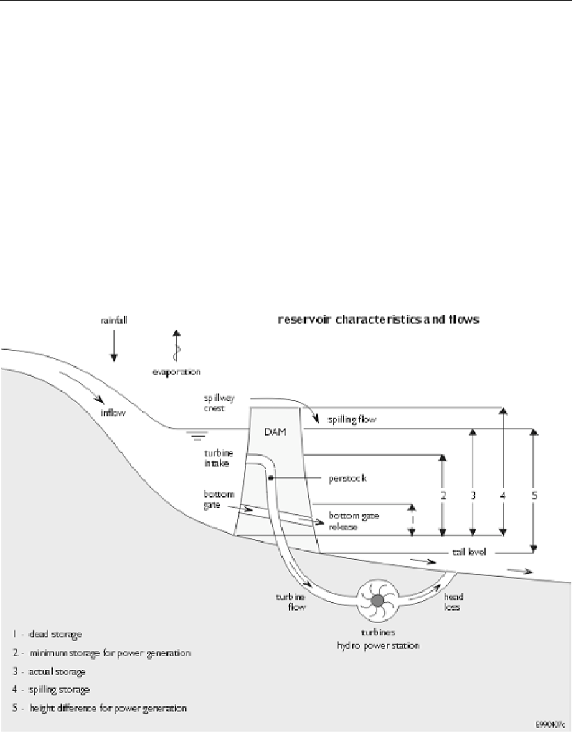
DRAFT
SOBEK, User Manual
Reservoir in SOBEK
Reservoirs are important structures in practical water resources management. A reservoir is
considered as advanced control, so it is implemented in the SOBEK real time control module
(SOBEK-RTC).
The following figure illustrates some of the reservoir concepts and terminology, like:
dead storage;
bottom gate (main gate);
turbine intake; and
spillway level.
Backwater outlets are not yet shown in the figure. The backwater gates represent abstractions
or spills from the reservoir which are not located at the main dam site.
Figure 6.111: Reservoir
Reservoir concept
The SOBEK reservoir includes the following aspects:
Reservoir operation rules (flood control curve, target curve, firm storage curve, hedging
rules below firm storage);
Multiple outlets (bottom gates, turbines, spillways, including backwater outlets)
Important here are the following 2 remarks:
not all outlets are obligatory,
outlets may be located on the same link, or on different links.
684 of 900 Deltares

DRAFT
Conceptual description
Q-H relations describing the relation between maximum flow and net-head for all outlets
(reflecting physical limitations);
Time series of maximum flows per outlet (reflecting imposed management);
Time series of release targets for downstream demands for all outlet links;
Time series of release targets for energy generation;
The operation of the SOBEK reservoir is based on the initial reservoir level and expected
inflow (defined by other decision parameters in SOBEK-RTC)
Application possibilities
The SOBEK-RTC reservoir module uses the initial reservoir level and an expected reservoir
inflow, together with the reservoir input data, to compute the desired release through the bot-
tom gate, turbine and spillway gate. The initial reservoir level and the expected reservoir
inflow are to be defined using decision parameters in SOBEK-RTC. This also allows for appli-
cations in flood-early warning systems (FEWS), where the determination of expected inflow
is an important aspect.
Furthermore, the reservoir module computes decision parameters for all outlet gates, which
can be used to define other decision parameters in RTC. The user thus has the possibility to
modify or overrule the decision parameters computed by the reservoir module. The setting of
the actual structure flows in SOBEK is determined by the decision parameter used to set the
structure flow, as specified by the user in the measure input file.
An important extra possibility of the SOBEK reservoir is that the outlets may be located on
different links. In practice, it quite often occurs that the outflows of main gate (bottom gate),
turbine and spillway do not come together on the same downstream link.
In the SOBEK reservoir design, there can be multiple bottom gates, turbines, and spillways.
Each of them may be on different outlet links, but also there may be several bottom gates,
on the same link or each on a different link. Backwater gate can thus be modelled in SOBEK
using a bottom gate on a separate link, with an appropriate downstream demand time series,
and appropriate Q-H relation describing the (physical) maximum abstraction capacity as a
function of the net head (=the head above intake level).
If these abstractions are to be modelled separate from the reservoir, SOBEK has the possibil-
ity to use a lateral discharge node. However, abstractions at these nodes are not depending
on the actual water level.
Rainfall and evaporation
In SOBEK, rainfall and evaporation can be modelled by specifying a lateral discharge using
a time series of rainfall or evaporation values in mm/timestep, and specifying a constant area
on which this rainfall/evaporation series applies. When applying this for a reservoir, one can
define the area at average target level as the area to be used in this computation.
Deltares 685 of 900
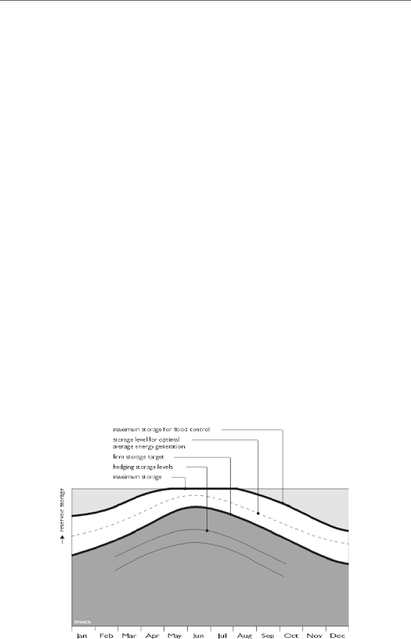
DRAFT
SOBEK, User Manual
Release targets
For the SOBEK reservoir, the user should specify time series of downstream release tar-
gets (demands) to be supplied from the reservoir. Since there may be different outlet links in
SOBEK, these demands need to be specified for all different outlet links. This is done using
input time series. It is anticipated that future versions allow to define the reservoir release tar-
gets by using decision parameters, summing the demands of various lateral discharges from
SOBEK-CF and/or SOBEK-RR. This gives a huge flexibility. However, the current approach
of directly specifying the release targets as input variables is very appropriate for testing and
comparing with any distribution model. In SOBEK, the user specifies a time series of desired
turbine flows as well.
Maximum flows
The maximum capacities of all outlet gates can be specified using a Q-h interpolation relation.
For the turbine gate, a distribution model determined the maximum possible flow through the
turbines based on the turbine characteristics (installed capacity, generation efficiency, head
loss relation etc.). In SOBEK, these hydropower data is not included, and a Q-h interpolation
relation for the turbines is specified directly.
SOBEK offers the extra possibility to impose other maximum flows as well. These can be
maximum flows reflecting e.g. water rights, or other limits imposed by the water authorities.
These maximum flows can be specified as time series for all outlet gates separately.
Reservoir operation
The rule curves of the SOBEK reservoir are using the same concepts as Deltares RIBASIM
distribution model, i.e. distinction is made between a flood control curve, a target curve and
a firm storage curve. Furthermore, the hedging rules on storage are implemented. These
hedging rules specify how releases are reduced when the reservoir is below firm storage.
The operation of the reservoir is as follows:
If the reservoir is above flood control level, try to come down to the flood control level
by any means. Just like in a distribution model, SOBEK uses first the turbines, then the
bottom gate, and finally the spillway. In case of multiple bottom gates, SOBEK simply uses
686 of 900 Deltares

DRAFT
Conceptual description
first the first bottom gate, then the second, etc.
If the reservoir is between flood control level and target level, the reservoir is allowed to
release more water, but only through the turbines (i.e. if extra energy can be generated). In
case of multiple turbine outlets, SOBEK simply uses the order in which the turbine outlets
are specified in the input data.
If the reservoir is between target level and firm storage level, no special action is taken.
If the reservoir is below firm storage, hedging rules are applied. They specify how much
the discharge from the reservoir is reduced, depending on the actual reservoir water level.
The releases on all outlet different links are reduced with the same percentage.
Deltares 687 of 900

DRAFT
SOBEK, User Manual
688 of 900 Deltares

DRAFT
References
Ackers, P., W. White, J. Perkins and A. Harrison, 1978. Weirs and Flumes for Flow Measure-
ment. John Wiley & Sons Ltd.
Amstrong, B. L., 1978. Derivation of initial soil moisture accounting parameters from soil prop-
erties for the national weather service river forecast system. Tech. rep., NOAA Technical
Memorandum NWS HYDRO 37.
Åström, K. J. and T. Hägglund, 1995. PID controllers: theory, design and tuning. Instrument
Society of America, Research Triangle Park, NC, USA, 2nd ed.
Becker, B., 2013. Inzet RTC-Tools voor het boezemmodel “Wetterskip Fryslân”. Report
1205773-000, Deltares, Delft. In Dutch.
Becker, B., R. Dahm, K.-J. van Heeringen, N. Goorden, N. Kramer, K. Kooij, J. Gooijer and
J. Jansen, 2012a. “Op zoek naar een optimaal ontwerp voor een groot uitwateringsgemaal
in het Lauwersmeer.” H2O 44 (13): 11–13. In Dutch.
Becker, B. and Q. Gao, 2012. Koppelen Sobek-modellen “Wetterskip Fryslân” en “Waterschap
Noorderzijlvest” via OpenMI. Report 1204514-000-ZWS-0007, Deltares, Delft. In Dutch.
Becker, B. and J. Talsma, 2014. “On the external and iterative coupling of multiple open
channel flow models with OpenMI.” Revista de Ingeniería Innova 6: 55–66.
Becker, B. P. J., D. Schwanenberg, T. Schruff and M. Hatz, 2012b. “Conjunctive real-time
control and hydrodynamic modelling in application to Rhine River.” In Proceedings of 10th
International Conference on Hydroinformatics. TuTech Verlag TuTech Innovation GmbH,
Hamburg, Germany.
Becker, B. P. J., J. Talsma, Q. Gao and E. Ruijgh, 2012c. “Coupling of multiple channel flow
models with OpenMI.” In Proceedings of 10th International Conference on Hydroinformat-
ics. Hamburg, Germany.
Bos, 1989. Discharge Measuring Structures. International Institute for Land Reclamation and
Improvement/ILRI, Wageningen, The Netherlands.
Cunge, J. A., F. M. Holly and A. Verwey, 1980. Practical aspects of computational river hy-
draulics. Boston; London; Melbourne; Boston; London; Melbourne: Pitman. Includes index.
D-WAQ PLT, 2013. D-Water Quality Processes Library Tables, Technical Reference Manual.
Deltares, 4.00 ed.
D-WAQ UM, 2013. D-Water Quality User Manual. Deltares, 4.02 ed.
Deltares, 2013. “RTC-Tools a toolbox for real-time control of hydraulic structures.” Published:
Deltares.
Dutch Hydrological Society, 2002. “Hydrologische woordenlijst.” Nederlandse Hydrologische
Vereniging.
Ellis, J. B. and J.-L. Bertrand-Krajewski, eds., 2010. Assessing infiltration and exfiltration on
the Performance of Urban Sewer Systems (APUSS). IWA Publishing, London, UK. ISBN:
978-1-84-339149-4.
Engelund, F. and E. Hansen, 1967. A monograph on Sediment Transport in Alluvial Streams.
Teknisk Forlag, Copenhagen.
Ernst, L., 1978. “Drainage of undulating sandy soils with high groundwatertables.” Journal of
Hydrology 39: 1–50.
Deltares 689 of 900

DRAFT
SOBEK, User Manual
Feddes, R. A., P. J. Kowalik, K. K. Malinka and H. Zaradny, 1978. Simulation of Field Water
Use and Crop Yield. John Wiley and Sons. PUDOC Wageningen.
Fischer, H., E. List, R. Koh, J. Imberger and N. Brooks, 1979. Mixing in inland and Coastal
Waters. Academic Press.
Gill, A. E., 1982. Atmosphere-Ocean dynamics, vol. 30 of International Geophysics Series.
Academic Press.
Gregersen, J., P. Gijsbers and S. Westen, 2007. “OpenMI: Open modelling Interface.” Journal
of Hydroinformatics 9 (3): 175–191. DOI: 10.2166/hydro.2007.023.
Hooghart, J. and W. Lablans, 1988. Van Penman naar Makkink: een nieuwe berekeningswi-
jze voor de klimatologische verdampingsgetallen. Rapporten en nota’s. Ministerie van Ver-
keer en Waterstaat, Koninklijk Nederlands Meteorologisch Instituut. (In Dutch), Project- en
Begeleidingsgroep Verdampingsberekeningen.
Ippen, A. and D. Harleman, 1961. “One dimensional analysis of salinity intrusion in estuaries.”
Civ. Eng. J. Hydraul. 96 (13-15): 1691-1709. Tech. Bull.
Karpf, C., J. Traenckner and P. Krebs, 2008. “Hydraulic modelling of sewage exfiltration.” In
11th International Conference on Urban Drainage. Edinburgh, Scotland, UK.
Knaap, F. Van der, 2000. Breach growth as a function of time; Deltares, memo’s 2 and 3 of
May 21 and September 5 respectively. Tech. Rep. Q2655, WL | Delft Hydraulics, Delft, The
Netherlands.
Kuijper, C. and L. van Rijn, 2011. “Analytical and Numerical Analysis of Tides and Salinities
in Estuaries; Part II: Salinity Distributions in Prismatic and Convergent Tidal Channels.”
Ocean Dynamics 61 (11): 1743:1765.
Lane, A., 1989. The heat balance of the North Sea. Tech. Rep. 8, Proudman Oceanographic
Laboratory.
Lindström, G., B. Johansson, M. Persson, M. Gardelin and S. Bergström, 1997. Development
and test of the distributed HBV-96 hydrological model. Tech. rep., Swedisch Meteological
and Hydrological Institute.
McCarthy, G., 1938. “The unit hydrograph and flood routing.” In Conference of North Atlantic
Division. US Engineering Office, Providence RI, New London, CT. Unpublished Paper.
Moore, R., P. Gijsbers, D. Fortune, J. Gregersen and M. Blind, 2005. OpenMI Document
Series: Part A – Scope for the OpenMI. Version 1.0 ed.
Moore, R. V. and C. I. Tindall, 2005. “An overview of the open modelling interface and
environment (the OpenMI).” Environmental Science & Policy 8 (3): 279–286. DOI:
10.1016/j.envsci.2005.03.009.
Nielsen, S. A. and E. Hansen, 1973. “Numerical simulation of the rainrain runoff process on
a daily basis.” Nordic Hydrology 4: 171–190.
NLingenieurs, 1978. Position paper Riolering. Tech. rep., NLingenieurs.
Octavio, K. A. H., G. H. Jirka and D. R. F. Harleman, 1977. Vertical Heat Transport Mecha-
nisms in Lakes and Reservoirs. Tech. Rep. 22, Massachusetts Institute of Technology.
Peck, E. L., 1978. Catchment modeling and initial parameter estimation for the National
Weather Service River Forecast System. Tech. rep., NOAA Tech. Memo. NWS HYDRO-
31, US Dept of Commerce, Silver Spring, Maryland, USA.
690 of 900 Deltares

DRAFT
References
RTC-Tools TRM, 2012. RTC-Tools a software package for modelling real-time control / Techni-
cal Reference Manual and Configuration Guidelines. Deltares, Delft. Version: 0.1.0.22313.
Rutsch, J., M., J. Rieckermann, C. J.B., J. Ellis, Vollertsen and P. Krebs, 2008. “Towards a
better understanding of sewer exflitration,.” In Water Research, vol. 42, pages 2385–2394.
Ryan, P. J., D. R. F. Harleman and K. D. Stolzenbach, 1974. “Surface Heat Loss From Cooling
Ponds.” Water Resources Research 10 (5): 930–938.
Savenije, H., 2012. “Salinity and Tides in Alluvial Estuaries.” 2nd completely revised edition.
Schellekens, J., B. P. J. Becker, G. Donchyts, N. Goorden, J. C. Hoogewoud, S. Patzke and
D. Schwanenberg, 2012. “OpenStreams: Open Source Components as Building Blocks
for Integrated Hydrological Models.” In Geophysical Research Abstracts, vol. 14 EGU2012,
page 3953. Vienna, Austria.
Schmidt, 1955. “Unknown.” .
Schwanenberg, D., B. Becker and T. Schruff, 2011. SOBEK-Grobmodell des staugeregelten
Oberrheins. Report no. 1201242-000-ZWS-0014, Deltares. In German.
SOBEK3_TRM, 2013. SOBEK 3 / Hydrodynamics Technical Reference Manual / SOBEK in
Delta Shell. Deltares, Delft. Version: 3.0.1.27817.
Stelling, G. S. and S. P. A. Duinmeijer, 2003. “A staggered conservative scheme for ev-
ery Froude number in rapidly varied shallow water flows.” International Journal Numerical
Methods In Fluids 43: 1329–1354.
Thatcher, M. L. and D. R. F. Harleman, 1972. A mathematical model for the prediction of
unsteady salinity intrusion in estuaries. Report no. 144, MIT School of Engineering Mas-
sachusetts Institute of Technologie, Department of Civil Engineering.
Vademecum, C., 1988. Werkgroep Herziening Cultuurtechnisch vademecum. Tech. rep.,
Cultuurtechnische vereniging.
Verheij, H., 2002. Modification breach growth model in HIS-OM. Tech. Rep. Q3299, WL | Delft
Hydraulics, Delft, The Netherlands. (in Dutch).
Wesseling, J., 1991. CAPSEV; steady state moisture flow theory. Program description user
manual. Tech. rep., Staring Centrum, Wageningen.
Deltares 691 of 900

DRAFT
SOBEK, User Manual
692 of 900 Deltares
DRAFT
A Dimension of Steel Cunnete Cross-sections
Table A.1: Steel cunette cross-section
Type 1: Three circle segments, a >= 120 degrees, a1 = 0 degrees; r3 =0
Type 2 & 3: Three circle segments only, a <120 degrees, a1 = 0 degrees; r3 =0
Type 4: Four circle segments
W = Width, including wave height (WH)
H = Height, including wave height (WH)
r = Radius r, including half the wave height (WH)
r1 = Radius r1, including half the wave height (WH)
r2 = Radius r2, including half the wave height (WH)
r3 = Radius r3, including half the wave height (WH)
a = Angle a
a1 = Angle a1
WH = Wave height of corrugated construction material
W H r r1 r2 r3 a a1 WH Remarks
cm cm cm cm cm cm deg deg cm
100 78 50 80 20 0 28 0 2 SGME formerly: EM 1
120 98 60 90 30 0 38 0 2 SGME formerly: EM 2
140 116 70 110 30 0 41 0 2 SGME formerly: EM 3
160 131 80 182 30 0 38 0 2 SGME formerly: EM 4
180 136 90 150 30 0 46 0 2 SGME formerly: EM 5
200 154 100 170 30 0 49 0 2 SGME formerly: EM 6
210 161 105 202 30 0 47 0 2 SGME formerly: EM 7
220 168 110 242 30 0 45 0 2 SGME formerly: EM 8
230 179 115 222 30 0 50 0 2 SGME formerly: EM 9
240 174 120 210 30 0 54 0 2 SGME formerly: EM 10
250 185 126 200 30 0 59 0 2 SGME formerly: EM 11
260 192 130 230 30 0 57 0 2 SGME formerly: EM 12
270 189 133 224 30 0 59 0 2 SGME formerly: EM 13
280 210 140 250 30 0 59 0 2 SGME formerly: EM 14
290 206 144 242 30 0 63 0 2 SGME formerly: EM 15
300 212 150 270 30 0 62 0 2 SGME formerly: EM 16
310 224 154 261 30 0 66 0 2 SGME formerly: EM 17
320 230 160 290 30 0 65 0 2 SGME formerly: EM 18
190 147 94,5 220,5 48,5 0 55,5 0 5 SGM-1-1
209 141 109,5 252,5 48,5 0 56,5 0 5 SGM-1-2
209 155 104,5 277,5 48,5 0 55,5 0 5 SGM-1-3
220 160 109,5 277,5 48,5 0 56,5 0 5 SGM-1-4
226 166 113,5 348,5 48,5 0 56,5 0 5 SGM-1-5
234 171 116,5 291,5 48,5 0 58 0 5 SGM-1-6
246 175 122,5 302,5 48,5 0 59,5 0 5 SGM-1-7
265 173 136,5 312,5 48,5 0 62,5 0 5 SGM-1-8
continued on next page
Deltares 693 of 900

DRAFT
SOBEK, User Manual
Table A.1 – continued from previous page
W H r r1 r2 r3 a a1 WH Remarks
cm cm cm cm cm cm deg deg cm
265 180 134,5 312,5 48,5 0 63,5 0 5 SGM-1-9
274 190 136,5 397,5 48,5 0 60,5 0 5 SGM-1-10
283 192 142,5 437,5 48,5 0 60,5 0 5 SGM-1-11
290 196 144,5 442,5 48,5 0 61,5 0 5 SGM-1-12
296 201 147,5 442,5 48,5 0 61,5 0 5 SGM-1-13
305 207 152,5 452,5 48,5 0 62,5 0 5 SGM-1-14
317 211 158,5 462,5 48,5 0 63,5 0 5 SGM-1-15
327 220 163,5 462,5 48,5 0 65,5 0 5 SGM-1-16
337 221 169,5 462,5 48,5 0 66,5 0 5 SGM-1-17
353 226 178,5 462,5 48,5 0 68,5 0 5 SGM-1-18
366 229 186,5 464,5 48,5 0 71,5 0 5 SGM-1-19
365 237 183,5 552,5 48,5 0 66,5 0 5 SGM-1-20
385 237 196,5 492,5 48,5 0 73,5 0 5 SGM-1-21
386 246 195,5 492,5 48,5 0 73,5 0 5 SGM-1-22
392 252 196,5 656,5 48,5 0 66,5 0 5 SGM-1-23
396 259 198,5 552,5 48,5 0 70,5 0 5 SGM-1-24
414 262 207,5 652,5 48,5 0 69,5 0 5 SGM-1-25
419 269 209,5 672,5 48,5 0 69,5 0 5 SGM-1-26
434 272 217,5 702,5 48,5 0 70,5 0 5 SGM-1-27
440 277 220,5 712,5 48,5 0 71,5 0 5 SGM-1-28
445 285 222,5 712,5 48,5 0 72,5 0 5 SGM-1-29
472 286 239,5 578,5 48,5 0 83,5 0 5 SGM-1-30
478 292 241,5 652,5 48,5 0 79,5 0 5 SGM-1-31
483 300 243,5 722,5 48,5 0 77,5 0 5 SGM-1-32
489 304 244,5 862,5 48,5 0 71,5 0 5 SGM-1-33
505 308 254,5 742,5 48,5 0 78,5 0 5 SGM-1-34
510 315 256,5 742,5 48,5 0 80,5 0 5 SGM-1-35
410 290 206,5 492,5 81,5 0 101,5 0 5 SGM-1-36
417 296 209,5 601,5 81,5 0 99,5 0 5 SGM-1-37
431 300 216,5 505,5 81,5 0 104,5 0 5 SGM-1-38
438 306 219,5 567,5 81,5 0 101,5 0 5 SGM-1-39
444 311 222,5 654,5 81,5 0 99,5 0 5 SGM-1-40
459 316 230,5 580,5 81,5 0 104,5 0 5 SGM-1-41
473 320 238,5 532,5 81,5 0 108,5 0 5 SGM-1-42
480 326 241,5 592,5 81,5 0 107,5 0 5 SGM-1-43
487 331 244,5 664,5 81,5 0 104,5 0 5 SGM-1-44
500 336 252,5 601,5 81,5 0 110,5 0 5 SGM-1-45
508 341 254,5 670,5 81,5 0 107,5 0 5 SGM-1-46
522 346 263,5 612,5 81,5 0 113,5 0 5 SGM-1-47
527 351 265,5 679,5 81,5 0 111,5 0 5 SGM-1-48
534 357 268,5 752,5 81,5 0 108,5 0 5 SGM-1-49
551 361 277,5 692,5 81,5 0 114,5 0 5 SGM-1-50
557 367 280,5 762,5 81,5 0 111,5 0 5 SGM-1-51
571 371 288,5 702,5 81,5 0 116,5 0 5 SGM-1-52
578 377 290,5 772,5 81,5 0 113,5 0 5 SGM-1-53
continued on next page
694 of 900 Deltares

DRAFT
Dimension of Steel Cunnete Cross-sections
Table A.1 – continued from previous page
W H r r1 r2 r3 a a1 WH Remarks
cm cm cm cm cm cm deg deg cm
593 381 299,5 702,5 81,5 0 119,5 0 5 SGM-1-54
599 387 302,5 777,5 81,5 0 116,5 0 5 SGM-1-55
605 392 304,5 852,5 81,5 0 114,5 0 5 SGM-1-56
611 398 306,5 952,5 81,5 0 111,5 0 5 SGM-1-57
627 402 315,5 862,5 81,5 0 118,5 0 5 SGM-1-58
632 408 317,5 902,5 81,5 0 116,5 0 5 SGM-1-59
185 155 93 172 63 0 159 0 5,5 SGMA formerly: MA 1
194 160 97 226 63 0 166 0 5,5 SGMA formerly: MA 2
228 173 118 177 63 0 137 0 5,5 SGMA formerly: MA 3
254 188 128 291 63 0 158 0 5,5 SGMA formerly: MA 4
289 207 145 476 63 0 167 0 5,5 SGMA formerly: MA 5
328 220 169 316 63 0 143 0 5,5 SGMA formerly: MA 6
343 230 174 419 63 0 155 0 5,5 SGMA formerly: MA 7
370 244 187 506 63 0 158 0 5,5 SGMA formerly: MA 8
377 249 190 602 63 0 163 0 5,5 SGMA formerly: MA 9
410 257 216 383 63 0 137 0 5,5 SGMA formerly: MA 10
418 262 217 425 63 0 143 0 5,5 SGMA formerly: MA 11
439 277 222 617 63 0 157 0 5,5 SGMA formerly: MA 12
446 367 223 394 131 0 175 0 5,5 SGMA formerly: MA 13
454 372 227 426 131 0 178 0 5,5 SGMA formerly: MA 14
489 387 245 392 131 0 165 0 5,5 SGMA formerly: MA 15
497 392 249 417 131 0 168 0 5,5 SGMA formerly: MA 16
519 409 259 511 131 0 176 0 5,5 SGMA formerly: MA 17
526 414 263 550 131 0 179 0 5,5 SGMA formerly: MA 18
548 418 276 441 131 0 161 0 5,5 SGMA formerly: MA 19
563 429 282 493 131 0 167 0 5,5 SGMA formerly: MA 20
584 445 292 592 131 0 175 0 5,5 SGMA formerly: MA 21
611 461 305 645 131 0 176 0 5,5 SGMA formerly: MA 22
630 472 315 658 131 0 175 0 5,5 SGMA formerly: MA 23
649 475 326 581 131 0 165 0 5,5 SGMA formerly: MA 24
676 498 338 724 131 0 175 0 5,5 SGMA formerly: MA 25
683 503 341 768 131 0 177 0 5,5 SGMA formerly: MA 26
702 514 351 779 131 0 176 0 5,5 SGMA formerly: MA 27
716 512 360 654 131 0 165 0 5,5 SGMA formerly: MA 28
729 523 366 721 131 0 169 0 5,5 SGMA formerly: MA 29
748 540 374 846 131 0 176 0 5,5 SGMA formerly: MA 30
768 550 384 856 131 0 175 0 5,5 SGMA formerly: MA 31
794 566 397 913 131 0 176 0 5,5 SGMA formerly: MA 32
814 576 407 922 131 0 175 0 5,5 SGMA formerly: MA 33
840 592 420 980 131 0 176 0 5,5 SGMA formerly: MA 34
860 603 430 989 131 0 175 0 5,5 SGMA formerly: MA 35
886 618 443 1047 131 0 176 0 5,5 SGMA formerly: MA 36
906 629 453 1055 131 0 175 0 5,5 SGMA formerly: MA 37
932 645 466 1114 131 0 176 0 5,5 SGMA formerly: MA 38
continued on next page
Deltares 695 of 900

DRAFT
SOBEK, User Manual
Table A.1 – continued from previous page
W H r r1 r2 r3 a a1 WH Remarks
cm cm cm cm cm cm deg deg cm
953 655 477 1121 131 0 175 0 5,5 SGMA formerly: MA 39
978 671 489 1180 131 0 176 0 5,5 SGMA formerly: MA 40
1001 737 501 923 166 0 177 0 5,5 SGMA formerly: MA 41
1027 754 513 963 166 0 178 0 5,5 SGMA formerly: MA 42
1047 765 523 974 166 0 177 0 5,5 SGMA formerly: MA 43
1072 781 536 1015 166 0 178 0 5,5 SGMA formerly: MA 44
1092 792 546 1026 166 0 177 0 5,5 SGMA formerly: MA 45
1118 809 559 1067 166 0 178 0 5,5 SGMA formerly: MA 46
1138 820 569 1077 166 0 178 0 5,5 SGMA formerly: MA 47
1163 836 582 1118 166 0 178 0 5,5 SGMA formerly: MA 48
1183 847 592 1129 166 0 178 0 5,5 SGMA formerly: MA 49
1208 864 604 1170 166 0 178 0 5,5 SGMA formerly: MA 50
219 169 115 155 63 0 129 0 5,5 SGMB formerly: MB 1
229 173 118 177 63 0 137 0 5,5 SGMB formerly: MB 2
240 178 127 173 63 0 128 0 5,5 SGMB formerly: MB 3
302 205 163 225 63 0 124 0 5,5 SGMB formerly: MB 4
340 224 179 297 63 0 136 0 5,5 SGMB formerly: MB 5
372 266 198 323 98 0 122 0 5,5 SGMB formerly: MB 6
381 270 201 363 98 0 127 0 5,5 SGMB formerly: MB 7
402 278 213 386 98 0 126 0 5,5 SGMB formerly: MB 8
419 287 219 496 98 0 135 0 5,5 SGMB formerly: MB 9
465 303 251 452 98 0 123 0 5,5 SGMB formerly: MB 10
529 328 289 516 98 0 121 0 5,5 SGMB formerly: MB 11
546 337 292 625 98 0 129 0 5,5 SGMB formerly: MB 12
567 345 304 644 98 0 128 0 5,5 SGMB formerly: MB 13
589 353 317 665 98 0 128 0 5,5 SGMB formerly: MB 14
604 362 319 818 98 0 135 0 5,5 SGMB formerly: MB 15
623 365 342 644 98 0 122 0 5,5 SGMB formerly: MB 16
639 374 343 771 98 0 130 0 5,5 SGMB formerly: MB 17
660 382 355 789 98 0 129 0 5,5 SGMB formerly: MB 18
668 387 356 870 98 0 132 0 5,5 SGMB formerly: MB 19
695 394 381 759 98 0 124 0 5,5 SGMB formerly: MB 20
723 424 390 838 112 0 128 0 5,5 SGMB formerly: MB 21
744 432 402 857 112 0 127 0 5,5 SGMB formerly: MB 22
765 440 415 876 112 0 126 0 5,5 SGMB formerly: MB 23
794 453 428 964 112 0 129 0 5,5 SGMB formerly: MB 24
816 461 441 982 112 0 128 0 5,5 SGMB formerly: MB 25
837 470 454 1000 112 0 128 0 5,5 SGMB formerly: MB 26
859 478 467 1017 112 0 127 0 5,5 SGMB formerly: MB 27
888 491 479 1111 112 0 129 0 5,5 SGMB formerly: MB 28
909 499 492 1127 112 0 129 0 5,5 SGMB formerly: MB 29
930 507 505 1144 112 0 128 0 5,5 SGMB formerly: MB 30
952 515 518 1161 112 0 127 0 5,5 SGMB formerly: MB 31
973 524 531 1177 112 0 127 0 5,5 SGMB formerly: MB 32
continued on next page
696 of 900 Deltares

DRAFT
Dimension of Steel Cunnete Cross-sections
Table A.1 – continued from previous page
W H r r1 r2 r3 a a1 WH Remarks
cm cm cm cm cm cm deg deg cm
1002 536 543 1274 112 0 129 0 5,5 SGMB formerly: MB 33
1023 545 556 1289 112 0 128 0 5,5 SGMB formerly: MB 34
1045 553 569 1305 112 0 128 0 5,5 SGMB formerly: MB 35
251 214 127 348 77 0 199 0 2 EW1
285 236 144 467 77 0 200 0 2 EW2
319 258 160 599 77 0 202 0 2 EW3
288 273 144 317 108 0 243 0 5,5 WA1
330 303 165 300 108 0 229 0 5,5 WA2
337 310 169 331 108 0 231 0 5,5 WA3
345 316 172 367 108 0 234 0 5,5 WA4
361 328 181 370 108 0 231 0 5,5 WA5
376 341 188 451 108 0 236 0 5,5 WA6
391 354 196 566 108 0 241 0 5,5 WA7
427 377 213 450 108 0 227 0 5,5 WA8
434 384 217 485 108 0 229 0 5,5 WA9
449 397 224 571 108 0 234 0 5,5 WA10
458 402 229 522 108 0 229 0 5,5 WA11
480 422 240 661 108 0 236 0 5,5 WA12
509 480 254 492 188 0 238 0 5,5 WA13
524 493 262 581 188 0 241 0 5,5 WA14
550 511 275 491 188 0 230 0 5,5 WA15
573 530 287 588 188 0 235 0 5,5 WA16
597 548 299 630 188 0 234 0 5,5 WA17
627 574 314 824 188 0 240 0 5,5 WA18
647 585 324 645 188 0 229 0 5,5 WA19
655 591 327 679 188 0 230 0 5,5 WA20
677 611 339 796 188 0 235 0 5,5 WA21
707 637 353 1012 188 0 240 0 5,5 WA22
720 641 360 758 188 0 228 0 5,5 WA23
745 659 372 795 188 0 228 0 5,5 WA24
757 673 378 961 188 0 235 0 5,5 WA25
769 677 384 831 188 0 228 0 5,5 WA26
781 692 390 1001 188 0 234 0 5,5 WA27
812 717 406 1091 188 0 235 0 5,5 WA28
832 728 416 980 188 0 230 0 5,5 WA29
849 740 424 978 188 0 228 0 5,5 WA30
861 754 430 1167 188 0 235 0 5,5 WA31
871 759 435 1104 188 0 232 0 5,5 WA32
892 779 446 1260 188 0 235 0 5,5 WA33
905 800 452 1191 215 0 235 0 5,5 WA34
929 819 464 1229 215 0 235 0 5,5 WA35
289 254 145 267 90 0 205 0 5,5 WB1
continued on next page
Deltares 697 of 900

DRAFT
SOBEK, User Manual
Table A.1 – continued from previous page
W H r r1 r2 r3 a a1 WH Remarks
cm cm cm cm cm cm deg deg cm
322 278 161 348 90 0 209 0 5,5 WB2
329 284 165 393 90 0 213 0 5,5 WB3
369 306 184 346 90 0 197 0 5,5 WB4
383 318 191 412 90 0 204 0 5,5 WB5
408 335 204 457 90 0 205 0 5,5 WB6
422 348 211 552 90 0 211 0 5,5 WB7
463 369 231 479 90 0 198 0 5,5 WB8
483 388 241 600 90 0 206 0 5,5 WB9
496 400 248 710 90 0 212 0 5,5 WB10
532 415 266 570 90 0 197 0 5,5 WB11
557 432 278 612 90 0 198 0 5,5 WB12
582 450 291 656 90 0 199 0 5,5 WB13
601 468 300 793 90 0 206 0 5,5 WB14
622 521 311 591 157 0 199 0 5,5 WB15
644 539 322 691 157 0 205 0 5,5 WB16
669 557 334 738 157 0 205 0 5,5 WB17
694 574 347 784 157 0 206 0 5,5 WB18
722 599 361 984 157 0 213 0 5,5 WB19
737 603 368 836 157 0 205 0 5,5 WB20
762 620 381 883 157 0 205 0 5,5 WB21
789 645 395 1086 157 0 211 0 5,5 WB22
812 655 406 977 157 0 206 0 5,5 WB23
830 666 415 980 157 0 204 0 5,5 WB24
855 684 428 1027 157 0 205 0 5,5 WB25
190 145 96 196,3 48,2 0 55,8 0 5,1 Old model, measures
w.r.t. central axis
198 150 99,3 252,9 48,2 0 54,6 0 5,1 Old model, measures
w.r.t. central axis
211 155 106,6 214,6 48,2 0 58,4 0 5,1 Old model, measures
w.r.t. central axis
219 160 109,9 267,2 48,2 0 56,9 0 5,1 Old model, measures
w.r.t. central axis
226 166 113 348,4 48,2 0 55,3 0 5,1 Old model, measures
w.r.t. central axis
240 170 120,6 281,4 48,2 0 59,4 0 5,1 Old model, measures
w.r.t. central axis
247 176 123,7 352,8 48,2 0 57,6 0 5,1 Old model, measures
w.r.t. central axis
253 181 126,7 467,1 48,2 0 55,6 0 5,1 Old model, measures
w.r.t. central axis
268 186 134,3 360,6 48,2 0 60,2 0 5,1 Old model, measures
w.r.t. central axis
274 191 137,1 456,4 48,2 0 58,1 0 5,1 Old model, measures
w.r.t. central axis
continued on next page
698 of 900 Deltares

DRAFT
Dimension of Steel Cunnete Cross-sections
Table A.1 – continued from previous page
W H r r1 r2 r3 a a1 WH Remarks
cm cm cm cm cm cm deg deg cm
289 196 145,2 369,8 48,2 0 63 0 5,1 Old model, measures
w.r.t. central axis
295 201 148 453,4 48,2 0 60,7 0 5,1 Old model, measures
w.r.t. central axis
301 207 150,5 580,9 48,2 0 58,1 0 5,1 Old model, measures
w.r.t. central axis
316 211 158,7 455,4 48,2 0 63,5 0 5,1 Old model, measures
w.r.t. central axis
331 216 167,3 391,6 48,2 0 68,8 0 5,1 Old model, measures
w.r.t. central axis
338 221 169,9 460,7 48,2 0 66,3 0 5,1 Old model, measures
w.r.t. central axis
352 226 178,8 403,6 48,2 0 72,1 0 5,1 Old model, measures
w.r.t. central axis
359 231 180,5 467,8 48,2 0 69,3 0 5,1 Old model, measures
w.r.t. central axis
365 237 183,1 552,2 48,2 0 66,5 0 5,1 Old model, measures
w.r.t. central axis
380 241 192,2 476,2 48,2 0 72,4 0 5,1 Old model, measures
w.r.t. central axis
387 247 194,3 553,2 48,2 0 69,6 0 5,1 Old model, measures
w.r.t. central axis
392 252 196,6 656,3 48,2 0 66,5 0 5,1 Old model, measures
w.r.t. central axis
397 258 198,8 801,8 48,2 0 63,5 0 5,1 Old model, measures
w.r.t. central axis
413 262 207,5 649,7 48,2 0 69,6 0 5,1 Old model, measures
w.r.t. central axis
430 267 216,9 563,1 48,2 0 75,9 0 5,1 Old model, measures
w.r.t. central axis
435 272 218,7 647,9 48,2 0 72,6 0 5,1 Old model, measures
w.r.t. central axis
440 278 220,7 758,4 48,2 0 69,3 0 5,1 Old model, measures
w.r.t. central axis
457 282 230,1 648,4 48,2 0 75,9 0 5,1 Old model, measures
w.r.t. central axis
472 286 239,7 578,6 48,2 0 82,8 0 5,1 Old model, measures
w.r.t. central axis
478 292 241,3 652 48,2 0 79,2 0 5,1 Old model, measures
w.r.t. central axis
484 298 243 742,9 48,2 0 75,7 0 5,1 Old model, measures
w.r.t. central axis
489 304 245,1 861,3 48,2 0 72,4 0 5,1 Old model, measures
w.r.t. central axis
505 308 254,5 741,4 48,2 0 79 0 5,1 Old model, measures
w.r.t. central axis
continued on next page
Deltares 699 of 900

DRAFT
SOBEK, User Manual
Table A.1 – continued from previous page
W H r r1 r2 r3 a a1 WH Remarks
cm cm cm cm cm cm deg deg cm
510 314 256,2 847,6 48,2 0 75,4 0 5,1 Old model, measures
w.r.t. central axis
410 290 205,9 491,7 81,2 0 100,5 0 5,1 Old model, measures
w.r.t. central axis
417 296 209 561,3 81,2 0 98,5 0 5,1 Old model, measures
w.r.t. central axis
431 300 216,9 505,2 81,2 0 103,1 0 5,1 Old model, measures
w.r.t. central axis
438 306 219,9 567,9 81,2 0 101,3 0 5,1 Old model, measures
w.r.t. central axis
444 311 222,5 654,3 81,2 0 99 0 5,1 Old model, measures
w.r.t. central axis
459 316 230,6 580,9 81,2 0 103,8 0 5,1 Old model, measures
w.r.t. central axis
473 320 239 532,1 81,2 0 108,9 0 5,1 Old model, measures
w.r.t. central axis
480 326 241,5 592 81,2 0 106,6 0 5,1 Old model, measures
w.r.t. central axis
487 331 244,3 664,4 81,2 0 104,3 0 5,1 Old model, measures
w.r.t. central axis
501 336 252,7 601,9 81,2 0 109,7 0 5,1 Old model, measures
w.r.t. central axis
508 341 255,2 671 81,2 0 107,1 0 5,1 Old model, measures
w.r.t. central axis
522 346 263,9 614,6 81,2 0 112,7 0 5,1 Old model, measures
w.r.t. central axis
529 351 266,2 680,2 81,2 0 110,2 0 5,1 Old model, measures
w.r.t. central axis
535 357 268,7 759,2 81,2 0 107,7 0 5,1 Old model, measures
w.r.t. central axis
550 361 277,3 689,8 81,2 0 113,2 0 5,1 Old model, measures
w.r.t. central axis
557 367 279,6 763,7 81,2 0 110,5 0 5,1 Old model, measures
w.r.t. central axis
571 371 288,5 699,7 81,2 0 116,3 0 5,1 Old model, measures
w.r.t. central axis
578 377 290,8 770,3 81,2 0 113,5 0 5,1 Old model, measures
w.r.t. central axis
593 381 299,7 710,1 81,2 0 119,3 0 5,1 Old model, measures
w.r.t. central axis
599 387 302 777,5 81,2 0 116,5 0 5,1 Old model, measures
w.r.t. central axis
605 392 304,3 857,2 81,2 0 113,7 0 5,1 Old model, measures
w.r.t. central axis
611 398 306,5 953,2 81,2 0 110,7 0 5,1 Old model, measures
w.r.t. central axis
continued on next page
700 of 900 Deltares

DRAFT
Dimension of Steel Cunnete Cross-sections
Table A.1 – continued from previous page
W H r r1 r2 r3 a a1 WH Remarks
cm cm cm cm cm cm deg deg cm
627 402 315,4 861,3 81,2 0 116,8 0 5,1 Old model, measures
w.r.t. central axis
632 408 317,5 951,2 81,2 0 113,8 0 5,1 Old model, measures
w.r.t. central axis
470 430 237,5 574,5 142,5 0 238 0 5,1 WU1
494 448 249,5 623,5 142,5 0 237 0 5,1 WU2
519 468 261,5 669,5 142,5 0 237 0 5,1 WU3
545 487 274,5 710,5 142,5 0 236 0 5,1 WU4
570 507 287,5 759,5 142,5 0 236 0 5,1 WU5
593 524 298,5 784,5 142,5 0 235 0 5,1 WU6
618 544 311,5 825,5 142,5 0 234 0 5,1 WU7
647 582 325,5 828,5 172,5 0 237 0 5,1 WU8
672 602 338,5 865,5 172,5 0 237 0 5,1 WU9
697 621 350,5 907,5 172,5 0 236 0 5,1 WU10
723 641 363,5 952,5 172,5 0 236 0 5,1 WU11
747 659 375,5 981,5 172,5 0 235 0 5,1 WU12
773 678 388,5 1025 172,5 0 235 0 5,1 WU13
796 696 400,5 1058 172,5 0 235 0 5,1 WU14
60 54 30 80 11 0 13,7 0 1,3 DM/2-1
80 55 40 116 11 0 15,1 0 1,3 DM/2-2
100 72 50 153 11 0 16,5 0 1,3 DM/2-3
120 89 60 189 11 0 17,9 0 1,3 DM/2-4
140 91 70 225 11 0 19,3 0 1,3 DM/2-5
160 108 80 262 11 0 20,7 0 1,3 DM/2-6
180 125 90 298 11 0 22,1 0 1,3 DM/2-7
200 126 100 334 11 0 23,5 0 1,3 DM/2-8
220 143 110 370 11 0 24,9 0 1,3 DM/2-9
240 160 120 407 11 0 26,3 0 1,3 DM/2-10
66 51 33,2 95,7 10,9 0 13 0 1,3 D-M.2-1
101 71 50,7 155,7 10,9 0 16 0 1,3 D-M.2-2
126 86 63,2 195,7 10,9 0 17 0 1,3 D-M.2-3
161 106 80,7 270,7 10,9 0 20 0 1,3 D-M.2-4
191 121 95,7 295,7 10,9 0 22 0 1,3 D-M.2-5
221 136 110,7 380,7 10,9 0 24 0 1,3 D-M.2-6
157 133 79 189 52 0 178 0 3,2 LA1
181 143 92 147 52 0 152 0 3,2 LA2
189 148 95 180 52 0 161 0 3,2 LA3
197 153 99 228 52 0 169 0 3,2 LA4
210 158 106 199 52 0 158 0 3,2 LA5
218 163 109 245 52 0 166 0 3,2 LA6
225 169 113 314 52 0 173 0 3,2 LA7
continued on next page
Deltares 701 of 900

DRAFT
SOBEK, User Manual
Table A.1 – continued from previous page
W H r r1 r2 r3 a a1 WH Remarks
cm cm cm cm cm cm deg deg cm
239 173 120 262 52 0 163 0 3,2 LA8
246 179 123 325 52 0 170 0 3,2 LA9
260 183 131 278 52 0 160 0 3,2 LA10
267 189 134 336 52 0 167 0 3,2 LA11
281 193 142 294 52 0 157 0 3,2 LA12
288 199 145 348 52 0 164 0 3,2 LA13
295 204 148 421 52 0 170 0 3,2 LA14
309 209 156 361 52 0 161 0 3,2 LA15
164 113 92 131 42 0 107 0 3,2 LB1
174 118 94 170 42 0 119 0 3,2 LB2
183 122 97 236 42 0 130 0 3,2 LB3
196 126 108 194 42 0 117 0 3,2 LB4
205 130 109 260 42 0 128 0 3,2 LB5
213 135 111 385 42 0 138 0 3,2 LB6
227 138 122 284 42 0 126 0 3,2 LB7
235 143 124 397 42 0 135 0 3,2 LB8
249 146 136 306 42 0 123 0 3,2 LB9
257 151 137 415 42 0 133 0 3,2 LB10
271 155 149 326 42 0 121 0 3,2 LB11
280 159 150 430 42 0 131 0 3,2 LB12
294 163 163 348 42 0 120 0 3,2 LB13
302 167 163 446 42 0 129 0 3,2 LB14
316 171 177 367 42 0 118 0 3,2 LB15
70 55 35 98 11 0 180 0 1,3 M1
80 63 40 116 11 0 180 0 1,3 M2
100 72 50 153 11 0 180 0 1,3 M3
120 89 60 189 11 0 180 0 1,3 M4
140 91 70 225 11 0 180 0 1,3 M5
160 108 80 262 11 0 180 0 1,3 M6
180 125 90 298 11 0 180 0 1,3 M7
200 126 100 334 11 0 180 0 1,3 M8
220 143 110 370 11 0 180 0 1,3 M9
240 160 120 407 11 0 180 0 1,3 M10
197 201 84 179 70 169 112 32 5,5 UF1
266 231 124 314 70 190 119 28 5,5 UF2
289 254 116 359 70 199 81 47 5,5 UF3
344 323 146 314 122 210 74 51 5,5 UF4
359 312 148 494 70 284 100 38 5,5 UF5
382 329 169 538 70 334 120 28 5,5 UF6
437 386 198 494 122 291 102 37 5,5 UF7
460 409 187 538 122 306 79 48 5,5 UF8
702 of 900 Deltares

DRAFT
B River Flow controller options
This is a more detailed description of the use of the so called River Flow controllers. Following
topics are discussed:
General
Controlling Procedure Applied in River Flow
Overview of Controllers Available in River Flow
Trigger Procedure Applied in River Flow
Overview of Triggers Available in River Flow
General
A distinction is to be made between a controller,a control parameter, and a controlled
parameter, viz:
A controller is referred to as the computational procedure, which facilitates the user-
defined way of controlling a particular structure;
A control parameter refers to a parameter, which acts as the input to the controller in order
to control another parameter, being the controlled parameter;
A controlled parameter refers to the parameter, which the user likes to be controlled in a
specific way during a computation.
Example 1:
Consider the fact that a user likes to maintain the discharge, flowing out of a small barrage
constant in time by manipulating the crest level of a weir accommodated in this barrage. For
this case the user can use the interval controller. The crest level of the weir will be the
control parameter, while the outflow discharge is the controlled parameter.
Example 2:
Consider a weir operated by a time controller, which maintains the user-defined time-dependent
crest levels of the weir. In this case the crest level is the controlled parameter. It will be ob-
vious that there is no control parameter in this example.
Following parameters of hydraulic structures can be used for controlling purposes, viz:
River weir: crest level can be adjusted.
Advanced weir: crest level can be adjusted.
General structure: crest level, crest width and gate lower edge level can be adjusted.
Database structure: crest level can be adjusted.
In the River Flow module compound structures can be defined, where several different type
of hydraulic structures can be defined next to each other at the same location. Each member
of the compound structure may have its own triggers and controllers.
Deltares 703 of 900

DRAFT
SOBEK, User Manual
Controlling Procedure Applied in the River Flow module
The procedure, applied in SOBEK, for controlling hydraulic structures is as follows:
The user has the option to define a trigger that is assigned to a particular controller. Dur-
ing a computation a trigger can either be "ON" or "OFF". In case a trigger is "ON", the
corresponding controller will be activated, resulting in the fact that a particular hydraulic
structure will be controlled in a used-defined way. In case a trigger is "OFF", the cor-
responding controller will be deactivated. In case no trigger is assigned to aparticular
controller, this controller will be active during the entire computation. It is not fruitful to use
a relative time controller and a relative from value (time) controller without triggers;
A controller can be activated or de-activated by a trigger or by a combined trigger (maxi-
mum of four triggers can be combined to one combined trigger);
Amaximum of four controllers can be assigned to one particular hydraulic structure. It
is to be mentioned that checks are not carried out for inconsistencies in the formulations
of the four user-defined controllers.
The controller is only activated once during a computational time step (i.e. at the be-
ginning of a time step execution), meaning that the value of the controlled parameter is
not updated during the Newton iteration process of solving the flow equations;
The user has to define the control frequency, which refers to the time interval, after
which the controlled parameter is to be updated again, in case the controller has not yet
been de-activated. A default value for the control frequency is 1 (one), meaning that the
controlled parameter will be updated at the beginning of each and every time step for
which the controller has not yet been deactivated.
Overview of Controllers Available in the River Flow module
Six different types of controllers are available, viz:
1 Time controller,
2 Relative time controller,
3 Relative from value (time) controller,
4 Hydraulic controller,
5 Interval controller, and
6 PID controller.
B.1 Time controller
The time controller can be used for changing the settings of a hydraulic structure (controlled
parameter) during a computation.
The controlled parameter can for instance be:
the crest level of a hydraulic structure,
the crest width of a hydraulic structure, or
the gate lower edge level of a hydraulic structure
Please note that there is no control parameter in case of a time controller.
Following input is to be specified for a time controller, viz:
Regarding the controlled parameter
Define whether it is the crest height, crest width or gate lower edge level of a particular
hydraulic structure.
704 of 900 Deltares

DRAFT
River Flow controller options
Specify the time-dependent values of the controlled parameter.
Regarding the control parameter:
A control parameter is not applicable.
Regarding the controller and control procedure:
Update frequency: This defines how often the controller function should be updated.
Normally this will be every time-step, but can also be an interval of more time steps.
When you enter 1, the controller will be updated every time-step; for 2 it will be updated
every second time-step, and so on. Default is 1.
Control mechanism: The procedure followed by the time controller is straightforward.
Based on the computational time ∆t, SOBEK determines in the user-defined time-table
the requested value for the controlled parameter. After that SOBEK takes care that this
value is given to the controlled parameter (e.g. the crest level, the crest width or the gate
lower edge level of the hydraulic structure)
Control accuracy and applicability: Using this option the user should pay much at-
tention in specifying a realistic time-table for the controlled parameter in order to avoid
instabilities in the computation. A realistic time-table for the controlled parameter means
a time-table which can be met from the hydrodynamic point of view.
B.2 Relative time controller
The relative time controller can be applied for changing the settings of a hydraulic structure
(controlled parameter) during a computation. The relative time controller is, therefore, a time
controller type of controller.
The difference with the time controller option comprise of the fact that in the relative time
controller option, the values for the controlled parameter have not to be specified for the entire
computation time. When activated the relative time controller starts at the top of the user-
defined time-table and from there on continues downward until the controller is de-activated
by its trigger (see also control mechanism).
The controlled parameter can for instance be:
the crest level of a hydraulic structure,
the crest width of a hydraulic structure, or
the gate lower edge level of a hydraulic structure.
Please note that there is no control parameter in case of a Relative time controller.
Following input is to be specified for a relative time controller, viz:
Regarding the controlled parameter:
Define wether it is the crest height, crest width or gate lower edge level of a particular
hydraulic structure.
Specify the relative time-dependent values of the controlled parameter.
Regarding the control parameter:
A control parameter is not applicable.
Deltares 705 of 900

DRAFT
SOBEK, User Manual
Regarding the controller and control procedure:
Update. Frequency This defines how often the controller function should be updated.
Normally this will be every time-step, but can also be an interval of more time steps.
When you enter 1, the controller will be updated every time-step; for 2 it will be updated
every second time-step, and so on. Default is 1.
Control mechanism:
For the first time that the controller is activated, the relative time table will be made
absolute (= computation time + relative time) and the controller will start from the
top of the table and will continue downwards untill the controller is deactivated by its
trigger. The table will remain absolute during the user defined so called Start period.
In other words in case the controller is de-activated and activated again within this
Start period, the controller table remains absolute and at the point-in-time when the
controller is activated again, the value coresponding to this absolute point-in-time will
be obtained from the controller Table. In case the controller is activated after the so
called Start period has passed, the controller table will be made absolute again and
the controller will start from the top of the table and will continue downwards;
Start period=0, means that each time the controller is triggered, the controller table
will be made absolute;
When the controller branches the end of the controller time table, the value of the
controlled parameter is kept constant at the value found in the last row of the time
table;
In case the user defined value for d(value)/dt is too small to allow for the in the
controller table defined changes in controlled parameter, SOBEK will divert from these
defined controlled parameter values in such way as the best fit the overal defined
controller table. d(value)/dt=0 means that there is no restriction in change in controlled
parameter over one computational time step.
Control accuracy and applicability: Using this option the user should pay much at-
tention in specifying a realistic time-table for the controlled parameter in order to avoid
instabilities in the computation. In addition the value of the controlled parameter at the
moment that the controller is activated should be preferably be known in order to avoid
large discontinuities and hence instabilities during the computation, which might even re-
sult in a termination of the program. A realistic time-table for the controlled parameter
means a time-table which can be met from the hydrodynamic point of view.
B.3 Relative from value (time) controller
The relative from value (time) controller can be used for changing the settings of a hy-
draulic structure (controlled parameter) during a computation. The relative from value (time)
controller is, therefore, a time controller type of controller. For the relative from value (time)
controller, the values for the controlled parameter have not to be specified for the entire com-
putation time. The relative from value (time) controller is usually applied when the actual val-
ues of the controlled parameter are unknown at the moment in which the relative from value
(time) controller is activated. Therefore, when activated the relative from value (time) con-
troller first determines the actual value of the controlled parameter. After that the relative from
(time) value controller starts in the user-defined time-table at the actual value of the controlled
parameter and continues downwards from this value onwards (see also control mechanism).
In this way possible large discontinuities in the value of the controlled parameter are avoided
and hence instabilities in SOBEK computations, leading to the possible termination of the
program.
Following input is to be specified for a relative from value controller, viz:
706 of 900 Deltares

DRAFT
River Flow controller options
Regarding the controlled parameter:
Define wether it is the crest height, crest width or gate lower edge level of a particular
hydraulic structure.
Specify the relative time-dependent values of the controlled parameter.
Regarding the control parameter:
A control parameter is not applicable.
Regarding the controller and control procedure:
Update frequency: This defines how often the controller function should be updated.
Normally this will be every time-step, but can also be an interval of more time steps.
When you enter “1”, the controller will be updated every time-step; for “2” it will be updated
every second time-step, and so on. Default is 1.
Control mechanism: The procedure of the relative from value controller is as follows:
For the first time that the controller is activated, the relative time table will be made
absolute (= computation time + relative time). The controller will determine the actual
value of the controlled parameter. After that the controller searches for the line in the
user-defined time table, which has the same value as the actual value of the controlled
parameter. From there on the controller will continue downwards in the controller
table untill it is de-activated. The controller table will remain absolute during the user
defined so called Start period. In other words in case the controller is de-activated
and activated again within this Start period, the controller table remains absolute and
at the point-in-time when the controller is activated again, the value corresponding to
this absolute point-in-time will be obtained from the controller table, which might lead
to a discontinuity in controlled parameter value. In case the controller is activated after
the so called Start period has passed, the controller table will be made absolute again
and the controller willl start at the row coinciding with the actual value for the controlled
parameter;
Start period=0, means that each time the controller is triggered the controller table will
be made absolute;
When the controller branches the end of the controller time table, the value of the
controlled parameter is kept constant at the value found in the last row of the time
table;
In case the user defined value for d(value)/dt is too small to allow for the in the con-
troller defined changes in controlled parameter, SOBEK will divert from these defined
controlled parameter values in such way as to best fit the overall defined controller
table. A value for d(value)/dt = 0 means that there is no restriction in the allowable
change in controlled parameter value over one computational time step.
Control accuracy and applicability: Using this option the user should pay much at-
tention in specifying a realistic time-table for the controlled parameter in order to avoid
instabilities in the computation. A realistic time-table for the controlled parameter means
a time-table which can be met from the hydrodynamic point of view.
Deltares 707 of 900

DRAFT
SOBEK, User Manual
B.4 Hydraulic controller
The hydraulic controller can be used to operate a hydraulic structure (i.e. the controlled
parameter) based on the actual value of a specified hydraulic parameter (i.e. the control
parameter).
The controlled parameter can for instance be:
the crest level of a hydraulic structure,
the crest width of a hydraulic structure, or
the gate lower edge level of a hydraulic structure
The control parameter can be either:
the actual value of a water level at a specific location,
the actual value of the averaged flow velocity in the total flow section at a specific location,
the actual direction of the flow at a specific location,
the actual value of a discharge at a specific location (or the sum of the actual discharge at
a maximum five locations),
the actual head-difference over a hydraulic structure. The head-difference of another
structure than the controlled structure can be used.
the actual pressure-difference over a hydraulic structure or the member of a compound
structure. The pressure-difference of another structure than the controlled structure can
be used.
The following input is to be specified for a Hydraulic controller, viz:
Regarding the controlled parameter.
Define whether it is the crest height, crest width or gate lower edge level of a particular
hydraulic structure.
Note that the requested values for the controlled parameter are determined from the con-
troller Table (see below). It is, therefore, not necessary to specify the minimum and max-
imum value of the control parameter as well as the maximum possible adjustment of the
control parameter over a time step
Regarding the control parameter.
Definition of the type of hydraulic control parameter (i.e. whether it is a water level, a
velocity, the flow direction, a discharge, a head difference over a structure, or a pressure
difference over a structure).
Definition of the location of the hydraulic control parameter (i.e. either the specific location
(in case of a water level, a velocity, the flow direction or discharge) or the concerning
structure in case of a head difference or pressure difference).
Definition of the controller-function (or controller table) for the specified hydraulic control
parameter. The controller-function contains the relation between the actual value of the
hydraulic control parameter and the by the user requested value of the controlled param-
eter (e.g. the crest height, the crest width or the gate lower edge level of the controlled
hydraulic structure).
Regarding the controller and control procedure.
Update frequency: This defines how often the controller function should be updated.
Normally this will be every time-step, but can also be an interval of more time steps.
708 of 900 Deltares

DRAFT
River Flow controller options
When you enter “1”, the controller will be updated every time-step; for “2” it will be updated
every second time-step, and so on. Default is 1.
Control mechanism: The procedure followed by the Hydraulic controller is straightfor-
ward. First, the actual value of the hydraulic controller for t=tis determined. Next the
value of controlled parameter (e.g. the crest height, crest width or gate lower edge level
of the hydraulic structure) is obtained by interpolation in the user-defined controller table.
Finally SOBEK adjusts the actual value at t=t+ ∆tof the crest height, crest width or
gate opening of the hydraulic structure in accordance with the findings of the interpolation
in the controller table.
Control accuracy and applicability: Using this option the user should pay much atten-
tion in specifying a realistic controller-function (i.e. the relation between the value of the
control parameter and the requested value of the controlled parameter) in order to avoid
instabilities in the computation. A realistic controller-function means a function which can
be met from the hydrodynamic point of view.
B.5 Interval controller
The interval controller can be used to operate a hydraulic structure (i.e. the control pa-
rameter) in such way that user-specified values of a hydraulic parameter (i.e. controlled
parameter) are maintained.
The controlled parameter can be either:
a water level at a specific location, or
a discharge at a specific in the model.
Note:
The location of the to be controlled parameter should be under the control range of the con-
cerning hydraulic structure.
The control parameter can for instance be either:
the crest level of a hydraulic structure;
the crest width of a hydraulic structure, or
the gate lower edge level of a hydraulic structure.
The following input is to be specified for a Interval controller, viz:
Regarding the controlled parameter:
Definition of the controlled parameter (i.e. water level or discharge at a particular location
in the model).
Setpoints for the controlled parameter. These are in fact the user-defined values for the
controlled parameter. There are two possibilities in SOBEK, viz:
a constant water level or discharge, or
a time-dependent water level or discharge, defined by means of a table.
Definition of the dead band type. On basis of the specified dead band type, SOBEK
determines whether the value of the controller v(e.g. crest height, crest width or gate
lower edge level of the hydraulic structure) are to be adjusted. The following dead band
types are available in SOBEK, viz:
a constant dead band value D, or.
a dead band Das percentage of the discharge.
Deltares 709 of 900

DRAFT
SOBEK, User Manual
In this case except for the percentage, the minimum and maximum dead band values are to
be specified as well.
Regarding the control parameter:
Define wether it is the crest height, crest width or gate lower edge level of a particular
hydraulic structure.
The so called “<Dead band” and “>Dead band” control values, that defines the direc-
tion in which the control parameter (e.g. gate lower edge level) should move in order to
maintain the defined set points for the controlled parameter (e.g. water level). In case ac-
tual value for controlled parameter is below set point + dead band, the control parameter
should move towards the value specified for “<Dead band”. In case the controlled pa-
rameter is above set point + dead band, the control parameter should move towards the
value specified for “>Dead band” (see also control mechanism below). Please note that
only positive value for the control interval (dVs) can be defined.
The “<Dead band” and “>Dead band” control values are also the range allowed for
the control parameter (e.g. crest level) in order to try to maintain the controlled parameter
within its defined set points.
Definition of the control interval (dvs) , which refers to the user-defined change in the value
of the control parameter over 1 (one) time step. The reason why the user has to define a
control interval (dvs) is the fact that in reality it takes time to adjust the crest height, crest
width or gate lower edge level of hydraulic structure. In practical situations there is a limit
to the change in the value of the control parameter over a time step. In SOBEK two types
of control interval can be defined, viz:
fixed control interval, meaning that if required the value of the control parameter can be
adjusted with a constant value only (for instance 0. 1 m’ in case of a gated structure).
variable control interval, meaning that if required the value of the control parameter
can be adjusted by the product of the actual computational time step ∆ttimes the
user-defined adaptation velocity v. For instance in case of a crest level as control
parameter and an adaptation velocity vof 0.002 m/s, means that over a time step ∆t
= 10 s, the change in value of the control parameter (if activated by its trigger) will be
10 ×0.002 = 0.02 m.
Regarding the controller and control procedure:
The update frequency: which refers to the time interval after which SOBEK updates the
value of the to-be-controlled parameter in case the controller has not yet been de-activated
by its trigger or combined trigger (see also point 3 under General aspects of controllers),
The control mechanism: SOBEK applies the following algorithm for determining whether
the value of the control parameter (v.) is to be updated, viz:
if −0.5D < e < +0.5Dthen Vs=Vs,old
if e < −0.5Dthen Vs=Vs,old +d∆vs
if e > +0.5Dthen Vs=Vs,old −d∆vs
in which:
Ddead band (in [m] in case of water level, and in [m3/s] in case of dis-
charge),
dcontrol direction (1 or -1).
Positive if “>Dead band” control value larger than “<Dead band” control
value.
Negative if “>Dead band” control value smaller than “<Dead band” control
value.
edeviation of the controlled parameter
710 of 900 Deltares

DRAFT
River Flow controller options
= setpoint - actual value of the controlled parameter
∆Vscontrol interval (fixed value or computed by ∆Vs=|v|∆t,
in which:
vadaptation velocity, please note that vis always positive
Vs,old value of the control parameter in the previous time step.
Controller accuracy and applicability: The interval controller is not a very advanced
type of controller. It is for instance, sensitive to instabilities, in particular if the adaptation
velocity, control frequency or dead band are not selected properly. Also the control history
(before the last time step is not taKing into account to determine the control parameter.
B.6 PID controller
As for the interval controller, the PID controller, can be used to operate a hydraulic structure
(i.e. the control parameter) in such way (i.e. by adjusting its crest level, crest width or gate
lower edge level) , that user-specified values of a hydraulic parameter (i.e. controlled param-
eter) are maintained. The difference with the interval controller option comprises of the fact
that the PID controller option does take the control history into account.
The controlled parameter can be either:
a water level at a specific location, or
a discharge at a specific location in the model.
Note:
The location of the controlled parameter should be under the control range of the concerning
hydraulic structure.
The control parameter can for instance be either:
the crest level of a hydraulic structure,
the crest width of a hydraulic structure, or
the gate lower edge level of a hydraulic structure
The following input has to be specified for a PID controller:
Regarding controlled parameter:
Definition of the controlled parameter (i.e. water level or discharge at a particular Iocation
in the model).
Setpoints for the controlled parameter. These are in fact the user-defined values for the
controlled parameter. There are two possibilities in SOBEK:
1 a constant water level or discharge, or
2 a time-dependent water level or discharge, defined by means of a table.
Deltares 711 of 900

DRAFT
SOBEK, User Manual
Regarding control parameter:
Define whether it is the crest height, crest width or gate lower edge level of a particular
hydraulic structure.
Initial value of the control parameter (e.g. initial crest width).
Maximum and minimum value of the control parameter (e.g. maximum and minimum val-
ues for the gate lower edge level).
Maximum adaptation velocity of the control parameter (vmax). This refers to the maximum
change in the value of the control parameter over one computational time step. For in-
stance in case of a crest level as control parameter vmax = 0.02 m/s means that over a
time step ∆t= 60 s, the crest may be lowered or raised over 0.02 ×60 = 1.2m.
Regarding controller and control procedure:
The control frequency, which refers to the time interval after which SOBEK updates the
value of the to-be-controlled parameter in case the controller has not yet been de-activated
by its trigger or combined trigger,
Control mechanism: Values for the following parameters are to be defined by the user:
K0
p, proportional gain factor.
K0
i, integral gain factor.
K0
d, differential gain factor.
The value of the control parameter w(t)(i.e. user-defined water level or discharge) is
computed as follows:
1 First compute the correction value
u(t) = K0
pe(t) + K0
i
t
X
t=0
e(t) + K0
d(e(t)−e(t−1)) (B.1)
K0
p=k1Kp, K0
i=k2Ki, K0
d=k3Kd(B.2)
2 Perform this correction value to the control parameter w(t)
w(t) = w(t−1) + u(t)(B.3)
in which:
Kp,Ki,KdCoefficient of the PID-controller (Åström and Hägglund,1995).
kjj= 1,2,3. Conversion factor between the controll parameter (e.g. dis-
charges [m3/s]) and the controlled parameter (e.g. water levels [m])
e(t)deviation of the controlled parameter y(t),e(t) = ysp(t)−y(t)
u(t)correction factor on the control parameter, e.g. e(t)≡0⇒u(t)=0⇒
w(t)is unchanged.
The above given equation for computing w(t)on basis of w(t−1),K0
p,K0
i,K0
d,e(t)
and e(t−1), refers to the fact that, for the PID controller method, the control history is
taken into account.
The following limitations are applied for the change in the control parameter ∆w(= w(t)−
w(t−1)) over one user-defined timestep (can be specified in Settings):
The value of the control parameter w(t)cannot become larger than the user-defined
maximum value.
The value of the control parameter w(t)cannot become smaller than the user-defined
minimum value.
The change in the control parameter cannot become larger than the user-defined max-
imum allowable change in the control parameter dvmax(= vmax∆t)over one user-
defined time-step.
712 of 900 Deltares

DRAFT
River Flow controller options
If necessary the computed value for the controlled parameter w(t)according to the for-
mula above is overruled by a value for the controlled parameter that meets the limitations
specified above.
Controller accuracy and applicability: Since the PID controller is taking into account
the history of the control parameter it is supposed to be more accurate than the interval
controller.
Selection of gain factors K0
p,K0
iand K0
d
The gain factors K0
p,K0
iand K0
dmust be calibrated for optimal performance of the PID
controller. For example the calibration can be carried out as follows:
Take K0
i,K0
dequal to zero, increase the value of K0
pgradually from zero until the solution
starts to oscillate. The sign of K0
pmust be chosen dependent of the type of structure and
the chosen control parameter (see note below)
Decrease K0
puntil the controller is stable again.
Increase the value of K0
dgradually. In case of small fast reacting channels start with
0.5Kp, in case of slow reacting channels like big rivers start with K0
p. When the controller
starts to oscillate, decrease Kd.
Tune K0
pand K0
duntil the result is satisfactory.
In most cases K0
ican be kept zero. The K0
ifactor can be used to smooth the movements
of the controller, but is often not necessary, the water movements are already smoothing by it
self. In case of non-constant target values the K0
ifactor is even disturbing a proper functioning
of the controller and should not be used at all.
A strict procedure for this calibration can not be presented, since the procedures and results
are depending on the type of model. However after having some experience with tuning
PID controllers the modeller will gain some ’Fingerspitzengefühl’ as the Germans call it. In
a model with several structures with PID controllers which have the same order of dimen-
sions like channel section lengths, cross-section sizes, and structures, the K-factors tuned
for one controller are a best guess for the other ones. Often they can be the same for all
structures/controllers.
Note:
Gain factors may be positive or negative. The choice of the sign depends on the type of
the control structure (e.g. crest level, crest width or gate lower edge level) and the location
(upstream or downstream of structure) and type (e.g. water level or discharge) of the hydraulic
parameter that is controlled by the PID controller. For example, consider a PID controller that
at a bifurcation tries to maintain a constant discharge, ysp(t), flowing into one branch by
manipulating the crest level of a River weir located in the branch that should receive this
constant discharge. In case the discharge, y(t), flowing into the branch of which its discharge
is controlled is too large, then the deviation eis negative (i.e. e(t) = ysp(t)−y(t)<0).
From a hydraulic point of view the crest level w(t)of the river weir is to be raised in order to
reduce the discharge flowing into the controlled branch. In order to achieve the K0
pgain factor
should be negative.
Note:
The hydraulic parameter must be taken at a location which is directly influenced by the PID
controller. The PID controller reacts also on the effect of its own actions. So it is not possible
to properly calibrate a PID controller with a controlled (hydraulic) parameter which location is
outside the influence area of the control structure.
Deltares 713 of 900

DRAFT
SOBEK, User Manual
714 of 900 Deltares
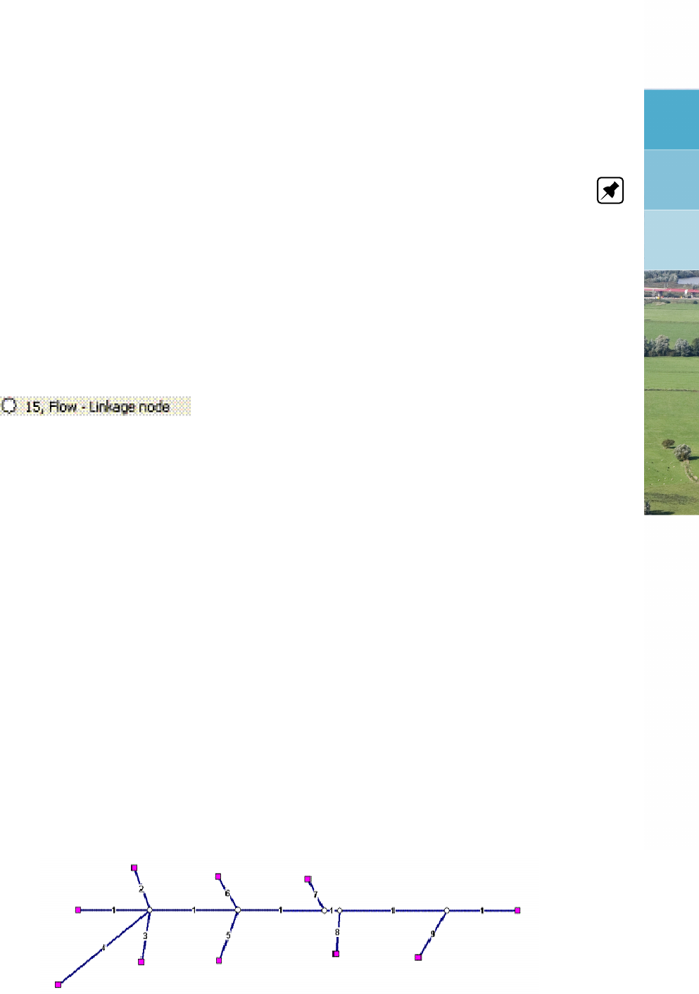
DRAFT
C Deprecated functionality
C.1 Linkage node
Note: The Flow - Linkage node is considered deprecated functionality. It is currently only
available for the purpose of backward compatibility. In SOBEK versions 2.12.004 and up-
wards, it is possible to add interpolation of Flow - Cross Section data between branches using
the Flow - Connection node. It is recommended to use this functionality rather than the Flow
- Linkage node.
The Flow -Linkage node is deprecated, see section C.1.2 for information on how to convert
existing linkage nodes in the model to connection nodes.
C.1.1 Flow - Linkage node (deprecated)
Description
In this chapter, the Flow - Linkage node is described.
As described in more detail below, the Flow - Linkage node was intended to easily add and
remove small tributaries to a parent river. Thus, the use of this node was limited to situations
where inflows have discharges of at least an order of magnitude lower than the parent river.
Please note that the Flow - Linkage Node option was not designed for modelling bifurcations.
For a detailed description of this node’s possible network configurations: see the "Flow -
Linkage node topology" section from the Reference Manual
This type of node is a combination of a normal Flow - Connection node and a Flow - calculation
point node. It has the following features:
The linkage node it does not change if you use the option <Set calculation grid branch>.
The location is fixed.
The linkage node can be used as start or end node (like a normal connection node) for
other branches.
It is very useful to have the main river as one long branch and to make the tributary rivers
confluencing with linkage nodes. See the picture below, with the branch IDs displayed. Branch
1 is the main river, while all other branches are confluences of other rivers (the inflows have
discharges of at least an order of magnitude lower than the parent river).
Figure C.1: River confluences with linkage nodes
The advantage of this method above using normal connection nodes for all the confluences is
Deltares 715 of 900
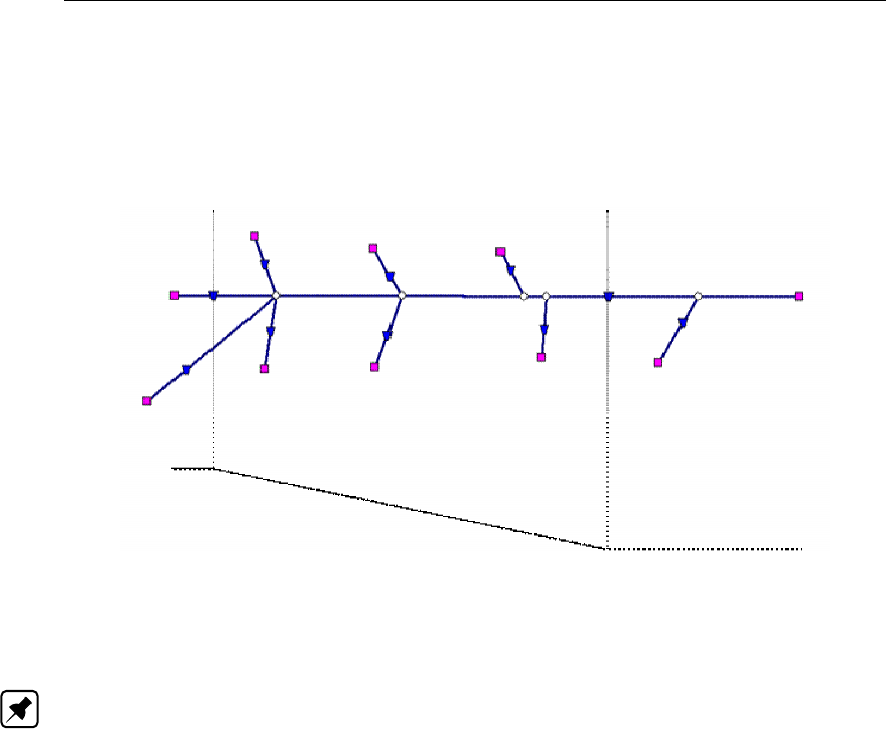
DRAFT
SOBEK, User Manual
that the interpolation of cross-sectional data interpolation over the main river always continues.
This is shown in the picture below. Although there are only two profile nodes at the main
branch, the interpolation is done like there are no confluences. By using normal connection
nodes for the confluences the interpolation only can be forced by added profile nodes with a
definition that should be interpolated by the modeller.
Figure C.2: River confluences for linkage nodes showing interpolation over linkage node
for main channel
Topology
Note: The Flow - Linkage node is considered deprecated functionality. It is currently only
available for the purpose of backward compatibility. In SOBEK versions 2.12.004 and up-
wards, it is possible to add interpolation of Flow - Cross Section data between branches using
the Flow - Connection node. It is recommended to use this functionality rather than the Flow
- Linkage node.
As described in more detail below, the Flow - Linkage node was intended to easily add and
remove small tributaries to a parent river. Thus, the use of this node was limited to situations
where inflows have discharges of at least an order of magnitude lower than the parent river.
Please note that the Flow - Linkage Node option was not designed for modelling bifurcations.
The modeller can easily connect new branches to Linkage nodes. This works similar to normal
connection nodes.
There is an extra functionality to join existing branches together as one branch, where the
existing connection nodes are replaced by linkage nodes. This operation is very useful as
many river systems are imported from GIS files, where each river section is defined as a
single branch. By using the <join branches>edit action, it is possible to join all these single
branches to one branch.
To make this option working correctly, it is required to have the option <Allow Edit for selected
objects>enabled.
716 of 900 Deltares

DRAFT
Deprecated functionality
Figure C.3: Check mark Allow Edit for selected objects
Furthermore, the active node type should be the Flow - Linkage node.
Figure C.4: Select Flow - Linkage node
The next step is to select the branches you want to join. This selection should include the
connection nodes.
Deltares 717 of 900
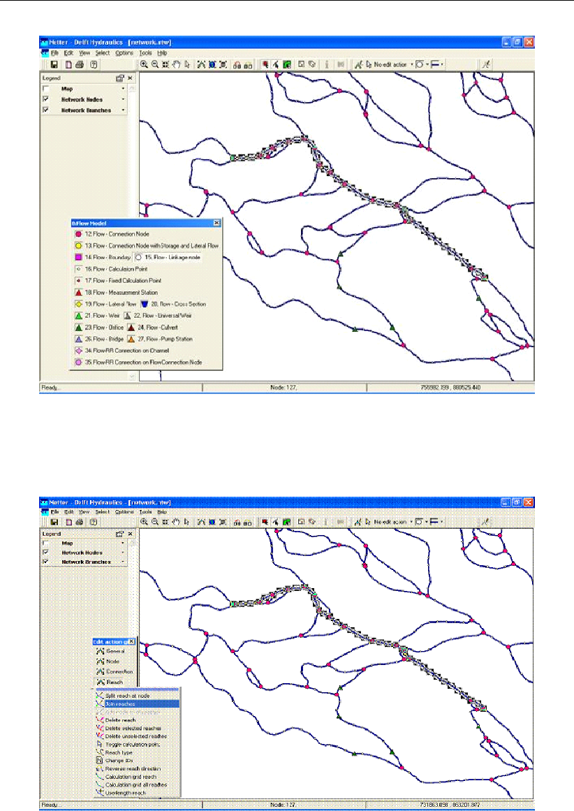
DRAFT
SOBEK, User Manual
Figure C.5: Select branch to join
Now you have to select the action <Join branches>.
Figure C.6: Select action <Join branches>
You will be asked by the editor if you are sure. If so, you press Yes and the join operation will
be performed.
718 of 900 Deltares
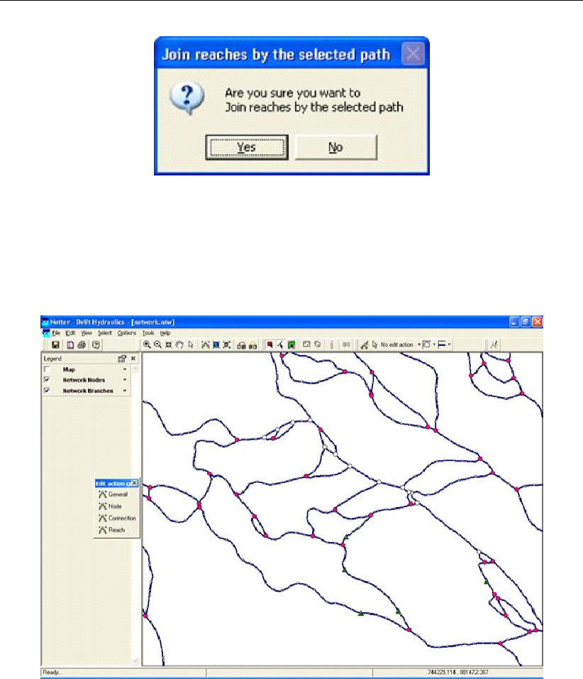
DRAFT
Deprecated functionality
Figure C.7: Join branches by the selectd path window
The existing connection nodes will be replaced by linkage nodes. Notice that also boundary
nodes or flow connection nodes with lateral flow and storage will be replaced if they are in the
selected path. You will lose the boundary, storage and/or flow definitions in that case.
Figure C.8: Existing node is replaced by Linkage Node
C.1.2 How to replace linkage nodes with connection nodes
This short tutorial will show you how to replace Flow - Linkage Nodes with Flow - Connection
Nodes and how to enable interpolation of bathymetry data over a Flow - Connection Node.
This tutorial is different from the other tutorials in that it is intended for users with existing
SOBEK models containing linkage nodes. Linkage nodes are considered deprecated (aban-
doned) functionality and should not be used. For more information about linkage nodes, and
why they were abandoned, see: Linkage node.
If you do not have any models with linkage nodes, this tutorial can be safely skipped as it does
not provide any essential information not already covered by other tutorials.
Start SOBEK.
Click on the Open Project button.
Select a project containing a linkage node you wish to replace.
Open the case you want to edit.
Deltares 719 of 900
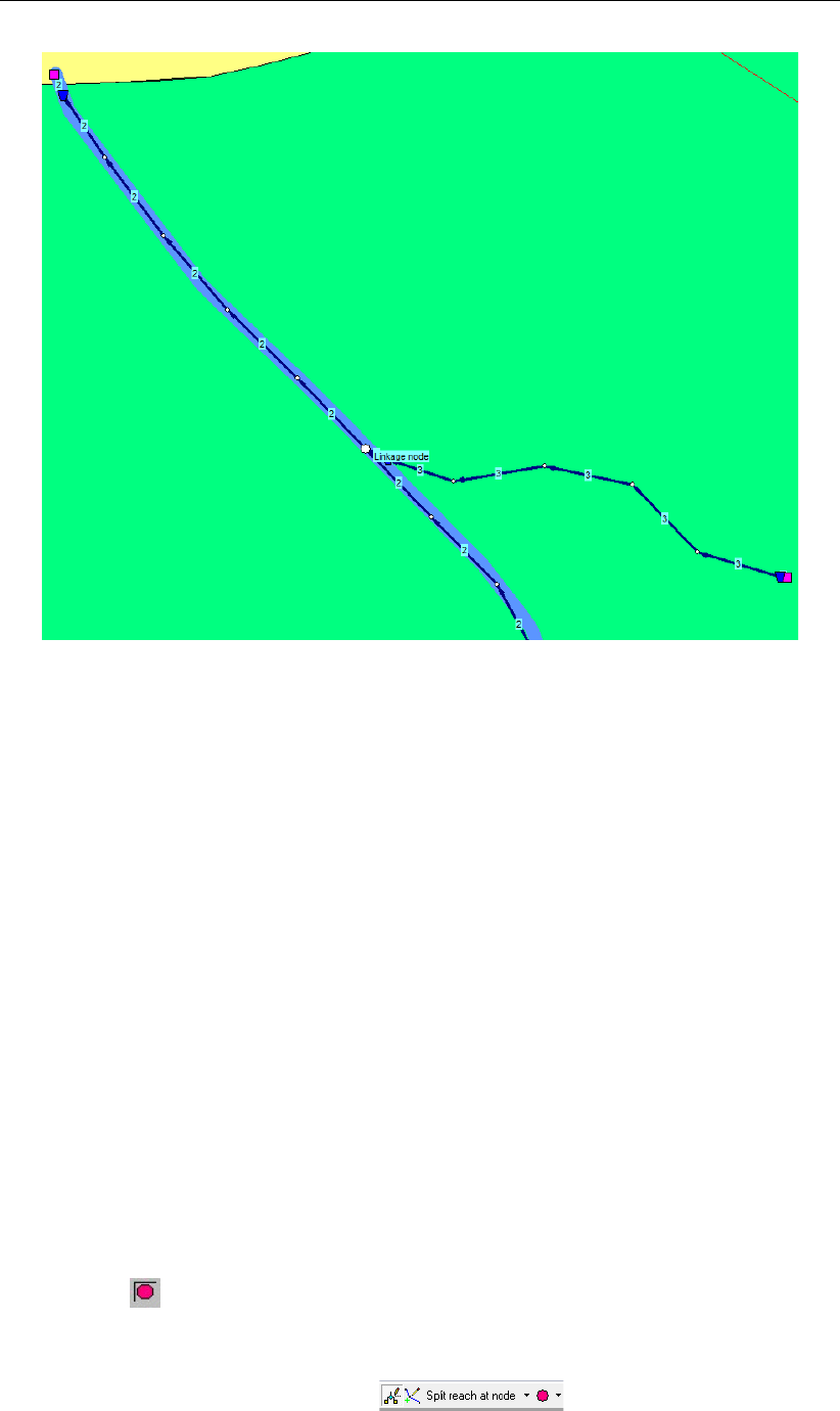
DRAFT
SOBEK, User Manual
Figure C.9: A schematisation with a Flow - Linkage Node.
Double click the ’Schematisation’ task block.
Click on the Edit Model button.
Your schematisation with a linkage node might look something like Figure C.9.
In the example shown in the screenshot, branch IDs have been visualised. This can be very
useful when editing the model as described below. It is possible to visualise branch IDs by
following these steps:
Select ’Options’ - ’Network Data...’.
On the tab ’Link’, select the radio button Branch.
Click on OK.
In the screenshot of our example, you can see two branches in the schematisation. Branch 2
is the main branch, and branch 3 is the tributary.
First we will change the linkage node into a Connection Node. By definition a connection node
is the start or end of a branch. So before we can place the connection node, it is necessary
to split the two branches into three branches:
Select the Edit Network button.
Select the node, Flow-Connection Node.
Select the button Split branch at node in the ’Branch’ toolbar.
Now your button bar should look like this:
Finally, left-click on the Flow - Linkage Node.
720 of 900 Deltares
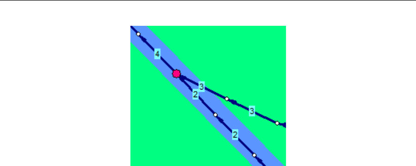
DRAFT
Deprecated functionality
Figure C.10: Example schematisation after the linkage node has been replaced by a con-
nection node.
The linkage has now been replaced by a connection node. In the example, the northern part
of the main branch has now become branch 4. See Figure C.10.
Now all that is left is to define between which branches we want to interpolate bathymetry
data.
Select the connection node.
Click on your right mouse button and select ’Model data’ - ’Flow Model’.
Turn on the option ’Interpolate Cross-section Bathymetry (only) over node’.
Click on the listbox next to First Branch and select branch: ’2’.
Click on the listbox next to Second Branch and select branch: ’4’.
See Figure C.11 for a filled in example using the above data.
Finally, click on OK.
Deltares 721 of 900
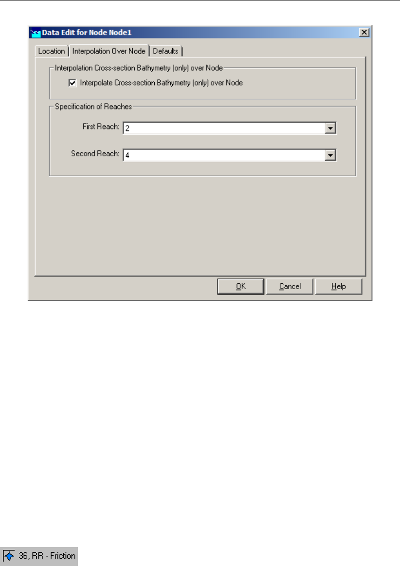
DRAFT
SOBEK, User Manual
Figure C.11: The filled in Data Edit screen for the example connection node.
Using this method, linkage nodes can be replaced by connection nodes. In the above exam-
ple, the Cross-section Bathymetry data is interpolated between branch 2 and branch 4.
Please note that every branch in SOBEK should contain at least one Cross-Section node.
Depending on the schematisation performing the above steps might therefore require the
user to add an extra cross-section after replacing the linkage node with a connection node.
Don’t forget to save your network before leaving NETTER.
For more information about connection node interpolation, see also: Flow - Connection node.
C.2 Rainfall Runoff Friction
C.2.1 Flow - RR-Friction (deprecated)
Friction node description
The RR Friction node creates a water level difference between two nodes that calculate open
water levels. The Friction node is designed to simulate the backwater effects of a narrow
channel with certain length, friction and bank slopes.
722 of 900 Deltares
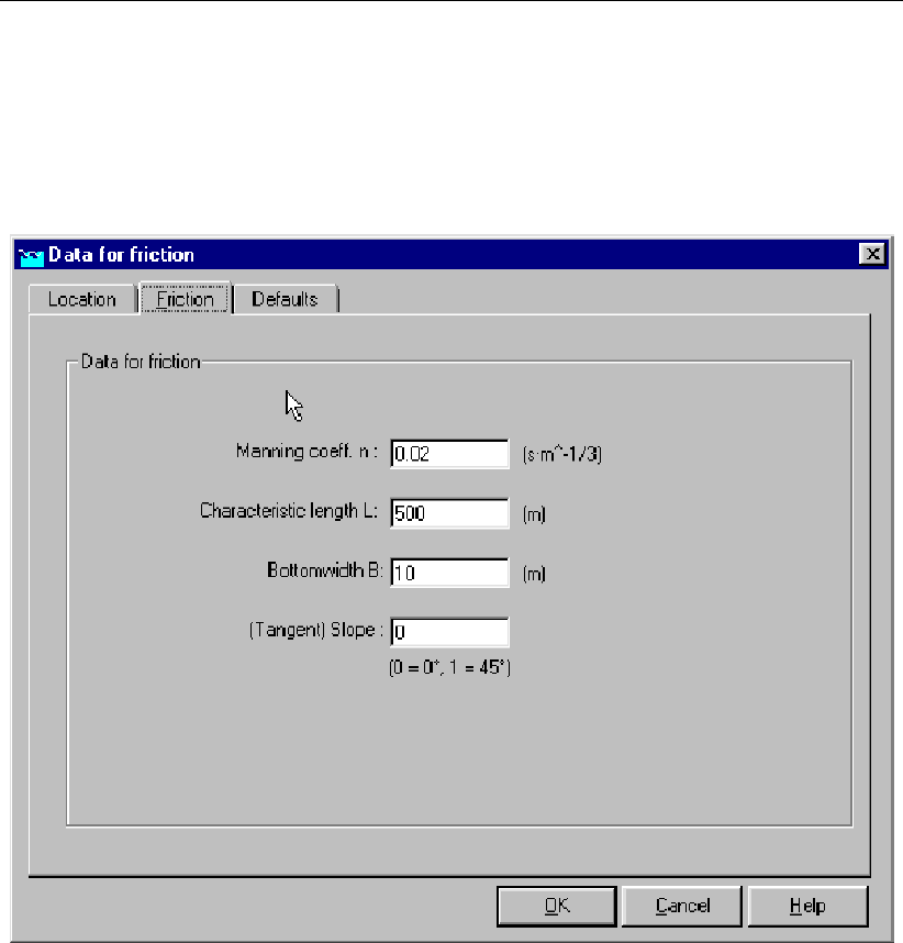
DRAFT
Deprecated functionality
Friction node input screens
When starting the model data editor for an RR Friction node type, the following tab will be
available for input:
Friction tab:
Figure C.12: Data for friction, the friction tab
The following parameters should be entered here:
Manning coefficient n:The hydraulic friction of the channel that the friction node repre-
sents
Characteristic length L:The length of the channel that the friction node represents
Bottom width B:The bed width of the channel that the friction node represents
Slope: The tangent of the channel bank sides slope. (Not the slope of the channel bed
itself!) 0 means that the banks are vertical. 1 means that the banks have a 45 degree
slope.
See also:
The Friction chapter from the RR Technical Reference Manual
Deltares 723 of 900
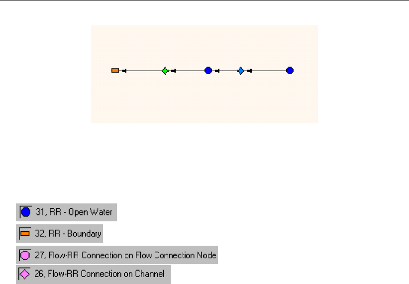
DRAFT
SOBEK, User Manual
Figure C.13: Connecting two RR open water nodes through an RR friction node
Friction node connections
The RR Friction should always interconnect two of the following nodes:
RR Open Water nodes:
RR boundary nodes:
CF RR on Flow connection nodes:
CF RR on channel connections:
RR Friction nodes can be used to connect two RR Open water nodes (i.e. in polder systems):
But they can also be used to connect an RR Open Water node to a Channel Flow connection
(i.e. in areas discharged by gravity where the second order water courses are modelled in an
RR open water node, and the first order water courses are modelled in the SOBEK Channel
Flow module).
724 of 900 Deltares
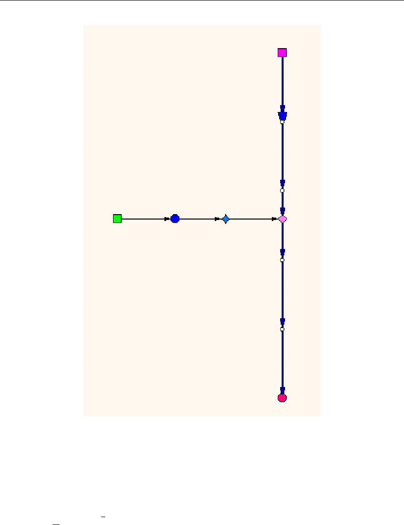
DRAFT
Deprecated functionality
Figure C.14: Connecting an RR Open Water node to a Channel via an RR Friction node.
C.2.2 RR Friction node (deprecated)
A friction node can be put between two open water nodes to account for a significant hydraulic
gradient. The discharge equation reads:
Q=1
nAR2/3√i(C.1)
QDischarge [m3/s]
nManning coefficient [s/m1/3]
AWetted area [m2]
RHydraulic radius [m]
iAverage hydraulic gradient [m/m]
The wetted area is calculated by
A=DW (C.2)
AWetted area [m2]
DAverage depth [m]
WAverage width [m]
Deltares 725 of 900
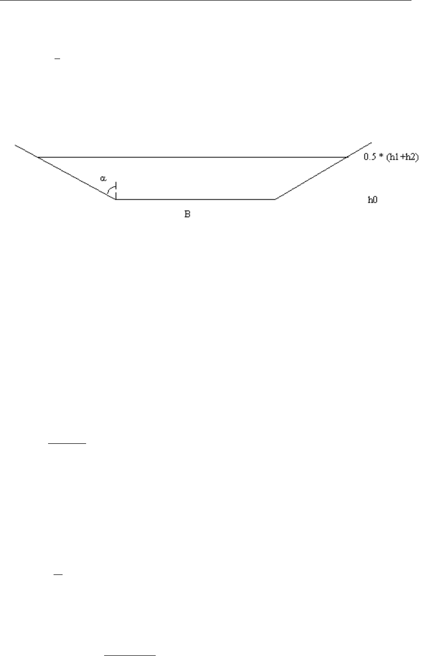
DRAFT
SOBEK, User Manual
D=1
2(h1−h2)−h0(C.3)
h1Upstream water level [m wrt reference level]
h2Downstream water level [m wrt reference level]
h0Bed level [m wrt reference level]
Figure C.15: Explanation of symbols for calculating the wetted area
When the friction node is put in between two RR-open water nodes, the bottom level h0is
computed as the average of the bottom level of both open water nodes. When the friction
node is put in between a RR-open water node and a RR- boundary node, the bottom level h0
is set equal to the bottom level of the open water node.
The average width is calculated by
W=B+ tan(α)D(C.4)
BBottom width [m]
The hydraulic gradient is calculated by
i=h1−h2
L(C.5)
ihydraulic gradient [m/m]
h1Upstream water level [m wrt reference level]
h2Downstream water level [m wrt reference level]
LCharacteristic length of water course [m]
The hydraulic radius Ris defined as the wetted area of the cross section divided by the wetted
perimeter.
R=A
P(C.6)
AWetted area [m2]
PWetted perimeter [m]
The wetted perimeter P is calculated by
P=B+ 2Dp1 + tan2α(C.7)
BBottom width [m]
DAverage depth [m]
αangle of the side slope with vertical
726 of 900 Deltares

DRAFT
D SOBEK input file formats
D.1 SOBEK Input file formats: the Model Database 4.00
D.1.1 Philosophy behind the Model Database
The combination of all SOBEK input files is called the Model Database.
The Model Database consists of a number of ASCII-files, which are logically separated into a
number of layers; each layer covers a number of files. Each file contains the definition of one
or more SOBEK-objects. In most cases the object has an attribute id which is the key to that
particular object.
For more information on the layers, see the chapter Subdivision into layers Database
For more information on the design conventions, see the chapter Input conventions
For exact description of certain input files, see the chapter of the module that has your
interest:
For the modules Channel Flow, River Flow and Sewer Flow: chapter 1DFLOW and Over-
land Flow(2D)
For the modules Rainfall-Runoff: chapter RR (Rainfall Runoff)
For the module Real Time Control: chapter RTC (Real Time control)
D.2 Structure of the Model Database: subdivision into layers
The following layers are distinguished in SOBEK:
1 Topography (TP)
2 Cross section (CR)
3 Structure (ST)
4 Friction (FR)
5 Condition (CN)
6 Initial conditions (IN)
7 Meteo (MT)
8 Dispersion (salt) (D)
9 Grid (GR)
10 Run time data (RT)
11 Transport (TR)
12 Substance (SB)
13 Measurements (ME)(cannot be edited by user)
In SOBEK, a distinction has been made between the objects as defined in the topography
layer and the necessary data for these objects. Most of the objects in the topography layer
are connected to the data objects via a so-called ’carrier id’.
There are two exceptions on this rule:
the data from the run-time layer (layer 10) and
the substances (layer 12)
Both of these data objects are not directly connected to an object from the topography layer.
The data in every other layer is either specified for a specific location or as a ’global definition’.
Each layer consists of one or more files, each containing data stored in records. These
records always start with a specific keyword in CAPITALS, and end with the same keyword in
Deltares 727 of 900

DRAFT
SOBEK, User Manual
lower-case.
The following list gives an overview of the different layers and their files. It should be noted
that not all files are necessary. For example, salt-related files are not necessary when the
salt module is not used. The file containing the file names has a standard Windows-INI file
structure. This means that the keywords are fixed and the file names behind the ’=’ can be
chosen freely. Within a layer the keywords should be unique.
[SOBEK ASCII Layer definition]
Version=2.01
[General]
SettingsFile=settings.dat
[Topography layer]
ntw=network.ntw
net=network.tp
cpt=network.cp
dat=nodes.dat
xyc=network.d12
[Cross Section layer]
net=network.cr
def=profile.def
dat=profile.dat
[Structure layer]
net=network.st
def=struct.def
dat=struct.dat
con=control.def
trg=trigger.def
cmp=struct.cmp
vlv=valve.tab
dbs=struct.def
[Friction layer]
bed=friction.dat
glf=friction.dat
exr=friction.dat
wnd=friction.dat
[Grid layer]
net=network.gr
[Condition layer]
net=network.cn
flb=boundary.dat
fll=lateral.dat
sab=boundary.sal
sal=lateral.sal
fbd=boundlat.dat
[Initial Conditions layer]
igl=initial.dat
ifl=initial.dat
isa=initial.sal
[Runtime Data layer]
flt=..\work\runtime.dat
fln=..\work\runtime.dat
flm=..\work\runtime.dat
flh=..\work\runtime.dat
san=..\work\runtime.dat
728 of 900 Deltares

DRAFT
SOBEK input file formats
sam=..\work\runtime.dat
sah=..\work\runtime.dat
inc=incclass.dat
net=network.me
[Meteo layer]
wnd=wind.#
bui=event.#
wlc=wnd_loc.dat
[Dispersion layer]
gld=globdisp.dat
lod=lokdisp.dat
fwt=freshwat.dat
mou=mouth.dat
brm=brmouth.dat
D.3 1DFLOW and Overland Flow(2D)
D.3.1 General principles of the model database
The SOBEK model database contains a number of ASCII-files. The database is logically
separated into a number of layers; each layer consists of a number of files. Each file contains
the definition of one or more SOBEK-objects. In most cases the object has an attribute id
which is the key to that particular object.
The following layers are distinguished in SOBEK:
Global definitions
Topography (TP)
Cross section (CR)
Structure (ST)
Friction (FR)
Condition (CN)
Initial conditions (IN)
Meteo (MT)
Dispersion (salt) (D)
Grid (GR)
Run time data (RT)
Transport (TR)
Substance (SB)
Measurements (ME) (cannot be edited by user)
In SOBEK, a distinction has been made between the objects as defined in the topography
layer and the necessary data for these objects. Most of the objects in the topography layer
are connected to the data objects via a so-called ’carrier id’.
There are two exceptions on this rule:
the data from the run-time layer (layer 10) and
the substances (layer 12)
Both of these data objects are not directly connected to an object from the topography layer.
The data in every other layer is either specified for a specific location or as a ’global definition’.
Each layer consists of one or more files, each containing data stored in records. These
Deltares 729 of 900

DRAFT
SOBEK, User Manual
records always start with a specific keyword in CAPITALS, and end with the same keyword in
lower-case.
The following list gives an overview of the different layers and their files. It should be noted
that not all files are necessary. For example, salt-related files are not necessary when the
salt module is not used. The file containing the file names has a standard Windows-INI file
structure. This means that the keywords are fixed and the file names behind the ’=’ can be
chosen freely. Within a layer the keywords should be unique.
[SOBEK ASCII Layer definition]
Version=2.01
[Global model] Rivers only
NrOfFiles=1
glb=defglb.1
[Topography layer]
NrOfFiles=7
ntw=network.ntw
net=network.tp
cpt=network.cp
nfl=network.fl
nsa=network.sa
nsm=network.sm
dat=nodes.dat
[Cross section layer]
NrOfFiles=3
net=network.cr
def=profile.def
dat=profile.dat
[Structure layer]
NrOfFiles=9
net=network.st
def=struct.def
dat=struct.dat
con=control.def
trg=trigger.def
sal=struct.sa
cmp=struct.cmp
cms=structcmp.sa
dbs=struct dbs
[Friction layer]
NrOfFiles=4
bed=bedfric.dat
wnd=windfric.dat
exr=exresist.dat
glf=globfric.dat
[Condition layer]
NrOfFiles=10
net=network.cn
flb=boundfl.dat
fll=laterfl.dat
wqb=boundwq.dat
wql=laterwq.dat
sab=boundsa.dat
sal=latersa.dat
mob=boundmo.dat
mon=nodesmo.dat
mol=latermo.dat
[Initial Conditions layer]
NrOfFiles=5
igl=incondgl.dat
ifl=incondfl.dat
iwq=incondwq.dat
isa=incondsa.dat
imo=incondmo.dat
730 of 900 Deltares

DRAFT
SOBEK input file formats
[Meteo layer]
NrOfFiles=4
wnd=wind.mt
sun-sunshine.mt
wat=wattemp.mt
air=airtemp.mt
[Dispersion layer]
NrOfFiles=5
gld=globdisp.dat
lod=lokdisp.dat
fwt=freshwat.dat
mou=mouth.dat
brm=brmouth.dat
[Grid layer]
NrOfFiles=3
net=grid.tp
seg=wqsegm.tp
lim=segmlm.tp
[Runtime Data layer]
NrOfFiles=18
flt=flowtim.dat
fln=flownum.dat
flm=flowmap.dat
flh=flowhis.dat
san=saltnum.dat
sam=saltmap.dat
sah=salthis.dat
sen=sednum.dat
sem=sedmap.dat
seh=sedhis.dat
mon=mornum.dat
mom=mormap.dat
moh=morhis.dat
wqt=wqtim.dat
wqn=wqnum.dat
wqm=wqmap.dat
wqh=wqhis.dat
pwq=prepwq.dat
[Transport layer]
NrOfFiles=1
dat=transprt.dat
[Substance layer]
NrOfFiles=1
sub=substanc.def
D.3.2 Global definitions file
This file is only present in case of SOBEK-River. An example of this file is as follows:
ca 0
APAC fl sd mp apac
mv 0
LRVD tp cr st cn in fr rt ds tr mt sb gr lrvd
LMTS xi 0.00 xa 150000.00 yi 0.00 ya 150000.00 lmts
rh 0
Only the first 2 record are used by the Parser
record 1:
ca area code: 0 = river 1 = estuary
Deltares 731 of 900

DRAFT
SOBEK, User Manual
record 2 (APAC):
APAC fl sd mp ..apac
This record contains the module identifiers. If an identifier is present the corresponding mod-
ule will be activated. The identifiers are:
fl flow module
sl salt module
sd sediment module
mp morphology
m2 2D-morphology
pq make water quality aggregation file
wq water quality module
mz Mozart coupling
record 3:
mv validation flag (1=model has been validated) (only for UI)
record 4 (LRVD):
Contains layer information (only for UI)
record 5 (LMTS):
Contains the dimensions of the area of the model (only for UI)
record 6:
rh refence level (only for UI)
D.4 2D Grid layer
Files in this layer
[2D grid layer]
NrOfFiles=1
net=..\work\network.d12
D.4.1 net-file (2D Grid layer)
This file describes the basic definition of 2D Grid [s] and the definitions of 1D Nodes (points)
or 1D branches (lines) lying within the 2D Grid. This also holds for 2D Points (Boundary
condition, Initial condition, Dam break structure) and 2D Line (combination of more than one
Boundary node)
DOMN id ’Example Sobek-FLS, Use New’ nm ’Example Sobek-FLS, Use New’
GFLS nc 61 nr 92 x0 101950 y0 463350 dx 100 dy 100 cp 0 fnm ” gfls
ISCHILDOF ci ’parent’
CHILDBLOCK ltX 124100 ltY 437400 rbX 126200 rbY 435800 ltC 11 ltR 1 rbC 32 rbR 17
childblock
PARENTBLOCK ltC 1 ltR 11 rbC 22 rbR 27 parentblock
ischildof
PT12 id ’92.31’ nm ’92.31’ ci ” lc 0 px 104994.2 py 454294.2 mc 31 mr 91 pt12
732 of 900 Deltares

DRAFT
SOBEK input file formats
PT12 id ’2_1’ nm ’2_1’ ci ’2’ lc 300.9696 px 104994.9 py 454595.1 mc 31 mr 88 pt12
LI12 id ’1’ nm ’1’ ci ” lc 0 bx 105683.4 by 454213.5 ex 107991.5 ey 454213.5 bc 38 br 92 ec
61 er 92 li12
LI12 id ’l_bound’ nm ’bound’ ci ” lc 0 bx 257778.51 by 585767.76 ex 257774.22 ey 584358.75
bc7br3ec7er17
TBLE cells 15
’7’ ’3’ <
..
’7’ ’17’ <
tble
li12
LM12 id ’l_meetraai’ nm ’meetraai’ ci ” lc 0 bx 257778.51 by 585767.76 ex 257774.22 ey
584358.75 bc 7 br 3 ec 7 er 17
TBLE cells 15
’7’ ’3’ <
..
’7’ ’17’ <
tble
TBLE crossings
PTCR cb ’10_7’ ci ’5’ lc 607.94 px 257776.34 py 585056.86 mc 7 mr 10 ptcr
tble
lm12
domn
where:
id 2D grid id
nm 2D grid name
GFLS...gfls = 2D grid definition
where:
nc number of column (m) in X direction
nr number of rows (n) in Y direction
x0 X coordinate
y0 Y coordinate
dx distance between two grid points in X directions (m)
dy distance between two grid points in Y directions (n)
cp 0 = 0 leftTop Corner (if grid definition file is *.dem, *.bil)
= 3 leftBottom Centre (if grid definition file is ARC-INFO *.asc)
fnm name of grid definition file (for example *.dem, *.asc etc.)
ISCHILDOF .. ischildof = definition of child-parent relation in case of multiple domain
where:
ci identification of Parent domain
CHILDBLOCK .. childblock = definition of rectangular within Parent domain by the child do-
main.
where:
ltX left top X coordinate (center of child 2D grid cell)
ltY left top Y coordinate (center of child 2D grid cell)
Deltares 733 of 900

DRAFT
SOBEK, User Manual
rbX right bottom X coordinate (center of child 2D grid cell)
rbY right bottom Y coordinate (center of child 2D grid cell)
ltC Left Column number of Parent domain cut by Child domain
ltR Right Column number of Parent domain cut by Child domain
rbC RightColumn number of Parent domain cut by Child domain
rbR Right Column number of Parent domain cut by Child domain
PARENTBLOCK .. parentblock = definition of rectangular within Child domain by the Parent
domain.
where:
ltC Left Column number of Child domain cut by Parent domain
ltR Right Column number of Child domain cut by Parent domain
rbC RightColumn number of Child domain cut by Parent domain
rbR Right Column number of Child domain cut by Parent domain
PT12 .. pt12 = definition of 1D and 2D Nodes (Points) lying within 2D grid
where:
id point object id
nm point object name
ci branch id (carrier id)
lc position relative to the branch origin (always 0)
px X-coordinate
py Y-coordinate
mc column position within 2D grid (m) in X direction
mr row position within 2D grid (n) in Y direction
LI12 .. li12 = definition of 2D Boundary Line or 1D2D Internal Boundary Line (lying within 2D
Grid)
where:
id line object id
nm line object name
ci ”
lc 0
bx begin X-coordinate
by begin Y-coordinate
ex end X-coordinate
ey end Y-coordinate
bc begin column position within 2D grid (m) in X direction
br begin row position within 2D grid (n) in Y direction
ec end column position within 2D grid (m) in X direction
er end row position within 2D grid (n) in Y direction
LM12 .. lm12 = definition of 2D Measurement Line (meetraai)
where:
id line object id
nm line object name
ci ”
lc 0
734 of 900 Deltares

DRAFT
SOBEK input file formats
bx begin X-coordinate
by begin Y-coordinate
ex end X-coordinate
ey end Y-coordinate
bc begin column position within 2D grid (m) in X direction
br begin row position within 2D grid (n) in Y direction
ec end column position within 2D grid (m) in X direction
er end row position within 2D grid (n) in Y direction
TBLE cells ncells tble = table of 2D grid cells and ncells is number of cells in table
TBLE crossings .. tble = table of 1D Channel/pipe crossing the 2D Measurement Line
PTCR .. ptcr = definition of 1D channel/pipe crossing the 2D Measurement Line
where:
cb id of the branch
ci if of the branch
lc location on branch from beginning point
mc column position within 2D grid (m) in X direction.
mr row position within 2D grid (n) in Y direction.
px X-coordinate of 2D grid point
py Y-coordinate of 2D grid point
D.5 Condition layer
This layer contains data for boundary conditions and lateral discharges.
Files in this layer
[Condition layer]
NrOfFiles=10
net=network.cn
flb=boundfl.dat
fll=laterfl.dat
wqb=boundwq.dat
wql=laterwq.dat
sab=boundsa.dat
sal=latersa.dat
mob=boundmo.dat
mon=nodesmo.dat
mol=latermo.dat
D.5.1 flb-file (condition layer)
This file contains de boundary conditions for the FLOW modules.
For Channel Flow, Sewer Flow and River Flow:
FLBO id ’1’ st 0 ty 0 h_ wd 0 1.2 0 flbo (constant H)
or
FLBO id ’1’ st 1 ty 0 q_ wd 0 1.2 0 flbo (constant Q)
or (variable discharge)
FLBO id ’1’ st 0 ty 1 q_ dt 1 TBLE .. tble flbo (variable Q)
or
FLBO id ’1’ st 0 ty 1 h_ dt 1 TBLE .. tble flbo (variable H)
or (Fourier boundary)
Deltares 735 of 900

DRAFT
SOBEK, User Manual
FLBO id ’1’ st 1 ty 1 q_ df 2 TBLE .. tble h0 0.5 w0 0.1 flbo
or (tidal boundary)
FLBO id ’1’ st 1 ty 1 q_ di 2 TBLE .. tble h0 0.5 flbo
or tables library
FLBO id ’TH5’ st 0 ty 0 h_ wt 11 ’TH5’ flbo
where:
id id
st storage on boundary node (storage only possible in case of SOBEK Urban)
0 = no storage
1 = storage
ty type boundary 0 = water level 1 = discharge
h_ wd 0 constant water level (only for ty 0)
h_ wt 1 variable water level as a function of time (TBLE ... tble)
h_ wt 11 use table from table library
h_ wf 2 only in SOBEK River: Fourier boundary for water level
h_ wi 3 only in SOBEK River: tidal boundary for water level
h_ wd 1 h_ wd 4
h_ wd 4 water level as a function of Q column 1 = Q column 2 = h
q_ dw 0 constant discharge
q_ dw 1 q_ dw 4
q_ dt 1 variable discharge as function of time (TBLE ... tble)
q_ df 2 SOBEK Estuarium model: Fourier boundary.
table with amplitude, phase
q_ di 3 SOBEK Estuarium model: tidal boundary
table with amplitude, frequency, phase.
q_ dw 4 Q = Q(H) according to Q-H table
column 1 = h
column 2 = Q
a0 only for Fourier and tidal boundary
w0 only for Fourier optie w0
Note: h_ wd 1, h_wd 4, q_ dw 1 and q_ dw 4 are handled by the Parser in the same manner.
For Overland Flow:
1D2DInternal Boundary Line:
D2LI id ’bound’ nm ’1D2D Internal Boundary Line’ ty 4 cp ’20’ d2li
2D Boundary Node:
D2PT id ’bound’ nm ’Boundary Node’ ty 0 h_wd 0 10.0 d2pt
2D Boundary Line:
D2LI id ’bound’ nm ’Boundary Line’ ty 1 q_ dw 0 0.5 d2li
where:
id identification
736 of 900 Deltares

DRAFT
SOBEK input file formats
ty boundary type
0 = water level
1 = flow/Flux
2 = velocity
4 = 1D2D Boundary Line.
h_ wd 0 10.0 constant water level; only for ty 0
h_ wd 1 water level as a function of Q *** not implemented yet
column 1 = discharge Q [m3/s]
column 2 = water level h [m w.r.t. reference level]
note: only for ty 0
h_ wt 1 variable water level as a function of time (TBLE ... tble)
column 1= time in hours from start of simulation
column 2 = water level h [m w.r.t. reference level]
note: only for ty 0.
q_ dw 0 0.5 = constant discharge [m3/s];
note: only for ty 1
q_ dw 1 Q=Q(H) according to Q-H table
column 1 = water level h [m w.r.t. reference level]
column 2 = discharge Q [m3/s]
note: only for ty 1
q_ dt 1 = variable discharge as a function of time (TBLE ... tble)
column 1 = time in hours from start of simulation
column 2 = discharge Q [m3/s]
note: only for ty 1
u_st 1 = velocity as a function of time (TBLE ... tble)
column 1 = time in hours from start of simulation
column 2 = velocity [m/s]
note: only for ty 2
cp identification of the connected 1D2D Internal Boundary Node (node only avail-
able in Channel Flow)
BTBL id ’TH5’ ty 0 h_ wt PDIN 0 0 pdin
TBLE
’2001/01/01;00:00:00’ .33
’2001/01/01;01:00:00’ .64
’2001/01/01;02:00:00’ .83
’2001/01/01;03:00:00’ .81
’2001/12/31;20:00:00’ -.3
’2001/12/31;21:00:00’ .27
’2001/12/31;22:00:00’ .8
’2001/12/31;23:00:00’ 1.1
tble btbl
BTBL id ’107’ sc 0 lt 0 PDIN 1 0 pdin
TBLE
’1990/01/01;00:00:00’ 2102.4
’1990/01/02;00:00:00’ 1716
’1990/01/03;00:00:00’ 1954.3
’1990/01/04;00:00:00’ 1734.9
’1990/09/26;00:00:00’ 112.8
’1990/09/27;00:00:00’ 130.24
’1990/09/28;00:00:00’ 216.23
Deltares 737 of 900

DRAFT
SOBEK, User Manual
’1990/09/29;00:00:00’ 152.37
’1990/09/30;00:00:00’ 99.31
tble btbl
D.5.2 fll-file (condition layer)
This file contains the lateral discharges on nodes/branches for the FLOW module.
Lateral discharge on branch:
FLBR id ’3’ sc 0 lt 0 dc lt 0 ir 0 ms ’station 1’ ii 0.005 ar 600000 flbr
or
FLBR id ’Intensity from Meteostation’ sc 0 lt 0 dc lt 7 ir 0.003 ms ’meteostation’ ii 0.002 ar
1000 flbr
or
FLBR id ’Constant intensity’ sc 0 lt 0 dc lt 6 ir 0.003 ms ’meteostation’ ii 0.002 ar 1000 flbr
or
FLBR id ’1’ ci ’1’ sc 0 lt 0 dc lt 1 0 0TBLE .. tble flbr
or
FLBR id ’11’ sc 0 lt 0 dc lt 0 1 0flbr
or
FLBR id ’107’ sc 0 lt 0 dc lt 11 ’107’ flbr
lateral structures:
FLBR id ’1’ sc 0 lt 0 dc lt 4 0 0 sd ’S1’ wl ow 0 -1 0 flbr
or
FLBR id ’1’ sc 0 lt 0 dc lt 4 0 0 sd ’S1’ wl ow 1 TBLE .. tble flbr
where:
id id
sc section (for 2D morphology !)
0 = left (=main section; default)
1 = right
lt length of discharge
0 = point discharge (m3/s)
>0 = discharge over a certain length (m2/s) (not in SOBEK-Urban/Rural)
-1 = discharge over the entire length of the branch (m3/s) (new in SOBEK
Urban/Rural)
dc lt table:dc lt 0= constant value,
dc lt 1 ’real’ table (first column=time, second column=discharge)
dc lw 2 as a function of the waterlevel (not in SOBEK Urban/Rural)
column 1 = h
column 2 = Q
dc lt 3 linked to another lateral discharge (’2nd station’) (not in SOBEK Urban/Rural)
dc lt 4 indicates lateral structure on a branch
dc lt 5 retention
dc lt 6 rational method with constant intensity
dc lt 7 with intensity from the rainfall station
dc lt 11 from a table library
ir constant intensity (mm/s)
ms meteo-station
738 of 900 Deltares

DRAFT
SOBEK input file formats
ii seepage/infiltration intensity (mm/s)
ar runoff area [m2]
sd id of structure definition (see STRUCT.DEF; only in case dc lt 4)
ci id of second station (only in case of dc lt 3; not in SOBEK Urban/Rural)
wl ow table with water levels outside the lateral structure
wl ow 0 constant as a table,
wl ow 1 ’real’ table
Sobek-lateral discharges on a node (Only for 2D-morphology):
FLND id ’1’ bi ’1’ ’2’ aw dd
TBLE ..
tble
dd
TBLE ..
tble
flnd
where:
bi branch id’s
aw dd alpha w0 as a function of Q
column 1 = table, discharge
column 2 = alpha w
dd alpha w1 as function of Q
column 1 =table, discharge
column 2 = alpha w
Only for SOBEK Urban/Rural
lateral discharge on node:
FLNO id ’1’ dc lt 0 -1.0 0 flno
or lateral structure on node:
FLNO id ’1’ lt 0 dc lt 4 0 0 sd ’S1’ wl ow 1 TBLE .. tble flno
where:
id id
dc lt table with lateral discharge
dc lt 0= constant as table,
dc lt 1= ’real’ table
column 1 = time
column 2 = discharge
dc lt 4= indicates the structure being a lateral structure.
dc lt 5 = retention
sd id of structure description (see STRUCT.DEF)
wl ow table with water levels outside the lateral structure
wl ow 0= constant as table,
wl ow 1= ’real’ table
diffuse lateral discharge on the branch
FLDI id ’15263’ ci ’15263’ sc 0 lt -1 dc lt 0 2 0 fldi
Deltares 739 of 900

DRAFT
SOBEK, User Manual
Where:
id id
ci id of second station
sc 0 lt -1 diffuse
dc lt 0 constant value [m3/s/m]
dc lt 1 = table
dc lt table with lateral discharge
dc lt 0= constant as table,
dc lt 1= ’real’ table
pipes with infiltration (trenches)
TRCH id ’38’ di ’3’ dl 1.05 dh 2.55 rt 22 pt 0.22 oi 2 il 0 pm 1 rg 2222 gl tt 0 1.45 trch
or
TRCH id ’36’ di ’19’ dl 0.1 dh 2 rt 10 pt 0.4 oi 2 il 0 pm 1 rg 1111 gl tt 1 PDIN 0 0 ” pdin
TBLE ’2011/11/29;00:00:00’ 1.11 <
’2011/11/29;01:00:00’ 1.22 <
’2011/11/29;02:00:00’ 1.33 <
’2011/11/29;03:00:00’ 1.44 <
tble trch
Where:
id (branch carrier)ID of Pipe with Infiltration
di ID of cross-section definition for trench (Id of cross-section of pipe is stored as
normal.)
Note: There is no difference in cross section definition of channel or trench or
pipe.
dl Distance invert level, the distance between the invert level of the pipe and the
invert level of the trench.
dh Trench height, if not (properly) specified the surface level is used as top of
trench.
rt Resistance factor pipe-trench
pt Porosity trench
oi option for initial water level trench
0 = Value specified by keyword il (default)
1 = Same as water level pipe
2 = Same as groundwater level
il Initial water level trench (for oi = 0)
pm Permeability of ground/soil
0 = Completely impermeable, no interaction between groundwater and trench
1 = Permeable
rg Resistance factor trench-ground, only relevant when ground is permeable
gl tt groundwater level
0 = Constant groundwater level, only relevant when ground is permeable
1 = Table with groundwater level varying in time
column 1 date/time stamp
column 2 groundwater level
740 of 900 Deltares

DRAFT
SOBEK input file formats
D.5.3 mob-file (condition layer)
This file contains the boundary conditions on nodes for the sediment/ morphology modules.
MPBO id ’1’ cy 1 bl bt 1
TBLE ..
tble
mpbo
where:
id id of the boundary condition
cy condition type
0 = load (as a constant, f(time), of f(Q))
1 = bed level (as a constant, of f(time)
lo load type
lo sd 0 load as constant
lo sd 2 load as function of the discharge Q
column 1 = Q
column 2 = load
column 3 = load right (only when using 2D morphology option)
lo st load as function of time
column 1 = time
column 2 = load
column 3 = load right
bl bt bed level table
bl bt 0 = constant
bl bt 1 = table
column 1 = time
column 2 = bed level
column 3 = bed level right
Note: The field se is generated internally by the user interface. se 0 = no 2D morphology,
se 1 = 2D morphology on next branch. This field is not required.
D.5.4 mol-file (condition layer)
This file contains the descriptions of the lateral discharges of sediment on branches.
MPBR id ’2’ ty 0 le 0 lt dl 0 10.0 mpbr
or
MPBR id ’2’ ty 1 le 0 di ’1’ ct co 0 50.0 mpbr
where:
id id
ty type condition:
1 = concentration
0 = dry load
sc section (only for 2D morphology option)
0 = left (default)
1 = right
le length
Deltares 741 of 900

DRAFT
SOBEK, User Manual
lt dl dry load table (only for ty 1)
lt dl 0 = constant
lt dl 1 = table function
column 1 = time
column 2 = load
di id of accompanying lateral discharge (only for ty 1: concentration)
ct co sediment load table (only for ty 0)
ct co 0 = constant,
ct co 1 = table
column 1 = time
column 2 =sediment load
D.5.5 mon-file (condition layer)
This file contains the description for morphology on nodes. For every node the distribution
of sediment over the different branches needs to be given. When the module Morphology is
used, there is a maximum of three branches for every node. This means that there are three
combinations of two branches related to the node.
MPND id ’0’ ty 0 1 0 aa 9.9999e+009 2 9.9999e+009
ba 9.9999e+009 0 9.9999e+009 rt d0 ’Distribution Ratio’
TBLE
tble
rt d1
TBLE
tble
rt d2 bi ’0’ ’1’ ’2’ se 0 0 0 as m0 as m1 ex 9.9999e+009 9.9999e+009 ds 1 ta 0 mpnd
or
MPND id ’1’ ty 0 0 0 aa 9.9999e+009 9.9999e+009 9.9999e+009
ba 9.9999e+009 9.9999e+009 9.9999e+009 rt d0 rt d1 rt d2 bi ’2’ ’3’ ’4’
se 0 0 0 as m0 as m1 ex 9.9999e+009 9.9999e+009 ds 0 ta 0 mpnd
Where:
id id
ty type distribution per combination of two branches (max. 3 combinations)
0 =proportional (distribution according to the ratio of the discharges)
1 =linear (according to a linear relation)
2 =ratio (distribution according to interpolation relation of ratios of Q and Sedi-
ment load)
aa alfa; only for type 1: linear distribution
ba beta; only for type 1: linear distribution
rt d0 distribution ratio table first couple
rt d1 distribution ratio table second couple
rt d2 distribution ratio table third couple
bi branch id’s of connection branches
as m0=alpha sedredge values for branch-couple 1; only if the 2D-morphology
option is selected.
as m1=alpha sedredge values for branch-couple 2; only if the 2D-morphology
option is selected.
ex exponents of sediment-distribution according to Wang:
1e exponent k for discharges
742 of 900 Deltares

DRAFT
SOBEK input file formats
2e exponent m for widths
ds distribution used for each branch-couple or for all branches attached to the
node:
0 = for all branches attached to the node
1 = for each branch-couple
ta type of distribution in case ds = 0 (all branches of node)
0 = proportional
3 = exponential function according to Wang
Note: The field se is generated internally by the user interface. se 0 = no 2D morphology, se
1 = 2D morphology on next branch. This field is not required.
D.5.6 net-file (condition layer)
This file contains information about the locations in the network for which conditions are de-
fined.
For Channel Flow, Sewer Flow and River Flow:
Locations flow conditions:
FLBO id ’1’ nm ’Bound_cond1’ ci ’4’ flbo Note: Fixed order
FLND id ’2’ nm ’Flowatnode1’ ci ’1’ flnd Note: Fixed order
FLBR id ’1’ nm ’Lateralflow op tak1’ ci ’1’ lc 100. Flbr Note: Fixed order
FLDI id ’1_1’ ci ’15263’ fldi Note: Diffuse lateral discharge whole branch
The following 3 types are only defined in SOBEK Urban/Rural:
FLNO id ’1’ nm ’Lateralflow op knoop1’ ci ’4’ flno
FLNX id ’1’ nm ’External Lateralflow knoop1’ ci ’3’ flnx
FLBX id ’1’ nm ’External Lateralflow op tak1’ ci ’5’ lc 50. flbx
Note: The ’Flow at node’ (FLND) can only be used in the case when 2D-morfology branches
connect to the node.
Locations conditions water quality:
WQBO id ’1’ nm ’ Wqbound1’ ci ’4’ wqbo
WQBR id ’2’ nm ’wq_at_branch’ ci ’5’ lc 300. wqbr
Locations conditions salt:
STBO id ’0’ nm ’Saltbound1’ ci ’4’ stbo
STBR id ’1’ nm ’Salt lat disch’ ci ’3’ lc 50. Stbr
STBR id ‘1’ nm ‘Salt lat conc ci ‘-1’ Stbr
Locations conditions sediment/morphology:
MPBO id ’1’ nm ’Sed_bound’ ci ’0’ mpbo
MPND id ’3’ nm ’Sed_disch_node’ ci ’2’mpnd
MPBR id ’5’ nm ’Sed_disch’ ci ’4’ lc 50. mpbr
where:
Deltares 743 of 900

DRAFT
SOBEK, User Manual
id id of the condition (boundary or lateral discharge)
nm name of the condition
ci carrier id (node id in case of a boundary or node condition, branch id in case of
a branch condition)
lc location (only in combination with a branch-id)
For Overland Flow:
1D2D Internal Boundary Node (node is only available in Channel Flow):
FL2B id ’pnt1D2Dboundary’ ci ’pnt1D2Dboundary’ px 101991.8 py 458610.7 fl2b
2D Boundary Node:
D2PT id ’bound’ nm ” ci ’1’ px 101991.8 py 458610.7 d2pt
2D Boundary Line and 1D2D Internal Boundary Line:
D2LI id ’l_bound’ nm ” ci ’l_bound’ bx 105683.4 by 454213.5 ex 107991.5 ey 454213.5 d2li
where:
id boundary id
nm boundary name
ci 2D grid id
px X coordinate within 2D Grid
py Y coordinate within 2D Grid
bx begin X coordinate within 2D grid for Boundary Line
by begin Y coordinate within 2D grid for Boundary Line
ex end X coordinate within 2D grid for Boundary Line
ey end Y coordinate within 2D grid for Boundary Line
Initial Condition Node:
D2IN id ’1’ ci ’1’ px 101991.8 py 458610.7 d2in
where:
id Initial Condition Node id
ci 2D grid id
px X coordinate within 2D Grid
py Y coordinate within 2D Grid
744 of 900 Deltares

DRAFT
SOBEK input file formats
D.5.7 sab-file (condition layer)
This file contains the boundary conditions for the saltmodule (SA)
STBO id ’1’ ty 1 co co 1
TBLE ..
tble
tl 0 tu 0 stbo
where:
id id
ty type of boundary
1 zero flux
0 concentration
co co concentrations (only for type 0)
co co 0 as constant
co co 1 as table
column 1 time
column 2 concentrations
tl Thatcher-Harleman time lag (only for SOBEK River, concentration boundary)
tu time lag used (only for SOBEK River model, concentration boundary)
D.5.8 sal-file (condition layer)
This file contains the descriptions of the lateral discharges for the saltmodule (SA).
STBR id 0 ty 0 le 100 lo lt 0 10 0 co ct 0
TBLE ..
tble
stbr
STBR id 0 ty 1 le 100 co ct 1
TBLE ..
tble
stbr
where:
id id of the lateral discharge of salt
ty type condition 0 = dry substance 1 = concentration
le length
lo lt load table (for ty 0)
lo lt 0 = constant
lo lt 1 = table as function of time
di id of accompanying lateral discharge (when ty 1: concentration)
co ct concentration table (only for ty 1)
co ct 0 = constant
itemco ct 1 = table as function of the time
Deltares 745 of 900

DRAFT
SOBEK, User Manual
D.5.9 wqb-file (condition layer)
This file contains de boundary conditions for 1DWAQ-module
WQBO id ’1’ ct ct 0 as SLST .. slst wqbo
where:
id id
ct ct concentration type
ct ct 0 constant boundary concentration
ct ct 1 boundary concentration as table function of time:
column 1 time
column 2 values for all substances as function of time
as between keywords SLST and slst a list:
the active substances
type (0=constant, 1=variable)
the value
Note: : If a time-dependant boundary condition is used (ct ct 1) for one substance, it is still
possible to enter constant values for other substances using the keyword as.
Only one timetable can be entered, so when more substances have a time dependant bound-
ary concentration, they should be entered in the same table for every timestep.
Note: The order of the substances after the keyword as SLST slst is identical as the order
in the table with concentrations as a function of time in the field ct ct 1
D.5.10 wql-file (condition layer)
This file contains the 1DWAQ conditions of the lateral discharges
SOBEK River FLBR
FLBR id ’1’ hs flbr
where:
id id lateral discharge
hs has substances
0 no
1 yes
as active substances
Between the keywords SLST slst a list of substances, the type of discharge (0=constant,
1=variable) and the value. A variable concentration is only possible when the flow itself varies.
Note: :Specification of water quality conditions; Keywords FLBR en WQBR
In SOBEK River two keywords are used to specify these conditions, FLBR and WQBR. This
depends on whether the condition is associated with lateral flow or with an input of a dry
substance. It seems logical, however, to switch to the use of only one keyword, WQBR.
746 of 900 Deltares

DRAFT
SOBEK input file formats
D.6 Cross Section layer
Files in this layer
[Cross section layer]
NrOfFiles=3
net=network.cr
def=profile.def
dat=profile.dat
D.6.1 dat-file (cross section layer)
This file contains a reference to the cross-section definition and information about the relative
height of the cross-section.
CRSN id ’crossloc1’ di ’crossdef1’ rl -0.5 ll -0.4 rs 0.9 ls 0.9 crsn
Note: Fixed order
Items in one record; ll, rs and ls optional, separated by 1 or more blanks where:
id id of cross-section location
di id of cross-section definition
rl reference level 1 (SOBEK River/Rural: level at the cross-section; SOBEK Ur-
ban/Rural: level at the end of the pipe)
ll reference level 2 (SOBEK Urban/Rural: level at the beginning of the pipe)
fg specification of flap gate (Pipe Only: 0 = None, 1 = Only Positive Flow, 2 = Only
Negative Flow)
us upstream slope (not in SOBEK Urban/Rural)
ds Downstream slope (not in SOBEK Urban/Rural)
rs Surface level right (same units as rl)
ls Surface level left (same units as rl)
In SOBEK-River a bed-level (code bl) was already given for the cross-section descriptions
(except for the tables, here it is given in the table itself). In addition, a local reference level rl
at the cross-section needs to be given.
In SOBEK Urban/Rural however, it is not possible to give a bed level for every cross-section
description. In this case, the bed level is given when placing the cross-section on a branch
(pipe) by means of the keywords rl and ll. These keywords give the bed levels of the bottom
of the pipe at the end and the beginning of the pipe, so that the slope is determined by the
length of the pipe and the difference in height rl-ll.
In SOBEK-River, rl stands for the reference level at the location of the cross-section, while
the slopes on the left and right side can differ. In the case of more cross-sections on one
branch, the bed level slope between the cross-sections is assumed to be constant (based on
the bed levels at the cross-sections corrected for local reference levels). For interpolation of
the cross-sections both the up- and the downstream slopes are used.
In SOBEK-Rural for open water, only rl is used and interpreted the same way as in SOBEK-
River.
Deltares 747 of 900

DRAFT
SOBEK, User Manual
D.6.2 def-file (cross section layer)
This file contains the descriptions of the cross sections. SOBEK River distinguishes 3 sections
while SOBEK Urban/Rural only distinguishes 1 section.
The following types of cross sections are considered:
0 tabulated
1 trapezium
2 open circle
3 sedredge (2D morfology)
4 closed circle
5 5.
6 egg shaped (width)
7 egg shaped 2 (radius) not implemented
8 closed rectangular not implemented
9 9.
10 yz table
11 asymmetrical trapeziodal
D.6.3 Tabulated cross section
CRDS id ’Crdef1’ nm ’Tabel1’ ty 0 wm 86.23 w1 0 w2 0 sw 0 lt lw
TBLE
-2.5516.8016.80 <
-1.0030.1330.13 <
-0.6530.1330.13 <
0.0086.2386.23 <
tble
dk 0 dc 99999. db 99999. df 99999. dt 99999.
gl 0.5 gu 0
crds
where:
id cross section definition id
nm cross section definition name
ty type cross section (0=table)
wm width main channel
w1 width floodplain 1 (used in River profile only, else value = 0)
w2 width floodplain 2 (used in River profile only, else value = 0)
sw sediment transport width (not in SOBEK Urban/Rural) Default 0. Only impor-
tant for module sediment/morphology
lt lw table for table profile between keywords TBLE and tble; the table contains
height, total width en flowing width.
dk summer dike (1 = active, 0 = not active) (in River profile only)
dc dike crest level in River profile only()
db floodplain base level behind dike (in River profile only)
df flow area behind dike (in River profile only)
dt total area behind dike (in River profile only)
gl ground layer depth (meter relative to bed level). In case of River profile, always
0
gu ground layer to be used within hydraulics calculation (1) or not (0). In case of
River profile, always 0
748 of 900 Deltares

DRAFT
SOBEK input file formats
In the Data Editor there are 5 other types of cross-sections available, however they are treated,
stored and processed as tabulated cross-sections. These types are:
1 Rectangular
2 Elliptical
3 Arch
4 Cunette
5 Steel Cunette
To be able to represent these cross-sections in the Data Editor properly, the records for this
cross-sections contain some extra keywords, which do not have any influence on the results
and are used by the Data Editor only.
These keywords for the different types are:
Rectangular:
rw width
rh height
Elliptical:
ew width
eh height
Arch:
aw width
ah height
aa height
Cunette:
cw width
Steel Cunette:
sh height
sr radius r
sr1 radius r1
sr2 radius r2
sr3 radius r3
sa angle a
sa1 angle a1
Deltares 749 of 900

DRAFT
SOBEK, User Manual
D.6.4 Trapezium cross section
CRDS id ’Crdef2’ nm ’Trapezium’ ty 1 wm 86.0 w1 0 w2 0 sw 0 bw 10 bs 0.5 aw 100 gl 0.5 gu
0 crds
Where:
id cross section definition id
nm cross section definition name
ty type cross section (1=trapezium)
bl bed level
wm width main channel
w1 width floodplain 1 (in SOBEK Urban/Rural always 0)
w2 width floodplain 2 (in SOBEK Urban/Rural always 0)
bw bottom width
bs bank slope (horizontal/vertical)
aw maximum flow width
gl ground layer depth (meter relative to bed level)
gu ground layer to be used within hydraulics calculation (1) or not (0).
Only important for module sediment/morphology (River)
sw sediment transport width (not in SOBEK Urban/Rural)
D.6.5 Open circle cross section
CRDS id ’Crdef3’ nm ’Opencirkel’ ty 2 rd 5 gl 0.5 gu 0 crds
where:
id cross section definition id
nm cross section definition name
ty type of cross section (2=open circle)
bl bed level
rd radius
gl ground layer depth (meter relative to bed level)
gu ground layer to be used within hydraulics calculation (1) or not (0).
Note: This profile cannot be used for sediment calculations (River). A table should be used
instead.
D.6.6 Sedredge cross section
Only for 2D morphology calculations (SOBEK-River). ’left’ means main channel, and ’right’ is
the floodplain.
CRDS id ’Crdef4’ nm ’Sedredge’ ty 3 ll 3 rl 2.5 lw 10 rw 5 crds
Where:
id cross section definition id
nm cross section definition name
ty type cross section (3=2D morphology sedredge profile)
ll left bed level
rl right bed level
lw left bed width
750 of 900 Deltares

DRAFT
SOBEK input file formats
rw right bed width
D.6.7 Closed circle cross section: (only SOBEK Urban/Rural)
CRDS id ’Crossdef5’ nm ’Geslotencirkel’ ty 4 rd 4 gl 0.5 gu 0 crds
Where:
id cross section definition id
nm cross section definition name
ty type cross section (4=closed circle)
bl bed level
rd radius
gl ground layer depth (meter relative to bed level)
gu ground layer to be used within hydraulics calculation (1) or not (0).
D.6.8 Egg shaped cross section: (only SOBEK Urban/Rural)
CRDS id ’Crossdef6’ nm ’Ei’ ty 6 bo 0.5 gl 0.5 gu 0 crds
Where:
id cross section definition id
nm cross section definition name
ty type cross section (6=egg shaped)
bl bed level
bo bottom width profile;
For this profile, the height is considered to be 1.5 * the width.
gl ground layer depth (meter relative to bed level)
gu ground layer to be used within hydraulics calculation (1) or not (0).
D.6.9 y-z table cross section: (only SOBEK Urban/Rural)
CRDS id ’Crdef’ nm ’y-z table1’ ty 10 lu 0 st 0 lt sw 0 12.0 lt yz
TBLE
0.0 12.0 <
1.0 10.0 <
2.0 9.0 <
3.0 9.5 <
4.0 10.5 <
5.0 11.0 <
tble
gl 0
gu 0
crds
or
CRDS id ’Crdef’ nm ’y-z table1’ ty 10 lu 0 st 0 lt sw
TBLE
12.0 0 <
20.0 1 <
tble
Deltares 751 of 900

DRAFT
SOBEK, User Manual
lt yz
TBLE
0.0 12.0 <
1.0 10.0 <
2.0 9.0 <
3.0 9.5 <
4.0 10.5 <
5.0 11.0 <
tble
gl 0
gu 0
crds
Where:
id cross section (profile) definition identification
nm cross section (profile) definition name
ty type of cross section (10 = yz table)
lu calculation of conveyance
0 = Open vertically segmented (default)
1 = Open lumped
2 = Closed lumped
st storage type
0 = reservoir
1 = loss of water above the highest point in the cross-sectional profile (depre-
cated since SOBEK 2.12.002a)
lt sw 0 storage width on surface in m
lt sw storage width on surface level as tabulated function of level above surface level
in m (starting from zero).
lt yz table for y-z values.
Y horizontal distance increasing from the left to right,
Z vertical distance increasing from bottom to top in m.
In other words, use a coordinate system to define the Y-Z profile.
gl ground layer depth (meter relative to bed level). Unused for y-z profiles and set
to 0.
gu ground layer to be used within hydraulics calculation (1) or not (0). Unused for
y-z profiles and set to 0.
D.6.10 Asymmetrical trapeziodal cross section: (only SOBEK Urban/Rural)
CRDS id ’Crdef’ nm ’Asymmetrical Trapezium1’ ty 11 st 0 lt sw 0 12.0 lt yz
TBLE
0 .0 12.0 <
1.0 10.0 <
2.0 9.0 <
3.0 9.5 <
4.0 10.5 <
5.0 11.0 <
tble
gl 0
gu 0
crds
752 of 900 Deltares

DRAFT
SOBEK input file formats
or
CRDS id ’Crdef’ nm ’Asymmetrical Trapezium1’ ty 11 st 0 lt sw
TBLE
12.0 0 <
20.0 1 <
tble
lt yz
TBLE
0 .0 12.0 <
1.0 10.0 <
2.0 9.0 <
3.0 9.5 <
4.0 10.5 <
5.0 11.0 <
tble
gl 0
gu 0
crds
Where:
id cross section (profile) definition identification
nm cross section (profile) definition name
ty type of cross section (11 = asymmetrical trapezium)
st storage type
0 = reservoir
1 = loss of water above the highest point in the cross-sectional profile (depre-
cated since SOBEK 2.12.002a)
lt sw 0 storage width on surface in m
lt sw storage width on surface level as tabulated function of level above surface level
in m (starting from zero).
lt yz table for y-z values.
Y horizontal distance increasing from the left to right ,
Z vertical distance increasing from bottom to top in m.
In other words, use a coordinate system to define the Y-Z profile.
gl ground layer depth (meter relative to bed level)
gu ground layer to be used within hydraulics calculation (1) or not (0).
D.6.11 net-file (cross section layer)
This file contains the definitions of the cross-section locations.
If the file version is 1.1 or higher (CR_1.1 in the first line), also records indicating the nodes
with storage are written to the file.
The cross-sections are defined using the CRSN record.
CRSN id ’c1’ nm ’crossdef1’ ci 10 lc 250.6 crsn Note: Fixed order
Where:
id id of cross-section location
nm name of cross-section definition
Deltares 753 of 900

DRAFT
SOBEK, User Manual
ci carrier id (branch id)
lc distance from the beginning of the branch
The storage nodes is defined using STON record.
STON id ’2’ ci ’1’ lc 0 st ’Normal’ ston
Where:
id node id
ci dummy
lc dummy
st dummy
Only the node id is used, but all record keywords must be present and have a (dummy) value.
If no STON record is written for the node, then the storage as defined in the file nodes.dat
should be skipped.
In the old definition of the file (version 1.0) all storage data on nodes is always used, although
the actual node type in the User Interface does not suggest this functionality.
D.7 Dispersion layer
This layer contains the information for modelling the dispersion, which is used by the saltmod-
ule.
Files in this layer
[Dispersion layer]
NrOfFiles=5
gld=globdisp.dat
lod=lokdisp.dat
fwt=freshwat.dat
mou=mouth.dat
brm=brmouth.dat
D.7.1 brm-file (dispersion layer)
This file contains the branch-mouth relations in SOBEK River, necessary for the Thatcher/Harle-
man formula and the empirical formula.
BRMT id ’2’ nm ’noname’ ci ’10’ mi DLST ’3’ ’4’ ’6’ dlst brmt
Where:
id branch-mouth id
nm name of the branch-mouth relation
ci carrier id (branch id)
mi necessary estuary-mouth id’s between the keywords DLST dlst (node id’s)
754 of 900 Deltares

DRAFT
SOBEK input file formats
D.7.2 gld-file (dispersion layer)
This file contains some global definitions concerning the dispersion: the type of dispersion
formulation, and some other global parameters.
GLDS op 0 ty 0 f1 1 glds
or
GLDS op 1 ty 0 f1 1 f2 2 glds
or
GLDS op 1 ty 1 ds tt
TBLE ..
tble glds
or
GLDS op 2 ty 0 f1 1 f3 3 f4 4 glds
or
GLDS op 3 ty 0 f1 1 f3 3 f4 4 glds
or
GLDS op 2 ty 2 ds tt DSPN id ’2’ nm ’modelwide’ ci ’-1’ ty 0 f1 1 f3 3 f4 4 dspn glds
Where:
op option type formulation
0 = option 1 (dispersion coefficient as a function of location or time)
1 = option 2 (dispersion coefficient as a linear function of the concentration-
gradient: f1(x, t) + f2(x, t)dc/dx)
2 = Thatcher-Harleman formula
3 = empirical formula, based on Thatcher-Harleman
ty type:
0 = constant
1 = f(time)
2 = f(place) (only for ’model wide’ definition)
f1 f1(x,t) in [m2/s]
f2 f2(x,t) in [m6/(kg s)]
f3 f3(x,t) [-]
f4 f4(x,t) [-]
dt tt dispersion table as function of the time
column 1 = time
the other columns are a selection of f1, f2, f3, f4, dependant of the type of dispersion chosen.
DSPN=keyword for the description of the model wide dispersion formulation (carrier id ’-1’).
Only relevant when dispersion is given as function of the location (type 2). The description of
the DSPN record is given in the lod-file. In this case, constants will always be used for the
model wide description.
Deltares 755 of 900

DRAFT
SOBEK, User Manual
Note: Functions f1 through f4 als defined as f(x, t); this means that they can either depend
of the place (f(x)) OR the time (f(t)), but NOT both.
Note: When defining global dispersion, f1 through f4 can be either a constant or a function
of time. The lod-file contains descriptions of Dispersion as a function of place.
D.7.3 fwt-file (dispersion layer)
This file contains de fresh water discharge data necessary for using an empirical formulation
(ty 3 in the gld-file) in SOBEK River.
FWTR id ’0’ nm ’freshwat1’ ci ’1’ lc 50 sg 0 fwtr
Where:
id id of the sweet water discharge/ extraction
nm name
vci carrier id (branch id)
lc location
sg sign
0 = positive (discharge)
1 = negative (extraction)
D.7.4 lod-file (dispersion layer)
This file contains the location-dependant dispersion information. These are linked to a branch-
id. This file is only necessary dispersion is entered as a function of place, in the gld-file.
DSPN id ’1’ nm ’Dispersietak1’ ci ’1’ ty 0 f1 11 f3 12 f4 13 dspn
or
DSPN id ’2’ nm ’Dispersietak2’ ci ’3’ ty 2 dl lt
TBLE ..
tble
dspn
Where:
id id dispersion
nm name
ci carrier id (=branch id)
ty type of dispersion function:
0 = constant
1 = f(time)
2 = f(place)
f1 t/m f4 see gld-file
l lt dispersion table as function of the location on the branch
column 1 = location
the other columns any one of f1, f2, f3, f4 depending on the chosen dispersion
formulation in the gld-file.
756 of 900 Deltares

DRAFT
SOBEK input file formats
D.7.5 mou-file (dispersion layer)
This file contains the so-called mouth parameters; they are only necessary for the Thatcher/Harle-
man formulation and the empirical formulation in case of an estuary model.
For the Thatcher-Harleman dispersion formulation:
MDSP id ’1’ nm ’noname’ ci ’4’ dm 1 cm 2 um 3 rm 1035 qm 5 mdsp
The empirical formula needs a couple of additional parameters:
MDSP id ’1’ nm ’noname’ ci ’4’ dm 1 cm 2 um 3 rm 1035 qm 5 p0 0 p1 1 u0 2 u1 3 mdsp
Where:
id id mouth id
nm name
ci carrier id of the node
dm reference water depth [m]
cm reference salt concentration [kg/m3]
um characteristic flood velocity [m/s]
rm rho seawater (default 1035 kg/m3)
qm initial fresh water discharge [m3/s]
p0 p0 [m3]
p1 p1 [m2]
u0 u0 [m/s]
u1 u1 [1/s]
D.8 Friction layer
Files in this layer
[Friction layer]
NrOfFiles=4
bed=bedfric.dat
wnd=windfric.dat
exr=exresist.dat
glf=globfric.dat
Friction information is connected to branches, and not to cross-sections. This means that no
information is necessary about the place of the friction on the branch, as it is for the cross-
sections. The friction itself can depend on for example the location on the branch (!), the
discharge, or the water level. Friction can be specified for main- and subsections.
D.8.1 bed-file (friction layer)
This file contains the bed friction data per branch.
For Channel Flow, Sewer Flow and River Flow:
BDFRid’1’ci’1’mf7mtcp0200mrcp0200s16s26sf7stcp0200srcp0200bdfr
Fixed number of items in one record, separated by 1 or more blanks
Where:
Deltares 757 of 900

DRAFT
SOBEK, User Manual
id id of bed friction definition
nm name of the bed friction definition (not in SOBEK Urban/Rural)
ci carrier id = id of the branch
mf main friction type (main = main channel)
0 = Chézy
1 = Manning
2 = Strickler Kn
3 = Strickler Ks
4 = White-Colebrook
5=-
6=-
7 = De Bos and Bijkerk
mt friction in positive flow direction
mt fq friction=f(Q)
mt fh C=f(h)
mt cp friction as a constant or as a function of the location on the branch
For fq, fh, and cp: a constant (entered as a table) or a real table:
0 = constant
1 = variable
The options fq and fh may have more dimensional tables:
column 1 =Q or h value,
column n = friction value on different locations along the branch for every Q or
h
Thus, the options fq and fh are a function of the location on the branch and Q
(of h).
The option cp (friction as function of the location) has a two-dimensional table:
column 1 = location along the branch
column 2 = friction-coefficient
mr friction in negative direction:
mr fq =friction=f(Q)
mr fh =friction=f(h)
mr cp =friction as a constant or as a function of the location on the branch)
Option fq, fh, and cp may contain a constant given in a table or a table.
0 = constant
1 = variable
s1 friction for floodplain 1 (not in SOBEK Urban/Rural)
can be either ’equal to main section’, or Chézy/. . ./Nikuradse. (0=Chézy,. . . ,6=Equal
to main section)
Note: Engelund cannot be used for the floodplains.
s2 friction for floodplain 2 (not in SOBEK Urban/Rural)
sf ground layer friction type (0 – 7 ) (for further details see description for mf)
st friction in positive direction
st cp (for all friction types, for further details see description for mt)
sr ground layer friction in negative direction
sr cp for all friction types (for further details see description for mt)
c1 cp,fq,fh=floodplain 1 friction coefficients (friction can be defined as a function
of Q, of h, of the location or as a constant.
r1 cp,fq,fh=floodplain 1 reversed flow friction coefficients as a function of Q, of
h, of the location or as a constant.
c2 cp,fq,fh=floodplain 2
r2 cp,fq,fh=floodplain 2 reversed flow
d9 f9=D90
Same friction for both directions (for SOBEK-River only)
758 of 900 Deltares

DRAFT
SOBEK input file formats
This feature is optional. It is defined by the flags em, er, e1, e2, e3, e4. If these flags are
present (in this order) they should follow the carrier id (ci ‘ ‘) immediately. These flags are only
used by the user interface. For the parser bed friction is fully defined by the keys mf etc.
BDFR id ’33’ nm ’(null)’ ci ’31’ em 0 er 0 e1 0 e2 0 e3 0 e4 0 mf 0 mt fh 3 50 9.9999e+009
’Chézy Coefficient Waterlevel’ PDIN 0 0 ” pdin CLTT ’H’ ’603.5’ cltt CLID ’(null)’ ’(null)’ clid
TBLE
-0.5 52.79 <
0 49.69 <
0.5 48.98 <
1 53.66 <
1.5 56.96 <
2 65.4 <
2.5 63.92 <
3 62.03 <
3.5 59.89 <
4 59.02 <
4.5 59.97 <
5 59.68 <
tble
mr fh 3 50 9.9999e+009 ’Chézy Coefficient Waterlevel’ PDIN 0 0 ” pdin CLTT ’H’ ’603.5’ cltt
CLID ’(null)’ ’(null)’ clid
TBLE
0 53.13 <
0.5 49.9 <
1 49.3 <
tble s1 0 c1 cp 0 35 9.9999e+009 r1 cp 0 35 9.9999e+009 s2 6 c2 cp 0 9.9999e+009
9.9999e+009 r2 cp 0 9.9999e+009 9.9999e+009 d9 f9 0 9.9999e+009 9.9999e+009
bdfr
Where:
em flag for main section
1 = bed friction for negative flow equals the definition for positive flow
0 = different friction definitions for both directions
er flag for main section
1 = bed friction for positive flow equals the definition for negative flow
0 = different friction definitions for both directions
e1 flag for floodplain 1
1 = bed friction for negative flow equals the definition for positive flow
0 = different friction definitions for both directions
e2 flag for floodplain 1
1 = bed friction for positive flow equals the definition for negative flow
0 = different friction definitions for both directions
e3 flag for floodplain 2
Same meaning as e1
e4 flag for floodplain 2
Same meaning as e2
Cross section related Friction
CRFR id ’fricid’ nm ’Friction1’ cs ’Crdef’
lt ys
TBLE
Deltares 759 of 900

DRAFT
SOBEK, User Manual
0.0 3.0 <
3.0 5.0 <
tble
ft ys
TBLE
7 20 <
7 20 <
tble
fr ys
TBLE
7 20 <
7 20 <
tble
crfr
Where:
cs ’Crdef’ = cross section definition id (only for yz profile and asymmetrical trapezium) to which
this friction definition applies
lt ys= table for y values which defines the sections (in this case 2) within the profile for definition
of friction, flow, etc.
Number of rows defines the number of defined sections and value per row defines the start
of a section and end of a section (horizontal distance increasing from the left to right ). For
example, the first defined section starts at Y= 0.0 (including) till Y =3.0 (not including), and
so on. Note: the defined sections should be based on the same coordinate system used in
defining yz table.
ft ys= table for friction values in positive direction for (in this case 2) sections (division) of cross
section with friction type (0-7), constant friction value, the number of rows should be the same
as number of sections defined in the ’lt ys’.
fr ys =table for friction values in negative direction for (in this case 2) sections (division) of
cross section with friction type (0-7), constant friction value the number of rows should be the
same as number of sections defined in the ’lt ys’.
Structure Friction (for SOBEK Rural / Urban only)
STFR id ’1’ ci ’Culvert1’ mf 7 mt cp 0 20 0 mr cp 0 20 0 s1 6 s2 6 sf 7 st cp 0 20 0 sr cp 0 20
0 stfr
Fixed number of items in one record, separated by 1 or more blanks
Where:
ci id of structure definition
mf main friction type (main = main channel)
0 = Chézy
1 = Manning
2 = Strickler Kn
3 = Strickler Ks
4 = Nikuradse
5 = Engelund
760 of 900 Deltares

DRAFT
SOBEK input file formats
6=-
7 = De Bos and Bijkerk
mt friction in positive flow direction
mt fq =friction=f(Q)
mt fh =C=f(h)
mt cp =friction as a constant or as a function of the location on the branch
For fq, fh, and cp: a constant (entered as a table) or a real table:
0 = constant
1 = variable
The options fq and fh may have more dimensional tables:
column 1 =Q or h value,
column n = friction value on different locations along the branch for every Q or
h
Thus, the options fq and fh are a function of the location on the branch and Q
(of h).
The option cp (friction as function of the location) has a two-dimensional table:
column 1 = location along the branch
column 2 = friction-coefficient
mr friction in negative direction:
mr fq =friction=f(Q)
mr fh =friction=f(h)
mr cp =friction as a constant or as a function of the location on the branch)
Option fq, fh, and cp may contain a constant given in a table or a table.
0 = constant
1 = variable
s1 friction for floodplain 1 (not in SOBEK Urban/Rural)
can be either ’equal to main section’, or Chézy/../Nikuradse. (0=Chézy,..,6=Equal
to main section)
Note: Engelund cannot be used for the floodplains.
s2 friction for floodplain 2 (not in SOBEK Urban/Rural)
sf ground layer friction type (0 - 7 ) (for further details see description for mf)
st friction in positive direction
st cp = (for all friction types, for further details see description for mt)
sr ground layer friction in negative direction
sr cp for all friction types (for further details see description for mt)
c1 cp,fq,fh=floodplain 1 friction coefficients (friction can be defined as a function
of Q, of h, of the location or as a constant.
r1 cp,fq,fh=floodplain 1 reversed flow friction coefficients as a function of Q, of
h, of the location or as a constant.
c2 cp,fq,fh=floodplain 2
r2 cp,fq,fh=floodplain 2 reversed flow
d9 f9 D90
For Overland Flow:
D2FR id ’1’ nm ’Frictie1’ ci ’1’ mf 0 mt cp 0 45 0 mw cp 0 45 0 d2fr
where:
id bed friction definition id
nm bed friction definition name (not available yet)
ci carrier id = branch id
mf main friction type (main = main channel)
0 = Chézy
Deltares 761 of 900

DRAFT
SOBEK, User Manual
1 = Manning
4 = White Colebrook
mt bed friction
mt cp 0 60 0 = all other cases
(Chézy / Manning etc. as constant or dependent on the location)
0 = constant
mw cp 2 ’c:\sobek\fls_files\bedfrict.asc’ ’ ’
2 = file
mw = wall friction
mw cp 0 60 0 = all other cases
(Chézy / Manning etc. as constant or dependent on the location)
0 = constant
mw cp 2 ’c:\sobek\fls_files\walfrict.asc’ ’ ’
2 = file
D.8.2 exr-file (friction layer)
This file contains the definition of ’extra resistance’.
XRST id ’5’ nm ’XRS05’ ty 0 rt rs
TBLE
..
..
tble xrst
Where:
id = id of the extra resistance definition
nm = name of the resistance definition
ty = type of extra resistance
0 = extra resistance based on ξ(∆H=ξ×Q× |Q|)
rt rs = table with extra resistance
column 1 = water level
column 2 = extra resistance
D.8.3 glf-file (friction layer)
This file contains two groups of global data:
data necessary for the Engelund bed friction formula
global bed friction parameters
As these parameters are defined globally, they are not linked to any specific location.
GLFR dd 1.65 s1 0.474 s2 0.55 p1 -6 p2 2.75 p3 5.5 p4 4.125 p5 -0.2 p6 2.447
a1 0.0005 a2 6e-005 ra 1.205
BDFR id ’0’ ci ’0’ mf 4 mt cp 0 0.003 0 mr cp 0 0.003 0 s1 6 s2 6 bdfr glfr
Where:
762 of 900 Deltares

DRAFT
SOBEK input file formats
dd delta D (global Engelund parameter)
s1 sigma1 (global Engelund parameter)
s2 sigma2 (global Engelund parameter)
p1 as11 (global Engelund parameter)
p2 as12 (global Engelund parameter)
p3 as21 (global Engelund parameter)
p4 as22 (global Engelund parameter)
p5 as31 (global Engelund parameter)
p6 as32 (global Engelund parameter)
a1 alpha1 (for wind friction)
a2 alpha2 (for wind friction)
ra rho air (for wind friction)
BDFR .... bdfr contains the global/default bed friction data.
D.8.4 wnd-file (friction layer)
This file contains information for calculation of the wind friction. Other information like the wind
speed and direction is stored in the meteo-layer.
WNDS id ’0’ nm ’null’ ci ’0’ lc 9.9E+009 sh ws 0 0 9.9E+009 wnds
or
WNDS id ’1’ nm ’null’ ci ’4’ lc 9.9E+009 sh ws 2
TBLE ...
tble
wnds
Where:
id id of wind friction definition
nm name of the wind friction definition
ci carrier id (id of the branch)
lc location on branch (not used)
sh ws wind shielding table
0 constant
2 variable as a function of the location on the branch
column 1 = location
column 2 = wind shielding factor (1=no wind shielding).
Global wind friction is indicated by the extra keyword GLFR ... glfr, with carrier id ci ’-1’.
D.9 Grid layer
Files in this layer
[Grid layer]
NrOfFiles=3
net=grid.tp
seg=wqsegm.tp
lim=segmlm.tp
Deltares 763 of 900

DRAFT
SOBEK, User Manual
D.9.1 net-file (grid layer)
SOBEK automatically connects an id to a grid point. This is necessary to process the results
per grid point via the HIS file format.
Grid table per branch
GRID id ’1’ ci ’1’ re 2 dc 2 gr gr
TBLE ..
tble
grid
Where:
id id of the grid table
ci carrier id (=branch id)
re type of branch identifiers
re 0 = default
re 2 = identifier based on name and distance
dc number of decimals
gr gr grid table, with the distance of every grid point from the beginning of the branch.
See ’Table’.
SOBEK-RE only:
GRID id ’0’ nm ’(null)’ ci ’0’ lc 9.9999e+009 se 0 oc 0 gr gr ’GridPoints on Branch <branch1>
with length: 10000.0’ PDIN 0 0 ” pdin CLTT ’Location’ ’1/R’ cltt CLID ’(null)’ ’(null)’ clid TBLE
...
tble
grid
D.9.2 seg-file (grid layer)
This file contains the definition of the segments for the 1DWAQ module.
SGMT id ’1’ nm ’Segment1’ sl DLST 3 4 2 dlst uo 0 sgmt
Where:
id segment id
nm segment name
sl segment limits, indicated by a list between the keywords DLST and dlst. This
list refers to id’s from the file with segment limits (lim-file)
uo parallel
0 = no
1 = yes
D.10 Groundwater layer
Files in this layer:
[Groundwater layer]
NrOfFiles=1
gwm=groundwater.gwm
764 of 900 Deltares

DRAFT
SOBEK input file formats
D.10.1 gwm-file (groundwater layer)
This file contains the groundwater parameters per branch (SOBEK River only)
GWPR id ’1’ nm ’gw’ ci ’-1’ mu tm 0 45 9.9999e+009 kd tk 0 1400 9.9999e+009 gc tg 0 20
9.9999e+009 hb th 0 2.5 9.9999e+009 gwpr
With:
id id of the groundwater definition
nm name of the groundwater definition
ci carrier id (= id of the branch)
mu tm storage coefficient table
0 = constant
1= table (f(x)) TBLE ...
(1st column=x, 2nd column= storage coefficient in [-])
kd tk hydraulic conductivity table
0 = constant
1= table (f(x)) TBLE ...
(1st column=x, 2nd column= hydraulic conductivity in [m2/d])
gc tg entrance resistance table
0 = constant
1= table (f(x)) TBLE ...
(1st column=x, 2nd column= entrance resistance in [d/m])
hb th initial groundwater level table
0 = constant
1= table (f(x)) TBLE ...
(1e column=x, 2e column= initial groundwater level in [m])
D.10.2 gwn-file (runtime-data layer)
The runtime-data layer (gwn-file) contains the numerical parameters. These consist of the
following parameters:
GWNM dh 0.000000 lr 0 ll 0 av 0 ol 0 bl 0 gwnm
where:
dh ∆h
lr length of the period containing recent water levels in n∆t
ll length of the period containing less recent water levels in n∆t
av length of the period containing less recent data, for which the average is calcu-
lated n∆t
ol length of the period containing ancient water levels n∆t
bl time between equilibrium water level and the first SOBEK water level n∆t
D.11 Initial Conditions layer
This layer contains the descriptions of the initial conditions. These can either be defined
globally or per branch. Furthermore, there are the options of auto-start (only for Flow module)
and restart.
Files in this layer
[Initial Conditions layer]
Deltares 765 of 900

DRAFT
SOBEK, User Manual
NrOfFiles=5
igl=incondgl.dat
ifl=incondfl.dat
iwq=incondwq.dat
isa=incondsa.dat
imo=incondmo.dat
D.11.1 ifl-file (initial conditions layer)
This file contains the description of initial conditions of the flow module. For global flow condi-
tions the additional keywords GLIN glin (and carrier id -1) are used.
For Channel Flow, Sewer Flow and River Flow:
FLIN id ’1’ nm ’Initcond1’ ci ’1’ q_ lq 0 0.01 ty 1 lv ll 1
TBLE ..
tble
flin
or
GLIN FLIN id ’1’ nm ’Initcond1’ ci ’-1’ q_ lq 0 0.01 ty 0 lv ll 0 0.05 flin glin
where:
id id
nm name
ci carrier id (branch id)
q_ lq initial discharge
q_ lq 0 = as a constant,
q_ lq 2 = as a function of the location on the branch
column 1 = location
column 2 = discharge
ty type water level/depth
1 = water level
0 = water depth
lv ll value for depth or water level
lv ll 0 = constant
lv ll 2 = table as function of the location op de branch
column 1 = location,
column 2 = water depth or water level
For Overland Flow:
D2IN id ’11’ ci ’-1’ lc 0 ty 1 lv ll 0 9.88 d2in
where:
id initial condition point id
ci branch id
lc 0
ty type water level
1=water level (always 1)
lv ll 0 9.88 = constant water level [m w.r.t. reference level]
766 of 900 Deltares

DRAFT
SOBEK input file formats
D.11.2 igl-file (initial conditions layer)
This file contains global definitions that have been entered in the UI in the settings screen.
GLIN fi 1 fr ’null’ glin
Where:
fi flow init
0 = user defined
1 = auto start
fr restart filename
D.11.3 imo-file (initial conditions layer)
This file contains the initial conditions for the sediment/ morphology module (SA). Global WQ
initial conditions start with GLIN, have a carrier id of -1, and end with glin.
MPIN id ’1’ ci ’8’ ty 2 dt gs
TBLE ..
tble
mpin
and
GLIN MPIN id ’1’ ci ’-1’ ty 0 c3 35 cm 40 c5 50 c9 90 mpin glin
Where:
id id
nm name
ci carrier id (branch id)
ty type
0 = constant
2 = as function of the location
c3 D35 constant
cm Dmedium constant
c5 D50 constant
c9 D90 constant
r3 right D35 constant (only 2D morphology)
rm right Dmedium constant (only 2D morphology)
r5 right D50 constant (only 2D morphology)
r9 right D90 constant (only 2D morphology)
dt gs table met grain sizes:
column 1 = location along the branch
column 2 = D35 value
column 3 = Dmedium value
column 4 = D50 value
column 5 = D90 value
For 2D morphology:
column 1 = location
column 2 = D35 left
column 3 = D35 right
column 4 = Dmedium left
column 5 = Dmedium right
Deltares 767 of 900

DRAFT
SOBEK, User Manual
column 6 = D50 left
column 7 = D50 right
column 8 = D90 left
column 9 = D90 right
Note: relation initial condition and bed-friction formulation
There is a relation between the type of initial condition and the type of bed friction on the
branch; for example, the Engelund friction needs only the D50 and D90 constants, Nikuradse
Dm and D90, Strickler Kn D50, Chézy f(Q) D35 and D50, and Chézy f(location) D50 and D90.
D.11.4 isa-file (initial conditions layer)
This file contains the initial conditions for the salt module (SA). Global WQ initial conditions
start with GLIN, have a carrier id of -1, and end with glin.
STIN id ’1’ nm ’Init1’ ci ’5’ ty 0 co co 0 90 stin
or
GLIN STIN id ’0’ nm ’Initglobal’ ci ’-1’ ty 1 co co 0 50 stin glin
Where:
id id of the initial condition
nm name of the initial condition
ci carrier id
ty type concentration:
0 = salt
1 = chloride
co co table with initial salt conditions
co co 0 = constant
co co 2 = table as a function of the location on branch
column 1 = location
column 2 = load
D.11.5 iwq-file (initial conditions layer)
This file contains the initial conditions for the WQ module (WQ). Global WQ initial conditions
start with GLIN, have a carrier id of -1, and end with glin.
WQINid ’1’ nm ’Initcond1’ ci ’1’
ac 1 as SLST ’Surtemp’ 0 11 ’dTR1’ 0 123 slst is SLST slst
wqin
or
GLIN WQINid ’0’ nm ’Initglob’ ci ’-1’
ac 1 as SLST ’Surtemp’ 0 11 ’dTR1’ 0 123 slst is SLST slst
wqin glin
Where:
id id of the initial condition
nm name of the initial condition
768 of 900 Deltares

DRAFT
SOBEK input file formats
ci carrier id (branch id)
ac active
as between the keywords SLSR and slst:
active substances
name of substance,
type initial condition (0=constant, 1/2= f(. . . ),
initial concentration
is between SLST and slst: list with inactive substances
D.12 Measured Data layer
Files in this layer:
[Measurements]
NrOfFiles=1
net=..\work\network.me
In SOBEK Urban/Rural, it is possible to define measurement stations that can be used as
target value locations for controllers.
D.12.1 net-file (measured data layer)
For Overland Flow:
History Node:
MEPT id ’11’ nm ” px 102791.8 py 459887.6 mept
Measurement Line (meetraai):
MELM id ’l_meetraai’ nm ’meetraai’ ci ” lc 0 bx 257778.51 by 585767.76 ex 257774.22 ey
584358.75 bc 7 br 3 ec 7 er 17 melm
where:
id id of the history node or measurement line
nm name of the history node or measurement line
ci ” (always blank)
lc 0 (always 0)
px X-coordinate within 2D grid
py Y-coordinate within 2D grid
bx Begin X-coordinate within 2D grid for Measurement Line
by Begin Y-coordinate within 2D grid for Measurement Line
ex End X-coordinate within 2D grid for Measurement Line
ey End Y-coordinate within 2D grid for Measurement Line
bc begin column position within 2D grid (m) in X direction
br begin row position within 2D grid (n) in Y direction
ec end column position within 2D grid (m) in X direction
er end row position within 2D grid (n) in Y direction
D.13 Meteo layer
Files in this layer
Deltares 769 of 900

DRAFT
SOBEK, User Manual
[Meteo layer]
NrOfFiles=4
wnd=wind.mt
sun-sunshine.mt
wat=wattemp.mt
air=airtemp.mt
This layer contains de descriptions of the meteo data which can be specified either globally
or per branch. This layer can be compared to the friction layer in the sense that there is no
separate file that contains references to locations, because the data is specified directly per
branch. In all files the keywords GLMT and glmt (with carrier id -1) can be used to specify a
’model wide’ meteo description.
D.13.1 air-file (meteo layer)
This file contains data about the air temperature. It can be used optionally by the 1DWAQ
module. GLMT lmt and a carrier id of -1 indicate a global definition.
GLMT MTEO id ’1’ nm ’globalairtemp’ ci ’-1’ au 0 mteo glmt
and
MTEO id ’2’ nm ’airtemp1’ci ’1’ au 1 at ta 0 10 mteo
Where:
id id of the air temperature definition
ci carrier id (= id of the branch)
au air temperature used
0 = no
1 = yes
at ta air temperature table
0 = constant
1 = table
column 1 = time
column 2 = air temperature
D.13.2 sun-file (meteo layer)
This file contains information about the sunshine per branch; this information can be used
optionally in the water quality module. GLMT, glmt and a carrier id of -1 indicate a global
definition.
GLMT MTEO id ’1’ nm ’globalsun’ ci ’-1’ su 1 sh ts 1
TBLE ..
tble
mteo glmt
and
MTEO id ’2’ nm ’suntak4’ci ’4’ su 0 mteo
Where;
id id of the sunshine definition
770 of 900 Deltares

DRAFT
SOBEK input file formats
nm name of the sunshine definition
ci carrier id (= id of the branch)
su sunshine used
0 = no
1 = yes
sh ts sunshine table
0 = constant
1 = table
column 1 = time
column 2 = sunshine in W/m2
D.13.3 wat-file (meteo layer)
This file contains information about the water temperature, that can be used optionally in the
salt module and water quality module. GLMT glmt and a carrier id of -1 indicate a global
definition.
GLMT MTEO id ’1’ nm ’globalwattemp’ ci ’-1’ tu 1 tp tw 1
TBLE ..
tble
mteo glmt
and
MTEO id ’3’ nm ’wattemp3’ci ’3’ tu 0 mteo
Where:
id id of the water temperature definition
ci carrier id (= id of the branch)
tu water temperature used
0 = no
1 = yes
tp tw water temperature table
0 = constant
1 = table
column 1 = time
column 2 = water temperature
D.13.4 wnd-file (meteo layer)
This file contains de wind descriptions per branch; this information can be used optionally in
the flow module. GLMT, glmt and a carrier id of -1 indicate a global definition.
GLMT MTEO id ’1’ nm ’globalwind’ ci ’-1’ wu 1 wv tv 0 3 wd td 0 270 mteo glmt
and
MTEO id ’2’ nm ’windtak1’ci ’1’ wu 0 mteo
Where:
id id of the wind definition
nm name of the wind definition
ci carrier id (= id of the branch)
Deltares 771 of 900

DRAFT
SOBEK, User Manual
wu wind used
0 = no
1 = yes
wv tv wind velocity table
0 = constant
1 = table (f(time)) TBLE ...
column 1 = time
column 2 = wind velocity in m/s
wd td wind direction table
0 = constant
1 = table (f(time)) TBLE ...
column 1 = time
column 2 = wind direction in degrees, North=0, East = 90, West=270
D.14 Run Time Data layer
This layer contains a number of different data elements for different modules. Files in this
layer
[Runtime Data layer]
NrOfFiles=18
flt=flowtim.dat
fln=flownum.dat
flm=flowmap.dat
flh=flowhis.dat
san=saltnum.dat
sam=saltmap.dat
sah=salthis.dat
sen=sednum.dat
sem=sedmap.dat
seh=sedhis.dat
mon=mornum.dat
mom=mormap.dat
moh=morhis.dat
wqt=wqtim.dat
wqn=wqnum.dat
wqm=wqmap.dat
wqh=wqhis.dat
pwq=prepwq.dat
In this case there are 5*4-3+1=18 files (4 files per module, FL, SA, SE, MO, WQ, but no file
with timeparameters for SA, SE and Mo, and an extra file for the link with WQ).
D.14.1 flh-file (SOBEK River) (run time data layer)
This file contains control parameters for the Flow History output.
FLHS it ITMS h\_ qt itms bi DLST ’1’ ’2’ dlst lc RLST 40 100 rlst
sl DLST ’0’ ’2’ dlst dl DLST ’0’ ’3’ dlst ts 1 flhs
Where:
it List with History output items, between keywords ITMS and itms. The same
items as for the MAP output can be selected. Extra available items are (only for
structures):
gh gate height
ch crest height
772 of 900 Deltares

DRAFT
SOBEK input file formats
cw crest width
qs flow at structure
bi list with branch-id’s, between keywords DLST dlst
lc list with location on branch, between keywords RLST rlst
sl list with structure id’s, between keywords DLST dlst
dl list with lateral discharge id’s, between keywords DLST dlst
ts output-interval in number of time steps
D.14.2 flm-file (run time data layer)
This file contains information for the map output of the flow module. Map output is generated
for all locations.
FLMP it ITMS h\_ qt itms st ’1994/01/01;00:00:00’ et ’1994/02/01;12:00:00’ ts 10 flmp
Where:
it List of map output items, between keywords ITMS itms.
In SOBEK River the following items can be chosen:
h water level
at area total
af area flow section
am flow area main section
a1 flow area floodplain1
a2 flow area floodplain2
qt total discharge
qm discharge main section
q1 discharge floodplain 1
q2 discharge floodplain 2
ct total Chézy
cm Chézy main section
c1 Chézy floodplain 1
c2 Chézy floodplain 2
ff flow width section
fm flow width main section
f1 flow width floodplain 1
f2 flow width floodplain 2
st start time (yyyy/mm/dd;hh:mm:ss)
et end time (yyyy/mm/dd;hh:mm:ss)
ts report time step (number of time steps)
D.14.3 fln-file (run time data layer)
This file contains numerical parameters for the flow module.
FLNMg_ 9.81 th 0.55 ps 0.5 rh 1000 ur 0.5 mi 50 sw 0.01 sd 0.1 cm 1 er 0 us 1
in 0.001 pc 1000 xn 50 sm 0.01 dt 1 flnm
Where:
g gravity acceleration (9.81 m/s2)
th theta (default 0.55)
ps psi (default 0.5)
Deltares 773 of 900

DRAFT
SOBEK, User Manual
rh rho (density of water; default 1000)
ur under relaxation (default 0.5)
mi max. number iterations (default 50)
sw stop criteria water level (default 0.01)
sd stop criteria discharge (default 0.1)
sr relative discharge stop criteria
cm calculation mode
0 = steady
1 = unsteady (default = unsteady)
gm continue after convergance
1 = no
0 = yes
er extra resistance (default 0)
us under relaxation structure (default 1)
in increment numerical differences structures (default 0.001)
pc pseudo-Courant number (default 1000)
xn max. number of iteration nodal administration matrix (default 50)
sm stop criteria, used in solving the nodal administration matrix
dt transition height for summer dikes (default 1)
xr type extra resistance
0 = eta
1 = ksi
D.14.4 flt-file (run time data layer)
This file contains the time related parameters for flow module.
For River model:
FLTM bt ’1994/01/01;00:00:00’ et ’1994/02/01;12:00:00’ ct ’00:10:00’ cd 0 fltm
For an estuary model:
FLTM bt ’1994/01/01;00:00:00’ et ’1994/02/01;12:00:00’ tp ’12:00:00’ tt 75 tf 1 nt 1 if 0 fltm
Where:
bt begin time
et end time
ct computation time step (hh:mm:ss); only for river model
cd computation time step days; only for river model
tp tidal period: length of tidal period (hh:mm:ss, default 12 hour)
tt time tidal: number of time steps per tidal period (default 75)
tf tidal flow: number of tidal periods per flow period (default 1)
nt number of flow periods per morphology time (default 1)
if number of initial flow periods (default 0)
ri restart interval (number of time steps) (0 = write information at the end of simu-
lation)
774 of 900 Deltares

DRAFT
SOBEK input file formats
D.14.5 lim-file (grid layer)
This file contains the segment boundaries for the WQ module.
SGLM id ’2’ nm ’Segmentlimit3’ ci 5 lc 180. st 2 sg 1 10 sglm
id id of segment boundary
nm name of segment boundary
ci carrier id (branch id)
lc location
st state 1 = ** 2 = **
sg list of id’s of the upper en lower segments
D.14.6 moh-file (run time data layer)
This file contains data for morphology History output:
MPHS it ITMS sd itms bi DLST ’1’ ’2’ dlst lc RLST 40 100 rlst mphs
Where:
it List of map output items, between keywords ITMS itms.
Choice between:
lv bed level
dz increase of bed level
ab mean bed level of main channel
cr adapted cross sections
da increase of cross-sectional area [m2]
sd integrated sediment transportbi=list with branch-id’s, between keywords DLST
dlst.
lc list with location on branch, between keywords RLST rlst. (gl=between DLST
en dlst: a list with grid points id’s; not yet implemented)
D.14.7 mom-file (run time data layer)
This file contains data for morphology map output.
MPMP it ITMS lv cr itms st ’1994/01/01;00:00:00’ et ’1994/02/01;12:00:00’ ts 1 mpmp
Where:
it List of map output items, between keywords ITMS itms.
Choice between:
lv bed level
dz increase of bed level
ab mean bed level of main channel
cr adapted cross sections
da increase of cross-sectional area [m2]
sd integrated sediment transport
st start time (yyyy/mm/dd;hh:mm:ss)
et end time (yyyy/mm/dd;hh:mm:ss)
ts report time step (number of calculation time steps)
Deltares 775 of 900

DRAFT
SOBEK, User Manual
D.14.8 pwq-file (run time data layer)
This file contains a parameter for the link between the flow module and the WQ module.
PRNM at 5 prnm
Where:
at aggregation time step: indicates the number of time steps of the flow module
that equal one time step of the WQ module.
D.14.9 mon-file (run time data layer)
This file contains the numerical parameters for the morphology module.
MPNM sf 1.01 me 0 mi 10 mpnm
Where:
sf stability factor
me method of adapting cross sections
0 = equal over transport width
1 = proportional to local water depth
mi max. number of iterations
D.14.10 sah-file (run time data layer)
This file contains data for the History output of the salt modules.
STHS it ITMS st sh itms bi DLST ’1’ ’2’ dlst lc RLST 40 100 rlst ts 1 sths
Where:
it list with History output items, between keywords ITMS and itms.
gl between DLST and dlst: a list with grid point id’s
bi list with branch-id’s, between keywords DLST dlst
lc list with location on the branch, between keywords RLST rlst
ts report time step (in number of time steps)
D.14.11 sam-file (run time data layer)
This file contains the control data for the map output of the salt module.
STMP it ITMS st sh itms st ’1994/01/01;00:00:00’ et ’1994/02/01;12:00:00’ ts 1 stmp
Where:
it list with selected output items, between keywords ITMS itms.
Available items are:
sa salt concentration
dp dispersion coefficient
dn density
st start time (yyyy/mm/dd;hh:mm:ss)
et end time (yyyy/mm/dd;hh:mm:ss)
ts report time step (number of time steps)
776 of 900 Deltares

DRAFT
SOBEK input file formats
D.14.12 san-file (run time data layer)
This file contains numerical parameters for the salt module.
STNM el 1000 fr 10 stnm
Where:
el estuary length
fr upper boundary Forester filter
D.14.13 seh-file (run time data layer)
This file contains data for the sediment history output.
SDHS it ITMS sd itms bi DLST ’1’ ’2’ dlst lc RLST 40 100 rlst ts 1 sdhs
Where:
it list with History output items, between keywords ITMS and itms. See SDMP
records.
bi list with branch-id’s, between keywords DLST dlst
lc list with location on branch, between keywords RLST rlst
ts report time step (in number of time steps)
D.14.14 sem-file (run time data layer)
This file contains data for the sediment map output.
SDMP it ITMS sd itms st ’1994/01/01;00:00:00’ et ’1994/02/01;12:00:00’ ts 10 sdmp
Where:
it List of map output items, between keywords ITMS itms.
Choice between:
sd sediment transport
lt sediment transport left channel (only for 2D morphology)
rt sediment transport right channel (only for 2D morphology)
ex sediment exchange van left naar right (only for 2D morphology)
st start time (yyyy/mm/dd;hh:mm:ss)
et end time (yyyy/mm/dd;hh:mm:ss)
ts report time step (number of time steps)
Deltares 777 of 900

DRAFT
SOBEK, User Manual
D.14.15 sen-file (run time data layer)
This file contains the numerical parameters for the sediment transport module.
SDNM kv 1e-006 rd 1.65 pk 0.4 al 0.2 rn 1 sdnm
Where:
kv kinematic viscosity
rd relative density
pk packing factor
al alluvial layer factor
rn=reduction parameter for actual transport width
D.14.16 wqh-file (run time data layer)
This file contains description of the 1DWAQ module history output.
WQHS st ’1994/01/01;00:00:00’ et ’1994/02/01;12:00:00’ ts 1 se DLST dlst sb TLST tlst wqhs
Where:
st start time (yyyy/mm/dd;hh:mm:ss)
et end time (yyyy/mm/dd;hh:mm:ss)
ts report time step (number of time steps)
se list of selected segments, between keywords DLST dlst
sb list of selected substances and process output items, between keywords TLST
tlst.
D.14.17 wqm-file (run time data layer)
This file contains the control parameters for the map output of the 1DWAQ module.
WQMP st ’1994/01/01;00:00:00’ et ’1994/02/01;12:00:00’ ts 1 sb TLST tlst wqmp
Where:
st start time (yyyy/mm/dd;hh:mm:ss)
et end time (yyyy/mm/dd;hh:mm:ss)
ts report time step (number of time steps)
sb list of selected substances, between keywords TLST tlst
D.14.18 wqn-file (run time data layer)
This file contains numerical parameters for the 1DWAQ module.
WQNM mn 1 sn 0 wqnm
Where:
mn main integration option
.. = backward in space and time
.. = modified 2nd order Runge Kutta
.. = 2nd order Lax Wendroff
.. = alternating direction implicit
.. = Modified Flux Corrected Transport
778 of 900 Deltares

DRAFT
SOBEK input file formats
.. = fully implicit integration in time
sn sub integration option
option 1:
.. = flows and dispersion as specified
.. = dispersion only if flow is not zero
.. = flows and dispersion as specified; no dispersion over open boundaries
.. = dispersion only if flow is not zero; no dispersion over open boundaries
option 2:
.. = use flow concentration transport over open boundaries
.. = use higher order approximation
D.14.19 wqt-file (run time data layer)
This file contains time parameters for the 1DWAQ module
WQTM ct ’01:00:00’ cd 0 wqtm
Where:
ct computation time step (hh:mm:ss)
cd computation time step days
D.15 Structure layer
Files in this layer
[Structure layer]
NrOfFiles=9
net=network.st
def=struct.def
dat=struct.dat
con=control.def
trg=trigger.def
sal=struct.sa
cmp=struct.cmp
cms=structcmp.sa
valve.tab
dbs=struct.dbs
D.15.1 cmp-file (structure layer)
(only SOBEK River)
This file contains de data of the compound structures.
STCM id ’1’ st DLST ’1’ ’2’ dlst stcm
Where:
id id of the compound structure
st list of structure id’s of all structures in the compound, between keywords DLST
dlst.
Deltares 779 of 900

DRAFT
SOBEK, User Manual
D.15.2 cms-file (structure layer)
(only SOBEK River)
This file contains the information of the compound structures for salt calculations, and is not
necessary for calculations without the salt module or when no compound structures are being
used.
The file is identical to the ’sal’ file except for two differences:
the id is now the identifier of the compound structure (instead of a normal structure id)
there is no ’cm’
STCMid’1’sy1el1er2l13l24r15r26sl1sr2stcm
D.15.3 con-file (structure layer)
This file contains the definition of the controllers for the structures.
There are 6 types of controllers:
0 time controller
1 hydraulic controller
2 interval controller
3 PID controller
4 relative time controller (not in SOBEK Urban/Rural)
5 relative from value controller; not in SOBEK Urban/Rural)
0. time controller:
River Controller:
CNTL id ‘24’ nm ‘RivCntrl’ ct 0 ca 2 ac 1 cf 1 ta 1 1 0 0 gi
’2”3”-1”-1’ ao 1 1 1 1 mc 0.0046 ti tv PDIN 0 0 pdin
TBLE
’1999/01/02;04:20:00’ 0
’1999/01/02;04:28:00’ 0.57
’1999/01/02;13:14:00’ 0.57
’1999/01/02;13:17:00’ 0
’1999/01/02;17:01:00’ 0
tble cntl
Urban/Rural Controller:
CNTL id ‘60’ nm ‘UrbRur’ ct 0 ac 1 ca 2 cf 1 mc 0 bl 1 ti tv
TBLE
’2004/11/26;00:00:00’ 2.2
’2004/11/26;01:00:00’ 2.33
’2004/11/26;02:00:00’ 2.12
’2004/11/26;03:00:00’ 2.2
’1999/01/02;17:01:00’ 0
tble cntl
2D Breaking – Dam controller:
780 of 900 Deltares

DRAFT
SOBEK input file formats
CNTL id ’##9’ nm ’2DdambrkContr’ ct 0 ca 5 ac 1 cf 1 ta 0 0 0 0 gi ’-1’ ’-1’ ’-1’ ’-1’ ao 1 1 1 1
mc 1110 ti tv PDIN 0 1 ’365;00:00:00’ pdin
TBLE
’2000/01/01;00:00:00’ 5 <
’2000/01/01;01:00:00’ 4 <
’2000/01/01;03:30:00’ 3 <
’2000/01/01;06:00:00’ 1 <
tble cntl
Where:
id id of the controller definition
nm name of the controller definition
ct controller type
0 = time controller
ca controlled parameter
0 = crest level
1 = crest width; (not in Urban/Rural Controller)
2 = gate height
3 = pump capacity (SOBEK Urban/Rural; not implemented)
4 =
5 =bottom level of 2D grid cell
ac controlled active yes/no
1 = active
0 = inactive
cf update frequency (number of timesteps)
ta trigger active (not in Urban/Rural Controller, 4 in River Controller)
0 = not active
1 = active
gi id of trigger description, -1 in case of non-active triggers (no triggers available
for Urban/Rural Controller, maximum of 4 triggers for a River Controller)
ao and(=1)/or(=0) relations when using more triggers (not in Urban/Rural Con-
troller, maximum of 4 triggers for a River Controller)
Example: [tr1 AND tr2] OR [tr3 AND tr4];
The combined trigger comprising of the four individual triggers tr1, tr2, tr3 and
tr4 is evaluated as follows:
1) the combined trigger is “true” in case trigger tr1 is “true” and trigger tr2 is
“true”;
2) the combined trigger is “true” in case trigger tr3 is “true” and trigger tr4 is
“true”;
3) the combined trigger is “false” for all situations except for the ones described
under point 1) and 2) above.
mc dValue/dt, denotes max. change velocity in controlled structure parameter (al-
ways 0 for Urban/Rural Controller)
bl interpolation method table (only for Urban/Rural Controller)
0 = no interpolation, a block function
1 = linear interpolation
ti tv time table
PDIN . . . . pdin = Characteristics of Time controller table
1st : 0/1 = Lineair function/Block function
2st : 0/1 = No periodicity/Use periodicity of
Deltares 781 of 900

DRAFT
SOBEK, User Manual
3st : periodicity in ddd;hh;mm;ss (only in case 2st =1)
TBLE . . . tble = Time controller table
Note :
For structure type 13 (SOBEK Urban/Rural 1D Dambreak Node, and for Formula 2 i.e:
td 2 = Verheij-vdKnaap (2002), the time table only has two rows
for example:
TBLE
’2000/01/06;10:00:00’ 0 <(‘Start Time’ Opening area in sq.m)
’2000/01/06;11:00:00’ 44.9 <(‘Time to branch lowest Level’ Opening area in sq m)
tble
1. hydraulic controller:
River Controller:
CNTL id ’P_1’ nm ’P_Amerongen’ ct 1 ca 0 ac 1 cf 1 ta 1 0 0 0 gi ’5’ ’-1’ ’-1’ ’-1’
ao 1 1 1 1 cp 1 mp 0 ml ’l_88’ ’61’ ’-1’ ’-1’ ’-1’ hc ht PDIN 0 0 pdin
TBLE
-999 5.71<
25 5.71 <
261 4.61<
504 3.48<
641 -1<
6000 -1<
tble cntl
Urban/Rural Controller:
CNTL id ‘60’ nm ’ExampleCntrl’ ct 1 ca 2 cf 1 ml ’l_88’ cp 1 bl 1 hc ht 1
TBLE
1 3.2<
2 4.2 <
2.5 4.45<
3 4.5<
tble cntl
Where:
id id of the controller definition
nm name of the controller definition
ta trigger active (not in Urban/Rural Controller, 4 in River Controller)
gi id of trigger description (not in Urban/Rural Controller, 4 in River Controller)
ao and/or relations when using more triggers (not in Urban/Rural Controller, 4 in
River Controller)
ct controller type
1 = hydraulic controller
ac controller is active
1 = active
782 of 900 Deltares

DRAFT
SOBEK input file formats
0 =not active
ca controlled parameter
0 = crest level
1 = crest width; (not in Urban/Rural Controller)
2 = gate height
3 = pump capacity (SOBEK Urban/Rural; not implemented)
cf control frequency (number of timesteps)
ml id of measurement node (5 locations in River Controller, at present 1 in
Urban/Rural Controller)
mp time lag between controlling parameter and controlled parameter
cb id of branch used for measuring (control branch)
(5 locations in River Controller, not in Urban/Rural Controller)
cl location (relative to beginning of branch) used for measuring (control location)
(5 locations in River Controller, not in Urban/Rural Controller)
cp type of measured parameter
0 = water level (on branch cb location cl)
1 = discharge (on branch cb location cl)
The following types of control parameters are available in River but not in Ur-
ban/Rural Controller:
2 = head difference (at a structure)
3 = velocity (on branch cb location cl)
4 = flow direction
5 = pressure difference
b1 Interpolation method table (only SOBEK Urban/Rural)
0 = none (block function)
1 = linear
hc ht control table with relation between measured and controller parameter
column 1 = measured parameter or summons of measured parameters
column 2 = settings of the controlled parameter
bl branch location used (not in Urban/Rural Controller)
0 = no
1 = yes
whether the 5 possible branch locations are being used by the hydraulic con-
troller; the table contains de value of the controlled parameter for the total of the
selected parameter. Note: this is sensitive to the branch direction.
si structure id (only for controlling head difference or pressure difference; not in
Urban/Rural Controller)
ps positive stream (only for controlling flow direction: control parameter 4=stream
direction; not in Urban/Rural Controller)
ns negative stream (only when using control parameter 4=stream direction; not in
Urban/Rural Controller)
2. Interval controller:
River Controller:
CNTL id ’18066’ nm ‘Arjan’ ct 2 ca 1 ac 1 cf 1 ta 1 0 1 0 gi ’5’ ’-1’ ’4’ ’-1’ ao 1 1 1 1
cp 1 ml ‘89’ ui 1.5 ua 2.5 cn 1 cv 0.05 dt 1 pe 20 di 200 da 205 sp tc 1 PDIN 0 0 pdin
TBLE
‘1999/11/30;00:00:00’ 1.5
‘1999/11/30;01:00:00’ 1
‘1999/11/30;02:00:00’ 1.25
tble cntl
Deltares 783 of 900

DRAFT
SOBEK, User Manual
Rural Controller:
CNTL id ’60’ nm ‘IntervCntrl’ ct 2 ac 1 ca 2 cf 1 ml ‘89’ cp 0 ui 3.2 ua 2.7 cn 1 du 0 cv 0.025
dt 0 d_0.05 bl 1 sp tc 0 1.23 0 cntl
Where:
id id of the controller definition
nm name of the controller definition
ta trigger active (not in Urban/Rural Controller, 4 in River Controller)
gi id van trigger description (not in Urban/Rural Controller, 4 in River Con-
troller)
ao and/or relations when using more triggers (not in Urban/Rural Controller, 4 in
River Controller)
ct controller type
2 = interval controller
ac controller is active
1 = active
0 =not active
ca controlled parameter
0 =crest level
1 =crest width; not in Urban/Rural Controller
2 =gate height
3 =pump capacity (Urban/Rural Controller)
cf control frequency (number of time steps)
cb id of branch used for measuring (control branch) (not in Urban/Rural Con-
troller)
cl location (relative to beginning of branch) used for measuring (control location) )
(not in Urban/Rural Controller)
ml id of measurement node
cp type of measured parameter
0 = water level (on branch cb location cl)
1 = discharge (on branch cb location cl)
ui Us minimum
ua Us maximum
cn control interval type
0 = fixed interval
1 = variable
du d(U) (fixed interval)
cv control velocity (variable interval)
dt dead band type
0 = fixed
1 = as percentage of the discharge (Not in Urban/Rural Controller)
d_ dead band step size (fixed)
pe dead band percentage D (not in Urban/Rural Controller)
di minimum dead band value (not in Urban/Rural Controller)
da maximum dead band value (not in Urban/Rural Controller)
bl interpolation method table (only in Urban/Rural Controller)
0 = none (block function)
1 = linear
sp tc 0 constant set point
sp tc 1 table with set point varying in time:
column 1 = date/time stamp,
column 2 = set points of the controlled parameter
784 of 900 Deltares

DRAFT
SOBEK input file formats
3. PID controller:
River Controller
CNTL id ’18067’ nm ’PIDCntrl’ ct 3 ca 0 ac 1 cf 1 ta 1 1 1 0 gi ’2’ ’7’ ’4’ ’-1’ ao 1 1 1 1 cp 0 ml
’116’ u0 1.5 ui 1 ua 2.5 va 0.5 pf 1.5 if 0.05 df 0.5 sp tc 0 1.5 0 cntl
Urban/Rural Controller
CNTL id ’60’ nm ’PIDCntrl’ ct 3 ac 1 ca 2 cf 1 ml ’116’ cp 0 ui 0.7 ua 1.7 u0 1.25 pf 0.56 if 0.04
df 0.25 va 0.01 bl 1 sp tc 1
TBLE
’1999/11/30;00:00:00’ 1.25
’1999/11/30;01:00:00’ 1.25
’1999/11/30;02:00:00’ 1.75
tble cntl
Where:
id id of the controller definition
nm name of the controller definition
ta trigger active (not in Urban/Rural Controller, 4 in River Controller)
gi id van trigger description (not in Urban/Rural Controller, 4 in River Con-
troller)
ao and/or relations when using more triggers (not in Urban/Rural Controller, 4 in
River Controller)
ct controller type
3 = PID controller
ac controller is active
1 = active
0 = not active
ca controlled parameter
0 = crest level
1 = crest width; (not in Urban/Rural Controller)
2 = gate height
3 = pump capacity (Urban/Rural Controller)
cf control frequency (number of time steps)
cb id of branch used for measuring (control branch) (not in Urban/Rural Con-
troller)
Only one location can be used here, as opposed to the hydraulic controller,
where 5 locations can be entered.
cl control location (relative to the beginning of the branch) (not in Urban/Rural
Controller)
ml id of measurement node
cp type of measured parameter
0 = water level (on branch cb location cl)
1 = discharge (on branch cb location cl)
ui Us minimum
ua Us maximum
u0 Us initial (not used, initial value is taken from structure definition)
pf K factor proportional
if K factor Integral
df K factor differential
Deltares 785 of 900

DRAFT
SOBEK, User Manual
va maximum speed of change (i.e. m/s for the crest of a movable weir)
bl interpolation method table (only Urban/Rural Controller)
0 = none (block function)
1 = linear
sp tc 0 constant set point
sp tc 1 table with set point varying in time:
column 1 = date/time stamp
column 2 = set points of the controlled parameter
4. ’relative time’ controller’/ 5. ’relative from value’ controller (only River Controller) is
the definition:
Relative Time Controller
CNTL id ‘P_0’ nm ‘P_Driel’ ct 4 ca 0 ac 1 cf 1 ta 0 1 0 0 gi ‘-1”3”-1”-1’ ao 1 1 1 1 mc 5 mp 0 ti
vv PDIN 0 0 pdin
TBLE
0 1.5
240 2
600 1.5
tble cntl
Relative from Value Controller
CNTL id ‘P_0’ nm ‘P_Driel’ ct 5 ca 0 ac 1 cf 1 ta 0 1 0 0 gi -1 3 -1 -1 ao 1 1 1 1 mc 5 mp 0 ti
vv PDIN 0 0 pdin
TBLE
0 1.5
240 2
600 1.5
tble cntl
Where:
id id of the controller definition
nm name of the controller definition
ta trigger active
gi id of the trigger description
ao and/or relations when using more triggers
ct Controller type
4 = relative time controller
5 = relative from value controller
ac controller active yes/ no
1 = active
0 =not active
ca controlled parameter
0 = crest level
1 = crest width
2 = gate height
cf control frequency (number of time steps)
mc max. change of dValue / dT
mp minimum period between two active periods of the time controller
ti vv table with set point varying in time:
column 1 = relative time
786 of 900 Deltares

DRAFT
SOBEK input file formats
column 2 = set point of the controlled parameter
Note: Relative time stamps
In a River Controller, the relative time is indicated by the number of time steps. So when the
size of the time steps changes, the reaction speed of the controller will change as well.
Note: Relative controllers
The ’relative time controller’ and the ’relative from value’ controller are derived from the time
controller. The time controller uses the absolute time while the relative time controller uses
the time from the moment the controller is active. This type of controller is used by BOS-
Nieuwe Waterweg to control the sluices with a fixed procedure, but variable starting time.The
’relative from value controller’ uses the actual value of the controlled parameter from the
moment the controller is active. Thus, the relative time is not set to zero, but set to the value
found in the given table.
D.15.4 dat-file (structure layer)
This file contains information about every structure in the network. This information consists
of a number of parameters of the structure and a reference to the description used for the
structure in the "def" file.
For Channel Flow, Sewer Flow and River Flow:
Urban/Rural structure:
STRU id ’59’ nm “ dd ’59’ ca 1 cj ’59’ stru
or
Single River Structure:
STRU id ’123’ nm “ dd ’17130’ df 1.5 ca 0 1 1 0 cj ’-1’ ’18070’ ‘P_1’ ‘-1’ cm 0 stru
or
River Structure which is member of Compound Structure:
STRU id ’105##1’ nm ‘Member01’ dd ’17129’ ca 1 0 0 0 cj ’18042’ ’-1’ ‘-1’ ‘-1’ cm 1 mo ‘105’
stru
Where:
id id of the structure
nm name of the structure
dd id of the structure definition (refers to the def-file)
ca indicates whether a controller is used (controller is active)
1 = active
0 = inactive
cj controller id’s
cm compound structure (Only in River Structure)
0 = the structure is not part of a compound structure
1 = the structure is part of a compound structure
mo member of compound structure (in case cm= 1) (Only in River Structure)
df structure inertia damping factor
Deltares 787 of 900

DRAFT
SOBEK, User Manual
if not present a default (setting) value will be used
Note: Controllers
In SOBEK Urban/Rural only one controller can be used for every structure; in SOBEK River
the maximum is 4; when less controllers are being used, the list of ’active controllers’ is filled
with 1 or more ’0’, and the list of controller id’s with 1 or more ’-1’.
For Overland Flow:
D2ST id ’49’ nm ’Houtrib2’ dd ’##4’ ou 0 ca 0 0 0 0 cj ’-1’ ’-1’ ’-1’ ’-1’ d2st
D2ST id ’56’ nm ’Houtrib1’ dd ’##3’ ou 1 ca 1 0 0 0 cj ’##5’ ’-1’ ’-1’ ’-1’ d2st
Where:
id id of the structure
nm name of the structure
dd id of the “Decrease in Height Table” (refers to the struct.def file)
ou denotes if a “Decrease in Height Table” or a “Controller” is active
0 = Decrease in Height Table is active
1 = Controller is active
ca indicates if controllers are active, applicable only in case ou=1, max. four con-
trollers
1 = active
0 = inactive
cj controller id’s
-1 = no controller is active
##5 = controller id (refers to the control.def file)
D.15.5 dbs-file (structure layer in SOBEK RE)
This file is only used in SOBEK-RE, see also the description of the definition of the Database
Structure in the structure Def-File.
This file contains the data bases of data base structures
STDS id ‘6’ db qt 5 TBLE .
0123456789<gate, h2/dh values.
1 0 -11 -12 -14 -15 U U U U <h1, Q-values
3970-11-13-16UUU<h1, Q-values
5 15 12 11 5 0 -12 -15 -16 U <h1, Q-values
7UUU10980-7-9<h1, Q-values
9UUUU119310<h1, Q-values
tble
db fi 5 TBLE
5 9 <
1 5 <
1 6 <
1 8 <
4 9 <
5 9 <
tble
stds
id identification of structure
788 of 900 Deltares

DRAFT
SOBEK input file formats
db qt table containing the data base.
db fi table that defines the part of the data base that has been filled in by the user.
Description of data base table (db qt).
The data base table contains a number of matrices (in this release 1 matrix). Every matrix
corresponds to one gate value. The matrices in the table are in the order of increasing
gate heights. Instead of gate height also a crest level or crest width can be used.
The first row contains a gate height and then H2- or dH-values.
The next rows contain discharges, but the first column contains a H1-value.
Not all discharges need to be defined by the user. The remaining discharges are deter-
mined by an extrapolation process in the UI. In this example the extrapolated values are
identified by U.
The H1, H2 and dH-values must increase along rows and columns.
D.15.6 def-file (structure layer)
This file contains general definitions of structures. The following types of structures are distin-
guished:
0 River weir (River module only)
1 River advanced weir (River module only)
2 General structure (River module only)
3 River pump (River module only)
4 Database structure(River module only)
5 -
6 Weir
7 Orifice
8 -
9 Pump
10 Culvert, Siphon and Inverse siphon
11 Universal weir
12 Bridge
13 Bbranch growth 1D Dam break node
112 Bbranch growth 2D Dam break node
SOBEK River weir:
STDS id ’17130’ nm ’Weir’ ty 0 cl 1.5 cw 3 cs 0 po 1 ps 0.82 pt pr PDIN 0 0 “ pdin
TBLE
0.82 1.00
0.86 0.95
0.90 0.90
0.94 0.80
0.96 0.70
0.97 0.60
1.00 0.00
tble no 1 ns 0.82 nt nr PDIN 0 0 “pdin
TBLE
0.82 1.00
0.86 0.95
0.90 0.90
0.94 0.80
0.96 0.70
Deltares 789 of 900

DRAFT
SOBEK, User Manual
0.97 0.60
1.00 0.00
tble stds
Where:
id id of the structure definition
nm name of the structure definition
ty type structure (0=SOBEK weir)
cl crest level
cs crest shape
0 = broad
1 = triangular
2 = round
3 = sharp
cw crest width
po correction coefficient for positive flow direction
ps submergence limit for positive direction
pt pr reduction table for positive flow direction
first column = (h2 - z) / (h1 - z)
second column = reduction factor for positive flow direction
no correction coefficient for negative flow direction
first column = (h2 - z) / (h1 - z)
second column = reduction factor for negative flow direction
ns submergence limit for negative flow direction
nt nr reduction table for negative flow direction
SOBEK River advanced weir:
STDSid ’17131’ nm ’advanced Weir’ ty 1 cl 1.5 sw 5 ni 7
ph 10 nh 10 pw 3nw 3pp 0.01np 0.01 pa 0.1na 0.1
stds
Where:
id id of the structure definition
nm name of the structure definition
ty type structure (1] SOBEK advanced weir)
cl crest level
sw sill width
ni number of piers
ph upstream face height for positive flow direction
nh upstream face height for negative flow direction
(height of the weir relative to the bed level at the upstream side)
pw weir design head for positive flow direction
nw design head for negative flow direction
pp pier contraction coefficient for positive flow direction
np pier contraction for negative flow direction
pa abutment contraction coefficient for positive flow direction
na abutment contraction coefficient for negative flow direction
Note: ph, pw, pp and pa are coefficients for positive flow;
nh, nw, np and na are coefficients for negative flow.
790 of 900 Deltares

DRAFT
SOBEK input file formats
SOBEK River general structure:
STDS id ’17129’ nm ’General’ ty 2
w1 75 wl 46.8 ws 46.8 wr 46.8 w2 75
z1 -6.5 zl -6.5 zs -6.5 zr -6.5 z2 -6.5 gh 20
pg 0.71 pd 0.64 pi 1 pr 0.8 pc 1
ng 0.71 nd 0.64 nf 1 nr 0.8 nc 1 er 1
stds
Where:
id id of the structure definition
nm name of the structure definition
ty type of structure (2] SOBEK general structure)
w1 w1: width upstream side of structure
wl wSdl: width structure upstream side
ws wS: width structure centre
wr wSdr: width structure downstream side
w2 w2: width downstream side of structure
z1 zb1: bed level upstream side of structure
zl zbSl: bed level upstream side structure
zs zbS: bed level at centre of structure
zr zbSr: bed level downstream side structure
z2 zb2: bed level downstream side of structure
gh gate lower edge level
pg free gate flow in positive flow direction
pd drowned gate flow in positive flow direction
pi free weir flow in positive flow direction
pr drowned weir flow in positive flow direction
pc contraction coefficient for positive flow direction
ng free gate flow in negative flow direction
nd drowned gate flow in negative flow direction
nf free weir flow in negative flow direction
nr drowned weir flow in negative flow direction
nc contraction coefficient for negative flow direction
er extra resistance
if not present a default (setting) value will be used
SOBEK River pump:
STDSid ’17127’ nm ’Pomp Example’ ty 3 dn -1 rt cr 1 PDIN 0 0 pdin
TBLE
0 1
1 .8
2 .6
3 .2
tble ct lt 1 PDIN 0 0 “ pdin
TBLE
12 1.7 1.5 0 0
tble stds
Where:
id id of the structure definition
nm name of the structure definition
Deltares 791 of 900

DRAFT
SOBEK, User Manual
ty type of structure (3] SOBEK River Pump)
dn control direction 1 = suction side control, pumps in positive branch direction.
-1 = suction side control, pumps in negative branch direction.
2 = delivery side control, pumps in positive branch direction.
-2 = delivery side control, pumps in negative branch direction.
rt cr reduction table for the pump capacity, as a function of the water level difference.
first column = level difference,
second column = reduction factor
rt cr 0 constant
rt cr 1 table
ct lt (one row) table with pump capacity and start and stop levels.
The first item is the pump capacity, the second and the third item are the start
and stop levels at the suction side of the pump and the
fourth and the fifth item are the start and stop levels at the delivery side of the
pump.
SOBEK-River Database structure:
The Database Structure consists of a set of one STDS-record and a MATR-record:
STDS id ’##3’ nm ’DB-Struc Example’ ty 4 cl 2.34 di 0 dm 1 d2 0stds
MATR id ‘##3’ db qt 5
TBLE
00.5123
0 0 -150.77 -212.77 -300.77 -335.77
.5 150.77 0 -150.77 -259.77 -335.77
1 212.77 150.77 -212.77 0 -300.77
2 300.77 259.77 212.77 0 -212.77
3 335.77 335.77 300.77 212.77 0
tble
db fi 5
TBLE
5 5
1 4
1 5
1 5
1 5
2 5
tble matr
Where in the STDS record:
id id of the structure definition
nm name of the structure definition
ty type of structure (4] databse structure)
cl crest level or reference level for values h1, h2 in database
di interpolation type
0 = linear
1 = spline
dm third dimension of data base i.e. number of gate values. In this release 1.
d2 value at second axis
0 : h2
1 : dh = h1 - h2
and where in the MATR record:
792 of 900 Deltares

DRAFT
SOBEK input file formats
id identification of structure
db qt table containing the data base
db fi table that defines the part of the data base that has been filled in by the user.
Description of data base table (db qt).
The data base table contains a number of matrices (in this release 1 matrix). Every matrix
corresponds to one gate value. The matrices in the table are in the order of increasing
gate heights. Instead of gate height also a crest level or crest width can be used.
The first row contains a gate height and then H2- or dH-values.
The next rows contain discharges, but the first column contains a H1-value.
Not all discharges need to be defined by the user. The remaining discharges are deter-
mined by an extrapolation process in the UI. In this example the extrapolated values are
identified by U.
The H1, H2 and dH-values must increase along rows and columns.
Note:
In SOBEK-RE the data in the MATR-record is written as an STDS-record with the same format
in a separate file, thd dbs-file.
SOBEK Urban/Rural weir:
STDS id ’S003’ nm ’stuw3’ ty 6 cl -1.5 cw 2.5 ce 1 sc 1 rt 0 stds
Where:
id id of the structure definition
nm name of the structure definition
ty type of structure (6] SOBEK Urban/Rural weir)
cl crest level
cw crest width (-1 : look at profile)
ce discharge coefficient (depends on crest shape)
sc lateral contraction coefficient
rt possible flow direction (relative to the branchdirection):
0 : flow in both directions
1 : flow from begin node to end node (positive)
2 : flow from end node to begin node (negative)
3 : no flow
SOBEK Urban/Rural orifice:
STDS id ’S003’ nm ’test onderlaat’ ty 7 cl -2.0 cw 1.0 gh 0.5 mu 0.63 sc 1 rt 0 mp 1 0.96 mn
0 0 stds
Where:
id id of the structure definition
nm name of the structure definition
ty type of structure (7 ] SOBEK Urban/Rural orifice)
cl crest level
cw crest width
gh gate height
mu contraction coefficient
sc lateral contraction coefficient
rt possible flow direction (relative to the branch direction):
Deltares 793 of 900

DRAFT
SOBEK, User Manual
0 : flow in both directions
1 : flow from begin node to end node (positive)
2 : flow from end node to begin node (negative)
3 : no flow
mp maximum flow in positive direction
mp <switch> <value>, where switch
0 : do not use
1 : use max. flow
mn maximum flow in negative direction
mp <switch> <value>, where switch
0 : do not use
1 : use max. flow
SOBEK Urban/Rural pump:
STDS id ’4’ nm ’Pomp 4’ ty 9 dn 2 rt cr 1
TBLE
2 0.5 <
5 0.7 <
8 0.9 <
tble ct lt 1
TBLE10 0.05 -0.20 0.05 1.50 <
10 0.10 -0.10 0.10 1.25 <
5 0.20 -0.05 0.20 1.00 <
tble stds
Where:
id id of the pomp definition
nm name of the pomp definition
ty type of structure (9 = pump)
dn flow direction/ control
1 = upward control
2 = downward control
3 = downward + upward control
-1, -2, -3 : same as positive, but flow direction opposite to branch direction. Or,
in the case of a lateral structure, for an extraction of water.
rt cr 1 reduction function of the water level difference, in a table
column 1 = water level difference (suction side - pressure side)
column 2 = reduction factor for capacity
rt cr 0 1 0 constant reduction factor (in this case, the reduction factor is 1).
ct lt 1 Table with 5 columns.
column 1 = extra capacity;
column 2 and 3 =start- en stop level for suction side
column 4 and 5 =start- en stop level for pressure side
SOBEK Urban/Rural Culvert, Siphon and Inverted Siphon:
STDS id ’culvert1’ nm ’culvert’ ty 10 tc 1 ll -2.0 rl -1.0 si ’Crdef’ li 0.63 lo 0.63 lb 0 ov -2.2 tv 1
‘Table1’ rt 0 dl 10.0 hs 7.6 he 8.8 stds
Where:
ty type of structure
10 = culvert or siphon or inverted siphon
794 of 900 Deltares

DRAFT
SOBEK input file formats
tc type of culvert
1 = culvert
2 = siphon
3 = inverted siphon
rl bed level (right)
ll bed level (left)
si id of cross section definition (profile.def), only closed profiles
li inlet loss coefficient
lo outlet loss coefficient
lb bend loss coefficient
ov initial opening level of valve
tv table of loss coefficient
0 no table, no valve
1 valve present, reference to table in file valve.tab. See detailed decription of
this file below.
rt possible flow direction (relative to the branch direction):
0 : flow in both directions
1 : flow from begin node to end node (positive)
2 : flow from end node to begin node (negative)
3 : no flow
dl length of culvert, siphon or inverted siphon
hs start level of operation of siphon
he end level of operation of siphon
SOBEK Urban/Rural Universal weir:
STDS id ’weir1’ nm ’UniversalWeir’ ty 11 cl 1.5 si ’trapezium1’ ce 1.0 sv 0.667 rt 0 stds
where:
ty type of structure
11 = Universal Weir
cl crest level
si id of cross section definition (profile.def), only YZ Table Profile and Asymmetri-
cal Trapezium Profile
ce coefficient in discharge formulation
sv water level based modular limit for rectangular sections, default 0.667 not to be
edited
rt possible flow direction (relative to the branch direction):
0 : flow in both directions
1 : flow from begin node to end node (positive)
2 : flow from end node to begin node (negative)
3 : no flow
SOBEK Urban/Rural Bridge:
STDS id ’bridge1’ nm ’bridge’ ty 12 tb 2 si ’trapezium1’ pw 0.5 vf 1.15 li 0.63 lo 0.63 dl 10.0 rl
-1.0 stds
where:
ty type of structure
12 = bridge
tb type of bridge
2 = pillar bridge
Deltares 795 of 900

DRAFT
SOBEK, User Manual
3 = abutment bridge
4 = fixed bed bridge
5 = soil bed bridge
si id of cross section definition (profile.def), only open profiles (if tb = 3,4, or 5)
pw total width of pillars in direction of flow (if tb] 2)
vf shape factor (if tb] 2)
li inlet loss coefficient
lo outlet loss coefficient
dl length of bridge in flow direction.
rl bottom level
SOBEK Urban/Rural 1D Dam break node:
STDS id ’dambreak’ nm ’Sobekdambreak’ ty 13 cl 1.5 cs 1 cw 10 ml -0.5
stds
where:
id id of the structure definition
nm name of the structure definition
ty structure type (13] SOBEK dambreak)
cl crest level ] Initial top level w.r.t. reference level [m]
cs crest shape
0 = broad crest (default)
cw crest width - initial width/gap [m]
ml minimum level w.r.t. reference level [m]
td type of dambreak-formula
1 = vdKnaap (2000) [default for backward compatibility]
2 = Verheij-vdKnaap(2002)
3 = ... not defined yet
t1 flag for using once hydraulic trigger i.s.o. start date/time
0 = use start date/time [default for backward compatibility]
1 = use once hydraulic trigger
f1 alpha constant for Verheij-vdKnaap(2002) (note: it is f1] F + one)
f2 beta constant for Verheij-vdKnaap(2002)
uc critical flow velocity sediment/soil [m/sec] for Verheij-vdKnaap(2002)
ce coefficient of discharge (not used)
rt possible flow direction (relative to the branch direction):
0 : flow in both directions (default and only possible value)
The following parameters are only used to generate the controller table
eq 0 sand for vdKnaap (2000) formula (if type of dambreak formula = vdKnaap; thus
td = 1)
eq 1 clay for vdKnaap (2000) i.e td = 1 (if type of dambreak formula = vdKnaap; thus
td = 1)
ts time start in ’yyyy/mm/dd;hh:mm:ss’
dt elasped time after the time start to branch lowest level ml in ’dd:hh:mm:ss’
ec maximum bbranch width in m - for vdKnaap (2000)
0 200 = constant width of 200 m
Initial top level w.r.t. reference level [m] - maximum initial opening depth [m] = minimum level
w.r.t. reference level [m]
SOBEK Urban/Rural 2D Dam break node:
796 of 900 Deltares

DRAFT
SOBEK input file formats
D2SD id ’dam’ nm ’breakstruct’ ty 112 t0 0.0 t1 4.0 dh lt 1
TBLE .... tble
d2sd
where:
id id of the structure definition
nm name of the structure definition
ty structure type (112 ] 2D Dam break node)
t0 start time in hours from start of simulation
t1 end time (not if if table) in hours
dh lt 1 decrease in height with time - table with time in hours and height decrease in m
dh lt 0 10.0 constant value - linear decrease in height m start at start time
wg 0 0 width growth at rate of 5% of grid size *** not yet implemented
wq 1 0.6 width growth at rate specified in m/sec *** not yet implemented
wd 0 0 no increase in width growth with time (assumed total grid size at beginning of
break) *** not yet implemented
wd 10.5 = increase in width with time in m till grid size *** not yet implemented
D.15.7 net-file (structure layer)
This file contains information about the placement of structures in the network. For every
place in the network that contains a structure, there is a definition:
For Channel Flow, Sewer Flow and River Flow:
STRU id ’S003’ nm ’Sluis3’ ci ’5’ lc 5007.6 stru
or
STCM id ’1’ nm ’compound23’ ci ’3’ lc 100 stcm
where:
id id of the structure
nm name of the structure
ci id of the branch (carrier id)
lc position relative to the beginning of the branch
In SOBEK Rural, the keyword STRU is used. For compound structures in SOBEK River, the
keyword STCM is used.
For Overland Flow:
D2ST id ’7’ nm ’ ’ ci ’-1’ lc 0 px 106075.3 py 458695.3 d2st
where:
id id of the structure
nm name of the structure
ci id of the branch (carrier id)
lc position relative to the beginning of the branch (always 0)
px X coordinate within 2D grid
py Y coordinate within 2D grid
Deltares 797 of 900

DRAFT
SOBEK, User Manual
D.15.8 sal-file (structure layer)
(only SOBEK River)
This file contains the data for salt calculations using single (non-compound) structures, and
is not necessary for calculations without the salt module. The information for the compound
structures is contained in another file, structcmp.sa.
STRUidsy1el1er2l13l24r15r26sl1sr2cm0stru
Where:
id structure id
sy type of salt modelling (salt type)
0 = equal salt concentrations on both sides of the structure
1 = different, complex formulation
2 = different, simple formulation
el effective length Left (if sy=1)
er effective length Right (if sy=1)
l1 gamma1Left (if sy=1)
l2 gamma2Left (if sy=1)
r1 gamma1Right (if sy=1)
r2 gamma2Right (if sy=1)
sl gammaSLeft (if sy=2)
sr gammaSRight (if sy=2)
cm compound structure:
0=structure is not part of a compound structure
1=structure is part of a compound structure
D.15.9 trg-file (structure layer)
Only in SOBEK River.
This file contains the definition of the triggers.
A trigger can be defined as:
Time Trigger:
TRGR id ’##12’ nm ’TimTrig’ ty 0 t1 0 tp 0 tt tr PDIN 1 0 pdin
TBLE
’1986/07/04;00:00:00’ 0 0 0 0 <
’1986/07/04;01:00:00’ 1 0 0 0 <
’1986/07/04;02:00:00’ 0 0 0 0 <
’1986/07/04;03:00:00’ 1 0 0 0 <
’1986/07/04;04:00:00’ 0 0 0 0 <
tble trgr
or
Hydraulic Trigger:
TRGR id ’##14’ nm ’HydTrig2’ ty 1 t1 0 tp 4 ts ’12’ ch 0 tt tr PDIN 1 0 pdin
TBLE
’1988/08/11;01:00:00’ 0 0 1 4.5 <
798 of 900 Deltares

DRAFT
SOBEK input file formats
’1988/08/11;02:00:00’ 0 0 0 5 <
’1988/08/11;03:00:00’ 0 0 0 4.5 <
tble trgr
or
Combined Trigger:
TRGR id ’##15’ nm ’CombiTrig’ ty 2 t1 0 tp 0 ml ’61’ tt tr PDIN 1 0 pdin
TBLE
’1991/04/06;00:00:00’ 1 1 0 2 <
’1991/04/06;01:00:00’ 1 0 1 5 <
’1991/04/06;02:00:00’ 0 1 0 3.3 <
’1991/04/06;03:00:00’ 1 0 1 4.5 <
’1991/04/06;04:00:00’ 0 1 0 3.55 <
tble trgr
Where:
id id of the trigger
nm name of the trigger
ty trigger type
0 = time
1 = hydraulic
2 = combined (both time and hydraulic)
t1 once trigger
0 = normal trigger (default)
1 = once trigger (only possible for hydraulic trigger)
tp trigger parameter (for hydraulic /combined triggers only)
0 = water level at branch location
1 = head difference over structure
2 = discharge at branch location
3 = gate lower edge level of structure
4 = crest level of structure
5 = crest width of structure
6 = waterlevel in retention area
7 = pressure difference over structure
Note:
These number differ from the ones used in the Nefis file, which uses 1,2,3,4,5,6,7,8.
A trigger refers to exactly 1 location (branch-location or structure)
ml measurement station id
ts structure id (for hydraulic/combined triggers only)
ch check on (only relevant if trigger parameter=3,4,5)
0 = value (default)
1 = direction
tt tr trigger table containing 5 columns:
column 1 = time (all types of triggers, including the hydraulic trigger; in this case,
the setpoint can de defined in time)
column 2 = on/off (for time trigger and combined trigger),
column 3 = and/or (for combined trigger),
column 4 = operation (hydraulic trigger: <or >)
column 5 = trigger parameter (for hydraulic and combined trigger)
Deltares 799 of 900

DRAFT
SOBEK, User Manual
D.15.10 Valve.tab (structure layer)
Table for loss coefficients of valve. Each table refers to valves which is set in different position
with relation to the structure. (for example before the culvert, within the culvert, etc. etc.)
VLVE id ’Table1’ nm ’Valve for culvert’ lt lc
TBLE
0 2.1 <
0.1 1.96 <
0.2 1.80 <
0.3 1.74 <
0.4 1.71 <
0.5 1.71 <
0.6 1.71 <
0.7 1.64 <
0.8 1.51 <
0.9 1.36 <
1.0 1.19 <
tble
vlve
Where:
nm name of the table which specifies the position of valve with relation to the struc-
ture
lt lc table for opening height of valve in percentage versus loss coefficient
D.16 Substance layer
This layer is different from the other layers. Firstly, there is no field id or nm starting a record.
Secondly, all processes are stored in one record and not in one record per process.
Files in this layer
[Substance layer]
NrOfFiles=1
sub=substanc.def
D.16.1 sub-file (substance layer)
sub=substanc.def
This file contains information about (i) the list of substances for SOBEK WQ, (ii) active pro-
cesses for SOBEK WQ, (iii) constants for SOBEK WQ and (iv) list of output variables for
SOBEK WQ.
SBST id ’cTR1’
md 1
nm ’Conservative tracer 1’
un ’mg/l’
as 1
sp 0
ct 0.1
ou 1
sbst
800 of 900 Deltares

DRAFT
SOBEK input file formats
Where:
id id (Character)
md type of list (Integer)
1 = substance
2 = constant
3 = active process
0 = output for SOBEK WQ yes/no
nm name (only relevant when md=1)
un unit (only relevant when md=1)
as (only relevant as md=1)
1 = active substance
0 = inactive substance
sp=0 constant (only relevant when md=2)
ct constant (only relevant when md=2)
ou (relevant for all values of md)
1 = write as output
0 = don’t write as output
D.16.2 Tables
The type table indication: (general)
0 = constant
1 = table as function of the time
2 = table as function of the location on the branch
3 = table as function of h for more locations on a branch, distances in CLTT
4 = table as function of Q for more locations on a branch, distances in CLTT
The name of the table (generated by the UI) (Optional)
The period and interpolation method:
PDIN
0 0 ” =interpolation continuous, no periodicity
1 0 ” =interpolation block, no periodicity
1 1 ’1;00:00:00’=interpolation block, periodicity on, defined as "d;hh:mm:ss", so in this exam-
ple 1 day
0 1 ’365;00:00:00’=interpolation continuous, periodicity on, so in this example 1 year
pdin
The header per column between quotes
CLTT ’kop1’ ’kop2’ cltt
The labels id
CLID ’null’ ’null’ clid
The table
Deltares 801 of 900

DRAFT
SOBEK, User Manual
Every record is separated with <sign. In case of an array with 1 column, 1 number per
record; in case of an arry with 2 columns, 2 numbers,.........
TBLE
<
<
tble
Example of bed-friction as function of water level at one location for flow- and reverse-flow
direction:
BDFR id ’33’ nm ’(null)’ ci ’31’ em 0 er 0 e1 0 e2 0 e3 0 e4 0 mf 0 mt fh 3 50 9.9999e+009
’Chézy Coefficient Waterlevel’ PDIN 0 0 ” pdin CLTT ’H’ ’603.5’ cltt CLID ’(null)’ ’(null)’ clid
TBLE
-0.5 52.79 <
0 49.69 <
0.5 48.98 <
1 53.66 <
1.5 56.96 <
2 65.4 <
2.5 63.92 <
3 62.03 <
3.5 59.89 <
4 59.02 <
4.5 59.97 <
5 59.68 <
tble
mr fh 3 50 9.9999e+009 ’Chézy Coefficient Waterlevel’ PDIN 0 0 ” pdin CLTT ’H’ ’603.5’ cltt
CLID ’(null)’ ’(null)’ clid
TBLE
0 53.13 <
0.5 49.9 <
1 49.3 <
tble
s1 0 c1 cp 0 35 9.9999e+009 r1 cp 0 35 9.9999e+009 s2 6 c2 cp 0 9.9999e+009 9.9999e+009
r2 cp 0 9.9999e+009 9.9999e+009 d9 f9 0 9.9999e+009 9.9999e+009 bdfr
D.16.3 Tables in network layer
Example:
’GridPoint Table’ PDIN 0 0 ” pdin CLTT ’Location’ ’1/R’ cltt CLID ” ” clid
TBLE
0 0 ” ’2’ ’2’ <
298.250949765087 0 ’2’ ’287_1’ ’3’ <
596.501899530173 0 ’4’ ’287_2’ ’7’ <
894.75284929526 0 ’7’ ’287_3’ ’5’ <
1193.00379906035 0 ’5’ ’287_4’ ’8’ <
1491.25474882543 0 ’8’ ’287_5’ ’6’ <
1789.50569859052 0 ’6’ ’287_6’ ’287_8’ <
2087.75664835561 0 ’287_8’ ’287_7’ ’287_9’ <
2386.00759812069 0 ’287_9’ ’287_8’ ’287_10’ <
2684.25854788578 0 ’287_10’ ’287_9’ ’287_11’ <
802 of 900 Deltares

DRAFT
SOBEK input file formats
2982.50949765087 0 ’287_12’ ’1_30’ ” <
tble grid
D.17 Topography layer
Files in this layer:
[Topography layer]
NrOfFiles=6
net=network.tp
cpt=network.cp
nfl=network.fl
nsa=network.sa
nsm=network.sm
dat=nodes.dat
D.17.1 cpt-file (topography layer)
This file contains the data for the wind curving points for every branch. It contains information
about the direction of parts of the branch relative to the north; this information is necessary
for the calculation of the wind friction.
BRCH id ’1’ cp 1 ct bc Note: Fixed order
TBLE ....
tble
brch
Where:
id branch id,
cp number of curving points
ct bc curving point table
TBLE ... tble = Table with ’curving points:
column 1 = location on the branch in meters
column 2 = angle (0 = north, 90= east)
D.17.2 dat-file (topography layer)
This file contains data for the modelling of different kinds of storage for nodes in sewer cal-
culations and for the specification of interpolation of cross-section bathymetry over the node
along two branches.
Node with storage:
NODE id ’1’ ty 0 ws 1.0 ss 100.0 wl -4.05 ml -1.0 node
Where:
id node id
ty type water on street
1 = reservoir
2 = closed
3 = loss
ws storage area (manhole)
ss street storage area
Deltares 803 of 900

DRAFT
SOBEK, User Manual
wl bed level storage reservoir (manhole)
ml street level
NODE id ’0-62’ ty 1 ct sw PDIN 1 0 ’ ’ pdin
TBLE
16.28 2 <
20.84 2 <
tble ct ss PDIN 0 0 ’ ’ pdin
TBLE
20.85100 <
21.9150 <
tble
node
Where:
ct sw TBLE .. tble = table for storage in well
ct ss TBLE .. tble = table for storage at street
PDIN 1 0 ’ ’ pdin = block function
PDIN 0 0 ’ ’ pdin = linear interpolation
Interpolation of cross-section bathymetry over the node along specified branches:
NODE id ’ND-4’ ty 0 ni 1 r1 ’rch-1’ r2 ’rch-2’ node
Where:
id node id
ty Node type, always 0, interpolation only for Connection Node
ni interpolation over Node
1 = On
0 = Off (default, also if record not present)
r1 branch id
r2 branch id, r1 and r2 cannot be the same. In case of ni = 0, r1 and r2 are ignored.
D.17.3 net-file (topography layer)
This file contains the date for the topography: the definitions and positions of the nodes and
branches.
The node definition:
NODE id ’1’ nm ’Node1’ px 11404.2 py 123768.5 nodeNote: Fixed order
Where:
id node id
nm name of the node
px position X (X coordinate)
py position Y (Y coordinate)
The branch definition:
BRCH id ’1’ nm ’Tak1’ bn ’1’ en ’2’ al ’1233.4’ brchNote: Fixed order
804 of 900 Deltares

DRAFT
SOBEK input file formats
Where:
id branch id
nm branch name
bn id begin node
en id end node
al actual length
Linkage nodes are described in NDLK records. A linkage node is handled as a normal calcu-
lation at the actual branch. The linkage node can be used as a start or end connection node
for another branch. For the actual branch, this linkage node should also be decribed in the
grid layer, at the same position at the branch.
NDLK id ’125’ ci ’RIV_350’ lc 25261.4 ndlk
id id of linkage node
ci branch id, where the linkage node is handled as calculation point
lc location at the branch
D.17.4 nfl-file (topography layer)
This file contains the information for the ’dry bed procedure’ in the flow module of SOBEK
River (NOT for SOBEK Urban/Rural). The data is necessary for each branch.
BRCH id ’1’ db 1 th 0.01 sh 10.0 brch
Where:
id branch id,
db dry bed procedure active (1) or not (0)
th threshold
sh slot depth (depth Preismann)
D.17.5 nsa-file (topography layer)
This file contains extra data for the boundary-nodes in a estuarium-model, necessary for the
salt module. Only SOBEK River, NOT for SOBEK Urban/Rural.
NODE id ’1’ mt 0 node
Where:
id node id
mt mouth
0 = boundary node does not have estuarium mouth
1 = boundary node does have estuarium mouth
This information is necessary for the choice of the formulation of the dispersion, when the
Thatcher-Harleman of the ’user defined’ option have been chosen. See dispersion layer for
more information.
Deltares 805 of 900

DRAFT
SOBEK, User Manual
D.17.6 nsm-file (topography layer)
This file contains the extra information necessary for the sediment/morphology module of
SOBEK. Only SOBEK-River, NOT for SOBEK Urban/Rural.
BRCH id ’1’ sd 0 fl 1 ft fl
TBLE
....
tble
rf 0 brch
Where:
id branch id
sd sedredge option
0 = no 2D morphology on this branch (default)
1 = 2D morphology on this branch
fl fixed layer (1=active, 0=not active)
ft fl fixed layer table (between keywords TBLE en tble)
The first column in the table contains the locations along the branch and the second column
contains the layer.
rf reduction function
0 = sinus
1 = linear
D.18 Transport formula layer
The descriptions of this layer are defined either globally or for a branch (linked to branch-id’s).
Files in this layer
[Transport layer]
NrOfFiles=1
dat=transprt.dat
D.18.1 dat-file (transport formula layer)
This file contains the parameters of the transport formulas used. It is only necessary when
the sediment/ morphology modules are used. A transport formula can be defined for every
branch. GLTR gltr and a carrier id of -1 indicate a global definition.
TRNS id ’1’ nm ’trans1’ ci ’3’ ty 0 mu 1 e1 0.4 e2 0.1 e3 0.5 e4 0.3 e5 0.1 e6 0.01 e7 1 trns
or
TRNS id ’3’ nm ’trans2’ ci ’1’ ty 5 mu au bu gu tc rf trns
or
GLTR TRNS id ’2’ nm ’globaltrans’ ci ’-1’ ty 1 mu 1.1 trns gltr
Where:
806 of 900 Deltares

DRAFT
SOBEK input file formats
id id transport
nm name
ci carrier id (branch id, -1 for a global definition)
ty type of transport formula
0 = Engelund/Hansen
1 = Meyer-Peter/Muller
2 = Ackers/White
3 = van Rijn
4 = Parker/Klingemann
5 = User formula
mu multiplication
au alpha_u (only for type 5: user formula)
bu beta_u (only for type 5: user formula)
gu gamma (only for type 5: user formula)
tc theta_c (only for type 5: user formula)
rf ripple factor (only for type 5: user formula)
0 = calculated by the model, (calculate)
1 = to be defined by user (define)
va value ripple factor (only for type 5, with switch rf=1)
e1 .. e7 7 extra parameters, only when using 2D morphology
D.19 RR (Rainfall Runoff)
Introduction
This document describes the model database (MDB) of Sobek-RR available in SOBEK ver-
sion 2.08 and higher.
RR datafiles
Control layer
Ini file (Delft_3B.Ini)
Topography layer
node file (3b_nod.tp)
link file (3b_link.tp)
runoff file (3b_runoff.tp)
Paved area layer
data file (paved.3b)
storage definition file (paved.sto)
dry weather flow file (paved.dwa)
table file (paved.tbl)
Unpaved area layer
data file (unpaved.3b)
storage definition file (unpaved.sto)
alfa definition file (unpaved.alf)
infiltration definition file (unpaved.inf)
seepage definition file (unpaved.sep)
Deltares 807 of 900

DRAFT
SOBEK, User Manual
table file (unpaved.tbl)
Greenhouse layer
data file (greenhse.3b)
roof storage file (greenhse.rf)
silo definition file (greenhse.sil)
Open water layer
data file (openwate.3b)
seepage definition file (openwate.sep)
table file (openwate.tbl)
Structure layer
data file (struct3b.dat)
definition file (struct3b.def)
controller file (contr3b.def)
table file (struct3b.tbl)
Boundary layer
data file (bound3b.3b)
table file (bound3b.tbl)
NWRW layer
data file (pluvius.3b)
dry weather flow file (pluvius.dwa)
general data (pluvius.alg)
table file (pluvius.tbl)
WWTP layer
data file (wwtp.3b)
table file (wwtp.tbl)
Industry layer
data file (industry.3b)
table file (industry.tbl)
Sacramento layer
data file (sacrmnto.3b)
capacities and contents definition file (sacrmnto.cap)
unit hydrograph definition file (sacrmnto.uh)
other data file (sacrmnto.oth)
Meteo and fixed files
storage coefficients soil types <..\..\fixed\bergcoef>
crop factors agricultural crops <..\..\fixed\cropfact>
808 of 900 Deltares

DRAFT
SOBEK input file formats
Capsim soil types <..\..\fixed\bergcoef.cap>
Capsim rootzone data <..\..\fixed\root_sim.inp>
Capsim unsaturated zone data <..\..\fixed\unsa_sim.inp>
greenhouse class file <..\..\fixed\kasklasse>
greenhouse initialisation file <..\..\fixed\kasinit>
greenhouse water use file <..\..\fixed\kasgebr>
crop factors open water <..\..\fixed\crop_ow>
rainfall file (1 or more events)
evaporation file
Default defition file <..\fixed\3bEdit.def>
Optional: New format greenhouse class file <..\fixed\3B\NewKasKlasData.dat>
Optional: New format greenhouse initialisation file <..\fixed\3B\NewKasInitData.dat>
Optional: New format greenhouse water use file <..\fixed\3B\NewKasGebrData.dat>
Optional: New format crop data <..\fixed\3B\NewCropData.dat>
Optional: New format open water crop factor data <..\fixed\3B\NewCropOWData.dat>
Optional: New format soil data <..\fixed\3B\NewSoilData.dat>
The files of the Topography layer are generated by the SOBEK Network Editor (Netter). The
other files are generated by other user interface programs like Settings, ModelEdit and Meteo,
or generated using a conversion tool. At the moment, there are conversion tools to convert
SUF-HYD files (Dutch standard files for sewer systems) and Diwa-Hydra files (an old Dutch
stationary open channel flow model). In the conversion of SUF-HYD files, the SOBEK-RR
input files for the NWRW layer are automatically generated.
D.19.1 Boundary layer
Data file: Bound3B.3B
This file contains the data for the nodes of model type 6 (boundary)
BOUN id ’1’ bl 0 -0.5 is 100. boun
With
id node identification
bl boundary level type
bl 0 0.5 = fixed boundary level, of 0.5 m NAP
bl 1 ’bound_1’ = variable boundary level with table identification ‘bound_1’
(data in Bound3B.Tbl file)
bl 2 ’3’ = variable boundary level, with on-line coupling SOBEK.
Data taken from id ‘3’ in the SOBEK-HIS-file.
is initial salt concentration (mg/l)
Boundary table file: Bound3b.Tbl
Boundary water levels and salt concentrations as a function of time, in case of option 1. Data
is known before the simulation starts.
BN_T id ’bnd_level’ nm ’IJsselmeer’ PDIN 1 0 ’ ’ pdin
TBLE
1997/01/01;00:00:00 -1.5 200<
1997/05/01;00;00;00 -1.45 220<
1997/10/01;00:00:00 -1.50 200<
tble
Deltares 809 of 900

DRAFT
SOBEK, User Manual
bn_t
With
id table identification
nm name of table
PDIN ..pdin = period and interpolation method
0 0 ’ ’ = interpolation continuous, no period
1 0 ’ ’ = interpolation block, no period
0 1 ’365;00:00:00’ = interpolation continuous, period in DDD;HH:mm:ss
1 1 ’1;00:00:00’ = interpolation block, period in DDD;HH:mm:ss
TBLE .. tble contains the table, first column is the date (year month day hour minute second),
the second column contains the boundary level in meters w.r.t. reference level (NAP), and the
third column contains the salt concentration (only used if salt computation option is switched
on).
D.19.2 Control layer
Ini file: DELFT_3B.Ini
This file is set-up with a Windows INI type of filestructure. If records are not present, defaults
will be used.
[System]
CaseName= Test
DebugFile=0
DebugTime=1 1
DebugTime2=900 905
DebugTimeCapsim=0 0
Version=2.04
SkipBinfile=-1 ! In 2.07 Altijd =-1;
! In 2.05 en 2.06 optioneel inlezen van data uit ASCII ipv Bin file.
CaseSensitive=-1 ! -1=yes; 0=no. Default -1. (ARS 4988)
TimeMessage=-1 ! -1=yes.Default 0=no. Shows time on screen after reading input
! data and just before starting actual calculations, and immediately
! after finishing actual calculations
[OutputOptions]
OutputTimestep=1 *1=yes, 0=no;
OutputEvent=1 *1=yes,0=no
OutputOverall=1 *not used?
OutputDetail=47 *number event
OutputScreen=0 *1=yes, 0=no
OutputOpenwater=1 *1=output w.r.t. NAP, 0=w.r.t. referemce level
OutputGroundwater=1 *1=w.r.t. NAP, 0=w.r.t. surface level
OutputBoundary=2 *0=no, 1=yes, Rijnland format; 2=yes, Pluvius format
OutputAtTimestep=1 *Output every xx timestep
OutputAtTimestepOption=1 *1=Current value, 2=Average value, 3=Maximum value
Reduced Output=0 !-1=yes: only output at open water, structures.
! Also balances and link flows.
! 0=no (default)
ExtendedBalance=0 ! 0=no, -1=yes. Default=0
OutputRRPaved=0 ! 0=no, -1=yes. Default=-1.
OutputRRUnpaved=1 ! 0=no, -1=yes. Default=-1.
OutputRRGreenhouse=0 ! 0=no, -1=yes. Default=-1.
OutputRROpenWater=1 ! 0=no, -1=yes. Default=-1.
OutputRRStructure=0 ! 0=no, -1=yes. Default=-1.
OutputRRBoundary=0 ! 0=no, -1=yes. Default=-1.
OutputRRNWRW=0 ! 0=no, -1=yes. Default=-1.
OutputRRWWTP=0 ! 0=no, -1=yes. Default=-1.
OutputRRIndustry=0 ! 0=no, -1=yes. Default=-1.
810 of 900 Deltares

DRAFT
SOBEK input file formats
OutputRRSacramento=0 ! 0=no, -1=yes. Default=-1.
OutputRRBalance=1 ! 0=no, -1=yes. Default=-1.
OutputRRSalt=0 ! 0=no, -1=yes. Default=-1.
OutputRRLinkFlows=1 ! 0=no, -1=yes. Default=-1.
[Options]
Dirlisting=1 (1=yes,0=no; within CMT always 1; indicator use @ in filenames)
WeirSettingTargetLevel=0 (Weir setting yes/no adjusted to be $<$= upstream target level; 0=no)
UnsaturatedZone=0 (0=no,1=Capsim,)
InitGwlOption=-1 ! This option is relevant when the initial groundwater level is
! specified with respect to surface level
! If no Scurve is used, initialisation is done w.r.t. the specified
! constant surface level.
! If an Scurve is used, it depends on the switch InitGwlOption
! 0 =when using SCurve: initialisation of groundwaterlevel w.r.t
! specified constant surface level
! Default=-1= in case of using Scurve: initialisation of
! groundwaterlevel relative to lowest point of the Scurve
InitBcOption=0 !How to initialize storage coefficients unpaved area
! 0 = using open water target level (default)
! 1 = using initial groundwater level
InitCapsimOption=1 ! 0 = default old initialisatie,
! 1 = at equilibrium moisture,
! 2 = at moisture content for pF=2
! 3 = at moisture content for pF=3
CapsimPerCropArea=0 ! 0 = call Capsim with crop area averaged data once per
! unpaved area
! Default= -1=call Capsim for each crop area seperately
KvdlVariatieOpenwater=0 !0 = groundwater level follows changes open water level (default)
!1 = treat changes open water level as rainfall/evaporation
KvdLInitOpenwater=0 !1=treat initial level difference open water - groundwater
!as rainfall/evaporation; see KvdLVariatieOpenwater option.
!default = 0
KvdLDimensionInDays=30 !Number of days history to be taken into account in Krayenhoff
! van de Leur calculations. If missing, backwards compatibility is
! accomplished by assuming 10 days, with a maximum of 999
! timesteps. If the record is specified, there is no maximum
! anymore. Only a warning is given if the number of timesteps
! exceeds 1000.
UnpavedScurveAreas=100 ! Number of sub areas for SCurve; default=100.
UnpavedScurveAlfaOption=0 ! 0 = absolute, 1=relative w.r.t. surface level; Default=0.
DrainageDeltaH=-1 ! -1=parallell systems (default), 0=stacked system;
MinimumDepthCF=0.0 ! Minimum depth in Channel Flow boundaries
! Below this level RR-unpaved infiltration from CF are stopped
ControlModule=-1 (-1=with control module, 0=without)
MaalstopModule=-1 (-1=with RTC module, 0=without)
ModFlowModule=0 (-1=with Modflow module, 0=without) \textbf{not yet operational}
WLMModule=0 !( -1=with WLM, 0=without) \textbf{not yet operational }
WQModule=0 !( -1=with WQ module, 0=without) \textbf{not yet operational}
SaltComputation=1 ! -1=yes, 0=no.
SaltConcOutput=0 ! -1=yes, 0=no.
SaltConcRainfall=8 (8 mg/l)
MinFillingPercentage=10 (below 10\% no extractions for greenhouse from storage basins)
RestartIn=1 (Use binary restart input file; 1=yes, 0=no)
RestartOut=0 (write binary restart file)
LowestRestartGwl= ! laagste toegestane restart grondwaterstand in m - maaiveld
SkipBoundaryLevelFromRestartFile=0 !0 or -1, default=0;
!-1 = do not use boundary levels from restart file
MaxIterations=5 ! maximum aantal iteraties binnen 1 tijdstap (default=5)
DetailedGwlComputation=-1 ! --1 = yes (default)
StepGwlStorageCoefficient=0.01 !Default 0.01 m.
CheckRootzoneGwl=-1 !-1=yes, 0=no (default).Checks whether groundwater levels
! is in the rootzone and sets storage coefficient to 0.01
BinaryInput=0 ! -1=yes, 0=no
BinaryOutput=0 ! -1=yes, 0=no
Defaultdataset=0 !1=yes,0=no; option from rainfall rainfall file
(=1 default dataset, 0 for the 44-year series)
Deltares 811 of 900

DRAFT
SOBEK, User Manual
EvaporationYear=-1 !-1 = check on year = rainfall year (default),
!xxxx=use data from year xxxx
GreenHouseYear=1951 !-1 = check on year = rainfall year (default),
!xxxx=use data from year xxxx
VolumeCheckFactorToCF=1 ! A multiplier on the computed maximum volume to be exchanged.
! Default=1. A large value effectively means that the volume check ! is not active.
VolumeCheckFactorToOW=1.0 ! A multiplier on the computed maximum volume to be exchanged.
! Default=1.0. A large value effectively means that the volume check ! is not active.
DetailedVolumeCheckMessages=-1 ! Enables extra information in Sobek\_3B log file in order to show at which locations VolumeCheck is active.
CoefRz=0.1 ! 4 Interpolation coefficients for interpolation in Capsim tables
CoefGwl=100. ! 2 coefficients en 2 power coefficients, voor root zone and
!groundwater level
PowerRz=2. !Default power coefficients PowerRz=PowerGwl=2
PowerGwl=2. ! weight coefficients CoefRz=0.1 and CoefGwl=100.
CheckBalance=0 ! 0 = no detailed output balance error per timestep, -1=yes
OpenWaterLevelComputations=Advanced
! Simple or Advanced. Default =Advanced
! Advanced = take into account storage on land of neighbouring
! nodes in computing open water levels
OpenWaterPrecipitation=0 ! 0 = rainfall at area at actual level, (Default)
! -1=at area at lowest surface level of connected nodes,
! if no paved/unpaved/greenhouse nodes connected, the area at
! maximum allowable level is used.
StructureOperation= ! 0 = Operate structure depending on initial level. (=default)
! 1 = Use SetFractionTime to switch on/off.
! (Sept 1999, ARS xxxx) For internal use only.
DrownedWeirDepth= ! Switch to set which depth is used in weir formula. Default=0.
! 0 = lowest depth; 1 = maximum depth; 2=average depth;
EmulateUnixOnPc= ! default=false; for testing Sobek-Parallell functionality only
For internal use only.
HeaderRunoffOutAlways= ! default=false; for testing Sobek-Parallell functionality only.
For internal use only.
FixARS5176= ! default=true, if =0 then false.
!(ARS5176=surface runoff bug fixed in April/May 2000)
FixARS8842= ! default=true, if =0 then false.
!(ARS8842=added volume check to unpaved module drainage to
! open water, January 2002)
FixARS11610= ! default=true, if =0 then false.
! (ARS11610=added volume check for drainage from unpaved area to boundary (CF node) (improved stability RR-CF on-line coupling)
FixARSControllerLvlCheck= ! default=true, if =0 then false.
!(Extra check that the computed weir controller flow satisfies the
! possible flow directions)
FixARS10084= ! default=.false., if=-1 then true. ! if gw on surface, include water layer on surface in dh.
FixARS12253= ! default=.false., if=-1 then true
! NWRW runoff delay correction (1s-1min) (in temporary version this switch was called FixArs12500)
CumulativeGroundwaterExceedance=0 ! 0=Sum, 1=Sum of squares above threshold; default=0
MessageInundation= ! 1 = detailed inundation message per node and timestep,
! 0 = no message
MessageVolumeCheck= ! 1 = yes, 0 = no message
MessagePerTimestep= ! 1 = 1 message per inundation timestep, 0 = no message
DailyRainfallStartHour= ! Option to specify start hour of daily rainfall.
! Default=0. 8=daily rainfall starts at 8 o’clock in the morning
EstimateRemainingDuration= ! 0 = no, -1=give estimate remaining runtime on screen
GenerateAanvoerAbr= ! 1= yes, 0=no; default=0
LargeBalanceErrorPercentage= ! Percentage ($>$0).
! An error message will be given if the total balance error for the
! RR simulation exceeds this percentage. Default value = 1.0
NewFormatCropFactors=0 ! 0=no, -1=yes. Option to use new format crop factors.
812 of 900 Deltares

DRAFT
SOBEK input file formats
CropDefinition=’Default’ ! If NewFormatCropFactors=-1, CropDefinition= is used to specify
! the set of crop definitions used. Default set is named ‘Default’.
! In the crop definition, crop names and crop factors are specified.
OpenWaterCropDefinition=’Default’ ! Cf. CropDefinition, but now for open water crop factors.
NewFormatSoilData=0 ! 0=no, -1=yes. Option to use new format soil data.
SoilDefinition=’Default’ ! If NewFormatSoilData=-1, SoilDefinition= is used to specify
! the set of soil data used. Default set is named ‘Default’.
! In the soil definition, soil names and soil data like storage
! coefficients are defined
NewFormatKasdata = 0 ! 0=no, -1=yes. Option to use new format greenhouse data.
KasDefinition=’Default’ ! If NewFormatKasdata is used, then KasDefinition= is used to
! specify the set of fixed greenhouse data used. This set contains
! greenhouse initialisation data and greenhouse water use data.
ParseTokenMethod=0 ! 0=no (default), -1=yes. Alternative method of parsing input files;
! at the moment only available for NWRW nodes.
HisConvergence=0 ! 0=no (default), -1=yes. Option to generate an extra His file called
! Convergence.His containing convergence info
! (compare with FlowAnal.His file of Sobek-CF-SF)
StructComp=0 ! 0=no (default, backwards compatible), -1=yes.
! If Structcomp=.true., then the same internal iteration criteria are
! used for weir, orifice and friction nodes.
RunOffOutHis=0 ! --1 = Runoff.Out in HIS format, 0=no.
SeparateRWA\_DWA ! --1=yes,separate DWA and RWA in Runoff.Out file, 0=no
DWAString=’DWA’ ! String to add to NWRW location for DWA
RWAString=’RWA’ ! String to add to NWRW location for RWA
NWRWContinuous=-1 !-1=yes, 0=no. Simulate NWRW model continuously for series of
! events, using an additional continuous bui file covering all events.
ConstantHdeZBergC=-1 !0=(default) no; --1=constant Hellinga-deZeeuw coefficient used.
WriteRestartFileWithAdimC=0 ! 0=no, -1=yes (default); includes AdimC Sacramento in restart file
VnotchWeirNrInterpolationpoints=14 ! number of interpolation points for Vnotch weir.
VnotchWeirh2h1Ratio=0.8 0.85 0.885 0.9 0.925 0.945 0.95 0.96 0.97 0.978 0.985 0.99 0.995 1.0
! Default values for H2H1 ratio Vnotch weir.
! Should be given for specified number of interpolation points.
VnotchWeirDrownedFlowReductionfactor= 1.0 0.96 0.9 0.87 0.8 0.7 0.67 0.6 .5 0.4 0.3 0.2 0.1
! Default values for drowned weir flow reduction factor
RestartOrderStrict=-1 !-1=true, 0=false. Default =0.
ReduceRROpenWaterInfiltrationAtNegativeVolume=-1 !0=false, -1= true, default value = false
[TimeSettings]
TimestepSize=3600 (computation timestepsize in seconds)
Timeweightfactor=0.5 ! weight factor of t=t0 and t=t + delta t.
TimestepExchange=3600 ! exchange timestepsize in seconds,
! should be a multiple of the computation timestepsize
! Default = equal to computation timestep
! At the moment, only for Modflow coupling a multiple is allowed.
ExchangeOption=Detail ! Detail, Average or Current;
!At the moment only option Detail is impemented!.
NightFromHrs=23 ! night yours from - to
NightToHrs=7
WeekHrsasNight=1 ! Weekend hours (Saturday, Sunday) to be considered as night?
! 1=yes, 0=no
EvaporationFromHrs=7 ! daily evaporation from - to
EvaporationToHrs=19
PeriodFromEvent=0 ! period derived from rainfall event file. -1=yes (default);0=no.
StartTime=1995/01/01;00:30:00 ! Start date and time of simulation (within rainfall event)
EndTime=1995/01/01;01:55:00 ! End date and time of simulation period
D.19.3 General layer
Storage coefficients soil types <..\..\fixed\bergcoef>
The fixed input file with soil type names and storage coefficients as a function of the soil type
and drainage basis. 12 soil types, 12 values for the drainage basis, followed by the table
Deltares 813 of 900

DRAFT
SOBEK, User Manual
with 12 lines (1 line per drainage basis) with the storage coefficients for all soil types for that
particular value of the drainage basis.
*Comment lines start with an *in column 1
*Bergingscoefficient, afh. ontw.diepte en grondsoort
*aantal grondsoorten (=12)
1 ’loamy, humous fine sand (mu = 0.115 per m)’
2 ’peat (mu = 0.103 per m)’
3 ’heavy clay (mu = 0.089 per m)’
4 ’humous clay and peat (mu = 0.085 per m)’
5 ’light loamy, medium coarse sand (mu = 0.084 per m)’
6 ’loamy silt (mu = 0.072 per m)’
7 ’humous clay and peat with silty top layer (mu = 0.069 per m)’
8 ’clay and light clay (mu = 0.062 per m)’
9 ’loamless, medium coarse and coarse sand (mu = 0.060 per m)’
10 ’silt (mu = 0.058 per m)’
11 ’very light clay (mu = 0.048 per m)’
12 ’sand with a silty top layer (mu = 0.044 per m)’
*aantal ontw.diepten (=12) (tov maaiveld)
-0.1 -0.2 -0.3 -0.4 -0.5 -0.6 -0.7 -0.8 -0.9 -1.0 -1.2 -1.5
*Grond1 2 3 4 5 6 7 8 9 10 11 12
0.0074 0.0077 0.0094 0.0063 0.0046 0.0049 0.0049 0.0048 0.0027 0.0029 0.0025 0.0013
0.0183 0.0153 0.0166 0.0134 0.0124 0.0103 0.0118 0.0092 0.0098 0.0066 0.0052 0.0032
0.0302 0.0226 0.0226 0.0206 0.0220 0.0158 0.0181 0.0132 0.0162 0.0105 0.0079 0.0052
0.0419 0.0305 0.0278 0.0279 0.0323 0.0211 0.0237 0.0171 0.0228 0.0145 0.0107 0.0074
0.0532 0.0387 0.0323 0.0350 0.0427 0.0262 0.0289 0.0206 0.0294 0.0186 0.0134 0.0096
0.0664 0.0467 0.0363 0.0420 0.0528 0.0310 0.0339 0.0240 0.0359 0.0226 0.0160 0.0120
0.0805 0.0545 0.0399 0.0486 0.0625 0.0364 0.0386 0.0271 0.0422 0.0265 0.0185 0.0143
0.0938 0.0621 0.0431 0.0551 0.0715 0.0416 0.0430 0.0300 0.0484 0.0303 0.0210 0.0167
0.1061 0.0702 0.0461 0.0613 0.0801 0.0466 0.0472 0.0328 0.0542 0.0341 0.0235 0.0191
0.1173 0.0784 0.0489 0.0673 0.0880 0.0514 0.0512 0.0355 0.0598 0.0377 0.0258 0.0214
0.1372 0.0939 0.0538 0.0786 0.1024 0.0605 0.0586 0.0404 0.0704 0.0446 0.0303 0.0261
0.1614 0.1158 0.0600 0.0941 0.1208 0.0729 0.0685 0.0470 0.0845 0.0541 0.0366 0.0329
Crop factors agricultural crops <..\..\fixed\cropfact>
The fixed input file with crop names and crop factors as a function of time.
1 year of data is enough, since it is assumed that the crop factors are constant over the years;
the variation is taken into account in the reference evaporation data and not in the crop factors.
The header of the file contains the number of crops and crop names.
*Aantal gewassen
16
*Namen
’grass ’
’corn ’
’potatoes ’
’sugarbeet ’
’grain ’
’miscellaneous ’
’non-arable land ’
’greenhouse area ’
’orchard ’
’bulbous plants ’
’foliage forest ’
’pine forest ’
’nature ’
’fallow ’
’vegetables ’
’flowers ’
814 of 900 Deltares

DRAFT
SOBEK input file formats
*Gemiddelde 1 2 3 4 5 6 7 8 9 10 11 12 13 14 15 16
1996 1 1 0.00 0.00 0.00 0.00 0.00 0.00 0.00 0.00 0.00 0.00 0.00 0.00 0.00 0.00 0.00 0.00
1996 1 2 0.00 0.00 0.00 0.00 0.00 0.00 0.00 0.00 0.00 0.00 0.00 0.00 0.00 0.00 0.00 0.00
1996 1 3 0.00 0.00 0.00 0.00 0.00 0.00 0.00 0.00 0.00 0.00 0.00 0.00 0.00 0.00 0.00 0.00
1996 1 4 0.00 0.00 0.00 0.00 0.00 0.00 0.00 0.00 0.00 0.00 0.00 0.00 0.00 0.00 0.00 0.00
1996 1 5 0.00 0.00 0.00 0.00 0.00 0.00 0.00 0.00 0.00 0.00 0.00 0.00 0.00 0.00 0.00 0.00
1996 1 6 0.00 0.00 0.00 0.00 0.00 0.00 0.00 0.00 0.00 0.00 0.00 0.00 0.00 0.00 0.00 0.00
1996 1 7 0.00 0.00 0.00 0.00 0.00 0.00 0.00 0.00 0.00 0.00 0.00 0.00 0.00 0.00 0.00 0.00
1996 1 8 0.00 0.00 0.00 0.00 0.00 0.00 0.00 0.00 0.00 0.00 0.00 0.00 0.00 0.00 0.00 0.00
1996 1 9 0.00 0.00 0.00 0.00 0.00 0.00 0.00 0.00 0.00 0.00 0.00 0.00 0.00 0.00 0.00 0.00
1996 1 10 0.00 0.00 0.00 0.00 0.00 0.00 0.00 0.00 0.00 0.00 0.00 0.00 0.00 0.00 0.00 0.00
1996 1 11 0.35 0.40 0.40 0.40 0.40 0.40 0.40 0.00 0.35 0.40 0.35 0.40 0.35 0.40 0.35 0.00
1996 1 12 0.35 0.40 0.40 0.40 0.40 0.40 0.40 0.00 0.35 0.40 0.35 0.40 0.35 0.40 0.35 0.00
1996 1 13 0.35 0.40 0.40 0.40 0.40 0.40 0.40 0.00 0.35 0.40 0.35 0.40 0.35 0.40 0.35 0.00
etc.
Capsim soil types <..\..\fixed\bergcoef.cap>
File containing the names of the 21 soil types of the Staring reeks used in Capsim.
1 ’Veengrond met veraarde bovengrond’
2 ’Veengrond met veraarde bovengrond, zand’
3 ’Veengrond met kleidek’
4 ’Veengrond met kleidek op zand’
5 ’Veengrond met zanddek op zand’
6 ’Veengrond op ongerijpte klei’
7 ’Stuifzand’
8 ’Podzol (Leemarm, fijn zand)’
9 ’Podzol (zwak lemig, fijn zand)’
10 ’Podzol (zwak lemig, fijn zand op grof zand)’
11 ’Podzol (lemig keileem)’
12 ’Enkeerd (zwak lemig, fijn zand)’
13 ’Beekeerd (lemig fijn zand)’
14 ’Podzol (grof zand)’
15 ’Zavel’
16 ’Lichte klei’
17 ’Zware klei’
18 ’Klei op veen’
19 ’Klei op zand’
20 ’Klei op grof zand’
21 ’Leem’
The list of 21 Capsim soil types in English:
Soil1 Decomposed clayey peat over eutrophic peat: peat soil with decomposed top-
soil (hVb, hVc)
Soil2 Decomposed mesotrophic peat over a coarse textured, sandy subsoil: peat soil
with decomposed topsoil (aVz, hVz)
Soil3 Humic very fine textured, clay topsoil over eutrophic peat: peat soil with a clay
cover (pVb, kVb)
Soil4 Humic very fine textured, clay topsoil over coarse textured, sandy subsoil: peat
soil with a clay cover (kVz)
Soil5 Humic, medium textured, sandy topsoil over coarse textured, sandy subsoil:
peat soil with sand cover (iWz, iWp)
Soil6 Decomposed clayey peat over unripened clay: peat soil with decomposed top-
soil (W0)
Soil7 Eolian, coarse textured sandy soil: sandy soil (Zd20, Zd21)
Deltares 815 of 900

DRAFT
SOBEK, User Manual
Soil8 Podzolic, coarse textured sandy soil: sandy soil (Hd21)
Soil9 Podzolic, medium textured sandy soil: sandy soil (Hn21)
Soil10 Podzolic, medium textured sandy soil over coarse textured sand:sandy soil
(Hn21g)
Soil11 Podzolic, medium textured sandy soil over boulder clay: sandy soil (Hn23x)
Soil12 Plaggen, coarse textured sandy soil: sandy soil (zEZ21)
Soil13 Humic gleysol, coarse textured sandy soil: sandy soil (pZg23)
Soil14 Podzolic, coarse textured sandy soil: sandy soil (gHd30)
Soil15 Calcareous, medium textured, clay soil: alluvial soil (Mn25A)
Soil16 Medium textured clay soil: alluvial soil (Mn35A, Rd90A, Rd90C)
Soil17 Fine textured clay soil: alluvial soil (Rn44C, gMn83C, kMn48C, Rn47C)
Soil18 Fine textured clay over mesotrophic peat: alluvial soil (RvO1C, Mv41C)
Soil19 Medium textured clay over sand: alluvial soil (Mn22A)
Soil20 Medium textured clay over coarse textured sand: alluvial soil(n52A)
Soil21 Eolian, medium textured loam: lvss soil (BLd6)
Capsim rootzone data <..\..\fixed\root_sim.inp>
This file contains the rootzone data. The lay-out of the file is column-wise, with:
column 1 = soil type
column 2 = crop type
column 3 = root zone thickness (mm)
column 4 = relative root zone storage for h1
column 5 = relative root zone storage for h2
column 6 = relative root zone storage for h3l
column 7 = relative root zone storage for h3h
column 8 = relative root zone storage for h4
The soil water pressure heads h1, h2, h3l, h3h, h4 are used to define evaporation reduction
(see technical reference for more explanation).
1 1 0.40 1.000 1.000 0.760 0.669 0.479
1 2 0.60 1.000 1.000 0.757 0.695 0.479
1 3 0.60 1.000 1.000 0.760 0.695 0.434
1 4 0.60 1.000 1.000 0.760 0.695 0.434
1 5 0.60 1.000 1.000 0.713 0.658 0.434
1 6 0.60 1.000 1.000 0.713 0.658 0.434
1 7 0.50 1.000 1.000 0.713 0.658 0.434
1 8 0.50 1.000 1.000 0.757 0.695 0.479
1 9 0.60 1.000 1.000 0.760 0.669 0.479
1 10 0.50 1.000 1.000 0.760 0.669 0.479
1 11 0.60 1.000 1.000 0.760 0.669 0.479
1 12 0.60 1.000 1.000 0.760 0.669 0.479
1 13 0.50 1.000 1.000 0.760 0.669 0.479
1 14 0.20 1.000 1.000 0.760 0.669 0.479
1 15 0.40 1.000 1.000 0.760 0.713 0.513
1 16 0.60 1.000 1.000 0.760 0.713 0.548
2 1 0.40 1.000 1.000 0.628 0.486 0.249
2 2 0.50 1.000 1.000 0.673 0.580 0.302
2 3 0.50 1.000 1.000 0.676 0.580 0.254
2 4 0.50 1.000 1.000 0.676 0.580 0.254
2 5 0.50 1.000 1.000 0.607 0.527 0.254
2 6 0.50 1.000 1.000 0.607 0.527 0.254
2 7 0.50 1.000 1.000 0.607 0.527 0.254
2 8 0.50 1.000 1.000 0.673 0.580 0.302
2 9 0.50 1.000 1.000 0.676 0.542 0.302
2 10 0.50 1.000 1.000 0.676 0.542 0.302
etc.
816 of 900 Deltares

DRAFT
SOBEK input file formats
Capsim unsaturated zone data <..\..\fixed\unsa_sim.inp>
This file contains the unsaturated zone data. The lay-out of the file is column-wise, with:
column 1 = soil type
column 2 = rootzone thickness (cm)
column 3 = groundwater level (meter below surface)
column 4 = root zone soil moisture storage in equilibrium conditions (mm)
column 5 = potential capillary rise (mm/day)
column 6 = storage coefficient (m/m)
1 10 0.00 61.6 5.000 0.000
1 10 0.10 61.0 5.000 0.010
1 10 0.20 59.8 5.000 0.018
1 10 0.30 58.7 5.000 0.029
1 10 0.40 57.7 3.546 0.038
1 10 0.50 56.7 2.392 0.049
1 10 0.60 55.9 1.780 0.062
1 10 0.70 55.1 1.397 0.070
1 10 0.80 54.4 1.134 0.081
1 10 0.90 53.8 0.942 0.091
1 10 1.00 53.2 0.797 0.101
1 10 1.10 52.6 0.684 0.110
1 10 1.20 52.1 0.595 0.119
1 10 1.30 51.6 0.521 0.126
1 10 1.40 51.2 0.461 0.135
1 10 1.50 50.8 0.410 0.142
1 10 1.60 50.4 0.367 0.149
1 10 1.70 50.0 0.330 0.156
1 10 1.80 49.6 0.298 0.162
1 10 1.90 49.3 0.271 0.168
1 10 2.00 49.0 0.246 0.174
1 10 2.10 48.7 0.225 0.180
1 10 2.20 48.4 0.206 0.185
1 10 2.30 48.1 0.190 0.190
1 10 2.40 47.8 0.175 0.195
1 10 2.50 47.6 0.162 0.199
1 10 3.00 46.4 0.112 0.220
1 10 4.00 44.6 0.060 0.251
1 10 5.00 43.2 0.035 0.275
1 10 10.00 39.1 0.002 0.341
1 20 0.00 123.2 5.000 0.000
1 20 0.10 122.6 5.000 0.010
1 20 0.20 120.8 5.000 0.010
1 20 0.30 118.5 5.000 0.018
1 20 0.40 116.4 5.000 0.028
1 20 0.50 114.4 3.916 0.039
1 20 0.60 112.6 2.749 0.052
1 20 0.70 111.0 2.074 0.063 etc.
Greenhouse class file <..\..\fixed\kasklasse>
This file contains the definition of the greenhouse classes; the name, the maximum storage
(in m3/ha), the maximum depth (m), and en evaporation indicator (0=no evaporation,1=yes)
Deltares 817 of 900

DRAFT
SOBEK, User Manual
*Kasklassen
*Code Name Max\_berging in m3/ha, Max.diepte, wel/geen verdamping uit bassins
1 ’$<$500 m3/ha’ 0 0. 0
2 ’ 500-1000’ 500 0.5 0
3 ’1000-1500’ 1000 1. 0
4 ’1500-2000’ 1500 1.5 1
5 ’2000-2500’ 2000 2. 1
6 ’2500-3000’ 2500 2.5 1
7 ’3000-4000’ 3000 3. 1
8 ’4000-5000’ 4000 4. 1
9 ’5000-6000’ 5000 5. 1
10 ’$>$6000-m3/ha’ 6000 5. 1
Greenhouse initialisation file <..\..\fixed\kasinit>
The greenhouse initialisation file defines the free space (available storage) at the start of the
simulation for each greenhouse class. It contains data from 1951 up to 1999. This data is
only used for defining the initial storage in the greenhouse storage basins.
*Grootte bassin (m3/ha)
*0 500 1000 1500 2000 2500 3000 4000 5000 6000
*Jaar Maand Dag Ruimte voor waterberging (m3)
1951 1 1 0 0 0 0 31 100 215 519 829 1078
1951 1 2 0 0 0 0 8 77 191 495 803 1052
1951 1 3 0 5 5 5 13 82 196 500 808 1057
1951 1 4 0 0 0 0 0 67 181 484 792 1040
1951 1 5 0 0 0 0 0 5 118 419 725 971
1951 1 6 0 0 0 0 0 0 108 409 715 960
1951 1 7 0 3 3 3 3 3 112 412 718 964
1951 1 8 0 0 0 0 0 0 85 384 689 934
1951 1 9 0 0 0 0 0 0 63 362 666 910
1951 1 10 0 0 0 0 0 0 32 330 633 876
1951 1 11 0 0 0 0 0 0 0 204 503 743
1951 1 12 0 0 0 0 0 0 0 181 479 718
1951 1 13 0 0 0 0 0 0 0 152 449 687
1951 1 14 0 0 0 0 0 0 0 127 424 661
Greenhouse water use file <..\..\fixed\kasgebr>
This file defines the actual water use (m3/ha) from the greenhouse storage basins by the
greenhouse crops for each day. Values are depending on year and date, but are assumed
independant of the size of the greenhouse storage basins (so independant of the greenhouse
class).
*Voor alle kasklassen hetzelfde
*Jaar Maand Dag EACT
1951 1 1 8.36
1951 1 2 7.04
1951 1 3 8.04
1951 1 4 7.04
1951 1 5 7.04
1951 1 6 7.04
1951 1 7 7.72
1951 1 8 7.04
1951 1 9 9.43
1951 1 10 7.53
1951 1 11 7.31
1951 1 12 10.94
1951 1 13 7.31
1951 1 14 7.51
Crop factors open water <..\..\fixed\crop_ow>
818 of 900 Deltares

DRAFT
SOBEK input file formats
The fixed input file with open water evaporation factors as a function of time. 1 year of data is
enough; it is assumed that the evaporation factors are same for all years.
*Oppervlaktewater
1
*Namen
’0.0 Oppervlaktewater ’
*Gemiddelde 1
1994 1 1 0.00
1994 1 2 0.00
1994 1 3 0.00
1994 1 4 0.00
1994 1 5 0.00
1994 1 6 0.00
1994 1 7 0.00
1994 1 8 0.00
1994 1 9 0.00
1994 1 10 0.00
1994 1 11 0.50
1994 1 12 0.50
1994 1 13 0.50
etc.
Rainfall file (1 or more events)
This file contains the rainfall data: the number of stations, the names (id’s) of the rainfall
stations, the number of rainfall events, the rainfall data timestep size (may be different from
the computation timestep size), the start date and duration of each event and the rainfall data
for each event.
*Name of this file: \SOB_LITE\FIXED\DEFAULT.BUI
*Date and time of construction: 17-04-1997 17:13:50
*Enige algemene wenken:
*Gebruik de default dataset voor overige invoer (altijd 1)
1
*Aantal stations
1
*Namen van stations
’Station1’
*Aantal gebeurtenissen (omdat het 1 bui betreft is dit altijd 1)
*en het aantal seconden per waarnemingstijdstap (10800 = 3x3600)
1 10800
*Elke commentaarregel wordt begonnen met een *(asteriks).
*Eerste record bevat startdatum en -tijd, lengte van de gebeurtenis in dd hh mm ss
*Het format is: yyyymmdd:hhmmss:ddhhmmss
*Daarna voor elk station de neerslag in mm per tijdstap.
1996110001300
0.2
0.2
0.2
0.2
0.2
0.2
0.2
0.2
0.2
Evaporation file
This file contains the evaporation data. It is assumed that meteo stations occur in the same
order as in the rainfall file. If the evaporation file contains less stations, missing stations will
use data from the first station in the file.
Deltares 819 of 900

DRAFT
SOBEK, User Manual
*Name of this file: \SOB\_LITE\FIXED\DEFAULT.EVP
*Date and time of construction: 10-03-2000 10:04:25
*Verdampingsfile
*Meteo data: evaporation intensity in mm/day
*First record: start date, data in mm/day
*Datum (year month day), verdamping (mm/dag) voor elk weerstation
*jaar maand dag verdamping[mm]
1996 1 1 0
1996 1 2 0
Default defition file <..\fixed\3bEdit.def>
This file contains some default values for records in the Sobek-RR MDB files for all types of
3B-nodes. The file is used by ModelEdit.
Optional: New format greenhouse class file file..\fixed\3B\NewKasKlasData.dat
This file contains the greenhouse class specification in a new format, which allows extensions
by the user.
The file contains two type of records: the KASD records and KLAS records. In the KASD
records the global definitions are placed, including references to the greenhouse initialisation
and greenhouse water use definitions. The KLAS record contains the greenhouse class defi-
nition. The file can contain multiple KASD and KLAS records. Selection of the actual records
used is done per case in the <Delft_3B.Ini>file (see description of the NewFormatKasData=
and KasDefinition= records).
An example input file:
KASD id ’Default’ nm ’Default kas initialisation’ nc 10 kk ’Default kasklassen’ ki ’Default kas
initialisation data’ kg ’Default kasgebruik data’ kasd
KASD id ’Low’ nm ’Low kas initialisation’ nc 10 kk ’Default kasklassen’ ki ’Low kas initialisation
data’ kg ’Low kasgebruik data’ kasd
KASD id ’Periodic test’ nm ’Periodic test’ nc 10 kk ’Default kasklassen’ ki ’Periodic kas initiali-
sation data’ kg ’Periodic kasgebruik data’ kasd
KASD id ’My own mix’ nm ’My own mix’ nc 10 kk ’Default kasklassen’ ki ’Low kas initialisation
data’ kg ’Periodic kasgebruik data’ kasd
with
id greenhouse definition id
nm greenhouse definition name
nc number of greenhouse classes
kk reference to greenhouse class definition
ki reference to greenhouse initialisation definition
kg reference to greenhouse water use definition
The KLAS record contains the greenhouse class definition.
KLAS id ’Default kasklassen’
nm ’<500 m3/ha’ ’ 500-1000’ ’1000-1500’ ’1500-2000’ ’2000-2500’ ’2500-3000’ ’3000-4000’
820 of 900 Deltares

DRAFT
SOBEK input file formats
’4000-5000’ ’5000-6000’ ’>6000-m3/ha’
mxstorage 0 500 1000 1500 2000 2500 3000 4000 5000 6000
mxdepth 0. 0.5 1. 1.5 2. 2.5 3. 4. 5. 5.
evap0001111111
KLAS
with
id greenhouse class definition id
nm names of greenhouse classes
mxstorage maximum storage per greenhouse class (m3/ha)
mxdepth maximum depth per greenhouse class (m)
evap 0=no evaporation, 1=evaporation from greenhouse class storage basins (per
class)
Optional: New format greenhouse initialisation file <..\fixed\3B\NewKasInitData.dat>
This file contains the greenhouse initialisation data in a new format, which allows extensions
by the user. The file contains INIT records. The INIT record contains a time table of green-
house initial free storage. The table is a standard SOBEK time table with options for interpo-
lation and periodicity. The file can contain multiple INIT records; selection of the actual record
used is based on the selected greenhouse definition from the greenhouse class file.
An example input file:
INIT id ’Default kas initialisation data’ PDIN 1 0 pdin TBLE
’1951/01/01;00:00:00’ 0 0 0 0 31 100 215 519 829 1078 <
’1951/01/02;00:00:00’ 0 0 0 0 8 77 191 495 803 1052 <
’1951/01/03;00:00:00’ 0 5 5 5 13 82 196 500 808 1057 <
’1951/01/04;00:00:00’ 0 0 0 0 0 67 181 484 792 1040 <
’1951/01/05;00:00:00’ 0 0 0 0 0 5 118 419 725 971 <
’1951/01/06;00:00:00’ 0 0 0 0 0 0 108 409 715 960 <
’1951/01/07;00:00:00’ 0 3 3 3 3 3 112 412 718 964 <
’1951/01/08;00:00:00’ 0 0 0 0 0 0 85 384 689 934 <
’1951/01/09;00:00:00’ 0 0 0 0 0 0 63 362 666 910 <
’1951/01/10;00:00:00’ 0 0 0 0 0 0 32 330 633 876 <
’1951/01/11;00:00:00’ 0 0 0 0 0 0 0 204 503 743 <
’1951/01/12;00:00:00’ 0 0 0 0 0 0 0 181 479 718 <
’1951/01/13;00:00:00’ 0 0 0 0 0 0 0 152 449 687 <
’1951/01/14;00:00:00’ 0 0 0 0 0 0 0 127 424 661 <
’1951/01/15;00:00:00’ 0 0 0 0 0 0 0 86 382 617 <
’1951/01/16;00:00:00’ 0 8 8 8 8 8 8 95 390 626 <
’1951/01/17;00:00:00’ 0 0 0 0 0 0 0 0 212 442 <
’1951/01/18;00:00:00’ 0 0 0 0 0 0 0 0 98 325 <
’1951/01/19;00:00:00’ 0 0 0 0 0 0 0 0 60 286 <
’1951/01/20;00:00:00’ 0 0 0 0 0 0 0 0 34 259 <
’1951/01/21;00:00:00’ 0 0 0 0 0 0 0 0 0 219 <
’1951/01/22;00:00:00’ 0 0 0 0 0 0 0 0 0 209 <
...
...
’1995/10/10;00:00:00’ 0 125 361 799 1216 1668 2135 2994 3346 3419 <
Deltares 821 of 900

DRAFT
SOBEK, User Manual
’1995/10/11;00:00:00’ 0 135 370 808 1226 1677 2145 3004 3356 3429 <
’1995/10/12;00:00:00’ 0 150 385 823 1241 1693 2161 3020 3372 3446 <
’1995/10/13;00:00:00’ 0 159 394 833 1250 1702 2170 3030 3382 3456 <
’1995/10/14;00:00:00’ 0 176 412 851 1269 1721 2189 3049 3402 3476 <
’1995/10/15;00:00:00’ 0 190 426 865 1283 1735 2204 3064 3417 3492 <
’1995/10/16;00:00:00’ 0 203 439 878 1297 1749 2218 3079 3432 3507 <
’1995/10/17;00:00:00’ 0 212 448 887 1305 1758 2227 3088 3441 3516 <
’1995/10/18;00:00:00’ 0 224 460 899 1318 1770 2239 3100 3454 3530 <
’1995/10/19;00:00:00’ 0 237 473 913 1331 1784 2253 3115 3469 3544 <
’1995/10/20;00:00:00’ 0 240 477 916 1334 1787 2257 3118 3472 3548 <
’1995/10/21;00:00:00’ 0 257 494 933 1352 1805 2274 3136 3491 3567 <
’1995/10/22;00:00:00’ 0 274 511 951 1370 1823 2293 3155 3510 3586 <
’1995/10/23;00:00:00’ 0 292 529 969 1388 1841 2311 3174 3529 3606 <
’1995/10/24;00:00:00’ 0 309 546 987 1406 1860 2330 3193 3549 3626 <
’1995/10/25;00:00:00’ 0 324 562 1002 1422 1876 2346 3209 3565 3643 <
’1995/10/26;00:00:00’ 0 324 562 1002 1421 1875 2345 3209 3565 3642 <
’1995/10/27;00:00:00’ 0 310 547 987 1406 1860 2330 3192 3548 3625 <
’1995/10/28;00:00:00’ 0 325 562 1002 1422 1876 2346 3209 3564 3642 <
’1995/10/29;00:00:00’ 0 342 579 1019 1439 1893 2363 3226 3583 3660 <
’1995/10/30;00:00:00’ 0 357 594 1035 1455 1909 2379 3243 3599 3677 <
’1995/10/31;00:00:00’ 0 371 609 1050 1470 1924 2395 3259 3616 3694 <
’1995/11/01;00:00:00’ 0 275 511 950 1368 1821 2290 3150 3504 3579 <
’1995/11/02;00:00:00’ 0 254 490 928 1346 1798 2267 3127 3480 3554 <
’1995/11/03;00:00:00’ 0 262 498 936 1354 1806 2275 3135 3488 3562 <
’1995/11/04;00:00:00’ 0 274 510 949 1367 1819 2288 3148 3502 3576 <
’1995/11/05;00:00:00’ 0 289 525 964 1382 1834 2303 3164 3517 3592 <
’1995/11/06;00:00:00’ 0 299 535 974 1392 1845 2314 3175 3528 3603 <
tble
init
INIT id ’Low kas initialisation data’ PDIN 1 0 pdin TBLE
’1951/01/01;00:00:00’ 0. 0. 0. 0. 0. 24. 74. 223. 322. 372. <
’1951/01/02;00:00:00’ 0. 0. 0. 0. 0. 0. 45. 193. 292. 341. <
’1951/01/03;00:00:00’ 0. 0. 0. 0. 0. 0. 44. 192. 291. 340. <
’1951/01/04;00:00:00’ 0. 0. 0. 0. 0. 0. 24. 172. 270. 318. <
’1951/01/05;00:00:00’ 0. 0. 0. 0. 0. 0. 0. 101. 197. 243. <
’1951/01/06;00:00:00’ 0. 0. 0. 0. 0. 0. 0. 86. 182. 227. <
’1951/01/07;00:00:00’ 0. 0. 0. 0. 0. 0. 0. 84. 179. 225. <
’1951/01/08;00:00:00’ 0. 0. 0. 0. 0. 0. 0. 50. 145. 190. <
’1951/01/09;00:00:00’ 0. 0. 0. 0. 0. 0. 0. 21. 115. 159. <
’1951/01/10;00:00:00’ 0. 0. 0. 0. 0. 0. 0. 0. 77. 120. <
’1951/01/11;00:00:00’ 0. 0. 0. 0. 0. 0. 0. 0. 0. 0. <
’1951/01/12;00:00:00’ 0. 0. 0. 0. 0. 0. 0. 0. 0. 0. <
’1951/01/13;00:00:00’ 0. 0. 0. 0. 0. 0. 0. 0. 0. 0. <
...
...
’1995/10/10;00:00:00’ 0. 72. 73. 408. 842. 1334. 1629. 2348. 2772. 2893. <
’1995/10/11;00:00:00’ 0. 76. 78. 412. 847. 1339. 1634. 2353. 2778. 2898. <
’1995/10/12;00:00:00’ 0. 83. 85. 420. 855. 1347. 1642. 2361. 2786. 2907. <
’1995/10/13;00:00:00’ 0. 88. 89. 424. 859. 1351. 1646. 2366. 2791. 2912. <
’1995/10/14;00:00:00’ 0. 96. 98. 433. 868. 1360. 1656. 2376. 2802. 2923. <
’1995/10/15;00:00:00’ 0. 102. 105. 440. 875. 1368. 1663. 2384. 2810. 2932. <
’1995/10/16;00:00:00’ 0. 109. 111. 446. 882. 1375. 1670. 2391. 2817. 2940. <
’1995/10/17;00:00:00’ 0. 111. 113. 448. 884. 1377. 1673. 2394. 2820. 2943. <
’1995/10/18;00:00:00’ 0. 116. 119. 454. 890. 1383. 1679. 2400. 2827. 2950. <
822 of 900 Deltares

DRAFT
SOBEK input file formats
’1995/10/19;00:00:00’ 0. 122. 125. 461. 897. 1390. 1686. 2407. 2834. 2957. <
’1995/10/20;00:00:00’ 0. 122. 124. 460. 896. 1389. 1685. 2406. 2834. 2957. <
’1995/10/21;00:00:00’ 0. 126. 129. 464. 900. 1394. 1690. 2412. 2839. 2963. <
’1995/10/22;00:00:00’ 0. 130. 133. 469. 905. 1399. 1695. 2418. 2845. 2969. <
’1995/10/23;00:00:00’ 0. 134. 138. 474. 910. 1404. 1701. 2423. 2852. 2976. <
’1995/10/24;00:00:00’ 0. 139. 143. 479. 916. 1410. 1707. 2430. 2859. 2983. <
’1995/10/25;00:00:00’ 0. 143. 147. 483. 920. 1415. 1712. 2435. 2864. 2989. <
’1995/10/26;00:00:00’ 0. 137. 140. 477. 914. 1408. 1705. 2428. 2857. 2982. <
’1995/10/27;00:00:00’ 0. 116. 119. 456. 892. 1386. 1683. 2406. 2834. 2958. <
’1995/10/28;00:00:00’ 0. 120. 123. 459. 896. 1390. 1687. 2410. 2839. 2964. <
’1995/10/29;00:00:00’ 0. 124. 127. 464. 901. 1395. 1692. 2416. 2845. 2970. <
’1995/10/30;00:00:00’ 0. 127. 131. 468. 905. 1399. 1697. 2420. 2850. 2975. <
’1995/10/31;00:00:00’ 0. 131. 135. 472. 909. 1404. 1701. 2425. 2855. 2981. <
’1995/11/01;00:00:00’ 0. 29. 32. 367. 802. 1295. 1591. 2312. 2739. 2861. <
’1995/11/02;00:00:00’ 0. 0. 2. 337. 772. 1265. 1560. 2280. 2706. 2827. <
’1995/11/03;00:00:00’ 0. 0. 1. 336. 772. 1264. 1560. 2280. 2706. 2827. <
’1995/11/04;00:00:00’ 0. 1. 3. 338. 773. 1266. 1562. 2282. 2708. 2830. <
’1995/11/05;00:00:00’ 0. 3. 5. 340. 776. 1269. 1564. 2285. 2711. 2834. <
’1995/11/06;00:00:00’ 0. 4. 6. 341. 777. 1270. 1566. 2287. 2713. 2836. <
tble
init
INIT id ’Periodic kas initialisation data’ PDIN 1 1 ’31536000’ pdin TBLE
’1994/01/01;00:00:00’ 0. 0. 0. 0. 0. 0. 0. 0. 0. 0. <
’1994/02/01;00:00:00’ 0. 0. 0. 0. 0. 0. 0. 0. 0. 0. <
’1994/03/01;00:00:00’ 0. 10. 10. 10. 10. 10. 10. 10. 10. 10. <
’1994/04/01;00:00:00’ 0. 20. 20. 20. 20. 20. 20. 20. 20. 20. <
’1994/05/01;00:00:00’ 0. 30. 30. 30. 30. 30. 30. 30. 30. 30. <
’1994/06/01;00:00:00’ 0. 40. 40. 40. 40. 40. 40. 40. 40. 40. <
’1994/07/01;00:00:00’ 0. 50. 50. 50. 50. 50. 50. 50. 50. 50. <
’1994/08/01;00:00:00’ 0. 50. 50. 50. 50. 50. 50. 50. 50. 50. <
’1994/09/01;00:00:00’ 0. 40. 40. 40. 40. 40. 40. 40. 40. 40. <
’1994/10/01;00:00:00’ 0. 30. 30. 30. 30. 30. 30. 30. 30. 30. <
’1994/11/01;00:00:00’ 0. 20. 20. 20. 20. 20. 20. 20. 20. 20. <
’1994/12/01;00:00:00’ 0. 10. 10. 10. 10. 10. 10. 10. 10. 10. <
’1994/12/31;23:59:00’ 0. 0. 0. 0. 0. 0. 0. 0. 0. 0. <
tble
init
Optional: New format greenhouse water use file <..\fixed\3B\NewKasGebrData.dat>
This file contains the greenhouse water use data in a new format, which allows extensions by
the user. The file can contain several GEBR records, in which typical water uses of green-
houses are specified in a standard SOBEK time table. Selection of the GEBR record to be
used is done by the selection of the greenhouse definition from the greenhouse class file. An
example input file is given below.
GEBR id ’Default kasgebruik data’ PDIN 1 0 pdin TBLE
’1951/01/01;00:00:00’ 8.36 <
’1951/01/02;00:00:00’ 7.04 <
’1951/01/03;00:00:00’ 8.04 <
’1951/01/04;00:00:00’ 7.04 <
’1951/01/05;00:00:00’ 7.04 <
’1951/01/06;00:00:00’ 7.04 <
’1951/01/07;00:00:00’ 7.72 <
’1951/01/08;00:00:00’ 7.04 <
Deltares 823 of 900

DRAFT
SOBEK, User Manual
’1951/01/09;00:00:00’ 9.43 <
’1951/01/10;00:00:00’ 7.53 <
’1951/01/11;00:00:00’ 7.31 <
’1951/01/12;00:00:00’ 10.94 <
’1951/01/13;00:00:00’ 7.31 <
’1951/01/14;00:00:00’ 7.51 <
’1951/01/15;00:00:00’ 9.81 <
’1951/01/16;00:00:00’ 10.61 <
’1951/01/17;00:00:00’ 7.31 <
’1951/01/18;00:00:00’ 9.17 <
’1951/01/19;00:00:00’ 7.31 <
’1951/01/20;00:00:00’ 7.31 <
...
...
’1995/11/10;00:00:00’ 9.88 <
’1995/11/11;00:00:00’ 12.61 <
’1995/11/12;00:00:00’ 12.88 <
’1995/11/13;00:00:00’ 12.18 <
’1995/11/14;00:00:00’ 9.65 <
’1995/11/15;00:00:00’ 7.41 <
’1995/11/16;00:00:00’ 7.81 <
’1995/11/17;00:00:00’ 6.70 <
’1995/11/18;00:00:00’ 8.21 <
’1995/11/19;00:00:00’ 7.15 <
’1995/11/20;00:00:00’ 13.20 <
tble
gebr
GEBR id ’Low kasgebruik data’ PDIN 1 0 pdin TBLE
’1951/01/01;00:00:00’ 2.17 <
’1951/01/02;00:00:00’ 1.84 <
’1951/01/03;00:00:00’ 2.09 <
’1951/01/04;00:00:00’ 1.84 <
’1951/01/05;00:00:00’ 1.84 <
’1951/01/06;00:00:00’ 1.84 <
’1951/01/07;00:00:00’ 2.01 <
’1951/01/08;00:00:00’ 1.84 <
’1951/01/09;00:00:00’ 2.45 <
’1951/01/10;00:00:00’ 1.96 <
’1951/01/11;00:00:00’ 2.67 <
’1951/01/12;00:00:00’ 3.97 <
...
...
’1995/12/07;00:00:00’ 2.11 <
’1995/12/08;00:00:00’ 2.86 <
’1995/12/09;00:00:00’ 2.24 <
’1995/12/10;00:00:00’ 1.82 <
’1995/12/11;00:00:00’ 1.65 <
’1995/12/12;00:00:00’ 1.94 <
’1995/12/13;00:00:00’ 1.73 <
’1995/12/14;00:00:00’ 2.23 <
’1995/12/15;00:00:00’ 1.93 <
’1995/12/16;00:00:00’ 2.38 <
’1995/12/17;00:00:00’ 2.11 <
’1995/12/18;00:00:00’ 1.56 <
824 of 900 Deltares

DRAFT
SOBEK input file formats
’1995/12/19;00:00:00’ 1.48 <
’1995/12/20;00:00:00’ 2.18 <
’1995/12/21;00:00:00’ 1.69 <
’1995/12/22;00:00:00’ 1.43 <
’1995/12/23;00:00:00’ 1.60 <
’1995/12/24;00:00:00’ 2.75 <
’1995/12/25;00:00:00’ 2.42 <
’1995/12/26;00:00:00’ 1.83 <
’1995/12/27;00:00:00’ 3.30 <
’1995/12/28;00:00:00’ 3.79 <
’1995/12/29;00:00:00’ 3.16 <
’1995/12/30;00:00:00’ 2.56 <
’1995/12/31;00:00:00’ 1.61 <
tble
gebr
GEBR id ’Periodic kasgebruik data’ PDIN 1 1 ’31536000’ pdin TBLE
’1995/01/01;00:00:00’ 2.00 2.00 2.00 2.00 2.00 2.00 2.00 2.00 2.00 2.00 <
’1995/02/01;00:00:00’ 2.00 2.00 2.00 2.00 2.00 2.00 2.00 2.00 2.00 2.00 <
’1995/03/01;00:00:00’ 5.00 5.00 5.00 5.00 5.00 5.00 5.00 5.00 5.00 5.00 <
’1995/05/01;00:00:00’ 6.00 6.00 6.00 6.00 6.00 6.00 6.00 6.00 6.00 6.00 <
’1995/07/01;00:00:00’ 7.00 7.00 7.00 7.00 7.00 7.00 7.00 7.00 7.00 7.00 <
’1995/09/01;00:00:00’ 6.00 6.00 6.00 6.00 6.00 6.00 6.00 6.00 6.00 6.00 <
’1995/10/01;00:00:00’ 5.00 5.00 5.00 5.00 5.00 5.00 5.00 5.00 5.00 5.00 <
’1995/11/15;00:00:00’ 2.00 2.00 2.00 2.00 2.00 2.00 2.00 2.00 2.00 2.00 <
’1995/12/31;23:59:00’ 2.00 2.00 2.00 2.00 2.00 2.00 2.00 2.00 2.00 2.00 <
tble
gebr
Optional: New format crop data <..\fixed\3B\NewCropData.dat>This file contains the
crop data (names and crop factors) in a new format, which allows extensions by the user. The
file contains 3 type of records:
CRPD records, containing the general crop definitions (id, name, number of crops, and
references to the crop name definition and crop factor definition)
NAME records, containing the crop name definitions.
CRF records, containing a time table with crop factors.
An example file is given below,
with
id id
nm name
nc number of crops
cn crop name definition
cf crop factor definition
PDIN pdin = as in other SOBEK time tables: interpolation and periodicity options
TBLE tble = as in other SOBEK time tables
BBB2.2
CRPD id ’Default’ nm ’Nederlandse gewasdefinitie’ nc 16 cn ’Dutch Crops’ cf ’Dutch Crop
Deltares 825 of 900

DRAFT
SOBEK, User Manual
factors’ crpd
CRPD id ’Example’ nm ’Example crop definition’ nc 1 cn ’Example Crops’ cf ’Example Crop
factors’ crpd
CRPD id ’Taiwan’ nm ’Taiwan crop definition’ nc 7 cn ’Taiwan Crops’ cf ’Taiwan Crop factors’
crpd
NAME id ’Dutch Crops’ nm
’grass ’
’corn ’
’potatoes ’
’sugarbeet’
’grain ’
’miscellaneous ’
’non-arable land’
’greenhouse area’
’orchard ’
’bulbous plants’
’foliage forest’
’pine forest ’
’nature ’
’fallow ’
’vegetables ’
’flowers ’
name
NAME id ’Taiwan Crops’ nm ’paddy1’ ’paddy2’ ’fishpond’ ’upland1’ ’upland2’ ’upland3’ ’fallow’
name
NAME id ’Example Crops’ nm ’all crops’ name
CRF id ’Dutch Crop factors’ nm ’Dutch Crop factors’ PDIN 1 1 ’31536000’ pdin TBLE
’1994/01/01;00:00:00’ 0.00 0.00 0.00 0.00 0.00 0.00 0.00 0.00 0.00 0.00 0.00 0.00 0.00 0.00
0.00 0.00 <
’1994/01/11;00:00:00’ 0.35 0.40 0.40 0.40 0.40 0.40 0.40 0.00 0.35 0.40 0.35 0.40 0.35 0.40
0.35 0.00 <
’1994/01/21;00:00:00’ 0.49 0.56 0.56 0.56 0.56 0.56 0.56 0.00 0.49 0.56 0.49 0.56 0.49 0.56
0.49 0.00 <
’1994/02/01;00:00:00’ 0.56 0.64 0.64 0.64 0.64 0.64 0.64 0.00 0.56 0.64 0.56 0.64 0.56 0.64
0.56 0.00 <
’1994/02/11;00:00:00’ 0.70 0.80 0.80 0.80 0.80 0.80 0.80 0.00 0.70 0.80 0.70 0.80 0.70 0.80
0.70 0.00 <
’1994/02/21;00:00:00’ 0.70 0.70 0.70 0.70 0.70 0.80 0.70 0.00 0.70 0.70 0.70 0.80 0.70 0.80
0.70 0.00 <
’1994/03/01;00:00:00’ 0.84 0.72 0.72 0.72 0.72 0.96 0.72 0.00 0.84 0.48 0.84 0.96 0.84 0.96
0.84 0.00 <
’1994/03/11;00:00:00’ 0.91 0.65 0.65 0.65 0.65 1.04 0.65 0.00 0.91 0.65 0.91 1.04 0.91 1.04
0.91 0.00 <
’1994/03/21;00:00:00’ 0.91 0.52 0.52 0.52 0.52 1.04 0.52 0.00 0.91 0.78 0.91 1.04 0.91 1.04
0.91 0.00 <
’1994/04/01;00:00:00’ 1.04 0.52 0.52 0.52 0.52 1.04 0.52 0.00 1.04 0.91 1.04 1.04 1.04 1.04
1.04 0.00 <
’1994/04/11;00:00:00’ 1.04 0.39 0.39 0.39 0.65 1.04 0.39 0.00 1.04 0.91 1.04 1.04 1.04 1.04
1.04 0.00 <
’1994/04/21;00:00:00’ 1.04 0.26 0.26 0.26 0.78 1.04 0.26 0.00 1.04 0.91 1.04 1.04 1.04 1.04
1.04 0.00 <
’1994/05/01;00:00:00’ 1.04 0.52 0.52 0.52 0.91 1.04 0.13 0.00 1.04 1.04 1.04 1.04 1.04 1.04
1.04 0.00 <
’1994/05/11;00:00:00’ 1.04 0.65 0.65 0.65 1.04 1.04 0.13 0.00 1.04 1.04 1.04 1.04 1.04 1.04
826 of 900 Deltares

DRAFT
SOBEK input file formats
1.04 0.00 <
’1994/05/21;00:00:00’ 1.04 0.78 0.78 0.78 1.17 1.04 0.13 0.00 1.04 1.04 1.04 1.04 1.04 1.04
1.04 0.00 <
’1994/06/01;00:00:00’ 1.05 0.92 0.92 0.92 1.31 1.05 0.13 0.00 1.05 1.05 1.05 1.05 1.05 1.05
1.05 0.00 <
’1994/06/11;00:00:00’ 1.05 1.05 1.05 1.05 1.31 1.05 0.13 0.00 1.05 1.05 1.05 1.05 1.05 1.05
1.05 0.00 <
’1994/06/21;00:00:00’ 1.05 1.18 1.18 1.18 1.18 1.05 0.13 0.00 1.05 0.92 1.05 1.05 1.05 1.05
1.05 0.00 <
’1994/07/01;00:00:00’ 1.03 1.16 1.16 1.16 1.16 1.03 0.13 0.00 1.03 0.77 1.03 1.03 1.03 1.03
1.03 0.00 <
’1994/07/11;00:00:00’ 1.02 1.14 1.14 1.14 1.14 1.02 0.13 0.00 1.02 0.64 1.02 1.02 1.02 1.02
1.02 0.00 <
’1994/07/21;00:00:00’ 0.99 1.12 1.12 1.12 0.99 0.99 0.12 0.00 0.99 0.50 0.99 0.99 0.99 0.99
0.99 0.00 <
’1994/08/01;00:00:00’ 0.97 1.09 1.09 1.09 0.73 0.97 0.12 0.00 0.97 0.12 0.97 0.97 0.97 0.97
0.97 0.00 <
’1994/08/11;00:00:00’ 0.95 1.07 0.95 1.07 0.36 0.95 0.12 0.00 0.95 0.12 0.95 0.95 0.95 0.95
0.95 0.00 <
’1994/08/21;00:00:00’ 0.94 1.06 0.83 1.06 0.24 0.94 0.12 0.00 0.94 0.12 0.94 0.94 0.94 0.94
0.94 0.00 <
’1994/09/01;00:00:00’ 0.94 1.05 0.70 1.05 0.23 0.94 0.23 0.00 0.94 0.23 0.94 0.94 0.94 0.94
0.94 0.00 <
’1994/09/11;00:00:00’ 0.94 1.05 0.59 1.05 0.35 0.94 0.35 0.00 0.94 0.35 0.94 0.94 0.94 0.94
0.94 0.00 <
’1994/09/21;00:00:00’ 0.94 1.05 0.47 1.05 0.47 0.94 0.47 0.00 0.94 0.47 0.94 0.94 0.94 0.94
0.94 0.00 <
’1994/10/01;00:00:00’ 0.70 0.40 0.40 0.40 0.40 0.80 0.40 0.00 0.70 0.40 0.70 0.80 0.70 0.80
0.70 0.00 <
’1994/10/11;00:00:00’ 0.63 0.45 0.45 0.45 0.45 0.72 0.45 0.00 0.63 0.45 0.63 0.72 0.63 0.72
0.63 0.00 <
’1994/10/21;00:00:00’ 0.56 0.48 0.48 0.48 0.48 0.64 0.48 0.00 0.56 0.48 0.56 0.64 0.56 0.64
0.56 0.00 <
’1994/11/01;00:00:00’ 0.56 0.56 0.56 0.56 0.56 0.64 0.56 0.00 0.56 0.56 0.56 0.64 0.56 0.64
0.56 0.00 <
’1994/11/11;00:00:00’ 0.49 0.56 0.56 0.56 0.56 0.56 0.56 0.00 0.49 0.56 0.49 0.56 0.49 0.56
0.49 0.00 <
’1994/11/21;00:00:00’ 0.42 0.48 0.48 0.48 0.48 0.48 0.48 0.00 0.42 0.48 0.42 0.48 0.42 0.48
0.42 0.00 <
’1994/12/01;00:00:00’ 0.00 0.00 0.00 0.00 0.00 0.00 0.00 0.00 0.00 0.00 0.00 0.00 0.00 0.00
0.00 0.00 <
’1994/12/31;23:59:00’ 0.00 0.00 0.00 0.00 0.00 0.00 0.00 0.00 0.00 0.00 0.00 0.00 0.00 0.00
0.00 0.00 <
tble
crf
CRF id ’Taiwan Crop factors’ nm ’Taiwan Crop factors’ PDIN 1 1 ’31536000’ pdin TBLE
’1994/01/01;00:00:00’ 0.60 0.00 1.20 0.20 0.00 0.80 0.40 <
’1994/01/11;00:00:00’ 0.80 0.60 1.20 0.20 0.40 1.00 0.40 <
’1994/01/21;00:00:00’ 1.00 0.80 1.20 0.20 0.40 1.10 0.40 <
’1994/02/01;00:00:00’ 1.10 1.00 1.20 0.50 0.60 0.00 0.40 <
’1994/02/11;00:00:00’ 1.00 1.10 1.20 1.10 0.80 0.00 0.40 <
’1994/02/21;00:00:00’ 1.10 1.10 1.20 1.10 1.00 0.00 0.40 <
’1994/03/01;00:00:00’ 1.15 1.10 1.20 1.10 1.10 0.00 0.40 <
’1994/03/11;00:00:00’ 1.15 1.15 1.20 0.90 1.10 0.00 0.40 <
Deltares 827 of 900

DRAFT
SOBEK, User Manual
’1994/03/21;00:00:00’ 1.15 1.15 1.20 0.90 0.80 0.00 0.40 <
’1994/04/01;00:00:00’ 1.00 1.00 1.20 0.70 0.80 0.00 0.40 <
’1994/04/11;00:00:00’ 1.00 1.00 1.20 0.60 0.60 0.00 0.40 <
’1994/04/21;00:00:00’ 1.00 0.80 1.20 0.60 0.60 0.00 0.40 <
’1994/05/01;00:00:00’ 1.00 0.80 1.20 0.40 0.60 0.00 0.40 <
’1994/05/11;00:00:00’ 0.80 0.60 1.20 0.40 0.40 0.00 0.40 <
’1994/05/21;00:00:00’ 0.80 .04 1.20 0.40 0.00 0.00 0.40 <
’1994/06/01;00:00:00’ 0.80 .05 1.20 0.40 0.00 0.00 0.40 <
’1994/06/11;00:00:00’ 0.80 .00 1.20 0.40 0.00 0.00 0.40 <
’1994/06/21;00:00:00’ 0.80 .00 1.20 0.40 0.00 0.00 0.40 <
’1994/07/01;00:00:00’ .00 .00 1.20 0.00 0.00 0.00 0.40 <
’1994/12/31;23:59:00’ .00 .00 1.20 0.00 0.00 0.60 0.40 <
tble
crf
CRF id ’Example Crop factors’ nm ’Example Crop factors’ PDIN 1 1 ’31536000’ pdin TBLE
’1994/01/01;00:00:00’ 0.90 <
’1994/06/11;00:00:00’ 0.90 <
’1994/12/31;23:59:00’ 0.90 <
tble
crf
Optional: New format open water crop factor data <..\fixed\3B\NewCropOWData.dat>
This file contains the open water crop factors in a new format, which allows extensions by the
user. This file is similar to the new format crop data file, but somewhat simpler because there is
only 1 ‘crop’, i.e. open water. There are two type of records, the CROW and the CRFO records.
The file can contain several CROW and CRFO records. Selection of the actual records used
is done by using the options NewFormatCropFactors=-1 and OpenWaterCropDefinition= in
the Delft_3B.Ini file. An example input file:
CROW ’Default’ nm ’Nederlandse openwaterverdamping’ nc 1 cn ’Open water Netherlands’
cf ’Dutch Open water crop factors’ crow
CROW id ’Example’ nm ’Example open water evaporation’ nc 1 cn ’Open water Example’ cf
’Example Open water crop factors’ crow
CROW id ’Taiwan’ nm ’Taiwan open water evaporation’ nc 1 cn ’Open water Taiwan’ cf ’Taiwan
Open water crop factors’ crow
CRFO id ’Dutch Open water crop factors’ nm ’Dutch Open water Crop factors’ PDIN 1 1
’31536000’ pdin TBLE
’1994/01/01;00:00:00’ 0.00 <
’1994/01/11;00:00:00’ 0.50 <
’1994/01/21;00:00:00’ 0.70 <
’1994/02/01;00:00:00’ 0.80 <
’1994/02/11;00:00:00’ 1.00 <
’1994/02/21;00:00:00’ 1.00 <
’1994/03/01;00:00:00’ 1.20 <
’1994/03/11;00:00:00’ 1.30 <
’1994/05/21;00:00:00’ 1.30 <
’1994/06/01;00:00:00’ 1.31 <
’1994/06/21;00:00:00’ 1.31 <
’1994/07/01;00:00:00’ 1.29 <
’1994/07/11;00:00:00’ 1.27 <
’1994/07/21;00:00:00’ 1.24 <
’1994/08/01;00:00:00’ 1.21 <
’1994/08/11;00:00:00’ 1.19 <
’1994/08/21;00:00:00’ 1.18 <
828 of 900 Deltares

DRAFT
SOBEK input file formats
’1994/09/01;00:00:00’ 1.17 <
’1994/09/21;00:00:00’ 1.17 <
’1994/10/01;00:00:00’ 1.00 <
’1994/10/11;00:00:00’ 0.90 <
’1994/10/21;00:00:00’ 0.80 <
’1994/11/01;00:00:00’ 0.80 <
’1994/11/11;00:00:00’ 0.70 <
’1994/11/21;00:00:00’ 0.60 <
’1994/12/01;00:00:00’ 0.00 <
’1994/12/31;23:59:00’ 0.00 <
tble
crfo
CRFO id ’Taiwan Open water crop factors’ nm ’Taiwan Open water Crop factors’ PDIN 1 1
’31536000’ pdin TBLE
’1994/01/01;00:00:00’ 1.00 <
’1994/02/01;00:00:00’ 1.05 <
’1994/03/01;00:00:00’ 1.10 <
’1994/04/01;00:00:00’ 1.15 <
’1994/05/01;00:00:00’ 1.10 <
’1994/06/01;00:00:00’ 1.05 <
’1994/07/01;00:00:00’ 1.00 <
’1994/08/01;00:00:00’ 0.95 <
’1994/09/01;00:00:00’ 0.95 <
’1994/10/01;00:00:00’ 1.00 <
’1994/12/31;23:59:00’ 1.00 <
tble
crfo
CRFO id ’Example Open water crop factors’ nm ’Example Open water Crop factors’ PDIN 1 1
’31536000’ pdin TBLE
’1994/01/01;00:00:00’ 1.2 <
’1994/12/31;23:59:00’ 1.2 <
tble
crfo
Optional: New format soil data <..\fixed\3B\NewSoilData.dat>
This file contains the soil data in a new format, which allows extensions by the user. The file
contains several type of records, and is used to specify data on the soil types (both with or
without Capsim).
SLDF records: containing general definitions and references to other records.
NAME records, containing the names of the soil types (both with or without Capsim)
(the names are actually only relevant for the user interface)
SDEF records, containing the drainage depths (for use without Capsim)
STAB records, containing the tables with storage coefficients for use without Capsim;
values are specified for the number of specified soil types (from the SLDF record) and the
number of drainage depths (from the STAB record)
SCNV records, containing conversion tables from soil types to use without Capsim to
Capsim soil types.
An example is given below.
SLDF id ’Default’ nm ’Dutch default soils no Capsim’ ns 12 sn ’Default soil names’ nd 12 sd
’Default soil depths’ st ’Default table soil storage coefficients’ nsc 21 snc ’Capsim soil names’
Deltares 829 of 900

DRAFT
SOBEK, User Manual
cv ’Default conversion’ sldf
SLDF id ’BergcoefARS4633’ nm ’Dutch default soils no Capsim’ ns 12 sn ’Default soil names’
nd 12 sd ’Default soil depths’ st ’Soil storage coefficients ARS4633’ nsc 21 snc ’Capsim soil
names’ cv ’Default conversion’ sldf
with
id id of soil definition
nm name of soil definition
ns number of soil types, no Capsim
nsc aantal bodemtypen, Capsim
sn soil names definition, no Capsim
snc soil names definition Capsim
nd number of drainage depths in table SDEF record
st soil storage coefficient table for ns soil types and sd drainage depths (no Cap-
sim)
cv id conversion tables
NAME id ’Default soil names’ nm
’loamy, humous fine sand (µ=0.115 per m)’
’peat (µ=0.103 per m)’
’heavy clay (µ=0.089 per m)’
’humous clay and peat (µ=0.085 per m)’
’light loamy, medium coarse sand (µ=0.084 per m)’
’loamy silt (µ=0.072 per m)’
’humous clay and peat with silty top layer (µ=0.069 per m)’
’clay and light clay (µ=0.062 per m)’
’loamless, medium coarse and coarse sand (µ=0.060 per m)’
’silt (µ=0.058 per m)’
’very light clay (µ=0.048 per m)’
’sand with a silty top layer (µ=0.044 per m)’
name
NAME id ’Capsim soil names’ nm
’Veengrond met veraarde bovengrond’
’Veengrond met veraarde bovengrond, zand’
’Veengrond met kleidek’
’Veengrond met kleidek op zand’
’Veengrond met zanddek op zand’
’Veengrond op ongerijpte klei’
’Stuifzand’
’Podzol (Leemarm, fijn zand)’
’Podzol (zwak lemig, fijn zand)’
’Podzol (zwak lemig, fijn zand op grof zand)’
’Podzol (lemig keileem)’
’Enkeerd (zwak lemig, fijn zand)’
’Beekeerd (lemig fijn zand)’
’Podzol (grof zand)’
’Zavel’
’Lichte klei’
830 of 900 Deltares

DRAFT
SOBEK input file formats
’Zware klei’
’Klei op veen’
’Klei op zand’
’Klei op grof zand’
’Leem’
name
with
id name definition id
nm crop names for all crops
(the number of names should match with the number specified in the SLDF
record for this name definition id)
SDEF id ’Default soil depths’ dp -0.1 -0.2 -0.3 -0.4 -0.5 -0.6 -0.7 -0.8 -0.9 -1.0 -1.2 -1.5 SDEF
with
id soil drainage depth definition id
dp drainage depths (corresponding with nd drainage depths as specified in the
SLDF record)
STAB id ’Default table soil storage coefficients’ nm ’Default ns*nd storage coefficient values’
sc
0.0050 0.0080 0.0230 0.0070 0.0030 0.0070 0.0060 0.0130 0.0020 0.0050 0.0070 0.0030
0.0145 0.0195 0.0385 0.0175 0.0100 0.0155 0.0150 0.0235 0.0085 0.0125 0.0140 0.0080
0.0243 0.0313 0.0497 0.0273 0.0190 0.0243 0.0243 0.0310 0.0157 0.0200 0.0200 0.0130
0.0342 0.0433 0.0585 0.0370 0.0290 0.0325 0.0338 0.0375 0.0225 0.0268 0.0252 0.0178
0.0486 0.0544 0.0654 0.0462 0.0390 0.0400 0.0414 0.0430 0.0292 0.0330 0.0300 0.0226
0.0635 0.0652 0.0713 0.0548 0.0490 0.0472 0.0480 0.0477 0.0360 0.0390 0.0342 0.0273
0.0777 0.0754 0.0766 0.0630 0.0580 0.0540 0.0540 0.0519 0.0424 0.0444 0.0380 0.0317
0.0910 0.0851 0.0810 0.0709 0.0678 0.0604 0.0596 0.0556 0.0486 0.0495 0.0415 0.0360
0.1034 0.0944 0.0850 0.0783 0.0763 0.0663 0.0649 0.0590 0.0547 0.0543 0.0447 0.0401
0.1148 0.1031 0.0887 0.0852 0.0845 0.0719 0.0697 0.0621 0.0605 0.0588 0.0476 0.0440
0.1350 0.1193 0.0950 0.0983 0.0992 0.0820 0.0786 0.0676 0.0713 0.0670 0.0529 0.0513
0.1595 0.1409 0.1027 0.1155 0.1182 0.0951 0.0902 0.0745 0.0858 0.0777 0.0597 0.0611
stab
STAB id ’Soil storage coefficients ARS4633’ nm ’Default ns*nd storage coefficient values’ sc
0.0074 0.0077 0.0094 0.0063 0.0046 0.0049 0.0049 0.0048 0.0027 0.0029 0.0025 0.0013
0.0183 0.0153 0.0166 0.0134 0.0124 0.0103 0.0118 0.0092 0.0098 0.0066 0.0052 0.0032
0.0302 0.0226 0.0226 0.0206 0.0220 0.0158 0.0181 0.0132 0.0162 0.0105 0.0079 0.0052
0.0419 0.0305 0.0278 0.0279 0.0323 0.0211 0.0237 0.0171 0.0228 0.0145 0.0107 0.0074
0.0532 0.0387 0.0323 0.0350 0.0427 0.0262 0.0289 0.0206 0.0294 0.0186 0.0134 0.0096
0.0664 0.0467 0.0363 0.0420 0.0528 0.0310 0.0339 0.0240 0.0359 0.0226 0.0160 0.0120
0.0805 0.0545 0.0399 0.0486 0.0625 0.0364 0.0386 0.0271 0.0422 0.0265 0.0185 0.0143
0.0938 0.0621 0.0431 0.0551 0.0715 0.0416 0.0430 0.0300 0.0484 0.0303 0.0210 0.0167
0.1061 0.0702 0.0461 0.0613 0.0801 0.0466 0.0472 0.0328 0.0542 0.0341 0.0235 0.0191
0.1173 0.0784 0.0489 0.0673 0.0880 0.0514 0.0512 0.0355 0.0598 0.0377 0.0258 0.0214
0.1372 0.0939 0.0538 0.0786 0.1024 0.0605 0.0586 0.0404 0.0704 0.0446 0.0303 0.0261
0.1614 0.1158 0.0600 0.0941 0.1208 0.0729 0.0685 0.0470 0.0845 0.0541 0.0366 0.0329
stab
with
Deltares 831 of 900

DRAFT
SOBEK, User Manual
id soil storage coefficient table id
nm name
sc storage coefficient vales (for nd drainage depths and ns soil types)
SCNV id ’Default conversion’ nocap ’Default soil names’ cap ’Capsim soil names’
c110117189116168211512c22277779911112151183412126scnv
with
id soil conversion tabel id
nocap soil names definitie zonder Capsim
cap soil names definitie met Capsim
c1 conversion table of soil type (no Capsim) to soil type Capsim
c2 conversion table of soil type Capsim to soil type (no Capsim)
D.19.4 Greenhouse layer
Data file: Greenhse.3b
This file contains the data for the nodes of model type 3 (greenhouse or glasshouse area)
GRHS id ’1’ na 10 ar 1000. 0. 0. 3000. 0. 0. 0. 0. 0. 0. sl 1.0 as 0. sd ’roofstor_1mm’ si
’silo_typ1’ ms ’meteostat1’ is 50.0 grhs
With
id node identification
na number or areas (default=10)
ar area (in m2) as a table with areas for all greenhouse classes (na values)
as greenhouse area connected to silo storage [m2]
sl surface level in m NAP
sd storage definition on roofs
si silo definition
ms identification of the meteostation
is initial salt concentration ([mg/l])
Roof storage file: Greenhse.rf
This file contains the roof storage definitions for the nodes of model type 3 (greenhouse area)
STDF id ’roofstor_1mm’ nm ’roof_1mm’ mk 1. ik 0. stdf
Where:
id storage identification
nm name (optional)
mk maximum storage on roofs (in mm). Default 1 mm. Initial value is zero by
default.
ik initial storage on roofs (in mm). Default 0. NOT READ. Default value zero
used.
Silo definition file: Greenhse.sil
This file contains the silo definitions for the nodes of model type 3 (greenhouse or glasshouse
832 of 900 Deltares

DRAFT
SOBEK input file formats
area)
SILO id ’silo_typ1’ nm ’silo_200m3’ sc 200.0 pc 0.2 silo
With:
id silo identification
nm name (optional)
sc silo capacity (m3/ha). Default 0.
pc silo pump capacity (m3/s). Default 0.
D.19.5 Industry layer
dat=industry.dat
This file contains the data for the nodes of model type 15: industrial demands and/or dis-
charges.
INDU id ’1’ dm ‘Qdemand’ ds ‘Qdis’ rf 90. sc. 100. co 1 indu
With
id node identification
dm name of demand table (refer to tbl file)
ds name of discharge table (refer to tbl file)
rf return flow percentage
sc salt concentration of discharge
co computation option: discharge as a table, of a percentage of allocation
1 = discharge and salt concentration as a table (ds field)
2 = fixed percentage and fixed salt concentration (rf and sc fields)
Optional fields:
redow reduction level open water specified as absolute level (0) or relative to target
level (1)
redlv level at open water node below which industrial abstraction is reduced
redbnlv level at boundary node below which industrial abstraction is reduced
redrf return flow reduction option
(0=same ratio as demand reduction; otherwise no reduction of return flow)
tab=industry.tbl
Contains demand flow and discharge flow and salt concentration tables
DISC id ’Qdis’ PDIN 1 1 ’1;00:00:00’ pdin
TBLE
1997/01/01;00:00:00 0.50 1000.0 <
1997/12/31;00:00:00 0.50 1000.0 <
tble
disc
DEMD id ’Qdemand’ PDIN 1 1 ’1;00:00:00’ pdin
TBLE
1997/01/01;00:00:00 0.60 <
1997/12/31;00:00:00 0.60 <
Deltares 833 of 900

DRAFT
SOBEK, User Manual
tble
demd
With
id table identification
nm table name
PDIN ..pdin = period and interpolation method
0 0 ’ ’ = interpolation continuous, no period
1 0 ’ ’ = interpolation block, no period
0 1 ’365;00:00:00’ = interpolation continuous, period in DDD;HH:mm:ss
1 1 ’1;00:00:00’ = interpolation block, period in DDD;HH:mm:ss
After the date and time fields in the table of the DISC record, the first value is the discharge
(m3/s), the second value is the salt concentration (g/m3).
The table of the DEMD records only contains a demand (m3/s).
D.19.6 NWRW layer
Data file: Pluvius.3B
This file contains the data for the nodes of model type 7 (NWRW rainfall-runoff nodes for
Sobek-Urban)
NWRW id ’1’ sl 2.0 ar 1. 2. 3. 4. 5. 6. 7. 8. 9. 10. 11. 12. np 3 dw ’125_lcd’ ms ’meteostat1’
nwrw
or
NWRW id ’1’ sl 2.0 na 2 aa 123 456 nw ‘special1’ ‘special2’ ar 1. 2. 3. 4. 5. 6. 7. 8. 9. 10.
11. 12. np 3 dw ’125_lcd’ ms ’meteostat1’ nwrw
With
id node identification
sl surface level (in m) (optional input data)
ar area (12 types) as combination of 3 kind of slopes (with a slope, flat, flat stretched)
and 4 types of surfaces (closed paved, open paved, roofs, unpaved)
a1=closed paved, with a slope
a2=closed paved, flat
a3=closed paved, flat stretched
a4=open paved, with a slope
..
a7=roofs, with a slope
..
a10=unpaved, with a slope
np number of people
dw dry weather flow identification
ms identification of the meteostation
834 of 900 Deltares

DRAFT
SOBEK input file formats
na number of special areas with special inflow characteristics
aa special area in m2 (for number of areas as specified after the na keyword)
nw reference to definition of special inflow characteristics (for na special areas)
Remarks:
- Number of areas (3 type of slopes, 4 types of surfaces, 12 possible combinations) is
hard-coded.
- Salt concentrations are not implemented for this type of node.
DWA file: Pluvius.Dwa
DWA id ’125_lcd’ nm ’125_liters per day’ do 1 wc 12. wd 125. wh 1.5 1.5 1.5 1.5 1.5 3.0 4.0
5.0 6.0 6.5 7.5 8.5 7.5 6.5 6.0 5.0 5.0 5.0 4.0 3.5 3.0 2.5 2.0 2.0 dwa
id dwa identification
nm name
do dry weather flow computation option
1 = nr. of people * constant DWA per capita per hour
2 = nr. of people * variable DWA per capita per hour
3 = 1 * constant DWA per hour
4 = 1 * variable DWA per hour
5 = using a table
wc water use per capita as a constant value per hour (l/hour)
wd water use per capita per day (l/day)
wh water use per capita per hour (24 percentages, total should be 100%)
dt dwa table id
NWRW table file: Pluvius.Tbl
This file contains the DWA discharges as a function of time. The lay-out is similar to other
time tables.
DW_T id ’DWA_table’ nm ’DWA_table’ PDIN 1 0 ’ ’ pdin
TBLE
1997/01/01;00:00:00 0.5 <
1997/05/01;00;00;00 0.55 <
1997/10/01;00:00:00 0.5 <
1997/12/31;23:59:00 0.50 <
tble
dw_t
With
id table identification
nm name of table
PDIN ..pdin = period and interpolation method
0 0 ’ ’ = interpolation continuous, no period
1 0 ’ ’ = interpolation block, no period
0 1 ’365;00:00:00’ = interpolation continuous, period in DDD;HH:mm:ss
Deltares 835 of 900

DRAFT
SOBEK, User Manual
1 1 ’1;00:00:00’ = interpolation block, period in DDD;HH:mm:ss
TBLE .. tble contains the table, first column is the date (year month day hour minute second),
second column the DWA discharge in m3/s.
General data: Pluvius.Alg
This file contains the general data for the nodes of model type 7 (NWRW rainfall-runoff nodes)
PLVG id ’-1’ nm ’ ’ ru 0.5 0.2 0.1 ms 0.0.5 1.0 0 0.5 1.0 0. 2. 4. 2. 4. 6. ix 0. 2.0 0. 5.0
im 0. 0.5 0. 1.0 ic 0.0 0.1 0.0 0.1 dc 0.0 3.0 0.0 3.0 od 0 or 0 plvg
With:
id identification (default id –1; this record is the default general definition)
nm name
ru runoff-delay factor for 3 types of slopes (with a slope, flat, flat stretched)
ms maximum storage (in mm per m2) for 12 types of area (see plv file)
ix maximum infiltration capacities in mm/hour for 4 types of surface
(closed paved, open paved, roofs, unpaved)
im minimum infiltration capacities in mm/hour for 4 types of surface
(closed paved, open paved, roofs, unpaved)
ic decrease in infiltration capacity (1/hour) for 4 types of surface
dc increase in infitration capacity (1/hour) for 4 types of surface
od option for infiltration from depressions (1=yes, 0=no)
or option for infiltration from runoff (1=yes, 0=no)
PLVA id ’Special1’ nm ’Special1’ ru .5 ms 1 ix 3 im 1 ic .5 dc .2 ef 1 od 1 or 0 plva
With:
id identification definition for special inflow areas
nm name
ru runoff-delay factor
ms maximum storage (in mm per m2)
ix maximum infiltration capacities in mm/hour
im minimum infiltration capacities in mm/hour
ic decrease in infiltration capacity (1/hour)
dc increase in infitration capacity (1/hour)
ef evaporation factor (default=1.0)
od option for infiltration from depressions (1=yes, 0=no)
or option for infiltration from runoff (1=yes, 0=no)
836 of 900 Deltares

DRAFT
SOBEK input file formats
D.19.7 Open water layer
Data file: Openwate.3b
This file contains the data for the nodes of model type 4 (open water area)
OPWA id ’1’ ml 0.0 rl 0.0 al 2 na 6 ar 10000. 110000. 120000. 130000 140000. 150000.
lv -1. -0.8 -0.6 -0.4 -0.2 0. bl -2.0 tl 0 -0.9 sp ’seep_1’ ms ’meteostat1’ is 75.0 opwa
With
id node identification
al area-level relation (only used by ModelEdit)
1 = constant area, 2=interpolation, 3=lineair
na number of area/level combinations. Default 6. NOT READ.
ar 6 values of area (in m2)
lv 6 corresponding values of level (m NAP) in increasing order
ml maximum allowable level (m NAP)
rl reference level (m NAP)
bl bottom level (m NAP)
Default 1 meter below lowest value from area-level relation.
sp seepage definition.
ms identification of the meteostation
is initial salt concentration (mg/l)
tl target level; constant or reference to a table.
tl 0 -0.9 = initial groundwater level as a constant, with value -0.9 m NAP.
tl 1 ’Tlv-Table’ = target open water levels as a table, with table id Tlv-Table.
Seepage definition file: Openwate.sep
This file contains the seepage definitions for the nodes of model type 4 (open water)
SEEP id ’seep_1’ nm ’constant seepage_1mm’ co 1 sp 1. ss 500. seep
SEEP id ’seep_2’ nm ’simple variable seepage’ co 2 cv 3.0 h0 ‘H0Table’ ss 500. seep
SEEP id ’seep_3’ nm ’variable seepage using coupling with Modflow’ co 3 cv 3.0 ss 500. seep
With:
id seepage identification
nm name
co computation option seepage
1 = constant seepage (default)
2 = variable seepage, using C and a table for H0
3 = variable seepage, using C and H0 from Modflow
If the co field is missing, co 1 will be assumed.
sp Seepage or percolation (mm/day)
Positive numbers represent seepage, negative numbers represent percolation.
Default 0.
ss salt concentration seepage (mg/l). Default 500 mg/l.
This value is only important for positive seepage values.
cv Resistance value C for aquitard
h0 reference to a table with H0 values
Remark: File could be combined with similar file from unpaved layer.
Deltares 837 of 900

DRAFT
SOBEK, User Manual
Open water table file: Openwate.tbl
This file contains the tables for target levels and variable H0 values for the open water nodes.
Table input of the target open water level as function of time.
OW_T id ’targetlevel table1’ PDIN 1 0 ’1;00:00:00’ pdin
TBLE
1995/01/01;00:00:00 0.3 <
1995/04/15;00:00:00 0.4 <
1995/09/14;23:00:00 0.4 <
1995/09/15;00:00:00 0.3 <
1995/12/31;23:59:00 0.3 <
tble
ow_t
With
id table identification
nm name of table
PDIN ..pdin = period and interpolation method
0 0 ’ ’ = interpolation continuous, no period
1 0 ’ ’ = interpolation block, no period
0 1 ’365;00:00:00’ = interpolation continuous, period in DDD;HH:mm:ss
1 1 ’1;00:00:00’ = interpolation block, period in DDD;HH:mm:ss
TBLE .. tble contains the table, first column is the date (year month day hour minute second),
second column the target level in m NAP. The <sign is a separator.
H0 table definitions:
H0_T id ’H0table’ PDIN 1 1 ’1;00:00:00’ pdin
TBLE
1995/01/01;00:00:00 0.4 <
1995/02/01;00:00:00 0.5 <
1995/03/01;00:00:00 0.5 <
1995/04/01;00:00:00 0.4 <
1995/05/01;00:00:00 0.3 <
1995/06/01;00:00:00 0.2 <
1995/07/01;00:00:00 0.1 <
1995/08/01;00:00:00 0.0 <
1995/09/01;00:00:00 0.0 <
1995/10/01;00:00:00 0.1 <
1995/11/01;00:00:00 0.2 <
1995/12/01;00:00:00 0.3 <
tble
h0_t
With:
838 of 900 Deltares

DRAFT
SOBEK input file formats
id table identification
PDIN .. pdin = period and interpolation method (for description see above)
D.19.8 Paved area layer
Data file: Paved.3B
This file contains the data for the nodes of model type 1 (paved or impervious area)
The keyword PAVE is used to mark the beginning of a record, and in lower case characters
it marks the end of a record. The keywords within the record may appear in any order (same
for other files). Some keywords within the records may be missing; in that case defaults will
be used. If essential keywords (e.g. the id) are missing, error message will follow.
PAVE id ’1’ ar 100000. lv 1.0 sd ’stor_1mm’ ss 0 qc 0 0.2 0 qo 1 1 so 0.5 0.5 si 0 0 ms
’meteostat1’ is 100. np 5000 dw ’1’ ro 1 ru 0.5 qh ‘Qhrelation’ pave
With
id node identification
ar area (in m2)
lv street level (m NAP)
sd storage identification
ss sewer system type (0=mixed, 1=separated, 2=improved separated)
qc capacity of sewer pump (m3/s)
qc 0 0.2 0.0 = capacity as a constant, with value 0.2 (mixed/rainfall sewer) and
0.0 (DWA in separated or improved separated systems). So, first value is for
mixed/rainfall sewer, second value for the dry weather flow (DWA) sewer.
qc 1 ’qctable1’ = capacity as a table, with table identification qctable1.
qo 1 1 = both sewer pumps discharge to open water (=default)
0 0 = both sewer pumps discharge to boundary
0 1 = rainfall or mixed part of the sewer pumps to open water,
DWA-part (if separated) to boundary
1 0 = rainfall or mixed part of the sewer discharges to boundary,
DWA-part (if separated) to open water
2 2 = both sewer pumps discharge to WWTP
2 1 = rainfall or mixed part of the sewer pumps to open water,
DWA-part (if separated) to WWTP
etc.
Note: first position of record is allocated to DWA sewer, second position
is allocated to mixed/rainfall sewer; 0=to boundary, 1= to openwater, 2=to
WWTP. In all other keywords the order is just the other way around!!!!
so sewer overflow level (first value for RWA/Mixed sewer, second value for DWA
sewer). If missing, the surface level will be used. The level is used to ver-
ify whether sewer overflows can occur (no overflows can occur if the related
boundary or open water level is higher)
si sewer inflow from open water/boundary possible yes/no (1=yes,0=no); first value
for RWA/Mixed sewer, second value for DWA sewer). Default value is 0, mean-
ing that no external inflow is possible.
s identification of the meteostation by a character id
If this id is missing in the rainfall file, data from the first station in the rainfall file
will be used.
is initial salt concentration (g/m3). Default 0.
Deltares 839 of 900

DRAFT
SOBEK, User Manual
np number of people
dw dry weather flow identification
ro runoff option
0 = default, no delay (=previous situation)
1 = using runoff delay factor (as in NWRW model)
2 = using Qh relation
ru runoff delay factor in (1/min) (as in NWRW model)
(only needed and used if option ro 1 is specified)
qh reference to Qh-relation
(only needed and used if option ro 2 is specified)
Spilling of paved area sewers occurs to the downstream open water node (if existing), other-
wise to the downstream boundary. In case no downstream open water node and no down-
stream boundary exists, an error message will be given.
Storage Definition file: Paved.Sto
This file contains the storage definitions for the nodes of model type 1 (paved or impervious
area)
STDF id ’stor_1mm’ nm ’storage 1mm’ ms 1. is 0. mr 7.0 0.0 ir 0.0 0.0 stdf
With
id storage identification
nm name (optional)
ms maximum storage on streets (mm). Default 1 mm.
is initial storage on streets (mm). Default 0.
mr maximum storage sewer (mm). Default 7 mm.
ir initial storage in sewer (mm). Default 0.
For mr and ir different sewer systems are distinghuished (mixed systems, separated systems,
improved separated system). The first value is for mixed and rainfall sewer, the second value
for DWA sewer.
DWF definition file: Paved.dwa
This file defined the dry weather flow for paved area. It is similar to the DWA file for the NWRW
rainfall-runoff model.
DWA id ’125_lcd’ nm ’125 liter per capita per day’ do 1 wc 12. wd 125. wh 1 2 3 4 5 6 7 8 9
10 11 12 13 14 15 16 17 18 19 20 21 22 23 24 sc 50. dwa
id dwa identification
nm dwa name
do dwa computation option
see NWRW dwa description.
wc water use per capita as a constant value per hour (l/hour)
wd water use per capita per day (l/day)
wh water use per capita per hour (24 percentages, total should be 100%)
sc salt concentration (mg/l) of DWA. Default 400 mg/l.
sc keyword is NOT READ. Default value always used.
Table definition file: Paved.tbl
840 of 900 Deltares

DRAFT
SOBEK input file formats
For table input of the sewer pump capacity as function of time.
QC_T id ’qctable1’ nm ’Test’ PDIN 1 0 ’ ’ pdin
TBLE
1997/01/01;00:00:00 1.0 0.0 <
1997/12/31;00:00:00 1.0 0.0 <
tble
qc_t
With
id table identification
nm table name
PDIN ..pdin = period and interpolation method
0 0 ’ ’ = interpolation continuous, no period
1 0 ’ ’ = interpolation block, no period
0 1 ’365;00:00:00’ = interpolation continuous, period in DDD;HH:mm:ss
1 1 ’1;00:00:00’ = interpolation block, period in DDD;HH:mm:ss
TBLE .. tble contains the table, first column is the date (year month day hour minute second),
second and third column the capacity in m3/s. Third column is default zero, can only be used
for separated sewer systems. The <sign is used to separate the rows.
Period can be indicated in DDD;HH:mm:ss indicates a yearly period, for example 365;00:00:00.
This option is especially useful for open water target levels as a table.
The period is indicated within quotes; this is also done in the SOBEK-CF modeldatabase.
For a Qh-table the following lay-out is used:
QHTB id ’Qhrelation’ nm ‘Qhrelation table’ TBLE
0.0 0.0 <
0.01 0.5 <
0.03 1.0 <
0.05 1.5 <
0.07 2.0 <
tble qhtb
With the keywords:
id reference to Qh-relation
nm name of Qh-relation
TBLE . . . tble = table, with
1st column = Q in mm/s,
2nd column = h in mm.
Deltares 841 of 900

DRAFT
SOBEK, User Manual
D.19.9 Runoff layer
Data file (sacrmnto.3b)
This file contains the data for the nodes Sacramento, HBV, SCS, NAM and external timeseries
SACR id ’5’ ar 319000000 ms ’1’ ca ’Capacities&Contents’ uh ’UnitHydrograph’ op ’OtherPa-
rameters’ sacr
EXTR id ‘nodeid’ ar 7010324 rs ‘rs7001’ ms ‘ms7001’ Extr
HBV id ‘nodeid’ ar 7010324 sl 300 snow ‘1’ soil ‘1’ flow ‘2’ hini’3’ ts ‘Moezeltemperature’ ms
‘Moezel’ aaf 0.9 hbv
SCS id ‘nodeid’ ar 7010324 slp 0.530683 le 2650.826 cn 50 ms ‘7001’ uh 1 amc 1 scs
SCS id ‘nodeid2’ ar 7010324 slp 0.530683 le 2650.826 cn 50 ms ‘7001’ uh 0 tl 1.0 scs
SCS id ‘nodeid3withbaseflow’ ar 7010324 slp 0.530683 le 2650.826 cn 50 ms ‘7001’ uh 0 tl
1.0 amc 1 bu 1 gsmax 100 gsinit 50 kr 0.01 scs
With
id node identification
ar area in m2
ca name of capacity and content definition (refer to sacrmnto.cap file)
uh name of unit hydrograph definition (refer to sacrmnto.uh file)
op name of definition of other parameters (refer to sacrmnto.oth file)
rs runoff station
ms meteo station
ts temperature station
sl surface level (altitude)
snow reference to snow definition in SNOW record
soil reference to soil definition in SOIL record
flow reference to flow definition in FLOW record
hini reference to initial water contents definition in HINI record
slp average basin slope (m/m)
le flow path length to outlet (m)
cn SCS curve number
uh SCS unit hydrograph option (optional)
default value uh 0 = HEC-HMS unit hydrograph; other option uh 1 = SCS di-
mensionless unit hydrograph.
tl SCS time lage (hours), optional input
(if not specified, computed using SCS time lag formula from SCS curve number,
average basin slope and flow path length)
amc antecedent moisture condition. 1=dry, 2=average, 3=wet.
The keyword is optional, if missing a default value of 2 is assumed.
aaf area adjustment factor. Optional keyword, default value 1.
Value should be >=0.
bu baseflow used; 0=no, 1=yes. Default 0
gsmax groundwater storage, maximum value (mm)
gsinit groundwater storage, initial value (mm)
kr recession coefficient Kr (1/day)
In the SACR, HBT and SCS record also the aaf keyword is optionally present to specify area
842 of 900 Deltares

DRAFT
SOBEK input file formats
adjustment factor. There are no other changes in the SACR, HBV, EXTR, SNOW, SOIL,
FLOW, HINI records in the Sacrmnto.3B file.
Capacities and contents definition file (sacrmnto.cap)
This file contains the definitions of the capacities, initial contents, and reservoir coefficients of
the Sacramento soil storage reservoirs.
CAPC id ’Capacities&Contents’ uztwm 50 uztwc 50 uzfwm 150 uzfwc 100 lztwm 150 lztwc
150 lzfsm 200 lzfsc 100 lzfpm 150 lzfpc 150 uzk .08 lzsk .05 lzpk .003 CAPC
With
id identification
uztwm upper zone tension water storage capacity (maximum content)
uztwc upper zone tension water initial content
uzfwm upper zone free water storage capacity (maximum content)
uzfwc upper zone free water initial content
lztwm lower zone tension water storage capacity
lztwc lower zone tension water initial content
lzfsm lower zone supplemental free water storage capacity
lzfsc lower zone supplemental free water initial content
lzfpm lower zone primary free water storage capacity
lzfpc lower zone primary free water initial content
uzk upper zone drainage rate
lzsk lower zone secondary drainage rate
lzpk lower zone primary drainage rate
Unit hydrograph definition file (sacrmnto.uh)
UNIHid’UnitHydrograph’uh1000000000000000000000000000000000
0 0 dt 1 unih
With
id identification
uh unit hydrograph components
dt step size to be applied on unit hydrograph components
other data file (sacrmnto.oth)
Other Sacramento parameters:
OPAR id ’OtherParameters’ zperc 5.0 rexp 9.0 pfree 0.2 rserv 0.95 pctim 0 adimp 0.5 sarva
0.0 side 0.0 ssout 0.0 pm 0.1 pt1 500 pt2 500 opar
With
id identification
zperc proportional increase in percolation from saturated to dry conditions
rexp exponent in percolation equation
pfree fraction of percolated water directly to lower zone free water
rserv fraction of lower zone free water unavailable for transpiration
pctim permanently impervious fraction of basin
adimp fraction of basin which becomes impervious as all tension water
Deltares 843 of 900

DRAFT
SOBEK, User Manual
requirements are met
sarva fraction of basin covered by streams, channels
side portion of baseflow not observed in the stream channel
ssout sub-surface outflow
pm time interval increment parameter
pt1 rainfall threshold 1
pt2 rainfall trheshold 2
For an explanation of the Sacramento concepts and parameters, reference is made to the
HYMOS manual.
D.19.10 NAM rainfall runoff model
The SOBEK graphical user interface writes all D-NAM input parameters (see section 5.4.13)
into six different type of NAM database records, that are stored in the <SACRMNTO.3B>
database file.
1NAM database record (Main record)
NAM id ’1’ nm ’1’ ar 5000000 sp ’##1’ lwd ’##1’ sr ’##1’ bf ’##1’ gw ’##1’ ms ’Station1’ aaf
1 nam
where:
id ID of D-NAM node
nm NAME of D-NAM node (optional)
ar Catchment area [m2]
sp Reference to NAMS database record with id=##1, containing the soil pa-
rameters definition
lwd Reference to NAML database record with id=##1, containing the levels and
initial water depth definition
sr Reference to NAMR database record with id=##1, containing the surface
runoff parameters definition
bf Reference to NAMB database record with id=##1, containing the base flow
parameters definition
gw Reference to NAMG database record with id=##1, containing groundwater
pump definition
ms Meteo-station
aaf Area adjustment factor [-]
2NAMS database record (Soil parameters definition)
NAMS id ’##1’ nm ’SoilDef01’ infcap 11 sfc 0.8 syrz 0.9 syss 0.4 capo 0 capc 12 capt
PDIN 0 0 ” pdin
TBLE
.2 15 <
.5 12 <
1 10 <
2 10 <
tble
pero 0 perc 8 pert PDIN 0 0 ” pdin
TBLE
01<
15<
28<
844 of 900 Deltares

DRAFT
SOBEK input file formats
4 16 <
tble
nams
where:
id ID of this NAMS database record, containing a particular soil parameter
definition
nm Name of this NAMS database record, containing a particular soil parameter
definition (shown in GUI)
infcap Maximum infiltration capacity (INF Cap) [mm/hr]
sfc Field capacity of root zone layer (sfc) [-]
syrz Specific yield of root zone layer (sy,rz) [-]
syss Specific yield of subsoil layer (sy,ss) [-]
capo Option for capillary rise (CR), 0 = Constant, 1 = Table
capc Capillary rise (CR) [mm/day] as a Constant
capt Capillary rise (CR) [mm/day] as Function of groundwater table depth in
default SOBEK format
pero Option for Percolation capacity (G), 0 = Constant, 1 = Table
perc Percolation Capacity (G) as a Constant [mm/day]
pert Percolation Capacity (G) as Function of groundwater table depth [mm/day]
in default SOBEK format
3NAML database record (Levels and initial water depth definition)
NAML id ’##1’ nm ’IniValDef01’ sl 6.66 rzbl 4 gwsbl 3 ui 25 li 400 gwsdi 45 naml
where:
id ID of this NAML database record, containing a particular level and initial
water depth definition
nm Name of this NAML database record, containing a particular level and initial
water depth definition (shown in GUI)
sl Surface level (SL) [m AD]
rzbl Bed level of the root zone layer (RZBL) [m AD].
gwsbl Bed level of the subsoil layer or groundwater storage (GW SBL) [m AD]
ui Initial water depth in the surface storage (Ui) [mm]
li Initial water depth in lower zone storage (Li) [mm]
gwsdi Initial water depth in groundwater storage (GW SDi) [mm]
4NAMR database record (Runoff parameters definition)
NAMR id ’##1’ nm ’Runoff’ cl 5000 ss 0.001 man 0.02 utof 5 ckif 1000 utif 1 ltif 5 namr
where:
id ID of this NAMR database record, containing a particular runoff parameters
definition
nm Name of this NAMR database record, containing a particular runoff param-
eter definition (shown in GUI)
cl Catchment length (CL) [m]
ss Averaged slope of the catchment surface area towards its overland outflow
point (S) [-]
man Manning value (n) for the roughness of the surface catchment area [s/m1/3]
utof Threshold, used in determining if water in the surface storage may flow out
Deltares 845 of 900

DRAFT
SOBEK, User Manual
as overland flow [mm]
ckif Reservoir coefficient used in routing interflow [days]
utif Threshold, used in determining if water in the surface storage may flow out
as interflow [mm]
ltif Lower-zone-storage-threshold, used in determining if water in the surface
storage may flow out as interflow [mm]
5NAMB database record (Base flow parameters definition)
NAMB id ’##1’ nm ’BaseFlow’ ckfastbf 1500. ckslowbf 2500. ckgwinf 3000. ltp 10. tfastbf
-1.0 tslowbf -5.0 namb
where:
id ID of this NAMB database record, containing a particular base flow param-
eter definition
nm Name of this NAMB database record, containing a particular base flow pa-
rameter definition (shown in GUI)
ckfastbf Reservoir coefficient used in routing fast base flow (CKF astBF ) [days]
ckslowbf Reservoir coefficient used in routing slow base flow (CKSlowBF ) [days]
ckgwinf Reservoir coefficient used for the inflow of external (ground)water
(CKGWInflow) [days]
ltp Threshold, used in determining if water in the lower zone storage may per-
colate to the groundwater storage (LT P ) [mm]
tfastbf Threshold for fast base flow (TF astBF ) [m AD]. Only water in the groundwa-
ter storage above TF astBF can flow out as fast base flow]
tslowbf Threshold for slow base flow (TSlowBF ) [m AD]. Only water in the ground-
water storage above TSlowBF can flow out as slow base flow
Note: CKGWInflow ≥CKSlowBF ≥CKFastBF ≥1.
6NAMG database record (Groundwater pump definition)
NAMG id ’##1’ nm ’GWPump’ po 0 pu 0.1 pt PDIN 0 1 ’365;00:00:00’ pdin
TBLE
’2001/01/01;00:00:00’ 0.0 <
’2001/03/31;23:59:00’ 0.0 <
’2001/04/01;00:00:00’ 0.1 <
’2001/09/30;23:59:00’ 0.1 <
’2001/10/01;00:00:00’ 0.0 <
’2001/12/31;00:00:00’ 0.0 <
tble
namg
where:
id ID of this NAMG database record, containing a particular groundwater pump
definition
nm Name of this NAMG database record, containing a particular groundwater
pump definition (used in GUI)
po Pumping option, 0 = Constant, 1 = Time Series
pu Discharge of the groundwater pump (GW P ump) as a Constant [m3/s]
pt Discharge of the groundwater pump (GW P ump) as a Time series [m3/s]
in default SOBEK format
846 of 900 Deltares

DRAFT
SOBEK input file formats
D.19.11 Walrus rainfall runoff model
The <delft_3b.ini>file:
The <delft_3b.ini>file contains switch (UseWalrusorWagmod=ModelName):
SOBEK 2: Switch set as UseWalrusorWagmod=WALRUS, means that the Walrus model
is run. Switch set as UseWalrusorWagmod=WAGMOD, means that the WAGMOD model
is run. Limitation, the Walrus and Wagmod model cannot jointly be used during a simula-
tion.
SOBEK 3: Switch is default set as UseWalrusorWagmod=WALRUS, since the Wagmod
model cannot be run in SOBEK 3.
Following five numerical parameters can be specified in the <delft_3b.ini>file, which control
the Walrus internal timestep (i.e. possible reductions of the user-defined timestep):
1 Walrus_min_deltime: minimum timestep in seconds (default=60.0)
2 Walrus_maxhchange: maximum change in the water depth of the surface water reservoir
and/or quickflow reservoir in 1 internal timestep in mm (default =10.0).
3 Walrus_minh: minimum water depth in the the surface water reservoir and/or quickflow
reservoir in mm (default =0.001).
4 Walrus_max_pstep: maximum precipitation in 1 internal Walrus timestep in mm (default
=10.0).
5 Walrus_max_substeps: maximum number of internal timesteps in 1 computation timestep
(default=288)
Note: For more information on the Walrus time step reduction procedure, reference is made
to section "Possible time step reductions and applied threshold values" in the technical refer-
ence manual.
Walrus database records in the <sacrmnto.3b>file
DeltaShell (graphical user interface) writes the input parameters of a Walrus catchment into
six different type of Walrus database records, that are stored in the <sacrmnto.3b>database
file. These Walrus database records are:
1 The WALR database record (main record):
WALR id ‘node id’ nm ‘node name’ ar 1000 sl 20.1 wa 0 cw 200 wit ‘wetness index ta-
ble’ cv 4 cg 5000000 cq 10 va 0 vit ‘Veq table’ ba 0 bit ‘evaporation reduction table’ qa 0
qit ‘Qh interpolation table’ cs 4 xs 1.5 as 0.01 cd 1500 hst 0 hsmin 0 hstable ‘1’ st 21 b
4.05 psi_ae 121 theta_s 0.395 hs0 0 hq0 0 dg0 0 dv0 0 q0 1 ms ‘meteostation’ msevap
‘evap’ fxs ‘sw supply/extraction’ fxg ‘seepage’ aaf 1.0 walr
where:
id Walrus node id
nm Walrus node name
ar Catchment surface area [m2]
sl Surface level of the catchment area (optional) [m AD]
wa -1 (wetness index is determined, applying the Walrus analytical formulation
Deltares 847 of 900

DRAFT
SOBEK, User Manual
for wetness index and value for parameter cw), or
0 (wetness index is determined, applying the user-defined interpolation ta-
ble for wetness index).
cw Wetness index parameter [mm] (default=200). Value for cw is only used if
wa=-1.
wit id of a user-defined interpolation table for the wetness index, which is to be
specified on a WETN database record. This interpolation table is only used
if wa=0.
cv Vadose zone relaxation time constant [hours] (default=4).
cg Constant parameter applied in computing groundwater drainage or infiltra-
tion [mm hour] (default=5000000).
cq Quickflow constant reservoir coefficient [hours] (default=10).
va -1 (equilibrium storage deficit is determined, applying the Walrus analytical
formulation for equilibrium storage deficit), or
0 (equilibrium storage deficit is determined, applying the user-defined inter-
polation table for equilibrium storage deficit).
vit id of a user-defined interpolation table for equilibrium storage deficit, which
is to be specified on a VEQD database record. This interpolation table is
only used if va=0.
ba -1 (transpiration reduction factor βis determined, applying the Walrus ana-
lytical formulation for β), or
0 (transpiration reduction factor βis determined, applying the user-defined
interpolation table for β).
bit id of a user-defined interpolation table for the transpiration reduction factor
β, which is to be specified on a BETA database record. This interpolation
table is only used if ba=0.
qa -1 (discharge Qflowing out of the surface water reservoir is determined,
applying the Walrus analytical formulation for Q), or
0 (discharge Qflowing out of the surface water reservoir is determined,
applying the user-defined interpolation table for Q).
qit id of a user-defined interpolation table for discharge Qflowing out of the
surface water reservoir, which is to be specified on a WQH database record.
This interpolation table is only used if qa=0.
cs Bankfull discharge of the surface water reservoir [mm/hour] (default=4).
Value for cs is only used if qa=-1.
xs Exponent in Walrus analytical formulation for computing discharge (Q) flow-
ing out of the surface water reservoir (default=1.5). Value for xs is only used
if qa=-1.
as Surface water area fraction, ratio of the area of the surface water reservoir
and the catchment surface area [-] (default=0.1)
cd Channel depth or bed level of the surface water reservoir [mm below SL]
(default=1500).
hst -1 (value of hS,min in the Walrus analytical formulation for discharge (Q)
flowing out of the surface water reservoir is defined as a time table), or
0 (a constant value is defined for hS,min in the Walrus analytical formulation
for discharge (Q) flowing out of the surface water reservoir).
hsmin For a water depth in the surface water reservoir equal to hS,min, the outflow
of the surface water reservoir Qequals zero. Value for hsmin is only used
if qa=-1.
hstable id of the user-defined time table for hsmin, which is to be specified on a
HSTT database record. This time table is only used if qa=-1 and hst=-1.
st Soil type (default; st=22 loamy sand). For soil types st=21 up to st=33 yields
that values for b, ψae and θSare read from Table D.1. For soil type st=34
(custom) yields that the values for b, ψae (or psi_ae) and θS(or theta_s) are
848 of 900 Deltares

DRAFT
SOBEK input file formats
applied, that are specified hereunder.
b Pore size distribution parameter [-]. This value for b is only used if soil type
st=34 (custom) is selected.
psi_ae Air entry pressure [mm]. This value for psi_ae is only used if soil type st=34
(custom) is selected.
theta_s Soil moisture content at saturation [-]. This value for theta_s is only used if
soil type st=34 (custom) is selected.
hs0 Initial water depth in surface water reservoir [mm]
hq0 Initial water level in quickflow reservoir [mm]
dg0 Initial groundwater table depth [mm]
dv0 Initial water-storage deficit (or availabe water storage capacity in vadose
zone of soil water reservoir [mm]
q0 Initial discharge flowing out of the surface water reservoir [mm/hour]
ms Reference (or id) to meteo-station with rainfall time-series in [mm/timestep]
msevap Reference (or id) to meteo-station with potential evapotranspiration time-
series in [mm/timestep] (to give the option to specify evaporation not only
as daily values, but in detail)
fxs Reference (or id) to surface water supply or extraction time-series in [mm/-
timestep] (from rainfall file)
fxg Reference (or id) to groundwater seepage or extraction time-series in [mm/-
timestep] (from rainfall file)
aaf Area adjustment factor for rainfall (default 1.0)
Please note that:
Input parameters ar, cw, cv, cg, cq, cs, cd, xs, hsmin, as, hs0, hq0, dg0, dv0 and q0
should be larger than or equal to zero.
For input parameters hsmin and cd should yield that hsmin < cd. Since, the q= 0
level (coinciding with hsmin) should be smaller than the channel depth (cd).
The groundwater reservoir area fraction (aG) is not defined in the WALR database
record, since aG= 1-as.
If a restart file is used, the values for hs0, hq0, dg0, dv0 and q0 are read from the
restart file. So the values specified in the WALR database record are neglected.
Time-series for precipitation (P), potential evapotranspiration (ETpot), groundwater
seepage and extraction (fxg) and external surface water supply or extraction (fxs) are
assigned to a particular meteo-station (ms). The id of this meteo-station as well as the
time-series data is read from a particular rainfall file.
Table D.1: Soil types and related Walrus parameter values.
Walrus
soil type
Nr.
Soil type
Description
Pore-size
distribution
parameter
b [-]
Air entry
pressure
Ψae [-]
Soil moisture
content at
saturation
θs[-]
21 sand 4.05 121 0.395
22 loamy_sand 4.38 90 0.410
23 sandy_loam 4.9 218 0.435
24 silt_loam 5.3 786 0.485
25 loam 5.39 478 0.451
26 sandy_clay_loam 7.12 299 0.42
27 silt_clay_loam 7.75 356 0.477
28 clay_loam 8.52 630 0.476
Deltares 849 of 900

DRAFT
SOBEK, User Manual
29 sandy_clay 10.4 153 0.426
30 silty_clay 10.4 490 0.492
31 clay 11.4 405 0.482
32 cal_Hupsel 2.63 90 0.418
33 cal_Cabauw 16.77 9 0.639
34 custom User defined User defined User defined
Note: Soil type descriptions "cal_Hupsel" and "cal_Cabauw" are respectively the cali-
brated dataset for the Hupselse Beek catchment and the Cabauw catchment in the Nether-
lands.
2 The WETN database record (Wetness index (W) interpolation table)
WETN id ‘wetness index table’ nv 4 dv 0 100 200 300 wi 1.0 0.7 0.1 0.0 wetn
where:
id Table id (matching with id given after keyword wit in the WALR database
record)
nv Number of values (length of table)
dv Water-storage deficit (dV) values [mm]. For dv should yield dv ≥0; con-
secutive values for dv should be increasing.
wi Wetness index (W) [-] For wi should yield 0≤wi ≤1; consecutive values
for wi should be non-increasing.
3 The BETA database record (Transpiration reduction (β) interpolation table)
BETA id ‘evaporation reduction table’ nv 5 dv 0 100 200 300 400 er 1.0 0.99 0.9 0.75
0.0 beta
where:
id Table id (matching with id given after keyword bit in the WALR record)
nv Number of values (length of table)
dv Water-storage deficit (dV)values [mm]. For dv should yield dv ≥0; consec-
utive values for dv should be increasing.
er Transpiration reduction factor (β) [-]. For er should yield 0≤er ≤1; con-
secutive values for er should be non-increasing.
4 The VEQD database record (Equilibrium water-storage deficit (dV,eq) interpolation table)
VEQD id ‘Veq table’ nv 6 dg 0 250 500 1000 1500 2000 veq 0.0 0.0 100 250 500 900
veqd
where:
id Table id (matching with id given after keyword vit in the WALR record)
nv Number of values (length of table)
dg Groundwater table depth (dG) [mm]. For dg should yield dg ≥0; consecu-
tive values for dg should be increasing.
veq Equilibrium water-storage deficit (dV,eq) [mm]. For veq should yield veq
≥0; consecutive values for veq should be non-decreasing.
850 of 900 Deltares

DRAFT
SOBEK input file formats
5 The WQH database record (Discharge relationship (Q=f(hS)interpolation table)
WQH id ‘Qh interpolation table’ nv 4 hs 0 1000 1500 2000 q 0.0 1.0 2.0 3.0 wqh
where:
id Table id (matching with id given after keyword qit in the WALR record)
nv Number of values (length of table)
hs Surface water depth (hS) [mm]. For hs should yield hs ≥0; consecutive
values for hs should be increasing.
q Discharge (Q) flowing out of the surface water reservoir [mm/hour]. For q
should yield q ≥0; consecutive values for q should be non-decreasing.
6 The HSTT database record (Time-series for hS,min)
HSTT id ’1’ nm ’table hsmin’
PDIN 1 0 ’365;00:00:00’ pdin
TBLE
’2016/01/01;00:00:00’ 0.0 <
’2016/04/01;00:00:00’ 20.0 <
’2016/10/01;00:00:00’ 0.0 <
’2016/12/31;23:59:00’ 0.0 <
tble
hstt
where:
id Table id (matching with id given after keyword hstable in the WALR database
record)
nm Name of table
PDIN 1 0 ‘365;00:00:00’ pdin
First value: 0 (linear interpolation) / 1(block interpolation)
Second value: 0 (no periodicity) / 1 (periodic)
Third value: period in ‘days;hh:mm:ss’ (only used if second value equals 1)
TBLE . . . tble
Free number of sub-records allowed. Each sub-record consecutively con-
tains: date ‘YYYY/MM/DD;hh:mm:ss’, value and <, denoting the end of a
sub-record.
D.19.12 Structure layer
Data file: Struct3b.dat
STRU id ’pomp1’ dd ’pomp1’ ca 0 0 0 0 cj ’-1’ ’-1’ ’-1’ ’-1’ STRU
With:
id node identification
dd structure definition
ca controller active (1=yes, 0=no.). To be consistent with the SOBEK model-
database 4 controllers are allowed. Only the first is used at the moment.
cj controller id’s (-1 for no controller). Only the first is used.
Structure table file: Struct3b.Tbl
Deltares 851 of 900

DRAFT
SOBEK, User Manual
Contains the tables of switch on/off levels for pumps (including inlet pumps), weir or gate
settings as a function of time, switch-on/off levels for inlet weirs and gates.
Switch-on and -off levels for a pump:
SWLV ’on-off_levels’ nm ’ pump1’ PDIN 0 0 ’1;00:00:00’ pdin
TBLE
1997/01/01;00:00:00 0.03 -0.03 0.10 0. 0.03 -0.05 0.10 0.02 <
1997/04/01;00:00:00 0.04 -0.03 0.10 0. 0.03 -0.05 0.10 0.02 <
1997/05/01;00:00:00 0.05 -0.03 0.10 0. 0.03 -0.05 0.10 0.02 <
1997/08/01;00:00:00 0.05 -0.03 0.10 0. 0.03 -0.05 0.10 0.02 <
1997/10/01;00:00:00 0.04 -0.03 0.10 0. 0.03 -0.05 0.10 0.02 <
1997/11/01;00:00:00 0.03 -0.03 0.10 0. 0.03 -0.05 0.10 0.02 <
tble
swlv
The first column in the table indicates the date, the second 4 values are the switch-on and off
levels relative to the related open water target levels during the day (on low, off low, on high,
off high), the next 4 values are the switch-on and off levels relative to the related open water
target levels during the night (on low, off low, on high, off high)
For a normal pump the switch-on levels will be higher than the switch-off levels; for an inlet
pump it will be just the other way around.
Switch-on and -off levels for a weir or gate:
For a weir or gate the table contains only 2 values per line, viz. the switch-on and off level
relative to the related open water target levels. The switch-on level for inlet weirs or gate will
be smaller than the switch-off level.
SWLV ’on-off_levels’ nm ’ weir1’ PDIN 0 0 ’1;00:00:00’ pdin
TBLE
1997/01/01;00:00:00 -0.05 0.03 <
1997/05/01;00:00:00 -0.03 0.05 <
1997/08/01;00:00:00 -0.05 0.03 <
1997/12/31;00:00:00 -0.05 0.03 <
tble
swlv
Consistency checks for normal pumps: (dn 1)
switch on levels >=switch off levels,
switch-on level low capacity <= switch-on level high capacity
switch-off level low capacity <= switch-off level high capacity
for dn 2 (inlet pump) just the other way around.
Initial weir or gate settings:
INST ’init_weir_setting’ nm ’ name1’ PDIN 0 0 ’1;00:00:00’ pdin
TBLE
1997/01/01;00:00:00 -1.5 <
1997/04/01;00:00:00 -1.45 <
1997/05/01:00:00:00 -1.40 <
852 of 900 Deltares

DRAFT
SOBEK input file formats
1997/09/01:00:00:00 -1.45 <
1997/10/01:00:00:00 -1.50 <
tble
inst
In previous versions of Sobek-RR always block interpolation was assumed, but since version
2.06.000.35g the data specified for PDIN .. pdin is used.
Controller definition file: Contr3B.Def
This file contains the definition of the controllers of RR-structures.
The following type of controllers are distinguished (type numbering starts at 11, to prevent
confusion with Sobek-controllers):
11 = 3B -PID controller (not yet available)
12 = 3B -fixed upstream level controller
13 = 3B -fixed level difference controller
14 = 3B -minimum level difference controller
15 = 3B -time controller
PID controller not yet defined and implemented
CNTL id ’1’ nm ’3B_PID’ ty 11 cntl
....
All controllers can at the moment only be defined for normal weirs, except for the time
controller. The time controller is also available for normal RR-pumps and RR-orifices.
Fixed upstream level controller with flow limitation:
CNTL id ’1’ nm ’target level controller’ ty 12 mf 1.0 ml -0.5 md -0.7 zmin -2.75 zmax -2.0 cntl
with
id controller definition identification
nm name
ty controller type (12=fixed upstream level controller)
mf maximum flow
ml maximum level above which the maximum flow may be exceeded
md maximum downstream level
zmin minimum crest level in m w.r.t. reference level (optional keyword);
(if this is not specified, the lowest crest level is taken equal to the bottom level
of
the boundary or the RR-open water; this keyword provides a way to specify a
higher lowest level)
zmax maximum crest level in m w.r.t. reference level (optional keyword);
(if this is not specified, the maximum crest level is taken equal to 9999.99;
this keyword provides a way to specify a lower maximum crest level)
Deltares 853 of 900

DRAFT
SOBEK, User Manual
This controller tries to maintain the upstream target level as long as the flow over the struc-
ture does not exceed the maximum flow; if the flow equals the maximum flow, the level may
increase up to the maximum level; at that time the maximum flow may also be exceeded. If
the downstream level exceeds the specified maximum downstream level, a more strict flow
limitation is used.
Firstly, it is verified that this flow can be physically realised by lowering the weir to the specified
lowest value zmin (either bottom level, or a higher user defined level).
Secondly, there may be a maximum crest level zmax which limits the operation of the weir.
If not specified, the controller operates such that negative weir flows are not allowed (this is
equivalent with specifying zmax very high). If a zmax is specified, negative flows may occur (if
the downstream level is higher than the upstream level; and also either the downstream level
is above the zmax level or the upstream level is below target level)
Fixed level difference controller:
CNTL id ’1’ nm ’3B_fixed level difference’ ty 13 cntl
With:
id controller definition identification
nm name
ty controller type (13=fixed level difference controller)
This controller requires no extra input data; the fixed level difference is taken as the difference
of the upstream and downstream target levels.
Minimum level difference controller:
CNTL id ’1’ nm ’3B_minimum level difference’ ty 14 ml 0.1 cntl
with
id controller definition identification
nm name
ty controller type (14=minimum level difference controller)
ml minimum level difference. NOT READ; minimum level difference is defined
as difference in upstream and downstream target levels.
Time controller:
CNTL id ’1’ nm ’3B_time controller’ ty 15 ts ’TimeTable’ cntl
With:
id controller definition identification
nm name
ty controller type (15=time controller)
tb name of controller table
This controller requires a table with the time settings of the crest level (weir), opening height
(gates), or capacity (pumps). All tables are specified in the Structure Table using the INST
records. This has the advantage that the table for the initial settings of weirs/gates and the
tables for the time controller can be the same.
854 of 900 Deltares

DRAFT
SOBEK input file formats
Equal filling controller:
** To be completed **
CNTL id ’1’ nm ’3B_equal filling controller’ ty 16 mf 1.0 mf2 5.0 zmin 0. zmax 1. cntl
with
id controller definition identification
nm name (optional)
ty controller type (16=equal filling controller)
mf maximum flow at target level (from upstream open water)
mf2 maximum flow at maximum level (from upstream open water)
zmin minimum crest level in m w.r.t. reference level (optional keyword);
(if this is not specified, the lowest crest level is taken equal to the bottom level
of
the boundary or the RR-open water; this keyword provides a way to specify a
higher lowest level)
zmax maximum crest level in m w.r.t. reference level (optional keyword);
(if this is not specified, the maximum crest level is taken equal to 9999.99;
this keyword provides a way to specify a lower maximum crest level)
Structure definition file: Struct3b.def
This file contains the data for the nodes of Sobek-RR-model type 8 to 12 (various types
of structures: pump, weir, gate, Manning resistance, Q-h relation). The following type of
structures are present in Sobek-RR:
8=pump
9=weir
10=gate
11=Manning resistance
12= Q-h relation
Where possible, the keywords are chosen equal as in the Sobek-modeldatabase, to enable
using the same conventions and routines.
The definition for a pump:
STDS id ’1’ nm ’3B-pomp’ ty 8 in 0 dn 1 nc 2 pc 0.5 0.2 so ’on-off_levels’ stds
With:
id id van de structure definition definition
nm name of pump (optional)
ty type of structure (8=3B-pomp)
in inlet pump (0=no, 1=yes). Default 0.
dn Direction and type of control
1 : Check upstream level only (normal pump). Default.
2 : Check downstream level only (inlet pump)
nc Number of capacities. Default = 2. NOT READ. Default value 2 used.
Deltares 855 of 900

DRAFT
SOBEK, User Manual
pc Pump capacities (in m3/s).
First value low capacity, second value extra capacity at high capacity.
In the future maybe more values, depending on nc.
so switch-on and switch-off levels. Reference to a table.
The definition for a weir:
STDS id ’1’ nm ’3B-overlaat’ ty 9 in 0 wt 1 dc 1.1 cl -1.5 cw 3.0 cp 1.5 rt 0 ws ’init_weir_setting’
fl 0. stds
or
STDS id ’1’ nm ’3B-overlaat’ ty 9 in 1 wt 2 sl 1.0 dc 1.1 cl -1.5 cw 3.0 cp 2.5 rt 0 ws
’init_weir_setting’ so ‘table2’ fl 0. stds
or
STDS id ’23’ nm ’3B-overlaat’ ty 9 wt 3 dc 1 cw 1 cw2 9 cl 1.1 cl2 1.3 cp 1.5 ws ” in 0 rt 0 stds
With:
id structure definition identification
nm name
ty structure type (9=3B-weir)
in inlet weir (0=no, 1=yes). Default 0.
wt weir type (1=rectangular weir, 2=V-shape weir, 3=2-stage weir)
sl slope (only for V-shape type of weir)
dc discharge coefficient. Default 1.0
cl crest level (m NAP)
cw crest width (m)
cw2 (additional) crest width 2nd stage (m)
cl2 crest level 2nd stage (m NAP)
The keywords cl2 and cw2 are only needed for 2-stage weirs.
The second crest level (cl2) should be higher than the first crest level (cl).
cp power coefficient. Default 1.5, for V-notch 2.5.
rt 0 = flow in both directions possible (default for normal weirs)
1 = only positive flow possible (default for inlet weirs)
2 = only negative flow possible
3 = no flow possible
ws Initial weir setting table as a function of time; if not present the initial weir setting
will default be equal to crest level;
fl Inlet flushing flow. Default 0. Only used for inlet weirs.
so table of switch-on and off levels. Only for inlet weirs.
For a gate:
STDS id ’1’ nm ’3B-onderlaat’ ty 10 in 0 dc1 cl -1.5 cp 0.5 cw 2.0 gh 1.0 mu 0.63 rt 0 gs
’init_setting’ fl 0. stds
With:
id structure definition identification
nm name
ty structure type (10=3B-gate)
in inlet gate (0=no, 1=yes). Default 0.
856 of 900 Deltares

DRAFT
SOBEK input file formats
mu contraction coefficient. Default 0.63
dc discharge coefficient. Default 1.0
cl (bottom) crest level (m NAP); default=bottom level of upstream open water
node,
if available.
cw crest width (m)
cp power coefficient; default 0.5 NOT READ. Always value 0.5 used.
gh gate height (opening height) in m NAP.
rt 0 = flow in both directions possible (default for normal weirs)
1 = only positive flow possible (default for inlet weirs)
2 = only negative flow possible
3 = no flow possible
gs Initial gate setting table as a function of time; if not present the initial gate setting
will default be equal to crest level;
fl Inlet flushing flow. Default 0. Only used for inlet gates.
so table of switch-on and off levels. Only for inlet gates.
For a Manning resistance:
STDS id ’1’ nm ’3B- weerstand’ ty 11 mn 0.02 cl 1000.0 dp 1.0 bw 3.0 ss 1.0 stds
With:
id structure definition identification
nm name
ty structure type (11=3B-Manning resistance)
mn Manning coefficient n
cl characteristic length (m)
dp depth wrt upstream reference level (in m)
bw bottom width (m)
ss slope talud (0=rectangular cross section, 1=slope of 45 degrees)
For a Q-h relation:
STDS id ’1’ nm ’3B-Q-h_relatie’ ty 12 qv -1.0 0. 0.5 1. 1.5 2. hv -0.1 0. 0.1 0.2 0.3 0.4 0.5 hr
0 stds
id structure definition identification
nm name
ty structure type (12=3B-Q-h relation)
qv 6 values for Q (m3/s)
hv 6 corresponding values of h (m NAP)
hr 0 = use upstream level in Q-h relation
1 = use downstream level in Q-h relation
2 = use level difference in Q-h relation
Deltares 857 of 900

DRAFT
SOBEK, User Manual
D.19.13 Topography layer
[Topography layer]
The topography layer consists of three files which describe the topography of the network.
The first file contains the list of all the nodes in the schematisation, the second file the list of
links (connections) between these nodes. The third file is only used in case of Sobek-Urban
models using the NWRW node type. The Topography layer in fact defines all the network
objects of which the attribute data are described in the other layers.
Node file: 3b_nod.tp
This file contains the node definitions for Sobek-Rural applications. The header line of this
file contains in the first positions the string ‘BBB2.2’. The keyword NODE is used to mark the
beginning of a record, and in lower case characters it marks the end of a record.
NODE id ’3B72’ nm ’Node1’ ri ’2’ mt 1 ‘6’ nt 23 ObID ‘SBK_SBK-3B-REACH’ px 11404.2 py
123768.5 node
With
id node identification
nm name of the node
ri branch identification
mt model nodetype
nt netter nodetype
ObID Object id
px position X (X coordinate)
py position Y (Y coordinate)
Remarks :
Remark 1: no weather station in this file!
Remark 2: For aggregation purposes it is very well possible that this file should be extended
with fields such as
au = administrative unit
rb = river basin
so that e.g. total areas or total waste loads can be determined later on by administrative unit
and/or river basins. Also a ‘multi-select’ option of changing some input data for all nodes
within one administrative unit, or setting default values per river basin, could be nice options
for a user.
Remark 3: Another suggestion is to include a second name in the file, to be able to have the
node names in two languages.
Remark 4: the following model types are available:
1=Paved area
2=Unpaved area
858 of 900 Deltares

DRAFT
SOBEK input file formats
3=Greenhouse
4=Open water
(5=Internally reserved for all structures)
6=Boundary
7=NWRW
8=pump
9=weir
10=orifice
11=Manning resistance
12=Q-h relation
14=WWTP (RWZI)
15=Industry
16=Sacramento (ObId ’3B_SACRAMENTO’)
23= Wagmod/Walrus
Remark 5: the Object id is used by RR to distinguish RR-boundaries from RR-CF connection
nodes. The RR model type of these different objects is the same (mt 1 ‘6’) , but there Netter
types and Object id’s are different.
Link file: 3B_Link.Tp
This file contains the link definitions for Sobek-Rural applications. The header line of this file
contains in the first positions the string ‘BBB2.2’.
BRCH id ’1’ nm ’Tak1’ ri ’-1’ mt 1 ‘0’ bt 11 ObID ‘3B-LINK’ bn ’1’ en ’2’ brch
With:
id link identification
nm name of the link
ri branch identification
mt model type
bt branch type
ObID Object identification
bn identification of begin node (‘from’ node)
en identification of end node (‘to’ node)
The branch identification is only used for special (aggregation) purposes of the NWRW rainfall-
runoff model which is used in Sobek-Urban applications.
The branch type and Object Id are not used by the RR-computational core, but are used
Deltares 859 of 900

DRAFT
SOBEK, User Manual
by user-interface programs (Netter). The model type of the links is used to check whether
RR-routing links are used or not.
Runoff file: 3B_Runoff.Tp
This file contains the NWRW node definitions for Sobek-Urban applications.
NODE id ’0-28’ ri ’1’ mt 1 ’7’ nt 3 ObID ’SBK_CONN&RUNOFF’ px 198002.5 py 457582.5
node
With
id node identification
nm name of the node
ri branch identification
mt model nodetype
nt netter nodetype
ObID Object id
px position X (X coordinate)
py position Y (Y coordinate)
The branch identification is only used for special (aggregation) purposes of the NWRW rainfall-
runoff model which is used in Sobek-Urban applications.
D.19.14 RR-Routing link layer
Data file (3B_Rout.3b)
This file contains the data for the links of model type 30: RR-Routing links.
The file contains two type of records, ROUT and RDEF records. The ROUT records contain
for each routing link a reference to the routing definition, while the RDEF records contain the
routing definition.
ROUT id ’l_8’ di ’1’ rout
ROUT id ’link_id’ di ’def-id’ rout
With
id link identification
di definition of routing id to be used
RDEF id ’1’ nm ’Donau’ nl 2 x 0.3 0.12 k 2.7 4.06 qm 4000 qi 2400 qo 2750 rdef
With
id routing definition id
nm routing definition name
rt routing type, type 0 = Muskingum
nl number of layers
x x coefficient per layer; there are as many coefficients as layers
k k coefficient per layer; there are as many coefficients as layers
qm maximum discharge Q per layer, except for the last layer
qi initial link inflow
860 of 900 Deltares

DRAFT
SOBEK input file formats
qo initial link outflow
D.19.15 Unpaved area layer
Data file: Unpaved.3B
This file contains the data for the nodes of model type 2 (pervious or unpaved area)
UNPV id ’1’ na 16 ar 1. 0. 3. 0. 0. 6. 0. 0. 0. 10. 11. 12. 13. 14. 15. 16. lv 1.0 ga 110.
co 1 su 0 sd ’ovhstor_1mm’ ad ’alfa_1’ sp ’seepage_1’ ic ’infcap_5’ bt 1 0 ig 0 0.5
mg 0.8 gl 1.5 ms ’meteostat1’ is 100. Unpv
With
id node identification
na number of areas (at the moment fixed at 16)
ar area (in m2) for all crops. In the user interface either the total area can be
specified, or the different areas per crop. In case the total area is specified, it is
put at the first crop (grass).
ga area for groundwater computations. Default = sum of crop areas.
lv surface level (=ground level) in m NAP
co computation option (1=Hellinga de Zeeuw (default), 2=Krayenhoff van de Leur,
3=Ernst)
rc reservoir coefficient (for Krayenhoff van de Leur only);
su Indicator Scurve used
su 0 = No Scurve used (Default)
su 1 ‘Scurve-id’ = Scurve used; Unpaved.Tbl contains defniition of table with id
‘Scurve-id’.
sd storage identification
ad alfa-level identification (for Hellinga de Zeeuw drainage formula only)
ed Ernst definition (for Ernst drainage formula only)
sp seepage identification.
ic infiltration identification
bt soil type (from file BERGCOEF or BergCoef.Cap)
Indices >100 are from Bergcoef.Cap.
ig initial groundwater level; constant, or as a table
ig 0 0.2 = initial groundwater level as a constant, with value 0.2 m below the
surface.
ig 1 ’igtable1’ = initial groundwater level as a table, with table identification
igtable1.
mg maximum allowed groundwater level (in m NAP)
gl initial depth of groundwater layer in meters (for salt computations)
ms identification of the meteostation
is initial salt concentration (mg/l) Default 100 mg/l
Alfa definition file: Unpaved.alf
This file contains the definitions of alfa-factors and related levels for the nodes of model type
2 (unpaved or pervious area). Also the Ernst definitions are included in this file.
ALFA id ’alfa_1’ nm ’set1 alfa factors’ af 5.0 0.9 0.7 0.6 0.3 0.03 lv 0. 1.0 2.0 alfa
ERNS id ’Ernst_1’ nm ’Ernst definition set1’ cvi 300 cvo 30 30 30 cvs 1 lv 0. 1.0 2.0 erns
Deltares 861 of 900

DRAFT
SOBEK, User Manual
With
id alfa-factors identification
nm name
af alfa factors (say a1 to a6) for Hellinga-de Zeeuw formula (1/day).
a1 = alfa factor surface runoff
a2 = alfa factor drainage to open water, top soil layer
a3 = alfa factor drainage to open water, second layer
a4 = alfa factor drainage to open water, third layer
a5 = alfa factor drainage to open water, last layer
a6 = alfa factor infiltration
cvi Resistance value (in days) for infiltration from open water into unpaved area
cvo Resistance value (in days) for drainage from unpaved area to open water, for 3
layers
cvs Resistance value (in days) for surface runoff
lv three levels below surface (say lv1, lv2, lv3), separating the zones with various
alfa-factors (or Ernst resistance values) for drainage.
a2 is used between surface level and lv1 m below the surface.
a3 is used between lv1 and lv2 m below the surface.
a4 is used between lv2 and lv3 m below the surface
a5 is used below lv3 m below surface.
Storage definition file: Unpaved.sto
This file contains the storage definitions for the nodes of model type 2 (unpaved or pervious
area)
STDF id ’ovhstor_1mm’ nm ’1 mm storage’ ml 1. il 0. STDF
With:
id storage identification
nm name
ml maximum storage on land (mm). Default 1 mm.
il initial storage on land (mm). Default 0.
Seepage definition file: Unpaved.sep
This file contains the seepage definitions for the nodes of model type 2 (unpaved or pervious
area)
SEEP id ’seep_1’ nm ’constant seepage_1mm’ co 1 sp 1. ss 500. seep
SEEP id ’seep_2’ nm ’simple variable seepage’ co 2 cv 3.0 h0 ‘H0Table’ ss 500. seep
SEEP id ’seep_3’ nm ’variable seepage using coupling with Modflow’ co 3 cv 3.0 ss 500. seep
With:
id seepage identification
nm name
co computation option seepage
1 = constant seepage (Default)
2 = variable seepage, using C and a table for H0
3 = variable seepage, using C and H0 from Modflow
862 of 900 Deltares

DRAFT
SOBEK input file formats
If the co field is missing, co 1 will be assumed.
sp Seepage or percolation (mm/day)
Positive numbers represent seepage, negative numbers represent percolation.
Default 0.
ss salt concentration seepage (mg/l). Default 500 mg/l.
This value is only important for positive seepage values.
cv Resistance value C for aquitard
h0 reference to a table with H0 values
Remark 1: This file has similar structure as a file of the open water layer.
Infiltration file: Unpaved.inf
This file contains the infiltration definitions for the nodes of model type 2 (unpaved or pervious
area)
INFC id ’infcap_5’ nm ’inf_5mm’ ic 5. INFC
With:
id infiltration identification
nm name
ic infiltration capacity of the soil, constant. (mm/hour)
Remark: no variable infiltration capacity implemented yet.
Table file: Unpaved.tbl
This file can contain three kinds of tables:
initial groundwater level as a function of time
S curve definitions
H0 definitions for variable seepage
Table input of the initial groundwater level as function of time.
IG_T id ’igtable1’ PDIN 1 1 ’0;10:00:00’ pdin
TBLE
1995/01/01;00:00:00 0.3 <
1995/03/01;00:00:00 0.2 <
1995/05/01;00:00:00 0.3 <
1995/07/01;00:00:00 0.4 <
1995/09/01;00:00:00 0.5 <
1995/11/01;00:00:00 0.4 <
tble
ig_t
With
id table identification
PDIN ..pdin = period and interpolation method
0 0 ’ ’ = interpolation continuous, no period
1 0 ’ ’ = interpolation block, no period
0 1 ’365;00:00:00’ = interpolation continuous, period in DDD;HH:mm:ss
Deltares 863 of 900

DRAFT
SOBEK, User Manual
1 1 ’1;00:00:00’ = interpolation block, period in DDD;HH:mm:ss
TBLE .. tble contains the table, first column is the date (year month day hour minute second),
second column the initial groundwater level in m below surface. The <sign is a separator.
S-curve definitions:
This table is not time depending, so different from the other types of tables in this file.
SC_T id ’ScurveTable’ nm ’ScurveTable1’ PDIN 1 1 ’0’ pdin
TBLE
0 -5.1 <
10 -5.0 <
80 -4.9 <
90 -4.2 <
100 -4.0 <
tble
sc_t
H0 table definitions:
H0_T id ’H0table’ PDIN 1 1 ’1;00:00:00’ pdin
TBLE
1995/01/01;00:00:00 0.4 <
1995/02/01;00:00:00 0.5 <
1995/03/01;00:00:00 0.5 <
1995/04/01;00:00:00 0.4 <
1995/05/01;00:00:00 0.3 <
1995/06/01;00:00:00 0.2 <
1995/07/01;00:00:00 0.1 <
1995/08/01;00:00:00 0.0 <
1995/09/01;00:00:00 0.0 <
1995/10/01;00:00:00 0.1 <
1995/11/01;00:00:00 0.2 <
1995/12/01;00:00:00 0.3 <
tble
h0_t
With:
id table identification
PDIN ..pdin = period and interpolation method (for description see above at IG_T record)
864 of 900 Deltares

DRAFT
SOBEK input file formats
D.19.16 WWTP layer
The RWZI layer represents nodes of model type 14 (WWTP’s or waste water treatment plants).
Table file (WWTP.Tbl)
Contains measured WWTP discharge flow (m3/s)
MEAS id ’WWTPTable’ nm ’Test’ PDIN 0 0 ’ ’ pdin
TBLE
1997/01/01;00:00:00 -1.0 <
1997/01/01;00:00:01 0.5 <
1997/01/02;00:00:00 0.55 <
1997/01/06;00:00:00 0.55 <
1997/01/06;00:00:01 0.5 <
1997/01/08;00:00:00 0.6 <
1997/01/10;00:00:00 0.6 <
1997/01/11;00:00:00 -1.0 <
1997/01/20;00:00:00 -1.0 <
1997/01/20;00:00:01 0.5 <
1997/01/30;00:00:00 0.54 <
1997/02/01;00:00:00 -1.0 <
tble
meas
With
id table identification
nm table name
PDIN ..pdin = period and interpolation method
0 0 ’ ’ = interpolation continuous, no period
1 0 ’ ’ = interpolation block, no period
0 1 ’365;00:00:00’ = interpolation continuous, period in DDD;HH:mm:ss
1 1 ’1;00:00:00’ = interpolation block, period in DDD;HH:mm:ss
Convention: Missing data is indiciated with -1. In that case the discharge of the WWTP is
equal to the computed inflow of the WWTP.
No salt concentration included in input table, is derived from inflow.
Data file (WWTP.3b)
This file contains the data of the WWTP node (RR model type 14).
WWTP id ’1’ tb 0 wwtp
With
id node identification
tb table used yes/no
Deltares 865 of 900

DRAFT
SOBEK, User Manual
tb 0 = no table of measured data; the WWTP outflow is equal to the sum of the
inflows.
tb 1 ‘WWTPTable’ = table of measured data with id ‘WWTPTable’
D.20 RTC (Real Time Control)
General
This document only describes the files of Real-time Control which can be edited by the user.
These files are indicated with an asterisk in the table.
The rainfall and wind files other input files which are editable by the user. These files are
described in the Rainfall-Runoff and Water Flow model database description.
Filename File description Input/
Output
file
User ed-
itable
RTC.FNM Filename file I
RTC.INI INI file with options I X
SBK_LOC.RTC File with Water Flow data locations avail-
able for Real-time Control
IX
3B_LOC.RTC File with Rainfall-Runoff data locations
available for Real-time Control
IX
PREC_LOC.RTC File with data locations for rainfall predic-
tion
IX
EXT_LOC.RTC File with other data locations (e.g. wind
prediction)
IX
Not used anymore I
Not used anymore I
DECISPAR.RTC Decision parameter definitions I X
SBK_MEAS.RTC Water Flow measure definitions I X
3B_MEAS.RTC Rainfall-Runoff measure definitions I X
SBK_RTC.HIS Communication file with results from Wa-
ter Flow data locations to Real-time Con-
trol
I
3B_RTC.HIS Communication file with results from
Rainfall-Runoff data locations to Real-
time Control
I
PRE_RTC.ASC Communication file with results from
Sobek-Predict data locations to Real-
time Control.
I
866 of 900 Deltares

DRAFT
SOBEK input file formats
Filename File description Input/
Output
file
User ed-
itable
EXT_RTC.ASC Communication file with results from
other data locations to Real-time Control
I
MONSTAT.WQ File with available WQ monitoring loca-
tions
IX
MONWQ.HIS Communication file with results from WQ
monitoring locations to Sobek-RTC
I
RTC_3B.OUT Communication file with results from
Real-time Control to Rainfall-Runoff
O
RTC_SBK.HIS Communication file with results from
Real-time Control to Water Flow
O
RTC_OUT.MSG Communication file with results from Wa-
ter Flow data locations to Real-time Con-
trol
O
RTC3BALL.HIS All output to Rainfall-Runoff O
RTCSBALL.HIS All output to Water Flow O
RTCPARAL.HIS All values of decision parameters O
RTC.DBG Debug file of Real-time Control O
*.BUI or *.RKS Rainfall file I Meteo
task
block
*.WDC or *.WND Wind file I Meteo
task
block
PRE_RAIN.HIS Rainfall prediction HIS file O
PRE_WND.HIS Wind prediction HIS file O
CTRL.INI Ini file for control module to enable on-
line coupling of Real-time Control with
other SOBEK modules.
I
rtc.ini-file (Control layer)
This file contains some general options in a Windows-ini file type structure. The file contains
general options such as version number, date, options indicating how Real-time Control is
used in combination with other modules, the time control of Real-time Control, etc. An example
file looks like this:
[General]
Version=1.00
Deltares 867 of 900

DRAFT
SOBEK, User Manual
Date = June 1997
[Options]
3B=-1 (with SOBEK-Rural RR)
-1=On;
0=Off;
input either by 0,-1,or On or Off.
Precipitation=-1
Extern=-1
Sobek=-1 (-1 = with a SOBEK 1DFLOW module)
WQ = -1 (-1 = with the SOBEK-Rural 1DWAQ module)
Control=INI
!available options:
3B=Event dates/times from Rainfall file;
INI = time control via this INI file
3Bformat=ASC
!options:
HIS = HIS format,
ASC = ASCII format .
Sbkformat=HIS
WQformat=HIS
ModePrecipitation=Actual
Available option:
!Actual = prediction is equal to actual precipitation according to rainfall file
ModeWind=Actual
Available option:
Actual = prediction is equal to actual wind data
PrecipTimeHorizon=5
Max. number of time steps ahead precipitation prediction
WindTimeHorizon=5
Max. number of time steps ahead for wind prediction
DecisionHorizon=720
Max. number of time steps memory for decision
parameters. Default=720
Debug=0
0=no debug file;
-1=debug file is generated.
DebugTime=1 2
DebugFromTimestep, DebugToTimestep
DebugTime2=101 102
DebugFromTimestep2, DebugToTimestep2
OutputTimestep=1
Output every x timesteps; default OutputTimestep=1
WriteRtcHisFiles=0
0=only writes overall HIS files for event 1
-1=writes overall his files for all events (default)
SetSequenceDecisionParameters=0
0 = (default) = by order in input file
-1 = determined by RTC
WindUseTableModule=-1
0=no (default),
-1=yes
ReduceWindTable=-1
0=no,
-1=yes (default); only reads part of the wind table within the specified
simulation period + time horizon prediction.
NLocHis=99
Maximum number of locations in on-line HIS files, default 9999.
NTimHis=99
Maximum number of timesteps from external HIS files, default 365*50*24.
NParQ=99
Maximum number of on-line available Water Quality parameters, default value 500.
FormatMeasureFiles209003=-1
0=False (Default), measure files are read according to the new format
-1=true, measure files are read according to the old 2.09.003 format
ReservoirMaxIterations=10
Maximum number of reservoir iterations, default value 10.
868 of 900 Deltares

DRAFT
SOBEK input file formats
ReservoirVolumeConvergenceCriterion=0.1
Volume convergence criterion for reservoir, default value 0.1 m3.
ReservoirFlowConvergenceCriterion=0.001
Flow convergence criterion for reservoir, default value 0.001 m3/s.
[Control]
Time step size etc.\ always through this data block;
Event data either here or through 3B Rainfall file.
NumberofEvents=1
Number of events
NumberofStepsperkeer=1
Should be 1
Deltat=0.010000
(Time step size; cf. definition of Time start below)
Timestart=19940901.000000
Start time per event
(year*10000+month*100+day+ ihour/100.+iminute/10000.+isecond/100000.)
LastTimeStep=8
Last time step of event
[CouplingMatlab]
MatlabMFileDir=Matlabdir
Matlab directory containing the input file
MatlabMFileName=matlabfile
Matlab input file name
MatlabDebugMode=1
Debug option (1=true)
MatlabRRData=0
0 = False (default);
1 = also RR open water levels are passed to MATLAB.
MatlabRainData=0
0 = False (default)
1 = also Rainfall data are passed to MATLAB.
MatlabWQData=0
Default 0=False.
If =1 then a selection of WQ data are passed to MATLAB.
MatlabNrWqPar=
Number of WQ parameters passed to MATLAB.
MatlabWQPar1= id of WQ parameter 1 to be passed to MATLAB
MatlabWQPar2= id of WQ parameter 2 to be passed to MATLAB
etc.\ up to the number of WQ parameters passed to MATLAB.
MatlabWithSobekCString=0
0= False. In each RTC time step the MATLAB set points will be used and transferred to the
SOBEK Water Flow and Rainfall-Runoff modules (default).
1= True. RTC will also request the SobekC en RRC strings from MATLAB. SobekC and RRC
can be used to specify whether the MATLAB values should be used or not, giving the option
for controlling at other time intervals. In RTC versions before March 2001 this option was
default.
MaxCountGeneral=100
Maximum number of items (RR data, WQ data, precipitation data) to be passed in 1 string to
Matlab.
MaxCountStructures=15
Maximum number of Flow-structures for which Sobek-Flow data is passed in 1 string to Mat-
lab.
MaxCountBranchSegments=50
Deltares 869 of 900

DRAFT
SOBEK, User Manual
Maximum number of Sobek-branchsegments for which data is passed in 1 string to Matlab.
MaxCountNodes=50
Maximum number of Sobek-nodes for which data is passed in 1 string to Matlab.
MaxCountBiLcLocations=30
Maximum number of Sobek-branch id point locations for which data is passed in 1 string to
Matlab.
MaxCountMeasLocations=30
Maximum number of Sobek-Measurement stations for which data is passed in 1 string to
Matlab.
D.20.1 Data Locations layer
sbk_loc.rtc-file (Data locations layer)
This file specifies the locations containing SOBEK data. These locations can subsequently
be used in specifying decision parameters in the RTC module.
The general format of available data records are:
SBKO id ’Sobek-id’ nm ’Sobekname’ bi ’branch-id’ lc 25.5 sbko
SBKO id ’meetid’ nm ’name’ in ’Node_id’ sbko
SBKO id ’meetid’ nm ’name’ ir ’Branchsegment_id’ sbko
SBKO id ’meetid’ nm ’name’ is ’Structure_id’ sbko
SBKO id ’meetid’ nm ’name’ ml ’MeasLoc_id’ sbko
SBKO id ’meetid’ nm ’name’ hl ’2DHistory location’ sbko
SBKO id ’meetid’ nm ’name’ db ’2D Breaking dam location’ sbko where:
id id of data location
nm name, which can be used as additional comment
bi SOBEK-branch id
lc location on the branch (in meters)
in node id
ir branch-id
is ] structure-id
ml measurement location-id
hl 2D-history location-id
db 2D-breaking dam location-id
Notice that ‘in’ can only be used to measure a water level (on nodes or calculation points),
‘ir’ can only be used to measure a discharge (on branch segments), ‘is’ can only be used to
measure the control structure parameter of a structure (crest level for weir, opening height for
orifice, discharge for pump and valve opening for culvert) and ‘ml’ can be used te measure a
discharge and/or water level, depending on the type of measurement station.
However, the user should still specify the correct variable (1=water level, 2=discharge, 3=struc-
ture parameter) in the definition of the decision parameter (see file description decision pa-
rameter file).
870 of 900 Deltares

DRAFT
SOBEK input file formats
Notice that ’ir’ is focused on the id of the first part of the branch segment.
Optionally, the data file may contain a header record. A header record either starts with an
asterisk ‘*’ or with the 3 characters ‘RTC’.
An example file:
RTC1.0
SBKO id ’Sbk_meas_id1’ nm ’Sobek_lokatie_1’ bi ’branch_id_1’ lc 25.5 sbko
SBKO id ’Sbk_meas_id2’ nm ’Sobek_lokatie_2’ bi ’branch_id_2’ lc 0. sbko
SBKO id ’meetid’ nm ’name’ is ’Structure_id’ sbko
3b_loc.rtc-file (Data locations layer)
This file contains the data-locations of Rainfall-Runoff module which are available in Real-
time Control. These locations can be used in the definition of Real-time Control decision
parameters.
The general format of a record is as follows:
3BO id ‘3B-id’ nm ‘3B-name’ 3bo
where:
id id of data location
nm name
Optionally, the data file may contain a header record. A header record either starts with an
asterisk ‘*’ or with the 3 characters ‘RTC’.
An example file:
RTC1.0
3BO id ’3B_id1’ nm ’3B_naam_1’ 3bo
3BO id ’3B_id2’ nm ’3B_naam_2’ 3bo
3BO id ’3B_id3’ nm ’3B_naam_3’ 3bo
prec_loc.rtc-file (Data locations layer)
This file contains the data-locations of SOBEK-RR which are available in SOBEK-RTC. These
locations can be used in the definition of SOBEK-RTC decision parameters.
The general format of a record is as follows:
PREC id ’precipitation-id’ nm ’precipitation-name’ prec where:
id id of precipitation location
nm name
Optionally, the data file may contain a header record. A header record either starts with an
asterisk ‘*’ or with the 3 characters ‘RTC’).
An example file:
RTC1.0
Deltares 871 of 900

DRAFT
SOBEK, User Manual
PREC id ’Neerslag1’ nm ’Neerslag1’ prec
PREC id ’Neerslag2’ nm ’Neerslag2’ prec
ext_loc.rtc-file (Data locations layer)
This file contains the other external data locations. The file can contain the wind predictions
computed in the Real-time Control module, and locations related to external HIS files. Wind
information concerns wind direction and wind velocity.
These external data locations can be used to define decision parameters.
The general format of a data record is:
EXT id ’external-id’ nm ’external-name’ ext
HEXT id ’BoezemlastDZV_Sacr’ nm ’BoezemlastDZV_Sacr’ hf ’..\fixed\Sacrmnto.His’ hl ’1427’
hp ’ChannelInflow [m3/s]’ hext where:
id id of external data location
nm name
hf external HIS filename
hl location from external HIS file
hp parameter from external HIS file
Optionally, the data file may contain a header record. A header record either starts with an
asterisk ‘*’ or with the 3 characters ‘RTC’.
An example file:
RTC1.0
EXT id ’Global wind’ nm ’global wind data’ ext
EXT id ’Extern2’ nm ’Extern serie2 for temperature’ ext
monstat.wq-file (Data locations layer)
This file contains the monitoring data locations defined in the water quality module. The file
may be empty or non-existent. The format is different from other data location files, since an
already existing input file of the water quality module is used.
The file contains a header with the lines:
MON1.0
# Monitoring area’s
Branch = 0
The next line contains the number of monitoring locations. Then, for each monitoring location
some lines are included. First, a line with:
Area nr Name: id
where:
nr number of the monitoring location
872 of 900 Deltares

DRAFT
SOBEK input file formats
id id of WQ monitoring location
and then some lines with additional data, not used by RTC.
An example file:
MON1.0
# Monitoring area’s
Branch = 0
5
Area 1 Name: WVO006
1,"l_307"
0
Area 2 Name: WVO023
1,"l_317"
0
Area 3 Name: BLV002
1,"l_255"
0
Area 4 Name: GHC002
1,"l_159"
0
Area 5 Name: WVO001
1,"l_389"
0
D.20.2 Decision layer
The decision parameter file contains the definition of the decision parameters. There are four
possible ways of defining decision parameters:
A first possible definition of a decision parameter is a linear combination of Water Flow re-
sults, Rainfall-Runoff results, predicted rainfall or other external (wind) data, on-line water
quality data, and other decision parameters.
A second option is to define decision parameters as a non-linear function of other decision
parameters.
A third option is to define decision parameters as SOBEK tables.
The fourth option is to define SOBEK reservoirs.
Furthermore, there are some standard predefined decision parameters which can be used to
define other decision parameters or measures. These predefined decision parameters are:
Year
Month
Day
Hour (an integer between 0 and 23)
Minute (an integer between 0 and 59)
Second (an integer between 0 and 59)
Date (a number defined as 10000*year+100*month+day)
Time (a number defined as 10000*hour+100*minute+second)
Date_Time (the number defined as date + time/10000)
Day of Week
0=Sunday;
1=Monday;
Deltares 873 of 900

DRAFT
SOBEK, User Manual
..
6=Saturday;
DECISPAR.RTC-file (Decision layer)
Function Decision Parameters
The value of decision parameters is based on data locations and also may be dependent of
other decision parameters. These decision parameters are specified in the PAR2 records.
In the User Interface these records are presented under Decision Parameters as Function
Parameters.
These data records may look like:
PAR2 id ’beslispar_1’ nm ’para_1’ iv 1 do ‘None’
DATA ty ‘ExtLoc’ lo ’Extern_id’ va 1 ca 0.1 cb -1 cn 0 data par2
or
PAR2 id ’beslispar_2’ nm ’para_2’ do ’Interpolate’
DATA ty ’2DFlowLoc’ lo ’2D_Weurt’ va 1 ca 1 cb 0 cn 0 data
DATA ty ’InterpolationTable’ lo ’InpTable_1’ va 1 ca 0 cb 0 cn 0 data par2
or
PAR2 id ’beslispar_3’ nm ’para_3’ do ‘multiply’
DATA ty ‘FlowLoc’ lo ’Sobek-id1’ va 1 ca 1. cb 0. cn 0 data
DATA ty ‘RRLoc’ lo ’3b-stuw’ va 3 ca 1. cb 0. cn 0 data
DATA ty ‘PrecipLoc’ lo ’Neerslag-id’ va 1 ca 1. cb 0. cn 0 data
DATA ty ‘RRLoc’ lo ’3B-ow’ va 1 ca 0.5 cb 0. cn 0 data
DATA ty ‘ParLoc’ lo ’beslispar_1’ va 1 ca 0 cb -1 cn -1 data
DATA ty ‘ExtLoc’ lo ’Extern_id’ va 1 ca 0.1 cb -1 cn 0 data
DATA ty ‘FlowLoc’ lo ’Sobek-id2’ va 2 ca. 2. cb. 1. cn -1 data par2 where:
id id of decision parameter
nm name of decision parameter
iv initial value to be used at beginning of simulation when parameter is used in
computations with negative time shift; the default initial value is 0 for all param-
eters
do mathematical actions or functions on location value[s]
The following functions (or mathematical actions) can be defined in PAR2 records:
Functions that can be applied using one argument only:
874 of 900 Deltares

DRAFT
SOBEK input file formats
Arccosine (result in degrees)
Arccosine (result in radians)
Arcsine (result in degrees)
Arcsine (argument in radians)
Arctangent (result in degrees)
Arctangent (result in radians)
Ceiling (smallest integer >= x)
Cosine (input argument in degrees)
Cosine (argument in radians)
Exponent
Floor (largest integer <= x)
Hyperbolic cosine
Hyperbolic sine
Hyperbolic tangens
Logarithm with base 10
Natural logarithm
Nearest integer
None (no function is applied)
Sine (input argument in degrees)
Sine (argument in radians)
Square
Square root
Tangent (input argument in degrees)
Tangent (argument in radians)
Functions that can be applied for two arguments only:
Interpolate (determine values using an Interpolation table)
Functions that can be applied for two or more arguments:
Add
Average
Divide
Max
Min
Multiply
Power
Subtract
The PAR2 record contains DATA sub-records with data for the specified locations. The data
items will appear in the same order as specified in the PAR2-record, so the order may influ-
ence the results, depending on the specified action function.
The DATA sub-record contains the following keywords:
ty Type of location, which can be:
‘FlowLoc’ = Water Flow Location in 1D schematization
‘RRLoc’ = Rainfall-Runoff Location
‘ExtLoc’ = External data from file
‘PrecipLoc’ = Precipitation Prediction Location
‘DateTimLoc’ = Date Time
‘ParLoc’ = (Other) Decision Parameter
‘WQLoc’ = Sobek-WQ Monitoring Location
’2DFlowLoc’ = Water Flow Location in 2D schematization
’InterpolationTable’ = Interpolation Table
lo Location-id (defined in RTC on the “Data Location” Tab)
va Selected variable, which has different values for the different data types:
Deltares 875 of 900

DRAFT
SOBEK, User Manual
Water Flow Location in 1D schematization:
Node:
1 = Water Level
4 = Water Depth
Reach Segment:
2 = Discharge
Structure:
5 = Crest Level
6 = Crest Width
7 = Gate Lower Level
8 = Opening Height
9 = Structure Flow Area
10 = Discharge Structure
11 = Structure Velocity
12 = Water Level Up
13 = Water Level Down
14 = Head
15 = Pressure Difference
16 = Pump Capacity
Measurement Location:
1D Flow Measurement Station:
1 = Water level
2 = Discharge
3 = Storage Surface Area
4 = Water Depth
Manhole Measurement Station:
1 = Water level
3 = Storage Surface Area
4 = Water Depth
Pipe Measurement Station:
2 = Discharge
Reach Location:
1 = Water level
2 = Discharge
3 = Storage Surface Area
4 = Water Depth
Water Flow Location in 2D schematization:
2D History Station & 2D Breaking - Dam:
1 = Water level
4 = Water depth
17 = Bed level
18 = U-velocity
19 = V-velocity
20 = C-Abs. flow velocity [=√U2+V2]
Rainfall-Runoff Location
1 = Open Water Level
2 = Groundwater Level
External data
From HIS-file
1 = Value
In case of Public Wind
1 = Wind Direction
2 = Wind Velocity
Precipitation Prediction Location
876 of 900 Deltares

DRAFT
SOBEK input file formats
1 . . . n = Prediction period in number of time steps
Decision Parameter
1 = Parameter Value
Date Time
1 = Actual Value, that can be
Integer value of:
Year(yyyy),
Month(mm),
Day(dd),
Hour(hh),
Minute(mm),
Second(ss),
Date(yyyymmdd),
Time(hhmmss),
Day_of_week(day no)
Real value of
Date+Time(yyyymmdd.hhmmss)
CompTimeStep (Timestep as defined in RTC settings)
Sobek-WQ Monitoring Location
SOBEK WQ variable (series id as character string)
ca coefficient for multiplication
cb constant for addition
cn time shift: integer values
1 represents: t+1
0 represents: t
-1 represents: t-1
-2 represents: t-2
etc.
When using negative time shifts, the value used for the first time steps will be
equal to the initial value of that parameter (see the iv keyword).
The value of the decision parameter is determined by executing the specified action over the
calculated values of all locations.
The time indexes are t,t−1,t−2. At the moment the time shift is limited to at most 720
time steps (based on 5 days memory of a computation time step of 10 minutes). This can be
specified in the INI file (keyword DecisionHorizon).
By using different time indices, a moving average or a trend can be determined. For instance,
by defining as a decision parameter: the water level at time step tminus the water level in time
step t−1, in fact the increase in water level will be determined. If the water level rises quickly,
you may want to take some measure. Real-time Control will remember the data values of all
data locations of the previous time steps; the communication with the other modules is such
that it only receives the values for the current time steps.
When you are using SOBEK-RTC in combination with WQ, you could define the decrease in
O2concentration, or the (increase) in fraction of WWTP water in the system as decision pa-
rameters, and define measures to set structure set points in the SOBEK Water Flow modules,
based on these (water quality based) decision parameters.
The coefficients for multiplication and addition can be positive, negative or zero. This gives
Deltares 877 of 900

DRAFT
SOBEK, User Manual
many possibilities in the definition of decision parameters. Even the definition of a constant
decision parameter is possible (specify zero for the multiplication value, and set the proper
addition value)
The time shifts can be zero or negative, meaning that the decision parameter is depending on
current or previous values of variables at data locations. If a decision parameter is depending
on other decision parameters, it should depend on values of previous time steps (since the
values for the current time step may not yet be defined). In that case only negative values for
the time shift are allowed.
PAR2 records may refer to decision parameter values for the current timesteps or for previ-
ous timesteps. When defining decision parameters depending on values of other decision
parameters in the same timesteps, dependency loops should be avoided.
The first set of functions can accommodate multiple arguments; in case of 1 argument (only
1 input decision parameter), the result is equal to that decision parameter. In case of 2 input
decision parameters a and b, the result is obvious. In case of 3 input decision parameters a,b,
and c, the result for the maximum operation will be: max (max(a,b),c)) which is the same as
max(a,b,c); the result of the power operation will be ((a**b)**c).
The result of the computations is as the name suggests; using the short notation d1for deci-
sion parameter 1, being equal to di1∗dc1+da1, the results are:
multiply: d1*d2
divide : d1 / d2
add: d1 + d2
subtract: d1 - d2
max: max (d1, d2)
min: min (d1, d2)
average: average (d1, d2) = add (d1, d2) / 2
power: power(d1,d2) = d1 ** d2
The generalisation to more than 2 arguments is obvious, e.g.
subtract (d1, d2, d3, d4) = d1- d2 - d3 - d4
divide (d1, d2, d3, d4) = ((( d1 / d2) / d3) / d4 )
average (d1, d2, d3) = add (d1, d2, d3) / 3 = (d1+d2+d3) / 3
Some example records:
PAR2 id ’PreviousLvlShimen’ nm ” do ’none’
DATA ty ’FlowLoc’ lo ’Lvl Lower Shimen’ va 1 ca 1 cb 0 cn -1 data par2
PAR2 id ’ExpectedRain402001_7’ nm ” do ’add’
DATA ty ’PrecipLoc’ lo ’402001_7’ va 1 ca 0.166 cb 0 cn 0 data
DATA ty ’PrecipLoc’ lo ’402001_7’ va 2 ca 0.166 cb 0 cn 0 data
DATA ty ’PrecipLoc’ lo ’402001_7’ va 3 ca 0.166 cb 0 cn 0 data
DATA ty ’PrecipLoc’ lo ’402001_7’ va 4 ca 0.166 cb 0 cn 0 data
DATA ty ’PrecipLoc’ lo ’402001_7’ va 5 ca 0.166 cb 0 cn 0 data
DATA ty ’PrecipLoc’ lo ’402001_7’ va 6 ca 0.166 cb 0 cn 0 data par2
PAR2 id ’ExpectedInflowShimen’ nm ” do ’max’
DATA ty ’ParLoc’ lo ’PreviousInflowShimen’ va 1 ca 1 cb 0 cn 0 data
DATA ty ’ParLoc’ lo ’ExpectedRunoffShimen’ va 1 ca 0.5 cb 0 cn 0 data par2
PAR2 id ’Downstream demands Shimen’ nm ” do ’add’
DATA ty ’ParLoc’ lo ’DemandTaoYuan’ va 1 ca 1 cb 0 cn 0 data
878 of 900 Deltares

DRAFT
SOBEK input file formats
DATA ty ’ParLoc’ lo ’PWS Shimen’ va 1 ca 1 cb 0 cn 0 data
DATA ty ’ParLoc’ lo ’Irr Demand Shimen’ va 1 ca 1 cb 0 cn 0 data par2
As the example indicates, records may be more than one line long. The beginning of a record
is indicated by PAR2 in capitals (upper case), and the end of a record is indicated by par2 in
lower case.
Time Decision Parameters
A third way for defining decision parameters is by defining SOBEK time-tables. In this way, a
decision parameter is simply defined as a standard SOBEK time-table. SOBEK-RTC allows
tables for one decision parameter at a time only. The table can contain interpolation and
periodicity switches.
The tables are defined using the PAR3 record.
PAR3 id ’MaxFlowOutlet2TimeTable’ PDIN 1 1 365;00:00:00 pdin
TBLE
’1995/01/01;00:00:00’ 9999. <
’1995/02/15;00:00:00’ 500. <
’1995/03/01;00:00:00’ 9999. <
’1995/06/01;00:00:00’ 750. <
’1995/12/31;23:59:00’ 750. <
tble par3
PAR3 id ’Cons.DemandOutlet1TimeTable’ PDIN 1 1 365;00:00:00 pdin
TBLE
’1995/01/01;00:00:00’ 0. <
’1995/03/01;00:00:00’ 60. <
’1995/12/31;23:59:00’ 60. <
tble par3
Where:
id id of decision parameter
PDIN .. pdin= option for interpolation and periodicity
= 1 1 365;00:00:00 means block functions, periodicity one year
= 0 0 means linear interpolation, no periodicity
= 0 1 365;00:00:00 means linear interpolation, period one year
= 1 0 means block function, no periodicity
TBLE .. tble = the table, containing date; time string, value, and
Interpolation Tables
Interpolation tables can be applied by an “Interpolate” function, that determines the values of
a particular “Interpolate Function Decision Parameter”. Values for the independent variable
are contained in the first column of an interpolation table, while values for the dependent
variable are contained in the second column. For the interpolation table given below yields
Deltares 879 of 900

DRAFT
SOBEK, User Manual
that an input (independent) value of 0.15 results in an output (dependent) value of 0.025.
Independent values may be contained in any data series defined in RTC. The dependent
values will be assigned to the concerning “Interpolate Function Decision Parameter.
Note that:
1 Independent values in the Interpolation Table (i.e. the values in the first Table column)
should be given in ascending order,
2 If the independent value is less than the independent value on first Table row, than the
dependent value will be equal to the dependent value on the first Table row,
3 If the independent value is larger than the independent value on the last Table row, than
the dependent value will be equal to the dependent value on the last Table row.
INTP id ’InpTable1’ nm ’InterpolationTable1’ v1 ’Heading_v1’ v2 ’Heading_v2’
TBLE
0.0 0.0 <
0.1 0.0 <
0.2 0.05 <
0.3 0.15 <
0.4 0.25 <
0.5 0.25 <
tble intp
where:
id id of interpolation table
nm name of interpolation table
v1 heading of column 1 (Independent input variable)
v2 heading of column 2 (Dependent variable)
SOBEK reservoir
SOBEK offers functionality of modelling reservoirs. This is done by defining a RSVP record in
the decision parameter file, and detailed reservoir information in the reservoir input file. An ex-
ample of the RSVP record is described in this subsection and the reservoir file (Reservoi.Rtc)
is described in the next subsection.
An example of the RSVP record:
RSVP id ’Res1’ nm ’ ’ nb 2 nq 5 nt 2 ns 1 hav ’HeadVolumeReservoir1’
rule ’RuleCurveRsv1’ hedg ’HedgingRule’
bg ’Bottom gate Definition’ tg ’Turbine gate Definition’ sg ’Spillway gate Definition’
dp ’RsvRes1BotGate1’ ’RsvRes1BotGate2’ ’RsvRes1TurbGate1’
’RsvRes1TurbGate2’ ’RsvRes1SpillGate1’
no 2 gb 1 2 gt 1 2 gs 2 dm ’Cons.DemandOutlet1TimeTable’
’Cons.DemandOutlet2’
mf ’9999’ ’MaxFlowOutlet2TimeTable’ il ’Initial RsvLvl1’ ei ’Expected Inflow1’ rsvp
880 of 900 Deltares

DRAFT
SOBEK input file formats
Where:
id reservoir id
nm name of the reservoir
nq total number of gates
nb number of bottom gates
nt number of turbine gates
ns number of spillway gates
SOBEK will check that nq=nb+nt+ns
dp id’s of decision parameters (flows over individual gates)
hav reference to head-area-volume curve definition
rule reference to rule curve definition
hedg reference to hedging rule definition
il reference to decision parameter representing initial reservoir level in
m (initial= at begin of time step)
ei reference to decision parameter representing expected inflow
(in m3/s)
no number of outlet links (check: no <= ng)
gb assignment of bottom gates to outlet links
gt assignment of turbine gates to outlet links
gs assignment of spillway gates to outlet links
mf reference to maximum flow definition for each outlet link
dm reference to demand definition for each outlet link
Combination of different type of decision parameters
In the decision parameter file, all type of decision parameters (PARA, PAR2, PAR3, and RSVP)
records can be used. There is no specific order of specification required. It is possible to use
decision parameters inRSVP records (i.e. the discharges over the different gates) as ’input’
decision parameters in PAR2 records.
Also the RSVP decision parameters may depend on other parameters (initial reservoir level,
expected inflow, consumptive demands on each downstream outlet) which itself may be de-
fined as decision parameters in PARA, PAR2, PAR3, or even other RSVP records.
Default RTC will compute the decision parameters in the order in which they are specified
in the input file. However, SOBEK-RTC can also determine the order of computations itself
(use the option SetSequenceDecisionParameters=-1 in the Ini file RTC.DAT). RTC will check
whether cyclic definitions of decision parameters occur. It is not allowed to define decision
parameter A depending on decision parameter B, decision parameter B depending on C,
and C on A for the same time step. Such cyclic chains of dependencies are only allowed
if somewhere a time delay is introduced (like the value of decision parameter A at time t is
depending on the value of decision parameter B at time t−1).
reservoi.rtc-file (Decision layer)
This file contains the detailed information of the SOBEK-reservoirs. The information is related
to the RSVP records in the decision parameter file (DECISPAR.RTC). The information in the
reservoir input file consists of:
level-area-volume curve of the reservoir (HAVC record)
reservoir rule curves (RULE record)
bottom gate data (BOTG record)
turbine data (TURB record)
spillway data (SPIL record)
Q-h relation data for individual gates (QHRE record)
Deltares 881 of 900

DRAFT
SOBEK, User Manual
maximum flow data for individual gates (MAXF record)
flow demands (for energy generation) for individual turbine gates (ENGD record)
hedging rule (HEDG record)
Each of these records is described below.
An example of each record with a description:
HAVC id ’HeadVolumeReservoir1’
TBLE
0100000000
1010000000100000000
2010000000200000000
3010000000300000000
4010000000400000000
5010000000500000000
tble havc
Where:
id id of the head-area-volume curve relation
TBLE .. tble contains the relation;
the first column is the level (in m with respect to reference level),
the second column is the area [m2]
the third column is the volume (m3)
RULE id ’RuleCurveRsv1’ PDIN 0 1 365;00:00:00 pdin
TBLE
’1995/01/01;00:00:00’ 50. 45. 40.
’1995/02/01;00:00:00’ 50. 45. 40.
’1995/03/01;00:00:00’ 50. 45. 40.
’1995/04/01;00:00:00’ 50. 45. 35.
’1995/05/01;00:00:00’ 50. 40. 30.
’1995/06/01;00:00:00’ 45. 35. 25.
’1995/07/01;00:00:00’ 40. 30. 20.
’1995/08/01;00:00:00’ 35. 30. 20.
’1995/09/01;00:00:00’ 35. 30. 20.
’1995/10/01;00:00:00’ 40. 35. 25.
’1995/11/01;00:00:00’ 45. 40. 30.
’1995/12/01;00:00:00’ 50. 45. 35.
’1995/12/30;00:00:00’ 50. 45. 40.
tble rule
Where:
id id of the rule curve
TBLE .. tble contains the rule curve time table;
the first column is the flood control level;
882 of 900 Deltares

DRAFT
SOBEK input file formats
the second column is the target level;
the third column is the firm level;
(all levels in m with respect to reference level)
the flood control level >= the target level >= the firm level
BOTG id ’Bottom gate Definition’ lv 0 10 qh ’Q-NetHead bottom gate’ ’Q-NetHead bottom
gate’
mf ’Max.Flow 999’ ’Max.Flow 999’ botg
Where:
id id of the bottom gate definition
lv intake levels for the number of bottom gates
(this number is defined in the RSVP record in DECISPAR.RTC)
qh reference to Q-h relations for all bottom gates
mf maximum flow definition for each individual bottom gate
TURB id ’Turbine gate Definition’ lv 20 15 qh ’Q-NetHead turbine gate’ ’Q-NetHead turbine
gate’
ed ’Energy demands’ ’Energy demands 2nd turbine’ mf ’Max.Flow turbine gate’ ’Max.Flow
turbine gate’ turb
Where:
id id of the turbine gate definition
lv intake levels for the number of turbines
(this number is defined in the RSVP record in DECISPAR.RTC)
qh reference to Q-h relations for all turbine gates
mf maximum flow definition for each individual turbine gate
ed energy demand definition for each individual turbine gate
(energy demands can of course only be defined for the turbine gates, not for
bottom gates or spillway gates)
SPIL id ’Spillway gate Definition’ lv 50 qh ’Q-NetHead spillway gate’ mf ’Max.Flow 999’ spil
Where:
id id of the spillway gate definition
lv intake levels for the number of spillways
(this number is defined in the RSVP record in DECISPAR.RTC)
qh reference to Q-h relations for all spillways
mf maximum flow definition for each individual spillway gate
MAXF id ’Max.Flow turbine gate’ PDIN 1 1 365;00:00:00 pdin
TBLE
’1995/01/01;00:00:00’ 31.25
’1995/01/15;00:00:00’ 27.
’1995/02/01;00:00:00’ 24.5
’1995/02/15;00:00:00’ 19.
’1995/03/01;00:00:00’ 50.
Deltares 883 of 900

DRAFT
SOBEK, User Manual
’1995/05/01;00:00:00’ 50.5
’1995/06/01;00:00:00’ 59.5
’1995/06/15;00:00:00’ 59.5
’1995/07/01;00:00:00’ 50.
’1995/07/15;00:00:00’ 50.
’1995/08/01;00:00:00’ 50.
’1995/08/15;00:00:00’ 50.
’1995/09/01;00:00:00’ 50.
’1995/10/01;00:00:00’ 50.
’1995/11/01;00:00:00’ 50.
’1995/12/01;00:00:00’ 50.
’1995/12/15;00:00:00’ 50.
’1995/12/31;23:59:00’ 50.
tble maxf
Where:
id id of the maximum flow definition
PDIN .. pdin = option for interpolation and periodicity
= 1 1 365;00:00:00 means block functions, periodicity one year
= 0 0 means linear interpolation, no periodicity
= 0 1 365;00:00:00 means linear interpolation, period one year
= 1 0 means block function, no periodicity
TBLE .. tble = the table, containing date;time string, value, and
QHRE id ’Q-NetHead bottom gate’
TBLE
0 999
10 999
20 999
30 999
40 999
45 999
50 999 tble qhre
Where:
id id of Q-h relation
TBLE .. tble contains the relation;
the first column is the flow (m3/s)
the second column is the water level h (m)
ENGD id ’Energy demands’ PDIN 1 1 365;00:00:00 pdin
TBLE
’1995/01/01;00:00:00’ 31.25
884 of 900 Deltares

DRAFT
SOBEK input file formats
’1995/01/15;00:00:00’ 27.
’1995/02/01;00:00:00’ 24.5
’1995/02/15;00:00:00’ 19.
’1995/03/01;00:00:00’ 12.5
’1995/04/01;00:00:00’ 12.5
’1995/05/01;00:00:00’ 12.5
’1995/06/01;00:00:00’ 12.5
’1995/10/01;00:00:00’ 12.5
’1995/11/01;00:00:00’ 12.5
’1995/12/31;23:59:00’ 12.5
tble engd
Where:
id id of the energy demand definition
PDIN .. pdin = option for interpolation and periodicity
= 1 1 365;00:00:00 means block functions, periodicity one year
= 0 0 means linear interpolation, no periodicity
= 0 1 365;00:00:00 means linear interpolation, period one year
= 1 0 means block function, no periodicity
TBLE .. tble = the table, containing date;time string, value, and <
The values specified in the table are flows in m3/s.
HEDG id ’HedgingRule’
TBLE
100 100
90 100
70 75
50 50
30 25
10 0 tble hedg
Where:
id id of hedging rule relation
TBLE .. tble contains the relation;
the first column is the level percentage (between 0 and 100)
( 0 corresponds with the level at dead storage (=the level at the lowest outlet);
100 corresponds with the firm level).
the second column is the release percentage (between 0 and 100)
Deltares 885 of 900

DRAFT
SOBEK, User Manual
D.20.3 Measures layer
sbk_meas.rtc-file (Measures layer)
In this file, the user can specify the measures related to structures/controllers in the Flow
module.
The measures are specified in an FLCM record for each controller which is controlled by RTC.
Each FLCM record contains one or more SBMS sub-records in which the measures for the
regarding controller are specified.
The general format of a data record is:
FLCM id ’Ctrl_id’ nm ’Comment’ na 0 iv 41.
SBMS pr 1 ty 5 nv 1 bp ’Decispar1’ cv 71.35 ch ’>’ sp 41.05 sbms
flcm
or
FLCM id ’Ctrl_id’ nm ’Comment’ na 0 iv 1.0
SBMS pr 1 ty 2 bp ’Decispar1’ nv 3 cv 1.0 2.0 sp 0.0 1.0 2.0 sbms
flcm
or
FLCM id ’Sbk-Cntrl-id’ nm ’Comment’ na 0 iv 41.
SBMS pr 1 ty 7 nv 1 bp ’Decispar1’ cp ’Decispar2’ ch ’>’ sp 41.05 sbms flcm
SBMS pr 2 ty 9 mi ‘Matlabid’ dv 18.0 sbms flcm
or
FLCM id ’Ctrl_1’ nm ’Comment’ na 0 iv 41.
SBMS pr 1 ty 8 nv 1 bp ’Decispar1’ cp ’Decispar2’ ch ’>’ psp ’Decispar3’ sbms
flcm
or
FLCM id ’Sobek1D2D_BottomLevel controller location X’ nm ’Comment’ na 0 iv 12.75
SBMS pr 1 ty 10 psp ’Bottom Level at location X’ sbms
flcm
where: in the FLCM record:
id Water Flow controller-id on which the measure is working
nm name of the controller, which can be used as additional comment
na option not active, 0 = active, <> 0 means not active. This option can be used
to switch off RTC for this pump while keeping the definition
iv initial set point value, and
in the SBMS sub-record:
pr priority
ty type of measure; the format of the record is depending on the type
2 = table with n check values, n set points
5 = record with n decision parameters, n check values and 1 set point (number);
886 of 900 Deltares

DRAFT
SOBEK input file formats
6 = record with n decision parameters, n check values and 1 set point as a
decision variable
7 = record with n decision parameters, n check parameters, 1 set point (number)
8 = record with n decision parameters, n check parameters and a set point as a
decision parameter
9 = MATLAB measure
10 = record with 1 setpoint decision parameter only
12 = external TCN measure
bp id of decision parameter
nv number of values or decision parameters (only for type ty 2, 5,6,7,8)
cv check value (only for type 2,5,6; nv values for type 2,5,6)
ch check to be carried on on the check value (not for type 2)
cp check decision parameter (only for measure type 7, 8)
sp set point of the controller (PID or interval controller) or the controlled parameter
(hydraulic controller or time controller) controlling the Flow-structure.
psp parameter set point (only for ty 6, 8, 10)
mi Matlab communication id, the id which is used in Matlab for this measure
ti TCN-id, the id which is used in TCN for this measure
The following table gives a concise overview of the measure types:
Measure
Description
Decision
parameters
Check
value/parameters
Setpoint
value/parameter
Measure
Type No.
Type A 1 none Interpolation Ta-
ble
2
Type B1 n n values 1 value 5
Type B2 n n values 1 parameter 6
Type B3 n n parameters 1 value 7
Type B4 n n parameters 1 parameter 8
Type B5 1 none 1 parameter 10
Type C1 none none from MATLAB 9
Type C2 none none from TCN 12
For measure type 5-8, the value of n may also be equal to 1.
It is possible to define multiple measures at one Flow controller. These measures can be
linked to the same decision parameter as well, but that is not required. If one of the de-
fined measures is active, the set point of local controller controlling the Flow structure will be
adjusted to that measure.
In defining measures of type 5 to type 8, the multiple condition check is performed using ‘AND’
logic: only of all conditions hold, the set point will be set according to the decision rule.
An example file:
Deltares 887 of 900

DRAFT
SOBEK, User Manual
FLM2.0
FLCM id ’Sobek_cntrlid1’ nm ’Comment’ na 0 iv 0.0
SBMS pr 2 ty 2 bp ’BesComment blispar1’ nv 3 cv 3.0 3.54 4.0 sp 3.5
3.52 3.99 sbms
SBMS pr 1 ty 5 bp ’Decispar2’ ’Decispar5’ nv 2 cv 3.0 5.0 ch ’<’ ’>’ sp 5.0 sbms
SBMS pr 1 ty 6 bp ’Decispar2’ ’Decispar5’ nv 2 cv 3.0 5.0 ch ’<’ ’>’ psp ’Decispar1’ sbms
SBMS pr 1 ty 7 bp ’Decispar2’ ’Decispar5’ nv 2 cp ’Decispar4’ ’Decispar3’ ch ’>’ ’<’
sp 5.0 sbms
SBMS pr 1 ty 8 bp ’Decispar2’ ’Decispar5’ nv 2 cp ’Decispar3’ ’Decispar4’ ch ’<’ ’>’
psp ’Decispar1’ sbms flcm
FLCM id ’0-68’ nm ’Comment’ na 0 iv 18.0
SBMS pr 2 ty 9 sbms flcm
FLCM id ’10-68’ nm ’Comment’ na 0 iv 5.25
SBMS pr 1 ty 12 sbms flcm
FLCM id ’Sobek1D2D_BottomLevel controller location X’ nm ’Comment’ na 0 iv 12.75
SBMS pr 1 ty 10 psp ’Bottom Level at location X’ sbms
flcm
With the exception of the MATLAB and TCN measures of types 9 and 12 respectively, all
measure types are related to a decision parameter (‘bp’ field in the data record). For the
MATLAB and TCN measure types, everything has to be defined in the MATLAB m-file or the
TCN csv-files.
Note:
It is possible to define multiple measures operating on the same controller, by giving them
the same id. If multiple measures with the same priority are defined and active on the same
controller, the last active one will define the setting of the controller.
3bmeas.rtc-file (Measures layer)
The Rainfall-Runoff measures are limited to structures (pumps, weirs, orifices, friction, Q-h
relations) in Rainfall-Runoff. A typical application is pump operation. In normal conditions the
pump operation in Rainfall-Runoff is based on water levels of open waters in Rainfall-Runoff
only. In a combined Water Flow - Rainfall-Runoff calculation, pumps in Rainfall-Runoff can be
switched off, based on the water levels in Water Flow. This is done using the Real-time Control
module. A typical application is for a combined ’polder-boezem’ network, using Rainfall-Runoff
for ’polder’ and Water Flow for the ’boezem’ network: polder pumps are switched off if the
‘boezem’ water level is too high. This is called a pumpstop measure.
Pumpstop measures for Rainfall-Runoff are specified using two types of records. First, a
measure is defined using a decision parameter and switch-on and off-levels. This allows to
determine whether a measure is active or not. Second, a pump in Rainfall-Runoff can be
linked to a measure. If the measure is active, Real-time Control will pass on to Rainfall-Runoff
that the pump should be switched off. If the measure is not active, Real-time Control will pass
on to Rainfall-Runoff that the pump may be switched on again. Whether the Rainfall-Runoff
pump is indeed switched on, is determined by the pump operation rules in Rainfall-Runoff.
Several pumps can be linked to the same measure. In fact, this is the main reason to use two
different data records: you only have to define the measure or decision rule once, and you
can link as many Rainfall-Runoff pumps to that measure as you like.
888 of 900 Deltares

DRAFT
SOBEK input file formats
Also it is possible that a Rainfall-Runoff pump is linked to several measures. The measure
with the highest priority determines what happens. If there are several measures of the same
priority, the following rules apply: if one of the measures is active, the Rainfall-Runoff pump
will be switched off. It can only be switched on again if all measures related to that pump are
inactive again.
This set-up of measures also allows to take measures on RR-weirs and RR-orifices. A pump
stop is then interpreted as a forcing to set Q=0; whereas with no pumpstop the discharge over
the weir or orifice is determined by the normal discharge formula. At the moment there is not
yet an option to distinguish the different high and low capacities of the Rainfall-Runoff pump:
a pumpstop applies to the full capacity.
Since August 2000 an extra option is available to operate the RR-pumps using MATLAB. With
MATLAB the user can change the switch-on and -off levels for the RR-pump at both the low
and high capacity.
The general format of data-records is as follows:
MLST id ’Measure2’ nm ’Comment 2’ bp ’trend_ow’ on -1 of 0 cn ’<’ cf ’>’ mlst
RRST id ’38’ nm ’Comment 3’ na 0
RRMS ty 9 pr 1 rrms
RRMS ty 10 ms ’Measure2’ pr 2 rrms rrst
where:
MLST record:
Id id of measure (MLST record)
nm name of the measure, which can be used as additional comment
bp id of decision parameter
on switch-on level measure
of switch-off level measure
cn check on switch-on level
cf check on switch-off level
and:
RRST record:
id id of Rainfall-Runoff pump
nm name of RR-Pump, which can be used as additional comment
na option not active, 0 = active, <> 0 means not active.
This option can be used to switch off RTC for this pump while keeping the definition
The RRST record contains one or more RRMS sub-records with the specification of the used
measure[s].
RRMS sub-record:
ty measure type,
9= MATLAB,
10= normal measure.
ms measure id, only applicable for type 10
pr priority
Deltares 889 of 900

DRAFT
SOBEK, User Manual
An example input file:
RRM2.0
MLST id ’Measure1’ nm ’Comment 1’ bp ’peil_ow’ on -595 of -605 cn ’<’ cf ’>’ mlst
MLST id ’Measure2’ nm ’Comment 2’ bp ’trend_ow’ on -1 of 0 cn ’<’ cf ’>’ mlst
MLST id ’Measure3’ nm ’Comment 3’ bp ’trend2’ on 1 of 0 cn ’>’ cf ’<’ mlst
RRST id ’111’ nm ’Comment 111’ na 0
RRMS ty 10 ms ’Measure1’ pr 1 rrms
RRMS ty 10 ms ’Measure2’ pr 1 rrms
rrst
RRST id ’2’ nm ’Comment 2’ na 0
RRMS ty 10 ms ’Measure3’ pr 1 rrms
rrst
RRST id ’38’ nm ’Comment 3’ na 0
RRMS ty 9 pr 1 rrms
RRMS ty 10 ms ’Measure2’ pr 2 rrms
rrst
890 of 900 Deltares

DRAFT
E Error Messages
E.1 Error Messages on Startup
Run-time Error ’53’: File not found: wlauth40.dll
This error will occur when the DS_Flex license manager has not been installed. SOBEK can
only be used when the license manager is installed, even the Free Trial mode. It is possible
to install the DS_Flex license manager by opening the SOBEK setup and following the de-
fault (recommended) installation options. For more information on installing the license man-
ager, see https://publicwiki.deltares.nl/display/LMADMIN/Deltares+
License+Management
E.2 General error messages or unexpected results
Decimal and digit grouping symbols
SOBEK uses the comma (,) as digit grouping symbol, and the dot (.) as decimal symbol.
The SOBEK user interface will ensure the correct symbols are written to the data files. When
directly editing the SOBEK data files (not recommended) incorrect use of the digit grouping
symbol as decimal symbol will result in unexpected behaviour that may cause error messages,
software crashes or unexpected results.
E.3 Error Messages Model data editor
Run time Error 62, Input past end of file.
This error may occur when you open the data editor for a 2D grid. It means that your 2D grid
file does not entirely comply to the ASCII standards. We have encountered 2D grid files made
by customers where the lines did not end with the obligatory "carriage linefeed" (Hexadecimal
code 0D 0A, ASCII character codes 13 and 10). These files had been made with MATLAB.
Read here how to create a correct 2D grid file from MATLAB: How to write a correct 2D-Grid
file from MATLAB:
If you use the command "open" in MATLAB for Windows, to start writing the grid file, you
should not use the -w option (write), but the -wt option (write text). Using the -wt option
means that MATLAB will write the text file platform dependently. In the case of a Windows
environment, it will write a "carriage linefeed" at the end of each line.
E.4 Error Messages SOBEK-Rural / Urban 1DFLOW
Fatal
Node x is connected to itself
Network input of this node is wrong
Delete node and add it in the right way
Fatal
Missing or corrupted definition and data file
Network and data can not be read from file by flow module
<sobek.mda>or <sobek.mdf>files might be write-protected or disk might be damaged
Fatal
Inquire next group failed
Network and data can not be read from file by flow module
<sobek.mda>or <sobek.mdf>files might be write-protected or disk might be damaged
Fatal
Unable to close definition file
Network and data can not be read from file by flow module
<sobek.mda>or <sobek.mdf>files might be write-protected or disk might be damaged
Deltares 891 of 900

DRAFT
SOBEK, User Manual
Fatal
Unable to close data file
Network and data can not be read from file by flow module
<sobek.mda>or <sobek.mdf>files might be write-protected or disk might be damaged
Fatal
Inquire group failure
Network and data can not be read from file by flow module
<sobek.mda>or <sobek.mdf>files might be write-protected or disk might be damaged
Fatal
Inquire cell failure
Network and data can not be read from file by flow module
<sobek.mda>or <sobek.mdf>files might be write-protected or disk might be damaged
Fatal
Inquire element failure
Network and data can not be read from file by flow module<sobek.mda>or <sobek.mdf>
files might be write-protected or disk might be damaged
Fatal
Get element failure
Network and data can not be read from file by flow module
<sobek.mda>or <sobek.mdf>files might be write-protected or disk might be damaged
Fatal
Unable to open definition file
Network and data can not be read from file by flow module
<sobek.mda>or <sobek.mdf>files might be write-protected or disk might be damaged
Fatal
Unable to open data file
Network and data can not be read from file by flow module
<sobek.mda>or <sobek.mdf>files might be write-protected or disk might be damaged
Fatal
Unknown element type
Network and data can not be read from file by flow module
<sobek.mda>or <sobek.mdf>files might be write-protected or disk might be damaged
Fatal
Variable already declared
Network and data can not be read from file by flow module
<sobek.mda>or <sobek.mdf>files might be write-protected or disk might be damaged
Fatal
Running out of data space
Network and data can not be read into memory by flow module
Disk might be full
Fatal
Running out of name space
Network and data can not be read into memory by flow module
Disk might be full
Fatal
Estimated time step too small
(Error message: plchdt) The time step that is necessary to compute the next solution
is smaller than 0.001s (the default minimum time step in SOBEK). This is due to an ex-
treme condition that occurred at a location in the network. To see where the extreme
condition occurs and what the extreme condition is, check the SOBEK log files (for ex-
ample: <sobek.log>) . For example, there might be an extreme large discharge due to
over-dimensioned structures. The description ’Estimated time step too small’ is usually
replaced with the error message ’plchdt’ in <sobek.log>).
892 of 900 Deltares

DRAFT
Error Messages
In order to obtain more information on time step reductions in your model, these advanced
options are available:
In Results in Charts and Results in Maps, the output for "Simulation Info at the Branch
Segments". This output is stored in the file <FLOWANAL.HIS>.
In the <sobek.log>file. More information about time step reductions becomes avail-
able in this file after setting the option "Debug=-1" in the <Sobeksim.ini>and running
a simulation.
In the <timers.his>. This file only becomes available after setting the option "UseTimers=-
1" in the <Sobeksim.ini>file, under the "SimulationOptions" category. In order to
decrease the amount of additional output this setting generates, set the value for the
setting TimersOutputFrequency=1 to a higher number, for example 10. This generates
Timer output every 10 time steps instead of every time step.
For more information about time step reductions, see also Time step reductions during
the simulation.
Note: Starting with SOBEK 2.14, SOBEK will automatically reduce the calculation time
step for locations where culverts are located below the cross-section bed level. This may
result in reduced simulation performance or the plchdt error message for models that con-
tain such inconsistencies. Besides manually ensuring culverts are not placed below the
cross-section bed level in the network, SOBEK offers an option to automatically adjust the
cross-section bed level when encountering this issue. For more information, search for
the setting Maximum Lowering of Cross-section Bed Level at Culvert in this manual.
Fatal
Restart time step not found
Restart data can not be read from fileDon not use this restart file
Fatal
Nefis error
Network and data can not be read into memory by flow module
Fatal
Error while reading SobekB file. Maximum number of SobekB connections exceeded
Module is not dimensioned for this large number of communication points
Use fewer points
Fatal
Error while reading node identifiers
<node.tbl>file is incorrect
Warning
No lateral discharges in file
Sobekb has run but no lateral discharge is written to <runoff.out>file
Run flow module stand alone
Fatal
Error while reading SobekB file. Number of identifiers on lateral discharge file exceeds
maximum. Module is not dimensioned for this large number of communication points
Use fewer points
Fatal
Error while reading SobekB file
<runoff.out>file is not right
<runoff.out>might be write-protected or disk might be damaged
Warning
Lateral discharge from file not found. Lateral discharge set to zero
<qlat.tbl>and <runoff.out>file are inconsistent
Check runoff
Warning
Deltares 893 of 900

DRAFT
SOBEK, User Manual
Extreme differences in bottom level in branch segment x
Difference in bed level over branch segment is more than meter
Check data
Fatal
Number of grid points from file and calculated inconsistent
There is an error in the network data
Check if all branches have a start and end node
Warning
Lateral outflow higher than half the volume in node/calculation point x
Withdrawals can cause negative water depths
Check (negative) lateral discharge near this location
Warning
Restart data at grid points inconsistent with present network. Continued with initial state
Network has changed since writing of restart file
Make new restart file
Warning
Restart data at structures inconsistent with present network. Continued with initial state
Network has changed since writing of restart file
Make new restart file
Warning
Restart data at controllers inconsistent with present network. Continued with initial state
Network has changed since writing of restart file
Make new restart file
Warning
Bed level higher than bottom connected branch in well x. Bed level moved to bottomcon-
nected branch Wrong (too high) bed level at this node
check data at this node
Warning
Extreme differences in levels of connected branches in node x
Connected branches differ more than meter in level at this node
Check data
Warning
Well surface table with one row in node x
This one value is used as constant surface
Use constant surface
Warning
Street surface table with one row in node x
This one value is used as constant surface
Use constant surface
Warning
Mass balance not closed in branch x at calculation point x
Netto inflowing water is not equal to storage. High discharges or velocities might be com-
puted
Check data at this location
Warning
Mass balance not closed in node x
Netto inflowing water is not equal to storage. High discharges or velocities might be com-
puted
Check data at this location
Warning
Steady state not branched in steps. Water level stop criterion = . m. Error = x
System is not suitable for a steady state calculation
Turn of discrete action like pumps switching on
Warning
894 of 900 Deltares

DRAFT
Error Messages
minutes not dividable by chosen time step
Results according to RIONED can not be given
Change time step
Warning
Street level lower than well depth in node x. Street level set one meter above well depth
Street level at this node is wrong
Change street level at this node
Warning
Missing tbl-files with identifiers
Might be an old <convert.exe>.
Use new <convert.exe>
Fatal
Error while reading branch identifiers
<branch.tbl>file is incorrect
Fatal
Error while reading structure identifiers
<struct.tbl>file is incorrect
Fatal
Error while reading lateral discharge identifiers
<qlat.tbl>file is incorrect
Warning
Structure x might generate numerical oscillations due to broad crest and few storage area
around the structure.
Storage surface over one meter above crest level next to structure is less than . times the
crest width. See if oscillations occur.
If yes add storage surface
Fatal
Error while reading calculation point identifiers
<grid.tbl>file is incorrect
Fatal
Error while reading branch-segment identifiers
<rchsegdw.tbl>file is incorrect
Warning
Lateral discharge set to zero
Withdrawal is to large to be used in a computation with a time step higher than.
Change large withdrawal at this location
Fatal
Two Q-boundaries on branch segment x
No calculation point on branch on which a solution can be found.
Numerical scheme can not deal with this. Change network
E.5 Error Messages SOBEK-Rural / Urban RR (Rainfall-Runoff)
66. error
unknown meteo-id or name of node
67. error
node-id found, but inconsistent node names
71. fatal error
fatal error <explanatory text>
902. fatal error
error in sub <subroutine-identifier>file is corrupt
911. fatal error
unexpected end of file
914. error
Deltares 895 of 900

DRAFT
SOBEK, User Manual
incorrect number of meteo stations
923. error
crop factor below zero or above 2.5
925. error
inconsistency in data
926. error
basin storage (min.) should be given as a percentage
932. error
time coefficient not in range 0–1
902. error
error reading file name <name>
896 of 900 Deltares

DRAFT
F The SOBEK OpenMI interface
F.1 Introduction
The OpenMI standard defines an interface that allows time dependent models to exchange
data at runtime (Moore et al.,2005). Model components that comply with the OpenMI stan-
dard can, without any programming, be coupled to OpenMI modelling systems (Moore and
Tindall,2005;Gregersen et al.,2007).
The intention of this chapter is to help modellers to setup OpenMI compositions with SOBEK.
The OpenMI interface of SOBEK has been applied several times for model coupling (see e. g.
Becker et al.,2012c;Becker and Talsma,2014;Becker,2013;Becker and Gao,2012;Becker
et al.,2012a;Schellekens et al.,2012;Becker et al.,2012b).
F.2 Installation
To use SOBEK within an OpenMI composition requires some installation steps. These steps
are described in Becker (2013), Schwanenberg et al. (2011) and Becker and Gao (2012).
F.3 The omi file
The omi file populates the OpenMI compliant component. The main information is the loca-
tion of the assembly (the computational core with OpenMI interface). Below an example for
an omi-file is given.
<Arguments>
<Argument Key="Model" ReadOnly="true" Value="CF" />
<Argument Key="ID" ReadOnly ="true" Value ="WF" />
<Argument Key="Directory" ReadOnly="true" Value=".\WF\CMTWORK" />
<Argument Key="Schematization" ReadOnly="true" Value="sobeksim.fnm" />
<Argument Key="ExchangeItemGroup" ReadOnly="true" Value="rtc" />
<Argument Key="SplitSpecificElementSets" ReadOnly="true"
Value="CalcPoints;Laterals;Pumps;Measurements;
Structures;HBoundaries;QBoundaries" />
<Argument Key="LogFile" ReadOnly="true" Value="D:\sh.txt" />
</Arguments>
Different argument keys are used to let the user to specify the component more in detail:
Model specifies the name of the model, appears in the yellow box in the OpenMI editor.
ID specifies an ID for the component, appears in the yellow box in the OpenMI editor.
Directory specifies the location of the schematization file (argument key Schematization)
Sobeksim.fnm relative from the location of the omi file or absolute.
SplitSpecificElementSets defines element sets to split. By default all groups appear as one
exchange item that groups all elements (for example all calculation points) as one element
set. The element set appears in the list of available exchange items. Should elements of this
element set be addressed separately, the element list should appear under this argument key.
ExchangeItemGroup specifies a group of exchange items that are used for typical tasks. The
following groups are available (not case sensitive):
rtc can be used for coupling of SOBEK models with real-time control models based on
based on RTC-Tools (Deltares,2013) as shown by Becker et al. (2012b) and Becker
(2013).
Deltares 897 of 900

DRAFT

Photo’s by: BeeldbankVenW.nl, Rijkswaterstaat / Joop van Houdt.
PO Box 177
2600 MH Del
Rotterdamseweg 185
2629 HD Del
The Netherlands
T +31 (0)88 335 81 88
F +31 (0)88 335 81 11
sales@deltaressystems.nl
www.deltaressystems.nl
DRAFT
