Volunteer Stream Monitoring: A Methods Manual SOP Water Sampling

WaterVolunteerStreamSamplingMethodsManual

User Manual: Pdf

Open the PDF directly: View PDF .
Page Count: 227 [warning: Documents this large are best viewed by clicking the View PDF Link!]

United States
Environmental Protection
Agency
Office of Water
4503F EPA 841-B-97-003
November 1997
Volunteer Stream Monitoring: A Methods
Manual
View full version of document
Adobe Acrobat Reader is required to view PDF documents. The most recent version of
the Adobe Acrobat Reader is available as a free download. An Adobe Acrobat plug-in for
assisted technologies is also available.
Contents
Chapter 1 Introduction
1.1 Manual Organization
Chapter 2 Elements of a Stream Study
2.1 Basic Concepts
2.2 Designing the Stream Study
2.3 Safety Considerations
2.4 Basic Equipment
Chapter 3 Watershed Survey Methods
3.1 How to Conduct a Watershed Survey
3.2 The Visual Assessment
Watershed Survey Visual Assessment (PDF, 15.4 KB)❍ 
Chapter 4 Macroinvertebrates and Habitat
4.1 Stream Habitat Walk
Stream Habitat Walk (PDF, 139.0 KB)❍ 

4.2 Streamside Biosurvey
Streamside Biosurvey: Macroinvertebrates (PDF, 32.7 KB)❍ 
Streamside Biosurvey: Habitat Walk (PDF, 24.6 KB)❍ 
4.3 Intensive Stream Biosurvey
Selecting Metrics to Determine Stream Health❍ 
Intensive Biosurvey: Macroinvertebrate Assessment (PDF, 92.7
KB)
❍ 
Intensive Biosurvey: Habitat Assessment (PDF, 82.8 KB)❍ 
Chapter 5 Water Quality Conditions
Quality Assurance, Quality Control, and Quality Assessment
Measures
❍ 
5.1 Stream Flow
Data Form for Calculating Flow (PDF, 9.7 KB)❍ 
5.2 Dissolved Oxygen and Biochemical Oxygen Demand
5.3 Temperature
5.4 pH
5.5 Turbidity
5.6 Phosphorus
5.7 Nitrates
5.8 Total Solids
5.9 Conductivity
5.10 Total Alkalinity
5.11 Fecal Bacteria
Water Quality Sampling Field Data Sheet (PDF, 6.2 KB)❍ 
Chapter 6 Managing and Presenting Monitoring Data
6.1 Managing Volunteer Data
6.2 Presenting the Data
6.3 Producing Reports
Appendices
A. Glossary

B. Scientific Supply Houses
C. Determining Latitude and Longitude
Worksheet for Calculating Latitude and Longitude (PDF, 23.5
KB)
❍ 
Acknowledgments
This draft manual was developed by the U.S. Environmental Protection Agency through
contract no. 68C30303 with Tetra Tech, Inc. and through cooperative agreement no.
CT901837010 with the River Watch Network. The project manager was Alice Mayio,
USEPA Offi ce of Wetlands Oceans and Watersheds. Principal authors include Eric
Dohner, Abby Markowitz, Michael Barbour, and Jonathan Simpson of Tetra Tech, Inc.;
Jack Byrne and Geoff Dates of River Watch Network; and Alice Mayio of USEPA.
Illustrations are by Emily Faalasli, Tetra Tech, Inc. In addition, a workgroup of volunteer
monitoring program coordinators contributed significantly to this product. The authors
wish to thank, in particular; Carl Weber of the University of Maryland and Save Our
Streams; Jay West and Karen Firehock of the Izaak Walton League of America; Anne
Lyon of the Tennessee Valley Authority; and the many reviewers who provided
constructive and insightful comments to early drafts of this document. This manual
would not have been possible with out their invaluable advice and assistance.
NOTICE:
This document has been reviewed in accordance with U.S. Environmental Protection
Agency policy and approved for publication. Mention of trade names or commercial
products does not constitute endorsement or recommendation for use.
< Previous · Table of Contents · Next >
Office of Wetlands, Oceans & Watersheds Home
Watershed Protection Home | Monitoring Water Quality Home
EPA Home | Office of Water | Search | Comments

Chapter 1

Introduction

1.1 - Manual Organization

As part of its commitment to volunteer monitoring, the U.S. Environmental Protection

Agency (EPA) has worked since 1990 to develop a series of guidance manuals for

volunteer programs. Volunteer Stream Monitoring: A Methods Manual, the third in the

series, is designed as a companion document to Volunteer Water Monitoring: A Guide

for State Managers. The guide describes the role of volunteer monitoring in state

programs and discusses how managers can best organize, implement, and maintain

volunteer programs. This document builds on the concepts discussed in the Guide for

State Managers and applies them directly to streams and rivers.

Streams and rivers are monitored by more volunteer programs than any other waterbody

type. According to the fourth edition of the National Directory of Volunteer

Environmental Monitoring Programs (January 1994), three-quarters of the more than 500

programs listed conduct some sort of stream assessment as part, or all, of their monitoring

project.

As the interest in monitoring streams grows, so too does the desire of groups to apply an

integrated approach to the design and implementation of programs. More and more,

volunteer monitors are interested in taking a combination of physical, chemical, and

biological measurements and are beginning to understand how land uses in a watershed

influence the health of its waterways. This document includes sections on conducting

in-stream physical, chemical, and biological assessments as well as landuse or watershed

assessments.

The chemical and physical measurements described in this document can be applied to

rivers or streams of any size. However, the biological components (macroinvertebrates

and habitat) should be applied only to "wadable" streams (i.e., where streams are small in

width and relatively shallow in depth, and where both banks are clearly visible).

The purpose of this manual is not to mandate new methods or override methods currently

being used by volunteer monitoring groups. Instead, it is intended to serve as a tool for

program managers who want to launch a new stream monitoring program or enhance an
existing program. Volunteer Stream Monitoring presents methods that have been adapted
from those used successfully by existing volunteer programs.
Further, it would be impossible to provide monitoring methods that are uniformly
applicable to all stream watersheds or all volunteer programs throughout the Nation.
Factors such as geographic region, program goals and objectives, and program resources
will all influence the specific methods used by each group. This manual therefore urges
volunteer program coordinators to work handinhand with state and local water quality
professionals or other potential data users in developing and implementing a volunteer
monitoring program. Through this partnership, volunteer programs gain improved
credibility and access to professional expertise and data; agencies gain credible data that
can be used in water quality planning. Bridges between citizens and water resource
managers are also the foundation for an active, educated, articulate, and effective
constituency of environmental stewards. This foundation is an essential component in the
management and preservation of our water resources.
EPA has developed two other methods manuals in this series. Volunteer Lake
Monitoring: A Methods Manual was published in December 1991. Volunteer Estuary
Monitoring: A Methods Manual was published in December 1993. To obtain any or all of
these documents, contact:
U.S. Environmental Protection Agency
Office of Wetlands, Oceans, and Watersheds
Volunteer Monitoring (4503F)
401 M Street, SW
Washington, DC 20460
< Previous · Table of Contents · Next >
Office of Wetlands, Oceans & Watersheds Home
Watershed Protection Home | Monitoring Water Quality Home
EPA Home | Office of Water | Search | Comments

1.1

Manual Organization

Volunteer Stream Monitoring: A Methods Manual is organized into six chapters. All

chapters include references for further reading.

Chapter One: Introduction

The first chapter introduces the manual and outlines its organization.

Chapter Two: Elements of a Stream Study

Chapter 2 introduces the concept of the stream environment and presents information on

the leading sources of pollution affecting streams in the United States. It then discusses in

some detail 10 questions volunteer program coordinators must answer in designing a

stream study, from knowing why monitoring is taking place to determining how the

program will ensure the data collected are credible. The chapter includes a highlight on

training volunteer monitors. The chapter concludes with safety and equipment

considerations.

Chapter Three: Watershed Survey Methods

This chapter describes how to conduct a watershed survey (also known as a watershed

inventory or visual survey), which can serve as a useful first step in developing a stream

monitoring program. It provides hints on conducting a background investigation of a

watershed and outlines steps for visually assessing the stream and its surrounding land

uses.

Chapter Four: Macroinvertebrates and Habitat

In this chapter, three increasingly complex methods of monitoring the biology of streams

are presented. The first is a simple stream survey that requires little training or

preparation; the second is a widely used macroinvertebrate sampling and stream survey

approach that yields a basic stream rating while monitors are still at the stream; and the

third is a macroinvertebrate sampling and advanced habitat assessment approach that

requires professional and laboratory support but can yield data on comparatively subtle

stream impacts.

Chapter Five: Water Quality and Physical Conditions

Chapter 5 summarizes techniques for monitoring 10 different constituents of water:

dissolved oxygen/biochemical oxygen demand, temperature, pH, turbidity, phosphorus,

nitrates, total solids, conductivity, total alkalinity, and fecal bacteria. The chapter begins

with a discussion on preparing sampling containers, highlights basic steps for collecting

samples, and discusses taking stream flow measurements. This chapter discusses why

each parameter is important, outlines sampling and equipment considerations, and

provides instructions on sampling techniques.

Chapter Six: Managing and Presenting Monitoring Data

Chapter 6 outlines basic principles of data management, with an emphasis on proper

quality assurance/quality control procedures. Spreadsheets, databases, and mapping

software are discussed, as are basic approaches to presenting volunteer data to different

audiences. These approaches include simple graphs, summary statistics, and maps.

Lastly, the chapter briefly discusses ideas for distributing monitoring results to the public.

Appendices

Appendix A provides a glossary of terms used in this manual.●

Appendix B lists a number of scientific supply houses where monitoring and

analytical equipment can be purchased.

●

Appendix C discusses how to determine the latitude and longitude of monitoring

locations.

●

References and Further Reading

Ely, E. 1994. A Profile of Volunteer Monitoring. Volunteer Monitor. 6(1):4.

Ely, E. 1994. The Wide World of Monitoring: Beyond Water Quality Testing. Volunteer

Monitor. 6(1):8.

Lee, V. 1994. Volunteer Monitoring: A Brief History. Volunteer Monitor. 6(1):14.

USEPA. 1996. The Volunteer Monitor's Guide To Quality Assurance Project Plans. EPA

841-B-96-003. September. Office of Wetlands, Oceans, and Watersheds, 4503F,

Washington, DC 20460.

USEPA. 1994. National Directory of Volunteer Environmental Monitoring Programs,

fourth edition. EPA 841-B-94-001. January. Office of Wetlands, Oceans, and

Watersheds, 4503F, Washington, DC 20460.

USEPA. 1993. Volunteer Estuary Monitoring: A Methods Manual, EPA 842B93004,
December. Office of Wetlands, Oceans, and Watersheds, 4503F, Washington, DC 20460.
USEPA. 1991. Volunteer Lake Monitoring: A Methods Manual, EPA 440/491002,
December. Office of Wetlands, Oceans, and Watersheds, 4503F, Washington, DC 20460.
USEPA. 1990. Volunteer Water Monitoring: A Guide for State Managers, EPA
440/490010, August. Office of Wetlands, Oceans, and Watersheds, 4503F, Washington,
DC 20460.
< Previous · Table of Contents · Next >
Office of Wetlands, Oceans & Watersheds Home
Watershed Protection Home | Monitoring Water Quality Home
EPA Home | Office of Water | Search | Comments

Chapter 2
Elements of a Stream Study
2.1 - Basic Concepts
2.2 - Designing the Stream Study
2.3 - Safety Considerations
2.4 - Basic Equipment
This chapter is divided into three sections. The first section provides a review of basic
concepts concerning watersheds, the water cycle, stream habitat, and water quality. This
background information is essential for designing a stream monitoring program that
provides useful data.
Section 2.2 presents the 10 critical questions that should be answered by program
planners. These include: Why is monitoring taking place? Who will use the monitoring
data? and What parameters or conditions will be monitored? The last section discusses
the importance of safety in the field and laboratory.
< Previous · Table of Contents · Next >
Office of Wetlands, Oceans & Watersheds Home
Watershed Protection Home | Monitoring Water Quality Home
EPA Home | Office of Water | Search | Comments

2.1

Basic Concepts

Watersheds

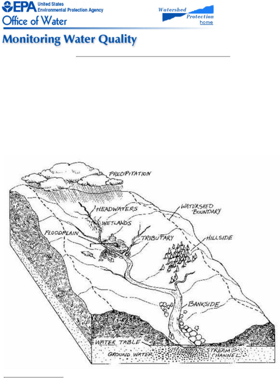
A watershed is the area of land from which runoff (from rain, snow, and springs) drains to a stream, river, lake, or

other body of water (Fig. 2.1). Its boundaries can be identified by locating the highest points of lands around the

waterbody. Streams and rivers function as the "arteries" of the watershed. They drain water from the land as they

flow from higher to lower elevations.

Figure 2.1

Cross section of a watershed

Volunteers should get to know the watersheds of their study streams.

A watershed can be as small or as large as you care to define it. This is because several watersheds of small

streams usually exist within the watershed of a larger river. The watershed of the Mississippi River, for example,

is about 1.2 million square miles and contains thousands of smaller watersheds, each defined by a tributary stream

that eventually drains into a larger river like the Ohio River or Missouri River and to the Mississippi itself.

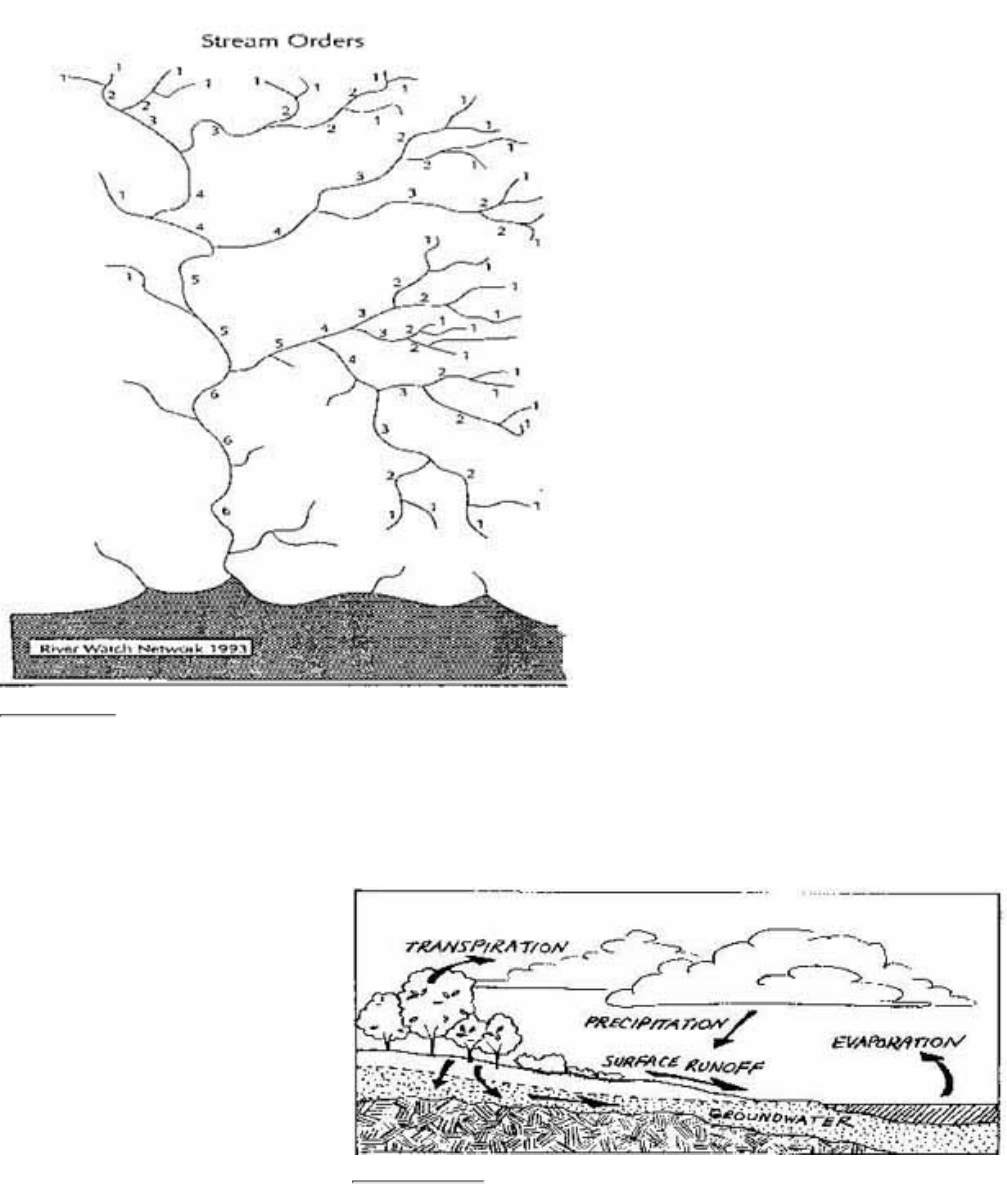
The River System

Figure 2.2

A representation of a river network with stream order marked

As streams flow downhill and meet other

streams in the watershed, a branching network

is formed (Fig. 2.2). When observed from the

air this network resembles a tree. The trunk of

the tree is represented by the largest river that

flows into the ocean or large lake. The

"tipmost" branches are the headwater streams.

This network of flowing water from the

headwater streams to the mouth of the largest

river is called the river system.

Water resource professionals have developed a

simple method of categorizing the streams in

the river system. Streams that have no

tributaries flowing into them are called

first-order streams. Streams that receive only

first-order streams are called second-order

streams. When two second-order streams meet,

the combined flow becomes a third-order

stream, and so on.

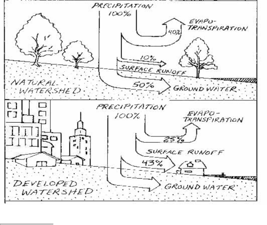
The Water Cycle

The water cycle is the movement of water

through the environment (Fig. 2.3). It is

through this movement that water in the river

system is replenished. When precipitation falls

to earth in a natural (undeveloped) watershed

in the midAtlantic states, for example, about

40 percent will be returned to the atmosphere

by evaporation or transpiration (loss of water vapor by plants). About 50 percent will percolate stream channel,

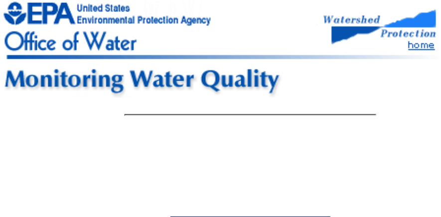
the ground water is discharged into the stream as a spring. The combination of ground water discharges to a

stream is defined as its baseflow. At times when there is no surface runoff, the entire flow of a stream might

actually be baseflow from ground water (Fig. 2.5).

Figure 2.3

The water cycle

Water moving through the water cycle replenishes streams in the watershed.

Some streams, on the other hand,

constantly lose water to the ground

water. This occurs when the water

table is below the bottom of the

stream channel. Stream water

percolates down through the soil until

it reaches the zone of saturation.

Other streams alternate between

losing and gaining water as the water

table moves up and down according

to the seasonal conditions or pumpage

by area wells.

The interactions between the

watershed, soils, and water cycle

define the natural water flow (hydrology) of any particular stream. Most significant is the fact that developed land

is more impervious than natural land. Instead of percolating into the ground, rain hits the hard surfaces of

buildings, pavement, and compacted ground and runs off into a storm drain or other artificial structure designed

to move water quickly away from developed areas and into a natural watercourse.

Figure 2.4

The fate of precipitation in undeveloped vs. developed watersheds

Survace runoff increases and ground water recharge decreases as watersheds become developed.

These conditions typically change the fate of precipitation in the water cycle (See Fig. 2.4, right panel). For

example:

Less precipitation is evaporated back to the atmosphere. (Water is transported rapidly away via storm

drains and is not allowed to stand in pools.)

●

Less precipitation is transpired back to the atmosphere from plants. (Natural vegetation is replaced by

buildings, pavement, etc.)

●

Less precipitation percolates through the soil to become ground water. (This can result in a lower water

table and can affect baseflow.)

●

More surface runoff is generated and transported to streams. (Streamflow becomes more intense during and

immediately after storms.)

●

Chapter 3, Watershed Survey Methods, is designed to help volunteers learn about their watershed. Using the

watershed survey approach, they will become familiar with their watershed's boundaries, its hydrologic features,

and the human uses of land and water that might be affecting the quality of the streams within it.

The Living Stream Environment

A healthy stream is a busy place. Wildlife and birds find shelter and food near and in its waters. Vegetation grows

along its banks, shading the stream, slowing its flow in rainstorms, filtering pollutants before they enter the

stream, and sheltering animals. Within the stream itself are fish and a myriad of insects and other tiny creatures

with very particular needs. For example, stream dwellers need dissolved oxygen to breathe; rocks, overhanging

tree limbs, logs, and roots for shelter; vegetation and other tiny animals to eat; and special places to breed and

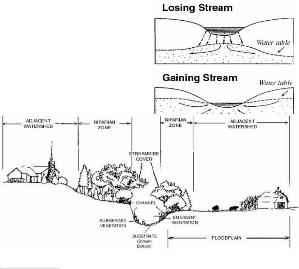
Figure 2.5

Streams losing and gaining water

The position of the water table sometimes plays a role in

determinating the amount of streamflow.

hatch their young. For many of these activities, they

might also need water of specific velocity, depth, and

temperature.

Human activities shape and alter many of these stream

characteristics. We dam up, straighten, divert, dredge,

dewater, and discharge to streams. We build roads,

parking lots, homes, offices, golf courses, and factories

in the watershed. We farm, mine, cut down trees, and

graze our livestock in and along stream edges. We also

swim, fish, and canoe in the streams themselves.

These activities can dramatically affect the many

components of the living stream environment (Fig. 2.6).

These components include:

Figure 2.6

Components of the stream system

Volunteers should be aware that the surrounding land affects stream habitat.

The adjacent watershed includes the higher ground that captures runoff and drains to the stream. For

purposes of this manual, the adjacent watershed is defined as land extending from the riparian zone to 1/4

mile from the stream.

The floodplain is the low area of land that surrounds a stream and holds the overflow of water during a

flood.

The riparian zone is the area of natural vegetation extending outward from the edge of the stream bank.

The riparian zone is a buffer to pollutants entering a stream from runoff, controls erosion, and provides

stream habitat and nutrient input into the stream. A healthy stream system generally has a healthy riparian

zone. Reductions and impairment of riparian zones occur when roads, parking lots, fields, lawns, and other

artificially cultivated areas, bare soil, rocks, or buildings are near the stream bank.

The stream bank includes both an upper bank and a lower bank. The lower bank normally begins at the

normal water line and runs to the bottom of the stream. The upper bank extends from the break in the

normal slope of the surrounding land to the normal high water line.

The streamside cover includes any overhanging vegetation that offers protection and shading for the stream

and its aquatic inhabitants.

Stream vegetation includes emergent, submergent, and floating plants. Emergent plants include plants with

true stems, roots, and leaves with most of their vegetative parts above the water. Submergent plants also

include some of the same types of plants, but they are completely immersed in water. Floating plants (e.g.,

duckweed, algae mats) are detached from any substrate and are therefore drifting in the water.

The channel of the streambed is the zone of the stream cross section that is usually submerged and totally

aquatic.

Pools are distinct habitats within the stream where the velocity of the water is reduced and the depth of the

water is greater than that of most other stream areas. A pool usually an has soft bottom sediments.

Riffles are shallow, turbulent, but swiftly flowing stretches of water that flow over partially or totally

submerged rocks.

Runs or glides are sections of the stream with a relatively low velocity that flow gently and smoothly with

little or no turbulence at the surface of the water.

10.

The substrate is the material that makes up the streambed, such as clay, cobbles, or boulders.11.

Whether streams are active, fast moving, shady, cold, and clear or deep, slowmoving, muddy, and warm--or

something in between--they are shaped by the land they flow through and by what we do to that land. For

example, vegetation in the stream's riparian zone protects and serves as a buffer for the stream's streamside cover,

which in turn shades and enriches (by dropping leaves and other organic material) the water in the stream

channel.

Furthermore, the riparian zone helps maintain the stability of the stream bank by binding soils through root

systems and helps control erosion and prevent excessive siltation of the stream's substrate. If human activities

begin to degrade the stream's riparian zone, each of these stream components--and the aquatic insects, fish, and

plants that inhabit them--also begins to degrade. Chapter 4 includes methods that volunteers can use to assess the

stream's living environment--specifically, the insects that live in the stream and the physical components of the

stream (the habitats) that support them.

Water Quality

The water in a stream is always moving and mixing, both from top to bottom and from one side of the stream to

the other. Pollutants that enter the stream travel some distance before they are thoroughly mixed throughout the

flow. For example, water upstream of a pipe discharging wastewater might be clean. At the discharge site and

immediately downstream, the water might be extremely degraded. Further downstream, in the recovery zone,

overall quality might improve as pollutants are diluted with more water. Far downstream the stream as a whole

might be relatively clean again. Unfortunately, most streams with one source of pollution often are affected by

many others as well.

Pollution is broadly divided into two classes according to its source. Point source pollution comes from a clearly

identifiable point such as a pipe which discharges directly into a waterbody. Examples of point sources include

factories, wastewater treatment plants, and illegal straight pipes from homes and boats.

Nonpoint source pollution comes from surface water runoff. It originates from a broad area and thus can be

difficult to identify. Examples of nonpoint sources include agricultural runoff, mine drainage, construction site

runoff, and runoff from city streets and parking lots.

Nationally, the pollutants most often found in the stream environment are not toxic substances like lead, mercury,

or oil and grease. More impacts are caused by sediments and silt from eroded land and nutrients such as the

nitrogen and phosphorus found in fertilizers, detergents, and sewage treatment plant discharges. Other leading

pollutants include pathogens such as bacteria, pesticides, and organic enrichment that leads to low levels of

dissolved oxygen. Common sources of pollution to streams include:

Agricultural activities such as crop production, cattle grazing, and maintaining livestock in holding areas or

feedlots. These contribute pollutants such as sediments, nutrients, pesticides, herbicides, pathogens, and

organic enrichment.

●

Municipal dischargers such as sewage treatment plants which contribute nutrients, pathogens, organic

enrichment, and toxicants.

●

Urban runoff from city streets, parking lots, sidewalks, storm sewers, lawns, golf courses, and building●

sites. Common pollutants include sediments, nutrients, oxygendemanding substances, road salts, heavy
metals, petroleum products, and pathogens.
Other commonly reported sources of pollutants are mining, industrial dischargers (factories), forestry activities,
and modifications to stream habitat and hydrology.
Chapter 5 describes methods volunteers can use to monitor water quality and detect pollutants from these sources.
< Previous · Table of Contents · Next >
Office of Wetlands, Oceans & Watersheds Home
Watershed Protection Home | Monitoring Water Quality Home
EPA Home | Office of Water | Search | Comments

2.2

Designing the Stream Study

Training Volunteer Monitors

Before beginning a stream monitoring study, volunteer program officials should develop a

design or plan that answers the 10 basic questions listed below. Without answers to these

questions, the monitoring program might well end up collecting data that do not meet

anyone's needs.

Answering these 10 questions is not easy. A planning committee composed of the program

coordinator, key volunteers, scientific advisors, program supporters, and data users should

resolve these questions well before the project gets under way. Naturally, the committee

should also address other planning questions less directly related to monitoring design,

such as how to recruit volunteers and how to secure funding for the project. Answers will

likely change as the program matures. For example, program coordinators might find that a

method is not producing data of high enough quality, data collection is too labor-intensive

or expensive, or additional parameters need to be monitored.

1. Why is the monitoring taking place?

Typical reasons for initiating a volunteer monitoring project include:

Developing baseline characterization data

●

Documenting water quality changes over time●

Screening for potential water quality problems●

Determining whether waters are safe for swimming●

Providing a scientific basis for making decisions on the management of a stream or

watershed

●

Determining the impact of a municipal sewage treatment facility, industrial facility,

or land use activity such as forestry or farming

●

Educating the local community or stream users to encourage pollution prevention

and environmental stewardship

●

Showing public officials that local citizens care about the condition and management

of their water resources

●

Of course, an individual program might be monitoring for a number of reasons. However,

it is important to identify one or two top reasons and develop the program based on those

objectives.

2. Who will use the monitoring data?

Knowing your data users is essential to the program development process. Potential data

users might include:

State, county, or local water quality analysts

●

The volunteers themselves●

Fisheries biologists●

Universities●

Schoolteachers●

Environmental organizations●

Parks and recreation staff●

Local planning and zoning agencies●

State environmental agencies●

State and local health departments●

Soil and water conservation districts●

Federal agencies such as the U.S. Geological Survey or U.S. Environmental

Protection Agency

●

Each of these users will have different data requirements. Some users, such as government

analysts and planning/zoning agencies, will have more stringent requirements than others

and will require higher levels of quality assurance. As the volunteer monitoring project is

being designed, program coordinators should contact as many potential information users

as possible to determine their data needs. It is important to have at least one user

committed to receiving and using the data. In some cases that user might be the monitoring

group itself.

3. How will the data be used?

The range of uses of volunteer data is limited only by the imagination. Volunteer data

could be used, for example, to influence local planning decisions about where to site a

sewage treatment facility or to publicize a water quality problem and seek community

solutions. Collected data could also be used to educate primary school children about the

importance of water resources. Other data uses include the support of:

Local zoning requirements

●

A stream protection study●

State preparation of water quality assessments●

Screening waters for potential problems●

The setting of statewide priorities for pollution control●

Each data use potentially has different data requirements. Knowing the ultimate uses of the

collected volunteer data will help determine the right kind of data to collect and the level of

effort required to collect, analyze, store, and report them.

Type Approach Applications* Table 2.1

Some types

monitoring

approaches

and their

application

Physical

Condition

Watershed

survey

Determine land use patterns; determine

presence of current and historical pollution

sources; identify gross pollution problems;

identify water uses, users, diversions, and

stream obstructions

Habitat

assessment

Determine and isolate impacts of pollution

sources, particularly land use activities;

interpret biological data; screen for

impairments

Biological

condition Macroinvertebrate

sampling

Screen for impairment; identify impacts of

pollution and pollution control activities;

determine the severity of the pollution

problem and rank stream sites; identify

water quality trends; determine support of

designated aquatic life uses.

Chemical

condition Water quality

sampling

Screen for impairment; identify specific

pollutants of concern; identify water quality

trends; determine support of designated

contact recreation uses; identify potential

pollution sources

* Beyond education and promoting stewardship

4. What parameters or conditions will be monitored?

Determining what to monitor will depend on the needs of the data users, the intended use

of the data, and the resources of the volunteer program. If the program's goal is to

determine whether a creek is suitable for swimming, for example, a human-healthrelated

parameter such as fecal coliform bacteria should be monitored. If the objective is to

characterize the ability of a stream to support sport fish, volunteers should examine stream

habitat characteristics, the aquatic insect community, and water quality parameters such as

dissolved oxygen and temperature. Alternatively, if a program seeks to provide baseline

data useful to state water quality or natural resource agencies, program designers should

consult those agencies to determine which parameters they consider of greatest value.

Money for test kits or meters, available laboratory facilities, help from state or university

advisors, and the abilities and desires of volunteers will also clearly have an impact on the

choice of parameters to be monitored. For characterization studies, EPA usually

recommends an approach that integrates physical, chemical, and biological parameters.

5. How good does the monitoring data need to be?

Some uses require high-quality data. For example, high-quality data are usually needed to

prove compliance with environmental regulations, assess pollution impacts, or make land

use planning decisions. In other cases the quality of the data is secondary to the actual

process of collecting it. This is often the case for monitoring programs that focus on the

overall educational aspects of stream monitoring.

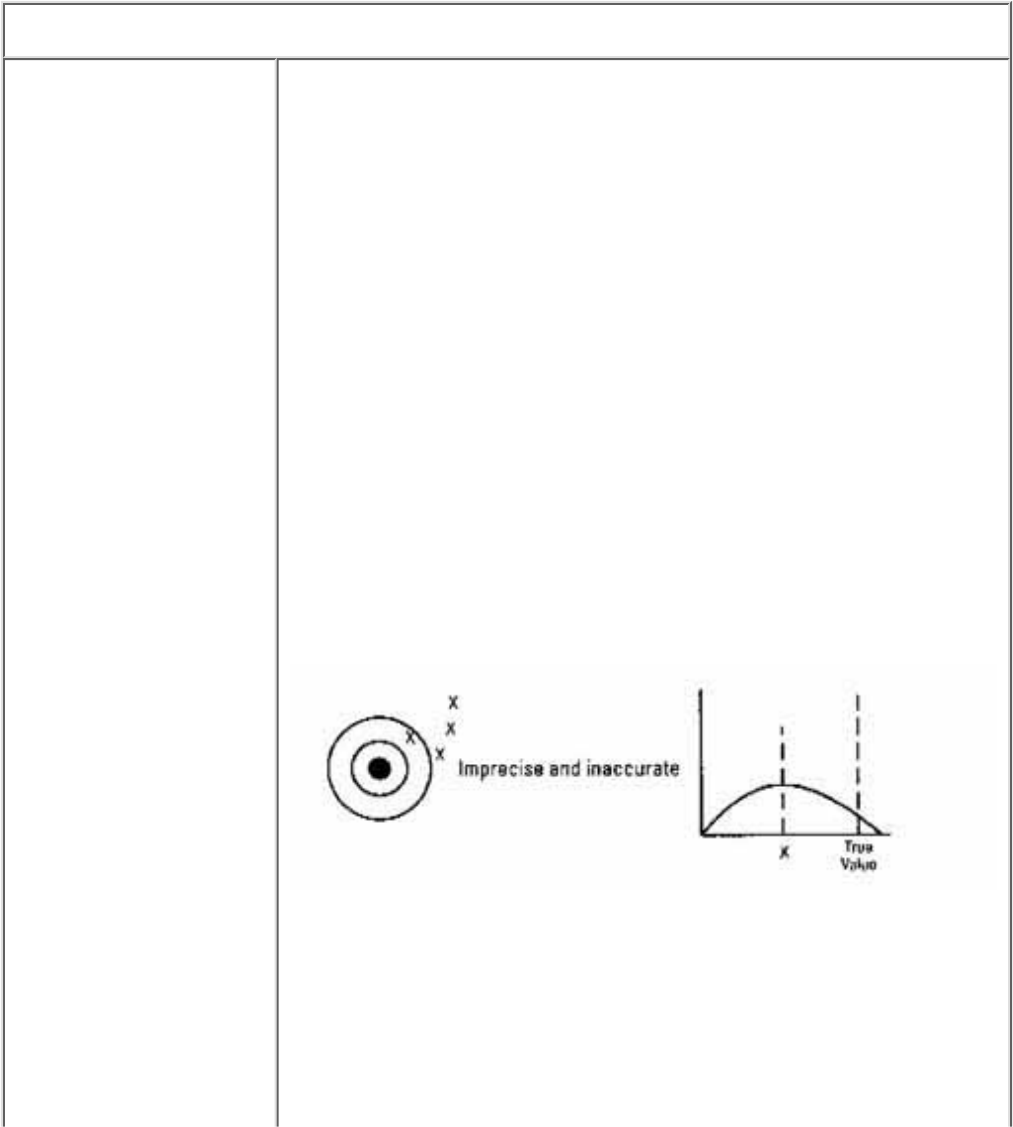
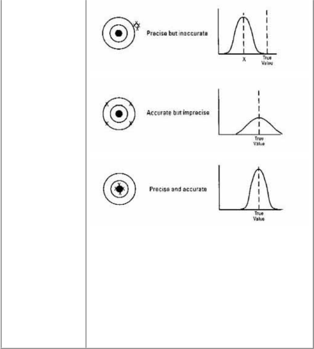
Data quality is measured in five ways accuracy, precision, completeness,

representativeness, and comparability (see box Data Quality Terms).

Data Quality Terms

● Accuracy is the

degree of agreement

between the sampling

result and the true

value of the

parameter or

condition being

measured. Accuracy

is most affected by

the equipment and the

procedure used to

measure the paramter.

● Precision, on the

other hand, refers to

how well you are able

to reproduce the

result on the same

sample, regardless of

accuracy. Human

error in sampling

techniques plays an

important role in

estimating precision.

● Representativeness

is the degree to which

collected data

actually represent the

stream condition

being monitored. It is

most affected by site

location.

● Completeness is a

measure of the

amount of valid data

actually obtained vs.

the amount expected

to be obtained as a

specified in the

original sampling

design. It is usually

expressed as a

percentage. For

example, if 100

samples were

scheduled but

volunteers sampled

only 90 times due to

bad weather or

broken equipment,

the completeness

record would be 90

percent.

● Comparability

represents how well

data from one stream

or stream site can be

compared to data

from another. Most

managers will

compare sites as part

of a statewide or

regional report on the

volunteer monitoring

program; therefore,

sampling methods

should be the same

from site to site.

6. What methods should be used?

The methods adopted by a volunteer program depend primarily on how the data will be

used and what kind of data quality is needed. There are, of course, many sampling

considerations including:

How samples will be collected (e.g., using grab samples or measuring directly with a

meter)

●

What sampling equipment will be used (e.g., disposable Whirlpak bags, glass●

bottles, 500-micron mesh size kick net, etc.)

What equipment preparation methods are necessary (such as container sterilization

or meter calibration)

●

What protocols will be followed (such as the Winkler method for dissolved oxygen,

intensive stream bioassessment approach for habitat and benthic macroinvertebrates,

etc.)

●

Analytical questions must also be addressed such as:

Will volunteers return to a lab for macroinvertebrate identification or dissolved

oxygen titration procedures or conduct them in the field?

●

Will a color wheel provide nitrate data of needed quality, or is a more sophisticated

approach needed?

●

Should visual observation and habitat assessment approaches be combined with

turbidity measures to best determine the impact of construction sites? While

sophisticated methods usually yield more accurate and precise data (if properly

carried out), they are also more costly and timeconsuming. This extra effort and

expense might be worthwhile if the goal of the program is to produce high-quality

data. Programs with an educational focus, however, can often use less sensitive

equipment and less sophisticated methods to meet their goals.

●

7. Where are the monitoring sites?

Sites might be chosen for any number of reasons such as accessibility, proximity to

volunteers' homes, value to potential users such as state agencies, or location in problem

areas. If the volunteer program is providing baseline data to characterize a stream or screen

for problems, it might wish to monitor a number of sites representing a range of conditions

in the stream watershed (e.g., an upstream "pristine" area, above and below towns and

cities, in agricultural areas and parks, etc.). For more specific purposes, such as

determining whether a stream is safe to swim in, it might only be necessary to sample

selected swimming areas. To determine whether a particular land use activity or potential

source of pollution is, in fact, having an impact, it might be best to monitor upstream and

downstream of the area where the source is suspected. To determine the effectiveness of

runoff control measures, a paired watershed approach might be best (e.g., sampling two

similar small watersheds, one with controls in place and one without controls).

A program manager might also select one or more sites near professionally monitored sites

in order to compare the quality of volunteer-generated data against professional data. It

might also be helpful to locate some sites near U.S. Geological Survey gauging stations,

which can provide useful data on streamflow. Certainly, for any volunteer program, safety

and accessibility (both legal and physical) will be important in determining site location.

No matter how sampling sites are chosen, most monitoring programs will need to maintain

the same sites over time and identify them clearly in their monitoring program design.

When selecting monitoring sites, ask the following questions. Based on the answers, you

may need to eliminate some sites or select alternative locations that meet your criteria:

Are other groups (local, state, federal agencies; other volunteer groups; schools or

colleges) already monitoring this site?

●

Can you identify the site on a map and on the ground?●

Is the site representative of the watershed?●

Does the site have water in it during the times of year that monitoring will take

place?

●

Is there safe, convenient access to the site (including adequate parking) and a way to

safely sample a flowing section of the stream? Is there access all year long?

●

Can you acquire landowner permission?●

Can you perform all the monitoring activities and tests that are planned at this site?●

Is the site far enough downstream of drains or tributaries? Is the site near tributary

inflows, dams, bridges, or other structures that may affect the results?

●

Have you selected enough sites for the study you want to do?●

Once you have selected the monitoring sites, you should be able to identify them by

latitude and longitude. This location information is critical if your data will potentially be

used in Geographical Information Systems (GIS) or in sophisticated data management

systems (See Appendix C).

8. When will monitoring occur?

A program should specify:

What time of day is best for sampling. (Temperature and dissolved oxygen, for

example, can fluctuate naturally as the sun rises and aquatic plants release oxygen.)

●

What time of year is best for sampling. (For example, there is no point in sampling

fecal coliform bacteria at swimming beaches in the winter, when no one is

swimming, or sampling intermittent streams at the height of summer, when because

of dry conditions the streams hold little water.)

●

How frequently should monitoring take place? (It is possible, for example, to

conduct too many biological assessments of a stream and thereby deplete the

stream's aquatic community. A program designed to determine whether polluted

runoff is a problem would do well to monitor after storms and heavy rainfalls.)

●

In general, monthly chemical sampling and twiceyearly biological sampling are considered

adequate to identify water quality changes over time. Biological sampling should be

conducted at the same time each year because natural variations in aquatic insect

population and streamside vegetation occur as seasons change. Monitoring at the same

time of day and at regular intervals (e.g., at 2:00 p.m. every 30 days) helps ensure

comparability of data over time.

9. How will monitoring data be managed and presented?

The volunteer program coordinator should have a clear plan for dealing with the data

collected each year. Field and lab data sheets should be checked for completeness, data

should be screened for outliers, and a database should be developed or adapted to store and

manipulate the data. The elements of such a database should be clearly explained in order

to allow users to interpret the data accurately and with confidence.

Program coordinators will also have to decide how they want to present data results, not

only to the general public and to specific data users, but also to the volunteers themselves.

Different levels of analysis might be needed for different audiences. A volunteer group

collecting data for state or county use should consult with the appropriate agency before

investing in computerized data management software because the agency could have

specific needs or recommendations based on its own data management protocols.

10. How will the program ensure that data are credible?

Developing specific answers to questions 19 is the first step in ensuring that data are

credible. Credible data meet specific needs and can be used with confidence for those

needs. Other steps include:

Properly training, testing, and retraining volunteers

●

Evaluating the program's success after an initial pilot stage and making any

necessary adjustments

●

Assigning specific quality assurance tasks to qualified individuals in the program●

Documenting in a written plan all the steps taken to sample, analyze, store, manage,

and present data

●

A written plan, known as a quality assurance project plan, can be elaborate or simple

depending on the volunteer program's goals. Its essential feature, however, is that it

documents how the data are to be generated. Without such knowledge, the data cannot be

used with confidence. It is also important for educating future volunteers and data users

about the program and the data. People might be analyzing the data 5 or 10 or more years

later to study trends in stream quality. (Note: EPA requires that any monitoring program

sponsored by EPA through grants, contracts, or other formal agreement must carry out a

quality assurance/quality control program and develop a quality assurance project plan.)

Put It in Writing
When you and the volunteer program planning committee have answered the
ten project design questions to everyone's satisfaction, your next critical step
is to put it all in writing. The written plan, including sampling and analytical
methods, sites, parameters, project goals, and data quality considerations, is
your bible. With a written plan you:
Document the particulars of your program for your data users
● 
Educate newcomers to the program● 
Ensure that newcomers will use the same methods as those who came
before them
● 
Keep an historical record for future program leaders, volunteers, and
data users
● 
Your written plan may simply consist of a study design and standard
● operating procedures such as a monitoring and lab methods manual. You
may, however, prefer to develop a more comprehensive quality assurance
project plan. The quality assurance project plan is a document that outlines
the procedures you will use to ensure high quality data when conducting
sample collection and analysis in your program.
By law, any water quality monitoring program that receives EPA funding is
required to have an EPA-approved quality assurance project plan. Even if
you don't receive EPA funding, you will find that preparing a written plan
helps ensure that your data are used with confidence, now and in the future.
(See The Volunteer Monitor's Guide to Quality Assurance Project Plans
(EPA 841-B-96-003 September 1996) for more information.)
< Previous · Table of Contents · Next >
Office of Wetlands, Oceans & Watersheds Home
Watershed Protection Home | Monitoring Water Quality Home
EPA Home | Office of Water | Search | Comments

Training Volunteer Monitors

Back to Section 2.2 - Designing the Stream Study

Training should be an essential component of any volunteer stream monitoring project.

When volunteers are properly trained in the goals of the volunteer project and its

sampling and analytical methods, they:

Produce higher quality, more credible data.

●

Better understand their role in protecting water quality.●

Are more motivated to continue monitoring.●

Save program manager time and effort by becoming better monitors who require

less supervision.

●

Feel more like part of a dedicated team.●

Some of the key elements to consider in developing a training program for volunteers

include the following:

Plan ahead. When you are in the early stages of developing your training program,

decide who will do the training, when training will occur, where it will be held,

what equipment and handouts volunteers will receive, and what, in they end, they

will learn. Plan on at least one initial training session at the start of the sampling

season and a quality control session somewhat into the season (to see if volunteers

are using the right methods, and to answer questions). If volunteers will be

sampling many different chemical parameters or will be conducting intensive

biological monitoring, you should probably schedule two initial training

sessions—one to introduce volunteers to the program, and the other to cover

sampling and analytical methods in detail. You might also want to plan a

postseason session that encourages volunteers to air problems, exchange

information, and make suggestions for the coming year. Make sure the program

planning committee agrees to the training plan.

Put it in writing. Once you've made these decisions, write them all down. Note the

training specifics in the program's quality assurance project plan. It might also help

to develop a "job description" for the volunteers that lists the tasks they will

perform in the field and lab, and that identifies the obligations to which they will

be held and the schedule they will follow. Hand this out at the first training session.

Volunteers should leave the session knowing what is expected of them. If they

decide not to join after all because the tasks are too onerous, it is better for you to

find out after the first session than later in the sampling year.

Be prepared. Nothing will discourage volunteers more than an illplanned, chaotic

initial training session. The elements of a successful initial training session include:

Enthusiastic, knowledgeable trainers

❍

Short presentations that encourage audience participation and don't strain

attention spans

❍

A low ratio of trainers to trainees❍

Presentations that include why the monitoring is needed, what the program

hopes to accomplish, and what will be done with the data

❍

An agenda that is followed (especially start and finish times)❍

Good acoustics, clear voices, and interesting audiovisual aids❍

Opportunities for all trainees to handle equipment, view demonstrations of

sampling protocols, and practice sampling

❍

Instruction on safety considerations❍

Refreshments and opportunities for trainees to meet one another, socialize,

and have fun

❍

Time for questions and answers.❍

Conduct quality control checks. After your initial training session(s), schedule

opportunities to "check up" on how your volunteers are performing. The purpose

of these quality control checks is to ensure that all volunteers are monitoring using

proper and consistent protocols, and to emphasize the importance of quality control

measures. Some time into the sampling season, observe how volunteers are

sampling, analyzing their samples, identifying macroinvertebrates, and recording

their results. Either observe volunteers in small groups at their monitoring sites or

bring them to a central location for an organized quality control session. If your

program is involved in chemical monitoring, you might want all volunteers to

analyze the same water sample using their own equipment, or hold a lab exercise in

which volunteers read and record results from equipment and kits that have already

been set up. For a biological monitoring program, have trainers or seasoned

volunteers observe sampling methods in the field and provide preserved samples of

macroinvertebrates for volunteers to identify. Reserve time to answer questions,

talk about initial findings, and have some fun.

Review the effectiveness of your training program. At the end of each training

session, encourage volunteers to fill out a training evaluation form. This form

should help you assess the effectiveness of individual trainers and their styles, the

handouts and audiovisual aids, the general atmosphere of the training session, and

what the volunteers liked most and least about the session. Use the results of the

evaluation to revise training protocols as needed to best meet program and

volunteer needs.

Office of Wetlands, Oceans & Watersheds Home

Watershed Protection Home | Monitoring Water Quality Home

EPA Home | Office of Water | Search | Comments

2.3

Safety Considerations

One of the most critical considerations for a volunteer monitoring program is the safety

of its volunteers. All volunteers should be trained in safety procedures and should carry

with them a set of safety instructions and the phone number of their program coordinator

or team leader. Safety precautions can never be overemphasized.

The following are some basic common sense safety rules. At the site:

Always monitor with at least one partner. Teams of three or four people are best.

Always let someone else know where you are, when you intend to return, and what

to do if you don't come back at the appointed time.

●

Develop a safety plan. Find out the location and telephone number of the nearest

telephone and write it down. Locate the nearest medical center and write down

directions on how to get between the center and your site(s) so that you can direct

emergency personnel. Have each member of the sampling team complete a

medical form that includes emergency contacts, insurance information, and

pertinent health information such as allergies, diabetes, epilepsy, etc.

●

Have a first aid kit handy (see box below). Know any important medical conditions

of team members (e.g., heart conditions or allergic reactions to bee stings). It is

best if at least one team member has first aid/CPR training.

●

Listen to weather reports. Never go sampling if severe weather is predicted or if a

storm occurs while at the site.

●

Never wade in swift or high water. Do not monitor if the stream is at flood stage.●

If you drive, park in a safe location. Be sure your car doesn't pose a hazard to other

drivers and that you don't block traffic.

●

Put your wallet and keys in a safe place, such as a watertight bag you keep in a

pouch strapped to your waist. Without proper precautions, wallet and keys might

end up downstream.

●

Never cross private property without the permission of the landowner. Better yet,

sample only at public access points such as bridge or road crossings or public

parks. Take along a card identifying you as a volunteer monitor.

●

Confirm that you are at the proper site location by checking maps, site●

descriptions, or directions.

Watch for irate dogs, farm animals, wildlife (particularly snakes), and insects such

as ticks, hornets, and wasps. Know what to do if you get bitten or stung.

●

Watch for poison ivy, poison oak, sumac, and other types of vegetation in your

area that can cause rashes and irritation.

●

Never drink the water in a stream. Assume it is unsafe to drink, and bring your

own water from home. After monitoring, wash your hands with antibacterial soap.

●

Do not monitor if the stream is posted as unsafe for body contact. If the water

appears to be severely polluted, contact your program coordinator.

●

Do not walk on unstable stream banks. Disturbing these banks can accelerate

erosion and might prove dangerous if a bank collapses. Disturb streamside

vegetation as little as possible.

●

Be very careful when walking in the stream itself. Rocky-bottom streams can be

very slippery and can contain deep pools; muddy-bottom streams might also prove

treacherous in areas where mud, silt, or sand have accumulated in sink holes. If

you must cross the stream, use a walking stick to steady yourself and to probe for

deep water or muck. Your partner(s) should wait on dry land ready to assist you if

you fall. Do not attempt to cross streams that are swift and above the knee in depth.

Wear waders and rubber gloves in streams suspected of having significant

pollution problems.

●

If you are sampling from a bridge, be wary of passing traffic. Never lean over

bridge rails unless you are firmly anchored to the ground or the bridge with good

hand/foot holds.

●

If at any time you feel uncomfortable about the condition of the stream or

your surroundings, stop monitoring and leave the site at once. Your safety is

more important than the data!

●

When using chemicals:

Know your equipment, sampling instructions, and procedures before going out into

the field. Prepare labels and clean equipment before you get started.

●

Keep all equipment and chemicals away from small children. Many of the

chemicals used in monitoring are poisonous. Tape the phone number of the local

poison control center to your sampling kit.

●

Avoid contact between chemical reagents and skin, eye, nose, and mouth. Never

use your fingers to stopper a sample bottle (e.g., when you are shaking a solution).

Wear safety goggles when performing any chemical test or handling preservatives.

●

Know chemical cleanup and disposal procedures. Wipe up all spills when they

occur. Return all unused chemicals to your program coordinator for safe disposal.

Close all containers tightly after use. Do not switch caps.

●

Know how to use and store chemicals. Do not expose chemicals or equipment to

temperature extremes or longterm direct sunshine.

●

First Aid Kit
The minimum first aid kit should contain the following items:
Telephone numbers of emergency personnel such as the police and an
ambulance service.
❍ 
Several band-aids for minor cuts.❍ 
Antibacterial or alcohol wipes.❍ 
First aid creme or ointment.❍ 
Several gauze pads 3 or 4 inches square for deep wounds with
excessive bleeding.
❍ 
Acetaminophen for relieving pain and reducing fever.❍ 
A needle for removing splinters.❍ 
A first aid manual which outlines diagnosis and treatment procedures.❍ 
A single-edged razor blade for minor surgery, cutting tape to size, and
shaving hairy spots before taping.
❍ 
A 2-inch roll of gauze bandage for large cuts.❍ 
A triangular bandage for large wounds.❍ 
A large compress bandage to hold dressings in place.❍ 
A 3-inch wide elastic bandage for sprains and applying pressure to
bleeding wounds.
❍ 
If a participant is sensitive to bee stings, include their
doctor-prescribed antihistamine.
❍ 
Be sure you have emergency telephone numbers and medical information
with you at the field site for everyone participating in field work (including
the leader) in case there is an emergency.
< Previous · Table of Contents · Next >
Office of Wetlands, Oceans & Watersheds Home
Watershed Protection Home | Monitoring Water Quality Home
EPA Home | Office of Water | Search | Comments

2.4

Basic Equipment

Much of the equipment a volunteer will need is easily obtained from either hardware

stores or scientific supply houses. Other equipment can be found around the house. In

either case, the volunteer program should clearly specify the equipment its volunteers

will need and where it should be obtained.

Listed below is some basic equipment appropriate for any volunteer field activity. Much

of this equipment is optional but will enhance the volunteers' safety and effectiveness.

Boots or waders; life jackets if you are sampling by boat

●

Walking stick of known length for balance, probing, and measuring●

Bright-colored snag- and thorn- resistant clothes; long sleeves and pants are best●

Rubber gloves to guard against contamination●

Insect repellent/sunscreen●

Small first aid kit, flashlight, and extra batteries●

Whistle to summon help in emergencies●

Refreshments and drinking water●

Clipboard, preferably with plastic cover●

Several pencils●

Tape measure●

Thermometer●

Field data sheet●

Information sheet with safety instructions, site location information, and numbers

to call in emergencies

●

Camera and film, to document particular conditions●

Specific equipment lists for the chemical and biological monitoring procedures included

in the manual are provided in the relevant chapters.

References and Further Reading
Dates, G. 1994. A Plan for Watershedwide Volunteer Monitoring. The Volunteer
Monitor. 6(2):8.
Ely, E. 1992. Building Credibility. The Volunteer Monitor. 4(2).
Ely, E. 1994. What Parameters Volunteer Groups Test. The Volunteer Monitor. 6(1):6.
Picotte, A. 1994. Citizen's Data Used to Set Phosphorus Standards. The Volunteer
Monitor. 6(1):18.
Weber, P. and F. Dowman. 1994. The Web of Water. The Volunteer Monitor. 6(2):10.
USEPA. 1990. Volunteer Water Monitoring: A Guide for State Managers. EPA
440/490010. August. U.S. Environmental Protection Agency, Office of Water,
Washington, DC 20460.
USEPA. 1993. EPA Requirements for Quality Assurance Project Plans for
Environmental Data Operations. EPA QA/R5. July. U.S. Environmental Protection
Agency, Quality Assurance Management Staff, Washington, DC 20460.
USEPA. 1993. Integrating Quality Assurance into Tribal Water Programs. U.S.
Environmental Protection Agency, Region 8, 999 18th St., Suite 500, Denver, CO 80202.
USEPA. 1996. The Volunteer Monitor's Guide To Quality Assurance Project Plans. EPA
841-B-96-003. September. Office of Wetlands, Oceans, and Watersheds, 4503F,
Washington, DC 20460.
< Previous · Table of Contents · Next >
Office of Wetlands, Oceans & Watersheds Home
Watershed Protection Home | Monitoring Water Quality Home
EPA Home | Office of Water | Search | Comments

Chapter 3

Watershed Survey Methods

3.1 - How to Conduct a Watershed Survey

3.2 - The Visual Assessment

One of the most rewarding and least costly stream monitoring activities a volunteer

program can conduct is the watershed survey. Some programs call it a windshield survey,

a visual survey, or a watershed inventory. It is, in essence, a comprehensive survey of the

geography, land and water uses, potential and actual pollution sources, and history of the

stream and its watershed.

The watershed survey may be divided into two distinct parts:

A onetime background investigation of the stream and its watershed. (To do this,

volunteers research town and county records, maps, photos, news stories, industrial

discharge records, and oral histories.)

●

A periodic visual assessment of the stream and its watershed. (To do this,

volunteers walk along the stream and drive through the watershed, noting key

features.)

●

The watershed survey requires little in the way of training or equipment. Its chief uses

include:

Screening for pollution problems

●

Identifying potential sources of pollution●

Identifying sites for monitoring●

Helping interpret biological and chemical information●

Giving volunteers and local residents a sense of the value of the stream or

watershed

●

Educating volunteers and the local community about potential pollution sources

and the stressors affecting the stream and its watershed

●

Providing a blueprint for possible community restoration efforts such as cleanups

and tree plantings

●

To actually determine whether those stressors are, in fact, affecting the stream requires
additional monitoring of chemical, physical, or biological conditions.
The watershed survey described in this chapter was developed from survey approaches
used by programs such as Rhode Island Watershed Watch, Maryland Save Our Streams,
the Delaware Department of Natural Resources and Environmental Control, and
Washington's AdoptA Stream Foundation. References are provided at the end of this
chapter for further information on watershed surveys.
< Previous · Table of Contents · Next >
Office of Wetlands, Oceans & Watersheds Home
Watershed Protection Home | Monitoring Water Quality Home
EPA Home | Office of Water | Search | Comments

3.1

How to Conduct a Watershed Survey

The Background Investigation

Researching the stream is generally a onetime activity that should yield valuable

information about the cultural and natural history of the stream and the uses of the land

surrounding it. This information will prove helpful in orienting new volunteers to the

purpose of the monitoring program, in building a sense of the importance of the stream

and its role in the watershed, and in identifying land use activities in the watershed with a

potential to affect the quality of the stream. The program might choose to monitor these

areas and activities more intensively in the future.

The background investigation is essentially a "detective investigation" for information on

the stream and includes the following steps:

Task 1 Determine what you want to know about your

stream

Before beginning the background investigation, establish what it is you want to know

about the stream you are surveying. Types of information include:

Location of the stream's headwaters, its length, where it flows, and where it

empties

●

Name and boundaries of the watershed it occupies, the population in the

watershed, and the communities through which it flows

●

Roles of various jurisdictions in managing the stream and watershed●

Percentage of watershed land area in each town or jurisdiction●

Land uses in the stream's watershed●

Industries and others that discharge to the stream●

Current uses of the stream (such as fishing, swimming, drinking water supply,

irrigation)

●

Historical land uses●

History of the stream●

Any or all of these types of information should prove valuable to the monitoring

program. You might also uncover other important information in the process. At a

minimum, the investigation should yield information on the size of the stream, watershed

boundaries, and general land use in the area. By establishing categories of information to

investigate, program coordinators can assign volunteers to specific activities and end up

with a complete picture of the stream that answers many questions of value to the

program.

Task 2 Determine the tools you will need

Offered below are some of the tools you will need to find answers in your background

investigation of the stream.

Stream headwaters, length, tributaries, final stream destination, and watershed boundaries

are best determined through maps. Of greatest value are U.S. Geological Survey 7 1/2-

minute topographic maps (on a 1:24,000 scale where 1 inch = 2,000 feet). At varying

degrees of resolution, they depict landforms, major roads and political boundaries,

developments, streams, tributaries, lakes, and other land features. Sporting goods stores

and bookstores often carry these maps, especially for recreational areas that are likely to

be hiked or camped. The maps can also be ordered through the U.S. Geological Survey

(see Obtaining USGS Topographic Maps).

Road, state, and county maps might also prove helpful in identifying some of these

stream and watershed features. Hydrologic unit maps, also available from the U.S.

Geological Survey but at a 1:100,000 scale of resolution (less detail than the 7 1/2-minute

maps cited above), might also help you determine hydrologic watershed boundaries.

Atlases and other reference materials at libraries can prove helpful in determining facts

about population in the watershed.

Land uses in the stream watershed might also be depicted on maps such as those

discussed above. You will verify this information in the second half of the watershed

survey, when you are actually in the field observing land around the stream. Information

from maps is particularly useful in developing a broad statement about general land use

in the stream watershed (e.g., land use in the hypothetical Volunteer Creek watershed is

60 percent residential, 20 percent parkland/recreational, and 20 percent light industrial).

Obtaining USGS Topographic Maps

The U.S. Geological Survey's Earth Science Information Centers can provide

you with a catalog of available USGS topographic maps, a brochure on how

to use topographic maps, and general information on ESIC services. Contact

the main ESIC office at:

USGS Earth Science Information Center

507 National Center

12201 Sunrise Valley Drive

Reston, VA 22092

1-800-USA-MAPS

You can obtain a free USGS Indexing Catalog to help you identify the

map(s) you need by calling 1-800-435-7627. If you know the coordinates of

the map you need, you can order it directly from:

USGS

Branch of Information Services

Box 25286

Denver, CO 80225

Place your order in writing and include a check for $4.00 per map plus $3.50

for shipping and handling. The ESIC can also refer you to commercial map

distributors that can get you the topographic maps sooner, for a higher fee.

USGS topographic maps might also be available from sporting goods stores

in your area.

Other sources of information include:

Land use plans from local planning offices, which include information not only for

current land uses but for potential uses for which the area is zoned

●

Conservation district offices or offices of the agricultural extension service or

Natural Resources Conservation Service (Formerly the Soil Conservation Service,

these offices might be able to provide information on agricultural land in rural

areas)

●

Local offices of the U.S. Geological Survey, which might provide a variety of

publications, special studies, maps, and photos on land uses and landforms in the

area

●

Aerial photographs, which might provide current and historical views of land uses●

Industries and others that discharge to the stream might be identified at the state, city, or

county environmental protection or water quality office. (The name of the agency will

vary by locality.) At these offices, you may ask to see records of industries with permits

to discharge treated effluent to streams. These records are maintained through the

National Pollutant Discharge Elimination System (NPDES). All industrial and municipal

dischargers are required to have permits that specify where, when, and what they are

allowed to discharge to waters of the United States.

Especially in older metropolitan areas, combined sewers are also potential discharges.

Combined sewers are pipes in which sanitary sewer waste overflow and storm water are

combined in times of heavy rain. These combined sewers are designed to discharge

directly into harbors and rivers during storms when the volume of flow in the sewers

exceeds the capacity of the sewer system. The discharge might include raw sanitary

sewage waste. Combined sewers do not flow in dry weather. Maps of sewer systems can

be obtained from your local water utility.

The state or local environmental agency should also be able to provide location

information on other potential pollution sources such as landfills, wastewater treatment

plants, and stormwater detention ponds.

Current uses of the stream are established in state water quality standards, which specify

what the uses of all state waters should be. These uses can include, for example, cold

water fisheries, primary contact recreation (swimming) and irrigation. The state also

establishes criteria or limits on pollutants in the waters necessary to maintain sufficient

water quality to support those uses, as well as a narrative statement that prohibits

degradation of waters below their designated uses.

Section 305(b) of the Clean Water Act requires states to report to the U.S. Environmental

Protection Agency on the designated uses of their waters, the extent of the impairment of

those uses, and the causes and sources of impairment. This information is kept on file at

the state water quality agency. While state reports cannot specify water uses and degree

of impairment in all individual streams in the state, they are a good starting point. Write

to the state water quality agency for its biennial water quality (section 305(b))

assessment.

You might also be able to obtain a copy of your state's water quality standards or

establish contact with a water quality specialist who can give you information on

standards for your stream. Again, information on actual water uses will be verified and

detailed once you walk the stream during the visual assessment portion of your watershed

survey.

Historical land uses and the history of the stream might take some legwork to uncover.

Local historical societies, libraries, and newspaper archives are good places to start. Look

for historical photos of the area and stories about fishing contests, fish kills, spills, floods,

and other major events affecting the stream and its watershed. County or town planning

offices might be able to provide information on when residential developments were built

and when streams were channelized or diverted. State and local transportation agencies

might have records on when highways and bridges were built. State environmental

regulatory agencies have records of past or current applications to modify stream

hydrology through dredging, channelization, and stream bank stabilization.

Long-time residents are another invaluable source of information on the history of your

stream. People who fished or swam in your stream in their youth might have witnessed

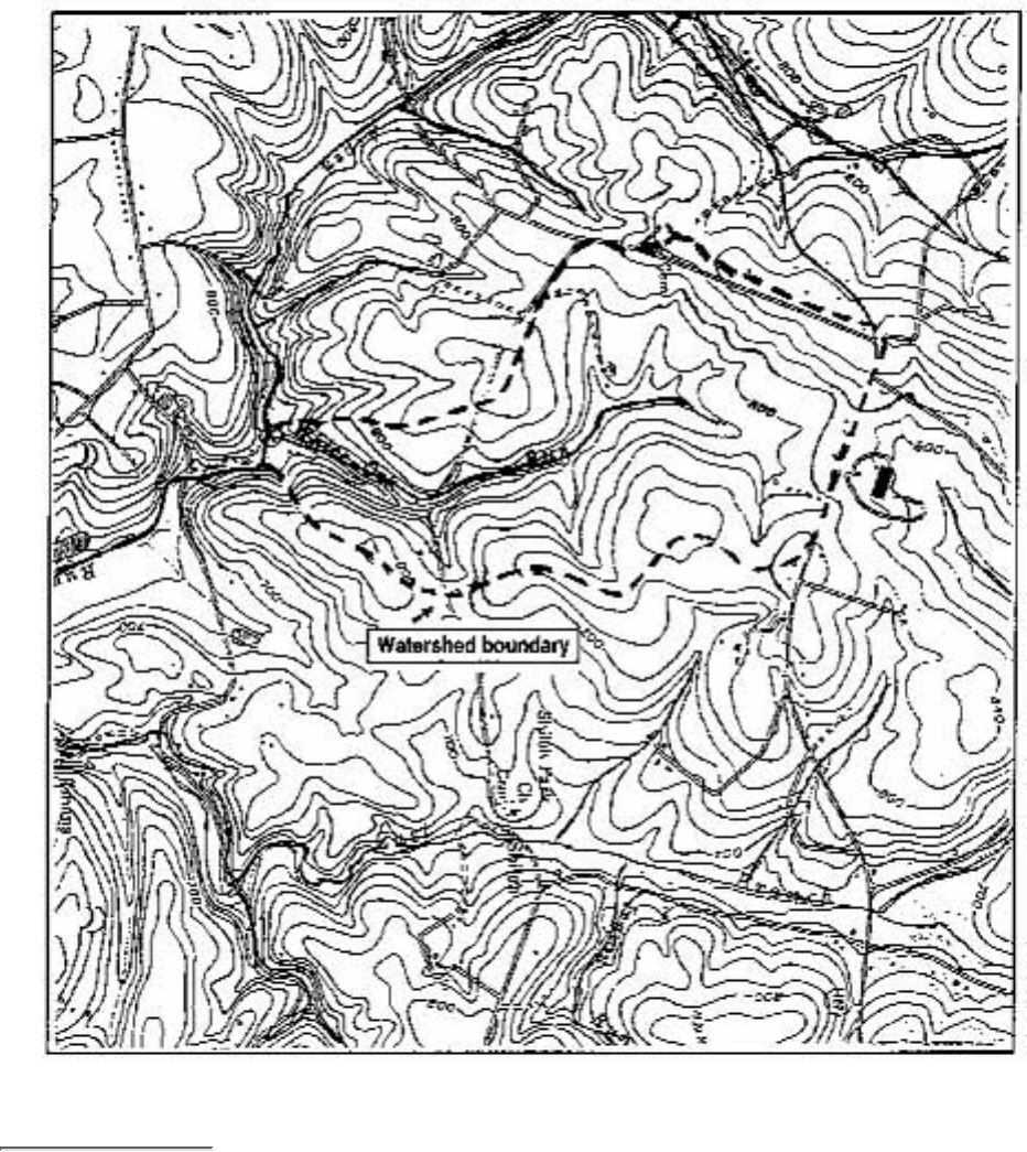
how the stream has changed. They might remember industries or land use activities of the

past such as mines or farms that could have affected the stream. They might have tales to

tell about fish they once caught or floods that led to channelization and dams.

Assembling such oral histories is a particularly good activity for schoolage volunteers.

Figure 3.1

A topographic map with a delineated watershed

Volunteers should learn to read a topo map to learn about the natural and cultural features of their

study stream's watershed.

Getting to Know the Boundaries of Your Watershed

Once you've obtained topographic maps of your area, follow these steps to

draw your watershed boundaries:

Locate and mark the downstream outlet of the watershed. For rivers

and streams, this is the farthest downstream point in which you are

interested.

Locate all water features such as streams, wetlands, lakes, and

reservoirs that eventually flow to the outlet. Start with major

tributaries, then include smaller creeks and drainage channels. To

determine whether a stream is flowing to or from a lake or river,

compare the elevation of land features to that of the waterbody.

Use arrows to mark the direction of stream or wetland flow.3.

Find and mark the high points (hills, ridges, saddles) on the map. Then

connect these points, following ridges and crossing slopes at right

angles to contour lines. This line forms the watershed boundary.

If you don't need to know exact watershed boundaries, simply look at the

pattern of streamflow and draw lines dividing different stream systems. This

will give you an idea of the shape of your watershed and those that border it.

Also, once you've identified watershed boundaries, water features, and flow

direction, you might want to transfer this information to a road map for easier

use.

From: Eleanor Ely, Delineating a Watershed,

The Volunteer Monitor 6(2), Fall 1994.

Task 3 Conduct the background investigation

It is best to conduct your background investigation of the stream in the early stages of the

volunteer program and use the information it uncovers to help design the program's

monitoring plan, future activities, and projects.

The investigation might emphasize those aspects which are most important to the

volunteers or the watershed, or it might include all the resources and tools listed above. In

any case, rely on the interests of the volunteers in designing and conducting the

background investigation, and divide duties among different volunteers.

Once the investigation has been conducted, either the program coordinator or an

interested volunteer should compile the information collected and present it to other

volunteers in written form or at a programwide meeting. At a minimum, key information

on land uses, water uses, watershed boundaries, and dischargers should be maintained in

written form for program use and for volunteers who might join the program at a later

date. Maps, photographs, and other information on previous water quality studies in the

watershed will be of particular value to the program over time.

Obtaining Aerial Photographs
Historic and current aerial photographs can be obtained from local, state, and
federal governments, as well as private firms. Try planning offices, highway
departments, soil and water conservation districts, state departments of
transportation, and universities.
Federal sources of aerial photographs include:
USGS Earth Science
Information Center
507 National Center
12201 Sunrise Valley Drive
Reston, VA 22092
1-800-USA-MAPS
● 
USDA Consolidated
Farm Service Agencies
Aerial Photography Field Office
222 West 2300 South
P.O. Box 30010
Salt Lake City, UT 84103-0010
801-524-5856
● 
Cartographic and Architectural Branch
National Archives and Records Administration
8601 Adelphi Road
College Park, MD 20740-6001
301-713-7040
● 
< Previous · Table of Contents · Next >
Office of Wetlands, Oceans & Watersheds Home
Watershed Protection Home | Monitoring Water Quality Home
EPA Home | Office of Water | Search | Comments

3.2

The Visual Assessment

To conduct the visual stream assessment portion of the watershed survey, volunteers

regularly walk, drive, and/or canoe along a defined stretch of stream observing water and

land conditions, land and water uses, and changes over time. These observations are

recorded on maps and on visual assessment data sheets and passed to the volunteer

coordinator, who can decide whether additional action is needed. Volunteers might

themselves follow up by reporting on problems such as fish kills, sloppy construction

practices, or spills they have identified during the visual assessment.

The basic steps to follow are:

Task 1 Determine the area to be assessed

The visual assessment will have most value if the same stream or segment of stream is

assessed each time. In this way, you will grow familiar with baseline stream conditions

and land and water uses, and will be better able to identify changes over time. You should

choose the largest area you feel comfortable assessing and ensure that it has easy, safe,

and legal access. The area should have recognizable boundaries that can be marked or

identified on road maps or U.S. Geological Survey topographic maps. This will help

future volunteers continue the visual assessment in later years and help the program

coordinator easily locate any problems that have been identified.

Once you have identified the area to be assessed, define it clearly in words (for example,

"Volunteer Creek from Bridge over Highway One to confluence of Happy Creek at

entrance to State Park"). Then, either draw the outline and significant features of the

stream and its surroundings on a blank sheet of paper or obtain a more detailed map of

the area, such as a plat, road, or neighborhood map. This will serve as the base map you

will use to mark stream obstructions, pollution sources, land uses, litter, spills, or other

problems identified during your visual assessment.

Task 2 Determine when to survey

Because land and water uses can change rapidly and because the natural condition of the

stream might change with the seasons, it is best to visually assess the stream or stream

segment at least three times a year. In areas with seasonal changes, the best times to

survey are:

Early spring, before trees and shrubs are in full leaf and when water levels are

generally high

●

Late summer, when trees and shrubs are in full leaf and when water levels are

generally low

●

Late fall, when trees and shrubs have dropped their leaves but before the onset of

freezing weather

●

In addition, you may wish to spotcheck potential problem areas more frequently. These

include construction sites, combined sewer overflow discharges, animal feedlots, or

bridge/highway crossings. If polluted runoff or failing septic systems are suspected,

schedule a survey during or after heavy rainfall. If a stream is diverted for irrigation

purposes, surveys during the summer season will identify whether water withdrawals are

affecting the stream.

Again, it is important to survey the stream at approximately the same time each season to

account for seasonal variations. You might find it productive to drive through the

watershed once a year and to walk the stream (or the stream's problem sites) at other

times (see Tasks 4 and 5).

Task 3 Gather necessary equipment

In addition to the general and safety equipment listed in Chapter 2, the following

equipment should be gathered before beginning the visual assessment:

Reference map such as road map or USGS topographic map, to locate the stream

and the area to be assessed

●

Base map to record land uses, land characteristics, stream obstructions, sources of

pollution, and landmarks

●

Field data sheet●

Additional blank paper, to draw maps or take notes if needed●

Relevant information from background investigation (e.g., location of NPDES

outfalls, farms, abandoned mines, etc.)

●

Task 4 Drive (or walk) the watershed

The purpose of driving (or walking) the watershed is to get an overall picture of the land

that is drained by your stream or stream segment. It will help you understand what

problems to expect in your stream, and it will help you know where to look for those

problems.

As with all other monitoring activities, you should undertake your watershed drive or

walk with at least one partner. If you are driving, one of you should navigate with a road

map and mark up the base map and field sheet with relevant discoveries while the other

partner drives. You might want to pull over to make detailed observations, particularly

near stream crossings. Remember never to enter private property without permission

(see section 2.3 - Safety Considerations).

As you drive or walk the watershed, look for the following:

The "lay" of the land--become aware of hills, valleys, and flat terrain. Does any of

this area periodically flood?

●

Bridges, dams, and channels--look for evidence of how the community has dealt

with the stream and its flood potential over the years. Are portions of it running

through concrete channels? Is it dammed, diverted, culverted, or straightened?

Where the road crosses the stream, is there evidence of erosion and pollution

beneath bridges? Is streamflow obstructed by debris hung up beneath bridges?

●

Activities in the watershed--look for land use activities that might affect your

stream. In particular, look for construction sites, parking lots, manicured lawns,

farming, cattle crossings, mining, industrial and sewage treatment plant discharges,

open dumps, and landfills. Look for the outfalls you identified in your background

investigation. Also look for forested land, healthy riparian zones, undisturbed

wetlands, wildlife, and the presence of recreational users of the stream such as

swimmers or people fishing. (Note that heavy recreational use or large flocks of

birds might adversely affect the quality of streams, ponds, lakes, and wetlands.)

●

Task 5 Walk the stream

Where you have safe public access or permission to enter the stream, stop driving or

walking the watershed and go down to the stream. Use all of your senses to observe the

general water quality condition. Does the stream smell? Is it strewn with debris or

covered with an oily sheen or foam? Does it flow quickly or sluggishly? Is it clear or

turbid? Are the banks eroded? Is there any vegetation along the banks? If you see

evidence of water quality problems at a particular site, you might want to investigate

them in more detail. Drive or walk upstream as far as you can, and try to identify where

the water quality problem begins.

Use your field data sheet to record your findings. Always be as specific as possible when

noting your location and the water conditions you are observing. Draw new maps or take

pictures if that will help you remember what you are observing. Don't be afraid to take

too many notes or draw too many pictures. You can always sort through them later.

Take note of the positive conditions and activities you see as well as the negative ones.

This, too, will help you characterize the stream and its watershed. Look for such things as

people swimming or fishing in the stream; stable, naturally vegetated banks; fish and

waterfowl; or other signs that the stream is healthy.

For more information on what to look for in and around the stream, consult Chapter 4

and, in particular, the Stream Habitat Walk.

Task 6 Review your maps/field data sheets

The last step of the watershed survey's visual assessment is to review the maps, drawings,

photos, and field data sheets you have assembled for your stream or stream segment.

What is this information telling you about problem sites, general stream condition,

potential for future degradation, and the need for additional action? In most cases you

will find that you have put together an interesting picture of your stream. This picture

might prompt additional monitoring or community activity, or could urge your program

coordinator to bring potential problems to the attention of water quality or public health

agencies in your area.

When reviewing your data, be sure maps are legible and properly identified, photos have

identifiable references, and field data sheets are filled out completely and accurately.

Your program coordinator might ask for your field data sheets, maps, and other material

and can probably help interpret the findings of your watershed survey.

References and Further Reading

Delaware Nature Education Center. 1996. Delaware Stream Watch Guide. July.

Ely, E. 1994. Delineating a Watershed. The Volunteer Monitor. 6(2):3.

Ely, E. 1994. LandUse Surveys. The Volunteer Monitor. 6(2):19.

Gordon, N.D., T.A. McMahon, et al. 1992. Stream Hydrology: An Introduction for

Ecologists. John Wiley and Sons.

Kerr, M. and V. Lee. 1992. Volunteer Monitoring: Pipe Detectives Manual. March 1992.

Rhode Island Sea Grant, University of Rhode Island, Coastal Resources Center.

Kerr, M. and V. Lee. 1992. Volunteer Monitoring: Shoreline Mapping Manual. March.

Rhode Island Sea Grant, University of Rhode Island, Coastal Resources Center.

Maryland Save Our Streams. Watershed Survey, Stream Survey, and Construction Site

Inventory (packets). Maryland Save Our Streams, 258 Scotts Manor Drive, Glen Burnie,

MD 21061.

Trautmann, N. and E. Barnaba. 1994. Aerial Photographs A Useful Monitoring Tool. The

Volunteer Monitor. 6(2):17.

University of Rhode Island. 1990. Rhode Island Watershed Watch: Shoreline Survey

Manual for Lakes, Rivers, and Streams. Draft. June.

Yates, S. 1988. Adopting a Stream: A Northwest Handbook. Adopt-A-Stream

Foundation. University of Washington Press.

For More Information on Your Watershed
EPA's Surf Your Watershed internet web site is a service designed to help
citizens locate, share, and use information on their watershed or community.
While you are conducting your watershed survey, you might find its features
of value. Surf provides:
Access to a large listing of protection efforts and volunteer
opportunities by watershed.
● 
Information on water resources, drinking water sources, land use.
population, wastewater dischargers, and water quality conditions.
● 
Capabilities to generate maps of your watershed and determine the
latitude and longitude of specific sites within it.
● 
Opportunity to share your watershed information with other on-line
groups through links with other pages and databases.
● 
You can reach Surf Your Watershed on the web at www.epa.gov/surf/.
Watershed Survey Visual Assessment (PDF, 15.0 KB)
Adobe Acrobat Reader is required to view PDF documents. The most recent version of the Adobe
Acrobat Reader is available as a free download. An Adobe Acrobat plug-in for assisted technologies is
also available.
< Previous · Table of Contents · Next >
Office of Wetlands, Oceans & Watersheds Home
Watershed Protection Home | Monitoring Water Quality Home
EPA Home | Office of Water | Search | Comments

Chapter 4

Macroinvertebrates and Habitat

4.1 - Stream Habitat Walk

4.2 - Streamside Biosurvey

4.3 - Intensive Stream Biosurvey

Biological monitoring, the study of biological organisms and their responses, is used to determine environmental

conditions. One type of biological monitoring, the biological survey or biosurvey, is described in this chapter. The

biosurvey involves collecting, processing, and analyzing aquatic organisms to determine the health of the biological

community in a stream.

In wadable streams (streams that can be easily walked across, with water no deeper than about thighhigh), the three

most common biological organisms studied are fish, algae, and macroinvertebrates. This manual discusses

macroinvertebrate monitoring only.

Macroinvertebrates are organisms that are large (macro) enough to be seen with the naked eye and lack a backbone

(invertebrate). They inhabit all types of running waters, from fastflowing mountain streams to slowmoving muddy

rivers. Examples of aquatic macroinvertebrates include insects in their larval or nymph form, crayfish, clams, snails,

and worms (Fig. 4.1). Most live part or most of their life cycle attached to submerged rocks, logs, and vegetation.

Aquatic macroinvertebrates are good indicators of stream quality because:

They are affected by the physical, chemical, and biological conditions of the stream.

●

They can't escape pollution and show the effects of short- and long term pollution events.●

They may show the cumulative impacts of pollution.●

They may show the impacts from habitat loss not detected by traditional water quality assessments.●

They are a critical part of the stream's food web.●

Some are very intolerant of pollution.●

They are relatively easy to sample and identify.●

The basic principle behind the study of macroinvertebrates is that some are more sensitive to pollution than others.

Therefore, if a stream site is inhabited by organisms that can tolerate pollution and the more pollutionsensitive

organisms are missing a pollution problem is likely.

For example, stonefly nymphs aquatic insects that are very sensitive to most pollutants cannot survive if a stream's

dissolved oxygen falls below a certain level. If a biosurvey shows that no stoneflies are present in a stream that used

to support them, a hypothesis might be that dissolved oxygen has fallen to a point that keeps stoneflies from

reproducing or has killed them outright.

This brings up both the advantage and disadvantage of the biosurvey. The advantage of the biosurvey is that it tells

us very clearly when the stream ecosystem is impaired, or "sick," due to pollution or habitat loss. It is not difficult to

realize that a stream full of many kinds of crawling and swimming "critters" is healthier than one without much life.

The disadvantage of the biosurvey, on the other hand, is that it cannot definitively tell us why certain types of

creatures are present or absent.

In this case, the absence of stoneflies might indeed be due to low dissolved oxygen. But is the stream

underoxygenated because it flows too sluggishly or because pollutants in the stream are damaging water quality by

using up the oxygen? The absence of stoneflies might also be due to other pollutants discharged by factories or

running off farmland, water temperatures that are too high, habitat degradation such as excess sand or silt on the

stream bottom that has ruined stonefly sheltering areas, or other conditions. Thus a biosurvey should be

accompanied by an assessment of habitat and water quality conditions in order to help explain biosurvey results.

Habitat, as it relates to the biosurvey, is defined as the space occupied by living organisms. In a stream, habitat for

macroinvertebrates includes the rocks and sediments of the stream bottom, the plants in and around the stream, leaf

litter and other decomposing organic material that falls into the stream, and submerged logs, sticks, and woody

debris. Macroinvertebrates need the shelter and food these habitats provide and tend to congregate in areas that

provide the best shelter, the most food, and the most dissolved oxygen. A habitat survey examines these aspects and

rates the stream according to their quality. This chapter includes both simple and intensive habitat surveys

volunteers can conduct.

Monitoring for water quality conditions such as low dissolved oxygen, temperature, nutrients, and pH helps identify

which pollutants are responsible for impacts to a stream. Water quality monitoring is discussed in Chapter 5.

Uses of the Biosurvey and Habitat Assessment

The information provided by biosurveys and habitat assessments can be used for many purposes.

Biosurveys can be used to identify problem sites along a stream. A habitat assessment can help determine

whether the problem is due, at least in part, to a habitat limitation such as poor bank conditions.

●

To identify the impact of pollution and of pollution control activities. Because macroinvertebrates are

stationary and are sensitive to different degrees of pollution, changes in their abundance and variety vividly

illustrate the impact pollution is having on the stream. Loss of macroinvertebrates in the stream, or of trees

along the stream bank, are environmental impacts that a wide segment of society can relate to. Similarly,

when a pollution control activity takes place say, a fence is built to keep cows out of the stream a biosurvey

may show that the sensitive macroinvertebrates have returned and a habitat assessment might find that the

formerly eroded stream banks have recovered.

●

To determine the severity of the pollution problem and to rank stream sites. To use biological data properly,

water resource analysts generally compare the results from the stream sites under study to those of sites in

ideal or nearly ideal condition (called a reference condition). Individual stream sites can then be ranked from

best to worst, and priorities can be set for their improvement.

●

To determine support of aquatic life uses. All states designate their waters for certain specific uses, such as

swimming or as cold water fishery. States establish specific standards (limits on pollutants) identifying what

concentrations of chemical pollutants are allowable if designated stream uses are to be maintained.

Increasingly, states are also developing biological criteria essentially, statements of what biological conditions

should be in various types of streams throughout the state. States are required by the Clean Water Act to

report on those waters which do not support their designated uses.

Biological surveys directly examine the aquatic organisms in streams and the stressors that affect them.

Therefore, these surveys are ideal tools to use in determining whether a stream's designated aquatic life uses

are supported.

●

To identify water quality trends. In any given site, biological data can be used to identify water quality trends

(increasing or decreasing) over several years.

●

Designing a Biosurvey Program

In most cases, this manual recommends that local aquatic biologists assist in the development of volunteer

biological monitoring programs. This is because the types of habitats and organisms in streams vary widely with

geography and climate. Tools as basic as macroinvertebrate identification keys might need to be adapted to local

conditions.

Many volunteer monitoring programs rely for assistance on aquatic biologists working for state water-quality or

natural resource agencies. Others are assisted by university personnel, hire their own expert staff, or contract out for

consulting services. Whatever the source of expertise, professional guidance is essential for creating a successful

biosurvey program. This manual strongly recommends a close level of coordination with state or local agencies

that might use the data volunteers collect.

Monitoring approaches--and the level of professional guidance and assistance needed--clearly vary with the goals

and resources of individual volunteer groups. Therefore, this manual presents three different approaches or tiers to

biological monitoring.

Taxonomic Classification

Scientists have developed a system for classifying all

living creatures based on shared characteristics

(taxonomic classification). It is a tiered system that

begins on a large scale (i.e., Animal Kingdom/Plant

Kingdom) and works its way down to the level of

individual species. To illustrate, the burrowing

mayfly is classified as folows.

Kingdom: Animal ....... Family: Ephemerida

Phylum: Arthropoda ....... Genus: Hexagenia

Class: Insecta ....... Species: limbata

Order: Ephemeroptera .......

Figure 4.2

Taxonomic

classification

system

Depending on the

program,

volunteers might

be asked to

identify

macroinvertebrates

to the order level

in the field or to

the family level if

using microscopes

in the laboratory.

Stream Habitat Walk (detailed

in section 4.1) is for groups

focused primarily on educating

volunteers about their streams

and for identifying severe

pollution problems. Volunteers

conduct simple visual

assessments of habitat to gain a

greater appreciation of local

stream ecology.

It is based on a protocol known

as Streamwalk developed by

the EPA Region 10 Office in

Seattle, Washington, and is

widely used by volunteers

throughout the Pacific

Northwest.

●

Streamside Biosurvey (detailed

in section 4.2) trains volunteers

to collect macroinvertebrates

and identify them to order level

(stonefly, mayfly, caddisfly,

etc.) in the field. Monitors

evaluate the macroinvertebrate

community structure by sorting

specimens into three general

sensitivity categories. In

addition, volunteers

characterize habitat by

conducting a modified Stream

Habitat Walk.

This tier is based on a protocol

developed by the Ohio

Department of Natural

Resources and adapted by the

Izaak Walton League of

America. It has been used by

volunteer monitors nationwide,

including programs in Ohio,

Tennessee, Georgia, Virginia,

Kentucky, Illinois, and West

Virginia.

●

Intensive Biosurvey (detailed in section 4.3) requires that volunteers work under the supervision of

professional aquatic biologists. Volunteers undergo formal training and conduct quality-controlled sampling

and analysis. Using microscopes in a laboratory setting, macroinvertebrates are identified to the family level

(what types of stoneflies, mayflies, caddisflies, etc.). Analytical techniques are subsequently applied to the

data to draw conclusions about the biological health of the sampled site. This rigorous biosurvey approach

results in data that can yield information on subtle stream impacts and trends.

Based primarily on EPA's Rapid Bioassessment Protocols, this approach has been adapted by Mary-land Save

●

Our Streams, the River Watch Network and other groups.
We have modified the approaches used by other groups to add to their capabilities or to make them more generally
applicable to all U.S. streams. Individual programs might choose to start with the simplest, least resource-intensive
approach and work their way toward increasing complexity as resources, expertise, and volunteer interest allow.
However, groups might decide to begin with a more complex approach that better suits their program goals. Table
4.1 illustrates some of the key differences in the three biological monitoring approaches discussed in this manual.
Protocol
Elements Stream Habitat
Walk Streamside
Biosurvey Intensive
Biosurvey
Table 4.1
Tiered
framwork
for
volunteer
biological
monitoring
programs
Program
designers
might
choose
simple or
complex
approaches
according
to program
goals and
resources.
Program
Objectives
● Education/public
awareness
● Gross problem
indentification/screening
● Education/public
awareness
● Problem
identification/screening
● Preliminary ranking of
sites for further study
● Education/public
awareness
● Problem
identification/screening
● Assessing severity of
problems
● Ranking of sites for
management action
Complexity
of Approach
● Simple visual
assessment of habitat and
physical characteristics
● Basic observational
biological data recording
general abundance/variety
of macroinvertebrates and
presence or absence of
macrophytes, algae, and
fish
● Visual assessment of
habitat and physical
characteristics
● In-streaming biota
collected and evaluated at
streamside for relative
sensitivity/tolerance and
identified to order/family
level
● Comprehensive habitat
and physical assessment
● Instream biota
collected, preserved, and
identified in lab to family
level (multimetric
approach)
● Reference sites or
conditions identified
Resource
Investment
● Scientific personnel
assist in project design,
preparation of
documentation, and
orientation of volunteers
● Minimal equipment
(maps, manuals, forms)
● Scientific personnel
involved in project
design, preparation of
documentation, training,
and supervision of
biosurveys
● Sampling gear, maps,
manuals, forms,
references
● Scientific personnel
active in all levels and
mandatory for assessment
and data interpretation
● Laboratory and storage
facilities in addition to
other equipment
● Voucher and reference
collections required
Training ● Primarily
self-instructional
● Periodic workshops
and streamside training
sessions
● Formal lab and field
training with experienced
team leaders before all
assessments
< Previous · Table of Contents · Next >
Office of Wetlands, Oceans & Watersheds Home
Watershed Protection Home | Monitoring Water Quality Home
EPA Home | Office of Water | Search | Comments

4.1

Stream Habitat Walk

The Stream Habitat Walk is an easy-to-use approach for identifying and assessing the elements of a stream's

habitat. It is based on a simple protocol known as Streamwalk, developed by EPA's Regional Office in Seattle,

Washington and consists primar ily of visual observation of stream habitat characteristics, wildlife present, and

gross physical attributes. A simple in-stream macroinvertebrate evaluation can also be performed. This approach

requires little in the way of equipment and training.

The Stream Habitat Walk is most useful as:

A screening tool to identify severe water quality problems

●

A vehicle for learning about stream ecosystems and environmental stewardship●

Because the Stream Habitat Walk is not scientifically rigorous, data from this approach are less likely to be used

by state and local water quality management agencies than are data from other biological monitoring approaches.

However, the Stream Habitat Walk's ease of use, adaptability, and low cost make it a highly attractive approach

for many programs whose primary focus is public awareness and citizen involvement.

Step 1--Prepare for the Walk

TASK 1 Schedule your Habitat Walk

To provide data that accurately characterize your stream and can be used to document general trends in your area,

you should walk the same site at least three times a year, during different seasons. It is usually best to visit your

site in early spring, l ate summer, and fall if you live in a part of the country that experiences seasonal variations

in leaf cover, vegetation growth, and water flow. It is a good idea to check with a local aquatic biologist for

assistance in determining the best times to schedule monitoring. For purposes of accuracy and consistency, it i s

best to monitor the same site from year to year and at the same time of the year (e.g., in the spring and, more

specifically, in the same month).

TASK 2 Obtain a U.S. Geological Survey (USGS) topographic map of your

area

One of the most valuable tools for conducting stream monitoring work is a U.S. Geological Survey (USGS)

topographic map. These "topo" maps display many important features of the landscape including elevations,

waterways, roads, and buildings. They are cri tical tools for defining the watershed of your study stream. (See

Chapter 3 for a discussion of topographic maps.)

TASK 3 Select and mark the Habitat Walk location(s)

Choosing the location for stream monitoring is a task defined by the goals of your individual program. Program

managers may select sites themselves or in collaboration with local or state water quality personnel. Other

programs allow their volunteers to c hoose the site based on their personal interests. (See Chapter 2 for a

discussion on choosing monitoring locations.) If a Watershed Survey is conducted (see Chapter 3), this

information should play a role in deciding which areas are the best candidates for the Stream Habitat Walk.

Once a monitoring site is chosen, it should be marked on the topo map. This will document the location and serve

as a record in case future volunteers or data users need to find the site.

TASK 4 Become familiar with safety procedures

Volunteers must always keep safety in mind while conducting any stream monitoring activity. Provide all Stream

Habitat Walk participants with a list of safety do's and don'ts and have them review this list thoroughly. Chapter

3 covers several important safety concerns that should be incorporated into a stream monitoring program.

Remember, volunteer safety is more important than the data. Some reminders include:

Let someone know where you're going and when you expect to return. Make sure you have an "in case of

emergency" phone number with you before leaving for the field.

●

Do not cross streams in high flows.●

Never go into the field alone; always work in teams of at least two people.●

If for any reason you feel unsafe, do not attempt to monitor on that day.●

TASK 5 Gather equipment and tools for the Habitat Walk

There is nothing more frustrating than arriving at a field monitoring site and not having all your equipment and

supplies. Providing volunteers with a checklist of necessary items will help keep them organized. In addition to

the basic equipment listed in Chapter 2, you will need the following for the Stream Habitat Walk. For locating the

site

U.S. Geological Survey (USGS) topographic map of the stream area (supplemented by regular street map if

needed)

●

For recording observations

Stream Habitat Walk field data sheet

●

For marking-off the stream stretch of study

Tape measure, string, or twine (25 yards)

●

For working in and around the stream

Thermometer for measuring water temperature (Scientific supply houses sell armored thermometers that

are best suited for this purpose, although you can obtain a good thermometer from an aquarium store. Some

thermometers need to be calibrated befor e use. See Chapter 5 for instruction on calibrating and using

thermometers.)

●

Watch with a second hand or a stopwatch●

For observing macroinvertebrates (optional)

A bucket

●

A shallow white pan. (Alternatives: white plastic plate or the bottom of a white plastic detergent jug)●

Tweezers or soft brush●

Ice cube trays (for sorting macroinvertebrates)●

Magnifying glass●

TASK 6 Become familiar with the Stream Habitat Walk field data sheet and

the definitions of its elements

It is important to become familiar with the Stream Habitat Walk field data sheet and its instructions before you

begin your Stream Habitat Walk. If you are unclear about any instructions when you are conducting your Walk,

just leave that space blank and k eep going. You might wish to contact your volunteer program coordinator for

further explanation after you have completed your Walk.

At the end of this section is a sample field data sheet. You might find it necessary to modify this sheet slightly to

better meet the needs of your volunteers, your ecological region, and your program. When you fill out your field

data sheet, base your re sponses on your best judgment of conditions in a stretch of stream that includes about 50

yards both upstream and downstream of the place where you are standing. If you identify features and problems

beyond your chosen 100-yard length, feel free to note t hem on your map and form. You might want to conduct

additional Walks in the area where those features are found.

Instructions on how to fill out the field data sheet are included right on the form. They are also covered in an

expanded format, with illustrations, in this text. Although many of the required measures are relatively

self-explanatory, it might be a good idea to make copies of these instructions for all volunteer teams to take into

the field as an additional training tool.

Step 2--Delineate and sketch your site

TASK 1 Delineate the site

Using your tape measure or 25 yards of string or twine, measure off four 25-yard lengths alongside the stream for

a total of 100 yards. Start from a point of reference such as a tree, large rock, or bend in the stream.

TASK 2 Sketch your site on the field data sheet

On the field data sheet, sketch the 100-yard section of stream. (Fig. 4.3). Drawing the map will familiarize you

with the terrain and stream features and provide you and other volunteers with a visual record of your habitat

walk. You should walk the 100-y ard length from at least one bank.

On your sketch, note features such as riffles, runs, pools, ditches, wetlands, dams, riprap, outfalls, tributaries,

landscape features, jogging paths, vegetation, and roads. Use your topo map or a compass to determine which

direction is north and mark it on your sketch. If you see important features outside your 100-yard length of

stream, mark them on your sketch but note that they are outside the stream reach. Remember to use pencil or

waterproof ink when drawing your map or filling out the field dat a sheets because regular ink will run if wet.

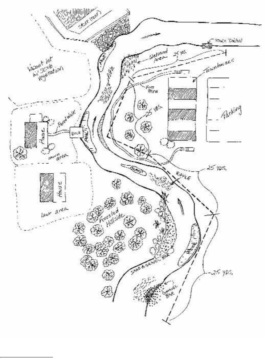
Figure 4.3

Example of stream sketch

Volunteers should note important stream features on their sketch including riffles and pools.

Select a 25-yard section of the site. You will be filling out your field data sheet for this section only. Mark the

section on the sketch. If you want to conduct multiple walks, choose another 25-yard section or move to an

entirely different location. Eve n though you will only be completing the data forms for the 25 yard reach, it is

important to sketch the full 100-yard section so that you can document the stream features surrounding the

evaluated reach.

TASK 3 Complete the top portion of your field data sheet

Include stream name, date, and county (or appropriate local designation) of your site, and describe its location as

precisely as possible. It is best to stand at or near a permanent marker such as a bridge, abutment, or road.

Remember, you or another volu nteer will be coming back to the same spot again and again, so be as specific as

you can. Some programs might ask you for the latitude and longitude of your location; others might ask for a map

reference number or other site identifier.

Latitude and longitude information is critical for mapping and for many data management programs. It is also

required if the data is to be entered in USEPA's STOrage and RETrieval System (STORET) or used in a

Geographical Information System (GIS).

An easy way to determine latitude and longitude is to use a global positioning system (GPS), a hand-held tool that

looks like a calculator. GPS units receive signals form orbiting satellites and then use the information from the

satellites to calculate th e lat/long coordinates of the user. In general, these tools are accurate up to 15 meters.

GPS units are relatively inexpensive and can be purchased from scientific supply houses and many camping or

outdoor stores. Many government agencies are using GPS an d might be able to loan a system to your program.

Latitude and longitude can also be calculated manually using a USGS topographical map and a ruler (See

Appendix C).

Step 3--Conduct the Stream Habitat Walk

Detailed instructions for performing the Stream Habitat Walk begin on page 48 of this section.

TASK 1 Complete the habitat characterization components of the walk for

the 25-yard section of stream: the "In-Stream Characteristics," "Stream

Bank and Channel Characteristics," and "Local Watershed

Characteristics" sections of the field data sheet

These elements involve making observations about the stream itself as well as the riparian zone and immediate

watershed.

TASK 2 Complete the "Visual Biological Survey" section of the field data

sheet

This involves simple visual observations of the presence or absence of wildlife and obvious aquatic life in the

stream, including fish, aquatic plants, and algae.

TASK 3 Complete the "Macroinverte-brate Survey" section of the field data

sheet

This is optional and serves as an introduction to the types of life that inhabit some of the microhabitats of the

stream the spaces under and on rocks and in and on twigs and leaves. To conduct this survey, you will need to

select the method(s) that best suits your stream. Use the rock-rubbing method in streams with riffles, or use the

stick-picking method if your stream does not have riffles. Clumps of submerged leaves may be present in either

type of stream and are often an important microhabitat for ma croinvertebrates. You may choose to sort through

these leaf packs in addition to rock-rubbing or stick-picking.

You will also need some specific equipment (a bucket, tweezers, picnic plate, etc.). Be sure to dress appropriately

because you'll probably get wet.

Remember to return the organisms to the stream when you finish the macroinvertebrate survey. Then, check to

make sure your field data sheet has been completed as fully as possible.

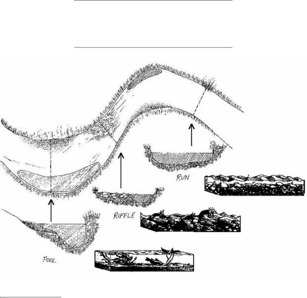
Step 4--Check data forms for completeness and return forms to program

coordinator

After completing the habitat characterization and biological survey, make sure you have completed the field data

sheet to the extent possible and that the recorded data are legible. If you are not able to determine how to answer a

question on the field da ta sheet, just leave the space blank. If you leave a space blank, indicate that it is because

you are not able to answer the question (e.g., write "not able to answer" or "does not apply" in the space).

Upon completion of the Stream Habitat Walk, present a copy of the field data sheet to your volunteer program

coordinator. You may want to keep a copy of the field data sheet, and other appropriate data, for your own

records and to evaluate any future disc repancies in the data. If you have identified an urgent problem, such as

leaking drums of chemicals, foul odors, or fish kills, contact your program coordinator or the agency with

whom you are working as soon as possible.

Instructions for completing the Stream Habitat Walk

data sheet

Figure 4.4

Overview and cross sections of a pool, riffle, and run

Varying flows and depths create a variety of habitats for macroinvertebrates.

For ease of use, the following numbered instructions correspond to the numbers on the field data sheet.

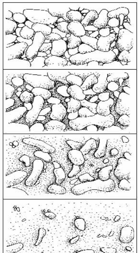
In-stream Characteristics

Pools, riffles, and runs. A mixture of flows and depth and provide a variety of habitats to support fish and

invertebrate life. Pools are deep with slow water. Riffles are shallow with fast, turbulent water running over

rocks. Runs are deep with fast water and little or no turbulence.

Stream bottom (substrate) is the material on the stream bottom. Identify what substrate types are present.

Substrate types include:

Silt/clay/mud. This substrate has a sticky, cohesive feeling. The particles are fine. The spaces

between the particles hold a lot of water, making the sediments behave like ooze.

❍

Sand (up to 0.1 inch). A sandy bottom is made up of tiny, gritty particles of rock that are smaller

than gravel but coarser than silt (gritty, up to ladybug size).

❍

Gravel (0.1-2 inches). A gravel bottom is made up of stones ranging from tiny quarter-inch pebbles

to rocks of about 2 inches (fine gravel - pea size to marble size; coarse gravel - marble to tennis ball

size).

❍

Cobbles (2-10 inches). Most rocks on this type of stream bottom are between 2 and 10 inches

(between a tennis ball and a basketball).

❍

Boulders (greater than 10 inches). Most of the rocks on the bottom are greater than 10 inches

(between a basketball and a car in size).

❍

Bedrock. This kind of stream bottom is solid rock (or rocks bigger than a car).❍

Embeddedness is the extent to which rocks (gravel,

cobbles, and boulders) are sunken into the silt, sand,

or mud of the stream bottom (Fig. 4.5). Generally,

the more rocks are embedded, the less rock surface

or space between rocks is available as habitat for

aquatic macroinvertebrates and for fish spawning.

Excessive silty runoff from erosion can increase a

stream's embedded-ness. To estimate

embeddedness, observe the amount of silt or finer

sediments overlying, in between, and surrounding

the rocks.

Presence of logs or woody debris (not twigs and

leaves) in stream can slow or divert water to

provide important fish habitat such as pools and

hiding places. Mark the box that describes the

general amount of woody debris in the stream.

Naturally occurring organic material in stream.

This material includes leaves and twigs. Mark the

box that describes the general amount of organic

matter in the stream.

Water appearance can be a physical indicator of

water pollution.

Clear - colorless, transparent

❍

Milky - cloudy-white or grey, not transparent;

might be natural or due to pollution

❍

Foamy - might be natural or due to pollution,

generally detergents or nutrients (foam that is

several inches high and does not brush apart

easily is generally due to some sort of

pollution)

❍

Turbid - cloudy brown due to suspended silt❍

Figure 4.5

A representation of a rocky-bottom stream becoming

embedded with sand and silt

As silt settles on the streambed, spaces between the rocks

are filled in and the stream becomes more embedded.

or organic material

Dark brown - might indicate that acids are

being released into the stream due to

decaying plants

❍

Oily sheen - multicolored reflection might

indicate oil floating in the stream, although

some sheens are natural

❍

Orange - might indicate acid drainage❍

Green - might indicate excess nutrients being

released into the stream

❍

Water odor can be a physical indicator of water pollution

No smell or a natural odor

❍

Sewage - might indicate the release of human waste material❍

Chlorine - might indicate over-chlorinated sewage treatment/water treatment plant or swimming

pool discharges

❍

Fishy - might indicate excessive algal growth or dead fish❍

Rotten eggs - might indicate sewage pollution (the presence of methane from anaerobic conditions)❍

Water temperature can be particularly important for determining the suitability of the stream as aquatic

habitat for some species of fish and macroinvertebrates that have distinct temperature requirements.

Temperature also has a direct effe ct on the amount of dissolved oxygen available to the aquatic organisms.

Measure temperature by submerging a thermometer for at least 2 minutes in a typical stream run. Repeat

once and average the results.

Stream Bank and Channel Characteristics

Depth of runs and pools should be determined by estimating the vertical distance from the surface to the

stream bottom at a representative depth at each of the two habitats.

The width of the stream channel can be determined by estimating the width of the streambed that is covered

by water from bank to bank. If it varies widely, estimate an average width.

10.

Stream velocity can have a direct influence on the health, variety, and abundance of aquatic communities. If

water flows too quickly, organisms might be unable to maintain their hold on rocks and vegetation and be

washed downstream; if wate r flows too slowly, it might provide insufficient aeration for species needing

high levels of dissolved oxygen. Stream velocity can be affected by dams, channelization, terrain, runoff,

and other factors. To measure stream velocity, mark off a 20-foot sec tion of stream run and measure the

time it takes a stick, leaf, or other floating biodegradable object to float the 20 feet. Repeat 3 times and pick

the average time. Divide the distance (20 feet) by the average time (seconds) to determine the velocity in

feet per second. (See Chapter 5, section 5.1 on flow for a more indepth discussion of using a float to

estimate velocity.

11.

The shape of the stream bank, the extent of artificial modifications, and the shape of the stream channel are

determined by standing at the downstream end of the 25-yard section and looking upstream.

The shape of the stream bank (Fig. 4.6) may include.

Vertical or undercut bank - a bank that rises vertically or overhangs the stream. This type of

bank generally provides good cover for macroinvertebrates and fish and is resistant to erosion.

However, if seriously undercut, it might be vulne rable to collapse.

■

Steeply sloping - a bank that slopes at more than a 30 degree angle. This type of bank is very

vulnerable to erosion.

■

Gradual sloping - a bank that has a slope of 30 degrees or less. This type of stream bank is

highly resistant to erosion, but does not provide much streamside cover.

■

●

Artificial bank modifications include all artificial structural changes to the stream bank such as riprap

(broken rock, cobbles, or boulders placed on earth surfaces such as the face of a dam or the bank of a

●

12.

Figure 4.6

Types of streambank shapes

Undercut banks provide good cover for fish and

macroinvertebrates.

stream, for protection against the action of

the water) and bulkheads. Determine the

approximate percentage of each bank (both

the left and right) that is artificially

covered by the placement of rocks, wood,

or concrete.

The shape of the stream channel can be

described as narrow (less than 6 feet wide

from bank to bank), wide (more than 6 feet

from bank to bank), shallow (less than 3

feet deep from the stream substrate to the

top of the banks) or deep (more than 3 feet

from the stream substrate to the top of the

banks). Choose the category that best

describes the channel.

●

Narrow, deep●

Narrow, shallow●

Wide, deep●

Wide, shallow●

Streamside cover information helps determine

the quality and extent of the stream's riparian

zone. This information is important at the stream

bank itself and for a distance away from the

stream bank. For example, trees, bushes, and tall

gr ass can contribute shade and cover for fish and

wildlife and can provide the stream with needed

organic material such as leaves and twigs. Lawns

indicate that the stream's riparian zone has been

altered, that pesticides and grass clippings are a

possible problem, and that little habitat and

shading are available. Bare soil and pavement

might indicate problems with erosion and runoff.

Looking upstream, provide this information for

the left and right banks of the stream.

13.

Evergreen trees (conifers) - cone-bearing trees that do not lose their leaves in winter.

●

Hardwood trees (deciduous) - in general, trees that shed their leaves at the end of the growing season.●

Bushes, shrubs - conifers or deciduous bushes less than 15 feet high.●

Tall grass, ferns, etc. - includes tall natural grasses, ferns, vines, and mosses.●

Lawn - cultivated and maintained short grass.●

Boulders - rocks larger than 10 inches.●

Gravel/cobbles/sand - rocks smaller than 10 inches; sand.●

Bare soil●

Pavement, structure - any structures or paved areas, including paths, roads, bridges, houses, etc.●

Stream shading is a measurement of the extent to which the stream itself is overhung and shaded by the

cover identified in 13 above. This shade (or overhead canopy) provides several important functions in the

stream habitat. The canopy cool s the water; offers habitat, protection, and refuge for aquatic organisms;

and provides a direct source of beneficial organic matter and insects to the stream. Determine the extent to

which vegetation shades the stream at your site.

14.

General conditions of the stream bank and stream channel, and other conditions that might be affecting the

stream are determined by standing at the downstream end of the 25-yard site and looking upstream. Provide

observations for the right and left banks of the stream.

15.

Stream bank conditions that might be affecting the stream.

Natural plant cover degraded. Note whether streamside vegetation is trampled or missing or has

been replaced by landscaping, cultivation, or pavement. (These conditions could lead to erosion.)

❍

Banks collapsed/eroded. Note whether banks or parts of banks have been washed away or worn

down. (These conditions could limit habitats in the area.)

❍

Garbage/junk adjacent to the stream. Note the presence of litter, tires, appliances, car bodies,

shopping carts, and garbage dumps.

❍

Foam or sheen on bank. Note whether there is foam or an oily sheen on the stream bank. Sheen may

indicate an oil spill or leak, and foam may indicate the presence of detergent.

❍

●

Stream channel conditions that might be affecting the stream.

Mud/silt/sand on bottom/entering stream. Excessive mud or silt can interfere with the ability of fish

to sight potential prey. It can clog fish gills and smother fish eggs in spawning areas in the stream

bottom. It can be an indication of p oor construction practices, urban area runoff, silviculture

(forestry-related activities), or agriculture in the watershed. It can also be a normal condition,

especially in a slow-moving, muddy-bottom stream.

❍

Garbage or junk in stream. Note the presence of litter, tires, appliances, car bodies, shopping carts,

and garbage.

❍

●

Other general conditions that might be affecting the stream.

Yard waste (e.g., grass clippings) - is there evidence that grass clippings, cut branches, and other

types of yard waste have been dumped into the stream?

❍

Livestock in or with unrestricted access to stream - are livestock present, or is there an obvious path

that livestock use to get to the water from adjacent fields? Is there streamside degradation caused by

livestock?

❍

Actively discharging pipes - are there pipes with visible openings discharging fluids or water into the

stream? Note such pipes even though you may not be able to tell where they come from or what they

are discharging.

❍

Other pipes - are there pipes near or entering the stream? Note such pipes even if you cannot find an

opening or see matter being discharged.

❍

Ditches - are there ditches, draining the surrounding land and leading into the stream?❍

Local watershed characteristics

Adjacent land uses can potentially have a great impact on the quality and state of the stream and

riparian areas. Determine the land uses, based on your own judgment of the activities in the

watershed surrounding your site within a quarter of a mile. Enter a "1" if a land use is present and a

"2" if it is clearly having a negative impact on the stream.

16.

Visual biological survey

Wildlife in the stream area might indicate it is of sufficient quality to support animals with food,

water, and habitat. Look for signs of frogs, turtles, snakes, ducks, deer, beaver, etc.

17.

Are fish present in the stream? Fish can indicate that the stream is of sufficient quality for other

organisms. Indicate the average size and note any visible barriers to the movement of fish in the

stream obstructions that would keep fish from moving freely upstream or downstream.

18.

Aquatic plants provide food and cover for aquatic organisms. Plants also might provide very general

indications of stream quality. For example, streams that are overgrown with plants could be over

enriched by nutrients. Streams devoid of pl ants could be affected by extreme acidity or toxic

pollutants. Aquatic plants may also be an indicator of stream velocity because plants cannot take root

in fast-flowing streams.

19.

Algae are simple plants that do not grow true roots, stems, or leaves and that mainly live in water,

providing food for the food chain. Algae may grow on rocks, twigs, or other submerged materials, or

20.

●

float on the surface of the water. The algae naturally occurs in green and brown colors. Excessive

algal growth may indicate excessive nutrients (organic matter or a pollutant such as fertilizer) in the

stream.

Macroinvertebrate survey (optional)

Macroinvertebrates are organisms that lack a backbone and can be seen with the naked eye such as

clams, mussels, snails, worms, crayfish, and larval insects. To locate macroinvertebrates in the

stream, use one or more of the following metho ds.

Rock-rubbing method. (Use this method in streams with riffle areas and rocky bottoms.)

Remove several rocks from within a riffle area of your stream site (e.g., randomly pick

1 rock from each side of the stream, 1 rock from the middle, and 1 rock from in

between). Try to choose rocks that are submerged during normal flow conditions. Each

rock should be about 4-6 inches in diameter and should be easily moved (not

embedded).

■

Either inspect the rock's surface for any living organisms or place the rock in a

light-colored bucket or shallow pan, add some stream water, and brush the rock with a

soft brush or your hands. Try to dislodge the foreign particles from the rock's surface.

Also look for clumps of gravel or leaves stuck to the rock. These clumps may be

caddisfly houses and should be dislodged as well.

■

●

Stick-picking method. (Use this method in streams without riffles or without a rock bottom.)

Collect several sticks (approximately 1 inch in diameter and relatively short) from

inside the stream site, and place then in a bucket filled with stream water. Select

partially decomposed objects that have soft, pulpy wood and a lot of crevices a nd are

found in the flowing water, not buried in the bottom. Pick the loose bark from the sticks

to find organisms.

■

Fill the shallow pan with water from the stream and remove one of the sticks from the

bucket. Examine the stick making sure you hold it over the pan so no organisms are

lost. Remember that the organisms will have sought shelter, and they could be hiding in

loose bark or crevices. After examining the sticks, it might be helpful to break up the

woody material. Examine each stick carefully. Using tweezers or a soft brush, carefully

remove anything that resembles a living organism and place it in the pan. Also examine

the bucket contents for anything that has fallen off the sticks.

■

●

Leaf pack-sorting method. (This method can be used in streams with or without a rock

bottom.)

Remove several handfuls of submerged leaves from the stream and place them into a

bucket. Remove the leaves one at a time and look closely for the presence of insects.

Using tweezers or soft brush, carefully remove anything that resembles a living

organism and place it in a pan containing stream water. Also examine the bucket

contents to see if anything has fallen off the leaves.

■

●

21.

Note whether you have found any macroinvertebrates using one of the above methods.22.

After collecting macroinvertebrates using any of the above methods, examine the types of organisms

by gross morphological features (e.g., snails or worm-like). Use a magnifying glass to observe the

organisms in water so you can clearly see the leg s, gills, and tails. Note the relative abundance of

each type on the field data sheet. When finished, return all the organisms to the stream.

Many types of macroinvertebrates can be found in a healthy stream. Because different species can

tolerate different levels of pollution, observing the variety and abundance of macroinvertebrates can

give you a sense of the stream's health. For exam ple, if pollution tolerant organisms are plentiful and

pollution intolerant ones are found only occasionally, this might indicate a problem in the stream.

Types of organisms you find may include:

Worm-like organisms (like worms and leeches) either adhere to rocks or sticks or move

slowly. They are generally tolerant of pollution.

■

23.

Crayfish look like lobsters or shrimp. They are generally somewhat tolerant of pollution.■ 
Snail-like organisms include snails and clam-like organisms. They range from somewhat
tolerant of pollution to somewhat intolerant.
■ 
Insects include a wide variety of organisms that generally have distinct legs, head, bodies, and
tails and often move quickly over rocks or sticks. They come in many sizes and shapes as well
as a wide range of pollution-tolerance levels.
■ 
When finished, return all organisms to the stream.
Stream Habitat Walk (PDF, 137.0 KB)
Adobe Acrobat Reader is required to view PDF documents. The most recent version of the Adobe Acrobat Reader is
available as a free download. An Adobe Acrobat plug-in for assisted technologies is also available.
< Previous · Table of Contents · Next >
Office of Wetlands, Oceans & Watersheds Home
Watershed Protection Home | Monitoring Water Quality Home
EPA Home | Office of Water | Search | Comments

4.2

Streamside Biosurvey

The Streamside Biosurvey is based on the simple macroinvertebrate sampling approach developed and used by the Ohio

Department of Natural Resources and the Izaak Walton League of America's Save Our Streams program and adapted by many

volunteer monitoring programs throughout the United States.

This assessment approach has two basic components. The first is a biosurvey of aquatic organisms that involves collecting and

identifying macroinvertebrates in the field and calculating an index of stream quality. The second is the habitat

characterization method known as the Streamside Biosurvey Habitat Walk.

Two methods of macroinvertebrate sampling are detailed in this section one for rocky-bottom streams (using a kick net) and

one for muddy-bottom streams (using a dip net). Figure 4.7 illustrates and describes the nets used for these assessments. Both

of these aquatic organism collection procedures have been widely tested and used successfully by many groups. You should

consult with a local aquatic scientist to determine which method is appropriate for streams in your area.

Note

The Streamside Biosurvey is based on protocols

developed and widely used by programs such as

the Ohio Department of Natural Resources, the

Izaak Walton League of America, and others. This

manual recommends some modifications to their

established protocols. These include:

A finer mesh size for the kick and dip nets

used to sample for macroinvertebrates

●

In rocky-bottom streams, compositing three

samples into one before identifying

macroinvertebrates rather than identifying

macroinvertebrates in three separate

samples and choosing the best result.

Compositing generally provides a more

representative sample of the

macroinvertebrate community than a

discrete sample taken from one part of the

riffle. Riffle areas have what is known as a

patchy distribution of organisms, meaning

that different types of organisms are

naturally found in different parts of the

riffle. In order to more accurately assess the

macroinvertebrate community in a

rocky-bottom stream site, it is important to

take a representative sample that includes

organisms found in different

microhabitats—such as in different parts of

the riffle or in riffles of various flows and

depths.

●

A new method for calculating the stream

quality rating. This modification

incorporates a weighting factor to take into

account the abundance of organisms in each

●

Like the Stream Habitat Walk described in Section 4.1, the Streamside

Biosurvey is useful as a screening tool to identify water quality problems

and as an educational tool to teach volunteers about pollution and stream

ecology. But instead of randomly picking up rocks or sticks and

brushing off macroinvertebrates for simple observation purposes,

Streamside Bio-survey volunteers are trained to use special nets and

standardized sampling protocols to collect organisms from a measured

area of stream habitat. Volunteers identify collected organisms, usually

to the order level, and sort them into taxonomic groups based on their

ability to tolerate pollution. Using this information, volunteers can then

calculate a simple stream quality rating of good, fair, or poor.

Because the Streamside Biosurvey involves a standardized sampling

protocol, a basic level of training, professional assistance, and a simple

stream rating based on macroinvertebrate diversity and abundance, this

approach is more effective than the Stream Habitat Walk in

characterizing stream health and determining general water quality

trends over several years. However, this method is not generally suited

to determining subtle pollution impacts due, in part, to its uncomplicated

level of macroinvertebrate identification and analysis. This, of course, is

also one of the Streamside Biosurvey's greatest strengths, since

volunteers can be easily trained in its methods.

Key features of the Streamside Biosurvey are as follows:

It includes the Streamside Biosurvey Habitat Walk as its physical

habitat characterization and visual biological characterization

components. This protocol is a somewhat more detailed version of

the Stream Habitat Walk described in Section 4.1.

●

It centers around a macroinvertebrate survey in which organisms

are collected according to specific protocols, identified in the field

(generally to taxonomic order), and are then released back into the

stream.

●

For the identification process, volunteers group

macroinvertebrates into three categories based on their pollution

tolerance or sensitivity. Volunteers then calculate a water quality

index by counting the specimens in each sensitivity category and

●

pollution tolerance category

(pollution-sensitive, somewhat tolerant, and

tolerant).

In muddy-bottom streams, varying how

much each habitat type is sampled

depending on its abundance at the sampling

site.

●

determining whether they are rare, common, or dominant;

multiplying the number of taxa in each category by a weighting

factor; adding all the scores; and comparing results to a water

quality rating scale that has been determined by a locally

knowledgeable biologist/ecologist.

The Streamside Biosurvey requires some equipment and training.

Training can be conducted at the stream site, although some

advance preparation is required. For example, a biologist with

regional experience should assist in developing the

macroinvertebrate key and the tolerance category groupings on

the field data sheets. A reference collection is recommended to

help volunteers identify macroinvertebrates.

●

Step 1 Prepare for the Streamside Biosurvey field work

Much of the preparation work for this approach is similar to that of the Stream Habitat Walk (section 4.1). Refer back to that

section for relevant information on the following tasks:

Scheduling the biosurvey

●

Obtaining a USGS topographical map●

Selecting and marking monitoring locations●

Becoming familiar with safety procedures●

TASK 1 Gather tools and equipment for the Streamside Biosurvey

In addition to the basic equipment listed in Section 2.4, you should collect the following equipment needed for the

macroinvertebrate collection of the Streamside Biosurvey:

Vial with tight cap filled about one-half full with 70 percent ethyl alcohol

●

Buckets (2)●

Hand lens, magnifying glass, or field microscope●

Tweezers, eyedropper, or spoon●

Plastic bag●

Large, shallow, white pans, such as dishpans (2)●

Spray water bottle●

Plastic ice cube tray●

Taxonomic key to aquatic organisms●

Calculator●

For rocky-bottom streams--Kick net, a fine mesh (500 µm) nylon net approximately 3x3 feet with a 3-foot long

supporting pole on each side is recommended--Figure 4.7).

●

For muddy-bottom streams--D-frame net (a dip net with a frame 12 inches wide with a fine nylon mesh, usually about

500 µm, attached to the frame).

●

Step 2 Collect and Sort Macroinvertebrates

The method you use to collect macroinvertebrates using this approach depends on the type of stream you are sampling.

Rocky-bottom streams are defined as those with bottoms made up of gravel, cobbles, and boulders in any combination and

usually have definite riffle areas. Riffle areas are fairly well oxygenated and, therefore, are prime habitats for benthic

macroinvertebrates. In these streams, use the rocky-bottom sampling method.

Muddy-bottom streams have muddy, silty, or sandy bottoms and lack riffles. Generally, these are slow moving, low-gradient

streams (i.e., streams that flow along relatively flat terrain). In such streams, macroinvertebrates generally attach themselves to

overhanging plants, roots, logs, submerged vegetation, and stream substrate where organic particles are trapped. In these

streams, use the muddy-bottom sampling method.

Both methods are detailed below. Regardless of which collection method is used, the process for counting, identifying, and

analyzing the macroinvertebrate sample for the Streamside Biosurvey is the same.

Rocky-Bottom Sampling Method

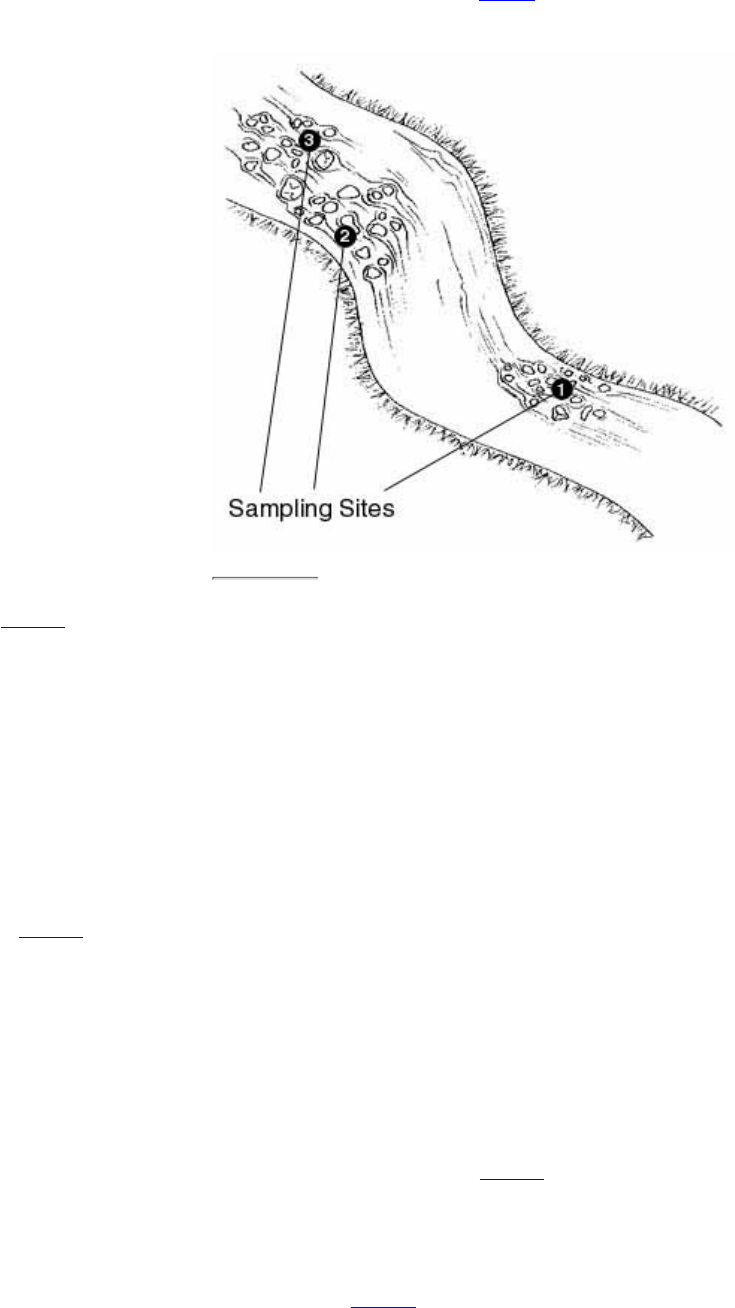
Use the following method of macroinvertebrate sampling in streams that have riffles and gravel/cobble substrates. You will

collect three samples at each site and composite (combine) them to obtain one large total sample.

TASK 1 Identify the sampling location

You should have already located your site on a map along with its latitude and longitude (see Task 3, in Section 4.1 - Stream

Habitat Walk).

Figure 4.8

Location of sample sites in a rocky-bottom stream with riffles

Within a 100 yard reach volunteers begin their sampling at the most

downstream site and then work their way upstream.

You are going to sample in three different spots

within a 100-yard stream reach. These spots may be

three separate riffles; one large riffle with different

current velocities; or, if no riffles are present, three

run areas with gravel or cobble substrate.

Combinations are also possible (if, for example, your

site has only one small riffle and several run areas).

Mark off your 100-yard stream reach. If possible, it

should begin at least 50 yards upstream of any

human-made modification of the channel, such as a

bridge, dam, or pipeline crossing, Avoid walking in

the stream, since this might dislodge

macroinvertebrates and alter your sampling results.

Sketch the 100-yard sampling area. Indicate the

location of your three sampling spots on the sketch.

Mark the most downstream site as Site 1, the middle

site as Site 2, and the upstream site as Site 3. (See

Fig. 4.8.)

TASK 2 Get into place

Always approach your sampling locations from the

downstream end and sample the site farthest

downstream first (Site 1) (see Fig. 4.9, Panel #1).

This minimizes the possibility of biasing your second

and third collections with dislodged sediment or

macroinvertebrates.

Always use a clean kick net, relatively free of mud

and debris from previous uses. Fill a bucket about

one third full with stream water and fill your spray

bottle.

Select a 3-foot by 3-foot riffle area for sampling at

Site 1. One member of the team, the net holder,

should position the net at the downstream end of this

sampling area. Hold the net handles at a 45 degree

angle to the water's surface (see Fig. 4.9, Panel #2).

Be sure that the bottom of the net fits tightly against

the stream-bed so no macroinvertebrates escape

under the net. You may use rocks from the sampling

area to anchor the net against the stream bottom.

Don't allow any water to flow over the net.

TASK 3 Dislodge the macroinvertebrates

Pick up any large rocks in the 3-foot by 3-foot sampling area and rub them thoroughly over the partially-filled bucket so

that any macroinvertebrates clinging to the rocks will be dislodged into the bucket (see Fig. 4.9, Panel #3). Then place

each cleaned rock outside of the sampling area. After sampling is completed, rocks can be returned to the stretch of

stream they came from.

The member of the team designated as the "kicker" should thoroughly stir up the sampling area with their feet, starting

at the upstream edge of the 3-foot by 3-foot sampling area and working downstream, moving toward the net. All

dislodged organisms will be carried by the stream flow into the net (see Fig. 4.9, Panel #4). Be sure to disturb the first

few inches of stream sediment to dislodge burrowing organisms. As a guide, disturb the sampling area for about 3

minutes, or until the area is thoroughly worked over.

Any large rocks used to anchor the net should be thoroughly rubbed into the bucket as above.3.

TASK 4 Remove the net

Next, remove the net without allowing any of the organisms it contains to wash away. While the net holder grabs the top

of the net handles, the kicker grabs the bottom of the net handles and the net's bottom edge. Remove the net from the

stream with a forward scooping motion (see Fig. 4.9, Panel #5).

Roll the kick net into a cylinder shape and place it vertically in the partially filled bucket. Pour or spray water down the

net to flush its contents into the bucket (see Fig. 4.9, Panel #6). If necessary, pick debris and organisms from the net by

hand. Release back into the stream any fish, amphibians, or reptiles caught in the net.

TASK 5 Collect the second and third samples

Once you have removed all the organisms from the net repeat these tasks at Sites 2 and 3. Put the samples from all three sites

into the same bucket. Combining the debris and organisms from all three sites into the same bucket is called compositing.

Hint: If your bucket is nearly full of water after you have washed the net clean, let the debris and organisms settle to the

bottom of the bucket. Then cup the net over the bucket and pour the water through the net into a second bucket. Inspect the

water in the second bucket to be sure no organisms came through.

TASK 6 Sort macroinvertebrates

Pour the contents of the bucket into a large, shallow, white pan. Add some stream water to the pan, and fill the ice cube tray

with stream water. Using tweezers, eye dropper, or spoon, pick through the leaf litter and organic material looking for

anything that swims, crawls, or seems to be hiding in a shell, like a snail. Look carefully; many of these creatures are quite

small and fast-swimming. Sort similar organisms into the ice cube tray.

Note: Instructions for counting, identifying, and analyzing the macroinvertebrate sample follow the muddy-bottom sampling

method. (See Step 3)

Muddy-Bottom Sampling Method

Picking Bugs

Some monitoring programs find it easier to collect

organisms from the net by hand-picking them

rather than washing the sample into a pan and then

trying to pick through the floating debris. The

advantage to placing the organisms in a pan is that

they are more likely to survive while in the pan

and their characteristic movements will help in

organism identification.

If you prefer to pick bugs directly off the net, a

white background, such as a white plastic trash

bag under the net, will help you see the bugs more

clearly. In addition, periodically wetting the net

with a water bottle will help keep the bugs alive

and moving.

Identification can be made easier if you sort the

organisms into groups based on physical

similarities and place them together in sections of

an ice cube tray as you pick them from the pan or

net.

In muddy-bottom streams, as in rocky- bottom streams, the goal is to

sample the most productive habitats available and look for the widest

variety of organisms. The most productive habitats are the ones that

harbor a diverse population of pollution sensitive-macroinvertebrates.

Volunteers should sample by using a D-frame net to jab at the habitat

and scoop up the organisms that are dislodged. The objective is to

collect a combined sample from 20 jabs taken from a variety of habitats.

TASK 1 Determine which habitats are present

Muddy-bottom streams usually have four habitats (Fig. 4.10). It is

generally best to concentrate sampling efforts on the most productive

habitat available, yet to sample other principal habitats if they are

present. This ensures that you will secure as wide a variety of organisms

as possible. Not all habitats are present in all streams or present in

significant amounts. If your sampling areas have not been preselected,

try to determine which of the following habitats are present. (Avoid

standing in the stream while making your habitat determinations.)

Vegetated bank margins. This habitat consists of overhanging

bank vegetation and submerged root mats attached to banks. The

bank margins may also contain submerged, decomposing leaf

packs trapped in root wads or lining the streambanks. This is

generally a highly productive habitat in a muddy_bottom stream,

and it is often the most abundant type of habitat.

●

Snags and logs. This habitat consists of submerged wood,●

Figure 4.10

Four habitats found in muddy-bottom streams

Volunteers will likely find the most macroinvertebrates in

vegetated habitats and snags and logs.

primarily dead trees, logs, branches, roots, cypress knees and leaf

packs lodged between rocks or logs. This is also a very productive

muddy-bottom stream habitat.

Aquatic vegetation beds and decaying organic matter. This

habitat consists of beds of submerged, green/leafy plants that are

attached to the stream bottom. This habitat can be as productive as

vegetated bank margins, and snags and logs.

●

Silt/sand/gravel substrate. This habitat includes sandy, silty, or

muddy stream bottoms; rocks along the stream bottom; and/or

wetted gravel bars. This habitat may also contains algae-covered

rocks (sometimes called Aufwuchs). This is the least productive

of the four muddy-bottom stream habitats, and it is always present

in one form or another (e.g., silt, sand, mud, or gravel might

predominate).

●

TASK 2 Determine how many times to jab in each habitat type

Your goal is to jab a total of 20 times. The D-frame net is 1 foot wide, and a jab should be approximately 1 foot in length.

Thus, 20 jabs equals 20 square feet of combined habitat.

If all four habitats are present in plentiful amounts, jab the vegetated banks 10 times and divide the remaining 10 jabs

among the remaining 3 habitats.

●

If three habitats are present in plentiful amounts and one is absent, jab the silt/sand/gravel substrate the least productive

habitat 5 times and divide the remaining 15 jabs among the other two more productive habitats.

●

If only two habitats are present in plentiful amounts, the silt/sand/gravel substrate will most likely be one of those

habitats. Jab the silt/sand/gravel substrate 5 times and the more productive habitat 15 times.

●

If some habitats are plentiful and others are sparse, sample the sparse habitats to the extent possible, even if you can

take only one or two jabs. Take the remaining jabs from the plentiful habitat(s). This rule also applies if you cannot

reach a habitat because of unsafe stream conditions. Jab a total of 20 times.

●

Because you might need to make an educated guess to decide how many jabs to take in each habitat type, it is critical that you

note, on the field data sheet, how many jabs you took in each habitat. This information can be used to help characterize your

findings.

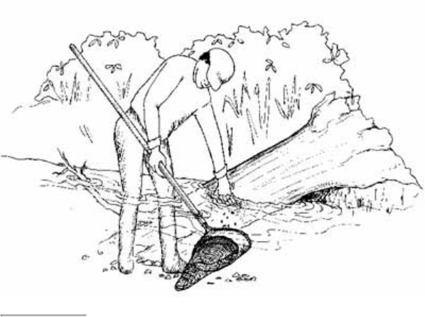
TASK 3 Get into place

Outside and downstream of your first sampling location (1st habitat), rinse the dip net and check to make sure it does not

contain any macroinvertebrates or debris from the last time it was used. Fill a bucket approximately one-third full with clean

stream water. Also, fill the spray bottle with clean stream water. This bottle will be used to wash down the net between jabs

and after sampling is completed.

This method of sampling requires only one person to disturb the stream habitats. While one person is sampling, a second

person should stand outside the sampling area, holding the bucket and spray bottle. After every few jabs, the sampler should

hand the net to the second person, who then can rinse the contents of the net into the bucket.

TASK 4 Dislodge the macroinvertebrates

Approach the first sample site from downstream, and sample as you walk upstream. Here is how to sample in the four habitat

types:

Sample vegetated bank margins by jabbing vigorously, with an upward motion, brushing the net against vegetation and

roots along the bank. The entire jab motion should occur underwater.

Figure 4.11

Collecting a sample from a log

Volunteer rubs the log with one hand and catches dislodged organisms and other

material in the net.

●

To sample snags and logs, hold the net with

one hand under the section of submerged

wood you are sampling. With the other hand

(which should be gloved), rub about 1

square foot of area on the snag or log. Scoop

organisms, bark, twigs, or other organic

matter you dislodge into your net. Each

combination of log rubbing and net

scooping is one jab (Fig. 4.11).

●

To sample aquatic vegetation beds, jab

vigorously, with an upward motion, against

or through the plant bed. The entire jab

motion should occur underwater.

●

To sample a silt/sand/gravel substrate, place

the net with one edge against the stream

bottom and push it forward about a foot (in

an upstream direction) to dislodge the first

few inches of silt, sand, gravel, or rocks. To

avoid gathering a netful of mud, periodically

sweep the mesh bottom of the net back and

forth in the water, making sure that water

does not run over the top of the net. This

will allow fine silt to rinse out of the net.

●

When you have completed all 20 jabs, rinse the net thoroughly into the bucket. If necessary, pick any clinging organisms from

the net by hand and put them in the bucket.

TASK 5 Sort the macroinvertebrates

Pour the contents of the bucket (water, organisms, and organic material) into a large, shallow, white pan and fill the ice cube

tray with clean stream water. Using tweezers, eye dropper, or spoon, pick through the leaf litter and organic material looking

for anything that swims, crawls, or seems to be hiding in a shell (like a snail). Look carefully; many of these creatures are

quite small and fast-swimming. Sort similar organisms into the plastic ice cube tray.

Step 3 Identify Macroinverte-brates and Calculate Stream Rating

The following methods are used for both the rocky- and muddy-bottom assessments.

Task 1 Identify Macroinvertebrates

Identify the collected macroinvertebrates. Using the hand lens or magnifying glass and the aquatic organism

identification key, carefully observe the collected macroinvertebrates. Refine your initial sort so that like individuals are

placed in the same section(s) of the ice cube tray. If you cannot identify an organism, place one or two specimens in the

alcohol-filled vial and forward it to your program coordinator for identification.

On your field data sheet, note the number of individuals of each type of organism you have identified (Section 3 of the

field data sheet See Fig. 4.12.).

Note: When you feel that you have identified all the organisms to the best of your ability, return the macroinvertebrates

to the stream.

Assign one of the following abundance codes to each type of organism. Record the code next to the actual count on the

field data sheet.

R (rare) = if 1-9 organisms are found in the sample

C (common) = if 10-99 organisms are found in the sample

D (dominant) = if 100 or more organisms are found in the sample

Your field data sheet should be organized to help you sort macroinvertebrates into three groups based on their ability to

tolerate pollution. A local authority (such as a state biologist or entomologist) should determine which organisms belong

in each pollution tolerance category for your region.

Generally, the three tolerance groups are as follows:

Group I (sensitive organisms) includes pollution- sensitive organisms such as mayflies, stoneflies, and non net-spinning

caddisflies, which are typically found in good-quality water.

●

Group II (somewhat sensitive organisms) includes somewhat pollution-tolerant organisms such as net-spinning

caddisflies, crayfish, sowbugs, and clams, found in fair-quality water.

●

Group III (tolerant organisms) includes pollution-tolerant organisms such as worms, leeches, and midges, found in

poor-quality water.

●

TASK 2 Calculate the stream quality rating

The stream water quality rating takes into account the pollution sensitivity of the organisms and their relative abundance. This

is accomplished through use of a weighting system.

The weighting system acknowledges the most desirable combinations of pollution sensitivity and abundance by assigning

these extra weights within a 5, 3, and 1 point scale. Pollution-sensitive organisms receive a weighting factor based on a 5-point

scale. Somewhat sensitive organisms are weighted on a 3-point scale, and tolerant organisms are weighted on a 1-point scale.

As can be seen in Table 4.2, a sample's ideal combination of organisms would be "sensitive" and "somewhat sensitive"

organisms in common abundance (10-99 organisms), and pollution "tolerant" organisms in rare abundance (less than 10

organisms). This is because it is never ideal for any given type of organism to dominate a sample, and because it is best to

have a wide variety of organisms including a few pollution-tolerant individuals.

Add the number of R's, C's and D's in each of the 3 pollution tolerance groupings. Then, for each grouping, multiply the

total number of R's, C's and D's by the relevant weighting factor. Table 4.3 illustrates sample calculations for

determining the water quality rating for (hypothetical) Volunteer Creek.

Note: The tolerance category groupings shown on the Biosurvey Data Sheet were developed for streams in the

mid-Atlantic (Maryland, Virginia, West Virginia, District of Columbia, Pennsylvania). These groupings may not totally

apply in other regions of the United States. It is important that a local aquatic biologist take a look at these

categories and make any changes necessary for your region.

In addition, depending on the level of taxonomic training volunteers receive, you might consider separating out some

other families of organisms. For instance, the tolerance groupings given here separate caddisflies into net-spinning and

non net-spinning families. Mayflies might also be separated into different tolerance groupings. It is not recommended

here, however, because of the difficulty in distinguishing mayfly families in the field without a microscope.

Some volunteer programs, like the one coordinated by the Audubon Naturalist Society in Maryland, conduct intensive

field identification training workshops and teach volunteers to distinguish several families in the field. Creating more

specific tolerance groupings may be an option for your program if you have the resources and expertise to conduct more

intensive taxonomic field training.

To obtain a water quality rating for the site, total the values for each group and add them together. The total score for

the sample stream site is: 16.2 (Group I) + 19.0 (Group II) + 2.3 (Group III) = 37.5.

The final step is to compare the score to water quality ratings (good to poor) established by a trained biologist familiar

with local stream fauna. Table 4.4 presents a tentative rating scale for streams in Maryland. Assuming Volunteer Creek

is located in Maryland, the stream would receive a rating of "Fair."

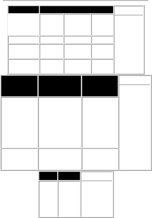
Note: In addition to adjusting the rating scale according to regional location, it might also need to be adjusted for

muddy-bottom vs. rocky-bottom streams. An experienced stream biologist can calculate the best rating system for your

area's streams by examining data from several streams.

Abundance Weighting Factor Table 4.2

Weighting

factors

used in

calculating

stream

water

quality

ratings

Group I

Sensitive

Group II

Somewhat

Sensitive

Group

III

Tolerant

Rare (R) 5.0 3.2 1.2

Common

Dominant

(D) 5.3 3.0 1.0

Group I

Sensitive

Group II

Somewhat

Sensitive Tolerant Table 4.3

Sample

calculations

of index

values for

Volunteer

Creek

1 (No. of R's)

x 5.0 = 5.0

2 (No. of C's)

x 5.6 = 11.2

3 (No. of R's) x

3.2 = 9.6

1 (No. of C's) x

3.4 = 3.4

2 (No. of D's) x

3.0 = 6.0

1 (No. of R's)

x 1.2 = 1.2

1 (No of C's)

x 1.1 = 1.1

Index Value

for Group I =

16.2

Index Value for

Group II = 19.20

Index Value

for Group III

= 2.3

Score Rating Table 4.4

Tentative

rating scale

for streams

Maryland

>40

20-40

<20

Good

Fair

Poor

In a healthy stream, the sensitive (Group I) organisms will be well represented in a sample. It is important to remember

that macroinvertebrate populations can fluctuate seasonally and that these natural fluctuations can affect your results.

Therefore, it is best to compare the results by season from year to year. (Compare your spring sampling results to each

other, not to fall results.)

Step 4 Conduct the Streamside Biosurvey: Habitat Walk

You will conduct a habitat assessment (which will include measuring general characteristics and local land use) in a

100-yard section of stream that includes the riffles from which organisms were collected.

TASK 1 Delineate the habitat assessment boundaries

Begin by identifying the most downstream riffle that was sampled for macroinvertebrates. Using your tape

measure or twine, mark off a 100-yard section extending 25 yards below the downstream riffle and about 75

yards upstream.

Complete the identifying information on your field data sheet for your habitat assessment site. On your stream

sketch, be as detailed as possible, and be sure to note which riffles were sampled.

TASK 2 Complete the Physical Characteristics, Local Watershed

Characteristics, and Visual Biological Survey sections of the field sheet

For safety reasons as well as to protect the stream habitat, it is best to estimate these characteristics rather than actually

wading into the stream to measure them.

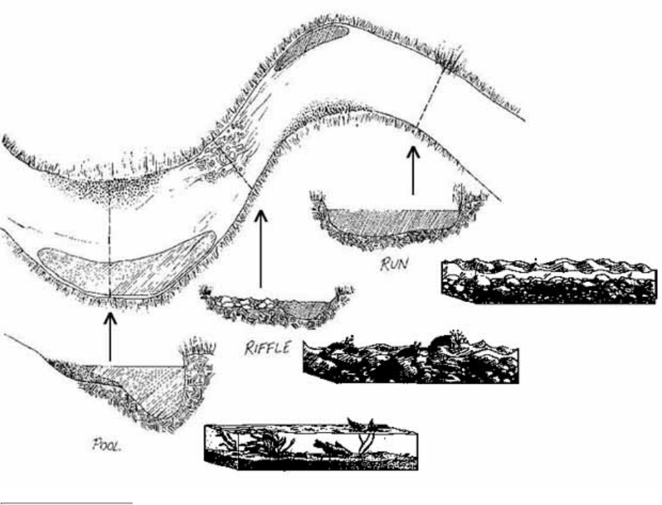
In-stream Characteristics

Figure 4.13

Overview and cross sections of a pool, riffle, and run

Varying flows and depths create a variety of habitats for macroinvertebrates.

Pools,

riffles,

and

runs

create

mixture

flows

and

depths

and

provide

variety

habitats

support

fish

and

invertebrate

life.

Pools

are

deep

with

slow

water.

Riffles

are

shallow

with

fast,

turbulent

water

running

over

rocks.

Runs

are

deep

with

fast

water

and

little

turbulence.

Stream bottom (substrate) is the material on the stream bottom. Identify what substrate types are present.

Substrate types include:

Silt/clay/mud--This substrate has a sticky, cohesive feeling. The particles are fine. The spaces between the

particles hold a lot of water, making the sediments behave like ooze.

■

Sand (up to 0.1 inch)--A sandy bottom is made up of tiny, gritty particles of rock that are smaller than

gravel but coarser than silt (gritty, up to pea size).

■

Gravel (0.1-2 inches)--A gravel bottom is made up of stones ranging from tiny quarter-inch pebbles to

rocks of about 2 inches (fine gravel - pea size to marble size; coarse gravel - marble to tennis ball size).

■

Cobbles (2-10 inches)--Most rocks on this type of stream bottom are between 2 and 10 inches (between a

tennis ball and a basketball).

■

Boulders (greater than 10 inches)--Most of the rocks on the bottom are greater than 10 inches (between a

basketball and a car in size).

■

Bedrock--is solid rock (or rocks bigger than a car).■

Estimate the percentage of substrate types at your site.

Embeddedness is the extent to which rocks (gravel,

cobbles, and boulders) are sunken into the silt, sand, or

mud of the stream bottom (Fig. 4.14). Generally, the more

rocks are embedded, the less rock surface or space

between rocks is available as habitat for aquatic

macroinvertebrates and for fish spawning. Excessive silty

runoff from erosion can increase the embeddedness in a

stream. To estimate the embeddedness, observe the

amount of silt or finer sediments overlying, in between,

and surrounding the rocks.

Streambed stability can provide additional clues to the

amount of siltation in a stream. When you walk in the

stream, note whether your feet sink significantly into sand

or mud.

Presence of logs or woody debris (not twigs and leaves) in

stream can slow or divert water to provide important fish

habitat such as pools and hiding places. Mark the box that

describes the general amount of woody debris in the

stream.

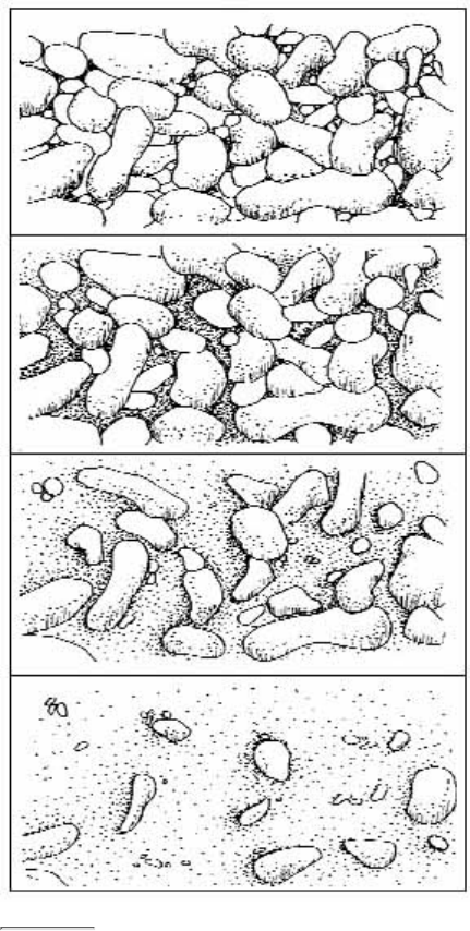
Figure 4.14

A representation of a rocky-bottom stream becoming

embedded with sand and silt

As silt settles on the streambed, spaces between the rocks

are filled in and the stream becomes more embedded.

Naturally occurring organic material in stream. This

material includes leaves and twigs. Mark the box that

describes the general amount of organic matter in the

stream.

Water appearance can be a physical indicator of water

pollution.

Clear - colorless, transparent

■

Milky - cloudy-white or grey, not transparent; might

be natural or due to pollution

■

Foamy - might be natural or due to pollution,

generally detergents or nutrients (foam that is

several inches high and does not brush apart easily

is generally due to some sort of pollution)

■

Turbid - cloudy brown due to suspended silt or

organic material

■

Dark brown - might indicate that acids are being

released into the stream due to decaying plants

■

Oily sheen - multicolored reflection might indicate

oil floating in the stream, although some sheens are

natural

■

Orange - might indicate acid drainage■

Green - might indicate excess nutrients being

released into the stream

■

Water odor can be a physical indicator of water pollution

No smell or a natural odor

■

Sewage - might indicate the release of human waste

material

■

Chlorine - might indicate over-chlorinated sewage

treatment/water treatment plant or swimming pool

discharges

■

Fishy - might indicate the presence of excessive

algal growth or dead fish

■

Rotten eggs - might indicate sewage pollution (the

presence of methane from anaerobic conditions)

■

Water temperature can be particularly important for

determining the suitability of the stream as aquatic habitat

for some species of fish and macroinvertebrates that have

distinct temperature requirements. Temperature also has a

direct effect on the amount of dissolved oxygen available

to the aquatic organisms. Measure temperature by

submerging a thermometer for at least 2 minutes in a

typical stream run. Repeat once and average the results.

Stream Bank and Channel Characteristics

Depth of runs and pools should be determined by estimating the vertical distance from the surface to the stream

bottom at a representative depth at each of the two habitats.

10.

The width of the stream channel can be determined by estimating the width of the streambed that is covered by

water from bank to bank. If it varies widely, estimate an average width.

11.

Stream velocity can have a direct influence on the health, variety, and abundance of aquatic communities. If water

flows too quickly, insects might be unable to maintain their hold on rocks and vegetation and be washed

downstream; if water flows too slowly, it might provide insufficient aeration for species needing high levels of

dissolved oxygen. Stream velocity can be affected by dams, channelization, terrain, runoff, and other factors. To

measure stream velocity, mark off a 20-foot section of stream run and measure the time it takes a stick, leaf, or

other floating biodegradable object to float the 20 feet. Repeat 5 times and pick the average time. Divide the

distance (20 feet) by the average time (seconds) to determine the velocity in feet per second. (See Chapter 5,

12.

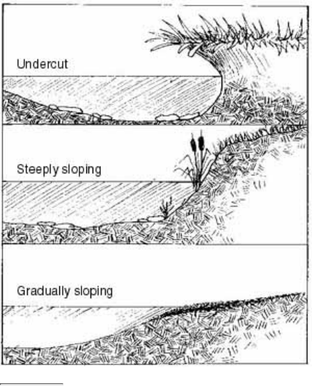
Section 1 on flow for a more in-depth discussion on using floats to estimate velocity.)

The shape of the stream bank, the extent of artificial modifications, and the shape of the stream channel are

determined by standing at the downstream end of the 25-yard section and looking upstream.

13.

The shape of the stream bank (Fig. 4.15) may include.

Figure 4.15

Types of streambank shapes

Undercut banks provide good cover for fish and

macroinvertebrates.

Vertical or undercut bank - a bank that rises

vertically or overhangs the stream. This type of

bank generally provides good cover for

macroinvertebrates and fish and is resistant to

erosion. However, if seriously undercut, it might

be vulnerable to collapse.

■

Steeply sloping - a bank that slopes at more than

a 30 degree angle. This type of bank is very

vulnerable to erosion.

■

Gradual sloping - a bank that has a slope of 30

degrees or less. Although this type of stream

bank is highly resistant to erosion, it does not

provide much streamside cover.

■

Artificial bank modifications include all structural

changes to the stream bank such as riprap (broken rock,

cobbles, or boulders placed on earth surfaces such as

the face of a dam or the bank of a stream, for protection

against the action of the water) and bulkheads.

Determine the approximate percentage of each bank

(both the left and right) that is artificially covered by

the placement of rocks, wood, or concrete.

The shape of the stream channel can be described as

narrow (less than 6 feet wide from bank to bank), wide

(more than 6 feet from bank to bank), shallow (less than

3 feet deep from the stream substrate to the top of the

banks) or deep (more than 3 feet from the stream

substrate to the top of the banks). Choose the category

that best describes the channel.

Narrow, deep

■

Narrow, shallow■

Wide, deep■

Wide, shallow■

Streamside cover information helps determine the quality and extent of the stream's riparian zone. This

information is important at the stream bank itself and for a distance away from the stream bank. For example,

trees, bushes, and tall grass can contribute shade and cover for fish and wildlife and can provide the stream with

needed organic material such as leaves and twigs. Lawns indicate that the stream's riparian zone has been altered,

that pesticides and grass clippings are a possible problem, and that little habitat and shading are available. Bare

soil and pavement might indicate problems with erosion and runoff. Looking upstream, provide an estimate of the

percentage of the stream bank (left and right stream banks) covered by the following:

Trees

■

Bushes, shrubs - conifers or deciduous bushes less than 15 feet high■

Tall grass, ferns, etc. - includes tall natural grasses, ferns, vines, and mosses■

Lawn - cultivated and maintained short grass■

Boulders - rocks larger than 10 inches■

Gravel/cobbles/sand - rocks smaller than 10 inches; sand■

Bare soil■

Pavement, structure - any man-made structures or paved areas, including paths, roads, bridges, houses, etc.■

14.

Stream shading is a measurement of the extent to which the stream itself is overhung and shaded by the cover

identified in 14 above. This shade (or overhead canopy) provides several important functions in the stream

habitat. It cools the water; offers habitat, protection, and refuge for aquatic organisms; and provides a direct

source of beneficial organic matter and insects to the stream. Determine the extent that vegetation shades the

15.

stream at the site.

General conditions of the stream bank and stream channel, and other conditions that might be affecting the

stream are determined by standing at the downstream end of the 25-yard site and looking upstream. Provide

observations for the right and left banks of the stream.

16.

Stream bank conditions that might be affecting the stream.

Natural plant cover degraded--note whether streamside vegetation is trampled or missing or has been

replaced by landscaping, cultivation, or pavement. (These conditions could lead to erosion.)

■

Banks collapsed/eroded--note whether banks or parts of banks have been washed away or worn down.

(These conditions could limit habitats in the area.)

■

Garbage/junk adjacent to the stream--note the presence of litter, tires, appliances, car bodies, shopping

carts, and garbage dumps.

■

Foam or sheen on bank--note whether there is foam or an oily sheen on the stream bank. Sheen may

indicate an oil spill or leak, and foam may indicate the presence of detergent.

■

Stream channel conditions that might be affecting the stream.

Mud/silt/sand on bottom/entering stream--can interfere with the ability of fish to sight potential prey. It can

clog fish gills and smother fish eggs in spawning areas in the stream bottom. It can be an indication of poor

construction practices, urban area runoff, silviculture (forestry-related activities), or agriculture in the

watershed. It can also be a normal condition, especially in a slow-moving, muddy-bottom stream.

■

Garbage or junk in stream--note the presence of litter, tires, appliances, car bodies, shopping carts, and

garbage.

■

Other general conditions that might be affecting the stream.

Yard waste (e.g., grass clippings)--is there evidence that grass clippings, cut branches, and other types of

yard waste have been dumped into the stream?

■

Livestock in or with unrestricted access to stream--are livestock present, or is there an obvious path that

livestock use to get to the water from adjacent fields? Is there streamside degradation caused by livestock?

■

Actively discharging pipes are there pipes--with visible openings discharging fluids or water into the

stream? Note such pipes even though you may not be able to tell where they come from or what they are

discharging.

■

Other pipes--are there pipes near or entering the stream? Note such pipes even if you cannot find an

opening or see matter being discharged.

■

Ditches--are there ditches, draining the surrounding land and leading into the stream?■

Local watershed characteristics

Adjacent land uses can potentially have a great impact on the quality and state of the stream and riparian areas.

Determine the land uses, based on your own judgment of the activities in the watershed surrounding your site

within a quarter of a mile. Enter a "1" if a land use is present and a "2" if it is clearly having a negative impact on

the stream.

17.

Visual biological survey

Are fish present in the stream? Fish can indicate that the stream is of sufficient quality for other organisms.18.

Barriers to the movement of fish in the stream are obstructions that would keep fish from moving freely upstream

or downstream.

19.

Aquatic plants provide food and cover for aquatic organisms. Plants also might provide very general indications

of stream quality. For example, streams that are overgrown with plants could be over enriched by nutrients.

Streams devoid of plants could be affected by extreme acidity or toxic pollutants. Aquatic plants may also be an

indicator of stream velocity because plants cannot take root in fast-flowing streams.

20.

Algae are simple plants that do not grow true roots, stems, or leaves and that mainly live in water, providing food

for the food chain. Algae may grow on rocks, twigs, or other submerged materials, or float on the surface of the

water. It naturally occurs in green and brown colors. Excessive algal growth may indicate excessive nutrients

(organic matter or a pollutant such as fertilizer) in the stream.

21.

Step 4 Complete all the field data sheets
After you have completed macroinvertebrate sampling, analysis of findings, and the habitat characterization, make sure
you have completed the field data sheet to the extent possible and that the recorded data are legible. If you are not able
to determine how to answer a question on the field data sheet, just leave the space blank. Return all completed forms to
your program coordinator.
Streamside Biosurvey: Macroinvertebrates (PDF, 28.7 KB)
Streamside Biosurvey: Habitat Walk (PDF, 22.3 KB)
Adobe Acrobat Reader is required to view PDF documents. The most recent version of the Adobe Acrobat Reader is available as a free
download. An Adobe Acrobat plug-in for assisted technologies is also available.
< Previous · Table of Contents · Next >
Office of Wetlands, Oceans & Watersheds Home
Watershed Protection Home | Monitoring Water Quality Home
EPA Home | Office of Water | Search | Comments

4.3

Intensive Stream Biosurvey

Selecting Metrics to Determine Stream Health

The Intensive Stream Biosurvey is based on the habitat assessment and macroinvertebrate

sampling approach developed by EPA in its Rapid Bioassessment Protocols for Streams

and Rivers (Protocol II) and adapted by volunteer monitoring programs such as Maryl

and Save Our Streams and River Watch Network.

Like the Stream Habitat Walk and Streamside Biosurvey, this approach includes a study

of macroinvertebrates and habitat. However, the Intensive Stream Biosurvey approach is

more rigorous; it requires substantial volunteer training in habitat and macroinve rtebrate

sampling methods and in macroinvertebrate identification. This approach also requires

the involvement of a stream biologist to advise the program participants regarding

everything from the selection of reference conditions to taxonomy and data an alysis.

Because of the need for training and professional assistance, the Intensive Stream

Biosurvey approach can be expensive and labor-intensive for the volunteer program. Its

benefits, however, are equally clear: with proper quality control and volunteer train ing,

the Intensive Stream Biosurvey can yield credible information on subtle stream impacts

and water quality trends. Key features of the Intensive Stream Biosurvey are as follows:

It relies on comparing the results for the sampling site to regional or local

reference conditions. This type of study is used to determine how streams in a

given area compare to the best possible conditions. The reference condition is a co

mposite of the best attainable (minimally impaired) stream conditions within the

region and should be determined by an experienced aquatic biologist familiar with

the characteristics of the ecological region.

●

It includes a detailed habitat assessment that requires the volunteer to rate 10

parameters on a scale of 0 to 20. The results of the habitat assessment are

compared to the score received by the stream's reference condition, and a percent s

imilarity score is calculated.

●

The methods for collecting macroinvertebrates are similar to those of the

Streamside Biosurvey. However, rather than being processed streamside, the entire

●

sample of macroinvertebrates is preserved and returned to a laboratory. A portion,

o r subsample, of the total organisms collected at each location is randomly

selected and identified to taxonomic family level in the lab. After identification, a

series of indices (or metrics) are calculated to provide a broad range of information

about th e stream site. The subsample and the rest of the collected organisms are

maintained as a voucher collection, which serves as a quality assurance

component.

The Intensive Stream Biosurvey requires that volunteers be extensively trained

before habitat assessment and macroinvertebrate sampling and before attempting

macroinvertebrate identification in the laboratory. An experienced aquatic biologi

st is needed to determine and evaluate the regional reference conditions; train

volunteers in habitat characteristics; and supervise and train volunteers in the

collection, processing, and identification of sample macroinvertebrates. A

laboratory (with mi croscopes) and a macroinvertebrate sample storage facility are

required.

●

Step 1 Prepare for the Intensive Stream Biosurvey field

work

Preparing for the Intensive Stream Biosurvey might take several months from the initial

planning stages to the time when actual sampling occurs. An aquatic biologist should be

centrally involved in all aspects of technical program development.

Issues that should be considered in planning the program include the following:

Availability of reference conditions for your area

●

Appropriate dates to sample in each season●

Appropriate sampling gear●

Sampling station location●

Availability of laboratory facilities and trainers●

Sample storage●

Data management●

Appropriate taxonomic keys, metrics, or measurements for macroinvertebrate

analysis

●

Habitat assessment consistency●

Some of the preparation work for this approach is similar to that of the Stream Habitat

Walk (section 4.1) and Streamside Biosurvey (section 4.2). Refer back to those sections

for relevant information on the following tasks:

Obtaining a USGS topographical map

●

Becoming familiar with safety procedures●

TASK 1 Select monitoring locations

If possible, the program coordinator, in conjunction with technical advisor(s), should

preselect sampling locations for each stream. This adds an element of quality control to

the sampling process. You might want to consider sampling at a few locations th at are

also sampled by state or local professionals, as a way to compare your results to theirs. Be

sure to secure approval to do so, however, and coordinate your sampling so as not to

affect professional results.

Provide detailed hand-drawn maps of the locations selected to the monitors. Know the

latitude and longitude of your monitoring locations. This is critical for mapping and for

many data management programs. Latitude and longitude can be calculated manually

(see Appendix C) or by using a hand-held Global Positioning System (GPS).

TASK 2 Schedule the field portion of the biosurvey

Schedule your Intensive Stream Biosurvey for a time of year for which reference

conditions have been established. Reference conditions might vary by season. It is also

essential that seasonal data be collected within the same index period, or window of ti

me, each year. In other words, if you sample during the last two weeks of March this

year, do the same next year.

Another factor to keep in mind is weather. It is best to wait at least a week after a heavy

rain or snow event before sampling. Heavy rains can have a scouring effect on

macroinvertebrates, washing them downstream. If this happens, samples collected will

not accurately reflect biological conditions. However, if you are studying the possible

impact of runoff from a particular source (such as a construction site), you might decide

to sample within a short time after heavy precipitation.

TASK 3 Gather tools and equipment for the Intensive

Stream Biosurvey

In addition to the basic sampling equipment listed for the Stream Habitat Walk, collect

the following equipment needed for the macroinvertebrate collection and habitat

assessment of the Intensive Stream Biosurvey:

Jars (2, at least quart size), plastic, wide-mouth with tight cap; one should be empty

and the other filled about two thirds full with 70 percent ethyl alcohol. (Jars can be

purchased from a scientific supply company or you might try using large pick le,

mayonnaise, or quart mason jars.)

●

Hand lens, magnifying glass, or field microscope●

Fine-point forceps●

Heavy-duty rubber gloves (kitchen gloves will work fine)●

Plastic sugar scooper or ice-cream scooper●

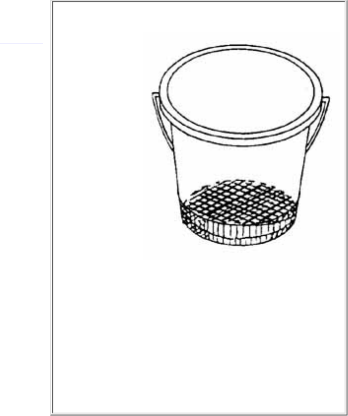
Sieve Buckets

Most

professional

biological

monitoring

programs

employ sieve

buckets as a

holding

container for

composited

samples. These

buckets have a

mesh bottom

that allows

water to drain

out while the organisms and debris remain. This

material can then be easily transferred to the

alcohol-filled jars. However, sieve buckets can be

expensive. Many volunteer programs employ

alternative equipment, such as the two regular

buckets described in this section. Regardless of the

equipment, the process for compositing and

transferring the sample is basically the same. The

decision is one of cost and convenience.

Kick net (rocky bottom

stream) or dip net (muddy

bottom stream) (see Fig. 4.7,

in Section 4.2 - Streamside

Biosurvey)

●

Buckets (2)●

String or twine (50 yards);

tape measure

●

Stakes (4)●

Orange (a stick, an apple, or

a fish float may also be used

in place of an orange) to

measure velocity

●

Reference maps indicating

general information pertinent

to the sampling area,

including the surrounding

roadways, as well as

hand-drawn station map

●

Station ID tags●

Spray water bottle●

Pencils (at least 2)●

TASK 4 Become

familiar with field data

sheets and instructions/definitions for conducting the

macroinvertebrate collection and Habitat Assessment

portions of the Intensive Biosurvey

Step 2 Conduct the Intensive Biosurvey field work

The method you use to collect macroinvertebrates using this approach depends on the

type of stream you are sampling.

Rocky-bottom streams are defined as those with bottoms made up of gravel, cobbles, and

boulders in any combination. They usually have definite riffle areas. Riffle areas are

fairly well oxygenated and, therefore, are prime habitats for benthic macroinvert ebrates.

In these streams, use the Rocky-Bottom sampling method.

Muddy-bottom streams have muddy, silty, or sandy bottoms that lack riffles. Usually,

these are slow-moving, low-gradient streams (i.e., streams that flow along flat terrain). In

such streams, macroinvertebrates generally attach to overhanging plants, root s, logs,

submerged vegetation, and stream substrate where organic particles are trapped. In these

streams, use the Muddy Bottom sampling method.

Each method is detailed below. Regardless of which collection method is used, the

process for counting, identifying, and analyzing the macroinvertebrate sample for the

Intensive Stream Biosurvey is the same. Following the discussion of both approaches to

macroinvertebrate collection and habitat assessment procedures is a section on analyzing

the sample.

Rocky-Bottom Streams

Part1: Macroinvertebrate Sampling Method

Use the following method of macroinvertebrate sampling in streams that have riffles and

gravel/cobble substrates. You will collect three samples at each site and composite them

to obtain one large total sample.

TASK 1 Identify the sampling location

You should already have located your site on a map along with its latitude and longitude

(see Task 3, Step 2 in Section 4.1 - Stream Habitat Walk)

You are going to sample in three different spots within a 100-yard stream site.

These spots may be three separate riffles; one large riffle with different current

velocities; or, if no riffles are present, three run areas with gravel or cobble sub

strate. Combinations are also possible (if, for example, your site has only one small

riffle and several run areas).

Mark off your 100-yard stream site. If possible, it should begin at least 50 yards

upstream of any human-made modification of the channel, such as a bridge, dam,

or pipeline crossing, Avoid walking in the stream, since this might dislodge

macroinvertebrat es and alter your sampling results.

Sketch the 100-yard sampling area. Indicate the location of your three sampling

spots on the sketch. Mark the most downstream site as Site 1, the middle site as

Site 2, and the upstream site as Site 3. (See Fig. 4.8.)

TASK 2 Get into place

(See Figure 4.9: Procedures for collecting a macroinvertebrate sample in a rocky-bottom

stream)

Always approach your sampling locations from the downstream end and

sample the site farthest downstream first (Site 1). This keeps you from biasing

your second and third collections with dislodged sediment or macroinvertebrates.

Always use a clean kick-seine, relatively free of mud and debris from previous

uses. Fill a bucket about one-third full with stream water and fill your spray bottle.

Select a 3-foot by 3-foot riffle area for sampling at Site 1. One member of the

team, the net holder, should position the net at the downstream end of this

sampling area. Hold the net handles at a 45 degree angle to the water's surface. Be

sure th at the bottom of the net fits tightly against the streambed so no

macroinvertebrates escape under the net. You may use rocks from the sampling

area to anchor the net against the stream bottom. Don't allow any water to flow

over the net.

TASK 3 Dislodge the macroinvertebrates

Pick up any large rocks in the 3-foot by 3-foot sampling area and rub them

thoroughly over the partially-filled bucket so that any macroinvertebrates clinging

to the rocks will be dislodged into the bucket. Then place each cleaned rock

outside of the sampling area. After sampling is completed, rocks can be returned to

the stretch of stream they came from.

The member of the team designated as the "kicker" should thoroughly stir up the

sampling area with their feet, starting at the upstream edge of the 3-foot by 3-foot

sampling area and working downstream, moving toward the net. All dislodged

organis ms will be carried by the stream flow into the net. Be sure to disturb the

first few inches of stream sediment to dislodge burrowing organisms. As a guide,

disturb the sampling area for about 3 minutes, or until the area is thoroughly

worked over.

Any large rocks used to anchor the net should be thoroughly rubbed into the bucket

as above.

TASK 4 Remove the net

Next, remove the net without allowing any of the organisms it contains to wash

away. While the net holder grabs the top of the net handles, the kicker grabs the

bottom of the net handles and the net's bottom edge. Remove the net from the

stream wi th a forward scooping motion.

Roll the kick net into a cylinder shape and place it vertically in the partially filled

bucket. Pour or spray water down the net to flush its contents into the bucket. If

necessary, pick debris and organisms from the net by hand. Release back into the

stream any fish, amphibians, or reptiles caught in the net.

TASK 5 Collect the second and third samples

Once you have removed all the organisms from the net, repeat these steps at Sites 2 and

3. Put the samples from all three sites into the same bucket. Combining the debris and

organisms from all three sites into the same bucket is called compositing.

Hint: If your bucket is nearly full of water after you have washed the net clean, let the

debris and organisms settle to the bottom of the bucket. Then cup the net over the bucket

and pour the water through the net into a second bucke t. Inspect the water in the second

bucket to be sure no organisms came through.

TASK 6 Preserve the sample

After collecting and compositing all three samples, it is time to preserve the

sample. All team members should leave the stream and return to a relatively flat

section of stream bank with all their equipment. The next step will be to remove

large pieces of debris (leaves, twigs, and rocks) from the sample. Carefully remove

the debris one piece at a time. While holding the material over the bucket, use the

forceps, spray bottle, and your hands to pick, rub, and rinse the leaves, twigs, and

rocks to remove any attached organisms. Use your magnifying lens and forceps to

find and remove small organisms clinging to the debris. When you are satisfied

that the material is clean, discard it back into the stream.

You will need to drain off the water before transferring material to the jar. This

process will require two team members. Place the kick net over the second bucket,

which has not yet been used and should be completely empty. One team member

should push the center of the net into bucket #2, creating a small indentation or

depression. Then, hold the sides of the net closely over the mouth of the bucket.

The second person can now carefully pour the remaining contents of bucket #1

onto a small area of the net to drain the water and concentrate the organisms. Use

care when pouring so that organisms are not lost over the side of the net (Fig.

4.16).

Figure 4.16

Use your spray bottle,

forceps, sugar scoop, and

gloved hands to remove

all the material from

bucket #1 onto the net.

When you are satisfied

that bucket #1 is empty,

use your hands and the

sugar scoop to transfer all

the material from the net

into the emp ty jar.

Bucket #2 captured the

water and any organisms

that might have fallen

through the netting during

pouring. As a final check,

repeat the process above,

but this time, pour bucket

#2 over the net, into

bucket #1. Transfer any

organisms on the net into

the ja r.

Pouring sample water through the net

Now, fill the jar (so that

all material is submerged)

with the alcohol from the

second jar. Put the lid

tightly back onto the jar

and gently turn the jar

upside down two or three

times to distribute the

alcohol and remove air

bubbles.

Complete the Sampling Station ID tag. Be sure to use a pencil, not a pen, because

the ink will run in the alcohol! The tag includes your station number, the stream,

location (e.g., upstream from a road crossing), date, time, and the names of the m

embers of the collecting crew. Place the ID tag into the sample container writing

side facing out, so that identification can be seen clearly.

Rocky-Bottom Streams

Part 2: Habitat Assessment Method

You will conduct a habitat assessment (which will include measuring general

characteristics and local land use) in a 100-yard section of stream that includes the riffles

from which organisms were collected.

TASK 1 Delineate the habitat assessment boundaries

Begin by identifying the most downstream riffle that was sampled for

macroinvertebrates. Using your tape measure or twine, mark off a 100-yard section

extending 25 yards below the downstream riffle and about 75 yards upstream.

Complete the identifying information on your field data sheet for your habitat

assessment site. On your stream sketch, be as detailed as possible, and be sure to

note which riffles were sampled.

TASK 2 Complete the General Characteristics and Local

Land Use sections of the field sheet

For safety reasons as well as to protect the stream habitat, it is best to estimate these

characteristics rather than actually wading into the stream to measure them.

General Characteristics

Water appearance can be a physical indicator of water pollution.

Clear - colorless, transparent

❍

Milky - cloudy-white or grey, not transparent; might be natural or due to

pollution

❍

Foamy - might be natural or due to pollution, generally detergents or❍

nutrients (foam that is several inches high and does not brush apart easily is

generally due to pollution)

Turbid - cloudy brown due to suspended silt or organic material❍

Dark brown - might indicate that acids are being released into the stream due

to decaying plants

❍

Oily sheen -multicolored reflection might indicate oil floating in the stream,

although some sheens are natural

❍

Orange - might indicate acid drainage❍

Green - might indicate excess nutrients being released into the stream❍

Water odor can be a physical indicator of water pollution.

None or natural smell

❍

Sewage - might indicate the release of human waste material❍

Chlorine - might indicate that a sewage treatment plant is over-chlorinating

its effluent

❍

Fishy - might indicate the presence of excessive algal growth or dead fish❍

Rotten eggs - might indicate sewage pollution (the presence of a natural gas)❍

Water temperature can be particularly important for determining whether the

stream is suitable as habitat for some species of fish and macroinvertebrates that

have distinct temperature requirements. Temperature also has a direct effect on t he

amount of dissolved oxygen available to aquatic organisms. Measure temperature

by submerging a thermometer for at least 2 minutes in a typical stream run. Repeat

once and average the results.

The width of the stream channel can be determined by estimating the width of the

streambed that is covered by water from bank to bank. If it varies widely along the

stream, estimate an average width.

Local Land Use

Local land use refers to the part of the watershed within 1/4 mile up-stream of and

adjacent to the site. Note which land uses are present, as well as which ones seem

to be having a negative impact on the stream. Base your observations on what you

can see, what you passed on the way to the stream, and, if possible, what you

notice as you leave the stream.

TASK 3 Conduct the habitat assessment

The following information describes the parameters you will evaluate for rocky-bottom

habitats. Use these definitions when completing the habitat assessment field data sheet.

The first two parameters should be assessed directly at the riffle(s) or run(s) that were

used for the macroinvertebrate sampling.

Attachment sites for macroinvertebrates are essentially the amount of living space

or hard substrates (rocks, snags) available for aquatic insects and snails. Many

insects begin their life underwater in streams and need to attach themselves to

rocks, logs, branches, or other submerged substrates. The greater the variety and

number of available living spaces or attachment sites, the greater the variety of

insects in the stream. Optimally, cobble should predominate and boulders and

gravel sho uld be common. The availability of suitable living spaces for

macroinvertebrates decreases as cobble becomes less abundant and boulders,

gravel, or bedrock become more prevalent.

Embeddedness refers to the extent to which rocks (gravel, cobble, and boulders)

are surrounded by, covered, or sunken into the silt, sand, or mud of the stream

bottom. Generally, as rocks become embedded, fewer living spaces are available t

o macroinvertebrates and fish for shelter, spawning and egg incubation.

To estimate the percent of embeddedness, observe the amount of silt or finer

sediments overlying and surrounding the rocks. If kicking does not dislodge the

rocks or cobbles, they might be greatly embedded.

The following eight parameters should be assessed in the entire 100-yard section of the

stream.

Shelter for fish includes the relative quantity and variety of natural structures in the

stream, such as fallen trees, logs, and branches; cobble and large rocks; and

undercut banks that are available to fish for hiding, sleeping, or feedin g. A wide

variety of submerged structures in the stream provide fish with many living spaces;

the more living spaces in a stream, the more types of fish the stream can support.

Channel alteration is basically a measure of large-scale changes in the shape of the

stream channel. Many streams in urban and agricultural areas have been

straightened, deepened (e.g., dredged), or diverted into concrete channels, often fo

r flood control purposes. Such streams have far fewer natural habitats for fish,

macroinvertebrates, and plants than do naturally meandering streams. Channel

alteration is present when the stream runs through a concrete channel; when

artificial embankment s, riprap, and other forms of artificial bank stabilization or

structures are present; when the stream is very straight for significant distances;

when dams, bridges, and flow-altering structures such as combined sewer overflow

(CSO) pipes are present; wh en the stream is of uniform depth due to dredging; and

when other such changes have occurred. Signs that indicate the occurrence of

dredging include straightened, deepened, and otherwise uniform stream channels,

as well as the removal of streamside vegeta tion to provide dredging equipment

access to the stream.

Sediment deposition is a measure of the amount of sediment that has been

deposited in the stream channel and the changes to the stream bottom that have

occurred as a result of the deposition. High levels of sediment deposition create an

uns table and continually changing environment that is unsuitable for many aquatic

organisms.

Sediments are naturally deposited in areas where the stream flow is reduced, such

as pools and bends, or where flow is obstructed. These deposits can lead to the

formation of islands, shoals, or point bars (sediments that build up in the stream,

usually a t the beginning of a meander) or can result in the complete filling of

pools. To determine whether these sediment deposits are new, look for vegetation

growing on them: new sediments will not yet have been colonized by vegetation.

Stream velocity and depth combinations are important to the maintenance of

healthy aquatic communities. Fast water increases the amount of dissolved oxygen

in the water; keeps pools from being filled with sediment; and helps food items

like leaves, twigs, and algae move more quickly through the aquatic system. Slow

water provides spawning areas for fish and shelters macroinvertebrates that might

be washed downstream in higher stream velocities. Similarly, shallow water tends

to be more easi ly aerated (i.e., it holds more oxygen), but deeper water stays

cooler longer. Thus the best stream habitat includes all of the following

velocity/depth combinations and can maintain a wide variety of organisms.

slow (<1 ft/sec), shallow (<1.5 ft)

slow, deep

fast, deep

fast, shallow

Measure stream velocity by marking off a 10-foot section of stream run and

measuring the time it takes a stick, orange, or other floating biodegradable object

to float the 10 feet. Repeat 5 times, in the same 10-foot section, and determine the

average tim e. Divide the distance (10 feet) by the average time (seconds) to

determine the velocity in feet per second.

Measure the stream depth by using a stick of known length and taking readings at

various points within your stream site, including riffles, runs, and pools. Compare

velocity and depth at various points within the 100-yard site to see how many of

the combi nations are present.

Channel flow status is the percent of the existing channel that is filled with water.

The flow status changes as the channel enlarges or as flow decreases as a result of

dams and other obstructions, diversions for irrigation, or drought. Wh en water

does not cover much of the streambed, the living area for aquatic organisms is

limited.

For the last three parameters, evaluate the condition of the right and left stream banks

separately. Define the " left" and "right" banks by standing at the downstream end of your

study stretch and looking upstream. Each bank is evaluated on a scale of 0- 10.

Bank vegetative protection measures the amount of the stream bank that is covered

by natural (i.e., growing wild and not obviously planted) vegetation. The root

systems of plants growing on stream banks help hold soil in place, reducing ero

sion. Vegetation on banks provides shade for fish and macroinvertebrates and

serves as a food source by dropping leaves and other organic matter into the

stream. Ideally, a variety of vegetation should be present, including trees, shrubs,

and grasses. Veg etative disruption can occur when the grasses and plants on the

stream banks are mowed or grazed, or when the trees and shrubs are cut back or

cleared.

Condition of banks measures erosion potential and whether the stream banks are

eroded. Steep banks are more likely to collapse and suffer from erosion than are

gently sloping banks and are therefore considered to have a high erosion potenti al.

Signs of erosion include crumbling, unvegetated banks, exposed tree roots, and

exposed soil.

The riparian vegetative zone width is defined here as the width of natural

vegetation from the edge of the stream bank. The riparian vegetative zone is a

buffer zone to pollutants entering a stream from runoff. It also controls erosion and

provides stream habitat and nutrient input into the stream.

A wide, relatively undisturbed riparian vegetative zone reflects a healthy stream

system; narrow, far less useful riparian zones occur when roads, parking lots,

fields, lawns, and other artificially cultivated areas, bare soil, rocks, or buildings

are nea r the stream bank. The presence of "old fields" (i.e., previously developed

agricultural fields allowed to revert to natural conditions) should rate higher than

fields in continuous or periodic use. In arid areas, the riparian vegetative zone can

be measu red by observing the width of the area dominated by riparian or

water-loving plants, such as willows, marsh grasses, and cottonwood trees.

Note: Instructions on sample processing, macroinvertebrate identification, and data

analysis follow the sections on muddy-bottom macroinvertebrate sampling and

habitat assessment. (See Step 3)

Muddy-Bottom Sampling

Part 1: Macroinvertebrate Sampling

In muddy-bottom streams, as in rocky- bottom streams, the goal is to sample the

most productive habitat available and look for the widest variety of organisms. The

most productive habitat is the one that harbors a diverse population of

pollution-sensitive macroinvertebrates. Volunteers should sample by using a

D-frame net to jab at the habitat and scoop up the organisms that are dislodged.

The idea is to collect a total sample that consists of 20 jabs taken from a variety of

habitats.

TASK 1 Determine which habitats are present

Muddy-bottom streams usually have four habitats (Fig. 4.17). It is generally best to

concentrate sampling efforts on the most productive habitat available, yet to

sample other principal habitats if they are present. This ensures that you will secure

as wi de a variety of organisms as possible. Not all habitats are present in all

streams or present in significant amounts. If your sampling areas have not been

preselected, try to determine which of the following habitats are present. (Avoid

standing in the st ream while making your habitat determinations.)

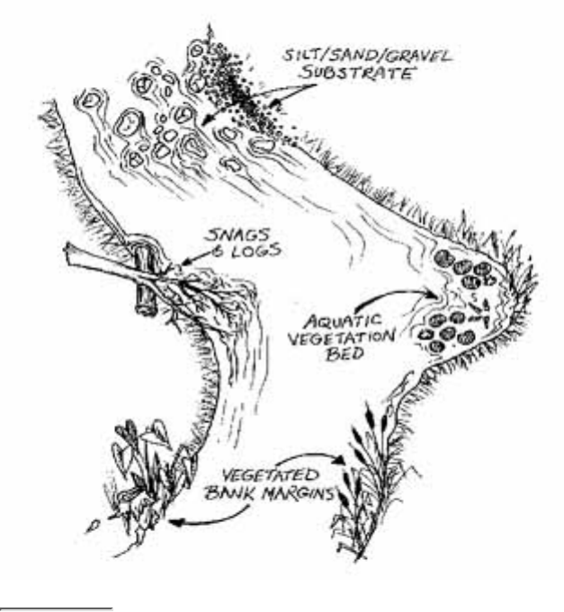
Figure 4.17

Four habitats found in muddy-bottom streams

Volunteers will likely find the most macroinvertebrates in

vegetated habitats and snags and logs.

Vegetated bank

margins consist

of overhanging

bank vegetation

and submerged

root mats

attached to

banks. The bank

margins may

also contain

submerged,

decomposing

leaf packs

trapped in root

wads or lining

the streambanks.

This is generally

a highly

productive

habitat in a

muddy-bottom

stream, and it is

often the most

abundant type of

habitat.

❍

Snags and logs consist of submerged wood, primarily dead trees, logs,

branches, roots, cypress knees and leaf packs lodged between rocks or logs.

This is also a very productive muddy-bottom stream habitat.

❍

Aquatic vegetation beds and decaying organic matter consist of beds of

submerged, green/leafy plants that are attached to the stream bottom. This

habitat can be as productive as vegetated bank margins, and snags and logs.

❍

Silt/sand/gravel substrate includes sandy, silty, or muddy stream bottoms;

rocks along the stream bottom; and/or wetted gravel bars. This habitat may

also contains algae-covered rocks (sometimes called Aufwuchs). This is the

least productiv e of the four muddy-bottom stream habitats, and it is always

present in one form or another (e.g., silt, sand, mud, or gravel might

predominate).

❍

TASK 2 Determine how many times to jab in each

habitat type

Your goal is to jab a total of 20 times. The D-frame net is 1 foot wide, and a jab

should be approximately 1 foot in length. Thus, 20 jabs equals 20 square feet of

combined habitat.

If all four habitats are present in plentiful amounts, jab the vegetated banks

10 times and divide the remaining 10 jabs among the remaining 3 habitats.

❍

If three habitats are present in plentiful amounts and one is absent, jab the

silt/sand/gravel substrate the least productive habitat 5 times and divide the

remaining 15 jabs among the other two more productive habitats.

❍

If only two habitats are present in plentiful amounts, the silt/sand/gravel

substrate will most likely be one of those habitats. Jab the silt/sand/gravel

substrate 5 times and the more productive habitat 15 times.

❍

If some habitats are plentiful and others are sparse, sample the sparse

habitats to the extent possible, even if you can take only one or two jabs.

Take the remaining jabs from the plentiful habitat(s). This rule also applies if

you cannot reach a habitat because of unsafe stream conditions. Jab a total of

20 times.

❍

Because you might need to make an educated guess to decide how many jabs to

take in each habitat type, it is critical that you note, on the field data sheet, how

many jabs you took in each habitat. This information can be used to help

characterize your fi ndings.

TASK 3 Get into place

Outside and downstream of your first sampling location (1st habitat), rinse the dip

net and check to make sure it does not contain any macroinvertebrates or debris

from the last time it was used. Fill a bucket approximately one-third full with clean

strea m water. Also, fill the spray bottle with clean stream water. This bottle will

be used to wash down the net between jabs and after sampling is completed.

This method of sampling requires only one person to disturb the stream habitats.

While one person is sampling, a second person should stand outside the sampling

area, holding the bucket and spray bottle. After every few jabs, the sampler should

hand the n et to the second person, who then can rinse the contents of the net into

the bucket.

TASK 4 Dislodge the macroinvertebrates

Approach the first sample site from downstream, and sample as you walk

upstream. Here is how to sample in the four habitat types:

Sample vegetated bank margins by jabbing vigorously, with an upward

motion, brushing the net against vegetation and roots along the bank. The

entire jab motion should occur underwater.

❍

To sample snags and logs, hold the net with one hand under the section of

submerged wood you are sampling (Fig. 4.18). With the other hand (which

should be gloved), rub about 1 square foot of area on the snag or log. Scoop

organisms, bark, twigs, or other organic matter you dislodge into your net.

Each combination of log rubbing and net scooping is one jab.

❍

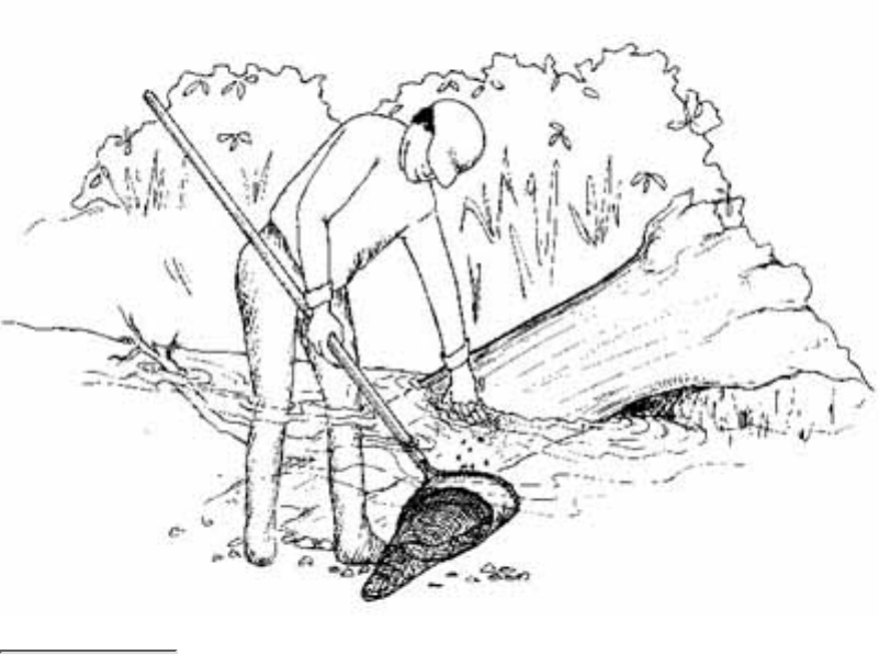
Figure 4.18

Collecting a sample from a log

Volunteer rubs the log with one hand and catches dislodged organisms and other

material in the net.

sample

aquatic

vegetation

beds,

jab

vigorously,

with

upward

motion,

against

through

the

plant

bed.

The

entire

jab

motion

should

occur

❍

underwater.

To sample a silt/sand/gravel substrate, place the net with one edge against

the stream bottom and push it forward about a foot (in an upstream

direction) to dislodge the first few inches of silt, sand, gravel, or rocks. To

avoid gathering a netful of mud, periodically sweep the mesh bottom of the

net back and forth in the water, making sure that water does not run over the

top of the net. This will allow fine silt to rinse out of the net. When you have

completed all 20 jabs, rinse the net thorough ly into the bucket. If necessary,

pick any clinging organisms from the net by hand and put them in the

bucket.

❍

TASK 5 Preserve the sample

Look through the material in the bucket and immediately return any fish,

amphibians, or reptiles to the stream. Carefully remove large pieces of debris

(leaves, twigs, and rocks) from the sample. While holding the material over

the bucket, use the forceps, spray bottle, and your hands to pick, rub, and

rinse the leaves, twigs, and rocks to remove any attached organisms. Use

your magnifying lens and forceps to find and remove small organisms

clinging to the debris. When you are satisfied that the m aterial is clean,

discard it back into the stream.

You will need to drain off the water before transferring material to the jar.

This process will require two team members. One person should place the

net into the second bucket, like a sieve (this bucket, which has not yet been

used, should be com pletely empty) and hold it securely. The second person

can now carefully pour the remaining contents of bucket #1 onto the center

of the net to drain the water and concentrate the organisms.

Use care when pouring so that organisms are not lost over the side of the net.

Use your spray bottle, forceps, sugar scoop, and gloved hands to remove all

the material from bucket #1 onto the net. When you are satisfied that bucket

#1 is empty, use your h ands and the sugar scoop to transfer all the material

from the net into the empty jar. You can also try to carefully empty the

contents of the net directly into the jar by turning the net inside out into the

jar.

Bucket #2 captured the water and any organisms that might have fallen

through the netting. As a final check, repeat the process above, but this time,

pour bucket #2 over the net, into bucket #1. Transfer any organisms on the

net into the jar.

Fill the jar (so that all material is submerged) with alcohol. Put the lid tightly

back onto the jar and gently turn the jar upside down two or three times to

distribute the alcohol and remove air bubbles.

Complete the sampling station ID tag. Be sure to use a pencil, not a pen,

because the ink will run in the alcohol. The tag should include your station

number, the stream, location (e.g., upstream from a road crossing), date,

time, and the names of the members of the collecting crew. Place the ID tag

into the sample container, writing side facing out, so that identification can

be seen clearly (Fig. 4.19).

STATION ID TAG

Station #: __________________________

Stream: _____________________________

Location: ___________________________

Date/Time: __________________________

Team members:

_____________________________________

Figure

4.19

Example

of a

Station

ID tag

prevent

samples

from

being

mixed up,

volunteers

should

place the

ID tag

inside the

sample

jar.

Muddy-Bottom

Streams

Part2: Habitat

Assessment

You will conduct a

habitat assessment

(which will include

measuring general

characteristics and local

land use) in a 100-yard

section of the stream

that includes the habitat

areas from which

organisms were

collected.

TASK 1

Delineate the

habitat

assessment boundaries

Begin by identifying the most downstream point that was sampled for

macroinvertebrates. Using your tape measure or twine, mark off a 100-yard

section extending 25 yards below the downstream sampling point and about

75 yards upstream.

Complete the identifying information on your field data sheet for your

habitat assessment site. On your stream sketch, be as detailed as possible,

and be sure to note which habitats were sampled.

TASK 2 Complete the General Characteristics and

Local Land Use sections of the field sheet

For safety reasons as well as to protect the stream habitat, it is best to estimate

these characteristics rather than actually wading into the stream to measure them.

For instructions on completing these sections of the field data sheet, see the

rocky-bot tom habitat assessment instructions.

TASK 3 Conduct the habitat assessment

The following information describes the parameters you will evaluate for

muddy-bottom habitats. Use these definitions when completing the habitat

assessment field data sheet.

Shelter for fish and attachment sites for macroinvertebrates are essentially

the amount of living space and shelter (rocks, snags, and undercut banks)

available for fish, insects, and snails. Many insects attach themselves to

rocks, logs, b ranches, or other submerged substrates. Fish can hide or feed

in these areas. The greater the variety and number of available shelter sites

or attachment sites, the greater the variety of fish and insects in the stream.

Many of the attachment sites result from debris falling into the stream from

the surrounding vegetation. When debris first falls into the water, it is

termed new fall and it has not yet been "broken down" by microbes

(conditioned) for macroinvertebrate co lonization. Leaf material or debris

that is conditioned is called old fall. Leaves that have been in the stream for

some time lose their color, turn brown or dull yellow, become soft and

supple with age, and might be slimy to the touch. Woody debris becom es

blackened or dark in color; smooth bark becomes coarse and partially

disintegrated, creating holes and crevices. It might also be slimy to the

touch.

Pool substrate characterization evaluates the type and condition of bottom

substrates found in pools. Pools with firmer sediment types (e.g., gravel,

sand) and rooted aquatic plants support a wider variety of organisms than do

pools with su bstrates dominated by mud or bedrock and no plants. In

addition, a pool with one uniform substrate type will support far fewer types

of organisms than will a pool with a wide variety of substrate types.

Pool variability rates the overall mixture of pool types found in the stream

according to size and depth. The four basic types of pools are large-shallow,

large-deep, small-shallow, and small-deep. A stream with many pool types

will support a wide variety of aquatic species. Rivers with low sinuosity

(few bends) and monotonous pool characteristics do not have sufficient

quantities and types of habitats to support a diverse aquatic community.

Channel alteration (See description in habitat assessment for rocky-bottom

streams.)

Sediment deposition (See description for rocky-bottom streams.)5.

Channel sinuosity evaluates the sinuosity or meandering of the stream.

Streams that meander provide a variety of habitats (such as pools and runs)

and stream velocities and reduce the energy from current surges during

storm events. Straight stream segments are characterized by even stream

depth and unvarying velocity, and they are prone to flooding. To evaluate

this parameter, imagine how much longer the stream would be if it were

straightened out.

Channel flow status (See description in habitat assessment for rocky-bottom

streams.)

Bank vegetative protection (See description for rocky-bottom streams.)8.

Condition of banks (See description for rocky-bottom streams.)9.

The riparian vegetative zone width (See description for rocky-bottom

streams.)

Reference Collection

A reference collection is a sample of locally-found macroinvertebrates

that have been identified, labelled, and preserved in alcohol. The program

advisor, along with a professional biologist/entomologist, should

assemble the reference collection, properly identify all samples, preserve

them in vials, and label them. This collection may then be used as a

training tool and, in the field, as an aid in macroinvertebrate

identification.

Step 3 Leave the field, complete data forms, clean

the site, and return material

After completing the stream characterization and habitat assessment, make

sure that all of the field data sheets have been completed properly and that

the information is legible. Be sure to include the site's identifying name and

the sampling date on each sheet. These will function as a quality control

element. If you can't determine how to answer a question on the field data

sheet, just leave the space blank.

Before you leave the stream location, make sure that all your equipment has

been collected and rinsed properly. Double-check to see that sample jars are

tightly closed and properly identified. All samples, field sheets, and

equipment should be returned to the coordinator at this point. You might

want to keep a copy of the field data sheet for comparison with future

monitoring trips and for personal records.

Step 4 Prepare for macro-invertebrate laboratory

work

This step includes all the work needed to set up a laboratory for processing

samples into subsamples and identifying macroinvertebrates to the family

level. A professional biologist/entomologist or the program advisor should

supervise the identification p rocedure. All interested volunteers should be

encouraged to participate. In general it is a good idea to train volunteers in

identification procedures before each lab session and to start new volunteers

10.

with less diverse samples. Refresher workshops for e xperienced volunteers

are strongly encouraged.

TASK 1 Gather tools and equipment for the

laboratory

The following lab equipment is recommended for the macroinvertebrate

identification process. Enough of each will need to be provided for each

volunteer work station:

Reference collection and taxonomic keys

■

Fine-point forceps■

Petri dishes or small, shallow, clear container■

Alcohol preservative (used in field and lab): 70 percent ethyl alcohol,

denatured; no other preservatives used

■

Microscope, dissecting microscope, and magnifying glass, or hands

lens

■

Sample containers, preferably shatterproof with poly-seal caps that

prevent evaporation of the preservative (jars or vials are used in field

and lab). Shatterproof vials with poly-seal caps are available from

scientific supply houses.

■

Wash bottles or spray bottles■

Shallow, rectangular white pans (large enough to hold entire

macroinvertebrate sample)

■

Additional shallow white containers (heavy duty plastic plates with a

rim, white pans, or cafeteria trays are all possible choices).

■

Plastic spoons or unslotted spatulas■

Sieve, purchased from scientific supply company (#30) or homemade

(with same mesh size as sampling net)

■

Permanent ink markers■

Ruler■

Macroinvertebrate assessment worksheet■

Pencils■

Note paper for counting■

TASK 2 Create gridded subsampling pans

Using the ruler, measure the inside width and length of the large rectangular

white pan. Draw a grid of evenly sized squares on the inside of the pan,

using permanent ink. The grid should fill the entire inside of the pan.

Number each square. One pan will be needed for each work station.

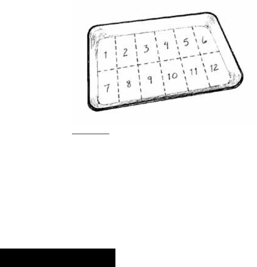
Volunteers will use these pans for randomizing the sample and selecting a

subsample of organisms.

TASK 3 Prepare the lab and the individual work

stations

Before volunteers enter the lab, the program manager will need to prepare

work stations. Make sure that all microscopes are functioning properly and

that each station has access to all other equipment. The reference collection

should be centrally located as should any other visual training displays. The

lab itself should be well lit and well ventilated. A copy of lab safety

instructions should be visible to all volunteers.

Figure 4.20

A Gridded subsampling pan

Volunteers collect a subsampling of organisms by picking them

from randomly selected grid squares.

Step 5

Conduct

macroinvertebrate processing and identification

If possible, before beginning the subsampling and identification processes,

all volunteers should become familiar with the lab equipment,

microscope(s), the reference collection, and the taxonomic key chosen by

the advisor. Processing a subsample and ide ntifying the organisms are two

separate activities. Some programs might prefer to split these tasks into

separate lab sessions.

Session 1:Picking a subsample of

aquatic organisms

TASK 1 Prepare the sample

Carefully remove the station ID tag from the sample container and put

it aside. You will need it later.

Cover the bottom of the gridded pan with about 1/4 inch of clean

water.

Pour the preserved sample (alcohol and debris) into the sieve and

wash off preservative over a sink, using a spray or wash bottle filled

with water.

Transfer the sample to the white gridded pan by turning the sieve

upside down over the pan. Tap it several times to empty the contents

onto the pan. Squirt a small amount of water over the bottom of the

sieve to flush the organisms into the pan.

With your hands and by gently shaking the pan, evenly disperse the

sample over the entire bottom of the pan, making sure that even the

corners are covered. The water will help in distributing the sample

throughout the pan. This is called randomizi ng the sample.

TASK 2 Randomly select a square for the

subsample

Randomly choose a square to start sorting organisms. You may use a

random numbers table, draw numbers from a hat, or roll a pair of dice.

The most important thing to remember is that the grid selection should

be random. Indicate the square number selected on the lab sheet.

Using a plastic spoon or unslotted spatula, remove all the material

from the square and transfer it to another container (another pan, tray,

or plate) for sorting. The organisms in this container will become your

subsample.

TASK 3 Pick the subsample

Prepare a container to house the subsample by filling a vial or jar

one-half full of alcohol. Place the new label into the vial, writing side

out. Keep the vial on a flat, stable area.

Using forceps, carefully and systematically remove all organisms

from the pan or tray and place them one by one into the prepared

subsample vial. Examine all debris such as leaves or sticks for

clinging organisms. Count each organism as it is tran sferred. Keep a

written count of the number of organisms you have transferred. The

objective is have at least 100 individual organisms in your subsample.

If you reach 100 and there are still organisms remaining in your

subsample plate or tray, continue pi cking until all the organisms are

removed even though you might end up with more than 100.

When you think all the organisms have been transferred from the plate

or tray to the subsample vial, have a second volunteer check to

confirm that all organisms have been removed. On your lab sheet,

record how many organisms are in the subsample.

If you finish picking the contents of the first square selected and have

fewer than 100 organisms, randomly select another square and repeat

the process of removing the contents of the square to the subsample

plate or tray; picking organisms with the forceps and transferring them

to the vial (all organisms that will be part of the subsample should be

transferred to the same vial). Record the number of organisms you

obtain from the second square. Repeat this process until at least 100

organisms hav e been placed into the vial or until the entire sample in

the gridded pan has been picked clean. Remember, any square started

must be picked clean.

If, after picking the entire gridded pan clean, you have fewer than 100

organisms, and your reference site produced 100 or more organisms,

either your site is impaired or your sampling technique is flawed. It is

also possible that recent heavy rains migh t have washed many

organisms downstream. If you do not find 100 organisms in the entire

sample, be sure to note the potential cause for such a problem on the

Habitat Assessment Data Sheet.

TASK 4 Label and store the subsample

Fill out a new Subsample ID Tag (Fig. 4.21) for the subsample. Remember

to use pencil because ink will run in the alcohol. The vial housing the

subsample must be labeled with the same station number, stream name,

location, and date found on the original s ample ID tag. The vial tag should

also include information on when the subsample was picked (i.e., 100 or

more organisms counted) and by whom. Place the tag in the vial with the

writing side out. Make sure the vial is tightly closed before giving the subs

ample in the vial to the program coordinator.

TASK 5 Replace remainder of original sample

back into the sample jar

Place the remaining sample back into the original container. Be sure that the

original station ID tag is included, writing side out. Fill the jar with 70

percent alcohol. This sample will be retained as part of a voucher collection.

Make sure the jar is t ightly closed before returning it to the program

coordinator.

SUBSAMPLE ID TAG

Station #: __________________________

Stream: _____________________________

Location: ___________________________

Date/Time: __________________________

Subsample team members:

_____________________________________

Figure 4.21

Example of

Subsample

ID tag

To prevent

wubsamples

from being

mixed up,

volunteers

should

place the ID

tag inside

the

subsample

jar.

Session 2:Identifying the subsample to

family level

TASK 1

Prepare

for the ID

Make

sure that

you have

several

petri

dishes,

fresh

alcohol,

and fresh

water

close at

hand.

Also

have

your

taxonomic

keys

handy for

all stages

of the ID

process.

Check to

make

sure that

your

microscope

working

properly.

Carefully

remove

the

station

ID tag

from the

subsample

vial and

put it

aside.

You will

need it

later. Be

sure no

organisms

are

clinging

to it. If

they are,

remove

them

with

forceps.

Using the

information

on the

station

ID tag,

complete

the first

section

of the

Macroinvertebrate

Assessment

Sheet

with your

name,

date, the

stream

name,

station

number,

and any

other

information

requested.

TASK 2 Identify the sample to order level

Place a few of the macroinvertebrates in a petri dish (or other small,

shallow container) and examine them under the microscope. Include

some ethyl alcohol in the dish to ensure that the organisms do not dry

out. Compare the organisms in the dish to those in the taxonomic key

and/or reference collection.

Roughly sort organisms by taxonomic order into petri dishes. Many

volunteers find it helpful to use one dish for every major taxonomic

order found in the subsample. Place any organism that you cannot

identify into another dish for the biological a dvisor to examine.

TASK 3 Identify the organisms within each order

to family level

Starting with one order, and using the taxonomic keys, reference

collection, and assistance of the biological advisor, identify each

individual to family level.

Keep a running count of how many individuals there are in each

family on a piece of scratch paper.

Place any organisms that you cannot identify into a separate container.

Make sure that the biological advisor sees them and assists you with

the ID.

After all organisms have been identified, note the total number of

organisms in each family on the Macroinvertebrate Assessment Sheet.

Write in pencil and make sure your writing is legible. These lab sheets

will be the basis for the data analysis. It is important that they are

accurate and easy to read.

TASK 4 Return the organisms to the vial

After you have identified and counted all organisms in the subsample,

return them to the subsample vial and replace the subsample ID Tag,

writing side out.

Refill the subsample vial with 70 percent ethyl alcohol (new or

recycled). Be sure to secure the caps on the vial tightly to prevent the

organisms from drying out.

Return the subsample vial and the assessment worksheet to the

program manager.

Voucher Collection

Maintaining a voucher collection adds another layer of credibility to the

program by documenting the accuracy of the volunteer identifications. It

substantiates and provides evidence to support the analysis of the data—a

powerful quality control element. However, an important issue to

consider is how long to keep the samples. Program managers, in

collaboration with technical advisors, will have to consider the following

in keeping a voucher collection.

Sample maintenance. Even jars and vials with tight fitting lids

require maintenance on a regular basis (every 2-3 months) to

ensure that alcohol levels are adequate.

■

Fire safety. When you are dealing with alcohol, you will need to

consider fire safety and ventilation issues to make sure that you are

in line with local codes.

■

Availability of storage space. In addition to needing well-ventilated

and fire-proof storage cabinet, you will need a well-ventilated room

to store samples. Samples should not be stored in someone's office

for any length of time.

■

Length of storage. How long samples should be maintained is an

issue determined by program goals. Data collected for regulatory

purposes will probably require longer storage than other samples.

Generally, 1-5 years is recommended for storage.

■

Step 6 Performing habitat assessment data

analysis

To evaluate the condition of your stream site properly, you should compare

it to an optimal or best condition found in the region. This is called a

reference condition. In an ideal world, the reference condition would reflect

the water quality, habitat, a nd aquatic life characteristics of pristine sites in

the same ecological region as your stream. In real life, however, few pristine

sites remain. The reference condition is, therefore, a composite of sites that

reflect the best physical, chemical, and bio logical conditions existing in

your ecological region. State water quality or natural resource agencies

might have already established reference conditions for the ecological

regions in your state.

Your program's consulting biologist should work in cooperation with the

state agency to identify the reference condition(s) you will need to conduct

an Intensive Stream Biosurvey. The biologist will use the reference

condition to establish a water quality rating system against which to rank

your monitored stream sites.

To perform the habitat assessment data analysis for the Intensive Stream

Biosurvey, perform the following tasks.

TASK 1 Determine the habitat index score

Add together the scores of all 10 habitat parameters. This sum is the habitat

index score for the study stretch.

TASK 2 Determine the percent similarity to the

reference score

Divide the habitat index score by the reference index score and then multiply

the result by 100. This number is the percent similarity to the reference

score.

TASK 3 Determine the stream habitat quality

rating

Compare the percent similarity of your results with the range of percent

similarity numbers in the stream habitat rating table to obtain the habitat

quality category for your site(s) (Table 4.5). Enter the appropriate

descriptive rating (excellent, good, fair, or poor) on the field data sheet. If

your score falls at or near the break between habitat quality categories, use

your best judgment to determine an appropriate rating.

% Similarity

to Reference

Score

Habitat

Quality

Category Attributes Table 4.5

Reference

scores for

sampling

site

comparison

If a score

falls at or

near the

break

between

categories,

use your

best

judgement

determine

the

appropriate

>90% Excellent Commparable to the

best situation to be

expected within an

ecoregion. Excellent

overall habitat structure

conducive to

supporting healthy

biological community.

score.

75-88% Good Habitat structure

slightly impaired.

Generally, diverse

instream habitat

well-developed; some

degradation of riparian

zone and banks; a small

amount of channel

alteration may be

present.

60-73% Fair Loss of habitat

compared to reference.

Habitat is a major

limiting factor to

supporting a healthy

biological community.

<58% Poor Severe habitat

alteration at all levels.

Step 7 Conduct macroinvertebrate data analysis

In general, the program's biological advisor, rather than the volunteers,

should analyze the results of the Intensive Stream Biosurvey's

macroinvertebrate identification. The advisor's knowledge of local

ecological conditions will help in the interpretati on of the data findings and

will lend additional credibility to the sampling effort. Volunteers can

contribute significantly to the advisor's data analysis by interpreting field

notes, assisting with macroinvertebrate identification, and counting

organism s on the aquatic macroinvertebrate assessment worksheet. Relay

the results of the data analysis to the volunteers as soon after the sampling

date as possible.

TASK 1 Determine which metrics or

measurements are appropriate

A number of metrics (or measures) can be used to calculate stream health

using benthic macroinvertebrates. These metrics should be calculated for

both the sample site and the reference condition. By comparing the two, the

program advisor can reach a clear understanding of the biological health of

the sampling site.

The Intensive Stream Biosurvey recommends the use of four basic metrics

(taxa richness, number of EPT taxa, percent abundance of EPT, and

sensitive taxa index) plus two optional metrics (percent abundance of

scrapers and percent abundance of shredders). T hese metrics are discussed

briefly below. Refer to the reference list for more information.

The term taxa (plural for taxon), used below, refers to the specific

taxonomic groupings to which organisms have been identified. For the

Intensive Stream Biosurvey, organisms are identified to the taxon of family.

Your volunteer monitoring program should identify organisms to a specific

taxonomic grouping if it is to compare results over time and between sites.

The following metrics are generally applicable throughout the country (but

confirm this with a local biologist).

Number of taxa (taxa richness)--this measure is a count of the number

of taxa (e.g., families) found in the sample. A high diversity or variety

is good.

Number of EPT taxa (EPT richness)--this measure is a count of the

number of taxa in each of three generally pollution-sensitive orders:

Ephemeroptera (mayflies), Plecoptera (stoneflies), and Trichoptera

(caddisflies). A high diversity or va riety is good.

Percent dominance--this measure is the percent composition of the

most abundant family from your station. It indicates how dominant a

single taxon is at a particular site. A high percent dominance is not

good.

Sensitive taxa index (modified Hilsenhoff index)--this measure is

calculated by multiplying the number of organisms in each taxon by

the pollution tolerance value assigned to each taxon, adding these for

all taxa represented in the sample, and dividing by the total number of

taxa in the sample. A high index number is not good.

Sensitive taxa index = E(Xit)/n

where:

E = the summation of Xit

Xi = the number of individuals in each taxon

t = tolerance value for each taxon in the sample

n = number of individuals in the sample

The following optional metrics can be used in rocky-bottom streams if at

least 10 scraper and shredder organisms are collected.

Percent abundance of scrapers--in the majority of rocky-bottom

streams, the basic food source for many aquatic organisms is algae

covering the rocks in the stream.

Macroinvertebrates that "scrape" or graze on these algae are known as

scrapers. To compute the percent abundance of the scrapers in the

macroinvertebrate community, divide the number of organisms

classified as grazers or scrapers by the total number of organisms in

the sample. A high percent abundance of scrapers is good.

Percent abundance of shredders--leaf litter and other plant debris are

broken down and processed by organisms called shredders. To

compute the percent abundance of shredders in the macroinvertebrate

community, divide the number of organisms classified as shredders by

the total number of organisms in the sample. A high percent

abundance of shredders is good.

The following optional metrics can be used in muddy-bottom streams

as additional metrics to provide more information about the condition

of the macroinvertebrate assemblage.

Percent abundance of EPT--this measure compares the number of

organisms in the EPT orders to the total number of organisms in the

sample. (The number of organisms in the EPT orders is divided by the

total number of organisms in the sample t o calculate a percent

abundance.) A high percent abundance of EPT orders is good.

Percent abundance of midge larvae--this measure compares the

number of midges to the total number of organisms in the sample.

(The number of organisms in the chironomidae family is divided by

the total number of organisms in the sample to c alculate a percent

composition.) A low percent abundance of midge larvae is good.

TASK 2 Calculate a score for the site

The metric worksheets Tables 4.6 and 4.7 are designed to help calculate a

total score for the monitored site. Table 4.8 provides an example of a sample

metric worksheet for the fic tional Volunteer Creek (rocky-bottom stream).

This score should be compared to reference conditions to determine the

biological condition of the stream at that site. You should also note that

these worksheets were developed for use in mid-Atlantic states; they might

need to be modified to reflect local conditions.

To calculate a score for your stream site using one of these worksheets, enter

the metric values at the monitored site in the (M) column. Compare each

metric value from your monitored site to the value ranges presented in the

biosurvey score columns. Choo se the matching range and circle it; this

gives you the corresponding score (6, 3, or 0) for your metric value. Add the

metric scores to obtain the total biosurvey score (see instructions in Tables

4.6 and 4.7< /a>).

TASK 3 Determine the biological condition

To determine the biological condition of the site, refer to Table 4.9,

Biosurvey Scoring Guide.

TASK 4 Return the lab sheets and metric

worksheets to the program coordinator

All remaining worksheets should be returned to the program coordinator

once the site's final score has been determined. The program coordinator will

determine how to proceed with the findings of the biological assessment

(e.g., the data may be entered int o a database or shared with a state or local

agency). It is important that the biological advisor include documentation of

any problems encountered in the process of monitoring, identifying

macroinvertebrates, or analyzing the data.

References and Further Reading

Note: References marked with (k) contain macroinvertebrate taxonomic

keys.

Brigham, A. R., W. U. Brigham, and A. Gnilka. 1982. Aquatic Insects and

Oligochaetes of North and South Carolina. Midwest Enterprises, Mahomet,

IL. (k)

Cummins, Kenneth W. and Margaret A. Wilzbach. 1985. Field Procedures

for Analysis of Functional Feeding Groups of Stream Macroinvertebrates.

University of Maryland, Frostburg. (k)

Dates, G. and J. Byrne. 1995. River Watch Network Benthic

Macroinvertebrate Monitoring Manual. River Watch Network. 153 State

St., Montpelier, VT 05602 ($25). (k)

Delaware Nature Education Center. 1996. Delaware Stream Watch Guide.

Delaware Nature Society, P.O. Box 700, Hockessin, DE 19707.

Fore, L., J. Karr, and R. Wiseman. 1996. Assessing Invertebrate Responses

to Human Activities: Evaluating Alternative Approaches. Journal of the

North American Benthological Society. 15(2):212-231.

Hilsenhoff, William L. 1982. Using a Biotic Index to Evaluate Water

Quality in Streams. Wisconsin Department of Natural Resources, Madison,

WI. Technical Bulletin No. 132.

Hilsenhoff, William L. 1988. Rapid Field Assessment of Organic Pollution

With a Family-level Biotic Index. Journal of the North American

Benthological Society, 7:65-68.

Izaak Walton League of America (IWLA). 1992. A Monitor's Guide to

Aquatic Macroinvertebrates. Izaak Walton League of America Save Our

Streams. 707 Conservation Lane, Gaithersburg, MD 20878. (k)

Izaak Walton League of America (IWLA). Stream Insects and Crustaceans

Card. Izaak Walton League of America Save Our Streams. 707

Conservation Lane, Gaithersburg, MD 20878. (k)

Karr, J. R. In press. Rivers As Sentinels: Using the Biology of Rivers to

Guide Landscape Management. In The Ecology and Management of Streams

and Rivers in the Pacific Northwest Coastal Ecoregion. Springer-Verlag,

Klemm, D.J., et al. 1990. Macroinvertebrate Field and Laboratory Methods

for Evaluating the Biological Integrity of Surface Waters.

EPA/600/4-90/030. U.S. Environmental Protection Agency, Office of

Research and Development, Cincinnati, OH.

Lathrop, J. 1989. A Naturalist's Key to Stream Macroinvertebrates for

Citizen Monitoring Programs in the Midwest. In Proceedings of the 1989

Midwest Pollution Control Biologists Meeting, Chicago IL, EPA

9059-89/007, ed. W.S. Davis and T.P. Simon, U SEPA Region 5 Instream

Biocriteria and Ecological Assessment Committee. Chicago, Illinois. (k)

Maryland Save Our Streams. 1994. Project Heartbeat Volunteer Monitoring

Handbook. Maryland Save Our Streams, 258 Scotts Manor Dr., Glen Burnie,

MD 21061.

McCafferty, W. P. 1981. Aquatic Entomology: The Fishermen's and

Ecologists' Illustrated Guide to Insects and Their Relatives. Science Books

International, Boston. (k)

McDonald, B., W. Borden, and J. Lathrop. Citizen Stream Monitoring: A

Manual for Illinois. ILENR/RE-WR90/18. Illinois Department of Energy

and Natural Resources.

Merritt, R. W. and K. W. Cummins, eds. 1984. An Introduction to the

Aquatic Insects of North America. 2nd. ed. Kendall/Hunt Publishing

Company, Dubuque. (k)

Moen, C. and J. Schoen. 1994. Habitat Monitoring. The Volunteer Monitor

6(2):1

Needham, James C. and Paul R. Needham. 1988. A Guide to the Study of

Fresh-Water Biology. Reiter's Scientific and Professional Books,

Washington, D.C. (k)

Peckarsky, Barbara L. et al., 1990. Freshwater Macroinvertebrates of

Northeastern North America. Cornell University Press, Ithaca, New York.

(k)

Pennak, Robert W. 1989. Fresh-Water Invertebrates of the United States:

Protoza to Mollusca. 3rd. ed. John Wiley and Sons, New York. (k)

Plafkin, J.L., M.T. Barbour, K.D. Porter. S.K. Gross, and R.M. Hughes.

1989. Rapid Bioassessment Protocols for Use in Streams and Rivers:

Benthic Macroinvertebrates and Fish. EPA 440/4-89-001. U.S.

Environmental Protection Agency, Office of Wetland s, Oceans, and

Watersheds, 4503F, Washington, DC 20460.

River Watch Network. 1992. A Simple Picture Key: Major Groups of

Benthic Macroinvertebrates Commonly Found in Freshwater New England

Streams. River Watch Network, 153 State St., Montpelier, VT 05602 (k)

Tennessee Valley Authority (TVA). 1994. Common Aquatic Flora and

Fauna of the Tennessee Valley. Water Quality Series Booklet 4. TVA,

Chattanooga, TN. (k)

Tennessee Valley Authority (TVA). 1988. Homemade Sampling Equipment.

Water Quality Series Booklet 2. TVA, Chattanooga, TN.

Thorp, J.H. and A.P. Covich, eds. 1991. Ecology and Classification of North

American Freshwater Invertebrates. Academic Press, NY. (Especially

Chapter 17 by W.L. Hilsenhoff) (k)

USEPA. 1992. Streamwalk Manual. March. U.S. Environmental Protection

Agency Region 10, Water Management Division, Seattle, WA.

USEPA. 1994. Biological Criteria: Technical Guidance for Small Streams

and Rivers. EPA 822-B-94-001. U.S. Environmental Protection Agency,

Office of Wetlands, Oceans, and Watersheds, 4503F, Washington, DC

20460.

USEPA. 1996. The Volunteer Monitor's Guide to Quality Assurance Project

Plans. EPA 841-B-96-003. U.S. Environmental Protection Agency, Office

of Wetlands, Oceans, and Watersheds, 4503F, Washington, DC 20460.

Intensive Biosurvey: Macroinvertebrate Assessment (PDF,

90.5 KB)

Intensive Biosurvey: Habitat Assessment (PDF, 80.8)

Adobe Acrobat Reader is required to view PDF documents. The most recent version of

the Adobe Acrobat Reader is available as a free download. An Adobe Acrobat plug-in for

assisted technologies is also available.

< Previous · Table of Contents · Next >
Office of Wetlands, Oceans & Watersheds Home
Watershed Protection Home | Monitoring Water Quality Home
EPA Home | Office of Water | Search | Comments

Selecting Metrics to Determine Stream Health

Back to Section 4.3 - Intensive Stream Biosurvey

Metrics are used to analyze and interpret biological data by condensing lists of organisms

into relevant biological information. In order to be useful, metrics must be proven to

respond in predictable ways to various types and intensities of stream impacts. This

manual recommends using a multimetric approach that combines several metrics into a

total Biosurvey Score. The four primary and two optional metrics discussed in this

chapter have been tested extensively in the mid-Atlantic region and have been shown to

respond in predictable ways to stream impacts. In other parts of the country, other metrics

and scoring systems may be more appropriate. For example, the Benthic Index of Biotic

Integrity (B-IBI), developed by Dr. James Karr, is another multimetric approach, using

different metrics, that has been tested in the Tennessee Valley, the Midwest, and the

northwest. The River Watch Network suggests that, while you should always use

multiple metrics to summarize your data, you shouldn't rely solely on an overall score to

interpret your data; individual metrics can also provide a wealth of information. In any

case you will need to select metrics that have been proven to respond predictably to

various impacts. As always, consult with your program's biological advisor for help in

selecting appropriate metrics for your region and for determining whether an overall

biosurvey score is recommended.

Below are metrics that are commonly used in rocky bottom streams. This is only a partial

list of the dozens of metrics used by monitoring programs throughout the country. These

metrics fall under four general categories: 1) taxa richness and composition, 2) pollution

tolerance and intolerance, 3) feeding ecology, and 4) population attributes. Metrics

marked with a (*) are included in the recommended suite of metrics in this manual. The

River Watch Network's Benthic Macroinvertebrate Monitoring Manual contains detailed

guidance on selecting, calculating, aggregating, and interpreting the metrics discussed

below. (See Dates, G. and J. Byrne in References and Further Reading)

Taxa Richness and Composition Metrics

Total Number of Taxa *: the total number of taxa found in the sample.

●

Number of EPT Taxa *: the combined number of mayfly (E), stonefly (P) and

caddisfly (T) taxa found in the sample. The number of taxa in each of these

macroinvertebrate orders can also be reported separately since each order may

respond differently to various impacts.

●

Number of Long-Lived Taxa: the number of organism families found in the sample

(such as giant stoneflies and dobson flies) that live more than one season.

●

Percent Abundance of the Major Groups *: the percent of the sample that is

comprised of individuals in each of the selected major groups (mostly orders).

●

Percent Model Affinity (Bode, 1991): used in conjunction with Percent

Composition of the Major Groups, this metric measures the similarity of the

sample to a model "nonimpacted" community of organisms (adjusted for

ecoregional conditions) based on the percent composition of the major groups.

●

Quantitative Similarity Index (from Shackleford, 1988): used in conjunction with

Percent Composition of the Major Groups, this metric shows the percent similarity

between two sites based on the percent of the sample in each of the major groups.

●

Dominants in Common (from Shackleford, 1988): the number of dominant (5 most

abundant families) families common to two sites.

●

Tolerance and Intolerance Metrics

Number of Intolerant Taxa: the number of taxa in the sample that are in the

10-15% of the least tolerant taxa in a region or that have a pollution tolerance value

of 1 (based on the Hilsenhoff scale of 0-10).

●

Percent of Individuals in Tolerant Taxa: the number of taxa in the sample that are

in the 10-15% of the most tolerant taxa in a region or that have a pollution

tolerance value of 10 (based on the Hilsenhoff scale of 0-10).

●

Number of Clinger Taxa: the number of families in the sample that live by clinging

to the bottom of the stream.

●

Sensitive Taxa Index *: the pollution tolerance values (based on the Hilsenhoff

scale of 0-10) assigned to each family aggregated into an overall pollution

tolerance value for the sample.

●

Feeding Ecology Metrics

Percent Composition of Functional Feeding Groups: the percentage of the total

number of individuals in the sample that belong to each of the five functional

feeding groups (scrapers, shredders, filtering collectors, gathering collectors, and

predators).

●

Percent Abundance of Scrapers *: the percent of the total number of individuals in

the sample that use bottom-growing algae as their primary food source.

●

Percent Abundance of Shredders *: the percent of the total number of individuals

in the sample that use leaves and other plant debris as their primary food source.

●

Percent Abundance of Predators: the percent of the total number of individuals in

the sample that eat other animals as their primary food source.

●

Population Attributes Metrics

Percent Dominance (of the most abundant family) *: the percentage of the total

number of individuals in the sample that are in the sample`s most abundant family.

●

Percent Dominance (of the three most abundant families): the percentage of the●

total number of individuals in the sample that are in the sample's three most

abundant families.

Organism Density Per Sample (total abundance): the total number of individuals

in the sample (calculated if a subsample is used).

Office of Wetlands, Oceans & Watersheds Home

Watershed Protection Home | Monitoring Water Quality Home

EPA Home | Office of Water | Search | Comments

●

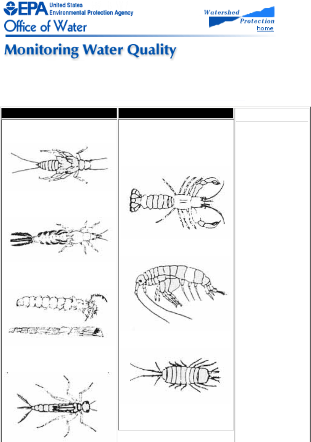
Figure 4.1

Back to Chapter 4 - Macroinvertebrates and Habitat

Insects Crustaceans Figure 4.1

Types of

macroinvertebrates

found in streams

Many biosurvey

programs include

the identification of

various

macroinvertebrates.

(Organisms are not

drawn to scale)

Stoneflies (Order: Plecoptera)

Mayflies (Order:

Ephemeroptera)

Caddisflies (Order:

Trichoptera)

Dragonflies & Damselflies

(Order: Odonata)

Crayfish & Freshwater shrimp

(Order: Decapoda)

Scud (Order: Amphipoda)

Isopod (Order: Isopoda)

Flies & Midgets (Order:

Diptera)

Water Bugs (Order: Hemiptera)

Dobsonfly (Order:

Megaloptera)

Beetles (Order: Coleoptera)

Snails

Mussels & Clams

Worms

Leeches

Office of Wetlands, Oceans & Watersheds Home

Watershed Protection Home | Monitoring Water Quality Home

EPA Home | Office of Water | Search | Comments

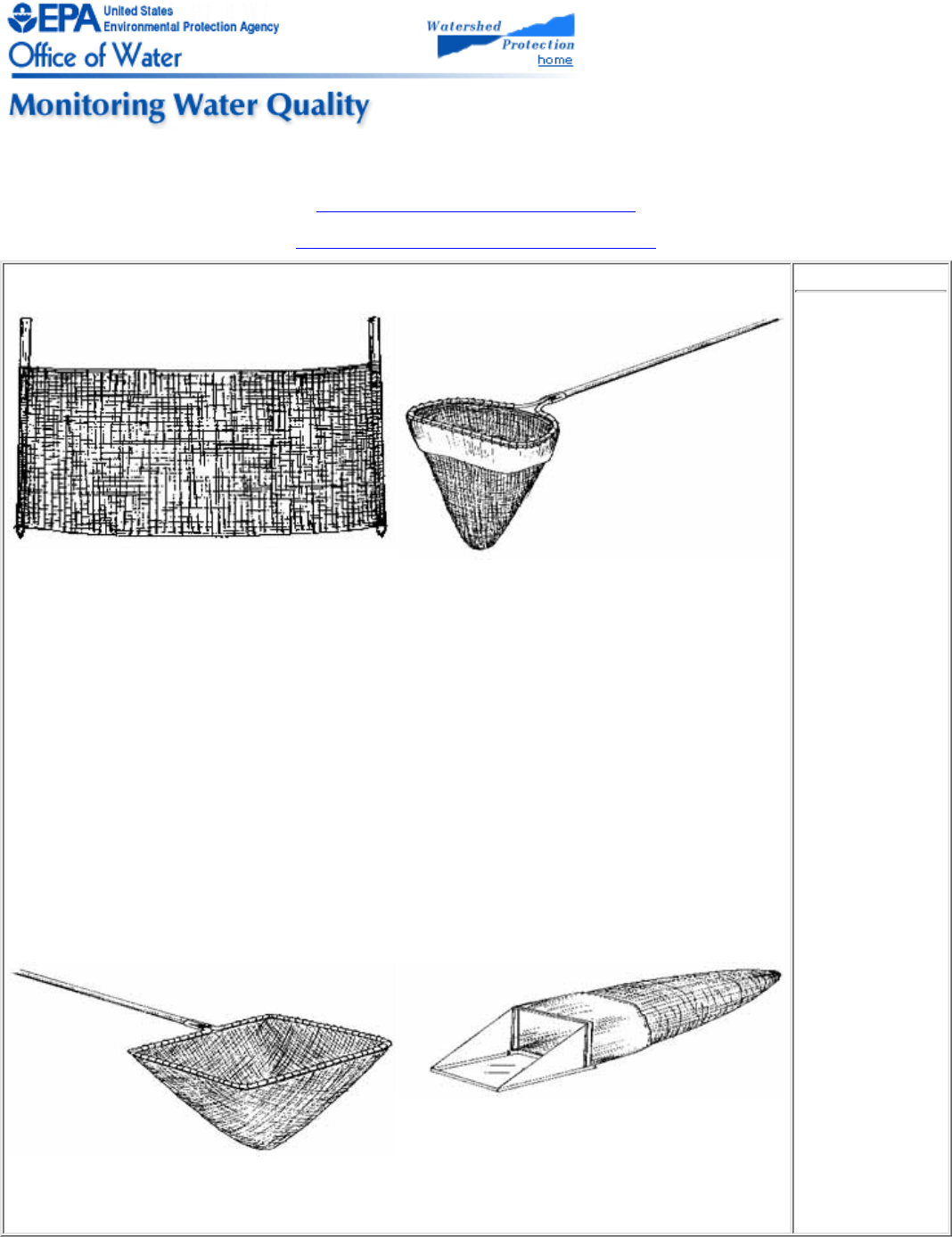
Figure 4.7

Back to Chapter 4.2 - Streamside Biosurvey

Back to Chapter 4.3 - Intensive Stream Biosurvey

Nets recommended in this manual

Kick net

For rocky-bottom stream sampling, a kick net of 590

µm (a #30 mesh size) or 500 µm (#35 mesh size) is

recommended. (Mesh size is usually measured in

microns, µm. The higher the number, the coarser the

mesh.)

D-frame net

For muddy-bottom stream sampling, a long-handled

D-frame or dip net is recommended for reaching into

vegetation that grows along stream banks or is

attached to the stream bottom, and for sweeping up

macroinvertebrates dislodged from woody debris.

D-frame nets also come in different mesh sizes.

This manual recommends that volunteer programs purchase their macroinvertebrate sampling nets from

scientific supply houses to ensure a standard degree of net quality and known mesh size. Some supply

houses might sell the components of the net separately. Volunteer programs then buy the net material

commercially, supply their own handles, and build the nets using volunteer labor.

Many programs use coarser mesh than is recommended in this manual. Coarser mesh is generally less

expensive. However, smaller organisms can be lost throguh the mesh during sampling. If you are in doubt

as to what mesh size to use, consult your technical a dvisor. If possible--and especially if you want your

volunteer data to be used by state and local water managers--it is best to use nets of the same type and size

as those which water quality professionals use in your state.

Other types of commonly used nets

Metal frame net

Used by the River Watch Network for sampling both

rocky-bottom and muddy-bottom streams.

Surber Sampler

Used by professional monitoring programs, this

sampler delineates an exact stream bottom area to be

disturbed.

Figure 4.7

Examples of

macroinvertebrates

sampling nets

Nets used by

professionals and

volunteers vary in

overall size, design,

and mesh size.

Office of Wetlands, Oceans & Watersheds Home

Watershed Protection Home | Monitoring Water Quality Home

EPA Home | Office of Water | Search | Comments

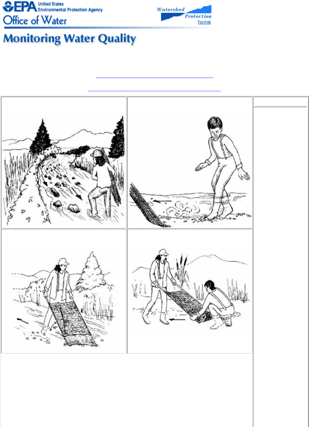
Figure 4.9

Back to Chapter 4.2 - Streamside Biosurvey

Back to Chapter 4.3 - Intensive Stream Biosurvey

1. Approach the sample site from the

downstream end. 4. Distrub the substrate thoroughly with your

feet. Figure 4.9

Procedures for

collecting a

macroinvertebrate

sample in a

rocky-bottom

stream

Volunteers must

follow set protocol

to collect an

unbiased sample.

2. Position the net at a 45° angle with the

bottom tight against the substrate. 5. Remove the net with a forward scooping

motion.

3. Dislodge macroinvertebrates by rubbing

rocks thoroughly. 6. Flush out the net with clean stream water.

Office of Wetlands, Oceans & Watersheds Home

Watershed Protection Home | Monitoring Water Quality Home

EPA Home | Office of Water | Search | Comments

Figure 4.12
Back to Section 4.2 - Streamside Biosurvey
Figure 4.12
Sample macroinvertebrate count for (hypothetical) Volunteer Creek
Office of Wetlands, Oceans & Watersheds Home
Watershed Protection Home | Monitoring Water Quality Home
EPA Home | Office of Water | Search | Comments

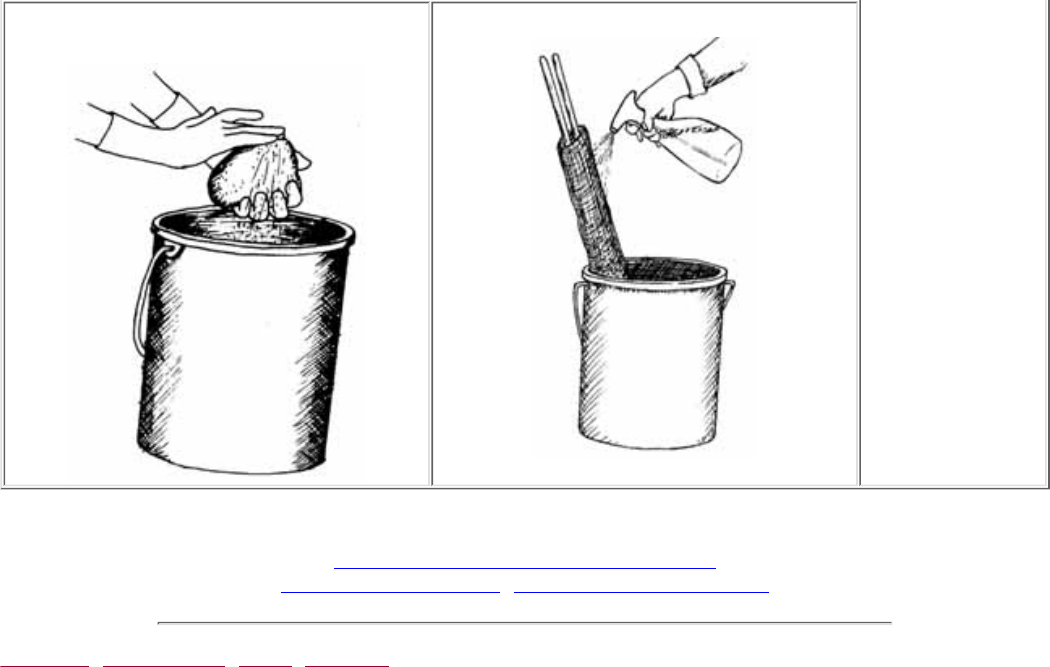
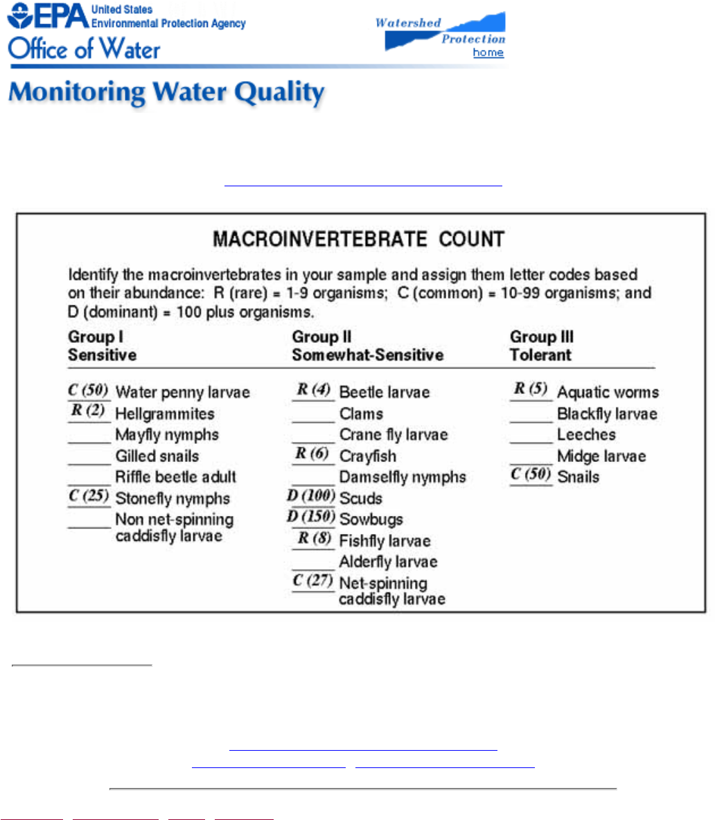
Tables 4.6 - 4.9

Back to Section 4.3 - Intensive Stream Biosurvey

Primary Metrics

(M)

Monitored

Site Values

Biosurvey Score

(Circle the appropriate range for

each metric)

Table 4.6

Metric

worksheet

for

rocky-bottom

streams

6 3 0

No. of Taxa .>15 15-8 <8

No. of EPT Taxa .>8 8-4 <4

% Dominance .<34% 34-67% >67%

Sensitive Taxa

Index .<4.8 4.8-6.4 >6.4

Optional Metrics . . . .

% Abundance of

Scrapers .>18% 18-10% <10

% Abundance of

Shredders .>9% 9-5% <5%

COLUMN SCORE

(Multiply no. of circled values by the

biosurvey score) . . .

TOTAL SCORE

(Sum all the column scores) . . .

Notes: If fewer than 60 individuals in the monitored site, don't calculate

metrics for any of the sites. Biosurvey scoring ranges determined for the

summer index period.

Primary Metrics

(M)

Monitored

Site Values

Biosurvey Score

(Circle the appropriate range for

each metric)

Table 4.7

Metric

worksheet for

muddy-bottom

streams

6 3 0

No. of Taxa .>19 19-10 <10

No. of EPT Taxa .>7 7-4 <4

% Dominance .<30% 30-50% >50%

Sensitive Taxa

Index .<5.0 5.0-6.8 >6.8

Optional Metrics . . . .

% Abundance of

EPT .>39% 39-20% <20

% Abundance of

Midge Larvae .>24% 24-60% <60%

COLUMN SCORE

(Multiply no. of circled values by the

biosurvey score) . . .

TOTAL SCORE

(Sum all the column scores) . . .

Notes: If fewer than 60 individuals in the monitored site, don't

calculate metrics for any of the sites. Biosurvey scoring ranges

determined for the summer index period.

Primary

Metrics

(M)

Monitored

Site Values

Biosurvey Score

(Circle the appropriate range

for each metric)

Table 4.8

Sample metric

worksheet for

Volunteer Creek

(hypothetical

rocky-bottom

stream)

There were 119

macroinvertebrates

in this sample.

6 3 0

No. of Taxa .>15 15-8 <8

No. of EPT Taxa .>8 8-4 <4

% Dominance .<34% 34-67% >67%

Sensitive Taxa

Index .<4.8 4.8-6.4 >6.4

COLUMN SCORE

(Multiply no. of circled values by

the biosurvey score) 6 9 0

TOTAL SCORE

(Sum all the column scores)

Biosurvey Score for this site

is 15

This site scores in the Fair

range, 9-15

Total Score

From

Metrics

Condition

Category Attributes

Table 4.9

Biosurvey

Scoring

Guide

This guide

is based on

the four

primary

metrics. If

your score

falls on the

boundary

of two

categories,

consider

the site's

habitat

assessment

results and

chemical

data, if

available,

confirming

your

assignment

to a

particular

category.

>18-24 Good Comparable to the best situation to

be expected within an ecoregion.

Balanced trophic structure.

Optimum community structure

(composition and dominance) for

stream size and habitat quality.

9-15 Fair Community structure less than

expected. Composition (species

richness) and diversity lower than

expected due to loss of some

pollution-intolerant forms. Percent

contribution of tolerant forms

increased. Reduction in EPT

index.

0-6 Poor Few species present. If high

denisities of organisms, then

dominated by one or two

polution-tolerant taxa.

Office of Wetlands, Oceans & Watersheds Home

Watershed Protection Home | Monitoring Water Quality Home

EPA Home | Office of Water | Search | Comments

Chapter 5
Water Quality Conditions
5.1 - Stream Flow
5.2 - Dissolved Oxygen and
Biochemical Oxygen Demand
5.3 - Temperature
5.4 - pH
5.5 - Turbidity
5.6 - Phosphorus
5.7 - Nitrates
5.8 - Total Solids
5.9 - Conductivity
5.10 - Total Alkalinity
5.11 - Fecal Bacteria
Quality Assurance, Quality Control, and Quality Assessment Measures
Water quality monitoring is defined here as the sampling and analysis of water constituents and conditions. These
may include:
Introduced pollutants, such as pesticides, metals, and oil
● 
Constituents found naturally in water that can nevertheless be affected by human sources, such as dissolved
oxygen, bacteria, and nutrients
● 
The magnitude of their effects can be influenced by properties such as pH and temperature. For example,
temperature influences the quantity of dissolved oxygen that water is able to contain, and pH affects the toxicity
of ammonia.
Volunteers, as well as state and local water quality professionals, have been monitoring water quality conditions
for many years. In fact, until the past decade or so (when biological monitoring protocols were developed and
began to take hold), water quality monitoring was generally considered the primary way of identifying water
pollution problems. Today, professional water quality specialists and volunteer program coordinators alike are
moving toward approaches that combine chemical, physical, and biological monitoring methods to achieve the
best picture of water quality conditions.
Water quality monitoring can be used for many purposes:
To identify whether waters are meeting designated uses. All states have established specific criteria (limits
on pollutants) identifying what concentrations of chemical pollutants are allowable in their waters. When
chemical pollutants exceed maximum or minimum allowable concentrations, waters might no longer be
able to support the beneficial uses such as fishing, swimming, and drinking for which they have been
designated. Designated uses and the specific criteria that protect them (along with antidegradation
statements say waters should not be allowed to deteriorate below existing or anticipated uses) together form
water quality standards. State water quality professionals assess water quality by comparing the
concentrations of chemical pollutants found in streams to the criteria in the state's standards, and so judge
whether streams are meeting their designated uses.
Water quality monitoring, however, might be inadequate for determining whether aquatic life uses are
being met in a stream. While some constituents (such as dissolved oxygen and temperature) are important
to maintaining healthy fish and aquatic insect populations, other factors, such as the physical structure of
the stream and the condition of the habitat, play an equal or greater role. Biological monitoring methods
(see Chapter 4) are generally better suited to determining whether aquatic life is supported.
● 
To identify specific pollutants and sources of pollution. Water quality monitoring helps link sources of
pollution to a stream quality problem because it identifies specific problem pollutants. Since certain
● 

activities tend to generate certain pollutants (e.g., bacteria and nutrients are more likely to come from an

animal feedlot than an automotive repair shop), a tentative link might be made that would warrant further

investigation or monitoring.

To determine trends. Chemical constituents that are properly monitored (i.e., consistent time of day and on

a regular basis, using consistent methods) can be analyzed for trends over time.

●

To screen for impairment. Finding excessive levels of one or more chemical constituents can serve as an

early warning "screen" of potential pollution problems.

●

Designing a water quality monitoring program

The first step in designing a water quality monitoring program is to determine the purpose of the monitoring. This

will help you select which parameters to monitor. The program steering committee should make this decision

based on factors such as:

Types of water quality problems and pollution sources that will likely be encountered (Table 5.1)

●

Cost of available monitoring equipment●

Precision and accuracy of available monitoring equipment●

Capabilities of the volunteers●

Source Common Associated Chemical Pollutants Table 5.1

Sources

and

associated

pollutants

A volunteer

water

quality

monitoring

program

should be

geared to

the types of

watershed

land uses

most often

encountered.

Cropland Turbidity, phosphorus, nitrates, temparature, total solids

Forestry harvest Turbidity, temperature, total solids

Grazing land Fecal bacteria, turbidity, phosphorus, nitrates, temperature

Industrial discharge Temperature, conductivity, total solids, toxics, pH

Mining pH, alkalinity, total dissolved solids

Septic systems Fecal bacteria (i.e., Escherichia coli, enterococcis), nitrates,

phosphorus, dissolved oxygen/biochemical oxygen demand,

conductivity, temperature

Sewage treatment plants Dissolved oxygen and biochemical oxygen demand, turbidity,

conductivity, phosphorus, nitrates, fecal bacteria, temperature, total

solids, pH

Construction Turbidity, temperature, dissolved oxygen and biochemical oxygen

demand, total solids, and toxics

Urban runoff Turbidity, phosphorus, nitrates, temperature, conductivity, dissolved

oxygen and biochemical oxygen demand

Because of the expense and difficulty involved, volunteers generally do not monitor for toxic substances such as

heavy metals and organic chemicals (e.g., pesticides, herbicides, solvents, and PCBs). They might, however,

collect water samples for analysis at accredited labs.

The parameters most commonly monitored by volunteers in streams are discussed in detail in this chapter. They

include stream flow, dissolved oxygen and biochemical oxygen demand, temperature, pH, turbidity, phosphorus,

nitrates, total solids, conductivity, total alkalinity, and fecal bacteria. Of these, the first five are the most basic and

should form the foundation of almost any volunteer water quality monitoring program.

Relatively inexpensive and simple-to-use kits are available from scientific supply houses to monitor these

pollutants. Many volunteer programs use these kits effectively. Meters and sophisticated lab equipment may be

more accurate, but they are also more expensive, less flexible (e.g., meters generally have to be read in the field),

and require periodic calibration. This chapter discusses specific equipment and sampling considerations for each

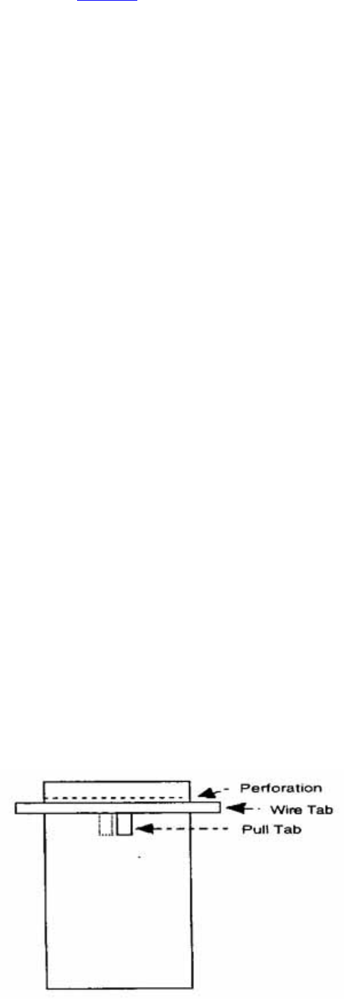
parameter, and usually describes several approaches to monitor them. Table 5.2 lists methods available for

monitoring key parameters, including the preferred testing site (lab or field).

General preparation and sampling considerations

The sections that follow will detail specific sampling and equipment considerations and analytical procedures for

each of the most common water quality parameters. There are, however, two general tasks that are accomplished

anytime water samples are taken. These are discussed below.

Task 1 Preparation of Sampling Containers

Reused sample containers and glassware must be cleaned and rinsed before the first sampling run and after each

run by following either Method A or Method B described below. The most suitable method depends on the

parameter being measured.

Method A: General Preparation of Sampling Containers

The following method should be used when preparing all sample containers and glassware for monitoring

conductivity, total solids, turbidity, pH, and total alkalinity. Wear latex gloves!

Wash each sample bottle or piece of glassware with a brush and phosphate-free detergent.1.

Rinse three times with cold tap water.2.

Rinse three times with distilled or deionized water.3.

Method B: Acid Wash Procedure for Preparing Sampling Containers This method should be used when

preparing all sample containers and glassware for monitoring nitrates and phosphorus. Wear latex gloves!

Wash each sample bottle or piece of glassware with a brush and phosphate-free detergent.1.

Rinse three times with cold tap water.2.

Rinse with 10 percent hydrochloric acid.3.

Rinse three times with deionized water.4.

Task 2 Collecting Samples

In general, sample away from the streambank in the main current. Never sample stagnant water. The outside

curve of the stream is often a good place to sample, since the main current tends to hug this bank. In shallow

stretches, carefully wade into the center current to collect the sample.

A boat will be required for deep sites. Try to maneuver the boat into the center of the main current to collect the

water sample.

When collecting a water sample for analysis in the field or at the lab, follow the steps below. For Whirl-pak®

Bags

Label the bag with the site number, date, and time.

Tear off the top of the bag along the perforation

above the wire tab just prior to sampling (Fig.

5.1). Avoid touching the inside of the bag. If you

accidentally touch the inside of the bag, use

another one.

Wading. Try to disturb as little bottom sediment

as possible. In any case, be careful not to collect

water that contains bottom sediment. Stand

facing upstream. Collect the water sample in

front of you.

Boat. Carefully reach over the side and collect

the water sample on the upstream side of the

boat.

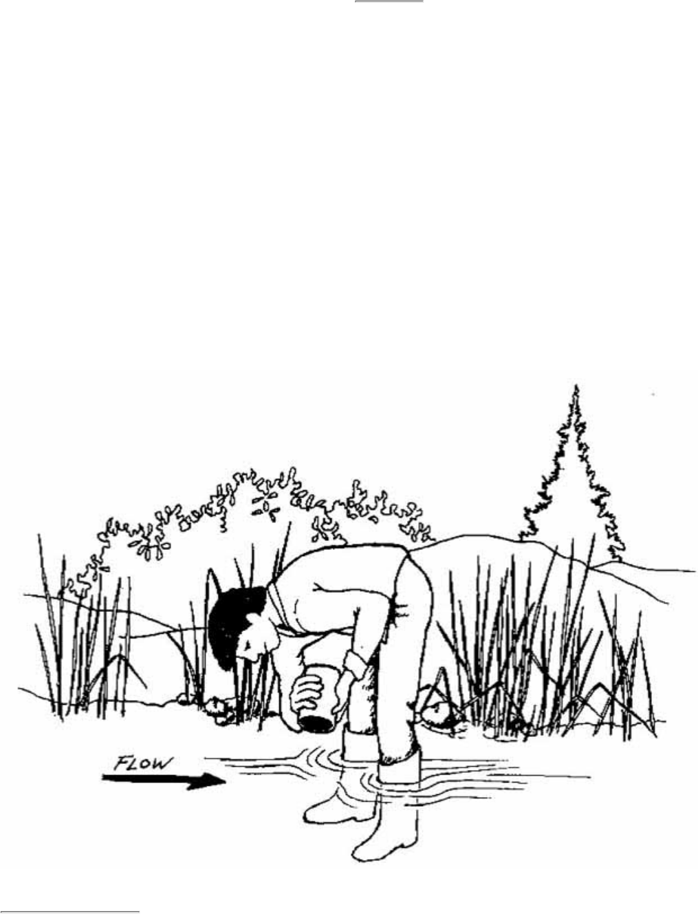
Figure 5.1

Sketch of a Whirl-pak® bag

Volunteers can be easily trained to use these factory-sealed,

disposable water sample collection bags.

Hold the two white pull tabs in each hand and

lower the bag into the water on your upstream

side with the opening facing upstream. Open the

bag midway between the surface and the bottom

by pulling the white pull tabs. The bag should

begin to fill with water. You may need to "scoop"

water into the bag by drawing it through the

water upstream and away from you. Fill the bag

no more than 3/4 full!

Lift the bag out of the water. Pour out excess water. Pull on the wire tabs to close the bag. Continue holding

the wire tabs and flip the bag over at least 4-5 times quickly to seal the bag. Don't try to squeeze the air out

of the top of the bag. Fold the ends of the wire tabs together at the top of the bag, being careful not to

puncture the bag. Twist them together, forming a loop.

Fill in the bag number and/or site number on the appropriate field data sheet. This is important! It is the

only way the lab coordinator know which bag goes with which site.

If samples are to be analyzed in a lab, place the sample in the cooler with ice or cold packs. Take all

samples to the lab.

For Screw-cap Bottles

To collect water samples using screw-cap sample bottles, use the following procedures (Fig. 5.2 and 5.3):

Figure 5.2

Getting into position to take a water sample

Volunteers should sample in the mail current, facing upstream.

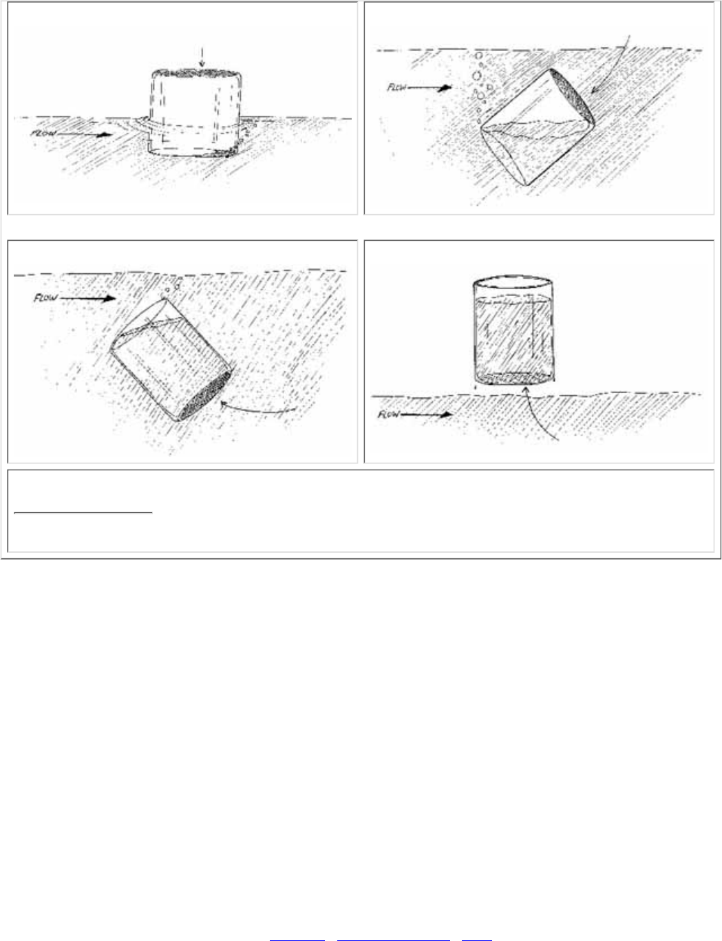
1. 2.

3. 4.

Figure 5.3

Taking a water sample

Turn the bottle into the current and scoop in an upstream direction.

Label the bottle with the site number, date, and time.1.

Remove the cap from the bottle just before sampling. Avoid touching the inside of the bottle or the cap. If

you accidentally touch the inside of the bottle, use another one.

Wading. Try to disturb as little bottom sediment as possible. In any case, be careful not to collect water that

has sediment from bottom disturbance. Stand facing upstream. Collect the water sample on your upstream

side, in front of you. You may also tape your bottle to an extension pole to sample from deeper water.

Boat. Carefully reach over the side and collect the water sample on the upstream side of the boat.

Hold the bottle near its base and plunge it (opening downward) below the water surface. If you are using an

extension pole, remove the cap, turn the bottle upside down, and plunge it into the water, facing upstream.

Collect a water sample 8 to 12 inches beneath the surface or mid-way between the surface and the bottom if

the stream reach is shallow.

Turn the bottle underwater into the current and away from you. In slow-moving stream reaches, push the

bottle underneath the surface and away from you in an upstream direction.

Leave a 1-inch air space (Except for DO and BOD samples). Do not fill the bottle completely (so that the

sample can be shaken just before analysis). Recap the bottle carefully, remembering not to touch the inside.

Fill in the bottle number and/or site number on the appropriate field data sheet. This is important because it

tells the lab coordinator which bottle goes with which site.

If the samples are to be analyzed in the lab, place them in the cooler for transport to the lab.

< Previous · Table of Contents · Next >

Office of Wetlands, Oceans & Watersheds Home

Watershed Protection Home | Monitoring Water Quality Home

EPA Home | Office of Water | Search | Comments

QUALITY ASSURANCE, QUALITY CONTROL, and QUALITY ASSESSMENT

MEASURES

Back to Chapter 5 - Water Quality Conditions

Quality assurance/quality control measures are those activities you undertake to demonstrate the accuracy (how

close to the real result you are) and precision (how reproducible your results are) of your monitoring. Quality

Assurance (QA) generally refers to a broad plan for maintaining quality in all aspects of a program. This plan

should describe how you will undertake your monitoring effort: proper documentation of all your procedures,

training of volunteers, study design, data management and analysis, and specific quality control measures. Quality

Control (QC) consists of the steps you will take to determine the validity of specific sampling and analytical

procedures. Quality assessment is your assessment of the overall precision and accuracy of your data, after you've

run the analyses.

Quality Control and Assessment Measures: Internal Checks

Internal checks are performed by the project field volunteers, staff, and lab.

Field Blanks. A trip blank (also known as a field blank) is deionized water which is treated as a sample. It

is used to identify errors or contamination in sample collection and analysis.

●

Negative and Positive Plates (for bacteria). A negative plate results when the buffered rinse water (the

water used to rinse down the sides of the filter funnel during filtration) has been filtered the same way as a

sample. This is different from a field blank in that it contains reagents used in the rinse water. There should

be no bacteria growth on the filter after incubation. It is used to detect laboratory bacteria contamination of

the sample. Positive plates result when water known to contain bacteria (such as wastewater treatment plant

influent) is filtered the same way as a sample. There should be plenty of bacteria growth on the filter after

incubation. It is used to detect procedural errors or the presence of contaminants in the laboratory analysis

that might inhibit bacteria growth.

●

Field Duplicates. A field duplicate is a duplicate river sample collected by the same team or by another

sampler or team at the same place, at the same time. It is used to estimate sampling and laboratory analysis

precision.

●

Lab Replicates. A lab replicate is a sample that is split into subsamples at the lab. Each subsample is then

analyzed and the results compared. They are used to test the precision of the laboratory measurements. For

bacteria, they are used to obtain an optimal number of bacteria colonies on filters for counting purposes.

●

Spike Samples. A known concentration of the indicator being measured is added to the sample. This should

increase the concentration in the sample by a predictable amount. It is used to test the accuracy of the

method.

●

Calibration Blank. A calibration blank is deionized water processed like any of the samples and used to

"zero" the instrument. It is the first "sample" analyzed and used to set the meter to zero. This is different

from the field blank in that it is "sampled" in the lab. It is used to check the measuring instrument

periodically for "drift" (the instrument should always read "0" when this blank is measured). It can also be

compared to the field blank to pinpoint where contamination might have occurred.

●

Calibration Standards. Calibration standards are used to calibrate a meter. They consist of one or more

"standard concentrations" (made up in the lab to specified concentrations) of the indicator being measured,

one of which is the calibration blank. Calibration standards can be used to calibrate the meter before

running the test, or they can be used to convert the units read on the meter to the reporting units (for

example, absorbance to milligrams per liter).

●

Quality Control And Assessment Measures: External Checks

External checks are performed by nonvolunteer field staff and a lab (also known as a "quality control lab"). The

results are compared with those obtained by the project lab.

External Field Duplicates. An external field duplicate is a duplicate river sample collected and processed

by an independent (e.g., professional) sampler or team at the same place at the same time as regular river

samples. It is used to estimate sampling and laboratory analysis precision.

●

Split Samples. A split sample is a sample that is divided into two subsamples at the lab. One subsample is

analyzed at the project lab and the other is analyzed at an independent lab. The results are compared.

●

Outside Lab Analysis of Duplicate Samples. Either internal or external field duplicates can be analyzed at

an independent lab. The results should be comparable with those obtained by the project lab.

●

Knowns. The quality control lab sends samples for selected indicators, labeled with the concentrations, to

the project lab for analysis prior to the first sample run. These samples are analyzed and the results

compared with the known concentrations. Problems are reported to the quality control lab.

●

Unknowns. The quality control lab sends samples to the project lab for analysis for selected indicators,

prior to the first sample run. The concentrations of these samples are unknown to the project lab. These

samples are analyzed and the results reported to the quality control lab. Discrepancies are reported to the

project lab and a problemidentification and solving process follows.

●

The table below shows the applicability of common quality control measures to the water quality indicators

covered in this manual.

Steps To Quality Control

Consult with your technical committee and/or program advisor to help you determine quality

assurance/quality control measures you will use to answer your questions and meet your data quality

requirements

Locate a quality control lab—-an independent lab that can run external checks for you.2.

Determine which quality checks you have the resources and capabilities to carry out. Your human and

financial resources and expertise might limit the water quality indicators your can monitor.

References

APHA. 1992. Standard Methods for the Examination of Water and Wastewater. 18th ed. American Public Health

Association, Washington, DC.

Intergovernmental Task Force on Monitoring Water Quality. 1994. Water quality monitoring in the United States.

1993 report and technical appendixes. Washington, DC.

Mattson, M. 1992. The basics of quality control. The Volunteer Monitor. 4(2) Fall 1992.

USEPA. 1983. Methods for chemical analysis of water and wastes. EPA600/479020. U.S. Environmental

Protection Agency, Environmental Monitoring and Support Laboratory, Cincinnati, OH. March.

USEPA. 1984. Guidance for preparation of combined work/quality assurance project plans for environmental

monitoring. ORWS QA1, U.S. Environmental Protection Agency, Office of Water Regulations and Standards.

Washington DC, May.

USEPA. 1996. The Volunteer Monitor's Guide to Quality Assurance Project Plans. EPA841-B-96-003.

Environmental Protection Agency, Office of Water, Washington, DC.

Common Quality Control Measures

..... Dissolved

Oxygen Temperature pH Turbidity Phosphorus Nitrates Total

Solids Conductivity Total

Alkalinity Fecal

Bacteria

Internal Checks

Field

blanks . . . • • • • • • .

Field

duplicates • • • • • • • • • •

Lab

replicates •.• • • • • • • •b

Positive

plates . . . . . . . . . •

Negative

plates . . . . . . . . . •

Spike

samples .•. . • • . . • •

Calibration

blank . . . • • • .•. .

Calibration

standard •a .• • • • .•. .

External Checks

External

field

duplicates . . • • • • • • • •

Split

samples . . • • • • • • • .

Outside lab

analysis •. . • • • • • • •

Verification . . . . . . . . . •

Knowns • .• • • • .• • •

Unknowns • .• • • • .• • •

a - using an oxygen-saturated sample

b - using subsamples of different sizes

Office of Wetlands, Oceans & Watersheds Home

Watershed Protection Home | Monitoring Water Quality Home

EPA Home | Office of Water | Search | Comments

5.1

Stream Flow

What is stream flow and why is it important?

Stream flow, or discharge, is the volume of water that moves over a designated point over

a fixed period of time. It is often expressed as cubic feet per second (ft3/sec).

The flow of a stream is directly related to the amount of water moving off the watershed

into the stream channel. It is affected by weather, increasing during rainstorms and

decreasing during dry periods. It also changes during different seasons of the year,

decreasing during the summer months when evaporation rates are high and shoreline

vegetation is actively growing and removing water from the ground. August and

September are usually the months of lowest flow for most streams and rivers in most of

the country.

Water withdrawals for irrigation purposes can seriously deplete water flow, as can

industrial water withdrawals. Dams used for electric power generation, particularly

facilities designed to produce power during periods of peak need, often block the flow of

a stream and later release it in a surge.

Flow is a function of water volume and velocity. It is important because of its impact on

water quality and on the living organisms and habitats in the stream. Large, swiftly

flowing rivers can receive pollution discharges and be little affected, whereas small

streams have less capacity to dilute and degrade wastes.

Stream velocity, which increases as the volume of the water in the stream increases,

determines the kinds of organisms that can live in the stream (some need fast-flowing

areas; others need quiet pools). It also affects the amount of silt and sediment carried by

the stream. Sediment introduced to quiet, slow-flowing streams will settle quickly to the

stream bottom. Fast moving streams will keep sediment suspended longer in the water

column. Lastly, fast-moving streams generally have higher levels of dissolved oxygen

than slow streams because they are better aerated.

This section describes one method for estimating flow in a specific area or reach of a

stream. It is adapted from techniques used by several volunteer monitoring programs and

uses a float (an object such as an orange, ping-pong ball, pine cone, etc.) to measure

stream velocity. Calculating flow involves solving an equation that examines the

relationship among several variables including stream cross-sectional area, stream length,

and water velocity. One way to measure flow is to solve the following equation:

Flow = ALC / T

Where:

A = Average cross-sectional area of the stream (stream width multiplied by average

water depth).

L = Length of the stream reach measured (usually 20 ft.)

C = A coefficient or correction factor (0.8 for rocky-bottom streams or 0.9 for

muddy-bottom streams). This allows you to correct for the fact that water at the

surface travels faster than near the stream bottom due to resistance from gravel,

cobble, etc. Multiplying the surface velocity by a correction coefficient decreases

the value and gives a better measure of the stream's overall velocity.

T = Time, in seconds, for the float to travel the length of L

How to Measure and Calculate Stream Flow

Task 1 Prepare before leaving for the sampling site

Refer to section 2.3 - Safety Considerations for details on confirming sampling date and

time, safety considerations, checking supplies, and checking weather and directions. In

addition to the standard sampling equipment and apparel, when measuring and

calculating flow, include the following equipment:

Ball of heavy-duty string, four stakes, and a hammer to drive the stakes into the

ground. The string will be stretched across the width of the stream perpendicular to

shore at two locations. The stakes are to anchor the string on each bank to form a

transect line.

●

Tape measure (at least 20 feet)●

Waterproof yardstick or other implement to measure water depth●

Twist ties (to mark off intervals on the string of the transect line)●

An orange and a fishing net (to scoop the orange out of the stream)●

Stopwatch (or watch with a second hand)●

Calculator (optional)●

Task 2 Select a stretch of stream

The stream stretch chosen for the measurement of discharge should be straight (no

bends), at least 6 inches deep, and should not contain an area of slow water such as a

pool. Unobstructed riffles or runs are ideal. The length that you select will be equal to L

in solving the flow equation. Twenty feet is a standard length used by many programs.

Measure your length and mark the upper and lower end by running a transect line across

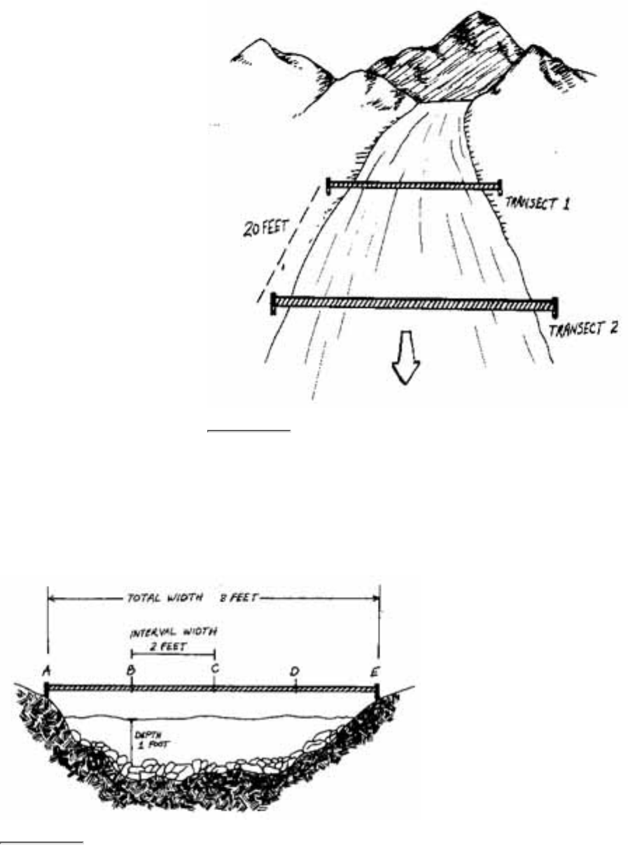
Figure 5.4

A diagram of a 20-foot transect

the stream perpendicular to the

shore using the string and stakes

(Fig. 5.4). The string should be

taut and near the water surface.

The upstream transect is

Transect #1 and the downstream

one is Transect #2.

Task 3 Calculate the

average

cross-sectional area

Cross-sectional area (A in the

formula) is the product of

stream width multiplied by

average water depth. To

calculate the average

cross-sectional area for the

study stream reach, volunteers

should determine the

cross-sectional area for each

transect, add the results together, and then divide by 2 to determine the average

cross-sectional area for the stream reach.

To measure cross-sectional area:

Figure 5.5

A cross section view to measure stream width and depth

Determine the average

depth along the transect

by marking off equal

intervals along the string

with the twist ties. The

intervals can be

one-fourth, one-half, and

three-fourths of the

distance across the

stream. Measure the

water's depth at each

interval point (Fig. 5.5).

To calculate average

depth for each transect,

divide the total of the

three depth measurements

by 4. (You divide by 4

instead of 3 because you

need to account for the 0

depths that occur at the

shores.) In the example

shown in Figure 5.6, the

average depth of Transect

#1 is 0.575 feet and the

average depth of Transect

#2 is 0.625 feet.

Determine the width of each transect by measuring the distance from shoreline to

shoreline. Simply add together all the interval widths for each transect to determine

its width. In the Figure 5.6 example, the width of Transect #1 is 8 feet and the

width of Transect #2 is 10 feet.

Calculate the cross-sectional area of each transect by multiplying width times

average depth. The example given in Figure 5.6 shows that the average

cross-sectional area of Transect #1 is 4.60 square feet and the average

cross-sectional area of Transect #2 is 6.25 square feet.

To determine the average cross-sectional area of the entire stream reach (A in the

formula), add together the average cross-sectional area of each transect and then

divide by 2. The average cross-sectional area for the stream reach in Figure 5.6 is

5.42 square feet.

Task 4 Measure travel time

Volunteers should time with a stopwatch how long it takes for an orange (or some other

object) to float from the upstream to the downstream transect. An orange is a good object

to use because it has enough buoyancy to float just below the water surface. It is at this

position that maximum velocity typically occurs.

The volunteer who lets the orange go at the upstream transect should position it so it

flows into the fastest current. The clock stops when the orange passes fully under the

downstream transect line. Once under the transect line, the orange can be scooped out of

the water with the fishing net. This "time of travel" measurement should be conducted at

least three times and the results averaged--the more trials you do, the more accurate your

results will be. The averaged results are equal to T in the formula. It is a good idea to

float the orange at different distances from the bank to get various velocity estimates.

You should discard any float trials if the object gets hung up in the stream (by cobbles,

roots, debris, etc.)

Task 5 Calculate flow

Recall that flow can be calculated using the equation:

Flow = ALC / T

Continuing the example in Fig. 5.6. say the average time of travel for the orange between

Transect #1 and #2 is 15 seconds and the stream had a rocky bottom. The calculation of

flow would be:
Where:
A = 5.42 ft2
L = 20 ft
C = 0.8 (coefficient for a rocky-bottom stream)
T = 15 seconds
Flow = 15 seconds (5.42 ft2) (20 ft) (0.8) / 15 sec.
Flow = 86.72 ft3/ 15 sec.
Flow = 5.78 ft3/sec.
Task 6 Record flow on the data form
On the following page is a form volunteers can use to calculate flow of a stream.
References
Adopt-A-Stream Foundation. Field Guide: Watershed Inventory and Stream Monitoring
Methods, by Tom Murdoch and Martha Cheo. 1996. Everett, WA.
Mitchell, M.K., and W. Stapp. Field Manual for Water Quality Monitoring. 5th Edition.
Thompson Shore Printers.
Missouri Stream Teams. Volunteer Water Quality Monitoring. Missouri Department of
Natural Resources, P.O. Box 176, Jefferson City, MO 65102.
Data Form for Calculating Flow (PDF, 82.8 KB)
Adobe Acrobat Reader is required to view PDF documents. The most recent version of the Adobe
Acrobat Reader is available as a free download. An Adobe Acrobat plug-in for assisted technologies is
also available.
< Previous · Table of Contents · Next >
Office of Wetlands, Oceans & Watersheds Home
Watershed Protection Home | Monitoring Water Quality Home
EPA Home | Office of Water | Search | Comments

5.2

Dissolved Oxygen and Biochemical Oxygen Demand

What is dissolved oxygen and why is it important?

The stream system both produces and consumes oxygen. It gains oxygen from the atmosphere and from plants as

a result of photosynthesis. Running water, because of its churning, dissolves more oxygen than still water, such as

that in a reservoir behind a dam. Respiration by aquatic animals, decomposition, and various chemical reactions

consume oxygen.

Wastewater from sewage treatment plants often contains organic materials that are decomposed by

microorganisms, which use oxygen in the process. (The amount of oxygen consumed by these organisms in

breaking down the waste is known as the biochemical oxygen demand or BOD. A discussion of BOD and how to

monitor it is included at the end of this section.) Other sources of oxygen-consuming waste include stormwater

runoff from farmland or urban streets, feedlots, and failing septic systems.

Oxygen is measured in its dissolved form as dissolved oxygen (DO). If more oxygen is consumed than is

produced, dissolved oxygen levels decline and some sensitive animals may move away, weaken, or die.

DO levels fluctuate seasonally and over a 24-hour period. They vary with water temperature and altitude. Cold

water holds more oxygen than warm water (Table 5.3) and water holds less oxygen at higher altitudes. Thermal

discharges, such as water used to cool machinery in a manufacturing plant or a power plant, raise the temperature

of water and lower its oxygen content. Aquatic animals are most vulnerable to lowered DO levels in the early

morning on hot summer days when stream flows are low, water temperatures are high, and aquatic plants have

not been producing oxygen since sunset.

Temperature

(°C) DO

(mg/l) Temperature

(°C) DO

(mg/l) Table 5.3

Maximum

dissolved

oxygen

concentrates

vary with

temperature

0 14.60 23 8.56

1 14.19 24 8.40

2 13.81 25 8.24

3 13.44 26 8.09

4 13.09 27 7.95

5 12.75 28 7.81

6 12.43 29 7.67

7 12.12 30 7.54

8 11.83 31 7.41

9 11.55 32 7.28

10 11.27 33 7.16

11 11.01 34 7.16

12 10.76 35 6.93

13 10.52 36 6.82

14 10.29 37 6.71

15 10.07 38 6.61

Sampling and Equipment

Considerations

In contrast to lakes, where DO levels are most likely to

vary vertically in the water column, the DO in rivers and

streams changes more horizontally along the course of

the waterway. This is especially true in smaller,

shallower streams. In larger, deeper rivers, some vertical

stratification of dissolved oxygen might occur. The DO

levels in and below riffle areas, waterfalls, or dam

spillways are typically higher than those in pools and

slower-moving stretches. If you wanted to measure the

effect of a dam, it would be important to sample for DO

behind the dam, immediately below the spillway, and

upstream of the dam. Since DO levels are critical to fish,

a good place to sample is in the pools that fish tend to

favor or in the spawning areas they use.

An hourly time profile of DO levels at a sampling site is

a valuable set of data because it shows the change in DO

levels from the low point just before sunrise to the high

16 9.85 39 6.51

17 9.65 40 6.41

18 9.45 41 6.41

19 9.26 42 6.22

20 9.07 43 6.13

21 8.90 44 6.04

22 8.72 45 5.95

point sometime in the midday. However, this might not

be practical for a volunteer monitoring program. It is

important to note the time of your DO sampling to help

judge when in the daily cycle the data were collected.

DO is measured either in milligrams per liter (mg/L) or

"percent saturation." Milligrams per liter is the amount of

oxygen in a liter of water. Percent saturation is the

amount of oxygen in a liter of water relative to the total

amount of oxygen that the water can hold at that temperature.

DO samples are collected using a special BOD bottle: a glass bottle with a "turtleneck" and a ground glass

stopper. You can fill the bottle directly in the stream if the stream is wadable or boatable, or you can use a

sampler that is dropped from a bridge or boat into water deep enough to submerse the sampler. Samplers can be

made or purchased. Dissolved oxygen is measured primarily either by using some variation of the Winkler

method or by using a meter and probe. Winkler Method The Winkler method involves filling a sample bottle

completely with water (no air is left to bias the test). The dissolved oxygen is then "fixed" using a series of

reagents that form an acid compound that is titrated. Titration involves the drop-by-drop addition of a reagent that

neutralizes the acid compound and causes a change in the color of the solution. The point at which the color

changes is the "endpoint" and is equivalent to the amount of oxygen dissolved in the sample. The sample is

usually fixed and titrated in the field at the sample site. It is possible, however, to prepare the sample in the field

and deliver it to a lab for titration.

Dissolved oxygen field kits using the Winkler method are relatively inexpensive, especially compared to a meter

and probe. Field kits run between $35 and $200, and each kit comes with enough reagents to run 50 to 100 DO

tests. Replacement reagents are inexpensive, and you can buy them already measured out for each test in plastic

pillows.

You can also buy the reagents in larger quantities, in bottles, and measure them out with a volumetric scoop. The

advantage of the pillows is that they have a longer shelf life and are much less prone to contamination or spillage.

The advantage of buying larger quantities in bottles is that the cost per test is considerably less.

The major factor in the expense of the kits is the method of titration they use eyedropper, syringe-type titrator, or

digital titrator. Eyedropper and syringe-type titration is less precise than digital titration because a larger drop of

titrant is allowed to pass through the dropper opening and, on a micro-scale, the drop size (and thus the volume of

titrant) can vary from drop to drop. A digital titrator or a buret (which is a long glass tube with a tapered tip like a

pipet) permits much more precision and uniformity in the amount of titrant that is allowed to pass.

If your program requires a high degree of accuracy and precision in DO results, use a digital titrator. A kit that

uses an eye dropper-type or syringe- type titrator is suitable for most other purposes. The lower cost of this type

of DO field kit might be attractive if you are relying on several teams of volunteers to sample multiple sites at the

same time.

Meter and Probe

A dissolved oxygen meter is an electronic device that converts signals from a probe that is placed in the water

into units of DO in milligrams per liter. Most meters and probes also measure temperature. The probe is filled

with a salt solution and has a selectively permeable membrane that allows DO to pass from the stream water into

the salt solution. The DO that has diffused into the salt solution changes the electric potential of the salt solution

and this change is sent by electric cable to the meter, which converts the signal to milligrams per liter on a scale

that the volunteer can read.

DO meters are expensive compared to field kits that use the titration method. Meter/probe combinations run

between $500 and $1,200, including a long cable to connect the probe to the meter. The advantage of a

meter/probe is that you can measure DO and temperature quickly at any point in the stream that you can reach

with the probe. You can also measure the DO levels at a certain point on a continuous basis. The results are read

directly as milligrams per liter, unlike the titration methods, in which the final titration result might have to be

converted by an equation to milligrams per liter.

However, DO meters are more fragile than field kits, and repairs to a damaged meter can be costly. The

meter/probe must be carefully maintained, and it must be calibrated before each sample run and, if you are doing

many tests, in between samplings. Because of the expense, a volunteer program might have only one meter/probe.

This means that only one team of samplers can sample DO and they will have to do all the sites. With field kits,

on the other hand, several teams can sample simultaneously.

Laboratory Testing of Dissolved Oxygen

If you use a meter and probe, you must do the testing in the field; dissolved oxygen levels in a sample bottle

change quickly due to the decomposition of organic material by microorganisms or the production of oxygen by

algae and other plants in the sample. This will lower your DO reading. If you are using a variation of the Winkler

method, it is possible to "fix" the sample in the field and then deliver it to a lab for titration. This might be

preferable if you are sampling under adverse conditions or if you want to reduce the time spent collecting

samples. It is also a little easier to titrate samples in the lab, and more quality control is possible because the same

person can do all the titrations.

How to collect and analyze samples

The procedures for collecting and analyzing samples for dissolved oxygen consist of the following tasks:

TASK 1 Prepare before leaving for the sampling site

Refer to section 2.3 - Safety Considerations for details on confirming sampling date and time, safety

considerations, checking supplies, and checking weather and directions. In addition to the standard sampling

equipment and apparel, when sampling for dissolved oxygen, include the following equipment:

If Using the Winkler Method

Labels for sample bottles

●

Field kit and instructions for DO testing●

Enough reagents for the number of sites to be tested●

Kemmerer, Van Dorn, or home-made sampler to collect deep-water samples●

A numbered glass BOD bottle with a glass stopper (1 for each site)●

Data sheet for dissolved oxygen to record results●

If Using a Meter and Probe

DO meter and probe (electrode) (NOTE: Confirm that the meter has been calibrated according to the

manufacturer's instructions.)

●

Operating manual for the meter and probe●

Extra membranes and electrolyte solution for the probe●

Extra batteries for the meter●

Extension pole●

Data sheet for dissolved oxygen to record results●

TASK 2 Confirm that you are at the proper location

The directions for sampling should provide specific information about the exact point in the stream from which

you are to sample; e.g., "approximately 6 feet out from the large boulder downstream from the west side of the

bridge." If you are not sure you are in the exact spot, record a detailed description of where you took the sample

so that it can be compared to the actual site later.

TASK 3 Collect samples and fill out the field data sheet

Winkler Method

Use a BOD bottle to collect the water sample. The most common sizes are 300 milliliters (mL) and 60 mL. Be

sure that you are using the correct volume for the titration method that will be used to determine the amount of

DO. There is usually a white label area on the bottle, and this may already be numbered. If so, be sure to record

that number on the field data sheet. If your bottle is not already numbered, place a label on the bottle (not on the

cap because a cap can be inadvertently placed on a different bottle) and use a waterproof marker to write in the

site number.

If you are collecting duplicate samples, label the duplicate bottle with the correct code, which should be

determined prior to sampling by the lab supplying the bottles. Use the following procedure for collecting a

sample for titration by the Winkler method:

Remember that the water sample must be collected in such a way that you can cap the bottle while it is still

submerged. That means that you must be able to reach into the water with both arms and the water must be

deeper than the sample bottle.

Carefully wade into the stream. Stand so that you are facing one of the banks.2.

Collect the sample so that you are not standing upstream of the bottle. Remove the cap of the BOD bottle.

Slowly lower the bottle into the water, pointing it downstream, until the lower lip of the opening is just

submerged. Allow the water to fill the bottle very gradually, avoiding any turbulence (which would add

oxygen to the sample). When the water level in the bottle has stabilized (it won't be full because the bottle

is tilted), slowly turn the bottle upright and fill it completely. Keep the bottle under water and allow it to

overflow for 2 or 3 minutes to ensure that no air bubbles are trapped.

Cap the bottle while it is still submerged. Lift it out of the water and look around the "collar" of the bottle

just below the bottom of the stopper. If you see an air bubble, pour out the sample and try again.

"Fix" the sample immediately following the directions in your kit:

Remove the stopper and add the fixing reagents to the sample.

❍

Immediately insert the stopper so air is not trapped in the bottle and invert several times to mix. This

solution is caustic. Rinse your hands if you get any solution on them. An orange-brown flocculent

precipitate will form if oxygen is present.

❍

Wait a few minutes until the floc in the solution has settled. Again invert the bottle several times and

wait until the floc has settled. This ensures complete reaction of the sample and reagents. The sample

is now fixed, and atmospheric oxygen can no longer affect it. If you are taking the sample to the lab

for titration, no further action is necessary. You can store the sample in a cooler for up to 8 hours

before titrating it in a lab. If you are titrating the sample in the field, see Task 4: Analyze the

Samples.

❍

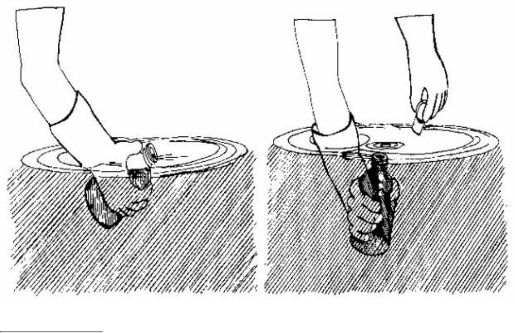
Figure 5.7

Taking a water sample for DO analysis

Point the bottle downstream and fill gradually. Cap underwater when full.

Using a DO Meter

If you are using a dissolved oxygen meter, be sure that it is calibrated immediately prior to use. Check the cable

connection between the probe and the meter. Make sure that the probe is filled with electrolyte solution, that the

membrane has no wrinkles, and that there are no bubbles trapped on the face of the membrane. You can do a field

check of the meter's accuracy by calibrating it in saturated air according to th e manufacturer's instructions. Or,

you can measure a water sample that is saturated with oxygen, as follows. (NOTE: You can also use this

procedure for testing the accuracy of the Winkler method.)

Fill a l-liter beaker or bucket of tap water. (You may want to bring a gallon jug with water in it for this

purpose.) Mark the bottle number as "tap" on the lab sheet.

Pour this water back and forth into another beaker 10 times to saturate the water with oxygen.2.

Use the meter to measure the water temperature and record it in the water temperature column on the field

data sheet.

Find the water temperature of your "tap" sample in Table 5.3. Use the meter to compare the dissolved

oxygen concentration of your sample with the maximum concentration at that temperature in the table.

Your sample should be within 0.5 mg/L. If it is not, repeat the check and if there is still an error, check the

meter's batteries and follow the troubleshooting procedures in the manufacturer's manual.

Once the meter is turned on, allow 15 minute equilibration before calibrating. After calibration, do not turn the

meter off until the sample is analyzed. Once you have verified that the meter is working properly, you are ready

to measure the DO levels at the sampling site. You might need an extension pole (this can be as simple as a piece

of wood) to get the probe to the proper sampling point. Simply secure the probe to the end of the extension pole.

A golfer's ball retriever works well because it is collapsible and easy to transport. To use the probe, proceed as

follows:

Place the probe in the stream below the surface.1.

Set the meter to measure temperature, and allow the temperature reading to stabilize. Record the

temperature on the field data sheet.

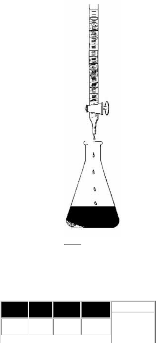
Switch the meter to read dissolved oxygen.3.

Record the dissolved oxygen level on the field data sheet.4.

TASK 4 Analyze the samples

Three types of titration apparatus can be used with the Winkler method: droppers, digital titrators, and burets. The

dropper and digital titrator are suited for field use. The buret is more conveniently used in the lab (Fig. 5.8)

Volunteer programs are most likely to use the dropper or digital titrator. For titration with a dropper or syringe,

which is relatively simple, follow the manufacturer's instructions. The following procedure is for using a digital

titrator to determine the quantity of dissolved oxygen in a fixed sample:

Figure 5.8

Titrating a DO sample using a buret

Select a sample volume and sodium thiosulfate titration cartridge for

the digital titrator corresponding to the expected dissolved oxygen

concentration according to Table 5.4. In most cases, you will use the

0.2 N cartridge and the 100-mL sample volume.

Insert a clean delivery tube into the titration cartridge.2.

Attach the cartridge to the titrator body.3.

Hold the titrator with the cartridge tip up. Turn the delivery knob to

eject air and a few drops of titrant. Reset the counter to 0 and wipe the

tip.

Use a graduated cylinder to measure the sample volume (from the

"fixed" sample in the 300-mL BOD bottle) according to Table 5.4.

Transfer the sample into a 250-mL Erlenmeyer flask, and place the

flask on a magnetic stirrer with a stir bar. If you are in the field, you can

manually swirl the flask to mix.

Place the delivery tube tip into the solution and turn the stirrer on to stir

the sample while you're turning the delivery knob.

Titrate to a pale yellow color.8.

Add two dropperfuls of starch indicator solution and swirl to mix. A

strong blue color will develop.

Continue to titrate until the sample is clear. Record the number of digits

required. (The color might reappear after standing a few minutes, but

this is not a cause for concern. The "first" disappearance of the blue

color is considered the endpoint.)

10.

Calculate mg/L of DO = digits required X digit multiplier (from Table

5.4).

11.

Record the results in the appropriate column of the data sheet.12.

Some water quality standards are expressed in terms of percent saturation. To

calculate percent saturation of the sample:

Find the temperature of your water sample as measured in the field.1.

Find the maximum concentration of your sample at that temperature as

given in Table 5.3.

Calculate the percent saturation, by dividing your actual dissolved

oxygen by the maximum concentration at the sample temperature.

Record the percent saturation in the appropriate column on the data

sheet.

Expected

Range Sample

Volume Titration

Cartridge Digit

Multiplier Table 5.4

Sample

volume

selection and

1-5

mg/L 200 mL 0.2 N 0.01

TASK 5 Return the samples and the

field data sheets to the lab/drop-off

point

corresponding

values for

Winkler

titration

2-10

mg/L 100 mL 0.2 N 0.02

10+

mg/L 200 mL 2.0 N 0.10

If you are using the Winkler method and delivering the

samples to a lab for titration, double-check to make sure

that you have recorded the necessary information for

each site on the field data sheet, especially the bottle

number and corresponding site nu mber and the times

the samples were collected. Deliver your samples and field data sheets to the lab. If you have already obtained the

dissolved oxygen results in the field, send the data sheets to your sampling coordinator.

What is biochemical oxygen demand and why is it important?

Biochemical oxygen demand, or BOD, measures the amount of oxygen consumed by microorganisms in

decomposing organic matter in stream water. BOD also measures the chemical oxidation of inorganic matter (i.e.,

the extraction of oxygen from water via chemical reaction). A test is used to measure the amount of oxygen

consumed by these organisms during a specified period of time (usually 5 days at 20 C). The rate of oxygen

consumption in a stream is affected by a number of variables: temperature, pH, the presence of certain kinds of

microorganisms, and the type of organic and inorganic material in the water.

BOD directly affects the amount of dissolved oxygen in rivers and streams. The greater the BOD, the more

rapidly oxygen is depleted in the stream. This means less oxygen is available to higher forms of aquatic life. The

consequences of high BOD are the same as those for low dissolved oxygen: aquatic organisms become stressed,

suffocate, and die.

Sources of BOD include leaves and woody debris; dead plants and animals; animal manure; effluents from pulp

and paper mills, wastewater treatment plants, feedlots, and food-processing plants; failing septic systems; and

urban stormwater runoff.

Sampling Considerations

BOD is affected by the same factors that affect dissolved oxygen (see above). Aeration of stream water by rapids

and waterfalls, for example will accelerate the decomposition of organic and inorganic material. Therefore, BOD

levels at a sampling site with slower, deeper waters might be higher for a given volume of organic and inorganic

material than the levels for a similar site in highly aerated waters.

Chlorine can also affect BOD measurement by inhibiting or killing the microorganisms that decompose the

organic and inorganic matter in a sample. If you are sampling in chlorinated waters, such as those below the

effluent from a sewage treatment plant, it is necessary to neutralize the chlorine with sodium thiosulfate. (See

APHA, 1992.)

BOD measurement requires taking two samples at each site. One is tested immediately for dissolved oxygen, and

the second is incubated in the dark at 20 C for 5 days and then tested for the amount of dissolved oxygen

remaining. The difference in oxygen levels between the first test and the second test, in milligrams per liter

(mg/L), is the amount of BOD. This represents the amount of oxygen consumed by microorganisms to break

down the organic matter present in the sample bottle during the incubation period. Because of the 5-day

incubation, the tests should be conducted in a laboratory.

Sometimes by the end of the 5-day incubation period the dissolved oxygen level is zero. This is especially true for

rivers and streams with a lot of organic pollution. Since it is not known when the zero point was reached, it is not

possible to tell what the BOD level is. In this case it is necessary to dilute the original sample by a factor that

results in a final dissolved oxygen level of at least 2 mg/L. Special dilution water should be used for the dilutions.

(See APHA, 1992.)

It takes some experimentation to determine the appropriate dilution factor for a particular sampling site. The final

result is the difference in dissolved oxygen between the first measurement and the second after multiplying the

second result by the dilution factor. More details are provided in the following section.

How to Collect and Analyze Samples
The procedures for collecting samples for BOD testing consist of the same steps described for sampling for
dissolved oxygen (see above), with one important difference. At each site a second sample is collected in a BOD
bottle and delivered to the lab for DO testing after the 5-day incubation period. Follow the same steps used for
measuring dissolved oxygen with these additional considerations:
Make sure you have two BOD bottles for each site you will sample. The bottles should be black to prevent
photosynthesis. You can wrap a clear bottle with black electrician's tape if you do not have a bottle with
black or brown glass.
● 
Label the second bottle (the one to be incubated) clearly so that it will not be mistaken for the first bottle.● 
Be sure to record the information for the second bottle on the field data sheet.● 
The first bottle should be analyzed just prior to storing the second sample bottle in the dark for 5 days at 20 C.
After this time, the second bottle is tested for dissolved oxygen using the same method that was used for the first
bottle. The BOD i s expressed in milligrams per liter of DO using the following equation:
DO (mg/L) of first bottle
- DO (mg/L) of second bottle
= BOD (mg/L)
References
APHA. 1992. Standard methods for the examination of water and wastewater. 18th ed. American Public Health
Association, Washington, DC.
< Previous · Table of Contents · Next >
Office of Wetlands, Oceans & Watersheds Home
Watershed Protection Home | Monitoring Water Quality Home
EPA Home | Office of Water | Search | Comments

5.3

Temperature

Why is temperature important?

The rates of biological and chemical processes depend on temperature. Aquatic

organisms from microbes to fish are dependent on certain temperature ranges for their

optimal health. Optimal temperatures for fish depend on the species: some survive best in

colder water, whereas others prefer warmer water. Benthic macroinvertebrates are also

sensitive to temperature and will move in the stream to find their optimal temperature. If

temperatures are outside this optimal range for a prolonged period of time, organisms are

stressed and can die. Temperature is measured in de-grees Fahrenheit (F) or degrees

Celsius (C).

For fish, there are two kinds of limiting temperatures the maximum temperature for short

exposures and a weekly average temperature that varies according to the time of year and

the life cycle stage of the fish species. Reproductive stages (spawning and embryo

development) are the most sensitive stages. Table 5.5 provides temperature criteria for

some species.

Species

Max.

weekly

average

temp. for

growth

(juveniles)

Max.

temp. for

survival

of short

exposure

(juveniles)

Max.

weekly

average

temp. for

spawning

Max.

temp. for

embryo

spawning

Table 5.5

Maximum

average

temperatures

for growth

and

short-term

maximum

temperatures

for selected

fish (°C and

° F)

Atlantic

salmon 20 °C (68

°F) 23 °C (73

°F) 5 °C (41

°F) 11 °C

(52 °F)

Bluegill 32 °C (90

°F) 35 °C (95

°F) 25 °C

(77 °F) 34 °C

(93 °F)

Brook trout 19 °C (66

°F) 24 °C (75

°F) 9 °C (48

°F) 13 °C

(55 °F)

Common

carp --- --- 21 °C

(70 °F) 33 °C

(91 °F)

Temperature

affects the

oxygen content

of the water

(oxygen levels

become lower as

temperature

increases); the

rate of

photosynthesis

by aquatic

plants; the

metabolic rates

of aquatic

organisms; and

the sensitivity of

Channel

catfish 32 °C (90

°F) 35 °C (95

°F) 27 °C

(81 °F) 29 °C

(84 °F)

Largemouth

bass 32 °C (90

°F) 34 °C (93

°F) 21 °C

(70 °F) 27 °C

(81 °F)

Rainbow

trout 19 °C (66

°F) 24 °C (75

°F) 9 °C (48

°F) 13 °C

(55 °F)

Smallmouth

bass 29 °C (84

°F) --- 17 °C

(63 °F) 23 °C

(73 °F)

Sockeye

salmon 18 °C (64

°F) 22 °C (72

°F) 10 °C

(50 °F) 13 °C

(55 °F)

a - Optimum or mean of the range of spawning

temperatures reported for the species

b - Upper temperature for successful incubation and

hatching reported for the species

c - Upper temperature for spawning

(Brungs and Jones 1977)

organisms to

toxic wastes,

parasites, and

diseases.

Causes of

temperature

change include

weather,

removal of

shading

streambank

vegetation,

impoundments

(a body of water

confined by a

barrier, such as a

dam), dis-charge

of cooling water, urban storm water, and groundwater inflows to the stream.

Sampling and Equipment Considerations

Temperature in a stream will vary with width and depth. It can be significantly different

in the shaded portion of the water on a sunny day. In a small stream, the temperature will

be relatively constant as long as the stream is uniformly in sun or shade. In a large

stream, temperature can vary considerably with width and depth regardless of shade. If it

is safe to do so, temperature measurements should be collected at varying depths and

across the surface of the stream to obtain vertical and horizontal temperature profiles.

This can be done at each site at least once to determine the necessity of collecting a

profile during each sampling visit. Temperature should be measured at the same place

every time.

Temperature is measured in the stream with a thermometer or a meter. Alcohol-filled

thermometers are preferred over mercury-filled because they are less hazardous if broken.

Armored thermometers for field use can withstand more abuse than unprotected glass

thermometers and are worth the additional expense. Meters for other tests, such as pH

(acidity) or dissolved oxygen, also measure temperature and can be used instead of a

thermometer.

How to sample

The procedures for measuring temperature consist of the following tasks.

TASK 1 Prepare before leaving for the sampling site

Refer to section 2.3 - Safety Considerations for details on confirming sampling date and

time, safety considerations, checking supplies, and checking weather and directions. In

addition to the standard sampling equipment and apparel, when measuring temperature

you will need:

A thermometer or meter

●

A data sheet for temperature to record results●

Be sure to let someone know where you are going and when you expect to return

TASK 2 Measure the temperature

In general, sample away from the streambank in the main current. The outside curve of

the stream is often a good place to sample since the main current tends to hug this bank.

In shallow stretches, wade into the center current carefully to measure temperature. If

wading is not possible, tape your thermometer to an extension pole or use a boat. Reach

out from the shore or boat as far as safely possible. If you use an extension pole, read the

temperature quickly before it changes to the air temperature.

If you are doing a horizontal or vertical temperature profile, make sure you can safely

reach all the points where a measurement is required before trying.

Measure temperature as follows:

Place the thermometer or meter probe in the water as least 4 inches below the

surface or halfway to the bottom if in a shallow stream.

If using a thermometer, allow enough time for it to reach a stable temperature (at

least 1 minute). If using a meter, allow the temperature reading to stabilize at a

constant temperature reading.

If possible, try to read the temperature with the thermometer bulb beneath the

water surface. If it is not possible, quickly remove the thermometer and read the

temperature.

Record the temperature on the field data sheet.4.

TASK 3 Return the field data sheets to the lab/dropoff

point.

References

Brungs, W.S. and B.R. Jones. 1977. Temperature Criteria for Freshwater Fish:

Protocols and Procedures. EPA-600/3-77-061. Environ. Research Lab, Ecological

Resources Service, U.S. Environmental Protection Agency, Office of Research and

Development, Duluth, MN.

< Previous · Table of Contents · Next >

Office of Wetlands, Oceans & Watersheds Home

Watershed Protection Home | Monitoring Water Quality Home

EPA Home | Office of Water | Search | Comments

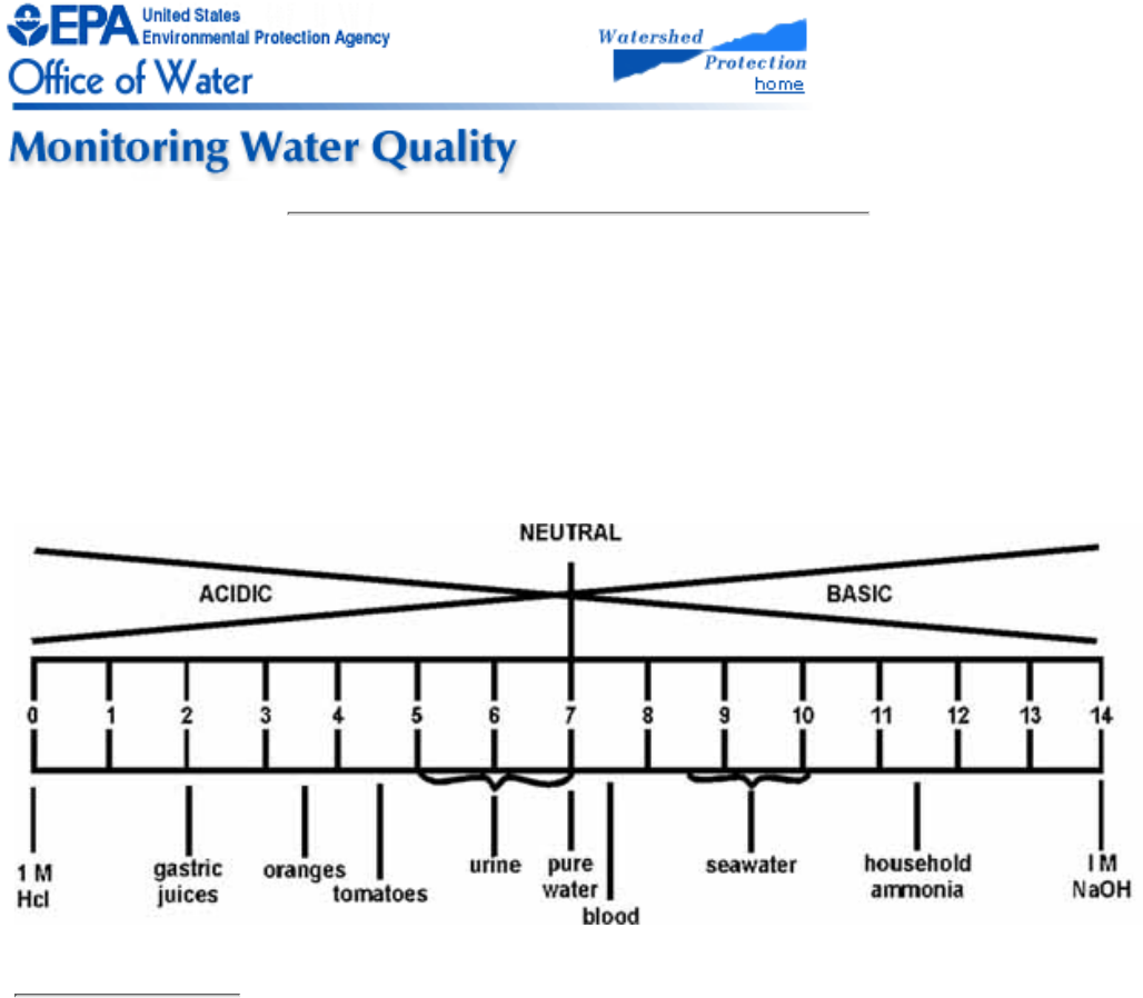
5.4

What Is pH and why is it important?

pH is a term used to indicate the alkalinity or acidity of a substance as ranked on a scale from 1.0 to 14.0. Acidity

increases as the pH gets lower. Fig. 5.9 present the pH of some common liquids.

Figure 5.9

pH of selected liquids

pH affects many chemical and biological processes in the water. For example, different organisms flourish within

different ranges of pH. The largest variety of aquatic animals prefer a range of 6.5-8.0. pH outside this range

reduces the diversity in the stream because it stresses the physiological systems of most organisms and can reduce

reproduction. Low pH can also allow toxic elements and compounds to become mobile and "available" for uptake

by aquatic plants and animals. This can produce conditions that are toxic to aquatic life, particularly to sensitive

species like rainbow trout. Changes in acidity can be caused by atmospheric deposition (acid rain), surrounding

rock, and certain wastewater discharges.

The pH scale measures the logarithmic concentration of hydrogen (H+) and hydroxide (OH-) ions, which make

up water (H+ + OH- = H2O). When both types of ions are in equal concentration, the pH is 7.0 or neutral. Below

7.0, the water is acidic (there are more hydrogen ions than hydroxide ions). When the pH is above 7.0, the water

is alkaline, or basic (there are more hydroxide ions than hydrogen ions). Since the scale is logarithmic, a drop in

the pH by 1.0 unit is equivalent to a 10-fold increase in acidity. So, a water sample with a pH of 5.0 is 10 times as

acidic as one with a pH of 6.0, and pH 4.0 is 100 times as acidic as pH 6.0.

Analytical and equipment considerations

pH can be analyzed in the field or in the lab. If it is analyzed in the lab, you must measure the pH within 2 hours

of the sample collection. This is because the pH will change due to the carbon dioxide from the air dissolving in

the water, which will bring the pH toward 7. If your program requires a high degree of accuracy and precision in

pH results, the pH should be measured with a laboratory quality pH meter and electrode. Meters of this quality

range in cost from around $250 to $1,000. Color comparators and pH "pocket pals" are suitable for most other

purposes. The cost of either of these is in the $50 range. The lower cost of the alternatives might be attractive if

you are relying on several teams of volunteers sampling multiple sites at the same time.

pH Meters

A pH meter measures the electric potential (millivolts) across an electrode when immersed in water. This electric

potential is a function of the hydrogen ion activity in the sample. Therefore, pH meters can display results in

either millivolts (mV) or pH units.

A pH meter consists of a potentiometer, which measures electric current; a glass electrode, which senses the

electric potential where it meets the water sample; a reference electrode, which provides a constant electric

potential; and a temperature compensating device, which adjusts the readings according to the temperature of the

sample (since pH varies with temperature). The reference and glass electrodes are frequently combined into a

single probe called a combination electrode.

There is a wide variety of meters, but the most important part of the pH meter is the electrode. Buy a good,

reliable electrode and follow the manufacturer's instructions for proper maintenance. Infrequently used or

improperly maintained electrodes are subject to corrosion, which makes them highly inaccurate.

pH "Pocket Pals" and Color Comparators

pH "pocket pals" are electronic hand-held "pens" that are dipped in the water and provide a digital readout of the

pH. They can be calibrated to one pH buffer (lab meters, on the other hand, can be calibrated to two or more

buffer solutions and thus are more accurate over a wide range of pH measurements).

Color comparators involve adding a reagent to the sample that colors the sample water. The intensity of the color

is proportional to the pH of the sample. This color is then matched against a standard color chart. The color chart

equates particular colors to associated pH values. The pH can be determined by matching the colors from the

chart to the color of the sample.

How to collect and analyze samples

The field procedures for collecting and analyzing samples for pH consist of the following tasks.

TASK 1 Prepare the sample containers

Sample containers (and all glassware used in this procedure) must be cleaned and rinsed before the first run and

after each sampling run by following the procedure described under Method A on page 128. Remember to wear

latex gloves.

TASK 2 Prepare before leaving for the sampling site

Refer to Section 2.3 - Saftey Considerations for details on confirming sampling date and time, picking up and

checking supplies, and checking weather and directions. In addition to the standard sampling equipment and

apparel, when sampling for pH, include the following equipment:

pH meter with combination temperature and reference electrode, or pH "pocket pal" or color comparator

●

Wash bottle with deionized water to rinse pH meter electrode (if appropriate)●

Data sheet for pH to record results●

Before you leave for the sampling site, be sure to calibrate the pH meter or "pocket pal." The pH meter and

"pocket pal" should be calibrated prior to sample analysis and after every 25 samples according to the instructions

that come with them.

If you are using a "pocket pal," use the buffer recommended by the manufacturer. If you are using a laboratory

grade meter, use two pH standard buffer solutions: 4.01 and 7.0. (Buffers can be purchased from test kit supply

companies, such as Hach or LaMotte.) Following are notes regarding buffers.
The buffer solutions should be at room temperature when you calibrate the meter.
● 
Do not use a buffer after its expiration date.● 
Always cap the buffers during storage to prevent contamination.● 
Because buffer pH values change with temperature, the meter must have a built-in temperature sensor that
automatically standardizes the pH when the meter is calibrated.
● 
Do not reuse buffer solutions!● 
TASK 3 Collect the sample
Refer to Task 2 in Chapter 5 - Water Quality Conditions for details on how to collect water samples using
screw-cap bottles or Whirl-pak® bags.
TASK 4 Measure pH
The procedure for measuring pH is the same whether it is conducted in the field or lab.
If you are using a "pocket pal" or color comparator, follow the manufacturer's instructions. Use the following
steps to determine the pH of your sample if you are using a meter.
Rinse the electrode well with deionized water.1. 
Place the pH meter or electrode into the sample. Depress the dispenser button once to dispense electrolyte.
Read and record the temperature and pH in the appropriate column on the data sheet. Rinse the electrode
well with deionized water. 3. Measure the pH of the 4.01 and 7.0 buffers periodically to ensure that the
meter is not drifting off calibration. If it has drifted, recalibrate it.
2. 
TASK 4 Return the field data sheets and samples to the lab or drop-off
point.
Samples for pH must be analyzed within 2 hours of collection. If the samples cannot be analyzed in the field,
keep the samples on ice and take them to the lab or drop-off point as soon as possible within the 2-hour limit.
References
APHA. 1992. Standard methods for the examination of water and wastewater. 18th ed. American Public Health
Association, Washington, DC. River Watch Network. 1992. Total alkalinity and pH field and laboratory
procedures (based on University of Massachusetts Acid Rain Monitoring Project). July 1.
< Previous · Table of Contents · Next >
Office of Wetlands, Oceans & Watersheds Home
Watershed Protection Home | Monitoring Water Quality Home
EPA Home | Office of Water | Search | Comments

5.5

Turbidity

What is turbidity and why is it important?

Turbidity is a measure of water clarity how much the material suspended in water

decreases the passage of light through the water. Suspended materials include soil

particles (clay, silt, and sand), algae, plankton, microbes, and other substances. These

materials are typically in the size range of 0.004 mm (clay) to 1.0 mm (sand). Turbidity

can affect the color of the water.

Higher turbidity increases water temperatures because suspended particles absorb more

heat. This, in turn, reduces the concentration of dissolved oxygen (DO) because warm

water holds less DO than cold. Higher turbidity also reduces the amount of light

penetrating the water, which reduces photosynthesis and the production of DO.

Suspended materials can clog fish gills, reducing resistance to disease in fish, lowering

growth rates, and affecting egg and larval development. As the particles settle, they can

blanket the stream bottom, especially in slower waters, and smother fish eggs and benthic

macroinvertebrates. Sources of turbidity include:

Soil erosion

●

Waste discharge●

Urban runoff●

Eroding stream banks●

Large numbers of bottom feeders (such as carp), which stir up bottom sediments●

Excessive algal growth.●

Sampling and equipment considerations

Turbidity can be useful as an indicator of the effects of runoff from construction,

agricultural practices, logging activity, discharges, and other sources. Turbidity often

increases sharply during a rainfall, especially in developed watersheds, which typically

have relatively high proportions of impervious surfaces. The flow of stormwater runoff

from impervious surfaces rapidly increases stream velocity, which increases the erosion

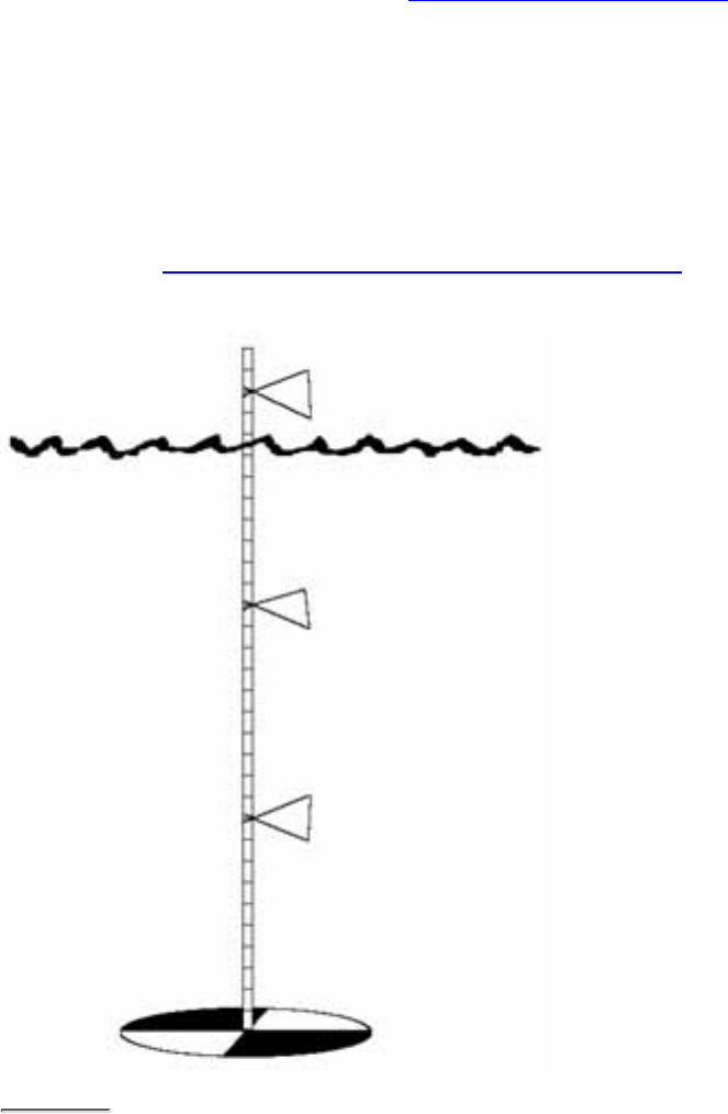
rates of streambanks and channels. Turbidity can also rise sharply during dry weather if

earth-disturbing activities are occurring in or near a stream without erosion control

practices in place.

Regular monitoring of turbidity can help detect trends that might indicate increasing

erosion in developing watersheds. However, turbidity is closely related to stream flow

and velocity and should be correlated with these factors. Comparisons of the change in

turbidity over time, therefore, should be made at the same point at the same flow.

Turbidity is not a measurement of the amount of suspended solids present or the rate of

sedimentation of a steam since it measures only the amount of light that is scattered by

suspended particles. Measurement of total solids is a more direct measure of the amount

of material suspended and dissolved in water (see section 5.9 - Conductivity).

Turbidity is generally measured by using a turbidity meter. Volunteer programs may also

take samples to a lab for analysis. Another approach is to measure transparency (an

integrated measure of light scattering and absorption) instead of turbidity. Water

clarity/transparency can be measured using a Secchi disk or transparency tube. The

Secchi disk can only be used in deep, slow moving rivers; the transparency tube, a

comparatively new development, is gaining acceptance in programs around the country

but is not yet in wide use (see Using a Secchi Disk or Tranparency Tube).

Figure 5.10

Using a Secchi disk to measure transparency

A turbidity

meter consists

of a light

source that

illuminates a

water sample

and a

photoelectric

cell that

measures the

intensity of

light scattered

at a 90 angle

by the

particles in the

sample. It

measures

turbidity in

nephelometric

turbidity units

or NTUs.

Meters can

measure

turbidity over

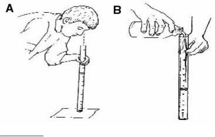
The disk is lowered until it is no longer visible.

That point is the Secchi disk depth.

Figure 5.11

Using a transparency tube

(A) Prepare the tranparency tube to take a reading. Place the tube on a

white surface and look vertically down the tube to see the wave pattern at

the bottom.

(B) Slowly pour water sample into the tube stopping intermittently to see if

the wave pattern has disappeared.

a wide range

from 0 to 1000

NTUs. A clear

mountain

stream might

have a

turbidity of

around 1

NTU, whereas

a large river

like the

Mississippi

might have a

dry-weather

turbidity of

around 10

NTUs. These

values can

jump into

hundreds of

NTU during

runoff events.

Therefore, the

turbidity meter

to be used should be reliable over the range in which you will be working. Meters of this

quality cost about $800. Many meters in this price range are designed for field or lab use.

Although turbidity meters can be used in the field, volunteers might want to collect

samples and take them to a central point for turbidity measurements. This is because of

the expense of the meter (most programs can afford only one and would have to pass it

along from site to site, complicating logistics and increasing the risk of damage to the

meter) and because the meter includes glass cells that must remain optically clear and

free of scratches.

Volunteers can also take turbidity samples to a lab for meter analysis at a reasonable cost.

How to sample

The procedures for collecting samples and analyzing turbidity consist of the following

tasks:

TASK 1 Prepare the sample containers

If factory-sealed, disposable Whirl-pak® bags are used to sample, no preparation is

needed. Reused sample containers (and all glassware used in this procedure) must be

cleaned before the first run and after each sampling run by following Method A described

in Chapter 5 - Water Quality Conditions.

TASK 2 Prepare before leaving for the sampling site

Refer to section 2.3 - Safety Considerations for details on confirming sampling date and

time, safety consideration, checking supplies, and checking weather and directions. In

addition to the standard sampling equipment and apparel, when sampling for turbidity,

include the following equipment:

Turbidity meter

●

Turbidity standards●

Lint-free cloth to wipe the cells of the meter●

Data sheet for turbidity to record results●

Be sure to let someone know where you are going and when you expect to return.

TASK 3 Collect the sample

Refer to Task 2 in Chapter 5 - Water Quality Conditions for details on how to collect

water samples using screw-cap bottles or Whirl-pak® bags.

TASK 4 Analyze the sample

The following procedure applies to field or lab use of the turbidity meter.

Prepare the turbidity meter for use according to the manufacturer's directions.1.

Use the turbidity standards provided with the meter to calibrate it. Make sure it is

reading accurately in the range in which you will be working.

Shake the sample vigorously and wait until the bubbles have disappeared. You

might want to tap the sides of the bottle gently to accelerate the process.

Use a lint-free cloth to wipe the outside of the tube into which the sample will be

poured. Be sure not to handle the tube below the line where the light will pass

when the tube is placed in the meter.

Pour the sample water into the tube. Wipe off any drops on the outside of the tube.5.

Set the meter for the appropriate turbidity range. Place the tube in the meter and

read the turbidity measurement directly from the meter display.

Record the result on the field or lab sheet.7.

Repeat steps 3-7 for each sample.8.

TASK 5 Return the samples and the field data sheets to
the lab/drop-off point.
If you are sending your samples to a lab for analysis, they must be tested within 24 hours
of collection. Keep samples in the dark and on ice or refrigerated.
References and Further Reading
APHA. 1992. Standard methods for the examination of water and wastewater. 18th ed.
American Public Health Association, Washington, DC.
Minnesota Pollution Control Agency. 1997. An Attempt to Classify Transparency Tube
Readings for Southern Minnesota, by Lee Ganske. Contact Louise Hotka, MPCA, Tel:
(612) 296-7223, E-mail: louise.hotka@pca.state.mn.us.
Mississippi Headwaters River Watch. 1991. Water quality procedures. Mississippi
Headwaters Board. March.
Mitchell, M.K., and W. Stapp. Field manual for water quality monitoring. 5th ed.
Thompson Shore Printers.
Tennessee Valley Authority (TVA). 1995 (draft). Clean Water Initiative Volunteer
Stream Monitoring Methods Manual. TVA, 1101 Market Street, CST 17D, Chattanooga,
TN 37402-2801
USEPA. 1991. Volunteer lake monitoring: A methods manual. EPA 440/4-91-002. Office
of Water, U. S. Environmental Protection Agency, Washington, DC.
White, T. 1994. Monitoring a watershed: Nationwide turbidity testing in Australia.
Volunteer Monitor. 6(2):22-23.
< Previous · Table of Contents · Next >
Office of Wetlands, Oceans & Watersheds Home
Watershed Protection Home | Monitoring Water Quality Home
EPA Home | Office of Water | Search | Comments

Back to Section 5.5 - Turbidity

Using a Secchi Disk or Transparency Tube

Secchi Disk

A Secchi disk is a black and white disk that is lowered by hand into the water to the depth

at which it vanishes from sight (Figure 5.10). The distance to vanishing is then recorded.

The clearer the water, the greater the distance. Secchi disks are simple to use and

inexpensive. For river monitoring they have limited use, however, because in most cases

the river bottom will be visible and the disk will not reach a vanishing point. Deeper,

slower moving rivers are the most appropriate places for Secchi disk measurement

although the current might require that the disk be extra-weighted so it does not sway and

make measurement difficult. Secchi disks cost about $50 and can be homemade.

The line attached to the Secchi disk must be marked according to units designated by the

volunteer program, in waterproof ink. Many programs require volunteers to measure to

the nearest 1/10 meter. Meter intervals can be tagged (e.g., with duct tape) for ease of

use.

To measure water clarity with a Secchi disk:

Check to make sure that the Secchi disk is securely attached to the measured line.

●

Lean over the side of the boat and lower the Secchi disk into the water, keeping

your back toward the sun to block glare.

●

Lower the disk until it disappears from view. Lower it one third of a meter and

then slowly raise the disk until it just reappears. Move the disk up and down until

the exact vanishing point is found.

●

Attach a clothespin to the line at the point where the line enters the water. Record

the measurement on your data sheet. Repeating the measurement will provide you

with a quality control check.

●

The key to consistent results is to train volunteers to follow standard sampling procedures

and, if possible, have the same individual take the reading at the same site throughout the

season.

Transparency Tube

Pioneered by Australia's Department of Conservation, the transparency tube is a clear,

narrow plastic tube marked in units with a dark pattern painted on the bottom. Water is

poured into the tube until the pattern disappears (Figure 5.11). Some U.S. volunteer

monitoring programs (e.g., the Tennessee Valley Authority (TVA) Clean Water Initiative

and the Minnesota Pollution Control Agency (MPCA)) are testing the transparency tube

in streams and rivers. MPCA uses tubes marked in centimeters, and has found tube

readings to relate fairly well to lab measurements of turbidity and total suspended solids

(although they do not recommend the transparency tube for applications where precise

and accurate measurement is required or in highly colored waters).

The TVA and MPCA recommend the following sampling considerations:

Collect the sample in a bottle or bucket in mid-stream and mid-depth if possible.

Avoid stagnant water and sample as far from the shoreline as is safe. Avoid

collecting sediment from the bottom of the stream.

●

Face upstream as you fill the bottle or bucket.●

Take readings in open but shaded conditions. Avoid direct sunlight by turning your

back to the sun.

●

Carefully stir or swish the water in the bucket or bottle until it is homogeneous,

taking care not to produce air bubbles (these will scatter light and affect the

measurement). Then pour the water slowly in the tube while looking down the

tube. Measure the depth of the water column in the tube when the symbol just

disappears.

●

For more information on using a transparency tube, see the references at the end of this

section. Many programs have begun making their own tubes. They now may also be

purchased in the U.S. (see Appendix B — Scientific Supply Houses).

Office of Wetlands, Oceans & Watersheds Home

Watershed Protection Home | Monitoring Water Quality Home

EPA Home | Office of Water | Search | Comments

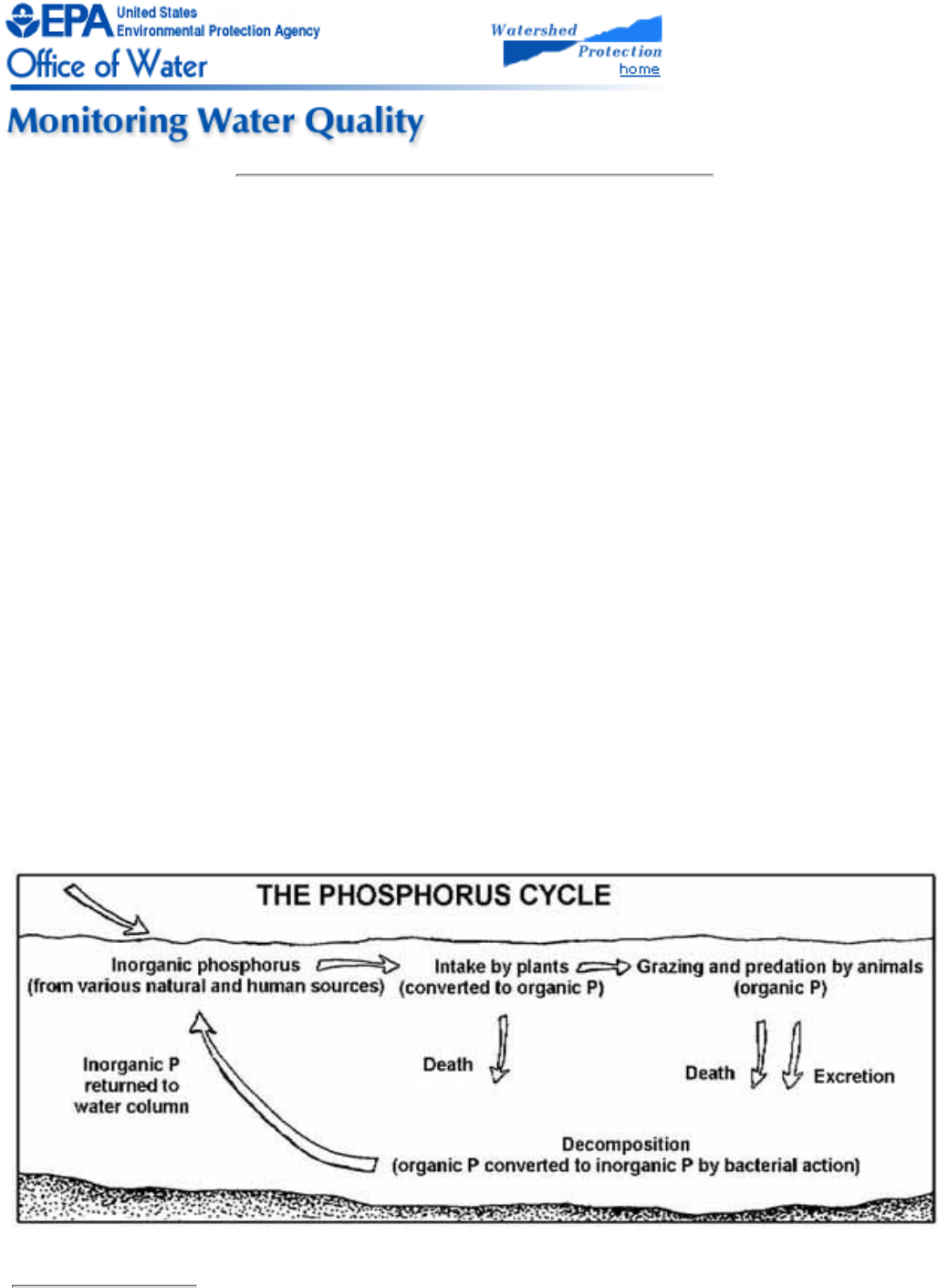
5.6

Phosphorus

Why is phosphorus important?

Both phosphorus and nitrogen are essential nutrients for the plants and animals that make up the aquatic food

web. Since phosphorus is the nutrient in short supply in most fresh waters, even a modest increase in phosphorus

can, under the right conditions, set off a whole chain of undesirable events in a stream including accelerated plant

growth, algae blooms, low dissolved oxygen, and the death of certain fish, invertebrates, and other aquatic

animals.

There are many sources of phosphorus, both natural and human. These include soil and rocks, wastewater

treatment plants, runoff from fertilized lawns and cropland, failing septic systems, runoff from animal manure

storage areas, disturbed land areas, drained wetlands, water treatment, and commercial cleaning preparations.

Forms of phosphorus

Phosphorus has a complicated story. Pure, "elemental" phosphorus (P) is rare. In nature, phosphorus usually

exists as part of a phosphate molecule (PO4). Phosphorus in aquatic systems occurs as organic phosphate and

inorganic phosphate. Organic phosphate consists of a phosphate molecule associated with a carbon-based

molecule, as in plant or animal tissue. Phosphate that is not associated with organic material is inorganic.

Inorganic phosphorus is the form required by plants. Animals can use either organic or inorganic phosphate.

Both organic and inorganic phosphorus can either be dissolved in the water or suspended (attached to particles in

the water column).

The phosphorus cycle

Figure 5.12

The phosphorus cycle

Phosphorus changes form as it cycles through the aquatic environment.

Phosphorus cycles through the environment, changing form as it does so (Fig. 5.12). Aquatic plants take in

dissolved inorganic phosphorus and convert it to organic phosphorus as it becomes part of their tissues. Animals

get the organic phosphorus they need by eating either aquatic plants, other animals, or decomposing plant and

animal material.

As plants and animals excrete wastes or die, the organic phosphorus they contain sinks to the bottom, where

bacterial decomposition converts it back to inorganic phosphorus, both dissolved and attached to particles. This

inorganic phosphorus gets back into the water column when the bottom is stirred up by animals, human activity,

chemical interactions, or water currents. Then it is taken up by plants and the cycle begins again.

In a stream system, the phosphorus cycle tends to move phosphorus downstream as the current carries

decomposing plant and animal tissue and dissolved phosphorus. It becomes stationary only when it is taken up by

plants or is bound to particles that settle to the bottom of pools.

In the field of water quality chemistry, phosphorus is described using several terms. Some of these terms are

chemistry based (referring to chemically based compounds), and others are methods-based (they describe what is

measured by a particular method).

The term "orthophosphate" is a chemistry-based term that refers to the phosphate molecule all by itself. "Reactive

phosphorus" is a corresponding method-based term that describes what you are actually measuring when you

perform the test for orthophosphate. Because the lab procedure isn't quite perfect, you get mostly orthophosphate

but you also get a small fraction of some other forms.

More complex inorganic phosphate compounds are referred to as "condensed phosphates" or "polyphosphates."

The method-based term for these forms is "acid hydrolyzable."

Monitoring phosphorus

Monitoring phosphorus is challenging because it involves measuring very low concentrations down to 0.01

milligram per liter (mg/L) or even lower. Even such very low concentrations of phosphorus can have a dramatic

impact on streams. Less sensitive methods should be used only to identify serious problem areas.

While there are many tests for phosphorus, only four are likely to be performed by volunteer monitors.

The total orthophosphate test is largely a measure of orthophosphate. Because the sample is not filtered,

the procedure measures both dissolved and suspended orthophosphate. The EPA-approved method for

measuring total orthophosphate is known as the ascorbic acid method. Briefly, a reagent (either liquid or

powder) containing ascorbic acid and ammonium molybdate reacts with orthophosphate in the sample to

form a blue compound. The intensity of the blue color is directly proportional to the amount of

orthophosphate in the water.

The total phosphorus test measures all the forms of phosphorus in the sample (orthophosphate, condensed

phosphate, and organic phosphate). This is accomplished by first "digesting" (heating and acidifying) the

sample to convert all the other forms to orthophosphate. Then the orthophosphate is measured by the

ascorbic acid method. Because the sample is not filtered, the procedure measures both dissolved and

suspended orthophosphate.

The dissolved phosphorus test measures that fraction of the total phosphorus which is in solution in the

water (as opposed to being attached to suspended particles). It is determined by first filtering the sample,

then analyzing the filtered sample for total phosphorus.

Insoluble phosphorus is calculated by subtracting the dissolved phosphorus result from the total

phosphorus result.

All these tests have one thing in common they all depend on measuring orthophosphate. The total orthophosphate

test measures the orthophosphate that is already present in the sample. The others measure that which is already

present and that which is formed when the other forms of phosphorus are converted to orthophosphate by

digestion.

Sampling and equipment considerations

Monitoring phosphorus involves two basic steps:

Collecting a water sample

●

Analyzing it in the field or lab for one of the types of phosphorus described above. This manual does not

address laboratory methods. Refer to the references cited at the end of this section.

●

Sample Containers

Sample containers made of either some form of plastic or Pyrex glass are acceptable to EPA. Because phosphorus

molecules have a tendency to "adsorb" (attach) to the inside surface of sample containers, if containers are to be

reused they must be acid-washed to remove adsorbed phosphorus. Therefore, the container must be able to

withstand repeated contact with hydrochloric acid. Plastic containers either high-density polyethylene or

polypropylene might be preferable to glass from a practical standpoint because they will better withstand

breakage. Some programs use disposable, sterile, plastic Whirl-pak® bags. The size of the container will depend

on the sample amount needed for the phosphorus analysis method you choose and the amount needed for other

analyses you intend to perform.

Dedicated Labware

All containers that will hold water samples or come into contact with reagents used in this test must be dedicated.

That is, they should not be used for other tests. This is to eliminate the possibility that reagents containing

phosphorus will contaminate the labware. All labware should be acid-washed. The only form of phosphorus this

manual recommends for field analysis is total orthophosphate, which uses the ascorbic acid method on an

untreated sample. Analysis of any of the other forms requires adding potentially hazardous reagents, heating the

sample to boiling, and using too much time and too much equipment to be practical. In addition, analysis for

other forms of phosphorus is prone to errors and inaccuracies in a field situation. Pretreatment and analysis for

these other forms should be handled in a laboratory.

Ascorbic Acid Method

In the ascorbic acid method, a combined liquid or prepackaged powder reagent, consisting of sulfuric acid,

potassium antimonyl tartrate, ammonium molybdate, and ascorbic acid (or comparable compounds), is added to

either 50 or 25 mL of the water sample. This colors the sample blue in direct proportion to the amount of

orthophosphate in the sample. Absorbance or transmittance is then measured after 10 minutes, but before 30

minutes, using a color comparator with a scale in milligrams per liter that increases with the increase in color hue,

or an electronic meter that measures the amount of light absorbed or transmitted at a wavelength of 700 - 880

nanometers (again depending on manufacturer's directions).

A color comparator may be useful for identifying heavily polluted sites with high concentrations (greater than 0.1

mg/L). However, matching the color of a treated sample to a comparator can be very subjective, especially at low

concentrations, and can lead to variable results.

A field spectrophotometer or colorimeter with a 2.5-cm light path and an infrared photocell (set for a wavelength

of 700-880 nm) is recommended for accurate determination of low concentrations (between 0.2 and 0.02 mg/L ).

Use of a meter requires that you prepare and analyze known standard concentrations ahead of time in order to

convert the absorbance readings of your stream sample to milligrams per liter, or that your meter reads directly as

milligrams per liter.

How to prepare standard concentrations

Note that this step is best accomplished in the lab before leaving for sampling. Standards are prepared using a

phosphate standard solution of 3 mg/L as phosphate (PO4). This is equivalent to a concentration of 1 mg/L as

Phosphorus (P). All references to concentrations and results from this point on in this procedure will be expressed

as mg/L as P, since this is the convention for reporting results.

Six standard concentrations will be prepared for every sampling date in the range of expected results. For most

samples, the following six concentrations should be adequate:

0.00 mg/L 0.12 mg/L

0.04 mg/L 0.16 mg/L

0.08 mg/L 0.20 mg/L

Proceed as follows:

Set out six 25-mL volumetric flasks one for each standard. Label the flasks 0.00, 0.04, 0.08, 0.12, 0.16, and

0.20.

Pour about 30 mL of the phosphate standard solution into a 50 mL beaker.2.

Use 1-, 2-, 3-, 4-, and 5-mL Class A volumetric pipets to transfer corresponding volumes of phosphate

standard solution to each 25-mL volumetric flask as follows:

Standard

Concentration mL of Phosphate

Standard Solution

0.00 0

0.04 1

0.08 2

0.12 3

0.16 4

0.20 5

Note: The standard solution is calculated based on the equation: A = (B x C) ö D

Where:

A = mL of standard solution needed

B = desired concentration of standard

C = final volume (mL) of standard

D = concentration of standard solution

For example, to find out how much phosphate standard solution to use to make a 0.04-mg/L standard:

A = (0.04 x 25) ö 1 A = 1 mL

Before transferring the solution, clear each pipet by filling it once with the standard solution and blowing it out.

Rinse each pipet with deionized water after use.

Fill the remainder of each 25 mL volumetric flask with distilled, deionized water to the 25 mL line. Swirl

to mix.

Set out and label six 50-mL Erlenmeyer flasks: 0.00, 0.04, 0.08, 0.12, 0.16, and 0.20. Pour the standards

from the volumetric flasks to the Erlenmeyer flasks.

List the standard concentrations (0.00, 0.04, 0.08, 0.12, 0.16, and 0.20) under "Bottle #" on the lab sheet.6.

Analyze each of these standard concentrations as described in the section below.7.

How to collect and analyze samples

The field procedures for collecting and analyzing samples for phosphorus consist of the following tasks:

TASK 1 Prepare the sample containers

If factory-sealed, disposable Whirl-pak® bags are used for sampling, no preparation is needed. Reused sample

containers (and all glassware used in this procedure) must be cleaned (including acid rinse) before the first run

and after each sampling run by following the procedure described in Method B on page 128. Remember to wear

latex gloves.

TASK 2 Prepare before leaving for the sample site

Refer to section 2.3 - Safety Considerations for details on confirming sampling date and time, safety

considerations, checking supplies, and checking weather and directions. In addition to sample containers and the

standard sampling apparel, you will need the following equipment and supplies for total reactive phosphorus

analysis:

Color comparator or field spectrophotometer with sample tubes for reading the absorbance of the sample

●

Prepackaged reagents (combined reagents) to turn the water blue●

Deionized or distilled water to rinse the sample tubes between uses●

Wash bottle to hold rinse water●

Mixing container with a mark at the recommended sample volume (usually 25 mL) to hold and mix the

sample

●

Clean, lint-free wipes to clean and dry the sample tubes●

Note that prepackaged reagents are recommended for ease and safety.

TASK 3 Collect the sample

Refer to Task 2 in the Introduction to Chapter 5 for details on how to collect water samples using screw-cap

bottles or Whirl-pak® bags.

TASK 4 Analyze the sample in the field (for total orthophosphate only)

using the ascorbic acid method.

If using an electronic spectrophotometer or colorimeter:

"Zero" the meter (if you are using one) using a reagent blank (distilled water plus the reagent powder) and

following the manufacturer's directions.

Pour the recommended sample volume (usually 25 mL) into a mixing container and add reagent powder

pillows. Swirl to mix. Wait the recommended time (usually at least 10 minutes) before proceeding.

Pour the first field sample into the sample cell test tube. Wipe the tube with a lint-free cloth to be sure it is

clean and free of smudges or water droplets. Insert the tube into the sample cell.

Record the bottle number on the field data sheet.4.

Place the cover over the sample cell. Read the absorbance or concentration of this sample and record it on

the field data sheet.

Pour the sample back into its flask.6.

Rinse the sample cell test tube and mixing container three times with distilled, deionized water. Avoid

touching the lower portion of the sample cell test tube. Wipe with a clean, lint-free wipe. Be sure that the

lower part of the sample cell test tube is clean and free of smudges or water droplets.

Be sure to use the same sample cell test tube for each sample. If the test tube breaks, use a new one and repeat

step 1 to "zero" the meter.

If using a color comparator:

Follow the manufacturer's directions. Be sure to pay attention to the direction of your light source when

reading the color development. The light source should be in the same position relative to the color

comparator for each sample. Otherwise, this is a source of significant error. As a quality check, have

someone else read the comparator after you.

Record the concentration on the field data sheet.2.

TASK 5 Return the samples (for lab analysis for other tests) and the field

data sheets to the lab/drop-off point.

Samples for different types of phosphorus must be analyzed within a certain time period. For some types of

phosphorus, this is a matter of hours; for others, samples can be preserved and held for longer periods. Samples

being tested for orthophosphate must be analyzed within 48 hours of collection. In any case, keep the samples on

ice and take them to the lab or drop-off point as soon as possible.

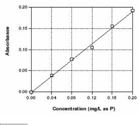
TASK 6 Analyze the samples in the lab.

Lab methods for other tests are described in the references below (APHA. 1992; Hach Company, 1992; River

Watch Network, 1992; USEPA, 1983).

TASK 7 Report the results and convert to milligrams per liter

First, absorbance values must be converted to milligrams per liter. This is done by constructing a "standard curve"

using the absorbance results from your standard concentrations.

Make an absorbance versus concentration graph on graph paper:

Make the "y" (vertical) axis and label it "absorbance." Mark this axis in 0.05 increments from 0 as

high as the graph paper will allow.

❍

Make the "x" (horizontal) axis and label it "concentration: mg/L as P." Mark this axis with the

concentration of the standards: 0, 0.04, 0.08, 0.12, 0.16, 0.20.

❍

Plot the absorbance of the standard concentrations on the graph.2.

Draw a "best fit" straight line through these points. The line should touch (or almost touch) each of the

points. If it doesn't, make up new standards and repeat the procedure.

Example: Suppose you measure the absorbance of the six standard concentrations as follows:

Concentration Absorbance

0.00 0.000

0.04 0.039

0.08 0.078

0.12 0.105

0.16 0.155

0.20 0.192

Figure 5.13

Absorbance of standard concentrations, when plotted,

should result in a straight line

The resulting standard curve is displayed in Fig. 5.13.

For each sample, locate the absorbance on the "y"

axis, read horizontally over to the line, and then more

down to read the concentration in mg/L as P.

Record the concentration on the lab sheet in the

appropriate column. NOTE: The detection limit for

this test is 0.01 mg/L. Report any results less than 0.01

as "<0.01." Round off all results to the nearest

hundredth of a mg/L.

Results can either be reported "as P" or "as PO4." Remember

that your results are reported as milligrams per liter weight

per unit of volume. Since the PO4 molecule is three times as

heavy as the P atom, results reported as PO4 are three times

the concentration of those reported as P. For example, if you

measure 0.06 mg/L as PO4, that's equivalent to 0.02 mg/L as

P. To convert PO4 to P, divide by 3. To convert P to PO4,

multiply by 3. To avoid this confusion, and since most state

water quality standards are reported as P, this manual

recommends that results always be reported as P.

References

APHA. 1992. Standard methods for the examination of water and wastewater. 18th ed. American Public Health

Association, Washington, DC.

Black, J.A. 1977. Water pollution technology. Reston Publishing Co., Reston, VA.

Caduto, M.J. 1990. Pond and brook. University Press of New England, Hanover, NH.

Dates, Geoff. 1994. Monitoring for phosphorus or how come they don't tell you this stuff in the manual?
Volunteer Monitor, Vol. 6(1), spring 1994.
Hach Company. 1992. Hach water analysis handbook. 2nd ed. Loveland, CO.
River Watch Network. 1991. Total phosphorus test (adapted from Standard Methods). July 17.
River Watch Network. 1992. Total phosphorus (persulfate digestion followed by ascorbic acid procedure, Hach
adaptation of Standard Methods). July 1.
USEPA. 1983. Methods for chemical analysis of water and wastes. 2nd ed. Method 365.2. U.S. Environmental
Protection Agency, Washington, DC.
< Previous · Table of Contents · Next >
Office of Wetlands, Oceans & Watersheds Home
Watershed Protection Home | Monitoring Water Quality Home
EPA Home | Office of Water | Search | Comments

5.7

Nitrates

What are nitrates and why are they important?

Nitrates are a form of nitrogen, which is found in several different forms in terrestrial and

aquatic ecosystems. These forms of nitrogen include ammonia (NH3), nitrates (NO3),

and nitrites (NO2). Nitrates are essential plant nutrients, but in excess amounts they can

cause significant water quality problems. Together with phosphorus, nitrates in excess

amounts can accelerate eutrophication, causing dramatic increases in aquatic plant

growth and changes in the types of plants and animals that live in the stream. This, in

turn, affects dissolved oxygen, temperature, and other indicators. Excess nitrates can

cause hypoxia (low levels of dissolved oxygen) and can become toxic to warm-blooded

animals at higher concentrations (10 mg/L) or higher) under certain conditions. The

natural level of ammonia or nitrate in surface water is typically low (less than 1 mg/L); in

the effluent of wastewater treatment plants, it can range up to 30 mg/L.

Sources of nitrates include wastewater treatment plants, runoff from fertilized lawns and

cropland, failing on-site septic systems, runoff from animal manure storage areas, and

industrial discharges that contain corrosion inhibitors.

Sampling and equipment considerations

Nitrates from land sources end up in rivers and streams more quickly than other nutrients

like phosphorus. This is because they dissolve in water more readily than phosphates,

which have an attraction for soil particles. As a result, nitrates serve as a better indicator

of the possibility of a source of sewage or manure pollution during dry weather.

Water that is polluted with nitrogen-rich organic matter might show low nitrates.

Decomposition of the organic matter lowers the dissolved oxygen level, which in turn

slows the rate at which ammonia is oxidized to nitrite (NO2) and then to nitrate (NO3).

Under such circumstances, it might be necessary to also monitor for nitrites or ammonia,

which are considerably more toxic to aquatic life than nitrate. (See Standard Methods

section 4500-NH3 and 4500-NO2 for appropriate nitrite methods; APHA, 1992)

Water samples to be tested for nitrate should be collected in glass or polyethylene

containers that have been prepared by using Method B in the introduction.

Volunteer monitoring programs usually use two methods for nitrate testing: the cadmium

reduction method and the nitrate electrode. The more commonly used cadmium reduction

method produces a color reaction that is then measured either by comparison to a color

wheel or by use of a spectrophotometer. A few programs also use a nitrate electrode,

which can measure in the range of 0 to 100 mg/L nitrate. A newer colorimetric

immunoassay technique for nitrate screening is also now available and might be

applicable for volunteers.

Cadmium Reduction Method

The cadmium reduction method is a colorimetric method that involves contact of the

nitrate in the sample with cadmium particles, which cause nitrates to be converted to

nitrites. The nitrites then react with another reagent to form a red color whose intensity is

proportional to the original amount of nitrate. The red color is then measured either by

comparison to a color wheel with a scale in milligrams per liter that increases with the

increase in color hue, or by use of an electronic spectrophotometer that measures the

amount of light absorbed by the treated sample at a 543-nanometer wavelength. The

absorbance value is then converted to the equivalent concentration of nitrate by using a

standard curve. Methods for making standard solutions and standard curves are presented

at the end of this section.

This curve should be created by the program advisor before each sampling run. The curve

is developed by making a set of standard concentrations of nitrate, reacting them and

developing the corresponding color, and then plotting the absorbance value for each

concentration against concentration. A standard curve could also be generated for the

color wheel.

Use of the color wheel is appropriate only if nitrate concentrations are greater than 1

mg/L. For concentrations below 1 mg/L, a spectrophotometer should be used. Matching

the color of a treated sample at low concentrations to a color wheel (or cubes) can be very

subjective and can lead to variable results. Color comparators can, however, be

effectively used to identify sites with high nitrates.

This method requires that the samples being treated are clear. If a sample is turbid, it

should be filtered through a 0.45-micron filter. Be sure to test whether the filter is

nitrate-free. If copper, iron, or other metals are present in concentrations above several

mg/L, the reaction with the cadmium will be slowed down and the reaction time will have

to be increased.

The reagents used for this method are often prepackaged for different ranges, depending

on the expected concentration of nitrate in the stream. For example, the Hach Company

provides reagents for the following ranges: low (0 to 0.40 mg/L), medium (0 to 4.5

mg/L), and high (0 to 30 mg/L). You should determine the appropriate range for the

stream being monitored.

Nitrate Electrode Method

A nitrate electrode (used with a meter) is similar in function to a dissolved oxygen meter.

It consists of a probe with a sensor that measures nitrate activity in the water; this activity

affects the electric potential of a solution in the probe. This change is then transmitted to

the meter, which converts the electric signal to a scale that is read in millivolts. The

millivolts are then converted to mg/L of nitrate by plotting them from a standard curve

(see above). The accuracy of the electrode can be affected by high concentrations of

chloride or bicarbonate ions in the sample water. Fluctuating pH levels can also affect the

reading by the meter.

Nitrate electrodes and meters are expensive compared to field kits that employ the

cadmium reduction method. (The expense is comparable, however, if a

spectrophotometer is used rather than a color wheel.) Meter/probe combinations run

between $700 and $1,200 including a long cable to connect the probe to the meter. If the

program has a pH meter that displays readings in millivolts, it can be used with a nitrate

probe and no separate nitrate meter is needed. Results are read directly as milligrams per

liter.

Although nitrate electrodes and spectrophotometers can be used in the field, they have

certain disadvantages. These devices are more fragile than the color comparators and are

therefore more at risk of breaking in the field. They must be carefully maintained and

must be calibrated before each sample run and, if you are doing many tests, between

samplings. This means that samples are best tested in the lab. Note that samples to be

tested with a nitrate electrode should be at room temperature, whereas color comparators

can be used in the field with samples at any temperature.

How to collect and analyze samples

The procedures for collecting and analyzing samples for nitrate consist of the following

tasks:

TASK 1 Prepare the sample containers

If factory-sealed, disposable Whirl-pak® bags are used for sampling, no preparation is

needed. Reused sample containers (and all glassware used in this procedure) must be

cleaned before the first run and after each sampling by following the method described on

page 128 under Method B. Remember to wear latex gloves.

TASK 2 Prepare before leaving for the sampling site

Refer to section 2.3 - Safety Considerations for details on confirming sampling date and

time, safety considerations, checking supplies, and checking weather and directions. In

addition to the standard sampling equipment and apparel, the following equipment is

needed when analyzing nitrate nitrogen in the field:

Color comparator or field spectrophotometer with sample tubes (for reading

absorbance of the sample)

●

Reagent powder pillows (reagents to turn the water red)●

Deionized or distilled water to rinse the sample tubes between uses●

Wash bottle to hold rinse water●

Waste bottle with secure lid to hold used cadmium particles, which should be

clearly labeled and returned to the lab, where the cadmium will be properly

disposed of

●

Mixing container with a mark at the sample volume (usually 25 mL) to hold and

mix the sample

●

Clean, lint-free wipes to clean and dry the sample tubes●

TASK 3 Collect the sample

Refer to Task 2 in Chapter 5 - Water Quality Conditions for details on collecting a

sample using screw-cap bottles or Whirl-pak® bags.

TASK 4 Analyze the sample in the field

Cadmium Reduction Method With a Spectrophotometer

The following is the general procedure to analyze a sample using the cadmium reduction

method with a spectrophotometer. However, this should not replace the manufacturer's

directions if they differ from the steps provided below:

Pour the first field sample into the sample cell test tube and insert it into the sample

cell of the spectrophotometer.

Record the bottle number on the lab sheet.2.

Place the cover over the sample cell. Read the absorbance or concentration of this

sample and record it on the field data sheet.

Pour the sample back into the waste bottle for disposal at the lab.4.

Cadmium Reduction Method With a Color Comparator

To analyze a sample using the cadmium reduction method with a color comparator,

follow the manufacturer's directions and record the concentration on the field data sheet.

TASK 5 Return the samples and the field data sheets to

the lab/drop-off point for analysis

Samples being sent to a lab for analysis must be tested for nitrates within 48 hours of

collection. Keep samples in the dark and on ice or refrigerated.

TASK 6 Determine results (for spectrophotometer

absorbance or nitrate electrode) in lab

Preparation of Standard Concentrations

Cadmium Reduction Method With a Spectrophotometer

First determine the range you will be testing (low, medium, or high). For each range you

will need to determine the lower end, which will be determined by the detection limit of

your spectrophotometer. The high end of the range will be the endpoint of the range you

are using. Use a nitrate nitrogen standard solution of appropriate strength for the range in

which you are working. A 1-mg/L nitrate nitrogen (NO3-N) solution would be suitable

for low-range (0 to 1.0 mg/L) tests. A 100-mg/L standard solution would be appropriate

for medium- and high-range tests. In the following example, it is assumed that a set of

standards for a 0 to 5.0 mg/L range is being prepared.

Example:

Set out six 25-mL volumetric flasks (one for each standard). Label the flasks 0.0,

1.0, 2.0, 3.0, 4.0, and 5.0.

Pour 30 mL of a 25-mg/L nitrate nitrogen standard solution into a 50-mL beaker.2.

Use 1-, 2-, 3-, 4-, and 5-mL Class A volumetric pipets to transfer corresponding

volumes of nitrate nitrogen standard solution to each 25-mL volumetric flask as

follows:

Standard

Solution mL of Nitrate Nitrogen

Standard Solution

0.0 0

1.0 1

2.0 2

3.0 3

4.0 4

5.0 5

Analysis of the Cadmium Reduction Method Standard Concentrations

Use the following procedure to analyze the standard concentrations.

Add reagent powder pillows to the nitrate nitrogen standard concentrations.1.

Shake each tube vigorously for at least 3 minutes.2.

For each tube, wait at least 10 minutes but not more than 20 minutes to proceed.3.

"Zero" the spectrophotometer using the 0.0 standard concentration and following

the manufacturer's directions. Record the absorbance as "0" in the absorbance

column on the lab sheet. Rinse the sample cell three times with distilled water.

Read and record the absorbance of the 1.0-mg/L standard concentration.5.

Rinse the sample cell test tube three times with distilled or deionized water. Avoid

touching the lower part of the sample cell test tube. Wipe with a clean, lint-free

wipe. Be sure that the lower part of the sample cell test tube is clean and free of

smudges or water droplets.

Repeat steps 3 and 4 for each standard.7.

Prepare a calibration curve and convert absorbance to mg/L as follows:

Make an absorbance versus concentration graph on graph paper:

(a) Make the vertical (y) axis and label it "absorbance." Mark this axis in 1.0

increments from 0 as high as the graph paper will allow.

(b) Make the horizontal (x) axis and label it "concentration: mg/L as nitrate

nitrogen." Mark this axis with the concentrations of the standards: 0.0, 1.0,

2.0, 3.0, 4.0, and 5.0.

❍

Plot the absorbance of the standard concentrations on the graph.❍

Draw a "best fit" straight line through these points. The line should touch (or

almost touch) each of the points. If it doesn't, the results of this procedure

are not valid.

❍

For each sample, locate the absorbance on the "y" axis, read over

horizontally to the line, and then move down to read the concentration in

mg/L as nitrate nitrogen.

❍

Record the concentration on the lab sheet in the appropriate column.❍

For Nitrate Electrode

Standards are prepared using nitrate standard solutions of 100 and 10 mg/L as nitrate

nitrogen (NO3-N). All references to concentrations and results in this procedure will be

expressed as mg/L as NO3-N. Eight standard concentrations will be prepared:

100.0 mg/L 0.40 mg/L

10.0 mg/L 0.32 mg/L

1.0 mg/L 0.20 mg/L

0.8 mg/L 0.12 mg/L

Use the following procedure:

Set out eight 25-mL volumetric flasks (one for each standard). Label the flasks

100.0, 10.0, 1.0, 0.8, 0.4, 0.32, 0.2, and 0.12.

To make the 100.0-mg/L standard, pour 25 mL of the 100-mg/L nitrate standard

solution into the flask labeled 100.0.

To make the 10.0-mg/L standard, pour 25 mL of the 10-mg/L nitrate standard

solution into the flask labeled 10.0.

To make the 1.0-mg/L standard, use a 10- or 5-mL pipet to measure 2.5 mL of the

10-mg/L nitrate standard solution into the flask labeled 1.0. Fill the flask with 22.5

mL distilled, deionized water to the fill line. Rinse the pipet with deionized water.

To make the 0.8-mg/L standard, use a 10- or 5-mL pipet or a 2-mL volumetric

pipet to measure 2 mL of the 10-mg/L nitrate standard solution into the flask

labeled 0.8. Fill the flask with about 23 mL distilled, deionized water to the fill

line. Rinse the pipet with deionized water. 6. To make the 0.4-mg/L standard, use a

10- or 5-mL pipet or a 1-mL volumetric pipet to measure 1 mL of the 10-mg/L

nitrate standard solution into the flask labeled 0.4. Fill the flask with about 24 mL

distilled, deionized water to the fill line. Rinse the pipet with deionized water.

To make the 0.32-, 0.2-, and 0.12-mg/L standards, follow step 4 to make a 25-mL

volume of 1.0 mg/L standard solution. Transfer this to a beaker. Pipet the

following volumes into the appropriately labeled volumetric flasks:

Standard

Solution mL of Nitrate Nitrogen

Standard Solution

0.32 8

0.20 5

0.12 3

Fill each flask up to the fill line. Rinse pipets with deionized water.

Analysis of the Nitrate Electrode Standard Concentrations

Use the following procedure to analyze the standard concentrations.

List the standard concentrations (100.0, 10.0, 1.0, 0.8, 0.4, 0.32, 0.2, and 0.12)

under "bottle #" on the lab sheet.

Prepare a calibration curve and convert to mg/L as follows:

Plot absorbance or mV readings for the 100-, 10-, and 1-mg/L standards on

semi-logarithmic graph paper, with concentration on the logarithmic (x) axis

and the absorbance or millivolts (mV) on the linear (y) axis.

For the nitrate electrode curve, a straight line with a slope of 58 ñ 3

mV/decade at 25 C should result. That is, measurements of 10- and

100-mg/L standard solutions should be no more than 58 ± 3 mV apart.

❍

Plot absorbance or mV readings for the 1.0-, 0.8-, 0.4-, 0.32-, 0.2-, and

0.12-mg/L standards on semi-logarithmic graph paper, with concentration on

the logarithmic (x) axis and the millivolts (mV) on the linear (y) axis.

For the nitrate electrode, the result here should be a curved line since the

response of the electrode at these low concentrations is not linear.

❍

For the nitrate electrode, recalibrate the electrodes several times daily by

checking the mV reading of the 10-mg/L and 0.4-mg/L standards and

adjusting the calibration control on the meter until the reading plotted on the

calibration curve is displayed again.

❍

References
APHA. 1992. Standard methods for the examination of water and wastewater. 18th ed.
American Public Health Association, Washington, DC.
< Previous · Table of Contents · Next >
Office of Wetlands, Oceans & Watersheds Home
Watershed Protection Home | Monitoring Water Quality Home
EPA Home | Office of Water | Search | Comments

5.8

Total Solids

What are total solids and why are they important?

Total solids are dissolved solids plus suspended and settleable solids in water. In stream

water, dissolved solids consist of calcium, chlorides, nitrate, phosphorus, iron, sulfur, and

other ions particles that will pass through a filter with pores of around 2 microns (0.002

cm) in size. Suspended solids include silt and clay particles, plankton, algae, fine organic

debris, and other particulate matter. These are particles that will not pass through a

2-micron filter.

The concentration of total dissolved solids affects the water balance in the cells of aquatic

organisms. An organism placed in water with a very low level of solids, such as distilled

water, will swell up because water will tend to move into its cells, which have a higher

concentration of solids. An organism placed in water with a high concentration of solids

will shrink somewhat because the water in its cells will tend to move out. This will in

turn affect the organism's ability to maintain the proper cell density, making it difficult to

keep its position in the water column. It might float up or sink down to a depth to which it

is not adapted, and it might not survive.

Higher concentrations of suspended solids can serve as carriers of toxics, which readily

cling to suspended particles. This is particularly a concern where pesticides are being

used on irrigated crops. Where solids are high, pesticide concentrations may increase well

beyond those of the original application as the irrigation water travels down irrigation

ditches. Higher levels of solids can also clog irrigation devices and might become so high

that irrigated plant roots will lose water rather than gain it.

A high concentration of total solids will make drinking water unpalatable and might have

an adverse effect on people who are not used to drinking such water. Levels of total

solids that are too high or too low can also reduce the efficiency of wastewater treatment

plants, as well as the operation of industrial processes that use raw water.

Total solids also affect water clarity. Higher solids decrease the passage of light through

water, thereby slowing photosynthesis by aquatic plants. Water will heat up more rapidly

and hold more heat; this, in turn, might adversely affect aquatic life that has adapted to a

lower temperature regime.

Sources of total solids include industrial discharges, sewage, fertilizers, road runoff, and

soil erosion. Total solids are measured in milligrams per liter (mg/L).

Sampling and equipment considerations

Total solids are important to measure in areas where there are discharges from sewage

treatment plants, industrial plants, or extensive crop irrigation. In particular, streams and

rivers in arid regions where water is scarce and evaporation is high tend to have higher

concentrations of solids and are more readily affected by human introduction of solids

from land use activities.

Total solids measurements can be useful as an indicator of the effects of runoff from

construction, agricultural practices, logging activities, sewage treatment plant discharges,

and other sources. As with turbidity, concentrations often increase sharply during rainfall,

especially in developed watersheds. They can also rise sharply during dry weather if

earth-disturbing activities are occurring in or near the stream without erosion control

practices in place. Regular monitoring of total solids can help detect trends that might

indicate increasing erosion in developing watersheds. Total solids are related closely to

stream flow and velocity and should be correlated with these factors. Any change in total

solids over time should be measured at the same site at the same flow.

Total solids are measured by weighing the amount of solids present in a known volume

of sample. This is done by weighing a beaker, filling it with a known volume,

evaporating the water in an oven and completely drying the residue, and then weighing

the beaker with the residue. The total solids concentration is equal to the difference

between the weight of the beaker with the residue and the weight of the beaker without it.

Since the residue is so light in weight, the lab will need a balance that is sensitive to

weights in the range of 0.0001 gram. Balances of this type are called analytical or Mettler

balances, and they are expensive (around $3,000). The technique requires that the beakers

be kept in a desiccator, which is a sealed glass container that contains material that

absorbs moisture and ensures that the weighing is not biased by water condensing on the

beaker. Some desiccants change color to indicate moisture content.

The measurement of total solids cannot be done in the field. Samples must be collected

using clean glass or plastic bottles or Whirl-pak® bags and taken to a laboratory where

the test can be run.

How to collect and analyze samples

The procedures for collecting and analyzing samples for total solids consist of the

following tasks:

TASK 1 Prepare the sample containers
Factory-sealed, disposable Whirl-pak® bags are easy to use because they need no
preparation. Reused sample containers (and all glassware used in this procedure) must be
cleaned and rinsed before the first sampling run and after each run by following the
procedure described in Method A in Task 1 in Chapter 5 - Water Quality Conditions.
TASK 2 Prepare before leaving for the sampling site
Refer to section 2.3 - Safety Considerations for details on confirming sampling
information. Be sure to let someone know where you are going and when you expect to
return.
TASK 3 Collect the sample
Refer to Task 2 in Chapter 5 - Water Quality Conditions for details on how to collect
water samples using screw-cap bottles or Whirl-pak® bags.
TASK 4 Return samples and field sheets to the
lab/drop-off point for analysis.
Samples that are sent to a lab for total solids analysis must be tested within seven days of
collection. Keep the samples on ice or refrigerated.
References
APHA. 1992. Standard methods for the examination of water and wastewater. 18th ed.
American Public Health Association, Washington, DC.
< Previous · Table of Contents · Next >
Office of Wetlands, Oceans & Watersheds Home
Watershed Protection Home | Monitoring Water Quality Home
EPA Home | Office of Water | Search | Comments

5.9

Conductivity

What is conductivity and why is it important?

Conductivity is a measure of the ability of water to pass an electrical current.

Conductivity in water is affected by the presence of inorganic dissolved solids such as

chloride, nitrate, sulfate, and phosphate anions (ions that carry a negative charge) or

sodium, magnesium, calcium, iron, and aluminum cations (ions that carry a positive

charge). Organic compounds like oil, phenol, alcohol, and sugar do not conduct electrical

current very well and therefore have a low conductivity when in water. Conductivity is

also affected by temperature: the warmer the water, the higher the conductivity. For this

reason, conductivity is reported as conductivity at 25 degrees Celsius (25 C).

Conductivity in streams and rivers is affected primarily by the geology of the area

through which the water flows. Streams that run through areas with granite bedrock tend

to have lower conductivity because granite is composed of more inert materials that do

not ionize (dissolve into ionic components) when washed into the water. On the other

hand, streams that run through areas with clay soils tend to have higher conductivity

because of the presence of materials that ionize when washed into the water. Ground

water inflows can have the same effects depending on the bedrock they flow through.

Discharges to streams can change the conductivity depending on their make-up. A failing

sewage system would raise the conductivity because of the presence of chloride,

phosphate, and nitrate; an oil spill would lower the conductivity.

The basic unit of measurement of conductivity is the mho or siemens. Conductivity is

measured in micromhos per centimeter (µmhos/cm) or microsiemens per centimeter

(µs/cm). Distilled water has a conductivity in the range of 0.5 to 3 µmhos/cm. The

conductivity of rivers in the United States generally ranges from 50 to 1500 µmhos/cm.

Studies of inland fresh waters indicate that streams supporting good mixed fisheries have

a range between 150 and 500 µhos/cm. Conductivity outside this range could indicate

that the water is not suitable for certain species of fish or macroinvertebrates. Industrial

waters can range as high as 10,000 µmhos/cm.

Sampling and equipment Considerations

Conductivity is useful as a general measure of stream water quality. Each stream tends to

have a relatively constant range of conductivity that, once established, can be used as a

baseline for comparison with regular conductivity measurements. Significant changes in

conductivity could then be an indicator that a discharge or some other source of pollution

has entered a stream.

Conductivity is measured with a probe and a meter. Voltage is applied between two

electrodes in a probe immersed in the sample water. The drop in voltage caused by the

resistance of the water is used to calculate the conductivity per centimeter. The meter

converts the probe measurement to micromhos per centimeter and displays the result for

the user. NOTE: Some conductivity meters can also be used to test for total dissolved

solids and salinity. The total dissolved solids concentration in milligrams per liter (mg/L)

can also be calculated by multiplying the conductivity result by a factor between 0.55 and

0.9, which is empirically determined (see Standard Methods #2510, APHA 1992).

Suitable conductivity meters cost about $350. Meters in this price range should also

measure temperature and automatically compensate for temperature in the conductivity

reading. Conductivity can be measured in the field or the lab. In most cases, it is probably

better if the samples are collected in the field and taken to a lab for testing. In this way

several teams of volunteers can collect samples simultaneously. If it is important to test in

the field, meters designed for field use can be obtained for around the same cost

mentioned above.

If samples will be collected in the field for later measurement, the sample bottle should

be a glass or polyethylene bottle that has been washed in phosphate-free detergent and

rinsed thoroughly with both tap and distilled water. Factory-prepared Whirl-pak® bags

may be used.

How to sample

The procedures for collecting samples and analyzing conductivity consist of the

following tasks:

TASK 1 Prepare the sample containers

If factory-sealed, disposable Whirl-pak® bags are used for sampling, no preparation is

needed. Reused sample containers (and all glassware used in this procedure) must be

cleaned before the first run and after each sampling run by following Method A as

described in MEthod A in Table 1 in Chapter 5 - Water Quality Conditions.

TASK 2 Prepare before leaving for the sampling site

Refer to section 2.3 - Safety Considerations for details on confirming sampling date and

time, safety considerations, checking supplies, and checking weather and directions. In

addition to the standard sampling equipment and apparel, when sampling for

conductivity, include the following equipment:

Conductivity meter and probe (if testing conductivity in the field)

●

Conductivity standard appropriate for the range typical of the stream●

Data sheet for conductivity to record results●

Be sure to let someone know where you are going and when you expect to return.

TASK 3 Collect the sample (if samples will be tested in the

lab)

Refer to Task 2 in Chapter 5 - Water Quality Conditions for details on how to collect

water samples using screw-cap bottles or Whirl-pak® bags.

TASK 4 Analyze the sample (field or lab)

The following procedure applies to field or lab use of the conductivity meter.

Prepare the conductivity meter for use according to the manufacturer's directions.1.

Use a conductivity standard solution (usually potassium chloride or sodium

chloride) to calibrate the meter for the range that you will be measuring. The

manufacturer's directions should describe the preparation procedures for the

standard solutio n.

Rinse the probe with distilled or deionized water.3.

Select the appropriate range beginning with the highest range and working down.

Read the conductivity of the water sample. If the reading is in the lower 10 percent

of the range, switch to the next lower range. If the conductivity of the sample ex

ceeds the range of the instrument, you may dilute the sample. Be sure to perform

the dilution according to the manufacturer's directions because the dilution might

not have a simple linear relationship to the conductivity.

Rinse the probe with distilled or deionized water and repeat step 4 until finished.5.

TASK 5 Return the samples and the field data sheets to

the lab/drop-off point.

Samples that are sent to a lab for conductivity analysis must be tested within 28 days of

collection. Keep the samples on ice or refrigerated.

References
APHA. 1992. Standard methods for the examination of water and wastewater. 18th ed.
American Public Health Association, Washington, DC.
Hach Company. 1992. Hach water analysis handbook. 2nd ed. Loveland, CO.
Mississippi Headwaters River Watch. 1991. Water quality procedures. Mississippi
Headwaters Board. March.
< Previous · Table of Contents · Next >
Office of Wetlands, Oceans & Watersheds Home
Watershed Protection Home | Monitoring Water Quality Home
EPA Home | Office of Water | Search | Comments

5.10

Total Alkalinity

What is total alkalinity and why is it important?

Alkalinity is a measure of the capacity of water to neutralize acids (see pH description).

Alkaline compounds in the water such as bicarbonates (baking soda is one type),

carbonates, and hydroxides remove H+ ions and lower the acidity of the water (which

means increased pH). They usually do this by combining with the H+ ions to make new

compounds. Without this acid-neutralizing capacity, any acid added to a stream would

cause an immediate change in the pH. Measuring alkalinity is important in determining a

stream's ability to neutralize acidic pollution from rainfall or wastewater. It's one of the

best measures of the sensitivity of the stream to acid inputs.

Alkalinity in streams is influenced by rocks and soils, salts, certain plant activities, and

certain industrial wastewater discharges.

Total alkalinity is measured by measuring the amount of acid (e.g., sulfuric acid) needed

to bring the sample to a pH of 4.2. At this pH all the alkaline compounds in the sample

are "used up." The result is reported as milligrams per liter of calcium carbonate (mg/L

CaCO3).

Analytical and equipment considerations

For total alkalinity, a double endpoint titration using a pH meter (or pH "pocket pal") and

a digital titrator or buret is recommended. This can be done in the field or in the lab. If

you will analyze alkalinity in the field, it is recommended that you use a digital titrator

instead of a buret because the buret is fragile and more difficult to set up and use in the

field. The alkalinity method described below was developed by the Acid Rain Monitoring

Project of the University of Massachusetts Water Resources Research Center.

Burets, titrators, and digital titrators for measuring

alkalinity

The total alkalinity analysis involves titration. In this test, titration is the addition of

small, precise quantities of sulfuric acid (the reagent) to the sample until the sample

reaches a certain pH (known as an endpoint). Th e amount of acid used corresponds to

the total alkalinity of the sample. Alkalinity can be measured using a buret, titrator, or

digital titrator (described below).

A buret is a long, graduated glass tube with a tapered tip like a pipet and a valve

that is opened to allow the reagent to drip out of the tube. The amount of reagent

used is calculated by subtracting the original volume in the buret from t he volume

left after the endpoint has been reached. Alkalinity is calculated based on the

amount used.

●

Titrators forcefully expel the reagent by using a manual or mechanical plunger.

The amount of reagent used is calculated by subtracting the original volume in the

titrator from the volume left after the endpoint has been reached. Alkalinity is then

calculated based on the amount used or is read directly from the titrator.

●

Digital titrators have counters that display numbers. A plunger is forced into a

cartridge containing the reagent by turning a knob on the titrator. As the knob

turns, the counter changes in proportion to the amount of reagent used. Alkalinity

is then calculated based on the amount used. Digital titrators cost approximately

$90.

●

Digital titrators and burets allow for much more precision and uniformity in the amount

of titrant that is used.

How to collect and analyze samples

The field procedures for collecting and analyzing samples for pH and total alkalinity

consist of the following tasks:

TASK 1 Prepare the sample containers

Sample containers (and all glassware used in this procedure) must be cleaned and rinsed

before the first run and after each sampling run by following the procedure described

under Method A in Chapter 5 - Water Quality Conditions. Remember to wear latex

gloves.

TASK 2 Prepare before leaving for the sampling site

Refer to section 2.3 - Safety Considerations for details on confirming sampling date and

time, safety considerations, checking supplies, and checking weather and directions. In

addition to the standard sampling equipment and apparel, when sampling for pH and

alkalinity include the following equipment:

Digital titrator●

100-mL graduated cylinder●

250-mL beaker●

pH meter with combination temperature and reference electrode or pH "pocket pal"●

Sulfuric acid titration cartridge, 0.16 N●

Data sheet for pH and total alkalinity to record results●

Alkalinity voluette ampules standard, 0.500 N, for accuracy check●

Wash bottle with deionized water to rinse pH meter electrode●

Magnetic stirrer, if titrated in the lab●

Be sure to calibrate the pH meter before you analyze a sample. The pH meter should be

calibrated prior to sample analysis and after every 25 samples according to the

instructions in the meter manual. Use two pH standard buffer solutions: 4.01 and 7.0. Fol

lowing are notes regarding buffers:

The buffer solutions should be at room temperature when you calibrate the meter.

●

Do not use a buffer after its expiration date.●

Always cap the buffers during storage to prevent contamination.●

Because buffer pH values change with temperature, the meter must have a built-in

temperature sensor that automatically standardizes the pH when the meter is

calibrated.

●

Do not reuse buffer solutions!●

Be sure to let someone know where you are going and when you expect to return.

TASK 3 Collect the sample

Refer to Task 2 in Chapter 5 - Water Quality Conditions for details on how to collect

water samples using screw-cap bottles or Whirl-pak® bags.

TASK 4 Measure total alkalinity (field or lab)

The following steps are for use of a digital titrator in the field or the lab. If you are using

a buret, consult Standard Methods (APHA, 1992).

Alkalinity is usually measured using sulfuric acid with a digital titrator. Sulfuric acid is

added to the water sample in measured amounts until the three main forms of alkalinity

(bicarbonate, carbonate, and hydroxide) are converted to carbonic acid. At pH 10,

hydroxide (if present) reacts to form water. At pH 8.3, carbonate is converted to

bicarbonate. At pH 4.5, it is certain that all carbonate and bicarbonate are converted to

carbonic aci d. Below this pH, the water is unable to neutralize the sulfuric acid and there

is a linear relationship between the amount of sulfuric acid added to the sample and the

change in the pH of the sample. So, additional sulfuric acid is added to the sample to

reduce the pH of 4.5 by exactly 0.3 pH units (which corresponds to an exact doubling of

the pH) to a pH of 4.2. However, the exact pH at which the conversion of these bases

might have happened, or total alkalinity, is still unknown. This procedure uses an

equation derived from the slope of the line described above to extrapolate back to the

amount of sulfuric acid that was added to actually convert all the bases to carbonic acid.

The multiplier (0.1) then converts this to total alkalinity as mg/L CaCO3. The following

steps outline the procedures necessary to determine the alkalinity of your sample.

Insert a clean delivery tube into the 0.16 N sulfuric acid titration cartridge and

attach the cartridge to the titrator body.

Hold the titrator, with the cartridge tip pointing up, over a sink. Turn the delivery

knob to eject air and a few drops of titrant. Reset the counter to 0 and wipe the tip.

Measure the pH of the sample (see pH, section 5.4). If it is less than 4.5, go to step

9 below.

Insert the delivery tube into the beaker containing the sample. Turn the delivery

knob while magnetically stirring the beaker until the pH meter reads 4.5. Record

the number of digits used to achieve this pH. Do not reset the counter.

Continue titrating to a pH of 4.2 and record the number of digits.5.

Apply the following equation: Alkalinity (as mg/L CaCO3) = (2a - b) x 0.1

Where:

a = digits of titrant to reach pH 4.5

b = digits of titrant to reach pH 4.2 (including digits required to get to pH 4.5)

0.1 = digit multiplier for a 0.16 titration cartridge and a 100-mL sample

Example:

Initial pH of sample is 6.5.

It takes 108 turns to get to a pH of 4.5.

It takes another 5 turns to get to pH 4.2, for a total of 113 turns.

Alkalinity =

=((2 x 108) - 113) x 0.1

10.3 mg/L

Record the results as mg/L alkalinity on the lab sheet.7.

Rinse the beaker with distilled water before the next sample.8.

If the pH of your water sample, prior to titration, is less than 4.5, proceed as

follows:

Insert the delivery tube into the beaker containing the sample.

❍

Turn the delivery knob while swirling the beaker until the pH meter reads

exactly 0.3 pH units less than the initial pH of the sample.

❍

Record the number of digits used to achieve this pH.❍

Apply the equation as in step 6, but a = 0 and b = the number of digits

required to reduce the initial pH exactly 0.3 pH units.

❍

Example:

Initial pH of sample is 4.3.

Enter "0" in the 4.5 column on the lab sheet.

Titrate to a pH of 0.3 units less than the initial pH in this cas 4.0.

It takes 10 digits to get to 4.0.

Enter this in the 4.2 column on the lab sheet and note that the pH endpoint is 4.0.

Alkalinity = (0 - 10) x 0.1 = -1.0.

Record the results as mg/L alkalinity on the lab sheet.

❍

Perform an accuracy check on the first field sample, halfway through the run, and

after analysis of the last sample as described below. Check the pH meter against

pH 7.0 and 4.01 buffers after every 10 samples.

10.

TASK 5 Perform an accuracy check

This accuracy check should be performed on the first field sample titrated, again about

halfway through the field samples, and at the final field sample.

Snap the neck off an alkalinity voluette ampule standard, 0.500 N. Or if using a

standard solution from a bottle, pour a few milliliters of the standard into a clean

beaker.

Pipet 0.1 mL of the standard to the titrated sample (see above). Resume titration

back to the pH 4.2 endpoint. Record the number of digits needed.

Repeat using two more additions of 0.1 mL of standard. Titrate to the pH 4.2 after

each addition.

Each 0.1-mL addition of standard should require 250 additional digits of 0.16 N

titrant.

TASK 6 Return the field data sheets and samples to the

lab or drop-off point

Alkalinity samples must be analyzed within 24 hours of their collection. If the samples

cannot be analyzed in the field, keep the samples on ice and take them to the lab or

drop-off point as soon as possible.

References

APHA. 1992. Standard methods for the examination of water and wastewater. 18th ed.

American Public Health Association, Washington, DC.

Godfrey, P.J. 1988. Acid rain in Massachusetts. University of Massachusetts Water

Resources Research Center, Amherst, MA.

River Watch Network. 1992. Total alkalinity and pH field and laboratory procedures

(based on University of Massachusetts Acid Rain Monitoring Project). July 1.

< Previous · Table of Contents · Next >

Office of Wetlands, Oceans & Watersheds Home

Watershed Protection Home | Monitoring Water Quality Home

EPA Home | Office of Water | Search | Comments

5.11

Fecal Bacteria

What are fecal bacteria and why are they important?

Members of two bacteria groups, coliforms and fecal streptococci, are used as indicators

of possible sewage contamination because they are commonly found in human and

animal feces. Although they are generally not harmful themselves, they indicate the

possible presence of pathogenic (disease-causing) bacteria, viruses, and protozoans that

also live in human and animal digestive systems. Therefore, their presence in streams

suggests that pathogenic microorganisms might also be present and that swimming and

eating shellfish might be a health risk. Since it is difficult, time-consuming, and

expensive to test directly for the presence of a large variety of pathogens, water is usually

tested for coliforms and fecal streptococci instead. Sources of fecal contamination to

surface waters include wastewater treatment plants, on-site septic systems, domestic and

wild animal manure, and storm runoff.

In addition to the possible health risk associated with the presence of elevated levels of

fecal bacteria, they can also cause cloudy water, unpleasant odors, and an increased

oxygen demand. (Refer to the section on dissolved oxygen.)

Indicator bacteria types and what they can tell you

The most commonly tested fecal bacteria indicators are total coliforms, fecal coliforms,

Escherichia coli, fecal streptococci, and enterococci. All but E. coli are composed of a

number of species of bacteria that share common characteristics such as shape, habitat, or

behavior; E. coli is a single species in the fecal coliform group.

Total coliforms are a group of bacteria that are widespread in nature. All members of the

total coliform group can occur in human feces, but some can also be present in animal

manure, soil, and submerged wood and in other places outside the human body. Thus, the

usefulness of total coliforms as an indicator of fecal contamination depends on the extent

to which the bacteria species found are fecal and human in origin. For recreational

waters, total coliforms are no longer recommended as an indicator. For drinking water,

total coliforms are still the standard test because their presence indicates contamination of

a water supply by an outside source.

Fecal coliforms, a subset of total coliform bacteria, are more fecal-specific in origin.

However, even this group contains a genus, Klebsiella, with species that are not

necessarily fecal in origin. Klebsiella are commonly associated with textile and pulp and

paper mill wastes. Therefore, if these sources discharge to your stream, you might wish to

consider monitoring more fecal and human-specific bacteria. For recreational waters, this

group was the primary bacteria indicator until relatively recently, when EPA began

recommending E. coli and enterococci as better indicators of health risk from water

contact. Fecal coliforms are still being used in many states as the indicator bacteria.

E. coli is a species of fecal coliform bacteria that is specific to fecal material from

humans and other warm-blooded animals. EPA recommends E. coli as the best indicator

of health risk from water contact in recreational waters; some states have changed their

water quality standards and are monitoring accordingly.

Fecal streptococci generally occur in the digestive systems of humans and other

warm-blooded animals. In the past, fecal streptococci were monitored together with fecal

coliforms and a ratio of fecal coliforms to streptococci was calculated. This ratio was

used to determine whether the contamination was of human or nonhuman origin.

However, this is no longer recommended as a reliable test.

Enterococci are a subgroup within the fecal streptococcus group. Enterococci are

distinguished by their ability to survive in salt water, and in this respect they more closely

mimic many pathogens than do the other indicators. Enterococci are typically more

human-specific than the larger fecal streptococcus group. EPA recommends enterococci

as the best indicator of health risk in salt water used for recreation and as a useful

indicator in fresh water as well.

Which Bacteria Should You Monitor?

Which bacteria you test for depends on what you want to know. Do you want to know

whether swimming in your stream poses a health risk? Do you want to know whether

your stream is meeting state water quality standards?

Studies conducted by EPA to determine the correlation between different bacterial

indicators and the occurrence of digestive system illness at swimming beaches suggest

that the best indicators of health risk from recreational water contact in fresh water are E.

coli and enterococci. For salt water, enterococci are the best. Interestingly, fecal

coliforms as a group were determined to be a poor indicator of the risk of digestive

system illness. However, many states continue to use fecal coliforms as their primary

health risk indicator.

If your state is still using total or fecal coliforms as the indicator bacteria and you want to

know whether the water meets state water quality standards, you should monitor fecal

coliforms. However, if you want to know the health risk from recreational water contact,

the results of EPA studies suggest that you should consider switching to the E. coli or

enterococci method for testing fresh water. In any case, it is best to consult with the water

quality division of your state's environmental agency, especially if you expect them to

use your data.

Sampling and equipment considerations

Bacteria can be difficult to sample and analyze, for many reasons. Natural bacteria levels

in streams can vary significantly; bacteria conditions are strongly correlated with rainfall,

and thus comparing wet and dry weather bacteria data can be a problem; many analytical

methods have a low level of precision yet can be quite complex; and absolutely sterile

conditions are required to collect and handle samples.

The primary equipment decision to make when sampling for bacteria is what type and

size of sample container you will use. Once you have made that decision, the same,

straightforward collection procedure is used regardless of the type of bacteria being

monitored. Collection procedures are described under "How to Collect Samples" below.

It is critical when monitoring bacteria that all containers and surfaces with which the

sample will come into contact be sterile. Containers made of either some form of plastic

or Pyrex glass are acceptable to EPA. However, if the containers are to be reused, they

must be sterilized using heat and pressure. The containers can be sterilized by using an

autoclave, which is a machine that sterilizes containers with pressurized steam. If using

an autoclave, the container material must be able to withstand high temperatures and

pressure. Plastic containers either high-density polyethylene or polypropylene might be

preferable to glass from a practical standpoint because they will better withstand

breakage. In any case, be sure to check the manufacturer's specifications to see whether

the container can withstand 15 minutes in an autoclave at a temperature of 121°C without

melting. (Extreme caution is advised when working with an autoclave.) Disposable,

sterile, plastic Whirl-pak® bags are used by a number of programs. The size of the

container will depend on the sample amount needed for the bacteria analysis method you

choose and the amount needed for other analyses.

There are two basic methods for analyzing water samples for bacteria:

The membrane filtration method involves filtering several different-sized portions

of the sample using filters with a standard diameter and pore size, placing each

filter on a selective nutrient medium in a petri plate, incubating the plates at a

specified temperature for a specified time period, and then counting the colonies

that have grown on the filter. This method varies for different bacteria types

(variations might include, for example, the nutrient medium type, the number and

types of incubations, etc.).

The multiple-tube fermentation method involves adding specified quantities of the

sample to tubes containing a nutrient broth, incubating the tubes at a specified

temperature for a specified time period, and then looking for the development of

gas and/or turbidity that the bacteria produce. The presence or absence of gas in

each tube is used to calculate an index known as the Most Probable Number

(MPN).

Given the complexity of the analysis procedures and the equipment required, field

analysis of bacteria is not recommended. Bacteria can either be analyzed by the volunteer

at a well-equipped lab or sent to a state-certified lab for analysis. If you send a bacteria

sample to a private lab, make sure that it is certified by the state for bacteria analysis.

Consider state water quality labs, university and college labs, private labs, wastewater

treatment plant labs, and hospitals. You might need to pay these labs for analysis.

This manual does not address laboratory methods because several bacteria types are

commonly monitored and the methods are different for each type. For more information

on laboratory methods, refer to the references at the end of this section. If you decide to

analyze your samples in your own lab, be sure to carry out a quality assurance/quality

control program. Specific procedures are recommended in the section below.

How to Collect Samples

The procedures for collecting and analyzing samples for bacteria consist of the following

tasks:

TASK 1 Prepare sample containers

If factory-sealed, presterilized, disposable Whirl-pak® bags are used to sample, no

preparation is needed. Any reused sample containers (and all glassware used in this

procedure) must be rinsed and sterilized at 121 C for 1 5 minutes using an autoclave

before being used again for sampling.

TASK 2 Prepare before leaving for the sampling site

Refer to section 2.3 - Safety Considerations for details on confirming sampling data and

time, picking up equipment, reviewing safety considerations, and checking weather and

directions. In addition, to sample for coliforms you sh ould check your equipment as

follows:

Whirl-pak® bags are factory-sealed and sterilized. Check to be sure that the seal

has not been removed.

●

Bottles should have tape over the cap or some seal or marking to indicate that they

have been sterilized. If any of the sample bottles are not numbered, ask the lab

coordinator how to number them. Unless sample container s are to be marked with

the site number, do not number them yourself.

●

TASK 3 Collect the sample

Refer Task 2 in Chapter 5 - Water Quality Conditions for details on collecting a sample

using screw-cap bottles or Whirl-pak® bags. Remember to wash your hands thoroughly

after collecting samples suspected of containing fecal contamination. Also, be careful not

to touch your eyes, ears, nose, or mouth until you've washed your hands.

Recommended field quality assurance/quality control procedures include:

Field Blanks. These should be collected at 10 percent of your sample sites along

with the regular samples. Sterile water in sterilized containers should be sent out

with selected samplers. At a predetermined sample site, the sampler fills the usual

sample container with this sterile water. This is labeled as a regular sample, but

with a special notation (such as a "B") that indicates it is a field blank. It is then

analyzed with the regular samples. Lab analysis should result in "0" bacteria counts

for all blanks. Blanks are used to identify errors or contamination in sample

collection and analysis.

●

Internal Field Duplicates. These should be collected at 10 percent of your sampling

sites along with the regular samples. A field duplicate is a duplicate stream sample

collected at the same time and at the same place either by the same sampler or by

another sampler. This is labeled as a regular sample, but with a special notation

(such as a "D") that indicates it is a duplicate. It is then analyzed with the regular

samples. Lab analysis should result in comparable bacteria counts per 100 mL for

duplicates and regular samples collected at the same site. Duplicates are used to

estimate sampling and laboratory analysis precision.

●

External Field Duplicates. An external field duplicate is a duplicate stream sample

collected and processed by an independent (e.g., professional) sampler or team at

the same place at the same time as regular stream samples. It is used to estimate

sampling and laboratory analysis precision.

●

TASK 4 Return the field data sheets and the samples to

the lab or drop-off point

Samples for bacteria must be analyzed within 6 hours of collection. Keep the samples on

ice and take them to the lab or drop-off point as soon as possible.

TASK 5 Analyze the samples in the lab

This manual does not address laboratory analysis of water samples. Lab methods are

described in the references below (APHA, 1992; River Watch Network, 1991; USEPA,

1985). However, the lab you work with should carry out the following recommended

laboratory quality assurance/quality control procedures:

Negative Plates result when the buffered rinse water (the water used to rinse down

the sides of the filter funnel during filtration) has been filtered the same way as a

sample. This is different from a field blank in that it contains reagents used in the

rinse water. There should be no bacteria growth on the filter after incubation. It is

used to detect laboratory bacteria contamination of the sample.

●

Positive Plates result when water known to contain bacteria (such as wastewater

treatment plant influent) is filtered the same way as a sample. There should be

plenty of bacteria growth on the filter after incubation. Positive plates are used to

detect procedural errors or the presence of contaminants in the laboratory analysis

●

that might inhibit bacteria growth.
Lab Replicates. A lab replicate is a sample that is split into subsamples at the lab.
Each subsample is then filtered and analyzed. Lab replicates are used to obtain an
optimal number of bacteria colonies on filters for counting purposes. Usually,
subsamples of 100, 10, and 1 milliliter (mL) are filtered to obtain bacteria colonies
on the filter that can be reliably and accurately counted (usually between 20 and 80
colonies). The plate with the count between 20 and 80 colonies is selected for
reporting the results, and the count is converted to colonies per 100 mL.
● 
Knowns. A predetermined quantity of dehydrated bacteria is added to the reagent
water, which should result in a known result, within an acceptable margin of error.
● 
Outside Lab Analysis of Duplicate Samples. Either internal or external field
duplicates can be analyzed at an independent lab. The results should be comparable
to those obtained by the project lab.
● 
References
APHA. 1992. Standard methods for the examination of water and wastewater. 18th ed.
American Public Health Association, Washington, DC.
Hogeboom, T. Microbiologist, Vermont Environmental Conservation Laboratory,
Waterbury, VT. Personal communication.
River Watch Network. 1991. Escherichia coli (E. coli) membrane filter procedure
(adapted from USEPA Method 1103.1, 1985). Montpelier, VT. October.
USEPA. 1985. Test methods for Escherichia coli and enterococci in water by the
membrane filter procedure (Method #1103.1). EPA 600/4-85-076. U.S. Environmental
Protection Agency, Environmental Monitoring and Support Laboratory, Cincinnati, OH.
USEPA. 1986. Bacteriological ambient water quality criteria for marine and fresh
recreational waters. EPA 440/5-84-002. U.S. Environmental Protection Agency, Office
of Research and Development, Cincinnati, OH.
Water Quality Sampling Field Data Sheet (PDF, 4.41 KB)
Adobe Acrobat Reader is required to view PDF documents. The most recent version of the Adobe
Acrobat Reader is available as a free download. An Adobe Acrobat plug-in for assisted technologies is
also available.
< Previous · Table of Contents · Next >
Office of Wetlands, Oceans & Watersheds Home
Watershed Protection Home | Monitoring Water Quality Home

EPA Home | Office of Water | Search | Comments

Figure 5.6

Back to Section 5.1 - Stream Flow

Determining Average Cross-Sectional Area (A)

Transect #1 (upstream) Transect #2 (downstream)

... Interal width

(feet) ... Depth

(feet) ... Interal width

(feet) ... Depth

(feet)

A to

B= 2.0 1.0 (at B) A

= 2.5 1.1 (at B)

B to

C= 2.0 0.8 (at C) B

= 2.5 1.0 (at C)

C to

D= 2.0 0.5 (at D) C

= 2.5 0.4 (at D)

D to

E= 2.0

---- 0.0

---- (shoreline) D

= 2.5

---- 0.0

---- (shoreline)

Totals 8.0 2.3 10.0 2.5

Average depth = 2.3/4 = 0.575 feet Average depth = 2.5/4 = 0.625 feet

Cross-sectional area of Transect #1 Cross-sectional area of Transect #2

= Total width X Average depth

= 8.0 ft X 0.575

= 4.60 ft2

= Total width X Average depth

= 10.0 ft X 0.625

= 6.25 ft2

Average area = (Cross-sectional area of Transect #1 + Cross-sectional area of Transect #2)/2

= (4.60 ft2 + 6.25 ft2)/2

=5.42 ft2

Figure 5.6

A sample calculation of average cross-sectional area

Office of Wetlands, Oceans & Watersheds Home

Back to Chapter 5 - Water Quality Conditions

Method Location

(Lab or

Field) Comments Table 5.2

Summary

chemical

monitoring

methods

Volunteers

can

measure

some

parameters

in the field

or in the

laboratory.

Dissolved Oxygen (DO)

Winkler with eye dropper Either If lab, the

sample is fixed

in field and

titrated in lab;

must be

measured within

8 hours of

collection.

Winkler with digital

titrator or buret Either

Meter Field

The meter is

fragile and must

be handled

carefully.

Biochemical Oxygen Demand (BOD)

Winkler with eye dropper

1st part -

Either

2nd part -

Lab

If lab, the

sample is fixed

in field and

titrated in lab;

must be

measured within

6 hours of

collection.

Winkler with digital

titrator or buret

1st part -

Either

2nd part -

Lab

If lab, the

sample is fixed

in field and

titrated in lab;

must be

measured within

6 hours of

collection.

Meter

1st part -

Either

2nd part -

Lab

The meter is

fragile and must

be handled

carefully; must

be measured

within 6 hours

of collection.

Temperature

Thermometer Field Cannot be done

in the lab.

Color comparator Either

If lab, measured

ASAP within 2

hours of

collection.

pH "Pocket Pal" Either

If lab, measured

ASAP within 2

hours of

collection.

Meter Either

If lab, measured

ASAP within 2

hours of

collection.

Turbidity

Meter Either

If lab, measured

ASAP within 24

hours of

collection.

Total Orthophosphate

Ascorbic Acid w/ color

comparator Either If lab, measured

within 48 hours

of collection.

Ascorbic acid w/

spectophotometer Either If lab, measured

within 48 hours

of collection.

Nitrate

Cadmium reduction w/

color comparator Either If lab, measured

within 48 hours

of collection.

Cadmium reduction w/

spectrophotometer Either If lab, measured

within 48 hours

of collection.

Total Solids

Oven drying/weighing Lab

Must be

measured within

7 days of

collection.

Conductivity

Meter Either

If lab, measured

ASAP within 28

days of

collection.

Total Alkalinity

Titration Either If lab, measured

within 24 hours

of collection.

Fecal Bacteria

Membrane filtration Lab

Must be

measured within

6 hours of

collection.

Office of Wetlands, Oceans & Watersheds Home

Watershed Protection Home | Monitoring Water Quality Home

EPA Home | Office of Water | Search | Comments

Chapter 6

Managing and Presenting Monitoring Data

6.1 - Managing Volunteer Data

6.2 - Presenting the Data

6.3 - Producing Reports

It is hard to overemphasize the importance of having established methods of handling

volunteer data, analyzing that data, and presenting results effectively to volunteers, the

public, and water resource decision-makers. Without these tools and processes, the data

that volunteers and program managers have labored hard to collect are virtually useless,

and the program will surely fail to meet its goals.

This chapter addresses data management and data presentation. Members of the program

planning committee will need to make many decisions on these issues before the first

field data sheet is filled out by the program's first volunteer. In particular, they should

consult any potential data users such as state water quality agencies or county planning

boards regarding their own data needs. Data users will be particularly concerned about:

Procedures used to verify and check the raw volunteer data.

●

Databases and software used to manage the data.●

Analytical procedures used to convert the raw data into findings and conclusions.●

Reporting formats.●

Data users may, for example, be able to offer concrete suggestions about databases and

presentation formats that will make the data more accessible to them. To ensure that all

questions about the validity of the data can be answered, the program planning committee

should develop and implement a quality assurance/quality control plan designed to

minimize data collection errors, weed out data that fail to meet the program's standards,

and effectively analyze and present the results. This plan should identify key personnel

with responsibilities for data management and data analysis and clearly indicate all the

steps the program will take to handle the data.

Unfortunately, volunteers and program coordinators seldom recognize the importance of

this aspect of a volunteer monitoring program. It tends to be considered "drudge" work

assigned to one or two technically inclined people. However, that attitude is seriously out
of date. Program organizers should make every effort to involve a range of volunteers
and program staff in all aspects of data management and presentation. Sufficient time
should be budgeted to the tasks that are involved. People who produce the reports should
be acknowledged. After all, it is the final reports that will be reviewed by stream
management decision-makers, not the field data sheets. No other tasks are more
important to the success of the volunteer stream monitoring program.
< Previous · Table of Contents · Next >
Office of Wetlands, Oceans & Watersheds Home
Watershed Protection Home | Monitoring Water Quality Home
EPA Home | Office of Water | Search | Comments

6.1

Managing Volunteer Data

The following steps will help ensure that the data collected by volunteers are well

managed, credible, and of value to potential data users.

Review Field Data Sheets

The volunteer program coordinator or designated analyst should screen and review the

field data sheets as they are received. This involves some basic "reality checks."

Questions that should be kept in mind include the following:

Are the results as might be anticipated, or are they highly unexpected? If

unexpected, are they still within the realm of possibility?

For example, can the kit or technique the volunteer used actually produce results

like that? Does the volunteer offer any possible explanations for the results (e.g., a

sewage treatment plant malfunction had been recently reported) or corollary

informatio n (e.g., a fish kill has been observed along with the extremely low

dissolved oxygen readings)? Also check for consistency between similar

parameters. For example, total dissolved solids and conductivity should track

together--if one goes up, so should the other. So should total solids and turbidity.

●

Are there outliers? (Findings that differ radically from past data or other data

from similar sites.)

Values that are off by a factor of 10 or 100 should be questioned. Follow up on any

data that seems suspect. If you can't come up with an explanation for why the

results are so unusual, but they are still within the realm of possibility, you may

want to f lag the data as questionable. Ask an experienced volunteer or program

staffer to sample at that site as a backup until uncertainties are resolved, or work

with the volunteer to verify that proper sampling and analytical protocols are being

foll owed.

●

Are the field data sheets complete?

If a volunteer is consistently leaving a section of the sheet incomplete, follow up

and ask why. Instructions may not always be easily understood. All sheets should

●

include site location and identification, name of the volunteer, date, time, an d

weather conditions.

Are all measurements reported in the correct units?

You should minimize the chance for error by including on the data form itself any

equations needed to convert measurements, and specify on the form what units

should be used. Check the math. All field data sheets should be kept on file in the

event that f indings are brought into question at a later date.

●

Review Information in Your Database

Once volunteer data enters a computerized database, it can take on a life of its own. It is a

phenomenon of human nature that data suddenly seem more believable once

computerized. Therefore, be sure to carefully screen information as soon as yo u enter it

into a database. Then review a printout (preferably with a fresh pair of eyes) against the

original field data sheets. One way to minimize transcription errors is to design the

computer input screens to look like the field data forms.

As a further check, you can run some simple calculations like determining medians and

means to make sure no errors have slipped through. (If the median and the mean are very

different, an outlier may be skewing the results.) Again, if you uncover unusual data

points that cannot be explained by backup information on the field data sheets or the

comment field in the database, flag the data as questionable until it can be verified.

Review Your Final Results

Once volunteer monitoring data has been entered into a database, the next step is to

generate reports on the findings of the data. Even at this stage you should continue to

look for inconsistencies and problems. For example, you should:

Review findings against previous years' data.

●

Look for outliers on graphs and maps.●

Not remove data just because you don't like it, but do investigate findings that are

unusual or can't be explained.

●

By the time you present your final results to your volunteers or other data users, you

should feel fully confident that you have assembled the best possible picture of water

quality conditions in your study streams.

Develop a Coding System

A coding system will help simplify the tracking and recording of data. Make sure,

however, that the system you create is easily understood and simple to use. Codes

developed for sample sites, parameters, and other information on field and lab sheets

shoul d parallel the codes you use in your database. If you will be sharing your

information with a state or local natural resource agency, you may want your coding

system to match or complement the agency system.

Sample Sites: Because sample sites tend to change over time, it is important to have a site

numbering system that accommodates change. A good convention to follow is to use a

site coding system that includes an abbreviation of the waterbody and a s ite number

(e.g., CtR020 for a site on the Connecticut River). For consistency, you might choose to

start the site numbers at the downstream end of the stream and increase them as you

move upstream (e.g., the first Connecticut River site would be CtR010, the second

CtR020, etc.). Leave extra numbers between sites to allow for your program's future

expansion.

Water Quality Parameters: It is also important to develop a coding system for each of the

water quality parameters you are testing. These are the codes you will use in the database

to identify and extract results. To keep the amount of clerical wor k to a minimum,

abbreviate without losing the ability to distinguish parameters from one another. For

example, EC could represent E. coli bacteria and FC fecal coliform bacteria.

Spreadsheets, Databases, and Mapping Software

Today's computer software includes a variety of spreadsheet and database packages that

allow you to sort, manipulate, and perform statistical analyses on the data you have

entered into the computer. For most applications, spreadsheets are adequate and hav e the

advantage of being relatively simple to use. Most spreadsheet packages have graphics

capabilities that will allow you to plot your data onto a graph of your choice (i.e., bar,

line, or pie chart). Examples of common spreadsheet software packages are Lotus 123,

Excel, and Quattro Pro.

Database software may be more difficult to master and usually lack the graphics

capabilities of spreadsheet software. If you manage large amounts of data, however, a

database is almost a necessity. Using a databa se, you can store and manipulate very large

data sets without sacrificing speed. The database can also relate records in one file to

records in another file. This allows you to break your data up into smaller, more easily

managed files that can work toget her as though they were one.

If you use database software for storage and retrieval, you may still want to use a

spreadsheet or other program with graphics capabilities. Many spreadsheet and database

software packages are compatible and will allow you to transport sets of data back a nd

forth with relative ease. Very large data sets can be organized and manipulated in a

database. Specific parts of the data (such as results for a particular metric from all stations

and all sampling events) can then be transported into the spreadsheet, statistically

analyzed, and graphically displayed. Examples of popular database software packages are

dBase, FileMaker Pro, and FoxPro.

An effective way to display your data is on a map of the stream or watershed. This clearly

illustrates the relationship between land uses and the quality of water, habitat, and

biological communities. This type of graphic display can be used to effectivel y show the

correlation between specific activities or land uses and the impacts they have on the

ecosystem. Simple personal computer-based mapping packages are available. They allow

you to enter layers of data and conduct spatial analysis of that data.

Systems that allow you to map and manipulate various layers of information (such as

water quality data, land use information, county boundaries, or geologic conditions) are

known as Geographic Information Systems (GIS). They can vary from simple systems r

un on personal computers to sophisticated and very powerful systems that run on large

mainframes. For any GIS application, you need to know the coordinates of your sample

sites--either their latitude and longitude, or some alternate system such as an EPA River

Reach File identifier. You can also locate your sites on a topographic map that can be

digitized on to an electronic map of the watershed. Once these points have been

established, you can link your database to the points on the map, query your data base,

and create graphic displays of the data.

Powerful GIS applications typically require expensive hardware, software, and technical

training. Any volunteer program interested in GIS applications should consider working

in partnership with other organizations such as universities, natural resource a gencies, or

large nonprofit groups that can provide access to a GIS.

Many people are capable of writing their own programs to manipulate and display data.

The disadvantage of using a "homegrown" software program, however, is that if its

author leaves, so too does all knowledge about how the program works. Commercial

software, on the other hand, comes with consumer services that provide over-the-phone

help and instructions, user's guides, replacement guarantees, and updates as the company

improves its product. Also, most commercial programs are developed to easily import

and export data in standard formats. This feature is important because if you want to

share data with other programs or organizations all you need are compatible software

programs.

STORET

EPA's national water and biological data storage and retrieval system,

STORET, is being modernized and will be available in 1998-1999. Volunteer

programs are encouraged to enter their data into the modernized STORET.

Individual systems will "feed" data to a centralized file server which will

permit national data analyses and through which data can be shared among

organizations. A specific set of quality control measures will be required for

any data entered into the system to aid in data sharing. For more information,

see the EPA web page at www.epa.gov/owow/STORET/.

< Previous · Table of Contents · Next >

Office of Wetlands, Oceans & Watersheds Home

Watershed Protection Home | Monitoring Water Quality Home

EPA Home | Office of Water | Search | Comments

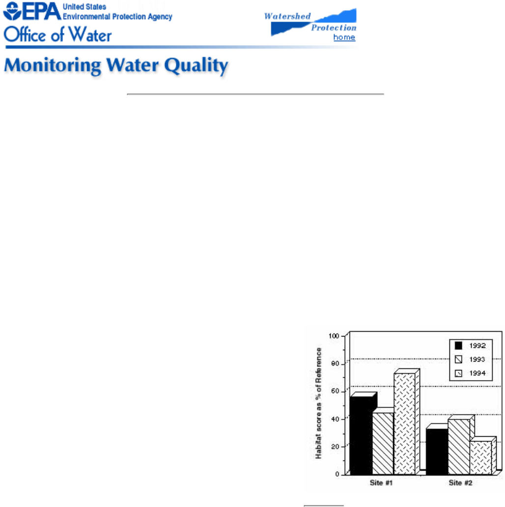
6.2

Presenting the Data

When presenting numerical data, one of your chief goals should be to maintain the attention and interest of your

audience. This is very difficult using tables filled with numbers. Most people will not be interested in the absolute

values of each parameter at each sampling site. Rather, they will want to know the bottom line for each site (e.g.,

is it good or bad) and seasonal and year to year trends.

Graphs and charts, therefore, are typically the best way to present volunteer data. Take care, however, that your

graphs "fit" your audience and are neither too technical nor too simplistic.

Graphs and Charts

Habitat scores as a percent of reference

condition at sites #1 and #2 for 1992-1994

Figure 6.1

Example of a bar graph displaying biological data

Graphs can be used to display the summarized results of large

data sets and to simplify complicated issues and findings. The

three basic types of graphs that are typically used to present

volunteer monitoring data are:

Bar graph

●

Line graph●

Pie chart●

Bar and line graphs are typically used to show results, such as

bioassessment scores, along a vertical or yaxis for a

corresponding variable (such as sampling date or site) which is

marked along the horizontal or xaxis. These types of graphs can

also have two vertical axes, one on each side, with two sets of

results shown in relation to each other and to the variable along

the xaxis.

Bar Graph

A bar graph uses columns with heights that represent the value of

the data point for the parameter being plotted. Fig. 6.1 is an

example using fictional data from Volunteer Creek.

Line Graph

A line graph is constructed by connecting the data points with a line. It can be effectively used for depicting

changes over time or space. This type of graph places more emphasis on trends and the relationship among data

points and less emphasis on any p articular data point.

Fig. 6.2 is an example of a line graph again using fictional data from Volunteer Creek.

Pie Chart

Pie charts are used to compare categories within the data set to the whole. The proportion of each category is

represented by the size of the wedge. Pie charts are popular due to their simplicity and clarity. (See Fig. 6.3)

Graphing Tips

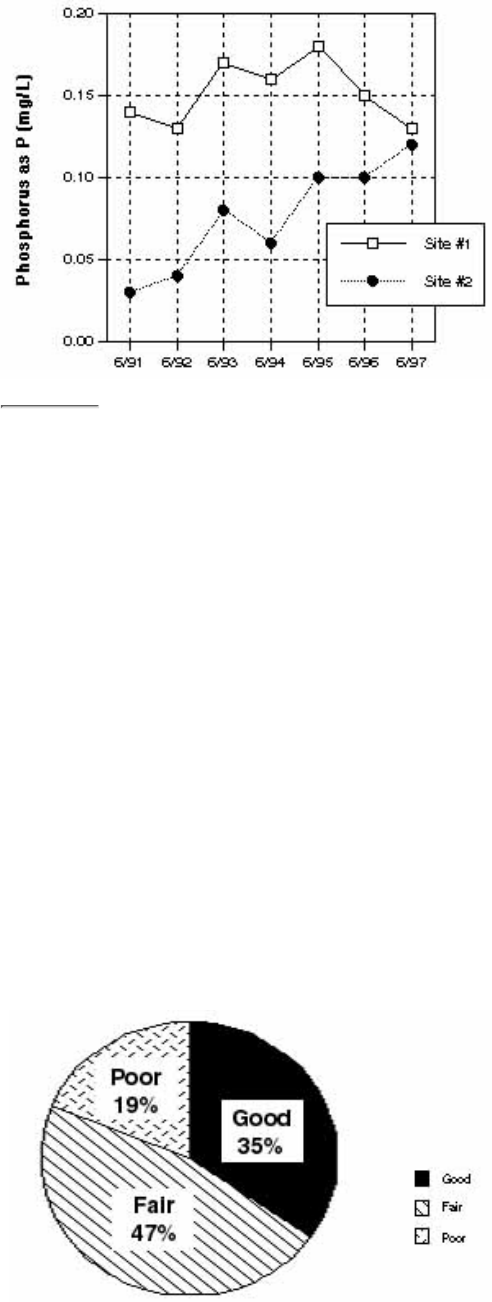
June phosphorus concentrations at Sites #1 and

#2 from 1991-1997

Figure 6.2

Example of a line graph depicting trends in phosphorus

data

Regardless of which graphic style you choose, follow

these rules to ensure you use them most effectively.

Each graph should have a clear purpose. The

graph should be easy to interpret and should relate

directly to the content of the text of a document or

the script of a presentation.

●

The data points on a graph should be

proportional to the actual values so as not to

distort the meaning of the graph. Labeling should

be clear and accurate and the data values should

be easily interpreted from the scales. Do not

overcrowd t he points or values along the axes. If

there is a possibility of misinterpretation,

accompany the graph with a table of the data.

●

Keep it simple. The more complex the graph, the

greater the possibility for misinterpretation.

●

Limit the number of elements. Pie charts should be

limited to five or six wedges, the bars in a bar

graph should fit easily, and the lines in a line

graph should be limited to three or less.

●

Consider the proportions of the graph and expand

the elements to fill the dimensions, thereby

creating a balanced effect. Often, a horizontal

format is more visually appealing and makes

labeling easier. Try not to use abbreviations that

are not obvious to someone who is unfamiliar

with the program.

●

Create titles that are simple, yet adequately

describe the information portrayed in the graph.

●

Use a legend if one is necessary to describe the

categories within the graph. Accompanying

captions may also be needed to provide an

adequate description of the elements.

●

Summary Statistics

Summary of water quality ratings for Volunteer

Creek

(total no. of stations=52)

Figure 6.3

Summary statistics can reduce a very large data set to a

few numerical values that can then be easily described

and analyzed. Such statistics include the mean and

standard deviation--two of the most frequently used

descriptors of environmental data.

Textbook statistics commonly assume that if a parameter

is measured many times under the same conditions, then

the measurement values will be randomly distributed

around the average with more values clustering near the

average than further away. In this i deal situation, a graph

of the frequency of each measure plotted against its

magnitude should yield a bell-shaped or normal curve.

The mean and the standard deviation determine the

height and breadth of this curve, respectively.

The mean is simply the sum of all the measurement

values divided by the number of measurements. This

Example of a pie chart summarizing water quality ratings

statistic is a measure of location and in a normal curve

marks the highest point at the center of the bell.

The standard deviation, on the other hand, describes the variability of the data points around the mean. Very

similar measurement values will have a small standard deviation while widely scattered data will have a much

larger standard deviation.

While both the mean and standard deviation are quite useful in describing stream data, often the actual measures

do not fit a normal distribution. Other statistics often come into play to describe the data. Some data are skewed

in one direction or the oth er. Other data may have a flattened bell shape.

It is important to note that biological information often does not follow normal, bell-shaped distribution. This is

because biological communities are dynamic, complex, and interdependent systems; many factors influence them,

and these cannot be statistica lly predicted. For example, bioassessment scores plotted against habitat assessment

scores will be at their best when habitat quality is at its best. For data that is non-normally distributed, the mean

and the standard deviation are not appropriate summary statistics.

For describing non-normally distributed data, it is best to use statistics that can convey the information for a

variety of conditions and which are not overly influenced by the data points at the extremes of the distribution.

The median and the interquart ile range are two statistics that are commonly used to describe the central tendency

and the spread around the median, respectively. These statistics are derived by placing the data points in order of

value from lowest to highest. The median is simply the value that is in the middle of the data set. The interquartile

range is the difference between the value at the 75 percent level and the value at the 25 percent level.

The best method for presenting this type of data is called a box and whisker plot. One simple box and whisker

plot will graphically display the following information:

Median

●

Variability of the data around the median●

Skew of the data●

Range of the data●

Size of the data set●

Statistical software packages for computers will easily construct box and whisker plots. You can construct these

plots by following procedure shown below:

Order the data from the lowest to the highest.1.

Plot the lowest and highest values on the graph as short horizontal lines. These are the extreme values of

the data set and represent the data range.

Determine the 75 percent value and the 25 percent value of the data set. These values define the

interquartile range and are represented by the location of the top and bottom lines of the box.

The horizontal length of the lines that define the top and bottom lines of the box (the box width) can be

used as a relative indication of the size of the data set. For example, the box width that describes a data set

of 20 values can be displayed twice as wide as a data set of 10 values. Any proportional scheme can be

used as long as it is consistently applied.

Close the box by drawing vertical lines that connect to the ends of the horizontal lines.5.

Plot the median inside the box.6.

Fig. 6.4 is an example depicting the extreme values, interquartile range, and median of biosurvey metric scores

from 52 sites sampled in Volunteer Creek in June, 1995.

Maps

Displaying the results of your monitoring data on a map can be a very effective way of showing the data and

helping people understand what it means. A map shows the location of sample sites in relation to l and features,

such as cities, wastewater treatment plants, farmland, and tributaries that may have an effect on water quality.

Because a map also displays the stream's relationship to neighborhoods, parks a nd recreational areas, it can help

to develop concern for the stream and strengthens interest in protecting it.

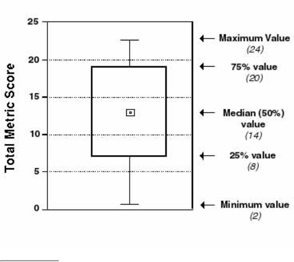
Box Plot of Total Metric Scores from June,

1995

(No. of sites=52)

Figure 6.4

Example of a box plot

Choosing a Map

It is best to have two types of maps. One

should be a working map with a lot of detail.

The other should be used for display

purposes. The working map should include

important features such as:

Stream and its tributaries

●

Wetlands●

Lakes and ponds●

Cultural features such as roads●

Rail and power lines; municipal

boundaries

●

Some indication of land use patterns

and vegetation.

●

The map should be of a scale large enough

to add the location of sample sites.

U.S. Geological Survey (USGS) 7.5 minute

quads (scale of 1:24,000; 1 in. = 2,000 ft)

are available with and without topographic

contours (elevation markings). These maps

are available for most of the United States.

The USGS maps are particularly useful if

your information will be incorporated into a geographic information system (GIS), since many of these systems

use the USGS maps as base maps. For your data to be used in a GIS, it is likely that you will have to provide the

latitude and longitude of your sample sites, which can be obtained by using the grid markings on the USGS

topographic maps. Several different coordinate systems are marked, including standard latitude/longitude and the

Universal Transmercator coordinates. For assistance in learning how to use these coordinate markings, talk to the

local USGS office or someone in the geography department at a university. It may also be possible for the GIS

office you work with you to "digitize" the maps, thus saving you the trouble of trying to calculate the coordinates.

The display map is best used to illustrate your program results at public meetings or in reports. This map should

be simpler than the detailed map and show only principal features such as roads, municipal boundaries, and

waterways. It should have sufficient detail and scale to show the location of sample sites, and have space for

summary information about each of the sample sites. Commercial road atlases and county or town road maps

available from state transportation departments are examples of the types of maps that can be used for display

purposes (See Fig. 6.5).

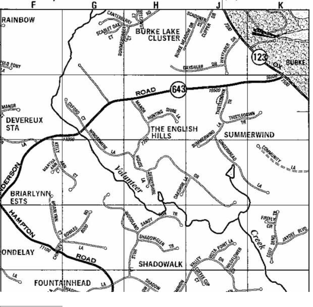
Figure 6.5

A road map is useful for displaying station locations

Creating a Display Map

Some suggestions for using a map to display your data include:

Keep the amount of information presented on each map to a minimum. Do not try to put so much on one

map that it becomes visually complicated and difficult to read or understand. Use another map to display a

different layer or "view" of the data. For example, if there are several dates for which you wish to display

sampling results, use one map for each date.

●

Clearly label the map and provide an explanation of how to interpret it. If you need a long and complicated

explanation, you may want to present the data differently. If you have reached a clear conclusion, state the

conclusion on the map. For example, if a map shows that tributaries are cleaner than the mainstem, use that

information as the subtitle of the map.

●

Provide a key to the symbols that are used on the map.●

Rather than packing lots of information into a small area of the map, use a "blowup" or enlargement of the

area elsewhere on the map to adequately display the information.

●

Use symbols that vary in size and pattern to represent the magnitude of results. For example, a site with a
fecal coliform level of 10 per 100 milliliters could be a light gray circle one-sixteenth inch diameter while a
site with a level of 200 per 100 milliliters would be a dark gray circle one-quarter inch diameter. Start by
finding the highest and lowest values, assign diameters and patterns to those and then fill in steps along the
way. For the above example you might have four ranges: 0 to 99, 100 to 199, 200 to 500 and 500 +.
● 
Maps on Demand
EPA provides a World Wide Web service known as Maps on Demand that
allows users to generate maps displaying environmental information for
anywhere in the U.S. (except Hawaii, Puerto Rico, and the Virgin Islands).
Types of information that can be mapped include EPA-regulated facilities,
demographic information, roads, streams, and drinking water sources. Maps
of varying scales can be generated on the site (latitude and longitude), zip
code, county, and basin levels. Submit your request and email address, and
after a brief wait, you will be able to view your map on-line or download it.
Maps on Demand can be reached through EPA's Surf Your Watershed
homepage at www.epa.gov/surf2/locate/.
< Previous · Table of Contents · Next >
Office of Wetlands, Oceans & Watersheds Home
Watershed Protection Home | Monitoring Water Quality Home
EPA Home | Office of Water | Search | Comments

6.3

Producing Reports

On a regular basis, a successful stream volunteer monitoring program should produce

reports that summarize key findings to volunteers; data users such as state water quality

agencies, and local planning boards; and/or the general public, including the media. State

water quality agencies will require detailed reports, whereas shorter and less technical

summaries are more appropriate for the general public. All reports should be subjected to

the review process prescribed by your Quality Assurance Project Plan.

Professional Report

In a report designed for water quality or planning professionals, you should go into detail

about:

The purpose of the study

●

Who conducted it●

How it was funded●

The methods used●

The quality control measures taken●

Your interpretation of the results●

Your conclusions and recommendations●

Further questions that have arisen as a result of the study.●

Graphics, tables and maps may be fairly sophisticated. Be sure to include the raw data in

an appendix and note any problems encountered.

Lay Report

A report for the general public should be short and direct. It is very important to write in

a nontechnical style and to include definitions for terms and concepts that may be

unfamiliar to the lay person. Simple charts, summary tables, and maps with

accompanying explanations can be especially useful. This type of report should include a

brief description of the program, the purpose of the monitoring, an explanation of the

parameters that were monitored, the location of sample sites, a summary of the results,

and any recommendations that may have been made.

Both types of reports should acknowledge the volunteers and the sources of funding.

Publicizing the Report

Develop a strategy for distributing and publicizing your report before it is completed. Be

sure the planning committee is confident about the data and comfortable with the

statements and conclusions that have been included in the document. When the report is

released to the public, you will need to be prepared to respond to questions regarding the

data and your interpretation of that data.

Some ideas for distributing the results and informing the public include the following:

Mailing the report. If you have access to a mailing list of people who are interested

in your stream, mail the report with a cover letter that summarizes the major

findings of the study. The cover letter should be brief and enticing so that the

recipient will be curious enough to read the report. If you want people to take some

kind of action, such as supporting the expenditure of public funds to upgrade a

sewage treatment plant, you may want to ask for their support in the cover letter. If

you do not have an extensive mailing list, perhaps other organizations that share

your goals would be willing to supply you with their list. Be sure to also send the

report to the newspapers, radio and television stations, and state and federal

agencies.

●

Speaking tour. You may also want to develop an oral presentation (with slides,

overheads, etc.) that could be offered to groups such as the Chamber of Commerce,

Rotary clubs, conservation organizations, schools, and government entities. Your

presentation could even be videotaped for distribution to a wider audience.

●

Public meetings. You may want to schedule a series of public meetings that

highlight the program and its findings and recommendations. At the meetings,

distribute the report, answer questions and tell your audience how they can get

involved. These meetings can also help you recruit more volunteers.

Be sure to schedule the meetings at times when people are more likely to attend

(i.e., weekday evenings, weekend days) and avoid periods when people are

normally busy or on vacation. Invite the media and publicize the meetings in

newspaper calendars, send press releases to newspapers, radio and television

stations and other organizations, and ask volunteers to distribute flyers at grocery

stores, city hall, etc.

●

News releases. Writing and distributing a news release is a cost-effective means of

informing the public about the results and accomplishments of your program.

Develop a mailing list of newspapers, radio and television stations, and

organizations that solicit articles for publication. Send the news release to

volunteers and others who are interested in publicizing the monitoring program.

The first page of your news release should feature the sponsoring organization's

name and logo to clearly designate the source of the news. Include a headline, the

●

date, a contact name and number, and whether the story is for release immediately

or a later date. The first paragraph should begin with a dateline (the city of origin

for the event or story described in the release) and include the essentials: who,

what, where, when, and why and a synopsis of the most important elements of the

story. The second paragraph should contain the second most important facts, the

third paragraph the third most important points and so on. Editors tend to chop off

the last paragraphs if short on space. Therefore, be sure to state your major points

early in the press release.

News conferences. If your report contains some real news, or if it has led to a

significant event, (e.g., the mayor or city council has recognized the value of the

report and issued a statement of support) hold a news conference. Timing and

location are important. Early in the day, but after 10 a.m. is good (most camera

crews start their workday at 9 a.m.) because it allows plenty of time to edit the tape

before the noon news broadcast. You may want to consider timing the conference

so that a TV station could broadcast it live at the noon or the evening news show.

For the conference, choose a place that has good visuals, such as location along the

river or water body that you have been studying, at your headquarters where

volunteers can be shown working in the background or at a recognition gathering

for volunteers.

●

Other publicity. Be creative in getting your report and message out. Try writing

op-ed articles for local or statewide papers, writing letters to the editor, producing

radio feeds (a recording of the group's leader played over the phone to a radio

station), issuing media advisories, and even advertising in publications. For more

help on getting your message across, consult the references cited below.

●

References and Further Reading

Byrnes, J. 1994. How Citizen Monitoring Data Became a Part of Community Life.

Volunteer Monitor. 6(1):17.

Ely, E. 1992. (ed.) Monitoring for Advocacy. Volunteer Monitor. 4(1) Spring 1992.

Ely, E. 1992. (ed.) Building Credibility. Volunteer Monitor. 4(2) Fall 1992.

Ely, E. 1994. Putting Data to Use. Volunteer Monitor. 6(1):11.

Ely, E. 1995. (ed.) Managing and Presenting Your Data. Volunteer Monitor. 7(1) Spring

1995.

Sweeney, K. 1989. The Media Director: Patagonia's Guide for Environmental Groups,

Ventura, CA.

Tufte, E.R. 1991. The Visual Display of Quantitative Information, Graphics Press,

Cheshire, Connecticut.

< Previous · Table of Contents · Next >

Office of Wetlands, Oceans & Watersheds Home

Watershed Protection Home | Monitoring Water Quality Home

EPA Home | Office of Water | Search | Comments

Appendix A:

Glossary

accuracy - a measure of how close repeated trials are to the desired target.

acidity - a measure of the number of free hydrogen ions (H+) in a solution that can

chemically react with other substances.

alkalinity - a measure of the negative ions that are available to react and neutralize free

hydrogen ions. Some of most common of these include hydroxide (OH), sulfate (SO4),

phosphate (PO4), bicarbonate (HCO3) and carbonate (CO3)

ambient - pertaining to the current environmental condition.

assemblage - the set of related organisms that represent a portion of a biological

community (e.g., benthic macroinvertebrates).

benthic - pertaining to the bottom (bed) of a water body.

biochemical oxygen demand (BOD) - the amount of oxygen consumed by

microorganisms as they decompose organic materials in water.

biological criteria - numerical values or narrative descriptions that depict the biological

integrity of aquatic communities in that state. May be listed in state water quality

standards.

buret - a graduated glass tube used for measuring and releasing small and precise

amounts of liquid.

channel - the section of the stream that contains the main flow.

channelization - the straightening of a stream; this often is a result of human activity.

chemical constituents - chemical components that are part of a whole.

cobble - medium-sized rocks (210 inches) that are found in a stream bed.

combined sewer overflow (CSO) - sewer systems in which sanitary waste and

stormwater are combined in heavy rains; this is especially common in older cities. The

discharge from CSOs is typically untreated.

community - the whole of the plant and animal population inhabiting a given area.

culvert - man-made construction that diverts the natural flow of water.

dframe net - a fine mesh net that is attached to a pole and used for sampling. It

resembles a butterfly net.

deionized water - water that has had all of the ions (atoms or molecules) other than

hydrogen and oxygen removed.

designated uses - state-established desirable uses that waters should support, such as

fishing, swimming, and aquatic life. Listed in state water quality standards.

dissolved oxygen (DO) - oxygen dissolved in water and available for living organisms to

use for respiration.

distilled water - water that has had most of its impurities removed.

effluent - wastewater discharge.

dredge - to remove sediments from the stream bed to deepen or widen the channel.

ecoregion - geographic areas that are distinguished from others by ecological

characteristics such as climate, soils, geology, and vegetation.

embeddedness - the degree to which rocks in the streambed are surrounded by sediment.

emergent plants - plants rooted underwater, but with their tops extending above the

water.

Erlenmeyer flask - a flask having a wide bottom and a smaller neck and mouth that is

used to mix liquids.

eutrophication - the natural and artificial addition of nutrients to a waterbody, which

may lead to depleted oxygen concentrations. Eutrophication is a natural process that is

frequently accelerated and intensified by human activities.

floating plants - plants that grow free floating, rather than being attached to the stream

bed.

flocculent (floc) - a mass of particles that form into a clump as a result of a chemical

reaction.

glide/run - section of a stream with a relatively high velocity and with little or no

turbulence on the surface of the water.

graduated cylinder - a cylinder used to measure liquids that is marked in units.

gross morphological features - large obvious identifying physical characteristics of an

organism.

headwaters - the origins of a stream.

hypoxia - depletion of dissolved oxygen in an aquatic system.

impairment - degradation.

impoundment - a body of water contained by a barrier, such as a dam.

inert - not chemically or physically active.

kick net - a fine mesh net used to collect organisms. Kick nets vary in size, but generally

are about three feet long and are attached to two wooden poles at each end.

land uses - activities that take place on the land, such as construction, farming, or tree

clearing.

macroinvertebrate - organisms that lack a backbone and can be seen with the naked eye.

NPDES- National Pollutant Discharge Elimination System, a national program in which

pollution dischargers such as factories and sewage treatment plants are given permits to

discharge. These permits contain limits on the pollutants they are allowed to discharge.

orthophosphate - inorganic phosphorus dissolved in water.

outfall - the pipe through which industrial facilities and wastewater treatment plants

discharge their effluent (wastewater) into a waterbody.

permeable - porous.

pH - a numerical measure of the hydrogen ion concentration used to indicate the

alkalinity or acidity of a substance. Measured on a scale of 1.0 (acidic) to 14.0 (basic);

7.0 is neutral.

phosphorus - a nutrient that is essential for plants and animals.

photosynthesis - the chemical reaction in plants that utilizes light energy from the sun to

convert water and carbon dioxide into simple sugars. This reaction is facilitated by

chlorophyll.

pipet - an eyedropper-like instrument that can measure very small amounts of a liquid.

pool - deeper portion of a stream where water flows slower than in neighboring,

shallower portions.

precision - a measure of how close repeated trials are to each other.

protocol - defined procedure.

reagent - a substance or chemical used to indicate the presence of a chemical or to induce

a chemical reaction to determine the chemical characteristics of a solution.

riffle - shallow area in a stream where water flows swiftly over gravel and rock.

riparian - of or pertaining to the banks of a body of water.

riparian zone - the vegetative area on each bank of a body of water.

riprap - rocks used on an embankment to protect against bank erosion.

run/glide - see glide/run.

saturated - inundated; filled to the point of capacity or beyond.

sheen - the glimmering effect that oil has on water as light is reflected more sharply off

the surface.

sieve bucket - a bucket with a screen bottom that is used to wash macroinvertebrate

samples and to remove excess silt and mud.

silviculture - forestry and the commercial farming of trees.

submergent plants - plants that live and grow fully submerged under the water.

substrate - refers to a surface. This includes the material comprising the stream bed or

the surfaces to which plants or animals may attach or live upon.

taxon (plural taxa) - a level of classification within a scientific system that categorizes

living organisms based on their physical characteristics.

taxonomic key - a quick reference guide used to identify organisms. They are available

in varying degrees of complexity and detail.

titration - the addition of small, precise quantities of a reagent to a sample until the

sample reaches a certain endpoint. Reaching the endpoint is usually indicated by a color

change.

tolerance - the ability to withstand a particular condition, e.g., pollution-tolerant

indicates the ability to live in polluted waters.

tributaries - a body of water that drains into another, typically larger, body of water.

turbidity - murkiness or cloudiness of water, indicating the presence of some suspended

sediments, dissolved solids, natural or manmade chemicals, algae, etc.

volumetric flask - a flask that holds a predetermined amount of liquid.

water quality criteria - maximum concentrations of pollutants that are acceptable, if

those waters are to meet water quality standards. Listed in state water quality standards.

water quality standards - written goals for state waters, established by each state and

approved by EPA.

watershed - the area of land drained by a particular river or stream system.

< Previous · Table of Contents · Next >

Office of Wetlands, Oceans & Watersheds Home

Watershed Protection Home | Monitoring Water Quality Home

EPA Home | Office of Water | Search | Comments

Appendix B:

Scientific Supply Houses

This is a partial list of chemical and scientific equipment supply companies from which

to purchase equipment for a volunteer monitoring program.

Aquatic Research Instruments

P.O. Box 2214

Seattle, WA 98111

(206) 789-0138

Water samplers, plankton nets, Surber samplers, Hess samplers, drift nets, calibrated

lines, armored thermometers, BOD bottles.

Ben Meadows

3589 Broad Street

Atlanta, GA 30341

(800) 241-6401

Waders, rubber boots, field water test equipment, kick nets, dip nets, wash buckets,

forceps.

Carolina Biological Supply Company

2700 York Court

Burlington, NC 272153398

(800) 3345551

Flexible arm magnifiers, hand lenses, forceps, kick nets, microscopes, reagents,

educational materials, live and mounted specimens for instruction.

Cole Palmer Instruments, Inc.

625 East Bunker Court

Vernon Hills, IL 60061

(800) 323-4340

Lab equipment, field water test equipment, microscopes.

Chemetrics

Route 28

Calverton, VA 22016-0214

(800) 356-3072

Water testing mini-kits for field analysis of dissolved oxygen, nitrate, nitrite, ammonia,

phosphates, chlorine, sulfur, manganese, etc.

Consolidated Plastics

8181 Darrow Road

Twinsburg, OH 44087

(800) 362-1000

Sampling trays, buckets, nalgene bottles, garbage bags, Whirl Paks ®.

Dazor Manufacturing Corp.

4483 Duncan Ave.

St. Louis, MO 63110

(800) 245-9103

Illuminated magnifiers.

Fisher Scientific

711 Forbes Ave.

Pittsburgh, PA 152194785

(800) 7667000

Lab equipment, sample bottles, sieves, reagents, incubators, water test equipment, Whirl

Paks ®.

Hach Equipment Company

P.O. Box 329

Loveland, CO 80539-0389

(800) 227-4224

Field and lab water testing equipment, spectrophotometers, incubators, water sampling

kits, fecal coliform sampling supplies, reagents, educational materials.

Hydrolab Corporation

P.O. Box 50116

Austin, TX 78763

(800) 949-3766

Water monitoring equipment and supplies.

LaMotte

P.O. Box 329

Chestertown, MD 21620

(800) 3443100

Water sampling kits, field and lab water testing equipment, Secchi disks, water samplers,

armored thermometers, calibrated lines, plankton nets, kicknets, educational materials.

Lawrence Enterprises

P.O. Box 344

Seal Harbor, ME 04675

(207) 276-5746

Transparency tubes, view scopes, Secchi disks, water samplers, kick nets, sieve buckets.

Millipore Corporation

397 Williams Street

Marlborough, MA 01752

(800) 645-5476

Fecal coliform testing supplies (complete sterile water filtration system), membrane

filters, sterile pipette, petri dishes, sterile media, other water sampling equipment and lab

supplies, incubators, Whirl Paks ®.

Nalge Company

P.O. Box 20365

Rochester, NY 14602

Fecal coliform testing supplies, disposal fecal coliform filtration systems, membrane

filters, sterile pipettes, petri dishes, incubators, Whirl Paks ®.

Nichols Net and Twine, Inc.

200 Highway 111

Granite City, IL 62040

(618) 797-0211

Kick nets.

Ohmicron

375 Pheasant Run

Newtown, PA 18940

(800) 544-8881

Immunoassay kits for pesticides, other contaminants.

Thomas Scientific Company

99 High Hill Road at I295

P.O. Box 99

Swedesboro, NJ 080850099

(609) 345-2100

Lab equipment, sample bottles, sieves, reagents, incubators, water test equipment, Whirl

Paks ®.

VWR Scientific

1230 Kennestone Circle

Marietta, GA 30066

(800) 932-5000

Glassware, labeling tape, sample vials, lab equipment, incubators, reagents, Whirl Paks

®.

Wards Biological and Lab Supplies

P.O. Box 92912

Rochester, NY 14692-9012

(800) 635-8439

Alcohol lamps, balances, microscopes, sample trays, goggles, rubber stoppers,

autoclaves, spectrophotometers, incubators, petri dishes, sterile pipettes, glassware,

educational materials, live and mounted specimens for instruction.
Wildco Wildlife Supply Company
301 Cass Street
Saginaw, MI 48602
(517) 7998100
Kick nets, wash buckets, field biological sampling equipment.
YSI Incorporated
1725 Brannum Lane
Yellow Springs, Ohio 45387
(513) 7677241
Water quality monitoring equipment supplies.
< Previous · Table of Contents · Next >
Office of Wetlands, Oceans & Watersheds Home
Watershed Protection Home | Monitoring Water Quality Home
EPA Home | Office of Water | Search | Comments

Appendix C:

Determining Latitude and Longitude

There are many ways that monitoring groups identify and describe the location of sampling sites. Commonly, monitoring

sites are described by stream name and geographic location, such as Volunteer Creek at Oak Road or Volunteer Creek

behind the picnic area in Volunteer Park. Often these description are accompanied by an assigned station number (i.e.

VC001, VC002). Some programs use river miles—the distance from the sampling station to the stream's mouth—as an

additional identifier.

Maps, in many forms, are also typically used to help identify sites. These include road maps, state/county maps, aerial

maps, hand-drawn site maps, and topographic maps. Section 3.1 in Chapter 3, Watershed Survey Methods, discusses the

various types of maps used by monitoring programs and provides information on obtaining topographic maps from the U.S.

Geological Survey (USGS).

The most accurate way to identify sampling locations is by determining their latitude and longitude. Any volunteer program

that wishes to have its data used by state, local, or federal agencies, or that plans to enter its data into a Geographic

Information Systems (GIS) either now or in the future, must provide latitudes and longitudes for its sampling locations.

EPA's STORET water quality database, for example, requires latitude/longitude information before any data can be entered.

Section 4.1 in Chapter 4, Macroinvertebrates and Habitat, briefly describes using a global positioning system (GPS) to

determine latitude and longitude. This hand-held tool is used in the field and receives signals from orbiting satellites to

calculate the lat/long coordinates of the user.

New tools are continuously developing to help you locate your sites. For example, EPA's Surf Your Watershed web page

ties in with the U.S. Geological Survey's Names Information System to provide latitude and longitude information for

locations throughout the U.S. These locations include bridges, schools, rivers, parks, and more. Visit this feature of Surf

Your Watershed at www.epa.gov/surf/surf_search.html for more information.

Latitude and longitude can also be calculated manually. To do this, you will need a topographic map, a metric ruler, and a

calculator. A worksheet for calculating latitude and longitude based on the EPA Region 10 Streamwalk protocol is

presented below.

Latitude and Longitude

Latitude and longitude are defined and measured in degrees (°), minutes ('), and seconds (''). There are 60 seconds in a

minute and 60 minutes in a degree of latitude and longitude.

Latitude (lat) is the angular distance of a particular location north or south from the equator. Latitude lines are called

parallels.

Longitude (long) is the angular distance of a particular location east or west of some prime meridian (usually Greenwich,

England). Longitude lines are called meridians.

Worksheet for Calculating Latitude and Longitude (PDF, 21.7 KB)
Adobe Acrobat Reader is required to view PDF documents. The most recent version of the Adobe Acrobat Reader is available as a free
download. An Adobe Acrobat plug-in for assisted technologies is also available.
< Previous · Table of Contents · Next >
Office of Wetlands, Oceans & Watersheds Home
Watershed Protection Home | Monitoring Water Quality Home
EPA Home | Office of Water | Search | Comments

Volunteer Stream Monitoring: A Methods Manual SOP Water Sampling

WaterVolunteerStreamSamplingMethodsManual

Navigation menu

Versions of this User Manual:

Views

Navigation