SPF R Users Guide
User Manual: Pdf
Open the PDF directly: View PDF ![]() .
.
Page Count: 16

SPF-R User’s Guide
Introduction
The following guide describes an automation tool that helps to develop and assess
Safety Performance Functions (SPFs). SPFs can be straightforward to develop. The process
requires a database of roadway segments (or intersections) containing segment length, number
of crashes, and traffic volumes for each site. A generalized linear model using negative binomial
regression is used to create an equation that relates observed crashes to traffic volume and
length (as well as other independent variables, if desired). Statistical packages such as SPSS,
SAS, Stata, and R Studio perform this regression easily with built-in tools. The process can also
be achieved in Microsoft Excel using solver or custom functions.
The above-mentioned tools are simple enough to generate an SPF manually but can be
cumbersome when trying to improve model development, which requires several iterations
while filtering the roadway dataset. Moreover, the creation of CURE Plots requires several steps
and considerable amount of overhead for large database. FHWA’s Calibrator tool readily
generates CURE Plots but is separate from the SPF development. This separation necessitates
several intermediate and repetitive steps.
The program “R Studio” can be used to simplify and streamline the SPF development
and assessment process for large datasets, and code was written to automate the entire
process. The following sections describe each section of the R Code – named “SPF-R.” The
source code is available on GitHub at: http://github.com/irkgreen/SPF-R. The code can be
modified as needed and meaningful changes may be committed to the GitHub repository so
that other safety professionals can benefit from the enhancements. GitHub is an online,
collaborative tool that allows anyone to download the source code and contribute.
The code requires an input file in CSV-format containing roadway segments or
intersections. Each record must contain, at a minimum, traffic volume (major and minor for
intersections), length (for roadway segments), and crashes. Optionally, the input file can

contain data about the roadway (shoulder width, lane width, curvature, etc.) and crash counts
by severity.
By default, SPF-R develops an SPF based on the input file using the model form shown in
Equation 1. A CURE Plot, scatter plot, and an Excel document containing the model parameters
and data are all saved to folder defined by the user. The following sections describe how to use
and modify SPF-R.
SPF-R Prerequisites
The above referenced source code was intended for use with R Studio. However, it may
work with other installations of R. A separate installation of Rtools as well four R Packages are
required. The following list describes the required tools:
• R Studio - https://www.rstudio.com/products/rstudio/download/
• Rtools - https://cran.r-project.org/bin/windows/Rtools/ 1
• Required packages: knitr, ggplot2, openxls, installr
An analyst may download and install both R Studio and Rtools from the links provided.
To install the required packages, the user will choose run Tools>Packages from the R Studio
menu and enter the comma-separated list of packages described above. R Studio provides
sufficient error messaging to help with most installation errors.
SPR-R Code Description
The following describes the purpose of each section of R-code and provides advice on
modification of code for other uses. Line numbers from the February 15, 2017 “commit” on
GitHub will be used as references. A “commit” is an upload to the repository. It is likely that the
repository will be modified after the release of this document; therefore, please refer to the
SHA hash b376201f1765f3fe3b0adadbbdd794db267c2cde.
Lines 1-17
The first few lines disable echo, clear the workspace, load libraries, and store the version
number. The workspace is cleared to simplify debugging as the previous workspace memory
1 When installing Rtools, make sure that the box is checked to have the installer edit your PATH.
can make it difficult to isolate errors. That said, this line can be removed if the user intends to
use previously stored data (warning – clearing the workspace will delete R Studio’s stored data).
Edit the version number as needed; however, the other lines should stay unchanged. Editing
the version is important so that results are tied to a specific version of SPF-R if changes are
made.
Lines 19-27
This code is used to specify an alternate location for the Windows User’s folder. For
most users, the default is sufficient. However, an alternate user folder can be hardcoded using
the computer’s computer name as shown in lines 21 and 23. This folder is a base folder for
input data as described below.
Lines 29-50
This section is used to map the data columns (from the input file – discussed below) to
the variables used to develop an SPF. You must specify a data column for TotalColumn,
AADTColumn, and LengthColumn. These columns represent the total crashes, traffic volume,
and length, respectively, for each site. The total crashes at each site could be for all crashes or a
specific crash type. TotalColumn must be used if only one specific crash severity is being
analyzed (e.g. fatal only crashes). However, if SPFs are to be developed for more than one
severity type then the KABCO columns can be used to simply the SPF development process. In
this case, the input dataset must include a column for each severity type. For example, you can
develop SPFs for five severity types by using the following mappings:
• TotalColumn = "Total" #The title of the column containing All Crashes (KABCO)
• KABCColumn = "KABC" #The title of the column containing KABC Crashes
• KABColumn = "KAB" #The title of the column containing KAB Crashes
• KAColumn = "KA" #The title of the column containing KA Crashes
• KColumn = "Fatal" #The title of the column containing K Only Crashes
Spaces should be avoided in all column names, however, you can replace spaces with a period:
"Total.Crashes"
Classes can be used if your dataset contains more than one group of roadway segments
or intersection types. For example, the dataset may contain several districts across a state. SPF-
R can be used to build a separate SPF for each district. The mapped ClassColumn must contain a
positive integer (e.g. district number). The lowest and highest integers must be defined with
ClassStart and ClassEnd. Gaps in the range should be avoided. For instance, a dataset might
include data for two highway types: rural, 2-lane roads and urban 4-lane divided roads. In this
dataset, all of the rural, 2-lane roads could be coded as HighwayType = 1 and the others as
HighwayType =2. ClassColumn would be set to “HighwayType” with ClassStart = 1 and ClassEnd
= 2.
The CSVPath variable is used to set the location of the input CSV file. This file must
contain all of the fields mapped above. The CSV must have a title row. The location is relative to
the folder set in line 26. Notice that R uses forward slashes (“/”) for file paths.
The OutputProject_Base is used to define the name of the output folder. The
myFilter_Base is used to apply a global filter to the data. Generally, it is good practice to specify
that traffic volume and length are both greater than zero to avoid errors in the regression. You
can reference a field in two ways:
• Directly – data$FieldName where FieldName is the name of the field in the input CSV
• Using pre-defined variables – data[[VariableName]] where VariableName is TotalColumn
or another previously defined field (ideal for dynamic assignment of a variable
throughout the code)
It is import to change the OutputProject_Base anytime the myFilter_Base is changed.
This will ensure that the modified SPF is saved to another folder instead of overwriting the
previous analysis. There is little warning about overwriting folders or files.
The InputData_Base is used to uniquely identify the analysis type. It is recommended
that the crash time period and crash type are described in this text string. This description will
be included in the output file. Lastly, initTheta is used to specify a starting point for the
overdispersion parameter. This can be adjusted if the regression model is not able to converge.
R Code uses Theta as opposed to k for the overdispersion parameter. Theta is the reciprocal of
k.
Lines 52-55
These comments simply show examples of advanced filters using AND (&) and OR (|)
operators. Notice that the presence of parenthesizes is important in developing filters. Text
string filters require the use of a single quote (apostrophe). R uses a single equal sign (=) to set a
variable, but double equal signs (==) to set a filter to an exact match (as opposed to an
inequality such as greater than).
Lines 57-92
These lines simply check for the input dataset and attempt to bind the data. A flag is set
to TRUE, if successful.
Lines 94-193
This section represents the main function to develop the model – RunSPF. These
statements are not actually executed until called upon later in the code. This may seem a bit
counterintuitive, but these lines will be explained in a later section.
Line 196
This line merely checks that the input dataset (CSV) was bound successfully. The
following lines will not execute if unsuccessful.
Lines 198-213
This section checks if the user has defined a column of classes. If a class column is set,
then the remaining code will loop through each class. In each loop, a filter will be added to the
base filter limited the dataset to class i where i is the current class. If no class is defined, then
no filter is applied and the loop is only executed once.
Lines 215-222
This section represents the primary SPF initialization. Three variables are temporarily
assigned to identify the crash column, the input dataset description, the output folder. The
RunSPF function is executed using the temporally assigned variables. Lastly, a message is
printed indicating that this code has completed.
Lines 227-272
This section executes the same code as in the previous section however the variables
are changed to reference the predefined severity columns, if enabled. The same three variables
are used but this time the crash columns are assigned accordingly. Similarly, the severity type is
indicated in the description variables.
Lines 94-193 (revisited)
This section develops the SPF and creates the output files. It should be more intuitive
now that the other sections have been explained. This function uses temporary variables such
that it can be called several times throughout the code. Care has been taken to make all of the
inputs and outputs generic. Line numbers are indicated where appropriate below.
A filter is applied using data from the base filter (line 43) and using a defined class (line
208), if applicable (line 97). This new data table is then sorted by the traffic volume column (line
100). The crash column is set to a variable to be used negative binomial model development
(line 103). A generalized linear model is used to compute the regression parameters. The
natural log is used to generalize the functional form of the SPF so that the parameters are
coefficients instead of exponents. As such, the natural log of traffic volume and length are
computed (lines 104-105). Optionally, length can be calculated directly from beginning and
ending points; however, segments with a length of zero will cause an error in the SPF function.
It is therefore recommended that length is included in the input file so that a simple filter can
be applied. Theta is initialized on line 45. An effort was made to group all user-defined settings
into a few sections of the code.
Line 112 executes regression based on the SPF model form. This code can be altered to support
other model forms. A few notes about the syntax:
• The variable to the left of the tilde (~) is the dependent variable – crashes.
• The plus sign is used to separate the independent variables. These are variables that are
affected by regression parameter as an exponent (e.g. AADTb or eSW*b).
• Any additional independent variable need to be added to lines 104-105 so that the
column titles are mapped to variables to be used in the glm.nb function.

• A natural log transformation must be computed for any variables lacking the exponent
(Euler’s number, e). Traffic volume (AADT) typically requires this transformation as
shown in Equation 1. Variable names that have been transformed should start with “ln”
to indicate the transformation.
• Advanced users can modify the code to include interaction terms
• Offset() is used to isolate variables that are not affected by a regression parameter (e.g.
Length). These variables should also be transformed using the natural log. Although the
current edition of the HSM (AAHSTO, 2010) treats length this way, there is some recent
evidence that Length should be modeled similar to AADT. In this case offset() can simply
be removed from the R code.
The following table lists three common SPF models and their R Code syntax.
Table F-1. Various SPF Forms and the Corresponding R Code Syntax
Description
Functional Form**
R Code
Typical
SPF=glm.nb(crash~lnADT+offset(lnL))
Alternate
SPF=glm.nb(crash~lnADT+lnL)
HSM
365 10
SPF=glm.nb(crash~offset(HSM*))
Intersection
__
SPF=glm.nb(crash~lnADT1+lnADT2)
Shoulder
SPF=glm.nb(crash~lnADT+SW+offset(lnL))
Interaction
SPF=glm.nb(crash~lnADT+SW+LW+SW*LW+offset(lnL))
*HSM = log(data2[[AADTColumn]]*data2[[LengthColumn]]*365*10^-6)
**LW = lane width, SW = shoulder width
Terms that are in exponential functional form (such as eb and eSW*b2) do not require a
transformation; however, length, power functions (such as AADTa), and any other terms require
a natural log transformation. Transformation is required so that the exponents (a, b, b2) can be
treated as coefficients and computed using linear regression. Consider the following
transformation:

=
ln()=ln( )
ln()=ln()+ln()+ln ()*
ln()=ln()++ ln()
where,
ln()= ln()
ln () = 1
*natural log identity
Notice that a and b can now be computed using linear regression with ln(L) as an offset.
In this model form a is the intercept and b is the regression coefficient for AADT. The same
transformation can be applied to other model forms using the same natural log identities. All
natural log transformations must be computed in the section of code starting at line 104.
Moreover, additional parameters (such as b1 and b2) must be referenced in the output section
near line 167 as discussed later.
More complicated model forms can also be used. In this case, it is advisable to check the
R-code syntax using Excel. This is easily accomplished by calculating the prediction using the
intended model form from within Excel. From here, the independent variables and model
parameters can be referenced directly. The resulting prediction can be compared to the fitted
result provided by R – conveniently stored in Excel as well. A perfect match (to several
decimals) confirms that the model form was properly converted. For example, consider the
fatal and injury SPF for two-lane rural road by Bauer and Harwood as described in the SPF
Development Guide:
=()
The equivalent R syntax for this model is:
#Point to variables
crash=data2[[CrashColumn]]
lnADT=log(data2[[AADTColumn]])
IHC=data2$IHC
ln2CD=ifelse(data2$CURVEDEG == 0 ,0,log(2*data2$CURVEDEG)*data2$IHC) # omit if DegreeOfCurve is zero**
G=data2$G
CD_L=data2$CURVEDEG*data2$IHC/(5730*data2[[LengthColumn]])
init.theta = initTheta
#################################################################
SPF=glm.nb(crash~lnADT+G+ln2CD+CD_L)
#################################################################
(Recall that CurveDegree=5730/R)
A variable dispersion can also be used but it requires an additional library. This library
will require significant modifications to the remainder of the code, however. The creation of
CURE plots, scatter plots, and SPFs metrics are all based on the glm output format. While some
of the code might work, much of it will require adjustments. As an alternative, these lines can
be commented out and a manually summary can be used to view the model results. The
following code shows the essential lines required to employ a variable dispersion.
library(gnlm)
#Point to variables
crash=data2[[CrashColumn]]
lnADT=log(data2[[AADTColumn]])
lnL=log(data2[[LengthColumn]])
SPF = gnlr(crash, dist="negative binomial", mu=~exp(a+b*lnADT+c*lnL), shape=~(const+b1*lnL), pmu=list(a=0,b=0,c=0),
pshape=c(0,0))
It should be noted that the results of this methodology have been compared to another
statistical package (Stata) and there are some discrepancies. The resulting parameters differ
slightly (likely variations in the way they are estimated) but not enough to change the
predictions. More importantly, the sign of the parameters are opposite. This may imply there is
a bug in R’s gnlm library (the results from Stata are more intuitive and are likely correct).
Validation should be used with other statistical packages before employing this feature. This
was observed when both reported parameters were found to be negative in Stata. While this
was consistent, it was not exhaustively tested and may not apply in all cases.
Line 116 adds the SPF predictions, residuals, and cumulative residuals to the recently
sorted table. The SPF prediction is simply the predicted crashes using the fitted SPF for each
record in the dataset. The residuals are the difference between the actual crash experience and
the prediction.
The next section (lines 118-146) calculates the information needed to create the CURE
Plot. The CURE Plot is a scatter plot of the cumulative residuals versus a sorted variable
(typically traffic volume). A standard deviation computation is used to create upper and lower

bounds for residuals exceeding 95% confidence boundaries. This section also flags road
segments that are outside of the bounds so that the Percent CURE Deviation (PCD) can be
computed. The ggplot2 library is used to generate the CURE plot and add labels. The resulting
graph is saved as a PNG file to the output folder.
CURE plots can also be generated for other variables. To accomplish this, the data must
be sorted by the variable of choice. It is common for length to be used in CURE plots as well as
traffic volume. The following code shows how to implement this change (underlined
statements can be changed to reference a variable other than length).
#sort by Length
data3 <- dataout[ order(dataout[[LengthColumn]]),]
#add new cumul
dataout2 <- cbind(data3,CumulRes2=cumsum(data3$Residuals))
#calculate data for CURE plot
datalimits2 <- data.frame(dataout2$Residuals)
datalimits2["Length"] <- NA
datalimits2$Length <- dataout2[[LengthColumn]]
datalimits2["CumulRes"] <- NA
datalimits2$CumulRes <- dataout2$CumulRes2
datalimits2["Squared_Res"] <- NA
datalimits2$Squared_Res <- datalimits2$dataout2.Residuals^2
datalimits2["CumulSqRes"] <- NA
datalimits2$CumulSqRes <- cumsum(datalimits2$Squared_Res)
datalimits2["SigmaSum"] <- NA
datalimits2$SigmaSum <- sqrt(datalimits2$CumulSqRes)
datalimits2["StdDev"] <- NA
datalimits2$StdDev <- datalimits2$SigmaSum*sqrt(1-datalimits2$CumulSqRes/sum(datalimits2$Squared_Res))
datalimits2["UpperLimit"] <- NA
datalimits2$UpperLimit <- datalimits2$StdDev * 1.96
datalimits2["LowerLimit"] <- NA
datalimits2$LowerLimit <- datalimits2$StdDev * (-1.96)
datalimits2["Per_CURE"] <- NA
datalimits2$Per_CURE <-
ifelse(datalimits2$CumulRes<=datalimits2$UpperLimit,ifelse(datalimits2$CumulRes>=datalimits2$LowerLimit,1,0),0)
#create CURE plot
CUREPlot2 <- ggplot(datalimits2, aes(datalimits2$Length, y = value, color = variable)) +
geom_point(aes(y = UpperLimit, col = "Upper")) +
geom_point(aes(y = LowerLimit, col = "Lower")) +
geom_point(aes(y = CumulRes, col = "CumulRes")) +
ggtitle("CURE Plot") +
labs(x="Length",y="Cumulative Residuals")
ggsave(file=paste0(OutPath,OutputProject,"_CURE_L.png"))
The same library is used to plot traffic volume versus crashes (actual) per mile (lines
148-154). The SPF predictions are also divided by segment length and plotted to visualize the
SPF model. This plot indicates the relative amount of dispersion in the data and is saved to the
output folder as a PNG. The scatter plot will include a curve represented by points that
describes the shape of the SPF normalized by length. When additional variables are added to
the SPF, this curve is obfuscated as each point is affected by more than just AADT (such as lane
or shoulder width). In this case it would be more appropriate to plot the SPF at various
combinations of the additional variables (e.g. SPFs for lane width of 9 feet, 10 feet, and 11 feet);
each with a slightly different shape. This can be added to the output but was beyond the scope
of this guide.
The next section (lines 156-170) calculates basic descriptive statistics about the data
such as total crashes, mileage, and number of records. Goodness-of-fit measures are also
calculated so that similar models can be compared and improved:
• An equivalent analog to R-squared does not exist for negative binomial regression;
however, a pseudo-R-squared can be computed.
• PCD is calculated by computing the percentage of segments that are outside of the
upper and lower confidence bands from the CURE Plot.
• The Maximum Absolute CURE Deviation is simply the largest (positive or negative)
cumulative residual. As described earlier, this can be useful in outlier and data error
detection.
• Lastly, the Mean Absolute Deviation (MAD) is computed as the average of the absolute
values of the residuals.
These metrics are stored into three arrays including the metric name, the value, and a
description. The descriptions, in many cases, include helpful comments such as if higher or
lower values are preferred or if there are recommended limits. For instance, the HSM has
recommendations for the number of crashes per year and miles in a network for SPF
development. It is important to note that these arrays must be altered if there are any changes
to the SPF functional form (as described in Table F-1). That is, if a minor AADT is added to the
SPF then the corresponding regression coefficient must also be added to the three arrays. The
coefficient is referenced using the following code:
coef(summary(SPF))["VariableName","Estimate"]
The term “VariableName” must be replaced with the variable used in line 112 that
corresponds to the coefficient. For instance, the following three lines of code would be used to

report the five regression coefficients described in Equation 2 (the altered and added code is
underlined).
datametrics <- data.frame(Values = c(Sample,Mileage,Crashes,RSquared,PCD,MACD,MAD,SPF$theta
,coef(summary(SPF))["(Intercept)","Estimate"],coef(summary(SPF))["lnADT","Estimate"],coef(summary(SPF))["G","Estimate"],
coef(summary(SPF))["ln2CD","Estimate"],coef(summary(SPF))["CD_L","Estimate"], SPF$SE.theta, SPF$aic, "", "", ""))
datametrics$Notes <- c("100-200 intersections*","100-200 miles*","300 crashes per year*","Higher values preferred","Less than
5%","Smaller values preferred","Smaller values preferred","Higher values preferred","(b0)","(b1)","(b2)","(b3)","(b4)", "", "",
myFilter, InputData,"*As recommended by FHWA-SA-14-004")
attr(datametrics, "row.names") <-
c("Sample","Length","Crashes","R2","PCD","MACD","MAD","Theta","Intercept","lnADT","G","ln2CD","CD_L","StdErr","AIC",
"Filter","Input Data","")
Care must be taken to ensure that each line is altered similarly such that each array
reports the data in the same order.
The next section (lines 172-180) calculates the Potential for Crash Reduction (PCR) using
the Empirical Bayes (EB) method as outlined in the HSM. The equation for the Empirical Bayes
estimate is:
EB[N] = w * E[N] + (1 - w) N
where:
EB[N] = EB estimate for site N
E[N]= predicted number of crashes for site N based on SPF
N = number of observed crashes at site N
w = weight equation defined as: 1 / [1 + (E[N]/θ)]
θ = over-dispersion parameter (reciprocal of k)
It should be noted that R terminology and the above methodology differs slightly from
the HSM. R reports the over-dispersion parameter as theta which is the reciprocal of k as
designated by the HSM and most other statistical packages (SPSS, SAS, etc.) Also, the input files
used for SPF development are typically created for a five-year period. That is, there is one
record per segment with a single traffic volume and an aggregated total of crashes for the
entire period. As such, there is no need to total the predicted number of crashes as shown in
the HSM in equation 3-10.
The EB estimate is a critical step in the network screening process as it addresses
regression-to-the-mean bias. An analyst may be tempted to compare the observed crashes (N)
to the prediction from the SPF (E[N]); however, this can potentially be misleading if the
observed crashes are uncharacteristically high or low. The EB estimate estimates the magnitude
of expected crashes by using the above weight equation.
PCR is then calculated by the following equation:
PCR = EB[N] - E[N]
This number represents the potential benefit that can be expected if the target crash
type is addressed such that the segment of roadway (or intersection) is to become more like
the average segment in the road type. That is, if an SPF was developed for lane departure
crashes and a PCR at a site was calculated to be 20.6 crashes, then installing rumble stripes
could be expected to eliminate nearly 21 crashes over 5-year period. A Crash Modification
Factor (CMF) could be used to quantify this reduction in crashes based on a specific
countermeasure.
The final section (lines 182-192) creates an Excel file with the metrics and goodness-of-
fit information. Original input data along with all site-specific data (e.g. PCR, weight, SPF
prediction, etc.) are also written out to the same Excel document in a separate sheet.
Configuring and Running SPF-R
The SPF development tool can easily be configured to work for a variety of SPF models. Filters
can be applied to develop SPFs for specific crash types or to change the roadway geometry. In
addition, classes can be used to develop SPFs for several subsets of data. The following is a
summary of the lines that are typically changed:
• Line 17 – Version number – It is good practice update this number to indicate significant
changes to the code base (please consider sharing any advancements on GitHub as
well).
• Line 26 – User folder – This variable is based on the current Windows User’s folder. This
is helpful as this path is different for every user.
• Lines 30-45 – Main Settings – As discussed earlier, these settings specify column names,
classes, severity outputs, main filter, and the input path (line 41). The input path can be
hard coded and will ignore the User Folder if convenient (e.g. CSVpath =
"C/Temp/Input.csv").
• Line 112 – SPF Model Form – This line allows the user to specify a different model form.
Be sure to add statements under line 102 if any additional variables are added to the
model. For instance, a variable for the natural log of traffic volume on the minor
approach would need to be added if you were developing an intersection SPF.
Generally, all other sections of the code should remain unchanged.
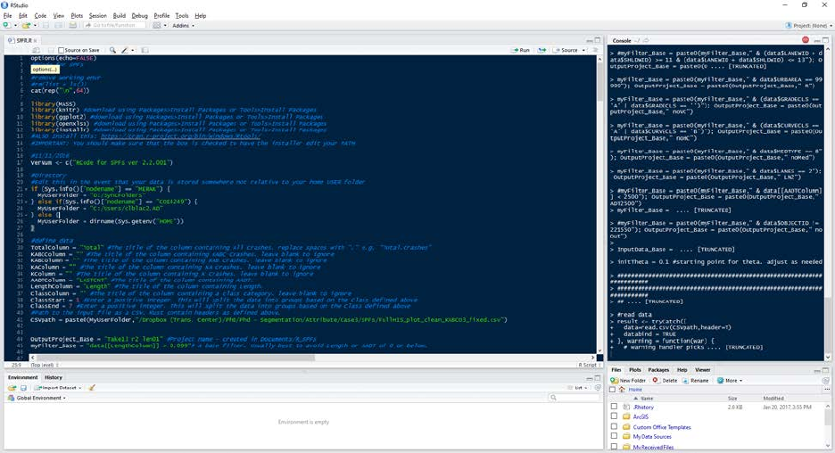
Once configured, a user simply executes the script using Code>Run Region>Run All (or
using the hotkey Ctrl+Alt+R). The code includes several printed statements that will appear in
the Console that can help with debugging. The following figure shows a typical R Studio layout.
SPF-R Output
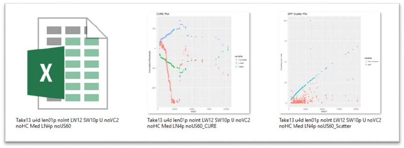
After a successful execution, a folder called “R_SPFs” will be created in the designated
output folder (a warning that this folder already exists will appear after the successive
executions). In this folder, a project folder will be created containing three files: and Excel
workbook with two worksheets, an image of a crash scatter plot, and an image of the CURE
Plot. Windows Explorer provides an easy way to view the output quickly if the thumbnails are
enlarged as shown below.
R Studio is able to process a large database with several classes (recall that classes are
groups of roadway segments or intersections) resulting in several SPFs in just a few minutes (on
a modern computer at the time of writing this paper). In fact, typical SPF development takes
only a few seconds.
Conclusions
This SPF development tool presented above is useful when trying to improve SPF
development. The effect that the roadway network’s heterogeneity has on SPF development
can be quickly explored by simply adjusting the output folder (line 42) and the base filter (line
43). Consider the following example:
• Base condition #1
o OutputProject_Base = "BC1-SW_2_LW_9"
o myFilter = "data$SHLDWID == 2 & data$LANEWID == 9
• Base condition #2
o OutputProject_Base = "BC1-SW_3_LW_10"
o myFilter = "data$SHLDWID == 3 & data$LANEWID == 10
In the above example, two SPFs can quickly be developed for the same roadway
network but for different specifications for shoulder and lane widths. Each SPF will be saved to
separate folders, named accordingly. The CURE Plots can be compared and further assessment
can be performed by opening the respective Excel files. Sample sizes and goodness-of-fit
measures can be compared as well to decide which SPF is more appropriate for the dataset.
The CURE plots provide a quick and visual screening process while other goodness-of-fit
measures allow the user to objectively compare SPFs.
Resources
The following resources offer information on SPF development and calibration.
• The Highway Safety Manual, First Edition
• NCHRP Project 20-7 (Task 332): User’s Guide to Develop Highway Safety Manual Safety
Performance Function (SPF) Calibration Factors.
• SPF Decision Guide: SPF Calibration vs. SPF Development.
o https://safety.fhwa.dot.gov/rsdp/downloads/spf_decision_guide_final.pdf
• SPF Development Guide: Developing Jurisdiction-Specific SPFs.
o https://safety.fhwa.dot.gov/rsdp/downloads/spf_development_guide_final.pdf
• The Art of Regression Modeling in Road Safety by Ezra Hauer
o http://www.springer.com/us/book/9783319125282
