Sage Beginner's Guide (2011)
User Manual: Pdf
Open the PDF directly: View PDF ![]() .
.
Page Count: 364 [warning: Documents this large are best viewed by clicking the View PDF Link!]
- Cover
- Copyright
- Credits
- About the Author
- About the Reviewers
- www.PacktPub.com
- Table of Contents
- Preface
- Chapter 1: What Can You Do with Sage?
- Chapter 2: Installing Sage
- Chapter 3: Getting Started with Sage
- How to get help with Sage
- Starting Sage from the command line
- Using the interactive shell
- Time for action – doing calculations on the command line
- Using the notebook interface
- Time for action – doing calculations with the notebook interface
- Displaying results of calculations
- Operators and variables
- Time for action – using strings
- Callable symbolic expressions
- Time for action – defining callable symbolic expressions
- Functions
- Time for action – calling functions
- Time for action – defining and using your own functions
- Time for action – defining a function with keyword arguments
- Objects
- Time for action – working with objects
- Summary
- Chapter 4: Introducing Python and Sage
- Python 2 and Python 3
- Writing code for Sage
- Sequence types: lists, tuples, and strings
- Time for action – creating lists
- Time for action – accessing items in a list
- Time for action – returning multiple values from a function
- Time for action – working with strings
- For loops
- Time for action – iterating over lists
- Time for action – computing a solution to the diffusion equation
- Time for action – using a list comprehension
- While loops and text file I/O
- Time for action – saving data in a text file
- Time for action – reading data from a text file
- If statements and conditional expressions
- Storing data in a dictionary
- Time for action – defining and accessing dictionaries
- Lambda forms
- Time for action – using lambda to create an anonymous
- function
- Summary
- Chapter 5: Vectors, Matrices, and Linear Algebra
- Vectors and vector spaces
- Time for action – working with vectors
- Time for action – manipulating elements of vectors
- Matrices and matrix spaces
- Time for action – solving a system of linear equations
- Time for action – accessing elements and parts of a matrix
- Time for action – manipulating matrices
- Time for action – matrix algebra
- Time for action – trying other matrix methods
- Time for action – computing eigenvalues and eigenvectors
- Time for action – computing the QR factorization
- Time for action – computing the singular value decomposition
- An introduction to NumPy
- Time for action – creating NumPy arrays
- Time for action – working with NumPy arrays
- Time for action – creating matrices in NumPy
- Summary
- Chapter 6: Plotting with Sage
- Confusion alert: Sage plots and matplotlib
- Plotting in two dimensions
- Time for action – plotting symbolic expressions
- Time for action – plotting a function with a pole
- Time for action – plotting a parametric function
- Time for action – making a polar plot
- Time for action – plotting a vector field
- Time for action – making a scatter plot
- Time for action – plotting a list
- Time for action – plotting with graphics primitives
- Using matplotlib
- Time for action – plotting functions with matplotlib
- Time for action – getting the matplotlib figure object
- Time for action – improving polar plots
- Time for action – making a bar chart
- Time for action – making a pie chart
- Time for action – plotting a histogram
- Plotting in three dimensions
- Time for action – make an interactive 3D plot
- Time for action – parametric plots in 3D
- Time for action – making some contour plots
- Summary
- Chapter 7: Making Symbolic Mathematics Easy
- Using the notebook interface
- Defining symbolic expressions
- Time for action – defining callable symbolic expressions
- Time for action – defining relational expressions
- Time for action – relational expressions with assumptions
- Manipulating expressions
- Time for action – manipulating expressions
- Time for action – working with rational functions
- Time for action – substituting symbols in expressions
- Time for action – expanding and factoring polynomials
- Time for action – manipulating trigonometric expressions
- Time for action – simplifying expressions
- Solving equations and finding roots
- Time for action – solving equations
- Time for action – finding roots
- Differential and integral calculus
- Time for action – calculating limits
- Time for action – calculating derivatives
- Time for action – calculating integrals
- Series and summations
- Time for action – computing sums of series
- Time for action – finding Taylor series
- Laplace transforms
- Time for action – computing Laplace transforms
- Solving ordinary differential equations
- Time for action – solving an ordinary differential equation
- Summary
- Chapter 8: Solving Problems Numerically
- Sage and NumPy
- Solving equations and finding roots numerically
- Time for action – finding roots of a polynomial
- Finding minima and maxima of functions
- Time for action – minimizing a function of one variable
- Time for action – minimizing a function of several variables
- Numerical approximation of derivatives
- Time for action – approximating derivatives with differences
- Time for action – computing gradients
- Numerical integration
- Time for action – numerical integration
- Time for action – numerical integration with NumPy
- Discrete Fourier transforms
- Time for action – computing discrete Fourier transforms
- Time for action – plotting window functions
- Solving ordinary differential equations
- Time for action – solving a first-order ODE
- Time for action – solving a higher-order ODE
- Time for action – alternative method of solving a system of ODEs
- Numerical optimization
- Time for action – linear programming
- Time for action – least squares fitting
- Time for action – a constrained optimization problem
- Probability
- Time for action – accessing probability distribution functions
- Summary
- Chapter 9: Learning Advanced Python Programming
- How to write good software
- Object-oriented programming
- Time for action – defining a class that represents a tank
- Time for action – making the tanks move
- Time for action – creating your first module
- Time for action – creating a vehicle base class
- Time for action – creating a combat simulation package
- Potential pitfalls when working with classes and instances
- Time for action – using class and instance attributes
- Time for action – more about class and instance attributes
- Time for action – creating empty classes and functions
- Handling errors gracefully
- Time for action – raising and handling exceptions
- Time for action – creating custom exception types
- Unit testing
- Time for action – creating unit tests for the Tank class
- Summary
- Chapter 10: Where to go from here
- Typesetting equations with LaTeX
- Time for action – PDF output from the notebook interface
- Time for action – working with LaTeX markup in the
- notebook interface
- Time for action – putting it all together
- Speeding up execution
- Time for action – detecting collisions between spheres
- Time for action – detecting collisions: command-line version
- Time for action – faster collision detection
- Time for action – using NumPy
- Time for action – optimizing collision detection with Cython
- Calling Sage from Python
- Time for action – calling Sage from a Python script
- Introducing Python decorators
- Time for action – introducing the Python decorator
- Making interactive graphics
- Time for action – making interactive controls
- Time for action – an interactive example
- Summary
- Index


Sage
Beginner's Guide
Unlock the full potenal of Sage for simplifying and
automang mathemacal compung
Craig Finch
BIRMINGHAM - MUMBAI
Sage
Beginner's Guide
Copyright © 2011 Packt Publishing
All rights reserved. No part of this book may be reproduced, stored in a retrieval system,
or transmied in any form or by any means, without the prior wrien permission of the
publisher, except in the case of brief quotaons embedded in crical arcles or reviews.
Every eort has been made in the preparaon of this book to ensure the accuracy of the
informaon presented. However, the informaon contained in this book is sold without
warranty, either express or implied. Neither the author, nor Packt Publishing, and its dealers
and distributors will be held liable for any damages caused or alleged to be caused directly or
indirectly by this book.
Packt Publishing has endeavored to provide trademark informaon about all of the
companies and products menoned in this book by the appropriate use of capitals.
However, Packt Publishing cannot guarantee the accuracy of this informaon.
First published: May 2011
Producon Reference: 1250411
Published by Packt Publishing Ltd.
32 Lincoln Road
Olton
Birmingham, B27 6PA, UK.
ISBN 978-1-849514-46-0
www.packtpub.com
Cover Image by Ed Maclean (edmaclean@gmail.com)

Credits
Author
Craig Finch
Reviewers
Dr. David Kirkby
Minh Nguyen
Acquision Editor
Usha Iyer
Development Editor
Hyacintha D'Souza
Technical Editor
Ajay Shanker
Indexers
Tejal Daruwale
Rekha Nair
Project Coordinator
Joel Goveya
Proofreaders
Aaron Nash
Mario Cecere
Graphics
Nilesh Mohite
Producon Coordinator
Adline Swetha Jesuthas
Cover Work
Adline Swetha Jesuthas

About the Author
Craig Finch is a Ph. D. Candidate in the Modeling and Simulaon program at the University
of Central Florida (UCF). He earned a Bachelor of Science degree from the University
of Illinois at Urbana-Champaign and a Master of Science degree from UCF, both in
electrical engineering. Craig worked as a design engineer for TriQuint Semiconductor, and
currently works as a research assistant in the Hybrid Systems Lab at the UCF NanoScience
Technology Center. Craig's professional goal is to develop tools for computaonal science
and engineering and use them to solve dicult problems. In parcular, he is interested
in developing tools to help biologists study living systems. Craig is commied to using,
developing, and promong open-source soware. He provides documentaon and "how-to"
examples on his blog at http://www.shocksolution.com.
I would like to thank my advisers, Dr. J. Hickman and Dr. Tom Clarke, for
giving me the opportunity to pursue my doctorate. I would also like to
thank my parents for buying the Apple IIGS computer that started it all.
About the Reviewers
Dr. David Kirkby is a chartered engineer living in Essex, England. David has a B.Sc. in
Electrical and Electronic Engineering, an M.Sc. in Microwaves and OptoElectronics, and a
Ph.D. in Medical Physics. Despite David's Ph.D. being in Medical Physics, it was primarily an
engineering project, measuring the opcal properes of human ssue, with a mixture of
Monte Carlo modeling, radio frequency design, and laser opcs. David was awarded his Ph.D.
in 1999 from University College London.
Although not a mathemacian, Dr. Kirkby has made extensive use of mathemacal soware.
Most of his experience has been with MathemacaTM from Wolfram Research, although he
has used both MATLABTM and SimulinkTM too.
David is the author of a number of open-source projects, including soware for modeling
transmission lines using nite dierence (http://atlc.sourceforge.net/), design of
Yagi-Uda antennas (http://www.g8wrb.org/yagi/) which can use a genec algorithm
for opmizaon, as well as soware for data collecon and analysis from electronic test
equipment. David once wrote a web-based interface to MathemacaTM (http://witm.
sourceforge.net/) which allows MathemacaTM to be used from a personal computer,
PDA or smartphone.
Soon aer the Sage project was started by Professor William Stein, Dr. Kirkby joined the
development of Sage. He primarily worked on the successful port of Sage to the Solaris and
OpenSolaris operang systems and encourages other developers to write portable code,
conforming to POSIX standard, avoiding GNUisms.
Professionally, David's skill sets include computer modeling, radio frequency design,
analogue circuit design, electromagnec compability and opcs—both free space
and integrated. David has also been a Solaris system administrator for the University of
Washington where the Sage project is based.
When not working on wring soware, David enjoys playing chess, gardening, and
spending me with his wife Lin and dog Smudge.
Readers wishing to contact Dr. Kirkby can do so via his website http://www.drkirkby.
co.uk/ where details of his consulng services may be found.
Minh Nguyen has been a contributor to the Sage project since December 2007. Over the
years, he has worked on various aspects of Sage ranging from the standard documentaon and
modules such as cryptography, number theory, and graph theory to the Sage build system. He
regularly maintains the Sage website and works on book projects that aim to provide in-depth
documentaon on using Sage to study cryptography and mathemacs. More of his ranngs
can be found at http://mvngu.wordpress.com.

www.PacktPub.com
Support les, eBooks, discount offers and more
You might want to visit www.PacktPub.com for support les and downloads related to
your book.
Did you know that Packt oers eBook versions of every book published, with PDF and ePub
les available? You can upgrade to the eBook version at www.PacktPub.com and as a print
book customer, you are entled to a discount on the eBook copy. Get in touch with us at
service@packtpub.com for more details.
At www.PacktPub.com, you can also read a collecon of free technical arcles, sign up for a
range of free newsleers and receive exclusive discounts and oers on Packt books and eBooks.
http://PacktLib.PacktPub.com
Do you need instant soluons to your IT quesons? PacktLib is Packt's online digital book
library. Here, you can access, read and search across Packt's enre library of books.
Why Subscribe?
Fully searchable across every book published by Packt
Copy & paste, print and bookmark content
On demand and accessible via web browser
Free Access for Packt account holders
If you have an account with Packt at www.PacktPub.com, you can use this to access
PacktLib today and view nine enrely free books. Simply use your login credenals for
immediate access.

Table of Contents
Preface 1
Chapter 1: What Can You Do with Sage? 9
Geng started 9
Using Sage as a powerful calculator 12
Symbolic mathemacs 14
Linear algebra 17
Solving an ordinary dierenal equaon 18
More advanced graphics 19
Visualising a three-dimensional surface 20
Typeseng mathemacal expressions 21
A praccal example: analysing experimental data 22
Time for acon – ng the standard curve 22
Time for acon – plong experimental data 24
Time for acon – ng a growth model 25
Summary 26
Chapter 2: Installing Sage 29
Before you begin 29
Installing a binary version of Sage on Windows 30
Downloading VMware Player 30
Installing VMWare Player 30
Downloading and extracng Sage 30
Launching the virtual machine 31
Start Sage 32
Installing a binary version of Sage on OS X 33
Downloading Sage 34
Installing Sage 34
Starng Sage 34

Table of Contents
[ ii ]
Installing a binary version of Sage on GNU/Linux 35
Downloading and decompressing Sage 35
Running Sage from your user account 36
Installing for mulple users 37
Building Sage from source 38
Prerequisites 38
Downloading and decompressing source tarball 39
Building Sage 39
Installaon 39
Summary 39
Chapter 3: Geng Started with Sage 41
How to get help with Sage 41
Starng Sage from the command line 42
Using the interacve shell 43
Time for acon – doing calculaons on the command line 43
Geng help 45
Command history 46
Tab compleon 47
Interacvely tracing execuon 48
Using the notebook interface 48
Starng the notebook interface 49
Time for acon – doing calculaons with the notebook interface 52
Geng help in the notebook interface 54
Working with cells 54
Working with code 55
Closing the notebook interface 55
Displaying results of calculaons 56
Operators and variables 56
Arithmec operators 57
Numerical types 58
Integers and raonal numbers 58
Real numbers 59
Complex numbers 60
Symbolic expressions 60
Dening variables on rings 61
Combining types in expressions 62
Strings 62
Time for acon – using strings 62
Callable symbolic expressions 63
Time for acon – dening callable symbolic expressions 64
Automacally typeseng expressions 65

Table of Contents
[ iii ]
Funcons 66
Time for acon – calling funcons 66
Built-in funcons 68
Numerical approximaons 68
The reset and restore funcons 69
Dening your own funcons 70
Time for acon – dening and using your own funcons 70
Funcons with keyword arguments 72
Time for acon – dening a funcon with keyword arguments 72
Objects 73
Time for acon – working with objects 74
Geng help with objects 75
Summary 77
Chapter 4: Introducing Python and Sage 79
Python 2 and Python 3 79
Wring code for Sage 80
Long lines of code 81
Running scripts 81
Sequence types: lists, tuples, and strings 82
Time for acon – creang lists 82
Geng and seng items in lists 85
Time for acon – accessing items in a list 85
List funcons and methods 87
Tuples: read-only lists 87
Time for acon – returning mulple values from a funcon 87
Strings 89
Time for acon – working with strings 90
Other sequence types 92
For loops 92
Time for acon – iterang over lists 92
Time for acon – compung a soluon to the diusion equaon 94
List comprehensions 99
Time for acon – using a list comprehension 99
While loops and text le I/O 101
Time for acon – saving data in a text le 101
Time for acon – reading data from a text le 103
While loops 105
Parsing strings and extracng data 105
Alternave approach to reading from a text le 106
If statements and condional expressions 107
Storing data in a diconary 108

Table of Contents
[ iv ]
Time for acon – dening and accessing diconaries 108
Lambda forms 110
Time for acon – using lambda to create an anonymous funcon 110
Summary 111
Chapter 5: Vectors, Matrices, and Linear Algebra 113
Vectors and vector spaces 113
Time for acon – working with vectors 114
Creang a vector space 115
Creang and manipulang vectors 116
Time for acon – manipulang elements of vectors 116
Vector operators and methods 117
Matrices and matrix spaces 118
Time for acon – solving a system of linear equaons 118
Creang matrices and matrix spaces 120
Accessing and manipulang matrices 120
Time for acon – accessing elements and parts of a matrix 120
Manipulang matrices 122
Time for acon – manipulang matrices 122
Matrix algebra 124
Time for acon – matrix algebra 124
Other matrix methods 125
Time for acon – trying other matrix methods 126
Eigenvalues and eigenvectors 127
Time for acon – compung eigenvalues and eigenvectors 127
Decomposing matrices 129
Time for acon – compung the QR factorizaon 129
Time for acon – compung the singular value decomposion 131
An introducon to NumPy 133
Time for acon – creang NumPy arrays 133
Creang NumPy arrays 134
NumPy types 135
Indexing and selecon with NumPy arrays 136
Time for acon – working with NumPy arrays 136
NumPy matrices 137
Time for acon – creang matrices in NumPy 137
Learning more about NumPy 139
Summary 139
Chapter 6: Plong with Sage 141
Confusion alert: Sage plots and matplotlib 141
Plong in two dimensions 141

Table of Contents
[ v ]
Plong symbolic expressions with Sage 142
Time for acon – plong symbolic expressions 142
Time for acon – plong a funcon with a pole 144
Time for acon – plong a parametric funcon 146
Time for acon – making a polar plot 147
Time for acon – plong a vector eld 149
Plong data in Sage 150
Time for acon – making a scaer plot 150
Time for acon – plong a list 151
Using graphics primives 153
Time for acon – plong with graphics primives 153
Using matplotlib 155
Time for acon – plong funcons with matplotlib 155
Using matplotlib to "tweak" a Sage plot 157
Time for acon – geng the matplotlib gure object 158
Time for acon – improving polar plots 159
Plong data with matplotlib 161
Time for acon – making a bar chart 161
Time for acon – making a pie chart 163
Time for acon – plong a histogram 164
Plong in three dimensions 165
Time for acon – make an interacve 3D plot 166
Higher quality output 167
Parametric 3D plong 168
Time for acon – parametric plots in 3D 168
Contour plots 169
Time for acon – making some contour plots 169
Summary 171
Chapter 7: Making Symbolic Mathemacs Easy 173
Using the notebook interface 174
Dening symbolic expressions 174
Time for acon – dening callable symbolic expressions 174
Relaonal expressions 176
Time for acon – dening relaonal expressions 176
Time for acon – relaonal expressions with assumpons 178
Manipulang expressions 179
Time for acon – manipulang expressions 179
Manipulang raonal funcons 180
Time for acon – working with raonal funcons 181
Substuons 182

Table of Contents
[ vi ]
Time for acon – substung symbols in expressions 182
Expanding and factoring polynomials 184
Time for acon – expanding and factoring polynomials 184
Manipulang trigonometric expressions 186
Time for acon – manipulang trigonometric expressions 186
Logarithms, raonal funcons, and radicals 187
Time for acon – simplifying expressions 187
Solving equaons and nding roots 190
Time for acon – solving equaons 190
Finding roots 191
Time for acon – nding roots 191
Dierenal and integral calculus 193
Time for acon – calculang limits 193
Derivaves 195
Time for acon – calculang derivaves 195
Integrals 198
Time for acon – calculang integrals 198
Series and summaons 199
Time for acon – compung sums of series 199
Taylor series 200
Time for acon – nding Taylor series 200
Laplace transforms 202
Time for acon – compung Laplace transforms 202
Solving ordinary dierenal equaons 204
Time for acon – solving an ordinary dierenal equaon 204
Summary 206
Chapter 8: Solving Problems Numerically 207
Sage and NumPy 208
Solving equaons and nding roots numerically 208
Time for acon – nding roots of a polynomial 208
Finding minima and maxima of funcons 210
Time for acon – minimizing a funcon of one variable 210
Funcons of more than one variable 211
Time for acon – minimizing a funcon of several variables 211
Numerical approximaon of derivaves 213
Time for acon – approximang derivaves with dierences 213
Compung gradients 215
Time for acon – compung gradients 215
Numerical integraon 217
Time for acon – numerical integraon 217

Table of Contents
[ vii ]
Numerical integraon with NumPy 219
Time for acon – numerical integraon with NumPy 219
Discrete Fourier transforms 220
Time for acon – compung discrete Fourier transforms 220
Window funcons 223
Time for acon – plong window funcons 223
Solving ordinary dierenal equaons 224
Time for acon – solving a rst-order ODE 224
Solving a system of ODEs 226
Time for acon – solving a higher-order ODE 226
Solving the system using the GNU Scienc Library 229
Time for acon – alternave method of solving a system of ODEs 229
Numerical opmizaon 231
Time for acon – linear programming 231
Fing a funcon to a noisy data set 233
Time for acon – least squares ng 233
Constrained opmizaon 235
Time for acon – a constrained opmizaon problem 235
Probability 236
Time for acon – accessing probability distribuon funcons 236
Summary 238
Chapter 9: Learning Advanced Python Programming 241
How to write good soware 242
Object-oriented programming 243
Time for acon – dening a class that represents a tank 244
Making our tanks move 249
Time for acon – making the tanks move 249
Creang a module for our classes 253
Time for acon – creang your rst module 253
Expanding our simulaon to other kinds of vehicles 258
Time for acon – creang a vehicle base class 258
Creang a package for our simulaon 263
Time for acon – creang a combat simulaon package 263
Potenal pialls when working with classes and instances 268
Time for acon – using class and instance aributes 269
Time for acon – more about class and instance aributes 270
Creang empty classes and funcons 272
Time for acon – creang empty classes and funcons 272
Handling errors gracefully 273
Time for acon – raising and handling excepons 274

Table of Contents
[ viii ]
Excepon types 278
Creang your own excepon types 279
Time for acon – creang custom excepon types 279
Unit tesng 284
Time for acon – creang unit tests for the Tank class 284
Strategies for unit tesng 288
Summary 289
Chapter 10: Where to go from here 291
Typeseng equaons with LaTeX 291
Installing LaTeX 292
Time for acon – PDF output from the notebook interface 293
The view funcon in the interacve shell 297
LaTeX mark-up in the notebook interface 297
Time for acon – working with LaTeX markup in the notebook interface 297
Time for acon – pung it all together 300
Speeding up execuon 304
Time for acon – detecng collisions between spheres 304
Time for acon – detecng collisions: command-line version 307
Tips for measuring runmes 309
Opmizing our algorithm 309
Time for acon – faster collision detecon 309
Opmizing with NumPy 311
Time for acon – using NumPy 311
More about NumPy 314
Opmizing with Cython 314
Time for acon – opmizing collision detecon with Cython 314
Calling Sage from Python 316
Time for acon – calling Sage from a Python script 316
Introducing Python decorators 319
Time for acon – introducing the Python decorator 319
Making interacve graphics 322
Time for acon – making interacve controls 322
Using interacve controls 328
Time for acon – an interacve example 328
Summary 330
Index 333
Preface
Results maer, whether you are a mathemacian, scienst, or engineer. The me that you
spend doing tedious mathemacal calculaons could be spent in more producve ways. Sage
is an open-source mathemacal soware system that helps you perform many mathemacal
tasks. There is no reason to compute integrals or perform algebraic manipulaons by hand
when soware can perform these tasks more quickly and accurately (unless you are a
student who is learning these procedures for the rst me). Students can also benet from
mathemacal soware. The ability to plot funcons and manipulate symbolic expressions
easily can improve your understanding of mathemacal concepts. Likewise, it is largely
unnecessary to write your own rounes for numerical mathemacs in low-level languages
such as FORTRAN or C++. Mathemacal soware systems like Sage have highly opmized
funcons that implement common numerical operaons like integraon, solving ordinary
dierenal equaons, and solving systems of equaons.
Sage is a collecon of nearly 100 mathemacal soware packages, which are listed at
http://www.sagemath.org/links-components.html. When possible, exisng tools
are integrated into Sage, rather than duplicang their funconality. The enre collecon of
tools can be downloaded and installed as a binary distribuon or compiled from source code.
The Python language provides a unied interface to all of the packages. Python is a high-
level, interpreted, object-oriented programming language that is already well established
in the research community. Users can interact with Sage through an interacve command-
line interface or a graphical notebook interface. Sage can also be used as a Python library or
embedded in LaTeX documents. Sage is "ocially" available for recent versions of OS X, Linux,
Solaris, and Open Solaris. It runs on Windows with the help of a virtual machine and it can
be used on other plaorms, with varying degrees of support. A current list of all the available
plaorms can be found at http://wiki.sagemath.org/SupportedPlatforms.

Preface
[ 2 ]
The mission statement of the Sage project is:
Creating a viable, free, open source alternative to Magma, Maple,
Mathematica, and Matlab.
If you are familiar with any of these commercial mathemacal soware systems, then you
already have a good idea what Sage does. Sage oers several advantages over its commercial
competors. Sage is free, open-source soware, released under the GNU Public License
version 2 or higher (GPLv2+). There is no cost to download and install Sage, whether you
want to put it on your personal computer, install it in a university teaching lab, or deploy
it on every workstaon in a company. This advantage is especially important in developing
countries. The GPL license also means that Sage is free, as in "freedom." There are no
restricons on how or where you use the soware, the license can never be revoked, and
there is no annual maintenance fee. Another advantage is that you have access to every
line of source code, so you can see how every calculaon is performed, and track exactly
what changes are made from one version to the next. Unlike commercial soware, the bug
list for Sage is public, and it can be accessed at http://trac.sagemath.org/. Users are
encouraged to parcipate in the development of Sage by reporng and xing bugs, and
contribung new capabilies. With bugs and source code open for public review, you can
have a high degree of condence that Sage will produce correct results.
This book is wrien for people who are new to Sage, and perhaps new to mathemacal
soware altogether. For this reason, the examples in the book emphasize undergraduate-level
mathemacs such as calculus, linear algebra, and ordinary dierenal equaons. However,
Sage is capable of performing advanced mathemacs, and it has been cited in over 80
mathemacal publicaons. A full list can be found at http://www.sagemath.org/library-
publications.html. To benet from this book, you should have some fundamental
knowledge of computer programming, but the Python language will be introduced as needed
throughout the book. The next chapter will take you through some examples that showcase a
small subset of Sage's capabilies.
What this book covers
Chapter 1, What can You do with Sage? covers how Sage can be used for: making simple
numerical calculaons; performing symbolic calculaons, solving systems of equaons and
ordinary dierenal equaons; making plots in two and three dimensions; and analyzing
experimental data and ng models.
Chapter 2, Installing Sage covers how to install a binary version of Sage on Windows and
install a binary version of Sage on OS X; install a binary version of Sage on GNU/Linux;
compile Sage from source.

Preface
[ 3 ]
Chapter 3, Geng Started with Sage covers using the interacve shell; using the notebook
interface; learning more about operators and variables; dening and using callable symbolic
expressions; calling funcons and making simple plots; dening your own funcons; and
working with objects in Sage.
Chapter 4, Introducing Python and Sage covers how to: use lists and tuples to store
sequenal data; iterate with loops; construct logical tests with "if" statements; read and
write data les; and store heterogeneous data in diconaries.
Chapter 5, Vectors, Matrices, and Linear Algebra covers how to create and manipulate vector
and matrix objects; how Sage can take the tedious work out of linear algebra; learning about
matrix methods for compung eigenvalues, inverses, and decomposions; and geng
started with NumPy arrays and matrices for numerical calculaons.
Chapter 6, Plong with Sage covers how to plot funcons of one variable; making various
types of specialized 2D plots such as polar plots and scaer plots; using matplotlib to
precisely format 2D plots and charts; and making interacve 3D plots of funcons of two
variables.
Chapter 7, Making Symbolic Mathemacs Easy covers how to create symbolic funcons
and expressions, and learn to manipulate them; solve equaons and systems of equaons
exactly, and nd symbolic roots; automate calculus operaons like limits, derivaves, and
integrals; create innite series and summaons to approximate funcons; perform Laplace
transforms; and nd exact soluons to ordinary dierenal equaons.
Chapter 8, Solving Problems Numerically covers how to nd the roots of an equaon;
compute integrals and derivaves numerically; nd minima and maxima of funcons;
compute discrete Fourier transforms, and apply window funcons; numerically solve an
ordinary dierenal equaon (ODE), and systems of ODEs; use opmizaon techniques
to t curves and nd minima; and explore the probability tools in Sage.
Chapter 9, Learning Advanced Python Programming covers how to dene your own classes;
use inheritance to expand the usefulness of your classes; organize your class denions in
module les; bundle module les into packages; handle errors gracefully with excepons;
dene your own excepons for custom error handling; and use unit tests to make sure your
package is working correctly.
Chapter 10, Where to go from here covers how to export equaons as PNG and PDF
les; export vector graphics and typeset mathemacal expressions for inclusion in LaTeX
documents; use LaTeX to document Sage worksheets; speed up collision detecon using
NumPy vector operaons; create a Python script that uses Sage funconality; and create
interacve graphical examples in the notebook interface.

Preface
[ 4 ]
What you need for this book
Required:
Sage
If using Windows, VMWare Player or VirtualBox is also required.
Recommended, but not strictly necessary: LaTeX
Oponal, for building Sage from source on Linux: GCC, g++, make, m4, perl,
ranlib, readline, and tar
Oponal, for building Sage from source on OS X: XCode
A web browser is required to use the notebook interface
Who this book is for
If you are an engineer, scienst, mathemacian, or student, this book is for you. To get the
most from Sage by using the Python programming language, we'll give you the basics of the
language to get you started. For this, it will be helpful if you have some experience with basic
programming concepts.
Conventions
In this book, you will nd several headings appearing frequently.
To give clear instrucons of how to complete a procedure or task, we use:
Time for action – heading
1. Acon 1
2. Acon 2
3. Acon 3
Instrucons oen need some extra explanaon so that they make sense, so they are
followed with:
What just happened?
This heading explains the working of tasks or instrucons that you have just completed.
Preface
[ 5 ]
You will also nd some other learning aids in the book, including:
Pop quiz – heading
These are short mulple choice quesons intended to help you test your own understanding.
Have a go hero – heading
These set praccal challenges and give you ideas for experimenng with what you have
learned.
You will also nd a number of styles of text that disnguish between dierent kinds of
informaon. Here are some examples of these styles, and an explanaon of their meaning.
Code words in text are shown as follows: "We can use the help funcon to learn more
about it."
A block of code is set as follows:
print('This is a string')
print(1.0)
print(sqrt)
Any command-line input or output is wrien as follows:
sage: R = 250e3
sage: C = 4e-6
sage: tau = R * C
sage: tau
New terms and important words are shown in bold. Words that you see on the screen, in
menus or dialog boxes for example, appear in the text like this: "clicking the Next buon
moves you to the next screen".
Warnings or important notes appear in a box like this.
Tips and tricks appear like this.

Preface
[ 6 ]
Reader feedback
Feedback from our readers is always welcome. Let us know what you think about this
book—what you liked or may have disliked. Reader feedback is important for us to
develop tles that you really get the most out of.
To send us general feedback, simply send an e-mail to feedback@packtpub.com, and
menon the book tle via the subject of your message.
If there is a book that you need and would like to see us publish, please send us a note in
the SUGGEST A TITLE form on www.packtpub.com or e-mail suggest@packtpub.com.
If there is a topic that you have experse in and you are interested in either wring or
contribung to a book, see our author guide on www.packtpub.com/authors.
Customer support
Now that you are the proud owner of a Packt book, we have a number of things to help
you to get the most from your purchase.
Downloading the example code
You can download the example code les for all Packt books you have purchased from your
account at http://www.PacktPub.com. If you purchased this book elsewhere, you can
visit http://www.PacktPub.com/support and register to have the les e-mailed directly
to you.
Errata
Although we have taken every care to ensure the accuracy of our content, mistakes do
happen. If you nd a mistake in one of our books—maybe a mistake in the text or the code—
we would be grateful if you would report this to us. By doing so, you can save other readers
from frustraon and help us improve subsequent versions of this book. If you nd any
errata, please report them by vising http://www.packtpub.com/support, selecng
your book, clicking on the errata submission form link, and entering the details of your
errata. Once your errata are veried, your submission will be accepted and the errata will
be uploaded on our website, or added to any list of exisng errata, under the Errata secon
of that tle. Any exisng errata can be viewed by selecng your tle from http://www.
packtpub.com/support.

Preface
[ 7 ]
Piracy
Piracy of copyright material on the Internet is an ongoing problem across all media. At Packt,
we take the protecon of our copyright and licenses very seriously. If you come across any
illegal copies of our works, in any form, on the Internet, please provide us with the locaon
address or website name immediately so that we can pursue a remedy.
Please contact us at copyright@packtpub.com with a link to the suspected pirated material.
We appreciate your help in protecng our authors, and our ability to bring you valuable
content.
Questions
You can contact us at questions@packtpub.com if you are having a problem with any
aspect of the book, and we will do our best to address it.
1
What Can You Do with Sage?
Sage is a powerful tool—but you don't have to take my word for it. This chapter will
showcase a few of the things that Sage can do to enhance your work. At this point, don't
expect to understand every aspect of the examples presented in this chapter. Everything will
be explained in more detail in the later chapters. Look at the things Sage can do, and start to
think about how Sage might be useful to you. In this chapter, you will see how Sage can be
used for:
Making simple numerical calculaons
Performing symbolic calculaons
Solving systems of equaons and ordinary dierenal equaons
Making plots in two and three dimensions
Analysing experimental data and ng models
Getting started
You don't have to install Sage to try it out! In this chapter, we will use the notebook interface
to showcase some of the basics of Sage so that you can follow along using a public notebook
server. These examples can also be run from an interacve session if you have installed Sage.
What Can You Do with Sage?
[ 10 ]
Go to http://www.sagenb.org/ and sign up for a free account. You can also browse
worksheets created and shared by others. If you have already installed Sage, launch the
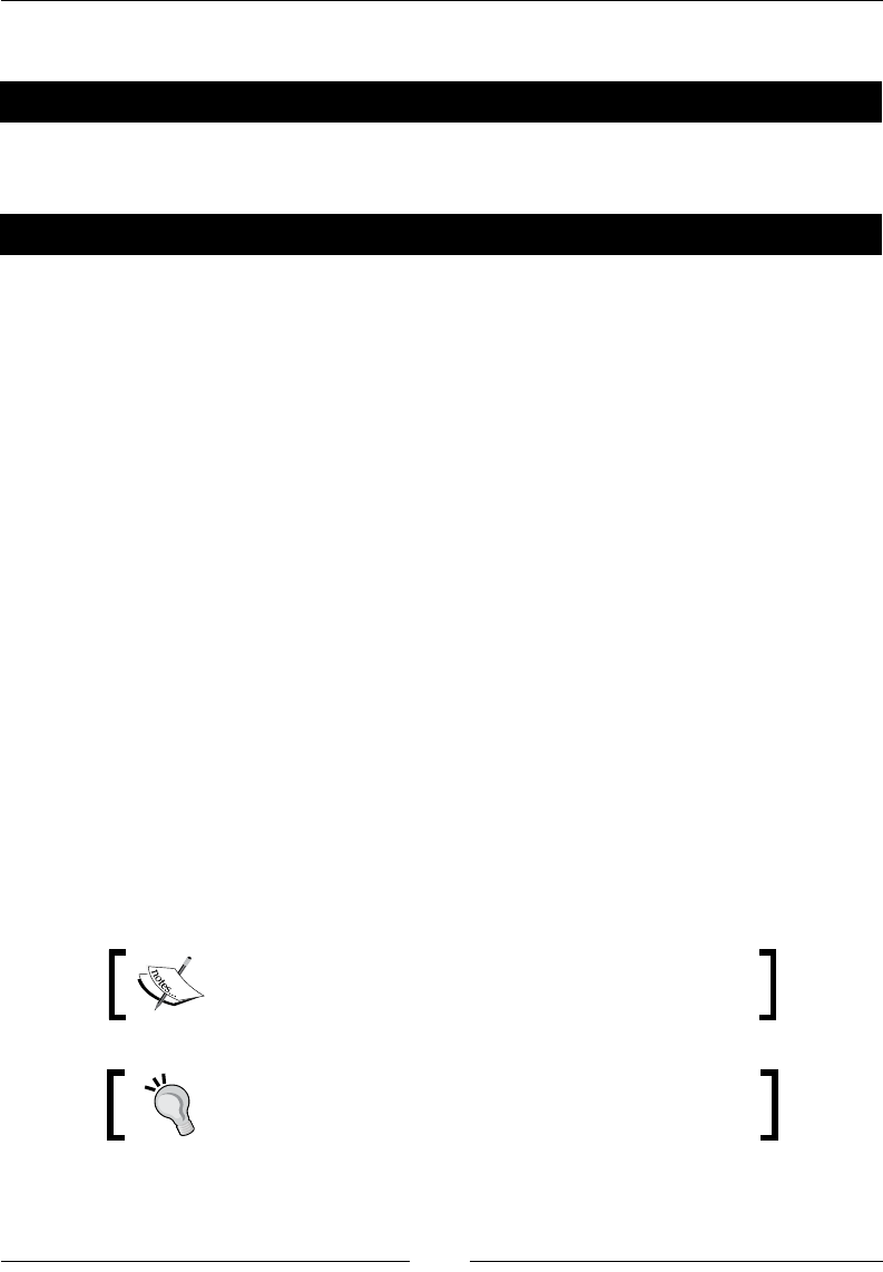
notebook interface by following the instrucons in Chapter 3. The notebook interface
should look like this:
Create a new worksheet by clicking on the link called New Worksheet:
Chapter 1
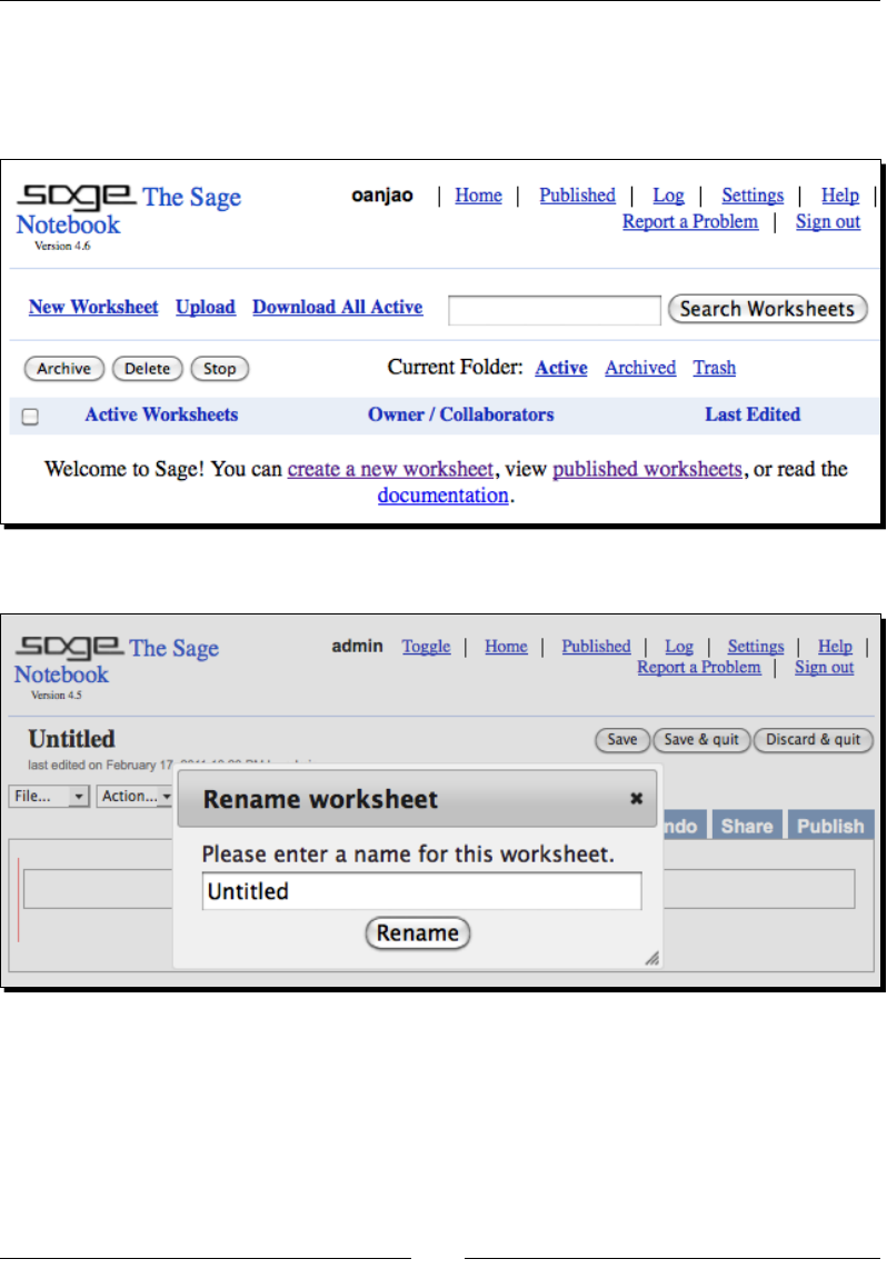
[ 11 ]
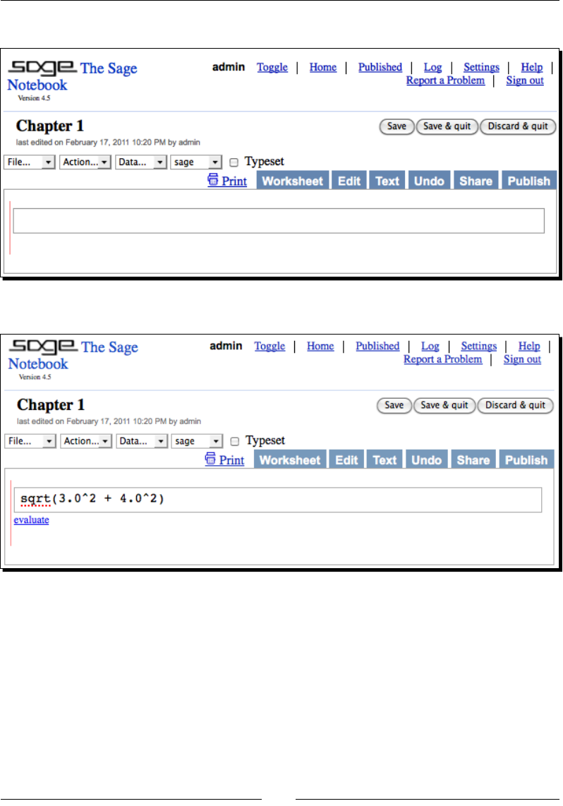
Type in a name when prompted, and click Rename. The new worksheet will look like this:
Enter an expression by clicking in an input cell and typing or pasng in an expression:
What Can You Do with Sage?
[ 12 ]
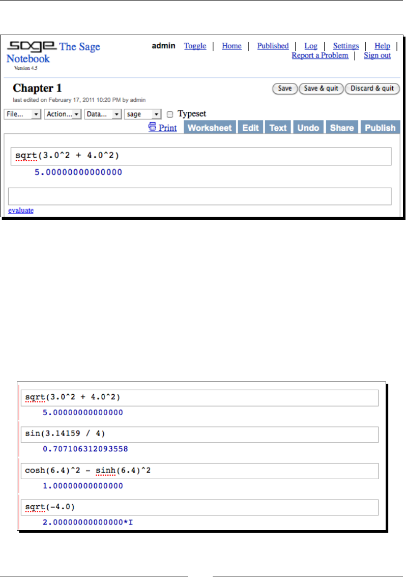
Click the evaluate link or press Shi-Enter to evaluate the contents of the cell.
A new input cell will automacally open below the results of the calculaon. You can also
create a new input cell by clicking in the blank space just above an exisng input cell. In
Chapter 3, we'll cover the notebook interface in more detail.
Using Sage as a powerful calculator
Sage has all the features of a scienc calculator—and more. If you have been trying to
perform mathemacal calculaons with a spreadsheet or the built-in calculator in your
operang system, it's me to upgrade. Sage oers all the built-in funcons you would expect.
Here are a few examples:
Chapter 1
[ 13 ]
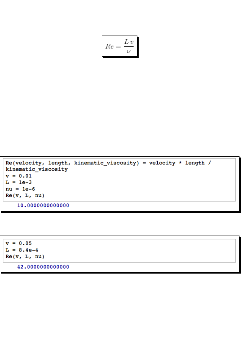
If you have to make a calculaon repeatedly, you can dene a funcon and variables to make
your life easier. For example, let's say that you need to calculate the Reynolds number, which
is used in uid mechanics:
You can dene a funcon and variables like this:
Re(velocity, length, kinematic_viscosity) = velocity * length /
kinematic_viscosity
v = 0.01
L = 1e-3
nu = 1e-6
Re(v, L, nu)
When you type the code into an input cell and evaluate the cell, your screen will look
like this:
Now, you can change the value of one or more variables and re-run the calculaon:
What Can You Do with Sage?
[ 14 ]
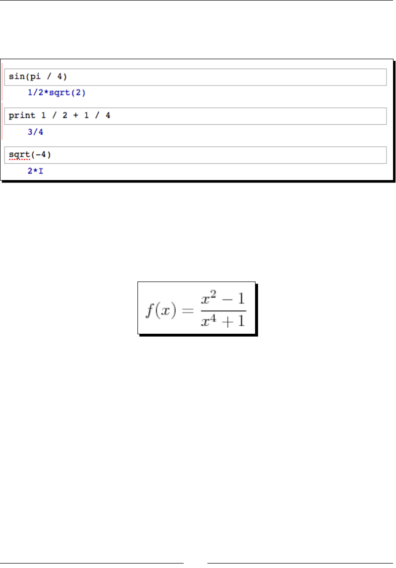
Sage can also perform exact calculaons with integers and raonal numbers. Using the pre-
dened constant pi will result in exact values from trigonometric operaons. Sage will even
ulize complex numbers when needed. Here are some examples:
Symbolic mathematics
Much of the diculty of higher mathemacs actually lies in the extensive algebraic
manipulaons that are required to obtain a result. Sage can save you many hours, and
many sheets of paper, by automang some tedious tasks in mathemacs. We'll start with
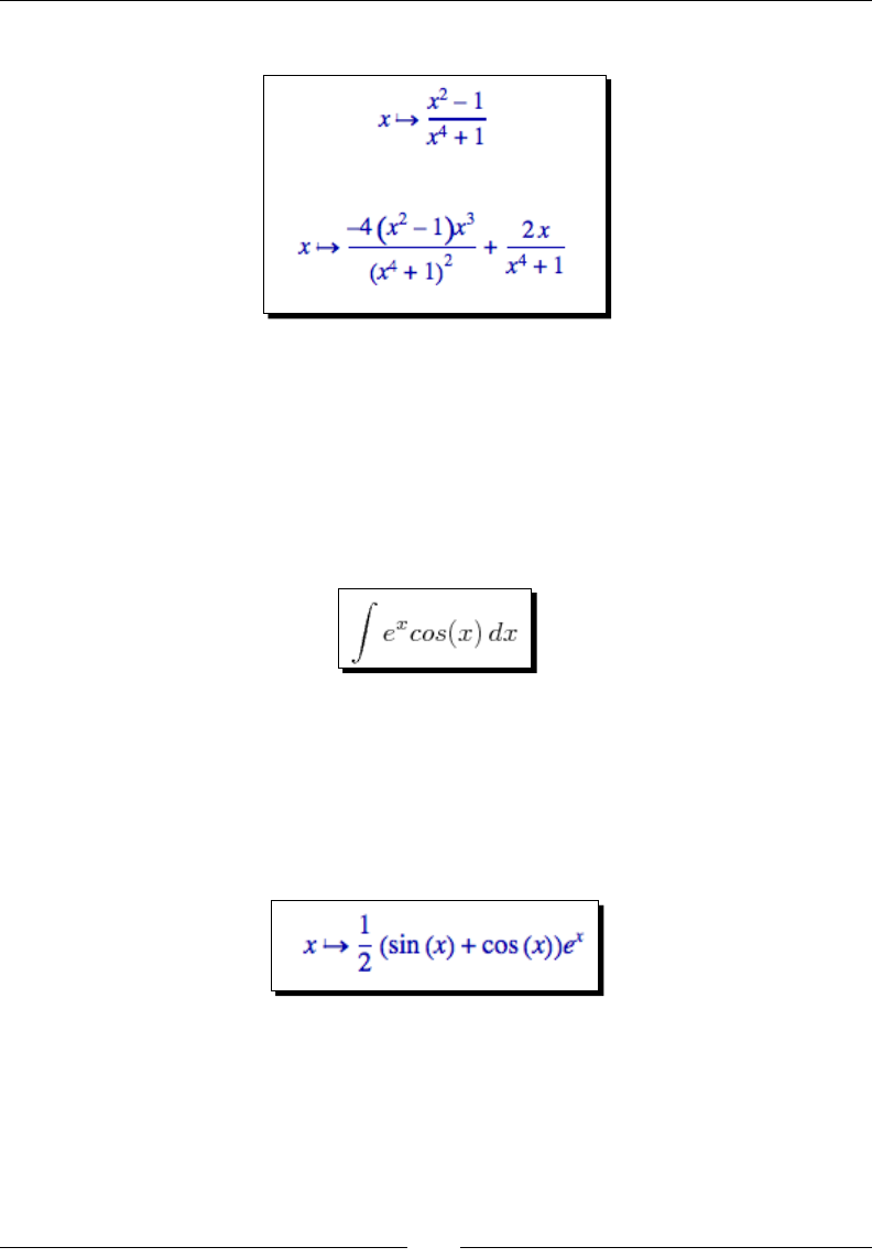
basic calculus. For example, let's compute the derivave of the following equaon:
The following code denes the equaon and computes the derivave:
var('x')
f(x) = (x^2 - 1) / (x^4 + 1)
show(f)
show(derivative(f, x))
Chapter 1
[ 15 ]
The results will look like this:
The rst line denes a symbolic variable x (Sage automacally assumes that x is always
a symbolic variable, but we will dene it in each example for clarity). We then dened a
funcon as a quoent of polynomials. Taking the derivave of f(x) would normally require
the use of the quoent rule, which can be very tedious to calculate. Sage computes the
derivave eortlessly.
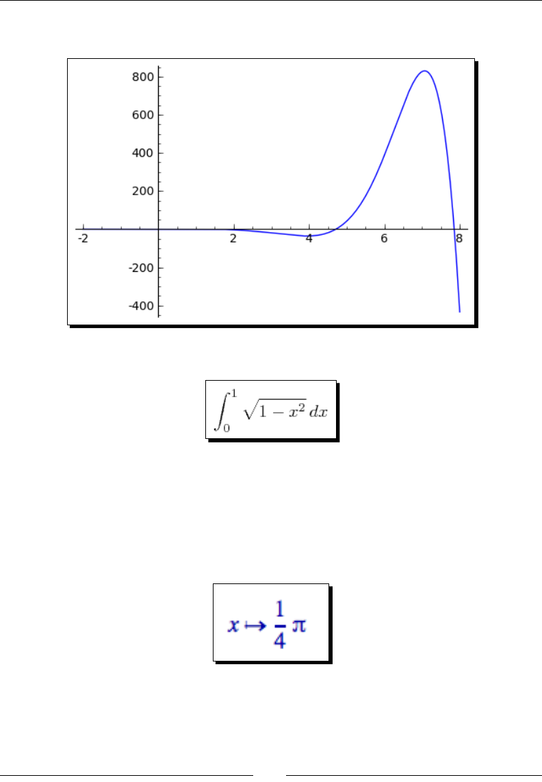
Now, we'll move on to integraon, which can be one of the most daunng tasks in calculus.
Let's compute the following indenite integral symbolically:
The code to compute the integral is very simple:
f(x) = e^x * cos(x)
f_int(x) = integrate(f, x)
show(f_int)
The result is as follows:
To perform this integraon by hand, integraon by parts would have to be done twice,
which could be quite me consuming. If we want to beer understand the funcon we just
dened, we can graph it with the following code:
f(x) = e^x * cos(x)
plot(f, (x, -2, 8))
What Can You Do with Sage?
[ 16 ]
Sage will produce the following plot:
Sage can also compute denite integrals symbolically:
To compute a denite integral, we simply have to tell Sage the limits of integraon:
f(x) = sqrt(1 - x^2)
f_integral = integrate(f, (x, 0, 1))
show(f_integral)
The result is:
This would have required the use of a substuon if computed by hand.
Chapter 1
[ 17 ]
Have a go hero
There is actually a clever way to evaluate the integral from the previous problem without
doing any calculus. If it isn't immediately apparent, plot the funcon f(x) from 0 to 1 and see
if you recognize it. Note that the aspect rao of the plot may not be square.
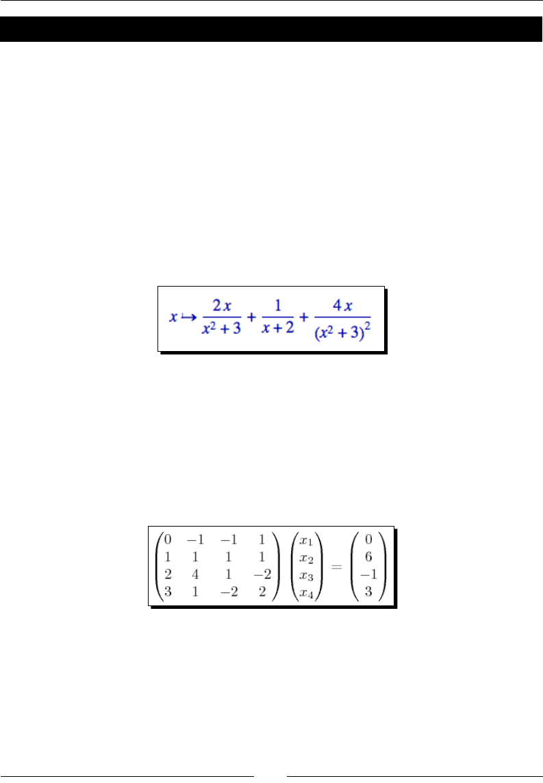
The paral fracon decomposion is another technique that Sage can do a lot faster than
you. The soluon to the following example covers two full pages in a calculus textbook —
assuming that you don't make any mistakes in the algebra!
f(x) = (3 * x^4 + 4 * x^3 + 16 * x^2 + 20 * x + 9) / ((x + 2) * (x^2 +
3)^2)
g(x) = f.partial_fraction(x)
show(g)
The result is as follows:
We'll use paral fracons again when we talk about solving ordinary dierenal equaons
symbolically.
Linear algebra
Linear algebra is one of the most fundamental tasks in numerical compung. Sage has many
facilies for performing linear algebra, both numerical and symbolic. One fundamental
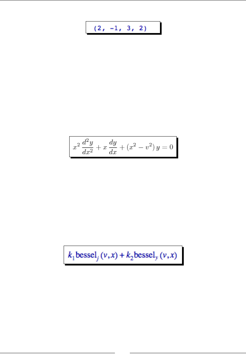
operaon is solving a system of linear equaons:
Although this is a tedious problem to solve by hand, it only requires a few lines of code in
Sage:
A = Matrix(QQ, [[0, -1, -1, 1], [1, 1, 1, 1], [2, 4, 1, -2],
[3, 1, -2, 2]])
B = vector([0, 6, -1, 3])
A.solve_right(B)
What Can You Do with Sage?
[ 18 ]
The answer is as follows:
Noce that Sage provided an exact answer with integer values. When we created matrix
A, the argument QQ specied that the matrix was to contain raonal values. Therefore,
the result contains only raonal values (which all happen to be integers for this problem).
Chapter 5 describes in detail how to do linear algebra with Sage.
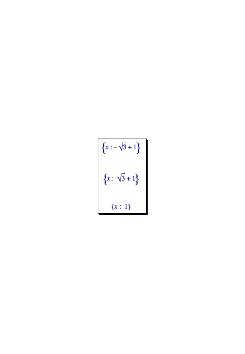
Solving an ordinary differential equation
Solving ordinary dierenal equaons by hand can be me consuming. Although many
dierenal equaons can be handled with standard techniques such as the Laplace
transform, other equaons require special methods of soluon. For example, let's try to
solve the following equaon:
The following code will solve the equaon:
var('x, y, v')
y=function('y', x)
assume(v, 'integer')
f = desolve(x^2 * diff(y,x,2) + x*diff(y,x) + (x^2 - v^2) * y == 0,
y, ivar=x)
show(f)
The answer is dened in terms of Bessel funcons:
It turns out that the equaon we solved is known as Bessel's equaon. This example
illustrates that Sage knows about special funcons, such as Bessel and Legendre funcons. It
also shows that you can use the assume funcon to tell Sage to make specic assumpons
when solving problems. In Chapter 7, we will explore Sage's powerful symbolic capabilies.
Chapter 1
[ 19 ]
More advanced graphics
Sage has sophiscated plong capabilies. By combining the power of the Python
programming language with Sage's graphics funcons, we can construct detailed
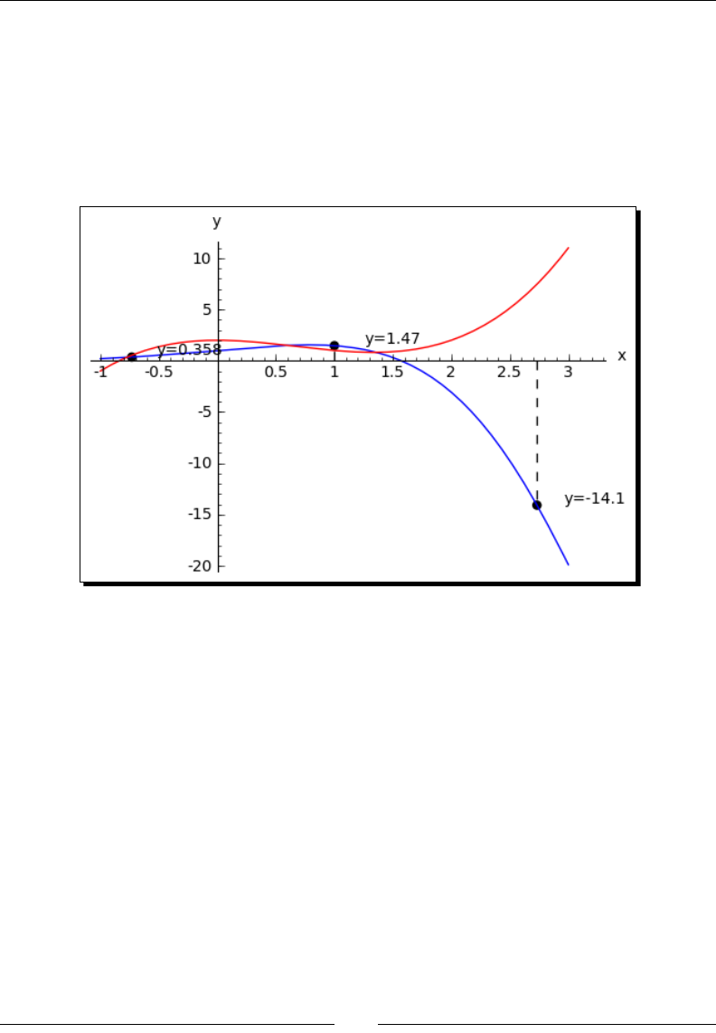
illustraons. To demonstrate a few of Sage's advanced plong features, we will solve a
simple system of equaons algebraically:
var('x')
f(x) = x^2
g(x) = x^3 - 2 * x^2 + 2
solutions=solve(f == g, x, solution_dict=True)
for s in solutions:
show(s)
The result is as follows:
We used the keyword argument solution_dict=True to tell the solve funcon to return
the soluons in the form of a Python list of Python diconaries. We then used a for loop
to iterate over the list and display the three soluon diconaries. We'll go into more detail
about lists and diconaries in Chapter 4. Let's illustrate our answers with a detailed plot:
p1 = plot(f, (x, -1, 3), color='blue', axes_labels=['x', 'y'])
p2 = plot(g, (x, -1, 3), color='red')
labels = []
lines = []
markers = []
for s in solutions:
x_value = s[x].n(digits=3)
y_value = f(x_value).n(digits=3)
labels.append(text('y=' + str(y_value), (x_value+0.5,
What Can You Do with Sage?
[ 20 ]
y_value+0.5), color='black'))
lines.append(line([(x_value, 0), (x_value, y_value)],
color='black', linestyle='--'))
markers.append(point((x_value,y_value), color='black', size=30))
show(p1+p2+sum(labels) + sum(lines) + sum(markers))
The plot looks like this:
We created a plot of each funcon in a dierent colour, and labelled the axes. We then used
another for loop to iterate through the list of soluons and annotate each one. Plong will
be covered in detail in Chapter 6.
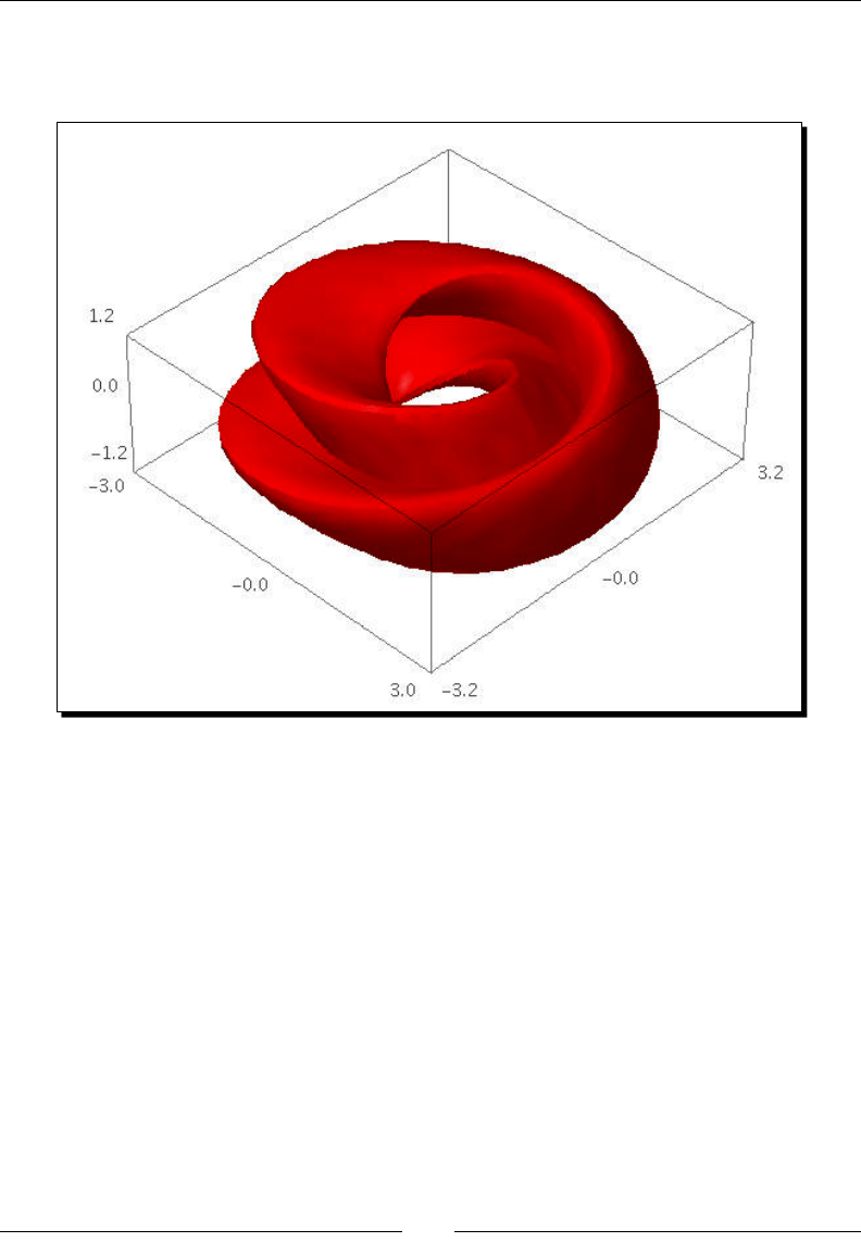
Visualising a three-dimensional surface
Sage does not restrict you to making plots in two dimensions. To demonstrate the 3D
capabilies of Sage, we will create a parametric plot of a mathemacal surface known as
the "gure 8" immersion of the Klein bole. You will need to have Java enabled in your web
browser to see the 3D plot.
var('u,v')
r = 2.0
f_x = (r + cos(u / 2) * sin(v) - sin(u / 2)
* sin(2 * v)) * cos(u)
f_y = (r + cos(u / 2) * sin(v) - sin(u / 2)
* sin(2 * v)) * sin(u)
Chapter 1
[ 21 ]
f_z = sin(u / 2) * sin(v) + cos(u / 2) * sin(2 * v)
parametric_plot3d([f_x, f_y, f_z], (u, 0, 2 * pi),
(v, 0, 2 * pi), color="red")
In the Sage notebook interface, the 3D plot is fully interacve. Clicking and dragging with
the mouse over the image changes the viewpoint. The scroll wheel zooms in and out, and
right-clicking on the image brings up a menu with further opons.
Typesetting mathematical expressions
Sage can be used in conjuncon with the LaTeX typeseng system to create publicaon-
quality typeset mathemacal expressions. In fact, all of the mathemacal expressions in this
chapter were typeset using Sage and exported as graphics. Chapter 10 explains how to use
LaTeX and Sage together.

What Can You Do with Sage?
[ 22 ]
A practical example: analysing experimental data
One of the most common tasks for an engineer or scienst is analysing data from an
experiment. Sage provides a set of tools for loading, exploring, and plong data. The
following series of examples shows how a scienst might analyse data from a populaon of
bacteria that are growing in a fermentaon tank. Someone has measured the opcal density
(abbreviated OD) of the liquid in the tank over me as the bacteria are mulplying. We want
to analyse the data to see how the size of the populaon of bacteria varies over me. Please
note that the examples in this secon must be run in order, since the later examples depend
upon results from the earlier ones.
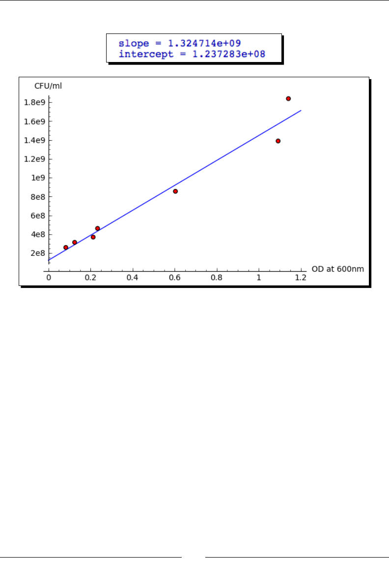
Time for action – tting the standard curve
The opcal density is correlated to the concentraon of bacteria in the liquid. To quanfy
this correlaon, someone has measured the opcal density of a number of calibraon
standards of known concentraon. In this example, we will t a "standard curve" to the
calibraon data that we can use to determine the concentraon of bacteria from opcal
density readings:
import numpy
var('OD, slope, intercept')
def standard_curve(OD, slope, intercept):
"""Apply a linear standard curve to optical density data"""
return OD * slope + intercept
# Enter data to define standard curve
CFU = numpy.array([2.60E+08, 3.14E+08, 3.70E+08, 4.62E+08,
8.56E+08, 1.39E+09, 1.84E+09])
optical_density = numpy.array([0.083, 0.125, 0.213, 0.234,
0.604, 1.092, 1.141])
OD_vs_CFU = zip(optical_density, CFU)
# Fit linear standard
std_params = find_fit(OD_vs_CFU, standard_curve,
parameters=[slope, intercept],
variables=[OD], initial_guess=[1e9, 3e8],
solution_dict = True)
for param, value in std_params.iteritems():
print(str(param) + ' = %e' % value)
# Plot
data_plot = scatter_plot(OD_vs_CFU, markersize=20,
facecolor='red', axes_labels=['OD at 600nm', 'CFU/ml'])
fit_plot = plot(standard_curve(OD, std_params[slope],
std_params[intercept]), (OD, 0, 1.2))
show(data_plot+fit_plot)
Chapter 1
[ 23 ]
The results are as follows:
What just happened?
We introduced some new concepts in this example. On the rst line, the statement import
numpy allows us to access funcons and classes from a module called NumPy. NumPy is
based upon a fast, ecient array class, which we will use to store our data. We created a
NumPy array and hard-coded the data values for OD, and created another array to store
values of concentraon (in pracce, we would read these values from a le) We then dened
a Python funcon called standard_curve, which we will use to convert opcal density
values to concentraons. We used the find_fit funcon to t the slope and intercept
parameters to the experimental data points. Finally, we ploed the data points with the
scatter_plot funcon and the ploed the ed line with the plot funcon. Note that we
had to use a funcon called zip to combine the two NumPy arrays into a single list of points
before we could plot them with scatter_plot. We'll learn all about Python funcons
in Chapter 4, and Chapter 8 will explain more about ng rounes and other numerical
methods in Sage.
What Can You Do with Sage?
[ 24 ]
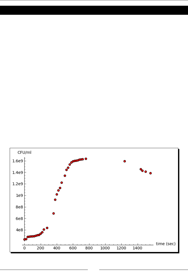
Time for action – plotting experimental data
Now that we've dened the relaonship between the opcal density and the concentraon
of bacteria, let's look at a series of data points taken over the span of an hour. We will
convert from opcal density to concentraon units, and plot the data.
sample_times = numpy.array([0, 20, 40, 60, 80, 100, 120,
140, 160, 180, 200, 220, 240, 280, 360, 380, 400, 420,
440, 460, 500, 520, 540, 560, 580, 600, 620, 640, 660,
680, 700, 720, 760, 1240, 1440, 1460, 1500, 1560])
OD_readings = numpy.array([0.083, 0.087, 0.116, 0.119, 0.122,
0.123, 0.125, 0.131, 0.138, 0.142, 0.158, 0.177, 0.213,
0.234, 0.424, 0.604, 0.674, 0.726, 0.758, 0.828, 0.919,
0.996, 1.024, 1.066, 1.092, 1.107, 1.113, 1.116, 1.12,
1.129, 1.132, 1.135, 1.141, 1.109, 1.004, 0.984, 0.972, 0.952])
concentrations = standard_curve(OD_readings, std_params[slope],
std_params[intercept])
exp_data = zip(sample_times, concentrations)
data_plot = scatter_plot(exp_data, markersize=20, facecolor='red',
axes_labels=['time (sec)', 'CFU/ml'])
show(data_plot)
The scaer plot looks like this:
Chapter 1
[ 25 ]
What just happened?
We dened one NumPy array of sample mes, and another NumPy array of opcal density
values. As in the previous example, these values could easily be read from a le. We used
the standard_curve funcon and the ed parameter values from the previous example
to convert the opcal density to concentraon. We then ploed the data points using the
scatter_plot funcon.
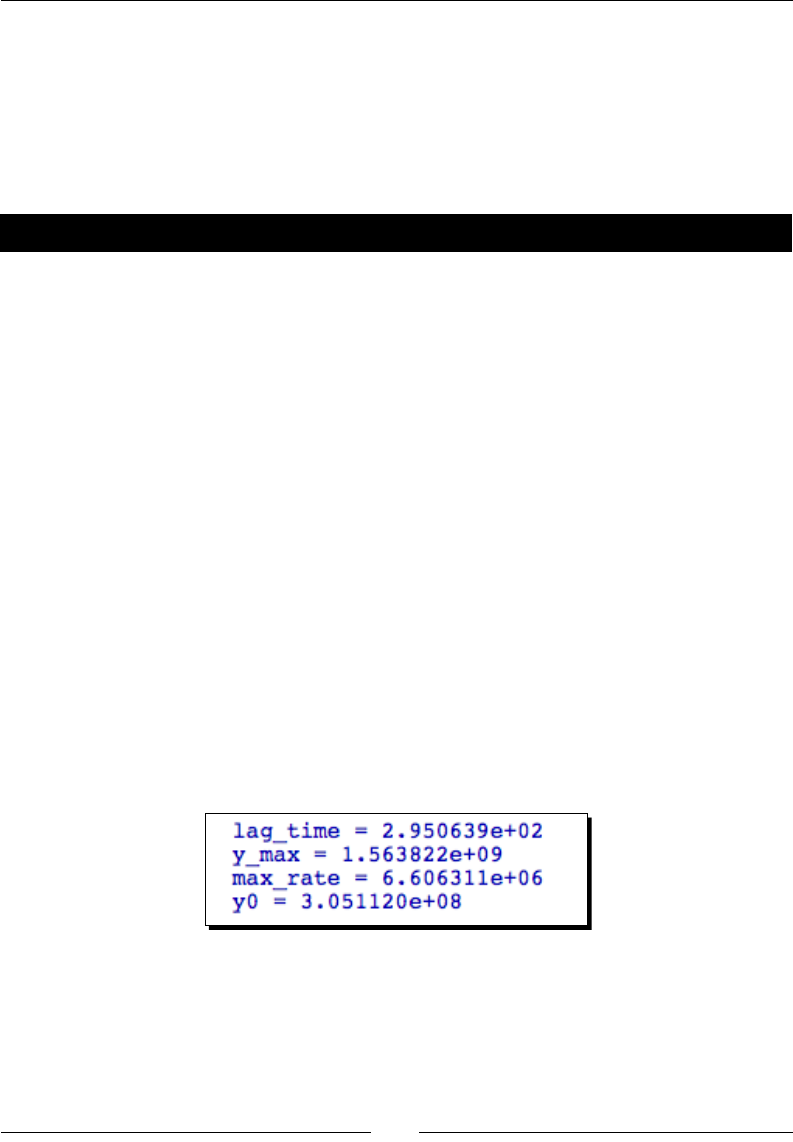
Time for action – tting a growth model
Now, let's t a growth model to this data. The model we will use is based on the Gompertz
funcon, and it has four parameters:
var('t, max_rate, lag_time, y_max, y0')
def gompertz(t, max_rate, lag_time, y_max, y0):
"""Define a growth model based upon the Gompertz growth curve"""
return y0 + (y_max - y0) * numpy.exp(-numpy.exp(1.0 +
max_rate * numpy.exp(1) * (lag_time - t) / (y_max - y0)))
# Estimated parameter values for initial guess
max_rate_est = (1.4e9 - 5e8)/200.0
lag_time_est = 100
y_max_est = 1.7e9
y0_est = 2e8
gompertz_params = find_fit(exp_data, gompertz,
parameters=[max_rate, lag_time, y_max, y0],
variables=[t],
initial_guess=[max_rate_est, lag_time_est, y_max_est, y0_est],
solution_dict = True)
for param,value in gompertz_params.iteritems():
print(str(param) + ' = %e' % value)
The ed parameter values are displayed:
Finally, let's plot the ed model and the experimental data points on the same axes:
gompertz_model_plot = plot(gompertz(t, gompertz_params[max_rate],
gompertz_params[lag_time], gompertz_params[y_max],
gompertz_params[y0]), (t, 0, sample_times.max()))
show(gompertz_model_plot + data_plot)
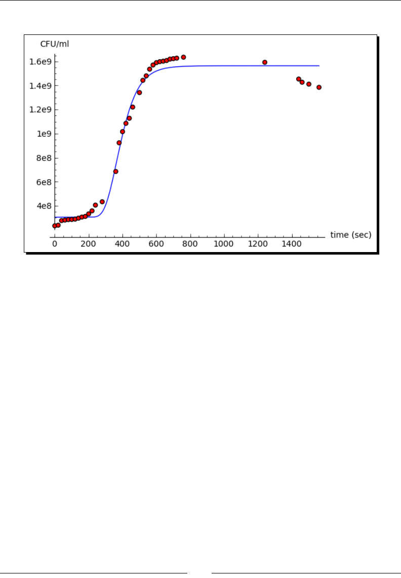
What Can You Do with Sage?
[ 26 ]
The plot looks like this:
What just happened?
We dened another Python funcon called gompertz to model the growth of bacteria
in the presence of limited resources. Based on the data plot from the previous example,
we esmated values for the parameters of the model to use an inial guess for the ng
roune. We used the find_fit funcon again to t the model to the experimental data,
and displayed the ed values. Finally, we ploed the ed model and the experimental
data on the same axes.
Summary
This chapter has given you a quick, high-level overview of some of the many things that Sage
can do for you. Don't worry if you feel a lile lost, or if you had trouble trying to modify the
examples. Everything you need to know will be covered in detail in later chapters.
Specically, we looked at:
Using Sage as a sophiscated scienc and graphing calculator
Speeding up tedious tasks in symbolic mathemacs
Solving a system of linear equaons, a system of algebraic equaons, and an
ordinary dierenal equaon

Chapter 1
[ 27 ]
Making publicaon-quality plots in two and three dimensions
Using Sage for data analysis and model ng in a praccal seng
Hopefully, you are convinced that Sage will be the right tool to assist you in your work, and
you are ready to install Sage on your computer. In the next chapter, you will learn how to
install Sage on various plaorms.
2
Installing Sage
Remember that you don't actually have to install Sage to start using it. You can start learning
Sage by ulizing one of the free public notebook servers that can be found at http://www.
sagenb.org/. However, if you nd that Sage suits your needs, you will want to install a
copy on your own computer. This will guarantee that Sage is always available to you, and
it will reduce the load on the public servers so that others can experiment with Sage. In
addion, your data will be more secure, and you can ulize more compung power to solve
larger problems. This chapter will take you through the process of installing Sage on various
plaorms.
In this chapter we shall:
Install a binary version of Sage on Windows and install a binary version of Sage on
OS X
Install a binary version of Sage on GNU/Linux
Compile Sage from source
Before you begin
At the moment, Sage is fully supported on certain versions of the following plaorms: some
Linux distribuons (Fedora, openSUSE, Red Hat, and Ubuntu), Mac OS X, OpenSolaris, and
Solaris. Sage is tested on all of these plaorms before each release, and binaries are always
available for these plaorms. The latest list of supported plaorms is available at http://
wiki.sagemath.org/SupportedPlatforms. The page also contains informaon about
plaorms that Sage will probably run on, and the status of eorts to port Sage to various
plaorms.

Installing Sage
[ 30 ]
When downloading Sage, the website aempts to detect which operang system you
are using, and directs you to the appropriate download page. If it sends you to the wrong
download page, use the "Download" menu at the top of the page to choose the correct
plaorm. If you get stuck at any point, the ocial Sage installaon guide is available at
http://www.sagemath.org/doc/installation/.
Installing a binary version of Sage on Windows
Installing Sage on Windows is slightly more involved than installing a typical Windows
program. Sage is a collecon of over 90 dierent tools. Many of these tools are developed
within a UNIX-like environment, and some have not been successfully ported to Windows.
Porng programs from UNIX-like environments to Windows requires the installaon of
Cygwin (http://www.cygwin.com/), which provides many of the tools that are standard
on a Linux system. Rather than aempng to port all of the necessary tools to Cygwin on
Windows, the developers of Sage have chosen to distribute Sage as a virtual machine that
can run on Windows with the use of the free VMWare Player. A port to Cygwin is in progress,
and more informaon can be found at http://trac.sagemath.org/sage_trac/wiki/
CygwinPort.
Downloading VMware Player
The VMWare Player can be found at http://www.vmware.com/products/player/.
Clicking the Download link will direct you to a registraon form. Fill out and submit the form.
You will receive a conrmaon email that contains a link that must be clicked to complete
the registraon process and take you to the download page. Choose Start Download
Manager, which downloads and runs a small applicaon that performs the actual download
and saves the le to a locaon of your choice.
Installing VMWare Player
Aer downloading VMWare Player, double-click the saved le to start the installaon
wizard. Follow the instrucons in the wizard to install the Player. You will have to reboot
the computer when instructed.
Downloading and extracting Sage
Download Sage by following the Download link from http://www.sagemath.org. The
site should automacally detect that you are using Windows, and direct you to the right
download page. Choose the closest mirror and download the compressed virtual machine.
Be aware that the le is nearly 1GB in size. Once the download is complete, right-click the
compressed le and choose Extract all from the pop-up menu.
Chapter 2
[ 31 ]
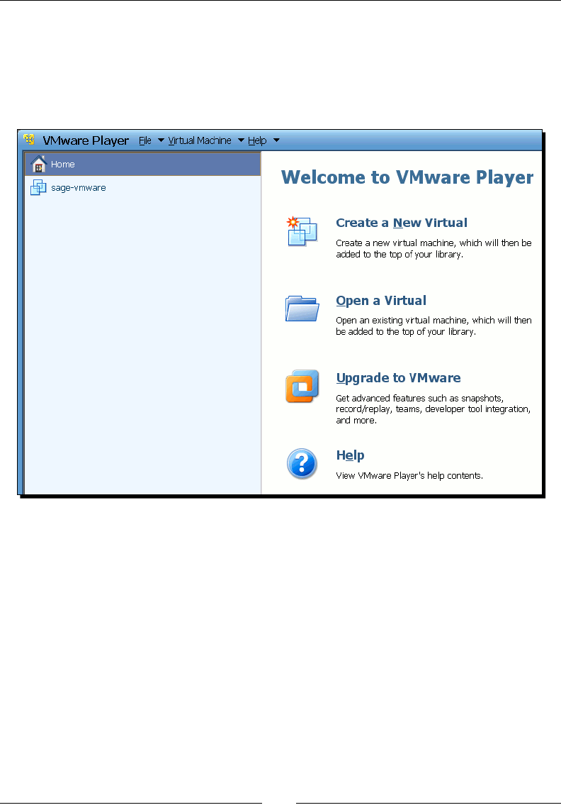
Launching the virtual machine
Launch VMware Player and accept the license terms. When the Player has started, click Open a
Virtual Machine and select the Sage virtual machine, which is called sage-vmware.vmx. Click
Play virtual machine to run Sage. If you have run Sage before, it should appear in the list of
virtual machines on the le side of the dialog box, and you can double-click to run it.
When the virtual machine launches, you may receive one or more warnings about various
devices (such as Bluetooth adapters) that the virtual machine cannot connect to. Don't
worry about this, since Sage doesn't need these devices.
Installing Sage
[ 32 ]
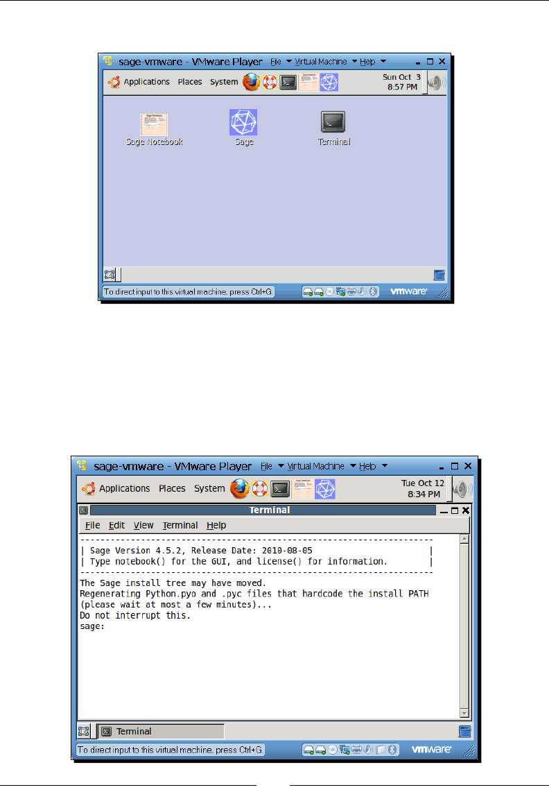
Start Sage
Once the virtual machine is running, you will see three icons. Double-clicking the Sage
Notebook icon starts the Sage notebook interface, while the Sage icon starts the command-
line interface. The rst me you run Sage, you will have to wait while it regenerates les.
When it nishes, you are ready to go.
You may get the warning "External network not set up" when launching the notebook
interface. This does not cause any problems.
Chapter 2
[ 33 ]
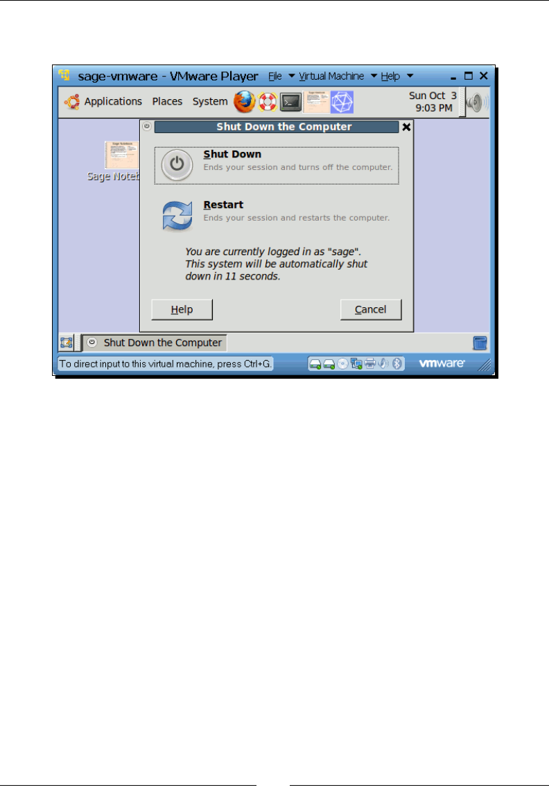
When you are done using Sage, choose Shut Down… from the System menu at the top of the
window, and a dialog will appear. Click the Shut Down buon to close the virtual machine.
Installing a binary version of Sage on OS X
On Mac OS X, you have the opon of installing a pre-built binary applicaon, or downloading
the source code and compiling Sage yourself. One advantage of the pre-built binary is
that it is very easy to install, because it contains everything you need to run Sage. Another
advantage of the binary is that building Sage from source requires a lot of computaonal
resources, and may take a long me on older machines. However, there are a number of
disadvantages to prebuilt binaries. The binary download is quite large, and the installed les
take up a lot of disk space. Many of the tools in the binary may be duplicates of tools you
already have on your system. Pre-built binaries cannot be tuned to take advantage of the
hardware features of a parcular plaorm, so building Sage from source is preferred if you
are looking for the best performance on CPU-intensive tasks. You will have to choose which
method is right for you.
Installing Sage
[ 34 ]
Downloading Sage
Download Sage by following the Download link from http://www.sagemath.org. The site
should automacally detect that you are using OS X, and direct you to the right download
page. Choose a mirror site close to you. Select your architecture (Intel for new Macs, or
PowerPC for older G4 and G5 macs). Then, click the link for the correct .dmg le for you
version of Mac OS X. If you aren't sure, click the Apple menu on the far le side of the menu
bar and choose About This Mac.
Installing Sage
Once the download is complete, double-click the .dmg le to mount the disk image. Drag
the Sage folder from the disk image to the desired locaon on your hard drive (such as the
Apps folder).
If the copy procedure fails, you will need to do it from the command line. Open the Terminal
applicaon and enter the following commands. Be sure to change the name sage-4.5-
OSX-64bit-10.6-i386-Darwin.dmg to the name of the le you just downloaded:
$ cd /Applications
$ cp -R -P /Volumes/sage-4.5-OSX-64bit-10.6-i386-Darwin.dmg /sage .
Aer the copy process is complete, right-click on the icon for the disk image, and choose
Eject.
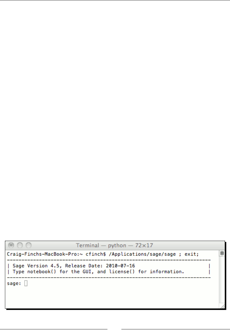
Starting Sage
Use the Finder to visit the Sage folder that you just created. Double-click on the icon called
Sage. It should open with the Terminal applicaon. If it doesn't start, right-click on the icon,
go to the Open With submenu and choose Terminal.app. The Sage command line will
now be running in a Terminal window. The rst me you run Sage, you will have to wait
while it regenerates les. When it nishes, you are ready to go.

Chapter 2
[ 35 ]
There are three ways to exit Sage: type exit or quit at the Sage command prompt, or press
Ctrl-D in the Terminal window. You can then quit the Terminal applicaon.
Installing a binary version of Sage on GNU/Linux
As with Mac OS X, you have the opon of installing a pre-built binary applicaon for your
version of Linux, or downloading the source code and compiling Sage yourself. The same
trade-os apply to Linux. Keep in mind that the Sage team only distributes pre-build binaries
for a few popular distribuons. If you are using a dierent distribuon, you'll have to compile
Sage from source anyway. The following instrucons will assume you are downloading a
binary applicaon. I will use Ubuntu as an example, but other versions of Linux should be
very similar.
Most modern Linux distribuons use a package manager to install and remove
soware. Sage is not available as an ocially supported package for any Linux
distribuon at this me. "Unocial" packages have been created for Debian,
Mandriva, Ubuntu, and possibly others, but they are unlikely to be up to date
and may not work properly. An eort to integrate Sage with Gentoo Linux can be
found at https://github.com/cschwan/sage-on-gentoo.
Downloading and decompressing Sage
Download the appropriate pre-built binary from http://www.sagemath.org/download-
linux.html. Choose the closest mirror, and then choose the appropriate architecture for
your operang system. If you're not sure whether your operang system is built for 32 or 64
bit operaon, open a terminal and type the following on the command line:
$ uname –m
If the output contains 64, then your system is probably a 64-bit system. If not, it's a 32-bit.
An alternave way to check is with the following command:
$ file /usr/bin/bin
If the le type contains 64, your kernel probably supports 64 bit applicaons. If not, you
need the 32 bit version. Select the appropriate prebuilt binary and save it to your computer.
Installing Sage
[ 36 ]
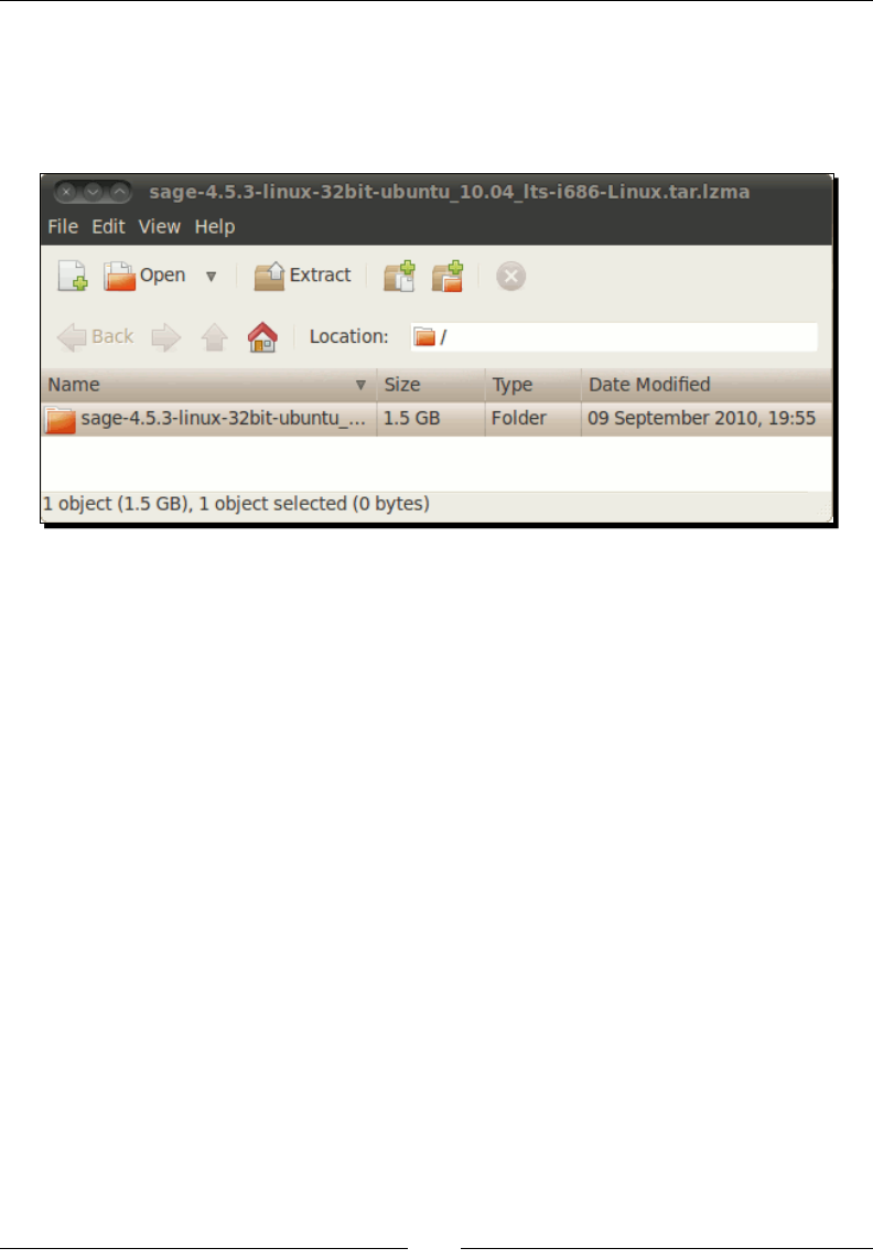
Once the download is done, uncompress the archive. You can use the graphical archiving tool
for your version of Linux (the Ubuntu archiver is shown in the following screenshot). If you
prefer the command line, type the following:
tar --lzma -xvf sage-*...tar.lzma
Running Sage from your user account
Aer decompression, you will have a single directory. This directory is self-contained, so
no further installaon is necessary. You can simply move it to a convenient locaon within
your home directory. This is a good opon if you don't have administrator privileges on the
system, or if you are the only person who uses the system. To run Sage, open a terminal and
change to the Sage directory (you will have to modify the command below, depending on the
version you installed and where you installed it):
cfinch@ubuntu:$ cd sage-4.5.3-linux-32bit-ubuntu_10.04_lts-i686-Linux
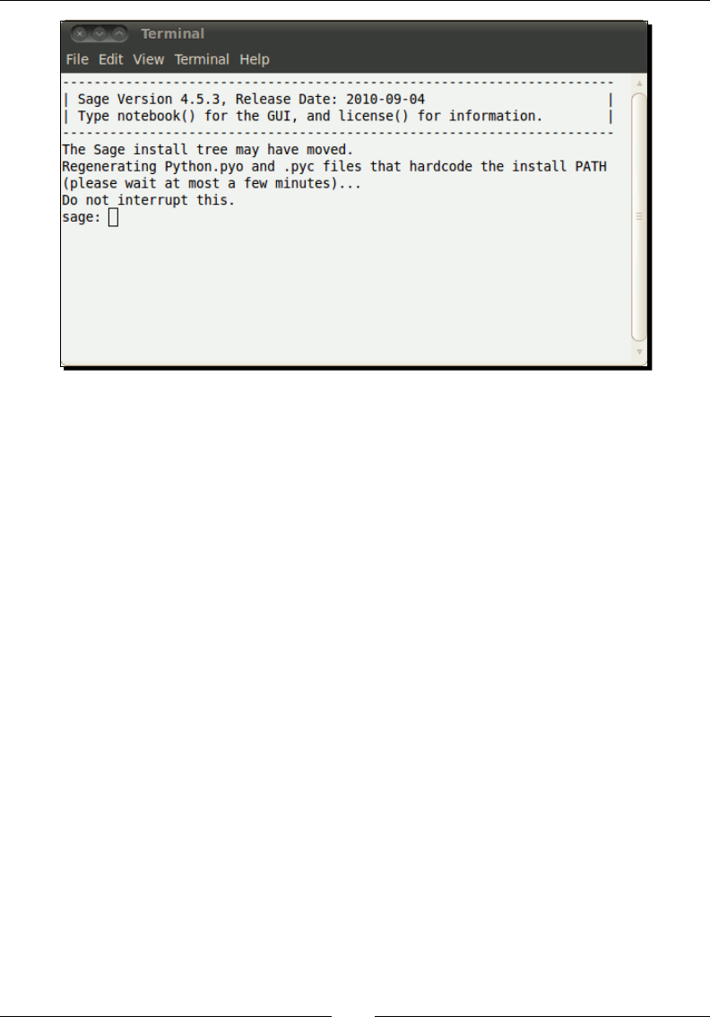
Run Sage by typing the following:
cfinch@ubuntu:$ ./sage
Don't forget the period before the slash! The rst me you run Sage, you will have to wait
while it regenerates les, as shown in the following screenshot. When it nishes, you are
ready to go.
Chapter 2
[ 37 ]
There are three ways to exit Sage: type exit or quit at the Sage command prompt, or press
Ctrl-D in the terminal window.
Installing for multiple users
If you are the administrator of a shared system, you may want to install Sage so that
everyone can use it. Since Sage consists of one self-contained directory, I suggest moving it
to the /opt directory:
sudo mv sage-4.5.3-linux-32bit-ubuntu_10.04_lts-i686-Linux /opt
[sudo] password for cfinch:
To make it easy for everyone to run Sage, make a symbolic link from /usr/bin to the actual
locaon:
cfinch@ubuntu:/usr/bin$ sudo ln -s /opt/sage-4.5.3-linux-32bit-
ubuntu_10.04_lts-i686-Linux/sage sage
[sudo] password for cfinch:
As before, Sage will have to regenerate its internal les the rst me it runs aer moving.
You should run Sage once as a user with administrave privileges, because other users won't
have the necessary write permissions to save the les. Once this is completed, any user will
be able to use Sage by typing Sage at the command prompt.

Installing Sage
[ 38 ]
Building Sage from source
This secon will describe how to build Sage from source code on OS X or Linux. Although
Sage consists of nearly 100 packages, the build process hides much of the complexity. It
is impossible to provide instrucons for all of the plaorms that can build Sage, but the
following guidelines should cover most cases. The ocial documentaon for building Sage
from source is available at http://sagemath.org/doc/installation/source.html.
Prerequisites
In order to compile Sage, you will need about 2.5GB of free disk space, and the following
tools must be installed:
GCC
g++
gfortran
make
m4
perl
ranlib
tar
readline and its development headers
ssh-keygen (only needed to run the notebook in secure mode)
latex (highly recommended, though not strictly required)
If you are running OS X (version 10.4 or later), install XCode to get all of these tools. XCode
is available for free when you sign up as a developer at http://developer.apple.com/.
Make sure that you have XCode version 2.4 or later.
If you are running Linux, use your package manager to install any missing tools. For example,
on a Debian-based system like Ubuntu, run the following on the command line:
$ sudo apt-get install build-essential m4 gfortran
$ sudo apt-get install readline-common libreadline-dev
To install LaTeX (oponal):
$ sudo apt-get install texlive xpdf evince xdvi

Chapter 2
[ 39 ]
Downloading and decompressing source tarball
Download the latest source tarball from http://sagemath.org/download-source.
html. Open a terminal, change to the directory where you saved the tarball, and
decompress it with the following command:
$ tar -xvf sage-*.tar
Building Sage
If you have a mul-core or mul-processor machine, you can speed up the build process
by performing a parallel compilaon. You can control this by seng the MAKE environment
variable. For example, using Bash syntax, you can set the MAKE variable to use four cores:
$ export MAKE="make -j4"
Change to the Sage directory:
$ cd sage-*
Build Sage:
$ make
Sage may take a long me (1 hour to several days) to compile, depending on the speed of
the machine.
Installation
When the compilaon process is done, you should be able to run Sage from the build
directory. If you want to move the Sage installaon or make it available to other users on a
shared Linux system, follow the direcons in the previous secons.
Summary
At this point, you should have a funconing Sage installaon on your machine. In the next
chapter, you'll learn the basics of using Sage.
3
Getting Started with Sage
In this chapter, you will learn the basic ideas that will be the foundaon for using all the
features of Sage. We will start by learning how to use the command line and notebook
interfaces eciently. Then, we'll look at basic concepts like variables, operators, funcons,
and objects. By the end of the chapter, you should be able to use Sage like a sophiscated
scienc graphing calculator.
Using the interacve shell
Using the notebook interface
Learning more about operators and variables
Dening and using callable symbolic expressions
Calling funcons and making simple plots
Dening your own funcons
Working with objects in Sage
How to get help with Sage
The Sage documentaon is accessible from the interacve shell and the notebook interface.
Further help is available on the Web. The main Sage documentaon page at http://www.
sagemath.org/help.html provides links to dozens of resources. A few of these links are
especially useful:
The ocial Sage tutorial can be found at http://www.sagemath.org/doc/
tutorial/, and it is also accessible from the Help link in the notebook interface.
The Python language tutorial at http://docs.python.org/tutorial/ will also
be helpful.
The reference manual at http://www.sagemath.org/doc/reference/
provides the full API documentaon, along with many examples.

Geng Started with Sage
[ 42 ]
Themac tutorials at http://www.sagemath.org/doc/thematic_tutorials/
index.html focus on specic topics.
The "Construcons" document at http://www.sagemath.org/doc/
constructions/index.html describes how to do specic things with Sage.
Interacve resources, including mailing lists, an IRC channel, and a discussion forum are
available if you get stuck. A complete list of these resources can be found at http://www.
sagemath.org/development.html. The mailing lists sage-support and sage-devel are
intended for general quesons. Other lists are available to discuss more specic topics.
Starting Sage from the command line
In the previous chapter, we learned how to start Sage. If you want to pass opons to Sage
when it starts, you can do so with command line arguments.
1. On OS X or a UNIX-like plaorm, start by opening a terminal window. On Windows,
start the virtual machine and double-click the Terminal icon.
2. If you have added the Sage applicaon directory to the PATH environment variable,
you can just type sage at the command prompt. If not, you will need to enter the full
path to the Sage binary.
3. Add command line arguments, separated by spaces, and press Enter. For example,
type the following at the command prompt to start Sage and automacally launch
the notebook interface:
$ /Applications/sage/sage -notebook
There are many command line arguments, but you probably won't need them right away.
Three of the most useful arguments are as follows:
Argument Descripon
-help Describe the most widely used command line arguments
-advanced Describe more advanced command line arguments
-notebook Start Sage and launch the notebook interface
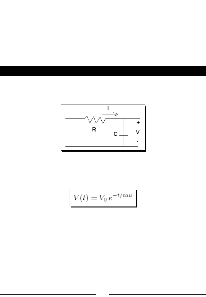
Chapter 3
[ 43 ]
Using the interactive shell
The interacve shell provides a command-line interface to Sage. When you are done using
Sage, remember to type quit or exit at the Sage prompt, or press Ctrl-D, to exit the
interacve shell. In the following examples, lines which start with the Sage command prompt
sage: indicate commands that you need to type in. Lines without the prompt indicate output
from Sage. Although most of the examples in this book ulize the notebook interface, they
will work in the interacve shell, unless noted otherwise.
Time for action – doing calculations on the command line
Let's say that you need to make some quick calculaons to design a simple electrical circuit.
We will use the example of a series RC circuit, which consists of a resistor and a capacitor
connected in series:
The voltage across the capacitor can be described by a linear, rst-order dierenal
equaon. Eventually we will learn to solve dierenal equaons with Sage, but for now we
will just use the soluon, which is well known:
1. Dene variables.
First, we'll dene some variables to work with. Type in the following text at the
command prompt, and press Enter aer every line:
sage: R = 250e3
sage: C = 4e-6
sage: tau = R * C
sage: tau
1.00000000000000

Geng Started with Sage
[ 44 ]
Sage doesn't give any output from variable denions. You can type the variable
name and press Enter to see what it contains.
2. Perform a calculaon.
The voltage across the capacitor is a funcon of me. Let's set an inial voltage v0
and compute the voltage aer one second:
sage: v0 = 100.0
sage: t = tau
sage: v0 * exp(-t / tau)
36.7879441171442
Here, we ulized the built-in funcon exp(x), which computes the value of e to the
power x. Aer a period of me equal to the me constant has elapsed, the voltage
is about 36% of its original value.
3. Change some values.
How does the voltage decay as me advances?
sage: t = 4 * tau
sage: v0 * exp(-t / tau)
1.83156388887342
Aer a length of me equal to four me constants, the voltage is less than two per cent of
its original value. Now, let's see how the value of tau impacts the voltage at a xed me.
Pressing the Up arrow allows you to scroll through the commands that you recently entered,
in reverse order. To scroll the other way, press the Down arrow. Use the Up and Down arrows
to get v = v0 * exp(-t / tau) on the command line, and edit it to match the following.
Press Enter to see the result.
sage: t = tau
sage: v0 * exp(-t / (2 * tau))
60.6530659712633
Now, let's see what happens if tau gets smaller. Press the Up arrow to edit the previous
command:
sage: v0 * exp(-t / (tau / 4))
1.83156388887342

Chapter 3
[ 45 ]
The me constant controls how quickly the voltage decays. If you are going to work on
something else, but might want to come back to this calculaon, you can save your session
with this command:
sage: save_session('RC_circuit')
This will save your variables in a le called RC_circuit.sobj in the top level of your home
directory. You can enter an absolute or relave path to save the le in other locaons. You
can load these variables at any me in the future using the following command:
sage: load_session('RC_circuit')
sage: who
C t tau v v0
The who command lists the variables that you have already dened. This is very handy if you
have a lot of variables and don't remember one of the names.
What just happened?
This example demonstrated some basic principles of command-line interacon with Sage. To
perform a calculaon, type an expression on the command line, and press Enter to see the
result. If the result of a calculaon is stored in a variable, it won't be shown. Typing the name
of a variable and pressing Enter shows its value. You can use the Up and Down arrow keys to
scroll through previous commands, edit a command, and run it again.
Getting help
There are three ways to get help from the Sage command line. To see the documentaon for
a command or funcon, type a ? on the command line aer the command. For example, to
learn about the exp funcon type following:
sage: exp?
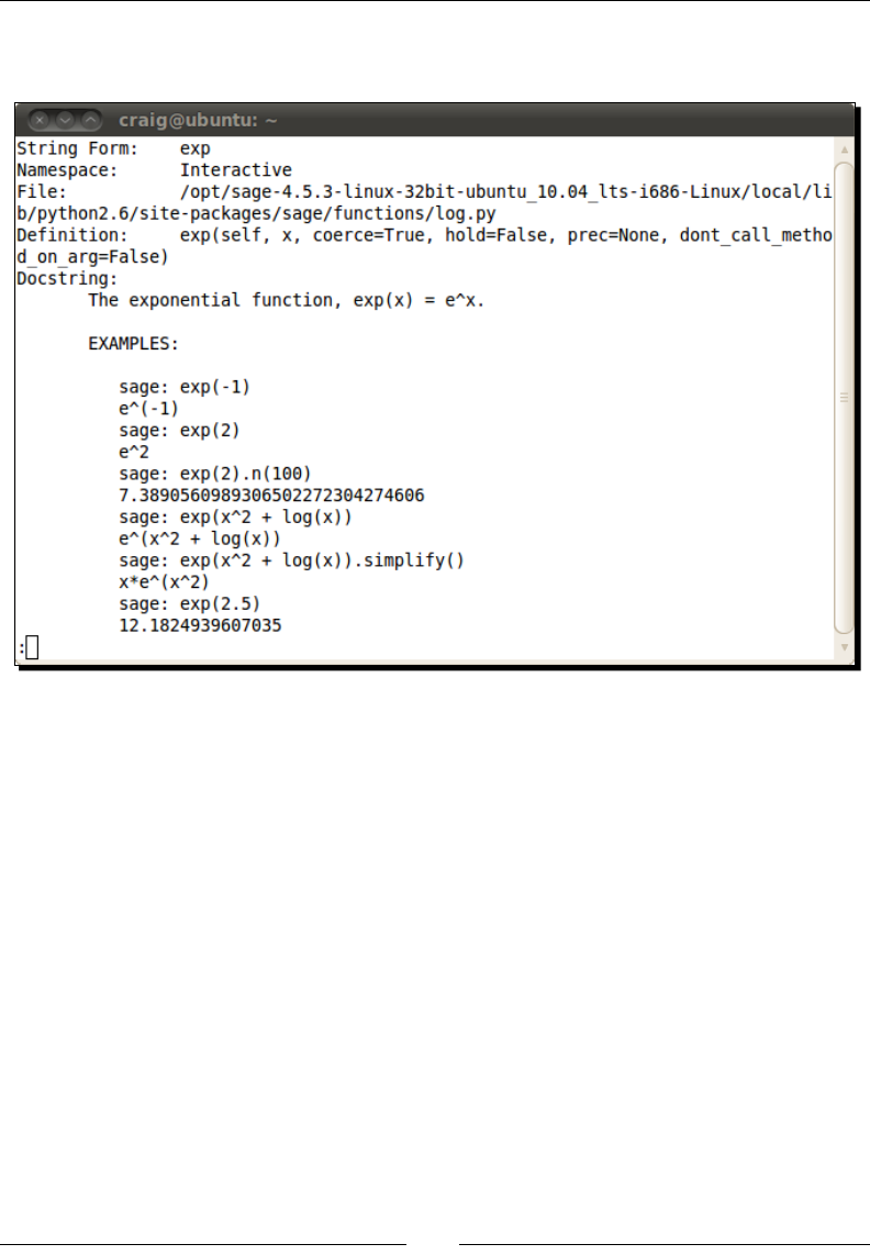
Geng Started with Sage
[ 46 ]
When you use any of the help commands, the normal contents of the terminal will be
replaced by a help screen, which looks like this:
Use the arrows to scroll up and down. Use the Spacebar to page down, and the b key to
page up. Press q to leave the help screen and return to the command line. If you want to see
the documentaon and the source code for the funcon (if the code is available), type two
queson marks aer the funcon name:
sage: exp??
Finally, to see the complete class documentaon, use the help funcon:
sage: help(exp)
Command history
The Sage command line has a number of built-in shortcuts that help you work more
eciently. Most of these will be familiar to people who have worked with UNIX-like
command line interfaces. We have already seen that you can use the Up arrow on your
keyboard to scroll through commands that you have previously entered. To see a list of
everything you have typed in this session, type %hist at the command prompt.

Chapter 3
[ 47 ]
We can use the %macro command, in conjuncon with the %hist command, to dene
macros. Let's say we frequently need to dene some physical constants, so we want to save
those commands as a macro. First, enter the following commands and then display them
with the %hist command:
sage: epsilon_zero = 8.85418782e-12
sage: mu_zero = 1.25663706e-6
sage: NA = 6.0221415e23
sage: %hist
1: epsilon_zero = RealNumber('8.85418782e-12')
2: NA = RealNumber('6.0221415e23')
3: mu_zero = RealNumber('1.25663706e-6')
4: _ip.magic("hist ")
Note that the results of the %hist command will be dierent on your screen, because
the command history for your session is not the same as the history for the session used
to create this example. Look at the output from %hist and note the number to the le of
each command. Now, use the %macro command to dene a macro called constants using
commands 1-3. You will have to replace the numbers 1 and 3 with the appropriate numbers
from your command line history.
sage: %macro constants 1-3
Macro `constants` created. To execute, type its name (without quotes).
Macro contents:
epsilon_zero = RealNumber('8.85418782e-12')
NA = RealNumber('6.0221415e23')
mu_zero = RealNumber('1.25663706e-6')
We can now use the command constants to quickly dene some variables that contain
physical constants. For more informaon about the %macro command, type the following:
sage: %macro?
Tab completion
Tab compleon can also make your life easier. Type the rst leer (or rst few leers) of a
command at the prompt, and press Tab to see a list of possible compleons. For example,
type pl and press Tab:
sage: pl
plot plot_step_function plotkin_bound_asymp
plot3d plot_vector_field plotkin_upper_bound
plot_slope_field plot_vector_field3d
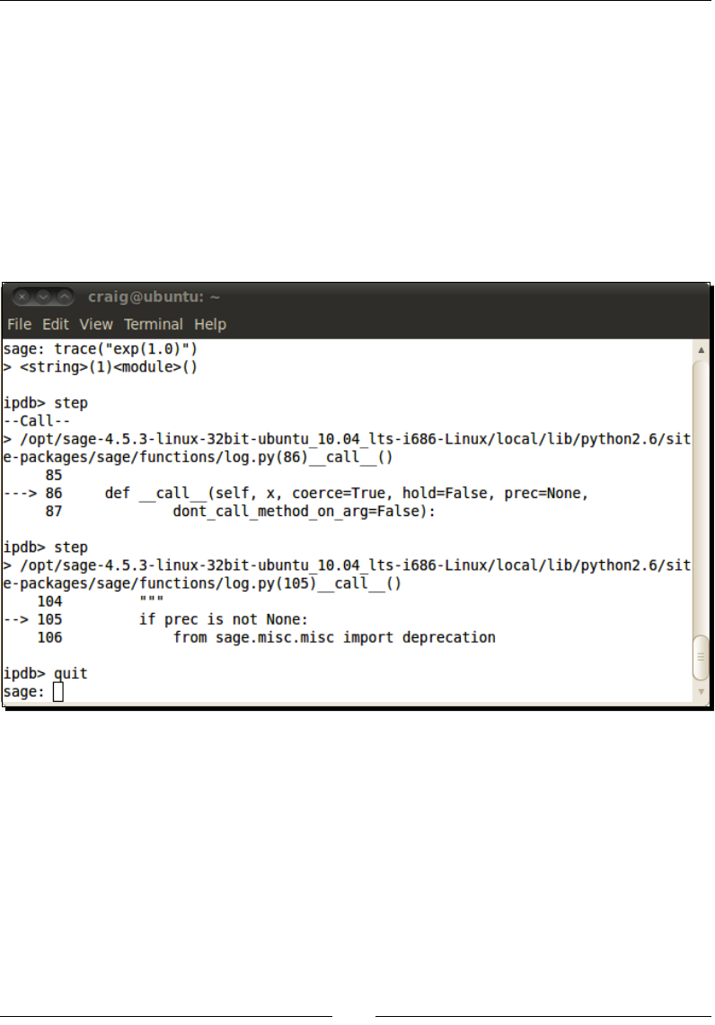
Geng Started with Sage
[ 48 ]
Interactively tracing execution
Only the interacve shell allows you to trace the execuon of a command interacvely. Use
the trace funcon, which accepts a string that contains a Sage command. For example, to
trace the execuon of the following exp funcon:
sage: trace("exp(1.0)")
This command starts the Python debugger, which gives you the ipdb> prompt. To step
through execuon of the funcon, type step (or just s) at the prompt and press Enter. Type
? to get help on other commands you can use in the debugger. Type quit (or just q) to quit
the debugger and return to the Sage command line. A typical session looks like this:
Using the notebook interface
The notebook interface is a more exible way to work with Sage. Your calculaons and the
resulng numbers and plots can be saved together in a worksheet. You can add headings and
text to document what you've done. In Chapter 10, we'll learn how to use LaTeX to typeset
mathemacal expressions right in a worksheet.
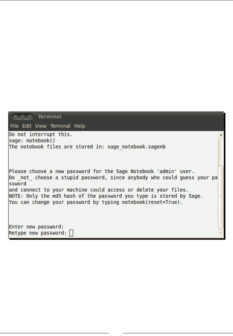
Chapter 3
[ 49 ]
Starting the notebook interface
There are several ways to start the notebook interface. If you are running Sage in a virtual
machine on Windows, double-click on the icon labelled Sage Notebook. If you are starng
Sage from the command line, you can use the –notebook opon to start Sage and launch
the notebook interface. If you already have the Sage interacve shell running, use the
notebook() funcon to start the notebook interface:
sage: notebook()
If a web browser doesn't open automacally, manually start the web browser and go to
http://localhost:8000.
If this is your rst me running the notebook interface, follow the prompts in the terminal
to enter a password for the administrave account.
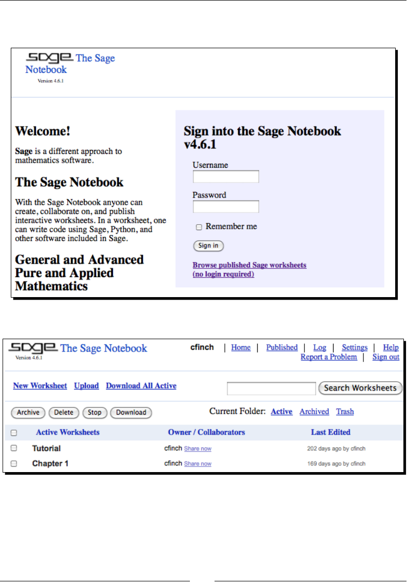
Geng Started with Sage
[ 50 ]
When you have entered a password, you will see a screen that allows you to log in. Log in
using the name and password you just created.
Once you have logged in, you will see the home page for the notebook interface:
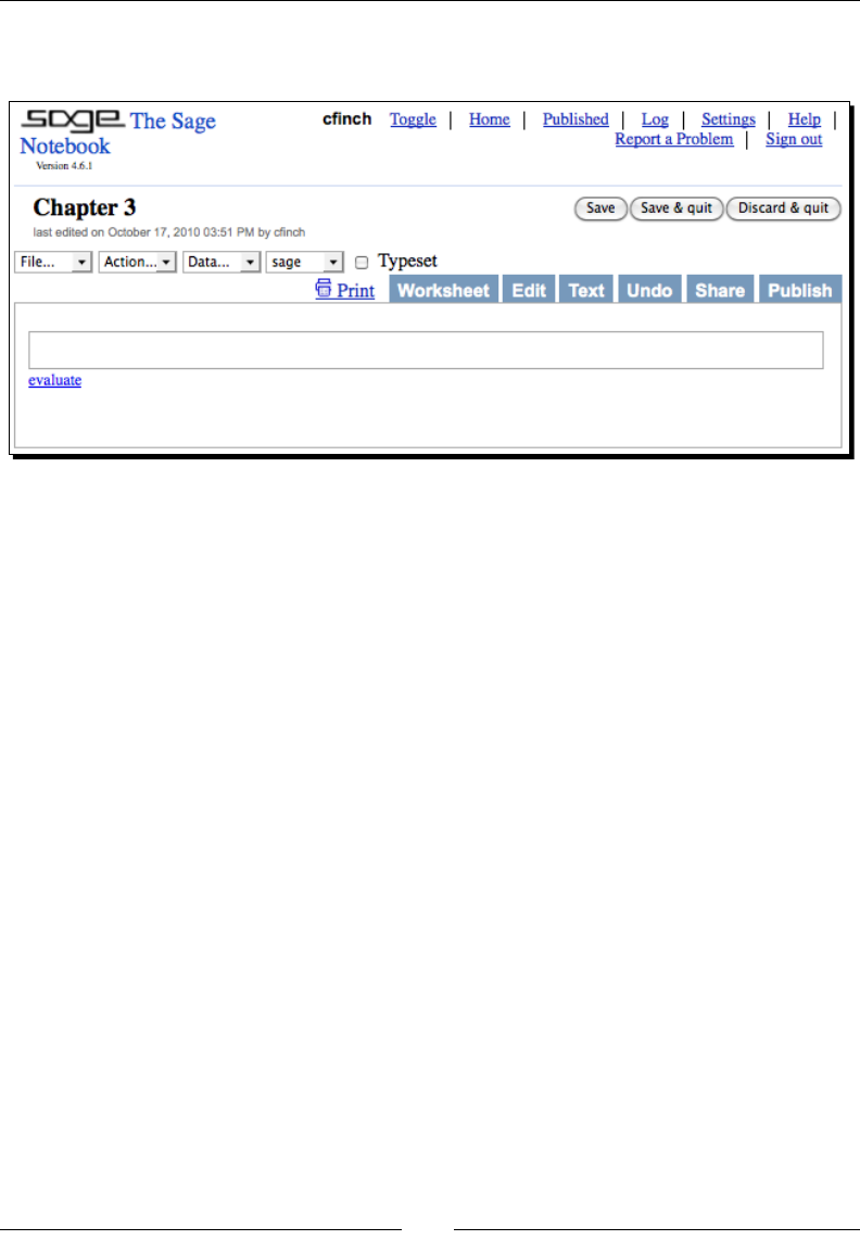
Chapter 3
[ 51 ]
You can create a new worksheet by clicking the New Worksheet link. When prompted, enter
a name in the dialog box. The blank worksheet should look like this:
You can access many powerful features of the notebook interface from this page:
The File menu allows you to perform operaons such as saving, renaming, and
deleng worksheets
The Acon menu allows you to control the evaluaon of cells, such as interrupng
a calculaon that is taking too long
The Data menu allows you to aach a data le to a worksheet
The sage menu allows you to choose which tool evaluates the code in a cell
The six tabs towards the right side of the screen allow you to perform other operaons:
The Worksheet tab shows the default view of the worksheet
The Edit tab allows you to edit a text representaon of the worksheet
The Text tab shows you a read-only text representaon of the worksheet
The Undo tab shows a revision history of the worksheet, and allows you to go back
to a previous version
The Share tab allows you to give other Sage users the ability to edit your worksheets
The Publish tab allows you to make your worksheet available on the Web, where it
can be viewed by anyone who can access the web server on your computer
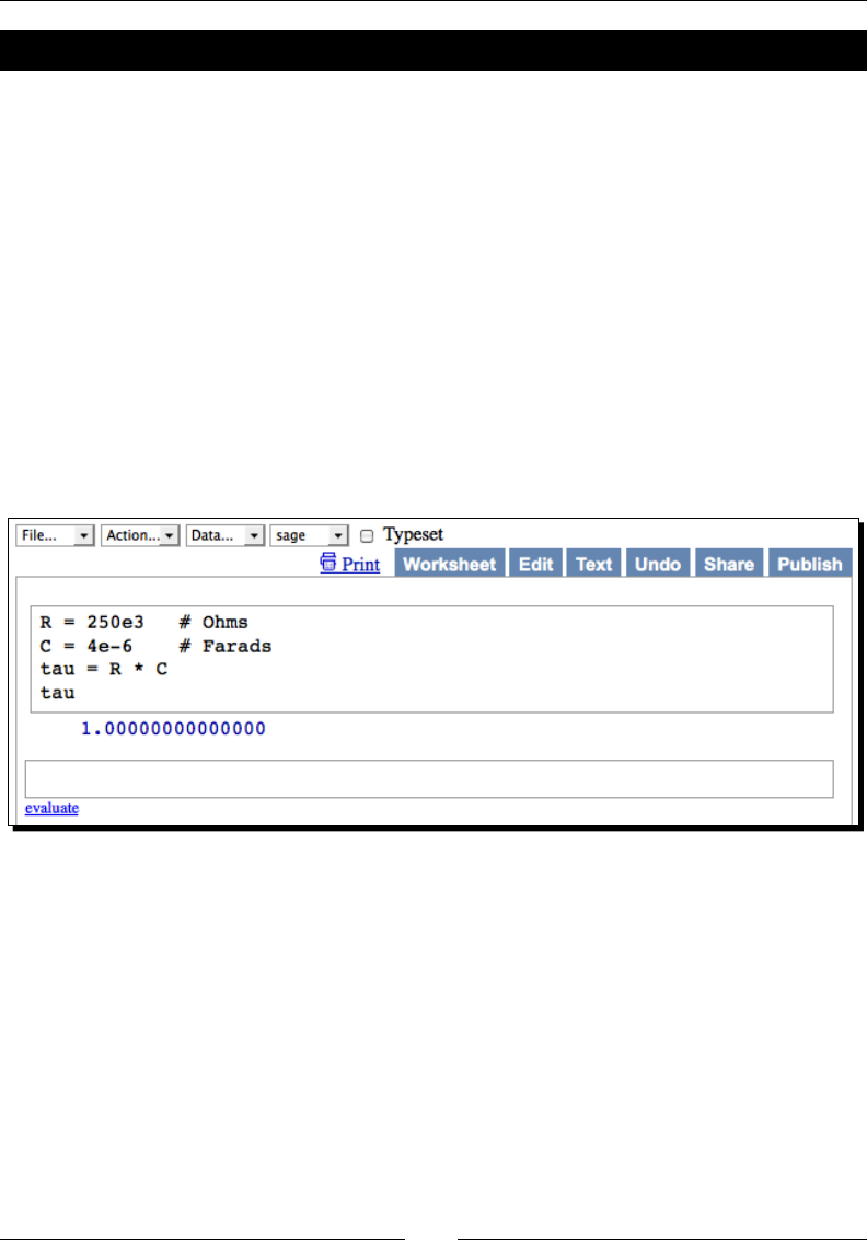
Geng Started with Sage
[ 52 ]
Time for action – doing calculations with the notebook interface
Now, we will use the Notebook interface to repeat the calculaons that we did with the
interacve shell. We will add some text to document what we've done.
1. Dene variables.
The empty white box in the middle of the worksheet is an input cell. Click in the
input cell and type in the following text:
R = 250e3 # ohms
C = 4e-6 # Farads
tau = R * C
tau
To evaluate the cell, press Shi-Enter or click the evaluate link, which is found just
below the boom-le corner of the input cell. As soon as the code executes, an
empty input cell appears on the screen below the previous cell. The screen will look
like this:
2. Perform a calculaon.
You can also insert an empty input cell by moving the cursor into the blank space
above or below an exisng cell. When a thin, solid bar appears in the blank space,
click to insert a new input cell. Enter the following code in the next input cell:
v0 = 20.0 # Volts
t = 1.0 # seconds
v0 * exp(-t / tau)
Click the evaluate link or press Shi-Enter to execute the code. The result will appear
below the input box.
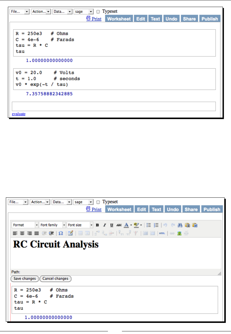
Chapter 3
[ 53 ]
3. Add documentaon.
Let's add a text eld to document what we've done. Move the mouse cursor to the
empty space just above the rst input box. As your mouse enters this area, a thin,
solid bar will appear. Hold down the Shi key and click on this rectangle to insert
a new text cell. The text cell will include a graphical editor that allows you to enter
text and apply HTML formang. Choose Heading 1 from the menu at the upper
le corner of the editor, and type RC Circuit Analysis into the box. Click the Save
Changes buon to exit the editor.

Geng Started with Sage
[ 54 ]
4. Save your work.
Click the Save buon at the top-right corner of the worksheet. If you are done with
this notebook, click Save & quit.
What just happened?
We repeated the calculaon that we performed earlier. This me, we were able to create
a single document that contains calculaons, results, and documentaon. We made use of
comments in the input cells to note the units for each value (you can also use comments on
the command line). A # sign indicates the beginning of a comment. Sage ignores anything
on the line aer the #. Get in the habit of using comments to remind yourself how the
code works. As in the interacve shell, no output is displayed when a value is assigned to a
variable. Only the last line of an input cell will produce output on the screen. We'll see how
to produce more output in the next secon.
Getting help in the notebook interface
To get help with the notebook interface, click the Help link in the upper-right corner of the
notebook window. To get help on a command or funcon, type the command name in an
empty input cell, followed by a ?. Press Tab, or evaluate the cell, to see the documentaon.
You can also type the command name followed by ?? to see the source code. Another
opon is to type help(command), which will result in a link that you can click to open
the documentaon in a new tab or window. To search the documentaon, type search_
doc("my query") in an empty input cell and evaluate the cell. You can also search the
source code by using search_src("my query").
Working with cells
The example showed some of the basic commands that can be used to edit worksheets.
The following shortcuts are useful for working with cells:
Evaluate cell With cursor in cell, hold Shi and press Enter
Insert new input cell Move cursor between cells and click when solid bar appears
Insert new text cell Move cursor between cells and Shi-click when solid bar appears
Delete cell Delete cell contents, and then press Backspace
Split cell at cursor Press Ctrl-;
Join two cells Click in the lower cell and press Ctrl-backspace

Chapter 3
[ 55 ]
Working with code
The notebook interface also provides some shortcuts to make it easier to edit code in
input cells:
Tab compleon Start typing the name of a command, funcon, or object and
press Tab to see possible compleons.
Indent block of text Highlight block and press > to indent or < to unindent. In
Firefox, highlight block and press Tab to indent or Shi-Tab to
unindent.
Comment a block of code Highlight code and press Ctrl-.
Uncomment a block of code Highlight code and press Ctrl-,
Close parenthesis Press Ctrl-0 to automacally insert a closing parenthesis
(if needed). Press Ctrl-0 mulple mes to close mulple
parentheses.
Closing the notebook interface
When you are done with your worksheet, click Save & quit at the upper-right corner of the
window. This will return you to the main screen of the notebook interface. Click Sign out (in
the upper-right hand corner of the window) to exit. To return to the command line interface,
click in the terminal window and press Ctrl-C to terminate the web server and resume using
the command line.
Have a go hero – using the notebook interface
We have just touched on a few aspects of the analysis of RC circuits. Using the Wikipedia
arcle as a reference, add more text boxes to explain more about the calculaons we just
performed.
http://en.wikipedia.org/wiki/RC_circuit
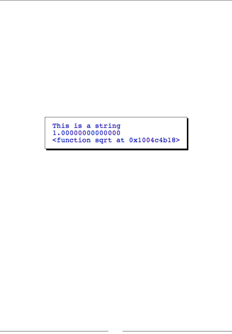
Geng Started with Sage
[ 56 ]
Displaying results of calculations
Before we go any further, we need to learn about the print funcon. print takes one
argument, which is enclosed in parenthesis. print evaluates its argument and writes the
result to either the interacve shell or an output cell in a worksheet. If the argument is a
string, print simply prints the string. If the argument is another type, it will be converted
to a string before being printed. By default, each call to the print funcon will result in a
new line of output. For example, enter the following code in an input cell to see how print
works in a worksheet:
print('This is a string')
print(1.0)
print(sqrt)
The result looks like this:
We'll use print extensively to display the output from Sage calculaons. In older Python
code, you will oen see print used as a statement instead of a funcon:
print 'This is a string'
Python versions 2.6 and later support using print as either a statement or a funcon.
However, in Python 3 and later only the funcon syntax will be supported. Therefore,
we will use print as a funcon in order to make our code compable with future versions
of Python.
Operators and variables
Operators and variables are two fundamental elements of numerical compung. Sage uses
the Python programming language as the interface for all of its components, so wring
code for Sage is very similar to wring Python code. Sage extends the Python language with
addional types that are well suited for mathemacal calculaons. In this secon, we'll learn
more about how operators and variables work in Sage.

Chapter 3
[ 57 ]
Arithmetic operators
The following table lists the operators that are available in Sage:
Operator Funcon Operator Funcon
=Assignment == Equality
+ Addion >Greater than
- Subtracon >= Greater than or equal to
*Mulplicaon <Less than
/ Division <= Less than or equal to
** or ^ Power != Not equal to
% Modulo (remainder)
// Integer quoent
Note that the assignment operator is a single equal sign, while the test for equality is a
double equal sign. The following example illustrates the dierence between the two:
sage: a = 4 # assigns the value 4 to a
sage: a == 5 # tests whether a is equal to 5
False
When performing arithmec, it is important to know which operaons take precedence over
others. Operaons with higher precedence will be done rst. The following table lists the
operators in order from lowest to highest precedence:
or
and
not
in, not in
is, is not
>, <=, >, >=, ==, !=, <>
+, -
*, /, %
**, ^
If there is any ambiguity, use parenthesis to make it clear which operaons should be done
rst. This will also make your code easier to read.

Geng Started with Sage
[ 58 ]
Pop quiz – working with operators
Try to gure out what answer Sage will give to the following math problems, and check your
answers with Sage:
2 + 3^2
4 + 2 * 5
3 * 2 == 2 * 10
5 * 2 > 7 + 1
2 + 1 == 3 * 1 and 5 < 6
True and not False or True
Numerical types
Variables in Sage, like Python, are dynamically typed. Unlike tradional languages such as C
or FORTRAN, Sage does not require you to declare variables before using them. A variable
can be assigned a real number in one line of code, an integer in another line, and a string
in the next. However, mathemacal operaons require numerical types to be dened with
more accuracy. The results of a calculaon can change, depending on the types of variables
involved. In the following examples, we will use the type funcon to determine the type of
any variable in Sage.
Integers and rational numbers
When you dene a variable without using a decimal point or exponenal notaon, Sage
assumes the variable is an integer. Operaons on integers can result in integers, raonal
numbers, or symbolic expressions. Evaluate the following code in an input cell:
a = 10
print(a)
print(type(a))
print(a / 3)
print(type(a / 3))
print(sqrt(a))
print(type(sqrt(a)))
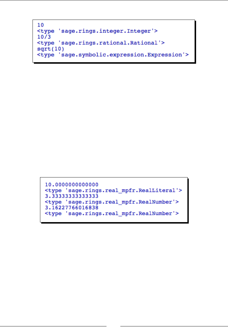
Chapter 3
[ 59 ]
The result should look like this:
Real numbers
A real number is any decimal number. Sage creates a real number when you dene a variable
using a decimal point or exponenal notaon. You can use the notaon "1e9" to represent
"one mes ten to the power nine."
b = 10.0
print(b)
print(type(b))
print(b / 3)
print(type(b / 3))
print(sqrt(b))
print(type(sqrt(b)))
The result should look like this:
Most operaons in Sage can return real numbers with arbitrary precision. Later in the
chapter, we'll see how to nd out how many bits of precision are available for a real
number. Note that the results of a oang-point calculaon depend on how the oang-
point operaons are implemented on a parcular type of processor. Therefore, oang-
point numbers shown here may be slightly dierent when the calculaons are repeated on
dierent plaorms.
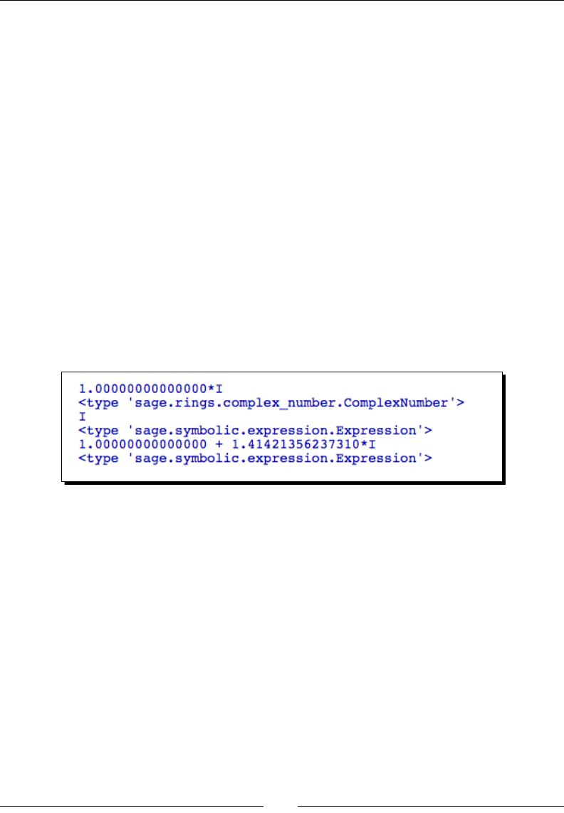
Geng Started with Sage
[ 60 ]
Complex numbers
Complex numbers consist of a real part and an imaginary part. Sage represents a complex
number with a complex number type or a symbolic type, depending on how you dene the
number. If you dene a complex number on the command line using the built-in constant I
(or i) to represent the square root of -1, then the number is stored as a symbolic expression.
Operaons on integers and raonal numbers will also return a symbolic expression. In
contrast, the square root of a negave real number is stored as a complex number type.
c1 = sqrt(-1.0)
print(c1)
print(type(c1))
c2 = sqrt(-1)
print(c2)
print(type(c2))
c3 = 1.0 + i*sqrt(2.0)
print(c3)
print(type(c3))
The result should look like this:
Symbolic expressions
In addion to numerical calculaons, Sage has extensive capabilies to perform symbolic
mathemacs. We'll cover this subject in detail in Chapter 7. For now, we'll use the var
funcon to declare symbolic variables.
var('x, y, z')
print(x)
print(type(x))
z = x + y
print(z)
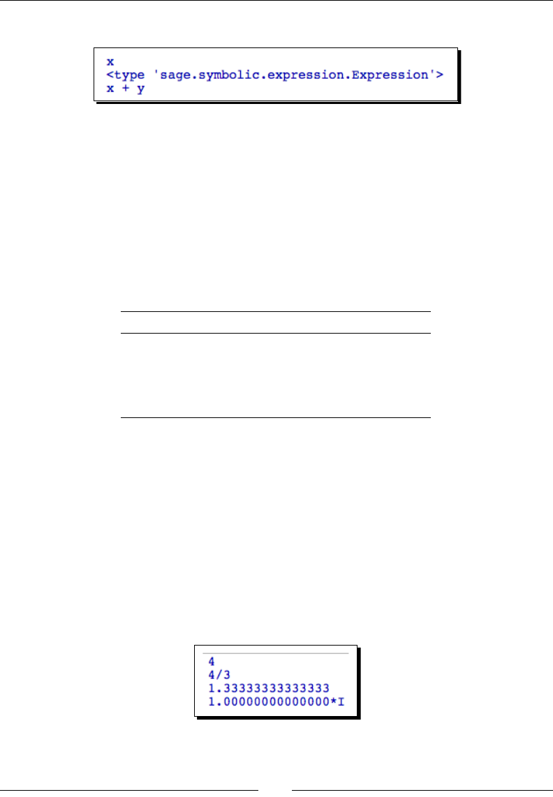
Chapter 3
[ 61 ]
The result should look like this:
var accepts a string argument with variable names separated by commas (we'll cover strings
in a bit). It makes the code more readable if you use a space aer each comma.
Dening variables on rings
For engineering and scienc computaon, you will generally use real or complex numbers
and ignore the other types. However, when working with symbolic mathemacs or doing
theorecal work, it may be very important to specify the correct ring for a variable. Sage
allows you to specify the ring over which a number is dened. Four commonly used rings are
as follows:
Ring Constructor in Sage
Integers ZZ
Raonal numbers QQ
Real numbers RR
Complex numbers CC
You can use rings to specify the type of a variable, as shown in this example:
integer_var = ZZ(4)
rational_var = QQ(4/3)
real_var = RR(4/3)
complex_var = CC(sqrt(-1))
print(integer_var)
print(rational_var)
print(real_var)
print(complex_var)
The result should look like this:

Geng Started with Sage
[ 62 ]
Noce that the expression QQ(4/3) returns an exact raonal number, but RR(4/3) returns
a oang-point approximaon. A useful trick is to use I to dene a complex number, and
then use CC to force the result to have a complex number type rather than a symbolic
expression type.
Combining types in expressions
It oen happens that integers, raonal numbers, real numbers, and complex numbers
need to be combined in a mathemacal expression. Most of the me, you don't need to
worry about this because Sage will automacally choose the best type for the result of the
calculaon, so that no informaon will be lost. For example, adding an integer to a real
number results in a real number, to avoid losing the non-integer part of the result.
Pop quiz – understanding types
What type will result from the following Sage commands? Check your answers with the type
funcon in Sage.
3/2
2/3.0
sin(pi/3)
sqrt(-1)
sqrt(-1.0)
CC(7 + 3 * i)
Strings
Strings are another fundamental type in Python and Sage. We will use strings extensively, in
conjuncon with the print funcon, to display results from our calculaons. We will also
use strings to document funcons that we dene.
Time for action – using strings
Let's pracce with strings:
string_1 = 'Single quoted string'
string_2 = "Sometimes it's good to use double quotes"
multiline_string = """ This string
contains single quotes ' and double quotes "
and spans multiple lines"""
print(string_1)
print(string_2)
print(multiline_string)
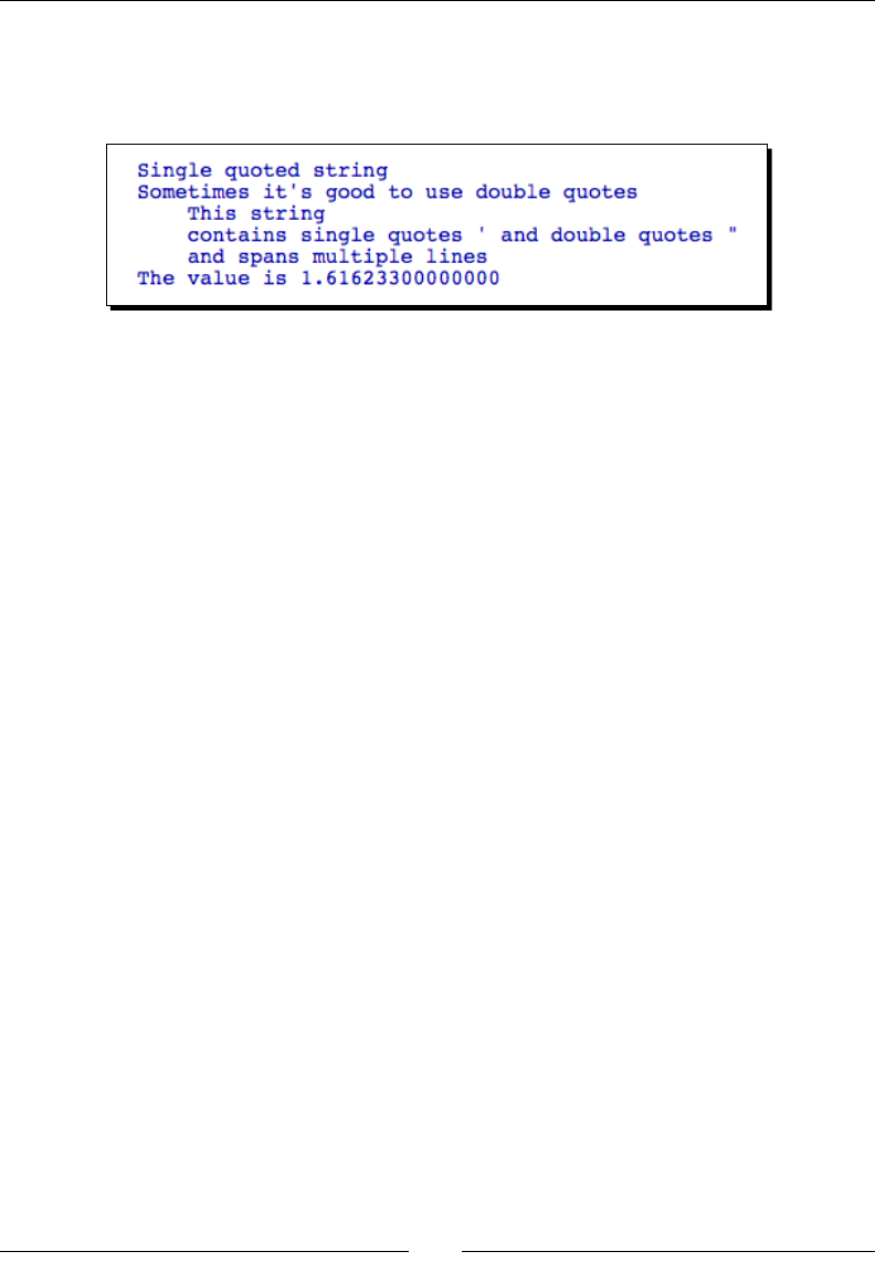
Chapter 3
[ 63 ]
numerical_value = 1.616233
print('The value is ' + str(numerical_value))
The result should look like this:
What just happened?
A string literal is an arbitrary sequence of characters enclosed in quotaon marks, such
as 'Single quoted string' in the example above. String literals can be assigned to
variables, like any other type. Single or double quotes can be used. If you need to use a
single quote within the string, you need to enclose the string in double quotes, as we did
with the string literal assigned to the variable string_2. Enclosing a string in triple quotes
(either single or double) allows you to include newlines and quotaon marks in the string.
We used triple quotes to assign a string value to the variable multiline_string.
The last two lines of the example show how we can use strings to improve the output
from our calculaons. The str funcon returns a string representaon of its argument,
which is a real number in this example. Every object in Sage, including funcons, has a
string representaon, although it's not necessarily useful. We then used the + operator to
concatenate (join) the two strings. This operator performs addion if used with numerical
types, and concatenaon if used with strings. This is known as operator overloading. We'll
use print, str, and the + operator extensively to improve the output from our calculaons.
Callable symbolic expressions
The denion of the word "funcon" is a potenal source of confusion in Sage because there
are two types of constructs that are commonly referred to as funcons. Mathemacians
dene a funcon as a relaon that associates each element of a given set (called the domain)
with an element of another set (the range). In computer programming, a funcon is a block
of code within a larger program that performs a specic task. Sage supports both types of
funcons. In order to avoid confusion, we will use the term "callable symbolic expression"
to refer to a funcon in the mathemacal sense. The word "funcon" will refer to a funcon
denion using the Python programming language, which we will learn about in the next
secon.
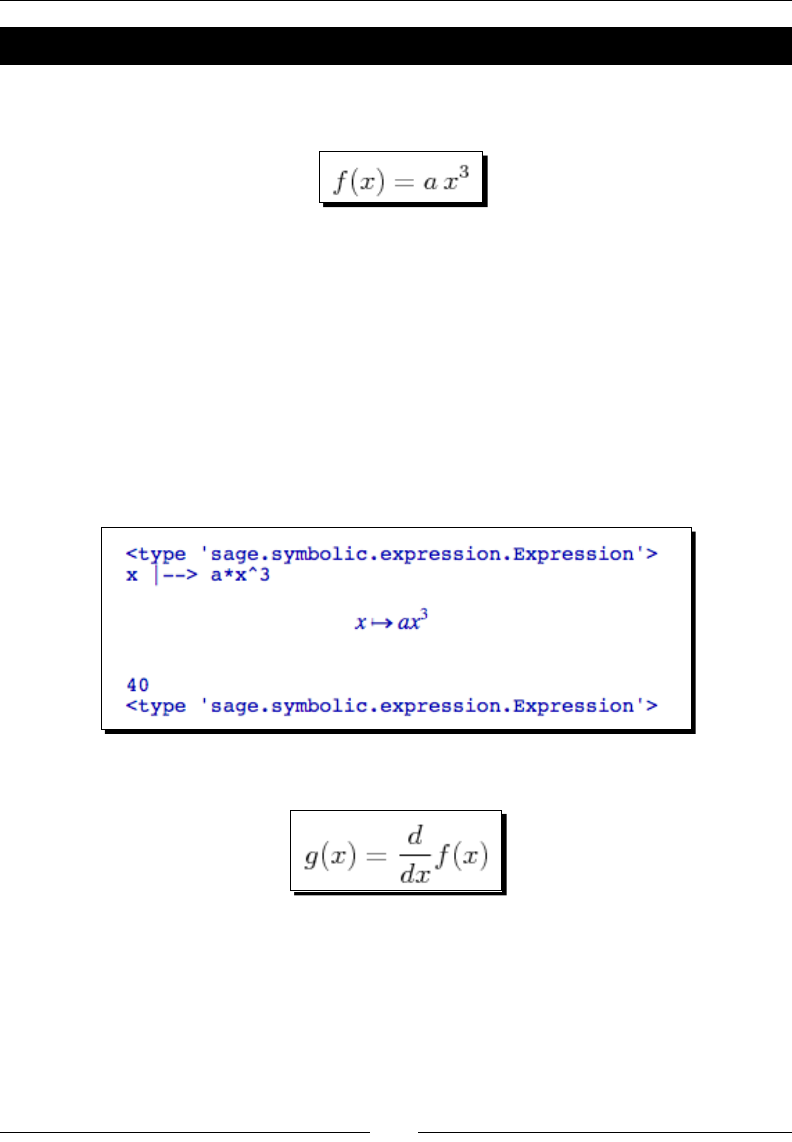
Geng Started with Sage
[ 64 ]
Time for action – dening callable symbolic expressions
Let's say we want to dene this mathemacal funcon and perform some calculaons
with it:
Evaluate the following code to dene the funcon:
var('a, x')
f(x) = a * x^3
print(type(f))
print(f)
show(f)
print(f(2, a=5))
print type(f(2, a=5))
The result should look like this:
Now, let's dene another funcon, which is the derivave of f(x):
Evaluate the following code to dene g(x):
g(x) = derivative(f, x)
show(g)
g(x=2, a=3)
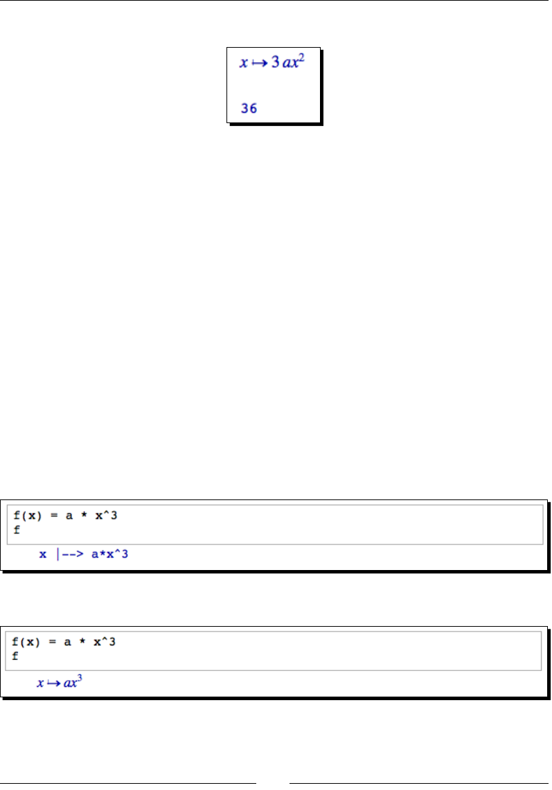
Chapter 3
[ 65 ]
The result should look like this:
What just happened?
We started out using the var funcon to dene some symbolic variables. Technically, we
didn't need to explicitly dene x as a symbolic variable, because Sage assumes that x is
symbolic by default. We then used the notaon f(x) = a * x^3 to dene a callable
symbolic expression called f, and we conrmed that f was symbolic by using the type
funcon. We used the print funcon to display f, and then introduced a new funcon
called show to display a typeset representaon of f. Finally, we called f with specic values
for x and a. When we evaluate f, the result always has a symbolic type, even when the
result is a numerical value.
In the next secon, we created a new callable symbolic expression called g that is dened as
the derivave of f with respect to x. derivative is a Sage funcon for compung symbolic
derivaves, which we'll cover in Chapter 7. We then computed the value of g for specic
numerical values of a and x to verify that g is also a callable symbolic expression.
Automatically typesetting expressions
Near the top of every worksheet is a check box with the label Typeset. When it's not
checked, symbolic expressions are displayed on a single line:
When the box is checked, expressions are typeset:
The Typeset check box has no eect on the print or show funcons; print always displays
an expression as text, and show always typesets expressions.
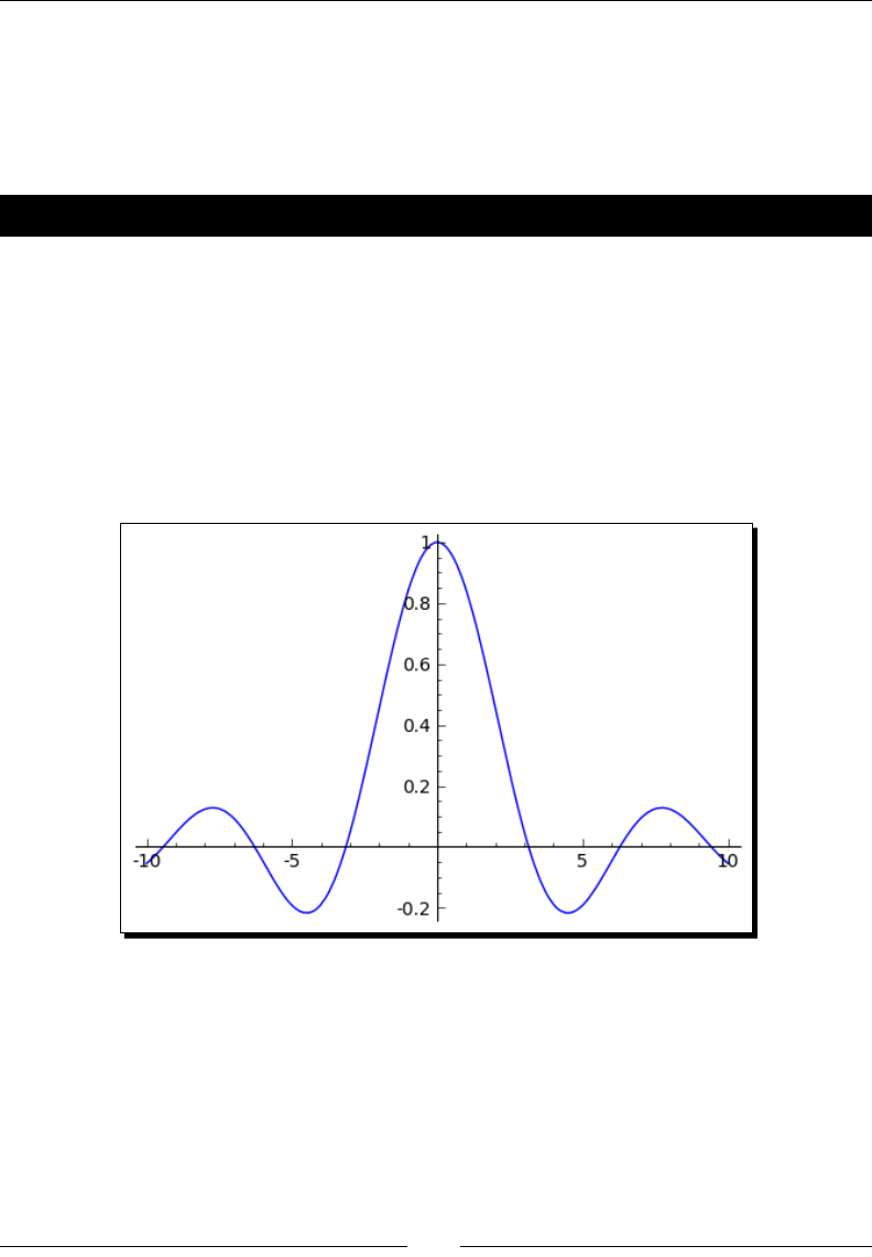
Geng Started with Sage
[ 66 ]
Functions
Funcons are a way to encapsulate and modularize data processing. Data can be passed to
a funcon using arguments. The funcon performs some kind of operaon, and (oponally)
returns a result.
Time for action – calling functions
We've already seen many simple examples of calling funcons. Now, we'll use the plot
funcon to illustrate more advanced ways to call funcons. Evaluate the following code:
var('x')
sinc(x) = sin(x) / x
plot(sinc, (x, -10, 10))
The result should look like this:
Now, let's customize our plot:
plot(sinc, x, xmin=-15, xmax=15, thickness=2, color='red',
legend_label='sinc')
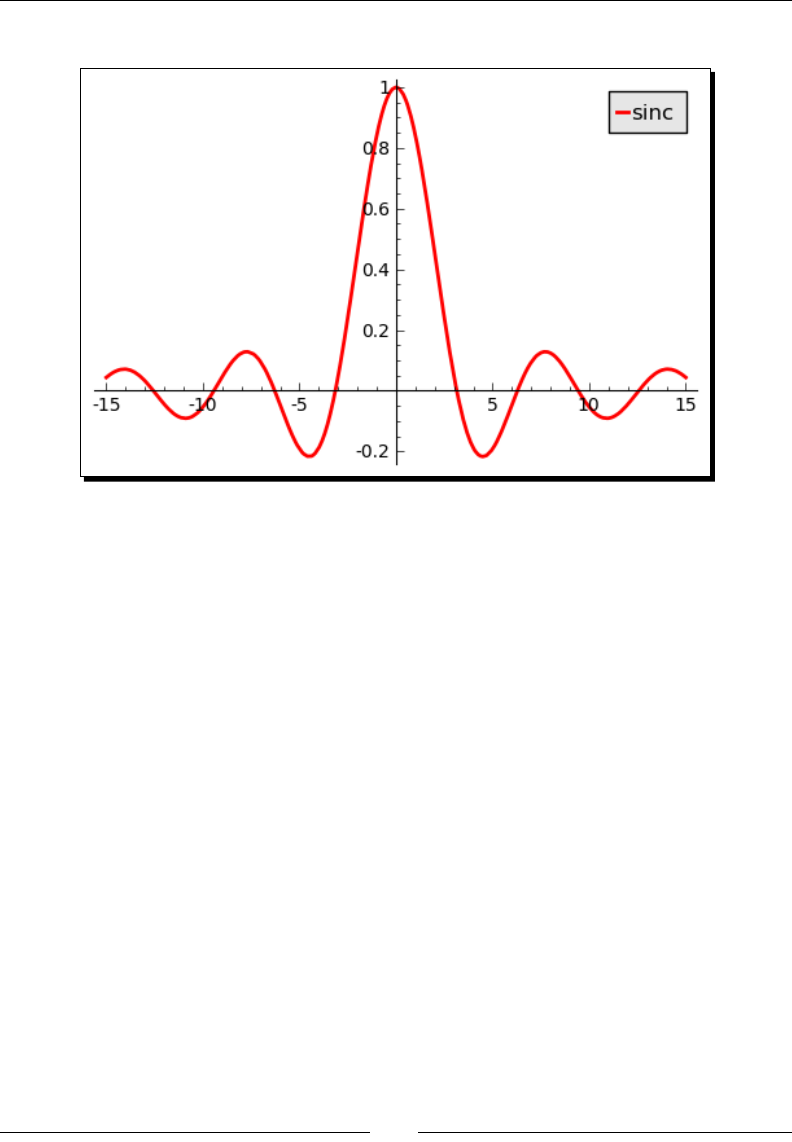
Chapter 3
[ 67 ]
The customized plot should look like this:
What just happened?
In the rst part of the example, we dened a callable symbolic expression that represents the
sinc funcon. This funcon has important applicaons in signal processing and informaon
theory. We ploed the funcon using a simple call to the plot funcon. When calling a
funcon with mulple arguments, it is important to put the arguments in the right order.
The rst argument to plot is the callable symbolic expression. The second argument is known
as a tuple, which we'll learn about in the next chapter. The tuple contains the independent
variable, the minimum value of the plong domain, and the maximum value of the domain.
In the second part of the example, we used keyword arguments to customize the plot.
The arguments we used in previous examples are called posional arguments. Posional
arguments are required, and they must occur in the correct order. A keyword argument is
oponal—if a keyword argument is not specied in the funcon call, it takes on a default
value. If keywords are used, the arguments can be placed in any order. However, keyword
arguments must come aer all the posional arguments. In general, a funcon is called using
the syntax:
result = function_name(argument_1, argument_2, … , argument_n,
keyword=value)

Geng Started with Sage
[ 68 ]
The number of posional arguments in the funcon call must match the number in the
denion. The funcon does not have to return a value, and you don't have to assign its
return value to a variable. In simple cases, it's possible to pass oponal arguments without
keywords by passing the oponal arguments in the right order. However, this is discouraged,
because it makes the code less readable and more prone to bugs.
Sage has very sophiscated plong capabilies, which we will cover in Chapter 6. If you are
interested in learning more now, evaluate the command plot? in a worksheet cell or in the
interacve shell to get help on the plot funcon.
Have a go hero – make some more plots
Use the plot command to make plots of some of the built-in mathemacal funcons listed
in the next secon. Pracce using keyword arguments to customize the plots. Then, use the
built-in funcons to dene a callable symbolic expression, and plot it.
Built-in functions
A vast number of funcons are pre-dened in Sage. Even more are available through Python
modules, which we will learn about in the next chapter. For now, here is a brief summary of
the most commonly used mathemacal funcons, and how to access them in Sage:
Funcon Sage Funcon Sage
sine sin(x) square root sqrt(x)
cosine cos(x) ex exp(x)
tangent tan(x) natural logarithm log(x)
arcsine arcsin(x) absolute value abs(x)
arccosine arccos(x) complex conjugate conjugate(x)
arctangent arctan(x)
Numerical approximations
Any numerical type in Sage can be converted to a real number with the numerical_approx
funcon (this funcon can also be abbreviated as n or N). For example:
print(pi)
print(numerical_approx(pi))
print(type(numerical_approx(pi)))
print(numerical_approx(pi, prec=16))
print(numerical_approx(pi, digits=5))
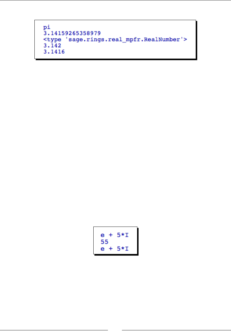
Chapter 3
[ 69 ]
The result should look like this:
The numerical_approx funcon accepts three arguments. The rst argument, which
is mandatory, is the item to be converted to a real number. The keyword argument prec
can be used to specify the number of bits of precision for the real number. Alternately, the
keyword argument digits can be used to specify the number of digits of precision.
The reset and restore functions
It's possible to accidentally re-dene a built-in funcon or constant. For example, the leers
i and n are commonly used as names for counng variables in loops. Fortunately, the
restore funcon can be used to restore predened global variables (such as i and n) to
their default values. Here's a short example:
print(e + i * 5)
i = 10
e = 5
print(e + i * 5)
restore('e i')
print(e + i * 5)
The result should look like this:
If you call restore without any arguments, it will restore all the predened variables to
their default values. Another useful funcon is called reset. This funcon deletes all the
variables you have dened, restores all global variables to their default values, and resets the
interfaces to other computer algebra systems.

Geng Started with Sage
[ 70 ]
If you start geng strange results from your calculaons, you may have
accidentally re-dened a built-in funcon or constant. Try calling the reset()
funcon and running the calculaon again. Remember that reset will delete
any variables or funcons that you may have dened, so your calculaon will
have to start over from the beginning.
Dening your own functions
Sage allows you to dene your own funcons using Python syntax. This will be very useful for
keeping your code organized, especially as we move into wring longer programs.
Time for action – dening and using your own functions
Let's return to the series RC circuit that we have been using as an example. We will now
dene a funcon that computes the voltage across the capacitor. You can enter the following
code in an input cell in a worksheet, or on the command line. When you type the colon at
the end of the rst line and press Enter, the cursor will automacally indent the lines that
follow. Make sure that you consistently indent each line inside the funcon.
def RC_voltage(v0, R, C, t):
"""
Calculate the voltage at time t for an R-C circuit
with initial voltage v0.
"""
tau = R * C
return v0 * exp(-t / tau)
R = 250e3 # Ohms
C = 4e-6 # Farads
v0 = 100.0 # Volts
t = 1.0 # seconds
v = RC_voltage(v0, R, C, t)
print('Voltage at t=' + str(n(t, digits=4)) + 's is ' +
str(n(v, digits=4)) + 'V')
This block of code produces the following output:
Voltage at t=1.000s is 36.79V

Chapter 3
[ 71 ]
If you are using the interacve shell, pressing Enter aer the rst line will create a blank line
so that you can enter the next line of the funcon, instead of execung the code. To return
to the command prompt, press Enter on a blank line. Dening a funcon on the command
line looks like this:
sage: def RC_voltage(v0, R, C, t,):
....: """
....: Calculate the voltage at time t for a series R-C circuit
....: with initial voltage v0.
....: """
....: tau = R * C
....: return v0 * exp(-t / tau)
....:
Our funcon even has documentaon like a built-in funcon. Execung the following
command displays the documentaon:
RC_voltage?
Having trouble geng the code running?
Python, like most programming languages, is very picky about how you type in
the code. This is oen frustrang for new programmers, but you'll quickly get
used to it. Go over what you typed in and look for these common mistakes.
Did you forget the colon aer the parenthesis when dening the funcon? Did
you uniformly indent each line within the funcon? Did you use three double
quotes on each end of the documentaon string? Also, pay aenon to the error
messages that are produced, parcularly the last one.
What just happened?
We dened a funcon and found that it can be used just like the built-in funcons in Sage.
Sage funcons are dened using the general form:
def function_name(argument_1, argument_2, … , argument_n):
"""
Documentation string here
"""
statement one
statement two
...
return some_value
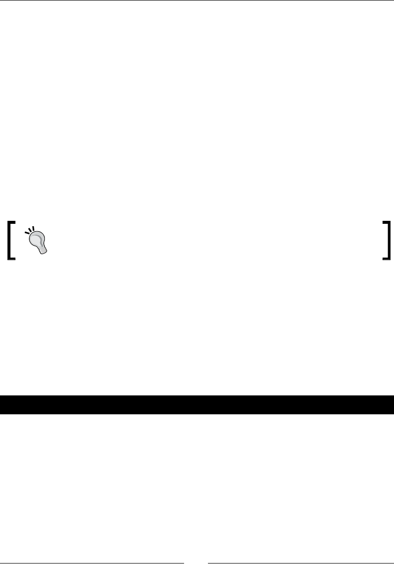
Geng Started with Sage
[ 72 ]
The rst line declares the name of the funcon and the argument list. Don't forget the colon
aer the argument list! It's also valid to dene a funcon without any arguments, in which
case the parenthesis must be empty.
The body of the funcon is a block of code that is uniformly indented. A unique feature of
the Python language is that indentaon is used to delimit blocks of code, rather than using
symbols like curly braces. That is why it is so important to indent each line in the body of the
funcon by the same amount. The rst item within the funcon body is called the docstring.
While this is oponal, it's good to get in the habit of including it. Sage displays the docstring
when the user asks for help on the funcon. The docstring is triple-quoted, which means
that Sage will display its contents exactly as you format them. Next, the funcon can have
any number of statements. Note that our funcon has its own local variable, tau. You can
also dene funcons within funcons. The nal line of the funcon denion is the return
keyword, followed by one or more variables whose values will be returned. If the funcon
doesn't return anything, the return keyword can be used without any variable names, or
return can be omied.
If you nd a block of code occurring more than once in your program, stop and
move that block of code to a funcon. Duplicate blocks of code will make your
programs harder to read and more prone to bugs.
Functions with keyword arguments
There are two good reasons to use keyword arguments when dening a funcon. One
reason is to allow the user to omit arguments that are seldom changed from their default
value. The other is to reduce confusion when calling the funcon. In the example above, it
might be easy to accidentally interchange the resistance and capacitance values when calling
the funcon, resulng in a bug that's hard to track down.
Time for action – dening a function with keyword arguments
Let's re-dene our funcon with keyword arguments:
def RC_voltage(t, v0=100, R=1000, C=1e-9):
"""
Calculate the voltage at time t for an R-C circuit
with initial voltage v0.
"""
tau = R * C
return v0 * exp(-t / tau)
res = 250e3 # Ohms
cap = 4e-6 # Farads

Chapter 3
[ 73 ]
v0 = 100.0 # Volts
t = 1.0 # seconds
v = RC_voltage(t, v0=v0, R=res, C=cap)
print('Voltage at t=' + str(n(t, digits=4)) + 's is ' +
str(n(v, digits=4)) + 'V')
The output is the same as the previous example.
What just happened?
Declaring keyword arguments is very similar to declaring posional arguments. If there are
keyword arguments, they must be dened aer the posional arguments. The default value
of each keyword argument must be given. The following is the general form of a funcon
denion with posional and keyword arguments:
def function_name(argument_1, argument_2, … , argument_n,
keyword_arg_1=default_value,… , keyword_arg_n=default_value ):
"""
Documentation string here
"""
statement one
statement two
...
return some_value
In our funcon denion, we used keyword arguments for the inial voltage, resistance,
and capacitance. We had to move the me argument t so that it came before the keyword
arguments. When we called the funcon, we used the keywords v0, R, and C to specify the
inial voltage, resistance, and capacitance. In this case, it doesn't really make sense to use
a keyword argument for t, since it's the only posional argument and there is no chance of
confusing it with the keyword arguments.
Objects
Over the past three decades, object-oriented programming (OOP) has created a fundamental
shi in the way that programmers approach problems. In the early days of OOP, people
involved in scienc compung could largely ignore object-oriented principles. Today, that
is no longer the case. While the algorithms of scienc compung are sll fundamentally
procedural, the soware packages are increasingly constructed in an object-oriented fashion.
OOP allows scienc soware to be more organized, easier to use, and more maintainable.
In this secon, you will learn how to use pre-dened objects in Sage. In Chapter 9, you will
learn how to create custom objects.
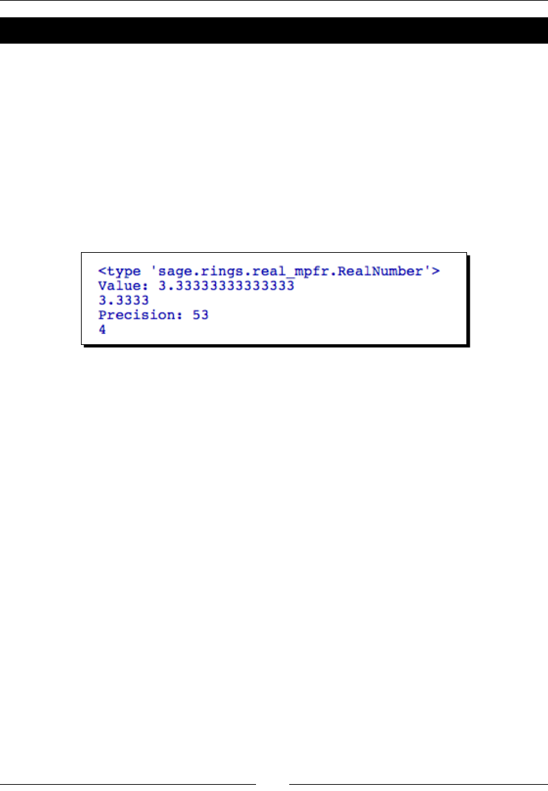
Geng Started with Sage
[ 74 ]
Time for action – working with objects
If you are already familiar with objects from another programming language (such as Java or
C++), then you will immediately be familiar with objects in Sage. If not, this example should
help you understand the concept:
real_number = RR(10/3)
print(type(real_number))
print('Value: ' + real_number.str())
print(real_number.n(digits=5))
print('Precision: ' + str(real_number.precision()))
print(real_number.ceil())
The result should look like this:
What just happened?
We've already been using objects without knowing it—every number in Sage is actually an
object! An object is a construct that consists of data (called aributes) and behaviours (called
methods). An object's aributes and methods are dened by a class. We say that an object
is an instance of a parcular class. In our example, the object called real_number is an
instance of a class called RR. We create an object using syntax that is just like a funcon call:
new_object = Class_Name(arg1, arg2, …)
The number and type of arguments (posional vs. keyword) will depend upon the class
denion.
The object called real_number has an aribute that stores a representaon of the oang-
point number 1.4372. It has another aribute that stores the precision of the oang-point
number. Objects can have other objects as aributes, leading to very complicated structures.
An object's aributes can be interrogated and manipulated using methods. Methods are
funcons that are associated with an object. For example, the precision method returns
the number of bits of precision for the real number:
real_number.precision()
We can use the str method to obtain a string representaon of a real number:
real_number.str()

Chapter 3
[ 75 ]
Methods are called with the syntax:
result = object_name.method_name(argument_1, argument_2, … ,
argument_n)
One of the strengths of object-oriented programming is that the design of the object limits
the ways that we can manipulate its data. For example, it wouldn't make any sense if we
were allowed to change the value of a oang-point number without updang the number
of bits of precision.
As you start using objects, you may be frustrated by the lack of direct access to
the data. You may nd yourself tempted to avoid using the methods, and directly
manipulate the data in an object. This defeats the purpose of using objects! If
the methods seem to be hindering your use of the object, you probably aren't
using them right. Take another look at the documentaon and examples, and
re-think your approach.
Getting help with objects
If you know an object's class, you can use the help funcon to see its architecture. In the
previous example, we used the type funcon to determine that a real number's class is
sage.rings.real_mpfr.RealNumber. We can use the help funcon to learn more
about it. In the interacve shell, the class documentaon looks like this:
sage: help(sage.rings.real_mpfr.RealLiteral)
Help on class RealNumber in module sage.rings.real_mpfr:
class RealNumber(sage.structure.element.RingElement)
| File: sage/rings/real_mpfr.pyx (starting at line 1034)
|
| A floating point approximation to a real number using any specified
| precision. Answers derived from calculations with such
| approximations may differ from what they would be if those
| calculations were performed with true real numbers. This is due to
| the rounding errors inherent to finite precision calculations.
|
| The approximation is printed to slightly fewer digits than its
| internal precision, in order to avoid confusing roundoff issues
| that occur because numbers are stored internally in binary.
|
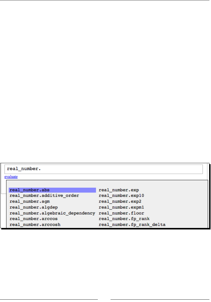
Geng Started with Sage
[ 76 ]
| Method resolution order:
| RealNumber
| sage.structure.element.RingElement
| sage.structure.element.ModuleElement
| sage.structure.element.Element
| sage.structure.sage_object.SageObject
| __builtin__.object
|
...
The same informaon is available from the notebook interface, but the formang will dier.
You can view the source code for a class by typing its name, followed by two queson marks:
RR??
You can quickly access a list of methods by typing the name of an object followed by a period
and pressing Tab. If the object has many methods and you are using the interacve shell,
Sage will give you fair warning:
sage: real_number.
Display all 105 possibilities? (y or n)
If you are using the notebook interface, a table of methods will appear:
To nd out more about a parcular method, type the name of the object, a period, and the
method name, followed by a queson mark. Here is an example of how this looks in the
interacve shell (it will also work in the notebook interface):
sage: real_number.cos?
Type: builtin_function_or_method
Base Class: <type 'builtin_function_or_method'>

Chapter 3
[ 77 ]
String Form: <built-in method cos of sage.rings.real_mpfr.RealLiteral
object at 0x100478c08>
Namespace: Interactive
Definition: real_number.cos(self)
Docstring:
Returns the cosine of this number
...
As with classes and funcons, typing two queson marks aer the method name will display
its source code.
Learning object-oriented programming for the rst me can be confusing, but it will pay o.
For now, we've only talked about how to use pre-dened types of objects. In Chapter 9, you
will learn how to dene your own classes for creang custom objects.
Summary
In this chapter, we learned the basics of interacng with Sage. Specically, we covered:
How to use the interacve shell
How to use the notebook interface to perform calculaons and add documentaon
to worksheets
Operators and variables
Calling funcons
Making simple plots
Dening our own funcons
Working with objects
We have only started to unlock the power and exibility of Sage. In the next chapter, we will
learn more about the programming features of Python that are available in Sage.
4
Introducing Python and Sage
By now, you have learned the basic principles of interacng with Sage. We will now unlock
the power of the Python programming language. The programmac features of Python
complement the mathemacal features of Sage.
In this chapter, we shall learn how to:
Use lists and tuples to store sequenal data
Iterate with loops
Construct logical tests with "if" statements
Read and write data les
Store heterogeneous data in diconaries
So, let's start programming…
Python 2 and Python 3
It is important to understand that two stable versions of Python are available. Python 2 was
rst released in October 2000, and version 2.7 is the latest in a long line of evoluonary
upgrades. The Python developers realized that certain aspects of the Python language
could not be improved without breaking compability with exisng code. The result was
Python 3, which is the rst release of Python that is intenonally backwards-incompable.
In other words, some code wrien for Python 2 will have to be modied to run on a Python
3 interpreter. For this reason, the migraon from Python 2 to Python 3 has been rather slow,
even though Python 3 is mature and stable. Version 2.7 is the nal release of Python 2, and
new features are being added only to Python 3. Sage uses Python 2.7 (as of Sage version
4.6), so the code in this book is wrien for Python 2.7. Whenever possible, the examples
have been wrien so that they will connue to run when Sage eventually switches to Python
3. When looking at Python documentaon and examples online, make sure that you are
reading about Python 2, rather than Python 3.

Introducing Python and Sage
[ 80 ]
Writing code for Sage
In this chapter, we'll be wring longer blocks of code. While all of the examples can be
entered and run using the notebook interface, it is oen easier to edit large secons of code
with a text editor that is specically designed for programming. These text editors have
special features, such as syntax highlighng and automac indentaon that can help you
write code more easily and avoid some common bugs. Unlike word processors or rich-text
editors, programmer's text editors save pure text les that do not contain hidden formang
informaon that can confuse the Python interpreter. Many good text editors are available;
the following editors are some popular free and open-source opons. GNU Emacs and vim
are two popular editors for Linux systems, although Windows, OS X, and Solaris versions are
also available. If you are used to the Windows or Mac user interface, it will take some me
to get comfortable with the user interface for Emacs or vim. Kate (KDE) and gedit (GNOME)
are available for Linux users who prefer a more convenonal user interface. Notepad++ is a
free, open-source programmer's text editor for Windows, with a familiar installaon process
and a friendly user interface. TextWrangler is a free text editor for OS X (although it is not
open source). jEdit is a Java-based cross-plaorm editor that will run on any plaorm that
supports Java. To nd out more and download the soware, use the following links:
http://www.gnu.org/software/emacs/
http://www.vim.org/
http://projects.gnome.org/gedit/
http://kate-editor.org/
http://notepad-plus-plus.org/
http://www.barebones.com/products/textwrangler/
http://www.jedit.org/
Since Sage uses the Python programming language, Sage code follows the same convenons
as Python code. These convenons are described in the Style Guide for Python (http://
www.python.org/dev/peps/pep-0008/). It is a good idea to familiarize yourself with
these convenons and follow them, so that your code can be easily read by other members
of the Sage and Python communies. Since Python uses indentaon to denote blocks of
code, one of the most important rules is to never mix tabs and spaces. If you use an external
text editor, congure the editor so that it inserts four spaces (rather than an invisible tab
character) every me you press the Tab key.

Chapter 4
[ 81 ]
Long lines of code
The convenon in the Python and Sage communies is to create scripts that are 80
characters wide. If a line of code is longer than 80 characters, it will have to be connued
on the next line. If a line needs to be connued, add a backslash \ as the last character on
the line:
term1 = (v2 * cos(n * float(pi)) - v1) / n \
* sin(n * float(pi) * x_val/l) \
* exp(-k * n**2 * float(pi)**2 * t / l**2)
This is called "explicit line joining." Expressions contained within parentheses, square
brackets, or curly braces can be split over more than one line without using a backslash,
which is called "implicit line joining." Implicitly joined lines can even contain comments:
parameters = {'diffusion coefficient' : k, # m^2/sec
'length' : l, # m
'left_BC' : v1, # m
'right_BC' :v2, # m
'time' : t, # sec
'num_x_steps' : num_x_steps}
In pure Python code, the indentaon of the connuaon lines is not important, although
they are usually indented for clarity. Sage occasionally has a problem with extra whitespace
in connuaon lines, which is why certain examples in this book have connuaon lines that
are not indented.
Running scripts
If you have entered code into a text editor, save the le with a .sage extension. Files with a
.sage extension may contain code that is specic to Sage, and a standard Python interpreter
may not be able to run them. Sage can also run les that have a .py extension. Files with
a .py extension should contain only Python code, so that they can be run with a standard
Python interpreter.
A le containing Sage source code can be loaded and run in Sage with the load command:
load("/Users/cfinch/Documents/Articles/Sage Math/Chapters/Chapter 4/
example1.py")
This works with either the Notebook or command-line interface. attach is another handy
command:
attach("/Users/cfinch/Documents/Articles/Sage Math/Chapters/Chapter 4/
example1.py")

Introducing Python and Sage
[ 82 ]
attach is similar to load, but it connues to monitor the text le for changes. Once you
make changes in the text editor and save them, all you have to do is press Enter on the Sage
command line, and Sage will automacally reload and re-run the le.
Sequence types: lists, tuples, and strings
Python has seven compound data types that are known as sequence types because they are
used to represent sequences of items. In this secon, we will learn about three of the most
commonly used sequence types. We'll start with lists, and learn many ways to create and
manipulate them. The concepts we learn will then be applied to tuples and strings.
Lists in Python are similar in concept to arrays in C and Fortran, and equivalent to lists in
Mathemaca and vectors in MATLAB. Python lists are much more powerful and exible
than arrays in lower-level programming languages like C.
Time for action – creating lists
Enter the following code into an input cell in a Sage notebook. Alternavely, you can create a
new text le containing the code, save it with a .sage extension, and use the load command
to run it in Sage.
# Creating lists with Python
list1 = ['a', 'b', 'c', 'd', 'e']
print("A list of characters: " + str(list1))
list2 = []
print("\nAn empty list: " + str(list2))
list2.append('f')
list2.append('g')
print("After appending items: " + str(list2))
list3 = list()
list3.extend(list1)
print("\nList 3 after extending: " + str(list3))
list3.append(list2)
print("List 3 after appending a list:" + str(list3))
list_of_ints = range(1, 11, 2)
print("\nA list of integers: " + str(list_of_ints))
# Sage-specific list creation
list_of_floats = srange(0.0, 2*n(pi), step=n(pi)/2, universe=RDF)
print("A list of real numbers:")
print(list_of_floats)
print("A list of symbols:")
print(srange(0, 2*pi, pi/4))
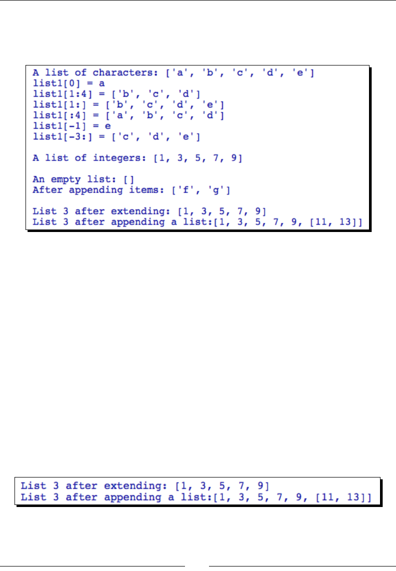
Chapter 4
[ 83 ]
list_of_ints_2 = [1..11, step=2]
print("Another list of integers: " + str(list_of_ints_2))
The output should look like this:
What just happened?
We demonstrated several ways to create lists. We started by using standard Python syntax
to create lists. A list can be dened with square brackets. The list can be empty, or you can
inialize the list with any number of items separated by commas:
new_list_object = [element_1, element_2, element_3]
empty_list = []
If you create an empty list, you can populate the list by using the append method to add a
new item to the end of the list:
empty_list.append(new_item)
You can use the extend method to add mulple elements to the end of the list:
empty_list.append([list_of_items])
You can also use append to add a list of items to an exisng list, but the results will be
dierent from extend:

Introducing Python and Sage
[ 84 ]
extend adds each item to the list, while append adds the enre list as a single item. This
example also demonstrates that you can nest lists, and that a single list can contain items of
dierent types.
The items in a list usually have the same type. Technically, it is possible to
mix types in a list, but this is generally not a good idea for keeping your code
organized and readable. If the need arises to use items of dierent types, it may
be beer to use a diconary, which is described later in this chapter.
Certain built-in funcons also return lists, such as the funcon list. If list is called with
a sequence type argument, it returns a list that contains the items of the sequence type;
if called with no argument, it returns an empty list. The range funcon creates a list of
integers. In its most basic form, it returns a list of integers that starts at zero and increments
by one unl it reaches (but does not include) the specied value:
sage: range(10)
[0, 1, 2, 3, 4, 5, 6, 7, 8, 9]
If two arguments are provided, range returns a list that starts at the rst argument and
increments by one unl it reaches (but does not include) the second argument:
sage: range(5,10)
[5, 6, 7, 8, 9]
If a third argument is present, it is used as the increment from one value to the next:
sage: range(2,10,3)
[2, 5, 8]
Sage provides some addional ways to create lists that complement the standard ways of
creang lists in Python. The srange funcon is a more exible version of range that can
create lists composed of any Sage numerical type. In the example, we used srange to create
a list of double-precision oang point numbers, as well as a list of symbolic values. srange
accepts the following oponal arguments:
Keyword Default
value
Descripon
end None Endpoint for sequence
step 1 Step
universe None Force all items to lie in the same universe (such as a parcular eld
or ring)
check True Ensure all elements lie in the same universe
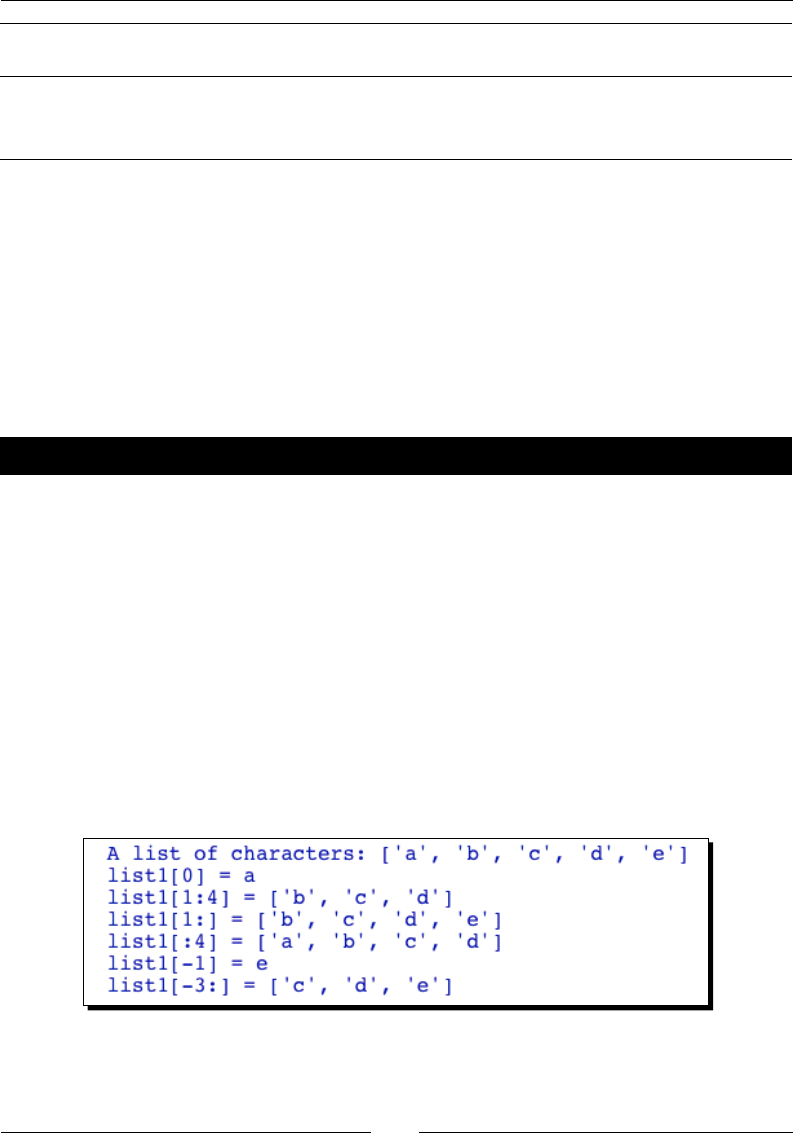
Chapter 4
[ 85 ]
Keyword Default
value
Descripon
include_endpoint False Include endpoint in sequence
endpoint_
tolerance
1.0e-05 For inexact rings, used to determine whether endpoint has been
reached
Sage has another shortcut for creang a list of integers that is similar to the range funcon:
[start_value..endpoint, step=1]
The start value and endpoint are enclosed in square brackets and separated by two decimal
points. The step can be specied with the step keyword (the default step is one).
Getting and setting items in lists
Now that we know how to create lists, we will learn how to get and set items in the list.
Time for action – accessing items in a list
Evaluate the following code:
list1 = ['a', 'b', 'c', 'd', 'e']
print("A list of characters: " + str(list1))
# Getting elements with indices and slices
print("list1[0] = " + str(list1[0]))
print("list1[1:4] = " + str(list1[1:4]))
print("list1[1:] = " + str(list1[1:]))
print("list1[:4] = " + str(list1[:4]))
print("list1[-1] = " + str(list1[-1]))
print("list1[-3:] = " + str(list1[-3:]))
The results should look like this:

Introducing Python and Sage
[ 86 ]
What just happened?
The items in a list can be accessed using an integer value, which is known as an index.
The index is placed in a square bracket like this:
sage: list1[0]
'a'
The index of the rst item is zero, the index of the next element is one, and so on. It's
also possible to select elements from the end of the list instead of the beginning. The
last element is -1, the second-to-last is -2, etc.
Mulple elements can be selected at once using slice notaon. The colon is the slice
operator. The slice starts at the index corresponding to the number before the colon and
goes up to (but does not include) the index corresponding to the number aer the slice.
list1[start_index:stop_index]
If the rst number is omied, the slice starts at the beginning of the list.
list1[:stop_index]
If the number aer the colon is missing, the slice goes all the way to the end of the list.
list2[start_index:]
The value of an item in a list can be changed using indices. You can also change mulple
items at the same me with slices. You can replace a slice of a list with a dierent number of
elements, and even delete the slice altogether. Slicing is a very powerful technique—and a
source of bugs unl you understand it thoroughly!
Pop quiz – lists and indexing
Test your understanding of lists with the following examples. Try to predict what the result
will be, and check your answers using Sage.
a = [1,3,5,7,9,11]
b = [0,2,4,6,8,10]
print(a[1])
print(a[0:4])
print(a[-1])
print(a[-4:-1])
print(a[-4:])
a[0] = 3.7324
print(a)
a[0:3] = b[0:3]

Chapter 4
[ 87 ]
print(a)
b[-2:] = []
print(b)
List functions and methods
Like everything in Sage, lists are objects. Every list has methods for manipulang the data
in the list. We've already used the append method to add items to the end of a list.
mylist.append(value) # Appends an item to end of list
In the next secon, we will use the append method in conjuncon with a for loop to
create a list of values.
The len funcon is used so oen with lists that it's worth menoning on its own. This
funcon returns the number of items in the list.
Python lists have many advanced features. It will be worth your me to browse
the Python documentaon at:
http://docs.python.org/tutorial/datastructures.
html#more-on-lists
http://docs.python.org/library/stdtypes.html#sequence-
types-str-unicode-list-tuple-buffer-xrange
Tuples: read-only lists
Lists are one example of a Python sequence type. A closely related type of sequence is called
a tuple. Tuples behave a lot like lists, but the data in a tuple is immutable. That means that
the data is essenally read-only—the elements in a tuple cannot be modied. Tuples are less
exible than lists, and therefore less widely used.
Time for action – returning multiple values from a function
Tuples are oen used to return mulple values from a Python funcon. Let's create a simple
funcon that takes the x, y, and z components of a Euclidean vector and returns the unit
vector that points in the same direcon.
def get_unit_vector(x, y, z):
"""
Returns the unit vector that is codirectional with
the vector with given x, y, z components.
This function uses a tuple to return multiple values.
"""
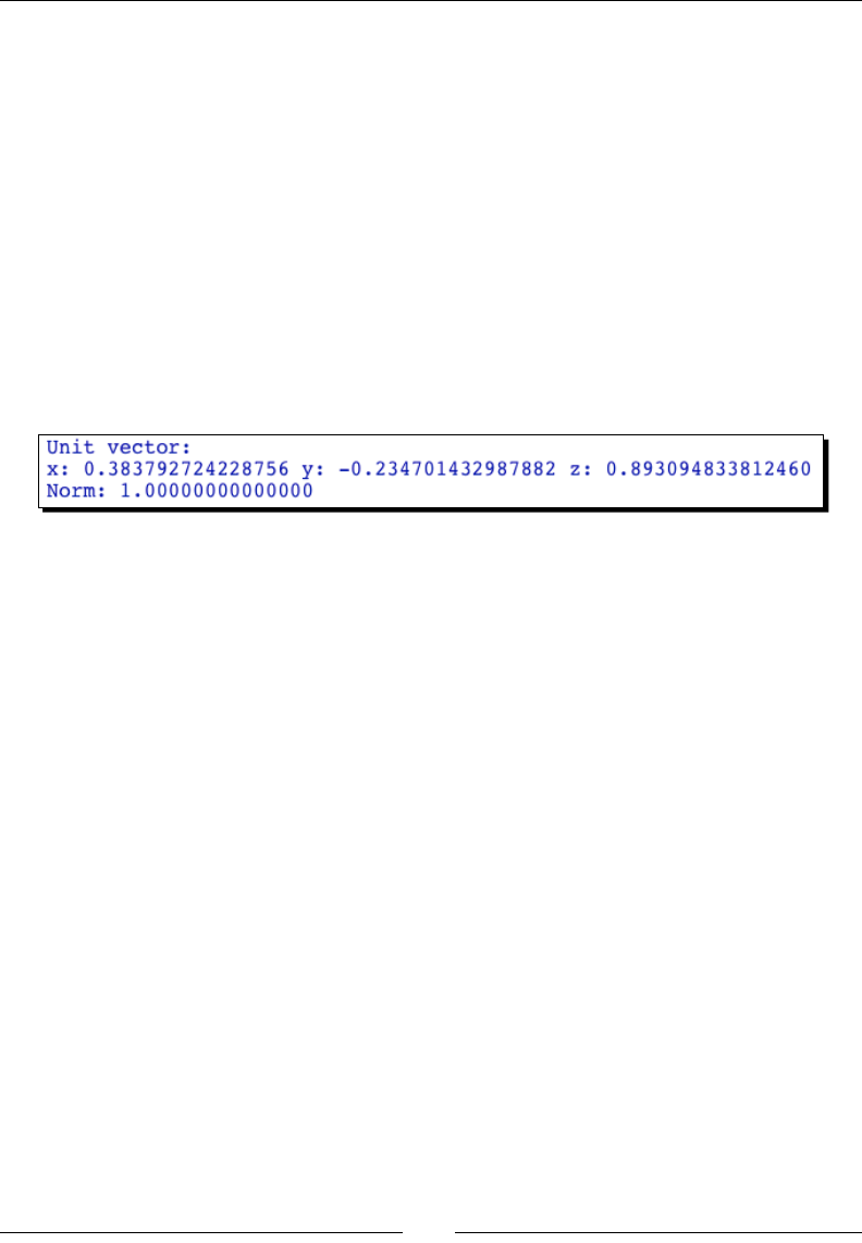
Introducing Python and Sage
[ 88 ]
norm = sqrt(x**2 + y**2 + z**2)
return x / norm, y / norm, z / norm
x = 3.434
y = -2.1
z = 7.991
unit_x, unit_y, unit_z = get_unit_vector(x, y, z)
print("Unit vector:")
print("x: " + str(unit_x) + " y: " + str(unit_y) +
" z: " + str(unit_z))
print("Norm: " + str(sqrt(unit_x**2 + unit_y**2 + unit_z**2)))
Execute the code. The results should look like this:
What just happened?
This example demonstrated how to return mulple values from a funcon. The funcon
denion should be familiar to you by now. The only new feature occurs in the last line of
the funcon:
return x / norm, y / norm, z / norm
All you have to do to create a tuple is string together mulple values with commas in
between. This is called "tuple packing." Oponally, you can put parenthesis around the tuple:
return (x / norm, y / norm, z / norm)
The only thing that's a lile tricky is when the tuple only has one element:
sage: tup = ('data',)
sage: tup = 'data',
You have to place a comma aer the element, in order to disnguish the tuple from a simple
variable. Alternavely, you can build up tuple by starng with an empty tuple and joining
other tuples using the + sign:
sage: tup = ()
sage: tup = tup + ('string data',)
sage: tup += (0.314,)
sage: tup

Chapter 4
[ 89 ]
('string data', 0.314000000000000)
Note that Python allows you to replace the construct var=var+value with the shortcut
var+=value. This shortcut can be used with any mathemacal operator in Python.
In the example, the funcon returned a three-element tuple, and we assigned the three
elements of the tuple to three variables using syntax similar to this:
sage: three_element_tuple = = ('a', 'b', 'c')
sage: v1, v2, v3 = three_element_tuple
This is the inverse of creang a tuple, so it is called "tuple unpacking." We can also access
elements of a tuple using index and slice notaon, just like we did with lists.
sage: tup = 0.9943, 'string data', -2
sage: tup[1]
'string data'
sage: tup[1:]
('string data', -2)
Note that slicing a tuple returns another tuple. Let's see what happens when we try to
modify an element in a tuple:
sage: tup[1] = 'new data'
----------------------------------------------------------------------
TypeError Traceback (most recent call last)
/Users/cfinch/Documents/Articles/Sage Math/Chapters/Chapter 4/<ipython
console> in <module>()
TypeError: 'tuple' object does not support item assignment
That's what we mean when we say tuples are immutable!
Strings
In the previous chapter, you learned a lile bit about strings. It turns out that strings in
Python are very powerful because they have all the features of sequence types. Strings are
immutable sequences, like tuples, and support indexing and slicing.
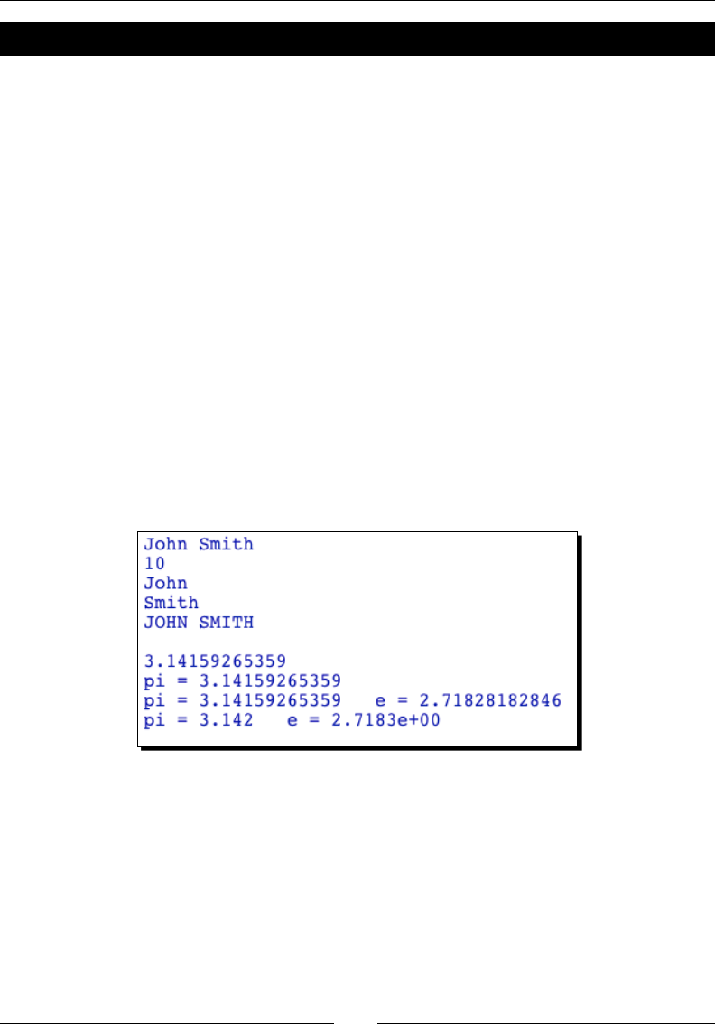
Introducing Python and Sage
[ 90 ]
Time for action – working with strings
Let's see how we can apply the principles of sequence types to strings. We'll also see
how to improve our output with the print funcon. Enter and run the following code:
first_name = 'John'
last_name = 'Smith'
full_name = first_name + ' ' + last_name
print(full_name)
print(len(full_name))
print(full_name[:len(first_name)])
print(full_name[-len(last_name):])
print(full_name.upper())
print('')
n_pi = float(pi)
n_e = float(e)
print(n_pi)
print("pi = " + str(n_pi))
print("pi = {0} e = {1}".format(n_pi, n_e))
print("pi = {0:.3f} e = {1:.4e}".format(n_pi, n_e))
The results should look like this:

Chapter 4
[ 91 ]
What just happened?
We started out by dening two strings that represent a person's rst name (given name)
and last name (family name). We joined the strings using the + operator, and computed the
length of the combined string with the len funcon. We then used some slice operaons
to extract the rst and last name from the string containing the full name. Like everything
else in Python, a string is an object, with a host of pre-dened methods. Because strings
are immutable, methods that modify the string actually return a copy of the string which
contains the modied data. For example, the upper method used in the example returned a
new string containing an upper-case version of the exisng string, rather than modifying the
exisng string. To get around this, we can assign the new string to the old variable:
sage: full_name = full_name.upper()
sage: full_name
'JOHN SMITH'
For a complete list of string methods in Python, check out http://docs.python.org/
library/stdtypes.html#string-methods
In the second part of the example, we used the float funcon to obtain Python oang-
point numbers that approximate pi and e. When we print the value of a number using the
print funcon or the str funcon, we have no control over how that number is displayed.
The format method of the string object gives us much more control over how the numbers
are displayed. We created a special string literal using double quotes, and called the format
method with one or more arguments. The rst argument of the format method is used
to replace {0}, the second argument is used to replace {1}, and so on. This is exactly
equivalent to using the str funcon to convert the numbers to strings, and then joining
them with the + operator. The nal line of the example shows the real advantage of using
format. By placing a format specicaon inside the curly braces, we can precisely control
how numerical values are displayed. We displayed pi as a oang-point number with three
decimal places, and we displayed e as an exponenal with four decimal places. Format
specicaons are very powerful, and can be used to control the display of many types of
data. A full descripon of format specicaons can be found at http://docs.python.
org/library/string.html#format-string-syntax.
The format method is relavely new in Python. A lot of code uses the older syntax:
print 'pi = %5.3f.' % n_pi
While the older syntax sll works, it is deprecated and will eventually be removed from the
language. Get in the habit of using the format method.

Introducing Python and Sage
[ 92 ]
Other sequence types
The principles you have learned in this secon also apply to four other sequence types:
Unicode strings, byte arrays, buers, and xrange objects. We will learn more about xrange
in the next secon. The unicode type is used to hold Unicode strings. Unicode is a system
that is designed to represent almost all of the dierent types of characters used in the vast
majority of the world's languages. In Python 2.x (currently used in Sage), built-in strings (the
str type) do not support Unicode. In Python 3.x, the str class has been upgraded to support
Unicode strings, and the unicode type is obsolete. The bytearray type is designed to store
a sequence of bytes, and seems to be used mainly for working with encoded characters. The
buffer type is rarely used, and has been eliminated from Python 3.
For loops
A Python for loop iterates over the items in a list. The for loop in Python is conceptually
similar to the foreach loop in Perl, PHP, or Tcl, and the for loop in Ruby. The Python for
loop can be used with a loop counter so that it works like the for loop in MATLAB or C, the
Do loop in Mathemaca, and the do loop in Fortran.
Time for action – iterating over lists
Let's say you have some data stored in a list, and you want to print the data in a parcular
format. We will use three variaons of the for loop to display the data.
time_values = [0.0, 1.5, 2.6, 3.1]
sensor_voltage = [0.0, -0.10134, -0.27, -0.39]
print("Iterating over a single list:")
for value in sensor_voltage:
print(str(value) + " V")
print("Iterating over multiple lists:")
for time, value in zip(time_values, sensor_voltage):
print(str(time) + " sec " + str(value) + " V")
print("Iterating with an index variable:")
for i in range(len(sensor_voltage)):
print(str(time_values[i]) + " sec " +
str(sensor_voltage[i]) + " V")
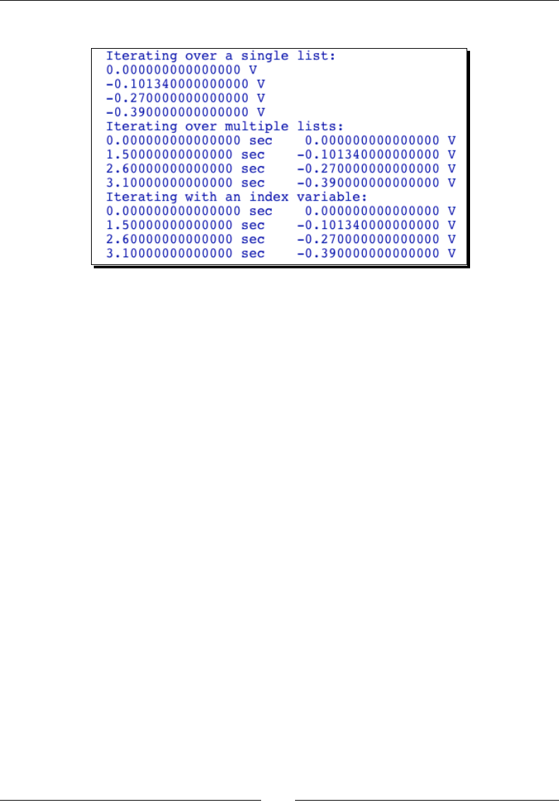
Chapter 4
[ 93 ]
The output should be:
What just happened?
We started by creang two lists: one to hold me values, and one to hold the measured
value at each me point. In the rst for loop, we iterated over the data list and printed
each value. We iterated over the list with the syntax:
for loop_variable in list_name:
statement 1
statement 2
On the rst iteraon, the loop variable takes on the value of the rst item in the list, and the
statements in the loop body are executed. On each subsequent iteraon, the loop variable
takes on the value of the next item in the list, and the statements in the loop body are
repeated for each item in the list.
The second for loop demonstrated how to loop over mulple lists simultaneously with the
zip funcon. zip accepts one or more sequence types (with the same number of elements)
as arguments and returns a list of tuples, where each tuple is composed of the one element
from each sequence. The syntax time,value was used to unpack each tuple, so that we
could access the values through the variables time and value. Iterang over both lists
allowed us to print out both the me and the corresponding measured value, which is much
more useful.
The third loop in the example demonstrated a dierent way to iterate over lists with
the syntax:
for loop_counter in range(len(list_name)):
statement 1
statement 2
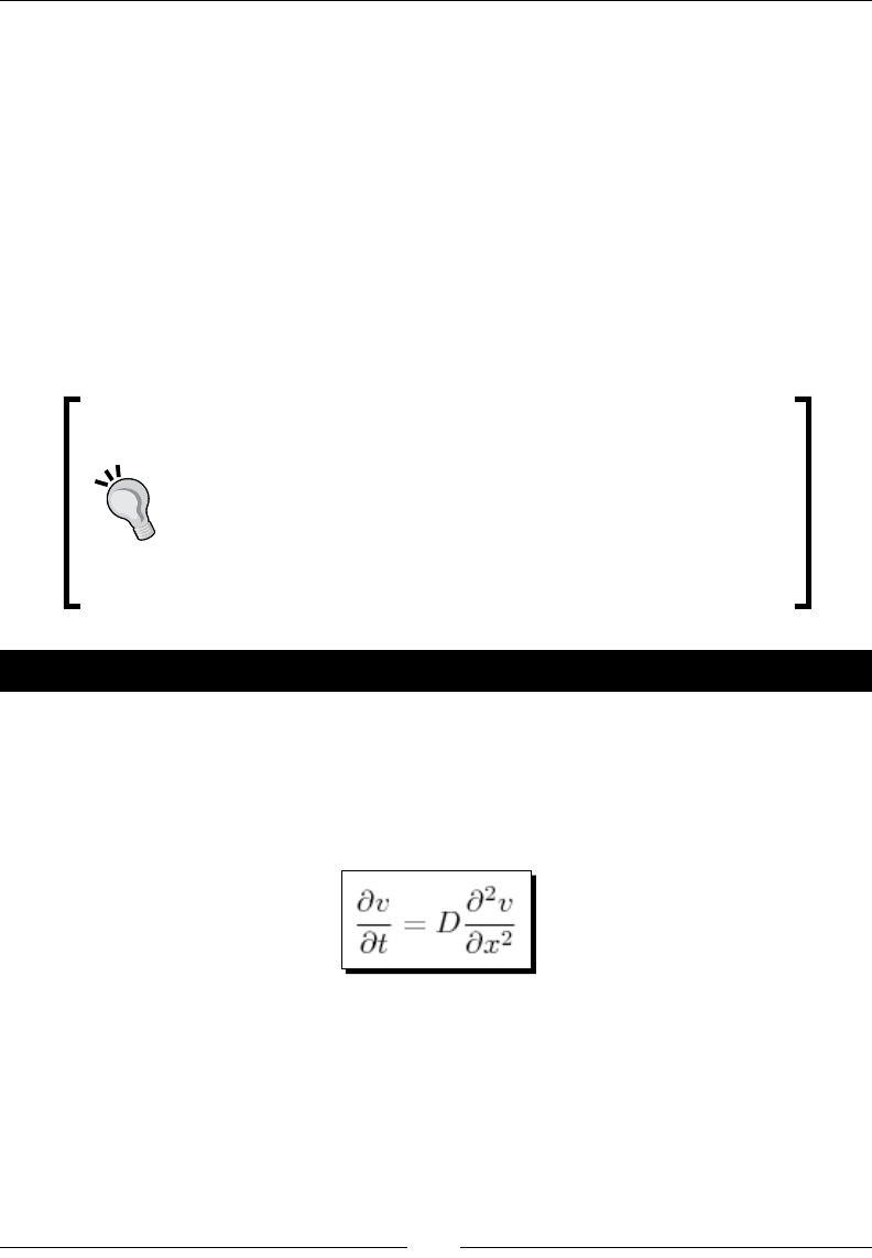
Introducing Python and Sage
[ 94 ]
The range and len funcons were used to generate a list of indices for the given list, and
the for loop iterated over the list of indices. The loop variable i was used as an index to
access the elements of the lists. This technique allows the Python for loop to be used in a
way that is conceptually similar to the for loop in MATLAB or C, the Do loop in Mathemaca,
and the do loop in Fortran.
The Python funcon xrange can be used in place of the range funcon in a for loop to
conserve memory. The range funcon creates a list of integers, and the for loop iterates
over the list. This list of integers can waste a lot of memory if the loop has to iterate millions
of mes. The xrange funcon returns an xrange object, that generates each integer only
when it is required. The xrange funcon accepts the same arguments as range. There is
also a Sage funcon called xsrange, which as before is analogous to srange.
Don't forget to put a colon at the end of the for statement!
Remember to consistently indent every statement in the loop body.
Although the variable i is oen used as a loop counter, the default
value of i in Sage is the square root of negave one. Remember
that you can use the command restore('i') to restore i to its
default value.
Time for action – computing a solution to the diffusion equation
It's me for a more involved example that illustrates the use of for loops and lists in
numerical compung. The analycal soluon to a paral dierenal equaon oen includes
a summaon of an innite series. In this example, we are going to write a short program that
computes a soluon to the diusion equaon in one dimension on a nite interval of length
l. The diusion equaon is dened by:
The diusion equaon can be used to model physical problems such as the diusion of
heat in a solid, or the diusion of molecules through a gas or liquid. The value of v(x,t) can
represent the temperature or concentraon at a point x and me t. The value of v is xed at
each end of the interval:
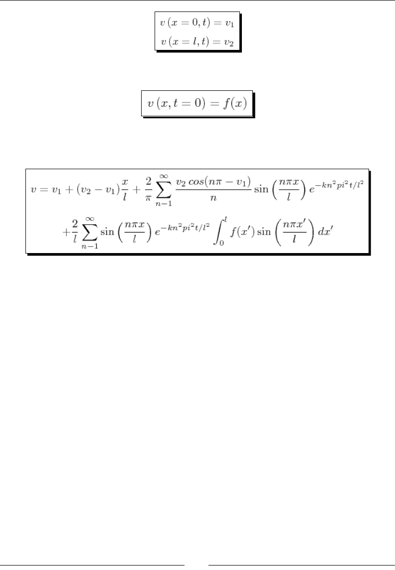
Chapter 4
[ 95 ]
The inial condion is that v is equal to an arbitrary funcon f(x):
The soluon to this boundary value problem can be found in a textbook such as The
Conducon of Heat in Solids by H. S. Carslaw and J. C. Jaeger:
This formula is quite complicated, and it's dicult to understand its physical meaning just by
looking at it. Let's use Sage to visualize the soluon to this boundary value problem. Create a
plain text le using the editor of your choice, and enter the following code. Save the le with
a .sage extension, such as example1.sage. If you are going to use the command line to run
the program, note the path to the locaon where you saved the le.
from matplotlib import pyplot as plt
def diffusion_profile(x,t,v1,v2,k,l):
"""
Compute the value at each point in space for a range of
x values at a single time point.
Arguments:
x list of x values
t time value (real number)
v1 concentration at left boundary
v2 concentration at right boundary
k diffusion coefficient
l length of interval
Returns a list of values at each point in space.
"""
pi_n = pi.numerical_approx()
v = []
for x_val in x:
sum1 = 0.0

Introducing Python and Sage
[ 96 ]
sum2 = 0.0
for n in xrange(1,100):
term1 = (v2 * cos(n * float(pi)) - v1) / n \
* sin(n * float(pi) * x_val/l) \
* exp(-k * n**2 * float(pi)**2 * t / l**2)
sum1 += term1
term2 = sin(n * float(pi) * x_val / l) \
* exp(-k * n**2 * float(pi)**2 * t / l**2) \
* l / (float(pi) * n) * (1 - cos(n * float(pi)))
sum2 += term2
v.append(v1 + ((v2 - v1) * x_val / l
+ 2 / float(pi) * sum1 + 2 / l * sum2))
return v
# Define coefficients
k = 0.1
l = 1.0
v1 = 0.0
v2 = 1.0
t = 1.0
x_max = 1.0
num_x_steps = 10
# Create a list of x values
dx = x_max/num_x_steps
x = srange(0.0, x_max + dx, dx)
# Set up plotting
plt.figure(figsize=(6,4)) # open new plotting window
plt.hold(True) # keep old plots
# Plot
profile = diffusion_profile(x,t,v1,v2,k,l)
plt.plot(x, profile) # plot the profile
# Finalize plot
plt.xlabel('x') # label the x axis
plt.ylabel('v') # label the y axis
plt.title('t='+str(t)) # add a title above plot
plt.axis([0.0, x_max, 0.0, 1.0]) # set xmin, xmax, ymin, ymax
plt.savefig('series_solution.png') # save a picture
Run the source code from the Sage command line or notebook interface using the load
command:
load example1.py
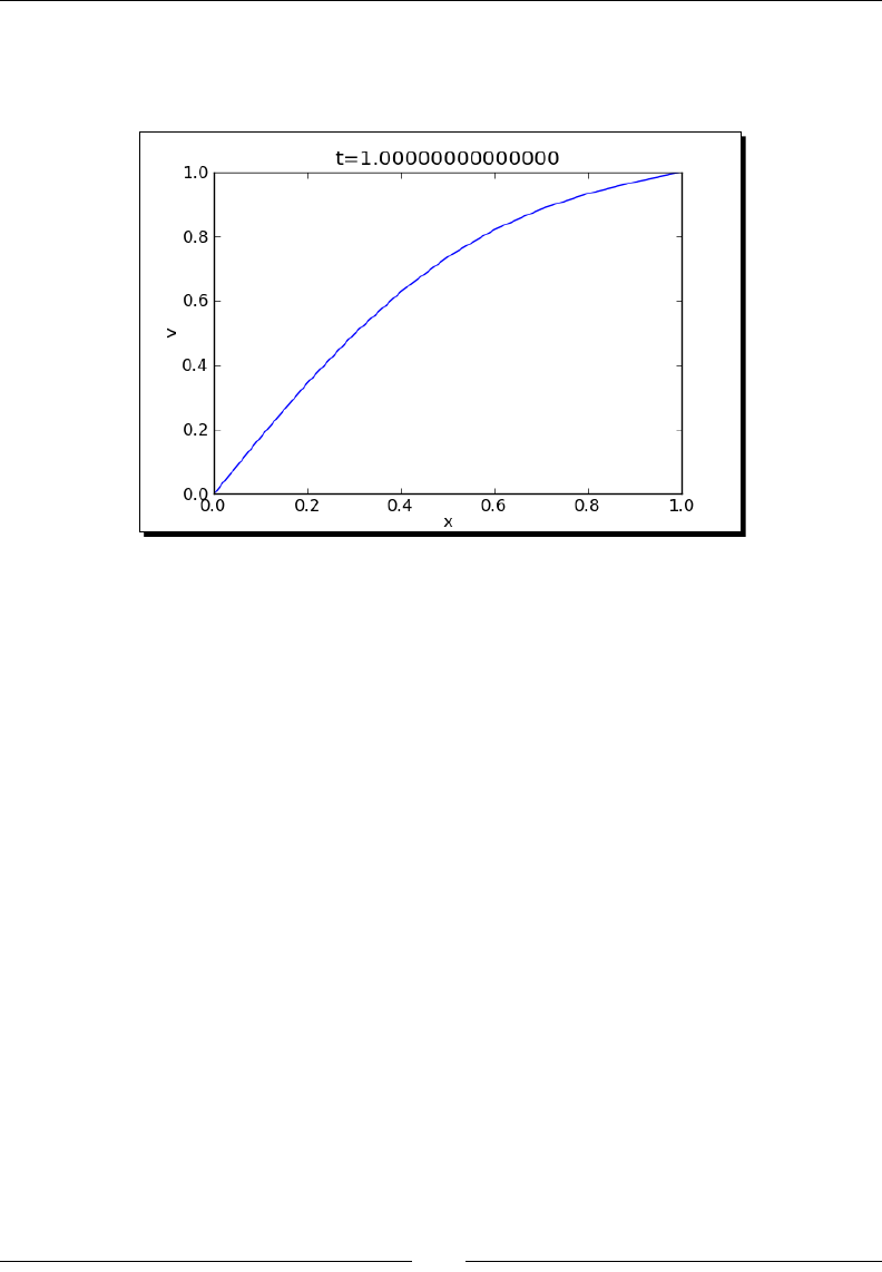
Chapter 4
[ 97 ]
The program saves the plot as an image. If you ran the program from the Sage command
line, you will have to open the le in an image viewer. If you ran the program from the
Notebook interface, Sage will automacally open the image le in a cell in your worksheet.
What just happened?
We dened a funcon that computes the temperature (or concentraon) for a range of
x values at a parcular me. We then dened parameters for the problem, and used the
funcon to solve the problem. We then used funcons from matplotlib to plot the results.
Let's go over each step of the example in more detail.
The funcon was dened as described in Chapter 3. We added a detailed docstring that
documents the arguments and describes what the funcon does. The rst statement in the
funcon used the numerical_approx method to obtain a oang-point representaon of
the symbolic constant pi. The calculaon consists of two nested for loops. The outer loop
iterates over the list of x values. The inner loop is used to sum up the rst 100 terms of the
innite series. The inner for loop uses the xrange funcon to obtain a list counter variable,
which we need to compute the value of each term in the series. With only 100 terms, we
could have used the range funcon in place of xrange. Note that we used the backslash
/ to explicitly join several long lines in the funcon. We also used implicit line joining in the
statement:
v.append(v1 + ((v2 - v1) * x_val / l
+ 2 / float(pi) * sum1 + 2 / l * sum2))
A backslash is not required for this statement because the expression is enclosed in
parenthesis.
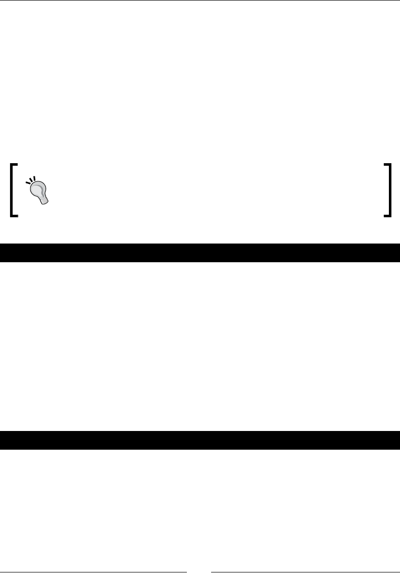
Introducing Python and Sage
[ 98 ]
Dening the parameters for the problem was straighorward. We used the Sage funcon
srange to generate a list of x values. We then used the pyplot interface to matplotlib
to plot the results. The rst line of the script makes funcons and classes from matplotlib
available to our program:
from matplotlib import pyplot as plt
Specically, we are imporng the module called pyplot from the package called matplotlib,
and we are assigning plt as a shortcut to pyplot. To access these funcons and classes, we
use the syntax plt.function_name. This keeps pyplot names from geng mixed up with
Sage names. Plong with pyplot will be covered in detail in Chapter 6.
When loops are nested, the code in the innermost loop executes most oen.
When a calculaon needs to run fast, you will get the greatest speed increase
by opmizing the code in the innermost loop. We'll cover opmizaon in
Chapter 10.
Pop quiz – lists and for loops
1. What is the value of the sum computed in the following loop?
sum = 0
for i in range(10):
sum += i
print(sum)
2. How many lines will be printed when the following loop runs?
for i in range(3):
for j in range(4):
print("line printed")
Enter the code in Sage to check your answers.
Have a go hero – adding another for loop
Try changing the value of the constant t to see the eect on the prole (suggested values:
0.01, 0.05, 0.1, and 1.0). This is a tedious process that can be automated with a for loop.
Dene a list containing me values, and add another for loop that repeats the calculaon
for various values of t.
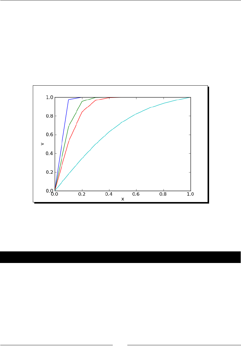
Chapter 4
[ 99 ]
To create a plot like the one shown below, these two plong statements should be placed
before the loop:
plt.figure(figsize=(6,4)) # open new plotting window
plt.hold(True) # keep old plots
Your loop should include only one plong statement in the loop body:
pylab.plot(x, profile) # plot the profile
The rest of the plong statements should come aer the loop.
List comprehensions
A list comprehension is a way of creang a list that is similar to a for loop, but more
compact.
Time for action – using a list comprehension
Let's see how list comprehensions work by comparing them to a for loop that performs a
similar operaon. Enter the following code in a text le or an input cell in a worksheet:
list1 = [' a ', ' b ', 'c ']
list1_stripped = []
for s in list1:
list1_stripped.append(s.strip())
print(list1_stripped)
list1_stripped_2 = [s.strip() for s in list1]
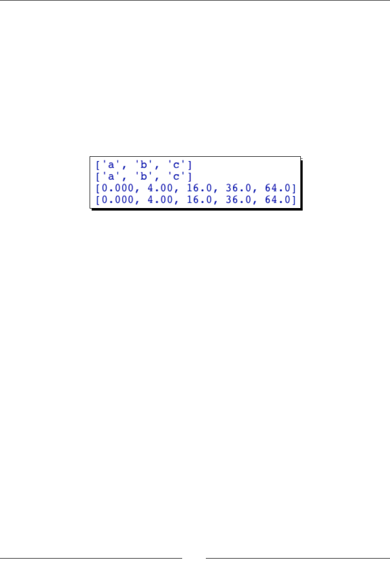
Introducing Python and Sage
[ 100 ]
print(list1_stripped_2)
list2 = []
for val in srange(0.0, 10.0, 1.0):
if val % 2 == 0:
list2.append(numerical_approx(val**2, digits=3))
print(list2)
list3 = [numerical_approx(val**2, digits=3) for val in
srange(0.0, 10.0, 1.0) if val % 2 == 0]
print(list3)
Run the example. You should get:
What just happened?
This example demonstrated how a list comprehension can be used in place of a for loop
to create a list. In the rst part of the example, we dened a list of strings, each of which
contained whitespace before and/or aer the character. First, we dened an empty list and
used a for loop to iterate over the list of strings. The string method strip was used to
remove the whitespace from each string, and we used the list method append to create
a new list of stripped strings. We then used a list comprehension to perform the same
operaon. The general syntax for a list comprehension is:
new_list = [ operation_on_value for value in existing_list ]
If you are creang a new list, then the exisng list can be generated by a funcon like range
or srange. In the second part of the example, we used a for loop with the srange funcon
to generate a list of even oang-point numbers. We used an if clause so that our list
will contain only squares of even numbers. We did this to demonstrate how the if clause
works—a beer way to generate a list of even numbers would be to give srange a step size
of two. We then repeated the operaon with a list comprehension. We'll learn more about
if statements soon. List comprehensions are somewhat more compact than an equivalent
for loop. For more examples of list comprehensions, see http://docs.python.org/
tutorial/datastructures.html#list-comprehensions

Chapter 4
[ 101 ]
While loops and text le I/O
Lists and loops are the two basic tools we need to access data that is stored in a le. The
problem with using a for loop to access a data le is that we don't necessarily know how
many iteraons will be needed, because we don't always know how many lines are in the
le. The soluon is to use a while loop.
Time for action – saving data in a text le
Let's save the results of a calculaon to a text le. In the next example, we will get the data
back into Sage. When you enter the following code, change the path to the data le so that it
gets saved in a convenient locaon.
from matplotlib import pyplot as plt
import os
# Create some data
times = srange(0.0, 10.0, 0.1)
data = [sin(t) for t in times]
# Plot the data
plt.figure(figsize=(6,4))
plt.plot(times, data)
plt.savefig('example2a.png')
plt.close()
# Save data to a text file
path = '/Users/cfinch/Documents/Writing/Sage for Beginners/Chapters/
Chapter 4/'
fileName = 'data.txt'
text_file = open(os.path.join(path, fileName), 'w')
for i in range(len(data)):
text_file.write('{0}, {1}{2}'.format(times[i], data[i],
os.linesep))
text_file.close()
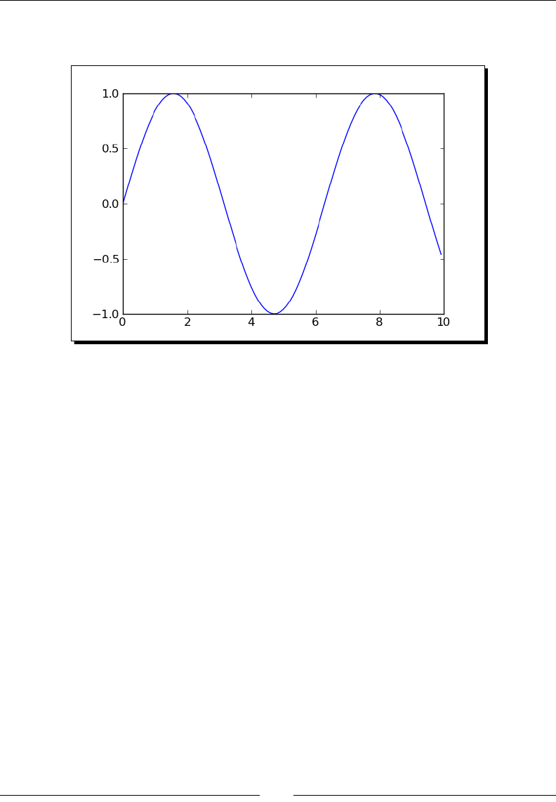
Introducing Python and Sage
[ 102 ]
Run the script using one of the methods previously described. A plot of the data is saved to a
PNG le, and the data is saved to a text le with two columns. The plot should look like this:
The rst few lines of the text le should look like this:
0.000000000000000, 0.000000000000000
0.100000000000000, 0.0998334166468282
0.200000000000000, 0.198669330795061
What just happened?
We used the srange funcon to generate a list of me points, and then used a list
comprehension to create a list containing the sine of each me point. We ploed the data,
using the pyplot interface to matplotlib, like we did in a previous example. The data
was then saved to a text le.
The le object is the key component in le operaons. A le object is created using the
open funcon:
text_file_object = open('data.txt', 'w')
The rst argument to open is a string containing the name of the le. The second argument
is a string that indicates in which mode the le should be opened. The rst leer of the
mode string chooses read, write, or append mode. The leer b can be appended to the
mode string to indicate that the le should be opened in binary mode. If the mode string is
omied, the le is opened for reading in text mode.

Chapter 4
[ 103 ]
Text
mode
string
Binary mode
string
Result
r rb File is opened for reading. The le must already exist. Aempng to
write to the le returns an error.
w wb File is opened for wring. If the le exists, it will be overwrien.
a ab File is opened for appending. Data that is wrien to the le will be
appended at the end of the le.
If you open a le in text mode, the special character \n may be converted to the appropriate
newline character for your plaorm. If you don't want this conversion to happen, add the
leer 'b' to the end of the mode string to open the le in binary mode.
We used the write method of the le object to write data to the le:
text_file.write(my_string)
The write method accepts one argument, which is the string to be wrien to the le. When
we were nished with the le, we used the close method to close it. It's very important to
close a le, especially when the le is open for wring. Many operang systems buer data,
rather than wring every lile piece of data to the le. Closing the le is the easiest way to
ensure that all of the data actually gets wrien to the le.
We used a module called os from the Python standard library module to help us write code
that can run on mulple plaorms. A text le must have a special character to denote the
end of each line in the le. Unfortunately, for historical reasons, each family of operang
systems (Mac, Windows, and UNIX) uses a dierent end-of-line character. The os module has
a constant called linesep that contains the correct character for the plaorm that the code
is run on. We used the statement import os to make the module available, and accessed
the constant using the syntax os.linesep. We also used the funcon os.path.join to
join the path to the le name with the correct character for the current operang system.
Time for action – reading data from a text le
Now, we will read the data from the text le. This is a good place to demonstrate the
while loop, since we won't always know in advance how many lines are in the le. Run the
following code to load the data.
from matplotlib import pyplot as plt
import os
path = '/Users/cfinch/Documents/Writing/Sage for Beginners/Chapters/
Chapter 4/'
fileName = 'data.txt'
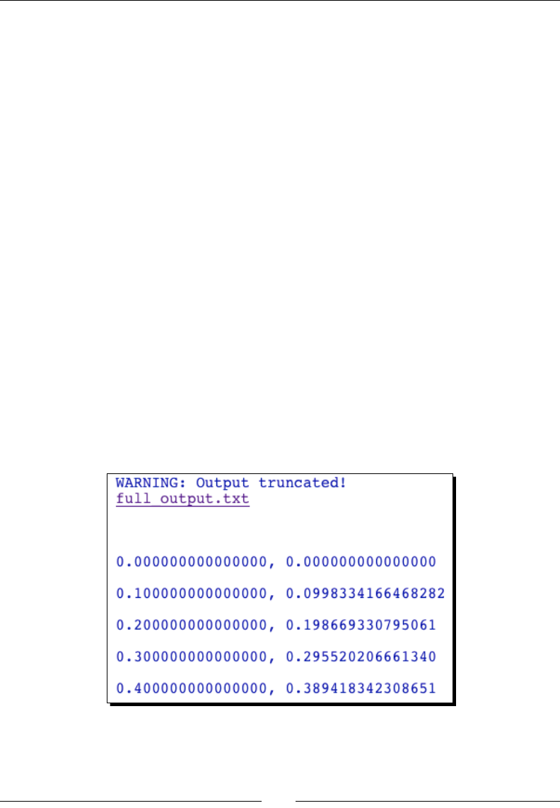
Introducing Python and Sage
[ 104 ]
# Read in the data file
times = []
data = []
text_file = open(os.path.join(path, fileName), 'r')
line = text_file.readline()
while len(line) > 0:
print(line)
# split each line into a list of strings
elements = line.split(',')
# Strip newlines and convert strings to real numbers
times.append(float(elements[0].strip()))
data.append(float(elements[1].strip()))
line = text_file.readline()
text_file.close()
# Plot the data
plt.figure()
plt.plot(times, data)
plt.savefig('example2b.png')
plt.close()
The data is ploed to another image le. This plot should be idencal to the plot in the
previous example. When you run this example in the Notebook interface, Sage will not print
every line of the le. When text output gets too long, Sage will truncate the output and
provide a link that you can click to see the rest of the output. The result will look like this:

Chapter 4
[ 105 ]
What just happened?
This script demonstrated how to open a text le for reading and read in one line at a me.
The open funcon was used to create a le object as previously described. Since we are
reading data, the readline method was used to read one line of data from the le and
return the line as a string. Once again, we used the os module to handle operaons involving
paths and newlines.
While loops
A while loop is used when we don't know how many iteraons will be required. The general
syntax for a while loop is:
while conditional_expression:
statement 1
statement 2
...
The loop iterates as long as the condional expression evaluates to the Boolean value True.
The loop terminates as soon as the expression evaluates to False. In this example, the
loop iterates as long as the string that is read from the le has one or more characters. The
readline method returns a string for every line in the le. Even a blank line has a newline
character, so the condional expression will be True for every line in the le. The readline
method returns an empty string aer reading the last line of the le, which causes the
condional expression to evaluate to False and end the loop. There are two very important
things to remember when using a while loop:
1. Make sure the condional expression can be evaluated before the rst iteraon of
the loop. In the example, the rst line is read from the le before the while loop.
2. Make sure that the condional expression will evaluate to False at some point.
Otherwise, the loop will repeat endlessly. The last statement of the loop in the
example loads another line from the le. When the end of the le is reached, the
condional expression will evaluate to False.
Parsing strings and extracting data
Since each line of the le was read as single string, we had to do some work to extract the
numerical data. First, we used the split method of the string object to break the string
at the comma:
elements = line.split(',')

Introducing Python and Sage
[ 106 ]
The result was a list of strings called elements. The rst element of this list is the string that
contains the me value. Next, we used the strip method of the string object to remove
any unnecessary white space, such as the invisible newline character that is found at the end
of every line:
elements[0].strip()
Finally, we used the float funcon to convert the string to a Python oang-point number,
and appended the result to a list. In the example, the parsing operaons were combined like
this:
times.append(float(elements[0].strip()))
data.append(float(elements[1].strip()))
Finally, the lists are ready to be ploed.
Alternative approach to reading from a text le
A Python le object is iterable, which means that you can iterate over a le object just like
you can iterate over a list. This allows you to use the following syntax:
for line in text_file:
# split each line into a list of strings
elements = line.split(',')
# Strip newlines and convert strings to real numbers
times.append(float(elements[0].strip()))
When using this approach, you should not include a call to text_file.readline() in
the loop body.
Have a go hero – dene a function for reading the text le
It's good pracce to organize your code as you're wring. In the previous example, we should
separate the code that reads the data from the le from the code that does the plong.
Dene a funcon that takes a le name as an argument and reads the data. Use a tuple to
return a list of me values and a list of data values. Call the funcon to read the data, and to
plot the data.

Chapter 4
[ 107 ]
Have a go hero – replace a for loop with a while loop
In a previous example, we used a for loop to sum up the rst 100 terms of an innite
series. The number 100 was chosen somewhat arbitrarily because it happened to work for
this parcular example. Some innite series may require more than 100 terms to converge,
while others may only require a few terms. We can improve this aspect of the program by
replacing the for loop that performs the summaon with a while loop. The summaon
should connue unl the sum changes very lile from one iteraon to the next.
If statements and conditional expressions
We have already seen condional expressions in the context of while loops. Condional
expressions can be used with if statements to allow a program to make decisions while it is
running. There are numerous applicaons for if statements. For example, they can be used
to detect invalid values and prevent errors:
input_value = 1e99
if input_value > 1e10:
print("Warning: invalid parameter detected.")
else:
print("--- Start of iteration ---")
The general syntax for an if statement is the following:
if conditional_expression:
statements
else:
statements
The else clause is oponal. Python doesn't have a switch statement for choosing between
mulple values. Instead, it has a special keyword called elif, which is a contracon of "else
if." This can be used to emulate a switch statement. For example, we can use if with elif
to choose an algorithm based on user input:
solution_type = "numerical"
if solution_type == "analytical":
print('analytical')
elif solution_type == "numerical":
print("numerical")
elif solution_type == "symbolic":
print("symbolic")
else:
print("ERROR: invalid solution type")

Introducing Python and Sage
[ 108 ]
if statements are not ideal for catching runme errors. In Chapter 9, we
will learn about excepons, which are a much more elegant way to deal with
runme errors.
Storing data in a dictionary
Diconaries are another fundamental data structure in Python. A diconary is similar to a
list in that it is comprised of a series of data elements. One important dierence is that a
diconary uses "keys" instead of indices to access elements. The keys can be strings or other
data types. While a list is a sequence, the elements in a diconary don't have any intrinsic
order. A diconary is a good choice to collect dierent types of data.
Time for action – dening and accessing dictionaries
Let's go back to our program that computes an analycal soluon to a boundary value
problem. Certain parameters are required to carry out the calculaon. So far, we just stored
the parameter as a collecon of numbers. In a more complex program, this simplisc
approach could introduce subtle bugs if we accidentally used one of the parameter variables
for something else.
# Define parameters
k = 0.1
l = 1.0
v1 = 0.0
v2 = 1.0
t = 1.0
num_x_steps = 10
# Store parameters in a dictionary
parameters = { 'diffusion coefficient' : k,
'length' : l,
'left_BC' : v1,
'right_BC' :v2,
'time' : t,
'num_x_steps' : num_x_steps
}
# Access the dictionary
print("Value of time is {0}".format(parameters['time']))
parameters['time'] = 2.0
print("New value of time is {0}".format(parameters['time']))
print('')
print("Dictionary contains {0} items:".format(len(parameters)))
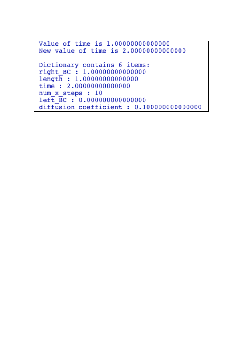
Chapter 4
[ 109 ]
for key, value in parameters.iteritems():
print('{0} : {1}'.format(key, value))
Run the script and review the output, which should look like this:
What just happened?
We have collected a variety of parameters into a single data structure using a diconary. We
used strings as keys to the diconary to make it easy to recall parameter values. We dened
the diconary using curly brackets to enclose key-value pairs:
empty_dict = {}
my_dict = { key1:value1, key2:value2, …, keyN:valueN}
Many operaons on diconaries are analogous to operaons on lists. We demonstrated
how to get and set values of items in the diconary using square brackets:
value = my_dict['key name']
Because the keys are not necessarily numbers, there is no equivalent of slices for
diconaries. The len funcon is also used to return the number of (key,value) pairs in a
diconary.
We then iterated over the diconary to print the keys and values using the iteritems
method:
for key, value in parameters.iteritems():
print(key)
print(value)
The method iterkeys iterates only over the keys, while itervalues iterates only over
the values. A full list of diconary methods can be found at http://docs.python.org/
library/stdtypes.html#dict
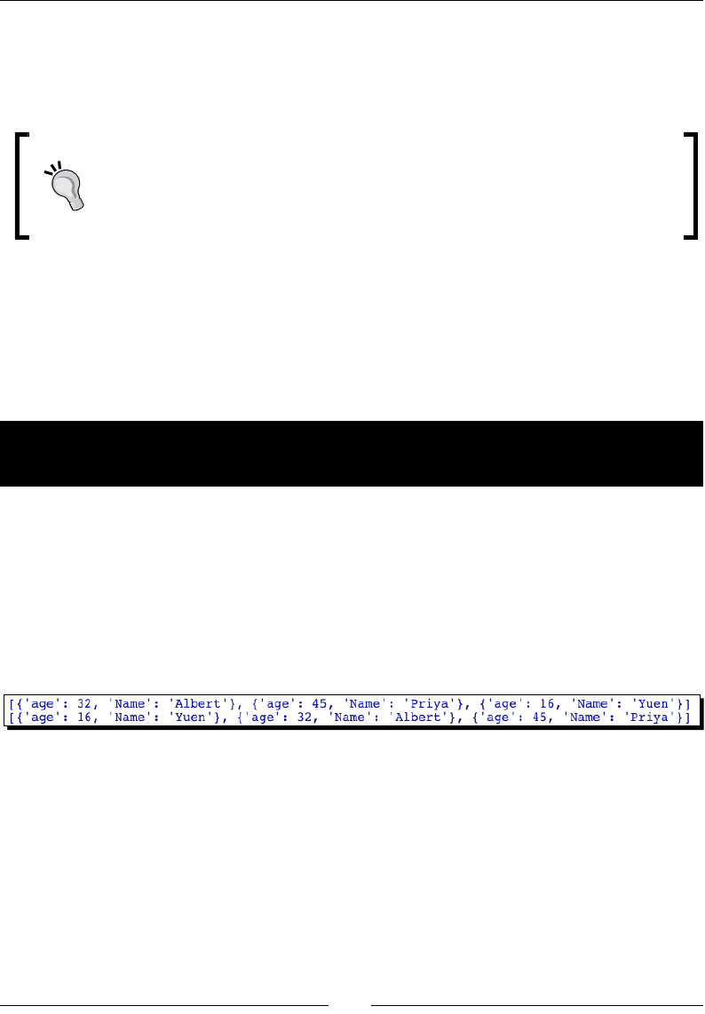
Introducing Python and Sage
[ 110 ]
Note that iterang over a diconary won't necessarily print the items in the same order
every me! An important disncon between diconaries and lists is that the elements in
a diconary have no intrinsic order. You should not rely upon the elements of a diconary
being returned in any parcular order.
Ordered diconaries
Python 2.7 and versions above 3.1.3 contain a new class called OrderedDict,
which works just like an ordinary diconary except that it remembers the order
in which items were inserted. This class is not available in Sage 4.6.1 because
Sage is sll using Python 2.6, but it should be available soon.
Lambda forms
Somemes you need to dene a short, simple Python funcon. You can always use the def
keyword to dene the funcon and give it a name. You can also use the lambda keyword to
dene an anonymous funcon that consists of a single expression.
Time for action – using lambda to create an anonymous
function
Why would you want an anonymous funcon? Let's try sorng a list of diconaries:
data = [{'Name':'Albert', 'age':32},
{'Name':'Yuen', 'age':16},
{'Name':'Priya', 'age':45}]
print(sorted(data))
print(sorted(data, key=lambda item : item['age']))
The results should look like this:
What just happened?
We dened a list of diconaries, each of which contains data about a person. We then
used the sorted funcon to sort the items in the list. The rst me we called sorted, it
appeared that the list had been sorted alphabecally, by the rst leer of each name. This
behaviour is unpredictable—if we added a last name to each diconary, would the rst
or last name be used as the sorng key? To prevent this kind of problem, we can use the
keyword key to specify a funcon that is called on each item before sorng takes place. In
the second funcon call, we used lambda to dene an anonymous funcon that returns the
integer value of 'age' from the diconary. We can see that the list is now sorted by age.

Chapter 4
[ 111 ]
The general syntax for declaring an anonymous funcon with lambda is:
lambda arg_1, arg_2, ... , arg_n : expression
There can be mulple arguments, but only one expression. Like nested funcons, lambda
forms can reference variables from their containing scope. Lambda forms are not used oen
in Python programming, but they do show up occasionally in Sage examples.
Summary
We learned about some key aspects of Python in this chapter. When combined with the
informaon in Chapter 3, we now have all the tools we need to implement algorithms in
Sage.
Specically, we covered:
How to create and run Sage scripts
Basic principles of sequence types like lists, tuples, and strings
How to store data more permanently in text les
Repeang operaons and iterang over lists with loops
Using condional expressions and logic to make decisions in a program
How to use diconaries to store data
This chapter provides a working knowledge of Python, but it is hardly complete. Refer to
the Python documentaon on the Web to learn more about the details of this powerful
programming language. Now that we have been introduced to sequence types like lists, we
can learn about specialized array and matrix types for performing mathemacal calculaons.
5
Vectors, Matrices, and Linear Algebra
Linear algebra is a fundamental task for mathemacal soware. Linear algebra is easily
automated because it involves tedious computaons that must be performed according
to well-dened formulas and algorithms. Sage has extensive support for various types of
calculaons with vectors and matrices. Sage's vector and matrix objects build upon the basic
mathemacal types that we learned about in Chapter 3. We will also learn about a Python
library called NumPy that is very useful for numerical calculaons.
In this chapter we will:
Learn how to create and manipulate vector and matrix objects
See how Sage can take the tedious work out of linear algebra
Learn about matrix methods for compung eigenvalues, inverses, and
decomposions
Get started with NumPy arrays and matrices for numerical calculaons
There are many ways to do linear algebra in Sage. Sage is a collecon of tools, each of which
has its own way of represenng vectors and matrices. Therefore, you will nd that there are
mulple ways to accomplish the same thing. We will focus on the high level constructs that
are unique to Sage. Then, we will introduce the NumPy package, which provides a powerful
set of tools for numerical computaon. Let's get started!
Vectors and vector spaces
Vectors and matrices are so important that they are represented by special types of objects
in Sage. We'll start with vectors.

Vectors, Matrices, and Linear Algebra
[ 114 ]
Time for action – working with vectors
Vectors have important applicaons in physics and engineering. Vectors are used to
represent posion, velocity, angular momentum, electromagnec elds, and so on. Let's see
how to perform some basic operaons with vectors in Sage. You can enter the following code
in an input cell in a worksheet, or enter it line by line in the interacve shell. You can also
enter the code into a plain text le, save it with a .sage extension, and run it from the Sage
command line as described in the previous chapter:
R3 = VectorSpace(QQ, 3)
(b1, b2, b3) = R3.basis()
print("Basis for space:")
print b1
print b2
print b3
vector1 = R3([-1, 2, 7]) # define some vectors
vector2 = R3([4, -9, 2])
print("Linear combinations:")
var('a b')
print(a * vector1 + b * vector2)
print("Norm of vector 1:")
print(sqrt(vector1 * vector1)) # definition
print(vector1.norm()) # using norm method
print("Scalar multiplication:")
print(2 * vector1)
print("Scalar (dot) products:")
print(vector1 * vector2) # using operators
print(vector1.inner_product(vector2)) # using methods
print(b1 * b2)
print("Pairwise product:")
print(vector1.pairwise_product(vector2))
print("Vector (cross) product:")
print(vector1.cross_product(vector2))
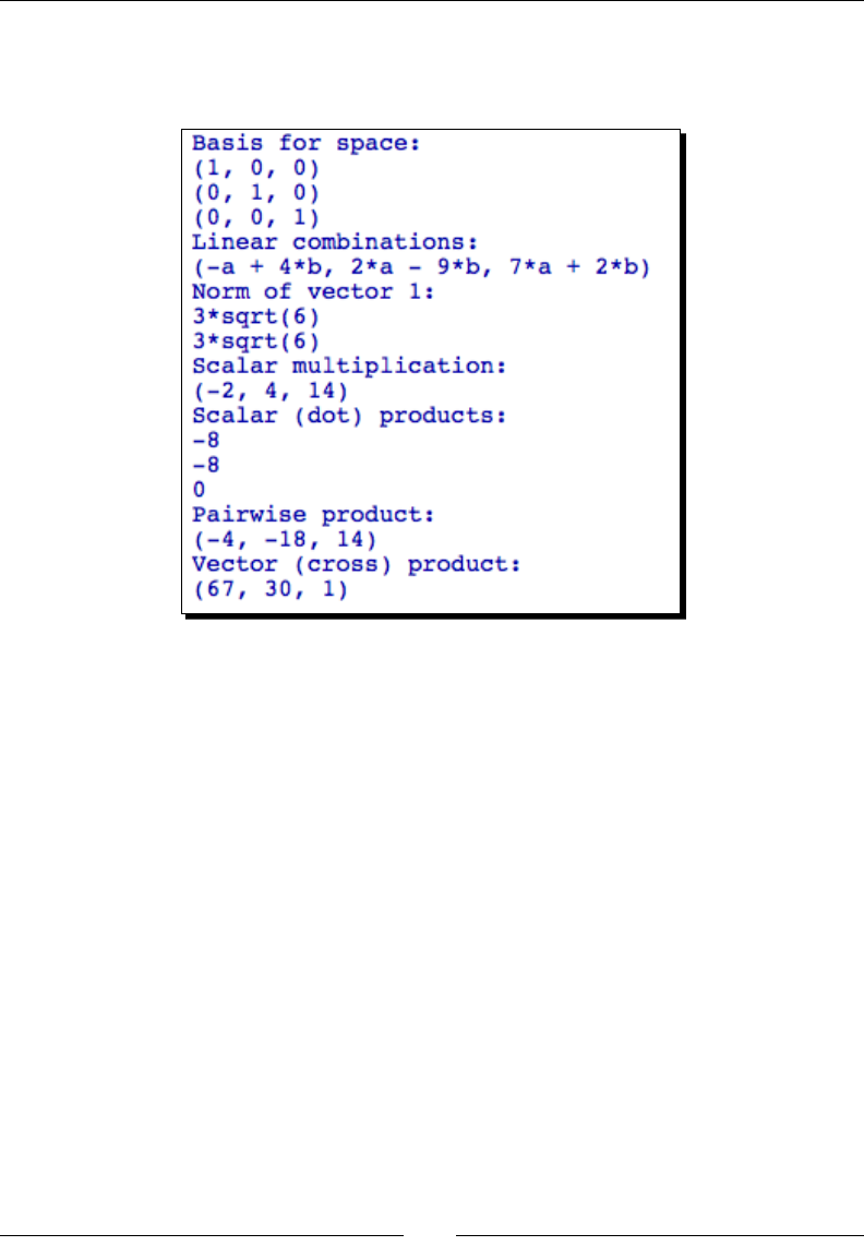
Chapter 5
[ 115 ]
Execute the code (remember that you can press Shi-Enter in an input cell to run the code
from the Notebook interface). If you are using the notebook interface, the result should
look like this:
What just happened?
This example demonstrated some of the most useful operaons that Sage can perform on
vectors. We started by dening a vector space that consists of three-element vectors with
raonal numbers as elements. While it's not strictly necessary to dene the vector space, it
does provide some helpful tools, such as access to the basis vectors of the space. We then
dened a pair of vectors and demonstrated various operaons, such as the cross product
and dot product.
Creating a vector space
The VectorSpace class is used to create an object that represents a vector space.
my_vector_space = VectorSpace(base_field, dimension)
The rst argument is the base eld, such as the eld of raonal, real, or complex numbers,
over which the vector space is dened. You can also dene a vector space over the symbolic
ring to perform symbolic calculaons. The second argument is the dimension of the space,
which is eecvely the number of elements in each vector.

Vectors, Matrices, and Linear Algebra
[ 116 ]
At this point, it is important to explain more about rings and elds. Rings were introduced in
Chapter 3. Fields are a superset of rings; every eld is a ring, but not every ring is a eld. The
following table summarizes the rings and elds that we have used so far:
Full name Shortcut Ring? Field? Descripon
IntegerRing ZZ Yes No Integers
RationalField QQ Yes Yes Raonal numbers
RealField RR Yes Yes Real numbers
ComplexField CC Yes Yes Complex numbers
All of the rings we have used so far are also elds, with the excepon of integers. Therefore,
you cannot use integers as the base eld for a vector. However, you can use the symbolic
ring SR as a base eld for a vector or vector space. The reason is that the symbolic ring is not
a ring in the strict mathemacal sense. The symbolic ring is simply a way of stang that a
parcular construct will contain symbols instead of numerical values.
Creating and manipulating vectors
There are two ways to create a vector object. In the example, we rst dened a vector space,
and used the vector space to create the vector. A list of elements (of the appropriate length)
is used to dene the elements of the new vector:
new_vector = my_vector_space([element_1, element_2, element_n])
The other way is to use the vector funcon, which automacally constructs a vector space
over the specied eld and returns a vector object:
new_vector = vector(base_field,[element_1, element_2, element_n])
The rst argument is the base eld, and the second is a list of elements. Both ways return
equivalent vectors.
Time for action – manipulating elements of vectors
The elements of a vector can be manipulated like the elements of any other Python
sequence type, such as lists and strings. That means individual elements are accessed using
square brackets, as shown in the following example:
u = vector(QQ, [1, 2/7, 10/3]) # QQ is the field of rational
numbers
print("u=" + str(u))
print("Elements: {0}, {1}, {2}".format(u[0], u[1], u[2]))
print("The slice [0:2] is {0}".format(u[0:2]))
print("The last element is {0}".format(u[-1]))
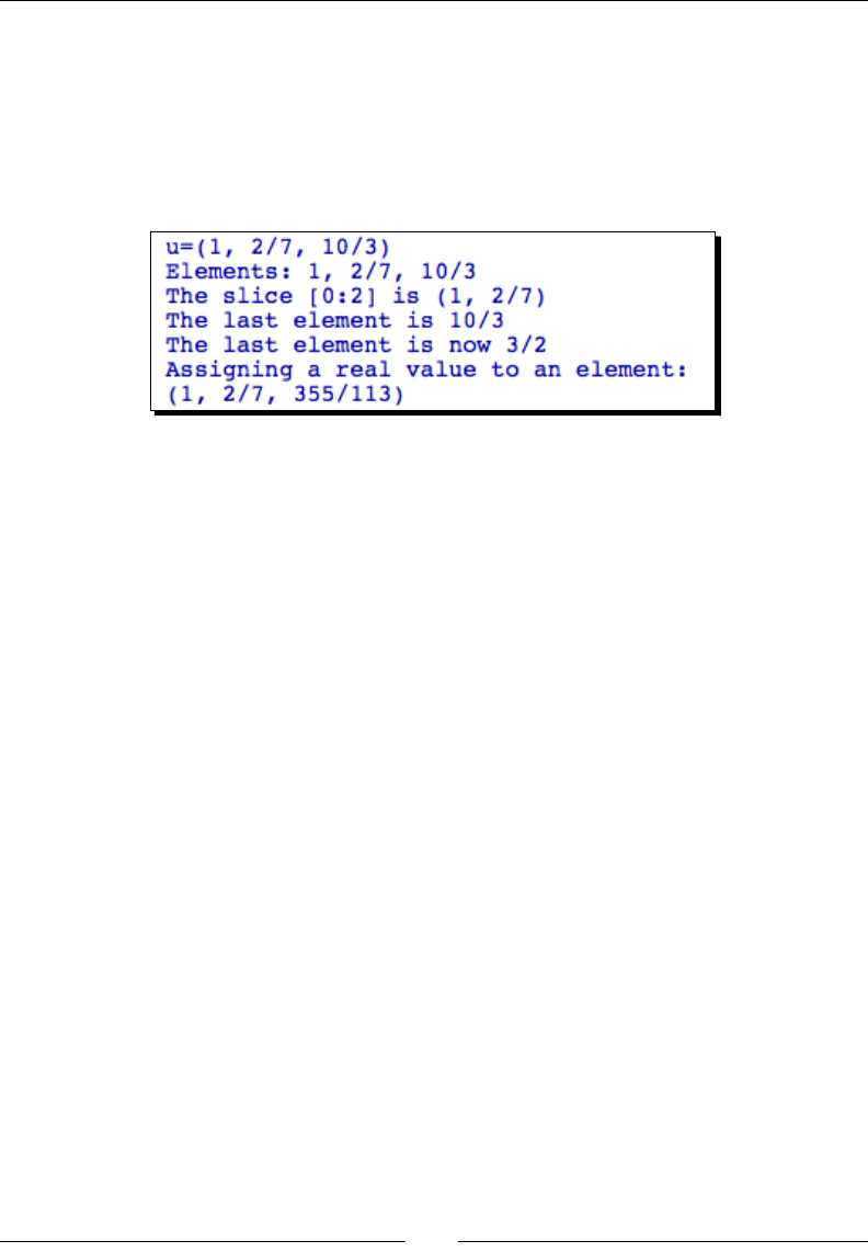
Chapter 5
[ 117 ]
u[len(u) - 1] = 3/2
print("The last element is now {0}".format(u[-1]))
print "Assigning a real value to an element:"
u[2] = numerical_approx(pi, digits=5)
print(u)
The output from this code will look like this if you are using the notebook interface:
What just happened?
We created a vector called u, dened over the eld of raonal numbers (remember that QQ
is a short form of RationalField) and manipulated the elements of the vector just like
elements in a list. We demonstrated that the usual tricks for accessing list elements work on
vectors. When we accessed an individual element of the vector, the result had a numerical
type. When we used slicing to extract one or more elements from a vector, the resulng
elements were returned as a vector object. We also used indexing to change the value of an
element in the vector.
Something interesng happened when we tried to assign a real value to an element of the
vector. Rather than returning an error, Sage found a raonal number to represent the real
value. The lesson here is that it's important to choose the right base eld in order to get the
right results. In general, you can use the RealField (RR) for most numerical calculaons,
unless you are working with complex number, when you should use ComplexField (CC).
For purely symbolic calculaons, use the symbolic ring SR.
Vector operators and methods
Sage supports a wide variety of arithmec operaons on vectors. The operators + and
– perform vector addion and subtracon, respecvely. The * operator performs scalar
mulplicaon if one variable is a vector and the other is a scalar. If both variables are vectors,
the * operator returns the inner (or scalar) product. The inner product is also available as a
method of the vector object, as shown in the example. Other vector methods include:
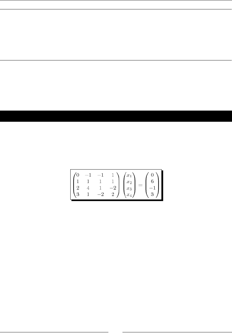
Vectors, Matrices, and Linear Algebra
[ 118 ]
u.dot_product(v) Same as the inner product u.v
u.cross_product(v) Cross product u x v
u.inner_product(v) Inner (scalar)product u.v
u.pairwise_product(v) Returns the vector (u[0]*v[0], u[1]*v[1], … , u[n-1]*v[n-1])
u.norm(p) p-norm of vector u. p=0 is the Euclidean norm. p=1 is the sum of the
elements, and p=Innity is the maximum element in u.
Matrices and matrix spaces
We will now look at matrices and matrix spaces. Sage uses a dierent type of object to
represent matrices.
Time for action – solving a system of linear equations
One of the most basic operaons in mathemacs is solving a system of linear equaons.
Many sophiscated numerical techniques, such as the nite element method, are designed
to reduce a complicated problem to a system of linear algebraic equaons that must be
solved. Let's see how vectors and matrices in Sage can make this easier. We will repeat the
example from Chapter 1, and explain it in more detail:
Enter the following code in a worksheet. If you are using the interacve shell, you will need
to have LaTeX installed to use the show command. If you don't have LaTeX, replace show
with print in this example and the ones that follow:
M4 = MatrixSpace(QQ, 4) # Rational numbers
print("Identity matrix:")
show(M4.identity_matrix())
A = M4.matrix([[0, -1, -1, 1], [1, 1, 1, 1], [2, 4, 1, -2],
[3, 1, -2, 2]])
print("Matrix A:")
show(A)
b = vector(QQ, [0, 6, -1, 3]) # Rational numbers
print("Vector b:")
show(b)
solution = A.solve_right(b)
print("Solution to A.x=b:")
show(solution)
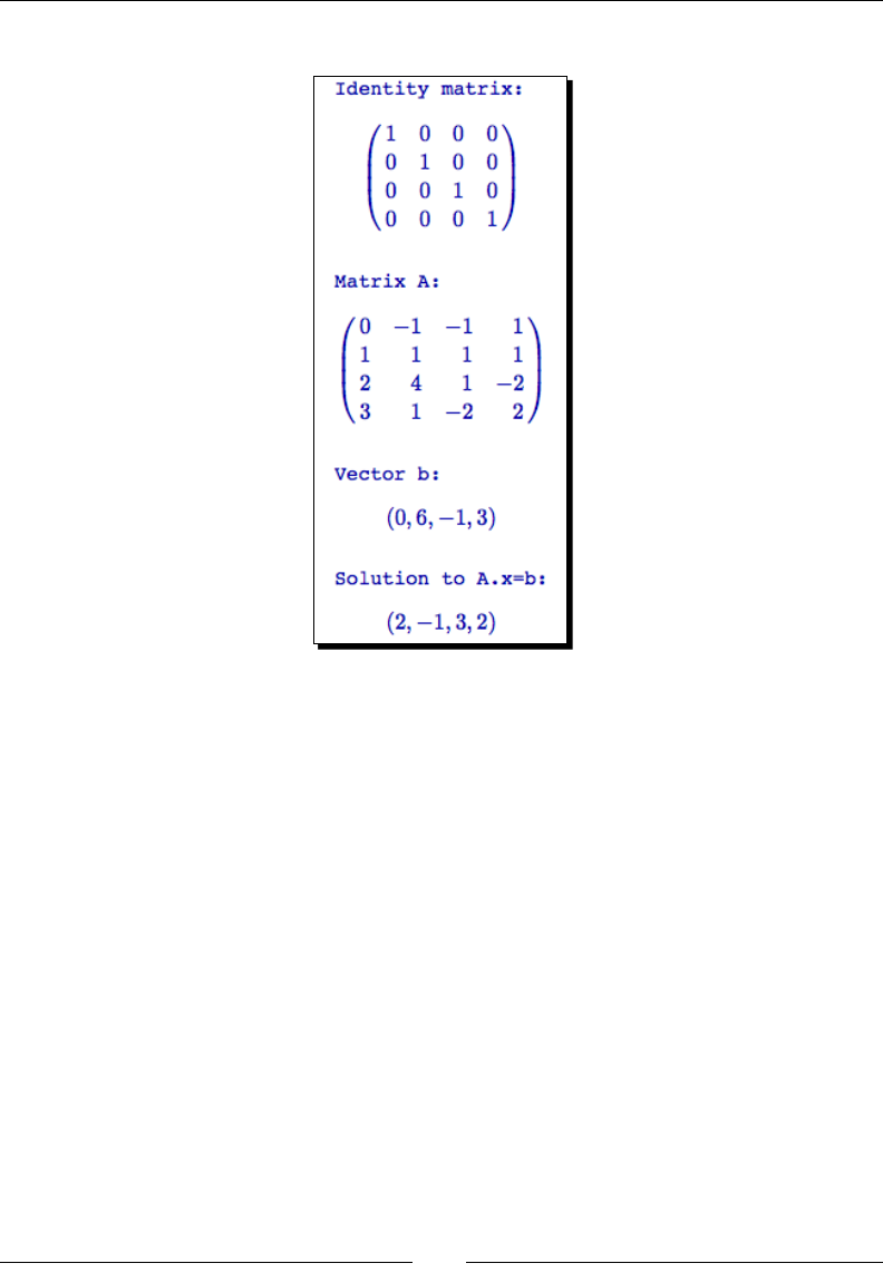
Chapter 5
[ 119 ]
Execute the code. The result will look like this:
What just happened?
We solved a system of linear equaons in just a few lines of code. First, we created a space of
4x4 matrices, dened over the ring of raonal numbers. We were able to get away with using
raonal numbers because this is a textbook example that was contrived to have an integer
soluon! In pracce, it makes more sense to dene a matrix over the ring of real or complex
numbers. Dening the matrix space gave us access to the appropriate identy matrix. We
used the show funcon to display the matrix as it would appear in a typeset document. You
can also use the print funcon. We then created a matrix in this space, and lled it with
integer elements. We also dened a vector of the appropriate length, and used the solve_
right method to solve the matrix equaon Ax=b. The backslash operator can be used as a
shortcut for the solve_right method:
A\b # equivalent to A.solve_right(b)

Vectors, Matrices, and Linear Algebra
[ 120 ]
Creating matrices and matrix spaces
The MatrixSpace class is used to create an object that represents a matrix space. The rst
argument is the base ring. Note that MatrixSpace requires a ring as its rst argument,
while VectorSpace requires a eld. The second argument is the number of rows in the
matrix, and the third argument is the number of columns. If the third argument is omied,
the matrix is assumed to be square. The oponal fourth argument can be used to indicate
that the matrix is sparse, which can reduce memory usage.
my_matrix_space = MatrixSpace(base_ring , nrows [, ncols] [, sparse])
Creang new matrices is similar to creang new vectors. Each row of the matrix is dened as
a list of elements. If you have already created a matrix space, a new matrix is created using
the matrix method:
new_matrix = my_matrix_space.matrix([row1, row2, row3])
If you don't need to explicitly create a matrix space, use Matrix to create a matrix in a
single step:
new_matrix = Matrix(base_ring,[row1, row2, row3])
Accessing and manipulating matrices
The elements of a matrix can be accessed using notaon similar to the notaon for vectors,
lists, and other Python sequence types. However, two indices are required to specify the row
and the column of each element.
Time for action – accessing elements and parts of a matrix
Let's experiment with dierent ways to access individual elements and parts of a matrix.
Enter and evaluate the following code:
A = Matrix(QQ, [[0, -1, -1, 1], [1, 1, 1, 1], [2, 4, 1, -2],
[3, 1, -2, 2]])
print("Matrix A:")
show(A)
# Getting elements of a matrix
print("A[0] = {0}".format(A[0]))
print("A[1, 2] = {0}".format(A[1, 2]))
print("A[2, 1] = {0}".format(A[2, 1]))
print("A[0:2]")
show(A[0:2])
print("A[0, 2:4] = {0}".format(A[0, 2:4]))
print("A[:,0]:")
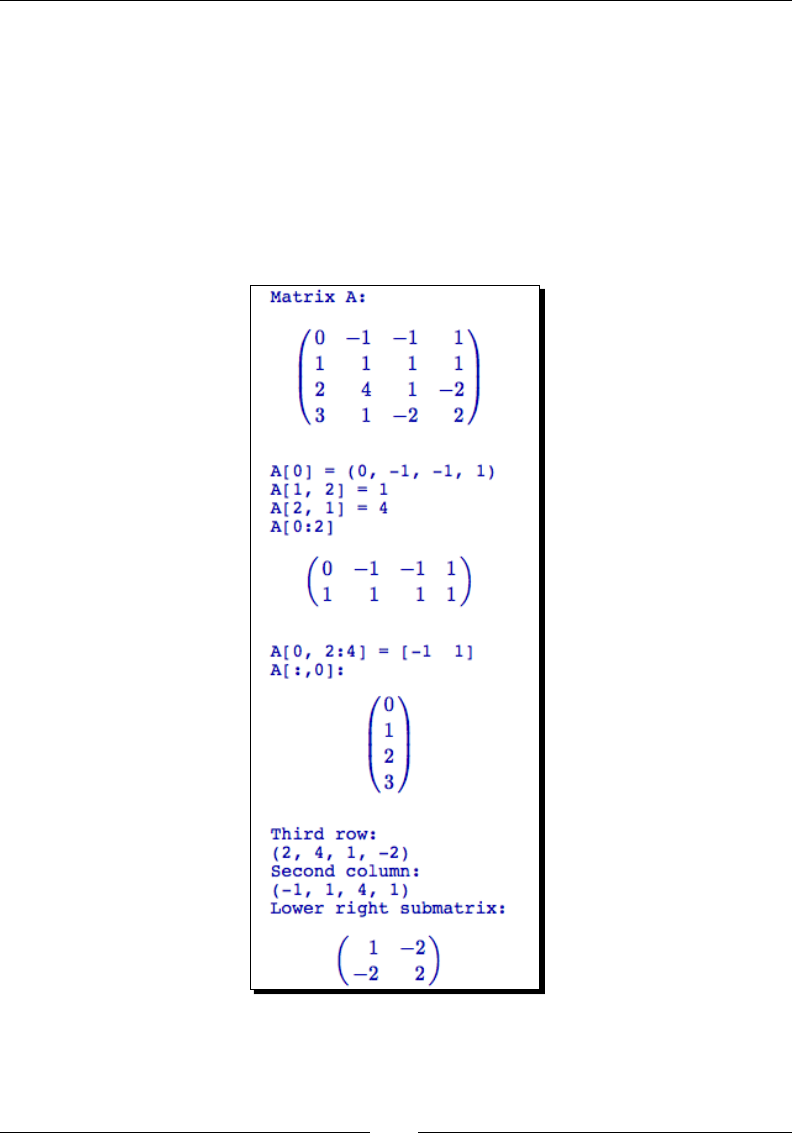
Chapter 5
[ 121 ]
show(A[:,0])
# Getting parts of a matrix
print("Third row:")
print(A.row(2))
print("Second column:")
print(A.column(1))
print("Lower right submatrix:")
show(A.submatrix(2, 2, 2, 2))
The result should look like this:

Vectors, Matrices, and Linear Algebra
[ 122 ]
What just happened?
The individual elements of a matrix are accessed using a pair of indices separated by a
comma. The rst index selects the row, and the second selects the column. Like all Python
sequence types, the indices start at zero. When you access a single element, the result is a
simple numeric type. Using a single index returns an enre row at once, as a vector object.
Slicing is a lile more complicated. Using a single slice argument returns one or more rows,
in the form of a matrix object. If you give two arguments and one of them is a slice, the
returned type might be a vector or a matrix. Here are some guidelines:
Accessing a single element returns a simple numeric type
Accessing a single row, or a slice of a single row, returns a vector type
Accessing elements from more than one row (such as a column or sub-matrix)
returns a matrix type
We also used the row, column, and submatrix methods of the Matrix object to get parts
of the matrix. The types returned by these operaons are also determined by the guidelines
given above. Try using the type funcon to check the type returned from the operaons in
this example.
Manipulating matrices
The previous example showed how we can get parts of matrix. A Sage matrix object also has
methods for performing elementary row operaons on the matrix.
Time for action – manipulating matrices
Let's try some elementary row operaons to see how they work. Evaluate the
following code:
A = Matrix(QQ, [[1, 2, 3], [4, 5, 6], [7, 8, 9]])
print("Matrix A:")
show(A)
# Elementary row operations
print("Scaling second row by two:")
A.rescale_row(1, 2)
show(A)
print("Swapping first and second rows:")
A.swap_rows(0, 1)
show(A)
print("Adding 3*(row 1) to row 0:")
A.add_multiple_of_row(0, 1 ,3)
show(A)
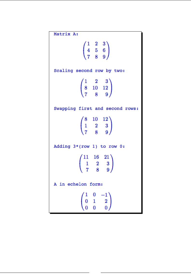
Chapter 5
[ 123 ]
print("A in echelon form:")
show(A.echelon_form())
The result will look like this:
What just happened?
We dened a matrix A and used its methods to perform some elementary row operaons.
You could use a sequence of these operaons to reduce a matrix to echelon form. However,
it's much easier to let Sage take care of that by using the echelon_form method.

Vectors, Matrices, and Linear Algebra
[ 124 ]
Pop quiz – manipulating matrices
Test your understanding of selecng elements and parts of matrices. For the matrix dened
below, what will the output be from each of these operaons? Check your answers by
entering the code in Sage:
A = Matrix(QQ, [[1, 2, 3], [4, 5, 6], [7, 8, 9]])
print(A[1])
print(type(A[1]))
print(A[1,2])
print(A[1:3,1:3])
print(type(A[1:3,1:3]))
print(A.column(2))
Matrix algebra
Sage denes standard operaons for performing matrix algebra. A few are available through
the standard operators, and the rest are available as matrix methods.
Time for action – matrix algebra
Let's try some basic matrix algebra. Enter and evaluate the following code:
M3 = MatrixSpace(QQ, 3, 2)
A = M3.matrix([[3, 2, 1], [4, 5, 6]])
B = M3.matrix([[2, 2, 2], [1, 2, 3]])
print("Matrix addition:")
show(A + B)
print("Scalar multiplication:")
show(1/2 * A)
var('a b c d e f')
C = Matrix(QQ, [[4, 2, 1], [5, 3, 7]])
D = Matrix(SR, [[a, b], [c, d], [e, f]])
print("Matrix multiplication:")
show(C * D)
var('x1 x2 x3')
X = vector([x1,x2,x3])
print("Multiplying a matrix and a vector:")
show(C * X)
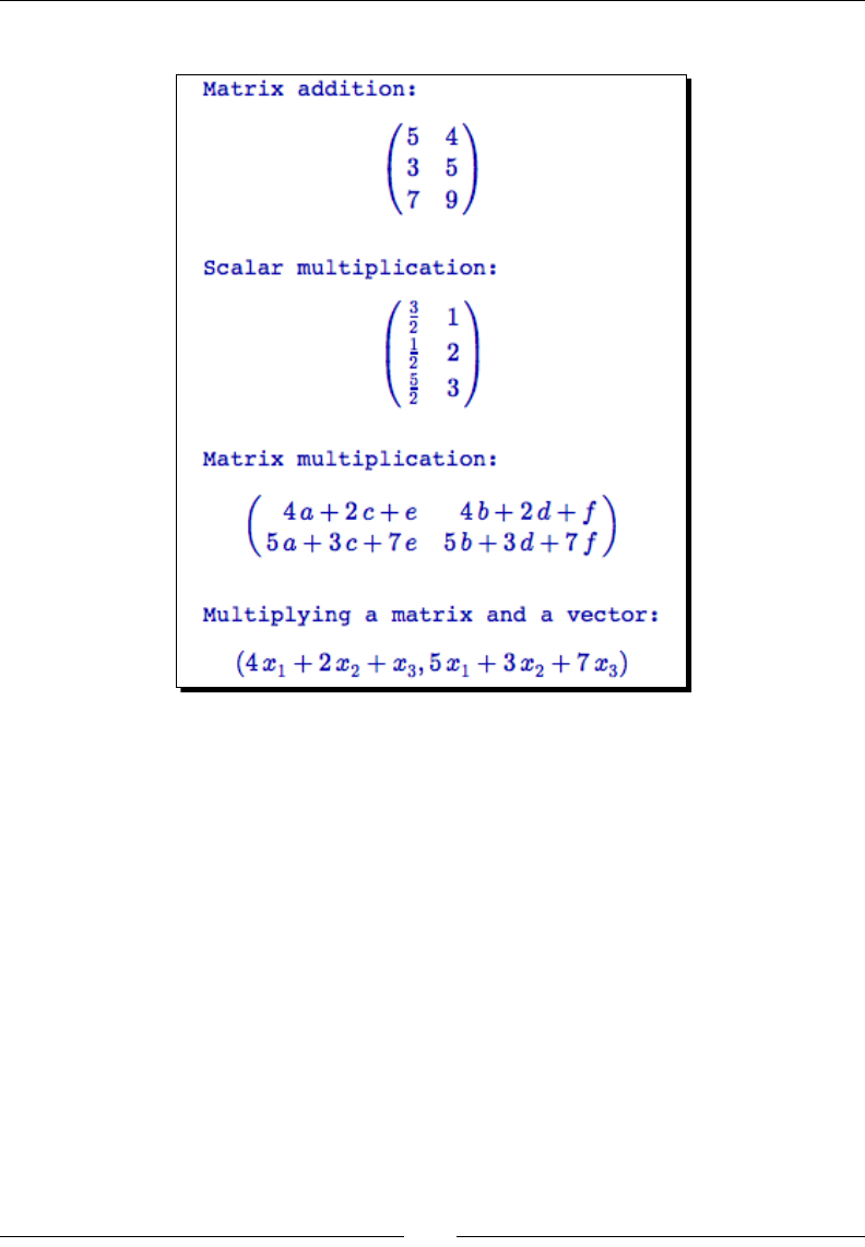
Chapter 5
[ 125 ]
The result should look like this:
What just happened?
We performed some basic matrix algebra. The + and – operators perform element-by-
element addion and subtracon. The * operator performs scalar mulplicaon if one
variable is a scalar, and it performs matrix mulplicaon if both arguments are matrices or
one is a matrix and one is a vector. We also demonstrated how to dene a matrix over the
symbolic ring.
Other matrix methods
Matrix objects in Sage have many handy methods for calculang various scalars and matrices
associated with a given matrix, such as its determinant, inverse matrix, and adjoint matrix.
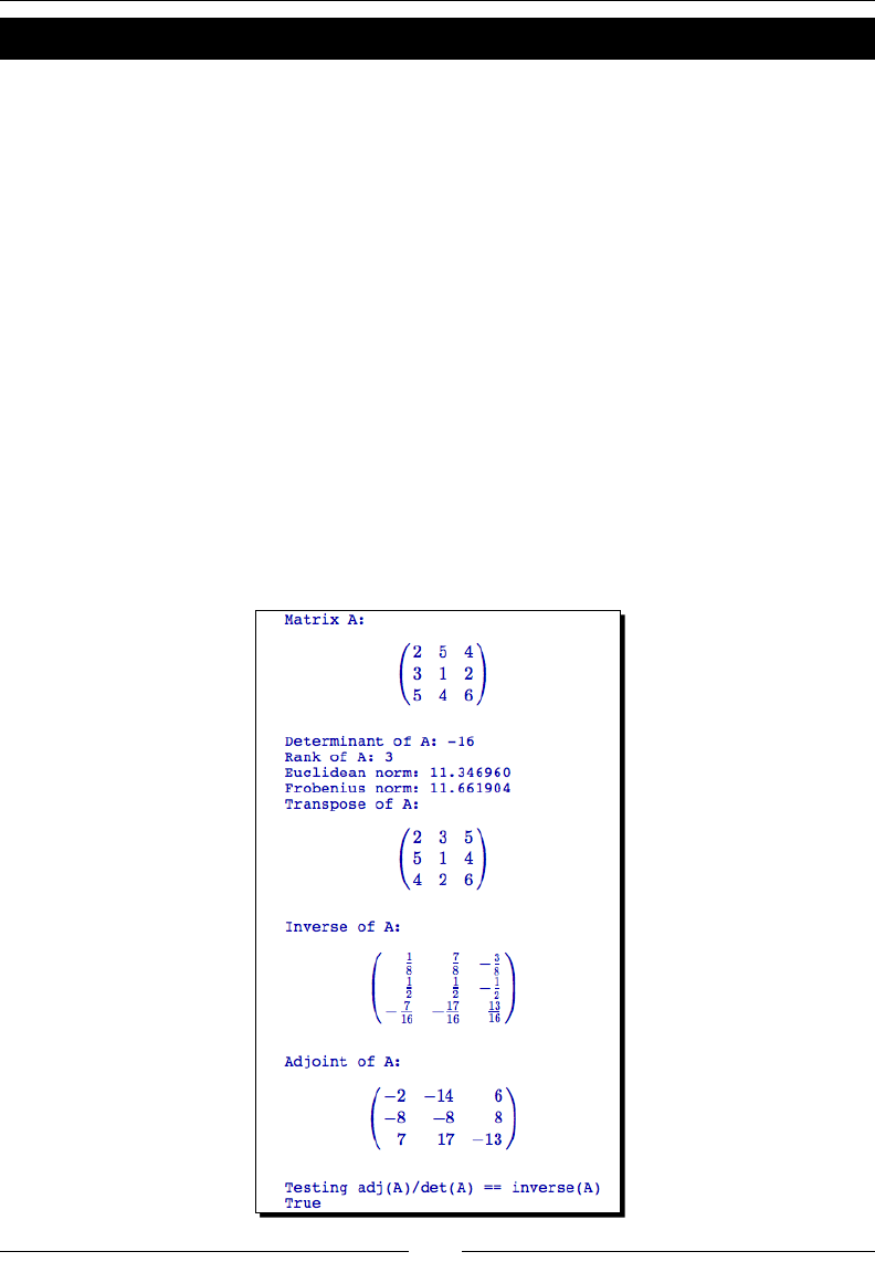
Vectors, Matrices, and Linear Algebra
[ 126 ]
Time for action – trying other matrix methods
Let's test out some other methods of the Matrix object:
A = matrix(QQ, [[2, 5, 4], [3, 1, 2], [5, 4, 6]])
print("Matrix A:")
show(A)
# Scalar operations
print("Determinant of A: {0}".format(A.det()))
print("Rank of A: {0}".format(A.rank()))
print("Euclidean norm: {0}".format(A.norm()))
print("Frobenius norm: {0}".format(A.norm('frob')))
# Matrix operations
print("Transpose of A:")
show(A.transpose())
print("Inverse of A:")
show(A.inverse())
print("Adjoint of A:")
show(A.adjoint())
print("Testing adj(A)/det(A) == inverse(A)")
A.adjoint()/A.det() == A.inverse()
The output should look like this:

Chapter 5
[ 127 ]
What just happened?
We created an object that represents a 3 by 3 matrix of raonal numbers, and used its
methods to calculate the determinant and rank of A. We then calculated its inverse and
its adjoint, and veried the relaonship between them. We also used the norm method to
compute two dierent norms of the matrix. When called with no arguments, norm returns
the Euclidean norm. The available norms are:
Argument Result
1 The largest column-sum norm
2 The Euclidean norm (default)
Innity The largest row-sum norm
'frob' The Frobenius (sum of squares) norm
Eigenvalues and eigenvectors
Compung the eigenvalues and eigenvectors for a matrix is important for many areas of
applied mathemacs. Sage includes funcons and methods that eliminate the tedious
calculaons that would be required to perform this important task by hand.
Time for action – computing eigenvalues and eigenvectors
Let's see how to compute the eigenvalues and eigenvectors for a 3x3 matrix. Evaluate the
following code:
A = Matrix(QQ, [[2, -3, 1], [1, -2, 1], [1, -3, 2]])
print("Matrix A:")
show(A)
print("Eigenvalues:")
print(A.eigenvalues())
ev = A.eigenvectors_right()
for v in ev:
print("Eigenvalue: {0}".format(v[0]))
print(" Multiplicity: {0}".format(v[2]))
print(" Eigenvectors:")
for e in v[1]:
print(" " + str(e))
print("Eigenmatrices:")
D, P = A.eigenmatrix_right()
print("D:")
show(D)
print("P:")
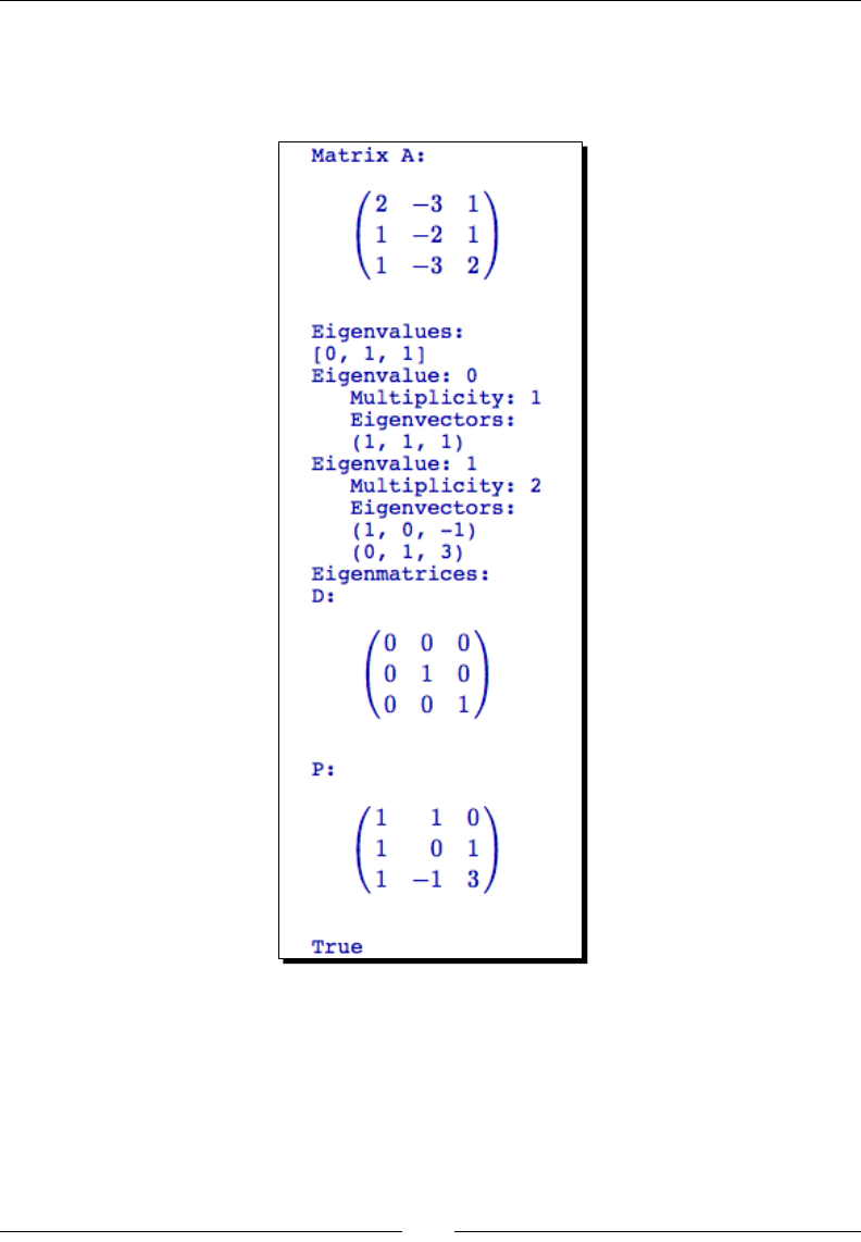
Vectors, Matrices, and Linear Algebra
[ 128 ]
show(P)
print(A*P == P*D)
The output should look like this:
Chapter 5
[ 129 ]
What just happened?
We dened a 3x3 matrix of raonal numbers, and used the eigenvalues method to return
a list of eigenvalues. We then used the eigenvectors_right method to return a list of
tuples that contain data about the eigenvectors. We used a for loop to iterate through the
list and print the informaon in a more readable format. Each element in the list is a tuple
with three elements. The rst is the eigenvalue, the second is the eigenvector, and the third
is the mulplicity of the eigenvalue. Finally, we calculated and displayed the eigenmatrices D
and P for matrix A, which sasfy the relaon A*P=P*D.
Have a go hero – verifying the eigenvalues and eigenvectors
Let A be an m x n matrix with eigenvalues given by:
For each eigenvalue, there is an eigenvector x, which sases the relaon:
In the previous example, we found the eigenvalues and eigenvectors for matrix A. Use Sage
to verify that each of those eigenvalues and eigenvectors sases the relaon above.
Decomposing matrices
Another important task in applied mathemacs is decomposing a matrix into a combinaon
of special matrices. There are a variety of well-known decomposions (also known as
factorizaons) that are used to solve various praccal problems in applied mathemacs.
Time for action – computing the QR factorization
The QR factorizaon can be used to solve linear least squares problems. The QR factorizaon
decomposes an m x n matrix A (with m≥n) into two matrices called Q and R, such that
A=QR. Q is an m x n matrix with orthonormal columns and R is an n x n matrix that is upper
triangular and inverble. In this example, we will see how easy it is to compute the QR
factorizaon with Sage.
# This is an example where it's important to specify the correct ring
A = Matrix(RDF, [[1, -1, 4], [1, 4, -2], [1, 4, 2], [1, -1, 0]])
print("Matrix A:")
show(A)
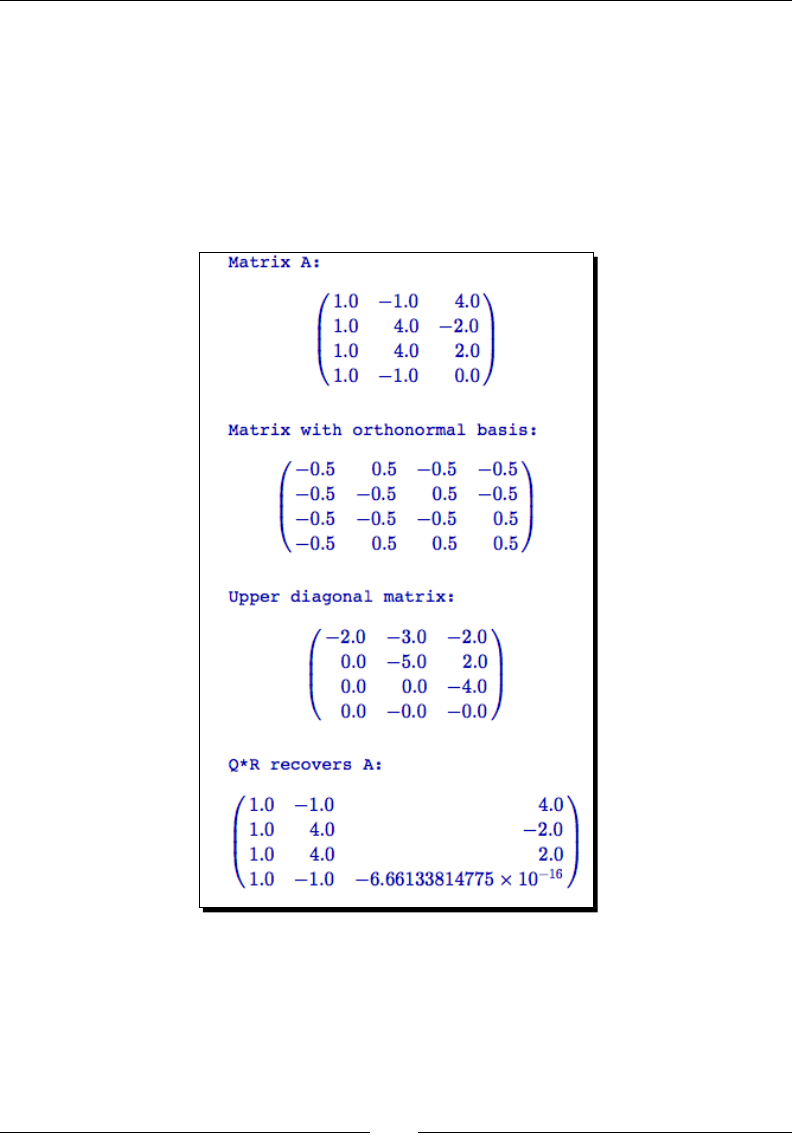
Vectors, Matrices, and Linear Algebra
[ 130 ]
Q, R = A.QR()
print("Matrix with orthonormal basis:")
show(Q)
print("Upper diagonal matrix:")
show(R)
print("Q*R recovers A:")
show(Q*R)
The output should look like this:
Chapter 5
[ 131 ]
What just happened?
We dened a 4 by 3 matrix called A over the ring called RDF, which is a shortcut for
RealDoubleField. An RDF object is a double-precision approximaon of a oang point
number, while a RealField object can have an arbitrary number of bits of precision. This is
another example where it is very important to choose the right ring. Matrix decomposions
in Sage are only dened for matrices constructed on RDF and its counterpart CDF, or
ComplexDoubleField. The QR method returns a tuple containing the matrices Q and R.
We printed out the matrices and veried that A = Q*R.
Time for action – computing the singular value decomposition
The singular value decomposion, or SVD, has numerous applicaons in stascs, signal
processing, and numerical analysis. An m x n matrix A is decomposed into three matrices: an
m x m unitary matrix U, an m x n diagonal matrix sigma, and an n x n real unitary matrix V.
These matrices sasfy the relaon:
Here, V* denotes the transpose of the complex conjugate of V.
It's also easy to compute the SVD with Sage:
A = Matrix(RDF, [[1,1], [1,1], [0,0]])
print("Matrix A:")
show(A)
print "SVD:"
U, Sigma, V = A.SVD()
print("U:")
show(U)
print("Sigma:")
show(Sigma)
print("V:")
show(V)
print("U.Sigma.V* recovers A:")
show(U*Sigma*(V.conjugate().transpose()))
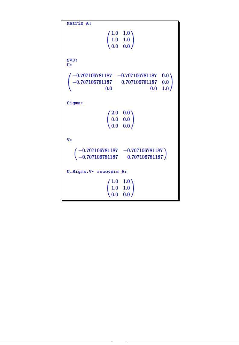
Vectors, Matrices, and Linear Algebra
[ 132 ]
The result should look like this:
What just happened?
As in the previous example, we dened a 4 by 3 matrix called A over the eld called RDF. The
SVD method returns a tuple containing the matrices U, Sigma, and V. We displayed these
matrices, and veried that they sasfy the mathemacal relaon shown in the introducon.
Matrix objects in Sage have methods for compung other decomposions. The method LU
computes the LU decomposion, and the method cholesky_decomposition computes
the Cholesky decomposion.
The nal line of this example shows that methods can be "chained" together. The methods
are evaluated in order, from le to right. The reason this works is that the expression
v.conjugate() returns a matrix object. We then call the method transpose of this
matrix object. In many cases, chaining methods can make your code more concise and
readable. Of course, it should be avoided if it makes the code less readable.
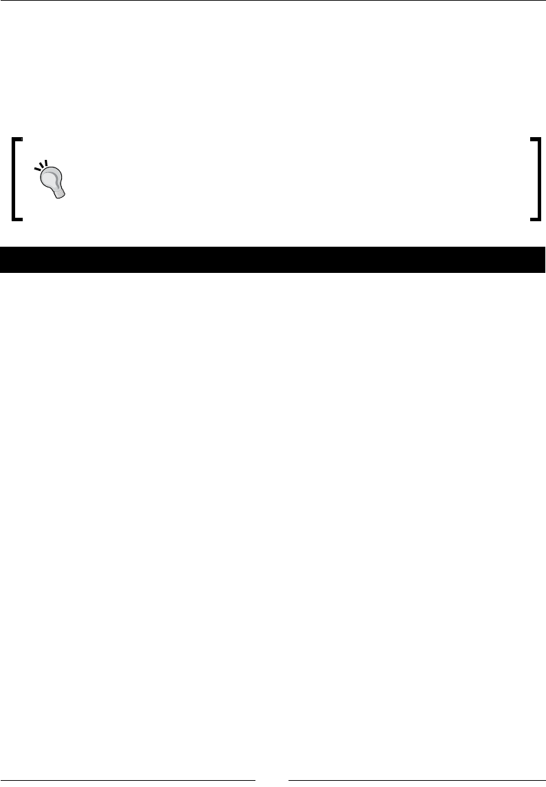
Chapter 5
[ 133 ]
An introduction to NumPy
NumPy is a package that turns Python into a powerful numerical compung language. The
core of NumPy is a powerful n-dimensional array class. The package also includes tools for
numerical linear algebra, Fourier transforms, and many other commonly used numerical
methods. To nd out more about NumPy, check out http://numpy.scipy.org/.
The current release of Sage is 4.6.1, which includes NumPy version 1.5. Because
NumPy is constantly evolving, the latest version of NumPy may dier slightly
from the version included with the latest version of Sage. Be aware of this as you
are looking at the documentaon, especially if you are using a dierent version
of NumPy in other Python code!
Time for action – creating NumPy arrays
The array class is the core of NumPy. Let's explore the various ways that we can create
NumPy arrays:
import numpy
print("array:")
a = numpy.array([1,2,3,9,10,11])
print(a)
print("arange:")
b = numpy.arange(0.0, 10.0, 3.0/2)
print(b)
print("zeros:")
c = numpy.zeros(5,dtype=int)
print(c)
print("ones:")
d = numpy.ones((4,1), dtype=numpy.float64)
print(d)
print("ones, 2D array:")
e = numpy.ones((3,2))
print(e)
print("empty:")
f = numpy.empty((1,4), dtype=numpy.float32)
print(f)
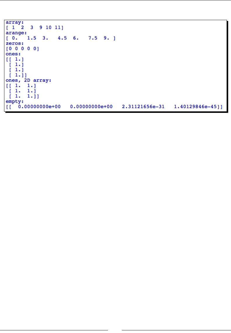
Vectors, Matrices, and Linear Algebra
[ 134 ]
The result should look like this:
What just happened?
In the rst line of the script, we used the import statement to make NumPy funcons and
objects available to Sage. In order to keep NumPy types separate from Sage types with the
same name, we access the NumPy types with the syntax numpy.type. In this example, we
used several funcons to create NumPy arrays. All of these funcons accept the oponal
argument dtype, which species the type for the elements in the array (NumPy types are
not the same as Sage types). We used the print funcon instead of the show funcon to
display the arrays we created. Since NumPy objects return only plain text representaons,
there is no reason to use show to display NumPy objects.
Creating NumPy arrays
NumPy includes many convenient funcons for creang arrays. The array funcon takes
a Python list as an argument, and returns an array with the contents of the list, with each
element converted to the specied type. arange is an extension of the range funcon that
we learned about in Chapter 4. The basic syntax is as follows:
new_array = arange([start,] stop [,step] [,dtype])

Chapter 5
[ 135 ]
If only one argument is provided, start is assumed to be zero and step is assumed to be
one. If two arguments are given, the rst is used as start and the second is assumed to be
stop, and step is assumed to be one. ones and zeros return an array of the given shape
and the specied type, with every element set to 1 or 0. The shape argument can be an
integer or a tuple. An integer creates a "row" array, while a tuple of the form (n,1) creates
a "column" array. Tuples of the form (m,n) or (m,n,p) create two-dimensional and three-
dimensional arrays, respecvely. empty is the fastest way to create an array of a specied
shape. It allocates the appropriate amount of space for the elements, based on the specied
type, but does not inialize the element values. Note that the values in an empty array will
be dierent every me it is created.
NumPy types
Every NumPy array has a type, and all the elements in the array must have the same type.
The following table will help you choose the appropriate type. When choosing a type, the
main factors are the maximum value that needs to be stored, the amount of precision
required, and the amount of memory required for the array. You must consider the amount
of RAM needed to hold the array during calculaons, and the amount of disk space required
if you are going to save the array to a le. For the simple exercises in this chapter, you will be
safe using the default 64-bit types:
bool Boolean (True or False) stored as a byte
int Default integer for the plaorm (normally either int32 or int64)
int8 Byte (-128 to 127)
int16 Integer (-32768 to 32767)
int32 Integer (-2147483648 to 2147483647)
int64 Integer (9223372036854775808 to 9223372036854775807)
uint8 Unsigned integer (0 to 255)
uint16 Unsigned integer (0 to 65535)
uint32 Unsigned integer (0 to 4294967295)
uint64 Unsigned integer (0 to 18446744073709551615)
float Shorthand for float64
float32 Single precision oat: sign bit, 8 bits exponent, 23 bits manssa
float64 Double precision oat: sign bit, 11 bits exponent, 52 bits manssa
complex Shorthand for complex128
complex64 Complex number, represented by two 32-bit oats (real and imaginary
components)
complex128 Complex number, represented by two 64-bit oats (real and imaginary
components)
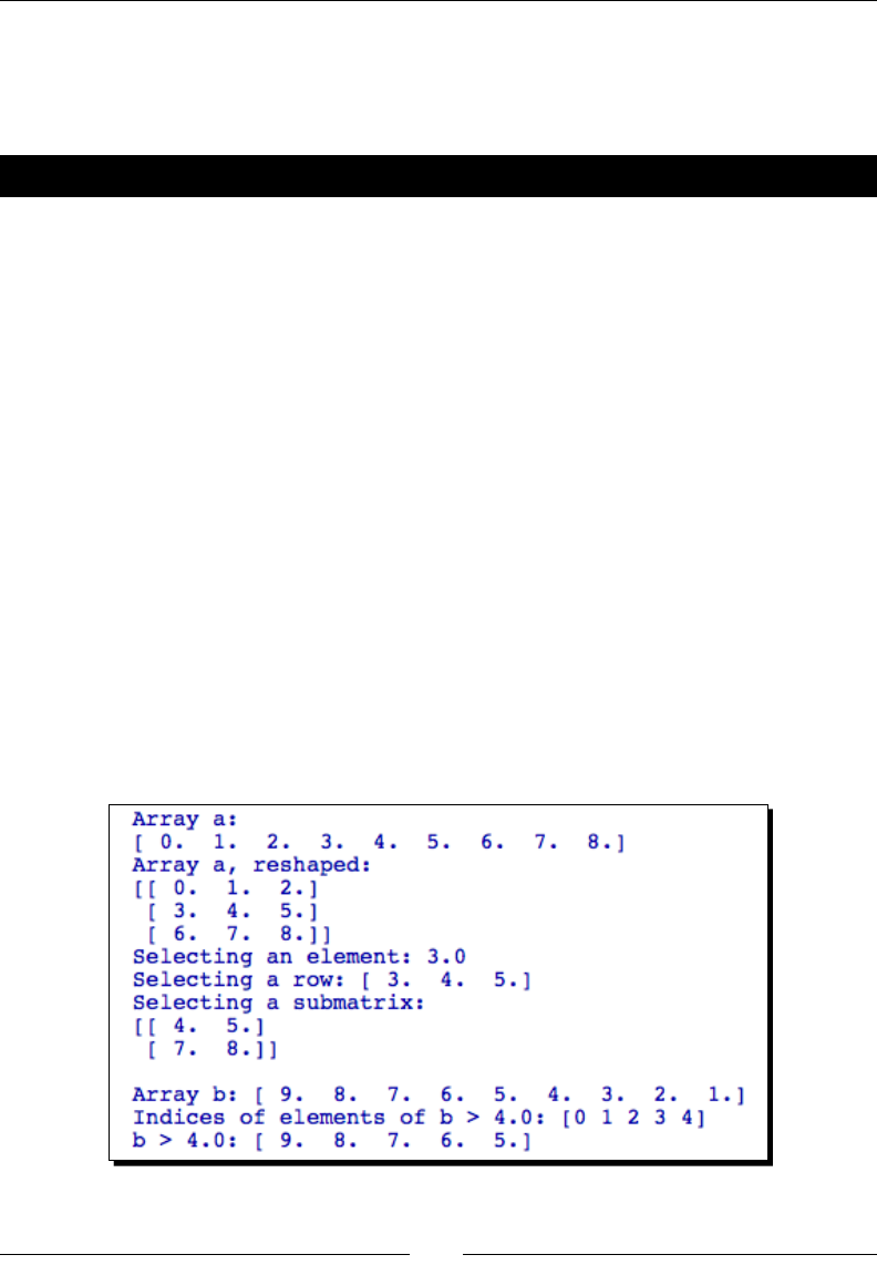
Vectors, Matrices, and Linear Algebra
[ 136 ]
Indexing and selection with NumPy arrays
All of the indexing and slicing tricks that we've learned so far also apply to NumPy arrays.
NumPy adds a few indexing tricks that help with processing numeric data.
Time for action – working with NumPy arrays
Let's explore some ways to select elements and sub-arrays from NumPy arrays:
import numpy
a = numpy.arange(9.0)
print("Array a:")
print(a)
a = a.reshape((3,3))
print("Array a, reshaped:")
print(a)
print("Selecting an element: {0}".format(a[1,0]))
print("Selecting a row: {0}".format(a[1]))
print("Selecting a submatrix:")
print(a[1:3,1:3])
b = numpy.arange(9.0, 0.0, -1.0)
print("\nArray b: {0}".format(b))
indices, = numpy.where(b > 4.0)
print("Indices of elements of b > 4.0: {0}".format(indices))
print("b > 4.0: {0}".format(b[b > 4.0]))
The output should be as follows:

Chapter 5
[ 137 ]
What just happened?
We used the arange funcon to create an array with nine oang-point elements. Since
we only provided a single argument, NumPy assumes that the rst element is zero and the
increment is one. We then used the array's reshape method to return a two-dimensional
array with three rows and three columns. reshape accepts a tuple that contains the
dimensions of the new array. Note that reshape returns a new array instead of modifying
the original array, so we have to use the syntax a = a.reshape((3,3)) to overwrite the
original array. Elements and subsets of this array were selected using the same slice notaon
that we used with Sage vectors and matrices.
We created a one-dimensional array to demonstrate how to select elements by value
from NumPy arrays. In this case, we specied a negave step, so arange created an array
with decreasing values. We used the where funcon to get a list of indices that met a
specic condion. where returns a list of lists of indices, so we used tuple unpacking to
obtain a single list. When where is used with mul-dimensional arrays, each list of indices
corresponds to one dimension of the array. The nal line of the example shows a shortcut for
obtaining the elements of an array that meet a certain criterion.
Have a go hero – replacing lists with NumPy arrays
In Chapter 4, we used lists and loops to compute the analycal soluon to a paral
dierenal equaon (see Time for acon – compung a soluon to the diusion equaon).
Go back to that example and replace the lists with NumPy arrays.
Replace the list called x with a NumPy array
Use arange to replace the for loop that was used to dene the x coordinates for
the calculaon
Use empty to create an array to replace the list called ideal_concentration
NumPy matrices
NumPy also includes a matrix class, which is disnct from the two-dimensional array that we
created in the previous example.
Time for action – creating matrices in NumPy
To illustrate some of the similaries and dierences between the linear algebra features of
Sage and NumPy, we'll repeat an earlier example in which we computed the singular value
decomposion of a matrix:
import numpy as np
print "Two ways of creating a Numpy matrix:"
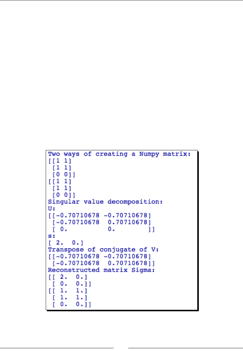
Vectors, Matrices, and Linear Algebra
[ 138 ]
A = np.matrix('1 1; 1 1; 0 0') # Matlab syntax
print(A)
A2 = np.matrix([[1,1], [1,1], [0,0]])
print(A2)
print("Singular value decomposition:")
U, s, Vstar = np.linalg.svd(A, full_matrices=False)
print("U:")
print(U)
print("s:")
print(s)
print("Transpose of conjugate of V:")
print(Vstar)
Sigma = np.diag(s)
print("Reconstructed matrix Sigma:")
print(Sigma)
print(np.dot(U, np.dot(Sigma, Vstar)))
The result should look like this:

Chapter 5
[ 139 ]
What just happened?
The example demonstrated two ways of creang a NumPy matrix object. To start with, we
used the statement import numpy as np so that we can use np as a shortcut for numpy.
This feature is handy for long package names that are used many mes, but it can also lead
to confusion when misused. We then tried two ways of creang NumPy matrix. The rst way
uses syntax that will be familiar to MATLAB users; the second uses standard Python notaon.
We then computed the singular value decomposion using the svd funcon from NumPy.
This funcon returns slightly dierent results than the SVD method of a Sage matrix object.
numpy.linalg.svd returns the conjugate transpose of matrix V, instead of V. NumPy
returns a vector instead of a full matrix for Sigma, so we had to construct matrix Sigma using
the diag funcon. diag accepts an array (or other sequence type) as an argument, and
returns a matrix with the elements of the array as the diagonal elements. For more about
the svd funcon in NumPy, try the following:
np.linalg.svd?
Learning more about NumPy
This has been a very brief introducon to NumPy. We will use arrays in Chapter 6 when we
learn about plong, and again in Chapter 8 when we learn about numerical methods. Even
then, we will barely begin to exploit the power of NumPy. Here are some resources to learn
more:
The ocial NumPy documentaon page at http://docs.scipy.org/doc/
The NumPy Tutorial at http://www.scipy.org/Tentative_NumPy_Tutorial
Download the Guide to NumPy from http://www.tramy.us/numpybook.pdf
Summary
We have seen that Sage can reduce or eliminate the tedious computaons that are required
when doing linear algebra by hand. The capabilies of Sage are equivalent to those found in
commercial mathemacal soware systems. Specically, we covered:
Creang vector spaces and vector objects, and performing basic operaons like
inner products and cross products
Creang matrix objects, performing elementary row operaons, and matrix algebra
Using matrix methods to calculate scalars and matrices such as determinants,
inverses, eigenvalues, and eigenvectors

Vectors, Matrices, and Linear Algebra
[ 140 ]
Using matrix methods to factorize and decompose matrices
Creang and manipulang NumPy arrays and matrices for working with numerical
data
In the next chapter, we will learn about the plong and graphics capabilies of Sage.
6
Plotting with Sage
Graphs, plots, and charts are useful tools to understand the behaviour of funcons and
visualize data. Sage comes with some powerful plong tools.
In this chapter we will:
Learn how to plot funcons of one variable
Make various types of specialized 2D plots such as polar plots and scaer plots
Use matplotlib to precisely format 2D plots and charts
Make interacve 3D plots of funcons of two variables
Let's start plong!
Confusion alert: Sage plots and matplotlib
The 2D plong capabilies of Sage are built upon a Python plong package called
matplotlib. The most widely used features of matplotlib are accessible through Sage
funcons. You can also import the matplotlib package into Sage, and use all of its features
directly. This is very powerful, but it's also confusing, because there's more than one way
to do the same thing. To further add to the confusion, matplotlib has two interfaces: the
command-oriented Pyplot interface and an object-oriented interface. The examples in this
chapter will aempt to clarify which interface is being used.
Plotting in two dimensions
Two-dimensional plots are probably the most important tool for visually presenng
informaon in math, science, and engineering. Sage has a wide variety of tools for making
many types of 2D plots.

Plong with Sage
[ 142 ]
Plotting symbolic expressions with Sage
We will start by exploring the plong funcons that are built in to Sage. They are generally
less exible than using matplotlib directly, but also tend to be easier to use.
Time for action – plotting symbolic expressions
Let's plot some simple funcons. Enter the following code:
p1 = plot(sin, (-2*pi, 2*pi), thickness=2.0, rgbcolor=(0.5, 1, 0),
legend_label='sin(x)')
p2 = plot(cos, (-2*pi, 2*pi), thickness=3.0, color='purple',
alpha=0.5, legend_label='cos(x)')
plt = p1 + p2
plt.axes_labels(['x', 'f(x)'])
show(plt)
If you run the code from the interacve shell, the plot will open in a separate window. If you
run it from the notebook interface, the plot will appear below the input cell. In either case,
the result should look like this:

Chapter 6
[ 143 ]
What just happened?
This example demonstrated the most basic type of plong in Sage. The plot funcon
requires the following arguments:
graphics_object = plot(callable symbolic expression, (independent_var,
ind_var_min, ind_var_max))
The rst argument is a callable symbolic expression, and the second argument is a tuple
consisng of the independent variable, the lower limit of the domain, and the upper
limit. If there is no ambiguity, you do not need to specify the independent variable. Sage
automacally selects the right number of points to make a nice curve in the specied
domain. The plot funcon returns a graphics object. To combine two graphics objects in
the same image, use the + operator: plt = p1 + p2. Graphics objects have addional
methods for modifying the nal image. In this case, we used the axes_labels method
to label the x and y axes. Finally, the show funcon was used to nish the calculaon and
display the image.
The plot funcon accepts oponal arguments that can be used to customize the appearance
and format of the plot. To see a list of all the opons and their default values, type:
sage: plot.options
{'fillalpha': 0.5, 'detect_poles': False, 'plot_points': 200,
'thickness': 1, 'alpha': 1, 'adaptive_tolerance': 0.01, 'fillcolor':
'automatic', 'adaptive_recursion': 5, 'exclude': None, 'legend_label':
None, 'rgbcolor': (0, 0, 1), 'fill': False}
Here is a summary of the opons for customizing the appearance of a plot:
Keyword Descripon
alpha Transparency of the line (0=opaque, 1=transparent)
ll True to ll area below the line
llalpha Transparency of the lled-in area (0=opaque, 1=transparent)
llcolor Color of the lled-in area
rgbcolor Color of the line

Plong with Sage
[ 144 ]
Sage uses an algorithm to determine the best number of points to use for the plot, and how
to distribute them on the x axis. The algorithm uses recursion to add more points to resolve
regions where the funcon changes rapidly. Here are the opons that control how the plot
is generated:
Keyword Descripon
adapve_recursion Max depth of recursion when resolving areas of the plot where the
funcon changes rapidly
adapve_tolerance Tolerance for stopping recursion
detect_poles Detect points where funcon value approaches innity (see next
example)
exclude A list or tuple of points to exclude from the plot
plot_points Number of points to use in the plot
Specifying colors in Sage
There are several ways to specify a color in Sage. For basic colors, you can use a
string containing the name of the color, such as red or blue. You can also use
a tuple of three oang-point values between 0 and 1.0. The rst value is the
amount of red, the second is the amount of green, and the third is the amount
of blue. For example, the tuple (0.5, 0.0, 0.5) represents a medium purple color.
Some funcons "blow up" to plus or minus innity at a certain point. A simplisc plong
algorithm will have trouble plong these points, but Sage adapts.
Time for action – plotting a function with a pole
Let's try to plot a simple funcon that takes on innite values within the domain of the plot:
pole_plot = plot(1 / (x - 1), (0.8, 1.2), detect_poles='show',
marker='.')
print("min y = {0} max y = {1}".format(pole_plot.ymax(),
pole_plot.ymin()))
pole_plot.ymax(100.0)
pole_plot.ymin(-100.0)
# Use TeX to make nicer labels
pole_plot.axes_labels([r'$x$', r'$1/(x-1)$'])
pole_plot.show()
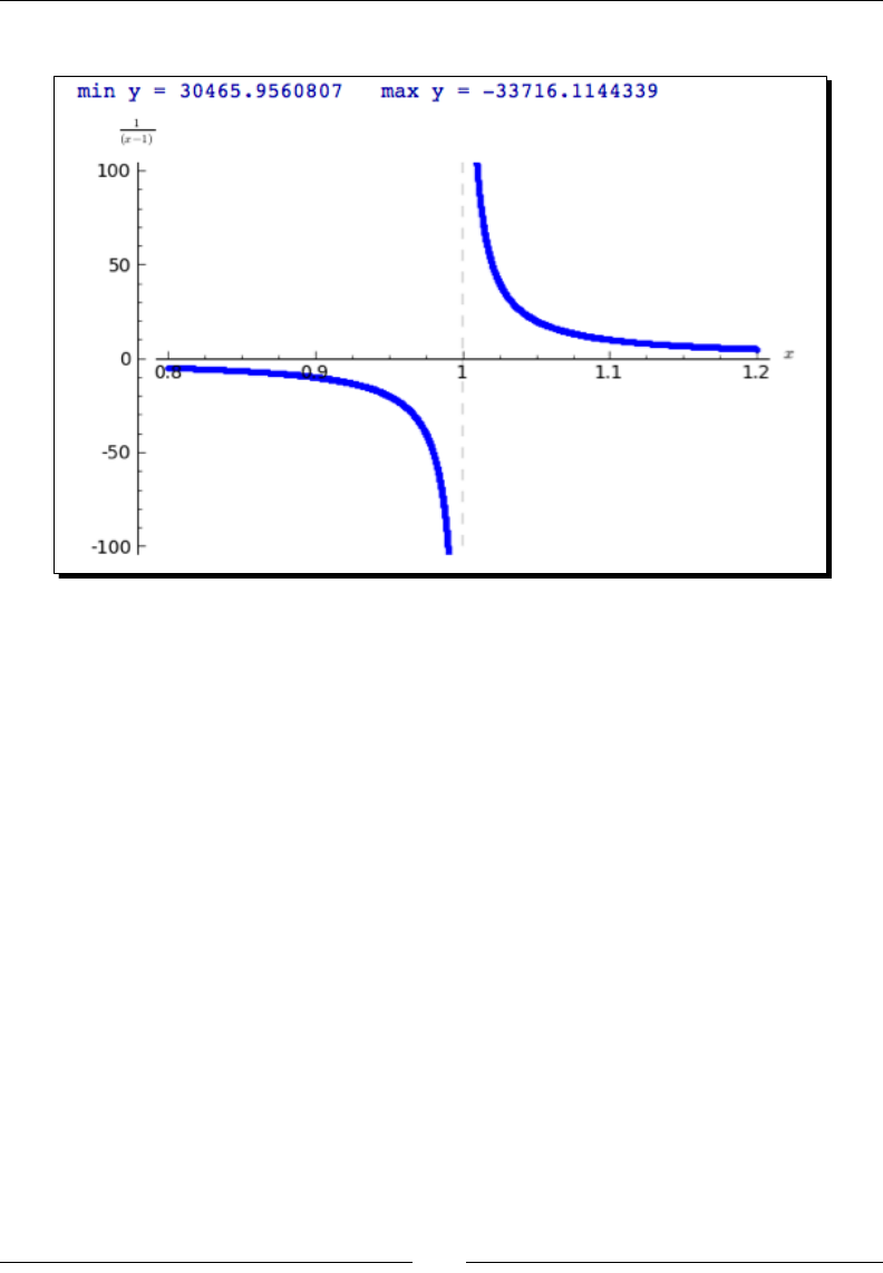
Chapter 6
[ 145 ]
The output from this code is as follows:
What just happened?
We did a few things dierently compared to the previous example. We dened a callable
symbolic expression right in the plot funcon. We also used the opon detect_
poles='show' to plot a dashed vercal line at the x value where the funcon returns
innite values. The opon marker='.' tells Sage to use a small dot to mark the individual
(x,y) values on the graph. In this case, the dots are so close together that they look like a fat
line. We also used the methods ymin and ymax to get and set the minimum and maximum
values of the vercal axis. When called without arguments, these methods return the
current values. When given an argument, they set the minimum and maximum values of the
vercal axis.
Finally, we labeled the axes with nicely typeset mathemacal expressions. As in the previous
example, we used the method axes_labels to set the labels on the x and y axes. However,
we did two special things with the label strings:
r'$\frac{1}{(x-1)}$'
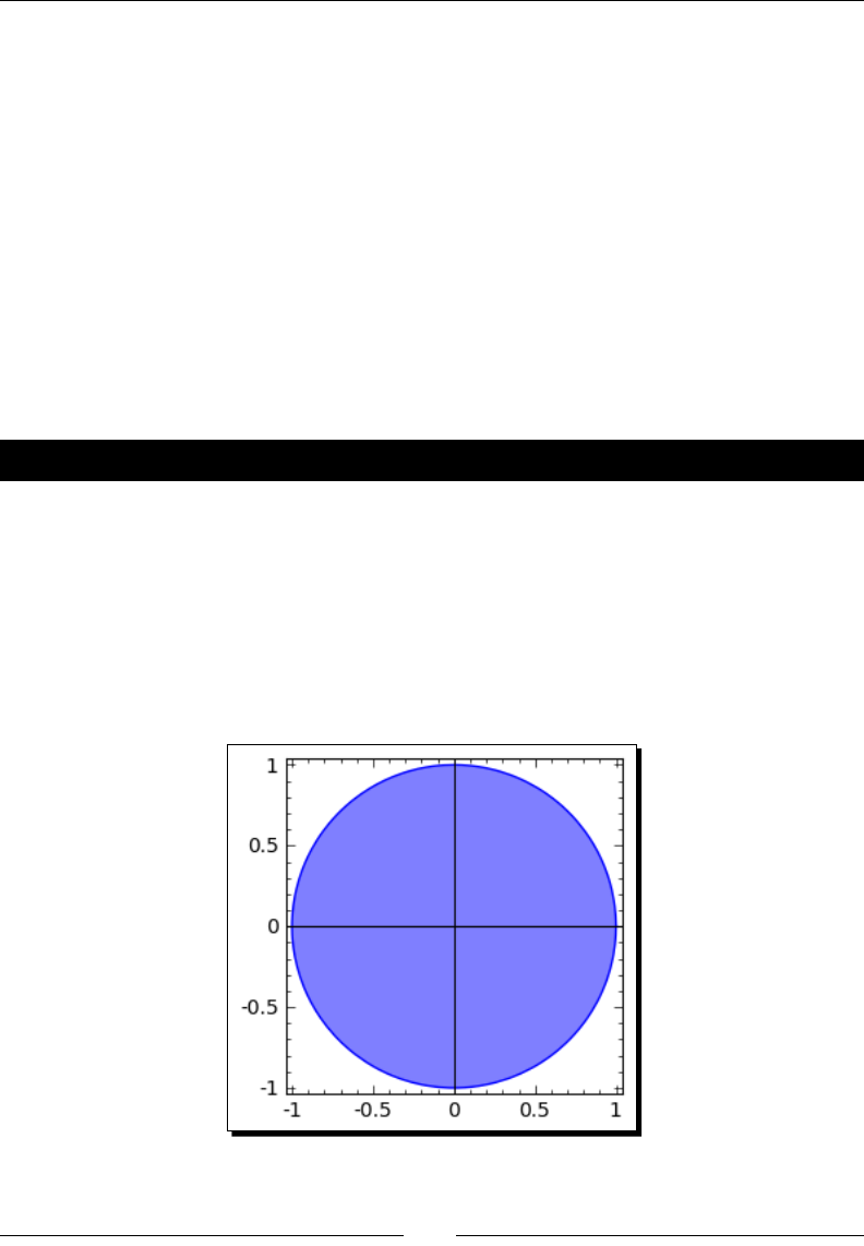
Plong with Sage
[ 146 ]
The leer r is placed in front of the string, which tells Python that this is a raw string. When
processing a raw string, Python does not interpret backslash characters as commands (such
as interpreng \n as a newline). Note that the rst and last characters of the string are
dollar signs, which tells Sage that the strings contain mark-up that needs to be processed
before being displayed. The mark-up language is a subset of TeX, which is widely used for
typeseng complicated mathemacal expressions. Sage performs this processing with a
built-in interpreter, so you don't need to have TeX installed to take advantage of typeset
labels. It's a good idea to use raw strings to hold TeX markup because TeX uses a lot of
backslashes. To learn about the typeseng language, see the matplotlib documentaon at:
http://matplotlib.sourceforge.net/users/mathtext.html
In Chapter 10, we'll see how TeX and its relave LaTeX can help us typeset mathemacal
expressions.
Time for action – plotting a parametric function
Some funcons are dened in terms of a parameter. Sage can easily plot parametric
funcons:
var('t')
pp = parametric_plot((cos(t), sin(t)), (t, 0, 2*pi),
fill=True, fillcolor='blue')
pp.show(aspect_ratio=1, figsize=(3, 3), frame=True)
The output from this code is as follows:
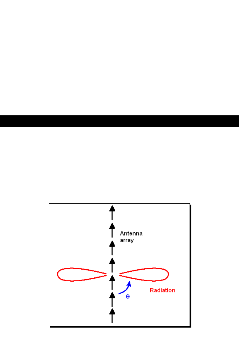
Chapter 6
[ 147 ]
What just happened?
We used two parametric funcons to plot a circle. This is a convenient place to demonstrate
the fill opon, which lls in the space between the funcon and the horizontal axis. The
fillcolor opon tells Sage which color to use for the ll, and the color can be specied
in the usual ways. We also demonstrated some useful opons for the show method (these
opons also work with the show funcon). The opon aspect_ratio=1 forces the x and y
axes to use the same scale. In other words, one unit on the x axis takes up the same number
of pixels on the screen as one unit on the y axis. Try changing the aspect rao to 0.5 and
2.0, and see how the circle looks. The opon figsize=(x_size,y_size) species the
aspect rao and relave size of the gure. The units for the gure size are relave, and don't
correspond to an absolute unit like inches or cenmetres. The opon frame=True places a
frame with ck marks around the outside of the plot.
Time for action – making a polar plot
Some funcons are more easily described in terms of angle and radius. The angle is the
independent variable, and the radius at that angle is the dependent variable. Polar plots are
widely used in electrical engineering to describe the radiaon paern of an antenna. Some
antennas are designed to transmit (or receive) electromagnec radiaon in a very narrow
beam. The beam shape is known as the radiaon paern. One way to achieve a narrow
beam is to use an array of simple dipole antennas, and carefully control the phase of the
signal fed to each antenna. In the following example, we will consider seven short dipole
antennas set in a straight line:
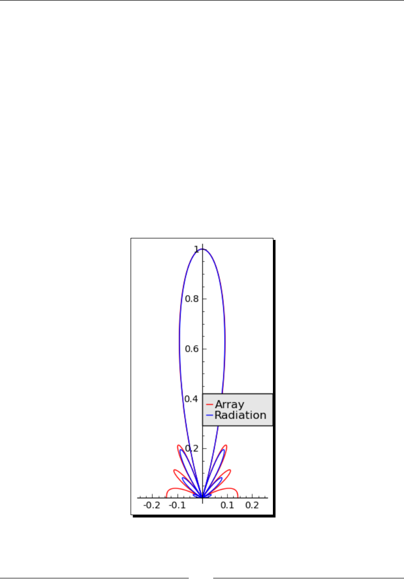
Plong with Sage
[ 148 ]
# A linear broadside array of short vertical dipoles
# located along the z axis with 1/2 wavelength spacing
var('r, theta')
N = 7
normalized_element_pattern = sin(theta)
array_factor = 1 / N * sin(N * pi / 2 * cos(theta)) \
/ sin(pi / 2 * cos(theta))
array_plot = polar_plot(abs(array_factor), (theta, 0, pi),
color='red', legend_label='Array')
radiation_plot = polar_plot(abs(normalized_element_pattern
* array_factor), (theta, 0, pi), color='blue',
legend_label='Radiation')
combined_plot = array_plot + radiation_plot
combined_plot.xmin(-0.25)
combined_plot.xmax(0.25)
combined_plot.set_legend_options(loc=(0.5, 0.3))
show(combined_plot, figsize=(2, 5), aspect_ratio=1)
Execute the code. You should get a plot like this:
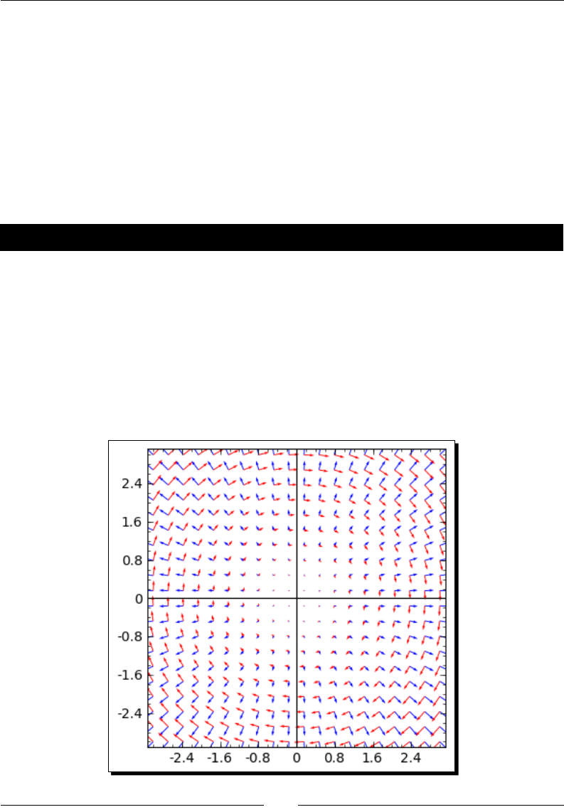
Chapter 6
[ 149 ]
What just happened?
We ploed a polar funcon, and used several of the plong features that we've already
discussed. There are two subtle points worth menoning. The funcon array_factor is
a funcon of two variables, N and theta. In this example, N is more like a parameter, while
theta is the independent variable we want to use for plong. We use the syntax (theta,
0, pi) in the plot funcon to indicate that theta is the independent variable. The second
new aspect of this example is that we used the methods xmin and xmax to set the limits of
the x axis for the graphics object called combined_plot. We also used the set_legend_
options of the graphics object to adjust the posion of the legend to avoid covering up
important details of the plot.
Time for action – plotting a vector eld
Vector elds are used to represent force elds such as electromagnec elds, and are used
to visualize the soluons of dierenal equaons. Sage has a special plong funcon to
visualize vector elds.
var('x, y')
a = plot_vector_field((x, y), (x, -3, 3), (y, -3, 3), color='blue')
b = plot_vector_field((y, -x), (x, -3, 3), (y, -3, 3), color='red')
show(a + b, aspect_ratio=1, figsize=(4, 4))
You should get the following image:

Plong with Sage
[ 150 ]
What just happened?
The plot_vector_field funcon uses the following syntax:
plot_vector_field((x_function,y_function), (x,x_min,x_max), (y,y_
min,y_max))
The keyword argument color species the color of the vectors.
Plotting data in Sage
So far, we've been making graphs of funcons. We specify the funcon and the domain, and
Sage automacally chooses the points to make a nice-looking curve. Somemes, we need to
plot discrete data points that represent experimental measurements or simulaon results.
The following funcons are used for plong dened sets of points.
Time for action – making a scatter plot
Scaer plots are used in science and engineering to look for correlaon between two
variables. A cloud of points that is roughly circular indicates that the two variables are
independent, while a more ellipcal arrangement indicates that there may be a relaonship
between them. In the following example, the x and y coordinates are contrived to make a
nice plot. In real life, the x and y coordinates would typically be read in from data les. Enter
the following code:
def noisy_line(m, b, x):
return m * x + b + 0.5 * (random() - 0.5)
slope = 1.0
intercept = -0.5
x_coords = [random() for t in range(50)]
y_coords = [noisy_line(slope, intercept, x) for x in x_coords]
sp = scatter_plot(zip(x_coords, y_coords))
sp += line([(0.0, intercept), (1.0, slope+intercept)], color='red')
sp.show()
The result should look similar to this plot. Note that your results won't match exactly, since
the point posions are determined randomly.
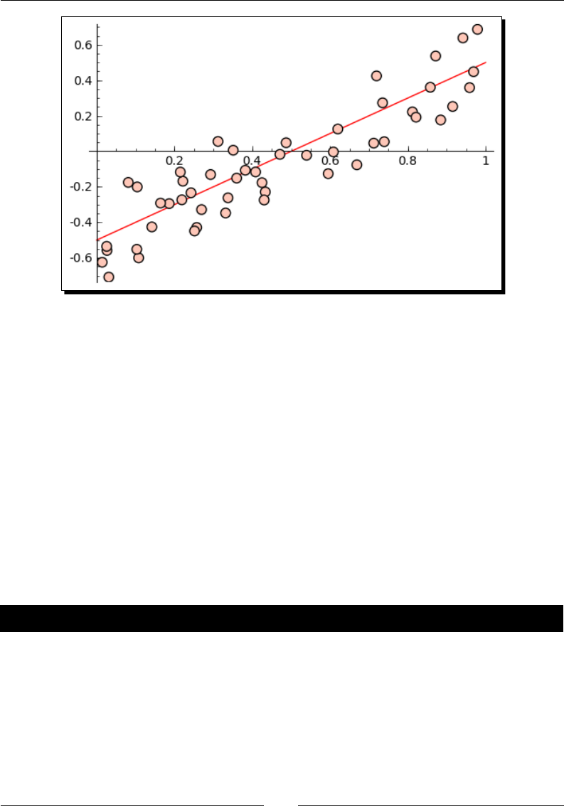
Chapter 6
[ 151 ]
What just happened?
We created a list of randomized x coordinates using the built-in random funcon. This
funcon returns a random number in the range 0 ≤ x < 1. We dened a funcon called
noisy_line that we then used to create a list of randomized y coordinates with a linear
relaonship to the x coordinates. We now have a list of x coordinates and a list of y
coordinates, but the scatter_plot funcon needs a list of (x,y) tuples. The zip funcon
takes the two lists and combines them into a single list of tuples. The scatter_plot
funcon returns a graphics object called sp. To add a line object to the plot, we use the
following syntax:
sp += line([(x1, y1), (x2,y2)], color='red')
The += operator is a way to increment a variable; x+=1 is a shortcut for x = x + 1.
Because the + operator also combines graphics objects, this syntax can be used to add a
graphics object to an exisng graphics object.
Time for action – plotting a list
Somemes, you need to plot a list of discrete data points. The following example might be
found in an introductory digital signal processing (DSP) course. We will use lists to represent
digital signals. We sample the analogue funcon cosine(t) at two dierent sampling rates,
and plot the resulng digital signals.
# Use list_plot to visualize digital signals
# Undersampling and oversampling a cosine signal
sample_times_1 = srange(0, 6*pi, 4*pi/5)
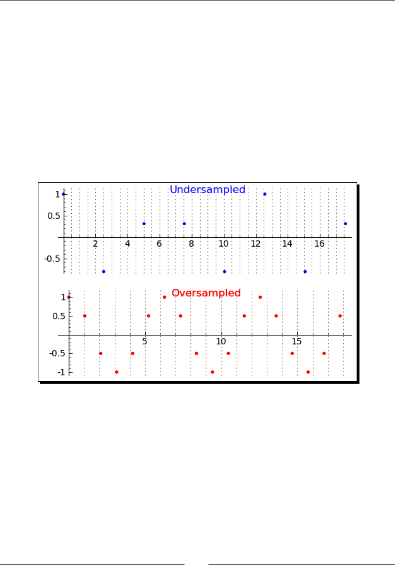
Plong with Sage
[ 152 ]
sample_times_2 = srange(0, 6*pi, pi/3)
data1 = [cos(t) for t in sample_times_1]
data2 = [cos(t) for t in sample_times_2]
plot1 = list_plot(zip(sample_times_1, data1), color='blue')
plot1.axes_range(0, 18, -1, 1)
plot1 += text("Undersampled", (9, 1.1), color='blue', fontsize=12)
plot2 = list_plot(zip(sample_times_2, data2), color='red')
plot2.axes_range(0, 18, -1, 1)
plot2 += text("Oversampled", (9, 1.1), color='red', fontsize=12)
g = graphics_array([plot1, plot2], 2, 1) # 2 rows, 1 column
g.show(gridlines=["minor", False])
The result is as follows:
What just happened?
The funcon list_plot works a lot like scatter_plot from the previous example, so I
won't explain it again. We used the method axes_range(x_min, x_max, y_min, y_
max) to set the limits of the x and y axes all at once. Once again, we used the += operator
to add a graphics object to an exisng object. This me, we added a text annotaon instead
of a line. The basic syntax for adding text at a given (x,y) posion is text('a string',
(x,y)). To see the opons that text accepts, type the following:
sage: text.options
{'vertical_alignment': 'center', 'fontsize': 10, 'rgbcolor': (0, 0,
1),
'horizontal_alignment': 'center', 'axis_coords': False}

Chapter 6
[ 153 ]
To display the two plots, we introduced a new funcon called graphics_array, which uses
the basic syntax:
graphics_array([plot_1, plot_2, ..., plot_n], num_rows, num_columns)
This funcon returns another graphics object, and we used the show method to display the
plots. We used the keyword argument gridlines=["minor", False] to tell Sage to
display vercal lines at each of the minor cks on the x axis. The rst item in the list species
vercal grid lines, and the second species horizontal grid lines. The following opons can be
used for either element:
"major" Grid lines at major cks
"minor" Grid lines at major and minor cks
False No grid lines
Try playing with these opons in the previous example.
Using graphics primitives
We've already seen that Sage has graphics primives such as lines and text annotaons. Sage
has other types of graphics primives that can be used for plong.
Time for action – plotting with graphics primitives
A class of mathemacal models called random sequenal adsorpon (RSA) models deals
with the paerns that result when two-dimensional shapes are randomly deposited onto a
plane. The following method can be used to visualize these kinds of models:
# Since the circles are random, your plot will not
# look exactly like the example!
circle_list = []
for i in range(15):
x = -5 + 10 * random()
y = -5 + 10 * random()
circle_list.append(circle((x, y), 1, facecolor='red',
edgecolor=(0, 0, 1), thickness=2, fill=True))
gr = sum(circle_list)
gr.axes(False)
gr.show(aspect_ratio=1, frame=True, gridlines=True, figsize=(4, 4))
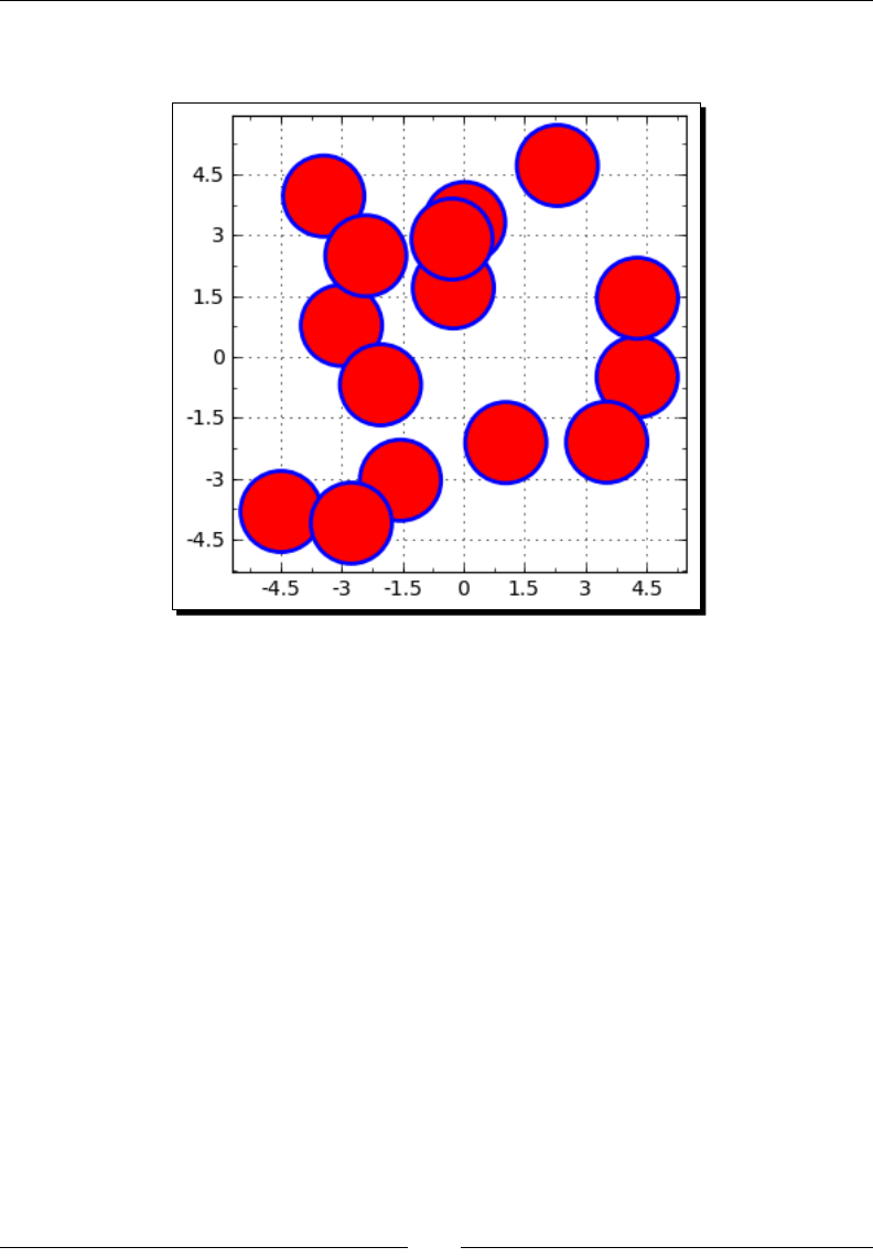
Plong with Sage
[ 154 ]
You should get a plot that resembles the one below. Because the posions of the circles are
randomly generated, your plot will not look exactly like this one.
What just happened?
We created a list of graphics objects with a for loop and the circle funcon. The basic
syntax for the circle funcon is as follows:
graphics_object = circle((center_x, center_y), radius)
In order to plot all the circles at once, we used the sum funcon to add up the list. We
then prevented the axes from being drawn by calling the method gr.axes(False).
Finally, when calling the show method we used the keyword argument frame=True to
draw a frame, with cks and labels, around the outside of the plong area. The argument
gridlines=True is a shortcut to acvate both horizontal and vercal grid lines. Sage has
many other types of primives, including ellipcal arcs, arrows, disks, ellipses, points, and
polygons, that are described in the Sage reference manual.

Chapter 6
[ 155 ]
Using matplotlib
We can access matplotlib directly to do things that we can't do with Sage plong funcons.
matplotlib has such a large number of opons and features that it deserves a separate book.
We will only touch on a few basic features. If you want to know more, the matplotlib website
has excellent documentaon:
http://matplotlib.sourceforge.net/contents.html
Time for action – plotting functions with matplotlib
To illustrate the similaries and dierences between plong with matplotlib and plong
with Sage, we will repeat the rst example of this chapter using the Pyplot interface to
matplotlib. Enter and evaluate the following code:
import numpy
import matplotlib.pyplot as plt
x = numpy.arange(-2 * numpy.pi, 2 * numpy.pi, 0.1)
func1 = numpy.sin(x)
func2 = numpy.cos(x)
plt.figure(figsize=(5.5, 3.7)) # size in inches
plt.plot(x, func1, linewidth=2.0, color=(0.5, 1,0),
label='$f(x)=sin(x)$')
plt.plot(x, func2, linewidth=3.0, color='purple', alpha=0.5,
label='$f(x)=cos(x)$')
plt.xlabel('$x$')
plt.ylabel('$f(x)$')
plt.title('Plotting with matplotlib')
plt.legend(loc='lower left')
plt.savefig('demo1.png')
plt.close()
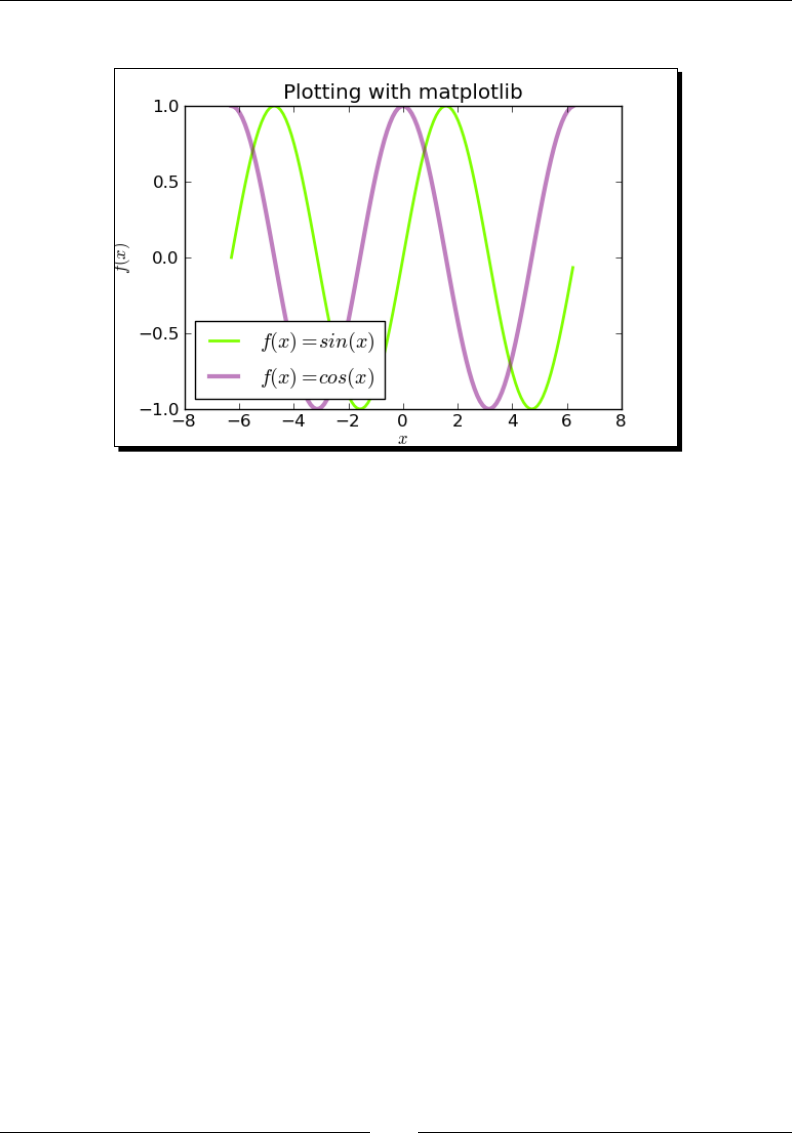
Plong with Sage
[ 156 ]
The result should be as follows:
What just happened?
We gained access to matplotlib funcons and types with the following line:
import matplotlib.pyplot as plt
We can now access these funcons as plt.function_name. We also import numpy so
that we can use its numerical arrays.
There is an important dierence between the Sage plot funcon and the matplotlib plot
funcon. matplotlib always plots lists or arrays of discrete points, rather than callable
symbolic expressions. This block of code creates an array of x values:
x = numpy.arange(-2*numpy.pi, 2*numpy.pi, 0.1)
func1 = numpy.sin(x)
func2 = numpy.cos(x)
func1 and func2 are arrays of y values. Noce that we specify the NumPy version of sin
and cos, since the Sage funcons don't know what to do with NumPy arrays. The syntax for
plong with matplotlib is as follows:
plt.figure()
plt.plot(x_values, y_values)

Chapter 6
[ 157 ]
The rst line creates an empty gure. The oponal argument figsize=(x_size, y_
size) sets the gure size in inches. The second line plots the data points that are specied
in the arrays or lists. By default, the points are connected with straight line segments. If
you specify points that are too far apart, you will see the line segments instead of a smooth
curve. The opons for the plt.plot funcon are very similar to the opons for the Sage
plot funcon. The following code labels the x and y axes, and places a tle above the gure:
plt.xlabel('$x$')
plt.ylabel('$f(x)$')
plt.title('Plotting with matplotlib')
plt.legend(loc='lower right')
The legend method places a legend on the gure. You can use TeX to format any text on the
plot by wrapping the text in dollar signs. The following code actually displays the plot:
plt.savefig('demo1.png')
plt.close()
If you are running this example from the notebook interface, the graphic will automacally
appear in the notebook. If you're running it in the interacve shell, you won't see any output.
The savefig funcon will save an image le in your home directory. To specify a dierent
path for saving les, pass a full or relave path in addion to the le name. For example:
sage: plt.savefig('Sage for Beginners/Chapter 6/Images/polar_plot.png')
matplotlib can save gures in a variety of image formats, such as png, pdf, ps (PostScript),
eps (encapsulated PostScript), and svg (scalable vector graphics). It will automacally
determine the correct format from the extension of the le name. You can also use the
format keyword to specify the image format. PNG is a raster format, which is compable
with Microso Oce and OpenOce. For publicaons, it is best to use a vector format like
PostScript, EPS, or PDF. The SVG format is used for displaying vector graphics on the Web.
Using matplotlib to "tweak" a Sage plot
Every Sage plot is actually an encapsulated matplotlib gure. We can get the underlying
gure and modify it.

Plong with Sage
[ 158 ]
Time for action – getting the matplotlib gure object
Let's say you've made a plot with Sage, but you want to x one or two formang details, and
Sage doesn't give you enough control. In this example, we'll use the object-oriented interface
of matplotlib:
# Create a Sage plot, as shown in the first example
p1 = plot(sin, (-2*pi, 2*pi), thickness=2.0, rgbcolor=(0.5,1,0))
p2 = plot(cos, (-2*pi, 2*pi), thickness=3.0, color='purple',
alpha=0.5)
plt = p1 + p2
# Get the Matplotlib object
fig = plt.matplotlib()
from matplotlib.backends.backend_agg import FigureCanvasAgg
fig.set_canvas(FigureCanvasAgg(fig)) # this line is critical
ax = fig.gca() # get current axes
# Add a legend and plot title
ax.legend(['sin(x)', 'cos(x)'])
ax.set_title('Modified with matplotlib')
# Add a y axis label in a custom location
ymin, ymax = ax.get_ylim()
ax.set_ylim(ymin, ymax*1.2)
ax.set_ylabel('$f(x)$', y=ymax*0.9)
# Fancy annotation of a point of interest
x_value = numerical_approx(-3*pi/4)
y_value = numerical_approx(cos(-3*pi/4))
ax.annotate('Point', xy=(x_value, y_value),
xytext=(-6, -0.5), color='red',
arrowprops=dict(arrowstyle="->", connectionstyle="angle3"))
# Show the matplotlib figure
fig.savefig('Sage_to_matplotlib.png')
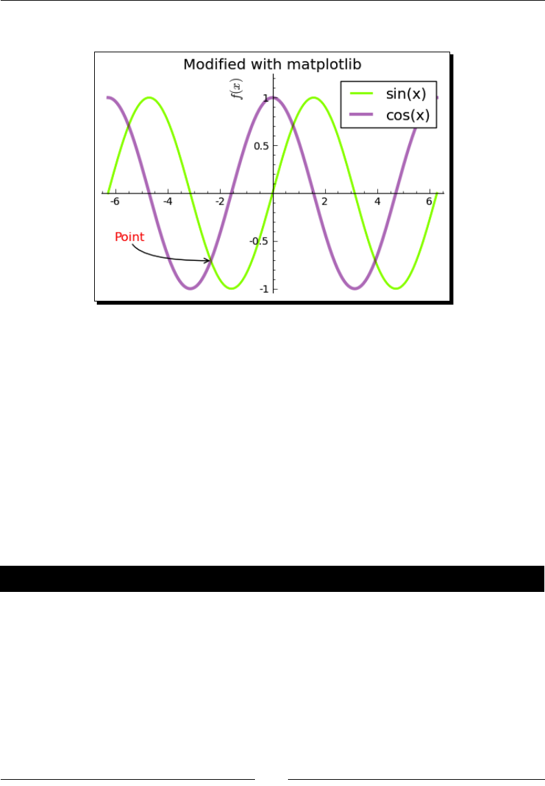
Chapter 6
[ 159 ]
The output should look like this:
What just happened?
We modied a plot with matplotlib. First, we used Sage plong commands to create a
Sage graphics object. We then used the matplotlib method of the Sage graphics object
to obtain the underlying matplotlib gure object. The rest of this example uses matplotlib
funcons, rather than Sage funcons, to modify the gure. It is crical to use the following
line of code:
fig.set_canvas(FigureCanvasAgg(fig))
The canvas is a "backend," which controls how matplotlib outputs the graphics it creates. Once
we set the right canvas, we used the gca method of the gure object to get an object that
represents the current axes. We then used methods of the axes object to modify the plot.
Time for action – improving polar plots
In a previous example, we made polar pots with the Sage funcon polar_plot. However,
polar plots in matplotlib look nicer because they are ploed on special axes. Let's use
matplotlib to make these plots again. This example uses the Pyplot interface to matplotlib:
import numpy
import matplotlib.pyplot as plt
# Repeat the antenna pattern example with the Pyplot interface
N = float(7)
theta = numpy.arange(0, numpy.pi, numpy.pi/100)
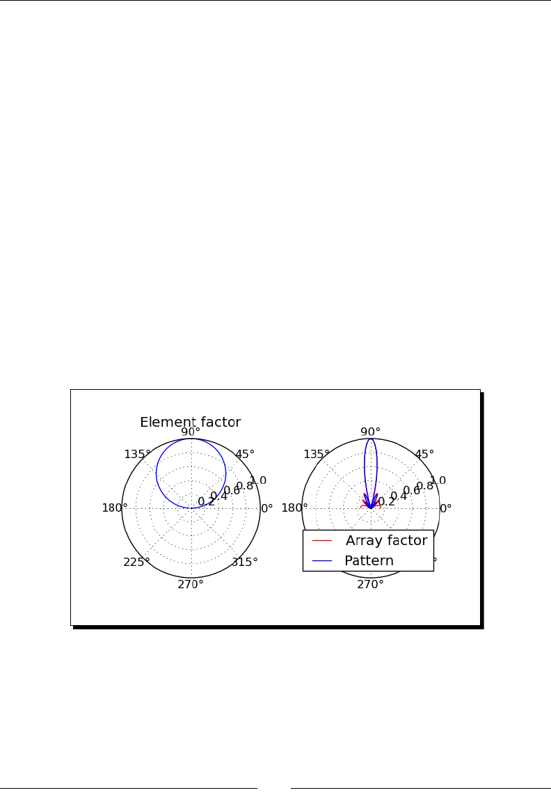
Plong with Sage
[ 160 ]
def normalized_element_pattern(theta):
return abs(numpy.sin(theta))
def array_factor(theta, N):
return abs(float(1 / N) * numpy.sin(float(N * pi / 2)
* numpy.cos(theta))
/ numpy.sin(float(pi / 2) * numpy.cos(theta)))
plt.figure(figsize=(6, 4))
plt.subplot(121, polar=True)
plt.polar(theta, normalized_element_pattern(theta))
plt.title('Element factor')
plt.subplot(122, polar=True)
plt.polar(theta, array_factor(theta, N), color='red',
label="Array factor")
plt.polar(theta, array_factor(theta, N) *
normalized_element_pattern(theta),
label="Pattern", color='blue')
plt.legend(loc='lower right', bbox_to_anchor = (1, 0))
plt.subplots_adjust(wspace=0.3)
plt.savefig('Polar_plot.png')
plt.close()

Chapter 6
[ 161 ]
What just happened?
We made polar plots on nicely formaed polar axes. We introduced a new Pyplot funcon
called subplot, which creates mulple axes on a single gure, arranged as a grid. Subplot
accepts three integer arguments that specify the arrangement of axes and chooses one of
the axes as the current axes object. The rst integer species the number of columns in
the grid, the second integer species the number of rows in the grid, and the third integer
selects the current axes object. The rst subplot, which is number one, is located in the
upper-le corner of the gure. Subplot numbers increase from le to right across a row, and
from top to boom. It is possible, although not recommended, to omit the commas between
arguments and pass a single three-digit integer value to subplot. This rather unusual syntax
was chosen for compability with the subplot funcon in MATLAB. We used the polar
keyword to choose polar axes for each of the subplots.
We also introduced a funcon called subplots_adjust, which we used to increase the
amount of horizontal space between the plots. This command can be used to adjust the
amount of space around and between subplots, using the following keyword arguments:
Keyword Default Meaning
le 0.125 Space to the le of the subplots
right 0.9 Space to the right of the subplots
boom 0.1 Space below the subplots
top 0.9 Space above the subplots
wspace 0.2 Space between columns of subplots
hspace 0.2 Space between rows of subplots
Plotting data with matplotlib
Because matplotlib plots arrays of points, it is well suited to working with data. You can make
many kinds of charts and publicaon-quality graphics with matplotlib.
Time for action – making a bar chart
Bar charts are oen used to present experimental data in scienc papers. Let's make a
chart with bars that represent the average value of some experimental data and add error
bars to represent the standard deviaon:
import numpy
import matplotlib.pyplot as plt
# Define experimental data
cluster1_data = numpy.array([9.7, 3.2])
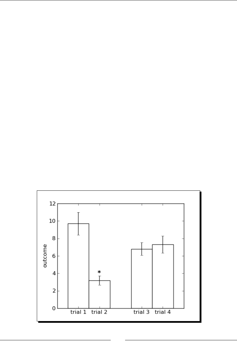
Plong with Sage
[ 162 ]
cluster1_x = numpy.array([2,4])
cluster1_error = numpy.array([1.3, 0.52])
cluster2_data = numpy.array([6.8, 7.3])
cluster2_x = numpy.array([8,10])
cluster2_error = numpy.array([0.72, 0.97])
# Join data arrays for plotting
data = numpy.concatenate([cluster1_data, cluster2_data])
bar_centers = numpy.concatenate([cluster1_x, cluster2_x])
errors = numpy.concatenate([cluster1_error, cluster2_error])
# Plot
fig = plt.figure(figsize=(5,4)) # size in inches
plt.bar(bar_centers, data, yerr=errors,
width=2.0, align='center', color='white', ecolor='black')
plt.ylabel('outcome')
plt.text(4, 4, '*', fontsize=14)
# Label ticks on x axis
axes = fig.gca()
axes.set_xticks(bar_centers)
axes.set_xticklabels(['trial 1', 'trial 2', 'trial 3', 'trial 4'])
plt.savefig('Bar_Chart.png')
plt.close()
The output should look like this:

Chapter 6
[ 163 ]
What just happened?
We created a publicaon-quality bar chart using the bar funcon from matplotlib. This
funcon has two mandatory arguments. The rst argument sets the horizontal locaon of
each bar, and the second sets the height of each bar. Here is a summary of the oponal
arguments we used to customize the appearance of the plot:
Keyword Descripon
yerr Sets the size of the error bars on top of each bar.
width Width of each bar.
align Determines how the rst argument is interpreted. If set to 'center',
the array sets the locaon of the centre of each bar; otherwise, it sets the
locaon of the le edge.
color The color of the ll inside the bars.
ecolor The color of the edge (outline) of the bars.
There are other oponal arguments, which are described in the matplotlib documentaon.
We used the text funcon to add text to the plot—in this case, an asterisk to indicate
that one of the bars is stascally disnct from the others. The text funcon requires
the x and y coordinates of the text, and a string containing the text to be displayed. The
fontsize keyword allowed us to change the size of the text. In order to customize the ck
labels on the x axis, we used the gca method of the gure object to get its axes object. We
then passed an array of bar centres to the set_xticks method so that cks will only be
displayed at the centre of each bar. We used the set_xticklabels method to label the
cks with strings instead of numbers.
Time for action – making a pie chart
matplotlib can also make business graphics that are more commonly associated with
spreadsheets. Let's try a pie chart:
import numpy
import matplotlib.pyplot as plt
data = [1.0, 10.0, 20.0, 30.0, 40.0]
explode = numpy.zeros(len(data))
explode[3] = 0.1
plt.figure(figsize=(4, 4))
plt.pie(data, explode=explode, labels=['a', 'b', 'c', 'd', 'e'])
plt.title('Revenue sources')
plt.savefig('Pie_chart.png')
plt.close()
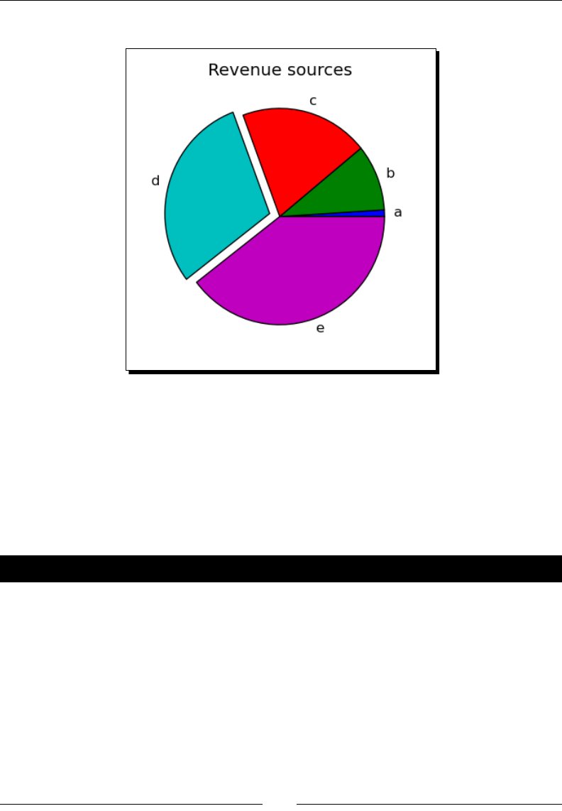
Plong with Sage
[ 164 ]
The plot should look like this:
What just happened?
We made a pie chart. The pie funcon in matplotlib only requires one argument, which is a
list of numbers that indicate the relave size of the slices. The explode opon takes a list of
numbers that show how far to oset each piece of the pie from the centre. In this case, we
created an array of zeros and set the fourth element to 0.1, which oset the fourth slice of
the pie. We used the keyword explode to pass this array to the pie funcon. We used the
labels keyword to pass a list of strings to be used as labels for each slice.
Time for action – plotting a histogram
matplotlib has a built-in funcon for making histograms, which are used to visualize the
distribuon of values in a set of data. In this example, we will generate an array of random
numbers that are drawn from a Gaussian distribuon:
import numpy
import matplotlib.pyplot as plt
data = numpy.random.normal(0, 1, size=1000)
plt.figure(figsize=(4, 4))
plt.hist(data, normed=True, facecolor=(0.9, 0.9, 0.9))
plt.savefig('Histogram.png')
plt.close()
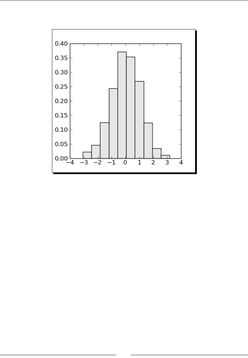
Chapter 6
[ 165 ]
The result should be similar to the following plot. Because we are generang random data,
your plot will not look exactly like this one:
What just happened?
We used the hist funcon to visualize the distribuon of values in an array of pseudo-
random numbers. hist requires one argument, which is an array containing the data. In
pracce, the data would typically consist of experimental measurements, sensor data, or
the results of a Monte Carlo simulaon. We used the oponal argument normed=True to
indicate that the histogram should be normalized, which means that its integral is one. The
facecolor keyword was used to specify the ll color of the bars as a tuple of R, G, B values.
Plotting in three dimensions
Sage can make 3D plots for visualizing funcons of two variables, as well as parametric
plots that create three-dimensional surfaces. It also has a variety of tools for making two-
dimensional representaons of three-dimensional surfaces.
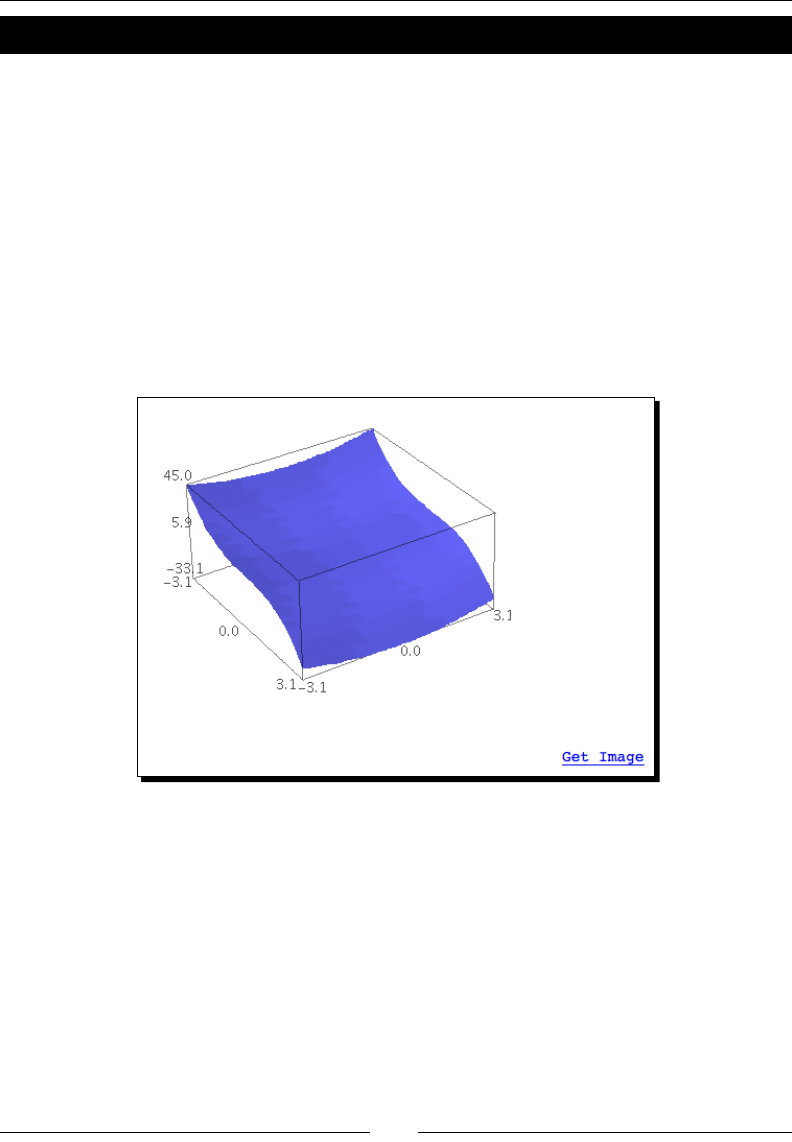
Plong with Sage
[ 166 ]
Time for action – make an interactive 3D plot
Let's make an interacve 3D plot.
var('x, y')
p3d = plot3d(y^2 + 1 - x^3 - x, (x, -pi, pi), (y, -pi, pi))
p3d.show()
If you run this example in the notebook interface, a Java applet called Jmol will run in the
cell below the code. If you run it from the interacve shell, Jmol will launch as a stand-alone
applicaon. Clicking and dragging on the gure with the le mouse buon will rotate the plot
in 3D space. Clicking and dragging with the centre buon, or moving the scroll wheel, zooms
in and out. Right-clicking brings up a menu that allows you to set various opons for Jmol.
Since Jmol is also used to visualize the 3D structures of molecules, some of the opons are not
relevant for plong funcons. Here is a screenshot of the funcon, ploed with Jmol:
What just happened?
We made a cool 3D plot that allowed us to explore a funcon of two variables. When
running Jmol as an applet in a worksheet, you can click on the "Get Image" link below the
plot to save an image of the plot in its current state. However, the image quality is not
parcularly high because it is saved in JPEG format. When Jmol is called from the command
line, it runs as a stand-alone applicaon, and more opons are available. You can save les
in JPEG, GIF, PPM, PNG, or PDF format. Note that the PDF format is a bitmap embedded in a
PDF le, rather than a true vector representaon of the surface. The syntax for using plot3d
is very simple:
plot3d(f(x,y), (x, x_min, x_max), (y, y_min, y_max))
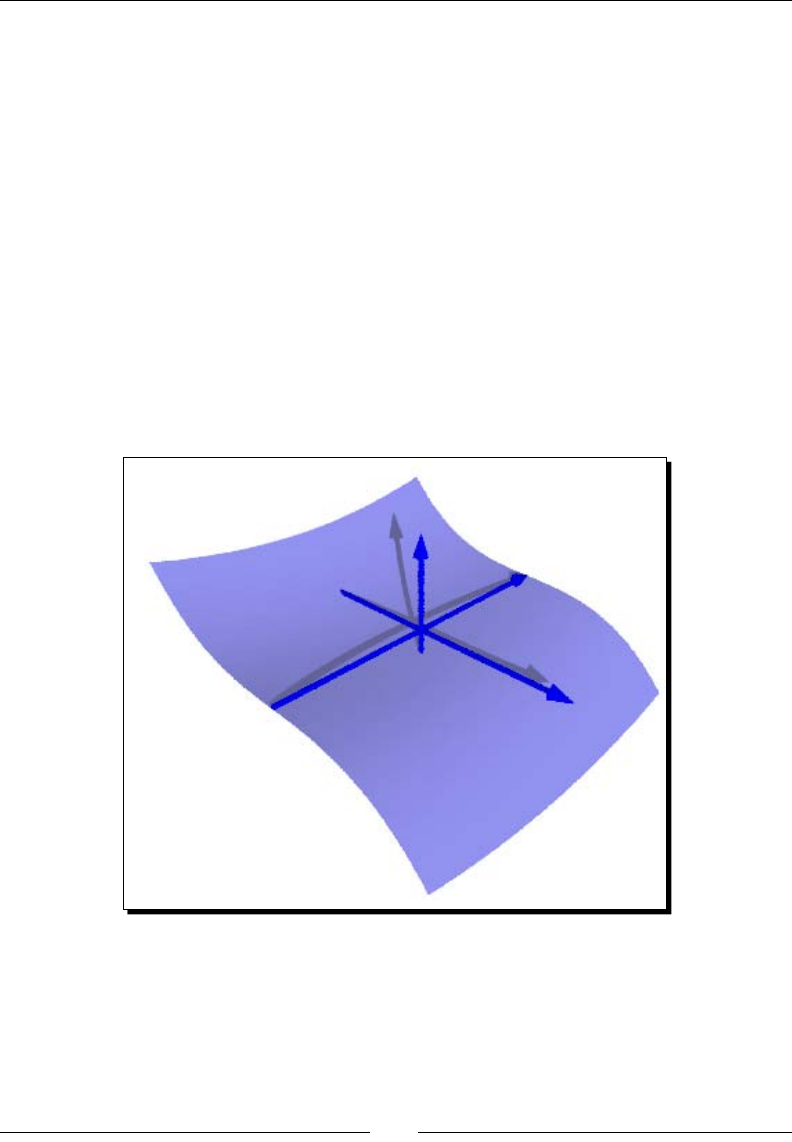
Chapter 6
[ 167 ]
There are a few oponal arguments to the show method that you can use to alter the
appearance of the plot. Seng mesh=True plots a mesh on the surface, and seng
dots=True plots a small sphere at each point. You can also use the transformation
keyword argument to apply a transformaon to the data—see the plot3d documentaon
for more informaon.
Higher quality output
We can improve the quality of saved images using ray tracing, which is an algorithm for
generang images that is based on opcal principles. Sage comes with ray tracing soware
called Tachyon, which can be used to view 3D plots. To acvate Tachyon, use the show
method with the viewer keyword as shown below:
p3d.show(viewer='tachyon', frame=False, axes=True)
Depending on the speed of your computer, the ray tracing may require a few seconds to a
few minutes.
The frame keyword selects whether or not to draw a box around the outer limits of the plot,
while the axes keyword determines whether or not the axes are drawn.
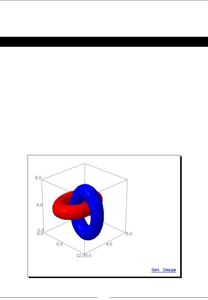
Plong with Sage
[ 168 ]
Parametric 3D plotting
Sage can also plot funcons of two variables that are dened in terms of a parameter. You
can make very complex surfaces in this way.
Time for action – parametric plots in 3D
We will plot two interlocking rings to demonstrate how complex surfaces are easily ploed
using three funcons of two parameters:
var('u, v')
f1 = (4 + (3 + cos(v)) * sin(u), 4 + (3 + cos(v)) * cos(u),
4 + sin(v))
f2 = (8 + (3 + cos(v)) * cos(u), 3 + sin(v), 4 + (3 + cos(v))
* sin(u))
p1 = parametric_plot3d(f1, (u, 0, 2 * pi), (v, 0, 2 * pi),
texture="red")
p2 = parametric_plot3d(f2, (u, 0, 2 * pi), (v, 0, 2 * pi),
texture="blue")
combination = p1 + p2
combination.show()
The result should look like this:

Chapter 6
[ 169 ]
What just happened?
We made a very complex 3D shape using the parametric_plot3d funcon. The oponal
arguments for this funcon are the same as the opons for the plot3d funcon.
Contour plots
Sage can also make contour plots, which are 2-D representaons of 3-D surfaces. While 3D
plots are eye-catching, a 2D plot can be a more praccal way to convey informaon about
the funcon or data set.
Time for action – making some contour plots
The following code will demonstrate four dierent ways to make a 2D plot of a 3D surface
with Sage:
var('x, y')
text_coords = (2, -3.5)
cp = contour_plot(y^2 + 1 - x^3 - x, (x, -3, 3), (y, -3, 3),
contours=8, linewidths=srange(0.5, 4.0, 0.5), fill=False,
labels=True, label_colors='black', cmap='gray', colorbar=False)
cp += text("Contour", text_coords)
ip = implicit_plot(y^2 + 1 - x^3 - x, (x, -3, 3), (y, -3, 3))
ip += text("Implicit", text_coords)
rp = region_plot(y^2 + 1 - x^3 - x < 0, (x, -3, 3), (y, -3, 3),
incol=(0.8, 0.8, 0.8)) # color is an (R,G,B) tuple
rp += text("Region", text_coords)
dp = density_plot(y^2 + 1 - x^3 - x, (x, -3, 3), (y, -3, 3))
dp += text("Density", text_coords)
show(graphics_array([cp, ip, rp, dp], 2, 2), aspect_ratio=1,
figsize=(6, 6))
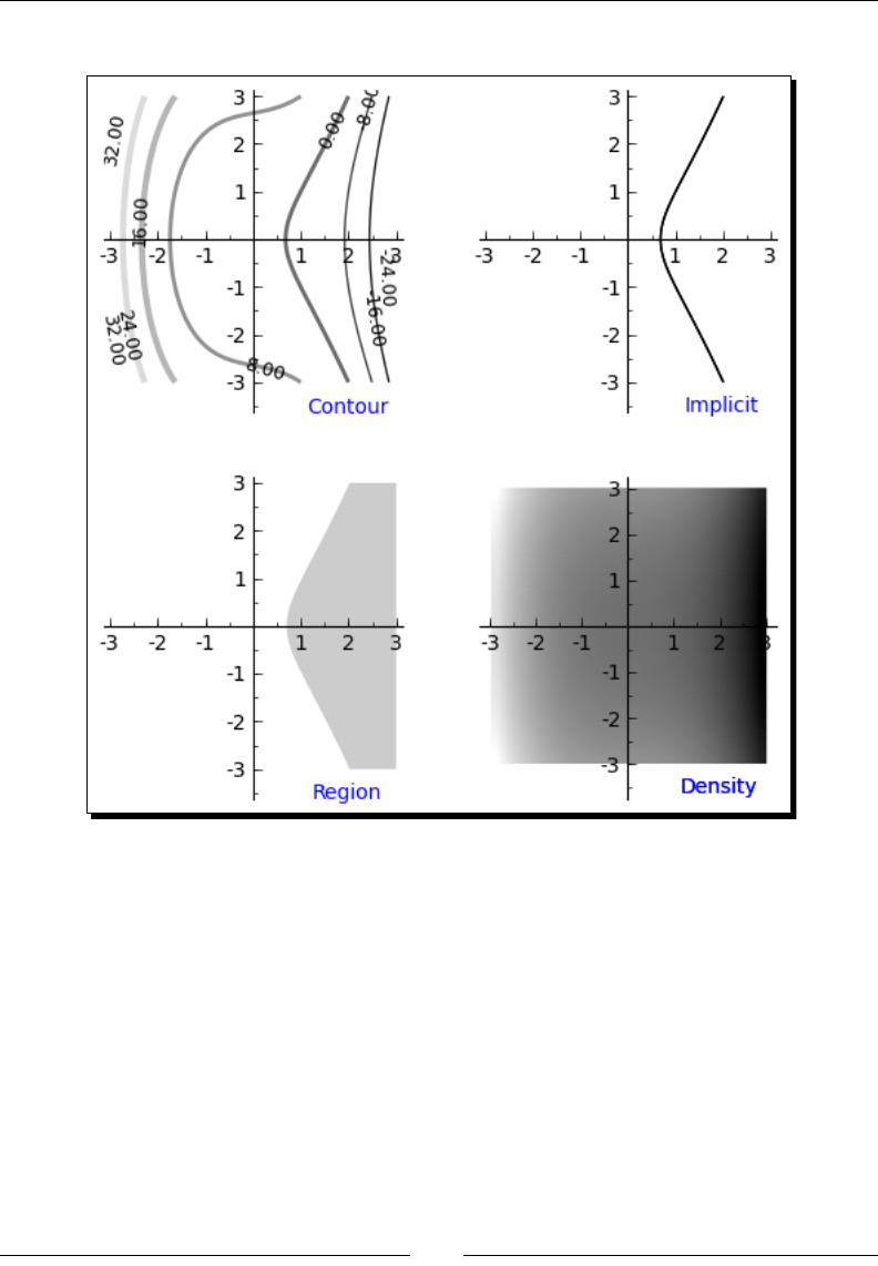
Plong with Sage
[ 170 ]
The output should be as follows:
What just happened?
The plots we made demonstrate four dierent ways of visualizing the funcon we ploed in
the previous example. All four funcons follow the same syntax as plot3d:
contour_plot(f(x,y), (x, x_min, x_max), (y, y_min, y_max))

Chapter 6
[ 171 ]
contour_plot plots level curves on the surface. In other words, z is constant on each
curve. implicit_plot does the same thing, but only plots the curve where z=0. region_
plot determines the curve for which z=0, and then lls in the region where z<0. Finally,
density_plot converts the z value of the funcon to a color value and plots a color
map of the z values over the x-y plane. We used the contour plot to demonstrate some of
the keyword arguments that can be used to control the appearance of the plot. Here is a
summary of the opons we used:
Keyword Descripon
contours The number of contours to draw
linewidths A list of line widths, corresponding to the number of contours
ll True to ll in between the contours
labels True to label each contour
label_colors Color to use for labels
cmap Color map to use for contour lines
colorbar True to display the a scale bar showing the color map
Summary
We have seen that Sage has powerful graphics capabilies. Specically, we learned about:
Plong funcons of one variable, in rectangular and polar coordinates
Seng opons that control the appearance of plots
Visualizing data with list_plot and scatter_plot
Using graphics primives to customize
Using matplotlib to gain more control over the formang of plots
Making various types of charts for presenng data
Making three-dimensional plots and contour plots
In the next chapter, we will learn how to use the powerful symbolic capabilies of Sage to
solve dicult problems in mathemacs, engineering, and science.
7
Making Symbolic Mathematics Easy
Every engineer, scienst, and mathemacian has taken classes that introduced calculus,
and many have learned more advanced mathemacs such as dierenal equaons.
Unfortunately, the majority of a student's me is oen spent performing algebra rather
than understanding advanced concepts. Sage has powerful tools that automate the tedious
process of moving symbols around in algebraic expressions. Further, Sage is capable of
dierenang and integrang complicated funcons, and performing Laplace transforms
that would otherwise need to be looked up in a reference book. In fact, Sage can perform
integrals and Laplace transforms that can't realiscally be performed by hand. Students and
professionals will nd it worth their me to learn how to ulize Sage to perform tedious
mathemacs so that they can focus on understanding important concepts and performing
creave problem-solving.
Although this chapter will focus on undergraduate-level mathemacs, Sage is also useful
for mathemacal research, as evidenced by the list of publicaons that reference Sage
(http://sagemath.org/library-publications.html). The lead developer of Sage
is a number theorist, and Sage is ahead of its commercial competors in the area of number
theory.
In this chapter, we will learn how to:
Create symbolic funcons and expressions, and learn to manipulate them
Solve equaons and systems of equaons exactly, and nd symbolic roots
Automate calculus operaons like limits, derivaves, and integrals
Create innite series and summaons to approximate funcons
Perform Laplace transforms
Find exact soluons to ordinary dierenal equaons
So let's get on with it...

Making Symbolic Mathemacs Easy
[ 174 ]
Using the notebook interface
All of the examples in this chapter were wrien using the notebook interface. I highly
recommend using the notebook for performing symbolic calculaons. The show funcon
(or method) generates nicely formaed output that is much easier to read than the text
representaon that you get on the command line.
Calling Maxima directly
Sage uses Maxima, an open-source computer algebra system, to handle many
symbolic calculaons. You can interact directly with Maxima from a Sage
worksheet or the interacve shell by using the maxima object. For a complete
tutorial with many examples, see http://www.sagemath.org/doc/
reference/sage/interfaces/maxima.html.
Dening symbolic expressions
Before we can start doing integrals, derivaves, and transforms, we have to dene the
variables and funcons that we are going to be working with. Funcons and relaons
in Sage are called symbolic expressions.
Time for action – dening callable symbolic expressions
In Chapter 3, we learned how to dene a mathemacal funcon as a callable symbolic
expression. Since we'll be working with callable symbolic expressions extensively in this
chapter, let's learn a lile more about how to use them. Enter the following code into an
input cell in a worksheet, and evaluate the cell:
var('a, b, c, x')
f(x) = a * x^2 + b * x + c # A callable symbolic expression
print("f(x):")
f.show()
print("Variables in f: {0} Arguments in f: {1}".format(
f.variables(), f.arguments()))
print("Type of f: {0}".format(type(f)))
g(x) = f.derivative(x)
print("g(x):")
g.show()
print("Variables in g: {0} Arguments in g: {1}".format(
g.variables(), g.arguments()))
g_plot = plot(g(a=1, b=-1), (-1, 1))
g_plot.axes_labels(['x', 'g(x)'])
show(g_plot, figsize=(3,3), aspect_ratio=1.0)
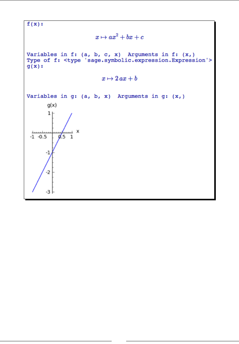
Chapter 7
[ 175 ]
The output is shown below:
What just happened?
We started with a var statement to tell Sage that x, a, b, and c are symbolic variables, which
also erases any previous values that we may have assigned to these variables. Technically,
we could have omied x from this list, since Sage automacally assumes that any variable
called x is a symbolic variable. We then dened a callable symbolic expression f(x). We
used the variables method to list all of the variables that are present in f. We also used
the method arguments to determine which variables are arguments. In this case, x is
the only argument because we dened f to be a funcon of x. In Sage, an argument is an
independent variable, while the other variables are more like parameters that are expected
to take on xed values.

Making Symbolic Mathemacs Easy
[ 176 ]
We used the derivative method to compute the derivave of f with respect to x, and
assign the result to another callable symbolic expression called g. Again, the methods
variables and arguments were used to see which variables and arguments are present in
g. Noce that the variable c is not present in g. Finally, we ploed funcon g to demonstrate
how to plot a callable symbolic expression with one argument and mulple variables. In
order to make a plot, Sage needs to have numerical values for the parameters a and b. In
the plot funcon call, we used keyword syntax to set values for these variables, and we set
limits for the domain of x in the usual way.
Relational expressions
A symbolic expression doesn't have to dene a mathemacal funcon. We can also express
equality and inequality with symbolic expressions.
Time for action – dening relational expressions
Let's express some simple inequalies as relaonal expressions to see how they work:
exp1 = SR(-5) < SR(-3) # use the symbolic ring
print("Expression {0} is {1}".format(exp1, bool(exp1)))
exp2 = exp1^2
print("Expression {0} is {1}".format(exp2, bool(exp2)))
forget()
exp3 = x^2 + 2 >= -3 * x^2
print("Expression {0} is {1}".format(exp3, bool(exp3)))
p1 = plot(exp3.lhs(), (x, -5, 5), legend_label='lhs')
# also lhs() or left_hand_side()
p2 = plot(exp3.rhs(), (x, -5, 5), color='red', legend_label='rhs')
# also rhs() or right_hand_side()
show(p1 + p2)
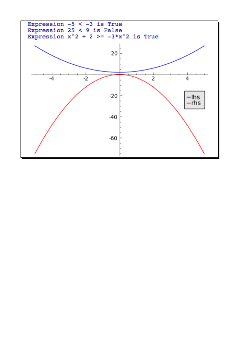
Chapter 7
[ 177 ]
The output is shown in the following screenshot:
What just happened?
We dened a simple relaonal expression that expresses an inequality between two
integers. We used the SR funcon to create symbolic objects, rather than integer objects,
that represent the values -5 and -3. This is important because we need to give Sage a
symbolic expression to work with. To evaluate the truth of the inequality, we used the bool
funcon. Next, we used the syntax exp1^2 to square both sides of the inequality, and used
bool to evaluate the new inequality. This would not have worked if we had dened the
inequality using integers.
We then created a relaonal symbolic expression involving the symbolic variable x. Since
the expression involves at least one symbolic variable, Sage treats the enre expression as
a symbolic expression. That's why we didn't need to use SR to create symbolic variables
instead of numerical variables. We called the forget funcon before evaluang the
expression, which clears any assumpons about any variables that may have been set (we'll
cover assumpons in the next example). To help understand why this expression evaluates
to True, we ploed each side of the expression on the same axes. The method left (and its
synonyms lhs and left_hand_side) return the le-hand side of an expression, while the
method right (and its synonyms rhs and right_hand_side) return the right-hand side.
The plot shows that the right-hand side is less than the le-hand side for all values of x, so
the expression evaluates to True. If the inequality is false for only one point in the domain,
then it evaluates to False.
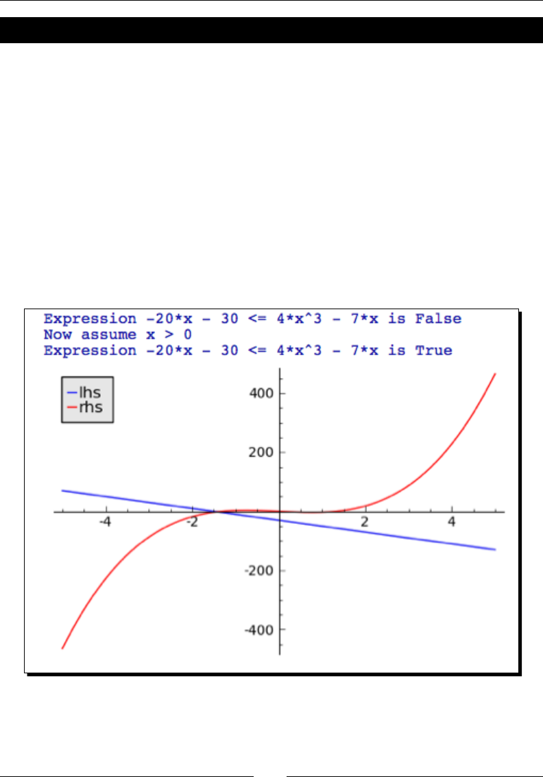
Making Symbolic Mathemacs Easy
[ 178 ]
Time for action – relational expressions with assumptions
Let's try a more complicated expression that states an inequality between two funcons.
We'll use plots to illustrate what's happening:
forget()
expr = -20 * x - 30 <= 4 * x^3 - 7 * x
print("Expression {0} is {1}".format(expr, bool(expr)))
p1 = plot(expr.left(), (x, -5, 5), legend_label='lhs')
p2 = plot(expr.right(),(x, -5, 5), color='red', legend_label='rhs')
assume(x > 0)
print("Now assume x > 0")
print("Expression {0} is {1}".format(expr, bool(expr)))
show(p1 + p2)
The output is shown in the following screenshot:

Chapter 7
[ 179 ]
What just happened?
We started the example with a call to the forget funcon, to clear any assumpons that
we may have made in other cells. The rst expression evaluated to False, because the
expression on the le-hand side is greater than the expression on the right-hand side over
part of the domain. However, when we used the assume statement to assert that x>0, the
expression evaluated to True. Looking at the plot, we can see why this is true.
Manipulating expressions
We've already seen how to square both sides of a relaonal expression. There are many
ways to manipulate relaonal expressions with Sage.
Time for action – manipulating expressions
Enter the following code into an input cell in a worksheet, and evaluate the cell:
var('x, y')
expr = (y - 7) / (x^2 + 1) == x^3 - 5
print("Expression:")
expr.show()
print("Two ways of multiplying both sides:")
show(expr.multiply_both_sides(x^2 + 1))
show(expr * (x^2 + 1))
# also divide_both_sides
expr = expr * (x^2 + 1)
print("Two ways of adding to both sides:")
show(expr.add_to_both_sides(7))
show(expr+7)
# also subtract_from_both_sides
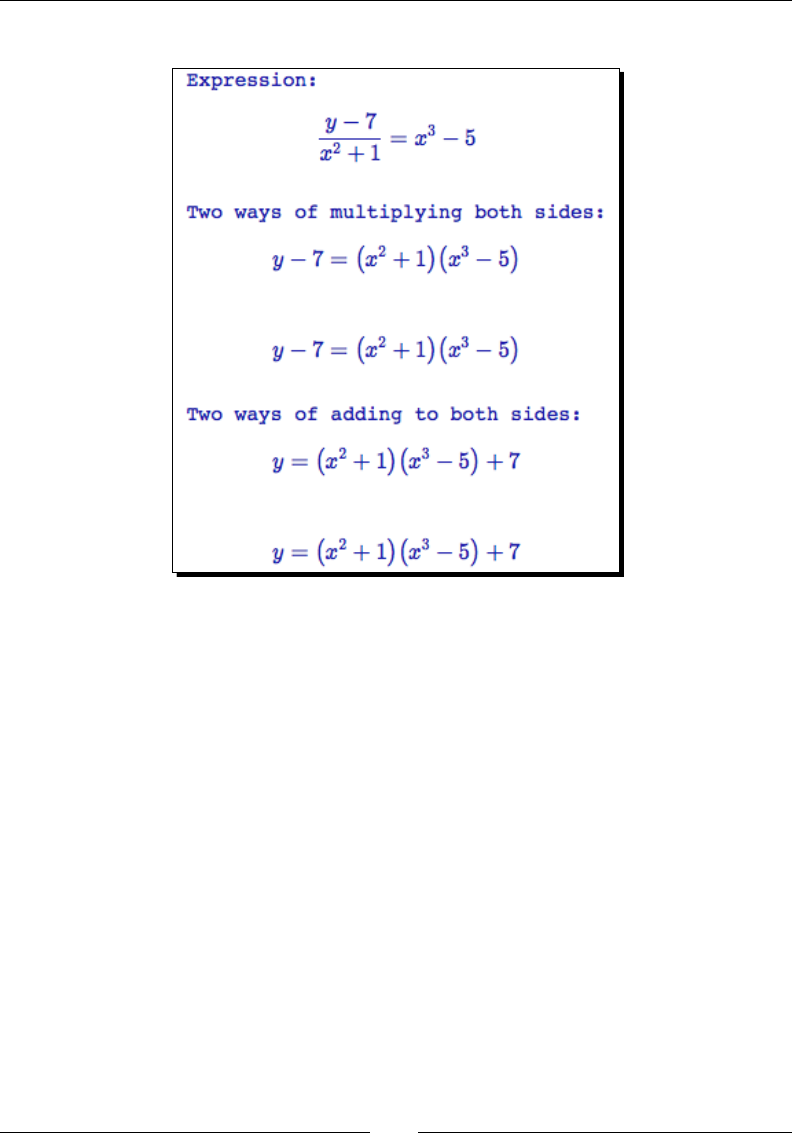
Making Symbolic Mathemacs Easy
[ 180 ]
The results are shown in the following screenshot:
What just happened?
This example showed how to perform one of the most basic algebraic re-arrangements:
performing the same operaon on both sides of a relaon. We can do this by using methods
of the symbolic expression object (add_to_both_sides, subtract_from_both_sides,
multiply_both_sides, divide_both_sides). We can also use the arithmec operators
+, -, *, and / to perform the same operaon on both sides of a relaon. Note that these
operaons return a new symbolic expression, instead of modifying the exisng expression.
To modify the expression, we use the syntax expr = expr * (x^2 + 1). We can also use
the shortcuts +=, -=, *=, and /=, just like ordinary arithmec.
Manipulating rational functions
Sage has special operaons that are useful for working with raonal funcons. A raonal
funcon is any funcon that can be wrien as the rao of two polynomial funcons. Raonal
funcons oen occur when using the Laplace transform to solve ordinary dierenal
equaons.
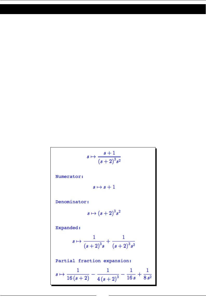
Chapter 7
[ 181 ]
Time for action – working with rational functions
Let's say you have used the Laplace transform to solve an ordinary dierenal equaon. You
have a raonal funcon in the s domain, and you need to transform it back to the original
problem domain. Here are some tools you can use to manipulate the symbolic expression to
make it easier to perform the inverse Laplace transform:
var('s')
F(s) = (s + 1) / (s^2 * (s + 2)^3)
show(F)
print("Numerator: ")
show(F.numerator())
print("Denominator: ")
show(F.denominator())
print("Expanded:")
show(F.expand_rational())
print("Partial fraction expansion:")
pf(s) = F.partial_fraction()
show(pf)
The results are shown in the following screenshot:

Making Symbolic Mathemacs Easy
[ 182 ]
What just happened?
We dened a raonal funcon, and demonstrated the ulity methods numerator and
denominator to obtain dierent parts of the expression. The method expand_rational
separates the expression into a sum of terms by mulplying out products of sums and
exponenals, spling the numerator into terms, and distribung mulplicaon over
addion. The method partial_fraction returns the paral fracon expansion of the
expression. This is an extremely tedious calculaon to perform by hand, and it is oen the
most me-consuming step in solving a dierenal equaon with the Laplace transform.
Substitutions
When working with symbolic expressions, it is oen necessary to substute one variable
or funcon for another. Substuon is oen a crical step when deriving an equaon or
simplifying an expression.
Time for action – substituting symbols in expressions
Let's see how to perform symbolic substuons with Sage.
var('x, y')
f(x) = 1 / x + 3 * x^2 + cos(x)
f.show()
print("Substitute for x with a keyword:")
show(f.subs(x=(7 * x)))
print("Substitute for x with a relational expression:")
show(f.substitute(x == 7 * x))
print("Substitute sine for cosine:")
show(f.substitute_function(cos, sin))
print("Substitute using a dictionary:")
show(f.substitute({1 / x: y^3, cos(x):sin(x)}))
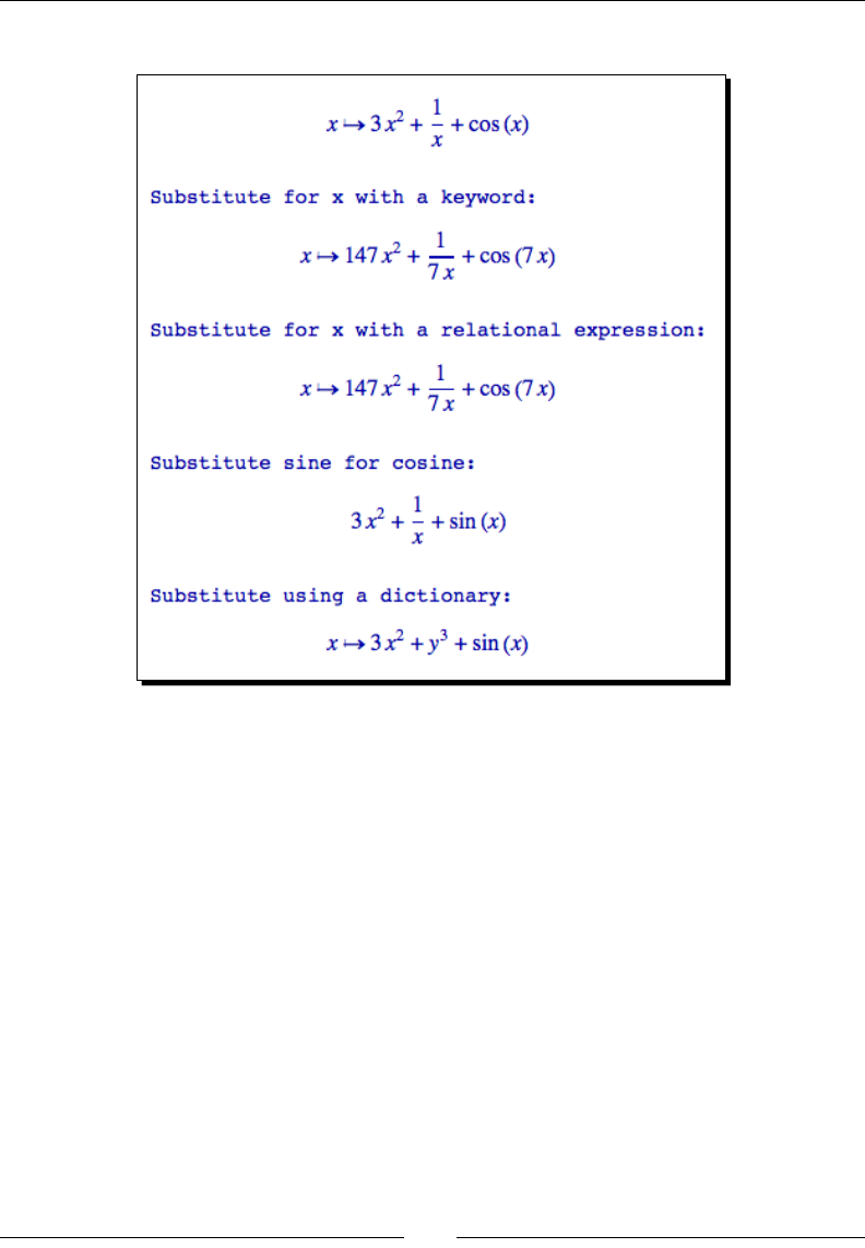
Chapter 7
[ 183 ]
The results are shown in the following screenshot:
What just happened?
We used several methods to substute both variables and funcons in a callable symbolic
expression. The methods called subs and substitute are idencal. If you only need to
replace a single symbol, a keyword argument can be used to specify which variable is to be
replaced, and what expression should take its place. Mulple keywords can be used to make
mulple substuons at the same me. A relaonal expression can be used to replace a
single symbol, or a sub-expression. We then used the method substitute_function to
replace one funcon (sine) with another (cosine). Finally, we demonstrated that a diconary
can be passed to the substitute (or subs) method to specify the substuon. Each
key:value pair in the diconary describes one substuon. The key is the expression to
be replaced, and the value is the replacement. Using a diconary is very exible, because
you can replace a variable, a sub-expression (such as 1/x), or a funcon. When you use a
diconary to replace a funcon, note that you have to describe the funcons as cos(x) and
sin(x), rather than cos and sin.

Making Symbolic Mathemacs Easy
[ 184 ]
Another way to perform substuons is with the substitute_expression method
(and its synonym subs_expr). These methods use the subst command in Maxima, which
performs a formal paern substuon. The results may not be mathemacally meaningful,
so it is best to avoid these two methods if possible.
Expanding and factoring polynomials
Expanding a polynomial is the process of converng the polynomial from a product of
sums to a sum of products. Factoring is the opposite process, in which a sum of products
is converted into a product of factors.
Time for action – expanding and factoring polynomials
A number of methods are especially useful when working with polynomials. Let's see how
they work:
var('x')
exp1 = (x + 3)^3 == (x - 1)^2
show(exp1)
print("Expanded expression:")
exp2 = exp1.expand()
show(exp2)
print("Expand left-hand side only:")
show(exp1.expand('left'))
lhs = exp1.expand('left').lhs()
print("Factor LHS:")
show(lhs.factor())
print("Information about the expanded LHS:")
print(" Highest degree of x on LHS: {0}".format(lhs.degree(x)))
print(" Coefficients: {0}".format(lhs.coeffs(x)))
print(" Coefficient of x^2: {0}".format(lhs.coeff(x,2)))
print(" Trailing coefficient of LHS: {0}".format
(lhs.trailing_coefficient(x)))
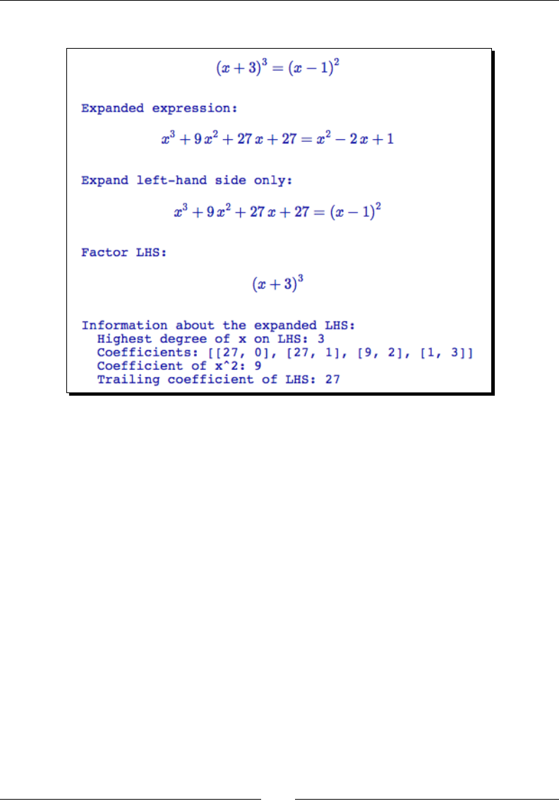
Chapter 7
[ 185 ]
The output is shown in the following screenshot:
What just happened?
We dened a relaonal symbolic expression that equates two polynomials. We used the
expand method (with no arguments) to mulply out the polynomials on each side of the
equality. We also used the expand method with the oponal argument 'left' to expand
only the le-hand side (you can also use 'right'). We then used the factor method
to factor the expanded le-hand side of the expression, and recovered its original form.
These two methods are complementary, and can be used to move back and forth between
dierent representaons of a polynomial.
We also demonstrated some methods that return informaon about polynomials. The
method degree returns the largest exponent of the given symbol in the polynomial. The
method coeffs (or coefficients) returns a list that contains the coecients of each
term in the polynomial. Each item in the list is another list. The rst item is the coecient,
and the second item is the degree of the term with that coecient. The coeff (or
coefficient) method allows us to get the coecient for a specic term. Its rst argument
species a symbol, and its second argument species the power of that symbol. You may
need to expand or factor the polynomial before calling this method. Finally, the method
trailing_coefficient (or trailing_coeff) was used to obtain the coecient for the
smallest power of x in the le-hand side.
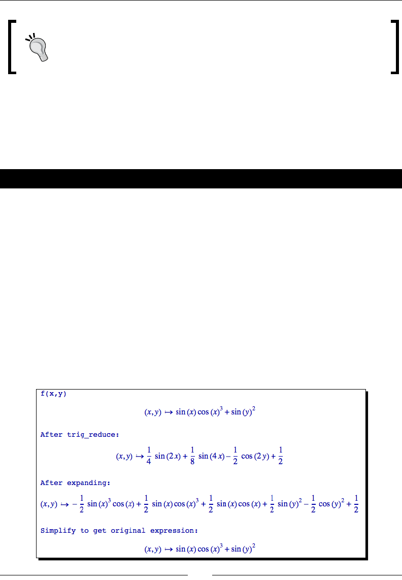
Making Symbolic Mathemacs Easy
[ 186 ]
The factor funcon in Sage is used to factor both polynomials and integers.
This behaviour is dierent from Mathemaca, where Factor[] is used to
factor polynomials and FactorInteger[] is used to factorize integers.
Manipulating trigonometric expressions
Expressions involving trigonometric funcons can be dicult to manipulate because of the
numerous trigonometric idenes that can be used (http://en.wikipedia.org/wiki/
List_of_trigonometric_identities). Fortunately, Sage can automate this process.
Time for action – manipulating trigonometric expressions
Sage has several methods that are used primarily when an expression involves trigonometric
funcons. Let's try them out.
var('x, y')
f(x, y) = sin(x) * cos(x)^3 + sin(y)^2
print("f(x, y)")
f.show()
g(x, y) = f.reduce_trig() # also trig_reduce
print("After trig_reduce:")
g.show()
print("After expanding:")
show(g.expand_trig()) # also trig_expand
print("Simplify to get original expression:")
show(g.expand_trig().trig_simplify()) # also simplify_trig
The output is shown in the following screenshot:

Chapter 7
[ 187 ]
What just happened?
We demonstrated some useful methods that are specically designed to manipulate
expressions that involve trigonometric funcons. expand_trig and reduce_trig (or
trig_expand and trig_reduce) are complementary methods that have a similar funcon
to those used in the previous example. We also introduced the method called trig_
simplify (or simplify_trig), which aempts to represent an expression in the most
compact way.
Logarithms, rational functions, and radicals
There are special rules for manipulang logarithms and radicals, so Sage has special methods
for expanding and simplifying expressions involving these operaons. There is also a
separate method for simplifying raonal expressions.
Time for action – simplifying expressions
In the following example, we will see how Sage can be used to simplify expressions that
involve exponenals, logarithms, raonal funcons, and square roots:
var('x')
# Logs
f(x) = log(x^2 * sin(x) / sqrt(1 + x))
print("Original function:")
f.show()
print("This form is easier to work with:")
show(f.expand_log())
print("Simplify expanded form:")
show(f.expand_log().simplify_log())
# Rational functions
f(x) = (x + 1) / (x^2 + x)
print("Original function:")
f.show()
print("Simplified:")
show(f.simplify_rational())
# Radicals
f(x) = sqrt(x^2+x)/sqrt(x)
print("Original function:")
f.show()
print("Simplified:")
show(f.simplify_radical())
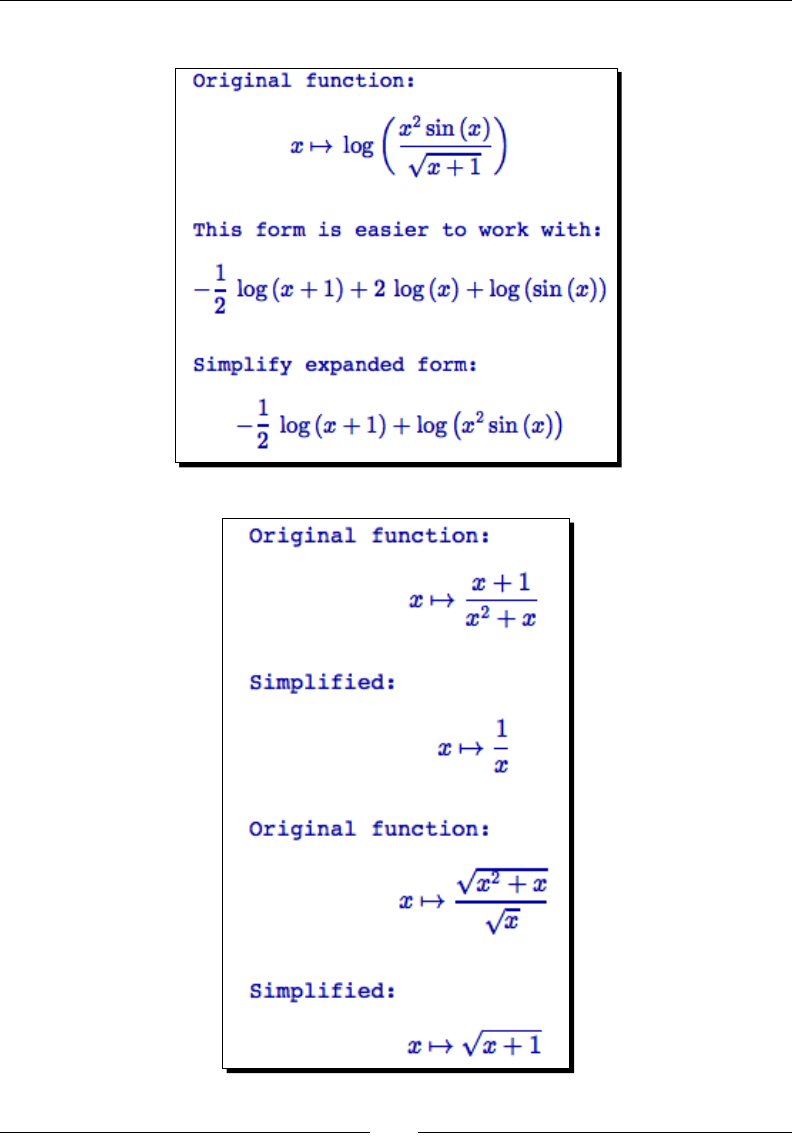
Making Symbolic Mathemacs Easy
[ 188 ]
The output is shown in the following screenshot:

Chapter 7
[ 189 ]
What just happened?
We demonstrated some special methods for expanding and simplifying expressions involving
logs, raonal funcons, and radicals. The following table summarizes the methods available
in Sage for simplifying and expanding expressions:
Method(s) Descripon
expand_log log_
expand
Expands logarithms of powers, logarithms of products, and logarithms
of quoents
simplify_log
log_simplify
Aempt to simplify an expression involving logarithms
simplify_rational
rational_simplify
Aempt to simplify an expression involving raonal expressions
radical_simplify
simplify_radical
exp_simplify
simplify_exp
Aempt to simplify an expression involving radicals
simplify_
factorial
factorial_
simplify
Simplify an expression by combining factorials and expanding binomials
into factorials
simplify_full
full_simplify
Applies the following operaons, in order: simplify_factorial,
simplify_trig, simplify_rational, simplify_radical,
simplify_log, and again simplify_rational
It can be tricky to get an expression in the form that you want. You may have to experiment
with various combinaons of expanding, simplifying, and factoring an expression. Part of the
problem is that it is dicult to quanfy the "simplest" form of an expression. Most of the
commands in Sage that factor, expand, or simplify expressions accept oponal arguments
that control how they work. Look at the documentaon for each method for more
informaon.
Logarithms in Sage
The log funcon in Sage assumes the base of the logarithm is e. If you want to
use a dierent base (such as 10), use the oponal argument with keyword base
to specify the base. For example: log(x, base=10)
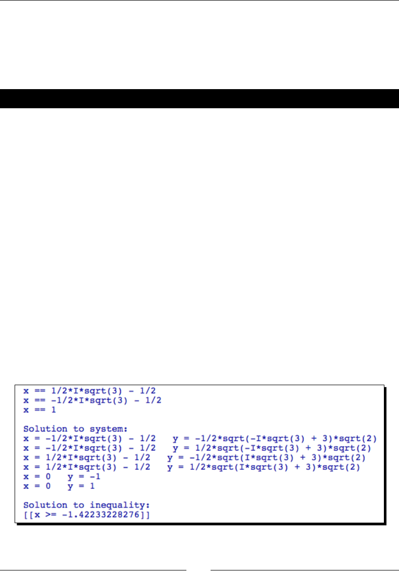
Making Symbolic Mathemacs Easy
[ 190 ]
Solving equations and nding roots
Solving equaons is a fundamental task in mathemacs. A related task is nding the values
of the independent variables for which a funcon is equal to zero, which is known as nding
its roots.
Time for action – solving equations
Enter the following code into an input cell in a worksheet, and evaluate the cell:
var('x, y')
# Solve a single equation
f(x) = x^3 - 1
solution1 = solve(f == 0, x)
for solution in solution1:
print(solution)
# Solve a system of equations
solutions = solve([x^2 + y^2 == 1, y^2 == x^3 + x + 1], x, y,
solution_dict=True)
print("\nSolution to system:")
for solution in solutions:
print("x = {0} y = {1}".format(solution[x], solution[y]))
# Solve an inequality
print("\nSolution to inequality:")
solve(-20 * x - 30 <= 4 * x^3 - 7 * x, x)
# Plotted in previous example
The output is shown in the following screenshot:

Chapter 7
[ 191 ]
What just happened?
We used the solve funcon to solve an equaon, a system of equaons, and an inequality.
The rst argument to solve is an equaon or a list of equaons. The next argument (or
arguments) is the variable or variables to solve for. By default, the soluons are returned
as a list of symbolic expressions. The oponal keyword argument solution_dict=True
causes the soluons to be returned as a list of diconaries. Each diconary has a key for each
variable that was solved for, and the value for a key is the soluon for that variable. Solving
an inequality uses the same syntax. In this case, Sage was unable to nd a symbolic soluon
to the inequality.
Finding roots
Finding the roots of an equaon (also known as the zeros of the equaon) is closely related
to solving an equaon. Callable symbolic expressions in Sage have a special method that
nds their roots.
Time for action – nding roots
Enter the following code into an input cell in a worksheet, and evaluate the cell:
# A problem we already know the answer to
var('a, b, c, x')
f(x) = a * x^2 + b * x + c
root_list = f.roots(x)
for root in root_list:
print("Root with multiplicity {0}:".format(root[1]))
show(root[0])
# Something more complicated
g(x) = expand((x^2 - 1)^3 * (x^2 + 1) * (x - 2));
g.show()
root_list = g.roots(x)
for root in root_list:
print("Root: {0} multiplicity: {1}".format(root[0], root[1]))
p1 = plot(g, (-2, 2))
p1.ymin(-10)
p1.show()
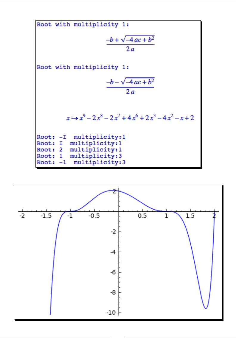
Making Symbolic Mathemacs Easy
[ 192 ]
The output is shown in the following screenshot:
Chapter 7
[ 193 ]
What just happened?
We started o by nding the roots for the general second-order polynomial with the roots
method. The result is a list of tuples that represent the roots. The rst item in each tuple is
the mulplicity, and the second item is the root. We passed the variable x to roots. If this
argument is not provided, roots formulates the soluon in terms of the default variable. We
then looked at a higher-order polynomial, which has three real roots and two complex roots.
The analycal results are conrmed by a plot of the funcon that shows the real roots of the
funcon. The roots method accepts several oponal arguments that control its behaviour:
Keyword Default Descripon
explicit_soluons True If False, also include implicit roots
mulplicies True If False, return a list of roots without mulplicies
ring None If a ring is specied, the expression is converted to a polynomial
over the ring, and the roots are found over the ring
Differential and integral calculus
Many branches of advanced mathemacs are built upon a foundaon of basic calculus. The
following examples will demonstrate how to use Sage to compute limits, derivaves, and
integrals of symbolic funcons.
Time for action – calculating limits
The concept of the limit is oen used to dene the integral and the derivave. Run the
following code to see how to compute limits with Sage:
var('x')
# Something easy
f(x) = 1 / x
print("Limit of 1/x as x->0+: {0}".format(limit(f, x=0,
dir='plus')))
print("Limit of 1/x as x->0-: {0}".format(limit(f, x=0
dir='minus')))
p1 = plot(f, (x, -1, 1), detect_poles='show')
p1.axes_range(-1, 1, -10, 10)
p1.show()
# Something more complex
g(x)=(2 * x + 8) / (x^2 + x - 12)
g.show()
print("Limit of g(x) as x->-4: {0}".format(limit(g, x=-4)))
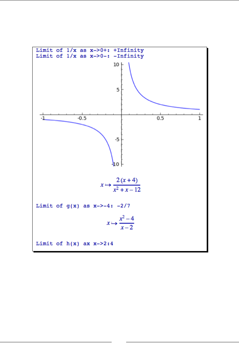
Making Symbolic Mathemacs Easy
[ 194 ]
h(x) = (x^2 - 4) / (x - 2)
h.show()
print("Limit of h(x) ax x->2: {0}".format(lim(h, x=2)))
The results are shown in the following screenshot:

Chapter 7
[ 195 ]
What just happened?
We started out by dening a simple funcon with a disconnuity at zero. We used the
funcon limit (or lim) to compute the limit as x approaches zero. The rst argument to
limit is a funcon, and the second argument is the value at which to compute the limit.
If the dir keyword argument is present, a one-sided limit is computed from either above
or below the specied value. The values '+', 'plus', or 'right' compute the limit from
above, while '-', 'minus'¸ or 'left' compute the limit from below. If dir is omied,
a two-sided limit is computed. limit also accepts the keyword argument taylor, which
is False by default. If taylor=True, then a Taylor series is used to approximate the
funcon when compung the limit. The second funcon we dened looks more complicated,
although the limit calculaon is straighorward. The third case demonstrated that Sage is
able to handle indeterminate forms, where the funcon evaluates to 0/0 at the given point.
Derivatives
The derivave describes how a funcon responds to an innitesimal change in one of its
independent variables. Derivaves are used to compute rates of change.
Time for action – calculating derivatives
Run the following code to see how to compute derivaves with Sage:
var('x, y')
f(x, y) = 3 * x^4 * y^3 + 9 * y * x^2 - 4 * x + 8 * y
print("f(x,y):")
f.show()
dfdx(x, y) = diff(f, x)
print("df/dx:")
dfdx.show()
dfdy(x, y) = diff(f, y)
print("df/dy:")
dfdy.show()
print("Second derivative:")
d2fdx2(x, y) = derivative(f, x, 2) # Synonym for diff
d2fdx2.show()
# Trigonometric functions
g(x) = sqrt(x^3 + csc(x))
print("g(x):")
g.show()
dgdx(x) = g.diff(x)
print("dg/dx:")
dgdx.show()
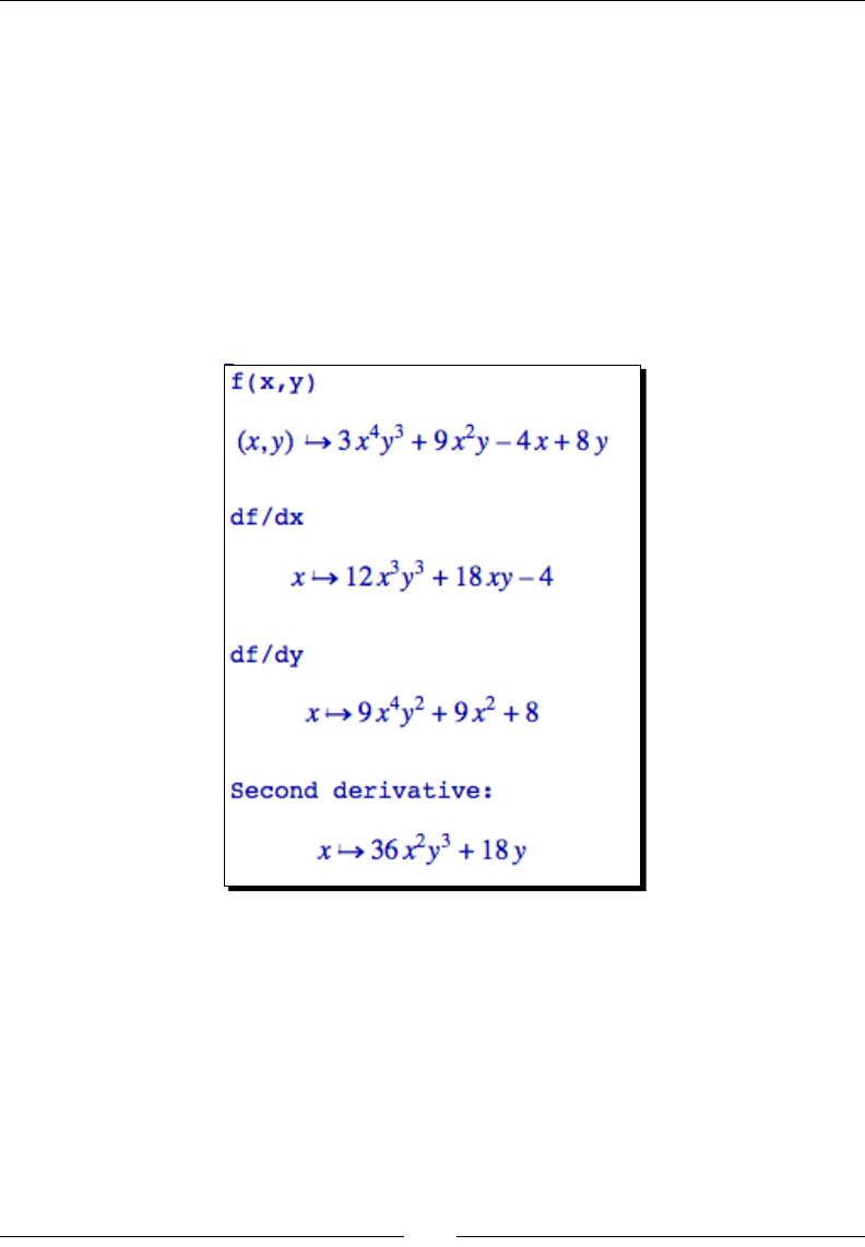
Making Symbolic Mathemacs Easy
[ 196 ]
# Implicit differentiation
# The next line tells Sage that y is a function of x
y(x) = function('y', x)
expr = 5 * y^2 + sin(y) == x^2
print("Expression:")
expr.show()
# take the derivative and solve for dy/dx
dydx = solve(diff(expr), diff(y))
print("dy/dx:")
dydx[0].show()
The results are shown in the following screenshot:
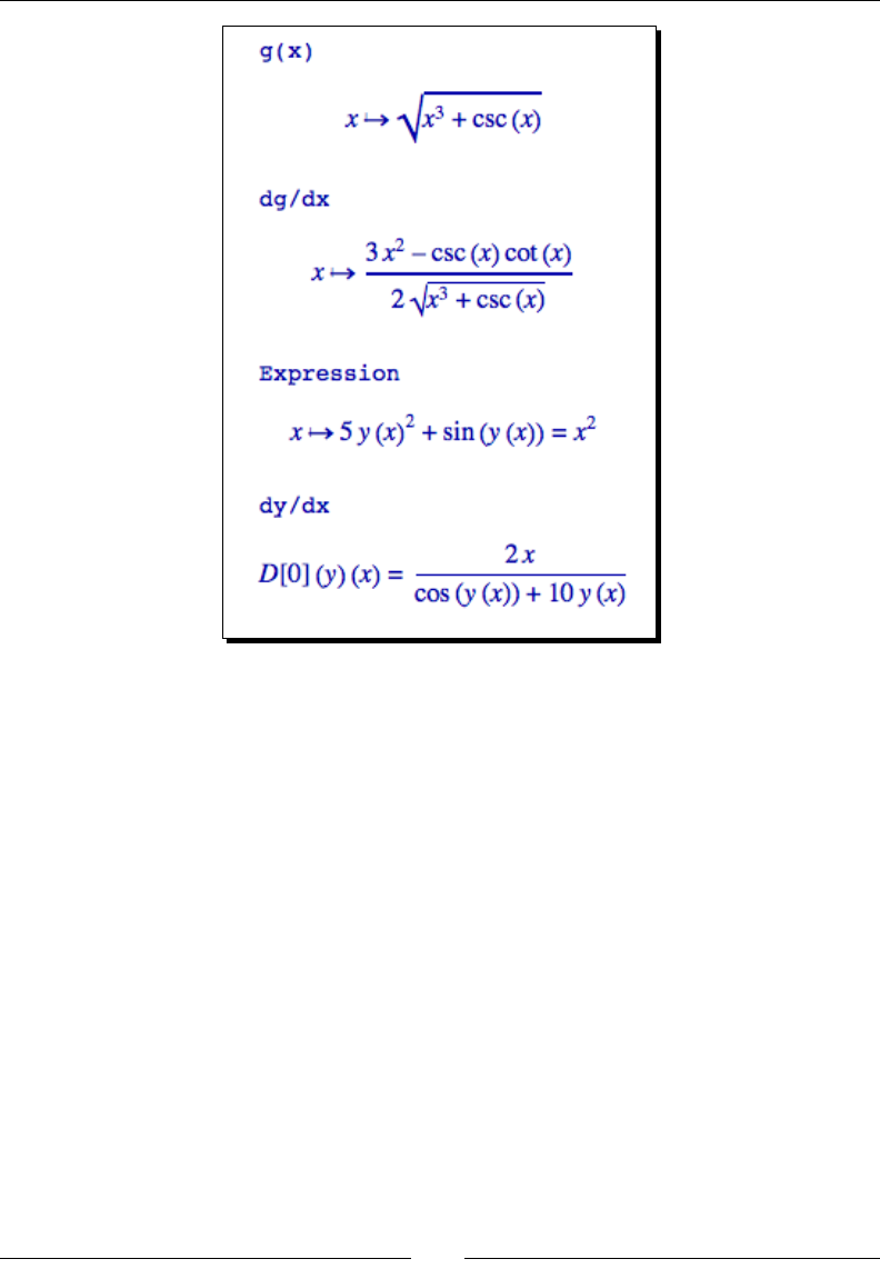
Chapter 7
[ 197 ]
What just happened?
Sage is able to compute derivaves for many types of funcons. You can use a funcon
called diff (or differentiate or derivative), or an equivalent method with the
same names. In the example, we used both the funcon form and the method form. When
calling diff as a funcon, the rst argument is a funcon which is dierenated against
the variable specied in the second argument. If a third argument is present, it is the degree
of the derivave (the default is one, for the rst derivave). We started by dening a long
polynomial funcon of two variables, x and y. We then dierenated with respect to each
variable. We also computed the second derivave. We didn't have to change anything to
compute the derivave of a trigonometric funcon. In the nal part of the example, we
demonstrated how to do implicit dierenaon. The funcon y(x) was dened implicitly
by a relaonal symbolic expression. We used the syntax y(x) = function('y', x)
to create a new symbolic funcon called y that is a funcon of x. The rst argument of
function is a string that contains the name of the new funcon. The next argument is
the argument of the symbolic funcon (it can have mulple arguments). We then used the
diff funcon to compute the derivave of the enre expression, and then used the solve
funcon to isolate the derivave.
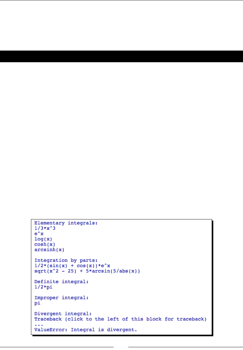
Making Symbolic Mathemacs Easy
[ 198 ]
Integrals
Sage is able to integrate many symbolic funcons that would need to be looked up in a table
of integrals, or computed using laborious methods like integraon by parts. Sage can easily
compute symbolic integrals that cannot be found in any book.
Time for action – calculating integrals
Run the following example to see how to compute integrals with Sage:
var('x')
print("Elementary integrals:")
f = x^2
print(f.integrate(x))
print(integral(e^x,x))
print(integral(1/x,x))
print(integral(sinh(x), x))
print(integral(1/sqrt(1+x^2),x))
print("\nIntegration by parts:")
print(integral(e^x*cos(x), x))
print(integral(sqrt(x^2-25)/x, x))
print("\nDefinite integral:")
print(integral(1/(1+x^2), x, -1, 1))
print("\nImproper integral:")
print(integral(1/(1+x^2), x, -infinity, infinity))
print("\nDivergent integral:")
print(integral(1/(1-x), x, 1,2)) # Diverges
The results are shown in the following screenshot:

Chapter 7
[ 199 ]
What just happened?
The funcon integrate (or integral) is used to compute integrals, and the methods
called integrate and integral do exactly the same thing. We started out by showing that
Sage knows about lots of the elementary integrals. We then showed that Sage easily handles
funcons that need to be integrated by parts, which can be very tedious to do by hand. If
integrate is called as a funcon, the rst argument is the funcon to be integrated, and
the second argument is the variable of integraon. If there are no addional arguments,
the integral is assumed to be indenite. If two addional arguments are present, they
are used as the limits of integraon. We showed that Sage can compute denite integrals
and improper integrals (one or more limits at innity.) In the nal case, we showed what
happens when an integral diverges: Sage simply prints an appropriate error message and
exits. integrate also accepts the oponal keyword argument algorithm to choose
the integraon algorithm, which can be set to 'maxima' (the default), 'sympy', or
'mathematica_free' (which uses http://integrals.wolfram.com/).
Series and summations
An innite series is a summaon of a sequence with an innite number of terms. Truncated
series are useful for approximang funcons. In this secon, we'll look at the capabilies
that Sage has for compung innite sequences and compung their sums.
Time for action – computing sums of series
Enter the following code into an input cell in a worksheet, and evaluate the cell:
var('x, n, k')
f(x) = sin(x) / x^2
f.show()
print("Power series expansion around x=1:")
s(x) = f.series(x==1, 3)
s.show()
print("Sum of alternating harmonic series:")
h(k) = (-1)^(k + 1) * 1 / k
print h.sum(k, 1, infinity)
print("Sum of binomial series:")
h(k) = binomial(n, k)
print h.sum(k, 1, infinity)
print("Sum of harmonic series:")
h(k) = 1 / k
print h.sum(k, 1, infinity) # Diverges
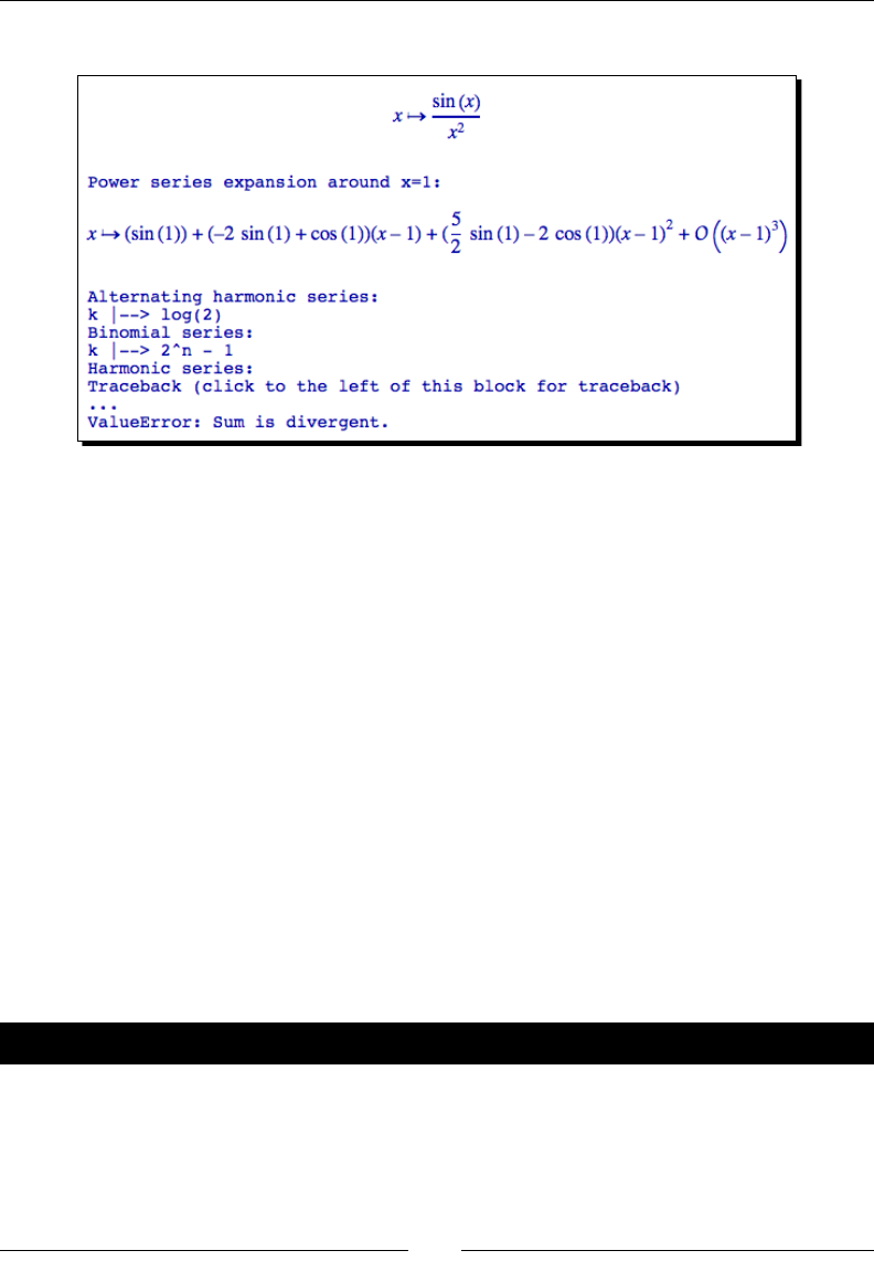
Making Symbolic Mathemacs Easy
[ 200 ]
The results are shown in the following screenshot:
What just happened?
We started by dening a funcon and using the series method to compute a power series
around the point x=1. The rst argument to series is the point at which to create the
series, and the second argument is the order of the computed series. Noce that Sages uses
"big O" notaon to denote the order of the series.
We then created several innite series and computed their sums. Sage can compute the sum
of any convergent series using the sum method. The rst argument to sum is the summaon
variable, the second argument is the lower endpoint, and the third argument is the upper
endpoint of the series. We used this method to compute the sum of the alternang
harmonic series and the binomial series. However, we ran into trouble when we tried to
compute the sum of the harmonic series, which is divergent. Fortunately, Sage handled this
problem gracefully.
Taylor series
A Taylor series is a series expansion of a funcon around a point. If the point is zero, the
series is known as a Maclaurin series. Taylor series are oen used to approximate funcons.
Time for action – nding Taylor series
Run the following code to see how to compute a one-dimensional Taylor series with Sage.
var('x,k')
colors=['red', 'black', 'green', 'magenta']
x1 = pi/2
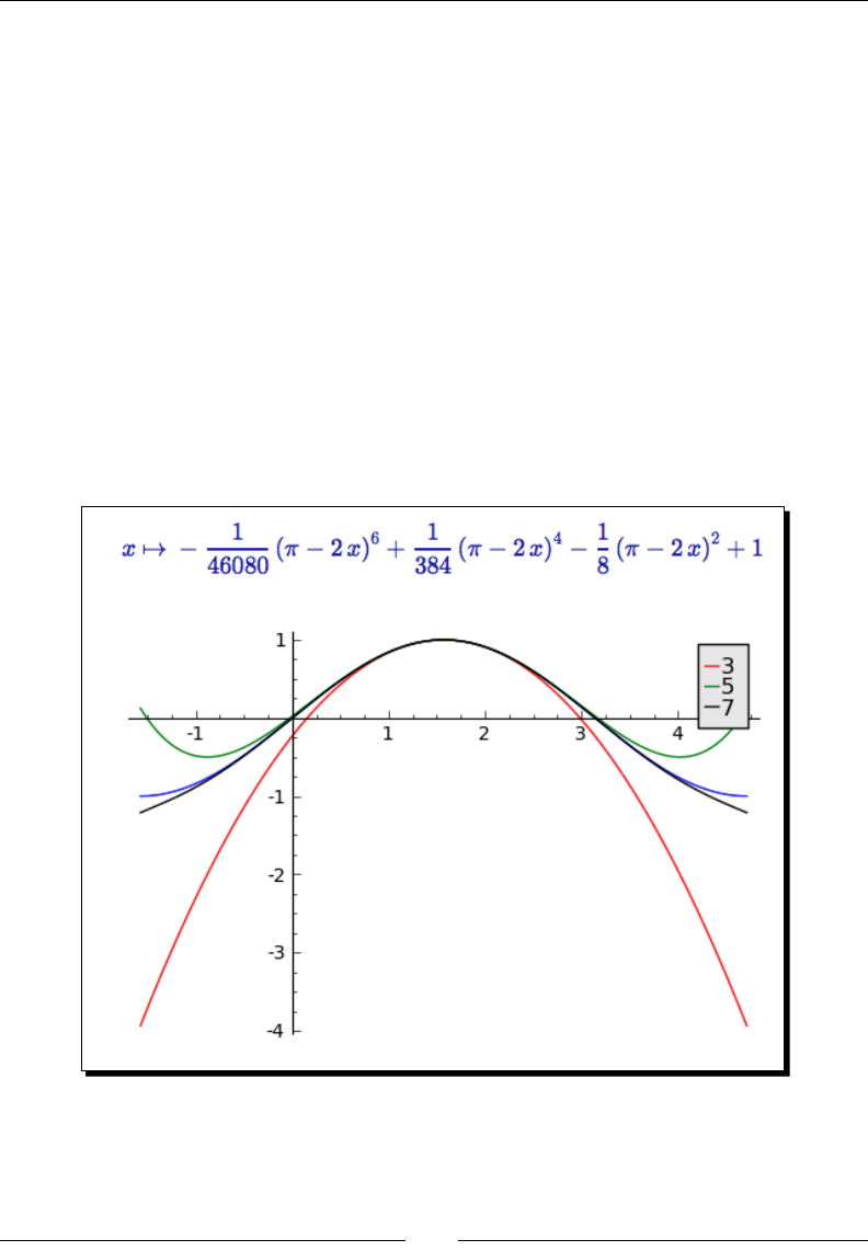
Chapter 7
[ 201 ]
xmin = x1 - pi; xmax = x1 + pi
f(x) = sin(x)
p1 = plot(f, (xmin, xmax), color='blue')
Taylor_series_3(x) = f.taylor(x, x1, 3)
p1 += plot(Taylor_series_3, (xmin, xmax), legend_label='3',
color='red')
Taylor_series_5(x) = f.taylor(x, x1, 5)
p1 += plot(Taylor_series_5, (xmin, xmax), legend_label='5',
color='green')
Taylor_series_7(x) = f.taylor(x, x1, 7)
p1 += plot(Taylor_series_7, (xmin, xmax), legend_label='7',
color='black')
Taylor_series_7.show()
show(p1)
The results are shown in the following screenshot:
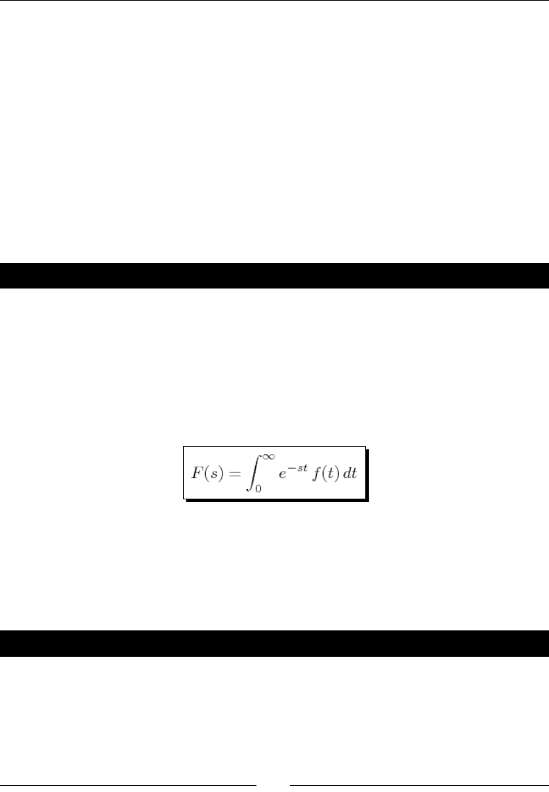
Making Symbolic Mathemacs Easy
[ 202 ]
What just happened?
The Taylor series expansion approximates the behaviour of a funcon in the vicinity of a
point. With an innite number of terms, the series should match the funcon exactly in a
small region near the point. However, the Taylor series provides a good approximaon with
only a nite number of terms. We used Sage to create a plot that illustrates how the Taylor
series approaches the funcon sin(x) near the point pi/2 as the number of terms in the series
increases.
We used the taylor method to create the Taylor series. The rst argument is the
independent variable, the second argument is the point, and the third argument is the order
of the series. In this case, we constructed Taylor series of order 3, 5, and 7 and ploed them
on the same axes with the sine funcon, in the vicinity of the point pi/2. We also displayed
the seventh-order Taylor series.
Have a go hero – Taylor series
Compute the Taylor series for the exp funcon about the point x=1. Use a plot to see how
well the Taylor series approximates the funcon as you increase the order of the Taylor
series.
Laplace transforms
The Laplace transform is dened as the integral:
This is for funcons that are dened for t ≥ 0. The Laplace transform is widely used for
solving ordinary dierenal equaons. It has applicaons in the theory of electrical circuits,
control systems, and communicaon systems. If you need to learn or review the basics of
Laplace transforms, you may want to consult Shaum's Outline of Laplace Transforms by
Murray Spiegel (McGraw-Hill, 1965).
Time for action – computing Laplace transforms
Evaluate the following code to see how to compute Laplace transforms with Sage:
var('t, a, k, s')
print("Elementary transform:")
f(t) = sin(k * t)
F(s) = f.laplace(t, s)
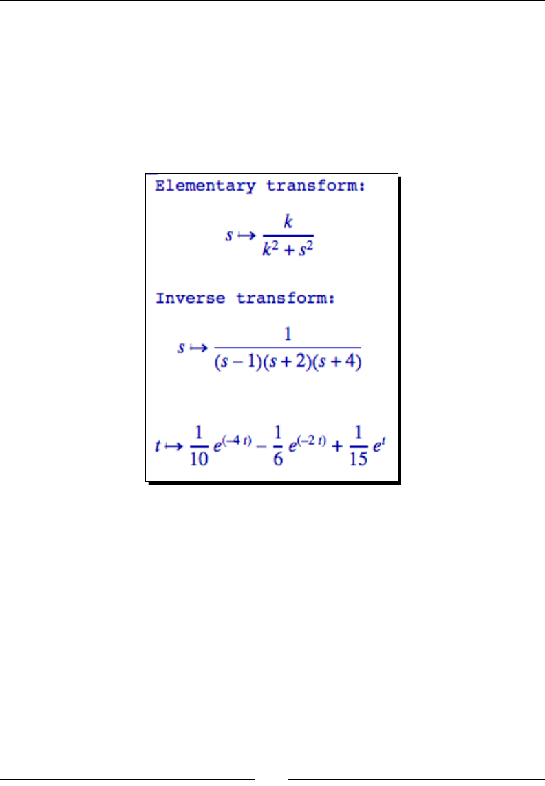
Chapter 7
[ 203 ]
F.show()
print("Inverse transform:")
G(s) = 1 / ((s - 1) * (s + 2) * (s + 4))
G.show()
g(t) = G.inverse_laplace(s, t)
g.show()
The results are shown in the following screenshot:
What just happened?
We used Sage to compute the Laplace transform and the inverse Laplace transform.
Normally, nding the Laplace transform would have required looking up the elementary
forms in a table. Compung the inverse transform requires performing a paral fracon
expansion and then nding the resulng terms in a table. The process is much faster with
Sage, and Sage can compute transforms that cannot praccally be computed by hand. We
used the laplace method to compute the forward transform, and inverse_laplace to
compute the reverse transform. Each of these methods computes the transform with respect
to a variable (the rst argument) using a transform parameter (the second argument.) It's
easier to think of the rst argument as the variable you are transforming from, and the
second as the variable you are transforming to.

Making Symbolic Mathemacs Easy
[ 204 ]
Solving ordinary differential equations
Ordinary dierenal equaons (ODEs) are widely used in applied mathemacs, engineering,
and the sciences. Sage enables you to nd exact soluons to many ODEs.
Time for action – solving an ordinary differential equation
The following code demonstrates how to solve ordinary dierenal equaons with Sage:
var('x, x1, x2, t')
# Finding a general solution
print("General solution:")
y = function('y', x)
ode = 4*diff(y, x, 2) + 36 * y == csc(3 * x)
y(x) = desolve(ode, y)
y.show()
# Solving an initial-value problem
print("Solving an initial-value problem:")
y = function('y', x)
ode = diff(y, x, 2) - 4 * diff(y, x) + 13 * y == 0
y(x) = desolve(ode, y, [0, -1, 2], ivar=x)
y.show()
# Solving a system of first-order equations
print("Solving a system of first-order ODEs:")
x1 = function('x1', t)
x2 = function('x2', t)
ode1 = 2 * diff(x1, t) + diff(x2, t) - x2 == t
ode2 = diff(x1, t) + diff(x2, t) == t^2
y1, y2 = desolve_system([ode1, ode2], [x1, x2],
ics=[0, 0, 0])
y1.show()
y2.show()
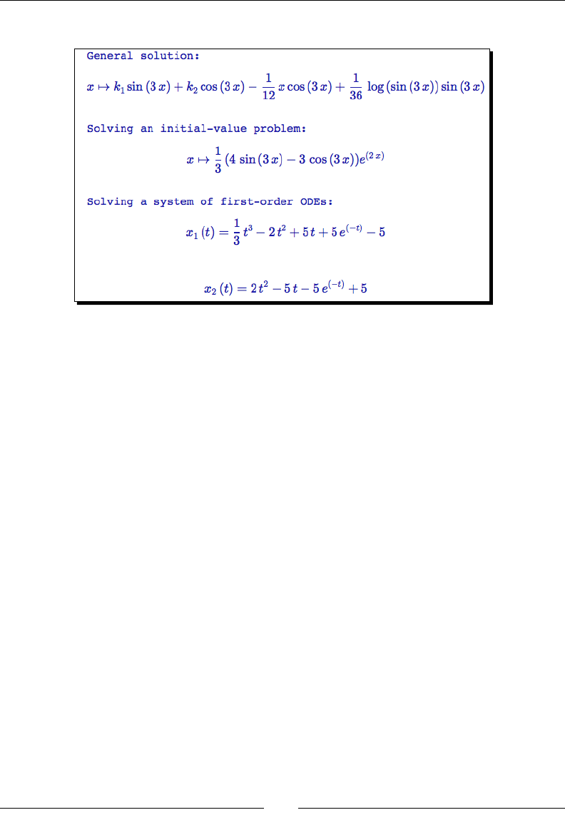
Chapter 7
[ 205 ]
The results are shown in the following screenshot:
What just happened?
The rst step towards solving a dierenal equaon with Sage is to create a symbolic
funcon that represents the soluon. In this example, we used function to create a
symbolic funcon called y that is a funcon of x. We then created a relaonal symbolic
expression called ode that implicitly denes y(x). Once the problem is set up, it is simple
to call the desolve funcon to obtain the soluon. desolve requires two arguments: the
relaonal expression that denes the dierenal equaon, and the dependent variable.
It returns an expression for the general soluon of the ODE. If the funcon has more than
one independent variable, then the independent variable must be specied using the ivar
keyword.
In the next part of the example, we used desolve to solve an inial-value problem with a
second-order ODE. The inial values of the independent variable, the dependent variable,
and the rst derivave of the dependent variable are used to form a list (in this order),
which was passed as an argument to desolve. Sage solves the inial-value problem and
returns the soluon as a symbolic expression. In the third part of the example, we used
desolve_system to solve a system of two rst-order ODEs. desolve_system can solve
systems of many rst-order dierenal equaons. Since a higher-order ODE can be wrien
as a system of rst-order ODEs, this does not limit the usefulness of desolve_system. We
dened two symbolic funcons, x1 and x2, which are funcons of t. The rst argument
of desolve_system is a list of dierenal equaons, and the second argument is a list of
dependent variables to solve for. We used the oponal argument with keyword ics to set
inial condions for the independent variable (t), x1, and x2, respecvely. The result is a
pair of symbolic expressions for x1 and x2. In the next chapter, we'll see how Sage can help
us solve dierenal equaons numerically.

Making Symbolic Mathemacs Easy
[ 206 ]
Summary
We covered a lot of material in this chapter. Sage makes it fast and easy to do tedious
symbolic tasks like compung integrals and Laplace transforms for complicated funcons. In
fact, the hardest part is making sure that you have dened your funcons and expressions
correctly.
Specically, we covered:
Working with symbolic expressions
Manipulang symbolic expressions to put them in the form you want
Performing basic calculus operaons like compung limits, derivaves, and integrals
Finding series representaons, and compung their sums
Compung Laplace transforms
Finding exact soluons to ordinary dierenal equaons
Sage has powerful symbolic capabilies. However, many real-world problems simply
don't have analycal soluons. In other cases, Sage might not be able to nd an analycal
soluon, even when it exists—soware is never perfect! Some symbolic operaons may
consume so much memory or CPU me that they become impraccal. Integrals, systems of
equaons, and dierenal equaons oen require numerical methods of soluon. Sage also
has powerful numerical capabilies, which we'll explore in the next chapter.
8
Solving Problems Numerically
The previous chapter described how to use Sage to solve many dicult problems in symbolic
mathemacs. While this capability is very useful, many real-world problems do not lend
themselves to symbolic computaon. Some dierenal equaons don't have closed-form
soluons, and not every integral can be computed in terms of elementary funcons. In other
cases, a funcon value may have to be computed from a look-up table that was derived
from experimental results, which precludes symbolic computaon. In this chapter, we will
demonstrate some of the tools in Sage that allow us to solve problems numerically.
We will learn how to:
Find the roots of an equaon
Compute integrals and derivaves numerically
Find minima and maxima of funcons
Compute discrete Fourier transforms, and apply window funcons
Numerically solve an ordinary dierenal equaon (ODE), and systems of ODEs
Use opmizaon techniques to t curves and nd minima
Explore the probability tools in Sage
Let's get started!

Solving Problems Numerically
[ 208 ]
Sage and NumPy
One potenal source of confusion in this chapter is that Sage incorporates funcons from
NumPy, Maxima, the GNU Scienc Library (GSL), and other sources. Whenever possible, we
will use funcons in Sage. However, somemes we need to go to NumPy to perform a parcular
calculaon. To minimize the possibility of confusion, do not use the syntax from numpy import
*. This imports every name from NumPy into Sage, overriding some pre-dened Sage funcons
and objects. Use the syntax shown in the examples, which keeps NumPy funcons separate
from Sage funcons.
Solving equations and nding roots numerically
We've already looked at solving systems of linear equaons in Chapter 5, when we learned
about linear algebra. We created matrices using integers or symbols, but you can just as
easily create vectors and matrices with real numbers or oang-point numbers. Chapter 5
also covered some numerical operaons on matrices, such as compung the QR factorizaon
and singular value decomposion. Now, we will learn how to nd roots of equaons
numerically in Sage.
Time for action – nding roots of a polynomial
Let's start by nding the roots of a polynomial.
g(x) = expand((x^2 - 1)^3 * (x^2 + 1) * (x - 2));
g.show()
print("Root at x = {0}".format(g.find_root(-2,2)))
print("Root at x = {0}".format(g.find_root(-2,0)))
print("Root at x = {0}".format(g.find_root(0.5,1.5)))
plt = plot(g, (x, -1.2, 2.01))
show(plt, figsize=(4, 3))
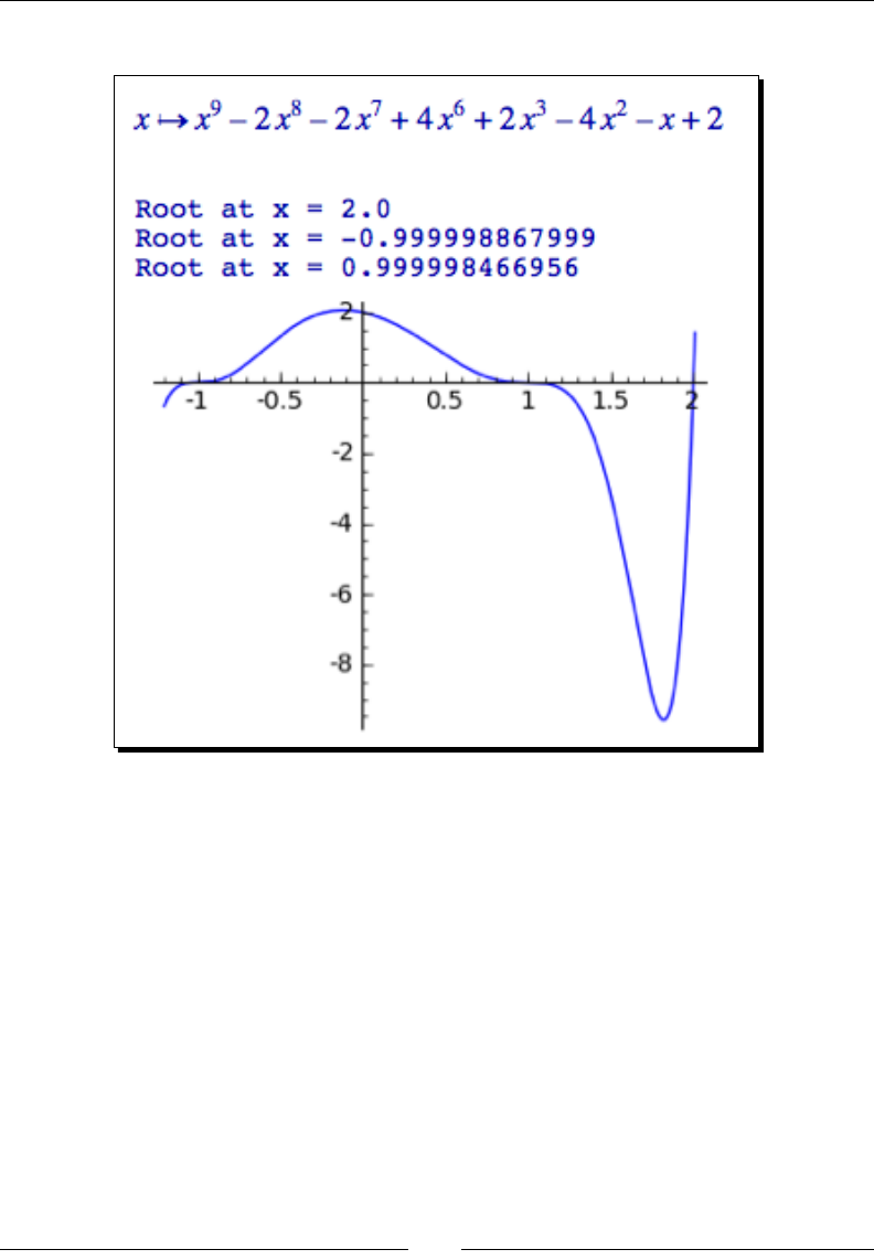
Chapter 8
[ 209 ]
The output is shown in the following screenshot:
What just happened?
We dened a fairly complicated polynomial equaon with a number of real and imaginary
roots. We can see that the funcon will have real roots at 1, -1, and 2 simply by looking at
the factored form of the funcon, which can be conrmed by looking at the plot. When
trying out a new numerical method, it's always a good idea to start with a problem that you
know the answer to, so that you can evaluate the accuracy and reliability of the method. The
find_root funcon is a relavely simple way to nd a single root within a given domain,
specied by the given end points. In the rst call, we gave find_root a wide span that
contained three roots, and it happened to nd the root at x=2. In the next two calls, we used
a narrower span that only included a single root in each span. Finding roots numerically is
relavely simple, but you have to understand the equaon you are working with to nd the
correct root.
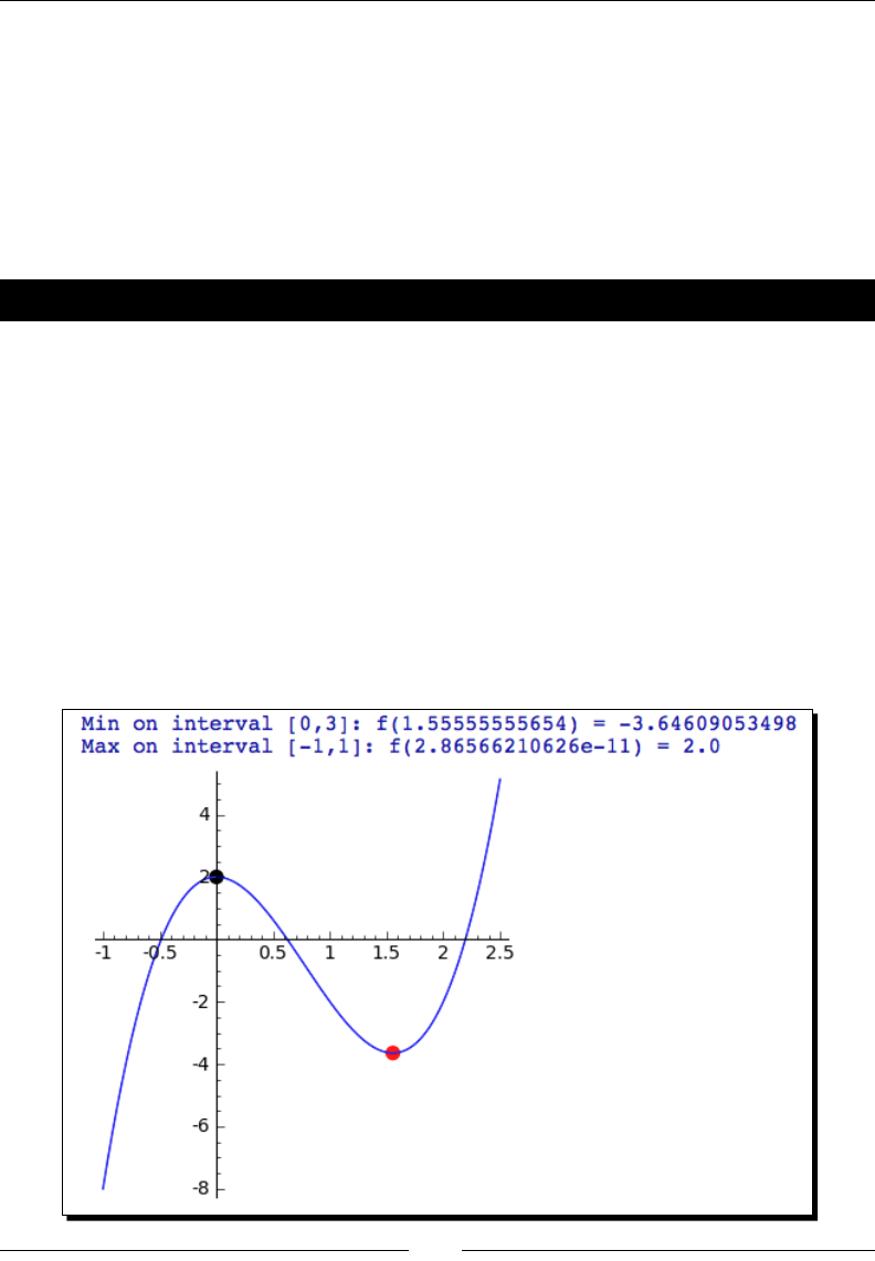
Solving Problems Numerically
[ 210 ]
Finding minima and maxima of functions
Somemes, we are interested in the minima or maxima of a funcon, rather than the zero
crossings. For example, an engineer might dene a funcon that esmates the cost of a
product. Finding the minimum of this funcon will help the engineer design a product with
the lowest cost. Conversely, one might want to maximize a funcon that represents the
performance of a system. The problem of nding minima and maxima is a form of numerical
opmizaon, which we'll cover later in the chapter.
Time for action – minimizing a function of one variable
We'll dene another funcon of one variable and let Sage nd the minimum:
var('x')
f = lambda x: 3 * x^3 - 7 * x^2 + 2
minval, x_min = find_minimum_on_interval(f, 0, 3)
print("Min on interval [0,3]: f({0}) = {1}".format(x_min, minval))
maxval, x_max = find_maximum_on_interval(f, -1, 1)
print("Max on interval [-1,1]: f({0}) = {1}".format(x_max, maxval))
f_plot = plot(f, (x, -1, 2.5))
min_point = point((x_min, minval), color='red', size=50)
max_point = point((x_max, maxval), color='black', size=50)
show(f_plot + min_point + max_point, figsize=(4, 4))
The results are shown in the following screenshot:

Chapter 8
[ 211 ]
What just happened?
We dened a funcon that represents a cubic polynomial using the lambda construct. Recall
from Chapter 4 that lambda is a shorthand way of dening a Python funcon. We used a
Python funcon, rather than a callable symbolic expression, because numerical methods are
designed to work with funcons that return real numbers. The funcons find_minimum_
on_interval and find_maximum_on_interval work in a similar way to find_root.
Each funcon accepts the endpoints of an interval and nds the minimum or maximum of
the funcon on that interval, and returns a tuple that contains the (x,y) coordinates of the
minimum or maximum. These funcons also accept the keyword argument tol to specify
the tolerance determines when the algorithm has converged on a maximum or minimum
(the default is 1.48e-8). The keyword argument maxfun sets a limit on the maximum number
of funcon evaluaons (default 500) that will be used to nd the point of interest. Finally, we
used the point graphics funcon to illustrate the points that we found.
Functions of more than one variable
Finding minima of a funcon of mulple variables is a more challenging problem because
each independent variable adds a new dimension to the search space. Sage uses a more
sophiscated funcon for minimizing funcons of two or more variables.
Time for action – minimizing a function of several variables
Now, we'll minimize a funcon of two variables, and use a contour plot to illustrate the
results:
var('x, y')
f = 100 * (y - x^2)^2 + (1 - x)^2 + 100 * (2 - y^2)^2 + (1 - y)^2
min = minimize(f, [0,0], disp=0)
plt = contour_plot(f, (x, -0.3, 2), (y, -0.3, 2), fill=False,
cmap='hsv', labels=True)
pt = point(min, color='red', size=50)
show(plt+pt, aspect_ratio=1, figsize=(4, 4))
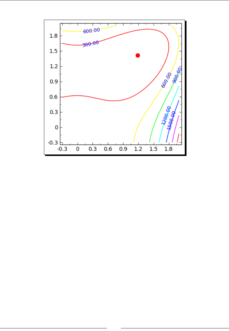
Solving Problems Numerically
[ 212 ]
The plot is shown below:
What just happened?
We started out by dening a callable symbolic expression that represents a polynomial
funcon of two variables. We then used minimize to nd a minimum of the funcon
near the point (0,0). minimize works a lile dierently from the funcons in the previous
examples. Rather than specifying limits on the domain of the problem, you need to pass
an inial guess to minimize so that it knows where to start searching for a minimum. Like
the funcons find_root and find_minimum_on_interval, minimize will only nd a
minimum in the vicinity of its starng point (if it exists), which is known as a local minimum.
We used the keyword argument disp=0 to prevent the funcon from displaying text that
summarizes its soluon process.
We will pause here to clarify the concept of local and global minima. A local minimum is the
lowest value that a funcon takes on over a poron of its domain. A funcon can have many
local minima. A funcon's global minimum is the lowest value of the funcon over its enre
domain. There is no general algorithm that can nd the global minimum of an arbitrary
funcon. Therefore, minimize (and all the other minimum-nding funcons in Sage) are
only guaranteed to nd a local minimum (assuming one exists), which may happen to also be
the global minimum.

Chapter 8
[ 213 ]
Minimizing a funcon of several variables is signicantly more complicated than minimizing a
funcon of one variable. minimize is actually an interface to several minimizaon algorithms.
If the funcon to be minimized is symbolic, the default algorithm is the Broyden-Fletcher-
Goldfarb-Shannon (bfgs) algorithm. If the funcon is a Python funcon, the simplex algorithm
is the default. The following table summarizes the opons that can be passed to minimize:
Keyword Descripon
disp 0 disables text output (default is 1)
algorithm A string value that species algorithm:
'default' chooses default (see text)
'simplex' chooses the simplex method
'powell' chooses Powell's conjugate gradient descent method
'bfgs' chooses Broyden-Fletcher-Goldfarb-Shannon (bfgs)
'cg' chooses conjugate-gradient (requires gradient)
'ncg' chooses Newton-conjugate-gradient (requires gradient and Hessian)
gradient Funcon that computes the gradient
hessian Funcon that computes the Hessian
If the funcon to be minimized is symbolic, you do not have to provide the Hessian or the
gradient because Sage will compute them symbolically. If the funcon to be minimized is
a Python funcon and you choose an algorithm that requires the Hessian or the gradient,
you will have to provide funcons that compute the Hessian and/or the gradient. The
Sage reference manual has an example that demonstrates how to minimize a Python
funcon with an algorithm that requires a gradient: http://www.sagemath.org/doc/
reference/sage/numerical/optimize.html
Numerical approximation of derivatives
In the previous chapter, we learned how to use Sage to compute derivaves of symbolic
funcons. Now, we will learn how to approximate derivaves numerically.
Time for action – approximating derivatives with differences
Let's start by dening a funcon of one variable. We'll use NumPy to esmate the derivave
numerically, and we'll plot the esmate with matplotlib.
import numpy as np
import matplotlib.pyplot as plt
import matplotlib as mpl
mpl.rc('font', size=10) # set default font size
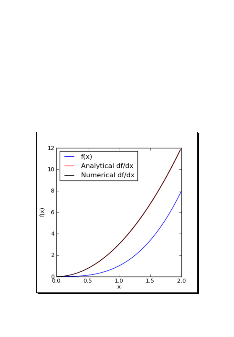
Solving Problems Numerically
[ 214 ]
dx = 0.01
x = np.arange(0, 2, dx)
f = power(x, 3)
dfdx = 3*power(x, 2)
plt.figure(figsize=(4, 4))
plt.plot(x, f, label='f(x)')
plt.plot(x, dfdx, color='red', label='Analytical df/dx')
df = np.diff(f)
plt.plot(x[:-1], df/dx, color='black', label='Numerical df/dx')
plt.xlabel('x')
plt.ylabel('f(x)')
plt.legend(loc='best')
plt.savefig('diff.png')
plt.close()
The output is shown in the following screenshot:
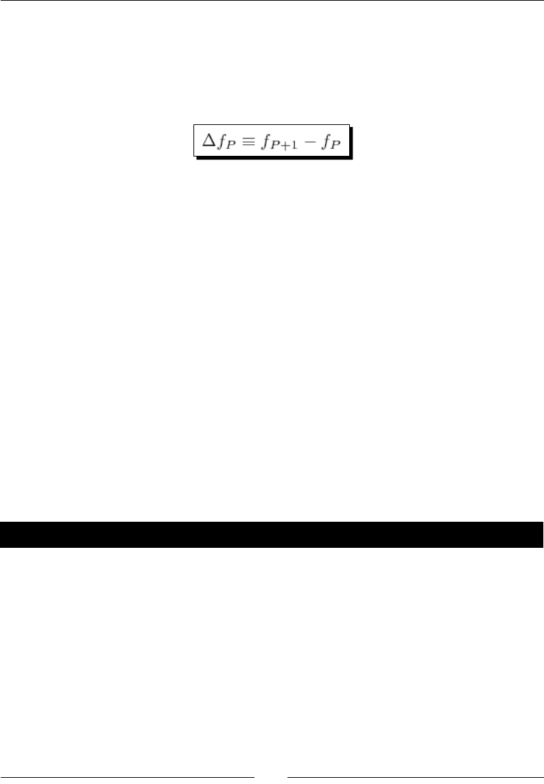
Chapter 8
[ 215 ]
What just happened?
We dened a simple polynomial, f(x)=x3. Its derivave can easily be calculated in closed form:
f'(x)=3x2. We dened a NumPy array of x values and computed the value of the funcon at
each point. We then used the diff funcon from NumPy to compute the forward nite
dierence at each point in the domain. The forward nite dierence is dened as:
diff accepts three arguments. The rst is a NumPy array containing values of the funcon.
The oponal keyword argument n species which order dierence to take (the default is
one, which approximates the rst derivave). The oponal keyword argument axis species
which axis of the array to use (if the array has more than one dimension). This keyword
allows diff to be used to approximate a paral derivave of a funcon of several variables.
To esmate the derivave, the nite dierence at each point is divided by the distance
between points, which we have dened as dx. We then ploed the numerical esmate of
the derivave along with the analycal derivave and veried that they match.
In this example, we evaluated a new numerical method by solving a problem with a known
answer. If used incorrectly, a numerical technique may give an invalid result without any
warning. It's important to replicate a known result to make sure you are using the method
correctly.
Computing gradients
For funcons of mulple variables, we can use paral derivaves to compute the derivave
with respect to one of the independent variables. The gradient gives the direcon of
steepest descent at any given point in the domain.
Time for action – computing gradients
Enter the following code into a cell in a Sage worksheet, and evaluate it:
import numpy as np
import matplotlib.pyplot as plt
def func(x,y):
return exp(-1 / 3 * x^3 + x - y^2)
dx = 0.2; dy = 0.2
grid = np.ogrid[-2 : 2 + dx : dx, -2 : 2 + dx : dx]
xlen = max(grid[0].shape)
ylen = max(grid[1].shape)
f = np.empty([xlen, ylen])
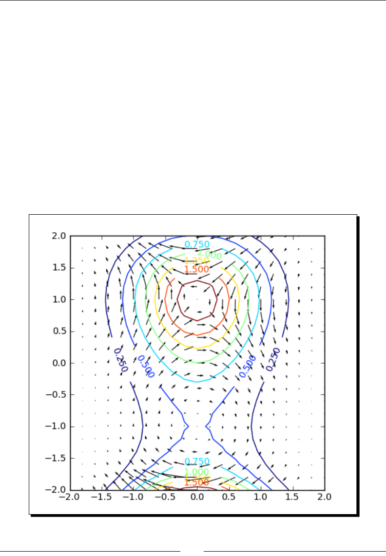
Solving Problems Numerically
[ 216 ]
for i in range(xlen):
for j in range(ylen):
f[i, j] = func(grid[0][i], grid[1][0,j])
plt.figure(figsize=(5, 5))
c = plt.contour(grid[0].flatten(), grid[1].flatten(), f)
plt.clabel(c) # label contours
plt.axis('scaled') # aspect ratio=1.0
# Compute and plot gradient of function
grad = np.gradient(f, dx, dy)
plt.quiver(grid[0].flatten(), grid[1].flatten(), grad[0], grad[1])
plt.savefig('contour.png')
plt.close()
A contour plot of the funcon is shown below, with overlaid vectors represenng
the gradient:

Chapter 8
[ 217 ]
What just happened?
Compung the gradient is actually the easiest aspect of this example. Since we are using
NumPy, we rst need to dene a two-dimensional grid of points. We use the ogrid funcon
from NumPy, which does exactly that. We then used two nested for loops to compute the
value of the funcon at each point in the grid. We used the contour funcon from Pyplot to
display the level contours of the funcon, and used the gradient funcon to compute the
gradient at each point of the grid. gradient is very similar to diff, except that it expects
an N-dimensional array as its rst argument. The next N arguments specify the grid spacing
for each dimension of the array. Finally, we used the quiver plong funcon from Pyplot
to display a vector that represents the gradient at each point of the grid. We can see that the
gradient is normal to the contour lines at each point.
Numerical integration
Numerical integraon (known in older literature as "quadrature") is another fundamental
operaon in numerical mathemacs.
Time for action – numerical integration
Let's start by using Sage funcons to numerically integrate a symbolic funcon of one
variable:
var('x')
f(x) = e^x * cos(x)
f.show()
a = 0
b = 8
p = plot(f, (x, a, b))
p.show(figsize=(4, 3))
print("Integral of f(x) from {0} to {1}:".format(a,b))
print(" Analytical definite integral: {0}"
.format(f.integral(x, a, b).n()))
integral_value, tolerance, num_evals, error_code = \
f.nintegral(x, a, b)
print(" Using nintegral: {0}".format(integral_value))
# also nintegrate
integral_value, tolerance = numerical_integral(f, a, b)
print(" Using numerical_integral: {0}".format(integral_value))
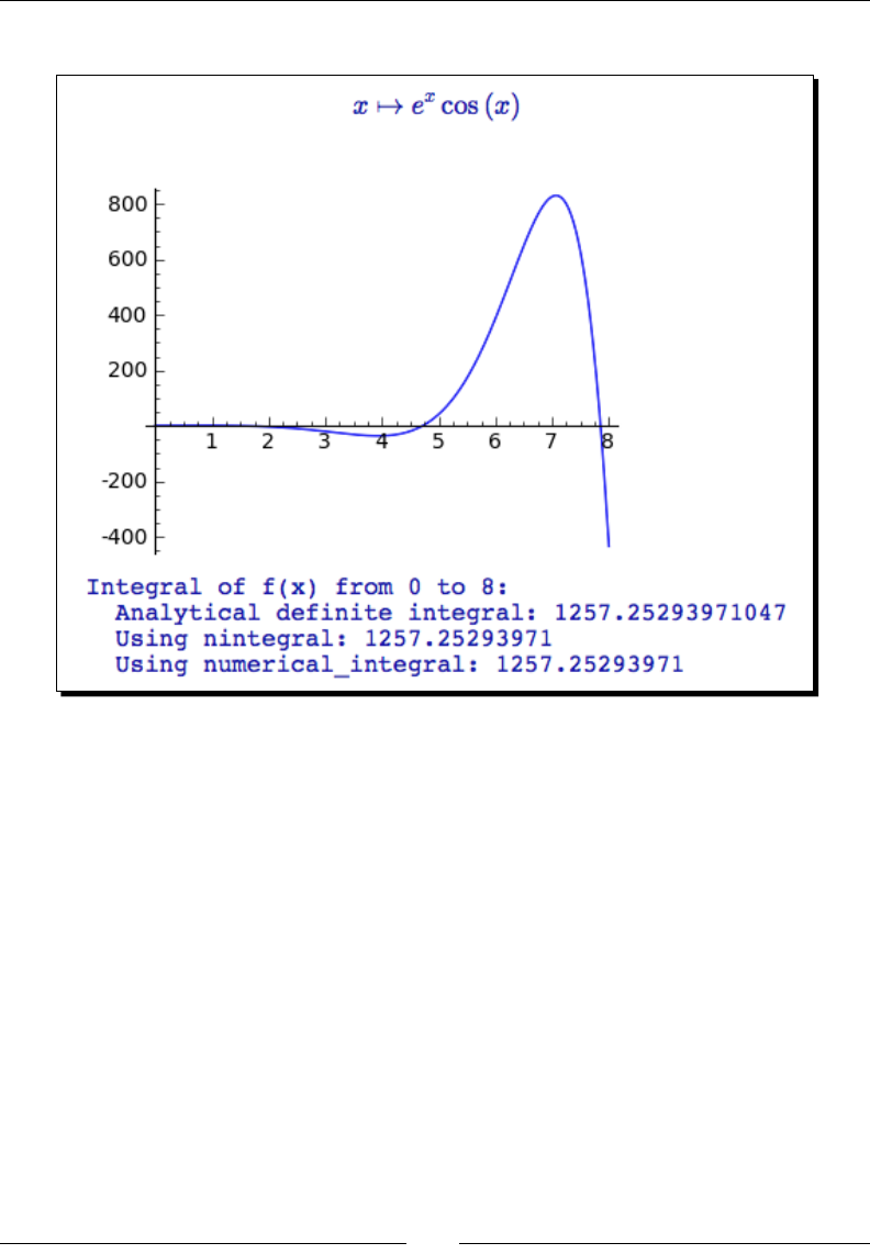
Solving Problems Numerically
[ 218 ]
A plot of the funcon, along with the integraon results, is shown below:
What just happened?
We dened a symbolic funcon f(x) and dened an interval on which to compute the denite
integral. As a point of reference, we used the symbolic integraon method integral
with limits to compute the denite integral symbolically. We used the method n (which is
a shortcut for numerical_approx) to convert the symbolic result into a decimal number for
comparison to the results of numerical integraon.
Sage has two types of numerical integraon. We used the numerical integraon method
nintegral (also called nintegrate) to perform the integraon numerically. These
methods call Maxima to perform the computaon, and return a tuple with four elements:
Approximaon to the integral (oat)
Esmated absolute error of the approximaon (oat)
The number of integrand evaluaons (integer)
An error code (integer)
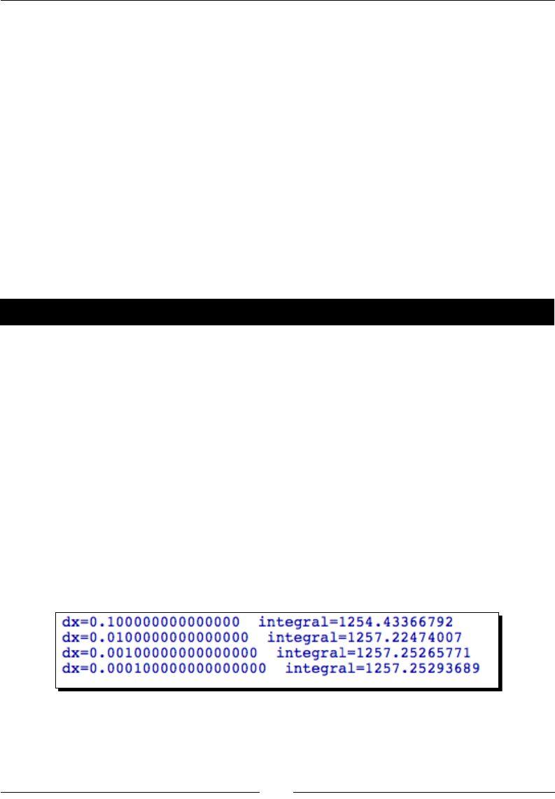
Chapter 8
[ 219 ]
We repeated the calculaon with numerical_integral, which uses the GNU Scienc
Library. This funcon returns a tuple that contains the integral value and an esmate of the
error. numerical_integral can be used to integrate funcons that are dened as callable
symbolic expressions or as Python funcons. Both methods of numerical integraon use
algorithms that automacally adapt to the funcon that is being integrated. We can see that
all three types of integraon obtain equivalent results.
Numerical integration with NumPy
Somemes, we may need to integrate a funcon that cannot be dened by a Python
funcon or a symbolic expression. This situaon may occur if the funcon values come
from experimental measurements or simulaon results. For example, if we have an array
of ux values over me, we can integrate the ux over me to obtain the total amount of
substance. If the values of a funcon are stored in an array, we can use NumPy to perform
the integraon.
Time for action – numerical integration with NumPy
We'll repeat the calculaon from the previous example with NumPy. Execute the following
code and see what happens:
import numpy as np
def func(x):
return np.exp(x) * np.cos(x)
a=0; b=8
dx = 0.1
for i in range(4):
x = np.arange(a, b + dx, dx)
f = func(x)
print("dx = {0} integral = {1}".format(dx, np.trapz(f,x)))
dx = dx / 10
The output is shown in the following screenshot:

Solving Problems Numerically
[ 220 ]
What just happened?
We dened a Python funcon that represents the mathemacal funcon used in the
previous example. We then used a for loop to numerically integrate the funcon with
trapz, using dierent spacing of the independent variable x. The rst argument to trapz is
a NumPy array that contains the values of the funcon to be integrated. The x values can be
specied as either an array of values (which do not have to be uniformly spaced) or a single
scalar value dx that denes the spacing between points. If the array containing the funcon
values has more than one dimension, the axis keyword can be used to specify the axis of
integraon.
Remember that all NumPy funcons operate on arrays of discrete points. The trapz
funcon is a very simple integrator that uses the trapezoidal rule to integrate a sequence of
points. Unlike the integraon funcons in Sage, trapz cannot adapt to the funcon being
integrated. To demonstrate this, we performed the integral with four dierent step sizes. You
can see that the precision of the integral increases as the step size decreases.
Discrete Fourier transforms
The Fourier transform is used in opcs, acouscs, radio engineering, and many other elds.
It is most oen used to transform a me-domain signal into the frequency domain so that
its frequency components can be analysed. Because most applicaons involve signals that
are sampled at discrete mes, the discrete Fourier transform (DFT) is an important part of
numerical compung.
Time for action – computing discrete Fourier transforms
Since the discrete Fourier transform operates on an array of samples from a signal, we'll use
the signal-processing tools in NumPy:
import numpy as np
import matplotlib.pyplot as plt
dt = 0.01
t = np.arange(-10, 10, dt)
f = np.sinc(t)
plt.figure(figsize=(6, 3))
plt.plot(t, f)
plt.savefig('f.png')
plt.close()
fourier_transform = np.fft.fft(f)
spectrum = np.absolute(fourier_transform)
phase = np.angle(fourier_transform)
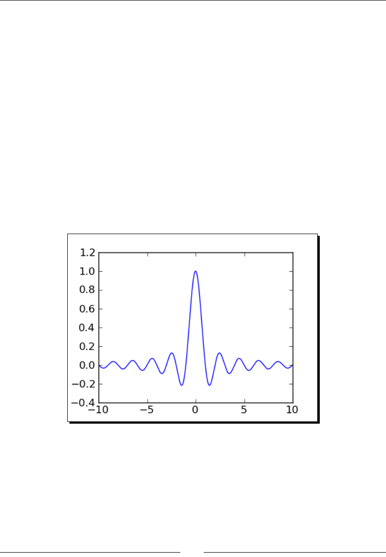
Chapter 8
[ 221 ]
freq = np.fft.fftfreq(t.shape[-1], d=dt)
spectrum = np.fft.fftshift(spectrum)
phase = np.fft.fftshift(phase)
freq = np.fft.fftshift(freq)
plt.figure(figsize=(6,3))
plt.plot(freq, spectrum)
plt.title('Magnitude')
plt.axis([-1.5, 1.5, spectrum.min(),spectrum.max()])
plt.savefig('spectrum.png')
plt.figure(figsize=(6,3))
plt.plot(freq, phase)
plt.title('Phase')
plt.axis([-1.5,1.5, phase.min(),phase.max()])
plt.savefig('phase.png')
plt.close()
The following plots show the funcon, its magnitude spectrum, and its phase spectrum:
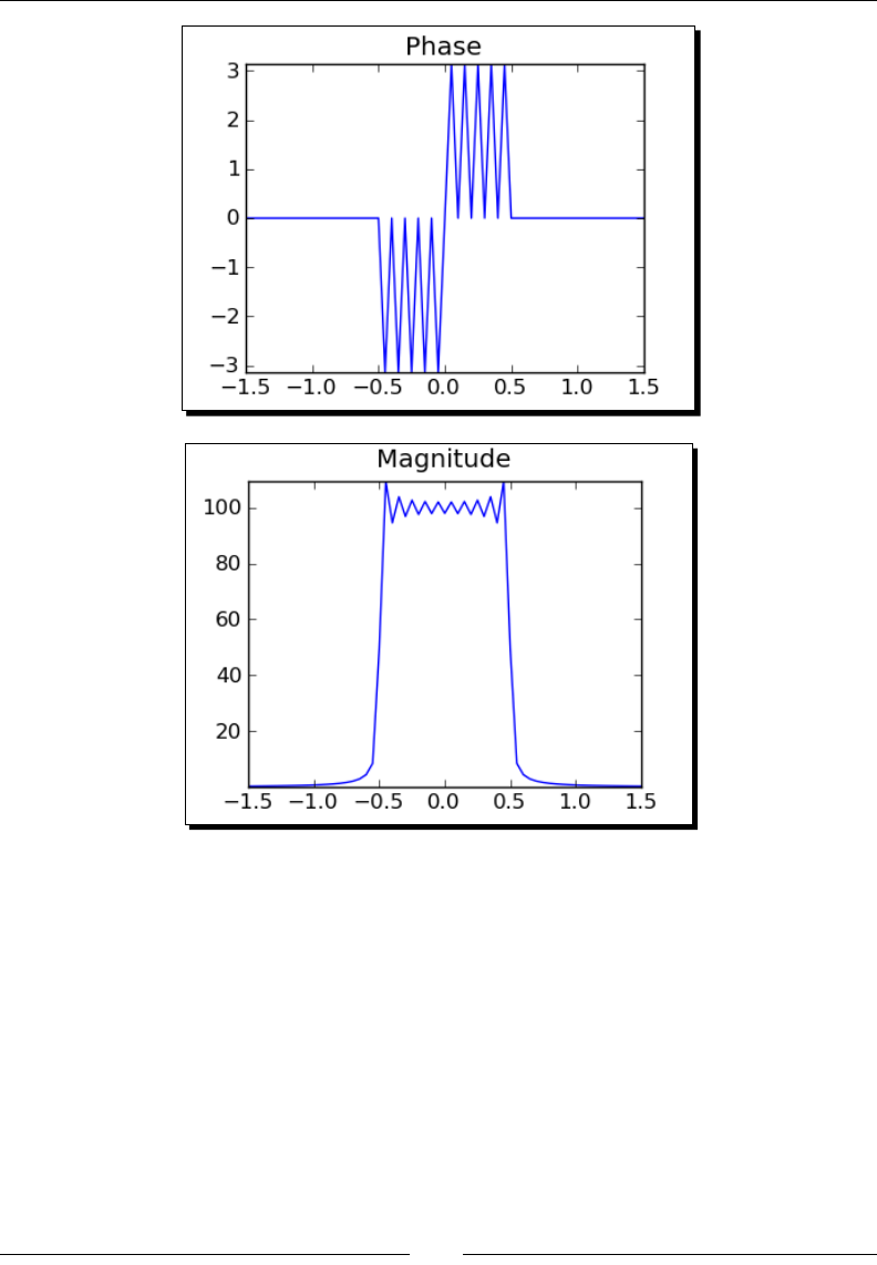
Solving Problems Numerically
[ 222 ]
What just happened?
We rst generated a me-domain signal to work with. The arange funcon was used
to create a series of sample mes, and the sinc funcon was used to compute the sinc
funcon at those mes. The rst plot shows the me-domain funcon that we are going to
analyse. We then used the fft funcon to compute the Fourier transform, which returns a
NumPy array of complex values. It is customary to plot the frequency spectrum as magnitude
and phase, so we used the absolute funcon to get the magnitude and the angle funcon
to get the phase. The fftfreq funcon accepts an array of sample mes and the me step,
and uses them to compute the frequency values for plong the frequency spectrum. The
fftshift funcon was used to shi the magnitude and phase arrays and the frequency
array so that the zero-frequency point was in the centre of the array. This is helpful for
making plots.
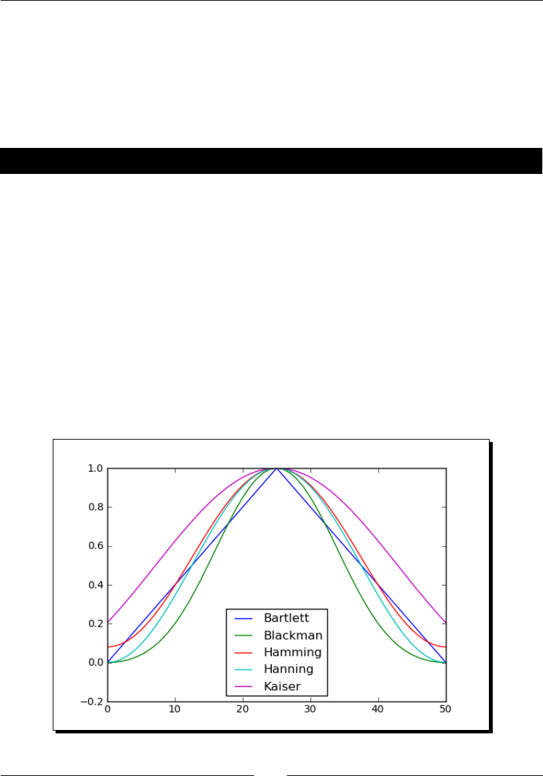
Chapter 8
[ 223 ]
Window functions
The sinc funcon that we used in the previous example is actually an approximaon to the
true sinc funcon, which extends from negave innity to posive innity. Because we used
nite data to compute the Fourier transform, we introduced a distoron into the frequency
spectrum. One way of reducing this distoron is by applying a window funcon to the signal
before performing the transform. All the common window funcons are built into NumPy.
Time for action – plotting window functions
Let's plot the window funcons available in NumPy:
import numpy as np
import matplotlib.pyplot as plt
plt.figure(figsize=(6,4))
plt.plot(np.bartlett(51), label="Bartlett")
plt.plot(np.blackman(51), label="Blackman")
plt.plot(np.hamming(51), label="Hamming")
plt.plot(np.hanning(51), label="Hanning")
plt.plot(np.kaiser(51,3), label="Kaiser")
plt.legend(loc='best')
plt.savefig('window_functions.png')
plt.close()
The output is shown below:

Solving Problems Numerically
[ 224 ]
What just happened?
Calling the funcon hamming(51) returns an array containing 51 samples of the Hamming
window funcon. The sample at the centre of the array corresponds to the centre of the
window, where it reaches the value of 1. The other window funcons work the same way,
except that the Kaiser window also requires a shape parameter.
Have a go hero – using window functions
Apply some of the window funcons to the sinc funcon in the example and compute the
DFT to see how the window funcons aect the frequency spectrum.
HINT: Generate an array of samples of the window funcon that has the same number
of samples as the array containing the sinc funcon, and mulply the two arrays before
performing the DFT.
Solving ordinary differential equations
In the previous chapter, we looked at some tools for nding exact soluons to ordinary
dierenal equaons (ODEs). Somemes, nding an exact soluon is impossible or
impraccal. Sage also has a powerful set of tools for solving ordinary dierenal equaons
numerically.
Time for action – solving a rst-order ODE
Let's start by solving a single, rst-order, ordinary dierenal equaon. We'll compare the
exact soluon to the numerical soluon:
var('x, y')
y = function('y', x)
ode = diff(y, x) + 1 / x * y == x * y^2
sol = desolve(ode, y, ics=[10, 1])
sol.show()
exact_plot = plot(sol, (x, 0.1, 10), color='red', marker='.')
rk4_plot = desolve_rk4(ode, y, ics=[10, 1], output='slope_field',
end_points=[0, 10])
show(exact_plot + rk4_plot, figsize=(4, 3))
The symbolic soluon is shown in the following screenshot, and its graph is ploed on the
same axes as the numerical soluon and the slope eld:
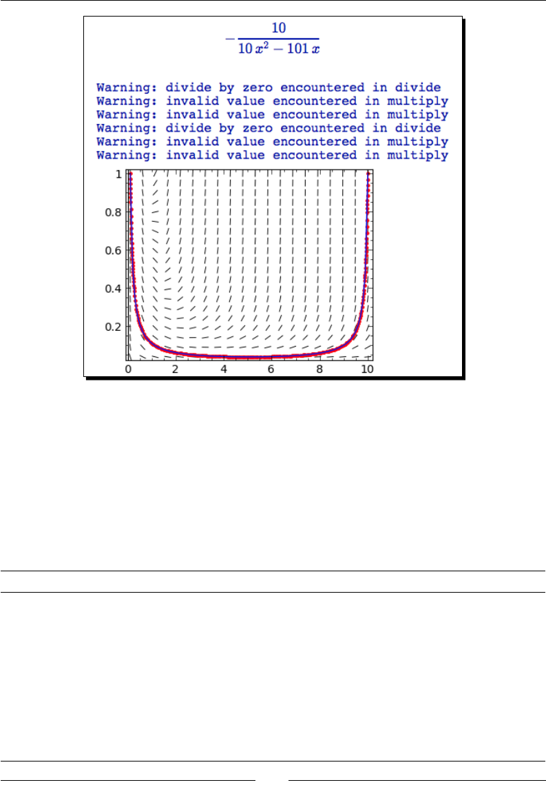
Chapter 8
[ 225 ]
What just happened?
As we explained in the previous chapter, we dened a symbolic ordinary dierenal
equaon and found the soluon using desolve. The warning messages occur during the
calculaon of the slope eld, and can be safely ignored. We then used the desolve_rk4
funcon to compute the soluon numerically. As its name implies, the funcons use the
4th order Runge-Kua method to integrate a single rst-order ordinary dierenal equaon
numerically (the funcon rk from Maxima's dynamics package is used to perform the
integraon). desolve_rk4 accepts the following keyword arguments:
Keyword Default Descripon
ics None List of inial condions for each variable.
ivar None Independent variable. Only required if there is more than one choice
for the independent variable.
end_
points
None The end points of the interval of integraon.
If end_points is a or [a], integrate between min(ics[0],a)
and max(ics[0],a).
If end_points is None, then end_points=ics[0]+10.
If end_points is [a,b] integrate between min(ics[0],a)
and max(ics[0],b).
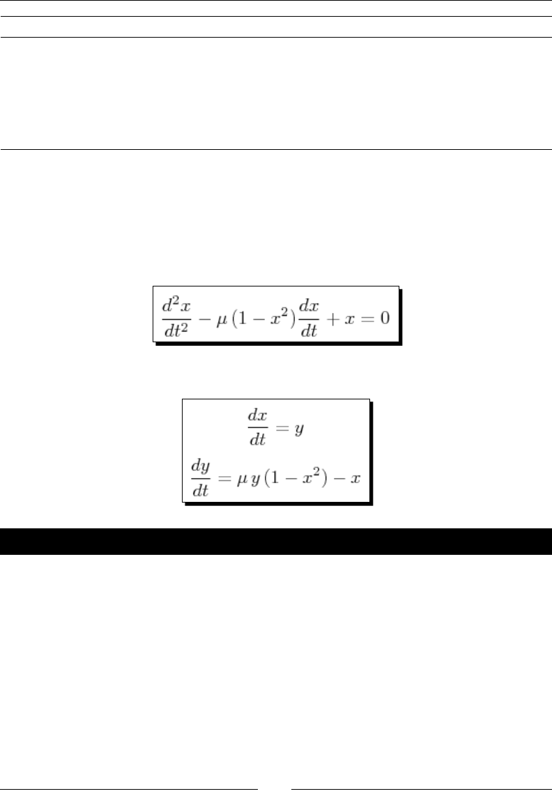
Solving Problems Numerically
[ 226 ]
Keyword Default Descripon
step 0.1 Step size for the independent variable.
output 'list' 'list' returns a list of lists of [x,y] values.
'plot' returns a plot of the soluon as a graphics object.
'slope_field' returns a plot of the soluon and the slope eld
as a graphics object.
Solving a system of ODEs
Sage also has tools to solve systems of ordinary dierenal equaons numerically. We can
use this capability to solve any higher-order ODE, since any higher-order ODE can be broken
down into a system of rst-order dierenal equaons. For the next two examples, we will
look at the van der Pol oscillator:
It can be wrien in terms of two rst-order ODEs:
Time for action – solving a higher-order ODE
Let's see if Sage can nd a symbolic soluon:
var('t')
x = function('x', t)
y = function('y', t)
u = 1.0
de1 = diff(x,t) - y == 0
de2 = diff(y,t) + x - u * y * (1 - x^2) == 0
Van_der_Pol = [de1, de2]
desolve_system(Van_der_Pol, [x, y], ics=[0, 2, 0])

Chapter 8
[ 227 ]
If you run this code, Sage will return an error. It is unable to nd a symbolic soluon. Now,
let's try to solve it numerically:
var('t, x, y')
u = 1.0
Van_der_Pol = [y, -x + u * y * (1 - x^2)]
sol = desolve_system_rk4(Van_der_Pol, [x, y], ivar=t,
ics=[0, 2, 0], end_points=[0, 20])
t = [i for i, j, k in sol]
x_sol = [j for i, j, k in sol]
y_sol = [k for i, j, k in sol]
# Plot results
import matplotlib.pyplot as plt
plt.figure(figsize=(4, 3))
plt.plot(t, x_sol)
plt.xlabel('t')
plt.ylabel('y(t)')
plt.subplots_adjust(bottom=0.15)
plt.savefig('Van_der_Pol_rk4.png')
plt.close()
# Limit cycle in the phase plane
plt.figure(figsize=(4, 4))
plt.plot(x_sol, y_sol)
plt.axis('scaled')
plt.xlabel('x')
plt.ylabel('y')
plt.savefig('Van_der_Pol_rk4_phase.png')
plt.close()
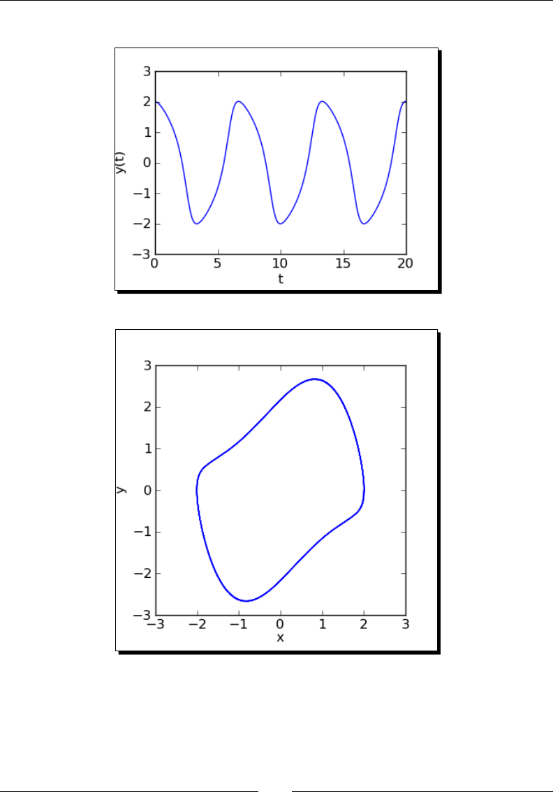
Solving Problems Numerically
[ 228 ]
The results should look like this:

Chapter 8
[ 229 ]
What just happened?
We used the funcon desolve_system_rk4 to solve the system. This funcon operates
just like desolve_rk4, except that it accepts a list of dierenal equaons as its rst
argument (both of these funcons ulize the rk funcon from Maxima to compute the
soluon.). An inial condion must also be provided for each variable—three, in this case.
We had to use the ivar keyword to specify that t is the independent variable. The funcon
returns the soluon as a list of lists:
[[0, 2, 0],
[0.1, 1.99093050354, -0.172638259608],
[0.2, 1.96694849768, -0.300697407982],
…
[0.4, 1.88817476497, -0.47282676678]]
We used list comprehensions to separate the soluons for x, y, and t into three dierent
lists. Since we are working with lists of points, we used matplotlib for plong. The rst plot
is the me-varying soluon to the van der Pol dierenal equaon. Note that we used the
matplotlib funcon subplots_adjust to ensure that the label for the t axis is visible. For
certain combinaons of gure size, font size, and plot size you will occasionally have to use
subplots_adjust to make a gure look right. In the second plot, we ploed x vs. y to
create a phase-plane plot. This is known as the limit cycle. Try varying the value of u in the
range of 0 to 5 to see how it impacts the soluon.
Solving the system using the GNU Scientic Library
Sage is a collecon of tools. You oen have a choice of several methods for accomplishing the
same task. While this can be confusing, one algorithm may be able to solve a problem that
another one couldn't. For solving ODEs, Sage also allows you to access the ODE solver from the
GNU Scienc Library (GSL). This solver gives you access to more soluon algorithms.
Time for action – alternative method of solving a system of ODEs
We'll solve the same problem again, using the numerical ODE solver from the GSL.
def f_1(t, y, params):
return [y[1], -y[0] - params[0] * y[1] * (y[0]**2 - 1.0)]
def j_1(t, y, params):
return [ [0.0, 1.0], [-2.0 * params[0] * y[0] * y[1] - 1.0,
-params[0] * (y[0] * y[0] - 1.0)] ]
T = ode_solver()
T.algorithm = "rk8pd"
T.function = f_1
T.jacobian = j_1
T.ode_solve(y_0=[2, 0], t_span=[0, 20], params=[1.0],
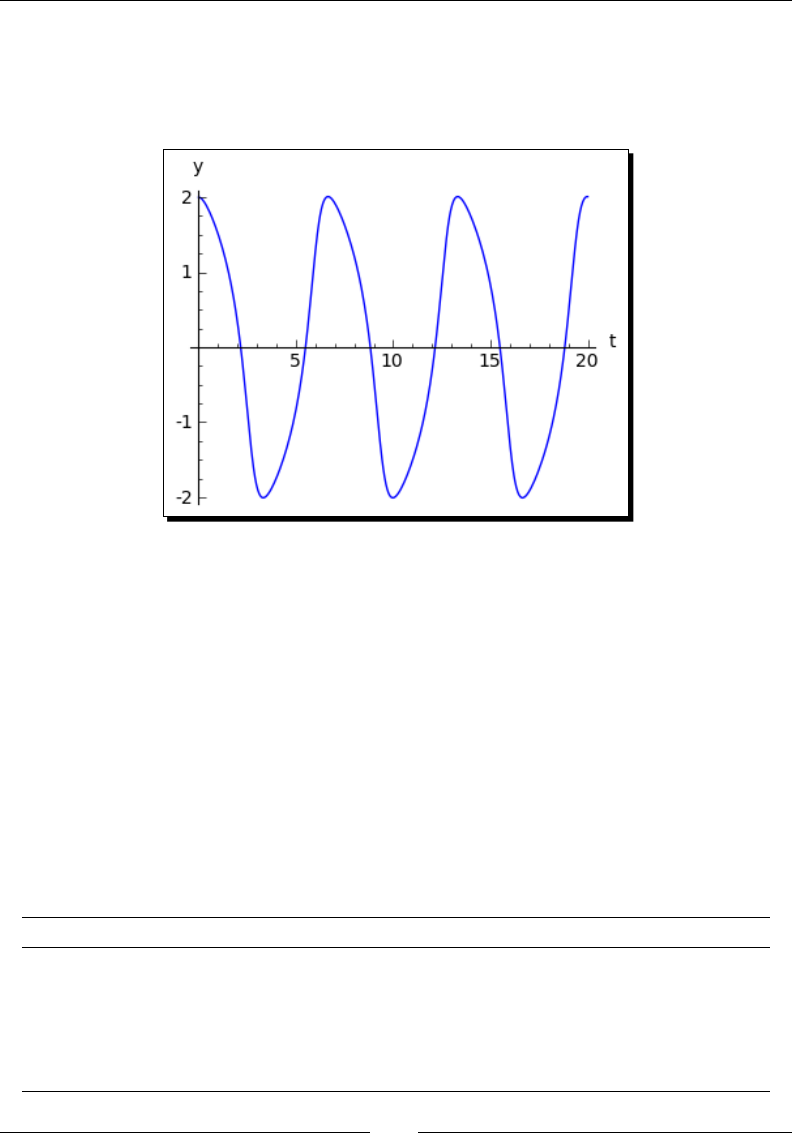
Solving Problems Numerically
[ 230 ]
num_points=1000)
interpolator = T.interpolate_solution()
plot(interpolator, (0, 20), axes_labels=('t','y'), figsize=(4,3))
The output is shown in the following screenshot:
What just happened?
This solver has a very dierent interface from the one in the previous example. The ordinary
dierenal equaons are dened by a Python funcon called f_1. The rst argument to this
funcon is the independent variable, the second is a list of dependent variables, and the
third is a list of parameters. y[0] represents the variable y, and y[1] represents x. In this case,
the parameter list has only one element, which is the value of u. We used similar syntax
to dene the Jacobian funcon, j_1. The Jacobian is only required for certain integraon
algorithms; see the ode_solver documentaon for more details.
The code T = ode_solver() creates a solver object. We used the aribute algorithm
to choose the rk8pd (Runge-Kua Prince-Dormand 8,9) algorithm, and used the aributes
function and jacobian to pass in the funcons we just dened. We called the method
ode_solve to solve the system, which accepts the following arguments:
Keyword Descripon
y_0 List of inial condions. Note that y[0] is y and y[1] is x, which is backwards
compared to the previous example!
t_span Domain of soluon, specied as a list: [start, stop].
params List of parameter values (in this case, u=1).
num_points Number of points for the soluon.

Chapter 8
[ 231 ]
Finally, we used the method interpolate_solution to obtain a spline object that
contains the soluon. We used the plot funcon to plot the soluon. The ode_solver
object is very powerful, and it is described in detail in the Sage documentaon.
Numerical optimization
We briey touched on numerical opmizaon in the secon on nding minimum values of
funcons. In general, opmizaon is a process of choosing the best element from a set of
possible elements. The criteria for choosing the "best" element are quaned in the form of
an objecve funcon that is to be minimized or maximized. The elements may be discrete
elements, or they may take on a connuous range of values. In general, opmizaon is a very
dicult problem that can be approached in many dierent ways. We will focus on the case
in which we seek to minimize a scalar-valued objecve funcon by choosing the values of
variables from a connuous set. The values of the variables may be limited by constraints.
Opmizaon is of great importance in science and engineering, where it is used for ng
funcons to data sets and nding opmal combinaons of design parameters.
Time for action – linear programming
First, we'll solve a linear programming problem with Sage. Although it is limited to solving
problems in which the objecve funcon and the constraints are linear funcons of the
variables, linear programming is widely taught in applied mathemacs courses and has many
praccal applicaons. Let's see how Sage can help us visualize what's going on in an example
problem from the Sage documentaon. The problem to be solved is as follows:
Minimize –4x1–5x2 subject to the following linear inequality constraints:
2x1+x2≤3
x1+2x2≤3
x1≥0
x2≥0
var('x, y')
c=vector(RDF,[-4, -5])
G=matrix(RDF,[[2, 1], [1, 2], [-1, 0], [0, -1]])
h=vector(RDF,[3, 3, 0, 0])
sol=linear_program(c, G, h)
print("Minimum: {0}".format(sol['x']))
print("Slack variables: {0}" .format(sol['s']))
c1_plot = implicit_plot(2 * x + y == 3, (x,0,2), (y,0,2))
c2_plot = implicit_plot(x + 2 * y == 3, (x,0,2), (y,0,2))
c3_plot = implicit_plot(x == 0, (x,0,2), (y,0,2))
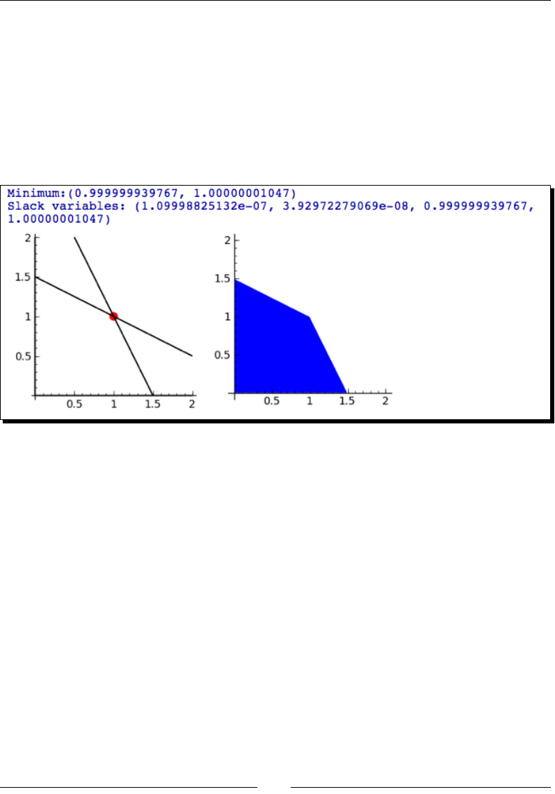
Solving Problems Numerically
[ 232 ]
c4_plot = implicit_plot(y == 0, (x,0,2), (y,0,2))
min_plot = point(sol['x'], color='red', size=50)
rp = region_plot([2 * x + y <= 3, x + 2 * y <= 3, x >= 0, y >= 0],
(x,0,2), (y,0,2))
g = graphics_array([c1_plot+c2_plot+c3_plot+c4_plot+min_plot,
rp], 1, 2)
g.show(aspect_ratio=1)
The output is shown below:
What just happened?
A linear program consists of a linear funcon to be minimized or maximized, and a set of
linear constraints. In this case, there are only two variables, which makes it easier to visualize
what's going on. We specied the funcon as a vector of coecients called c. We created
a matrix G that represents the le-hand side of the constraints. Each row in the matrix is a
vector of coecients for that constraint. Note that linear_program expects all constraints
to specied as lhs < rhs, so we have to enter the third and fourth constraints with negave
coecients. The right-hand sides of the constraints were used to form another vector called
h. The two vectors and the matrix were passed as arguments to linear_program, which
returns the soluon as a diconary. The diconary contains informaon about the soluon,
the minimized parameters, the slack variables, and the soluon to the dual program (for
more about slack variables and the dual program, see http://en.wikipedia.org/
wiki/Linear_programming or an opmizaon textbook). linear_program accepts
an oponal argument with the keyword solver, which determines which solver is used.
If the value is None (the default), the solver from the Python package CVXOPT is used. If
solver='glpk', the solver from the GNU Linear Programming Kit (GLPK) is used.

Chapter 8
[ 233 ]
The plong features of Sage can help us visualize the problem and the soluon. We
formulated the constraints as equalies, and ulized the implicit_plot funcon to plot
the resulng lines in the x-y plane. We used the point funcon to add a dot to indicate the
locaon of the minimum. We also used region_plot to plot the region dened by the
inequalies. Going further, we could use a contour plot to show how the objecve funcon
varies over the domain.
Fitting a function to a noisy data set
Fing a funcon to data is one of the most common applicaons of numerical opmizaon
for engineers and sciensts. This is oen referred to as "least squares ng," because an
opmal t is achieved when the sum of squared errors is minimized.
Time for action – least squares tting
The following is adapted from an example in the Sage documentaon:
var('a, b, c, x')
set_random_seed(0.0)
data = [(i, 1.2 * sin(0.5 * i - 0.2) + 0.1 *
normalvariate(0, 1)) for i in xsrange(0, 4 * pi, 0.2)]
data_plot = list_plot(data)
model(x) = a * sin(b * x - c)
fitted_params = find_fit(data, model, solution_dict=True)
print("a = {0}".format(fitted_params[a]))
print("b = {0}".format(fitted_params[b]))
print("c = {0}".format(fitted_params[c]))
g(x) = model.subs(a=fitted_params[a], b=fitted_params[b], c=fitted_
params[c])
fitted_plot = plot(g(x), (x, 0, 4 * pi), color='red')
show(data_plot + fitted_plot, figsize=(4, 3))
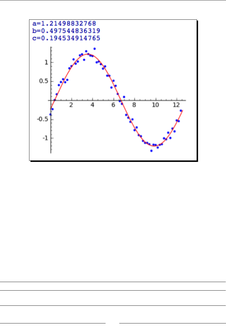
Solving Problems Numerically
[ 234 ]
The noisy data, and the ed funcon, are shown below:
What just happened?
Aer declaring some symbolic variables, we called the set_random_seed funcon to x
the seed for the pseudo-random number generator. A pseudo-random number generator
will always generate the same sequence of numbers for a given seed value. Seng the
seed ensures that the plot you create will be idencal to the one in the example. We
used a fairly complex list comprehension to construct the pseudo-random data set. We
also dened a callable symbolic expression called model that has one variable and three
variable parameters. We then used find_fit to vary the parameters unl an opmal t
was achieved. find_fit has only two required arguments: a list containing the data and
the model to be ed. The keyword argument solution_dict=True tells the funcon to
return the ed values as a diconary, rather than a list of relaons. Having the parameter
values in a diconary allows us to substute the values back into the model, using the
subs method. Finally, we ploed the ed funcon. find_fit accepts several addional
oponal arguments:
Keyword Default Descripon
initial_guess 1 for each
parameter
List containing an inial guess for each parameter.

Chapter 8
[ 235 ]
Keyword Default Descripon
parameters None List of parameters (only required if the model is a Python
funcon).
variables None List of variables (only required if the model is a Python
funcon).
Constrained optimization
Constrained opmizaon is useful when there are constraints on the parameter values.
These may be simple constraints, such as a parameter that must be greater than zero.
The constraints can also be more complicated funcons that involve several parameters.
Time for action – a constrained optimization problem
The following example is adapted from a textbook on operaons research:
#Ronald L. Rardin. "Optimization in Operations Research."
# Prentice-Hall, Upper Saddle River, NJ, 1998. Example 14.3, p. 792
# Global constants
d1 = 2.5
d2 = 40
t1 = 0.6
t2 = 1.0
p0 = 200
initial_guess = [20, 500]
def x3(x):
return 36.25 * (d2 - x[0]) * (t2 - t1) / t1 * log(x[1] / p0)
def x4(x):
return 348300 * (d2 - x[0]) * (t2 - t1)/ x[1]
def f(x):
return 61.8 + 5.72 * x[0] + 0.0175 * x3(x)^0.85 + \
0.0094 * x4(x)^0.75 + 0.006 * t1 * x3(x)
c_1 = lambda p: p[0]
c_2 = lambda p: p[1]
c_3 = lambda p: t2 * p[0] - d1 * t1 - d2 * (t2 - t1)
c_4 = lambda p: p[1] - p0
(x1, x2) = minimize_constrained(f, [c_1,c_2,c_3,c_4], initial_guess)
print('x1 = {0}'.format(x1))
print('x2 = {0}'.format(x2))
print('x3 = {0}'.format(x3([x1,x2])))
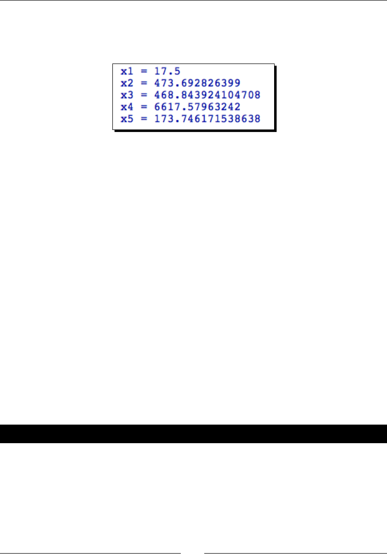
Solving Problems Numerically
[ 236 ]
print('x4 = {0}'.format(x4([x1,x2])))
print('x5 = {0}'.format(f([x1,x2])))
The ed values are:
What just happened?
First, we dened some constants that are used in the models. These are xed values that are
not opmized. This problem has four parameters, but only the rst two are independent.
Parameters x3 and x4 are funcons of x1 and x2, so we dened Python funcons to calculate
their values. We also dened the objecve funcon f, which is the funcon that we want
to minimize. The objecve funcon has one argument, which is a list that contains the
two parameters to be ed. We then dened four constraint funcons using the lambda
construct (we could also have used normal funcon denions). We called minimize_
constrained to perform the actual opmizaon. It requires three arguments: the objecve
funcon, a list of constraints, and a list of inial guesses for each parameter. The oponal
parameter gradient is a funcon that is required if the constraints are given as a list
of intervals. The keyword parameter algorithm can be used to specify the algorithm.
Currently, the only alternave is 'l-bfgs-b'.
Probability
We will end this chapter with a brief introducon to probability in Sage. Many applicaons,
such as Monte Carlo simulaons, require a series of pseudorandom numbers that are drawn
from a specied distribuon. Sage has many built-in probability distribuons that can be
used to generate pseudorandom numbers, as well as obtaining analycal distribuons.
Time for action – accessing probability distribution functions
In the following code, we will see how to access probability distribuons in Sage, obtain
random variates from a specied distribuon, and plot their distribuon:
import matplotlib.pyplot as plt
variance = 0.75
# GNU Scientific Library
gaussian = RealDistribution('gaussian', variance)
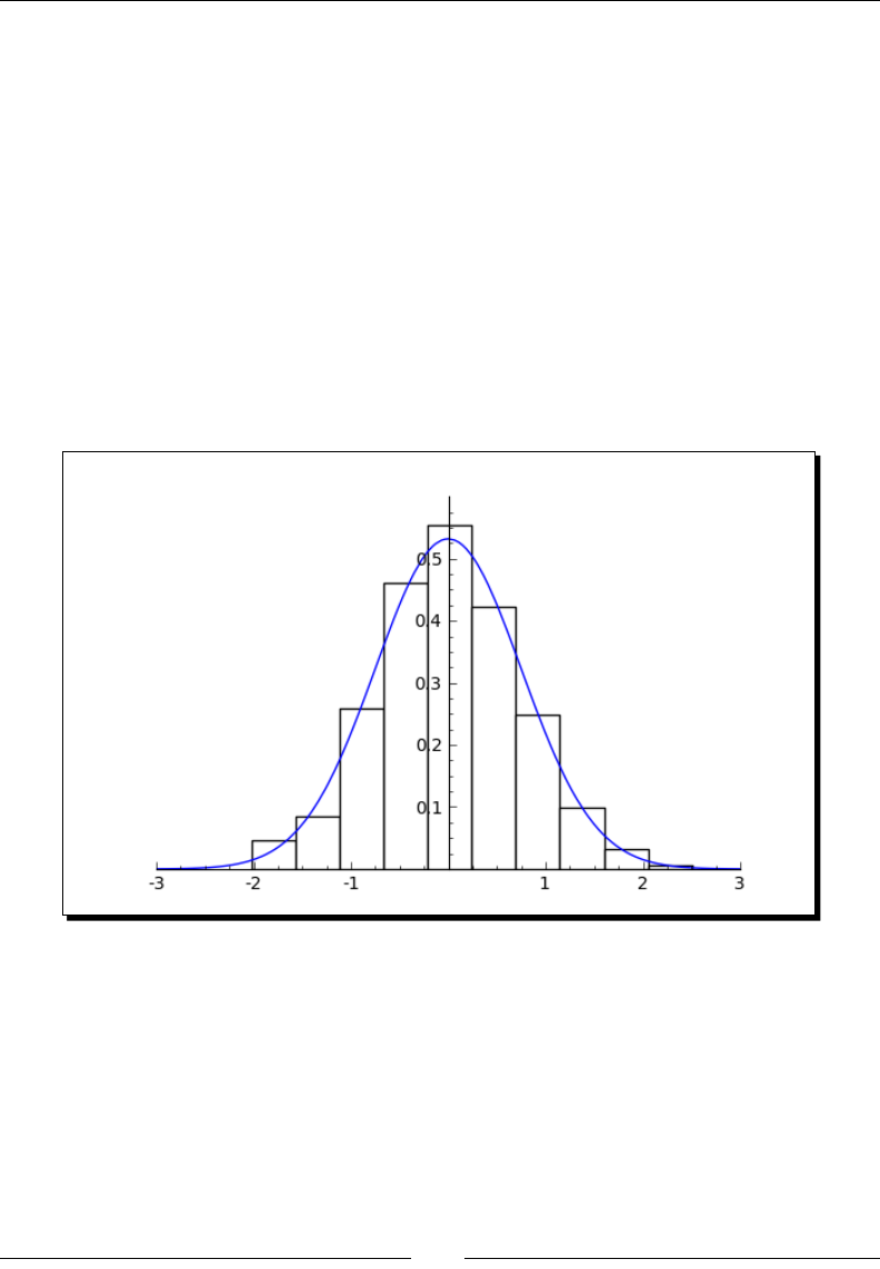
Chapter 8
[ 237 ]
gaussian.set_seed(0.0)
random_values = [gaussian.get_random_element() for i in range(1000)]
gaussian_plot = gaussian.plot((-5, 5))
# Get the Matplotlib object for the Gaussian plot
fig = gaussian_plot.matplotlib()
from matplotlib.backends.backend_agg import FigureCanvasAgg
fig.set_canvas(FigureCanvasAgg(fig)) # this line is critical
ax = fig.gca()
# Add a histogram
ax.hist(np.array(random_values), normed=True, facecolor='white')
ax.axis([-3, 3, 0, 0.6])
fig.savefig('hist.png')
The result should look like this:

Solving Problems Numerically
[ 238 ]
What just happened?
We rst called RealDistribution, which returns a Sage probability distribuon object.
Sage uses the random number generators from the GNU Scienc Library. In this case, we
specied a Gaussian distribuon with a variance of 0.75. We then called the set_seed
method to ensure that the histogram generated in this example would match the plot you
obtain when you run the code. To get a single real number drawn from this distribuon, call
the get_random_element method. To plot a histogram from a bunch of random numbers,
we used a list comprehension to call this method repeatedly. If you are not concerned about
the formang of the plot, you can use the generate_histogram_plot method of the
RealDistribution object to plot a histogram showing the distribuon of random values
from the specied distribuon.
In this example, we wanted to make a plot that shows a normalized histogram superimposed
on a plot of the normal distribuon. Unfortunately, Sage does not yet have a funcon for
plong histograms. We called the plot method of the RealDistribution object to plot
the analycal Gaussian distribuon. We then obtained a matplotlib gure from the Sage
graphics object, following the procedure described in Chapter 6. We obtained the current
axes using the gca funcon and added a histogram plot, using the matplotlib funcon hist
as described in Chapter 6.
NumPy also features high-quality random number generators, which can be found in the
numpy.random module. You can generate an enre NumPy array of random variates
with a single funcon call, which avoids the need to use a list comprehension. If you need
to generate a very large number of random variates, using NumPy can speed up your
code signicantly because it avoids the relavely slow process of looping in Python. The
documentaon for the random module can be found at http://docs.scipy.org/doc/
numpy/reference/routines.random.html. The documentaon is also included with
Sage, and can be accessed by execung the following commands:
import numpy
numpy.random?
Summary
This chapter covered a broad range of techniques in numerical mathemacs. We learned
about the tools that Sage oers for:
Finding the zeros of a funcon
Compung integrals and derivaves numerically
Finding minimum values of funcons of one or more variables
Compung the discrete Fourier transform, and using window funcons
Solving an ordinary dierenal equaon (ODE) numerically

Chapter 8
[ 239 ]
Numerically solving a higher-order ODE by transforming it into a system of
rst-order ODEs
Using opmizaon techniques for linear programming, ng curves to data,
and nding an opmal soluon in the presence of constraints
Using probability distribuons to obtain pseudo-random numbers
By now, you have all the basic informaon that you need to start using Sage to solve
problems in applied mathemacs. However, there is sll more to learn! Python is a very
powerful programming language that makes complex programming tasks possible. We'll
learn more about advanced programming techniques in the next chapter.
9
Learning Advanced Python
Programming
In Chapter 4, we learned about the basic elements of Python programming that you need to
use Sage eecvely. Throughout the following chapters, we saw various examples of objects
in Sage, such as the ode_solver object we used in the last chapter. In this chapter, you will
learn how to dene your own classes to create custom objects. Objects are a way to bundle
data and algorithms together to help you keep your code organized. You will also learn to
handle runme errors in your programs by using excepons. Finally, you will learn how unit
tesng can help you avoid bugs in your code. Many of the concepts in this chapter are used
by soware engineers on large projects. It might seem to be "overkill" to use these principles
on the short scripts you have been wring, but short scripts tend to grow into long programs.
A lile bit of discipline early in the programming process can save a lot of me later on.
In this chapter, you will learn how to:
Dene your own classes
Use inheritance to expand the usefulness of your classes
Organize your class denions in module les
Bundle module les into packages
Handle errors gracefully with excepons
Dene your own excepons for custom error handling
Use unit tests to make sure your package is working correctly
Let's see how object-oriented programming can help us write code more eecvely.

Learning Advanced Python Programming
[ 242 ]
How to write good software
Wring good soware requires a combinaon of creavity and discipline. This secon is
a brief overview of the discipline of soware development. There are many approaches
to developing soware, and the subject can be highly controversial! Look at what others
have done and develop a process that works for you or your team. A good place to start is
http://en.wikipedia.org/wiki/Software_development_methodology. First, we'll
outline the formal soware development process that is used for large projects. Then, we'll
see how elements of this process can be applied to any project.
The rst stage is requirements analysis, which is the process of dening and documenng
exactly what the soware is supposed to accomplish. The requirements are used to write
a specicaon for the project. The specicaon is then used to dene the structure of the
program, such as funcons, classes, data, methods, and so on. The next stage is wring the
actual code, which is followed by tesng to ensure that the soware meets the specicaon.
A crical aspect of the project is wring documentaon, which ideally takes place while
the code is being wrien. Once the soware is working correctly and released to the users,
it enters the maintenance phase. Bugs are xed as they are reported, improvements are
made, and new features may be added. The maintenance phase can be easy or it can
be a nightmare, depending on the quality of the soware design, implementaon, and
documentaon.
All of these concepts can (and should) be applied to the short scripts that you write on
a daily basis. Requirements analysis can be as simple as pausing before implemenng
a funcon or class to think about what it needs to accomplish. One trick is to write the
docstring before wring the actual code. Use the docstring to organize your thoughts
and document what the inputs and outputs of the code will be. Before you jump into
wring code, think about the approach you're going to take. For more complex code, you
might want to consult books, journal arcles, or open-source projects to see how others
have approached the subject (and make sure that you are not re-invenng the wheel). In
pracce, a lot of projects start o as lile scripts or snippets of code, and gradually grow
into monsters. It's important to recognize when your code is geng out of control. Take a
short break from programming, and ask yourself how to organize the code more eecvely.
Do you need to dene a funcon to replace redundant code? Would it help to use an object
represent this concept? Do the variable names make sense? Do you have enough comments
to make it clear what's going on? If you have to x a bug in this code six months from now,
will you understand how it works? If not, take the me to improve the documentaon right
now. In the long run, it will save you a lot of me if you develop the discipline to write clean,
organized, well-documented code.

Chapter 9
[ 243 ]
Version control (also known as revision control or source control) is a process of tracking and
managing changes in programs and documentaon. Version control tools can be very helpful
even for small projects, and they are essenal for large projects with mulple developers.
For example, the Sage project uses an open-source version control tool called Mercurial. The
Web interface at http://hg.sagemath.org/ allows you to browse the Sage source code
and track changes. Sage also provides funcons that allow you to work with Mercurial from
within the notebook interface. The documentaon for the Mercurial interface is available
at http://www.sagemath.org/doc/reference/sage/misc/hg.html. Other popular
open-source version control tools include Bazaar, Git, and Subversion.
Object-oriented programming
An object is a construct that contains data and has methods that operate on its data. A
class denes how data is stored in an object, and what methods are available to work with
the data. A class is like a blueprint that describes how a house is to be built. An object is
like a house that is constructed from the blueprint. Many houses can be constructed from
the same blueprint. Although the houses are built from the same plans and have the same
structure, each house is an independent enty, and the contents of each house can be
dierent. In Python, an object is known as an instance of a class. If you're new to object-
oriented programming, a good starng point is to use objects as models of concrete objects
in the real world. Once you've become familiar with the concept, you can use objects to
represent all kinds of concepts. For more informaon about the general principles of object-
oriented programming, read http://en.wikipedia.org/wiki/Object-oriented_
programming.
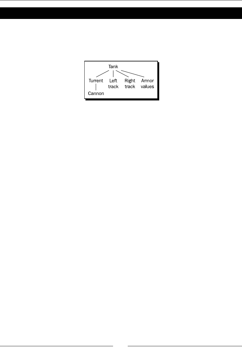
Learning Advanced Python Programming
[ 244 ]
Time for action – dening a class that represents a tank
To start out, we will dene a class that models a tank (meaning a tracked, armored ghng
vehicle). A tank typically runs on two connuous tracks, and it has a rotang turret that
houses a powerful cannon. The relaonship between the various components of a tank is
shown in the following diagram:
Based on this conceptual representaon, we will dene classes to represent the cannon,
the tracks, and turret. We will then dene another class that ulizes these classes to model
a tank. To keep the example simple, we'll use point values to represent the relave strength
of the tank's armor and the damage inicted by its main gun. Although this is a simple "toy"
example, a class like this could be used as the foundaon of a video game or a simulator for
military training:
class Cannon():
"""Model of a large cannon."""
def __init__(self, damage):
"""Create a Cannon instance
Arguments:
damage Integer that represents
the damage inflicted by the cannon
"""
# _damage amount of damage inflicted by cannon (integer)
# _operational True if operational, False if disabled
self._damage = damage
self._operational = True
def __str__(self):
return 'Damage value:' + str(self._damage)
class Track():
"""Model of a continuous track."""
def __init__(self):
# _operational True if operational, False if disabled
self._operational = True
class Turret():
"""Model of a tank turret."""

Chapter 9
[ 245 ]
def __init__(self, gun):
"""Create a Turret instance
Arguments:
gun instance of Gun class
"""
# _gun instance of Gun class
# _operational True if operational, False if disabled
self._gun = gun
self._operational = True
def __str__(self):
return(str(self._gun))
class Tank():
"""Model of an armored fighting vehicle."""
def __init__(self, armor_values, cannon_damage_value):
"""Create a tank instance
Arguments:
armor_values A dictionary of armor values
of the form:
{'front' : 100, 'side' : 50, 'rear' : 25,
'turret' : 75}
cannon_damage_value Integer that represents
the damage inflicted by the main gun
"""
# Initialize armor
self._frontal_armor = armor_values['front']
self._left_armor = armor_values['side']
self._right_armor = armor_values['side']
self._rear_armor = armor_values['rear']
self._turret_armor = armor_values['turret']
# Add tank components
main_gun = Cannon(cannon_damage_value)
self._turret = Turret(main_gun)
self._left_track = Track()
self._right_track = Track()
def __str__(self):
import os
ls = os.linesep
description = 'Tank parameters:' + ls
description += ' Armor values:' + ls

Learning Advanced Python Programming
[ 246 ]
description += ' Front:' + str(self._frontal_armor) + ls
description += ' Left:' + str(self._left_armor) + ls
description += ' Right:' + str(self._right_armor) + ls
description += ' Rear:' + str(self._rear_armor) + ls
description += ' Turret:' + str(self._turret_armor) + ls
description += ' Weapons:' + ls
description += ' Main cannon:' + ls
description += ' ' + str(self._turret) + ls
return description
# Define parameters for the tank
armor_values = {'front' : 100, 'side' : 50, 'rear' : 25,
'turret' : 75}
main_gun_damage = 50
# Create a tank object
tank = Tank(armor_values, main_gun_damage)
print(tank)
Use the load command on the Sage command line or in a cell in a worksheet to run the
code. If you run it from the command line, the output should look like this:
sage: load("4460_9_1.py")
Tank parameters:
Armor values:
Front:100
Left side:50
Right side:50
Rear:25
Turret:75
Weapons:
Main cannon:
Damage value:50
What just happened?
We used our knowledge of a real-world object (an armored ghng vehicle) to construct
a conceptual model of a tank. We then used Python to implement an object-oriented
representaon of a tank. We dened a Tank class, which uses point values to keep track of
the amount of armor on the tank. Each instance of the Tank class has an associated instance
of the Turret class, which in turn has an instance of a Cannon. Each Tank instance also has
two instances of the Track class, to represent the le and right tracks.

Chapter 9
[ 247 ]
The keyword class is used to start each class denion, followed by the name of the
class, and a set of parenthesis and a colon. By convenon, Python class names start with an
upper-case leer, and use a mix of upper- and lower-case leers, rather than underscores,
to separate words (known as camel case, because the upper-case leers can resemble the
humps of a camel). This convenon helps us disnguish between an object named tank
and a class named Tank. The pair of parenthesis is used for inheritance, which we'll get to
in moment. Methods for the class are dened using funcon denion syntax, and they are
indented to show that they are part of the class denion. The rst argument to a method
is special, and by convenon the name self is used. self refers to the instance itself. The
self argument allows a method to access data and call other methods from the class or
instance, using the syntax self.method_name(). However, when the methods are called
from outside of the class, the self keyword is omied.
The rst method we dened for each class is called __init__. In Python, the __init__
method is automacally called when an instance is rst created. This special method has
the same purpose as a constructor in other object-oriented languages. If data needs to
be inialized every me an instance is created, that code should go into __init__. If no
inializaon needs to be done, then you can omit this method from the class denion. The
Tank class and the Turret class have addional arguments to __init__ that are used to
set inial values for the data in the objects, while the Cannon and Track classes do not
have any arguments. Keyword arguments can also be used with the __init__ method. An
instance of the Tank class can be created using funcon call syntax. The name of the class is
used instead of a funcon name, and the argument list must match the arguments required
by the __init__ method (ignoring self, as previously menoned).
Instance variables are created in the __init__ method with the syntax self.var_name
= value. Instance variables can be public or non-public. Public instance variables can be
modied by code outside of the class, while non-public variables are only supposed to be
modied within the class. By convenon, public instance variables have regular names, and
non-public instance variables have names that start with a single underscore. We dened
our class with non-public instance variables to encourage users to use methods to get and
set the values. Methods can also be non-public, in which case their names also start with a
single underscore. Note that Python does not prevent outside code from modifying non-public
variables or calling non-public methods. That is why they are called non-public, rather than
private. Python doesn't have truly private instance variables or methods.

Learning Advanced Python Programming
[ 248 ]
Another special method is called __str__, which is an oponal method that returns a
string representaon of an object. Because we have dened this method for the Tank and
Cannon classes, we can use the syntax print(tank) to display useful data about the
instance. This method is also called when the instance is an argument to the str funcon.
Noce how the __str__ method of the Tank class actually calls the str funcon to get a
text representaon of the Cannon instance. It would be possible for the __str__ method
of the Tank class to go and get the value of _damage directly from the Cannon object and
convert it to a string, but this would be an unwise shortcut. In the future, we might decide
to completely change the internal structure of the Cannon class, and the variable damage_
value may go away. By using methods to access the data from an object, we keep our code
more organized and prevent bugs. If we try to use print with an instance that does not
have a __str__ method, we will only get a crypc message about the type of object and its
memory address. For example:
sage: print(tank._left_track)
<__main__.Track instance at 0x100463440>
Note that the memory address that is printed on your system will probably be dierent.
Immediately aer each class denion and funcon denion, there is a triple-quoted string
called a docstring. This string is used to document the purpose of the class or funcon. When
you ask for help on a class or instance, Sage and Python use the docstring to provide help.
For example:
sage: Tank?
Type: classobj
String Form: __main__.Tank
Namespace: Interactive
File: /Applications/sage/local/lib/python2.6/site-packages/IPython/
FakeModule.py
Docstring:
Model of an armored fighting vehicle.
Constructor information:
Definition: Tank(self, armor_values, cannon_damage_value)
Docstring:
Constructs a tank instance
Arguments:
armor_values A dictionary of armor values of the form:
{'front' : 100, 'side' : 50, 'rear' : 25, 'turret' : 75}

Chapter 9
[ 249 ]
cannon_damage_value Integer that represents the damage
inflicted by the main gun
You should write docstrings for all public modules, funcons, classes, and methods. A
general guide to wring good docstrings can be found at http://www.python.org/
dev/peps/pep-0257/. Our Tank class is useful for organizing and displaying data, but
the instances don't do much. Let's make them do something useful.
Making our tanks move
At a simplisc level, a tank only has to do two things: move and shoot. Let's start by giving
our tank model the ability to move.
Time for action – making the tanks move
To start out, we will dene aributes and methods that allow the tank instances to move.
Execute this enhanced version of the previous example:
class Cannon():
"""Model of a large cannon."""
def __init__(self, damage):
"""Create a Cannon instance
Arguments:
damage Integer that represents
the damage inflicted by the cannon
"""
# _damage amount of damage inflicted by cannon (integer)
# _operational True if operational, False if disabled
self._damage = damage
self._operational = True
def __str__(self):
return 'Damage value:' + str(self._damage)
class Track():
"""Model of a continuous track."""
def __init__(self):
# _operational True if operational, False if disabled
self._operational = True
class Turret():
"""Model of a tank turret."""
def __init__(self, gun):
"""Create a Turret instance

Learning Advanced Python Programming
[ 250 ]
Arguments:
gun instance of Gun class
"""
# _gun instance of Gun class
# _operational True if operational, False if disabled
self._gun = gun
self._operational = True
def __str__(self):
return(str(self._gun))
class Tank():
"""Model of an armored fighting vehicle."""
def __init__(self, armor_values, cannon_damage_value, position):
"""Create a tank instance
Arguments:
armor_values A dictionary of armor values
of the form:
{'front' : 100, 'side' : 50, 'rear' : 25,
'turret' : 75}
cannon_damage_value Integer that represents
the damage inflicted by the main gun
position (x,y) tuple of coordinates
"""
# Initialize armor
self._frontal_armor = armor_values['front']
self._left_armor = armor_values['side']
self._right_armor = armor_values['side']
self._rear_armor = armor_values['rear']
self._turret_armor = armor_values['turret']
# Add tank components
main_gun = Cannon(cannon_damage_value)
self._turret = Turret(main_gun)
self._left_track = Track()
self._right_track = Track()
# Intialize position
self._x = position[0]
self._y = position[1]
def __str__(self):
import os
ls = os.linesep
description = 'Tank parameters:' + ls

Chapter 9
[ 251 ]
description += ' Armor values:' + ls
description += ' Front:' + str(self._frontal_armor) + ls
description += ' Left:' + str(self._left_armor) + ls
description += ' Right:' + str(self._right_armor) + ls
description += ' Rear:' + str(self._rear_armor) + ls
description += ' Turret:' + str(self._turret_armor) + ls
description += ' Weapons:' + ls
description += ' Main cannon:' + ls
description += ' ' + str(self._turret) + ls
return description
def move(self, direction, distance):
"""Move the tank.
Arguments:
direction floating-point number representing
the compass angle of movement in degrees. North is
0,
east is 90, south is 180, and west is 270.
0 <= direction < 360
distance distance to move (in meters)
"""
if (direction < 0) or (direction >= 360):
print("Error: Direction must be greater than or equal \
to zero and less than 360.")
elif distance < 0:
print("Error: Negative distance.")
else:
self._x += n(distance * cos(direction * pi / 180))
self._y += n(distance * sin(direction * pi / 180))
def get_position(self):
"""Returns a tuple with the (x,y) coordinates of the tank's
current location.
"""
return (float(self._x), float(self._y))
# Define parameters for the tank
armor_values = {'front' : 100, 'side' : 50, 'rear' : 25,
'turret' : 75}
main_gun_damage = 50
initial_position = (0.0, 0.0)
# Create a tank object
tank = Tank(armor_values, main_gun_damage, initial_position)
pos = tank.get_position()
print("Initial position: x = {0:.2f}m y = {1:.2f}m".format(pos[0],
pos[1]))

Learning Advanced Python Programming
[ 252 ]
# Move 10m north
tank.move(0.0, 10.0)
pos = tank.get_position()
print("Current position: x = {0:.2f}m y = {1:.2f}m".format(pos[0],
pos[1]))
# Now move 10m east
tank.move(90.0, 10.0)
pos = tank.get_position()
print("Current position: x = {0:.2f}m y = {1:.2f}m".format(pos[0],
pos[1]))
# Move southwest, back to the origin
tank.move(225.0, sqrt(10.0**2 + 10.0**2))
pos = tank.get_position()
print("Current position: x = {0:.2f}m y = {1:.2f}m".format(pos[0],
pos[1]))
# Try a move which doesn't make sense
tank.move(-2,-1)
If you run this example from the command line, you should get the following results:
sage: load("4460_9_2.py")
Initial position: x = 0.00m y = 0.00m
Current position: x = 10.00m y = 0.00m
Current position: x = 10.00m y = 10.00m
Current position: x = -0.00m y = 0.00m
Error: Direction must be greater than or equal to zero and less than 360.
What just happened?
We dened two new methods, and made some changes to __init__. If our tanks are going
to move, they must have an inial posion, so we added an argument called position to
__init__. This argument is a tuple, which is used to inialize two new aributes, x and y
(for simplicity, we'll assume the tank is located on a plane). We also added a method called
get_position, which simply returns the current locaon of the tank as a tuple of Python
float values. We have to force the return values to be oats to ensure that they will be
formaed correctly when the values are printed. Sage RealNumber objects evaluate to
strings when used as arguments to format, so they must be converted to Python
oang-point numbers in order to use Python's format specicaons for real numbers.

Chapter 9
[ 253 ]
The new method called move is a lile more interesng. It accepts a direcon and a
distance, and updates the x and y coordinates of the tank accordingly. However, this method
checks to ensure that the direcon and distance are valid before the tank is moved. If the
arguments are not valid, an error message is printed and the tank does not move. This
method illustrates a principle of object-oriented programming: whenever possible, dene
methods and use them to interact with the data in an object. Ulize the input methods to
make sure the inputs are valid before you accept them. move calculates a new posion for
the tank (in Cartesian coordinates) using the Sage funcons sin and cos. The n funcon
(short for numerical_approx) is used to ensure that the x and y values are stored as Sage
RealNumber objects.
Have a go hero – checking the values passed to __init__
The __init__ method doesn't check whether or not the armor values, cannon damage
value, and inial posion are valid. You could accidentally construct a tank with a negave
armor value, for example. It's also a good idea to check the type of the arguments, or force
them to have the correct type, to avoid unexpected results. The armor value and cannon
damage value should be integers and the posion should be a tuple of real numbers. Add
code to validate the values that are passed to __init__.
Creating a module for our classes
Our classes are geng to the point where they are useful, but the code is also geng rather
lengthy. With each new example, we nd ourselves duplicang much of the code from the
previous example. Python provides modules to help us re-use code without duplicaon.
Time for action – creating your rst module
Create a new Python le called tank.py that contains the following code:
import sage.all
class Cannon():
"""Model of a large cannon."""
def __init__(self, damage):
"""Create a Cannon instance
Arguments:
damage Integer that represents
the damage inflicted by the cannon
"""
# _damage amount of damage inflicted by cannon (integer)
# _operational True if operational, False if disabled
self._damage = damage

Learning Advanced Python Programming
[ 254 ]
self._operational = True
def __str__(self):
return 'Damage value:' + str(self._damage)
class Track():
"""Model of a continuous track."""
def __init__(self):
# _operational True if operational, False if disabled
self._operational = True
class Turret():
"""Model of a tank turret."""
def __init__(self, gun):
"""Create a Turret instance
Arguments:
gun instance of Gun class
"""
# _gun instance of Gun class
# _operational True if operational, False if disabled
self._gun = gun
self._operational = True
def __str__(self):
return(str(self._gun))
class Tank():
"""Model of an armored fighting vehicle."""
def __init__(self, armor_values, cannon_damage_value, position):
"""Create a tank instance
Arguments:
armor_values A dictionary of armor values
of the form:
{'front' : 100, 'side' : 50, 'rear' : 25,
'turret' : 75}
cannon_damage_value Integer that represents
the damage inflicted by the main gun
position (x,y) tuple of coordinates
"""
# Initialize armor
self._frontal_armor = armor_values['front']
self._left_armor = armor_values['side']
self._right_armor = armor_values['side']
self._rear_armor = armor_values['rear']
self._turret_armor = armor_values['turret']

Chapter 9
[ 255 ]
# Add tank components
main_gun = Cannon(cannon_damage_value)
self._turret = Turret(main_gun)
self._left_track = Track()
self._right_track = Track()
# Intialize position
self._x = position[0]
self._y = position[1]
def __str__(self):
import os
ls = os.linesep
description = 'Tank parameters:' + ls
description += ' Armor values:' + ls
description += ' Front:' + str(self._frontal_armor) + ls
description += ' Left:' + str(self._left_armor) + ls
description += ' Right:' + str(self._right_armor) + ls
description += ' Rear:' + str(self._rear_armor) + ls
description += ' Turret:' + str(self._turret_armor) + ls
description += ' Weapons:' + ls
description += ' Main cannon:' + ls
description += ' ' + str(self._turret) + ls
return description
def move(self, direction, distance):
"""Move the tank.
Arguments:
direction floating-point number representing
the compass angle of movement in degrees. North is
0,
east is 90, south is 180, and west is 270.
0 <= direction < 360
distance distance to move (in meters)
"""
if (direction < 0) or (direction >= 360):
print("Error: Direction must be greater than or equal \
to zero and less than 360.")
elif distance < 0:
print("Error: Negative distance.")
else:
self._x += n(distance * cos(direction * pi / 180))
self._y += n(distance * sin(direction * pi / 180))
def get_position(self):
"""Returns a tuple with the (x,y) coordinates of the tank's

Learning Advanced Python Programming
[ 256 ]
current location.
"""
return (float(self._x), float(self._y))
In the same directory, create another Python le that contains the following code:
import tank
# Define parameters for the tank
armor_values = {'front' : 100, 'side' : 50, 'rear' : 25,
'turret' : 75}
main_gun_damage = 50
initial_position = (0.0, 0.0)
# Create a tank object
tank_1 = tank.Tank(armor_values, main_gun_damage, initial_position)
pos = tank_1.get_position()
print("Initial position: x = {0:.2f}m y = {1:.2f}m".format(pos[0],
pos[1]))
# Move 10m north
tank_1.move(0.0, 10.0)
pos = tank_1.get_position()
print("Current position: x = {0:.2f}m y = {1:.2f}m".format(pos[0],
pos[1]))
# Now move 10m east
tank_1.move(90.0, 10.0)
pos = tank_1.get_position()
print("Current position: x = {0:.2f}m y = {1:.2f}m".format(pos[0],
pos[1]))
# Move southwest, back to the origin
tank_1.move(225.0, sqrt(10.0**2 + 10.0**2))
pos = tank_1.get_position()
print("Current position: x = {0:.2f}m y = {1:.2f}m".format(pos[0],
pos[1]))
# Try a move which doesn't make sense
tank_1.move(-2,-1)
Execute the script you just created. You should see the following results, which are idencal
to the previous example:
sage: load 4460_9_3.py
Initial position: x = 0.00m y = 0.00m
Current position: x = 10.00m y = 0.00m
Current position: x = 10.00m y = 10.00m
Current position: x = -0.00m y = 0.00m
Error: Direction must be greater than or equal to zero and less than 360.

Chapter 9
[ 257 ]
What just happened?
We took the code from the previous example and split it into two les. The rst one, which
we called tank.py, is a module that contains our class denions. The name of this le
becomes the name of the module, so it should follow the Python naming convenons for
modules: use lower-case leers, with underscores if necessary, and keep the name as short
as possible while sll being clear about what the module contains.
We have to make one important change to the code in the tank module. We now have to
import names from Sage using the syntax import sage.all. We can then access Sage
variables and funcons with the following syntax:
sage.all.cos(direction * sage.all.pi / 180)
To understand why we have to do this, we have to know a lile bit about namespaces
and scope in Python. A namespace is a conceptual space that maps names to objects.
A scope is a poron of a Python program in which names from a certain namespace are
directly accessible. When working on the Sage command line, all of the built-in names
(of classes, funcons, instances, variables, and so on) are accessible. Our module has its
own, separate namespace, so names that we take for granted on the command line aren't
directly accessible in the module. Hence, we use the import statement to make all the
standard Sage names available throughout our module. In fact, each me a funcon or class
is dened, a new local namespace is created. That's why the names you create within a
funcon denion are only visible within that funcon (and funcons declared within that
funcon). The technical aspects of namespaces and scoping are explained in the Python
documentaon.
Ideally, a Python package would be designed so that the user only has to import the sub-
packages or modules that are required to use a subset of its funconality. However, the only
way to use Sage names in a Python module (as of Sage version 4.6.1) is to import sage.
all. There is no way to import a subset of Sage's funconality. Since Sage is rather large, we
placed the import statement at the beginning of the class denion so that Sage is imported
only once, when the tank module is loaded. If we placed the import statement in method
move, it could potenally be imported more than once (although the Python interpreter tries
to avoid this), slowing down the funcon call.
The second le is a script that imports the module and uses the classes to create and move
a tank instance. We use the syntax import tank to import the module called tank.py. We
can then use the syntax tank.Tank to access the Tank class from the tank module. We
don't have to import any of the other classes, because we don't access them outside of the
tank module. Note that we have also changed the name of the tank instance to tank_1 so
that it does not conict with the module name. This makes it possible to use the command
reload(tank) to reload the module (see p).
Learning Advanced Python Programming
[ 258 ]
reload the module aer making changes
Let's say you created the module tank.py and used import tank to make
its names available in a Sage script, or on the Sage command line. During
tesng, you found and xed a bug, and saved the module le. However, Sage
won't recognize that you changed anything unless you use the command
reload(tank) to force it to reload the module. When working with mulple
modules in a package, you may need to import a module on the command line
(or in a worksheet cell) before reloading it.
Expanding our simulation to other kinds of vehicles
So far, we have dened a rudimentary framework for a simulaon of tank combat. What
if we want to include other types of military vehicles in our simulaon, such as armored
personnel carriers (APCs), armored cars, and supply trucks? We could dene a class for each
of those vehicles, but there would certainly be some duplicaon between the classes. For
example, every vehicle class would need to dene a method to get the vehicle posion and
move the vehicle. How can we avoid this duplicaon?
Time for action – creating a vehicle base class
We can avoid duplicang code in related classes by applying the object-oriented principle
of inheritance. Inheritance allows a class to be derived from a base class. The derived
class inherits the methods and aributes of the base class, and adds its own aributes
and methods. This can be rather confusing, so we'll jump into a concrete example. Since
tanks, APCs, armored cars, and trucks are all vehicles, we will create a base class for ground
vehicles. Then, we will dene derived classes to represent various types of vehicles. Enter
the following code into a le called vehicle.py:
import sage.all
class Cannon():
"""Model of a large cannon."""
def __init__(self, damage):
"""Create a Cannon instance
Arguments:
damage Integer that represents
the damage inflicted by the cannon
"""
# _damage amount of damage inflicted by cannon (integer)
# _operational True if operational, False if disabled
self._damage = damage

Chapter 9
[ 259 ]
self._operational = True
def __str__(self):
return 'Damage value:' + str(self._damage)
class Track():
"""Model of a continuous track."""
def __init__(self):
# _operational True if operational, False if disabled
self._operational = True
class Turret():
"""Model of a tank turret."""
def __init__(self, gun):
"""Create a Turret instance
Arguments:
gun instance of Gun class
"""
# _gun instance of Gun class
# _operational True if operational, False if disabled
self._gun = gun
self._operational = True
def __str__(self):
return(str(self._gun))
class Ground_Vehicle():
"""Base class for all ground vehicles"""
def __init__(self, position):
"""Create a vehicle instance
position (x,y) tuple of coordinates
"""
# Intialize position
self._x = position[0]
self._y = position[1]
def move(self, direction, distance):
"""Move the tank.
Arguments:
direction floating-point number representing
the compass angle of movement in degrees. North is
0,
east is 90, south is 180, and west is 270.
0 <= direction < 360
distance distance to move (in meters)

Learning Advanced Python Programming
[ 260 ]
"""
if (direction < 0) or (direction >= 360):
print("Error: Direction must be greater than or equal \
to zero and less than 360.")
elif distance < 0:
print("Error: Negative distance.")
else:
self._x += sage.all.n(distance * sage.all.cos(direction *
sage.all.pi / 180))
self._y += sage.all.n(distance * sage.all.sin(direction *
sage.all.pi / 180))
def get_position(self):
"""Returns a tuple with the (x,y) coordinates of the tank's
current location.
"""
return (float(self._x), float(self._y))
class Tank(Ground_Vehicle):
"""Model of an armored fighting vehicle."""
def __init__(self, armor_values, cannon_damage_value, position):
"""Constructs a tank instance
Arguments:
armor_values A dictionary of armor values
of the form:
{'front' : 100, 'side' : 50, 'rear' : 25,
'turret' : 75}
cannon_damage_value Integer that represents
the damage inflicted by the main gun
position (x,y) tuple of coordinates
"""
# Initialize armor
self._frontal_armor = armor_values['front']
self._left_armor = armor_values['side']
self._right_armor = armor_values['side']
self._rear_armor = armor_values['rear']
self._turret_armor = armor_values['turret']
# Add tank components
main_gun = Cannon(cannon_damage_value)
self._turret = Turret(main_gun)
self._left_track = Track()
self._right_track = Track()
Ground_Vehicle.__init__(self, position)
def __str__(self):

Chapter 9
[ 261 ]
import os
ls = os.linesep
description = 'Tank parameters:' + ls
description += ' Armor values:' + ls
description += ' Front:' + str(self._frontal_armor) + ls
description += ' Left:' + str(self._left_armor) + ls
description += ' Right:' + str(self._right_armor) + ls
description += ' Rear:' + str(self._rear_armor) + ls
description += ' Turret:' + str(self._turret_armor) + ls
description += ' Weapons:' + ls
description += ' Main cannon:' + ls
description += ' ' + str(self._turret) + ls
return description
Now, we need to modify the script that creates Tank instances so that the tank class is
imported from the vehicle module instead of the tank module:
import vehicle
# Define parameters for the tank
armor_values = {'front' : 100, 'side' : 50, 'rear' : 25,
'turret' : 75}
main_gun_damage = 50
initial_position = (0.0, 0.0)
# Create a tank object
tank_1 = vehicle.Tank(armor_values, main_gun_damage, initial_position)
pos = tank_1.get_position()
print("Initial position: x = {0:.2f}m y = {1:.2f}m".format(pos[0],
pos[1]))
# Move 10m north
tank_1.move(0.0, 10.0)
pos = tank_1.get_position()
print("Current position: x = {0:.2f}m y = {1:.2f}m".format(pos[0],
pos[1]))
# Now move 10m east
tank_1.move(90.0, 10.0)
pos = tank_1.get_position()
print("Current position: x = {0:.2f}m y = {1:.2f}m".format(pos[0],
pos[1]))
# Move southwest, back to the origin
tank_1.move(225.0, sqrt(10.0**2 + 10.0**2))
pos = tank_1.get_position()
print("Current position: x = {0:.2f}m y = {1:.2f}m".format(pos[0],
pos[1]))

Learning Advanced Python Programming
[ 262 ]
# Try a move which doesn't make sense
tank_1.move(-2,-1)
When we run this script, we should get the same results as the previous example:
sage: load("4460_9_4.py")
Initial position: x = 0.00m y = 0.00m
Current position: x = 10.00m y = 0.00m
Current position: x = 10.00m y = 10.00m
Current position: x = -0.00m y = 0.00m
Error: Direction must be greater than or equal to zero and less than 360.
What just happened?
We created a base class called Ground_Vehicle to contain methods and aributes that are
common to all ground vehicles. For now, every ground vehicle has a posion that is stored
as a pair of coordinates, a method to update the posion, and a method that returns the
current posion. Since a vehicle has to have a dened posion for movement to make any
sense, the __init__ method accepts one argument that sets the inial posion.
The rst line of the Tank class denion was modied to show that the class is derived from
the class Ground_Vehicle:
class Tank(Ground_Vehicle):
Since the methods move and get_position are dened in Ground_Vehicle, we removed
them from the Tank class denion. We say that Tank inherits these methods from
Ground_Vehicle. We can also override inherited methods. For example, let's say that we
have dened a class that represents a wheeled vehicle:
class Wheeled_Vehicle(Ground_Vehicle):
We want to implement a special version of the move method that reduces the mobility
of wheeled vehicles when they travel o-road. If we dene a method called move in the
Wheeled_Vehicle class, it will override the move method dened in the base class.
We also made an important change in the __init__ method of the Tank class. We used
the following syntax to call the __init__ method of the base class to set the inial posion
of the vehicle:
Ground_Vehicle.__init__(self, position)
You must explicitly call the __init__ method of the base class (if it has one) from the
__init__ method of the derived class in order to properly inialize the object.

Chapter 9
[ 263 ]
Note that we didn't have to make any changes in the code that creates Tank instances, aside
from changing the name of the module we are imporng. Changes to the class structure
were transparent to the code that creates and uses Tank instances. A well-designed class
implements an interface, and all interacon with the class takes place through the interface.
If you improve the design of the class without changing its funcon, a process known as
refactoring, the interface should not change. Although Python does not have a formal
language element for dening interfaces, it's helpful to think in terms of interfaces when
designing classes.
Creating a package for our simulation
A logical step in developing our simulaon is to add derived classes for dierent types of
vehicles. Before we do that, let's take a minute to improve the organizaon of the code by
creang a package. A package is a collecon of modules, organized in a tree of directories.
Time for action – creating a combat simulation package
Create a directory called combatsim. The name of the directory is the name of the package,
so it should follow the Python naming convenons for packages. The name should use
lower-case leers and should be as short as possible, in case someone wants to use your
package on a system that doesn't support long names. Underscores are ocially discouraged
in package names, but don't be afraid to use them if it makes the package name easier to
understand. Now, create a new le in the directory called __init__.py. Leave this le empty.
It only needs to be present to tell the Python interpreter that this directory is a package.
In the directory combatsim, enter the following code in a le called components.py.
Essenally, we're just going to cut and paste to place the denions for the Cannon, Track,
and Turret classes into their own les. We will repeat the process with the denions of
the classes Ground_Vehicle and Tank.
class Cannon():
"""Model of a large cannon."""
def __init__(self, damage):
"""Create a Cannon instance
Arguments:
damage Integer that represents
the damage inflicted by the cannon
"""
# _damage amount of damage inflicted by cannon (integer)
# _operational True if operational, False if disabled
self._damage = damage
self._operational = True
def __str__(self):

Learning Advanced Python Programming
[ 264 ]
return 'Damage value:' + str(self._damage)
class Track():
"""Model of a continuous track."""
def __init__(self):
# _operational True if operational, False if disabled
self._operational = True
class Turret():
"""Model of a tank turret."""
def __init__(self, gun):
"""Create a Turret instance
Arguments:
gun instance of Gun class
"""
# _gun instance of Gun class
# _operational True if operational, False if disabled
self._gun = gun
self._operational = True
def __str__(self):
return(str(self._gun))
Now, create another le in the combatsim directory called vehicle.py, and enter the
following code to dene the Ground_Vehicle base class:
import sage.all
class Ground_Vehicle():
"""Base class for all ground vehicles"""
def __init__(self, position):
"""Create a vehicle instance
position (x,y) tuple of coordinates
"""
# Intialize position
self._x = position[0]
self._y = position[1]
def move(self, direction, distance):
"""Move the tank.
Arguments:
direction floating-point number representing
the compass angle of movement in degrees. North is
0,
east is 90, south is 180, and west is 270.
0 <= direction < 360

Chapter 9
[ 265 ]
distance distance to move (in meters)
"""
if (direction < 0) or (direction >= 360):
print("Error: Direction must be greater than or equal \
to zero and less than 360.")
elif distance < 0:
print("Error: Negative distance.")
else:
self._x += sage.all.n(distance * sage.all.cos(direction *
sage.all.pi / 180))
self._y += sage.all.n(distance * sage.all.sin(direction *
sage.all.pi / 180))
def get_position(self):
"""Returns a tuple with the (x,y) coordinates of the tank's
current location.
"""
return (float(self._x), float(self._y))
Create another le in the combatsim directory called tank.py, and enter the following code:
import sage.all
class Ground_Vehicle():
"""Base class for all ground vehicles"""
def __init__(self, position):
"""Create a vehicle instance
position (x,y) tuple of coordinates
"""
# Intialize position
self._x = position[0]
self._y = position[1]
def move(self, direction, distance):
"""Move the vehicle.
Arguments:
direction floating-point number representing
the compass angle of movement in degrees. North
is 0, east is 90, south is 180, and west is 270.
0 <= direction < 360
distance distance to move (in meters)
"""
if (direction < 0) or (direction > 360):
print("Error: Direction must be greater than or equal \
to zero and less than 360.")
elif distance < 0:
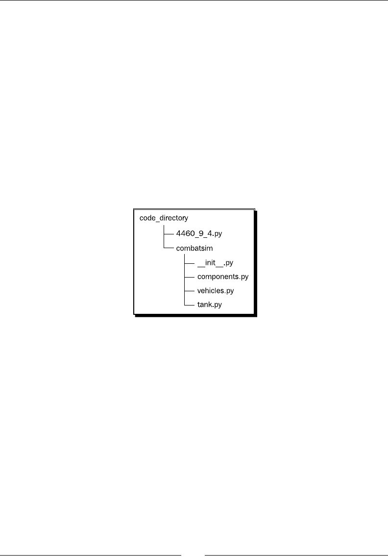
Learning Advanced Python Programming
[ 266 ]
print("Error: Negative distance.")
else:
self._x += sage.all.n(distance * sage.all.cos(direction *
sage.all.pi / 180))
self._y += sage.all.n(distance * sage.all.sin(direction *
sage.all.pi / 180))
def get_position(self):
"""Returns a tuple with the (x,y) coordinates of the tank's
current location.
"""
return (float(self._x), float(self._y))
Finally, we need to make a slight change in the code that creates instances of the Tank class.
Enter the following code in a le that resides in the same directory as combatsim. When you
are done, the le hierarchy should look like this:
from combatsim import tank
# Define parameters for the tank
armor_values = {'front' : 100, 'side' : 50, 'rear' : 25,
'turret' : 75}
main_gun_damage = 50
initial_position = (0.0, 0.0)
# Create a tank object
tank_1 = tank.Tank(armor_values, main_gun_damage, initial_position)
pos = tank_1.get_position()
print("Initial position: x = {0:.2f}m y = {1:.2f}m".format(pos[0],
pos[1]))
# Move 10m north
tank_1.move(0.0, 10.0)
pos = tank_1.get_position()
print("Current position: x = {0:.2f}m y = {1:.2f}m".format(pos[0],
pos[1]))

Chapter 9
[ 267 ]
# Now move 10m east
tank_1.move(90.0, 10.0)
pos = tank_1.get_position()
print("Current position: x = {0:.2f}m y = {1:.2f}m".format(pos[0],
pos[1]))
# Move southwest, back to the origin
tank_1.move(225.0, sqrt(10.0**2 + 10.0**2))
pos = tank_1.get_position()
print("Current position: x = {0:.2f}m y = {1:.2f}m".format(pos[0],
pos[1]))
# Try a move which doesn't make sense
tank_1.move(-2,-1)
When you run the code, you should get the same results as before, if you have done
everything right:
sage: load("4460_9_5.py")
Initial position: x = 0.00m y = 0.00m
Current position: x = 10.00m y = 0.00m
Current position: x = 10.00m y = 10.00m
Current position: x = -0.00m y = 0.00m
Error: Direction must be greater than or equal to zero and less than 360.
What just happened?
We have now split the example into four les. Class denions reside in a package called
combatsim, which contains the modules components, vehicle, and tank. The rst line
of the le tank.py is:
from components import *
This code imports all of the names from the module components. Since we are imporng
names from another module in the same package, and we created both modules, it's okay
to use import *. In general, you should avoid using import * outside of these special
circumstances. The reason is that two modules might dene funcons or classes with the
same name. If you import * from several packages, you don't know which funcon or class
you are actually using. For example, NumPy and Sage both dene the sin funcon, but its
behaviour is dierent. That is why we always import numpy and then access individual
funcons with the syntax numpy.sin(x).

Learning Advanced Python Programming
[ 268 ]
We also had to modify the import statements in the le that creates Tank instances.
The line imports the name Tank from the module named tank in the package named
combatsim:
from combatsim.tank import Tank
The syntax follows this paern:
from package.module import name
The following line imports only the class Ground_Vehicle from the module
called vehicle:
from vehicle import Ground_Vehicle
Imporng only the classes you absolutely need makes your code much easier to debug and
maintain than using import *. Now that we've goen things organized, it's me to take
advantage of our new base classes.
Have a go hero – adding another derived class
Using the Tank class as an example, add a derived class for another type of ground vehicle,
such as an armored personnel carrier (APC). Create a new module in the combatsim package
and use it to dene your class. A typical APC is similar to a tank, with two tracks, an armored
hull, and a gun turret. However, the APC also carries infantry, and the gun is typically a
small-calibre, rapid-re cannon. You'll need to add component class denions in the le
components.py to represent the automac cannon and the cargo of infantry. Once you have
a working APC class, try adding a cargo truck. Since trucks have four or six wheels instead of
tracks, you'll have to add a component to represent the wheels.
Potential pitfalls when working with classes and
instances
We've learned the general thought processes and the syntax needed to design our own
classes, and organize them in modules and packages. In the following example, we're going
to move away from our combat simulaon and construct some simple test classes to further
illustrate how Python classes work. The purpose of these examples is to demonstrate some
behavior that may seem strange and cause your programs to behave in unexpected ways if
you don't understand the underlying principles.

Chapter 9
[ 269 ]
Time for action – using class and instance attributes
Enter the following code into a text le, or an input cell in a worksheet:
class Test():
class_list = []
def __init__(self):
self.instance_list = []
instance_1 = Test()
instance_2 = Test()
instance_1.instance_list.append(1)
instance_2.instance_list.append(2)
print("Instance 1 instance_list:" + str(instance_1.instance_list))
print("Instance 2 instance_list:" + str(instance_2.instance_list))
print("Appending values to class_list:")
instance_1.class_list.append(3)
instance_2.class_list.append(4)
print("Instance 1 class_list:" + str(instance_1.class_list))
print("Instance 2 class_list:" + str(instance_2.class_list))
print("Adding new attributes:")
instance_1.new_list = [5,6]
instance_2.new_list = [7,8]
print("Instance 1 new list:" + str(instance_1.new_list))
print("Instance 2 new list:" + str(instance_2.new_list))
The output should look like this:
sage: load("4460_9_6.py")
Instance 1 instance_list:[1]
Instance 2 instance_list:[2]
Appending values to class_list:
Instance 1 class_list:[3, 4]
Instance 2 class_list:[3, 4]
Adding new attributes:
Instance 1 new list:[5, 6]
Instance 2 new list:[7, 8]

Learning Advanced Python Programming
[ 270 ]
What just happened?
We dened a simple class called Test, which has two data aributes. instance_list is
dened in the __init__ method, just like the instance aributes we've used in previous
examples. class_list is dened outside of __init__, similar to the way in which
methods are dened. This makes class_list a class aribute. We then created two
instances of the class and performed some experiments with the aributes.
We appended a dierent number to each of the instance lists, and printed the contents of
the list. Because each instance gets its own copy of an instance aribute, each list contains
a single value. When we appended numbers to the class_list aribute, the results
were very dierent. The reason is that there is only one copy of a class aribute, which is
shared by all instances of that class. Appending a number to the class_list aribute of
instance_1 is exactly the same as appending a number to the class_list aribute of
instance_2, since both operaons work on the same list! Finally, we added a new aribute
called new_list to each instance. Aributes that are added aer an instance is created are
instance aributes, as we can see by their behavior.
Time for action – more about class and instance attributes
Enter the following code into a text le, or an input cell in a worksheet:
class Test2():
value1 = 5
def method1(self):
return 'Old Method '
instance_1 = Test2()
instance_2 = Test2()
print("Instance 1, value1 = " + str(instance_1.value1))
print("Instance 2, value1 = " + str(instance_2.value1))
print("Changing value1:")
instance_1.value1 = 6
print("Instance 1, value1 = " + str(instance_1.value1))
print("Instance 2, value1 = " + str(instance_2.value1))
print("Instance 1, method1: " + instance_1.method1())
print("Instance 2, method1: " + instance_2.method1())
def new_method():
return 'New Method'
print("Adding a new method:")
instance_1.method1 = new_method
print("Instance 1, method1: " + instance_1.method1())
print("Instance 2, method1: " + instance_2.method1())

Chapter 9
[ 271 ]
The output should look like this:
sage: load("4460_9_7.py")
Instance 1, value1 = 5
Instance 2, value1 = 5
Changing value1:
Instance 1, value1 = 6
Instance 2, value1 = 5
Instance 1, method1: Old Method
Instance 2, method1: Old Method
Adding a new method:
Instance 1, method1: New Method
Instance 2, method1: Old Method
What just happened?
This example demonstrates some of the more subtle aspects of class and instance aributes.
Class Test2 has a class data member called value1 which happens to be an integer. Inially,
both instances reported the same value for value1. We then used the following statement
to assign a new value to value1:
instance_1.value1 = 6
However, when we printed the value from both instances, we got dierent numbers, even
though value1 was dened as a class aribute. This happens because the statement above
replaces the class aribute value1 with an instance aribute called value1. instance_1
now has its own instance aribute called value1, while instance_2 has a class aribute
called value1. Recall that in the previous example, the class aribute was a list, and we
appended data to the list. This modies the exisng list, rather than replacing it, so it
remains a class aribute.
We then demonstrated that class methods follow the same rules as class aributes. All
instances of a class share the same methods. We can dene a new funcon and use it to
replace an exisng method (or add a new method, if we give it a new name). The same rules
apply to methods as to aributes. The new method becomes an aribute method, and it is
only aached to instance_1.

Learning Advanced Python Programming
[ 272 ]
Creating empty classes and functions
There are two circumstances where it is advantageous to dene a class without adding any
aributes or methods. One is during the inial stage of coding a module or package, when
you want to dene a class or a funcon as a "placeholder" or a "stub" and ll it in later. The
other is when you need a class to act like a struct in C or a record in Pascal. Let's look at
an example to see how empty classes and funcons work.
Time for action – creating empty classes and functions
Enter the following code into a text le, or an input cell in a worksheet:
# Create an empty class to use as a data structure
class Struct():
pass
# Use pass to define empty methods
class VTOL():
"""Class to represent airborne vehicles with VTOL
(Vertical Take-Off/Landing) capabilities, such as
helicopters, tilt-rotors, and Harrier jump jets.
"""
def __init__(self):
pass
def move(self, horizontal_angle, vertical_angle, distance):
pass
data_container = Struct()
data_container.name = "String data"
data_container.count = 14
data_container.remainder = 0.1037
print(data_container.name)
print(data_container.count)
print(data_container.remainder)
The output should look like this:
sage: load 4460_9_8.py
String data
14
0.1037

Chapter 9
[ 273 ]
What just happened?
If you aempt to dene a funcon or a class with no indented code following it, the Python
interpreter will give you an error message. The pass keyword allows us to dene empty
classes and funcons. We dened an empty class called Struct and created an instance,
and then added instance aributes. This is a convenient shortcut when you need to group
some dierent data types together (a diconary is another opon).
We also dened a "skeleton" class that could potenally be added to the vehicles module
in our combatsim package. We used the pass keyword to dene empty methods. This is a
good strategy to use when you are designing a class. Think about all the methods you want
to add, and what arguments they will need. If you don't have me to implement them all
right away, use the pass keyword to dene empty methods so that you don't forget about
them. It's even beer if you add a docstring to each empty method, to describe what it's
supposed to do.
Handling errors gracefully
Your programs are eventually going to have errors. Generally, errors fall into two categories:
errors in the design of the program logic (bugs), and errors that happen when the code is
used incorrectly. The rst type of error can be minimized with thoughul program design,
and caught by thorough tesng (described in the next secon). Errors of the second kind
are almost guaranteed to happen. An integer will be passed where a oat is expected, a
denominator will approach zero, or there won't be enough lines in a data le. In Python,
these runme errors are called excepons, to disnguish them from syntax errors that will
prevent a program from running. We can easily generate a few examples on the command
line. Here's a TypeError excepon, which occurs when something has the wrong type:
sage: sin("one")
-----------------------------------------------------------------------
TypeError Traceback (most recent call last)
/Users/cfinch/Documents/Articles/Sage Math/Chapters/Chapter 9/
Code/<ipython console> in <module>()
/Applications/sage/local/lib/python2.6/site-packages/sage/symbolic/
function.so in sage.symbolic.function.GinacFunction.__call__ (sage/
symbolic/function.cpp:6572)()
/Applications/sage/local/lib/python2.6/site-packages/sage/symbolic/
function.so in sage.symbolic.function.Function.__call__ (sage/symbolic/
function.cpp:4336)()

Learning Advanced Python Programming
[ 274 ]
TypeError: cannot coerce arguments: no canonical coercion from <type
'str'> to Symbolic Ring
And here's a ZeroDivisionError excepon, which is self-explanatory:
sage: 1/0
-----------------------------------------------------------------------
ZeroDivisionError Traceback (most recent call last)
/Users/cfinch/Documents/Articles/Sage Math/Chapters/Chapter 9/
Code/<ipython console> in <module>()
/Applications/sage/local/lib/python2.6/site-packages/sage/structure/
element.so in sage.structure.element.RingElement.__div__ (sage/structure/
element.c:11973)()
/Applications/sage/local/lib/python2.6/site-packages/sage/rings/integer.
so in sage.rings.integer.Integer._div_ (sage/rings/integer.c:11163)()
/Applications/sage/local/lib/python2.6/site-packages/sage/rings/integer_
ring.so in sage.rings.integer_ring.IntegerRing_class._div (sage/rings/
integer_ring.c:5022)()
ZeroDivisionError: Rational division by zero
Excepons don't have to cause the program to come to a sudden halt and spew out
incomprehensible error codes to the user. Python provides tools for customizing and
handling excepons that help us manage runme errors.
Time for action – raising and handling exceptions
Let's go back to the combat simulaon example. We wrote code that printed an error
message when the move method received invalid arguments. We will rewrite the
error-handling code to use excepons. Replace the contents of the le vehicle.py in
the combatsim package with the following code:
import sage.all
class Ground_Vehicle():
"""Base class for all ground vehicles"""
def __init__(self, position):
"""Create a vehicle instance

Chapter 9
[ 275 ]
position (x,y) tuple of coordinates
"""
# Intialize position
self._x = position[0]
self._y = position[1]
def move(self, direction, distance):
"""Move the vehicle.
Arguments:
direction floating-point number representing
the compass angle of movement in degrees. North is
0,
east is 90, south is 180, and west is 270.
0 <= direction < 360
distance distance to move (in meters)
"""
if (direction < 0) or (direction >= 360):
raise ValueError("Error: Direction must be greater \
than or equal to zero and less than 360.")
if distance < 0:
raise ValueError("Error: Distance must be >= 0.")
self._x += sage.all.n(distance * sage.all.cos(direction *
sage.all.pi / 180))
self._y += sage.all.n(distance * sage.all.sin(direction *
sage.all.pi / 180))
def get_position(self):
"""Returns a tuple with the (x,y) coordinates of the tank's
current location.
"""
return (float(self._x), float(self._y))
Enter the following code into a Python le in the same directory as combatsim:
from combatsim import tank
# Define parameters for the tank
armor_values = {'front' : 100, 'side' : 50, 'rear' : 25,
'turret' : 75}
main_gun_damage = 50
initial_position = (0.0, 0.0)
# Create a tank object
tank_1 = tank.Tank(armor_values, main_gun_damage, initial_position)
pos = tank_1.get_position()

Learning Advanced Python Programming
[ 276 ]
print("Initial position: x = {0:.2f}m y = {1:.2f}m".format(pos[0],
pos[1]))
# Move 10m north
try:
tank_1.move(0.0, 10.0)
except ValueError as error:
print(error.args[0])
else:
pos = tank_1.get_position()
print("Current position: x = {0:.2f}m y = {1:.2f}
m".format(pos[0], pos[1]))
# Try invalid direction
try:
tank_1.move(361, 10.0)
except ValueError as error:
print(error.args[0])
else:
pos = tank_1.get_position()
print("Current position: x = {0:.2f}m y = {1:.2f}
m".format(pos[0], pos[1]))
# Try invalid distance
try:
tank_1.move(90, -1.0)
except ValueError as error:
print(error.args[0])
else:
pos = tank_1.get_position()
print("Current position: x = {0:.2f}m y = {1:.2f}
m".format(pos[0], pos[1]))
The results should look like this:
sage: load("4460_9_9.py")
Initial position: x = 0.00m y = 0.00m
Current position: x = 10.00m y = 0.00m
Error: Direction must be greater than or equal to zero and less than 360.
Error: Distance must be >= 0.

Chapter 9
[ 277 ]
What just happened?
We modied the move method in the Ground_Vehicle class so that it raises an excepon
when it encounters an invalid argument. An excepon is an object that gets passed up the
chain of calling funcons unl it gets handled or causes the program to terminate. When an
excepon is raised, execuon stops and the excepon is immediately passed to the calling
code. For example, if the direction argument to the move method is invalid, an excepon
will be raised and the value of distance will not be checked. The following syntax raises an
excepon:
raise ExceptionType(args)
There are many types of pre-dened excepons, which we'll describe soon. In this case, we
chose the ValueError excepon, since we are checking for invalid values of the arguments.
ValueError excepons accept a single oponal argument, which is a string that describes
the error in more detail.
The general syntax for handling excepons looks like this:
try:
statement 1
statement 2
...
except ExceptionType1 as error:
handle exception
except ExceptionType2:
handle exception
else:
statements
finally:
clean up
To handle excepons raised by one or more statements, enclose the statements in a try
block. Aer the try block, enclose excepon-handling code in one or more except blocks.
If you want access to the excepon object, you can use the following syntax which assigns
the name error to the excepon object:
except ExceptionType1 as error:
We can then access a tuple containing the excepon's arguments with error.args. Since
this excepon has a single string argument, we printed the value of the rst argument in
the tuple. You can handle mulple excepon types with the following syntax:
except (ExceptionType1, ExceptionType2) as error:

Learning Advanced Python Programming
[ 278 ]
The else keyword is used to indicate code that should only be executed if there is no
excepon. In this example, we only want to print the posion of the tank if it has changed.
We only want to print the locaon if there is no excepon and the tank moves, so we placed
the print funcon in the else clause. You can also include a finally clause, which is a
good place to put clean-up statements like closing open les. The code in a finally clause
will be executed whether or not an excepon is raised.
Using excepons has improved our simulaon in several ways. The classes dened in the
combatsim package no longer rely on the print funcon to pass error messages to the user.
This makes the package much more exible. If the combat simulator is eventually used with
a graphical user interface, prinng error messages to the terminal won't be very eecve.
Handling excepons also allows the code to connue running aer an excepon occurs. If we
didn't handle excepons, execuon would have stopped the rst me move was called with
invalid arguments.
Exception types
The following excepons are built in to Python. Try to raise the most appropriate error to
inform your users what the problem is. More informaon on any excepon type can be
found using the Sage help system, or the Python documentaon.
AsseronError KeyError RunmeError UnicodeDecodeError
AributeError KeyboardInterrupt StopIteraon UnicodeTranslateError
EOFError MemoryError SyntaxError ValueError
FloangPointError NameError SystemExit VMSError
GeneratorExit NotImplementedError TypeError WindowsError
IOError OSError UnboundLocalError ZeroDivisionError
ImportError OverowError UnicodeError
IndexError ReferenceError UnicodeEncodeError
Have a go hero – raising exceptions in the __init__ method of Tank
In a previous exercise, you were asked to check for valid arguments in the __init__ method
of the Tank class. While this was good pracce, it wasn't very praccal, because the instance
was created even if you caught an error. Now, modify the __init__ method again to raise
excepons when errors are found.

Chapter 9
[ 279 ]
Creating your own exception types
You can also create your own excepon types by dening an excepon class that is derived
from one of the exisng excepon types. This is handy when you want to disnguish
categories of errors that are unique to your program.
Time for action – creating custom exception types
We will nally give our tanks the ability to re their cannons. Adding a fire method means
that we will need to raise excepons related to cannon re, in addion to excepons that
come from movement. To handle this situaon, we will dene custom error classes. Create a
le called excepons.py in the combatsim directory and enter the following code:
class CombatsimError(Exception):
"""Base class for exceptions generated by combatsim"""
def __init__(self, value):
"""Create a CombatsimError exception.
Arguments:
value String describing the error
"""
Exception.__init__(self, value)
class MoveError(CombatsimError):
def __init__(self, value):
CombatsimError.__init__(self,value)
class ShootError(CombatsimError):
def __init__(self, value):
CombatsimError.__init__(self,value)
Enter the following code in vehicle.py in the combatsim directory:
import sage.all
from exceptions import *
class Ground_Vehicle():
"""Base class for all ground vehicles"""
def __init__(self, position):
"""Create a vehicle instance
position (x,y) tuple of coordinates
"""
# Intialize position
self._x = position[0]
self._y = position[1]
def move(self, direction, distance):
"""Move the vehicle.

Learning Advanced Python Programming
[ 280 ]
Arguments:
direction floating-point number representing
the compass angle of movement in degrees. North is
0,
east is 90, south is 180, and west is 270.
0 <= direction < 360
distance distance to move (in meters)
"""
if (direction < 0) or (direction >= 360):
raise MoveError("Error: Direction must be greater \
than or equal to zero and less than 360.")
if distance < 0:
raise MoveError("Error: Distance must be >= 0.")
self._x += sage.all.n(distance * sage.all.cos(direction *
sage.all.pi / 180))
self._y += sage.all.n(distance * sage.all.sin(direction *
sage.all.pi / 180))
def get_position(self):
"""Returns a tuple with the (x,y) coordinates of the tank's
current location.
"""
return (float(self._x), float(self._y))
Enter the following code in tank.py in the combatsim directory:
from components import *
from exceptions import *
from vehicle import Ground_Vehicle
class Tank(Ground_Vehicle):
"""Model of an armored fighting vehicle."""
def __init__(self, armor_values, cannon_damage_value, position):
"""Constructs a tank instance
Arguments:
armor_values A dictionary of armor values
of the form:
{'front' : 100, 'side' : 50, 'rear' : 25,
'turret' : 75}
cannon_damage_value Integer that represents
the damage inflicted by the main gun
position (x,y) tuple of coordinates
"""
# Initialize armor
self._frontal_armor = armor_values['front']

Chapter 9
[ 281 ]
self._left_armor = armor_values['side']
self._right_armor = armor_values['side']
self._rear_armor = armor_values['rear']
self._turret_armor = armor_values['turret']
# Add tank components
main_gun = Cannon(cannon_damage_value)
self._turret = Turret(main_gun)
self._left_track = Track()
self._right_track = Track()
Ground_Vehicle.__init__(self, position)
def __str__(self):
import os
ls = os.linesep
description = 'Tank parameters:' + ls
description += ' Armor values:' + ls
description += ' Front:' + str(self._frontal_armor) + ls
description += ' Left:' + str(self._left_armor) + ls
description += ' Right:' + str(self._right_armor) + ls
description += ' Rear:' + str(self._rear_armor) + ls
description += ' Turret:' + str(self._turret_armor) + ls
description += ' Weapons:' + ls
description += ' Main cannon:' + ls
description += ' ' + str(self._turret) + ls
return description
def fire(self, direction, elevation):
""" Fire the cannon.
Arguments:
direction degrees, 0 <= direction < 360
elevation degrees, 0 <= direction < 90
"""
if (direction < 0) or (direction >= 360):
raise ShootError("Error: Firing direction must be \
greater than or equal to zero and less than 360.")
if (elevation < 0) or (elevation >= 90):
raise ShootError("Error: Firing elevation must be \
greater than or equal to zero and less than 90.")
print "Bang!"

Learning Advanced Python Programming
[ 282 ]
Enter the following code in a new Python le in the same directory as combatsim:
from combatsim import tank
import combatsim.exceptions as ex
# Define parameters for the tank
armor_values = {'front' : 100, 'side' : 50, 'rear' : 25,
'turret' : 75}
main_gun_damage = 50
initial_position = (0.0, 0.0)
# Create a tank object
tank_1 = tank.Tank(armor_values, main_gun_damage, initial_position)
pos = tank_1.get_position()
print("Initial position: x = {0:.2f}m y = {1:.2f}m".format(pos[0],
pos[1]))
# Move 10m north
try:
tank_1.move(0.0, 10.0)
except ex.MoveError as error:
print(error)
else:
pos = tank_1.get_position()
print("Current position: x = {0:.2f}m y = {1:.2f}
m".format(pos[0], pos[1]))
# Valid arguments to fire method
try:
tank_1.fire(325,24)
except ex.ShootError as error:
print(error.args[0])
# Invalid arguments to fire method
try:
tank_1.fire(325,-1)
except ex.CombatsimError as error:
print(error.args[0])
# Invalid arguments to move and fire methods
try:
tank_1.move(-1,1)
tank_1.fire(325,97)
except (ValueError, ex.ShootError) as error:
print("Firing error.")
print(error.args[0])
except ex.MoveError as error:
print("Movement error:")
print(error.args[0])

Chapter 9
[ 283 ]
The results should look like this:
sage: load("4460_9_10.py")
Initial position: x = 0.00m y = 0.00m
Current position: x = 10.00m y = 0.00m
Bang!
Error: Firing elevation must be greater than or equal to zero and less
than 90.
Movement error:
Error: Direction must be greater than or equal to zero and less than 360.
What just happened?
We added a new module called exceptions to the combatsim package. This module
denes a base class called CombatsimError, which is derived from the Python base class
Exception. In general, custom excepons are derived from Exception. We then derived
two new classes, MoveError and ShootError, which are derived from CombatsimError.
It is convenon to create a custom base class for all excepons raised by a module or
package, and to use the word "Error" when naming excepon classes.
We added one line at the top of vehicle.py to import all of the new excepon denions.
Remember that, in general, it is best to avoid the syntax import *. In this case, we are
imporng names from another module within the same package, so it is unlikely that names
will conict. We changed the move method so that it raises a MoveError excepon, instead
of a ValueError excepon, if either of the parameters is invalid. We also import the new
excepon classes in tank.py, and we added a method called fire. This method accepts
two arguments, direction and elevation, which are the compass direcon (in degrees)
in which the cannon is poinng and the elevaon of the gun above horizontal (in degrees),
respecvely. For simplicity, we assume that the elevaon must be greater than or equal to 0
degrees and less than 90 degrees. If either the direcon or elevaon is incorrect, the method
raises a ShootError excepon.
In the le 4460_9_10.py, we import the module containing our custom excepon classes.
Each try block that contains a call to the move method now catches excepons of the
MoveError class. We added a try block containing a call to the new fire method, which
catches excepons of type ShootError. We also called the fire method inside a try
block that catches errors of the excepon base class, CombatsimError. This works because
ShootError is derived from CombatsimError, and the excepon handler for a base class
will also handle any derived excepons.
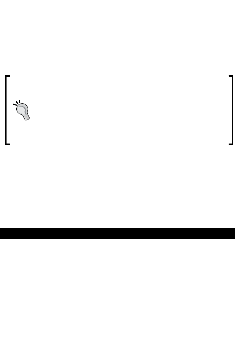
Learning Advanced Python Programming
[ 284 ]
Finally, we called both the move method and the fire method in the same try block.
We use two except statements to catch two dierent excepon classes and handle them
dierently. This is a good reason to dene your own excepon classes—if we had just raised
ValueError excepons, we would have had no way to know where an excepon came
from (other than looking at its argument). Note that the output only shows a MoveError,
even though the call to tank.fire would have produced an error as well (elevaon >
90). Because the move method raised an excepon, the interpreter skipped directly to the
except block, ignoring the rest of the statements in the try block.
Tips for using excepons correctly
The whole idea of using excepons is to make it easier to idenfy and handle
specic runme errors in your programs. You defeat the purpose of using
excepons if you place too many lines of code in a try block, because then it's
hard to tell which statement raised the excepon. It's also a bad idea to have a
bare except: statement that doesn't specify the excepon type that is being
caught. This syntax will catch any type of excepon, including SystemExit and
KeyboardInterrupt excepons, making it hard to terminate a misbehaving
program. It's also considered bad pracce to catch an excepon without properly
handling it, as this pracce can mask errors.
Unit testing
As object-oriented programs get larger and more complicated, debugging can become more
dicult. Unit tesng is a paradigm for verifying and validang soware. A unit is the smallest
part of the program that can be tested, such as an individual funcon or method. Unit tesng
is the pracce of tesng each individual unit, by itself, to ensure that it responds correctly.
Python has a package in the standard library called unittest to help you implement unit
tests for your code.
Time for action – creating unit tests for the Tank class
Let's see how unittest can help us test the Tank class. Enter the following code into a text
le in the same directory as the combatsim package:
import combatsim
import combatsim.exceptions as ex
import unittest
class TestTank(unittest.TestCase):
"""Tests for the combatsim package."""
def setUp(self):
"""Called before EACH test is run."""
# Define parameters for the tank

Chapter 9
[ 285 ]
armor_values = {'front' : 100, 'side' : 50, 'rear' : 25,
'turret' : 75}
main_gun_damage = 50
initial_position = (0.0, 0.0)
# Create a tank object
self.tank = combatsim.tank.Tank(armor_values, main_gun_damage,
initial_position)
def test_get_position(self):
"""Test method get_position"""
position = self.tank.get_position()
self.assertEqual(position, (0.0, 0.0))
def test_move(self):
"""Test method move"""
self.tank.move(0, 1)
position = self.tank.get_position()
self.assertEqual(position, (1, 0))
def test_move_arg1(self):
"""Test method move, arg 1 invalid"""
self.assertRaises(ex.MoveError, self.tank.move, 360, 1)
def test_move_arg2(self):
"""Test method move, arg 2 invalid"""
self.assertRaises(ex.MoveError, self.tank.move, 159, -1)
def test_fire(self):
"""Test method fire. This test is designed to FAIL \
so you can see what a failed test looks like."""
result = self.tank.fire(90,30)
self.assertEqual(result, True)
suite = unittest.TestLoader().loadTestsFromTestCase(TestTank)
unittest.TextTestRunner(verbosity=2).run(suite)
Run the script. You should get output like this:
sage: load("4460_9_11.py")
Test method fire. This test is designed to FAIL so you can see what a
failed test looks like. ... Bang!
FAIL
Test method get_position ... ok
Test method move ... ok
Test method move, arg 1 invalid ... ok

Learning Advanced Python Programming
[ 286 ]
Test method move, arg 2 invalid ... ok
======================================================================
FAIL: Test method fire. This test is designed to FAIL so you can see
what a failed test looks like.
----------------------------------------------------------------------
Traceback (most recent call last):
File "./4460_9_11.py", line 42, in test_fire
self.assertEqual(result, True)
AssertionError: None != True
----------------------------------------------------------------------
Ran 5 tests in 0.006s
FAILED (failures=1)
What just happened?
We started out by imporng the Tank class from combatsim.tank and imporng the
combatsim.exceptions module, just like we did before. We also imported the unittest
module. We created a class called TestTank, which is derived from unittest.TestCase,
for the purpose of tesng the Tank class. Each of the methods of TestTank tests a specic
feature of the Tank class. However, we need to create an instance of the Tank class before
we can start tesng. The method called setUp is called before each test is run. If we had to
do some cleanup (such as closing a le or a database connecon) aer each test, we would
have placed this code in a method called tearDown.
Each test method has a docstring that explains what it does. The docstring is especially
important for test methods because it is used to document the result of the test. The
method test_get_position starts by calling the get_position method of a Tank
instance created by setUp. The next statement uses assertEqual to check that the
posion returned by get_position matches the posion specied in setUp. This is all you
have to do—the rest is handled automacally by unittest. The next method, test_move,
works in a similar way.

Chapter 9
[ 287 ]
The methods test_move_arg1 and test_move_arg2 are somewhat dierent. These
methods intenonally cause the move method to raise an excepon by passing invalid
arguments. The syntax for this is slightly dierent. The assertRaises method takes three
arguments: the name of the excepon that should be raised, the method to be tested, and
any arguments for the method to be tested. In this case, the arguments are two numbers
that represent direcon and distance. I also included a method called test_fire, which
fails because the re method doesn't really do anything. This method was included so that
you can see what happens when a test fails. Noce that the test method docstring is printed
to help you understand which test failed.
The nal two lines of the example are shortcuts to help us create a test suite and run the
tests. The following statement creates a test suite called suite:
suite = unittest.TestLoader().loadTestsFromTestCase(TestTank)
The following line calls the run method of a class called TextTestRunner that comes
with unittest:
unittest.TextTestRunner(verbosity=2).run(suite)
This class provides a simple text interface that runs the tests and prints the results.
This short example demonstrates only the most basic features of unittest. Look at the
unittest documentaon to get an idea of what it can do to help you test larger and more
complex packages. There are more assert methods to handle various types of output from
the methods you are tesng. Here is a list of the assert methods available in Python 2.6;
even more are available in Python 2.7 and higher:
assertTrue(expr) Test fails if expr is False
assertEqual(rst, second) Test fails if first is not equal to second
assertNotEqual(rst, second) Test fails if first is equal to second
assertAlmostEqual(rst, second,
[,places])
Test fails if the dierence between first and second is
greater than places decimal places (default 7)
assertNotAlmostEqual(rst,
second[,places])
Test fails if the dierence between first and second is
smaller than places decimal places (default 7)
assertRaises(excepon, callable
[,args])
Test fails unless exception is raised by callable
(with oponal args passed to callable)
assertFalse(expr) Test fails if expr is True

Learning Advanced Python Programming
[ 288 ]
Strategies for unit testing
Dening unit tests requires careful thought and a fair amount of judgement. It's impossible,
or at least highly impraccal, to test every possible execuon path in most programs. Before
wring tests, the developer should think about the intended use of the code and refer back
to the requirements that may have been dened before the code was wrien. The following
are some suggesons for unit tests:
Boundary (or edge) cases test how the code performs when one of its parameters
reaches an extreme value
A corner case tests what happens when all of the parameters take on extreme
values
Branch tesng aempts to test all branches of the source code at least once
Excepon tests check to make sure that excepons are raised and handled properly
Run the code with a set of xed inputs to ensure that it reproduces known results
(such as published results)
Randomly generate valid inputs and run the code to see if certain combinaons of
parameters lead to an error
For some types of tests, such as corner cases, the author of the code is the best person to
write the test. On large projects, unit tests are oen wrien by someone other than the
author of the code. The tests are wrien to cover the requirements that were dened for
the soware. This approach has the advantage that the tests may uncover assumpons that
were made by the person who wrote the code.
If you have wrien some code that you would like to have included in the Sage library, you
will have to become familiar with the tesng standards of the Sage project. The Sage project
uses a type of tesng called doctesng to ensure quality. The docstring for each funcon
or module is wrien in a special format that includes a secon with examples. Doctesng
automacally searches for examples in the docstring (hence the name), runs them, and
veries that the results are correct. More informaon about doctesng Sage modules and
the convenons for wring docstrings is available at:
http://www.sagemath.org/doc/developer/doctesting.html
http://www.sagemath.org/doc/developer/conventions.html
Have a go hero – creating some unit tests
Dene two methods to verify that the fire method of the Tank class raises the right
excepon when invalid arguments are passed to the method. Use test_move_arg1 as
an example.

Chapter 9
[ 289 ]
Summary
This chapter introduced you to the principles of object-oriented programming. You have
learned how to create classes in Python, and how to use them to organize your code. We
also touched on some general soware engineering principles, including the concept of unit
tesng. Specically, we:
Dened classes to represent an armoured ghng vehicle
Used inheritance to represent other types of military vehicles
Organized the class denions into modules
Created a package to contain our modules
Learned how to handle excepons
Dened our own excepons specic to the Vehicle and Tank classes
Created unit tests to make sure our classes are working correctly
Now, we'll move on to some advanced techniques to help you get the most out of Sage.
10
Where to go from here
The previous chapters have introduced you to many aspects of Sage. This chapter contains a
collecon of topics that you may nd useful aer you have become familiar with the basics
of Sage. Specically, we will learn how to:
Export equaons as PNG and PDF les
Export vector graphics and typeset mathemacal expressions for inclusion
in LaTeX documents
Use LaTeX to document Sage worksheets
Speed up collision detecon using NumPy vector operaons and Cython
Create a Python script that uses Sage funconality
Create interacve graphical examples in the notebook interface
Let's get started.
Typesetting equations with LaTeX
Sage makes it easy to document and publish mathemacal results with a document mark-up
language called LaTeX. The TeX typeseng system is used to process LaTeX les to create
documents, in much the same way that web browsers parse HTML documents to create web
pages. A plain text le containing LaTeX markup is passed to the TeX processor. The processor
parses the source le, includes graphics from other les, and produces a vector graphics le
in a format such as DVI (Device Independent), Postscript, or PDF. Other types of documents
can also be created. Many publishers of mathemacal and scienc books and journals
encourage authors to submit their work as LaTeX les, and some journals require authors to
use it. Both TeX and LaTeX are available under open-source licenses. LaTeX requires an enre
book of its own; this secon will only give you the bare minimum of informaon you need to
use LaTeX with Sage. Sage does not include LaTeX, so we will start by installing LaTeX.

Where to go from here
[ 292 ]
Installing LaTeX
In order for the following examples to run, you need to have LaTeX installed on your system.
If you are building Sage from source, it is recommended that you install LaTeX before building
Sage. For UNIX operang systems like Solaris and OpenSolaris, and UNIX-like systems such as
Linux, install the TeX Live distribuon. If it is not available through your distribuon's package
manager, it can be downloaded directly from http://www.tug.org/texlive/. For OS X,
install MacTeX, which is based on TeX Live. MacTex can be found at http://www.tug.org/
mactex/.
You can install TeX on Windows, but Sage will not be able to access it because Sage runs
in a Linux virtual machine. You will have to install a Linux version of TeX within the virtual
machine. If you simply want to run TeX on Windows, try MiKTeX (http://www.miktex.
org/). proTeXt (http://www.tug.org/protext/) is another distribuon for Windows
that is based on MiKTeX and includes some addional tools.
First, let's verify that the basic tools are installed. The following commands can be entered
on the command line, or in an input cell in a worksheet. The results will vary, depending on
which operang system you are using. On OS X, you will see:
sage: print latex.engine()
latex
sage: print sage.misc.viewer.viewer()
sage-open
sage: print sage.misc.viewer.pdf_viewer()
sage-native-execute sage-open
sage: print sage.misc.viewer.dvi_viewer()
sage-native-execute sage-open
The rst line shows that an external LaTeX processor is available, and will be used as the
engine for processing LaTeX. The next three lines show that sage-open will be used to view
both PDF and DVI les. This means that the default applicaons for OS X will be used to open
PDF and DVI les. On Ubuntu Linux (or Windows, since Sage runs in a Linux virtual machine),
you will see:
sage: print latex.engine()
latex
sage: print sage.misc.viewer.viewer()
xdg-open
sage: print sage.misc.viewer.pdf_viewer()
sage-native-execute xdg-open
sage: print sage.misc.viewer.dvi_viewer()
sage-native-execute xdg-open

Chapter 10
[ 293 ]
OpenSolaris:
sage: print latex.engine()
latex
sage: print sage.misc.viewer.viewer()
xdg-open
sage: print sage.misc.viewer.pdf_viewer()
sage-native-execute xdg-open
sage: print sage.misc.viewer.dvi_viewer()
sage-native-execute xdg-open
sage: print sage.misc.viewer.pdf_viewer()
sage-native-execute xdg-open
If you have set the SAGE_BROWSER environment variable to force Sage to use
a parcular web browser, you might have trouble viewing PDF or DVI les in an
external viewer. If this occurs, unset SAGE_BROWSER, and change the default
web browser for your operang system so that Sage will use the correct browser.
Time for action – PDF output from the notebook interface
Enter the following code into an input cell in a worksheet, and evaluate the cell.
var('n,x,t')
J_n(n,x) = 1/pi*integral(cos(n*t-x*sin(t)), t)
J_n
show(J_n)
view(J_n)
view(J_n, mode='display'))
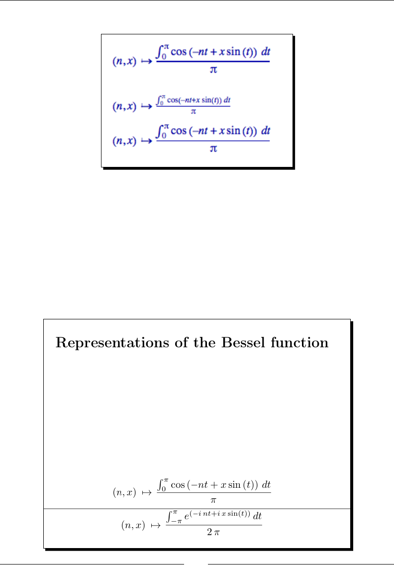
Where to go from here
[ 294 ]
You should see the following results in your worksheet:
Let's say you want to generate a PDF le. Enter the following code aer evaluang the code
from the rst example:
restore('i'))
J_n_2(n, x) = 1 / (2 * pi) * integral(exp(-i * (n * t - x * sin(t))),
t, -pi, pi)
view([J_n, J_n_2], title='Representations of the Bessel function',,
sep='\hrule', viewer='pdf', mode='display')
You will not see any output in the worksheet. Instead, the external viewer should open a
new window with a PDF le that contains the following content:
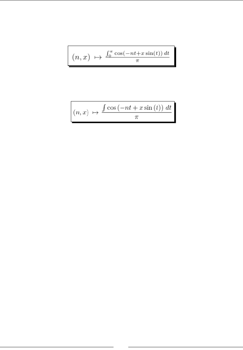
Chapter 10
[ 295 ]
If you only want to output a single equaon as a PDF le, rather than an enre page, try this:
view(J_n, viewer='pdf', tightpage=True, mode='display')
The results should look like this:
Now, try this:
sage.misc.latex.png(J_n, 'J_n.png')
You should see this:
What just happened?
In the rst example, we dened a funcon J_n that represents a Bessel funcon of the rst
kind. Bessel funcons are a type of "special funcon" that are used to represent soluons to
certain types of paral dierenal equaons. You don't need to know any more than that to
understand this example, but you can nd more informaon at http://en.wikipedia.
org/wiki/Bessel_function.
We used the familiar show funcon to display the Bessel funcon, and we demonstrated
how to use the view funcon. view returns a LaTeX representaon of its argument. When
called from the notebook interface, the LaTeX mark-up is automacally parsed by jsMath,
which produces an HTML expression that your browser can display. jsMath is a collecon
of JavaScript programs that display mathemacal content on web pages. It is installed
on the server side, so the user doesn't need to install any soware to view mathemacal
expressions. However, mathemacal expressions will look much beer if the user downloads
a set of TeX fonts.
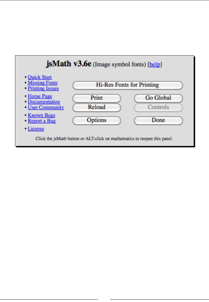
Where to go from here
[ 296 ]
You may have noced the lile jsMath buon on the lower right-hand corner of every Sage
worksheet. When you click the buon, you get a control panel that allows you to set various
opons. Click the buon labelled Hi-Res Fonts for Prinng to download the TeX fonts (if the
buon is greyed out, you already have the fonts). You can nd out more about jsMath and
download the TeX fonts directly at:
http://www.math.union.edu/~dpvc/jsMath/
The output from show is somewhat larger than the output produced by view. The reason is
that LaTeX has two modes for displaying mathemacs: inline and display. Inline mode is used
when you want to put mathemacal symbols on the same line as text, and display mode is
used when you want to display an expression on a line by itself. By default, view uses inline
mode, but we can change that with the mode keyword. When we used the mode keyword
to set the mode to 'display', the output from view was equivalent to the output from
show.
The next part of the example showed how to generate a PDF le containing mathemacal
expressions. We dened another callable symbolic expression called J_n_2, which is an
alternave representaon of a Bessel funcon. Note that we started the example with the
line restore('i'). By default, Sage denes the symbol i as the square root of negave
one, which is how we intend to use it in this example. However, i is frequently used as a
counng variable in for loops. We used the restore funcon to restore the symbol to its
default value, to ensure that the code runs correctly even if i has already been used as a
counng variable in a previous calculaon.

Chapter 10
[ 297 ]
When view receives the keyword argument viewer='pdf', the LaTeX output is used to
create an external PDF le instead of being passed to jsMath. This part of the example also
showed how to typeset mulple expressions in the same PDF document. We created a list
containing both equaons, and used this list as the rst argument to view. When view
receives a list of objects for output to a PDF le, it typesets each one on its own line. The
sep keyword argument species what kind of separaon should be used between the
expressions. In this case, the LaTeX command \hrule creates a horizontal line. Somemes,
we don't want to generate a whole page of output for a single equaon. The third part of the
example shows how the keyword argument tightpage=True shrinks the page to t ghtly
around a single typeset expression.
In the fourth part of the example, we used the png funcon to create a bitmap image
of a mathemacal expression. Bitmaps are not the best way to represent mathemacal
expressions, but somemes they might be the only opon. The png funcon uses the system
TeX installaon to create a DVI le, and then uses an external program called dvipng to
convert it to a PNG bitmap. This will only work if an external installaon of LaTeX is present.
The view function in the interactive shell
You can also use the view funcon on the Sage command line. However, you will need to
have a LaTeX distribuon installed on your system in order to see the output.
LaTeX mark-up in the notebook interface
The previous example produced some nice output, but it was not very exible. What if we
are wring an enre paper or book with LaTeX, and we want to integrate equaons from
Sage into our work? Let's see what else we can do with LaTeX.
Time for action – working with LaTeX markup in the
notebook interface
Enter the following into an input cell in the worksheet:
var('n, x, t')
J_n(n, x) = 1 / pi * integral(cos(n * t - x * sin(t)), t, 0, pi)
latex(J_n)
You will get a string of LaTeX mark-up that represents the object J_n:
\left( n, x \right) \ {\mapsto} \ \frac{\int_{0}^{\pi} \cos\left(-n t + x
\sin\left(t\right)\right)\,{d t}}{\pi}
You can paste this text directly into an exisng LaTeX document. This funcon will also work
on the Sage command line.
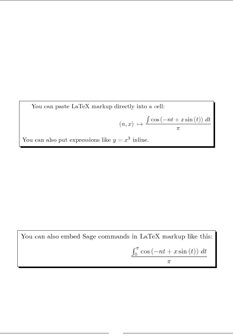
Where to go from here
[ 298 ]
You can also use the notebook interface to evaluate LaTeX expressions. Enter this into an
input cell (you can copy and paste the markup for the mathemacal expression from the
previous example):
%latex
You can paste LaTeX markup directly into a cell:
\[
\left( n, x \right) \ {\mapsto} \ \frac{\int \cos\left(-n t + x \sin\
left(t\right)\right)\,{d t}}{\pi}
\]
You can also put expressions like \(y=x^3\) inline.
The result should be:
Another neat trick is that we can actually embed Sage commands into LaTeX mark up.
Enter the following code into another input cell:
%latex
You can also embed Sage commands in LaTeX markup like this:
\[
\sage{latex(J_n(n,x))}
\]
The result should be:
We can also use LaTeX to typeset mathemacal expressions in text cells in the notebook. Use
shi-click to insert a new text cell, and enter the following text:
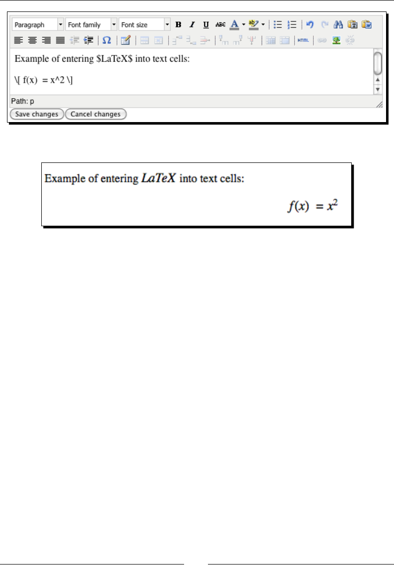
Chapter 10
[ 299 ]
When you save the text, the cell should look like this:
What just happened?
Every Sage object is required to provide a LaTeX representaon of itself. In the previous
examples, we saw how to use the view funcon to generate LaTeX and automacally
process it to create graphics. In this example, we used the latex funcon to return a string
of LaTeX commands that represent a mathemacal expression. We then created a new cell in
the worksheet and entered %latex in the rst line. This directs Sage to evaluate the rest of
the cell as a LaTeX expression. We pasted in the output from the latex funcon, adding \[
before the markup and \] aer. The backslash with square brackets tells the LaTeX processor
that the enclosed commands should be processed in "math mode." Square brackets cause
the expression to be rendered in display mode, while parenthesis are used to indicate inline
mode. This example uses both modes to illustrate the dierences. You will somemes see
two dollar signs $$ used to indicate math display mode, and a single dollar sign $ used to
indicate inline mode. Using dollar signs is discouraged, since it can cause problems with
certain LaTeX packages. While you wouldn't want to typeset a whole document in a Sage
notebook cell, the ability to process LaTeX mark-up is very useful for previewing snippets of
LaTeX to make sure it will display correctly.

Where to go from here
[ 300 ]
The next block of code shows how to embed a Sage command into LaTeX mark-up. The
LaTeX command \sage{sage_command} tells the TeX processor to run sage_command
using Sage, insert the results into the LaTeX mark-up, and connue processing. In this case,
we simply used the latex funcon to return the LaTeX representaon of a funcon. This
is handy, because your LaTeX output will automacally incorporate any changes you make
in your mathemacal expressions. We can take this a step farther, and use the \sage
command in LaTeX mark-up outside of Sage. This requires some extra conguraon of your
TeX distribuon; more details can be found at:
http://www.sagemath.org/doc/tutorial/sagetex.html
Time for action – putting it all together
Let's produce a simple document with LaTeX that incorporates typeset equaons and graphics.
This is a suitable starng point for a report, journal arcle, or homework assignment. First, let's
make a plot of the Bessel funcon of the rst kind for three values of n.
from matplotlib import pyplot as plt
import numpy
def J_n_numerical(n, x):
integrand(n1, x1, t) = cos(n1 * t - x1 * sin(t))
J_n = numpy.zeros(len(x))
for j in range(len(x)):
J_n[j] = 1 / pi.n() * integrand(n1=n, x1=x[j]).nintegrate(t,
0, pi)[0]
return J_n
n_values = [0, 1, 2]
x = numpy.arange(0.0, 10.0, 0.1)
plt.figure()
for n in n_values:
plt.plot(x, J_n_numerical(n, x), label='n=' + str(n))
plt.xlabel('x')
plt.ylabel('J(x)')
plt.legend(loc='upper right')
plt.savefig('J_n.pdf')
plt.close()
The plot will be saved as a PDF le in the SAGE_TEMP directory, so you won't see the plot
in your browser. Instead, you will see a link to the le. Click this link to open the le in a PDF
viewer, and save a copy in a convenient locaon. Now, create a plain text le and save it with
a .tex extension in the same directory as the PDF plot. Enter the following LaTeX mark-up in
the text le:

Chapter 10
[ 301 ]
\documentclass{report}
\usepackage{graphicx}
\begin{document}
\title{A Simple \LaTeX{} Document}
\author{Your Name}
\maketitle
\begin{abstract}
The abstract text goes here.
\end{abstract}
\section{Introduction}
Write your introduction here.
\section{Mathematics}
Some text...
\subsection{Subsection Heading Here}
Equations...
\begin{equation}
\label{simple_equation}
\left( n, x \right) \ {\mapsto} \ \frac{\int_{0}^{\pi} \cos\
left(-n t + x \sin\left(t\right)\right)\,{d t}}{\pi}
\end{equation}
\subsection{Subsection Heading Here}
Graphics...
\begin{figure}
\centering
\includegraphics[width=3.0in]{J_n.pdf}
\caption{Bessel function of the first kind}
\end{figure}
\section{Conclusion}
Write your conclusion here.
\end{document}
The exact method you will use to process the LaTeX document depends on which operang
system and TeX distribuon you are using. On Linux or OS X, you can use the command line.
In a terminal window, change to the directory where you saved the LaTeX source le and PDF
le. On the command line, enter:
pdflatex Bessel_functions.tex
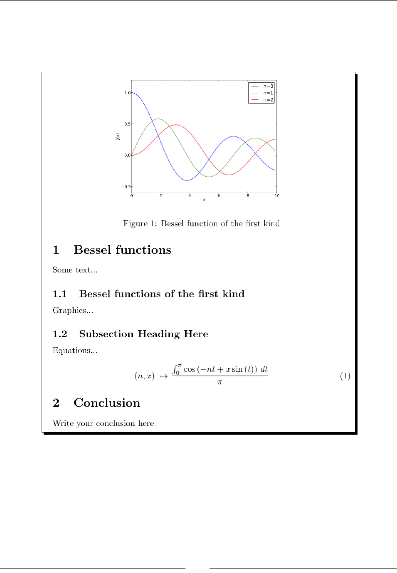
Where to go from here
[ 302 ]
Your TeX distribuon may include other applicaons that eliminate the need to use the
command line. You will get a bunch of text output in the terminal that can be safely ignored
as long as no errors are generated. A new PDF le should be created in the same directory.
The PDF le should look like this:

Chapter 10
[ 303 ]
What just happened?
This example used informaon from several previous chapters. We'll start by reviewing how
we ploed the Bessel funcon. Because the integral used to dene the Bessel funcon does
not have an analycal soluon, we had to use numerical integraon. We used matplotlib for
plong because it is beer than the built-in plot funcon for numerical data, and gives
us the opon to save the plot in various le formats. We dened a funcon called J_n_
numerical that accepts an array of x values and returns an array of values of the Bessel
funcon. Within this funcon, a NumPy array is created using the zeros funcon, and a
for loop is used to iterate over the x values. The nintegrate method is used for numerical
integraon. The resulng array of funcon values was ploed using the plot command
from Matplotlib, and we added axes labels and a legend. Finally, we saved the plot as a PDF
le. If you are comfortable with LaTeX, an alternave procedure is to save the data in a le so
that it can be read and ploed with a LaTeX package called PGFPlots (http://pgfplots.
sourceforge.net/).
We then created a fairly minimal LaTeX source le. The source le begins with the
\documentclass{article} command, which sets the document class to article.
There are many other classes, but the basic opons are article, report, and book.
This command is required in all LaTeX source les. Your document is also required to
include a pair of commands: \begin{document} at the beginning and \end{document}
at the end. The other commands are oponal. We also chose to use the command
\usepackage{graphicx}, that is similar in concept to the import statement in Python,
to use the package called graphicx. We will use this package to import the graphics we
saved with Sage.
We copied the LaTeX mark-up that represents our equaon from the Sage worksheet, and
pasted it between the commands \begin{equation} and \end{equation}. We then
used the commands \begin{figure} and \end{figure} to dene a gure, and used
the \includegraphics[width=3.0in]{J_n.pdf} command to include the PDF le
we saved. If the PDF le isn't in the same directory as the LaTeX source le, then you must
include the path to the le. The \caption{} command adds a capon to the gure.
This secon is only a brief introducon to LaTeX, which requires a book or two of its own.
This example demonstrates how LaTeX can produce a beauful document with a minimum
of eort. It will be worth your me to learn more about this powerful tool. A list of LaTeX
resources can be found at http://www.latex-project.org/guides/

Where to go from here
[ 304 ]
Have a go hero – Bessel functions of the second kind
Using the previous example as a foundaon, add a secon that documents Bessel funcons
of the second kind. Dene a symbolic funcon, get its LaTeX representaon, and paste it into
a new secon of the LaTeX document. Then, dene a numerical funcon that can be used for
plong and plot the graph using Matplotlib. Include the plot in your LaTeX document. You
may nd this Wikipedia arcle useful as a reference, and to make sure your plot is correct:
http://en.wikipedia.org/wiki/Bessel_function
Speeding up execution
In this secon, we're going to learn how to make Sage and Python code run faster. This
secon has been le unl the last chapter because opmizing the speed of your code is
only important in a few specic circumstances. This philosophy is summarized in a famous
quote from Donald Knuth, author of the TeX typeseng system: "We should forget about
small eciencies, say about 97% of the me: premature opmizaon is the root of all evil."
If you consider the amount of me that you spend on a programming project, from start
to nish, only a small poron is usually spent waing for the program to run. Most of the
me is spent wring the program, tesng it, xing bugs, and going back into the code a year
later and trying to gure out why you wrote it a certain way. To truly save me, the most
important thing you can do is to write neat, legible code, and document it well. However, in
mathemacal and scienc compung, there are circumstances where it is helpful to reduce
a program's runme. For example, climate simulaons and some number theory calculaons
can consume days of me on massively parallel clusters. Tesng and debugging also go much
faster when a program runs in seconds instead of minutes. Keep these general principles in
mind as we go through the following series of examples.
Time for action – detecting collisions between spheres
We will use collision detecon as an example to demonstrate some common opmizaon
techniques. Detecng collisions is an important part of Monte Carlo simulaons, that are
used in physics and chemistry to simulate the moon of molecules and parcles. Collision
detecon is also used in ight simulators and video games. It is easy to detect collisions
between spheres, so most collision detecon algorithms dene a "bounding sphere" around
each complex object, and check for intersecons between the bounding spheres. If the
bounding spheres intersect, then more computaonally expensive calculaons are used to
determine whether or not the objects themselves actually overlap.

Chapter 10
[ 305 ]
This example is designed to be run from the notebook interface. First, let's create a box full
of randomly placed spheres. The number of spheres is set so that the example runs in a
reasonable length of me on a 2009 MacBook Pro. You may need to adjust the number of
spheres to get reasonable runmes on your parcular system. Enter the following code into
an input cell in a worksheet:
dimension = 20
num_particles = 500
radius = 1.0
rng = RealDistribution('uniform', [0,dimension], seed=1)
x = [rng.get_random_element() for i in range(num_particles)]
y = [rng.get_random_element() for i in range(num_particles)]
z = [rng.get_random_element() for i in range(num_particles)]
We can visualize the parcles in three dimensions using the following code. Rendering
500 spheres in 3D takes a while, so you may not want to run this part of the example
on an older system.
grobs = []
for i in range(num_particles):
grobs.append( sphere((x[i], y[i], z[i]), size=radius,
color='red'))
show(sum(grobs))
Finally, check for collisions by running the following code from a worksheet cell:
%time
import numpy
collisions_1 = numpy.zeros(num_particles, dtype=numpy.bool)
for i in range(num_particles):
for j in range(0,i):
r = sqrt((x[i] - x[j])**2 + (y[i] - y[j])**2 + (z[i] -
z[j])**2)
if r < 2*radius:
collisions_1[i] = True
for j in range(i+1,num_particles):
r = sqrt((x[i] - x[j])**2 + (y[i] - y[j])**2 + (z[i] -
z[j])**2)
if r < 2*radius:
collisions_1[i] = True
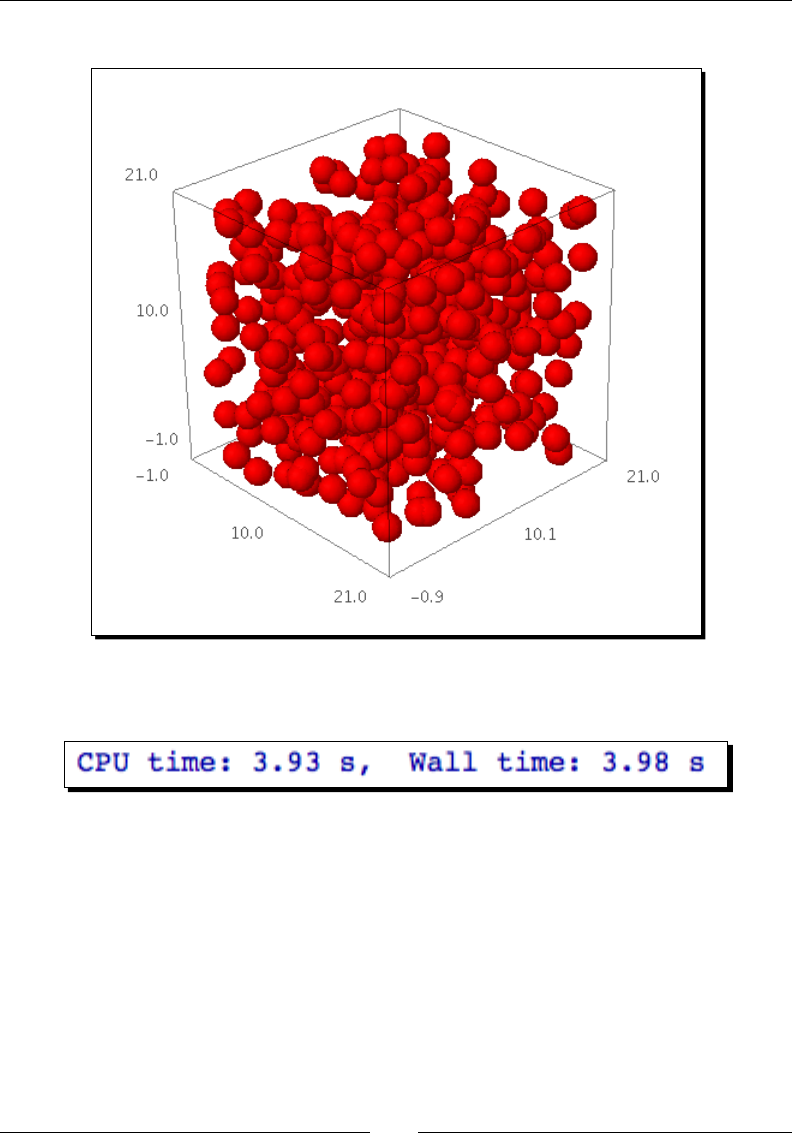
Where to go from here
[ 306 ]
The spheres look like this:
The collision detecon itself doesn't give any output; it stores the results in an array of
Boolean values. The execuon me is printed:
As we opmize the code in the following examples, we will check to make sure the results
match the results from this example.
What just happened?
We started out by using list comprehensions and the RealDistribution class (introduced
in Chapter 8) to obtain three lists of x, y, and z coordinates that represent the centres of the
spheres. 500 spheres were randomly distributed throughout a cubic region of space. We
then used the sphere funcon to obtain a 3D graphical representaon of each sphere, and
displayed them together. The sphere funcon accepts the following arguments:
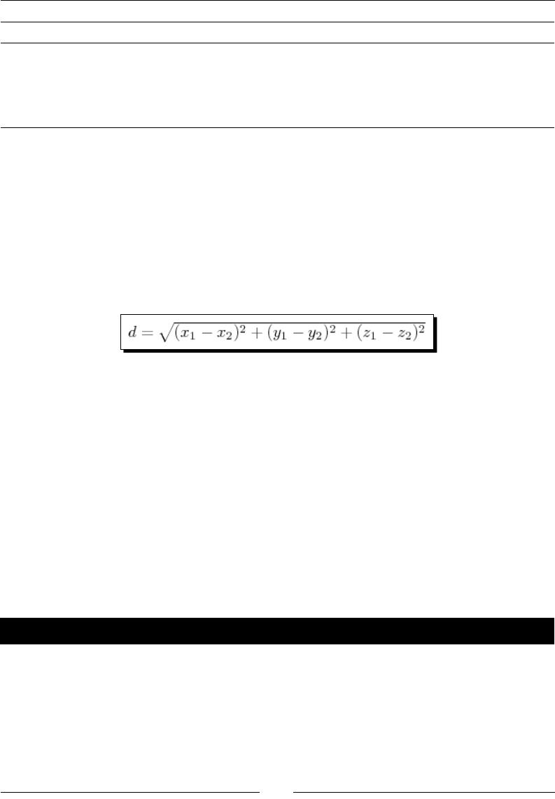
Chapter 10
[ 307 ]
Keyword Default value Descripon
center (0,0,0) Posion of the centre of the sphere (x, y, z)
radius 1 Radius of the sphere
color blue Color of the sphere
opacity 1 Floang point number between 0 (transparent) and 1 (opaque)
The input cell that contains the actual collision detecon algorithm starts with %time on the
rst line. This tells Sage to me the execuon of the code in the cell. We placed the code to
create and plot the spheres in separate cells because we only want to measure the runme
of the collision detecon. We then created a NumPy array of Boolean values, inialized to
False, using the zeros funcon (we would have used ones if we wanted the default values
to be True). Later on, you'll see why we used a NumPy array for this purpose instead of a list.
The actual collision detecon algorithm is simple. The outer for loop iterates over each
sphere in the list. The formula:
is used to compute the distance between the centre of sphere i and each of the other
spheres. If the centre-centre distance is less than twice the radius, then the spheres intersect
and the value of collisions_1[i] is set to True. This approach is conceptually simple
and computaonally inecient. If there are N parcles in the list, the collision detecon
must be performed N2 mes. The performance of the algorithm scales poorly as the number
of parcles increases. Fortunately, there is a lot we can do to improve this!
The Sage notebook interface reports two runmes for the code: CPU me and wall me. The
CPU me is the amount of me that code actually ran on the processor, while the wall me
is simply the total me required for the code to run (as it would be measured by a clock on
the wall). For this example, the two are almost idencal. If the CPU had to wait on another
operaon to nish, such as accessing a le on disk, the wall me could be considerably
longer than the CPU me.
Time for action – detecting collisions: command-line version
This example repeats the previous example using the command-line interface. Create a script
in a plain-text editor and enter the following code:
dimension = 20
num_particles = 500
radius = 1.0
rng = RealDistribution('uniform', [0,dimension], seed=1)

Where to go from here
[ 308 ]
x = [rng.get_random_element() for i in range(num_particles)]
y = [rng.get_random_element() for i in range(num_particles)]
z = [rng.get_random_element() for i in range(num_particles)]
import numpy
collisions_1 = numpy.zeros(num_particles, dtype=numpy.bool)
start_time = walltime()
for i in range(num_particles):
for j in range(0,i):
r = sqrt((x[i] - x[j])**2 + (y[i] - y[j])**2 + (z[i] -
z[j])**2)
if r < 2*radius:
collisions_1[i] = True
for j in range(i+1,num_particles):
r = sqrt((x[i] - x[j])**2 + (y[i] - y[j])**2 + (z[i] -
z[j])**2)
if r < 2*radius:
collisions_1[i] = True
print(walltime(start_time))
Save it with a .sage extension, and use the load command to run it in the interacve shell.
The runme will be displayed when the script is nished:
sage: load collision_detection_1_Sage.sage
4.08416008949
What just happened?
This example is very similar to the previous example. The major dierence is the way in
which the run me is measured. The funcon wall_time(t) returns the length of me
that has elapsed since me t. We called wall_time at the beginning of the block of code
to determine the start me. We then called wall_time again at the end of the block,
passing the start me as an argument, to get the amount of me required to run the block
of code. This process can be used to adapt the following notebook examples so they can
be run on the command line. The funcon cputime can be used to obtain the CPU me in
the same way. The cputime funcon has one addional oponal keyword argument called
subprocesses, which is False by default. If set to True, cputime will also measure the
CPU me used by any subprocesses that are spawned by Sage (Sage creates subprocesses to
run tools such as Gap or Singular).

Chapter 10
[ 309 ]
Tips for measuring runtimes
Measuring run mes can be tricky. Here are a few ps to make your measurements as
accurate as possible:
1. Make sure nothing else is using the CPU while you run the code. This may seem
obvious, but you need to be especially careful if your code is running for a long
period of me. Make sure a scheduled process, like a virus scan, doesn't start in the
middle of the run. On OS X or Linux, use the top command (in a terminal) to see
informaon about running processes. In Solaris or OpenSolaris, use prstat. For
Windows, use the Task Manager.
2. Disk access is much slower than calculaons on the CPU. Avoid reading or wring
les, and don't use so much memory that your program has to swap to disk (unless,
of course, you're trying to benchmark disk access).
3. Disable wring to the screen when benchmarking—this is also slow.
4. Run the code several mes and average the results. You might have to discard the
ming value for the rst run, which may be much slower because it has to compile
code, or load libraries or data into memory.
5. Opmizaon can be very specic to a parcular language, operang system, and
type of CPU. Your results may vary!
Optimizing our algorithm
The algorithm you use to solve a problem has a major impact on the me required to solve
the problem, so improving the algorithm is one of the things you should consider when
you need to reduce the run me. However, opmizing an algorithm may require a lot of
your me, and the resulng code may be much harder to debug (which is why premature
opmizaon is considered to be the root of all evil). Before you start opmizing, try to take
advantage of the many opmized rounes that are built into Sage. Also, look at journal
arcles, books, and open-source projects to see if an opmized algorithm already exists.
Time for action – faster collision detection
In this example, we are going to apply a couple of simple tricks and see how they impact
the runme. Assuming you've already dened the spheres in the previous example, you can
enter and run the following code in a worksheet cell:
%time
import numpy
collisions_2 = numpy.zeros(num_particles, dtype=numpy.bool)
r_min = 4*radius**2
for i in range(num_particles):
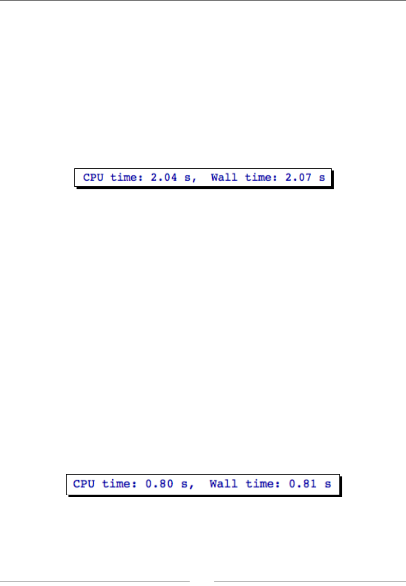
Where to go from here
[ 310 ]
for j in range(0,i):
r_squared = (x[i] - x[j])**2 + (y[i] - y[j])**2 + (z[i] -
z[j])**2
if r_squared < r_min:
collisions_2[i] = True
for j in range(i+1,num_particles):
r_squared = (x[i] - x[j])**2 + (y[i] - y[j])**2 + (z[i] -
z[j])**2
if r_squared < r_min:
collisions_2[i] = True
The code will print the runme:
It's about twice as fast! Not bad for two minor changes. Now, try this:
%time
import numpy
collisions_3 = numpy.zeros(num_particles, dtype=numpy.bool)
r_min = 4*radius**2
for i in range(num_particles):
for j in range(0,i):
r_squared = (x[i] - x[j])*(x[i] - x[j]) + \
(y[i] - y[j])*(y[i] - y[j]) + (z[i] - z[j])*(z[i] -z[j])
if r_squared < r_min:
collisions_3[i] = True
for j in range(i+1,num_particles):
r_squared = (x[i] - x[j])*(x[i] - x[j]) + \
(y[i] - y[j])*(y[i] - y[j]) + (z[i] - z[j])*(z[i] - z[j])
if r_squared < r_min:
collisions_3[i] = True
Let's check to make sure we are sll geng the right answers:
print((collisions_1 == collisions_2).all())
print((collisions_2 == collisions_3).all())
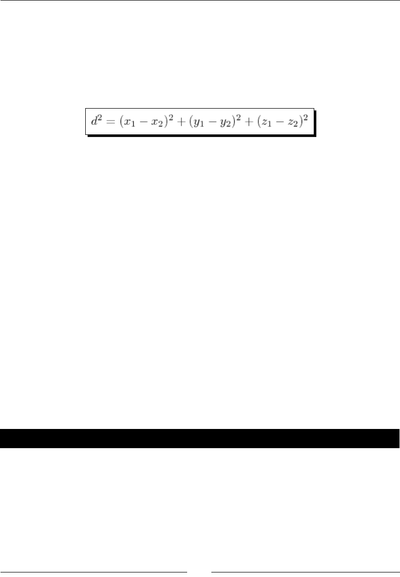
Chapter 10
[ 311 ]
The result should be True for both lines.
What just happened?
We made two changes in this example that signicantly reduced the runme. First, we
realized that we don't actually have to calculate the square root of the distance between
the centres of the spheres. We can compare the squared distance to (2r)2:
The square root is a computaonally intensive operaon. Eliminang the square root cut
the execuon me in half, which is a prey good return for such a simple change. We
also moved the calculaon of the squared radius out of the loop so that it only has to be
computed once. In the second part of the example, we used mulplicaon instead of the
exponenal operator to perform the squaring operaon. This change again decreased the
runme by more than 50%.
The nal step of this example was to compare the results from these two runs to the results
from the rst example. Using NumPy arrays to store the results makes the comparison a
lot easier. We can test for equality between two arrays with the == operator. The result is a
NumPy array of Boolean values that are True where the two arrays match and False where
they do not. If the two arrays are idencal, the result should be True everywhere. Since the
result is an array, we used the all method, which returns True if all the values of the array
are True.
Optimizing with NumPy
So far, we have been using NumPy because of its useful features, but it can also help us
speed up our code. Using NumPy, you can perform operaons on arrays without using
Python for loops. NumPy operaons are much faster than Python loops, because the
crical parts of NumPy are wrien in C and opmized for speed.
Time for action – using NumPy
Enter the following code in a new cell in the worksheet to dene the spheres using NumPy:
import numpy
dimension = 20
num_particles = 500
radius = 1.0
rng = numpy.random.mtrand.RandomState(seed=[1])
x_np = rng.uniform(0, dimension, num_particles)
Where to go from here
[ 312 ]
y_np = rng.uniform(0, dimension, num_particles)
z_np = rng.uniform(0, dimension, num_particles)
Now, enter the following code in another cell to detect collisions:
%time
collisions_4 = numpy.zeros(num_particles, dtype=numpy.bool)
r_min = numpy.float64(4*radius**2)
for i in range(num_particles):
for j in range(0,i):
r_squared = (x_np[i] - x_np[j])*(x_np[i] - x_np[j]) \
+ (y_np[i] - y_np[j])*(y_np[i] - y_np[j]) \
+ (z_np[i] - z_np[j])*(z_np[i] - z_np[j])
if r_squared < r_min:
collisions_4[i] = True
for j in range(i+1,num_particles):
r_squared = (x_np[i] - x_np[j])*(x_np[i] - x_np[j]) \
+ (y_np[i] - y_np[j])*(y_np[i] - y_np[j]) \
+ (z_np[i] - z_np[j])*(z_np[i] - z_np[j])
if r_squared < r_min:
collisions_4[i] = True
The notebook prints the runme:
In another cell, try using NumPy this way:
%time
collisions_5 = numpy.zeros(num_particles, dtype=numpy.bool)
r_min = numpy.float64(4*radius**2)
for i in range(num_particles):
if i>0:
d2 = numpy.power((x_np[i]-x_np[0:i]),2) \
+ numpy.power((y_np[i]-y_np[0:i]),2) \
+ numpy.power((z_np[i] - z_np[0:i]),2)
if d2.min() < r_min:
collisions_5[i] = True
if i+1 < num_particles:
d2 = numpy.power((x_np[i]-x_np[i+1:]),2) \
+ numpy.power((y_np[i]-y_np[i+1:]),2) \
+ numpy.power((z_np[i]-z_np[i+1:]),2)
Chapter 10
[ 313 ]
if d2.min() < r_min:
collisions_5[i] = True
The notebook prints the runme:
Finally, let's make sure that both computaons return the same results:
print((collisions_4 == collisions_5).all()
As before, the result should be True for both cases.
What just happened?
We started out by creang spheres using NumPy's random number capabilies. We
created an instance of RandomState and inialized it with a seed so that it would provide
repeatable, pseudo-random numbers. RandomState has methods that return numbers
drawn from various types of random distribuons. In this case, we used the uniform
method to obtain numbers drawn from a uniform distribuon between zero and the
maximum size of the box. The rst two arguments to uniform dene the lower and
upper limits, and the third argument denes the number of random numbers to generate.
The funcon returns a NumPy array containing the random numbers. Dozens of other
distribuons are available; a complete list is available in the NumPy Reference.
In the rst part of the example, replacing Sage funcons and operators with NumPy funcons
actually increased the runme! This example demonstrated that simply replacing Sage
funcons with NumPy funcons doesn't speed up the code. However, this aempt did not
ulize the full power of NumPy. The second part of the example showed how to use NumPy to
opmize execuon speed. The inner for loops were replaced with NumPy vector operaons.
The expression x_np[i]-x_np[0:i] computes the dierence between the single value of
x_np[i] and all the values in the array x_np[0:i], and returns an array. The NumPy funcon
power squares all of these values, and + operator performs element-by-element addion on
the results from each power operaon. In the end, the array d2 held the square of the distance
from parcle i to each of the other parcles. We then used the min method of the array
class to nd the minimum squared distance between sphere centers. If this value is less than
(2r)2, then the spheres overlap.
Many numerical algorithms consist of nested loops. The statements in the
innermost loop are executed more mes than statements in the outer loops, so
you will get the most "bang for your buck" by focusing your opmizaon eorts
on the innermost loop.

Where to go from here
[ 314 ]
More about NumPy
NumPy vector operaons are fast because the NumPy library consists of highly opmized,
compiled code. Instead of spending your me guring how to opmize a mathemacal
operaon, you can take advantage of the hard work that has already been done. One of the
reasons that compiled code is fast is because it ulizes parallel processing. Modern CPUs
(even single-core units) have the ability to execute mulple instrucons in parallel. When
you dene a loop in an interpreted language like Python, the interpreter executes the loop
operaons sequenally. When you compile code that contains a loop, the compiler checks
to see if the loop operaons have to be executed sequenally. If not, the loop is converted
to a dierent form and its instrucons are executed in parallel on the CPU. By using vector
operaons on NumPy arrays, you can take advantage of parallel execuon to speed up
mathemacal operaons.
Just about every common mathemacal operaon is implemented as a funcon or method
in NumPy. Mathemacal operaons such as addion, subtracon, mulplicaon, division,
and exponents are performed element by element. The result is an array with the same
length as the original. In previous chapters, we have already touched on a few, such as the
fast Fourier transform and window funcons. A categorized list of all the NumPy funcons is
available at:
http://www.scipy.org/Numpy_Functions_by_Category
Optimizing with Cython
Cython is a language for wring C extensions for the Python language. The Cython language
is very similar to Python, but supports some addional features that allow it to be compiled
to highly opmized C code. It is very easy to use Cython from Sage.
Time for action – optimizing collision detection with Cython
1. Dene a funcon with Cython:
%cython
import numpy
def cython_collisions(x, y, z, radius):
num_particles = len(x)
collisions = numpy.zeros(num_particles, dtype=numpy.bool)
r_min = numpy.float64(4*radius**2)
for i in range(num_particles):
if i>0:
d2 = numpy.power((x[i]-x[0:i]),2) \
+ numpy.power((y[i]-y[0:i]),2) \
+ numpy.power((z[i] - z[0:i]),2)
Chapter 10
[ 315 ]
if d2.min() < r_min:
collisions[i] = True
if i+1 < num_particles:
d2 = numpy.power((x[i]-x[i+1:]),2) \
+ numpy.power((y[i]-y[i+1:]),2) \
+ numpy.power((z[i]-z[i+1:]),2)
if d2.min() < r_min:
collisions[i] = True
return collisions
When you run this cell, it may take a minute or two to compile for the rst me.
The results will look similar to this:
2. In another cell, enter the following code to create the parcles and call the Cython
funcon:
%time
import numpy
dimension = 20
num_particles = 500
radius = 1.0
rng = numpy.random.mtrand.RandomState(seed=[1])
x_np = rng.uniform(0, dimension, num_particles)
y_np = rng.uniform(0, dimension, num_particles)
z_np = rng.uniform(0, dimension, num_particles)
collisions_6 = cython_collisions(x_np, y_np, z_np, radius)
3. The results should look like this:
4. Verify that the results are correct:
print((collisions_4 == collisions_6).all())
The result should be True.

Where to go from here
[ 316 ]
What just happened?
We created a Cython cell by placing %cython on the rst line. We then dened a funcon
that checks for collisions between hard spheres, using essenally the same code from the
previous example. When we ran the cell, Cython compiled the code into a C extension.
The only visible result of the computaon is two links that appeared in the worksheet.
Clicking the le-hand link will show you the C code that Cython generated. The right-hand
link will take you to an opmizaon report that shows your Cython source code with color
highlighng. Code that has a white or lightly colored background is highly "typed," meaning
that it translates to almost pure C without any calls to the Python API. Code that is more
brightly colored requires more calls to Python, and therefore runs slower. The opmizaon
report for this code shows that there is plenty of room for improvement in the opmizaon.
However, when we ran the code to test the Cython funcon, the execuon was more than
three mes faster than the previous example. We also veried that the results are the same.
This brief demonstraon shows how useful Cython can be for opmizing code, and how
easy it is to use Cython from Sage. You can learn more about the Cython project at http://
cython.org/
Have a go hero – further optimization with Cython
Increase the number of parcles in the example unl it takes several seconds for the Cython
code to run on your computer. Then, connue opmizing the Cython code, following the
instrucons and examples on the Cython website. Use the opmizaon report as a guide to
tell you which parts of the code are closest to pure C.
Calling Sage from Python
You may want to create Python scripts that take advantage of the funconality of Sage,
without having to run Sage itself. You can think of Sage as a giant module that can be
imported into a Python program, which can then be run from the command line. We briey
used this capability in Chapter 9, when we imported some simple mathemacal funcons
from Sage to use in a Python module.
Time for action – calling Sage from a Python script
Sage has advanced numerical integrators that adapt to the rate of change in the funcon
being integrated. Let's say that you want to use one of these integrators to integrate an
analycal funcon. You only want to use the integrator, so you don't want to manually start
Sage and load a script just to access one funcon. We can create a stand-alone Python script
that calls Sage when necessary. Create a new plain text le, enter the following code, and
save it with a .py extension.

Chapter 10
[ 317 ]
#!/usr/bin/env sage -python
from sage.all import *
vars={}
# Define limits of integration
vars['a'] = 0
vars['b'] = 8
sage_eval('None', cmds='f(x)=e^x*cos(x)', locals=vars)
print vars['f']
sage_eval('None', cmds='value, tol = numerical_integral(f,a,b)',
locals=vars)
print(vars['value'])
There are two ways to run this script. One opon is to open a terminal and enter the
following command. If the Sage installaon is on your path, you can simply type:
$ sage –python /path/to/script/4460_10_8.py
in which you specify the full or relave path to the script. If Sage is not on your path, you
will have to either provide the full path to the Sage executable, or change to the top-level
directory of your Sage installaon. For example:
$ $ /Applications/sage_source/sage-4.6.1/sage -python 4460_10_8.py
The result should be:
x |--> e^x*cos(x)
1257.25293971
You can also set up the script so that it can be executed directly. On Solaris, OS X, or Linux,
use the chmod command on the command line:
bash$ chmod u+x 4460_10_8.py
The directory where Sage is installed also has to be in your system PATH variable. For
example, on a UNIX or UNIX-like system:
bash$ echo $PATH
/usr/bin:/bin:/usr/sbin:/sbin:/usr/local/bin:/usr/texbin:/usr/X11/bin
bash$ PATH=$PATH:/Applications/sage
bash$ export PATH
bash$ echo $PATH
/usr/bin:/bin:/usr/sbin:/sbin:/usr/local/bin:/usr/texbin:/usr/X11/bin:/
Applications/sage

Where to go from here
[ 318 ]
Run the script from the command line by typing:
bash$ ./4460_10_8.py
The result should be:
x |--> e^x*cos(x)
1257.25293971
What just happened?
Wring a Python script that uses Sage requires a dierent approach than wring a Sage
script. Our script has to be valid Python, so we can't directly use Sage-specic syntax, like a
mathemacal funcon denion: f(x)=e^x*cos(x). First, we have to use the statement
from sage.all import * to access names from Sage. Then, we have to use the sage_
eval funcon to "wrap" Sage expressions. This funcon accepts four arguments:
Argument Keyword Default Descripon
source A string to be evaluated
local variables locals None A diconary of variables for Sage to use
commands cmds '' A string of commands to be executed before the
source is evaluated
pre-parse source preparse True Disable the Sage pre-parser
We created an empty diconary called vars, and created items a and b to contain integers
that dene the interval of integraon. We then used the funcon call:
sage_eval('None', cmds='f(x)=e^x*cos(x)', locals=vars)
to dene the funcon we want to integrate. Note that the source was set to 'None', and the
funcon denion was passed as a command string. Aer this funcon call, the diconary of
variables contains a new item called f, which holds the Sage funcon. We then performed
the integraon with:
sage_eval('None', cmds='value, tol = numerical_integral(f,a,b)',
locals=vars)
Once again, the integraon funcon call is passed as a command string. Basically, any
expression that involves variable assignment needs to be passed with the cmd keyword.
The source string is only used to evaluate expressions that don't involve assigning values to
variables. When this command string is executed, Sage gets the values of a and b from the
diconary of variables, and computes the integral. Aerwards, you can see that the variables
value and tol have been added to the diconary.

Chapter 10
[ 319 ]
In this example we used the all module to import everything from Sage at once. This may
cause you a lile concern since Sage is huge, and it is considered good pracce to import
only the funcons and classes that you actually need. At this point, Sage is not structured
in such a way that you can import a subset of packages and modules and expect that it will
work correctly. You have to import everything.
If you want to try this example interacvely on the Python command line, run
Sage with the –python opon to get an interacve Python shell. You can then
run each of these expressions on the command line and see the results.
Have a go hero – solving an ODE symbolically from Python
In Chapter 8, we learned how to solve an ordinary dierenal equaon with the desolve
funcon. Repeat that example using a Python script to access Sage funcons to solve the
equaon. You won't be able to view plots from the Python script, so don't try to plot the
soluon.
Introducing Python decorators
We need to take a lile detour here to introduce one of the newer features of the Python
language: the Python decorator. This is not an implementaon of the "decorator" design
paern, although the concepts are similar. We'll need decorators to implement the
interacve graphics that will be introduced in the next secon.
Time for action – introducing the Python decorator
Enter the following code into a cell in a workbook and run it. You can also run this on the
Sage command line, but the HTML formang will not look nice!
def html_table(func):
def display_output(*args):
result = func(*args)
html_string = '<table border=1><tr>'
for item in result:
html_string += '<td>' + str(item) + '</td>'
html_string += '</tr></table>'
html(html_string)
return result
return display_output
Where to go from here
[ 320 ]
@html_table
def square_list(my_list):
for i in range(len(my_list)):
my_list[i] = my_list[i]**2
return my_list
x = square_list([1.0, 2.0, 3.0])
print x
The result should be:
What just happened?
We dened a simple funcon called square_list, that accepts a list as an argument,
squares every item in the list, and returns the squared list. Since you've just been introduced
to NumPy, you should recognize that this is not really a useful funcon in Sage, but it will
serve to illustrate how decorators work. We dened a decorator funcon called html_table
that accepts a funcon as an argument called func. The decorator funcon denes and
returns a new funcon called display_output that accepts the same arguments as func
and returns the same results as func. However, before it returns, display_output creates
and displays an HTML table that shows the values in the list. We use the @ symbol to indicate
that html_table decorates square_list. The syntax:
@decorator_function
def my_function():
pass
is simply a shortcut for:
def my_function():
pass
decorator_function(my_function)
When we call square_list, the call is intercepted and html_table is called with square_
list as its argument. html_table returns an "improved" version of square_list which
is then called with the appropriate arguments. The result is the formaed list that you see in
the output.

Chapter 10
[ 321 ]
This has been only a brief introducon to funcon decorators. Class decorators were
introduced in Python 2.6. If you're going to be wring your own decorators, you will need to
learn more about how to do it correctly. Python decorators are very exible and powerful,
and they give you the power to write convoluted code. The following resources should help
you:
http://docs.python.org/release/2.4/whatsnew/node6.html
http://docs.python.org/release/2.6/whatsnew/2.6.html#pep-3129-class-
decorators
http://wiki.python.org/moin/PythonDecoratorLibrary
Pop quiz – understanding function decorators
What is the output from the following code? Try to gure it out, and then run it to check
your answer.
def decorator(func):
def print_value(*args):
print "Value is:"
result = func(*args)
return result
return print_value
@decorator
def my_function(my_arg):
print my_arg
return my_arg
x = my_function('text')
Have a go hero – improving the decorator
The html_table decorator can only handle a one-dimensional list, but it could easily be
extended to mul-dimensional lists, Sage matrices, or NumPy matrices. Extend the decorator
funcon so that it displays two-dimensional data as an HTML table. Use the starng tag
<tr> and ending tag </tr> to create a new row in the table. For help with HTML tables,
check out:
http://www.w3schools.com/html/html_tables.asp

Where to go from here
[ 322 ]
Have a go hero – the memoize decorator
The opmizaon technique known as "memoizaon" speeds up funcon calls by caching
the results of previous funcon calls and returning a saved value when the funcon is called
again when the same arguments are used. A Python decorator is a good way to add this
ability to exisng Python funcons. Look at the examples in the links below, and implement
a "memoize" decorator that you can use to speed up funcon calls.
http://en.wikipedia.org/wiki/Memoization
http://wiki.python.org/moin/PythonDecoratorLibrary#Memoize
Making interactive graphics
The Sage notebook interface can be used to make interacve examples that are controlled
by simple graphical controls. This feature is comparable to the Manipulate funcon in
Mathemaca. Interacve graphics are especially useful for creang teaching tools to help
students learn new mathemacal concepts. We will make extensive use of the Python
decorators that were introduced in the previous secon.
Time for action – making interactive controls
This example consists of a gallery of all the basic controls that can be used in the Sage
notebook interface. The code is followed by the result from running that code in an input cell.
@interact
def _(t=text_control('Static text goes here')):
pass
@interact
def _(value = slider(vmin=0, vmax=10, step_size=1, default=5,
label='Slide me:', display_value = True)):
print value
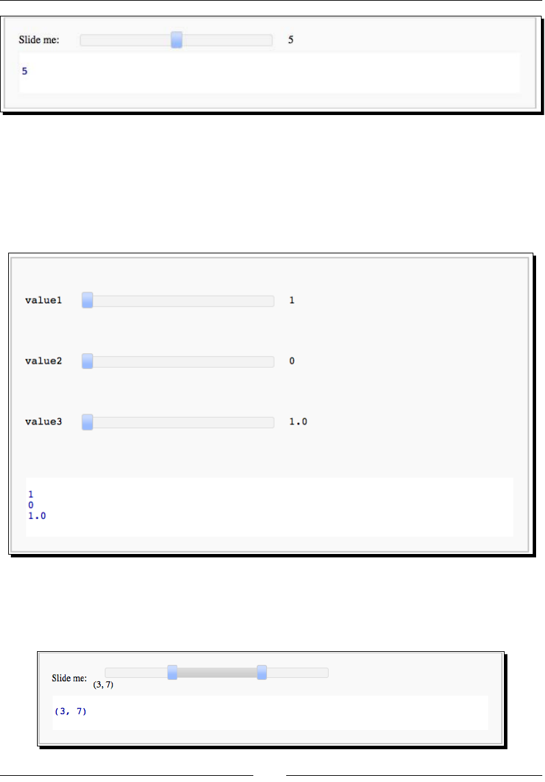
Chapter 10
[ 323 ]
Here is a shorthand way to create the same type of control:
@interact # Shortcuts
def _(value1=(1..10), value2=(0,100,10), value3=(1,10)):
print value1
print value2
print value3
@interact
def _(value = range_slider(0, vmax=10, step_size=1, default=(3,7),
label='Slide me:', display_value = True)):
print value
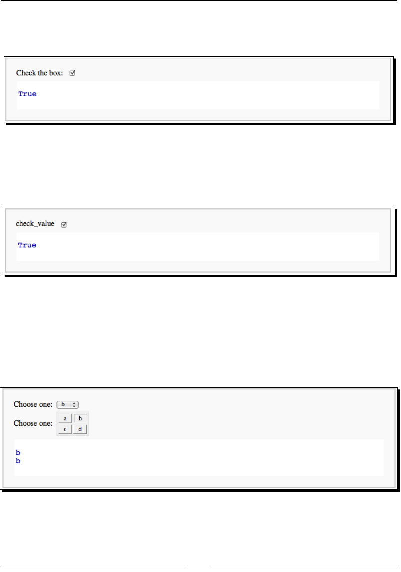
Where to go from here
[ 324 ]
@interact
def _(checked = checkbox(True, "Check the box:")):
print checked
Here is a shorthand way to create the same type of control:
@interact
def _(check_value = True): # Shortcut
print check_value
@interact
def _(value1 = selector(['a','b','c'], label='Choose one:',
default='b'),
value2 = selector(['a','b','c','d'], label='Choose one:',
default='b', nrows=2, ncols=2)):
print value1
print value2
Here is a shorthand way to create the same type of control:
@interact # Shortcuts
def _(value1 = ['a','b','c'], value2=[1,2,3,4,5,6]):
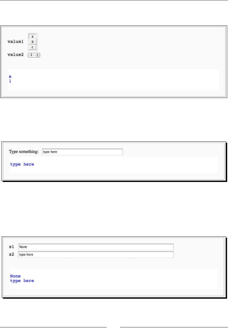
Chapter 10
[ 325 ]
print value1
print value2
@interact
def _(s = input_box(default='type here', label='Type something: ',
type=str, width=40)):
print s
Here is a shorthand way to create the same type of control:
@interact # Shortcut
def _(s1, s2 = 'type here'):
print s1
print s2
@interact
def _(m = input_grid(nrows=2, ncols=2, default=0,
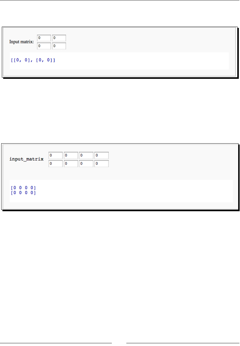
Where to go from here
[ 326 ]
label='Input matrix:')):
print m
Here is a shorthand way to create the same type of control:
default_matrix = Matrix(QQ, 2, 4)
@interact # Shortcut
def _(input_matrix = default_matrix):
print input_matrix
@interact
def _(color = color_selector(default=(1,0,0),
label='Choose a color:', widget='farbtastic', hide_box=False)):
print color
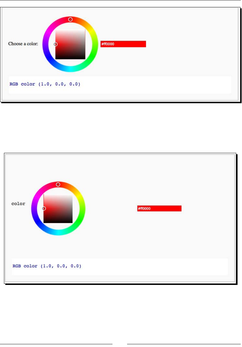
Chapter 10
[ 327 ]
Here is a shorthand way to create the same type of control:
@interact # Shortcut
def _(color = Color('red')):
print color

Where to go from here
[ 328 ]
What just happened?
This example makes use of Python funcon decorators, that were introduced in the previous
example. Sage denes a decorator called interact. When you decorate a funcon with @
interact, interact is called, and the funcon you dened is passed as an argument.
interact uses your funcon to construct an interacve graphical user interface. The syntax
for doing this is somewhat unusual. The keyword arguments of your funcon dene the
elements of the interface, and the statements in the body of the funcon determine what
happens when the user interacts with the controls. The code that creates a check box is a
good place to start:
@interact
def _(checked = checkbox(True, "Check the box:")):
print checked
The name of the funcon we dene doesn't really maer, as long as it doesn't conict with
any other names, so the convenon is to use a single underscore. There's nothing magical
about the underscore; you could give the funcon any name. The funcon has a single
keyword argument. The keyword is the variable name that will contain the result from
the control, and checkbox is the funcon that creates the control. checkbox takes two
oponal arguments: the default value, and a label for the control. When the user clicks
on the checkbox, the statements in the funcon body are executed. In this case, the value
returned by the control is just printed below the control.
There are also shortcuts for creang many of the controls. The shortcuts typically give you
less control over the appearance of the controls. I don't recommend using the shortcuts,
because someone who is unfamiliar with the shortcut will have no idea how the code works
unl they study the documentaon for the interact module. Code should generally be
self-explanatory. The shortcuts are listed here so that you can understand what is going on if
you come across them in other examples.
Using interactive controls
Time for action – an interactive example
Let's take an example from Chapter 8 and make it interacve. Run the following code in a
worksheet:
var('x,y')
@interact
def _(c1 = slider(vmin=0, vmax=3, default=2, label='c1:'),
c2 = slider(vmin=-3, vmax=3, default=1, label='c2:'),
c3 = slider(vmin=-3, vmax=3, default=1, label='c3:'),
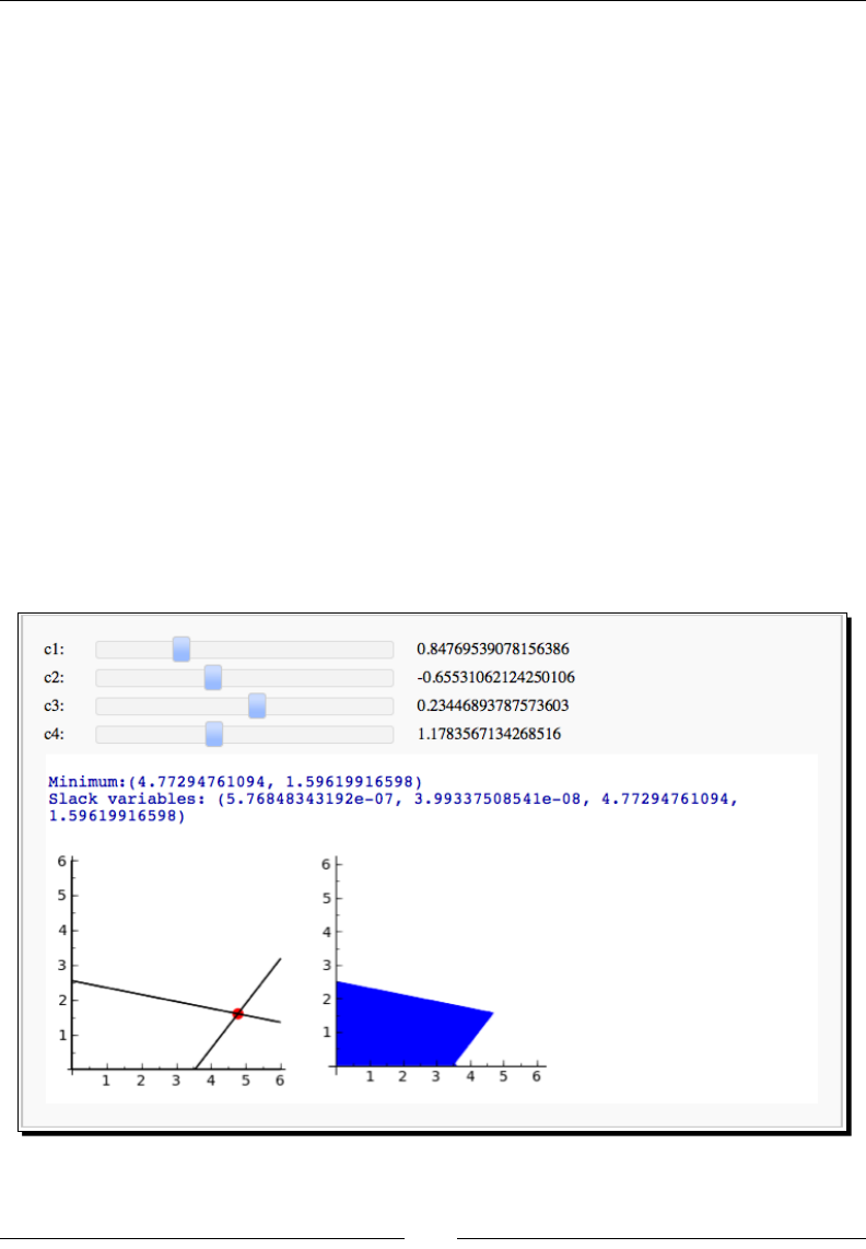
Chapter 10
[ 329 ]
c4 = slider(vmin=0, vmax=3, default=2, label='c4:')):
c=vector(RDF,[-4,-5])
G=matrix(RDF,[[c1,c2],[c3,c4],[-1,0],[0,-1]])
h=vector(RDF,[3,3,0,0])
sol=linear_program(c,G,h)
print "Minimum:" + str(sol['x'])
print "Slack variables: " + str(sol['s'])
c1_plot = implicit_plot(c1*x + c2*y ==3, (x,0,6), (y,0,6))
c2_plot = implicit_plot(c3*x + c4*y == 3, (x,0,6), (y,0,6))
c3_plot = implicit_plot(x == 0, (x,0,6), (y,0,6))
c4_plot = implicit_plot(y == 0, (x,0,6), (y,0,6))
min_plot = point(sol['x'], color='red', size=50)
rp = region_plot([c1*x + c2*y <= 3, c3*x + c4*y <= 3, x >= 0,
y >= 0], (x,0,6), (y,0,6))
g = graphics_array([c1_plot+c2_plot+c3_plot+c4_plot+min_plot,
rp],1,2)
g.show(aspect_ratio=1)
The results should look like this:

Where to go from here
[ 330 ]
Play with the sliders to adjust two of the lines that constrain the minimizaon problem.
Noce that the coordinates of the minimum are printed every me you move a slider,
and the plots change to reect the new constraints and the locaon of the minimum.
What just happened?
We started with an example from Chapter 8, and made it interacve. We dened a funcon
with a single underscore as its name, and used the decorator syntax to decorate the funcon
with interact. We created four slider controls, using the syntax described in the previous
example. We then pasted the code from Chapter 8 into the funcon body and made a few
changes. The linear constraints are represented as a matrix G and a vector h. We changed
four of the entries in the matrix to be variables rather than hard-coded values. The slider
controls set the values for these variables. When you move a slider, the constraints change,
the minimum is recalculated, and the plots are redrawn. Note that this example is a good
choice for user interacon because the linear program can be solved quickly; if the code
took minutes or hours to run, there would be no point in making it interacve!
The complete documentaon of the interact module can be found at:
http://sagemath.org/doc/reference/sagenb/notebook/interact.html
Many interactive examples, along with source code, can be found at:
http://wiki.sagemath.org/interact
Have a go hero – Taylor series
In Chapter 7, we used an example to demonstrate a Taylor series converges to a funcon
in a region as the number of terms in the series increases. Convert this example so that it
is interacve. Allow the user to change the number of terms in the series, and update the
graph to show how the series converges to the funcon.
Summary
This chapter provided you with advanced tools that will help you get the most out of Sage.
We learned about:
Exporng mathemacal expressions in PDF les and PNG bitmaps
Generang LaTeX mark-up that describes a mathemacal expression
Incorporang LaTeX mark-up into a text cell in a workbook
Processing LaTeX mark-up in a workbook
Using NumPy to improve the execuon speed of your code

Chapter 10
[ 331 ]
Using Sage from a stand-alone Python script
Creang interacve graphical examples in the notebook interface
I hope you have found Sage to be a useful tool that takes much of the pain out of
mathemacs. This book has only scratched the surface of its capabilies, especially if you are
interested in advanced mathemacs. Refer to the online documentaon for Sage and Python
to learn more. The Sage worksheets published at http://www.sagenb.org/pub/ can also
be an excellent resource.
Symbols
2D plong capabilies, Sage 141, 142
3D capabilies, Sage 20, 21
-advanced argument 42
\capon{} command 303
.dmg le 34
\documentclass{arcle} command 303
-help argument 42
%hist command 46
\includegraphics[width=3.0in]{J_n.pdf}
command 303
__init__ method 247, 253, 262
%macro command 47
-notebook argument 42
/opt directory 37
.sage extension 114
# sign 54
__str__ method 248
A
absolute funcon 222
Acon menu 51
adapve_recursion opon 144
adapve_tolerance opon 144
algorithm
collision, detecng 309-311
opmizing 309
algorithm keyword 199
algorithm opon 213
align argument 163
alpha opon 143
angle 147
angle funcon 222
anonymous funcon
creang, lambda used 110
append method 83, 87
arange funcon 137
arbitrary precision 59
arguments method 175
arithmec operators, Sage
^ 57
- 57
* 57
** 57
/ 57
// 57
% 57
+ 57
= 57
about 57
armoured personnel carriers (APCs) 258
array_factor funcon 149
assert methods, Python 287
assertRaises method 287
assume funcon 18
assume statement 179
aach command 81
aributes
about 74
dening, for tank model 249-252
axes keyword 167
axes_labels method 143, 145
B
bar chart
about 161
creang 161-163
bar funcon 163
Index

[ 334 ]
Bazaar 243
Bessel funcons 18
big O notaon 200
binary version, Sage
installing, on GNU/Linux 35
installing, on Mac OS X 33
installing, on Windows 30
bool funcon 177
Broyden-Fletcher-Goldfarb-Shannon algorithm
213
bugs 242, 273
built-in funcons, Sage 68
C
calculaons
performing, on command line 43-45
performing, with notebook interface 52, 54
results, displaying of 56
callable symbolic expressions
about 63, 174
dening 64, 65
camel case 247
Cannon class 246
cells
working with 54
chmod command 317
cholesky_decomposion method 132
circle funcon 154
class
about 243
empty classes, creang 272, 273
using 269-271
classes
module, dening for 253-257
class_list aribute 270
cmap opon 171
cmd keyword 318
code
working with 55
coes method 185
color argument 150, 163
colorbar opon 171
colors
specifying, in Sage 144
column method 122
combat simulaon package
creang 263-268
combined_plot object 149
command history 46, 47
command line
calculaons, performing on 43-45
command line arguments, Sage
about 42
-advanced 42
-help 42
-notebook 42
complex 3D shape
creang 168, 169
complex numbers 60
components module 267
condional expressions 107
constrained opmizaon 235
constrained opmizaon problem 235, 236
contour funcon 217
contour plots
about 169
creang 169-171
contours opon 171
cpume funcon 308
custom excepon types
creang 279-284
Cygwin
URL 30
Cython
collision detecon, opmizing 314-316
opmizing with 314
D
damage_value variable 248
data
extracng 105
funcon, ng to 233, 234
reading, from text le 103-105
storing, in diconaries 108
storing, in text le 101-103
plong, in Sage 150
plong, with matplotlib 161-163
Data menu 51
decomposions 129
denite integral example 16
def keyword 110

[ 335 ]
degree method 185
denominator method 182
derivave example 14
derivave method 176
derivaves
approximang, numerically 213, 215
approximang, with dierences 213, 215
calculang 196, 197
desolve funcon 205, 319
desolve_system argument 205
detect_poles opon 144
diag funcon 139
diconaries
about 108
accessing 108, 109
data, storing in 108
dening 108, 109
dierences
derivaves, approximang with 213, 215
dierenal equaons 173
di funcon 197, 215
digital signal processing (DSP) 151
dir keyword 195
discrete Fourier transform (DFT)
about 220
compung 220, 222
discussion forum 42
disp opon 213
docstring 242, 248, 286
docstrings
URL, for guidelines 249
doctesng 288
documentaon phase 242
domain 63
downloading
Sage 30
VMware Player 30
E
echelon_form method 123
ecolor argument 163
Edit tab 51
eigenvalues
about 127
compung 127-129
verifying 129
eigenvalues method 129
eigenvectors
about 127
compung 127-129
verifying 129
eigenvectors_right method 129
else keyword 278
empty classes
creang 272, 273
end_points keyword 225
equaons
solving 190, 191
solving, with Sage 208, 209
except block 284
excepons
about 273, 274
handling 274-278
raising 274-278
types 278
excepon types
creang 279-284
exclude opon 144
exit command 37, 43
expand method 185
expand_raonal method 182
expand_trig funcon 187
experimental data
analysing 22-26
plong 24, 25
exp funcon 48, 202
explicit line joining 81
explicit_soluons keyword 193
explode opon 164
expressions
manipulang 179, 180
simplifying 187, 189
symbols, substung in 183
types, combining in 62
exp(x) funcon 44
extend method 83
F
facecolor keyword 165
Factor[] 186
FactorInteger[] 186
factor method 185, 186

[ 336 ]
False opon 153
freq funcon 222
funcon 222
shi funcon 222
elds 116
gsize opon 147
File menu 51
llalpha opon 143
llcolor opon 143, 147
ll opon 143, 147, 171
nally clause 278
nd_t funcon 23, 26
nd_maximum_on_interval funcon 211
nd_minimum_on_interval funcon 211
nd_root funcon 209, 211
nite element method 118
re method 279
rst-order ODE
solving 224, 225
oat funcon 91, 106
fontsize keyword 163
forget funcon 177, 179
for loop
about 19, 92, 129, 154, 220
another for loop, adding 98
lists, iterang 92, 93
replacing, with while loop 107
soluon to diusion equaon,
compung 94-97
format keyword 157
format method 91
Fourier transform 220
frame keyword 167
from numpy import * syntax 208
funcons
about 66
calling 66-68
creang 272, 273
dening 70-72
dening, for reading text le 106
dening, with keyword arguments 72, 73
ng, to data 233, 234
maxima, nding for 210-213
minima, nding for 210-213
minimizing, of one variable 210, 211
minimizing, of two variables 211-213
mulple values, returning from 87, 88
plong, with matplotlib 155-157
plong, with pole 144-146
plong, with Sage 142-144
G
gca method 159, 163
gedit(GNOME) 80
generate_histogram_plot method 238
get_posion method 252, 262
get_random_element method 238
Git 243
GNU Linear Programming Kit (GLPK) 232
GNU Scienc Library (GSL)
about 208
system of ODEs, solving 229-231
gompertz funcon 26
gradient
about 215
compung 215-217
gradient funcon 217
gradient opon 213
graphics_array funcon 153
graphics primives
plong with 153, 154
Ground_Vehicle class 262, 277
growth model
ng 25, 26
H
Hamming window funcon 224
help commands, Sage 45, 46
help funcon 46, 75
hessian opon 213
higher-order ODE
solving 226-229
hist funcon 165
histogram
plong 164, 165
html_table decorator 321
I
if statements 107
implicit_plot funcon 233
import statement 134, 257
index 86

[ 337 ]
innite series 199
inial_guess argument 234
installaon, LaTeX
notebook interface, PDF output 293-296
installaon, Sage 34
installaon, VMWare Player 30
installing
LaTeX 292
Sage 34
VMWare Player 30
XCode 38
instance 243
instance aributes
using 269-271
instance variables 247
integers 58, 59
integral method 199
integrals
calculang 198, 199
integrate funcon 199
integraon example 15
interacve 3D plot
creang 166
interacve graphic examples
interacve controls, making 322-328
interacve controls, using 328, 330
interacve shell
about 43
command history 46, 47
execuon, tracing of command 48
tab compleon 47
interact module
documentaon 330
interpolate_soluon method 231
inverse_laplace method 203
ipdb> prompt 48
IRC channel 42
items
accessing, in lists 85, 86
iteritems method 109
iterkeys method 109
itervalues method 109
ivar keyword 205, 225, 229
J
Jacobian funcon 230
Java applet 166
jcs keyword 225
jEdit 80
Jmol 166
K
Kate (KDE) 80
KeyboardInterrupt excepon 284
keyword arguments
about 67
funcons, dening with 72, 73
keywords
center 307
color 307
opacity 307
radius 307
L
label_colors opon 171
labels keyword 164, 171
lambda
about 211
anonymous funcon, creang 110
lambda construct 211
lambda keyword 110
laplace method 203
Laplace transform
about 202
compung, with Sage 202, 203
LaTeX
equaons, typeseng 291
installing 292
view funcon 297
latex funcon 300
LaTeX mark-up, in notebook interface
working with 297-303
LaTeX typeseng system 21
launching
virtual machine 31-33
VMware Player 31-33
least squares ng 233, 234
le method 177
legend method 157
len funcon 87, 94, 109
limit funcon 195

[ 338 ]
limits
calculang 193, 195
linear algebra 17, 18, 113
linear programming
solving, with Sage 231, 232
linewidths opon 171
list comprehension
about 99
using 99, 100
list_plot funcon 152
lists
about 82
append method 87
creang 82-84
funcons 87
items, accessing in 85, 86
len funcon 87
methods 87
plong 151, 152
load command 82, 246
logarithms, Sage 189
log funcon 189
M
mailing lists 42
maintenance phase 242
major opon 153
MAKE environment variable 39
Manipulate funcon 322
marker opon 145
MATLAB 82, 161
matplotlib 98
about 141
data, plong with 161-163
funcons, plong with 155-157
histogram, plong 164, 165
object-oriented interface 141
Pyplot interface 141
URL, for documentaon 146
matplotlib documentaon
URL 146
matplotlib gure object
geng 158, 159
matrices
about 113
accessing 120, 122
creang 120
creang, in NumPy 137, 139
decomposing 129, 130
manipulang 120-123
matrix algebra
about 124
performing 124, 125
matrix elements
accessing 120, 122
matrix methods 126, 127
Matrix object 126
MatrixSpace class 120
matrix spaces
creang 120
maxfun argument 211
maxima
nding, for funcons 210-213
Maxima 174, 208
Mercurial 243
method
nintegrate 303
methods
dening, for tank model 249-252
MiKTeX 292
minima
nding, for funcons 210-213
minor opon 153
module
dening, for classes 253-257
reloading 258
Monte Carlo simulaon 165, 236
move method 262
mulline_string variable 63
mulple users
Sage, installing for 37
mulple values
returning, from funcon 87, 88
mulplicies keyword 193
N
namespace 257
nintegral method 218
nintegrate method 303
noisy_line funcon 151
norm method 127
notebook() funcon 49

[ 339 ]
notebook interface
about 48, 243
calculaons, performing with 52, 54
closing 55
code, eding in input cells 55
help, geng with 54
menus 51
starng 49, 50
tabs 51
using 174
notebook interface example 10-12
Notepad++ 80
numerator method 182
numerical_approx funcon
about 68
arguments 69
numerical_approx funcon, arguments
digits 69
prec 69
numerical approximaons 68, 69
numerical_approx method 97
numerical integraon
about 217
performing, with NumPy 219, 220
numerical opmizaon 231
numerical types, Sage
about 58
complex numbers 60
integers 58, 59
raonal numbers 58, 59
real numbers 59
symbolic expressions 60
num_points argument 230
NumPy
about 23, 113, 133, 208, 314
matrices, creang in 137, 139
numerical integraon, performing with 219, 220
opmizing with 311
URL 133
URL, for ocial documentaon 139
using 311-313
window funcons, plong in 223, 224
NumPy arrays
creang 133, 134
working with 136
NumPy Tutorial
URL 139
NumPy, types
about 135
bool 135
complex 135
complex64 135
complex128 135
oat 135
oat32 135
oat64 135
int 135
int8 135
int16 135
int32 135
int64 135
uint8 135
uint16 135
uint32 135
uint64 135
O
object-oriented programming (OOP)
about 73
URL, for principles 243
objects
about 73, 241, 243
help funcon 75-77
working with 74, 75
ODE. See ordinary dierenal equaon
ode_solver object 241
ogrid funcon 217
open-source version control tool 243
opcal density 22
OrderedDict 110
ordered diconaries 110
ordinary dierenal equaon
about 204
solving 18, 204, 205, 224-229
output keyword 226
P
package
about 263
creang, for simulaon 263-268
parameters argument 235
parametric 3D plong 168, 169

[ 340 ]
parametric funcon
plong 146, 147
parametric_plot3d funcon 169
params argument 230
paral fracon decomposion 17
paral_fracon method 182
pass keyword 273
PATH environment variable 42
pi constant 14
pie chart
creang 164
pie funcon 164
placeholder 272
plaorm support, Sage 29
plot3d funcon 169
plot command 303
plot funcon 23, 66, 67, 143
plot_points opon 144
plong capabilies 19, 20
plot_vector_eld funcon 150
plt.funcon_name funcon 156
plt.plot funcon 157
PNG 157
png funcon 297
point graphics funcon 211
polar keyword 161
polar plot
about 147
creang 147-149
improving 159-161
pole
funcons, plong with 144-146
polynomial
roots, nding of 208, 209
polynomials
expanding 184, 185
factoring 184, 185
powerful calculator
Sage, using as 12, 13
precision method 74
print funcon 56, 62, 118, 119
probability distribuon funcons
accessing 236, 238
proTeXt 292
Publish tab 51
pyplot interface 98
Python
about 71
assert methods 287
condional expressions 107
for loops 92
if statements 107
lambda keyword 110
sequence types 82
strings methods, reference link 91
while loops 105
Python 2 79
Python 3 79
Python class names
convenons 247
Python code execuon
algorithm, opmizing 309
collision detecon, opmizing 314
NumPy, opmizing with 311
runme measurments, ps 309
sphere collision, detecng 304-307
sphere collision detecon, command-line
interface used 307, 308
steps 304
Python decorators
about 319, 320
funcon decorators 321
improving 321
memoizaon 322
Python lists 82
Python scripts
ordinary dierenal equaon, solving 319
Sage, calling 316-319
Sage, creang 316
Q
QR factorizaon
about 129
compung 129, 131
quadrature. See numerical integraon
quit command 37, 43
R
radius 147
random funcon 151
random sequenal adsorpon (RSA) 153
range 63

[ 341 ]
range funcon 94
raonal funcons
manipulang 180, 182
working with 181, 182
raonal numbers 58, 59
ray tracing 167
RDF object 131
readline method 105
RealDistribuon class 306
RealDistribuon object 238
real number 59
real_number object 74
record 272
reduce_trig funcon 187
relaonal expressions
about 176
dening 177, 179
requirements analysis 242
reset funcon 69
reshape method 137
restore funcon 69, 296
results
displaying, of calculaons 56
return keyword 72
revision control. See version control
Reynolds number example 13
rgbcolor opon 143
ring
variables, dening on 61
ring keyword 193
roots
nding 193
nding, of polynomial 208, 209
roots method 193
row method 122
Runge-Kua method 225
S
Sage
2D plong capabilies 141, 142
about 9, 30, 113
arithmec operators 57
basic operaons, performing with
vectors 114, 115
binary version, installing on Windows 30
building 39
built-in funcons 68
callable symbolic expressions 63-65
colors, specifying in 144
command line arguments 42
compiling, from source 38
contour plots, creang 169-171
data, plong in 150
decompressing 35
derivaves, approximang numerically 213, 215
derivaves, calculang with 196, 197
discrete Fourier transform (DFT), compung
with 220, 222
downloading 30-35
equaons, solving with 190, 191, 208, 209
exing 35
experimental data, analysing 22-26
expressions, manipulang with 179, 180
expressions, simplifying 187, 189
extracng 30
funcons, dening 70-72
funcons 66-68
funcons, plong with 142-144
gradient, compung 215-217
graphics primives 153, 154
help commands 45, 46
history 173
installing 34
installing, for mulple users 37
integrals, calculang with 198, 199
interacve 3D plot, creang 166
interacve shell 43
Laplace transform, compung with 202, 203
limits, calculang with 193, 195
linear algebra 17, 18
linear programming, solving with 231, 232
logarithms 189
matplotlib 155-157
matplotlib gure object, geng 158, 159
matrices, creang 120
MatrixSpace class 120
matrix spaces, creang 120
Maxima 174
maxima, nding of funcons 210-213
methods, for expanding expressions 189
methods, for simplifying expressions 189
minima, nding of funcons 210-213
notebook interface 48-55, 174

[ 342 ]
notebook interface example 10-12
numerical type operators 58
objects 73, 75
ordinary dierenal equaons, solving
with 18, 204, 205, 224-229
parametric 3D plong 168, 169
parametric funcons, plong 146, 147
polar plots, improving 159-161
plaorm support 29
plong capabilies 19, 20
probability distribuon funcons,
accessing 236, 238
raonal funcons, manipulang with 181, 182
relaonal expressions 177, 179
roots, nding of polynomial 208, 209
roots, nding with 193
running, from user account 36
series, compung with 199, 200
starng 34
strings 62, 63
symbolic expressions, dening 174, 175
symbolic funcon, integrang
numerically 217-219
symbolic mathemacs 14-16
symbols, substung in expressions 183
system of linear equaons, solving 118, 119
Taylor series, compung with 201, 202
three-dimensional surface, visualising 20, 21
trigonometric expressions, manipulang
with 186, 187
two-dimensional plots 141
URL, for construcons document 42
URL, for documentaon page 41
URL, for downloading 30, 34
URL, for free account 10
URL, for free public notebook servers 29
URL, for installaon guide 30
URL, for ocial tutorial 41
URL, for reference manual 41
URL, for resources 42
URL, for supported plaorms list 29
URL, for themac tutorials 42
using, as powerful calculator 12, 13
sage code
long lines of code 81
scripts, running 81
wring 80
Sage code execuon
steps 304
Sage, compiling
prerequisites 38
Sage documentaon 41
Sage, installing on GNU/Linux 35
Sage, installing on Mac OS X 33
Sage, installing on Windows
VMware Player, downloading 30
VMware Player, installing 30
sage menu 51
sage.rings.real_mpfr.RealNumber class 75
sage-vmware.vmx 31
saveg funcon 157
scaer_plot funcon 23, 151
scaer plots
about 150
creang 151
scope 257
scripts
running 81
self argument 247
sequence types, Python
about 82
buer type 92
bytearray type 92
lists 82
strings 89
tuple 87
unicode type 92
series
compung 199, 200
series method 200
set_seed method 238
setUp method 286
set_xcklabels method 163
set_xcks method 163
Share tab 51
show command 118
show funcon 65, 119, 174, 295
show method 147, 154
simulaon
expanding 258-262
package, creang for 263-268
sinc funcon 67, 222
singular value decomposion (SVD)
about 131

[ 343 ]
compung 131, 132
slicing 122
soware development
overview 242, 243
solve funcon 191, 197
solve_right method 119
sorted funcon 110
source
Sage, compiling from 38
source control. See version control
source tarball
downloading 39
URL, for downloading 39
specicaons 242
sphere funcon 306
srange funcon 84, 102
SR funcon 177
standard curve
ng 22, 23
standard_curve funcon 23, 25
step keyword 226
str funcon 63, 91
string literal 63
strings
about 62, 89
parsing 105
using 62
working with 90, 91
str method 74
struct 272
submatrix method 122
subplot funcon 161
subplots_adjust funcon 161, 229
subs method 183
subst command 184
substute_expression method 184
substute_funcon method 183
substute method 183
Subversion 243
sum funcon 154, 200
symbolic expressions
about 60, 143, 174
dening 175
symbolic funcon
integrang, numerically 217-219
symbolic mathemacs 14-16
symbols
substung, in expressions 183
SystemExit excepon 284
system, of linear equaons
solving 118, 119
system, of ODEs
solving 226
solving, GNU Scienc Library
(GSL) used 229-231
T
tab compleon 47
Tachyon 167
Tank class
about 246
dening 244-246
unit tests, creang for 284-287
tank model
aributes, dening for 249-252
methods, dening for 249-252
move ability, providing 249-252
tank.py le
creang 253
taylor keyword 195
taylor method 202
Taylor series
about 200, 330
compung, with Sage 201, 202
tearDown method 286
Test class 270
test_re method 287
tesng phase 242
TestTank class 286
TeX 146
text le
data, reading from 103-105
data, storing in 101-103
text_le.readline() method 106
text funcon 163
Text tab 51
TextWrangler 80
three-dimensional surface
visualising 20, 21
tol argument 211
top command 309
trace funcon 48

[ 344 ]
Track class 246
trailing_coecient method 185
trapz argument 220
trigonometric expressions
manipulang 186, 187
trig_simplify funcon 187
truncated series 199
try block 277, 284
t_span argument 230
tuple
about 67, 87, 143, 211
mulple values, returning from funcon 87, 88
Turret class 245, 246
two-dimensional plots 141
TypeError excepon 273
type funcon 58
types
combining, in expressions 62
U
u.cross_product(v) method 118
u.dot_product(v) method 118
u.inner_product(v) method 118
Undo tab 51
unit 284
unit tesng
about 284
strategies 288
unit tests
creang, for Tank class 284-287
u.norm(p) method 118
u.pairwise_product(v) method 118
user account
Sage, running from 36
V
ValueError excepon 277
var funcon 60, 65
variables
dening, on ring 61
variables argument 235
variables method 175
var statement 175
vector elements
manipulang 116, 117
vector elds
about 149
plong 149, 150
vector funcon 116
vector object
creang 116, 117
vectors
about 113, 114
manipulang 116, 117
methods 117
operators 117
working with 114, 115
vector space
creang 116
VectorSpace class 115
vehicle base class
creang 258-262
vehicle module 261
vehicle.py le 258
version control 243
viewer keyword 167
view funcon 295, 297
virtual machine
launching 31-33
VMware Player
downloading 30
installing 30
launching 31-33
W
while loop
about 105
for loop, replacing with 107
using 101
who command 45
width argument 163
window funcons
about 223
plong, in NumPy 223, 224
worksheets
commands, for eding 54
Worksheet tab 51


Thank you for buying
Sage Beginner's Guide
About Packt Publishing
Packt, pronounced 'packed', published its rst book "Mastering phpMyAdmin for Eecve
MySQL Management" in April 2004 and subsequently connued to specialize in publishing
highly focused books on specic technologies and soluons.
Our books and publicaons share the experiences of your fellow IT professionals in adapng
and customizing today's systems, applicaons, and frameworks. Our soluon based books
give you the knowledge and power to customize the soware and technologies you're
using to get the job done. Packt books are more specic and less general than the IT books
you have seen in the past. Our unique business model allows us to bring you more focused
informaon, giving you more of what you need to know, and less of what you don't.
Packt is a modern, yet unique publishing company, which focuses on producing quality,
cung-edge books for communies of developers, administrators, and newbies alike. For
more informaon, please visit our website: www.packtpub.com.
About Packt Open Source
In 2010, Packt launched two new brands, Packt Open Source and Packt Enterprise, in order
to connue its focus on specializaon. This book is part of the Packt Open Source brand,
home to books published on soware built around Open Source licences, and oering
informaon to anybody from advanced developers to budding web designers. The Open
Source brand also runs Packt's Open Source Royalty Scheme, by which Packt gives a royalty
to each Open Source project about whose soware a book is sold.
Writing for Packt
We welcome all inquiries from people who are interested in authoring. Book proposals
should be sent to author@packtpub.com. If your book idea is sll at an early stage and you
would like to discuss it rst before wring a formal book proposal, contact us; one of our
commissioning editors will get in touch with you.
We're not just looking for published authors; if you have strong technical skills but no wring
experience, our experienced editors can help you develop a wring career, or simply get
some addional reward for your experse.
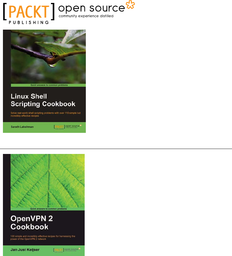
Linux Shell Scripting Cookbook
ISBN: 978-1-849513-76-0 Paperback: 360 pages
Solve real-world shell scripng problems with over
110 simple but incredibly eecve recipes
1. Master the art of craing one-liner command
sequence to perform tasks such as text processing,
digging data from les, and lot more
2. Praccal problem solving techniques adherent to
the latest Linux plaorm
3. Packed with easy-to-follow examples to exercise all
the features of the Linux shell scripng language
OpenVPN 2 Cookbook
ISBN: 978-1-849510-10-3 Paperback: 356 pages
100 simple and incredibly eecve recipes for
harnessing the power of the OpenVPN 2 network
1. Set of recipes covering the whole range of tasks for
working with OpenVPN
2. The quickest way to solve your OpenVPN problems!
3. Set up, congure, troubleshoot and tune OpenVPN
4. Uncover advanced features of OpenVPN and even
some undocumented opons
Please check www.PacktPub.com for information on our titles
