Samuel E. Buttrey, Lyn R. Whitaker A Data Scientist’s Guide To Acquiring, Cleaning, And
User Manual: Pdf
Open the PDF directly: View PDF ![]() .
.
Page Count: 293 [warning: Documents this large are best viewed by clicking the View PDF Link!]

A Data Scientist’s Guide to Acquiring,
Cleaning, and Managing Data in R
Samuel E. Buttrey and Lyn R. Whitaker
Naval Postgraduate School, California, United States
is edition first published 2018
© 2018 John Wiley & Sons Ltd
Library of Congress Cataloging-in-Publication Data applied for
Hardback ISBN: 9781119080022
Contents
1R1
1.1 Introduction 1
1.1.1 What Is R? 1
1.1.2 Who Uses R and Why? 2
1.1.3 Acquiring and Installing R 2
1.1.4 Starting and Quitting R 3
1.2 Data 3
1.2.1 Acquiring Data 3
1.2.2 Cleaning Data 4
1.2.3 e Goal of Data Cleaning 4
1.2.4 Making Your Work Reproducible 5
1.3 e Very Basics of R 5
1.3.1 Top Ten Quick Facts You Need to Know about R 5
1.3.2 Vocabulary 8
1.3.3 Calculating and Printing in R 11
1.4 Running an R Session 12
1.4.1 Where Your Data Is Stored 13
1.4.2 Options 13
1.4.3 Scripts 14
1.4.4 R Packages 14
1.4.5 RStudio and Other GUIs 15
1.4.6 Locales and Character Sets 15
1.5 Getting Help 16
1.5.1 At the Command Line 16
1.5.2 e Online Manuals 16
1.5.3 On the Internet 17
Preface xvii
About the Companion Website xxi
1.5.4 Further Reading 17
1.6 How to Use is Book 17
1.6.1 Syntax and Conventions in is Book 17
1.6.2 e Chapters 18
2 R Data, Part 1: Vectors 21
2.1 Vectors 21
2.1.1 Creating Vectors 21
2.1.2 Sequences 22
2.1.3 Logical Vectors 23
2.1.4 Vector Operations 24
2.1.5 Names 27
2.2 Data Types 27
2.2.1 Some Less-Common Data Types 28
2.2.2 WhatTypeofVectorIsis? 28
2.2.3 Converting from One Type to Another 29
2.3 Subsets of Vectors 31
2.3.1 Extracting 31
2.3.2 Vectors of Length 0 34
2.3.3 Assigning or Replacing Elements of a Vector 35
2.4 Missing Data (NA) and Other Special Values 36
2.4.1 e Effect of NAsinExpressions 37
2.4.2 Identifying and Removing or Replacing NAs37
2.4.3 Indexing with NAs39
2.4.4 NaN and Inf Values 40
2.4.5 NULL Values 40
2.5 e table() Function 40
2.5.1 Two- and Higher-Way Tables 42
2.5.2 Operating on Elements of a Table 42
2.6 Other Actions on Vectors 45
2.6.1 Rounding 45
2.6.2 Sorting and Ordering 45
2.6.3 Vectors as Sets 46
2.6.4 Identifying Duplicates and Matching 47
2.6.5 Finding Runs of Duplicate Values 49
2.7 Long Vectors and Big Data 50
2.8 Chapter Summary and Critical Data Handling Tools 50
3 R Data, Part 2: More Complicated Structures 53
3.1 Introduction 53
3.2 Matrices 53
3.2.1 Extracting and Assigning 54
3.2.2 Row and Column Names 56
3.2.3 Applying a Function to Rows or Columns 57
3.2.4 Missing Values in Matrices 59
3.2.5 Using a Matrix Subscript 60
3.2.6 Sparse Matrices 61
3.2.7 ree- and Higher-Way Arrays 62
3.3 Lists 62
3.3.1 Extracting and Assigning 64
3.3.2 Lists in Practice 65
3.4 Data Frames 67
3.4.1 Missing Values in Data Frames 69
3.4.2 Extracting and Assigning in Data Frames 69
3.4.3 Extracting ings at Aren’t ere 72
3.5 Operating on Lists and Data Frames 74
3.5.1 Split, Apply, Combine 75
3.5.2 All-Numeric Data Frames 77
3.5.3 Convenience Functions 78
3.5.4 Re-Ordering, De-Duplicating, and Sampling from Data Frames 79
3.6 Date and Time Objects 80
3.6.1 Formatting Dates 80
3.6.2 Common Operations on Date Objects 82
3.6.3 Differences between Dates 83
3.6.4 Dates and Times 83
3.6.5 Creating POSIXt Objects 85
3.6.6 Mathematical Functions for Date and Times 86
3.6.7 Missing Values in Dates 88
3.6.8 Using Apply Functions with Dates and Times 89
3.7 Other Actions on Data Frames 90
3.7.1 Combining by Rows or Columns 90
3.7.2 Merging Data Frames 91
3.7.3 Comparing Two Data Frames 94
3.7.4 Viewing and Editing Data Frames Interactively 94
3.8 Handling Big Data 94
3.9 Chapter Summary and Critical Data Handling Tools 96
4 R Data, Part 3: Text and Factors 99
4.1 Character Data 100
4.1.1 e length() and nchar() Functions 100
4.1.2 Tab, New-Line, Quote, and Backslash Characters 100
4.1.3 e Empty String 101
4.1.4 Substrings 102
4.1.5 Changing Case and Other Substitutions 103
4.2 Converting Numbers into Text 103
4.2.1 Formatting Numbers 103
4.2.2 Scientific Notation 106
4.2.3 Discretizing a Numeric Variable 107
4.3 Constructing Character Strings: Paste in Action 109
4.3.1 Constructing Column Names 109
4.3.2 Tabulating Dates by Year and Month or Quarter Labels 111
4.3.3 Constructing Unique Keys 112
4.3.4 Constructing File and Path Names 112
4.4 Regular Expressions 112
4.4.1 Types of Regular Expressions 113
4.4.2 Tools for Regular Expressions in R 113
4.4.3 Special Characters in Regular Expressions 114
4.4.4 Examples 114
4.4.5 e regexpr() Function and Its Variants 121
4.4.6 Using Regular Expressions in Replacement 123
4.4.7 Splitting Strings at Regular Expressions 124
4.4.8 Regular Expressions versus Wildcard Matching 125
4.4.9 Common Data Cleaning Tasks Using Regular Expressions 126
4.4.10 Documenting and Debugging Regular Expressions 127
4.5 UTF-8 and Other Non-ASCII Characters 128
4.5.1 Extended ASCII for Latin Alphabets 128
4.5.2 Non-Latin Alphabets 129
4.5.3 Character and String Encoding in R 130
4.6 Factors 131
4.6.1 What Is a Factor? 131
4.6.2 Factor Levels 132
4.6.3 Converting and Combining Factors 134
4.6.4 Missing Values in Factors 136
4.6.5 Factors in Data Frames 137
4.7 R Object Names and Commands as Text 137
4.7.1 R Object Names as Text 137
4.7.2 R Commands as Text 138
4.8 Chapter Summary and Critical Data Handling Tools 140
5 Writing Functions and Scripts 143
5.1 Functions 143
5.1.1 Function Arguments 144
5.1.2 Global versus Local Variables 148
5.1.3 Return Values 149
5.1.4 Creating and Editing Functions 151
5.2 Scripts and Shell Scripts 153
5.2.1 Line-by-Line Parsing 155
5.3 Error Handling and Debugging 156
5.3.1 Debugging Functions 156
5.3.2 Issuing Error and Warning Messages 158
5.3.3 Catching and Processing Errors 159
5.4 Interacting with the Operating System 161
5.4.1 File and Directory Handling 162
5.4.2 Environment Variables 162
5.5 Speeding ings Up 163
5.5.1 Profiling 163
5.5.2 Vectorizing Functions 164
5.5.3 Other Techniques to Speed ings Up 165
5.6 Chapter Summary and Critical Data Handling Tools 167
5.6.1 Programming Style 168
5.6.2 Common Bugs 169
5.6.3 Objects, Classes, and Methods 170
6 Getting Data into and out of R 171
6.1 Reading Tabular ASCII Data into Data Frames 171
6.1.1 Files with Delimiters 172
6.1.2 Column Classes 173
6.1.3 Common Pitfalls in Reading Tables 175
6.1.4 An Example of When read.table() Fails 177
6.1.5 Other Uses of the scan() Function 181
6.1.6 Writing Delimited Files 182
6.1.7 Reading and Writing Fixed-Width Files 183
6.1.8 A Note on End-of-Line Characters 183
6.2 Reading Large, Non-Tabular, or Non-ASCII Data 184
6.2.1 Opening and Closing Files 184
6.2.2 Reading and Writing Lines 185
6.2.3 Reading and Writing UTF-8 and Other Encodings 187
6.2.4 e Null Character 187
6.2.5 Binary Data 188
6.2.6 Reading Problem Files in Action 190
6.3 Reading Data From Relational Databases 192
6.3.1 Connecting to the Database Server 193
6.3.2 Introduction to SQL 194
6.4 Handling Large Numbers of Input Files 197
6.5 Other Formats 200
6.5.1 Using the Clipboard 200
6.5.2 Reading Data from Spreadsheets 201
6.5.3 Reading Data from the Web 203
6.5.4 Reading Data from Other Statistical Packages 208
6.6 Reading and Writing R Data Directly 209
6.7 Chapter Summary and Critical Data Handling Tools 210
7 Data Handling in Practice 213
7.1 Acquiring and Reading Data 213
7.2 Cleaning Data 214
7.3 Combining Data 216
7.3.1 Combining by Row 216
7.3.2 Combining by Column 218
7.3.3 Merging by Key 218
7.4 Transactional Data 219
7.4.1 Example of Transactional Data 219
7.4.2 Combining Tabular and Transactional Data 221
7.5 Preparing Data 225
7.6 Documentation and Reproducibility 226
7.7 eRoleofJudgment 228
7.8 Data Cleaning in Action 230
7.8.1 Reading and Cleaning BedBath1.csv 231
7.8.2 Reading and Cleaning BedBath2.csv 236
7.8.3 Combining the BedBath Data Frames 238
7.8.4 Reading and Cleaning EnergyUsage.csv 239
7.8.5 Merging the BedBath and EnergyUsage Data Frames 242
7.9 Chapter Summary and Critical Data Handling Tools 245
8 Extended Exercise 247
8.1 Introduction to the Problem 247
8.1.1 e Goal 248
8.1.2 Modeling Considerations 249
8.1.3 Examples of ings to Check 249
8.2 e Data 250
8.3 Five Important Fields 252
8.4 Loan and Application Portfolios 252
8.4.1 Layout of the Beachside Lenders Data 253
8.4.2 Layout of the Wilson and Sons Data 254
8.4.3 Combining the Two Portfolios 254
8.5 Scores 256
8.5.1 Scores Layout 256
8.6 Co-borrower Scores 257
8.6.1 Co-borrower Score Examples 258
8.7 Updated KScores 259
8.7.1 Updated KScores Layout 259
8.8 Loans to Be Excluded 260
8.8.1 Sample Exclusion File 260
8.9 Response Variable 260
8.10 Assembling the Final Data Sets 262
8.10.1 Final Data Layout 262
8.10.2 Concluding Remarks 263
A Hints and Pseudocode 265
A.1 Loan Portfolios 265
A.1.1 ings to Check 266
A.2 Scores Database 267
A.2.1 ings to Check 268
A.3 Co-borrower Scores 269
A.3.1 ings to Check 270
A.4 Updated KScores 271
A.4.1 ings to Check 272
A.5 Excluder Files 272
A.5.1 ings to Check 272
A.6 Payment Matrix 273
A.6.1 ings to Check 274
A.7 Starting the Modeling Process 275
Bibliography 277
Index 279
k
k k
k
Preface
Statisticians use data to build models, and they use models to describe the world
and to make predictions about what will happen next. ere has been a large
number of very good books that describe statistical modeling, but these model-
ing efforts usually start with a set of “clean,” well-behaved data in which nothing
is missing or anomalous.
In real life, data is messy. ere will be missing values, impossible values,
and typographical errors. Data is gathered from multiple sources, leading to
both duplication and inconsistency. Data that should be categorical is coded
as numeric; data that should be numeric can appear categorical; data can be
hidden inside free-form text; and data can be in the form of dates in a wide
number of possible formats. We estimate that 80% of the time taken in any
data analysis problem is taken up just in reading and preparing the data. So, any
analyst needs to know how to acquire data and how to prepare it for modeling,
and the steps taken should be automatic, as far as possible, and reproducible.
is book describes how to handle data using the R software. R is the most
widely used software in statistics, and it has the advantage of being free,
open-source, and available on every major computing platform. Whatever
software you use, you will find yourself facing the issues of acquiring, cleaning,
and merging data, and documenting the steps you took. We hope this book
will help you do these things efficiently.
Sam Buttrey and Lyn WhitakerMonterey, California, USA
November 30, 2016
k
Don’t forget to visit the companion website for this book:
www.wiley.com/go/buttrey/datascientistsguide
ere you will find valuable material designed to enhance your learning,
including:
•A complete listing of all the R code in the Book
•Example datasets used in the Exercises
Companion Website

k
k k
k
1
1
R
1.1 Introduction
is book focuses on one problem that is common to almost every statistical
problem – indeed, to almost any problem involving any sort of analysis. at
problem is acquiring and preparing the data. Across our many years of data
analysis, we have learned that seemingly 80% of our time – maybe more – goes
into the data preparation steps (a belief echoed by others such as Dasu and
Johnson, 2003). Collectively, we call these actions data cleaning, although,
as we will discuss later, we sometimes use that term for something a little
more specific. Regardless of the name, almost any analysis requires that you
(i) acquire that data, that is, read it into the computer program; (ii) clean the
data, that is, identify entries that are duplicated or clearly erroneous or anoma-
lous, and take other preparation steps (e.g., combining entries such as “Female,”
“female,” and “F”); (iii) merge data from different sources; and (iv) prepare
the data for modeling, which might involve dividing a set of numeric values
into subsets, combining states into regions, and so on. is book discusses
some approaches for accomplishing these four steps in the R language (R Core
Team, 2013). A fifth problem, which receives less emphasis, is the problem of
long-term curation of the data. Which parts of the data must be saved and in
what way? We address that question by reference to the idea of reproducible
research, which we discuss later in this chapter, and later in the book as well.
1.1.1 What Is R?
R is a computer program that lets you analyze data. By “analyze” we mean, first,
read the data into the program and then operate on it – drawing graphs and
charts, manipulating values, fitting statistical models, and so on. (Notice that
we prefer to call data “it” rather than “them.” We discuss this choice briefly
toward the end of the chapter.) R is both a statistical “environment” and also

k
k k
k
2A Data Scientist’s Guide to Acquiring, Cleaning, and Managing Data in R
a programming language, and it is very widely used both in commercial and
academic settings. R is free and open-source and runs on Windows, Apple, and
Linux operating systems. It is maintained by a group of volunteers who release
bug fixes and new features regularly.
1.1.2 Who Uses R and Why?
R started as a tool for statisticians, evolving from a language called S that
was created in the 1970s. Today, R remains the primary language of academic
statisticians, and it also has a prominent place among analysts in business
and government as well. It is used not only for building statistical models
but also for handling and cleaning data, as in this book, and for developing
new statistical methods, building simulations, for visualization, and generally
for all the data-handling tools the statistician and the data scientist require.
Because of the ease with which users can develop and distribute new methods,
R has also become the tool of choice in certain fast-growing fields such as
biostatistics and genetics. Articles on “surveys of the top tools used by data
scientists” inevitably name R as one of the important tools with which data
scientists, as well as statisticians, should be familiar. Moreover, R’s popularity is
such that there are extensions to R (see “packages” in Section 1.4.4) that allow
you to connect to other programs such as the Python and Java languages, the
H2O machine-learning system, the ArcGIS geographical information system,
and many more.
1.1.3 Acquiring and Installing R
e primary way to acquire R is to download it from the Internet. e main
RwebsiteforRiswww.r-project.org,andthewww.cran.r-project
.org page (“CRAN” standing for “Comprehensive R Archive Network”) is
where you can download R itself. ere are in fact dozens of “mirror” sites for
CRAN – that is, websites that are essentially copies of the CRAN site – so as
to reduce the load on the CRAN site. You can probably find a mirror near you
on the “mirrors” page. After you download R, install it in the way you would
normally install a program on your operating system.
At any one time, users around the world will be running slightly different
versions of R, since new ones are released fairly frequently. For example, at this
writing the current version of R was called 3.3.2, but many users are still using
3.2 or earlier versions. is will almost never cause problems, but it is a good
idea to update your version of R from time to time.
ere are also several slightly different versions of R distributed other than at
CRAN. Microsoft R Open is a particular version of R that uses a different set
of math libraries intended to make certain computations faster. Like “regular”
R, Microsoft R Open is free, although it does not run on OS X. Other ver-
sions of R are intended to communicate with relational databases or with other

k
k k
k
R3
big-data platforms. For this book, we will assume you are running “regular”
R – but in any case for our purposes all versions of R should behave exactly the
same way.
1.1.4 Starting and Quitting R
e way you start R depends on your operating system. Normally double-
clicking on an R icon will be enough to get R started. In the command-
line interface of many Linux systems, or using the OS X terminal window, it
may be enough just to type the upper-case letter R(or, for Windows command
lines, Rgui). When R has started, you will see the command prompt >. is is
the R console, the place where commands are entered. At this point, you can
start typing commands to R. When it comes time to quit R, you can either
“kill” the window in the usual way (for OS X, the red dot, the lightswitch in the
top right, or via the File dialog; for Windows, the red X or File dialog) or you
can type the q() command. In either case, R will then ask you if you want to
“Save workspace image.” If you answer “yes” to this question, R will save to the
disk any changes you made during the current session, whereas if you answer
“no,” R will return its workspace to the condition it was in when R was last
started. We almost always want to answer “yes” to this question!
1.2 Data
Data is information about the elements of whatever problem we are investigat-
ing. Data comes in many forms, but for our purposes it will always be presented
in a set of computer-ready values. For example, a database concerning birds
might include text about the habits of the birds, numbers giving lengths and
weights of the individuals, maps showing migration patterns, images showing
the birds themselves, sound recordings of the birds’ calls, and so on. Although
they look very different, all of these different pieces of information can be rep-
resented in the computer in digital form in one way or another. In this example,
one of our primary tasks might be to ensure that each bird’s description is cor-
rectly matched with the correct map, image, and song file. Our data analysis
projects rarely include data quite so disparate, but in almost every case we need
to acquire data, clean it (a process we start to describe in what follows and con-
tinue throughout the book), and prepare it for modeling, and in almost every
case we expect our data to consist of both numeric and textual values.
1.2.1 Acquiring Data
e first step in a data analysis project, of course, is to get the data into R where
it can be manipulated. We are old enough to remember the days when this
involved typing all the data from the back of a book or journal paper into a

k
k k
k
4A Data Scientist’s Guide to Acquiring, Cleaning, and Managing Data in R
statistics package by hand, but happily this is not necessary today. On the other
hand, data now comes in a variety of formats, few of which were created with
the convenience of the data scientist in mind. In Chapter 6, we describe some
of these common formats and how to use R to read data effectively.
1.2.2 Cleaning Data
We “clean” data when we detect (and, in many cases, remove) anomalies.
Anomalies will very often be missing values, but they might also be absurd
ones,aswhenpeople’sagesarereportedas999or−1. Sometimes, as in our
earlier example, we might have genders reported as “Female,” “female,” and “F”
and we want to combine these three values. In the cleaning process we might
learn, for example, that one data source produced no data at all in August 2016;
this sort of fact will need to be brought to the attention of the data provider.
e data cleaning process also involves merging data from different sources,
extracting subsets or reshaping the data in some way. All in all, data cleaning
is the process of turning raw data, received from one or more providers, into a
data set that can be used in visualization, modeling, and decision-making.
In practice these steps are iterative. Our cleaning process not only informs the
modeling, but it sometimes leads us to re-acquire the data in a different, more
usable form. Similarly, insights from modeling will often lead us to prepare the
data in a new and more revealing way – because it is when we model that we
often discover anomalies or other interesting attributes of the data.
1.2.3 The Goal of Data Cleaning
What a “clean” data set should look like depends on what your goals are. One
useful perspective is given by Wickham (2014), who describes what he calls
“tidy” data. A tidy data set is rectangular (or tabular); each row describes one
unit of analysis (an observation), and each column gives one measurement (a
variable). For example, in a data set giving measurements about people, each
row would concern itself with a person, and the columns might give height,
weight, age, blood type, and so on.
In some problems, it is not immediately clear what the unit of analysis is.
For example, imagine data that describes the locations of boats over the course
of a month, as recorded by GPS. For some purposes, a “tidy” data set would
have one row per GPS ping, each row giving a ship identifier, a location, and
a time. For other purposes, we might prefer a data set with one row per boat,
each row giving the southernmost point that ship reaches, or perhaps giving a
binary indicator of whether the ship did, or did not, spend time in international
waters. Some data – images and sound, for example – do not lend themselves
to this “tidy” approach.

k
k k
k
R5
e exact layout of your final data will depend on what you plan to do with
it – and in some cases this won’t be known until after you have operated on
the data.
1.2.4 Making Your Work Reproducible
It is vital that other people be able to reproduce the actions you took on your
data. Ideally, you or another analyst should be able to start with your raw data,
run all the steps you applied to it, and emerge with exactly the same clean, pre-
pared data sets. is will be useful to you when you encounter a situation similar
to the one in the previous paragraph, where the form of the new data needs to
be designed. But it is even more important for another analyst, since if you
or another analyst can reproduce your results there will be no disagreement
about the data. e act of making research reproducible has, in recent years,
been rightfully recognized as a cornerstone of scientific progress. Record and
document every step you take so that others can repeat them.
1.3 The Very Basics of R
is book is about handling data in R. It cannot teach you the very basics of R in
detail – although, happily, there are many good books and online resources that
can. (We give a few examples at the end of this chapter.) In this section, we list a
few of the most basic facts about R, but, again, this book is not intended to teach
you R. Rather, we focus on the details of R and of the way data is represented
in R, in order to help you understand some of the ways to acquire, clean, and
handle data inside R.
1.3.1 Top Ten Quick Facts You Need to Know about R
In this section, we give a few of the most important facts about R a beginner
needs to know. ere will be more detail on these facts later in the chapter and
throughout the book.
1) e prompt is (by default) >. If you leave a command incomplete, maybe
because there is an unclosed parenthesis or quotation mark, R gives you
the continuation prompt, which is +. e Esc key (Windows) or control-C
(other systems) produces the break command, which will take you back to
the regular prompt. In this example, we show what a completed command
looks like – in this case, R is computing the value of 3 divided by 2.
>3/2
[1] 1.5

k
k k
k
6A Data Scientist’s Guide to Acquiring, Cleaning, and Managing Data in R
Here, R produced the prompt (>), and we typed 3/2and pressed the
Enter (or “Return”) key. R then produced the output. We will talk about
the [1] part in Chapter 2, but the computed value of 1.5 is shown. In
the following example, we show what happens when we press Enter after
typing the slash character:
>3/
+2
[1] 1.5
Here, since the expression on the first line was incomplete, R produced the
continuation prompt, +.Whenwetyped2and hit Enter, the expression
was complete and the result was shown. In case of confusion, press break
until the original >prompt is showing.
In examples in this book where we want to show the R output, we also
show the >prompt in front of our code. Remember, that >is produced by
R; you don’t need to type that yourself. (At the end of the chapter, we tell
youwhereyoucangetallthecodefromthebookinelectronicform.)
2) R is case-sensitive, which means that upper- and lower-case letters
are different in R. For example, the built-in R object LETTERS gives
all 26 upper-case letters. A different item called letters contains the
lower-case versions of the alphabet. ere is no built-in object called
Letters.
3) Show an object by typing its name. For example, if you type ls by itself,
you see the contents of the function whose name is ls, the one that lists all
the objects in your workspace (which we define later). To actually run the
function and see the objects, you need to type the function’s name together
with parentheses. In this case, list your objects by typing ls().
4) Get help for a function or object named thing with the command
help(thing) or ?thing. For example, to see the help for the
ls() function, type help(ls). If you don’t know the name, try
help.search() with a relevant word in quotation marks; for example,
try help.search ("matrices") to see functions that handle
matrices.
5) Assign a value or object to a name with the left-arrow (less-than plus
hyphen): for example, the command a<-1creates a new object named
awith value 1. (You can also assign with a command such as a=1,
but we don’t recommend it.) e assignment will over-write any existing
object named ayou might have had. Once you create an object, it is in
your “workspace,” and your workspace can be saved when you quit. So
unless your computer crashes, when you create an object it will persist
until you delete it. Display the set of objects in your workspace with
objects() or ls();removeanobjectwithremove() or rm().Not
every character is permitted in the name of an R object. Start a name

k
k k
k
R7
with a letter or a dot, and then stick to numbers, letters, underscores,
and dots. Names cannot contain spaces. In this example, we show some
assignmentsthatsucceedandsomethatdonot.
>a<-1
> a.1 <- 1
>2a<-1
Error: unexpected symbol in "2a"
>a2<-1
Error: unexpected numeric constant in "a 2"
e first two of these assignments succeed, because aand a.1 are valid
names. e last two fail because they refer to invalid names.
6) e comment character is #. A comment ends at the end of the line. If you
want a comment to span multiple lines, you need to start each comment
line with #.
7) Recall earlier commands with the up-arrow. You can edit an earlier
command and then press the Enter key to run the new version. e
history() command shows a list of your recent commands; put a
number in (as in history(500))toseemore.
8) When referring to file names, R itself uses the forward slash in the console.
e Windows file system uses the backward slash, so Windows users may
usethat,too,butinthatcaseyouhavetotype\\ (we talk more about
this later on). For example, a Windows user who wants to access a file
named c:\temp\mycode.R in an R command will need to type either
c:/temp/mycode.R or c:\\temp\\mycode.R. You’ll need to use a
regular, single backslash if you are interacting with the Windows operat-
ing system and not R – if, for example, you are presented with a graphical
“select file” window. e file systems for OS X and Linux users use the
forward slash at all times.
9) Just about any function you want is built into R, so R makes an excellent
calculator. For example,
> sin (log (34))
[1] -0.375344
is says that the sine (using radians) of the logarithm (base e)of34is
−0.375344. Most functions allow you to specify “arguments,” values you
pass to the function to modify its behavior. Some must be specified; others
have default values. For example, log (34, 10) produces the base 10
logarithm instead of the natural logarithm. If a function accepts multiple
arguments, you will need to specify them in the proper order – or by name.
In this example, the arguments to log are named xand base (see the
help at ?log), so we could have entered log(base = 10, x = 34)
too.

k
k k
k
8A Data Scientist’s Guide to Acquiring, Cleaning, and Managing Data in R
10) R’s operators include the comparison operators != for “not equal,” == for
“is equal to,” <= and >= for“lessthanorequalto”and“greaterthanorequal
to,” and the arithmetic operators *for “multiplied by” and ^for “raised to
the power of.”
1.3.2 Vocabulary
As we get started, it will be worthwhile for us to repeat some of the vocabulary
of R, and of data, that you should be familiar with. In this section, we define
some of the terms that are commonly used in discussion of R, both in this book
and elsewhere.
vector Avector is the simplest piece of data in R. It consists of one or more
entries (also called “items” or “elements”) that are all either text or all num-
bers or all “logical” (i.e., TRUE or FALSE). (Technically, a vector might have
length 0, and there are some other types, but that last sentence covers 99%
of what you will do with R.) For example, the value of the famous constant 𝜋
is built into R as the object pi,andtheRobjectpi is a numeric vector with
length 1. We talk about vectors in Chapter 2.
matrix Amatrix is just a two-dimensional vector in rectangular shape. While
matrices are important in statistics, they are less important in the data clean-
ing process. Still, it is useful to know about matrices in preparation for using
data frames (below). We discuss matrices at the start of Chapter 3.
list Alist is an R object that can hold other R objects. Lists are everywhere in
R and you will need to know how to create them and access their elements.
We discuss lists starting in Section 3.3.
data frame Adata frame is a cross between a matrix and a list. Like a matrix, it
is rectangular, but like a list it can contain items of different sorts – numeric,
text, and so on – as its columns. You can think of a data frame as a list of
vectors all of which are the same length. Most of the data we encounter will
be in the form of data frames, and, if it isn’t, we will usually try to put it into
a data frame. We talk about data frames starting in Section 3.4.
object An object is a general word for anything in R. Usually, we will use this to
refer to data objects such as vectors, matrices, lists, or data frames, but we
might use “object” to refer to a function, a file handle, or anything else with
anameinR.
rows and columns A data frame and a matrix are two-dimensional rectan-
gular objects, consisting of rows and columns. Our goal, in a data cleaning
problem, is almost always to produce one or more data frames whose rows
correspond to the things being measured, and whose columns give the
different measurements. For example, in a military manpower problem each
row might represent a soldier, and the columns would give measurements
such as age, sex, rank, and years in service. Statisticians sometimes call
rows and columns “observations” and “variables” (although that second

k
k k
k
R9
word has another meaning in R, see the following discussion). Confusingly,
other terms exist too: authors in machine learning talk of “instances” (or
“entities”) and “attributes” (“features”). We will use “rows” and “columns”
when the emphasis is on the representation of the data in a data frame, and
“observations” and “variables” when the emphasis is on the role being played
by the data.
variable Avariable is also a generic term for an R object, especially one of
the objects in our workspace. e name is slightly misleading because the
object’s value doesn’t have to change. We would call pi a “variable,” at least
in casual conversation.
operator An operator describes an action on one or two objects – often vec-
tors – and produces a result. For example, the *operator, placed between two
numbers, produces their product. Most operators act on two things – we say
they are “binary.” e +and -operators can also be “unary,” meaning they
act on one number. So in the expression -3,the-is a unary operator. Oper-
ations are often “vectorized,” meaning they act separately on each item of a
vector.
function Afunction isakindofRobjectthatcantakeanaction.Functions
often accept arguments to control the computations they make, and pro-
duce “return values,” the results of the computation. For example, the cos()
function takes as its one argument the size of an angle, in radians, and pro-
duces, as its return value, the cosine of that angle. So typing cos(1) invokes
a function and produces a value of about 0.54. Operators are functions, too,
although they don’t look like it. For example, you can multiply two numbers
by calling the *function explicitly with two arguments, though you’ll need
quotation marks; "*"(3, 4) operates *on 3 and 4 and produces 12. Func-
tions are covered in detail in Chapter 5.
expression An expression is a legal R “phrase” that would produce an action if
you entered it into R. For example, a<-3is an expression that, if evaluated,
would cause an item ato be created and given the value 3. at expression
is called an assignment.pi > 3 is an expression that would produce TRUE,
since the number pi is greater than 3. is is an example of a comparison.
Just typing 2is also an expression; the system interprets this as being the
same as print(2), and prints out the value 2. Most expressions involve the
use of functions or operators, as well as R variables.
command We often use the word “command” as a casual shortcut to mean
“function,” “operator,” or “expression.” For example, we might say “use the
help command” instead of “run the help function.”
script Ascript is a text file that can list R commands. We use script files in all
of our projects and we recommend that you do, too. We discuss scripts in
Chapter 5.
workspace e workspace is the set of objects (data and functions) in our cur-
rent environment. ese are objects we have created.

k
k k
k
10 A Data Scientist’s Guide to Acquiring, Cleaning, and Managing Data in R
working directory e working directory is the folder on your computer where
your R data is stored. By default, R will look in this directory for any exter-
nal files you might ask for. We talk more about the working directory in the
following section.
With this vocabulary in mind it is easier to discuss some of the ways that R
operates. As an example, it’s not always obvious what the different operators
in R will do in weird cases. We know that 3<10is TRUE. What is the value
of 3 < "10"?eanswerisFALSE. R cannot compare a number to a char-
acter, so converts both values into characters. en the comparison is made
alphabetically. So just as "Apple" < "Banana" is TRUE because "Apple"
comes first in alphabetical order, so too does "10" come before "3" –since,
as always, we compare the initial characters first, and the 1character precedes
the 3character in our computer’s sorting system. We talk much more about
the different types of data in R, and converting between them, in Chapter 2.
Another example of unexpected behavior has to do with the way R reads
commands typed in at the command line. We saw that the command a<-3
assigns the value 3to an object a. However, what happens when you type
a<-3, with a space between <and -?eansweristhatRattachesthe
hyphen to the value 3, and then compares the value of ato the number -3.In
general, spaces will not affect your R commands – but in this case the space
“broke” the assignment operator <-.
R objects have names and names have to conform to a small set of rules. If
data is brought in from outside R, perhaps from a spreadsheet, names will be
changed if they need to be made valid (details can be seen in the help for the
make.names() function). Technically it is possible to force R to use invalid
names, but don’t do that. A few names in R are reserved, meaning they cannot
beusedasthenameofanRvariable.Forexample,youcannotnameanobject
TRUE; that name is reserved. (You may name an object T, because that name
isn’t reserved, but we don’t recommend it.) It is also wise to try to avoid giv-
ing an object the name of an existing R function (although there are lots of R
functions and some are obscure). If you name a vector sum, and then use the
sum() function to add things up, R will be smart enough to differentiate your
vector from the system’s function. But if you create a function called sum() in
your workspace, R will use that one (since your function will appear first on the
search path; see “search path” in Section 1.4.1). is is almost never what you
want. e R functions c() and t() provide good examples of names to avoid.
Finally, R can operate in an “object-oriented” way. A number of R functions
are “generic,” meaning that have specific methods to handle specific data types.
For example, the summary() function applied to a numeric vector gives some
information about the values in the vector, but the same function applied to
the output of a modeling function will often give summary statistics about the
model. e exact action that the generic function takes depends on the “class”

k
k k
k
R11
(i.e., the type) of the object passed to it. We run across a few of these generic
functions in the following few chapters and discuss object-oriented program-
ming briefly in Section 5.6.3
1.3.3 Calculating and Printing in R
R performs calculations and prints results. In this section, we talk about some
of the differences between what R computes and what it prints, as well as how
text data is represented.
Floating-Point Error
isisagoodplacetodiscussanissuethatarisesinalotofdatacleaningprob-
lems and has caught us and our students off-guard more than once. For almost
all computations, R uses “double-precision floating-point” arithmetic, as most
other systems do. What this means is that R can represent numbers up to about
±1.79 ×10±308 with at least some accuracy. However, double precision is not
exact. Consider this example, in which we multiply together the numbers (1/49)
and 49.
> 1/49 * 49
[1] 1 # as expected
> 1 - (1/49 * 49)
[1] 1.110223e-16
> (49 * 1/49) == (1/49 * 49) # should be TRUE
[1] FALSE
e first computation shows the “expected” product of (1/49) and 49 – the
value 1. In fact, though, the second computation shows that this prod-
uct is not exactly 1; it differs from 1 by a tiny amount that we might call
“floating-point error.” at amount was so small that it wasn’t displayed in the
first computation, according to R’s default display conditions. (e command
print(1/49 * 49, digits = 16) will reveal that this product is
computed as a number very slightly less than 1.) is is not a bug in R; it’s a
statement about the way double-precision floating-point arithmetic works,
analogous to the way that in ordinary arithmetic, the number 0.333333 …
is not quite 1/3. e final computation shows the practical effect of this: if
you compare two floating-point values directly, they might be recorded as
being different just because of floating-point error. You will need to be aware
of this when you compare the results of doing the same computation in two
different ways.
Significant Digits
In the above-mentioned example, we saw how R printed 1even though
the number in question was slightly different. While R’s computations use

k
k k
k
12 A Data Scientist’s Guide to Acquiring, Cleaning, and Managing Data in R
double-precision floating point, its display will generally print a smaller
number of digits than are available. Moreover, R formats outputs in a neat
way, so that typing 2.00 produces 2, but typing 2.01 prints out as 2.01.
ese formatting choices are most noticeable when many values are being
shown. e display that R chooses does not affect the precision with which
it does calculations. Of course you can force R to round off the results of
its calculation; we discuss formatting, rounding, and scientific notation in
Chapter 4.
Character Strings
We will spend a lot of time in this book handling text or character data, data
in the form of letters such as "Oakland" or "Missing".Sometimes,asis
common, we will call a set of characters a string. In R, strings are enclosed by
quotation marks, and either the double-quotation mark "orthesingleone
’can be used. A string delineated by single-quotation marks is converted
into the other kind. e two kinds of quotation marks make it possible to
insert a quote into a string, such as this: "She said ’No.’ " (If you
typed "She said "No." ", you would see R produce an error.) If you type
’She said "No." ’, the outside quotes are converted to double quotes.
en, since there are double quotes on the inside, too, those interior quotation
marks are “protected” by preceding them with the backslash character. e
result is converted into "She said \"No.\" "
is idea of “protecting” certain special characters goes beyond quotation
marks. e character that marks the end of a line of text is called “new-line” and
is written as \n, backslash followed by n. Typing this character requires two
keystrokes, but it counts as only one character. In general, special characters
are “protected” by the backslash characters. Besides the quotation mark and the
new-line, the important special characters are \t,thetab,and\\,thebackslash
itself. e backslash also serves to introduce strings in special formats, such as
hexadecimal (e.g., "\xb1" produces the character with hexadecimal value b1,
which displays as the plus-minus sign, ±) or Unicode (e.g., "\U20ac" uses
Unicode to display the Euro currency symbol). We talk much more about text
in general and Unicode in particular in Chapter 4.
1.4 Running an R Session
Once you start using R you may find yourself using it for lots of different
projects. Although this is partly a matter of taste, we find it useful to keep
separate sets of data for separate projects. In this section, we describe where R
keeps your data, and some other aspects of R with which you will need to be
familiar.

k
k k
k
R13
1.4.1 Where Your Data Is Stored
When you start R, you start it in a working directory, and this directory forms
the starting point for where R looks for, and stores, data. For example, typing
list.files() will list all of the files in your working directory. When you
quit R and save the workspace, a file with all of your R objects will be created
in that same directory. is file is named .RData. e leading dot in the name
is important, because some terminal programs, such as the “bash” command
interpreter, do not by default list files whose names start with a dot. We don’t
recommend changing the name of the .RData file.
is provides a natural mechanism for project management. To prepare for a
new project on a system with a command-line interface, just create a new direc-
tory and start R from there (see “starting R” above). On systems with desktop
icons, copy an existing R icon, edit the properties to point to the new directory,
and add the project name to the icon. e details of this operation will depend
on your operating system. In this way, you can keep the different .RData files
for your different projects separate.
When you start R, it will use an existing .RData fileifthereisoneinthe
working directory, or create a new, empty one if there is not. Often we have a
certain number of objects from earlier projects that we want in the new project.
ere are two mechanisms for acquiring those existing R objects. In one case,
we literally copy all the objects from another .RData in a different project’s
directory into the existing workspace, using the load() function. is can
be dangerous because objects being copied will over-write existing ones with
the same names. A second mechanism uses attach(), which puts the other
.RData on the “search path.” e search path is a list of places where R looks
for objects when you mention them. You can examine your current search path
with the search() command. e first entry on the search path is the current
.RData file (although it carries the confusing name .GlobalEnv); most of
the other entries on the search path are put there by R itself. When you use a
name such as pi, R looks for that object in your workspace, and then in each
of the packages or directories named in the search path until it finds one by
that name. You can attach other .RData files anywhere in the search path,
except in the first position; usually we put them into position two so that they
are searched right after the local workspace. We talk more about getting data
into and out of R in Chapter 6.
1.4.2 Options
R maintains a list of what it calls “options,” which describe aspects of your inter-
action with it. For example, one option sets the text editor that R calls when
you edit a function, one describes how much memory is set aside for R, one
lets you change the prompt character from its default, and so on. Generally, we

k
k k
k
14 A Data Scientist’s Guide to Acquiring, Cleaning, and Managing Data in R
find the default values reasonable, but the help for the options() function
describes the possible values and running options() shows you the current
ones. Changes to the options last only for this R session. Section 3.3.2 shows an
example of setting one of the options.
1.4.3 Scripts
Most of the work we do with R is interactive – that is, we issue commands
and wait for R’s response. is use of R is best when we are exploring data and
developing approaches to handling and modeling it. As we develop sets of com-
mands for a particular project, we can combine these into “scripts,” which are
simply files full of commands. Having a set of commands together allows us
to execute them in exactly the same way every time, and it allows us to add
comments and other notes that will be useful to us and to other users whom
we share the code with. is approach, while still interactive, is best when we
have developed an approach and want to use it repeatedly. Scripts also provide
a natural mechanism for project management: often we start with an empty
workspace and use scripts to populate the workspace by reading and preparing
data, loading from other sources, or attaching other directories, before starting
on the modeling steps.
R can also be run in batch mode – that is, it can start, run a single set of
commands, and then stop. is approach can be used when the same task needs
to be performed repeatedly, perhaps on different data – say, every day to process
data gathered overnight. We talk about scripts and batch use of R in Chapter 5.
1.4.4 R Packages
Apackage is a set of functions (and maybe data and other stuff too) that pro-
vides an extension to R. R comes with a set of packages, some of which are
automatically placed onto the search path, and others of which are not. If a
package is present on your computer but not in your search path, you can access
(or “load”) it with the library() or require() command (these two differ
only in how they react if a package cannot be found). A package only needs to
be loaded once per R session, but when you re-start R you will need to re-load
packages. ere are also thousands of additional packages that have been con-
tributedbyRusersthatcanbefoundontheInternet,primarilyatthemain
repository at cran.r-project.org and its mirror sites. If your computer
is connected to the Internet, you can install a package (if you know its name)
with the install.packages() command. If that works, the package will
still need to be loaded with the library() command. If your computer is
not connected to the Internet, you can still install packages from a disk file if
one is available. Most of the code in this book requires no additional packages,
although in some cases we will point out cases where additional packages make
particular tasks easier, more efficient, or, in rare cases, possible.

k
k k
k
R15
It is possible to force certain packages to be loaded whenever you start R.
When we anticipate needing a package, our preference is to include a call to
library() or require() inside our scripts.
1.4.5 RStudio and Other GUIs
e “look” of R depends on your operating system. At its most basic – and we
often see this when we are connecting to remote servers – R consists only of a
command line. On the most popular platforms – Windows and OS X – running
R produces a graphical user interface, or GUI. is is a set of windows con-
taining a number of menu items giving selections, or buttons that help you
perform common tasks. Most of the GUI, though, consists of the console. A
few enhanced GUIs are available. Perhaps the most widely used among these
is RStudio (RStudio Team, 2015), a development environment that includes a
console window, a set of script window tabs, and better handling of multiple
graphics windows. RStudio comes in free and paid versions for all operating
systems and is available from its maker at rstudio.com. We have found that
many of our students prefer the more interactive, perhaps more modern feel of
RStudio to the standard R interface – but underneath, the R language is exactly
the same.
1.4.6 Locales and Character Sets
R is essentially the same program whether you run it on Windows, OS X, or
Linux. (ere are minor differences in the way you access external files and
in some low-level technical functions that will not be relevant in data clean-
ing.) In particular, R is an English-language program, so a “for” loop is always
indicated by for(). Speakers of many languages can arrange to have error
messages delivered in their language, if this ability is configured at the time R is
installed – see the help for the Sys.setenv() function and for “environment
variables.”
Even though R is in English, it is possible to set the “locale” of R. is allows
you to change the way that R does things such as format currency values.
English speakers use the dot as the decimal separator and the comma to set
off thousands from hundreds, but many Europeans use those two characters
in reverse. Other locale settings affect the abbreviations in use for days of
the week and months of the year. We discuss some of these in Chapter 3, but
one important one to note here is the “collation” setting. is describes how
R sorts alphabetical items. Under the usual choices on Windows and OS X,
lower- and upper-case letters are sorted together, so that “a” precedes “A”
in alphabetical order, but both precede “b.” To continue an earlier example,
this ensures that "apple" < "banana" and "apple" < "Banana"
are both TRUE. However, on some Linux systems the so-called “C” collation
sequence is used. In that scheme, all the upper-case letters come before

k
k k
k
16 A Data Scientist’s Guide to Acquiring, Cleaning, and Managing Data in R
any of the lower-case ones – so that "apple" < "banana" is TRUE,but
"apple" < "Banana" is FALSE. Moreover, as the help for Comparison
points out, “in Estonian, Zcomes between Sand T.” You have to be aware of
your both locale and the relevant language whenever you compare strings.
Another aspect of character handling is the use of different character sets.
Text in non-Roman languages such as Hebrew or Korean requires some special
considerations. We discuss these at some length in Chapter 4.
1.5 Getting Help
R has a number of ways of getting help to you. “Help” can mean information
about the specific syntax of individual R commands, about putting the pieces
of R together in programs, or about the details of the various statistical models
and tools that R provides. In this section, we describe some of the resources
available to help you learn about R.
1.5.1 At the Command Line
e most basic help is provided at the command line, through the commands
help(),?and help.search(). e first two commands act identically and
will be most useful when you need information on a particular R function or
operator whose name you know. In most cases, the argument doesn’t need to
be in quotation marks, though it may be – so help(matrix) or ?"matrix"
both bring up a page about some matrix functions. Quotation marks will
be required when looking for help on some elements of the R language – so
?"for" gives the help page for the for looping term and help("==")
produces the page on comparison operators. e help.search() command
is useful when the subject, rather than the name, is known; this command
opens a window (depending on your operating system) that gives links to
associated R objects. A related command is the apropos() function, which
takes a character argument (as in apropos("matrix"))andreturnsa
vector of names of objects containing that string (in this example, every object
with matrix in its name). A final piece of command-line help is provided by
the args() function, which takes a function and displays the set of arguments
expected by, and default values provided by that function.
1.5.2 The Online Manuals
When you install R, you are given the opportunity to install the online manuals
with it. ese manuals are generally correct and complete, but they are intended
as references, and are not always useful as tutorials.

k
k k
k
R17
1.5.3 On the Internet
e main page for the R project is r-project.org. is is the central repos-
itory for R and its documentation. If you are interested in participating in a
community of R users, you might consider joining one of the mailing lists,
which you can find under mail.html at that page.
R is very popular and there are lots and lots of blogs, pages, and other web
documents that address R and solve specific problems. Your favorite Internet
search engine will be able to find dozens of these.
1.5.4 Further Reading
A lot of documentation comes with R when you install in the usual way. You
can find a list of these manuals under Help |Manuals in Windows, or Help |R
Help on OS X, or with help.start(). e “Introduction to R” manual is a
good place to start.
e book “e Art of R Programming” (Matloff, 2011) is a nice tour of many R
features ranging from beginning to advanced. As its name suggests, the empha-
sis is on writing powerful and efficient R programs. Many other books introduce
the use of R, or describe its application in specific fields such as economics or
genomics. e r-project website has a list of over 150 books using R. As we
mentioned earlier, that site also maintains mailing lists for interested users, and
a quick web search will reveal scores of blogs and web pages devoted to R and
to answering R questions.
e recent book by Wickham and Grolemond (2016) describes those authors’
approach to not only data cleaning but a set of additional tasks, including visual-
ization and modeling, which we think of as beyond the scope of data acquisition
and cleaning. at approach requires an entire set of tools from packages out-
side R – although they come conveniently bundled together – as well as a new
vocabulary. is ecosystem has its adherents, but we prefer to use base R where
possible.
1.6 How to Use This Book
1.6.1 Syntax and Conventions in This Book
We reproduce a lot of R code in this book. R code is indicated in a fixed-width
font like this. Since R is case-sensitive, our text will exactly match what is
typedintoR–exceptthatintheprosewecapitalizelettersofRobjectsifthey
appear at the beginning of sentences. Inside a paragraph, or when we want to
show a sequence of commands, we reproduce exactly what we type, like this:

k
k k
k
18 A Data Scientist’s Guide to Acquiring, Cleaning, and Managing Data in R
sqrt(pi). When we also want to show what R returns, the code will be shown
with the prompt and the literal R output, like this:
> sqrt (pi)
[1] 1.772454
Unlike the example in the “top ten quick fact” #1, we suppress the continuation
prompt +,sothatitisnotconfusedwiththeordinaryplussign.
ere are several different schemes for formatting code that you can find
described on the Internet, and they do not always agree. To us the most impor-
tant rule is to make your code easy to read. is means, first, use spacing and
indenting in a helpful and consistent way, and second, add plenty of comments
to help the reader. ere is always a temptation to write code as quickly as pos-
sible, with an eye toward worrying about neatness later. Resist that temptation!
Code is for sharing and for re-use.
On a lighter note, we know that the word “data” originated as the plural of
the singular “datum,” but it has long been permitted to construe “data” in the
singular, and we do that in this book. You will find us saying “the data is...” rather
than“are.”isisintentional.
1.6.2 The Chapters
In order to use R wisely, you have to understand what data looks like to R. e
following three chapters describe the sorts of data that R recognizes, and how
to manipulate R’s objects. We start by describing vectors, the simplest form of
data in R, in Chapter 2. is chapter describes the common types of vectors,
the different ways to extract subsets from them, and how to change values in
vectors. It also describes how R stores missing values, an integral part of almost
every data cleaning problem. e chapter concludes with a look at the impor-
tant table() function and some of the basic operations on vectors – sorting,
identifying duplicates, computing unions and intersections of sets, and so on.
Chapter 3 describes more complicated data structures: matrices, lists, and
finally data frames. Understanding how data frames work is critical to using R
intelligently. We defer until this chapter discussion of how R handles times and
dates, because part of that discussion requires an understanding of lists.
e final data chapter, Chapter 4, discusses the last important data type – text
or character data. Text data is stored in vectors and data frames such as other
kinds, but there are a number of operations specific to text. is chapter
describes how to manipulate text in R – changing case, extracting and
assembling pieces of strings, formatting numbers into strings, and so on. One
important topic is regular expressions, a set of tools for finding strings that
contain a pattern of characters. is chapter also discusses the UTF-8 system
of encoding non-Roman alphabets such as Greek or Chinese and R’s concept
of factors, which are important in modeling but often cause problems during
the data cleaning process.

k
k k
k
R19
Chapter 5 discusses two types of tool used to automate computations in R:
functions and scripts. ese different, but related, tools, will be part of every
analysis you ever do, so you should understand how to construct them intelli-
gently. We also look briefly at “shell scripts,” which are a special sort of script
that let you run R in batch, rather than interactive mode, and discuss some of
the tools available in R for debugging.
isisabookaboutcleaningdata,butthedatatobecleanedneedsto
come from somewhere. Chapter 6 describes the different ways to bring
data into R: from other R sessions, from spreadsheet-like text files, from
relational databases, and so on. We describe two of the formats in which data
is commonly found in modern applications: XML and JSON. We also describe
how to acquire data programmatically from web pages.
Chapter 7 takes a bigger view of the data cleaning process. While the earlier
chapters focus on the nuts and bolts of R as they relate to data cleaning, this
chapter describes the sort of challenges in a real-life data cleaning project. We
talk about how to combine data from different sources and give examples of the
sort of anomalies that you have to expect in dealing with real data. In almost
every case you will have to rely on judgment, rather than just on a cookbook
of techniques. We spend some time discussing the role of judgment on data
cleaning.
The Exercise
e culmination of the book is the data cleaning exercise presented in
Chapter 8. is chapter presents a complicated data acquisition and cleaning
problem that, while artificial, reflects many of the problems and challenges we
have seen over our years of real-life data handling experience. If you can find
your way through to the end of the exercise, we expect that you will be well
prepared to handle the data the real world sends your way.
Critical Data Handling Tools
In every chapter, we have set aside the final section to recap commands and
tools we think are particularly important when it comes to data handling and
manipulation. If you can master the use of these tools, and apply them wisely,
you can reduce the risk of missing important information in your data.
The Code
All of the code reproduced in this book appears in scripts in the cleaning
Book package you can download from the CRAN website. You can open these
scripts in R and run the code from there – although since most examples are
very short, we suggest that you consider typing them in yourself, to get a feel
for the R language.

k
k k
k
21
2
R Data, Part 1: Vectors
e basic unit of computation in R is the vector. A vector is a set of one or
more basic objects of the same kind.(Actually,itisevenpossibletohavea
vector with no objects in it, as we will see, and this happens sometimes.) Each
oftheentriesinavectoriscalledanelement. In this chapter, we talk about
the different sorts of vectors that you can have in R. en, we describe the
very important topic of subsetting, which is our word for extracting pieces of
vectors – all of the elements that are greater than 10, for example. at topic
goes together with assigning, or replacing, certain elements of a vector. We
describe the way missing values are handled in R; this topic arises in almost
every data cleaning problem. e rest of the chapter gives some tools that are
useful when handling vectors.
2.1 Vectors
By a “basic” object, we mean an object of one of R’s so-called “atomic” classes.
ese classes, which you can find in help(vector),arelogical (values
TRUE or FALSE, although Tand Fare provided as synonyms); integer;
numeric (also called double); character, which refers to text; raw,
which can hold binary data; and complex. Some of these, such as complex,
probably won’t arise in data cleaning.
2.1.1 Creating Vectors
Wearemostlyconcernedwithvectorsthathavebeengiventousasdata.How-
ever, there are a number of situations when you will need to construct your own
vectors. Of course, since a scalar is a vector of length 1, you can construct one
directly, by typing its value:
>5
[1] 5

k
k k
k
22 A Data Scientist’s Guide to Acquiring, Cleaning, and Managing Data in R
Rdisplaysthe[1] before the answer to show you that the 5isthefirstelement
of the resulting vector. Here, of course, the resulting vector only had one entry,
but R displays the [1] nonetheless. ere is no such thing as a “scalar” in R;
even 𝜋, represented in R by the built-in value pi, is a vector of length 1. To
combine several items into a vector, use the c() function, which combines as
manyitemsasyouneed.
> c(1, 17)
[1] 1 17
> c(-1, pi, 17)
[1] -1.000000 3.141593 17.000000
> c(-1, pi, 1700000)
[1] -1.000000e+00 3.141593e+00 1.700000e+06
Rhasformattedthenumbersinthevectorsinaconsistentway.Inthesec-
ond example, the number of digits of pi is what determines the formatting;
see Section 1.3.3. In example three, the same number of digits is used, but
the large number has caused R to use scientific notation. We discuss that in
Section 4.2.2. Analogous formatting rules are applied to non-numeric vectors
as well; this makes output much more readable. e c() function can also be
used to combine vectors, as long as all the vectors are of the same sort.
Another vector-creation function is rep(), which repeats a value as many
times as you need. For example, rep(3, 4) produces a vector of four 3s. In
this example, we show some more of the abilities of rep().
> rep (c(2, 4), 3) # repeat a vector
[1]242424
> rep (c("Yes", "No"), c(3, 1)) # repeat elements of vector
[1] "Yes" "Yes" "Yes" "No"
> rep (c("Yes", "No"), each = 8)
[1] "Yes" "Yes" "Yes" "Yes" "Yes" "Yes" "Yes" "Yes" "No"
[10] "No" "No" "No" "No" "No" "No" "No"
e last two examples show rep() operating on a character vector. e final
one shows how R displays longer vectors – by giving the number of the first
element on each line. Here, for example, the [10] indicates that the first "No"
on the second line is the 10th element of the vector.
2.1.2 Sequences
We also very often create vectors of sets of consecutive integers. For example,
we might want the first 10 integers, so that we can get hold of the first 10 rows
in a table. For that task we can use the colon operator, :. Actually, the colon
operator doesn’t have to be confined to integers; you can also use it to produce
a sequence of non-integers that are one unit apart, as in the following example,
butwehaven’tfoundthattobeveryuseful.

k
k k
k
R Data, Part 1: Vectors 23
> 1:5
[1]12345
> 6:-2
[1]6543210-1-2#Cangoinreverse, by 1
> 2.3:5.9
[1] 2.3 3.3 4.3 5.3 # Permitted (but unusual)
> 3 + 2:7 # Watch out here! This is 3 +
[1]5678910 #(vector produced by 2:7)
> (3 + 2):7
[1] 5 6 7 # This is 5:7
In that last pair of examples, we see that R evaluates the 2:7 operation before
adding the 3. is is because :has a higher precedence in the order of opera-
tions than addition. e list of operators and their precedences can be found at
?Syntax, and precedence can always be over-ridden with parentheses, as in
the example – but this is the only example of operator precedence that is likely
to trip you up. Also notice that adding 3to a vector adds 3to each element of
that vector; we talk more about vector operations in Section 2.1.4.
Finally, we sometimes need to create vectors whose entries differ by a num-
ber other than one. For that, we use seq(), a function that allows much finer
control of starting points, ending points, lengths, and step sizes.
2.1.3 Logical Vectors
We can create logical vectors using the c() function, but most often they
are constructed by R in response to an operation on other vectors. We saw
examples of operators back in Section 1.3.2; the R operators that perform
comparisons are <,<=,>,>=,== (for “is equal to”) and != (for “not equal to”).
In this example, we do some simple comparisons on a short vector.
> 101:105 >= 102 # Which elements are >= 102?
[1] FALSE TRUE TRUE TRUE TRUE
> 101:105 == 104 # Which equal (==) 104?
[1] FALSE FALSE FALSE TRUE FALSE
Of course, when you compare two floating-point numbers for equality, you
can get unexpected results. In this example, we compute 1 - 1/46 * 46,
which is zero; 1 - 1/47 * 47, and so on up through 50. We have seen this
example before!
> 1 - 1/46:50 * 46:50 == 0
[1] TRUE TRUE TRUE FALSE TRUE
We noted earlier that R provides Tand Fas synonyms for TRUE and FALSE.
Wesometimesusethesesynonymsinthebook.However,itisbesttobeware
of using these shortened forms in code. It is possible to create objects named

k
k k
k
24 A Data Scientist’s Guide to Acquiring, Cleaning, and Managing Data in R
Tor F, which might interfere with their usage as logical values. In contrast,
the full names TRUE and FALSE are reserved words in R. is means that you
cannot directly assign one of these names to an object and, therefore, that they
are never ambiguous in code.
The Number and Proportion of Elements That Meet a Criterion
One task that comes up a lot in data cleaning is to count the number (or pro-
portion) of events that meet some criterion. We might want to know how many
missing values there are in a vector, for example, or the proportion of elements
that are less than 0.5. For these tasks, computing the sum() or mean() of a
logical vector is an excellent approach. In our earlier example, we might have
been interested in the number of elements that are ≥102, or the proportion that
are exactly 104.
> 101:105 >= 102
[1] FALSE TRUE TRUE TRUE TRUE
> sum (101:105 >= 102)
[1] 4 # Four elements are >= 102
> 101:105 == 104
[1] FALSE FALSE FALSE TRUE FALSE
> mean (101:105 == 104)
[1] 0.2 # 20% are == 104
It may be worth pondering this last example for a moment. We start with the
logical vector that is the result of the comparison operator. In order to apply
a mathematical function to that vector, R needs to convert the logical ele-
ments to numeric ones. FALSE values get turned into zeros and TRUE values
into ones (we discuss conversion further in Section 2.2.3). en, sum() adds
up those 0s and 1s, producing the total number of 1s in the converted vec-
tor – that is, the number of TRUE values in the logical vector or the number
of elements of the original vector that meet the criterion by being ≥102. e
mean() function computes the sum of the number of 1s and then divides that
sum by the total number of elements, and that operation produces the propor-
tion of TRUE values in the logical vector,thatis,theproportionofelements
in the original vector that meet the criterion.
2.1.4 Vector Operations
Understanding how vectors work is crucial to using R properly and efficiently.
Arithmetic operations on vectors produce vectors, which means you very often
do not have to write an explicit loop to perform an operation on a vector. Sup-
pose we have a vector of six integers, and we want to perform some operations
on them. We can do this:
> 5:10
[1]5678910
> (5:10) + 4

k
k k
k
R Data, Part 1: Vectors 25
[1] 91011121314
> (5:10)^2 # Square each element;
[1] 25 36 49 64 81 100 # parentheses necessary
Just to repeat, arithmetic and most other mathematical operations operate on
vectors and return vectors. So if you want the natural logarithm of every item
in a vector named x, for example, you just enter log(x).Ifyouwantthe
square of the cosine of the logarithm of every element of x, you would use
cos(log(x))^2, and so on. ere are functions, such as length(),sum(),
mean(),sd(),min(),andmax(), that operate on a vector and produce a
single number (which, to be sure, is also a vector in R). ere are also func-
tions such as range(), which returns a vector containing the smallest and
largest values, and summary(), which returns a vector of summary statistics,
but one of the sources of R’s power is the ability to perform computations on
every element of a vector at once.
In the last two examples above, we operated on a vector and a single number
simultaneously. R handles this in the natural way: by repeating the 4(in the first
example) or the 2(in the second) as many times as needed. R calls this recycling.
In the following example, we see what R does in the case of operating on two
vectors of the same length. e answer is, it performs the operation between
the first elements of each vector, then the second elements, and so on. In the
opening command, we have the usual assignment, using <-, and also an addi-
tional set of parentheses outside that command. ese additional parentheses
cause the result of the assignment to be printed. Without them, we would have
created thing1, but its value would not have been displayed.
> (thing1 <- c(20, 15, 10, 5, 0)^2)
[1] 400 225 100 25 0
> (thing2 <- 105:101)
[1] 105 104 103 102 101
> thing2 + thing1
[1] 505 329 203 127 101
> thing2 / thing1
[1] 0.2625000 0.4622222 1.0300000 4.0800000 Inf
In the last lines, R computes the ratios element by element. e final ratio,
101/0, yields the result Inf, referring to an infinite value. We discuss Inf more
in Section 2.4.4. e following example compares a function that returns a sin-
gle,summaryvaluetoonethatoperateselementbyelement.
> max (thing2, thing1)
[1] 400
> pmax (thing2, thing1)
[1] 400 225 103 102 101
e max() function produces the largest value anywhere in any of its
arguments – in this case, the 400 from the first element of thing1.e

k
k k
k
26 A Data Scientist’s Guide to Acquiring, Cleaning, and Managing Data in R
pmax() (“parallel maximum”) function finds the larger of the first element of
the two vectors, and the larger of the second element of the two vectors, and
so on.
Two logical vectors can also be combined element by element, using the |
logical operator for “or” (i.e., returning TRUE if either element is TRUE)and
the &operator for “and” (i.e., returning TRUE only if both elements are TRUE).
ese operators differ in a subtle way from their doubled versions || and &&.
e single versions evaluate the condition for every pair of elements from both
vectors, whereas the doubled versions evaluate multiple TRUE/FALSE condi-
tions from left to right, stopping as soon as possible. ese doubled versions
aremostusefulin,forexample,if() statements.
Recycling
ere can be a complication, though: what if two vectors being operated on are
not of the same length?
> 5:10 + c(0, 10, 100, 1000, 10000, 100000) # Two 6-vectors
[1] 5 16 107 1008 10009 100010 # Add by element
> 5:10 + c(1, 10, 100) # A 6-vector and a 3-vector
[1] 6 16 107 9 19 110 # The 3-vector is replicated
> 5:10 + 3:7 # A 6-vector and a 5-vector
[1] 8 10 12 14 16 13 # 5+3, 6+4, ..., 9+7, 10+3
Warning message:
In 5:10 + 3:7 :
longer object length is not a multiple of shorter length
It is important to understand these last two examples because the problem
of mismatched vector lengths arises often. In the first of the two examples, the
3-vector (1, 10, 100) was added to the first three elements of the 6-vector,
and then added again to the second three elements. Once again R is recycling.
No warning was issued because 3 is a factor of 6, so the shorter vector was
recycled an exact number of times. In the final example, the 5-vector was
added to the first five elements of the 6-vector. In order to finish the addition,
R recycled the first element of the 5-vector, the value 3. at value was added
to the last entry of the 6-vector, 10, to produce the final element of the result,
13. e recycling only used part of the 5-vector; since 5 is not a factor of 6, a
warning was issued.
Recycling a vector of length 1, as we did when we computed (5:10) + 4,
is very common. Recycling vectors of other lengths is rarer, and we suggest you
avoid it unless you are certain you know what you are doing. When you see
the longer object length... warning as we did in the last example, we
recommend you treat that as an error and get to the root of that problem.
Tools for Handling Character Vectors
Almost every data cleaning problem requires some handling of characters.
Either the data contains characters to start with – maybe names and addresses,
or dates, or fields that indicate sex, for example – or we will need to construct

k
k k
k
R Data, Part 1: Vectors 27
some (perhaps turning sexes labeled 1or 2into Mand F). We also often need to
search through character strings to find ones that match a particular pattern;
remove commas or currency signs that have been put into formatted numbers
(such as “$2500.00”); or discretize a numeric variable into a smaller number
of groups (such as turning an Age field into levels Child,Teen,Adult,
Senior). Character data is so important, and so common, that we have
devoted an entire chapter (Chapter 4) to special techniques for handling it.
2.1.5 Names
Avectormayhavenames, a vector of character strings that act to identify the
individual entries. It is possible to add names to a vector, and in this section we
give examples of that. More commonly, though, R adds names to a table when
you tabulate a vector using the table() function. We will have more to say
about table(), and the names it produces, in Section 2.5. In the meantime,
here is a simple example of a vector with names. Notice that the third name
has an embedded space. is name is not “syntactically valid” according to R’s
rules. A syntactically valid name has only letters, numbers, dots, and under-
scores and starts either with a letter or a dot and then a non-numeric character.
It is usually a bad practice to have a vector’s names be invalid, but, as we show in
the following example, it is possible. See Section 3.4.2 for information on how
to ensure that your names are valid.
> vec <- c(101, 102, 103)
> names(vec)
NULL
> names(vec) <- c("a", "b", "Long name")
> names(vec)
[1] "a" "b" "Long name"
After the second line, R returned the special value NULL to indicate that the vec-
tor had no names. (We talk more about NULL in Section 2.4.5.) e names()
function then assigned names to the elements of the vector. We can also assign
names directly in the c() function, as in this example.
> c(a = 101, b = 102, Long.name = 103)
a b Long.name
101 102 103
In this case, we used a syntactically valid name; an invalid one would have had
to be enclosed in quotation marks.
2.2 Data Types
e three data types we have mentioned so far – numeric, logical, and charac-
ter – are the ones we most often use. R does support several other data types. In
this section, we mention these datatypes briefly, and then discuss the important

k
k k
k
28 A Data Scientist’s Guide to Acquiring, Cleaning, and Managing Data in R
topic of converting data from one type to another. Sometimes this is an opera-
tion we do explicitly and intentionally; other times R performs the conversion
automatically.
2.2.1 Some Less-Common Data Types
Integers
R can represent as integer values between −(231 −1)and 231 −1. (is num-
ber is 2,147,483,647.) Values outside this range may be displayed as if they were
integers, but they will be stored as doubles. When doing calculations, R auto-
matically converts values that are too big to be integers into doubles, so the only
time integer storage will matter is if you explicitly convert a really large value
into an integer (see Section 2.2.3). If you need R to regard an item as an integer
for some reason, you can append Lon its end. So, for example, 123 is numeric
but 123L is regarded as an integer value. Of course, it only makes sense to add
Lto a thing that really is an integer.
Raw
“Raw” refers to data kept in binary (hexadecimal) form. is is the format that
data from images, sound, or video will take in R. We rarely need to handle that
kind of file in a data cleaning problem. However, we do sometimes resort to
using raw data when a file has unexpected characters in it, or at the beginning
of an analysis when we do not know what sort of data a file might have. In that
case, the data will be read into R and held as a vector of class raw.Araw vector
is a string of bytes represented in hexadecimal form. It can be converted into
character data (when that makes sense) with the rawToChar() function. We
talk more about reading raw data, particularly to handle the case of unexpected
characters, in Section 6.2.5.
Complex Numbers
R has the ability to manipulate complex numbers (numbers such as 1.3 −2.4i,
where iis √−1). Since complex numbers almost never arise in data cleaning,
we will not discuss them in this book.
2.2.2 What Type of Vector Is This?
Youcanusuallytellwhatsortofvectoryouhavebylookingatafewofitsentries.
Character data has entries surrounded by quotes; numeric entries have
no quotes; and logical entries are either TRUE or FALSE.So,forexample,
the value "TRUE", with quotation marks, can only belong to a character vec-
tor. ere are also several functions in R that tell you explicitly what sort of
thing you have. Two of these functions, mode() and typeof(),tellyouthe
basic type of vector. ey are essentially identical for our purposes, except that
typeof() differentiates between integer and double,whereasmode()

k
k k
k
R Data, Part 1: Vectors 29
calls them both numeric.estr() function (for “structure”) not only tells
you the type of vector but also shows you the first few entries. A related func-
tion, class(), is a more general operator for complex types.
A second group of functions gives a TRUE/FALSE answer as to whether
a specific vector has a specific mode. ese functions are named is.
logical(),is.integer(),is.numeric(),andis.character(),
and each returns a single logical value describing the type of the vector.
A more general version, is(),letsyouspecifytheclassasanargument:
so is.numeric(pi) is identical to is(pi, "numeric").ismore
general form is particularly useful when testing for more complicated, possibly
user-defined classes.
2.2.3 Converting from One Type to Another
It is important to remember that a vector can contain elements of only one type.
When types are mixed – for example, if you inadvertently insert a character
element into a numeric vector – R modifies the entire vector to be of the more
complicated type. Here is an example:
> c(1, 4, 7, 2, 5) # Create numeric vector
[1]14725
> c(1, 4, 7, 2, 5, "3") # What if one element is character?
[1] "1" "4" "7" "2" "5" "3"
In this example, the entire vector got converted to character.eruleis
that R will convert every element of a vector to the “most complicated” type
of any of the elements. Logical is the least complicated type, followed by
raw,numeric,complex, and then character.(Raw vectorsbehavealittle
differently from the others. See Section 6.2.5.)
It is important to know what values the less complicated types get when they
are converted to more complicated ones. Logical elements that are converted
into numeric become 0 where they have the value FALSE and 1 where they are
TRUE. A logical converted into a character, however, gets values "FALSE" and
"TRUE". A number gets converted into a high-accuracy text representation of
itself, as we see in these examples.
> 1/7
[1] 0.1428571 # by default, 7 digits are displayed
> c(1/7, "a")
[1] "0.142857142857143" "a"
One instance where R frequently performs conversions automatically is from
integer to numeric types.
Conversion Functions
R will convert less complicated types into more complicated ones where
required. Sometimes you need to force the elements of a vector back into a

k
k k
k
30 A Data Scientist’s Guide to Acquiring, Cleaning, and Managing Data in R
less complicated representation. Just as there are functions whose names start
with is. fortestingthetypeofanobject,thereisasetofas. functions for
converting from one type to another. e rules are these: a character will be
successfullyconvertedtoanumericifithasthesyntaxofanumber.Itmay
have leading or trailing spaces (or new-lines or tabs), but no embedded ones; it
may have leading zeros; it may have a decimal point (but only one); it may not
have embedded commas; it may have a leading minus or plus sign, and, if it is
in scientific notation, the exponent character Emay be in upper- or lower-case
and may also be followed by a minus or plus sign. In this example, we show
some character strings that do and do not get converted to numbers. Notice
that the elements of the vector that do not get converted turn into missing
values (NA). We discuss missing values in Section 2.4.
> as.numeric (c(" 123.5 ", "-123e-2", "4,355", "45. 6",
"$23", "75%"))
[1] 123.50 -1.23 NA NA NA NA
Warning message:
NAs introduced by coercion
In this case, the first two elements were successfully converted. e third has a
comma,thefourthhasanembeddedspace,andthelasttwohavenon-numeric
characters. In order to convert strings such as those into numbers, you would
have to remove the offending characters. We describe how to manipulate text
in Chapter 4.
e warning message you see here is a very common one. Unlike most
warning messages, this one will often arise naturally in the course of data
cleaning – but make sure you understand exactly where it’s coming from.
e only character values that can be successfully converted into
logical are "T","TRUE","True",and"true" and "F","FALSE",
"False",and"false". In this case, no extraneous spaces are permitted.
All other character values are converted into NAs.
e rule is simple for converting numeric values into logical ones.
Numeric values that are zero become FALSE; all other numbers become TRUE.
e only issue is that sometimes numbers you expect to be zero aren’t quite
because of floating-point error. In this example, we convert some numbers and
expressions to logical.
> as.logical (c(123, 5 - 5, 1e-300, 1e-400, 1 - 1/49 * 49))
[1] TRUE FALSE TRUE FALSE TRUE
e first element here is clearly non-zero, so it gets converted to TRUE.e
second evaluates to exactly zero and produces FALSE. e third is non-zero,
but the fourth counts as zero since it is outside the range of double precision
(see Section 1.3.3). e last element is our running example of an expression
that“should”bezerobutisnot(again,seeSection1.3.3).Sinceitisnotzero,

k
k k
k
R Data, Part 1: Vectors 31
it gets converted to TRUE.Numeric, non-missing values never produce NA
when converted to logical.
2.3 Subsets of Vectors
We very often need to pull out just a piece of a vector. is is called subsetting
or extracting.Inmostcases,whereweextractasubset,wecanuseasimilar
expression to replace (or assign) new values to a subset of the elements in a
vector. Knowing how to do this is crucial to data cleaning in R; you cannot
work efficiently in R without understanding this material.
2.3.1 Extracting
We constantly perform this operation in one form or another when cleaning
data: we look at subsets of rows or columns, we examine a vector for anoma-
lous entries, we extract all the elements of one vector for which another has a
specific value, and so on. ere are three methods by which we can extract a
subset of a vector. First, we can use a numeric vector to specify which elements
to extract. is numeric vector is an example of a “subscript” and its entries
are called “indices.” Second, we can use a logical subscript; and, third, we can
extract elements using their names.
Numeric Subscripts
e most basic way to extract a piece of a vector is to use a numeric subscript
inside square brackets. For example, if you have a vector named a,thecom-
mand a[1] will extract the first element of a.eresultofthatcommandisa
vector of length 1, of the same mode as the original a.ecommanda[2:5]
will produce a vector of length 4, with the second through fifth elements of
a. If you ask for elements that aren’t there – if, for example, aonly had three
elements – then R will fill up the missing spots with missing (NA) values. We dis-
cussthosefurtherinSection2.4.Inthisexample,wehaveavectoracontaining
the numbers from 101 to 105.
> (a <- 101:105)
[1] 101 102 103 104 105
> a[3]
[1] 103
It’s possible to pull out elements in any order, just by preparing the subscript
properly. You can even use a numeric expression to compute your subscript,
but only do this if you’re sure your expression is an integer. If the result of your
expression isn’t an integer, even if it misses by just a tiny bit, you will get some-
thing you might not expect.

k
k k
k
32 A Data Scientist’s Guide to Acquiring, Cleaning, and Managing Data in R
> a[c(4, 2)]
[1] 104 102
> a[1+1] # A simple expression; this works
[1] 102
> a[2.999999999999999] # This is truncated to 2, but...
[1] 102
> a[2.9999999999999999] # exactly 3 in double-precision.
[1] 103
> a[49 * (1/49)] # This index gets truncated to zero;
integer (0) # R produces a vector of length zero
ere are two kinds of special values in numeric subscripts: negative values
and zeros. Negative values tell R to omit those values, instead of extracting
them – so a[-1], for example, returns everything except the first element of a.
You can have more than one negative number in your subscript, but you cannot
mix positive and negative numbers, and that makes sense. (For example, in the
expression a[c(-1, 3)], should the second element be returned or not?)
Zeros are another special value in a subscript. ey are simply ignored by
R. Zeros appear primarily as a result of the match() function; you will rarely
use them intentionally yourself. Knowing that zeros are permitted helps make
sense of the error message in the following example, though.
> a[-2] # Omit element 2
[1] 101 103 104 105
> a[c(-1, 3)] # Illegal
Error in a[c(-1, 3)] : only 0's may be mixed
with negative subscripts
> a[-1:2] # Illegal, because -1:2 evaluates to -1, 0, 1, 2
Error in a[-1:2] : only 0's may be mixed
with negative subscripts
> a[-(1:2)] # -(1:2) is (-1, -2): omit elements 1 and 2.
[1] 103 104 105
Logical Subscripts
Logical subscripts are also very powerful. A logical subscript is a logical vec-
tor of the same length as the thing being extracted from. Values in the original
vector that line up with TRUE elements of the subscript are returned; those that
line up with FALSE are not.
We almost never construct the logical subscript directly, using c().Instead
it is almost always the result of a comparison operation. In this example, we
start with a vector of people’s ages, and extract just the ones that are >60.
> age <- c(53, 26, 81, 18, 63, 34)
>age>60
[1] FALSE FALSE TRUE FALSE TRUE FALSE
> age[age > 60]
[1] 81 63

k
k k
k
R Data, Part 1: Vectors 33
e age > 60 vector has one entry for each element of age,soitiseasyto
use that to extract the numeric values of age,whichare>60. But the power
of logical subscripting goes well beyond that. Imagine that we also knew the
names of each of the people. Here we show how to extract the names just for
the people whose ages are >60.
> people <- c("Ahmed", "Mary", "Lee", "Alex", "John", "Viv")
> age > 60 # Just as a reminder
[1] FALSE FALSE TRUE FALSE TRUE FALSE
> people[age > 60] # Return name where (age > 60) is TRUE
[1] "Lee" "John"
is particular manipulation – extracting a subset of one vector based on
values in another – is something we do in every data cleaning problem. It is
important to be sure that you know exactly how it works.
One case where results might be unexpected is when you inadvertently cause
a logical subscript to be converted to a numeric one. In the example above,
suppose we had saved the logical vector as a new R object called age.gt.60.
In the following example, we show what happens if R is allowed to convert that
logical vector into a numeric one.
> age.gt.60 <- age > 60
> people[age.gt.60]
[1] "Lee" "John" # as expected
> people[0 + age.gt.60]
[1] "Ahmed" "Ahmed"
> people[-age.gt.60]
[1] "Mary" "Lee" "Alex" "John" "Viv"
In the 0 + age.gt.60 example, R has to convert the logical subscript to
numeric in order to perform the addition. After the addition, then, the subscript
has the values 001010, and the extraction produces the first element of
the vector two times, ignoring the zeros. In the following example, the negative
sign once again causes R to convert the logical subscript to numeric; after the
application of the sign operator the subscript has the values 00-10-10.
e extraction drops the first element (because of the -1 value) and the rest are
returned. is is a mistake we sometimes make with a logical subscript – in this
example, we probably intended to enter people[!age.gt.60],withthe!
operator,inordertoreturnpeoplewhoseagesarenotgreaterthan60.
When using a logical subscript, it is possible for the two vectors – the data
and the subscript – to be of different lengths. In that case R recycles the shorter
one, as described in Section 2.1.4. is might be useful if, say, you wanted to
keep every third element of your original vector, but in general we recommend
that your logical subscript be the same length as the original vector.
e which() function can be used to convert a logical vector into a numeric
one. It returns the indices (i.e., the position numbers) of the elements that are

k
k k
k
34 A Data Scientist’s Guide to Acquiring, Cleaning, and Managing Data in R
TRUE. So this is particularly useful when trying to find one or two anomalous
entries in a long vector of logical values. To find the locations of the minimum
valueinavectory,youcanusewhich(y == min(y)), but the act of find-
ing the index specifically of the minimum or maximum value is so common
that there are dedicated functions, called which.min() and which.max(),
for this task. ere is one difference, though: these two functions break ties by
selecting the first index for which yis at its maximum or minimum, whereas
which() returns all the matching indices.
Using Names
e third kind of subscripting is to use a vector’s names. Since names are char-
acters, a name subscript will need to be a character as well. Here is a named
vector, together with an example of subscripting by name.
> (vec <- c(a = 12, b = 34, c = -1))
abc
12 34 -1
> vec["b"]
b
34
> vec[names (vec) != "a"]
bc
34 -1
To show all the values except the one named a, it is tempting to try something
like vec[-"a"]. However, R tries to compute the value of “negative a,” fails,
andproducesanerror.efinalexampleaboveshowsonewaytoexcludethe
element with a particular name from being extracted.
Named vectors are not uncommon, but they do not come up very often in
data cleaning. e real use of names will become clearer in Chapter 3, where
we will encounter rectangular structures that have row names, column names,
or, very often, both.
2.3.2 Vectors of Length 0
Any of these extraction methods can produce a vector of length 0, if no element
meets the criterion. is happens particularly often when all of the elements
of a logical subscript are FALSE. A vector of length 0 is displayed as inte-
ger(0),numeric(0),character(0),orlogical(0). In this example,
we show how such a vector might arise.
> (b <- c(101, 102, 103, 104))
[1] 101 102 103 104
> a <- b[b < 99] # Reasonable, but no elements of b are < 99
>a
numeric(0) # a has length 0

k
k k
k
R Data, Part 1: Vectors 35
A zero-length vector cannot be used intelligently in arithmetic, and watch
out: the sum() of a numeric or logical vector of length 0 is itself zero. If a
zero-lengthvectorisusedastheconditioninanif() statement, an error
results.isisanerrorthatarisesindatacleaning,asinthisexample:
> sum (a)
[1] 0 # Possibly unexpected
> sum (a + 12345)
[1] 0 # Definitely unexpected
> if (a < 2) cat ("yes\n")
Error in if (a < 2) cat("yes\n") : argument is length zero
In the last example, we made use of the cat() function, which writes its
arguments out to the screen, or, as R calls it, the console. e \n represents the
new-line, to return the cursor to the left of the screen. When writing functions
to do data cleaning (Chapter 5), we will need to check that the conditions
being tested are not vectors of length 0.
2.3.3 Assigning or Replacing Elements of a Vector
Every operation that extracts some values can also be used to replace those val-
ues, simply using the extraction operation on the left side of an assignment. Of
course, R will require that the resulting vector have all its entries of the same
type. So, for example, a[2] <- 3 will replace the second entry of awith the
value 3.Ifais logical, this operation will force it to be numeric; if ais character,
the second entry of awill be assigned the character value "3".Justaswecan
extract using logical subscripts or names, we can use those subscripting tech-
niques for assignment as well. ese examples show replacement with numeric
and logical subscripts.
> (a <- c(101, 102, -99, 104, -99, 9106)) # last item should
[1] 101 102 -99 104 -99 9106 # have been 106
> a[6] <- 106 # numeric subscript
>a
[1] 101 102 -99 104 -99 106
> a[a < 0] <- 9999 # logical subscript
>a
[1] 101 102 9999 104 9999 106
As we mentioned, a logical subscript will almost always have the same length as
the data vector on which it is operating. In the preceding example, the logical
subscript a<0has the same length as aitself.
ese examples show how names can be used to assign new values to the
elements of a vector.
> b <- c("A", "missing", "C", "D")
> names (b) <- c("Red", "White", "Blue", "Green")

k
k k
k
36 A Data Scientist’s Guide to Acquiring, Cleaning, and Managing Data in R
>b
Red White Blue Green
"A" "missing" "C" "D"
> b["White"] <- "B" # name subscript
>b
Red White Blue Green
"A" "B" "C" "D"
It is also possible to assign to elements of a vector out past its end. is is one
way to combine two vectors. Elements that are not assigned will be given the
special NA value (see the following section). Another way to combine two vec-
tors is with the c() command, but either way, if two vectors of different types
are combined, R will need to convert them to the same type. In this example,
we combine two vectors.
> a <- 101:103
> b <- c(7, 2, 1, 15)
> c(a, b) # Combine two vectors
[1] 101 102 103 7 2 1 15
> a # Unchanged; no assignment made
[1] 101 102 103
> a[4:7] <- b # index non-existent values
>a
[1] 101 102 103 7 2 1 15
>b
[1]72115
> b[6] <- 22 # index non-existent value
>b
[1]72115NA22 #b[5] filled in with NA
In the last example, b[6] was assigned, but no instruction was given about
what to do with the newly created fifth element of b. R filled it in with the special
missing value code, NA. e following section describes how NA values operate
in R.
2.4 Missing Data (NA) and Other Special Values
In R, missing values are identified by NA (or, under some circumstances, by
<NA>; see Sections 2.5 and 4.6). is is a special code; it is not the two capital
letters Nand Aput together. Missing values are inevitable in real data, so it is
important to know the effect they have on computations, and to have tools to
identify them and replace them where necessary. In this section, we discuss NA
values in vectors; subsequent chapters expand the discussion to describe the
effect of NA values in other sorts of R objects.
Missing values arise in several ways. First, sometimes data is just missing – it
would make sense for an observation to be present, but in fact it was lost

k
k k
k
R Data, Part 1: Vectors 37
or never recorded. Second, some observations are inherently missing. For
example, a field named MortPayRat might contain the ratio of a customer’s
monthly home mortgage payment to her monthly income. Customers with
no mortgage at all would presumably have no value for this field. An NA value
would make more sense than a zero, which would suggest a mortgage payment
of zero. ird, as we saw in the last section, missing values appear when we
try to extract an item that was never present in a vector. For example, the
built-in item letters is a vector containing the 26 lower-case letters of the
English alphabet. e expression letters[27] will return an NA. Finally, we
sometimes see other special values Inf or -Inf or NaN in response to certain
computations, like trying to divide by zero. ose special values can often be
treated as if they were NA values. We discuss these and a final special value,
NULL,inthissection.
Sincealltheelementsofavectormustbeofthesamekind,thereare
actually several different kinds of NA.AnNA in a logical vector is a little
different from an NA in a numeric or character one. (ere are actually objects
named NA_real_,NA_integer_,andNA_character_, which make this
explicit.) Normally, the difference will not matter, but there is one case where
knowing about the types of NA can explain some behavior that both arises
fairly often and also seems mysterious. We mention this in Section 2.4.3.
2.4.1 The Effect of NAs in Expressions
A general, if imprecise, rule about NA values is that any computation with an
NA itself becomes an NA. If you add several numbers, one of which is an NA,
the sum becomes NA. If you try to compute the range of a numeric with miss-
ing values, both the minimum and maximum are computed as NA.ismakes
sense when you think of an NA as an unknown that could take on any value.
Basic mathematical computations for numeric vectors all allow you to specify
the na.rm = TRUE argument, to compute the result after omitting missing
values.
2.4.2 Identifying and Removing or Replacing NAs
In every data cleaning problem we need to determine whether there are NA
values. What you cannot do to identify missing values is to compare them
directly to the value NA. Just as adding an NA to something produces an NA,
comparing an NA to something produces NA.Soifavariablething has value
3, the expression thing == NA produces NA,andifthing has value NA,the
expression thing == NA also produces NA. To determine whether any of
your values are missing, use the anyNA() function. is operates on a vector
and returns a logical, which is TRUE if any value in the vector is NA.More
useful, perhaps, is the is.na() function: if we have a vector named vec,a
call to is.na(vec) returns a vector of logicals, one for each element in vec,

k
k k
k
38 A Data Scientist’s Guide to Acquiring, Cleaning, and Managing Data in R
giving TRUE for the elements that are NA and FALSE for those that are not.
We can also use which(is.na(vec)) to find the numeric indices of the
missing elements. Here, we show an example of a vector with NA values and
some example of what operations can, and cannot, be performed on them.
> (nax <- c(101, 102, NA, 104))
[1] 101 102 NA 104
> nax * 2 # Arithmetic on NAs gives NAs...
[1] 202 204 NA 208
> nax >= 102 # ...as do comparisons
[1] FALSE TRUE NA TRUE
> mean (nax) # One NA affects the computation
[1] NA
> mean (nax, na.rm = TRUE) # na.rm = TRUE excludes NAs
[1] 102.3333
> is.na (nax) # Locate NAs with logical vector
[1] FALSE FALSE TRUE FALSE
> which (is.na (nax)) # Numeric indices of NAs
[1] 3
When your data has NA or other special values, you are faced with a deci-
sion about how to handle them. Generally they can be left alone, replaced, or
removed. Removing missing values from a single vector is easy enough; the
command vec[!is.na(vec)] will return the set of non-missing entries in
vec. A more sophisticated alternative is the na.omit() function, which not
only deletes the missing values but also keeps track of where in the vector they
used to be. is information is stored in the vector’s “attributes,” which are extra
pieces of information attached to some R objects.
> nax[!is.na (nax)] # Return the non-missing values
[1] 101 102 104
> (nay <- na.omit (nax)) # This keeps track of deleted ones
[1] 101 102 104
attr(,"na.action")
[1] 3
attr(,"class")
[1] "omit"
Data cleaners will very often want to record information about the original
location of discarded entries. In this example, these can be extracted with a
command like attr(nay, "na.action").
ings get more complicated when the vector is one of many that need to
be treated in parallel, perhaps because the vector is part of a more compli-
cated structure like a matrix or data frame. Often if an entry is to be deleted, it
needs to be deleted from all of these parallel items simultaneously. We talk more
about these structures, and how to handle missing values in them, in Chapter
3. (We also note that most modeling functions in R have an argument called

k
k k
k
R Data, Part 1: Vectors 39
na.action that describes how that function should handle any NA values it
encounters. is is outside our focus on data cleaning.)
2.4.3 Indexing with NAs
When an NA appears in an index, NA is produced, but the actual effect that R
produces can be surprising. is arises often in data cleaning, since it is com-
mon to have a vector (usually fairly long and as part of a larger data set) with
many NAs that you may not be aware of. Suppose we have a vector of data b
and another vector of indices a, and we want to extract the set of elements of
bfor which ahas the value 1, like this: b[a == 1].ecomparisona==1
will return NA wherever ais missing, and b[NA] produces NA values. So the
resultisavectorwithboththeentriesofbfor which a==1and also one NA
for every missing value in a. is is almost never what we want. If we want to
extract the values of bfor which ais both not missing and also equal to 1, we
have to use the slightly clunky expression b[!is.na(a) & a == 1].is
example shows what this might look like in practice.
> (b <- c(101, 102, 103, 104))
[1] 101 102 103 104
> (a <- c(1, 2, NA, 4))
[1] 1 2 NA 4
> b[!is.na (a) & a == 2] # We probably want this...
[1] 102
> b[a == 2] # ...and not this.
[1] 102 NA
In the following example, we show how two commands that look alike are
treated slightly differently by R.
> b[a[2]] # a[2] = 2; extract element 2 of b
[1] 102 # ... which is 102
> b[a[3]] # a[3] is NA
[1] NA
> (a <- as.logical (a)) # Now convert a to logical
[1] TRUE TRUE NA TRUE
> b[a[3]] # a[3] is NA
[1] NA NA NA NA
In the first example of b[a[3]], the value in a[3] was a numeric NA,soR
treated the subscripting operation as a numeric one. It returned only one value.
In the second example, a[3] was a logical NA, and when R subscripts with a
logical – even when that logical value is NA – it recycles the subscript to have
the same length as the index (we saw this in Section 2.1.4).
e lesson here is that when you have an NA in a subscript, R may return
something other than what you expect.

k
k k
k
40 A Data Scientist’s Guide to Acquiring, Cleaning, and Managing Data in R
2.4.4 NaN and Inf Values
A different kind of special value can arise when a computation is so big that
it overflows the ability of the computer to express the result. Such a value is
expressed in R as Inf or -Inf. On 64-bit machines Inf is a bit bigger than
1.79 ×10308; it most often appears when a positive number is accidentally
divided by zero. Inf values are not missing, and is.na(Inf) produces
FALSE. Another special value is NaN, “not a number,” which is the result of
certain specific computations such as 0/0 or Inf + -Inf or computing the
mean of a vector of length 0. Unlike Inf,anNaN valueisconsideredtobe
missing. As with NA values, Inf and NaN values take over every computation
in which they are evaluated. ere are rules for when more than one is
present – for example, Inf + NA gives NA,butNaN + NA gives NaN.Froma
data cleaning perspective, all of these values cause trouble and you will gener-
ally want to identify any of these values early on. e function is.finite()
is useful here; this produces TRUE for numbers that are neither NA nor NaN
nor Inf or -Inf.Sointhatsenseitservesasacheckonvalidvalues.Tosee
whether every element of a numeric vector vec consists of values that are not
any of these special ones, use the command all(is.finite(vec)).
2.4.5 NULL Values
AfinalsortofspecialvalueistheRvalueNULL.ANULL is an object with zero
length, no contents and no class. (A vector of length 0 has no contents, but
since it has a class – numeric, logical, or something else – it is not NULL.) In
data cleaning, NULLs most often arise when attempting to access an element
of a list, or a column of a data frame, which does not exist. We discuss this in
Section 3.4.3. For the moment, the important point is that we can test for NULL
values with the is.null() function, and that if you index using a NULL value
the result will be a vector of length 0.
2.5 The table() Function
e table() function is so important in data cleaning that it merits its own
section. is command, as its name suggests, produces a table giving, for each
of the unique values in its argument, the number of times that value appears.
In this example, we will create a vector with some color names in it, and we will
add in an NA as well.
> vec <- rep (c("red", "blue", NA, "green"), c(3, 2, 1, 4))
> vec
[1] "red" "red" "red" "blue" "blue" NA
[7] "green" "green" "green" "green"
> table (vec)

k
k k
k
R Data, Part 1: Vectors 41
vec
blue green red
243
ere are a couple of things to notice here. First, the ordering of the results in
the table is alphabetical, rather than being determined by the order the entries
appear in the vector vec. Second, the resulting object is not quite a named
vector, as you can see by the word vec that appears above the word blue.
(We omit this line in many future displays to save space.) In fact, this object
has class table, but it can be treated like a named vector – so, for example,
table(vec)["green"] produces 4. ird, by default table omits NA as
well as NaN values. In data cleaning this is almost never what we want. ere
are two different arguments to the table() function that serve to declare how
you want missing values to be treated. e first of these is named useNA.is
argument takes the character values "no" (meaning exclude NA values, which
was the default as seen earlier), "ifany" (meaning to show an entry for NAs
if there are any, but not if there aren’t) and "always", meaning to show an
entry for NAs whether there are any NA values or not. In our current example,
where there is one NA,thetable() command with useNA set to "ifany"
or "always" will produce output like this:
> table (vec, useNA = "always")
blue green red <NA>
2431
Notice that R displays the entry for NA values as <NA>, with angle brackets.
is makes it easier to use the characters "NA" as a regular character string,
perhaps for “North America” or possibly “sodium.” (is angle bracket usage
will appear again later.) R will not be confused if you have both NA values and
also actual character strings with the angle brackets, such as "<NA>",butit
is definitely a bad practice. To see what happens when there are no NAs, let us
look at the same vector without its missing entry, which is number 6.
> table (vec[-6], useNA="ifany")
blue green red
243
> table (vec[-6], useNA="always")
blue green red <NA>
2430
For data cleaning purposes, we almost always want to know about missing
values, so we will almost always want useNA to be "ifany" or "always".
e second missing-value argument, exclude, allows you to exclude specific
values from the table. By default, exclude has the value c(NA, NaN),
which is why those values do not appear in tables. Most commonly we set
this value to NULL to signify that no entries should be excluded, although
sometimes we exclude certain very common values. Here we might want to

k
k k
k
42 A Data Scientist’s Guide to Acquiring, Cleaning, and Managing Data in R
exclude the common value green while tabulating all other values, including
NAs. e following example shows how we can do that. It also shows the use
of exclude = NULL.
> table (vec, exclude="green")
blue red <NA>
231
> table (vec, exclude=NULL)
blue green red <NA>
2431
It is possible to supply both useNA and exclude at the same time, but the
results may not be what you expect. We recommend using either useNA or
exclude to display missing values in every table.
2.5.1 Two- and Higher-Way Tables
If we give two vectors of the same length to the table() function, the result
is a two-way table, also called a cross-tabulation. For example, suppose we had
a vector called years, one for each transaction in our data set, with values
2015,2016,and2017; and suppose we also had a vector called months,
of the same length, with values such as "Jan","Feb",andsoon.en
table(years, months) would produce a 3 ×12 table of counts, with
each cell in the table telling how many entries in the two vectors had the values
for the cell. at is, the top-left cell would give the number of entries from
January 2015; the one to the right of that would give the number of entries for
February 2015; and so on. (If there are fewer than 12 months represented in
the data, of course, there will be fewer than 12 columns in the table.) is is an
important data cleaning task – to determine whether two variables are related
in ways we expect. If, for example, we saw no transactions at all in March 2016,
we would want to know why.
InR,atwo-waytableistreatedthesameasamatrix; we discuss matrices
in detail in the following chapter. For very large vectors, the data.table()
function in the data.table package (Dowle et al., 2015) may prove more
efficient than table(). ree- and higher-way tables are produced when the
arguments to table() are three or more equal-length vectors. ese tables
are treated in R as arrays;wegiveanexampleinSection3.2.7.extabs()
function is also useful for creating more complex tables.
2.5.2 Operating on Elements of a Table
e table() command counts the number of observations that fall into a par-
ticular category. In the example above, the table(years, months) com-
mand produces a two-way table of counts. Often we want to know more than
just how many observations fall into a cell. R has several special-purpose func-
tions that operate on tables. e prop.table() function takes, as its first

k
k k
k
R Data, Part 1: Vectors 43
argument, the output from a call to table(), and depending on its second
argument produces proportions of the total counts in the table by cell, or by
row, or by column. In this example we set up three vectors, each of length 15.
en we show the effect of calling table(), and of calling prob.table() on
the result. By default, prop.table() computes the proportions of observa-
tionsineachcellofthetable.Inthefinalexample,weusethesecondargument
of 2to compute the proportions within each column; supplying 1would have
produced the proportions within each row.
> yr <- rep (2015:2017, each=5)
> market <- c("a", "a", "b", "a", "b", "b", "b", "a", "b",
"b", "a", "b", "a", "b", "a")
> cost <- c(64, 87, 71, 79, 79, 91, 86, 92, NA,
55, 37, 41, 60, 66, 82)
> (tab <- table (market, yr))
yr
market 2015 2016 2017
a313
b242
> prop.table (tab) # These proportions sum to 1
yr
market 2015 2016 2017
a 0.20000000 0.06666667 0.20000000
b 0.13333333 0.26666667 0.13333333
> prop.table (tab, 2) # Each column's proportions sum to 1
yr
market 2015 2016 2017
a 0.6 0.2 0.6
b 0.4 0.8 0.4
e margin.table() command produces the marginal totals from a
table – that is, row or column totals (controlled by the second argument) for a
two-way table, and corresponding sums for a higher-way one. e addmar-
gins() function incorporates those totals into the table, producing a new
row or column named Sum (or both). is is often a summary statistic we want,
but watch out – the convention regarding the second argument of addmar-
gins() is not the same as that of prop.table() and margin.table().
is example shows addmargins() in action.
> addmargins (tab) # append row and column sums
yr
market 2015 2016 2017 Sum
a3137
b2428
Sum 5 5 5 15
> addmargins (tab, 2) # append column sums

k
k k
k
44 A Data Scientist’s Guide to Acquiring, Cleaning, and Managing Data in R
yr
market 2015 2016 2017 Sum
a3137
b2428
We might also want to know the average, standard deviation, or maximum of
entries in a numeric variable, broken down by which cell they fall into. In our
example, we might want the maximum cost among the three observations
from 2015 with market a, and for the two from 2015 and market b,andso
on. For this purpose we use the tapply() function, whose name reminds us
that it applies a function to a table. is function’s arguments are the vector
on which to do the computation (in our example, cost), an argument named
INDEX describing the grouping (here, we might use the vector yr), and then
the function to be applied. e following example shows tapply() at work.
Inthefirstline,weusethemin() function to produce the minimum value for
each year – but an NA is produced for 2016 since one cost for that year is
NA.Wecanpassthena.rm = TRUE argument into tapply(),whichthen
passes it into min() as in the following example, if we want to compute the
minimum value among non-missing entries.
> tapply (cost, yr, min) # find minimum within each yr
2015 2016 2017
64 NA 37
> tapply (cost, yr, min, na.rm = TRUE)
2015 2016 2017
64 55 37
It is possible to extend this example to the two-way case of minimum cost,
or another statistic, by both market and year. Here the tabularization part, rep-
resented by the argument INDEX, needs to be a list. We discuss lists starting
in Section 3.3; for the moment, just know that a list is required when group-
ing with more than one vector. In the first example as follows, we compute
themeanofthecost values for each combination of market and year (using
na.rm = TRUE as above, and the list() function to construct the list). In
the second example, we show how we can supply our own function “in line,”
which makes it more transparent than if we had written a separate function.
e details of writing functions are covered in Chapter 5, but here our function
takes one argument, named x, and returns the value given by the sum of the
squares of the entries of x. (In this example, we pass the na.rm = TRUE argu-
ment directly to sum to keep our function simpler.) e tapply() function
is in charge of calling our function six times, once for each cell of the table.
> tapply (cost, list (market, yr), mean, na.rm = TRUE)
2015 2016 2017
a 76.66667 92.00000 59.66667
b 75.00000 77.33333 53.50000

k
k k
k
R Data, Part 1: Vectors 45
> tapply (cost, list (market, yr),
function (x) sum (x^2, na.rm = TRUE))
2015 2016 2017
a 17906 8464 11693
b 11282 18702 6037
2.6 Other Actions on Vectors
In this section, we describe additional actions on vectors that we find partic-
ularly important for data cleaning. is includes rounding numeric values,
sorting, set operations, and the important topics of identifying duplicates and
matching.
2.6.1 Rounding
R operates on numeric vectors using double-precision arithmetic, which means
that often there are more significant digits available than are useful. Results will
often need to be displayed with, say, two or three significant digits. e natural
way to prepare displays like this is through formatting the numbers – that
is, changing the way they display, but not their actual values. We discuss
formatting in Section 4.2. But sometimes we want to change the numbers
themselves, perhaps to force them to be integers or to have only a few signifi-
cant digits. e round() function and its relatives do this. Round() lets the
user specify the number of digits to the right of the decimal place to be saved;
the signif() function lets him or her specify the total number of significant
digits retained. So round(123.4567, 3) produces 123.457, while
signif(123.4567, 3) produces 123. A negative second argument pro-
duces rounding the nearest power of 10, so round(123.4567, -1) rounds
to the nearest 10 and produces 120, while round(123.4567, -2)
rounds to the nearest 100 and produces 100.etrunc() function discards
the part the decimal and produces an integer; floor() and ceiling()
round to the next lower and next higher integer, respectively, so floor(-3.4)
is -4 while trunc(-3.4) is -3. Rounding of problematic entries (like those
that end in a 5) can be affected by floating-point error (see Section 1.3.3).
2.6.2 Sorting and Ordering
It is common to have to sort the elements of a vector, and the sort() function
performs that task in R. By default, the sort is from smallest to largest, but the
decreasing = TRUE argument will reverse the order. ere are two minor
complications. First, sort() will drop NA and NaN values by default, giving a
vector shorter than the original when these values are present. is behavior
is controlled by the na.last argument, which itself defaults to NA.Ifsetto
TRUE, this argument will have the sort() function place NA and NaN values
at the end, and, if FALSE, at the beginning of the sorted output.

k
k k
k
46 A Data Scientist’s Guide to Acquiring, Cleaning, and Managing Data in R
A second complication is in sorting character vectors. Sorting in this case is
alphabetical, of course, so if the characters are text representations of numbers
such as "1","2","5","10",and"18", the resulting output, sorted alpha-
betically, will be "1","10","18","2",and"5". Moreover, the sorting order
depends on the character set and locality being used. We mentioned this in
Section 1.4.6 and address it further in Section 4.5.
e related order() function returns a set of indices that you can use to sort
avector.isisusefulwhenyouwanttore-arrangeonevector’svaluesinthe
order specified by a second vector. (If that sounds as if it wouldn’t be a common
task, wait until Section 3.5.4.) In this example, we have a vector of names, and
a vector of scores, and we want the names in ascending order of score.
> nm <- c("Freehan", "Cash", "Horton",
"Stanley", "Northrop", "Kaline")
> scores <- c(263, 263, 285, 259, 264, 287) # 2 tied at 263
> nm[order(scores)] # ascending order of score
[1] "Stanley" "Freehan" "Cash"
[4] "Northrop" "Horton" "Kaline"
> nm[order(scores, nm)] # tie broken by nm
[1] "Stanley" "Cash" "Freehan" # (alphabetically)
[4] "Northrop" "Horton" "Kaline"
> nm[order (scores, decreasing = TRUE)] # descending
[1] "Kaline" "Horton" "Northrop"
[4] "Freehan" "Cash" "Stanley"
As in the example, the order() function can be given more than one vector.
In this case, the second vector is used to break ties in the first; if a third vector
were supplied, it would be used to break any remaining ties, and so on. It is
very common to re-order a set of data that has time indicators (month and year,
maybe) from oldest to newest. e order() function has the same na.last
argument that sort() has, although its default value is TRUE.
2.6.3 Vectors as Sets
Oftenweneedtofindtheextenttowhichtwovectorshavevaluesthatoverlap.
For example, we might have customer data from two sources and we want
to determine the extent to which the customer IDs agree; or we might want
to find the set of states in which none of our customers reside. ese call for
techniques that treat vectors as sets and that will normally be most useful
when the data is a small number of integers, character data, or factors, about
which we say more in Section 4.6. ey can be used with non-integer data
as well, but as always we cannot rely on two floating-point numbers that we
expect to be equal actually being equal.
e essential set membership operation is performed by the %in% function.
R has a few functions with names like this, surrounded by percentage signs.

k
k k
k
R Data, Part 1: Vectors 47
is allows us to use a command like a %in% b, rather than the equivalent,
but perhaps less transparent, is.element(a, b). e return value is a vec-
tor the same length as a, with a logical indicating whether each element of a
is found anywhere in b.Indatacleaningweveryoftentabulatetheresultof
this function call; so a command like table(a %in% b) produces a table of
FALSE and TRUE, giving the number of items in athat were not found in b,
and the number that were. For this purpose, an NA value in amatches only an
NA in b,andsimilarlyanNaN value in amatches only an NaN value in b.In
this example, we compare some alphanumeric characters to the built-in data
set letters containing the 26 lower-case letters of the alphabet.
> c("g", "5", "b", "J", "!") %in% letters
[1] TRUE FALSE TRUE FALSE FALSE
> table (c("g", "5", "b", "J", "!") %in% letters)
FALSE TRUE
32
e union(),intersect(),andsetdiff() functions produce the
union, intersection, and difference between two sets. is example shows
those functions in action.
> union (c("g", "5", "b", "J", "!"),
letters) # elements in either vector
[1] "g" "5" "b" "J" "!" "a" "c" "d" "e" "f" "h" "i" "j"
[14] "k" "l" "m" "n" "o" "p" "q" "r" "s" "t" "u" "v" "w"
[27] "x" "y" "z"
> intersect (c("g", "5", "b", "J", "!"),
letters) # elements in both vectors
[1] "g" "b"
> setdiff (c("g", "5", "b", "J", "!"),
letters) # elements of a not in b
[1] "5" "J" "!"
2.6.4 Identifying Duplicates and Matching
Another data cleaning task is to find duplicates in vectors. e anyDupli-
cated() function tells you whether any of the elements of a vector are
duplicates. e unique() function extracts only the set of distinct values
(including, by default, NA and NaN). e distinct values appear in the output
in the order in which they appear in the input; for data cleaning purposes we
will often sort those unique values.
Often it will be important to know which elements are duplicates. e
duplicated() function returns a logical vector with the value TRUE for
the second and subsequent entries in a set of duplicates. However, the first
entry in a set of duplicates is not indicated. For example, duplicated
(c(1, 2, 1, 1)) returns FALSE FALSE TRUE TRUE; the first 1is not

k
k k
k
48 A Data Scientist’s Guide to Acquiring, Cleaning, and Managing Data in R
considered duplicated under this definition. (Alternatively, the fromLast
=TRUEargument reads from the end of the vector back to the begin-
ning, but again the “first” member of a set of duplicates is not indicated.)
Combining a call with fromLast = FALSE and one with fromLast
=TRUE,usingtheunion() function, identifies all duplicates.
A common task is to find all the entries that are duplicated anywhere in the
data set (or that are never duplicated). One way to do this is via table().Any
value that appears more than once is, of course, duplicated (but remember that
floating-point numbers might not match exactly). In this example, we construct
a vector from the lower-case letters, but add a few duplicates.
> let <- c(letters, c("j", "j", "x"))
> (tab <- table (let))
let
abcdefghijklmnopqrstuvwxyz
11111111131111111111111211
> which (tab != 1) # table locations where duplicates appear
jx
10 24 # 10th & 24th table entries aren't ones
> names (tab)[tab != 1]
[1] "j" "x"
It is often useful to use table() twice in a row. is example counts the num-
ber of entries that appear once, twice, and so on in the original data. Consider
this example:
> table (table (let))
123
24 1 1 # 24 entries are 1, one is 2, one is 3
e last line shows that there are 24 entries in let that appear once; one entry,
x, that appears twice; and one entry, j,thatappearsthreetimes.Weusethisin
almost every data cleaning problem to find entries that appear more often than
we expect. In a real application, we might have tens of thousands of elements
and only a few duplicates. e which(tab != 1) command shows us the
elements that are duplicated, but not how many times each one appears; the
table(table(let)) command shows us how many duplicates there are,
but not which letter goes with which count.
Another important task is matching, which is where we identify where, in a
vector, we can find the values in another vector. We will find this particularly
useful when merging data frames in Section 3.7.2. ere are two ways to han-
dle elements that do not match; they can be returned as NA,preservingthe
length of the original argument in the length of the return value, or, with the
nomatch = 0 argument, they can be returned as 0, which allows the return
value to be used as an index. In this example, we match two sets of names.

k
k k
k
R Data, Part 1: Vectors 49
> nm <- c("Jensen", "Chang", "Johnson",
"Lopez", "McNamara", "Reese")
> nm2 <- c("Lopez", "Ruth", "Nakagawa", "Jensen", "Mays")
> match (nm, nm2)
[1] 4 NA NA 1 NA NA
> nm2[match (nm, nm2)]
[1] "Jensen" NA NA "Lopez" NA NA
e third command tells us that the first element of nm,whichisJensen,
appears in position 4 of nm2; the second element of nm,Chang,doesnotappear
in nm2, and so on. We can extract the elements that matched from the nm2 vec-
tor as in the last line – but the NA entries in the output of match() produce
NAs in the vector of names. An easier approach is to supply the nomatch = 0
argument,asinthisexample.
> match (nm, nm2, nomatch = 0)
[1]400100
> nm2[match (nm, nm2, nomatch = 0)]
[1] "Jensen" "Lopez"
We use match() (or its equivalent) in any data cleaning problem that requires
combining two data sets. Understanding how match() works makes data
cleaning easier. Match() is, in fact, a more powerful version of %in%.
2.6.5 Finding Runs of Duplicate Values
During a data cleaning problem, it often happens that a particular identifier – a
name or account number, perhaps – appears many times in an input data set. As
an example we might be given a list of payments, with each payment identified
by a customer number and each customer contributing dozens of payments.
It will be useful to count the number of times each repeated item appears. We
also use this on logical vectors to find, for example, the locations and lengths of
sets of payments that are equal to 0. e rle() function (the name stands for
“run length encoding”) does exactly this: given a vector, it returns the number
of “runs” – that is, repetitions – and each run’s length. In this example, we show
what the output of the rle() function looks like.
> rle (c("a", "b", "b", "a", "c", "c", "c"))
Run Length Encoding
lengths: int [1:4] 1 2 1 3
values : chr [1:4] "a" "b" "a" "c"
is output shows that the vector starts with a run of length 1 (the first element
in the lengths vector)withvaluea(the values vector); then a run of length
2 with value b; and so on. e output is actually returned in the form of a list
with two parts named lengths and values; in Section 3.3, we discuss how
to access the pieces of a list individually.

k
k k
k
50 A Data Scientist’s Guide to Acquiring, Cleaning, and Managing Data in R
2.7 Long Vectors and Big Data
Starting in version 3.0.0, R introduced something called a long vector,aspecial
mechanism that allows vectors to be much longer than before. Since there are
only 231 −1 values of an integer, entries in a long vector beyond that point will
have to be indexed by double indices. Other than that, this extension should,
in principle, be invisible to users. One exception is that the match() function,
and its descendants, is.element() and %in%, do not work on long vectors.
On long vectors, table() can be very slow and the data.table package
provides some faster alternatives. R’s documentation suggests avoiding the use
of long vectors that are characters.
2.8 Chapter Summary and Critical Data Handling
Tools
is chapter introduces R vectors, which come in several forms, primarily logi-
cal, numeric, and character. e mode(),typeof(),andclass() functions
give you information about the class of a vector. e set of is. functions like
is.numeric() returns a TRUE/FALSE result when an object is of the spec-
ified model, and the set of as. functions performs the conversion. Remember
that logicals are simpler than numerics, and numerics simpler than character,
and that converting from a simpler to a more complicated mode is straightfor-
ward. Converting from a more complicated to a simpler mode follows these
rules:
•Converting character to numeric produces NA for things that aren’t numbers,
like the character strings "TRUE" or "$199.99".
•Converting character to logical produces NA for any string that isn’t "TRUE",
"True","true","T","FALSE","False","false" or "F".
•Converting numeric to logical produces FALSE for a zero and TRUE for any
non-zero entry (and watch out for floating-point error here).
Extracting and assigning subsets of vectors are critical parts of any data clean-
ing project. We can use any of the modes as an index or “subscript” with which
to extract or assign. A logical subscript returns the values that match up with
its TRUE entries. Logical subscripts are extended by recycling where neces-
sary(butmostoftenwhenwedothisitisbymistake).Anumericsubscript
returns the values specified in the subscript – and, unsurprisingly, numeric sub-
scripts are not recycled. e which() command identifies TRUE values in a
logical vector, so you can use that to convert a logical subscript to a numeric
one. Finally, a character subscript will extract, from a named vector, elements
whose names are present in the subscript (and, again, this kind of subscript is
not recycled).

k
k k
k
R Data, Part 1: Vectors 51
Any kind of vector can have missing values, indicated by NA, and there are
a few other special values as well. Missing values influence computations they
areinvolvedin,soweoftenwanttosupplyanargumentlikena.rm = TRUE
to a function computing a sum, mean or other summary statistic on numeric
data. You should expect to encounter missing values in any data set from any
source and be prepared to accommodate them.
e table() function is critical to data cleaning. It tabulates a vector,
returning the number of times each unique value appears, with names corre-
sponding to the original values in the data set. Passing two or more vectors
to table() produces a two- or higher-way cross-tabulation. We recom-
mend adding the useNA = "ifany",useNA = "always",orexclude
= NULL arguments to ensure that table() counts and displays the number
of NA values, unless you’re certain no values are missing. Using table() on
the output of table() –asintable(table(x)) –tellsushowmany
items in a vector xappear once, twice, and so on. is is useful for detecting
entries that appear more often than expected.
Using names() on the output of table() will produce the unique entries
in a vector, but we also use the unique() function to find these. We spend
a lot of energy in identifying duplicates, and the duplicated() function is
useful here – although, remember, it does not return TRUE for the first item in a
set of duplicates. e is.element() and %in% functions help determine the
extent to which two sets of values overlap; both of these are simpler versions
of the match() function, which is critical to combining data from different
sources.

k
k k
k
53
3
R Data, Part 2: More Complicated Structures
3.1 Introduction
R data is made up of vectors, but, as you already know, there are more
complicated structures that consist of a group of vectors put together. In
this chapter, we talk about the three major structures in R that data handlers
need to know about. e most important of these is the data frame,inwhich,
eventually, almost all of our data will be held. But in order to build up to the
data frame, we first need to describe matrices and lists. A data frame is part
matrix, part list, and in order to use data frames most efficiently, you need to
be able to think of it in both ways. Furthermore, we do encounter matrices in
the data cleaning world, since the table() command can produce something
that is basically a matrix.
3.2 Matrices
Amatrix (plural matrices) is essentially a vector, arrayed in a (two-dimensional)
rectangle. As with a vector, every element of a matrix needs to be of the same
type – logical, numeric, or character. Most of the matrices we will see will be
numeric, but it is also possible to have a logical matrix, typically for subscript-
ing, as we shall see. We start using the vector of 15 numbers, 101, 102, …, 115,
to produce a 5 ×3 (i.e., five rows by three columns) numeric matrix.
> (a <- matrix (101:115, nrow = 5, ncol = 3))
[,1] [,2] [,3]
[1,] 101 106 111
[2,] 102 107 112
[3,] 103 108 113
[4,] 104 109 114
[5,] 105 110 115

k
k k
k
54 A Data Scientist’s Guide to Acquiring, Cleaning, and Managing Data in R
ere are a couple of points to mention here. First, the matrix is filled column
by column, with the first column being filled before the second one starts. We
often intuitively expect the matrix to be filled row by row, because our data
comes in rows, and we read English left-to-right, but this is not how R works. If
you need to load your data into your matrix by rows, use the byrow = TRUE
argument. is arises when you copy a matrix off of a web page, for example;
we expect the entries to be read along the top line, but R stores them down the
first column. (We come back to this example in Section 6.5.3.)
Second, notice the row and column indicators such as [4,] and [,2].In
the following section, we will see how to use those numbers to extract elements
from the matrix, or to assign new ones.
ird, the length() operatorcanbeusedonamatrix,butitreturnsthe
total number of elements in the matrix. More often we want to know the num-
ber of rows and columns; that information is returned by the nrow() and
ncol() functions, or jointly by the dim() function, which gives the numbers
of rows and columns in that order:
> length (a)
[1] 15
> dim (a)
[1] 5 3
Fourth, in our example, we used the matrix() function to create the
matrix from one long vector. An alternative is to create a matrix from a set
of equal-length vectors. e cbind() function (“c” for column) combines a
set of vectors into a matrix column by column, while rbind() performs the
operation row by row. If the vectors are of unequal length, R will use the usual
recycling rules (Section 2.1.4). Again, all of the elements of a matrix need to be
of the same sort, so if any vector is of type character, the entire matrix will be
character.
As with vectors, arithmetic operations on matrices are performed element by
element, so A^2 squares each element of Aand A*Bmultiplies two matrices
element by element. ere are special symbols for matrix-specific operations:
for example, A %*% B performs the usual kind of matrix multiplication, t(A)
transposes a matrix, and solve() inverts a matrix. ese operations do not
tend to come up much in data cleaning, but often, we want to perform an oper-
ation on a matrix row by row or column by column. We come back to these row
and column operations in Section 3.2.3.
3.2.1 Extracting and Assigning
Since a matrix is just a vector, it is possible to use a subscript just like the
one we used in Section 2.3.1 to pull out or replace an element. In the example
above, a[6] would produce 106 (remember that we count by columns first),
and a[6] <- 999 would replace that element with 999. However, it is much

k
k k
k
R Data, Part 2: More Complicated Structures 55
more common to identify elements of a matrix by two subscripts, one for the
row and one for the column. ese two subscripts are separated by a comma.
In our example, a[1,2] would produce 106, and a[1,2] <- 999 would
replacethatvalue.
Ofcourse,itispossibletoaskformorethanoneentryatatime.Inthis
example, we ask for a 3 ×2 sub-matrix from our original matrix a:
> a[c(4, 2), c(3, 1)]
[,1] [,2]
[1,] 114 104
[2,] 112 102
etworowsweaskedfor,numbers4and2,inthatorder,arereturned,with
the corresponding entries from columns 3 and 1, in that order. Just as when we
use subscripts on a vector, we may use duplicate subscripts; a vector of negative
numbers indicates that the corresponding entries should be removed.
If you leave one of the two subscripts empty, you are asking for an entire row
or column. is command says “give me all the rows except for number 2, and
all the columns.”
> a[-2,]
[,1] [,2] [,3]
[1,] 101 106 111
[2,] 103 108 113
[3,] 104 109 114
[4,] 105 110 115
Notice here that some rows have been renumbered. e row that had been
number 5 in the original ais now the fourth row. is is not surprising, but it
raisesthequestionastowhetherwemightbeabletokeeptrackofrowsthat
have been deleted, since that would help us audit changes we have made to the
data. We will describe one way to do that using row names in Section 3.2.2.
In addition to using a numeric subscript, we can use a logical one. Logical
subscripts for rows or columns act exactly as logical subscripts for vectors (see
Section 2.3.1). Whether you use numeric or logical subscripts, subscripting a
matrix with row and column indices will return a rectangular object. To extract
values from, or assign new values to, a non-rectangular set of entries, you can
use a matrix subscript, which we describe in Section 3.2.5.
Demoting a Matrix to a Vector
In order to turn a matrix into a vector, use the c() function on it. Just as c()
creates vectors from individual elements (see, e.g., Section 2.1.1), it also cre-
ates vectors from matrices. In our example, c(a) will produce a vector of 15
numbers. e entries in that vector come from the first column, followed by
the second column, and so on. In order to extract data row by row, transpose
the matrix first, using the t() function in a command like c(t(a)).

k
k k
k
56 A Data Scientist’s Guide to Acquiring, Cleaning, and Managing Data in R
Sometimes, though, R produces a vector from a matrix when we did not
expect it. In this example, see what happens when we ask for, say, the second
column of a. Remember that ahas five rows and three columns.
> a[,2]
[1] 106 107 108 109 110
e result of this operation is not a matrix with five rows and one column;
it is a vector of length 5. is reduction – or “demotion” – from a matrix to
a vector follows a general rule in R under which dimensions of length 1 are
usually removed (“dropped”) by default. is can cause trouble when you have
a function that is expecting a matrix, perhaps because it plans to use dim() to
find the number of rows. If you pass a single column of a matrix, that is, a vector,
such a function would call dim() on a vector, which returns the value NULL.
e way around this is to specify that this dropping should not take place, using
the drop = FALSE argument, like this:
> a[,2,drop = FALSE]
[,1]
[1,] 106
[2,] 107
[3,] 108
[4,] 109
[5,] 110
e result of that operation is a matrix with five rows and one column. When
building functions that take subsets of matrices, it is often a good idea to use
drop = FALSE to ensure that the resulting subset is itself a matrix and not a
vector value.
3.2.2 Row and Column Names
It is very convenient to have a matrix whose rows and columns have names.
We can assign (and extract) row and column names with the dimnames()
function, described in Section 3.3.2, and there are also functions named
rownames() and colnames() to do the same job. (ere is also an equiv-
alent row.names() function, spelled with a dot, but, interestingly, there is
no col.names() function.) Rows and columns are named automatically
by the table() function (technically, a two-way table has class table,not
matrix, but that distinction will not matter here). We start this extended
example by constructing a table.
> yr <- rep (2015:2017, each = 5)
> market <- c(2, 2, 3, 2, 3, 3, 3, 2, 3, 3, 2, 3, 2, 3, 2)
> (tbl <- table (market, yr))

k
k k
k
R Data, Part 2: More Complicated Structures 57
yr
market 2015 2016 2017
2313
3242
Notice that the row-name entries ("2" and "3" under market)arenota
column of the table; they are merely identifiers. is table has three columns,
not four. Now we show the column names and demonstrate how they can be
changed using the colnames() function.
> colnames (tbl)
[1] "2015" "2016" "2017"
> colnames (tbl) <- c("FY15", "FY16", "FY17")
> tbl
yr
market FY15 FY16 FY17
2313
3242
Onceroworcolumnnameshavebeenassigned,wecanrefertothembyname
as well as by number. is makes it possible to refer to a row or column in a con-
sistent way, without having to know its location. Notice, though, that dimension
names are characters, even if they look numeric. So, for example, tbl[2,] will
produce the second row of the matrix tbl, while tbl["2",] will produce the
row whose name is "2", regardless of what number that row has – and even if
earlierrowshavebeenremoved.
> tbl[2,]
FY15 FY16 FY17
242
> tbl["2",]
FY15 FY16 FY17
313
3.2.3 Applying a Function to Rows or Columns
ere are lots and lots of operations on matrices supported by R, but many
of them are mathematical and not useful in data cleaning. One operation that
does come up, though, is running a function separately on each row or column
of a matrix. A few of these are so common that they are built in. Specifically,
there are functions named colSums() and rowSums(), which compute all
of the column sums or row sums, and corresponding functions for the means,
colMeans() and rowMeans(). Very often, though, you want to apply some
custom function, such as the one that tells how many entries are NA or missing.
e facility for doing this is the apply() function, to which you supply the
matrix, the direction of travel (1 for across rows, 2 for down columns), and
then the function that is to be applied to each row or column. is last can be

k
k k
k
58 A Data Scientist’s Guide to Acquiring, Cleaning, and Managing Data in R
a function built into R, a function you have written yourself, or even a function
defined on the fly.
> a <- matrix (101:115, 5, 3)
# These four commands produce identical results
> rowSums (a)
> apply (a, 1, sum)
# Pass argument na.rm into the sum() function
> apply (a, 1, sum, na.rm = T)
> apply (a, 1, function (x) sum (x))
[1] 318 321 324 327 330
# User-written command selects the second-smallest entry
# in each column
> apply (a, 2, function (x) sort(x)[2])
[1] 102 107 112
If each call to the function returns a vector of the same length, apply()
creates a matrix. In this example, we use the range() function to produce
two values for each column of a.
> apply (a, 2, range)
[,1] [,2] [,3]
[1,] 101 106 111
[2,] 105 110 115
When apply() is used with a vector-valued function, such as range() in
the last example, the output is arranged in columns, regardless of whether the
operation was performed on the rows or the columns of the original matrix.
is does not always match our intuition, particularly when the operation was
performed on rows. In this example, we show the row-by-row ranges of the a
matrix and then transpose using the t() function.
> apply(a, 1, range)
[,1] [,2] [,3] [,4] [,5]
[1,] 101 102 103 104 105
[2,] 111 112 113 114 115
# Use t() to transpose that matrix
> t(apply(a, 1, range))
[,1] [,2]
[1,] 101 111
[2,] 102 112
[3,] 103 113
[4,] 104 114
[5,] 105 115
A difficulty arises when different calls to the function produce vectors of dif-
ferent lengths. In that case, R cannot construct a matrix and has to return the
results in the form of a list (we discuss lists in Section 3.3). is might arise, say,

k
k k
k
R Data, Part 2: More Complicated Structures 59
when looking for the locations of unusual values by column. In this example, we
look for the locations in each column of values greater than 109 in the matrix a.
> apply (a, 2, function (x) which (x > 109))
[[1]]
integer(0)
[[2]]
[1] 5
[[3]]
[1]12345
is result tells us that the first column has no entries >109, the second col-
umn’s fifth entry is >109, and all five entries in the third column are >109. In
general, you have to be aware that apply() mightreturnalistifthefunction
being applied can return vectors of different lengths.
3.2.4 Missing Values in Matrices
One very common use of apply() is to count the number of missing values in
each row or column, since missing values always affect how we do data cleaning.
is code shows how to count the number of NA value in each column. To show
off some more of R’s capabilities, we use the semicolon, which allows multiple
commands on one line, and the multiple assignment operation, which lets us
assign several things at once.
> a <- matrix (101:115, 5, 3); a[5, 3] <- a[3, 1] <- NA; a
[,1] [,2] [,3]
[1,] 101 106 111
[2,] NA 107 112
[3,] 103 108 113
[4,] 104 109 114
[5,] 105 110 NA
> apply (a, 2, function (x) sum (is.na (x)))
[1] 1 0 1
From the last command, we see there is one missing value in each of columns
1and3.
We saw how to use which() to identify missing values in a vector back
in Section 2.4, and the same command can also identify missing values in a
matrix. By default, which(is.na(vec)) will return the indices of vec with
missing values as if vec had been stretched out into a long vector (column by
column, as always). However, the arr.ind = TRUE argument will supply the
row and column indices of the items selected by which(). is is extremely
useful in tracking down a small number of missing values. In this example, we
use which() to identify the missing entries in a.

k
k k
k
60 A Data Scientist’s Guide to Acquiring, Cleaning, and Managing Data in R
> which (is.na (a))
[1] 3 15
> which (is.na (a), arr.ind = TRUE)
row col
[1,] 2 1
[2,] 5 3
Here, which() returns a matrix with two named columns and two unnamed
rows. Of course, this approach is not limited to finding NAs. It can also be used
to find negative values, or anything else that is unexpected and needs to be
cleaned.
3.2.5 Using a Matrix Subscript
In the last example, we saw how which() with arr.ind = TRUE returns
a matrix giving a vector of rows and a vector of columns that, together,
identify the cells that had NA values. One underused feature of R is that
we can use a matrix subscript, such as the one returned by which() with
arr.ind = TRUE to extract from, or assign to, another matrix. We can
also use the vector returned by the ordinary use of which(),butthematrix
approach sometimes makes it much easier to extract the necessary rows or
columns. In this example, we construct a matrix with five columns of data and
a sixth column named "Use". is final column tells us which of the data
columns should be extracted for each of the rows.
> b <- matrix (1:20, nrow = 4, byrow = TRUE)
> b <- cbind (b, c(3, 2, 0, 5))
> colnames (b) <- c("P1", "P2", "P3", "P4", "P5", "Use")
> rownames (b) <- c("Spring", "Summer", "Fall", "Winter")
>b
P1 P2 P3 P4 P5 Use
[1,]12345 3
[2,]678910 2
[3,] 11 12 13 14 15 0
[4,] 16 17 18 19 20 5
Since the first row’s value of Use is 3, we want to extract the third element of
that row; since the second row’s value of Use is 2, we want the second element
of that row; and so on. Without the ability to use a matrix subscript, we might
be forced to loop through the rows of b, but in R we can extract all these items
in one call. Our matrix subscript has two columns, one giving the rows from
which we are extracting (in this case, all the rows of bin order) and another
giving the column from which to extract (in this case, the values in the Use
column of b). Here we show we can construct this matrix subscript and use it
to extract the relevant entries of b.

k
k k
k
R Data, Part 2: More Complicated Structures 61
> (subby <- cbind (1:nrow(b), b[,"Use"]))
[,1] [,2]
[1,] 1 3
[2,] 2 2
[3,] 3 0
[4,] 4 5
> b[subby]
[1] 3 7 20
Notice that in this example the value of Use in the third row was zero – and
therefore no value was produced for that row of the matrix subscript (see “zero
subscripts” in Section 2.3.1). Negative values cannot be used in a matrix sub-
script.
As a real-life example of where this might occur, we were recently given a
matrix of customer payments. e first 96 columns contained monthly pay-
mentamounts.elastcolumngavethenumberofthemonthwiththelastpay-
ment in it. Our task was to extract the payment amount whose month appeared
in that final column. So if, in the first row, that column had the value 15,we
would have extracted the amount from the 15th column of the payment matrix;
and so on for the second and subsequent rows.
Two points here: notice that we extracted in our example earlier using
b[subby] using no additional commas. e matrix subscript defines both
rows and columns. Second, remember to use cbind() to construct the
subscript argument (our subby above). Make sure that the matrix subscript
really is a matrix, and not two separate vectors, or you will extract rows and
columns separately. Matrix subscripting works with names, too. If our matrix b
had had both row and column names, we could have used a character matrix in
exactly the same way as the numeric subby.Inthatcase,bwould need both
row and column names so that both columns of the subscript argument could
be character. We cannot have one vector be numeric and the other character,
because we need to combine them into a matrix, and all the entries in a matrix
have to be of the same type. It is also possible to have a logical matrix act as a
subscript – but the results are surprising and we do not recommend it.
3.2.6 Sparse Matrices
Asparse matrix is one whose entries are largely zero. For example, in a language
processing application we might form a matrix with words in the rows and doc-
uments in the columns. en a particular cell, say, the ijth one, would have a
zero if word idid not appear in document j, and since, in many examples, most
words do not appear in most documents that matrix might have a high propor-
tion of zeros. ere are a number of schemes for representing sparse matrices.
e recommended Matrix package (Bates and Maechler, 2016) implements

k
k k
k
62 A Data Scientist’s Guide to Acquiring, Cleaning, and Managing Data in R
many of these. We encounter sparse matrices in our work, but rarely in the
context of data cleaning, so we will not discuss them in this book.
3.2.7 Three- and Higher-Way Arrays
ree-way (and higher-way) matrices are called arrays in R. An array looks like
a matrix in that all of its elements need to be of the same type, but a three-way
array requires three subscripts, a four-way array requires four subscripts, and so
on. e only time we seem to have encountered such a thing in data cleaning is
when constructing a three- or higher-way table(). In this example, we show
athree-waytablemadefromthreevectorseachoflength8,andthenweextract
the value 3from the second row of the first column of the first “panel.”
> who <- rep (c("George", "Sally"), c(2, 6))
> when <- rep (c("AM", "PM"), 4)
> worked <- c(T, T, F, T, F, T, F, T)
> (sched <- table (who, when, worked))
, , worked = FALSE
when
who AM PM
George 0 0
Sally 3 0
, , worked = TRUE
when
who AM PM
George 1 1
Sally 0 3
> sched[2,1,1]
[1] 3
Manycommandsthatworkonmatrices,like,apply() and prop.table(),
operate on arrays as well. You can also use c() on an array to produce a vec-
tor – in this case, the first column of the first panel is followed by the second
column of the first panel, and so on. e aperm() function plays the role of
t() for higher-way arrays.
3.3 Lists
Alist is the most general type of R object. A list is a collection of things that
might be of different types or sizes; a list might include a numeric matrix, a
character vector, a function, another list, or any other R object. Almost every
modeling function in R returns a list, so it is important to understand lists when

k
k k
k
R Data, Part 2: More Complicated Structures 63
using R for modeling, but we also need to describe lists because one special sort
of list is the data frame, which we describe in the following section.
Normally, we will encounter lists as return values from functions, but we can
create a list with the list() function, like this:
> (mylist <- list (alpha = 1:3, b = "yes", funk = log, 45))
$alpha
[1] 1 2 3
$b
[1] "yes"
$funk
function (x, base = exp(1)) .Primitive("log")
[[4]]
[1] 45
Listsalsoappearastheoutputfromthesplit() function, which divides a
vector into (possibly unequal-length) pieces according to the value of another
vector. We use this frequently in data cleaning. For example, we might divide
a vector of people’s ages according to their gender. In this simple example, we
show how split() produces a list; later, in Section 3.5.1, we show how that
listcanbeputtouse.
> ages <- c(26, 45, 33, 61, 22, 71, 43)
> gender <- c("F", "M", "F", "M", "M", "F", "F")
> split (ages, gender)
$F
[1] 26 33 71 43
$M
[1] 45 61 22
> split (ages, ages > 60)
$‘FALSE‘
[1] 26 45 33 22 43
$‘TRUE‘
[1] 61 71
It is worth noting that if the second argument – gender in this case – has miss-
ing values, those values will be dropped from the output of split().Notice
also that in the second example the names of the list elements have been sur-
rounded by backward quotes. is is for display, because FALSE and TRUE are
not valid names here, but the character strings "FALSE" and "TRUE" are.
e length of a list, as found using length(), is the number of elements,
regardless of how big each individual element is. e lengths() function

k
k k
k
64 A Data Scientist’s Guide to Acquiring, Cleaning, and Managing Data in R
returns a vector of lengths, one for each element on the list. In our example,
length(mylist) returns the value 4, whereas lengths(mylist) returns
a vector with four lengths in it (including the length of 1 that is returned for the
function funk()). e str() command we described in Section 2.2.2 works
on lists as well. e resulting value printed to the screen gives a description of
every element on the list – one line for atomic elements and multiple lines for
lists within lists. is is one way to help understand the structure of your data
quickly.
3.3.1 Extracting and Assigning
In the first example in this section, the first three elements were given names
and the fourth was not. at output hints at how to extract items from a list. You
can use double square brackets – so mylist[[4]] will return 45 – or, if an
element has a name, you can use the dollar sign and the name – so mylist$b
will return "yes",andsplit(ages, ages > 60)$"TRUE" will return the
vector of ages >60. Single square brackets can be used, with a numeric, logi-
cal, or name subscript, but there’s a catch – single square brackets return a list,
not the contents of the list. is is useful if you want only a couple of pieces
of a list. For example, mylist[1:2] will return a list with the first two ele-
ments of mylist,andmylist[1] will return a list with the first element of
mylist – not as a vector but as a list. A logical subscript will also work here:
mylist[c(T, T, F, F)] willreturnthesamelistasmylist[c(1,2)]
or mylist[c("alpha", "b")]. Most of the lists we run into will have
names, and we usually extract elements one at a time with the dollar sign, but
the distinction between single and double brackets is still important. Single
brackets create lists; double brackets extract contents. And what happens in our
example if you ask for mylist[[2:3]] or mylist[[c(F, T, T, F)]]?
Unsurprisingly, these commands generate errors.
When you request a list item using single brackets and a name that is not
present on the list, R returns a list with one NULL element; with double brackets
or the dollar sign, it returns the NULL itself. is is consistent with the rule
that says single brackets produce lists, while double brackets and dollar signs
extract contents. Using double brackets with a numeric subscript greater than
the number of elements in the list, such as mylist[[11]] in our example,
produces an error rather than a NULL.
Of course, to extract elements of a list by name, we need to know the names.
We can determine the names a list has using the names() function. If the
list has no names at all, this function will return NULL; if some elements have
names, the names() function will return an empty string for those elements
with no names. is example shows the names of the mylist list.
> names(mylist)
[1] "alpha" "b" "funk" ""

k
k k
k
R Data, Part 2: More Complicated Structures 65
We can also use the names() function on the left-hand side of an assignment
to change the names of the elements on a list. For example, the commands
names(mylist)[4] <- "RPM" would change the name of the fourth ele-
ment of mylist to "RPM".
Unlike when you use single or double square brackets, when using the dollar
sign to extract an item, you don’t need its full name. (Technically, you can pass
the exact argument into double square brackets to control this behavior, but
we don’t.) You only need enough to identify the item unambiguously. In this
example, mylist$a would be enough to produce the same numeric vector
returned by mylist$alpha, but if there were two items on the list, say alpha
and algorithm,typingmylist$a would produce NULL. You would need to
specify at least mylist$alp in order to be unambiguous. It’s often convenient
to use these abbreviated names, but that approach is best suited for quick work
at the command line. We recommend using full names in functions and scripts,
to avoid confusion or even an error if new items get added to the list later.
To replace an item on a list, just re-assign it. If you want to add a new
item to a list, just assign the new item to a new name. Here, naturally, you
need to use the item’s full name. If your mylist has an item called alpha
and you use the command mylist$alp <- 3,youwillcreateanewitem
named alp and leave the old one, alpha, unchanged. To delete an item from
a list, you can use subscripting as we did for a vector. For example, either
mylist <- mylist[c(1, 2, 4)] or mylist <- mylist[-3] will
drop the third entry. But another, possibly easier, way is to assign NULL
to the name or number. In this example, mylist$funk <- NULL or
mylist[[3]] <- NULL would remove the item named funk from
mylist. is behavior means that it is difficult to intentionally store a NULL
value in a list, but this does not seem to be much of a limitation.
Another useful function for operating on lists is unlist(),which,asits
names suggests, tries to turn your entire list into a vector. When the list con-
tains unusual objects, such as the function element of the mylist list in our
example, the results of unlist() can be difficult to predict. is example
showstheeffectofunlist() operating on a list of regular vectors, which we
create by excluding the function element of mylist().
> unlist (mylist[-3])
alpha1 alpha2 alpha3 b
"1" "2" "3" "yes" "45"
Here we can see that R has produced names for each of the elements from the
vector mylist$a, and in a well-behaved list these names can be useful.
3.3.2 Lists in Practice
Generally, we do not need lists much when data cleaning. As we have noted,
lists arise as the output of many R functions – a function in R cannot return

k
k k
k
66 A Data Scientist’s Guide to Acquiring, Cleaning, and Managing Data in R
more than one result, so if a function computes two things of different sizes,
it will need to return a list. For example, the rle() function we described in
Chapter 2 returns the lengths of runs and, separately, the value associated with
each run. It is then your job to extract the pieces from the list. e pieces will
almost always be named, so they will be able to be extracted using the $opera-
tor. (In the case of rle(), the pieces are called lengths and values.) Lists
also arise as the output from the split() command. Normally, after calling
split() we would then call an apply()-typefunctiononeachelementof
the resulting list. We describe this in Section 3.5.1. And, of course, the apply
functions can themselves produce lists, as we saw in Section 3.2.3.
Another common context in which lists arise concerns the dimension names
of a matrix. e dimnames() function returns NULL when applied to a matrix
without row or column names. Otherwise, it returns a list with two elements:
the vector of row names and the vector of column names. In general, this return
has to be a list, rather than a matrix, because the number of rows and number
of columns will be different. Either of the two entries may be NULL,becausea
matrix may have row names without column names, or vice versa. e dim-
names() function may be used to assign, as well as extract, dimension names.
ese examples continue the earlier ones using the two-way table tbl and the
three-way table sched from Sections 3.2.2 and 3.2.7, respectively, and show
dimnames() at work. Notice that dimnames() produces a list with three
vectors of names from the three-way table.
> dimnames(tbl)
$market
[1] "2" "3"
$yr
[1] "FY15" "FY16" "FY17"
> dimnames (sched)
$who
[1] "George" "Sally"
$when
[1] "AM" "PM"
$worked
[1] "FALSE" "TRUE"
As we have seen before, dimension names are always characters. So in the
three-way array example, the names for the worked dimension are the char-
acter strings "FALSE" and "TRUE", not the logical values. In the following
example, we show how we can modify an element of the dimnames() list.

k
k k
k
R Data, Part 2: More Complicated Structures 67
> dimnames(tbl)[[2]][1] <- "Archive"
> tbl
yr
market Archive FY16 FY17
2 313
3 242
In the dimnames() assignment we change the first column name. Here,
dimnames(tbl) produces a list, the [[2]] part extracts the vector
of column names, and the [1] part accesses the element we want to
change. Of course, we could have achieved the same result with dimnames
(tbl)$yr[1] <- "Archive".
Another list that arises from R itself is the list of session options, returned
from a call to the options() function. is list includes dozens of elements
describing things such as the number of digits to be displayed, the current
choice of editor, the choices going into scientific notation, and many more.
Calling names(options()) will produce a vector of the names of the
current options. You can examine a particular option, once you know its
name, with a command like options()$digits. To set an option, pass
itsnameandvalueintotheoptions() function, with a command like
options(digits = 9).
3.4 Data Frames
Now that we understand how matrices and lists work, we can focus on the
most important object of all, the data frame. A data frame (written with a dot
in R, as data.frame) is a list of vectors, all of which are the same length, so
that they can be arrayed in a matrix-like rectangle. (Technically, the elements
of a data frame can also be matrices, as long as they are of the right size, but
let us avoid that complication. For our purposes, the elements of a data frame
will be ordinary vectors.) e vectors in the list serve as the columns in the
rectangle. A data frame looks like a matrix, with the critical difference that
the different columns can be of different types. One column can be numeric,
another character, a third factor, a fourth logical, and so on. Each vector
has elements of one type, as usual, but the data frame allows us to store the
sort of data we get in real life. So a data frame about people might contain
their names (which would probably be character), their ages (often numeric,
but possibly factor), their gender (possibly character, possibly factor), their
eligibility for a particular program (which might be logical), and so on. In this
example, we use the data.frame() function to construct a data frame. In
data cleaning, our data frames are very often produced by functions that read
in data from the disk, a database, or some other source. We describe methods

k
k k
k
68 A Data Scientist’s Guide to Acquiring, Cleaning, and Managing Data in R
of acquiring data in Chapter 6, but for the moment we will use this simple
example.
> (mydf <- data.frame (
Who = letters[1:5], Cost = c(3, 2, 11, 4, 0),
Paid = c(F, T, T, T, F), stringsAsFactors = FALSE))
Who Cost Paid
1 a 3 FALSE
2 b 2 TRUE
3 c 11 TRUE
4 d 4 TRUE
5 e 0 FALSE
ere are a few points worth noting here. First, R has provided row names
(visible as 1through 5on the left) to the data frame automatically. A matrix
need not have row names or column names, and a list need not have names,
but a data frame must always have both row names and column names.
R will create them if they are not explicitly assigned, as it did here. e
data.frame() function ensures (unless you specify otherwise) that column
names are valid and not duplicated. You may specify row names explicitly,
using the row.names argument, in which case they must be not duplicated
and not missing. Column names can be examined and set using the names()
command, as with a list, or with the colnames() or dimnames() com-
mands, as with a matrix. Generally, you will probably find the names() or
colnames() approaches to be easier, since they involve vectors and not a list.
For row names, the rownames() and row.names() functions allow the
row names of a data frame to be examined or assigned. Section 3.2.2 describes
how row names can be useful when handling matrices, and those points are
true for data frames as well.
A second point is that, by default, the data.frame() function turns char-
acter vectors into factors. Factors are discussed in Section 4.6, and, as we men-
tion there, they are useful, even required, in some modeling contexts. ey are
rarely what we want in data cleaning, however. e best way to keep factors out
of data frames is to not allow them in the first place; we accomplished this in
the example above by passing the stringsAsFactors = FALSE argument
to the data.frame() function. Without that argument, the Who column of
mydf would have been a factor variable with five levels. Another way to prevent
factors from being created is to set the stringsAsFactors global option
to be FALSE,usingtheoptions(stringsAsFactors = FALSE) com-
mand. However, we cannot rely on all of the users of our code having that setting
in place, so we always try to remember to turn this option off explicitly when
we call data.frame(). is issue will arise again when we talk about com-
bining data frames later in this section, and about reading data in from outside
sourcesinChapter6.

k
k k
k
R Data, Part 2: More Complicated Structures 69
ere are several functions that help you examine your data frame. Of
course, in many cases, it will be too big to simply print out and examine. e
head() and tail() functions display only the first or last six rows of a data
frame, by default, but this can be changed by the second argument, named n.
So head(mydf, n = 10) will show the first 10 rows, tail(mydf, 12)
will show the last 12, and, using a negative argument, head(mydf, -120)
will show all but the last 120. e str() function prints a compact represen-
tation of a data frame that includes the type of each column, as well as the first
few entries. Other useful functions include dim(),toreportthenumbersof
rows and columns, and summary(), which gives a brief description of each
column.
3.4.1 Missing Values in Data Frames
Because the columns of a data frame can be of different classes, missing val-
ues can be of different classes, too. A missing value in a numeric column will
be a numeric missing value, while in a character column, the missing value
will be of the character type. We discussed missing values at some length in
Section 2.4. It is always good to know where missing values come from and
why they exist – often investigating the causes of “missingness” will lead to dis-
coveries about the data. e is.na() function operates on a data frame and
returns a logical-valued matrix showing which elements (if any) are missing;
the anyNA() function operates on data frames as well. One approach to han-
dling missing data is to simply omit any observations (rows) of the data frame in
which one or more elements is missing. R’s na.omit() function does exactly
that. (For this purpose, NaN is missing but Inf and -Inf arenot.)isisthe
default behavior for a number of R’s modeling functions, but in general we do
not recommend deleting records with missing values until the reason for the
values being missing is understood.
3.4.2 Extracting and Assigning in Data Frames
Since a data frame is matrix-like and also list-like, we can use both matrix-style
and list-style subsetting operations on a data frame. One difference appears
when we select a single row. With a matrix, selecting a single row returns a
vector, unless you specify drop = FALSE (see Section 3.2.1). However, with
a data frame, even a single row is returned as a data frame with one row because
in general even one row of a data frame will contain entries of different types.
Withthatonedifference,weextractrowsfromadataframejustaswe
extract rows from a matrix – by number, including negatives; using a logical
vector; or by names (as we mentioned, the rows of a data frame, and the
columns, always have names). We can extract columns using either list-style
access or matrix-style access. List-style access uses single brackets to produce

k
k k
k
70 A Data Scientist’s Guide to Acquiring, Cleaning, and Managing Data in R
sub-lists, which in this case means that using single brackets will produce
a data frame. Double bracket subscripts, or the dollar sign, will produce a
vector. e difference is that double brackets require an exact name, unless
exact = FALSE is set, whereas the dollar sign only requires enough of the
name to be unambiguous. If there are two columns with similar names, and
your request is not sufficient to determine a unique answer, nothing at all
(i.e., NULL) is returned. erefore, it makes sense, particularly when writing
functions for other people, to use full names for columns.
Matrix-style access uses column names or numbers; just as with a matrix,
selecting only one column will produce a vector unless you explicitly set
drop = FALSE. is example shows a number of ways of extracting columns
from data frames. We start by showing list-style access using single brackets.
> mydf[2] # Numeric subscript
Cost
13
22
311
44
50
> mydf["Cost"] # Subscript by name
Cost
13
22
311
44
50
> mydf[c(F, T, F)] # Logical subscript
Cost
13
22
311
44
50
Each of those operations produced a data frame with five rows and one column
(which is, of course, a list). In the following examples, we use double brack-
ets together with a numeric or character subscript and produce a vector. As
with a list, a logical subscript with more than one TRUE inside a pair of dou-
blebracketswillproduceanerror.(Youmighthaveexpectedthesameresult
with a numeric subscript; in fact, a numeric subscript of length 2 can be used;
it acts as a one-row matrix subscript.) When using a character index inside
double brackets, you can specify exact = FALSE to permit the same sort of
matching that we get with the dollar sign.

k
k k
k
R Data, Part 2: More Complicated Structures 71
> mydf[[2]]
[1]321140
> mydf[["Cost"]]
[1]321140
> mydf[["C"]]
NULL
> mydf[["C", exact = FALSE]]
[1]321140
Notice that the result in each of these cases is a vector. In the following
examples, we show the use of the dollar sign to extract a column. In this
case, as we mentioned, we need to specify only enough of the name to be
unambiguous.
> mydf$W # Extracts the "Who" column
[1] "a" "b" "c" "d" "e"
e dollar sign can only refer to one column at a time. To extract more than one
column, we can use single brackets as above, or matrix-style access in which
we explicitly specify rows and columns. As with a matrix, leaving one of those
two indices blank will select all of them, and R will produce vectors from sin-
gle columns unless the drop = FALSE argument is specified. is example
shows extraction using matrix-style syntax.
> mydf[1:2, c("Cost", "Paid")]
Cost Paid
1 3 FALSE
2 2 TRUE
> mydf[,"Who", drop = FALSE] # Example of drop = FALSE
Who
1a
2b
3c
4d
5e
Removing a column from a data frame is exactly like removing an element
from a list and is accomplished in the same way – by assigning NULL to
the column reference. Running the command mydf$Paid <- NULL will
remove the column Paid from the data frame using list-style notation, and
mydf[,"Paid"] <- NULL performs the same task using matrix-style
notation.
To replace subsets of elements you can once again use the matrix-style
or list-style syntax. So, for example, mydf[c(1,3), "b"] <- "A" and
mydf$b[c(1,3)] <- "A" both replace the first and third entries of the b
column of mydf with "A". (Of course, if that column had been numeric or
logical before, this operation will force R to convert it to character.)

k
k k
k
72 A Data Scientist’s Guide to Acquiring, Cleaning, and Managing Data in R
3.4.3 Extracting Things That Aren’t There
e critical difference between a matrix and a data frame is that the columns
of a data frame can be vectors of different types. Another difference manifests
itself when you try to access an element that isn’t there, maybe because you
asked for a row or column number that was too big or a row or column name
that didn’t exist. In a vector, attempts to extract an item beyond the end of the
vector will produce NAs. But if you ask a matrix for a row or column that doesn’t
exist, R will produce an error. is example shows the difference:
> (mat <- matrix (1001:1006, 2, 3)) # Matrix with six items
# Ask for a non-existent entry, using vector-like indexing
> mat[8]
[1] NA
> mat[,4] # Ask for a non-existent column
Error in mat[, 4] : subscript out of bounds
In general, we prefer the error. A function that sees an NA will often try to carry
on, whereas an error will force you to stop and figure out what has happened.
e situation with data frames (and lists) is different. Supplying subscripts for
which there are no rows produces one row with all NAs for every unusable sub-
script. e entries in these rows will have the same classes (numeric, character,
etc.)thatthedataframehad.isariseswhensomerowshavebeendeleted,
and then you, or a program, try to access one of the deleted rows by name. In
this example, we show how asking for rows that don’t exist can cause trouble.
> mydf2 <- data.frame (alpha = 1:5, b = c(T, T, F, T, F),
NX = c("NA", "NB", "NC", "ND", "NE"),
stringsAsFactors = FALSE,
row.names = c("Red", "Blue", "White", "Reddish", "Black"))
> mydf2
alpha b NX
Red 1 TRUE NA
Blue 2 TRUE NB
White 3 FALSE NC
Reddish 4 TRUE ND
Black 5 FALSE NE
# Let's ask for rows that don't exist.
> mydf2[c(9, 4, 7, 1),]
alpha b NX
NA NA NA <NA>
Reddish 4 TRUE ND
NA.1 NA NA <NA>
Red 1 TRUE NA
In this example, we see that the resulting data frame has four rows, two of
which contain only NA values. e character column’s NAs are represented with

k
k k
k
R Data, Part 2: More Complicated Structures 73
angle brackets, as <NA>, to make it easy to distinguish a missing value from
the legitimate character string NA in row 1. e first two columns’ NAsare
numeric and logical. As elsewhere (e.g., Section 2.4.3), logical subscripts will
recycle – which is rarely what you want – and usually produce unwanted results
when they contain NAs.
In the following example, we show one more operation that can produce
rows with NAs in them. Since our data frame has rows named both "Red"
and "Reddish", asking for a row named "Re" is ambiguous and produces
a row of NAs. (In contrast, the row names of a matrix may not be abbreviated;
supplying a name that is not an exact row name produces an error.)
> mydf2["Re",] # Not enough to be unambiguous
alpha b c
NA NA NA <NA>
A much more frequent problem happens when accessing columns. If you
access a non-existent column in the matrix or list styles, using an abbrevia-
tion, R produces an error. In our example, mydf2[,"gamma"] (referring to a
non-existent column), mydf2[,"N"] (referring to an abbreviated name, with
acomma),andmydf2["N"] (without the comma) all produce errors. In con-
trast, when using the double-bracket notation, NULL is returned when a name
is abbreviated or non-existent. (As we mentioned with lists, there is in fact
an exact argument to the double brackets that we do not use.) Just like the
NA returned when accessing a non-existent element of a vector, this NULL has
the potential to be more trouble than an error would have been. e use of
the dollar sign, as we mentioned, permits the use of unambiguously abbrevi-
ated names but produces a NULL when used with a non-existent name. In this
example, we show how asking for a non-existent name can produce an unex-
pected result.
# Ask for the first column by abbreviated name.
> mydf2$alph
[1] 1 2 3 4 5 # No problem
# Create another column with a similar name
> mydf2$alpha.plus.1 <- mydf2$alpha + 1
> mydf2$alph
NULL
> mydf2$alph + 1 # No error, but..
numeric(0) # probably unexpected
e second-to-last operation produced NULL because alph was not sufficient
to differentiate between the columns alpha and alpha.plus.1.Ifarow
or column name matches exactly, R will extract it properly (so if you have
alpha and alpha.plus.1 and ask for alpha, there is no ambiguity). It
is a good practice to use complete names, unless there is a strong reason
not to.

k
k k
k
74 A Data Scientist’s Guide to Acquiring, Cleaning, and Managing Data in R
3.5 Operating on Lists and Data Frames
Very often we will want to operate on each of the elements of a list or each
of the rows or columns of a data frame. For example, we might want to know
how many missing values are in each column. In Section 3.2.3, we saw a matrix
using apply(),butapply() does not work on a list (since a list doesn’t have
dimensions). e apply() function does work on data frames, but it first con-
verts the data frame into a matrix. is conversion will only be sensible when all
the columns are of the same type, as with the all-numeric data frame described
inSection3.5.2.Inothercases,theresultscanbequiteunexpected.Inthis
example, we operate on the rows of a data frame, using apply(),toshowhow
this can go wrong.
> (dd <- data.frame (a = c(TRUE, FALSE), b = c(1, 123),
cc = c("a", "b"), stringsAsFactors = FALSE))
abc
1 TRUE 1 a
2 FALSE 123 b
> apply (dd, 1, function (x) x)
[,1] [,2]
a " TRUE" "FALSE"
b " 1" "123"
cc "a" "b"
Here the function passed to apply() does nothing but return whatever it
passed to it. Since data frame dd has a character column, apply() converted
the whole data frame into a character matrix. It does this in part by calling
the format() function column by column, producing the results seen here:
avalue" TRUE" with a leading space in row 1 (formatted to be the same
length as the string "FALSE"), and "1"with two leading spaces in row 2
(formatted to be the same length as the string "123"). Analogous conversions
happen whenever a data frame with at least one column that is neither logical
nor numeric is passed to apply(), used in other matrix functions such as t()
(transpose), or accessed with a matrix subscript.
A general approach to this sort of operation (element by element for a list, col-
umn by column for a data frame) is supplied by sapply() and lapply().
e lapply() function always returns a list, whereas sapply() runs
lapply() and then tries to make the output into a vector (if the function
always returns a vector of length 1) or a matrix (if the function returns a
vector of constant length). Be careful, though, because if the different function
calls return items of different lengths, sapply() will need to return a list,
just as the ordinary apply() function did back in Section 3.2.3. Moreover,
if the function returns elements of different types (perhaps as a row of a
data frame), sapply() will try to convert these to a common type. In these

k
k k
k
R Data, Part 2: More Complicated Structures 75
cases, use lapply(). e following example shows one very common use of
sapply(), which is to return the classes of each column in a data frame.
> sapply (mydf2, class)
alpha b NX alpha.plus.1
"integer" "logical" "character" "numeric"
In this example, the regular apply() function will convert the whole data
frame to character first, before computing the classes, which it would report
as all character.
It is easy to operate on the columns of a data frame (or the elements of a list)
with lapply() and sapply() functions. As we have seen, it is more difficult
to operate on the rows. ese two functions provide a solution to this problem.
ey can be used with an ordinary numeric vector as their first argument,
in which case they act like a for() loop, applying their function to each
element of the vector. e for()-like behavior of lapply() and sapply()
is most useful when using a complicated function on each row of a data frame.
e command sapply (1:nrow(ourdf), function (i) fancy
(ourdf[i,])) runs a user-written function called fancy() on each row
of a data frame. supplied by sapply() and lapply().eargumentto
fancy() really is a data frame, and not one that has been converted into a
matrix. In this example, we show how we might identify rows that contain the
number 1. Note that the naïve use of apply() does not find the number 1 in
thefirstrow.
> apply (dd, 1, function (x) any (x == 1))
[1] FALSE FALSE
> sapply (1:2, function (i) any (dd[i,] == 1))
[1] TRUE FALSE
3.5.1 Split, Apply, Combine
e family of apply() functions all operate as part of strategy that Wickham
(2011) calls “split-apply-combine.” e data is split (possibly by row, possibly
by column), a function is applied to each piece, and the results recombined.
We have already met the tapply() function (Section 2.5.2), which performs
exactly this set of operations on vectors. We can also do this explicitly via
split() and sapply() or lapply(). We start the following example
by constructing a data frame with some people’s ages, genders, and ages of
spouses, and computing the average value of Age by Gender. In this example,
we do not specify stringsAsFactors = FALSE.
> age <- data.frame (Age = c(35, 37, 56, 24, 72, 65),
Spouse = c(34, 33, 49, 28, 70, 66),
Gender = c("F", "M", "F", "M", "F", "F"))

k
k k
k
76 A Data Scientist’s Guide to Acquiring, Cleaning, and Managing Data in R
> split (age$Age, age$Gender)
$F
[1] 35 56 72 65
$M
[1] 37 24
> sapply (split (age$Age, age$Gender), mean)
FM
57.0 30.5
Here the split() function returns a list with the elements of Age divided
by value of Gender.ensapply() operates the mean() function on
each element of the list and returns a vector (i.e., it performs both the
“apply” and “combine” operations). In this example, we could have used
tapply(age$Ages, age$Gender, mean) to produce an identical result.
However, unlike tapply(),split() can operate on a data frame, pro-
ducingalistofdataframes.Wecanthenwriteafunctiontooperateoneach
data frame. In this example, we split our data frame by Gender and then use
summary() on each of the resulting data frames to return some informa-
tion about every column. Summary() applied to the factor column Gender is
more informative than when applied to a character column; this is why we did
not specify stringsAsFactors = FALSE earlier. e result of the calls to
summary() appears as a specially formatted table.
> split (age, age$Gender)
$F
Age Spouse Gender
135 34 F
356 49 F
572 70 F
665 66 F
$M
Age Spouse Gender
237 33 M
424 28 M
> lapply (split (age, age$Gender), summary)
$F
Age Spouse Gender
Min. :35.00 Min. :34.00 F:4
1st Qu.:50.75 1st Qu.:45.25 M:0
Median :60.50 Median :57.50
Mean :57.00 Mean :54.75
3rd Qu.:66.75 3rd Qu.:67.00
Max. :72.00 Max. :70.00

k
k k
k
R Data, Part 2: More Complicated Structures 77
$M
Age Spouse Gender
Min. :24.00 Min. :28.00 F:0
1st Qu.:27.25 1st Qu.:29.25 M:2
Median :30.50 Median :30.50
Mean :30.50 Mean :30.50
3rd Qu.:33.75 3rd Qu.:31.75
Max. :37.00 Max. :33.00
Using sapply() in this case produces an unexpected result (try it!). at
function tries hard to construct a vector or matrix whenever it can. A
single command that produces essentially the same final result, without
letting you save the list, is the by() function. In this example, by(age,
age$Gender, summary) performs the summary() operation on each
column, broken down by gender.
Under some circumstances, the three tasks of split, apply, and combine might
require separate functions, each of which may have its own arguments and con-
ventions. e dplyr package Wickham and Francois (2015) presents a set of
tools that aim to make this sort of processing more consistent. Although this
package is intended for data frames, the earlier plyr Wickham (2011) package
handles lists and arrays as well. Both are intended to be fast and efficient and
to permit parallel computation, which we address in Section 5.5. We have been
accustomed to performing these tasks in regular R, and we recommend that
users know how to perform these tasks there, since lots of existing code and
users take that approach.
3.5.2 All-Numeric Data Frames
We noted above that it is difficult to apply a function to the rows of a data
frame because the entries of a row may have different classes. All-numeric data
frames, though – those whose columns are all logical or numeric – behave
specially in these situations. When one of these data frames is converted to
a matrix the numeric nature of the columns is preserved (with logicals being
converted to numeric). ese data frames can also be transposed, or accessed
with a matrix subscript, without losing their numeric nature. All-numeric data
frames provide a useful way of storing numbers in a matrix-like way while being
able to use data-frame-like syntax – but, again, as soon as one character column
(perhaps an ID) is added, the nature of the data frame changes.
Just as there are functions as.numeric() and so on to convert vectors
from one class to another (see Section 2.2.3), R provides as.matrix() and
as.data.frame() functions to convert data frames to matrices and vice
versa. is is mostly useful for all-numeric data frames or for older functions
that require numeric matrices.

k
k k
k
78 A Data Scientist’s Guide to Acquiring, Cleaning, and Managing Data in R
3.5.3 Convenience Functions
We encourage users to use long names for their data objects and for their col-
umn names, for increased readability. However, this often leads to a situation
wheretouseasimpleexpressionweneedalonglineliketheoneinthisexample:
CustPayment2016$JanDebt + CustPayment2016$FebPurch -
CustPayment2016$FebPmt
e with() and within() functions provide an easier way to perform oper-
ations such as these, and they are particularly useful when the same operation
needs to be done multiple times on multiple data objects, usually data frames.
For each of these functions, we pass the data frame’s name and then the expres-
sion to be performed, like this:
with (CustPayment2016, JanDebt + FebPurch - FebPmt)
One issue that if the expression includes an assignment, the assignment is
ignored. In order to create a new column in CustPayment2016 we would
need code like this:
CustPayment2016$FebDebt <- with (CustPayment2016,
JanDebt + FebPurch - FebPmt)
As an alternative, the within() function can perform assignments; it returns
a copy of the data with the expression evaluated. In this case, we could add a
new column called FebDebt to the data frame with a command like this:
CustPayment2016 <- within (CustPayment2016,
FebDebt <- JanDebt + FebPurch - FebPmt)
Notice that in this example within() returns a copy, which then needs to be
saved.
Two more convenience functions are the subset() and transform()
functions. Much beloved of beginners, they make the subsetting and trans-
formation process easier to follow by helping do away with square brackets.
For example, we might extract all the rows of data frame dfor which column
Price is positive with a command like d[ d$Price > 0,];subset()
allows us to use the alternative subset(d, Price > 0).Itisalsopossible
to extract a subset of columns at the same time. e transform() function
allows the user to specify transformations to existing columns in a data frame
and returns the updated version. e help pages for both of these functions are
accompanied by warnings that recommend using them interactively only, not
for programming, and we generally avoid them.
A final convenience function is the ability to “pipe” provided by the %>%
function in the magrittr package (Bache and Wickham, 2014). is
is intended to make code more readable by allowing one function’s out-
put to serve as another’s input directly at the command line, rather than

k
k k
k
R Data, Part 2: More Complicated Structures 79
requiring nested calls. For example, consider this evaluation of a mathematical
expression:
> cos (log (sqrt (8 - 3)))
[1] 0.6933138
In R, we have to read this from the inside out: we compute 8 −3; take the
square root of the result; take the logarithm of that result; and finally compute
thecosineoftheresultfromthelog() function. Using the pipe notation, we
can pass the results of one computation to the next in the order in which they
are performed. is example shows the same computation performed using
the pipe notation.
> (8 - 3) %>% sqrt %>% log %>% cos
[1] 0.6933138
e pipe notation is particularly useful for nested functions and can be brought
to bear on data frames. However, be aware that not every function is suitable
for piping, and notice that the order of precedence required that we surround
the 8 −3 with parentheses.
3.5.4 Re-Ordering, De-Duplicating, and Sampling from Data Frames
Data frames can be re-ordered (i.e., sorted) using a command that extracts
all the rows in a new order. is ordering will usually be a vector of row
indices constructed with the order() function (see Section 2.6.2). So if a
data frame named cust has columns ID and Date,thenord <- order
(cust$ID, cust$Date) (or the slightly more convenient alternative,
ord <- with(cust, order (ID, Date))) will produce a vec-
tor ord that shows the ordering of the data frame’s rows by increasing
ID, and then by increasing Date within ID. erefore, the command
cust <- cust[ord,] will replace the old cust with the newly
ordered one.
In Section 2.6.4, we saw that the unique() function returns the unique
entries in a vector, while its counterpart duplicated() returns a logical vec-
tor that is TRUE for any entry that appears earlier in the vector. ese two
functions operate directly on matrices and data frames as well. So the com-
mand unique(mydf) takes a data frame named mydf and returns the set of
non-duplicated rows. As always, floating-point error can be a problem when
detecting whether two things are identical.
One more operation that comes up is random sampling from a data frame.
isisagoodplanwhentheoriginaldatasetissobigthatitcannotbeeasily
used for testing, for example, or plotting. As with re-ordering, the idea is to
construct a sample of row indices and then to subset the data frame with that
sample. e sample() commandisusefulhere.Initsmostbasicform,we

k
k k
k
80 A Data Scientist’s Guide to Acquiring, Cleaning, and Managing Data in R
pass an integer named xgivingthenumberofrowsinthedataframeandan
argument named size giving the desired sample size. e result is a random
set of integers selected without replacement with each value from 1 to xbeing
equally likely. To sample 200 rows from a data frame named mydf, we could use
the command sam <- sample(nrow(mydf), 200) to get a vector of 200
row numbers, and then mydf[sam,] to do the sampling. (is presumes that
there are 200 or more rows in mydf. If not, R produces an error.) Of course, the
new data frame’s rows will maintain the numbers they had in the original mydf,
so the row names of the new version will be out of order. If that bothers you, a
quick sam <- sort(sam) prior to subsetting will fix that. e sample()
function also has a number of more sophisticated features, including sampling
with replacement and the ability to specify different probabilities for different
choices.
3.6 Date and Time Objects
Most data cleaning problems will include dates (and sometimes times). e
most important tasks we face with dates in data cleaning are doing arithmetic
(e.g., adding a number of days to a date or finding the number of days between
two dates) and extracting each date’s day, day of the week, month, calendar
quarter, or year. Objects representing dates and times come in several forms in
R, but since one of them takes the form of a list, we have postponed discussion
of those objects until here.
3.6.1 Formatting Dates
ere are lots of ways to display a date in text, and during data cleaning it will
feel like you meet all of them. Americans might write July 4, 2017 as “7/4/17,”
but to most of the rest of the world, this indicates April 7th. Furthermore,
this representation leaves unclear precisely where in the string the day starts;
it starts in the third character for an American’s “7/4/17” but in the first for
an internationally formatted date like “26/05/17.” e two unambiguous for-
mats “2017-07-04” and “2017/07/04” are good starting points for storing dates,
especially in text files outside of R. (e value “2017-7-4” is permitted, but this
format leads to date strings of different lengths; 20170704 is easy to mistake for
an integer.)
e simplest date class in R is called Date, and an object of this class is
represented internally as an integer representing the number of days since a
particular “origin” date. e as.Date() function converts text into objects of
class Date in two ways. First, it can convert an integer number of days since
the origin into a date. e usual origin date in R is January 1, 1970, or, unam-
biguously, “1970-01-01.” In this example, we show how a vector of integers can
be converted into a Date object.

k
k k
k
R Data, Part 2: More Complicated Structures 81
> (dvec <- as.Date (c(0, 17250:17252),
origin = "1970-01-01"))
[1] "1970-01-01" "2017-03-25" "2017-03-26" "2017-03-27"
Notice that the value 0is converted into the origin date, “1970-01-01.” If we
are given integer dates, we need to know what the origin is supposed to be.
is concern arises when reading data in from the Excel spreadsheet program.
Excel uses integer dates, but the origins are different between Windows and
Mac, and Excel mistakenly treats 1900 as a leap year. We describe this in more
detail in Section 6.5.2 when we describe reading data in.
e second conversion that as.Date() can perform is to convert text-
based representations such as “7/4/17” or “July 4, 2017,” using a format
string that describes the way the input text is formatted. Each piece of the
format string that starts with %identifies one part of the date or time; other
pieces represent characters such as space, comma, /,or-between pieces
of the input text. For example, %B matches the name of the month and %a
matches the name of the day of the week. e most important pieces of the
format are %d for day of the month, %m for the month, and %y and %Y for
two- and four-digit year, respectively. (Two-digit years between 69 and 99
are assumed to be twentieth-century ones starting with 19, and the rest,
twenty-first-century ones.) e help page for as.Date() refers us to the help
page for strptime(), which lists all of the possibilities. For example, this
command uses the format string "%B %d, %Y" to convert text dates such as
"September 20, 2016" into a Date object.
> as.Date (c("Feb 29, 2016", "Feb 29, 2017",
"September 30, 2017"), format = "%b %d, %Y")
[1] "2016-02-29" NA "2017-09-30"
Notice that the format string had to contain the same pattern of spaces
and comma that the input text had. R was able to read both the three-letter
abbreviation Feb and the full name September – but it produced an NA for
Feb 29, 2017 which was not a legitimate date.
e names of the days of the week, and the months of the year, are set by the
computer’s locale (see Section 1.4.6). By changing locales R can be made to read
in days or months in other languages, as well, which is useful when data comes
from international sources. In this example, we have some dates in which the
month has been given in Spanish. By changing the locale we can read these in;
then by re-setting the locale we can use as.character() to convert them
into English.
> sp.dates <- c("3 octubre 2016", "26 febrero 2017",
"5 mayo 2017")
> as.Date (sp.dates, format = "%d %B %y")
[1] NA NA NA
# Not understood in English locale; use Spanish for now

k
k k
k
82 A Data Scientist’s Guide to Acquiring, Cleaning, and Managing Data in R
> Sys.setlocale ("LC_TIME", "Spanish")
[1] "Spanish_Spain.1252" # Setting was successful
> (dts <- as.Date (sp.dates, format = "%d %B %Y"))
[1] "2016-10-03" "2017-02-26" "2017-05-05"
> Sys.setlocale ("LC_TIME", "USA") # Change back
[1] "English_United States.1252" # Setting was successful
> as.character (dts, "%d %B %Y")
[1] "03 October 2016" "26 February 2017" "05 May 2017"
3.6.2 Common Operations on Date Objects
ere are a number of convenience functions to manipulate date objects. e
months() and weekdays() functions act on Date objects and return the
names of the corresponding months and days of the week. Each has an abbre-
viate argument that defaults to FALSE;whensettoTRUE these arguments
produce three-letter abbreviations. In this example, we show examples of these
convenience functions.
> d1 <- as.Date ("2017-01-02")
> d2 <- as.Date ("2017-06-15")
> weekdays (c(d1, d2))
[1] "Monday" "Thursday"
> months (c(d1, d2))
[1] "January" "June"
> months (c(d1, d2), abbreviate = TRUE)
[1] "Jan" "Jun"
> quarters (c(d1, d2))
[1] "Q1" "Q2"
ere is no function to extract the numeric day, month, or year from a Date
object. ese operations are performed using the format() function, which
calls format.Date() to produce character output that can then be converted
to numeric using as.numeric(). e elements of the format string are like
those that are used in as.Date(). is example shows how to extract some
of those pieces from a vector of Date objects – but, again, note that the output
of format() is text.
> format (c(d1, d2), "%Y")
[1] "2017" "2017"
> format (c(d1, d2), "%d")
[1] "02" "15"
> format (d1, "%A, %B %m, %Y")
[1] "Monday, January 01, 2017"
e final command shows a more sophisticated formatting operation, using a
format string like the one in as.Date().
It is permitted to use decimals in a Date object to represent times of
day. If you want to create a date object to represent 1:00 p.m. on July 29,

k
k k
k
R Data, Part 2: More Complicated Structures 83
2015, as.Date(16645 + 13/24, origin = "1970-01-01") will
return a numeric, non-integer object that can be used as a date. However,
as.Date("2017-07-29 13:00:00") producesaDatethatisrepresented
internally by the integer 17,376 – the time portion is ignored. Moreover
non-integer parts are never displayed and can even be truncated by some
operations. When times of day are required, it is a better idea to use a POSIXt
object (Section 3.6.4).
3.6.3 Differences between Dates
Very often we need to know how far apart two dates are. e difference between
two Date objects is not a date; it is instead a period of time. In R, one of
these differences is stored as a difftime object. Some functions, such as
mean() and range(), handle difftime objects in the expected way. Oth-
ers, such as hist() (to produce a histogram) or summary(), fail or produce
unhelpful results. Normally, we will convert difftime objects into numeric
items with as.numeric(). Be careful, though: the units that R uses for the
conversion can depend on the size of the difference, whereas for data clean-
ing we almost always want to use one consistent choice of unit. erefore, it
is a good habit, when converting difftime objects to numbers, to specify
units = "days" (or whichever unit we want) explicitly. In this example,
which continues the one above, we show addition on dates plus an example of
adifftime object.
# Date objects are numeric; we can add and subtract them
>d1+30
[1] "2017-07-02"
>(d<-d2-d1)
Time difference of 13 days # an object of class difftime
> as.numeric (d) # convert to numeric, in days
[1] 13
> units (d)
[1] "days"
> as.numeric (d, units = "weeks")
[1] 1.857143
In the last pair of commands, we saw that as.numeric() produced an out-
put in days by default, the units being revealed by the units() command.
We can also set the units of a difftime object explicitly, with a command
like units(d) <- "weeks",orusethedifftime() function directly, like
difftime(d2, d1, units = "weeks").
3.6.4 Dates and Times
If you don’t need to do computations with times – only with dates – the Date
class will be enough, at least back to 1752, when Britain switched from the Julian

k
k k
k
84 A Data Scientist’s Guide to Acquiring, Cleaning, and Managing Data in R
to the Gregorian calendar. If you need to do computations on times, there is a
second set of objects that are stronger at storing and computing those. ese
are named POSIXct and POSIXlt objects, after the POSIX set of standards.
Collectively, these two types of objects are called POSIXt objects. POSIXt
objects measure the number of seconds (possibly with a decimal part) since
the beginning of January 1, 1970 using Coordinated Universal Time (UTC),
which is identical to Greenwich Mean Time (GMT). (Technically, the POSIX
standard does not include leap seconds, a vector of which is given by R’s built-in
.leap.seconds variable. is has never affected us.)
e POSIXlt object is implemented as a list, which makes it easy to extract
pieces; the POSIXct object acts more like a number, which makes it the choice
for storing as a column in a data frame. We start with an example of a POSIXlt
number. It prints out in a character string, but it behaves like a list. One unusual
feature is that, to see the names of the list, you need to unlist() the object
first. For example,
> (start <- as.POSIXlt("2017-01-17 14:51:23"))
[1] "2017-01-17 14:51:23 PST" # R has inferred time zone PST
> unlist (start)
sec min hour mday mon year wday yday
"23" "51" "14" "17" "0" "117" "2" "16"
isdst zone gmtoff
"0" "PST" NA
Here start really is a list, and we can extract components in the usual way,
with a dollar sign or double brackets (but, although you can use its names,
names(start) is NULL, and you cannot extract a subset of components with
single brackets). Notice also that the first day of the month gets number 1,but
the first month of the year, January, carries the number 0, and that the year
element counts the number of years since 1900. e advantage of a list is that,
given a vector of POSIXlt objects named date.vec, say, you can extract all
the months at once with data.vec$mon – but again, January is month 0 and
December is month 11. Weekdays are given in the list by wday, with 0–6 rep-
resenting Sunday through Saturday, respectively. e weekdays() function
from above, and the other Date functions, also work on POSIXt objects – but
be aware that the results are displayed in the locale of the user. Notice that the
time zone above, PST, is deduced by our computer from its locale. e help
for DateTimeClasses gives more information on the niceties of time zones,
many of which are system specific.
Although we can use the weekdays(),months(),andquarters()
functions on POSIXct objects, we extract other components, such as years
or hours, via the format() function, as we did for Date objects. is is
slightly less efficient than the list-type extraction from a POSIXlt object,
butwerecommendusingPOSIXct objects where possible, because we have

k
k k
k
R Data, Part 2: More Complicated Structures 85
encountered unexpected behavior when changing time zones with POSIXlt
objects.
It is worth noting that although a POSIXt object may have a time, a time
is not required. When a Date object is converted into a POSIXt object, the
resulting object is given a time of 00:00 (i.e., midnight) in UTC. A vector of
POSIXt objects that are all at midnight display without the time visible, but
they do contain a time value. When a POSIXt object is converted to a Date
object, the time is truncated.
3.6.5 Creating POSIXt Objects
R’s as.POSIXct() and as.POSIXlt() functions convert text that is unam-
biguously formatted into POSIXt objects just as as.Date() does. Here the
date can be followed by a 24-hour clock time like 17:13:14 or a 12-hour time
with an AM/PM indicator. More usefully, perhaps, these functions allow the use
of a format string such as the one used by as.Date(). is format string, doc-
umented in the help for strptime(), allows times, time zones, and AM/PM
indicators, attributes that are also accepted by as.Date(). Often we discard
time information, since we are only interested in dates, but sometimes discard-
ing time information can lead to incorrect conclusions. In this example, we
construct two POSIXct objects that represent the same moment expressed in
two different time zones.
> (ct1 <- as.POSIXct ("Mar 31, 2017 10:26:08 pm",
format = "%b %d, %Y %I:%M:%S %p"))
[1] "2017-03-31 22:26:08 PDT"
> (ct2 <- as.POSIXct ("2017-04-01 05:26:08", tz = "UTC"))
[1] "2017-04-01 05:26:08 UTC"
> as.numeric (ct1 - ct2, units = "secs")
[1] 0
e first date, ct1, is not given an explicit time zone, so the system selects the
local one (shown here as PDT). In the second example, we explicitly provide the
UTC indicator with the tz argument. e as.numeric() command shows
that the two times are identical. ere are a few confusing properties of POSIXt
objects. All the objects in a vector of length >1 will be displayed with the local
time zone, and their weekdays() and months() willbe,too.Forasingle
object, though, these functions refer to the time zone of the object, although,
as this example shows, there is a complication.
> c(ct1, ct2)
[1] "2017-03-31 22:26:08 PDT" "2017-03-31 22:26:08 PDT"
> weekdays (c(ct1, ct2))
[1] "Friday" "Friday"
> weekdays (ct2) #
[1] "Saturday"

k
k k
k
86 A Data Scientist’s Guide to Acquiring, Cleaning, and Managing Data in R
> weekdays (c(ct2))
[1] "Friday"
e top command shows that the vector of dates is displayed in our locale.
at date refers to a moment that was on a Friday locally. When weekdays()
acts on ct2 by itself, though, it shows that that moment was on a Saturday in
Greenwich. In the final command, the c() causes ct2 to be converted to local
time, where its date falls on a Friday.
To explicitly convert the time zone of a POSIXct object, you can set its
tzone attribute, with a command like attr(ct1, tzone = "UTC"),or,
equivalently, with tzone = "GMT";seethehelpforSys.timezone() for
a way to determine the names of time zones. (e approach for POSIXlt
objects is more complicated and we do not discuss it here.) Note that when
POSIXct objects are converted to Date objects, they are rendered in UTC,
so as.Date(ct1) and as.Date(ct2) both produce dates with value
"2017-04-01".
e format string that is passed to as.POSIXct() allows for a lot of flexibil-
ity in the way dates are formatted. is example shows how you might convert
R’s own date stamp, produced by the date() function, into a POSIXct object
and then a Date object.
> (curdate <- date())
[1] "Wed Sep 21 00:36:47 2016"
> (now <- as.POSIXct (curdate,
format = "%A %B %d %H:%M:%S %Y"))
[1] "2016-09-21 00:36:47 PDT" # POSIXct object
> as.Date (now)
[1] "2016-09-21"
As long as the format of the dates in your data is consistent, it will probably
be possible to read them in using as.POSIXct().Insomecases,dates
may appear with extraneous text. If the contents of the text is known exactly,
the text can be matched. For example, the string Wednesday, the 17th
of March, 2017 at 6:30 pm canbereadinwiththeformatstring
"%A, the %dth of %B, %Y at %I:%M %p". But this formatting will fail
for the 21st or the 22nd or if the input string ends with p.m. (with
periods). In cases where there is variable, extraneous text, you may have to
resort to manipulating the text strings using the tools in Chapter 4.
3.6.6 Mathematical Functions for Date and Times
Since Date and POSIXt objects are numeric, many functions intended to
work on numeric data also work on these date objects. In particular, range(),
max(),min(),mean(),andmedian() objectsinR.allproducevectors

k
k k
k
R Data, Part 2: More Complicated Structures 87
of date objects. e diff() function computes differences between adjacent
elements in a vector, so diff(range(x)) produces the range of dates in the
vector xas a difftime object. e summary() function acts on a vector
of date objects, producing an object that is slightly different from a vector of
dates but still usable. You can also tabulate Date and POSIXct objects with
table() –buttable() does not work on the list-like POSIXlt objects.
e seq() function can also be used to generate a sequence of dates. is
is useful for generating the endpoints of “bins” for histograms or other sum-
maries.Aswementioned,Date objects are implemented in units of days, so
a sequence of Date objects one unit apart has values 1 day apart by default.
However, POSIXt objects are in units of seconds, so a sequence of POSIXt
objects one unit apart are 1 second apart. One way to create a sequence of
POSIXt objects representing consecutive days is to use by = 86400,since
there are 86,400 seconds in a day. However, R has a better approach. When
called with a vector of Date or POSIXt objects, the seq() function invokes
one of the functions, seq.Date() or seq.POSIXt(),thatissmarterabout
date objects. ese functions let you use the by argument with a word like
"hour","day" and so on. An additional value "DSTday" (for POSIXt only)
ignores daylight saving time to produce the same clock time every day. In this
example, we generate some sequences of Date and POSIXt objects. Notice
that R suppresses times for POSIXt dates when all of the times in the vector
are midnight.
> seq (as.Date ("2016-11-04"), by = 1, length = 4)
[1] "2016-11-04" "2016-11-05" "2016-11-06" "2016-11-07"
# Create and save a POSIXct object, for convenience
> ourPos <- as.POSIXct ("2016-11-04 00:00:00")
> seq (ourPos, by = 1, length = 3)
[1] "2016-11-04 00:00:00 PDT" "2016-11-04 00:00:01 PDT"
[3] "2016-11-04 00:00:02 PDT"
> seq (ourPos, by = "day", length = 3)
[1] "2016-11-04 PDT" "2016-11-05 PDT" "2016-11-06 PDT"
> seq (ourPos, by = "day", length = 4)
[1] "2016-11-04 00:00:00 PDT" "2016-11-05 00:00:00 PDT"
[3] "2016-11-06 00:00:00 PDT" "2016-11-06 23:00:00 PST"
> seq (ourPos, by = "DSTday", length = 4)
[1] "2016-11-04 PDT" "2016-11-05 PDT" "2016-11-06 PDT"
[4] "2016-11-07 PST"
> seq (ourPos, by = "month", length = 4)
[1] "2016-11-04 PDT" "2016-12-04 PST" "2017-01-04 PST"
[4] "2017-02-04 PST"
In the top example, we see a sequence of Date objects1dayapart(asspecified
by by = 1). at same specification produces POSIXt dates 1 second apart.

k
k k
k
88 A Data Scientist’s Guide to Acquiring, Cleaning, and Managing Data in R
Using by = "day" moves the clock by 24 hours, but since the Pacific Time
Zone, where these examples were generated, switched from daylight saving to
standard time on November 6, 2016, the old time of midnight standard time
was advanced 24 hours to 11 p.m. standard time. With by = "DSTday"
the clock time is preserved across days. e final example shows how we can
advance 1 month at a time – the help for seq.POSIXt() shows how these
functions adjust for the case when advancing by month starting at January 31,
for example.
Differences between two POSIXt objects, like differences between Date
objects, are represented by difftime objects in R. Here, though, you need
to be even more careful to specify the units when converting the difftime
object to numeric. is example shows how neglecting that specification can
cause problems.
> d1 <- as.POSIXct ("2017-05-01 12:00:00")
> d2 <- as.POSIXct ("2017-05-01 12:00:06") # d1 + 6 seconds
> d3 <- as.POSIXct ("2017-05-07 12:00:00") # d1 + 6 days
> (d2 - d1) == (d3 - d1)
[1] FALSE # expected
> as.numeric (d2 - d1) == as.numeric (d3 - d1)
[1] TRUE # possibly unexpected
Here the d2 −d1 difference has the value 6 seconds, while the d3 −d1
difference has the value 6 days. e units are preserved in the difftime
objects but discarded by as.numeric().Itisagoodpracticetoalways
specify units = "days" or whatever your preferred unit is, whenever you
convert a difftime object to a numeric value.
3.6.7 Missing Values in Dates
Dates of different classes should not be combined in a vector. It is always wise
touseanexplicitfunctiontoforcealltheelementsofadatevectortohavethe
same class. is also applies to missing values in date objects – they need to be
oftheproperclass.Inthisexample,wecombineanNA with the d1 date from
above, using the c() function. e c() function can call a second function
depending on the class of its first argument – c.Date(),c.POSIXct() or
c.POSIXlt().
> c(d1, NA)
[1] "2017-05-01 12:00:00 PDT" NA
> c(NA, d1)
[1] NA 1493665200
> c(as.POSIXct (NA), d1)
[1] NA "2017-05-01 12:00:00 PDT"
> c(NA, as.Date (d1))
[1] NA 17287

k
k k
k
R Data, Part 2: More Complicated Structures 89
e first command succeeds, as expected, because c.POSIXct() is able to
convert the NA value into a POSIXct object. In the second command, though,
c() sees the NA and does not call a class-specific function. Instead, it converts
both values to numeric. e resulting second element is the number of seconds
since the POSIXt origin date. e way around this is to explicitly specify an NA
value of class POSIXct, as in the third command. e final command shows
that this problem exists for Date objects as well – here, d1 is converted into
the number of days since the origin date. e lesson is that you should ensure
that every date element, even the NA ones, in your vector has the same class.
3.6.8 Using Apply Functions with Dates and Times
Often a data set will arrive as a data frame with a series of dates in each row.
ese might be dates on which a phenomenon is repeatedly recorded –
monthly manpower data, for example, or payment information. If an operation
needs to be performed on each row – say, finding the range of the dates in each
one – it is tempting to use apply() on such a data frame. As with earlier
examples (Section 3.5), this will not succeed – even (perhaps surprisingly) if
the data frame’s columns are all Date or all POSIXct. A better approach is
to operate on each row via the lapply() or sapply() functions. Here we
show an example of a data frame whose columns are both Date objects.
> date.df <- data.frame (
Start = as.Date (c("2017-05-03", "2017-04-16")))
> date.df$End <- as.Date (c("2018-06-01", "2018-02-16"))
> date.df
Start End
1 2017-05-03 2018-06-01
2 2017-04-16 2018-02-16
> apply (date.df, 1, function (x) x[2] - x[1])
Error in x[2] - x[1]: non-numeric arg. to binary operator
Here, the apply() function converts the data frame to a character matrix.
(Why it does not convert it to a numeric one is not clear.) So the mathematical
operation fails. One way to apply the function to each row is via sapply(),as
in this example:
> sapply (1:2, function (i)
as.numeric (date.df[i,2] - date.df[i,1],
units = "days"))
[1] 394 306
Using sapply() to index the rows, we can compute each difference in days in
a straightforward way. In general, you will need to pay attention when dealing
with data frames of dates row by row.

k
k k
k
90 A Data Scientist’s Guide to Acquiring, Cleaning, and Managing Data in R
3.7 Other Actions on Data Frames
It is a rare data cleaning task that does not involve manipulating data frames,
and one very common operation is to combine two data frames. ere are
essentially three ways in which we might want to combine data frames: by
columns (i.e., combining horizontally); by rows (i.e., stacking vertically); and
matching up rows using a key (which we call merging). e first two of these are
straightforward and the third is only a little more complicated. In this section,
we describe these tasks, as well as some other actions you can perform on data
frames. We show some more detailed examples in Chapter 7.
3.7.1 Combining by Rows or Columns
When we talk about “combining data frames by columns,” we mean combining
them side by side, creating a “wide” result whose number of columns is the
sum of the numbers of columns in the things being combined. We have seen
the cbind() function, which is the preferred function for joining matrices. We
can also supply two data frames as arguments to the data.frame() function
and R will join them. Both cbind() and data.frame() can incorporate
vectors and matrices in its arguments as well – but they will convert characters
to factors unless you explicitly provide the stringsAsFactors = FALSE
argument. R is prepared to recycle some inputs, but it is best if the things being
combined have the same numbers of rows.
Recall that a data frame needs to have column names, and that we (almost)
always want these to be distinct. If two columns have the same name, R will use
the make.names() function with the unique = TRUE argument to con-
struct a set of distinct names. If three data frames each have a column named
a, for example, the result will have columns a,a.1,anda.2.Itisalwaysa
good idea to examine the set of column names for duplication (perhaps using
intersection() as in Section 2.6.3) to ensure that you know what action R
will take.
Combining data frames by rows means stacking them vertically, creating
a “tall” result whose number of rows is the sum of the numbers of rows in
the things being combined. e rbind() function combines data frames in
this way. We can only operate rbind() on things with the same number of
columns; moreover, the columns need to have the same names, but they need
not be in the same order; R will match the names up. You will almost always
want the columns being joined to be of the same sort – numeric with numeric,
character with character, POSIXct with POSIXct, and so on – otherwise,
R will convert each column to a common class. We usually check the classes
explicitly and recommend you pass the stringsAsFactors = FALSE
argument to rbind(). If we have two data frames called df1 and df2,we
start by comparing the names, using code like this:

k
k k
k
R Data, Part 2: More Complicated Structures 91
> n1 <- names (df1)
> n2 <- names (df2)
> all (sort (n1) == sort (n2)) # should be TRUE
We sort the names of each data frame to account for the fact that they might be
out of order. Next, we extract the class of each column. e results, c1 and c2
as follows, will often be vectors, although they might be lists if some columns
produce a vector of length 2 or more. (is will be the case if any columns are
POSIXct objects.) We compare these two objects as in this example:
> c1 <- sapply (df1, class)
> c2 <- sapply (df2, class)
> isTRUE (all.equal (c1, c2[names (c1)])) # should be TRUE
Notice that we re-order the names of c2 so that they match the order of
the names of c1.eall.equal() function compares two objects and
returns TRUE if they match, and a small report (a vector of character strings)
describing their differences if they do not. is report is useful, but to test for
equality in, for example, an if() statement, the isTRUE() function is useful.
is function produces TRUE if its argument is a single TRUE,asreturned
by all.equal() when its arguments match, and FALSE if its argument is
anything else, like the character strings produced by all.equal() when its
arguments differ.
If the data frames being combined have the usual unmodified numeric row
names, R will adjust them so that the resulting row names go from 1 upward,
but if there are non-numeric or modified row names, R will try to keep them,
again deconflicting matches to ensure that row names are distinct.
When combining a large number of data frames, the do.call() function
will often be useful. is function takes the name of a function to be run,
and a list of arguments and runs the function with those arguments. For
example, the command log(x = 32, base = 2) produces the result
5,becauselog
2(32)=5. We get the exact same result with the command
do.call("log", list(x = 32, base = 2)).Noticethatthe
arguments are specified in the form of a list. is mechanism allows us to
combinealargenumberofdataframesinafairlysimpleway.Supposewe
have a list of data frames named list.of.df (such a list arises frequently
as the output from lapply()). Extracting the individual data frames from
the list can be tedious, but we can rbind() them all with a command like
do.call ("rbind", list.of.df) (assuming the data frames meet the
rbind() criteria). If the data frames are not already on a list, we can construct
such a list with a command like list(first.df, second.df, ...).
3.7.2 Merging Data Frames
Merging is a more complicated and powerful operation. In the usual type of
merging, each data frame has a “key” field, typically a unique one. e merge()

k
k k
k
92 A Data Scientist’s Guide to Acquiring, Cleaning, and Managing Data in R
matches up the keys and produces a data frame with one row per key, with all of
the columns from both of the data frames. ere are three main complications
here: what to do when keys are present in one data set but not in the other,
what to do when keys are duplicated, and what to do when keys match only
approximately.
e action when keys are present in one data set, but not in the other, is con-
trolled by the all.x and all.y arguments, both of which default to FALSE.
For this purpose, xrefers to the first-named data set and yto the second. By
default, the result of the merge has one row for each key that appears in both x
and y(except when there are duplicated keys). Database users call this an “inner
join.” When all.x = TRUE and all.y = FALSE, the result has one row
for each key in x(this is a “left join”). Columns of the corresponding keys that
do not appear in yare filled with NA values. Naturally, the converse is true when
all.x = FALSE and all.y = TRUE – the result has one row for each key
in yand the result has NAs for those columns contributed from xfor those
keys that did not appear in y.Whenall.x = TRUE and all.y = TRUE,
the result has one row for every key in either xor y(this is an “outer join”). In
this example, we merge two small data sets to show the behavior brought about
by all.x and all.y.
> (df1 <- data.frame (Key = letters[1:3], Value = 1:3,
stringsAsFactors = FALSE))
Key Value
1a 1
2b 2
3c 3
> (df2 <- data.frame (Key = c("a", "c", "f"),
Origin = 101:103, stringsAsFactors = FALSE))
Key Origin
1 a 101
2 c 102
3 f 103
> merge (df1, df2, by = "Key") # inner join
Key Value Origin
1 a 1 101
2 c 3 102
> merge (df1, df2, by = "Key", all.x = TRUE) # left join
Key Value Origin
1 a 1 101
2b 2 NA
3 c 3 102
> merge (df1, df2, by = "Key", all.y = TRUE) # right join
Key Value Origin
1 a 1 101

k
k k
k
R Data, Part 2: More Complicated Structures 93
2 c 3 102
3 f NA 103
> merge (df1, df2, by = "Key", all.x = TRUE,
all.y = TRUE) # outer join
Key Value Origin
1 a 1 101
2b 2 NA
3 c 3 102
4 f NA 103
e behavior of merge() when keys are duplicated is straightforward, but
it is rarely what we want. It is best to remove rows with duplicate keys, or to
create a new column with a unique key, before merging. e number of rows
produced by merge() when there are duplicates is the number of pairs of keys
that match between the two data frames. In this example, we establish some
duplicated keys and show the behavior of merge in the left join case.
> (df3 <- data.frame (Key = c("b", "b", "f", "f"),
Origin = 101:104, stringsAsFactors = FALSE))
Key Origin
1 b 101
2 b 102
3 f 103
4 f 104
> merge (df1, df3, by = "Key", all.x = TRUE)
Key Value Origin
1a 1 NA
2 b 2 101
3 b 2 102
4c 3 NA
Here the merge produces one row every time a key in df1 matches a key in
df3 – even if that happens more than once – in addition to producing rows
for every key that does not match. If df1 had included two rows with the Key
value of b,asdf3 does, then the result would have had four rows with Key
value b.
e issue of matching when keys that match only approximately is a thornier
one. is arises when matching on people’s names, for example, since these are
often represented in slightly different ways – think about the slightly differing
strings “George H. W. Bush,” “George HW Bush,” “George Bush 41,” and so on.
e adist() and agrep() functions (see also the discussion of grep() in
Section 4.4.2) help find keys that match approximately, but this sort of “fuzzy
matching” (also called “entity resolution” or “record linkage”) is beyond the
scope of this book.

k
k k
k
94 A Data Scientist’s Guide to Acquiring, Cleaning, and Managing Data in R
3.7.3 Comparing Two Data Frames
At some point you will have two versions of a data frame, and you will want
to know if they are identical. “Identical” can mean slightly different things
here. For example, if two numeric vectors differ only by floating-point error,
we would probably consider them identical. If a character vector has the
same values as a factor, that might be enough to be identical, but it might
not. e identical() function tests for very strict equivalence and can
be used on any R objects. It returns a single logical value, which is TRUE
when the two items are equal. e help page notes that this function should
usually be applied neither to POSIXlt objects nor, presumably, to data frames
containing these. is is partly because two times might represent the same
value expressed in two different time zones.
e all.equal() function described above compares two objects but
with slightly more room for difference. e tolerance argument lets you
decide how different two numbers need to be before R declares them to be
different. By default, R requires that the two data frames’ names and attributes
match, but those rules can be over-ridden. Moreover, two POSIXlt items
that represent the same time are judged equal. When two items are equal
under these criteria, all.equal() returns TRUE.Sincethereturnvalue
of all.equal() when its two arguments are not equal is a vector of text
strings, one correct way to compare data frames aand bfor equality is with
isTRUE(all.equal (a, b)).
3.7.4 Viewing and Editing Data Frames Interactively
R has a couple of functions that will let you edit a matrix, list, or data frame in
an interactive, spreadsheet-like form. e View() function shows a read-only
representation of a data frame, whereas edit() allows changes to be made.
e return value from the edit() function can be saved to reflect the changes.
A more dangerous option is provided by data.entry(); changes made by
that function are saved automatically. If you use these functions to clean your
data, of course, your steps will not be reproducible, and we strongly recommend
using commented scripts and functions, which we describe in Chapter 5.
3.8 Handling Big Data
e ability to acquire, clean, handle, and model with big data sets will surely
become more and more important in coming years. From its beginning, R has
assumed that all relevant data will fit into main memory on the machine being
used, and although the amount of memory installed in a computer has certainly
grown over time, the size of data sets has been growing much faster. Handling
data sets too big for the computer is not part of this book’s focus, but in the

k
k k
k
R Data, Part 2: More Complicated Structures 95
following section we lay out some ideas for dealing with data sets that are just
too big to hold in memory.
Given data that requires more storage than main memory can provide, we
oftenproceedbybreakingthedataintopiecesoutsideofR.Fortextdataweuse
the command-line tools provided by the bash program (Free Software Founda-
tion, 2016), a widespread command interpreter that comes standard on OS X
and Linux systems and which is available for Windows as well. Bash includes
tools such as split, which breaks up a data set by rows; cut,whichextracts
specific columns; and shuf, which permutes the lines in a file (which helps
when taking random samples). ese tools provide the ability to break the data
into manageable pieces.
Another approach for manipulating large data, this time inside R (in main
memory), was noted in Section 2.7. R has support for “long vectors,” those
whoselengthsexceed2
31 −1, but these are not recommended for character
data. Moreover, they are vectors rather than data frames, so the long vector
approach does not mirror the data frame approach.
Sometimesthedatacanfitintomemory,butthesystemisveryslowperform-
ing any actions on it. In this case, the data.table packages might be useful;
it advertises very fast subsetting and tabulation. Unfortunately, the syntax of
the calls inside the data.table package is just foreign enough to be confus-
ing. We will not cover the use of data.table in this book. If specific actions
are slow, we can often gain insight by “profiling,” which is where we determine
which actions are using up large amounts of time. e “Writing R Extensions”
manual has a section on profiling (Section 3) that might be useful here.
Other ways to speed up computations include compiling functions and run-
ning in parallel. We discuss these and other ways to make your functions faster
in Section 5.5.
ere are several add-in packages that provide the ability to maintain
“pointers” to data on disk, rather than reading the data into main memory. e
advantage of this approach is that the size of objects it can handle is limited
only by disk storage, which can be expected to be huge. In exchange, of course,
we have to expect processing to be much slower because so much disk access
can be required. Packages with this approach include bigmemory (Kane et al.,
2013) and its relatives, and ff (Adler et al., 2014) . e tm package (Feinerer
et al., 2008) does something similar for large bodies of text.
R is so popular in the data science world that there are many other programs,
including big data storage mechanisms, for which R interfaces are available.
is allows you to use familiar R commands to access these other mechanisms
without having to understand the details of those programs. In this way, you
cankeepyourdatainarelationaldatabaseorsomestoragefacilitythatuses,
for example, distributed memory for efficient retrieval. ese approaches are
beyond the scope of this book, but we have some discussion of acquiring data
from a relational database in Chapter 6.

k
k k
k
96 A Data Scientist’s Guide to Acquiring, Cleaning, and Managing Data in R
3.9 Chapter Summary and Critical Data
Handling Tools
Matrices are important in many mathematical and statistical contexts, but they
do not play an important role in data cleaning. However, learning about matri-
ces makes learning about data frames more natural. Data frames also have the
attributes of lists, so we have discussed lists as well in this chapter. But the
important type of object in this chapter, and in R generally, is the data frame.
Data frames are often created by reading data in from outside R. We can also
create them directly by combining vectors, matrices, or other data frames with
the cbind(),rbind(),ormerge() functions. We can add a character vec-
tor to a data frame with the dollar-sign notation, but whenever we supply a
character vector as a column to be added to a data frame via data.frame()
or cbind(), we need to specify the stringsAsFactors = FALSE argu-
ment.
Onceourdatahasbeenplacedintoadataframe(say,onecalleddata1), we
oftenstartbyrecordingtheclassesofeachcolumninavector,usingacom-
mand like col.cl <- sapply(data1, function(x) class(x)[1]).
We use the function shown here rather than simply using the class()
function, as we did earlier, to account for columns with a vector of two or
more classes – usually these would be columns with one of the date classes like
POSIXct. Keeping the names data1 for the data and col.cl for the vector
ofclassesinthisexample,weusecommandssuchastheseaspartofourdata
cleaning process:
•table(col.cl) to tabulate the column classes. Often we will have an
expectation that some proportion of the columns will be numeric, or that
we will have, say, exactly 10 date columns. is is a good starting point to see
ifthedataframelooksasweexpect.
•sapply(data1, function(x) sum(is.na(x))) to count missing
values by column. If the number of columns is large, we would often use
table() on the result of the sapply() call to see if there are a few
columns with a large number of missing values. It is also interesting if many
columns report the same number of missing values. For example, if there
are 56 different columns each with exactly 196 missing values, we might
hypothesize that those are the very same 196 records in every column –
and investigate them. In some cases, we might also count the number
of negative values or values equal to 99 or some other “missing” code.
Instead of the function above, then, we might substitute function
(x) sum (x < 0, na.rm = TRUE) or something analogous.
•sapply(data1[,col.cl == "numeric"], range) to compute
the ranges of numeric columns in a search for outliers or anomalies. If some
columns have class “integer” we will need to address those as well, perhaps

k
k k
k
R Data, Part 2: More Complicated Structures 97
using col.cl %in% c("numeric", "integer").Wemighthaveto
add the na.rm = TRUE argument, and we might also use other functions
here such as mean(),median(),orsd().
•sapply(data1, function(x) length(unique(x))) to count
unique values by column. Since these numbers will count NA values, we
might instead use function(x) length(unique(na.omit(x))).
e apply() family functions provide a lot of power, but they need to be
exercised carefully on data frames. e apply() function itself converts the
data frame to a matrix first, and should only be used if all the columns of a data
frameareofthesametype.Sapply() tries to return a vector or matrix if it can,
so if the return elements are of different classes they will often be converted. We
suggest using lapply() unless you know that one of the other functions will
succeed.
Another important focus of this chapter was on date (and time) objects.
Although Date and POSIXct objects are implemented inside R in a numeric
fashion, they are not quite numeric items in the usual ways. Similarly, while
the POSIXlt object has some numeric features, it is best thought of as a list.
So we deferred description of these objects until this chapter. Date and time
data take up a lot of energy in the data cleaning process because the number of
formats is large and variable and because of complications such as time zones
and date arithmetic.

k
k k
k
99
4
R Data, Part 3: Text and Factors
A lot of data comes in character (“string”) form, sometimes because it really
is text, and sometimes because it was originally intended to be numeric but
included a small number of non-numeric items such as, for example, the word
“Missing.” Almost every data cleaning problem requires manipulating text in
some way, to find entries that include particular strings, to modify column
names, or something else. In this chapter, we describe some of the operations
you can perform on character data. is includes extracting pieces of strings,
formatting numbers as text, and searching for matches inside text.
However, there are really two ways that character data can be stored in R. One
is as a vector of character strings, as we saw in Chapter 2. e tools we men-
tioned above are primarily for this sort of data. A second way text can appear
inRisasafactor, which is a way of storing individual text entries as integers,
together with a set of character labels that match the integers back to the text.
Factors are important in many R modeling functions, but they can cause trou-
ble. We discuss factors in Section 4.6.
One consideration has become much more important in recent years: han-
dling text from alphabets other than the English one. We are very often called
on to deal with text containing accented characters from Western European
languages, and increasingly, particularly as a result of data from social media
sources, we find ourselves with text in other alphabets such as Cyrillic, Arabic,
or Korean. e Unicode system of representing all the characters from all the
world’s alphabets (together with other symbols such as emoji) is implemented
in R through encodings including the very popular UTF-8; Section 4.5 discusses
how we can handle non-English texts in R.

k
k k
k
100 A Data Scientist’s Guide to Acquiring, Cleaning, and Managing Data in R
4.1 Character Data
4.1.1 The length() and nchar() Functions
e length of a character vector is, as with other vectors, the number of
elements it has. In the case of a character vector, you also might want to know
how many characters are in each element. We use the nchar() function
for that. Remember that some characters require two keystrokes to type (see
Section 1.3.3 for a discussion), but they still count as only one character. In this
example, we construct a character vector and observe how many characters
each element has.
> (planets <- c("Mercury", "Venus", NA, "Mars"))
[1] "Mercury" "Venus" NA "Mars"
> length (planets) # Four elements
[1] 4
> nchar (planets) # Count characters
[1] 7 5 NA 4
Notice that the number of characters in the missing value is itself missing. In
older versions of R (through 3.2), nchar() reported the lengths of missing
values as 2 – as if those entries were made up of the two characters NA.Starting
with version 3.3, returning NA for that string’s length is the default, though the
older behavior can be requested by passing the keepNA = FALSE argument.
4.1.2 Tab, New-Line, Quote, and Backslash Characters
ere are a few characters in R that need special treatment. We discussed
this in Section 1.3.3, but it is worth repeating that if you want to enter a tab,
a new-line character, a double quotation mark, or a backslash character, it
needs to be “protected” – we say “escaped” – by a backslash. e leading
backslash does not count as a character and is not part of the string – it’s just
a way to enter these characters that otherwise would be taken literally. As an
example, consider entering into R this text: She wrote, "To enter a
'new-line,'type "\n" ." Normally, of course, we enclose text in quota-
tion marks, but here R will think that the character string ends at the quotation
mark preceding To. To remedy that, we escape the two inner double quota-
tion marks. (Alternatively, we could enclose the entire quote in single, instead
of double quotation marks. en we would have to escape the two inner single
quotation marks.) Moreover, the backslash is a special character. It, too, needs
to be escaped. So to enter our quote into an R object, we need to type this:
> (quo <-
"She wrote, \"To enter a 'new-line,' type \"\\n\".\"")
[1] "She wrote, \"To enter a 'new-line,' type \"\\n\".\""

k
k k
k
R Data, Part 3: Text and Factors 101
> nchar (quo)
[1] 47
> cat (quo, "\n")
She wrote, "To enter a 'new-line,' type "\n"."
Notice the length of the string as given by nchar(). Even though it takes 52
keystrokes to type it in, there are only 47 characters in the string. ere is no
real difference between single and double quotes in R; if you create a string
with single quotes, it will be displayed just as if it had been created with double
quotes.
e backslash also escapes hexadecimal (base 16) and Unicode entries.
Hexadecimal values describe entries in the ASCII table that converts binary
values into text ones. For example, if you type "\x45", R returns the value
from the ASCII table that has been given value 45 in base 16 (69 in decimal):
the upper-case E. Passing the string "\x45" to nchar() returns the value 1.
Unicode entries can be one or more characters, and arguments to nchar()
help control what that function will return in more complicated examples. We
talk more about Unicode in Section 4.5.
4.1.3 The Empty String
In an earlier chapter (Section 2.3.2), we saw that some vectors have length
0. We could create a character vector of length 0 with a command like
character(0). However, something that is much more common in text
handling is the empty string, which is a regular character string that does
not happen to have any characters in it. is is indicated by "", two quote
characters with nothing between them. at empty string has length() 1but
nchar() 0. Often the empty string will correspond to a missing value but not
always. It is very common to see empty strings when, for example, reading data
in from spreadsheets. In our experience, spreadsheets will sometimes produce
empty strings, and other times produce strings of spaces (e.g., sometimes,
when all the other entries in a column are two characters long, the empty cells
of the spreadsheet may contain two spaces). Naturally, these different types of
empty or blank strings will need to be addressed in any data cleaning task.
One area of confusion is when using table() on a character vector. e
names() of the table will always be exactly right, but since those names are
displayed without quotation marks, leading spaces are impossible to see.
> vec <- c (" ", " ", "", " ", "", "2016", "",
" 2016", "2016", " ")
> table (vec)
vec
2016 2016
32212
> names (table (vec))
[1] "" " " " " " 2016" "2016"

k
k k
k
102 A Data Scientist’s Guide to Acquiring, Cleaning, and Managing Data in R
In this example, we have items that are empty, items that consist of one space
and three spaces, and items that look like 2016 but sometimes with a leading
space.
e output of the table() function is not enough to determine the values
being tabulated because of the leading spaces. We need the names() func-
tion applied to the table (or, equivalently, something like unique(vec))to
determine what the values are.
e nzchar() is a fast way to determine whether a string is empty or not;
it returns TRUE for strings that have non-zero length and FALSE for empty
strings (think of “nz” as indicating “non-zero”).
4.1.4 Substrings
Another action we perform frequently in data cleaning is to extract a piece
of a string. is might be extracting a year from a text-formatted date,
for example, or grabbing the last five characters of a US mailing address,
which hold the ZIP code. e tool for this is the substring() func-
tion, which takes a piece of text, an argument first giving the position
ofthefirstcharactertoextract,andanargumentlast that gives the
last position. e last argument defaults to 1 million, so unless your
strings exceed that length, last canbeomittedwhenweseektheendof
a string. For example, to extract characters three and four from a string
named dt containing "2017-02-03",weusethecommandsubstring
(dt, 3, 4); the result is the string "17". (If the string has fewer than three
characters, the empty string is returned.) To extract the final five characters we
could use substring(dt, nchar(dt) - 4). is extracts characters
6–10 from a string of length 10, characters 21–25 from a string of length 25,
and so on.
e substring() function works on vectors, so substring(vec,
nchar(vec) - 4) will produce a vector the same length as vec, giving the
last five (or up to five) characters of each of its entries. In this example,
the first argument was a numeric vector, and in general both first and
last may be vectors. is lets us use substring() to pull out parts of each
element in a string vector depending on its contents (e.g., “all the characters
after the first parenthesis”).
We can exploit this vectorization to use substring() to break a string
into its individual characters. e command substring(a, 1:nchar(a),
1:nchar(a)) does exactly that, just as if we had called substring(a, 1,
1),substring(a, 2, 2), and so on. Another, slightly more efficient, way
to break a string into its characters is mentioned below under strsplit()
(Section 4.4.7).
Oneofthestrengthsofsubstring() isthatitcanbeusedontheleftside
of an assignment operation. For example, to change the last two letters of each

k
k k
k
R Data, Part 3: Text and Factors 103
month’s name to "YZ", you could do this, using R’s built-in month.name
object,aswedointhisexample.
> new.month <- month.name
> substring (new.month, nchar (new.month) - 1) <- "YZ"
> new.month
[1] "JanuaYZ" "FebruaYZ" "MarYZ" "AprYZ"
[5] "MYZ" "JuYZ" "JuYZ" "AuguYZ"
[9] "SeptembYZ" "OctobYZ" "NovembYZ" "DecembYZ"
4.1.5 Changing Case and Other Substitutions
R is case-sensitive, and so we often need to manipulate the case of characters
(i.e., change upper-case letters to lower-case or vice versa). e tolower()
and toupper() functions perform those operations, as does the equivalent
casefold() function, which takes an argument called upper that describes
the direction of the intended change (upper = TRUE means “change to
upper case,” with FALSE, the default, indicating “change to lower case”). Note
that case-folding works with non-Roman alphabets in which that operation is
defined, such as Cyrillic and Greek. e help page for these functions describes
a more complicated approach that can capitalize the first letter in each word,
which is particularly useful for multi-word names such as “kuala lumpur” or
“san luis obispo.”
A more general substitution facility is provided by the chartr() (“character
translation”) function. is takes two arguments that are vectors of characters,
plus a string, and it changes each character in the first argument into the cor-
responding character in the second argument.
4.2 Converting Numbers into Text
Numbers get special treatment when they are converted into text because R
needs to decide how they should be formatted. As we have seen earlier, R for-
mats entries in a numeric vector for display, but that formatting is part of the
print-out, not part of the vector, and the formatting can change when the vec-
tor changes. In this section, we describe some of the details of those formatting
choices. We also describe how R uses scientific notation, and how you can cre-
ate categorical versions of numeric vectors.
4.2.1 Formatting Numbers
Often it is convenient to represent a series of numbers in a consistent format for
reporting. e primary tools for formatting are format() and sprintf().
Format() provides a number of useful options, particularly for lining up deci-
mal points and commas. (e European usage, with a comma to denote the start

k
k k
k
104 A Data Scientist’s Guide to Acquiring, Cleaning, and Managing Data in R
of the decimal and a period to separate thousands, is also supported.) Of course,
formatting strings nicely in R doesn’t guarantee that those strings will line up
nicely in a report; that will depend on which font is used to display the format-
ted strings. Still, format() isafastandeasywaytoformatasetofnumbersin
a common way. Important arguments are digits, to determine the number
of digits, nsmall to determine the number of digits in the “small” part (i.e., to
the right of the decimal point), big.mark to determine whether a comma is
used in the “big” part, drop0trailing, which removes trailing zeros in the
small part, and zero.print,which,ifTRUE, causes zeros to be printed with
spaces. (You can also specify an alternate character like a dot, which might be
useful when most entries are zero.)
isexampleshowssomeoftheseargumentsatwork.
# Seven digits by default, decimals aligned
> format (c(1.2, 1234.56789, 0))
[1] " 1.200" "1234.568" " 0.000"
# Add comma separator
> format (c(1.2, 1234.56789, 0), big.mark=",")
[1] " 1.200" "1,234.568" " 0.000"
# Currency style, blank zeros
> format (c(1.2, 1234.56789, 0), digits = 6, nsmall=2,
zero.print=F, width=2)
[1] " 1.20" "1234.57" " "
In the last example, the digits and nsmall arguments had to be chosen
carefully in order to produce exactly two digits to the right of the decimal point.
(e nsmall argument describes the minimum, not the maximum, number of
digits to be printed.) ere are a few formatting tasks, including incorporating
text and adding leading zeros, that format() is not prepared for, and these
are handled by sprintf().
e sprintf() function takes its name from a common function in the
C language (the name evokes “string print, formatted”). is powerful func-
tion is complicated, and we just give a few examples here. e important point
about sprintf() is the format string argument, which describes how each
number is to be treated. (In R fashion, the format string can be a vector, in
which case either that argument or the numerics being formatted may have
to be recycled in the manner of Section 2.1.4.) A format string contains text,
which gets reproduced in the function’s output (this is useful for things such as
dollar signs) and conversion strings, which describe how numbers and other
variables should appear in that output. Conversion strings start with a per-
cent sign and contain some optional modifiers and then a conversion character,
which describes the manner of object being formatted. Although sprintf()
can produce hexadecimal values and scientific notation (see the following dis-
cussion) with the proper conversion characters, the two most useful are i(or d)
for integer values, ffor double-precision numerics, and sfor character strings.

k
k k
k
R Data, Part 3: Text and Factors 105
So, for example, sprintf("%f", 123) formats 123 as a double precision
using its default conversion options and produces the text "123.000000",
while sprintf("%f", 123.456) produces "123.456000".
Much of the power in sprintf() comes from the modifiers. Primary
among these are the field width and precision, two numbers separated by a
period that give the minimum width (the total number of characters, including
sign and decimal point) and the number of digits to the right of the decimal
points, respectively. Other modifiers include the 0, to pad with leading zeros;
the space modifier, which leaves a space for the sign if there isn’t one (so that
negative and positive numbers line up), and the +modifier, which produces
plus signs for positive numbers. So, to continue the example, the format
string in sprintf("%9.1f", 123.456) asks for a field width of 9 and a
precision of 1, and the result is the nine-character string " 123.5".e
command sprintf("%09.1f", 123.456) asks for leading zeros and
therefore produces "0000123.5". e items to be formatted, and even the
format string itself, can be vectors. is vectorization makes it straightforward
to insert numbers into sentences like this:
costs <- c(1, 333, 555.55, 123456789.012)
# Format as integers using %d
> sprintf ("I spent $%d in %s", costs, month.name[1:4])
[1] "I spent $1 in January" "I spent $333 in February"
[3] "I spent $555 in March" "I spent $123456789 in April"
In this example, each element of costs and month.name[1:4] is used, in
turn, with the format string.
e format strings are very flexible. We show two more examples here.
# Format as double-precision (%f) with default precision
> sprintf ("I spent $%f in %s", costs, month.name[1:4])
[1] "I spent $1.000000 in January"
[2] "I spent $333.000000 in February"
[3] "I spent $555.550000 in March"
[4] "I spent $123456789.012000 in April"
# Format as currency, without specifying field width
> sprintf ("I spent $%.2f in %s", costs, month.name[1:4])
[1] "I spent $1.00 in January"
[2] "I spent $333.00 in February"
[3] "I spent $555.55 in March"
[4] "I spent $123456789.01 in April"
One final feature of sprintf() is that field width or precision (but not both)
canthemselvesbepassedasanargumentbyspecifyinganasteriskinthefor-
mat conversion string. is allows fine-tuning of the widths of output, which
is useful in reporting. Suppose we wanted all four output strings from the last
example to have the same length. We can compute the length of the largest

k
k k
k
106 A Data Scientist’s Guide to Acquiring, Cleaning, and Managing Data in R
number in costs (after rounding to two decimal points) and supply that length
as the field width, as seen in this example.
> biggest <- max (nchar (sprintf ("%.2f", costs)))
> sprintf ("I spent $%*.2f in %s",
biggest, costs, month.name[1:4])
[1] "I spent $ 1.00 in January"
[2] "I spent $ 333.00 in February"
[3] "I spent $ 555.55 in March"
[4] "I spent $123456789.01 in April"
Although sprintf() is complicated, it is very handy for at least one
job – generating labels that look like 001,002,003, and so on. e command
sprintf("%03d", 1:100) will generate 100 labels of that sort.
4.2.2 Scientific Notation
Scientific notation is the practice of representing every number by an optional
sign, a number between 1 and 10, and a multiplier of a power of 10. e choice
that R makes to put a number into scientific notation depends on the number
of significant digits required. For example, the number 123,000,050 is written
1.23e+08, but 123,000,051 is written 123000051. When one number in a
vector (or matrix) needs to be represented in scientific notation, R represents
them all that way, which can be helpful or annoying, depending on the job at
hand. In this example, we show some of the effects of the way R displays num-
bers in scientific notation. Notice that the rules are slightly different for integer
and for floating-point values.
> 100000 # Big enough to start scientific notation
[1] 1e+05
> c(1, 100000) # Both numbers get scientific notation
[1] 1e+00 1e+05
> c(1, 100000, 123456) # R keeps precision here
[1] 1 100000 123456
> as.integer (10000000 + 1)
[1] 10000001 # Integers are a little different
ere is no easy way to change scientific notation for a single command.
e R option scipen controls the “crossover” points between regular
(“fixed”) and scientific notation, which depends on the number of char-
acters required to print the vector out. (is, in turn, depends on the
number of digits R is prepared to display, which depends on the digits
option.) Set options(scipen = 999) to disable all scientific notation,
and options(scipen = -999) to require scientific notation every-
where–butdon’tforgettosetitbacktothedefaultvalueof0as needed.
(As with other options() calls, the value of scipen is re-set when you

k
k k
k
R Data, Part 3: Text and Factors 107
close and re-open R.) An alternative is to use the format() command with
the scientific = FALSE option. is example shows the format()
command at work on a large number.
> format (10000000)
[1] "1e+07" # scientific notation
> format (100000000, scientific = FALSE)
[1] "100000000"
Notice that, like sprintf(),format() always produces a character string,
which makes further numeric computation difficult.
4.2.3 Discretizing a Numeric Variable
Very often we construct a discretized, categorical version of a numeric vector
with just a few levels for exploration or modeling purposes (we sometimes call
this procedure “binning”). For example, we might want to convert a numeric
vector into a categorical with levels “Small,” “Medium,” and “Large.” e natu-
raltoolforthisinRisthecut() function. e arguments are the vector to be
discretized, the breakpoints, and, optionally, some labels to be applied to the
new levels. e result of a call to cut() is a factor vector; we discuss factors
in Section 4.6, but for the moment we will simply convert the result back to
characters. In this example, we start with a numeric vector and bin them into
three groups. We will set the boundary points at 4 and 7.
> vec <- c(1, 5, 6, 2, 9, 3, NA, 7)
> as.character (cut (vec, c(1, 4, 7, 10)))
[1] NA "(4,7]" "(4,7]" "(1,4]" "(7,10]" "(1,4]"
[7] NA "(4,7]"
e cut() function has some distracting quirks. By default, intervals
do not include their left endpoint, so that in this example, the value 1
does not belong to any interval. is produces the NA in element 1 of the
output; the second, of course, arises from the missing value in vec.e
include.lowest = TRUE argument will force the leftmost breakpoint to
belong to the leftmost bin. In this example, the number 1 would be found in
the leftmost bin if include.lowest = TRUE were specified. Alternatively,
the right = FALSE argument makes intervals include their left end and
exclude their right (in which case include.lowest = TRUE actually refers
to the largest of the breakpoints). In this example, any values larger than 10
would have produced NAsaswell.isrequiresthatyouknowthelowerand
upper limits of the data before deciding what the breakpoints need to be.
If the exact locations of the breakpoints are not important, cut() provides
a straightforward way to produce bins of equal width or of approximately
equal counts. e first is accomplished by specifying the breaks argument as

k
k k
k
108 A Data Scientist’s Guide to Acquiring, Cleaning, and Managing Data in R
an integer. In this case, cut() assigns every non-missing observation (even
the lowest) to one of the bins. For bins of approximately equal counts, we can
compute the quantiles of the numeric vector and use those as breakpoints.
e following two examples show both of these approaches on a set of 100
numbers generated from R’s random number generator with the standard
normal distribution. We use the set.seed() function to initialize the
random number generator; if you use this command your generator and ours
should produce the same numbers. First we pass breaks as an integer to
produce bins of approximately equal width.
> set.seed (246)
> vecN <- rnorm (100)
> table (cut (vecN, breaks = 5))
(-3.18,-1.94] (-1.94,-0.709] (-0.709,0.522]
22152
(0.522,1.75] (1.75,2.99]
20 5
In the following example, we use R’s quantile() function to compute the
minimum, quartiles and maximum of the vecN vector. (Other choices are pos-
sible through the use of the probs argument.) Once the quantiles are com-
puted we can pass them as breakpoints to produce four bins with approximately
equal counts – but, as before, cut() produces NA for the smallest value unless
include.lowest = TRUE –andbydefault,table() omits NA values.
> quantile (vecN)
0% 25% 50% 75% 100%
-3.17217563 -0.61809034 -0.06712505 0.45347704 2.98469969
> table (cut (vecN, quantile (vecN))) # lowest value omitted
(-3.17,-0.618] (-0.618,-0.0671] (-0.0671,0.453]
24 25 25
(0.453,2.98]
25
> table (cut (vecN, quantile (vecN), include.lowest = TRUE))
[-3.17,-0.618] (-0.618,-0.0671] (-0.0671,0.453]
25 25 25
(0.453,2.98]
25
Notice how supplying include.lowest = TRUE changed the first bin from
a half-open interval (indicated by the label starting with ()toaclosedone
(label starting with [). In general, the default labels are somewhat unwieldy – a
character value like "(-0.618,-0.0671]" will be difficult to manage. e
cut() function allows us to pass in a vector of text labels using the labels
argument.

k
k k
k
R Data, Part 3: Text and Factors 109
4.3 Constructing Character Strings: Paste in Action
Character strings arise in data we bring in from other sources, but very often we
need to construct our own. e primary tool for building character strings is the
paste() function, plus its sibling paste0().Initssimplestform,paste()
sticks together two character vectors, converting either or both, as necessary,
from another class into a character vector first. By default R inserts a space
in between the two. For example, paste("a" ,"b") produces the result
"a b" while paste(1 == 2, 1 + 2) evaluates the two arguments, con-
verts them to character (see Section 2.2.3) and produces "FALSE 3".
In practice, we prefer to control the character that gets inserted. We want
a space sometimes, for example, when constructing diagnostic messages, but
more often we want some other separator, in order to construct valid column
names, for example. e sep argument to paste() allows us to specify the
separator. Very often in our work we use a period, by setting sep = ".",or
no separator at all, by setting sep = "".Inthelattercase,wecanalsousethe
paste0() function, which according to the help file operates more efficiently
in this case.
What really gives paste() its power is that it handles vectors. If any of its
arguments is a vector, paste() returns a vector of character strings, recycling
(Section 2.1.4) shorter ones as needed. is gives us great flexibility in con-
structing sets of strings. For example, the command paste0("Col", LET-
TERS) produces a vector of the strings "ColA","ColB",andsoon,upto
"ColZ".
A final useful argument to paste() is collapse, which combines all the
strings of the vector into one long string, using the separator specified by the
value of the collapse argument. Common choices are the empty string "",
which joins the pieces directly, and the new-line and tab characters, when for-
matting text for output to tables.
Paste() is such a big part of character manipulation in R that we think it
important to show a few examples of how it works and where it can be useful.
4.3.1 Constructing Column Names
When a data frame is constructed from data without header names, R con-
structs names such as V1 and V2. Normally, we will want to replace these
with meaningful names of our own, but in big data sets the act of typing
in those names is tedious and error-prone. Moreover it is often true that
the names follow a pattern – for example, we might have a customer ID
followed by 36 months of balance data from 2016 to 2018, followed by 36
months of payment data for the same years. One way to generate those latter

k
k k
k
110 A Data Scientist’s Guide to Acquiring, Cleaning, and Managing Data in R
72 names is through the outer() function. is function operates on two
vectors and performs another function on each pair of elements from the
two vectors, producing a matrix of results. For example, outer(1:10,
1:10, "*") produces a 10 ×10 multiplication table. e command
outer(month.abb, 2016:2018, paste, sep="."), similarly,
produces a matrix. In this example, we show the first few rows of that matrix
using the head() command.
> head (outer (month.abb, 2016:2018, paste, sep = "."), 3)
[,1] [,2] [,3]
[1,] "Jan.2016" "Jan.2017" "Jan.2018"
[2,] "Feb.2016" "Feb.2017" "Feb.2018"
[3,] "Mar.2016" "Mar.2017" "Mar.2018"
To construct column labels with Bal. onthefront,wecansimplypastethat
string onto the elements of the matrix. Remember that paste() converts its
arguments into character vectors before operating, so the result of this oper-
ation is a vector of column labels, as shown in this example, where again we
show only a few of the elements of the result.
> myout <- outer (month.abb, 2016:2018, paste, sep = ".")
> paste0 ("Bal.", myout)[1:3]
[1] "Bal.Jan.2016" "Bal.Feb.2016" "Bal.Mar.2016"
So to construct a vector with all 73 desired names, we could use a single com-
mand as in this example.
newnames <- c("ID", paste0 ("Bal.", myout),
paste0 ("Pay.", myout))
We note that outer() is not very efficient. For very big data sets, we might
create separate vectors from the year part and the month part, and then paste
them together. Suppose that the balance and payment values alternated, so the
first two columns gave balance and payment for January 2016, the next two for
February 2016, and so on. en a straightforward way to construct the labels
using paste() is by repeating the components as needed, with rep(),and
then pasting the resulting vectors together:
# 2 values x 12 months x 3 years
part1 <- rep (c("Bal", "Pay"), 12 * 3)
# Double each month, repeat x 3
part2 <- rep (rep (month.abb, each = 2), 3)
part3 <- rep (2016:2018, each = 24)
newnames <- c("ID", paste (part1, part2, part3, sep = "."))
e task in this example could actually have been done more easily with
expand.grid(). is function takes, as arguments, vectors of values
and produces a data frame containing all combinations of all the values.

k
k k
k
R Data, Part 3: Text and Factors 111
Since the output is a data frame, for many purposes you will want to specify
stringsAsFactors = FALSE.enextstepistousepaste() on the
columns of the data frame. We use paste() regularly and in many contexts.
4.3.2 Tabulating Dates by Year and Month or Quarter Labels
Often we want to summarize vectors of dates (Section 3.6) across, for example,
years, months, or calendar quarters. An easy way to do this is by pasting
together identifiers of year and month, then using table() or tapply() to
compute the relevant numbers of interest. We use paste() here because the
built-in months() and quarters() functions do not produce the year as
well (and the format() function does not extract quarters). In this example,
we first generate 600 dates at random between January 1, 2015 and December
31, 2016 (a period of 731 days) and then tabulate them by quarter.
> set.seed (2016)
> dts <- as.Date (sample (0:730, size = 600),
origin = "2015-01-01")
> table (quarters (dts)) # Shows calendar quarter
Q1 Q2 Q3 Q4
134 153 151 162
To combine both year and quarter, we can use substring() to extract
the years, then paste them together with the quarters. (We could also have
extracted the years with format(dts, "%Y").) We put the years first in
these labels so that the table labels are ordered chronologically. In this example,
we paste the year and quarter, and then tabulate.
> table (paste0 (substring (dts, 1, 4), ".",
quarters (dts)))
2015.Q1 2015.Q2 2015.Q3 2015.Q4 2016.Q1 2016.Q2 2016.Q3
72 71 75 81 62 82 76
2016.Q4
81
To add months to the years, we could call the months() function and once
again use paste() to combine the year and month information. Alterna-
tively, we can use format() directly, as in this example. Notice, however, that
table() sorts its entries alphabetically by name.
> (mtbl <- table (format (dts, "%Y.%B")))
2015.April 2015.August 2015.December ...
24 23 24 ...
To put these entries into calendar order explicitly, we can use paste0() to
construct a vector of names to be used as an index. en we can use that index
to re-arrange the entries in the mtbl table. We show that in this example.

k
k k
k
112 A Data Scientist’s Guide to Acquiring, Cleaning, and Managing Data in R
> (month.order <- paste0 (2015:2016, ".", month.name))
[1] "2015.January" "2016.February" "2015.March" ...
> mtbl[month.order]
2015.January 2016.February 2015.March ...
24 21 27 ...
4.3.3 Constructing Unique Keys
Often we need to construct a single column that uniquely labels each row in a
data frame. For example, we might have a table with one row for each customer
in every month in which a transaction took place. Neither customer number
nor month is enough to uniquely identify a transaction, but we can construct
a unique key by pasting account number, year, and month. In this example, we
would probably use a two-digit numeric month here and put year before month.
at way an alphabetical ordering of the keys would put every customer’s trans-
actions together in increasing date order.
4.3.4 Constructing File and Path Names
In many data processing applications, our data is spread out over many files and
we need to process all the files automatically. is might require constructing
file names by pasting together a path name, a separator like /, and a file name. R
can then loop over the set of file names to operate on each one. As an example,
one way to get the full (absolute) file names of all the files in your working
directory is by combining the name of the directory (retrieved with getwd())
and the names of the files (retrieved with list.files()). e command
paste(getwd(), list.files(), sep = "/") produces a character
vector of the absolute file names of files in the working directory. is is not
quite the same as the output from list.files(full.names = TRUE);
we discuss interacting with the file system in more detail in Section 5.4.
4.4 Regular Expressions
Aregular expression isapatternusedinatooltofindstringsthatmatch
the pattern. e patterns can be very complicated and perform surprisingly
sophisticated matches, and in fact entire books have been written about regular
expressions. While we cannot cover all the complexities of regular expressions
in this book, we can make you knowledgeable enough to do powerful things.
We use regular expressions to find strings that match a rule, or set of rules,
called a pattern. For example, the pattern amatches strings that include one
or more instances of aanywhere in them. e pattern a8 matches strings with
a8, with no intervening characters. Most characters, such as aand 8in this
example, match themselves. What gives regular expressions their power is the

k
k k
k
R Data, Part 3: Text and Factors 113
ability to add certain other characters that have special meaning to the pattern.
e exact set of special characters differs across the different kinds of regu-
lar expression, but as a first example, the character ^means “at the start of a
line,” and $means “at the end of a line.” So the pattern ^The matches every
string that starts with The;end$ matches every string that ends with end,and
^No$ matches every string that consists entirely of No. By default, patterns are
case-sensitive, but shortly we will see how to ignore case.
4.4.1 Types of Regular Expressions
e details of regular expressions differ from one implementation to the next,
so a regular expression you write for R may not work in, for example, Python
or another language. Actually, R supports two sorts of regular expressions:
one is POSIX-style (named for the same POSIX standards group that gave us
the POSIXt date objects), and the other is Perl-style, referring to the regular
expressions used in the Perl language. (Specifically, if you need to look this up
somewhere, the POSIX style incorporates the GNU extensions and the Perl
style comes via the PCRE library.) By default, POSIX regular expressions are
used in R.
4.4.2 Tools for Regular Expressions in R
ere are three primary tools for regular expressions in R: grep() and its vari-
ants, regexpr() and its variants, and sub() and its variants. ese three
are similar in implementation. We start by describing grep() in some detail.
e grep() function takes a pattern and a vector of strings, and returns a
numeric vector giving the indices of the strings that match the pattern. With the
value = TRUE argument, grep() returns the matching strings themselves.
e related function grepl() (the letter lon the end standing for “logical”)
returns a logical vector with TRUE indicating the elements that match. In this
example, we look through R’s built-in state.name vector to find elements
with the capital letter C.
> grep ("C", state.name)
[1]5673340
> grep ("C", state.name, value = TRUE)
[1] "California" "Colorado" "Connecticut"
[4] "North Carolina" "South Carolina"
> grep ("^C", state.name, value = TRUE)
[1] "California" "Colorado" "Connecticut"
e first call to grep() produces a vector of indices. ese five numbers show
the locations in state.name where strings containing Ccan be found. With
value = TRUE, the names of the matching states are returned. In the final
example, we search only for strings that start with C.

k
k k
k
114 A Data Scientist’s Guide to Acquiring, Cleaning, and Managing Data in R
Several other arguments are also important. First, the ignore.case argu-
ment defaults to FALSE,butwhensettoTRUE,itallowsthesearchtoignore
whether letters are in upper- or lower-case. Second, setting invert = TRUE
reverses the search – that is, grep() produces the indices of strings that do
notmatchthepattern.(einvert argument is not available for grepl(),
but of course you can use !applied to the output of grepl() to produce
a logical vector that is TRUE for non-matchers.) ird, fixed = TRUE
suspends the rules about patterns and simply searches for an exact text string.
is is particularly useful when you know your pattern, and also it has a
special character in it – such as, for example, a negative amount indicated
with parentheses, such as ($1,634.34). To continue an earlier example,
grep("^The", vec) finds the entries of vec that start with the three
characters The,whereasgrep("^The", vec, fixed = TRUE) finds
the entries that include the four characters ^The anywhere in the string.
A fourth useful argument is perl,which,whensettoTRUE,leadsthegrep
functions to use Perl-type regular expressions. Perl-type regular expressions
have many strengths, but for this development we will describe the default,
POSIX style. Finally, all of these regular expression functions permit the use of
the useBytes argument, which specifies that matching should be done byte
by byte, rather than character by character. is can make a difference when
using character sets in which some characters are represented by more than
onebyte,suchasUTF-8(seeSection4.5).
4.4.3 Special Characters in Regular Expressions
We have seen how ^and $match, respectively, the beginning and end of a line.
ere are a number of other special characters that have specific meanings in
a regular expression. In order for one of these special characters to be used to
stand for itself, it needs to be “protected” by a backslash. We talk more about
the way backslashes multiply in R regular expressions in the following section.
Table 4.1 lists the special characters in R’s implementation of POSIX regu-
lar expressions. Many implementations of regular expressions work on lines of
text in a file, so we use the word “line” here synonymously with “element of a
character vector.”
4.4.4 Examples
In this section, we show our first examples of using regular expressions to locate
matching strings. Remember that, by default, grep() gives the indices of the
matching strings; pass value = TRUE togetthestringsthemselvesanduse
grepl() to get a logical indication of which strings match. In these func-
tions, a string matches or does not – there is no notion of the position within
astringwhereamatchtakesplace.etoolforthatisregexpr(),described

k
k k
k
R Data, Part 3: Text and Factors 115
Table 4.1 Special characters in R (POSIX) regular expressions
Char Name Purpose Example
Matching characters
.Period Match any character t.e matches strings with tae,tbe
t9e,t;e, and so on, anywhere
[] Brackets Match any character t[135]e matches t1e,t3e,t5e;
between them t[1-5]e matches t1e,t2e,…,t5e,
but note: [a-d] might mean[abcd]
or [aAbBcCdD], depending on your
computer. See “character ranges”
^Caret (i) Start of line ^L matches lines starting with L
(ii) “Not” when appear- t[^h]e matches lines containing t,
ing first in brackets then something not an h,thene
$Dollar End of line the$ matches lines ending with the
|Pipe “Or” operator th|sc matches either th or sc
() Parentheses Grouping operators
\\ Backslash Escape character See text
Repetition characters
{} Braces Enclose repetition (a|b){3}matches lines with three
operators (a or b)’s in a row, for example, aba,bab,…
,Comma Separate repetition j{2,4}matches jj,jjj,jjjj
operators
*Asterisk Match 0 or more ab* matches a,ab,abb,…
+Plus Match 1 or more ab+ matches ab,abb,abbb,…
?Question mark Match 0 or 1 ab? matches aor ab
in Section 4.4.5. We start by creating a vector of strings that contain the string
sen in different cases and locations.
> sen <- c("US Senate", "Send", "Arsenic", "sent", "worsen")
> grep ("Sen", sen) # which elements have "Sen"?
[1] 1 2
> grep ("Sen", sen, value = TRUE) # elements with "Sen"
[1] "US Senate" "Send"
> grep ("[sS]en", sen, value = TRUE) # either case "S"
[1] "US Senate" "Send" "Arsenic" "sent" "worsen"
> grep ("sen", sen, value = TRUE, # upper or lower-case
ignore.case = T)

k
k k
k
116 A Data Scientist’s Guide to Acquiring, Cleaning, and Managing Data in R
[1] "US Senate" "Send" "Arsenic" "sent" "worsen"
> grep ("^[sS]en", sen, value = T) # start "Sen" or "sen"
[1] "Send" "sent"
> grep ("sen$", sen, value = T) # end with "sen"
[1] "worsen"
e first grep() produces the indices of elements that match the pattern – this
is useful for extracting the subset of items that match. e second grep() uses
value = TRUE to returns the element themselves. ese simple examples
start to show the power of regular expressions. at power is multiplied by the
ability to detect repetition, as we see next.
Repetition
e second part of Table 4.1 describes some repetition operators. Often we seek
not a single character, but a set of matching characters – a series of digits, for
example. e regular expression repetition operator ?allows for zero or one
matches, essentially making the match optional; the *allows for zero or more,
and the +operator allows for one or more matches. So the pattern 0+ matches
one or more consecutive zeros. Since the dot character matches any character,
the combination .+ means “a sequence of one or more characters”; this combi-
nation appears frequently in regular expressions. We also often see the similar
pattern .* for “zero or more characters.” e following example shows how we
can match strings with extraneous text using repetition operators. We start by
creating a vector of strings, and our goal is to find elements of the vector that
start with Reno and are followed at some point later in the string by a ZIP code
(five digits).
> reno <- c("Reno", "Reno, NV 895116622", "Reno 911",
"Reno Nevada 89507")
> grep ("Reno.+[0-9]{5}", reno, value = TRUE)
[1] "Reno, NV 895116622" "Reno Nevada 89507"
Here, the .+ accounts for any text after the oin Reno and the [0-9]{5}
describes the set of five digits. It is tempting to add spaces to your pattern to
make it more readable, but this is a mistake; the regular expression will then
take the spaces literally and require that they appear. Notice that the nine-digit
number was also matched by the {5}repetition, since the first five of the nine
digits satisfy the requirement.
We end this section with a more complicated example. Here, we search for
strings with dates in the form of a one- or two-digit numeric day, a month name
(as a three-letter abbreviation), and a four-digit year number, when there might
be text between any of these pieces. is example shows the text to be matched.
> dt <- c("Balance due 16 Jun or earlier in 2017",
"26 Aug or any day in 3018",
"'76 Trombones' marched in a 1962 film",

k
k k
k
R Data, Part 3: Text and Factors 117
"4 Apr 2018", "9Aug2006",
"99 Voters May Register in 20188")
e pieces of the regular expression to detect the dates are these. First, we can
have leading text, so .* will match that if it is present. Second, [0-3]?[0-9]
matches a one-digit number (since the first digit is optional, as indicated by the
?) or a two-digit number less than 40. Next, there is (optional) additional text,
followed by a set of month names. e month-related part of the pattern looks
like (Jan|Feb|Mar...|Dec), where the pipes denote that any month will
match and the parentheses make this a single pattern. (e abbreviations in
the pattern will match a full name in the text.) Finally, we match some more
additional text, followed by four digits that have to start with a 1 or a 2. We
construct the month-related part of the pattern first by using paste() with
the collapse argument.
> (mo <- paste (month.abb, collapse = "|"))
[1] "Jan|Feb|Mar|Apr|May|Jun|Jul|Aug|Sep|Oct|Nov|Dec"
> re <- paste0 (".*[0-3]?[0-9].*(", mo, ").*[1-2][0-9]{3}")
> grep (re, dt, value = TRUE)
[1] "Balance due 13 Jun or earlier in 2017"
[2] "26 Aug or any day in 2018"
[3] "9Aug2006"
[4] "99 Voters May Register in 20188"
Notice that the mar in marched doesnotmatchthemonthabbreviationMar.
However, the 99 in the final string matches the day portion of our pattern. at
is because the [0-3] is optional; the first 9matches in the [0-9] pattern and
the second, in the .* pattern. Moreover, the five-digit year 20188 in that string
matches the pattern [1-2][0-9]{3}because its first four digits do. We see
how to refine this example later in the section – but regular expressions are
tricky!
The Pain of Escape Sequences
Special characters give regular expression much of their power. But sometimes
we need to use special characters literally – for example, we might want to find
strings that contain the actual dollar sign $. A dollar sign in a pattern normally
indicates the end of a line; to use it literally in a pattern it needs to be “escaped”
with a backslash. So in order for the regular expression “engine” to look for a
dollar sign, we need to pass it the pattern \$. But remember that to type a back-
slash into R, we need to type two backslashes, since R also uses the backslash
as the character that “protects” certain other characters (in strings like \n for
new-line). at is, we have to type \\$ in R so that the engine can see \$ and
know to search for a dollar sign. In this example, we create a vector of character
strings and search for a dollar sign among them. Remember that $matches the
end of a string. In the first grep() command below, the pattern $matches
every element in the vector that has an end – all of them.

k
k k
k
118 A Data Scientist’s Guide to Acquiring, Cleaning, and Managing Data in R
> vec <- c("c:\\temp", "/bin/u", "$5", "\n", "2 back: \\\\")
> grep ("$", vec) # Indices of elements with ends
[1]12345
> grep ("\$", vec, value = TRUE)
Error: '\$' is an unrecognized escape...
> grep ("\\$", vec, value = TRUE)
[1] "$5"
e pattern \$ looks to R as if we are constructing a special “protected” charac-
ter such as \n or \t. Since there is no such character in R, we see an error. e
next command produces the elements of vec that contain dollar signs since
value = TRUE; in this case, the only element that matches is $5.
Other special characters also need to be escaped. To search for a dot, use \\.;
to search for a left parenthesis, use \\(, and so on. e “pain” of this section’s
title refers to searching for the backslash itself. Since a backslash is represented
as \\, and we need to pass two of them to the engine, the pattern for finding
backslashes in a string is \\\\. is looks like four characters, but it’s actually
two (as nchar ("\\\\") will confirm). e first tells the regular expression
engine to take the second literally.
Backslashes are fortunately pretty rare in text, but they do arise in path names
in the Windows operating system. In this example, we show how we can locate
strings containing the backslash character.
> grep ("\\", vec)
Error in grep("\\", vec) :
invalid regular expression '\', reason 'Trailing backslash'
> grep ("\\\\", vec, value = TRUE) # elements with \
[1] "c:\\temp" "2 back: \\\\"
> grep ("\\\\\\\\", vec, value = TRUE) # two backslashes
[1] "2 back: \\\\"
In the first command, the backslash \\ in valid in R, but because the regular
expression engine uses the backslash as well, it expects a second character (like
$in our example above). When no second character is found, grep() pro-
duces an error. e second example shows the elements of vec that contain a
backslash. Notice that the \n character in position 4 is a single character. e
backslash depicts its special nature but is not part of the actual character. e
final pattern matches the string with two backslashes.
e fixed = TRUE argument can alleviate some of the pain when search-
ing for text that includes special characters. In this example, we repeat the
searches above using fixed = TRUE.
> grep ("\\", vec, value = TRUE, fixed = TRUE) # one \
[1] "c:\\temp" "2 back: \\\\"
> grep ("\\\\", vec, value = TRUE, fixed = TRUE) # two \
[1] "2 back: \\\\"

k
k k
k
R Data, Part 3: Text and Factors 119
As a final example in this section, we show how we can use the pipe character
|to find elements of vec with either forward slashes or backslashes.
> grep ("\\\\|/", vec, value = TRUE)
[1] "c:\\temp" "/bin/u" "2 back: \\\\"
> grep ("\\|/", vec, value = TRUE, fixed = TRUE)
character(0)
In the first command, we found strings containing either a backslash (\\\\)
or forward slash (/), the two separated by the pipe character indicating “or.” In
thesecondcommand,weusedfixed = TRUE to look for strings containing
the literal text \|/ in that order – and of course none was found.
Character Ranges and Classes
We saw earlier how we can match ranges of digits by enclosing them in square
brackets as [0-9]. is extends to other sets of characters. For example,
we might want to match any of the lower-case letters, or any punctuation
character, or any of the letters A–G of the musical scale. It is easy to specify a
range of characters using square brackets and a hyphen, so [a-z] matches a
lower-case letter and [A-G] matches an upper-case musical note. To match
musical notes given in either case, we can combine a range with the pipe
character: [A-G]|[a-g] matches any of those seven letters in either case.
To include a hyphen in the pattern, put it first or last in the brackets. (You can
also put an opening square bracket in a set or range, but to include a closing
square bracket, you will need to escape it so that the set isn’t seen as ending
with that character.) So, for example, the range [X-Z] matches “any of the
letters X,Yor Z,” and includes Y,whereastheset[XZ-] matches “any of X,Z,
or hyphen” and does not.
We can negate a character class or range by preceding it with the caret char-
acter ^.Sotheset[^XZ-] matches any characters other than X,Z, or hyphen.
Notice that the caret must be inside the brackets; outside, it matches the start of
thelineaswesawabove.Acaretelsewherethanthefirstcharacterisinterpreted
literally – that is, it matches the caret character.
ere is a predefined set of character classes thatmakesiteasytospec-
ify certain common sets. ese include [:lower:],[:upper:],and
[:alpha:] for lower-case, upper-case, and any letters; [:digit:] for dig-
its; [:alnum:] for alphanumeric character (letters or numbers); [:punct:]
for punctuation; and a few more (see the help pages). Notice that the name of
theclassincludesthesquarebrackets;tousetheseinaregularexpressionthey
need to be enclosed in another set of square brackets. So, for example, the
pattern [[:digit:]] matches one digit, and [^[:digit:]] matches any
character that is not a digit. We start this example by showing how to identify
strings that include, or do not include, upper-case letters.
> vec <- c("1234", "6", "99 Balloons", "Catch 22", "Mannix")
> grep ("[[:upper:]]", vec, value = TRUE) # any upper-case

k
k k
k
120 A Data Scientist’s Guide to Acquiring, Cleaning, and Managing Data in R
[1] "99 Balloons" "Catch 22" "Mannix"
> grep ("[^[:upper:]]", vec, value = TRUE) # any non-upper
[1] "1234" "6" "99 Balloons" "Catch 22"
[5] "Mannix"
> grep ("^[^[:upper:]]+$", vec, value = TRUE) # no upper
[1] "1234" "6"
e first grep() uses the [:upper:] character class to identify strings with
at least one upper-case character in them. It is tempting to think that the sec-
ond regular expression, [^[:upper:]], will find strings consisting only of
non-upper-case characters, but as you can see the result is something different.
In fact, this pattern matches every string that has at least one non-upper-case
character. e last example shows how to identify strings consisting entirely of
these characters – we specify that a sequence of one or more non-upper-case
characters (i.e., [^[:upper:]] followed by +) should be all that can be found
on the line (i.e., between the ^and the $).
Some classes are so commonly used that they have aliases. We can use \d for
[:digit:] and \s for [:space:],and\D and \S for “not a digit,” “not a
space.” (Here, “space” includes tab and possibly other more unusual characters.)
is makes it easy to, for example, find strings that contain no digits at all, as
we see in this example.
> grep ("^[^[:digit:]]+$", vec, value = TRUE) # long way
[1] "Mannix"
> grep ("^\\D*$", vec, value = TRUE) # shorter
[1] "Mannix"
Word Boundaries
Oftenwerequirethatamatchtakeplaceonawordboundary,thatis,atthe
beginning or end of a word (which can be a space or related character such as
tab or new-line, or at the beginning or end of the string). Word boundaries are
indicated by \b, or by the pair \< and \>. e characters that are considered to
go into a word include all the alphanumeric (non-space) characters. Recall our
earlier example where we tried to locate strings with dates included – such as,
for example, "4 Apr 2018". Our earlier effort inadvertently matched a year
with the value 20188. Using the word-boundary characters, we can specify
that, in order to match, a string must include a word with exactly four digits.
is example shows how that might be done.
> (newvec <- grep ("\\<\\d{4}\\>", dt, value = TRUE))
[1] "Balance due 16 Jun or earlier in 2017"
[2] "26 Aug or any day in 3018"
[3] "'76 Trombones' marched in a 1962 film"
[4] "4 Apr 2018"
> grep (mo, newvec, value = TRUE)
[1] "Balance due 16 Jun or earlier in 2017"

k
k k
k
R Data, Part 3: Text and Factors 121
[2] "26 Aug or any day in 3018"
[3] "4 Apr 2018"
In the first command, we found strings that contained words of exactly four dig-
its and saved the result into the new item newvec. e second command then
searched for the month string in that new vector. We did not look for the days
in this example, but in practice we very often use multiple passes (sometimes
with invert = TRUE) in order to extract the set of strings we need. It may
be more computationally efficient to call grep() only once for any problem,
but that may not be the fastest route overall.
4.4.5 The regexpr() Function and Its Variants
While grep() identifies strings that match patterns, the regexpr()
function is more precise: it returns the location of the (first) match within the
string – that is, the number of the first character of the match. We can use this
information to not only identify strings that contain numbers but also extract
the number itself. is example shows the result of calling regexpr() with
a pattern that looks for the first stand-alone integer in each string. It is not
enough to extract a set of digits because that would match strings such as
11-dimensional or B2B. Word boundaries provide the mechanism for
specifying an integer, as seen here:
> (regout <- regexpr ("\\<\\d+\\>", dt))
[1]13121-11
attr(,"match.length")
[1]2221-12
attr(,"useBytes")
[1] TRUE
e regexpr() function returns a vector (plus some other information we
describe as follows). e vector, which starts with 13, shows the number of the
character where the first integer begins. For example, the number 16 in the first
element of dt appears starting at the 13th character in that string, the number
26 starts in the 1st character of the second element, and so on. e -1 in the
fifth position indicates that string does not contain an integer as a word.
e function also returns attributes, extra pieces of information attached to
its output. e match.length attributeinthiscasegivesthelengthofthe
match – so the first element is 2because the integer in the first string is two
characters long; the fourth is 1because the integer in the fourth string is one
character long. (We will not need the useBytes attribute.) We could extract
the match.length vector using the attr() function, and then use sub-
string() to extract the numbers in the strings. But a more convenient alter-
native is provided by regmatches(), which takes the initial string and the
output of regexpr() and performs the extraction for us, as in this example.

k
k k
k
122 A Data Scientist’s Guide to Acquiring, Cleaning, and Managing Data in R
> regmatches (dt, regout)
[1] "13" "26" "76" "4" "99"
ere are five entries in this vector because only five of the strings contained
integers. (e -1 values in the original vector remind you of which strings did
not produce values here.)
Finding All Matches
e regexpr() function finds the first instance of a match in a vector of
strings. To find all the matches is only a little more complicated. We use the
gregexpr() function, the gevoking “global.” e return value of greg-
expr() is a list, not a vector, because some strings may contain many integers.
However, regmatches() works on this return value just as it does for reg-
expr(). In this example, we extract all of the integers from each of our strings
in one command.
# Note that some output from this command is suppressed
> (gout <- gregexpr ("\\<\\d+\\>", dt))
[[1]]
[1] 13 34
attr(,"match.length")
[1] 2 4
...
[[2]]
[1] 1 22
attr(,"match.length")
[1] 2 4
...
[[6]]
[1] 1 27
attr(,"match.length")
[1] 2 5
...
> regmatches (dt, gout)
[[1]]
[1] "13" "2017"
[[2]]
[1] "26" "2018"
[[3]]
[1] "76" "1962"
[[4]]
[1] "4" "3018"
[[5]]
character(0)

k
k k
k
R Data, Part 3: Text and Factors 123
[[6]]
[1] "99" "20188"
> matrix (as.numeric (unlist (regmatches (dt, gout))),
ncol = 2, byrow = TRUE)
[,1] [,2]
[1,] 13 2017
[2,] 26 2018
[3,] 76 1962
[4,] 4 3018
[5,] 99 20188
Here, the result of the call to regmatches() is a list of length 6, one for each
string in the original dt. e fifth entry in the list is empty because the fifth
entry of dt had no integers that were words. e final command shows one way
youmightformthelistintoatwo-columnnumericmatrix,ausefulsteponthe
way to constructing a data frame. A second approach would use do.call()
and rbind().
Greedy Matching
By default, regular expression matching is “greedy” – that is, matches are as
long as possible. As an example consider using the pattern \\d.*\\d to find a
digit, zero or more characters, and a second digit in the string "4 Apr 3018".
You might expect the regular expression engine to find the string "4 Apr 3",
butinfactitgathersasmuchaspossible:"4 Apr 3018", stopping at the last
8. Adding a question mark makes the match “ungreedy” (or “lazy”) – so that
\\d.*?\\d produces "4 Apr 3".
4.4.6 Using Regular Expressions in Replacement
In addition to finding matches, R has tools that allow you to replace the part
of the string that matches a pattern with a new string. ese are sub(),which
replaces the first matching pattern, and gsub(), which replaces all the match-
ing patterns. e replacement text is not a regular expression. For example, here
is a vector of four character strings. In the first example, we replace the first
lower-case iwith the number 9. In the second, we replace the first instance
of either ior Iwith 9, and in the last, we replace all instances of either one
with 9.
> (mytxt <- c("This is", "what I write.",
"Is it good?", "I'm not sure."))
[1] "This is" "what I write." "Is it good?" "I'm not sure."
> sub("i", "9", mytxt) # replace first i with 9
[1] "Th9s is" "what I wr9te." "Is 9t good?" "I'm not sure."
> sub("[iI]", "9", mytxt) # replace first (i or I) with 9
[1] "Th9s is" "what 9 write." "9s it good?" "9'm not sure."

k
k k
k
124 A Data Scientist’s Guide to Acquiring, Cleaning, and Managing Data in R
> gsub("[iI]", "9", mytxt) # replace all (i or I) with 9
[1] "Th9s 9s" "what 9 wr9te." "9s 9t good?" "9'm not sure."
Sometimes the text being matched is needed in the replacement. is can
sometimes be done very neatly using “backreferences.” When a regular
expression is enclosed in parentheses, its matching strings get labeled by
integers and can be re-used in the replacement string by referring to them as
\1,\2, and so on – of course, to be typed into R as \\1,\\2,andsoon.In
this example, we are given names in the form “Firstname Lastname” and asked
to produce names of the form “Lastname, Firstname.”
> folks <- c("Norman Bethune", "Ralph Bunche",
"Lech Walesa", "Nelson Mandela")
> sub ("([[:alpha:]]+) ([[:alpha:]]+)", "\\2, \\1", folks)
[1] "Bethune, Norman" "Bunche, Ralph" "Walesa, Lech"
[4] "Mandela, Nelson"
e first argument to the sub() command gave the pattern: a series of one or
more letters (captured as backreference 1), a space, and another series of letters
(backreference 2). e replacement part gives the second backreference, then
a comma and space, and then the first backreference. We note that this task is
more complicated with people whose names use three words, since sometimes
the second word is a middle or maiden name (as with John Quincy Adams or
Claire Booth Luce) and sometimes it is part of the last name (Martin Van Buren,
Arthur Conan Doyle) – and of course some people’s names require four or more
words (Edna St Vincent Millay, Aung San Suu Kyi).
4.4.7 Splitting Strings at Regular Expressions
It is common to want to split a string whenever a particular character
occurs. is is more or less the opposite of the paste() operation. For
example, in our work we often construct a unique key to identify each of
our observations, using paste(). We might combine a company identifier,
transaction identifier, and date, with a command like key <- paste
(co.id, tr.id, date, sep = "-"). Of course, in this example, the
sep = "-" argument specifies a hyphen as the separator.
At a later time, it might be necessary to “unpaste” those keys into their indi-
vidual parts. e strsplit() function performs this duty. In this example,
strsplit(key, "-") produces a list with one entry for each string in key.
Eachentryisavectorofpartsthatresultwhenthekeyisbrokenatitshyphens;
so if one key looked like 00147-NY-2016-K before the split, the correspond-
ing entry in the output of strsplit() would be a vector with four elements
(and no hyphens). If the key had two hyphens in a row, there would have been
an empty string in the output vector. In this example, we show the effect of
strsplit() on several keys constructed using hyphens.

k
k k
k
R Data, Part 3: Text and Factors 125
> keys <- c("CA-2017-04-02-66J-44", "MI-2017-07-17-41H-72",
"CA-2017-08-24-Missing-378")
> (key.list <- strsplit (keys, "-"))
[[1]]
[1] "CA" "2017" "04" "02" "66J" "44"
[[2]]
[1] "MI" "2017" "07" "17" "41H" "72"
[[3]]
[1] "CA" "2017" "08" "24" "Missing" "378"
In cases like these, where the number of pieces is the same in every key, it
is common to construct a matrix or data frame from the parts. We saw a
similar example using the output of regmatches() in an earlier section.
Here,weconstructacharactermatrixinthesameway.Wecanthenuse
data.frame() to make the matrix into a data frame, although the columns
of the latter will be character unless you then convert them explicitly.
> matrix (unlist (key.list), ncol = 6, byrow = TRUE)
[,1] [,2] [,3] [,4] [,5] [,6]
[1,] "CA" "2017" "04" "02" "66J" "44"
[2,] "MI" "2017" "07" "17" "41H" "72"
[3,] "CA" "2017" "08" "24" "Missing" "378"
Note that the alternative do.call("rbind", key.list) produces the
same character matrix.
Unlike the sep argument to paste(), which is a character string, the
second argument to strsplit() canbearegularexpression.estr-
split() function also accepts the fixed,perl,anduseBytes arguments
as the other regular expression operators do. Because that second argument
can be a regular expression, extra work is required to split at periods. e
command strsplit(key, ".") produces a split at every character, since
the period can represent any character, so it returns an unhelpful vector of
empty strings. e command strsplit(key, "\\.") or its alternatives,
strsplit(key, "[.]") or strsplit(key, ".", fixed = TRUE)
will split at periods. Remember that the output of strsplit() is always a
list, even if only one character string is being split.
4.4.8 Regular Expressions versus Wildcard Matching
e patterns used in regular expressions are more complicated, and more
powerful, than the sort of wildcard matching that many users will have
seen as part of a command-line interpreter. In wildcard matching, the only
special characters are *, meaning “match zero or more characters,” and ?,
meaning “match exactly one character.” So, for example, the wildcard-type

k
k k
k
126 A Data Scientist’s Guide to Acquiring, Cleaning, and Managing Data in R
pattern *an? matches any string that includes an followed by exactly one
more character. R does not use wildcard matching, but it does allow you to
convert a wildcard pattern, which R calls a “glob,” into a regular expression,
by means of the glob2rx() function. For example, glob2rx("*an?")
produces "^.*an.$".Noticethe^and $sign; glob2rx() adds those
by default, but they can be omitted with the trim.head = TRUE and
trim.tail = TRUE arguments.
4.4.9 Common Data Cleaning Tasks Using Regular Expressions
Regular expressions make it possible to do many complicated things to text,
specific to your particular problem and data. ere are a few operations,
though, that seem to be called for in a lot of data cleaning tasks. In these
sections, we describe how to do some of these.
Removing Leading and Trailing Spaces
One frequent need in text handling is removing leading and trailing spaces from
text. e regular expression "^ *" matches any string with leading spaces,
while " *$" matches one with trailing spaces. To match either or both of these,
we combine them with the pipe character, and use gsub() instead of sub()
since some strings will have both kinds of matches – as in this example.
> gsub ("^ *| *$", "", c(" Both Kinds ", "Trailing ",
"Neither", " Leading"))
[1] "Both Kinds" "Trailing" "Neither" "Leading"
Here, the embedded space inside "Both Kinds" doesnotmatch–itis
neither leading nor trailing – and is not deleted. e command gsub(" ",
"", vec) will remove all spaces in every element of vec.
Converting Formatted Currency into Numeric
We see something similar in formatted currency amounts such as
$12,345.67. Here, we need to remove the currency symbol and the
comma before converting to numeric. If the only currency sign we expected to
encounter was the dollar sign, we might do this:
> as.numeric (gsub ("\\$|,", "", "$12,345.67"))
[1] 12345.67
Recall that the as.numeric() will accept and ignore leading and trailing
spaces. More generally, we might delete any non-numeric leading characters
like this:
> as.numeric (gsub ("^[^0-9.]|,", "", "$12,345.67"))
[1] 12345.67
> as.numeric (gsub ("^[^[:digit:]]|,", "", "$12,345.67"))
[1] 12345.67

k
k k
k
R Data, Part 3: Text and Factors 127
In this example, the first ^indicates “a string that starts with ···.” e [^0-9.]
bracketed expression starts with a ^, meaning “not,” so that part means “any-
thing except a number or a dot.” e |, sequence says “or a comma,” so the
regular expression will find any leading non-numeric (and non-period) charac-
ters,aswellasanycommasanywhere,anddeletethemall.
Removing HTML Tags
Occasionally,wecomeacrosstextformattedwithHTMLtags.eseare
instructions to the browser regarding display of the material, so, for example,
<b>Bold</b> formats the word “Bold” in bold face. Other tags indicate
headings, delineate cells of tables, paragraphs, and so on. It can be useful to
strip out all of the formatting information as a first step toward processing
the text. Every tag starts with the angle bracket <and ends with >.So,given
a character string txt,thecommandgsub("<.*?>", "", txt) will
delete all the brackets (the <and >are treated literally) and all the text between
any pair (here, the .* indicates “zero or more characters” and the ?instructs
the engine to match in a lazy way).
Converting Linux/OS X File Paths to R and Windows Ones
e Windows file system uses the backward slash, \, to separate directories
in a file path, whereas Linux and Mac operating systems use the forward
one, /. Suppose we are given a Linux-style path like /usr/local/bin,and
we want to switch the direction of the slashes. e command gsub("/",
"\\\\", "/usr/local/bin") will produce the desired result. To make
the change in the other direction, the command gsub("\\\\", "/",
"\\usr\\local\\bin") will convert Windows path separators to Linux
ones. As an alternative in this case, we can specify the matching pattern exactly
with a command like gsub("\\", "/", "\\usr\\local\\bin",
fixed = TRUE).
4.4.10 Documenting and Debugging Regular Expressions
Regular expressions are complicated, and debugging them is hard. It is annoy-
ing (and time-consuming) to try to fix a regular expression that you know is
wrong, but you’re not sure why. It is worse to have one that is wrong and not
knowing it. ere are online aids to diagnosing problems with regular expres-
sions that we have found useful. An Internet search will turn up a number of
helpful sites – but make sure that the site you find describes the regular expres-
sion type (POSIX with GNU extensions or PCRE) that you use. Because regular
expressions are complicated, be sure to document them as well as you can.
Write out the patterns you expect to match and the rules you use to match
them.

k
k k
k
128 A Data Scientist’s Guide to Acquiring, Cleaning, and Managing Data in R
4.5 UTF-8 and Other Non-ASCII Characters
4.5.1 Extended ASCII for Latin Alphabets
Up until now we have implicitly been dealing only with the “usual” characters,
those found on a keyboard used in English-speaking countries. e starting
point for the way characters are displayed is ASCII, a table that gives charac-
ters and the corresponding standard digital representations. ASCII provides
representations of only 128 characters, many of which are unprintable “con-
trol” characters, such as tab, new-line, or the command to ring the bell of an
old-fashioned teleprinter. Much of the text we handle in our work is of this
sort, but ASCII does not include codes for letters with accents or other diacrit-
ical marks, required for many Western European languages. Every computer
today honors a much broader character set, often based on a standard named
latin1, but realized in slightly different ways by different manufacturers. For
example, Windows uses its own “Win-1252” table, which includes some char-
acters not found in latin1, such as the Euro currency symbol and the curly
“smart quotes,” and Apple OS X uses a table called “Mac OS Roman.” Each
character has a hexadecimal representation – for example, the upper-case E
withacircumflex,Ê,hascodeca, and typing "\xca" into R (with quota-
tion marks because this is text) will produce that character. e \x is used to
introduce hexadecimal notation in R, and it is case-sensitive – \X may not be
used – but the hexadecimal digits themselves are not case-sensitive. Entering
text in hexadecimal is different from entering numeric values in hexadecimal.
Typing 0xca produces the number whose hexadecimal value is ca,thatis,the
number 202. Typing "\xca" producesthecharacterwhosecodeintheASCII
table is ca,thatis,Ê.
Characters represented by their hexadecimal codes can be used just like reg-
ular characters, as arguments to grep() or other functions. (ey can also
be entered in other, different ways that depend on your computer and key-
board.) Almost all of these characters will display on your screen, depending
on which fonts you have installed. One exceptional character is the so-called
null character, which has code 00 (following the convention that every charac-
ter requires two hexadecimal digits). is character is not permitted in R text;
if needed nulls can be held in objects of class raw, but they should be avoided.
In Chapter 6, we describe how you can skip null characters when reading data
from outside sources.
e Windows and OS X character codes generally coincide. e one com-
monly encountered character for which the two disagree is the Euro currency
symbol, €, which was introduced after the latin1 standard was decided. In
the Win-1252 table, the symbol has hexadecimal value 80, whereas in OS X, it
has db.

k
k k
k
R Data, Part 3: Text and Factors 129
4.5.2 Non-Latin Alphabets
Of course, the need for standardization goes beyond the Euro sign. Increasingly,
with the availability of data from social media data and other sources, analysts
need methods to read, store, and process characters from very different lan-
guages such as Chinese, Arabic, and Russian. e computing communities have
settled on Unicode, which is a system that intends to describe all the symbols
in all the world’s alphabets. Unicode values are shown in R by preceding them
with \U (or \u, but the upper-case Uis more general). Unicode includes ASCII
as a subset. For example, the lower-case letter khas an ASCII and Unicode rep-
resentation as the hexadecimal value 6b,sotyping"\U6b" or "\U006B" into
R will produce a lower-case k. As with other hexadecimal encodings, Unicode
characters may be in either case.
As a non-Latin example, the two Chinese characters represent the word
“China” in (simplified) Chinese. ese cannot be represented in ASCII, but
their Unicode representations are (from left) "\U4E2D" and "\U56FD",and
these values can be entered (inside quotation marks) directly in R, as in this
example:
> "\U4e2d\U56fd"
[1] # If fonts permit
> nchar ("\U4e2d\U56fd")
[1] 2 # Two characters...
> nchar ("\U4e2d\U56fd", type = "bytes")
[1] 6 # ...requiring six bytes in UTF-8
ere are several ways to represent Unicode, but the most popular, particu-
larly in web pages, is UTF-8. In this encoding, each character in Unicode is
represented by one or more bytes. For our purposes, it is not important to
know how the encoding works, but it is important to be aware that some char-
acters, particularly those in non-European alphabets, require more than one
byte. In the example above, the two Chinese characters take up six bytes in
UTF-8.
Depending on your computer, its fonts, and the windowing system, the Chi-
nese characters may not appear. Instead, you might see the Unicode representa-
tion (such as \U4e2d), an empty square indicating an unprintable character, an
empty space, or even, on some computers, some seemingly garbled characters
such as . Sometimes these characters indicate the latin1 encoding, but
on some computers the very same representation will be used for UTF-8. You
can ensure that the computer knows these characters are UTF-8 by examining
their encoding (the following section). e important point is that the display
of UTF-8 characters can be inconsistent from one machine to the next, even
when the encodings are correctly preserved. We talk about reading and writing
UTF-8 text in Section 6.2.3.

k
k k
k
130 A Data Scientist’s Guide to Acquiring, Cleaning, and Managing Data in R
4.5.3 Character and String Encoding in R
Handling Unicode in R requires knowledge of one more detail, which is “en-
coding.” R assigns an encoding to every element in a character vector (and
different elements in a vector may have different encodings). ASCII strings are
unencoded (so their encoding is marked as unknown); strings with latin1
characters (but no non-Latin Unicode) are encoded as latin1 and strings
with non-Latin Unicode are encoded as UTF-8.eEncoding() function
returns the encoding of the strings in a vector and iconv() will convert the
encodings. In the following first example, we create a latin1 string and look
for the à character using regexpr(). e search succeeds whether the regular
expression is entered in latin1 style (as "\xe0"), Unicode style (as "\Ue0",
or directly with the keyboard. In each case, the à is found in location 9 as we
expect.
> (yogi <- "It's d\xe9j\xe0 vu all over again.")
[1] "It's d ’
ej‘
a vu all over again."
> Encoding (yogi)
[1] "latin1"
> c(regexpr ("\xe0", yogi), regexpr ("\ue0", yogi),
regexpr ("‘
a", yogi))
[1] 9 9 9
Different encodings only cause problems in the rare cases where the Win-1252
and Mac OS Roman pages disagree with Unicode, and the primary example of
this issue is, again, the Euro sign. In this example, we create a string containing
theEurosignusingtheWindowsvalue"\x80" (to repeat this example with OS
X, use "\xdb"). We then use grepl() tochecktoseeifthesignisfoundinthe
string. R encodes the string as latin1 when it sees the non-ASCII character.
Here, the Euro sign in the latin1 string is not matched by the Unicode Euro,
but after the string is converted into UTF-8, the Unicode Euro is matched.
> (bob <- "bob owes me \x80123")
[1] "bob owes me €123"
> Encoding (bob)
[1] "latin1"
> (euro <- "\U20ac") # Assign Unicode Euro
[1] "€"
> Encoding (euro)
[1] "UTF-8"
> grepl (euro, bob) # Is it there?
[1] FALSE
> (bob <- iconv (bob, to = "UTF-8")) # Convert to UTF-8
[1] "bob owes me €123"
> grepl (euro, bob) # Is it there?
[1] TRUE

k
k k
k
R Data, Part 3: Text and Factors 131
Notice that iconv() hasnoeffectonstringsthatcontainonlyASCIItext.
ese will continue to have encoding “unknown.”
UTF-8 is vital for handling non-European text. Although the display is not
always perfect, R is usually intelligent about handling UTF-8 once it is read
in. UTF-8 text behaves as expected in regular expressions, paste() and other
string manipulation tools. R’s functions to read from, and write to, files also sup-
port the notion of encoding in UTF-8 and other formats. We talk more about
reading and writing UTF-8 in Chapter 6.
We have noted that the display of UTF-8 strings can be unexpected on some
computers (at least, for some characters). Even on computers equipped with
the correct fonts, though, an issue arises when UTF-8 characters are part of a
data frame. When the print() function is applied to a data frame, it calls the
print.data.frame() function, which in turns calls format().islater,
though, reacts poorly to UTF-8, often converting it into a form like <U+4E2D>.
In this example, we create a data frame with those Chinese characters and show
the results of printing the data frame.
> data.frame (a = "\U4e2d\U56fd", stringsAsFactors = FALSE)
a
1 <U+4E2D><U+56FD>
Here, the data.frame() command produced a data frame whose
oneentrywastwocharacters.edataframe,asdisplayedbythe
print.data.frame() function, shows the <U+4E2D>-type notation.
Despite the display, the underlying values of the characters are unchanged – as
seen in the next command.
> data.frame (a = "\U4e2d\U56fd",
stringsAsFactors = FALSE)[1,1]
[1]
R shows the expected result because print() isbeingcalledonavector,not
a data frame.
Sometimes, UTF-8 is inadvertently saved to disk in the <U+4E2D> form as
literal characters – <followed by U, and so on. At the end of the chapter, we
show one way to reconstruct the original UTF-8 from this representation.
4.6 Factors
4.6.1 What Is a Factor?
Afactor is a special type of R vector that looks like text but in many cases
behaves like an integer. Factors are important in modeling, but they often cause
trouble in data entry and cleaning. In this section, we describe how factors are
created, how they behave, and how to get them to do what you want them to do.

k
k k
k
132 A Data Scientist’s Guide to Acquiring, Cleaning, and Managing Data in R
Factors arise in several ways. You can create a factor vector from some other
vector using the factor() or equivalent as.factor() function; this will
often be a final step, after data cleaning has been completed and modeling is
about to start. Factors are also created automatically by R when constructing
data frames, or when character vectors are added into data frames, with the
data.frame() or cbind() functions (Sections 3.4 and 3.7.1), or when read-
ing data into R from other formats (Section 6.1.2). In both of these cases, the
behavior can be changed through a function argument or global option.
Factors are useful in a number of places in R but particularly in modeling.
ey provide a natural and powerful way of representing categorical variables
in a statistical model. However, we recommend that you only turn character
vectors into factors when all the data cleaning is finished and it is time to start
modeling. Chapter 7 shows a complete data cleaning example in depth and
there we ensure that our character data starts out and remains as character.
Still, it is important to understand how factors work in R.
ink of a factor as having two parts. One part is the set of possible values, the
“levels.” In a manpower example, the levels of a factor named “Gender” might
be “Male” and “Female,” and perhaps a third called “Not Recorded.” e sec-
ond part is a set of integer codes that R uses to represent and store the levels.
ese codes start at 1 and go up. By default, R assigns codes to levels alphabet-
ically – so in this example, “Female” would be represented by 1, “Male” by 2,
and “Not Recorded” by 3. e class() of a factor vector is factor,show-
ing its special nature, but the mode() of a factor vector is numeric,andthe
typeof() is integer, referring to the underlying codes that R stores. e
advantage of this representation is efficiency: in a data set of a million observa-
tions, it is clearly much more efficient to store a million small integers than to
store millions of copies of longer strings.
4.6.2 Factor Levels
Once a set of levels is defined for a factor, it is resistant to change. If you try to
change a value of one of the elements of a factor vector to a new value that is
not already a level, R sets that value to NA and issues a warning. Conversely, if
you remove all the elements with a particular value from the vector, that value
is still one of the levels. In this example, we create a factor whose levels are the
three colors of a traffic light.
> (cols <- factor (c("red", "yellow", "green", "red",
"green", "red", "red")))
[1] red yellow green red green red red
Levels: green red yellow
> table (cols)
green red yellow
241

k
k k
k
R Data, Part 3: Text and Factors 133
We can tell that the result is showing factor levels, rather than character strings,
because there are no quotation marks and because R also prints out the levels
themselves. Notice that the levels consist of the unique values in the vector,
sorted alphabetically, and that the table() command performs as expected
on the factor vector. e levels and labels arguments to the factor()
function control the setting and ordering of the factor’s levels. In the following
example, we show what happens when we exclude the elements whose values
are green from the vector.
> cols[cols != "green"]
[1] red yellow red red red
Levels: green red yellow
> table (cols[cols != "green"])
green red yellow
041
In this example, we see that the green level is still present in the vector,
even though none of the elements in the vector have that value. Moreover,
the table() command acknowledges the empty level. is can be annoying
when many levels are empty, but it can also be helpful when, for example,
levelsaremonthsoftheyearandsomesourcesomitsomemonths.Inthis
case, tables constructed from the different sources can be expected to line up
nicely.
Another way in which factor levels are resistant to change is shown in this
example, where we try to change the value yellow to amber.Westartby
making a copy of cols called cols2.
> cols2 <- cols
> cols2[2] <- "amber"
Warning message:
In ‘[<-.factor‘(‘*tmp*‘, 2, value = "amber") :
invalid factor level, NA generated
> cols2
[1] red <NA> green red green red red
Levels: green red yellow
is assignment failed because amber is not one of the levels of the factor
vector cols2.Itwouldhavebeenokaytoassigntotheyellow element of
our vector the value green or red because those levels existed in the factor.
But trying to assign a new value, such as amber, generates an NA. Notice how
that NA is displayed with angle brackets, as <NA>, to help distinguish it from a
legitimate level value of NA.
e levels() function shows you the set of levels in a factor, and you can
usethatfunctioninanassignmenttochangethelevels.Here,weshowhowwe
mighthavechangedtheyellow level to have a different label.

k
k k
k
134 A Data Scientist’s Guide to Acquiring, Cleaning, and Managing Data in R
> levels(cols)
[1] "green" "red" "yellow"
> levels(cols)[3] <- "amber"
> cols
[1] red amber green red green red red
Levels: green red amber
is operation changes only the level labels; the underlying integer values are
not changed. Here, then, the labels are no longer in alphabetical order. We
often want to control the order of the levels in our factors; a good example is
when we tabulate a factor whose levels are the names of the months. By default,
the levels are set alphabetically (April, then August, and so on, up to Septem-
ber) – this affects the output of the table() function (and more, like the way
plots are laid out). e order of the levels can be specified in the original call to
the factor() function, and we can re-order the levels using another call to
factor(),asinthisexample:
> levels(cols)
[1] "green" "red" "amber"
> factor (cols, levels = c("red", "amber", "green"))
[1] red amber green red green red red
Levels: red amber green
In this example, we changed the level through use of the factor() function.
To repeat, assigning to the levels() function changes only the labels, not the
underlying integers. e following example shows one common error in factor
handling, which is assigning levels directly.
> (bad.idea <- cols)
[1] red amber green red green red red
Levels: green red amber
> levels(bad.idea) <- c("red", "amber", "green")
> bad.idea
[1] amber green red amber red amber amber
Levels: red amber green
Here, the elements of bad.idea that used to be red are now amber.Ifyou
use this approach, make sure this is what you wanted.
e feature of R that causes more data-cleaning problems than any other,
we think, is this: Factor values are easy to convert into their integer codes but
we almost never want this. In the following section, we see an example of how
having a factor can produce unexpected results.
4.6.3 Converting and Combining Factors
To convert a factor fto character, simply use as.character(f). Actually,
thehelpfilestellusthatitis“slightlymoreefficient”touselevels(f)[f].

k
k k
k
R Data, Part 3: Text and Factors 135
Here, the interior [f] is indexing the set of levels after converting f,
internally, to its underlying integer codes. Usually, we use the slightly less
efficient approach because we think it is easier to read. R’s conversion of factors
to integers can be useful when exploited carefully; this arises more often in
plotting than in data cleaning.
Whenafactorfhas text labels that look like integers, it is tempting to try to
convert it directly into a numeric vector using as.numeric(). is is almost
always a mistake; convert levels to numeric only after first converting to charac-
ter. is example shows how this conversion can go wrong. We start by creating
a factor containing levels that look numeric, except that one of the values in the
vector (and therefore one of the levels of the factor) is the text string Missing.
is factor is intended to give the indices of elements to be extracted from the
vector src.
> wanted <- factor (c(2, 6, 15, 44, "Missing")) # indices
> src <- 101:200 # vector to extract from
> as.numeric (wanted) # ...but this happens
[1]24135
> src[wanted]
[1] 102 104 101 103 105
When wanted is created, its text labels ("2","6",…,"Missing")are
stored, together with its integer codes. By default, these are assigned according
to the alphabetical order of the labels; so "15" gets level 1, "2" gets level 2,
"44" gets level 3, and so on. When we enter src[wanted], R uses these
integer codes to extract elements from src.Ifweactuallywantthe2nd,6th,
15th, and so on elements of src,wehavetoconverttheelementsofwanted
to character first, and then to numeric, as in this example.
> src[as.numeric (as.character (wanted))]
[1] 102 106 115 144 NA
Warning message:
NAs introduced by coercion
Here, the warning message is harmless – it indicates that the text Missing
could not be converted to a numeric value.
One time that the behavior of factors can be helpful is when we need to
convert text into numeric labels for whatever reason. For example, given
a character vector sex containing the values "F" and "M",wemightbe
called on to produce a numeric vector with 0for "F" and 1for "M".In
this case, factor(sex) creates a factor with levels 1 and 2; as.numeric
(factor(sex)) creates an integer vector with values 1 and 2; and therefore
as.numeric(factor(sex)) - 1 produces a numeric vector with values
0and1.

k
k k
k
136 A Data Scientist’s Guide to Acquiring, Cleaning, and Managing Data in R
It is surprisingly difficult to combine two factor vectors, even if they have the
same levels. R will convert both vectors to their underlying integer codes before
combining them. Our recommendation is to always convert factors to charac-
ters before doing anything else to them. ere is one happy exception, though,
when two or more data frames containing factors are being combined with
rbind() (Section 6.5). Other than in this case, however, combining factor vec-
tors will usually end badly. We recommend converting factors into character,
combining, and then, if necessary, calling factor() to return the new vector
to factor form.
4.6.4 Missing Values in Factors
Like other vectors, factors may have missing values. Missing values look like
NA values in most vectors, but in factors they are represented by <NA> with
angle brackets. is level is special and does not prevent you from having a real
level whose value is actually <NA>, but you should avoid that. (Analogously, it’s
permitted to have the string value "NA", and it is a good idea to avoid that, too.)
Values of a factor that are missing have no level. In this example, we create a
vector with missing values, and also with values that are legitimately "NA" and
"<NA>".
> (f <- factor (c("b", "a", "NA", "b", NA, "a", "c",
"b", NA, "<NA>")))
[1] b a NA b <NA> a c b <NA> <NA>
Levels: <NA> a b c NA # alphabetized by default
> table (f, exclude=NULL)
<NA> a b c NA <NA>
123112
levels (f)
[1] "<NA>" "a" "b" "c" "NA"
e levels() function makes no mention of the true missing values, since
they do not have a level. e first <NA> in the output of table() describes
the final element of the vector, whereas the last <NA> refers to the two items
that really were missing. Clearly there is a possibility of confusion here.
When elements of a factor vector are missing, the addNA() function can be
used to add an explicit level (which is itself NA) to the factor. More often we
want to replace the NA values with an explicit level so that, for example, those
entries are accounted for in the result of table(). In this example, we show
one way to add such a level.
> (f <- factor (c("b", "a", NA, "b", "b", NA, "c", "a")))
[1] b a <NA> b b <NA> c a
Levels: a b c
> f <- as.character(f) # Convert to character
> f[is.na (f)] <- "Missing" # Replace missings

k
k k
k
R Data, Part 3: Text and Factors 137
> (f <- factor (f)) # Re-factorize
[1] b a Missing b b Missing c a
Levels: a b c Missing
Here, the factor is converted to character, missing values replaced by a value
like Missing, and then the vector converted back to factor.
4.6.5 Factors in Data Frames
Factors routinely appear in data frames, and, as we have mentioned, they are
important in R modeling functions. Factors inside data frames act just like fac-
tors outside them (except sometimes when printing, as we saw with Chinese
characters in an earlier example) – they have a fixed set of levels and they are
represented internally as integers. A few points should be noticed here. First,
as we mentioned above, R is not good at combining factor vectors on their
own, but when data frames containing factors are combined with rbind(),
R creates new factors from the factors in the input, extending the set of levels
toincludeallthelevelsfrombothdataframes.esetoflevelsisformedby
concatenating the two initial sets; the levels are not re-sorted. (If a column is
factor but its corresponding column in another data frame is character, then the
resulting combined column will have the class of the column in the first data
frame passed to rbind().) Second, applying functions to the rows of a data
frame containing factors can produce unexpected results. We discuss apply-
ingfunctionstotherowsofadataframeinSection3.5andtheconcernsthere
apply even more to data frames containing factor levels. Our recommendation
is to not use apply() functions on data frames, particularly with columns of
different types. Instead, use sapply() or lapply() on columns. If you need
to process rows separately, loop over the rows with a command like lapply
(1:nrow(mydf), function(i) ...) where your function operates on
mydf[i,],theith row of the data frame mydf.
4.7 R Object Names and Commands as Text
4.7.1 R Object Names as Text
In some data cleaning problems, a large set of related objects need to be cre-
ated or processed. For example, there might be 500 tables stored in disk files,
and we want to read them all into R, saving them in objects with names such as
M2.2013.Jan,M2.2013.Feb,···,andM2.2016.Dec.Or,wemighthave
data frames named p001,p002,···,p100 and we want to run a function
on each one. It is easy enough to construct the set of names using paste()
and sprintf() (see Section 4.2.1). But there is a distinction between the
name "p001" (a character string with four characters) and the R object p001

k
k k
k
138 A Data Scientist’s Guide to Acquiring, Cleaning, and Managing Data in R
(a data frame). e R command get() accepts a character string and returns
theobjectwiththatname.(Ifthereisnoobjectbythatname,anerrorispro-
duced; the related function exists() cantesttoseewhethersuchanobject
exists, and get0() allows a value to be specified in place of the error.)
One place where get() is useful is when examining the contents of your
workspace. e ls() command returns the names of the objects there; by
using get() in a loop we can apply a function to every object in the workspace.
For example, the object.size() function reports the size of an object in
yourworkspaceinbytes(bydefault).isfunctionoperatesonanobject,not
a name in character form. So often we do something like this: first, we pro-
duce the set of names of the objects of interest, perhaps with a command like
projNames <- ls(pattern = "^projA") to identify all the names of
objects that start with projA. en, the command sapply(projNames,
function(i) object.size(get(i))) passes each name to the func-
tion, and the function uses get() to produce the object itself and report its
size. e result is a named vector of the sizes of every object in the workspace
whose name starts with projA.
e complement of get() is assign(). is takes a name and a value and
creates a new R object with that name and value. Be careful; it will over-write
an existing object with that name. Assigning is useful when each iteration of
a loop produces a new object. In the following example, we use a for() loop
to create an item named AA whose value is 1, one named BB with value 2, and
so on, up to an object ZZ with value 26. (We used double letters here to avoid
creating an item Fthat might conflict with the alias for FALSE.)
> for (i in 1:26)
assign (paste0 (LETTERS[i], LETTERS[i]), i, pos = 1)
> get ("WW") # Example
[1] 23
# Remove the 26 new objects from the workspace
> remove (list = grep ("^[A-Z]{2}$", ls (), value = T))
e final command uses a regular expression to remove all items in the
workspace whose names start (^)withaletter([A-Z])thatisrepeated
({2}) and then come to an end ($). e remove() and rm() commands
operate identically. Notice the pos = 1 argument to assign().Atthe
command line this has no effect. Inside a function it creates a variable in your
R workspace, not one local to the function. We discuss the notions of global
and local variables in Section 5.1.2.
4.7.2 R Commands as Text
It is also possible to construct R commands as text and then execute them. Sup-
pose in our earlier example that we have objects p001,p002,···,p100 and
we want to run a function report() on each one, producing results res001,

k
k k
k
R Data, Part 3: Text and Factors 139
···,res100. We could use the get() and assign() approach from above,
like this:
nm <- paste0 ("p", sprintf ("%03d", 1:100)) # Object names
res <- paste0 ("res", sprintf ("%03d", 1:100))# Result names
for (i in nm) {# Begin loop
result <- report (get (i)) # Run function
assign (res[i], result, pos=1)
}
But it is easy to think of more complicated examples where each call is different.
Perhaps the caller needs to supply the month and year associated with a file as
an argument, or perhaps each call requires an additional argument whose name
also varies. In these cases, it can be useful to construct a vector of R commands
using, say, paste0(), and then execute them. is requires a two-step pro-
cess: first the text is passed to parse() with the text argument, to create an
R “expression” object; then the eval() function executes the expression. For
example, to compute the logarithm of 11 and assign it to log.11 we can use
the command eval(parse(text = "log.11 <- log(11)")).After
this command runs, our R workspace has a new variable called log.11 whose
valueisabout2.4.
Imagine having objects p001,p002,…,p100 and also q001,q002,…,
q100, and suppose we wanted to run res001 <- report(p001, q001),
res002 <- report(p002, q002) and so on. It is simple to construct a
set of 100 character strings containing these commands:
> num <- sprintf ("%03d", 1:100) # 001, 002, etc.
> pnm <- paste0 ("p", num)
> qnm <- paste0 ("q", num)
> rnm <- paste0 ("res", num)
> cmd <- paste0 (rnm, " <- report (", pnm, ", ", qnm, ")")
> cmd[45] # as an example
[1] "res045 <- report (p045, q045)"
Now all 100 reports can be run with the command eval(parse(text =
cmd)).isapproachcanbothsavetimeandcutdownontheerrorsasso-
ciated with copying and modifying dozens – or hundreds – of similar lines
of code.
As a final example, we encountered a problem with some UTF-8 data
(Section 4.5), which we solved with regular expressions (Section 4.4) and
eval(). Under some circumstances, UTF-8 can be saved to disk as ASCII in
aformlike"<U+4E2D><U+56FD>" – that is, with a literal representation of
<,U,+, and so on. To convert this into “real” UTF-8, we used regular expres-
sions and the gsub() command to delete each >and to replace each <U+
with \U. Of course, +and \are special characters and will need to be escaped.
en we surrounded the entire result in quotation marks. e resulting string

k
k k
k
140 A Data Scientist’s Guide to Acquiring, Cleaning, and Managing Data in R
contains what we might have typed in at the R command line, and when it is
executed with parse() and eval(), the UTF-8 characters are produced, as
in this example:
> inp <- "<U+4E2D><U+56FD>" # ASCII (not UTF-8)
> (out <- gsub (">", "", inp)) # remove > chars
[1] "<U+4E2D<U+56FD"
> (out <- gsub ("<U\\+", "\\\\U", out)) # change <U+ to \U
[1] "\\U4E2D\\U56FD"
> (out <- paste0 ("\"", out, "\"")) # add quotes
[1] "\"\\U4E2D\\U56FD\""
> eval (parse (text = out))
[1]
4.8 Chapter Summary and Critical Data Handling
Tools
is chapter discusses character data, which forms an important part of almost
every data cleaning project. Even if you have very little data in text form you
will need to be proficient at handling text in order to modify column names or
to operate on multiple files across multiple directories. is chapter includes
discussion of these important R tools:
•e substring() function, which extracts a piece of a string as identified
by the starting and ending positions. is function and the others in this
chapter are made more powerful by the fact that they are vectorized, so they
can operate on a whole set of strings as once.
•e format() and sprintf() functions, which help convert numeric
values into nicely-formatted strings. Sprintf() in particular provides a
powerful interface for formatting values into report-like strings. Also handy
here is the cut() function, which lets us convert a numeric variable into a
categorical one for reporting or modeling.
•e paste() and paste0() functions. ese combine strings into longer
ones in a vectorized way. We use the paste functions in every data cleaning
project.
•Regular expression functions. ese functions (grep() and grepl(),
regexpr() and gregexpr(),sub() and gsub(),andstrsplit())
use regular expressions to find, extract, or replace parts of strings that match
patterns. e power of regular expressions comes from the flexibility that
the patterns provide. Regular expressions form a big subject, but we find
that even a limited knowledge of them makes data cleaning much easier and
more efficient.

k
k k
k
R Data, Part 3: Text and Factors 141
•Tools for UTF-8. UTF-8 describes a particular, popular encoding of the set
of Unicode characters. More and more data cleaning problems will involve
non-Roman text and R provides tools for handling these strings.
•Factors. Factors are indispensable in some modeling contexts in R, and they
provide for efficient storage of text items. In data cleaning tasks, however,
they often get in the way. Remember to convert factors, even ones that look
numeric, into character before converting the result into numeric.
•e get() and assign() functions. ese let us manipulate R objects
by name, even when the name is held in an R object. is can make some
repetitive tasks much simpler. e combination of parse() and eval()
lets us construct R commands and execute them – again, allowing us to exe-
cute sequences of commands once we have created them with paste() and
other tools.

k
k k
k
143
5
Writing Functions and Scripts
Functions and scripts are two methods by which we can do repetitive tasks eas-
ily. ey have similar goals, but they operate in different ways. In our work, we
use both, and every data cleaning project will require that you create functions
or scripts – probably both but almost certainly scripts, since R already has lots
of functions to perform lots of necessary tasks – and, of course, we have met
many of these in earlier chapters.
Writing functions is more difficult than writing scripts because there are
strict rules about what functions can do and how they operate. In contrast, a
script is very often just a saved set of commands that you typed in to accomplish
a particular task. Of course, the commands you type in are themselves calls to
R’s built-in functions, and sometimes you need to do something for which no
function has been written. In that case, you may have to write your own. In this
chapter, we describe what functions and scripts do and their relative strengths.
5.1 Functions
Afunction is a special R object. If you have made it this far in the book, you
probably know a lot about how functions work. But we want to repeat some of
the details here, to make clear the important points that will come up when you
start writing your own. A function’s text starts with the reserved word func-
tion, then it has its list of arguments inside parentheses, and then it has the
body of the function enclosed in braces. If the body is only one line, the braces
are unnecessary, but we recommend that you use them anyway. For example,
suppose you needed a function that takes the numbers xand yas input and
returns the value √x+y.Ifxis negative, the value of √xis not defined, so the
function issues a warning and returns NA. In the following code, we define this
function and assign it to an R object named funk.Noticethatinthefunction
“declaration” (where the arguments are specified), the yargument is given the
default value of 2. If no value is entered for x, the function will fail, because x

k
k k
k
144 A Data Scientist’s Guide to Acquiring, Cleaning, and Managing Data in R
has no default value, but if no value is entered for y, the default value of 2 is
used. is code shows the definition of the function.
> funk <- function (x, y = 2) {
# Example function to compute sqrt (x) + y
# Arguments: x, numeric;
# y, numeric
if (x < 0) {
warning ("Negative number cannot be funk-i-fied")
return (NA)
}
return (sqrt(x) + y)
}
> funk (x = 9, y = 3) # run with x = 9, y = 3
[1] 6
In the final command we run the function, passing in both arguments explic-
itly. Just typing the name funk, without parentheses, causes R to print out the
function itself. Notice that our function includes some comments. In this case,
we have listed the arguments together with their types. It is important to doc-
ument all of your functions, even the ones you only plan to use yourself. In
addition to the arguments, this documentation might include the date, version
number, author, or other relevant information.
ere are several aspects to a function, and you will need to understand
all of them to use functions properly. ese include the arguments (informa-
tion passed into the function), the return value (information computed and
returned), and side effects (actions by the function beyond simply computing
the return value). is section describes the different pieces of an R function.
5.1.1 Function Arguments
An argument is a value passed to a function. e aforementioned funk func-
tion has two arguments named xand y. R functions may have as many argu-
ments as needed (or none at all). Arguments may be vectors or data frames or
lists or functions or any other R object. is means that if you develop a func-
tion, particularly for other users, the first thing it should do is to ensure that
the arguments are of the types expected by the user. For example, the funk
function checks to see that the argument xis a non-negative number. But what
happens if the user passes a data frame or a character string or a list? e func-
tion developer needs to detect these unexpected inputs and stop gracefully. We
discuss error handling in Section 5.3.
Argument Matching
When a user calls a function, he or she may specify the arguments by name.
In this case, R knows unambiguously which input goes with which argument.

k
k k
k
Writing Functions and Scripts 145
So, in our example, the call funk(x = 4, y = 1) will produce the result
3, and so too will the call funk(y = 1, x = 4). e user may also specify
arguments without naming them. In this case, R matches arguments in the call
to arguments in the function declaration by position. Since funk listed xbefore
y, the call funk(9, 3) is equivalent to funk(x = 9, y = 3).
Arguments are matched by partial names in a way similar to the way that the
elements of a list can be matched by an unambiguous substring (see Section
3.3.1). If a function ghas arguments dimension,data,andsubset,for
example, the user may specify s,su,orsub to supply the subset argument.
An argument dis ambiguous and will produce an error, but da would suffice
to supply the data argument. While this is permitted, we recommend using
full names where possible. is enhances readability and lessens the chance of
confusion if a function is updated later to include more arguments.
If some arguments are named and others are not, named arguments are
matched by name and the others by position. In the example of the previ-
ous paragraph, the call g(data = 2, 5, 3) will assign 2as the data
argument, then 5as the dimension argument, and then 3as subset.In
interactive work we often match arguments by position, but when constructing
code we plan to save, re-use, distribute or archive we try to specify arguments
by name.
The Ellipsis
Some functions are defined with one special argument, the ellipsis (...). is
is R’s mechanism for allowing functions to accept variable numbers of argu-
ments. e ellipsis captures all of the arguments that are not otherwise matched
and presents them to the function as a list. One complication is that the names
of function arguments defined after the ellipsis may not be abbreviated. For
example, the table() function takes the ellipsis as its first argument; this
allows us to pass as many vectors as needed into the function. Subsequent argu-
ments include the exclude and usaNA arguments described in Section 2.5. In
this example, we show what happens when one of those names is abbreviated.
> table (c(1, 1, 2, 3, 1, NA, 2, 1), use = "always")
Error in table(c(1, 1, 2, 3, 1, NA, 2, 1), use = "always") :
all arguments must have the same length
> table (c(1, 1, 2, 3, 1, NA, 2, 1), useNA = "always")
1 2 3 <NA>
4211
In the first command, table() sees two vectors to tabulate. e use argu-
ment is insufficient to act as the usaNA instruction, so it is treated as an input
vector of length 1 (with the value "always"). Unable to create a two-way table
from vectors of different lengths, table() produces an error. In the second
command, the complete name successfully indicates the action to perform with

k
k k
k
146 A Data Scientist’s Guide to Acquiring, Cleaning, and Managing Data in R
the NA. We can examine the arguments of table() using the args() func-
tion, as follows:
> args (table)
function (..., exclude = if (useNA == "no") c(NA, NaN),
useNA = c("no", "ifany", "always"),
dnn = list.names(...), deparse.level = 1)
NULL
is output shows that the ellipsis precedes the useNA argument in the defini-
tion. erefore, the name useNA needs to be specified in its entirety.
Very often the ellipsis is one of the final arguments in the function definition.
is has two consequences. First, arguments defined after the ellipsis must be
matched by name exactly. If not – if you supply an argument whose name is
not in the declaration – that argument will often “fall into” the ellipsis and be
ignored. For example, when you type the name of a data frame at the command
line, R invokes a particular function called print.data.frame().is
function takes an argument called digits that specifies the precision of the
printing of numeric columns – but this argument is defined only after the
ellipsis, so its name must be matched exactly. Specifying digit = 3,for
example, has no effect – the name digit does not match an argument exactly,
so the argument digit = 3 is given to the ellipsis, which ignores it. In this
example, we construct a data frame and then use print.data.frame() to
display it.
> (newdf <- data.frame (a = c(1, 2.345)))
a
1 1.000
2 2.345
> print.data.frame (newdf, digits = 2)
a
1 1.0
2 2.3
> print.data.frame (newdf, digit = 2)
a
1 1.000
2 2.345
Here, the mis-typed argument name digit has had no effect on the output,
but no error or warning is produced. is points up the importance of com-
paring the output you see to what you expect. Similarly, arguments that are
unmatched are often ignored in functions with the ellipsis; in this example, we
show how a made-up argument name does not produce an error or warning
in print.data.frame() – but it does in the log() function, which is
defined with no ellipsis.
> print.data.frame (newdf, NOTANARGUMENT = 1)

k
k k
k
Writing Functions and Scripts 147
a
1 1.000
2 2.345
> log (newdf) # this is valid, but...
a
1 0.0000000
2 0.8522854
> log (newdf, NOTANARGUMENT = 1) # ...this is not.
Error in log(newdf, NOTANARGUMENT = 1) :
unused argument (NOTANARGUMENT = 1)
In this example, we used the print.data.frame() function to print a
data frame. However, we could have just used print(); R will detect that
the object being printed is a data frame and use the appropriate printing
function. We saw this in Section 4.5.3. is practice of having “generically”
named functions such as print() call functions specific to a data type is an
example of “object-oriented programming.” In this approach, the class of an
object being operated on helps to determine the operation being performed.
We have seen other examples of this behavior earlier in the book. For example,
we saw how seq() calls seq.POSIXt() in Section 3.6.6. We talk a little
more about object-oriented programming in Section 5.6.3.
Most commonly ellipses are used for function that will call other functions
and pass arguments down to the function being called. For example, lots of
functionsthatwewritedrawplotsusingtheplot() function. e plot()
function accepts dozens of possible arguments reflecting the values of “graph-
ical parameters” such as colors, line sizes, typefaces, and axes. Rather than
prepare our plot function for every possible argument, we will often create a
function similar to the following one.
myplot <- function (x, y, ...) {
# Do stuff here
plot (x, y, ...) # Call plot()
}
In this example, any arguments after xand yare passed to plot() just as they
were supplied by myplot(), in the same order with the same names. If we
needed access to the individual arguments passed in the ellipsis, we could cap-
ture those arguments with a command such as mylist <- list(...) and
use mylist like any other R list. In this example, we examine the arguments
passed to our function myplot() to see if the argument xlab is among them,
and, if so, print it.
> myplot <- function (x, y, ...) {
mylist <- list (...) # grab extra arguments
plot (x, y, ...) # Call plot()
if (any (names (mylist) == "xlab"))
cat ("xlab was supplied as ", mylist$xlab, "\n")
}

k
k k
k
148 A Data Scientist’s Guide to Acquiring, Cleaning, and Managing Data in R
> myplot (1:5, 1:5, xlab = "Plot of x vs y")
xlab was supplied as Plot of x vs y
Modifying an argument and passing it along as part of the ellipsis requires
some thought. Suppose our standard required that x-axislabelsalwaysbein
upper case. To modify the value of the xlab argument, the easiest way is to add
the xand yarguments to mylist, and then to invoke the plot() function
via do.call(plot, mylist). We rarely need to do this, but for advanced
userswegivehereanexampleofhowitmightbedone.
myplot <- function (x, y, ...) {
mylist <- list (...) # grab extra arguments
if (any (names (mylist) == "xlab"))
mylist$xlab <- casefold (mylist$xlab, upper = TRUE)
mylist$x <- x; mylist$y <- y
do.call (plot, mylist)
}
Missing Arguments
Sometimes users do not pass an argument, because it is optional, because they
are satisfied with the default value, or by mistake. e missing() function
returns TRUE if an argument is missing. If an argument named arg has not
been supplied and has no default value, then any reference to arg in the
code, other than a call to the missing(arg) function, will produce an error.
Here, missing(arg) will produce TRUE and the code can then determine
what action to take. When used inside a function, the missing() function
should be used only near the beginning of a function (since, e.g., if arg gets
assigned in the code, then missing(arg) will subsequently be FALSE). An
argument that is not passed explicitly is considered to be missing even if it has
a default value.
5.1.2 Global versus Local Variables
Alocal variable is one that exists only inside your function. All of the variables
inside your function are local. at is, when the function starts, it creates a spe-
cial area of memory where local variables are stored and manipulated, and when
the function ends, that area of memory (and the variables in it) is destroyed.
Other variables are global; most often global variables are in your workspace.
e R variables in the workspace that are supplied as values to the function are
untouched (but see “side effects,” as follows). is example demonstrates how
workspace values passed to a function are unchanged.
> new <- function (a = 5) {
a<-a+1
cat ("a is now", a, "\n")
return (a)
}

k
k k
k
Writing Functions and Scripts 149
> a <- 11
> new (a)
a is now 12
[1] 12
>a
[1] 11
e value of the global variable ain the workspace is 11 before the call and 11
after. e local a, inside the function, changes, but that change has no effect on
the global one. Another way to say this is that R uses the “call by value” approach.
(In one alternative scheme, “call by reference,” the item passed into the argu-
ment is a reference to the global variable, so changes to the reference produce
changes in the global variable.) ere are some packages that implement “call
by reference” in R, and this approach can bring efficiencies, but discussion of
this strategy is beyond the scope of this book.
It is possible to access global variables directly from inside a function, sim-
ply by referring to them by name. We might use system-defined global vari-
ables such as pi or letters, in our functions, but you should avoid using
your own workspace objects directly in your functions. e objects in your
workspace can change, and in any case such a function would not be usable
by another user. Instead, pass into the function all of the values it will need as
arguments. e one exception to this informal rule is when writing a function
to be used by a one-time application of apply() or its relatives, when oper-
ating on, for example, the rows of a data frame. Recall from Section 3.5 that
it is unwise to use apply() directly on a data frame’s rows. In that section,
we operated on the rows of a data frame named dd with code such as sap-
ply(1:nrow(dd), function (x) any (dd[i,] == 1)). Although
the embedded function uses the workspace variable dd, this approach is pow-
erful and convenient.
As a side observation, note the cat() statement designed to print out some
text and the value of ain the aforementioned example. At the command line,
you can simply type ato have the system print its value. Inside a function,
though, a line with only aon it has no effect – the value of ais evaluated, which
in more complicated examples might require some processing, but nothing is
assigned or printed. To print a value to the screen from inside a function, use
cat() or print() explicitly.
5.1.3 Return Values
e most important thing functions do is to produce a return value,whichis
the results of the computation done by the function. In R, a function always
produces one return value, so if you want to compute different things inside a
function, and return them, you have to combine them into a vector, matrix, data
frame, or list. A function returns whatever is inside the first call to return()

k
k k
k
150 A Data Scientist’s Guide to Acquiring, Cleaning, and Managing Data in R
that it encounters; if there isn’t a call to return(), the function returns what-
ever the last line it executes produces. You can hide a function’s return value
with the invisible() command, but every function has an output. If you
assign the output of a function with an invisible return value, that value is pre-
served in the usual way.
Side Effects
Functions can do other things beyond producing return values. ese things are
called side effects. One important side effect is to produce graphics. It is also
possible to change global variables with a function, separate from the return
value (see the discussion of assign() in Section 4.7.1), and indeed some-
times R modifies global variables without using the return value, intentionally.
For example, the fix() function (Section 5.1.4) creates and modifies func-
tions, and the edit() function (Section 3.7.4) modifies data frames and other
Robjects.Wedonot recommend changing global variables in your code.
A third, more benign, side effect is to print out information for debugging
purposes. is is very handy, particularly when the function needs to run hun-
dreds or thousands of times. We talk more about debugging in Section 5.3.
Another common side effect is to write files to the disk. ese might be text
files with data in them, they might be tables of results, they might be graphics,
or something else. We discuss the ways to get data out of R in Chapter 6.
Side effects can be good or bad. It is important to recognize when one of your
functions produces a side effect. Such a function might even behave differently
at a different time, or on another machine.
When a Function Produces Errors or Warnings
A function that has been successfully created or edited is always syntactically
correct. However, functions can still produce errors, either because the inputs
were unexpected, or because you tried to read a file that didn’t exist, because
R encountered an NA for which it was unprepared, or R tried to perform
arithmetic on a character vector, or for one of many other reasons. When an
error results, an error message is produced and the function terminates. Local
variables are lost and no return value is produced. However, any side effects
produced by code before the error occur.
Sometimes, functions produce warnings rather than errors. A function that
produces warnings will nonetheless return a value. Still, unless you’re sure you
understand the cause of the warnings, we recommend that you not ignore them.
We talk more about errors, warnings, and debugging in Section 5.3.3.
Cleaning Up
When a function completes, there might be a few bookkeeping-type tasks
that remain before the result can be returned. For example, files or other
connections (Chapter 6) might need to be closed, graphics devices reset, and

k
k k
k
Writing Functions and Scripts 151
warnings re-armed. Moreover, we usually want these actions performed even if
the function exits prematurely because of an error. e on.exit() function
allows you to specify one or more expressions to be evaluated however the
function ends. We show an example in Section 6.2.6.
5.1.4 Creating and Editing Functions
Itispossibletotypeafunctioninatthecommandline,butthisisalmostnever
practical. Instead, R provides a simple interface to one of your system’s editing
programs to allow you to create and edit functions. e R function is called
fix(). You can create a new function newf by entering fix(newf) and the
editor will appear with an empty function skeleton that looks like this:
function ()
{
}
If the function newf already exists, the fix(newf) command will open
the existing function for editing. e exact editor that R uses depends
on what is available on your system and its name can be displayed by
options()$editor. When you are done editing, exit the editor. In Win-
dows, with the default editor, you can do that by clicking the red X in the top
right and choose “Yes” to keep modifications; in OS X’s default, click the red
dotinthetopleftandchoose“Save.”Donotchoose“SaveAs”fromtheFile
menu. In Linux using the default “vi” editor, type :wq to save and quit, or
:q! to exit without saving your changes. Other editors may require different
keystrokes, of course. If you asked for modifications to be saved, R checks to
see if the new version of the function has no errors and, if so, saves it so that
the function is ready to use.
If R detects that errors have been introduced, it will produce an error message
that, apart from the details, might look something like this:
Error in .External2(C_edit, name, file, title, editor) :
unexpected symbol occurred on line 3
use a command like
x <- edit()
to recover
e second line contains the meat of the error message: the cause (in this case,
“unexpected symbol,” but many other choices are possible) and the location
(here, line 3). e last part of the error message is a specific instruction that
is unclear to many R beginners. It says that to resume editing the flawed func-
tion newf, we should enter the command newf <- edit().eedit()
command, without any argument, edits the function most recently operated on;
here this command re-edits our newf function. If our modifications produce
a valid function, that function is saved to the object newf. Otherwise, the next

k
k k
k
152 A Data Scientist’s Guide to Acquiring, Cleaning, and Managing Data in R
error detected will be reported, and we can enter newf <- edit() to edit
the function once again. You will need to produce an error-free version of your
function before R will save it. Edit() without an argument always operates on
the most recently edited function. We recommend using it only immediately
after encountering an editing error and otherwise using fix().
Reading and Writing Functions to and from Disk
It is easy to store functions in readable text files, so this is a natural way to
save and distribute them. We prefer to save functions using the dump()
command. Dump() creates a disk file with the exact text of your function
(including comments, blank lines, and UTF-8). e first argument to dump()
is a vector of the names of the items to be dumped. e second argument
gives the name of the disk file to be created. For example, to dump a single
function named newf to a file named newf.txt, you can use the command
dump("newf", "newf.txt").
Importantly, dump() also adds an assignment line at the top of the disk
file – so if you dump a function named newf, the first line of the file looks
like newf <-; the second line starts with function and begins the function
definition.
Once a function is on disk, it can be read back into R using the
source() command. is command reads disk files containing R code
and executes the code in your R session. In this example, the command
source("newf.txt") willreadthefileandre-createthefunctioninyour
workspace with its original name. is will over-write an R object named
newf if one exists.
It is equally possible to call dump() with a vector of names of R objects. is
vector can include the names of lists, data frames, or other R objects as well
as functions. So, this is one quick way to transport a set of objects from one
machine or user to another.
However, dump() is not equipped to handle certain complicated objects.
e saveRDS() function (the letters RDS evoke “R data serialization”)
takes an object and produces a binary disk file with all of that object’s data
and attributes. Each call to saveRDS() applies to exactly one R object.
So, for example, saveRDS(myobj, "newfile") produces a disk file
named "newfile" with a binary representation of the R object myobj.
e complementary action is performed by readRDS():inthiscase,
readRDS("newfile") returns the object just as it was saved. Note
that readRDS() does not replace the existing myobj; instead, it simply
returns the object. You can assign the return value with a command such
as newobj <- readRDS("newfile"), which will create a new object
newobj that is identical to the original myobj.
e save() function operates on sets of objects. We call it by passing the
names of objects (in quotation marks) rather than passing the object itself.

k
k k
k
Writing Functions and Scripts 153
e resulting file should be readable by R on any machine or operating system.
(Make sure that the two machines share the same character set, like UTF-8.)
Moreover, the file can be compressed at the time it is created.e complement
of save() is load(); this function reads in a file created by save() and
re-creates the items specified at the time the file was created. An important
distinction between load() and readRDS() is that with load(),allthe
objects are automatically re-created with their original names. is means that
R will over-write any existing objects with those names.
5.2 Scripts and Shell Scripts
A script is a text file that contains R commands and possibly other lines as well.
We like to differentiate between two sorts of these text files: files we call scripts
and files we call shell scripts. (e word “shell” here refers to a command line,
like Terminal on OS X or cmd.exe on Windows. Admittedly, these two names
are more similar than perhaps they should be.) A script is just a text file with
stuff in it. New scripts are created through the File |New script (or New Doc-
ument) dialog, and existing ones can be opened under File |Open script (or
Open Document). A script file will contain R commands, but it might also con-
tain comments, musings, invalid pieces of code you plan to fix someday, or
other notes. In normal, interactive usage, the script will be visible in a sepa-
rate window. You can run the line that the cursor is sitting on with control-R
(command-R in OS X), or highlight a few lines with the mouse and run those,
also with control-R, or run the entire script using “Run all” from the “Edit”
menu. (ose who prefer keyboard commands can run an entire script using
control-A to select all the lines, and then control-R to run them.) After you
modify a script you can save the updated version however your system requires.
We use scripts to store a lot of our commands, and we often run them bit by
bit, interactively, a few lines at a time. Running lines from a script is not like
running a function. Instead it is like typing commands, one at a time, into the
console. ere are no “local” variables in a script; every assignment is made
immediately in the global workspace. If you run several lines of a script at once,
and one produces an error, R will still attempt to run all the others. (In contrast,
remember, when a function encounters an error, it quits.)
A script can also be run, all at once, like a function, through the source()
command we described earlier (Section 5.1.4). In this case, like a script run
interactively, there are no local variables. An error terminates a script being
run via source(), and only the commands prior to the error are executed.
Also as with a function, if you want to print intermediate results to the screen
during a script file being source()-d, you need to explicitly call cat() or
print() inside the script. A script to be run in this way is often a good product
to deliver to another R user; you can deliver the data as one part (perhaps using

k
k k
k
154 A Data Scientist’s Guide to Acquiring, Cleaning, and Managing Data in R
one of the techniques in Chapter 6) and a script to read or manipulate it, make
computations, draw pictures, or anything else as another. In fact, we some-
times deliver several scripts for performing the different tasks of the project,
together with one parent or “wrapper” script that allows the user to invoke all
of the other scripts in the proper order. e scripts for the extended exercise in
Chapter 8 operate in this way, with a wrapper that can invoke a number of other
scripts. ese scripts and the wrapper can be found in the cleaningBook
package.
Ordinary scripts are good for developing techniques to handle data, or for
tasks that will only be done one or two times. A shell script is useful in a pro-
duction environment where a specific task needs to be performed every day,
for example – frequently and automatically. A shell script is also a text file, but
it is a unit intended to be run all at once by R or another program, not as part of
an interactive session but from an outside “shell” program. In this way, a shell
script is like a script to be run via source(). e difference is that a script is
run from within R, either interactively or via source(), whereas a shell script
is run from a command line without having to open R.
A particular version of the R program called “Rscript” (included when you
acquire R) runs shell scripts. Shell scripts differ from regular scripts in that
the very first line will always look like #!Rscript. ose first two characters,
#!, are sometimes whimsically called “shebang” or “hash bang.” ey indicate
that this line is a comment (the #), but that it’s a very special sort of com-
mentthatmayonlybeplacedonline1ofthescript(the!). e Rscript
after the shebang tells the operating system that the file that contains it is filled
with commands intended to be executed by Rscript. Lots of other programs,
besides Rscript, also support shell scripts, so you might see files that start
#!python or #!ruby or something else.
Onenotehereisthattheoperatingsystemneedstoknowhowtofind
the Rscript program. Generally, the set of folders the operating system
will search is set by the PATH environment variable (see Section 5.4.2 for a
discussion of environment variables). If the PATH hasnotbeensettoinclude
thefolderthatholdstheRscript program, the first line of the shell script
will need to specify the complete path to Rscript. For example, on one of
our Linux machines, a shell script might start with the line #!/usr/bin/
Rscript.
It is common for details – information about, say, input files, output location,
numbers of replications, and so on – to be passed into the shell script via envi-
ronment variables. An alternative, perhaps more R-like, mechanism is given
by the commandArgs() function, which produces a vector of the arguments
passed to Rscript at the time it was called. Either approach requires that the
shell script know where to look for the information it needs, of course, whereas
with an interactive script this information will often be entered by the user at
the command line.

k
k k
k
Writing Functions and Scripts 155
Once Rscript reaches the end of a shell script, it stops and control returns
to the command-line interface from which it was started. Normally, the point
of the shell script will be to produce some output files, graphics, or informa-
tive messages. You can also have the shell script modify the contents of your
R workspace, but this is not the default and we avoid it because it feels messy.
e command Rscript --help will show you some of the options available
when running shell scripts.
5.2.1 Line-by-Line Parsing
If you use scripts, you will probably some day copy a piece of a function into
a script window and run it from there. Remember that a function is an entire
unit, but a script is a sequence of lines. is distinction can cause problems.
Suppose that you have some code like this:
if (i > 100)
x<-x+200
else
x<-x-200
In a function, this will do just what you think it will; it will look at the value of
iand use that to decide what to do with x. In a script, this code will fail. Here’s
why: remember, the script executes line by line. e first line is clearly incom-
plete, so R waits for the second line. At the end of the second line, the script
interpreter has seen an entire R expression, and it executes it. If iis > 100
then xis set to x + 200. Now it comes to the third line and it thinks a new
expression has started with an else that has no paired if. Executing a script
is just like typing the lines of the script into the console.
In this example, you would have to use braces to “protect” the else.Inthe
following code, the second line doesn’t end the expression because there is still
an open brace.
if (i > 100) {
x<-x+200
}else {
x<-x-200
}
e choice of whether to construct a function or script is a personal one.
As we have said, functions operate on local variables, so there is less danger of
them over-writing items in your global workspace or of them creating unneces-
sary copies of large data sets. Moreover, R examines functions for errors before
saving them. However, functions are difficult to transport and need to be run
all at once, not in pieces. Scripts are less formal; they can be run bit by bit and
passed around as simple text files. However, they only create global variables,
over-writing the existing objects with the same name in the process.

k
k k
k
156 A Data Scientist’s Guide to Acquiring, Cleaning, and Managing Data in R
5.3 Error Handling and Debugging
At some point, sad to say, your function or script will fail unexpectedly or pro-
duce unexpected results. You will need to debug it. Debugging is a difficult task;
there are many more ways to do something wrongly than there are to do it cor-
rectly, and it is difficult to anticipate all the possible ways your function might
be called. Still, there are several ways to approach debugging, with different lev-
els of complexity. is section describes some of these approaches, from least
to most complicated.
5.3.1 Debugging Functions
cat() Statements
e easiest way to debug is to insert cat() statements into your code at strate-
gic locations, to print out intermediate results. Of course it’s difficult to know in
advance what the best locations will be. If your function is failing with an error
message, then of course you want your cat() to be higher up than the place
where you think the error takes place. We recommend labeling your cat()
statements, particularly if you insert several, to display where in the program
they are placed and what the program is about to do. So, for example, you might
have cat() statements that look like the following:
cat ("A: Start setup, i is", i, " dim (X):", dim (X), "\n")
cat ("B: Top of loop, xcount is", xcount, "\n")
cat ("C: End loop, result[1:3] is", result[1:3], "\n")
and so on. e cat() statements are easy to put in and take out (the labeling
scheme helps ensure you remove them all), but for them to be informative,
you must have selected the proper thing to display. We have sometimes
found it useful to include an argument to the function being debugged that
controls whether this diagnostic printing takes place. Conventionally, such
an argument is called verbose. So some of our functions include a number
of lines like, for example, if(verbose) {cat("Now operating on
file", fname, "\n")}.everbose argument might be logical, or it
might be numeric, with higher numbers producing more detailed diagnostics.
A little note that writes a line every hundredth iteration or so can be very reas-
suring. e %% operator gives remainders, so if you have a loop variable named
i, the line if(i %% 100 == 0) cat(We’re on rep", i, "\n")
will print a line when iis 100, 200, and so on.
ere is a complication when using a function to print out intermediate diag-
nostic messages. For efficiency R uses buffered output, which means that it
saves up a lot of these messages to deliver them all at once. For diagnostic pur-
poses, we often want the messages to be shown as soon as they are generated; in
these cases, we turn buffering off. In Windows, you can do that by right-clicking

k
k k
k
Writing Functions and Scripts 157
inside the console window (not on its title bar) and selecting “Buffered Output”;
control-W will toggle its setting back and forth.
The traceback() Function
When an error occurs, your first question will often be where, exactly, the prob-
lem was. Although the line number is often printed, that might be unhelpful if
the function that failed is nested inside a sequence of calls. A call to the trace-
back() function is often the first action to take when an error occurs. Its goal
is to show the sequence of function calls that led to the error and it often (but
perhaps not always) succeeds. We give a brief example in Section 5.3.3. e
recover() function will help advanced users; it lists the set of calls and starts
a browser session in the one that the user selects.
The browser() Function
e browser() function represents a big step forward in interactive debug-
ging. When a function or script encounters a call to browser(),itpausesand
produces a prompt like Browse[1].(e[1] part indicates that this prompt
arose from a function called at the command line; for a function called by a
function it would be [2], and higher numbers would indicate even more nest-
ing of function calls.) At the browser prompt, you can type the name of an
object to display it, enter other function calls, create local variables, and do
other things you can do in a regular R session – but usually we use the browser
to display or modify the values of variables in the function. ere are a few com-
mands you can issue to the browser: cmeans “continue” (i.e., resume running),
smeans “step” (go to the next statement, even if it’s inside another function),
nmeans “next” (i.e., go to the next statement, treating function calls as if they
were one step), fmeans “finish this loop or function,” and Qmeans “quit the
browser.” Since these are command names, if you need to print out the value of
a variable named cor for another of these, you need to do that explicitly with a
command such as print(c). It is also worth knowing that, inside a function,
the ls() command shows you only the variables local to that function. To see
the variables in the global workspace, specify ls(pos = 1).
Just as we sometimes set up a verbose argument that allows the user to
specifythatdiagnosticmessagesbeprintedout,itissometimesvaluabletoadd
an argument such as browse that specifies where calls to browser() might
be made. Ensure that this argument is FALSE by default if you give your code
to other users, since the browser prompt has the potential to confuse them.
The debug() Function
Another mechanism for debugging expands on the browser() call. e
debug() function labels a function as “to be debugged,” so that, whenever the
function is run, browsing starts at its top. e label persists until it is removed
with undebug();thedebugonce() function imposes the label for only one

k
k k
k
158 A Data Scientist’s Guide to Acquiring, Cleaning, and Managing Data in R
run of the function. Debugging produces the browser prompt; it just saves you
fromhavingtoincludeanexplicitcalltobrowser() inthetextofthefunction.
5.3.2 Issuing Error and Warning Messages
Sometimes, you will want to stop your function early, perhaps because argu-
ments of the wrong type were passed, or some value important to the com-
putation is missing. Other times, you might want the function to produce a
warning in the R style and then continue processing. e stop() and warn-
ing() functions and their relatives perform these tasks in R.
Producing Errors
Stop() stops the function and prints its argument to the console, so in a
function called funk,thecodestop("Integer needed") will produce
the message Error in funk() : Integer needed. (Notice that no
“new-line” character is needed in the error text.) Even if the function with the
stop() was called from inside another function, control returns all the way
out to the command line. (In the following section, we show how that behavior
canbemodified.)
One very common use of stop() is to test whether all the arguments are
of the expected type. Our code often includes lines such as if(!is.matrix
(X)) stop("X must be matrix"). If multiple strings need to be com-
bined – often a good practice since it allows you to include diagnostic informa-
tioninthemessages–usepaste() (Section 4.3) first.
An enhancement to stop() is provided by stopifnot(),whichacts
like stop() unless every one if its arguments evaluates to a vector of TRUE
values.ismakesiteasytohandleasetofargumentsatonce,aswellas
the case where NAs are found inside a vector. Suppose we require that an
argument bmust be present, and contain elements that are greater than zero
and also not missing. We could ensure that in a function with code such as
if(any(is.na (b)) || any(b < 0)) {stop("Illegal argu-
ment b")}but we would need to have one line for each of the several
arguments that had that requirement. Here we used the double-vertical
bar version of OR so that R would stop evaluating if the first any() were
TRUE. In this case, it would be easier to specify stopifnot(b > 0).is
function evaluates all its arguments with an implicit all() command, and
calls stop() unless all its arguments are TRUE.
Here, if any element of bis negative or NA, the implicit all() command will
return something other than TRUE,andthefunctionwouldstopwiththeerror
message Error: b > 0 is not TRUE.
Warnings
In situations that do not require the function to stop entirely, you can issue a
warning to your user. R has two functions with similar names that help you

k
k k
k
Writing Functions and Scripts 159
manage warnings: warning() and warnings().Likestop(),thewarn-
ing() function prints out text supplied by the function (often after a call to
paste() to assemble some diagnostic information), but with warning() the
function attempts to continue.
e exact behavior of warning messages is determined by the value of the
warn option. is value can be displayed with a call to options()$warn.By
default, warn has the value 0. is means that warnings are printed after con-
trol is returned to the command line. If there are fewer than 10 warnings, their
text is printed out; if there are more than 10, a single message indicating how
many messages are there is displayed. In that case, as the messages point out,
the individual messages can be accessed with a call to the warnings() func-
tion. If warn is set to 1, with the command options(warn = 1), warning
messages appear as they are generated, instead of being saved up until con-
trol returns to the console. An even more rigorous choice is warn = 2,which
causes any warning to be treated as an error. is is particularly useful in a
debugging environment and we often choose this option. In your own use of R,
you should investigate every warning until you are certain as to why it is being
produced. We also recommend that you anticipate that your users will ignore
your warnings – because they will.
One final choice of value for warn is possible; if warn is set to a negative
value, all warnings will be suppressed. is is almost never a good idea,
although we do know of one exception. We often run into a case where the
contents of a character vector (say, vec) are mostly numeric, with a few
non-numeric items that we are prepared to convert to NA. For example, vec
might represent the number of days since a customer declared bankruptcy,
and it might have the value c("342", "1101", "Never", "615").
Acalltoas.numeric(vec) will produce a warning (“NAs introduced by
coercion”) that should be ignored, and we do not like to produce warnings
that we really do want our users to ignore. Happily, the suppressWarn-
ings() function takes care of this by setting warn to −1 just long enough
to execute the expression passed to it. In this case, the call suppress-
Warnings(as.numeric(vec)) will produce a numeric vector with one
NA – and no warning.
5.3.3 Catching and Processing Errors
An error, as we mentioned earlier, causes R to stop processing and return con-
trol to the command line, even if the error takes place in a nested stack of
function calls. ere are many circumstances where we would rather intercept
the error processing, take some necessary action, and then resume processing.
As R has evolved, the mechanisms for this have become more sophisticated,
but the most basic of these mechanisms is the try() function. e try()
function lets you “try” a call to an R expression. If the call fails, the return value

k
k k
k
160 A Data Scientist’s Guide to Acquiring, Cleaning, and Managing Data in R
is an object of class “try-error,” whereas if it succeeds, the return value is the
value of the call. As an example, consider a function athat computes the square
of its argument. is function, as follows, issues an error if its argument is not
supplied:
a <- function (arg1) {
if (missing (arg1)) stop ("Missing argument in a!")
return (arg1^2)
}
Now suppose we have a function bthat calls a, but does so without checking to
see whether the argument is supplied. In our example, bhas parameters input
(which defaults to 9) and offset, the latter of which is used as the input to
a().ebfunction then returns input + a(offset). is example shows
the bfunction, and the result of its being run with no arguments as input.
# Compute input + a (offset)
> b <- function (input = 9, offset) {
a.result <- a (offset)
return (input + a.result)
}
>b()
Error in a(offset) : Missing argument in a!
e error took place inside a(), but control was returned to the command line
immediately. If we had not known where the error occurred, we might have
called traceback(). is example shows the result of that call.
> traceback ()
3: stop("Missing argument in a!") at #2
2: a(offset) at #3
1: b()
e output of traceback() is not always helpful or easy to read. We start at
the bottom and work up. In this case, we can see that the error arose in a call
to b(), which called a() at its line 3 (i.e., the third line of the b() function).
e error took place at the second line of a().
In this next version of b(),weusetry() to see whether the call to a() can
be completed successfully. If it cannot, we issue a warning and set the value of
offset to3.isexampleshowsanupdatedversionofb() and the result of
running it.
> b <- function (input = 9, offset) {
a.check <- try (a.result <- a (offset))
if (class (a.check)[1] == "try-error") {
warning ("Call to a() failed; setting a.result = 3")
a.result <- 3
}

k
k k
k
Writing Functions and Scripts 161
return (input + a.result)
}
>b()
Error in a(offset) : Missing argument!
[1] 12
Warning message:
In b() : Call to a() failed; setting a.result to 3
In this example, the function is completed, returning the value 12. e text of
the error was still produced, though; this can be disconcerting to users, and it
canbeturnedoffwiththesilent = TRUE argument to the try() function.
Indeed, with both silent = TRUE and no call to warning(), this error will
be handled without notifying the user at all – which very well may not be what
you want. Notice, by the way, that when we examine the class of the a.check
variable, we use class(a.check)[1].e[1] is there because lots of
R objects have a vector of classes. Comparing that vector to the single value
"try-error" will produce a warning, just the action we’re hoping to avoid.
We have found try() to be particularly useful when we are relying on pro-
grams and files outside R’s control. For example, if a call to an outside function
fails,orifoneinaseriesoffilescannotbereadin,wewillusuallywanttotrap
the error, inform the user and continue processing. R also supplies more sophis-
ticated error handling, which allow different treatments of errors and warnings,
which allow functions to signal unusual conditions and other functions to inter-
pret those signals, and which allow more control over restarting. A discussion
of those is outside the scope of a book on data cleaning, but interested R pro-
grammers should start at the help page for tryCatch().
5.4 Interacting with the Operating System
A function or script will very often need to interact with the operating system.
For example, it might need to get a list of all the files in a particular directory
whose names end in .data so it can process them. It might need to create a
new sub-directory for results (this is an example of a “side effect”), and so on. A
number of built-in functions manage R’s access to the file system. As examples,
we saw dump() and source() in Section 5.1.4 as ways to interact with files.
Many scripts – particularly those used for cleaning data – start by acquiring
the data from an outside source such as a file or relational database. is is
such an important part of the data cleaning process that we devote the following
chapter (Chapter 6) to the topic of getting data into and out of R. In this section,
we give a couple of examples of the different ways that R can interact with the
operating system, separately from the chore of actually acquiring data from an
outside source.

k
k k
k
162 A Data Scientist’s Guide to Acquiring, Cleaning, and Managing Data in R
5.4.1 File and Directory Handling
By default, R presumes that the files it is dealing with are in the working direc-
tory. is is normally the directory from which R was started. So, a command
such as source ("myfile.txt") is assumed to refer to a file in the work-
ing directory, and a command such as cat(message, file = "output")
will likewise create a file in that directory. e getwd() command prints the
working directory to the screen; the setwd() command allows you to change
the working directory to a new location.
e list.files() command, with no arguments, will show you all the
files in the working directory. is function has a large number of useful
arguments. By default, only the file name, without the path, is returned.
However, it is possible to list the files in a vector of directories, in which case
the full.names = TRUE argument will return a path name (relative to the
working directory) for each file. Full names are also useful when using the
recursive = TRUE argument to find files in the working directory and
all of its subdirectories. More important, perhaps, is the ability to select files
that match a regular expression (Section 4.4). So, for example, the command
list.files("..", pattern = "xlsx*$", recursive = TRUE)
will list all files whose names end in xls or xlsx in any directory underneath
the parent (..) of the working directory. OS X and Linux users may find the
ignore.case argument useful as well, and other arguments control the
inclusion of directories in the listing.
Beyond merely listing the files, we often want to determine something
about their content. e file.info() command gives some information
about a file – here, the full name will be needed for a file outside the working
directory – and a series of commands with names such as file.copy(),
file.exists() (to check for existence), and the slightly more dangerous
file.remove() are also available. For directories there are the correspond-
ing functions dir.exists() and dir.create() that, respectively, test
for the existence of a directory and create one.
5.4.2 Environment Variables
An environment variable is a name and (single) value stored inside the oper-
ating system. ese are available for programs to read and, in some cases, cre-
ateorupdate.Forexample,onmostsystems,anenvironmentvariablenamed
HOME holds the location of the user’s home directory. When R starts, it reads a
few existing variables (e.g., LC_ALL describes the locale – see Section 1.4.6) and
creates a few of its own (e.g., R_HOME gives the directory where R is installed).
Environment variables are case-sensitive in OS X and Linux and not in Win-
dows, but it is conventional to use all upper case for variable names.
Environment variables provide a convenient way for one program to com-
municate with another. In R, the set of environment variables is available

k
k k
k
Writing Functions and Scripts 163
through the Sys.getenv() function, which returns a vector whose names
and values are the names and values of all the variables in the environment.
islistisoftenlongandunwieldy,butyoucanspecifyparticularvariables
to extract with a command such as Sys.getenv("R_HOME").Variables
canbecreatedorupdatedwithSys.setenv().So,forexample,wemight
create a new environment variable named REPS with a command such as
Sys.setenv(REPS = 12). Now if R starts another program, R’s environ-
ment will be available in that program, and in particular that program will
be able to determine that the value REPS had been set to "12". (Notice the
quotation marks; environment values are always treated as text by R.) Envi-
ronment variables are one way to pass information from “outside” into R in,
for example, a shell script. Notice that a function that creates an environment
variable is producing a side effect (see Section 5.1.3).
5.5 Speeding Things Up
Some functions are fast and some are slow. Sometimes functions are so slow
that they keep you from doing what you need to do. e slow speed can be a
function of things outside R’s control – maybe a file is just very big, or is being
fetched over a slow network connection – but it can also be a result of ineffi-
cient programming. In this section, we talk about how to measure a function’s
performance and then give a few ideas on how to speed things up.
5.5.1 Profiling
e process of measuring how much time and memory a function uses is called
“profiling.” e very simplest way of measuring how much time a function uses
is with the system.time() function, which essentially reads the computer’s
clock at the beginning and end of a call to an R expression and reports the
difference. While this is a useful measure, it does neither divide the time used
into pieces attributable to each of the function’s components nor address mem-
ory use.
R has a much more sophisticated profiling tool based on the Rprof() func-
tion. is can help you identify both the steps that use a lot of time and also
the ones using a lot of memory. is function writes out a log file describing
what R is doing 50 times a second, by default (and so these files can get big).
After your function terminates, the summaryRprof() function can produce
a report. e help page for Rprof() and the chapter of the online manual ref-
erenced there address this topic in detail. While profiling can be important in a
production environment where a function is run thousands of times, we rarely
find need of it in our more interactive functions for data cleaning that are only
run a few times.

k
k k
k
164 A Data Scientist’s Guide to Acquiring, Cleaning, and Managing Data in R
5.5.2 Vectorizing Functions
It is almost always useful to ensure that a function can act on vectors of any
length as well as on single values. Moreover, using a vectorized function on a
vector will almost always be more efficient than looping over the individual
entries. Often vectorization will happen automatically, at least in part, because
arithmetic functions such as +are themselves vectorized. However, the
funk() function from the start of the chapter is not properly vectorized.
eexampleinFigure5.1showsthatfunctionontheleft(wehaveshortened
the text of the warning) and a vectorized version on the right.
Here, the non-vectorized behavior was associated with the if(x < 0)
statement that was part of error checking. In the vectorized version, we
initialize the out vector with NAs, then fill only the values for which xis ≥0.
As a technical note, the initial out is actually a logical vector because NAsare
logical by default. e vector gets converted to a numeric as soon as the first
numeric is stored in it, but if no xvalues are ≥0 this function will return a
logical vector. If this were an issue, we would get around it by initializing out
as as.numeric(rep(NA, length(x)).
One source of slow R code is inefficient looping. If it is possible to replace a
for() or while() loop with a call to one of the apply functions, the result
will almost always be faster. e apply functions use looping internally, too,
but usually in a much more efficient way. Sometimes, replacing a for() loop
will be difficult – for example, if the action to be taken on iteration idepends
on the results from iteration i−1. But we always try to vectorize our functions.
However, sometimes vectorization makes code harder to read and maintain.
It is gratifying to produce a function that runs faster, but sometimes it is the
total time taken to code, run, explain, and maintain that is the more important
measure of quality. In the sort of large data sets we run into, with many more
rows than columns, the critical point is to work hard to avoid looping over rows.
Looping over columns is usually much less costly. Data in other formats (e.g.,
with many more than columns than rows) will need to be approached differ-
ently.
Non-vectorized Vectorized
funk <- function (x, y = 2) {
if (x < 0) {
warning ("Neg(s)")
return (NA)
}
return (sqrt(x) + y)
}
funk <- function (x, y = 2) {
out <- rep (NA, length (x))
if (any (x < 0)) warning ("Neg(s)")
out[x >= 0] <- sqrt(x[x >0]) + y
return (out)
}
Figure 5.1 Vectorized and non-vectorized code example.

k
k k
k
Writing Functions and Scripts 165
5.5.3 Other Techniques to Speed Things Up
Vectorization is always the first thing to try when you need to speed up your
R code. But sometimes a fully vectorized function is just not fast enough. e
rest of this section suggests some avenues to try when looking for more speed
from your R computations.
Compiling
One quick way to gain some speed is through compiling, which is the
translation of R code (which, of course, looks something like English)
into “byte code,” which the machine can read much faster and more effi-
ciently. Indeed almost all of the R’s built-in functions have already been
compiled into byte code; type the name of a function like qand you will
see near the bottom a line with a byte-code address, like, for example,
<bytecode: 0x00000000067c6368>.ebuilt-inpackagecompiler
allows you to compile your own functions, either one at a time with cmpfun()
for functions (or compile() for expressions), or package by package with
compilePKGS(). Sometimes, compilation does not appear to speed things
up, but it is easy to try. In this example, we show system.time() applied to
a simple function, which, essentially, does nothing.
> dumb <- function (n = 100) {
for (i in 1:n) {}
}
> system.time (dumb (6e8))
user system elapsed
33.48 0.23 33.71
e function dumb() takes no action, but in our example it does so six hundred
million times. R required about 34 seconds for those operations, although the
exact time can vary. e result of system.time() will depend greatly on
how fast your computer is; we show our result as a baseline. (Our machine is
fast. If you try this example, you might want to start with a smaller number.) In
this case, anyway, compilation definitely helps. e following example shows
the result of compiling the function (an operation that used 0.02 seconds of
elapsed time) and then running it.
> dc <- cmpfun (dumb)
> system.time (dc (6e8))
user system elapsed
7.33 0.00 7.34
In this example, we see a substantial savings from compiling – the compiled ver-
sion required only 22% of the time required by the original. Another very useful
approach is the “just-in-time” compilation enabled by a call to enableJIT(),
with an integer argument describing the details of how the compilation should

k
k k
k
166 A Data Scientist’s Guide to Acquiring, Cleaning, and Managing Data in R
work. Specifically, enableJIT(3) performs as much compilation as possible.
Once this call has been made, functions are compiled right before their first use
(and stay compiled). In this way, you do not need to specify specific functions
to be compiled – they all are – and this has the potential to result in substantial
time savings. In practice, it sometimes happens that the time-consuming parts
of your data cleaning tasks are being done inside built-in functions – and these
will probably already have been compiled. On the other hand, there are very few
drawbacks to compilation. To “uncompile” a function, edit it with fix() –or
“deparse” it to convert it to text, and then convert it back into a function, with
acommandsuchasdc <- eval(parse(text = deparse(dc, con-
trol="useSource"))).
Parallel Processing
An even greater gain in processing speed can sometimes be realized using par-
allel processing, which exploits the fact that modern computers almost all have
multiple “cores” capable of more-or-less independent processing. e built-in
package parallel allows control over the use of multiple cores. Using the
parallel package requires three steps: first, a “cluster” of cores is created,
possibly with the makeCluster() command. (Creating the cluster may take
a few seconds, but it only needs to be done once per session.) Second, any nec-
essary items from the global workspace need to be passed to the cluster via
acalltoclusterExport(). Finally, the cluster created in the first step is
passed to one of the functions that knows how to exploit it. For example, the
parSapply() function acts as a “parallel sapply(),” running a function on
the columns of a data frame, with different cores acting on different columns.
emachineonwhichwewrotethisbookhas32cores–wecandeterminethis
viaacalltothedetectCores() function – so in this example we set aside 24
of them to act as the cluster. Creating the cluster takes about 5 seconds in this
example. Next we export the dumb() and dc() functions so that the cluster
can use them, and then we run parSapply() to run 24 separate instances of
each of these functions.
> detectCores () # after library (parallel)
[1] 32
> clust <- makeCluster (24)
> clusterExport (clust, c("dumb", "dc"))
> system.time (
parSapply (clust, 1:24, function (i) dumb (6e8/24)))
user system elapsed
0.00 0.00 2.29
> system.time (
parSapply (clust, 1:24, function (i) dc (6e8/24)))
user system elapsed
0.00 0.00 0.67

k
k k
k
Writing Functions and Scripts 167
Because we were running 24 instances of our dumb() and dc() functions,
we only needed to run 1/24th of the iterations within each instance. Notice the
substantial time savings realized from running in parallel – even more so when
running the compiled version of the function. Interestingly, functions inside a
call to parSapply() are not automatically compiled even if enableJIT()
has been called; you will need to compile them explicitly (or run them first,
to get them to compile if enableJIT() has been set) and then export the
compiled version to the cluster.
It is a good practice to stop the cluster with stopCluster() when parallel
processing is complete, although the cluster will be stopped when R termi-
nates.
Even More Speed
When even more speed is required, R can interface nicely with code that is com-
piled down to the machine level. Often this is code from somewhere else that
was originally written in, say, C or Fortran. We run code like this all the time
inside R, and in packages, without even knowing it. e ability to write this
sort of code is perhaps more valuable for production environments requiring
lots of specialized computation than for the sorts of data cleaning problems
relevant to this book, and we will not discuss this here. e help pages for
dyn.load() and .C(), and especially Chapter 5 (“System and foreign lan-
guage interfaces”) of the “Writing R Extensions” manual will be useful starting
points. e Rcpp package provides another, cleaner approach to incorporat-
ing C++ code, and the paper of Eddelbuettel and Françcois (2011), and their
web page, www.rcpp.org, together with that of Wickham, adv-r.had.co
.nz/Rcpp.html, provide more details for the interested user.
5.6 Chapter Summary and Critical Data Handling
Tools
is chapter discusses functions and scripts, two ways to automate actions in
R. Every data cleaning task will generate one or more of these. Functions are
self-contained but hard to transport. Unless you include a side effect (such as
plotting or writing to a file) they operate on local variables and do nothing
more than compute a return value. Scripts are easy-to-read text files that act
as sets of commands – often including lots of function calls and even function
definitions – just like those you type into the console (including commands that
may not be valid). All variables in a script are global.
Important features of functions (and scripts) include the following:
•Function arguments are matched by name and by position. Names can often
be abbreviated. One special argument is the ellipsis ..., which allows the

k
k k
k
168 A Data Scientist’s Guide to Acquiring, Cleaning, and Managing Data in R
number of arguments to vary. However, names of arguments defined after
the ellipsis cannot be abbreviated, and the ellipsis can “consume” arguments
whose names are typed in error. It is important for you as the function devel-
oper – and as a user – to check the arguments carefully. e missing()
function is useful here.
•A function has a return value. is can only be one R object, so if you need
to return several items, put them into a list. If you do not want a function to
return any value, end it with a call to invisible().
•Side effects are when a function does something other than compute and
return a value. Sometimes these are harmless, as when a function draws a
plot, or necessary, as when a function reads in data from a disk file. Some-
times side effects are dangerous, as when a function changes or deletes an
object in the global workspace. Avoid this sort of side effect.
•Functions can be saved to disk with dump() andrestoredwithsource(),
or via save() and restored via load(). Scripts are saved as ordinary text
files, but using source() on a script file causes its code to be run.
•Functions and scripts will have errors. Debugging is a substantial part
of every development effort. We can debug with a simple method, such
as inserting cat() statements, or via the more sophisticated interactive
debugging tools browser() and debug(). Our functions can generate
our own errors (and warnings), and these can be handled via try().Ifa
function produces an error or warning, be sure to find out why – but do not
expect your users to behave similarly.
•Functions and scripts can access files and directories through ordinary R
functions.
•To speed things up, try compiling your functions, either individually with
cmpfun() from the compiler package, or via enableJIT(),which
compiles every function it runs. For problems with large loops, you can
achieve substantial gains in speed via parallel processing through the
parallel package.
5.6.1 Programming Style
In any data cleaning project you should expect to deliver your functions and
scripts, as well as your results. Your code should be neatly and consistently for-
matted. A number of proposed R style guides can be found on the Internet
and inevitably they disagree. For example, one source suggests separating parts
of an R object’s names with underscores (as in first_sub_total) while
another recommends never using underscores. R’s code itself uses different
schemes in different places. Make sure your names are meaningful – sis an
uninformative name for a standard deviation, for example. e cost of typing
longer variable names is less than the cost of debugging code later when you
cannot remember what that variable was for.

k
k k
k
Writing Functions and Scripts 169
Our recommendation is to select a style and stick with it. Most importantly,
add comments to your code – more than you think you need. Use spacing –
blank lines, spaces around operators, and indentation – for readability. For
example, in our code we do not indent commands in a function that are not
part of an if(),for(), or similar clause. en, we indent four spaces for
each such nested clause. Other programmers indent everything inside a func-
tion. On another point, consider including dates or version numbers in your
functions and scripts.
It is as important to write readable code as it is to write efficient code.
Tailor your style to your reader. For example, suppose you want to check
whether a vector has a zero length. We would use an expression such as
if(length(x) == 0) .... is shows clearly the two things being
compared. Some programmers use the more cryptic if(!length(x))....
HereRcomputesthelength,thenconvertsittoalogicaltobeabletoapply
the !operator. If the length is 0, then !0 produces TRUE.Evenifthislatter
approach were marginally faster it would not be worth it.
5.6.2 Common Bugs
In this section, we mention a number of the bugs we see in our, and other
people’s, R code. Avoiding these bugs is a good start toward building useful,
re-usable code.
•Many bugs arise from unexpected input, so when you prepare a function
for someone else’s use, you should consider testing the classes, sizes, and
other attributes of input arguments to ensure they match what a function
expects. Sometimes, the “unexpected” behavior is related to missingness, so
if a computation depends on, say, the average of some input vector, you, as a
function writer, will need to decide whether an NA in the input should cause
the function to stop (perhaps testing with anyNA()) or whether the average
should be computed with the missing values excluded (using mean() with
na.rm = TRUE in this example).
•Another common input error arises from R’s habit of converting a one-row
or one-column matrix into a vector (see Section 3.2.1). Users might
intend to pass a matrix to a function expecting one, using a call like
myfun(mymat[mymat$Price > 10,]) to select only those rows for
which Price is greater than 10. If there is only one such row, though, R will
silently convert that row into a vector. Code that relies on matrix attributes,
such as trying to determine how many columns a matrix has using dim(),
will fail.
•A third common error arises from the way that missing values propagate
through computations. We very often use the if() function, but a call to
if(x) produces an error if xis NA. When you observe this error, you will
want to find the source of the missing value.

k
k k
k
170 A Data Scientist’s Guide to Acquiring, Cleaning, and Managing Data in R
•Errors often arise when reading disk files (if they are not present) or writ-
ing them (if a folder does not exist or if permissions are not properly set).
Check for these conditions with one of the file-handling functions such as
file.exists(), to check whether a file is present, or file.info(),to
see if a file is writeable.
•We commonly see a warning when a function expects a single result and gets
avectoroflength2ormore.Forexample,inmanycases,codewillcheckthe
class of an object with code such as if(class(obj) == "lm") ....
Since many objects have a vector of classes, this code will produce a warning
(and examine only the first element of the class vector).
•An even more serious problem can occur when sapply() (Section 3.5)
runsafunctiononadataframeorlistthatisexpectedtoreturnasinglevalue
for each column in the data frame. We saw in Section 3.2.3 how a problem
arises if the function in question can return results of different lengths.
5.6.3 Objects, Classes, and Methods
We showed an earlier example where calling print() on a data frame led
to R calling another function, print.data.frame(). is is an example
of a widely used programming approach in which the type of object passed
to a function determines the action the function will take. In this example,
print() is a “generic” function and print.data.frame() is a “method”
that is applied to data frame objects. R has almost 200 different methods
for the print() function; you can see them with the command methods
("print").Asintheprint.data.frame() example, the names of
methods are constructed from the generic function’s name, a dot, and the
object type. To give another example, we construct sequences of POSIXt
objects using the seq() function (Section 3.6.6). R detects the class of the
POSIXt object and runs the specific seq.POSIXt() function.
is approach, in which one function can have many methods, based on the
class of the object passed to it, is part of “object-oriented programming,” a
widespread architecture of programming languages. R has two different ways to
implement object-oriented programming. Neither is important enough to data
cleaning to be part of this book, but you should be aware that many R functions
are equipped to perform different duties based on different inputs. Sometimes,
you will need to look up the specific function, rather than the generic one, in
the help pages.

k
k k
k
171
6
Getting Data into and out of R
Earlier chapters in this book have described what data in R looks like and how
to manipulate it. In this chapter, we describe how to get data into R for analysis,
and how to get updated data back out. Reading data into R is the first step in
everydatacleaningproject,soitisinthischapterthattherealworkofdata
cleaning begins. But we start with a note on keeping track of your data’s prove-
nance, which is the word we use to describe the documentation of your data’s
history. You should know where you acquired every bit of your data, from what
source, and on what date. A natural place to keep that information is in your
scripts. Often, we have one or more scripts devoted to reading in the data, and
these start with some description of the date, the source of the data, the com-
mands to do the actual reading, and some notes on problems we encountered
reading the data in.
Keeping track of the data’s provenance is always important, but it is espe-
cially important if the underlying data is subject to change, perhaps because
you extracted it from a database, a public site, or a web page under someone
else’s control. It is through this sort of documentation that you can make your
research reproducible by others.
6.1 Reading Tabular ASCII Data into Data Frames
Mostofthedataweread–andwrite–inRcomestousintheformofrect-
angular or tabular data, that is, data arranged with observations in rows and
measurements in columns. We expect that every row will have exactly the same
number of items. Being able to get these data files into R cleanly is a critical part
of data cleaning. Unfortunately, there are a lot of ways a file can be badly put
together. In this section, we describe how to read tabular data files into R data
frames and some approaches to try when things aren’t working. Writing data
from R to disk is generally straightforward and we discuss that briefly at the end

k
k k
k
172 A Data Scientist’s Guide to Acquiring, Cleaning, and Managing Data in R
of the section. In this section, we focus on ASCII text, and in the next section,
we describe the minor complications brought about by UTF-8.
6.1.1 Files with Delimiters
Perhaps, the most common sort of file we read in is a delimited file in which each
observation is represented by a single row. Within the line, the fields are sepa-
rated by a delimiter, which will usually be a single character such as a comma,
tab, semicolon, pipe character (|), or exclamation point. Sometimes, a space
or spaces are used as the delimiter. e end of each line is marked with the
end-of-line character (but, as we observe in Section 6.1.8, these can vary across
platforms). e advantage of delimited files is that, being text, they are easy
to move across systems and easy to inspect by eye (although of course fields
will generally not line up). Unlike fields in fixed-width files, fields in delimited
files need never be truncated nor made artificially too big. On the downside,
like other text files, delimited files are not good at representing numeric data
efficiently. Moreover, on occasion users will inadvertently insert the delimiter
character into regular fields (we illustrate this later in the chapter).
e principal tool for reading in delimited files in R is the read.table()
function, together with its offspring read.csv() and read.delim().
(“CSV” names the popular “Comma-Separated Values” file format.) ese
three functions are identical except for their default settings. All three of these
produce data frames; if you need a matrix, the best approach is to construct
a data frame and then convert it via as.matrix(). Two more functions,
read.csv2() and read.delim2(), are also available; these are just like
read.csv() and read.delim() except they expect the European-style
comma for the decimal point and that read.csv2() uses the semi-colon as
its delimiter.
e read.table() function and the others employ a host of arguments
that allow most delimited files to be read in. ese arguments are optional and
have default values that are sometimes useful and sometimes not.
e most important of these arguments are as follows:
•header: a logical indicating whether the disk file has header labels in the
first row. If so, set this to TRUE and those labels will be used as column head-
ers (after being passed through the make.names() function to make them
valid for that use).
•sep: the separator character. is might be a comma for a CSV, a tab (written
\t) for a tab-separated file, a semi-colon, or something else.
•quote: a set of characters to be used to surround quotes, discussed as fol-
lows.
•comment.char: the character that is understood to introduce a comment
line.

k
k k
k
Getting Data into and out of R 173
•stringsAsFactors: a logical that determines whether columns that
appear to be characters are converted to factors or left as characters.
•colClasses: a vector that explicitly gives the class of each column.
•na.strings: a vector specifying the indicator(s) of missing values in the
input data.
Other options control the number of lines skipped before the reading starts,
the maximum number of rows to read, whether blank lines are omitted or
included, and more, but the ones above are generally the arguments we worry
about first. e choice of sep character can often be inferred from the name
of the file (comma for files whose names end in CSV and tab for TSV, although
this is not a requirement). When the separator is unknown, we either try the
usual ones, use an external program to examine the first few lines of the file,
or resort to the scan() function (discussed later in this section). e default
value of sep is the empty string, "", which indicates that any amount of white
space (including tabs) serves as the delimiter. is is intended for text that has
been formatted to line up nicely on the page (so that extra spaces or tabs have
been added for readability). Setting sep to be the space character, "",means
that read.table() will split the line at every space (and never at a tab).
We have also found that the quote,comment.char,andstringsAs-
Factors arguments, in particular, very often need to be set explicitly in data
cleaning tasks. By default, the set of quote characters is set to be both 'and
"in read.table(),andtojust"in the other functions. is means that
a string inside quotation marks such as "Ann Arbor, MI" is treated as a
single unit. is is a valid approach when the separator is a space, since other-
wise that phrase would look as if it has been made up of three separate fields.
e single quote mark would be useful in the corresponding British environ-
ment, where its use is more common. In our work, the single quote is found
most often as an apostrophe, and if the single quote is part of the quote argu-
ment, the apostrophe in the phrase Coeur d’Alene, Idaho will be taken
as starting a very long string that might not be ended until a later entry contains
Peter O’Toole or Martha’s Vineyard. We generally turn the interpre-
tation of quotation marks off by passing quote = "",orsettheargumentto
recognize only the double quotation mark by passing quote = "\"".
Similarly, the comment character defaults to R’s own comment character, the
hash mark or pound sign (#). Lots of code has comments, but comments in data
arerare.Muchmoreoftenweseethepoundsignaslegitimatetextinanexpres-
sion such as Giants are #1! or 241 E. 58th St. #8A. We generally
turn comments off by passing comment.char = "".
6.1.2 Column Classes
e stringsAsFactors argument is one of a set of arguments that aims
to help R figure out what to do with the data that it reads in. We have

k
k k
k
174 A Data Scientist’s Guide to Acquiring, Cleaning, and Managing Data in R
encountered this name when constructing data frames with data.frame()
and cbind() in Section 3.4. Its default TRUE value specifies that any column
found to be character should be converted to a factor. is can cause problems
inacoupleofways.First,itisoftenthecasethatnumericcolumnscanhave
a small number of unexpected text items in them, particularly missing values
codes that are different from the default NA that R expects. In this case, the
read.table() function interprets these columns as character and then
converts them to factors. Second, even for text data we generally want the
raw text for purposes of data cleaning; we switch to factors only when we are
ready to begin modeling. One way around this automatic conversion is to set
stringsAsFactors = FALSE, and we almost always pass this argument
when we are reading in data. e exceptions are when we know that the data
is numeric (and pre-cleaned), and when we use colClasses,whichwe
describe in the following paragraph. In fact, this issue arises so often that R
has a built-in option to set the default behavior of stringsAsFactors.
However, we rarely use this option because we want our scripts to be portable
to other users who might not have set it, and for aesthetic reasons we hesitate
to have our scripts set other users’ options.
A more flexible approach is provided by the colClasses argument. is
allows you to specify the column type for each of the columns at the time you
read the table. Of course, this information is not always available – sometimes
you have to read the data to figure out what is in it. Passing the nrows argument
allows you to specify how many rows read.table() should read. So often
we read just a few dozen lines and inspect the resulting data set to get an idea
about what classes to expect.
e colClasses argumentcanbespecifiedasavectorwhoselengthisthe
number of columns in the input file, or as a named vector, in which case you
can name specific columns, and R assigns classes to the rest. It does this by
reading the entire file, so supplying column classes explicitly can often speed
up the reading of a big file.
In addition to the basic types of numeric,character,andlogical,you
can also specify Date or POSIXct, and there is an approach by which you can
convert the input into other classes as well (see the help for read.table()).
e elements of colClasses arerecycledintheusualway,socol-
Classes = "character" converts all columns to characters – which is
often a good place to start in a data cleaning problem where the data is poorly
documented or of suspect quality. e as.is argument provides another way
to keep columns from being converted.
As an example of where colClasses canbehelpful,considerthecase
where a column consists of numbers that might have leading zeros, such
as US five-digit ZIP codes. Without colClasses, such a column would
automatically be converted to numeric, producing values whose leading zeros
would be lost – so the ZIP code for Logan Airport in Boston would come out as

k
k k
k
Getting Data into and out of R 175
the number 2128 instead of the expected 02128.estringsAsFactors
argument would have no effect here since R would see the column as numeric.
In this example, we could replace the missing zeros using sprintf() as in
Section 4.2.1, but a more direct approach is to specify "character" in the
colClasses argument.
6.1.3 Common Pitfalls in Reading Tables
In this section, we describe common problems we encounter when reading text
files into R and some ways you might address them. In any particular case, it is
difficult to know which issue is causing the problem. After we describe some of
these problems, we give an example of how we might go about diagnosing them
with a small realistic data set that appears to have a deceptively simple problem.
Embedded Delimiters
We have mentioned that problems commonly arise when the table to be read
includes #or quote characters. Another problem arises when the data has the
separator character (say, a comma) included as part of some text. Data of the
sort arises particularly often when the original source of the file is a spread-
sheet. Textual comments in spreadsheets very often have commas (or tabs,
which are introduced when the user enters a new-line character within a cell).
It also happens that cities get recorded in a form like “Hempstead, Long Island”
or “Westminster, Orange County.” If those text fields are surrounded by quota-
tion marks then R can interpret them correctly using quote="\"", but this is
rarely seen in spreadsheet data. More often, embedded delimiters require some
effort to correct, and in the following section we give an example.
Unknown Missing Value Indicator
Another set of problems arises when the “missing value” indicator is unknown.
By default, R expects missing values to be indicated by NA,butthena.
strings argument allows a set of values to be supplied. Any value in the
input that matches an element of na.strings will be interpreted as a
missing value – and blank fields will also be taken as missing, except in
character or factor fields. For example, a spreadsheet from the Excel program
canhavevaluessuchas#NULL!,#N/A,or#VALUE!, so these would be good
candidates for including in na.strings. If they are included, then columns
that are otherwise numeric (or logical) will be correctly interpreted, whereas if
they are not, then those columns will be interpreted as characters – and as we
discussed earlier, character columns are treated as factors by default.
Empty or Nearly Empty Fields
Empty fields – those with nothing in them – generally do not cause prob-
lems, since they are brought in as NA valuesinnumericfields.Aswenoted

k
k k
k
176 A Data Scientist’s Guide to Acquiring, Cleaning, and Managing Data in R
in Section 4.1.3, though, sometimes text data – particularly from spread-
sheets – represents empty cells by strings with a single space (or, sometimes, a
few spaces in a row). We sometimes think of these cells as “nearly empty.” is
problem is often hard to detect ahead of time, since empty and nearly empty
cells of a spreadsheet look alike. So the first thing we do, when we read in a data
frame, is to determine the number of numeric and character or factor columns
(and logical, too, though these are rarer). For a data frame named ourdf,
forexample,werunthecommandtable(sapply(ourdf, func-
tion(x) class(x))) and compare what we see to what we expect. In
much of our work we expect 50–75% or more of the columns to be numeric,
so if there are no, or only a few, numerics, we conclude that there are textual
values – often, missing-value indicators or nearly empty values – in those
numeric columns. If we know that a particular column (say, one called
NumID) should be numeric but is being represented as character, we can
tabulate the elements that R is unable to convert, with a command like
table(ourdf$NumID[is.na(as.numeric(ourdf$NumID))]).is
is often a good starting point for examining the set of missing value indicators in
thedata.esecanthenbeincludedinthena.strings argument in another
call to read.table() – or we can explicitly set them to NA ourselves.
Blank Lines
A less common problem occurs when the input file has blank rows.
Read.table() will skip these by default, and this is often what we
want. However, in some cases it is important that the lines from two different
files correspond. In this case set skip.blank.lines = FALSE and blank
lines will be included in the output. e entries in these lines will appear as NA
in numeric columns and as the empty string "" in character ones.
Row Names
In Section 3.4, we noted that a data frame in R must have row and column
names. When a data frame is produced by one of the read.table() func-
tions, the default behavior is for R to create row names from the integers 1, 2,
and so on, unless the header has one fewer field than the data rows, in which
case R uses the first column’s values as the row names. Remember that row
names need to be unique; if yours are not, you can force R to supply integer
row names by passing row.names = NULL.
You can also specify one of the columns to be used as row names explicitly, by
passing its name or number with the row.names argument. (is argument
can also be used with a vector of row names, but we rarely use that feature.) It
can be useful to specify row names when they represent something important
because the names can be used explicitly in subsetting statements.

k
k k
k
Getting Data into and out of R 177
6.1.4 An Example of When read.table() Fails
ere are some data sets for which our initial attempts at using read.table()
just will not work because of one or more of the problems we have
described – or something else. Sometimes we correct these problems,
when we find them, by modifying the original data directly and documenting
that fact. More often, we can read the data into R by suitable choice of argu-
ments to read.table(), and sometimes read.table() just cannot be
used and we resort to the more primitive, but more flexible, function scan(),
which we describe later in the chapter.
In this example, we show a small sample of the sort of text we are often sup-
plied with and try to read it into R. e following text has been saved as a file
named addresses.csv in our working directory.
ID,LastName,Address,City,State
001,O'Higgins,48 Grant Rd.,Des Moines,IA
011,Macina,401 1st Ave., Apt 13G,New York,NY
242,Roeder,71 Quebec Ave.,E. Thetford,VT
146,Stephens,1234 Smythe St., #5,Detroit,MI
241,Ishikawa,986 OceanView Dr.,Pacific Grove,CA
Because the file’s name ends in csv, we will presume that the file uses commas
as separators (although this is not always the case), and that the file includes a
header row. In real life, it is a good idea to examine the file first, where possible,
using a text editor or file viewer.
Using the lessons learned from the previous section, we know to specify the
arguments quote = "",comment.char = "",andstringsAsFac-
tors=FALSE. Our first effort produces this error:
> read.table ("addresses.csv", header = TRUE, sep = ",",
quote = "", comment.char = "", stringsAsFactors = FALSE)
Error in scan(file = file, what = what, sep = sep, ...
line 1 did not have 6 elements
is error is telling us that the longest line encountered contained six elements
(fields), whereas at least one other – in this case, the header, line 1 – had fewer.
Either the header or some of the data is lacking a field – or has too many. Notice
that the error was issued by the scan() function, which is itself called by
read.table().
Using read.table()
Ournextstepinthisprocessmightbetoexaminethefirstrowtomakesure
this is a header row and to determine the number of fields. When we add the
nrows = 1 argument to read.table(),andsetheader to FALSE,we
extract the very first row in the file.

k
k k
k
178 A Data Scientist’s Guide to Acquiring, Cleaning, and Managing Data in R
> read.table ("addresses.csv", header = FALSE, sep = ",",
quote = "", comment.char = "", stringsAsFactors = FALSE,
nrows = 1)
V1 V2 V3 V4 V5
1 ID LastName Address City State
R has returned a data frame with one row. Since no row or column names were
provided, R has added them (the 1at the left and the V1 through V5 at the
top). e header contains five fields, so we expect every row of the data to have
fivefieldsaswell.WecandeterminethenumberoffieldsthatRseesineach
row with the count.fields() command. Since this command produces
one number for every row in the file, we normally pass its output directly to
table(), but here we show it explicitly.
> count.fields ("addresses.csv", sep = ",", quote = "",
comment.char = "")
[1]556565
e fact that the second and fourth lines of the file (after the header) contain
six fields and the others do not is now visible. We can suspect that those rows
each contain an extra delimiter. Files with embedded delimiters are particularly
painful to handle. We extract the first problematic line with read.table()
by skipping the first two and reading only the third (using skip = 2 and
nrows = 1). R returns a data frame with seven columns, as shown here.
> read.table ("addresses.csv", header = FALSE, sep = ",",
quote = "", comment.char = "", stringsAsFactors = FALSE,
nrows = 1, skip = 2)
V1 V2 V3 V4 V5 V6
1 11 Macina 401 1st Ave. Apt 13G New York NY
We are prepared to conclude that the problem with the file is that some of the
entries in the Address column contain embedded commas – but we would
look at the other problem rows to be sure.
When there are delimiters embedded in fields, one quick way to get the data
into R with read.table() is by passing the fill = TRUE argument. is
is intended to produce a data frame with the largest number of columns nec-
essary to hold any line. If it succeeds, and there are only a small number of
defective lines, the final column of the new data frame will be almost empty. e
rows where there are entries in the final column will help you figure out where
the problems in the input data are arising. Here, we show the results of using
the fill = TRUE argument, and assign the return value of read.table()
to an object named add.
> (add <- read.table ("addresses.csv", header = TRUE,
sep = ",", quote = "", comment = "",
stringsAsFactors = FALSE, fill = TRUE))

k
k k
k
Getting Data into and out of R 179
ID LastName Address City State
001 O'Higgins 48 Grant Rd. Des Moines IA
011 Macina 401 1st Ave. Apt 13G New York NY
242 Roeder 71 Quebec Ave. E. Thetford VT
146 Stephens 1234 Smythe St. #5 Detroit MI
241 Ishikawa 986 OceanView Dr. Pacific Grove CA
ere are two things to notice here. First, R has produced row names from the
ID column since the header had one fewer entry than the longest row. is
also causes the column names to be shifted to the right. Had there been dupli-
cate entries in that column, read.table() would have failed and we would
have supplied row.names = NULL on our next effort. Second, the second
and fourth rows’ addresses have been broken at the extra delimiter. is causes
those rows to extend over six columns, leaving them as the only ones with
entries in the rightmost column.
If all the problematic lines appear to be broken in the same way, we would
probably fix them directly in R. In this example, we would start by identifying
the broken lines, paste columns 2 and 3 to complete the address, and then move
columns 4 and 5 into positions 3 and 4. is code shows the steps we might take,
and what the add data frame looks like at this point.
> fixers <- add$State != "" # logical vector
> add[fixers, 2] <- paste (add[fixers,2], add[fixers,3])
> add[fixers, 3:4] <- add[fixers, 4:5]
> add
ID LastName Address City State
001 O'Higgins 48 Grant Rd. Des Moines IA
011 Macina 401 1st Ave. Apt 13G New York NY NY
242 Roeder 71 Quebec Ave. E. Thetford VT
146 Stephens 1234 Smythe St. #5 Detroit MI MI
241 Ishikawa 986 OceanView Dr. Pacific Grove CA
All that remains is to adjust the column names, remove the rightmost column,
and insert the current row names as a column (replacing them, perhaps, with
integers). is code shows how this might be done.
# Save column names, then remove last column
> mycolnames <- colnames (add)
> add$State <- NULL
# Insert the ID column
> add <- data.frame (ID = rownames (add), add)
> colnames (add) <- mycolnames # now assign column names
> rownames (add) <- NULL # replace old row names
> rm (fixers, mycolnames) # clean up!
It was convenient to save the column names before performing the other modi-
fications and then to re-assign them at the end. We include this lengthy example

k
k k
k
180 A Data Scientist’s Guide to Acquiring, Cleaning, and Managing Data in R
because these are the sorts of problems we face almost every time we read text
data into R. Note that in the last command we remove some temporary vari-
ables. Although we have not been showing this in our code, it is something we
do regularly, to keep the workspace clean and reduce the risk of inadvertently
re-using an existing object.
Using scan()
Sometimes, there are multiple problems with an input data set – highly
variable numbers of fields, different separators used in different places, and
so on. A good general-purpose data input tool is scan(), which with the
sep = "\n" argument, reads entire lines into an R character vector. By
default, scan() expects to encounter numbers, so in reading text we need to
pass the what = character(), or, for short, the what = "" argument.
Like read.table(),scan() has a host of arguments to let you handle all
sorts of text files. is example shows the output of using scan() on our
addresses.csv file.
> (addscan <- scan ("addresses.csv", what = "", sep = "\n",
quote = "", comment.char = ""))
Read 6 items
[1] "ID,LastName,Address,City,State"
[2] "001,O'Higgins,48 Grant Rd.,Des Moines,IA"
[3] "011,Macina,401 1st Ave., Apt 13G,New York,NY"
[4] "242,Roeder,71 Quebec Ave.,E. Thetford,VT"
[5] "146,Stephens,1234 Smythe St., #5,Detroit,MI"
[6] "241,Ishikawa,986 OceanView Dr.,Pacific Grove,CA"
We can fix addscan directly by replacing the third comma by another charac-
ter – a semi-colon, say – in every row with six commas. is is less complicated
that it might appear at first, and represents the sort of data cleaning we do regu-
larly. We start by identifying the problem rows, either with count.fields()
as before, or directly, using gregexpr() from Section 4.4.5.
> commas <- gregexpr (",", addscan) # locate all commas
> length.5 <- lengths(commas) == 5 # identify long rows
> comma.be.gone <- sapply (commas[length.5],
function (x) x[3])
Each element of the commas list consists of a vector giving the locations of
the commas within a line. In this last command, we have extracted the third
element of each of these vectors. So comma.be.gone gives the location of
the third comma on those lines with a total of five commas. Now we replace
those commas by semicolons.
> substring (addscan[length.5], comma.be.gone,
comma.be.gone) <- ";"
> addscan
[1] "ID,LastName,Address,City,State"

k
k k
k
Getting Data into and out of R 181
[2] "001,O'Higgins,48 Grant Rd.,Des Moines,IA"
[3] "011,Macina,401 1st Ave.; Apt 13G,New York,NY"
[4] "242,Roeder,71 Quebec Ave.,E. Thetford,VT"
[5] "146,Stephens,1234 Smythe St.; #5,Detroit,MI"
[6] "241,Ishikawa,986 OceanView Dr.,Pacific Grove,CA"
Now that addscan isexactlyaswewantittobe,wehaveatleastthreechoices.
First, we can write it back out to disk (using the write.table() function
we describe later) in preparation for re-reading. is approach uses extra disk
space, but it has the advantage of creating a clean data set for other users. Sec-
ond, we can pass the addscan vector back to read.table() using the text
argument, and it will be interpreted just as if the text had been read from a file.
is example shows the output from that call.
> read.table (text = addscan, header = TRUE, sep = ",",
quote = "", comment = "", stringsAsFactors = FALSE)
ID LastName Address City State
1 1 O'Higgins 48 Grant Rd. Des Moines IA
2 11 Macina 401 1st Ave.; Apt 13G New York NY
3 242 Roeder 71 Quebec Ave. E. Thetford VT
4 146 Stephens 1234 Smythe St.; #5 Detroit MI
5 241 Ishikawa 986 OceanView Dr. Pacific Grove CA
is approach is straightforward but may not be very efficient for very large
character vectors. Notice also that the ID column has been interpreted
as numeric, so that the leading zeros have been removed. We can correct
this by passing the colClasses argument. In this case, since ID is the
only column whose class needs to be specified explicitly, we would pass
colClasses = c(ID = "character").
A final method of handling an object like addscan is to use strsplit()
to create a list consisting of one character vector for each row, broken at its
commas.Wecanthenusedo.call() and rbind() to combine the elements
of the list, as described in Section 3.7.1. is approach is fast, and well suited
to large data objects, although it produces a character matrix that needs to be
converted into a data frame, with column names and classes that need to be set.
6.1.5 Other Uses of the scan() Function
As we have seen, the scan() function is the most general way to read data
into R. In this section, we describe some other cases where its use might be
necessary.
Headers, Page Numbers, and Other Superfluous Text
One case where scan() is necessary is when the data set being read in was
formatted by some program that was expecting to produce printed material.
Often data like that will contain page headers and footers, and these need to

k
k k
k
182 A Data Scientist’s Guide to Acquiring, Cleaning, and Managing Data in R
be detected and removed. When we encounter this, we generally use scan()
with sep = "\n" toreadthedatainaslines,thenusearegularexpression
(Section 4.4) to detect and remove the offending lines. For example, if a vector
old returned from scan() contains lines that start with Page:,acommand
like new <- old[!grepl("^Page:", old)] will produce a new vector
omitting those lines. In this case, you have to examine the original data to deter-
mine the format of the header and footer lines, and ensure that no “real” lines
are deleted inadvertently. A similar problem can arise when the original pro-
gram contains both data and also total and sub-total lines – these, too, will need
to be detected and deleted.
Input Records on Multiple Lines
It also happens sometimes that the headers occupy several lines (as with other
difficulties, this arises in data from spreadsheets). If only the headers, and not
the data, wrap around lines, the natural way to handle this is to omit the headers
using the skip argument; so skip = 3, for example, skips the first three rows
of the file. en the headers can be added back in after the data frame is created.
When the individual records are broken across multiple lines, and the number
oflinesisthesameforeveryrecord,itispossibletopersuadescan() to read
these data in pieces. is requires passing a list in the what argument – see
the help for scan() for the details. In fact, though, we usually scan() the
whole file in, as a series of lines, and then operate on the components. If every
inputrecordtakesupthreelines,say,thenweknowthatlinesofthefirsttype
are found in positions 1, 4, 7, and so on; we can generate this sequence with
seq(1, by = 3, to = n) where nis the number of lines read. (Remem-
ber to account for the header if there is one.) en lines of the second type are
found at locations one greater than those of the first type, and so on. Having
identified the lines that make up each type, we can then paste() the strings
of different types into a character vector with one element per original obser-
vation. Finally, we can pass this vector to read.table() using the text
argument as in the previous example.
All of this may seem like a lot of work, but, as we have claimed throughout the
book, a huge proportion of our time as statisticians and data scientists is taken
up with tasks like this. e more efficiently we can take care of data issues, the
faster we can get to the modeling part.
6.1.6 Writing Delimited Files
e write.table() function acts to write a delimited file, just as read
.table() reads one. (And, just as there are the read.csv() and read
.csv2() analogs to read.table(), R also provides write.csv() and
write.csv2().) We normally pass write.table() a data frame, though
a matrix can be written as well, and we generally supply the delimiter with the
sep argument, since the default choice of a space is rarely a good one. A few

k
k k
k
Getting Data into and out of R 183
other arguments are useful as well. First, the resulting entries from character
and factor columns are quoted by default; we often turn this behavior off with
quote = FALSE, depending on what the recipient of the output is expecting.
Quoting becomes necessary, though, when character values might contain the
delimiter, or when it is important to retain leading zeros in identifiers that
look numeric (01,02, etc.). Second, row names are written by default; we
rarely want these, so we generally specify row.names = FALSE.Incontrast,
the default setting of the col.names argument, which is TRUE, usually is
what we want. e exception is when we plan to do a number of writes to
a single file. In that case, the first write will usually specify col.names =
TRUE and append = FALSE, and subsequent ones will specify col.names
= FALSE and append = TRUE.
6.1.7 Reading and Writing Fixed-Width Files
One alternative to the delimited file is the fixed-width file. In this approach,
each field occupies the same positions on each line. For example, an account
number might take up characters 1–9, the customer’s last name characters
10–24, and so on. is sort of output was more common in the past because it
is the preferred format of the COBOL language that is no longer widely used.
Dependingonthelayout,itispossibleforthefixed-widthapproachtousemuch
less space than the delimited one. For example, a comma-separated file with a
million rows and a thousand columns will have roughly a billion commas in it.
(On the other hand, each record in our example will have 15 characters for a
customer’s last name, so the design will waste space for customers with names
such as Lee, and truncate those with more than 15 characters.) Moreover, ran-
dom access is possible in a fixed-width file; if the customer’s last name starts
in position 10, and each line has 351 characters, then the millionth customer’s
name must start at character 351,000,010. A program that needs that name
can “seek” directly to the relevant character, whereas with a delimited file it
would have to read a million lines of different lengths. Despite these advantages,
fixed-width files seem to arise nowadays only from older systems.
e R function to read these files is read.fwf().Ithasmanyofthesame
arguments as read.table(). e most important additional argument is
widths, a vector of integers giving the lengths of the fields. In our example
above, the first two elements of widths would be 9 and 15, those being the
lengths of the account number and customer’s name.
It is rare to have to write a fixed-width file – indeed, we have never had to. e
gdata package (Warnes et al., 2015) has a routine aptly named write.fwf()
that appears to do this job. We have not tested it.
6.1.8 A Note on End-of-Line Characters
For historical reasons, Windows text files use two characters to denote the
end of a line – carriage return (\r in R) and line feed (\n), whereas OS X

k
k k
k
184 A Data Scientist’s Guide to Acquiring, Cleaning, and Managing Data in R
and Linux use only the \n character (and older Apple computers used only
\r). is can cause problems when passing text files between systems, but R
is generally forgiving. e scan() function recognizes any of these line end-
ings, and write.table() permits some flexibility in the eol (“end of line”)
argument. Mac and Linux users can also use gsub() to remove any \r char-
acters. Although R is more forgiving than some other applications, you should
be aware that text files’ endings can differ from platform to platform.
6.2 Reading Large, Non-Tabular, or Non-ASCII Data
Most of the text data we get into R comes via scan() or read.table().But
there are at least two cases where we need more than these techniques alone
can provide. First, some files – and we expect this to be ever more common
in the future – are simply too big to fit into the main memory of the com-
puter. We briefly discussed some ways around this limitation in Section 3.8.
If the entire file is needed, then the techniques of that section may be neces-
sary. Often, though, the file is huge but the subset of records that we need is
not. In that case, we need the ability to filter the data set, without first reading
it all into memory.
esecondcaseinvolvesfilesthatarenotintabularformatssuitablefor
read.table(). ese might be text in a non-tabular format, such as the pop-
ular JSON and XML formats we discuss in this chapter; free-form text such
as log files and other documents; or binary data such as images and sounds.
For all of these cases, R provides the ability to perform basic file operations
on disk files. By “basic file operations” we mean opening a file to get access to
its contents, reading it bit by bit so that we can operate on the part that was
read, writing results to the file (usually we will read from one file and write to
another), seeking (i.e., resetting our current position in the file), and then clos-
ing the file. In fact, in most circumstances, we open two files, one for input and
another for output. We read the input file sequentially (i.e., starting at the begin-
ning and all the way through); when we encounter records of interest we write
them, or something about them, to the output file; and then when the input
file has been read we close both files. ese basic file operations are most often
performed on text files divided into discrete lines, but they also apply to files
with binary or other data. In this section, we describe these basic file operations
and how they might be used within R.
6.2.1 Opening and Closing Files
e first step in file handling is to open the file. We must first know whether
the file contains text (which might be UTF-8) or whether the data is binary (as
an image, video, or music file). is is not always easy to ascertain inside R,

k
k k
k
Getting Data into and out of R 185
although the name of the file is often informative. Most often the file format is
supplied to us by the client.
When we open a file in R, we are really creating a connection,whichisa
method of communication not only to and from files but also to and from other
devices and processes. Files are very much the most common sort of connec-
tions we use, so in these sections we will focus on tools for handling files.
A file is opened with the file() function and its relatives. ese related
functions, such as gzfile(), provide the ability to open files in some of the
popular zipped formats, like gzip. e help for the file() function shows the
formats supported. (ere is also an open() command, which is more suited
to non-file connections.)
e file functions return a connection object that stores all the information
that R needs to have about the connection, and we use this connection object in
subsequent calls to the functions that will read from, write to, seek in, or close
files. When we open a file, we pass an argument called open that describes
whether the file is to be read from, written to, or appended to (open = "r",
"w" or "a",respectively).Ifa+is added, the file is opened for both reading and
writing (but open = "w+" truncates the file first), and if a bor tis added the
file is explicitly opened in binary or text mode. So, for example, open = "rb"
opens a binary file for reading, and open = "a+b" opens a binary file for
reading and appending.
Once you have finished with a connection, you should close it with the
close() function. is is a good practice even though R will close it for you
when your session terminates.
6.2.2 Reading and Writing Lines
Once the connection object is available, we pass it to the reading and writing
functions. e readLines() function reads text lines – that is, pieces of text
terminated by the new-line character. We specify the number of lines to read
with the nargument (n=-1meaning to read all lines). Rather than read one
lineatatime,itfeelsasifitshouldbefastertoreadalarge“chunk”oflinesat
once, process them, and then read another chunk. In reality, though, the situa-
tion is complicated by the way the operating system itself prepares “caches” of
disk files in main memory. When programming, you have to balance the (pos-
sible) gain in speed of reading a chunk of lines at once with the simplicity of
code to handle just one line at a time.
As an example, consider using readLines() to read lines from the
addresses.csv file of the example from last section. (readLines() pro-
duces the same result as scan() with what = "" and sep = "\n".) Oper-
ating on a file, readLines() opens the file, reads as many lines as requested
with the nargument and then closes the file. e reading always begins at
line 1. In this example, we read one line at a time from the addresses.
csv file.

k
k k
k
186 A Data Scientist’s Guide to Acquiring, Cleaning, and Managing Data in R
> readLines ("addresses.csv", n = 1)
[1] "ID,LastName,Address,City,State"
> readLines ("addresses.csv", n = 1)
[1] "ID,LastName,Address,City,State"
Here, the same line is returned from both calls because readLines() opens
and closes the file each time. If you want to read the data in pieces, you will need
to open a connection and pass the connection to readLines().Operatingon
a connection, readLines() reads the number of lines requested and keeps
track of its location in the file for future calls. Here, we read the first few lines
of addresses.csv via a connection.
> con <- file ("addresses.csv", open = "r")
> readLines (con, n = 2)
[1] "ID,LastName,Address,City,State"
[2] "001,O'Higgins,48 Grant Rd.,Des Moines,IA"
> readLines (con, n = 2)
[1] "011,Macina,401 1st Ave., Apt 13G,New York,NY"
[2] "242,Roeder,71 Quebec Ave.,E. Thetford,VT"
> close (con)
e readLines() and scan() functions applied to a connection provide a
natural way to read very large data files piece by piece.
Analogously to readLines(),writeLines() writes a vector of charac-
ters out to a file (adding in the new-line separator). Again, passing a file name
causes the file to be opened, written, and closed – so in order to append data to
a file, you will want to open a connection and pass the connection to write-
Lines().
Besides opening, closing, reading, and writing files, there are two other
basic file operations to know about. When a file is opened for read or write,
R maintains a “pointer” that describes the current location in the file. (Files
opened for both read and write have two of these.) e seek() function
with its default arguments returns the current location in the file (in terms of
number of bytes from the start of the file). Passing the where argument lets
you re-set the file pointer to a position of your choice. is is useful if you need
to jump to a prespecified position. However, the help tells us that “use of seek
on Windows is discouraged.”
e final operation, flush(), can be used after a file output command to
ensure that the write operation gets committed to disk right away. Without this
operation, the output from the write operations may be cached – that is, saved
up by the operating system for a convenient time. e flush() command will
be useful when you are monitoring a program’s output, or when it is important
to perform a write right away to protect against a system crash.

k
k k
k
Getting Data into and out of R 187
6.2.3 Reading and Writing UTF-8 and Other Encodings
We described UTF-8 and other encodings in Section 4.5, and you have to expect
that you will be called on to read some non-ASCII text soon and ever more
frequently in the future. Many of the text-reading functions we describe in this
chapter, such as read.table() and scan(),havetwoargumentsinplaceto
handle UTF-8-related chores. e fileEncoding argument lets you specify
the encoding in the file that you are reading in, while the encoding argument
specifies the encoding of the R object that contains the data read in. Remember,
though, as we saw in Section 4.5.3, that UTF-8 inside a data frame will often be
displayed with the <U+0000>-type notation.
When reading data line by line, it is best to ascertain in advance whether
the file contains UTF-8. en it can be opened by passing encoding =
"UTF-8" to the file() command, and read using readLines(), again
with encoding = "UTF-8". ere is no cost to passing these options
to a file containing simple ASCII text, since ASCII is a subset of UTF-8.
However, if the file was created with latin1 or another different encoding,
certain characters will be handled incorrectly with the UTF-8 options.
Writing UTF-8 is best accomplished by first creating a file connection with
the file() function with open = "w" and encoding = "UTF-8".en
text can be written to the connection using writeLines() with the use-
Bytes = TRUE argument. (We have not always had success using write
.table() with UTF-8 data.) By default the useBytes argument is FALSE,
which tells R to convert encoded strings back to the native encoding before
writing. For non-UTF-8 locales, particularly in Windows, this conversion can
lead to unexpected results. Be aware that operating systems and locales treat
UTF-8 differently – in some cases, inconsistently.
6.2.4 The Null Character
e “null” is the character whose hexadecimal value is 00, sometimes denoted
in R by 0x00 using R’s hexadecimal notation (so this is not the same as R’s NULL
value). Null characters should generally not be found in regular text and in fact
are not permitted in R. However, the null is used as an end-of-string marker in
theClanguage,andyouhavetoexpecttoencountersometextwithnullsinit.
Moreover, we occasionally encounter text files with nulls embedded in them,
for whatever reason. By default, scan() and read.table() stop reading
when a null character is encountered and resume with the next field. Setting the
skipNul argument to TRUE allows scan() and read.table() to skip over
nulls. For delimited data, this is generally a safe choice, although you will not
see any warning that nulls were detected and skipped. If there are “intentional”

k
k k
k
188 A Data Scientist’s Guide to Acquiring, Cleaning, and Managing Data in R
nulls in the text, and you need to detect and keep them, you will need to read
the file as binary data using readBin(), which we discuss as follows.
6.2.5 Binary Data
e readBin() function reads binary data. We rarely use this to read actual
binary data like images because data like that is rarely part of a data cleaning
exercise. However, sometimes the data is so messy that this is the one of the
few approaches that seems to work (see our next example). It is also one way to
read text data with embedded nulls if you want to preserve all the characters in
the original text. is arises when a fixed-width file has embedded nulls.
e readBin() function requires that you specify the number of bytes
to be read, since it does not recognize end-of-line characters. e return
value of readBin() is a vector whose class is raw – and indeed it looks
on the screen like a stream of hexadecimal bytes. ere are only a couple of
things we can do with raw data in R (unless we have some custom plan for
it). We can write it back out, using writeBin(),orwecanconvertitinto
datainoneoftheRformats.Ifweknowthattherawdatarepresentstext,
we can convert it with rawToChar() – unless there are embedded nulls.
If our vector myvec is raw, then nulls can be replaced with a command like
myvec[myvec == 0x00] <- as.raw(0x20). is will replace all the
nulls by the character whose value is hexadecimal 0x20 – the space. So if
necessary we might read in such a file in chunks of arbitrary size, convert the
nulls to spaces, then write the data back out as binary or convert to text. If all
has gone well, the resulting file should then be able to be read by read.fwf()
or readLines().
To set up the next example we construct a character vector representing some
entriesinafixed-widthfile.Weembedanullinoneoftheentriesandthenwrite
the resulting vector to a disk file called nully.txt.
Each entry has 16 characters, counting the new-line appended for conve-
nience. e strings contain a 3-character id (e.g., 001), a 10-character name
(Jenkins, including three trailing spaces), and a 2-character state.
> thg <- c("001Jenkins MI\n", "002O'FlahertyIA\n",
"003Lee HI\n")
Now we replace the apostrophe in the second string with a null character.
Since nulls are illegal in R, some extra steps are required to make this mod-
ification. We convert the string to a raw vector named second.bytes
using the charToRaw() function. is produces the hexadecimal values
30 30 32 representing “002” and so on. We then replace the fifth element of
second.bytes with the null character, indicated by as.raw(0x00).
> (second.bytes <- charToRaw (thg[2]))
[1] 30 30 32 4f 27 46 6c 61 68 65 72 74 79 49 41 0a

k
k k
k
Getting Data into and out of R 189
> second.bytes[5] <- as.raw (0x00)
> second.bytes
[1] 30 30 32 4f 00 46 6c 61 68 65 72 74 79 49 41 0a
> rawToChar (second.bytes)
Error in rawToChar(second.bytes) :
embedded nul in string: '002O\0FlahertyIA\n'
e final command shows that after the modification, this vector cannot be
converted back to character because it has the embedded null.
Now let us write that vector to a disk file. In order to write the sec-
ond.bytes item we will need to use writeBin(),sowewillusethatfor
the other strings as well. In this code, we write the three strings individually to
a connection opened for binary writing.
> con <- file ("nully.txt", "wb")
> writeBin (charToRaw (thg[1]), con)
> writeBin (second.bytes, con)
> writeBin (charToRaw (thg[3]), con)
> close (con)
e nully.txt file is now complete; it consists of three text lines of which the
second has an embedded null. When we read that into R, read.fwf() omits
the part of the second line following the null character and emits a warning, as
we show here.
> read.fwf ("nully.txt", c(3, 10, 2))
V1 V2 V3
1 1 Jenkins MI
2 2 O <NA>
3 3 Lee HI
Warning message:
In readLines(file, n = thisblock) :
line 2 appears to contain an embedded nul
Despite indications in the help file, read.fwf() does not respect the skip-
Nul argument.Whenweusescan(), we have two unappetizing choices. If
skipNul is FALSE,scan() will stop reading the second line after the null
just as read.fwf() does. But if skipNul is TRUE,scan() will produce
only 14 characters for the second line – and the fields will no longer line up. e
following example shows the output from scan() when applied to this file.
> scan ("nully.txt", what="", sep="\n", skipNul = TRUE)
Read 3 items
[1] "001Jenkins MI"
[2] "002OFlahertyIA"
[3] "003Lee HI"
e removal of the null has led to the second string being one character too
short. For example, its “state” field does not line up with the others’.

k
k k
k
190 A Data Scientist’s Guide to Acquiring, Cleaning, and Managing Data in R
e best way around this may be by reading the binary data directly using
readBin(). Here, we show how that might be done, exploiting the fact that
each line is known to contain 16 characters. We open the file for binary reading
by passing the open = "rb" argument to the file() function, read all 48
characters, and convert null characters to space (the character with hex value
0x20).
> con <- file ("nully.txt", "rb")
> lns <- readBin (con, what="raw", n = 48)
> lns[lns == as.raw (0x00)] <- as.raw (0x20)
> rawToChar (lns)
[1] "001Jenkins MI\n002O FlahertyIA\n003Lee HI\n"
> (lns <- strsplit (rawToChar (lns), "\n")[[1]])
[1] "001Jenkins MI"
[2] "002O FlahertyIA"
[3] "003Lee HI"
e final command splits the string at the new-line values to produce a vector
of three equal-length strings. Given the starting and ending locations of
the fields, we can then produce a matrix by breaking the strings into their
componentpieces.isexampleshowshowthatmightbedone.
> start <- c(1, 4, 14)
> end <- c(3, 13, 15)
> sapply (1:3,
function (i) substring (lns, start[i], end[i]))
[,1] [,2] [,3]
[1,] "001" "Jenkins " "MI"
[2,] "002" "O Flaherty" "IA"
[3,] "003" "Lee " "HI"
is example is complicated, but handling data with embedded nulls or other
problematic characters is a difficult problem that really does arise in practice.
Sometimes, reading the data as binary is the only road available.
6.2.6 Reading Problem Files in Action
In this section, we show a function we wrote to handle a real-life problem read-
ing text data. We were given a series of large XML files. We discuss XML in
Section 6.5.3, but for this purpose think of XML as text. For unknown reasons,
these files contained embedded null characters, and also a small number of
“control” characters (non-ASCII characters with hexadecimal values ≥80). In
general, XML may contain UTF-8 and other non-ASCII characters, but never
nulls – and these control characters were known to be erroneous.
Each one of these files took up around 600 MB and consisted of one text
line with no end-of-line character anywhere. Regular text tools run into prob-
lems handling lines of this size, as does R. Using scan() or readLines(),

k
k k
k
Getting Data into and out of R 191
R would try to read one of these files into memory as a character vector with
one (enormous) entry. Officially, a character string in R can contain just about
2 GB, but we had no success in reading this object into R in order to break it
into manageable pieces.
Instead our approach was to read each file as raw data in pieces. When we
converted the pieces to character, we discovered that the XML files contained
tags such as <ROW> and </ROW>, which supplied a natural place into which
to insert new-line characters to break the text into lines. It was also during this
investigation that we discovered the embedded null and control characters. We
wrote a small function to read the entire file bit by bit, remove the offending null
and control characters, add the new-lines at the appropriate places, and write
the resulting bits back out. e output from this function was a text file that
could be read handily, one line at a time, in groups of lines, or using an XML
reading function of the sort we describe in Section 6.5.3.
We give the details of this function in three pieces. In the first piece of
the function, we open the input file as binary and the output file as text.
e on.exit() functions (Section 5.1.3) ensure that the files are properly
closed even if the function aborts; without the add = TRUE argument the
expression in the second call would replace the action specified in the first. e
chunk argument describes the number of characters we will read at one time.
function (xml.in, xml.out, chunk = 10000)
{
# Open input file as read only, binary
fi <- file (xml.in, open = "rb")
# Open output file for write only, text
fo <- file (xml.out, open = "wt")
on.exit (close (fi))
on.exit (close (fo), add = TRUE)
In the second piece of the function, we read chunk characters as raw data. e
while(1) starts an infinite loop that is ended when the function encounters
break. If no data is read, the input file has been used up (we might say
“exhausted”). If fewer than chunk characters are read, we have reached the
end of the file – but we still have to process the final chunk. We find the
unwanted characters – the null, whose hexadecimal value is 0x00,andthe
non-ASCII, whose values are 0x80 and above – and replace them by spaces.
while (1) {# loop until "break"
# Read text. If none is returned, the file is empty.
txt.raw <- readBin (fi, "raw", n = chunk) # the maximum
if (length (txt.raw) == 0) break
# Replace those are 0x00 or >= 0x80 with 0x20 (space)
txt.raw[txt.raw == as.raw (0x00) |
txt.raw >= as.raw (0x80)] <- as.raw (0x20)
txt <- rawToChar (txt.raw)

k
k k
k
192 A Data Scientist’s Guide to Acquiring, Cleaning, and Managing Data in R
At the end of this last operation, txt contains the character values from the
input, except with spaces where nulls and other non-ASCII characters used
to be. In the rest of the function, we add the new-line characters after every
instance of </ROW> (using the gsub() function from Section 4.4.6) and write
thetextout.WecannotusewriteLines() becausewedonotwanttoinsert
a new-line character at the end of the 10,000-character chunk. Instead, we use
the writeChar() function. By default, this adds a null character after its
end-of-string character, but when we set eos = NULL the string is written
out with no terminator. (We could alternatively have opened the file to write
binary and used writeBin() to write the raw data. Writing text data with
writeBin() produces a null character in the output.) Finally, we check to see
whether the number of characters read is less than the size of chunk.Ifso,we
must have exhausted the input file, and we break, relying on on.exit() to
close the files. (We use number of characters read, rather than written, because
that number does not count the number of new-line characters inserted.)
# Replace </ROW> with </ROW>\n wherever the former appears
txt <- gsub ("</ROW>", "</ROW>\n", txt)
# Write output. If txt is short, input is exhausted; quit.
writeChar (txt, fo, eos=NULL)
if (nchar (txt.raw) < chunk) break
}# end "while"
}
isexampledemonstratesthesortsoftasksthatwe,asdatascientists,are
called on to perform in order to read data as part of a data cleaning exercise. As
a data scientist, you will need to be prepared to handle this sort of messy data.
6.3 Reading Data From Relational Databases
A lot of data is stored in relational databases. A database has two parts: first,
a set of tables of data together with rules that describe their content and keys
that link the tables together. e second part is software to access the data in
customized ways. e software is often called a “relational database manage-
ment system,” and the acronyms RDBMS or just DBMS are often used. Popular
examples of these programs include Access and SQL Server, from the Microsoft
Corporation; Oracle and the open-source MySQL, from the Oracle Corpora-
tion; and the open-source PostgreSQL and SQLite. All of these use something
called the “Structured Query Language,” or SQL, a (mostly) standardized lan-
guage designed specifically for interacting with database management systems.
In this section, we discuss how to connect to a database and extract its data into
R for cleaning and management.
Remember that database programs are specifically designed and engineered
to hold and manipulate large amounts of data. So it is almost always a good

k
k k
k
Getting Data into and out of R 193
idea to let the database do the work of filtering and merging data sets, rather
than reading all the data into R and operating on it there. Of course, when the
data tables in question are small, it doesn’t matter much one way or the other
where the work is done. But where the data is large, we recommend using the
database as much as possible – which means learning at least a little SQL.
6.3.1 Connecting to the Database Server
e first step in using a database is connecting to it. With some exceptions
discussed in what follows, a database system will run as a “server” in a pro-
cess – that is, a running program – located either on your computer, or on
another computer on your network. Some person or organization will need to
be in charge of that program (starting it, stopping it, updating the data and per-
missions, etc.). at person (the database administrator) will know the name
of the machine on which the server is running, and any user/password infor-
mation you will need to access data in the system. In order to connect your R
session to the database server, you will need a driver,whichisapieceofsoft-
ware that lets the operating system connect to the database. In some cases,
drivers will already be present on your computer, but in others, you will need
to acquire and install one yourself. Your database administrator will be able to
tell you what driver to use and how to install it. e first time you connect to
the database you will provide a “data source name,” or DSN, that will be used
to refer to the database on subsequent occasions.
Open Database Connectivity
e Open Database Connectivity (ODBC) protocol is an effort to make
different database software appear the same to clients like R. Just about all
databases support ODBC, and the R package RODBC (Ripley and Lapsley,
2015) provides an interface to ODBC-compliant databases. (Some databases,
such as the well-known Oracle one, support additional, specific packages that
may be more efficient than RODBC.) If you have a DSN named “source” in
place, for example, the command odbcConnect("source") will make the
connection; additional arguments let you specify a username (argument uid)
and password (pwd) if required. Once the connection is made, the function
returns an object (a “handle”) that holds the details about the connection.
is handle is then passed to all the other functions that communicate with
the database. In this example, we show how we might connect to a database
via ODBC, then use the sqlTables() command to list the names of all the
tables in the database.
han <- odbcConnect (dsn = "source", uid = "us", pwd = "abc")
sqlTables (han) # list all table names
Generally, the functions whose names start with odbc are the lower-level ones,
and the ones whose names start with sql are easier to use with data frames.

k
k k
k
194 A Data Scientist’s Guide to Acquiring, Cleaning, and Managing Data in R
Once you know the names of the tables in the database, the sqlColumns()
function will return some information about the columns in a specific table,
such as their names and types.
While the connection is open, SQL commands (see the following sections)
canbeissueddirectlythroughthesqlQuery() function. Once the connec-
tion han is no longer needed, it can be closed with either the close(han) or
the odbcClose(han) commands.
6.3.2 Introduction to SQL
All relational databases use SQL to access and manage data. SQL is a big sub-
ject, and there are many books and web sites devoted to teaching it. Inevitably,
perhaps, different databases can have slight differences in the SQL and data
types they support. In this section, we describe the basic SQL commands that
you might need to extract data from databases into R. ese commands will
normally be passed to the database through one of the ODBC functions, such
as sqlQuery(), as a character string – see the following few examples. SQL
commands are not case-sensitive; table and column names might be, depending
on the database. Here, we follow one common convention, where we put SQL
keywords in upper-case letters and table and column names in lower-case.
The SELECT Command
e most important SQL command is SELECT,whichisthecommandused
to create a data frame in R from a table in the database. Suppose that we
know, from our earlier call to sqlTables(), that a particular table is called
accounts. en the SQL command SELECT * FROM accounts will
return the entire table. We would normally specify this query as a character
string passed as an argument to sqlQuery(). is example shows how we
can acquire an entire table, presuming that the handle han created above is
still valid.
acc <- sqlQuery (han, "SELECT * FROM accounts")
Here, the asterisk asks for all columns, so after this operation completes, the
new data frame acc will have all the data from the database table accounts.
Often we will want only a subset of rows and columns. We can use the
sqlColumns() function to learn the names of the columns in the table;
we can then supply the desired names explicitly in the SELECT statement.
e SELECT command has many other possible additions that control the
selection of subsets of rows. For example, the next command will return only
the three named columns, and only the rows for which accyear was ≥2016.
recent <- sqlQuery (han, "SELECT accno, accyear, accamt
FROM accounts WHERE accyear >= 2016",
stringsAsFactors = FALSE)

k
k k
k
Getting Data into and out of R 195
e sqlQuery() function supports a stringsAsFactors argument but
not the colClasses one. In addition to returning the data itself, the database
can perform simple arithmetic operations. For example, nn <- sqlQuery
(han, "SELECT COUNT(*) FROM accounts") gives the number of
rows in the table. Other operators compute maxima or minima, combine
columns arithmetically, compute logarithms, aggregate data into groups, and
so on.
Joining Tables
Besides extracting a table, or part of a table, the most important thing a database
can do for us is to match up two tables, according to the value of a column in
each one, and return the results of the match. In SQL, we call this a “join”; in R,
we call it a “merge,” based on the merge() function that does the same thing
for data frames (see Section 3.7.2). So, for example, suppose that in our database
table accounts has a column called accno and table payment has a column
called acct. Suppose each of these two columns contains account numbers
in the same format. We want to produce a new table with all the columns of
accounts and all the columns of payment, and all the rows for which the
two account numbers match. is command shows how SQL can be used to
join the two tables.
matchers <- sqlQuery (han, "SELECT * FROM accounts, payment
WHERE accounts.accno = payment.acct")
e database is in charge of sorting the tables to make the account numbers
line up. Typically, we expect the result of this command to have as many rows
as there are account numbers that are common to the two tables. (is can
be different, though, if there are duplicated account numbers.) is so-called
“inner join” is just one way to join tables. e “left join” produces a new table
with one row for each entry in accounts (again, if there are no duplicates in
the index used to do the join). Entries in accounts with no match in payment
are returned, but of course there are missing values for those rows’ entries in
the columns from payment. is command shows how to produce a left join
between the tables in this example.
matchers <- sqlQuery (han, "SELECT * FROM accounts
LEFT JOIN payment ON accounts.accno = payment.acct")
“Right” and “outer” joins (Section 3.7.2) are constructed similarly.
Getting Results in Pieces
e sqlQuery() command actually performs two tasks. First, it sends the
query to the database, and then it fetches the results. For really big tables, it
makes sense to separate these tasks; the first query starts the retrieval pro-
cess, and then subsequent calls retrieve rows chunk by chunk. When we want a

k
k k
k
196 A Data Scientist’s Guide to Acquiring, Cleaning, and Managing Data in R
single table, the sqlFetch() command will get the first batch, with the num-
ber of rows given by the max argument; subsequent calls should be made to
sqlFetchMore(), again using the max argument. When executing a more
complicated query, a call to sqlQuery() with max can be followed by a call
to sqlGetResults().(eargumentrows_at_time is an instruction to
the database, which does not affect the number of rows returned.)
Other SQL Commands
ere are many other SQL commands, but most of them (e.g., INSERT,
UPDATE,DELETE,andCREATE TABLE) are intended for data management
and will normally be used by the database administrator rather than by the
users of data. ere are two more SQL commands other than SELECT that
every data handler should know. One is CREATE TEMPORARY TABLE,which,
as its name suggests, creates a temporary table that will be deleted when
theSQLconnectionisclosed.(Whetheryouhavepermissiontocreatesuch
a table is decided by the database administrator.) In a recent project, for
example, we needed to extract rows for a particular set of keys from a number
of large tables. It was convenient to create a temporary table and insert those
keys into it (which we did via the sqlSave() function). We could then
use sqlQuery() to construct an inner join that returned only the rows
corresponding to keys in the temporary table. In this way, we allowed the
database, rather than R, to be the data manager.
e second command worth noting is EXPLAIN.iscommanddoesnot
perform any action; instead, it causes the database to describe what steps it
wouldhavetaken,hadtheEXPLAIN notbeenspecified.iscanbeuseful
when designing a query against a very large database, or one that will return
a very big result set. If there are two different approaches, EXPLAIN might
give information as to which is more efficient. Different databases approach
this in different ways, returning different information, and indeed some do not
support EXPLAIN at all, so consult your database’s documentation if you want
to use this feature.
Serverless Databases
Microsoft Access and SQLite are two “serverless” databases. With these prod-
ucts, the entire database, together with details of table layouts and so on, is
stored in one large file. Clients such as R treat the file as a database, acting as
their own server. is makes these two databases particularly well suited to
smaller applications. For connections to Access, you can either set the Access
file up as a DSN, or use the Access-specific functions like odbcConnectAc-
cess() in the RODBC package to connect to the file. e RSQLite package
(Wickham et al., 2014) connects R to SQLite databases; it looks much like the
RODBC package, but the function names are slightly different. In either case,
SQL commands can then be used to extract data.

k
k k
k
Getting Data into and out of R 197
Our extended exercise in Chapter 8 uses the RSQLite package, so here we
present a few of the functions you will need to communicate with RSQLite
from R. ese functions include the following:
•dbConnect() initializes an RSQLite connection. We would normally
start a session with a command like han <- dbConnect (SQLite(),
dbname = <fname>),where<fname> is the name of the file containing
thedata.iscommandcreatesahandlenamedhan, which will be passed
to the other SQLite functions.
•dbListTables() lists the tables in the database. In our example, the com-
mand dbListTables(han) would produce a character vector with the
names of the SQLite tables.
•dbListFields() lists the fields (columns) in a table.
•dbGetQuery() executes a query and captures the returned data, analo-
gously to sqlQuery() in the RODBC package.
•dbSendQuery() and dbFetch() create a query and then receive data
from it. ese are similar in use to sqlQuery() followed by sqlGetRe-
sults(),exceptthatdbSendQuery() returns no data at all; it only pre-
pares the database to return data in subsequent calls to dbFetch().
Other (NoSQL) Databases
Recent years have seen the growth of the so-called “NoSQL” databases.
Sometimes, these actually support SQL-type commands; their “NoSQL”
nature comes from the way transactions are handled within the database.
Others have a different model for storing and extracting data. For example,
the well-known MongoDB system uses a version of JSON (see Section 6.5.3).
Most of these databases have the ability to connect from R, but you will need
to find the right package for each one.
We can only barely scratch the surface of SQL, and interacting with
databases, here. If you are going to use databases regularly, it will definitely be
worth your while learning more. Remember that data-management tasks such
as subsetting and merging will almost always be more efficient in the database
than in R.
6.4 Handling Large Numbers of Input Files
R provides a set of tools that allow us to interact with the computer’s operating
system. ese allow us to perform tasks such as creating and removing directo-
ries and listing files that match patterns, and these tasks typically form part of
any data cleaning project. It is particularly important to be able to handle files
and directories automatically when there are hundreds or thousands of them.
For example, we sometimes receive data in the form of a set of directories, each

k
k k
k
198 A Data Scientist’s Guide to Acquiring, Cleaning, and Managing Data in R
filled with zipped files. We want to avoid unzipping these files manually, and
instead use R to unzip them all at once.
ere are at least two ways to have R interact with the operating system.
First, R has a set of built-in commands that perform file- and directory-related
tasks. ese include list.files(), which allows you to list only the files
whose names match a regular expression (Section 4.4), unzip() for unzip-
ping zip files, and a set of functions whose names start with file –among
them, file.copy(),file.remove(),andfile.rename().
e second way to interact with the operating system is by calling system
utilities directly through the system() function. is method may allow more
flexibility, but will normally be less general, since the set of utilities available will
be different between operating systems. Using this approach will make your
efforts more difficult to reproduce.
Besides manipulating existing files, R also provides tools for downloading,
particularly the download.file() function. We talk more about acquiring
data from the Internet in Section 6.5.3. e ability to download and then
access a file entirely within R contributes to the reproducibility of your code
and solutions.
Example
As an example, consider a data set consisting of a directory containing 12
sub-directories of our working directory. Suppose that the sub-directories
have names such as 2016.Jan and 2016.Feb. For this example, each
sub-directory contains a few hundred comma-separated values files, each file
individually zipped. Each file has the same named columns in the same order.
e total size of all the files is not enough to overwhelm R, so the goal is to read
all of the files into one R data frame, with the resulting data frame containing
all of the original columns, plus two more columns giving the month and year
associated with each row.
is is only an example. In practice, the files might be huge or in an odd for-
mat. ey might have been prepared with another tool like gzip or tar. As a data
scientist, you have to expect to receive data in whatever way the supplier can
imagine.
In this example, we would use unz() to open each of the zip files. To do
this, we need to know not only the name of the zip file but also the original file’s
name. If the name or names of the file or files inside a zip file are unknown, they
can be retrieved via the unzip() function with the list = TRUE argument;
but in this example, we will presume that the zip file’s name is the same as the
original name, except that the ending .csv has been replaced by .zip.
Suppose that the first file in the 2016.Jan directory is called Alameda.
zip. We can open and read that file with code like this:
fi <- unz ("2016.Jan/Alameda.zip", "Alameda.csv", "r")
out <- read.delim (fi)

k
k k
k
Getting Data into and out of R 199
Notice that the read.delim() functions and the other read.table()
offspring can read from the connection directly. If the file was too big to read all
at once, we might use scan() – interestingly, readLines() is not available
for connections from unz().Wechoseread.delim() here because it sets
the separator character to the tab, the quote argument to the double-quote
only, and header to TRUE. Of course, we may have to experiment to find the
proper settings of these arguments.
Now that we can read one file, we need to establish the loop to read them
all. Finding the names of all the zip files in any subdirectory below this one
is straightforward using the list.files() command. We can restrict the
directories to search by supplying a vector of sub-directory names, which might
be the output from the list.dirs() command,butherewewillassumethat
the only sub-directories present are the relevant ones. We need the full names
of the files in order to open them, but we want only the file name, not the path
part, in order to reconstruct the original file name. So we call list.files()
twice. In the first call, we extract only the file names. en a call to sub() will
produce the name of the unzipped file by replacing the ending zip of the file
name with csv. is code shows how this might be done.
zips <- list.files (pattern = "\\.zip$",
recursive = TRUE, full.names = FALSE)
csvs <- sub ("\\.zip$", "\\.csv", zips)
Here, of course, "\\.zip$" is a regular expression that restricts attention to
files whose names end with .zip.
Now we need to know the year and month associated with each directory.
We can find this in the vector of full names, which we produce by calling
list.files() asecondtimewiththefull.names = TRUE argument.
en the year appears in characters 3–6 (because each file name starts with
the working directory, ./), and the month in characters 8–10. In a more com-
plicated situation, we might need a regular expression or another approach to
find these values. In this example, our code might look like this.
fullzips <- list.files (pattern = "\\.zip$",
recursive = TRUE, full.names = TRUE)
year <- substring (fullzips, 3, 6)
mon <- substring (fullzips, 8, 10)
At the end of this operation, we can construct a loop that sequentially reads
each file, adds a column with month and year, and appends it to a data frame.
is example shows what that code might look like.
result <- NULL # empty object
for (i in 1:length (zips)) {
fi <- unz (fullzips[i], csvs[i], "r")
out <- data.frame (Year = year[i], Month = month[i],

k
k k
k
200 A Data Scientist’s Guide to Acquiring, Cleaning, and Managing Data in R
read.delim (fi, stringsAsFactors = FALSE))
result <- rbind (result, out)
}
In this example, we used repeated calls to rbind() to construct the result. is
is an inefficient operation, since R needs to adjust the size of the data frame on
every iteration of the loop. However, it is easy in implementation, and we only
need to run this code once. A more efficient approach might be to create the
data frame ahead of time (if we knew or could estimate the total number of
rows needed) or to read the files separately and join them at the end.
6.5 Other Formats
A number of newer formats for storing data are becoming increasingly com-
monly used. Handling this data often requires the use of packages that are not
included in base R. In this section we describe some of these formats and the
toolsusedtoreadandwritethem–but,asalways,keepinmindthatpackages
tend to evolve faster than R itself does.
6.5.1 Using the Clipboard
e “clipboard” is a mechanism for moving text data between programs.
In Windows, R sees the clipboard as a file named “clipboard” (so this is
a bad name for a regular disk file). ere is also a larger version called
“clipboard-128.” As we mention below, the clipboard is particularly helpful
for bringing in data from spreadsheets like Excel: you can simply high-
light a rectangular area in Excel and copy to the clipboard; then in R,
read.table("clipboard", sep = "\t") will bring the data in.
All of the usual arguments to read.table(),particularlyheader and
stringsAsFactors, will need to be set in the usual way. Conversely,
we can put an R data frame into a spreadsheet by running a command
like write.table(mydf, "clipboard", sep = "\t") in R, then
switching to the clipboard and using that program’s “paste” command.
e procedure is somewhat different across Windows, Mac, and Linux,
however,anditdoesrequiretheusertousethecopyandpastecom-
mands. So an approach that uses the clipboard might be difficult for other
users to reproduce. Still, the clipboard is a good way to get quick and easy
access to data from other programs. In Mac, the two commands above
would look like read.table(pipe("pbpaste"), sep = "\t") and
write.table(mydf, pipe("pbcopy"), sep = "\t").Linuxis
more variable, but the help for the file() function gives some suggestions.
In using the clipboard to copy text in from other programs, you need to be
aware that some word-processing software may, depending on the settings,

k
k k
k
Getting Data into and out of R 201
automatically convert certain characters into others that “look nicer.” (is
doesn’t appear to be a problem with spreadsheet programs.) Specifically, if
you type into Microsoft Word "She said it wasn’t so -- and I
believed her", that program will convert the quotation marks to the
curved so-called “smart quotes” (like the ones seen surrounding “smart
quotes”). Similarly, the apostrophe will be curved and the two hyphens will
be converted into a dash. None of those characters are ASCII, and this text is
not a valid R string, because R does not recognize the quotation marks – so
if you try to paste this text directly into an R session, you will see an error.
If the text is surrounded with ordinary R-style quotation marks, then you
will have a valid R string. You can replace these non-ASCII characters using
gsub() – for example, gsub("[^[:print:]]", "", a) removes all
the so-called “non-printable” characters from a, leaving only letters, numbers,
and spaces. An alternative is to copy the text from the word processor to the
clipboard and scan() it into R from there, but the way clipboards handle
non-ASCII text is subject to change.
Be aware that many applications use the clipboard. If you copy text from the a
spreadsheet to the clipboard, but then copy anything else, your clipboard con-
tents will be changed. is includes copying text in an R script window, as, for
example, when you highlight the text of a command and right-click to execute
that command.
6.5.2 Reading Data from Spreadsheets
In our work, we very often need to read data in from spreadsheets, and by a
very large margin the most commonly used spreadsheet is Microsoft Excel.
Excel uses at least two file formats, an older one identified by names that end in
.xls and a newer one identified by names ending in .xlsx. Different pack-
ages handle these formats: the gdata package has a read.xls() function,
while xlsx (Dragulescu, 2014) provides a read.xlsx() function.
But an Excel “workbook” can contain many spreadsheets, and need not be
rectangular as a data frame must be. While it is possible to specify a specific
sheetofaworkbook,wehavefoundthatiftherearejustafewmoderate-sized
data sets, it is often fastest to copy them to the clipboard and read them into
Excel from there. Another common approach is to use Excel to write the spread-
sheet as a tab- or comma-separated file.
Copying from the clipboard has at least two obvious disadvantages: first, it
makes it harder for another user to reproduce your work, since they need to
open the Excel workbook. is supposes that the user has Excel, or at least
one of the open-source spreadsheet programs that can read the Excel formats
(and often older formats or very complicated, macro-laden spreadsheets
can cause problems with these other tools). en the user has to find the
proper sheet, and copy the proper cells to the clipboard – and this leads to

k
k k
k
202 A Data Scientist’s Guide to Acquiring, Cleaning, and Managing Data in R
the second problem, because, as we mentioned earlier, the Windows and
Mac/Linux implementations of clipboard are not the same. To make your work
reproducible you should give instructions as to how to read your data that
work on any machine. Alternatively, you might use the spreadsheet program
to save the worksheet in a text format, like a tab-delimited one. at way other
users will be able to read the data directly into R.
Another issue that has caused trouble in the past when reading data from
Excel spreadsheets via the clipboard is that confusion can arise if the rows have
different lengths. When reading from a file, the fill = TRUE argument to
read.table() will add blank fields on the ends of lines, but this has not
always been successful when reading from the clipboard. As a quick manual
adjustment, you can add a new column out at the right edge of the spreadsheet
containing all zeros, say, and then read the data in.
If you are confronted with a large number of spreadsheets, you will find it
necessary to use one of the packages like xlsx to automate the reading process.
e decision about whether to use a package to read an Excel file or to read it
through the clipboard depends on the number of sheets needed, their size and
complexity, and the sorts of documentation that are going to be required. We
usually read our Excel sheets in via the clipboard – but we acknowledge the
difficulties that come with that.
One aspect of Excel that can cause confusion is its convention regarding
dates. Dates can be displayed in many user-selectable formats, but internally
a date is represented by the number of days since December 30, 1899, so that
March 1, 1900 is day 61. (ere is no support for dates before January 1, 1900,
and in an additional complication, day 60 is understood by Excel to have been
February 29, 1900 – even though 1900 was not a leap year.) Times are indicated
by fractional days, so 61.75 represents 6:00 p.m. on March 1, 1900. Often when
youreadinanExcelcolumnusingoneoftheread.table() functions, your
output will contain text-format dates that can be handled in the usual way,
assuming you know the display format. (is is another example where you
want to remember to set stringsAsFactors to FALSE.) If you read in an
Excel column (say, df$indate) with numeric dates, they can be converted
to Date objects with a command such as as.Date(df$indate, ori-
gin = "1899/12/30"). If you need times of day as well, recall from
Section 3.6.2 that Date objects have their non-integer time parts truncated
under some circumstances. So the safest plan is to use Excel to export the
dates and times in a text format. Alternatively, you might convert the numeric
days to seconds, by multiplying by 86,400, and then converting the resulting
values into a vector of one of the POSIX time classes, with a command
like as.POSIXct(86400 * df$indate, origin = "1899/12/30",
tz = "UTC").Inthisexample,weselectedtheUTCtimezoneexplicitly
since otherwise R would have chosen the local time zone.

k
k k
k
Getting Data into and out of R 203
6.5.3 Reading Data from the Web
A lot of data is now stored on the World Wide Web. Some of this is stored
statically, that is, in files on a server somewhere. is will often be HTML
data, like tables in ordinary web pages. However, a lot of data is not stored in
a page; rather, it is held in a database and returned dynamically, in response
to requests. For example, think of a web page that displays next week’s flights
between San Francisco and New York. is page is generated dynamically
in response to your input parameters, and might be different if generated a
few hours from now. Moreover, some services return responses in a more
complicated format like XML or JSON. In this section, we talk about how to
read files in common web-based formats; then we look briefly at retrieving
dynamic data from web servers.
Copying Tables from the Web via the Clipboard
HTML, the “hyper-text markup language,” is the format for displaying most
web pages. So a lot of data in the world is embedded in HTML, usually inside
tables.eHTMLcodeforasimple2 ×2 table might look like this example.
<html>
<table><tr><th>Name</th><th>Amount</th></tr>
<tr><td>Dylan</td><td>116.34</td></tr>
<tr><td>Garcia</td><td>953.21</td></tr>
</table></html>
HTML is made up of “tags,” like <html> and <td>,thatoftencomein
pairs – so, for example, a row of a table starts with <tr> and ends with </tr>.
Tables in web pages are often easy to copy to the clipboard. We can simply
highlight them with the mouse and use the usual copy command (control-C
in Windows, command-C on Mac). en read.table("clipboard")
with the default value of the sep argument will very often produce accept-
able results. You may want to set other options, such as header and
stringsAsFactors as well.
Reading Web Pages in HTML
If we need to acquire a large number of web pages, an automatic procedure
is necessary. One simple way to acquire a web page, if the address is known,
is through the getURI() function of the RCurl package (Temple Lang,
2015a). For example, the command groucho <- getURI("https://en
.wikipedia.org/wiki/Groucho_Marx") will retrieve the Wikipedia
page on Groucho Marx, in HTML, and save it as a character vector of length
1. (e task of converting from HTML to text is not, alas, a trivial one. We give
one approach after we discuss XML as follows.) More often, we want to extract
data that has been formatted in an HTML table. Our usual tool for ingesting
HTML tables is the readHTMLTable() function from the XML package

k
k k
k
204 A Data Scientist’s Guide to Acquiring, Cleaning, and Managing Data in R
Temple Lang (2015b). It returns a list, with one entry for each table on the web
page. For some web pages, this function works flawlessly. However, a lot of
web pages are designed more for display than for serious data storage. Formats
can change over time and the HTML used does not always adhere strictly to
standards. Even when tables are returned cleanly, it is often true that the first
row contains the headers, and the columns have all been made into factors.
Although the output from readHTMLTable() may require additional pro-
cessing, using that function is almost always a better solution than writing a
custom function to look through the HTML tags, maybe using regular expres-
sions. If you will need to read substantial amounts of HTML as part of your
project, we recommend downloading the HTML pages to your local machine,
perhaps using download.file() to make a copy on disk, or getURI() to
read the text into R. at way, if the developers of the web change the format
or data, your code will continue to work on your local copy.
XML
XML, despite standing for “eXtensible Markup Language,” is not so much a
language as a method of defining strict rules for document layouts. An XML
document will normally be expressed as a nested list in R. e XML package
handles the reading and writing of XML documents, and in fact reads XML
in two distinct ways. e xmlTreeParse() function reads in a file (or, with
the asText argument, takes in some text that is already in R) and produces a
tree-like object of class XMLDocument. is acts like an R list, so if you know
the exact names of the fields of interest, you can extract them. As an example,
consider this simple XML file:
<?xml version="1.0" encoding="UTF-8"?>
<Fields>
<Client><Name>Dylan</Name><Amt>116.34</Amt></Client>
<Client><Name>Garcia</Name><Amt>953.21</Amt></Client>
</Fields>
If we write this into a file called example1.xml, we can read that file into an
XMLDocument.eXMLDocument object is a long and complicated list. With
enough information, we can extract the value of the first Amt field directly, as
in this example.
> xx <- xmlTreeParse (file = "example1.xml")
> xmlValue(xx$doc$children[["Fields"]][[1]][["Amt"]])
[1] "116.34"
e xmlValue() function converts the list element, which is an object of class
xmlNode, into text. But clearly this approach is difficult for large or deeply
nested documents. A better approach to handling XML is to read the file into
RusingthexmlParse() function, which produces an object of class XMLIn-
ternalDocument. We cannot extract elements from these documents using

k
k k
k
Getting Data into and out of R 205
the list-type notation above, but documents of this sort can be searched with
the xpathSApply() function using syntax derived from the XPath language
intended for this purpose. A description of XPath is beyond the scope of this
book, but lots of documentation and examples are available on the Internet.
Here, we show the use of the simplest XPath command, the // command that
performs a basic search. Notice that we search for Amt without needing to know
the names of its parent nodes.
> yy <- xmlParse (file = "example1.xml")
> xpathSApply (yy, "//Amt")
[[1]]
<Amt>116.34</Amt>
[[2]]
<Amt>953.21</Amt>
e output of xpathSApply() here is a list of objects of class xmlNode.
In the following example, we use the ordinary sapply() function to have
xmlValue() operate on each of the xmlNodes, finally producing a vector
of (character) amounts.
> sapply (xpathSApply (yy, "//Amt"), xmlValue)
[1] "116.34" "953.21"
e xpathSApply() function is also useful for converting HTML text
retrieved from a URL into readable text. For example, recall that in the
last section we saw how we might retrieve the Wikipedia entry for Grou-
cho Marx using the getURI() function. Recall that the entry was saved
in a character vector of length 1 named groucho. en, analogously to
the xmlTreeParse() function, the XML package provides a function
htmlTreeParse().WhenusedwiththeuseInternalNodes = TRUE
argument, this function produces an object of class HTMLInternalDocu-
ment. is class is a particular sort of XMLInternalDocument. erefore,
the xpathSApply() function can be used as before. In this example, from
Luis (2011), we search for the HTML “new paragraph” tag, <p>, and apply the
xmlValue() command to extract the value from each paragraph found into
alist.Wethenuseunlist() to produce a vector. e following commands
show how the text might be extracted from the HTML. e output is a
character vector with one entry for each paragraph in the original HTML
document.
> grou.tree <- htmlTreeParse (groucho, useInternal = TRUE)
> unlist (xpathSApply (grou.tree, "//p", xmlValue))
[1] "Julius Henry Marx (October 2, 1890 - August 19, ...
[2] "He made 13 feature films with his siblings the ...
[3] "His distinctive appearance, carried over from ...
:::

k
k k
k
206 A Data Scientist’s Guide to Acquiring, Cleaning, and Managing Data in R
XML handles Unicode in a natural way and elements of an XML document
canbeexpectedtobeencodedinUTF-8.
JSON
JSON, the “JavaScript Object Notation,” is another text-based format for con-
taining list-like data. For example, Twitter messages are often stored in JSON,
one message per JSON object. A JSON object is enclosed in braces and essen-
tially consists of series of pairs like "name":value, separated by commas. e
“value” part of the object can be a value or another series of "name":value
pairs. JSON also supports an “array” object, analogous to an R vector. So a JSON
object can be directly represented by an (possibly nested) R list.
e rjson (Couture-Beil, 2014), RJSONIO (Temple Lang, 2014), and
jsonlite (Ooms, 2014) packages read and write JSON objects and make
the underlying JSON essentially transparent to the user. Often you will be
presented with a file containing a whole set of JSON messages, one per line. If
the file is small, it might be easiest to read the entire file into R using scan()
with sep = "\n" and what = "", and then apply one of conversion
functions like fromJSON() to each of the messages. In this example, we show
what some of the data from the previous XML file might look like as text after
its JSON representation is read into an R object named zz.
>zz
[1] "{\"Name\":\"Dylan\",\"Amt\":\"116.34\"}"
[2] "{\"Name\":\"Garcia\",\"Amt\":\"953.21\"}"
Now we can use sapply() to have the fromJSON() function (we used the
one from the RJSONIO package) operate on each line.
> sapply (zz, fromJSON, USE.NAMES = FALSE)
[,1] [,2]
Name "Dylan" "Garcia"
Amt "116.34" "953.21"
e USE.NAMES = FALSE argument prevents the converter from construct-
ing unwieldy column names.
If the file is too big to import into R directly, it can be opened and read one
line at a time, as discussed in Section 6.2 earlier in this chapter.
Like XML, JSON is able to handle Unicode in a native way, so you should
expect to see UTF-8 in the data you acquire.
Reading Data Via a REST API
REST, which stands for “representational state transfer,” is the most straight-
forward of the ways to send data from a web server to a client like R. (Another
popular approach, SOAP, will not be discussed here.) Data suppliers will
often permit clients to establish REST connections to retrieve data by means

k
k k
k
Getting Data into and out of R 207
of specially formatted requests. e description of those requests is often
published in an API, “applications programmer interface.” For example,
GoogleMapspublishesanAPIthatdescribeshowtoextractmapdatafrom
its database, and Bing Translate has a different API describing how to use
that tool to translate text from one language to another. If you want to use a
commercial API, be sure you understand the terms of use.
In many cases, developers have created R packages to make using the API as
straightforward as possible. In these examples, there are the RgoogleMaps
package (Loecher and Ropkins, 2015) for Google Maps and the translateR
package (Lucas and Tingley, 2014) for Bing Translate.
Each API will have its own rules, particularly regarding authentication. If no
packageexists,butyoucanseethewebpage,youcanoftenemulatetheactions
of a user by creating your own request. is can be sent to the server as a “get” or
“post” request via the getForm() and postForm() functions in the RCurl
package, or with the GET() function in the httr package (Wickham, 2015). In
either case, you will need to know the name-value pairs that the server expects.
Often these can be deduced by reading the underlying HTML in your browser,
or by examining the requests sent to the server when you click manually (since
for “get” requests that information appears in your browser’s URL line).
As an example, at the time of this writing, the US Census Bureau
maintained an API that lets you look at certain values associated with
international trade. is API, for which documentation is available
at the URL www.census.gov/data/developers/data-sets/
international-trade.html, expects a “get” request to be sent to
the location //api.census.gov/data /timeseries/intltrade/
exports,withargumentsget giving the fields to be retrieved and YEAR and
MONTH specifying the year and month of interest. is command shows the
sending of the request with the result being stored in an object called cens.In
this example, we request the year-to-date value of exports ("ALL_VAL_YR")
foreachofthe“end-usecodes”("E_ENDUSE") and their descriptions
("E_ENDUSE_LDESC") for April of 2016.
> url <- paste0 ("https://api.census.gov/data/timeseries/",
"intltrade/exports/enduse")
# For GET(), enclose API arguments via "query" as a list
> cens <- GET (url, query = list (
get = "E_ENDUSE,E_ENDUSE_LDESC,ALL_VAL_YR",
YEAR = "2016", MONTH = "04"))
e cens object is an object belonging to a special class called “response.”
Operating on this object with the content() function produces a list that
be reshaped into a matrix via do.call() and rbind(). is example shows
that call and a small part of the result.

k
k k
k
208 A Data Scientist’s Guide to Acquiring, Cleaning, and Managing Data in R
> do.call (rbind, content (cens))[1:4,]
[,1] [,2]
[1,] "E_ENDUSE" "E_ENDUSE_LDESC"
[2,] "" "TOTAL EXPORTS FOR ALL END-USE CODES"
[3,] "0" "FOODS, FEEDS, AND BEVERAGES"
[4,] "00000" "WHEAT"
[,3] [,4] [,5]
[1,] "ALL_VAL_YR" "YEAR" "MONTH"
[2,] "465400958493" "2016" "04"
[3,] "38996430386" "2016" "04"
[4,] "1606226019" "2016" "04"
e resulting matrix will often need some cleaning before it can be converted
into a data frame, particularly with regard to column headers. In this well-
behaved example, all of the components of the list produced by content()
had the same length. In general, that might not be true. Here, we could extract
every month for every year by passing suitable values of YEAR and MONTH
parameters. As elsewhere, it might be a good idea to save the data to disk so
that its provenance is assured if the provider were to change the interface or
modify the data. REST APIs almost always deliver their data as JSON, XML,
or HTML.
Streaming Data
Sometimes, we need to capture streaming data, like feeds from sensors or from
a supplier like the Twitter platform. We have not encountered the need for this
in our own data cleaning problems, but at least in some cases the connection is
straightforward. We can open a “socket,” which is a communications endpoint,
once we are given an IP address for the server and a “port number,” an integer
that specifies the address of the socket. e socketConnection() func-
tion establishes the connection. You will probably want to specify blocking
=TRUEso that subsequent reads do not complete until something is actually
read.
6.5.4 Reading Data from Other Statistical Packages
In days gone by, a statistician would often need to read data saved in a for-
mat specific to another statistical package, such as SAS, SPSS, or Minitab. e
recommended package foreign (R Core Team, 2015) provides interfaces to
these and some other formats. Again, though, formats evolve and very often it
will be safest and maybe even easiest to receive data as tab-delimited text or
in another text format. In any case, our experience has been that the need to
import data from other statistical packages is very much less than it used to be.

k
k k
k
Getting Data into and out of R 209
6.6 Reading and Writing R Data Directly
R’s own format for saving objects is a binary one, which is only readable by R
itself. It is often useful to save objects in R format as an archive, a backup, or
so that they can be passed to another user or machine because the format of R
data files is the same across all computers and operating systems. e primary
functions for saving and loading R objects are saveRDS() and readRDS(),
for individual objects, and save() and load(), for groups of objects.
e saveRDS() function (the letters RDS evoke “R data serialization”)
takes an object and produces a disk file with all of that object’s data and
attributes. Saving a data frame to a spreadsheet-type text file can lose some
information, and in any case saveRDS() works on any R object. Each call
to saveRDS() applies to exactly one R object. So, for example, saveRDS
(myobj, "newfile") produces a disk file named "newfile" with a
binary representation of the R object myobj. e complementary action is
performed by readRDS():inthiscase,readRDS("newfile") returns the
object just as it was saved. Note that readRDS() doesnotreplacetheexisting
myobj; instead, it simply returns the object. You can save it with a command
like newobj <- readRDS("newfile"), which will create a new object
newobj that is identical to the original myobj.
You can save a whole set of objects with the save() function. e output
of save() is one big file with all the referenced objects stored in it. e
save() functions let you specify the objects as objects, so, for example,
save(myframe, myresults, myfunction, file = "output")
saves three objects into a file called "output". But, perhaps more conve-
niently, it also lets you specify objects by name using the list argument.
Alternatively, that last command could have been written save(list = c
("myframe", "myresults", "myfunction"), file = "output").
In this case, the second command requires slightly more typing, but the savings
are clear when it comes time to save every object whose name starts with
projectA, with a command like save(list = ls(pattern=
"^projectA"), file = "output"). Here, of course, the caret sign
(^) is part of a regular expression (Section 4.4) that extracts from ls() only
objects whose names start with projectA.Tosavealltheobjectsinyour
workspace, you can use the save.image() command. is is a useful way
to move your entire workspace over to a different machine, for example, and
this command is called when you quit R and ask to “save the workspace.” e
save.image() function creates or updates a file named .RData by default.
e load() function serves as the complement to save(),restoringallthe
objects stored on disk by save(). It will over-write any existing object with
thesamenameasonebeingrestored,soload() can be dangerous. A useful

k
k k
k
210 A Data Scientist’s Guide to Acquiring, Cleaning, and Managing Data in R
alternative is attach(), which allows you to add an R data file to the search
path, that is, the set of places that R will look for objects. In this way, a set of
objects can be made read-only. is is particularly useful for large, static data
sets that need not be loaded into your working directory.
6.7 Chapter Summary and Critical Data Handling
Tools
is chapter discusses getting data into R. Most often this will come in the form
of text files arranged in a tabular format, with one observation per row and one
measurement per column. Section 6.1 discusses different methods of reading
these files, primarily through the read.table() function and its offspring.
ese functions will be able to handle a great many of these types of files. You
will need to know whether the file is delimited or fixed-width. In the former
case, you will need to know the delimiter, whether there are headers, whether
we expect quotation marks, and other attributes of the file. For fixed-width files,
we need to know the widths of each of the fields.
However we acquire a text file, we will probably want to set stringsAs-
Factors = FALSE so that character data are not converted into factors. We
may need to look for missing value indicators or other anomalies and re-read
the data. Indeed, reading data into R is very often an iterative process, requiring
us to refine our approach on each step until the data is exactly what we expect.
Some data cannot be read with read.table() becauseitistoobroken,
too big, or not tabular. Data is sometimes “broken” by having extra delimiters
embedded, and we give an example of how to handle a file broken in this way.
We usually approach broken files using scan() or, if necessary, readBin().
Section 6.2 discusses approaches for very large or non-tabular data. We can
open a file and read it piece by piece, processing the pieces one at a time until the
file is exhausted. is is the usual approach for log files, JSON or XML (formats
we describe later in the chapter), or any sort of text that is non-tabular. Binary
files can be read in this way as well, though this is rarely needed. One time this
need does arise is when, for whatever reason, the source file includes embedded
null characters.
is section includes some code that we used in a real-life example where
some (purportedly) text files both lacked new-line characters and also included
embedded null and control characters. e example describes some prepro-
cessing steps we had to take in order to make the data readable.
In Section 6.3, we describe how R can connect to a relational database in
order to extract data. In order to interact with a database you will need to know
at least a little of the SQL. is language works with all major databases and
provides a framework for extracting and merging tables and subsets of tables.

k
k k
k
Getting Data into and out of R 211
Section 6.4 describes another common problem in data cleaning – how to
handle large numbers of directories and files. We give an example of the sort
of task we are called on to perform. Handling problems of this sort requires
more than just understanding how to read and process individual files. It is also
necessary to know how to navigate the operating system, and to understand the
R tools that make it possible to perform file-system tasks such as listing the files
in a directory and managing zipped files.
We spend some time on acquiring data in other formats in Section 6.5. Most
ofthenon-textdatawegetisintheformofspreadsheets,soitisimportantto
know how to access the data inside these files. Often the clipboard provides a
simple way of transferring the data from a spreadsheet, though this is not very
automatic. e clipboard is also a reasonable way to grab one or two tables from
a web page in order to read them into R. We also show how to read a table from
a web page directly, via the readHTMLTable() function in the XML package.
We can also read the HTML text of a web page – but then we are faced with the
problem of extracting the important information from among the HTML tags.
Data scientists need to be familiar with XML and JSON, two text-based for-
mats that are in increasingly common use. Add-on packages provide the ability
to read data in these formats into R objects. ese are the common formats for
data returned from the Web via a REST query, and we give an example of such
aquery.
Finally,wediscusshowRstoresitsownobjects.R’sinternalformatisbinary
and not human-readable, but there is no better format for passing R data
between different machines.

k
k k
k
213
7
Data Handling in Practice
In our experience, a data cleaning project arises out of a modeling or data
exploration problem. We are given some data (or perhaps a description of
data that the project sponsor plans to eventually provide) and, usually, a
problem to be solved. ere is no fixed method for undertaking a data cleaning
project, but we think of the process as having four parts: acquiring and reading
the data, actually cleaning the data, combining the data (when it comes from
multiple sources), and preparing the data for analysis. (We sometimes use
“data cleaning” in both a broad sense and also as the name of a specific set of
tasks. Here, we are using “data handling” as the umbrella term for these four
tasks.) Of course, the “cleaning” part is never really finished, and often the most
important cleaning tasks are discovered as data sets are combined, or even as
the modeling proceeds. In this chapter, we describe the tasks associated with
each of the four parts of data cleaning. en, we emphasize the importance of
reproducibility and documentation and give a detailed example at the end.
7.1 Acquiring and Reading Data
Acquiring data is, of course, the act of actually taking delivery of the data. Very
often the final data, the data that will be used for building models, will come
not in one big file but from a number of sources and in varying formats. So
it is important for the data cleaner to be prepared to read in text, spreadsheet
data, XML, JSON, and to handle non-standard formats as well. e exercise in
Chapter 8 includes examples of all of these data types.
Acquiring data turns out to be more difficult than you might expect. Data
providers are sometimes reluctant to release data, fearing the loss of propri-
etary or sensitive information. Some providers try to be helpful by providing
summarized data, or by taking it on themselves to delete or fill in records with
missing values. Sometimes, the data sets are so big that just moving them can
be a challenge. We have used e-mail attachments, DVDs, secure file transfer,

k
k k
k
214 A Data Scientist’s Guide to Acquiring, Cleaning, and Managing Data in R
downloads from cloud-based servers, and even hard drives sent through the
mail for transfer. Our advice is to get as much data as possible, at as detailed a
level as possible. It is disruptive to your project to realize after you receive the
data from your first request that an important file is missing; the person send-
ing you the data may be less inclined to focus on your second or third request.
Of course, another issue is that often we don’t know what’s in the data until we
receive it, and only then can we evaluate whether we have what we need – and,
often, once we receive some data we understand enough about the problem to
determinewhatdataweshouldhaveaskedforinthefirstplace.
Oncewehavetakenpossessionofthedata,thenextstepisalmostalways
to read the data into an R data frame using the techniques of Chapter 6. e
initial cleaning process begins here, since it is at this point that you will start
to identify missing value indicators, determine column classes and get an idea
ofthesizeandcomplexityofthedata.isisalsoagoodpointtoensurethat
your column names are meaningful and tractable. For instance, we recently got
a data set of credit bureau data in which the nearly 200 columns had unwieldy
names like “Number Open Installment Trades with Credit Limit <5000 with bal
>0 and reported within 6 months.” Our first task was to change all the names to
ones that would be more manageable in R. is was time-consuming, tedious,
difficult to automate – and necessary.
Another important element you will usually want in any data cleaning project
is a key field, an indicator that uniquely identifies each observation. For a piece
of equipment, this might be a serial number; for a person from the United
States, it might be a Social Security Number (although these are sensitive, we
generally ask our providers to construct and provide a different, unique iden-
tifier). In many cases, one individual may have multiple records – in a medical
example, each person may have many visits to a doctor, for example. We might
then construct our own key, combining social Security Number with date. It is
particularly important to have a key field when combining data from different
sources; we talk more about this in Section 7.3.3.
7.2 Cleaning Data
e actual steps in data cleaning will depend on the data, and what we expect to
find in each column. Of course, before anything is changed we want to see what
the data looks like. In general, whenever we receive a data set, we tabulate the
keys, looking for duplicates. If there are duplicate keys, we try to see if entire
records are duplicated, and, if there are, we may delete the duplicates and record
this fact. But if there are duplicate keys that go with distinct records, we have to
evaluate whether this describes real observations, errors, or another condition.
We look at every column’s type (character, numeric, etc.), and count the
number of missing values in every column. Even when there are thousands of

k
k k
k
Data Handling in Practice 215
columns, it is useful to tabulate the column classes and to draw a histogram
of, or get summary statistics on, the numbers of missing values. Often a set of
columns will have the same number of missing values, and you will then find
that they are all missing on the very same observations. Frequently, this will
arise because those observations all failed to match some specific data source
when the data frame was being constructed. You then have to decide whether
to keep those columns, remove them, or maybe create a new logical column
describing whether each observation was, or was not, missing those columns.
For numeric columns, we very often want to see the mean value (among
non-missing items) and, usually, the range. e range helps us spot anoma-
lies – negative numbers where they are unexpected, or 999 codes used as
missing values – quickly. For columns that are supposed to be integer or
character, we will often want to know the number of unique values; if this is
very different from what we expect, we would investigate further. For example,
a column measuring “number of home mortgages” will most commonly have
the values 0 or 1. If such a column had hundreds of distinct values we might
want to investigate. Conversely, a column named “Salesperson ID” might be
expected to have hundreds of values. In that case if there were only a few, we
would want to understand why. For categorical or integer variables with only a
few values, we will tabulate them, looking for unusual values. If we encounter
a column with values “A,” “B,” “Other,” and “other,” for example, we will almost
certainly consider combining those last two values. As with numeric columns,
it is helpful to look at maxima and minima of date fields. We tabulate dates
by month or quarter, looking for anomalous conditions like months with no
observations.
Once we have identified missing or clearly erroneous data, we face a deci-
sion. If the data came recently from a specific provider, we might return to that
provider, point out the issues, and hope for corrected data. More often, we will
have to act on our own and take steps to keep those values from disrupting our
analysis. For example, suppose we have a data set giving information about sol-
diers. If a field giving a particular soldier’s age contains the value 999, and we
expect to need the age in our analysis, we might make a note of the soldier’s
identification or other key value, then delete that record and continue. Dele-
tion should be a rare tactic. If, say, 30% of soldiers had the 999 code, we might
need to do something else. We might replace the erroneous value with a valid
one using an “imputation” method, or we might mark the 999 values as NA.
Alternatively, if we do not anticipate using the age in modeling or other efforts,
we might let the value stay as it is – but the fact that there are some soldiers
whose age is equal to 999 is still important information about the quality of the
data. You will want to report data quality issues to the data provider and project
sponsor.
Each data frame will need to be examined on its own, but the cleaning process
also needs to consider the collective set of data frames that go into the project.

k
k k
k
216 A Data Scientist’s Guide to Acquiring, Cleaning, and Managing Data in R
For example, one data frame might indicate sex by a code like Mor Fand maybe
a missing or unknown code, say, Z. A second data frame might have a column
that gives TRUE for females and FALSE for males. Either of these schemes is
adequate on its own, but if the data frames need to be combined, we will need
to select a scheme from one data frame and impose it on the other.
Moreover, if two data sets provide the same information – sex, in this
example – for the same observations, it is generally a good idea to see how
oftentheyagree,asameasureofdataquality.Inthecaseofsex,weexpect
to see almost no disagreements – people do change sex, but rarely, and
disagreements are probably more likely to be due to transcription or other
errors. More often, in our experience, we will see two sources agreeing almost
all the time when both are present, but one source reporting many more
missing values than the other. is can give us information about the overall
data quality of the sources. Inevitably, experience and outside knowledge will
help you spot anomalies. As an example, we were given a data set of car loans
in which the cars were about 70% used and 30% new. When the same company
sent us an update, the new file described cars that were about 30% used and
70% new. Neither is unreasonable taken alone, but when we saw both files we
were certain an error had been made – and we were right.
7.3 Combining Data
We discussed combining data frames in Section 3.7. In that section, we focused
on the mechanics of using R to combine data frames. As we described there,
data frames can be joined three ways: by row (stacking vertically), by column
(combining horizontally), or using a key (which we call merging). is section
looks at some of the practical considerations we encounter when combining
data frames in real data cleaning problems.
7.3.1 Combining by Row
As we noted earlier, most data cleaning projects involve data from a number
of sources. ese might be different sets of similar observations that should
be combined row-wise. For example, we might get identically formatted tables
from each of several laboratories that should be combined, one table on top
of the next, into the final data set. Suppose we wanted to combine data sets
named NYC,ATL,andPHX, representing input from our labs in New York,
Atlanta,andPhoenix.Firstwewillneedtoensurethatthedatasetshaveexactly
the same column names – often names will differ in case, or in the use of
dots as separators. Second, columns with the same name should have the same
class – character, numeric, logical, or date. ird, we usually want the set of
values in categorical variables to match. If one data set’s column Success has

k
k k
k
Data Handling in Practice 217
values Yes and No, say, and the other uses TRUE and FALSE, we will want to
modify one to match the other. Fourth, we examine the key fields to ensure that
they will be unique in the new, combined data set. If not, we might construct a
new key that adds NYC,ATL,orPHX onto the front or rear of the existing key.
Even if the keys are unique, we normally append a new column to each table,
giving its source, just to be unambiguous.
We combine data sets like these with R’s rbind() command , which we
introduced in Section 3.7.1. is function will respond properly if columns with
the same names appear in different orders in the two data sets. However, it will
not complain if categorical columns do not have the same sets of values. So
when we combine data sets in this row-wise manner, we often use code like
that in the following examples to ensure that they do have the same values. We
start by ensuring that all three data frames have the same number of columns,
and that their names match. We sort the names because the columns might be
in different orders in the different data frames.
# Values at right show expected output from each command
length (unique (c (ncol (NYC), ncol (ATL), ncol (PHX))) # 1
all (sort (names (NYC)) == all (sort (names (ATL))) # TRUE
all (sort (names (NYC)) == all (sort (names (PHX))) # TRUE
We now check that the column classes match one another. Here we use the
slightly different technique of calling all.equal() on the two vectors rather
than all() on the comparison. e all.equal() approach will be neces-
sary when comparing lists.
all.equal (sapply (NYC, class),
sapply (ATL, class)[names (NYC)]) # TRUE
all.equal (sapply (NYC, class),
sapply (PHX, class)[names (NYC)]) # TRUE
e class() function returns a vector of length 2 or more, rather than a
single entry, for some columns (like, e.g., columns of POSIX date objects).
In that case, we can replace sapply(NYC, class) by sapply(NYC,
function(x) class(x)[1]).
In the next step, we identify the sets of categorical or factor variables, and
extract from each one its unique values. In the following code, we explicitly
convert any factor variables to character for the purpose of comparing their
unique values.
cats <- names (NYC)[sapply (NYC, class) == "character" ||
sapply (NYC, class) == "factor"]
levs.nyc <- lapply (NYC[,cats],
function (x) unique (sort (as.character (x))))
levs.atl <- lapply (ATL[,cats],
function (x) unique (sort (as.character (x))))
levs.phx <- lapply (PHX[,cats],

k
k k
k
218 A Data Scientist’s Guide to Acquiring, Cleaning, and Managing Data in R
function (x) unique (sort (as.character (x))))
all.equal (levs.nyc, levs.atl) &&
all.equal (levs.nyc, levs.phx) # TRUE
e levs objects are lists of levels, which we sorted alphabetically (since
unique() does not sort). e all.equal() functions produce logical
values, which we combine with the && operator. If the result is TRUE,weknow
that all three data frames’ sets of character or factor variables have exactly the
same sets of values.
e final step in this operation is to create a column identifying each data
frame’ssourceandthentocombinethethreedataframes,asweshowhere.
NYC$Source <- "NYC"
ATL$Source <- "ATL"
PHX$Source <- "PHX"
big <- rbind (NYC, ATL, PHX, stringsAsFactors = FALSE)
Notice the use of the stringsAsFactors = FALSE argument in the call to
rbind(). As we said in Section 4.6.5, rbind() behaves more gracefully with
factors, or mixtures of factors and characters, than some other R functions. Still,
we recommend using the stringsAsFactors = FALSE argument during
the data cleaning process. We generally want to create factors only at the end
of the cleaning process (see Section 7.5).
7.3.2 Combining by Column
Two data frames with the same number of rows can be combined “horizontally”
using the data.frame() function. is straightforward operation produces
a result whose number of columns is simply the sum of the numbers of columns
in the components. However, the joining is done naïvely. If the components are
data frames Aand B, the first row of Ais joined to the first row of B,thesecondto
the second, and so on. e data.frame() function ensures that the column
namesintheresultaredistinct,sosomeofthecolumnnamesintheseconddata
frame may be changed. e cbind() function does not de-conflict column
names, so we recommend using data.frame() for this job. e row names
in the result come from the first data frame that has (non-default) ones.
7.3.3 Merging by Key
A more sophisticated operation is needed when two data sets have information
about the same observations but possibly in different orders. In this case, the
data needs to be “merged,” that is, combined into one wide data set. We do this
by joining the tables according to their key values; in R, we use the merge()
function (see Section 3.7.2). In its simplest form, merge() takes two data sets
and returns a new one with the values from each key combined into one row.
If keys are unique, and every key appears in both data sets, this operation is

k
k k
k
Data Handling in Practice 219
straightforward. e behavior when the keys are duplicated is slightly tricky;
we make sure that our keys are always unique. We may also need to decide
whattodoaboutrecordsthatappearinonetablebutnotboth.emerge()
function accepts arguments that control this behavior.
Two facts about merge() are worth remembering. First, the return from the
merge() function is, by default, sorted according to the key, so the order of the
rows may have changed compared to the ordering in the source tables. A sec-
ond, more important point has to do with what happens when the two source
tables have columns with the same name. If both of the original tables contain
a column named State, for example, the output will contain two columns
State.x and State.y.etermState is now not enough to name a col-
umn unambiguously, so code that worked on the State column in either of the
two original data sets will fail on the merged one. Moreover, if the merged data
is now merged again with a third input, that third input will contribute a col-
umn just called State (since that name is now not a duplicate). If you intend
to keep both of a pair of like-named columns after a merge, we recommend
changing their names in a controlled way, ahead of time.
7.4 Transactional Data
Onetypeofdatathatisworthfurthermentionhereistransactional data.In
contrast to tabular data, in which we might expect one row per key, transac-
tional data sets often have many rows for each key, with each row representing
a single transaction. ink of a log of clicks at a website, for example, identified
by user; each user may contribute dozens of clicks in a single session. Or think
of a data set of bank transactions identified by the customer’s account number.
If the interest is in individual transactions, then the data set is well on its way
to being useful. However, if the interest is in account numbers, we may want
to summarize all the transactions for a particular customer so as to produce a
data set with one row per account rather than one row per customer.
In the rest of this section, we illustrate working with transactional data by ref-
erence to a real-life problem we encountered recently. is example is lengthy,
but it serves to show some of the techniques that will be useful when handling
this and other sorts of data.
7.4.1 Example of Transactional Data
We were given a large data set regarding a particular survey taken by soldiers
that was intended to elicit the soldier’s emotional state. e key field was an
identifier that was unique to each soldier. is survey was administered approx-
imately every year, so most soldiers appear multiple times in this data set. e
actual survey data set had several million rows, and each row contained the

k
k k
k
220 A Data Scientist’s Guide to Acquiring, Cleaning, and Managing Data in R
answer to perhaps 150 questions, but for this demonstration we will show a
sample survey data set with only one question (to which is answer is an integer
on the scale of 1–5). Our sample survey data frame survey has seven rows, as
shown here. Like the original, our sample data is sorted by Date within ID.
> survey
ID Date Response
1 AA 2012-09-26 3
2 AA 2014-01-16 4
3 CC 2013-03-13 3
4 CC 2014-04-30 5
5 CC 2015-03-31 4
6 DD 2013-06-03 2
7 EE 2013-12-02 4
We would consider this to be tabular data if our interest were primarily in
each survey response. If our interest were primarily in each soldier, we would
consider this to be transactional data. We have already seen some ways to sum-
marize data like this. For example, we might compute the average Response
for each ID using the tapply() function, with code like with(survey,
tapply(Response, ID, mean)). More generally, we might be interested
in building a data set with one row per soldier, where each row has the earliest
date taken, perhaps, the average response, the number of responses, and so on.
One useful tool for transforming transactional data into a tabular form is
the rle() function from Section 2.6.5. Since the records are sorted by ID,
the rle() function, applied to the IDs, computes the “runs” of ID values. It
returns a list with two elements named lengths and values.evalues
component is a vector of distinct soldier IDs (one entry for each ID for which
thereisatleastonesurvey),andthelengths componentgivesthenumberof
times that ID appeared in each run. at number is, of course, an integer giving
thenumberofsurveystakenbyeachsoldier.iscodeshowsthelistproduced
as output of the call to rle(). Despite the special print format, the elements
of this object can be accessed in the same way as elements of an ordinary list.
> (rle.out <- rle (survey$ID))
Run Length Encoding
lengths: int [1:4] 2 3 1 1
values : chr [1:4] "AA" "CC" "DD" "EE"
is output is useful for many tasks that need to be performed on transac-
tional data. For example, since lengths gives the lengths of the runs for
each ID, we can identify the ending points of the runs for each soldier with
end <- cumsum(rle.out$lengths).enthestartingpointcanbe
computed with start <- c(1, end[-length(end)] + 1) –herewe
startthefirstrunat1andstartthelastoneafterthesecond-to-lastendpoint.
With these starting and ending points in hand, we can answer even difficult

k
k k
k
Data Handling in Practice 221
and complicated questions about the contents of the records within each run.
For example, suppose we wanted to identify soldiers who had an increase of
exactly 1 between one value of the Response and the next. Assuming that
records are sorted by Date within ID, we can construct a function diff1
that extracts the set of records associated with a particular index of start
and end and determines whether any of the differences are equal to 1. en we
can apply that function to each pair of corresponding start and end values,
as shown in the following code.
> diff1 <- function (i) {
recs <- survey[start[i]:end[i],]
if (any (diff (recs$Response) == 1)) TRUE else FALSE
}
> sapply (1:length (start), diff1)
[1] TRUE FALSE FALSE FALSE
e output shows us that AA is the only soldier with an increase in Response
of exactly 1 from one survey to the next. In this example, we could also have
used tapply(), which has the additional advantage of not relying on global
variables (as our diff1 relies on start and end and survey). However,
tapply() cannot be applied to a data frame. If we needed all the information
for each soldier, another alternative is to combine split() with lapply(),
but that approach seems to be slower and more memory-intensive.
7.4.2 Combining Tabular and Transactional Data
We continue this example by reference to the real-life problem that inspired
it. We were actually given two large data sets. One contained the surveys we
described earlier. e second listed soldiers who had undergone deployment
overseas, giving an ID and the starting and ending dates of the deployment.
Many soldiers had more than one deployment. When read into R, the actual
deployment data frame had some hundreds of thousands of rows, but for this
example we use five deployments. is code shows what the five sample deploy-
ments look like, as stored in an R data frame called deploy.
> deploy
ID Start End
1 AA 2014-05-05 2014-11-08
2 BB 2012-10-15 2013-07-19
3 CC 2013-08-16 2014-04-03
4 CC 2015-11-01 2015-05-17
5 EE 2013-02-20 2013-05-18
Like the surveys, this data set has been sorted to be in ascending order of ID.
Our ultimate goal was to identify soldiers who had taken the survey both before
and after deployment, to see whether deployments might be associated with

k
k k
k
222 A Data Scientist’s Guide to Acquiring, Cleaning, and Managing Data in R
changes in emotional state. To do that, we wanted to create a data set with one
row per deployment. Each row of this final data will indicate the latest survey
for each soldier, among those that preceded the deployment start date, and the
earliest survey among those that follow the deployment end date. In this way,
we would have the surveys that most closely bracketed the deployment. Sol-
diers might appear twice in the data set, possibly bracketed by different pairs
of surveys. In fact it would, in theory, be possible for two deployments by the
same soldier to be bracketed by the same pair of surveys, but we judged this to
be unlikely and not damaging to the analysis. In this example, the deployment
data set is already tabular (since we are interested in deployments, not individ-
ual soldiers), and the survey data set is transactional. A natural first step is to
look for missing values, especially in responses and dates.
Once we were satisfied with the quality of the data, we decided to cre-
ate, as an intermediate product, a data set with one row per deployment,
each row containing the dates of all the surveys for that soldier. Of course,
different soldiers take the survey different numbers of times, so we found
the maximum number of survey taken by any soldier with a command like
max(rle.out$lengths).Wemighthaveusedmax(table(survey
$ID)), although we would expect that to take much longer.
In this case, the maximum number of surveys taken is three, by soldier CC.So
we created a character matrix with three columns. We used characters because
Date objects in a matrix get converted to numeric. is character matrix was
called datemat. is code shows how the datemat matrix might be con-
structed. Notice that, for the moment, this matrix is constructed without an ID.
> deploy.unique.ID <- unique (deploy$ID)
> datemat <- matrix ("", nrow = length (deploy.unique.ID),
ncol = max (rle.out$lengths))
In order to fill datemat,weusetherle() function from the example
above and the idea of a matrix subscript from Section 3.2.5. However, we need
to exclude soldiers who took the survey who are not in the set of deployers.
In this code, we remove those entries from the survey data frame, producing
surv.short, and then re-run rle().
> surv.short <- survey[is.element (survey$ID, deploy$ID),]
> rle.out <- rle (surv.short$ID)
We can now create a two-column matrix subscript, to be used to enter dates
into the datemat matrix. Each row of the matrix subscript, as you recall, gives
a row and column number of an entry to be filled. e column numbers are the
values from 1 to 3 giving the column of datemat where the date of the survey
will be recorded. For example, the first soldier, AA, took two surveys, so we will
fill columns 1 and 2 of that soldier’s row. We will want to generate a vector like
1:2 for that soldier. e second soldier took three surveys, so we will fill all

k
k k
k
Data Handling in Practice 223
three columns, using a vector like 1:3, and so on. We can compute a list with
the relevant vectors using sapply(), as we show in the following code. en
unlist() extracts a vector of values from the list.
> surv.lens <- sapply (rle.out$length, function (i) 1:i)
> (col.surveys <- unlist (surv.lens))
[1]121231
e col.surveys vector gives the columns into which the dates need to be
placed. e IDs that go along with each of these entries are precisely the entries
in surv.short$ID. However, rather than the text IDs, we want the (numeric)
row number of datemat, which we can get using the match() function to
match the IDs from the surveys to the set of unique deployment IDs. is code
shows how we construct the vector giving the row of datemat desired for each
survey.
> (row.surveys <- match (surv.short$ID, deploy.unique.ID))
[1]113334
> (mat.subset <- cbind (row.surveys, col.surveys))
row.surveys col.surveys
[1,] 1 1
[2,] 1 2
[3,] 3 1
[4,] 3 2
[5,] 3 3
[6,] 4 1
Wecannowseethatthismatrixcanbecorrectlyusedasasubscript.(Wecan
also see why datemat has no extraneous columns like ID; we want to refer to
the first date column as column number 1.) e date of the first survey should
be entered into the first row and first column of datemat;thesecondsurvey
was taken by the same soldier, so its date, too, should go into the first row, but
this one should go into the second column; and so on.
e final steps are these. First, we use the matrix subscript to fill the
datemat matrixwiththesurveydates.Wemakethesecharacter explic-
itly. en we create a data frame consisting of the unique IDs from the
deployment file, together with the dates from the datemat matrix. We
merge the original deploy data to this new data frame by ID, creating a
data set with one row per deployment (the merge() command, you will
recall, takes care of the fact that some soldiers deploy more than once). ese
commands show the construction of the final combined data set, which we
call dd.
> datemat[mat.subset] <- as.character (surv.short$Date)
> date.df <- data.frame (ID = deploy.unique.ID, datemat,
stringsAsFactors = FALSE)

k
k k
k
224 A Data Scientist’s Guide to Acquiring, Cleaning, and Managing Data in R
> (dd <- merge (deploy, date.df, by = "ID"))
ID Start End X1 X2 X3
1 AA 2014-05-05 2014-11-08 2012-09-26 2014-01-16
2 BB 2012-10-15 2013-07-19
3 CC 2013-08-16 2014-04-03 2013-03-13 2014-04-30 2015-03-31
4 CC 2015-11-01 2015-05-17 2013-03-13 2014-04-30 2015-03-31
5 EE 2013-02-20 2013-05-18 2013-12-02
With this data set in hand, we can now determine which deployments are brack-
eted by surveys. We need to be aware that the Start and End columns are
Date objects, whereas the survey dates in the three rightmost columns are
character. We also need to be aware that some entries in those last three
columns are empty. For each row we extract the largest date “to the left of”
(i.e., smaller than) the non-entry survey dates, using -Inf when none is found.
en extract the smallest date to the right, using Inf if none is found. is code
defines a function bracket() that performs this computation and shows the
effect of it operating on each of the rows of dd.eresultisnamedbrack.
> bracket <- function (i) {
dat <- dd[i,] # extract ith row
dts <- dat[,4:6] # grab dates and...
dts <- dts[dts != ""] # omit empties
left <- max (-Inf, dts[dts < as.character (dat$Start)])
right <- min (Inf, dts[dts > as.character (dat$End)])
c(left, right)
}
> (brack <- sapply (1:nrow (dd), bracket))
[,1] [,2] [,3] [,4] [,5]
[1,] "2014-01-16" "-Inf" "2013-03-13" "2015-03-31" "-Inf"
[2,] "Inf" "Inf" "2014-04-30" "Inf" "2013-12-02"
As we noted in Section 5.1.2, bracket() is a function that relies on variables
in the workspace (in this case, dd). We usually avoid this reliance, but this func-
tion provides a convenient way to operate on the rows of dd, and we will only
use this function once.
e result in brack gives one column per row of dd.Onlythethirdrow
of dd – the first deployment of soldier CC – is bracketed by surveys. Now we
simplify the dd data set by combining its ID with the transpose of the brack
matrix. Having identified the “bracketing” survey dates, we now want to extract
the responses for those surveys. e natural way to do this is to identify every
survey by a unique key consisting of the soldier’s ID and the date. We construct
these keys both in the new dd data set, and also in the original survey data set.
en match() can be used to bring in the responses from the two bracketing
surveys. is final piece of code shows how this is accomplished. Notice that
the columns from brack are now named X1 and X2.
> dd <- data.frame (ID = dd$ID, t(brack),
stringsAsFactors = TRUE)
> left.key <- paste0 (dd$ID, ".", dd$X1)

k
k k
k
Data Handling in Practice 225
> right.key <- paste0 (dd$ID, ".", dd$X2)
# Add key, then use match
> survey$key <- paste0 (survey$ID, ".", survey$Date)
> dd$ResponseLeft <-
survey$Response[match (left.key, survey$key)]
> dd$ResponseRight <-
survey$Response[match (right.key, survey$key)]
>dd
ID X1 X2 ResponseLeft ResponseRight
1 AA 2014-01-16 Inf 4 NA
2 BB -Inf Inf NA NA
3 CC 2013-03-13 2014-04-30 3 5
4 CC 2015-03-31 Inf 4 NA
5 EE -Inf 2013-12-02 NA 4
Obviously, the bracketed deployments are the ones with both responses
present. If we were writing a script to identify these deployments, we would
take a minute here to remove the temporary variables we created – left.key,
right.key,andsoon.
7.5 Preparing Data
We draw a distinction between the “cleaning” step, where we detect and adjust
anomalies, and the “preparation” step (although these two certainly overlap).
In the preparation step, we create new columns for the purpose of making
modeling easier or more revealing, without affecting the existing columns.
One such action is binning, where we create a new character vector with a
small set of levels (such as “small,” “medium,” and “large”) from a numeric
vector. As another example, it is common in regression problems to transform
a numeric variable by taking its logarithm. We might combine categorical
variables, converting a three-level Race factor and a two-level Sex factor
into a single six-level factor, and so on. All of these steps are intended for
modeling, not data cleaning, and the specific steps will depend on the models
being used.
Another common action is creating a new, small set of categorical levels from
an existing, much larger set. It is helpful to have a cross-reference table that
connects one set to the other. For example, given a set of US states, we might
want to create a new column of the corresponding census regions (Northwest,
Midwest, South, and West – we use this example in Chapter 8 as well). Suppose
that we have a data set dat with a column named State already in it. We can
use the cross-reference data frame state.tbl from the cleaningBook
package. is data frame has State in one column and Region in another.
en the match() function allows us to add a Region column to dat
with a command like dat$Region <- state.tbl$Region[match
(dat$State, state.tbl$State)].

k
k k
k
226 A Data Scientist’s Guide to Acquiring, Cleaning, and Managing Data in R
In this example, we can also use merge() to join the dat and state.tbl
data frames. We are most accustomed to using match() for tasks that involve
a column or two because we often do not need all the columns from the second
data set to be added to the first. e important difference between match()
and merge() arises in the case of duplicate keys. e match() finds only one
match (the first one) if there is one, whereas merge() returns all of the records
with the matching key.
Here, the match() function produces a vector the same length as
dat$State, each entry of which gives the number of the element of
state.tbl$State matched by that element of dat$State.enwelook
up the values of state.tbl$Region that correspond to those matches
to find the regions. (Elements in dat that do not match the cross-reference
table will produce NA in the output.) is use of a cross-reference table is
very common and makes code to create the new columns easy to read and
repeatable – but make sure that the cross-reference table does not have
duplicated keys.
Although it is technically a modification of an existing column, we include
in the data preparation step the act of changing the class of one column to
another class. e most common of these transformations arises when con-
verting a character vector to a factor (Section 4.6) using the factor() or
as.factor() functions, since we generally avoid factors when we first read in
the data. Eventually, factors may be needed for modeling efforts. When convert-
ing a character vector into a factor, remember that you can control the ordering
of the factor levels (which otherwise defaults to alphabetical). e “baseline”
level of a factor is the first one, and it is often useful to select the baseline care-
fully, as the most common or least interesting level, perhaps.
Changing the class of one or two columns in a data frame is straightforward.
Changing the class of many things requires some care. In particular, it is gen-
erally a bad idea to use apply() or sapply() for this task on a data frame
because these functions return a matrix (in which all of the entries must be of
the same class). e lapply() functioncanbeused,thoughitproducesalist
that then needs to be manipulated. An inelegant but easy alternative is a simple
for() loop.
7.6 Documentation and Reproducibility
ere are at least two sorts of documentation in a data cleaning process: the
documentation provided to you with the data and the documentation you gen-
erate as you go through the steps. e first of these is often called a “data dictio-
nary.” is should contain a manifest of all the files delivered, with the names of
each column and the possible values. is is a good place to record the source
of the data and the dates on which each piece of it was received. e more
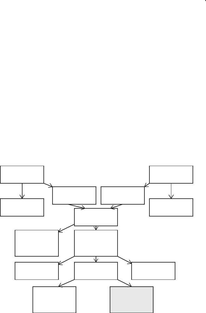
k
k k
k
Data Handling in Practice 227
detailed a data dictionary is, the easier we can expect the data cleaning tasks to
be. However, data dictionaries are often incomplete – for example, it is com-
mon to find levels or missing value indicators in the data that are not listed in
the dictionary. In some cases, the dictionary is just wrong; this might happen
when you are provided an outdated version, for example. All you can do in this
case is to try to communicate with the data provider and make some educated
guesses. We talk about the role of judgment in the next section.
e second sort of documentation in a data cleaning effort is the documenta-
tion that you generate to describe what you did. At a very minimum, you should
produce your R scripts and any custom functions that you wrote as part of the
effort – and, like all scripts and functions, these should be laid out in a clear
way, with enough comments that a new user can figure out what you did.
More often we produce a real write-up, just for the data handling effort,
laying out all of the steps that we took in text, rather than just as R comments.
It is particularly important to list actions that resulted in observations being
deleted, with reasons and counts. In fact, most of our reports include a
flowchart describing the number of observations at each step in the data
cleaning process. Figure 7.1 shows an example of such a chart. In this example,
observations came from two sources, as shown in the upper corners. A small
number of observations are deleted because they lack payment information;
Western Office
134,246
Eastern Office
96,442
Western w/Pay
133,845
No Pay Info
401 (0.3%)
No Pay Info
262 (0.3%)
Merged
230,025
Match to
archive
220,967
No archive
match
9,058 (3.9%)
RCODE = “XX”
1,123 (0.5%)
RCODE = “??”
864 (0.4%)
Good RCODE
218,980
Start Date >=
2016-08-31
17,288 (7.8%)
Ready for
modeling
201,692
Eastern w/Pay
96,180
Figure 7.1 Example population flowchart.

k
k k
k
228 A Data Scientist’s Guide to Acquiring, Cleaning, and Managing Data in R
then the two remaining sets of observations are merged into one data set of
230,025 observations. In subsequent cleaning steps, we lose observations that
fail to match back to a particular archive, that have unexpected values of a
field called RCODE, and whose start dates are too recent. e rectangle in the
bottom right gives the number of observations that have survived the different
cleaning steps.
We also recommend that you create, as one of your products, a master table
with every key and the disposition of the record for that key (in our example,
“no payment information,” “illegal RCODE,”etc.).atwayyouandthesponsor
can quickly identify the outcome associated with every record.
Perhaps the most important goal of the documentation that you produce is
to make the data handling process “reproducible.” at is, any R user should be
able to take your data, and your scripts and functions, run through the data han-
dling process from beginning to end and produce exactly the same output that
you did. Sometimes, this will be impossible – if, for example, you are acquiring
data from a database that gets updated frequently. But usually you want to think
of this as a requirement. In fact, it may be worth moving your data, scripts, and
functions to a new directory (or even a new machine, perhaps with a different
operating system) and re-running your handling process there, to ensure that
you aren’t, for example, relying on variables in your R environment that won’t
be present in the new directory.
Notice that the ordering of the steps will affect the numbers in the flowchart.
Suppose that some of the rows were both missing payment information and
also had illegal RCODEs. en the counts associated with those two exclusions
will depend on the order in which they are applied. In this case, we would
expect the final count to be the same regardless of the order of the operations
(although the master table may change). However, in other cases, particularly
those involving judgment (next section), we have to expect that two different
data cleaners will end up with two slightly different data sets, depending on the
choices they make.
7.7 The Role of Judgment
e data scientist is confronted with data and with rules for preparing it, and
yet inevitably is called on to exercise his or her judgment during the cleaning
process. As an artificial example, imagine a data set called indat that included
city names and two-letter state abbreviations. As part of the data cleaning pro-
cess you, as the analyst, construct a table of the length (i.e., nchar())ofthe
abbreviations, expecting to see every entry with the value 2. However, you find
that a number of state abbreviations in fact have four characters each, so you
tabulate the set of state abbreviations with four characters. So far, your code
might look like this:

k
k k
k
Data Handling in Practice 229
table (nchar (indat$State))
24
9203 84
table (indat$State[nchar (indat$State) == 4])
CITY
84
Something seems to have gone wrong here. You tabulate the values in the
City field for the 84 records whose State field has the CITY value, and you
see this:
table (indat$City[nchar (indat$State) == 4])
NEW YORK
84
At this point, the issue seems clear: these 84 records presumably should have
been recorded as “city =‘New York’, state =‘NY’ ” but instead were recorded
as “city =‘New York’, state =‘City’.” Having identified the issue, though, some
steps remain. Are the data suppliers aware of this anomaly? ey will need to
be informed, maybe right away if fresh data is required, but maybe, for com-
paratively unimportant problems, in the final project documentation. Does this
error suggest that other fields in those same records are less reliable? Is it accept-
able to change the state for these 84 records to NY? Are there other entries
correctly labeled “city =‘New York,’ state =‘NY’ ” (or “city =’New York City,’
state =‘NY’ ”), and, if so, do these differ from the mislabeled ones, perhaps in
terms of date?
Issues like this arise in almost every data cleaning problem. e analyst has
the responsibility of alerting the data provider as to problems, but she must
also forge ahead. e most important rule is that everythingmustbedocu-
mented. Documentation will appear in the code, but it must also be in the
human-readable materials returned to the client. We are always wary of mak-
ing changes to our customers’ data, and yet we very often end up doing just
that – informing the customer of what changes were made, why, and how many
records were affected.
One more place where the analyst’s judgment can be required is in miss-
ing value handling. Some missing values appear to have arisen more or less
at random; the rest of the record and entries for that field in other records are
generally not missing. Missing values like these can often be incorporated into
the modeling process.
Other records might have almost all missing entries. Since these carry almost
no information, they will often need to be discarded. On the other hand, fields
for these observations that are present might be informative about some items
of interest. For example, if a set of records, missing most fields, contains age and
sex information, those values might be useful when assessing the population of
customers, even if they are not useful for modeling outcomes. So, at each stage,

k
k k
k
230 A Data Scientist’s Guide to Acquiring, Cleaning, and Managing Data in R
it is important to report the number of observations used for any particular
graph, table, or statistic.
Often values marked as missing actually indicate something. For example,
one field might carry information about whether a customer has ever declared
bankruptcy. Suppose that such a field has only two unique values: Yand
the missing value NA, and suppose that only a few percent are marked Y.It
mightbereasonabletojudgethatNA was recorded for customers with no
bankruptcy, change those to N, and proceed (documenting this change, of
course, and reporting it). Now suppose that this field had three distinct values:
Ymaking up, say, 2% of the values, Nmaking up 94%, and NA accounting for
the remaining 4% of values. Here, the way forward is not as clear.
Judgment arises when combining the levels of categorical values. For
example, one field might record whether an applicant rents a home, owns
it, lives with parents, or has some other housing situation; imagine that the
documentation specifies that these choices will be represented with values R,
O,P,andX, respectively. Suppose that when you tabulate that field, you find
about 60% Rvalues, 20% Ovalues, 10% Pvalues, and 3% Xvalues; but you also
find 4% r, in lower-case, and 3% missing values. Even though ris not listed
as a possible choice, it seems reasonable to assign them to the Rgroup, with
corresponding documentation to be included in the final report. On the other
hand, if instead of rthe value had been J, we might have made a different
choice. And what about the missing values? Since Ris the most common
group, it will under some circumstances make sense to insert an Rinto those
records. Alternatively, since missing value is “other than R,O,orP,” we might
move those items with missing values into the Xgroup – or we might create a
new label called Missing. e path to take has to depend on the frequency
of anomalous entries, the frequencies of the existing entries (as, here, where R
isthemostcommon),andtheultimategoalsoftheanalysis,andthesecallfor
the analyst’s judgment in consultation with the data providers.
7.8 Data Cleaning in Action
In this section, we demonstrate some of our approaches on some data inspired
by a real problem we investigated. is data concerns somewhat more than 100
homes in the eastern part of the United States. It comes in the form of three
CSV files, which you can find in the cleaningBook package. Each property
is described by its size (in number of bedrooms and number of bathrooms),
the state in which it is located, and its area (in square feet). is information
is held in two separate files, named BedBath1.csv and BedBath2.csv.
e electrical usage, measured at a meter, for each property has been recorded
over six consecutive calendar quarters. is information is held in a third file,
EnergyUsage.csv, which should include all the homes in the first two files.

k
k k
k
Data Handling in Practice 231
Homes are identified by a serial number, which consists of one of the letters
A,H,orP, followed by three digits and then a “trailer” made up of three more
digits; trailers are one of 001 through 009.
e ultimate goal of the effort was to model the changes in electrical usage
acrosstime,particularlyinspecificsubsetsofhousesthataresimilarinterms
of their size and location. e goal of the data cleaning portion is simply to
combine the three data sets into one that is suitable for the modeling effort. In
the following sections, we handle each file one at a time.
7.8.1 Reading and Cleaning BedBath1.csv
Reading
Since the BedBath1 file has a name ending in .csv,itseemsreasonableto
presumethatitiscomma-separated.Wemightstartusingscan() to extract
and examine a few rows of the file, but very often we wade right in with the
hope that the first call will produce the desired result. In this case, we start with
acalltoread.csv() and then show a few rows. Recall that this function calls
read.table() with quote= "\"" and comment.char = "" as well
as sep = ",".
> bb1 <- read.csv ("BedBath1.csv", stringsAsFactors = FALSE)
> bb1[1:4,]
SerText Bed Bath SqFt State
Prop # P477005 and land 3 3 1580 PA
H644009 as identifier 3 2 1/2 1490 CT
House Num H260008 2 1 910 CT
Property A834009 house and land 2 1 1/2 980 CT
We have learned a few things here. First, it appears that we have encountered an
embedded comma problem – the fourth row has one more entry than the oth-
ers. As a result, the text from the first column has been made into row names. If
any row had had too many commas, read.csv() would have failed. Second,
the numbers for Bath must be text because they include entries like 2 1/2.
We may want to convert that number to 2.5. ird, the property identifier is
enclosed inside some text, and not in a consistent location from row to row.
We will need to extract the ID from the surrounding text.
e first thing to handle is the embedded comma. Let us double-check by
extracting the first few rows of text using scan() toensurethatthatis,infact,
the issue. is code shows how we might do that.
> bb1 <- scan ("BedBath1.csv", sep = "\n", what = "")
Read 77 items
> bb1[1:5]
[1] "SerText,Bed,Bath,SqFt,State"
[2] "Prop # P477005 and land,3,3,1580,PA"

k
k k
k
232 A Data Scientist’s Guide to Acquiring, Cleaning, and Managing Data in R
[3] "H644009 as identifier,3,2 1/2,1490,CT"
[4] "House Num H260008,2,1,910,CT"
[5] "Property A834009, house and land,2,1 1/2,980,CT"
ere really is a comma after the property ID, and before the word “house,” in
thefifthline.Inthenextstep,weusecount.fields() to see how frequently
there is one extra comma and to examine what rows with extra commas look
like.
> table (count.fields ("BedBath1.csv", sep = ",",
comment.char = ""))
56
66 11
> bb1[6 == count.fields ("BedBath1.csv", sep = ",",
comment.char = "")]
[1] "Property A834009, house and land,2,1 1/2,980,CT"
[2] "Property P589004, house and land,3,3,1560,NY"
[3] "Property P450001, house and land,3,2,1400,PA"
:::
[8] "Property A303001, house and land,3,2,c. 1460,PA"
:::
All 11 of the lines with 6 fields include the “house and land” notation. So we
will just remove the first comma from each of those 11 lines. Notice also that
in the eighth line the square footage value, c. 1460, is not numeric. We will
need to address this shortly. First, though, we remove the first comma in each
of the over-long lines using sub().enwecanpasstheresultasthetext
argument to read.csv() to produce a data frame.
> comm <- (6 == count.fields ("BedBath1.csv", sep = ",",
comment.char = ""))
> bb1[comm] <- sub (",", "", bb1[comm])
> bb1 <- read.csv (text = bb1, stringsAsFactors = FALSE)
> bb1[1:4,]
SerText Bed Bath SqFt State
1 Prop # P477005 and land 3 3 1580 PA
2 H644009 as identifier 3 2 1/2 1490 CT
3 House Num H260008 2 1 910 CT
4 Property A834009 house and land 2 1 1/2 980 CT
In the first command, we located the rows with six fields (i.e., five commas). In
the second, we removed those commas. After the call to read.csv() in the
third line, we can see that the fields appear to line up, at least in the first few
rows.Wemoveontothecleaningstep.
Cleaning
Now we examine the classes of the columns using a call to sapply().

k
k k
k
Data Handling in Practice 233
> sapply (bb1, class)
SerText Bed Bath SqFt State
"character" "integer" "character" "character" "character"
is final command shows that the Bed field has been recognized as
integer, which suggests that the fields are properly lined up. It also confirms
our previous observation that the Bath and SqFt columns will need to be
cleaned in order to make them numeric.
Now let us extract the ID from the SerText field. Since we know that the
ID consists of an A, H, or P followed by six digits, we can extract the ID with a
regular expression, as shown in the next code segment.
> (bb1$ID <- regmatches (bb1$SerText,
regexpr ("[AHP][[:digit:]]{6}", bb1$SerText)))
[1] "P477005" "H644009" "H260008" "A834009" ...
> table (is.na (bb1$ID))
FALSE
76
> table (nchar (bb1$ID))
7
76
e second command, of course, shows us that no IDs are missing, and the
third, that every ID has seven characters. We might look further into the ID
values by ensuring that they all really do start with A, H, or P, that they all end
with a three-digit number of the form 00x, and so on.
As to the Bath column, we can use sub() to replace every instance of 1/2
with .5. Notice how the text to be replaced includes the space that separates
the two parts of, for example, 21/2. After that substitution, we should be
able to convert the column to numeric. We will create a new variable with the
numeric version of Bath first, to ensure that the conversion went successfully.
is code shows how we can compare the original Bath with the newly con-
structed version.
> bath <- as.numeric (sub (" 1/2", ".5", bb1$Bath))
> table (bath, bb1$Bath, useNA = "ifany")
bath 1 1 1/2 2 2 1/2 3
1 5 00 00
1.50 180 00
20 018 00
2.5 0 0 0 20 0
30 00 015
We can tell that this conversion has succeeded by examining the table, and we
can see that there are no missing values in the bb1$Bath column. As a result,
we can replace the Bath column in the data set with the bath variable just
constructed, as we do here.

k
k k
k
234 A Data Scientist’s Guide to Acquiring, Cleaning, and Managing Data in R
> bb1$Bath <- bath
e final preparatory step for this data involves addressing the non-numeric
entries in the SqFt column. e non-numeric entries, of course, would be
turned into NA by as.numeric(). e following command shows how we
can use this fact to show the set of non-numeric SqFt entries.
> bb1[is.na (as.numeric (bb1$SqFt)),"SqFt"]
[1] "∼1510" "c. 970" "∼1460"
[4] "c. 1470" "c. 920" "approx. 1510"
[7] "∼1580" "c. 1460" "∼1600"
[10] "∼1560" "approx. 1440" "∼1460"
[13] "approx. 1450"
Warning message:
In ‘[.data.frame‘(bb1, is.na(as.numeric(bb1$SqFt)), "SqFt"):
NAs introduced by coercion
In another example, there might have been too many to view, but here we can
see that the non-numeric entries come in three types: those that start c.,those
that start ∼,andthosethatstartapprox.enextsteprequiressomejudg-
ment. We will elect to remove the qualifiers and report the square footage using
the integer given; but we would certainly report this choice.
One way to extract the numeric part is, as before, with a regular expression.
In the first command, as shown below, we search for a sequence of digits, and
then use regmatches() to extract that sequence. is produces a character
vector we name sqft. en, we extract the values of sqft,whichcorrespond
to non-numeric entries in the original bb1$SqFt vector. We display the first,
second, and the sixth elements of that subset to ensure that each different sort
of “approximate” notation is corrected properly.
> sqft <- regmatches (bb1$SqFt,
regexpr ("([[:digit:]]+)", bb1$SqFt))
> sqft[is.na (as.numeric (bb1$SqFt))][c(1, 2, 6)]
[1] "1510" "970" "1510" # warning message suppressed
Now that sqft appears to contain the correct value for every row, we can con-
vert it into a numeric vector and assign the result to the SqFt column of bb1.
is code shows that operation, together with the first few rows of the modified
data frame.
> bb1$SqFt <- as.numeric (sqft)
> bb1[1:3,]
SerText Bed Bath SqFt State ID
1 Prop # P477005 and land 3 3.0 1580 PA P477005
2 H644009 as identifier 3 2.5 1490 CT H644009
3 House Num H260008 2 1.0 910 CT H260008
Our data cleaning for this file is nearly complete. e SerText column is
redundant but not otherwise bothersome. However, a few checks remain.

k
k k
k
Data Handling in Practice 235
First, we examine the classes of the column to ensure they are as we
expect – character for the first and last two, numeric for the others. Sec-
ond, we look for duplicated rows and duplicated ID values. We could use
any(duplicated()) here, but we are in the habit of using table().at
way, if there are duplicates, we know how many are there.
> sapply (bb1, class)
SerText Bed Bath SqFt State
"character" "integer" "numeric" "numeric" "character"
ID
"character"
> table (duplicated (bb1)) # duplicated rows?
FALSE
76
> table (duplicated (bb1$ID)) # duplicated IDs?
FALSE TRUE
75 1
Apparently there is a duplicated ID. Let us determine its value and then extract
the rows for that ID.
> bb1$ID[duplicated (bb1$ID)]
[1] "P888009"
> bb1[bb1$ID == "P888009",]
SerText Bed Bath SqFt State ID
23 Property ID P888009 2 1.5 920 PA P888009
49 P888009 as identifier 2 1.5 920 PA P888009
e good news is that these two rows are identical except for the original
SerText. It is almost certainly safe to delete one of the two. Still, the fact
of the duplication might reveal something about the process by which the
data has been collected, stored, or transmitted, and it should be reported. e
following commands show how we might delete one of these two rows as
well as the SerText column. We examine the dimensionality, mostly for our
awareness. Finally, we tabulate the State column, again just for our general
awareness.
> bb1 <- bb1[-23,] # using row number from above
> bb1[bb1$ID == "P888009",] # double-check!
SerText Bed Bath SqFt State ID
49 P888009 as identifier 2 1.5 920 PA P888009
> bb1$SerText <- NULL # delete columns
> dim (bb1)
[1] 75 5
> table (bb1$State, useNA = "ifany")
CT NY PA
28 17 30

k
k k
k
236 A Data Scientist’s Guide to Acquiring, Cleaning, and Managing Data in R
Deleting row 23 is a quick operation, but it is slightly dangerous, in that if it were
inadvertently repeated a different row would be (wrongly) removed. It might be
safer to use a command like
> bb1 <- bb1[-(which (bb1$ID == "P888009")[2]),]
Here, if there is a second row with the given ID, it will be removed. If not, the
value of which(bb1$ID == "P888009")[2] will be NA, and the attempt
to compute bb1[-NA,] will produce an error.
As a final cleaning step for this data frame we might examine our summary
statistics for our numeric columns (Bed and SqFt), looking for missing and
anomalous values – but in this case, it may make sense to wait until the final
data set has been constructed.
7.8.2 Reading and Cleaning BedBath2.csv
Reading
We continue the data cleaning exercise by reading the BedBath2.csv file.
As before, it is not implausible that everything will be well formatted, so we call
read.csv() and examine the first few lines.
> bb2 <- read.csv ("BedBath2.csv", stringsAsFactors = FALSE)
> bb2[1:3,]
[1] "P957001\t3\t2\tNew York\t1440"
[2] "H429005\t2\t1.5\tNew Jersey\t950"
[3] "P226003\t2\t1.5\tNew York\t930"
Apparently this file, despite having a name that ends in .csv,isinfact
tab-separated. Naturally we try again, adding sep = "\t" to read.csv()
as shown here. (We might just as well have used read.table() or
read.delim().) We also examine the dimension of the resulting data frame
and the classes of its columns.
> bb2 <- read.csv ("BedBath2.csv", sep = "\t",
stringsAsFactors = FALSE)
> bb2[1:3,]
PropId Bed Bath State Size
1 P957001 3 2.0 New York 1440
2 H429005 2 1.5 New Jersey 950
3 P226003 2 1.5 New York 930
> dim (bb2)
[1] 40 5
e data frame appears to have been constructed successfully.
Cleaning
A natural first step in the cleaning process, as with bb1, is to examine the classes
of the columns. is code shows how we can do that.

k
k k
k
Data Handling in Practice 237
> sapply (bb2, class)
PropId Bed Bath State Size
"character" "integer" "numeric" "character" "integer"
We see a few things here. First, the IDs, called PropId here, seem to be whole
(at least, in the first few rows). We might use table(nchar(bb2$PropId))
to examine them further. e Bath and Size columns are properly numeric,
as well. e State entries are full names rather than two-letter postal
codes, but this is easily handled. e data appears to have been read in
properly. Let us look for duplicate keys, both within this data set and between
the two.
> table (duplicated (bb2))
FALSE
40
> table (duplicated (bb2$PropId))
FALSE
40
> length (intersect (bb1$ID, bb2$PropId))
[1] 0
Our 40 PropId values are distinct, and they do not overlap with any of the ID
values in bb1. In order to join the two bb datasets,wewillneedtoconvertthe
two-letter state codes into state names, or vice versa. Let us tabulate the bb2
state codes.
> table (bb2$State, useNA = "ifany")
Connecticut New Jersey New York
10 15 15
It seems reasonable to convert these state names to their corresponding
two-letter codes. We could construct an ad hoc cross-reference table for this
purpose, but we can just as easily construct a table of state names and codes
from the built-in R objects state.name and state.abb. e following
code shows how we can build this cross-reference table.
> state.xref <- data.frame (Name = state.name,
Abbr = state.abb, stringsAsFactors = FALSE)
> state.xref[1:3,] # check
Name Abbr
1 Alabama AL
2 Alaska AK
3 Arizona AZ
Now we use match() to extract the row numbers of state.xref where the
entries of bb2$State are found. Extracting the Abbr entries for those row
numbers produces the desired two-letter codes. We call that vector of codes
state.2 and cross-tabulate it with the original State values as a check.

k
k k
k
238 A Data Scientist’s Guide to Acquiring, Cleaning, and Managing Data in R
> state.2 <- state.xref$Abbr[match (bb2$State,
state.xref$Name)]
> table (state.2, bb2$State, useNA = "ifany")
state.2 Connecticut New Jersey New York
CT 10 0 0
NJ 0 15 0
NY 0 0 15
Sincethathasworked,wecannowreplacetheState values with the
state.2 vector. e following command completes the data cleaning for
BedBath2.csv.
> bb2$State <- state.2
It may be worth noting, particularly for readers accustomed to SQL, that we
could have “joined” the bb2 and xref tables with merge(),asinthisexample.
> merge (bb2, state.xref, by.x = "State", by.y = "Name",
all.x = TRUE)
is command produces one row for every entry in bb2,sinceall.x = TRUE.
e State column of bb2 is matched with the Name column of state.xref.
7.8.3 Combining the BedBath Data Frames
We can now stack the two bb data frames vertically; they have the same
columns, of the same type, with the same values. We need only to ensure that
the column names match. To do that, we can rename the PropId and Size
columns of bb2 to ID and SqFt,soastomatchbb1 (or, of course, vice versa).
We need not re-order the columns; the rbind() function for data frames will
take care of that. is code shows the renaming, and the call to rbind() that
produces the final BedBath data set.
> names (bb2)[names (bb2) == "PropId"] <- "ID"
> names (bb2)[names (bb2) == "Size"] <- "SqFt"
> bedbath <- rbind (bb1, bb2, stringsAsFactors = FALSE)
Notice that to identify the first column to rename we use [names (bb2) ==
"PropId"] rather than [1].eID column is column number 1, but perhaps
in another iteration it might end up in a different position. Relying on the name,
rather than the number, is safer.
Once we have the combined data set, we should examine it. It is always a
good idea to check for missing values, to count the number of unique entries,
construct a few more tables, and compute summary statistics. e following
commands show a few of the computations that might perform in this example.
> sapply (bedbath, function (x) sum (is.na (x)))
Bed Bath SqFt State ID
00000

k
k k
k
Data Handling in Practice 239
> sapply (bedbath, function (x) length (unique (x)))
Bed Bath SqFt State ID
3 5 35 4 115
> with (bedbath, table (Bed, Bath), useNA = "ifany")
Bath
Bed 1 1.5 2 2.5 3
27250 00
30 0312123
40 00 80
> summary (bedbath$SqFt)
Min. 1st Qu. Median Mean 3rd Qu. Max.
860 985 1450 1334 1495 1690
e first command shows that this data set has no missing values. e sec-
ond shows, first, that the ID numbers are unique, as intended, and that there
are only 35 distinct values of SqFt. ese values were rounded, so this is not
implausible. e cross-tabulation of Bed and Bath is also plausible, with bigger
houses having both more bedrooms and more bathrooms. Finally, the sum-
mary() of the SqFt column shows no obvious anomalies.
7.8.4 Reading and Cleaning EnergyUsage.csv
Reading
Now we read in the data set with the energy usage data. We start with
read.csv() as before.
> kwh <- read.csv ("EnergyUsage.csv",
stringsAsFactors = FALSE)
> kwh[1:3,]
Serial X2016.Q1 X2016.Q2 X2016.Q3 X2016.Q4
1 A594-005 2271.074 2245.196 2767.31 3713.24
2 P957-001 3565.268 3255.392 2880.485 3446.105
3 H625-003 2919.32 2334.8498 2821.3652 #N/A
X2017.Q1 X2017.Q2
1 3647.2811 3499.3139
2 3440.72 3485.93
3 #N/A #N/A
> sapply (kwh, class)
Serial X2016.Q1 X2016.Q2 X2016.Q3
"character" "character" "character" "character"
X2016.Q4 X2017.Q1 X2017.Q2
"character" "character" "character"
e file appears to be comma-delimited, but the “energy usage” columns are
all of mode character. For at least the last few, this must be, at least in part,
due to the #N/A missing value code. Recall that R produces valid column names

k
k k
k
240 A Data Scientist’s Guide to Acquiring, Cleaning, and Managing Data in R
when it reads data in. In this case, it has added the letter Xto the front of column
names like 2016.Q1; we will continue to use those modified names.
Let us read the data again, specifying that value as the missing value string.
We also observe that the Serial field looks as if it contains the ID,butwitha
hyphen.
> kwh <- read.csv ("EnergyUsage.csv", na.strings = "#N/A",
stringsAsFactors = FALSE)
> kwh[1:3,]
Serial X2016.Q1 X2016.Q2 X2016.Q3 X2016.Q4
1 A594-005 2271.074 2245.196 2767.310 3713.240
2 P957-001 3565.268 3255.392 2880.485 3446.105
3 H625-003 2919.320 2334.850 2821.365 NA
X2017.Q1 X2017.Q2
1 3647.281 3499.314
2 3440.720 3485.930
3NANA
e data has been properly read in. Some missing values remain, and we will
keep our eye on them to see, if, for example, they arise more frequently in some
time periods or locations than in others.
Cleaning
We start by examining the classes just as before.
> sapply (kwh, class)
Serial X2016.Q1 X2016.Q2 X2016.Q3
"character" "numeric" "numeric" "numeric"
X2016.Q4 X2017.Q1 X2017.Q2
"numeric" "numeric" "numeric"
Since the columns all have the expected class, we turn our concern to the
Serial field. We will need to remove the hyphen to get these values to match
up with bedbath.iscodeusessub() to perform that task.
> kwh$Serial <- sub ("-", "", kwh$Serial)
> kwh$Serial[1:4] # check
[1] "A594005" "P957001" "H625003" "P462004"
at conversion seems to have succeeded, although as before we might look
more deeply. Let us now look for duplicate rows, duplicate keys, and duplicate
values within columns.
> table (duplicated (kwh)) # duplicate rows?
FALSE
116
> table (duplicated (kwh$Serial)) # duplicate keys?

k
k k
k
Data Handling in Practice 241
FALSE TRUE
115 1
> sapply (kwh,
function (x) length (unique (x))) # duplicate values?
Serial X2016.Q1 X2016.Q2 X2016.Q3 X2016.Q4 X2017.Q1 X2017.Q2
115 112 108 104 103 94 95
LetusstartwiththeitemwiththeduplicatevalueofSerial. As we did before,
we will extract both the rows for this Serial value.
> kwh$Serial[duplicated (kwh$Serial)]
[1] "P888009"
> kwh[kwh$Serial == "P888009",]
Serial X2016.Q1 X2016.Q2 X2016.Q3 X2016.Q4
16 P888009 NA NA 2797.175 3700.685
88 P888009 2244.566 2526.494 2797.175 3628.685
X2017.Q1 X2017.Q2
16 NA 3608.844
88 4310.686 3608.844
First, we note that the duplicated key is the same one that was duplicated in the
bed and bath data. Second, the two rows for this key are not identical, as they
were there. Our inclination is to drop the first of these two rows, reasoning that
they are equal when not missing, except in one place. Again, this is a judgment
we make pending communication with the data provider. In this next piece of
code we remove row 16, identified as the first of the duplicates.
> kwh <- kwh[-(which (kwh$Serial == "P888009")[1],]
e issue of duplicates within columns is subtler. Each of the numeric columns
has at least a few duplicate values, and this is probably not surprising. We might
expect a few matches just by coincidence. However, there may be a trend toward
more duplication as we move to the right of the data set. In the next line, we use
the table(table()) approach to examine the frequency of common values.
If common values are just coincidence, then most likely we would see sets of
pairs, each with a common value, rather than a group of four or five entries with
the very same value.
> table (table (kwh$X2017.Q2))
16
93 1
ere is, in fact, a set of six observations with the very same value in the
X2017.Q2 column. is seems unexpected. In this code, we display those six
observations.
> which (6 == table (kwh$X2017.Q2))
4847.51
50

k
k k
k
242 A Data Scientist’s Guide to Acquiring, Cleaning, and Managing Data in R
> kwh[!is.na (kwh$X2017.Q2) & kwh$X2017.Q2 == 4847.51,]
Serial X2016.Q1 X2016.Q2 X2016.Q3 X2016.Q4
31 P308007 4059.905 3875.015 3034.91 3990.26
44 H958007 3771.095 5358.575 3034.91 3990.26
48 H419006 5360.750 1078.055 NA NA
60 H619001 3570.185 2400.890 3034.91 3990.26
112 A542003 2126.240 2951.270 3034.91 3990.26
116 A436004 1181.540 2951.270 3034.91 3990.26
X2017.Q1 X2017.Q2
31 4512.2 4847.51
44 4512.2 4847.51
48 4512.2 4847.51
60 4512.2 4847.51
112 4512.2 4847.51
116 4512.2 4847.51
e value 50 returned from the which() command just indicates that the
entry of interest happened to be the 50th entry in the table. We are more inter-
ested in the duplicated value, which is 4847.51. We can see that a number of
properties have the same value not just for the X2017.Q2 column but for oth-
ers as well.
Once again the analyst needs to come to some judgment as to how to pro-
ceed. In the real-life case from which this example was derived, we were able
to communicate with the data provider and learn that these readings were esti-
mated on occasions when meters could not be read, the estimation deriving
from an average of a set of properties. We continued constructing the data,
documenting our findings.
7.8.5 Merging the BedBath and EnergyUsage Data Frames
e two data sets are nearly ready to merge. ey have keys in the same format
and issues with the data have been resolved. All that remains is to ensure that
the two sets of keys do, in fact, refer to the same properties. In this code, we
tabulate the number of keys in bedbath that appear in kwh,andviceversa.
> table (is.element (bedbath$ID, kwh$Serial))
TRUE
115
> table (is.element (kwh$Serial, bedbath$ID))
TRUE
115
Wheretherearenoduplicates,weneednotdothisinbothdirections–butwe
recommend it anyway. Since all the keys match, we can now merge the two data
sets by the Serial and ID keys. is code shows how we construct the final
data set for this example.

k
k k
k
Data Handling in Practice 243
> properties <- merge (kwh, bedbath, by.x = "Serial",
by.y = "ID")
> properties[1:4,] # Check
Serial X2016.Q1 X2016.Q2 X2016.Q3 X2016.Q4 X2017.Q1
1 A195008 4226.522 3961.223 4117.505 4683.680 NA
2 A255003 3558.008 3512.932 3645.375 4182.305 5108.536
3 A294008 3897.872 3352.718 2073.440 3013.130 3644.720
4 A301008 3327.296 3365.249 2997.545 5168.420 4151.660
X2017.Q2 Bed Bath SqFt State
1 7022.795 2 1.0 950 NY
2 5695.186 3 2.5 1460 CT
3 3590.420 3 2.5 1510 NY
4 3080.435 3 2.0 1430 NJ
Our properties data set is complete and appears to be clean, although it still
has missing values. Moreover, we have not examined the usage numbers very
carefully. ese following commands give examples of the sorts of analyses we
might perform to examine these numbers. We start by creating a vector Xcols
to identify the columns of usage – that is, the ones whose names start with X.
> Xcols <- grep ("X", names (properties), value = TRUE)
> sapply (properties[,Xcols], function (x) sum (is.na (x)))
X2016.Q1 X2016.Q2 X2016.Q3 X2016.Q4 X2017.Q1 X2017.Q2
46571516
> sapply (properties[,Xcols], range, na.rm = T)
X2016.Q1 X2016.Q2 X2016.Q3 X2016.Q4 X2017.Q1 X2017.Q2
[1,] 976.010 881.09 680.1299 680.690 1138.697 2123.470
[2,] 5847.704 10267.73 5448.1001 8484.425 9307.250 8421.106
e number of NA values increases slightly with increasing quarter, ending up
at about 10% of the rows. In the second command, we compute the range of
each column. e maxima of the usage values increase, but none are negative
or otherwise obviously anomalous.
We might also compute other summary statistics, like, for example, typi-
cal usage by state. For one quarter’s usage, this is easy to compute using the
tapply() function, as we demonstrate in the first command as follows. e
second command shows how this might be computed simultaneously for every
quarter.
> tapply (properties$X2016.Q1, properties$State, mean,
na.rm = TRUE)
CT NJ NY PA
3123.335 3321.658 3416.334 3237.445
> sapply (properties[,Xcols], function (qtr) {
tapply (qtr, properties$State, mean, na.rm=TRUE)})

k
k k
k
244 A Data Scientist’s Guide to Acquiring, Cleaning, and Managing Data in R
X2016.Q1 X2016.Q2 X2016.Q3 X2016.Q4 X2017.Q1 X2017.Q2
CT 3123.335 2776.943 2871.059 4005.165 4461.140 4918.352
NJ 3321.658 2953.894 2892.502 3922.922 4445.038 4556.398
NY 3416.334 3120.687 3056.265 4043.530 4602.037 5085.058
PA 3237.445 3092.234 3239.677 3996.064 4669.660 4829.615
is last command loops over the columns whose names appear in Xcols,
calling tapply() for each one. e results are assembled into a matrix auto-
matically. We might plot this matrix; we might plot usage by square footage for
each state or quarter; we might examine the distributions of values by quarter,
perhaps with boxplots; and so on. After some investigation like this, we can
now begin the modeling process. is would be the stage at which to convert
the State column into a factor variable.
We note here that our final product consisted of one row per property. To
strictly conform with the notion of “tidy” data from Chapter 1, in which each
usage observation occupies one row, one more transformation is necessary. We
know that the final data set will have 115 ×6=690 rows. e usage entries
will come from the Xcols columns. We can extract these using the stack()
function, which both produces the vector of 690 usage entries, and also includes
a second, factor vector identifying the source of the usage by name. is code
shows how we might do this.
> stack.output <- stack (properties, Xcols)
> stack.output
values ind
1 4226.522 X2016.Q1
2 3558.008 X2016.Q1
3 3897.872 X2016.Q1
:::
115 3825.980 X2016.Q1
116 3961.223 X2016.Q2
:::
We can see the transition from values that originated in the X2016.Q1 column
to ones from the X2016.Q2 column after the 115th row. Now we replicate
the remaining columns six times, and attach the result to the stack.output
object.
> usages <- data.frame (
properties[rep (1:nrow(properties), 6),c(1, 8:11)],
stack.output)
> usages[1:3,] # check
Serial Bed Bath SqFt State values ind
1 A195008 2 1.0 950 NY 4226.522 X2016.Q1
2 A255003 3 2.5 1460 CT 3558.008 X2016.Q1
3 A294008 3 2.5 1510 NY 3897.872 X2016.Q1

k
k k
k
Data Handling in Practice 245
After this operation, our new usages datasetis690×7. If we need to
add columns giving the year or the quarter, we can use a command like
usages$Year <- substring (usages$ind, 2, 5).
7.9 Chapter Summary and Critical Data Handling
Tools
is chapter describes some of the practical steps we need to take in a real data
cleaning problem. ese include acquiring the data, cleaning the data, com-
bining cleaned data sets from different sources, and, finally, undertaking any
necessary data preparation steps. All four of these steps require detailed docu-
mentation, both to describe the steps you took and to make them reproducible.
e documentation you produce should also describe steps where you exer-
cised judgment. is might involve deleting records with mostly missing values,
or replacing a small number of missing values with another value. You might
document anomalies on which you took no action at all – for example, if you
observe that all the loans in a data set had dates whose days of the week were
Monday or Wednesday, that might seem peculiar but not impossible, depend-
ing on the business practices of the data provider. Of course, the more you know
about the organization, the data, and the way it is gathered and processed, the
better your judgment can be.
Some data is transactional, meaning that it can reflect multiple observations
for each item of interest. We demonstrate some approaches for handling this
sort of data. While the demonstration requires a certain amount of explanation,
the script to actually perform the tasks requires only a few dozen lines of code.
e final section of the chapter goes through an example of cleaning some
fairly small data sets. is example demonstrated a number of the challenges
that face us in our day-to-day business of handling data: embedded delimiters,
inconsistent key conventions, missing or duplicate values, and so on.
ere are, inevitably, many more ways that data can need cleaning that
the example did not touch upon. It did not, for example, involve data from
non-delimited formats such as Excel, JSON, or XML, or importing data from
a relational database. It did not require us to write a specialized function, nor
did it require the handling of dates or times. Many of these complications are
taken up in the extended exercise in the following chapter, but you should be
aware that data you get will very often involve a combination of input types
and require a number of approaches.

k
k k
k
247
8
Extended Exercise
In this chapter, we set up a guided data cleaning task, from beginning to end.
is data (including the company and personal names and addresses) is entirely
fabricated and is intended only to demonstrate some of the concepts in this
book – but every quirk you see in this data is based on actual data we encoun-
tered doing real projects. Unlike the smaller examples in earlier chapters, these
data sets are large enough so that you cannot spot all of their anomalies by eye.
However, you will be able to open and examine these outside of R – unlike some
ofthedatasetswedealwithinreallife.
is exercise requires time and focus to complete. You will get the most bene-
fit from this book if you read the chapter all the way through and try to perform
all the tasks in the exercise. Part of the exercise is figuring out exactly what needs
to be done at each step and in which order. We have included some “pseu-
docode” – high-level descriptions of the algorithms we used to perform the
tasks – and some hints in Appendix A. However, we recommend you only use
that when you find yourself stuck. e actual code we used to do the cleaning
is available in the cleaningBook package. Again, you will receive the most
benefit when you try to solve the problem in it entirely before looking at our
code – and you may find a different, or better, way of getting the job done.
8.1 Introduction to the Problem
is data comes from a hypothetical client company called Hardy Business
Loans, which lends money to small businesses. Sometimes, the borrower is the
business itself; other times, the borrower is one (or more) of the business’s prin-
cipal owners or partners. e loans are for small- to medium-sized pieces of
equipment: for a restaurant, this might be a pizza oven or espresso maker; for
a trucking business, it might be a truck or a copying machine; for a gardening
business, it might be a backhoe. Hardy Business Loans has acquired portfolios
of loans from two different companies, “Beachside Lenders” and “Wilson and

k
k k
k
248 A Data Scientist’s Guide to Acquiring, Cleaning, and Managing Data in R
Sons,” and inevitably the data for these two different portfolios has different
layouts and fields.
Each portfolio consists of applications and loans, each identified by a key
(although application keys are different from loan keys). Every loan should have
a corresponding application, but some applications do not lead to loans – they
are said to be “unbooked,” whereas those that are made into loans are “booked.”
An application might end up unbooked because the lender declined the appli-
cation, or because the borrower found the money elsewhere, or perhaps for
other reasons.
At the time the application is made, the lender consults several other com-
panies that provide information about the creditworthiness of the borrower.
In real life, these would include various credit reporting agencies, which
supply information about the credit habits and experience of individuals,
and also corresponding repositories of similar information for businesses.
Our “agency” data is modeled on the sorts of data made available from these
reporting agencies.
In many cases, the reporting agencies supply many columns containing
“low-level” data for each customer, and also a single “agency score.” Low-level
data might include, for example, the number of times a customer was 30 days
late on a credit card bill, the number of department store charge cards he or
she has, whether he or she ever declared bankruptcy, and dozens of similar
items. e agency score is a single number intended to rate the customers’
overall creditworthiness that combines all the low-level information using an
algorithm that is typically proprietary. Since Hardy acquires data from several
agencies, each borrower might have several agency scores. Lenders like Hardy
use the scores, but they might want access to the low-level data as well. For
example, a used-car dealer might want to build a custom score that focuses
specifically on borrowers’ past record with car-loan payments. In our case,
the list of variables we need in the output includes a few of these low-level
variables and also all of the agency scores.
8.1.1 The Goal
e goal of the data cleaning exercise is to produce tabular data with one row
per loan and with all the necessary columns of descriptive data. (e set of
columns to be retained will be discussed shortly.) We will also need to report
on observations that were omitted and the reason, whether it was too much
missing data, no matching records in agency data, or something else. We may
need to show the distribution of loans by region of the country and by calendar
quarter, through tables, graphs, and perhaps by other variables as well.
Our output will be in two data frames (or, if you prefer, one big data frame
with records of two types). e first data set comes from the booked loans. For
these loans, we will need to construct the “response variable” for later mod-
eling efforts. is is the measurement that describes the outcome of the loan.

k
k k
k
Extended Exercise 249
In other applications this might be a number, but in this case it will be one of
the levels “Good” or “Bad.” (We give the definitions of those terms used in the
material that follows.) So each row of this part of the output will contain one
of those values as a response, a number of measurements on different variables
(the “predictors”), and perhaps one or more keys that allow the final data to be
linked to the components from which it was built.
e modeling step – which is not part of this exercise – will use the predictor
variables to predict the response variable. If the responses in the booked loans
can be predicted accurately, Hardy Business Loans could use that model as a
screening tool by which to evaluate the risk of new loans or of its portfolio.
In addition to the predictors and the response for booked records, we must
also construct a similar data set using the records from unbooked applications.
By applying the model to the set of unbooked applications, Hardy can learn
about the rates at which it is turning away potentially successful borrowers. Of
course, these unbooked records do not have response variables. But it may be
possible to estimate how unbooked applications would have fared, based on the
statistical model from the booked ones. So we need to prepare the unbooked
applicants and the loans in a common way.
8.1.2 Modeling Considerations
e data sets that we produce at the end of this exercise are a beginning, not an
end. We can expect to make further changes as the modeling proceeds. ese
are the steps we called “preparing data” in Section 7.5. For example, we might
choose to transform a numeric variable by, say, taking its logarithm. Categor-
ical variables may need to be re-grouped, or numeric ones binned. We might
exclude more records as we determine their data to be unreliable. e processes
of cleaning, preparing, and modeling are iterative ones.
Another consideration is that we might want to divide the data into pieces,
one piece (the “training set”) for building models and a second piece (the “test
set”) for evaluating them. is division might be performed at random, with,
say, 30% of the entire data set retained as a test set, but we might also sample
using a more complicated scheme if, say, we wanted the training set to have a
higher proportion of Wilson and Sons loans, or newer loans, than the data as a
whole. In any case, this important consideration is not part of our exercise.
8.1.3 Examples of Things to Check
To the extent possible you should check every column against the data
dictionary. We have intentionally (and, probably, unintentionally) introduced
anomalous entries into the data to mirror the sorts of problems we encounter
in practice. Follow the steps mentioned in Section 7.2 in looking for duplicates
and ensuring that the set of column classes is as expected. Look at the maxima
and minima of numeric and date columns, and tabulate the categorical ones.

k
k k
k
250 A Data Scientist’s Guide to Acquiring, Cleaning, and Managing Data in R
Examining each column in isolation is a good start, but it is also worthwhile
to compare pairs of columns. Of course, there are a lot of pairs and often they
cannot all be checked. But it may be worthwhile to build two-way tables of
important categorical variables, keeping an eye out for unexpected results like
months with almost no observations.
In practice, you will often find that some predictor variables are available
from more than one source. When two offerings of the same variable are avail-
able, you might consult the data provider to see if they are considered to be
equally reliable. As we said in Section 7.2, it is useful to compute the propor-
tion of times that the two agree – often, we find that two versions of a variable
(call them “A” and “B”) have the same values when both are present, but that A is
missing much more often than B. In that case we will use B, possibly augment-
ing its own missing entries by values taken from A. When A and B disagree
on other than missingness, we exercise our judgment in deciding how to move
forward. In this exercise, we do not expect that sort of overlap in variables to
occur–butitdoeshappeninpractice.
8.2 The Data
e data for this exercise needs to be constructed by combining inputs from
seven sources. e sections following this one describe each of these sources
in detail, and give layouts or sample data. e seven sources are as follows:
•the two loan and application portfolios, one from Beachside and one from
Wilson, giving information about the borrower and the product to be pur-
chased with the loan;
•the scores database, giving scores for the borrowers from four agencies,
including a score called “KSC” or “KScore”;
•the co-borrower scores, giving agency scores for co-signers of those loans
that have them;
•a set of updated KScores, which may supersede the KScore in the borrowers’
data;
•a set of loans to be excluded from the final data set; and
•the payment matrix, showing payment information for up to 48 prior billing
periods.
Figure 8.1 shows a diagram of one process that can be used to construct
the final data. e loan and application portfolios (two left items, top row)
contain the information about borrowers and loans. e layouts of these tables
are described in Section 8.4. ese tables include low-level predictors; these
will then be joined to the scores database (Section 8.5), shown in the top
center-right of the figure, which contains the agency scores for the loans and
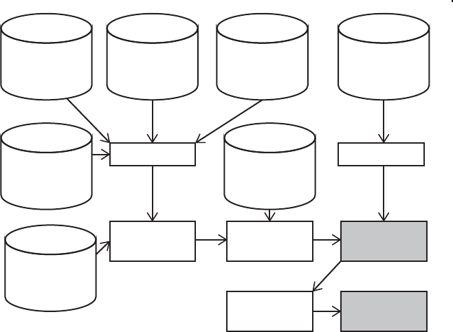
k
k k
k
Extended Exercise 251
Ta b l e
Fixed
JSON
Co-borrower
scores
Beachside
predictors
Wilson
predictors Scores Payment
matrix
XML
Exclusions
Ta b l e
Predictors Response
Cleaned
data
Final data
for models
Updated
predictors
Final
predictors
Updated
KScores
Select
Good/Bad
Ta b l eSQL
Figure 8.1 Schematic of the data cleaning process for the example data.
applications in the two portfolios. Some loans have co-borrowers; those scores
are supplied in the co-borrowers data (Section 8.6), shown at center left in
the figure.
ere are then two modifications that need to be imposed on the data. First,
a set of updated KScores (bottom left of figure) is available; loans and applica-
tions appearing in that data set may have to have their KScore values updated
(see Section 8.7). In addition, a small number of loans and applications should
be excluded from the modeling effort, based on some exclusion data (middle
right of picture). We apply this exclusion as the last step in generating the pre-
dictors, because the excluded records need to be updated anyway, for a later
effort, which is not part of this exercise. e payment matrix (Section 8.9),
shown at top right, is used to generate the response variable for the model-
ing process. e algorithm described in that section can be used to determine
whether the performance of a loan was “Good,” “Bad,” or “Indeterminate.” e
final data set will include only those loans whose performance was “Good” or
“Bad.” e final set of predictors is joined with the response (for the booked
records that have one) to produce the cleaned data (gray box, mid-lower right).
Finally, we exclude unbooked records or those whose response was “Indetermi-
nate” to produce the subset of records that will be used in the initial modeling
effort (bottom right of figure).

k
k k
k
252 A Data Scientist’s Guide to Acquiring, Cleaning, and Managing Data in R
8.3 Five Important Fields
ere are five fields that are vital to this exercise, which are as follows:
Application Number: A 10-digit number identifying the application. Every
application has a unique application number, and application numbers
should be distinct between the two portfolios.
Loan Number: A field identifying the loan for booked applications. In the
Wilson portfolio, the loan number is supposed to consist of a six-digit
customer identification, followed by a three-digit “instance” number. e
instance number starts at 001 and increases when a previous customer
receives a second or third loan. In some cases, though, the instance is
missing. In that case 001 can be used. e Beachside portfolio identifies
loans by a six-digit number with no instance. It is possible for the same
six-digit number to be used in both portfolios, purely by happenstance,
which, combined with the fact that some Wilson loans do not have instance
numbers, means that six-digit loan numbers are not necessarily unique.
Application Date: e date on which the application was completed. For the
purposes of evaluating unbooked loans in the modeling process, we must
restrict ourselves to using only information that was available by this date.
So if a particular unbooked application is dated November 30, 2016, we will
ignore scores, co-borrower information, and updated KScores recorded after
that date.
Loan Date: e date on which a loan is “booked” (made official). For booked
loans, scores and other updated information recorded after this date should
be ignored.
Active Date: We will use the term “active date” to identify the application date
for unbooked applications and the loan date for booked loans. is date is
important because it marks the date on which a decision is made, and agency
scores, for example, that are recorded after the active date will need to be
ignored. Unlike the other important fields, active date has to be inferred.
8.4 Loan and Application Portfolios
e two portfolios acquired by Hardy Business Loans come from two sources:
Beachside Lenders and Wilson and Sons. Both sets of data provide low-level
reporting agency data recorded at or before the active date for both unbooked
applications and loans.
e data for Beachside Lenders appears as an Excel workbook named
Beach.xlsx in the newer .xlsx format. Data for the Wilson portfolio
comesinanExcelworkbooknamedwilson.xls in the older .xls format.
e Wilson data can contain multiple loans for one borrower (although each

k
k k
k
Extended Exercise 253
has a separate application number). We might treat these multiple loans as if
they are independent (although they are not), or we might keep only the most
recent ones (although in that case we presumably lose some information), or
we might try combining multiple loans for the same borrower. In any case, the
number of multiple borrowers is so small that it will almost certainly make
no difference. For this example, we will keep all of the loans as if they are
independent.
Most of the variables that we need to extract or, in some cases, construct,
for the modeling effort are given in Table 8.1 and are laid out in the following
three sections. e table lists the desired columns both by the Beachside names
and by their Wilson names, which are, inevitably, different. e two layouts
in the following sections, and Table 8.1, serve as the data dictionary (Section
7.6) for the loan and application portfolios. In theory, you would hope that the
data dictionary would give a complete and accurate description of the data.
In our example, though – just as in real life – you may find slight discrepan-
cies between what the dictionary says the data should look like, and what is
actually in the data. Finding these discrepancies and adjusting for them – and
documenting them – is part of the exercise!
8.4.1 Layout of the Beachside Lenders Data
e Beachside portfolio contains information about 23 attributes of 8621 loan
applications. ose 23 columns are described here. A number of columns, such
as the Dbl and KAK columns in the final entry on the list, contain information
that is never used. is is a common occurrence.
•APP_NO,APP_DT,LOAN_NO,LOAN_DT: Application number and applica-
tion date for every entry; loan number and loan date for booked loans
•STAT: e status of the application (Booked, Decline, TUD; see below)
•CUST_NM,CUST_ADD1,CUST_CT,CUST_ST,CUST_ZIP: Name, address,
city,state,andZIPcodeofcustomer
•TOT_COST,LOAN_AMT: Total cost of equipment and amount of loan
•GCORP,Local: Used to construct “credit risk” (see section 8.4.3)
•TIB: Time in business, in years
•ASSET_NEW: T if the equipment was to be purchased new, F if purchased
used
•BUS_TYPE,ASSET_TYPE,Dbl,KAK,Folds,JL,2BC,MM ? :Unused.
e STAT column describes the status of the loan. For booked loans, this
will be “Booked.” For unbooked applications, this can be either “Decline,”
meaning that the lender declined to make the loan, or “TUD,” which indicates
that the borrower “Turned Us Down.” is happens either because a borrower
finds more favorable terms elsewhere, or changes her mind about whether
the purchase is necessary (or goes out of business or another unusual event
takes place).

k
k k
k
254 A Data Scientist’s Guide to Acquiring, Cleaning, and Managing Data in R
8.4.2 Layout of the Wilson and Sons Data
e Wilson data has 10,587 rows and 23 columns. Most of these columns
carry the same information as in the Beachside portfolio, though with different
names. e Wilson columns are shown here.
•Appl Number,Appl Date,Loan Number,Loan Date: Application
number and date for every entry; loan number with instance and loan date
for booked loans
•Application Status: Application status, like the STAT column from
Beachside. Values are Approved (booked), Declined, Incomplete (equivalent
to “TUD” in Beachside)
•Customer Name,City,State,Zip: Identification of customer
•Total Cost,Net Loan Amount: e cost of the equipment and the size
of the loan
•GC Indicator,Local Cred: Used to construct “credit risk”
•Business Start Date: Date on which business began operating
•New/Used Indicator: Indicates whether the equipment being pur-
chased is “New” or “Used”
•Customer Type,Equipment Class,CVR Indicator,Reclass
Indicator,Minimum GM,2nd Gen PP,GS Indicator:Unused.
8.4.3 Combining the Two Portfolios
Table 8.1 shows the columns required for the modeling effort that can be found
in, or derived from, the two portfolios or the additional data. In a real example,
we might keep dozens, scores, or even hundreds of columns, some formed by
transforming or combining others. For each column in the final data set, we
give the corresponding columns in the two loan portfolios: “derived” denotes
columns that need to be constructed, using details that follow the table. Just as
in real life, we will need to combine columns with different names and values
that nonetheless represent the same underlying measurement.
e Time in Business field measures the amount of time that the borrower
has been in business – in other words, its age (in years). In the Beachside case,
this is given directly, in years, by the TIB column. In the case of Wilson, we
will need to deduce this from the date that the business was reported to have
started, given by the Business Start Date column. e age is the time between
the business start date and the active date (i.e., the Loan Date for booked loans,
the Application Date for unbooked ones).
e Region column represents the census region associated with each state.
Table 8.2 gives a table showing which state (by abbreviation) is assigned to
which region. is information is also available in the cleaningBook pack-
age in a more convenient form, as a 50-row data frame called state.tbl.
Observations from locations not in any region (such as Canada or Puerto Rico)
should be given the value “Other” for the Region field.

k
k k
k
Extended Exercise 255
Table 8.1 Columns required for predictive model
Name Beachside Wilson Notes
App Number APP_NO Appl Number Application number
App Date APP_DT Appl Date Application date
Loan Number LOAN_NO Loan Number Loan number (if booked)
Loan Date LOAN_DT Loan Date Loan date (if booked)
AppStat STAT Application Booked, declined,
Status or TUD
Time in Business TIB Derived Time in business
State CUST_ST Customer Customer state/province
State
Region Derived Derived Customer region (see notes)
Cost TOT_COST Total Cost Total equipment cost
Loan Amount LOAN_AMT Net Loan Loan amount
Amount
Down Derived Derived Down payment (numeric)
New/Used ASSET_NEW New / Used New/used indicator: T
Indicator (“new”) or Fin Beachside,
New or Used forWilson
CredRisk Derived Derived Credit risk (see notes)
Source Derived Derived Beachside or Wilson
Co-borrower Derived Derived (see notes)
Table 8.2 State abbreviations by census region
Region State
Midwest IL,IN,IA,KS,MI,MN,MO,NE,ND,OH,SD,WI
Northeast CT,ME,MA,NH,NJ,NY,PA,RI,VT
South AL,AR,DC,DE,FL,GA,KY,LA,MD,MS,NC,OK,SC,TN,
TX, VA, WV
West AK,AZ,CA,CO,HI,ID,MT,NV,NM,OR,UT,WA,WY
e loan amount is usually smaller than the equipment cost, since most
customers will make a down payment or trade in an older piece of equipment.
e Down column is computed as Cost −Loan Amount; this may be useful in
a predictive model since companies that can make large down payments may
be healthier – or, alternatively, a large down payment may leave them short
on cash.

k
k k
k
256 A Data Scientist’s Guide to Acquiring, Cleaning, and Managing Data in R
e CredRisk credit rating is derived from two other columns present in the
portfolio files. First, the GCORP or GC variable gives the borrower a letter grade
from A(the highest score) to D.Second,theLocal score gives a number from
1(the highest) to 3. We will need to create a new credit risk predictor by com-
bining those two indicators into a single column with values A1,A2,A3,B1,
andsoon–exceptthatC3 and all the Dratings should be combined into a
single level called X.
e co-borrower indicator shows whether an applicant has a co-borrower.
is is determined by the existence of co-borrower scores in the data of
Section 8.6. Application numbers for which co-borrowers appear in that data
should be given a co-borrower value of TRUE, and all others should be given
the value FALSE.
8.5 Scores
Each customer may have been assigned scores by the different agen-
cies.Primaryborrowers’scoresarestoredinanSQLiterepositorycalled
scores.sqlite, accessible via SQL (see Section 6.3). Agencies report
scores fairly frequently, and customers’ scores can change from time to time.
For each customer, we want the score that was the most recent at the time
of the active date. Scores that are recorded after the active date are not to be
used in our modeling efforts. However, the active date is not part of the scores
database; it comes from the loan and application portfolios. In our example,
each customer can have scores from up to four agencies. ese scores have the
names “Rayburn,” “KScore,” “J&G,” and “NorthEast.” Valid values for scores
are 200–899, so values outside this range should be ignored.
In the database, customers are identified by an eight-digit customer number,
which is not the same as an application or loan number. e database contains a
table named CScore containing this customer number, the agency scores, and
the month associated with the scores. Each customer may have many records,
one for each reporting month, so this table does not have a unique key (although
one could be created by combining the customer number and month). A second
table, CusApp, links customer numbers to application numbers. e following
section shows the layouts of these tables.
8.5.1 Scores Layout
e four agency scores are supplied in the scores database as an SQLite repos-
itory. e repository contains two tables. e layouts are shown in Tables 8.3
and 8.4. In the “format” columns, each 9 corresponds to a digit, and YYYYMM,
of course, corresponds to a four-digit year and two-digit month. e CScore
table holds the scores. Each set of four scores corresponds to a single month,
given in the ScoreMonth field.

k
k k
k
Extended Exercise 257
Table 8.3 CScore table
Name Format Description
Customer 99999999 Customer number
RAY 999 ree-digit Rayburn score
JNG 999 ree-digit J&G score
KSC 999 ree-digit KScore
NE 999 ree-digit NorthEast score
ScoreMonth YYYYMM Month associated with scores
Table 8.4 CusApp table
Name Format Description
Customer 99999999 Eight-digit customer number
Appl 9999999999 Ten-digit application number
e CusApp table cross-references the customer number to the application
number.
8.6 Co-borrower Scores
Some personal borrowers specify co-borrowers, who are other individuals
who co-sign for the loan, thereby promising to pay the lender if the original
borrower defaults. Borrowers with co-borrowers might be expected to be
more likely to pay the loan back, on average, depending, perhaps on the
creditworthiness of the co-borrower. Co-borrowers have their own agency
scores; that information (for both of the portfolios) is stored in the text file
called CoBorrScores.txt. is file consists of a series of transactional
records, each co-borrower being represented by between three and a few
dozen records. Records come in different types, the different types being
indicated by the three-letter sequence starting in position 9. e first record
for each co-borrower is the master record with three-letter sequence J01.is
J01 record contains the application number associated with that co-borrower,
in character positions 20–29. Any other characters in the J01 line can
be ignored.
All the records for a single co-borrower will be on separate lines following
the J01 record. ese other records can be of several types; for our purposes,
we are interested only in records of type ERS, which give co-borrower scores.

k
k k
k
258 A Data Scientist’s Guide to Acquiring, Cleaning, and Managing Data in R
Records with types other than J01 or ERS should be ignored. Each ERS record
reports a score type (with Rayburn, KScore, J&G, and NorthEast being abbre-
viated by RAY,KSC,JNG,andNTH, respectively), the score value, and a score
date in format MM/DD/YYYY (and followed by other information not needed
forthisexercise).Foreachco-borrowerwewantthelatestvalueofeachscore
that precedes the active date, except that, as before, only scores in the range
200–899 should be used. e following section shows examples of the records
in the co-borrower file for a particular co-borrower.
8.6.1 Co-borrower Score Examples
Co-borrowers can have different numbers of records; the only way to tell that
we have seen all the records for a particular individual is by observing that
the next record has type J01 (except for the very last co-borrower in the
file). As with the scores database, we want to extract from the co-borrower
file the agency scores immediately before the active date, and, again, the
active date is not found in the file. Here are some example records from the
CoBorrScores.txt file; assume that these are the only records for this
co-borrower.
SuppDat J01 AppNum 3385219170 Source 2151 Seq 661 Mod1 N ...
SuppDat BBR Check 2 Center 21 Audit F ...
SuppDat ERS NTH 720 10/31/2016 Mod N Report1 YNY
SuppDat ERS JNG 692 12/12/2016 Mod Y Report1 YYY
SuppDat ERS NTH 999 12/31/2016 Mod N Report1 NNY
SuppDat FOE OfcCode 22X OfcState NY OfcReg 22 OfcHold N...
SuppDat ERS RAY 999 10/31/2016 Mod Y Report1 NNN
SuppDat ERS NTH 717 11/30/2016 Mod N Report1 YNY
In this example, we see scores for application number 3385219170. e second
and sixth lines have codes BBR and FOE; these lines should be ignored. e
JNG score has the single entry 692, and that pair of score and date should be
retained. e RAY score is given as 999, so no Rayburn score is retained for this
co-borrower. ere are three reports of a score of type NTH; of these, the most
recent has value 999 and should be ignored. So two (score, date) pairs need to
be returned for the NTH score for this co-borrower. erefore, this co-borrower
should be associated with a total of three pairs of scores and dates. e actual
NTH score entered into the final database will depend on the active date for
this application. If the active date is October 30, 2016 or earlier, none of the
three NTH rows in the example apply, and no NTH score will be used. If the
active date is between October 31, 2016 and November 29, 2016, the third row
of the example (the first of the NTH rows) applies, and the NTH score for this
co-borrower should be reported as 720. Finally, if the active date of the applica-
tion is November 30, 2016 or later, the last row of the example applies and the
NTH score should be reported as 717.

k
k k
k
Extended Exercise 259
8.7 Updated KScores
e scores database includes a column called KSC,whichreportsKScores,
one of the agency scores to be used in the modeling. Many of these KScores
are missing in the original scores database. However, in the time since that
database was assembled, the lenders have acquired a new set of KScores
from the vendor of KScores, and they want to insert those scores into the
predictor data frame. ese scores are delivered as JSON records in one file
named KScore.update.json. (Technically, a file with a set of valid JSON
records is not itself valid JSON, but there you have it.) is file is small enough
that it can be read into memory all at once, though if it were not we could
certainly read one line at a time in the style of the examples in Section 6.2.
Updated KScores refer to primary borrowers only, not to co-borrowers. Not
every customer will have an updated KScore, and some updates will refer to
customers not in our analysis. e appid field in a JSON record will introduce
an application number, but those application numbers have been treated as
numeric, with leading zeros inadvertently removed. JSON records with fields
called KScore will be relevant, as long as the score is between 200 and 899.
Eachrecordwillcontainafieldcalledrecord-date; scores whose values of
record-date are more recent than the active date of the application in ques-
tion should also be ignored. If there is more than one update for a particular
account, we should use the more recent among those whose record-date
value precede the active date for this account. e KScore.update.json
file may contain other fields, too, including values of other scores, but those
scores, too, should be ignored. Only the KScore and its corresponding date
and application number are of interest for this portion of the data preparation.
8.7.1 Updated KScores Layout
e values of KSC retrieved from the scores database described in the pre-
vious section need to be updated for those applications that appear in the
KScore.update.json file. is file consists of a set of entries (“messages”)
in JSON format. Messages that do not include a field named KScore are not of
interest. From those that do, we will extract the application identifier (appid,
with leading zeros truncated), the score itself (KScore,representedasastring)
and the date associated with the score (record-date, in MM-DD-YYYY
format).
Example messages might look like this:
{"appid":"442480", "Rayburn":"721", "NorthEast":"999",
"record-date":"09-20-2016"}
{"appid":"621877", "KScore":"999", "J&G":"744",
"record-date":"03-31-2016"}
{"appid":"3826", "Rayburn":"699", "KScore":"685",

k
k k
k
260 A Data Scientist’s Guide to Acquiring, Cleaning, and Managing Data in R
"J&G":"701", "record-date":"10-03-2016"}
{"appid":"3826", "KScore":"676", "record-date":"12-19-2016"}
Here, the first record would be ignored, because no KScore is reported, and the
second would be ignored because the KScore has an invalid value. e third and
fourth records might cause the KScore for application number 0000003826
to be updated. If that application’s active date (application date for unbooked
loans, loan date for booked ones) was earlier than October 3, 2015, no update
is performed; if the application’s date is between October 3 and December 19,
2016, the KScore for that application would be updated to 685; if the applica-
tion’s date was later than December 19, 2016, the KScore for that application
would be updated to 676.
8.8 Loans to Be Excluded
e lender has specified that a small number of loans be excluded entirely
from the modeling effort. e loans to be excluded are among those for which
XML files are found in the Excluders directory. Each XML file corresponds
to one loan, identified by that loan’s application number in the <APPID> field.
Any XML file that contains a field called <EXCLUDE>, for which the value
of the <EXCLUDE> field is “Yes” or “Contingent,” should be excluded. e
<EXCLUDE> field, if it exists, will be found inside an element named DATA.
Applications that do not appear in XML files, or whose XML files do not have
an <EXCLUDE> field, or whose values of <EXCLUDE> are other than Yes or
Contingent, should not be excluded on the basis of their XML data.
8.8.1 Sample Exclusion File
Here, we present a sample file of the sort in the exclusion directory. is file
would lead to the exclusion of application number 0134292005, since the value
of the EXCLUDE field is Yes. Other fields in the XML files can be ignored.
<?xml version="1.0"?>
<rpt><CLASS2 type="a">Supp</CLASS2><APPID>0134292005</APPID>
<DATA><PRELIM>Yes</PRELIM><CR2>25167</CR2>
<EXCLUDE>Yes</EXCLUDE><CATCODE>36H</CATCODE></DATA>
</rpt>
8.9 Response Variable
In this section, we describe how to construct the response variable for our mod-
eling effort. is is the measurement that describes the outcome of the loan. In
other applications this might be a number, but in this case it will be one of
the levels “Good,” “Bad,” or “Indeterminate.” We will construct these values

k
k k
k
Extended Exercise 261
from the payment matrix contained in the Payments.txt file. For each loan
(identified by a payment identifier found in the portfolio files), this fixed-width
file contains information about the last 48 months. For each month, the file
records four items: the amount paid, the amount delinquent (which can accu-
mulate from month to month), the billing date, and the number of months since
the account was last fully paid. Each payment record also carries a 10-digit
application identifier.
e file will carry zeros in all four fields for any month earlier than the loan
origination date. For example, a loan that was 10 months old will have 10 sets
of payment information (from 1 month ago, 2 months ago, etc.) preceded by 38
sets of zeros. e layout of this file comes to us in the following COBOL code,
which we provide because on some occasions our documentation has come to
us in the form of COBOL specifications like this one:
001000 01 PAY-LAYOUT.
001100 05 APPID PIC X(10).
001200 05 FILLER PIC X(01).
001300 05 PAYMENT-REC OCCURS 48 TIMES.
001400 10 AMT-PD PIC S9(9)V99.
001500 10 AMT-DELQ PIC S9(9)V99.
001600 10 BILL-DATE PIC 9(8).
001700 10 MONTHS-SINCE-PAID PIC 999.
Even without knowing COBOL, you can probably deduce that this record
starts with a 10-character payer identifier called APPID. e PIC X(10)
tells us to expect 10 alphanumeric characters. e 11th character, indicated by
FILLER, can be ignored. en there follow 48 instances of four fields each.
PIC 9 clauses indicate numeric values, so the S9(9)V99 tells us that, for
each of the first two fields, we can expect a sign (positive or negative, or a
space which also indicates a positive value) and a numeric value of 11 digits,
with an “implied” decimal point before the last 2 digits. at is, no actual
space is set aside for the decimal point; dollar amounts are represented in
pennies, but the layout tells the program where the decimal point is supposed
to be. (is sort of storage was very common in COBOL, a language that is
no longer widely used.) e third element in each set is an eight-digit date,
in YYYYMMDD format, and the fourth is a three-digit number giving the
number of months that the account was past due. e months are in order in
every set, with the least recent month being associated with the first set of four
values and the most recent being the 48th. Examples of this data might look,
in part, like the line in the following example. ese lines are very long; for
display purposes, we have wrapped lines around the page so that two lines in
the display correspond to one line of the file.
0034344639 00000000000 0000000000000000000000
00000000000 0000000000000000000000...

k
k k
k
262 A Data Scientist’s Guide to Acquiring, Cleaning, and Managing Data in R
0048268540 00000860623 0000000000020101214000
00000000000 0000086062320110114001...
In this example, the first account did not have a loan 48 months ago, so the val-
ues for that month are all zeros. e second customer paid $8606.23 (AMT-PD
with a space for the sign and the implicit decimal point) in the first month. She
was not delinquent, so the AMT-DELQ field carries a space for the sign and then
11 zeros. e billing date for that payment was 2010-12-14, and the customer
was up to date, so the “months since paid” field carries the value 000. In the
second month, with billing date 2011-01-14, the customer paid nothing and
was delinquent by $8606.23; during that month, the “months since paid” field
had the value 001. Each row will have a total of 48 of these 33-character sets of
payment records.
We are now ready to define our response variable. Of course, this will nor-
mally be defined by the client (in this case, Hardy Business Loans) rather than
the data cleaner. For this example we will implement these rules, which are han-
dled in priority order, so that, for example, a customer who meets the criterion
of rule 1 is not considered by a later rule.
1) Any customer whose loan is six or fewer months old is considered Inde-
terminate.
2) A customer who is ever 3 months delinquent, or who is 2 months delinquent
on two different occasions, is Bad.
3) A customer who is ever more than $50,000 delinquent is Bad.
4) Customers who meet none of these criteria are Good.
Since the payment file has a fixed format, it is natural to read it into R with
read.fwf() (Section 6.1.7), although if the file were huge it might be more
efficient to read it line by line and decode it ourselves.
8.10 Assembling the Final Data Sets
e final product from this exercise should be two data sets, one with booked
loans whose outcome is not “Indeterminate,” and one with all other applica-
tions – or, if you prefer, one combined data set containing both booked and
unbooked applications.
8.10.1 Final Data Layout
At the conclusion of the exercise, each data set should consist of these pieces:
•Identifying information for each entry: application number; application
portfolio (Beachside or Wilson); loan number (if any); loan and application
dates, or a single column giving the active date.

k
k k
k
Extended Exercise 263
•e value of the response variable (“Good” or “Bad”) for loans. For the
unbooked applications we can omit this column, or we might create an
empty column so that the two data sets have exactly the same set of columns.
•e remaining columns from Table 8.1.
•Four columns of agency scores, with a suitable indicator to denote missing
scores, and with KScores updated as appropriate. It might be of value to keep
the corresponding score dates for documentation purposes.
•Four columns of agency scores for co-borrowers, again with a suitable indi-
cator of missingness, and possibly including corresponding dates for these
scores as well. For observations without co-borrowers, of course, all of these
co-borrower scores will be missing.
It is also important to keep track of your code and your assumptions. You will
also want to construct a table giving, for each application number found in any
source, its ultimate disposition – whether it appears in the final data set or was
deleted, and, if so, why. You may also want to construct a flowchart like the one
in Figure 7.1.
8.10.2 Concluding Remarks
e exercise in this chapter is intended to bring together a number of the
skills and techniques described throughout the book. If you can complete the
exercise in a satisfactory way, we think we are well on your way to mastering
the important skills of data cleaning.
Having said that, let us assure you that there are many ways to do data
cleaning in general, and this exercise in particular. After the authors devised
the data for this book, we set out to do the exercise separately. We took quite
different paths: one of us started with Beachside, then moved on to Wilson,
and then combined the two data sets into one to create the first big data set of
the exercise. e other went column by column through Table 8.1, extracting
the Beachside and Wilson versions and cleaning and combining them. One of
us turned dates into Date objectstoensurethattheyweresortedcorrectly;
the other used YYYYMMDD-style text objects, turning them into POSIXt-type
dates as needed. One of us turned “unknown” values for the New/Used column
into “Used,” and the other left them as “unknown.” Of course, in real life
we would have tried to refer the question of what action to take to the data
provider, and possibly to whomever will be doing to modeling as well. Despite
our different approaches, our final products agreed almost exactly – “almost”
because of the judgments made in handling the small numbers of unexpected
values. For the purposes of evaluating our exercise, we worked separately. In
real data cleaning work, though, you will probably find it helpful to work in a
small group, or at least to show your work to a colleague who can understand
and comment on the steps.

k
k k
k
264 A Data Scientist’s Guide to Acquiring, Cleaning, and Managing Data in R
When we originally wrote this exercise, it had more steps. e additional
ones, inspired though they were by real data we analyze, were tedious
and repetitive, so we took them out. But just because they are not in the
exercise doesn’t mean your data cleaning tasks won’t be filled with tedious,
detail-oriented actions. For example, you might look at the BUS_TYPE and
ASSET_TYPE columns in the Beachside portfolio, which match up, more
or less, to the Customer Type and Equipment Class columns in the
Wilson one. In order to include those columns in the final output you need to
examine the set of labels in the two portfolios and decide how to match them
up. For any one column from two sources this task is easy enough, but given
dozens of these the workload can be intimidating.
We said at the beginning of the book that data cleaning might take up 80%
of the time we devote to a project. It is not always fun or glamorous, but it
always needs to be done properly. In order to be good at data cleaning in
R, you will need to understand what data is available, and how it is represented.
You will need to be familiar with the different formats in which data arrives,
and how to combine data from different sources. Perhaps most importantly
you will need to know at least a little about how the data is collected and how
it is intended to be used. One of the great things about being a data scientist
is that you get to learn at least a little bit about a lot of fields, and a lot of that
learning comes from practicing with real data.

k
k k
k
265
Chapter 8 described a data handling task involving acquiring data from
spreadsheets, a database, JSON, XML, and fixed-width text files. e formats
and layouts of the data are documented in that chapter. In this appendix,
we give some extra hints about how to proceed. We recommend trying the
exercise first, without referring to this appendix until you need to.
Some of these hints come in the form of “pseudocode.” is is the program-
mer’s term for instructions that describe an algorithm in ordinary English,
rather than in the strict form of code in R or another computer language. e
actual R code we used can be found in the cleaningBook package.
A.1 Loan Portfolios
Reading, cleaning, and combining the loan portfolios (Section 8.4) is the first
task in the exercise, and perhaps the most time-consuming. However, none of
the tasks needed to complete this task is particularly challenging from a tech-
nical standpoint.
If you have a spreadsheet program such as Excel that can open the file, the
very first step in this process might be to use that program to view the file. Look
at the values. Are there headers? Can you see any missing value codes? Are some
columns empty? Do any rows appear to be missing a lot of values? Are values
unexpectedly duplicated across rows? Are there dates, currency amounts, or
other values that might require special handling?
en, it is time to read the two data sets into R and produce data frames,
using one of the read.table() functions. We normally start with
quote = "" or quote = "\"" and comment.char = "".Youmight
select stringsAsFactors = FALSE, in which case numeric fields in the
data will appear as numeric columns in the data frame. is sets empty entries
in those columns of the spreadsheet to NA and also has the effect of stripping
leading zeros in fields that look numeric, like the application number. As one
Hints and Pseudocode

k
k k
k
266 A Data Scientist’s Guide to Acquiring, Cleaning, and Managing Data in R
alternative, you might set colClasses = "character",inwhichcaseall
of the columns of the data frame are defined to be of type character.Inthis
case, empty fields appear as the empty string "". Eventually, columns that are
intended to be numeric will have to be converted. On the other hand, leading
zeros in application numbers are preserved. From the standpoint of column
classes, perhaps the best way to read the data in is to pass colClasses as
a vector to specify the classes of individual columns – but this requires extra
exploration up front to determine those classes.
Pseudocode for the step of reading, cleaning, and combining the portfolio
data files might look like this. In this description, we treat the files separately.
You might equally well treat them simultaneously, creating the joint data set as
you go.
for each of {Beachside, Wilson}
read in file
examine keys and missing values
discard unneeded columns
convert formatted columns (currencies, dates) to R types
ensure categorical variables have the correct levels
construct derived variables
ensure categorical variables levels match between data sets
ensure column names match between data sets
ensure keys are unique across data sets
add an identifying column to each data set
join data sets row-wise (vertically)
A.1.1 Things to Check
As you will see, the portfolio data sets are messy, just as real-life data is messy.
As you move forward, you will need to keep one eye on the data itself, one eye on
the data dictionary, and one eye on the list of columns to construct. (We never
said this would be easy.) Consider performing the sorts of checks listed here, as
well as any others you can think of. Remember to specify exclude = NULL
or useNA = "ifany" in calls to table() to help identify missing values.
•What do the application numbers look like? Do they all have the expected
10 digits? Are any missing? Are there duplicate rows or duplicate application
numbers? If so, can rows be safely deleted?
•What do missing value counts look like by column? Are some columns miss-
ing a large proportion of entries? Are some rows missing most entries, and,
if so, should they be deleted?
•Do the values of categorical variables match the values in the data dictionary?
Ifnot,arethedifferenceslargeorsmall?Cansomelevelsbeconvertedinto
others? If two categorical variables measure similar things, cross-tabulate

k
k k
k
Hints and Pseudocode 267
them to ensure that they are associated. At this stage, it might be worthwhile
to consider the data from the modeling standpoint. For example, if a large
number of categorical values are missing, it might be worthwhile to create
a new level called Missing. If there are a number of values that apply to
only a few records each, it might be wise to combine them into an Other
category.
•Are there columns with special formatting, like, for example, currency values
that look like $1,234.56? Convert them to numeric.
•Across the set of numeric columns, what sorts of ranges and averages do
you see? Are they plausible? For columns that look like counts, what are the
most common values? Are there some values that look as if they might be
special indicators (999 for a person’s age, 99 or −1 for number of mortgages)?
Consider computing the correlation matrix of numeric predictors to see if
columns that should carry similar information are in fact correlated.
•What format are the date columns in? If you plan to do arithmetic on dates,
like, for example, computing the number of days between two dates, you will
need to ensure that dates use one of the Date or POSIXt classes. If all you
need to do is to sort dates, you can also use a text format like YYYYMMDD,
since these text values will sort alphabetically just as the underlying date val-
ues would. Keeping dates as characters can save you a lot of grief when you
might inadvertently turn a Date or POSIXt object into numeric form. e
date formats are easier to summarize and to use in plots, however. Examine
the dates. Are there missing values? What do the ranges look like? Consider
plotting dates by month or quarter to see if there are patterns.
•Computing derived variables often involves a table lookup. For example, in
the exercise, you can determine each state’s region from a lookup into a table
that contains state code and region code. e cleaning issue is then a matter
of identifying codes not in the table and determining what to do with them.
Once the two loan portfolios have been combined, we can start in on the
remaining data sets. In the sections that follow, we will refer to the combined
portfolio data set as big. When we completed this step, our big data frame
had 19,196 rows and 17 columns; yours may be slightly different, depending on
the choices you made in this section.
A.2 Scores Database
e agency scores (Section 8.5) are stored in an SQLite database. e first order
of business is to connect to the database and look at a few of its records. Do the
extracted records match the descriptions in the data dictionary in Chapter 8?
Count the numbers of records. If these are manageable, we might just as well
read the entire tables into R, but if there are many millions or tens of millions
of records we might be better off reading them bit by bit.

k
k k
k
268 A Data Scientist’s Guide to Acquiring, Cleaning, and Managing Data in R
In this case, the tables are not particularly large. Pseudocode for the next steps
might look as follows:
read Cscore table into an R data frame called cscore
read CusApp table into an R data frame called cusapp
add application number from cusapp to cscore
add active date from big to cscore
discard records for which ScoreMonth > active date
discard records with invalid scores
order cscore by customer number and then by date, descending
for each customer i, for each agency j
find the first non-missing score and date
We did not find a particularly efficient way to perform this last step.
A.2.1 Things to Check
Aswithalmostalldatasets,theagencyscoreshavesomedataqualityissues.
Items to consider include the following:
•What do the application numbers and customer numbers from cusapp look
like? Do they have the expected numbers of digits? Are any duplicated or
missing? What proportion of application numbers from cusapp appears
in big, and what proportion of application numbers from big appears in
cusapp? Are there customer numbers in cscore that do not appear in
cusapp or vice versa?
•Summarize the values in the agency score columns. What do missing values
look like in each column? What proportion of scores is missing? Are any
values outside the permitted range 200–899?
•e ScoreMonth column in the cscore table is in YYYYMM format, with-
out the day of the month. However, the active date field from big has days of
the month (and, depending on your strategy, might be in Date or POSIXt
format). How should we compare these two types of date?
In the final step, we merge the data set of scores with the big data set
created by combining the two loan portfolios. Recall that duplicate keys are
particularly troublesome in R’s merge() function – so it might be worthwhile
to double-check for duplicates in the key, which in this case is the application
number, in the two data frames being merged. Does the merged version
of big have the same number of rows as the original? If the original has,
say, 17 columns and the new version 26, you might ensure that the first 17
columns of the new version match the original data, with a command like
all.equal(orig, new[,1:17]).

k
k k
k
Hints and Pseudocode 269
A.3 Co-borrower Scores
e co-borrower scores (Section 8.6) make up one of the trickiest of the data
sets, because of their custom transactional format (Section 7.4). We start by
noting that there are 73,477 records in the data set, so it can easily be handled
entirely inside R. If there had been, say, a billion records, we would have needed
to devise a different approach. We start off with a pseudocode as follows:
read data into R using scan() with sep = "\n"
discard records with codes other than ERS or J01
discard ERS records with invalid scores
At this point, we are left with the J01 records, which name the application
number, and the ERS records, which give the scores. It will now be convenient
to construct a data frame with one row for each score. is will serve as an
intermediate result, a step toward the final output, which will be a data frame
with one row for each application number. is intermediate data frame will,
of course, contain an application number field. (is is just one approach, and
other equally good ones are possible.) We take the following steps:
extract the application numbers from the J01 records
use the rle() function on the part of the string
that is always either J01 or ERS
Recall that each application is represented by a J01 record followed by a series
of ERS records. If the data dictionary is correct, the result of the rle() func-
tion will be a run of length 1 of J01, followed by a run of ERS, followed by
another run of length of 1 of J01, followed by another run of ERS,andsoon.
So, values 2, 4, 6, and so on of the length component of the output of rle()
will give the number of ERS records for each account. Call that subset of length
values lens. en, we operate as follows:
construct a data frame with a column called Appl,
produced by replicating the application numbers
from the J01 records lens times each
add the score identifier (RAY, KSC) etc.
add the numeric score value
add the score date
insert the active date from big
delete records for which the score date > active date
At this stage, we have a data set with the information we want, except that
some application numbers might still have multiple records for the same
agency. A quick way to get rid of the older, unneeded rows is to construct a
key consisting of a combination of application number and agency (like, e.g.,
3004923564.KSC). Now sort the data set by key, and by date within key, in
descendingorder.Weneedtokeeponlythefirstrecordforeverykey–that

k
k k
k
270 A Data Scientist’s Guide to Acquiring, Cleaning, and Managing Data in R
is, we can delete records for which duplicated(),actingonthatnewly
created key field, returns TRUE.
Following the deletion of older scores, we have a data set (call it co.df)with
all the co-borrower scores, arrayed one per score. (When we did this, we had
4928 scores corresponding to 1567 application numbers.) Now we can use a
matrixsubscript(Section3.2.5)toassembletheseintoamatrixthathasonerow
per application number. We start by creating a data frame with the five desired
columns: places for the JNG,KSC,NTH,andRAY scores and the application
number. It is convenient to put the application number last. Call this new data
frame co.scores. en, we continue as follows:
construct the vector of row indices by matching the
application number from co.df to the application number
from co.scores. This produces a vector of length 4,928
whose values range from 1 to 1,567
construct the vector of column indices by matching the score
id from co.df to the vector c("JNG", "KSC", "NTH",
"RAY"). This produces a vector of length 4,928
whose values range from 1 to 4
combine those two vectors into a two-column matrix
use the matrix to insert scores from co.df into co.scores
A.3.1 Things to Check
As with the other data sets, the most important issues with the co-borrower
data are key matching, missing values, and illegal values. You might examine
points like the following:
•What do the application numbers look like? Do they have 10 digits? What
proportion of application numbers appears in big? In our experience the
proportion of loans with co-borrowers has often been on the order of 20%.
Are there application numbers that do not appear in big? If there are a lot
of these we might wonder if the application numbers had been corrupted
somehow.
•After reading the data in, check that the fields extracted are what you expect.
Do the score identifiers all match JNG, and so on? Are the score values mostly
in the 200–899 range? Do the dates look valid?
•We expect some scores to be 999 or out of range. What proportions of those
values do we see? Are some months associated with large numbers or pro-
portions of illegal score values? Are these any non-numeric values, which
mightindicatethatweextractedthewrongportionoftherecord?
When the co-borrowers data set is complete, we can merge it to big.Since
big already has columns names JNG,KSC,NE,andRAY,itmightbeusefulto

k
k k
k
Hints and Pseudocode 271
rename the columns of our co.score before the merge to Co.JNG and so on.
(At this point, you have probably noticed that the NorthEast score is identified
by NE in the scores database but by NTH in the co-borrower scores. It might be
worthwhile making these names consistent.)
A final task in this step is to add a co-borrower indicator, which is TRUE
when an application number from big is found in our co.scores and FALSE
otherwise. Actually, this approach has the drawback that it will report FALSE
for applications with co-borrowers for which every score was invalid or more
recent than the active date (if there are any). If this is an issue, you will need to
go back and modify the script by creating the indicator before any ERS records
are deleted. is is a good example of why documenting your scripts as you go
is necessary.
A.4 Updated KScores
e updated KScores (Section 8.7) are given in a series of JSON messages. For
eachmessage,weneedtoextractfieldsnamedappid and record-date,if
they exist. We start with pseudocode as follows:
read the JSON into R with scan() and sep = "\n"
remove messages in which the string "KScore" does not appear
write a function to handle one JSON message: return appid,
KScore, record-date if found, and (say) "none" if not
apply that function to each message
Using sapply() in that last command produces a two-row matrix that should
be transposed. Using lapply() produces a list of character vectors of length
2 that should be combined row-wise, perhaps via do.call().Ineithercase,
it will be convenient to produce a data frame with three columns. We continue
to work on that data frame with operations as follows:
remove rows with invalid scores
add active date from big
remove rows for which KScore date is > active date
keep the most recent row for each application id
is final data set contains the KScores that are eligible to update the ones in
big. Presumably, it only makes sense to update scores for which the one is big
is either missing, or carries an earlier date than the one in our updated KScore
data. When we did this, we found 1098 applications in the updated KScore data
set, and they all corresponded to scores that were missing in big. So, all 1098
of these KScore entries in big should be updated. In a real example, you would
have to be prepared to update non-missing KScores as well.

k
k k
k
272 A Data Scientist’s Guide to Acquiring, Cleaning, and Managing Data in R
A.4.1 Things to Check
As with the other data sets, the important checks are for keys, missing, dupli-
cated, and illegal values. In this case, we might consider some of the following
points:
•Are a lot of records missing application numbers? Examine a few to make
sure that it is the data, not the code, at fault. Are any application numbers
duplicated? What proportion of application numbers appears in big?
•Are many records missing KScores? at might be odd given the specific
purpose of this data set. What do the KScores that are present look like? Are
many missing or illegal?
•What proportion of update records carries dates more recent than the active
date? If this proportion is very large, it can suggest an error on the part of the
data supplier.
A.5 Excluder Files
e Excluder files (Section 8.8) are in XML format. We need to read each XML
file and determine whether it has (i) a field called APPID and(ii)afieldcalled
EXCLUDE, found under one called DATA. In pseudocode form, the task for the
excluderdatamightlookasfollows:
acquire a vector of XML file names from the Excluders dir.
use sapply to loop over the vector of names of XML files:
read next XML file in, convert to R list with xmlParse()
if there is a field named "APPID", save it as appid
otherwise set appid to None
if there is a field named "EXCLUDE" save it as exclude
otherwise set exclude to None
return a vector of appid and exclude
e result of this call to sapply() will be a matrix with two rows. It will be
convenient to transpose it, then convert it into a data frame and rename the
columns, perhaps to Appl and ExcCode. Call this data frame excluder.
A.5.1 Things to Check
•Are there duplicate rows or application numbers? is is primarily just a
check on data quality. Presumably, if an application number appears twice in
the excluders data set, that record will be deleted, just as if it had appeared
once.
•Do the columns have missing values?
•Are the values in the ExcCode column what we expect (“Yes,” “No,” “Con-
tingent”)? We can now drop records for which ExcCode is anything other
than Yes or Contingent.

k
k k
k
Hints and Pseudocode 273
•Do the application numbers in excluder match the ones in the big
(combined) data set? Do they have 10 digits? If there are records with no
application number, or whose application numbers do not appear elsewhere,
theycanbedroppedfromtheexcluder data set.
When we are satisfied with the excluder data set, we can remove the
matching rows from big. When we did this, our data set ended up with 19,034
rows and between 30 and 40 columns, depending on exactly which columns
we chose to save.
A.6 Payment Matrix
Recall from Section 8.9 that every row of the payment matrix contains a
fixed-layout record consisting of a 10-digit application number, then a space,
and then 48 repetitions of numeric fields of lengths 12, 12, 8, and 3 characters.
ose values will go into a vector that will define the field widths. We might
also set up a vector of column names, by combining names like Appl and
Filler with 48 repetitions of four names like Pay,Delq,Date,andMo.We
pasted those 48 replications together with the numbers 48:1 to create unique
and easily tractable names. We also know that the first two columns should be
categorical; among the repeaters, we might specify that all should be numeric,
or perhaps that the two amounts should be numeric and the date and number
of months, character.
With that preparation, we are ready to read in the file, using read
.fwf() and the widths, names, and column classes just created. We called
that data frame pay.
Our column naming convention makes it easy to extract the names of the
date columns with a command like grep("Date", names(pay)).For
example, recall that we will declare as “Indeterminate” any record with six
or fewer non-zero dates. We can use apply() across the rows of our pay
data frame, operating just on the subset of date columns, and run a function
that determines whether the number of zero entries is ≤6. (Normally, we are
hesitant to use apply() ontherowsofadataframe.Inthiscase,weare
assured that the relevant columns are all of identical types and lengths.)
Now, we create a column of status values, and wherever the result of this
apply() is TRUE, we insert Indet into the corresponding spots in that vec-
tor. Our code might look something like the following:
set up pay$Good as a character vector in the pay data frame
apply to the rows of pay[,grep ("Date", names (pay))]
a function that counts the number of entries that are
0 or "00000000"
set pay$Good to Indet when that count is <= 6

k
k k
k
274 A Data Scientist’s Guide to Acquiring, Cleaning, and Managing Data in R
Our column naming convention also makes it easy to check our work. For
example, we might pick out some number haphazardly – say, 45 – and look at
the entries in pay for the 45th Indet entry. (is feels wiser than using the
very first one, since the first part of the file might be different from the middle
part.) In this example, our code might look as follows:
pick some number, like, say, 45
extract the row of pay corresponding to the 45th Indet
-- call that rr
pay[rr, grep ("Date", names (pay))] shows that row
Now we perform similar actions for the other possible outcomes. At this
stage, it makes sense to keep the different sorts of bad outcomes separate, com-
bining them only at the end. One bad outcome is when an account is 3 months
delinquent. We apply() a function that determines whether the maximum
valueinanyofthemonthfieldsis≥3. For those rows that produce TRUE,we
insert a value like bad3 into the pay$Good unless it is already occupied with
an Indet value. Again, it makes sense to examine a couple of these records to
ensure that our logic is correct.
Another bad outcome occurs when there are at least two instances of month
values equal to 2, and a third is when the delinquency value passes $50,000. In
each of these cases, we update the pay$Good vector, ensuring that we only
update entries that have not already been set. It is a good idea to check a few of
the records for each indicator as we did earlier.
Records that do not get assigned Indet nor one of the bad values are
assigned Good.Oncewehavetabulatedthebadvaluesseparately,wecancom-
bine them into a single Bad value.isway,wecancomparethefrequencies
of the different outcomes to see if what we see matches what we expect.
A.6.1 Things to Check
erearelotsofwaysthatthesepaymentrecordscanbeinconsistent.e
extent of your exploration here might depend on the time available. But we
give, as examples, some of the questions you might ask of this data.
•What do the application numbers look like? Do they have 10 digits? Are any
missing? Does every booked record have payment information, and does
every record with payment information appear in big?Whatistheright
action to take for booked records with no payment information – set their
response to Indet?
•What are the proportions of the different outcomes? Do they look reason-
able? For example, if 90% of records are marked Indet we might be con-
cerned.
•What do the amounts look like? Are they ever negative, missing, or absurd?
•Are the dates valid? We expect every entry to be a plausible value in the
form YYYYMMDD or else a zero or set of zeros. Are they? Are adjacent dates 1

k
k k
k
Hints and Pseudocode 275
month apart, as we expect? Are there zeros in the interior of a set of non-zero
dates?
•Are adjacent entries consistent? For example, if month 8 shows a delinquency
of 4 months, and month 10 shows a delinquency of 6 months, then we expect
month 9 to show a delinquency of 5 months. Are these expected patterns
followed?
Once the response variable has been constructed, we can merge big with
pay. Actually, since we only want the Good column from pay,wemergebig
with the two-column data set consisting of Appl and Good extracted from
pay. In this way, we add the Good column into big.
A.7 Starting the Modeling Process
Our data set is now nearly ready for modeling, although we could normally
expect to convert character columns to factor first. Moreover, we often
find errors in our cleaning processes or anomalous data when the modeling
begins – requiring us to modify our scripts. In the current example, let us see if
the Good column constructed above is correlated with the average of the four
scores. is R code shows one way we might examine that hypothesis using the
techniques in the book.
> big$AvgScore <- apply (big[,c("RAY", "JNG", "KSC", "NE")],
1, mean, na.rm = T)
> gb <- is.element (big$Good, c("Good", "Bad")) &
!is.na (big$AvgScore)
e gb vector is TRUE for those rows of big for which the Good column has
one of the values Good or Bad,andAvgScore is present, meaning that at least
one agency score was present.
We can now divide the records into groups, based on average agency score.
Here we show one way to create five groups; we then tabulate the numbers of
Good and Bad responses by group.
> qq <- quantile (big$AvgScore, seq (0, 1, len=6),
na.rm = TRUE)
> (tbl <- table (big$Good[gb], cut (big$AvgScore[gb], qq,
include.lowest = TRUE), useNA = "ifany"))
[420,598] (598,649] (649,696] (696,748] (748,879]
Bad 641 620 514 449 384
Good 607 721 811 926 1067
> round (100 * prop.table (tbl, 2), 1)
[420,598] (598,649] (649,696] (696,748] (748,879]
Bad 51.4 46.2 38.8 32.7 26.5
Good 48.6 53.8 61.2 67.3 73.5

k
k k
k
276 A Data Scientist’s Guide to Acquiring, Cleaning, and Managing Data in R
We can see a relationship between agency scores and outcome from the tables.
e first shows the counts, and the second uses prop.table() to compute
percentages within each column. In the group with the lowest average score
(left column), there are about as many Bad entries as Good ones. As we move
to the right, the proportion of Good entries increases; in the group with the
highest average scores, almost 75% of entries are Good ones. is is consistent
with what we expect, since higher scores are supposed to be an indication of
higher probability of good response.

k
k k
k
277
Bibliography
Adler, D., Gläser, C., Nenadic, O., Oehlschlägel, J., and Zucchini, W. (2014) ff:
Memory-Efficient Storage of Large Data on Disk and Fast Access Functions.R
Package Version 2.2-13.
Bache, S.M. and Wickham, H. (2014) magrittr: A Forward-Pipe Operator for R.R
Package Version 1.5.
Bates, D. and Maechler, M. (2016) Matrix: Sparse and Dense Matrix Classes and
Methods. R Package Version 1.2-6.
Couture-Beil, A. (2014) rjson: JSON for R. R Package Version 0.2.15.
Dasu, T. and Johnson, T. (2003) Exploratory Data Mining and Data Cleaning,
John Wiley & Sons, Inc., Hoboken, NJ.
Dowle, M., Srinivasan, A., Short, T., with contributions from Saporta, R.,
Lianoglou, S., and Antonyan, E. (2015) data.table: Extension of Data.frame.R
Package Version 1.9.6.
Dragulescu, A.A. (2014) xlsx: Read, Write, Format Excel 2007 and Excel
97/2000/XP/2003 files. R Package Version 0.5.7.
Eddelbuettel, D. and François, R. (2011) Rcpp: seamless R and C++ integration.
Journal of Statistical Software,40 (1), 1–18.
Feinerer, I., Hornik, K., and Meyer, D. (2008) Text mining infrastructure in R.
Journal of Statistical Software,25 (5), 1–54.
Free Software Foundation (2016) GNU Bash, https://www.gnu.org/software/bash/
bash.html (accessed 19 November 2016).
Kane, M.J., Emerson, J., and Weston, S. (2013) Scalable strategies for computing
with massive data. Journal of Statistical Software,55 (14), 1–19.
Loecher, M. and Ropkins, K. (2015) RgoogleMaps and loa: unleashing R graphics
power on map tiles. Journal of Statistical Software,63 (4), 1–18.
Lucas, C. and Tingley, D. (2014) translateR: Bindings for the Google and Microsoft
Translation APIs. R Package Version 1.0.
Luis (2011) Reading HTML Pages in R for Text Processing, http://www
.quantumforest.com/2011/10/reading-html-pages-in-r-for-text-processing/
(accessed 13 October 2016).
Matloff, N. (2011) e Art of R Programming, No Starch Press, San Francisco, CA.

k
k k
k
278 Bibliography
Ooms, J. (2014) e Jsonlite Package: A Practical and Consistent Mapping Between
JSON Data and R Objects, arXiv:1403.2805 [stat.CO].
R Core Team (2013) R: A Language and Environment for Statistical Computing,R
Foundation for Statistical Computing, Vienna, Austria.
R Core Team (2015) foreign: Read Data Stored by Minitab, S, SAS, SPSS, Stata,
Systat, Weka, dBase,... R package version 0.8-66.
Ripley, B. and Lapsley, M. (2015) RODBC: ODBC Database Access.RPackage
Version 1.3-12.
RStudio Team (2015) RStudio: Integrated Development Environment for R.
RStudio, Inc., Boston, MA.
Temple Lang, D. (2014) RJSONIO: Serialize R objects to JSON, JavaScript Object
Notation. R Package Version 1.3-0.
Temple Lang, D. (2015a) RCurl: General Network (HTTP/FTP/...) Client Interface
for R. R Package Version 1.95-4.7.
Temple Lang, D. (2015b) XML: Tools for Parsing and Generating XML Within R
and S-Plus. R Package Version 3.98-1.3.
Warnes, G.R., Bolker, B., Gorjanc, G., Grothendieck, G., Korosec, A., Lumley, T.,
MacQueen, D., Magnusson, A., Rogers, J. et al. (2015) gdata: Various R
Programming Tools for Data Manipulation. R Package Version 2.17.0.
Wickham, H. (2011) e split-apply-combine strategy for data analysis. Journal of
Statistical Software,40 (1), 1–29.
Wickham, H. (2014) Tidy data. Journal of Statistical Software,59 (10), 1–23, doi:
10.18637/jss.v059.i10.
Wickham, H. (2015) httr: Tools for Working with URLs and HTTP.RPackage
Version 1.0.0.
Wickham, H. and Francois, R. (2015) dplyr: A Grammar of Data Manipulation.R
package version 0.4.3.
Wickham, H. and Grolemond, G. (2016) R for Data Science, O’Reilly, Sebastopol,
CA.
Wickham, H., James, D.A., and Falcon, S. (2014) RSQLite: SQLite Interface for R.R
Package Version 1.0.0.

k
k k
k
279
Index
!operator 23, 33
.C() 167
.GlobalEnv 13
.RData 13, 209
/7, 112, 127
:operator 22
<- 6
?16
[,] 55, 71
drop argument 56
[] 31, 54, 64, 70
[[ ]] 64, 70
#, R comment character 7, 173
#!,see shell scripts
#!Rscript,see shell scripts
$operator 64, 71
%>% 78
%% 156
%in% 47
&and && 26, 218
\ 7, 100, 119, 127
\n100, 184
\r184
\t100
\uand \Ufor Unicode, see UTF-8
\x,see hexadecimal
|and || 26
... 145
0x see hexadecimal
a
addmargins() 43
addNA() 137
adist() 93
agrep() 93
all() 40, 217
all.equal() 91, 94, 217
anyDuplicated() 47
anyNA() 37, 69
aperm() 62
apply() 57
problems on data frames 74–75, 89
apropos() 16
args() 16, 146
arguments, see function
as.character() 135
as.data.frame() 77
as.Date() 80, 202
format argument 81
as.factor() 132, 226
as.logical() 30
as.matrix() 77, 172
as.numeric() 30, 82, 83, 135, 176
units argument 85
as.POSIXct() 85, 202
as.POSIXlt() 84
as.raw() 188, 191
ASCII, see character data type
assign() 138, 150

k
k k
k
280 Index
assigning 35–36, 54, 65, 69, 71
attach() 13, 210
attr() 38, 86
attributes 38
b
backslash, see \
bash command interpreter 95
Beach.xlsx,see data sets
BedBath1.csv,see data sets
BedBath2.csv,see data sets
binary data, see data
browser() 157
buffered output 156
by() 77
c
c() 22, 85, 88
call by reference 149
call by value 149
carriage return, see \r
casefold() 103
cat() 149, 153, 156, 157
cbind() 54, 90, 132
stringsAsFactors argument
90
ceiling() 45
character data type 12, 22, 107
latin1 128
ASCII 101, 128–130
changing case 103
currency 117, 127, 128
encoding 130
leading and trailing spaces 126
character(0) 101
charToRaw() 188
class() 29, 132, 161, 217
clipboard 200–201, 203
close() 189, 194
clusterExport() 166
cmpfun() 165
COBOL 261
CoBorrScores.txt,see data sets
colnames() 56, 68, 179
colon operator, see :operator
colRows() 57
colSums() 57
column names 214
commands as text 139
comment character 7
comparison operators 8, 23, 26
compiling, see functions
complex data type 28
connection 185, 186, 193, 208
converting between data types, see data
type
count.fields() 178
CRAN 2, 14
cross-reference table 225, 237, 254
CSV 172, 177
cumsum() 220
currency, see character data type
cut() 107
d
data
acquiring 3, 4
binary 185, 188–190
HTML 203, 207
JSON 206, 259
large files 184–187, 192
many files 197
other packages 208
provenance 171
relational databases 192–256
serverless, 196
streaming 208
tabular 4, 171
time zones 202
transactional 219–225, 257
via REST API 206
web 203–208
XML 190, 204–206, 260
data frame 8, 67–80
all-numeric 77
assigning 69

k
k k
k
Index 281
column names 68, 73, 78, 90, 109,
179
combining 216
by column, 90, 218
by key, 92, 218, 242–245
by row, 90, 137, 216, 238
comparing 94
missing values 69
operating on columns 74
operating on rows 75
row names 68, 72, 176, 179
subsetting 69–73
UTF-8 in 131
data handling 213
acquiring 213, 231–232, 236–239
cleaning 214–216, 232–238,
240–249
combining, see data frame
documentation 5, 226–229
judgment 228
preparing 225, 249, 275
data sets
Beach.xlsx 252
BedBath1.csv 231
BedBath2.csv 236
CoBorrScores.txt 257, 269
EnergyUsage.csv 239
Excluders directory 260, 272
KScore.update.json 259,
271
Payments.txt 261, 273
scores.sqlite 256, 267
state.tbl 225, 254
wilson.xls 252
data type
character see character data type
complex 28
conversion 24, 27–31, 136,
226
determining 29
factor, see factor
integer 28
logical 23
numeric or double 21, 45
raw 28, 188
data.frame() 67, 90, 132, 218
row.names argument 68
stringsAsFactors argument
68, 76, 90
data.table() 42
date() 86
Date class 80, 174
dates 80–89
Date class 80, 174
and times 83–88
am/pm indicator, 86
differences 83, 86, 88
formatting 80–83, 111
in Excel 202
missing values 88
POSIX classes 83, 174
tabulating 111
time zones, see time zones
dbConnect() 197
dbFetch() 197
dbGetQuery() 197
dbListFields() 197
dbListTables() 197
dbSendQuery() 197
debug() 158
debugonce() 158
delimited files 172–183
deparse() 166
detectCores() 166
diff() 86
difftime() 83
dim() 54, 69
dimnames() 56, 66, 68
do.call() 91, 181
double, see numeric data type
download.file() 198, 204
DSN 193, 196
dump() 152
duplicated() 47, 79
duplicates 47, 79, 214, 235
dyn.load() 167

k
k k
k
282 Index
e
edit() 94, 150, 151
editor 151
ellipsis, see ...
embedded delimiters 175, 231
empty string 101, 175
enableJIT() 165, 167
Encoding() 130
encoding, see character data type
end of line, see \n
EnergyUsage.csv,see data
sets
environment variables 15, 162
Euro currency symbol 129, 131
eval() 140, 166
Excel 81, 101, 175, 200, 201, 252
dates 202
Excluders directory, see data sets
expand.grid() 111
extracting, see subsetting
f
factor
combining 136
levels 132, 133
missing values 133, 137
factor() 132–134, 226
file() 185, 190
file names 7, 112, 127, 162
file operations 185, 186
file.copy() 198
file.info() 162
file.remove() 198
file.rename() 198
fix() 151
fixed-width files 183
floating-point error 11, 23, 30, 79
floor() 45
flush() 186
for() 138, 164
format() 82, 103, 107
formatting numbers 103–107
fromJSON() 206, 207
functions 9, 143–167
arguments 144–148
compiling 165
debugging 156–158
editing 151
errors 158, 159
parallel processing 166
profiling 95, 163
return values 149
side effects 150
speeding things up 163–167
warnings 158
g
GET() 207
get() 138
getForm() 207
getURI() 203
getwd() 112, 162
Giants 173
glob2rx() 126
global variables 138, 148
GMT, Greenwich Mean Time, see time
zones
greedy matching, see regular
expressions
gregexpr() 123, 180
grep() 113–121
grepl() 113
gsub() 124
gzfile() 185
h
head() 69, 110
help() 16
help.search() 6, 16
hexadecimal 101, 128, 187, 188
history() 7
HTML, see data
HTML tags 127
htmlTreeParse() 205

k
k k
k
Index 283
i
iconv() 130
identical() 94
if() 155, 191
Inf 25, 40
install.packages() 14
integer data type 28
intersect() 47
invisible() 150
is() 29
is.character() 29
is.element() 47, 50
is.finite() 40
is.integer() 29
is.logical() 29
is.na() 37, 59, 69, 176
is.null() 40
is.numeric() 29
isTRUE() 91, 94
j
join
in R, see merge()
in SQL 195
JSON, see data
k
key field 90, 92, 112, 125, 192, 214,
218, 226
KScore.update.json,see data
sets
l
lapply() 74, 75, 89, 91, 137, 226
latin1,see character data type
lazy matching, see regular expressions
leading spaces, see character data type
leading zeros 105, 106, 175, 181
leap seconds 84
length() 25, 54, 63, 100
lengths() 63
LETTERS 6, 109, 138
letters 6, 37
levels() 134, 137
library() 14
list 8, 62–67
POSIXlt class 84
assigning 64
names of 64
operating on 74–77
subsetting 64
list() 63, 91, 147
list.dirs() 199
list.files() 13, 112, 162, 198,
199
load() 13, 153, 209
local variables 138, 148
locales 15, 81
logical data type 23
logical subscript, see subsetting
long vectors 50, 95
ls() 6, 157
m
make.names() 10, 90, 172
makeCluster() 166
margin.table() 43
match() 48, 50, 223, 225, 226
matching 48
matrix 8, 53–62
assigning 54
demoting 55
missing values 59
row and column names 56, 66
subsetting 55–56, 60
three- and higher-way 62
matrix() 53
matrix subscript, see subsetting
max() 25, 86
memory, managing 95
merge, see data frame
merge() 92, 195, 218, 223
methods() 170
missing() 148

k
k k
k
284 Index
missing values 36–39, 214, 229
identifying 37
in nchar() 100
in computation 37
in data frames 69
in dates 88
in factors 133, 136
in matrices 59
omitting 38
reading in 175
subsetting with 39
mode() 28, 132
month.abb 110
month.name 103
months() 82, 84
n
NA,see missing values
na.omit() 38, 69
names() 27, 64, 68
NaN 40
nchar() 100, 130
ncol() 54
new-line, see \n
nrow() 54, 80
NULL 27, 40, 64, 71, 176
null character 128, 187, 188, 191
numeric data type 21
converting to text 103
discretizing 107
scientific notation 106
nzchar() 102
o
object names 6, 10, 138
object-oriented programming 147,
170
object.size() 138
objects() 6
ODBC 193
odbcConnect() 193
odbcConnectAccess() 196
on.exit() 151, 191, 192
operating system, interacting with
161–163, 198
options() 14, 67, 68, 106, 151,
159
order() 46, 79
outer() 110
p
packages 14
RCurl 203, 207
RJSONIO 206
RODBC 193, 196
RSQLite 196
RStudio 15
Rcpp 167
RgoogleMaps 207
XML 203, 205
bigmemory 95
cleaningBook 19, 154, 225, 230,
247, 265
compiler 165
data.table 42, 50, 95
dplyr 77
ff 95
foreign 208
gdata 201
httr 207
jsonlite 206
magrittr 78
parallel 166
plyr 77
rjson 206
tm 95
translateR 207
xlsx 201
Matrix 61
parallel processing, see functions
parSapply() 166
parse() 139, 166
paste() 109–112
paste0(),see paste()
Payments.txt,see data sets
pi 8

k
k k
k
Index 285
pipe() 200
plot() 147
POSIX date classes 83, 94
operations on 86
POSIX regular expressions, see regular
expressions
postForm() 207
print() 131, 153
profiling, see functions
prop.table() 42
provenance, see data
pseudocode 265
q
q() 3
quantile() 108
quarters() 84, 111
quotation marks 100
r
R1
acquiring 2
assignment 6
basics 5–16
break command 5
console 3
graphical user interface 15
help 6, 16, 17
installing 2
packages, see packages
prompt 5
startng and quitting 3
workspace 6,9,209
range() 58, 86
raw data type 28, 188
rawToChar() 28, 188, 191
rbind() 54, 90, 136, 181, 200, 217,
218
stringsAsFactors argument
90
read.fwf() 183
read.table() 172–180, 199, 202,
203
colClasses argument 173, 174
comment.char argument 172,
173, 177
encoding argument 187
fileEncoding argument 187
fill argument 178, 202
header argument 172, 177
na.strings argument 173, 175,
176
nrows argument 174, 177, 178
quote argument 172, 173, 175,
177
row.names argument 176
sep argument 172
skip.blank.lines argument
176
skipNul argument 187
skip argument 178
stringsAsFactors argument
173, 177
text argument 181
from clipboard 200
read.xls() 201
read.xlsx() 201
readBin() 188–190
readHTMLTable() 203
readLines() 185
readRDS() 152, 209
recycling 25–26
logical subscripts 39
regexpr() 121–123
regmatches() 122
regular expressions 112–128
backreferences 124
character classes 120
escape sequences 117
greedy matching 123
lazy matching 123
leading and trailing spaces
126
multiple matching 122
repetition 117
replacement 123

k
k k
k
286 Index
regular expressions (contd.)
special characters 113–116
table, 114
splitting strings 124
vs. wildcard matching 126
word boundaries 121
relational databases, see data
remove(),see rm()
rep() 22, 110
replacing, see assigning
reproducible research, see data
handling
require() 14
REST, see data
return() 150
return values, see function
rle() 49, 220
rm() 6, 138, 179, 180
round() 45
row.names() 56
rownames() 56, 179
RProf() 163
Rscript, see shell scripts
runs 49
s
sample() 80
sapply() 74, 75, 89, 137
save() 153, 209
save.image() 209
saveRDS() 152, 209
scan() 180–182, 186, 187
scientific notation, see numeric data
type
scores.sqlite,see data sets
scripts 9, 14, 153–155
search() 13
seek() 186
seq() 23, 87, 182
sequences 22
set.seed() 108
setdiff() 47
setwd() 162
shell scripts 154–155
signif() 45
socketConnection() 208
sort() 45
sorting 16, 45, 79
source() 152, 153
special characters for regular
expressions 114
split() 63, 75
spreadsheets, see Excel
sprintf() 104–106, 175
SQL, see data
sqlClose() 194
sqlColumns() 194
sqlFetch() 196
sqlFetchMore() 196
sqlGetResults() 196
SQLite() 197
sqlQuery() 194, 195
sqlSave() 196
sqlTables() 193
stack 244
state.tbl,see data sets
stop() 158
stopCluster() 167
stopifnot() 158
str() 29, 64, 69
string, see character data type
strsplit() 124–126, 181
sub() 123
subsetting
by name 34, 56, 64, 70
data frame 69–73
logical subscript 32, 55, 64, 70
matrices 55–56, 60
matrix subscript 60, 222
missing values in subscript 39
negative subscripts 32
numeric subscript 31, 54, 64, 70
vectors 31–34
zeros in subscript 32

k
k k
k
Index 287
substring() 102
substrings
see character data type 102
summary() 25, 69, 76, 87, 239
summaryRprof 163
suppressWarnings() 159
Sys.getenv() 163
Sys.setenv() 15, 163
Sys.timezone() 86
system() 198
system.time() 163, 165
t
t() 54
tab, see \t
table() 40, 56, 87, 111
exclude argument 41
useNA argument 41
table(table()) 48
tables 40–45, 56
character strings 101
date objects 87
marginal totals 43
missing values in 41–42
proportions 42
two- and higher-way 42–45, 56, 62
tabular data, see data
tail() 69
tapply() 44
INDEX argument 44
text, see character data type
time zones 84, 86
times, see dates
to.lower() 103
to.upper() 103
traceback() 157, 160
trailing spaces, see character data type
triocular 266
trunc() 45
try() 159
TSV 173
typeof() 28, 132
u
undebug() 158
Unicode, see UTF-8
union() 47
unique() 47, 79
unlist() 65, 84, 205
unz() 198
unzip() 198
UTC, see time zones
UTF-8 129–187, 206
in data frame 131
v
vector 8, 21
as sets 46–47
assigning 35
conversion 29–31
length zero 34
logical 23, 30
comparisons, 23
mean of, 24
sum of, 24
long 50
names of 27
sorting 45
subsetting 31–34
View() 94
w
warning() 159
warnings() 159
weekdays() 82, 84–86
which() 33
on a matrix 59
which.max() 34
which.min() 34
while() 191
wildcard matching, see regular
expressions
wilson.xls,see data sets
with() 78
within() 78

k
k k
k
288 Index
working directory 10, 13
workspace, see R
write.csv(),see write.table()
write.table() 182
append argument 183
col.names argument 183
quote argument 183
row.names argument 183
to clipboard 200
writeBin() 189
writeChar() 192
writeLines() 186
useBytes argument 187
x
XML, see data
xmlParse() 204
xmlTreeParse() 204
xmlValue() 204, 205
Xpath 205
xpathSapply() 205
xtabs() 42
z
zipped files 185, 198
