Solution Manual Artificial Intelligence A Modern Approach
User Manual: Pdf
Open the PDF directly: View PDF ![]() .
.
Page Count: 181 [warning: Documents this large are best viewed by clicking the View PDF Link!]

Instructor’s Manual:
Exercise Solutions
for
Artificial Intelligence
A Modern Approach
Second Edition
Stuart J. Russell and Peter Norvig
Upper Saddle River, New Jersey 07458

Library of Congress Cataloging-in-Publication Data
Russell, Stuart J. (Stuart Jonathan)
Instructor’s solution manual for artificial intelligence : a modern approach
(second edition) / Stuart Russell, Peter Norvig.
Includes bibliographical references and index.
1. Artificial intelligence I. Norvig, Peter. II. Title.
Vice President and Editorial Director, ECS: Marcia J. Horton
Publisher: Alan R. Apt
Associate Editor: Toni Dianne Holm
Editorial Assistant: Patrick Lindner
Vice President and Director of Production and Manufacturing, ESM: David W. Riccardi
Executive Managing Editor: Vince O’Brien
Managing Editor: Camille Trentacoste
Production Editor: Mary Massey
Manufacturing Manager: Trudy Pisciotti
Manufacturing Buyer: Lisa McDowell
Marketing Manager: Pamela Shaffer
c2003 Pearson Education, Inc.
Pearson Prentice Hall
Pearson Education, Inc.
Upper Saddle River, NJ 07458
All rights reserved. No part of this manual may be reproduced in any form or by any means, without
permission in writing from the publisher.
Pearson Prentice Hall Ris a trademark of Pearson Education, Inc.
Printed in the United States of America
10 9 8 7 6 5 4 3 2 1
ISBN: 0-13-090376-0
Pearson Education Ltd., London
Pearson Education Australia Pty. Ltd., Sydney
Pearson Education Singapore, Pte. Ltd.
Pearson Education North Asia Ltd., Hong Kong
Pearson Education Canada, Inc., Toronto
Pearson Educaci´on de Mexico, S.A. de C.V.
Pearson Education—Japan, Tokyo
Pearson Education Malaysia, Pte. Ltd.
Pearson Education, Inc., Upper Saddle River, New Jersey

Preface
This Instructor’s Solution Manual provides solutions (or at least solution sketches) for
almost all of the 400 exercises in Artificial Intelligence: A Modern Approach (Second Edi-
tion). We only give actual code for a few of the programming exercises; writing a lot of code
would not be that helpful, if only because we don’t know what language you prefer.
In many cases, we give ideas for discussion and follow-up questions, and we try to
explain why we designed each exercise.
There is more supplementary material that we want to offer to the instructor, but we
have decided to do it through the medium of the World Wide Web rather than through a CD
or printed Instructor’s Manual. The idea is that this solution manual contains the material that
must be kept secret from students, but the Web site contains material that can be updated and
added to in a more timely fashion. The address for the web site is:
http://aima.cs.berkeley.edu
and the address for the online Instructor’s Guide is:
http://aima.cs.berkeley.edu/instructors.html
There you will find:
Instructions on how to join the aima-instructors discussion list. We strongly recom-
mend that you join so that you can receive updates, corrections, notification of new
versions of this Solutions Manual, additional exercises and exam questions, etc., in a
timely manner.
Source code for programs from the text. We offer code in Lisp, Python, and Java, and
point to code developed by others in C++ and Prolog.
Programming resources and supplemental texts.
Figures from the text; for overhead transparencies.
Terminology from the index of the book.
Other courses using the book that have home pages on the Web. You can see example
syllabi and assignments here. Please do not put solution sets for AIMA exercises on
public web pages!
AI Education information on teaching introductory AI courses.
Other sites on the Web with information on AI. Organized by chapter in the book; check
this for supplemental material.
We welcome suggestions for new exercises, new environments and agents, etc. The
book belongs to you, the instructor, as much as us. We hope that you enjoy teaching from it,
that these supplemental materials help, and that you will share your supplements and experi-
ences with other instructors.
iii

Solutions for Chapter 1
Introduction
1.1
a. Dictionary definitions of intelligence talk about “the capacity to acquire and apply
knowledge” or “the faculty of thought and reason” or “the ability to comprehend and
profit from experience.” These are all reasonable answers, but if we want something
quantifiable we would use something like “the ability to apply knowledge in order to
perform better in an environment.”
b. We define artificial intelligence as the study and construction of agent programs that
perform well in a given environment, for a given agent architecture.
c. We define an agent as an entity that takes action in response to percepts from an envi-
ronment.
1.2 See the solution for exercise 26.1 for some discussion of potential objections.
The probability of fooling an interrogator depends on just how unskilled the interroga-
tor is. One entrant in the 2002 Loebner prize competition (which is not quite a real Turing
Test) did fool one judge, although if you look at the transcript, it is hard to imagine what
that judge was thinking. There certainly have been examples of a chatbot or other online
agent fooling humans. For example, see See Lenny Foner’s account of the Julia chatbot
at foner.www.media.mit.edu/people/foner/Julia/. We’d say the chance today is something
like 10%, with the variation depending more on the skill of the interrogator rather than the
program. In 50 years, we expect that the entertainment industry (movies, video games, com-
mercials) will have made sufficient investments in artificial actors to create very credible
impersonators.
1.3 The 2002 Loebner prize (www.loebner.net) went to Kevin Copple’s program ELLA. It
consists of a prioritized set of pattern/action rules: if it sees a text string matching a certain
pattern, it outputs the corresponding response, which may include pieces of the current or
past input. It also has a large database of text and has the Wordnet online dictionary. It is
therefore using rather rudimentary tools, and is not advancing the theory of AI. It is provid-
ing evidence on the number and type of rules that are sufficient for producing one type of
conversation.
1.4 No. It means that AI systems should avoid trying to solve intractable problems. Usually,
this means they can only approximate optimal behavior. Notice that humans don’t solve NP-
complete problems either. Sometimes they are good at solving specific instances with a lot of
1

2 Chapter 1. Introduction
structure, perhaps with the aid of background knowledge. AI systems should attempt to do
the same.
1.5 No. IQ test scores correlate well with certain other measures, such as success in college,
but only if they’re measuring fairly normal humans. The IQ test doesn’t measure everything.
A program that is specialized only for IQ tests (and specialized further only for the analogy
part) would very likely perform poorly on other measures of intelligence. See The Mismea-
sure of Man by Stephen Jay Gould, Norton, 1981 or Multiple intelligences: the theory in
practice by Howard Gardner, Basic Books, 1993 for more on IQ tests, what they measure,
and what other aspects there are to “intelligence.”
1.6 Just as you are unaware of all the steps that go into making your heart beat, you are
also unaware of most of what happens in your thoughts. You do have a conscious awareness
of some of your thought processes, but the majority remains opaque to your consciousness.
The field of psychoanalysis is based on the idea that one needs trained professional help to
analyze one’s own thoughts.
1.7
a. (ping-pong) A reasonable level of proficiency was achieved by Andersson’s robot (An-
dersson, 1988).
b. (driving in Cairo) No. Although there has been a lot of progress in automated driving,
all such systems currently rely on certain relatively constant clues: that the road has
shoulders and a center line, that the car ahead will travel a predictable course, that cars
will keep to their side of the road, and so on. To our knowledge, none are able to avoid
obstacles or other cars or to change lanes as appropriate; their skills are mostly confined
to staying in one lane at constant speed. Driving in downtown Cairo is too unpredictable
for any of these to work.
c. (shopping at the market) No. No robot can currently put together the tasks of moving in
a crowded environment, using vision to identify a wide variety of objects, and grasping
the objects (including squishable vegetables) without damaging them. The component
pieces are nearly able to handle the individual tasks, but it would take a major integra-
tion effort to put it all together.
d. (shopping on the web) Yes. Software robots are capable of handling such tasks, par-
ticularly if the design of the web grocery shopping site does not change radically over
time.
e. (bridge) Yes. Programs such as GIB now play at a solid level.
f. (theorem proving) Yes. For example, the proof of Robbins algebra described on page
309.
g. (funny story) No. While some computer-generated prose and poetry is hysterically
funny, this is invariably unintentional, except in the case of programs that echo back
prose that they have memorized.
h. (legal advice) Yes, in some cases. AI has a long history of research into applications
of automated legal reasoning. Two outstanding examples are the Prolog-based expert

3
systems used in the UK to guide members of the public in dealing with the intricacies of
the social security and nationality laws. The social security system is said to have saved
the UK government approximately $150 million in its first year of operation. However,
extension into more complex areas such as contract law awaits a satisfactory encoding
of the vast web of common-sense knowledge pertaining to commercial transactions and
agreement and business practices.
i. (translation) Yes. In a limited way, this is already being done. See Kay, Gawron and
Norvig (1994) and Wahlster (2000) for an overview of the field of speech translation,
and some limitations on the current state of the art.
j. (surgery) Yes. Robots are increasingly being used for surgery, although always under
the command of a doctor.
1.8 Certainly perception and motor skills are important, and it is a good thing that the fields
of vision and robotics exist (whether or not you want to consider them part of “core” AI).
But given a percept, an agent still has the task of “deciding” (either by deliberation or by
reaction) which action to take. This is just as true in the real world as in artificial micro-
worlds such as chess-playing. So computing the appropriate action will remain a crucial part
of AI, regardless of the perceptual and motor system to which the agent program is “attached.”
On the other hand, it is true that a concentration on micro-worlds has led AI away from the
really interesting environments (see page 46).
1.9 Evolution tends to perpetuate organisms (and combinations and mutations of organ-
isms) that are succesful enough to reproduce. That is, evolution favors organisms that can
optimize their performance measure to at least survive to the age of sexual maturity, and then
be able to win a mate. Rationality just means optimizing performance measure, so this is in
line with evolution.
1.10 Yes, they are rational, because slower, deliberative actions would tend to result in
more damage to the hand. If “intelligent” means “applying knowledge” or “using thought
and reasoning” then it does not require intelligence to make a reflex action.
1.11 This depends on your definition of “intelligent” and “tell.” In one sense computers only
do what the programmers command them to do, but in another sense what the programmers
consciously tells the computer to do often has very little to do with what the computer actually
does. Anyone who has written a program with an ornery bug knows this, as does anyone
who has written a successful machine learning program. So in one sense Samuel “told” the
computer “learn to play checkers better than I do, and then play that way,” but in another
sense he told the computer “follow this learning algorithm” and it learned to play. So we’re
left in the situation where you may or may not consider learning to play checkers to be s sign
of intelligence (or you may think that learning to play in the right way requires intelligence,
but not in this way), and you may think the intelligence resides in the programmer or in the
computer.
1.12 The point of this exercise is to notice the parallel with the previous one. Whatever you
decided about whether computers could be intelligent in 1.9, you are committed to making the

4 Chapter 1. Introduction
same conclusion about animals (including humans), unless your reasons for deciding whether
something is intelligent take into account the mechanism (programming via genes versus
programming via a human programmer). Note that Searle makes this appeal to mechanism
in his Chinese Room argument (see Chapter 26).
1.13 Again, the choice you make in 1.11 drives your answer to this question.

Solutions for Chapter 2
Intelligent Agents
2.1 The following are just some of the many possible definitions that can be written:
Agent: an entity that perceives and acts; or, one that can be viewed as perceiving and
acting. Essentially any object qualifies; the key point is the way the object implements
an agent function. (Note: some authors restrict the term to programs that operate on
behalf of a human, or to programs that can cause some or all of their code to run on
other machines on a network, as in mobile agents.)
Agent function: a function that specifies the agent’s action in response to every possible
percept sequence.
Agent program: that program which, combined with a machine architecture, imple-
ments an agent function. In our simple designs, the program takes a new percept on
each invocation and returns an action.
Rationality: a property of agents that choose actions that maximize their expected util-
ity, given the percepts to date.
Autonomy: a property of agents whose behavior is determined by their own experience
rather than solely by their initial programming.
Reflex agent: an agent whose action depends only on the current percept.
Model-based agent: an agent whose action is derived directly from an internal model
of the current world state that is updated over time.
Goal-based agent: an agent that selects actions that it believes will achieve explicitly
represented goals.
Utility-based agent: an agent that selects actions that it believes will maximize the
expected utility of the outcopme state.
Learning agent: an agent whose behavior improves over time based on its experience.
2.2 A performance measure is used by an outside observer to evaluate how successful an
agent is. It is a function from histories to a real number. A utility function is used by an agent
itself to evaluate how desirable states or histories are. In our framework, the utility function
may not be the same as the performance measure; furthermore, an agent may have no explicit
utility function at all, whereas there is always a performance measure.
2.3 Although these questions are very simple, they hint at some very fundamental issues.
Our answers are for the simple agent designs for static environments where nothing happens
5
6 Chapter 2. Intelligent Agents
while the agent is deliberating; the issues get even more interesting for dynamic environ-
ments.
a. Yes; take any agent program and insert null statements that do not affect the output.
b. Yes; the agent function might specify that the agent print when the percept is a
Turing machine program that halts, and otherwise. (Note: in dynamic environ-
ments, for machines of less than infinite speed, the rational agent function may not be
implementable; e.g., the agent function that always plays a winning move, if any, in a
game of chess.)
c. Yes; the agent’s behavior is fixed by the architecture and program.
d. There are agent programs, although many of these will not run at all. (Note: Any
given program can devote at most bits to storage, so its internal state can distinguish
among only past histories. Because the agent function specifies actions based on per-
cept histories, there will be many agent functions that cannot be implemented because
of lack of memory in the machine.)
2.4 Notice that for our simple environmental assumptions we need not worry about quanti-
tative uncertainty.
a. It suffices to show that for all possible actual environments (i.e., all dirt distributions and
initial locations), this agent cleans the squares at least as fast as any other agent. This is
trivially true when there is no dirt. When there is dirt in the initial location and none in
the other location, the world is clean after one step; no agent can do better. When there
is no dirt in the initial location but dirt in the other, the world is clean after two steps; no
agent can do better. When there is dirt in both locations, the world is clean after three
steps; no agent can do better. (Note: in general, the condition stated in the first sentence
of this answer is much stricter than necessary for an agent to be rational.)
b. The agent in (a) keeps moving backwards and forwards even after the world is clean.
It is better to do once the world is clean (the chapter says this). Now, since
the agent’s percept doesn’t say whether the other square is clean, it would seem that
the agent must have some memory to say whether the other square has already been
cleaned. To make this argument rigorous is more difficult—for example, could the
agent arrange things so that it would only be in a clean left square when the right square
was already clean? As a general strategy, an agent can use the environment itself as
a form of external memory—a common technique for humans who use things like
appointment calendars and knots in handkerchiefs. In this particular case, however, that
is not possible. Consider the reflex actions for and . If either of
these is , then the agent will fail in the case where that is the initial percept but
the other square is dirty; hence, neither can be and therefore the simple reflex
agent is doomed to keep moving. In general, the problem with reflex agents is that they
have to do the same thing in situations that look the same, even when the situations
are actually quite different. In the vacuum world this is a big liability, because every
interior square (except home) looks either like a square with dirt or a square without
dirt.

7
Agent Type Performance
Measure Environment Actuators Sensors
Robot soccer
player
Winning game,
goals for/against
Field, ball, own
team, other team,
own body
Devices (e.g.,
legs) for
locomotion and
kicking
Camera, touch
sensors,
accelerometers,
orientation
sensors,
wheel/joint
encoders
Internet
book-shopping
agent
Obtain re-
quested/interesting
books, minimize
expenditure
Internet Follow link,
enter/submit data
in fields, display
to user
Web pages, user
requests
Autonomous
Mars rover Terrain explored
and reported,
samples gathered
and analyzed
Launch vehicle,
lander, Mars
Wheels/legs,
sample collection
device, analysis
devices, radio
transmitter
Camera, touch
sensors,
accelerometers,
orientation
sensors, ,
wheel/joint
encoders, radio
receiver
Mathematician’s
theorem-proving
assistant
Figure S2.1 Agent types and their PEAS descriptions, for Ex. 2.5.
c. If we consider asymptotically long lifetimes, then it is clear that learning a map (in
some form) confers an advantage because it means that the agent can avoid bumping
into walls. It can also learn where dirt is most likely to accumulate and can devise
an optimal inspection strategy. The precise details of the exploration method needed
to construct a complete map appear in Chapter 4; methods for deriving an optimal
inspection/cleanup strategy are in Chapter 21.
2.5 Some representative, but not exhaustive, answers are given in Figure S2.1.
2.6 Environment properties are given in Figure S2.2. Suitable agent types:
a. A model-based reflex agent would suffice for most aspects; for tactical play, a utility-
based agent with lookahead would be useful.
b. A goal-based agent would be appropriate for specific book requests. For more open-
ended tasks—e.g., “Find me something interesting to read”—tradeoffs are involved and
the agent must compare utilities for various possible purchases.

8 Chapter 2. Intelligent Agents
Task Environment Observable Deterministic Episodic Static Discrete Agents
Robot soccer Partially Stochastic Sequential Dynamic Continuous Multi
Internet book-shopping Partially Deterministic Sequential Static Discrete Single
Autonomous Mars rover Partially Stochastic Sequential Dynamic Continuous Single
Mathematician’s assistant Fully Deterministic Sequential Semi Discrete Multi
Figure S2.2 Environment properties for Ex. 2.6.
c. A model-based reflex agent would suffice for low-level navigation and obstacle avoid-
ance; for route planning, exploration planning, experimentation, etc., some combination
of goal-based and utility-based agents would be needed.
d. For specific proof tasks, a goal-based agent is needed. For “exploratory” tasks—e.g.,
“Prove some useful lemmata concerning operations on strings”—a utility-based archi-
tecture might be needed.
2.7 The file "agents/environments/vacuum.lisp" in the code repository imple-
ments the vacuum-cleaner environment. Students can easily extend it to generate different
shaped rooms, obstacles, and so on.
2.8 A reflex agent program implementing the rational agent function described in the chap-
ter is as follows:
(defun reflex-rational-vacuum-agent (percept)
(destructuring-bind (location status) percept
(cond ((eq status ’Dirty) ’Suck)
((eq location ’A) ’Right)
(t ’Left))))
For states 1, 3, 5, 7 in Figure 3.20, the performance measures are 1996, 1999, 1998, 2000
respectively.
2.9 Exercises 2.4, 2.9, and 2.10 may be merged in future printings.
a. No; see answer to 2.4(b).
b. See answer to 2.4(b).
c. In this case, a simple reflex agent can be perfectly rational. The agent can consist of
a table with eight entries, indexed by percept, that specifies an action to take for each
possible state. After the agent acts, the world is updated and the next percept will tell
the agent what to do next. For larger environments, constructing a table is infeasible.
Instead, the agent could run one of the optimal search algorithms in Chapters 3 and 4
and execute the first step of the solution sequence. Again, no internal state is required,
but it would help to be able to store the solution sequence instead of recomputing it for
each new percept.
2.10
9
Figure S2.3 An environment in which random motion will take a long time to cover all
the squares.
a. Because the agent does not know the geography and perceives only location and local
dirt, and canot remember what just happened, it will get stuck forever against a wall
when it tries to move in a direction that is blocked—that is, unless it randomizes.
b. One possible design cleans up dirt and otherwise moves randomly:
(defun randomized-reflex-vacuum-agent (percept)
(destructuring-bind (location status) percept
(cond ((eq status ’Dirty) ’Suck)
(t (random-element ’(Left Right Up Down))))))
This is fairly close to what the Roomba vacuum cleaner does (although the Roomba
has a bump sensor and randomizes only when it hits an obstacle). It works reasonably
well in nice, compact environments. In maze-like environments or environments with
small connecting passages, it can take a very long time to cover all the squares.
c. An example is shown in Figure S2.3. Students may also wish to measure clean-up time
for linear or square environments of different sizes, and compare those to the efficient
online search algorithms described in Chapter 4.
d. A reflex agent with state can build a map (see Chapter 4 for details). An online depth-
first exploration will reach every state in time linear in the size of the environment;
therefore, the agent can do much better than the simple reflex agent.
The question of rational behavior in unknown environments is a complex one but it is
worth encouraging students to think about it. We need to have some notion of the prior
10 Chapter 2. Intelligent Agents
probaility distribution over the class of environments; call this the initial belief state.
Any action yields a new percept that can be used to update this distribution, moving
the agent to a new belief state. Once the environment is completely explored, the belief
state collapses to a single possible environment. Therefore, the problem of optimal
exploration can be viewed as a search for an optimal strategy in the space of possible
belief states. This is a well-defined, if horrendously intractable, problem. Chapter 21
discusses some cases where optimal exploration is possible. Another concrete example
of exploration is the Minesweeper computer game (see Exercise 7.11). For very small
Minesweeper environments, optimal exploration is feasible although the belief state
update is nontrivial to explain.
2.11 The problem appears at first to be very similar; the main difference is that instead of
using the location percept to build the map, the agent has to “invent” its own locations (which,
after all, are just nodes in a data structure representing the state space graph). When a bump
is detected, the agent assumes it remains in the same location and can add a wall to its map.
For grid environments, the agent can keep track of its location and so can tell when it
has returned to an old state. In the general case, however, there is no simple way to tell if a
state is new or old.
2.12
a. For a reflex agent, this presents no additional challenge, because the agent will continue
to as long as the current location remains dirty. For an agent that constructs a
sequential plan, every action would need to be replaced by “ until clean.”
If the dirt sensor can be wrong on each step, then the agent might want to wait for a
few steps to get a more reliable measurement before deciding whether to or move
on to a new square. Obviously, there is a trade-off because waiting too long means
that dirt remains on the floor (incurring a penalty), but acting immediately risks either
dirtying a clean square or ignoring a dirty square (if the sensor is wrong). A rational
agent must also continue touring and checking the squares in case it missed one on a
previous tour (because of bad sensor readings). it is not immediately obvious how the
waiting time at each square should change with each new tour. These issues can be
clarified by experimentation, which may suggest a general trend that can be verified
mathematically. This problem is a partially observable Markov decision process—see
Chapter 17. Such problems are hard in general, but some special cases may yield to
careful analysis.
b. In this case, the agent must keep touring the squares indefinitely. The probability that
a square is dirty increases monotonically with the time since it was last cleaned, so the
rational strategy is, roughly speaking, to repeatedly execute the shortest possible tour of
all squares. (We say “roughly speaking” because there are complications caused by the
fact that the shortest tour may visit some squares twice, depending on the geography.)
This problem is also a partially observable Markov decision process.

Solutions for Chapter 3
Solving Problems by Searching
3.1 Astate is a situation that an agent can find itself in. We distinguish two types of states:
world states (the actual concrete situations in the real world) and representational states (the
abstract descriptions of the real world that are used by the agent in deliberating about what to
do).
Astate space is a graph whose nodes are the set of all states, and whose links are
actions that transform one state into another.
Asearch tree is a tree (a graph with no undirected loops) in which the root node is the
start state and the set of children for each node consists of the states reachable by taking any
action.
Asearch node is a node in the search tree.
Agoal is a state that the agent is trying to reach.
An action is something that the agent can choose to do.
Asuccessor function described the agent’s options: given a state, it returns a set of
(action, state) pairs, where each state is the state reachable by taking the action.
The branching factor in a search tree is the number of actions available to the agent.
3.2 In goal formulation, we decide which aspects of the world we are interested in, and
which can be ignored or abstracted away. Then in problem formulation we decide how to
manipulate the important aspects (and ignore the others). If we did problem formulation first
we would not know what to include and what to leave out. That said, it can happen that there
is a cycle of iterations between goal formulation, problem formulation, and problem solving
until one arrives at a sufficiently useful and efficient solution.
3.3 In Python we have:
#### successor_fn defined in terms of result and legal_actions
def successor_fn(s):
return [(a, result(a, s)) for a in legal_actions(s)]
#### legal_actions and result defined in terms of successor_fn
def legal_actions(s):
return [a for (a, s) in successor_fn(s)]
def result(a, s):
11
12 Chapter 3. Solving Problems by Searching
for (a1, s1) in successor_fn(s):
if a == a1:
return s1
3.4 From http://www.cut-the-knot.com/pythagoras/fifteen.shtml, this proof applies to the
fifteen puzzle, but the same argument works for the eight puzzle:
Definition: The goal state has the numbers in a certain order, which we will measure as
starting at the upper left corner, then proceeding left to right, and when we reach the end of a
row, going down to the leftmost square in the row below. For any other configuration besides
the goal, whenever a tile with a greater number on it precedes a tile with a smaller number,
the two tiles are said to be inverted.
Proposition: For a given puzzle configuration, let denote the sum of the total number
of inversions and the row number of the empty square. Then is invariant under any
legal move. In other words, after a legal move an odd remains odd whereas an even
remains even. Therefore the goal state in Figure 3.4, with no inversions and empty square in
the first row, has , and can only be reached from starting states with odd , not from
starting states with even .
Proof: First of all, sliding a tile horizontally changes neither the total number of in-
versions nor the row number of the empty square. Therefore let us consider sliding a tile
vertically.
Let’s assume, for example, that the tile is located directly over the empty square.
Sliding it down changes the parity of the row number of the empty square. Now consider the
total number of inversions. The move only affects relative positions of tiles , , , and .
If none of the , , caused an inversion relative to (i.e., all three are larger than ) then
after sliding one gets three (an odd number) of additional inversions. If one of the three is
smaller than , then before the move , , and contributed a single inversion (relative to
) whereas after the move they’ll be contributing two inversions - a change of 1, also an odd
number. Two additional cases obviously lead to the same result. Thus the change in the sum
is always even. This is precisely what we have set out to show.
So before we solve a puzzle, we should compute the value of the start and goal state
and make sure they have the same parity, otherwise no solution is possible.
3.5 The formulation puts one queen per column, with a new queen placed only in a square
that is not attacked by any other queen. To simplify matters, we’ll first consider the –rooks
problem. The first rook can be placed in any square in column 1, the second in any square in
column 2 except the same row that as the rook in column 1, and in general there will be
elements of the search space.
3.6 No, a finite state space does not always lead to a finite search tree. Consider a state
space with two states, both of which have actions that lead to the other. This yields an infinite
search tree, because we can go back and forth any number of times. However, if the state
space is a finite tree, or in general, a finite DAG (directed acyclic graph), then there can be no
loops, and the search tree is finite.
3.7
13
a. Initial state: No regions colored.
Goal test: All regions colored, and no two adjacent regions have the same color.
Successor function: Assign a color to a region.
Cost function: Number of assignments.
b. Initial state: As described in the text.
Goal test: Monkey has bananas.
Successor function: Hop on crate; Hop off crate; Push crate from one spot to another;
Walk from one spot to another; grab bananas (if standing on crate).
Cost function: Number of actions.
c. Initial state: considering all input records.
Goal test: considering a single record, and it gives “illegal input” message.
Successor function: run again on the first half of the records; run again on the second
half of the records.
Cost function: Number of runs.
Note: This is a contingency problem; you need to see whether a run gives an error
message or not to decide what to do next.
d. Initial state: jugs have values .
Successor function: given values , generate , , (by fill-
ing); , , (by emptying); or for any two jugs with current values
and , pour into ; this changes the jug with to the minimum of and the
capacity of the jug, and decrements the jug with by by the amount gained by the first
jug.
Cost function: Number of actions.
1
2 3
4 5 6 7
8 9 10 1211 13 14 15
Figure S3.1 The state space for the problem defined in Ex. 3.8.
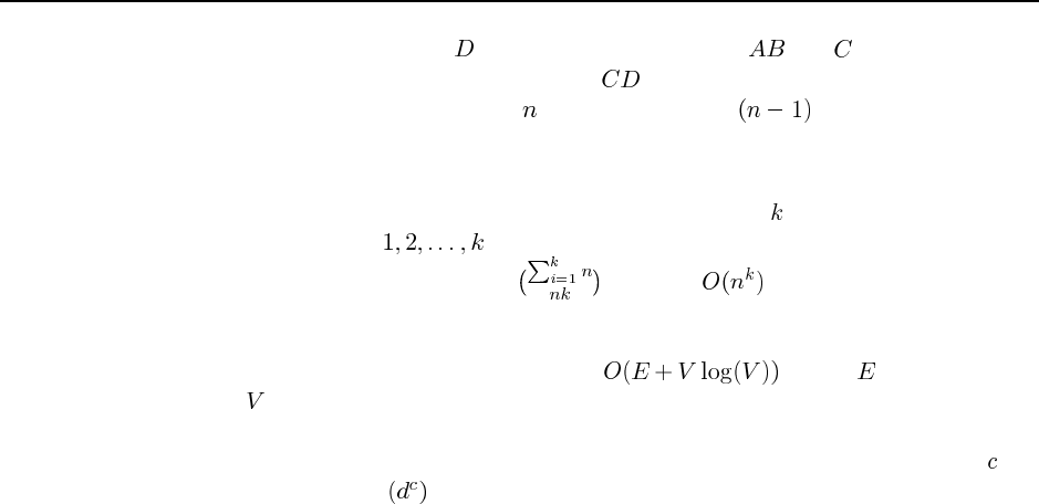
3.8
a. See Figure S3.1.
b. Breadth-first: 1 2 3 4 5 6 7 8 9 10 11
Depth-limited: 1 2 4 8 9 5 10 11
Iterative deepening: 1; 1 2 3; 1 2 4 5 3 6 7; 1 2 4 8 9 5 10 11
14 Chapter 3. Solving Problems by Searching
c. Bidirectional search is very useful, because the only successor of in the reverse direc-
tion is . This helps focus the search.
d. 2 in the forward direction; 1 in the reverse direction.
e. Yes; start at the goal, and apply the single reverse successor action until you reach 1.
3.9
a. Here is one possible representation: A state is a six-tuple of integers listing the number
of missionaries, cannibals, and boats on the first side, and then the seond side of the
river. The goal is a state with 3 missionaries and 3 cannibals on the second side. The
cost function is one per action, and the successors of a state are all the states that move
1 or 2 people and 1 boat from one side to another.
b. The search space is small, so any optimal algorithm works. For an example, see the
file "search/domains/cannibals.lisp". It suffices to eliminate moves that
circle back to the state just visited. From all but the first and last states, there is only
one other choice.
c. It is not obvious that almost all moves are either illegal or revert to the previous state.
There is a feeling of a large branching factor, and no clear way to proceed.
3.10 For the 8 puzzle, there shouldn’t be much difference in performance. Indeed, the file
"search/domains/puzzle8.lisp" shows that you can represent an 8 puzzle state as
a single 32-bit integer, so the question of modifying or copying data is moot. But for the
puzzle, as increases, the advantage of modifying rather than copying grows. The
disadvantage of a modifying successor function is that it only works with depth-first search
(or with a variant such as iterative deepening).
3.11 a. The algorithm expands nodes in order of increasing path cost; therefore the first
goal it encounters will be the goal with the cheapest cost.
b. It will be the same as iterative deepening, iterations, in which nodes are
generated.
c.
d. Implementation not shown.
3.12 If there are two paths from the start node to a given node, discarding the more ex-
pensive one cannot eliminate any optimal solution. Uniform-cost search and breadth-first
search with constant step costs both expand paths in order of -cost. Therefore, if the current
node has been expanded previously, the current path to it must be more expensive than the
previously found path and it is correct to discard it.
For IDS, it is easy to find an example with varying step costs where the algorithm returns
a suboptimal solution: simply have two paths to the goal, one with one step costing 3 and the
other with two steps costing 1 each.
3.13 Consider a domain in which every state has a single successor, and there is a single goal
at depth . Then depth-first search will find the goal in steps, whereas iterative deepening
search will take steps.
15
3.14 As an ordinary person (or agent) browsing the web, we can only generarte the suc-
cessors of a page by visiting it. We can then do breadth-first search, or perhaps best-search
search where the heuristic is some function of the number of words in common between the
start and goal pages; this may help keep the links on target. Search engines keep the complete
graph of the web, and may provide the user access to all (or at least some) of the pages that
link to a page; this would allow us to do bidirectional search.
3.15
a. If we consider all points, then there are an infinite number of states, and of paths.
b. (For this problem, we consider the start and goal points to be vertices.) The shortest
distance between two points is a straight line, and if it is not possible to travel in a
straight line because some obstacle is in the way, then the next shortest distance is a
sequence of line segments, end-to-end, that deviate from the straight line by as little
as possible. So the first segment of this sequence must go from the start point to a
tangent point on an obstacle – any path that gave the obstacle a wider girth would be
longer. Because the obstacles are polygonal, the tangent points must be at vertices of
the obstacles, and hence the entire path must go from vertex to vertex. So now the state
space is the set of vertices, of which there are 35 in Figure 3.22.
c. Code not shown.
d. Implementations and analysis not shown.
3.16 Code not shown.
3.17
a. Any path, no matter how bad it appears, might lead to an arbitraily large reward (nega-
tive cost). Therefore, one would need to exhaust all possible paths to be sure of finding
the best one.
b. Suppose the greatest possible reward is . Then if we also know the maximum depth of
the state space (e.g. when the state space is a tree), then any path with levels remaining
can be improved by at most , so any paths worse than less than the best path can be
pruned. For state spaces with loops, this guarantee doesn’t help, because it is possible
to go around a loop any number of times, picking up rewward each time.
c. The agent should plan to go around this loop forever (unless it can find another loop
with even better reward).
d. The value of a scenic loop is lessened each time one revisits it; a novel scenic sight
is a great reward, but seeing the same one for the tenth time in an hour is tedious, not
rewarding. To accomodate this, we would have to expand the state space to include a
memory—a state is now represented not just by the current location, but by a current
location and a bag of already-visited locations. The reward for visiting a new location
is now a (diminishing) function of the number of times it has been seen before.
e. Real domains with looping behavior include eating junk food and going to class.
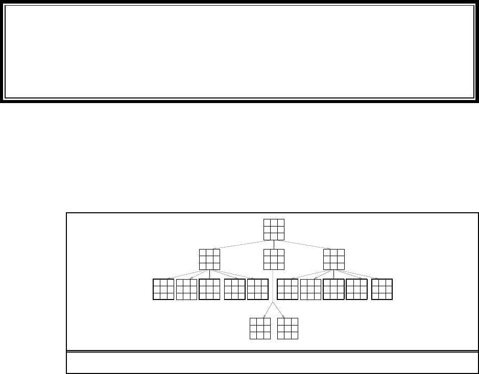
3.18 The belief state space is shown in Figure S3.2. No solution is possible because no path
leads to a belief state all of whose elements satisfy the goal. If the problem is fully observable,
16 Chapter 3. Solving Problems by Searching
L
R
L R
S SS
Figure S3.2 The belief state space for the sensorless vacuum world under Murphy’s law.
the agent reaches a goal state by executing a sequence such that is performed only in a
dirty square. This ensures deterministic behavior and every state is obviously solvable.
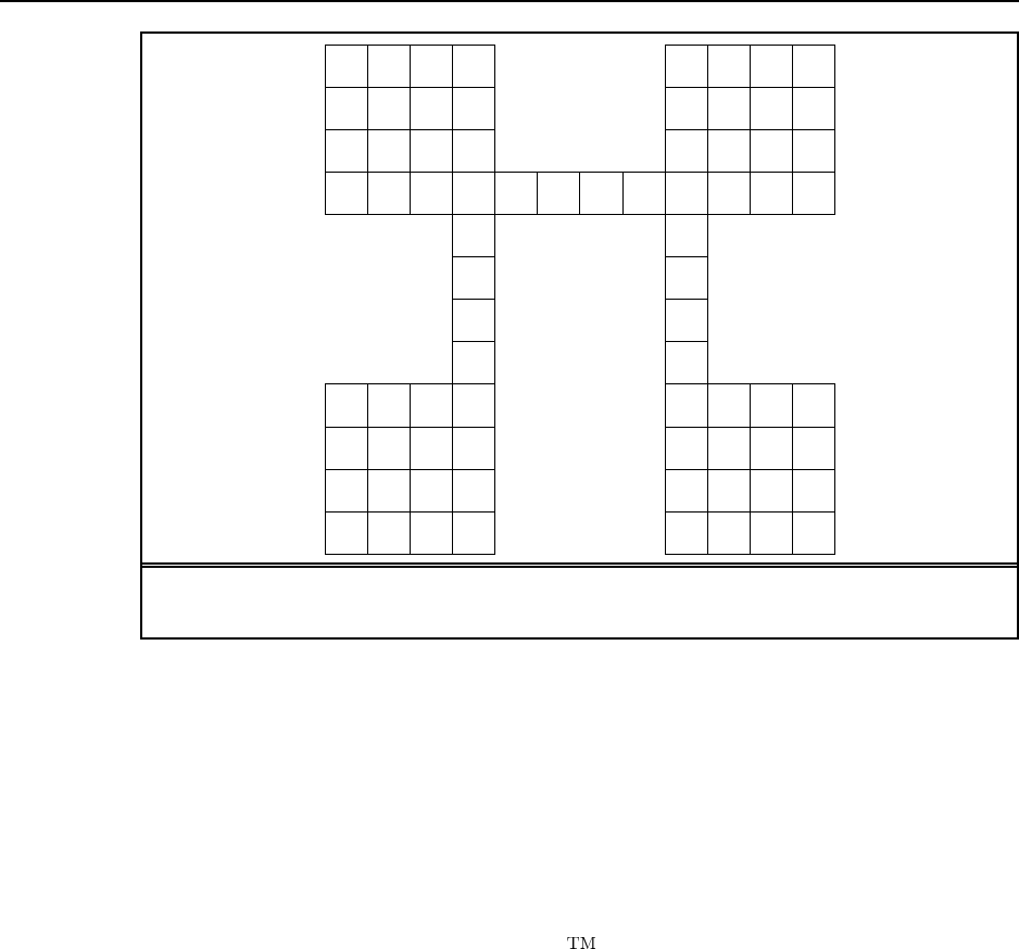
3.19 Code not shown, but a good start is in the code repository. Clearly, graph search
must be used—this is a classic grid world with many alternate paths to each state. Students
will quickly find that computing the optimal solution sequence is prohibitively expensive for
moderately large worlds, because the state space for an world has states. The
completion time of the random agent grows less than exponentially in , so for any reasonable
exchange rate between search cost ad path cost the random agent will eventually win.
Solutions for Chapter 4
Informed Search and Exploration
4.1 The sequence of queues is as follows:
L[0+244=244]
M[70+241=311], T[111+329=440]
L[140+244=384], D[145+242=387], T[111+329=440]
D[145+242=387], T[111+329=440], M[210+241=451], T[251+329=580]
C[265+160=425], T[111+329=440], M[210+241=451], M[220+241=461], T[251+329=580]
T[111+329=440], M[210+241=451], M[220+241=461], P[403+100=503], T[251+329=580], R[411+193=604],
D[385+242=627]
M[210+241=451], M[220+241=461], L[222+244=466], P[403+100=503], T[251+329=580], A[229+366=595],
R[411+193=604], D[385+242=627]
M[220+241=461], L[222+244=466], P[403+100=503], L[280+244=524], D[285+242=527], T[251+329=580],
A[229+366=595], R[411+193=604], D[385+242=627]
L[222+244=466], P[403+100=503], L[280+244=524], D[285+242=527], L[290+244=534], D[295+242=537],
T[251+329=580], A[229+366=595], R[411+193=604], D[385+242=627]
P[403+100=503], L[280+244=524], D[285+242=527], M[292+241=533], L[290+244=534], D[295+242=537],
T[251+329=580], A[229+366=595], R[411+193=604], D[385+242=627], T[333+329=662]
B[504+0=504], L[280+244=524], D[285+242=527], M[292+241=533], L[290+244=534], D[295+242=537], T[251+329=580],
A[229+366=595], R[411+193=604], D[385+242=627], T[333+329=662], R[500+193=693], C[541+160=701]
4.2 gives . This behaves exactly like uniform-cost search—the factor
of two makes no difference in the ordering of the nodes. gives A search. gives
, i.e., greedy best-first search. We also have
which behaves exactly like A search with a heuristic . For , this is always
less than and hence admissible, provided is itself admissible.
4.3
a. When all step costs are equal, , so uniform-cost search reproduces
breadth-first search.
b. Breadth-first search is best-first search with ; depth-first search is
best-first search with ; uniform-cost search is best-first search with
17
18 Chapter 4. Informed Search and Exploration
.
c. Uniform-cost search is A search with .
SAG
B
h=7
h=5
h=1 h=0
21
4
4
Figure S4.1 A graph with an inconsistent heuristic on which GRAPH-SEARCH fails to
return the optimal solution. The successors of are with and with . is
expanded first, so the path via will be discarded because will already be in the closed
list.
4.4 See Figure S4.1.
4.5 Going between Rimnicu Vilcea and Lugoj is one example. The shortest path is the
southern one, through Mehadia, Dobreta and Craiova. But a greedy search using the straight-
line heuristic starting in Rimnicu Vilcea will start the wrong way, heading to Sibiu. Starting
at Lugoj, the heuristic will correctly lead us to Mehadia, but then a greedy search will return
to Lugoj, and oscillate forever between these two cities.
4.6 The heuristic (adding misplaced tiles and Manhattan distance) sometimes
overestimates. Now, suppose (as given) and let be a goal that is
suboptimal by more than , i.e., . Now consider any node on a path to an
optimal goal. We have
so will never be expanded before an optimal goal is expanded.
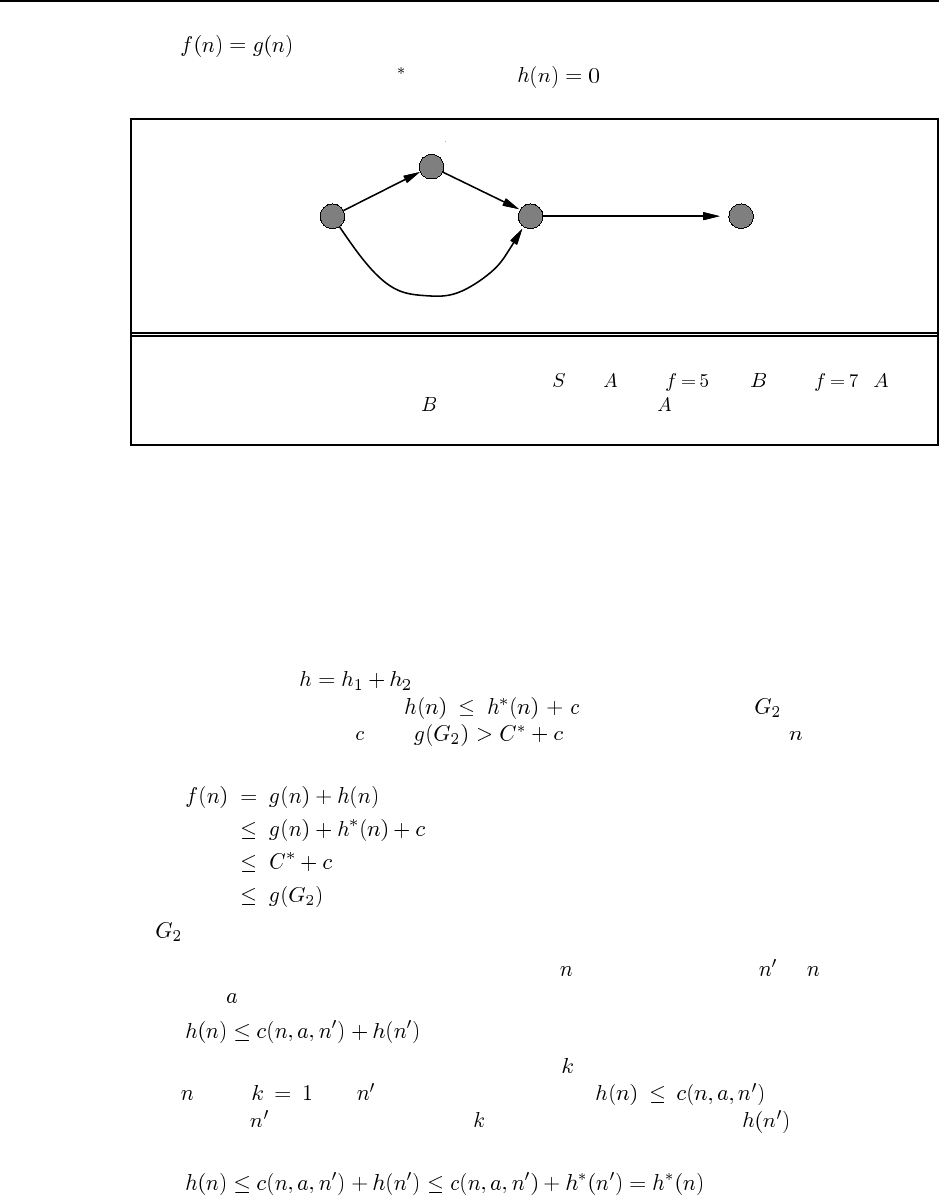
4.7 A heuristic is consistent iff, for every node and every successor of generated by
any action ,
One simple proof is by induction on the number of nodes on the shortest path to any goal
from . For , let be the goal node; then . For the inductive
case, assume is on the shortest path steps from the goal and that is admissible by
hypothesis; then
19
so at steps from the goal is also admissible.
4.8 This exercise reiterates a small portion of the classic work of Held and Karp (1970).
a. The TSP problem is to find a minimal (total length) path through the cities that forms
a closed loop. MST is a relaxed version of that because it asks for a minimal (total
length) graph that need not be a closed loop—it can be any fully-connected graph. As
a heuristic, MST is admissible—it is always shorter than or equal to a closed loop.
b. The straight-line distance back to the start city is a rather weak heuristic—it vastly
underestimates when there are many cities. In the later stage of a search when there are
only a few cities left it is not so bad. To say that MST dominates straight-line distance
is to say that MST always gives a higher value. This is obviously true because a MST
that includes the goal node and the current node must either be the straight line between
them, or it must include two or more lines that add up to more. (This all assumes the
triangle inequality.)
c. See "search/domains/tsp.lisp" for a start at this. The file includes a heuristic
based on connecting each unvisited city to its nearest neighbor, a close relative to the
MST approach.
d. See (Cormen et al., 1990, p.505) for an algorithm that runs in time, where
is the number of edges. The code repository currently contains a somewhat less
efficient algorithm.
4.9 The misplaced-tiles heuristic is exact for the problem where a tile can move from square
A to square B. As this is a relaxation of the condition that a tile can move from square A to
square B if B is blank, Gaschnig’s heuristic canot be less than the misplaced-tiles heuristic.
As it is also admissible (being exact for a relaxation of the original problem), Gaschnig’s
heuristic is therefore more accurate.
If we permute two adjacent tiles in the goal state, we have a state where misplaced-tiles
and Manhattan both return 2, but Gaschnig’s heuristic returns 3.
To compute Gaschnig’s heuristic, repeat the following until the goal state is reached:
let B be the current location of the blank; if B is occupied by tile X (not the blank) in the
goal state, move X to B; otherwise, move any misplaced tile to B. Students could be asked to
prove that this is the optimal solution to the relaxed problem.
4.11
a. Local beam search with is hill-climbing search.
b. Local beam search with : strictly speaking, this doesn’t make sense. (Exercise
may be modified in future printings.) The idea is that if every successor is retained
(because is unbounded), then the search resembles breadth-first search in that it adds
one complete layer of nodes before adding the next layer. Starting from one state, the
algorithm would be essentially identical to breadth-first search except that each layer is
generated all at once.
c. Simulated annealing with at all times: ignoring the fact that the termination step
would be triggered immediately, the search would be identical to first-choice hill climb-
20 Chapter 4. Informed Search and Exploration
ing because every downward successor would be rejected with probability 1. (Exercise
may be modified in future printings.)
d. Genetic algorithm with population size : if the population size is 1, then the
two selected parents will be the same individual; crossover yields an exact copy of the
individual; then there is a small chance of mutation. Thus, the algorithm executes a
random walk in the space of individuals.
4.12 If we assume the comparison function is transitive, then we can always sort the nodes
using it, and choose the node that is at the top of the sort. Efficient priority queue data
structures rely only on comparison operations, so we lose nothing in efficiency—except for
the fact that the comparison operation on states may be much more expensive than comparing
two numbers, each of which can be computed just once.
Arelies on the division of the total cost estimate into the cost-so-far and the cost-
to-go. If we have comparison operators for each of these, then we can prefer to expand a
node that is better than other nodes on both comparisons. Unfortunately, there will usually
be no such node. The tradeoff between and cannot be realized without numerical
values.
4.13 The space complexity of LRTA is dominated by the space required for ,
i.e., the product of the number of states visited ( ) and the number of actions tried per state
( ). The time complexity is at least for a naive implementation because for each
action taken we compute an value, which requires minimizing over actions. A simple
optimization can reduce this to . This expression assumes that each state–action pair
is tried at most once, whereas in fact such pairs may be tried many times, as the example in
Figure 4.22 shows.
4.14 This question is slightly ambiguous as to what the percept is—either the percept is just
the location, or it gives exactly the set of unblocked directions (i.e., blocked directions are
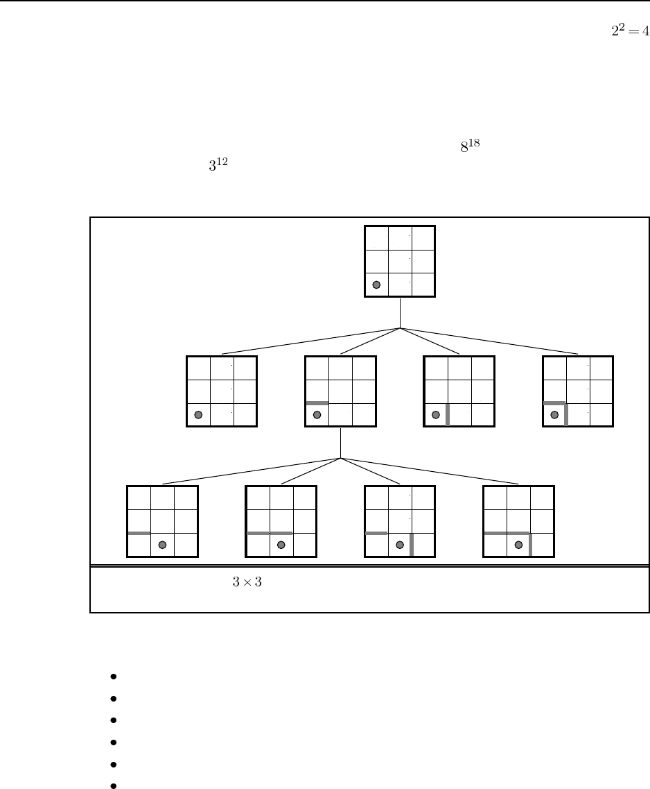
illegal actions). We will assume the latter. (Exercise may be modified in future printings.)
There are 12 possible locations for internal walls, so there are possible environ-
ment configurations. A belief state designates a subset of these as possible configurations;
for example, before seeing any percepts all 4096 configurations are possible—this is a single
belief state.
a. We can view this as a contingency problem in belief state space. The initial belief state
is the set of all 4096 configurations. The total belief state space contains belief
states (one for each possible subset of configurations, but most of these are not reach-
able. After each action and percept, the agent learns whether or not an internal wall
exists between the current square and each neighboring square. Hence, each reachable
belief state can be represnted exactly by a list of status values (present, absent, un-
known) for each wall separately. That is, the belief state is completely decomposable
and there are exactly reachable belief states. The maximum number of possible
wall-percepts in each state is 16 ( ), so each belief state has four actions, each with up
to 16 nondeterministic successors.
21
b. Assuming the external walls are known, there are two internal walls and hence
possible percepts.
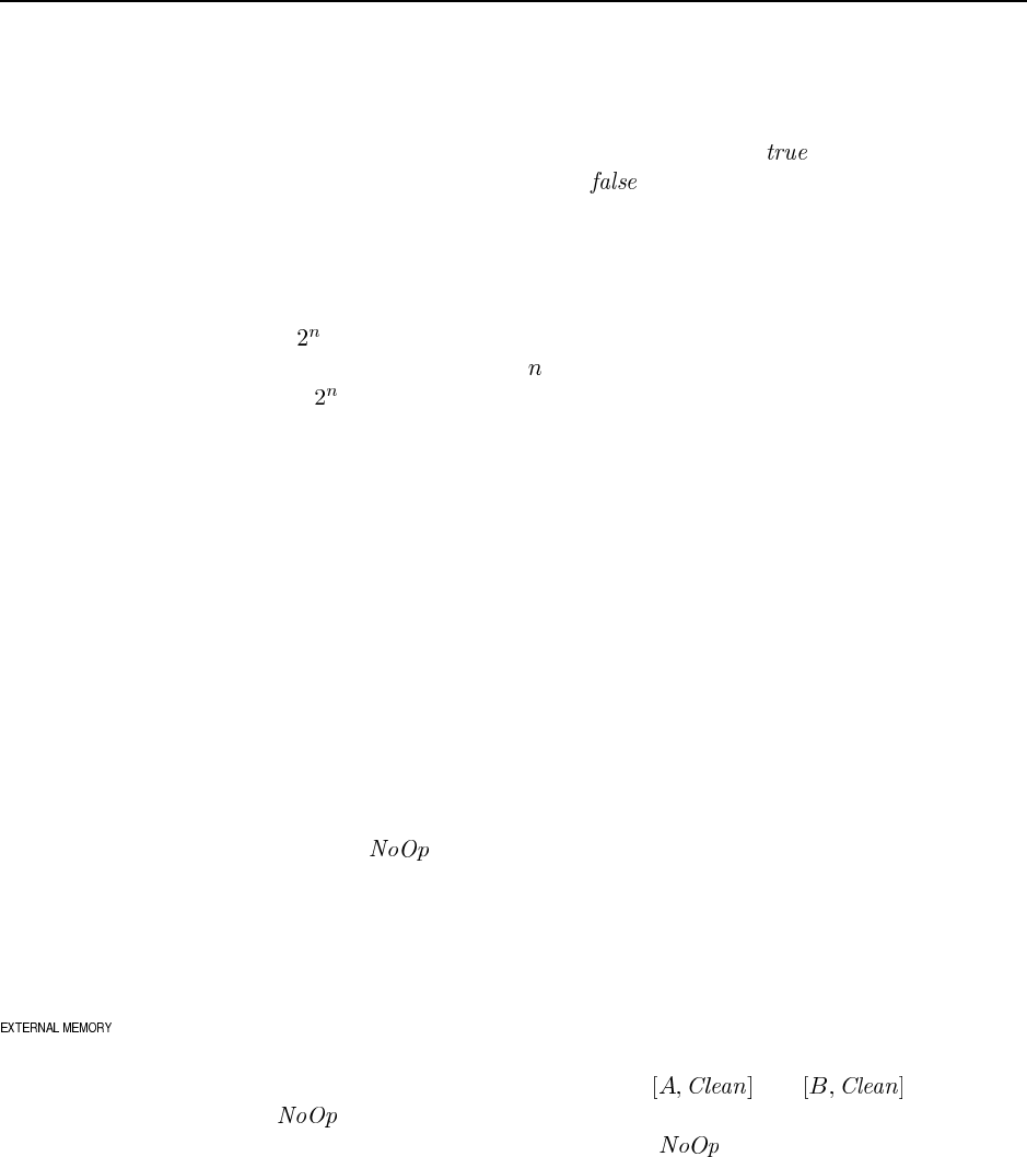
c. The initial null action leads to four possible belief states, as shown in Figure S4.2. From
each belief state, the agent chooses a single action which can lead to up to 8 belief states
(on entering the middle square). Given the possibility of having to retrace its steps at
a dead end, the agent can explore the entire maze in no more than 18 steps, so the
complete plan (expressed as a tree) has no more than nodes. On the other hand,
there are just , so the plan could be expressed more concisely as a table of actions
indexed by belief state (a policy in the terminology of Chapter 17).
? ??
? ??
?
?
?
?
?
?
? ??
??
?
?
?
?
?
? ??
??
?
?
?
?
?
? ??
??
?
?
?
?
?
? ??
??
?
?
?
?
?
? ??
?
?
?
?
?
? ??
?
?
?
?
?
? ??
?
?
?
?
?
? ??
?
?
?
?
?
NoOp
Right
Figure S4.2 The maze exploration problem: the initial state, first percept, and one
selected action with its perceptual outcomes.
4.15 Here is one simple hill-climbing algorithm:
Connect all the cities into an arbitrary path.
Pick two points along the path at random.
Split the path at those points, producing three pieces.
Try all six possible ways to connect the three pieces.
Keep the best one, and reconnect the path accordingly.
Iterate the steps above until no improvement is observed for a while.
4.1 4.16 Code not shown.
22 Chapter 4. Informed Search and Exploration
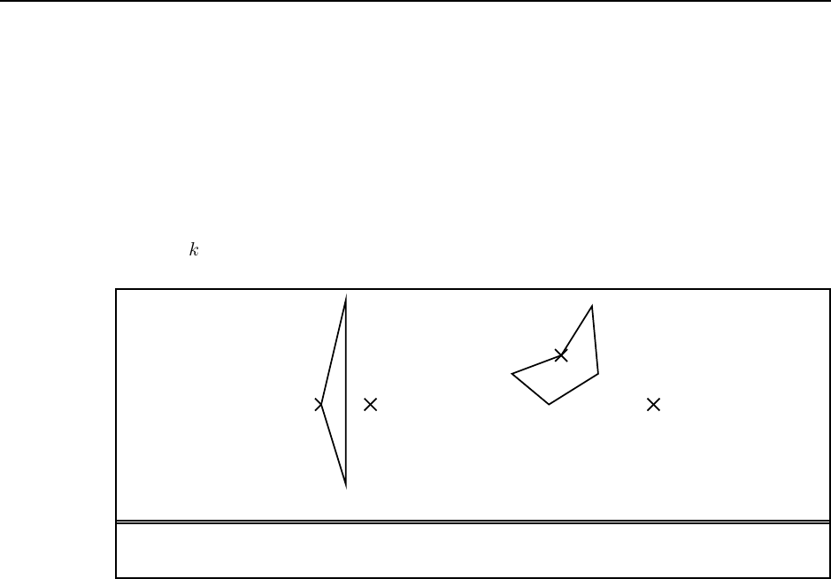
4.17 Hillclimbing is surprisingly effective at finding reasonable if not optimal paths for very
little computational cost, and seldom fails in two dimensions.
a. It is possible (see Figure S4.3(a)) but very unlikely—the obstacle has to have an unusual
shape and be positioned correctly with respect to the goal.
b. With convex obstacles, getting stuck is much more likely to be a problem (see Fig-
ure S4.3(b)).
c. Notice that this is just depth-limited search, where you choose a step along the best path
even if it is not a solution.
d. Set to the maximum number of sides of any polygon and you can always escape.
Current
position Goal
(a) (b)
Current
position
Goal
Figure S4.3 (a) Getting stuck with a convex obstacle. (b) Getting stuck with a nonconvex
obstacle.
4.18 The student should find that on the 8-puzzle, RBFS expands more nodes (because
it does not detect repeated states) but has lower cost per node because it does not need to
maintain a queue. The number of RBFS node re-expansions is not too high because the
presence of many tied values means that the best path changes seldom. When the heuristic is
slightly perturbed, this advantage disappears and RBFS’s performance is much worse.
For TSP, the state space is a tree, so repeated states are not an issue. On the other hand,
the heuristic is real-valued and there are essentially no tied values, so RBFS incurs a heavy
penalty for frequent re-expansions.

Solutions for Chapter 5
Constraint Satisfaction Problems
5.1 Aconstraint satisfaction problem is a problem in which the goal is to choose a value
for each of a set of variables, in such a way that the values all obey a set of constraints.
Aconstraint is a restriction on the possible values of two or more variables. For exam-
ple, a constraint might say that is not allowed in conjunction with .
Backtracking search is a form depth-first search in which there is a single representa-
tion of the state that gets updated for each successor, and then must be restored when a dead
end is reached.
A directed arc from variable to variable in a CSP is arc consistent if, for every
value in the current domain of , there is some consistent value of .
Backjumping is a way of making backtracking search more efficient, by jumping back
more than one level when a dead end iss reached.
Min-conflicts is a heuristic for use with local search on CSP problems. The heuristic
says that, when given a variable to modify, choose the value that conflicts with the fewest
number of other variables.
5.2 There are 18 solutions for coloring Australia with three colors. Start with SA, which
can have any of three colors. Then moving clockwise, WA can have either of the other two
colors, and everything else is strictly determined; that makes 6 possibilities for the mainland,
times 3 for Tasmania yields 18.
5.3 The most constrained variable makes sense because it chooses a variable that is (all
other things being equal) likely to cause a failure, and it is more efficient to fail as early
as possible (thereby pruning large parts of the search space). The least constraining value
heuristic makes sense because it allows the most chances for future assignments to avoid
conflict.
5.4 a. Crossword puzzle construction can be solved many ways. One simple choice is
depth-first search. Each successor fills in a word in the puzzle with one of the words in the
dictionary. It is better to go one word at a time, to minimize the number of steps.
b. As a CSP, there are even more choices. You could have a variable for each box in
the crossword puzzle; in this case the value of each variable is a letter, and the constraints are
that the letters must make words. This approach is feasible with a most-constraining value
heuristic. Alternately, we could have each string of consecutive horizontal or vertical boxes
be a single variable, and the domain of the variables be words in the dictionary of the right
23
24 Chapter 5. Constraint Satisfaction Problems
length. The constraints would say that two intersecting words must have the same letter in the
intersecting box. Solving a problem in this formulation requires fewer steps, but the domains
are larger (assuming a big dictionary) and there are fewer constraints. Both formulations are
feasible.
5.5 a. For rectilinear floor-planning, one possibility is to have a variable for each of the
small rectangles, with the value of each variable being a 4-tuple consisting of the and
coordinates of the upper left and lower right corners of the place where the rectangle will
be located. The domain of each variable is the set of 4-tuples that are the right size for the
corresponding small rectangle and that fit within the large rectangle. Constraints say that no
two rectangles can overlap; for example if the value of variable is , then no other
variable can take on a value that overlaps with the to rectangle.
b. For class scheduling, one possibility is to have three variables for each class, one with
times for values (e.g. MWF8:00, TuTh8:00, MWF9:00, ...), one with classrooms for values
(e.g. Wheeler110, Evans330, ...) and one with instructors for values (e.g. Abelson, Bibel,
Canny, ...). Constraints say that only one class can be in the same classroom at the same time,
and an instructor can only teach one class at a time. There may be other constraints as well
(e.g. an instructor should not have two consecutive classes).
5.6 The exact steps depend on certain choices you are free to make; here are the ones I
made:
a. Choose the variable. Its domain is .
b. Choose the value 1 for . (We can’t choose 0; it wouldn’t survive forward checking,
because it would force to be 0, and the leading digit of the sum must be non-zero.)
c. Choose , because it has only one remaining value.
d. Choose the value 1 for .
e. Now and Xare tied for minimum remaining values at 2; let’s choose .
f. Either value survives forward checking, let’s choose 0 for .
g. Now has the minimum remaining values.
h. Again, arbitrarily choose 0 for the value of .
i. The variable must be an even number (because it is the sum of less than 5
(because ). That makes it most constrained.
j. Arbitrarily choose 4 as the value of .
k. now has only 1 remaining value.
l. Choose the value 8 for .
m. now has only 1 remianing value.
n. Choose the value 7 for .
o. must be an even number less than 9; choose .
p. The only value for that survives forward checking is 6.
q. The only variable left is .
r. The only value left for is 3.
25
s. This is a solution.
This is a rather easy (under-constrained) puzzle, so it is not surprising that we arrive at a
solution with no backtracking (given that we are allowed to use forward checking).
5.7 There are implementations of CSP algorithms in the Java, Lisp, and Python sections
of the online code repository; these should help students get started. However, students will
have to add code to keep statistics on the experiments, and perhaps will want to have some
mechanism for making an experiment return failure if it exceeds a certain time limit (or
number-of-steps limit). The amount of code that needs to be written is small; the exercise is
more about running and analyzing an experiment.
5.8 We’ll trace through each iteration of the while loop in AC-3 (for one possible ordering
of the arcs):
a. Remove , delete from .
b. Remove , delete from , leaving only .
c. Remove , delete from .
d. Remove , delete from , leaving only .
e. Remove , delete from .
f. Remove , delete from , leaving only .
g. Remove , delete from .
h. Remove , delete from .
i. remove , delete from , leaving no domain for .
5.9 On a tree-structured graph, no arc will be considered more than once, so the AC-3
algorithm is , where is the number of edges and is the size of the largest do-
main.
5.10 The basic idea is to preprocess the constraints so that, for each value of , we keep
track of those variables for which an arc from to is satisfied by that particular value
of . This data structure can be computed in time proportional to the size of the problem
representation. Then, when a value of is deleted, we reduce by 1 the count of allowable
values for each arc recorded under that value. This is very similar to the forward
chaining algorithm in Chapter 7. See ? (?) for detailed proofs.
5.11 The problem statement sets out the solution fairly completely. To express the ternary
constraint on , and that , we first introduce a new variable, . If the
domain of and is the set of numbers , then the domain of is the set of pairs of
numbers from , i.e. . Now there are three binary constraints, one between and
saying that the value of must be equal to the first element of the pair-value of ; one
between and saying that the value of must equal the second element of the value
of ; and finally one that says that the sum of the pair of numbers that is the value of
must equal the value of . All other ternary constraints can be handled similarly.
Now that we can reduce a ternary constraint into binary constraints, we can reduce a
4-ary constraint on variables by first reducing to binary constraints as
26 Chapter 5. Constraint Satisfaction Problems
shown above, then adding back in a ternary constraint with and , and then reducing
this ternary constraint to binary by introducing .
By induction, we can reduce any -ary constraint to an -ary constraint. We can
stop at binary, because any unary constraint can be dropped, simply by moving the effects of
the constraint into the domain of the variable.
5.12 A simple algorithm for finding a cutset of no more than nodes is to enumerate all
subsets of nodes of size , and for each subset check whether the remaining nodes
form a tree. This algorithm takes time , which is .
Becker and Geiger (1994; http://citeseer.nj.nec.com/becker94approximation.html) give
an algorithm called MGA (modified greedy algorithm) that finds a cutset that is no more than
twice the size of the minimal cutset, using time , where is the number of
edges and is the number of variables.
Whether this makes the cycle cutset approach practical depends more on the graph
involved than on the agorithm for finding a cutset. That is because, for a cutset of size , we
still have an exponential factor before we can solve the CSP. So any graph with a large
cutset will be intractible to solve, even if we could find the cutset with no effort at all.
5.13 The “Zebra Puzzle” can be represented as a CSP by introducing a variable for each
color, pet, drink, country and cigaret brand (a total of 25 variables). The value of each variable
is a number from 1 to 5 indicating the house number. This is a good representation because it
easy to represent all the constraints given in the problem definition this way. (We have done
so in the Python implementation of the code, and at some point we may reimplement this
in the other languages.) Besides ease of expressing a problem, the other reason to choose a
representation is the efficiency of finding a solution. here we have mixed results—on some
runs, min-conflicts local search finds a solution for this problem in seconds, while on other
runs it fails to find a solution after minutes.
Another representation is to have five variables for each house, one with the domain of
colrs, one with pets, and so on.
Solutions for Chapter 6
Adversarial Search
6.1 Figure S6.1 shows the game tree, with the evaluation function values below the terminal
nodes and the backed-up values to the right of the non-terminal nodes. The values imply that
the best starting move for X is to take the center. The terminal nodes with a bold outline are
the ones that do not need to be evaluated, assuming the optimal ordering.
x
x
x
x o x
o
x o x
o
x
o
x
o
x
o
x o x
o
x
o
x
o
x
o
1
−1 1 −2
1 −1 0 0 1 −1 −2 0 −1 0
1 2
Figure S6.1 Part of the game tree for tic-tac-toe, for Exercise 6.1.
6.2 Consider a MIN node whose children are terminal nodes. If MIN plays suboptimally,
then the value of the node is greater than or equal to the value it would have if MIN played
optimally. Hence, the value of the MAX node that is the MIN node’s parent can only be
increased. This argument can be extended by a simple induction all the way to the root. If
the suboptimal play by MIN is predictable, then one can do better than a minimax strategy.
For example, if MIN always falls for a certain kind of trap and loses, then setting the trap
guarantees a win even if there is actually a devastating response for MIN. This is shown in
Figure S6.2.
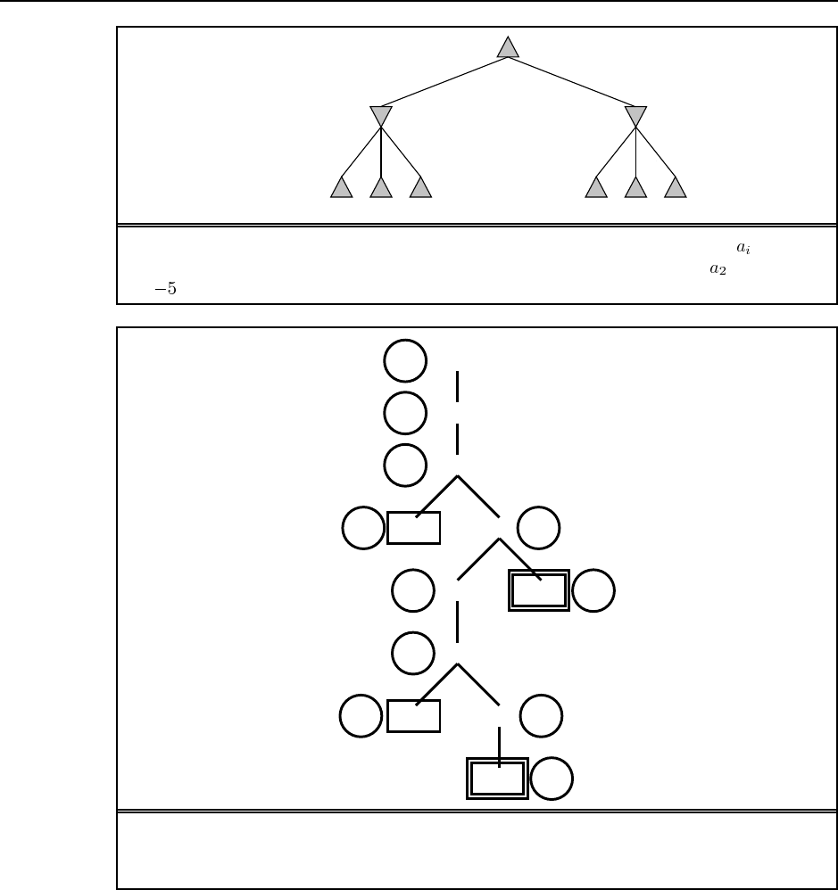
6.3
a. (5) The game tree, complete with annotations of all minimax values, is shown in Fig-
ure S6.3.
b. (5) The “?” values are handled by assuming that an agent with a choice between win-
ning the game and entering a “?” state will always choose the win. That is, min(–1,?)
is –1 and max(+1,?) is +1. If all successors are “?”, the backed-up value is “?”.
27
28 Chapter 6. Adversarial Search
MAX
MIN
a1
A
B D
−101000 1000
2
b3
b
1
b2
d
1
d3
d
−5−5−5
a2
Figure S6.2 A simple game tree showing that setting a trap for MIN by playing is a win
if MIN falls for it, but may also be disastrous. The minimax move is of course , with value
.
(1,4)
(2,4)
(2,3)
(1,3)
(1,2)
(3,2)
(3,4)
(4,3)
(3,1)
(2,4)
(1,4)
+1
−1
?
?
?
−1
−1
−1
+1
+1
+1
Figure S6.3 The game tree for the four-square game in Exercise 6.3. Terminal states are
in single boxes, loop states in double boxes. Each state is annotated with its minimax value
in a circle.
c. (5) Standard minimax is depth-first and would go into an infinite loop. It can be fixed
by comparing the current state against the stack; and if the state is repeated, then return
a “?” value. Propagation of “?” values is handled as above. Although it works in this
case, it does not always work because it is not clear how to compare “?” with a drawn
position; nor is it clear how to handle the comparison when there are wins of different
degrees (as in backgammon). Finally, in games with chance nodes, it is unclear how to
29
compute the average of a number and a “?”. Note that it is not correct to treat repeated
states automatically as drawn positions; in this example, both (1,4) and (2,4) repeat in
the tree but they are won positions.
What is really happening is that each state has a well-defined but initially unknown
value. These unknown values are related by the minimax equation at the bottom of page
163. If the game tree is acyclic, then the minimax algorithm solves these equations by
propagating from the leaves. If the game tree has cycles, then a dynamic programming
method must be used, as explained in Chapter 17. (Exercise 17.8 studies this problem in
particular.) These algorithms can determine whether each node has a well-determined
value (as in this example) or is really an infinite loop in that both players prefer to stay
in the loop (or have no choice). In such a case, the rules of the game will need to define
the value (otherwise the game will never end). In chess, for eaxmple, a state that occurs
3 times (and hence is assumed to be desirable for both players) is a draw.
d. This question is a little tricky. One approach is a proof by induction on the size of the
game. Clearly, the base case is a loss for A and the base case is a win for
A. For any , the initial moves are the same: A and B both move one step towards
each other. Now, we can see that they are engaged in a subgame of size on the
squares , except that there is an extra choice of moves on squares and
. Ignoring this for a moment, it is clear that if the “ ” is won for A, then A
gets to the square before B gets to square (by the definition of winning) and
therefore gets to before B gets to , hence the “ ” game is won for A. By the same
line of reasoning, if “ ” is won for B then “ ” is won for B. Now, the presence of
the extra moves complicates the issue, but not too much. First, the player who is slated
to win the subgame never moves back to his home square. If the player
slated to lose the subgame does so, then it is easy to show that he is bound to lose the
game itself—the other player simply moves forward and a subgame of size is
played one step closer to the loser’s home square.
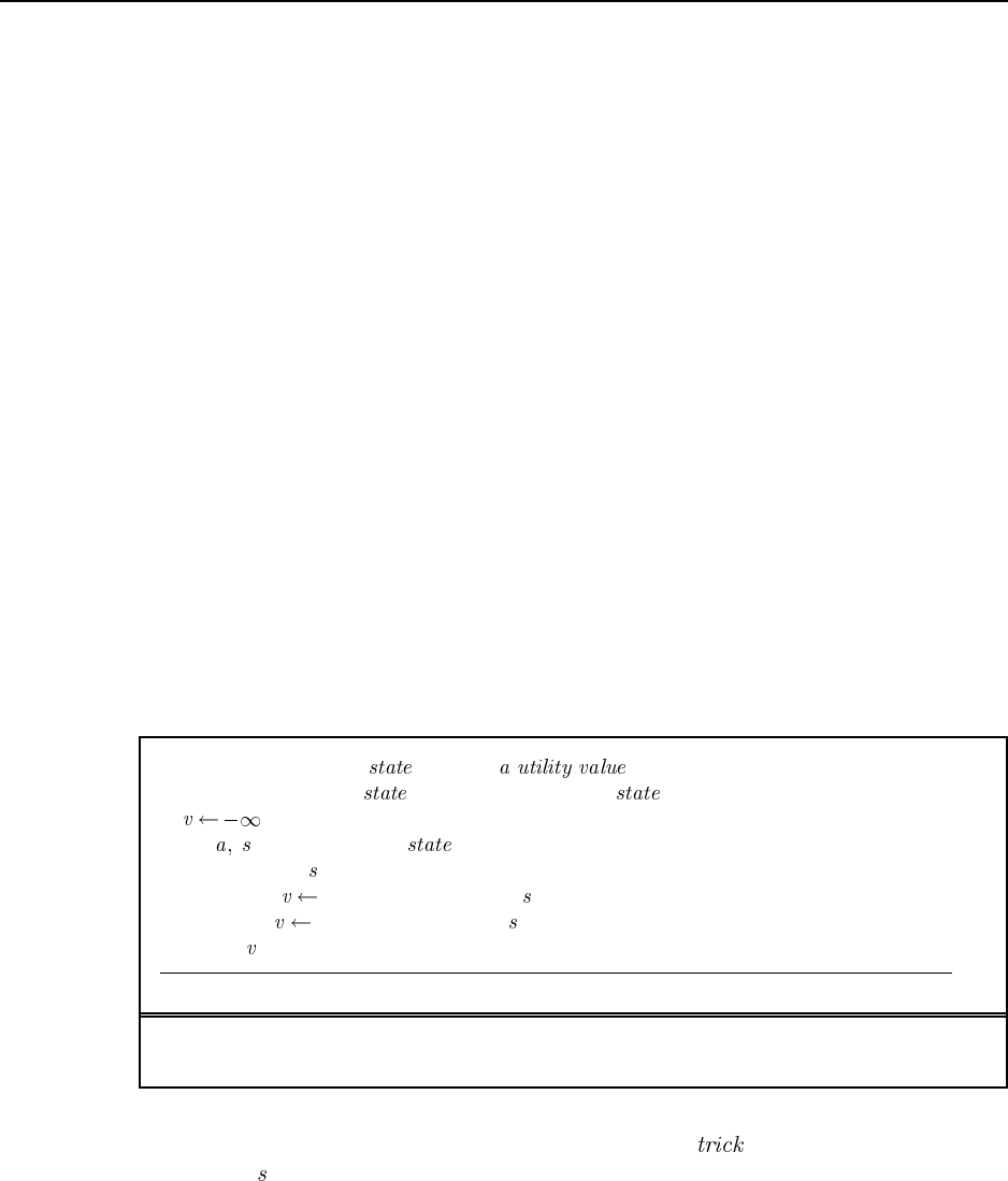
6.4 See "search/algorithms/games.lisp" for definitions of games, game-playing
agents, and game-playing environments. "search/algorithms/minimax.lisp" con-
tains the minimax and alpha-beta algorithms. Notice that the game-playing environment is
essentially a generic environment with the update function defined by the rules of the game.
Turn-taking is achieved by having agents do nothing until it is their turn to move.
See "search/domains/cognac.lisp" for the basic definitions of a simple game
(slightly more challenging than Tic-Tac-Toe). The code for this contains only a trivial eval-
uation function. Students can use minimax and alpha-beta to solve small versions of the
game to termination (probably up to ); they should notice that alpha-beta is far faster
than minimax, but still cannot scale up without an evaluation function and truncated horizon.
Providing an evaluation function is an interesting exercise. From the point of view of data
structure design, it is also interesting to look at how to speed up the legal move generator by
precomputing the descriptions of rows, columns, and diagonals.
Very few students will have heard of kalah, so it is a fair assignment, but the game
is boring—depth 6 lookahead and a purely material-based evaluation function are enough
30 Chapter 6. Adversarial Search
to beat most humans. Othello is interesting and about the right level of difficulty for most
students. Chess and checkers are sometimes unfair because usually a small subset of the
class will be experts while the rest are beginners.
6.5 This question is not as hard as it looks. The derivation below leads directly to a defini-
tion of and values. The notation refers to (the value of) the node at depth on the path
from the root to the leaf node . Nodes are the siblings of node .
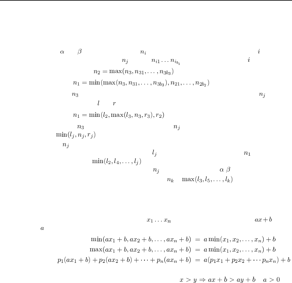
a. We can write , giving
Then can be similarly replaced, until we have an expression containing itself.
b. In terms of the and values, we have
Again, can be expanded out down to . The most deeply nested term will be
.
c. If is a max node, then the lower bound on its value only increases as its successors
are evaluated. Clearly, if it exceeds it will have no further effect on . By extension,
if it exceeds it will have no effect. Thus, by keeping track of this
value we can decide when to prune . This is exactly what - does.
d. The corresponding bound for min nodes is .
6.7 The general strategy is to reduce a general game tree to a one-ply tree by induction on
the depth of the tree. The inductive step must be done for min, max, and chance nodes, and
simply involves showing that the transformation is carried though the node. Suppose that the
values of the descendants of a node are , and that the transformation is , where
is positive. We have
Hence the problem reduces to a one-ply tree where the leaves have the values from the original
tree multiplied by the linear transformation. Since if , the
best choice at the root will be the same as the best choice in the original tree.
6.8 This procedure will give incorrect results. Mathematically, the procedure amounts to
assuming that averaging commutes with min and max, which it does not. Intuitively, the
choices made by each player in the deterministic trees are based on full knowledge of future
dice rolls, and bear no necessary relationship to the moves made without such knowledge.
(Notice the connection to the discussion of card games on page 179 and to the general prob-
lem of fully and partially observable Markov decision problems in Chapter 17.) In practice,
the method works reasonably well, and it might be a good exercise to have students compare
it to the alternative of using expectiminimax with sampling (rather than summing over) dice
rolls.
31
6.9 Code not shown.
6.10 The basic physical state of these games is fairly easy to describe. One important thing
to remember for Scrabble and bridge is that the physical state is not accessible to all players
and so cannot be provided directly to each player by the environment simulator. Particularly
in bridge, each player needs to maintain some best guess (or multiple hypotheses) as to the
actual state of the world. We expect to be putting some of the game implementations online
as they become available.
6.11 One can think of chance events during a game, such as dice rolls, in the same way
as hidden but preordained information (such as the order of the cards in a deck). The key
distinctions are whether the players can influence what information is revealed and whether
there is any asymmetry in the information available to each player.
a. Expectiminimax is appropriate only for backgammon and Monopoly. In bridge and
Scrabble, each player knows the cards/tiles he or she possesses but not the opponents’.
In Scrabble, the benefits of a fully rational, randomized strategy that includes reasoning
about the opponents’ state of knowledge are probably small, but in bridge the questions
of knowledge and information disclosure are central to good play.
b. None, for the reasons described earlier.
c. Key issues include reasoning about the opponent’s beliefs, the effect of various actions
on those beliefs, and methods for representing them. Since belief states for rational
agents are probability distributions over all possible states (including the belief states of
others), this is nontrivial.
function MAX-VALUE( ) returns
if TERMINAL-TEST( ) then return UTILITY( )
for in SUCCESSORS( ) do
if WINNER( ) = MAX
then MAX(v, MAX-VALUE( ))
else MAX(v, MIN-VALUE( ))
return
Figure S6.4 Part of the modified minimax algorithm for games in which the winner of the
previous trick plays first on the next trick.
6.12 (In the first printing, this exericse refers to WINNER( ); subsequent printings refer
to WINNER( ), denoting the winner of the trick just completed (if any), or null.) This question
is interpreted as applying only to the observable case.
a. The modification to MAX-VALUE is shown in Figure S6.4. If MAX has just won a trick,
MAX gets to play again, otherwise play alternates. Thus, the successors of a MAX node
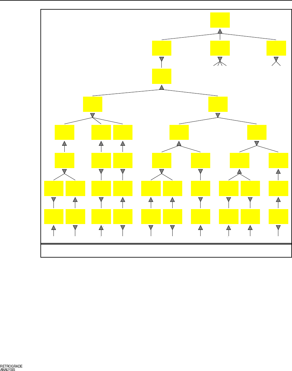
32 Chapter 6. Adversarial Search
MAX MIN
S 2
H 6 4
D 6
C 9,8 10,5
MAX MIN
S 2
H 4
D 6
C 9,8 10,5
MAX MIN
S 2
H 6 4
D
C 9,8 10,5
MAX MIN
S 2
H 6 4
D 6
C 9 10,5
MAX MIN
S 2
H
D 6
C 9,8 10,5
MAX MIN
S 2
H
D 6
C 9 10,5
MAX MIN
S 2
H
D
C 9,8 10,5
MAX MIN
S
H
D
C 9,8 10,5
MAX MIN
S 2
H
D
C 9,8 10
MAX MIN
S 2
H
D
C 9,8 5
MAX MIN
S
H
D
C 9 10,5
MAX MIN
S 2
H
D
C 9 10
MAX MIN
S 2
H
D
C 9 5
MAX MIN
S
H
D
C 9 5
MAX MIN
S
H
D
C 9 10
MAX MIN
S
H
D
C 9
MAX MIN
S
H
D
C 10
MAX MIN
S 2
H
D
C 9
MAX MIN
S 2
H
D
C 9
MAX MIN
S
H
D
C 9
MAX MIN
S 2
H
D
C
MAX MIN
S 2
H
D 6
C 9 10
MAX MIN
S 2
H
D 6
C 9 5
MAX MIN
S 2
H
D
C 9 10
MAX MIN
S 2
H
D 6
C 10
MAX MIN
S
H
D
C 9 10
MAX MIN
S 2
H
D
C 9
MAX MIN
S
H
D
C 10
MAX MIN
S 2
H
D
C
MAX MIN
S
H
D 6
C
MAX MIN
S 2
H
D 6
C
MAX MIN
S
H
D 6
C 9 5
MAX MIN
S 2
H
D 6
C 9
MAX MIN
S
H
D
C 9 5
MAX MIN
S
H
D 6
C 5
MAX MIN
S
H
D
C 9
MAX MIN
S
H
D 6
C
MAX MIN
S 2
H
D 6
C
MAX MIN
S 2
H
D
C
+2 +2 0 +4 +2 +4 0 0 −2 +2
+2 +2 0 +4 +2 +4 0 0 −2 +2
+2 +2 0 +4 +2 +4 0 0 −2 +2
+2
+2
0+4
0+4
0
+2 0 0 +2
0
+2
0
0
0
Figure S6.5 Ex. 6.12: Part of the game tree for the card game shown on p.179.
can be a mixture of MAX and MIN nodes, depending on the various cards MAX can
play. A similar modification is needed for MIN-VALUE.
b. The game tree is shown in Figure S6.5.
6.13 The naive approach would be to generate each such position, solve it, and store the
outcome. This would be enormously expensive—roughly on the order of 444 billion seconds,
or 10,000 years, assuming it takes a second on average to solve each position (which is
probably very optimistic). Of course, we can take advantage of already-solved positions
when solving new positions, provided those solved positions are descendants of the new
positions. To ensure that this always happens, we generate the final positions first, then their
predecessors, and so on. In this way, the exact values of all successors are known when each
state is generated. This method is called retrograde analysis.

33
6.14 The most obvious change is that the space of actions is now continuous. For example,
in pool, the cueing direction, angle of elevation, speed, and point of contact with the cue ball
are all continuous quantities.
The simplest solution is just to discretize the action space and then apply standard meth-
ods. This might work for tennis (modelled crudely as alternating shots with speed and direc-
tion), but for games such as pool and croquet it is likely to fail miserably because small
changes in direction have large effects on action outcome. Instead, one must analyze the
game to identify a discrete set of meaningful local goals, such as “potting the 4-ball” in pool
or “laying up for the next hoop” in croquet. Then, in the current context, a local optimization
routine can work out the best way to achieve each local goal, resulting in a discrete set of pos-
sible choices. Typically, these games are stochastic, so the backgammon model is appropriate
provided that we use sampled outcomes instead of summing over all outcomes.
Whereas pool and croquet are modelled correctly as turn-taking games, tennis is not.
While one player is moving to the ball, the other player is moving to anticipate the opponent’s
return. This makes tennis more like the simultaneous-action games studied in Chapter 17. In
particular, it may be reasonable to derive randomized strategies so that the opponent cannot
anticipate where the ball will go.
6.15 The minimax algorithm for non-zero-sum games works exactly as for multiplayer
games, described on p.165–6; that is, the evaluation function is a vector of values, one for
each player, and the backup step selects whichever vector has the highest value for the player
whose turn it is to move. The example at the end of Section 6.2 (p.167) shows that alpha-beta
pruning is not possible in general non-zero-sum games, because an unexamined leaf node
might be optimal for both players.
6.16 With 32 pieces, each needing 6 bits to specify its position on one of 64 squares, we
need 24 bytes (6 32-bit words) to store a position, so we can store roughly 20 million positions
in the table (ignoring pointers for hash table bucket lists). This is about one-ninth of the 180
million positions generated during a three-minute search.
Generating the hash key directly from an array-based representation of the position
might be quite expensive. Modern programs (see, e.g., Heinz, 2000) carry along the hash
key and modify it as each new position is generated. Suppose this takes on the order of 20
operations; then on a 2GHz machine where an evaluation takes 2000 operations we can do
roughly 100 lookups per evaluation. Using a rough figure of one millisecond for a disk seek,
we could do 1000 evaluations per lookup. Clearly, using a disk-resident table is of dubious
value, even if we can get some locality of reference to reduce the number of disk reads.
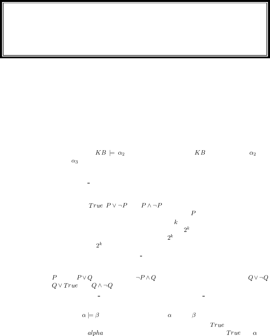
Solutions for Chapter 7
Agents that Reason Logically
7.1 The wumpus world is partially observable, deterministic, sequential (you need to re-
member the state of one location when you return to it on a later turn), static, discrete, and
single agent (the wumpus’s sole trick—devouring an errant explorer—is not enough to treat
it as an agent). Thus, it is a fairly simple environment. The main complication is the partial
observability.
7.2 To save space, we’ll show the list of models as a table rather than a collection of dia-
grams. There are eight possible combinations of pits in the three squares, and four possibili-
ties for the wumpus location (including nowhere).
We can see that because every line where is true also has true.
Similarly for .
7.3
a. There is a pl true in the Python code, and a version of ask in the Lisp code that
serves the same purpose. The Java code did not have this function as of May 2003, but
it should be added soon.)
b. The sentences , , and can all be determined to be true or false in
a partial model that does not specify the truth value for .
c. It is possible to create two sentences, each with variables that are not instantiated in
the partial model, such that one of them is true for all possible values of the variables,
while the other sentence is false for one of the values. This shows that in general one
must consider all possibilities. Enumerating them takes exponential time.
d. The python implementation of pl true returns true if any disjunct of a disjunction
is true, and false if any conjunct of a conjunction is false. It will do this even if other
disjuncts/conjuncts contains uninstantiated variables. Thus, in the partial model where
is true, returns true, and returns false. But the truth values of ,
, and are not detected.
e. Our version of tt entails already uses this modified pl true. It would be slower
if it did not.
7.4 Remember, iff in very model in which is true, is also true. Therefore,
a. A valid sentence is one that is true in all models. The sentence is also valid in all
models. So if is valid then the entailment holds (because both and hold
34

35
Model
,
,
,
, ,
,
,
,
, ,
, ,
, ,
,,,
,
,
,
,
, ,
, ,
, ,
,,,
,
,
,
, ,
, ,
, ,
,,,
Figure 7.1 A truth table constructed for Ex. 7.2. Propositions not listed as true on a given
line are assumed false, and only entries are shown in the table.
in every model), and if the entailment holds then must be valid, because it must be
true in all models, because it must be true in all models in which holds.
b. doesn’t hold in any model, so trivially holds in every model that holds
in.
c. holds in those models where holds or where holds. That is precisely the
case if is valid.
d. This follows from applying cin both directions.
36 Chapter 7. Agents that Reason Logically
e. This reduces to c, because is unsatisfiable just when is valid.
7.5 These can be computed by counting the rows in a truth table that come out true. Re-
member to count the propositions that are not mentioned; if a sentence mentions only and
, then we multiply the number of models for by to account for and .
a. 6
b. 12
c. 4
7.6 A binary logical connective is defined by a truth table with 4 rows. Each of the four
rows may be true or false, so there are possible truth tables, and thus 16 possible
connectives. Six of these are trivial ones that ignore one or both inputs; they correspond to
, , , , and . Four of them we have already studied: .
The remaining six are potentially useful. One of them is reverse implication ( instead of
), and the other five are the negations of and . (The first two of these
are sometimes called nand and nor.)
7.7 We use the truth table code in Lisp in the directory logic/prop.lisp to show each
sentence is valid. We substitute P, Q, R for because of the lack of Greek letters in
ASCII. To save space in this manual, we only show the first four truth tables:
> (truth-table "P ˆ Q <=> Q ˆ P")
-----------------------------------------
P Q P ˆ Q Q ˆ P (P ˆ Q) <=> (Q ˆ P)
-----------------------------------------
F F F F \(true\)
T F F F T
F T F F T
T T T T T
-----------------------------------------
NIL
> (truth-table "P | Q <=> Q | P")
-----------------------------------------
P Q P | Q Q | P (P | Q) <=> (Q | P)
-----------------------------------------
F F F F T
T F T T T
F T T T T
T T T T T
-----------------------------------------
NIL
> (truth-table "P ˆ (Q ˆ R) <=> (P ˆ Q) ˆ R")
-----------------------------------------------------------------------
P Q R Q ˆ R P ˆ (Q ˆ R) P ˆ Q ˆ R (P ˆ (Q ˆ R)) <=> (P ˆ Q ˆ R)
-----------------------------------------------------------------------
F F F F F F T
T F F F F F T
F T F F F F T

37
T T F F F F T
F F T F F F T
T F T F F F T
F T T T F F T
T T T T T T T
-----------------------------------------------------------------------
NIL
> (truth-table "P | (Q | R) <=> (P | Q) | R")
-----------------------------------------------------------------------
P Q R Q | R P | (Q | R) P | Q | R (P | (Q | R)) <=> (P | Q | R)
-----------------------------------------------------------------------
F F F F F F T
T F F F T T T
F T F T T T T
T T F T T T T
F F T T T T T
T F T T T T T
F T T T T T T
T T T T T T T
-----------------------------------------------------------------------
NIL
For the remaining sentences, we just show that they are valid according to the validity
function:
> (validity "˜˜P <=> P")
VALID
> (validity "P => Q <=> ˜Q => ˜P")
VALID
> (validity "P => Q <=> ˜P | Q")
VALID
> (validity "(P <=> Q) <=> (P => Q) ˆ (Q => P)")
VALID
> (validity "˜(P ˆ Q) <=> ˜P | ˜Q")
VALID
> (validity "˜(P | Q) <=> ˜P ˆ ˜Q")
VALID
> (validity "P ˆ (Q | R) <=> (P ˆ Q) | (P ˆ R)")
VALID
> (validity "P | (Q ˆ R) <=> (P | Q) ˆ (P | R)")
VALID
7.8 We use the validity function from logic/prop.lisp to determine the validity
of each sentence:
> (validity "Smoke => Smoke")
VALID
> (validity "Smoke => Fire")
SATISFIABLE
> (validity "(Smoke => Fire) => (˜Smoke => ˜Fire)")
SATISFIABLE
> (validity "Smoke | Fire | ˜Fire")
VALID
38 Chapter 7. Agents that Reason Logically
> (validity "((Smoke ˆ Heat) => Fire) <=> ((Smoke => Fire) | (Heat => Fire))")
VALID
> (validity "(Smoke => Fire) => ((Smoke ˆ Heat) => Fire)")
VALID
> (validity "Big | Dumb | (Big => Dumb)")
VALID
> (validity "(Big ˆ Dumb) | ˜Dumb")
SATISFIABLE
Many people are fooled by (e) and (g) because they think of implication as being cau-
sation, or something close to it. Thus, in (e), they feel that it is the combination of Smoke
and Heat that leads to Fire, and thus there is no reason why one or the other alone should
lead to fire. Similarly, in (g), they feel that there is no necessary causal relation between Big
and Dumb, so the sentence should be satisfiable, but not valid. However, this reasoning is
incorrect, because implication is not causation—implication is just a kind of disjunction (in
the sense that is the same as ). So is
equivalent to , which is equivalent to ,
which is true whether is true or false, and is therefore valid.
7.9 From the first two statements, we see that if it is mythical, then it is immortal; otherwise
it is a mammal. So it must be either immortal or a mammal, and thus horned. That means it
is also magical. However, we can’t deduce anything about whether it is mythical. Using the
propositional reasoning code:
> (setf kb (make-prop-kb))
#S(PROP-KB SENTENCE (AND))
> (tell kb "Mythical => Immortal")
T
> (tell kb "˜Mythical => ˜Immortal ˆ Mammal")
T
> (tell kb "Immortal | Mammal => Horned")
T
> (tell kb "Horned => Magical")
T
> (ask kb "Mythical")
NIL
> (ask kb "˜Mythical")
NIL
> (ask kb "Magical")
T
> (ask kb "Horned")
T
7.10 Each possible world can be written as a conjunction of symbols, e.g. .
Asserting that a possible world is not the case can be written by negating that, e.g.
, which can be rewritten as . This is the form of a clause; a conjunction
of these clauses is a CNF sentence, and can list all the possible worlds for the sentence.
7.11
39
a. This is a disjunction with 28 disjuncts, each one saying that two of the neighbors are
true and the others are false. The first disjunct is
The other 27 disjuncts each select two different to be true.
b. There will be disjuncts, each saying that of the symbols are true and the others
false.
c. For each of the cells that have been probed, take the resulting number revealed by the
game and construct a sentence with disjuncts. Conjoin all the sentences together.
Then use DPLL to answer the question of whether this sentence entails for the
particular pair you are interested in.
d. To encode the global constraint that there are mines altogether, we can construct
a disjunct with disjuncts, each of size . Remember, . So for
a Minesweeper game with 100 cells and 20 mines, this will be morre than , and
thus cannot be represented in any computer. However, we can represent the global
constraint within the DPLL algorithm itself. We add the parameter min and max to
the DPLL function; these indicate the minimum and maximum number of unassigned
symbols that must be true in the model. For an unconstrained problem the values 0 and
will be used for these parameters. For a mineseeper problem the value will be
used for both min and max. Within DPLL, we fail (return false) immediately if min is
less than the number of remaining symbols, or if max is less than 0. For each recursive
call to DPLL, we update min and max by subtracting one when we assign a true value
to a symbol.
e. No conclusions are invalidated by adding this capability to DPLL and encoding the
global constraint using it.
f. Consider this string of alternating 1’s and unprobed cells (indicated by a dash):
|-|1|-|1|-|1|-|1|-|1|-|1|-|1|-|
There are two possible models: either there are mines under every even-numbered
dash, or under every odd-numbered dash. Making a probe at either end will determine
whether cells at the far end are empty or contain mines.
7.12
a.is equivalent to by implication elimination (Figure 7.11), and
is equivalent to by de Morgan’s rule, so
is equivalent to .
b. A clause can have positive and negative literals; arrange them in the form
. Then, setting , we have
is equivalent to
40 Chapter 7. Agents that Reason Logically
c. For atoms where UNIFY :
SUBST
7.13
a.
b.
c. These formulae are the same as (7.7) and (7.8), except that the for pit is replaced by
for wumpus, and for breezy is replaced by for smelly.
7.14 Optimal behavior means achieving an expected utility that is as good as any other
agent program. The PL-WUMPUS-AGENT is clearly non-optimal when it chooses a random
move (and may be non-optimal in other braqnches of its logic). One example: in some cases
when there are many dangers (breezes and smells) but no safe move, the agent chooses at
random. A more thorough analysis should show when it is better to do that, and when it is
better to go home and exit the wumpus world, giving up on any chance of finding the gold.
Even when it is best to gamble on an unsafe location, our agent does not distinguish degrees
of safety – it should choose the unsafe square which contains a danger in the fewest number
of possible models. These refinements are hard to state using a logical agent, but we will see
in subsequent chapters that a probabilistic agent can handle them. does
7.15 PL-WUMPUS-AGENT keeps track of 6 static state variables besides KB. The difficulty
is that these variables change—we don’t just add new information about them (as we do with
pits and breezy locations), we modify exisitng information. This does not sit well with logic,
which is designed for eternal truths. So there are two alternatives. The first is to superscript
each proposition with the time (as we did with the circuit agents), and then we could, for
example, do TELL to say that the agent is at location at time 3. Then at time 4,
we would have to copy over many of the existing propositions, and add new ones. The second
possibility is to treat every proposition as a timeless one, but to remove outdated propositions
from the KB. That is, we could do RETRACT and then progTell to
indicate that the agent has moved from to . Chapter 10 describes the semantics and
implementation of RETRACT.
NOTE: Avoid assigning this problem if you don’t feel comfortable requiring students
to think ahead about the possibility of retraction.
7.16 It will take time proportional to the number of pure symbols plus the number of unit
clauses. We assume that is false, and prove a contradiction. is
equivalent to . From this sentence the algorithm will first eliminate all the pure

41
symbols, then it will work on unit clauses until it chooses (which is a unit clause); at that
point it will immediately recognize that either choice (true or false) for leads to failure,
which means that the original non-negated assertion is true.
7.17 Code not shown.

Solutions for Chapter 8
First-Order Logic
8.1 This question will generate a wide variety of possible solutions. The key distinction
between analogical and sentential representations is that the analogical representation au-
tomatically generates consequences that can be “read off” whenever suitable premises are
encoded. When you get into the details, this distinction turns out to be quite hard to pin
down—for example, what does “read off” mean?—but it can be justified by examining the
time complexity of various inferences on the “virtual inference machine” provided by the
representation system.
a. Depending on the scale and type of the map, symbols in the map language typically
include city and town markers, road symbols (various types), lighthouses, historic mon-
uments, river courses, freeway intersections, etc.
b. Explicit and implicit sentences: this distinction is a little tricky, but the basic idea is that
when the map-drawer plunks a symbol down in a particular place, he says one explicit
thing (e.g. that Coit Tower is here), but the analogical structure of the map representa-
tion means that many implicit sentences can now be derived. Explicit sentences: there
is a monument called Coit Tower at this location; Lombard Street runs (approximately)
east-west; San Francisco Bay exists and has this shape. Implicit sentences: Van Ness
is longer than North Willard; Fisherman’s Wharf is north of the Mission District; the
shortest drivable route from Coit Tower to Twin Peaks is the following .
c. Sentences unrepresentable in the map language: Telegraph Hill is approximately coni-
cal and about 430 feet high (assuming the map has no topographical notation); in 1890
there was no bridge connecting San Francisco to Marin County (map does not repre-
sent changing information); Interstate 680 runs either east or west of Walnut Creek (no
disjunctive information).
d. Sentences that are easier to express in the map language: any sentence that can be
written easily in English is not going to be a good candidate for this question. Any
linguistic abstraction from the physical structure of San Francisco (e.g. San Francisco
is on the end of a peninsula at the mouth of a bay) can probably be expressed equally
easily in the predicate calculus, since that’s what it was designed for. Facts such as
the shape of the coastline, or the path taken by a road, are best expressed in the map
language. Even then, one can argue that the coastline drawn on the map actually consists
of lots of individual sentences, one for each dot of ink, especially if the map is drawn
42
43
using a digital plotter. In this case, the advantage of the map is really in the ease of
inference combined with suitability for human “visual computing” apparatus.
e. Examples of other analogical representations:
Analog audio tape recording. Advantages: simple circuits can record and repro-
duce sounds. Disadvantages: subject to errors, noise; hard to process in order to
separate sounds or remove noise etc.
Traditional clock face. Advantages: easier to read quickly, determination of how
much time is available requires no additional computation. Disadvantages: hard to
read precisely, cannot represent small units of time (ms) easily.
All kinds of graphs, bar charts, pie charts. Advantages: enormous data compres-
sion, easy trend analysis, communicate information in a way which we can in-
terpret easily. Disadvantages: imprecise, cannot represent disjunctive or negated
information.
8.2 The knowledge base does not entail . To show this, we must give a model
where and but is false. Consider any model with three domain elements,
where and refer to the first two elements and the relation referred to by holds only for
those two elements.
8.3 The sentence is valid. A sentence is valid if it is true in every model. An
existentially quantified sentence is true in a model if it holds under any extended interpretation
in which its variables are assigned to domain elements. According to the standard semantics
of FOL as given in the chapter, every model contains at least one domain element, hence,
for any model, there is an extended interpretation in which and are assigned to the first
domain element. In such an interpretation, is true.
8.4 stipulates that there is exactly one object. If there are two objects, then
there is an extended interpretation in which and are assigned to different objects, so the
sentence would be false. Some students may also notice that any unsatisfiable sentence also
meets the criterion, since there are no worlds in which the sentence is true.
8.5 We will use the simplest counting method, ignoring redundant combinations. For the
constant symbols, there are assignments. Each predicate of arity is mapped onto a -ary
relation, i.e., a subset of the possible -element tuples; there are such mappings. Each
function symbol of arity is mapped onto a -ary function, which specifies a value for each
of the possible -element tuples. Including the invisible element, there are choices
for each value, so there are functions. The total number of possible combinations
is therefore
Two things to note: first, the number is finite; second, the maximum arity is the most
crucial complexity parameter.
8.6 In this exercise, it is best not to worry about details of tense and larger concerns with
consistent ontologies and so on. The main point is to make sure students understand con-
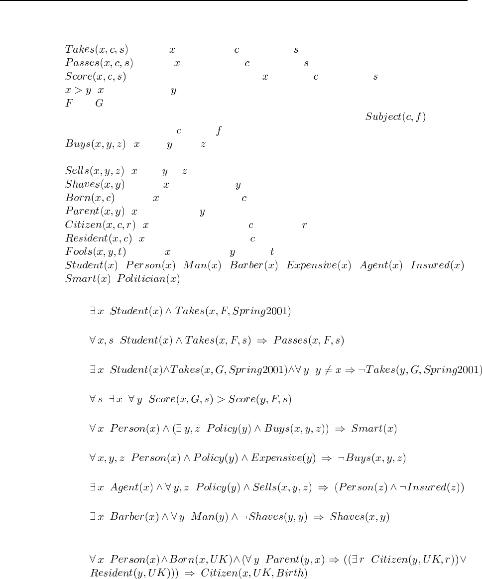
44 Chapter 8. First-Order Logic
nectives and quantifiers and the use of predicates, functions, constants, and equality. Let the
basic vocabulary be as follows:
: student takes course in semester ;
: student passes course in semester ;
: the score obtained by student in course in semester ;
: is greater than ;
and : specific French and Greek courses (one could also interpret these sentences as re-
ferring to any such course, in which case one could use a predicate meaning
that the subject of course is field ;
: buys from (using a binary predicate with unspecified seller is OK but
less felicitous);
: sells to ;
: person shaves person
: person is born in country ;
: is a parent of ;
: is a citizen of country for reason ;
: is a resident of country ;
: person fools person at time ;
, , , , , , ,
, : predicates satisfied by members of the corresponding categories.
a. Some students took French in spring 2001.
.
b. Every student who takes French passes it.
.
c. Only one student took Greek in spring 2001.
.
d. The best score in Greek is always higher than the best score in French.
.
e. Every person who buys a policy is smart.
.
f. No person buys an expensive policy.
.
g. There is an agent who sells policies only to people who are not insured.
.
h. There is a barber who shaves all men in town who do not shave themselves.
.
i. A person born in the UK, each of whose parents is a UK citizen or a UK resident, is a
UK citizen by birth.
.
j. A person born outside the UK, one of whose parents is a UK citizen by birth, is a UK
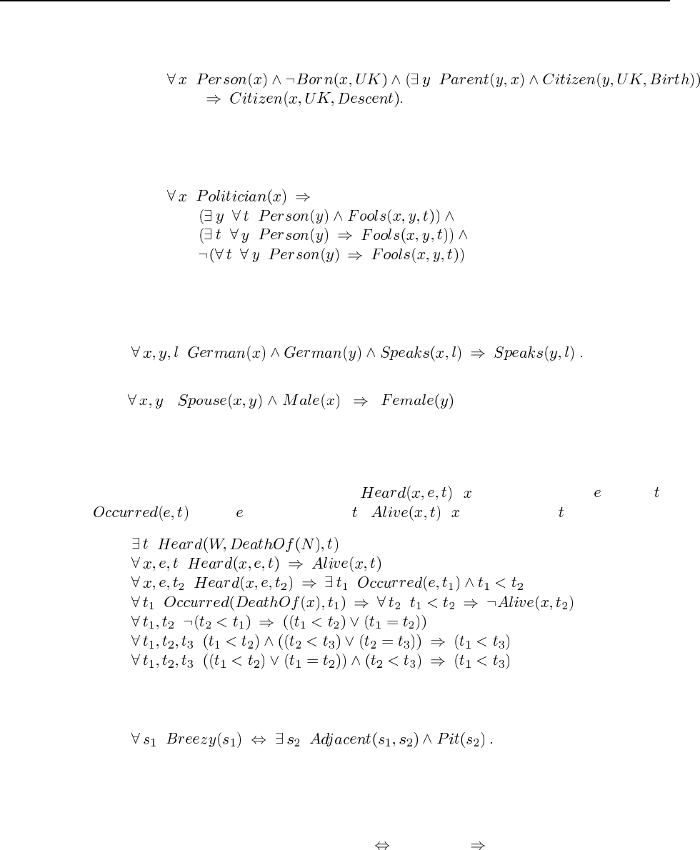
45
citizen by descent.
k. Politicians can fool some of the people all of the time, and they can fool all of the people
some of the time, but they can’t fool all of the people all of the time.
8.7 The key idea is to see that the word “same” is referring to every pair of Germans. There
are several logically equivalent forms for this sentence. The simplest is the Horn clause:
8.8 . This axiom is no longer true in
certain states and countries.
8.9 This is a very educational exercise but also highly nontrivial. Once students have
learned about resolution, ask them to do the proof too. In most cases, they will discover
missing axioms. Our basic predicates are ( heard about event at time );
(event occurred at time ); ( is alive at time ).
8.10 It is not entirely clear which sentences need to be written, but this is one of them:
That is, a square is breezy if and only if there is a pit in a neighboring square. Generally
speaking, the size of the axiom set is independent of the size of the wumpus world being
described.
8.11 Make sure you write definitions with . If you use , you are only imposing con-
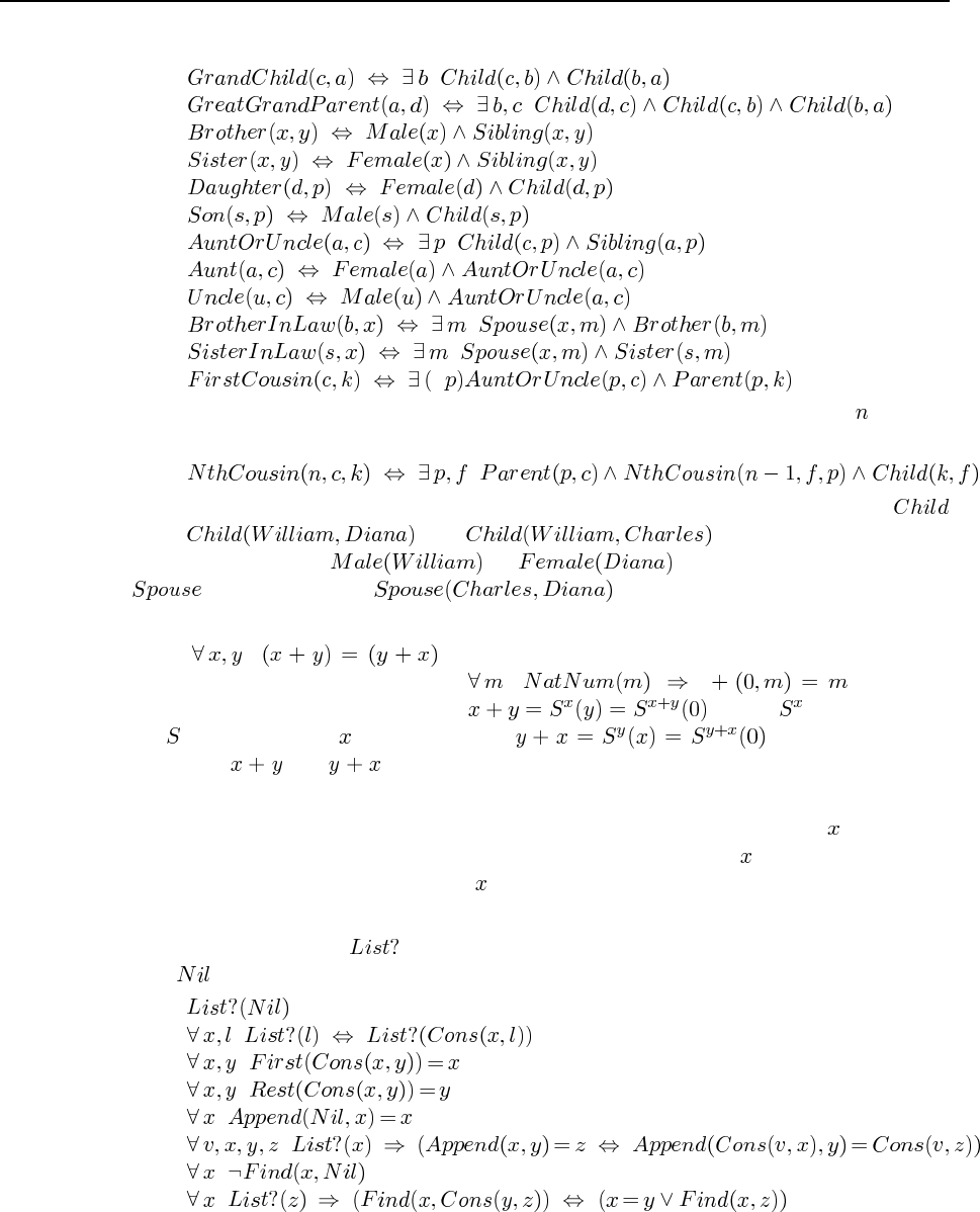
46 Chapter 8. First-Order Logic
straints, not writing a real definition.
A second cousin is a a child of one’s parent’s first cousin, and in general an th cousin
is defined as:
The facts in the family tree are simple: each arrow represents two instances of
(e.g., and ), each name represents a
sex proposition (e.g., or ), each double line indicates a
proposition (e.g. ). Making the queries of the logical
reasoning system is just a way of debugging the definitions.
8.12 . This does follow from the Peano axioms (although we
should write the first axiom for + as ). Roughly
speaking, the definition of + says that , where is shorthand for
the function applied times. Similarly, . Hence, the axioms
imply that and are equal to syntactically identical expressions. This argument
can be turned into a formal proof by induction.
8.13 Although these axioms are sufficient to prove set membership when is in fact a
member of a given set, they have nothing to say about cases where is not a member. For
example, it is not possible to prove that is not a member of the empty set. These axioms may
therefore be suitable for a logical system, such as Prolog, that uses negation-as-failure.
8.14 Here we translate to mean “proper list” in Lisp terminology, i.e., a cons structure
with as the “rightmost” atom.

47
8.15 There are several problems with the proposed definition. It allows one to prove, say,
but not ; so we need an additional symmetry
axiom. It does not allow one to prove that is false, so it needs to be
written as
Finally, it does not work as the boundaries of the world, so some extra conditions must be
added.
8.16 We need the following sentences:
8.17 There are three stages to go through. In the first stage, we define the concepts of one-
bit and -bit addition. Then, we specify one-bit and -bit adder circuits. Finally, we verify
that the -bit adder circuit does -bit addition.
One-bit addition is easy. Let be a function of three one-bit arguments (the third
is the carry bit). The result of the addition is a list of bits representing a 2-bit binary
number, least significant digit first:
-bit addition builds on one-bit addition. Let be a function that takes
two lists of binary digits of length (least significant digit first) and a carry bit (initially
0), and constructs a list of length that represents their sum. (It will always be
exactly bits long, even when the leading bit is 0—the leading bit is the overflow
bit.)
The next step is to define the structure of a one-bit adder circuit, as given in Section ??.
Let be true of any circuit that has the appropriate components and
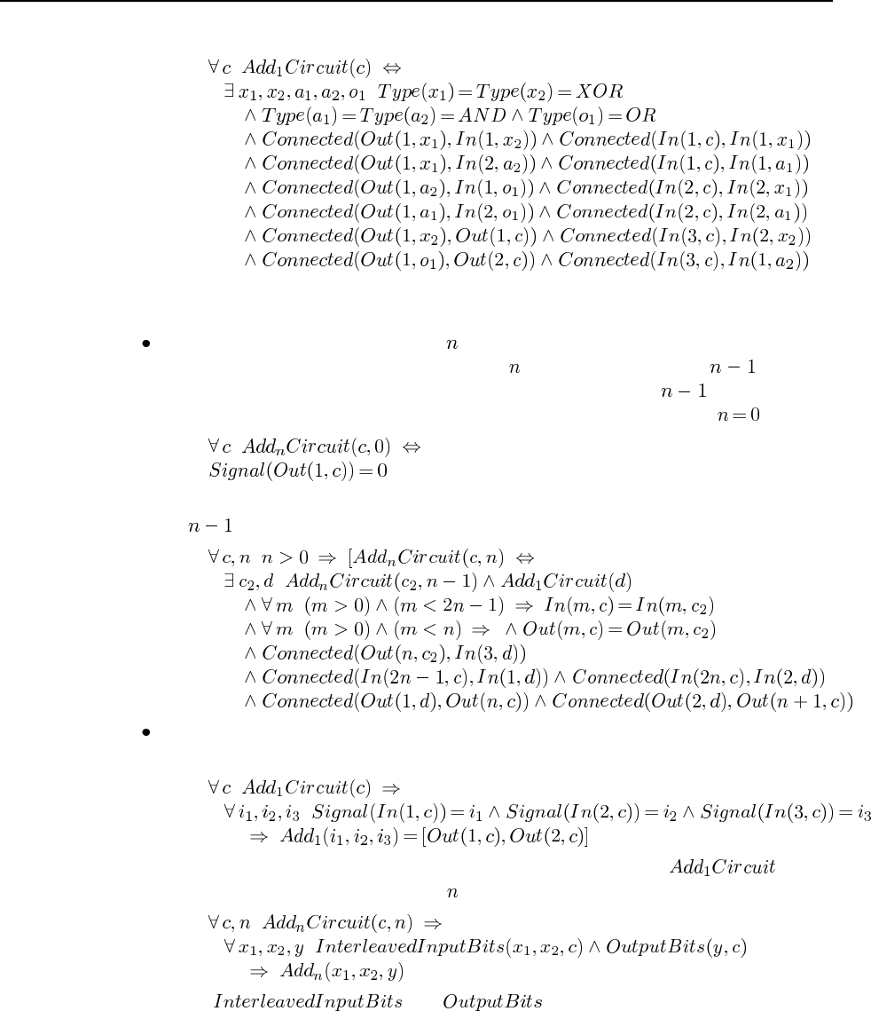
48 Chapter 8. First-Order Logic
connections:
Notice that this allows the circuit to have additional gates and connections, but they
won’t stop it from doing addition.
Now we define what we mean by an -bit adder circuit, following the design of Figure
8.6. We will need to be careful, because an -bit adder is not just an -bit adder
plus a one-bit adder; we have to connect the overflow bit of the -bit adder to the
carry-bit input of the one-bit adder. We begin with the base case, where :
Now, for the recursive case we specify that the first connect the “overflow” output of
the -bit circuit as the carry bit for the last bit:
Now, to verify that a one-bit adder circuit actually adds correctly, we ask whether, given
any setting of the inputs, the outputs equal the sum of the inputs:
If this sentence is entailed by the KB, then every circuit with the design
is in fact an adder. The query for the -bit can be written as
where and are defined appropriately to map bit
sequences to the actual terminals of the circuit. [Note: this logical formulation has not
been tested in a theorem prover and we hesitate to vouch for its correctness.]
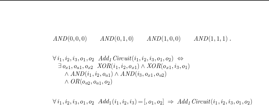
49
8.18 Strictly speaking, the primitive gates must be defined using logical equivalences to
exclude those combinations not listed as correct. If we are using a logic programming system,
we can simply list the cases. For example,
For the one-bit adder, we have
The verification query is
It is not possible to ask whether particular terminals are connected in a given circuit, since
the terminals is not reified (nor is the circuit itself).
8.19 The answers here will vary by country. The two key rules for UK passports are given
in the answer to Exercsie 8.6.
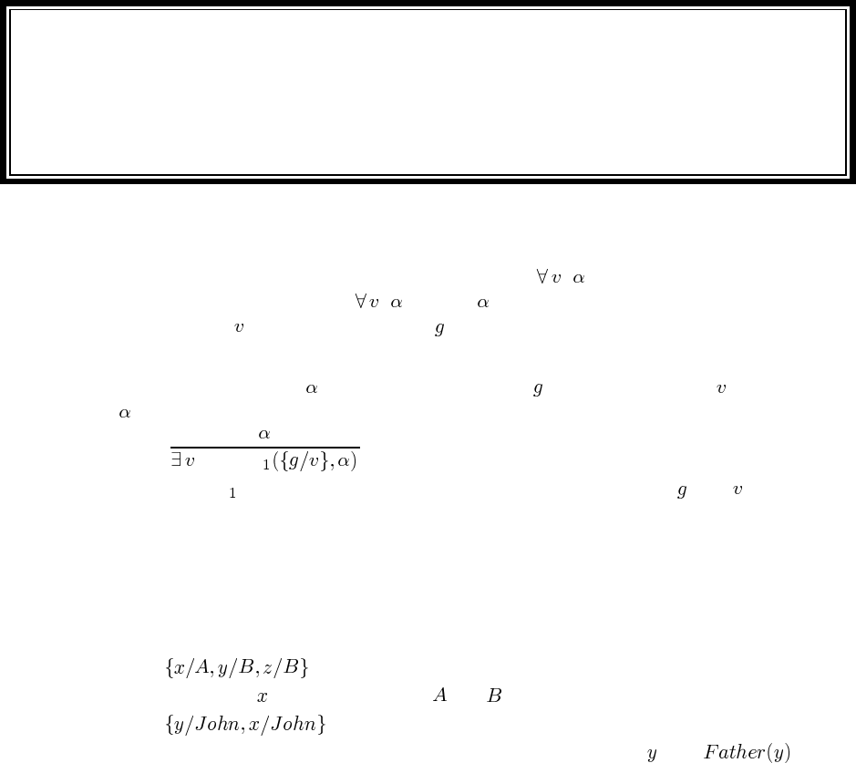
Solutions for Chapter 9
Inference in First-Order Logic
9.1 We want to show that any sentence of the form entails any universal instantiation
of the sentence. The sentence is true if is true in all possible extended interpretations.
But replacing with any ground term must count as one of the interpretations, so if the
original sentence is true, then the instantiated sentence must also be true.
9.2 For any sentence containing a ground term and for any variable not occuring in
, we have
SUBST
where SUBST is a function that substitutes for a single occurrence of with .
9.3 Both b and c are valid; a is invalid because it introduces the previously-used symbol
Everest. Note that c does not imply that there are two mountains as high as Everest, be-
cause nowhere is it stated that BenNevis is different from Kilimanjaro (or Everest, for that
matter).
9.4 This is an easy exercise to check that the student understands unification.
a.(or some permutation of this).
b. No unifier ( cannot bind to both and ).
c. .
d. No unifier (because the occurs-check prevents unification of with ).
9.5 Employs(Mother(John), Father(Richard)) This page isn’t wide enough to draw the dia-
gram as in Figure 9.2, so we will draw it with indentation denoting children nodes:
[1] Employs(x, y)
[2] Employs(x, Father(z))
[3] Employs(x, Father(Richard))
[4] Employs(Mother(w), Father(Richard))
[5] Employs(Mother(John), Father(Richard))
[6] Employs(Mother(w), Father(z))
[4] ...
[7] Employs(Mother(John), Father(z))
[5] ...
50
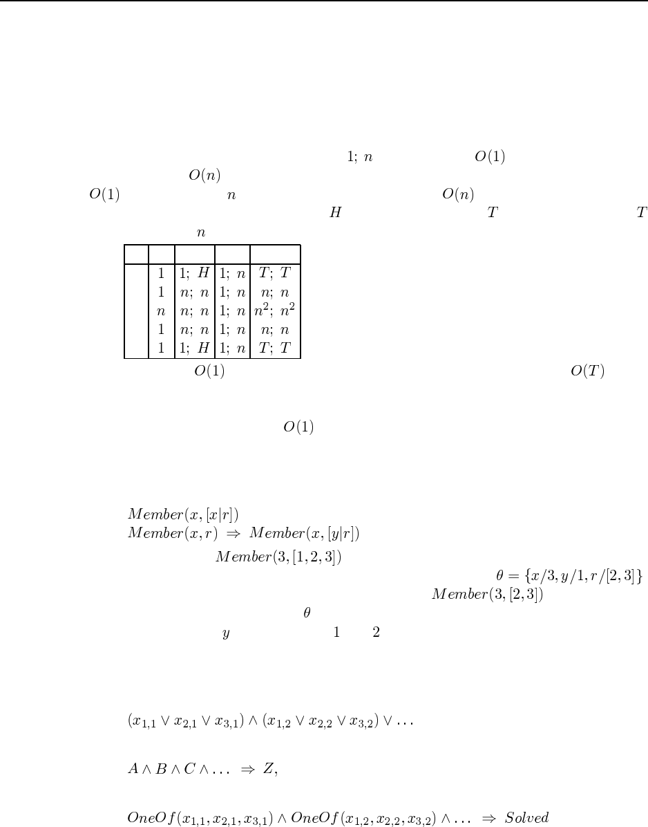
51
[8] Employs(Mother(w), y)
[9] Employs(Mother(John), y)
[10] Employs(Mother(John), Father(z)
[5] ...
[6] ...
9.6 We will give the average-case time complexity for each query/scheme combination in
the following table. (An entry of the form “ ” means that it is to find the first solution
to the query, but to find them all.) We make the following assumptions: hash tables give
access; there are people in the data base; there are people of any specified age;
every person has one mother; there are people in Houston and people in Tiny Town;
is much less than ; in Q4, the second conjunct is evaluated first.
Q1 Q2 Q3 Q4
S1
S2
S3
S4
S5
Anything that is can be considered “efficient,” as perhaps can anything . Note
that S1 and S5 dominate the other schemes for this set of queries. Also note that indexing on
predicates plays no role in this table (except in combination with an argument), because there
are only 3 predicates (which is ). It would make a difference in terms of the constant
factor.
9.7 This would work if there were no recursive rules in the knowledge base. But suppose
the knowledge base contains the sentences:
Now take the query , with a backward chaining system. We unify the
query with the consequent of the implication to get the substitution .
We then substitute this in to the left-hand side to get and try to back
chain on that with the substitution . When we then try to apply the implication again, we
get a failure because cannot be both and . In other words, the failure to standardize
apart causes failure in some cases where recursive rules would result in a solution if we did
standardize apart.
9.8 Consider a 3-SAT problem of the form
We want to rewrite this as a single define clause of the form
along with a few ground clauses. We can do that with the definite clause

52 Chapter 9. Inference in First-Order Logic
along with the ground clauses
9.9 We use a very simple ontology to make the examples easier:
a.
b.
c.
d.
e.
(Note we couldn’t do because that is not in the form
expected by Generalized Modus Ponens.)
f.(here is a Skolem function).
9.10 This questions deals with the subject of looping in backward-chaining proofs. A loop
is bound to occur whenever a subgoal arises that is a substitution instance of one of the goals
on the stack. Not all loops can be caught this way, of course, otherwise we would have a way
to solve the halting problem.
a. The proof tree is shown in Figure S9.1. The branch with and
repeats indefinitely, so the rest of the proof is never reached.
b. We get an infinite loop because of rule b, .
The specific loop appearing in the figure arises because of the ordering of the clauses—
it would be better to order before the rule from b. However, a loop
will occur no matter which way the rules are ordered if the theorem-prover is asked for
all solutions.
c. One should be able to prove that both Bluebeard and Charlie are horses.
d. Smith et al. (1986) recommend the following method. Whenever a “looping” goal
occurs (one that is a substitution instance of a supergoal higher up the stack), sus-
pend the attempt to prove that subgoal. Continue with all other branches of the proof
for the supergoal, gathering up the solutions. Then use those solutions (suitably in-
stantiated if necessary) as solutions for the suspended subgoal, continuing that branch
of the proof to find additional solutions if any. In the proof shown in the figure, the
is a repeated goal and would be suspended. Since no other
way to prove it exists, that branch will terminate with failure. In this case, Smith’s
method is sufficient to allow the theorem-prover to find both solutions.
9.11 Surprisingly, the hard part to represent is “who is that man.” We want to ask “what
relationship does that man have to some known person,” but if we represent relations with
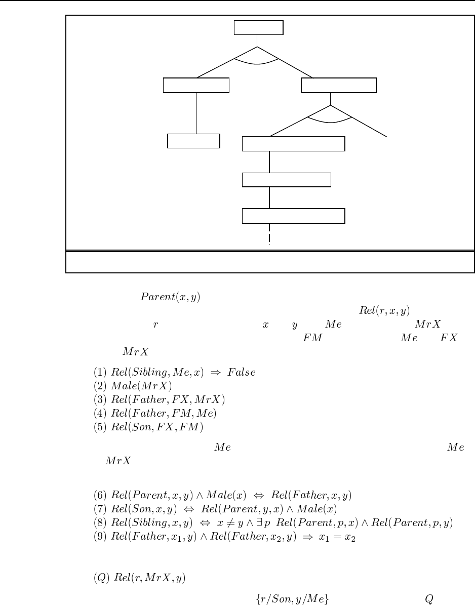
53
Parent(y,Bluebeard)
Horse(h)
Offspring(h,y)
Parent(y,h)
Horse(Bluebeard)
Yes, {y/Bluebeard,
h/Charlie}
Offspring(Bluebeard,y)
Offspring(Bluebeard,y)
Figure S9.1 Partial proof tree for finding horses.
predicates (e.g., ) then we cannot make the relationship be a variable in first-
order logic. So instead we need to reify relationships. We will use to say that the
family relationship holds between people and . Let denote me and denote
“that man.” We will also need the Skolem constants for the father of and for
the father of . The facts of the case (put into implicative normal form) are:
We want to be able to show that is the only son of my father, and therefore that is
father of , who is male, and therefore that “that man” is my son. The relevant definitions
from the family domain are:
and the query we want is:
We want to be able to get back the answer . Translating 1-9 and into INF
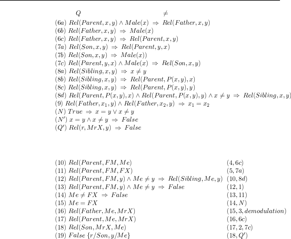
54 Chapter 9. Inference in First-Order Logic
(and negating and including the definition of ) we get:
Note that (1) is non-Horn, so we will need resolution to be be sure of getting a solution. It
turns out we also need demodulation (page 284) to deal with equality. The following lists the
steps of the proof, with the resolvents of each step in parentheses:
9.12 Here is a goal tree:
goals = [Criminal(West)]
goals = [American(West), Weapon(y), Sells(West, y, z), Hostile(z)]
goals = [Weapon(y), Sells(West, y, z), Hostile(z)]
goals = [Missle(y), Sells(West, y, z), Hostile(z)]
goals = [Sells(West, M1, z), Hostile(z)]
goals = [Missle(M1), Owns(Nono, M1), Hostile(Nono)]
goals = [Owns(Nono, M1), Hostile(Nono)]
goals = [Hostile(Nono)]
goals = []
9.13
a. In the following, an indented line is a step deeper in the proof tree, while two lines at
the same indentation represent two alternative ways to prove the goal that is unindented

55
above it. The P1 and P2 annotation on a line mean that the first or second clause of P
was used to derive the line.
P(A, [1,2,3]) goal
P(1, [1|2,3]) P1 => solution, with A = 1
P(1, [1|2,3]) P2
P(2, [2,3]) P1 => solution, with A = 2
P(2, [2,3]) P2
P(3, [3]) P1 => solution, with A = 3
P(3, [3]) P2
P(2, [1, A, 3]) goal
P(2, [1|2, 3]) P1
P(2, [1|2, 3]) P2
P(2, [2|3]) P1 => solution, with A = 2
P(2, [2|3]) P2
P(2, [3]) P1
P(2, [3]) P2
b.Pcould better be called Member; it succeeds when the first argument is an element of
the list that is the second argument.
9.14 The different versions of sort illustrate the distinction between logical and procedu-
ral semantics in Prolog.
a.sorted([]).
sorted([X]).
sorted([X,Y|L]) :- X<Y, sorted([Y|L]).
b.perm([],[]).
perm([X|L],M) :-
delete(X,M,M1),
perm(L,M1).
delete(X,[X|L],L). %% deleting an X from [X|L] yields L
delete(X,[Y|L],[Y|M]) :- delete(X,L,M).
member(X,[X|L]).
member(X,[_|L]) :- member(X,L).
c.sort(L,M) :- perm(L,M), sorted(M).
This is about as close to an executable formal specification of sorting as you can
get—it says the absolute minimum about what sort means: in order for Mto be a sort of
L, it must have the same elements as L, and they must be in order.
d. Unfortunately, this doesn’t fare as well as a program as it does as a specification. It
is a generate-and-test sort: perm generates candidate permutations one at a time, and
sorted tests them. In the worst case (when there is only one sorted permutation, and
it is the last one generated), this will take generations. Since each perm is
and each sorted is , the whole sort is in the worst case.
e. Here’s a simple insertion sort, which is :
isort([],[]).
isort([X|L],M) :- isort(L,M1), insert(X,M1,M).

56 Chapter 9. Inference in First-Order Logic
insert(X,[],[X]).
insert(X,[Y|L],[X,Y|L]) :- X=<Y.
insert(X,[Y|L],[Y|M]) :- Y<X, insert(X,L,M).
9.15 This exercise illustrates the power of pattern-matching, which is built into Prolog.
a. The code for simplification looks straightforward, but students may have trouble finding
the middle way between undersimplifying and looping infinitely.
simplify(X,X) :- primitive(X).
simplify(X,Y) :- evaluable(X), Y is X.
simplify(Op(X)) :- simplify(X,X1), simplify_exp(Op(X1)).
simplify(Op(X,Y)) :- simplify(X,X1), simplify(Y,Y1), simplify_exp(Op(X1,Y1)).
simplify_exp(X,Y) :- rewrite(X,X1), simplify(X1,Y).
simplify_exp(X,X).
primitive(X) :- atom(X).
b. Here are a few representative rewrite rules drawn from the extensive list in Norvig (1992).
Rewrite(X+0,X).
Rewrite(0+X,X).
Rewrite(X+X,2*X).
Rewrite(X*X,Xˆ2).
Rewrite(Xˆ0,1).
Rewrite(0ˆX,0).
Rewrite(X*N,N*X) :- number(N).
Rewrite(ln(eˆX),X).
Rewrite(XˆY*XˆZ,Xˆ(Y+Z)).
Rewrite(sin(X)ˆ2+cos(X)ˆ2,1).
c. Here are the rules for differentiation, using d(Y,X) to represent the derivative of ex-
pression Ywith respect to variable X.
Rewrite(d(X,X),1).
Rewrite(d(U,X),0) :- atom(U), U /= X.
Rewrite(d(U+V,X),d(U,X)+d(V,X)).
Rewrite(d(U-V,X),d(U,X)-d(V,X)).
Rewrite(d(U*V,X),V*d(U,X)+U*d(V,X)).
Rewrite(d(U/V,X),(V*d(U,X)-U*d(V,X))/(Vˆ2)).
Rewrite(d(UˆN,X),N*Uˆ(N-1)*d(U,X)) :- number(N).
Rewrite(d(log(U),X),d(U,X)/U).
Rewrite(d(sin(U),X),cos(U)*d(U,X)).
Rewrite(d(cos(U),X),-sin(U)*d(U,X)).
Rewrite(d(eˆU,X),d(U,X)*eˆU).
9.16 Once you understand how Prolog works, the answer is easy:
solve(X,[X]) :- goal(X).
solve(X,[X|P]) :- successor(X,Y), solve(Y,P).
We could render this in English as “Given a start state, if it is a goal state, then the path
consisting of just the start state is a solution. Otherwise, find some successor state such that
there is a path from the successor to the goal; then a solution is the start state followed by that
path.”
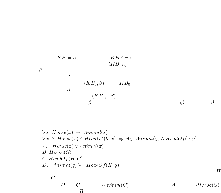
57
Notice that solve can not only be used to find a path Pthat is a solution, it can also be
used to verify that a given path is a solution.
If you want to add heuristics (or even breadth-first search), you need an explicit queue.
The algorithms become quite similar to the versions written in Lisp or Python or Java or in
pseudo-code in the book.
9.17 This question tests both the student’s understanding of resolution and their ability to
think at a high level about relations among sets of sentences. Recall that resolution allows one
to show that by proving that is inconsistent. Suppose that in general the
resolution system is called using ASK . Now we want to show that a given sentence,
say is valid or unsatisfiable.
A sentence is valid if it can be shown to be true without additional information. We
check this by calling ASK where is the empty knowledge base.
A sentence that is unsatisfiable is inconsistent by itself. So if we the empty knowl-
edge base again and call ASK the resolution system will attempt to derive a con-
tradiction starting from . If it can do so, then it must be that , and hence , is
inconsistent.
9.18 This is a form of inference used to show that Aristotle’s syllogisms could not capture
all sound inferences.
a.
b.
(Here . comes from the first sentence in a. while the others come from the second.
and are Skolem constants.)
c. Resolve and to yield . Resolve this with to give .
Resolve this with to obtain a contradiction.
9.19 This exercise tests the students understanding of models and implication.
a. (A) translates to “For every natural number there is some other natural number that is
smaller than or equal to it.” (B) translates to “There is a particular natural number that
is smaller than or equal to any natural number.”
b. Yes, (A) is true under this interpretation. You can always pick the number itself for the
“some other” number.
c. Yes, (B) is true under this interpretation. You can pick 0 for the “particular natural
number.”
d. No, (A) does not logically entail (B).
e. Yes, (B) logically entails (A).
f. We want to try to prove via resolution that (A) entails (B). To do this, we set our knowl-
edge base to consist of (A) and the negation of (B), which we will call (-B), and try to
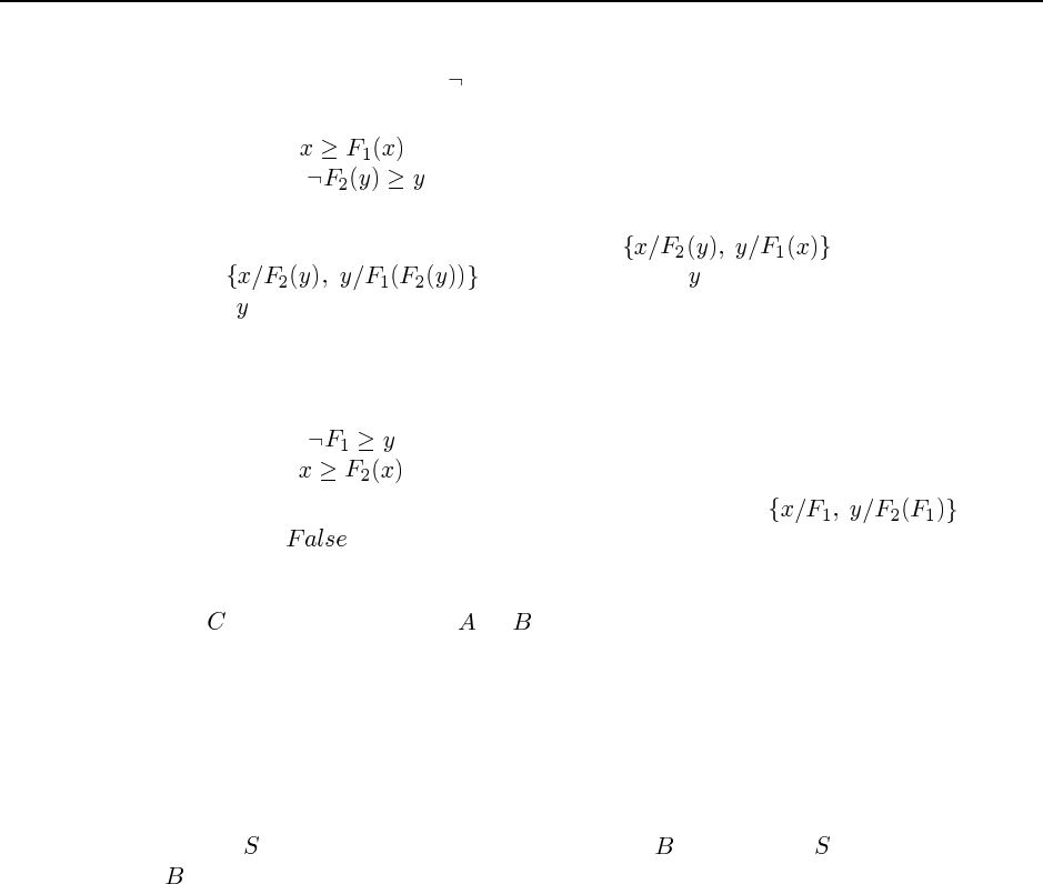
58 Chapter 9. Inference in First-Order Logic
derive a contradiction. First we have to convert (A) and (-B) to canonical form. For (-B),
this involves moving the in past the two quantifiers. For both sentences, it involves
introducing a Skolem function:
(A)
(-B)
Now we can try to resolve these two together, but the occurs check rules out the unifica-
tion. It looks like the substitution should be , but that is equivalent
to , which fails because is bound to an expression contain-
ing . So the resolution fails, there are no other resolution steps to try, and therefore (B)
does not follow from (A).
g. To prove that (B) entails (A), we start with a knowledge base containing (B) and the
negation of (A), which we will call (-A):
(-A)
(B)
This time the resolution goes through, with the substitution , thereby
yielding , and proving that (B) entails (A).
9.20 One way of seeing this is that resolution allows reasoning by cases, by which we can
prove by proving that either or is true, without knowing which one. With definite
clauses, we always have a single chain of inference, for which we can follow the chain and
instantiate variables.
9.21 No. Part of the definition of algorithm is that it must terminate. Since there can be
an infinite number of consequences of a set of sentences, no algorithm can generate them
all. Another way to see thatthe answer is no is to remember that entailment for FOL is
semidecidable. If there were an algorithm that generates the set of consequences of a set of
sentences , then when given the task of deciding if is entailed by , one could just check
if is in the generated set. But we know that this is not possible, therefore generating the set
of sentences is impossible.

Solutions for Chapter 10
Knowledge Representation
10.1 Shooting the wumpus makes it dead, but there are no actions that cause it to come
alive. Hence the successor-state axiom for just has the second clause:
where is defined appropriately in terms of the locations of and and the
orientation of . Possession of the arrow is lost by shooting, and again there is no way to
make it true:
10.2
Notice that the recursion needs no base case because we already have the axiom
10.3 This question takes the student through the initial stages of developing a logical rep-
resentation for actions that incorporates more and more realism. Implementing the reasoning
tasks in a theorem-prover is also a good idea. Although the use of logical reasoning for the
initial task—finding a route on a graph—may seem like overkill, the student should be im-
pressed that we can keep making the situation more complicated simply by describing those
added complications, with no additions to the reasoning system.
a. .
b. .
c. The successor-state axiom should be mechanical by now. :
59
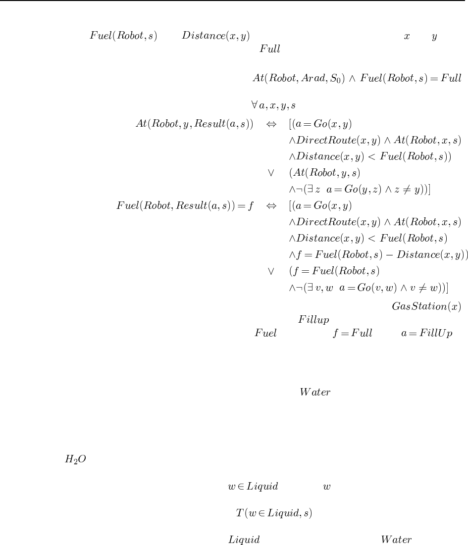
60 Chapter 10. Knowledge Representation
d. To represent the amount of fuel the robot has in a given situation, use the function
. Let denote the distance between cities and , mea-
sured in units of fuel consumption. Let be a constant denoting the fuel capacity of
the tank.
e. The initial situation is described by .
The above axiom for location is extended as follows (note that we do not say what
happens if the robot runs out of gas). :
f. The simplest way to extend the representation is to add the predicate ,
which is true of cities with gas stations. The action is described by adding
another clause to the above axiom for , saying that when .
10.4 This question was inadvertently left in the exercises after the corresponding material
was excised from the chapter. Future printings may omit or replace this exercise.
10.5 Remember that we defined substances so that is a category whose elements
are all those things of which one might say “it’s water.” One tricky part is that the English
language is ambiguous. One sense of the word “water” includes ice (“that’s frozen water”),
while another sense excludes it: (“that’s not water—it’s ice”). The sentences here seem to
use the first sense, so we will stick with that. It is the sense that is roughly synonymous with
.
The other tricky part is that we are dealing with objects that change (freeze and melt)
over time. Thus, it won’t do to say , because (a mass of water) might be a
liquid at one time and a solid at another. For simplicity, we will use a situation calculus
representation, with sentences such as . There are many possible correct
answers to each of these. The key thing is to be consistent in the way that information is
represented. For example, do not use as a predicate on objects if is used as a
substance category.
a. “Water is a liquid between 0 and 100 degrees.” We will translate this as “For any
water and any situation, the water is liquid iff and only if the water’s temperature in the
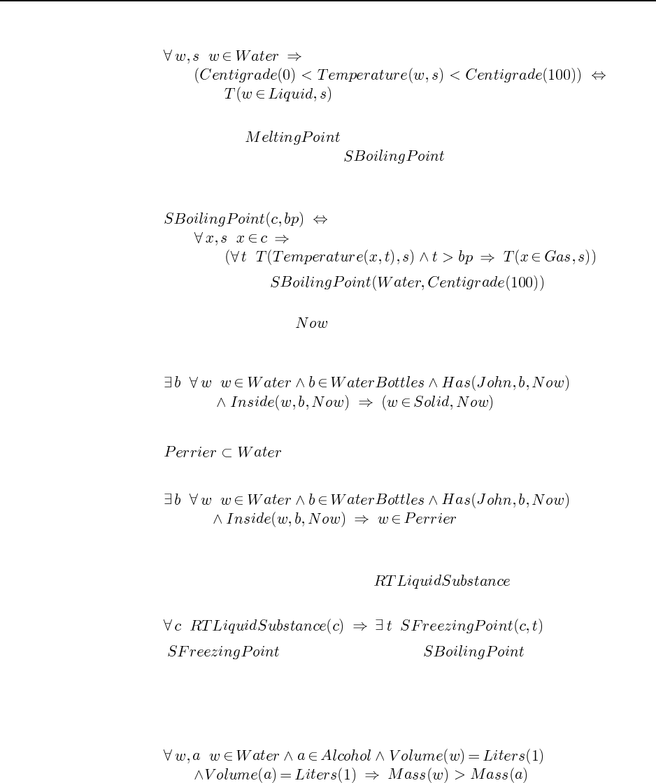
61
situation is between 0 and 100 centigrade.”
b. “Water boils at 100 degrees.” It is a good idea here to do some tool-building. On
page 243 we used as a predicate applying to individual instances of
a substance. Here, we will define to denote the boiling point of all
instances of a substance. The basic meaning of boiling is that instances of the substance
becomes gaseous above the boiling point:
Then we need only say .
c. “The water in John’s water bottle is frozen.”
We will use the constant to represent the situation in which this sentence holds.
Note that it is easy to make mistakes in which one asserts that only some of the water
in the bottle is frozen.
d. “Perrier is a kind of water.”
e. “John has Perrier in his water bottle.”
f. “All liquids have a freezing point.”
Presumably what this means is that all substances that are liquid at room temper-
ature have a freezing point. If we use to denote this class of
substances, then we have
where is defined similarly to . Note that this state-
ment is false in the real world: we can invent categories such as “blue liquid” which do
not have a unique freezing point. An interesting exercise would be to define a “pure”
substance as one all of whose instances have the same chemical composition.
g. “A liter of water weighs more than a liter of alcohol.”
10.6 This is a fairly straightforward exercise that can be done in direct analogy to the cor-
responding definitions for sets.
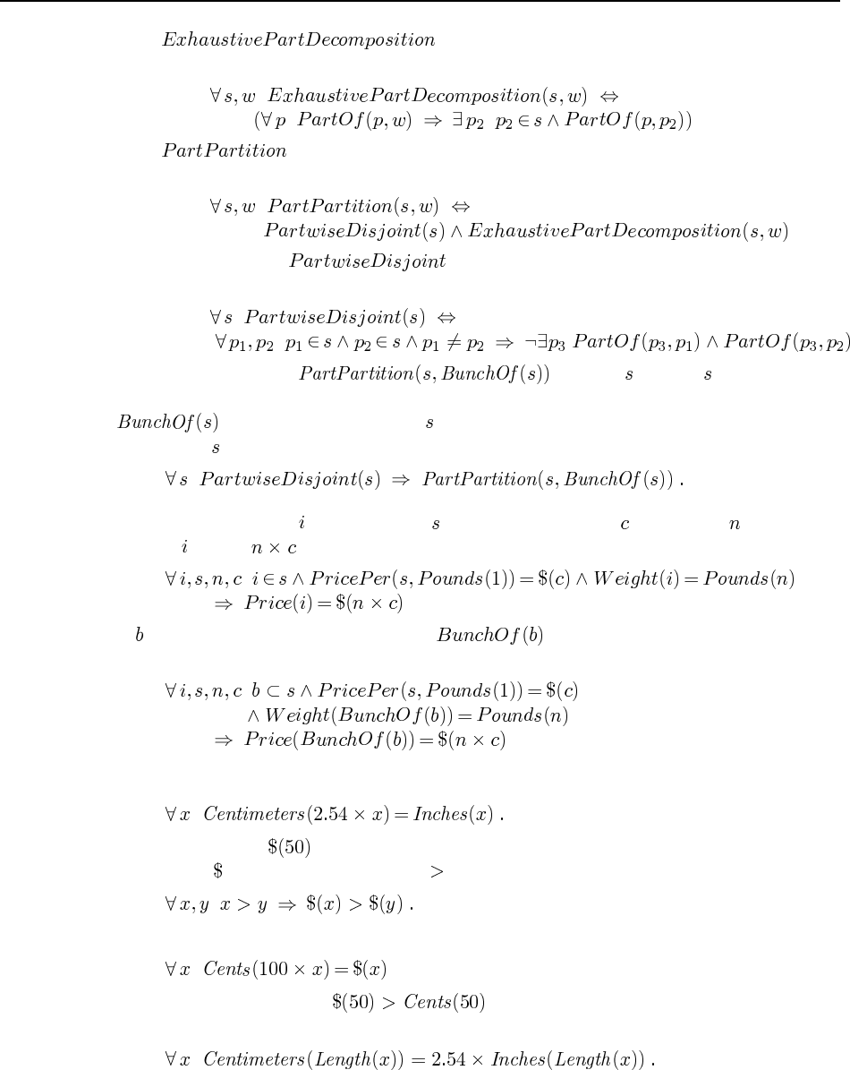
62 Chapter 10. Knowledge Representation
a. holds between a set of parts and a whole, saying
that anything that is a part of the whole must be a part of one of the set of parts.
b. holds between a set of parts and a whole when the set is disjoint and is
an exhaustive decomposition.
c. A set of parts is if when you take any two parts from the set, there
is nothing that is a part of both parts.
It is not the case that for any . A set may consist of
physically overlapping objects, such as a hand and the fingers of the hand. In that case,
is equal to the hand, but is not a partition of it. We need to ensure that the
elements of are partwise disjoint:
10.7 For an instance of a substance with price per pound and weight pounds, the
price of will be , or in other words:
If is the set of tomatoes in a bag, then is the composite object consisting of
all the tomatoes in the bag. Then we have
10.8 In the scheme in the chapter, a conversion axiom looks like this:
“50 dollars” is just , the name of an abstract monetary quantity. For any measure func-
tion such as , we can extend the use of as follows:
Since the conversion axiom for dollars and cents has
it follows immediately that .
In the new scheme, we must introduce objects whose lengths are converted:
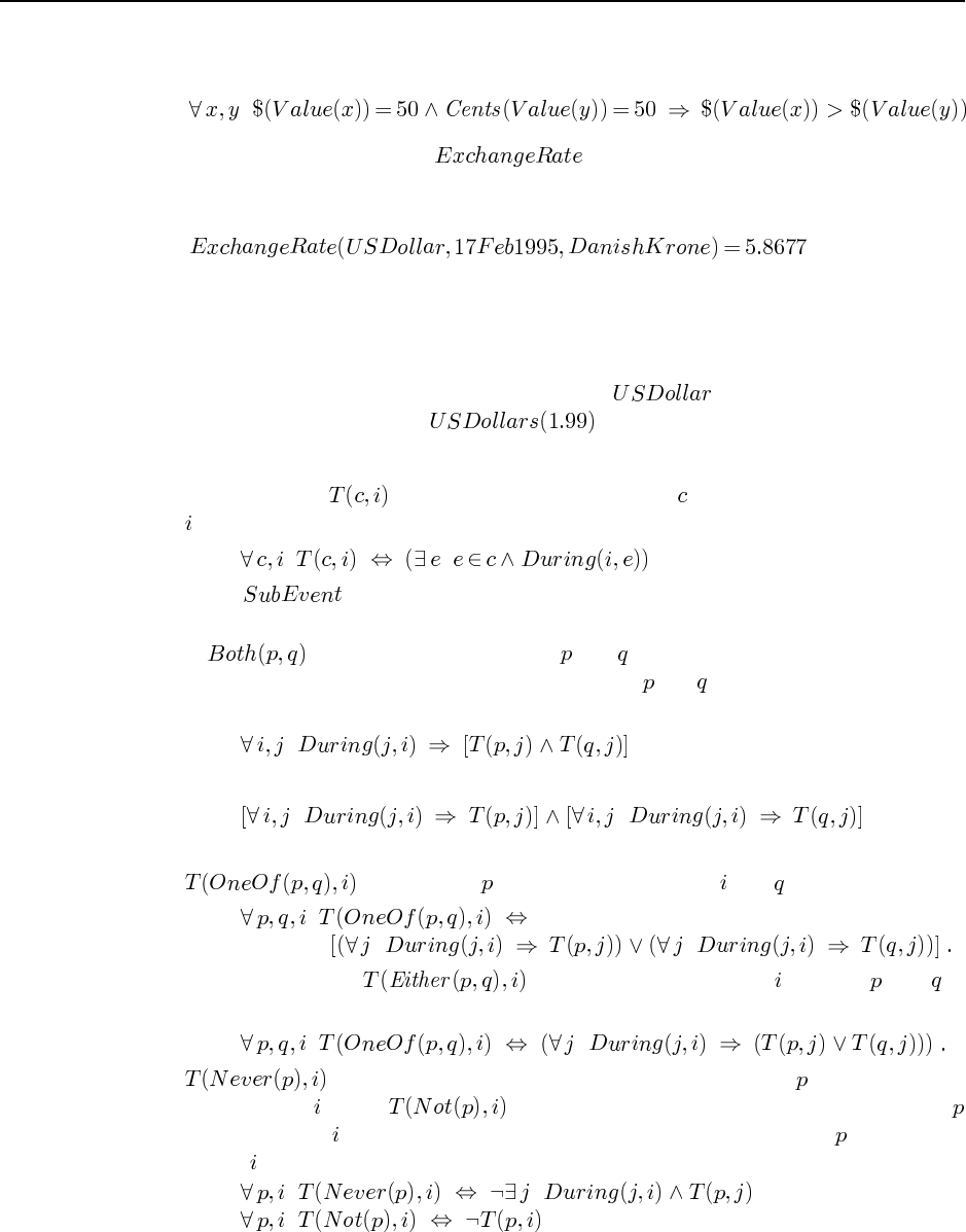
63
There is no obvious way to refer directly to “50 dollars” or its relation to “50 cents”. Again,
we must introduce objects whose monetary value is 50 dollars or 50 cents:
10.9 We will define a function that takes three arguments: a source cur-
rency, a time interval, and a target currency. It returns a number representing the exchange
rate. For example,
means that you can get 5.8677 Krone for a dollar on February 17th. This was the Federal
Reserve bank’s Spot exchange rate as of 10:00 AM. It is the mid-point between the buying and
selling rates. A more complete analysis might want to include buying and selling rates, and
the possibility for many different exchanges, as well as the commissions and fees involved.
Note also the distinction between a currency such as and a unit of measurement,
such as is used in the expression .
10.10 Another fun problem for clear thinkers:
a. Remember that means that some event of type occurs throughout the interval
:
Using as the question requests is not so easy, because the interval subsumes
all events within it.
b. A event is one in which both and occur throughout the duration of the
event. There is only one way this can happen: both and have to persist for the whole
interval. Another way to say it:
is logically equivalent to
whereas the same equivalence fails to hold for disjunction (see the next part).
c. means that a event occurs throughout or a event does:
On the other hand, holds if, at every point in , either a or a is
happening:
d. should mean that there is never an event of type going on in any
subinterval of , while should mean that there is no single event of type
that spans all of , even though there may be one or more events of type for subinter-
vals of :
64 Chapter 10. Knowledge Representation
One could also ask students to prove two versions of de Morgan’s laws using the two
types of negation, each with its corresponding type of disjunction.
10.11 Any object is an event, and is the event that for every subinterval of
time, refers to the place where is. For example, is the complex event
consisting of his home from midnight to about 9:00 today, then various parts of the road, then
his office from 10:00 to 1:30, and so on. To say that an event is fixed is to say that any two
moments of the event have the same spatial extent:
10.12 We will omit universally quantified variables:
10.13
“ ” “ “” “””
“ ” “ “” “””
10.14 Here is an initial sketch of one approach. (Others are possible.) A given object to be
purchased may require some additional parts (e.g., batteries) to be functional, and there may
also be optional extras. We can represent requirements as a relation between an individual
object and a class of objects, qualified by the number of objects required:
We also need to know that a particular object is compatible, i.e., fills a given role appropri-
ately. For example,
Then it is relatively easy to test whether the set of ordered objects contains compatible re-
quired objects for each object.
10.15 Plurals can be handled by a relation between strings, e.g.,
“ ” “ ”
plus an assertion that the plural (or singular) of a name is also a name for the same category:
65
Conjunctions can be handled by saying that any conjunction string is a name for a category if
one of the conjuncts is a name for the category:
where is defined appropriately in terms of concatenation. Probably it would be
better to redefine instead.
10.16 Chapter 22 explains how to use logic to parse text strings and extract semantic infor-
mation. The outcome of this process is a definition of what objects are acceptable to the user
for a specific shopping request; this allows the agent to go out and find offers matching the
user’s requirements. We omit the full definition of the agent, although a skeleton may appear
on the AIMA project web pages.
10.17 Here is a simple version of the answer; it can be elaborated ad infinitum. Let the term
denote the event category of buyer buying object from seller for price .
We want to say about it that transfers the money to , and transfers ownership of to .
10.18 Let denote the class of events where person trades object to
person for object :
Now the only tricky part about defining buying in terms of trading is in distinguishing a price
(a measurement) from an actual collection of money.
10.19 There are many possible approaches to this exercise. The idea is for the students to
think about doing knowledge representation for real; to consider a host of complications and
find some way to represent the facts about them. Some of the key points are:
Ownership occurs over time, so we need either a situation-calculus or interval-calculus
approach.
There can be joint ownership and corporate ownership. This suggests the owner is a
group of some kind, which in the simple case is a group of one person.
Ownership provides certain rights: to use, to resell, to give away, etc. Much of this is
outside the definition of ownership per se, but a good answer would at least consider
how much of this to represent.
Own can own abstract obligations as well as concrete objects. This is the idea behind
the futures market, and also behind banks: when you deposit a dollar in a bank, you
are giving up ownership of that particular dollar in exchange for ownership of the right

66 Chapter 10. Knowledge Representation
to withdraw another dollar later. (Or it could coincidentally turn out to be the exact
same dollar.) Leases and the like work this way as well. This is tricky in terms of
representation, because it means we have to reify transactions of this kind. That is,
must be an object, not a predicate.
10.20 Most schools distinguish between required courses and elected courses, and between
courses inside the department and outside the department. For each of these, there may be re-
quirements for the number of courses, the number of units (since different courses may carry
different numbers of units), and on grade point averages. We show our chosen vocabulary by
example:
Student Jones’ complete course of study for the whole college career consists of Math1,
CS1, CS2, CS3, CS21, CS33 and CS34, and some other courses outside the major.
Jones meets the requirements for a major in Computer Science
Courses Math1, CS1, CS2, and CS3 are required for a Computer Science major.
A student must take at least 18 units in the CS department to get a degree in CS.
One can easily imagine other kinds of requirements; these just give you a flavor.
In this solution we took “over an extended period” to mean that we should recommend
a set of courses to take, without scheduling them on a semester-by-semester basis. If you
wanted to do that, you would need additional information such as when courses are taught,
what is a reasonable course load in a semester, and what courses are prerequisites for what
others. For example:

67
The problem with finding the best program of study is in defining what best means to the
student. It is easy enough to say that all other things being equal, one prefers a good teacher
to a bad one, or an interesting course to a boring one. But how do you decide which is best
when one course has a better teacher and is expected to be easier, while an alternative is more
interesting and provides one more credit? Chapter 16 uses utility theory to address this. If
you can provide a way of weighing these elements against each other, then you can choose a
best program of study; otherwise you can only eliminate some programs as being worse than
others, but can’t pick an absolute best one. Complexity is a further problem: witha general-
purpose theorem-prover it’s hard to do much more than enumerate legal programs and pick
the best.
10.21 This exercise and the following two are rather complex, perhaps suitable for term
projects. At this point, we want to strongly urge that you do assign some of these exercises
(or ones like them) to give your students a feeling of what it is really like to do knowl-
edge representation. In general, students find classification hierarchies easier than other rep-
resentation tasks. A recent twist is to compare one’s hierarchy with online ones such as
yahoo.com.
10.22 This is the most involved representation problem. It is suitable for a group project of
2 or 3 students over the course of at least 2 weeks.
10.23 Normally one would assign 10.22 in one assignment, and then when it is done, add
this exercise (posibly varying the questions). That way, the students see whether they have
made sufficient generalizations in their initial answer, and get experience with debugging and
modifying a knowledge base.
10.24 In many AI and Prolog textbooks, you will find it stated plainly that implications
suffice for the implementation of inheritance. This is true in the logical but not the practical
sense.
a. Here are three rules, written in Prolog. We actually would need many more clauses on
the right hand side to distinguish between different models, different options, etc.
worth(X,575) :- year(X,1973), make(X,dodge), style(X,van).
worth(X,27000) :- year(X,1994), make(X,lexus), style(X,sedan).
worth(X,5000) :- year(X,1987), make(X,toyota), style(X,sedan).
To find the value of JB, given a data base with year(jb,1973),make(jb,dodge)
and style(jb,van) we would call the backward chainer with the goal worth(jb,D),
and read the value for D.
b. The time efficiency of this query is , where in this case is the 11,000 entries in
the Blue Book. A semantic network with inheritance would allow us to follow a link
from JB to 1973-dodge-van, and from there to follow the worth slot to find the
dollar value in time.
c. With forward chaining, as soon as we are told the three facts about JB, we add the new
fact worth(jb,575). Then when we get the query worth(jb,D), it is to
find the answer, assuming indexing on the predicate and first argument. This makes
logical inference seem just like semantic networks except for two things: the logical
68 Chapter 10. Knowledge Representation
inference does a hash table lookup instead of pointer following, and logical inference
explicitly stores worth statements for each individual car, thus wasting space if there
are a lot of individual cars. (For this kind of application, however, we will probably
want to consider only a few individual cars, as opposed to the 11,000 different models.)
d. If each category has many properties—for example, the specifications of all the replace-
ment parts for the vehicle—then forward-chaining on the implications will also be an
impractical way to figure out the price of a vehicle.
e. If we have a rule of the following kind:
worth(X,D) :- year-make-style(X,Yr,Mk,St),
year-make-style(Y,Yr,Mk,St), worth(Y,D).
together with facts in the database about some other specific vehicle of the same type
as JB, then the query worth(jb,D) will be solved in time with appropriate
indexing, regardless of how many other facts are known about that type of vehicle and
regardless of the number of types of vehicle.
10.25 When categories are reified, they can have properties as individual objects (such as
and ) that do not apply to their elements. Without the distinction be-
tween boxed and unboxed links, the sentence might mean
that every singleton set has one element, or that there si only one singleton set.

Solutions for Chapter 11
Planning
11.1 Both problem solver and planner are concerned with getting from a start state to a goal
using a set of defined operations or actions. But in planning we open up the representation of
states, goals, and plans, whcihc allows for a wider variety of algorithms that decompose the
search space.
11.2 This is an easy exercise, the point of which is to understand that “applicable” means
satisfying the preconditions, and that a concrete action instance is one with the variables
replaced by constants. The applicable actions are:
A minor point of this is that the action of flying nowhere—from one airport to itself—is
allowable by the definition of , and is applicable (if not useful).
11.3 For the regular schema we have:
When we add we get:
In general, we (1) created a predicate for each action, and then, for each fluent
such as , we create a predicate that says the fluent keeps its old value if either an irrelevant
action is taken, or an action whose precondition is not satisfied, and it takes on a new value
according to the effects of a relevant action if that action’s preconditions are satisfied.
69

70 Chapter 11. Planning
11.4 This exercise is intended as a fairly easy exercise in describing a domain. It is similar
to the Shakey problem (11.13), so you should probably assign only one of these two.
a. The initial state is:
b. The actions are:
ACTION: PRECOND:
EFFECT:
ACTION: PRECOND:
EFFECT:
ACTION:
PRECOND:
EFFECT:
ACTION:
PRECOND:
EFFECT:
ACTION:
PRECOND:
EFFECT:
ACTION: PRECOND:
EFFECT:
c. In situation calculus, the goal is a state such that:
In STRIPS, we can only talk about the goal state; there is no way of representing the fact
that there must be some relation (such as equality of location of an object) between two
states within the plan. So there is no way to represent this goal.
d. Actually, we did include the precondition. This is an example of the qualifi-
cation problem.
11.5 Only positive literals are represented in a state. So not mentioning a literal is the same
as having it be negative.
11.6 Goals and preconditions can only be positive literals. So a negative effect can only
make it harder to achieve a goal (or a precondition to an action that achieves the goal). There-
fore, eliminating all negative effects only makes a problem easier.
11.7
a. It is feasible to use bidirectional search, because it is possible to invert the actions.
However, most of those who have tried have concluded that biderectional search is

71
generally not efficient, because the forward and backward searches tend to miss each
other. This is due to the large state space. A few planners, such as PRODIGY (Fink and
Blythe, 1998) have used bidirectional search.
b. Again, this is feasible but not popular. PRODIGY is in fact (in part) a partial-order
planner: in the forward direction it keeps a total-order plan (equivalent to a state-based
planner), and in the backward direction it maintains a tree-structured partial-order plan.
c. An action can be added if all the preconditions of have been achieved by other
steps in the plan. When is added, ordering constraints and causal links are also added
to make sure that appears after all the actions that enabled it and that a precondition
is not disestablished before can be executed. The algorithm does search forward, but
it is not the same as forward state-space search because it can explore actions in parallel
when they don’t conflict. For example, if has three preconditions that can be satisfied
by the non-conflicting actions , , and , then the solution plan can be represented
as a single partial-order plan, while a state-space planner would have to consider all
permutations of , , and .
d. Yes, this is one possible way of implementing a bidirectional search in the space of
partial-order plans.
11.8 The drawing is actually rather complex, and doesn’t fit well on this page. Some key
things to watch out for: (1) Both and actions are possible at level ; the planes
can still fly when empty. (2) Negative effects appear in , and are mutex with their positive
counterparts.
11.9
a. Literals are persistent, so if it does not appear in the final level, it never will and never
did, and thus cannot be achieved.
b. In a serial planning graph, only one action can occur per time step. The level cost (the
level at which a literal first appears) thus represents the minimum number of actions in
a plan that might possibly achieve the literal.
11.10 A forward state-space planner maintains a partial plan that is a strict linear sequence
of actions; the plan refinement operator is to add an applicable action to the end of the se-
quence, updating literals according to the action’s effects.
A backward state-space planner maintains a partial plan that is a reversed sequence of
actions; the refinement operator is to add an action to the beginning of the sequence as long
as the action’s effects are compatible with the state at the beginning of the sequence.
11.11 The initial state is:
The goal is:
First we’ll explain why it is an anomaly for a noninterleaved planner. There are two subgoals;
suppose we decide to work on first. We can clear off of and then move
72 Chapter 11. Planning
on to . But then there is no way to achieve without undoing the work we have
done. Similarly, if we work on the subgoal first we can immediately achieve it in
one step, but then we have to undo it to get on .
Now we’ll show how things work out with an interleaved planner such as POP. Since
isn’t true in the initial state, there is only one way to achieve it: ,
for some . Similarly, we also need a step, for some . Now let’s look
at the step. We need to achieve its precondition . We could do
that either with or with . Let’s assume we choose the
latter. Now if we bind to , then all of the preconditions for the step
are true in the initial state, and we can add causal links to them. We then notice that there
is a threat: the step threatens the condition that is required by
the step. We can resolve the threat by ordering after the
step. Finally, notice that all the preconditions for are true in
the initial state. Thus, we have a complete plan with all the preconditions satisfied. It turns
out there is a well-ordering of the three steps:
11.12 The actions we need are the four from page 346:
ACTION: PRECOND: EFFECT:
ACTION: EFFECT:
ACTION: PRECOND: EFFECT:
ACTION: EFFECT:
One solution found by GRAPHPLAN is to execute RightSock and LeftSock in the first time
step, and then RightShoe and LeftShoe in the second.
Now we add the following two actions (neither of which has preconditions):
ACTION: EFFECT:
ACTION: EFFECT:
The partial-order plan is shown in Figure S11.1. We saw on page 348 that there are 6 total-
order plans for the shoes/socks problem. Each of these plans has four steps, and thus five
arrow links. The next step, Hat could go at any one of these five locations, giving us
total-order plans, each with five steps and six links. Then the final step, Coat, can go in
any one of these 6 positions, giving us total-order plans.
11.13 The actions are quite similar to the monkey and banannas problem—you should prob-
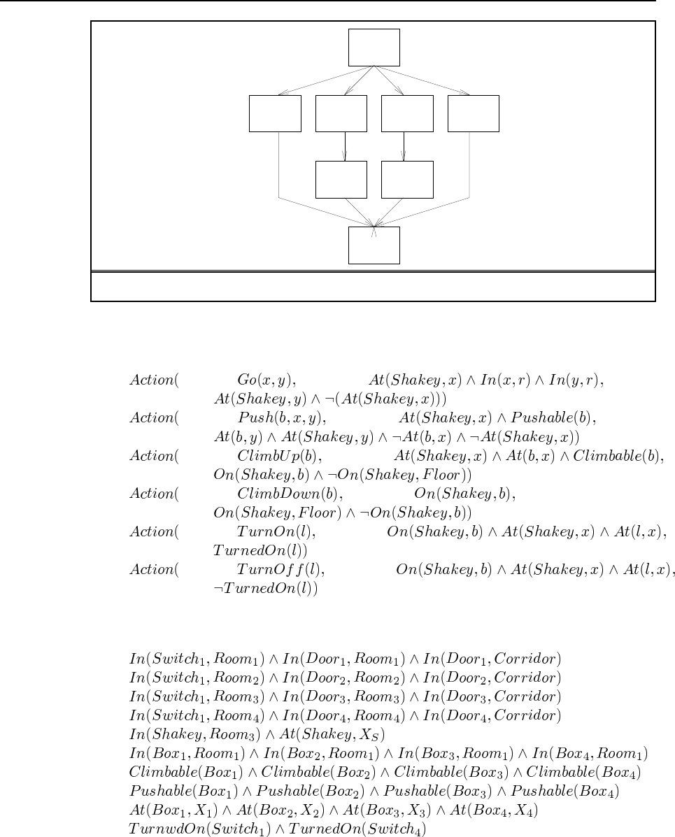
73
Start
Finish
Left
Sock Right
Sock
Left
Shoe Right
Shoe
Hat Coat
Figure S11.1 Partial-order plan including a hat and coat, for Exercise 11.1.
ably assign only one of these two problems. The actions are:
ACTION: PRECOND:
EFFECT:
ACTION: PRECOND:
EFFECT:
ACTION: PRECOND:
EFFECT:
ACTION: PRECOND:
EFFECT:
ACTION: PRECOND:
EFFECT:
ACTION: PRECOND:
EFFECT:
The initial state is:
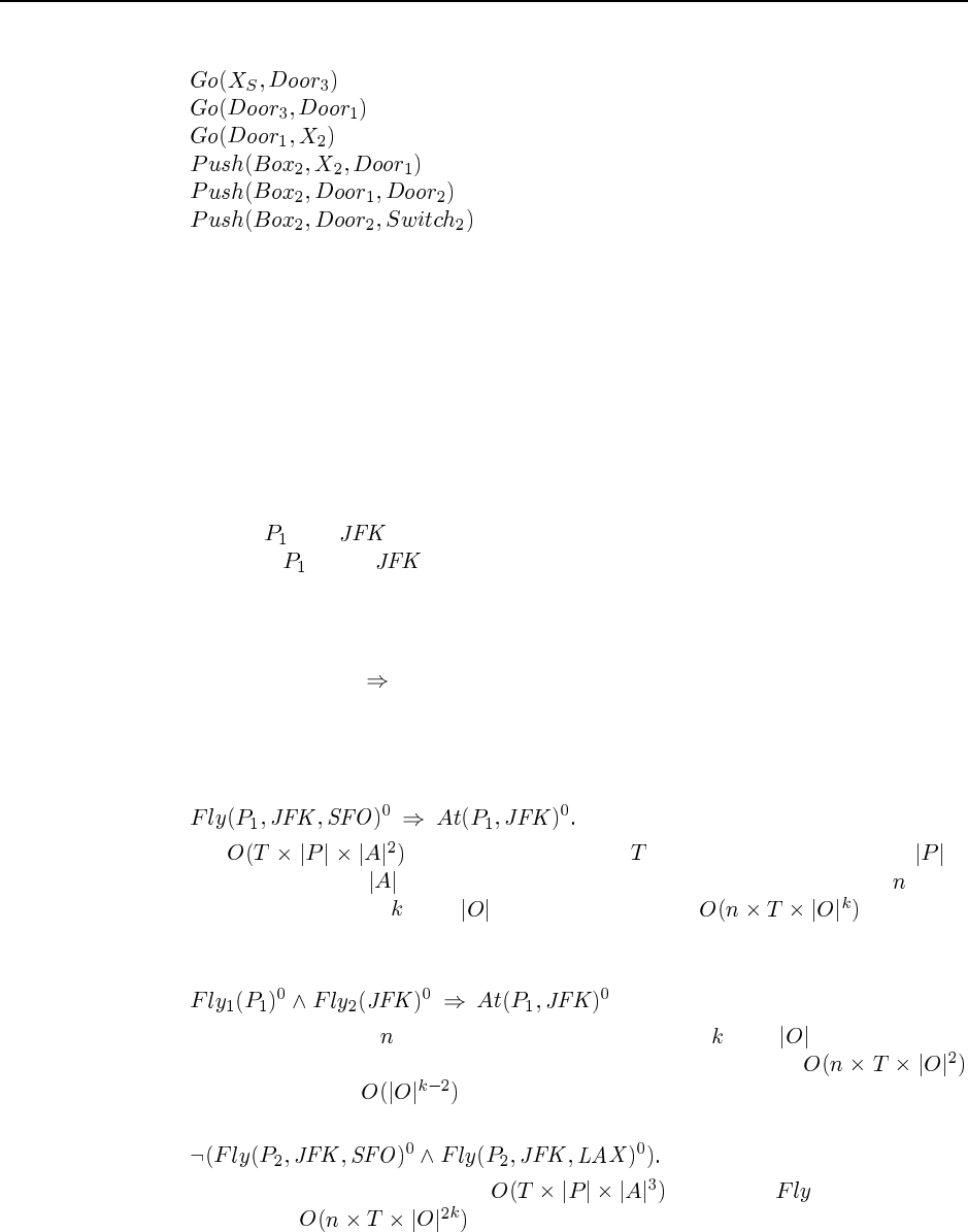
74 Chapter 11. Planning
A plan to achieve the goal is:
11.14 GRAPHPLAN is a propositional algorithm, so, just as we could solve certain FOL by
translating them into propositional logic, we can solve certain situation calculus problems by
translating into propositional form. The trick is how exactly to do that.
The Finish action in POP planning has as its preconditions the goal state. We can create
aFinish action for GRAPHPLAN, and give it the effect Done. In this case there would be a
finite number of instantiations of the Finish action, and we would reason with them.
11.15 (Figure (11.1) is a little hard to find—it is on page 403.)
a. The point of this exercise is to consider what happens when a planner comes up with an
impossible action, such as flying a plane from someplace where it is not. For example,
suppose is at and we give it the action of flying from Bangalore to Brisbane.
By (11.1), was at and did not fly away, so it is still there.
b. Yes, the plan will still work, because the fluents hold from the situation before an inap-
plicable action to the state afterward, so the plan can continue from that state.
c. It depends on the details of how the axioms are written. Our axioms were of the form
Action is possible Rule. This tells us nothing about the case where the action is
not possible. We would need to reformulate the axioms, or add additional ones to say
what happens when the action is not possible.
11.16 Aprecondition axiom is of the form
There are of these axioms, where is the number of time steps, is
the number of planes and is the number of airports. More generally, if there are action
schemata of maximum arity , with objects, then there are axioms.
With symbol-splitting, we don’t have to describe each specific flight, we need only say
that for a plane to fly anywhere, it must be at the start airport. That is,
More generally, if there are action schemata of maximum arity , with objects, and each
precondition axiom depends on just two of the arguments, then there are
axioms, for a speedup of .
An action exclusion axiom is of the form
With the notation used above, there are axioms for . More generally,
there can be up to axioms.

75
With symbol-splitting, we wouldn’t gain anything for the axioms, but we would
gain in cases where there is another variable that is not relevant to the exclusion.
11.17
a. Yes, this will find a plan whenever the normal SATPLAN finds a plan no longer than
.
b. No.
c. There is no simple and clear way to induce WALKSAT to find short solutions, because
it has no notion of the length of a plan—the fact that the problem is a planning problem
is part of the encoding, not part of WALKSAT. But if we are willing to do some rather
brutal surgery on WALKSAT, we can achieve shorter solutions by identifying the vari-
ables that represent actions and (1) tending to randomly initialize the action variables
(particularly the later ones) to false, and (1) prefering to randomly flip an earlier action
variable rather than a later one.
Solutions for Chapter 12
Planning and Acting in the Real
World
12.1
a. is eligible to be an effect because the action does have the effect of moving
the clock by . It is possible that the duration depends on the action outcome, so if
disjunctive or conditional effects are used there must be a way to associate durations
with outcomes, which is most easily done by putting the duration into the outcome
expression.
b. The STRIPS model assumes that actions are time points characterized only by their pre-
conditions and effects. Even if an action occupies a resource, that has no effect on the
outcome state (as explained on page 420). Therefore, we must extend the STRIPS for-
malism. We could do this by treating a RESOURCE: effect differently from other effects,
but the difference is sufficiently large that it makes more sense to treat it separately.
12.2 The basic idea here is to record the initial resource level in the precondition and the
change in resource level in the effect of each action.
a. Let denote the fact that there are screws. We need to add
to the initial state, and add a fourth argument to the predicate indicating the
number of screws required—i.e., and .
We add to the precondition of and add as a fourth argument
of the literal. Then add to the effect of .
b. A simple solution is to say that any action that consumes a resource is potentially in
conflict with any causal link protecting the same resource.
c. The planner can keep track of the resource requirements of actions added to the plan
and backtrack whenever the total usage exceeds the initial amount.
12.3 There is a wide range of possible answers to this question. The important point is that
students understand what constitutes a correct implementation of an action: as mentioned on
page 424, it must be a consistent plan where all the preconditions and effects are accounted
for. So the first thing we need is to decide on the preconditions and effects of the high-level
actions. For GetPermit, assume the precondition is owning land, and the effect is having a
permit for that piece of land. For HireBuilder, the precondition is having the ability to pay,
and the effect is having a signed contract in hand.
76
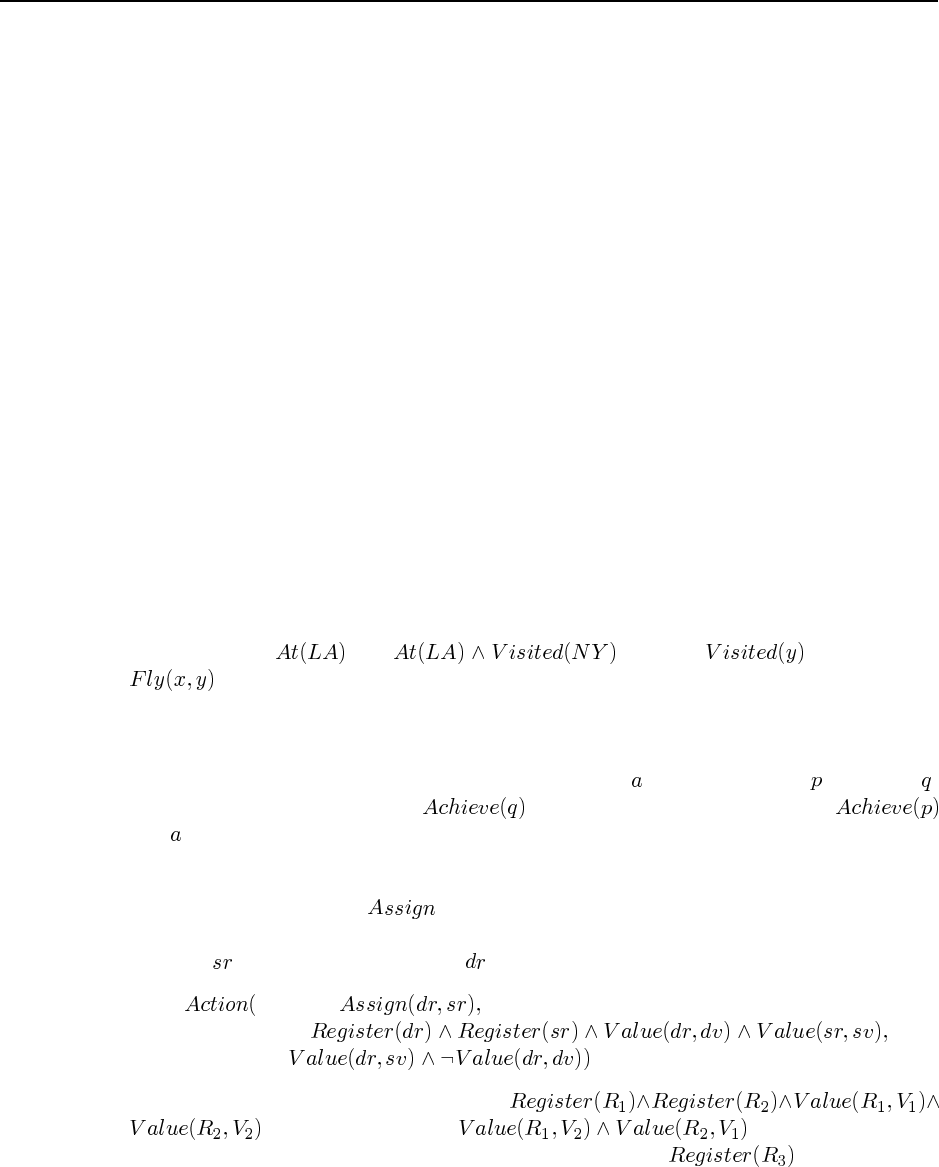
77
One possible decomposition for GetPermit is the three-step sequence GetPermitForm,
FillOutForm, and GetFormApproved. There is a causal link with the condition HaveForm
between the first two, and one with the condition HaveCompletedForm between the last two.
Finally, the GetFormApproved step has the effect HavePermit. This is a valid decomposition.
For HireBuilder, suppose we choose the three-step sequence InterviewBuilders,Choose-
Builder, and SignContract. This last step has the precondition AbleToPay and the effect Have-
ContractInHand. There are also causal links between the substeps, but they don’t affect the
correctness of the decomposition.
12.4 Consider the problem of building two adjacent walls of the house. Mostly these sub-
plans are independent, but they must share the step of putting up a common post at the corner
of the two walls. If that step was not shared, we would end up with an extra post, and two
unattached walls.
Note that tasks are often decomposed specifically so as to minimize the amount of step
sharing. For example, one could decompose the house building task into subtasks such as
“walls” and “floors.” However, real contractors don’t do it that way. Instead they have “rough
walls” and “rough floors” steps, followed by a “finishing” step.
12.5 In the HTN view, the space of possible decompositions may constrain the allowable
solutions, eliminating some possible sequences of primitive actions. For example, the de-
composition of the LAToNYRoundTrip action can stipulate that the agent should go to New
York. In a simple STRIPS formulation where the start and goal states are the same, the empty
plan is a solution. We can get around this problem by rethinking the goal description. The
goal state is not , but . We add as an effect of
. Then, the solution must be a trip that includes New York. There remains the prob-
lem of preventing the STRIPS plan from including other stops on its itinerary; fixing this is
much more difficult because negated goals are not allowed.
12.6 Suppose we have a STRIPS action description for with precondition and effect .
The “action” to be decomposed is . The decomposition has two steps:
and . This can be extended in the obvious way for conjunctive effects and precondi-
tions.
12.7 We need one action, , which assigns the value in the source register (or variable
if you prefer, but the term “register” makes it clearer that we are dealing with a physical
location) to the destination register :
ACTION:
PRECOND:
EFFECT:
Now suppose we start in an initial state with
and we have the goal . Unfortunately, there
is no way to solve this as is. We either need to add an explicit condition to the
initial state, or we need a way to create new registers. That could be done with an action for
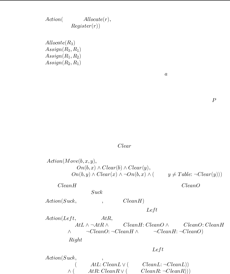
78 Chapter 12. Planning and Acting in the Real World
allocating a new register:
ACTION:
EFFECT:
Then the following sequence of steps constitues a valid plan:
12.8 For the first case, where one instance of action schema is in the plan, the reformula-
tion is correct, in the sense that a solution for the original disjunctive formulation is a solution
for the new formulation and vice versa. For the second case, where more than one instance
of the action schema may occur, the reformulation is incorrect. It assumes that the outcomes
of the instances are governed by a single hidden variable, so that if, for example, is the
outcome of one instance it must also be the outcome of the other. It is possible that a solution
for the reformulated case will fail in the original formulation.
12.9 With unbounded indeterminacy, the set of possible effects for each action is unknown
or too large to be enumerated. Hence, the space of possible actions sequences required to
handle all these eventualities is far too large to consider.
12.10 Using the second definition of in the chapter—namely, that there is a clear
space for a block—the only change is that the destination remains clear if it is the table:
PRECOND:
EFFECT:when
12.11 Let be true iff the robot’s current square is clean and be true iff the
other square is clean. Then is characterized by
PRECOND: EFFECT:
Unfortunately, moving affects these new literals! For we have
PRECOND:
EFFECT:when when
when when
with the dual for .
12.12 Here we borrow from the last description of the on page 433:
PRECOND:
EFFECT:when when
when when
12.13 The main thing to notice here is that the vacuum cleaner moves repeatedly over dirty
areas—presumably, until they are clean. Also, each forward move is typically short, followed

79
by an immediate reversing over the same area. This is explained in terms of a disjunctive
outcome: the area may be fully cleaned or not, the reversing enables the agent to check, and
the repetition ensures completion (unless the dirt is ingrained). Thus, we have a strong cyclic
plan with sensing actions.
12.14
a. “Lather. Rinse. Repeat.”
This is an unconditional plan, if taken literally, involving an infinite loop. If the pre-
condition of is , and the goal is , then execution monitoring will
cause execution to terminate once is achieved because at that point the correct
repair is the empty plan.
b. “Apply shampoo to scalp and let it remain for several minutes. Rinse and repeat if
necessary.”
This is a conditional plan where “if necessary” presumably tests .
c. “See a doctor if problems persist.”
This is also a conditional step, although it is not specified here what problems are tested.
12.17 First, we need to decide if the precondition is satisfied. There are three cases:
a. If it is known to be unsatisfied, the new belief state is identical to the old (since we
assume nothing happens).
b. If it is known to be satisfied, the unconditional effects (which are all knowledge propo-
sitions) are added and deleted from the belief state in the usual STRIPS fashion. Each
conditional effect whose condition is known to be true is handled in the same way. For
each setting of the unknown conditions, we create a belief state with the appropriate
additions and deletions.
c. If the status of the precondition is unknown, each new belief state is effectively the
disjunction of the unchanged belief state from (a) with one of the belief states obtained
from (b). To enforce the “list of knowledge propositions” representation, we keep those
propositions that are identical in each of the two belief states being disjoined and discard
those that differ. This results in a weaker belief state than if we were to retain the
disjunction; on the other hand, retaining the disjunctions over many steps could lead to
exponentially large representations.
12.18 For we have the obvious dual version of Equation 12.2:
PRECOND:
EFFECT:when
when when
With , dirt is sometimes deposited when the square is clean. With automatic dirt sensing,
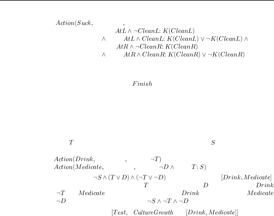
80 Chapter 12. Planning and Acting in the Real World
this is always detected, so we have a disjunctive conditional effect:
PRECOND:
EFFECT:when
when
when
when
12.19 The continuous planning agent described in Section 12.6 has at least one of the listed
abilities, namely the ability to accept new goals as it goes along. A new goal is simply added
as an extra open precondition in the step, and the planner will find a way to satisfy
it, if possible, along with the other remaining goals. Because the data structures built by
the continuous planning agent as it works on the plan remain largely in place as the plan is
executed, the cost of replanning is usually relatively small unless the failure is catastrophic.
There is no specific time bound that is guaranteed, and in general no such bound is possible
because changing even a single state variable might require completely reconstructing the
plan from scratch.
12.20 Let be the proposition that the patient is dehydrated and be the side effect. We
have
PRECOND: EFFECT:
PRECOND: EFFECT:when
and the initial state is . The solution plan is .
There are two possible worlds, one where holds and one where holds. In the first,
causes and has no effect; in the second, has no effect and
causes . In both cases, the final state is .
12.21 One solution plan is if then .
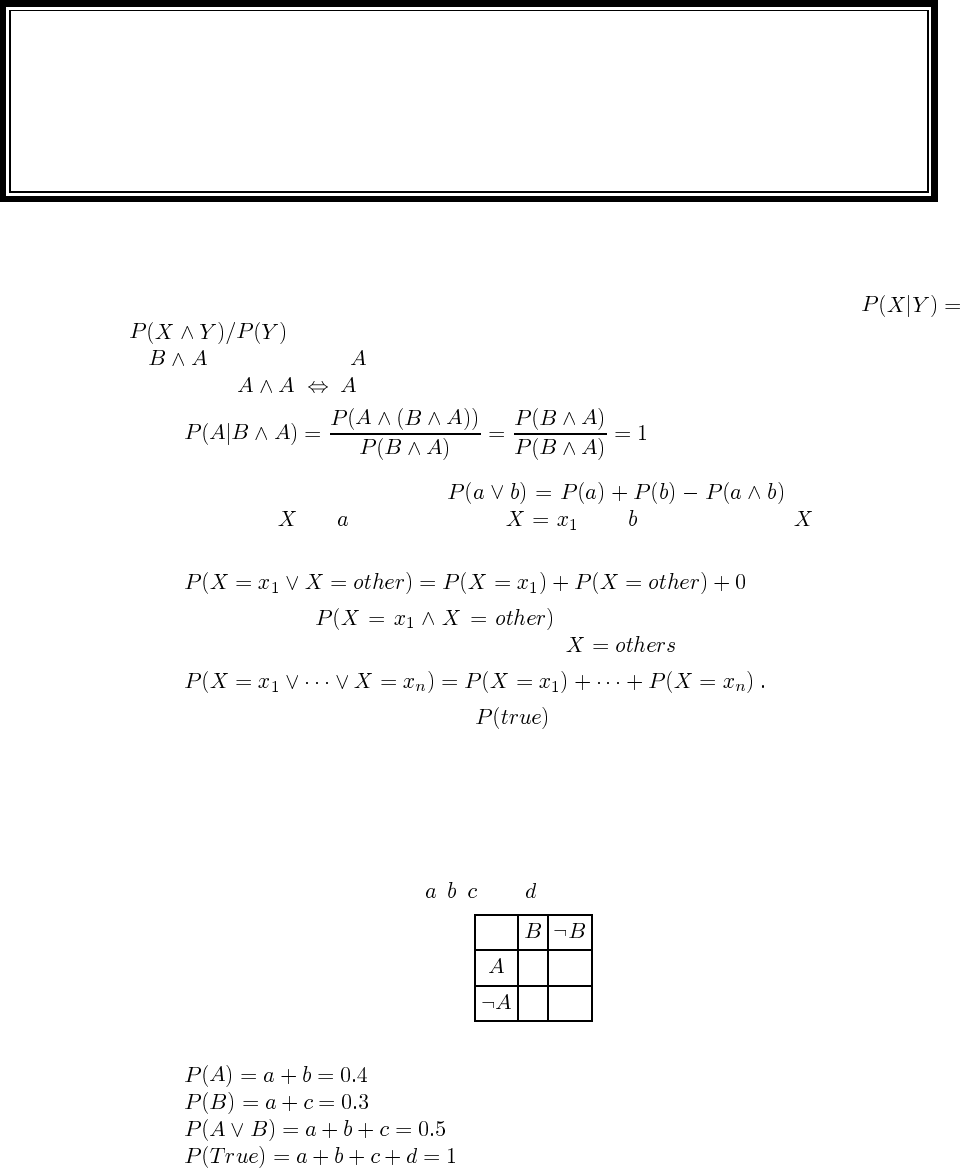
Solutions for Chapter 13
Uncertainty
13.1 The “first principles” needed here are the definition of conditional probability,
, and the definitions of the logical connectives. It is not enough to say that
if is “given” then must be true! From the definition of conditional probability, and
the fact that and that conjunction is commutative and associative, we have
13.2 The main axiom is axiom 3: . For the discrete
random variable , let be the event that , and be the event that has any other
value. Then we have
where we know that is 0 because a variable cannot take on two
distinct values. If we now break down the case of , we eventually get
But the left-hand side is equivalent to , which is 1 by axiom 2, so the sum of the
right-hand side must also be 1.
13.3 Probably the easiest way to keep track of what’s going on is to look at the probabil-
ities of the atomic events. A probability assignment to a set of propositions is consistent
with the axioms of probability if the probabilities are consistent with an assignment to the
atomic events that sums to 1 and has all probabilities between 0 and 1 inclusive. We call the
probabilities of the atomic events , , , and , as follows:
a b
c d
We then have the following equations:
81
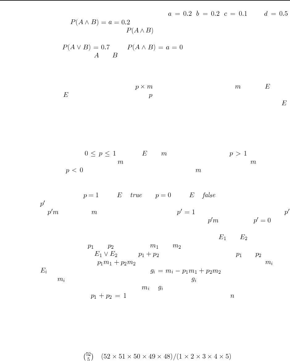
82 Chapter 13. Uncertainty
From these, it is straightforward to infer that , , , and .
Therefore, . Thus the probabilities given are consistent with a rational
assignment, and the probability is exactly determined. (This latter fact can be seen
also from axiom 3 on page 422.)
If , then . Thus, even though the bet outlined in
Figure 13.3 loses if and are both true, the agent believes this to be impossible so the bet
is still rational.
13.4 ? (?, ?) argues roughly as follows: Suppose we present an agent with a choice: either
definitely receive monetary payoff , or choose a lottery that pays if event occurs
and 0 if does not occur. The number for which the agent is indifferent between the two
choices (assuming linear utility of money), is defined to be the agent’s degree of belief in .
A set of degrees of belief specified for some collection of events will either be coherent,
which is defined to mean that there is no set of bets based on these stated beliefs that will
guarantee that the agent will lose money, or incoherent, which is defined to mean that there
is such a set of bets. De Finetti showed that coherent beliefs satisfy the axioms of probability
theory.
Axiom 1: , for any and . If an agent specifies , then the agent
is offering to pay more than to enter a lottery in which the biggest prize is . If an agent
specifies , then the agent is offering to pay either or 0 in exchange for a negative
amount. Either way, the agent is guaranteed to lose money if the opponent accepts the right
offer.
Axiom 2: when is and when is . Suppose the agent assigns
as the degree of belief in a known true event. Then the agent is indifferent between a payoff
of and one of . This is only coherent when . Similarly, a degree of belief of
for a known false event means the agent is indifferent between and 0. Only makes
this coherent.
Axiom 3: Given two mutually exclusive, exhaustive events, and , and respective
degrees of belief and and payoffs and , it must be that the degree of belief for
the combined event equals . The idea is that the beliefs and constitute
an agreement to pay in order to enter a lottery in which the prize is when
occurs. So the net gain is defined as . To avoid the possibility
of the amounts being chosen to guarantee that every is negative, we have to assure that
the determinant of the matrix relating to is zero, so that the linear system can be solved.
This requires that . The result extends to the case with mutually exclusive,
exhaustive events rather than two.
13.5 This is a classic combinatorics question that could appear in a basic text on discrete
mathematics. The point here is to refer to the relevant axioms of probability: principally,
axiom 3 on page 422. The question also helps students to grasp the concept of the joint
probability distribution as the distribution over all possible states of the world.
a. There are = = 2,598,960 possible
five-card hands.
83
b. By the fair-dealing assumption, each of these is equally likely. By axioms 2 and 3, each
hand therefore occurs with probability 1/2,598,960.
c. There are four hands that are royal straight flushes (one in each suit). By axiom 3, since
the events are mutually exclusive, the probability of a royal straight flush is just the sum
of the probabilities of the atomic events, i.e., 4/2,598,960 = 1/649,740.
d. Again, we examine the atomic events that are “four of a kind” events. There are 13
possible “kinds” and for each, the fifth card can be one of 48 possible other cards. The
total probability is therefore .
These questions can easily be augmented by more complicated ones, e.g., what is the proba-
bility of getting a full house given that you already have two pairs? What is the probability of
getting a flush given that you have three cards of the same suit? Or you could assign a project
of producing a poker-playing agent, and have a tournament among them.
13.6 The main point of this exercise is to understand the various notations of bold versus
non-bold P, and uppercase versus lowercase variable names. The rest is easy, involving a
small matter of addition.
a. This asks for the probability that Toothache is true.
b. This asks for the vector of probability values for the random variable Cavity. It has two
values, which we list in the order . First add up
. Then we have
P
c. This asks for the vector of probability values for Toothache, given that Cavity is true.
P
d. This asks for the vector of probability values for Cavity, given that either Toothache or
Catch is true. First compute
. Then
P
13.7 Independence is symmetric (that is, and are independent iff and are indepen-
dent) so is the same as . So we need only prove that
is equivalent to . The product rule, , can
be used to rewrite as , which simplifies to
13.8 We are given the following information:

84 Chapter 13. Uncertainty
and the observation . What the patient is concerned about is . Roughly
speaking, the reason it is a good thing that the disease is rare is that is propor-
tional to , so a lower prior for will mean a lower value for .
Roughly speaking, if 10,000 people take the test, we expect 1 to actually have the disease, and
most likely test positive, while the rest do not have the disease, but 1% of them (about 100
people) will test positive anyway, so will be about 1 in 100. More precisely,
using the normalization equation from page 428:
The moral is that when the disease is much rarer than the test accuracy, a positive test result
does not mean the disease is likely. A false positive reading remains much more likely.
Here is an alternative exercise along the same lines: A doctor says that an infant who
predominantly turns the head to the right while lying on the back will be right-handed, and
one who turns to the left will be left-handed. Isabella predominantly turned her head to the
left. Given that 90% of the population is right-handed, what is Isabella’s probability of being
right-handed if the test is 90% accurate? If it is 80% accurate?
The reasoning is the same, and the answer is 50% right-handed if the test is 90% accu-
rate, 69% right-handed if the test is 80% accurate.
13.9 The basic axiom to use here is the definition of conditional probability:
a. We have
PP
P
and
P P P
P
P
P
P
P
hence
P P P
b. The derivation here is the same as the derivation of the simple version of Bayes’ Rule
on page 426. First we write down the dual form of the conditionalized product rule,
simply by switching and in the above derivation:
P P P
Therefore the two right-hand sides are equal:
P P P P
Dividing through by Pwe get
PP P
P
85
13.10 The key to this exercise is rigorous and frequent application of the definition of con-
ditional probability, P P P . The original statement that we are given
is:
P P P
We start by applying the definition of conditional probability to two of the terms in this
statement:
PP
Pand PP
P
Now we substitute the right hand side of these definitions for the left hand sides in the original
statement to get:
P
PPP
P
Now we need the definition once more:
PP P
We substitute this right hand side for Pto get:
P P
PPP
P
Finally, we cancel the Pand Ps to get:
PP
The second part of the exercise follows from by a similar derivation, or by noticing that
and are interchangeable in the original statement (because multiplication is commutative
and means the same as ).
In Chapter 14, we will see that in terms of Bayesian networks, the original statement
means that is the lone parent of and also the lone parent of . The conclusion is that
knowing the values of and is the same as knowing just the value of in terms of telling
you something about the value of .
13.11
a. There are ways to pick a coin, and 2 outcomes for each flip (although with the fake
coin, the results of the flip are indistinguishable), so there are total atomic events.
Of those, only 2 pick the fake coin, and result in heads. So the probability
of a fake coin given heads, , is .
b. Now there are atomic events, of which pick the fake coin, and result
in heads. So the probability of a fake coin given a run of heads, , is
. Note this approaches 1 as increases, as expected. If ,
for example, than .
c. There are two kinds of error to consider. Case 1: A fair coin might turn up heads
times in a row. The probability of this is , and the probability of a fair coin being
chosen is . Case 2: The fake coin is chosen, in which case the procedure
86 Chapter 13. Uncertainty
always makes an error. The probability of drawing the fake coin is . So the total
probability of error is
13.12 The important point here is that although there are often many possible routes by
which answers can be calculated in such problems, it is usually better to stick to systematic
“standard” routes such as Bayes’ Rule plus normalization. Chapter 14 describes general-
purpose, systematic algorithms that make heavy use of normalization. We could guess that
, or we could calculate it from the information already given (although the
idea here is to assume that is not known):
Normalization proceeds as follows:
13.13 The question would have been slightly more consistent if we had asked about the
calculation of Pinstead of . Showing that a given set of information
is sufficient is relatively easy: find an expression for Pin terms of the given
information. Showing insufficiency can be done by showing that the information provided
does not contain enough independent numbers.
a. Bayes’ Rule gives
PP P
P
Hence the information in (ii) is sufficient—in fact, we don’t need Pbecause
we can use normalization. Intuitively, the information in (iii) is insufficient because
Pand Pprovide no information about correlations between and
that might be induced by . Mathematically, suppose has possible values and
and have and possible respectively. Pcontains
independent numbers, whereas the information in (iii) contains
numbers—clearly insufficient for large , , and . Similarly, the
information in (i) contains numbers—again
insufficient.
b. If and are conditionally independent given , then
P P P
Using normalization, (i), (ii), and (iii) are each sufficient for the calculation.
13.14 When dealing with joint entries, it is usually easiest to get everything into the form of
probabilities of conjunctions, since these can be expressed as sums of joint entries. Beginning
with the conditional independence constraint
P P P
87
we can rewrite it using the definition of conditional probability on each term to obtain
P
P
P
P
P
P
Hence we can write an expression for joint entries:
PP P
PP P
P
This gives us 8 equations constraining the 8 joint entries, but several of the equations are
redundant.
13.15 The relevant aspect of the world can be described by two random variables: means
the taxi was blue, and means the taxi looked blue. The information on the reliability of
color identification can be written as
We need to know the probability that the taxi was blue, given that it looked blue:
Thus we cannot decide the probability without some information about the prior probability
of blue taxis, . For example, if we knew that all taxis were blue, i.e., , then
obviously . On the other hand, if we adopt Laplace’s Principle of Indifference,
which states that propositions can be deemed equally likely in the absence of any differenti-
ating information, then we have and . Usually we will have
some differentiating information, so this principle does not apply.
Given that 9 out of 10 taxis are green, and assuming the taxi in question is drawn
randomly from the taxi population, we have . Hence
13.16 This question is extremely tricky. It is a variant of the “Monty Hall” problem, named
after the host of the game show “Let’s Make a Deal” in which contestants are asked to choose
between the prize they have already won and an unknown prize behind a door. Several dis-
tinguished professors of statistics have very publically got the wrong answer. Certainly, all
such questions can be settled by repeated trials!
Let = “x will be freed”, = “x will be executed”. If the information provided by
the guard is expressed as then we get:
This would be quite a shock to —his chances of execution have increased! On the other
hand, if the information provided by the guard is expressed as = “The guard said that ”
then we get:
88 Chapter 13. Uncertainty
Thus the key thing that is missed by the naive approach is that the guard has a choice of whom
to inform in the case where A will be executed.
One can produce variants of the question that reinforce the intuitions behind the correct
approach. For example: Suppose there now a thousand prisoners on death row, all but one
of whom will be pardoned. Prisoner A finds a printout with the last page torn off. It gives
the names of 998 pardonees, not including A’s name. What is the probability that A will
be executed? Now suppose A is left-handed, and the program was printing the names of all
right-handed pardonees. What is the probability now? Clearly, in the first case it is quite
reasonable for to get worried, whereas in the second case it is not—the names of right-
handed prisoners to be pardoned should not influence A’s chances. It is this second case that
applies in the original story, because the guard is precluded from giving information about
.
13.17 We can apply the definition of conditional independence as follows:
P e P e P e P e
Now, divide the effect variables into those with evidence, E, and those without evidence, Y.
We have
PeyP y e
yP P y P
P P yP P y
P P
where the last line follows because the summation over yis 1. Therefore, the algorithm
computes the product of the conditional probabilitites of the evidence variables given each
value of the cause, multiplies each by the prior probability of the cause, and normalizes the
result.
13.18 This question is essentially previewing material in Chapter 23 (page 842), but stu-
dents should have little difficulty in figuring out how to estimate a conditional probability
from complete data.
a. The model consists of the prior probability Pand the conditional probabil-
ities P. For each category , Pis estimated as the
fraction of all documents that are of category . Similarly, P
is estimated as the fraction of documents of category that contain word .
b. See the answer for 13.17. Here, every evidence variable is observed, since we can tell
if any given word appears in a given document or not.
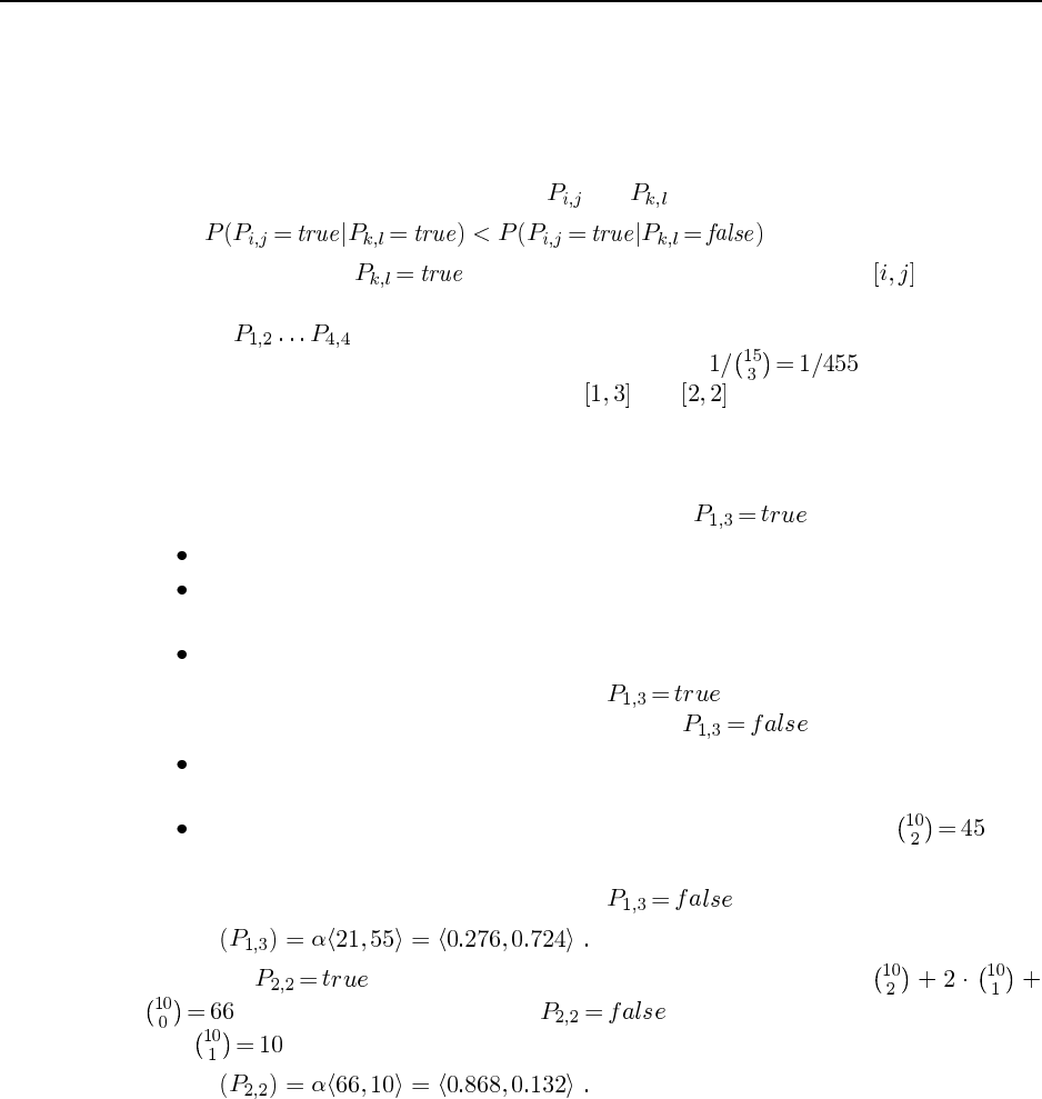
89
c. The independence assumption is clearly violated in practice. For example, the word pair
“artificial intelligence” occurs more frequently in any given document category than
would be suggested by multiplying the probabilities of “artificial” and “intelligence”.
13.19 This probability model is also appropriate for Minesweeper (Ex. 7.11). If the total
number of pits is fixed, then the variables and are no longer independent. In general,
because learning that makes it less likely that there is a mine at (as there are
now fewer to spread around). The joint distribution places equal probability on all assign-
ments to that have exactly 3 pits, and zero on all other assignments. Since there
are 15 squares, the probability of each 3-pit assignment is .
To calculate the probabilities of pits in and , we start from Figure 13.7. We
have to consider the probabilities of complete assignments, since the probability of the “other”
region assignment does not cancel out. We can count the total number of 3-pit assignments
that are consistent with each partial assignment in 13.7(a) and 13.7(b).
In 13.7(a), there are three partial assignments with :
The first fixes all three pits, so corresponds to 1 complete assignment.
The second leaves 1 pit in the remaining 10 squares, so corresponds to 10 complete
assignments.
The third also corresponds to 10 complete assignments.
Hence, there are 21 complete assignments with .
In 13.7(b), there are two partial assignments with :
The first leaves 1 pit in the remaining 10 squares, so corresponds to 10 complete assign-
ments.
The second leaves 2 pits in the remaining 10 squares, so corresponds to com-
plete assignments.
Hence, there are 55 complete assignments with . Normalizing, we obtain
P
With , there are four partial assignments with a total of
complete assignments. With , there is only one partial assignment
with complete assignments. Hence
P
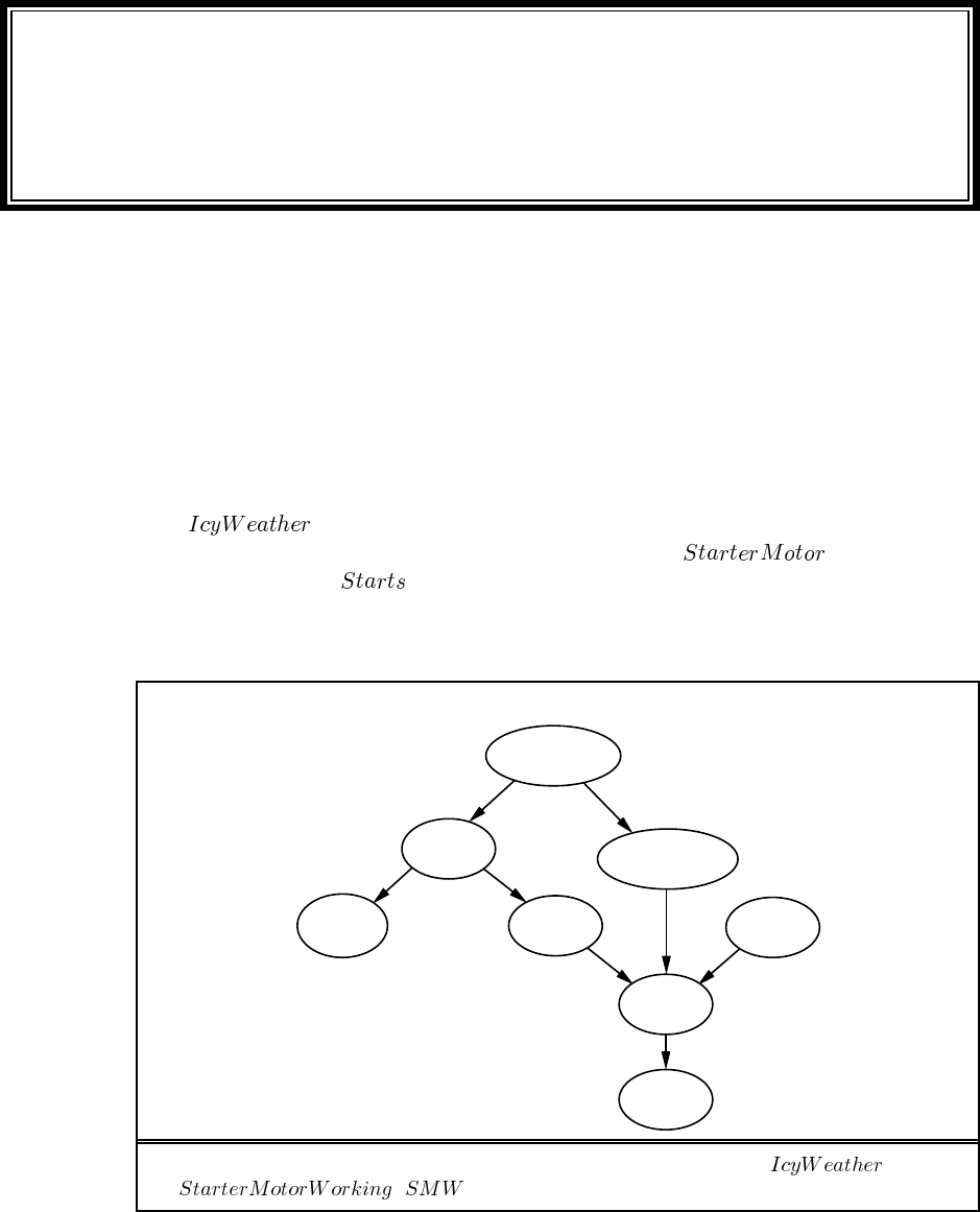
Solutions for Chapter 14
Probabilistic Reasoning
14.1 Adding variables to an existing net can be done in two ways. Formally speaking,
one should insert the variables into the variable ordering and rerun the network construction
process from the point where the first new variable appears. Informally speaking, one never
really builds a network by a strict ordering. Instead, one asks what variables are direct causes
or influences on what other ones, and builds local parent/child graphs that way. It is usually
easy to identify where in such a structure the new variable goes, but one must be very careful
to check for possible induced dependencies downstream.
a.is not caused by any of the car-related variables, so needs no parents.
It directly affects the battery and the starter motor. is an additional
precondition for . The new network is shown in Figure S14.1.
b. Reasonable probabilities may vary a lot depending on the kind of car and perhaps the
personal experience of the assessor. The following values indicate the general order of
Radio
Battery
Ignition Gas
Starts
Moves
IcyWeather
1
2
2
2
2
8
1
2
StarterMotor
Figure S14.1 Car network amended to include and
( ).
90
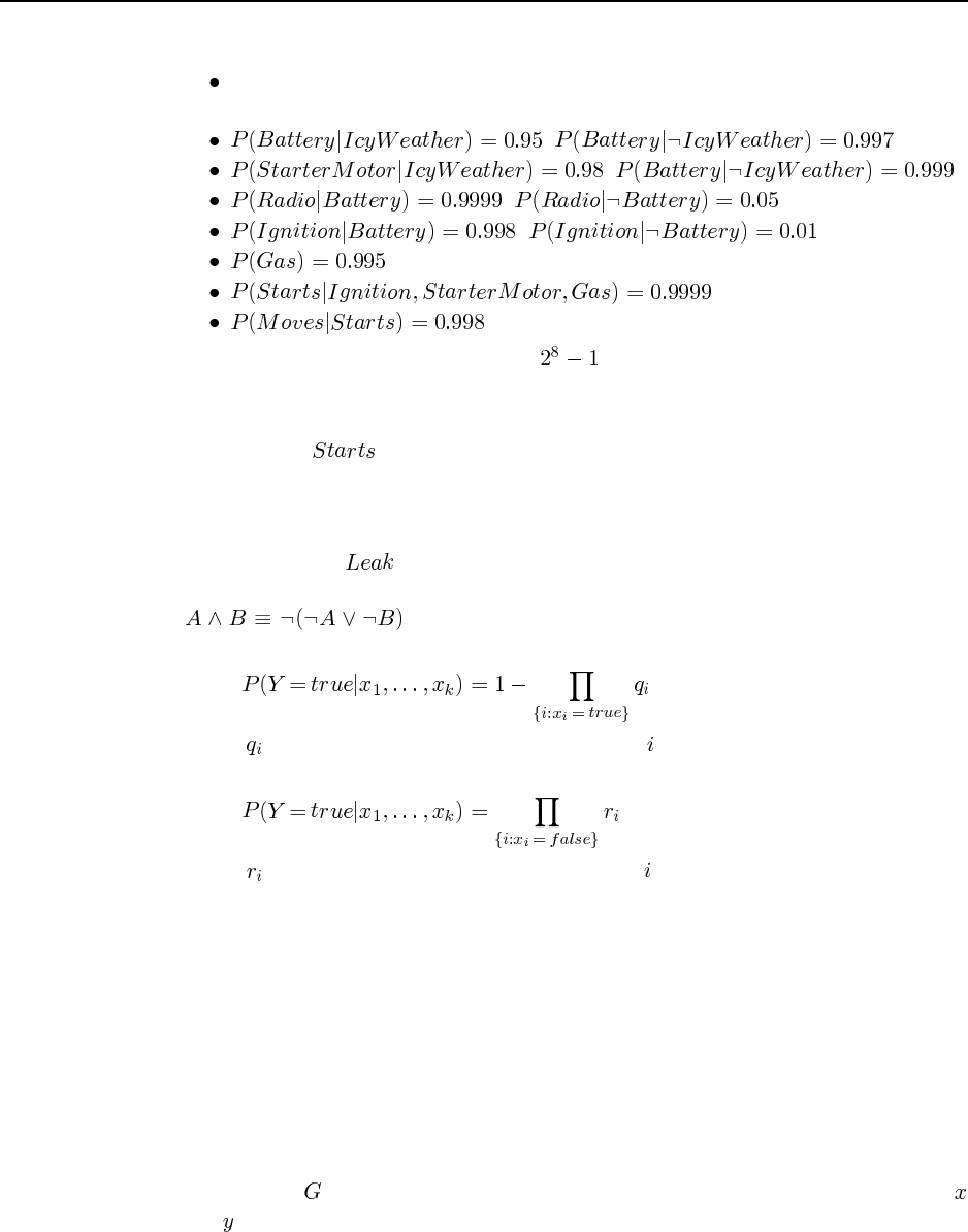
91
magnitude and relative values that make sense:
A reasonable prior for IcyWeather might be 0.05 (perhaps depending on location
and season).
, .
, .
, .
, .
.
, other entries 0.0.
.
c. With 8 Boolean variables, the joint has = 255 independent entries.
d. Given the topology shown in Figure S14.1, the total number of independent CPT entries
is 1+2+2+2+2+1+8+2= 20.
e. The CPT for describes a set of nearly necessary conditions that are together
almost sufficient. That is, all the entries are nearly zero except for the entry where all
the conditions are true. That entry will be not quite 1 (because there is always some
other possible fault that we didn’t think of), but as we add more conditions it gets closer
to 1. If we add a node as an extra parent, then the probability is exactly 1 when
all parents are true. We can relate noisy-AND to noisy-OR using de Morgan’s rule:
. That is, noisy-AND is the same as noisy-OR except that the
polarities of the parent and child variables are reversed. In the noisy-OR case, we have
where is the probability that the presence of the th parent fails to cause the child to
be true. In the noisy-AND case, we can write
where is the probability that the absence of the th parent fails to cause the child to
be false (e.g., it is magically bypassed by some other mechanism).
14.2 This question exercises many aspects of the student’s understanding of Bayesian net-
works and uncertainty.
a. A suitable network is shown in Figure S14.2. The key aspects are: the failure nodes are
parents of the sensor nodes, and the temperature node is a parent of both the gauge and
the gauge failure node. It is exactly this kind of correlation that makes it difficult for
humans to understand what is happening in complex systems with unreliable sensors.
b. No matter which way the student draws the network, it should not be a polytree because
of the fact that the temperature influences the gauge in two ways.
c. The CPT for is shown below. The wording of the question is a little tricky because
and are defined in terms of “incorrect” rather than “correct.”
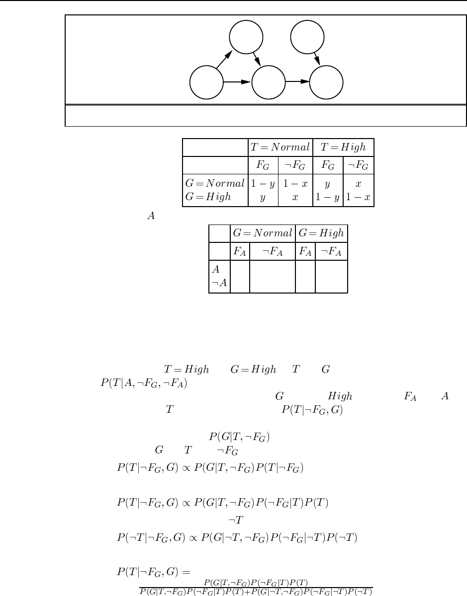
92 Chapter 14. Probabilistic Reasoning
TGA
FGFA
Figure S14.2 A Bayesian network for the nuclear alarm problem.
d. The CPT for is as follows:
0 0 0 1
1 1 1 0
e. This part actually asks the student to do something usually done by Bayesian network
algorithms. The great thing is that doing the calculation without a Bayesian network
makes it easy to see the nature of the calculations that the algorithms are systematizing.
It illustrates the magnitude of the achievement involved in creating complete and correct
algorithms.
Abbreviating and by and , the probability of interest here
is . Because the alarm’s behavior is deterministic, we can reason
that if the alarm is working and sounds, must be . Because and are
d-separated from , we need only calculate .
There are several ways to go about doing this. The “opportunistic” way is to notice
that the CPT entries give us , which suggests using the generalized Bayes’
Rule to switch and with as background:
We then use Bayes’ Rule again on the last term:
A similar relationship holds for :
Normalizing, we obtain
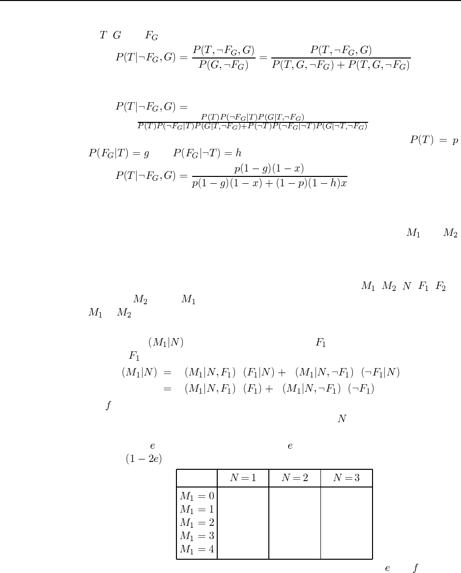
93
The “systematic” way to do it is to revert to joint entries (noticing that the subgraph
of , , and is completely connected so no loss of efficiency is entailed). We have
Now we use the chain rule formula (Equation 15.1 on page 439) to rewrite the joint
entries as CPT entries:
which of course is the same as the expression arrived at above. Letting ,
, and , we get
14.3
a. Although (i) in some sense depicts the “flow of information” during calculation, it is
clearly incorrect as a network, since it says that given the measurements and ,
the number of stars is independent of the focus. (ii) correctly represents the causal
structure: each measurement is influenced by the actual number of stars and the focus,
and the two telescopes are independent of each other. (iii) shows a correct but more
complicated network—the one obtained by ordering the nodes , , , , . If
you order before you would get the same network except with the arrow from
to reversed.
b. (ii) requires fewer parameters and is therefore better than (iii).
c. To compute P, we will need to condition on (that is, consider both possible
cases for , weighted by their probabilities).
P P P P P
P P P P
Let be the probability that the telescope is out of focus. The exercise states that this
will cause an “undercount of three or more stars,” but if = 3 or less the count will
be 0 if the telescope is out of focus. If it is in focus, then we will assume there is a
probability of of counting one two few, and of counting one too many. The rest of
the time , the count will be accurate. Then the table is as follows:
f + e(1-f) f f
(1-2e)(1-f) e(1-f) 0.0
e(1-f) (1-2e)(1-f) e(1-f)
0.0 e(1-f) (1-2e)(1-f)
0.0 0.0 e(1-f)
Notice that each column has to add up to 1. Reasonable values for and might be
0.05 and 0.002.
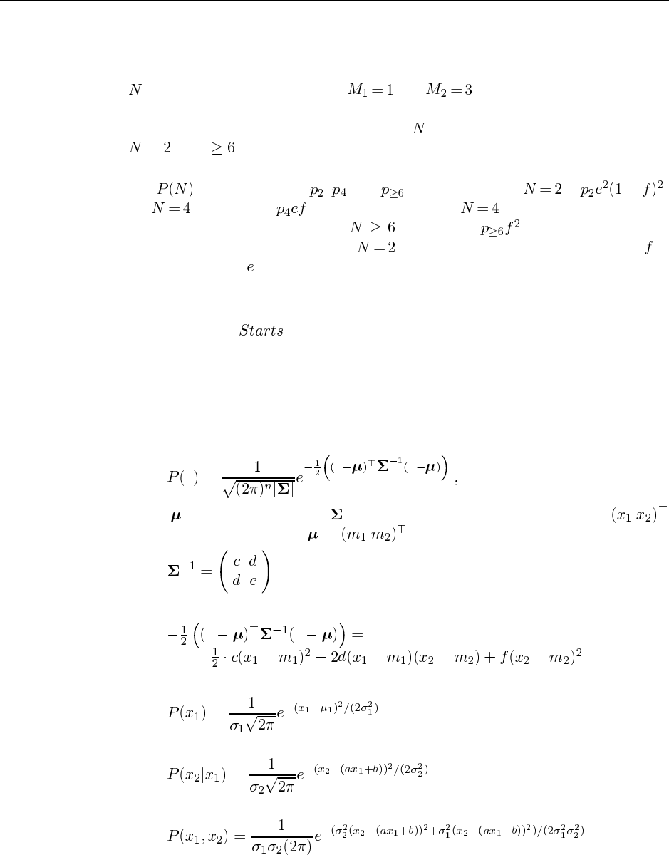
94 Chapter 14. Probabilistic Reasoning
d. This question causes a surprising amount of difficulty, so it is important to make sure
students understand the reasoning behind an answer. One approach uses the fact that
it is easy to reason in the forward direction, that is, try each possible number of stars
and see whether measurements and are possible. (This is a sort of
mental simulation of the physical process.) An alternative approach is to enumerate the
possible focus states and deduce the value of for each. Either way, the solutions are
, 4, or .
e. We cannot calculate the most likely number of stars without knowing the prior distribu-
tion . Let the priors be , , and . The posterior for is ;
for it is at most (at most, because with the out-of-focus telescope
could measure 0 instead of 1); for it is at most . If we assume that the
priors are roughly comparable, then is most likely because we are told that is
much smaller than .
For follow-up or alternate questions, it is easy to come up with endless variations on the
same theme involving sensors, failure nodes, hidden state. One can also add in complex
mechanisms, as for the variable in exercise 14.1.
14.5 This exercise is a little tricky and will appeal to more mathematicaly oriented students.
a. The basic idea is to multiply the two densities, match the result to the standard form for
a multivariate Gaussian, and hence identify the entries in the inverse covariance matrix.
Let’s begin by looking at the multivariate Gaussian. From page 982 in Appendix A we
have
xx x
where is the mean vector and is the covariance matrix. In our case, xis
and let the (as yet) unknown be . Suppose the inverse covariance matrix is
Then, if we multiply out the exponent, we obtain
x x
Looking at the distributions themselves, we have
and
hence
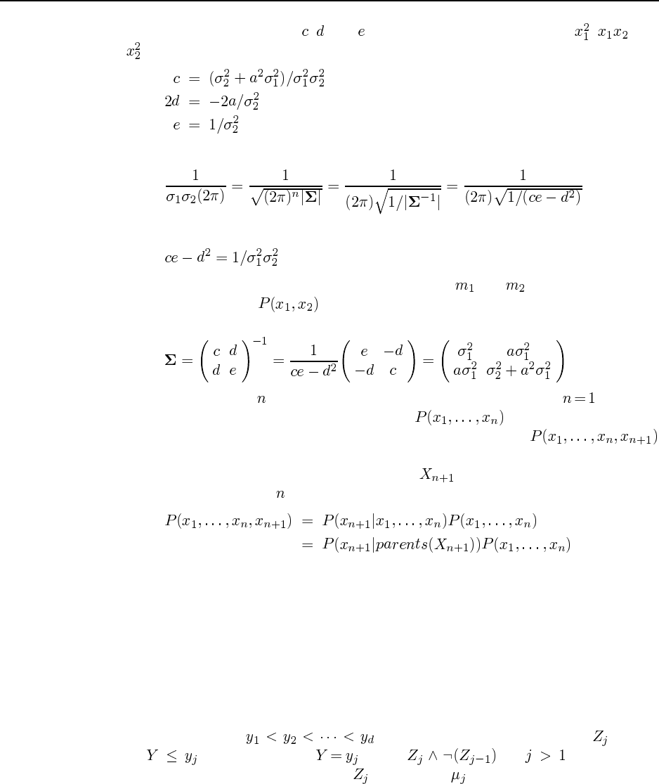
95
We can obtain equations for , , and by picking out the coefficients of , , and
:
We can check these by comparing the normalizing constants.
from which we obtain the constraint
which is easily confirmed. Similar calculations yield and , and plugging the re-
sults back shows that is indeed multivariate Gaussian. The covariance matrix
is
b. The induction is on , the number of variables. The base case for is trivial.
The inductive step asks us to show that if any constructed with linear–
Gaussian conditional densities is multivariate Gaussian, then any
constructed with linear–Gaussian conditional densities is also multivariate Gaussian.
Without loss of generality, we can assume that is a leaf variable added to a net-
work defined in the first variables. By the product rule we have
which, by the inductive hypothesis, is the product of a linear Gaussian with a multivari-
ate Gaussian. Extending the argument of part (a), this is in turn a multivariate Gaussian
of one higher dimension.
14.6
a. With multiple continuous parents, we must find a way to map the parent value vector to
a single threshold value. The simplest way to do this is to take a linear combination of
the parent values.
b. For ordered values , consider the Boolean proposition defined
by . The proposition is just for . Now we can
propose probit distributions for each , with means also in increasing order.
14.7 This question definitely helps students get a solid feel for variable elimination. Stu-
dents may need some help with the last part if they are to do it properly.
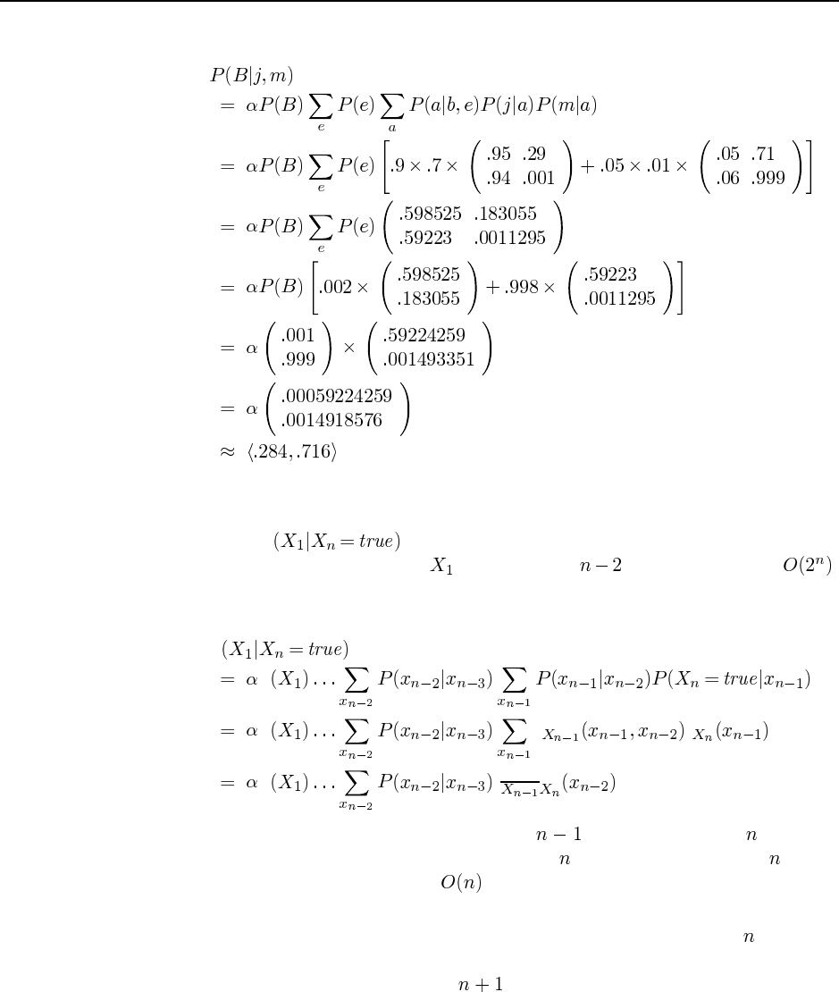
96 Chapter 14. Probabilistic Reasoning
a.
b. Including the normalization step, there are 7 additions, 16 multiplications, and 2 divi-
sions. The enumeration algorithm has two extra multiplications.
c. To compute Pusing enumeration, we have to evaluate two complete
binary trees (one for each value of ), each of depth , so the total work is .
Using variable elimination, the factors never grow beyond two variables. For example,
the first step is
P
P
P f f
P f
The last line is isomorphic to the problem with variables instead of ; the work
done on the first step is a constant independent of , hence (by induction on , if you
want to be formal) the total work is .
d. Here we can perform an induction on the number of nodes in the polytree. The base
case is trivial. For the inductive hypothesis, assume that any polytree with nodes can
be evaluated in time proportional to the size of the polytree (i.e., the sum of the CPT
sizes). Now, consider a polytree with nodes. Any node ordering consistent with
the topology will eliminate first some leaf node from this polytree. To eliminate any
leaf node, we have to do work proportional to the size of its CPT. Then, because the
network is a polytree, we are left with independent subproblems, one for each parent.
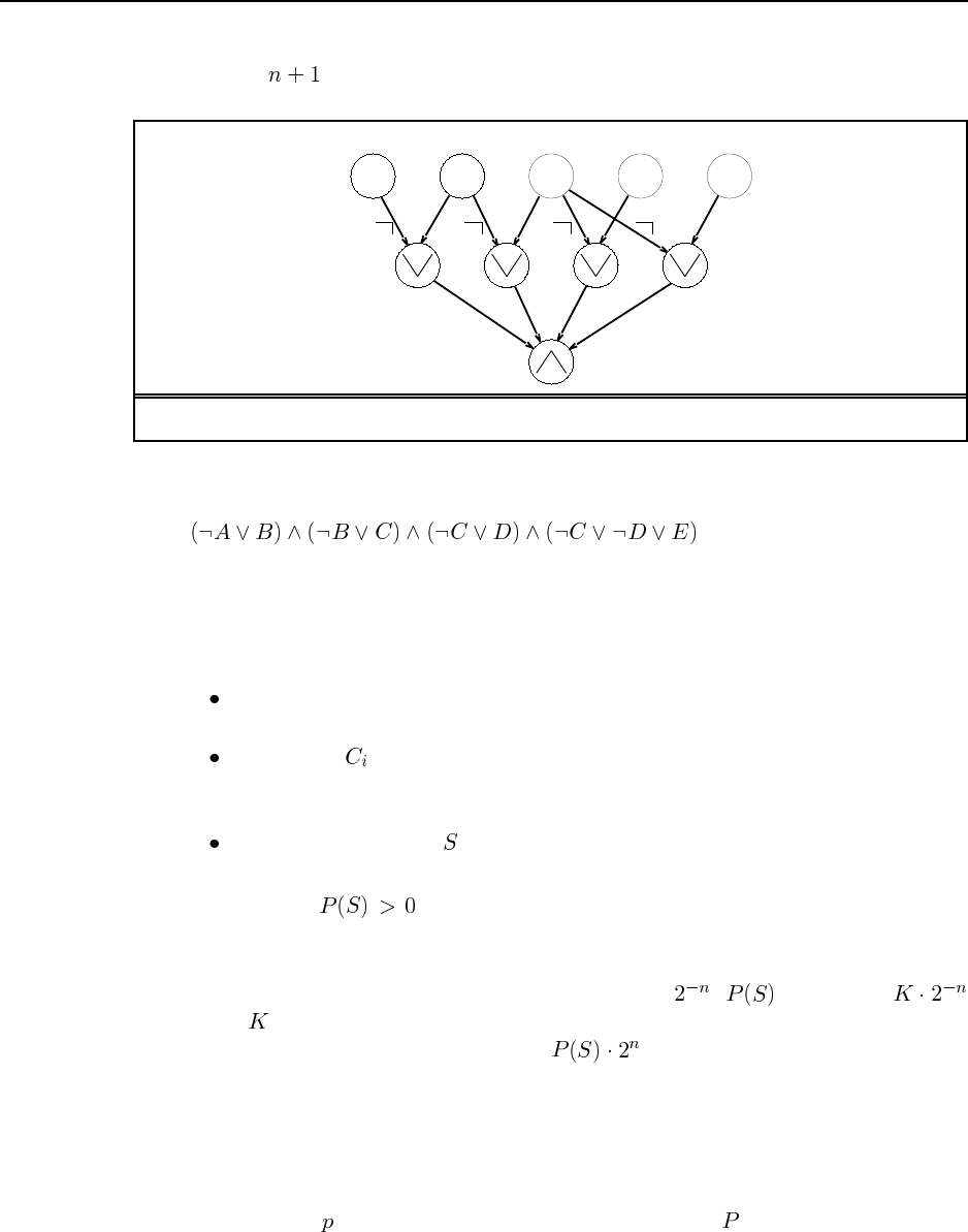
97
Each subproblem takes total work proportional to the sum of its CPT sizes, so the total
work for nodes is proportional to the sum of CPT sizes.
C2
C1C3C4
S
B
0.50.50.5 0.50.5
A C D E
Figure S14.3 A Bayesian network corresponding to a SAT problem.
14.8 Consider a SAT problem such as the following:
The idea is to encode this as a Bayes net, such that doing inference in the Bayes net gives the
answer to the SAT problem.
a. Figure S14.3 shows the Bayes net corresponding to this SAT problem. The general
construction method is as follows:
The root nodes correspond to the logical variables of the SAT problem. They have
a prior probability of 0.5.
Each clause is a node. Its parents are the variables in the clause. The CPT is
deterministic and implements the disjunction given in the clause. (Negative literals
in the clause are indicated by negation symbols on the links in the figure.)
A single sentence node has all the clauses as parents and a CPT that implements
deterministic conjunction.
It is clear that iff the SAT problem is satisfiable. Hence, we have reduced
SAT to Bayes net inference. Since SAT is NP-complete, we have shown that Bayes net
inference is NP-hard (even without evidence).
b. The prior probability of each complete assignment is . is therefore
where is the number of satisfying assignments. Hence, we can count the number
of satisfying assignments by computing . This amounts to a reduction of the
problem of counting satisfying assignments to Bayes net inference; since the former is
#P-complete, the latter is #P-hard.
14.9
a. To calculate the cumulative distribution of a discrete variable, we start from a vector
representation of the original distribution and a vector of the same dimension.
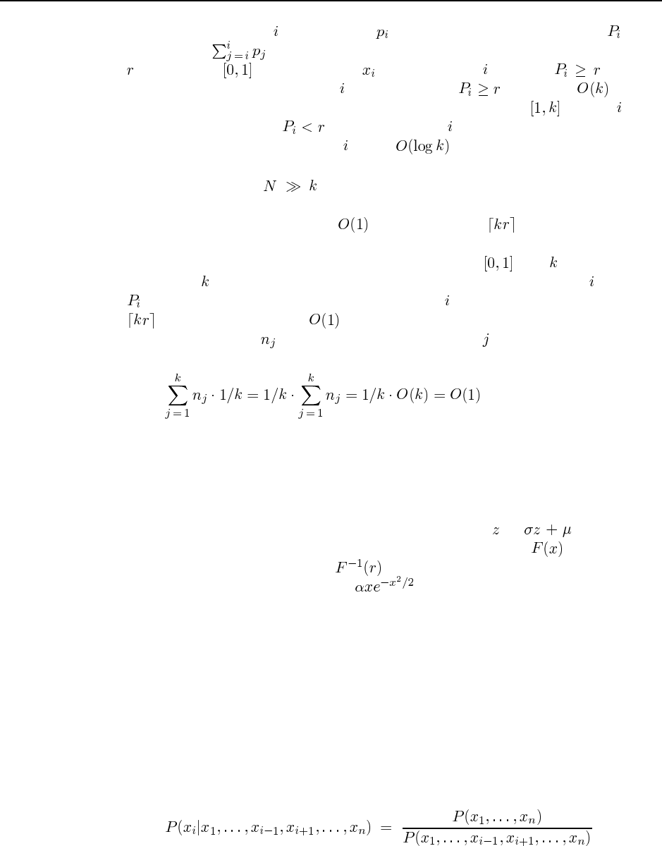
98 Chapter 14. Probabilistic Reasoning
Then, we loop through , adding up the values as we go along and setting to the
running sum, . To sample from the distribution, we generate a random number
uniformly in , and then return for the smallest such that . A naive
way to find this is to loop through starting at 1 until . This takes time. A
more efficient solution is binary search: start with the full range , choose at the
midpoint of the range. If , set the range from to the upper bound, otherwise set
the range from the lower bound to . After iterations, we terminate when the
bounds are identical or differ by 1.
b. If we are generating samples, we can afford to preprocess the cumulative
distribution. The basic insight required is that if the original distribution were uniform,
it would be possible to sample in time by returning . That is, we can index
directly into the correct part of the range (analog random access, one might say) instead
of searching for it. Now, suppose we divide the range into equal parts and
construct a -element vector, each of whose entries is a list of all those for which
is in the corresponding part of the range. The we want is in the list with index
. We retrieve this list in time and search through it in order (as in the naive
implementation). Let be the number of elements in list . Then the expected runtime
is given by
The variance of the runtime can be reduced by further subdividing any part of the range
whose list contains more than some small constant number of elements.
c. One way to generate a sample from a univariate Gaussian is to compute the discretized
cumulative distribution (e.g., integrating by Taylor’s rule) and use the algorithm de-
scribed above. We can compute the table once and for all for the standard Gaussian
(mean 0, variance 1) and then scale each sampled value to . If we had a
closed-form, invertible expression for the cumulative distribution , we could sam-
ple exactly, simply by returning . Unfortunately the Gaussian density is not
exactly integrable. Now, the density is exactly integrable, and there are cute
schemes for using two samples and this density to obtain an exact Gaussian sample. We
leave the details to the interested instructor.
d. When querying a continuous variable using Monte carlo inference, an exact closed-form
posterior cannot be obtained. Instead, one typically defines discrete ranges, returning
a histogram distribution simply by counting the (weighted) number of samples in each
range.
14.10 These proofs are tricky for those not accustomed to manipulating probability expres-
sions, and students may require some hints.
a. There are several ways to prove this. Probably the simplest is to work directly from the
global semantics. First, we rewrite the required probability in terms of the full joint:
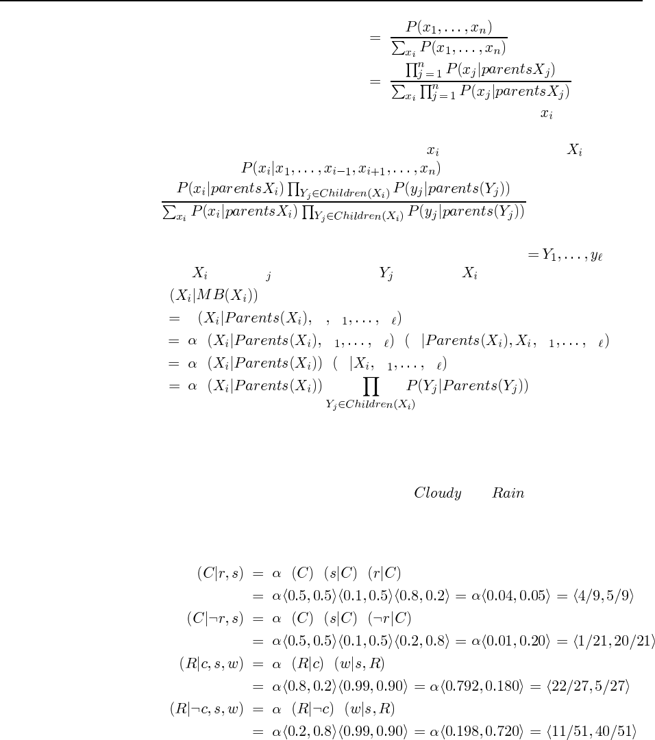
99
Now, all terms in the product in the denominator that do not contain can be moved
outside the summation, and then cancel with the corresponding terms in the numerator.
This just leaves us with the terms that do mention , i.e., those in which is a child
or a parent. Hence, is equal to
Now, by reversing the argument in part (b), we obtain the desired result.
b. This is a relatively straightforward application of Bayes’ rule. Let Ybe the
children of and let Zbe the parents of other than . Then we have
P
P Y Z Z
P Z Z P Y Z Z
P P Y Z Z
P
where the derivation of the third line from the second relies on the fact that a node is
independent of its nondescendants given its children.
14.11
a. There are two uninstantiated Boolean variables ( and ) and therefore four
possible states.
b. First, we compute the sampling distribution for each variable, conditioned on its Markov
blanket.
PP P P
P P P P
P P P
P P P
Strictly speaking, the transition matrix is only well-defined for the variant of MCMC in
which the variable to be sampled is chosen randomly. (In the variant where the variables
are chosen in a fixed order, the transition probabilities depend on where we are in the
ordering.) Now consider the transition matrix.
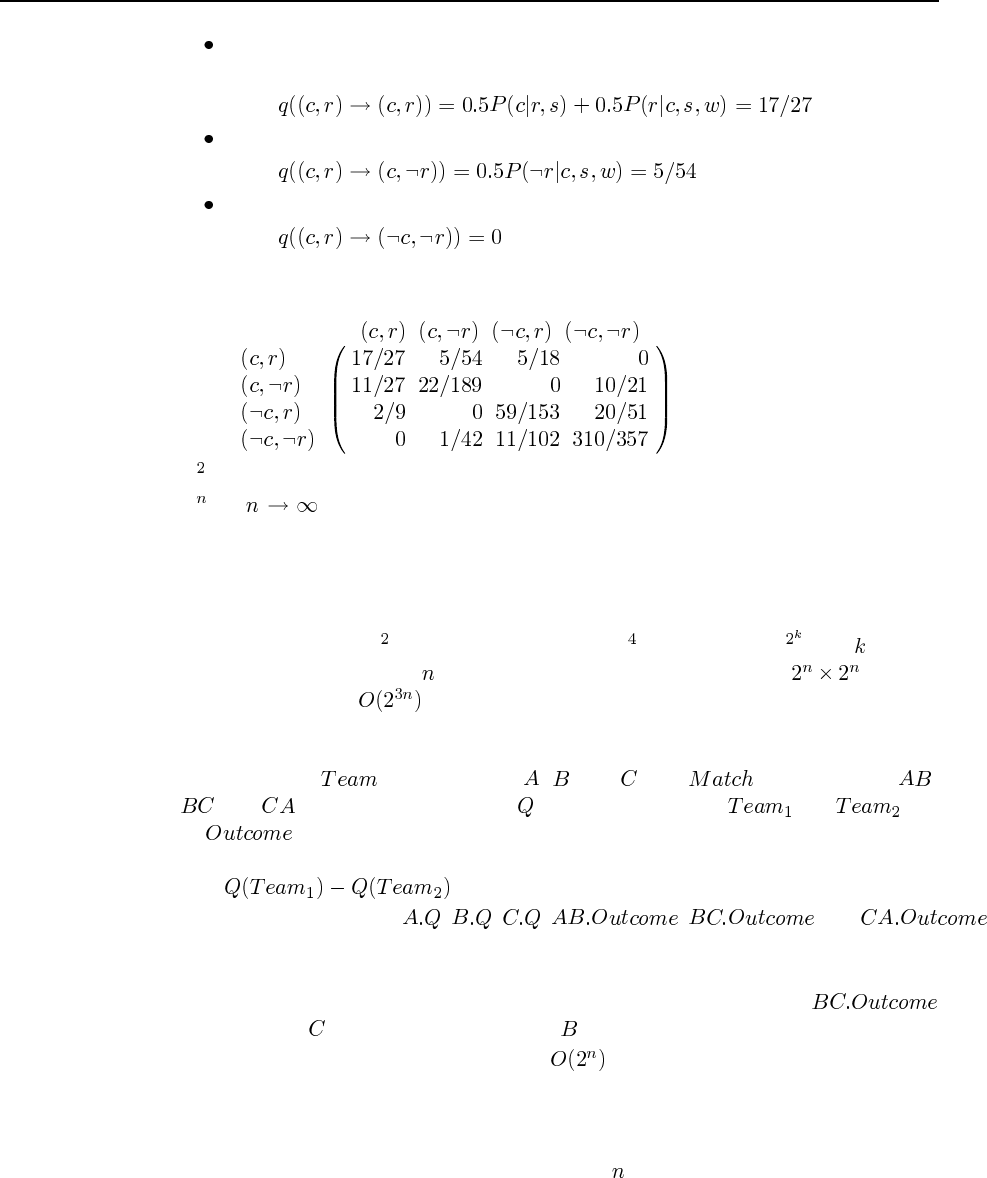
100 Chapter 14. Probabilistic Reasoning
Entries on the diagonal correspond to self-loops. Such transitions can occur by
sampling either variable. For example,
Entries where one variable is changed must sample that variable. For example,
Entries where both variables change cannot occur. For example,
This gives us the following transition matrix, where the transition is from the state given
by the row label to the state given by the column label:
c.Qrepresents the probability of going from each state to each state in two steps.
d.Q(as ) represents the long-term probability of being in each state starting in
each state; for ergodic Qthese probabilities are independent of the starting state, so
every row of Qis the same and represents the posterior distribution over states given
the evidence.
e. We can produce very large powers of Qwith very few matrix multiplications. For
example, we can get Qwith one multiplication, Qwith two, and Qwith . Unfor-
tunately, in a network with Boolean variables, the matrix is of size , so each
multiplication takes operations.
14.12
a. The classes are , with instances , , and , and , with instances ,
, and . Each team has a quality and each match has a and and
an . The team names for each match are of course fixed in advance. The prior
over quality could be uniform and the probability of a win for team 1 should increase
with .
b. The random variables are , , , , , and .
The network is shown in Figure S14.4.
c. The exact result will depend on the probabilities used in the model. With any prior on
quality that is the same across all teams, we expect that the posterior over
will show that is more likely to win than .
d. The inference cost in such a model will be because all the team qualities become
coupled.
e. MCMC appears to do well on this problem, provided the probabilities are not too
skewed. Our results show scaling behavior that is roughly linear in the number of
teams, although we did not investigate very large .
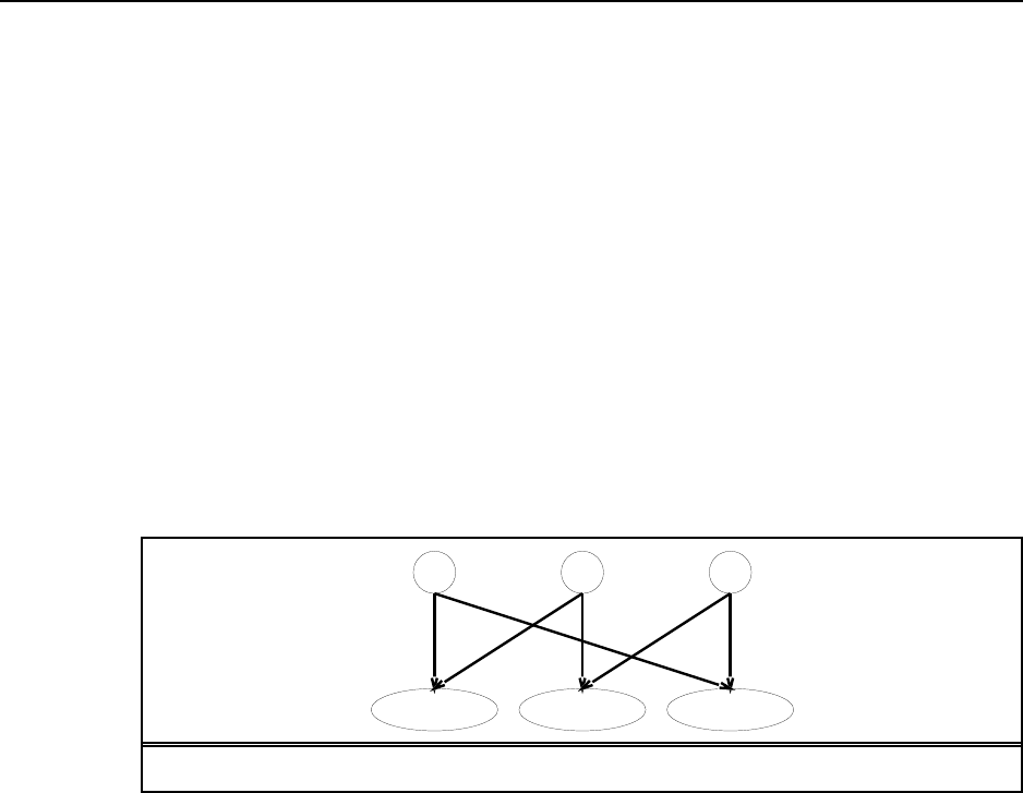
101
A.Q B.Q C.Q
AB.Outcome BC.Outcome CA.Outcome
Figure S14.4 A Bayesian network corresponding to the soccer model of Exercise 14.12.
Solutions for Chapter 15
Probabilistic Reasoning over Time
15.1 For each variable that appears as a parent of a variable , define an auxiliary
variable , such that is parent of and is a parent of . This gives us
a first-order Markov model. To ensure that the joint distribution over the original variables
is unchanged, we keep the CPT for is unchanged except for the new parent name, and
we require that Pis an identity mapping, i.e., the child has the same value as the
parent with probability 1. Since the parameters in this model are fixed and known, there is no
effective increase in the number of free parameters in the model.
15.2
a. For all , we the filtering formula
P P P
At the fixed point, we additionally expect that P P . Let the
fixed-point probabilities be . This provides us with a system of linear equa-
tions:
Solving this system, we find that .
b. The probability converges to as illustrated in Figure S15.1. This convergence
makes sense if we consider a fixed-point equation for P:
P
P
That is, .
Notice that the fixed point does not depend on the initial evidence.
15.3 This exercise develops the Island algorithm for smoothing in DBNs (?).
102
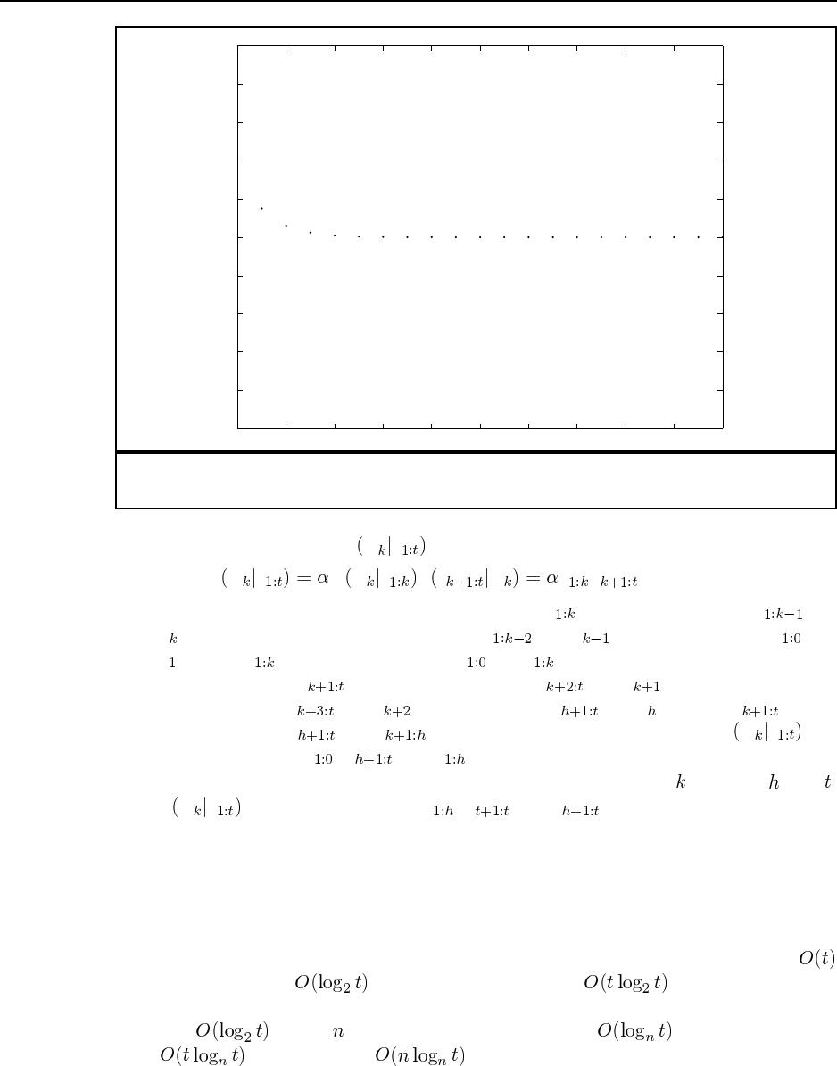
103
0 2 4 6 8 10 12 14 16 18 20
0
0.1
0.2
0.3
0.4
0.5
0.6
0.7
0.8
0.9
1
Figure S15.1 A graph of the probability of rain as a function of time, forecast into the
future.
a. The chapter shows that P X e can be computed as
P X e P X e P e X f b
The forward recursion (Equation 15.3) shows that fcan be computed from fand
e, which can in turn be computed from fand e, and so on down to fand
e. Hence, fcan be computed from fand e. The backward recursion (Equation
15.7) shows that bcan be computed from band e, which in turn can be
computed from band e, and so on up to band e. Hence, bcan be
computed from band e. Combining these two, we find that P X e can
be computed from f,b, and e.
b. The reasoning for the second half is essentially identical: for between and ,
P X e can be computed from f,b, and e.
c. The algorithm takes 3 arguments: an evidence sequence, an initial forward message,
and a final backward message. The forward message is propagated to the halfway point
and the backward message is propagated backward. The algorithm then calls itself
recursively on the two halves of the evidence sequence with the appropriate forward
and backward messages. The base case is a sequence of length 1 or 2.
d. At each level of the recursion the algorithm traverses the entire sequence, doing
work. There are levels, so the total time is . The algorithm does
a depth-first recursion, so the total space is proportional to the depth of the stack,
i.e., . With islands, the recursion depth is , so the total time is
but the space is .
104 Chapter 15. Probabilistic Reasoning over Time
15.4 This is a very good exercise for deepening intuitions about temporal probabilistic rea-
soning. First, notice that the impossibility of the sequence of most likely states cannot come
from an impossible observation because the smoothed probability at each time step includes
the evidence likelihood at that time step as a factor. Hence, the impossibility of a sequence
must arise from an impossible transition. Now consider such a transition from to
for some , , . For to be the most likely state at time , even though
it cannot be reached from the most likely state at time , we can simply have an -state system
where, say, the smoothed probability of is and the remaining states
have probability . The remaining states all transition deterministically to .
From here, it is a simple matter to work out a specific model that behaves as desired.
15.5
a. Looking at the fragment of the model containing just , X, and X, we have
P X xx P x
From the properties of the Kalman filter, we know that the integral gives a Gaussian
for each different value of . Hence, the prediction distribution is a mixture of
Gaussians, each weighted by .
b. The update equation for the switching Kalman filter is
P X e
P e X xP x e P X x
P e X e P xP x e P X x
We are given that P x e is a mixture of Gaussians. Each Gaussian is subject to
different linear–Gaussian projections and then updated by a linear-Gaussian observa-
tion, so we obtain a sum of Gaussians. Thus, after steps we have Gaussians.
c. Each weight represents the probability of one of the sequences of values for the
switching variable.
15.6 This is a simple exercise in algebra. We have
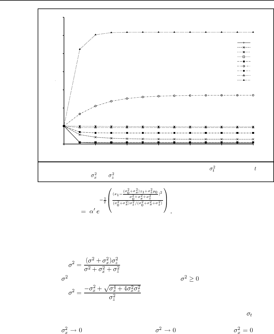
105
0
1
2
3
4
5
6
7
0 2 4 6 8 10 12
Variance of posterior distribution
Number of time steps
sx2=0.1, sz2=0.1
sx2=0.1, sz2=1.0
sx2=0.1, sz2=10.0
sx2=1.0, sz2=0.1
sx2=1.0, sz2=1.0
sx2=1.0, sz2=10.0
sx2=10.0, sz2=0.1
sx2=10.0, sz2=1.0
sx2=10.0, sz2=10.0
Figure S15.2 Graph for Ex. 15.7, showing the posterior variance as a function of for
various values of and .
15.7
a. See Figure S15.2.
b. We can find a fixed point by solving
for . Using the quadratic formula and requiring , we obtain
We omit the proof of convergence, which, presumably, can be done by showing that the
update is a contraction (i.e., after updating, two different starting points for become
closer).
c. As , we see that the fixed point also. This is because implies
a deterministic path for the object. Each observation supplies more information about
this path, until its parameters are known completely.
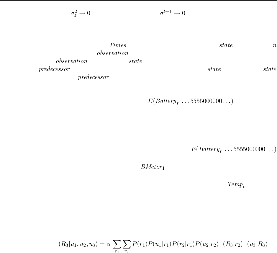
106 Chapter 15. Probabilistic Reasoning over Time
As , the variance update gives immediately. That is, if we have an
exact observation of the object’s state, then the posterior is a delta function about that
observed value regardless of the transition variance.
15.8 There is one class, . Each element of the class has a attribute with
possible values and an attribute which may be discrete or continuous. The parent
of the attribute is the attribute of the same time step. Each time step has
relation to another time step, and the parent of the attribute is the
attribute of the time step.
15.9
a. The curve of interest is the one for . In the absence
of any useful sensor information from the battery meter, the posterior distribution for
the battery level is the same as the projection without evidence. The transition model
for the battery includes a small probability for downward transitions in the battery level
at each time step, but zero probability for upward transitions (there are no recharging
actions in the model). Thus, the stationary distribution towards which the battery level
tends has value 0 with probability 1. The curve for
will asymptote to 0.
b. See Figure S15.3. The CPT for has a probability of transient failure (i.e.,
reporting 0) that increases with temperature.
c. The agent can obviously calculate the posterior distribution over by filtering
the observation sequence in the usual way. This posterior can be informative if the
effect of temperature on transient failure is non-negligible and transient failures occur
more frequently than do major changes in temperature. Essentially, the temperature is
estimated from the frequency of “blips” in the sequence of battery meter readings.
15.10 The process works exactly as on page 507. We start with the full expression:
P P P
Whichever order we push in the summations, the variable elimination process never creates
factors containing more than two variables, which is the same size as the CPTs in the original
network. In fact, given an HMM sequence of arbitrary length, we can eliminate the state
variables in any order.
15.11 The model is shown in Figure S15.4. The key point to note is that any phone variation
at one point (here, [aa] vs. [ey] in the fourth phone) results in variation at three points because
of the effects on the preceding and succeeding phones.
15.12 The [C1,C2] and [C6,C7] must come from the onset and end, respectively. The C3
could come from 2 sources, the onset or the mid, and the [C4, C4] combination could come
from 3 sources: mid-mid, mid-end, or end-end. You can’t go directly from onset to end, so
the only possible paths (along with their path and output probabilities) are as follows:
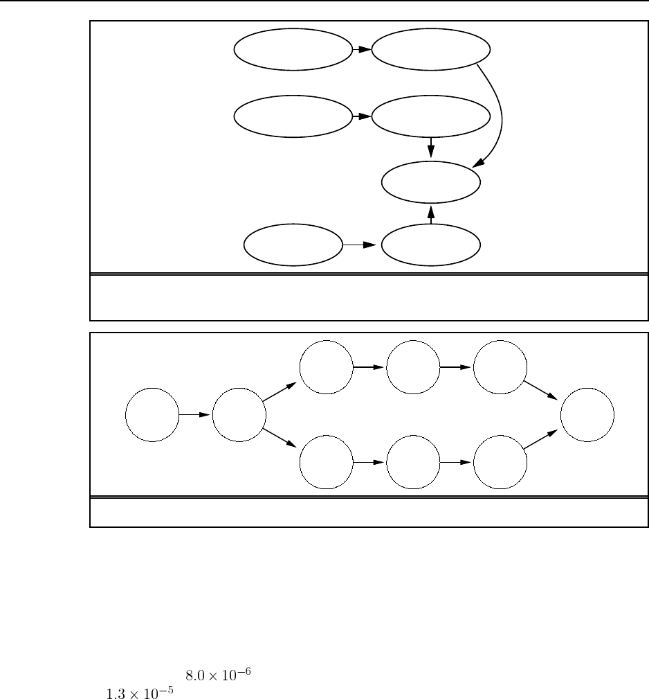
107
1
Battery
Battery 0
1
BMeter
0
BMBroken 1
BMBroken
0
Temp 1
Temp
Figure S15.3 Modification of Figure 15.13(a) to include the effect of external temperature
on the battery meter.
t(_,ow) ow(t,m)
m(ow.ey)
m(ow,aa)
ey(m,t)
aa(m,t)
t(ey,ow)
ow(t,_)
t(aa,ow)
Figure S15.4 Transition diagram for the triphone pronunciation model in Ex. 15.11.
C1 C2 C3 C4 C4 C6 C7
OOOMMEE (* .3 .3 .7 .9 .1 .4 .6 .5 .2 .3 .7 .7 .5 .4) = 4.0e-6
OOOMEEE (* .3 .3 .7 .1 .4 .4 .6 .5 .2 .3 .7 .1 .5 .4) = 2.5e-7
OOMMMEE (* .3 .7 .9 .9 .1 .4 .6 .5 .2 .2 .7 .7 .5 .4) = 8.0e-6
OOMMEEE (* .3 .7 .9 .1 .4 .4 .6 .5 .2 .2 .7 .1 .5 .4) = 5.1e-7
OOMEEEE (* .3 .7 .1 .4 .4 .4 .6 .5 .2 .2 .1 .1 .5 .4) = 3.2e-8
So the most probable path is OOMMMEE (that is, onset-onset-mid-mid-mid-end-end), with
a probability of . The total probability of the sequence is the sum of the five paths,
or .
Solutions for Chapter 16
Making Simple Decisions
16.1 It is interesting to create a histogram of accuracy on this task for the students in the
class. It is also interesting to record how many times each student comes within, say, 10% of
the right answer. Then you get a profile of each student: this one is an accurate guesser but
overly cautious about bounds, etc.
16.2 The expected monetary value of the lottery is
Although , it is not necessarily irrational to buy the ticket. First we will consider
just the utilities of the monetary outcomes, ignoring the utility of actually playing the lottery
game. Using to represent the utility to the agent of having dollars more than the
current state, and assuming that utility is linear for small values of money (i.e.,
for ), the utility of the lottery is:
This is more than when . Thus, for a purchase
to be rational (when only money is considered), the agent must be quite risk-seeking. This
would be unusual for low-income individuals, for whom the price of a ticket is non-trivial. It
is possible that some buyers do not internalize the magnitude of the very low probability of
winning—to imagine an event is to assign it a “non-trivial” probability, in effect. Apparently,
these buyers are better at internalizing the large magnitude of the prize. Such buyers are
clearly acting irrationally.
Some people may feel their current situation is intolerable, that is,
. Therefore the situation of having one dollar more or less would be equally intolerable,
and it would be rational to gamble on a high payoff, even if one that has low probability.
Gamblers also derive pleasure from the excitement of the lottery and the temporary
possession of at least a non-zero chance of wealth. So we should add to the utility of playing
the lottery the term to represent the thrill of participation. Seen this way, the lottery is just
another form of entertainment, and buying a lottery ticket is no more irrational than buying
108
109
a movie ticket. Either way, you pay your money, you get a small thrill , and (most likely)
you walk away empty-handed. (Note that it could be argued that doing this kind of decision-
theoretic computation decreases the value of . It is not clear if this is a good thing or a bad
thing.)
16.3
a. The probability that the first heads appears on the th toss is , so
b. Typical answers range between $4 and $100.
c. Assume initial wealth (after paying to play the game) of ; then
Assume for simplicity. Then
d. The maximum amount is given by the solution of
For our simple case, we have
or .
16.4 This is an interesting exercise to do in class. Choose , = $100, $1000,
$10000, $1000000. Ask for a show of hands of those preferring the lottery at different values
of . Students will almost always display risk aversion, but there may be a wide spread in its
onset. A curve can be plotted for the class by finding the smallest yielding a majority vote
for the lottery.
16.5 The program itself is pretty trivial. But note that there are some studies showing you
get better answers if you ask subjects to move a slider to indicate a proportion, rather than
asking for a probability number. So having a graphical user interface is an advantage. The
main point of the exercise is to examine the data, expose inconsistent behavior on the part of
the subjects, and see how people vary in their choices.
16.6 The protocol would be to ask a series of questions of the form “which would you
prefer” involving a monetary gain (or loss) versus an increase (or decrease) in a risk of death.

110 Chapter 16. Making Simple Decisions
For example, “would you pay $100 for a helmet that would eliminate completely the one-in-
a-million chance of death from a bicycle accident.”
16.7 The complete proof is given by Keeney and Raiffa (1976).
16.8 This exercise can be solved using an influence diagram package such as IDEAL. The
specific values are not especially important. Notice how the tedium of encoding all the entries
in the utility table cries out for a system that allows the additive, multiplicative, and other
forms sanctioned by MAUT.
One of the key aspects of the fully explicit representation in Figure 16.5 is its amenabil-
ity to change. By doing this exercise as well as Exercise 16.9, students will augment their
appreciation of the flexibility afforded by declarative representations, which can otherwise
seem tedious.
a. For this part, one could use symbolic values (high, medium, low) for all the variables
and not worry too much about the exact probability values, or one could use actual
numerical ranges and try to assess the probabilities based on some knowledge of the
domain. Even with three-valued variables, the cost CPT has 54 entries.
b. This part almost certainly should be done using a software package.
c. If each aircraft generates half as much noise, we need to adjust the entries in the
CPT.
d. If the noise attribute becomes three times more important, the utility table entries must
all be altered. If an appropriate (e.g., additive) representation is available, then one
would only need to adjust the appropriate constants to reflect the change.
e. This part should be done using a software package. Some packages may offer VPI
calculation already. Alternatively, one can invoke the decision-making package repeat-
edly to do all the what-if calculations of best actions and their utilities, as required in
the VPI formula. Finally, one can write general-purpose VPI code as an add-on to a
decision-making package.
16.9 The information associated with the utility node in Figure 16.6 is an action-value table,
and can be constructed simply by averaging out the , , and nodes in Fig-
ure 16.5. As explained in the text , modifications to aircraft noise levels or to the importance
of noise do not result in simple changes to the action-value table. Probably the easiest way
to do it is to go back to the original table in Figure 16.5. The exercise therefore illustrates the
tradeoffs involved in using compiled representations.
16.10 The answer to this exercise depends on the probability values chosen by the stu-
dent.
16.11 This question is a simple exercise in sequential decision making, and helps in making
the transition to Chapter 17. It also emphasizes the point that the value of information is
computed by examining the conditional plan formed by determining the best action for each
possible outcome of the test. It may be useful to introduce “decision trees” (as the term is
used in the decision analysis literature) to organize the information in this question. (See Pearl
(1988), Chapter 6.) Each part of the question analyzes some aspect of the tree. Incidentally,
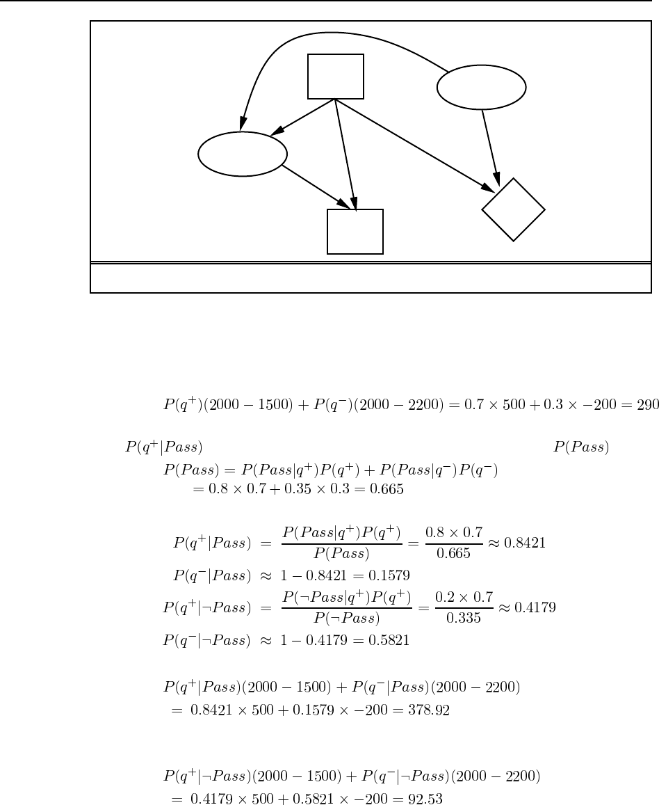
111
Test
Buy U
Outcome
Quality
Figure S16.1 A decision network for the car-buying problem.
the question assumes that utility and monetary value coincide, and ignores the transaction
costs involved in buying and selling.
a. The decision network is shown in Figure S16.1.
b. The expected net gain in dollars is
c. The question could probably have been stated better: Bayes’ theorem is used to compute
, etc., whereas conditionalization is sufficient to compute .
Using Bayes’ theorem:
d. If the car passes the test, the expected value of buying is
Thus buying is the best decision given a pass. If the car fails the test, the expected value
of buying is
Buying is again the best decision.
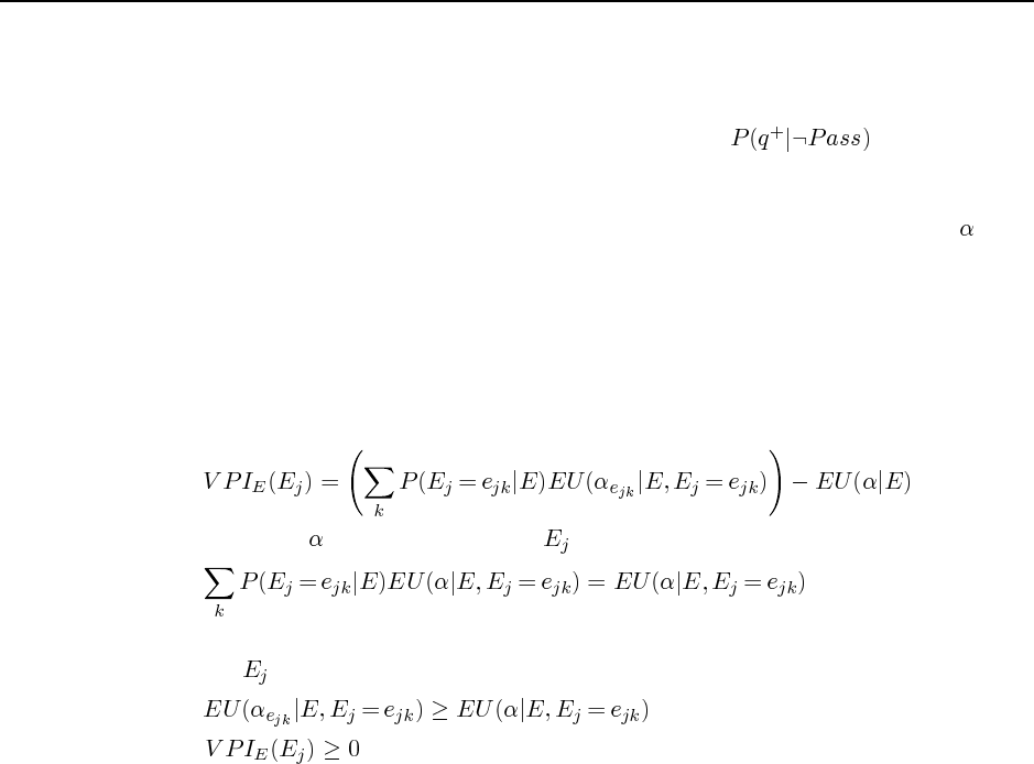
112 Chapter 16. Making Simple Decisions
e. Since the action is the same for both outcomes of the test, the test itself is worthless (if
it is the only possible test) and the optimal plan is simply to buy the car without the test.
(This is a trivial conditional plan.) For the test to be worthwhile, it would need to be
more discriminating in order to reduce the probability . The test would
also be worthwhile if the market value of the car were less, or if the cost of repairs were
more.
An interesting additional exercise is to prove the general proposition that if is the
best action for all the outcomes of a test then it must be the best action in the absence
of the test outcome.
16.12 Intuitively, the value of information is nonnegative because in the worst case one
could simply ignore the information and act as if it was not available. A formal proof therefore
begins by showing that this policy results in the same expected utility. The formula for the
value of information is
If the agent does given the information , its expected utility is
where the equality holds because the LHS is just the conditionalization of the RHS with
respect to . By definition,
hence .
16.13 This is relatively straightforward in the AIMA2e code release. We need to add node
types for action nodes and utility nodes; we need to be able to run standard Bayes net infer-
ence on the network given fixed actions, in order to compute the posterior expected utility; and
we need to write an “outer loop” that can try all possible actions to find the best. Given this,
adding VPI calculation is straightforward, as described in the answer to Exercise 16.8.

Solutions for Chapter 17
Making Complex Decisions
17.1 This question helps to bring home the difference between deterministic and stochastic
environments. Here, even a short sequence spreads the agent all over the place. The easiest
way to answer the question systematically is to draw a tree showing the states reached after
each step and the transition probabilities. Then the probability of reaching each leaf is the
product of the probabilities along the path, because the transition probabilities are Markovian.
If the same state appears at more than one leaf, the probabilities of the leaves are summed
because the events corresponding to the two paths are disjoint. (It is always a good idea to
ensure that students justify these kinds of probabilistic calculations, especially since some-
times the “naive” approach gets the wrong answer.) The states and probabilities are: (3,1),
0.01; (3,2), 0.08; (3,3), 0.09; (4,2), 0.18; (4,3), 0.64.
17.2 Stationarity requires the agent to have identical preferences between the sequence pair
and between the sequence pair . If the
utility of a sequence is its maximum reward, we can easily violate stationarity. For example,
but
We can still define as the expected maximum reward obtained by executing starting
in . The agent’s preferences seem peculiar, nonetheless. For example, if the current state
has reward max, the agent will be indifferent among all actions, but once the action is
executed and the agent is no longer in , it will suddenly start to care about what happens
next.
17.3 A finite search problem (see Chapter 3) is defined by an initial state , a successor
function that returns a set of action–state pairs, a step cost function , and a goal
test. An optimal solution is a least-cost path from to any goal state.
To construct the corresponding MDP, define unless is a
goal state, in which case (see Ex. 17.5 for how to obtain the effect of a three-
argument reward function); define if ; and . An optimal
solution to this MDP is a policy that follows the least-cost path from each state to its nearest
goal state.
17.4
113
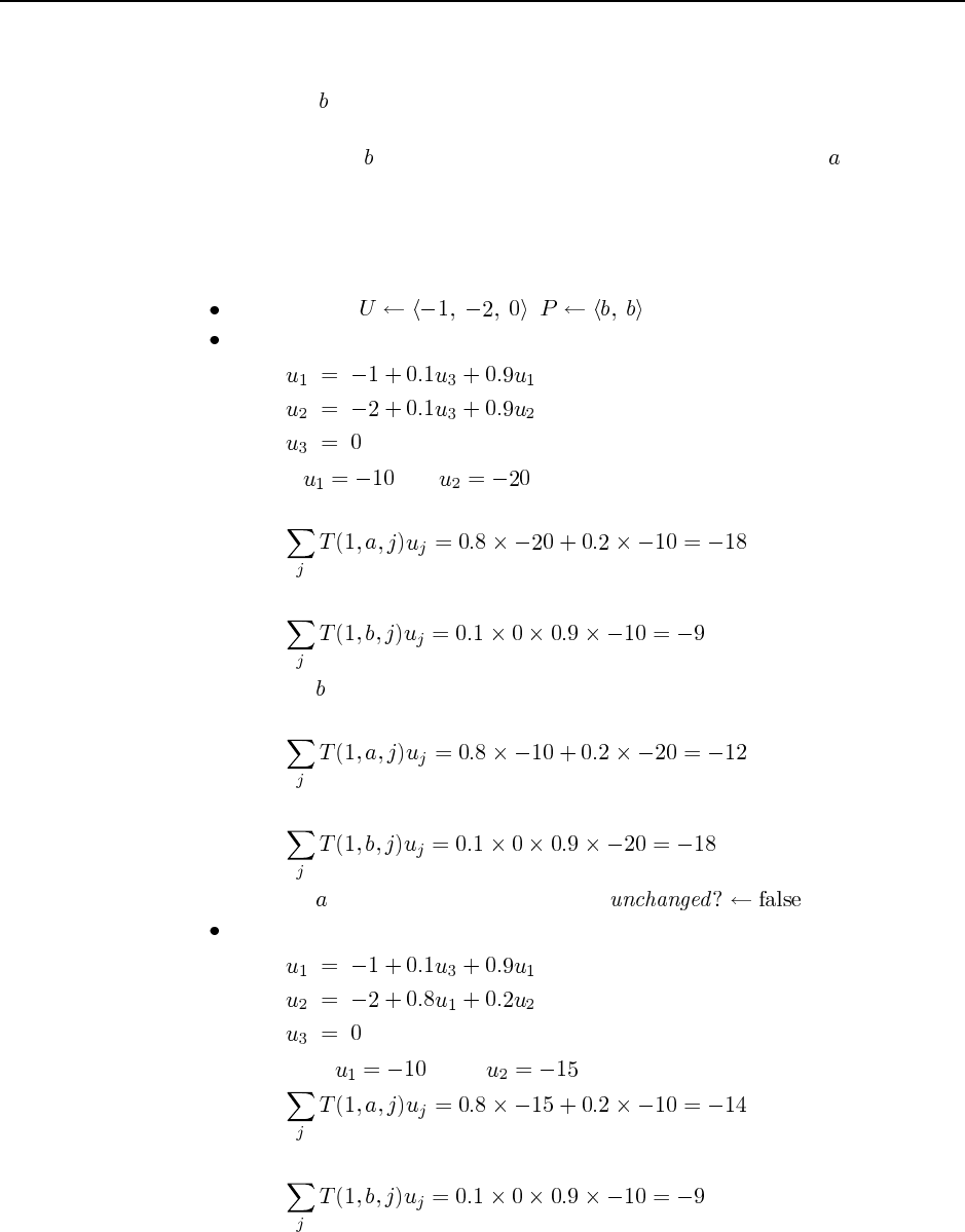
114 Chapter 17. Making Complex Decisions
a. Intuitively, the agent wants to get to state 3 as soon as possible, because it will pay a
cost for each time step it spends in states 1 and 2. However, the only action that reaches
state 3 (action ) succeeds with low probability, so the agent should minimize the cost
it incurs while trying to reach the terminal state. This suggests that the agent should
definitely try action in state 1; in state 2, it might be better to try action to get to state
1 (which is the better place to wait for admission to state 3), rather than aiming directly
for state 3. The decision in state 2 involves a numerical tradeoff.
b. The application of policy iteration proceeds in alternating steps of value determination
and policy update.
Initialization: , .
Value determination:
That is, and .
Policy update: In state 1,
while
so action is still preferred for state 1.
In state 2,
while
so action is preferred for state 1. We set and proceed.
Value determination:
Once more ; now, . Policy update: In state 1,
while
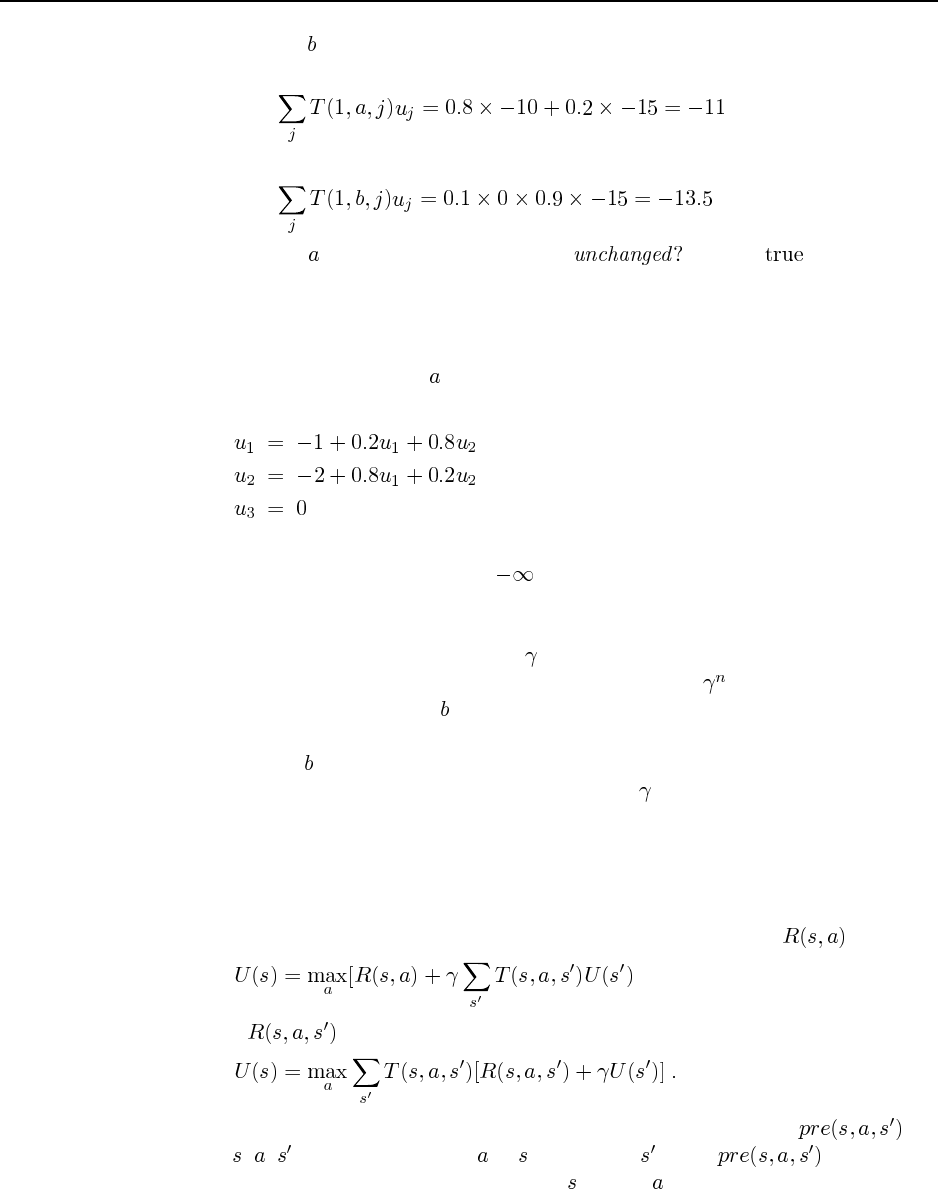
115
so action is still preferred for state 1.
In state 2,
while
so action is still preferred for state 1. remains , and we termi-
nate.
Note that the resulting policy matches our intuition: when in state 2, try to move to state
1, and when in state 1, try to move to state 3.
c. An initial policy with action in both states leads to an unsolvable problem. The initial
value determination problem has the form
and the first two equations are inconsistent. If we were to try to solve them iteratively,
we would find the values tending to .
Discounting leads to well-defined solutions by bounding the penalty (expected dis-
counted cost) an agent can incur at either state. However, the choice of discount factor
will affect the policy that results. For small, the cost incurred in the distant future
plays a negligible role in the value computation, because is near 0. As a result,
an agent could choose action in state 2 because the discounted short-term cost of re-
maining in the non-terminal states (states 1 and 2) outweighs the discounted long-term
cost of action failing repeatedly and leaving the agent in state 2. An additional exer-
cise could ask the student to determine the value of at which the agent is indifferent
between the two choices.
17.5 This is a deceptively simple exercise that tests the student’s understanding of the for-
mal definition of MDPs. Some students may need a hint or an example to get started.
a. The key here is to get the max and summation in the right place. For we have
and for we have
b. There are a variety of solutions here. One is to create a “pre-state” for
every , , , such that executing in leads not to but to . In this state
is encoded the fact that the agent came from and did to get here. From the pre-state,
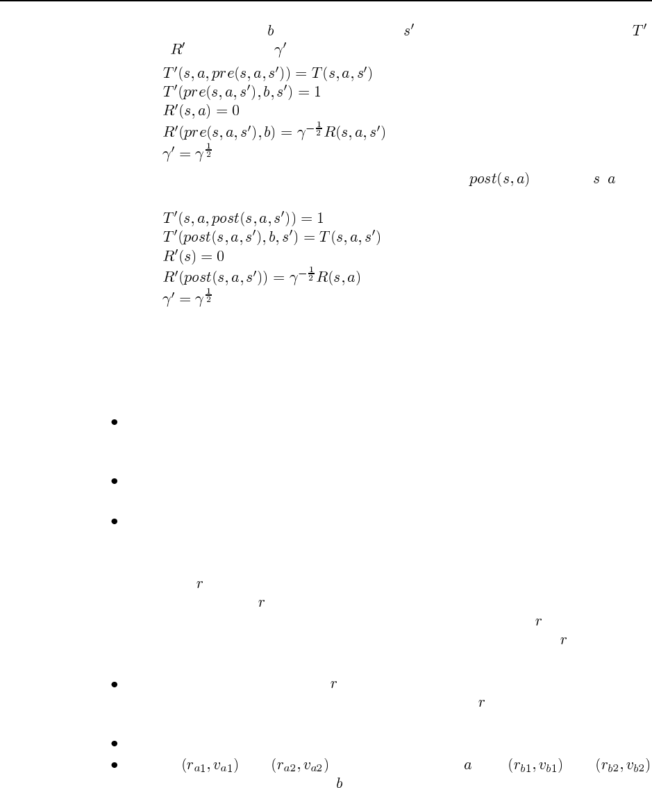
116 Chapter 17. Making Complex Decisions
there is just one action that always leads to . Let the new MDP have transition ,
reward , and discount . Then
c. In keeping with the idea of part (b), we can create states for every , , such
that
17.6 The framework for this problem is in "uncertainty/domains/4x3-mdp.lisp".
There is still some synthesis for the student to do for answer b. For c. some experimental de-
sign is necessary.
17.7 This can be done fairly simply by:
Call policy-iteration (from "uncertainty/algorithms/dp.lisp")on
the Markov Decision Processes representing the 4x3 grid, with values for the step cost
ranging from, say, 0.0 to 1.0 in increments of 0.02.
For any two adjacent policies that differ, run binary search on the step cost to pinpoint
the threshold value.
Convince yourself that you haven’t missed any policies, either by using too coarse an
increment in step size (0.02), or by stopping too soon (1.0).
One useful observation in this context is that the expected total reward of any fixed
policy is linear in , the per-step reward for the empty states. Imagine drawing the total reward
of a policy as a function of —a straight line. Now draw all the straight lines corresponding
to all possible policies. The reward of the optimal policy as a function of is just the max of
all these straight lines. Therefore it is a piecewise linear, convex function of . Hence there
is a very efficient way to find all the optimal policy regions:
For any two consecutive values of that have different optimal policies, find the optimal
policy for the midpoint. Once two consecutive values of give the same policy, then
the interval between the two points must be covered by that policy.
Repeat this until two points are known for each distinct optimal policy.
Suppose and are points for policy , and and
are the next two points, for policy . Clearly, we can draw straight lines through these
pairs of points and find their intersection. This does not mean, however, that there is no
other optimal policy for the intervening region. We can determine this by calculating

117
the optimal policy for the intersection point. If we get a different policy, we continue
the process.
The policies and boundaries derived from this procedure are shown in Figure S17.1. The
figure shows that there are nine distinct optimal policies! Notice that as becomes more
negative, the agent becomes more willing to dive straight into the –1 terminal state rather
than face the cost of the detour to the +1 state.
The somewhat ugly code is as follows. Notice that because the lines for neighboring
policies are very nearly parallel, numerical instability is a serious problem.
(defun policy-surface (mdp r1 r2 &aux prev (unchanged nil))
"returns points on the piecewise-linear surface
defined by the value of the optimal policy of mdp as a
function of r"
(setq rvplist
(list (cons r1 (r-policy mdp r1)) (cons r2 (r-policy mdp r2))))
(do ()
(unchanged rvplist)
(setq unchanged t)
(setq prev nil)
(dolist (rvp rvplist)
(let* ((rest (cdr (member rvp rvplist :test #’eq)))
(next (first rest))
(next-but-one (second rest)))
(dprint (list (first prev) (first rvp)
’* (first next) (first next-but-one)))
(when next
(unless (or (= (first rvp) (first next))
(policy-equal (third rvp) (third next) mdp))
(dprint "Adding new point(s)")
(setq unchanged nil)
(if (and prev next-but-one
(policy-equal (third prev) (third rvp) mdp)
(policy-equal (third next) (third next-but-one) mdp))
(let* ((intxy (policy-vertex prev rvp next next-but-one))
(int (cons (xy-x intxy) (r-policy mdp (xy-x intxy)))))
(dprint (list "Found intersection" intxy))
(cond ((or (< (first int) (first rvp))
(> (first int) (first next)))
(dprint "Intersection out of range!")
(let ((int-r (/ (+ (first rvp) (first next)) 2)))
(setq int (cons int-r (r-policy mdp int-r))))
(push int (cdr (member rvp rvplist :test #’eq))))
((or (policy-equal (third rvp) (third int) mdp)
(policy-equal (third next) (third int) mdp))
(dprint "Found policy boundary")
(push (list (first int) (second int) (third next))
(cdr (member rvp rvplist :test #’eq)))
(push (list (first int) (second int) (third rvp))
(cdr (member rvp rvplist :test #’eq))))
(t (dprint "Found new policy!")
(push int (cdr (member rvp rvplist :test #’eq))))))

118 Chapter 17. Making Complex Decisions
(let* ((int-r (/ (+ (first rvp) (first next)) 2))
(int (cons int-r (r-policy mdp int-r))))
(dprint (list "Adding split point" (list int-r (second int))))
(push int (cdr (member rvp rvplist :test #’eq))))))))
(setq prev rvp))))
(defun r-policy (mdp r &aux U)
(set-rewards mdp r)
(setq U (value-iteration mdp
(copy-hash-table (mdp-rewards mdp) #’identity)
:epsilon 0.0000000001))
(list (gethash ’(1 1) U) (optimal-policy U (mdp-model mdp) (mdp-rewards mdp))))
(defun set-rewards (mdp r &aux (rewards (mdp-rewards mdp))
(terminals (mdp-terminal-states mdp)))
(maphash #’(lambda (state reward)
(unless (member state terminals :test #’equal)
(setf (gethash state rewards) r)))
rewards))
(defun policy-equal (p1 p2 mdp &aux (match t)
(terminals (mdp-terminal-states mdp)))
(maphash #’(lambda (state action)
(unless (member state terminals :test #’equal)
(unless (eq (caar (gethash state p1)) (caar (gethash state p2)))
(setq match nil))))
p1)
match)
(defun policy-vertex (rvp1 rvp2 rvp3 rvp4)
(let ((a (make-xy :x (first rvp1) :y (second rvp1)))
(b (make-xy :x (first rvp2) :y (second rvp2)))
(c (make-xy :x (first rvp3) :y (second rvp3)))
(d (make-xy :x (first rvp4) :y (second rvp4))))
(intersection-point (make-line :xy1 a :xy2 b)
(make-line :xy1 c :xy2 d))))
(defun intersection-point (l1 l2)
;;; l1 is line ab; l2 is line cd
;;; assume the lines cross at alpha a + (1-alpha) b,
;;; also known as beta c + (1-beta) d
;;; returns the intersection point unless they’re parallel
(let* ((a (line-xy1 l1))
(b (line-xy2 l1))
(c (line-xy1 l2))
(d (line-xy2 l2))
(xa (xy-x a)) (ya (xy-y a))
(xb (xy-x b)) (yb (xy-y b))
(xc (xy-x c)) (yc (xy-y c))
(xd (xy-x d)) (yd (xy-y d))
(q (- (* (- xa xb) (- yc yd))
(* (- ya yb) (- xc xd)))))
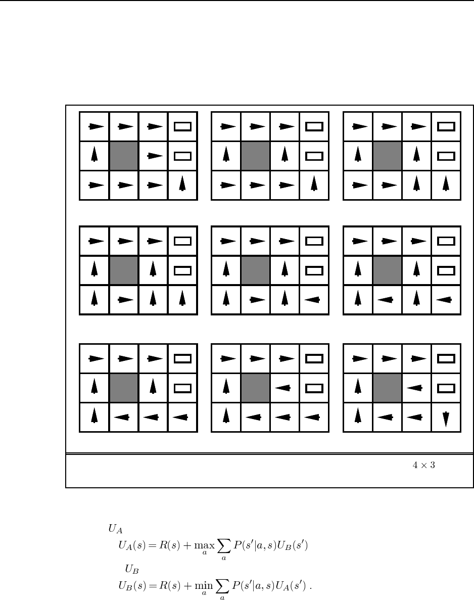
119
(unless (zerop q)
(let ((alpha (/ (- (* (- xd xb) (- yc yd))
(* (- yd yb) (- xc xd)))
q)))
(make-xy :x (float (+ (* alpha xa) (* (- 1 alpha) xb)))
:y (float (+ (* alpha ya) (* (- 1 alpha) yb))))))))
− 1
+ 1
− 1
+ 1
− 1
+ 1
− 1
+ 1
− 1
+ 1
− 1
+ 1
− 1
+ 1
− 1
+ 1
− 1
+ 1
r = [−1.6284 : −1.3702] r = [−1.3702 : −0.7083]
r = [−0.7083 : −0.4278] r = [−0.4278 : −0.0850] r = [−0.0850 : −0.0480]
r = [−0.0480 : −0.0274] r = [−0.0274 : −0.0218] r = [−0.0218 : 0.0000]
r = [− : −1.6284]
8
Figure S17.1 Optimal policies for different values of the cost of a step in the envi-
ronment, and the boundaries of the regions with constant optimal policy.
17.8
a. For we have
and for we have
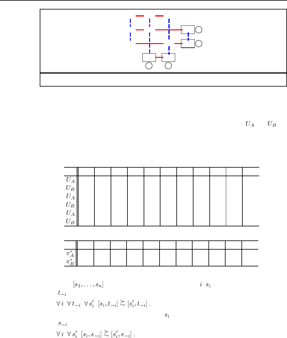
120 Chapter 17. Making Complex Decisions
(1,4)
(1,3)
(1,2)
(2,4)
(2,3)
(2,1)
(3,4)
(3,2)
(3,1)
(4,3)
(4,2)
−1 −1
+1
+1
Figure S17.2 State-space graph for the game on page 190 (for Ex. 17.8).
b. To do value iteration, we simply turn each equation from part (a) into a Bellman update
and apply them in alternation, applying each to all states simultaneously. The process
terminates when the utility vector for one player is the same as the previous utility
vector for the same player (i.e., two steps earlier). (Note that typically and are
not the same in equilibrium.)
c. The state space is shown in Figure S17.2.
d. We mark the terminal state values in bold and initialize other values to 0. Value iteration
proceeds as follows:
(1,4) (2,4) (3,4) (1,3) (2,3) (4,3) (1,2) (3,2) (4,2) (2,1) (3,1)
00000+1 0 0 +1 –1 –1
0 0 0 0 –1 +1 0 –1 +1 –1 –1
0 0 0 –1 +1 +1 –1 +1 +1 –1 –1
–1 +1 +1 –1 –1 +1 –1 –1 +1 –1 –1
+1 +1 +1 –1 +1 +1 –1 +1 +1 –1 –1
–1 +1 +1 –1 –1 +1 –1 –1 +1 –1 –1
and the optimal policy for each player is as follows:
(1,4) (2,4) (3,4) (1,3) (2,3) (4,3) (1,2) (3,2) (4,2) (2,1) (3,1)
(2,4) (3,4) (2,4) (2,3) (4,3) (3,2) (4,2)
(1,3) (2,3) (3,2) (1,2) (2,1) (1,3) (3,1)
17.9 This question is simple a matter of examining the definitions. In a dominant strategy
equilibrium , it is the case that for every player , is optimal for every combi-
nation by the other players:
In a Nash equilibrium, we simply require that is optimal for the particular current combi-
nation by the other players:
Therefore, dominant strategy equilibrium is a special case of Nash equilibrium. The converse
does not hold, as we can show simply by pointing to the CD/DVD game, where neither of the
Nash equilibria is a dominant strategy equilibrium.
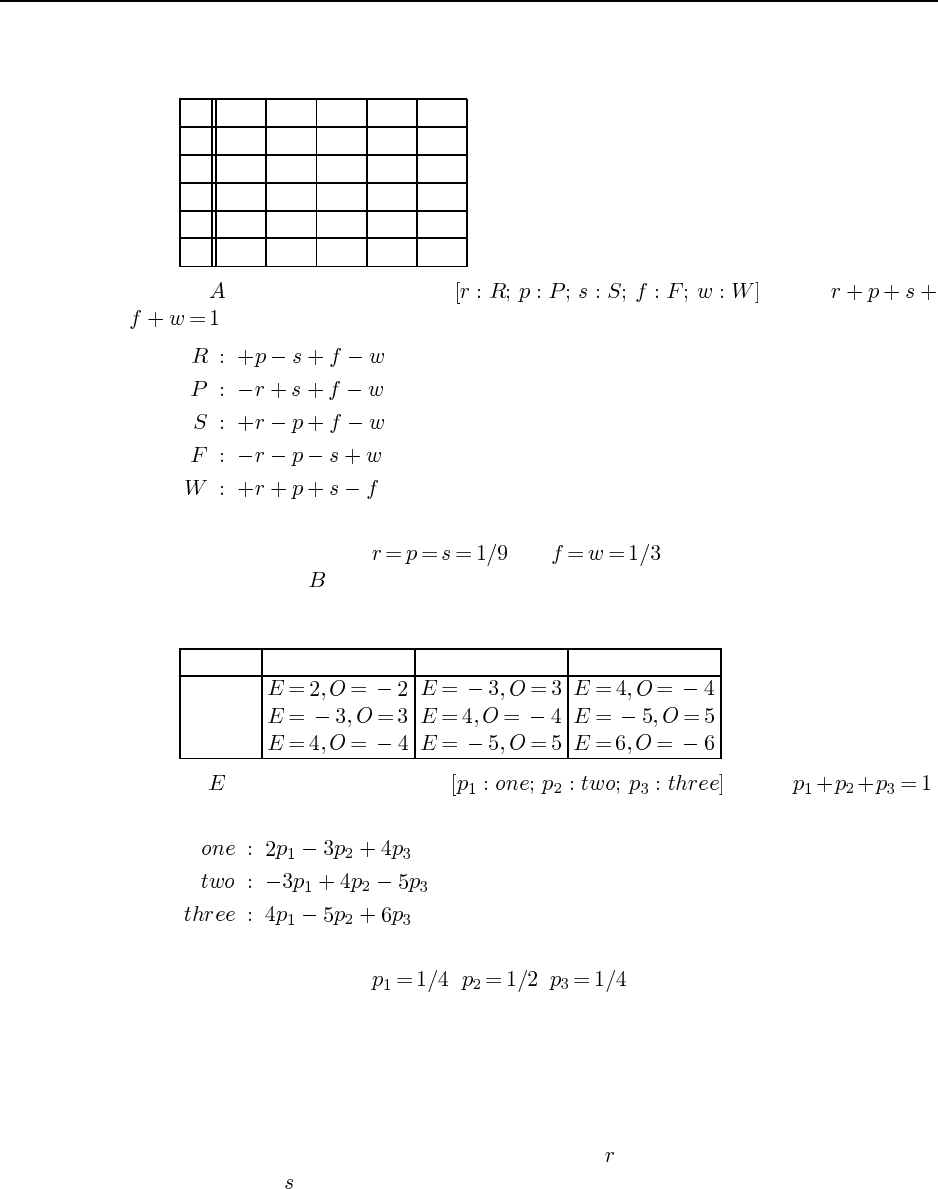
121
17.10 In the following table, the rows are labelled by A’s move and the columns by B’s
move, and the table entries list the payoffs to A and B respectively.
R P S F W
R 0,0 –1,1 1,-1 –1,1 1,-1
P 1,-1 0,0 –1,1 –1,1 1,-1
S –1,1 1,-1 0,0 –1,1 1,-1
F 1,-1 1,-1 1,-1 0,0 –1,1
W –1,1 –1,1 –1,1 1,-1 0,0
Suppose chooses a mixed strategy , where
. The payoff to A of B’s possible pure responses are as follows:
It is easy to see that no option is dominated over the whole region. Solving for the intersection
of the hyperplanes, we find and . By symmetry, we will find the
same solution when chooses a mixed strategy first.
17.11 The payoff matrix for three-finger Morra is as follows:
O: one O: two O: three
E: one
E: two
E: three
Suppose chooses a mixed strategy , where .
The payoff to E of O’s possible pure responses are as follows:
It is easy to see that no option is dominated over the whole region. Solving for the intersection
of the hyperplanes, we find . , . The expected value is 0.
17.12 Every game is either a win for one side (and a loss for the other) or a tie. With 2 for a
win, 1 for a tie, and 0 for a loss, 2 points are awarded for every game, so this is a constant-sum
game.
If 1 point is awarded for a loss in overtime, then for some games 3 points are awarded
in all. Therefore, the game is no longer constant-sum.
Suppose we assume that team A has probability of winning in regular time and team
B has probability of winning in regular time (assuming normal play). Furthermore, assume
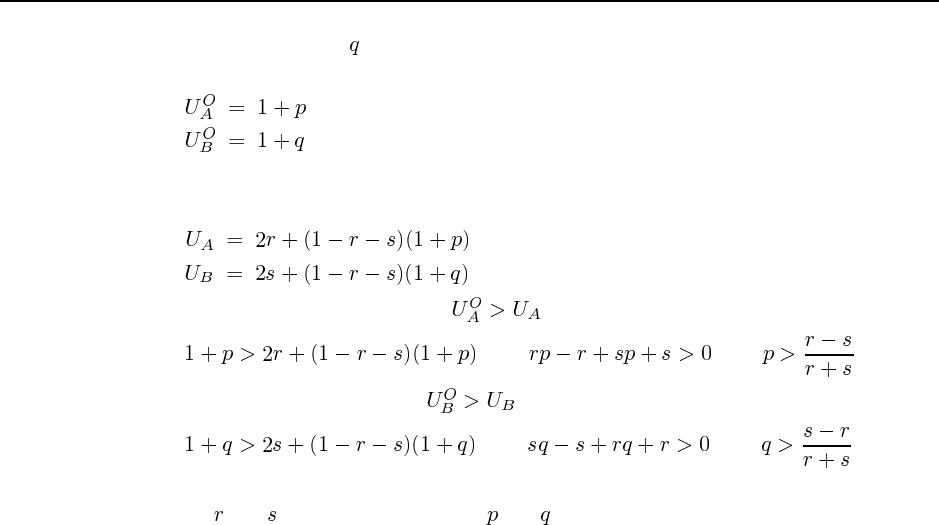
122 Chapter 17. Making Complex Decisions
team B has a probability of winning in overtime (which occurs if there is a tie after regular
time). Once overtime is reached (by any means), the expected utilities are as follows:
In normal play, the expected utilities are derived from the probability of winning plus the
probability of tying times the expected utility of overtime play:
Hence A has an incentive to agree if , or
or or
and B has an incentive to agree if , or
or or
When both of these inequalities hold, there is an incentive to tie in regulation play. For any
values of and , there will be values of and such that both inequalities hold.
For an in-depth statistical analysis of the actual effects of the rule change and a more
sophisticated treatment of the utility functions, see “Overtime! Rules and Incentives in the
National Hockey League” by Stephen T. Easton and Duane W. Rockerbie, available at
http://people.uleth.ca/˜rockerbie/OVERTIME.PDF.
17.13 We apply iterated strict dominance to find the pure strategy. First, Pol: do nothing
dominates Pol: contract, so we drop the Pol: contract row. Next, Fed: contract dominates
Fed: do nothing and Fed: expand on the remaining rows, so we drop those columns. Finally,
Pol: expand dominates Pol: do nothing on the one remaining column. Hence the only Nash
equilibrium is a dominant strategy equilibrium with Pol: expand and Fed: contract. This is
not Pareto optimal: it is worse for both players than the four strategy profiles in the top right
quadrant.

Solutions for Chapter 18
Learning from Observations
18.1 The aim here is to couch language learning in the framework of the chapter, not to
solve the problem! This is a very interesting topic for class discussion, raising issues of
nature vs. nurture, the indeterminacy of meaning and reference, and so on. Basic references
include Chomsky (1957) and Quine (1960).
The first step is to appreciate the variety of knowledge that goes under the heading
“language.” The infant must learn to recognize and produce speech, learn vocabulary, learn
grammar, learn the semantic and pragmatic interpretation of a speech act, and learn strategies
for disambiguation, among other things. The performance elements for this (in humans) and
their associated learning mechanisms are obviously very complex and as yet little is known
about them.
A naive model of the learning environment considers just the exchange of speech sounds.
In reality, the physical context of each utterance is crucial: a child must see the context in
which “watermelon” is uttered in order to learn to associate “watermelon” with watermel-
ons. Thus, the environment consists not just of other humans but also the physical objects
and events about which discourse takes place. Auditory sensors detect speech sounds, while
other senses (primarily visual) provide information on the physical context. The relevant
effectors are the speech organs and the motor capacities that allow the infant to respond to
speech or that elicit verbal feedback.
The performance standard could simply be the infant’s general utility function, however
that is realized, so that the infant performs reinforcement learning to perform and respond to
speech acts so as to improve its well-being—for example, by obtaining food and attention.
However, humans’ built-in capacity for mimicry suggests that the production of sounds sim-
ilar to those produced by other humans is a goal in itself. The child (once he or she learns to
differentiate sounds and learn about pointing or other means of indicating salient objects) is
also exposed to examples of supervised learning: an adult says “shoe” or “belly button” while
indicating the appropriate object. So sentences produced by adults provide labelled positive
examples, and the response of adults to the infant’s speech acts provides further classification
feedback.
Mostly, it seems that adults do not correct the child’s speech, so there are very few neg-
ative classifications of the child’s attempted sentences. This is significant because early work
on language learning (such as the work of Gold, 1967) concentrated just on identifying the
set of strings that are grammatical, assuming a particular grammatical formalism. If there are
123

124 Chapter 18. Learning from Observations
only positive examples, then there is nothing to rule out the grammar . Some
theorists (notably Chomsky and Fodor) used what they call the “poverty of the stimulus” argu-
ment to say that the basic universal grammar of languages must be innate, because otherwise
(given the lack of negative examples) there would be no way that a child could learn a lan-
guage (under the assumptions of language learning as learning a set of grammatical strings).
Critics have called this the “poverty of the imagination” argument—I can’t think of a learning
mechanism that would work, so it must be innate. Indeed, if we go to probabilistic context
free grammars, then it is possible to learn a language without negative examples.
18.2 Learning tennis is much simpler than learning to speak. The requisite skills can be
divided into movement, playing strokes, and strategy. The environment consists of the court,
ball, opponent, and one’s own body. The relevant sensors are the visual system and propri-
oception (the sense of forces on and position of one’s own body parts). The effectors are
the muscles involved in moving to the ball and hitting the stroke. The learning process in-
volves both supervised learning and reinforcement learning. Supervised learning occurs in
acquiring the predictive transition models, e.g., where the opponent will hit the ball, where
the ball will land, and what trajectory the ball will have after one’s own stroke (e.g., if I hit
a half-volley this way, it goes into the net, but if I hit it that way, it clears the net). Rein-
forcement learning occurs when points are won and lost—this is particularly important for
strategic aspects of play such as shot placement and positioning (e.g., in 60% of the points
where I hit a lob in response to a cross-court shot, I end up losing the point). In the early
stages, reinforcement also occurs when a shot succeeds in clearing the net and landing in the
opponent’s court. Achieving this small success is itself a sequential process involving many
motor control commands, and there is no teacher available to tell the learner’s motor cortex
which motor control commands to issue.
18.3 This is a deceptively simple question, designed to point out the plethora of “excep-
tions” in real-world situations and the way in which decision trees capture a hierarchy of
exceptions. One possible tree is shown in Figure S18.1. One can, of course, imagine many
more exceptions. The qualification problem, defined originally for action models, applies a
fortiori to condition–action rules.
18.4 In standard decision trees, attribute tests divide examples according to the attribute
value. Therefore any example reaching the second test already has a known value for the
attribute and the second test is redundant. In some decision tree systems, however, all tests
are Boolean even if the attributes are multivalued or continuous. In this case, additional tests
of the attribute can be used to check different values or subdivide the range further (e.g., first
check if , and then if it is, check if ).
18.5 The algorithm may not return the “correct” tree, but it will return a tree that is logi-
cally equivalent, assuming that the method for generating examples eventually generates all
possible combinations of input attributes. This is true because any two decision tree defined
on the same set of attributes that agree on all possible examples are, by definition, logically
equivalent. The actually form of the tree may differ because there are many different ways to
represent the same function. (For example, with two attributes and we can have one tree
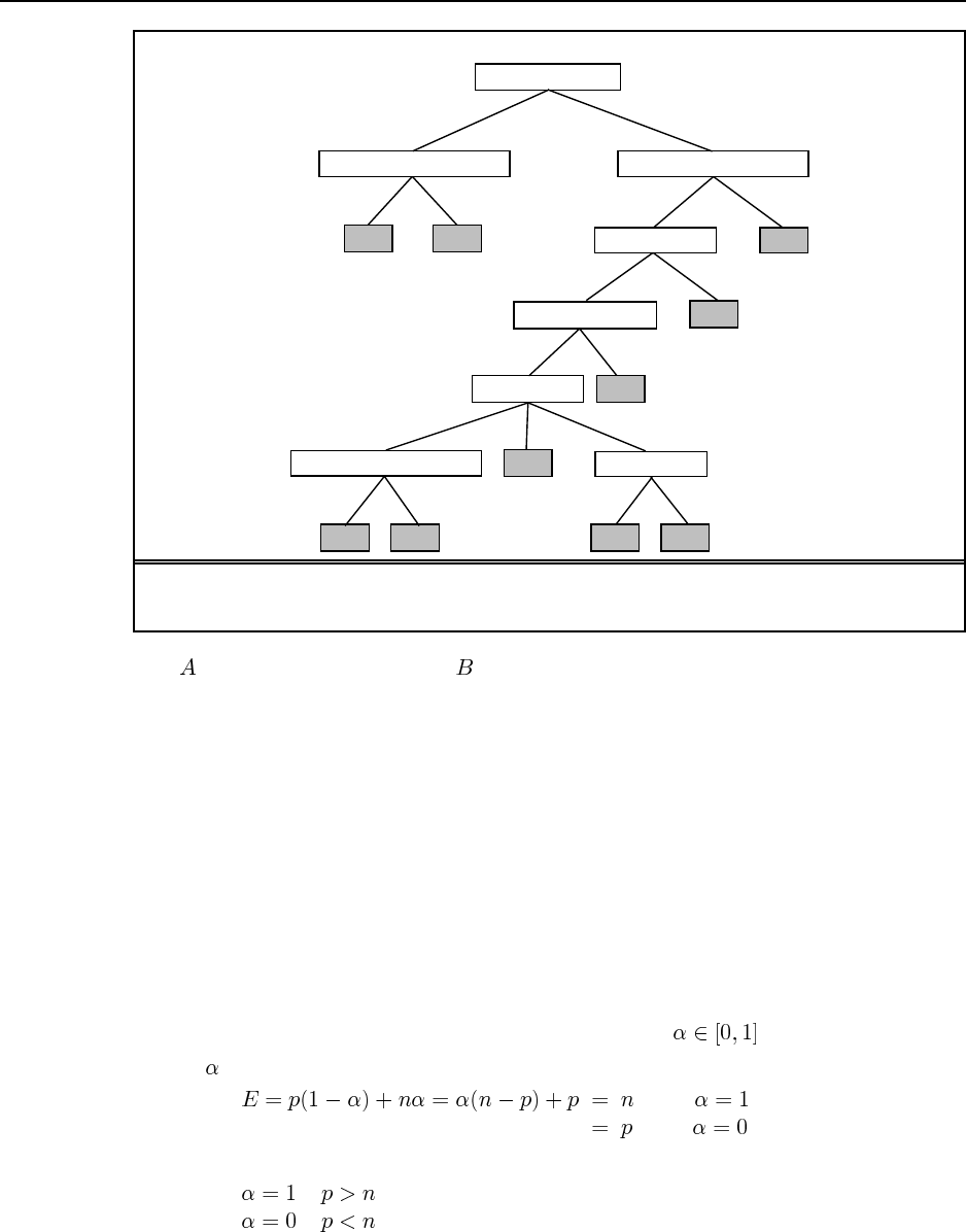
125
No Yes
No Yes
No Yes
No
NoYes
No
Yes
No Yes
FrontOfQueue?
IntersectionBlocked?CarAheadMoving?
No Yes
No Yes
No Yes
CrossTraffic?
Pedestrians?
NoTurning?
No RightLeft
OncomingTraffic? Cyclist?
No Yes
NoYes
Figure S18.1 A decision tree for deciding whether to move forward at a traffic intersec-
tion, given a green light.
with at the root and another with at the root.) The root attribute of the original tree may
not in fact be the one that will be chosen by the information gain geuristic when applied to
the training examples.
18.6 This is an easy algorithm to implement. The main point is to have something to test
other learning algorithms against, and to learn the basics of what a learning algorithm is in
terms of inputs and outputs given the framework provided by the code repository.
18.7 If we leave out an example of one class, then the majority of the remaining examples
are of the other class, so the majority classifier will always predict the wrong answer.
18.8 This question brings a little bit of mathematics to bear on the analysis of the learning
problem, preparing the ground for Chapter 20. Error minimization is a basic technique in
both statistics and neural nets. The main thing is to see that the error on a given training
set can be written as a mathematical expression and viewed as a function of the hypothesis
chosen. Here, the hypothesis in question is a single number returned at the leaf.
a. If is returned, the absolute error is
when
when
This is minimized by setting
if
if
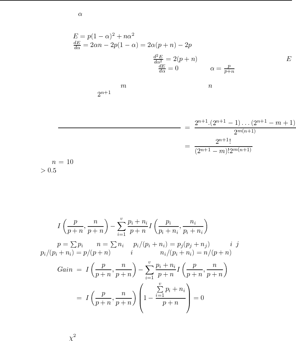
126 Chapter 18. Learning from Observations
That is, is the majority value.
b. First calculate the sum of squared errors, and its derivative:
The fact that the second derivative, , is greater than zero means that
is minimized (not maximized) where , i.e., when .
18.9 Suppose that we draw examples. Each example has input features plus its classi-
fication, so there are distinct input/output examples to choose from. For each example,
there is exactly one contradictory example, namely the example with the same input features
but the opposite classification. Thus, the probability of finding no contradiction is
number of sequences of mnon-contradictory examples
number of sequences of mexamples
For , with 2048 possible examples, a contradiction becomes likely with probability
after 54 examples have been drawn.
18.10 This result emphasizes the fact that any statistical fluctuations caused by the random
sampling process will result in an apparent information gain.
The easy part is showing that the gain is zero when each subset has the same ratio of
positive examples. The gain is defined as
Since and , if for all , then we must have
for all , and also . From this, we obtain
18.11 This is a fairly small, straightforward programming exercise. The only hard part is
the actual computation; you might want to provide your students with a library function
to do this.
18.12 This is another straightforward programming exercise. The follow-up exercise is to
run tests to see if the modified algorithm actually does better.
127
18.13 Let the prior probabilities of each attribute value be . (These prob-
abilities are estimated by the empirical fractions among the examples at the current node.)
From page 540, the intrinsic information content of the attribute is
Given this formula and the empirical estimates of , the modification to the code is
straightforward.
18.14
18.15 Note: this is the only exercise to cover the material in section 18.6. Although the
basic ideas of computational learning theory are both important and elegant, it is not easy to
find good exercises that are suitable for an AI class as opposed to a theory class. If you are
teaching a graduate class, or an undergraduate class with a strong emphasis on learning, it
might be a good idea to use some of the exercises from Kearns and Vazirani (1994).
a. If each test is an arbitrary conjunction of literals, then a decision list can represent
an arbitrary DNF (disjunctive normal form) formula directly. The DNF expression
, where is a conjunction of literals, can be represented by a
decision list in which is the th test and returns if successful. That is:
Since any Boolean function can be written as a DNF formula, then any Boolean function
can be represented by a decision list.
b. A decision tree of depth can be translated into a decision list whose tests have at most
literals simply by encoding each path as a test. The test returns the corresponding leaf
value if it succeeds. Since the decision tree has depth , no path contains more than
literals.
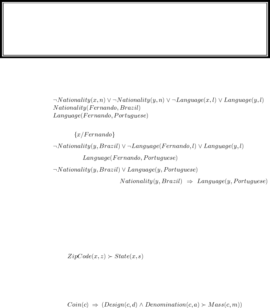
Solutions for Chapter 19
Knowledge in Learning
19.1 In CNF, the premises are as follows:
We can prove the desired conclusion directly rather than by refutation. Resolve the first two
premises with to obtain
Resolve this with to obtain
which is the desired conclusion .
19.2 This question is tricky in places. It is important to see the distinction between the
shared and unshared variables on the LHS and RHS of the determination. The shared vari-
ables will be instantiated to the objects to be compared in an analogical inference, while the
unshared variables are instantiated with the objects’ observed and inferred properties.
a. Here we are talking about the zip codes and states of houses (or addresses or towns). If
two houses/addresses/towns have the same zip code, they are in the same state:
The determination is true because the US Postal Service never draws zipcode bound-
aries across state lines (perhaps for some reason having to do with interstate commerce).
b. Here the objects being reasoned about are coins, and design, denomination, and mass
are properties of coins. So we have
This is (very nearly exactly) true because coins of a given denomination and design are
stamped from the same original die using the same material; size and shape determine
volume; and volume and material determine mass.
128
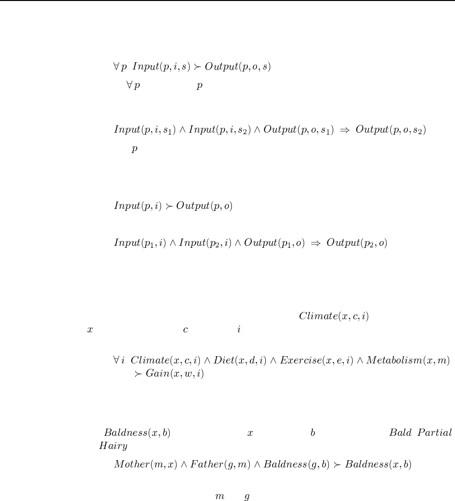
129
c. Here we have to be careful. The objects being reasoned about are not programs but
runs of a given program. (This determination is also one often forgotten by novice
programmers.) We can use situation calculus to refer to the runs:
Here the captures the variable so that it does not participate in the determination
as one of the shared or unshared variables. The situation is the shared variable. The
determination expands out to the following Horn clause:
That is, if has the same input in two different situations it will have the same output
in those situations. This is generally true because computers operate on programs and
inputs deterministically; however, it is important that “input” include the entire state of
the computer’s memory, file system, and so on. Notice that the “naive” choice
expands out to
which says that if any two programs have the same input they produce the same output!
d. Here the objects being reasoned are people in specific time intervals. (The intervals
could be the same in each case, or different but of the same kind such as days, weeks,
etc. We will stick to the same interval for simplicity. As above, we need to quantify the
interval to “precapture” the variable.) We will use to mean that person
experiences climate in interval , and we will assume for the sake of variety that a
person’s metabolism is constant.
While the determinations seems plausible, it leaves out such factors as water intake,
clothing, disease, etc. The qualification problem arises with determinations just as with
implications.
e. Let mean that person has baldness (which might be , ,
or , say). A first stab at the determination might be
but this would only allow an inference when two people have the same mother and ma-
ternal grandfather because the and are the unshared variables on the LHS. Also, the
RHS has no unshared variable. Notice that the determination does not say specifically
that baldness is inherited without modification; it allows, for example, for a hypothet-
ical world in which the maternal grandchildren of a bald man are all hairy, or vice
versa. This might not seem particularly natural, but consider other determinations such
as “Whether or not I file a tax return determines whether or not my spouse must file a
tax return.”
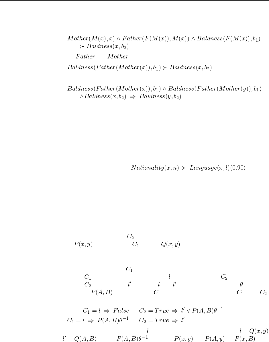
130 Chapter 19. Knowledge in Learning
The baldness of the maternal grandfather is the relevant value for prediction, so that
should be the unshared variable on the LHS. The mother and maternal grandfather are
designated by skolem functions:
If we use and as function symbols, then the meaning becomes clearer:
Just to check, this expands into
which has the intended meaning.
19.3 Because of the qualification problem, it is not usually possible in most real-world
applications to list on the LHS of a determination all the relevant factors that determine
the RHS. Determinations will usually therefore be true to an extent—that is, if two objects
agree on the LHS there is some probability (preferably greater than the prior) that the two
objects will agree on the RHS. An appropriate definition for probabilistic determinations
simply includes this conditional probability of matching on the RHS given a match on the
LHS. For example, we could define to mean
that if two people have the same nationality, then there is a 90% chance that they have the
same language.
19.4 This exercise test the student’s understanding of resolution and unification, as well as
stressing the nondeterminism of the inverse resolution process. It should help a lot in making
the inverse resolution operation less mysterious and more amenable to mathematical analysis.
It is helpful first to draw out the resolution “V” when doing these problems, and then to do a
careful case analysis.
a. There is no possible value for here. The resolution step would have to resolve away
both the on the LHS of and the on the right, which is not possible.
(Resolution can remove more than one literal from a clause, but only if those literals
are redundant—i.e., one subsumes the other.)
b. Without loss of generality, let contain the negative (LHS) literal to be resolved away.
The LHS of therefore contains one literal , while the LHS of must be empty.
The RHS of must contain such that and unify with some unifier . Now we
have a choice: on the RHS of could come from the RHS of or of .
Thus the two basic solution templates are
;
;
Within these templates, the choice of is entirely unconstrained. Suppose is
and is . Then could be (or or ) and
131
the solutions are
;
;
c. As before, let contain the negative (LHS) literal to be resolved away, with on the
RHS of . We now have four possible templates because each of the two literals in
could have come from either or :
;
;
;
;
Again, we have a fairly free choice for . However, since contains and , cannot
bind those variables (else they would not appear in ). Thus, if is , then
must be also and will be empty.
19.5 We will assume that Prolog is the logic programming language. It is certainly true that
any solution returned by the call to will be a correct inverse resolvent. Unfortunately,
it is quite possible that the call will fail to return because of Prolog’s depth-first search. If
the clauses in and are infelicitously arranged, the proof tree might go down
the branch corresponding to indefinitely nested function symbols in the solution and never
return. This can be alleviated by redesigning the Prolog inference engine so that it works
using breadth-first search or iterative deepening, although the infinitely deep branches will
still be a problem. Note that any cuts used in the Prolog program will also be a problem for
the inverse resolution.
19.6 This exercise gives some idea of the rather large branching factor facing top-down ILP
systems.
a. It is important to note that position is significant— is very different from
! The first argument position can contain one of the five existing variables
or a new variable. For each of these six choices, the second position can contain one of
the five existing variables or a new variable, except that the literal with two new vari-
ables is disallowed. Hence there are 35 choices. With negated literals too, the total
branching factor is 70.
b. This seems to be quite a tricky combinatorial problem. The easiest way to solve it
seems to be to start by including the multiple possibilities that are equivalent under
renaming of the new variables as well as those that contain only new variables. Then
these redundant or illegal choices can be removed later. Now, we can use up to
new variables. If we use new variables, we can write literals, so using
exactly variables we can write literals. Each of these
is functionally isomorphic under any renaming of the new variables. With variables,
132 Chapter 19. Knowledge in Learning
there are are renamings. Hence the total number of distinct literals (including those
illegal ones with no old variables) is
Now we just subtract off the number of distinct all-new literals. With new variables,
the number of (not necessarily distinct) all-new literals is , so the number with exactly
is . Each of these has equivalent literals in the set. This gives us
the final total for distinct, legal literals:
which can doubtless be simplified. One can check that for and this gives
35.
c. If a literal contains only new variables, then either a subsequent literal in the clause
body connects one or more of those variables to one or more of the “old” variables,
or it doesn’t. If it does, then the same clause will be generated with those two literals
reversed, such that the restriction is not violated. If it doesn’t, then the literal is either
always true (if the predicate is satisfiable) or always false (if it is unsatisfiable), inde-
pendent of the “input” variables in the head. Thus, the literal would either be redundant
or would render the clause body equivalent to .
19.7 FOIL is available on the web at http://www-2.cs.cmu.edu/afs/cs/project/ai-repository-
/ai/areas/learning/systems/foil/0.html (and possibly other places). It is worthwhile to experi-
ment with it.
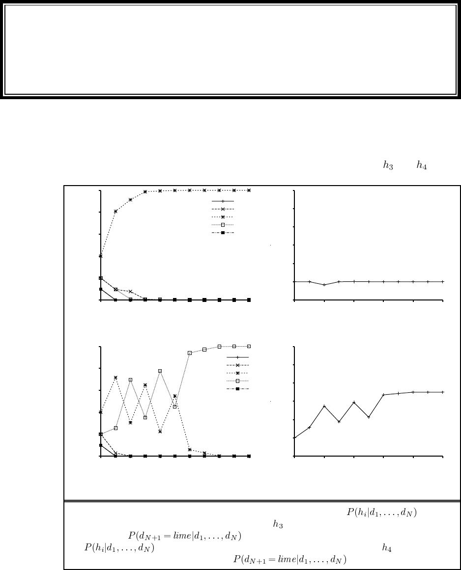
Solutions for Chapter 20
Statistical Learning Methods
20.1 The code for this exercise is a straightforward implementation of Equations 20.1 and
20.2. Figure S20.1 shows the results for data sequences generated from and . (Plots
0
0.2
0.4
0.6
0.8
1
0 20 40 60 80 100
Posterior probability of hypothesis
Number of samples in d
P(h1 | d)
P(h2 | d)
P(h3 | d)
P(h4 | d)
P(h5 | d)
0.4
0.5
0.6
0.7
0.8
0.9
1
0 20 40 60 80 100
Probability that next candy is lime
Number of samples in d
(a) (b)
0
0.2
0.4
0.6
0.8
1
0 20 40 60 80 100
Posterior probability of hypothesis
Number of samples in d
P(h1 | d)
P(h2 | d)
P(h3 | d)
P(h4 | d)
P(h5 | d)
0.4
0.5
0.6
0.7
0.8
0.9
1
0 20 40 60 80 100
Probability that next candy is lime
Number of samples in d
(c) (d)
Figure S20.1 Graphs for Ex. 20.1. (a) Posterior probabilities over a
sample sequence of length 100 generated from (50% cherry + 50% lime). (b) Bayesian
prediction given the data in (a). (c) Posterior probabilities
over a sample sequence of length 100 generated from (25% cherry
+ 75% lime). (d) Bayesian prediction given the data in (c).
133
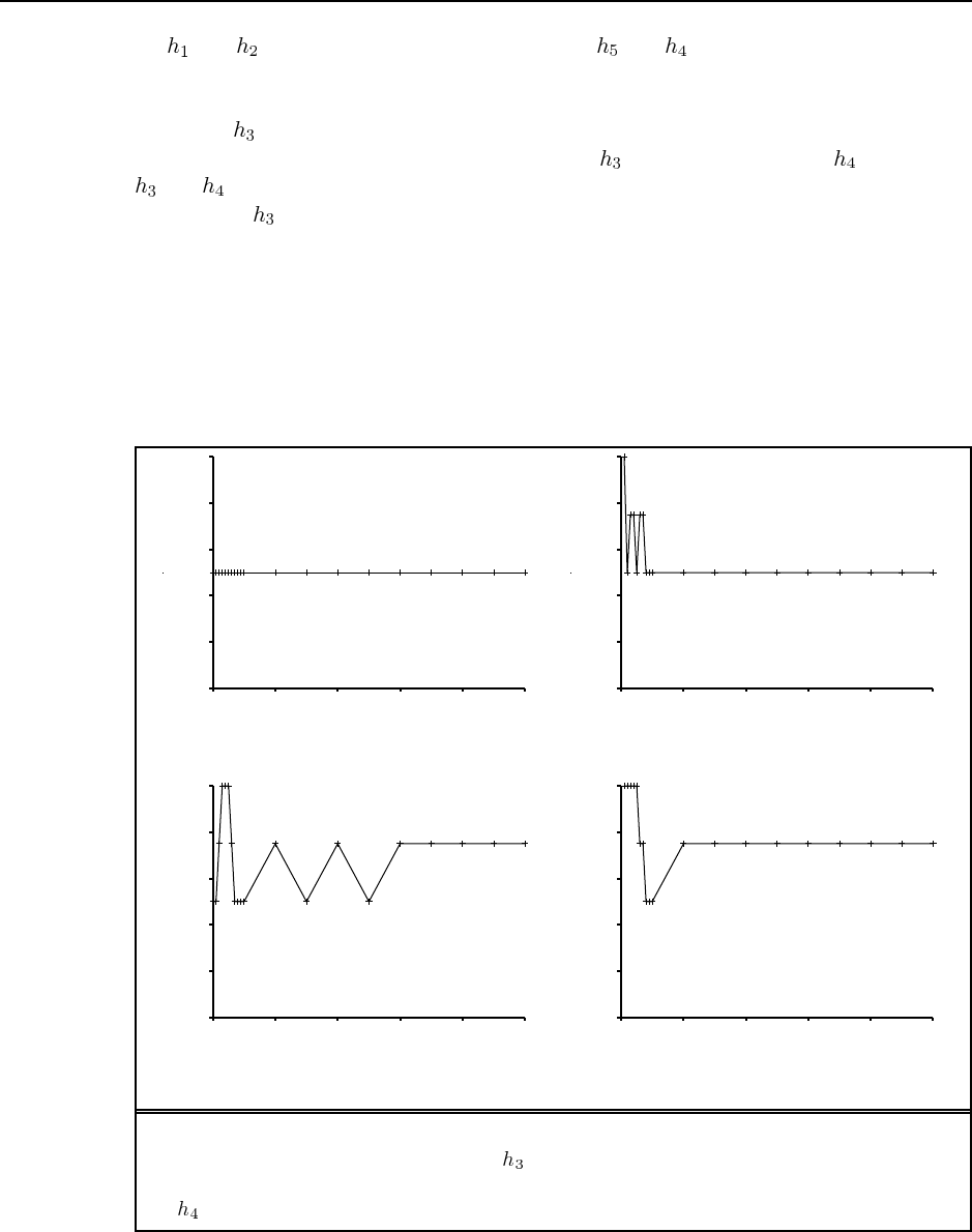
134 Chapter 20. Statistical Learning Methods
for and are essentially identical to those for and .) Results obtained by students
may vary because the data sequences are generated randomly from the specified candy dis-
tribution. In (a), the samples very closely reflect the true probabilities and the hypotheses
other than are effectively ruled out very quickly. In (c), the early sample proportions are
somewhere between 50/50 and 25/75; furthermore, has a higher prior than . As a result,
and vie for supremacy. Between 50 and 60 samples, a preponderance of limes ensures
the defeat of and the prediction quickly converges to 0.75.
20.2 Typical plots are shown in Figure S20.2. Because both MAP and ML choose exactly
one hypothesis for predictions, the prediction probabilities are all 0.0, 0.25, 0.5, 0.75, or 1.0.
For small data sets the ML prediction in particular shows very large variance.
20.3 This is a nontrivial sequential decision problem, but can be solved using the tools
developed in the book. It leads into general issues of statistical decision theory, stopping
rules, etc. Here, we sketch the “straightforward” solution.
0
0.2
0.4
0.6
0.8
1
0 20 40 60 80 100
Probability that next candy is lime
Number of samples in d
0
0.2
0.4
0.6
0.8
1
0 20 40 60 80 100
Probability that next candy is lime
Number of samples in d
(a) (b)
0
0.2
0.4
0.6
0.8
1
0 20 40 60 80 100
Probability that next candy is lime
Number of samples in d
0
0.2
0.4
0.6
0.8
1
0 20 40 60 80 100
Probability that next candy is lime
Number of samples in d
(c) (d)
Figure S20.2 Graphs for Ex. 20.2. (a) Prediction from the MAP hypothesis given a sample
sequence of length 100 generated from (50% cherry + 50% lime). (b) Prediction from the
ML hypothesis given the data in (a). (c) Prediction from the MAP hypothesis given data from
(25% cherry + 75% lime). (d) Prediction from the ML hypothesis given the data in (c).
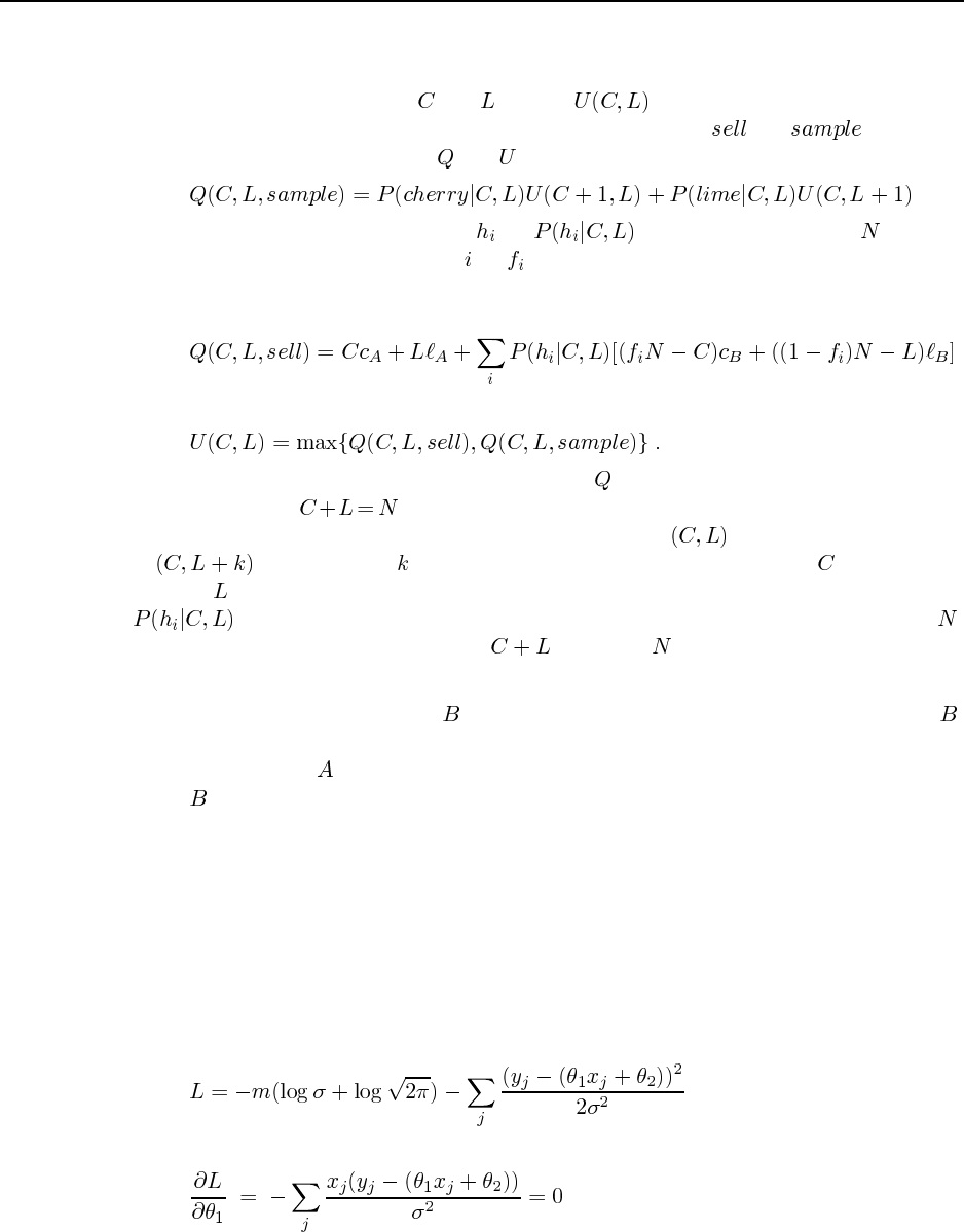
135
We can think of this problem as a simplified form of POMDP (see Chapter 17). The
“belief states” are defined by the numbers of cherry and lime candies observed so far in the
sampling process. Let these be and , and let be the utility of the corresponding
belief state. In any given state, there are two possible decisions: and . There is a
simple Bellman equation relating and for the sampling case:
Let the posterior probability of each be , the size of the bag be , and the
fraction of cherries in a bag of type be . Then the value obtained by selling is given by
the value of the sampled candies (which Ann gets to keep) plus the price paid by Bob (which
equals the expected utility of the remaining candies for Bob):
and of course we have
Thus we can set up a dynamic program to compute given the obvious boundary conditions
for the case where . The solution of this dynamic program gives the optimal policy
for Ann. It will have the property that if she should sell at , then she should also sell
at for all positive . Thus, the problem is to determine, for each , the threshold
value of at or above which she should sell. A minor complication is that the formula for
should take into account the non-replacement of candies and the finiteness of ,
otherwise odd things will happen when is close to .
20.4 The Bayesian approach would be to take both drugs. The maximum likelihood ap-
proach would be to take the anti- drug. In the case where there are two versions of ,
the Bayesian still recommends taking both drugs, while the maximum likelihood approach is
now to take the anti- drug, since it has a 40% chance of being correct, versus 30% for each
of the cases. This is of course a caricature, and you would be hard-pressed to find a doctor,
even a rabid maximum-likelihood advocate who would prescribe like this. But you can find
ones who do research like this.
20.5 Boosted naive Bayes learning is discussed by ? (?). The application of boosting to
naive Bayes is straightforward. The naive Bayes learner uses maximum-likelihood parameter
estimation based on counts, so using a weighted training set simply means adding weights
rather than counting. Each naive Bayes model is treated as a deterministic classifier that picks
the most likely class for each example.
20.6 We have
hence the equations for the derivatives at the optimum are
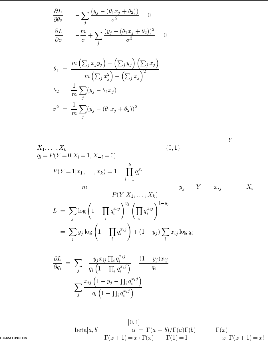
136 Chapter 20. Statistical Learning Methods
and the solutions can be computed as
20.7 There are a couple of ways to solve this problem. Here, we show the indicator vari-
able method described on page 743. Assume we have a child variable with parents
and let the range of each variable be . Let the noisy-OR parameters be
. The noisy-OR model then asserts that
Assume we have complete-data samples with values for and for each . The
conditional log likelihood for is given by
The gradient with respect to each noisy-OR parameter is
20.8
a. By integrating over the range , show that the normalization constant for the dis-
tribution is given by where is the Gamma
function, defined by and . (For integer , .)
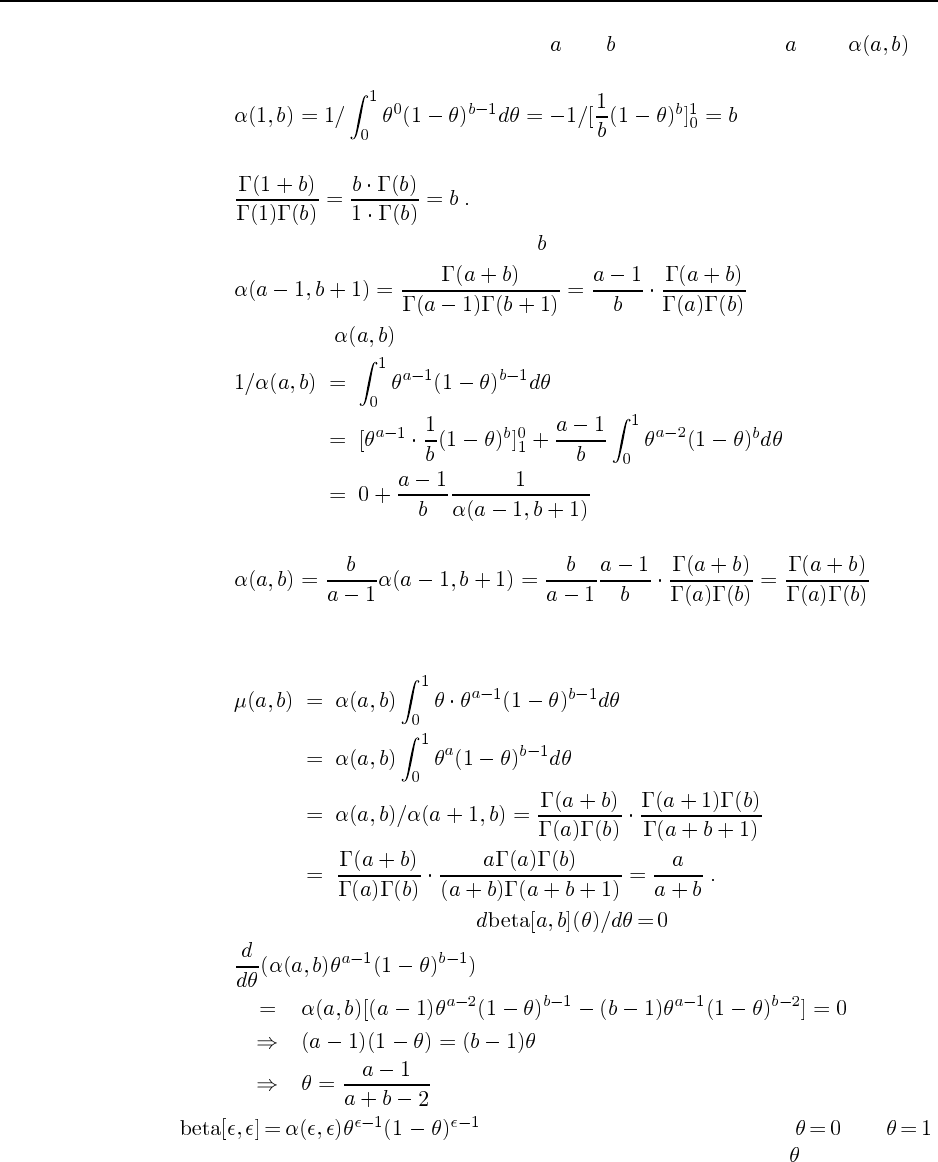
137
We will solve this for positive integer and by induction over . Let be
the normalization constant. For the base cases, we have
and
For the inductive step, we assume for all that
Now we evaluate using integration by parts. We have
Hence
as required.
b. The mean is given by the following integral:
c. The mode is found by solving for :
d. tends to very large values close to and ,
i.e., it expresses the prior belief that the distribution characterized by is nearly deter-
ministic (either positively or negatively). After updating with a positive example we
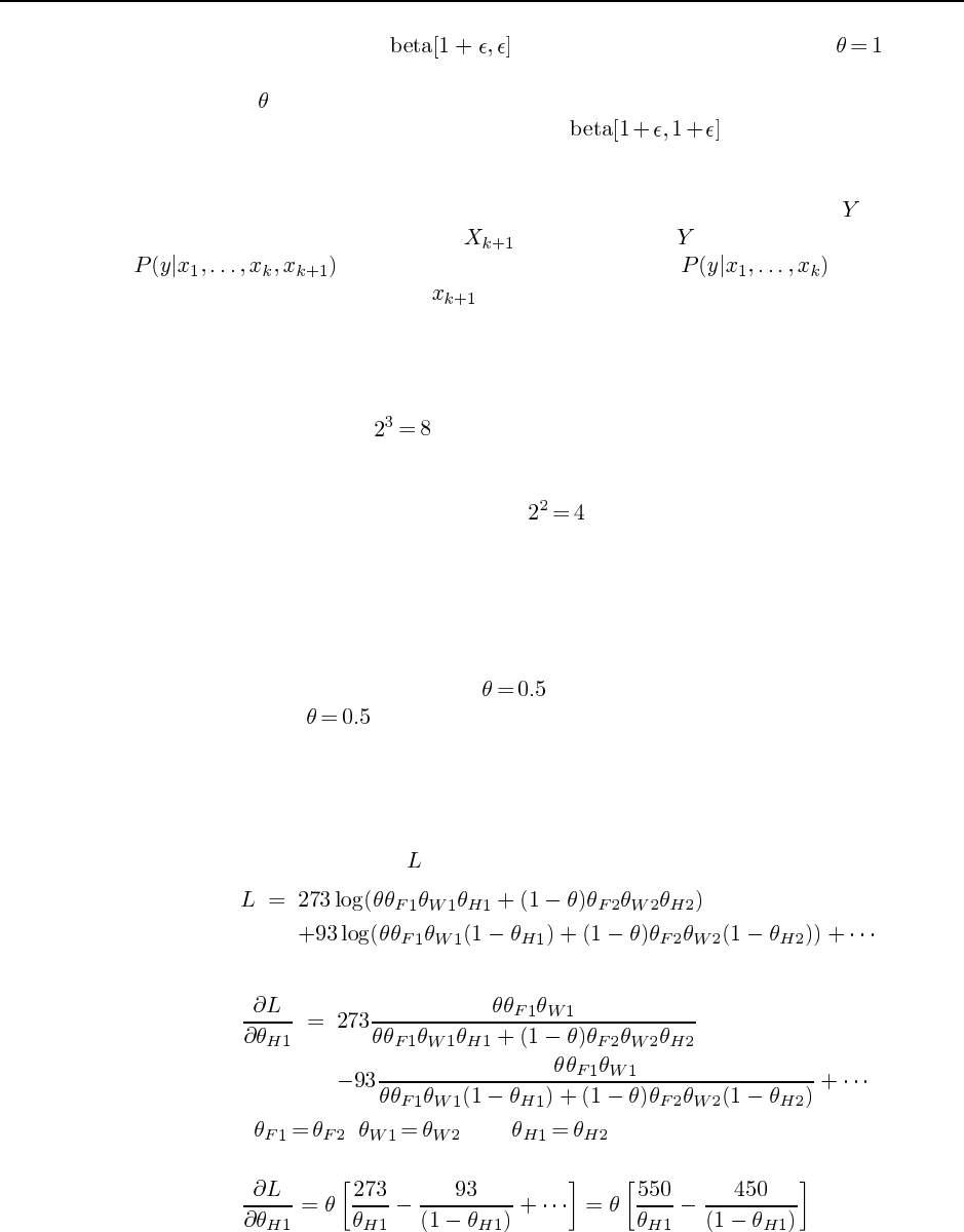
138 Chapter 20. Statistical Learning Methods
obtain the distribution , which has nearly all its mass near (and the
converse for a negative example), i.e., we have learned that the distribution character-
ized by is deterministic in the positive sense. If we see a “counterexample”, e.g., a
positive and a negative example, we obtain , which is close to uniform,
i.e., the hypothesis of near-determinism is abandoned.
20.9 Consider the maximum-likelihood parameter values for the CPT of node in the orig-
inal network, where an extra parent will be added to . If we set the parameters for
in the new network to be identical to in the original
netowrk, regardless of the value , then the likelihood of the data is unchanged. Maxi-
mizing the likelihood by altering the parameters can then only increase the likelihood.
20.10
a. With three attributes, there are seven parameters in the model and the empirical data
give frequencies for classes, which supply 7 independent numbers since the 8
frequencies have to sum to the total sample size. Thus, the problem is neither under-
nor over-constrained. With two attributes, there are five parameters in the model and
the empirical data give frequencies for classes, which supply 3 independent num-
bers. Thus, the problem is severely underconstrained. There will be a two-dimensional
surface of equally good ML solutions and the original parameters cannot be recovered.
b. The calculation is sketched and partly completed on pages 729 and 730. Completing
it by hand is tedious; students should encouraged to implement the method, ideally in
combination with a bayes net package, and trace its calculations.
c. The question should also assume to simplify the analysis. With every parameter
identical and , the new parameter values for bag 1 will be the same as those for
bag 2, by symmetry. Intuitively, if we assume initially that the bags are identical, then
it is as if we had just one bag. Likelihood is maximized under this constraint by setting
the proportions of candy types within each bag to the observed proportions. (See proof
below.)
d. We begin by writing out for the data in the table:
Now we can differentiate with respect to each parameter. For example,
Now if , , and , the denominators simplify, everything
cancels, and we have

139
First, note that will have the same value except that and are reversed,
so the parameters for bags 1 and 2 will move in lock step if . Second, note that
when , i.e., exactly the observed proportion of
candies with holes. Finally, we can calculate second derivatives and evlauate them at
the fixed point. For example, we obtain
which is negative (indicating the fixed point is a maximum) only when .
Thus, in general the fixed point is a saddle point as some of the second derivatives may
be positive and some negative. Nonetheless, EM can reach it by moving along the ridge
leading to it, as long as the symmetry is unbroken.
20.11 XOR (in fact any Boolean function) is easiest to construct using step-function units.
Because XOR is not linearly separable, we will need a hidden layer. It turns out that just one
hidden node suffices. To design the network, we can think of the XOR function as OR with
the AND case (both inputs on) ruled out. Thus the hidden layer computes AND, while the
output layer computes OR but weights the output of the hidden node negatively. The network
shown in Figure S20.3 does the trick.
t = 0.5 t = 0.2
W = 0.3
W = 0.3
W = 0.3
W = 0.3
W =− 0.6
Figure S20.3 A network of step-function neurons that computes the XOR function.
20.12 The examples map from to coordinates as follows:
(negative) maps to
(positive) maps to
(positive) maps to
(negative) maps to
Thus, the positive examples have and the negative examples have .
The maximum margin separator is the line , with a margin of 1. The separator
corresponds to the and axes in the original space—this can be thought of as the
limit of a hyperbolic separator with two branches.
20.13 The perceptron adjusts the separating hyperplane defined by the weights so as to
minimize the total error. The question assumes that the perceptron is trained to convergence
(if possible) on the accumulated data set after each new example arrives.
There are two phases. With few examples, the data may remain linearly separable and
the hyperplane will separate the positive and negative examples, although it will not represent

140 Chapter 20. Statistical Learning Methods
the XOR function. Once the data become non-separable, the hyperplane will move around to
find a local minimum-error configuration. With parity data, positive and negative examples
are distributed uniformly throughout the input space and in the limit of large sample sizes the
minimum error is obtained by a weight configuration that outputs approximately 0.5 for any
input. However, in this region the error surface is basically flat, and any small fluctuation in
the local balance of positive and negative examples due to the sampling process may cause
the minimum-error plane to move around drastically.
Here is some code to try out a given training set:
(setq *examples*
’(((T . 0) (I1 . 1) (I2 . 0) (I3 . 1) (I4 . 0))
((T . 1) (I1 . 1) (I2 . 0) (I3 . 1) (I4 . 1))
((T . 0) (I1 . 1) (I2 . 0) (I3 . 0) (I4 . 1))
((T . 0) (I1 . 0) (I2 . 1) (I3 . 1) (I4 . 0))
((T . 0) (I1 . 0) (I2 . 0) (I3 . 1) (I4 . 1))
((T . 1) (I1 . 1) (I2 . 0) (I3 . 0) (I4 . 0))
((T . 0) (I1 . 1) (I2 . 1) (I3 . 0) (I4 . 0))
((T . 1) (I1 . 0) (I2 . 1) (I3 . 1) (I4 . 1))
((T . 0) (I1 . 0) (I2 . 1) (I3 . 1) (I4 . 0))))
(deftest ex20.13
((setq problem
(make-learning-problem
:attributes ’((I1 0 1) (I2 0 1) (I3 0 1) (I4 0 1))
:goals ’((T 0 1))
:examples (subseq *examples* 0 <n>)))) ;;;; vary <n> as needed
;; Normally we’d call PERCEPTRON-LEARNING here, but we need added control
;; to set all the weights to 0.1, so we build the perceptron ourselves:
((setq net (list (list (make-unit :parents (iota 5)
:children nil
:weights ’(-1.0 0.1 0.1 0.1 0.1)
:g #’(lambda (i) (step-function 0 i)))))))
;; Now we call NN-LEARNING with the perceptron-update method,
;; but we also make it print out the weights, and set *debugging* to t
;; so that we can see the epoch number and errors.
((let ((*debugging* t))
(nn-learning
problem net
#’(lambda (net inputs predicted target &rest args)
(format t ‘‘˜&˜A Weights = ˜{˜4,1F ˜}˜%’’
(if (equal target predicted) ‘‘YES’’ ‘‘NO ‘‘)
(unit-weights (first (first net))))
(apply #’perceptron-update net inputs predicted target args))))))
Up to the first 5 examples, the network converges to zero error, and converges to non-zero
error thereafter.
20.14 According to ? (?), the number of linearly separable Boolean functions with inputs
is
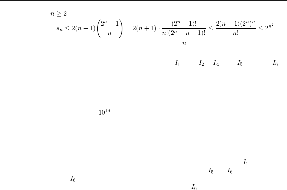
141
For we have
so the fraction of representable functions vanishes as increases.
20.15 These examples were generated from a kind of majority or voting function, where
each input has a different number of votes: 10 for , 4 for to , 2 for , and 1 for . If
you assign this problem, it is probably a good idea to tell the students this. Figure S?? shows
a perceptron and a feed-forward net with logical nodes that represent this function. Our in-
tuition was that the function should have been easy to learn with a perceptron, but harder
with other representations such as a decision tree. However, it turns out that there are not
enough examples for even a perceptron to learn. In retrospect, that should not be too surpris-
ing, as there are over different Boolean functions of six inputs, and only 14 examples.
Running the following code (which makes use of the code in learning/nn.lisp and
learning/perceptron.lisp) we find that the perceptron quickly converges to learn
all 14 training examples, but it performs at chance level on the five-example test set we made
up (getting 2 or 3 out of 5 right on most runs). (The student who did not know what the un-
derlying function was would have to keep out some of the examples to use as a test set.) The
weights vary widely from run to run, although in every run the weight for is the highest
(as it should be for the specified function), and the weights for and are usually low, but
sometimes is higher than other nodes. This may be a result of the fact that the examples
were chosen to represent some borderline cases where casts the deciding vote. So this
serves as a lesson: if you are “clever” in choosing examples, but rely on a learning algorithm
that assumes examples are chosen at random, you will run into trouble. Here is the code we
used:
(defun test-nn (net problem &optional
(examples (learning-problem-examples problem)))
(let ((correct 0))
(for-each example in examples do
(if (eql (cdr (first example))
(first (nn-output net (rest example)
(learning-problem-attributes problem)
nil)))
(incf correct)))
(values correct ’out-of (length examples))))
(deftest ex20.15
((setq examples
’(((T . 1) (I1 . 1) (I2 . 0) (I3 . 1) (I4 . 0) (I5 . 0) (I6 . 0))
((T . 1) (I1 . 1) (I2 . 0) (I3 . 1) (I4 . 1) (I5 . 0) (I6 . 0))
((T . 1) (I1 . 1) (I2 . 0) (I3 . 1) (I4 . 0) (I5 . 1) (I6 . 0))
((T . 1) (I1 . 1) (I2 . 1) (I3 . 0) (I4 . 0) (I5 . 1) (I6 . 1))
((T . 1) (I1 . 1) (I2 . 1) (I3 . 1) (I4 . 1) (I5 . 0) (I6 . 0))
((T . 1) (I1 . 1) (I2 . 0) (I3 . 0) (I4 . 0) (I5 . 1) (I6 . 1))
((T . 0) (I1 . 1) (I2 . 0) (I3 . 0) (I4 . 0) (I5 . 1) (I6 . 0))
((T . 1) (I1 . 0) (I2 . 1) (I3 . 1) (I4 . 1) (I5 . 0) (I6 . 1))
((T . 0) (I1 . 0) (I2 . 1) (I3 . 1) (I4 . 0) (I5 . 1) (I6 . 1))
((T . 0) (I1 . 0) (I2 . 0) (I3 . 0) (I4 . 1) (I5 . 1) (I6 . 0))
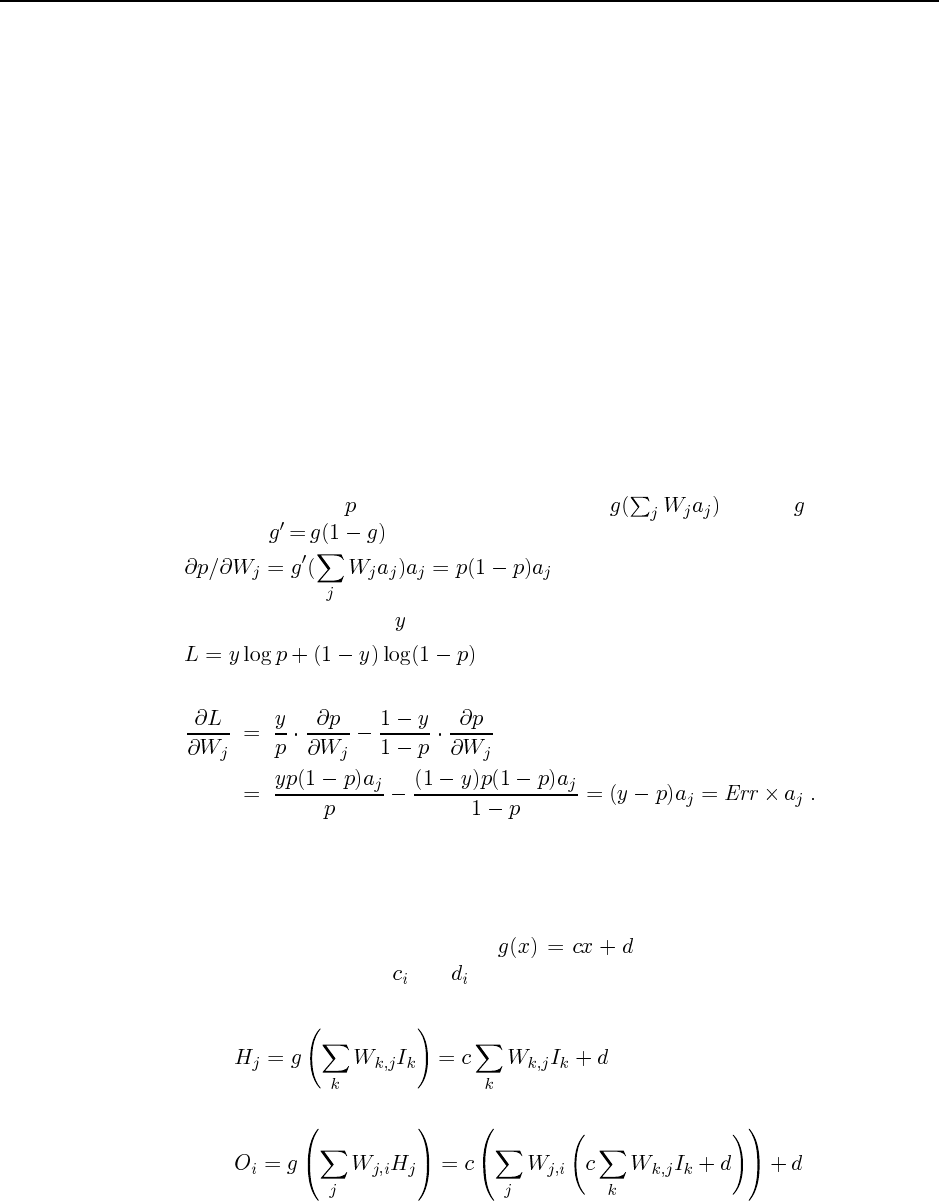
142 Chapter 20. Statistical Learning Methods
((T . 0) (I1 . 0) (I2 . 1) (I3 . 0) (I4 . 1) (I5 . 0) (I6 . 1))
((T . 0) (I1 . 0) (I2 . 0) (I3 . 0) (I4 . 1) (I5 . 0) (I6 . 1))
((T . 0) (I1 . 0) (I2 . 1) (I3 . 1) (I4 . 0) (I5 . 1) (I6 . 1))
((T . 0) (I1 . 0) (I2 . 1) (I3 . 1) (I4 . 1) (I5 . 0) (I6 . 0)))))
((setq problem
(make-learning-problem
:attributes ’((I1 0 1) (I2 0 1) (I3 0 1) (I4 0 1) (I5 0 1) (I6 0 1))
:goals ’((T 0 1))
:examples examples)))
((setq net (perceptron-learning problem)))
((setq weights (unit-weights (first (first net)))))
((test-nn net problem)
(= * 14))
((test-nn net problem
’(((T . 1) (I1 . 1) (I2 . 0) (I3 . 0) (I4 . 1) (I5 . 0) (I6 . 0))
((T . 0) (I1 . 0) (I2 . 0) (I3 . 1) (I4 . 1) (I5 . 1) (I6 . 1))
((T . 1) (I1 . 1) (I2 . 1) (I3 . 0) (I4 . 0) (I5 . 1) (I6 . 0))
((T . 0) (I1 . 1) (I2 . 0) (I3 . 0) (I4 . 0) (I5 . 0) (I6 . 0))
((T . 1) (I1 . 0) (I2 . 1) (I3 . 1) (I4 . 1) (I5 . 1) (I6 . 1))))
(= * 5)))
20.16 The probability output by the perceptron is , where is the sigmoid
function. Since , we have
For a datum with actual value , the log likelihood is
so the gradient of the log likelihood with respect to each weight is
20.17 This exercise reinforces the student’s understanding of neural networks as mathemat-
ical functions that can be analyzed at a level of abstraction above their implementation as a
network of computing elements. For simplicity, we will assume that the activation function
is the same linear function at each node: . (The argument is the same (only
messier) if we allow different and for each node.)
a. The outputs of the hidden layer are
The final outputs are
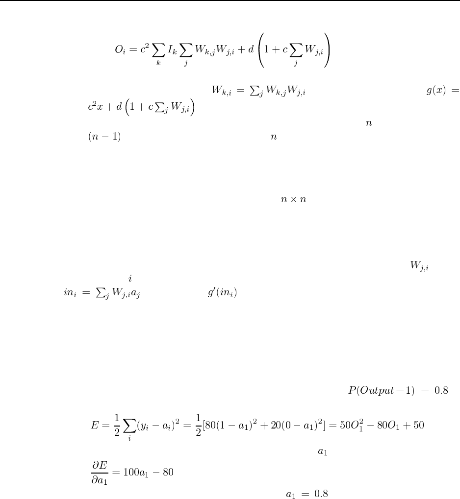
143
Now we just have to see that this is linear in the inputs:
Thus we can compute the same function as the two-layer network using just a one-layer
perceptron that has weights and an activation function
.
b. The above reduction can be used straightforwardly to reduce an -layer network to an
-layer network. By induction, the -layer network can be reduced to a single-
layer network. Thus, linear activation function restrict neural networks to represent only
linearly functions.
20.18 The implementation of neural networks can be approached in several different ways.
The simplest is probably to store the weights in an array. Everything can be calculated
as if all the nodes were in each layer, with the zero weights ensuring that only appropriate
changes are made as each layer is processed.
Particularly for sparse networks, it can be more efficient to use a pointer-based im-
plementation, with each node represented by a data structure that contains pointers to its
successors (for evaluation) and its predecessors (for backpropagation). Weights are at-
tached to node . In both types of implementation, it is convenient to store the summed input
and the value . The code repository contains an implementation
of the pointer-based variety. See the file learning/algorithms/nn.lisp, and the
function nn-learning in that file.
20.19 This question is especially important for students who are not expected to implement
or use a neural network system. Together with 20.15 and 20.17, it gives the student a concrete
(if slender) grasp of what the network actually does. Many other similar questions can be
devised.
Intuitively, the data suggest that a probabilistic prediction is
appropriate. The network will adjust its weights to minimize the error function. The error is
The derivative of the error with respect to the single output is
Setting the derivative to zero, we find that indeed . The student should spot the
connection to Ex. 18.8.
20.20 The application of cross-validation is straightforward—the methodology is the same
as that for any parameter selection problem. With 10-fold cross-validation, for example, each
size of hidden layer is evaluated by training on 90% subsets and testing on the remaining
10%. The best-performing size is then chosen, trained on all the training data, and the result
is returned as the system’s hypothesis. The purpose of this exercise is to have the student
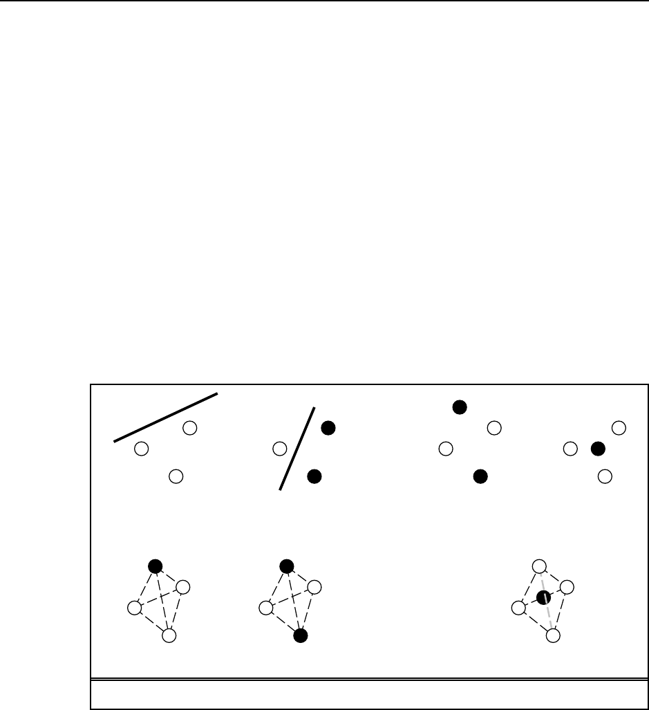
144 Chapter 20. Statistical Learning Methods
understand how to design the experiment, run some code to see results, and analyze the result.
The higher-order purpose is to cause the student to question results that make unwarranted
assumptions about the representation used in a learning problem, whether that representation
is the number of hidden nodes in a neural net, or any other representational choice.
20.21 The main purpose of this exercise is to make concrete the notion of the capacity of a
function class (in this case, linear halfspaces). It can be hard to internalize this concept, but
the examples really help.
a. Three points in general position on a plane form a triangle. Any subset of the points
can be separated from the rest by a line, as can be seen from the two examples in
Figure S20.4(a).
b. Figure S20.4(b) shows two cases where the positive and negative examples cannot be
separated by a line.
c. Four points in general position on a plane form a tetrahedron. Any subset of the points
can be separated from the rest by a plane, as can be seen from the two examples in
Figure S20.4(c).
d. Figure S20.4(d) shows a case where a negative point is inside the tetrahedron formed
by four positive points; clearly no plane can separate the two sets.
(a) (b)
(c) (d)
Figure S20.4 Illustrative examples for Ex. 20.21.
Solutions for Chapter 21
Reinforcement Learning
21.1 The code repository shows an example of this, implemented in the passive envi-
ronment. The agents are found under lisp/learning/agents/passive*.lisp and
the environment is in lisp/learning/domains/4x3-passive-mdp.lisp. (The
MDP is converted to a full-blown environment using the function mdp->environment
which can be found in lisp/uncertainty/environments/mdp.lisp.)
21.2 Consider a world with two states, and , with two actions in each state: stay still
or move to the other state. Assume the move action is non-deterministic—it sometimes fails,
leaving the agent in the same state. Furthermore, assume the agent starts in and that is a
terminal state. If the agent tries several move actions and they all fail, the agent may conclude
that is 0, and thus may choose a policy with , which is an
improper policy. If we wait until the agent reaches before updating, we won’t fall victim
to this problem.
21.3 This question essentially asks for a reimplementation of a general scheme for asyn-
chronous dynamic programming of which the prioritized sweeping algorithm is an exam-
ple (Moore and Atkeson, 1993). For a., there is code for a priority queue in both the Lisp and
Python code repositories. So most of the work is the experimentation called for in b.
21.4 When there are no terminal states there are no sequences, so we need to define se-
quences. We can do that in several ways. First, if rewards are sparse, we can treat any state
with a reward as the end of a sequence. We can use equation (21.2); the only problem is that
we don’t know the exact totl reward of the state at the end of the sequence, because it is not
a terminal state. We can estimate it using the current estimate. Another option is to
arbitrarily limit sequences to states, and then consider the next states, etc. A variation on
this is to use a sliding window of states, so that the first sequence is states , the second
sequence is , etc.
21.5 The idea here is to calculate the reward that the agent will actually obtain using a
given estimate of and a given estimated model . This is distinct from the true utility of
the states visited. First, we compute the policy for the agent by calculating, for each state, the
action with the highest estimated utility:
145
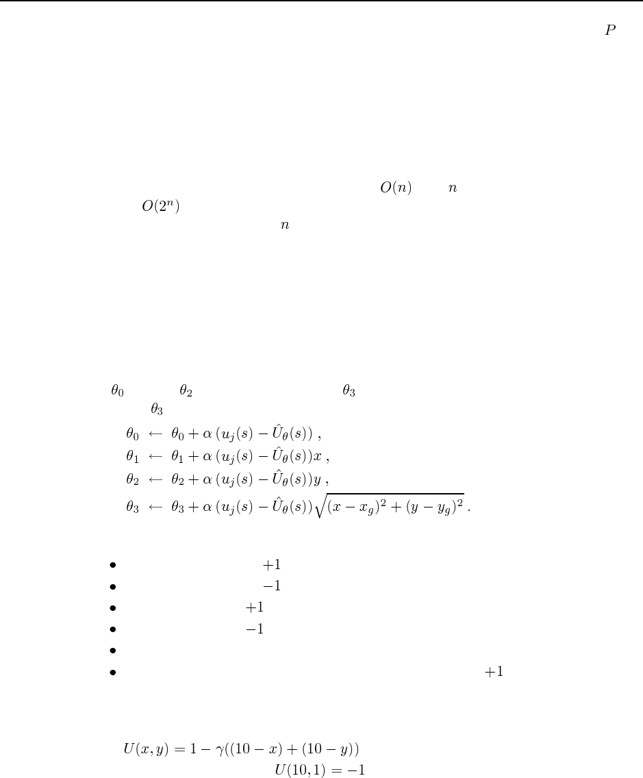
146 Chapter 21. Reinforcement Learning
Then the expected values can be found by applying value determination with policy and
can then be compared to the optimal values.
21.6 The conversion of the vacuum world problem specification into an environment suit-
able for reinforcement learning can be done by merging elements of mdp->environment
from lisp/uncertainty/environments/mdp.lisp with elements of the corre-
sponding function problem->environment from lisp/search/agents.lisp. The
point here is twofold: first, that the reinforcement learning algorithms in Chapter 20 are lim-
ited to accessible environments; second, that the dirt makes a huge difference to the size of
the state space. Without dirt, the state space is with locations. With dirt, the state
space is because each location can be clean or dirty. For this reason, input general-
ization is clearly necessary for above about 10. This illustrates the misleading nature of
“navigation” domains in which the state space is proportional to the “physical size” of the
environment. “Real-world” environments typically have some combinatorial structure that
results in exponential growth.
21.7 Code not shown. Several reinforcement learning agents are given in the directory
lisp/learning/agents.
21.8 This utility estimation function is similar to equation (21.9), but adds a term to repre-
sent Euclidean distance on a grid. Using equation (21.10), the update equations are the same
for through , and the new parameter can be calculated by taking the derivative with
respect to :
21.9 Possible features include:
Distance to the nearest terminal state.
Distance to the nearest terminal state.
Number of adjacent terminal states.
Number of adjacent terminal states.
Number of adjacent obstacles.
Number of obstacles that intersect with a path to the nearest terminal state.
21.10 This is a relatively time-consuming exercise. Code not shown to compute three-
dimensional plots. The utility functions are:
a. is the true utility, and is linear.
b. Same as in a, except that .
c. The exact utility depends on the exact placement of the obstacles. The best approxima-
tion is the same as in a. The features in exercise 21.9 might improve the approximation.
147
d. The optimal policy is to head straight for the goal from any point on the right side of
the wall, and to head for (5, 10) first (and then for the goal) from any point on the left
of the wall. Thus, the exact utility function is:
(if )
(if )
Unfortunately, this is not linear in and , as stated. Fortunately, we can restate the
optimal policy as “head straight up to row 10 first, then head right until column 10.”
This gives us the same exact utility as in a, and the same linear approximation.
e. is the true utility. This is also not linear in and ,
because of the absolute value signs. All can be fixed by introducing the features
and .
21.11 The modification involves combining elements of the environment converter for games
(game->environment in lisp/search/games.lisp) with elements of the function
mdp->environment. The reward signal is just the utility of winning/drawing/losing and
occurs only at the end of the game. The evaluation function used by each agent is the utility
function it learns through the TD process. It is important to keep the TD learning process
(which is entirely independent of the fact that a game is being played) distinct from the
game-playing algorithm. Using the evaluation function with a deep search is probably better
because it will help the agents to focus on relevant portions of the search space by improving
the quality of play. There is, however, a tradeoff: the deeper the search, the more computer
time is used in playing each training game.
21.12 Code not shown.
21.13 Reinforcement learning as a general “setting” can be applied to almost any agent
in any environment. The only requirement is that there be a distinguished reward signal.
Thus, given the signals of pain, pleasure, hunger, and so on, we can map human learning
directly into reinforcement learning—although this says nothing about how the “program”
is implemented. What this view misses out, however, is the importance of other forms of
learning that occur in humans. These include “speedup learning” (Chapter 21); supervised
learning from other humans, where the teacher’s feedback is taken as a distinguished input;
and the process of learning the world model, which is “supervised” by the environment.
21.14 DNA does not, as far as we know, sense the environment or build models of it. The
reward signal is the death and reproduction of the DNA sequence, but evolution simply mod-
ifies the organism rather than learning a or function. The really interesting problem is
deciding what it is that is doing the evolutionary learning. Clearly, it is not the individual (or
the individual’s DNA) that is learning, because the individual’s DNA gets totally intermingled
within a few generations. Perhaps you could say the species is learning, but if so it is learning
to produce individuals who survive to reproduce better; it is not learning anything to do with
the species as a whole rather than individuals. In The Selfish Gene, Richard Dawkins (1976)
proposes that the gene is the unit that learns to succeed as an “individual” because the gene is
preserved with small, accumulated mutations over many generations.
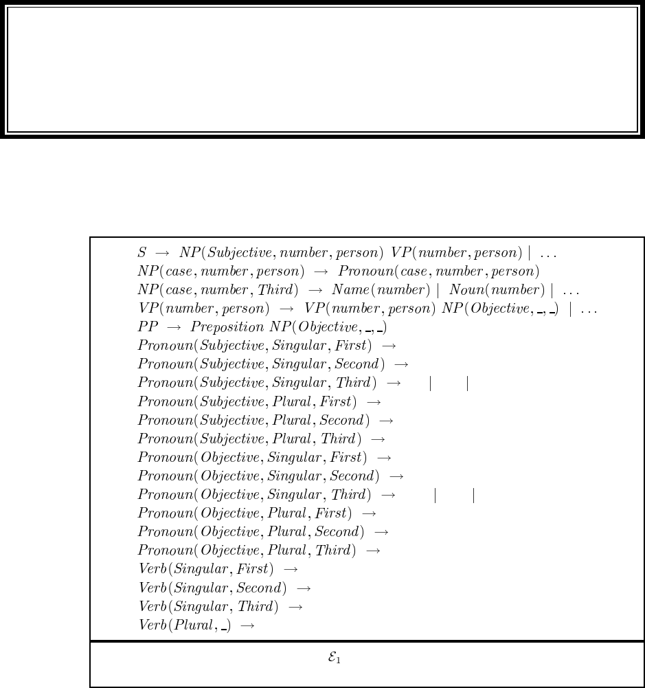
Solutions for Chapter 22
Communication
22.1 No answer required; just read the passage.
Iyou
he she it
we
you
they
me
you
him her it
usyou
them
smell
smell
smells
smell
Figure S22.1 A partial DCG for , modified to handle subject–verb number/person
agreement as in Ex. 22.2.
22.2 See Figure S22.1 for a partial DCG. We include both person and number annotation al-
though English really only differentiates the third person singular for verb agreement (except
for the verb be).
22.3 See Figure S22.2
148

149
a an the
the some many
Figure S22.2 A partial DCG for , modified to handle article–noun agreement as in
Ex. 22.3.
22.4 The purpose of this exercise is to get the student thinking about the properties of natural
language. There is a wide variety of acceptable answers. Here are ours:
Grammar and Syntax Java: formally defined in a reference book. Grammaticality is
crucial; ungrammatical programs are not accepted. English: unknown, never formally
defined, constantly changing. Most communication is made with “ungrammatical” ut-
terances. There is a notion of graded acceptability: some utterances are judged slightly
ungrammatical or a little odd, while others are clearly right or wrong.
Semantics Java: the semantics of a program is formally defined by the language spec-
ification. More pragmatically, one can say that the meaning of a particular program
is the JVM code emitted by the compiler. English: no formal semantics, meaning is
context dependent.
Pragmatics and Context-Dependence Java: some small parts of a program are left
undefined in the language specification, and are dependent on the computer on which
the program is run. English: almost everything about an utterance is dependent on the
situation of use.
Compositionality Java: almost all compositional. The meaning of “A + B” is clearly
derived from the meaning of “A” and the meaning of “B” in isolation. English: some
compositional parts, but many non-compositional dependencies.
Lexical Ambiguity Java: a symbol such as “Avg” can be locally ambiguous as it might
refer to a variable, a class, or a function. The ambiguity can be resolved simply by
checking the declaration; declarations therefore fulfill in a very exact way the role
played by background knowledge and grammatical context in English. English: much
lexical ambiguity.
Syntactic Ambiguity Java: the syntax of the language resolves ambiguity. For exam-
ple, in “if (X) if (Y) A; else B;” one might think it is ambiguous whether the “else”
belongs to the first or second “if,” but the language is specified so that it always belongs
to the second. English: much syntactic ambiguity.
Reference Java: there is a pronoun “this” to refer to the object on which a method was
invoked. Other than that, there are no pronouns or other means of indexical reference;
no “it,” no “that.” (Compare this to stack-based languages such as Forth, where the
stack pointer operates as a sort of implicit “it.”) There is reference by name, however.
Note that ambiguities are determined by scope—if there are two or more declarations
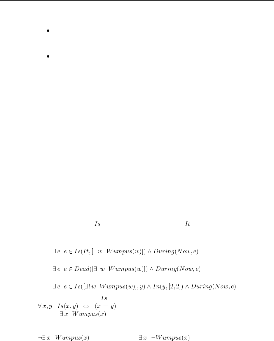
150 Chapter 22. Communication
of the variable “X”, then a use of X refers to the one in the innermost scope surrounding
the use. English: many techniques for reference.
Background Knowledge Java: none needed to interpret a program, although a local
“context” is built up as declarations are processed. English: much needed to do disam-
biguation.
Understanding Java: understanding a program means translating it to JVM byte code.
English: understanding an utterance means (among other things) responding to it appro-
priately; participating in a dialog (or choosing not to participate, but having the potential
ability to do so).
As a follow-up question, you might want to compare different languages, for example: En-
glish, Java, Morse code, the SQL database query language, the Postscript document descrip-
tion language, mathematics, etc.
22.5 This exercise is designed to clarify the relation between quasi-logical form and the
final logical form.
a. Yes. Without a quasi-logical form it is hard to write rules that produce, for example,
two different scopes for quantifiers.
b. No. It just makes ambiguities and abstractions more concise.
c. Yes. You don’t need to explicitly represent a potentially exponential number of disjunc-
tions.
d. Yes and no. The form is more concise, and so easier to manipulate. On the other hand,
the quasi-logical form doesn’t give you any clues as to how to disambiguate. But if
you do have those clues, it is easy to eliminate a whole family of logical forms without
having to explicitly expand them out.
22.6 Assuming that is the interpretation of “is,” and is the interpretation of “it,” then
we get the following:
a. It is a wumpus:
b. The wumpus is dead:
c. The wumpus is in 2,2:
We should define what means—one reasonable axiom for one sense of “is” would be
. (This is the “is the same as” sense. There are others.) The
formula is a reasonable semantics for “It is a wumpus.” The problem is if
we use that formula, then we have nowhere to go for “It was a wumpus”—there is no event to
which we can attach the time information. Similarly, for “It wasn’t a wumpus,” we can’t use
, nor could we use . So it is best to have an explicit
event for “is.”
151
22.7 This is a very difficult exercise—most readers have no idea how to answer the ques-
tions (except perhaps to remember that “too few” is better than “too many”). This is the
whole point of the exercise, as we will see in exercise 23.14.
22.8 The purpose of this exercise is to get some experience with simple grammars, and to
see how context-sensitive grammars are more complicated than context-free. One approach to
writing grammars is to write down the strings of the language in an orderly fashion, and then
see how a progression from one string to the next could be created by recursive application
of rules. For example:
a. The language : The strings are , , , . . . (where indicates the null string).
Each member of this sequence can be derived from the previous by wrapping an at
the start and a at the end. Therefore a grammar is:
b. The palindrome language: Let’s assume the alphabet is just , and . (In general, the
size of the grammar will be proportional to the size of the alphabet. There is no way to
write a context-free grammar without specifying the alphabet/lexicon.) The strings of
the language include , a, b, c, aa, bb, cc, aaa, aba, aca, bab, bbb, bcb, . . . . In general,
a string can be formed by bracketing any previous string with two copies of any member
of the alphabet. So a grammar is:
c. The duplicate language: For the moment, assume that the alphabet is just . (It is
straightforward to extend to a larger alphabet.) The duplicate language consists of the
strings: , , , , , , , . . . Note that all strings are of even length.
One strategy for creating strings in this language is this:
Start with markers for the front and middle of the string: we can use the non-
terminal for the front and for the middle. So at this point we have the string
.
Generate items at the front of the string: generate an followed by an , or a
followed by a . Eventually we get, say, . Then we no longer need
the marker and can delete it, leaving .
Move the non-terminals and down the line until just before the . We end
up with .
Hop the s and s over the , converting each to a terminal ( or ) as we go.
Then we delete the , and are left with the end result: .

152 Chapter 22. Communication
Here is a grammar to implement this strategy:
(starting markers)
(introduce symbols)
(delete the marker)
(move non-terminals down to the )
(hop over and convert to terminal)
(delete the marker)
Here is a trace of the grammar deriving :
22.9 Grammar (A) does not work, because there is no way for the verb “walked” followed
by the adverb “slowly” and the prepositional phrase “to the supermarket” to be parsed as a
verb phrase. A verb phrase in (A) must have either two adverbs or be just a verb. Here is the
parse under grammar (B):
S---NP-+-Pro---Someone
|
|-VP-+-V---walked
|
|-Vmod-+-Adv---slowly
|
|-Vmod---Adv---PP---Prep-+-to
|
|-NP-+-Det---the
|
|-NP---Noun---supermarket

153
Here is the parse under grammar (C):
S---NP-+-Pro---Someone
|
|-VP-+-V---walked
|
|-Adv-+-Adv---slowly
|
|-Adv---PP---Prep-+-to
|
|-NP-+-Det---the
|
|-NP---Noun---supermarket
22.10 Code not shown.
22.11 Code not shown.
22.12 This is the grammar suggested by the exercise. There are additional grammatical
constructions that could be covered by more ambitious grammars, without adding any new
vocabulary.
(for relative clause)
Running the parser function parses from the code repository with this grammar and with
strings of the form , and then just counting the number of results, we get:
N1 2 3 4 5 6 7 8 9 10
Number of parses 0 0 1 2 3 6 11 22 44 90
To count the number of sentences, de Marcken implemented a parser like the packed forest
parser of example 22.10, except that the representation of a forest is just an integer count of
the number of parses (and therefore the combination of adjacent forests is just the product
of the constituent forests). He then gets a single integer representing the parses for the whole
200-word sentence.
22.13 Here’s one way to draw the parse tree for the story on page 823. The parse tree of the
students’ stories will depned on their choice.
Segment(Evaluation)
Segment(1) ‘‘A funny thing happened’’
Segment(Ground-Figure)
Segment(Cause)
Segment(Enable)
Segment(2) ‘‘John went to a fancy restaurant’’

154 Chapter 22. Communication
Segment(3) ‘‘He ordered the duck’’
Segment(4) ‘‘The bill came to $50’’
Segment(Cause)
Segment(Enable)
Segment(Explanation)
Segment(5) ‘‘John got a shock...’’
Segment(6) ‘‘He had left his wallet at home’’
Segment(7) ‘‘The waiter said it was all right’’
Segment(8) ‘‘He was very embarrassed...’’
22.14 Now we can answer the difficult questions of 22.7:
The steps are sorting the clothes into piles (e.g., white vs. colored); going to the washing
machine (optional); taking the clothes out and sorting into piles (e.g., socks versus
shirts); putting the piles away in the closet or bureau.
The actual running of the washing machine is never explicitly mentioned, so that is one
possible answer. One could also say that drying the clothes is a missing step.
The material is clothes and perhaps other washables.
Putting too many clothes together can cause some colors to run onto other clothes.
It is better to do too few.
So they won’t run; so they get thoroughly cleaned; so they don’t cause the machine to
become unbalanced.

Solutions for Chapter 23
Probabilistic Language Processing
23.1 Code not shown. The approach suggested here will work in some cases, for authors
with distinct vocabularies. For more similar authors, other features such as bigrams, average
word and sentence length, parts of speech, and punctuation might help. Accuracy will also
depend on how many authors are being distinguished. One interesting way to make the task
easier is to group authors into male and female, and try to distinguish the sex of an author not
previously seen. This was suggested by the work of Shlomo Argamon.
23.2 Code not shown. The distribution of words should fall along a Zipfian distribution: a
straight line on a log-log scale. The generated language should be similar to the examples in
the chapter.
23.3 Code not shown. There are now several open-source projects to do Bayesian spam
filtering, so beware if you assign this exercise.
23.4 Doing the evaluation is easy, if a bit tedious (requiring 150 page evaluations for the
complete 10 documents 3 engines 5 queries). Explaining the differences is more diffi-
cult. Some things to check are whether the good results in one engine are even in the other
engines at all (by searching for unique phrases on the page); check whether the results are
commercially sponsored, are produced by human editors, or are algorithmically determined
by a search ranking algorithm; check whether each engine does the features mentioned in the
next exercise.
23.5 One good way to do this is to first find a search that yields a single page (or a few pages)
by searching for rare words or phrases on the page. Then make the search more difficult by
adding a variant of one of the words on the page—a word with different case, different suffix,
different spelling, or a synonym for one of the words on the page, and see if the page is still
returned. (Make sure that the search engine requires all terms to match for this technique to
work.)
23.6 Computations like this are given in the book Managing Gigabytes (Witten et al., 1999).
Here’s one way of doing the computation: Assume an average page is about 10KB (giving
us a 10TB corpus), and that index size is linear in the size of the corpus. Bahle et al. (2002)
show an index size of about 2GB for a 22GB corpus; so our billion page corpus would have
an index of about 1TB.
155

156 Chapter 23. Probabilistic Language Processing
23.7 Code not shown. The simplest approach is to look for a string of capitalized words,
followed by “Inc” or “Co.” or “Ltd.” or similar markers. A more complex approach is to
get a list of company names (e.g. from an online stock service), look for those names as
exact matches, and also extract patterns from them. Reporting recall and precision requires a
clearly-defined corpus.
23.8 The main point of this exercise is to show that current translation software is far from
perfect. The mistakes made are often amusing for students.
23.9 Here is a start of a grammar:
time => hour ":" minute
| extendedhour
| extendedhour "o’clock"
| difference before_after extendedhour
hour => 1 | 2 | ... | 24 | "one" | ... | "twelve"
extendedhour => hour | "midnight" | "noon"
minute => 1 | 2 | ... | 60
before-after => "before" | "after" | "to" | "past"
difference => minute | "quarter" | "half"
23.10
a. “I have never seen a better programming language” is easy for most people to see.
b. “John loves mary” seems to be prefered to “Mary loves John” (on Google, by a margin
of 2240 to 499, and by a similar margin on a small sample of respondents), but both are
of course acceptable.
c. This one is quite difficult. The first sentence of the second paragraph of Chapter 22
is “Communication is the intentional exchange of information brought about by the
production and perception of signs drawn from a shared system of conventional signs.”
However, this cannot be reliably recovered from the string of words given here. Code
not shown for testing the probabilities of permutations.
23.11 In parlimentary debate, a standard expression of approval is “bravo” in French, and
“hear, hear” in English. That means that in going from French to English, “bravo” would
often have a fertility of 2, but for English to French, the fertility distribution of “hear” would
be half 0 and half 1 for this usage. For other usages, it would have various values, probably
centered closely around 1.
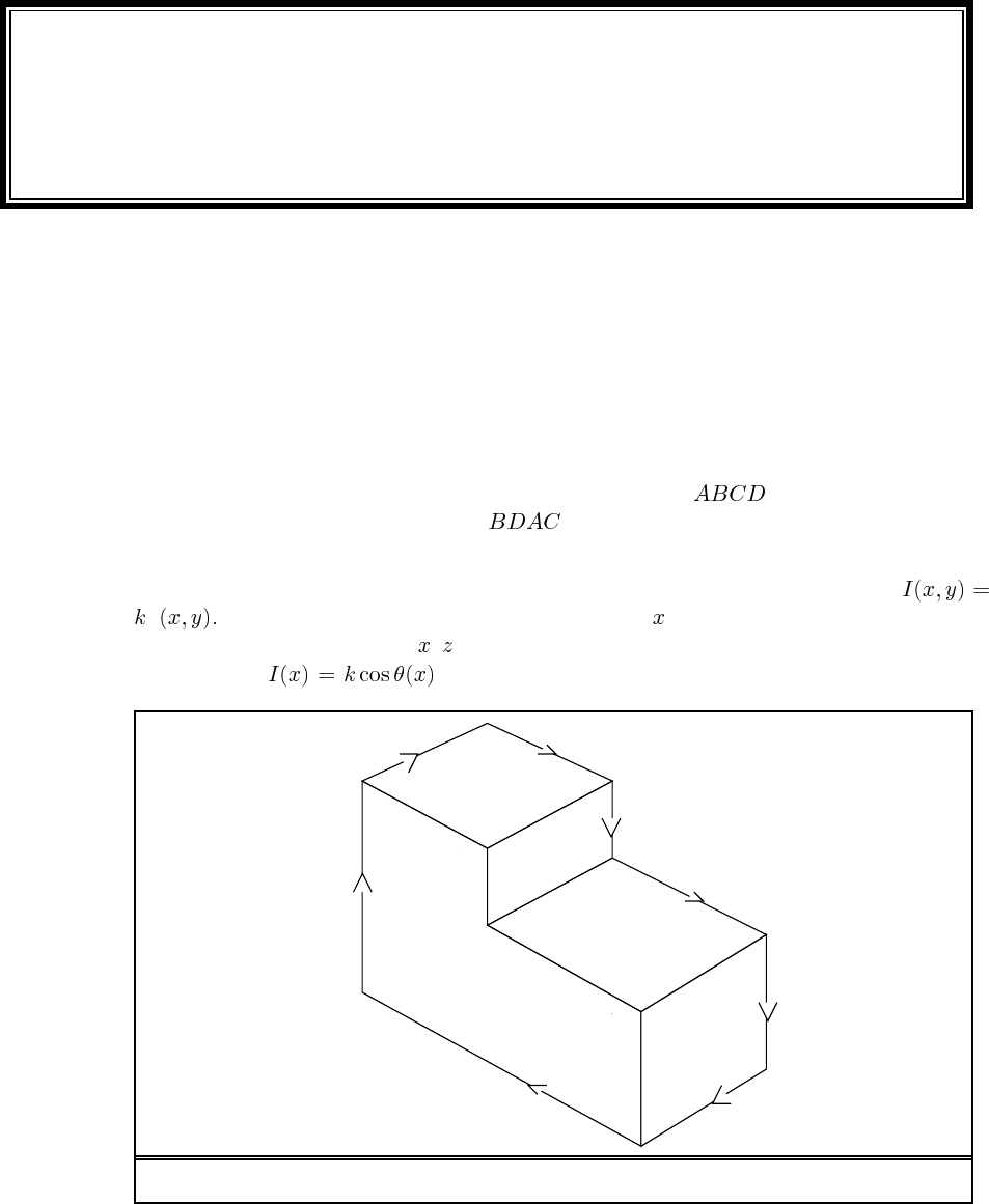
Solutions for Chapter 24
Perception
24.1 The small spaces between leaves act as pinhole cameras. That means that the circular
light spots you see are actually images of the circular sun. You can test this theory next time
there is a solar eclipse: the circular light spots will have a crescent bite taken out of them as
the eclipse progresses. (Eclipse or not, the light spots are easier to see on a sheet of paper
than on the rough forest floor.)
24.2 Given labels on the occluding edges (i.e., they are all arrows pointing in the clockwise
direction), there will be no backtracking at all if the order is ; each choice is forced
by the existing labels. With the order , the amount of backtracking depends on the
choices made. The final labelling is shown in Figure S24.1.
24.3 Recall that the image brightness of a Lambertian surface (page 743) is given by
n s. Here the light source direction sis along the -axis. It is sufficient to consider a
horizontal cross-section (in the – plane) of the cylinder as shown in Figure S24.2(a). Then,
the brightness for all the points on the right half of the cylinder. The left
A
B
C
D
+ +
+−
++
+
Figure S24.1 Labelling of the L-shaped object (Exercise 24.2).
157
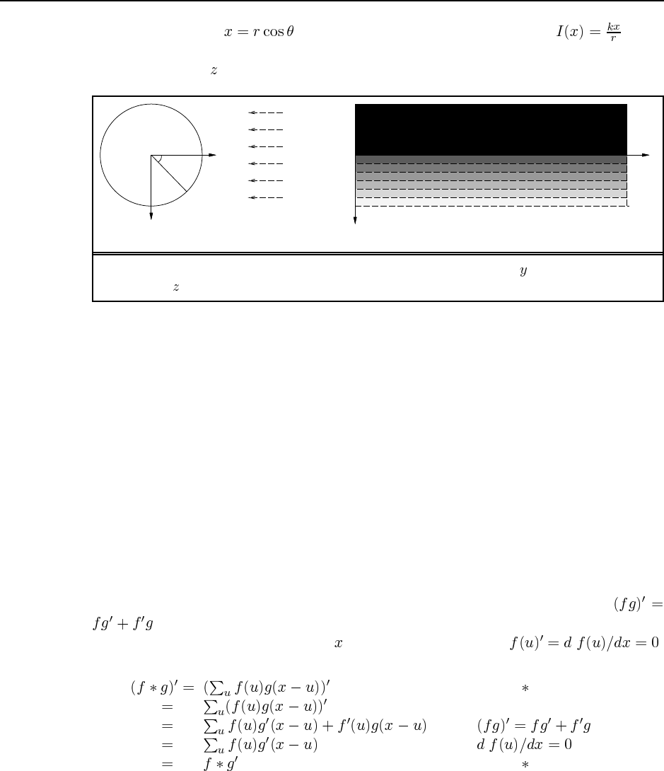
158 Chapter 24. Perception
half is in shadow. As , we can rewrite the brightness function as which
reveals that the isobrightness contours in the lit part of the cylinder must be equally spaced.
The view from the -axis is shown in Figure S24.2(b).
x
y
x
r
z
illumination
θ
viewer (a) (b)
Figure S24.2 (a) Geometry of the scene as viewed from along the -axis. (b) The scene
from the -axis, showing the evenly spaced isobrightness contours.
24.4 We list the four classes and give two or three examples of each:
a.depth: Between the top of the computer monitor and the wall behind it. Between the
side of the clock tower and the sky behind it. Between the white sheets of paper in the
foreground and the book and keyboard behind them.
b.surface normal: At the near corner of the pages of the book on the desk. At the sides of
the keys on the keyboard.
c.reflectance: Between the white paper and the black lines on it. Between the “golden”
bridge in the picture and the blue sky behind it.
d.illumination: On the windowsill, the shadow from the center glass pane divider. On the
paper with Greek text, the shadow along the left from the paper on top of it. On the
computer monitor, the edge between the white window and the blue window is caused
by different illumination by the CRT.
24.5 This exercise requires some basic algebra, and enough calculus to know that
. Students with freshman calculus as background should be able to handle it. Note
that all differentiation is with respect to . Crucially, this means that .
We work the solution for the discrete case; the continuous (integral) case is similar.
(definition of )
(derivative of a sum)
(since )
(since )
(definition of )
24.6 Before answering this exercise, we draw a diagram of the apparatus (top view), shown
in Figure S24.3. Notice that we make the approximation that the focal length is the distance
from the lens to the image plane; this is valid for objects that are far away. Notice that this
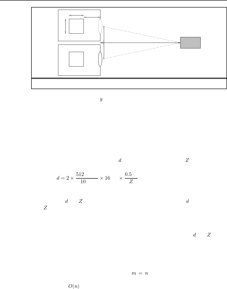
159
512x512
pixels
10cm
10cm
16cm
16m Object
0.5m
0.5m
Figure S24.3 Top view of the setup for stereo viewing (Exercise 24.6).
question asks nothing about the coordinates of points; we might as well have a single line
of 512 pixels in each camera.
a. Solve this by constructing similar triangles: whose hypotenuse is the dotted line from
object to lens, and whose height is 0.5 meters and width 16 meters. This is similar
to a triangle of width 16cm whose hypotenuse projects onto the image plane; we can
compute that its height must be 0.5cm; this is the offset from the center of the image
plane. The other camera will have an offset of 0.5cm in the opposite direction. Thus the
total disparity is 1.0cm, or, at 512 pixels/10cm, a disparity of 51.2 pixels, or 51, since
there are no fractional pixels. Objects that are farther away will have smaller disparity.
Writing this as an equation, where is the disparity in pixels and is the distance to
the object, we have:
pixels
cm cm m
b. In other words, this question is asking how much further than 16m could an object be,
and still occupy the same pixels in the image plane? Rearranging the formula above by
swapping and , and plugging in values of 51 and 52 pixels for , we get values of
of 16.06 and 15.75 meters, for a difference of 31cm (a little over a foot). This is the
range resolution at 16 meters.
c. In other words, this question is asking how far away would an object be to generate a
disparity of one pixel? Objects farther than this are in effect out of range; we can’t say
where they are located. Rearranging the formula above by swapping and we get
51.2 meters.
24.7 In the 3-D case, the two-dimensional image projected by an arbitrary 3-D object can
vary greatly, depending on the pose of the object. But with flat 2-D objects, the image is
always the “same,” except for its orientation and position. All feature points will always be
present because there can be no occlusion, so . Suppose we compute the center of
gravity of the image and model feature points. For the model this can be done offline; for
the image this is . Then we can take these two center of gravity points, along with an
160 Chapter 24. Perception
arbitrary image point and one of the model points, and try to verify the transformation for
each of the cases. Verification is as before, so the whole process is .
A follow-up exercise is to look at some of the tricks used by Olson (1994) to see if they are
applicable here.
24.8 A, B, C can be viewed in stereo and hence their depths can be measured, allowing
the viewer to determine that B is nearest, A and C are equidistant and slightly further away.
Neither D nor E can be seen by both cameras, so stereo cannot be used. Looking at the
figure, it appears that the bottle occludes D from Y and E from X, so D and E must be further
away than A, B, C, but their relative depths cannot be determined. There is, however, another
possibility (noticed by Alex Fabrikant). Remember that each camera sees the camera’s-eye
view not the bird’s-eye view. X sees DABC and Y sees ABCE. It is possible that D is very
close to camera X, so close that it falls outside the field of view of camera Y; similarly, E
might be very close to Y and be outside the field of view of X. Hence, unless the cameras
have a 180-degree field of view—probably impossible—there is no way to determine whether
D and E are in front of or behind the bottle.
24.9
a. False. This can be quite difficult, particularly when some point are occluded from one
eye but not the other.
b. True. The grid creates an apparent texture whose distortion gives good information as
to surface orientation.
c. False. It applies only to trihedral objects, excluding many polyhedra such as four-sided
pyramids.
d. True. A blade can become a fold if one of the incident surfaces is warped.
e. True. The detectable depth disparity is inversely proportional to .
f. False.
g. False. A disk viewed edge-on appears as a straight line.
24.10 There are at least two reasons: (1) The leftmost car appears bigger and cars are
usually roughly similar in size, therefore it is closer. (2) It is assumed that the road surface is
an approximately horizontal ground plane, and that both cars are on it. In that case, because
the leftmost car appears lower in the image, it must be closer.
25 ROBOTICS
25.1 To answer this question, consider all possibilities for the initial samples before and
after resampling. This can be done because there are only finitely many states. The following
C++ program calculates the results for finite . The result for is simply the posterior,
calculated using Bayes rule.
int
main(int argc, char *argv[])
{
// parse command line argument
if (argc != 3){
cerr << "Usage: " << argv[0] << " <number of samples>"
<< " <number of states>" << endl;
exit(0);
}
int numSamples = atoi(argv[1]);
int numStates = atoi(argv[2]);
cerr << "number of samples: " << numSamples << endl
<< "number of states: " << numStates << endl;
assert(numSamples >= 1);
assert(numStates >= 1);
// generate counter
int samples[numSamples];
for (int i = 0; i < numSamples; i++)
samples[i] = 0;
// set up probability tables
assert(numStates == 4); // presently defined for 4 states
double condProbOfZ[4] = {0.8, 0.4, 0.1, 0.1};
double posteriorProb[numStates];
for (int i = 0; i < numStates; i++)
posteriorProb[i] = 0.0;
double eventProb = 1.0 / pow(numStates, numSamples);
//loop through all possibilities
for (int done = 0; !done; ){
// compute importance weights (is probability distribution)
double weight[numSamples], totalWeight = 0.0;
for (int i = 0; i < numSamples; i++)
totalWeight += weight[i] = condProbOfZ[samples[i]];
// normalize them
for (int i = 0; i < numSamples; i++)
weight[i] /= totalWeight;
// calculate contribution to posterior probability
for (int i = 0; i < numSamples; i++)
posteriorProb[samples[i]] += eventProb * weight[i];
// increment counter
for (int i = 0; i < numSamples && i != -1;){
samples[i]++;
if (samples[i] >= numStates)
samples[i++] = 0;
else
i = -1;
if (i == numSamples)
done = 1;
}
}
// print result
cout << "Result: ";
for (int i = 0; i < numStates; i++)
cout << " " << posteriorProb[i];
cout << endl;
// calculate asymptotic expectation
double totalWeight = 0.0;
for (int i = 0; i < numStates; i++)
totalWeight += condProbOfZ[i];
cout << "Unbiased:";
for (int i = 0; i < numStates; i++)
cout << " " << condProbOfZ[i] / totalWeight;
cout << endl;
// calculate KL divergence
double kl = 0.0;
for (int i = 0; i < numStates; i++)
kl += posteriorProb[i] * (log(posteriorProb[i]) -
log(condProbOfZ[i] / totalWeight));
cout << "KL divergence: " << kl << endl;
}
(a) (b)
Figure S25.1 Code to calculate answer to exercise 25.1.
a. The program (correctly) calculates the following posterior distributions for the four
states, as a function of the number of samples . Note that for , the measurement
is ignored entirely! The correct posterior for is calculated using Bayes rule.
161
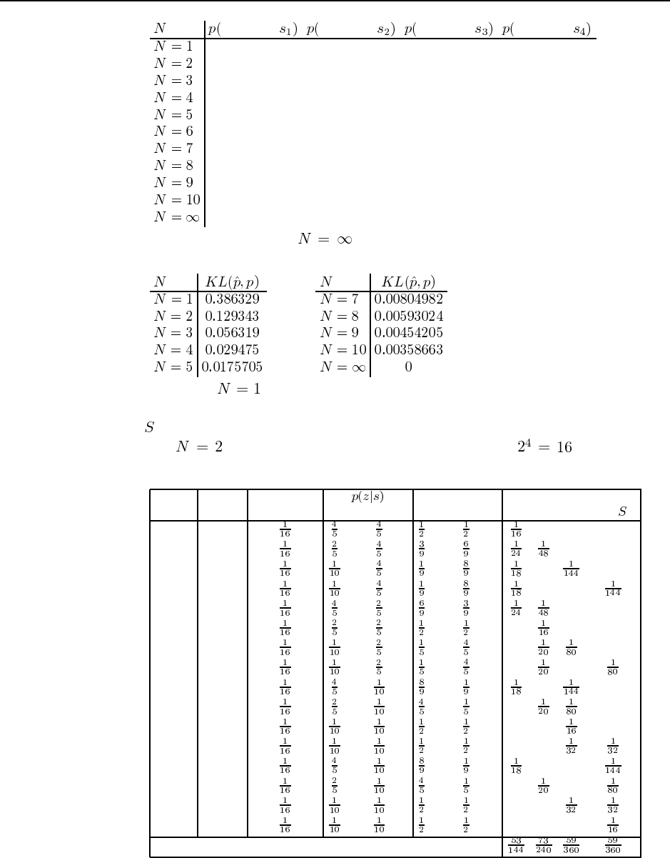
162 Chapter 25. Robotics
sample at sample at sample at sample at
0.25 0.25 0.25 0.25
0.368056 0.304167 0.163889 0.163889
0.430182 0.314463 0.127677 0.127677
0.466106 0.314147 0.109874 0.109874
0.488602 0.311471 0.0999636 0.0999636
0.503652 0.308591 0.0938788 0.0938788
0.514279 0.306032 0.0898447 0.0898447
0.522118 0.303872 0.0870047 0.0870047
0.528112 0.30207 0.0849091 0.0849091
0.532829 0.300562 0.0833042 0.0833042
0.571429 0.285714 0.0714286 0.0714286
b. Plugging the posterior for into the definition of the Kullback Liebler Diver-
gence gives us:
c. The proof for is trivial, since the re-weighting ignores the measurement proba-
bility entirely. Therefore, the probability for generating a sample in any of the locations
in is given by the initial distribution, which is uniform.
For , a proof is easily obtained by considering all ways in which
initial samples are generated:
number samples probability weights probability of resampling
of sample set for each sample for each sample for each location in
1 0 0 0 0 0
2 0 1 0 0
3 0 2 0 0
4 0 3 0 0
5 1 0 0 0
6 1 1 0 0 0
7 1 2 0 0
8 1 3 0 0
9 2 0 0 0
10 2 1 0 0
11 2 2 0 0 0
12 2 3 0 0
13 3 0 0 0
14 3 1 0 0
15 3 2 0 0
16 3 3 0 0 0
sum of all probabilities
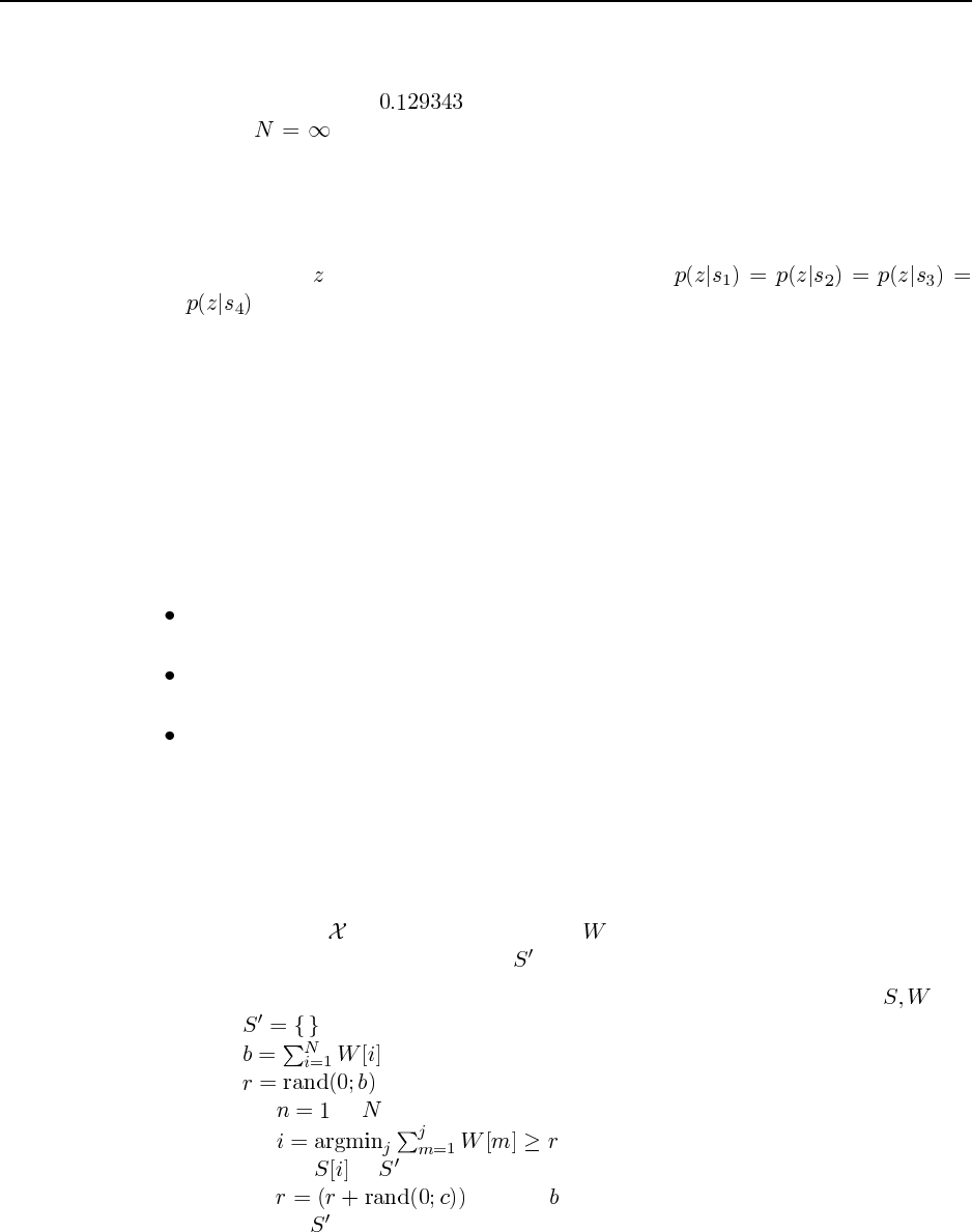
163
A quick check should convince you that these numbers are the same as above. Placing
this into the definition of the Kullback Liebler divergence with the correct posterior
distribution, gives us .
For we know that the sampler is unbiased. Hence, the probability of gen-
erating a sample is the same as the posterior distribution calculated by Bayes filters.
Those are given above as well.
d. Here are two possible modifications. First, if the initial robot location is known with
absolute certainty, the sampler above will always be unbiased. Second, if the sensor
measurement is equally likely for all states, that is
, it will also be unbiased. An invalid answer, which we frequently encountered
in class, pertains to the algorithm (instead of the problem formulation). For example,
replacing particle filters by the exact discrete Bayes filer remedies the problem but is
not a legitimate answer to this question. Neither is the use of infinitely many particles.
25.2 Implementing Monte Carlo localization requires a lot of work but is a premiere way to
gain insights into the basic workings of probabilistic algorithms in robotics, and the intricacies
inherent in real data. We have used this exercise in many courses, and students consistently
expressed having learned a lot. We strongly recommend this exercise!
The implementation is not as straightforward as it may appear at first glance. Common
problems include:
The sensor model models too little noise, or the wrong type of noise. For example, a
simple Gaussian will not work here.
The motion model assumes too little or too much noise, or the wrong type of noise.
Here a Gaussian will work fine though.
The implementation may introduce unnecessarily high variance in the resulting sam-
pling set, by sampling too often, or by sampling in the wrong way. This problem man-
ifests itself by diversity disappearing prematurely, often with the wrong samples sur-
viving. While the basic MCL algorithm, as stated in the book, suggests that sampling
should occur after each motion update, implementations that sample less frequently
tend to yield superior results. Further, drawing samples independently of each other
is inferior to so-called low variance samplers. Here is a version of low variance sam-
pling, in which denotes the particles and their importance weights. The resulting
resampled particles reside in the set .
function LOW-VARIANCE-WEIGHTED-SAMPLE-WITH-REPLACEMENT
( ):
for to do
add to
modulo
return
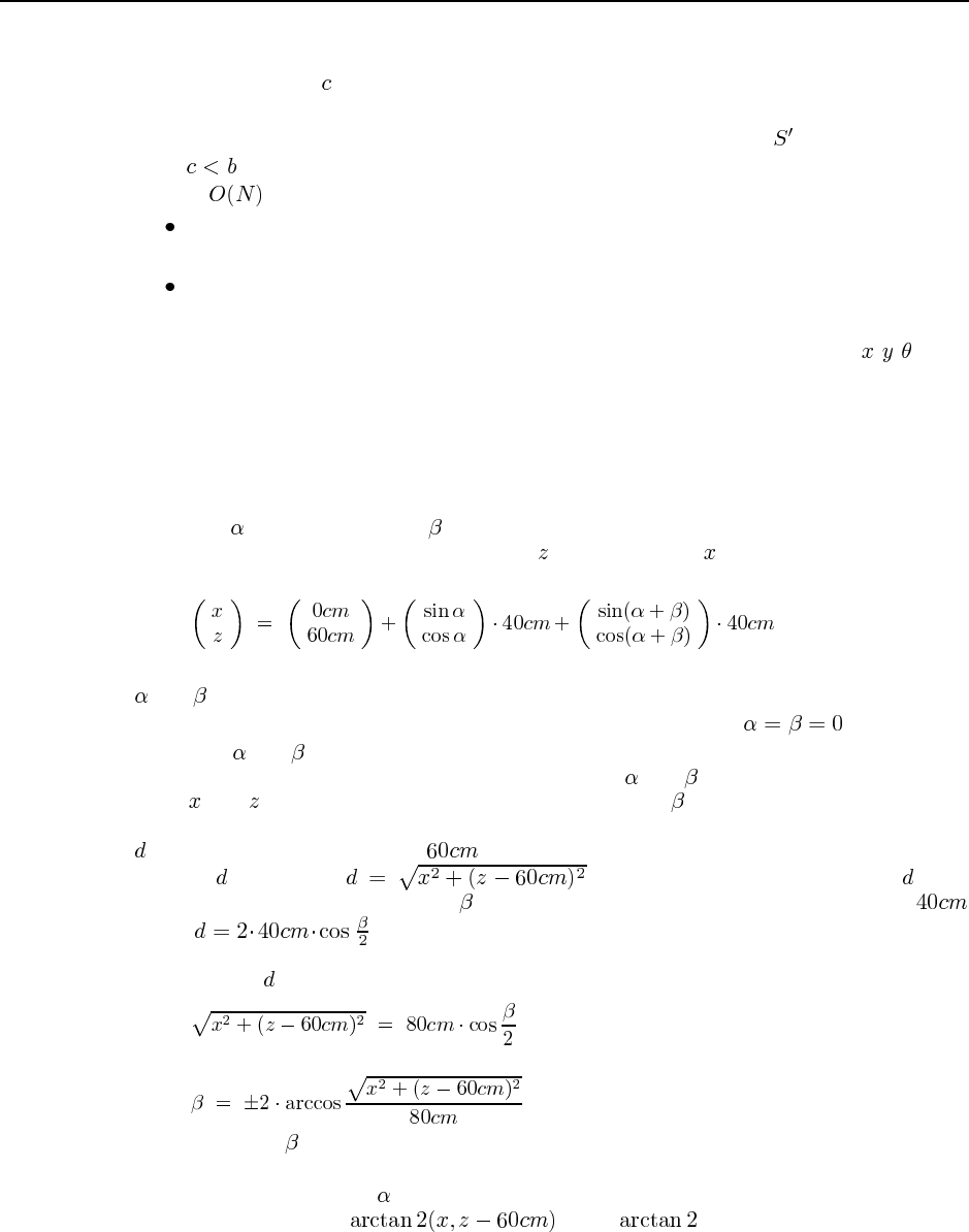
164 Chapter 25. Robotics
The parameter determines the speed at which we cycle through the sample set. While
each sample’s probability remains the same as if it were sampled independently, the re-
sulting samples are dependent, and the variance of the sample set is lower (assuming
). As a pleasant side effect, the low-variance samples is also easily implemented
in time, which is more difficult for the independent sampler.
Samples are started in the occupied or unknown parts of the map, or are allowed into
those parts during the forward sampling (motion prediction) step of the MCL algorithm.
Too few samples are used. A few thousand should do the job, a few hundred will
probably not.
The algorithm can be sped up by pre-caching all noise-free measurements, for all - - poses
that the robot might assume. For that, it is convenient to define a grid over the space of all
poses, with 10 centimeters spatial and 2 degrees angular resolution. One might then compute
the noise-free measurements for the centers of those grid cells. The sensor model is clearly
just a function of those correct measurements; and computing those takes the bulk of time in
MCL.
25.3 Let be the shoulder and be the elbow angle. The coordinates of the end effector are
then given by the following expression. Here is the height and the horizontal displacement
between the end effector and the robot’s base (origin of the coordinate system):
Notice that this is only one way to define the kinematics. The zero-positions of the angles
and can be anywhere, and the motors may turn clockwise or counterclockwise. Here we
chose define these angles in a way that the arm points straight up at ; furthermore,
increasing and makes the corresponding joint rotate counterclockwise.
Inverse kinematics is the problem of computing and from the end effector coordi-
nates and . For that, we observe that the elbow angle is uniquely determined by the
Euclidean distance between the shoulder joint and the end effector. Let us call this distance
. The shoulder joint is located above the origin of the coordinate system; hence, the
distance is given by . An alternative way to calculate is by
recovering it from the elbow angle and the two connected joints (each of which is
long): . The reader can easily derive this from basic trigonomy, exploiting
the fact that both the elbow and the shoulder are of equal length. Equating these two different
derivations of with each other gives us
(25.1)
or
(25.2)
In most cases, can assume two symmetric configurations, one pointing down and one
pointing up. We will discuss exceptions below.
To recover the angle , we note that the angle between the shoulder (the base) and the
end effector is given by . Here is the common generalization
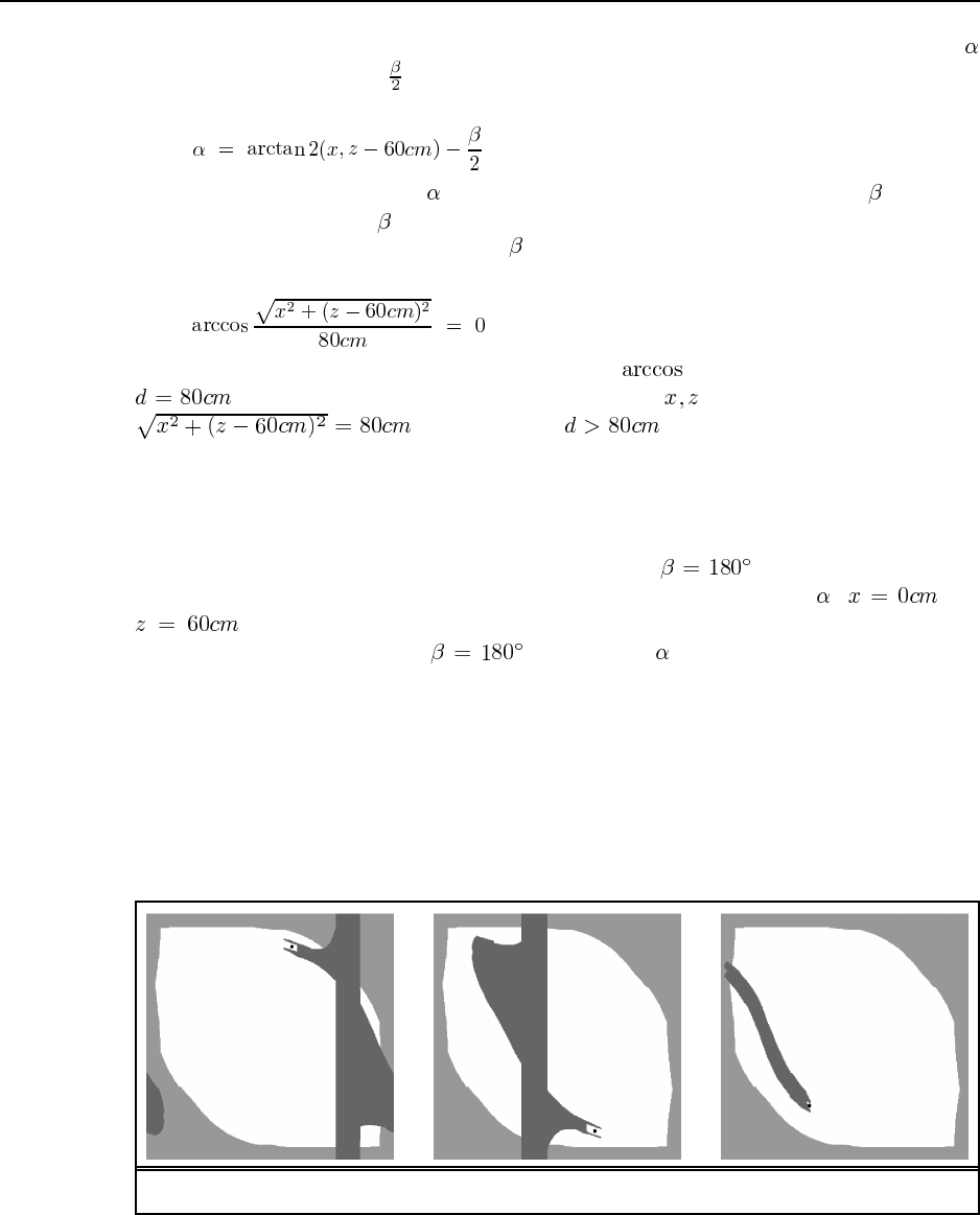
165
of the arcus tangens to all four quadrants (check it out—it is a function in C). The angle
is now obtained by adding , again exploiting that the shoulder and the elbow are of equal
length:
(25.3)
Of course, the actual value of depends on the actual choice of the value of . With the
exception of singularities, can take on exactly two values.
The inverse kinematics is unique if assumes a single value; as a consequence, so does
alpha. For this to be the case, we need that
(25.4)
This is the case exactly when the argument of the is 1, that is, when the distance
and the arm is fully stretched. The end points then lie on a circle defined by
. If the distance , there is no solution to the inverse
kinematic problem: the point is simply too far away to be reachable by the robot arm.
Unfortunately, configurations like these are numerically unstable, as the quotient may
be slightly larger than one (due to truncation errors). Such points are commonly called singu-
larities, and they can cause major problems for robot motion planning algorithms. A second
singularity occurs when the robot is “folded up,” that is, . Here the end effector’s
position is identical with that of the robot elbow, regardless of the angle : and
. This is an important singularity, as there are infinitely many solutions to the
inverse kinematics. As long as , the value of can be arbitrary. Thus, this sim-
ple robot arm gives us an example where the inverse kinematics can yield zero, one, two, or
infinitely many solutions.
25.4 Code not shown.
25.5
a. The configurations of the robots are shown by the black dots in the following figures.
Figure S25.2 Configuration of the robots.
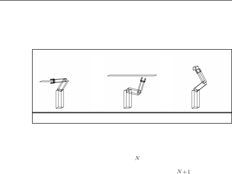
166 Chapter 25. Robotics
b. The above figure answers also the second part of this exercise: it shows the configura-
tion space of the robot arm constrained by the self-collision constraint and the constraint
imposed by the obstacle.
c. The three workspace obstacles are shown in the following diagrams:
Figure S25.3 Workspace obstacles.
d. This question is a great mind teaser that illustrates the difficulty of robot motion plan-
ning! Unfortunately, for an arbitrary robot, a planar obstacle can decompose the workspace
into any number of disconnected subspaces. To see, imagine a 1-DOF rigid robot that
moves on a horizontal rod, and possesses upward-pointing fingers, like a giant fork.
A single planar obstacle protruding vertically into one of the free-spaces between the
fingers could effectively separate the configuration space into disjoint subspaces.
A second DOF will not change this.
More interesting is the robot arm used as an example throughout this book. By
slightly extending the vertical obstacles protruding into the robot’s workspace we can
decompose the configuration space into five disjoint regions. The following figures
show the configuration space along with representative configurations for each of the
five regions.
Is five the maximum for any planar object that protrudes into the workspace of this
particular robot arm? We honestly do not know; but we offer a $1 reward for the first
person who presents to us a solution that decomposes the configuration space into six,
seven, eight, nine, or ten disjoint regions. For the reward to be claimed, all these regions
must be clearly disjoint, and they must be a two-dimensional manifold in the robot’s
configuration space.
For non-planar objects, the configuration space is easily decomposed into any num-
ber of regions. A circular object may force the elbow to be just about maximally
bent; the resulting workspace would then be a very narrow pipe that leave the shoulder
largely unconstrained, but confines the elbow to a narrow range. This pipe is then easily
chopped into pieces by small dents in the circular object; the number of such dents can
be increased without bounds.
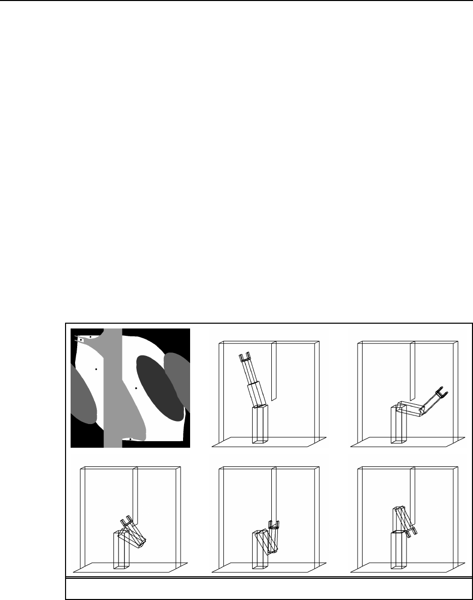
167
25.6 A simple deliberate controller might work as follows: Initialize the robot’s map with
an empty map, in which all states are assumed to be navigable, or free. Then iterate the
following loop: Find the shortest path from the current position to the goal position in the
map using A*; execute the first step of this path; sense; and modify the map in accordance
with the sensed obstacles. If the robot reaches the goal, declare success. The robot declares
failure when A* fails to find a path to the goal. It is easy to see that this approach is both
complete and correct. The robot always find a path to a goal if one exists. If no such path
exists, the approach detects this through failure of the path planner. When it declares failure,
it is indeed correct in that no path exists.
A common reactive algorithm, which has the same correctness and completeness prop-
erty as the deliberate approach, is known as the BUG algorithm. The BUG algorithm dis-
tinguishes two modes, the boundary-following and the go-to-goal mode. The robot starts in
go-to-goal mode. In this mode, the robot always advances to the adjacent grid cell closest to
the goal. If this is impossible because the cell is blocked by an obstacle, the robot switches to
the boundary-following mode. In this mode, the robot follows the boundary of the obstacle
until it reaches a point on the boundary that is a local minimum to the straight-line distance
to the goal. If such a point is reached, the robot returns to the go-to-goal mode. If the robot
reaches the goal, it declares success. It declares failure when the same point is reached twice,
which can only occur in the boundary-following mode. It is easy to see that the BUG algo-
rithm is correct and complete. If a path to the goal exists, the robot will find it. When the
robot declares failure, no path to the goal may exist. If no such path exists, the robot will
Figure S25.4 Configuration space for each of the five regions.

168 Chapter 25. Robotics
ultimately reach the same location twice and detect its failure.
Both algorithms can cope with continuous state spaces provides that they can accurately
perceive obstacles, plan paths around them (deliberative algorithm) or follow their boundary
(reactive algorithm). Noise in motion can cause failures for both algorithms, especially if the
robot has to move through a narrow opening to reach the goal. Similarly, noise in perception
destroys both completeness and correctness: In both cases the robot may erroneously con-
clude a goal cannot be reached, just because its perception was noise. However, a deliberate
algorithm might build a probabilistic map, accommodating the uncertainty that arises from
the noisy sensors. Neither algorithm as stated can cope with unknown goal locations; how-
ever, the deliberate algorithm is easily converted into an exploration algorithm by which the
robot always moves to the nearest unexplored location. Such an algorithm would be complete
and correct (in the noise-free case). In particular, it would be guaranteed to find and reach
the goal when reachable. The BUG algorithm, however, would not be applicable. A common
reactive technique for finding a goal whose location is unknown is random motion; this algo-
rithm will with probability one find a goal if it is reachable; however, it is unable to determine
when to give up, and it may be highly inefficient. Moving obstacles will cause problems for
both the deliberate and the reactive approach; in fact, it is easy to design an adversarial case
where the obstacle always moves into the robot’s way. For slow-moving obstacles, a common
deliberate technique is to attach a timer to obstacles in the grid, and erase them after a certain
number of time steps. Such an approach often has a good chance of succeeding.
25.7 There are a number of ways to extend the single-leg AFSM in Figure 25.22(b) into a set
of AFSMs for controlling a hexapod. A straightforward extension—though not necessarily
the most efficient one—is shown in the following diagram. Here the set of legs is divided into
two, named A and B, and legs are assigned to these sets in alternating sequence. The top level
controller, shown on the left, goes through six stages. Each stage lifts a set of legs, pushes the
ones still on the ground backwards, and then lowers the legs that have previously been lifted.
The same sequence is then repeated for the other set of legs. The corresponding single-
leg controller is essentially the same as in Figure 25.22(b), but with added wait-steps for
synchronization with the coordinating AFSM. The low-level AFSM is replicated six times,
once for each leg.
For showing that this controller is stable, we show that at least one leg group is on the
ground at all times. If this condition is fulfilled, the robot’s center of gravity will always be
above the imaginary triangle defined by the three legs on the ground. The condition is easily
proven by analyzing the top level AFSM. When one group of legs in (or on the way to
from ), the other is either in or , both of which are on the ground. However, this proof
only establishes that the robot does not fall over when on flat ground; it makes no assertions
about the robot’s performance on non-flat terrain. Our result is also restricted to static stabil-
ity, that is, it ignores all dynamic effects such as inertia. For a fast-moving hexapod, asking
that its center of gravity be enclosed in the triangle of support may be insufficient.
25.8 We have used this exercise in class to great effect. The students get a clearer picture of
why it is hard to do robotics. The only drawback is that it is a lot of fun to play, and thus the
students want to spend a lot of time on it, and the ones who are just observing feel like they
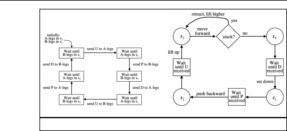
169
(a) (b)
Figure S25.5 Controller for a hexapod robot.
are missing out. If you have laboratory or TA sections, you can do the exercise there.
Bear in mind that being the Brain is a very stressful job. It can take an hour just to stack
three boxes. Choose someone who is not likely to panic or be crushed by student derision.
Help the Brain out by suggesting useful strategies such as defining a mutually agreed Hand-
centric coordinate system so that commands are unambiguous. Almost certainly, the Brain
will start by issuing absolute commands such as “Move the Left Hand 12 inches positive y
direction” or “Move the Left Hand to (24,36).” Such actions will never work. The most useful
“invention” that students will suggest is the guarded motion discussed in Section 25.5—that
is, macro-operators such as “Move the Left Hand in the positive y direction until the eyes say
the red and green boxes are level.” This gets the Brain out of the loop, so to speak, and speeds
things up enormously.
We have also used a related exercise to show why robotics in particular and algorithm
design in general is difficult. The instructor uses as props a doll, a table, a diaper and some
safety pins, and asks the class to come up with an algorithm for putting the diaper on the
baby. The instructor then follows the algorithm, but interpreting it in the least cooperative
way possible: putting the diaper on the doll’s head unless told otherwise, dropping the doll
on the floor if possible, and so on.

Solutions for Chapter 26
Philosophical Foundations
26.1 We will take the disabilities (see page 949) one at a time. Note that this exercise might
be better as a class discussion rather than written work.
a.be kind: Certainly there are programs that are polite and helpful, but to be kind requires
an intentional state, so this one is problematic.
b.resourceful: Resourceful means “clever at finding ways of doing things.” Many pro-
grams meet this criteria to some degree: a compiler can be clever making an optimiza-
tion that the programmer might not ever have thought of; a database program might
cleverly create an index to make retrievals faster; a checkers or backgammon program
learns to play as well as any human. One could argue whether the machines are “re-
ally” clever or just seem to be, but most people would agree this requirement has been
achieved.
c.beautiful: Its not clear if Turing meant to be beautiful or to create beauty, nor is it clear
whether he meant physical or inner beauty. Certainly the many industrial artifacts in
the New York Museum of Modern Art, for example, are evidence that a machine can
be beautiful. There are also programs that have created art. The best known of these
is chronicled in Aaron’s code: Meta-art, artificial intelligence, and the work of Harold
Cohen (McCorduck, 1991).
d.friendly This appears to fall under the same category as kind.
e.have initiative Interestingly, there is now a serious debate whether software should take
initiative. The whole field of software agents says that it should; critics such as Ben
Schneiderman say that to achieve predictability, software should only be an assistant,
not an autonomous agent. Notice that the debate over whether software should have
initiative presupposes that it has initiative.
f.have a sense of humor We know of no major effort to produce humorous works. How-
ever, this seems to be achievable in principle. All it would take is someone like Harold
Cohen who is willing to spend a long time tuning a humor-producing machine. We note
that humorous text is probably easier to produce than other media.
g.tell right from wrong There is considerable research in applying AI to legal reasoning,
and there are now tools that assist the lawyer in deciding a case and doing research. One
could argue whether following legal precedents is the same as telling right from wrong,
and in any case this has a problematic conscious aspect to it.
170

171
h.make mistakes At this stage, every computer user is familiar with software that makes
mistakes! It is interesting to think back to what the world was like in Turing’s day,
when some people thought it would be difficult or impossible for a machine to make
mistakes.
i.fall in love This is one of the cases that clearly requires consciousness. Note that while
some people claim that their pets love them, and some claim that pets are not conscious,
I don’t know of anybody who makes both claims.
j.enjoy strawberries and cream There are two parts to this. First, there has been little to
no work on taste perception in AI (although there has been related work in the food and
perfume industries; see http://198.80.36.88/popmech/tech/U045O.html for one such ar-
tificial nose), so we’re nowhere near a breakthrough on this. Second, the “enjoy” part
clearly requires consciousness.
k.make someone fall in love with it This criteria is actually not too hard to achieve; ma-
chines such as dolls and teddy bears have been doing it to children for centuries. Ma-
chines that talk and have more sophisticated behaviors just have a larger advantage in
achieving this.
l.learn from experience Part VI shows that this has been achieved many times in AI.
m.use words properly No program uses words perfectly, but there have been many natural
language programs that use words properly and effectively within a limited domain (see
Chapters 22-23).
n.be the subject of its own thought The problematic word here is “thought.” Many pro-
grams can process themselves, as when a compiler compiles itself. Perhaps closer to
human self-examination is the case where a program has an imperfect representation
of itself. One anecdote of this involves Doug Lenat’s Eurisko program. It used to run
for long periods of time, and periodically needed to gather information from outside
sources. It “knew” that if a person were available, it could type out a question at the
console, and wait for a reply. Late one night it saw that no person was logged on, so it
couldn’t ask the question it needed to know. But it knew that Eurisko itself was up and
running, and decided it would modify the representation of Eurisko so that it inherits
from “Person,” and then proceeded to ask itself the question!
o.have as much diversity of behavior as man Clearly, no machine has achieved this, al-
though there is no principled reason why one could not.
p.do something really new This seems to be just an extension of the idea of learning
from experience: if you learn enough, you can do something really new. “Really” is
subjective, and some would say that no machine has achieved this yet. On the other
hand, professional backgammon players seem unanimous in their belief that TDGam-
mon (Tesauro, 1992), an entirely self-taught backgammon program, has revolutionized
the opening theory of the game with its discoveries.
26.2 No. Searle’s Chinese room thesis says that there are some cases where running a
program that generates the right output for the Chinese room does not cause true understand-
ing/consciousness. The negation of this thesis is therefore that all programs with the right

172 Chapter 26. Philosophical Foundations
output do cause true understanding/consciousness. So if you were to disprove Searle’s the-
sis, then you would have a proof of machine consciousness. However, what this question is
getting at is the argument behind the thesis. If you show that the argument is faulty, then you
may have proved nothing more: it might be that the thesis is true (by some other argument),
or it might be false.
26.3 Yes, this is a legitimate objection. Remember, the point of restoring the brain to normal
(page 957) is to be able to ask “What was it like during the operation?” and be sure of
getting a “human” answer, not a mechanical one. But the skeptic can point out that it will not
do to replace each electronic device with the corresponding neuron that has been carefully
kept aside, because this neuron will not have been modified to reflect the experiences that
occurred while the electronic device was in the loop. One could fix the argument by saying,
for example, that each neuron has a single activation energy that represents its “memory,” and
that we set this level in the electronic device when we insert it, and then when we remove it,
we read off the new activation energy, and somehow set the energy in the neuron that we put
back in. The details, of course, depend on your theory of what is important in the functional
and conscious functioning of neurons and the brain; a theory that is not well-developed so
far.
26.4 This exercise depends on what happens to have been published lately. The NEWS
and MAGS databases, available on many online library catalog systems, can be searched
for keywords such as Penrose, Searle, Chinese Room, Dreyfus, etc. We found about 90
reviews of Penrose’s books. Here are some excerpts from a fairly typical one, by Adam
Schulman (1995).
Roger Penrose, the distinguished mathematical physicist, has again entered the lists to rid
the world of a terrible dragon. The name of this dragon is ”strong artificial intelligence.”
Strong Al, as its defenders call it, is both a widely held scientific thesis and an ongoing
technological program. The thesis holds that the human mind is nothing but a fancy calcu-
lating machine-”-a computer made of meat”–and that all thinking is merely computation;
the program is to build faster and more powerful computers that will eventually be able to
do everything the human mind can do and more. Penrose believes that the thesis is false
and the program unrealizable, and he is confident that he can prove these assertions.
In Part I of Shadows of the Mind Penrose makes his rigorous case that human conscious-
ness cannot be fully understood in computational terms. How does Penrose prove that
there is more to consciousness than mere computation? Most people will already find it
inherently implausible that the diverse faculties of human consciousness–self-awareness,
understanding, willing, imagining, feeling–differ only in complexity from the workings
of, say, an IBM PC.
Students should have no problem finding things in this and other articles with which to dis-
agree. The comp.ai Newsnet group is also a good source of rash opinions.
Dubious claims also emerge from the interaction between journalists’ desire to write
entertaining and controversial articles and academics’ desire to achieve prominence and to be
viewed as ahead of the curve. Here’s one typical result— Is Nature’s Way The Best Way?,
Omni, February 1995, p. 62:

173
Artificial intelligence has been one of the least successful research areas in computer
science. That’s because in the past, researchers tried to apply conventional computer
programming to abstract human problems, such as recognizing shapes or speaking in
sentences. But researchers at MIT’s Media Lab and Boston University’s Center for Adap-
tive Systems focus on applying paradigms of intelligence closer to what nature designed
for humans, which include evolution, feedback, and adaptation, are used to produce com-
puter programs that communicate among themselves and in turn learn from their mistakes.
Profiles In Artificial Intelligence, David Freedman.
This is not an argument that AI is impossible, just that it has been unsuccessful. The full
text of the article is not given, but it is implied that the argument is that evolution worked
for humans, therefore it is a better approach for programs than is “conventional computer
programming.” This is a common argument, but one that ignores the fact that (a) there are
many possible solutions to a problem; one that has worked in the past may not be the best in
the present (b) we don’t have a good theory of evolution, so we may not be able to duplicate
human evolution, (c) natural evolution takes millions of years and for almost all animals
does not result in intelligence; there is no guarantee that artificial evolution will do better (d)
artificial evolution (or genetic algorithms, ALife, neural nets, etc.) is not the only approach
that involves feedback, adaptation and learning. “Conventional” AI does this as well.
26.5 This also might make a good class discussion topic. Here are our attempts:
intelligence: a measure of the ability of an agent to make the right decisions, given the
available evidence. Given the same circumstances, a more intelligent agent will make better
decisions on average.
thinking: creating internal representations in service of the goal of coming to a conclu-
sion, making a decision, or weighing evidence.
consciousness: being aware of one’s own existence, and of one’s current internal state.
Here are some objections [with replies]:
For intelligence, too much emphasis is put on decision-making. Haven’t you ever
known a highly intelligent person who made bad decisions? Also no mention is made of
learning. You can’t be intelligent by using brute-force look-up, for example, could you? [The
emphasis on decision-making is only a liability when you are working at too coarse a gran-
ularity (e.g., “What should I do with my life?”) Once you look at smaller-grain decisions
(e.g., “Should I answer a, b, c or none of the above?), you get at the kinds of things tested by
current IQ tests, while maintaining the advantages of the action-oriented approach covered
in Chapter 1. As to the brute-force problem, think of intelligence in terms of an ecological
niche: an agent only needs to be as intelligent as is necessary to be successful. If this can be
accomplished through some simple mechanism, fine. For the complex environments that we
humans are faced with, more complex mechanisms are needed.]
For thinking, we have the same objections about decision-making, but in general, think-
ing is the least controversial of the three terms.
For consciousness, the weakness is the definition of “aware.” How does one demon-
strate awareness? Also, it is not one’s true internal state that is important, but some kind of
abstraction or representation of some of the features of it.

174 Chapter 26. Philosophical Foundations
26.6 It is hard to give a definitive answer to this question, but it can provoke some interesting
essays. Many of the threats are actually problems of computer technology or industrial society
in general, with some components that can be magnified by AI—examples include loss of
privacy to surveillance, and the concentration of power and wealth in the hands of the most
powerful. As discussed in the text, the prospect of robots taking over the world does not
appear to be a serious threat in the foreseeable future.
26.7 Biological and nuclear technologies provide mush more immediate threats of weapons,
yielded either by states or by small groups. Nanotechnlogy threatens to produce rapidly re-
producing threats, either as weapons or accidently, but the feasibility of this technology is still
quite hypothetical. As discussed in the text and in the previous exercise, computer technology
such as centralized databases, network-attached cameras, and GPS-guided weapons seem to
pose a more serious portfolio of threats than AI technology, at least as of today.
26.8 To decide if AI is impossible, we must first define it. In this book, we’ve chosen a
definition that makes it easy to show it is possible in theory—for a given architecture, we
just enumerate all programs and choose the best. In practice, this might still be infeasible,
but recent history shows steady progress at a wide variety of tasks. Now if we define AI as
the production of agents that act indistinguishably form (or at least as intellgiently as) human
beings on any task, then one would have to say that little progress has been made, and some,
such as Marvin Minsky, bemoan the fact that few attempts are even being made. Others think
it is quite appropriate to address component tasks rather than the “whole agent” problem.
Our feeling is that AI is neither impossible nor a ooming threat. But it would be perfectly
consistent for someone to ffel that AI is most likely doomed to failure, but still that the risks
of possible success are so great that it should not be persued for fear of success.

Solutions for Chapter 27
AI: Present and Future
There are no exercises in this chapter. There are many topics that are worthy of class dis-
cussion, or of paper assignments for those who like to emphasize such things. Examples
are:
What are the biggest theoretical obstacles to successful AI systems?
What are the biggest practical obstacles? How are these different?
What is the right goal for rational agent design? Does the choice of a goal make all that
much difference?
What do you predict the future holds for AI?
175
Bibliography
Andersson, R. L. (1988). A robot ping-pong
player: Experiment in real-time intelligent con-
trol. MIT Press, Cambridge, Massachusetts.
Bahle, D., Williams, H., and Zobel, J. (2002).
Efficient phrase querying with an auxiliary in-
dex. In Proceedings of the ACM-SIGIR Confer-
ence on Research and Development in Informa-
tion Retrieval, pp. 215–221.
Chomsky, N. (1957). Syntactic Structures. Mou-
ton, The Hague and Paris.
Cormen, T. H., Leiserson, C. E., and Rivest, R.
(1990). Introduction to Algorithms. MIT Press,
Cambridge, Massachusetts.
Dawkins, R. (1976). The Selfish Gene. Oxford
University Press, Oxford, UK.
Gold, E. M. (1967). Language identification in
the limit. Information and Control,10, 447–474.
Heinz, E. A. (2000). Scalable search in computer
chess. Vieweg, Braunschweig, Germany.
Held, M. and Karp, R. M. (1970). The traveling
salesman problem and minimum spanning trees.
Operations Research,18, 1138–1162.
Kay, M., Gawron, J. M., and Norvig, P. (1994).
Verbmobil: A Translation System for Face-To-
Face Dialog. CSLI Press, Stanford, California.
Kearns, M. and Vazirani, U. (1994). An In-
troduction to Computational Learning Theory.
MIT Press, Cambridge, Massachusetts.
Keeney, R. L. and Raiffa, H. (1976). Decisions
with Multiple Objectives: Preferences and Value
Tradeoffs. Wiley, New York.
McCorduck, P. (1991). Aaron’s code: Meta-
art, artificial intelligence, and the work of Harold
Cohen. W. H. Freeman, New York.
Moore, A. W. and Atkeson, C. G. (1993). Pri-
oritized sweeping—reinforcement learning with
less data and less time. Machine Learning,13,
103–130.
Norvig, P. (1992). Paradigms of Artificial Intel-
ligence Programming: Case Studies in Common
Lisp. Morgan Kaufmann, San Mateo, California.
Pearl, J. (1988). Probabilistic Reasoning in Intel-
ligent Systems: Networks of Plausible Inference.
Morgan Kaufmann, San Mateo, California.
Quine, W. V. (1960). Word and Object.
MIT Press, Cambridge, Massachusetts.
Schulman, A. (1995). Shadows of the mind: A
search for the missing science of consciousness
(book review). Commentary,99, 66–68.
Smith, D. E., Genesereth, M. R., and Ginsberg,
M. L. (1986). Controlling recursive inference.
Artificial Intelligence,30(3), 343–389.
Tesauro, G. (1992). Practical issues in temporal
difference learning. Machine Learning,8(3–4),
257–277.
Wahlster, W. (2000). Verbmobil: Foundations of
Speech-to-Speech Translation. Springer Verlag.
Witten, I. H., Moffat, A., and Bell, T. C. (1999).
Managing Gigabytes: Compressing and Index-
ing Documents and Images (second edition).
Morgan Kaufmann, San Mateo, California.
177
