Stochastic GW Manual V1.0
User Manual: Pdf
Open the PDF directly: View PDF ![]() .
.
Page Count: 26

stochasticGW – User manual and Tutorial (version 1.0)
Vojtěch Vlček,1,2Christopher Arntsen,3Wenfei Li,1Roi Baer,4
Eran Rabani,5,6and Daniel Neuhauser1
1Department of Chemistry and Biochemistry,
University of California, Los Angeles California 90095, USA.
2After July 1st, 2018: Department of Chemistry and Biochemistry, University
of California, Santa Barbara California 93106, USA
3Department of Chemistry,
Youngstown State University, Youngstown, Ohio 44555
4Fritz Haber Center for Molecular Dynamics, Institute of Chemistry,
The Hebrew University of Jerusalem, Jerusalem 91904, Israel
5Department of Chemistry,
University of California, Berkeley, California 94720, USA
6The Sackler Center for Computational Molecular Science,
Tel Aviv University, Tel Aviv 69978, Israel

Contents
1 Introduction 3
2 License 4
3 Overview 5
4 Code status 7
5 Downloading, compilation and installation 8
5.1 Downloading and installation ..................... 8
5.2 Compilation ............................... 8
5.3 Implementation ............................. 8
6 Input files 10
6.1 Brief overview of the input files .................... 10
6.2 Detailed description of the files and flags ............... 10
7 Output 18
8 Tutorial 20
8.1 H2: Combined Stochastic and Deterministic treatment ....... 20
8.2 C60: Fully stochastic calculation ................... 23
9 Acknowledgements 26
2stochasticGW - User manual and Tutorial

1 Introduction
This manual details stochasticGW , a software for large scale linear-scaling
G0W0stochastic calculations. The code combines the success of the G0W0ap-
proximation, a quantitative approach for vertical ionization energies and electron
affinities, with the ability of stochastic methods to tackle very large systems. The
methodology was introduced and detailed in several recent references, especially:
Ref. I : D. Neuhauser, Y. Gao, C. Arntsen, C. Karshenas, E. Rabani and R. Baer,
Breaking the theoretical scaling limit for predicting quasiparticle energies:
The stochastic GW approach, Phys. Rev. Lett., 113, 076402 (2014).
https://journals.aps.org/prl/abstract/10.1103/PhysRevLett.113.076402
Ref. II : V. Vlcek, E. Rabani, D. Neuhauser and R. Baer, Stochastic GW calculations
for molecules, J. Chem. Theo. Comput. 13, 4997 (2017).
https://arxiv.org/abs/1612.08999
Ref. III : V. Vlcek, W. Li, R. Baer, E. Rabani and D. Neuhauser, Turbo-boosting
GW beyond >10,000 electrons using fractured stochastic orbitals, to be
placed on the Arxiv (2018)
If this is your first time using this manual, read the Overview and Downloading→Sections: 3, 5 & 8
and compilation section, and then jump to the Tutorial.
stochasticGW - User manual and Tutorial 3

2 License
Unless otherwise stated, all files distributed in this package are licensed under
the following terms:
stochasticGW
Developed by:
stochasticGW, University of California, Los Angeles
http://www.stochasticgw.com/
Permission is hereby granted, free of charge, to any person obtaining a copy of the
stochasticGW software and associated documentation files (the “Software”), to
deal with the Software without restriction, including without limitation the rights
to use, copy, modify, merge, publish, distribute, sublicense, and/or sell copies of
the Software, and to permit persons to whom the Software is furnished to do so,
subject to the following conditions:
1. Redistributions of source code must retain the above copyright notice, this
list of conditions and the following disclaimers.
2. Redistributions in binary form must reproduce the above copyright notice,
this list of conditions and the following disclaimers in the documentation
and/or other materials provided with the distribution.
3. Neither the names of stochasticGW , stochasticGW, University of Cal-
ifornia, Los Angeles, nor the names of its contributors may be used to
endorse or promote products derived from this Software without specific
prior written permission.
THE SOFTWARE IS PROVIDED “AS IS”, WITHOUT WARRANTY OF ANY
KIND, EXPRESS OR IMPLIED, INCLUDING BUT NOT LIMITED TO THE
WARRANTIES OF MERCHANTABILITY, FITNESS FOR A PARTICULAR
PURPOSE AND NONINFRINGEMENT. IN NO EVENT SHALL THE CON-
TRIBUTORS OR COPYRIGHT HOLDERS BE LIABLE FOR ANY CLAIM,
DAMAGES OR OTHER LIABILITY, WHETHER IN AN ACTION OF CON-
TRACT, TORT OR OTHERWISE, ARISING FROM, OUT OF OR IN CON-
NECTION WITH THE SOFTWARE OR THE USE OR OTHER DEALINGS
WITH THE SOFTWARE.
You are under no obligation whatsoever to provide any bug fixes, patches, or
upgrades to the features, functionality or performance of the source code (“En-
hancements”) to anyone; however, if you choose to make your Enhancements
available either publicly, or directly to stochasticGW University of California,
Los Angeles, without imposing a separate written license agreement for such En-
hancements, then you hereby grant the following license: a non-exclusive, royalty-
free perpetual license to install, use, modify, prepare derivative works, incorporate
into other computer software, distribute, and sublicense such enhancements or
derivative works thereof, in binary and source code form.
4stochasticGW - User manual and Tutorial

3 Overview
stochasticGW calculates a matrix element of the self-energy in the G0W0ap-
proximation
Σ (ω) = Dφ
ˆ
Σ (ω)
φE,(1)
where φis a single particle orbital of the molecule studied (typically a HOMO or
LUMO), associated with a DFT Hamiltonian ˆ
H;ˆ
Σis the self-energy operator,
composed of a static exchange component (X) and a polarization part (P)
Dφ
ˆ
Σ (ω)
φE=Dφ
ˆ
ΣX
φE+Dφ
ˆ
ΣP(ω)
φE,(2)
where the latter is a Fourier transform
Dφ
ˆ
ΣP(ω)
φE=Zeiωt Dφ
ˆ
ΣP(t)
φEdt. (3)
In the G0W0approximation the coordinate representation of ˆ
ΣP(t)is extremely
simple:
ΣP(r,r0, t) = G0(r,r0, t)WPr,r0, t+,(4)
where we introduced the non-interacting Green’s function and the dynamical part
of the effective interaction.
The starting point (used for G0and W), is a Kohn-Sham Hamiltonian which
is constructed from ground state orbitals φ. At the moment (version 1.0) the
stochasticGW code is limited to an LDA starting point – this restriction will
be lifted in the upcoming versions of the code. Orbitals φare represented on a
real-space grid and have to be supplied by the user.
The matrix element of the self-energy is evaluated as a statistical average over
multiple stochastic realizations - the number of Monte Carlo samples. The
stochastic approach uses multiple resolutions of the identity with random func-
tions for several purposes:
•Separating the product of G0and WP, converting the calculation of ΣP
into evaluating a matrix element of WP.
•Evaluating a matrix element of WP R (where the Rsubscript indicates a
causal, i.e., retarded effective interaction) by stochastic TDH (time-dependent
Hartree, yielding RPA) or stochastic TDDFT .
•Converting the matrix elements of WP R to matrix elements of WP(the time-
ordered effective interaction) through a stochastic fragment basis approach
(Ref. III).
The eventual method scales practically linearly (or better) with system size; for
details of the method and scaling read Refs. I&II and, for the closest description
to the present version, Ref. III
The program outputs the matrix element of the polarization self-energy,
Dφ
ˆ
ΣP(ω)
φE, over a wide range of frequencies, as well as the exchange self-
energyDφ
ˆ
ΣX
φE. The code also prints the estimate of the quasiparticle energy
stochasticGW - User manual and Tutorial 5

of state φfor the given number of Monte Carlo samples, obtained from solving
the quasiparticle equation:
ε=εKS +Dφ
ˆ
ΣX+ˆ
ΣP(ε)−ˆvxc
φE,(5)
where εKS is Kohn-Sham eigenvalue of the eigenstate φand ˆvxc is the (mean-
field) exchange-correlation potential. The input and output are detailed in the
sections below.
6stochasticGW - User manual and Tutorial

4 Code status
Several items in this 1.0 version have not been implemented or tested. Specifically,
note that:
•The code has not been tested for open-shell systems.
•The core-shell exchange correction is implemented but not tested.
•Only a local LDA exchange-correlation potential is implemented.
•The numbers of points in each dimension, nx,ny,nz need all to be even.
•The maximum angular momentum in the nonlocal pseudopotentials needs
to be 1or 2or 3. If it is 1then it is necessary to have lloc=2.
stochasticGW - User manual and Tutorial 7

5 Downloading, compilation and installation
5.1 Downloading and installation
stochasticGW is a Fortran code requiring Open MPI parallelization; The tgz
tar file is available from:
https://github.com/stochasticGW/stochasticGW
For installation, first unpack the archive:
tar -xzvf sgw-v1.0.tgz
Upon unpacking, you will get a directory sgw-v1.0 with a README file and 3
subdirectories:
examples/ PP/ README src/
The installation of the package is detailed then in README and is repeated here.
An installation of the FFTW library (version 3.1 or higher) is a prerequisite; it can!→be downloaded from http://www.fftw.org.
5.2 Compilation
In the src directory you will find a makefile that needs a little modification
depending on your system settings, as described below.
Edit makefile and specify your parallel compiler (FCMPI) and FFTW library (FFTFLG).
The flags for the parallel compiler (MPIFLG) can usually be left unaltered.
The supplied header of makefile reads:
FCMPI = mpif90
MPIFLG = -DMPI -O3
FFTFLG = -lfftw3
The stochasticGW code is built simply by writing:
make
in the src directory.
After successful compilation, the stochasticGW executable, sgw.x, will be found
in the src directory.
Make sure sgw.x has been created
ls -l sgw.x
5.3 Implementation
Now you are ready to implement the code. Then, say you want to run it in a
directory you will call ∼/mygwrun. Go there, and copy the H2example input,
the executable, and pseudopotentials to this directory:
mkdir ~/mygwrun
cd ~/mygwrun
cp ~/sGW_v1/examples/H2/* .
cp ~/sGW_v1/src/sgw.x .
cp -r ~/sGW_v1/PP/ .
8stochasticGW - User manual and Tutorial

At this point, your mygwrun directory should contain the following:
cnt.ini counter.inp INPUT log_h2example PP random.inp sgw.x wf.txt
where PP is a directory (with pseudopotentials). All these files are inputs except
for log_h2example.
To run the H2example (from the Tutorial) on, say, 30 cores, write
mpirun -n 30 ./sgw.x >& log &
The output file log should match log_h2example.
After the H2test is finished, you can run any other molecule/material you want.
You’ll need to change a few items, detailed below and in the Tutorial.
•Change INPUT as needed – especially make sure that you change ntddft
to be between 8 and 30.
•Change the atomic coordinates (cnt.ini).
•Bring your own wf.txt (or better yet, wf.bin ) file that contains the oc-
cupied DFT energies and functions.
•And remember to include in PP/ any pseudopotential you need.
stochasticGW - User manual and Tutorial 9

6 Input files
6.1 Brief overview of the input files
Two groups of input files are required in the working directory. One set includes
general parameters, and the other system-specific files.
Seed, labels and flags
random.inp : seed file for the random number generator.
counter.inp : a label file with a counter for modifying the random number input and
for labeling the input. Using this file simplifies working simultaneously on
multiple runs.
INPUT : general input file with flags and parameters.
System specific files
cnt.ini : atomic position file (in Angstroms or atomic units).
*UPF/*fhi : pseudopotential files (only two formats are currently supported). These
files should be placed in a subdirectory of the working directory, PP/
wf.txt or wf.bin : text or binary file with all occupied (and possibly a few unoccupied) wave-
functions.
orb.txt (optional) : an orbital wavefunction (“φ” in the previous discussion) for which the self-
energy matrix element is needed. Usually this file will not be given and
instead φwill be extracted from wf.txt or wf.bin.
6.2 Detailed description of the files and flags
FILE: random.inp
A file with 6 lines, each with 4 integer numbers (Fortran format integer*8).
These are the seeds for the KISS random-number algorithm. Each line in is a
seed for a different random variable used in the StochasticGW algorithm.
FILE: counter.inp
A file with a single integer that labels the output directories and files and also
modifies the seed. It alleviates the need for different runs to use different ran-
dom.inp files when the calculation is repeated to reduce the statistical error (see
example below)
10 stochasticGW - User manual and Tutorial

Example
Let’s say we want nmctot=2000 stochastic samples.aThis can be achieved
by a single run with 2000 stochastic samples, or perhaps, due to computer
jobs scheduling issues, it may be easier to submit 5 different jobs, each with
400 stochastic samples.
For these 5 jobs we would need, in principle, 5 different random.inp files with
totally different values, which is cumbersome. We therefore use counter.inp.
Each counter modifies the values of the variables from random.inp. So in
our example we would only need to submit 5 different jobs, each with the
same random.inp file, and in each run the counter.inp file contains a dif-
ferent integer from, say, 0 to 4 (or any other 5 different integers).
Then, at the end of the 5 runs, average the 5 output quasiparticle energies
or 5 output self-energies files.
asee also the buffer_size variable, which controls the parallelization of multiple stochas-
tic states.
FILE: INPUT
Main file for flags and parameters. For most variables the default values are
appropriate. Examples are shown in the Tutorial.
Specifically, only one set of variables has to be specified in INPUT: the names of
the pseudopotentials (variable: pps). Other parameters need to be included in
the INPUT file only if they differ from their default values. The format for most
variables (except for the pseudopotential names) is:
variable name
<value>
<empty line>
The order is not important, but no variable should be repeated; lines starting
with #are ignored. The input variables are:
pps : a label indicating the beginning of the list of pseudopotentials. After the
last pseudopotential put a line starting with #. The pseudopotentials listed
must be present in a subdirectory of the working directory (where the INPUT
file is) called PP/. It is recommended to use well-tested pseudopotentials.
At present, the supported formats are *UPF and *fhi. In addition, the
code currently supports only the LDA functional. In the next versions,
other functionals will be included too.
Note that the program will issue a warning if the pseudopotential wavefunc-!→tions are not properly normalized, but it will then normalize them properly.
scratch : (default: GW_SCRATCH) the prefix of the name of the scratch directory; the
scratch directory is then appended by the counter (from the counter.inp
file).
stochasticGW - User manual and Tutorial 11

Example
If counter.inp contains the number 0, and the relevant segment from
INPUT is
scratch
/scratch/john/GW_SCRATCH
<empty line>
then the scratch directory will be /scratch/john/GW_SCRATCH.0
The scratch directory contains several intermediate files. It should be
ideally not placed on the main shared disk but on fast disks connected
to each core, if such disks are available.
Each core will try to create this scratch directory, unless it was created
earlier by another core accessing the same scratch disk.
nmctot : (default: 1000) the number of stochastic realizations used for statistical av-
eraging (Monte Carlo iterations). Typically 300-2000 iterations are needed
for acceptable convergence. The error in the output self-energy and quasi-
particle energies decreases as 1
√nmctot .
If nmctot is larger than the number of MPI processes Nproc the calcu-
lation will be repeated (nmctot/Nproc) times. For instance: if you set
nmctot=1000 and distribute the job over Nproc=100 cores, the calculation
will be repeated 10 times on each core.
If needed, the program increases nmctot so that mod(nmctot,Nproc)=0.
binary : (default: .TRUE.) a logical variable; designating whether the occupied wave-
functions are stored in a binary file wf.bin or a text one wf.txt.
periodic : (default: .FALSE.) a logical variable designating whether the calculation is
periodic (restricted to Γ-point sampling).
box : (default: pos) a character*3 variable designating the way the calculation
box is constructed. Two values are allowed, pos and sym .
The first choice, pos, implies that the calculation box is (in Bohr!)
[0,nx*dx][0,ny*dy][0,nz*dz]. The wavefunctions in wf.txt are then
interpreted to start at the corner of this box, (0,0,0). Such box convention
is used in Quantum Espresso and most planewave codes. Note that in our
code the coordinates in the cnt.ini file need to fit in the box (or more
preceisely, if they are given in Angstrom, their values in Bohr need to fit in
the box). If they do not fit in the box the program will stop.
The second, sym, assumes that the box of the calculation is
[-nx*dx/2,nx*dx/2][-ny*dy/2,ny*dy/2][-nz*dz/2,nz*dz/2]
(again in Bohr), i.e., its center is the origin. The wavefunctions in wf.txt
are again interpreted to start at the corner of the box, which is now
(-nx*dx/2,-ny*dy/2,-nz*dz/2). Again, the coordinates in cnt.ini need
to fit in the box (once expressed in Bohr). This symmetric box convention
is more natural for non-periodic molecules.
multiplicity : (default: 1) either 1 or 2; 1 indicates a closed-shell calculation, 2 an open
12 stochasticGW - User manual and Tutorial

shell. Note: the program was not tested for open-shell systems,
and at this stage should be trusted only for closed-shell calcula-
tions.
ekcut : (default: 25.0) a cutoff (in Hartree) on the kinetic energy. Even though
there is a formal maximum on the kinetic energy on the grid (and the grid
is supplied elsewhere, see below) it is numerically better to use a lower
cutoff. In practice one should use a value somewhat higher than the depth
of the pseudopotentials. For calculations with a new element check the
convergence of the calculations with ekcut=15 to 30 Hartree.
gamma : (default: 0.06) energy broadening parameter for ΣP(Section 3 in Ref. II and
the supplementary material in Ref. I). Generally 0.06 should be fine. An
increased gamma reduces the computational effort and improves somewhat
the statistics, but if gamma is too large the broadening will be too severe
leading to wrong quasiparticle predictions.
orb_indx : (default: -1). If orb_indx>0 its value designates the orbital φwhich will
be used in the calculation of the self-energy (e.g., if orb_indx=5 then φis
the 5th eigenstate). If orb_indx is -1 then φshould be read from orb.txt .
ntddft : (default: 15) the number of stochastic states used in the time-dependent
RPA or TDDFT calculation (in the Wpart of GW ). For very small systems,
use ∼30. For large systems with hundreds of electrons or more, it is enough
to use ∼8orbitals.
For open-shell systems (multiplicity=2) ntddft denotes the number of
stochastic TDRPA/TDDFT states for each spin.
For a non-stochastic TDRPA/TDDFT propagation, use ntddft = -1. Then!→a deterministic TDRPA/TDDFT calculation is used for calculating the ac-
tion of W. In this case all occupied orbitals are excited and propagated.
This choice should only be done for small systems, since it increases the
computational time considerably. A non-stochastic calculation of the ac-
tion of Wis neither feasible nor needed for large systems, since the stochas-
tic calculation of the action of Wis getting progressively better for bigger
systems.
units_nuc : (default: Bohr) either Angstrom, or Bohr. Controls the units for the nuclear
positions input (in the cnt.ini file).
flg_dyn : (default: .FALSE.) logical variable; .FALSE. implies an RPA calculation;
.TRUE. yields a TDDFT calculation of the action of Wwhere the exchange-
correlation potential is updated at each time-step.
The following variables could usually be safely kept at their default values: :
dt : (default: 0.05) time step in atomic units for the TD propagation of W(note:
0.05 a.u.'1.2 attosec). If desired, dt could be reduced to 0.03, although
0.05 generally works well.
nxi : (default: 10,000) Number of random spanning vectors (denoted Nξin Ref.-
III). Usually there’s no need to change the default.
segment_fraction : (default: 0.003) The ratio of the size of each stochastic vector ξto the total
grid length. See Ref. III. Usually there’s no need to change the default.
stochasticGW - User manual and Tutorial 13

sm : (default: 0.0001) The perturbation parameter (denoted τin Eq. 29 in
Ref. II). The results should not vary for sm in the range 10−5–10−3.
scale_vh : (default: 2; but will be set to 1 by the program if periodic) allowed values
1 or 2. Controls whether a Martyna-Tuckerman1grid-doubling is used in
the TDRPA/TDDFT calculations. If the calculation is periodic, scale_vh
would be set in the program to 1 regardless of the input value. For non-
periodic molecules, scale_vh formally needs to be set at 2. So since the
program automatically sets scale_vh, there is usually no need to touch this
variable.
nrppmx : (default: 1200) an upper bound on the number of radial grid points for
the pseudopotential. No need to change unless a new pseudopotential with
more than 1200 grid points is used.
buffer_size : (default: 1) the number of cores used in each independent stochastic runs.
For intermediate or large size systems (hundreds or thousands of electrons)
choose the default (1) which uses the least total CPU resources. But for
very large systems, the wall-time of the calculation could be too long when
using a buffer_size of 1. Generally, it is a good idea to use a buffer_size
which either equals to the number of cores on each CPU, or divides it (e.g.,
if there are 12 cores on each CPU, use a buffer_size of 1,2,3,4,6 or 12).
Also, if buffer_size is >1, aim at having mod(ntddft+1,buffer_size)=0.
For instance: if buffer_size is 12, use ntddft=11, 23 or 35. If ntddft is
bigger the convergence is somewhat faster, but the effort grows, so values
in the range 8-30 are usually the most efficient.
Example
Let’s say that a giant system requires about 1000 Monte Carlo itera-
tions. One could use 1000 cores and then each core will be used for
a single Monte Carlo iteration. But say that such a single calculation
took 2 days (i.e., each core takes 2 days), while the computer-center al-
location limits each run to be 1 day long. In that case, it is necessary
to spread each single calculation to several cores. For example, use
then a buffer_size of 4 and 4000 mpi cores to do the 1000 Monte-
Carlo iterations, and each group of 4 cores will do a single stochastic
run. The calculation will then take a shorter wall-time.
Note: to spread the work in each separate run to several cores, we
use the mpi_comm_split routine, which divides the cores to subsets,
usually labeled as colors. Further details can be found on the web.
a
aa good introduction is in http://www.bu.edu/tech/support/research/
training-consulting/online-tutorials/mpi/more/mpi_comm_split/
1G.J. Martyna, and M.E. Tuckerman, “A reciprocal space based method for treating long range
interactions in ab-initio and force-field-based calculation in clusters”, J. Chem. Phys. 110,
2810 (1999),doi:10.1063/1.477923
14 stochasticGW - User manual and Tutorial

FILE: cnt.ini
Nuclear positions in a Cartesian format:
<element name> <x-coordinate> <y-coordinate> <z-coordinate>
The element name is in a 1- or 2-character format (e.g., H or Si). The nuclear
units could be in Angstrom or Bohr (the units are specified by the units_nuc
variable, the default of which is Bohr), but recall that all other quantities in
the code are calculated in atomic units, i.e., Hartree for energies and Bohr for
distances.
FILE: wf.txt
A wavefunction input file (required if binary =.FALSE.) with all occupied (and
potentially a few unoccupied) eigenstates. The first 6 lines detail the grid used
(lengths in Bohr), followed by the multiplicity (which needs to match the default
value or, if given, the value in INPUT), and the Kohn-Sham eigenvalues. Then
each wavefunction is given, preceded by the state-indicies (and possibly the spin-
index, if multiplicity=2). The file contains the state index on the 12th,14th, . . .
lines:
nx <number of points along the x direction>
ny <number of points along the y direction>
nz <number of points along the z direction>
dx <grid spacing in the x direction>
dy <grid spacing in the y direction>
dz <grid spacing in the z direction>
nsp <multiplicity>
nstates <number of states in this wf.txt file>
evls
<kohn-Sham eigenvalues>
orbitals
1 <spin-index of 1st orbital>
<1st orbital>
2 <spin-index of 2nd orbital>
<2nd orbital>
.
.
.
Note that the list of Kohn-Sham eigenvalues should include all "nstates" eigen-
values.
The program determines the number of states to be read based on the ionic
charges provided in the pseudopotential files. If the normalization of any orbital
is incorrect a warning is issued but the program continues.
The orbital is given as usual in Fortran with the left-most index (x) varying the
fastest. Each orbital should contain nx ·ny ·nz points.
If the multiplicity is 2 (open-shell), the spin-index of each orbital should be 1 or
2 (indicating an αor βspin). The spin-index is not required if the multiplicity
is 1 (closed-shell).
stochasticGW - User manual and Tutorial 15

FILE: wf.bin
The wavefunction input file (required if binary =.TRUE.). Analogous to wf.txt.
When preparing this binary file from your favorite DFT program output, you
should follow the example of the following code segment:
real*8 hw(1:nstates)
real*8 orbitals(1:ngrid,1:nstates)
...
open(9,file=’wf.bin’,status=’old’,form=’unformatted’)
write(9)’nx ’,nx
write(9)’ny ’,ny
write(9)’nz ’,nz
write(9)’dx ’,dx
write(9)’dy ’,dy
write(9)’dz ’,dz
write(9)’nsp ’,nsp
write(9)’nstates ’,nstates
write(9)’evls ’
write(9)(hw(i),i=1,nstates)
write(9)’orbitals ’
do i=1,nstates
! ispin: 1 for closed shell; 1 or 2 for open shell.
write(9)i, ispin(i)
write(9)u(1:ngrid,i)
enddo
close(9)
Each text string in lines 1-9 and 11 is of length 9.
At present, the user needs to prepare wf.bin, but in future versions we would
supply preparation routines that process the output of Quantum Espresso, Abinit,
and other DFT programs and produce the proper wf.bin file.
FILE: orb.txt
Orbital φfor which the quasiparticle energy is sought. This orbital is usually
taken from a DFT code. Typically it will be the HOMO or the LUMO. The file
is organized similarly to the wavefunction file, and the heading values need to
match those in wf.txt or wf.bin
nx <number of points along the x direction>
ny <number of points along the y direction>
nz <number of points along the z direction>
dx <grid spacing in the x direction>
dy <grid spacing in the y direction>
dz <grid spacing in the z direction>
nsp <multiplicity>
orb <kohn sham orbital energy for this specific orbital>
<values of the orbital φon the grid>
16 stochasticGW - User manual and Tutorial

The program issues an error warning if the normalization of φis wrong (but will
not stop).
If the orb_indx variable is specified, with a value bigger than 0, then orb.txt is
not needed and φwill be taken directly from the wavefunction file.
FILE: *UPF/*fhi
A pseudopotential file is needed for each of the elements in the molecule (i.e.,
each of the different element in cnt.ini). The names of the pseudopotential
files are specified by variable pps. The pseudopotentials should be placed in a
subdirectory, PP/
At present the program only handles pseudopotentials with a single Kleinman-
Bylander2state for each angular momentum. Note that such pseudopotentials
are known to have ghost states for heavier elements and some choices of specific
pseudopotentials. 3The user should verify that there are no ghost states for
each of the pseudopotentials. This can be verified, for example, with a DFT code
that uses the Kleinman-Bylander decomposition (e.g., Quantum Espresso). Such
a DFT code should be used for checking for ghost states in very small systems
(atoms or small molecules) each of which contains one or more of the atoms in
the system with its associated pseudopotentials.
Also note that we have not extensively checked/verified pseudopotentials with
core-charge exchange corrections.
Future versions of the code would incorporate more general pseudopotentials.
2L. Kleinman and D. M. Bylander, “Efficacious form for model pseudopotentials.",
Phys. Rev. Lett. 48, 1425 (1982), https://doi.org/10.1103/PhysRevLett.48.1425
3A specific example for a problematic pseudopotential is the usual one for hydrogen when
lmax=3 is used. Therefore, for H use lmax=1 and lloc=2, see the H.pw-mt_fhi.UPF pseudopo-
tential in the supplied PP directory
stochasticGW - User manual and Tutorial 17

7 Output
During the run a standard output (log file) details the input variables, possi-
ble errors, warnings, timing and a few additional details, as well as the output
energies. We separately supply the self-energy as a function of frequency.
If the calculation is repeated for several Monte-Carlo steps on each core, the
variable designating the current step has the range:
MC_STEP =1, ...,nmctot ×buffer_size
ncores (6)
(see nmctot and buffer_size for details). The quasiparticle energy is estimated
at each cycle together with its stochastic error (see the Tutorial).
Here is an example of the tail of the log_h2example file from the Tutorial, for
an MPI run using n_cores = 30 cores and with buffer_size = 1.
######## Accumulative # of Monte Carlo steps : MC= 120 ########
Completed Monte Carlo steps in each core : MC_STEP= 4
-0.378696 E
-0.424763 <V>
120 -0.646902 0.000000 MC, <X> +-stat.err
120 0.018595 0.012778 MC, Sig_R(e_qp) +-stat.err
120 -0.018666 0.008620 MC, Sig_R(e_ks) +-stat.err
120 -0.000045 0.000009 MC, Sig_I(e_ks) +-stat.err
120 0.894364 MC, Z
120 -0.594063 MC, Elin
120 -0.582239 0.012778 MC, E_qp +-stat.err
120 0.003750 0.000543 MC, Ei_qp +-stat.err
Time: MC_STEP: 4 => time: 306.175140
Time: program end 306.199127
The tail details the MC_STEP = 4th calculation step, so
nmctot = 120 = MC_STEP ×n_cores total calculations were done.
The DFT orbital energy is -0.378696, followed by <V> ≡ hφ|ˆvxc|φi.
The following lines are all in the same format: number of Monte Carlo samples (
120 – denoted MC; since this is the final step of the calculation, it coincides with
the value of nmctot); variable name, its statistical error and labels. Specifically:
•Expectation value of the non-local Hartree-Fock exchange, <X>=Dφ
ˆ
ΣX
φE,
calculated deterministically, without statistical error.
•Sig_R is the real part of the self-energy evaluated either at the quasiparticle
energy (e_qp) or at the starting point KS eigenvalue energy (e_ks).
•Sig_I is the imaginary part of the self-energy.
•Zis the renormalization factor.
•Elin is the often-used but crude linear extrapolation quasiparticle energy
estimate based on a renormalization factor Z.
•Finally, E_qp and Ei_qp are the real and imaginary parts of the quasiparticle
energy obtained by properly solving Eq. 5.
18 stochasticGW - User manual and Tutorial

The last two lines provide CPU wall-timing in seconds.
The quasiparticle energy can also be read directly from the header of the self-
energy curve which is provided in the file SigW.txt in the GW_OUTPUT.X directory
(where Xis the number in counter.inp file). If the run crashes for some reason
prior to completion, SigW.txt will contain the most up-to-date information.
Example
Here is a sample SigW.txt file header.
#
# SigW output from stochastic GW
# 8192 plotting frequencies
#
# MC_STEP (Monte Carlo steps on each core)
# 4
#
# N_cores
# 30
#
# Buffer_size (# cores per indep. run)
# 1
#
# MC (accumulative # Monte Carlo runs) =MC_STEP*(N_cores/buffer_size)
# 120
#
# KS energy
# -0.378696352
#
# <X> d<X>
# -0.646901488 0.00000000
#
# <vxc>
# -0.424763411
#
# e_qp_real, de_qp_real
# -0.582239330 1.27781946E-02
#
# e_qp_imag, de_qp_imag
# 3.74985230E-03 5.42658614E-04
#
# w SigW_real SigW_imag dSigW_real dSigw_imag
#
The header first reports that the file contains the self-energy at 8192 fre-
quency points. It then repeats the information from the output log file on
the number of MC steps, the Kohn-Sham energy, the expectation values, the
polarization self-energies and the quasiparticle energies. The rest of the file,
after the header, contains the frequency-dependent polarization self-energies
and their statistical deviation.
Each line of the header is introduced with #, so that it is ignored by many
plotting programs. Therefore, the polarization part of the self-energy con-
tained in the SigW.txt file can easily be visualized (see the example in the
Tutorial).
Further, intermediate information is placed in the directory GW_WORK.X (where X
stands for number specified in counter.inp); it contains files similar to SigW.txt
taken at intermediate number of Monte Carlo iterations. It also contains a file
(details_output.txt) with detailed information on the run that in case of trou-
ble could be useful for debugging. The scratch directory (specified by the scratch
variable) contains intermediate files that can be safely discarded after the run.
stochasticGW - User manual and Tutorial 19

8 Tutorial
In this section we illustrate using two examples how to execute the program, and
discuss the meaning of the most important input variables.
The examples presented in this section were selected to quickly illustrate how!→the stochasticGW code works. For production runs the user should carefully
investigate the convergence with respect to the grid size, spacing and other pa-
rameters.
8.1 H2: Combined Stochastic and Deterministic treatment
In this example, we calculate the ionization potential of an H2molecule. Note that
calculations for small molecules require relatively much more effort vs.
the extremely large systems for which stochasticGW was developed.
The DFT estimate of the H2ionization potential is −10.3eV, which is too
low compared with the experimental result4(−15.4eV) and is corrected by
the GW calculation in the next step. Before we can proceed with running the
stochasticGW code, we need the occupied wavefunctions, wf.txt, which is
provided in examples directory. User can obtain it from other codes, such as
Quantum Espresso5or others.
(i) running the stochasticGW code
The example INPUT file is:
pps
H.pw-mt_fhi.UPF
#
scratch_path
.
ekcut
15d0
nmctot
120
ntddft
-1
gamma
0.06
binary
F
4http://webbook.nist.gov/cgi/cbook.cgi?ID=C1333740&Mask=20
5http://www.quantum-espresso.org/wp-content/uploads/Doc/INPUT_PP.html
20 stochasticGW - User manual and Tutorial

orb_indx
1
scale_vh
1
box
sym
The user should be familiar with all the input variables listed here. Note specifi-!→cally:
•We used scale_vh=1 to expedite the calculation, although formally it needs
to be 2.
•We set ntddft=-1 to indicate that the time-dependent Hartree (RPA) cal-
culation of the effect of WPshould be deterministic, using here the single
occupied state.
As explained in Section 5, the working directory should contain and INPUT
and several other input files: wf.txt,cnt.ini,counter.inp,random.inp as
well as the PP/ pseudopotential directory that needs to contain (at least) the
H.pw-mt_fhi.UPF hydrogen pseudopotential file.
For simplicity we assume that the working directory contains also the sgw.x
executable.
The stochasticGW calculation is then run; for example, to run on 120 MPI
cores, write
mpirun -n 120 ./sgw.x >& log
The log file prints all parameters and information about all files as well as the
starting point energy in Hartree units :
<phi|H|phi> from orbital in orb.txt is: -0.378696352
vs. eorb as read: -0.378631353
This orbital energy slightly differs from the DFT input value; this is because the
Hamiltonian in the underlying DFT calculation slightly differs from the Hamil-
tonian constructed in stochasticGW .
After the calculation finishes, we look at the end of the log file where the quasi-
particle energy is provided :
120 -0.582239 0.012778 MC, E_qp +-stat.err
This value, which is the solution of Eq. 5, is in the right ballpark (−15.8±0.3eV
compared to the experimental value of −15.4eV), but shows significant statistical
error. Since the statistical error is generally proportional to 1/√nmctot, it is
necessary to use nmctot ∼120 ∗(0.3/0.05)2∼4000 Monte Carlo iterations for a
statistical accuracy of 0.05 eV.
The program finds the εthat solves Eq. 5self-consistently, automatically, i.e.,
since Σ (ω)is given at all frequencies the program searches for the energy (ε)
stochasticGW - User manual and Tutorial 21

where Eq. 5is fulfilled (or more precisely, the it searches for the closest solution
to the Kohn-Sham energy).
It is instructive however to graphically do this procedure, by plotting the real-part
of the self-energy from the SigW.txt located here in the GW_OUTPUT.0 directory
(where 0is the number in the counter.inp file).
The SigW.txt file has a header that, for completeness, essentially duplicates the
output in the log file, as presented in Section 7. The header was presented in the
8.
After the header the frequency dependent polarization part of the self-energy is
given. We concentrate on the first and second columns showing to the frequency
(w) and the real part of the self-energy (SigW_real, i.e., Σp(ω)).
Specifically, we use gnuplot6to find the graphical solution to Eq. 5. As mentioned,
lines starting with #are ignored. In the GW_OUTPUT.X directory start gnuplot by
typing
gnuplot
and (inside gnuplot) write:
gnuplot> set xrange [-1.0:0.0]
gnuplot> set yrange [-1.0:0.0]
gnuplot> p ’SigW.txt’ u 1:(-0.37870+0.64690+$2+0.42476) w l, x w l
The first two lines set the range of the horizontal ωaxis (x) and vertical axis to
be in a large region in which the quasiparticle energy is expected.
The third line plots the right hand side of Eq. 5,εKS+Dφ
ˆ
ΣX+ˆ
ΣP(ε)−ˆvxc
φE=
(-0.37870+0.64690+$2+0.42476). Here, $2 stands for the second column of
the file, SigW_real= ΣP(ω). The remaining values in the brackets are the
Kohn-Sham orbital energy, exchange part of the self-energy, and negative of the
exchange-correlation potential energy, all given in the header.
The second plotted line is the frequency (its values are identical to the horizontal
xaxis). The crossing of these two curves occurs at the quasiparticle energy, as
shown below.
6http://www.gnuplot.info/
22 stochasticGW - User manual and Tutorial
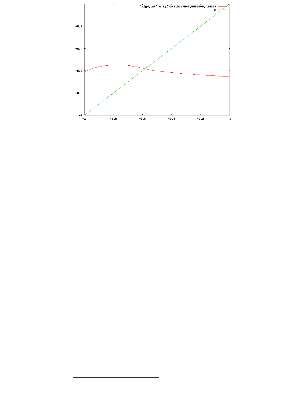
By zooming in we see that the intersection occurs at ε=−0.582 Hartree =
−15.8eV, i.e., close to the value found in the SigW.txt file.
If the Kohn-Sham eigenvalue is very far from the predicted quasiparticle energy!→or the self-energy is very oscillatory, then check the results graphically, since there
could be several graphical solutions to Eq. 5.
The calculation should now be repeated with a higher value of nmctot to see how
the statistical error decreases with the number of MC samples.
In the production runs, carefully check the value of the energy broadening pa-
rameter gamma.
8.2 C60: Fully stochastic calculation
Here we discuss a fully stochastic calculation of the electron affinity of C60; this
system is already big enough to profit from the stochastic treatment, since using
all the 120 occupied states for the time propagation is tedious and won’t bring
a large speedup over conventional approaches. We also illustrate how the tim-
ing and accuracy depends on the number of stochastic states (ntddft), on the
energy broadening parameter (gamma), and on the nxi and segment_fraction
parameters,
The user should first finish the previous example and get familiar with preparation
of the input files and the stochasticGW output.
We use a grid of 803points, with a spacing of 0.4Bohr. The LDA estimate of
electron affinity is 0.1645 Hartree, i.e., 4.48 eV, which is too high compared with
the experimental value of 2.69 eV.7
You should copy the files in the example directory ∼/sGW_v1/examples/C60
to your desired directory
mkdir ~/mygwrun
cd ~/mygwrun
cp ~/sGW_v1/examples/C60/* .
cp ~/sGW_v1/src/sgw.x .
7https://aip.scitation.org/doi/abs/10.1063/1.4881421?journalCode=jcp
stochasticGW - User manual and Tutorial 23

cp -r ~/sGW_v1/PP/ .
The INPUT file is now:
pps
06-C.LDA.fhi
#
scratch_path
.
ekcut
20d0
nmctot
840
ntddft
8
units_nuc
bohr
gamma
0.06
binary
T
orb_indx
121
flg_dyn
T
box
sym
Note that for the LUMO energy we use a TDDFT effective potential instead of
an RPA (i.e., we set flg_dyn to be T). As explained in Ref. 1, this yields a
much better LUMO energy.
In addition, the wf.bin waveufunction file for C60 is quite large (almost 1 giga-
byte) so it is stored separately and you should download a zipped version of it
from
http://www.chem.ucla.edu/dept/Faculty/dxn/pdf/wf.bin.gz
and then write
gunzip wf.bin.gz
The calculation should be again done via mpi, e.g.,
mpirun -n 840 ./sgw.x >& log &
or, if one wants to use a lower number of cores and get the same exact numbers,
use, e.g.,
mpirun -n 120 ./sgw.x >& log &
albeit the calculation will be then approximately 840/120=7 times slower.
At the end of the calculation, the output file shows a quasiparticle energy (real
and imaginary parts) of
840 -0.096131 0.001864 MC, E_qp +-stat.err
so the real part of the GW quasi-partilce energy is −0.096131 a.u.=-2.62eV with
a statistical error of 0.00186 a.u.=0.05 eV. This value is very close to the 2.69
eV experimental electron affinity of a single C60.
24 stochasticGW - User manual and Tutorial

When run on a modern supercomputer, the wall time of the calculation (read in
the last few lines of the log file) was only 2994 sec=0.83 hr per each iteration.
For verification, we also ran, beyond this first run, several runs with different pa-
rameters: an increased number of stochastic TDDFT states ntddft=16, a reduced
energy width γ= 0.04 and different combination of the stochastic fragment pa-
rameters, nxi=5000-20,000 and segment_fraction=0.001, 0.003. There was
essentially no change in the results, and the real-part of the quasiparticle energy
changed by only 0.03 eV, i.e., less than the statistical error.
Finally, we also ran the RPA simulations (by removing the flg_dyn parameter,
which defaults to .false.), leading to a much deeper LUMO,
840 -0.124621 0.001648 MC, E_qp +-stat.err
i.e., −0.124621 a.u.=-3.39eV.
stochasticGW - User manual and Tutorial 25

9 Acknowledgements
We are grateful for support by multiple sources.
This work was supported by the Center for Computational Study of Excited-State
Phenomena in Energy Materials at the Lawrence Berkeley National Laboratory,
which is funded by the U.S. Department of Energy, Office of Science, Basic Energy
Sciences, Materials Sciences and Engineering Division under Contract No. DE-
AC02-05CH11231, as part of the Computational Materials Sciences Program.
The work was further supported by the National Science Foundation, grants
DMR-1611382 and CHE-1112500 of Daniel Neuhauser, and CHE-1465064 of Eran
Rabani.
The Israel Science Foundation supported the work through grant 189/14 to Roi
Baer and through a FIRST Program grant (1700/14) to Roi Baer and Eran Ra-
bani. Roi Baer also acknowledges support by the Binational Science Foundation,
Grant 2015687.
The code was tested and optimized within the XSEDE8computational project
TG-CHE170058.
The stochasticGW code was mostly self-written, but it has several publicly
available routines, primarily the KISS random number generator of George Marsaglia;
we use, and slightly modified, the implementation of Jean-Michel Brankart. The
stochasticGW package also includes several spline routines from Numerical
Recipes.9
8J. Towns, T. Cockerill, M. Dahan, I. Foster, K. Gaither, A. Grimshaw, V. Hazlewood, S. Lath-
rop, D. Lifka, G. D. Peterson, et al. Xsede: accelerating scientific discovery. Comput. Sci.
Eng. 16,62 (2014). https://aip.scitation.org/doi/abs/10.1109/MCSE.2014.80
9http://www.nr.com/
26 stochasticGW - User manual and Tutorial
