TTi Communications MOSERS Guide 2007 2nd Edition Edited Texas.Guide.to.Accepted.Mobile.Source.Emission.Reduction.Strategies August.2007
User Manual: Pdf
Open the PDF directly: View PDF ![]() .
.
Page Count: 354 [warning: Documents this large are best viewed by clicking the View PDF Link!]

TEXAS DEPARTMENT OF TRANSPORTATION
The Texas Guide to Accepted Mobile Source
Emission Reduction Strategies
2ND EDITION

The Texas Guide to Accepted
Mobile Source Emission
Reduction Strategies
Prepared by the
Texas Transportation Institute
in cooperation with the
Texas Department of Transportation
and in association with
Environmental Protection Agency
Federal Highway Administration
Federal Transit Administration
Texas Commission on Environmental Quality
AUGUST 2007
Cover: Photo illustration for illustrative purposes only.

i
Acknowledgments
Several Texas agencies participated in the peer review of the original edition of the guide. The
comments and suggestions from these agencies are greatly appreciated:
• Federal Highway Administration;
• Environmental Protection Agency, Region VI;
• Texas Commission on Environmental Quality;
• Texas Department of Transportation, Transportation Planning and
Programming Division;
• Texas Department of Transportation, Environmental Affairs
Division;
• Texas Department of Transportation, Tyler District;
• North Central Texas Council of Governments;
• Houston-Galveston Area Council;
• Capital Area Metropolitan Planning Organization; and
• El Paso Metropolitan Planning Organization.
The guide was created by the Texas Transportation Institute under the auspices of TxDOT Contract
50-7XXIA001, “Assisting TxDOT in Meeting Federal Requirements.” Key personnel involved in
the creation of the guide include:
Texas Department of Transportation
• Jack Foster,
• Fred Marquez,
• Michelle Conkle, and
• Tim Juarez;
Texas Transportation Institute
• Todd Carlson,
• Jason Crawford,
• Edward Sepulveda, and
• Montie Wade.
ii

iii
TABLE OF CONTENTS
PREFACE ................................................................................................................................ix
PART A
1.0 THE BASICS — AIR POLLUTANTS ......................................................................A.1.1
CRITERIA POLLUTANTS....................................................................................................A.1.1
Ozone (O3) ..............................................................................................................................A.1.2
Particulate Matter (PM) .........................................................................................................A.1.2
Carbon Monoxide (CO) .......................................................................................................A.1.3
Mobile Source Air Toxics......................................................................................................A.1.3
2.0 MOBILE SOURCE EMISSION REDUCTION STRATEGIES:
LEGISLATION AND REGULATIONS................................................................A.2.1
CLEAN AIR ACT, 1970..........................................................................................................A.2.1
CLEAN AIR ACT AMENDMENTS, 1977.........................................................................A.2.2
CLEAN AIR ACT AMENDMENTS, 1990.........................................................................A.2.3
INTERMODAL SURFACE TRANSPORTATION EFFICIENCY ACT....................A.2.4
TRANSPORTATION EQUITY ACT FOR THE 21ST CENTURY ..............................A.2.5
SAFE, ACCOUNTABLE, FLEXIBLE, EFFICIENT TRANSPORTATION
EQUITY ACT: A LEGACY FOR USERS................................................................A.2.5
THE CONFORMITY RULE.................................................................................................A.2.5
3.0 NATIONAL AMBIENT AIR QUALITY STANDARDS (NAAQS) ........................A.3.1
DESIGNATIONS ....................................................................................................................A.3.1
OZONE STANDARDS..........................................................................................................A.3.2
Ozone Classifications.............................................................................................................A.3.3
Texas Nonattainment Areas for Eight-Hour Ozone Standards......................................A.3.3
Early Action Compact Areas................................................................................................A.3.4
PARTICULATE MATTER STANDARDS.........................................................................A.3.5
Nonattainment Areas for PM in Texas...............................................................................A.3.5
CARBON MONOXIDE STANDARDS.............................................................................A.3.5
Carbon Monoxide Classifications ........................................................................................A.3.6
Nonattainment Areas for CO in Texas...............................................................................A.3.6
4.0 TRANSPORTATION ACTIVITY AND EMISSION REDUCTION.....................A.4.1
TRANSPORTATION SYSTEM CHARACTERISTICS ..................................................A.4.1
TECHNICAL ANALYSIS......................................................................................................A.4.2
TRANSPORTATION IMPACTS..........................................................................................A.4.4
TRAVEL DEMAND MANAGEMENT.............................................................................A.4.4
EMISSION REDUCTION OBJECTIVES .........................................................................A.4.5
Trip Eliminations/Reductions..............................................................................................A.4.6
Travel Distance/VMT Reductions......................................................................................A.4.6
Traffic Flow Impacts .............................................................................................................A.4.6
Demand Shifting.....................................................................................................................A.4.7
Vehicle Types..........................................................................................................................A.4.7
iv
5.0 EMISSIONS FACTOR MODELING .......................................................................A.5.1
AIR QUALITY MODELING................................................................................................A.5.1
EMISSION FACTORS AND INVENTORIES.................................................................A.5.3
MOBILE .................................................................................................................................A.5.3
MOBILE6 ...............................................................................................................................A.5.4
MOVES ...................................................................................................................................A.5.5
6.0 STATE IMPLEMENTATION PLAN (SIP) AND
TRANSPORTATION CONFORMITY.................................................................A.6.1
STATE IMPLEMENTATION PLAN .................................................................................A.6.1
SIP AND NONATTAINMENT...........................................................................................A.6.2
Monitoring Network..............................................................................................................A.6.3
Emissions Inventory ..............................................................................................................A.6.3
Data Analysis...........................................................................................................................A.6.3
Future Emissions Estimates .................................................................................................A.6.3
Computer Modeling and Simulation ...................................................................................A.6.4
Pollution Control Identification...........................................................................................A.6.4
Emissions Budgets .................................................................................................................A.6.4
INTERAGENCY COOPERATION IN SIP DEVELOPMENT ..................................A.6.4
FEDERAL APPROVAL PROCESS.....................................................................................A.6.5
EPA Preliminary Review.......................................................................................................A.6.6
State Notice of a SIP Public Hearing ..................................................................................A.6.6
SUBMITTAL OF A SIP REVISION....................................................................................A.6.6
Transportation Conformity...................................................................................................A.6.7
Conformity in Nonattainment Areas...................................................................................A.6.7
7.0 MOBILE SOURCE EMISSION REDUCTION STRATEGIES.............................A.7.1
DEFINITIONS AND ACRONYMS....................................................................................A.7.1
14 CAAA MOBILE SOURCE EMISSION REDUCTION STRATEGIES.................A.7.4
OTHER MOBILE SOURCE EMISSION REDUCTION STRATEGIES.................A.7.11
8.0 MOBILE SOURCE EMISSION REDUCTION STRATEGY UTILIZATION .....A.8.1
PROGRAM DEVELOPMENT VERSUS INDIVIDUAL IMPLEMENTATION ....A.8.1
ENVIRONMENTAL PROTECTION AGENCY CRITERIA FOR MOBILE
SOURCE EMISSION REDUCTION STRATEGIES TO BE INCLUDED
IN SIPS .............................................................................................................................A.8.2
SUBMITTING TRANSPORTATION CONTROL MEASURES .................................A.8.2
MPO AND IMPLEMENTING AGENCY RESPONSIBILITIES................................A.8.3
Timely Implementation of TCMs in SIPs ..........................................................................A.8.4
Criteria for Demonstrating Timely Implementation of TCMs in TIPs .........................A.8.6
TCM Substitution Process ....................................................................................................A.8.7
TAKING EMISSION CREDIT............................................................................................A.8.7
Where Credits Can Be Taken: SIP or Conformity ............................................................A.8.8
State Implementation Plan....................................................................................................A.8.8
Conformity Determination ...................................................................................................A.8.9
CREDIT DURATIONS ..........................................................................................................A.8.9

v
9.0 DATA SOURCES FOR MOBILE SOURCE EMISSION
REDUCTION STRATEGIES ................................................................................A.9.1
CURRENT AVAILABLE DATA .........................................................................................A.9.2
TEXAS DEPARTMENT OF TRANSPORTATION.......................................................A.9.4
TEXAS COMMISSION ON ENVIRONMENTAL QUALITY ....................................A.9.4
UNITED STATES CENSUS BUREAU..............................................................................A.9.5
FIELD DATA COLLECTION .............................................................................................A.9.5
PROFESSIONAL JUDGMENT...........................................................................................A.9.6
10.0 ANALYSIS TOOLS AND TECHNIQUES............................................................. A.10.1
ON MODEL VERSUS OFF MODEL: AREN’T BOTH MODELED?.....................A.10.1
GENERAL METHOD (UNDERSTANDING THE BIG BLOCKS)........................A.10.2
TRIP BEHAVIOR MODIFICATION STRATEGIES...................................................A.10.3
SYSTEM IMPROVEMENT STRATEGIES.....................................................................A.10.4
VEHICLE/FUEL TECHNOLOGY STRATEGIES......................................................A.10.4
PROJECT RANKING CRITERIA.....................................................................................A.10.5
Travel Impacts ......................................................................................................................A.10.5
Emission Impacts.................................................................................................................A.10.6
Local Participation/Funding...............................................................................................A.10.6
Accelerated Implementation...............................................................................................A.10.6
Cost-Effectiveness................................................................................................................A.10.6
SUMMARY OF PROCESS FRAMEWORK.....................................................................A.10.7
Regional Travel Demand Models.......................................................................................A.10.7
Travel Demand Model Post-processors ........................................................................ A.10.11
Traffic Simulation Models................................................................................................ A.10.11
Off-Network Analyses or Sketch-Planning Tools........................................................ A.10.15
Empirical Comparisons .................................................................................................... A.10.16
Benefits of Standardized Analysis Methods .................................................................. A.10.17
11.0 MOBILE SOURCE EMISSION REDUCTION STRATEGY
DOCUMENTATION ........................................................................................... A.11.1
PROJECT DESCRIPTIONS AND BENEFITS..............................................................A.11.1
SUMMARY DOCUMENTATION ....................................................................................A.11.2
CONSISTENT LEVEL OF DETAIL................................................................................A.11.3
EXAMPLES OF DOCUMENTATION............................................................................A.11.5
FIELD EVALUATIONS FOR VALIDATION ..............................................................A.11.8
STANDARD MOBILE SOURCE EMISSION REDUCTION STRATEGY
DOCUMENTATION FORM ...................................................................................A.11.8
PART B
1.0 INTRODUCTION.....................................................................................................B.1.1
2.0 SOURCES FOR INDIVIDUAL VARIABLES FOR MOSERS
METHODOLOGIES ..............................................................................................B.2.1
SCOPING INPUTS .................................................................................................................B.2.1
TRAFFIC....................................................................................................................................B.2.3
EMISSIONS...............................................................................................................................B.2.7
FACTORS ................................................................................................................................B.2.10
vi
3.0 IMPROVED PUBLIC TRANSIT..............................................................................B.3.1
3.1 System/Service Expansion.............................................................................................B.3.4
3.2 System/Service Operational Improvements ...............................................................B.3.6
3.3 Marketing Strategies ........................................................................................................B.3.8
4.0 HIGH-OCCUPANCY VEHICLE FACILITIES ......................................................B.4.1
4.1 Freeway HOV Facilities..................................................................................................B.4.3
4.2 Arterial HOV Facilities...................................................................................................B.4.6
4.3 Parking Facilities at Entrances to HOV Facilities ......................................................B.4.9
4.4 Single-Occupant Vehicle Utilization of HOV Lanes ...............................................B.4.10
5.0 EMPLOYER-BASED TRANSPORTATION MANAGEMENT
PROGRAMS ............................................................................................................B.5.1
5.1 Transit/Rideshare Services.............................................................................................B.5.5
5.2 Bicycle and Pedestrian Programs ..................................................................................B.5.7
5.3 Employee Financial Incentives......................................................................................B.5.9
6.0 TRIP-REDUCTION ORDINANCES ......................................................................B.6.1
6.1 Negotiated Agreements ..................................................................................................B.6.3
6.2 Trip-Reduction Programs...............................................................................................B.6.5
6.3 Mandated Ridesharing and Activity Programs............................................................B.6.7
6.4 Requirements for Adequate Public Facilities...............................................................B.6.9
6.5 Conditions of Approval for New Construction........................................................B.6.11
7.0 TRAFFIC FLOW IMPROVEMENTS ......................................................................B.7.1
7.1 Traffic Signalization.........................................................................................................B.7.4
7.2 Traffic Operations...........................................................................................................B.7.7
7.3 Enforcement and Management...................................................................................B.7.11
7.4 Intelligent Transportation Systems .............................................................................B.7.15
7.5 Railroad Grade Separation ...........................................................................................B.7.20
8.0 PARK-AND-RIDE/FRINGE PARKING .................................................................B.8.1
8.1 New Facilities...................................................................................................................B.8.2
8.2 Improved Connections to Freeway System.................................................................B.8.3
8.3 Onsite Support Services..................................................................................................B.8.5
8.4 Shared-Use Parking .........................................................................................................B.8.7
9.0 VEHICLE USE LIMITATIONS AND RESTRICTIONS.......................................B.9.1
9.1 No-Drive Days.................................................................................................................B.9.2
9.2 Control of Truck Movement .........................................................................................B.9.5
10.0 AREA-WIDE RIDESHARE INCENTIVES........................................................... B.10.1
10.1 Commute Management Organizations ......................................................................B.10.3
10.2 Transportation Management Associations ................................................................B.10.6
10.3 Tax Incentives and Subsidy Programs........................................................................B.10.9
11.0 BICYCLE AND PEDESTRIAN PROGRAMS ....................................................... B.11.1
11.1 Bicycle and Pedestrian Lanes or Paths .......................................................................B.11.4
11.2 Bicycle and Pedestrian Support Facilities and Programs.........................................B.11.8
12.0 EXTENDED VEHICLE IDLING.......................................................................... B.12.1
12.1 Controls on Drive-Through Facilities ........................................................................B.12.2
12.2 Controls on Heavy-Duty Vehicles ..............................................................................B.12.4
13.0 EXTREME LOW TEMPERATURE COLD STARTS........................................... B.13.1

vii
14.0 WORK SCHEDULE CHANGES ............................................................................ B.14.1
14.1 Telecommuting ..............................................................................................................B.14.4
14.2 Flextime...........................................................................................................................B.14.6
14.3 Compressed Work Week..............................................................................................B.14.7
15.0 ACTIVITY CENTERS............................................................................................. B.15.1
15.1 Design Guidelines and Regulations ............................................................................B.15.2
15.2 Parking Regulations and Standards.............................................................................B.15.4
15.3 Mixed-Use Development .............................................................................................B.15.7
16.0 ACCELERATED VEHICLE RETIREMENT....................................................... B.16.1
16.1 Cash Payments...............................................................................................................B.16.3
17.0 PARKING MANAGEMENT................................................................................... B.17.1
17.1 Preferential Parking for HOVs....................................................................................B.17.3
17.2 Public Sector Parking Pricing.......................................................................................B.17.5
17.3 Parking Requirements in Zoning Ordinances...........................................................B.17.8
17.4 On-Street Parking Controls .......................................................................................B.17.11
18.0 VEHICLE PURCHASES AND REPOWERING................................................... B.18.1
18.1 Clean Vehicle Program .................................................................................................B.18.2
19.0 CONGESTION PRICING ...................................................................................... B.19.1
19.1 Facility Pricing................................................................................................................B.19.3
19.2 Cordon Pricing...............................................................................................................B.19.7
20.0 MOSERS EQUATIONS ..........................................................................................B.20.1
21.0 VARIABLES ............................................................................................................. B.21.1
PART C: MOSERS ANALYSIS GUIDANCE....................................................................C.1.1
Variables......................................................................................................................................C.1.1
PART D: ACRONYMS AND GLOSSARY.........................................................................D.1.1
1.0 ACRONYMS .................................................................................................................. D.1.1
2.0 GLOSSARY.................................................................................................................... D.2.1

viii
LIST OF FIGURES
PART A
Figure 5.1 Air Quality Modeling Components......................................................................................A.5.2
Figure 6.1 Example of Roles and Responsibilities in SIP Development ..........................................A.6.2
Figure 7.1 Historical Context of Technical Terminology....................................................................A.7.4
Figure 10.1 Analysis Blocks....................................................................................................................A.10.2
Figure 10.2 Off-Model Analysis Flow Chart.......................................................................................A.10.7
Figure 11.1 Sample Documentation Format .......................................................................................A.11.3
Figure 11.2 Components of Good Documentation...........................................................................A.11.5
PART B
Figure 2.1 Trip Chaining...........................................................................................................................B.2.9
LIST OF TABLES
PART A
Table 10.1 Strategies for Representing MOSERS in Travel Demand Models ...............................A.10.9
Table 10.2 MOSERS Analyzed by Traffic Simulation Models...................................................... A.10.13
Table 11.1 MOSERS Cost-Effectiveness Summary Table................................................................A.11.3
ix
PREFACE
The United States Environmental Protection Agency (EPA) sets and enforces the National
Ambient Air Quality Standard (NAAQS). In 2007, four areas in the state of Texas were
considered in nonattainment for the primary ozone standard: Beaumont-Port Arthur, Dallas-
Fort Worth, San Antonio, and Houston-Galveston-Brazoria.
Before the current NAAQS for ozone was adopted, additional areas of the state initiated
Early Action Compacts (EACs) to address air quality issues in their region. These areas
included Longview-Tyler and Austin. They have been able to plan, fund, implement, and
analyze mobile source emission reduction strategies. Many of these measures are specified in
the 1990 Clean Air Act Amendments (CAAA), and several others were developed in the
field in the last decade.
This new edition of the guide is an updated reference for new and experienced technical
staff in metropolitan areas undertaking transportation/air quality planning to better
understand and utilize mobile source emission reduction strategies as they seek to achieve
attainment for NAAQS. It is also intended to serve as an introduction for transportation
professionals in new nonattainment areas with little or no experience in transportation/air
quality issues. The guide provides an overview of the transportation/air quality relationship,
along with specific details about mobile source emission reduction strategies, and serves
several functions.
First, it is a tool for technical staff to assess the benefits of state implementation plan (SIP)
elements, conduct transportation conformity analysis, and initiate proactive emission
reduction programs to fulfill national air quality standards. Formulating plans to attain air
quality standards can be a long, arduous process for staff and elected officials. Mobile
source emission reduction strategies are a key part of the process, but information regarding
their use and analysis is not readily available in one source. This guide is an attempt to
provide the most relevant information for these mobile source emission reduction strategies
in one location.
Second, the guide provides technical staff with appropriate transportation/air quality
resources for SIP revision and conformity analysis. The guide provides information, but also
points staff in the right direction for further information on topics that are larger than
mobile source emission reduction strategies or are outside the scope of the guide. The CD-
ROM provides an instant library of resources for the planner.
Third, the analysis methodologies attempt to equalize strategy analysis between regions. As a
result, conformity analysis should be expedited since any questions arising from differences
in analysis results will be attributed to differences in local or project-specific inputs, rather
than methodology. Reviewing agencies will avoid slowing the approval process if analysis
and documentation presented by nonattainment areas are based on the same methodology.
This unified methodology avoids “black box syndrome” and increases the efficiency of the
review process.
x
The intent of this guide is that the analysis methodologies contained within serve as a
starting point for discussion, evaluation, validation, and improvement. Mobile source
emission reduction strategy analysis has not been standardized before in the field; regions
develop their own analysis methodologies and present them for documentation by review
agencies. The included strategies may not be as extensive as those projects implemented by
the various nonattainment areas, and these methodologies may lack some modeling
characteristics of a strategy. As a result, technical staffs are strongly encouraged to assess the
analysis methodologies and, if better methodologies can be developed, present them for peer
review, discussion, and adoption by the Transportation/Air Quality Technical Working
Group. The methodology will then replace or be added to the collection of methodologies
in the guide.
Fourth, this guide seeks to standardize the terminology of emission reduction measures
among technical staff. The term “mobile source emission reduction strategy” is an attempt
to bring greater clarity to discussion of emission reduction measures among professionals in
the state. As the field has developed, mobile source emission reduction strategies have
usually been referred to as transportation control measures (TCMs) as identified in the
CAAA. However, the use of the acronym “TCM” has increasingly referred to those
emission reduction measures in a SIP. Many emission reduction strategies are implemented
outside of a SIP, and referring to them as TCMs tends to create confusion. Mobile source
emission reduction strategies denote the entire universe of emission reduction measures
developed out of the original CAAA measures. It encompasses a much broader range of
projects than TCM currently does. Within the guide, an emission reduction strategy is
designated a TCM only as part of a SIP. In other words, a mobile source emission reduction
strategy in a SIP is a TCM.
ORGANIZATION OF THE GUIDE
The second edition is divided into four main sections.
Part A provides an overview of transportation/air quality planning basics. It discusses
mobile source pollutants, the national air quality standards, and mobile source emission
reduction strategies. It highlights mobile source emission reduction strategy planning,
implementation, analysis, and documentation for review agencies. This edition contains
updates to transportation legislation such as the Safe, Accountable, Flexible, Efficient
Transportation Equity Act: A Legacy for Users (SAFETEA-LU) and future emissions factor
models. Graphics were updated throughout the document. Readers should gain a better
understanding of the role of mobile source emission reduction strategies in the context of
achieving air quality standards.
Part B discusses mobile source emission reduction strategies in more depth. It focuses on
the specific measures, their requirements, and applicability and provides equations to
document the air quality benefits of the measure. The guide contains 17 separate strategies,
with a total of 56 individual project/program types. Each strategy is described, and then
every program is summarized by goal, description, applicability, and methodology.
Equations, developed since the first edition, are included in their respective strategy.
xi
Part C, a new section of the guide, contains data guidance based on work conducted since
the previous edition. Values or ranges are given for a selected number of the variables used
in Part B. These values or ranges may be of use to analysts and organizations that lack the
resources or time necessary to gather local data.
Part D contains an updated acronym list and glossary.
A companion CD-ROM is included in the guide. It contains numerous appendices, reports,
and links to applicable laws and regulations on emission reduction strategies. It provides
transportation planners with a quick and useful library for accepted mobile source emission
reduction strategies.
xii
A
.1.1
1.0 THE BASICS — AIR POLLUTANTS
Section Objective
This section introduces the main pollutants involved in the
relationship between air quality and transportation. The standards by
which the pollutants are measured (National Ambient Air Quality
Standards [NAAQS]) are outlined, along with an explanation of
attainment designations.
CRITERIA POLLUTANTS
The United States Environmental Protection Agency (EPA), in
response to the Clean Air Act of 1970 (CAA) and subsequent
amendments, established NAAQS for several pollutants that
adversely affect human health and welfare. These are termed
“criteria” pollutants. The EPA, through state or local air quality
agencies, monitors these pollutants against NAAQS. The six criteria
pollutants are:
• Carbon monoxide (CO),
• Lead (Pb),
• Nitrogen dioxide (NO2),
• Ozone (O3),
• Particulate matter (PM), and
• Sulfur dioxide (SO2).
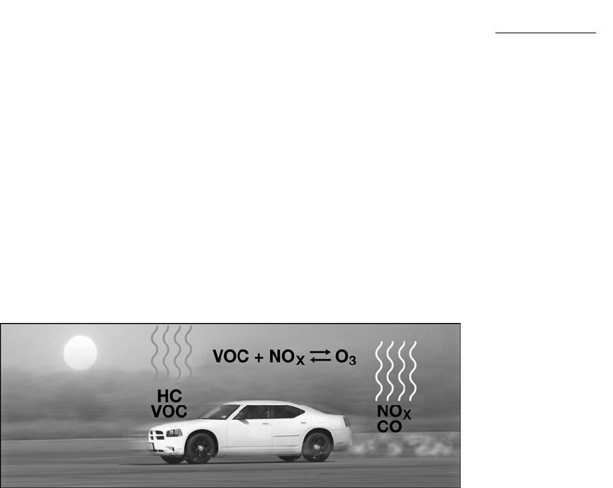
The transportation field focuses on three criteria pollutants: CO, PM,
and ozone. CO and PM are directly emitted from motor vehicles.
Ozone is formed through a complex chemical reaction between two
pollutants emitted from motor vehicles: hydrocarbons (HC) and
oxides of nitrogen (NOx). HC and NOx are called “precursor”
pollutants. Above certain standard levels (discussed in Section 3), the
three criteria pollutants can cause or exacerbate health problems and
even increase mortality rates.
Transportation
Criteria Pollutants
Ozone
Particulate matter
Carbon monoxide

A
.1.2
Ozone
O3 is formed by the reaction of NOx and volatile organic compounds
(VOCs) in the presence of sunlight. O3 occurs naturally in the upper
atmosphere, providing protection from ultraviolet radiation. O3 at
ground level, however, is a noxious pollutant. Ground-level O3 is a
major component of smog.
Ozone is a severe irritant. It can be responsible for coughing,
choking, and stinging eyes associated with smog. O3 can damage
lung tissue, aggravate respiratory disease, and increase susceptibility
to respiratory infections. Children are especially vulnerable, as are
adults with existing health conditions. Ground-level O3 may even
affect breathing in healthy adults.
Peak concentrations of O3 usually occur in the summertime. It
should be remembered that in addition to O3 sources in a particular
region, O3 might also travel from other areas upwind. This is called
ozone regional transport.
Particulate Matter
PM includes dust, dirt, soot, smoke, and liquid droplets directly
emitted into the air by sources such as factories, power plants, cars,
construction activity, fires, and natural windblown dust. Particles
formed in the atmosphere by condensation or the transformation of
emitted gases such as SO2 and VOCs are also considered particulate
matter.
Based on studies of human populations exposed to high
concentrations of particles and laboratory studies of animals and
humans, PM can have major effects on human health. These include
effects on breathing and respiratory symptoms, aggravation of
existing respiratory and cardiovascular disease, alterations in the
body’s defense systems against foreign materials, damage to lung
tissue, carcinogenesis, and premature death. The major population
groups that appear to be most sensitive to the effects of PM include
individuals with chronic obstructive pulmonary or cardiovascular
disease or influenza, asthmatics, the elderly, and children. PM also
soils and damages materials and is a major cause of visibility
impairment in the United States.
Particulate matter is often referred to as PM 2.5 and PM 10. Particles
less than 2.5 microns in diameter (PM 2.5) are created from fuel
combustion in motor vehicles and other sources. Coarser particles
less than 10 microns in diameter (PM 10) generally consist of
windblown dust and are released through materials handling,
Ozone
concentrations
peak in the
summertime
A
.1.3
agriculture, and crushing and grinding operations. The EPA has used
these designations since 1987 when research determined that these
smaller-sized particles are more likely responsible for most of the
adverse health effects of particulate matter. The smaller particles
have a greater ability to reach the thoracic or lower regions of the
respiratory tract.
Carbon Monoxide
CO is a colorless, odorless, and poisonous gas produced by
incomplete burning of carbon in fuels. When CO enters the
bloodstream, it reduces the delivery of oxygen to the body’s organs
and tissues. The negative health effects of CO vary depending on the
length and intensity of exposure and the health of the individual.
Health threats are most serious for those who suffer from
cardiovascular disease, particularly those with angina or peripheral
vascular disease. Exposure to elevated CO levels can cause dizziness,
headaches, fatigue, and impairment of visual perception, manual
dexterity, learning ability, and performance of complex tasks.
According to the EPA, 77 percent of nationwide CO emissions are
from transportation sources. The largest emission contribution
comes from highway motor vehicles. The focus of CO monitoring
has been on traffic-oriented sites in urban areas where the main
source of CO is motor vehicle exhaust. High concentrations of CO
can occur along roadsides in heavy traffic and in enclosed areas.
Major intersections and poorly ventilated tunnels are examples of
these areas. CO concentrations typically peak in colder months,
when CO vehicle emissions are greater and nighttime inversion
conditions are more frequent. Other major CO sources are wood-
burning stoves, incinerators, and industrial sources.
Mobile Source Air Toxics
Mobile source air toxics (MSATs) are compounds, emitted from
highway vehicles that are known or suspected to cause cancer and
other serious health and environmental effects. Motor vehicles emit
Major intersections
and poorly
ventilated tunnels
are examples of
potential high CO
concentrations

A
.1.4
several pollutants that the EPA classifies as known or probable
human carcinogens. For example, benzene is a known human
carcinogen, while formaldehyde, acetaldehyde, 1, 3-butadiene, and
diesel particulate matter are probable human carcinogens. The EPA
estimates that MSATs account for as much as half of all cancers
attributed to outdoor sources of air toxics.
The EPA master list of MSATs is quite extensive and contains over
425 identified compounds emitted from highway vehicles. Some
toxic compounds are present in gasoline and are emitted into the air
when gasoline evaporates or passes through the engine as unburned
fuel.
In 2002, the EPA developed a list of 21 MSATs and then refined it
further, compiling a subset of six that were identified as having the
greatest influence on health. This subset includes:
• Benzene,
• 1, 3-butadiene,
• Formaldehyde,
• Acrolein,
• Acetaldehyde, and
• Diesel particulate matter (DPM).
MSATs do not have NAAQS associated with them at this time.
These compounds occur naturally in petroleum and become more
concentrated when petroleum is refined to produce high-octane
gasoline. Benzene is a component of gasoline. Cars emit small
quantities of benzene in unburned fuel, or as vapor when gasoline
evaporates. A significant amount of automotive benzene comes
from the incomplete combustion of compounds in gasoline.
Formaldehyde, acetaldehyde, diesel particulate matter, and 1, 3-
butadiene are not present in fuel but are byproducts of incomplete
combustion. Formaldehyde and acetaldehyde are also formed
through a secondary process when other mobile source pollutants
undergo chemical reactions in the atmosphere.
Sources
Air Toxics from Motor Vehicles: Environmental Fact Sheet, United States
Environmental Protection Agency, August 1994.
Expanding and Updating the Master List of Compounds Emitted by Mobile
Sources — Phase III: Final Report, prepared for the EPA by ENVIRON
International Corporation, Novato, California, February 2006.
MSATs are
increasingly
important in the air
quality field
MSATs do not
have NAAQS
associated with
them at this time
A
.1.5
Fact Sheet, Final Revisions to the National Ambient Air Quality Standards for
Particle Pollution (Particulate Matter), United States Environmental
Protection Agency, September 21, 2006.
The Green Book, Office of Air Quality Planning and Standards, United
States Environmental Protection Agency, 2007.
The Plain English Guide to the Clean Air Act, United States
Environmental Protection Agency, PA-400-K-93-001, April 1993.
A
.1.6
A
.2.1
2.0 MOBILE SOURCE EMISSION REDUCTION
STRATEGIES: LEGISLATION AND REGULATIONS
Section Objective
This section will introduce the reader to the relevant legislation and
regulations in the transportation/air quality relationship over the last
30 years.
CLEAN AIR ACT, 1970
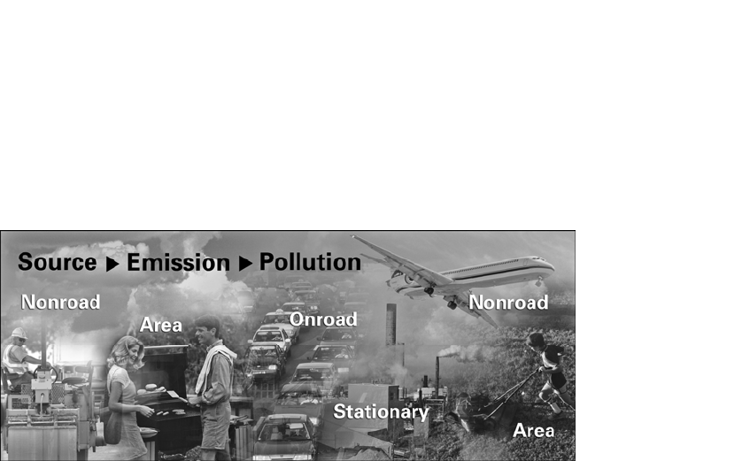
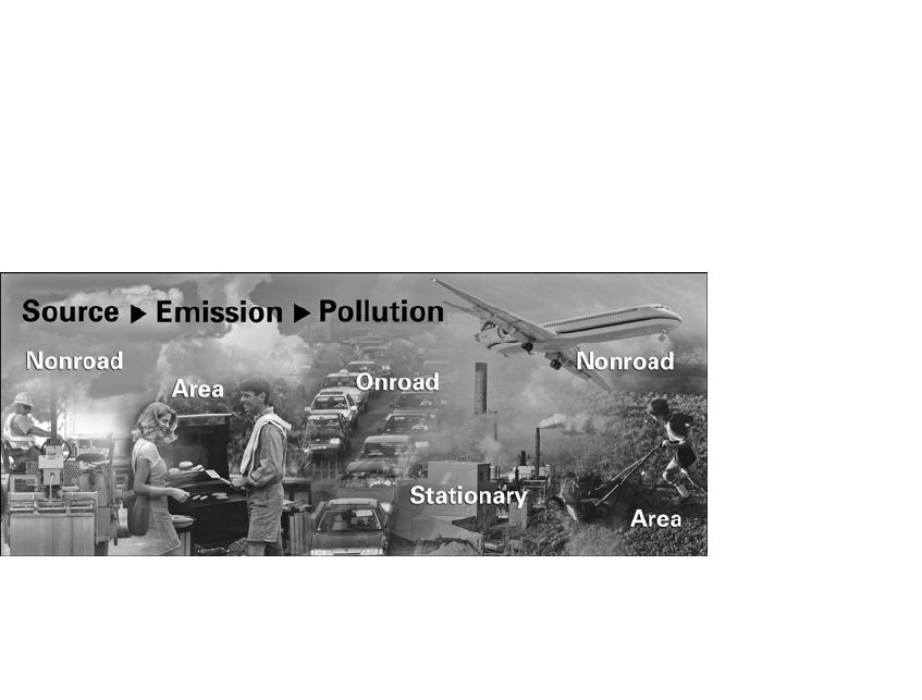
The Clean Air Act (CAA) was the initial comprehensive federal law
that regulates air emissions from area, stationary, and mobile sources.
Area sources are small sources of air toxics producers such as gasoline
stations and dry cleaners.
Stationary sources are places or objects that release pollutants and do not
move around. Stationary sources include power plants, incinerators,
houses, etc.
Mobile sources are moving objects that release pollution; mobile
sources include cars, trucks, buses, planes, trains, motorcycles, and
gasoline-powered lawn mowers. Mobile sources are divided into two
groups:
• Road vehicles, which include cars, trucks, and buses; and
• Nonroad vehicles, which include trains, planes, and lawn
mowers.
Transportation by its very nature concentrates on mobile sources.
The CAA authorized the EPA to establish, maintain, and enforce
NAAQS to protect public health and the environment.
Transportation/air
quality deals with
mobile sources
The EPA
establishes,
maintains, and
enforces NAAQS

A
.2.2
The CAA required the EPA to set national health-based air quality
standards to protect against common pollutants including ozone
(smog), carbon monoxide, sulfur dioxide, nitrogen dioxide, lead, and
particulate matter. The EPA identified these six pollutants as
“criteria” pollutants. State governments must devise cleanup plans to
meet the established standards by a specific date. Areas with the
highest levels of smog were given a longer time to meet the
standards. In addition, the EPA sets national standards for major
new sources of pollution such as automobiles, trucks, and electric
power plants.
The goal of the CAA was to set and achieve NAAQS in every state
by 1975. The setting of maximum pollutant standards was coupled
with directing the states to develop state implementation plans (SIPs)
applicable to appropriate industrial sources in the state.
As a response to the CAA, in 1975 the Federal Highway
Administration (FHWA) and the Urban Mass Transportation
Administration (UMTA), precursor to the Federal Transit
Administration, issued “Joint Regulations on Urban Transportation
Planning.” The highlights included:
• The governor must designate a metropolitan planning
organization (MPO) in each urban area as a condition for
continued federal assistance.
• The MPO must develop a unified planning work program
and a prospectus of the planning process.
• The metropolitan transportation plan (MTP) must consist of
a long-range element and a transportation system
management (TSM) element.
• The MPO must develop a transportation improvement
program (TIP) and an annual element detailing the following
year’s projects.
CLEAN AIR ACT AMENDMENTS, 1977
The 1977 amendments to the CAA set new dates for achieving
attainment of NAAQS since many areas of the country had failed to
meet the original deadlines. In addition, these amendments were
enacted:
• The amendments required revisions to SIPs for areas in
nonattainment of NAAQS.
• SIPs were required to develop transportation control plans
that included programs to reduce mobile source emissions.
1970 Clean Air
Act
Created the EPA,
authorized to
establish NAAQS
Required SIPs to
meet standards
Set deadline for
nonattainment
areas

A
.2.3
• Regulations in 1981 were issued that required transportation
plans, programs, and projects to conform to the approved
SIPs giving priority to transportation control measures
(TCMs).
CLEAN AIR ACT AMENDMENTS, 1990
The 1990 Clean Air Act Amendments (CAAA) built on the main
aspects of the CAA, but also contain several new provisions. These
were the most significant amendments to the CAA. The CAAA are
divided into a number of titles addressing a broad range of pollution
control and abatement issues. The CAAA were intended to meet
inadequately addressed problems derived from the CAA such as acid
rain, ground-level ozone, stratospheric ozone depletion, and air
toxics.
The 11 titles in the CAAA are:
• Title I: Nonattainment. This title defines various categories of
ozone (six classifications), carbon monoxide (two
classifications), and particulate matter (two categories)
nonattainment regions and establishes deadlines ranging from
3 to 20 years for regions to achieve specified air quality
standards. Smaller pollution sources were included in heavily
polluted regions to allow regulatory agencies greater freedom
to address the full range of pollution sources. The
amendments also supplant the 1970 provision of “reasonable
further progress” with annual emission reduction goals.
• Title II: Mobile Sources. Title II specifies over 90 emissions
standards for vehicle emissions including reductions of
hydrocarbons (HC) and oxides of nitrogen (NOx) by
35 percent and 60 percent, respectively, for all new cars
beginning with the 1996 model year. Oil companies are
required to offer alternative gasoline formulations (including
mixtures of gasoline with ethanol and methanol, liquefied
petroleum gas, and liquefied natural gas) that produce fewer
emissions during combustion, particularly in nonattainment
areas. In addition, auto manufacturers are required to
produce experimental cars for sale in southern California that
meet even more stringent emission standards.
• Title III: Hazardous Air Pollutants. Title III lists 189
chemicals for which the EPA is to phase in emission
standards by the year 2000. These pollutants are known or
reasonably suspected to be carcinogenic, mutagenic,
1990 Clean Air
Act
Amendments
Each state must
submit a SIP to
the EPA
Ozone
nonattainment
areas must
demonstrate
“reasonable
further progress”
toward attainment
in specific
milestone years
Expanded
conformity to
mean attainment
strategies must
conform to SIP
purpose of
reducing severity
of NAAQS
violations
Projected
emissions of
transportation
projects and
programs must
reconcile with
required emission
reductions in the
SIP

A
.2.4
teratogenic, or neurotoxic; to cause reproductive
dysfunctions; or to be acutely toxic.
• Title IV and Title V: Acid Deposition Control and Permits.
These titles establish an emissions trading program for sulfur
dioxide (SO2), the primary precursor to acid deposition.
• Title VI: Stratospheric Ozone Protection. Title VI
domestically implements the Montreal Protocol on
Substances That Deplete the Ozone Layer by requiring a
phase-out of specific ozone-depleting chemicals such as
chlorofluorocarbons (CFCs) and carbon tetrachloride.
• Title VII: Enforcement. This provision enhances EPA
monitoring requirements and updates penalties to make them
consistent with those in other environmental statutes.
• Title XI: Clean Air Employment Transition Assistance. Title
XI authorizes the secretary of labor to establish a
compensation, retraining, and relocation program to assist
workers laid off because of their company’s compliance with
the Clean Air Act.
• The other titles (VIII, IX, and X) in the act are smaller
provisions. They require EPA monitoring and study of
smaller pollution sources and research into pollution and its
health effects and require the EPA to utilize subcontractors
owned by socially or economically disadvantaged persons.
INTERMODAL SURFACE TRANSPORTATION
EFFICIENCY ACT
The 1991 Intermodal Surface Transportation Efficiency Act (ISTEA)
was the most significant federal transportation legislation since the
Interstate Highway System in the 1950s. It was the first major
attempt to approach transportation planning and funding from a
comprehensive, decentralized, multimodal perspective. This policy-
making philosophy within ISTEA was reiterated with its
reauthorization in 1998 through the Transportation Equity Act for
the 21st Century (TEA-21).
ISTEA authorized the Congestion Mitigation and Air Quality
Improvement Program (CMAQ) to provide funding for surface
transportation and other related projects that contribute to air quality
improvements and congestion mitigation. The CAAA and ISTEA,
along with CMAQ, were intended to refocus transportation planning
toward a more inclusive, environmentally sensitive, and multimodal
approach to addressing transportation problems.
The main goal of CMAQ is to fund transportation projects that
reduce emissions in nonattainment and maintenance areas. CMAQ is
ISTEA established
CMAQ

A
.2.5
targeted at areas of the country with the most severe air quality
problems. Funds must be spent in nonattainment or maintenance
areas. Although the emission reductions achieved by the program are
relatively small to attain the NAAQS, CMAQ funding can prove to
be an asset to state departments of transportation (DOTs) and MPOs
in meeting emission reduction requirements.
TRANSPORTATION EQUITY ACT FOR THE 21
ST
CENTURY
The 1998 Transportation Equity Act for the 21st Century (TEA-21)
built upon the foundation laid down by ISTEA. TEA-21
reauthorized CMAQ. It also expanded provisions to improve bicycle
and pedestrian facilities.
The core ISTEA metropolitan and statewide transportation planning
requirements remained intact under TEA-21. It emphasized the role
of state and local officials in tailoring the planning process to meet
metropolitan and state transportation needs.
The legislation also ensured the establishment of a new monitoring
network for the PM2.5 standard, promulgated at the time of the act.
SAFE, ACCOUNTABLE, FLEXIBLE, EFFICIENT
TRANSPORTATION EQUITY ACT: A LEGACY FOR
USERS
The Safe, Accountable, Flexible, Efficient Transportation Equity Act:
A Legacy for Users (SAFETEA-LU) was signed into law in 2005.
This legislation continues to build upon the framework of ISTEA
and TEA-21 with some modifications to programs and procedures
pertaining to emission reduction strategies, primarily requiring
conformity determinations on updated transportation plans every
four years.
CMAQ has been reauthorized. SAFETEA-LU now requires the
Secretary of Transportation to evaluate and assess the effectiveness
of a representative sample of CMAQ projects and to maintain a
database of the various projects.
THE CONFORMITY RULE
In 1993, the EPA released the “Criteria and Procedures for
Determining Conformity to Transportation Plans Rule,” referred to
CMAQ emission
reductions are
small but still
assets to MPOs
and DOTs
TEA-21 built upon
ISTEA
Conformity
established
interagency
consultation
procedures
SAFETEA-LU
extends conformity
cycle

A
.2.6
as the “conformity rule.” It established interagency consultation
procedures for determining transportation plan and program
conformity. It outlined the criteria for conformity determination,
including the following:
• Transportation plans, programs, and projects must be based
on the latest planning assumptions and the latest emission
estimation model available.
• Plans, programs, and projects must provide for the timely
implementation of TCMs.
• The rule requires a TIP and conforming plan to be in place
before project approval, and the project must come from
them.
• Plans, programs, or projects must not cause or contribute to
new pollutant violations or increase the severity of current
problems.
• Plans, programs, and projects must be consistent with SIP
emission targets.
• Projects must eliminate or reduce CO violations.
Sources
1990 Clean Air Act Amendments.
The Green Book, Office of Air Quality Planning and Standards, United
States Environmental Protection Agency, 2007.
Meyer, Michael D., and Miller, Eric J., Urban Transportation Planning,
2nd Ed., McGraw-Hill, New York, 2001.
The Plain English Guide to the Clean Air Act, United States
Environmental Protection Agency, PA-400-K-93-001, April 1993.
Safe, Accountable, Flexible, Efficient Transportation Equity Act: A
Legacy for Users.
Transportation Equity Act for the 21st Century.
Latest planning
assumptions
Timely
implementation of
TCMs

A.3.1
3.0 NATIONAL AMBIENT AIR QUALITY STANDARDS
(NAAQS)
Section Objective
This section provides a more detailed discussion of the NAAQS for
each of the transportation criteria pollutants and their relation to
Texas.
Under authority of the CAA and its subsequent amendments, the
EPA Office of Air Quality Planning and Standards sets the NAAQS
for each of the criteria pollutants. The CAAA established two types
of national air quality standards:
• Primary standards set limits to protect public health, including
the health of sensitive populations such as asthmatics,
children, and the elderly.
• Secondary standards set limits to protect public welfare,
including protection against decreased visibility and damage
to animals, crops, vegetation, and buildings.
Units of measure for the standards are:
• Parts per million (ppm) by volume,
• Milligrams per cubic meter of air (mg/m3), and
• Micrograms per cubic meter of air (µg/m3).
DESIGNATIONS
Based on the measurements gathered from air quality monitoring in a
region, an area receives a NAAQS designation of attainment,
nonattainment, or unclassifiable for a criteria pollutant.
Attainment
An area that meets the national primary or secondary
ambient air quality standard for the pollutant
Primary standards
protect public
health
Secondary
standards protect
public welfare

A.3.2
OZONE STANDARDS
As discussed in Section 1, ozone (O3) is a byproduct of the
interaction of oxides of nitrogen (NOx) and hydrocarbons in the
atmosphere. Both are emitted by motor vehicles. Peak ozone
concentrations typically occur during hot, dry, stagnant summertime
conditions. This strong seasonality of O3 levels makes it possible for
areas to limit their O3 monitoring to a certain portion of the year,
termed the O3 season. The length of the O3 season varies from one
area of the country to another. May through October is typical, but
states in the south and southwest may monitor the entire year.
The EPA published revisions to the ozone standards in July 1997.
The two primary changes to the O3 standard were a change in
averaging time and a strengthening of the standard. The current
standard takes the fourth highest daily maximum eight-hour average
over the course of three years. The three-year average cannot exceed
0.08 ppm. An area meets the O3 NAAQS if the fourth highest daily
maximum eight-hour average over the course of three years does not
exceed the threshold. To be in attainment, an area must meet the O3
NAAQS for three consecutive years.
Ozone standard is
0.08
pp
m
Fourth highest
daily maximum
eight-hour average
over the course of
three years
Attainment
requires meeting
the ozone
standard for three
years
Unclassifiable
An area that cannot be classified on the basis of available
information as meeting or not meeting the national primary
or secondary ambient air quality standard for the pollutant
Nonattainment
An area that does not meet (or that contributes to ambient
air quality in a nearby area that does not meet) the national
primary or secondary ambient air quality standard for the
pollutant

A.3.3
Ozone Classifications
The nonattainment designation for the O3 eight-hour average is
classified as to the degree of nonattainment:
• Extreme 0.187 ppm and above
• Severe 17 0.127 up to but not including 0.187 ppm
• Severe 15 0.120 up to but not including 0.127 ppm
• Serious 0.107 up to but not including 0.120 ppm
• Moderate 0.092 up to but not including 0.107 ppm
• Marginal 0.085 up to but not including 0.092 ppm
Texas Nonattainment Areas for Eight-Hour Ozone Standards
Beaumont-Port Arthur (Marginal)
Hardin County
Jefferson County
Orange County
Dallas-Fort Worth (Moderate)
Collin County
Dallas County
Denton County
Ellis County
Johnson County
Kaufman County
Parker County
Rockwall County
Tarrant County
Houston-Galveston-Brazoria (Moderate)
Brazoria County
Chambers County
Fort Bend County
Galveston County
Harris County
Liberty County
Montgomery County
Waller County
San Antonio (Subpart 1 Early Action Compact)
Bexar County
Comal County
Guadalupe County
Four ozone
nonattainment
areas in Texas
Dallas-Fort Worth
Houston
Beaumont-Port
Arthur
San Antonio

A.3.4
Victoria County in Victoria is considered a maintenance area for
ozone due to incomplete data.
MPOs in the Texas nonattainment areas include:
• Alamo Area Council of Governments (San Antonio),
• South East Texas Regional Planning Commission
(Beaumont-Port Arthur),
• North Central Texas Council of Governments in the Dallas-
Fort Worth Metroplex, and
• Houston-Galveston Area Council.
Early Action Compact Areas
In December of 2002, the State of Texas submitted Early Action
Compacts (EACs) pledging to reduce emissions earlier than required
for compliance with the new eight-hour ozone standard. The state
had to meet specific criteria and certain milestones. For those
counties in the EAC agreement that the EPA has designated
nonattainment for the eight-hour standard, the EPA will defer the
effective date of the nonattainment designation.
In Texas, EAC areas are:
Austin-San Marcos
Bastrop County
Caldwell County
Hays County
Travis County
Williamson County
Longview-Tyler
Gregg County
Harrison County
Rusk County
Smith County
Upshur County
San Antonio is an EAC area, but has not met the eight-hour standard
and is included by the EPA in the nonattainment list pending EAC
deadline at the end of 2007.
MPOs in the EAC areas include:
• Capital Area Metropolitan Planning Organization (Austin)
and
• East Texas Council of Governments Tyler-Longview).
Two EAC areas in
Texas

A.3.5
EACs require communities to develop and implement air pollution
control strategies, including mobile source emission reduction
strategies. The agreements require them to account for emissions
growth and achieve and maintain the eight-hour ozone standard.
EAC areas must attain the eight-hour ozone standard no later than
December 31, 2007. In areas that do not meet the EAC deadline, the
nonattainment designation will become effective April 15, 2008. The
EPA will withdraw that nonattainment deferral if an area misses any
milestone set out in the EAC.
PARTICULATE MATTER STANDARDS
The air quality standards for particulate matter were revised by the
EPA in 2006. The new standards tightened the 24-hour fine particle
standard from 65 µg/m3 to 35 µg/m3, and retained the current annual
fine particle standard at 15 µg/m3. The EPA decided to retain the
existing 24-hour PM 10 standard of 150 µg/m3. The agency revoked
the annual PM 10 standard because available evidence did not suggest
a link between long-term exposure to PM 10 and health problems.
To attain the PM 2.5 annual standard, the three-year average of the
weighted annual mean PM 2.5 concentrations from single or multiple
community-oriented monitors must not exceed 15.0 µg/m3. To
attain the 24-hour standard, the three-year average of the 98th
percentile of 24-hour concentrations at each population-oriented
monitor within an area must not exceed 35 µg/m3.
For the 24-hour PM 10 standard, attainment is met when
measurement of PM 10 does not exceed the standard more than once
per year on average over three years.
Nonattainment Areas for PM in Texas
El Paso County, including the City of El Paso, is in moderate
nonattainment for PM 10.
CARBON MONOXIDE STANDARDS
The NAAQS for carbon monoxide (CO) is 9 ppm, measured as an
eight-hour nonoverlapping average, not to be exceeded more than
once per year. An area meets the carbon monoxide NAAQS if no
more than one eight-hour value per year exceeds the threshold. (High
values that occur within eight hours of the first one are exempted.
EAC areas must
attain the eight-
hour ozone
standard no later
than
December 31,
2007
PM Standards
PM 10
24-hour average
150 µg/m3
Primary and secondary
PM 2.5
Annual
15 µg/m3
24-hour average
35 µg/m3
Primary and secondary
CO standard is
9 ppm on an
eight-hour
nonoverlapping
average

A.3.6
This is known as using nonoverlapping averages.) The rounding
convention in the standard specifies that values of 9.5 ppm or greater
are counted as exceeding the level of the standard. To be in
attainment, an area must meet the NAAQS for two consecutive years
and carry out air quality monitoring during the entire time period.
The air quality CO value is estimated using EPA guidance for
calculating design values published in the Laxton Memorandum
issued by the EPA on June 18, 1990.
Carbon Monoxide Classifications
The nonattainment designation for the CO eight-hour average is
further classified as to the degree of nonattainment:
• Serious 16.5 ppm and above
• Moderate 9.1 up to 16.4 ppm
Nonattainment Areas for CO in Texas
El Paso County is classified in moderate nonattainment (12.7 ppm)
for CO. The Texas Commission on Environmental Quality (TCEQ)
has recently submitted a request to the EPA for the county to be
designated a maintenance area for the pollutant.
Sources
The Green Book, Office of Air Quality Planning and Standards, United
States Environmental Protection Agency, 2007.
“Ozone and Carbon Monoxide Design Value Calculations,”
memorandum from W. Laxton, United States Environmental
Protection Agency, June 18, 1990.
Texas Commission on Environmental Quality.
A.4.1
4.0 TRANSPORTATION ACTIVITY AND EMISSION
REDUCTION
Section Objective
This section provides an overview of the activities in a transportation
system. This perspective is then related to transportation demand
management (TDM) and efforts to reduce emissions.
TRANSPORTATION SYSTEM CHARACTERISTICS
Transportation is a trip from an origin to a destination taken
primarily to accomplish some purpose. At the metropolitan and
regional level, transportation is the aggregate of hundreds of
thousands of individual trip-making decisions. These trips
(decisions) result in vehicle and passenger trips during specific time
periods. A transportation system consists of the facilities and
services that allow these travel movements to occur. The
characteristics of these travel flows and of the facilities and services
that enable them are basic to an understanding of transportation. It
is the relationship among travel patterns, transportation facilities, and
the economic, social, and environmental context of a region that
forms the basis of transportation analysis and policy decisions.
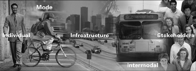
Transportation systems consist of five main components:
• Individual traveler,
• Stakeholders
• Mode of transportation,
• Infrastructure of the system, and
• Intermodal connections.
Transportation planners devote considerable attention to the
characteristics of the users of a transportation system.
Understanding the motivations and influences on an individual for
choosing one mode of travel over another is very important.

A.4.2
The mode of transportation used receives a high level of technical
analysis. Planners focus on estimating the levels of usage for the
various transportation modes in a system given the performance
characteristics of the mode and the motivations of individual users.
Infrastructure refers to the facilities, networks, and services necessary
in the system to provide mobility. This component has received the
most attention in the transportation planning process. Operational
performance that allows for efficient mobility and accessibility within
the system is a major goal of the planning process. Increasingly
sophisticated travel demand models have been developed in the last
decades to predict future performance needs of the system. As the
amount of land, public support, and funding for road expansion has
decreased in the last decade, more attention has been given to
operations and management of the infrastructure. Planners have also
begun focusing on changing demand itself within the system through
various techniques, rather than on accommodating the predicted
increase.
Intermodal connections consider system connectivity and the ease by
which a user can travel from origin to destination at an acceptable
level of performance. Transfer points, terminals, and stations are of
importance to system performance.
Stakeholders are those individuals and organizations that are affected
by transportation, such as employers, workers, governments,
social/cultural groups, environmental groups, and neighborhood
associations.
TECHNICAL ANALYSIS
The interaction of the components and characteristics of a
transportation system lend themselves to high levels of technical
analysis. Over the last half-century, transportation planners and
researchers have refined the tools available to practitioners in order
to plan a system more effectively and efficiently. There are several
characteristics related to use of a transportation system that are
important for understanding the technical analysis in the planning
process and the types of strategies considered by decision makers.
Each can be found in some form within most transportation analysis
tools. They are:
• Trip purpose,
• Temporal distribution of trip making,
• Spatial distribution of travel,
• Mode choice,
Technology has
improved analysis
capabilities over
last few decades

A.4.3
• Safety, and
• Cost.
Passenger trips are modeled by planners in terms of the purpose the
trip serves for the user. Traditional purposes include trips for: work,
shopping, recreation, business, and school. Trips are defined as one-
way movements, so the category of “home” is appended to many
trips, creating five classifications: home-based work, home-based
shop, home-based school, home-based other, and non-home based.
In recent years, planners have seen an increase in multipurpose trip
making, referred to as trip chaining.
Trip making in most areas of the United States evidences a distinct
temporal distribution — trips that are distributed in significant ways
in the course of a day. The classic example of temporal distribution
is the “double peaking” of trips because of the two rush hours in a
workday. On the other hand, truck traffic does not correspond
temporally with rush-hour traffic. Rather, it shows a single peak in
the course of work hours. All modes of travel can be distributed
temporally for analysis purposes, and this distribution provides
helpful data for planners in terms of infrastructure and demand
management.
Spatial distribution of trips is directly related to land use patterns and
network configuration of a system. Every trip begins and ends at a
specific geographical point. As a result, planners are able to model
travel flows on networks that reflect the movements of goods and
services throughout a region. Modeling spatial distribution is an
important element in planning since it can indicate where
transportation problems are likely to occur, analyze the performance
level of the existing system, and identify areas that will require action
to improve system performance.
Mode choice, or modal distribution, is the proportion of trips made
in a region by different travel modes (transit, automobile, walking,
etc.). Modal distribution varies from city to city and area to area due
to availability, condition of the system, and environment. Mode
Trip purpose
Distribution in time
durin
g
the da
y
Distribution in the
system related to
land use and
network
configuration
Some go by car,
bus, or train; walk;
or ride a bike

A.4.4
selection is influenced by trip time, both actual and perceived, and
mode availability, among other factors. Therefore, an understanding
of this characteristic is essential to planners in a locality. With the
passing of ISTEA in 1991, greater emphasis has been placed on
shifting modal patterns of trip making away from single-occupant
automobiles.
Arriving at destinations safely is a primary goal of travelers. While
transportation fatality rates have declined over the last several
decades, safety projects and research remain a high priority in the
transportation field.
Travelers incur out-of-pocket and time value costs whenever a trip is
made. Travel cost is often defined and perceived differently by users,
stakeholders, and system providers. Because of these differences,
travel cost can be a difficult characteristic to define. Nevertheless,
costs are critical to transportation investment strategies.
TRANSPORTATION IMPACTS
Transportation systems have many tremendous impacts on society;
some are readily apparent, while others may be harder to perceive.
Transportation impacts include noise, air quality, water quality,
energy consumption, ecology, aesthetics, land use, infrastructure,
employment, income, and community cohesion, among others.
Impacts are created through both construction and use of the system.
They can be direct and indirect.
The impact of most interest in this guide is the physical impact of
transportation activity on air quality. Transportation activity can be a
major source of air pollution. It is the attempt to control the impact
of transportation on air quality that has led to various legislative and
regulatory efforts such as the NAAQS, the conformity rule, and
amendments to the CAA.
TRAVEL DEMAND MANAGEMENT
As noted in the discussion above, greater attention has been given in
the last 20 years to altering the demand of a transportation system
rather than building larger facilities. In the 1980s, urban
transportation agencies began to utilize the concept of travel demand
management. As we shall see, TDM strategies and programs are very
similar to mobile source emission reduction strategies and
incorporate many of the same concepts. TDM programs can be
Safety is a high
priority under
SAFETEA-LU
Every trip has
some form of cost
but can be hard to
define
Transportation
activity has a
physical impact on
air quality
Primary purpose
of TDM is to
reduce or spread
the number of
vehicles using the
system at a given
time

A.4.5
considered mobile source emission reduction strategies, and they, in
reverse, can be considered TDM projects.
The primary purpose of TDM is to reduce or spread the number of
vehicles using the road system while providing a wide variety of
mobility options to those who wish to travel. To accomplish these
changes, TDM programs rely on incentives or disincentives to make
these shifts in behavior attractive. In terms of air quality, reductions
in the number of vehicle trips reduce vehicle miles traveled (VMT),
which in turn reduces emissions. Initiating a TDM program is a
technique to achieve the NAAQS.
The term TDM encompasses both alternatives to driving alone and
the techniques or supporting strategies that encourage the use of
these modes. The application of such TDM alternatives and the
implementation of supporting strategies can occur at different levels
under the direction of a variety of groups. One level of application
found in many parts of the country is at individual employer sites or
at locations where there are many employers grouped together.
Another level of application is on an area-wide basis. In this type of
application, the primary focus of the TDM program is to affect as
many travelers as possible within an area-wide travel system.
TDM strategies include carpool/vanpools, compressed/flextime/
staggered work weeks, congestion pricing, high-occupancy vehicle
(HOV) lanes, mixed-use development, and telecommuting. All of
these examples can be considered mobile source emission reduction
strategies.
Effective TDM employer programs usually employ a wide variety of
TDM alternatives and strategies, each mutually supporting the overall
objective of trip reduction.
EMISSION REDUCTION OBJECTIVES
Regional mobile source emissions are reduced one of five ways:
• Trip elimination/reductions,
• Travel distance/VMT reductions,
• Traffic flow impacts,
• Demand shifting, and
• Vehicle types.
Less vehicles
means less VMT
Less VMT means
less emissions
A.4.6
Trip Eliminations/Reductions
Projects seeking to eliminate or
reduce trip making also reduce
start (cold and hot) emissions
and hot-soak emissions.
Starting emissions can be a
significant portion of the entire
trip’s emissions. Projects that
seek to reduce trips will provide
greater benefits than other strategies.
The EPA’s current version of the Mobile Source Emissions Factor
(MOBILE) model, its computer model for estimating motor vehicle
emissions, also produces trip- and VMT-based emission factors.
MOBILE6 includes the trip-based emissions (starts and soaks) in the
VMT-based factors.
Travel Distance/VMT Reductions
Some TDM projects simply
attempt to reduce the amount of
VMT applied to the
transportation system. The
reduction allows the demand on
the system to operate with
improved performance and
reduced running emissions.
Traffic Flow Impacts
Improving traffic flow in the system to reduce delays and improve
speeds reduces running emissions. Vehicles emit more pollutants
(higher emission factors in grams per mile) at extremely low or high
speeds or under hard acceleration. Under these conditions, emissions
are greater because the engines run in a non-stoichiometric condition,
meaning the engine air/fuel ratio runs either too lean or too rich.
Smoothing traffic flow to maintain optimal and consistent speeds can
reduce running emissions.
MOBILE emission factors,
discussed in the next section, are
often used for conditions that
they were not originally
intended, but represent the best
available science for which to
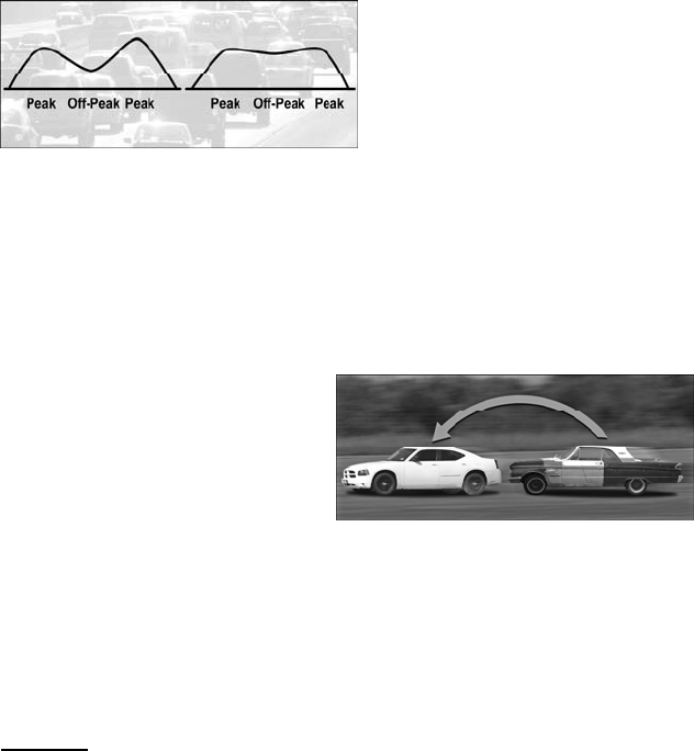
A.4.7
evaluate project impacts. The emission factors provided by
MOBILE represent emissions from a typical driving cycle
(accelerations, cruising, decelerations, and idling), which has an
overall average speed. The emission factors for these average speeds
are then commonly used for analyses with constant vehicle speeds.
Demand Shifting
Similar to the two previous
objectives, shifting travel
demand from peak conditions to
times where recurrent and
nonrecurrent congestion is less
pronounced reduces running
emissions. Operating speeds of vehicles shifted out of the peak
period are likely to increase. Knowledge of peak and off-peak period
speeds is required to estimate the emission benefits of these
strategies.
Vehicle Types
Some strategies focus on
improving the vehicle fleet
emission factors by removing
high-emitting vehicles. An
example program is
accelerated vehicle retirement,
commonly referred to as “Cash for Clunkers.” This program seeks
to remove older, more polluting vehicles from the fleet, replacing
them with newer, cleaner-burning vehicles. Results of this program
modify the vehicle age distribution used in the emission factor
models and lower emission rates.
Sources
Meyer, Michael D., and Miller, Eric J., Urban Transportation Planning,
2nd Ed., McGraw-Hill, New York, 2001.
Overview of Travel Demand Management Measures: Final Report, United
States Department of Transportation, DOT-T-94-11, January 1994.
A Sampling of Emissions Analysis Techniques for Transportation Control
Measures, Cambridge Systematics, Inc., Federal Highway
Administration, Washington, D.C., October 2000.
A.4.8
TDM Case Studies and Commuter Testimonials, Transportation Demand
Management Institute of the Association for Commerce
Transportation, Washington, D.C., August 1997.

A
.5.1
5.0 EMISSIONS FACTOR MODELING
Section Objective
In this section, we introduce and discuss the emissions factor
modeling process. An overview of the MOBILE model, the current
emissions factor model, is given, along with its relationship to Mobile
Source Emission Reduction Strategies (MOSERS). An emissions
factor model is fundamental for assessing the nature and magnitude
of on-road motor vehicle emissions and their impacts on ambient air
quality.
AIR QUALITY MODELING
The relationship between air quality and transportation system
performance is an ongoing issue for planners. It is a complex
relationship requiring large amounts of data and significant time to
analyze and report. Efforts to evaluate the air quality impact of on-
road vehicles are by nature interdisciplinary and require the
interaction of three different models and related areas of expertise:
travel demand models, emissions factor models, and air quality
models.
Travel demand models determine the amount of transportation
activity occurring in a region based on an understanding of the daily
activities of individuals and employers as well as the resources and
transportation infrastructure available to households and individuals
when making their activity and travel decisions.
The second component is emissions factor models. These models
convert information on driving conditions, vehicle and driver
behavior, and environmental factors into estimates of motor vehicle
emissions rates. They are based on the relationship between vehicle
activities and vehicle emissions.
The EPA has developed a computer model called MOBILE to
estimate motor vehicle emissions. MOBILE estimates emissions
rates based on vehicle type, average speed, ambient temperature, and
other factors. The product of the transportation activity and the
emissions rates from MOBILE results in emissions estimates for
each modeled pollutant (carbon monoxide [CO], volatile organic
compounds [VOCs], and oxides of nitrogen [NOx]) for different
vehicle types in three major geographic regions (low altitude, high
altitude, and California). MOBILE is presented in more detail later in
this section.
Travel demand
models provide
vehicle activity
Emissions factor
models provide
pollutant rates by
vehicle activity
A
.5.2
It is very important that estimates of transportation activity and
emissions rates be in balance with respect to fidelity, accuracy, and
precision to ensure the reasonableness of the emissions estimates.
Planners should understand the different aspects of each component
when considering them in their policy analysis.
The third component of the modeling trilogy is the regional and
microscale modeling of air quality, or dispersion models. These
models translate emissions inventories into predicted ambient
pollutant concentrations that carry through space and time. It uses
data on emissions, meteorological conditions, and topographic
characteristics to compute the dispersion of pollutants in the
atmosphere. The model then predicts the concentrations of
pollutants at certain locations over specified time periods.
Dispersion models are much more complex than emissions models
since they must account for the transport of pollutants over distance.
These components are illustrated below.
×
Source: Meyer and Miller, Urban Transportation Planning
Figure 5.1 Air Quality Modeling Components
Transportation
activity and
emissions rates
must be in balance
for good analysis
Microscale air
q
ualit
y
models
Travel Demand
Models
(VMT and Avg. Speed)
MOBILE Model
(Emissions Rates by
Speed and Vehicle Type)
On-Road Mobile Emissions Estimates
(VOCs, NOx, CO, and PM)
CO
Concentration
O3 and PM
Concentration
by Time and
Location
Dispersion
Model
Air Quality Model
Emissions by Grid
and Time of Day
A
rea Source
Biogenics
Nonroad
Stationary
Meteorological

A
.5.3
EMISSION FACTORS AND INVENTORIES
Emission factors and emission inventories have long been
fundamental tools for air quality management. Emission factors are
important for developing emission control strategies. The passage of
the CAAA increased the need for criteria pollutant emission factors
and inventories.
Ideally, data from source-specific emissions tests or continuous
emissions monitors are preferred for estimating a source’s emissions
because these data provide the best representation of the tested
source’s emissions. However, test data from individual sources are
not always available, and they may not reflect the variability of actual
emissions over time. Therefore, emission factors are frequently the
best or only method available for estimating emissions.
An emission factor is a representative value relating the quantity of a
pollutant released to the atmosphere with an activity associated with
the release of that pollutant. These factors are usually expressed as
the weight of the pollutant divided by a unit weight, volume, travel
distance, or duration of the activity emitting the pollutant. In most
cases, these factors are simply averages of all available data of
acceptable quality.
An emission inventory is an estimate of the total emissions in an
urban area measured over time. Emission inventories can be
compared with air pollutant levels in an area to determine if increased
emissions decrease the air quality. Emission inventories have many
purposes, including those involving ambient dispersion modeling and
analysis, control strategy development, and screening sources for
compliance investigations.
MOBILE
Texas uses the MOBILE model to simulate actual emissions from
automobiles over varying scales of resolution (local, regional, and
state). MOBILE is used in the documentation of emission
reductions in SIPs, the assessment of air quality impacts of
transportation projects (including the demonstration of conformity
of transportation and air quality plans), and the assessment of mobile
source emission reduction strategies. As the use of the model has
progressed, transportation agencies and MPOs have come to rely on
MOBILE in fulfilling their obligations under the CAAA and
subsequent transportation legislation.
A primary use of MOBILE is in developing on-road mobile source
emission inventories. Emissions rates developed in the model are
Emission factors
are frequently the
best method
available for
estimating
emissions
Texas uses only
the MOBILE
model
MOBILE develops
on-road mobile
source emission
factors

A
.5.4
combined with average vehicle speeds and travel activity estimates to
develop the inventories. The emission rates generated by MOBILE
require a multitude of input assumptions. For most input
assumptions, MOBILE provides national default values, or users can
input locally specific values.
MOBILE was developed originally to estimate overall emissions
levels, trends over time, and the effectiveness of mobile source
emission control strategies. The role of MOBILE has expanded in
ways that now require higher standards of accuracy that incorporate a
greater degree of complexity.
The EPA first developed MOBILE in the late 1970s. Every few
years, the model has had significant updates and new releases as new
data become available, new regulations are promulgated, new
emission standards are established, and the vehicle emissions process
is better understood. Each new version of the model has become
more complex in approach and has provided the user with additional
options in order to customize emissions factor estimates to local
conditions.
Underlying database changes in the model and changes in modeling
methodology in each successive version have resulted in changes to
predicted total on-road vehicle emissions. From one model version
to the next, these changes can be either increases or decreases in
emission factors, and the changes are not always in the same
direction for each pollutant.
MOBILE6
The current generation MOBILE model, MOBILE6, is based on a
tremendous amount of new vehicle emission testing data collected in
the last decade. MOBILE6 also incorporates a set of modeling tools
for the estimation of emissions produced by on-road and off-road
mobile sources.
The design of the modeling system was guided by four broad
objectives:
• All pollutants and all mobile sources at the levels of
resolution needed for the diverse applications of the system
should be encompassed.
• It should be developed according to principles of sound
science.
• Software design of the model should be efficient and flexible.
• Implementation of the model should be in a clear and
consistent manner.
MOBILE 6.2 is
most recent
version and is
available from the
EPA

A
.5.5
Significant changes in MOBILE6 from previous versions include:
• Dramatically lower basic emissions rates after 2007,
• Separation of start and running exhaust emissions, and
• Addition of so-called off-cycle emissions (aggressive driving
and air conditioning operation).
MOVES
The EPA’s Office of Transportation and Air Quality (OTAQ) is
developing a modeling system designated the Motor Vehicle
Emission Simulator (MOVES) to keep pace with new analysis needs,
modeling approaches, and data. The new system will estimate
emissions for on-road and nonroad sources, cover a broad range of
pollutants, and allow multiple-scale analysis, from fine-scale analysis
to national inventory estimation. The new system will be a
multivariate tool rather than a single software program. It will consist
of software, algorithms, underlying data and guidance necessary for
use in all official analyses associated with regulatory development,
compliance with statutory requirements, and inventory projections.
When fully implemented, MOVES will serve as the replacement for
MOBILE6.
Sources
Introduction to Emission Factors, Office of Air Quality Planning and
Standards, United States Environmental Protection Agency, 2007.
Meyer, Michael D., and Miller, Eric J., Urban Transportation Planning,
2nd Ed., McGraw-Hill, New York, 2001.
Modeling Mobile-Source Emissions, Committee to Review EPA’s Mobile
Source Emissions Factor (MOBILE) Model, Board on
Environmental Studies and Toxicology, Transportation Research
Board, National Research Council, 2000.
Off-Model Air Quality Analysis: A Compendium of Practice, Federal
Highway Administration Southern Resource Center, Atlanta,
Georgia, August 1999.
A Sampling of Emissions Analysis Techniques for Transportation Control
Measures, Cambridge Systematics, Inc., Federal Highway
Administration, Washington, D.C., October 2000.
The MOVES
model is the next
generation
modeling system
for vehicle
emissions
A
.5.6

A
.6.1
6.0 STATE IMPLEMENTATION PLAN (SIP) AND
TRANSPORTATION CONFORMITY
Section Objective
This section presents an overview of the state implementation plan.
It discusses the SIP process among relevant transportation agencies
and includes SIP components for nonattainment areas. An overview
of transportation conformity is also presented.
STATE IMPLEMENTATION PLAN
The SIP is the legal and federally enforceable plan for each state that
identifies the air pollution control strategies to attain and/or maintain
the primary and secondary NAAQS set forth in Section 109 of the
CAA and the Code of Federal Regulations (CFR) (40 CFR 50.4
through 50.12) in each EPA–designated nonattainment or
maintenance area. A SIP must be adopted by the state and approved
by the EPA for each pollutant for which the state violates the
NAAQS. The SIP is developed through a collaborative public
process and submitted by the governor’s designee to the EPA.
The contents of a typical SIP fall into three categories:
• State-adopted control measures, which consist of either
rules/regulations or source-specific requirements (e.g., orders
and consent decrees);
• State-submitted “nonregulatory” components (e.g.,
attainment plans, rate-of-progress plans, emission inventories,
transportation emission reduction measures, statutes demonstrating
legal authority, monitoring networks, etc.); and
• Additional requirements promulgated by the EPA, in the
absence of a corresponding state provision, to satisfy a
mandatory Part D or Section 110 CAA requirement.
Section 110 and Part D of the CAA describe the many elements of a
SIP, such as emission inventories, a monitoring network, an air
quality analysis, modeling results, attainment demonstrations,
enforcement mechanisms, and regulations that have been adopted by
the state to attain or maintain NAAQS. (Section 110 and Part D of
the CAA are included in the CD-ROM companion to this guide.)
The SIP also contains documents specific to each nonattainment area
within the state.
The SIP is required and approved by the EPA pursuant to
Section 110 of the CAA. Part D of the CAA mandates SIP
TCMs are in the
category of state-
submitted
nonregulatory
components of a
SIP
Section 110 and
Part D of the CAA
describe SIP
elements
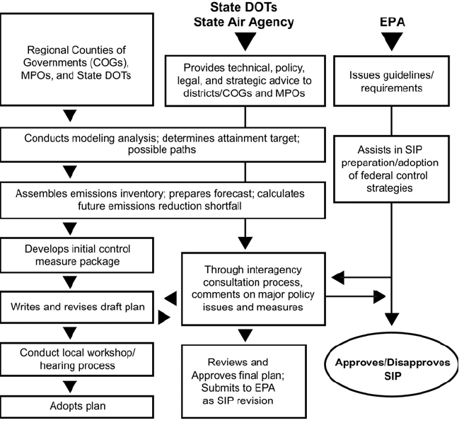
A
.6.2
requirements particular to nonattainment areas. Additional
regulatory requirements that spell out the procedures for preparing,
adopting, and submitting SIPs and their revisions are further codified
in 40 CFR 51 and are included in the CD-ROM companion. All of
these documents form the basis for the discussion below.
Because SIPs are continually updated, Section 110(h) of the CAA
requires the EPA to periodically publish SIP compilation documents.
Source: Federal Highway Administration’s Transportation Conformity Reference Guide, adapted from California Air
Resources Board
Figure 6.1 Example of Roles and Responsibilities in SIP
Development
SIP AND NONATTAINMENT
Areas not conforming to NAAQS within each state may be
designated nonattainment and are then subject to additional planning
and control requirements. Accordingly, different regulations or
programs in the SIP will apply to different areas.

A
.6.3
The following components are typically included for each
nonattainment area.
Monitoring Network
By measuring the ambient concentrations of the criteria pollutants,
the Texas Commission on Environmental Quality (TCEQ) can learn
where and by how much any one of these pollutants exceeds its air
quality standard. At the same time, the TCEQ collects meteorological
information at each monitoring site. TCEQ monitors a number of
representative sites for each area studied.
Emissions Inventory
An emissions inventory of the pollutants or their known precursors
from point, area, and mobile sources in the nonattainment area is
compiled. The emission inventory also includes a biogenic (natural)
emissions category.
All O3 nonattainment areas, classified as marginal and above, and
carbon monoxide (CO) areas must conduct these inventories and
submit them to the EPA every three years until attainment. This
provision is important because it means that SIPs need to be
periodically updated when new emission factors are approved by the
EPA, or when other changes in the overall level of emissions over
earlier estimates are anticipated.
Emissions reductions needed to achieve the NAAQS are determined
based on the emissions inventory.
Data Analysis
Air quality data and meteorological information are studied to find
the appropriate relationship between emissions and air quality. This
knowledge is then combined with the emissions inventory to
determine what reductions are needed to attain the NAAQS within
deadlines identified in the CAA.
Future Emissions Estimates
Emissions are projected to target attainment years by the use of
growth factors such as population increases and also are adjusted for
the impacts of adopted emission control strategies, such as the
federal motor vehicle control program or cleaner fuels used
statewide. Both modeling and actual inventories are used to make
estimates.
Nonattainment
areas must have a
monitoring system
to measure criteria
pollutants
Emissions
inventories of
area, point, and
mobile sources
must be compiled

A.6.
4
Computer Modeling and Simulation
Sophisticated modeling programs analyze the effectiveness of
strategies proposed to control air pollution. It is then determined
whether selected controls will enable the area to comply with the
standard by the mandated date.
Pollution Control Identification
The specific emissions controls to be applied to pollution sources are
identified and then demonstrated that they will achieve the desired
goals. The SIP is revised:
• As new control strategies are adopted,
• When the attainment status of an area changes,
• As the result of new or improved emissions data, or
• In response to new federal mandates.
The first SIP in Texas was submitted in response to CAA
requirements in 1972.
Emissions Budgets
TCEQ allocates emissions reduction budgets to individual pollution
sources (i.e., mobile, point, and area). The SIP then assigns specific
emissions reduction levels to each source category. For the on-road
mobile source category of emissions, the emissions reduction level is
further refined into a regulatory limit on emissions, referred to as a
motor vehicle emissions budget (MVEB) for on-road mobile sources.
Motor vehicle emissions are estimated based upon the number of
vehicles in the region, their age, the rate of fleet turnover to newer
and cleaner vehicles, seasonal temperatures in the region, vehicle
miles traveled (VMT), population growth, and other factors. A
motor vehicle emissions budget is the portion of the total allowable
emissions for any criteria pollutant or its precursors defined in the
SIP revision for a certain date for the purpose of meeting reasonable
further progress milestones or demonstrating attainment or
maintenance of the NAAQS.
INTERAGENCY COOPERATION IN SIP
DEVELOPMENT
Transportation and air quality agencies need to develop SIPs
cooperatively in order to achieve the needed levels of emissions
Motor vehicle
emissions budget
is a limit on mobile
sources of
pollutants
Interagency
cooperation is
essential to SIP
development

A
.6.5
reductions. Different pollution control strategies will require
approval at different levels of government. MPOs, Councils of
Government (COGs), transit agencies, Texas Department of
Transportation (TxDOT), or TCEQ cannot individually create,
develop, or implement the measures required in the SIP. For
example, some control strategies, like controls on automobiles and
aircraft, are usually adopted by the federal government. Other
strategies, like controls on fuels, inspection and maintenance
programs, or market measures, can be adopted and effectively
implemented and enforced at the state level. Control measures such
as transit investments or HOV lanes must be implemented at the
local or regional level; however, these control measures may require
state legislation or approval. Therefore, by its very nature, the SIP is
a collaborative process.
FEDERAL APPROVAL PROCESS
The federal approval process for SIPs resides solely with the EPA.
Once the state formally adopts the regulations and control strategies
through a public notice, public hearing, public comment period, and
a formal adoption by a state-authorized rulemaking body, the state
plan is ready for submittal to the EPA.
States send the adopted state rules, regulations, or control strategies
to the EPA for inclusion in the federally enforceable SIP. The EPA
begins its review as soon as possible, provides public notice, and
requests additional public comment on the plan. The EPA must
consider any adverse comments from the public comment period
before a final action. Until the EPA approves a SIP, the submitted
regulations are state enforceable only. This may result in state-
enforceable SIPs differing from federally enforceable SIPs.
After its final approval actions, the EPA incorporates all state
regulations, supporting information, and effective dates, sent under
Section 110 of the CAA, into the federally approved SIP. The EPA
maintains records of such SIP actions through “incorporation by
reference” (IBR) in 40 CFR 52. This means that the specific state
regulations are cited in the CFR and are therefore considered a part
of the CFR just as if the text were fully printed in the CFR. Because
of this action, the federal government does not reproduce the text of
the federally approved state regulations in the CFR.
The IBR format allows both the EPA and the public to know which
measures are contained in a given SIP and ensure that the state is
enforcing the regulations. The format also allows both the EPA and
EPA approves
SIPs after a formal
public process

A
.6.6
the public to take enforcement action, should a state not enforce its
SIP-approved regulations.
EPA Preliminary Review
States are able to gain preliminary EPA comments on draft
documents intended to be SIP revisions. States seek EPA
preliminary review before official notice of public hearings,
incorporating EPA comments early in the process. For the state to
be successful at incorporating these comments, the EPA must return
comments on the draft SIP revisions soon after receipt of the draft.
It should be noted that these comments reflect only the official EPA
regional position. Depending on regional office procedures, EPA
regional counsel concurrence and/or high-level signoff may be
required.
State Notice of a SIP Public Hearing
If the state does not seek preliminary review from the EPA before
notification of a public hearing, the EPA prepares comments that are
included in the public record. The EPA prepares written comments
and will either testify at the hearing and submit written comments, or
submit written comments during the public comment period.
SUBMITTAL OF A SIP REVISION
The SIP is considered an evolving document. It can be revised by
the state as necessary to address unique air pollution problems, as in
nonattainment. As a result, the EPA occasionally must take action
on SIP revisions submitted by states that may contain new and/or
revised regulations.
When a state formally submits a SIP revision request, the EPA
regional office begins a formal review process following procedures
prescribed in the CAA and various provisions of 40 CFR. The EPA
reviews the SIP for conformance with federal policies and regulations
in 40 CFR 52, entitled Approval and Promulgation of Implementation Plans,
thereby making the state regulations federally enforceable. They
perform the conformance review by first announcing their intent in
the Federal Register through a Notice of Proposed Rulemaking
(NPR), with an appropriate public comment period, and then
publishing a Federal Register Notice (FRN) that codifies the SIP
regulation. Once these control measures are approved following the
process above, they are incorporated into the SIP and are identified
in 40 CFR 52 as described above.
A SIP is an
evolving document
40 CFR 52 is the
federal regulation
for SIPs

A
.6.7
Transportation Conformity
Transportation conformity is a method to ensure that federal funding
and approval are given to those transportation plans, programs, and
projects that are consistent with air quality goals. It ensures that
these transportation activities do not worsen air quality or interfere
with the purpose of the SIP, which is to meet the NAAQS.
According to the CAA, transportation plans, programs, and projects
cannot:
• Create new NAAQS violations,
• Increase the frequency or severity of existing NAAQS
violations, or
• Delay attainment of the NAAQS.
The concept of coordinating the transportation and air quality
planning processes and ensuring that transportation plans are
consistent with SIPs began with the Clean Air Act Amendments of
1977. The most recent update to these requirements was included in
the Clean Air Act Amendments of 1990. ISTEA, TEA-21, and
SAFETEA-LU have reinforced the need for coordinated
transportation and air quality planning through the metropolitan
planning provisions. The CAA conformity provisions are interpreted
through regulations that set out the procedures and criteria for
compliance. The regulations governing implementation requirements
are included in the EPA transportation conformity rule and ISTEA’s
metropolitan planning regulations.
The state must make conformity determinations at least every four
years, or as changes are made to plans, transportation improvement
plans (TIPs), or projects. SIP revisions that establish or revise a
transportation-related emissions budget, or add or delete TCMs, may
also trigger new conformity determinations.
Conformity in Nonattainment Areas
In order to receive transportation funding or approvals from the
FHWA/Federal Transit Administration (FTA), state and local
transportation agencies in nonattainment or maintenance areas must
demonstrate that they meet the transportation conformity
requirements of the CAA as set forth in the transportation
conformity rule. To meet these requirements, MPOs must explicitly
show that the anticipated emissions resulting from implementation of
transportation plans, programs, and projects are consistent with and
conform to the purpose of the SIP for air quality. As stated in CAA
176(c)(1):
Conformity
ensures
transportation
planning is
consistent with air
quality goals
Conformity
determinations
must be made
every four years

A
.6.8
No department, agency, or instrumentality of the Federal Government
shall engage in, support in any way or provide financial assistance for,
license or permit, or approve, any activity which does not conform to an
implementation plan after it has been approved or promulgated under
CAA section 110.
No metropolitan planning organization designated under section 134 of
title 23, United States Code, shall give its approval to any project,
program, or plan which does not conform to an implementation plan
approved or promulgated under section 110. The assurance of
conformity to such an implementation plan shall be an affirmative
responsibility of the head of such department, agency, or instrumentality.
The key components of the conformity determination include
regional emissions analysis, project-level analysis, and, if TCMs are
part of the attainment demonstration, an assurance that TCMs are
being implemented on schedule.
The foundation upon which a conformity determination is based is
the MVEB in an approved SIP or a SIP budget that was found
adequate by the EPA. This budget establishes the maximum
aggregate emissions allowed by the transportation plan and TIP. The
regional analysis must comply with specific modeling requirements
included in the regulation.
Because of the strict nature of the conformity rules, when a region
fails to demonstrate conformity with the SIP, federal transportation
funding is then not made available, and those projects funded in full
or part by federal funds can only complete their current project
phase. New projects cannot begin, and current ones cannot enter the
next phase of development, unless they are included as a TCM in the
SIP. This is called a conformity lapse. Some projects are exempt
from a lapse, but they focus mainly on safety-related improvements.
Given the possible consequences of a conformity lapse, elected
officials and decision makers need to be prepared to make difficult
choices should they be faced with this situation.
Sources
30 TAC §114.260, Transportation Conformity.
40 CFR 51, Requirements for Preparation, Adoption, and Submittal
of Implementation Plans.
40 CFR 52, Approval and Promulgation of Implementation Plans.
1990 Clean Air Act Amendments.
Failure to
demonstrate
conformity leads to
severe limits on
federal funds
Conformity must
show that TCMs
are on schedule
A
.6.9
Safe, Accountable, Flexible, Efficient Transportation Equity Act: A
Legacy for Users.
Transportation Conformity Reference Guide, Federal Highway
Administration, May 2000.
A
.6.10

A.7.1
7.0 MOBILE SOURCE EMISSION REDUCTION
STRATEGIES
Section Objective
In this section, we look at mobile source emission reduction
strategies in greater detail.
DEFINITIONS AND ACRONYMS
For planning and engineering professionals entering the
transportation/air quality field, the acronym “TCM” is used
interchangeably in several different documents and funding programs
but with one common element: they are projects that are not typical
capacity improvements through construction of additional general
purpose lanes.
Transportation control measures (TCMs) are defined in the
transportation conformity rule as any measure that is specifically
identified and committed to in the applicable SIP that is either one of
the types listed in §108 of the CAA, or any other measure for the
purpose of reducing emissions or concentrations of air pollutants
from transportation sources by reducing vehicle use or changing
traffic flow or congested conditions. Vehicle technology-based, fuel-
based, and maintenance-based measures that control the emissions
from vehicles under fixed traffic conditions are not TCMs.
The term “TCM” encompasses elements of both transportation
supply management (TSM) and transportation demand management
(TDM). TSM generally refers to the use of low capital-intensive
transportation improvements to increase the operational efficiency of
transportation facilities and services. These can include traffic flow
improvements and high-occupancy vehicle lanes. TDM generally
refers to policies, programs, and actions that are directed toward
decreasing the use of single-occupant vehicles, including carpool and
vanpool programs, parking management, and park-and-ride lots.
TDMs also can include activities to encourage shifting or spreading
peak travel periods. In practice, there is considerable overlap among
these concepts, and TCM, TSM, and TDM are often used
interchangeably.
Section 108 of the CAAA lists 16 TCMs as:
(i) Programs for improved public transit;
TCM, TSM, and
TDM are often
used
interchangeably

A.7.2
(ii) Restriction of certain roads or lanes to, or construction of
such roads or lanes for use by, passenger buses or high-
occupancy vehicles (HOV);
(iii) Employer-based transportation management plans,
including incentives;
(iv) Trip-reduction ordinances;
(v) Traffic flow improvement programs that achieve
emission reductions;
(vi) Fringe and transportation corridor parking facilities
serving multiple-occupancy vehicle programs or transit
service;
(vii) Programs to limit or restrict vehicle use in downtown
areas or other areas of emission concentration particularly
during periods of peak use;
(viii) Programs for the provision of all forms of high-
occupancy, shared-ride services;
(ix) Programs to limit portions of road surfaces or certain
sections of the metropolitan area to the use of
nonmotorized vehicles or pedestrian use, both as to time
and place;
(x) Programs for secure bicycle storage facilities and other
facilities, including bicycle lanes, for the convenience and
protection of bicyclists, in both public and private areas;
(xi) Programs to control extended idling of vehicles;
(xii) Programs to reduce motor vehicle emissions, consistent
with Title II, which are caused by extreme cold start
conditions;
(xiii) Employer-sponsored programs to permit flexible work
schedules;
(xiv) Programs and ordinances to facilitate nonautomobile
travel, provide and utilize mass transit, and generally
reduce the need for single-occupant vehicle (SOV) travel,
as part of transportation planning and development
efforts of a locality, including programs and ordinances
applicable to new shopping centers, special events, and
other centers of vehicle activity;
(xv) Programs for new construction and major
reconstructions of paths, tracks, or areas solely for the use
of pedestrian or other nonmotorized means of
transportation when economically feasible and in the
public interest (For purposes of this clause, the
Administrator shall also consult with the Secretary of the
Interior.); and
(xvi) Programs to encourage the voluntary removal from use
and the marketplace of pre-1980 model year light-duty
vehicles and pre-1980 model light-duty trucks.

A.7.3
CAAA TCMs
(Consolidated)
Improved Public Transit
Improved HOV Facilities
Employer-Based Transportation Management Programs
Trip Reduction Ordinances
Traffic Flow Improvements
Park-And-Ride/Fringe Parking
Vehicle Use Limitations/Restrictions
Area-Wide Rideshare Incentives
Bicycle And Pedestrian Programs (ix, x, xv)
Extended Vehicle Idling
Extreme Low-Temperature Cold Starts
Work Schedule Changes
Activity Centers
CMAQ allocates funds to states to implement programs often
referred to as TCMs that help areas meet the NAAQS for ozone,
CO, and PM. These CMAQ project types are generally the
following:
• Transit improvements,
• Shared-ride services,
• Traffic flow improvements,
• Demand management strategies,
• Pedestrian and bicycle programs,
• Inspection and maintenance (I/M) programs,
• Diesel retrofits,
• Public-private partnerships,
• Education and outreach projects, and
• Experimental pilot projects.
Many other projects not listed in the SIP or funded through CMAQ
are used for emission budget credit during the conformity
determination process. Some of them may be referred to as TCMs.
Beginning in 1998, the EPA allowed projects under the Voluntary
Mobile Source Emissions Reduction Program (VMEP) to be used for
SIP emission reduction credit. These are small-scale projects, some
of which are very similar to TCMs.
To minimize confusion over the use of TCM in different contexts,
this guide introduces a new term to encompass all of these measures.
Mobile source emission reduction strategies are a set of project types
known to reduce mobile source emissions and assist nonattainment
MOSERS —
mobile source
emission reduction
strategies

A.7.4
TSM
TDM
TERM
areas in meeting the NAAQS. Mobile source emission reduction
strategies help to reduce on-road mobile source emissions from
transportation sources by reducing VMT, reducing the number or
length of vehicle trips, or changing traffic flow. They may include
types listed in Section 108 of the CAAA. Measures that reduce
emissions by improving vehicle technologies, fuels, or maintenance
practices are not mobile source emission reduction strategies.
1960-1990 1990-Today Today-Future
~1970-Today
TCMs
MOSERS
Figure 7.1 Historical Context of Technical Terminology
14 CAAA MOBILE SOURCE EMISSION REDUCTION
STRATEGIES
The 14 consolidated CAAA mobile source emission reduction
strategy categories are described below in greater detail.
1. Improved Public Transit
The goal of improved public transit is to provide incentives for
single-occupancy vehicle commuters to utilize public transit and
forego driving. This mobile source emission reduction strategy is
comprised mainly of three components:
• System/service expansion projects that attempt to increase
ridership by providing new rail system services and expanding
bus services,
• System/service operational improvements that focus on
improved geographic coverage and scheduling changes that
make mass transit a more attractive option, and
VMEP
TSM
TDM
TCM
A.7.5
• Inducements to travelers to increase ridership that include
improvements in fare structures and policies, marketing
programs, and passenger amenities.
2. Improved HOV Facilities
HOV lanes are intended to maximize the person-carrying capacity of
the roadway by altering the design and/or operation of the facility to
provide priority treatment for vehicles with two or more occupants.
HOV facilities encourage travelers to shift from low-occupancy
vehicles traveling in congested general purpose lanes to HOV use by
providing two important incentives: reduced travel time and
improved trip time reliability. These facilities should reduce vehicle
trips, VMT, congestion, and associated emissions from these
activities.
HOV facilities have been implemented throughout the United States,
the city of Houston being a primary Texas example. HOV lanes are
typically open to buses and other vehicles with a minimum of two or
three occupants, although some are designated bus only.
Many types of HOV facilities exist. Some examples include:
• Separate roadways exclusive to HOV use;
• Bypass lanes at metered freeway entrance ramps;
• Lanes constructed within the freeway right-of-way but
physically separated from the general purpose freeway lanes
and for HOV use only;
• Concurrent flow lanes moving in the same direction of travel
that is not physically separated from the general purpose
traffic lanes; and
• Contraflow lanes in the off-peak direction of travel, typically
the innermost lane, designated for exclusive use by eligible
vehicles traveling in the peak direction.
Other HOV facilities include queue bypass, bus streets, and bus
tunnels. The most common forms of HOV facilities are concurrent
flow HOV lanes followed by exclusive HOV lanes in freeway rights-
of-way.
A.7.6
3. Employer-Based Transportation Management Programs
Employers can play an important role in many mobile source
emission reduction strategies because of their influence over
employee travel behavior, work schedule, parking, compensation, and
benefit policies and practices. Strategies often developed or
promoted by employers include the following:
• Improved commute alternatives (i.e., carpooling, vanpooling,
and increased use of transit);
• Facility improvements to encourage the use of these
alternatives; and
• On-site support services to ensure an efficient, supportive
program.
Alternatives to single occupancy vehicles (SOV) commutes serve to
reduce VMT and congestion. Although these opportunities exist to
provide commute alternatives to the SOV, incentives are often
necessary to overcome the cost or convenience advantages of SOVs
and to level the economic competition between the SOV and other
transportation modes. Incentives are especially needed to promote
commute alternatives in suburban areas, where employment
destinations are widely scattered and the employer generally provides
on-site parking at no charge. These incentives can include direct
subsidies for transit use or ridesharing, parking pricing systems that
favor HOVs, and guaranteed ride home programs. The most
effective employer programs frequently use a variety of commute
alternatives, at the same time offering incentives to increase their use.
4. Trip-Reduction Ordinances
Trip-reduction ordinances (TROs) differ from many other mobile
source emission reduction strategies in that they do not directly
control transportation in a specific way. TROs are regulatory
mechanisms that require or provide incentives or disincentives to
promote the use of various other mobile source emission reduction
strategies. A TRO is a municipal, county, regional, or state regulation
that usually involves the participation of developers and/or
employers in trip demand management. These regulations attempt to
mitigate social and environmental impacts of personal travel
decisions through incentive and disincentive programs. A TRO may
affect various groups, including employers, employees, and
developers.
A.7.7
5. Traffic Flow Improvements
Traffic flow improvements are a range of measures that enhance the
capacity and efficiency of a roadway system without adding extra
lanes or new roads. The logic behind this mobile source emission
reduction strategy is that improved operations efficiency decreases
congestion and congestion-related emissions. However, once traffic
congestion is reduced, motorists may feel encouraged to make more
vehicle trips, leading to increased VMT and an increase in the
associated emissions. Strategies to improve traffic flow can be
grouped into three main types:
• Traffic signalization,
• Traffic operations, and
• Enforcement and management.
Traffic signalization represents the most common traffic
management technique applied in the United States. Traffic signal
improvements can include the following:
• Updating traffic signals to utilize more modern hardware,
allowing for more sophisticated traffic flow strategies to be
planned;
• Timing traffic signals to correspond to current traffic flows
and patterns, reducing unnecessary delays;
• Coordinating and interconnecting signals to better interface
pre-timed and traffic actuated signals, actively managed
timing plans, and master controllers to minimize the number
and frequency of stops necessary at intersections; and
• Removing signals at intersections no longer requiring
signalized stop control to reduce vehicle delays and
unwarranted stops.
Traffic operations describe several types of roadway improvement
projects, including:
• Converting two-way streets to one-way operation to improve
corridor travel times and increase roadway capacity;
• Restricting left turns on two-way streets as a means of
eliminating conflicts with left turn movements, thereby
reducing congestion and delay;
• Separating turning vehicles from through traffic with
channelized turn lanes and raised medians;
• “Channelizing” roadways and intersections (i.e., clearly
marking travel lanes and paths with striping and signage to
reduce motorist confusion and uncertainty by channeling
A.7.8
traffic into the proper position on the street) to improve
vehicular flow and capacity; and
• Widening and reconstructing roadways and intersections to
reduce bottlenecks along sections where traffic capacity is
below that of the adjacent street (e.g., traffic islands, turning
lanes, and signage).
Several types of programs fall under enforcement and management:
• Incident management systems, consisting of roving tow or
service vehicles, motorist aid call boxes, incident teams,
roadway detectors to monitor traffic volumes, signage
systems, traffic operations centers, contingency planning, and
improved information availability to consumers through radio
and television;
• Ramp metering, a technique to improve traffic flow on
freeways by using signals to regulate traffic entering the
highway so that it enters only at pre-timed intervals or at
times determined by traffic volumes on the ramp or on the
highway; and
• All other enforcement of traffic and parking program
regulations necessary when individuals are required to change
or adhere to a particular travel and parking behavior.
6. Park-and-Ride/Fringe Parking
Park-and-ride lots are generally located in outlying areas and serve as
a central transfer point between SOVs, ridesharing, and transit
services. In most cases, parking at the lot is free. Park-and-ride lots
enhance the convenience of an alternative commute trip. This
mobile source emission reduction strategy may entail construction of
new facilities such as park-and-ride lots, direct connector ramps
between park-and-ride lots and freeways, and retail and family
essential services at or near park-and-ride lots. Another example is
shared-use parking whereby the same parking lot may be used for
park-and-ride and local business. Park-and-ride lot operators may
also provide preferential parking to HOVs and transit/shuttle service
from the lot.
7. Vehicle Use Limitations/Restrictions
Limiting or restricting vehicle use attempts to reduce emissions by
control of time, location, and speed of vehicles in particular areas
under certain circumstances. Diversion of routes may be utilized
through delivery truck restrictions, turn restrictions, parking controls,
and exclusive bus lanes. Drivers of designated vehicles, usually
according to license plate, are encouraged or are restricted to not
A.7.9
drive on specific days. Truck movements can be limited in certain
areas of central business districts or congested areas.
8. Area-Wide Rideshare Incentives
State, regional, and local rideshare incentives have been developed in
some areas to encourage commuters to use alternatives to driving
alone to work and to encourage employers to provide in-house
programs that promote ridesharing among employees. There are
three main types of area-wide rideshare incentives or programs:
• Area-wide commute management organizations provide
carpool and vanpool matching services, shared-ride taxis, and
other commute trip elimination strategies.
• Transportation management associations or organizations
(TMAs/TMOs) are generally business partnerships that
provide similar services as commute management
organizations directly to members or provide a channel for
organized private sector involvement in public sector
planning.
• State and local tax incentives and subsidy programs facilitate
new vanpools, transit ridership, or carpooling by offering tax
incentives for participating in a ridesharing program and by
providing regulatory exemptions for vehicles participating in
shared-ride arrangements.
9. Bicycle and Pedestrian Programs
Bicycle and pedestrian program mobile source emission reduction
strategies can be used to reduce emissions associated with
transportation. Since the early 1970s, bicycling has received increased
attention, not only as an attractive recreational activity, but also as a
viable commute alternative. Many communities have developed
bicycle plans and built facilities. Similar to bicycling, the idea of
walking as a means of transportation has been recognized as an
alternative to using an automobile and is becoming more popular.
Planners are beginning to incorporate criteria for pedestrian
circulation and bicycle travel into the requirements for developing
new activity centers. Traffic congestion and air quality objectives
benefit from any shifting of low-occupancy vehicle trips of any
purpose to bicycling and walking.
10. Extended Vehicle Idling
Science generally shows that vehicles emit the greatest amount of
pollutants at low speeds and very high speeds. Mobile source
emission reduction strategies that attempt to minimize the extent of
A.7.10
vehicles idling at low speeds reduce overall emissions in the area. It
may entail limitations on or prohibition of drive-through facilities in
congested areas or limitations on the amount of time construction or
heavy-duty vehicles may idle. Modifications can be mandated to
vehicle engines, shutting them off after a set amount of idling time.
11. Extreme Low-Temperature Cold Starts
The initial vehicle start at very low temperatures creates a higher
amount of emissions than at warmer temperatures. Mobile source
emission reduction strategies in this category attempt to minimize
this effect by encouraging or requiring preliminary warming of
engines with electrical devices. Although northern parts of Texas do
experience cold winter weather, Texas does not consider this mobile
source emission reduction strategy relevant to state emission
reduction efforts.
12. Work Schedule Changes
Changes in work schedule can effectively reduce congestion and
improve air quality. Employers are the key players in making this
work because they set work hour policies. Work schedule changes
may improve air quality and reduce congestion. There will be fewer
VMT across the work week, and employees will be arriving and
departing during non-peak periods, thus reducing concentrations of
ozone precursors. Three implementation options are discussed
below. All three measures are similar in cost, benefit, and
implementation, and so are grouped as one mobile source emission
reduction strategy.
• Staggered work hours allow employees to begin work in
intervals across the morning. Start times may be 15 minutes
apart throughout the morning, and employees are required to
work for eight hours from their start time. The goal of this
strategy is to spread a given amount of traffic over a longer
period of time around peak periods, which reduces
concentrations of ozone precursors.
• Flextime arrangements allow employees to select their arrival
and departure times. These have much the same impact as
more structured staggered work hours. More flexibility in
scheduling may allow some employees to rideshare who
would be unable to otherwise. The fact that fewer people are
arriving at the same time may discourage some ridesharing as
well.
• Compressed work weeks allow employees to work more
hours in fewer days than the usual 8-hour-per-day schedule.
The “4/10” work week is a common option in which
A.7.11
employees work 10 hours per day over 4 days. Another
common approach is the “9/80” work week. Employees
work 80 hours over nine workdays with the tenth workday
off.
13. Activity Centers
This mobile source emission reduction strategy requires attention to
the transportation/land use relationship. It attempts to reduce
localized areas of high congestion and emissions through land use
regulations. Strategies in this category can include design guidelines
that require facilities that encourage non-SOV travel to the activity
center and parking regulations at the center. Requirements for
mixed-use development through zoning and other land use
ordinances may be used. Local government will play a key role in the
utilization of this mobile source emission reduction strategy.
14. Accelerated Vehicle Retirement
Accelerated vehicle retirement, or scrappage, programs reduce
emissions by removing older, high-emissions vehicles from the road
before they would normally be retired. Scrappage programs typically
focus on older vehicles because emission inventory estimates indicate
that older vehicles, which make up a small portion of the overall
vehicle population, account for a disproportionately large amount of
the mobile source emissions. This imbalance is primarily because
older vehicles have emission standards that are less stringent than
standards for newer vehicles, and average emissions tend to increase
with a vehicle’s age and mileage because of wear on both the vehicle
and its emission control technology.
OTHER MOBILE SOURCE EMISSION REDUCTION
STRATEGIES
These mobile source emission reduction strategies are non-CAAA
measures used by organizations. Parking management programs are
the most common of the three presented below.
Congestion Pricing
Congestion pricing is a relatively new mobile source emission
reduction strategy that is often referred to as “value pricing.” This
mobile source emission reduction strategy, which is still in the pilot
program stage of development in the United States, operates in one
of two ways. It either provides a disincentive to driving on highly
used roadways by imposing fees in congested areas that vary

A.7.12
depending on location, time, or vehicle occupancy, or it offers a
priced alternative to a congestion roadway that enables the motorist
to reach his or her destination more quickly. These fees are intended
to reduce congestion and improve air quality by encouraging people
to change their travel patterns by shifting to off-peak periods, less
congested travel routes, HOVs, or a different mode of transport.
There are several congestion pricing measures that may be
implemented:
• Variable tolls,
• HOV lane permits,
• VMT fees, and
• Parking fees.
Parking Management
Parking management is a mobile source emission reduction strategy
that administers the supply of available parking spaces. Parts of this
mobile source emission reduction strategy are found in several other
mobile source emission reduction strategies, but it is listed here as a
separate mobile source emission reduction strategy program to be
utilized as a response to nonattainment. The goal is to limit and
allocate the overall number of vehicle parking spaces in a particular
area that will in turn encourage SOV users to switch to other means
of travel. Common forms of parking management include:
• Limiting total available parking,
• Providing preferential parking for desired travel modes such
as commuters or vanpools,
• Setting minimum or maximum parking space ratios in zoning
ordinances, and
• Implementing time limits on existing vehicle parking spaces.
Vehicle Purchases and Repowering
Vehicle emission rates can be reduced through the purchase of motor
vehicles certified to pollute less than typical new vehicles. As an
alternative to vehicle purchase, complete engine replacements may be
done on older vehicles to reduce their emissions.
Sources
30 TAC §114.270, Transportation Control Measures.
1990 Clean Air Act Amendments.

A.7.13
Cambridge Systematics, Inc., Transportation Control Measure Information
Document, Report No. 400-R-92-006, Office of Mobile Sources,
United States Environmental Protection Agency, Washington, D.C.,
March 1992.
Knapp, Keith K., Rao, K. S., Crawford, Jason A., and Krammes,
Raymond A., The Use and Evaluation of Transportation Control Measures,
Report No. FHWA/TX-94/1279-6, Texas Transportation Institute,
College Station, Texas, 1994.
Transportation Conformity: A Basic Guide for State and Local Officials,
Publication No. FHWA-EP-00-015, Federal Highway
Administration, Revised June 19, 2000.
Transportation Conformity Reference Guide, Federal Highway
Administration, May 2000.
Transportation Control Measures: Program Information Directory,
Transportation Air Quality Center, Office of Transportation and Air
Quality, United States Environmental Protection Agency,
http://www.epa.gov/otaq/transp.htm.
A.7.14

A.8.1
8.0 MOBILE SOURCE EMISSION REDUCTION
STRATEGY UTILIZATION
Section Objective
In this section, we will outline the responsibilities of the MPO and
implementing agencies regarding MOSERS. A discussion of the use
of MOSERS in the SIP is included along with issues surrounding
implementation of the MOSERS. Finally, the question of MOSERS
credit is presented.
PROGRAM DEVELOPMENT VERSUS INDIVIDUAL
IMPLEMENTATION
By selecting mutually supportive actions, possible synergy between
the individual actions may be gained. However, if strategies are not
coordinated, they may conflict with one another and actually reduce
the amount of emission credit gained in the region. The interaction
between mobile source emission reduction strategy projects falls into
one of four categories:
• Directly additive — Projects are unrelated and affect different
portions or markets in the transportation system.
• Sequentially additive — Projects generally affect the same
portion or market in the transportation system but are neither
coordinated nor supporting measures. The effect of these
project pairs is less than directly additive.
• Synergistic — Projects generally affect the same portion or
market in the transportation system and act in supporting
roles. The effect of these project pairs is greater than directly
additive.
• Conflicting — Conflicting incentives reduce individual project
effectiveness.
No guidance is currently available to assess the magnitude or nature
of synergistic reactions to program implementation. Some resources
are available in the CD-ROM companion that better define some of
the interactions between typical mobile source emission reduction
strategy projects.
Documentation of mobile source emission reduction strategy
programs within SIP and conformity documents requires that states
report and document each individual project independently. This can
pose a challenge to MPO staff in taking synergistic credits of mobile
source emission reduction strategy projects. Proper documentation
MOSERS need to
be coordinated to
gain their full effect
emissions benefit
The CD-ROM
included with this
guide contains
helpful resources

A.8.2
including justification of assumptions is required to demonstrate
proper analysis for synergistic measures.
EPA CRITERIA FOR MOBILE SOURCE EMISSION
REDUCTION STRATEGIES TO BE INCLUDED IN SIPS
Mobile source emission reduction strategies must satisfy the
following eight criteria before EPA will consider them for approval
in a SIP:
• A complete description of the measure and its estimated
emissions reduction benefits;
• Evidence that the measure was properly adopted by a
jurisdiction with legal authority to commit to and execute the
measure;
• Evidence that funding has been (or will be) obligated to
implement the measure;
• Evidence that all necessary approvals have been obtained
from all appropriate government agencies (including MPOs
and state transportation departments, if applicable);
• Evidence that a complete schedule to plan, implement, and
enforce the measure has been adopted by the implementing
agency or agencies;
• A description of the monitoring program to assess the
measures’ effectiveness and to allow for necessary in-place
corrections or alterations;
• Governor’s approval of the SIP; and
• Public hearing (as part of the SIP approval process).
SUBMITTING TCMS
Nonattainment and maintenance areas can include mobile source
emission reduction strategies in SIPs as control measures to support
the SIP demonstration or as contingency measures. If mobile source
emission reduction strategies are included as control measures in the
SIP, they must be implemented, and timely implementation must be
demonstrated as part of the conformity determination.
If included in a SIP, a mobile source emission reduction
strategy is referred to as a transportation control measure
(TCM).

A.8.3
The Revisions to the State Implementation Plan for the Control of Ozone Air
Pollution, released by TCEQ on May 30, 2000, outlines the process for
submitting TCMs in the SIP in the state of Texas. Title 30 TAC
114.270 of the Texas Administrative Code (TAC) was adopted by the
TCEQ to require MPOs to submit specific TCM commitments and
to ensure adequate funding, implementation, and emissions
reductions through the TIP and MTP process. MPOs have an
opportunity to revise the TIP and MTP to provide additional TCMs
as necessary to achieve fully anticipated emission reductions.
The TCM rule (30 TAC 114.270) is the enforcement mechanism for
mobile source emission reduction strategies in the state of Texas.
TCEQ first adopted the TCM rule in October of 1993 and revised it
in July of 1994. Problems in the rule became evident regarding
quantification of the emissions benefits of a mobile source emission
reduction strategy, documentation requirements, and TCM
substitution. Complaints were raised with both the EPA and local
MPOs. The TCM rule was ultimately revised again in 2000 to
address these concerns.
The 2000 rule and SIP revision applies to MPOs and agencies that
implement TCMs in designated nonattainment or maintenance areas,
as defined in 30 TAC 101.1. The purpose of the rule is to implement
requirements relating to TCMs, address the roles and responsibilities
of the MPOs and implementing transportation agencies in
nonattainment and maintenance areas, and provide a method for the
substitution of mobile source emission reduction strategies without a
SIP revision. The rule requires TCM project-specific descriptions
and estimated emissions reductions to be included in the SIP.
MPO AND IMPLEMENTING AGENCY
RESPONSIBILITIES
The TAC defines the responsibilities for both the MPO and
implementing agencies (the full section of the code is provided in the
CD-ROM companion) on matters for TCM reporting (the TAC
language uses TCM and is reflected here). These reports cover
annual estimates of emissions credits, a five-year rolling inventory,
and assurances that funding is committed to these projects.
As stated in the TAC, the MPO shall:
• Ensure that all responsibilities required by an annual estimate
of the emission reductions achieved from implementation of
the TCM and a comparison of the actual and projected
reductions are fulfilled.
The state TCM
rule is the
enforcement
mechanism for
MOSERS.

A.8.4
• Maintain, on a rolling basis, complete and accurate records of
all TCMs for at least five years. TCM records shall be
sufficient to accurately reflect the effectiveness of the TCM
program and shall include the following:
o The annual status of the implementation of the TCM,
including quantification of progress;
o An annual estimate of the funding and other resources
expended toward implementing the TCM and a
comparison of the actual and projected expenditures;
o An annual estimate of the emission reductions achieved
from implementation of the TCM and a comparison of
the actual and projected reductions; and
o Any modifications to the TCM since the last annual
report and/or projected modifications for the next
reporting period to compensate for a shortfall in the
implementation of the TCM or in the associated
emissions reductions.
• Make such records available to representatives of the TCEQ,
EPA, FHWA, FTA, TxDOT, local air pollution agencies
having jurisdiction in the area, and the public, upon request.
According to the TAC, the implementing agency shall have the
responsibility to:
• Ensure that all responsibilities required by providing evidence
that funding has been, or will be, obligated to implement the
TCMs are fulfilled.
• Provide to the MPO upon request:
o A complete description of the TCMs and their associated
estimated emission reduction benefits;
o Evidence that the TCMs were properly adopted by a
jurisdiction with legal authority to commit to and execute
the program;
o Evidence that funding has been, or will be, obligated to
implement the TCMs; and
o A description of the monitoring program to assess the
TCM effectiveness.
Timely Implementation of TCMs in SIPs
Those mobile source emission reduction strategies that are included
in an EPA-approved SIP and that are eligible for federal funding are
designated TCMs and are subject to the timely implementation
requirement. TCMs included within the SIP must have funding
TCMs must be
implemented in a
timely manner

A.8.5
priority consistent with the SIP schedule for implementation in a
timely manner. Because the MPO or state is required to ensure
timely implementation of TCMs, it ensures that they are not
postponed due to lack of a funding commitment.
Transportation planners should be aware of the relationship between
timely implementation of TCMs and conformity determinations and
TIPs. It is clear from the criteria below that funding and
implementation of TCMs in an approved SIP receive high priority.
Transportation projects used to attain NAAQS in a nonattainment
area that are lacking in funding or implementation will negatively
affect conformity determinations and TIPs in the area.
The FHWA’s Transportation Conformity Guide provides the relevant
sections below regarding timely implementation of mobile source
emission reduction strategies, both as TCMs within SIPs and those
adopted that are not in the implementation plan.
CAA §176(c)(2)(B), 42 U.S.C. §7502(c)(2)(B):
No metropolitan planning organization or other recipient of funds under
title 23, United States Code, or the Urban Mass Transportation Act
shall adopt or approve a transportation improvement program of projects
until it determined that such program provides for timely implementation
of transportation control measures consistent with schedule included in the
application implementation plan (SIP).
58 FR 62197, November 24, 1993:
EPA believes that the determination of “timely implementation” should
focus on the prospective schedule for TCM implementation, and all past
delays should be irrelevant. Therefore, it is permissible for the plan/TIP
to project completion of a TCM implementation milestone which is later
than the SIP schedule if the lateness is due to delays which have already
occurred, or due to the time reasonably required to complete remaining
essential steps (such as preparation of a NEPA document, design, work
right-of-way acquisition, Federal permits, construction, etc.). It is also
permissible to allow time for obtaining State or local permits if the project
has not yet advanced to the point where a permit could have been applied.
However, where implementation milestones have been missed or are
projected to be missed, agencies must demonstrate that maximum priority
Transportation projects with demonstrated air quality
benefits are to receive priority allocation of funds
regardless of funding source. Therefore, TCMs included in
the SIP must receive maximum priority for approval,
funding, and timely implementation.
A.8.6
is being given to TCM implementation. All possible actions must be
taken to shorten the time periods necessary to complete essential steps in
TCM implementation — for example, by increasing the funding rate —
even though the timing of other projects may be affected. It is not
permissible to have prospective discrepancies with the SIP’s TCM
implementation schedule due to lack of programming funding in the TIP,
lack of commitment to the project by sponsoring agency, unreasonably
long periods to complete future work due to lack of staff or other agency
resources, lack of approval or consent by local government bodies, or
failure to have applied for a permit where necessary work preliminary to
such application has been completed.
However, where statewide and metropolitan funding resources and
planning and management capabilities are fully consumed with
responding to damage from natural disasters, civil unrest, or terrorist
acts, TCM implementation can be determined to be timely without
regard to the above, provided reasonable efforts are being made. The
burden of proof will be on the agencies making conformity determinations
to demonstrate that the amount of time to complete remaining
implementation steps will not exceed that specified in the SIP without
good cause, and that where possible, steps will be completed more rapidly
than assumed in the SIP in order to make up lost time.
As part of the interagency consultation process when TCMs included
in an approved SIP have been delayed in the past or are currently
behind schedule, a determination must be made that all obstacles to
implementation have been identified and are being overcome. In
addition, the United States Department of Transportation (USDOT)
must, in approving a conformity determination, find that priority is
being given to TCMs included in approved SIPs.
Criteria for Demonstrating Timely Implementation of TCMs in
TIPs
To demonstrate timely implementation of TCMs for TIPs, states
must meet the following criteria:
Code of Federal Regulations (CFR), 40 CFR §93.113(c)(1-3), as
amended by 62 FR 43780, 43809-10, August 15, 1997:
(1) An examination of the specific steps and funding source(s) needed to
fully implement each TCM indicates that TCMs which are eligible for
funding under title 23 U.S.C. or the Federal Transit Laws are on or
ahead of the schedule established in the applicable implementation plan,
or if such TCMs are behind the schedule established in the applicable
implementation plan, the MPO and DOT have determined that past
obstacles to implementation of the TCMs have been identified and have

A.8.7
been or are being overcome, and that all State and local agencies with
influence over approvals or funding for TCMs are giving maximum
priority to approval or funding of TCMs over other projects within their
control, including projects in locations outside the nonattainment or
maintenance area.
(2) If TCMs in the applicable implementation plan have previously been
programmed for Federal funding but the funds have not been obligated
and the TCMs are behind the schedule in the implementation plan, then
the TIP cannot be found to conform if the funds intended for those
TCMs are reallocated to projects in the TIP other than TCMs, or if
there are no other TCMs in the TIP, if the funds are reallocated to
projects in the TIP other than projects which are eligible for Federal
funding intended for air quality improvement projects, e.g. the Congestion
Mitigation and Air Quality Improvement Program.
(3) Nothing in the TIP may interfere with the implementation of any
TCM in the applicable implementation plan.
TCM Substitution Process
SAFETEA-LU streamlined the TCM substitution process.
SAFETEA-LU amends the CAA to provide a process for replacing
TCMs in approved SIPs with alternate TCMs or for adding TCMs to
approved SIPs.
SAFETEA-LU provides that substitute TCMs can replace or be
added to existing TCMs in approved SIPs if:
• The substitute TCM achieves equal or greater emissions
reductions;
• The schedule is consistent with the existing TCM or, if the
implementation date has passed, as soon as practicable but no
later than the date reductions are needed;
• Adequate personnel, funding, and enforcement are
demonstrated; and
• The substitute TCM is developed through a collaborative
process that includes public comment and concurrence by the
MPO, the air agency, and the EPA.
No substitution mechanism in the SIP is needed, and substitution
does not require a new conformity determination or SIP revision.
TAKING EMISSION CREDIT
If mobile source emission reduction strategy implementation has
been assured or the measure has been partially implemented and it
SAFETEA-LU
streamlined the
TCM substitution
process; the state
rule aligns with the
federal rule

A.8.8
can be demonstrated that it is providing quantifiable emissions
reduction benefits for the part of the measure that has been
implemented, then it should be included in an emissions analysis. If
the mobile source emission reduction strategy has been delayed
beyond the scheduled implementation date(s) in the approved SIP,
then it should not be included in the emissions analysis.
Where Credits Can Be Taken: SIP or Conformity
Mobile source emission reduction strategy credits can be taken in
either the SIP or conformity documents. Taking credit in each
document has advantages and disadvantages. Because of this, there is
no professional consensus as to the best location to record these
credits. Local decisions will prevail according to the level of
commitment and certainty/uncertainty that the projects will be
implemented as planned, according to both scope and time.
We list the advantages and disadvantages for each document below.
State Implementation Plan
Advantages
• Regions can take credits toward attainment.
• TCMs that are included in approved SIPs may proceed
during a conformity lapse.
• Including mobile source emission reduction strategies in
the SIP may be an ultimate effort to prevent federal
sanctions.
• Inclusion in the SIP demonstrates good faith toward
attainment goals.
• Project descriptions are more specific.
• Projects are incorporated into the CFR.
Disadvantages
• SIP proposals are legally binding and enforceable.
• Implementation is required by the date indicated.
• Regions will face possible federal sanctions if mobile
source emission reduction strategies are not implemented.
• It is a difficult process to modify the scope or
implementation date of the project and requires public
hearings for changes.
• Regions may feel that the projects are “micromanaged.”
• It reduces the available motor vehicle emissions budget
for conformity determinations.
Local decisions
will determine
where credits are
to be taken

A.8.9
• If all reductions are listed as SIP mobile source emission
reduction strategies, there may be no additional credits
available to pass conformity.
Conformity Determination
Advantages
• It can help make up for inadequate reductions.
• A lesser degree of commitment is required from the
implementing agency.
• There is more flexibility so that projects might be moved
from one year to the next or the scope expanded or
contracted.
• The detail of documentation is less than required for the
SIP.
Disadvantages
• Projects listed in these documents do not advance during
conformity sanctions.
• If projects are not implemented in time, conformity
cannot be demonstrated.
CREDIT DURATIONS
No clear guidance exists at this time regarding mobile source
emission reduction strategy project life, but it does vary between
project types. Project life may be defined by annual funding
commitments or use of available capacity or other means. Until more
definitive conclusions are developed on the emissions project life of a
strategy, professional judgment will continue to be necessary.
The Transportation Research Board has provided some guidance for
mobile source emission reduction strategy project lives. The life
effectiveness for various strategies includes:
• One to two years for existing transit service improvements,
TDM programs, ridesharing and vanpool programs, and
pricing and fare strategies;
• Two to four years for intersection improvements;
• Three years for signalization improvements;
• Four to five years for telecommunications/telework
programs;
• 10 to 12 years for intelligent transportation systems (ITS),
new buses or alternative fuel buses, bicycle/pedestrian
facilities, and park-and-ride lots;
Project lifetimes are
not definitive; use
realistic,
conservative
assumptions when
estimating lifetimes

A.8.10
• 20 years for roadway improvements including HOV; and
• 30 to 35 years for rail transit systems, parking structures, and
pavements.
For some mobile source emission reduction strategies, the amount of
emission reductions declines over time. For example, intersection
signal retiming may show immediate benefits, but these benefits are
eroded as additional demand is attracted to the intersection, resulting
in a decreased level of service. The declining emission benefit is
assumed to decrease in a linear manner each year until the project life
is expended. For these project types, one-half of the initial emissions
benefit is taken for each year of the project’s life. This is equivalent
to annualizing the emission benefit.
The EPA allows areas to implement and claim SIP credit for the
Voluntary Mobile Source Emissions Reduction Program (VMEP).
VMEPs encompass many mobile source control measures, some of
which are mobile source emission reduction strategies. However, the
EPA’s guidance establishes a cap on the SIP credit allowed for
VMEPs to 3 percent of the total projected future year emissions
reductions required to attain the NAAQS. The EPA notes that the
emissions reduction potential of VMEPs is generally a fraction of one
ton per day.
Sources
30 TAC 101.A, General Air Quality Rules.
30 TAC §114.270, Transportation Control Measures.
Eisinger, D. S., et al., Transportation Control Measures: State
Implementation Plan Guidance, prepared for United States
Environmental Protection Agency, Washington, D.C., September
1990, cited in Knapp, Keith K., Rao, K. S., Crawford, Jason A., and
Krammes, Raymond A., The Use and Evaluation of Transportation Control
Measures, Report No. FHWA/TX-94/1279-6, Texas Transportation
Institute, College Station, Texas, 1994.
Guidance on Incorporating Voluntary Mobile Source Emission Reduction
Programs in State Implementation Plans (SIPs), Memorandum from
Richard D. Wilson, Acting Assistant Administrator for Air and
Radiation, United States Environmental Protection Agency, October
24, 1997.
Howitt, Arnold M., and Moore, Elizabeth M., Linking Transportation
and Air Quality Planning: Implementation of the Transportation Conformity
Does the
emissions benefit
of a project erode
over time?
A.8.11
Regulations in 15 Nonattainment Areas, EPA 420-R-99-011, United
States Environmental Protection Agency, March 1999.
Revisions to the State Implementation Plan for the Control of Ozone
Air Pollution, Texas Natural Resource Conservation Commission,
May 2000.
Safe, Accountable, Flexible, Efficient Transportation Equity Act: A
Legacy for Users.
Transportation Conformity Reference Guide, Federal Highway
Administration, May 2000.
A.8.12

A.9.1
9.0 DATA SOURCES FOR MOBILE SOURCE
EMISSION REDUCTION STRATEGIES
Section Objective
This section provides the reader with potential data sources for
MOSERS analysis. Three collection methods are discussed: use of
existing data, field collection, and professional judgment. The need
for good quality, local data is emphasized.
Data collection is a time-consuming but important step in mobile
source emission reduction strategy analysis. Part of the reason is the
lengthy implementation period of some mobile source emission
reduction strategies, but it is also caused by the need for data
collection from various sources. There is no one data source for
mobile source emission reduction strategy analysis. Instead, a variety
of data sources for different individual mobile source emission
reduction strategies must be used. Some data are fairly easy to access
and gather, while some information must be inferred from several
different sources.
The primary goal of data collection for mobile source emission
reduction strategy analysis is to gather high-quality, locally valid
transportation and emissions data in order to document the impact of
the mobile source emission reduction strategy. Data quality affects
the results more than any other factor. The availability of local data is
crucial for calculating reliable results. Section 2 of Part B lists all the
variables required to document the emissions impact of individual
mobile source emission reduction strategies using the equations
given. To determine these variables, the analyst must attempt to
provide good data.
There are three primary methods of accumulating data in order to
analyze mobile source emission reduction strategies:
• Current available data — the information can be compiled
from “on-hand” sources.
• Field data collection by the agency — in order to fill gaps
in the current data or to acquire information that is simply
not available to the professional, personnel from the
organization must go out to the field and collect it.
• Professional judgment — when no data are available or the
agency is unable to collect it, agency personnel can rely on
their experience and personal knowledge base to make an
educated estimate of the needed data or use data from other
similar regions.
Good Data =
Good Analysis =
Good
Documentation

A.9.2
It is suggested that data be collected both before and after
implementation of the measures to confirm inputs and improve the
analysis process. This process may require several years because of
the time required to implement some mobile source emission
reduction strategies.
Data types and requirements vary from mobile source emission
reduction strategy to mobile source emission reduction strategy.
Variables relevant to one mobile source emission reduction strategy
(i.e., average vehicle speed near an intersection before mobile source
emission reduction strategy implementation) are not required for
other measures, such as bicycle lanes.
Transportation professionals should be aware of the spatial scale of
an individual mobile source emission reduction strategy when
evaluating its effectiveness. The mobile source emission reduction
strategy may have impacts on local, corridor, or regional areas.
The smaller the intended effect of a mobile source emission
reduction strategy, the larger the number of ambient air quality
observations that must be collected before and after implementation
in order to show any measurable effect with an acceptable level of
confidence.
CURRENT AVAILABLE DATA
There are many sources of data available for mobile source emission
reduction strategy analysis.
Evaluation of the impact of on-road motor vehicles requires the
interaction of travel demand models and emission factor models.
Both models can be sources of data to analyze the effects of mobile
source emission reduction strategies in a region, if they are available.
They are discussed in detail in other sections of Part A, but in this
section the data that can be derived from them are highlighted.
Travel demand models determine the amount of transportation
activity occurring in a region based on an understanding of individual
trip behavior within the transportation system. While mobile source
emission reduction strategies are considered “off model,”
components of a regional travel demand model can be used as data
sources for analyzing individual mobile source emission reduction
strategies. The five basic components of a travel demand model are:
LOCAL DATA ARE CRUCIAL!
Different MOSERS
require different
data inputs
Travel demand
models and
emission factor
models are
excellent sources
of data

A.9.3
• Demographic data,
• Trip generation,
• Trip distribution,
• Mode choice, and
• Route choice.
All five of these components can be utilized in mobile source
emission reduction strategy analysis. They can aid in the pre-
implementation analysis of a proposed mobile source emission
reduction strategy and provide the planner with a baseline from
which to gauge the impact of a mobile source emission reduction
strategy on the transportation network.
If a transportation demand model is not available for the
nonattainment area, then the data collection process may be more
difficult because the needed data may need to be collected from
multiple sources.
Emission factor models estimate emission rates based on vehicle
type, average speed, ambient temperature, fuel, maintenance, and
vehicle age. In Texas, MOBILE6 is the model used. It is described
in greater detail in Section 5.0. Inputs used in the model that can be
of importance to mobile source emission reduction strategy analysis
are:
• Average vehicle speeds by vehicle class,
• VMT by vehicle class,
• Vehicle age distributions, and
• Ambient temperature.
Existing air monitoring data can be used to assess mobile source
emission reduction strategy effectiveness; however, aspects of the
monitoring system make it difficult to separate out the effects of any single mobile
source emission reduction strategy. Planners should strive to isolate
the effect of the mobile source emission reduction strategy to the
fullest extent possible, regardless of the difficulty of doing so.
In order to obtain the most accurate estimate of mobile source
emission reduction strategy effectiveness for a specific region, data
specific to that region must be used. Variables such as regional
VMT, trips per person, and regional trips by mode will vary based
upon the characteristics of the region itself. This includes the
availability of differing transit modes, land use patterns and
geographic characteristics of the area, and socio-economic
characteristics. Mobile source emission reduction strategy–related
travel, VMT, and mobile source emissions changes will vary
MOBILE6 is the
emission factor
model used in
Texas

A.9.4
according to these characteristics. If local data are not used, then the
reviewing agencies may require justification of the utilized data.
Texas Department of Transportation (TxDOT)
TxDOT, through district offices and the Transportation Planning
and Programming Division (TPP) in Austin, can provide most of the
available data on the regional roadway system. Engineers and
professionals in these offices can provide the expertise regarding any
aspect of the system in a nonattainment area. TxDOT performs a
regular program of traffic counts and highway performance in all
districts within the state. The most recent data from these analyses
are an excellent place to start gathering needed data.
TPP performs annual statewide system traffic counts, urban area
saturation counts on a five-year cycle for all 25 urban areas, vehicle
classifications, and automated traffic recordings (ATRs) used for
annual, seasonal, daily, and hourly traffic analysis.
Urban area travel surveys are conducted including individual surveys
for households, workplaces, special traffic generators, external traffic,
travel times, vehicle operating characteristics, and onboard transit.
Travel demand models are calibrated, validated, and applied for each
of 25 urban study areas to provide traffic assignment data for
alternative transportation system scenarios and long-range plan
updates. Special studies are conducted for HOV projects, TIP and
long-range plan (LRP) air quality conformity analysis, and on-road
mobile source emissions analysis used for Urban Airshed Modeling.
MPOs in a near or new nonattainment area should already have an
established relationship with TPP through efforts on the TIP and
LRP development.
Texas Commission on Environmental Quality (TCEQ)
Environmental data that are not confidential are available from
TCEQ databases. TCEQ is responsible for developing the SIP,
defining air quality modeling parameters, and developing control
strategies to reduce air pollution.
TCEQ conducts air monitoring to facilitate meeting federal and state
mandates. Using data collected at monitoring sites, the agency
determines whether areas in Texas meet federal air quality standards
for the criteria pollutants. Air monitoring data are available on the
TCEQ website.
TxDOT is a rich
source of
transportation data
for an area

A.9.5
The TCEQ Monitoring Operations Division collects information
around the state on meteorological conditions and levels of ozone,
carbon monoxide, sulfur dioxide, nitrogen dioxide, respirable
particulate matter, lead, hydrogen sulfide, and volatile organic
compounds (VOCs). These data are available electronically and in
hard copy through the Data Management Section. The most current
information available is on the TCEQ website.
UNITED STATES CENSUS BUREAU
The U.S. Census Bureau can provide data on freight movement and
vehicle fleet characteristics through its Census Transportation
Planning Package (CTPP). It is a set of 12 CD-ROM discs with
special tabulations of place-of-work and transportation data focused
on the data needs of transportation officials. Census data can
provide demographic information for a region.
FIELD DATA COLLECTION
If available sources cannot provide the comprehensive data required
to analyze an individual mobile source emission reduction strategy,
local agencies may need to collect their own locally specific data for
required variables. Depending on the mobile source emission
reduction strategy, this process may entail traffic surveys, field
surveys, home interviews for travel behavior, local business surveys,
or parking surveys.
For example, parking lot utilization rates in areas with implemented
parking management programs may require a planner to physically
observe the lot(s) before and after implementation in order to deduce
utilization rates. Data from the regional travel demand model or
traffic analysis by TxDOT do not provide parking data of a quality
high enough for analysis of the measure. The local agency must
collect it.
The cost of large-scale data collection and the resources and man-
hours needed to conduct it successfully must be considered by the
agency. Traffic surveys or air monitoring in corridors can be both
time consuming and expensive. National Cooperative Highway
Research Program (NCHRP) Project 8-33 determined that a
specialized advanced monitoring program for ozone, requiring two
13-week periods of study, would cost $1.3 million.
This guide’s emission calculations rely on factor variables (Fx) in the
equations presented in Part B for individual mobile source emission
Small-scale field
data collection by
an agency can be
low cost and
effective

A.9.6
reduction strategies to narrow the scope or effect to subsets of a
group. These may require field collection to obtain the travel impact
of the measure. For example, the number of commuters that have
shifted to rideshare or transit as part of an employer-based program
can be inferred from traffic count or transit ridership data, but
concluding that the cause is the specific mobile source emission
reduction strategy requires surveys by the agency of the businesses
involved or individual commuters.
PROFESSIONAL JUDGMENT
If no data can be found, collected, or inferred from existing data,
transportation planners may rely on their professional judgment to
determine values of factors used in determining mobile source
emission reduction strategy effectiveness. This method should be
used only as a last resort. To receive credit for a TCM in a SIP,
review agencies expect that documentation accurately reflect
quantifiable benefits of the measure. The best method to achieve
that is locally specific data of a high quality collected through
scientific means. An individual transportation professional may be
correct in his assumption as to the value assigned to a variable, but
the assumption must be based on verifiable methods. This is difficult
to do, even with decades of experience.
Using professional judgment is tempting when analyzing mobile
source emission reduction strategies since there is no universally
accepted method of analysis for the measures. Furthermore, it is very
hard to gauge the effectiveness of an individual mobile source
emission reduction strategy at a regional level within an emission
program using several mobile source emission reduction strategies.
Despite the accumulated wisdom of many transportation
professionals in the field, verifiable quantitative data should be
utilized whenever possible.
Sources
Austin, B. S., et al., Methodologies for Estimating Emission and Travel
Activity Effects of TCMs, prepared for United States Environmental
Protection Agency, July 1994.
Cambridge Systematics, Inc., A Sampling of Emissions Analysis
Techniques for Transportation Control Measures, Cambridge,
Massachusetts, October 2000.
Harvey, Greig, et al., A Manual of Regional Transportation Modeling
Practice for Air Quality Analysis, July 1993.

A.10.1
10.0 ANALYSIS TOOLS AND TECHNIQUES
Section Objective
This section provides the reader with a general understanding of the
basic elements for project analysis. The terms “on model” and “off
model” are defined for the reader. This is followed by descriptions
of general analysis steps for three broad MOSERS types. The section
concludes with a discussion of available analysis tools.
Transportation projects are analyzed for engineering, economic,
safety, and operational impacts, among other aspects. The method of
analysis can vary widely. Understanding the inputs, assumptions, and
calculations from these methods or tools is required before accepting
the results given to the analyst.
While many methods have been developed, as shown below, the
ability of practitioners to successfully analyze mobile source emission
reduction strategies still relies heavily on the assumptions that go into
the analysis. The data limitations regarding cost-effectiveness and
difficulties associated with identifying the “true” costs and benefits
make this process even more complex. The effectiveness of mobile
source emission reduction strategy activities is often small relative to
the size and complexity of a community’s transportation network. It
often takes a number of mobile source emission reduction strategies
working in tandem to produce a synergy necessary to see the
cumulative effects of such strategies. It also takes creativity in
developing new approaches such as parking cash-out, carsharing, or
pay at the pump insurance. Currently, there is a need for more pre-
and post-analysis to determine how effective mobile source emission
reduction strategies can be.
ON MODEL VERSUS OFF MODEL: AREN’T BOTH
MODELED?
Transportation/air quality analysis typically refers to two types of
analyses: on model and off model. On model refers to those projects
whose travel effects can be quantified using travel demand model
networks and other methods. For those projects that cannot be
adequately represented within a travel demand model, off-model
techniques are used.
Off-model techniques vary widely. Some techniques are as simple as
“back of the envelope” calculations, whereas others are in the form
of computer interfaces using a set of generalized equations.
MOSERS are
quantified using
off-model
techniques while
using on-model
sources for data
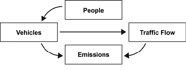
A.10.2
GENERAL METHOD (UNDERSTANDING THE BIG
BLOCKS)
A simplified approach to mobile source emission reduction strategy
analysis does exist. Though models and equations may process
inputs differently, their approach is very similar. Mobile source
emission reduction strategy analysis can be broken down into several
general steps, in which various relationships may define the result.
The four analysis blocks are shown in Figure 10.1.
Figure 10.1 Analysis Blocks
People refers to the population that is affected by the project. This
may be as small as an office building or as large as regional
participation in a specific program. This analysis block can be
expressed as person trips, mode share, travel time, and trip ends.
Vehicles refers to the activity people conduct with their personal mode
of transportation. This can be vehicle trips, peak vehicle trips,
vehicle miles traveled, and engine starts.
Traffic flow refers to how the participants’ mode of travel is improved.
This can be a change in overall travel speed, regional speed, or
corridor speed, as well as reduced numbers of vehicle accelerations
and idling times.
Finally, emissions refers to how pollutants from the personal mode of
transportation are affected. In most cases, differences between
before and after emission rates are used to determine benefits.
Comprehensive emissions assessments include running, evaporative,
crankcase, engine start, and diurnal emissions.
Emission factors for each component are provided by EPA’s
MOBILE6 emission factor model, used outside of California.
California uses the EMFAC emission model. EMFAC is maintained
by the California Air Resources Board (CARB).
A.10.3
The MPO and/or TCEQ develop emission factors. These factors
reflect daily temperatures, vehicle mix and age distribution, fuel
characteristics, inspection and maintenance (I/M) programs, and
other factors representative for the local area.
TRIP BEHAVIOR MODIFICATION STRATEGIES
For TDM projects whose goal is to modify travel behaviors, the
following generalized steps may be used.
First, the project scope (physical limits, use, and participants) must be
defined. This is a critical step to the overall process. Though some
TDMs will require inputs readily available, others will require some
assumptions. Assumptions may be developed from survey data,
experiences from other similar areas, or use of mode choice models.
These assumptions should be well documented and reviewed
periodically to ensure that they are reasonable. This should result in
the number of person trips affected.
Second, the person trips are transformed into vehicle trips. This can
be done by dividing person trips by an appropriate regional or
corridor average vehicle occupancy (AVO). If employer-based
strategies are used, an AVO specific to that center would be
preferable to regional or corridor averages.
Third, the vehicle trips are applied over a certain length to yield
changes in VMT. Again, regional or corridor average trip lengths can
be used, but preference should be given to data that are as project
level as possible.
Fourth, changes in speed (project level or regionally) are determined.
Speed changes may be determined using elasticity.
Elasticity states how a percent change in an input variable affects a
percent change in an output variable. They are developed through
direct observation or from results obtained by an approved mode
choice model. Elasticity is generally not valid outside the range of
values developed for them, nor applicable between different regions.
The travel results are then used with emission factors derived from
MOBILE6. Trip end emissions and VMT-related emissions are
calculated from steps two through four.
A.10.4
SYSTEM IMPROVEMENT STRATEGIES
The focus of these project types is to optimize the flow within the
transportation system given the current and future travel demand on
it. Examples of these projects include HOV lanes, freeway ramp
metering, and traffic signal coordination. These projects seek to
directly affect local, corridor, or regional travel speeds by reducing
delays and smoothing vehicle accelerations. Hard vehicle
accelerations can increase emission rates for certain pollutants by 10
times normal running emission rates.
First, the project scope is defined by determining the number of
vehicles (volume or ADT) impacted by the strategy. These data can
be gathered from the field directly through observation or by
consulting local or state traffic databases for current volumes.
Second, determine changes in system performance measures such as
average speed or delay, a surrogate for idling time, through traffic
simulation software or other sketch-planning methods. Only in rare
cases should professional estimates be used to determine travel
impacts. In these cases, justification of the estimate should be
provided to the reviewing agencies and included in the
documentation.
Third, the system performance changes are translated into emission
changes using MOBILE. Before and after emission rates for
corresponding before and after speeds are applied to the project
scope to determine the daily emission benefits.
VEHICLE/FUEL TECHNOLOGY STRATEGIES
Projects founded in modifications to vehicles or fuels for cleaner
burning engines, fuels, or systems directly affect the base emissions
rate. An example of a project fitting this strategy is alternative-fuel
vehicles. These projects do not seek to modify either travel behavior
or system performance; instead, they seek to alter the fleet emission
characteristics by lowering overall emission rates.
Vehicle or fuel technology projects simply require a scope and the
change in emission rates. The scope is then applied to the difference
in emission rates from before and after the project implementation.

A.10.5
PROJECT RANKING CRITERIA
The appropriate selection of transportation projects is always an
important task. When comparing TDM-type strategies, several
ranking criteria may be used. Depending on regional priorities, these
criteria can be weighted to choose the most appropriate projects.
Prioritization can be consolidated in major categories or composed of
subcategories with unique weighting.
Consider the following examples that demonstrate the differences.
Example 1: Major Criteria-Only Project Evaluation System
Example 2: Stratified Project Evaluation System
Travel Impacts
Travel impacts refer to how the project changes person trips, vehicle
trips, VMT, or speeds. Each of the travel impacts affects total
mobile source emissions; some impacts are greater than others. If a
region’s goal is to significantly reduce starting emissions, then
changes in person trips or vehicle trips should have higher weight
Points
Criteria 1 40
Criteria 2 30
Criteria 3 30
TOTAL 100
Points
Criteria 1 40
Subcriteria 1-1 20
Subcriteria 1-2 60
Subcriteria 1-3 20
Subtotal 100
Criteria 2 30
Criteria 3 30
Subcriteria 3-1 70
Subcriteria 3-2 30
Subtotal 100
TOTAL 100
A.10.6
assignments. If the region’s goal is to minimize efforts to modify
travel behavior and instead improve the transportation network
performance, then changes in behavior or speeds will be more
significant.
Emission Impacts
Emission impacts refer to how the project will reduce CO, VOC,
NOx or PM and whether it addresses hot spots or not (for CO only).
Emphasis should be placed on pollutants of interest to regional air
quality attainment. In many nonattainment areas, the focus of
control plans is to manage and reduce the amounts of VOC and NOx
produced by transportation facilities. In these cases, significant
weighting should be assigned to each.
Local Participation/Funding
Local participation/funding is important if local jurisdictions are
willing to partially fund a project. Local participation in a proposed
project demonstrates additional support and need for advancement.
These projects may be less likely to be postponed to later analysis
years when accommodating the accelerated funding and
implementation for regionally significant projects.
Accelerated Implementation
Accelerated implementation is important for areas seeking rapid
deployment of air quality strategies to reach attainment status or help
to prevent reclassification to worse nonattainment status.
Accelerated implementation refers to projects that will be operational
within 2 years of adoption into the TIP.
Cost-Effectiveness
Cost-effectiveness can be an additional criterion by which projects
are ranked and selected. This should be expressed as dollars spent
(implementation and operating) per pound of pollutant reduced.
California assesses cost-effectiveness for the total pollutant reduction
(total organic gases [ROG] + NOx + PM 10) as opposed to cost-
effectiveness for each individual pollutant.
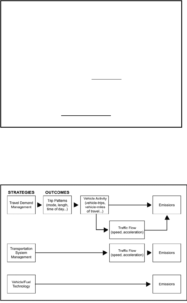
A.10.7
SUMMARY OF PROCESS FRAMEWORK
The analytical process using three strategies is summarized
graphically in Figure 10.2, excluding cost-effectiveness and project
ranking.
Figure 10.2 Off-Model Analysis Flow Chart
Regional Travel Demand Models
A standard tool for transportation modeling in regional
transportation planning is the travel demand model. The travel
demand model for a region is composed of many smaller traffic
analysis zones and a transportation structure or network connecting
Project costs are amortized over the expected life of the project
given a discount rate. The amortization formula yields a capital
recovery factor, which, when multiplied by the funding, gives the
annual funding for the project over its expected lifetime. The
discount rate reflects the opportunity cost of public funds for the
clean air programs. This is the level of earning that could be
reasonably expected by investing public funds in various financial
instruments, such as United States Treasury securities. Cost-
effectiveness is calculated by dividing the annualized funds by
annual emission reductions.
Capital Recovery Factor (CRF) = 1)1(
)()1(
−+
+
n
n
i
ii
where i = discount rate
n = project life
Cost-Effectiveness = (CRF * Funding) __
(ROG + NOx + PM 10)
A.10.8
each of the zones. Travel demand models do not provide a local
street level of detail and are focused on a more homogenous area.
Many factors characterize the transportation network. These factors
include the monetary cost and availability (time) of travel by mode
between each pair of traffic analysis zones. The model’s future
conditions are a function of the proposed transportation network
given demands from forecasted population and employment
characteristics for each traffic analysis zone. The model calculations
are powered by travel survey data, which are used to predict trip
generation by type in each traffic analysis zone, how these trips are
distributed, which modes of travel are used, and what paths each trip
takes in the network. This is also referred to as the “four-step”
modeling process of trip generation, trip distribution, mode choice,
and trip assignment.
Advantages
Travel demand models are good tools for estimating the impacts of
large-scale projects that can be translated to the model’s
transportation network, but are weak for estimating small-scale
projects at a local level. Because of the regional nature of the travel
demand model, changes in VMT and speeds are identified across the
entire transportation network.
The use of regional travel demand models may be better received by
reviewing agencies. Reviewers typically have a higher confidence in
the results obtained from the travel demand models because they are
more familiar with its analysis concepts (four-step process). MPOs
invest a great deal of staff time and data collection efforts toward the
regional travel demand model. In addition, validation and calibration
processes are performed on these models.
The models are also dynamic. For this reason, vehicle demand is
redistributed on the transportation network as projects are evaluated.
Redistribution better simulates traveler decisions made based on rate
and cost (monetary and time) of travel. Redistribution may also
impact other projects on the transportation network, which can then
be evaluated simultaneously for any adverse impacts or lessened
credits.

A.10.9
Table 10.1 Strategies for Representing MOSERS
in Travel Demand Models
Control Measure Strategy
Area-wide
rideshare
incentives
•Increase time due to meeting pool members at
park-and-ride lot or other locations.
•Reduce time and cost due to HOV use and
ridesharing.
•Reduce access time at destination to represent
preferential parking.
•Change auto occupancy.
Area-wide
employer trip-
reduction
strategies
•Reduce the number of vehicle trips by traffic
analysis zone (TAZ).
Improved public
transit
•Reduce transit travel time and/or wait time.
•Reduce transit passenger cost.
•Change transit network to reflect improvements in
service.
High-occupancy
vehicle lanes
•Recode the network with HOV links parallel to
existing links.
•Reduce travel time and cost for rideshare vehicles
between zones connected by HOV lanes.
Parking
management
•Increase parking costs.
•Increase link capacity and speeds to reflect parking
restraints or reduce travel time and cost for
nonscheduled road users.
•Increase access (walk) time at destination to
represent parking restraints.
Bicycle and
pedestrian
programs
•Reduce trip generation rates for shorter trips.
Vehicle use
limitations/
restrictions
•Set infinitely high impedance values for specific
links, or delete links from the network.
•Reduce the number of vehicle trips by TAZ
Traffic flow
improvements
•Adjust travel times, turn penalties, parking, and
capacities for individual links and nodes.
The travel demand model generates a wealth of information. Even if
the regional travel demand model is not used to evaluate benefits of
mobile source emission reduction strategies, a variety of data can be
mined for use in other analysis tools. For example, average trip
lengths or the number of trips made in peak/off-peak periods can be
derived from trip tables and network data.
The mode choice model, an integral part of the regional travel
demand model, can be used independently of the travel demand
model to evaluate some mobile source emission reduction strategies.
A.10.10
If the regional travel demand model has met approval from reviewing
and oversight agencies, few problems during conformity
determinations or SIP review would be expected.
Disadvantages
Travel demand models have a limited application to only a few
mobile source emission reduction strategy–type projects. These
models have difficultly assessing impacts from regional policies where
travel is minimally affected at the zonal level, but where the aggregate
benefits are measurable.
The model’s scale may be too large to support mobile source
emission reduction strategy evaluation in many cases. Travel demand
models can study regional and corridor-level impacts of major
infrastructure developments. In some cases, this geographic scale is
too large to quantify the small benefits derived from projects.
Travel demand models generate speed estimates that represent the
average traffic flow conditions on the links within the network.
These speeds may be representative of field speeds in some cases.
Because of the low confidence that speeds generated by the model
are equivalent to field speeds associated with individual links, link
speeds should not be used.
Travel demand models are not equipped to predict shifts in travel
demand due to employer-based transportation management
programs and similar programs initiated by the local government.
Zonal changes are required for these types of strategies.
Use of the regional travel demand model for some mobile source
emission reduction strategy projects can require a significant level of
effort to develop the appropriate inputs to describe the project.
Professional experience greatly reduces the time required to find or
develop mobile source emission reduction strategy project inputs for
use in the regional travel demand model.
Emission factors applied to model output outside the regional travel
demand model use spreadsheets or other customized software. Some
software programs (Post Processor for Air Quality [PPAQ] and
Surface Transportation Efficiency Analysis Model [STEAM])
automate the processing of travel model outputs and emission
factors.
Finally, travel demand models can produce errors of over 30 percent
in link volumes and over 50 percent in link speeds. The magnitude
of these errors greatly exceeds the magnitude of the travel impacts of
most mobile source emission reduction strategies.
A.10.11
Travel Demand Model Post-Processors
These analysis tools take the information provided by the travel
demand models in the form of trip tables and process the results
outside of the travel demand model once the network scenario is
modeled. They typically have interfaces to an emission factor model
or have the emission factors coded into the program. Some tools
also reconcile VMT between the regional travel demand models and
the Highway Performance Monitoring System (HPMS).
Advantages
Post-processing tools can provide sound analysis methodologies
directly to data generated from the regional travel demand model.
Some post-processing tools can evaluate a variety of TDM projects.
The capabilities of a post-processor are independent of other
technologies used by other available post-processing tools.
Disadvantages
Not all post-processors estimate travel and emissions impacts. Some
perform only one of the functions. The FHWA TDM Evaluation
Model is an example of a post-processor which can estimate VMT
impacts of TDM projects but does not have the capability to estimate
emission changes from those projects. In this case, the analyst is
required to use the TDM Evaluation Model results with trip-end
and/or VMT-related emission factors in an additional post-
processing procedure.
Use of post-processing tools requires experience with regional travel
demand models. If staff members are not experienced with regional
travel demand models, they should seek assistance from experienced
modelers before proceeding with these tools.
Examples include:
• FHWA TDM Evaluation Model,
• FHWA STEAM,
• PAQONE, and
• PPAQ.
Traffic Simulation Models
Classified as either microscopic or macroscopic in nature, traffic
simulation models are another available resource and are suited to
analyze impacts of some mobile source emission reduction strategy
projects. Because the model environment is physical in nature (lanes,
A.10.12
intersections, traffic volumes, turning movements, etc.), these tools
are not suited for evaluating projects influencing travel behavior.
Table 10.2 shows some of the available traffic simulation models and
the projects that they can be used to evaluate.
Advantages
These tools explicitly represent most traffic control devices (signals,
stop signs, yield signs, etc.) without the use of surrogate measures to
account for these controls. In contrast, travel demand models cannot
directly evaluate improvements of signal coordination in a corridor,
but use surrogates (adjustments to travel time or link capacity) to
model their impacts.
When properly calibrated, microsimulation tools can provide better
estimates of traffic flow than travel demand models. In addition, the
travel outputs generated by these tools are comparable to actual field
measurements.
Microscopic models are able to estimate the speed profile of vehicles
and idling time. In addition, they can provide indications of
acceleration rates. Because of this, they can evaluate the impacts
from changes in acceleration and idling. These are two impacts
provided by traffic signal hardware and timing improvements.
Microsimulation tools can better represent the road network than
travel demand models. Their use is best for arterial streets and
freeway sections. The tools can often account for vehicle
interactions in merge and weaving areas, as well as along arterial
streets as vehicles accelerate and decelerate.
Some microsimulation tools produce speed and acceleration results.
Some models incorporate emission factors that can be used with the
travel output. In these cases, traffic flow improvement projects
might be better evaluated for their travel and emission projects.

A.10.13
Table 10.2 MOSERS Analyzed by Traffic Simulation Models
Control
Measure
CORFLO
INTRAS
FREQ
NETSIM
PASSER
II
PASSER
III
TRANSY
T-7F
Intersection
Signal
Improvements
No No No Yes Yes DMD Yes
Arterial Signal
Improvements
Yes No No Yes Yes No Yes
Area Signal
Improvements
Yes No No Yes No No Yes
Eliminate
Unnecessary
Controls
CRDR No No ARTL No No No
Restriping to
Increase Lanes
CRDR FWY FWY ARTL ARTL No ARTL
One-Way
Streets
Yes No No Yes Yes No Yes
Turn Lane
Installation
CRDR FWY FWY ARTL ARTL DMD ARTL
Turning
Movement
Restrictions
Yes No No Yes Yes DMD Yes
Reversible
Traffic Lanes
CRDR FWY FWY ARTL ARTL No ARTL
Intersection
Widening
No No No No No No No
Road Widening CRDR FWY FWY ARTL ARTL DMD ARTL
Improved
Traffic Control
Devices
CRDR FWY FWY ARTL SIG SIG SIG
Grade
Separation
Yes No No Yes No No Yes
Incident
Detection and
Management
Systems
No Yes No No No No No
Lane Use
Restrictions by
Vehicle Type
No FWY No ARTL No No No
Freeway
Diversion and
Advisory
Signing
No No No No No No No
Ramp Metering No Yes Yes No No No No
Integrated
Surveillance
and Control
No No No No No No No
Parking
Restriction
Yes No No Yes Yes No Yes
Motorist
Advisory
No No No No No No No
Peak-Period
Pricing
No No No No No No No
A.10.14
Disadvantages
Microsimulation tools are limited to evaluating the range of traffic
flow improvement projects and a limited number of market-based
strategies. In addition, there is no single microsimulation tool that
can evaluate all of the project types that can be evaluated by
simulation tools.
Traffic simulation tools are not responsive to shifts in travel demand.
They use traffic volumes supplied by the user but cannot forecast
changes in demand within the network because of other network
changes. These tools also lack a mode choice model and
mechanisms for distributing trips on the network.
Some tools are not equipped with an emissions estimation module
and require post-analysis to estimate changes in trip-end emissions,
start emissions, and diurnal emissions. Even if a specific tool does
provide a method for estimating emissions, a good understanding of
the base emission rates and application are required to accurately
interpret the results. They may not reflect the regional characteristics
or VMT and vehicle fleet mixtures.
For network tools, a considerable amount of calibration is required to
obtain reasonable estimates of traffic variables and thus emissions.
For example, FRESIM has nearly 20 embedded parameters that the
user can change to calibrate the model to local conditions.
Calibration is among the more difficult tasks in any modeling effort.
Some simulation packages include vehicle emission factors. These
emission factors may require adjustment to represent local
conditions. A thorough review of the program’s internal emission
factor data is required prior to any adjustments. This ensures that
analysis staff is aware of the nature of the emission factors and their
use within the package before making adjustments that may not be
appropriate.
Examples
Microscopic tools include:
• PASSER,
• TRANSYT,
• FREQ, and
• SYNCHRO.
A.10.15
Macroscopic tools include:
• CORFLO and
• NETSIM.
Off-Network Analyses or Sketch-Planning Tools
These tools entail a more formal process than use of empirical
comparisons. They typically estimate travel and emission impacts
from a variety of MOSERS types. They are best at estimating gross
impacts of projects. In contrast to previous tools, these techniques
are not validated or calibrated and are less rigorous in nature. Few
regions evaluate the accuracy of these techniques through
comparisons of before and after studies. These tools typically use
regional travel data generated through the travel demand modeling
process or other means in conjunction with the characteristics of the
mobile source emission reduction strategy to estimate regional
emission impacts.
Advantages
In most cases, sketch-planning tools are easy to use. They do not
require a great deal of training to operate or use, in contrast to
regional travel demand models. Data are supplied to the tools, and
then the tools generate output.
Some sketch-planning tools attempt to segregate impacts to work and
nonwork trips and by the peak and off-peak periods. Unlike the
travel demand models, these tools chain trips together for defining
the trip purpose. This is a more accurate representation of the true
purpose of a trip, such as a work trip with one or more intermediate
stops before reaching the final destination. Therefore, differences
will exist between regional travel demand model trip tables and the
trips used by these tools.
Once foundation data are input for use, many projects can be
evaluated sequentially, or staff may experiment with project scopes to
determine desired levels of effectiveness. The ability to analyze
several projects in a rapid fashion allows MPO staff to quickly
process many projects in a short amount of analysis time.
Disadvantages
Agency reviewers may perceive the use of these tools as a black box
if sufficient documentation is not provided or if they lack experience
using and judging the tools’ results. Care should also be taken by
A.10.16
MPO staff using these tools so that they fully understand how the
data are used and what the results indicate.
Some tools can require extensive data collection from the travel
demand model and various other sources. This may require a
majority of the total analysis effort. Data from a variety of sources
including the census and regional travel demand model are required.
Mining or transforming surrogate data into the proper input data can
be labor intensive.
If data for these tools are not available, staff may rely on the use of
assumptions to complete the analysis. If assumptions are used, they
should be clearly indicated or summarized for the reviewing agency.
If the assumptions are not referenced from other documents where
values were used, then sufficient justification should be provided for
the reviewing agency to determine if the assumption is acceptable or
not.
For some mobile source emission reduction strategy projects,
planning assumptions regarding the scope of the project in mobile
source emission reduction strategies of vehicle trip, VMT, and speed
changes must be made. These assumptions are typically made for
supply management projects in lieu of simulating the effects. Again,
reasonable assumptions should be made and well documented.
Examples are
• TCM Tools,
• TCM Analyst,
• DRCOG CM/AQ Evaluation Model,
• Texas Transportation Institute (TTI) CM/AQ Evaluation
Model,
• FHWA Southern Resource Center Off-Model Analysis
Techniques, and
• FHWA Sketch-Planning Analysis Spreadsheet model
(SPASM).
Empirical Comparisons
This is one of the simplest methods for estimating the emission
impacts of mobile source emission reduction strategy projects. It is
also one of the least precise and least accurate methods. Planners use
experiences from other similar areas to estimate the impacts in one’s
own area. This analysis method was suggested in A Manual of
Transportation-Air Quality Modeling for Metropolitan Planning Organizations.
A.10.17
Advantages
This is the simplest approach for estimating travel and emission
impacts of mobile source emission reduction strategy–type projects.
Project scopes and their results might be proportionately scaled up or
down to fit a region’s planned project. Extreme care must be given
to the appropriate application of this approach to extremely similar
cases and areas so that comparable results can be expected.
The empirical data must be stringently evaluated for accuracy and
reliability. Mobile source emission reduction strategy impacts are
difficult or impossible to measure directly and require other ways to
collect or estimate the data. A good understanding of how a project’s
results were calculated is required so that the results may be correctly
applied to a new region.
Disadvantages
Generally, there is a lack of available before and after data to evaluate
mobile source emission reduction strategy impacts. Though regions
may validate their mobile source emission reduction strategy impacts,
this information is difficult to find and obtain because it is not widely
available through technical information services.
Considerable staff time can be invested to investigate the results of
similar projects under consideration. Although information on
reasons for a project’s success or failure is invaluable and can be
applied across geographic boundaries, the results of the projects
themselves are less applicable, unless many of the characteristics
between the regions are similar.
Interagency consultation partners are least likely to accept benefits
from this approach. The success or failure of a mobile source
emission reduction strategy is dependent on many local factors: area
size, demographics, available infrastructure, and land use patterns.
Therefore, rigorous approaches are more likely to be required for
acceptance by federal and state reviewing agencies.
Benefits of Standardized Analysis Methods
A variety of simulation tools are required to evaluate a typical range
of strategies selected for a region. As demonstrated in this section,
no single analysis tool can successfully evaluate all mobile source
emission reduction strategy project types. As a result, a region or
state may elect to adopt a standardized set of analysis methods.

A.10.18
Standardization provides several benefits. First, reviewing agencies
become familiar with these methods. As a result, review of off-
model analyses can be expedited. Fewer questions of estimated
emission benefits may be raised during review. Second, inter-regional
comparisons can be made. In particular, reviewing agencies may
desire to compare assumptions. In many cases, these planning
assumptions significantly impact the estimated emissions benefits.
Though not required during formal review, MPOs or the state could
review project cost-effectiveness. Suggested projects might then be
developed by maximizing the cost-effectiveness under fiscally
constrained transportation plans. Finally, generalizations regarding
mobile source emission reduction strategies can be made once a
significant number of projects are evaluated in a like manner.
Sources
Cambridge Systematics, Inc., A Sampling of Emissions Analysis
Techniques for Transportation Control Measures, Federal Highway
Administration, Washington, D.C., October 2000.
Cambridge Systematics, Inc., Transportation Control Measure Information
Document, Report No. 400-R-92-006, Office of Mobile Sources,
United States Environmental Protection Agency, Washington, D.C.,
March 1992.
Eisinger, D. S., et al., Transportation Control Measures: State
Implementation Plan Guidance, prepared for United States
Environmental Protection Agency, Washington, D.C., September
1990, cited in Knapp, Keith K., Rao, K. S., Crawford, Jason A., and
Krammes, Raymond A., The Use and Evaluation of Transportation Control
Measures, Report No. FHWA/TX-94/1279-6, Texas Transportation
Institute, College Station, Texas 1994.
Harvey, G., et al., A Manual of Transportation-Air Quality Modeling for
Metropolitan Planning Organizations, developed for National Association
of Regional Councils, Washington, D.C., November 1992, cited in
Knapp, Keith K., Rao, K. S., Crawford, Jason A., and Krammes,
Raymond A., The Use and Evaluation of Transportation Control Measures,
Report No. FHWA/TX-94/1279-6, Texas Transportation Institute,
College Station, Texas, 1994.
Knapp, Keith K., Rao, K. S., Crawford, Jason A., and Krammes,
Raymond A., The Use and Evaluation of Transportation Control Measures,
Report No. FHWA/TX-94/1279-6, Texas Transportation Institute,
College Station, Texas, 1994.
Methods to Find the Cost Effectiveness of Funding Air Quality Projects: For
Evaluating Motor Vehicle Registration Fee Projects and Congestion Mitigation
A.10.19
and Air Quality Improvement (CMAQ) Projects, California Air Resources
Board and CalTrans, 1999 Ed.
TDM Case Studies and Commuter Testimonials, Transportation Demand
Management Institute of the Association for Commerce
Transportation, Washington, D.C., August 1997.
A.10.20

A.11.1
11.0 MOBILE SOURCE EMISSION REDUCTION
STRATEGY DOCUMENTATION
Section Objective
This section provides guidance for documenting MOSERS. Features
are identified that help create useful MOSERS documentation. A
standard form is provided.
Good documentation of mobile source emission reduction strategies
is crucial for gaining emission credit for submitted measures and
conformity determination of the SIP. All off-model analysis
documentation should be consistent throughout. Documentation
might be provided in either electronic or hardcopy formats to the
reviewing agencies. A standard documentation format should be
followed to expedite the interagency consultation partner review for
conformity determination.
Planners must maintain data in such a way as to facilitate comparison
of the planned and actual efficacy of the mobile source emission
reduction strategies.
PROJECT DESCRIPTIONS AND BENEFITS
Good documentation of a TCM project should include:
• Project TIP ID,
• Project Name,
• Description (project limits/scope and objective);
• One small, descriptive paragraph about the project or
measure and its relation to larger programs and scope,
expected emissions benefits, and limitations;
• Project limits or scope;
• Specific location;
• Funding category;
• Responsible implementation agency;
• Letting date;
• Implementation date;
• Methodology used to derive the TCM project benefits;
The goal when creating MOSERS
documentation should be to provide the same
level of detail for all MOSERS with a consistent
methodology used for each measure.
Good
documentation
saves time and
trouble with
reviewing
agencies
A.11.2
• Analysis Tool – (description or note);
• Data sources;
• Assumptions and the basis for the assumptions;
• Documentation and references;
• Whether the methodology is nationally or locally derived;
• Detail of the equations or processes used to estimate benefits;
• Sample calculations for one inventoried like project;
• Documentation of spreadsheet (if used) equations through
inclusion or hardcopy printouts;
• Procedures for obtaining and maintaining data;
• Expected benefits;
• Travel (trips removed, VMT removed/reduced, and speed
improvements);
• Emissions (rate source, assumptions, trip-end emissions, and
running emissions);
• Cost-effectiveness (life cycle or effective period,
implementation, and operating costs);
• Major summary;
• Emission reduction;
• Total cost; and
• Annual cost per unit reduced.
SUMMARY DOCUMENTATION
There are currently no standard guidelines for summary
documentation. A variety of tables can be generated to display
project listings and the travel and emission benefits of those projects.
A sampling of summary documentation is described below.
One area chose to summarize their TIP projects for conformity
following the format in Figure 11.1.
Using this format, on-model and off-model projects are clearly
separated for the reviewing agencies. Separating out how the
analyses were conducted will allow the reviewing agency to check that
modeled projects are ones that can actually be modeled. It also
enables the reviewing agency to identify and verify that off-model
analyses were performed correctly and that their benefits are
accurately represented.

A.11.3
Figure 11.1 Sample Documentation Format
Cost-effectiveness summaries are also valuable. When used, these
tables provide a broad overview of strategy benefits and costs. Many
of the mobile source emission reduction strategy projects may be
toward the top of the table and can vary in expense. Only a few
projects will yield high emission benefits toward the bottom of the
table.
Table 11.1 MOSERS Cost-Effectiveness Summary Table
Emissions
Reduction
Revenue
Producing
$0 –
$49K
per Ton
$50K –
$99K
per Ton
$100K –
$249K
per Ton
$250K –
$499K
per Ton
> $500
per Ton
< 0.5
0.5 – 0.99
1.0 – 1.49
1.5 – 1.99
2.0 – 2.49
2.5 – 2.99
3.0 – 3.49
3.5 – 3.99
4.0 – 4.49
4.5 – 4.99
5.0 – 5.49
5.5 – 5.99
≥ 6.0
CONSISTENT LEVEL OF DETAIL
A complete, accurate description of units is required to avoid
confusion during review. Review of off-model analysis
documentation has revealed that slight mistakes in designating units
are sometimes made. For example, when calculating annual VMT
reductions from a project, one document identified the result as
“annual miles.” This prompted closer inspection of the analysis
FY 2xxx TIP PROJECTS
2xxx MODEL
County TIP# Project/Facility Limits Improvement
Projects listed here
2xxx OFF-MODEL
County TIP# Project/Facility Limits Improvement
Projects listed here

A.11.4
method to understand what the units actually meant and how the
figure was derived.
Perform dimensional analysis checks on analysis steps as part of
continued quality control. This quality control step can save valuable
reviewing time and ensure that benefit estimates are accurate and
calculated correctly. In rare cases, this is found to be a problem, but
efforts should be made during the preparation of each document to
minimize the effects of improper analysis.
The MPO should ensure consistency between the emissions
evaluated in the travel demand model and off-model analyses. This is
of concern for hydrocarbon emissions as precursors to ozone.
Hydrocarbons can be reported several ways according to the type of
interest. The most common usages are:
• Volatile organic compounds (VOCs),
• Hydrocarbons (HC),
• Total organic gases (TOG), and
• Reactive organic gases (ROG).
Some analysis tools may report hydrocarbon emission credits in one
of these forms. There is no consistent method for reporting these
types of emissions in analysis tools because there is no consistency
among the states. In Texas, standard practice is to use VOC
emissions.
The use of conservative assumptions is recommended. Including
conservative assumptions during analysis will prevent a region from
over-committing and failing to reach project goals. If the
assumptions are applicable to other project types, then the
assumption should be used. If the assumption varies, justification or
proper referencing should be provided to the reviewing agency.
All factors used in the TCM analysis should be well documented.
Proper and complete documentation will prevent any omissions that
might confuse reviewing agencies. Omissions and lack of references
are important keys used by reviewing agencies to request additional
information, resulting in delays.
In Texas, VOC is
used to report
hydrocarbons
Conservative
assumptions for
project benefits
are highly
recommended
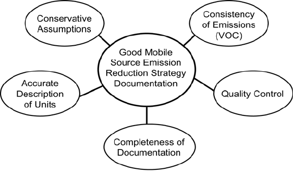
A.11.5
Figure 11.2 Components of Good Documentation
EXAMPLES OF DOCUMENTATION
TCM documentation is not consistent between nonattainment areas
or states. There are several examples of good documentation
practices found, and there are equally as many examples of poor
documentation practices. Two examples are provided below to
demonstrate differences in documentation practices. Both examples
provide evidence of good and poor documentation. Deficiencies and
comments on the documentation are highlighted in the examples by
numbered notes on the side of the example
The first example shows all inputs and assumptions and makes good
use of data and the equations used. It states the analysis calculations;
however, no sources for data or calculations are provided. There is
also a discrepancy between 250 days of use and the 365 days used to
calculate the emissions reduction. The funding for the measure is
provided since TCMs must have funding sources secured to be
included in a SIP, although the funding source is not included.
Operations and maintenance (O&M) costs are not included in the
cost-effectiveness calculation. Finally, no dates for the project are
given.
In example 2, no funding levels or cost-benefit analyses are provided.
The documentation is not well organized, making it difficult to find
key data. The calculations are difficult to follow.

A.11.6
Example 1: Off-Model Documentation
Traffic Signal Coordination n
The city’s master traffic signal controller was replaced with a new controller with
expanded capacity. This allowed 26 more intersections to be coordinated.
Inputs to Calculate Cost-Effectiveness:
Funding dollars (funding): $90,000 o
Effectiveness period (life): 5 years
Days of use/year (D): 250
Length of congested roadway segment (L): 8.07 miles
Traffic volume during congested period (congested traffic): 88,643 trips
per day
Before speed: 28 mph p
After speed: 33 mph
Emissions Factor Inputs (from Table 4):
Before Speed Factor After Speed Factor
ROG Factor 0.51 grams per mile 0.43 grams per mile
NOx Factor 1.14 1.13
PM 10 Factor 0 0
Calculations: q
Annual Project VMT (VMT) = (D) * (L) * (Congested Traffic)
=250 * 8.07 * 88,643 =
178,837,253 annual miles
Annual Emission Reductions (ROG, NOx, and PM 10) in lb. per year
= [(0.50) * (VMT) * (Bef Speed Fctr – Aft Speed Fctr)]/454 grams per lb.
Note: Initial speed improvements decline to zero improvement by the end of the
effectiveness period. In order to account for this, the emission reduction equation
reduces initial emission reduction benefits by one half.
ROG: [(0.50) * (178,837,253) * (0.51 – 0.43)]/454 = 15,757 lb. per year
NOx: [(0.50) * (178,837,253) * (1.14 – 1.13)]/454 = 1,970 lb. per year
PM 10: [(0.50) * (178,837,253) * (0 – 0)]/454 = 0 lb. per year
Capital Recovery Factor (CRF)
= [(1 + i)n (i)] / [(1 + i)n ] – 1 = 0.23,
where n = project life (5 years) and i = discount rate (5 percent)
Cost-Effectiveness of Funding Dollars r
= (CRF * Funding)/(ROG + NOx + PM 10) =
[0.23 * 90,000] / 17,727 =
$1 per lb.
FOR CMAQ PROJECTS ONLY:
Once emissions reductions have been calculated, add them together
(15,727 + 1,970 = 17,727) and convert emissions reductions to kg/day:
= lb. reduced per year / (2.2 lb./kg * 365 days/year)
= 17,727 / (2.2 * 365)
= 22 kg/day
n No dates
o No funding
category
p No sources for
volume or speed
q Good use of
equations and
data below
r O&M costs
not included

A.11.7
Example 2: Off-Model Documentation
DESCRIPTION: 41 intersections with fiber optic cable installed. n
o
Project will reduce the travel time for trips within the district and also help
reduce delays during diversion route strategies. This project is for arterials in
the city of Birmingham. Emissions reductions for air quality includes project (5)
City Center Congestion Management Plan.
Vehicle miles traveled along those routes are 415.340 vehicle miles per day.
p
Average delay reductions per mile are 46 seconds/vehicle for en route drive
information, respectively, during peak hour periods.
(Source: Phase I report, Congestion Management System/IVHS Program Study for
Birmingham, Alabama, by Parsons Brinkerhoff Quade and Douglas, Inc., April 1995)
q
Idling emission rate for delay is based on Mobile 5.0 in year 1998.
HC & NOx Worksheet for (12):
r
Criteria & Assumptions* s
Description Assumption Note
Total vehicle miles in locations 415,340 No
Peak hours period 2.0 hours
Avg. delay reductions per veh.-mile 46.0 seconds/veh.
for en route drive inform.
HC idling emission rate 62.81 grams/hour (1998)
NOx idling emission rate at 11.26 grams/hour (1998)
Methodology t
E = D × VMT × Eri where
E = HC or NOx emissions reductions in grams per day
VMT = VT × L
D = delay reductions per vehicle mile during peak hours
ERi = idling emissions rate
Result
Item Reduction Note
HC reduction = Delay × ERi 66,672 grams
= (46)/3600 × 415340 × (0,1x2) × 62.814
NOx reduction = (E by Bike) + (E by Ped) 10,393 grams/d
=(46)/3600 × 415340 × (0.1x2) × 11.26
VMT Reductions = 0 vehicle miles/year
n No dates
o Good
description, but no
funding given
p No source
q Good source
r No project life
s No days/year
t Lack of proper
unit conversion
A.11.8
FIELD EVALUATIONS FOR VALIDATION
It is extremely important that strong consideration be given to
documenting the actual impacts of mobile source emission reduction
strategy projects. For many TDM programs, data are limited on the
actual changes to travel impacts, given costs of the programs. For
evaluation methods to become more accurate, data of this nature are
required so that refinements to the analysis techniques may be made.
Careful planning should be directed at validating mobile source
emission reduction strategy inputs. Doing so ensures that project
scope and other planning assumptions, from which emission credits
are derived, are verified for the given credit applied to emission
budgets.
STANDARD MOBILE SOURCE EMISSION REDUCTION
STRATEGY DOCUMENTATION FORM
On the next page, a sample mobile source emission reduction
strategy documentation form is provided. The form allows for
adequate description, quantification, and documentation of mobile
source emission reduction strategy projects. The space used for each
section can be expanded as needed. By standardizing documentation,
interagency consultation will be more efficient and SIP and
conformity decisions expedited.

A.11.9
Expected MOSERS Documentation Elements
Mobile Source Emission Reduction Strategy Documentation
Project TIP ID:
Project name:
Description (objective):___________________________________________
______________________________________________________________
Project limits or scope (specific location or locations):___________________
Funding Category:
Implementation agency: _____________________
Letting date: _______________________________
Implementation date: _______________________
Project Benefits Methodology:
Analysis tool:
Is the methodology national or locally derived?
Inputs and sources/assumptions and their basis:
Procedures for obtaining and maintaining data (brief description):
Equations or processes used to estimate benefits (travel, emissions):
Sample calculations for one inventoried like project:
Other documentation and references (include or attach documentation of
spreadsheet equations, if used):
Expected Benefits:
Travel (vehicle trips removed, VMT removed/reduced, speed improvements,
delay reduction):
Emissions (rate source, assumptions, trip end emissions, running emissions):
Cost-effectiveness (life cycle or effective period, implementation and operating
costs):
Major Summary:
Emission reduction (lb./day or tons/day) (kg/day — CMAQ):
Total cost:
Annual cost per unit reduced ($/ton):
A.11.10

B.1.1
1.0 INTRODUCTION
Part A of the guide introduced accepted mobile source emission
reduction strategies. They were placed in historical context and
beside current transportation/air quality policy and issues. The
reader should now have a firm, basic knowledge of mobile source
emission reduction strategies and their place within air quality
planning.
This part of the guide describes the individual mobile source
emission reduction strategies (MOSERS) in greater detail. All 16
1990 Clean Air Act Amendments (CAAA) emission reduction
measures (eligible transportation control measures [TCMs]) are
included along with three other categories of mobile source emission
reduction strategies. Three CAAA measures that refer to bicycle and
pedestrian programs are combined, as described in Part A. Each
category of mobile source emission reduction strategies is introduced
as a section and then subdivided into individual measures. The
individual measures are described along with potential applications.
An equation is then provided to derive the daily emission reduction
of the strategy for analysis and reporting. Finally, the last sections
consolidate the variables and individual equations for quick review or
reference.
The critical issue with mobile source emission reduction strategies
stated earlier is the inability to evaluate their impacts using the
traditional travel demand modeling process. Travel demand models,
the primary tool of transportation planning, cannot assess specifics of
small-scale projects such as intersection and signal improvements.
Therefore, mobile source emission reduction strategies are evaluated
“off model” and do not benefit from the many internal travel model
features affecting volumes and speeds region-wide.
Part A of the guide discussed synergy between individual mobile
source emission reduction strategies in a package of measures.
Several measures within Part B are recommended for implementation
in combination with others. This combining of measures makes it
difficult to separate out the impacts of any single trip-reduction
measure since the measures are not strictly additive due to their
complementary nature.
Because federal and state agencies have not adopted one set of
methodologies, each region has developed its own approach to
evaluating mobile source emission reduction strategies priorities.
These variations cause evaluation inconsistencies between regions
and states. Evaluation of mobile source emission reduction strategies
projects has been enhanced by post-processing software packages
Each MOSERS is
described and given
potential applications
An equation is given
for analysis of each
strategy

B.1.2
that estimate several measures and assess the likely effects of a
particular project. Such models are designed to link directly to the
traditional travel demand modeling process through trip tables.
Unfortunately, software packages to estimate effects on travel activity
or air quality do not exist for all mobile source emission reduction
strategies, and regions must devise their own methods to evaluate
these measures.
This section is an attempt to standardize mobile source emission
reduction strategies analysis for transportation practitioners.
Although there are software programs available to analyze mobile
source emission reduction strategies, one of the purposes of this
guide is to gain consensus with respect to mobile source emission
reduction strategy documentation. Different software programs
make different assumptions regarding the measures; emissions
reductions in one program may not coincide with reductions in
another. This guide does not recommend any TCM analysis software
packages because they are considered to be cumbersome for the
interagency review process during state implementation plan (SIP)
revision. Therefore, sketch-planning techniques are used. They are
the easiest to apply and provide a foundation on which to build more
in-depth analysis of individual measures.
The equations presented for each measure in the guide should be
considered only a beginning. They serve as a basis for conversations
and discussions between the interagency review partners and the
nonattainment areas regarding mobile source emission reduction
strategy use. Also, the equations provide a starting point for near-
nonattainment areas to utilize mobile source emission reduction
strategies when formulating their emission reduction programs as
part of a regionally coordinated prevention initiative.
Part B is an attempt
to standardize
MOSERS analysis
Sketch planning
technique is used for
the equations

B.2.1
2.0 SOURCES FOR INDIVIDUAL VARIABLES FOR
MOSERS METHODOLOGIES
Many inputs are necessary to analyze and document the emissions
benefits of MOSERS. Listed below are the input variables required
to compute the emissions reduction benefit for the individual mobile
source emission reduction strategies presented in this part of the
guide.
Emphasized again, locally specific data should be the first preferred
source for analysis. The most reliable results for estimating emission
reduction benefits are derived from data that are specific to a
nonattainment area. Section 9 of Part A discussed the various
methods of data collection for estimating benefits. It is noted that
locally specific data are not always available, but the initial intent of
practitioners should be to seek out and/or gather data from their
region before borrowing and applying data from other regions.
The primary goal of implementing the various strategies is to help
attain the National Ambient Air Quality Standards (NAAQS) for the
area. Practitioners will desire every emission reduction benefit that
can be counted toward attainment. No one individual mobile source
emission reduction strategy will solve a region’s air quality problem.
It is a combination of strategies that will work best in the situation.
There is only so much benefit to be derived from a single strategy.
Practitioners should not attribute through the individual variables
more benefit than can realistically be derived. Unrealistic
assumptions for the benefits of an individual strategy will, in all
likelihood, be discovered by the review agencies. Therefore,
conservative estimates should be used for the variables in the
methodologies.
The input variables are listed below in alphabetical order by category.
A description of potential sources for the variables is given within
each category.
SCOPING INPUTS
Length and numbers are fairly easy to acquire although some
variables such as number of participants in a strategy may require
surveys of commuters or local businesses.
HH
AREA
Number of households in strategy area
L Length of affected roadway (miles)
Local data are
crucial for analysis
and should be the
first source searched
Use conservative,
realistic assumptions
B.2.2
L
i
Length of each freeway affected by intelligent
transportation systems (ITS) (miles)
N Number of affected corridors
N
BW
Number of participants in bike/pedestrian programs
N
BW, SOV
Number of participants in bike/pedestrianPrograms
who previously used single-occupancy vehicles
(SOVs)
N
D
Number of days in the program
N
DUi
Number of development units by type
N
HBO
Average number of home-based other trips
N
ND
Number of people using the park-and-ride lot but
not driving to it
N
NW
Average number of nonwork trips
N
OPH
Number of off-peak hours
N
P
Number of participants
N
PH
Number of peak hours (AM and/or PM)
N
PK
Number of spaces in parking lot
N
PK, A
Number of parking spaces allowed after
implementation of control
N
PK, B
Number of parking spaces allowed before
implementation of control
N
PPK
Number of preferential spaces in parking lot
N
PR, HOV
Number of high-occupancy vehicle (HOV) parking
spaces at the park-and-ride facility
N
RS
Number of participants in rideshare programs
N
RSt
Average number of times the vehicle is restarted
N
T
Number of participants using transit facilities
N
TR
Number of new transit ridership
N
V
Number of vehicles
N
V, PRI
Number of HOVs using prioritized lane
N
VA
Number of vehicles after implementation
N
VB
Number of vehicles before implementation
Time can be easily computed and estimated from available data and
field collection.
t
A
Time after implementation of strategy (hours)
t
B
Time before implementation of strategy (hours)
t
q
Average time spent in queue waiting to enter freeway
(hours)
Fees for use of road facilities can be easily obtained.
FEE
A
Price for facility use after implementation of measure
(decimal)
FEE
B
Price for facility use before implementation of
measure (decimal)
B.2.3
Parking fee structure changes will require field collection through
surveys of parking lots in affected areas.
∆P
fee
Percentage change in parking fee structure (decimal)
TRAFFIC
Average daily traffic (ADT) in areas affected by an implemented
emission reduction strategy can be derived from local traffic counts
conducted by the Texas Department of Transportation (TxDOT) or
other local sources. For specific HOV facilities related to individual
strategies, some data may need to be field collected by the local
agency. Conservative estimates should be given for ADT after
implementation of strategies (lower instead of higher).
AADT Annual average daily traffic in corridor (vehicles/day)
ADT
A
Average daily traffic on facility after implementation
(vehicles/day)
ADT
A, ALT
Average daily traffic on alternate route(s) after
implementation (vehicles/day)
ADT
B
Average daily traffic on facility before implementation
(vehicles/day)
ADT
B, ALT
Average daily traffic on alternate route(s) before
implementation (vehicles/day)
ADT
i
Average daily traffic for each affected link
ADT
T
Total average daily traffic for affected system
(vehicles/day)
Delay and delay reduction can be estimated from the regional travel
demand model, stopped delay studies, and average speeds derived
from TxDOT traffic analysis.
D
A
Average vehicle delay at intersection after
implementation (hours)
D
B
Average vehicle delay at intersection before
implementation (hours)
DR
OP
Estimated delay reduction during off-peak period
(seconds)
DR
P
Estimated delay reduction during peak period
(seconds)
Idling may be inferred from stopped delay studies.
I
OP
Off-peak hour reduction in idling emissions (hours)
I
P
Peak hour reduction in idling emissions (hours)
B.2.4
Vehicle occupancy can be derived from occupancy surveys, transit
ridership data, and business or commuter surveys. Metropolitan
planning organizations (MPOs), rideshare agencies, and local transit
agencies are potential sources of these data.
AVO
RS
Average vehicle occupancy of rideshare
(persons/vehicle)
OCC Average vehicle occupancy (persons/vehicle)
The percentage of drivers shifting to bike or pedestrian mode can be
estimated through surveys in the area affected by the strategy.
PMS Percentage mode shift from driving to
bike/pedestrian (decimal)
Trip length variables can be acquired from the regional travel demand
model, census data, or local travel surveys. MPOs, TxDOT, and
rideshare agencies may be able to provide these data. Trip length
varies by purpose; pick the one that is most appropriate to the
strategy.
TL
A
Average auto trip length after implementation (miles)
TL
B
Average auto trip length before implementation
(miles)
TL
B, BW
Average length of participants’ trip before
participating in the bike/pedestrian program (miles)
TL
HBO
Average trip length of home-based other
TL
NW
Average nonwork trip length (miles)
TL
PR
Average auto trip length to the park-and-ride lot
(miles)
TL
PURi
Average trip length by trip purpose (miles)
TL
RS
Average auto trip length to rideshare location (miles)
TL
TC
Average auto trip length to the telecommuting center
(miles)
TL
W
Average auto trip length (miles)
TR
DUi
Daily trip rate by development unit type
Utilization rate of a parking lot may require field observation but can
also be derived through business surveys.
U
P
Parking lot utilization rate (estimate)
U
P, A
Utilization rate of parking lot after implementation
(decimal)
U
P, B
Utilization rate of parking lot before implementation
(decimal)
U
P, HOV
Utilization rate of parking spaces by HOVs (decimal)
B.2.5
U
PPK
Utilization rate of preferential parking spaces
(decimal)
Traffic volume can be computed through traffic counts, both
automated and manual.
V
A
Average traffic volume per operating period on main
lanes after implementing ramp metering
V
B
Average traffic volume per operating period on main
lanes before implementing ramp metering
V
D, OP
Average daily volume for the corridor during off-peak
hours
V
D, P
Average daily volume for the corridor during peak
hours
V
GP, A
Average hourly volumes on general purpose lanes
during peak hours after implementation of HOV
facility
V
GP, B
Average hourly volumes on general purpose lanes
during peak hours before implementation of HOV
facility
V
H, A
Average hourly volumes on HOV lanes during peak
hours
V
H, OP
Number of vehicles that pass through the intersection
per hour during the off-peak period
V
H, P
Number of vehicles that pass through the intersection
per hour during the peak period
Vehicle miles traveled (VMT) can be derived from the regional travel
demand model or calculation of products of trip lengths and
volumes. TxDOT, census data, travel surveys, and local MPOs are
sources for these data.
VMT
Auto, A
Vehicle miles traveled by auto after implementation
VMT
Auto, B
Vehicle miles traveled by auto before implementation
VMT
BUS
Vehicle miles traveled by transit vehicle
VMT
Bus, A
Vehicle miles traveled by transit vehicle after
implementation (estimate)
VMT
Bus, B
Vehicle miles traveled by transit vehicle before
implementation
VMT
GP, A
Vehicle miles traveled on general purpose lanes after
implementation (estimate)
VMT
GP, B
Vehicle miles traveled on general purpose lanes
before implementation
VMT
H, A
Vehicle miles traveled on HOV lane after
implementation (estimate)
VMT
H, B
Vehicle miles traveled on HOV lane before
implementation of strategy
VMT
OP
Off-peak hour reduction in speed emissions
B.2.6
VMT
P
Vehicle miles traveled by fleet composite
VMT
PH
Peak hour reduction in speed emissions
VMT
R
Reduction in daily automobile vehicle miles traveled
VMT
R, BW
Reduction in daily auto vehicle miles traveled by
bike/pedestrian mode
VMT
R, OP
Reduction in regional off-peak period VMT after no-
drive days implemented
VMT
R, P
Reduction in regional peak period VMT after no-
drive days implemented
VMT
R, RS
Reduction in daily auto vehicle miles traveled by
rideshare mode
VMT
R, T
Reduction in daily auto vehicle miles traveled by
transit mode
VMT
REP
VMT of the vehicle to be replaced
Vehicle trips can be derived from traffic data from local MPOs and
TxDOT, supplemented by local surveys or counts if determined to
be feasible and required.
BASE Number of daily trips generated by nonregulated
residential and commercial uses (trips)
HH
TRIPS
Average number of trips per household in strategy
area
VT
A
Average daily vehicle trips after implementation
VT
ALT
Vehicle trips on alternate facility
VT
B
Average daily vehicle trips before implementation
VT
BUS
Daily vehicle trips by bus or other transit vehicle
VT
NC
Vehicle trips remaining on facility after
implementation
VT
R
Reduction in number of daily automobile vehicle trips
VT
R, BW
Reduction in number of daily vehicle trips by
bike/pedestrian mode
VT
R, OP
Reduction in regional number of off-peak period
vehicle trips after no-drive days implemented
VT
R, P
Reduction in regional number of peak period vehicle
trips after no-drive days implemented
VT
R, RS
Reduction in number of daily vehicle trips by
rideshare mode
VT
R, T
Reduction in number of daily vehicle trips by transit
mode
VT
S
Vehicle trips on facility shifted to no cost or lower
cost time period
VT
R
is the total number of trip changes of four types: work peak
trips, work off-peak trips, nonwork peak trips, and nonwork off-peak
trips.
B.2.7
EMISSIONS
A variety of vehicle emission sources can be used during analysis.
The most used sources are running exhaust, start exhaust, and
evaporative hot soak. Running exhaust emissions are influenced by
vehicle operating speeds. Start exhaust and evaporative hot soak
emissions are influenced by engine on/off activity. Most of the
emission variables can be derived directly using the Mobile Source
Emissions Factor (MOBILE) model and its output. In some cases,
additional processing may be required to aggregate to the level
specified by the variable. Where speed emission factor is used in this
guide, this refers to the speed-dependent running exhaust emission
factor output by MOBILE.
E
OP
Emissions generated by congestion on affected
roadway system during the off-peak period for each
pollutant (oxides of nitrogen [NOx], volatile organic
compound [VOC], or carbon monoxide [CO])
(grams)
E
P
Emissions generated by congestion on affected
roadway system during the peak period for each
pollutant (NOx, VOC, or CO) (grams)
E
REG
Regional freeway emissions (grams)
EF
A
Speed-based running exhaust emission factor after
implementation (NOx, VOC, or CO) (grams/mile)
EF
A, ALT
Speed-based running exhaust emission factor on
alternate route after implementation (NOx, VOC, or
CO) (grams/mile)
EF
A, i
Speed-based running exhaust emission factor for fleet
composite (including trucks) (NOx, VOC, or CO)
(grams/mile)
EF
A, OP
Speed-based running exhaust emission factor during
off-peak hours in affected corridor after
implementation (NOx, VOC, or CO) (grams/mile)
EF
A, P
Speed-based running exhaust emission factor during
peak hours in affected corridor after implementation
(NOx, VOC, or CO) (grams/mile)
EF
B
Speed-based running exhaust emission factor for
affected roadway before implementation (NOx, VOC,
or CO) (grams/mile)
EF
B, ALT
Speed-based running exhaust emission factor on
alternate route before implementation (NOx, VOC, or
CO) (grams/mile)
EF
B, i
Speed-based running exhaust emission factor for
defined fleet composite (excluding trucks) (NOx,
VOC, or CO) (grams/mile)
B.2.8
EF
B, OP
Speed-based running exhaust emission factor during
off-peak hours in affected corridor after before
implementation (NOx, VOC, or CO) (grams/mile)
EF
B, P
Speed-based running exhaust emission factor during
peak hours in affected corridor before
implementation (NOx, VOC, or CO) (grams/mile)
EF
BUS
Speed-based running exhaust emission factor for
transit vehicle (grams/mile)
EF
GP, A
Speed-based running exhaust emission factor on
general purpose lanes after implementation (NOx,
VOCs, or CO) (grams/mile)
EF
GP, B
Speed-based running exhaust emissions factor on
general purpose lanes before implementation (NOx,
VOC, or CO) (grams/mile)
EF
H, A
Speed-based running exhaust emission factor on
HOV lane after implementation (NOx, VOC, or CO)
(grams/mile)
EF
H, B
Speed-based running exhaust emissions factor on
HOV lane before implementation (NOx, VOC, or
CO) (grams/mile)
EF
I
Emission factor for idling (NOx, VOC, or CO)
(grams/hour)
EF
N
Replacement vehicle speed-based running exhaust
emission factor (NOx, VOC, or CO) (grams/mile)
EF
O
Retired vehicle speed-based running exhaust emission
factor (NOx, VOC, or CO) (grams/mile)
EF
PURi
Speed-based running exhaust emission factor by trip
purpose (NOx, VOC, or CO) (grams/mile)
This guide uses trip end factors to represent all associated vehicle
engine start/stop emissions (includes start emissions at a minimum
and may include hot soak emissions) of a vehicle trip measured in
grams per trip. This factor can be calculated by using information
from MOBILE6 database output.
TEF
AUTO
Auto trip-end emission factor (NOx, VOC, and CO)
(grams/trip)
TEF
BUS
Bus (or other transit vehicle) trip-end emission factor
(NOx, VOC, or CO) (grams/trip)
TEF
TRK
Truck trip-end emission factor (NOx, VOC, or CO)
(grams/trip)
In applying trip emission factors (TEF) in these methodologies, the
user will build the TEF based on the characteristics of the individual
measure and the underlying regional characteristics. Work trips may
have a minimum of two cold starts and two hot soaks, or may be
characterized with an offsite lunch trip leading to four cold starts and
four hot soaks (trips to work, to lunch, to work, and to home). In

B.2.9
reality, there may be a typical local combination that also accounts for
errands along a primary trip (trip chaining, as demonstrated in Figure
2.1), such as stops at the cleaners and grocery store on the way home
from the work site.
Figure 2.1 Trip Chaining
TEF can be derived from MOBILE6 with regional data using the
following process:
1. MOBILE6 can calculate the factor in grams per trip by taking
GM_DAY or GM_HOUR outputs (grams per day or hour)
and dividing it by the value in the STARTS column (number
of starts for the unit of time).
2. Exhaust start and evaporative hot soak emission estimates
from MOBILE are directly influenced by a set of MOBILE6
commands. MOBILE6 includes default values for engine
starts per day (STARTS PER DAY command), the
distribution of starts by hour of the day (START DIST
command), the distribution of hot soak length by hour of the
day (SOAK DISTRIBUTION command), and the
distribution of hot soak duration by time period (HOT
SOAK ACTIVITY command). If the MOBILE default
values are not used and customized or locally collected data
are desired instead, the local dataset should be consistent with
other highway-related planning assumptions and should
receive approval from the interagency consultation partners
(United States Environmental Protection Agency [EPA],
Federal Highway Administration [FHWA], Federal Transit
Administration [FTA], Texas Commission on Environmental
Quality [TCEQ], TxDOT, MPO, and local transit agencies).
Statistically valid instrumented vehicle studies are
recommended to develop these datasets for local conditions;
the EPA should be consulted before implementing the
instrumented vehicle study.
Work
School
Store
Home
B.2.10
3. One procedure to derive a grams per start emission rate is to
use the DAILY OUTPUT command option to obtain daily
engine start results in the database output. The grams for
engine starts field (GM_DAY) from this output is divided by
the engine starts per day field (STARTS) for each record.
The registration distribution field can be used to generate a
weighted start emission factor for each vehicle type over all
model years. Hot and cold start emission factors can be
calculated by modifying the SOAK DISTRIBUTION input
to represent only cold or hot start soak periods. The soak
time affects exhaust start and exhaust running emissions.
Prior to the development and application of hot and cold
start emission factors, the EPA and other interagency
consultation partners should review the proposed plan.
4. Similarly, a hot soak emission factor can be derived by
dividing the grams for hot soaks field (GM_DAY) by the
engine offs per day (ENDS) for each record. The registration
distribution field can be used to generate a weighted start
emission factor for each vehicle type over all model years.
5. After the start emission factors are calculated, emission
changes due to trip reductions are determined by multiplying
the trip changes (VTR) by the start emission factors for each
of the three pollutants and the appropriate vehicle classes.
6. Hot soak emission changes can be calculated by multiplying
the change in total trips by the evaporative hot soak emission
factor generated by MOBILE for each applicable vehicle
class.
FACTORS
The various factor variables (F) can be derived from multiple
sources: travel demand models, emissions inventories, fleet
inventories, rideshare agencies, and local surveys conducted by
agency staff.
F
AT
Percentage of participants who previously drove
SOVs (decimal)
F
BW, SOV
Percentage of new participants in the bike/pedestrian
programs who previously drove SOVs (decimal)
F
C
Compliance factor (decimal)
F
CND
Percent compliance of the no-drive days program
(decimal)
F
ECP
Percentage of existing carpools (decimal)
F
Eff
Project effectiveness factor for each affected freeway
B.2.11
F
EN, OP
Percent of nonrecurrent congestion eliminated on
roadways with ITS deployment, off-peak period
(decimal)
F
EN, P
Percent of nonrecurrent congestion eliminated on
roadways with ITS deployment, peak period (decimal)
F
ER, OP
Percent of recurrent congestion eliminated on
roadways with ITS deployment, off-peak period
(decimal)
F
ER, P
Percent of recurrent congestion eliminated on
roadways with ITS deployment, peak period (decimal)
F
ITS
Percent of roadway system coverage with ITS
deployment (decimal)
F
NR
Nonrecurring emissions (decimal)
F
NR, OP
Percent of roadway system emissions caused by
nonrecurring congestion in the off-peak period
(decimal)
F
NR, P
Percent of roadway system emissions caused by
nonrecurring congestion in the peak period (decimal)
F
OPH
Percent of off-peak hours/emissions affected by ITS
deployment (decimal)
F
PARK
Percent of vehicles that park instead of using the
drive-through facility due to imposed control
(decimal)
F
PURi
Percentage of trips saved by trip purpose (decimal)
F
RS
Percentage of people attracted to the HOV facility
using rideshare (decimal)
F
RS, SOV
Percentage of people attracted to the HOV facility
using rideshare that previously used an SOV (decimal)
F
SOV
Percentage of those people continuing to use an SOV
for their full commute (decimal)
F
T
Percentage of people attracted to the HOV facility
using a transit vehicle (decimal)
F
T, SOV
Percentage of people using a transit vehicle that
previously were vehicle drivers (decimal)
F
USE
Percentage of park-and-ride users that utilize the
facilities (decimal)
F
W
Percentage of participating vehicles commuting to
work (decimal)
Design guidelines and mixed-use developments will require an
estimate of vehicle trips saved as a result of the design and/or
regulation.
CAP Internal capture rate of regulated development
(decimal)
B.2.12
The elasticity variable can be determined from data from TxDOT or
local MPOs. Regional travel demand models rely on these elasticities
in the mode choice module.
Є Price elasticity for mode and time shift or facility
charge
Є
fee
Price elasticity for mode shift
B.3.1
3.0 IMPROVED PUBLIC TRANSIT
Programs for improved public transit
Section 108 (i), CAAA
Improving public transit involves implementation of new or
expanded public transit services or facilities. The improvements may
be accomplished for all transit modes such as buses, light and heavy
rail, and paratransit.
EPA identifies three main components of improved public transit:
• System/service expansion projects attempt to increase ridership by
providing new rail system services and/or expanding bus
services. For buses, the number of routes can be increased,
higher service frequencies can be implemented, or routes can
be extended to reflect new development. Express bus
services can be an alternative to SOVs by providing faster
routes between suburban communities and downtown areas.
In some cities, bus lanes on main highways enable people to
save both time and money in their commute to work. In the
rail system category, there are four major types of transit
services:
o Heavy rail rapid transit is characterized by high speeds
(more than 70 mph) and high capacity (between 20,000
and 34,000 passengers per hour), and is considered to be
most efficient when serving areas with more than
50 million square feet of nonresidential development.
o Light rail transit systems are designed for medium
capacity (ranging from 2000 to 20,000 passengers per
hour) and less developed urban areas.
o Commuter rail is characterized by high-speed, station-to-
station service and is designed to transport people from
suburbs to downtown areas.
o Fully automated rail systems circulate within urban areas
and allow people easier access to congested facilities such
as downtown areas or airports.
• System/service operational improvements focus on geographic
coverage and scheduling changes that make mass transit a
more attractive option to residents and commuters. Improved
transfer procedures between transportation modes such as
car/transit, pedestrian/transit, and bicycle/transit may
encourage increased ridership on public transportation. An
improved fleet maintenance program increases the efficiency
B.3.2
of system operations and projects a perception of reliability to
commuters.
• Inducements to potential transit users include:
o Improvements in fare structures and policies that include
monthly or weekly passes, fare simplification (i.e.,
multiple operators accepting one fare medium), and fare
reductions;
o Marketing programs that include customer service and
intense marketing of transit services; and
o Passenger amenities that include provision of transit
shelters, benches, maps, visually pleasing aesthetics, and
improved comfort of buses and trains.
According to the EPA, air quality benefits from improving public
transit are not difficult to estimate relative to other MOSERS because
the number of new passengers utilizing the improved transit system
can be easier to quantify. This information provides a basis for
estimates of the number of vehicles, miles traveled, and air emissions
reduced.
There are several things to consider when considering improving
public transit as an air emission reduction measure:
• Costs of transit projects need to be seriously evaluated.
Projects may be extremely costly if they are capital intensive
and rely on infrastructure changes. Many urban rail systems
have cost several billion dollars to plan, design, construct, and
implement. At the other end of the cost range, system
operational improvements and public awareness programs are
less expensive. Improving bus shelters, instituting regional
fare structures, and using better signage are examples of
effective improvements that cost much less than the capital-
intensive examples mentioned above. It may take a long
period of time before infrastructure improvements are fully
operational. Planning and implementation timelines are very
important because TCMs in the SIP must be funded and
implemented in a timely manner. Implementing changes to
mass transit systems often requires substantial up-front
investment of government resources. Nonattainment areas
attempting to implement major transit projects into their air
quality programs without adequate political and financial
support may run into problems.
• Improving transit systems is a complex process because of
the extensive planning and coordination required.
B.3.3
o Prior to extending rail or bus service, transportation
departments need to secure adequate funding. This is
often difficult because voter approval or permission from
the state legislature is usually required.
o To ensure the effectiveness of a public transit project,
land use patterns in the region must be considered. For
example, transit services should be designed in
conjunction with urban development plans to ensure that
new development is served by transit. Additional
considerations should be made to provide minimal
walking distances to transit corridors and adequately
controlled parking. Transit expansions should be part of
a larger, more complex urban design project.
• Once projects are completed, aggressive marketing strategies
should be initiated to encourage public utilization of the new
or improved system. However, attempting to change people’s
behavior and attitude toward daily transportation can be a
significant obstacle to a program’s success. Public outreach
materials and advertisements may be helpful in increasing
voluntary ridership, but employer incentives are more likely
to be effective. Improved public transit may not create
immediate increased ridership despite the public awareness
campaigns.
B.3.4
3.1 System/Service Expansion
Strategy: Increase ridership by providing new rail system
services and/or expanding bus services.
Description: Expansion of a transit system or service can include
the addition of rail services through increased
frequency or route extension. Bus or paratransit
services can be expanded with new vehicles and/or
route extensions.
Application: Large cities or communities with enough population
density to support reasonably frequent transit service.
Variables: EF
B
: Speed-based running exhaust emission
factor for affected roadway before
implementation (NOx , VOC, or
CO)(grams/mile)
EF
BUS
: Speed-based running exhaust emission
factor for transit vehicle (NOx, VOC,
or CO) (grams/mile)
F
T, SOV
: Percentage of people using a transit
vehicle that previously were vehicle
drivers (decimal)
N
TR
: New transit ridership
TEF
AUTO
: Auto trip-end emission factor (NOx,
VOC, and CO) (grams/trip)
TEF
BUS
: Bus (or other transit vehicle) trip-end
emission factor (NOx, VOC, or CO)
(grams/trip)
TL
W
: Average auto trip length (miles)
VMT
BUS
: Vehicle miles traveled (VMT) by
transit vehicle
VMT
R
: Reduction in daily automobile VMT
VT
BUS
: Daily vehicle trips by bus or other
transit vehicle
B.3.5
VT
R
: Reduction in number of daily
automobile vehicle trips
Equation:
Daily Emission Reduction = A + B – C – D
A = VT
R
* TEF
AUTO
Reduction in auto start emissions from trips reduced
B= VMT
R
* EF
B
Reduction in auto running exhaust emissions from VMT
reductions
C = VT
BUS
* TEF
BUS
Increase in emissions from additional bus starts
D = VMT
BUS
* EF
BUS
Increase in emissions from additional bus running exhaust
emissions
Where
VTR = NTR * FT, SOV
Number of new transit riders multiplied by the percentage of riders
shifting from single-occupant auto use
VMTR = VTR * TLW
Number of vehicle trips reduced multiplied by the average auto trip
length
Final unit of measure: grams/day
Source: Texas Transportation Institute
B.3.6
3.2 System/Service Operational Improvements
Strategy: Increase ridership on existing transit systems.
Description: Operational improvements focus on enhancing the
efficiency of a transit system and providing more
effective service. These improvements are intended
to attract new riders and reduce the number of
vehicle trips. Improvements can be made, among
others, in scheduling, routes, fleet maintenance
programs, geographic coverage, improved mode
transfer procedures, and monitoring operations.
Application: Cities and/or corridors with existing transit systems,
new land development, limited parking, and heavy or
increasing congestion.
Variables: EF
B
: Speed-based running exhaust emission
factor for affected roadway before
implementation (NOx, VOC, or CO)
(grams/mile)
EF
BUS
: Speed-based running exhaust emission
factor for transit vehicle (NOx, VOC,
or CO) (grams/mile)
F
T, SOV
: Percentage of people using a transit
vehicle that previously were vehicle
drivers (decimal)
N
TR
: New transit ridership
TEF
AUTO
: Auto trip-end emission factor (NOx,
VOC, or CO) (grams/trip)
TEF
BUS
: Bus (or other transit vehicle) trip-end
emission factor (NOx, VOC, or
CO) (grams/trip)
TL
W
: Average auto trip length (miles)
VMT
BUS
: VMT by transit vehicle
VMT
R
: Reduction in daily automobile VMT
VT
BUS
: Daily vehicle trips by transit vehicle
B.3.7
VT
R
: Reduction in number of daily
automobile vehicle trips
Equation:
Daily Emission Reduction = A + B – C – D
A = VT
R
* TEF
AUTO
Reduction in auto start emissions from trips reduced
B= VMT
R
* EF
B
Reduction in auto running exhaust emissions from VMT
reductions
C = VT
BUS
* TEF
BUS
Increase in emissions from additional bus starts
D = VMT
BUS
* EF
BUS
Increase in emissions from additional bus running exhaust
emissions
Where
VTR = NTR * FT, SOV
Number of new transit riders multiplied by the percentage of riders
shifting from single-occupant auto use
VMTR = VTR * TLW
Number of vehicle trips reduced multiplied by the average auto trip
length
Final unit of measure: grams/day
Source: Texas Transportation Institute
B.3.8
3.3 Marketing Strategies
Strategy: Increase ridership by enhancing market demand for
transit services.
Description: Marketing programs attempt to increase demand for a
transit system. Programs can include improvements
in fare structures and policies such as monthly or
weekly passes, fare simplification (i.e., multiple
operators accepting one fare medium), and fare
reductions. Transit operators can promote customer
service programs that enhance responsiveness to
passenger concerns. Operators can also add or
improve passenger amenities such as provision of
transit shelters, benches, maps, visually pleasing
aesthetics, and improved comfort of buses and trains.
This strategy excludes adding more transit vehicles as
a result of ridership increase. If additional buses are
needed, use the equation in 3.1.
Application: Cities with existing and proposed transit systems.
Variables: EF
B
: Speed-based running exhaust emission
factor before implementation (NOx,
VOC, or CO) (grams/mile)
F
T, SOV
: Percentage of people using a transit
vehicle that previously were vehicle
drivers (decimal)
N
TR
: New transit ridership
TEF
AUTO
: Auto trip-end emission factor (NOx,
VOC, or CO) (grams/trip)
TL
W
: Average auto trip length (miles)
VMT
R
: Reduction in daily automobile VMT
VT
R
: Reduction in number of daily
automobile vehicle trips
B.3.9
Equation:
Daily Emission Reduction = A + B
A = VT
R
* TEF
AUTO
Reduction in auto start emissions from trip reductions
B = VMT
R
* EF
B
Reduction in auto running exhaust emissions from trip reductions
Where
VTR = NTR * FT, SOV
Number of new transit riders multiplied by the percentage of riders
shifting from single-occupant auto use
VMTR = VTR * TLW
Number of vehicle trips reduced multiplied by the average auto trip
length
Final unit of measure: grams/day
Source: CalTrans
B.3.10
B.4.1
4.0 HIGH-OCCUPANCY VEHICLE FACILITIES
Restriction of certain roads or lanes to, or construction of such roads or lanes for
use by, passenger buses or high-occupancy vehicles
Section 108 (ii), CAAA
According to EPA, high-occupancy vehicle (HOV) lanes are one of
the most frequently implemented mobile source emission reduction
measures. HOV lanes are designated exclusively for use by vehicles
with multiple occupants such as carpools, vanpools, and transit
vehicles. Implementing HOV facilities can involve adding entirely
new capacity or reallocating existing capacity. Along with a range of
physical options, HOV facilities have operative options such as full-
time HOV-only use, peak time use, and reversing the travel direction
of facilities during peak times. HOV lanes can increase transit use
and car occupancy for work-related trips in congested urban travel
corridors.
The most effective HOV lane improvements generally involve
regional networks of linked lanes, with a system of supporting
facilities and services. Historically, the most successful HOV
applications have been along “radial” corridors into major central
cities where HOV users can save at least 10 minutes of travel time
compared to using mixed-traffic lanes. EPA studies show that HOV
lanes are generally more effective if implemented along with transit
improvements, park-and-ride lots, employer-based transportation
programs, and commuter parking subsidies.
Because of substantial physical and financial requirements, state
departments of transportation (DOTs) usually implement HOV
lanes. Historically, the EPA has found the typical time frame for
implementing HOV lanes is three to eight years for planning, design,
and construction. Private or nonprofit authorities may construct and
operate HOV facilities along the lines of a toll road (high-occupancy
toll [HOT] lanes). Operators can use discriminatory pricing strategies
such as granting toll discounts to HOVs to promote utilization.
Potential land acquisition often determines feasibility and the time
required to implement the project. Also, HOV project planning and
design is a political process involving various parties, including
political leaders, business groups, and citizen groups. Discussions
and negotiation among them, while very important, may add time to
the project.
HOV projects can be very expensive, depending on such factors as
right-of-way acquisition or cost of land, bridge and overpass
modifications, and interchange and ramp modifications to provide
B.4.2
access. Total costs of some HOV projects have exceeded several
hundred million dollars.
HOV impacts on air quality are fairly complex, but Los Angeles, San
Francisco, Washington, D.C., and Portland have documented
emissions impacts from their HOV projects. Assessments of the
effectiveness of HOV lane facilities in reducing system-wide
emissions have generally found reductions amounting to less than
1 percent.
HOV lanes reduce air pollution emissions by reducing running and
trip-end emissions. Reductions in running emissions are derived by
increasing average speeds from low speeds in congested traffic to
50 mph in HOV lanes, and increasing the use of buses, vanpools, and
carpools results in less VMT. If riders do not take additional trips,
HOV lanes will also reduce trip-end emissions. However, if users of
HOV lanes meet their pool or bus through a park-and-ride
arrangement, these trip-end emissions may offset the reduced air
emissions benefits. When calculating the effectiveness of HOV lanes
in reducing emissions, trip-end emissions resulting from using
linkages must be considered.
Two important factors in implementing a successful HOV program
have been identified. Enforcement is critical. EPA studies show that
early and substantial enforcement of HOV rules on a new facility is
the best determinant of long-term public compliance. Also,
education and marketing programs that promote the benefits and use
of the HOV facilities, both during and after construction, increase
the potential for users of the facility.
B.4.3
4.1 Freeway HOV Facilities
Strategy: Reduce emissions by decreasing VMT and increase
average speeds on the lane.
Description: Separate lanes on controlled access highways are
created for vehicles containing a specified minimum
number of passengers. The lane may be concurrent
flow, be barrier/buffer separated, or have a separate
right-of-way.
Application: Highways in areas of traffic congestion with sufficient
available right-of-way.
Variables: AVO
RS
: Average vehicle occupancy of
rideshare (persons/vehicle)
EF
B
: Speed-based running exhaust emission
factor before implementation (NOx ,
VOC, or CO) (grams/mile)
EF
GP, A
: Speed-based running exhaust emission
factor after implementation of HOV
facility (general purpose lanes) (NOx,
VOC, or CO) (estimate)
EF
H, A
: Speed-based running exhaust emission
factor on HOV facility (NOx, VOC,
or CO) (estimate)
F
RS
: Percentage of people attracted to the
HOV facility using rideshare (decimal)
F
RS, SOV
: Percentage of people attracted to the
HOV facility using rideshare that
previously were vehicle drivers
(decimal)
F
T
: Percentage of people attracted to the
HOV facility using a transit vehicle
(decimal)
F
T, SOV
: Percentage of people using a transit
vehicle that previously were vehicle
drivers (decimal)
B.4.4
L: Length of HOV facility (miles)
NP: Total number of expected people
using the HOV lanes per day
N
PH
: Number of peak hours (AM and/or
PM)
TEF
AUTO
: Auto trip-end emission factor (NOx,
VOC, or CO) (grams/trip)
TL
W
: Average auto trip length (miles)
V
GP, A
: Average hourly volumes on general
purpose lanes during peak hours after
implementation of HOV facility
V
GP, B
: Average hourly volumes on general
purpose lanes during peak hours
before implementation of HOV
facility
V
H, A
: Average hourly volumes on HOV
lanes during peak hours
VMT
R
: Reduction in daily automobile VMT
VT
R
: Reduction in number of daily
automobile vehicle trips (estimate)
Equation:
Daily Emission Reduction = A+ B + C + D
A = V
H, A
* (EF
B
– EF
H, A
) * N
PH
* L
Change in running exhaust emissions from vehicles shifting from
general purpose lanes to HOV lanes
B = (V
GP, B
* EF
B
– V
GP, A
* EF
GP, A
) * N
PH
* L
Change in running exhaust emissions of vehicles in general
purpose lanes as a result of vehicles shifted away from general
purpose lanes
C = VT
R
* TEF
AUTO
B.4.5
Reduction in auto start exhaust emissions from trip reductions
D = VMT
R
* EF
B
Reduction in auto running exhaust emissions from trip reductions
Where
VTR
= NP
* (FT
* FT, SOV + FRS * FRS, SOV) * (1 – 1/AVORS)
Number of HOV users multiplied by the sum of the fraction of
users selecting transit multiplied by the percentage that previously
drove single-occupant vehicles added by the fraction of users selecting
ridesharing multiplied by the percentage that previously drove
single-occupant vehicles multiplied by the percentage of ridesharers
that are passengers
VMTR = VTR * TLW
Number of vehicle trips reduced multiplied by the average auto trip
length
Final unit of measure: grams/day
Source: CalTrans (adapted by Texas Transportation Institute)
B.4.6
4.2 Arterial HOV Facilities
Strategy: Reduce emissions by decreasing VMT and increasing
average speeds on the lane.
Description: Separate lanes on arterials are created for vehicles
containing a specified minimum number of
passengers. The lane may be concurrent flow, be
barrier/buffer separated, or have separate rights-of-
way.
Application: Roadways in areas of traffic congestion with sufficient
available right-of-way.
Variables: EF
B
: Speed-based running exhaust emission
factor before implementation (NOx,
VOC, or CO) (grams/mile)
EF
GP, A
: Speed-based running exhaust emission
factor after implementation of HOV
facility (general purpose lanes) (NOx,
VOC, or CO) (estimate)
EF
H, A
: Speed-based running exhaust emission
factor on HOV facility (NOx, VOC,
or CO) (estimate)
F
RS
: Percentage of people attracted to the
HOV facility using rideshare (decimal)
F
RS, SOV
: Percentage of people attracted to the
HOV facility using rideshare that
previously were vehicle drivers
(decimal)
F
T
: Percentage of people attracted to the
HOV facility using a transit vehicle
(decimal)
F
T, SOV
: Percentage of people using a transit
vehicle that previously were vehicle
drivers (decimal)
L: Length of HOV facility (miles)
B.4.7
NP: Number of expected person trips on
the HOV lanes per day
N
PH
: Number of peak hours for each peak
period (AM and PM)
TEF
AUTO
: Auto trip-end emission factor (NOx,
VOC, or CO) (grams/trip)
TL
W
: Average auto trip length (miles)
V
GP, A
: Average hourly volumes on general
purpose lanes during peak hours after
implementation of HOV facility
V
GP, B
: Average hourly volumes on general
purpose lanes during peak hours
before implementation of HOV
facility
V
H, A
: Average hourly volumes on HOV
lanes during peak hours
VMT
R
: Reduction in daily automobile VMT
VT
R
: Reduction in number of daily
automobile vehicle trips (estimate)
Equation:
Daily Emission Reduction = A+ B + C + D
A = V
H, A
* (EF
B
– EF
H, A
) * N
PH
* L
Change in running exhaust emissions from vehicles shifting to
HOV lane
B = (V
GP, B
* EF
B
– V
GP, A
* EF
GP, A
) * N
PH
* L
Change in running exhaust emissions of vehicles in general
purpose lanes as a result of vehicles shifted away from general
purpose lanes
C = VT
R
* TEF
AUTO
Reduction in auto start exhaust emissions from trip reductions
B.4.8
D = VMT
R
* EF
B
Reduction in auto running exhaust emissions from trip reductions
Where
VTR
= NP
* (FT
* FT, SOV + FRS * FRS, SOV) * 2 trips/day
Number of HOV users multiplied by the sum of the fraction of
users selecting transit multiplied by the percentage that previously
drove SOVs added by the fraction of users selecting ridesharing
multiplied by the percentage that previously drove single-occupant
vehicles multiplied by two trips per day (round trip)
VMTR = VTR * TLW
Number of vehicle trips reduced multiplied by the average auto trip
length
Final unit of measure: grams/day
Source: CalTrans (adapted by Texas Transportation Institute)
B.4.9
4.3 Parking Facilities at Entrances to HOV Facilities
Strategy: Reduce VMT.
Description: The transfer point between vehicle and HOV is made
more efficient by constructing park-and-ride lots at
entrances to HOV facilities.
Application: Cities with HOV facilities and sufficient public transit
systems. Planners should be cautious to avoid double-
counting of benefits. Analyze parking related to new
use of the HOV facility.
Variables: EF
B
: Speed-based running exhaust emission
factor before implementation (NOx,
VOC, or CO) (grams/mile)
N
PK
: Number of parking spaces
U
P
: Parking lot utilization rate (estimate)
TL
PR
: Average auto trip length from home
to parking facility (miles)
TL
W
: Average length of affected auto trips
(miles)
Equation:
Daily Emission Reduction =
N
PK
* U
P
* (TL
W
– TL
PR
) * EF
B
* 2 trips/day
Reduction in running exhaust emissions from reduced VMT resulting from park-and-ride lot
use
Final unit of measure: grams/day
Source: Texas Transportation Institute
B.4.10
4.4 SOV Utilization of HOV Lanes
Strategy: Reduce emissions by increasing average speed on the
main lanes of a controlled access highway with an
existing HOV facility.
Description: Areas can increase utilization of their HOV lanes by
permitting SOVs to use the facility for a fee. The
strategy will reduce the number of vehicles on the
main lanes of the highway, leading to an increase in
the average speed along the highway from the
reduced congestion. SOVs may be allowed to use the
HOV facility at certain times (peak hours) or
throughout the day.
Application: Congested highways with existing HOV lanes
operating under capacity.
Variables: EF
GP, A
: Speed-based running exhaust
emissions factor on general purpose
lanes after implementation (NOx,
VOC, or CO) (grams/mile)
EF
GP, B
: Speed-based running exhaust
emissions factor on general purpose
lanes before implementation (NOx,
VOC, or CO) (grams/mile)
EF
H, A
: Speed-based running exhaust
emissions factor on HOV lane after
implementation (NOx, VOC, or CO)
(grams/mile)
EF
H, B
: Speed-based running exhaust
emissions factor on HOV lane before
implementation (NOx, VOC, or CO)
(grams/mile)
VMT
GP, A
: Vehicle miles traveled on general
purpose lanes after implementation
(estimate)
VMT
GP, B
: Vehicle miles traveled on general
purpose lanes before implementation
B.4.11
VMT
H, A
: Vehicle miles traveled on HOV lane
after implementation (estimate)
VMT
H, B
: Vehicle miles traveled on HOV facility
before implementation of strategy
Є: Price elasticity of volume change due
to facility charge
Equation:
Daily Emission Reduction = A – B
A = VMT
GP, B
* EF
GP, B
+ VMT
H, B
* EF
H, B
The running exhaust emissions of the affected highway before
implementation of the strategy for both the general purpose and
HOV lanes
B = VMT
GP, A
* EF
GP, A
+ VMT
H, A
* EF
H, A
The running exhaust emissions of the affected highway after
implementation of the strategy for both the general purpose and
HOV lanes
Where
VMTGP, A = VMTGP, B – (VMTGP, B * Є)
The expected VMT on the general purpose lane after
implementation is equal to the VMT of the lanes before
implementation multiplied by the price elasticity subtracted from the
VMT before implementation
VMTH, A = VMTH, B – (VMTH, B * Є)
The expected VMT on the HOV lane after implementation is
equal to the VMT of the HOV lane before implementation
multiplied by the price elasticity subtracted from the VMT before
implementation
Final unit of measure: grams/day
Source: Houston-Galveston Area Council
B.4.12
B.5.1
5.0 EMPLOYER-BASED TRANSPORTATION
MANAGEMENT PROGRAMS
Employer-based transportation management plans, including incentives
Section 108 (iii), CAAA
Employer-based transportation management programs principally
serve home-to-work trips in urban areas with populations of 250,000
or more. Primarily large employers, i.e., those having more than 100
employees at a single work site, have used employer-based
transportation management programs. Employers provide
information and incentives for employees who pool or use alternative
forms of transportation for their daily commute.
Because home-to-work trips account for only 25 to 33 percent of all
peak period trips made in most urban areas, the impact of commute
management on areawide VMT is limited. However, the commuter
market represents the best potential for grouping riders, removing
vehicle trips, and reducing VMT. Reducing commuter trips not only
reduces emissions associated with VMT but also those associated
with “cold starts,” when commuters set out in the morning, and “hot
soaks,” when vehicles are parked at work and continue to produce
evaporative emissions even after the engines are turned off.
The 1990 CAAA required the implementation of employer-based
transportation management programs in severe and extreme ozone
nonattainment areas. The programs can consist of both voluntary
and mandatory measures. According to EPA, a package of various
complementary measures produces the greatest impacts. For an
individual employer, trip-reduction effects can be seen immediately.
In addition to improving air quality primarily by reduced automobile
trips and VMT, employer-based transportation management
programs can provide savings benefits in the following areas:
• Vehicle expenses,
• Road construction and operation and maintenance (O&M)
costs,
• Expenditures on public services devoted to vehicle traffic,
and
• Resource consumption.
Employer-based transportation management programs can be highly
cost-effective. Employers incur initial costs to design the program
and to develop eligibility requirements for their employees.
Monitoring and accounting costs are incurred periodically. Variation
B.5.2
in costs of programs is based on the size of the employer, the nature
and complexity of programs offered, and the amount of the subsidy
offered.
The EPA has identified three types of employer-based transportation
management programs with their associated costs:
General travel allowance programs require considerable planning and
promotional efforts before implementation, but ongoing
administrative costs are relatively small. Employees can use general
travel allowances for any transportation mode or for
nontransportation purposes. Program monitoring costs are low, and
accounting costs are negligible because the allowance is given out to
all employees as a bonus. The only significant cost to the employer is
the cost of the allowance itself. The cost can be at least partially
offset because the reduction in the number of employees needing
parking can generate savings in maintenance, monthly parking lease
costs, and savings in future capital requirements.
• Targeted or specific allowance programs, such as transit and vanpool
allowances, require ongoing administrative effort for
accounting and monitoring eligibility requirements among
employees.
• Flexible use of allowances for transportation services provided
by many different operators is the largest and most complex
program and may cost even more because of greater
administrative, monitoring, and accounting needs.
Because employer-based transportation management programs are
implemented by private entities, they do not require a substantial
investment in government resources. The amount of time required
to implement an incentive program is relative to the complexity of
the measures offered. Some employer-based transportation
management programs can be implemented almost immediately,
while others require more time.
One significant concern for practitioners is the long-term
sustainability of program impacts. Program effectiveness can
diminish if management support or financial commitment wanes, or
if employee turnover increases. The EPA has found programs that
include financial incentives are more likely to have sustainable results.
The following list summarizes three types of financial incentives and
their goals:
• Tax incentives can allow employers and developers to provide
facilities and equipment conducive to ridesharing. They may
be in the form of investment tax credits or accelerated
depreciation.
B.5.3
• Subsidy programs can help initiate a program by providing
additional funding to enlist employer involvement and reduce
the initial risk for employers in attempting a new program.
The goal of the subsidies is for employers see the benefits of
the program and then continue subsidizing on their own to
satisfy employee desire for using the program and/or to
comply with regional or local mandates. Some subsidy
programs target commuters directly when employer
involvement is unlikely or impractical. For example, vanpool
subsidies tied to corridor reconstruction projects can aid in
the formation of vanpools among commuters using the
affected facilities, regardless of their particular job location.
• Enabling legislation can eliminate or minimize barriers to
widespread implementation of employer-based trip-reduction
programs. A legal requirement mandating employer or
developer involvement is a powerful determinant of program
effectiveness. Mandatory participation is essential to assuring
widespread participation by enough employers to have an
area-wide impact.
The EPA has several observations regarding employer-based
transportation management programs:
• Employer size and location do not seem to determine
program effectiveness. Although downtown settings have an
obvious potential to be effective, many successful programs
have been located in large suburban activity centers. One
possible explanation is that less ridesharing occurs naturally in
those areas, which allows the program more opportunities to
shift commuters’ mode of transportation.
• The costs and benefits of employer-based transportation
management programs are more difficult to measure than
other mobile source emission reduction strategies. The
primary area of uncertainty regarding these programs is the
difficulty in determining causality between areawide
promotional efforts and VMT and emission impacts. It is a
difficult task to separate out the impacts of these programs
above and beyond those reported for employers or to
speculate on the increase in VMT or emissions if these
programs did not exist.
• It is difficult to separate out the impacts of any single trip-
reduction strategy; and the techniques are not strictly additive
due to the complementary nature of many strategies. Care
must be taken not to double-count the effectiveness of
employer-based transportation management programs with
the benefits of area-wide rideshare incentives.
B.5.4
• The roles and responsibilities of the various public, nonprofit,
and for-profit organizations involved in promoting
ridesharing and other travel alternatives within a region need
to be carefully delineated so that the various efforts are not
perceived as either duplicative or conflicting by employers
and individuals.
B.5.5
5.1 Transit/Rideshare Services
Strategy: Reduce vehicle trips and emissions through increased
use of transit, carpooling, or vanpooling.
Description: Employers or groups of employers in activity centers
provide transportation service to and from the work
site to transit facilities and homes. The services can
include subscription buses, midday and park-and-ride
shuttles, and guaranteed ride home programs.
Application: Large companies or groups of cooperating businesses.
Variables: EF
A
: Speed-based running exhaust emission
factor after implementation (NOx ,
VOC, or CO) (grams/mile)
EF
B
: Speed-based running exhaust emission
factor before implementation (NOx,
VOC, or CO) (grams/mile)
N
VA
: Number of vehicles after
implementation
N
VB
: Number of vehicles before
implementation
TEF
AUTO
: Auto trip-end emission factor (NOx,
VOC, or CO) (grams/trip)
TL
A
: Average auto trip length after
implementation (miles)
TL
B
: Average auto trip length before
implementation (miles)
VT
A
: Vehicle trips after implementation
VT
B
: Vehicle trips before implementation
Note: If an automobile is used instead of a van for ridesharing,
replace auto emission factors for van emission factors.
B.5.6
Equation:
Daily Emission Reduction = (A – B) + C
A = VT
B
* TL
B
* EF
B
Auto running exhaust emissions before strategy implementation
B = VT
A
* TL
A
* EF
A
Auto running exhaust emissions after strategy implementation
C = (VT
B
– VT
A
) * TEF
AUTO
Reduction in start exhaust emissions from reduction in vehicle
trips to/from employment center
Where
VTA = NVA * 2 trips/day
VTB = NVB * 2 trips/day
Number of vehicles before or after strategy implementation
multiplied by two trips per day (round trip)
Final unit of measure: grams/day
Source: Texas Transportation Institute
B.5.7
5.2 Bicycle and Pedestrian Programs
Strategy: Reduce vehicle trips, VMT, and emissions through
provision of bicycle and pedestrian support facilities
and programs.
Description: Employers provide support facilities and/or services
to encourage employees to bicycle or walk to work.
The programs include credits to be used toward
purchases of bicycles; bonus days off; shower and
locker facilities; free reflective vest, helmet, nightlight,
and mirror; reduced-cost purchase program for
bicycles; onsite bicycle repair shop with mechanics
and pick-up service; and forgiveness for occasional
tardiness. In a Washington, D.C., area program,
employers must provide at least one bicycle for every
50 employees for midday employee business and
personal use.
Bicycle and pedestrian programs can be classified in
three different TCMs under the 1990 CAAA. In this
instance, the program is employer based and is placed
in this category. This is a clear example of the overlap
found amid the various mobile source emission
reduction strategies.
Application: Areas with existing bicycle and/or pedestrian paths
that can serve businesses or business centers.
Variables: EF
B
: Speed-based running exhaust emission
factor for the average speed of
participants’ trip before participating
in the bike/pedestrian program (NOx,
VOC, or CO) (grams/mile)
F
BW, SOV
: Percentage of new cyclists who
previously drove an SOV (decimal)
N
BW
: Number of participants in the
bike/pedestrian program
TEF
AUTO
: Auto trip-end emission factor (NOx,
VOC, or CO) (grams/trip)
B.5.8
TL
B, BW
: Average length of participants’ trip
before participating in the
bike/pedestrian program (miles)
(The National Personal Transportation Survey
estimated 1.8 miles, yet MPOs may want to use
a more regionally significant estimate.)
VMT
R
: Reduction in daily auto vehicle miles
traveled
VT
R
: Reduction in number of daily auto
vehicle trips
Equation:
Daily Emission Reduction = A + B
A = (VT
R
* TEF
AUTO
)
Reduction in auto start emissions from trip reductions
B = (VMT
R
* EF
B
)
Reduction in auto running exhaust emissions from trip reductions
Where
VTR = NBW * FBW, SOV * 2 trips/day
Number of bike and pedestrian participants multiplied by the
number of participants that previously drove SOVs multiplied by
two trips per day (round trip)
VMTR = VTR * TLB, BW
The vehicle trips reduced multiplied by the average auto commute
trip length
Final unit of measure: grams/day
Source: CalTrans/CARB and FHWA Southern Resource Center
(modified by Texas Transportation Institute)
B.5.9
5.3 Employee Financial Incentives
Strategy: Reduce SOVs for commuting through provision of
incentives to employees to use transportation
alternatives.
Description: Employers can provide direct financial incentives to
employees to use alternative forms of transportation
in their commute. Carpooling, transit use, and
parking subsidies for HOV lane users are examples of
these types of incentives.
Application: Measure can be used in conjunction with
carpool/vanpool programs or matching services, in
areas with adequate public transit and in areas with
controlled or limited parking.
Variables: EF
B
: Speed-based running exhaust emission
factor before implementation (NOx,
VOC, or CO) (grams/mile)
F
BW, SOV
: Percentage of new participants in the
bike/pedestrian programs who
previously drove SOVs (decimal)
F
RS, SOV
: Percentage of new participants in the
rideshare programs who previously
drove SOVs (decimal)
F
T, SOV
: Percentage of new participants using
transit facilities who previously drove
SOVs (decimal)
N
BW
: Number of participants in
bike/pedestrian programs
N
P
: Total number of participants (estimate)
N
RS
: Number of participants in rideshare
programs
N
T
: Number of participants using transit
facilities
TEF
AUTO
: Auto trip-end emission factor (NOx,
VOC, or CO) (grams/trip)
B.5.10
TL
W
: Average auto trip length (miles)
VMT
R
: Reduction in daily auto vehicle miles
traveled
VT
R
: Reduction in number of daily vehicle
trips
Equation:
Daily Emission Reduction = A + B
A = (VT
R
* TEF
AUTO
)
Reduction in auto start emissions from trip reductions
B = (VMT
R
* EF
B
)
Reduction in auto running exhaust emissions from trip reductions
Where
NP = (NRS * FRS, SOV) + (NT * FT, SOV) + (NBW * FBW, SOV)
Number of rideshare participants previously driving SOVs added
to number of transit participants previously driving SOVs added
to number of bike and pedestrian participants previously driving
SOVs
VTR = NP * 2 trips/day
Number of participants multiplied by two trips per day (round
trip)
VMTR = VTR * TLW
The vehicle trips reduced multiplied by the average auto commute
trip length
Final unit of measure: grams/day
Source: Texas Transportation Institute
B.6.1
6.0 TRIP-REDUCTION ORDINANCES
Trip-reduction ordinances
Section 108 (iv), CAAA
Trip-reduction ordinances (TROs) consist of regulations or similar
measures requiring implementation of other mobile source emission
reduction strategies. TROs may specify emission reduction strategies
or simply require a set reduction in VMT, trips, or other measure of
reduced travel.
TROs are applied in a variety of ways, depending upon the needs of a
particular locality. The focus of these ordinances has been to
encourage socially beneficial travel choices rather than controlling
traveler behavior. Most TROs, therefore, offer a range of travel
options, but the individual traveler’s choice is voluntary. The most
successful programs incorporate agencies, employees, and developers
into the creation of TROs.
TROs have existed for well over a decade, with most early examples
appearing in California. Due to a history of congestion and air quality
problems, state legislative actions, and the interaction of CAAA
requirements with the nonattainment status of its major urban areas,
California remains the state with the most significant experience with
TROs.
TROs are applicable in large metropolitan areas and surrounding
suburbs. Most measures are geared toward companies or
developments of a minimum size. This size restriction reduces
hardships on small companies and limits enforcement costs for the
jurisdiction. The criterion often used for companies is the number of
employees at a location. A TRO usually specifies that if a company
has greater than the threshold number of employees (e.g., more than
50), it must begin complying with measures of the local TRO. In
some jurisdictions, multiple thresholds exist. For example, a
company with 50 employees might only have to provide preferred
parking for carpools, while a company with 500 employees would be
expected to provide a shuttle to the local subway station. Developers
of residential, commercial, or mixed-use properties may be forced to
adopt a series of measures, depending on the size of the facility. For
example, a developer may need to provide vanpool parking if the
office complex being built exceeds a certain size (e.g., 25,000 square
feet) or if it will house more than a given number of workers.
Enforcement is another aspect of TROs that needs to be taken into
consideration. Some TROs are purely voluntary, relying on the good
will of businesses in achieving trip-reduction goals. In areas where
B.6.2
compulsory TROs have been enacted, compliance is unavoidable for
employers and developers. While some TROs specify no penalties,
the majority of programs specify fines for given periods of
noncompliance. Fines in one TRO study varied from $500 per
month to $25,000 per day. In Sacramento County, California,
noncompliance may be treated as a criminal misdemeanor. However,
failing to fully implement TRO measures is rarely treated as a
violation. This is especially true for first-time offenders or if the
TRO has been recently implemented. Enforcement and punishment
are usually reserved for organizations that display willful disregard
toward the measure. The “spirit” of most TROs encourages
participation rather than punishment of laggards.
Some TRO measures affect only new developments/businesses. This
leads to older businesses feeling no effects from a regulation, while
similar organizations that are new to a community are faced with
regulatory compliance efforts. Most TRO regulations, by their nature,
affect businesses equally in the community. In most cases, good-faith
compliance efforts by most organizations provide the important
groundwork to achieve the desired environmental and social benefits,
without placing undue burden on any one segment of the economy.
B.6.3
6.1 Negotiated Agreements
Strategy: Achieve emission reduction goals through negotiation
between local authorities and private companies or
developers.
Description: Trip-reduction requirements can be used as a
bargaining element in negotiations over rezonings
and/or as part of a public-private development
agreement. Negotiated agreements allow the trip-
reduction program to be formulated to mitigate the
emission impacts of the specific project under
consideration, but may also lead to considerable
variation among the requirements imposed on similar
projects.
Application: Large companies and development projects in large
metropolitan areas and suburbs.
Variables: EF
B
: Speed-based running exhaust emission
factor before implementation (NOx ,
VOC, or CO) (grams/mile)
F
BW, SOV
: Percentage of new participants in the
bike/pedestrian programs who
previously drove SOVs (decimal)
F
RS, SOV
: Percentage of new participants in the
rideshare programs who previously
drove SOVs (decimal)
F
T, SOV
: Percentage of new participants using
transit facilities who previously drove
SOVs (decimal)
N
BW
: Number of participants in
bike/pedestrian programs
N
P
: Total number of participants
N
RS
: Number of participants in rideshare
programs
N
T
: Number of participants using transit
facilities
B.6.4
TEF
AUTO
: Auto trip-end emission factor (NOx,
VOC, or CO) (grams/trip)
TL
W
: Average auto trip length (miles)
VMT
R
: Reduction in daily auto vehicle miles
traveled
VT
R
: Reduction in number of daily vehicle
trips
Equation:
Daily Emission Reduction = A + B
A = (VT
R
* TEF
AUTO
)
Reduction in auto start emissions from trip reductions
B = (VMT
R
* EF
B
)
Reduction in auto running exhaust emissions from trip reductions
Where
NP = (NRS * FRS, SOV) + (NT * FT, SOV) + (NBW * FBW, SOV)
Number of program participants previously driving SOVs added
to number of transit participants previously driving SOVs added
to number of bike and pedestrian participants previously driving
SOVs
VTR = NP * 2 trips/day
Number of participants multiplied by two trips per day (round
trip)
VMTR = VTR * TLW
The vehicle trips reduced multiplied by the average auto commute
trip length
Final unit of measure: grams/day
Source: Texas Transportation Institute
B.6.5
6.2 Trip-Reduction Programs
Strategy: Achieve emission reduction goals by requiring specific
reductions in the number of vehicle trips by
employees of large companies.
Description: Trip-reduction programs require employers of
specific-size companies to reduce the number of
commute trips made by employees. Program goals
can be mandatory or voluntary for employers. The
program encourages use of alternative modes of
travel including ridesharing, transit, walking/bicycling,
and telecommuting among employees.
Application: Large companies and development projects in large
metropolitan areas and suburbs.
Variables: EF
B
: Speed-based running exhaust emission
factor before implementation (NOx,
VOC, or CO) (grams/mile)
F
BW, SOV
: Percentage of new participants in the
bike/pedestrian programs who
previously drove SOVs (decimal)
F
RS, SOV
: Percentage of new participants in the
rideshare programs who previously
drove SOVs (decimal)
F
T, SOV
: Percentage of new participants using
transit facilities who previously drove
SOVs (decimal)
N
BW
: Number of participants in
bike/pedestrian programs
N
P
: Total number of participants
N
RS
: Number of participants in rideshare
programs
N
T
: Number of participants using transit
facilities
TEF
AUTO
: Auto trip-end emission factor (NOx,
VOC, or CO) (grams/trip)
B.6.6
TL
W
: Average auto trip length (miles)
VMT
R
: Reduction in daily auto vehicle miles
traveled (estimate)
VT
R
: Reduction in number of daily vehicle
trips
Equation:
Daily Emission Reduction = A + B
A = (VT
R
* TEF
AUTO
)
Reduction in auto start emissions from trip reductions
B = (VMT
R
* EF
B
)
Reduction in auto running exhaust emissions from trip reductions
Where
NP = (NRS * FRS, SOV) + (NT * FT, SOV) + (NBW * FBW, SOV)
Number of rideshare participants previously driving SOVs added
to number of transit participants previously driving SOVs added
to number of bike and pedestrian participants previously driving
SOVs
VTR = NP * 2 trips/day
Number of participants multiplied by two trips per day (round
trip)
VMTR = VTR * TLW
The vehicle trips reduced multiplied by the average auto commute
trip length
Final unit of measure: grams/day
Source: Texas Transportation Institute
B.6.7
6.3 Mandated Ridesharing and Activity Programs
Strategy: Decrease the number of commute trips by employees.
Description: Mandatory ridesharing programs require employers
who employ more than a certain number of
employees to implement ridesharing and/or related
alternative commute programs. The reduction goals
can vary according to the specific emission reduction
needs of the locality. Program goals can be measured
in various ways including improvement in employee
average vehicle ridership or a decrease in employee
home-based work trips.
Application: Large companies and development projects in large
metropolitan areas and suburbs.
Variables: EF
B
: Speed-based running exhaust emission
factor (NOx, VOC, or CO)
(grams/mile)
F
BW, SOV
: Percentage of new participants in the
bike/pedestrian programs who
previously drove SOVs (decimal)
F
RS, SOV
: Percentage of new participants in the
rideshare programs who previously
drove SOVs (decimal)
F
T, SOV
: Percentage of new participants using
transit facilities who previously drove
SOVs (decimal)
N
BW
: Number of participants in
bike/pedestrian programs
N
P
: Total number of participants
N
RS
: Number of participants in rideshare
programs
N
T
: Number of participants using transit
facilities
TEF
AUTO
: Auto trip-end emission factor (NOx,
VOC, or CO) (grams/trip)
B.6.8
TL
W
: Average auto trip length (miles)
VMT
R
: Reduction in daily auto vehicle miles
traveled
VT
R
: Reduction in number of daily vehicle
trips
Equation:
Daily Emission Reduction = A + B
A = (VT
R
* TEF
AUTO
)
Reduction in auto start emissions from trip reductions
B = (VMT
R
* EF
B
)
Reduction in auto running exhaust emissions from trip reductions
Where
NP = (NRS * FRS, SOV) + (NT * FT, SOV) + (NBW * FBW, SOV)
Number of rideshare participants previously driving SOVs added
to number of transit participants previously driving SOVs added
to number of bike and pedestrian participants previously driving
SOVs
VTR = NP * 2 trips/day
Number of participants multiplied by two trips per day (round
trip)
VMTR = VTR * TLW
The vehicle trips reduced multiplied by the average auto commute
trip length
Final unit of measure: grams/day
Source: Texas Transportation Institute
B.6.9
6.4 Requirements for Adequate Public Facilities
Strategy: Provide necessary infrastructure to implement
emission reduction strategies.
Description: These policies require that adequate public facilities
be in place (or at least programmed and funded)
before additional development can be approved. They
may call for developers to implement specific types of
facilities and services (e.g., park-and-ride lots at all
major housing developments, sidewalks and bike
paths, onsite transit pass sales, and rideshare
matching) and/or may establish performance
standards with the means of achieving those
standards subject to negotiation.
.
Application: Large companies and development projects in large
metropolitan areas and suburbs.
Variables: EF
B
: Speed-based running exhaust emission
factor (NOx, VOC, or CO)
(grams/mile)
F
BW, SOV
: Percentage of new participants in the
bike/pedestrian programs who
previously drove SOVs (decimal)
F
RS, SOV
: Percentage of new participants in the
rideshare programs who previously
drove SOVs (decimal)
F
T, SOV
: Percentage of new participants using
transit facilities who previously drove
SOVs (decimal)
N
BW
: Number of participants in
bike/pedestrian programs
N
P
: Total number of participants
N
RS
: Number of participants in rideshare
programs
N
T
: Number of participants using transit
facilities
B.6.10
TEF
AUTO
: Auto trip-end emission factor (NOx,
VOC, or CO) (grams/trip)
TL
W
: Average auto trip length (miles)
VMT
R
: Reduction in daily auto vehicle miles
traveled
VT
R
: Reduction in number of daily vehicle
trips
Equation:
Daily Emission Reduction = A + B
A = (VT
R
* TEF
AUTO
)
Reduction in auto start emissions from trip reductions
B = (VMT
R
* EF
B
)
Reduction in auto running exhaust emissions from trip reductions
Where
NP = (NRS * FRS, SOV) + (NT * FT, SOV) + (NBW * FBW, SOV)
Number of rideshare participants previously driving SOVs added
to number of transit participants previously driving SOVs added
to number of bike and pedestrian participants previously driving
SOVs
VTR = NP * 2 trips/day
Number of participants multiplied by two trips per day (round
trip)
VMTR = VTR * TLW
The vehicle trips reduced multiplied by the average auto commute
trip length
Final unit of measure: grams/day
Source: Texas Transportation Institute
B.6.11
6.5 Conditions of Approval for New Construction
Strategy: Implement mandatory utilization of mobile source
emission reduction strategies.
Description: Incorporation of mobile source emission reduction
strategies in all new development projects over a
certain size as a condition of approval. For example,
a construction permit may require establishment of
onsite parking spaces for high-occupancy vehicles; an
occupancy permit may require an onsite
transportation coordinator.
Application: Large development projects in large metropolitan
areas and suburbs.
Variables: EF
B
: Speed-based running exhaust emission
factor (NOx, VOC, or CO)
(grams/mile)
F
BW, SOV
: Percentage of new participants in the
bike/pedestrian programs who
previously drove SOVs (decimal)
F
RS, SOV
: Percentage of new participants in the
rideshare programs who previously
drove SOVs (decimal)
F
T, SOV
: Percentage of new participants using
transit facilities who previously drove
SOVs (decimal)
N
BW
: Number of participants in
bike/pedestrian programs
N
P
: Total number of participants
N
RS
: Number of participants in rideshare
programs
N
T
: Number of participants using transit
facilities
TEF
AUTO
: Auto trip-end emission factor (NOx,
VOC, or CO) (grams/trip)
B.6.12
TL
W
: Average auto trip length (miles)
VMT
R
: Reduction in daily auto vehicle miles
traveled
VT
R
: Reduction in number of daily vehicle
trips
Equation:
Daily Emission Reduction = A + B
A = (VT
R
* TEF
AUTO
)
Reduction in auto start emissions from trip reductions
B = (VMT
R
* EF
B
)
Reduction in auto running exhaust emissions from trip reductions
Where
NP = (NRS * FRS, SOV) + (NT * FT, SOV) + (NBW * FBW, SOV)
Number of rideshare participants previously driving SOVs added
to number of transit participants previously driving SOVs added
to number of bike and pedestrian participants previously driving
SOVs
VTR = NP * 2 trips/day
Number of participants multiplied by two trips per day (round
trip)
VMTR = VTR * TLW
The vehicle trips reduced multiplied by the average auto commute
trip length
Final unit of measure: grams/day
Source: Texas Transportation Institute
B.7.1
7.0 TRAFFIC FLOW IMPROVEMENTS
Traffic flow improvement programs that achieve emission reductions
Section 108 (v), CAAA
Traffic flow improvements are a very wide range of measures for
improving the operational efficiency of an intersection or corridor,
generating small increases in capacity or delay reduction without the
addition of extra lanes or new roads. The logic behind this emission
reduction strategy is that reducing congestion and delays will also
decrease congestion-related emissions. Traffic flow improvements
have been used for decades, with projects becoming increasingly
more complex as congestion on U.S. roadways has worsened.
Improvements generally provide a cost-effective method to reduce
congestion although their effects on vehicular traffic can be difficult
to quantify. Also, once traffic is less congested and flows more
efficiently, motorists may increase vehicle trips, leading to increased
VMT and increased emissions. Planners should be aware of the difficulties
in quantification of the benefits of the strategy because of the potential increases in
VMT.
Strategies to improve traffic flow can be grouped into four general
types:
• Traffic signalization,
• Traffic operations,
• Enforcement and management, and
• Intelligent Transportation Systems (ITS).
Traffic signalization represents the most common traffic
management technique applied in the United States. Traffic signal
improvements can include the following:
• Updating traffic signal hardware to utilize more modern
technology, allowing for more sophisticated traffic flow
strategies to be planned;
• Timing traffic signals to correspond with current traffic
flows, reducing unnecessary delays;
• Coordinating and interconnecting signals to better interface
pre-timed and traffic actuated signals, actively managed
timing plans, and master controllers to minimize the number
and frequency of stops necessary at intersections; and
• Removing signals at intersections no longer requiring
signalized stop control to reduce vehicle delays and
unwarranted stops on the major street.
B.7.2
Traffic operations describe several types of roadway improvement
projects, including:
• Converting two-way streets to one-way operation to improve
corridor travel times and increase roadway capacity;
• Restricting left turns on two-way streets as a means of
eliminating conflicts with left-turn movements, thereby
reducing congestion and delay;
• Separating turning vehicles from through traffic with
continuous median strip turn lanes;
• “Channelizing” roadways and intersections (i.e., clearly
marking travel lanes and paths with striping and signage to
reduce motorist confusion and uncertainty by channeling
traffic into the proper position on the street) to improve
vehicular flow and capacity; and
• Widening and reconstructing short sections of roadways and
intersections to reduce bottlenecks along sections where
traffic capacity is below that of the adjacent street (e.g., traffic
islands, turning lanes, and signage).
Several types of programs fall under enforcement and management:
• Incident management systems consist of roving tow or
service vehicles, motorist aid call boxes, incident teams,
signage systems, contingency planning, and improved
information availability to consumers through radio and
television.
• Ramp metering, a technique for improving traffic flow on
freeways, uses signals to regulate traffic entering the highway
to pre-timed intervals or to intervals determined by traffic
volumes on the ramp or the highway.
• This area also includes all other enforcement of traffic and
parking program regulations necessary for individuals to
adapt or adhere to particular travel and parking behaviors.
ITS applies information processing, communications technology,
advanced control strategies, and electronics to improve the safety and
efficiency of a transportation system. In the context of mobile
source emission reduction strategies, ITS emphasizes advanced traffic
control, incident management, and corridor management. This area
includes the following:
• Transportation management centers (TMCs) contain closed-
circuit monitors for observing traffic conditions. Cameras are
placed along sections of freeways or arterials commonly
B.7.3
congested during commute hours. These cameras enable
TMC personnel to observe traffic and respond to situations
in a timely manner, reducing adverse effects on the
commuting traffic. TMCs serve as information and
communication conduits between transportation personnel
and law enforcement officials.
• The Congestion Management System (CMS), a decision
support tool, provides an integrated approach to planning by
assessing information on all asset inventories, including
condition and operational performance. Designed to assist
decision makers in choosing cost-effective strategies and
actions, CMS is a systematic approach to improving the
efficiency of transportation assets. CMS is a tool for data
management, analysis, and deficiency identification for all
state highway assets, as well as local roadways. CMS uses
historic, current, and forecasted attributes to help identify
current and future congested roadways. It also incorporates
travel demand forecasting capabilities for urban and rural
areas to assess transportation system performance, identifying
areas where it is unacceptable. Performance measures with
localized thresholds allow CMS to address movement of
people, vehicles, and goods based on goals and objectives in
specific areas.
Typically, city and county public works departments implement
traffic flow improvements with financial assistance provided by state
and federal funding sources. Because these actions facilitate urban
driving, there is usually little public opposition, except perhaps for
local residents who may object to disruptions caused by construction.
Many small jurisdictions and even some large central cities have
limited traffic engineering capabilities and budgets. In those cases,
traffic signal management and roadway maintenance and design are
often limited to the most basic or rudimentary installation and
maintenance functions.
Implementing programs of interrelated traffic flow enhancement
strategies can lead to substantial reductions in travel time and delay.
Combined with signalization improvements and enforcement, traffic
operations can fundamentally affect circulation in a relatively large
area, improving system travel speed and efficiency overall. For any
improvement to be successful, good coordination must exist between
state and local traffic agencies and the police department assigned
enforcement responsibilities.
B.7.4
7.1 Traffic Signalization
Strategy: Reduce carbon monoxide (CO) and hydrocarbon
(HC) emissions by decreasing vehicular stops and
idling, which would in turn reduce travel times and
traffic delays.
Description: Traffic signalization increases the efficiency of traffic
flow at intersections by improving interconnection
and coordination of signals, leading to reductions in
travel times, delay, and stop-and-go driving. Traffic
signalization can be as simple as updating equipment
and/or software or improving the timing plan.
These projects are generally the most available tool
for reducing congestion on local and arterial streets.
Significant improvements in travel speed and/or time
can be achieved.
Because signal improvements reduce travel times and
stop-and-go driving conditions, they can measurably
reduce CO and HC emissions as well as reduce fuel
consumption. The effects on vehicular emissions,
however, can be difficult to quantify. Although
system-wide air quality benefits might be low,
measurable benefits to local air quality and congestion
relief are common in downtown areas and major
activity sites or corridors.
Traffic signalization improvements may encourage
additional traffic, increasing VMT. An increase in
VMT along a roadway with improved traffic flow
would offset some of the short-term air quality
improvements generated by faster, more consistent
travel speeds. Also, by reducing travel time on
affected corridors, traffic signalization may attract
additional vehicles and divert motorists from
alternative modes of transportation.
The costs of a traffic signalization program will vary
depending on the type of improvement and number
of signals involved. Updating a signalized intersection
requires a new traffic controller or traffic control
software strategy. Timing plan improvements entail a
labor-intensive data collection effort to determine
new signal timings and subsequent re-timing of
B.7.5
signals at each location. Signal coordination and
interconnection require cable installation, as well as a
series of controllers or a centralized computer-based
master control system. To remove signals, a field
survey must be performed to substantiate the
elimination of the signals. Fieldwork is also necessary
to remove the equipment.
Application: Major arterials or high-capacity roadways with
uncoordinated traffic signals.
Variables: D
A
: Average vehicle delay at intersection
after implementation (hours)
D
B
: Average vehicle delay at intersection
before implementation (hours)
EF
A, OP
: Speed-based running exhaust emission
factor during off-peak hours in
affected corridor after implementation
(NOx , VOC, or CO) (grams/mile)
EF
A, P
: Speed-based running exhaust emission
factor during peak hours in affected
corridor after implementation (NOx,
VOC, or CO) (grams/mile)
EF
B, OP
: Speed-based running exhaust emission
factor during off-peak hours in
affected corridor before
implementation (NOx, VOC, or CO)
(grams/mile)
EF
B, P
: Speed-based running exhaust emission
factor during peak hours in affected
corridor before implementation (NOx,
VOC, or CO) (grams/mile)
EF
I
: Idling emission factor (NOx, VOC, or
CO) (grams/hour)
L: Length of corridor affected by
signalization project (miles)
V
D, OP
: Average daily volume for the corridor
during off-peak hours
B.7.6
V
D, P
: Average daily volume for the corridor
during peak hours
Equation:
For corridors:
Daily Emission Reduction (for each approach)
= A + B
A = V
D, P
* (EF
B, P
– EF
A, P
) * L
Change in running exhaust emissions from improved traffic flow
during the peak period
B = V
D, OP
* (EF
B, OP
– EF
A, OP
) * L
Change in running exhaust emissions from improved traffic flow
during the off-peak period
Final unit of measure: grams/day
Source: Federal Highway Administration (FHWA) Southern
Resource Center (modified by Texas Transportation Institute)
For individual intersection or grade separation:
Daily Emission Reduction = A + B
A = (D
B
– D
A
) * EF
I
* V
D, P
Change in idling emissions from reduced vehicle delay times during
the peak period
B = (D
B
– D
A
) * EF
I
* V
D, OP
Change in idling emissions from reduced vehicle delay times during
the off-peak period
Final unit of measure: grams/day
Source: Texas Transportation Institute
B.7.7
7.2 Traffic Operations
Strategy: Reduce congestion in corridors and intersections,
improving traffic speeds and reducing idling times,
leading to lower emissions and improved traffic
system efficiency.
Description: Traffic operation improvements, similar to traffic
signalization improvements (see Section 7.1),
primarily focus on reducing congestion on local and
arterial streets by improving the system’s efficiency.
Generally, each action will improve traffic flow and
safety. Many roadway changes require only signage
and pavement marking changes with little new
construction and are relatively quick to implement.
While costs vary, these projects are relatively
inexpensive compared to other types of traffic flow
solutions. Converting streets to one-way operations
or implementing left-turn restrictions at intersections
involves installing new signage and possibly removing
or relocating existing signs and traffic signals.
Implementing a continuous left-turn median lane
requires new signage and lane markings and
modifications to existing signage and signals.
Similarly, improving the channelization of a roadway
or intersection requires pavement striping, markings,
and signage.
The system-wide air quality benefits are low and
difficult to predict. However, in conjunction with
their known effectiveness at improving traffic
bottlenecks and flow, these programs should provide
measurable reductions in localized CO and HC
emissions. Some EPA case studies cite reductions in
CO and VOC emissions and decreasing hours of
delay, along with increases in average speed and
intersection capacity.
Combined with signalization improvements and
enforcement, traffic operations can provide a plan
that effectively improves circulation in a relatively
large area, resulting in overall advancements in system
travel speed and efficiency.
B.7.8
Application: Areas where changes in lane use are permitted, areas
with sufficient right-of-way for roadway widening,
and areas with adequate right-of-way at corners.
Variables: DR
OP
: Estimated delay reduction during off-
peak period (seconds)
DR
P
: Estimated delay reduction during peak
period (seconds)
EF
I
: Idling emission factor (NOx, VOC, or
CO) (grams/hour)
EF
A, OP
: Speed-based running exhaust emission
factor during the off-peak period after
implementation (NOx, VOC, or CO)
(grams/mile)
EF
A, P
: Speed-based running exhaust emission
factor during the peak period after
implementation (NOx, VOC, or CO)
(grams/mile)
EF
B, OP
: Speed-based running exhaust emission
factor during the off-peak period
before implementation (NOx, VOC,
or CO) (grams/mile)
EF
B, P
: Speed-based running exhaust emission
factor during the peak period before
implementation (NOx, VOC, or CO)
(grams/mile)
I
OP
: Off-peak hour reduction in idling
emissions (hours)
I
P
: Peak hour reduction in idling
emissions (hours)
L: Length of affected roadway (miles)
N
OPH
: Number of off-peak hours
N
PH
: Number of peak hours
B.7.9
V
H, OP
: Number of vehicles that pass through
the intersection per hour during the
off-peak period
V
H, P
: Number of vehicles that pass through
the intersection per hour during the
peak period
VMT
OP
: Off-peak hour reduction in speed
emissions
VMT
PH
: Peak hour reduction in speed
emissions
Equation:
Daily Emission Reduction = A + B + C
A = (I
P
+ I
OP
) * EF
I
Change in idling exhaust emissions from improved traffic flow
during the peak and off-peak periods
B = (EF
B, P
– EF
A, P
) * VMT
PH
Change in running exhaust emissions from improved traffic flow
during the peak period
C = (EF
B, OP
– EF
A, OP
) * VMT
OP
Change in running exhaust emissions from improved traffic flow
during the off-peak period
Where
IP = (NPH * VH, P * DRP)/3600 seconds per hour
IOP = (NOPH * VH, OP * DROP)/3600 seconds per hour
Reduction of idling in the peak and off-peak period
VMTPH = NPH * VH, P * L
VMTOP = NOPH * VH, OP * L
Vehicle miles traveled affected by the strategy in the peak and
off-peak periods
Final unit of measure: grams/day
B.7.10
Source: Texas Transportation Institute (modified from CARB and
FHWA Southern Resource Center)
B.7.11
7.3 Enforcement and Management
Strategy: Help reduce congestion and improve travel times on
local and arterial roads and highways by consistent
enforcement of road facility use and effective incident
detection.
Description: Enforcement and management programs provide a
variety of tools that, alone or in combination with
other measures such as traffic operations and
signalization improvements, can provide additional
means to improve traffic flow conditions, both locally
and at the corridor-wide level.
Many traffic flow improvements involve some
modifications of driving behavior by local residents
and commuters. As a result, the programs most likely
to be successful are those providing the greatest
incentives or disincentives to change. Strict
enforcement of traffic flow improvements such as
restricted left turns and parking limitations, for
example, discourages violations. If initial
enforcement of the programs is pursued vigorously, it
can eventually be relaxed somewhat. Overly restrictive
measures should be avoided. Very high fines, for
instance, may be unacceptable to most users,
fostering general resentment toward the program.
Enforcement and management strategies typically
involve a substantial amount of time and planning to
implement when compared to signalization or
operations improvement programs.
Management measures can implement on-street
parking and may involve establishing new no-
stopping zones at select locations for the peak period
or all day; relocation and consolidation of cab stands,
tour bus stops, loading zones, and handicapped
parking spaces; and removal of short-term parking
meters.
Incident detection programs can significantly reduce
the average duration of lane blockages. Roving tow or
service vehicles can respond rapidly to traffic
blockages. Using a surveillance and management
system can increase the percentages of highway
B.7.12
sections that are relatively free flowing versus those
that are congested. Broad application of ramp
metering can significantly benefit regional mobility by
increasing average highway speeds, decreasing travel
times, and reducing congestion on the corridor.
Enforcement activities feature a highly visible
program that includes meter readers, motorcycle
police officers, and tow trucks. For example, an
intense enforcement policy would reduce the number
of illegal long-term parking at metered spaces,
increasing curb-side parking capacity, and would also
reduce incidences of double parking, improving
arterial capacity and decreasing travel times.
Enforcement and management activities impose
capital, operating, and maintenance costs. For
example, an enforcement program at a specific facility
includes the labor costs associated with traffic control
officers providing patrols and surveillance of the
facility during its operation. Traffic and parking
enforcement programs require meter readers,
uniformed police officers, and tow trucks. However,
the revenue generated by fines usually exceeds costs
by a factor of seven or more.
An incident management system entails costs for
embedded traffic detectors, changeable message signs,
closed-circuit televisions, and central computer
control. Metered ramps require additional signals and
signage.
Application: Controlled access highways and arterials.
Note:
Because of the high costs of enforcement and management programs,
this measure is recommended for roads having a major impact on area-wide
mobility.
Note:
Ramp metering may result in long queues at particular ramps and
higher localized CO concentrations. With traffic speed improvements brought
on by metering, increases in traffic volume may be detected, which may
increase VMT, thereby making air quality improvements difficult to predict.
Variables for Incident Management Programs:
ADTi: Average daily traffic for each affected
link

B.7.13
ADT
T
: Total average daily traffic for affected
system (vehicles/day)
E
REG
: Regional freeway emissions (grams)
(Variable can be difficult to infer from available data.
Travel demand model can be used, using links,
volumes, and average speeds along mainlines to infer
regional emissions, but may require extra time and
effort on the part of planners.)
F
Eff
: Project effectiveness factor for each
affected freeway
(The FHWA Southern Resource Center, August
1999, reports a 50 percent effectiveness rate for
detection and response, 25 percent for motor assistance
patrol, and 15 percent for surveillance.)
F
NR
: Nonrecurring emissions (decimal)
(According to the FHWA Southern Resource Center,
August 1999 report, 4.9 percent of freeway emissions
are caused by nonrecurring congestion.)
Equation for Incident Management:
Daily Emission Reduction =
∑
=⎟
⎟
⎠
⎞
⎜
⎜
⎝
⎛
n
1i
NR
T
i
Eff i
REG ADT
ADT
F
FE * **
The amount of regional nonrecurring congestion emissions
multiplied by the sum of each link’s effectiveness and proportion to
the total regional average daily traffic (ADT)
Final unit of measure: grams/day
Source: Texas Transportation Institute
Variables for Ramp Metering:
EF
A
: Speed-based running exhaust emission
factor for mainline after
implementation (NOx, VOC, or CO)
(grams/mile)
EF
B
: Speed-based running exhaust emission
factor for mainline before
implementation (NOx, VOC, or CO)
(grams/mile)
B.7.14
EF
I
: Idling emission factor (NOx, VOC, or
CO) (grams/hour)
L: Length of freeway corridor impacted
by ramp metering (in hours) (miles)
t
q
: Average time spent in queue waiting
to enter freeway (hours)
N
V
: Number of vehicles using metered
ramps
V
A
: Average traffic volume per operating
period on main lanes after
implementing ramp metering
V
B
: Average traffic volume per operating
period on main lanes before
implementing ramp metering
Equation for Ramp Metering:
Daily Emission Reduction = A – B
A = [(V
B
* EF
B
) – (V
A
* EF
A
)] * L
The change in running exhaust emissions on the freeway along the
metered section
B = N
V
* t
q
* EF
I
The increase in idling exhaust emissions from queuing at the metered ramps
Final unit of measure: grams/day
Source: Texas Transportation Institute
B.7.15
7.4 Intelligent Transportation Systems (ITS)
Strategy: Improve traffic speeds and reduce idling time through
advanced traffic control systems and more efficient
incident and corridor management.
Description: ITS combines the strengths of regional transportation
planning models and traffic simulation models with
overall transportation management strategies. It
applies information technologies to the effective
management of a traffic system and has received
greater emphasis as a transportation planning concept
since the Intermodal Surface Transportation
Efficiency Act (ISTEA).
However, planners should be aware that some ITS
methodologies require very detailed input data and
complex computer models. Also, ITS entails
potentially high costs to plan, implement, and utilize.
Implementation of highway information management
systems, from conceptual planning to the complete
system, can require five to ten years.
Examples of ITS projects include transportation
management centers. These centers contain closed-
circuit monitors and many other data collection tools
to observe traffic conditions. Cameras are placed
along portions of freeways or arterials that commonly
experience congestion difficulties during commute
hours. These cameras enable personnel within the
TMC to observe traffic and respond to situations in a
timely manner, reducing the adverse effects on
commuting traffic. TMCs serve as information and
communication conduits between transportation
personnel and law enforcement officials.
The Congestion Management System (CMS), a
decision support tool, provides an integrated
approach to planning by assessing information on all
asset inventories, including condition and operational
performance. Designed to assist decision makers in
choosing cost-effective strategies and actions, CMS is
a systematic approach to improving the efficiency of
transportation assets. CMS is a tool for data
management, analysis, and deficiency identification
for all state highway assets, as well as local roadways.
B.7.16
CMS uses historic, current, and forecasted attributes
to support identification of current and future
congested roadways. It also incorporates travel
demand forecasting capabilities for urban and rural
areas to assess transportation system performance and
identify areas with unacceptable performance.
Performance measures with localized thresholds allow
CMS to address movement of people, vehicles, and
goods based on goals and objectives of specific areas.
In areas where ITS solutions are being considered and
evaluated, researchers have found at least one out of
three conditions exists:
• Cooperation and a partnership approach
among all agencies involved in operating and
enforcing laws on the transportation system.
• Improved communication and coordination
across geographic boundaries and between
agencies. ITS is a metropolitan and regional
solution and requires a high level of
cooperation among entities to be effective.
ITS cannot be achieved by a single agency.
• Coordinated collection of data and use of
information. ITS, especially TMCs, requires a
larger amount of data collection, storage, and
analysis than many agencies have previously
amassed. Integration of the electronic
systems that make up the different
components is a key issue.
These conditions are considered preliminary but
necessary steps that heighten awareness of the
benefits of ITS solutions and allow for the
consideration of ITS solutions. Without these
conditions, planners should be cautious in
considering ITS solutions as a MOSERS project in
their area.
Application: Controlled-access highways and arterials.
Note:
Because of the high costs of ITS programs, this measure is
recommended for high-volume roads having major impact on area-
wide mobility.

B.7.17
Equation 1
Variables: ADT
i
: Average daily traffic for each affected
roadway
EF
A
: Speed-based running exhaust emission
factor after implementation (NOx,
VOC, or CO) (grams/mile)
EF
B
: Speed-based running exhaust emission
factor before implementation (NOx,
VOC, or CO) (grams/mile)
L
i
: Length of each freeway affected by
ITS (miles)
N: Number of affected corridors
Equation:
Daily Emission Reduction =
∑
=
−
n
iiABii
1
])(**[ EFEFADTL
The sum of each ITS link’s change in running exhaust emissions resulting from improved traffic flow
Peak and off-peak hours can be split in equation.
Final unit of measure: grams/day
Source: Texas Transportation Institute
Equation 2
Variables: E
OP
: Emissions generated by congestion on
affected roadway system during the
off-peak period for each pollutant
(NOx, VOC, or CO) (grams)
E
P
: Emissions generated by congestion on
affected roadway system during the
peak period for each pollutant (NOx,
VOC, or CO) (grams)
F
EN, OP
: Percent of nonrecurrent congestion
eliminated on roadways with ITS
deployment, off-peak period (decimal)
B.7.18
F
EN, P
: Percent of nonrecurrent congestion
eliminated on roadways with ITS
deployment, peak period (decimal)
F
ER, OP
: Percent of recurrent congestion
eliminated on roadways with ITS
deployment, off-peak period (decimal)
F
ER, P
: Percent of recurrent congestion
eliminated on roadways with ITS
deployment, peak period (decimal)
F
ITS
: Percent of roadway system coverage
with ITS deployment (decimal)
F
NR, OP
: Percent of roadway system emissions
caused by nonrecurring congestion in
the off-peak period (decimal)
F
NR, P
: Percent of roadway system emissions
caused by nonrecurring congestion in
the peak period (decimal)
F
OPH
: Percent of off-peak hours/emissions
affected by ITS deployment (decimal)
Equation:
Daily Emission Reduction = A + B + C + D
A = E
P
* F
N, RP
* F
ITS
* F
EN, P
Change in emissions from alleviating peak hour nonrecurrent congestion
B = E
OP
* F
OPH
* F
NR, OP
* F
ITS
* F
EN, OP
Change in emissions from alleviating off-peak hour nonrecurrent
congestion
C = E
P
* F
ITS
* (1 – F
N, RP
) * F
ER, P
Change in emissions reduced from alleviating peak hour recurrent
congestion
D = E
OP
* F
OPH
* F
ITS
* (1 – F
NR, OP
) * F
ER, OP
Change in emissions from alleviating off-peak hour recurrent congestion
B.7.19
Final unit of measure: grams/day
Source: North Central Texas Council of Governments, 2006
B.7.20
7.5 Railroad Grade Separation
Strategy: Reduce congestion in corridors by reducing idling
times and leading to lower emissions and improved
traffic system efficiency.
Description: Railroad grade separations remove periodic traffic
delays on major roadways by raising or lowering
either the rail line or the roadway and permitting
more efficient flow of traffic at major rail crossings.
This strategy can be a large-scale project and may
require high costs in right-of-way (ROW) and
construction. Close cooperation must be gained with
the affected railroad company. The system-wide air
quality benefits are low and difficult to predict.
However, these programs should provide measurable
reductions in localized CO and HC emissions. Delay
time is eliminated at the rail grade separation.
Application: Arterials with delays caused by at-grade rail crossings.
Variables: EF
I
: Idling emission factor (NOx, VOC, or
CO) (grams/hour)
t
C
: Average amount of time rail crossing
is closed due to train crossing
(hours/crossing)
t
H
: Duration of analysis period (hours)
t
H, C
: Hours per analysis period roadway is
closed due to train crossing
V: Bi-directional arterial volume for
analysis period
Equation:
Daily Emission Reduction = A * B
A = t
H, C
/ t
H
* V
The number of vehicles affected by rail crossing delays
B = t
C
/ 2 * EF
I
B.7.21
The average idling emissions resulting from affected traffic idling
at the closed crossing (assumed to be half of the average time the
roadway is closed per train crossing)
Final unit of measure: grams/day
Source: TTI
B.7.22
B.8.1
8.0 PARK-AND-RIDE/FRINGE PARKING
Fringe and transportation corridor parking facilities serving multiple-occupancy
vehicle programs or transit service
Section 108 (vi), CAAA
Park-and-ride/fringe parking facilitates passenger transfer to transit
services, carpooling, and vanpooling. The lots are usually located at
key highway interchanges or along heavily traveled corridors remote
from the central business district or major activity centers. Their
availability promotes the use of transit services and the
implementation of rideshare programs.
The parking lots accommodate drivers who wish to use transit or join
carpools or vanpools at the lots to complete their trips to the work
site. This results in decreases in the number of vehicles entering
congested areas and, as a result, reduces emissions. State or local
transportation agencies may informally designate or formally establish
these parking facilities.
The costs of this emission reduction strategy are relatively high but
not as expensive as HOV facilities. Design and construction of the
site and operation and maintenance after it is built are the main
investments. Land acquisition costs may be significant, but many lots
are built in system highway or transit right-of-way next to transit
stations or centers.
Key issues in considering park-and-ride and fringe lots include:
• Consideration of local traffic conditions around potential
sites should be given to avoid intensifying local traffic or air
quality problems.
• Lots should have adequate pedestrian and bicycle access.
• Planners should consider the availability of personal services
such as banks, cleaners, convenience stores, and daycare at or
near the lot.
B.8.2
8.1 New Facilities
Strategy: Reduce vehicle trips and vehicle miles traveled (VMT)
by enhancements of transit system and ridesharing.
Description: Construction of new park-and-ride facilities in
locations remote from the central city area or major
business activity centers or on the fringes of major
employment centers. Lots or garages are constructed
adjacent to or very near transit facilities or heavily
traveled corridors. These lots are designed to be
conducive to several modes of transportation
including pedestrian and bicycle facilities. New
facilities will require coordination with other
transportation agencies, and political and citizen
groups.
Application: Cities with HOV facilities or public transit systems.
Variables: EF
B
: Speed-based running exhaust emission
factor before implementation (NOx ,
VOC, or CO) (grams/mile)
N
PK
: Number of parking spaces
TL
PR
: Average auto trip length from home
to parking facility (miles)
TL
W
: Average auto work trip length (miles)
U
P
: Parking lot utilization rate (estimate)
Equation:
Daily Emission Reduction =
N
PK
* U
P
* (TL
W
– TL
PR
) * EF
B
* 2 trips/day
Reduction in running exhaust emissions from reduced VMT resulting
from park-and-ride lot use
Final unit of measure: grams/day
Source: Texas Transportation Institute
B.8.3
8.2 Improved Connections to Freeway System
Strategy: Enhance the attraction of using park-and-ride lots.
Description: A direct connector ramp between park-and-ride lots
and a freeway is an enhancement of the service
provided by the lot. Some emissions will be reduced
as buses, vans, and carpools idle less while waiting to
enter and exit the freeway. This strategy serves to
enable park-and-ride lots and improves public transit.
This measure is also more expensive than others. The
location of the lot relative to the freeway will
determine the cost of constructing the ramp. Parking
lots adjacent to highways, requiring little site
preparation, should demand less funding than others
in more remote locations.
Application: Urban areas with park-and-ride lots, transit service,
and rideshare programs.
Variables: EF
A
: Speed-based running exhaust emission
factor after implementation (NOx,
VOC, or CO) (grams/mile)
EF
B
: Speed-based running exhaust emission
factor before implementation (NOx,
VOC, or CO) (grams/mile)
F
AT
: Percentage of participants who
previously drove single-occupancy
vehicles (SOVs) (decimal)
N
P
: Number of new park-and-ride
participants
TL
PR
: Average trip length to park-and-ride
facility (miles)
TL
W
: Average auto trip length (miles)
VMT
Auto, A
: Vehicle miles traveled by auto after
implementation
VMT
Auto, B
: Vehicle miles traveled by auto before
implementation
B.8.4
VMT
Bus A
: Vehicle miles traveled by transit
vehicle after implementation
VMT
Bus B
: Vehicle miles traveled by transit
vehicle before implementation
Equation:
Daily Emission Reduction = A + B
A = (VMT
Bus, B
* EF
B
– VMT
Bus, A
* EF
A
) +
(VMT
Auto, B
* EF
B
– VMT
Auto, A
* EF
A
)
Reduction in vehicle running exhaust emissions from improved travel
time from park-and-ride lot to freeway entrance
B = N
P
* F
AT
* TL
PR
*EF
B
* 2 trips/day
Reduction in auto running exhaust emissions from a reduction in
commute trip length multiplied by two trips per day (round trip)
Final unit of measure: grams/day
Source: Texas Transportation Institute
B.8.5
8.3 Onsite Support Services
Strategy: Reduce VMT through clustering of personal services
at park-and-ride/fringe parking lots.
Description: Park-and-ride/fringe parking lots that provide
personal support services enhance passenger use of
the lot. Riders are able to conduct personal business
in one place, which reduces VMT.
Some services and amenities provided at park-and-
ride/fringe parking lots include convenience stores,
financial services, child-care centers, postal services,
laundry/dry cleaning, and food services.
Application: Urban areas with existing park-and-ride/fringe
parking lots.
Variables: EF
B
: Speed-based running exhaust emission
factor before implementation (NOx,
VOC, or CO) (grams/mile)
F
AT
: Percentage of participants who
previously drove SOVs (decimal)
F
USE
: Percentage of park-and-ride users that
utilize the facilities
N
HBO
: Average number of home-based other
trips
N
P
: Number of new participants using
onsite services at the park-and-ride/
fringe parking lots
N
PK
: Number of parking spaces
TL
HBO
: Average trip length of home-based
other
TL
PR
: Average trip length to facility (miles)
TL
W
: Average auto trip length (miles)
U
P
: Parking lot utilization rate (estimate)
B.8.6
Equation:
Daily Emission Reduction = A + B + C
A = (N
PK
* U
P
* F
USE
)* N
HBO
* TL
HBO
* EF
B
Reduction in auto running exhaust emissions from a reduction in
home-based other trips
B = (N
PK
* U
P
* F
USE
)* N
HBO
* TEF
AUTO
Reduction in auto start exhaust emissions from a reduction in
home-based other trips
C = N
P
* F
AT
* TL
PR
*EF
B
* 2 trips/day
Reduction in auto running exhaust emissions from a reduction in
commute trip length multiplied by two trips per day (round trip)
Final unit of measure: grams/day
Source: Texas Transportation Institute
B.8.7
8.4 Shared-Use Parking
Strategy: Enhance park-and-ride services and subsequent
reduced VMT and vehicle trips.
Description: In some urban locations, it may be more cost-efficient
for a city to establish park-and-ride service at an
existing parking lot. Joint use of lots at shopping
malls, theaters, churches, or stadiums can be
negotiated with property owners or management
companies.
Application: Cities with transit service.
Variables: EF
B
: Speed-based running exhaust emission
factor before implementation (NOx,
VOC, or CO) (grams/mile)
N
PK
: Number of parking spaces
TL
PR
: Average auto trip length from home
to parking facility (miles)
TL
W
: Average auto work trip length (miles)
U
P
: Parking lot utilization rate (estimate)
Equation:
Daily Emission Reduction =
N
PK
* U
P
* (TL
W
– TL
PR
) * EF
B
* 2 trips/day
Reduction in running exhaust emissions from reduced VMT
resulting from park-and-ride lot use
Final unit of measure: grams/day
Source: Texas Transportation Institute
B.8.8
B.9.1
9.0 VEHICLE USE LIMITATIONS AND
RESTRICTIONS
Programs to limit or restrict vehicle use in downtown areas or other areas of
emission concentration particularly during periods of peak use
Section 108 (vii), CAAA
Vehicle use limitations/restrictions are techniques for restricting the
use of certain types of vehicles in a given geographic area or specified
time period. There are three major categories of vehicle use
restrictions:
• Route diversion,
• No-drive days, and
• Control of truck movements.
Although pedestrian and transit malls have been created in many
downtown areas in the United States and auto-restricted zones have
been used in Europe and Asia, vehicle use limitations and restrictions
are still a potentially debatable technique for a local government or
agency to implement. All these program types should accommodate
the needs of commercial interests requiring accessibility by
customers/clients for goods delivery in designated areas. Clear and
careful consideration of an area’s economic strengths and weaknesses
should be made before restricting vehicle use. Regardless of the final
policy, alternative means of providing access to, and circulation
within, the area affected by the program should be developed.
B.9.2
9.1 No-Drive Days
Strategy: Reduce vehicle trips and vehicle miles traveled
(VMT).
Description: No-drive days request or require identified individuals
to not operate their vehicles on designated days,
reducing the number of vehicles on roads. A
particular letter or number on their license plates
usually identifies the individuals. The program can be
mandatory or voluntary. In the United States, no-
drive days are currently all voluntary.
Alternative transportation on no-drive days must be
available to drivers and coordinated with the program.
This measure may be difficult to initiate without an
existing transit system, rideshare, or employer-based
programs.
No-drive day programs require significant marketing
efforts and cooperation of local media.
Application: Cities or areas that are well served by transit or where
alternate transportation is available.
Variables: EF
B, OP
: Speed-based running exhaust emission
factor on roadway during off-peak
period before no-drive days
implemented (NOx , VOC, or CO)
(grams/mile)
EF
B, P
: Speed-based running exhaust emission
factor on roadway during peak period
before no-drive days implemented
(NOx,, VOC, or CO) (grams/mile)
F
CND
: Percent compliance of the no-drive
days program (decimal)
F
W
: Percentage of participating vehicles
commuting to work (decimal)
N
NW
: Average number of nonwork trips
N
V
: Number of vehicles participating
B.9.3
TEF
AUTO
: Auto trip-end emission factor (NOx,
VOC, or CO) (grams/trip)
TL
NW
: Average nonwork trip length (miles)
TL
W
: Average work trip length (miles)
VMT
R, OP
: Reduction in regional off-peak period
VMT after no-drive days implemented
VMT
R, P
: Reduction in regional peak period
VMT after no-drive days implemented
VT
R, OP
: Reduction in regional number of off-
peak period vehicle trips after no-
drive days implemented
VT
R, P
: Reduction in regional number of peak
period vehicle trips after no-drive days
implemented
Equation:
Daily Emission Reduction = A + B + C
A = VMT
R, P
* EF
B, P
Reduction in auto running exhaust emissions resulting from
reduced peak period VMT multiplied by the average peak period
running exhaust emission factor
B = VMT
R, OP
* EF
B, OP
Reduction in auto running exhaust emissions resulting from
reduced off-peak period VMT multiplied by the average off-peak
period running exhaust emission factor
C = (VT
R, P
+ VT
R, OP
) * TEF
AUTO
Reduction in auto start emissions from trip reductions
Where
VTR, P = NV * FCND * FW * 2 trips/day
The number of vehicles affected by the program multiplied by the
compliance rate with the program multiplied by the fraction of
B.9.4
vehicle use for commute trips multiplied by two trips per day (round
trip)
VTR, OP = NV * FCND * (1 – FW) * NNW
The number of vehicles affected by the program multiplied by the
compliance rate with the program multiplied by the fraction of
vehicle use for noncommute trips multiplied by the average number
of noncommute auto trips per day
VMTR, P = VTR, P * TLW
VMTR, OP = VTR, OP * TLNW
The vehicle trips reduced multiplied by the average auto commute or
noncommute trip length
Final unit of measure: grams/day
Source: Texas Transportation Institute
B.9.5
9.2 Control of Truck Movement
Strategy: Reduce congestion along corridors and reduce idling.
Reduce ozone formation through an offset in
emission times.
Description: Cities can regulate the movement of trucks within
some areas at certain times. Historically, these
programs have involved restricting trucks on local
streets in certain areas of the central business district
during peak hours, designating specific loading zones,
delivery schedules, and truck routes, as well as
multiple business delivery consolidation. However,
controlling truck movements requires various legal
restrictions that practitioners should definitely
consider when proposing such measures. The
cooperation and support of the trucking industry are
crucial to program success.
Implementation of controls must involve
consideration of time periods and routes currently
being used for movements, direct costs to businesses
for the controls, and indirect costs to the economy
for changing truck movement patterns. Therefore,
local traffic and economic data are essential to
planning controls.
Application: Downtown areas or major business activity centers
with alternate freeway and arterial routes available.
Variables: EF
A, i
: Speed-based running exhaust emission
factor for fleet composite (including
trucks) (NOx, VOC, or CO)
(grams/mile)
EF
B, i
: Speed-based running exhaust emission
factor for defined fleet composite
(excluding trucks) (NOx, VOC, or
CO) (grams/mile)
i: Time period
L: Length of roadway(s) in strategy area
(miles)
B.9.6
VMT
P
: Vehicle miles traveled by fleet
composite
Equation:
Daily Emission Reduction =
∑ [VMT
P
* EF
B, i
– VMT
P
* EF
A, i
]
i
The running exhaust emissions on the affected links before control
subtracted by the running exhaust emissions on the affected links
after control
Final unit of measure: grams/day
Source: Texas Transportation Institute
B.10.1
10.0 AREA-WIDE RIDESHARE INCENTIVES
Programs for the provision of all forms high-occupancy, shared-ride services
Section 108 (viii), CAAA
Area-wide rideshare incentives promote and assist state, regional, and
local efforts aimed at encouraging commuters to use alternatives to
SOVs in traveling to work and encourage employers to provide in-
house programs that promote ridesharing, transit, bicycling, and
walking among employees. This strategy facilitates most employer-
based transportation management programs and provides another
example of the overlap between individual emission reduction
strategies. The EPA has found that these programs are effective in
enhancing the emission reduction efforts of small- and medium-sized
businesses in an area.
The three main categories of area-wide rideshare incentives include
the following:
• Commute management organizations are third-party ridesharing
agencies that provide rideshare matching or alternative
commute organization or incentive programs. The programs
focus largely on employers, given their influence over
employee commute and working patterns.
• Transportation management associations (TMAs) provide a
structure for developers, property managers, employers, and
public officials to cooperatively promote programs that
mitigate traffic congestion, assist commuters, and encourage
particular modes of travel in specific areas. TMAs can also
provide government and private industry with a forum for
discussion of current and future roadway and transit needs in
an area.
• State and local tax incentive and subsidy programs provide
incentives and disincentives for employers and employees to
consider and utilize alternative modes of transportation to
commute instead of SOVs.
The costs and benefits of area-wide rideshare incentive programs are
difficult to measure. The EPA has found it difficult to establish
causality between area-wide incentives and reduced vehicle miles
traveled (VMT) and emissions. Commute management
organizations, TMAs, and state and local tax incentives and subsidies
are supportive of in-house employer programs, but the agency has
concluded that there appears to be no evaluation that has estimated
the impact of these programs above and beyond that attributable to
the employer programs. The programs do improve the effectiveness
B.10.2
of employer-based ridesharing programs, produce results among
unaffiliated commuters, and serve to maintain existing levels of
shared ride modes. It is a difficult task to separate the impacts of
these programs above and beyond those reported for employers or to
speculate on the increase in VMT or emissions if these programs did
not exist.
As noted in Section 4 (employer-based transportation management
programs), care must be taken not to double-count the effectiveness
of area-wide rideshare incentives with the benefits of employer-based
transportation management programs. The roles and responsibilities
of various public, nonprofit, and for-profit organizations involved in
promoting ridesharing and other travel alternatives within a region
must be carefully delineated so their various efforts are not perceived
as either duplicative or conflicting by employers and individuals.
B.10.3
10.1 Commute Management Organizations
Strategy: Facilitate and promote ridesharing activities to reduce
vehicle trips and VMT.
Description: Commute management organizations are third-party
ridesharing agencies that provide rideshare matching
or alternative commute organization or incentive
programs. The programs focus largely on employers,
given their influence over employee commute and
working patterns. Organization services can include
computerized carpool matching, vanpool managing,
and providing vanpool vehicles, marketing, and
technical assistance to employers.
Application: Urban areas with populations of 50,000 or more
where taxes or other public funding can be obtained
for transportation/air quality purposes.
Variables: AVO
RS
: Average vehicle occupancy of
rideshare (persons/vehicle)
EF
B
: Speed-based running exhaust emission
factor before implementation (NOx ,
VOC, or CO) (grams/mile)
F
BW, SOV
: Percentage of new participants in the
bike/pedestrian programs who
previously drove SOVs (decimal)
F
RS, SOV
: Percentage of new participants in the
rideshare programs who previously
drove SOVs (decimal)
F
T, SOV
: Percentage of new participants using
transit facilities who previously drove
SOVs (decimal)
N
BW
: Number of participants in
bicycle/pedestrian programs
N
RS
: Number of participants in rideshare
N
T
: Number of participants using transit
facilities
B.10.4
TEF
AUTO
: Auto trip-end emission factor (NOx,
VOC, and CO) (grams/trip)
TL
RS
: Average auto trip length to rideshare
facility (miles)
TL
T
: Average auto trip length to transit
facility (miles)
TL
W
: Average auto trip length to work
(miles)
VMT
R
: Reduction in daily auto vehicle miles
traveled
VMT
R, BW
: Reduction in daily auto vehicle miles
traveled by bike/pedestrian mode
VMT
R, RS
: Reduction in daily auto vehicle miles
traveled by rideshare mode
VMT
R, T
: Reduction in daily auto vehicle miles
traveled by transit mode
VT
R
: Reduction in number of daily vehicle
trips
VT
R, BW
: Reduction in number of daily vehicle
trips by bike/pedestrian mode
VT
R, RS
: Reduction in number of daily vehicle
trips by rideshare mode
VT
R, T
: Reduction in number of daily vehicle
trips by transit mode
Equation:
Daily Emission Reduction = A + B
A = (ΣVT
R
* TEF
AUTO
)
Reduction in auto start emissions from trip reductions
B = (ΣVMT
R
* EF
B
)
Reduction in auto running exhaust emissions from trip reductions
B.10.5
Where
1 = FT, SOV + FRS, SOV + FBW, SOV
The fractions of strategy participants that shift to other modes from
single-occupant vehicles
VTR, T = NT * FT, SOV * 2 trips/day
VTR, RS = NRS * (1 – 1 / AVORS) * FRS, SOV * 2 trips/day
VTR, BW = NBW * FBW, SOV * 2 trips/day
The number of participants multiplied by the fraction of SOV
drivers that switch to another mode multiplied by two trips per day
(round trip)
VMTR, T = VTR, T * (TLW – TLT)
VMTR, RS = VTR, RS * (TLW – TLRS)
VMT
R, BW = VTR, BW * TLW
The vehicle trip reduction multiplied by the change in average trip
length after the mode switch
Final unit of measure: grams/day
Source: CalTrans/CARB (adapted by Texas Transportation Institute)
B.10.6
10.2 Transportation Management Associations
Strategy: Facilitate efforts by private industry and government
to effectively manage local, metropolitan, and county
transportation issues.
Description: Transportation management associations are private
organizations that provide a structure for developers,
property managers, employers, and public officials to
cooperatively promote programs that mitigate traffic
congestion, assist commuters, and encourage
particular modes of travel in specific areas. TMAs
can also provide government and private industry
with a forum for discussion of current and future
roadway and transit needs in an area. TMAs are
implemented by private entities and therefore do not
require a substantial investment from government
resources. California has the largest number of
TMAs in the nation.
According to the EPA, TMA development activities
can be very time consuming, often requiring one to
two years before the TMA is fully operational.
Application: Urban areas with large groups of individual
employers.
Variables: AVO
RS
: Average vehicle occupancy of
rideshare (persons/vehicle)
EF
B
: Speed-based running exhaust emission
factor before implementation (NOx,
VOC, or CO) (grams/mile)
F
BW, SOV
: Percentage of new participants in the
bike/pedestrian programs who
previously drove SOVs (decimal)
F
RS, SOV
: Percentage of new participants in the
rideshare programs who previously
drove SOVs (decimal)
F
T, SOV
: Percentage of new participants using
transit facilities who previously drove
SOVs (decimal)
B.10.7
N
BW
: Number of participants in
bicycle/pedestrian programs
N
RS
: Number of participants in rideshare
N
T
: Number of participants using transit
facilities
TEF
AUTO
: Auto trip-end emission factor (NOx,
VOC, and CO) (grams/trip)
TL
RS
: Average auto trip length to rideshare
facility (miles)
TL
T
: Average auto trip length to transit
facility (miles)
TL
W
: Average auto trip length to work
(miles)
VMT
R
: Reduction in daily auto vehicle miles
traveled
VMT
R, BW
: Reduction in daily auto vehicle miles
traveled by bike/pedestrian mode
VMT
R, RS
: Reduction in daily auto vehicle miles
traveled by rideshare mode
VMT
R, T
: Reduction in daily auto vehicle miles
traveled by transit mode
VT
R
: Reduction in number of daily vehicle
trips
VT
R, BW
: Reduction in number of daily vehicle
trips by bike/pedestrian mode
VT
R, RS
: Reduction in number of daily vehicle
trips by rideshare mode
VT
R, T
: Reduction in number of daily vehicle
trips by transit mode
Equation:
Daily Emission Reduction = A + B
B.10.8
A = (ΣVT
R
* TEF
AUTO
)
Reduction in auto start emissions from trip reductions
B = (ΣVMT
R
* EF
B
)
Reduction in auto running exhaust emissions from trip reductions
Where
1 = FT, SOV + FRS, SOV + FBW, SOV
The fractions of strategy participants that shift to other modes from
single-occupant vehicles
VTR, T = NT * FT, SOV * 2 trips/day
VTR, RS = NRS * (1 – 1/AVORS) * FRS, SOV * 2 trips/day
VTR, BW = NBW * FBW, SOV * 2 trips/day
The number of participants multiplied by the fraction of SOV
drivers that switch to another mode multiplied by two trips per day
(round trip)
VMTR, T = VTR, T * (TLW – TLT)
VMTR, RS = VTR, RS * (TLW – TLRS)
VMT
R, BW = VTR, BW * TLW
The vehicle trip reduction multiplied by the change in average trip
length after the mode switch
Final unit of measure: grams/day
Source: CalTrans/CARB (adapted by Texas Transportation Institute)
B.10.9
10.3 Tax Incentives and Subsidy Programs
Strategy: Use taxes and subsidies to provide disincentives to
SOVs and incentives to alternative commute modes,
thereby reducing vehicle trips and VMT.
Description: State and local tax incentive and subsidy programs
provide incentives and/or disincentives for employers
and employees to consider and utilize alternative
modes of transportation to commute instead of
SOVs.
Three types of financial incentives and their goals are
summarized below:
• Tax incentives can allow employers and
developers to provide facilities and equipment
conducive to ridesharing. They may be in the
form of investment tax credits or accelerated
depreciation of facilities.
• Subsidy programs can help initiate a program by
providing additional funding to enlist
employer involvement and improve the
preliminary risk to employers attempting a
new program. The goal of the subsidies is for
employers to see the benefits of the program
and then continue the subsidies on their own
to satisfy employee desire and/or to comply
with regional or local mandates. Some subsidy
programs target commuters directly, when
employer involvement is unlikely or
impractical. For example, vanpool subsidies
tied to corridor reconstruction projects can
aid in the formation of vanpools among
commuters using the affected facilities
regardless of their particular job location.
• Enabling legislation can eliminate or minimize
barriers to widespread implementation of
employer-based trip-reduction programs. A
legal requirement mandating employer or
developer involvement is a powerful
determinant of program effectiveness.
Mandatory participation is key to assuring
widespread participation by enough employers
to have an area-wide impact.
B.10.10
Application: Areas where taxes and public funding can be obtained
for this purpose.
Variables: AVO
RS
: Average vehicle occupancy of
rideshare (persons/vehicle)
EF
B
: Speed-based running exhaust emission
factor before implementation (NOx,
VOC, or CO) (grams/mile)
F
BW, SOV
: Percentage of new participants in the
bike/pedestrian programs who
previously drove SOVs (decimal)
F
RS, SOV
: Percentage of new participants in the
rideshare programs who previously
drove SOVs (decimal)
F
T, SOV
: Percentage of new participants using
transit facilities who previously drove
SOVs (decimal)
N
BW
: Number of participants in
bicycle/pedestrian programs
N
RS
: Number of participants in rideshare
N
T
: Number of participants using transit
facilities
TEF
AUTO
: Auto trip-end emission factor (NOx,
VOC, and CO) (grams/trip)
TL
RS
: Average auto trip length to rideshare
facility (miles)
TL
T
: Average auto trip length to transit
facility (miles)
TL
W
: Average auto trip length to work
(miles)
VMT
R
: Reduction in daily auto vehicle miles
traveled
VMT
R, BW
: Reduction in daily auto vehicle miles
traveled by bike/pedestrian mode
B.10.11
VMT
R, RS
: Reduction in daily auto vehicle miles
traveled by rideshare mode
VMT
R, T
: Reduction in daily auto vehicle miles
traveled by transit mode
VT
R
: Reduction in number of daily vehicle
trips
VT
R, BW
: Reduction in number of daily vehicle
trips by bike/pedestrian mode
VT
R, RS
: Reduction in number of daily vehicle
trips by rideshare mode
VT
R, T
: Reduction in number of daily vehicle
trips by transit mode
Equation:
Daily Emission Reduction = A + B
A = (ΣVT
R
* TEF
AUTO
)
Reduction in auto start emissions from trip reductions
B = (ΣVMT
R
* EF
B
)
Reduction in auto running exhaust emissions from trip reductions
Where
1 = FT, SOV + FRS, SOV + FBW, SOV
The fractions of strategy participants that shift to other modes from
single-occupant vehicles
VTR, T = NT * FT, SOV * 2 trips/day
VTR, RS = NRS * (1 – 1/AVORS) * FRS, SOV * 2 trips/day
VTR, BW = NBW * FBW, SOV * 2 trips/day
The number of participants multiplied by the fraction of SOV
drivers that switch to another mode multiplied by two trips per day
(round trip)
VMTR, T = VTR, T * (TLW – TLT)
VMTR, RS = VTR, RS * (TLW – TLRS)
B.10.12
VMT
R, BW = VTR, BW * TLW
The vehicle trip reduction multiplied by the change in average trip
length after the mode switch
Final unit of measure: grams/day
Source: CalTrans/CARB (adapted by Texas Transportation
Institute)
B.11.1
11.0 BICYCLE AND PEDESTRIAN PROGRAMS
Programs to limit portions of road surfaces or certain sections of the metropolitan
area to the use of nonmotorized vehicles or pedestrian use, both as to time and
place
Section 108 (ix),
Programs for secure bicycle storage facilities and other facilities, including bicycle
lanes, for the convenience and protection of bicyclists, in both public and private
areas
Section 108 (x), CAAA
Programs for new construction and major reconstructions of paths, tracks, or areas
solely for the use by pedestrian or other nonmotorized means of transportation
when economically feasible and in the public interest. For purposes of this clause,
the Administrator shall also consult with the Secretary of the Interior
Section 108 (xv), CAAA
Bicycling and walking represent viable alternatives to most SOV trips.
Every trip shifted from an SOV to a bicycle or walking results in a
100 percent reduction in vehicle emissions for that trip.
Bicycle and pedestrian programs can be adapted to a community’s
characteristics (e.g., topography, population, and existing
infrastructure) and the budget of the administering agency. Common
types of bicycle and pedestrian facilities include the following:
• Routes, lanes, and paths;
• Sidewalks and walkways;
• Plans and maps;
• Bicycle coordinators;
• Racks and other storage facilities;
• Shower facilities and clothing lockers;
• Connections with transit;
• Ordinances for bicycle parking;
• Education, media, and promotions;
• Sidewalk furniture; and
• Pedestrian safety modifications.
According to The EPA studies, bicycling and walking can substitute
for short trips, 5 miles or less in length for bicycle trips and less than
one-half mile for walking trips. The amount of VMT reduced may
be small, but the air emissions benefits can be much greater because
cold-start and hot-soak emissions comprise a large portion of the
B.11.2
total emissions per vehicle trip.
Bicycle and pedestrian programs are often packaged with other
strategies. The EPA notes that many employers provide bike and
pedestrian facilities as part of their employer-based transportation
management program. Many public transit improvement plans also
support bicycle and pedestrian programs by incorporating elements
to improve access to transit facilities. Municipal and regional trip-
reduction ordinances can mandate these types of programs. Traffic
flow improvements may indirectly support bicycle and pedestrian
programs by improving signal intersections and increasing safety for
bicyclists and pedestrians.
Costs for developing, maintaining, and operating a bicycle or
pedestrian program may include the following:
• Salary and benefits for a program coordinator and staff,
• Land acquisition,
• Bike lane construction,
• Bike path construction,
• Bicycle lockers and racks,
• Publications,
• Signage striping,
• Maintenance,
• Enforcement, and
• Educational materials.
Except for equipment, direct cost to travelers is minimal.
Three main factors affect the viability of bicycling and walking as
alternative transportation:
• Trip distance, defined above as 5 miles or less for bicycles
and less than one-half mile for pedestrians;
• Safety, both along the path or lane and at the destination site;
and
• Weather conditions, since inclement weather is not conducive
to either mode.
The EPA reports that the following local factors help to ensure a
successful program:
• Short travel distances between residential areas and key trip
attractions;
• High concentrations of people under age 40;
B.11.3
• Compatible infrastructure that can be modified into
appropriate facilities;
• Areas with localized congestion or crowded parking facilities;
and
• Marketing and education efforts including maps and plans,
safety training, promotions, and media events.
Factors that negatively affect bicycle and pedestrian programs are:
• Missing links in the network of lanes and trails,
• Lack of safe routes to work destinations,
• Conflicts with traffic laws that give preference to autos, and
• Lack of facilities to accommodate activities.
B.11.4
11.1 Bicycle and Pedestrian Lanes or Paths
Strategy: Replace vehicle trips and VMT with bicycle and
pedestrian travel.
Description: A large number of bicycle and pedestrian projects are
available to practitioners for implementation in air
quality mitigation efforts. With ISTEA, the
Transportation Equity Act for the 21st Century (TEA-
21), and the Safe, Accountable, Flexible, Efficient
Transportation Equity Act: A Legacy for Users
(SAFETEA-LU), funding for these types of programs
has increased dramatically in the last decade. They
include:
• Reallocation of right-of-way to accommodate
bicycles and pedestrians;
• Traffic calming programs;
• Median refuges at key minor street crossings
and bike-friendly signals;
• Independent bicycle/pedestrian structures or
those in conjunction with other existing or
planned transportation facilities;
• New trails, connecting existing trail segments,
and encouraging developers to include trails in
their developments;
• Improved connections between residential
areas and transit stops, providing secure
bicycle parking at stops and providing for
carrying bicycles on the system;
• On bridges, reallocation of bridge deck width
by shifting lane lines, modifying surface for
better bicycle stability, modifying ramps to
discourage high-speed turning movements,
and, as a last resort, developing bicycle
connections independent of the bridge in
question;
• Safety upgrades at intersections;
• Bicycle-sensitive loop detectors in new
installations and existing installations
retrofitted where needed;
• Replacing bad drain grate standards with
bicycle-safe models, replacing or modifying
existing installations, and, as a routine

B.11.5
practice, considering bicyclists when locating
new utilities;
• Providing smooth paved shoulders on all new
construction and reconstruction; and
• Increasing bike parking regularly.
Application: Areas where travel distances (residential/work or
retail sites, for example) are short enough for
bicycle/pedestrian travel to be practical.
Equation 1
Variables: AADT: Average annual daily traffic in corridor
(vehicles/day)
EF
B
: Speed-based running exhaust emission
factor for participants’ trip before
participating in the bike/pedestrian
program (NOx , VOC, or CO)
(grams/mile)
HH
AREA
: Number of households in strategy
area
HH
TRIPS
: Average number of trips per
household in strategy area
L: Length of facility (miles)
PMS: Percentage mode shift from driving to
bike/pedestrian (decimal)
TL
B
: Average auto trip length before
implementation (miles)
Equation:
For a facility parallel to an existing roadway:
Daily Emission Reduction =
AADT * PMS * L * EF
B
The average annual daily traffic of the corridor multiplied by the percentage
of drivers shifting to bike/pedestrian multiplied by the length of the project
facility multiplied by the speed-based running exhaust emission factor for
participants’ trip before participating in the bike/pedestrian program

B.11.6
Final unit of measure: grams/day
Source: Capitol Area MPO (CAMPO)
For a facility without a parallel roadway:
Daily Emission Reduction =
HH
AREA
* HH
TRIPS
* PMS * TL
B
* EF
B
The number of households in the area affected by the strategy multiplied by
the average number of household trips in the strategy area by the percentage
of drivers shifting to bike/pedestrian multiplied by the length of the project
facility multiplied by the speed-based running exhaust emission factor for
participants’ trip before participating in the bike/pedestrian program
Final unit of measure: grams/day
Source: El Paso MPO
Equation 2
Variables: EF
B
: Speed-based running exhaust emission
factor for participants’ trip before
participating in the bike/pedestrian
program (NOx, VOC, or CO)
(grams/mile)
N
BW
: Number of new participants on the
bike/pedestrian facility
TEF
AUTO
: Auto trip-end emission factor (NOx,
VOC, or CO) (grams/trip)
TL
B
: Average auto trip length before
implementation (miles)
Equation:
Daily Emissions Reduction = A + B
A = (N
BW
* TL
B
* EF
B
)
The number of new bicycle/pedestrian facility users multiplied by the
bicycle and/or pedestrian trip length multiplied by the speed-based running
exhaust emission factor for participants’ trip before participating in the
bicycle/pedestrian program
B = (N
BW
* TEF
AUTO
)
B.11.7
The number of new bicycle/pedestrian facility users multiplied by the trip-
end emission factor
Note:
For this equation, TEF
AUTO
is computed for cold-start emissions
only.
Final unit of measure: grams/day
Source: North Central Texas Council of Governments, 2006
B.11.8
11.2 Bicycle and Pedestrian Support Facilities and Programs
Strategy: Enhance replacement of vehicle trips and VMT
through provision of facilities for bicycle and
pedestrian travel.
Description: Many support facilities are provided as part of
employer-based transportation management programs
and improving transit. They can include sidewalks,
intersection improvements, sidewalk furniture, bicycle
racks on buses, lockers and shower facilities,
education, and promotions.
Application: Areas where travel distances (residential/work or
retail sites, for example) are short enough for
bicycle/pedestrian travel to be practical.
Variables: EF
B
: Speed-based running exhaust emission
factor for the average speed of
participants’ trip before participating
in the bike/pedestrian program (NOx,
VOC, or CO) (grams/mile)
F
BW, SOV
: Percentage of new participants in the
bike/pedestrian programs who
previously drove SOVs (decimal)
N
BW
: Number of new participants in the
bike/pedestrian programs
TEF
AUTO
: Auto trip-end emission factor (NOx,
VOC, or CO) (grams/trip)
TL
W
: Average auto trip length to work
(miles)
VMT
R
: Reduction in daily auto vehicle miles
traveled
VT
R
: Reduction in number of daily auto
vehicle trips
Equation:
Daily Emission Reduction = A + B
B.11.9
A = (VT
R
* TEF
AUTO
)
Reduction in auto start emissions from trip reductions
B = (VMT
R
* EF
B
)
Reduction in auto running exhaust emissions from trip reductions
Where
VTR = NBW * FBW, SOV * 2 trips/day
The number of bicycle and pedestrian program participants
multiplied by the fraction of participants that shifted from single-
occupant vehicle use multiplied by two trips per day (round trip)
VMTR = VTR * TLW
The vehicle trips reduced multiplied by the average auto commute
trip length.
Final unit of measure: grams/day
Source: CalTrans/CARB
B.12.2
B.12.1
12.0 EXTENDED VEHICLE IDLING
Programs to control extended idling of vehicles
Section 108 (xi), CAAA
This mobile source emission reduction strategy attempts to reduce
the amount of time that vehicles spend in idle mode as part of their
overall operation. Idling restrictions primarily lower CO emissions
from both gasoline-powered and diesel-powered motor vehicles in
affected areas. The restrictions do provide for some NOx emission
reductions.
Examples of idling restrictions include:
• Controls on the construction and operation of drive-through
facilities, such as banks, fast food restaurants, and
pharmacies; and
• Controls on extended idling during layover time, particularly
of diesel engines used by transit vehicles and delivery trucks.
Exemptions are usually provided for emergency vehicles or idling
required by traffic delays, for refrigerated cargo, and for driver sleep
breaks.
The time threshold for requiring idling restriction varies across
programs and urban contexts. Some programs set the limit at
30 minutes for combustion engines in cars and trucks. In Houston,
vehicles over 14,000 pounds are limited to five minutes of idling
when operating in the nonattainment area.
Implementation of these types of controls on vehicle operations
should be conducted at the regional or state level, except for
restrictions on drive-through facilities, which are a local responsibility
enforced through the zoning code. Individual attempts at restrictions
could result in a confusing patchwork of regulations in a
nonattainment area and may not provide an effective reduction
measure.
In California, negative experience with idling restrictions at rail
crossings suggested that an enforcement mechanism is required for
these programs but did not specify the types of penalties needed.
Public education campaigns regarding the need for controls on idling
emissions should be considered when implementing idling restriction
measures.
B.12.2
12.1 Controls on Drive-Through Facilities
Strategy: Reduce vehicle emissions.
Description: This measure involves limitations on the operation of
drive-through facilities at businesses that provide
drive-through service. Examples of these types of
businesses are fast food restaurants, banks, and dry
cleaners. Limitations may be placed on the operating
hours of the facility, usually at peak traffic hours or
peak restaurant hours. Prohibitions on construction
of new facilities may also be implemented.
Application: Large urban areas.
Variables: EF
I
: Idling emission factor (NOx, VOC, or
CO) (grams/hour)
F
PARK
: Percent of vehicles that park instead
of using the drive-through facility due
to imposed control (decimal)
N
V
: Average number of vehicles using the
drive-through facility
t
A
: Time spent in queue after
implementation of control (hours)
t
B
: Time spent in queue before
implementation of control (hours)
TEF
AUTO
: Auto trip-end emission factor (NOx,
VOC, or CO) (grams/trip)
Equation:
Daily Emission Reduction = A – B + C
A = N
V
* t
B
* EF
I
The amount of idling exhaust emissions generated before the
control
B = (1 – F
PARK
) * N
V
* t
A
* EF
I
The idling exhaust emissions after the control is in place
B.12.3
C = F
PARK
* N
V
* (TEF
AUTO
)
The increase in start exhaust emissions resulting from consumers
now parking their vehicle in lieu of idling their vehicle
Final unit of measure: grams/day
Source: Texas Transportation Institute
B.12.4
12.2 Controls on Heavy-Duty Vehicles
Strategy: Reduce vehicle emissions.
Description: This measure places restrictions on idling time for
trucks, buses, locomotives, construction, and other
heavy-duty on-road vehicles in the nonattainment
area. The restriction may be automatic or manually
implemented. Automatic restrictions would require a
modification to a vehicle engine design that shuts off
an idling vehicle engine after a set time limit. Manual
restrictions would require the operator of the vehicle
to shut off the engine.
The primary attraction of this measure to the
regulated community is that it provides emission
reduction benefits while also providing a cost savings
through reduction in motor fuel consumption.
Application: Medium-sized and large urban areas with significant
fleets of heavy-duty vehicles, including bus transit
systems.
Variables: EF
I
: Idling emission factor for trucks
(NOx, VOC, or CO) (gram/hours)
F
C
: Compliance factor (decimal)
N
RSt
: Average number of times vehicle is
restarted
N
V
: Number of vehicles with restricted
idling time
t
A
: Time per truck heavy-duty vehicles are
allowed to spend idling after
restriction (hours)
t
B
: Average time per truck heavy-duty
vehicles spend idling before restriction
(hours)
TEF
TRK
: Truck trip-end emission factor (NOx,
VOC, or CO) (grams/trip)
B.12.5
Equation:
Daily Emission Reduction = A * (B – C)
A = N
V
* F
C
The number of vehicles with restricted idling time multiplied by the
percentage of vehicles in compliance with the strategy
B = EF
I
* (t
B
– t
A
)
The reduction in idling exhaust emissions from reduced time spent
in idling
C = N
RSt
* TEF
TRK
The increase in start exhaust emissions resulting from engine
restarts
Final unit of measure: grams/day
Source: Texas Transportation Institute
B.12.6
B.13.1
13.0 EXTREME LOW TEMPERATURE COLD STARTS
Programs to reduce motor vehicle emissions which are caused by extreme cold-start
conditions
Section 108 (xii), CAAA
This emission reduction strategy consists of actions that can be taken
by states and local areas over and above the federal cold temperature
CO standard and that are applicable under extremely cold conditions,
e.g., temperatures in the range of 0° F to –20° F, or even colder.
These measures normally are directed at reducing vehicle startup
emissions during these extremely cold temperature episodes.
Since the required climactic conditions occur very rarely in southern
states, this strategy is not recommended for consideration in the state
of Texas.
B.13.2
B.14.1
14.0 WORK SCHEDULE CHANGES
Employer-sponsored programs to permit flexible work schedules
Section 108 (xiii), CAAA
The goal of implementing work schedule changes is to reduce the
volume of commute traffic during peak traveling times by spreading
or moving those trips to other times of day. The programs may be
voluntary, mandatory, or used by employers to satisfy trip-reduction
ordinances or air quality regulations. The EPA Office of Mobile
Sources has found that schedule change programs achieve greater
success and gain employee approval if employers adopt the changes
voluntarily with employee input.
There are three main types of changes to work schedules:
• Telecommuting is work done on a regular basis from daily to
once a week at an alternative work site such as the employee’s
home or a telecommuting center. A center is a facility that
provides the employer, employee, and customers with all
requirements to perform work and services without traveling
to the employee’s main work site and may be operated by a
single or consortium of businesses.
• Flextime allows employees to set arrival and/or departure
times with the approval of the employer in order to avoid
traveling at peak traffic times, but all employees are present
for some core period of the workday.
• Compressed work weeks are work scheduling programs that
condense a standard number of work hours into fewer than
five days per week or fewer than 10 days per two-week
period. For example, four days at 10 hours per day or
80 hours over nine days.
Work schedule changes are relatively easy to establish for several
reasons, including the following:
• No infrastructure costs or front-end investment of
government resources is required.
• These measures can be adopted voluntarily and require no
approval from government agencies: there is no potentially
lengthy process of obtaining funds and/or government
approval.
• The measures can be easily explained to and understood by
employees.
Although work schedule changes are relatively easy to administer,
they require careful planning and coordination to be successful.
B.14.2
Transportation planners need to be aware of employer issues with
implementing work schedule changes. In terms of cost, businesses
planning and implementing the policies must be compared to the
potential savings that employees will gain with costs to implement
and maintain them. Labor hours will be required to plan and
implement the changes, increased facility security may be required
since some workers will stay later or arrive earlier, and there may be
increased utility needs as the facility is used longer in the day. Client
relations and intra-department activities within the business or agency
accustomed to the previous work hours need to be considered.
Businesses must also ensure that the programs are consistent with
union agreements.
The EPA Office of Mobile Sources has found that several factors
should be considered when attempting to use work schedule changes
as a mobile emission reduction strategy:
• Diminished benefits as the decrease in work trip vehicle miles
traveled (VMT) may be mitigated to some extent by increased
nonwork travel for people working compressed work weeks.
The potential exists that although employees may benefit
from driving on their day off, congestion and air quality may
not significantly improve overall. However, more trips are
likely to be taken during off-peak congestion hours so that
the time distribution of ozone precursors is widened and
ozone formation is retarded.
• Potential reduction in ridesharing and transit use by employees may
occur because of variable work hours. Businesses should
coordinate the schedule changes, whenever possible, with
transit and ridesharing services. Schedules for these services
may need to be modified as a response to new arrival and
departure times.
• Pilot programs are recommended for three to six months before
committing to the changed hours so that the policies can be
evaluated in terms of employee morale, productivity, and
financial ramifications.
• Applicability of variable work hour strategies can be an issue
for businesses. Organizations that rely heavily on process
manufacturing usually need all workers to be present at the
same time to work efficiently. Compressed work weeks may
be a more suitable option for manufacturing plants than a
flextime or staggered hours policy. Service businesses may be
more able to rotate worker schedules and permit flextime
policies.
• Location of the organization implementing a work schedule
change may be a factor influencing success. Flextime policies
may be more successful in areas of greater workplace density
B.14.3
where associated traffic is highly concentrated around peak
periods.
B.14.4
14.1 Telecommuting
Strategy: Reduce vehicle trips and work trip VMT.
Description: Telecommuting involves employees working at home
or at satellite work centers with approval of
employers for one or more days per week. Satellite
work centers are constructed and maintained by
employers or agencies and provide the required work
tools for an employee to perform his or her tasks.
Telecommuting has grown with the rise and adoption
of information technology in the last two decades.
The use of centers does not reduce trips but can
significantly decrease VMT.
Application: Organizations that do not require daily face-to-face
customer or coworker interaction or that otherwise
require the constant physical presence of the
employee.
Variables: EF
B
: Speed-based running exhaust emission
factor before implementation (NOx,
VOC, or CO) (grams/mile)
N
D
: Number of days in program
N
P
: Number of participants
TEF
AUTO
: Auto trip-end emission factor (NOx ,
VOC, or CO) (grams/trip)
TL
T
: Average auto trip length to the
telecommuting center (miles)
TLW: Average auto trip length to work
(miles)
VMT
R
: Reduction in daily vehicle miles
traveled
VT
R
: Reduction in number of daily auto
vehicle trips

B.14.5
Equations:
Telecommuting (Home)
Daily Emission Reduction = A + B
A = (VT
R
* TEF
AUTO
)
Reduction in auto start emissions from trip reductions
B = (VMT
R
* EF
B
)
Reduction in auto running exhaust emissions from trip reductions
Where
VTR = NP * ND /5 * 2 trips/day
Number of people working at home multiplied by the average
number of days worked at home per work week multiplied by two
trips per day (round trip)
VMTR = VTR * TLW
The vehicle trips reduced multiplied by the auto commute trip
length
Telecommuting (Center)
Daily Emission Reduction = VMT
R
* EF
B
Reduction in auto running exhaust emissions from trip reductions
Where
VMTR = VTR * (TLW – TLTC)
The vehicle trips reduced multiplied by the reduced auto commute
trip length
Final unit of measure: grams/day
Source: CalTrans/CARB
B.14.6
14.2 Flextime
Strategy: Reduce peak hour congestion.
Description: Flextime allows employees to set arrival and/or
departure times with the approval of the employer in
order to avoid traveling at peak traffic times, but all
employees are present for some core period of the
workday.
Application: Businesses or agencies that do not require specific
hours of employee availability.
Variables: EF
A
: Speed-based running exhaust emission
factor for participants after
implementation (NOx, VOC, or CO)
(grams/mile)
EF
B
: Speed-based running exhaust emission
factor for participants before
implementation (NOx, VOC, or CO)
(grams/mile)
N
D
: Number of days in program
N
P
: Number of participants
TLW: Average auto trip length of commute
to work (miles)
Equation:
Daily Emission Reduction =
(N
P
* TLW) * (EF
B
– EF
A
) * N
D
/5
The number of flextime participants multiplied by the average
auto commute trip length multiplied by the change in auto running
exhaust emission factors due to improved average travel speed
multiplied by the percentage of the work week affected by the
strategy
Note:
For each hour affected by implementation of the flextime
program (usually peak periods)
Final unit of measure: grams/day
Source: Texas Transportation Institute
B.14.7
14.3 Compressed Work Week
Strategy: Reduce work trips, VMT, and traffic volume by
reducing days of travel to work site by employees and
spreading trips outside the peak period.
Description: Compressed work weeks are work scheduling
programs that condense a standard number of work
hours into fewer than five days per week or fewer
than 10 days per two-week period, e.g., four days at
10 hours per day or 80 hours over nine days.
Application: Employers who determine that productivity and
services by their organization can be maintained by a
compressed work schedule.
Variables: EF
B
: Speed-based running exhaust emission
factor before implementation (NOx,
VOC, or CO) (grams/mile)
N
D
: Number of work days eliminated
N
D, PRG
: Number of work days in the
scheduling program (five or 10 days)
N
P
: Number of participants
TEF
AUTO
: Auto trip-end emission factor (NOx,
VOC, or CO) (grams/trip)
TL
W
: Average auto trip length of commute
to work (miles)
VMT
R
: Reduction in daily vehicle miles
traveled
VT
R
: Reduction in number of daily vehicle
trips
Equation:
Daily Emission Reduction = A + B + C
A = (VT
R
* TEF
AUTO
)
Reduction in auto start emissions from trip reductions
B.14.8
B = (VMT
R
* EF
B
)
Reduction in auto running exhaust emissions from trip reductions
C = N
P
* TL
W
* (EF
B
* EF
A
) * N
D
/ N
D, PRG
The number of participants multiplied by the average auto commute
trip length multiplied by the change in auto running exhaust emission
factors due to improved average travel speed multiplied by the percentage
of the work week affected by the strategy
Where
VTR = NP * ND / ND, PRG * 2 trips/day
The number of program participants multiplied by the number of
work days eliminated divided by the number of work days within
the scheduling program multiplied by two trips per day (round trip)
VMTR = VTR * TLW
The vehicle trips reduced multiplied by the average auto commute
trip length
Final unit of measure: grams/day
Source: CalTrans/CARB
B.15.1
15.0 ACTIVITY CENTERS
Programs and ordinances to facilitate non-automobile travel, provision, and
utilization of mass transit, and to generally reduce the need for single-occupant
vehicle travel, as part of transportation planning and development efforts of a
locality, including programs and ordinances applicable to new shopping centers,
special events, and other centers of vehicle activity
Section 108 (xiv), CAAA
Programs to reduce vehicular travel in activity centers are another
mobile source emission reduction strategy that enables other more
specific emission reduction strategies to occur. Activity center
measures involve urban design and transportation measures,
guidelines, and regulations designed to reduce automobile trips and
to promote nonautomobile travel associated with the use of a
cohesive nexus of activity such as office parks, shopping centers,
mixed-use developments, and other areas of vehicle activity.
The guidelines and regulations may take a number of forms,
including:
• Transit-friendly design guidelines and ordinances,
• Vanpool and carpool considerations,
• Pedestrian and bicycle design considerations,
• Parking management,
• Mixed-use development ordinances and zones,
• Site plan review ordinances, and
• Higher density land development.
By incorporating opportunities for alternative travel modes such as
transit, HOVs, bicycles, and walking into the overall design of new
development, the desirability of these alternative modes is enhanced.
Higher density development encourages transit and HOV use. A
balanced mix of land uses in denser areas can reduce the need for
certain types of vehicle trips if the need can be met in the immediate
vicinity of residence or place of work.
The use of activity centers for emission reduction is a long-term
strategy. The development of new or greatly modified urban design
codes and regulations requires a significant amount of time and
political discussion. If approved, new infrastructure and public
services for the activity centers must then be designed and
implemented.
B.15.2
15.1 Design Guidelines and Regulations
Strategy: Reduce vehicle trips and VMT.
Description: Land use design guidelines and regulations used in the
context of this strategy require HOV/transit/bicycle/
pedestrian access in the design of facilities within land
developments. Unless similar guidelines or
regulations have been adopted by a city within an
area, creation and adoption of these regulations will
take significant periods of time. Changes in
development codes are a politically contentious issue
in any municipality, requiring much discussion and
debate.
The last decade has seen greater interest in transit-
oriented development, sustainable development, and
New Urbanism in urban planning, ranging from sites
within urban areas such as Sacramento, California, or
new cities such as Celebration, Florida. Their present
success is indicative of an available market for these
types of design guidelines.
Application: Cities with transit service or areas available for higher
density development.
Variables: BASE: Number of daily trips generated by
nonregulated residential and
commercial uses (trips)
CAP: Internal capture rate of regulated
development (decimal)
EF
PURi
: Speed-based running exhaust emission
factor by trip purpose (NOx , VOC, or
CO) (grams/mile)
F
PURi
: Percentage of trips saved by trip
purpose
N
DUi
: Number of development units by type
TL
PURi
: Average trip length by trip purpose
(miles)
B.15.3
TR
DUi
: Daily trip rate by development unit
type
Equation:
Daily Emission Reduction =
∑ BASE
*
CAP * F
PURi
* TL
PURi
* EF
PURi
The number of trips reduced as a result of the mixed-use
development multiplied by fraction of trips by purpose multiplied
by the associated average trip length and speed-based emission
factor
Where
BASE = ∑ NDU * TRDui
The number of daily trips generated by nonmixed residential and
commercial uses equals number of units generated by a typical
development times the trip rate by purpose
Final unit of measure: grams/day
Source: CAMPO
B.15.4
15.2 Parking Regulations and Standards
Strategy: Reduce vehicle trips and VMT.
Description: This emission reduction strategy is very similar to
those found in Section 17 (“Parking Management”),
and the reader is referred to that section for greater
detail. In this specific case, the use of the limitations
on parking is to encourage and enforce the
development of high-density activity centers.
Application: Cities developing activity centers.
Variables: AVO
RS
: Average vehicle occupancy of
rideshare (persons/vehicle)
EF
B
: Speed-based running exhaust emission
factor before implementation (NOx,
VOC, or CO) (grams/mile)
F
BW, SOV
: Percentage of new participants in the
bike/pedestrian programs who
previously drove SOVs (decimal)
F
RS, SOV
: Percentage of new participants in the
rideshare programs who previously
drove SOVs (decimal)
F
T, SOV
: Percentage of new participants using
transit facilities who previously drove
SOVs (decimal)
N
BW
: Number of participants in
bicycle/pedestrian programs
N
RS
: Number of participants in rideshare
N
T
: Number of participants using transit
facilities
TEF
AUTO
: Auto trip-end emission factor (NOx,
VOC, and CO) (grams/trip)
TL
RS
: Average auto trip length to rideshare
facility (miles)
B.15.5
TL
T
: Average auto trip length to transit
facility (miles)
TL
W
: Average auto trip length to work
(miles)
VMT
R
: Reduction in daily auto vehicle miles
traveled
VMT
R, BW
: Reduction in daily auto vehicle miles
traveled by bike/pedestrian mode
VMT
R, RS
: Reduction in daily auto vehicle miles
traveled by rideshare mode
VMT
R, T
: Reduction in daily auto vehicle miles
traveled by transit mode
VT
R
: Reduction in number of daily vehicle
trips
VT
R, BW
: Reduction in number of daily vehicle
trips by bike/pedestrian mode
VT
R, RS
: Reduction in number of daily vehicle
trips by rideshare mode
VT
R, T
: Reduction in number of daily vehicle
trips by transit mode
Equation:
Daily Emission Reduction = A + B
A = (ΣVT
R
* TEF
AUTO
)
Reduction in auto start emissions from trip reductions
B = (ΣVMT
R
* EF
B
)
Reduction in auto running exhaust emissions from trip reductions
Where
1 = FT, SOV + FRS, SOV + FBW, SOV
B.15.6
The fractions of strategy participants that shift to other modes from
SOVs
VTR, T = NT * FT, SOV * 2 trips/day
VTR, RS = NRS * (1 – 1/AVORS) * FRS, SOV * 2 trips/day
VTR, BW = NBW * FBW, SOV * 2 trips/day
The number of participants multiplied by the fraction of SOV
drivers that switch to another mode multiplied by two trips per day
(round trip)
VMTR, T = VTR, T * (TLW – TLT)
VMTR, RS = VTR, RS * (TLW – TLRS)
VMT
R, BW = VTR, BW * TLW
The vehicle trip reduction multiplied by the change in average trip
length after the mode switch
Final unit of measure: grams/day
Source: CalTrans/CARB (adapted by Texas Transportation Institute [TTI])
B.15.7
15.3 Mixed-Use Development
Strategy: Reduce vehicle trips and VMT through high-density
development of mixed-use land developments.
Description: Mixed-use development is a broad range of land use
regulations, ordinances, and guidelines that require a
variety of residential, retail, and other land uses
clustered together in a limited land space rather than
segregated and spread in a larger area. This is a long-
term strategy to be implemented in significant
magnitude over a long period of time.
Mixed-use developments fulfill the following criteria:
• Three or more significant revenue-producing
uses (such as office, retail, residential,
hotel/motel, entertainment, cultural,
recreation, etc.) that in well-planned projects
are mutually supporting;
• Significant physical and functional integration
of project components (and thus a relatively
intensive use of land), including uninterrupted
pedestrian connections; and
• Development in conformance with a coherent
plan (which frequently stipulates the type and
scale of uses, permitted densities, and related
developmental consideration).
Many terms can be used to describe this measure such
as New Urbanism, transit-oriented development,
sustainable development, and cluster development.
All generally require greater density requirements,
smaller lots, less segregation of land use with a mix of
housing, business, recreation, and retail industries.
Mixed-use development is intended to provide site
amenities that encourage ridesharing or transit use,
thus decreasing reliance on SOV use.
Application: New developments or redevelopment in urban areas.
Variables: BASE: Number of daily trips generated by
nonmixed residential and commercial
uses
B.15.8
CAP: Internal capture rate of mixed use
development (decimal)
EF
PURi
: Speed-based running exhaust emission
factor by trip purpose (NOx, VOC, or
CO) (grams/mile)
FPURi: Percentage of trips saved by trip
purpose (decimal)
TL
PURi
: Average trip length by trip purpose
(miles)
Equation:
Daily Emission Reduction =
∑ BASE
*
CAP * F
PURi
* TL
PURi
* EF
PURi
The number of trips reduced as a result of the mixed-use
development multiplied by the reduction in auto running exhaust
emissions from the trips reduced
Where
BASE = ∑ NDU * TRDui
The number of daily trips generated by nonmixed residential and
commercial uses equals number of units generated by a typical
development times the trip rate by purpose
Final unit of measure: grams/day
Source: CAMPO
B.16.1
16.0 ACCELERATED VEHICLE RETIREMENT
Program to encourage the voluntary removal from use and the marketplace of pre-
1980 model year light-duty vehicles and pre-1980 model light-duty trucks
Section 108 (xvi), CAAA
Accelerated vehicle retirement, or vehicle scrappage, involves an
offer to purchase older vehicles having high emission rates to remove
these vehicles from the active vehicle fleet in an area. The program
operates by an organization, usually private, paying a fee to owners of
older, high-emission vehicles who voluntarily turn in their vehicle.
The vehicle is then scrapped, removing it from use. The fee for the
vehicle, also called a bounty, is usually a fixed price per scrapped
vehicle although different amounts can be offered for different
model years. Individual vehicle emissions characteristics might also
be used as a criterion for scrappage.
A scrappage program requires a funding source before it can be
initiated. Public agencies may find this initial cost prohibitive, either
in amount or difficulty obtaining approval. Private companies
looking to offset emissions elsewhere in their company with the
emissions reductions from the program may implement scrappage
programs.
According to the EPA Office of Mobile Sources, vehicle retirement
programs can be made more cost-effective by linking them to
regional programs that are designed to measure the emissions of
individual vehicles, such as inspection and maintenance (I/M)
programs and remote sensing programs. The advantage of this
linkage is that vehicles can be screened to help ensure that only
vehicles that emit above the applicable standards and cannot be
repaired at reasonable cost are scrapped.
The cost-effectiveness of a scrappage program is likely to decline
over time as the pool of older, high-emission vehicles is reduced.
Vehicle owners wishing to participate may hold onto their vehicles
and scrap them at the end of a continuous or long-running program.
The program is more effective if limited in duration.
The amount of the bounty is a critical variable in a scrappage
program. If the bounty is too low, the program will not attract
enough vehicles to have any real impact on air quality. If the bounty
is too high, the program will attract vehicles that are newer and
cleaner, which would limit the program’s overall impact and reduce
its cost-effectiveness. Also, the program would not be able to
remove as many vehicles out of the fleet. For the most part, actual
scrappage programs have offered somewhere between $500 and
B.16.2
$1000 per scrapped vehicle, with the most common bounty being
$700.
Vehicle eligibility for scrappage programs must be well defined. A
basic criterion is vehicle age and/or model year. The vehicle should
also be operational. Requiring that it be driven to the program site
ensures this criterion. Registration of the vehicle should reflect origin
within the program area so that emissions reductions are actually
achieved in the area.
The costs of an accelerated vehicle retirement program to the
implementing agency are equal to the bounty price per vehicle, plus
any administrative costs per vehicle, multiplied by the number of
vehicles scrapped by the program.
B.16.3
16.1 Cash Payments
Strategy: Reduce fleet vehicle emissions.
Description: Cash payment, or a bounty, is offered for older, high-
emission vehicles. The vehicles are then scrapped.
In some instances, nonemission-related parts from
the vehicles may be salvaged for use as replacement
parts. Cash payment programs should include follow-
up and evaluation procedures to minimize any
uncertainty in emission benefits.
Application: Best when utilized in conjunction with a regional
inspection and maintenance (I/M) program.
Congestion Mitigation and Air Quality Improvement
Program (CMAQ) funds cannot be used for this
strategy.
Variables: VMT
A
: VMT) by the vehicle (estimate)
VMT
B
: VMT by the vehicle to be replaced
(estimate)
EF
N
: Replacement vehicle speed-based
running exhaust emission factor (NOx
, VOC, or CO) (grams/mile)
EF
O
: Retired vehicle speed-based running
exhaust emission factor (NOx, VOC,
or CO) (grams/mile)
Equation:
Daily Emission Reduction =
VMT
B
* EF
O
– VMT
A
* EF
N
The average daily VMT of vehicles removed from service
multiplied by the average daily composite emission factor for
vehicles removed from service subtracted by the average daily
VMT of new vehicles multiplied by the average daily composite
emission factor for the replacement vehicles
Final unit of measure: grams/day
Source: TTI
B.16.4
B.17.1
17.0 PARKING MANAGEMENT
The management of parking supply and demand is not a mobile
source emission reduction strategy created specifically by the CAAA,
but is usually implemented in conjunction with other congestion
management and emission reduction measures. Most urban areas
have some form of parking management.
Parking management efforts attempt to reduce vehicle trips and
VMT by providing disincentives to SOV travel to an area of a city.
Strategies favor carpools and vanpools. Increases in parking costs or
decreases in availability encourage use of alternative modes. Air
quality benefits through parking management strategies are derived
when travelers choose an alternative method to SOV travel because
of preferential parking for that mode or limited parking availability in
an area for SOV travel.
Examples of management strategies include:
• Preferential parking pricing programs for high-occupancy
vehicles (HOVs),
• Preferential parking for HOVs,
• Parking fee structures that discourage long-term parking,
• Increased parking fees,
• Limitations on new public and private spaces, and
• Zoning regulations with parking controls for new
developments.
Since these strategies are implemented as one part of a larger package
of measures, the actual impact of parking management measures on
SOV travel is difficult to quantify. It is difficult to separate the
impacts of this measure itself from the overall program.
Parking management measures may be voluntary or required by
ordinance. The measure does not require a substantial amount of
financial resources to implement (administration, signage,
enforcement, and surveys, if needed), but it is possible that a large
amount of political capital may be required to overcome possible
business and employer objections to reducing or limiting available
parking. Implementing mandatory parking supply reductions may be
unpopular with merchants, employers, or residents and require
consensus building to implement a policy that is generally accepted.
The EPA Office of Mobile Sources reports that cities that already
have a comprehensive parking plan for downtown or suburban areas
may already have the necessary experience, personnel, and resources
to effectively implement a parking supply program.
B.17.2
Policies that limit available parking supply have a greater chance of
success if the following aspects are evident:
• Current parking is well utilized.
• Transit, bicycle and pedestrian, and ridesharing facilities and
programs exist to absorb commuters that no longer drive.
• High-density central business districts or activity centers are
present.
• The area has high land values and strong economic
development.
• Vacant land and neighborhoods in the area do not have the
capacity to absorb the parking overflow or are well controlled
by parking restrictions.
B.17.3
17.1 Preferential Parking for HOVs
Strategy: Reduce vehicle trips and VMT by providing
incentives for HOV travel.
Description: Incentives are provided to HOV travelers by
providing cost-free and/or reserved HOV parking
spaces in an area or specific site. The incentives can
also be indirect. For example, increased parking fees
at the destination for SOVs discourage SOV travel
but do not directly promote HOVs.
Application: Cities and the areas within them with controlled
parking.
Variables: EF
B
: Speed-based running exhaust emission
factor before implementation (NOx ,
VOC, or CO) (grams/mile)
F
ECP
: Percentage of existing carpools
(decimal)
N
PPK
: Number of preferential spaces in
parking lot
OCC: Average occupancy of HOV
(persons/vehicle)
TEF
AUTO
: Auto trip-end emission factor (NOx,
VOC, or CO) (grams/trip)
TL
W
: Average auto trip length to work
before implementation of measure
(miles)
U
PPK
: Utilization rate of preferential parking
spaces (decimal)
VMT
R
: Reduction in daily automobile VMT
VT
R
: Reduction in number of daily vehicle
trips
Equation:
Daily Emission Reduction = A + B
B.17.4
A = (VT
R
* TEF
AUTO
)
Reduction in auto start emissions from trip reductions
B = (VMT
R
* EF
B
)
Reduction in auto running exhaust emissions from trip reductions
Where
VTR = NPPK * UPPK * (1 – FECP) * (OCC – 1) * 2
trips/day
Number of preferential parking spaces multiplied by the parking
utilization rate of the preferential parking spaces multiplied by the
fraction of new carpools multiplied by the average number of
passengers after implementation multiplied by two trips per day
(round trip)
VMTR = VTR * TLW
The vehicle trip reduction multiplied by the average auto commute
trip length
Final unit of measure: grams/day
Source: TTI
B.17.5
17.2 Public Sector Parking Pricing
Strategy: Reduce vehicle trips and VMT through
disincentives.
Description: Cities modify parking fee and time structures at
municipal lots to discourage use of the lot. The
measure can include increasing charges for peak hour
parking, raising parking fees equivalent to commercial
lots, or not having a daily maximum parking fee.
Application: Cities and areas within them with controlled parking.
Variables: AVO
RS
: Average vehicle occupancy of
rideshare (persons/vehicle)
EF
B
: Speed-based running exhaust emission
factor before implementation (NOx,
VOC, or CO) (grams/mile)
F
BW, SOV
: Percentage of new participants in the
bike/pedestrian programs who
previously drove SOVs (decimal)
F
RS, SOV
: Percentage of new participants in the
rideshare programs who previously
drove SOVs (decimal)
F
SOV
: Percentage of those people continuing
to use an SOV for their full commute
(decimal)
F
T, SOV
: Percentage of new participants using
transit facilities who previously drove
SOVs (decimal)
N
PK
: Number of spaces in parking lot
TEF
AUTO
: Auto trip-end emission factor (NOx,
VOC, or CO) (grams/trip)
TLRS: Average auto trip length to rideshare
location (miles)
TLT: Average auto trip length to transit
location (miles)
B.17.6
TLW: Average auto trip length of commute
to work (miles)
U
P
: Utilization rate of parking lot
VMT
R
: Reduction in daily auto vehicle miles
traveled
VMT
R, BW
: Reduction in daily auto vehicle miles
traveled by bike/pedestrian mode
VMT
R, RS
: Reduction in daily auto vehicle miles
traveled by rideshare mode
VMT
R, T
: Reduction in daily auto vehicle miles
traveled by transit mode
VT
R
: Reduction in number of daily vehicle
trips
∆P
fee
: Percentage change in parking fee
structure (decimal)
Є
fee
: Price elasticity for mode shift
Equation:
Daily Emission Reduction = A + B
A = (VT
R
* TEF
AUTO
)
Reduction in auto start emissions from trip reductions
B = (ΣVMT
R
* EF
B
)
Reduction in auto running exhaust emissions from trip reductions
Where
1 = FSOV + FT, SOV + FR, SOV + FBW, SOV
The fractions of affected drivers that will continue to drive SOVs
and those that shift to other available modes
VTR = (∆Pfee * Єfee * NPK * UP) * (1 – FSOV) * 2 trips/day
B.17.7
The change in parking fees multiplied by a price elasticity
multiplied by the number of affected parking spaces and their
utilization rate multiplied by the fraction of SOVs that make a
mode switch multiplied by two trips per day (round trip)
VMTR, T = VTR * FT, SOV * (TLW – TLT)
VMTR, RS = VTR * (1 – 1 / AVORS) * FRS, SOV * 2 trips/day
VMTR, BW = VTR * FBW, SOV * TLW
The vehicle trip reduction multiplied by the fraction of SOV
drivers that switch to another mode multiplied by the change in
average trip length after the mode switch
Final unit of measure: grams/day
Source: TTI
B.17.8
17.3 Parking Requirements in Zoning Ordinances
Strategy: Limit parking supply through land use controls.
Description: Areas can provide limits on the amount of parking
available in new land development within the city or
area through their zoning ordinances or other land
use controls. The main technique is to establish a
maximum amount of parking that a developer cannot
exceed, rather than a traditional minimum parking
supply for a new project. Changes to land use
regulations may cause a potentially contentious
political debate among citizens. Transportation
planners should be aware of the possibility.
Application: New land use developments in high-density urban
areas with adequate public transit access.
Variables: EF
B
: Speed-based running exhaust emission
factor before implementation (NOx,
VOC, or CO) (grams/mile)
F
BW, SOV
: Adjustment factor for people who
previously drove an SOV for their full
commute and shift to rideshare
(decimal)
F
RS, SOV
: Adjustment factor for people who
previously drove an SOV for their full
commute and shift to rideshare
(decimal)
F
SOV
: Percentage of those people continuing
to use an SOV for their full commute
(decimal)
F
T, SOV
: Adjustment factor for people who
drove an SOV for their full commute
and shift to transit (decimal)
N
P
: Number of participants
N
PK, A
: Number of parking spaces allowed
after implementation of control
B.17.9
N
PK, B
: Number of parking spaces allowed
before implementation of control
OCC: Average occupancy (persons/vehicle)
TEF
AUTO
: Auto trip-end emission factor (NOx,
VOC, or CO) (grams/trip)
TL
RS
: Average auto trip length to rideshare
location (miles)
TL
T
: Average auto trip length to transit
location (miles)
TL
W
: Average auto trip length of commute
to work (miles)
U
P, A
: Utilization rate of parking lot after
implementation (decimal)
U
P, B
: Utilization rate of parking lot before
implementation (decimal)
VMT
R
: Reduction in daily auto vehicle miles
traveled
VMT
R, BW
: Reduction in daily auto vehicle miles
traveled by bike/pedestrian mode
VMT
R, RS
: Reduction in daily auto vehicle miles
traveled by rideshare mode
VMT
R, T
: Reduction in daily auto vehicle miles
traveled by transit mode
VT
R
: Reduction in number of daily vehicle
trips
VT
R, BW
: Reduction in number of daily vehicle
trips by bike/pedestrian mode
VT
R, RS
: Reduction in number of daily vehicle
trips by rideshare mode
VT
R, T
: Reduction in number of daily vehicle
trips by transit mode
B.17.10
Equation:
Daily Emission Reduction = A + B
A = (ΣVT
R
* TEF
AUTO
)
Reduction in auto start emissions from trip reductions
B = (ΣVMT
R
* EF
B
)
Reduction in auto running exhaust emissions from trip reductions
Where
1 = FSOV + FT, SOV + FRS, SOV + FBW, SOV
The fractions of affected drivers that will continue to drive single-
occupant vehicles and those that shift to other available modes
NP = (NPK, B * UP, B – NPK, A * UP, A) * OCC * (1 – FSOV)
The difference between the number of parking spaces affected before
the control multiplied by the parking utilization rate before the
control and the number of parking spaces affected after the control
multiplied by the parking utilization rate after the control
multiplied by the average vehicle occupancy multiplied by the
fraction of single-occupant vehicles that make a mode switch
multiplied by two trips per day (round trip)
VTR, T = NP * FT, SOV * 2 trips/day
VTR, RS = NP * (1 – 1 / AVORS) * FRS, SOV * 2 trips/day
VTR, BW = NP * FBW, SOV * 2 trips/day
The number of participants multiplied by the fraction of single-
occupant vehicle drivers that switch to another mode multiplied by
two trips per day (round trip)
VMTR, T = VTR, T * (TLW – TLT)
VMTR, RS = VTR, RS * (TLW – TLRS)
VMT
R, BW = VTR, BW * TLW
The vehicle trip reduction multiplied by the change in average trip
length after the mode switch
Final unit of measure: grams/day
Source: TTI
B.17.11
17.4 On-Street Parking Controls
Strategy: Reduce vehicle trips and VMT by providing
disincentives to on-street parking in urban areas.
Description: Cities can utilize several techniques to limit on-street
parking in urban areas, including increased meter fees
that discourage long-term parking, curb parking
restrictions, peak hour parking bans, and residential
parking controls. In addition, parking times can be
decreased. Enforcement of the parking regulations
should be strengthened. Planners should keep in
mind that this measure is more effective in high-
density areas such as central business districts or
activity centers with limited available parking.
Applied to areas with excess parking supply or
dispersed development, this measure may simply
reallocate the parking and not aid in encouraging
alternative modes of travel.
Application: Areas of higher density, activity centers, or congested
roadways with limited parking.
Variables: EF
B
: Speed-based running exhaust emission
factor before implementation (NOx,
VOC, or CO) (grams/mile)
F
BW, SOV
: Adjustment factor for people who
previously drove an SOV for their full
commute and shift to rideshare
(decimal)
F
RS, SOV
: Adjustment factor for people who
previously drove an SOV for their full
commute and shift to rideshare
(decimal)
F
SOV
: Percentage of those people continuing
to use an SOV for their full commute
(decimal)
F
T, SOV
: Adjustment factor for people who
drove an SOV for their full commute
and shift to transit (decimal)
N
P
: Number of participants
B.17.12
N
PK
: Number of spaces in parking lot
N
PK, A
: Number of parking spaces allowed
after implementation of control
N
PK, B
: Number of parking spaces allowed
before implementation of control
OCC: Average occupancy (persons/vehicle)
TEF
AUTO
: Auto trip-end emission factor (NOx,
VOC, or CO) (grams/trip)
TL
RS
: Average auto trip length to rideshare
location (miles)
TL
T
: Average auto trip length to transit
location (miles)
TL
W
: Average auto trip length of commute
to work (miles)
U
P
: Utilization rate of parking lot
U
P, A
: Utilization rate of parking lot after
implementation (decimal)
U
P, B
: Utilization rate of parking lot before
implementation (decimal)
VMT
R
: Reduction in daily auto vehicle miles
traveled
VMT
R, BW
: Reduction in daily auto vehicle miles
traveled by bike/pedestrian mode
VMT
R, RS
: Reduction in daily auto vehicle miles
traveled by rideshare mode
VMT
R, T
: Reduction in daily auto vehicle miles
traveled by transit mode
VT
R
: Reduction in number of daily vehicle
trips
VT
R, BW
: Reduction in number of daily vehicle
trips by bike/pedestrian mode
B.17.13
VT
R, RS
: Reduction in number of daily vehicle
trips by rideshare mode
VT
R, T
: Reduction in number of daily vehicle
trips by transit mode
∆P
fee
: Percentage change in parking fee
structure (decimal)
Є
fee
: Price elasticity for mode shift
Equation:
For parking fee increases:
Daily Emission Reduction = A + B
A = (VT
R
* TEF
AUTO
)
Reduction in auto start emissions from trip reductions
B = (ΣVMT
R
* EF
B
)
Reduction in auto running exhaust emissions from trip reductions
Where
1 = FSOV + FT, SOV + FRS, SOV + FBW, SOV
The fractions of affected drivers that will continue to drive single-
occupant vehicles and those that shift to other available modes
VTR = (∆Pfee * Єfee * NPK * UP) * (1 – FSOV) * 2 trips/day
The change in parking fees multiplied by a price elasticity
multiplied by the number of affected parking spaces and their
utilization rate multiplied by the fraction of SOVs that make a
mode switch multiplied by two trips per day (round trip)
VMTR, T = VTR * FT, SOV * (TLW – TLT)
VMTR, RS = VTR * (1 – 1 / AVORS) * FRS, SOV *
(TLW – TLRS)
VMT
R, BW = VTR * FBW, SOV * TLW
The vehicle trip reduction multiplied by the fraction of SOV
drivers that switch to another mode multiplied by the change in
average trip length after the mode switch
B.17.14
For parking controls:
Daily Emission Reduction = A + B
A = (ΣVT
R
* TEF
AUTO
)
Reduction in auto start emissions from trip reductions
B = (ΣVMT
R
* EF
B
)
Reduction in auto running exhaust emissions from trip reductions
Where
1 = FSOV + FT, SOV + FRS, SOV + FBW, SOV
The fractions of affected drivers that will continue to drive single-
occupant vehicles and those that shift to other available modes
NP = (NPK, B * UP, B – NPK, A * UP, A) * OCC * (1 – FSOV)
The difference between the number of parking spaces affected before
the control multiplied by the parking utilization rate before the
control and the number of parking spaces affected after the control
multiplied by the parking utilization rate after the control
multiplied by the average vehicle occupancy multiplied by the
fraction of single-occupant vehicles that make a mode switch
multiplied by two trips per day (round trip)
VTR, T = NP * FT, SOV * 2 trips/day
VTR, RS = NP * (1 – 1 / AVORS) * FRS, SOV * 2 trips/day
VTR, BW = NP * FBW, SOV * 2 trips/day
The number of participants multiplied by the fraction of single-
occupant vehicle drivers that switch to another mode multiplied by
two trips per day (round trip)
VMTR, T = VTR, T * (TLW – TLT)
VMTR, RS = VTR, RS * (TLW – TLRS)
VMT
R, BW = VTR, BW * TLW
The vehicle trip reduction multiplied by the change in average trip
length after the mode switch
Final unit of measure: grams/day
Source: Texas Transportation Institute
B.18.1
18.0 VEHICLE PURCHASES AND REPOWERING
Vehicle emission rates can be reduced through the purchase of motor
vehicles certified to pollute less than typical new vehicles. Programs
that provide complete engine replacements that result in lower
pollution may also be implemented.
This measure has received new emphasis in federal transportation
legislation. It is funded primarily through CMAQ.
B.18.2
18.1 Clean Vehicle Program
Strategy: Reduce vehicle emissions through new vehicle
technology.
Description: Public funding can be committed toward the
incremental cost of vehicles with lower emissions for
public fleets. The program aids in converting light-
duty vehicles, buses, and heavy-duty delivery trucks to
natural gas and building a fleet of lower emission
vehicles. Programs are open to all public fleets, transit
agencies, and private companies.
Application: Cities, agencies, and employers with a large vehicle
fleet.
Variables: EF
A
: Speed-based running exhaust emission
factor after replacement (NOx , VOC,
or CO) (grams/mile)
EF
B
: Speed-based running exhaust emission
factor before replacement (NOx,
VOC, or CO) (grams/mile)
VMT
REP
: VMT of the vehicle to be replaced
Equation:
Daily Emission Reduction =
VMT
REP
* (EF
B
– EF
A
)
Average daily VMT of the replaced vehicle multiplied by the change
in pre-replacement and post-replacement composite emission factors
Final unit of measure: grams/day
Source: CalTrans/CARB
B.19.1
19.0 CONGESTION PRICING
Congestion pricing is the imposition of fees, in differential rates
varying by time of day and/or location depending on the level of
congestion, on road users in congested zones or traveling on
congested roadways.
Depending on the scope of the project, there are three types of
congestion pricing policies:
• Facility pricing is levied on one or several roadways that link
residential areas to downtown commercial districts. Fees may
be imposed on new or existing roads, but it is usually more
politically acceptable to impose fees on new facilities because
people would view the policy as taking away a free service. In
order for a pricing measure to be considered an application of
facility pricing, the purpose of the measure must be to reduce
congestion.
• Regional network pricing levies fees on drivers traveling on a
network of similar roads (e.g., highways). Unlike facility
pricing, network pricing applies fees on multiple roads going
in many directions. This fee structure results in a more
accurate fee for vehicle use than facility pricing because more
of the trip is included within the boundary of the system.
Fees may be collected from a series of tollbooths along the
network or from entrance and exit ramps on controlled
access facilities.
• Cordon pricing charges vehicles that enter high-activity areas
such as central business districts. Areas of high congestion
are identified and encircled with one or more cordons (lines).
Vehicles may enter the area on different types of roads (e.g.,
arterials or highways). Fees are then collected from drivers
through tollbooths at the cordon, special area permits, or
parking permits. Prices may vary by time of day so that
drivers may be reluctant to enter the cordoned areas during
typical peak congestion periods. Although this pricing
measure has been successfully implemented in such countries
as Singapore, Norway, and England, it has yet to be
implemented in the United States.
Congestion pricing policies are only in the pilot program stage of
development in the United States, so there is little empirical evidence
on the extent to which VMT and emissions are reduced.
Theoretically, emissions will be reduced considerably because VMT
and idling will decrease. The imposed fees will provide an incentive
for people to switch from SOVs to HOVs or mass transit. Therefore,
B.19.2
fewer total VMT will accumulate, directly eliminating emissions.
Fewer VMT will occur during peak periods, which results in less
idling. Moreover, the revenue generated by the pricing policy may be
used for transportation improvements.
Many existing toll roads cannot be considered examples of
congestion pricing policies because their purpose is largely to raise
revenue. Toll roads may be viewed as congestion pricing mechanisms
if the fees are structured in such a manner as to influence demand.
Although implementing congestion pricing policies is not typically as
expensive as other emission reduction strategies such as building rail
lines, there are important cost considerations such as:
• Financial and human resources for planning phases,
• Implementing tolls and HOV fees,
• Public education and marketing campaigns, and
• Ongoing operations and maintenance.
The scope of the pricing policy greatly determines program cost.
Facility pricing programs generally cost significantly less than regional
network pricing and cordon pricing because as little as one roadway
is affected.
Congestion pricing is relatively risky to implement because:
• Citizens will be paying for a service they had perceived to be
receiving free of charge.
• The policy may be politically unpopular, especially if people
are willing to endure congestion rather than pay more out-of-
pocket expense to lessen it.
• Because congestion pricing is still in the pilot stage, the
amount of emissions reductions from these measures cannot
be projected with great certainty.
B.19.3
19.1 Facility Pricing
Strategy: Mitigate congestion through reduction of trips and
VMT.
Description: Facility pricing is levied on one or several roadways
that link residential areas to downtown commercial
districts. Fees may be imposed on new or existing
roads, but it is usually more politically acceptable to
impose fees on new facilities because people would
not view the policy as taking away a free service. In
order for a pricing measure to be considered an
application of facility pricing, the purpose of the
measure must be to reduce congestion.
Single facility projects are best suited for a corridor
connecting residential neighborhoods with downtown
areas. However, there are at least two disadvantages
to this option, increasing VMT and moving
congestion.
Total VMT may actually increase as a consequence of
imposing fees on the most direct route that people
travel due to drivers diverting to nontoll alternate
routes. Drivers may continue to avoid the fees by
driving on the alternate routes, thereby merely
shifting congestion to nonpriced areas of the city.
Among the congestion pricing measures, single
facility projects are generally the easiest type of policy
to enact according to the EPA Office of Mobile
Sources. Some of the reasons that single facility
projects are easy to implement include:
• Simplest to design and require the least up-
front investment of government resources;
• Easily monitored and evaluated, especially if
the facility has few entrances, exits, and
alternate routes; and
• Relatively more politically acceptable because
they focus on only one route. Under single
facility programs, there may be alternative free
routes people can choose, whereas regional
network pricing projects may result in people
being charged no matter which route they use.
B.19.4
Regional network pricing levies fees on drivers
traveling on a network of similar roads (e.g.,
highways). Unlike facility pricing, network pricing
applies fees on multiple roads going in many
directions. This fee structure results in a more
accurate cost for vehicle use than facility pricing
because more of the trip is included within the
boundary of the system. Fees may be collected from a
series of tollbooths along the network or from
entrance and exit ramps on controlled access facilities.
Because regional network pricing is more
comprehensive than facility pricing, it has a greater
potential to eliminate many free alternative routes.
However, if a viable public transit system is
unavailable in the area, then this measure could be
difficult to implement. If drivers have a choice in
choosing one mode of transit over another, regional
network pricing may be very effective in reducing
congestion and improving air quality because of its
comprehensiveness. The measure can provide strong
incentive for people to ride in carpools, use public
transit, or adjust their travel time in the face of high
tolls.
If the network of roads to be priced encompasses
several jurisdictions, coordination among
transportation officials and agencies is crucial to
implementation and success of the measure.
A regional pricing strategy may be analyzed in the
same way as facility pricing with the analysis
conducted for each roadway affected by the strategy.
Application: Highways or controlled access facilities between
residential areas and central commercial areas. This
strategy should only be used for CMAQ purposes.
Variables: EF
A
: Speed-based running exhaust emission
factor after implementation on
affected roadway (grams/mile)
EF
B
: Speed-based running exhaust emission
factor on affected roadway before
implementation (NOx , VOC, or CO)
(grams/mile)
B.19.5
FEE
A
: Price for facility use after
implementation of measure (decimal)
FEE
B
: Price for facility use before
implementation of measure (decimal)
TEF
AUTO
: Auto trip-end emission factor (NOx,
VOC, or CO) (grams/trip)
TL
A
: Average auto trip length after
implementation of measure (miles)
TL
B
: Average auto trip length before
implementation of measure (miles)
VMT
R
: Reduction in daily auto vehicle miles
traveled
VT
ALT
: Vehicle trips on alternate facility
VT
B
: Vehicle trips on facility before
implementation of measure
VT
NC
: Vehicle trips remaining on facility
after implementation
VT
R
: Reduction in number of daily
automobile vehicle trips
VT
S
: Vehicle trips on facility shifted to no
cost or lower cost time period
Є: Price elasticity for mode and time shift
Equation:
Daily Emission Reduction = A + B + C + D
A = (VT
R
* TEF
AUTO
) + (VMT
R
* EF
B
)
Reduction in auto start emissions from trip reductions plus the
reduction in auto running exhaust emissions from trip reductions
B = VT
S
* TL
B
* (EF
B
– EF
A
)
Reduction in auto running exhaust emissions from trips shifted to
a no cost or lower cost time period
B.19.6
C = VT
ALT
* (TL
B
* EF
B
– TL
A
* EF
A
)
Reduction in auto running exhaust emissions from trips on an
alternate facility during the same time period
D = VT
NC
* TL
B
* (EF
B
– EF
A
)
Reduction in auto running exhaust emissions due to a speed
change for trips remaining on the facility after implementation
Where
VMT
R = VTR * TLB
VT
R = Є * (FEEB – FEEA) * VTB
VT
S = Є * (FEEB – FEEA) * VTB
The price elasticity for use of the facility multiplied by the difference
in the fee for use of the facility before and after strategy
implementation multiplied by the number of vehicle trips before
implementation
VT
B = VTR + VTS + VTALT + VTNC
Final unit of measure: grams/day
Source: TTI
B.19.7
19.2 Cordon Pricing
Strategy: Mitigate congestion.
Description: Cordon pricing charges vehicles that enter high-
activity areas such as central business districts. Areas
of high congestion are identified and encircled with
one or more cordons (lines). Vehicles may enter the
area on different types of roads (e.g., arterials or
highways). Fees are then collected from drivers
through tollbooths at the cordon, special area permits,
or parking permits. Prices may vary by time of day so
that drivers may be reluctant to enter the cordoned
areas during typical peak congestion periods.
Cordon pricing has potential disadvantages:
• Although it may relieve inner-city congestion,
cordon pricing policy may not reduce traffic
on the region’s freeway system leading into
the city.
• Once vehicles pay the fee for entering the
area, there is no price difference for people
who drive for a longer period of time than
others.
• Cordon pricing may also result in the
unintended consequence of congestion
moving into streets adjacent to the cordoned
area. Similar to single facility pricing,
congestion may simply shift from the priced
roadways to other nontoll alternative routes.
• An inequitable situation for businesses within
the affected district may result if people
choose to avoid fees and do business
elsewhere. Commercial delivery businesses
and companies in the transportation industry
that need access to affected areas may also be
negatively affected if not exempted.
Application: Major business districts or other concentrated
congested areas.
Variables: EF
A
: Speed-based running exhaust emission
factor after implementation on
affected roadway (grams/mile)
B.19.8
EF
B
: Speed-based running exhaust emission
factor on affected roadway before
implementation (NOx, VOC, or CO)
(grams/mile)
FEE
A
: Price for facility use after
implementation of measure (decimal)
FEE
B
: Price for facility use before
implementation of measure (decimal)
TEF
AUTO
: Auto trip-end emission factor (NOx,
VOC, or CO) (grams/trip)
TL
A
: Average auto trip length after
implementation of measure (miles)
TL
B
: Average auto trip length before
implementation of measure (miles)
VMT
R
: Reduction in daily auto vehicle miles
traveled
VT
ALT
: Vehicle trips on alternate facility
VT
B
: Vehicle trips on facility before
implementation of measure
VT
NC
: Vehicle trips remaining on facility
after implementation
VT
R
: Reduction in number of daily
automobile vehicle trips
VT
S
: Vehicle trips on facility shifted to no
cost or lower cost time period
Є: Price elasticity for mode and time shift
Equation:
Daily Emission Reduction = A + B + C + D
A = (VT
R
* TEF
AUTO
) + (VMT
R
* EF
B
)
Reduction in auto start emissions from trip reductions plus the
reduction in auto running exhaust emissions from trip reductions
B.19.9
B = VT
S
* TL
B
* (EF
B
– EF
A
)
Reduction in auto running exhaust emissions from trips shifted to
a no cost or lower cost time period
C = VT
ALT
* (TL
B
* EF
B
– TL
A
* EF
A
)
Reduction in auto running exhaust emissions from trips shifted to
an alternate destination during the same time period
D = VT
NC
* TL
B
* (EF
B
– EF
A
)
Reduction in auto running exhaust emissions from trips
remaining on the same routes after implementation
Where
VMT
R = VTR * TLB
VT
R = Є * (FEEB – FEEA) * VTB
VT
S = Є * (FEEB – FEEA) * VTB
The price elasticity for use of the facility multiplied by the difference
in the fee for use of the facility before and after strategy
implementation multiplied by the number of vehicle trips before
implementation
VT
B = VTR + VTS + VTALT + VTNC
Final unit of measure: grams/day
Source: TTI
B.19.10
B.20.1
20.0 MOSERS EQUATIONS
This section presents a consolidated list of the MOSERS equations
from the previous sections of Part B.
3.1 System/Service Expansion
Daily Emission Reduction = A + B – C – D
A = VT
R
* TEF
AUTO
Reduction in auto start emissions from trips reduced
B= VMT
R
* EF
B
Reduction in auto running exhaust emissions from VMT
reductions
C = VT
BUS
* TEF
BUS
Increase in emissions from additional bus starts
D = VMT
BUS
* EF
BUS
Increase in emissions from additional bus running exhaust
emissions
Where
VTR = NTR * FT, SOV
Number of new transit riders multiplied by the percentage of riders
shifting from single-occupant auto use
VMTR = VTR * TLW
Number of vehicle trips reduced multiplied by the average auto trip
length
Final unit of measure: grams/day
Source: Texas Transportation Institute
3.2 System/Service Operational Improvements
Daily Emission Reduction = A + B – C – D
A = VT
R
* TEF
AUTO
B.20.2
Reduction in auto start emissions from trips reduced
B= VMT
R
* EF
B
Reduction in auto running exhaust emissions from VMT
reductions
C = VT
BUS
* TEF
BUS
Increase in emissions from additional bus starts
D = VMT
BUS
* EF
BUS
Increase in emissions from additional bus running exhaust
emissions
Where
VTR = NTR * FT, SOV
Number of new transit riders multiplied by the percentage of riders
shifting from single-occupant auto use
VMTR = VTR * TLW
Number of vehicle trips reduced multiplied by the average auto trip
length
Final unit of measure: grams/day
Source: Texas Transportation Institute
3.3 Marketing Strategies
Daily Emission Reduction = A + B
A = VT
R
* TEF
AUTO
Reduction in auto start emissions from trip reductions
B = VMT
R
* EF
B
Reduction in auto running exhaust emissions from trip reductions
Where
VTR = NTR * FT, SOV
B.20.3
Number of new transit riders multiplied by the percentage of riders
shifting from single-occupant auto use
VMTR = VTR * TLW
Number of vehicle trips reduced multiplied by the average auto trip
length
Final unit of measure: grams/day
Source: CalTrans
4.1 Freeway HOV Facilities
Daily Emission Reduction = A+ B + C + D
A = V
H, A
* (EF
B
– EF
H, A
) * N
PH
* L
Change in running exhaust emissions from vehicles shifting from
general purpose lanes to HOV lanes
B = (V
GP, B
* EF
B
– V
GP, A
* EF
GP, A
) * N
PH
* L
Change in running exhaust emissions of vehicles in general
purpose lanes as a result of vehicles shifted away from general
purpose lanes
C = VT
R
* TEF
AUTO
Reduction in auto start exhaust emissions from trip reductions
D = VMT
R
* EF
B
Reduction in auto running exhaust emissions from trip reductions
Where
VTR
= NP
* (FT
* FT, SOV + FRS * FRS, SOV) * (1 – 1/AVORS)
Number of HOV users multiplied by the sum of the fraction of
users selecting transit multiplied by the percentage that previously
drove SOVs added by the fraction of users selecting ridesharing
multiplied by the percentage that previously drove SOVs multiplied
by the percentage of ridesharers that are passengers
VMTR = VTR * TLW
Number of vehicle trips reduced multiplied by the average auto trip
length
B.20.4
Final unit of measure: grams/day
Source: CalTrans (adapted by TTI)
4.2 Arterial HOV Facilities
Daily Emission Reduction = A+ B + C + D
A = V
H, A
* (EF
B
– EF
H, A
) * N
PH
* L
Change in running exhaust emissions from vehicles shifting to
HOV lane
B = (V
GP, B
* EF
B
– V
GP, A
* EF
GP, A
) * N
PH
* L
Change in running exhaust emissions of vehicles in general
purpose lanes as a result of vehicles shifted away from general
purpose lanes
C = VT
R
* TEF
AUTO
Reduction in auto start exhaust emissions from trip reductions
D = VMT
R
* EF
B
Reduction in auto running exhaust emissions from trip reductions
Where
VTR
= NP
* (FT
* FT, SOV + FRS * FRS, SOV) * 2 trips/day
Number of HOV users multiplied by the sum of the fraction of
users selecting transit multiplied by the percentage that previously
drove SOVs added by the fraction of users selecting ridesharing
multiplied by the percentage that previously drove SOVs multiplied
by two trips per day (round trip)
VMTR = VTR * TLW
Number of vehicle trips reduced multiplied by the average auto trip
length
Final unit of measure: grams/day
Source: CalTrans (adapted by TTI)
4.3 Parking Facilities at Entrances to HOV Facilities
Daily Emission Reduction =
N
PK
* U
P
* (TL
W
– TL
PR
) * EF
B
* 2 trips/day
B.20.5
Reduction in running exhaust emissions from reduced VMT
resulting from park-and-ride lot use
Final unit of measure: grams/day
Source: TTI
4.4 SOV Utilization of HOV Lanes
Daily Emission Reduction = A – B
A = VMT
GP, B
* EF
GP, B
+ VMT
H, B
* EF
H, B
The running exhaust emissions of the affected highway before
implementation of the strategy for both the general purpose and
HOV lanes
B = VMT
GP, A
* EF
GP, A
+ VMT
H, A
* EF
H, A
The running exhaust emissions of the affected highway after
implementation of the strategy for both the general purpose and
HOV lanes
Where
VMTGP, A = VMTGP, B – (VMTGP, B * Є)
The expected VMT on the general purpose lane after
implementation is equal to the VMT of the lanes before
implementation multiplied by the price elasticity subtracted from the
VMT before implementation
VMTH, A = VMTH, B – (VMTH, B * Є)
The expected VMT on the HOV lane after implementation is
equal to the VMT of the HOV lane before implementation
multiplied by the price elasticity subtracted from the VMT before
implementation
Final unit of measure: grams/day
Source: Houston-Galveston Area Council (HGAC)
5.1 Transit/Rideshare Services
Daily Emission Reduction = (A – B) + C
A = VT
B
* TL
B
* EF
B
Auto running exhaust emissions before strategy implementation
B.20.6
B = VT
A
* TL
A
* EF
A
Auto running exhaust emissions after strategy implementation
C = (VT
B
– VT
A
) * TEF
AUTO
Reduction in start exhaust emissions from reduction in vehicle
trips to/from employment center
Where
VTA = NVA * 2 trips/day
VTB = NVB * 2 trips/day
Number of vehicles before or after strategy implementation
multiplied by two trips per day (round trip)
Final unit of measure: grams/day
Source: TTI
5.2 Bicycle and Pedestrian Programs
Daily Emission Reduction = A + B
A = (VT
R
* TEF
AUTO
)
Reduction in auto start emissions from trip reductions
B = (VMT
R
* EF
B
)
Reduction in auto running exhaust emissions from trip reductions
Where
VTR = NBW * FBW, SOV * 2 trips/day
Number of bike and pedestrian participants multiplied by the
number of participants that previously drove single-occupant
vehicles multiplied by two trips per day (round trip)
VMTR = VTR * TLB, BW
The vehicle trips reduced multiplied by the average auto commute
trip length
Final unit of measure: grams/day
B.20.7
Source: CalTrans/CARB and FHWA Southern Resource Center
(modified by Texas Transportation Institute)
5.3 Employee Financial Incentives
Daily Emission Reduction = A + B
A = (VT
R
* TEF
AUTO
)
Reduction in auto start emissions from trip reductions
B = (VMT
R
* EF
B
)
Reduction in auto running exhaust emissions from trip reductions
Where
NP = (NRS * FRS, SOV) + (NT * FT, SOV) + (NBW * FBW, SOV)
Number of rideshare participants previously driving SOVs added
to number of transit participants previously driving SOVs added
to number of bike and pedestrian participants previously driving
SOVs:
VTR = NP * 2 trips/day
Number of participants multiplied by two trips per day (round
trip)
VMTR = VTR * TLW
The vehicle trips reduced multiplied by the average auto commute
trip length
Final unit of measure: grams/day
Source: TTI
6.1 Negotiated Agreements
Daily Emission Reduction = A + B
A = (VT
R
* TEF
AUTO
)
Reduction in auto start emissions from trip reductions
B = (ΣVMT
R
* EF
B
)
Reduction in auto running exhaust emissions from trip reductions
B.20.8
Where
NP = (NRS * FRS, SOV) + (NT * FT, SOV) + (NBW * FBW, SOV)
Number of program participants previously driving SOVs added
to number of transit participants previously driving SOVs added
to number of bike and pedestrian participants previously driving
SOVs
VTR = NP * 2 trips/day
Number of participants multiplied by two trips per day (round
trip)
VMTR = VTR * TLW
The vehicle trips reduced multiplied by the average auto commute
trip length
Final unit of measure: grams/day
Source: TTI
6.2 Trip-Reduction Programs
Daily Emission Reduction = A + B
A = (VT
R
* TEF
AUTO
)
Reduction in auto start emissions from trip reductions
B = (ΣVMT
R
* EF
B
)
Reduction in auto running exhaust emissions from trip reductions
Where
NP = (NRS * FRS, SOV) + (NT * FT, SOV) + (NBW * FBW, SOV)
Number of rideshare participants previously driving SOVs added
to number of transit participants previously driving SOVs added
to number of bike and pedestrian participants previously driving
SOVs
VTR = NP * 2 trips/day
Number of participants multiplied by two trips per day (round
trip)
B.20.9
VMTR = VTR * TLW
The vehicle trips reduced multiplied by the average auto commute
trip length
Final unit of measure: grams/day
Source: TTI
6.3 Mandated Ridesharing and Activity Programs
Daily Emission Reduction = A + B
A = (VT
R
* TEF
AUTO
)
Reduction in auto start emissions from trip reductions
B = (ΣVMT
R
* EF
B
)
Reduction in auto running exhaust emissions from trip reductions
Where
NP = (NRS * FRS, SOV) + (NT * FT, SOV) + (NBW * FBW, SOV)
Number of rideshare participants previously driving SOVs added
to number of transit participants previously driving SOVs added
to number of bike and pedestrian participants previously driving
SOVs
VTR = NP * 2 trips/day
Number of participants multiplied by two trips per day (round
trip)
VMTR = VTR * TLW
The vehicle trips reduced multiplied by the average auto commute
trip length
Final unit of measure: grams/day
Source: Texas Transportation Institute
6.4 Requirements for Adequate Public Facilities
Daily Emission Reduction = A + B
A = (VT
R
* TEF
AUTO
)
B.20.10
Reduction in auto start emissions from trip reductions
B = (ΣVMT
R
* EF
B
)
Reduction in auto running exhaust emissions from trip reductions
Where
NP = (NRS * FRS, SOV) + (NT * FT, SOV) + (NBW * FBW, SOV)
Number of rideshare participants previously driving single-occupant
vehicle added to number of transit participants previously driving
single-occupant vehicle added to number of bike and pedestrian
participants previously driving single-occupant vehicle
VTR = NP * 2 trips/day
Number of participants multiplied by two trips per day (round
trip)
VMTR = VTR * TLW
The vehicle trips reduced multiplied by the average auto commute
trip length
Final unit of measure: grams/day
Source: Texas Transportation Institute
6.5 Conditions of Approval for New Construction
Daily Emission Reduction = A + B
A = (VT
R
* TEF
AUTO
)
Reduction in auto start emissions from trip reductions
B = (ΣVMT
R
* EF
B
)
Reduction in auto running exhaust emissions from trip reductions
Where
NP = (NRS * FRS, SOV) + (NT * FT, SOV) + (NBW * FBW, SOV)
Number of rideshare participants previously driving single-occupant
vehicle added to number of transit participants previously driving
single-occupant vehicle added to number of bike and pedestrian
participants previously driving single-occupant vehicle
B.20.11
VTR = NP * 2 trips/day
Number of participants multiplied by two trips per day (round
trip)
VMTR = VTR * TLW
The vehicle trips reduced multiplied by the average auto commute
trip length
Final unit of measure: grams/day
Source: Texas Transportation Institute
7.1 Traffic Signalization
For corridors:
Daily Emission Reduction (for each approach)
= A + B
A = V
D, P
* (EF
B, P
– EF
A, P
) * L
Change in running exhaust emissions from improved traffic flow
during the peak period
B = V
D, OP
* (EF
B, OP
– EF
A, OP
) * L
Change in running exhaust emissions from improved traffic flow
during the off-peak period
Final unit of measure: grams/day
Source: FHWA Southern Resource Center (modified by TTI)
For individual intersection or grade separation:
Daily Emission Reduction = A + B
A = (D
B
– D
A
) * EF
I
* V
D, P
Change in idling emissions from reduced vehicle delay times during
the peak period
B = (D
B
– D
A
) * EF
I
* V
D, OP
Change in idling emissions from reduced vehicle delay times during
the off-peak period
B.20.12
Final unit of measure: grams/day
Source: TTI
7.2 Traffic Operations
Daily Emission Reduction = A + B + C
A = (I
P
+ I
OP
) * EF
I
Change in idling exhaust emissions from improved traffic flow
during the peak and off-peak periods
B = (EF
B, P
– EF
A, P
) * VMT
P
Change in running exhaust emissions from improved traffic flow
during the peak period
C = (EF
B, OP
– EF
A, OP
) * VMT
OP
Change in running exhaust emissions from improved traffic flow
during the off-peak period
Where
IP = (NPH * VH, P * DRP)/3600 seconds per hour
IOP = (NOPH * VH, OP * DROP)/3600 seconds per hour
Reduction of idling in the peak and off-peak period
VMTP = NPH * VH, P * L
VMTOP = NOPH * VH, OP * L
VMT affected by the strategy in the peak and off-peak periods
Final unit of measure: grams/day
Source: TTI (modified from CARB and FHWA Southern Resource
Center)

B.20.13
7.3 Enforcement and Management
Equation for Incident Management:
Daily Emission Reduction =
∑
=⎟
⎟
⎠
⎞
⎜
⎜
⎝
⎛
n
1i
NR
T
i
Eff i
REG ADT
ADT
F
FE * **
The amount of regional nonrecurring congestion emissions
multiplied by the sum of each link’s effectiveness and proportion to
the total regional ADT.
Final unit of measure: grams/day
Source: TTI
Equation for Ramp Metering:
Daily Emission Reduction = A – B
A = [(V
B
* EF
B
) – (V
A
* EF
A
)] * L
The change in running exhaust emissions on the freeway along the
metered section
B = N
V
* t
q
* EF
I
The increase in idling exhaust emissions from queuing at the
metered ramps
Final unit of measure: grams/day
Source: Texas Transportation Institute
7.4 Intelligent Transportation Systems (ITS)
Equation 1
Daily Emission Reduction =
∑
=
−
n
iiABii
1
])(**[ EFEFADTL
The sum of each ITS link’s change in running exhaust emissions
resulting from improved traffic flow
Peak and off-peak hours can be split in equation.
Final unit of measure: grams/day
Source: TTI

B.20.14
Equation 2
Daily Emission Reduction = A + B + C + D
A = E
P
* F
N, RP
* F
ITS
* F
EN, P
Change in emissions from alleviating peak hour nonrecurrent congestion
B = E
OP
* F
OPH
* F
NR, OP
* F
ITS
* F
EN, OP
Change in emissions from alleviating off-peak hour nonrecurrent
congestion
C = E
P
* F
ITS
* (1 – F
N, RP
) * F
ER, P
Change in emissions reduced from alleviating peak hour recurrent
congestion
D = E
OP
* F
OPH
* F
ITS
* (1 – F
NR, OP
) * F
ER, OP
Change in emissions from alleviating off-peak hour recurrent congestion
Final unit of measure: grams/day
Source: North Central Texas Council of Governments, 2006
7.5 Railroad Grade Separation
Daily Emission Reduction = A * B
A = t
H, C
/ t
H
* V
The number of vehicles affected by rail crossing delays
B = t
C
/ 2 * EF
I
The average idling emissions resulting from affected traffic idling
at the closed crossing (assumed to be half of the average time the
roadway is closed per train crossing)
Final unit of measure: grams/day
Source: TTI
8.1 New Facilities
Daily Emission Reduction =
N
PK
* U
P
* (TL
W
– TL
PR
) * EF
B
* 2 trips/day
B.20.15
Reduction in running exhaust emissions from reduced VMT resulting
from park and ride lot use
Final unit of measure: grams/day
Source: TTI
8.2 Improved Connections to Freeway System
Daily Emission Reduction = A + B
A = (VMT
Bus, B
* EF
B
– VMT
Bus, A
* EF
A
) +
(VMT
Auto, B
* EF
B
– VMT
Auto, A
* EF
A
)
Reduction in vehicle running exhaust emissions from improved travel
time from park-and-ride lot to freeway entrance
B = N
P
* F
AT
* TL
PR
*EF
B
* 2 trips/day
Reduction in auto running exhaust emissions from a reduction in
commute trip length multiplied by two trips per day (round trip)
Final unit of measure: grams/day
Source: TTI
8.3 Onsite Support Services
Daily Emission Reduction = A + B + C
A = (N
PK
* U
P
* F
USE
)* N
HBO
* TL
HBO
* EF
B
Reduction in auto running exhaust emissions from a reduction in
home-based other trips
B = (N
PK
* U
P
* F
USE
)* N
HBO
* TEF
AUTO
Reduction in auto start exhaust emissions from a reduction in
home-based other trips
C = N
P
* F
AT
* TL
PR
*EF
B
* 2 trips/day
Reduction in auto running exhaust emissions from a reduction in
commute trip length multiplied by two trips per day (round trip)
Final unit of measure: grams/day
Source: TTI
B.20.16
8.4 Shared-Use Parking
Daily Emission Reduction =
N
PK
* U
P
* (TL
W
– TL
PR
) * EF
B
* 2 trips/day
Reduction in running exhaust emissions from reduced VMT
resulting from park-and-ride lot use
Final unit of measure: grams/day
Source: Texas Transportation Institute
9.1 No-Drive Days
Daily Emission Reduction = A + B + C
A = VMT
R, P
* EF
B, P
Reduction in auto running exhaust emissions resulting from
reduced peak period VMT multiplied by the average peak period
running exhaust emission factor
B = VMT
R, OP
* EF
B, OP
Reduction in auto running exhaust emissions resulting from
reduced off-peak period VMT multiplied by the average off-peak
period running exhaust emission factor
C = (VT
R, P
+ VT
R, OP
) * TEF
AUTO
Reduction in auto start emissions from trip reductions
Where
VTR, P = NV * FCND * FW * 2 trips/day
The number of vehicles affected by the program multiplied by the
compliance rate with the program multiplied by the fraction of
vehicle use for commute trips multiplied by two trips per day (round
trip)
VTR, OP = NV * FCND * (1 – FW) * NNW
The number of vehicles affected by the program multiplied by the
compliance rate with the program multiplied by the fraction of
vehicle use for noncommute trips multiplied by the average number
of noncommute auto trips per day
VMTR, P = VTR, P * TLW
B.20.17
VMTR, OP = VTR, OP * TLNW
The vehicle trips reduced multiplied by the average auto
commute or noncommute trip length
Final unit of measure: grams/day
Source: TTI
9.2 Control of Truck Movement
Daily Emission Reduction =
∑ [VMT
P
* EF
B, i
– VMT
P
* EF
A, i
]i
The running exhaust emissions on the affected links before control
subtracted by the running exhaust emissions on the affected links
after control
Final unit of measure: grams/day
Source: TTI
10.1 Commute Management Organizations
Daily Emission Reduction = A + B
A = (ΣVT
R
* TEF
AUTO
)
Reduction in auto start emissions from trip reductions
B = (ΣVMT
R
* EF
B
)
Reduction in auto running exhaust emissions from trip reductions
Where
1 = FT, SOV + FRS, SOV + FBW, SOV
The fractions of strategy participants that shift to other modes from
single-occupant vehicles
VTR, T = NT * FT, SOV * 2 trips/day
VTR, RS = NRS * (1 – 1 / AVORS) * FRS, SOV * 2 trips/day
VTR, BW = NBW * FBW, SOV * 2 trips/day
The number of participants multiplied by the fraction of single-
occupant vehicle drivers that switch to another mode multiplied by
two trips per day (round trip)
VMTR, T = VTR, T * (TLW – TLT)
B.20.18
VMTR, RS = VTR, RS * (TLW – TLRS)
VMT
R, BW = VTR, BW * TLW
The vehicle trip reduction multiplied by the change in average trip
length after the mode switch
Final unit of measure: grams/day
Source: CalTrans/CARB (adapted by TTI)
10.2 Transportation Management Associations
Daily Emission Reduction = A + B
A = (ΣVT
R
* TEF
AUTO
)
Reduction in auto start emissions from trip reductions
B = (ΣVMT
R
* EF
B
)
Reduction in auto running exhaust emissions from trip reductions
Where
1 = FT, SOV + FRS, SOV + FBW, SOV
The fractions of strategy participants that shift to other modes from
SOVs
VTR, T = NT * FT, SOV * 2 trips/day
VTR, RS = NRS * (1 – 1/AVORS) * FRS, SOV * 2 trips/day
VTR, BW = NBW * FBW, SOV * 2 trips/day
The number of participants multiplied by the fraction of single-
occupant vehicle drivers that switch to another mode multiplied by
two trips per day (round trip)
VMTR, T = VTR, T * (TLW – TLT)
VMTR, RS = VTR, RS * (TLW – TLRS)
VMT
R, BW = VTR, BW * TLW
The vehicle trip reduction multiplied by the change in average trip
length after the mode switch
Final unit of measure: grams/day
Source: CalTrans/CARB (adapted by TTI)
B.20.19
10.3 Tax Incentives and Subsidy Programs
Daily Emission Reduction = A + B
A = (ΣVT
R
* TEF
AUTO
)
Reduction in auto start emissions from trip reductions
B = (ΣVMT
R
* EF
B
)
Reduction in auto running exhaust emissions from trip reductions
Where
1 = FT, SOV + FRS, SOV + FBW, SOV
The fractions of strategy participants that shift to other modes from
single-occupant vehicles
VTR, T = NT * FT, SOV * 2 trips/day
VTR, RS = NRS * (1 – 1/AVORS) * FRS, SOV * 2 trips/day
VTR, BW = NBW * FBW, SOV * 2 trips/day
The number of participants multiplied by the fraction of single-
occupant vehicle drivers that switch to another mode multiplied by
two trips per day (round trip)
VMTR, T = VTR, T * (TLW – TLT)
VMTR, RS = VTR, RS * (TLW – TLRS)
VMT
R, BW = VTR, BW * TLW
The vehicle trip reduction multiplied by the change in average trip
length after the mode switch
Final unit of measure: grams/day
Source: CalTrans/CARB (adapted by TTI)
11.1 Bicycle and Pedestrian Lanes or Paths
For a facility parallel to an existing roadway:
Daily Emission Reduction =
AADT * PMS * L * EF
B
The average annual daily traffic of the corridor multiplied by the
percentage of drivers shifting to bike/pedestrian multiplied by the length
of the project facility multiplied by the speed-based running exhaust

B.20.20
emission factor for participants’ trip before participating in the
bike/pedestrian program
Final unit of measure: grams/day
Source: CAMPO
For a facility without a parallel roadway:
Equation 1
Daily Emission Reduction =
HH
AREA
* HH
TRIPS
* PMS * TL
B
* EF
B
The number of households in the area affected by the strategy multiplied by
the average number of household trips in the strategy area by the percentage
of drivers shifting to bike/pedestrian multiplied by the length of the project
facility multiplied by the speed-based running exhaust emission factor for
participants’ trip before participating in the bike/pedestrian program
Final unit of measure: grams/day
Source: El Paso MPO
Equation 2
Daily Emissions Reduction = A + B
A = (N
BW
* TL
B
* EF
B
)
The number of new bicycle/pedestrian facility users multiplied by the
bicycle and/or pedestrian trip length multiplied by the speed-based
running exhaust emission factor for participants’ trip before
participating in the bicycle/pedestrian program
B = (N
BW
* TEF
AUTO
)
The number of new bicycle/pedestrian facility users multiplied by the
trip-end emission factor
Note:
For this equation, TEF
AUTO
is computed for cold-start
emissions only.
Final unit of measure: grams/day
Source: North Central Texas Council of Governments, 2006
11.2 Bicycle and Pedestrian Support Facilities and Programs
Daily Emission Reduction = A + B
A = (VT
R
* TEF
AUTO
)
B.20.21
Reduction in auto start emissions from trip reductions
B = (VMT
R
* EF
B
)
Reduction in auto running exhaust emissions from trip reductions
Where
VTR = NBW * FBW, SOV * 2 trips/day
The number of bicycle and pedestrian program participants
multiplied by the fraction of participants that shifted from single-
occupant vehicle use multiplied by two trips per day (round trip)
VMTR = VTR * TLW
The vehicle trips reduced multiplied by the average auto
commute trip length
Final unit of measure: grams/day
Source: CalTrans/CARB
12.1 Controls on Drive-Through Facilities
Daily Emission Reduction = A – B + C
A = N
V
* t
B
* EF
I
The amount of idling exhaust emissions generated before the
control
B = (1 – F
PARK
) * N
V
* t
A
* EF
I
The idling exhaust emissions after the control is in place
C = F
PARK
* N
V
* (TEF
AUTO
)
The increase in start exhaust emissions resulting from consumers
now parking their vehicle in lieu of idling their vehicle
Final unit of measure: grams/day
Source: TTI
12.2 Heavy-Duty Vehicles
Daily Emission Reduction = A * (B – C)

B.20.22
A = N
V
* F
C
The number of vehicles with restricted idling time multiplied by the
percentage of vehicles in compliance with the strategy
B = EF
I
* (t
B
– t
A
)
The reduction in idling exhaust emissions from reduced time spent
in idling
C = N
RSt
* TEF
TRK
The increase in start exhaust emissions resulting from engine
restarts
Final unit of measure: grams/day
Source: TTI
14.1 Telecommuting
Telecommuting (Home)
Daily Emission Reduction = A + B
A = (VT
R
* TEF
AUTO
)
Reduction in auto start emissions from trip reductions
B = (VMT
R
* EF
B
)
Reduction in auto running exhaust emissions from trip reductions
Where
VTR = NP * ND /5 * 2 trips/day
Number of people working at home multiplied by the average
number of days worked at home per work week multiplied by two
trips per day (round trip)
VMTR = VTR * TLW
The vehicle trips reduced multiplied by the auto commute trip
length

B.20.23
Telecommuting (Center)
Daily Emission Reduction = VMT
R
* EF
B
Reduction in auto running exhaust emissions from trip reductions
Where
VMTR = VTR * (TLW – TLTC)
The vehicle trips reduced multiplied by the reduced auto
commute trip length
Final unit of measure: grams/day
Source: CalTrans/CARB
14.2 Flextime
Daily Emission Reduction = (N
P
* TLW) * (EF
B
– EF
A
) * N
D
/5
The number of flextime participants multiplied by the average
auto commute trip length multiplied by the change in auto running
exhaust emission factors due to improved average travel speed
multiplied by the percentage of the work week affected by the
strategy
Note:
For each hour affected by implementation of the flextime
program (usually peak periods)
Final unit of measure: grams/day
Source: TTI
14.3 Compressed Work Week
Daily Emission Reduction = A + B + C
A = (VT
R
* TEF
AUTO
)
Reduction in auto start emissions from trip reductions
B = (VMT
R
* EF
B
)
Reduction in auto running exhaust emissions from trip reductions
C = N
P
* TL
W
* (EF
B
* EF
A
) * N
D
/ N
D, PRG
B.20.24
The number of participants multiplied by the average auto commute trip
length multiplied by the change in auto running exhaust emission factors
due to improved average travel speed multiplied by the percentage of the
work week affected by the strategy
Where
VTR = NP * ND / ND, PRG * 2 trips/day
The number of program participants multiplied by the number of
work days eliminated divided by the number of work days within
the scheduling program multiplied by two trips per day (round trip)
VMTR = VTR * TLW
The vehicle trips reduced multiplied by the average auto commute
trip length
Final unit of measure: grams/day
Source: CalTrans/CARB
15.1 Design Guidelines and Regulations
Daily Emission Reduction =
∑ BASE
*
CAP * F
PURi
* TL
PURi
* EF
PURi
The number of trips reduced as a result of the mixed-use
development multiplied by fraction of trips by purpose multiplied
by the associated average trip length and speed-based emission
factor
Where
BASE = ∑ NDU * TRDui
The number of daily trips generated by nonmixed residential and
commercial uses equals number of units generated by a typical
development times the trip rate by purpose
Final unit of measure: grams/day
Source: CAMPO
15.2 Parking Regulations and Standards
Daily Emission Reduction = A + B
A = (ΣVT
R
* TEF
AUTO
)
B.20.25
Reduction in auto start emissions from trip reductions
B = (ΣVMT
R
* EF
B
)
Reduction in auto running exhaust emissions from trip reductions
Where
1 = FT, SOV + FRS, SOV + FBW, SOV
The fractions of strategy participants that shift to other modes from
SOVs
VTR, T = NT * FT, SOV * 2 trips/day
VTR, RS = NRS * (1 – 1/AVORS) * FRS, SOV * 2 trips/day
VTR, BW = NBW * FBW, SOV * 2 trips/day
The number of participants multiplied by the fraction of SOV
drivers that switch to another mode multiplied by two trips per day
(round trip)
VMTR, T = VTR, T * (TLW – TLT)
VMTR, RS = VTR, RS * (TLW – TLRS)
VMT
R, BW = VTR, BW * TLW
The vehicle trip reduction multiplied by the change in average trip
length after the mode switch
Final unit of measure: grams/day
Source: CalTrans/CARB (adapted by TTI)
15.3 Mixed-Use Development
Daily Emission Reduction =
∑ BASE
*
CAP * F
PURi
* TL
PURi
* EF
PURi
The number of trips reduced as a result of the mixed-use
development multiplied by the reduction in auto running exhaust
emissions from the trips reduced
Where
BASE = ∑ NDU * TRDui
The number of daily trips generated by nonmixed residential and
commercial uses equals number of units generated by a typical
development times the trip rate by purpose
Final unit of measure: grams/day
B.20.26
Source: CAMPO
16.1 Cash Payments
Daily Emission Reduction = VMT
B
* EF
O
–
VMT
A
* EF
N
The average daily VMT of vehicles removed from service
multiplied by the average daily composite emission factor for
vehicles removed from service subtracted by the average daily
VMT of new vehicles multiplied by the average daily composite
emission factor for the replacement vehicles
Final unit of measure: grams/day
Source: TTI
17.1 Preferential Parking for HOVs
Daily Emission Reduction = A + B
A = (VT
R
* TEF
AUTO
)
Reduction in auto start emissions from trip reductions
B = (VMT
R
* EF
B
)
Reduction in auto running exhaust emissions from trip reductions
Where
VTR = NPPK * UPPK * (1 – FECP) * (OCC – 1) * 2
trips/day
Number of preferential parking spaces multiplied by the parking
utilization rate of the preferential parking spaces multiplied by the
fraction of new carpools multiplied by the average number of
passengers after implementation multiplied by two trips per day
(round trip)
VMTR = VTR * TLW
The vehicle trip reduction multiplied by the average auto commute
trip length
Final unit of measure: grams/day
Source: TTI
B.20.27
17.2 Public Sector Parking Pricing
Daily Emission Reduction = A + B
A = (VT
R
* TEF
AUTO
)
Reduction in auto start emissions from trip reductions
B = (ΣVMT
R
* EF
B
)
Reduction in auto running exhaust emissions from trip reductions
Where
1 = FSOV + FT, SOV + FRS, SOV + FBW, SOV
The fractions of affected drivers that will continue to drive SOVs
and those that shift to other available modes
VTR = (∆Pfee * Єfee * NPK * UP) * (1 – FSOV) * 2 trips/day
The change in parking fees multiplied by a price elasticity
multiplied by the number of affected parking spaces and their
utilization rate multiplied by the fraction of SOVs that make a
mode switch multiplied by two trips per day (round trip)
VMTR, T = VTR * FT, SOV * (TLW – TLT)
VMTR, RS = VTR * (1 – 1 / AVORS) * FRS, SOV * 2 trips/day
VMTR, BW = VTR * FBW, SOV * TLW
The vehicle trip reduction multiplied by the fraction of SOV
drivers that switch to another mode multiplied by the change in
average trip length after the mode switch
Final unit of measure: grams/day
Source: TTI
17.3 Parking Requirements in Zoning Ordinances
Daily Emission Reduction = A + B
A = (ΣVT
R
* TEF
AUTO
)
Reduction in auto start emissions from trip reductions
B = (ΣVMT
R
* EF
B
)
B.20.28
Reduction in auto running exhaust emissions from trip reductions
Where
1 = FSOV + FT, SOV + FRS, SOV + FBW, SOV
The fractions of affected drivers that will continue to drive SOVs
and those that shift to other available modes
NP = (NPK, B * UP, B – NPK, A * UP, A) * OCC * (1 – FSOV)
The difference between the number of parking spaces affected before
the control multiplied by the parking utilization rate before the
control and the number of parking spaces affected after the control
multiplied by the parking utilization rate after the control
multiplied by the average vehicle occupancy multiplied by the
fraction of SOVs that make a mode switch multiplied by two trips
per day (round trip)
VTR, T = NP * FT, SOV * 2 trips/day
VTR, RS = NP * (1 – 1 / AVORS) * FRS, SOV * 2 trips/day
VTR, BW = NP * FBW, SOV * 2 trips/day
The number of participants multiplied by the fraction of SOV
drivers that switch to another mode multiplied by two trips per day
(round trip)
VMTR, T = VTR, T * (TLW – TLT)
VMTR, RS = VTR, RS * (TLW – TLRS)
VMT
R, BW = VTR, BW * TLW
The vehicle trip reduction multiplied by the change in average trip
length after the mode switch
Final unit of measure: grams/day
Source: TTI
17.4 On-Street Parking Controls
For parking fee increases:
Daily Emission Reduction = A + B
A = (VT
R
* TEF
AUTO
)
Reduction in auto start emissions from trip reductions
B = (ΣVMT
R
* EF
B
)
B.20.29
Reduction in auto running exhaust emissions from trip reductions
Where
1 = FSOV + FT, SOV + FRS, SOV + FBW, SOV
The fractions of affected drivers that will continue to drive SOVs
and those that shift to other available modes
VTR = (∆Pfee * Єfee * NPK * UP) * (1 – FSOV) * 2
trips/day
The change in parking fees multiplied by a price elasticity
multiplied by the number of affected parking spaces and their
utilization rate multiplied by the fraction of SOVs that make a
mode switch multiplied by two trips per day (round trip)
VMTR, T = VTR * FT, SOV * (TLW – TLT)
VMTR, RS = VTR * (1 – 1 / AVORS) * FRS, SOV * (TLW –
TLRS)
VMTR, BW = VTR * FBW, SOV * TLW
The vehicle trip reduction multiplied by the fraction of SOV
drivers that switch to another mode multiplied by the change in
average trip length after the mode switch
For parking controls:
Daily Emission Reduction = A + B
A = (ΣVT
R
* TEF
AUTO
)
Reduction in auto start emissions from trip reductions
B = (ΣVMT
R
* EF
B
)
Reduction in auto running exhaust emissions from trip reductions
Where
1 = FSOV + FT, SOV + FRS, SOV + FBW, SOV
The fractions of affected drivers that will continue to drive SOVs
and those that shift to other available modes
NP = (NPK, B * UP, B – NPK, A * UP, A) * OCC * (1 – FSOV)
B.20.30
The difference between the number of parking spaces affected before
the control multiplied by the parking utilization rate before the
control and the number of parking spaces affected after the control
multiplied by the parking utilization rate after the control
multiplied by the average vehicle occupancy multiplied by the
fraction of single-occupant vehicles that make a mode switch
multiplied by two trips per day (round trip)
VTR, T = NP * FT, SOV * 2 trips/day
VTR, RS = NP * (1 – 1 / AVORS) * FRS, SOV * 2 trips/day
VTR, BW = NP * FBW, SOV * 2 trips/day
The number of participants multiplied by the fraction of single-
occupant vehicle drivers that switch to another mode multiplied by
two trips per day (round trip)
VMTR, T = VTR, T * (TLW – TLT)
VMTR, RS = VTR, RS * (TLW – TLRS)
VMT
R, BW = VTR, BW * TLW
The vehicle trip reduction multiplied by the change in average trip
length after the mode switch
Final unit of measure: grams/day
Source: TTI
18.1 Clean Vehicle Program
Daily Emission Reduction = VMT
REP
* (EF
B
–
EF
A
)
Average daily VMT of the replaced vehicle multiplied by the
change in pre-replacement and post-replacement composite emission
factors
Final unit of measure: grams/day
Source: CalTrans/CARB
19.1 Facility Pricing
Daily Emission Reduction = A + B + C + D
A = (VT
R
* TEF
AUTO
) + (VMT
R
* EF
B
)
Reduction in auto start emissions from trip reductions plus the
reduction in auto running exhaust emissions from trip reductions
B = VT
S
* TL
B
* (EF
B
– EF
A
)
B.20.31
Reduction in auto running exhaust emissions from trips shifted to a no
cost or lower cost time period
C = VT
ALT
* (TL
B
* EF
B
– TL
A
* EF
A
)
Reduction in auto running exhaust emissions from trips on an
alternate facility during the same time period
D = VT
NC
* TL
B
* (EF
B
– EF
A
)
Reduction in auto running exhaust emissions due to a speed change for
trips remaining on the facility after implementation
Where
VMT
R = VTR * TLB
VT
R = Є * (FEEB – FEEA) * VTB
VT
S = Є * (FEEB – FEEA) * VTB
The price elasticity for use of the facility multiplied by the difference
in the fee for use of the facility before and after strategy
implementation multiplied by the number of vehicle trips before
implementation
VT
B = VTR + VTS + VTALT + VTNC
Final unit of measure: grams/day
Source: TTI
19.2 Cordon Pricing
Daily Emission Reduction = A + B + C + D
A = (VT
R
* TEF
AUTO
) + (VMT
R
* EF
B
)
Reduction in auto start emissions from trip reductions plus the
reduction in auto running exhaust emissions from trip reductions
B = VT
S
* TL
B
* (EF
B
– EF
A
)
Reduction in auto running exhaust emissions from trips shifted to
a no cost or lower cost time period
C = VT
ALT
* (TL
B
* EF
B
– TL
A
* EF
A
)
Reduction in auto running exhaust emissions from trips shifted to
an alternate destination during the same time period
B.20.32
D = VT
NC
* TL
B
* (EF
B
– EF
A
)
Reduction in auto running exhaust emissions from trips
remaining on the same routes after implementation
Where
VMT
R = VTR * TLB
VT
R = Є * (FEEB – FEEA) * VTB
VT
S = Є * (FEEB – FEEA) * VTB
The price elasticity for use of the facility multiplied by the difference
in the fee for use of the facility before and after strategy
implementation multiplied by the number of vehicle trips before
implementation
VT
B = VTR + VTS + VTALT + VTNC
Final unit of measure: grams/day
Source: TTI
B.21.1
21.0 VARIABLES
AADT: Average annual daily traffic in corridor (vehicles/day)
ADT
A
: Average daily traffic on facility after implementation (vehicles/day)
ADT
A, ALT
: Average daily traffic on alternate route(s) after implementation (vehicles/day)
ADT
B
: Average daily traffic on facility before implementation (vehicles/day)
ADT
B, ALT
: Average daily traffic on alternate route(s) before implementation
(vehicles/day)
ADTi: Average daily traffic for each affected link
ADT
T
: Total average daily traffic for affected system (vehicles/day)
AVO
RS
: Average vehicle occupancy of rideshare (persons/vehicle)
BASE: Number of daily trips generated by nonregulated residential and commercial
uses (trips)
CAP: Internal capture rate of regulated development (decimal)
D
A
: Average vehicle delay at intersection after implementation (hours)
D
B
: Average vehicle delay at intersection before implementation (hours)
DR
OP
: Estimated delay reduction during off-peak period (seconds)
DR
P
: Estimated delay reduction during peak period (seconds)
E
OP
: Emissions generated by congestion on affected roadway system during the
off-peak period for each pollutant (NOx, VOC, or CO) (grams)
E
P
: Emissions generated by congestion on affected roadway system during the
peak period for each pollutant (NOx, VOC, or CO) (grams)
E
REG
: Regional freeway emissions (grams)
EF
A
: Speed-based running exhaust emission factor after implementation (NOx,
VOC, or CO) (grams/mile)
EF
A, ALT
: Speed-based running exhaust emission factor on alternate route after
implementation (NOx, VOC, or CO) (grams/mile)
EF
A, i
: Speed-based running exhaust emission factor for fleet composite (including
trucks) (NOx, VOC, or CO) (grams/mile)
EF
A, OP
: Speed-based running exhaust emission factor during off-peak hours in
affected corridor after implementation (NOx, VOC, or CO) (grams/mile)
EF
A, P
: Speed-based running exhaust emission factor during peak hours in affected
corridor after implementation (NOx, VOC, or CO) (grams/mile)
EF
B
: Speed-based running exhaust emission factor for affected roadway before
implementation (NOx, VOC, or CO) (grams/mile)
EF
B, ALT
: Speed-based running exhaust emission factor on alternate route before
implementation (NOx, VOC, or CO) (grams/mile)
EF
B, i
: Speed-based running exhaust emission factor for defined fleet composite
(excluding trucks) (NOx, VOC, or CO) (grams/mile)
B.21.2
EF
B, OP
: Speed-based running exhaust emission factor during off-peak hours in
affected corridor after before implementation (NOx, VOC, or CO)
(grams/mile)
EF
B, P
: Speed-based running exhaust emission factor during peak hours in affected
corridor before implementation (NOx, VOC, or CO) (grams/mile)
EF
BUS
: Speed-based running exhaust emission factor for transit vehicle (grams/mile)
EF
GP, A
: Speed-based running exhaust emission factor on general purpose lanes after
implementation (NOx, VOC, or CO) (grams/mile)
EF
GP, B
: Speed-based running exhaust emissions factor on general purpose lanes
before implementation (NOx, VOC, or CO) (grams/mile)
EF
H, A
: Speed-based running exhaust emission factor on HOV lane after
implementation (NOx, VOC, or CO) (grams/mile)
EF
H, B
: Speed-based running exhaust emissions factor on HOV lane before
implementation (NOx, VOC, or CO) (grams/mile)
EF
I
: Emission factor for idling (NOx, VOC, or CO) (grams/hour)
EF
N
: Replacement vehicle speed-based running exhaust emission factor (NOx,
VOC, or CO) (grams/mile)
EF
O
: Retired vehicle speed-based running exhaust emission factor (NOx, VOC, or
CO) (grams/mile)
EF
PURi
: Speed-based running exhaust emission factor by trip purpose (NOx, VOC, or
CO) (grams/mile)
F
AT
: Percentage of participants who previously drove single-occupancy vehicles
(decimal)
F
BW, SOV
: Percentage of new participants in the bike/pedestrian programs who
previously drove single-occupancy vehicles (decimal)
F
C
: Compliance factor (decimal)
F
CND
: Percent compliance of the no-drive days program (decimal)
F
ECP
: Percentage of existing carpools (decimal)
F
Eff
: Project effectiveness factor for each affected freeway
F
EN, OP
: Percent of non-recurrent congestion eliminated on roadways with ITS
deployment, off-peak period (decimal)
F
EN,P
: Percent of non-recurrent congestion eliminated on roadways with ITS
deployment, peak period (decimal)
F
ER,OP
: Percent of recurrent congestion eliminated on roadways with ITS
deployment, off-peak period (decimal)
F
ER,P
: Percent of recurrent congestion eliminated on roadways with ITS
deployment, peak period (decimal)
F
ITS
: Percent of roadway system coverage with ITS deployment (decimal)
F
NR
: Nonrecurring emissions (decimal)
F
NR, OP
: Percent of roadway system emissions caused by nonrecurring congestion in
the off-peak period (decimal)
F
NR, P
: Percent of roadway system emissions caused by nonrecurring congestion in
the peak period (decimal)
F
OPH
: Percent of off-peak hours/emissions affected by ITS deployment (decimal)
F
PARK
: Percent of vehicles that park instead of using the drive-through facility due to
imposed control (decimal)
F
PURi
: Percentage of trips saved by trip purpose (decimal)
B.21.3
F
RS
: Percentage of people attracted to the HOV facility using ride share (decimal)
F
RS, SOV
: Percentage of people attracted to the HOV facility using rideshare that
previously used a SOV (decimal)
F
SOV
: Percentage of those people continuing to use a SOV for their full commute
(decimal)
F
T
: Percentage of people attracted to the HOV facility using a transit vehicle
(decimal)
F
T, SOV
: Percentage of people using a transit vehicle that previously were vehicle
drivers (decimal)
F
USE
: Percentage of park-and-ride users that utilize the facilities (decimal)
F
W
: Percentage of participating vehicles commuting to work (decimal)
FEE
A
: Price for facility use after implementation of measure (decimal)
FEE
B
: Price for facility use before implementation of measure (decimal)
HH
AREA
: Number of households in strategy area
HH
TRIPS
: Average number of trips per household in strategy area
I
OP
: Off-peak hour reduction in idling emissions (hours)
I
P
: Peak hour reduction in idling emissions (hours)
L: Length of affected roadway (miles)
L
i
: Length of each freeway affected by ITS (miles)
N: Number of affected corridors
N
BW
: Number of participants in the bike/pedestrian program
N
BW, SOV
: Number of participants in bike/pedestrian programs who previously drove
SOVs
N
D
: Number of days in program
N
DUi
: Number of development units by type
N
HBO
: Average number of home-based other trips
N
ND
: Number of people using the park-and-ride lot but not driving to it
N
NW
: Average number of nonwork trips
N
OPH
: Number of off-peak hours
N
P
: Number of participants
N
PH
: Number of peak hours (AM and/or PM)
N
PK
: Number of spaces in parking lot
N
PK, A
: Number of parking spaces allowed after implementation of control
N
PK, B
: Number of parking spaces allowed before implementation of control
N
PPK
: Number of preferential spaces in parking lot
N
PR, HOV
: Number of HOV parking spaces at the park-and-ride facility
N
RS
: Number of participants in rideshare programs
N
RSt
: Average number of times vehicle is restarted
N
T
: Number of participants using transit facilities
N
TR
: Number of new transit ridership
N
V
: Number of vehicles
N
V, PRI
: Number of high occupancy vehicles using prioritized lane
N
VA
: Number of vehicles after implementation
B.21.4
N
VB
: Number of vehicles before implementation
OCC: Average vehicle occupancy (persons/vehicle)
PMS: Percentage mode shift from driving to bike/pedestrian (decimal)
t
A
: Time after implementation of strategy (hours)
t
B
: Time before implementation of strategy (hours)
t
q
: Average time spent in queue waiting to enter freeway (hours)
TEF
AUTO
: Auto trip-end emission factor (NOx, VOC, and CO) (grams/trip)
TEF
BUS
: Bus (or other transit vehicle) trip-end emission factor (NOx, VOC, or CO)
(grams/trip)
TEF
TRK
: Truck trip-end emission factor (NOx, VOC, or CO) (grams/trip)
TL
A
: Average auto trip length after implementation (miles)
TL
B
: Average auto trip length before implementation (miles)
TL
B, BW
: Average length of participants’ trip before participating in the
bike/pedestrian program (miles)
TL
HBO
: Average trip length of home-based other
TL
NW
: Average nonwork trip length (miles)
TL
PR
: Average auto trip length to the park-and-ride lot (miles)
TL
PURi
: Average trip length by trip purpose (miles)
TL
RS
: Average auto trip length to rideshare location (miles)
TL
TC
: Average auto trip length to the telecommuting center (miles)
TL
W
: Average auto trip length (miles)
TR
DUi
: Daily trip rate by development unit type
U
P
: Parking lot utilization rate (estimate)
U
P, A
: Utilization rate of parking lot after implementation (decimal)
U
P, B
: Utilization rate of parking lot before implementation (decimal)
U
P, HOV
: Utilization rate of parking spaces by HOVs (decimal)
U
PPK
: Utilization rate of preferential parking spaces (decimal)
V
A
: Average traffic volume per operating period on main lanes after
implementing ramp metering
V
B
:
Average traffic volume per operating period on main lanes before
implementing ramp metering
V
D, OP
: Average daily volume for the corridor during off-peak hours
V
D, P
: Average daily volume for the corridor during peak hours
V
GP, A
: Average hourly volumes on general purpose lanes during peak hours after
implementation of HOV facility
V
GP, B
: Average hourly volumes on general purpose lanes during peak hours before
implementation of HOV facility
V
H,A
: Average hourly volumes on HOV lanes during peak hours
V
H, OP
: Number of vehicles that pass through the intersection per hour during the
off-peak period
B.21.5
V
H, P
: Number of vehicles that pass through the intersection per hour during the
peak period
VMT
Auto, A
: Vehicle miles traveled by auto after implementation
VMT
Auto, B
: Vehicle miles traveled by auto before implementation
VMT
BUS
: Vehicle miles traveled by transit vehicle
VMT
Bus, A
: Vehicle miles traveled by transit vehicle after implementation (estimate)
VMT
Bus, B
: Vehicle miles traveled by transit vehicle before implementation
VMT
GP, A
: Vehicle miles traveled on general purpose lanes after implementation
(estimate)
VMT
GP, B
: Vehicle miles traveled on general purpose lanes before implementation
VMT
H, A
: Vehicle miles traveled on HOV lane after implementation (estimate)
VMT
H, B
: Vehicle miles traveled on HOV facility before implementation of strategy
VMT
OP
: Off-peak hour reduction in speed emissions
VMT
P
: Vehicle miles traveled by fleet composite
VMT
PH
: Peak hour reduction in speed emissions
VMT
R
: Reduction in daily automobile vehicle miles traveled
VMT
R, BW
: Reduction in daily auto vehicle miles traveled by bike/pedestrian mode
VMT
R, OP
: Reduction in regional off-peak period VMT after no-drive days implemented
VMT
R, P
: Reduction in regional peak period VMT after no-drive days implemented
VMT
R, RS
: Reduction in daily auto vehicle miles traveled by rideshare mode
VMT
R, T
: Reduction in daily auto vehicle miles traveled by transit mode
VMT
REP
: Vehicle miles traveled of the vehicle to be replaced
VT
A
: Average daily vehicle trips after implementation
VT
ALT
: Vehicle trips on alternate facility
VT
B
: Average daily vehicle trips before implementation
VT
BUS
: Daily vehicle trips by bus or other transit vehicle
VT
NC
: Vehicle trips remaining on facility after implementation
VT
R
: Reduction in number of daily automobile vehicle trips
VT
R, BW
: Reduction in number of daily vehicle trips by bike/pedestrian mode
VT
R, OP
: Reduction in regional number of off-peak period vehicle trips after no-drive
days implemented
VT
R, P
: Reduction in regional number of peak period vehicle trips after no-drive days
implemented
VT
R, RS
: Reduction in number of daily vehicle trips by rideshare mode
VT
R, T
: Reduction in number of daily vehicle trips by transit mode
VT
S
: Vehicle trips on facility shifted to no cost or lower cost time period
∆P
fee
: Percentage change in parking fee structure (decimal)
Є: Price elasticity for mode and time shift or facility charge
Є
fee
: Price elasticity for mode shift
B.21.6

C.1.1
PART C MOSERS ANALYSIS GUIDANCE
It is crucial to attempt to collect and use local data for mobile source
emission reduction strategy (MOSERS) analysis. Sections 9.0 and
10.0 in Part A, along with Part B, emphasize the importance of
locally collected, valid data. However, there are circumstances that
dictate use of other sources of data for strategy analysis. Agencies
performing the analysis may lack sufficient resources (i.e., funds,
personnel, or time) to collect the data. This section provides values
for several of the variables used in the strategy equations in Part B.
Many of the variables in Part B can be readily computed with
available data in specific regions or cities. The variables below were
chosen for their difficulty in deriving a value at the metropolitan
planning organization (MPO) or Texas Department of
Transportation (TxDOT) district level or require a review of past and
current practice from other areas of the country. For all of these
variables, conservative assumptions are given.
Providing a realistic value or range of values for these variables will
allow transportation/air quality practitioners in nonattainment and
Early Action Compact (EAC) areas in the State of Texas to more
efficiently perform their emissions benefit analyses for reviewing
agencies and the general public.
Variables
AVO
RS
: Average vehicle occupancy of rideshare
(persons/vehicle)
Equations: 4.1 Freeway High-Occupancy Vehicle (HOV)
Facilities
10.1 Commute Management Organizations
10.2 Transportation Management Associations
10.3 Tax Incentives and Subsidy Programs
15.2 Parking Regulations and Standards
17.2 Public Sector Parking Pricing
Value: 2.25 persons/vehicle
The default value was derived from HOV occupancy rates found in
the Dallas-Fort Worth and Houston areas and a study of carpooling
in the Houston area in Transportation Research Record (TRR) 1321
(Bullard, 1991). The Texas Transportation Institute (TTI) has
collected HOV occupancy data for both metropolitan areas.
Houston data are provided in Houston Managed Lanes Case Study: The
Evolution of the Houston HOV System (Turnbull, 2003), while collected
Other sources of
data may be
necessary for
analysis
Agencies may lack
time, resources, or
funding for data
collection
Variables below
chosen for difficulty
in getting value at
MPO level

C.1.2
data for Dallas-Fort Worth were provided by the System Operation
Management Program in the TTI-Arlington office (TTI, 2004).
Houston has an HOV occupancy rate of 2.25; Dallas-Fort Worth has
one of 2.20.
Equation 4.1 is an HOV strategy, and the value is considered
applicable to the other equations. Research reviewed on strategies in
area-wide rideshare incentives does not provide occupancy rates
within programs. Activity center MOSER research is not available.
Parking management projects reviewed did not reveal occupancy
rates.
Many rideshare programs involve large employers or focus on
specific areas in a metropolitan region. The programs may include
vanpools that include several more than two or three occupants in a
vehicle. A default value of 2.25 allows the agency to capture this
greater activity, while remaining conservative enough to avoid
attributing greater benefit than experience noted in the literature
provide.
F
AT
: Percentage of participants who previously drove
single-occupancy vehicles (decimal)
Equations: 8.2 Improved Connections to Freeway
System
8.3 Onsite Support Services
Value: 0.5 (50 percent)
Transit Cooperative Research Program (TCRP) Report 95, Chapter 3:
Park-and-Ride/Pool, provides aggregated prior mode information for
park-and-ride lot users based on lot surveys (Transportation Research
Board, 2004). The data are aggregated from 300 lot surveys
conducted throughout the country. The default value assumes that
new users of a park-and-ride lot drawn by improved accessibility or
onsite support services will follow a similar prior mode split.
F
BW, SOV
: Percentage of new participants in the
bike/pedestrian programs who previously drove
single-occupancy vehicles (decimal)
Equations: 5.2 Bicycle and Pedestrian Programs
5.3 Employee Financial Incentives
6.1 Negotiated Agreements
6.2 Trip-Reduction Programs
C.1.3
6.3 Mandated Ridesharing and Activity
Programs
6.4 Requirements for Adequate Public
Facilities
10.1 Commute Management Organizations
10.2 Transportation Management Associations
10.3 Tax Incentives and Subsidy Programs
11.2 Bicycle and Pedestrian Support Facilities
and Programs
15.2 Parking Regulations and Standards
17.2 Public Sector Parking Pricing
17.3 Parking Requirements in Zoning
Ordinances
17.4 On-Street Parking Controls
Value: 0.009 (0.9 percent)
(Not available [N/A] for 5.2 and 11.2, where it is a
scoping variable)
All equations except 5.2 and 11.2 address the modal split between
transit, rideshare, and bicycle/pedestrian upon implementation of the
strategy. Equations 5.2 and 11.2 ask for a percentage of new
participants for a bicycle/pedestrian program itself. The expected
values for those two equations would be higher. (For example, if an
employer currently has 50 workers who bike to work and
construction of new bicycle support facilities at the employment site
encourages 10 new, former single-occupancy vehicle (SOV) drivers
to commute by bicycle, then the factor value would be 0.2. The
number of current bicycle commuters at an employer or within a
region can be more easily derived through surveys as can potential
new riders. Therefore, no default value is given for the two
equations.)
In a program that incorporates more potential new travel modes, the
share of new bicycle/pedestrian travelers is much smaller. The
default value for all other equations is derived from a parking pricing
study along with bicycle commute to work data. The parking pricing
study found that cashing out employer-paid parking at eight firms in
Southern California increased bicycle commuting share by
0.2 percent. In the context of the increased carpool/vanpool and
transit commute modes at the firms, bicycle commute trips
constituted 1.8 percent of the total mode shift away from SOV
commutes (Transportation Research Board [TRB], 1987).
Bicycle commute to work percentages for Dallas-Fort Worth and
Houston are 0.14 and 0.35, respectively, based on United States
Census data. The national average is 0.4 percent (Dill and Carr,
2003). Averaging the two urban areas gives us 0.21 percent, half of

C.1.4
the national average. If it is assumed that the attraction to bicycle
mode for commuting is only half that of more bicycle-friendly states
such as California, Oregon, and Washington, then bicycling and
pedestrian programs will provide only half of the mode shift from the
Shoup study noted above (0.18 percent). Therefore, only 0.9 percent
(~1 out of 100) of SOV drivers will participate in a
bicycle/pedestrian program as part of area-wide rideshare incentives,
trip-reduction ordinances, or parking management programs.
F
C
: Compliance factor (decimal)
Equations: 12.2 Controls on Heavy-Duty Vehicles
Value: N/A
Compliance with idling restrictions on heavy-duty vehicles was not
found in the literature. Recent research was found regarding idling
characteristics: Lutsey et al., 2004; Baker et al., 2004. However, no
data regarding actual controls on idling and compliance were found
in these sources.
F
CND
: Percent compliance of the no-drive days
program (decimal)
Equation: 9.1 No-Drive Days
Value: N/A
Research is not available to ascertain values for this particular factor.
No instances of implementation of the strategy were found.
Representatives from the California Air Resources Board were
interviewed regarding the strategy and were not aware of research or
data regarding the factor.
F
NR
: Nonrecurring emissions (decimal)
Equations: 7.3 Enforcement and Management
Value: Context Sensitive (0.13-0.30)
(13 percent-30 percent)
Researchers from the University of California at Berkeley created a
methodology for measuring recurrent and nonrecurrent delay on
urban freeways and applied the method to two freeways in the Los

C.1.5
Angeles area and one in the San Francisco Bay area (Skabardonis,
2003). They concluded a range of 13 to 30 percent of total delay
from nonrecurring congestion on freeways. This range of values may
be used to compute the amount of nonrecurring emissions in a
region if the amount of increased delay is assumed to be a surrogate
for emissions.
F
PARK
: Percentage of vehicles that park instead of using
the drive-through facility due to imposed control
(decimal)
Equations: 12.1 Controls on Drive-Through Facilities
Value: N/A
Although drive-through restrictions have been attempted, no
research was found to ascertain values for this particular factor.
Representatives from the California Air Resources Board were
interviewed regarding the strategy and were not aware of research or
data regarding the factor.
F
RS
: Percentage of people attracted to the HOV
facility using rideshare (decimal)
Equations: 4.1 Freeway HOV Facilities
4.2 Arterial HOV Facilities
Value: Context Sensitive (0.63-0.87)
(63 percent-87 percent)
TTI conducted a study of managed lanes in the Houston
metropolitan area (Turnbull, 2003). TTI also collected data on HOV
use in the Dallas-Fort Worth area. Based on data presented in the
study and collected in the Dallas-Fort Worth area, far too great a
range for this variable is given to justify a default value. In the
Houston area, 63 percent of HOV users are in a form of rideshare,
while in Dallas-Fort Worth 87 percent are. This range of values lies in
the structure of the respective HOV programs in the two
metropolitan areas. Houston’s transit system utilizes the HOV lanes
more so than in Dallas-Fort Worth, so a lesser percentage of the total
number of vehicles using the HOV lanes will be ridesharing. Local
agencies implementing an HOV system should take note of the
proposed use of the system by the local transit agency to derive this
value.

C.1.6
F
RS, SOV
: Percentage of people attracted to the HOV
facility using rideshare that previously used an
SOV (decimal)
Equations: 4.1 Freeway HOV Facilities
4.2 Arterial HOV Facilities
5.3 Employee Financial Incentives
6.1 Negotiated Agreements
6.2 Trip-Reduction Programs
6.3 Mandated Ridesharing and Activity
Programs
6.4 Requirements for Adequate Public
Facilities
10.1 Commute Management Organizations
10.2 Transportation Management Associations
10.3 Tax Incentives and Subsidy Programs
15.2 Parking Regulations and Standards
17.2 Public Sector Parking Pricing
17.3 Parking Requirements in Zoning
Ordinances
17.4 On-Street Parking Controls
Value: 0.40 (40 percent)
The default value is based on TxDOT Research Report 484, An
Evaluation of the Impact of Permitting Carpools to Use the Katy Transitway
conducted by TTI. The research study was conducted in 1984-1987.
The TxDOT study provides figures for previous travel mode for
both vanpoolers and carpoolers before implementation of HOV
lanes in the Houston area. Vanpoolers who previously drove alone
before joining their current vanpool ranged from 33 to 36 percent.
Carpoolers who previously drove alone showed a higher range from
42 to 52 percent (TTI, 1987).
The variable in the equations does not separate vanpool and carpool
participants. In the interest of using conservative estimates for
variables, the default value of 0.40 is given. It allows respect for both
types of travel but prevents overestimates in deriving strategy
benefits.

C.1.7
F
SOV
: Percentage of those people continuing to use an
SOV for their full commute (decimal)
Equations: 17.2 Public Sector Parking Pricing
17.3 Parking Requirements in Zoning
Ordinances
17.4 On-Street Parking Controls
Value: 0.90 (with parking policies and no transit)
(90 percent)
0.80 (with parking policies and transit)
(80 percent)
The default values are derived from TCRP Report 95, Chapter 13:
Parking Pricing. They are based on an average of reductions in SOV
travel as a response to implementation of various parking fees and
restrictions in the Los Angeles and Sacramento areas. The research
indicated that greater reductions in SOV trips are possible if the
metropolitan area has a transit system (TRB, 2005). Since Texas
nonattainment and EAC areas have transit systems, a default value is
provided.
F
T
: Percentage of people attracted to the HOV
facility using a transit vehicle (decimal)
Equations: 4.1 Freeway HOV Facilities
4.2 Arterial HOV Facilities
Value: Context Sensitive (0.10-0.35) (10 percent-
35 percent)
The TTI studies of managed lanes in the Houston and Dallas-Fort
Worth metropolitan areas indicate a fairly large range for this
variable; therefore, it cannot justify a default value. In the Houston
area, 35 percent of HOV use is in a form of transit (Turnbull, 2003),
while in Dallas-Fort Worth 10 percent is (TTI, 2004). This range of
values lies in the structure of the respective HOV programs in the
two metropolitan areas. Houston’s transit system utilizes the HOV
lanes more so than in Dallas-Fort Worth; therefore, the percentage is
higher. Local agencies implementing an HOV system should take
note of the proposed use of the system by the local transit agency to
derive this value.

C.1.8
F
T, SOV
: Percentage of people attracted to the HOV
facility using a transit vehicle that previously
used an SOV (decimal)
Equations: 3.2 System/Service Operational
Improvements
3.3 Marketing Strategies
4.1 Freeway HOV Facilities
4.2 Arterial HOV Facilities
5.3 Employee Financial Incentives
6.1 Negotiated Agreements
6.2 Trip-Reduction Programs
6.3 Mandated Ridesharing and Activity
Programs
6.4 Requirements for Adequate Public
Facilities
10.1 Commute Management Organizations
10.2 Transportation Management Associations
10.3 Tax Incentives and Subsidy Programs
15.2 Parking Regulations and Standards
17.2 Public Sector Parking Pricing
17.3 Parking Requirements in Zoning
Ordinances
17.4 On-Street Parking Controls
Value: 0.35 (35 percent)
The default value is derived from TxDOT Research Report 484, An
Evaluation of the Impact of Permitting Carpools to Use the Katy Transitway
conducted by TTI from 1984 to 1987. Transit rider surveys
conducted under the auspices of the research project found that 34 to
38 percent of transitway bus users previously drove alone.
F
USE
: Percentage of park-and-ride users that utilize the
facilities (decimal)
Equations: 8.3 Onsite Support Services
Value: 0.43 (43 percent)
A study conducted by the Center for Urban Transportation Research
on shared-use park-and-ride lots in Florida showed that 43 percent of
drivers utilizing the lot also use the available retail facilities in or
adjacent to the lots (Wambalaba, 2004). The research was based on a
survey of lot users and retail owners and operators at the sites. It is
the only full-fledged research project pertaining to this variable found

C.1.9
in the literature. The research design and methodology appear valid
to justify use as a default value.
F
W
: Percentage of participating vehicles commuting
to work (decimal)
Equations: 9.1 No-Drive Days
Value: N/A
This factor is in an equation for no-drive days programs. No
research has been performed to ascertain values for this particular
factor. No instances of implementation of the strategy were found.
Representatives from the California Air Resources Board were
interviewed regarding the strategy and were not aware of research or
data regarding the factor.
L: Length of affected roadway (miles)
Equations: 7.1 Traffic Signalization
7.2 Traffic Operations
Value: 0.1 miles
This variable is in several equations, but an attempt to derive a
default value was conducted specifically for intersection
improvements in 7.1 and 7.2. Although no consensus was found in
the literature as to the amount of affected roadway for an intersection
improvement, it is determined best to maintain the 0.1 mile length
used by the North Central Texas Council of Governments given in
the MOSERS guide. Major metropolitan areas can improve several
hundred intersections in their regions as part of efforts to garner
emission reduction benefits. In order to avoid potential overlap and
to isolate the effects of a signalization, timing, or operational
improvement at an individual intersection, a conservative distance of
0.1 miles is maintained.
Exceptions to this distance are possible due to the particular
characteristics of an intersection. For example, improvements to
high-speed intersections may encompass more distance to compute
benefits. There is also a need to better understand the affected length
of isolated intersections.

C.1.10
OCC: Average occupancy of HOV (persons/vehicle)
Equations: 17.1 Preferential Parking for HOVs
17.3 Parking Requirements in Zoning
Ordinances
Value: 2.2 persons/vehicle
Based on data from TTI for both Houston and Dallas-Fort Worth
HOV managed lanes, the default value is derived (Turnbull, 2003).
Houston has an HOV occupancy rate of 2.25; Dallas-Fort Worth has
one of 2.2 (TTI, 2004). Both numbers were computed from data on
AM peak hour activity on six HOV facilities in each metropolitan
area. Opting for a conservative estimate, the lower figure is used as
the default value.
PMS: Percentage mode shift from driving to
bike/pedestrian (decimal)
Equations: 11.1 Bicycle and Pedestrian Lanes or Paths
Value: 0.01 (1 percent)
Bicycle commute to work percentages for Dallas-Fort Worth and
Houston are 0.14 and 0.35, respectively. The national average is
0.4 percent (Dill and Carr, 2003). Averaging the two urban areas
gives us 0.21 percent, half of the national average. In the discussion
of the default value for variable F
BW, SOV
, it was estimated that only
0.9 percent (~1 out of 100) of SOV drivers will participate in a
bicycle/pedestrian program as part of area-wide rideshare incentives,
trip-reduction ordinances, or parking management programs.
Equation 11.1 addresses bicycle/pedestrian lanes in general, so it will
capture recreational use and other nonwork-based trips. This allows
for a slight increase in the default value but remains a conservative
estimate.
Proximity to the lane or path increases use, so a denser, mixed-use
urban area may generate greater mode shift for a particular
bike/pedestrian project.

C.1.11
Є: Price elasticity for facility charge
Equations: 4.4 SOV Utilization of HOV Lanes
19.1 Facility Pricing
19.2 Cordon Pricing
Value: –0.35
TCRP Report 95, Chapter 14: Road Value Pricing, provides the
current definitive word on congestion road pricing. Compiling many
different research studies of price elasticities, both nationally and
internationally, ranges of elasticities for road pricing are derived.
Including all instances analyzed of creating new and changing pre-
existing toll rates, the range of elasticity is from 0.0 to –0.5 (TRB,
2003). The default value is a professional judgment based on analysis
of the research found. The zero value was one instance of a toll
increase on already tolled drivers and is not evidence that
implementing a congestion pricing system would have no effect on
driver behavior.
Є
fee
: Price elasticity for price shift
Equations: 17.2 Public Sector Parking Pricing
17.4 On-Street Parking Controls
Value: –0.3
According to TCRP Report 95, Chapter 13: Parking Pricing,
“research appears to corroborate conventional wisdom that parking
demand, as measured strictly by number of cars parking (parking
facility entries), is inelastic with respect to price.” Surveys, data
collection, and modeled parking demand elasticities for changes in
parking price generally range from –0.1 to –0.6, with –0.3 being the
most frequently cited value. The figure of –0.3 given in the report
can be used for both commute and non work-based trips (TRB,
2005).
Sources
“2002 Vehicle Occupancy Study for the Kansas City Metropolitan
Area,” Mid-America Regional Council, 2002.
Al-Kazily, Joan, “Analysis of Park-and-Ride Lot Use in the
Sacramento Region,” Transportation Research Record 1321,
Transportation Research Board, 1991.
C.1.12
Bullard, Diane L., “Analysis of Carpool Survey Data from the Katy,
Northwest, and Gulf Transitways in Houston, Texas,” Transportation
Research Record 1321, Transportation Research Board, 1991.
Cain, Alasdair, et al., “Impact of Variable Pricing on Temporal
Distribution of Travel Demand,” Transportation Research Record 1747,
Transportation Research Board, 2001.
Christiansen, Torben, et al., “Transportation Demand Management
at Small Employer Sites,” Transportation Research Record 1390,
Transportation Research Board, 1993.
Chun, Deborah, “Ridesharing and the Consumer: A Tale of Two
Marketing Strategies,” Transportation Research Record 1390,
Transportation Research Board, 1993.
Clifton, Kelly, and Krizek, Kevin, The Utility of the NHTS in
Understanding Bicycle and Pedestrian Travel, Prepared for National
Household Travel Survey Conference: Understanding Our Nation’s
Travel, Washington, D.C., November 2004.
Dill, Jennifer, and Carr, Theresa, “Bicycle Commuting and Facilities
in Major U.S. Cities: If You Build Them, Commuters Will Use
Them,” Transportation Research Record 1828, Transportation Research
Board, 2003.
Eastern Research Group, et al., Heavy-Duty Vehicle Idle Activity and
Emissions Characterization Study, Texas Commission on Environmental
Quality, August 31, 2004.
Erhardt, Gregory D., et al., “Modeling the Choice to Use Toll and
High-Occupancy Vehicle Facilities,” Transportation Research Record
1854, Transportation Research Board, 2003.
An Evaluation of the Impact of Permitting Carpools to Use the Katy
Transitway, TxDOT Research Report 484, Texas Transportation
Institute, 1987.
Evans, John J., and Pratt, Richard, TCRP Report 95: Traveler Response to
Transportation System Changes, Chapter 5: Vanpools and Buspools,
Transit Cooperative Research Program, Transportation Research
Board, 2005.
Evans, John J., et al., TCRP Report 95: Traveler Response to Transportation
System Changes, Chapter 14: Road Value Pricing, Transit Cooperative
Research Program, Transportation Research Board, 2003.
C.1.13
Hartgen, David T., and Bullard, Kevin C., “What Has Happened to
Carpooling: Trends in North Carolina, 1980 to 1990,” Transportation
Research Record 1390, Transportation Research Board, 1993.
“High Occupancy Vehicle Lane Operational Summary, April 2004,”
Data provided by Texas Transportation Institute Systems Operation
Management Program.
HOV Systems Manual, NCHRP Report 414, Transportation Research
Board, 1998.
Kumzyak, J. Richard, et al., TCRP Report 95: Traveler Response to
Transportation System Changes, Chapter 18: Parking Management and
Supply, Transit Cooperative Research Program, Transportation
Research Board, 2003.
Lutsey, Nicholas, et al., “Heavy Duty Truck Idling Characteristics:
Results from a Nationwide Truck Survey,” Transportation Research
Record 1880, Transportation Research Board, 2004.
McCollom, Brian E., and Pratt, Richard, TCRP Report 95: Traveler
Response to Transportation System Changes, Chapter 12: Transit Pricing
and Fares, Transit Cooperative Research Program, Transportation
Research Board, 2004.
Mehranian, Maria, et al., “Parking Cost and Mode Choices among
Downtown Workers; A Case Study,” Transportation Research Record
1130, Transportation Research Board, 1987.
Morris, Hugh, “Commute Rates on Urban Trails: Indicators from the
2000 Census,” Transportation Research Record 1878, Transportation
Research Board, 2004.
Murray, Pamela M., et al., “Methodology for Assessing High-
Occupancy Toll-Lane Usage and Network Performance,”
Transportation Research Record 1765, Transportation Research Board,
2001.
Skabardonis, Alexander, et al., “Measuring Recurrent and
Nonrecurrent Traffic Congestion,” Transportation Research Record 1856,
Transportation Research Board, 2003.
Smith, Virginia, and Beroldo, Steve, “Tracking the Duration of New
Commute Modes Following Service from a Ridesharing Agency,”
Transportation Research Record 1781, Transportation Research Board,
2002.
C.1.14
Stinson, Monique A., and Bhat, Chandra R., “Frequency of Bicycle
Commuting: Internet-Based Survey Analysis,” Transportation Research
Record 1878, Transportation Research Board, 2004.
Swords, Andrew R., et al., “Analytical Framework for Prioritizing
Bicycle and Pedestrian Investment,” Transportation Research Record
1878, Transportation Research Board, 2004.
Transit Oriented Development in the United States: Experiences, Challenges,
and Prospects, TCRP Report 102, Transportation Research Board,
2004.
Turnbull, Katherine F., Houston Managed Lanes Case Study: The
Evolution of the Houston HOV System, Texas Transportation Institute,
College Station, Texas, September 2003.
Turnbull, Katherine F., et al., TCRP Report 95: Traveler Response to
Transportation System Changes, Chapter 3: Park-and-Ride/Pool, Transit
Cooperative Research Program, Transportation Research Board,
2004.
Vaca, Erin, and Kuzmyak, J. Richard, TCRP Report 95: Traveler
Response to Transportation System Changes, Chapter 13: Parking Pricing
and Fees, Transit Cooperative Research Program, Transportation
Research Board, 2005.
“Vehicle Occupancy Ratios on Connecticut State Roads,”
Connecticut Public Transportation Commission, 1997.
Wambalaba, Francis, Evaluation of Shared Use Park & Ride Impact on
Properties, Report NCTR 527-10, Center for Urban Transportation
Research, Tampa, Florida, April 2004.
Wambalaba, Francis, Price Elasticity of Rideshare: Commuter Fringe Benefits
for Vanpools, Report NCTR 527-14, Center for Urban Transportation
Research, Tampa, Florida, June 2004.
Zimmerman, Karl, et al., “Improved Detection and Control System
for Isolated High-Speed Signalized Intersections,” Transportation
Research Record 1856, Transportation Research Board, 2003.
D.1.1
PART D ACRONYMS AND GLOSSARY
1.0 ACRONYMS
AADT Annual average daily traffic
ADT Average daily traffic
AQ Air quality
ATR Automatic Traffic Recorder
AVO Average vehicle occupancy
CAA Clean Air Act of 1970
CAAA 1990 Clean Air Act Amendments
CalTrans California Department of Transportation
CAMPO Capitol Area Metropolitan Planning Organization
CARB California Air Resources Board
CFC Chlorofluorocarbon
CFR Code of Federal Rules
CMAQ Congestion Mitigation and Air Quality Improvement Program
CO Carbon monoxide
COG (Regional) Councils of Governments
CRF Capital recovery factor
CTPP Census Transportation Planning Package
DOT State department of transportation
EAC Early Action Compact
EMFAC Emission factor model used in California, maintained by CARB
EPA (United States) Environmental Protection Agency
FHWA Federal Highway Administration
FRN Federal Register Notice
FTA Federal Transit Administration
HC Hydrocarbons
HOT High-occupancy toll (lanes)
HOV High-occupancy vehicle
HPMS Highway Performance Monitoring System
IBR Incorporation by reference
I/M Inspection and Maintenance
ITS Intelligent Transportation System
ID Identification
ISTEA 1991 Intermodal Surface Transportation Efficiency Act
LRP Long Range Planning
MOBILE EPA’s computer model for estimating motor vehicle emissions
MOBILE6 Current version of model used in Texas
MOSERS Mobile Source Emission Reduction Standards
MOVES Motor Vehicle Emission Simulator
MPO Metropolitan planning organization
MSAT Mobile source air toxics
MTP Metropolitan transportation plan
MVEB Motor vehicle emissions budget
NAAQS National Ambient Air Quality Standards
D.1.2
NCHRP National Cooperative Highway Research Program
NEPA National Environmental Protection Act
NO2 Nitrogen dioxide
NOX Oxides of nitrogen
NPR Notice of Proposed Rulemaking
O3 Ozone
O&M Operations and maintenance
OTAQ Office of Transportation and Air Quality
PASSER Traffic simulation model, microscopic tool
Pb Lead
PM Particulate matter
PM 10 Particles of matter under 10 microns in diameter
PM 2.5 Particles of matter under 2.5 microns in diameter
PPAQ Post Processor for Air Quality
ppm Parts per million by volume
ROG Total organic gases
SAFETEA-LU Safe, Accountable, Flexible, Efficient Transportation Equity Act:
A Legacy for Users
SIP State implementation plan
SO2 Sulfur dioxide
SOV Single-occupancy vehicle
STEAM FHWA Surface Transportation Efficiency Analysis Model
TAC Texas Administrative Code
TAZ Traffic analysis zone
TCEQ Texas Commission on Environmental Quality
TCM Transportation control measures
TDM Transportation demand management
TEA-21 Transportation Equity Act for the 21st Century
TERM Transportation Emission Reduction Measure
TIP Transportation improvement program
TMA Traffic management association
TMO Traffic management organization
TOG Reactive organic gases
TRO Trip-reduction ordinance
TSM Transportation system management
TTI Texas Transportation Institute
TWG Technical Working Group (Conformity Documentation Task Group)
TxDOT Texas Department of Transportation
UMTA Urban Mass Transportation Administration
USC United States Code
USDOT United States Department of Transportation
VMEP Voluntary mobile source emissions reduction program
VMT Vehicle miles traveled
VOC Volatile organic compounds
.
D.2.1
2.0 GLOSSARY
Accelerated vehicle retirement, or vehicle scrappage, involves an offer to purchase older
vehicles, typically vehicles having high emission rates, in order to remove these vehicles from
the active vehicle fleet in an area. The program operates by an organization, usually private,
paying a fee to owners of older, high-emission vehicles who voluntarily turn in their vehicle.
The vehicle is then scrapped, removing it from use. The fee, also called a bounty, for the
vehicle is usually a fixed price per scrapped vehicle although different amounts can be
offered for different model years. Individual vehicle emissions characteristics might also be
used as a criterion for scrappage.
Acid deposition takes two forms, wet and dry. Wet deposition occurs when sulfur dioxide
and nitrogen oxides react in the atmosphere with water vapor and return to earth as acidic
water commonly referred to as “acid rain.” Dry deposition occurs when sulfur dioxide and
nitrogen oxides react, but not with water. It settles out of the atmosphere as particles or
gases.
Alternative gasoline formulations are mixtures of gasoline with ethanol and methanol,
liquefied petroleum gas, and liquefied natural gas that produce fewer emissions during
combustion, particularly in nonattainment areas.
Ambient air is the encompassing atmosphere within the surrounding area.
Ambient temperature means within the range of temperatures of the surrounding area.
Area sources are small sources of air toxics producers such as gasoline stations and dry
cleaners.
Attainment is the classification assigned to an area that meets the national primary or
secondary ambient air quality standard (National Ambient Air Quality Standards) for a
criteria pollutant.
Carbon monoxide (CO) is a colorless, odorless, and poisonous gas produced by
incomplete burning of carbon in fuels.
“Channelizing” roadways and intersections (i.e., clearly marking travel lanes and paths with
striping and signage to reduce motorist confusion and uncertainty by channeling traffic into
the proper position on the street) improves vehicular flow and capacity.
Clean Air Act (CAA), 1970, is the comprehensive federal law that regulates air emissions
from area, stationary, and mobile sources.
Clean Air Act Amendments (CAAA), 1990, built on the main aspects of the CAA but also
contain several new provisions. These were the most significant amendments to the CAA.
The CAAA are divided into a number of “titles” addressing a broad range of pollution
control and abatement issues. The CAAA were intended to meet inadequately addressed
.
D.2.2
problems derived from the CAA such as acid rain, ground-level ozone, stratospheric ozone
depletion, and air toxics.
Commute management organizations (CMO) are third-party ridesharing agencies that
provide rideshare matching or alternative commute organization or incentive programs. The
programs focus largely on employers, given their influence over employee commute and
working patterns.
Compressed work weeks are work scheduling programs that condense a standard number
of work hours into fewer than five days per week or fewer than 10 days per two-week
period, e.g., four days at 10 hours per day or 80 hours over nine days.
Conflicting incentives reduce individual project effectiveness.
Conformity determination is based on the measurements gathered for air quality
monitoring in a region; an area receives a designation of attainment, nonattainment, or
unclassifiable of the National Ambient Air Quality Standards for a criteria pollutant.
Conformity lapse occurs when a region fails to demonstrate conformity with the state
implementation plan. Federal transportation funding is then not made available, and those
projects funded in full or part by federal funds come to a halt unless they are included as a
transportation control measure in the state implementation plan. Some projects are exempt
from a lapse, but they focus mainly on safety-related improvements.
Conformity rule is found in “Criteria and Procedures for Determining Conformity to
Transportation Plans Rule,” released in 1993 by the United States Environmental Protection
Agency, establishing interagency consultation procedures for determining transportation
plan and program conformity. It outlines the criteria for conformity determination.
Congestion Management Process (CMP) is a decision support tool that provides an
integrated approach to planning by assessing information on all asset inventories, including
condition and operational performance. Designed to assist decision makers in choosing
cost-effective strategies and actions, CMP is a systematic approach to improving the
efficiency of transportation assets.
Congestion Mitigation and Air Quality Improvement Program (CMAQ) was
authorized by the 1991 Intermodal Surface Transportation Efficiency Act to provide funding
for surface transportation and other related projects that contribute to air quality
improvements and congestion mitigation. The main goal of CMAQ is to fund
transportation projects that reduce emissions in nonattainment and maintenance areas.
Congestion pricing is a relatively new mobile source emission reduction strategy that is
often referred to as “value pricing.” This strategy, which is still in the pilot program stage of
development in the United States, operates in one of two ways. It either provides a
disincentive to driving on highly used roadways by imposing fees in congested areas that
vary depending on location, time, or vehicle occupancy, or it offers a priced alternative to a
congested roadway that enables the motorist to reach his or her destination more quickly.
These fees are intended to reduce congestion and improve air quality by encouraging people
.
D.2.3
to change their travel patterns by shifting to off-peak periods, less congested travel routes,
high-occupancy vehicles, or a different mode of transport. There are several congestion
pricing measures that may be implemented: variable tolls, high-occupancy vehicle lane
permits, vehicle miles traveled fees, and parking fees.
Cordon pricing charges vehicles that enter high-activity areas such as central business
districts. Areas of high congestion are identified and encircled with one or more cordons
(lines).
Criteria pollutants are the six pollutants identified by the United States Environmental
Protection Agency (EPA) as having adverse effects on human health and welfare: carbon
monoxide (CO), lead (Pb), nitrogen dioxide (NO2), ozone (O3), particulate matter (PM), and
sulfur dioxide (SO2). The EPA, through state or local air quality agencies, monitors these
pollutants within the National Ambient Air Quality Standards.
Directly additive projects are unrelated and affect different portions or markets in the
transportation system.
Dispersion models model air quality on a regional scale and microscale. These models
translate emissions inventories into ambient pollutant concentrations that carry though space
and time. They use data on emissions, meteorological conditions, and topographic
characteristics to compute the dispersion of pollutants in the atmosphere. The models then
predict the concentrations of pollutants at sensitive receptor locations over specified time
periods. Dispersion models are much more complex than emissions models because they
must account for the transport of pollutants over distance.
Elasticity states how a percent change in an input variable affects a percent change in an
output variable. They are developed through direct observation or from results obtained by
an approved mode choice model. Elasticity is generally not valid outside the range of values
developed for them, nor applicable between different regions.
Emission factors are representative values that attempt to relate the quantity of a pollutant
released into the atmosphere with an activity associated with the release of that pollutant.
These factors are usually expressed as the weight of pollutant divided by a unit weight,
volume, distance, or duration of the activity emitting the pollutant. In most cases, these
factors are simply averages of all available data of acceptable quality.
Emissions are gases and particles put into the air or emitted by various sources.
Emissions inventory is an estimate of the total emissions in an urban area measured over
time. They can be compared with air pollutant levels in an area to determine if increased
emissions decrease the air quality. Emissions inventories have many purposes including
ambient dispersion modeling and analysis, control strategy development, and screening
sources for compliance investigations.
Emissions models are computerized simulation models that convert information on
driving conditions, vehicle and driver behavior, and environmental factors into estimates of
.
D.2.4
motor vehicle emissions. They are based on the relationship between vehicle activities and
vehicle emissions.
Empirical comparison is one of the simplest methods for estimating the emission impacts
of mobile source emission reduction strategies. It is also one of the least precise and
accurate methods. Experiences from other similar areas are used to estimate the impacts in
one’s own area. This analysis method was suggested in A Manual of Transportation-Air Quality
Modeling for Metropolitan Planning Organizations.
Enabling legislation can eliminate or minimize barriers to widespread implementation of
employer-based trip-reduction programs. A legal requirement mandating employer or
developer involvement is a powerful determinant of program effectiveness. Mandatory
participation is crucial to assuring widespread participation by enough employers to have an
area-wide impact.
Facility pricing is levied on one or several roadways that link residential areas to downtown
commercial districts.
Flextime allows employees to set arrival and/or departure times with the approval of the
employer in order to avoid traveling at peak traffic times, but all employees are present for
some core period of the workday.
Fuel characteristics are the attributes of the fuel types used in the vehicle fleet in a region.
Hard vehicle accelerations can increase emission rates for certain pollutants by 10 times
normal running emission rates.
Hot soak emissions occur when vehicles are parked at work and continue to produce
evaporative emissions even after the engines are turned off.
Hydrocarbons (HC) are a precursor chemical for the creation of ozone. Hydrocarbons are
a component of mobile source emissions (cars, trucks, and buses).
Intelligent transportation systems (ITS) apply information processing, communications
technology, advanced control strategies, and electronics to improve the safety and efficiency
of a transportation system. In the context of mobile source emission reduction strategies,
ITS emphasizes advanced traffic control, incident management, and corridor management.
Interagency consultation is required for conformity determination. It requires regular
contact and effective communication between practitioners with applicable agencies such as
the United States Environmental Protection Agency, Texas Department of Transportation,
metropolitan planning organizations, Texas Commission on Environmental Quality, and
United States Department of Transportation during the state implementation plan revision
and conformity determination process.
Intermodal connections consider system connectivity and the ease by which a user can
travel from origin to destination at an acceptable level of performance. Transfer points,
terminals, and stations are of importance to system performance.
.
D.2.5
Intermodal Surface Transportation Efficiency Act (ISTEA) was the most significant
federal transportation legislation since the Interstate Highway System in the 1950s. It was
the first major attempt to approach transportation planning and funding from a
comprehensive, decentralized, multimodal perspective.
Maintenance area is a region that has marginal attainment for a criteria pollutant.
Metropolitan planning organizations (MPOs) develop transportation plans and
programs for the metropolitan area.
MOBILE is a computerized emissions model first developed by the United States
Environmental Protection Agency in the late 1970s. Every few years, the model has had
significant updates and new releases as new data become available, new regulations are
promulgated, new emissions standards are established, and the vehicle emissions process is
better understood. Each new version of the model has become more complex in approach
and has provided the user with additional options in order to customize emissions factor
estimates to local conditions.
MOBILE6 is the version currently used in Texas and was released in 2002.
Mobile source is a moving object that releases pollution; mobile sources include cars,
trucks, buses, planes, trains, motorcycles, and gasoline-powered lawn mowers. Mobile
sources are divided into road and nonroad vehicles.
Mobile source air toxics (MSATs) are compounds emitted from highway vehicles and
nonroad equipment that are known or suspected to cause cancer or other serious health and
environmental effects.
Mode choice models, an integral part of the regional travel demand model, can be used
independently of the travel demand model to evaluate some emission reduction strategies. If
the regional travel demand model has met approval from reviewing and oversight agencies,
few problems during conformity determinations or state implementation plan review would
be expected.
Motor Vehicle Emission Simulator (MOVES) is a United States Environmental
Protection Agency effort to develop a new set of modeling tools for the estimation of
emissions produced by on-road and nonroad mobile sources. Also known as the “New
Generation Model,” MOVES will encompass all pollutants (including hydrocarbons [HC],
carbon monoxide [CO], oxides of nitrogen [NOx], particulate matter [PM], air toxics, and
greenhouse gases) and all mobile sources at the levels of resolution needed for the diverse
applications of the system.
Motor vehicle emissions budget is the mechanism the United States Environmental
Protection Agency has identified for carrying out the demonstration of consistency.
Transportation conformity determinations are an affirmation that this test has been met.
Multimodal refers to all transportation modes in general. It is often used as a synonym for
intermodalism.
.
D.2.6
National Ambient Air Quality Standards (NAAQS) was authorized by the Clean Air Act
of 1970 . The United States Environmental Protection Agency was authorized to establish,
maintain, and enforce national health-based air quality standards to protect against common
pollutants including ozone (smog), carbon monoxide, sulfur dioxide, nitrogen dioxide, lead,
and particulate soot.
No-drive days requests or requires identified individuals to not operate their vehicles on
designated days, reducing the number of vehicles on roads. A particular letter or number on
their license plate usually identifies the individuals. The program can be mandatory or
voluntary. In the United States, no-drive days are all currently voluntary.
Nonattainment areas do not meet (or contribute to ambient air quality in a nearby area
that does not meet) the national primary or secondary ambient air quality standard for a
criteria pollutant
Nonroad (or off-road) vehicles include trains, planes, and lawn mowers.
Nonstoichiometric condition is the condition under which vehicles emit more pollution
because the engines’ air/fuel ratio runs either too lean or too rich. Vehicles emit more
pollutants (higher emission factors in grams per mile) at extremely low or high speeds or
under hard acceleration.
O3 season is a certain portion of the year, usually during hot, dry, stagnant summertime
conditions, when peak ozone concentrations typically occur. This strong seasonality of O3
levels makes it possible for areas to limit their O3 monitoring to that season.
Off-cycle emissions include aggressive driving and air conditioning operations in vehicles.
Off-model transportation/air quality analysis techniques vary from TERM to TERM.
Some techniques are as a simple as “back of the envelope” calculations, whereas others are
in the form of computer interfaces using a set of generalized equations.
On-model transportation/air quality analysis refers to those projects whose travel
effects can be quantified using travel demand model networks and other methods. For
those projects that cannot be adequately represented within a travel demand model, off-
model techniques are used.
Oxides of nitrogen (NOx) are precursor chemicals for the creation of ozone. NOx are a
component of mobile source emissions (cars, trucks, and buses).
Ozone (O3) is formed by the reaction of NOx and volatile organic compounds (VOC) in the
presence of sunlight. O3 occurs naturally in the upper atmosphere providing protection
from ultraviolet radiation. O3 at ground level, however, is a noxious pollutant and a major
component of smog.
Ozone regional transport means that, in addition to O3 sources in your particular region,
O3 might also travel from other areas upwind.
.
D.2.7
Paratransit is comparable transportation required by the American Disabilities Act for
individuals with disabilities who are unable to use fixed route transportation systems.
Particulate matter (PM) includes dust, dirt, soot, smoke, and liquid droplets directly
emitted into the air by sources such as factories, power plants, cars, construction activity,
fires, and natural windblown dust. Particles formed in the atmosphere by condensation or
the transformation of emitted gases such as SO2 and volatile organic compounds are also
considered particulate matter
PM 10 are coarse particles under 10 microns in diameter that consist generally of windblown
dust and are released through materials handling, agriculture, and crushing and grinding
operations.
PM 2.5 are particles under 2.5 microns in diameter that are created from fuel combustion in
motor vehicles and other sources.
Precursor pollutants, such as hydrocarbons (HC) and oxides of nitrogen (NOx), chemically
react in the atmosphere to form ozone. Many HC and NOx are emitted from motor
vehicles.
Primary standards set limits to protect public health, including the health of “sensitive”
populations such as asthmatics, children, and the elderly.
Regional network pricing levies fees on drivers traveling on a network of similar roads
(e.g., highways). Unlike facility pricing, network pricing applies fees on multiple roads going
in many directions.
Ridership is the number of passenger trips on a transit system in a given time period.
Road (or on-road) vehicles include cars, trucks, and buses.
Running emissions are those emitted by a mobile source when its engine is operating at a
stabilized temperature (hot stabilized).
Safe, Accountable, Flexible, Efficient Transportation Equity Act: A Legacy for Users
(SAFETEA-LU), signed on August 10, 2005, authorizes the federal surface transportation
programs for highways, highway safety, and transit for the five-year period 2005-2009.
Secondary standards set limits to protect public welfare, including protection against
decreased visibility and damage to animals, crops, vegetation, and buildings.
Sequentially additive projects affect generally the same portion or market in the
transportation system but neither coordinate with nor support measures. The effect of these
project pairs is less than directly additive.
Sketch-planning tools or off-network analyses entail a more formal process than use of
empirical comparisons. They typically estimate travel and emission impacts from a variety of
transportation demand management project types. They are best at estimating gross impacts
.
D.2.8
of projects. In contrast to previous tools, these techniques are not validated or calibrated
and are less rigorous in nature. Few regions evaluate the accuracy of these techniques
through comparisons of before and after studies. These tools typically use regional travel
data generated through the travel demand modeling process or other means in conjunction
with the characteristics of the emission reduction strategy to estimate regional emission
impacts. Examples are: TCM Tools, TCM Analyst, DRCOG CM/AQ Evaluation Model,
Texas Transportation Institute CM/AQ Evaluation Model, Federal Highway Administration
(FHWA) Southern Resource Center Off-Model Analysis Techniques, and FHWA Sketch
Planning Analysis Spreadsheet Model (SPASM).
Stakeholders are those individuals and organizations that are affected by transportation.
Employers, producers, government, and social/cultural groups are examples, as are those
groups that may be negatively affected by the system, i.e., environmental groups and
neighborhood associations.
Standardized analysis methods may be adopted by a state to evaluate mobile source
emission reduction strategies because no single analysis tool can evaluate all strategies.
Start emissions are emitted by mobile sources at engine ignition and warm-up of the
engine.
State implementation plan (SIP) is the legal and federally enforceable plan for each state
that identifies the air pollution control strategies to attain and/or maintain the primary and
secondary National Ambient Air Quality Standards (NAAQS) set forth in Section 109 of the
Clean Air Act of 1970 and Code of Federal Rules (40 CFR 50.4 through 50.12) in each
United States Environmental Protection Agency (EPA)–designated nonattainment or
maintenance area. A SIP must be adopted by the state and approved by the EPA for each
pollutant for which the state violates the NAAQS. The SIP is developed through a
collaborative public process, formally adopted by the state, and then submitted by the
governor’s designee to the EPA.
Stationary sources are places or objects that release pollutants and do not move around.
Stationary sources include power plants, incinerators, houses, etc.
Subsidy programs can help initiate a program by providing additional funding to enlist
employer involvement and improve the preliminary risk to employers attempting a new
program. The goal of the subsidies is for employers to see the benefits of the program, and
then continue the subsidies on their own to satisfy employee desire and/or to comply with
regional or local mandates. Some subsidy programs target commuters directly when
employer involvement is unlikely or impractical. For example, vanpool subsidies tied to
corridor reconstruction projects can aid in the formation of vanpools among commuters
using the affected facilities regardless of their particular job location.
Synergistic projects affect generally the same portion or market in the transportation system
and act in supporting roles. The effect of these project pairs is greater than directly additive.
.
D.2.9
Tax incentive can allow employers and developers to provide facilities and equipment
conducive to ridesharing. It may be in the form of investment tax credits or accelerated
depreciation of facilities.
Tax incentive and subsidy programs (state and local) provide incentives and disincentives
for employers and employees to consider and utilize alternative modes of transportation to
commute instead of single-occupancy vehicles.
Telecommuting is work done on a regular basis from daily to once a week at an alternative
work site such as the employee’s home or a telecommuting center. A center is a facility that
provides the employer, employee, and customers with all the requirements to perform work
and services without traveling to the employee’s main worksite and may be operated by a
single or consortium of businesses.
Traffic simulation models can be classified as either microscopic or macroscopic in nature.
Traffic simulation models are another available resource and are suited to analyze impacts of
mobile source emission reduction strategies. Because the model environment is physical in
nature (lanes, intersections, traffic volumes, turning movements, etc.), these tools are not
suited for evaluating projects influencing travel behavior. These tools explicitly represent
most traffic control devices (signals, stop signs, yield signs, etc.) without the use of surrogate
measures to account for these controls. When properly calibrated, microsimulation tools
can provide better estimates of traffic flow than travel demand models. In addition, the
travel outputs generated by these tools are comparable to actual field measurements.
Microscopic tools include PASSER, TRANSYT, FREQ, and SYNCHRO; macroscopic
tools include CORFLO and NETSIM.
Transitional ozone nonattainment areas, or “near-nonattainment areas,” have been
created in the state of Texas. These are areas that had met the previous one-hour O3
standard but will likely not meet the new eight-hour standard.
Transportation conformity is a Clean Air Act requirement intended to ensure that new
transportation investments do not jeopardize air quality in nonattainment and maintenance
areas. According to the Clean Air Act, no transportation activity can be funded or
supported by the federal government unless it conforms to the purpose of a state’s air
quality plan.
Transportation Conformity Guide, from the Federal Highway Administration, provides
sections regarding timely implementation of mobile source emission reduction strategies,
both within state implementation plans and those not adopted in the implementation plan.
Transportation control measures (TCMs) encompass elements of both transportation
system management (TSM) and transportation demand management (TDM).
Transportation system management generally refers to the use of low capital-intensive
transportation improvements to increase the efficiency of transportation facilities and
services. These can include carpool and vanpool programs, parking management, traffic
flow improvements, high-occupancy vehicle lanes, and park-and-ride lots. Transportation
demand management generally refers to policies, programs, and actions that are directed
toward decreasing the use of single-occupancy vehicles. TDM also can include activities to
.
D.2.10
encourage shifting or spreading peak travel periods. In practice, there is considerable
overlap among these concepts, and TCM, TSM, and TDM are often used interchangeably.
Transportation Equity Act for the 21st Century (TEA-21) reiterated and reauthorized the
policy-making philosophy within the Intermodal Surface Transportation Efficiency Act in
1998.
Transportation infrastructure refers to the facilities, networks, and services necessary in
the system to provide mobility. This component has received the most attention in the
transportation planning process.
Transportation management associations (TMAs) provide a structure for developers,
property managers, employers, and public officials to cooperatively promote programs that
mitigate traffic congestion, assist commuters, and encourage particular modes of travel in
specific areas. TMAs can also provide government and private industry with a forum for
discussion of current and future roadway and transit needs in an area.
Transportation management centers (TMCs) contain closed-circuit monitors for
observing traffic conditions. TMCs serve as information and communication conduits
between transportation personnel and law enforcement officials.
Transportation system management generally refers to the use of low capital-intensive
transportation improvements to increase the efficiency of transportation facilities and
services. These can include carpool and vanpool programs, parking management, traffic
flow improvements, high-occupancy vehicle lanes, and park-and-ride lots.
Travel demand management (TDM) is a group of strategies that seek to modify the
travel demand placed on the transportation system. Trip behavior is modified through trip
elimination or shortening, and shifting trip times outside of peak travel times. Examples of
these projects are ridesharing, telecommuting, and flexible work hours.
Travel demand model for a region is composed of many smaller traffic analysis zones and
a transportation structure or network connecting each of the zones. Travel demand models
are good tools for estimating the impacts of large-scale projects that can be translated to the
model’s transportation network, but are weak for estimating small-scale projects at a local
level
Travel demand model post-processors are analysis tools that take the information
provided by the travel demand models in the form of trip tables and process the results
outside of the travel demand model once the network scenario is modeled. They typically
have interfaces to an emission factor model or have the emission factors coded into the
program. Some tools also reconcile vehicle miles traveled between the regional travel
demand models and Highway Performance Monitoring System. Some examples are: Federal
Highway Administration (FHWA) TDM Evaluation Model, FHWA Surface Transportation
Efficiency Analysis Model (STEAM), PAQONE, and Post Processor for Air Quality
(PPAQ).
.
D.2.11
Unclassifiable is an area that cannot be classified on the basis of available information as
meeting or not meeting the national primary or secondary ambient air quality standard for
the criteria pollutant.
Vehicle purchases and repowering can reduce vehicle emission rates through the
purchase of motor vehicles certified to pollute less than typical new vehicles. As an
alternative to vehicle purchase, complete engine replacements may be done on older vehicles
to reduce their emissions.
